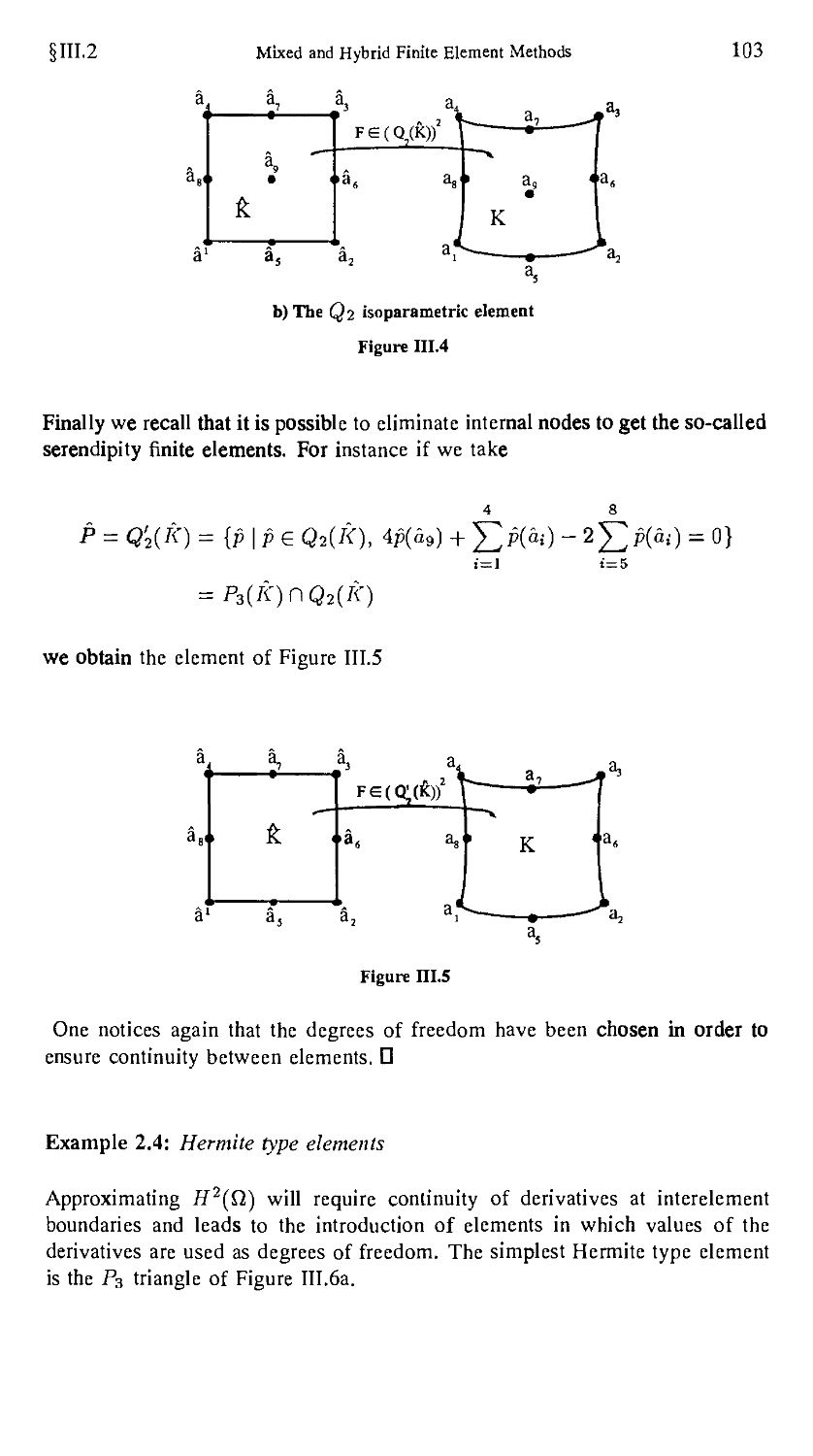
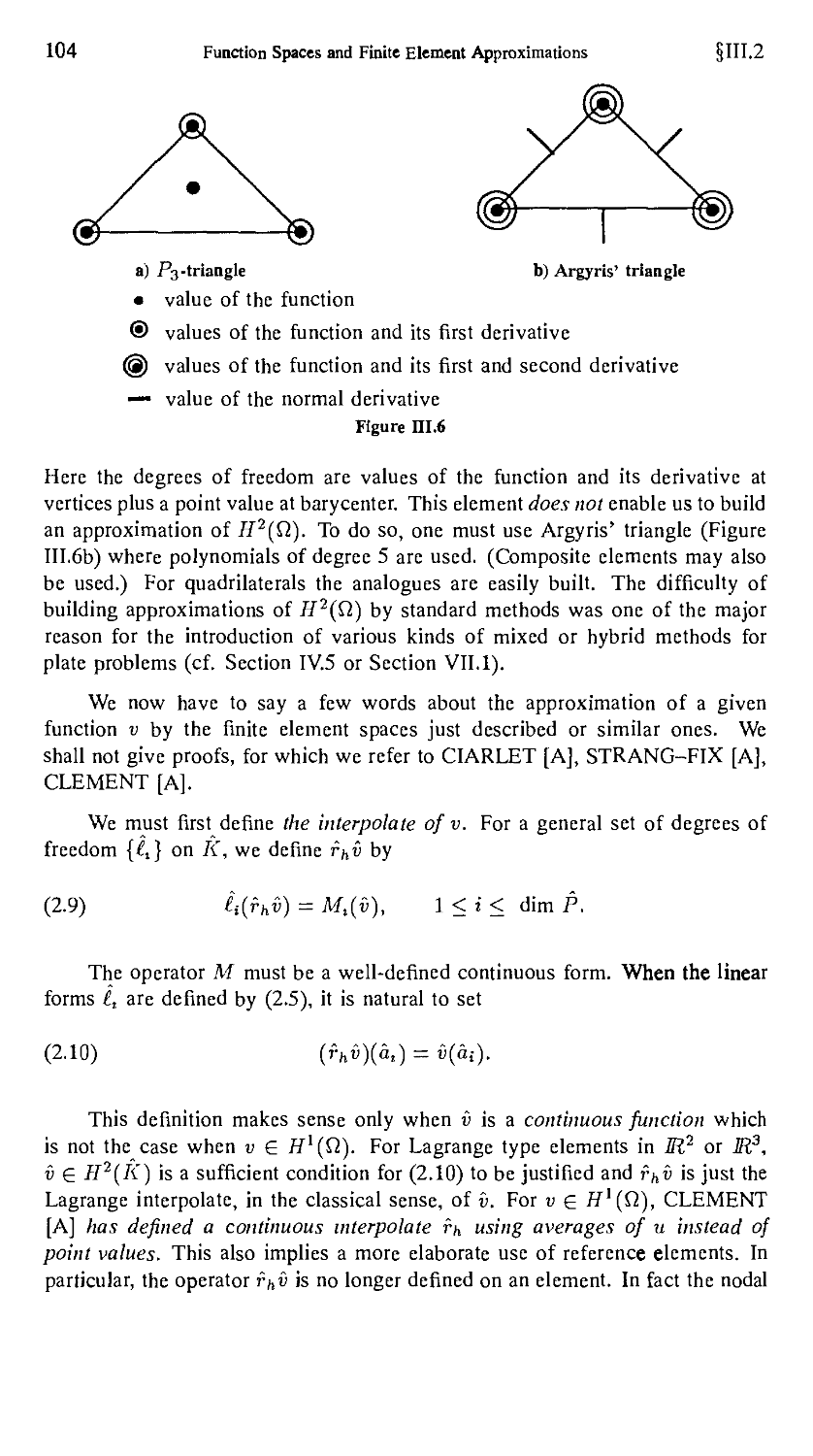
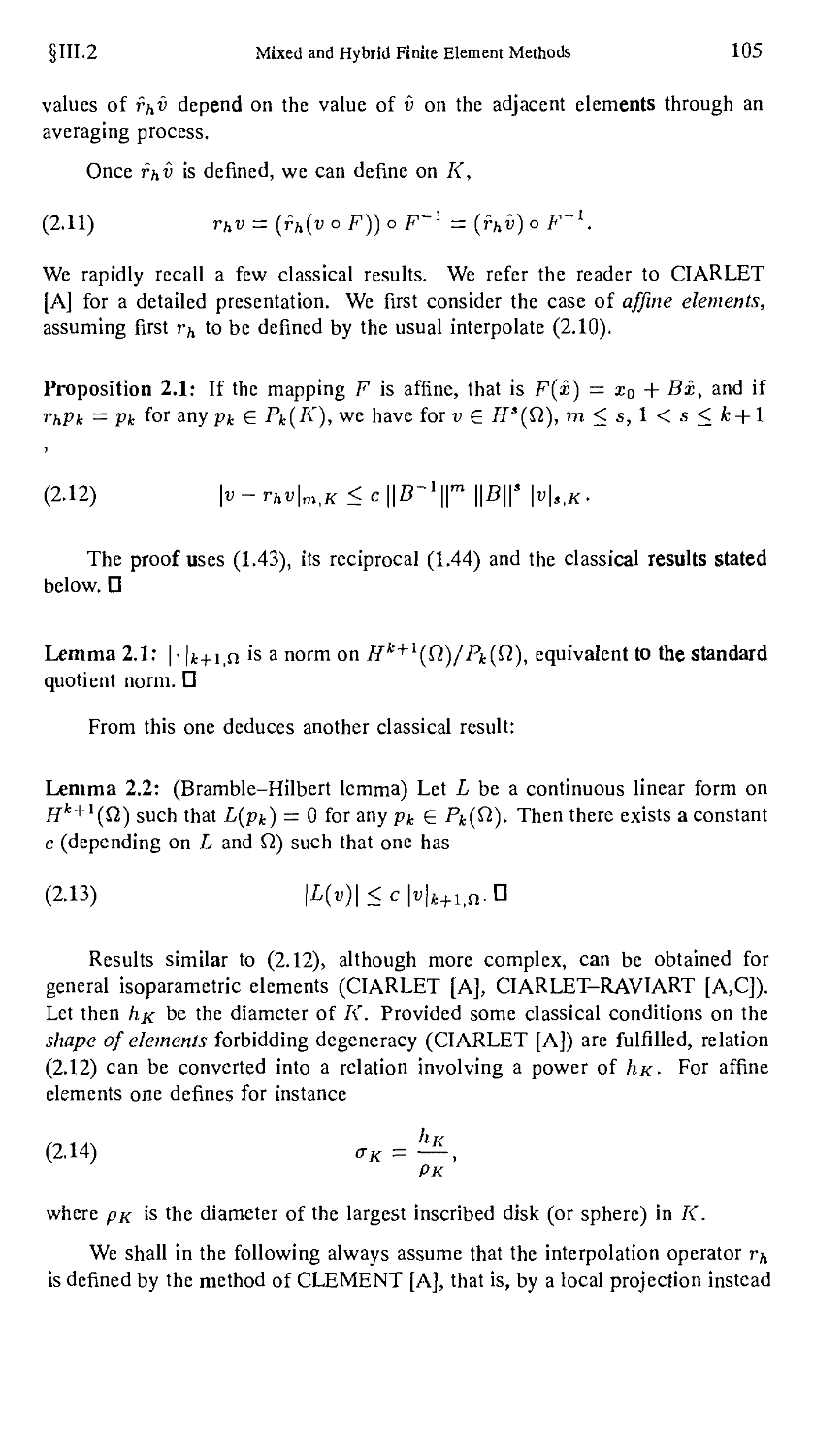
/


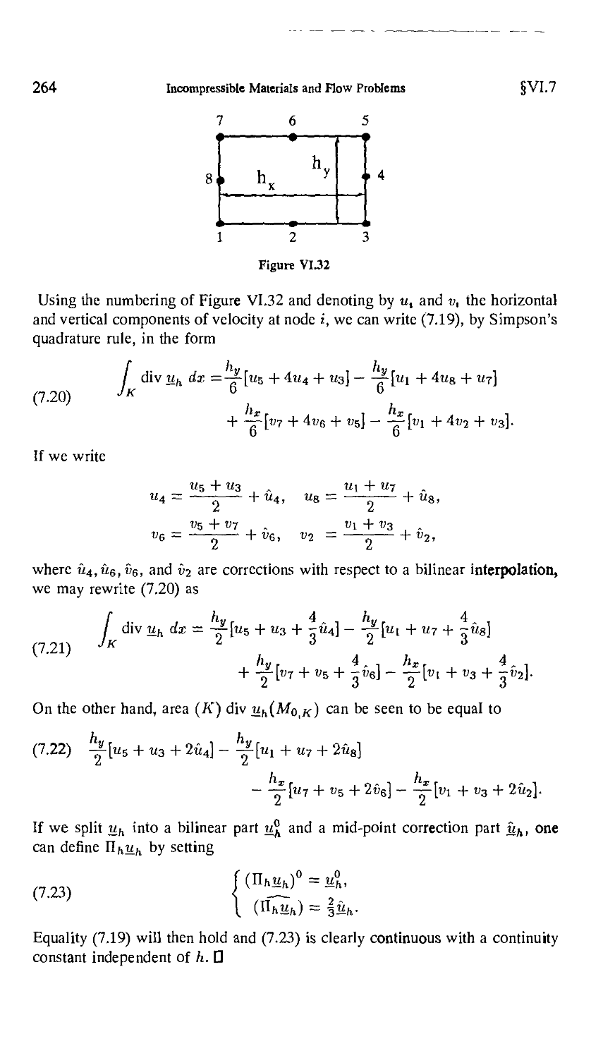


Text
Brezzi • Fortin
Mixed and Hybrid Finite clement Methods
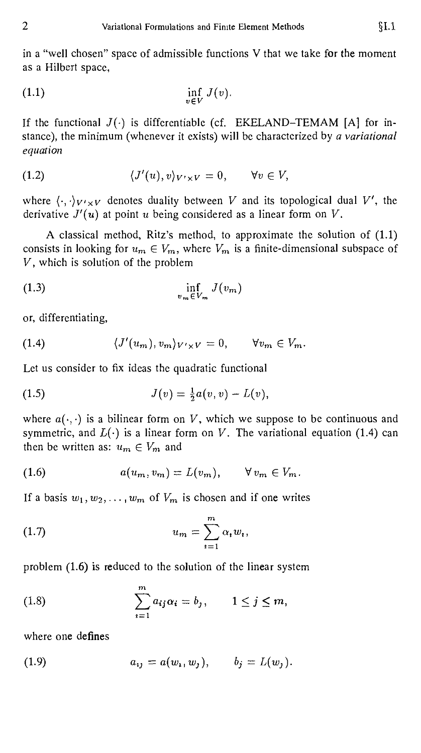
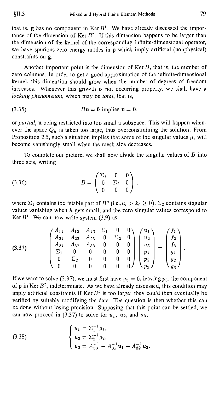
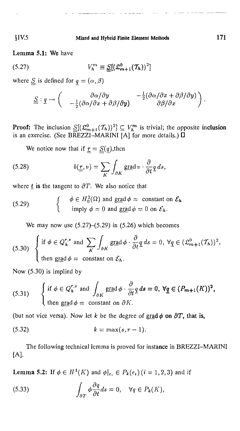
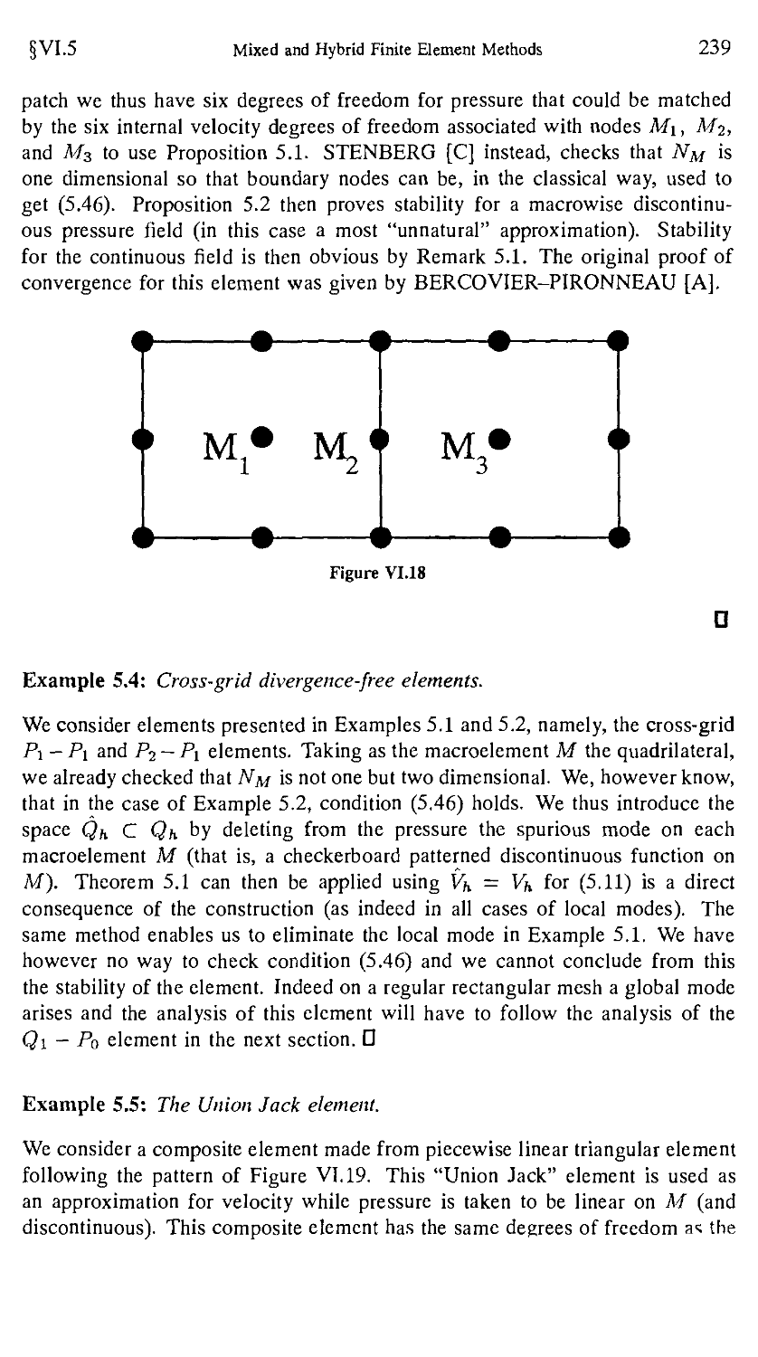
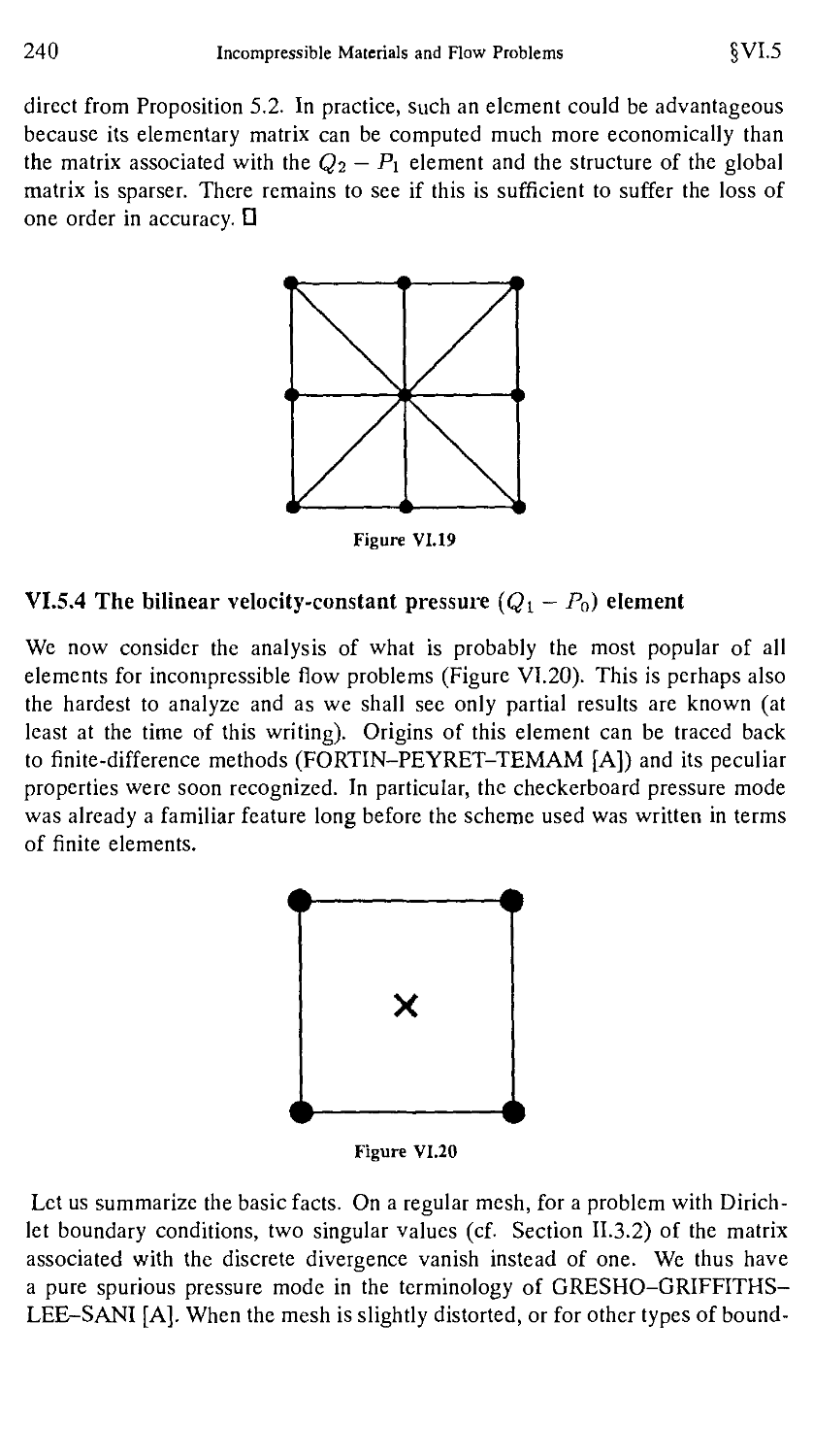
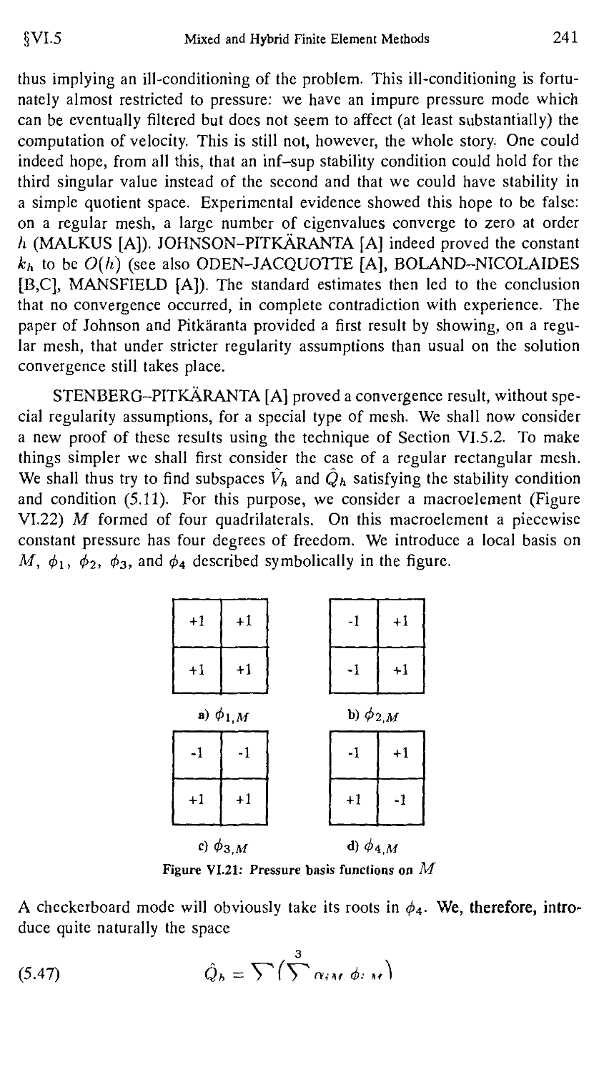
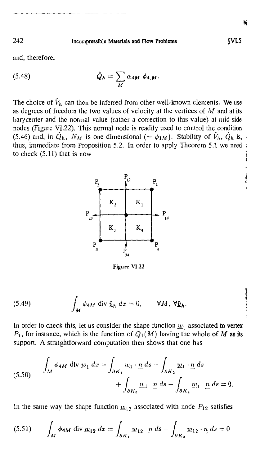
Mixed and hybrid finite element methods are widely employed in
many areas of computational engineering. Their mathematical
properties have been thoroughly studied and a general theory has
emerged. This book gives a unified presentation of this mathe-
mathematical theory. It presents all the standard results, in particular the
construction of elements adapted to the'mixed formulations and
also the more recent techniques of stabilization. It also introduces
the treatment of continuity conditions at interfaces through multi-
multipliers, which leads to better properties to the discrete problem.
Besides the general theory, many applications are considered, in
particular, elasticity problems and moderately thick plates prob-
problems are treated extensively. An entire chapter is devoted to the
approximation of incompressible flows or incompressible elastici-
elasticity, providing a state-ofTthe-art access to the field.
ISBN 0-387-97582-9
ISBN 3-540-97582-9
Franco Brezzi
Michel Fortin
Mixed and
Hybrid Finite
Element Methods
(fill/ Springer-Veriag
Springer Series in
Computational
Mathematics
15
Editorial Board
:.R.MjFaham, Murray Hill (NJ)
J. Stoer, Wurzburg
R, Varga, Kent (Ohio)
Franco Brezzi Michel Fortin
Mixed and Hybrid
Finite Element Methods
With 65 Illustrations
Springer-Verlag
New York Berlin Heidelberg London
Paris Tokyo Hong Kong Barcelona
Franco Brezzi Michel Fortin
University of Pavia Departement de Mathematiques
Institute of Numerical Analysis et de Statistique
5 Corso Carlo Alberto Universite Laval
1-27100 Pavia Quebec G1K 7P4
Italy Canada
Mathematics Subject Classification: 73XX, 76XX
Library of Congress Cataloging-in-Publication Data
Brezzi, Franco.
Mixed and hybrid finite element methods / Franco Brezzi, Michel
Fortin.
p. cm - (Springer series in computational mathematics ; 15)
Includes bibliographical references and index.
ISBN 0-387-97582-9 (alk. paper)
1. Finite element method. I. Brezzi, F. (Franco), 1945- .
II Title. III. Series.
TA347.F5F68 1991
620'.001'51535--dc20 91-10909
Printed on acid-free paper.
© 1991 Springer-Verlag New York Inc.
All rights reserved. This work may not be translated or copied in whole or in part without the
written permission of the publisher (Springer-Verlag New York, Inc., 175 Fifth Avenue, New
York, NY 10010, USA), except for brief excerpts in connection with reviews or scholarly
analysis. Use in connection with any form of information and retrieval, electronic adaptation,
computer software, or by similar or dissimilar methodology now known or hereafter developed
is forbidden.
The use of general descriptive names, trade names, trademarks, etc., in this publication, even
if the former are not especially identified, is not to be taken as a sign that such names, as
understood by the Trade Marks and Merchandise Marks Act, may accordingly be used freely
by anyone.
Photocomposed copy prepared from the author's TgX file.
Printed and bound by Edwards Brothers, Inc., Ann Arbor, Michigan.
Printed in the United States of America.
987654321
ISBN 0-387-97582-9 Springer-Verlag New York Berlin Heidelberg
ISBN 3-540-97582-9 Springer-Verlag Berlin Heidelberg New York
Preface
When, a few years ago, we began the redaction of this book, we had the naive
thought that the theory of mixed and hybrid finite element methods was ripe
enough for a unified presentation. We soon realized that things were not so
simple and that, if basic facts were known, many obscure zones remained in
many applications. Indeed the literature about nonstandard finite element method
is still evolving rapidly and this book cannot pretend to be complete. We
would rather like to lead the reader through the general framework in which
development is taking place.
We have therefore built our presentation around a few classical examples:
Dirichlet's problem, Stokes problem, linear elasticity, ... They are sketched
in Chapter I and basic methods to approximate them are presented in Chapter
IV, following the general theory of Chapter II and using finite element spaces
of Chapter III. Those four chapters are therefore the essential part of the book.
They are complemented by the following three chapters which present a more
detailed analysis of some problems.
Chapter V comes back to mixed approximations of Dirichlet's problem
and analyses, in particular, the (lambda)-trick that enables to make the link
between mixed methods and more classical non-conforming methods. Chapter
VI deals with Stokes problem and Chapter VII with linear elasticity and the
Mindlin-Reissner plate model.
The reader should not look here for practical implementation tricks. Our
goal was to provide an analysis of the methods in order to understand their
properties as thoroughly as possible. We refer, among others, to the recent
work of BATHE [A] or HUGHES [A] or to the classical and indispensable book
vi Preface
of ZIENKIEWICZ [A] for practical considerations. We are of course strongly
indebted to CIARLET [A] which remains the essential reference for the classical
theory of finite element methods. Finally we also refer to ROBERTS-THOMAS
[A] for another presentation of mixed methods.
This book would never have come to its end without the help, encour-
encouragement and criticisms of our friends and colleagues. We must also thank all
those who took the time reading the first draft of our manuscript and proposed
significant improvements. We hope that the final result will better than what
one might expect, according to the quotations thereafter, of the hybrid resulting
of a collaboration between Pavia and Quebec.
Apris atque sui setosus nascitur hybris. (C. Plinius Caecilius Secondus.)
Mixtumque genus prolesque biformis. (Publius Virgilius Maro.)
Contents
Preface v
Chapter I: Variational Formulations and Finite Element Methods 1
§1. Classical Methods 1
§2. Model Problems and Elementary Properties
of Some Functional Spaces 4
§3. Duality Methods 11
3.1. Generalities 11
3.2. Examples for symmetric problems 13
3.3. Duality methods for nonsymmetric bilinear forms 23
§4. Domain Decomposition Methods, Hybrid Methods 24
§5. Augmented Variational Formulations 30
§6. Transposition Methods 33
§7. Bibliographical remarks 35
Chapter II: Approximation of Saddle Point Problems 36
§1. Existence and Uniqueness of Solutions 36
1.1. Quadratic problems under linear constraints 37
1.2. Extensions of existence and uniqueness results 44
§2. Approximation of the Problem 51
2.1. Basic results 51
2.2. Error estimates for the basic problem 54
2.3. The inf-sup condition: criteria 57
2.4. Extensions of error estimates 61
2.5. Various generalizations of error estimates 63
viii Contents
2.6. Perturbations of the problem, nonconforming methods 65
2.7. Dual error estimates 70
§3. Numerical Properties of the Discrete Problem 73
3.1. The matrix form of the discrete problem 73
3.2. Eigenvalue problem associated with the inf-sup condition ... 75
3.3. Is the inf-sup condition so important? 78
§4. Solution by Penalty Methods, Convergence of
Regularized Problems 80
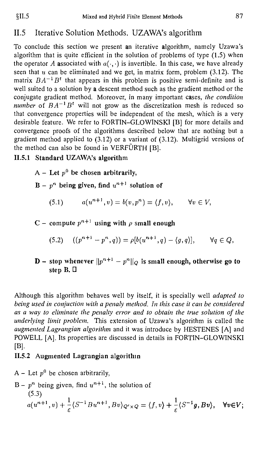
§5. Iterative Solution Methods. Uzawa's Algorithm 87
5.1. Standard Uzawa's algorithm 87
5.2. Augmented Lagrangian algorithm 87
§6. Concluding Remarks 88
Chapter III: Function Spaces and Finite Element Approximations 89
§1. Properties of the spaces //'(ft) and H(div; fi) 89
1.1. Basic results 89
1.2. Properties relative to a partition of Q 93
1.3. Properties relative to a change of variables 95
§2. Finite Element Approximations of H1 (fi) and H2(Q) 99
2.1. Conforming methods 99
2.2. Nonconforming methods 107
2.3. Nonpolynomial approximations: Spaces ££(<£a) Ill
2.4. Scaling arguments Ill
§3. Approximations of //(div; fl) 113
3.1. Simplicial approximations of H(div; K) 113
3.2. Rectangular approximations of //(div; K) 119
3.3. Interpolation operator and error estimates 124
3.4. Approximation spaces for //(div; fi) 131
§4. Concluding Remarks 132
Chapter IV: Various Examples 133
§1. Nonstandard Methods for Dirichlet's Problem 134
1.1. Description of the problem 134
1.2. Mixed finite element methods for Dirichlet's problem 135
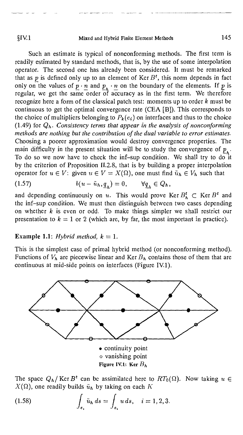
1.3. Primal hybrid methods 140
1.4. Dual hybrid methods 149
§2. Stokes Problem 155
§3. Elasticity Problems 159
§4. A Mixed Fourth-Order Problem 164
4.1. The tp-ui biharmonic problem 164
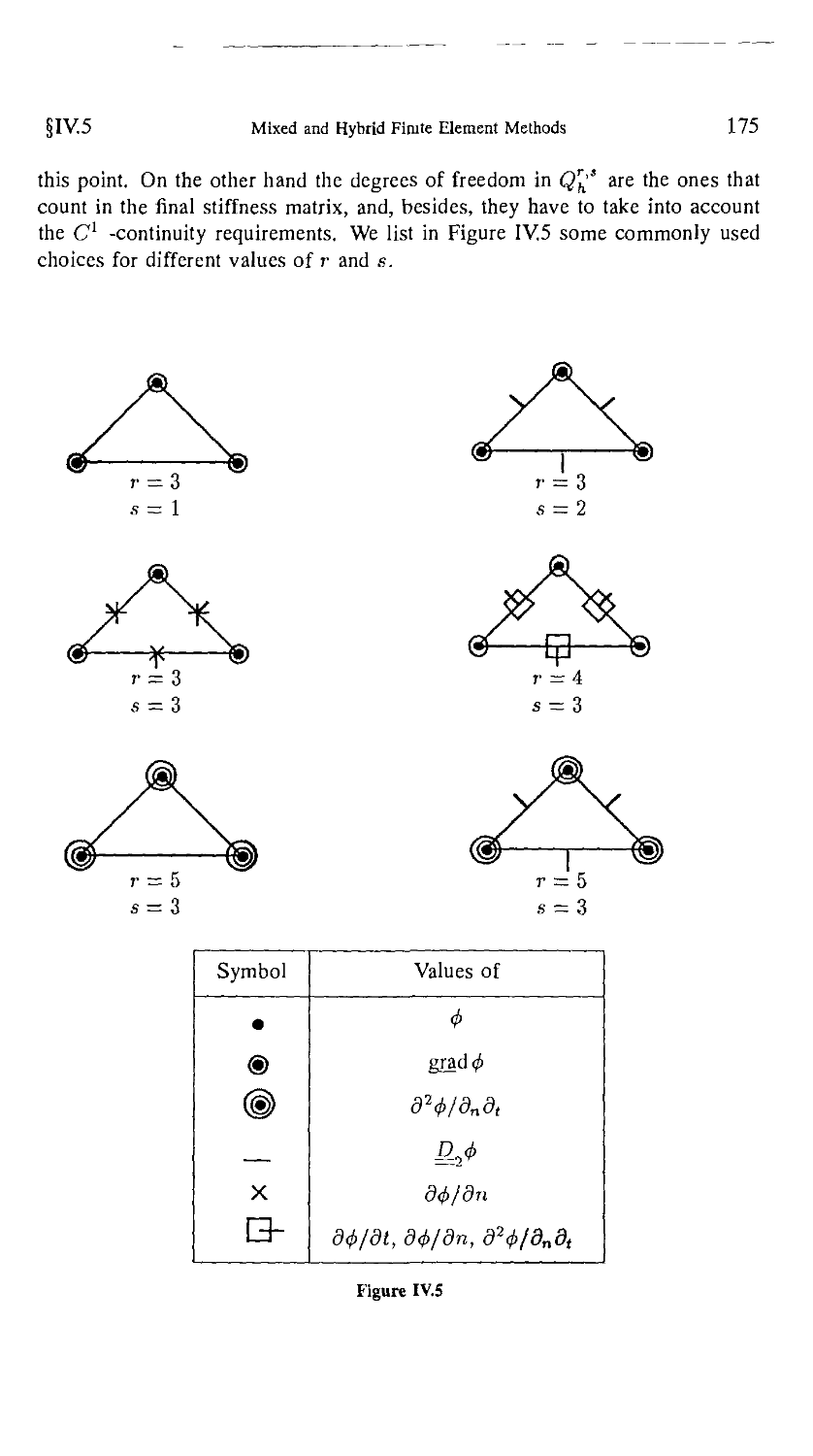
§5. Dual Hybrid Methods for Plate Bending Problems 167
Chapter V: Complements on Mixed Methods for Elliptic Problems 177
§1. Numerical Solutions 177
1.1. Preliminaries 177
1.2. Interelement multipliers 178
Contents ix
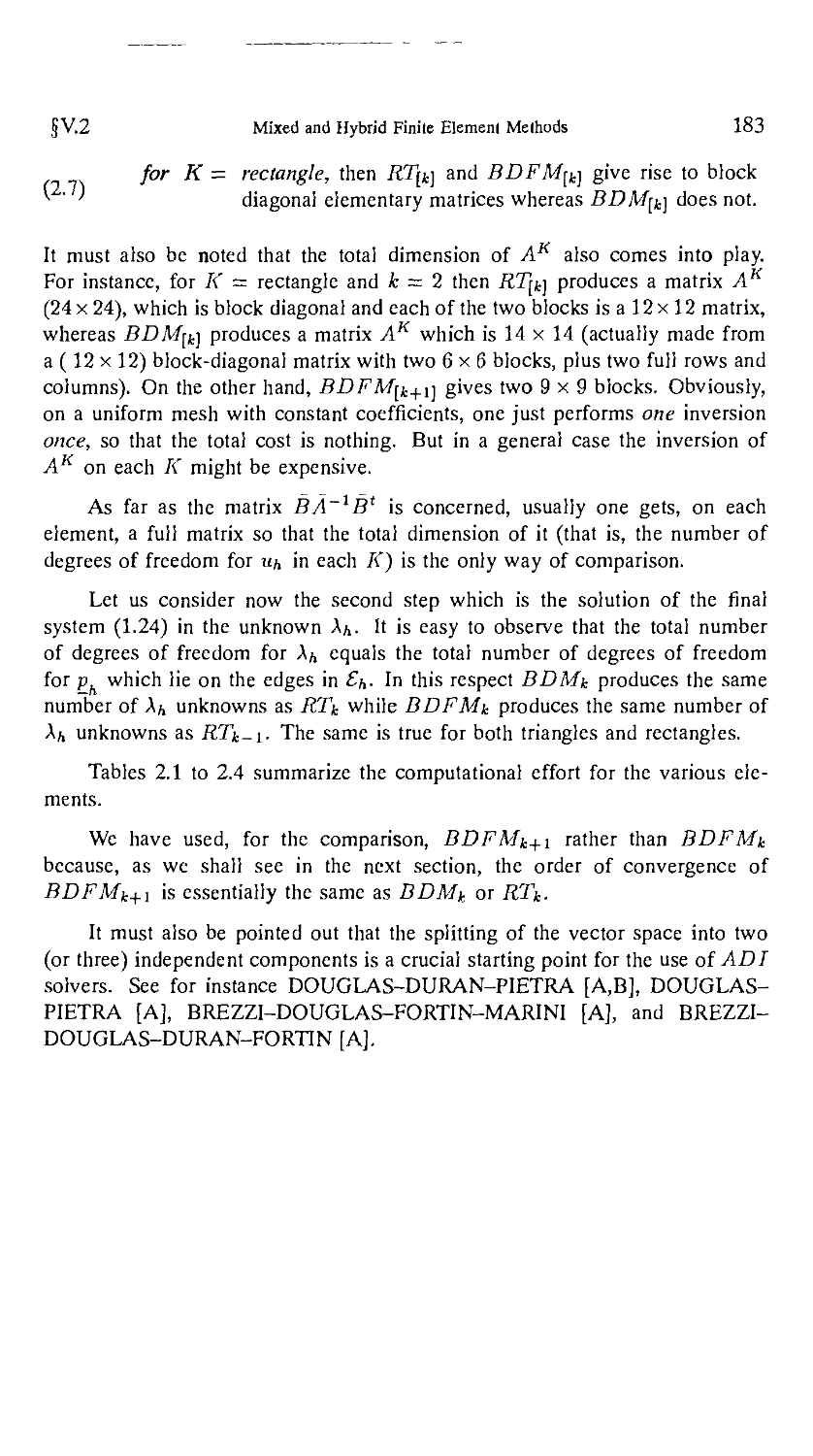
§2. A Brief Analysis of the Computational Effort 182
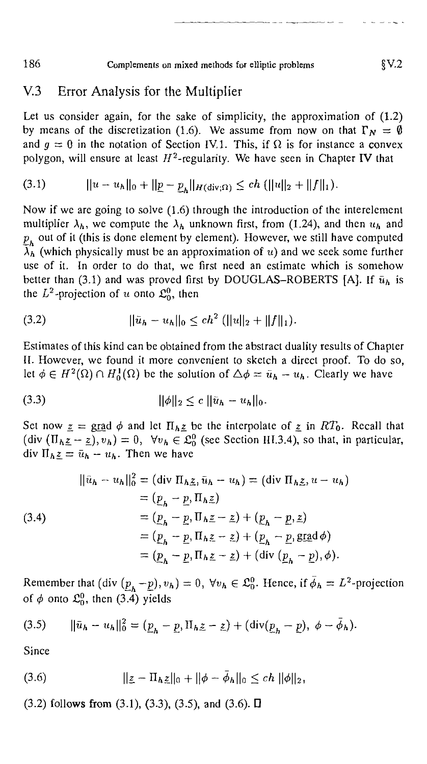
§3. Error Analysis for the Multiplier 186
§4. Error Estimates in Other Norms 191
§5. Application to an Equation Arising
from Semiconductor Theory 193
§6. How Things Can Go Wrong 195
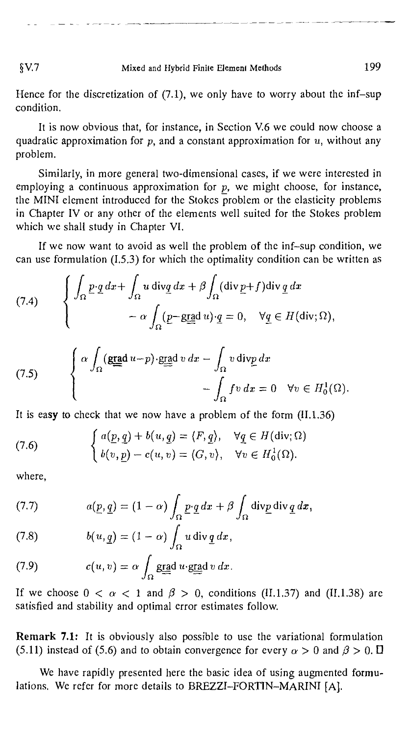
§7. Augmented Formulations 198
Chapter VI: Incompressible Materials and Flow Problems 200
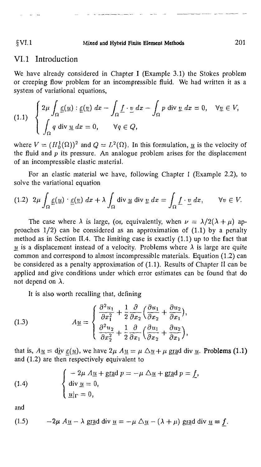
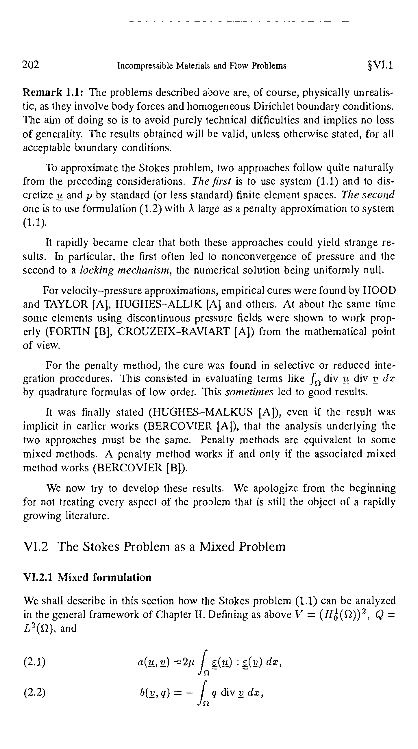
§1. Introduction 201
§2. The Stokes Problem as a Mixed Problem 202
2.1. Mixed Formulation 202
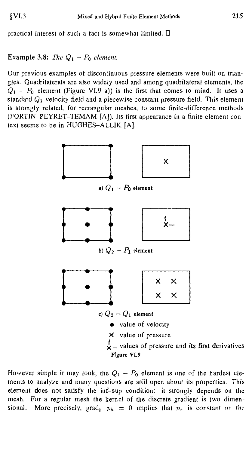
§3. Examples of Elements for Incompressible Materials 206
3.1. Simple examples 207
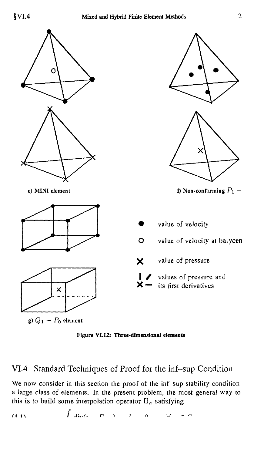
§4. Standard Techniques of Proof for the inf-sup Condition 219
4.1. General results 224
4.2. Higher order methods 227
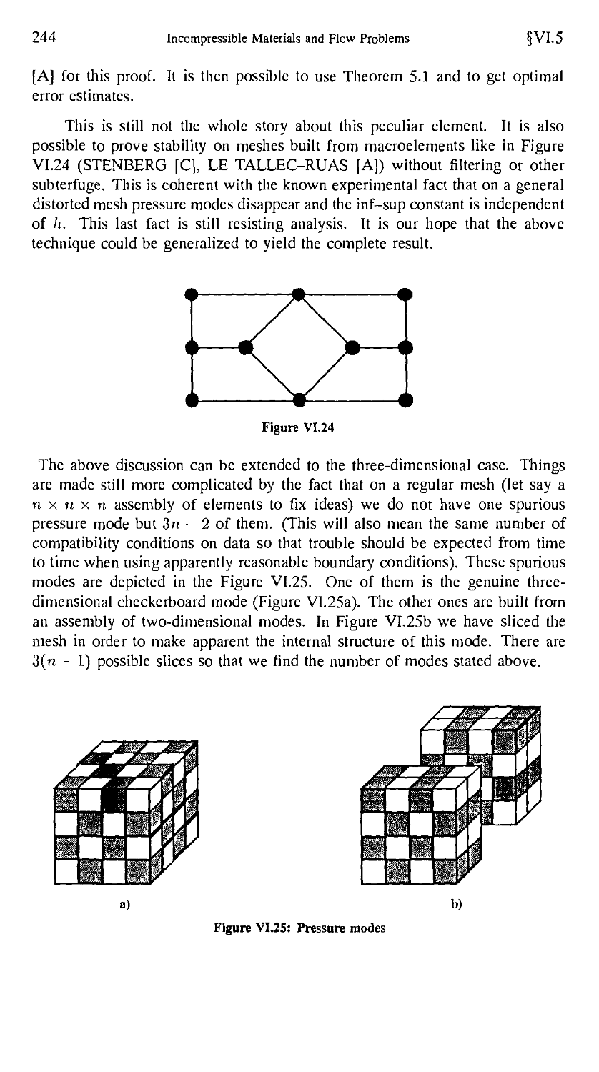
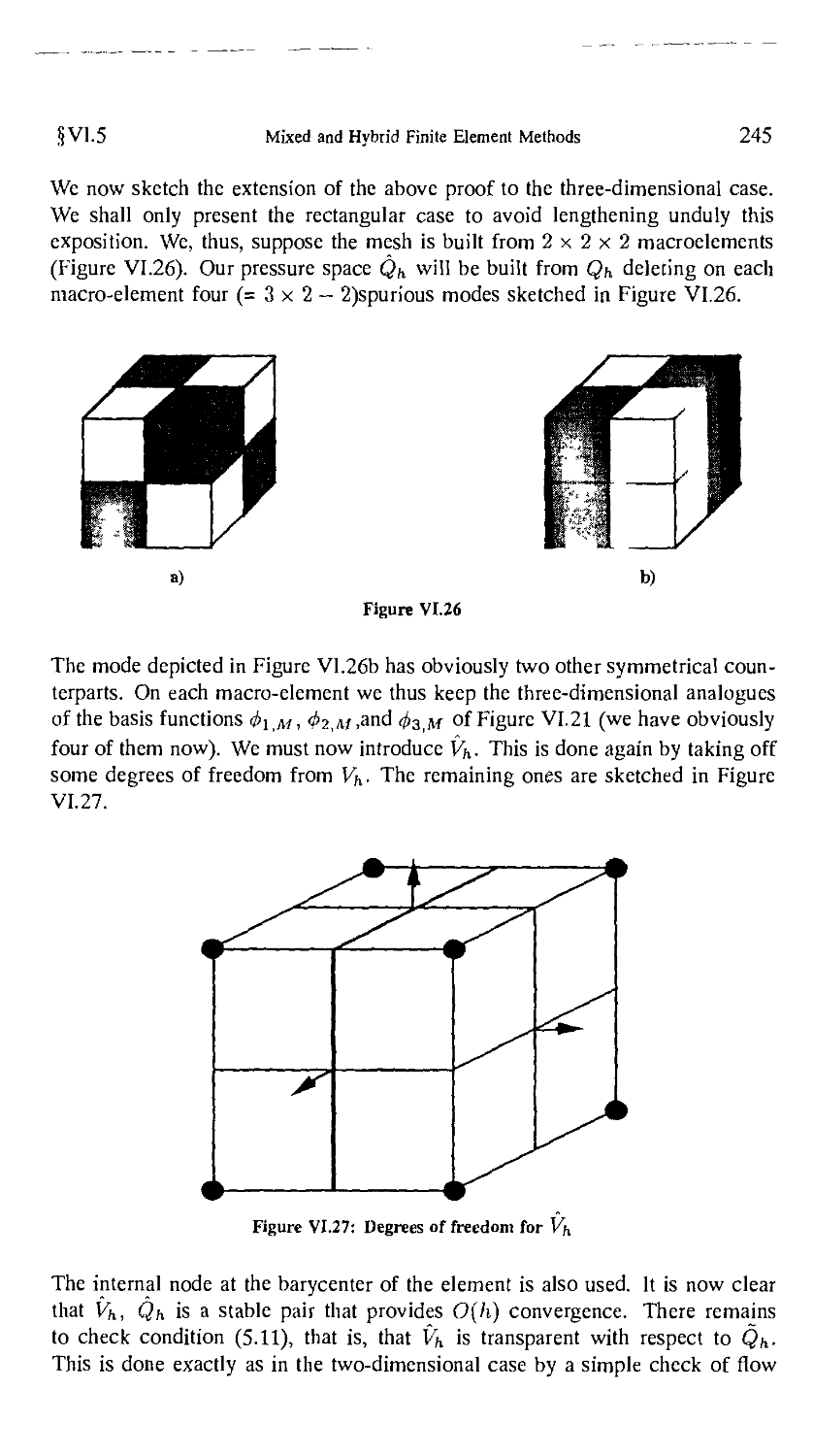
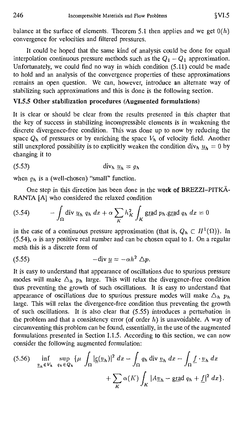
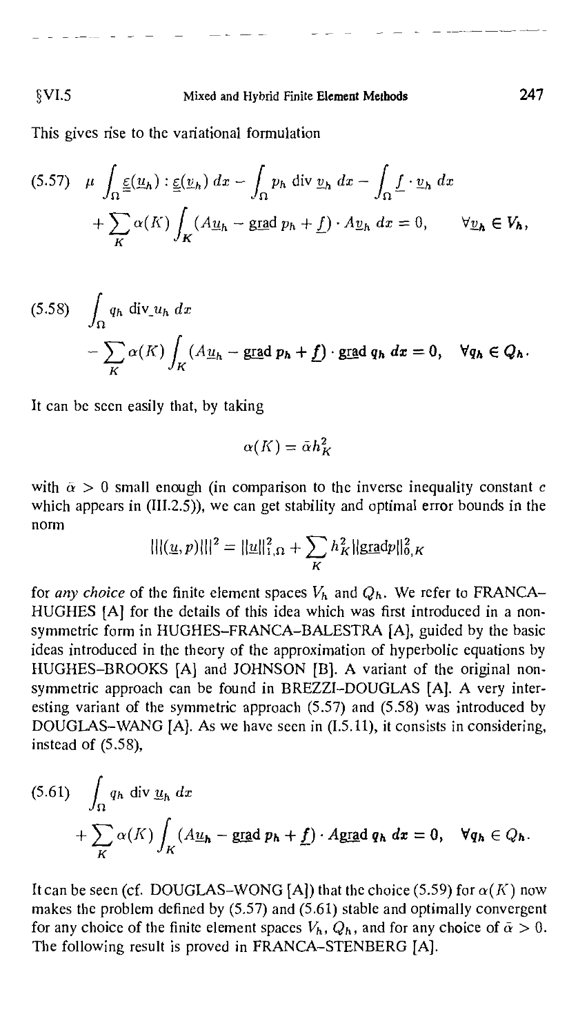
§5. Macroelement Techniques and Spurious Pressure Modes 228
5.1. Some remarks about spurious pressure modes 228
5.2. An abstract convergence result 231
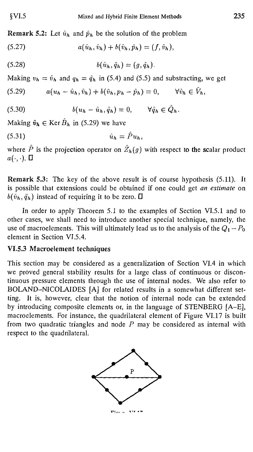
5.3. Macroelement techniques 235
5.4. The bilinear velocity-constant pressure (Qi-Po) element .... 240
5.5. Other stabilization procedures, (Augmented Formulations)... 246
§6. An Alternative Technique of Proof
and Generalized Taylor-Hood Element 252
§7. Nearly Incompressible Elasticity, Reduced Integration
Methods and Relation with Penalty Methods 258
7.1. Variational formulations and admissible discretizations 258
7.2. Reduced integration methods 259
7.3. Effects of inexact integration 263
§8. Divergence-Free Basis, Discrete Stream Functions 267
§9. Other Mixed and Hybrid Methods for Incompressible Flows.... 272
Chapter VII: Other Applications 274
§1. Mixed Methods for Linear Thin Plates 274
§2. Mixed Methods for Linear Elasticity Problems 282
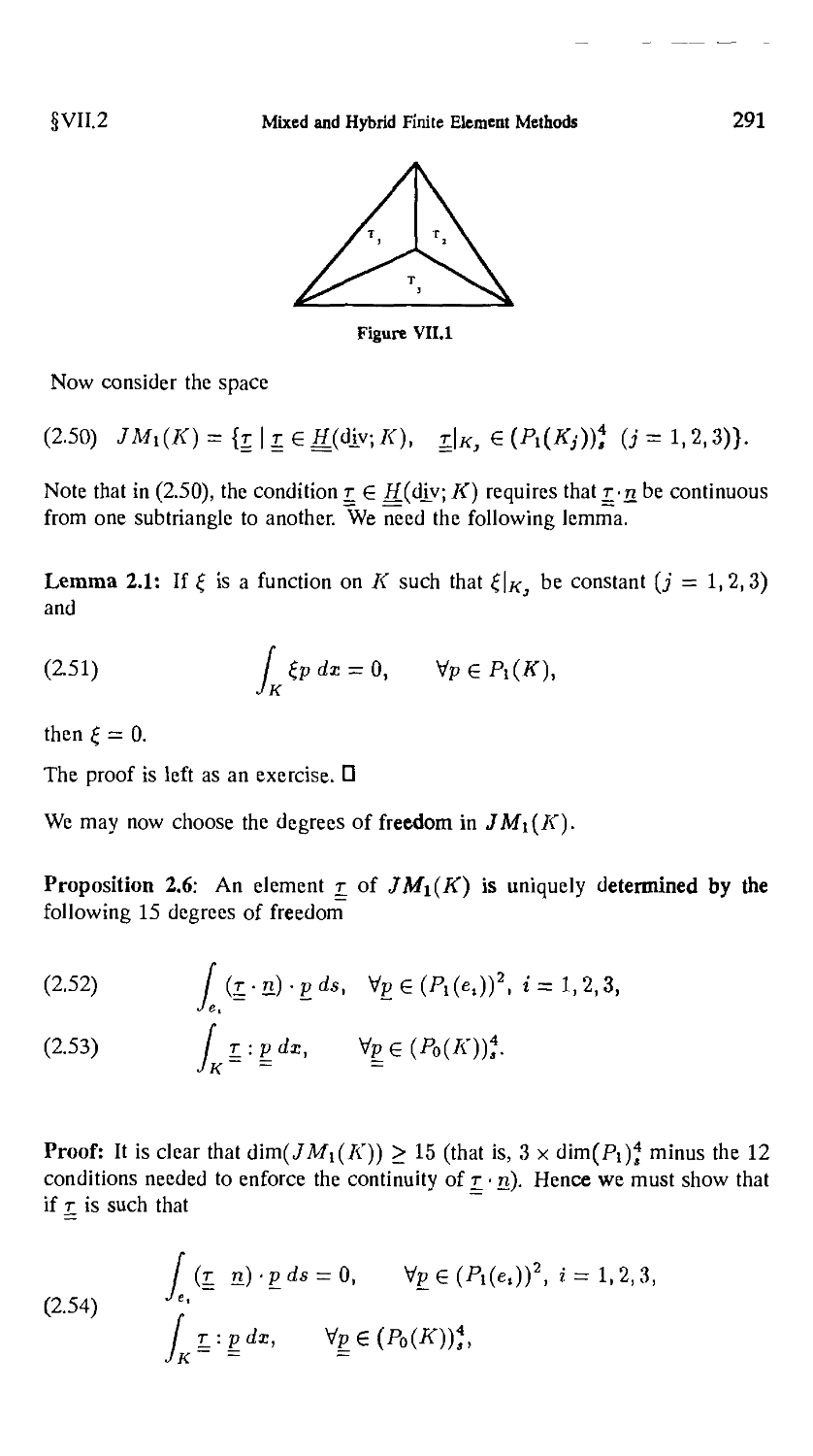
§3. Moderately Thick Plates 295
3.1. Generalities 295
3.2. Discretization of the problem 303
3.3. Continuous Pressure Approximations 322
3.4. Discontinuous Pressure Approximations 322
References 324
Index 344
Variational Formulations and Finite
Element Methods
Although we shall not define in this chapter mixed and hybrid (or other non-
standard) finite element methods in a very precise way, we would like to situate
them in a sufficiently clear setting. As we shall see, boundaries between dif-
different methods are sometimes rather fuzzy. This will not be a real drawback
if we nevertheless know how to apply correctly the principles underlying their
analysis.
After having briefly recalled some basic facts about classical methods, we
shall present a few model problems. The study of these problems will be the
kernel of this book. We shall thereafter rapidly recall basic principles of duality
theory as this will be our starting point to introduce mixed methods. Domain de-
decomposition methods (allied to duality) will lead us to hybrid methods. Finally,
we shall present a few ideas about transposed formulations as they can help to
understand some of the weak problems generated by the previous methods.
I.I Classical Methods
We recall here in a very simplified way some results about optimization methods
and the classical finite element method. Such an introduction cannot be complete
and does not want to be. We refer the reader to CIARLET [A] or RAVIART-
THOMAS [D], among others, where standard finite element methods are clearly
exposed. We also refer to DAUTRAY-LIONS [A] where an exhaustive analysis
of many of our model problems can be found.
Let us then consider a very common situation where the solution of a
physical problem minimizes some functional (usually an "energy functional"),
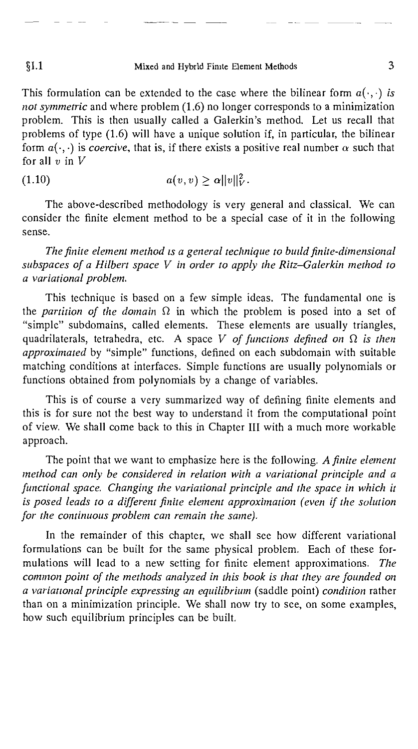
2 Variational Formulations and Finite Element Methods §1.1
in a "well chosen" space of admissible functions V that we take for the moment
as a Hilbeit space,
A.1) inf J(«).
If the functional J(-) is differentiable (cf. EKELAND-TEMAM [A] for in-
instance), the minimum (whenever it exists) will be characterized by a variational
equation
A.2) (J'(u),v)v*v=0, Vv£V,
where (-,-)v'xv denotes duality between V and its topological dual V', the
derivative J'(u) at point u being considered as a linear form on V.
A classical method, Ritz's method, to approximate the solution of A.1)
consists in looking for um £ Vm, where Vm is a finite-dimensional subspace of
V, which is solution of the problem
A.3) inf J(vm)
<im£Vm
or, differentiating,
A.4) {J'(um),vm)v>xv = 0, Vvm G Vm.
Let us consider to fix ideas the quadratic functional
A.5) J(v) = ±a(v,v)-L(y),
where a(-,-) is a bilinear form on V, which we suppose to be continuous and
symmetric, and L(-) is a linear form on V. The variational equation A.4) can
then be written as: wm £ Vm and
A.6) n(tim,tim) = i(tim), v«meym.
If a basis w\, W2,. ■ ■, wm of Vm is chosen and if one writes
m
A.7) um -^2a,w,,
« = i
problem A.6) is reduced to the solution of the linear system
m
A.8) ^
where one defines
A.9) atJ = a(wt,wj), bj = L(w}).
§1.1 Mixed and Hybrid Finite Element Methods 3
This formulation can be extended to the case where the bilinear form a(-,-) is
not symmetric and where problem A.6) no longer corresponds to a minimization
problem. This is then usually called a Galerkin's method. Let us recall that
problems of type A.6) will have a unique solution if, in particular, the bilinear
form a(-, •) is coercive, that is, if there exists a positive real number a such that
for all v in V
A.10) a(v,v)>a\\v\\l.
The above-described methodology is very general and classical. We can
consider the finite element method to be a special case of it in the following
sense.
The finite element method is a general technique to build finite-dimensional
subspaces of a Hilbert space V in order to apply the Ritz-Galerkin method to
a variational problem.
This technique is based on a few simple ideas. The fundamental one is
the partition of the domain Q in which the problem is posed into a set of
"simple" subdomains, called elements. These elements are usually triangles,
quadrilaterals, tetrahedra, etc. A space V of functions defined on Q is then
approximated by "simple" functions, defined on each subdomain with suitable
matching conditions at interfaces. Simple functions are usually polynomials or
functions obtained from polynomials by a change of variables.
This is of course a very summarized way of defining finite elements and
this is for sure not the best way to understand it from the computational point
of view. We shall come back to this in Chapter III with a much more workable
approach.
The point that we want to emphasize here is the following. A finite element
method can only be considered in relation with a variational principle and a
functional space. Changing the variational principle and the space in which it
is posed leads to a different finite element approximation (even if the solution
for the continuous problem can remain the same).
In the remainder of this chapter, we shall see how different variational
formulations can be built for the same physical problem. Each of these for-
formulations will lead to a new setting for finite element approximations. The
common point of the methods analyzed in this book is that they are founded on
a variational principle expressing an equilibrium (saddle point) condition rather
than on a minimization principle. We shall now try to see, on some examples,
how such equilibrium principles can be built.
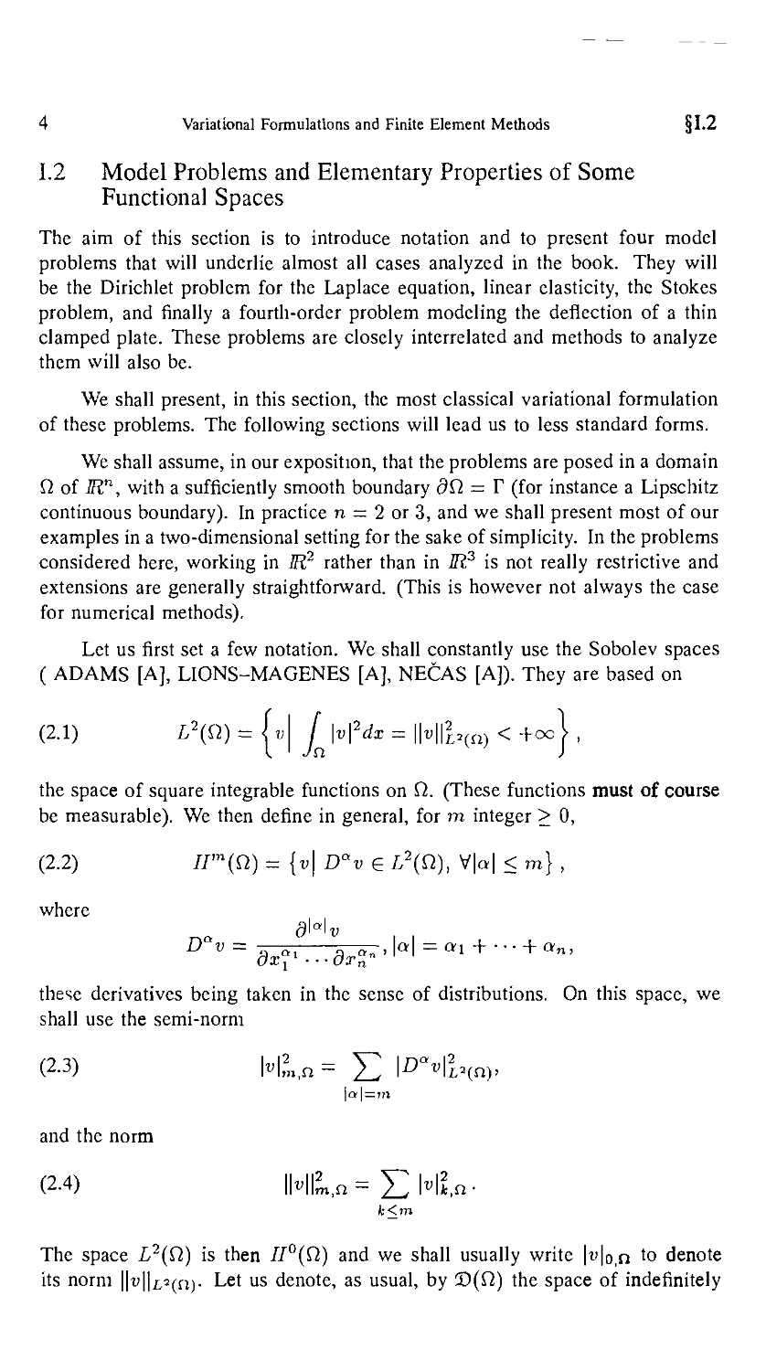
4 Variational Formulations and Finite Element Methods §1.2
1.2 Model Problems and Elementary Properties of Some
Functional Spaces
The aim of this section is to introduce notation and to present four model
problems that will underlie almost all cases analyzed in the book. They will
be the Dirichlet problem for the Laplace equation, linear elasticity, the Stokes
problem, and finally a fourth-order problem modeling the deflection of a thin
clamped plate. These problems are closely interrelated and methods to analyze
them will also be.
We shall present, in this section, the most classical variational formulation
of these problems. The following sections will lead us to less standard forms.
We shall assume, in our exposition, that the problems are posed in a domain
Q of Mn, with a sufficiently smooth boundary <9fi = F (for instance a Lipschitz
continuous boundary). In practice n = 2 or 3, and we shall present most of our
examples in a two-dimensional setting for the sake of simplicity. In the problems
considered here, working in JR2 rather than in El3 is not really restrictive and
extensions are generally straightforward. (This is however not always the case
for numerical methods).
Let us first set a few notation. We shall constantly use the Sobolev spaces
( ADAMS [A], LIONS-MAGENES [A], NECAS [A]). They are based on
B.1) L\i1) = {«| J \v\2dx = ||«||£a(n) < +oo
the space of square integrable functions on Q. (These functions must of course
be measurable). We then define in general, for m integer > 0,
B.2) //m(Q) = {v\ Dav £ L2(Q), V|a| < m} ,
where
these derivatives being taken in the sense of distributions. On this space, we
shall use the semi-norm
B-3) \vt,a= E PaHl»(n)>
\a\ = m
and the norm
B-4) Nl2x,n=X>l*,n-
The space L2(Q.) is then 77°(f2) and we shall usually write Ho,n t0 denote
its norm ||^||i2(rij- Let us denote, as usual, by D(f2) the space of indefinitely
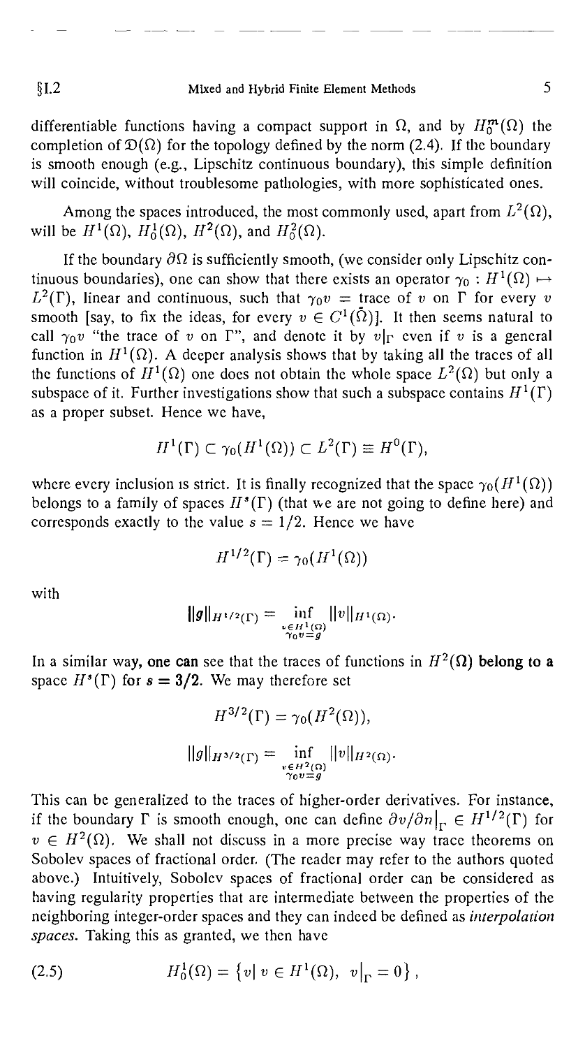
§1.2 Mixed and Hybrid Finite Element Methods 5
differentiable functions having a compact support in f2, and by H™(Q) the
completion of D(Q) for the topology denned by the norm B.4). If the boundary
is smooth enough (e.g., Lipschitz continuous boundary), this simple definition
will coincide, without troublesome pathologies, with more sophisticated ones.
Among the spaces introduced, the most commonly used, apart from L2(Q),
will be //'(fi), #<j(fi), H2(tt), and
If the boundary <9f2 is sufficiently smooth, (we consider only Lipschitz con-
continuous boundaries), one can show that there exists an operator 70 : iJ'(f2) >—>■
L2(F), linear and continuous, such that jov = trace of v on F for every v
smooth [say, to fix the ideas, for every v £ Cl((l)]. It then seems natural to
call 70U "the trace of v on F", and denote it by u|r even if n is a general
function in Hl(Cl). A deeper analysis shows that by taking all the traces of all
the functions of //'(ft) one does not obtain the whole space L2{0.) but only a
subspace of it. Further investigations show that such a subspace contains HX{T)
as a proper subset. Hence we have,
II1 (T) C 7o(//1(")) C L2(T) = H°(T),
where every inclusion is strict. It is finally recognized that the space 7o(//'(f2))
belongs to a family of spaces //'(F) (that we are not going to define here) and
corresponds exactly to the value s = 1/2. Hence we have
with
\o I
yo=g
In a similar way, one can see that the traces of functions in H2(Q) belong to a
space H'(T) for s = 3/2. We may therefore set
H3'2(r)=l0(H2(Q)),
3(D = inf IMU2(fi)-
This can be generalized to the traces of higher-order derivatives. For instance,
if the boundary F is smooth enough, one can define dv/dn\r £ HX^2(T) for
v £ H2(Q). We shall not discuss in a more precise way trace theorems on
Sobolev spaces of fractional order. (The reader may refer to the authors quoted
above.) Intuitively, Sobolev spaces of fractional order can be considered as
having regularity properties that are intermediate between the properties of the
neighboring integer-order spaces and they can indeed be defined as interpolation
spaces. Taking this as granted, we then have
B.5) 14@)= {v\v£Hl(n), u|r = 0},
6 Variational Formulations and Finite Element Methods §1.2
B.6) H20(Q) = L\v£ H2(Q), v\r = 0, |^|r = o
For v £ 77q(J}), we have the Poincare inequality,
B.7) Mo,n
and the seminorm | ■ |ifi is therefore a norm on II^(Q), equivalent to || ■ ||i,n-
We shall also need to consider functions that vanish on a part of the boundary;
suppose F = D U N, a partition of F into disjoint parts, one then defines
B.8) H^D(Q) = {v\vGHl(Q), v\D = 0}
and one has H&(Q.) C H^d^) c Hl(Sl). In Chapter III, we will discuss the
properties of these spaces; the above definitions are sufficient to allow us to
present some examples.
Example 2.1: Boundary value problems for the Laplace equation.
This is a very classical case that in fact led to the definition of Sobolev spaces.
Let us consider, on Hq(Q), f £ L2(Q) being given, the following minimization
problem
B.9) inf i / \gadv\2dx- f fv dx,
where |grad v\2 = \dv/dxi\ + \dv/dx2 — grad v ■ grad v. One shows
easily (cf. CEA [A], LIONS-MAGENES [A], NECAS [A] for instance) that
this problem has a unique solution w, characterized by: u £ //q(^) and
B.10) ( grad w grad v dx = f fv dx, Vi> G H^
Jn Jn
This solution u then satisfies, in the sense of distributions,
-Aw = / in fi,
which is a standard Dirichlet problem. If Hq(Q) were replaced by
one would get instead of B.11), a mixed type problem
B 12)
§1.2 Mixed and Hybrid Finite Element Methods 7
We thus have Dirichlet boundary conditions on D and Neumann conditions on
N. In particular, for N = F, we get a Neumann problem. It must be noted that
minimizing B.9) on 7J'(Q) instead of Hl(Q) will define u up to an additive
constant, and requires the compatibility condition fnfdx = 0, which can be
seen to be necessary from B.10), taking v = 1 in Q.
If we denote by H~ll2{T) the dual space of Hll2(T), and we take g G
H~1I2(T), we can consider the functional
B.13) | / |grad v\2dx - f fv dx - (g, v),
Jo. Jo.
where the bracket (•,•) denotes duality between H-ll2(T) and H1/2(T). We
shall sometimes write formally frgv ds instead of (g,v). Minimizing B.13)
on III d(^) leads to the problem
B.14)
When D = 0 the solution is defined up to an additive constant and we must
choose / and g such that fnfdx — jr g ds = 0.
These problems are among the most classical of mathematical physics and
we do not have to emphasize their importance. In the following chapters we
shall need to use regularity results for the problems introduced above. We have
supposed up to now / £ L2(Q). For the Dirichlet problem B.11) we could have
assumed / to belong to a weaker space, namely, / £ iJ~'(Q) = (Hq(Q))',
and nevertheless obtained u £ Hl(Q). Indeed, if / is taken in L2(Q) and
the boundary F is Lipschitzian and convex, one can prove (NECAS [A]) that
u e H2(U) and that
B.15) ||«||2in < c|/|Oln-
Regularity results are essential to many approximation results and are funda-
fundamental to obtain error estimates. We refer the reader to GRISVARD [B] for the
delicate questions of the regularity of the general problem B.12) in a domain
with corners. D
Example 2.2: Linear elasticity.
We shall try to determine the displacement u = {wi,w2} of an elastic material
under the action of some external forces. We suppose the displacement to
be small and the material to be isotropic and homogeneous. (CIARLET [A],
MARSDEN-HUGHES [A]). The domain fi is the initial configuration of the
Variational Formulations and Finite Element Methods
§1.2
body. To set our problem, we must introduce some notation from continuum
mechanics. First we define the linearized strain tensor e(y) by
B.16)
The trace tr(e) of this tensor is nothing but the divergence of the displacement
field
B.17)
We shall also use the deviatoric e_D of the tensor e, that is,
B.18)
where S_ is the standard Kronecker tensor. The deviatoric is evidently built to
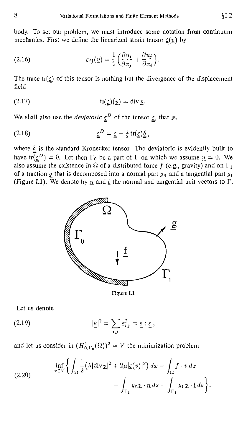
have tr(£D) = 0. Let then Fo be a part of F on which we assume u = 0. We
also assume the existence in Q of a distributed force / (e.g., gravity) and on F!
of a traction g that is decomposed into a normal part gn and a tangential part gt
(Figure I.I). We denote by n and t_ the normal and tangential unit vectors to F.
Figure I.I
Let us denote
B.19)
and let us consider in (Hg po(^)J = ^ t':e minimization problem
1
inf
B.20)
(v)\2) dx
- f f_-v^dx
— I gnV.-Rd-s— I gtH-tds>.
§1.2 Mixed and Hybrid Finite Element Methods 9
Constants X and n, the Lame coefficients, depend on the physical properties of
the material considered. Solution u of this problem is then characterized by
B.21)
2fi / e(w) :e_(v_) dx + X / divu div^ dx
Jn ~ Jn.
= / / ■ v dx + I gnv_'nds+ gtH-tds.
We now use the classical integration by parts formula, ni being some tensor,
B.22) / m : e(v) dx = — / (djym) -y_dx + I mnnv_-nds + / mnt2L-tds,
Ja ~ Jn ~ Jv Jr
where mnn and mnt denote the normal and tangential parts of the traction vector
mn, i.e.,
imnn = ^niij mnj = ^ { ^ mi} nj } m = ^(mn), nit
B.24)
Equation B.21) can now be interpreted as
-B^j diy|(«) + X grad div «) = / in ft,
u r = 0,
2A(£nn + A div m = </„ on Fi,
2p£n( = ff( on Fi.
Let us now introduce the stress tensor s_= sD + p6_ and the constitutive law
B.25) (
[ 2(A + ) divu,
relating stresses to displacements. It is now clear that the first equation of B.24)
expresses the equilibrium condition of continuum mechanics,
B.26) div|+/ = 0.
In applications, the constitutive law B.25) will vary depending on the type
of materials and will sometimes take very nonlinear forms. Moreover, large
displacements will require a much more complex treatment. Nevertheless the
problem described remains valuable as a model for more complicated situations.
The case of an incompressible material is specially important. It leads to
the same equations as in the study of viscous incompressible flows. D
10 Variational Formulations and Finite Element Methods §1.2
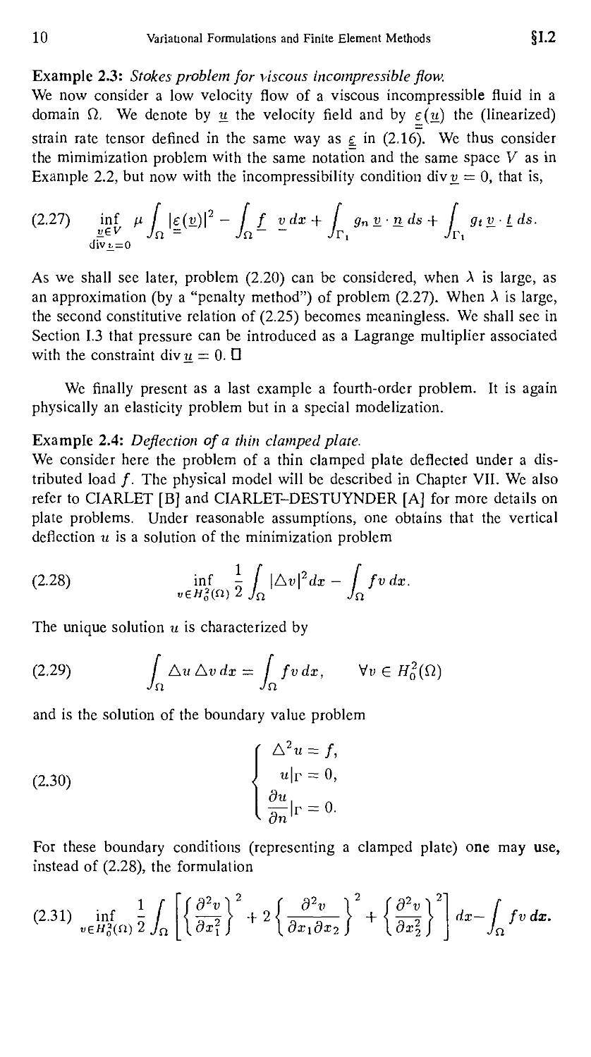
Example 2.3: Stokes problem for viscous incompressible flow.
We now consider a low velocity flow of a viscous incompressible fluid in a
domain Q. We denote by u the velocity field and by e(u) the (linearized)
strain rate tensor defined in the same way as e in B.16). We thus consider
the mimimization problem with the same notation and the same space V as in
Example 2.2, but now with the incompressibility condition div;u = 0, that is,
B.27) inf fi I \e(v)\2 - If v dx + [ gnvnds + / gtvtds.
a^v Jn = Jn~ ~ ir, Jr,
divt^O
As we shall see later, problem B.20) can be considered, when X is large, as
an approximation (by a "penalty method") of problem B.27). When A is large,
the second constitutive relation of B.25) becomes meaningless. We shall see in
Section 1.3 that pressure can be introduced as a Lagrange multiplier associated
with the constraint divw = 0. D
We finally present as a last example a fourth-order problem. It is again
physically an elasticity problem but in a special modelization.
Example 2.4: Deflection of a thin clamped plate.
We consider here the problem of a thin clamped plate deflected under a dis-
distributed load /. The physical model will be described in Chapter VII. We also
refer to CIARLET [B] and CIARLET-DESTUYNDER [A] for more details on
plate problems. Under reasonable assumptions, one obtains that the vertical
deflection u is a solution of the minimization problem
B.28) inf \ f \Av\2dx- I fvdx.
The unique solution u is characterized by
B.29) I Aw Av dx - ( fv dx, Vu G #02(Q)
Jn Jn
and is the solution of the boundary value problem
B.30)
On
For these boundary conditions (representing a clamped plate) one may use,
instead of B.28), the formulation
,nf
fiJ Jn
§1.3 Mixed and Hybrid Finite Element Methods 11
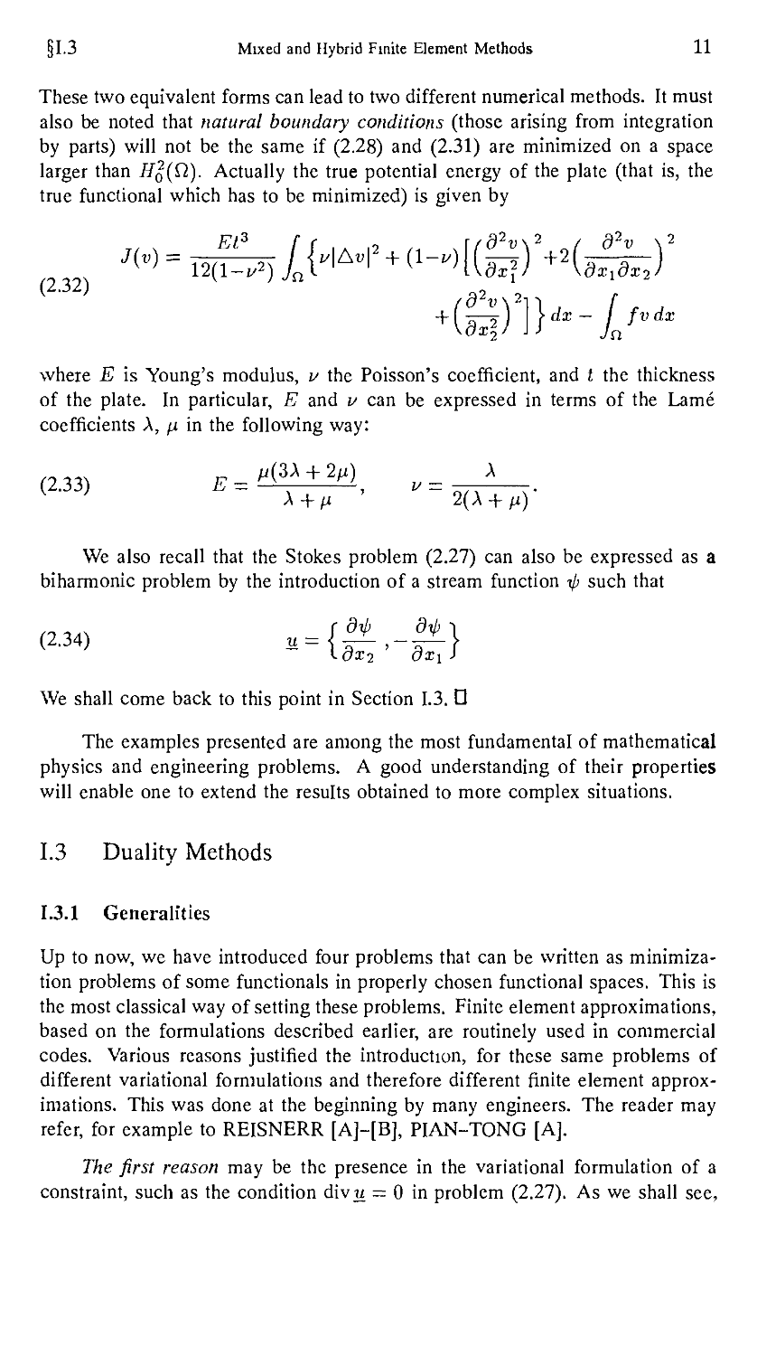
These two equivalent forms can lead to two different numerical methods. It must
also be noted that natural boundary conditions (those arising from integration
by parts) will not be the same if B.28) and B.31) are minimized on a space
larger than //q(Q). Actually the true potential energy of the plate (that is, the
true functional which has to be minimized) is given by
B32)
wheie E is Young's modulus, v the Poisson's coefficient, and t the thickness
of the plate. In particular, E and v can be expressed in terms of the Lame
coefficients \, \x in the following way:
B.33)
We also recall that the Stokes problem B.27) can also be expressed as a
biharmonic problem by the introduction of a stream function -0 such that
«={£■-&}
We shall come back to this point in Section 1.3. D
The examples presented are among the most fundamental of mathematical
physics and engineering problems. A good understanding of their properties
will enable one to extend the results obtained to more complex situations.
1.3 Duality Methods
1.3.1 Generalities
Up to now, we have introduced four problems that can be written as minimiza-
minimization problems of some functionals in properly chosen functional spaces. This is
the most classical way of setting these problems. Finite element approximations,
based on the formulations described earlier, are routinely used in commercial
codes. Various reasons justified the introduction, for these same problems of
different variational formulations and therefore different finite element approx-
approximations. This was done at the beginning by many engineers. The reader may
refer, for example to REISNERR [A]-[B], PIAN-TONG [A].
The first reason may be the presence in the variational formulation of a
constraint, such as the condition divw = 0 in problem B.27). As we shall see,
12 Variational Formulations and Finite Element Methods §1.3
it is difficult (and not necessary) to build finite element approximations satis-
satisfying exactly this constraint. It will be more efficient to modify the variational
formulation and to introduce pressure.
A second reason may lie in the physical "importance" of the variables
appearing in the problem. In elasticity problems, for example, it is often more
useful to compute accurately stresses rather than displacements. In the standard
formulation, stresses can be recovered from the displacements by B.25) or
some other analogue law. Their computation requires the derivatives of the
displacement field u. From a numerical point of view, differentiating implies a
loss of precision. It is therefore appealing to look for a formulation in which
constraints are readily accessible.
A third reason comes from difficulties arising in the discretization of spaces
of regular functions such as H$(Q) appearing in Example 2.4. Approximating
this space by a finite element method implies ensuring continuity of the deriva-
derivatives at interfaces between elements. This is possible but more cumbersome
than approximating, say, II1 (Q). A variational formulation enabling to decom-
decompose a fourth-order problem into a system of second-order problems permits one
to avoid building complicated elements at the price of introducing some other
difficulties.
Finally, a last reason could be to look for a weaker variational formulation
corresponding better in some cases to available data (e.g., punctual loads) for
which standard formulations may become meaningless due to a lack of regularity
of the solution.
We must also point out that the "nonstandard" formulations which we
shall now describe have been initially introduced by engineers for one or some
of the reasons discussed above. We quote in this respect, but in a totally
non exhaustive way, FRAEIJS DE VEUBEKE [A], HELLAN [A], HERMANN
[A], PIAN [A], TONG-PIAN [A], On the other hand, very powerful tools for
the transformation of variational problems can be found in convex analysis and
duality theory (AUBIN [B], BARBU-PRECUPANU [A], EKELAND-TEMAM
[A], ROCKAFELLAR [A]). It is neither possible nor desirable here to develop
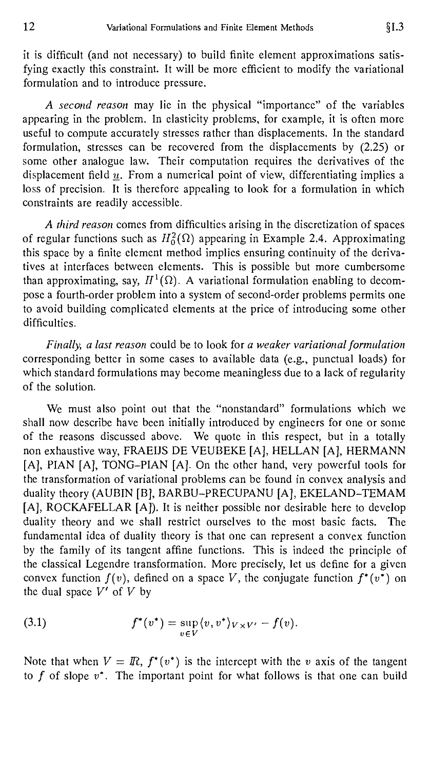
duality theory and we shall restrict ourselves to the most basic facts. The
fundamental idea of duality theory is that one can represent a convex function
by the family of its tangent affine functions. This is indeed the principle of
the classical Legendre transformation. More precisely, let us define for a given
convex function f(v), defined on a space V, the conjugate function f*{v*) on
the dual space V of V by
C.1) r(V) = anp{v,v*)VxV. - f(v).
v£V
Note that when V = R, f*(v*) is the intercept with the v axis of the tangent
to / of slope v*. The important point for what follows is that one can build
§1.3 Mixed and Hybrid Finite Element Methods 13
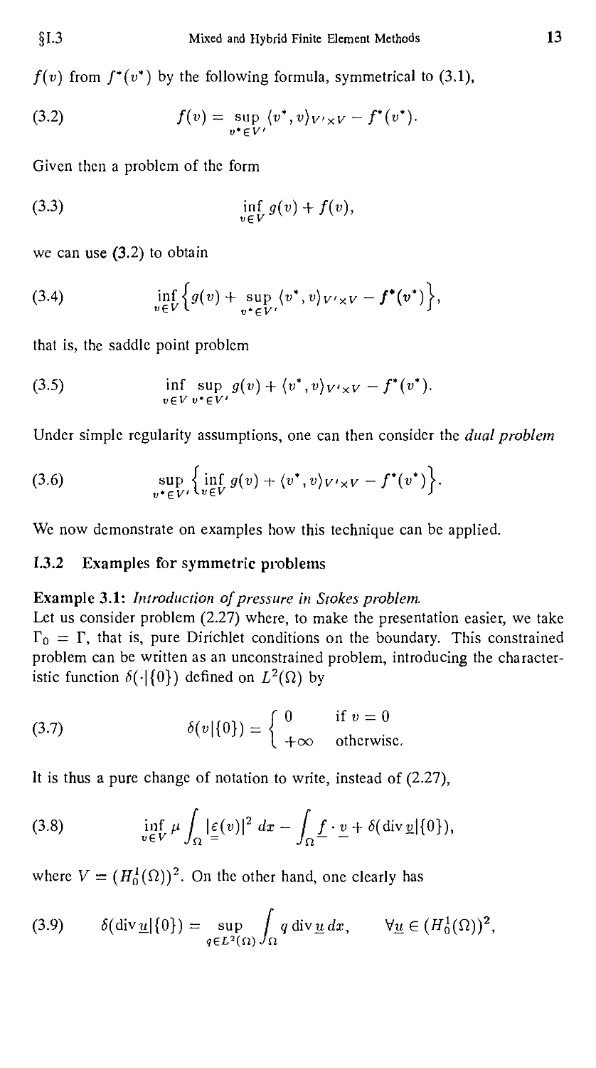
f(v) from f*(v*) by the following formula, symmetrical to C.1),
C.2) /(«)= sup {v*,v)v,xV-r(V).
Given then a problem of the form
C.3) jfv9(v) + f(v),
we can use C.2) to obtain
C.4) inf {$(«)+ sup (v\v)vlxV-f*(vt)\,
that is, the saddle point problem
C.5) inf sup g(v) + (v*,v)vlxV -f*(v*).
Under simple regularity assumptions, one can then consider the dual problem
C.6) sup {inf g(v) + (v\v)V'xv - f*(v*)\.
We now demonstrate on examples how this technique can be applied.
1.3.2 Examples for symmetric problems
Example 3.1: Introduction of pressure in Stokes problem.
Let us consider problem B.27) where, to make the presentation easier, we take
Fo = F, that is, pure Dirichlet conditions on the boundary. This constrained
problem can be written as an unconstrained problem, introducing the character-
characteristic function <*>(-|{0}) defined on L2(Q) by
0.7) «M{o»=f° if;=0
v v ' ' \ +oo otherwise.
It is thus a pure change of notation to write, instead of B.27),
C.8) inf p I \e{v)\2 dx - f f-v + 8(divv\{0}),
where V = G7O'(Q)J. On the other hand, one clearly has
C.9) 5(divw|{0}) = sup f qdivudx, Vw£(
14 Variational Formulations and Finite Element Methods §1.3
and the minimization problem C.8) can be transformed into the saddle point
problem
C.10) inf sup n I \e(v)\2dx- / /• v_dx - / qdivvdx.
irgy ^6L2(fi) Jn ~ Jn Jn
This apparently simple trick has in reality completely changed the nature
of the problem. We now have to find a pair (u,p) solution of the variational
system
i / e(w) : £(v) dx- / / • v_ dx - / pdivv_dx = 0, Vv G V,
C.11) \ f ~ " "
The second equation of C.11) evidently expresses the condition divu = 0. In
order to use C.11), we shall have to show the existence of a saddle point (u,p),
in particular the existence of the Lagrange multiplier p. This will be done in
Chapter II. The variational system C.11) can be interpreted in the form
{— 2[iAu + grad p = /,
divw = 0,
where one uses the operator Ay. = djy£(;»)
1 d (du\ du2 \
C.13) Au = q2 1 a a a
~ ' A •■- 1 a (ou\ ou2 "i
2 dx\ l9x2 3xi / ,
Under the divergence-free condition div u — 0, this can also be written
fA*AH +
V ' ' \divw = 0,
which is the classical form of the Stokes problem. U
Problem C.10) has the general form
C.15) inf sup L(v,q),
VQ
where L(v,q) is a convex-concave functional on V x Q. If one first eliminates
q by computing
J(v) = sup L{v,q),
§1.3 Mixed and Hybrid Finite Element Methods 15
one falls back on the original problem, the primal problem. Reversing the order
of operations (this cannot always be done, but no problems arise in the examples
we present), and eliminating v from L(v,q) by defining
C.16) J*(q)=infL(v,q)
leads to the dual problem
C.17) 8iipJ*(9).
We now apply this idea to the previous examples.
Example 3.2: Dual problem for the Stokes problem.
In the case of Stokes problem, the dual problem can be expressed, as we shall
see, in many equivalent ways. In order to find it, we must, given q, find the
minimum in v of L{v_, q) = \x Jn |£(d)|2 dx — Jn / • v dx — J^q div y_ dx. This
minimum is characterized by
C.18) 2n I £(« ) : e(v) dx - \ f_v_- I q divj, dx = 0, Wv G V,
denoting by uq the minimum point. Making v = u^ this gives
C.19) 2jj / |£(«,)|2 dx- ( /•« dx- I q&vuq dx = 0.
Using C.19) to evaluate L^, q), the dual problem can be written as an optimal
control problem,
C.20) sup -n f \t(u)\2 dx,
where un is the solution of
f —la Aun + grad q — f,
C.21) I -?^K- L<
Denoting by G the Green operator defining the solution of C.21), that is,
C.22) «,=G(/-grad9),
and using C.22) in C.20), one can get from C.19)
C.23) inf / grad q ■ G(grad q) dx - / G(f) ■ grad q dx.
i Jn Jn
16 Variational Formulations and Finite Element Methods §1.3
One notices that this dual problem is a problem in grad q. It is well known that
the solution p is defined (for Dirichlet conditions on w) only up to an additive
constant. One can interpret C.23) as the equation
C.24) div(Ggrad9) = div(G/).
If one defines on V = (//"^Q)J the norm,
C.25) \\f\\l = (Gf,f)VxV;
problem C.23) can be written as a least-squares problem
C.26) 2
The presence of a Green operator makes this dual problem difficult to handle
directly. It is however implicitly the basis of some numerical solution procedures
(FORTIN-GLOWINSKI [B], THOMASSET [A]). We will present other dual
problems that will have direct importance and that will be handled as such.
Example 3.3: A duality method for nearly incompressible elasticity.
We already noted in Example 2.2 and Example 2.3 that the linear elasticity prob-
problem and Stokes problem are very close when a nearly incompressible material
is considered. We now develop this analogy in the framework of Example 3.1.
The starting point will be the obvious result,
C.27) — / | div jj| dx = sup / q divy_ dx — — / |^| dx.
2 Jn qsL2(n)Jn ^ Jn
Substituting C.27) into B.20) we get, by the same methods as in the previous
examples, the problem
inf sup fi I \£.(v_)\ dx — I qdivv_dx / |^| dx
C.28) ^ •"'<"> Ja = ~ Ja *XJa
— / f ■ v dx — I gnv_'Qds— I gtv_t_ds.
Jn~ ~ Jvt Jvi
The solution (u,p) of problem C.28) is characterized by the system
2a1 / S.(m) : £.(u) dx — I p div n dx
Jn~ ~ Jn
= / f_-v_dx+ / (gn v- n + gt v-t) ds, VtigV,
Jn ir,
/ q div u + - / pq dx = 0, V? G L2(Q).
. Jn * Jn
This can be summarized by saying that we transformed our original problem into
a system by introducing the auxiliary variable p = A div u. It must be noted that
this also makes our minimization problem become a saddle point problem. We
shall see in Chapter VI that this apparently tautological change has implications
in the building of numerical approximations to B.20) that remain valid when A
is large. U
§1.3 Mixed and Hybrid Finite Element Methods 17
Example 3.4: Dualization of the Dirichlet problem.
The result that we shall get here can be obtained by many methods. Techniques
of convex analysis permit one to extend what appears to be a trick to much
more complex situations. However it will be sufficient for our purpose to use
the simple development below. Let us then consider the Dirichlet problem,
C.30) inf - / I grad v\2 dx - fv dx.
In many applications grad v rather than v is the interesting variable. For instance,
in thermodiffusion problems, grad v will be the heat flux, which is very often
more important to know than temperature v. What we now do is essentially to
introduce the auxiliary variable p = grad v to transform our Dirichlet problem
into a system. To do so, we use the same trick as in Example 3.3 and write
C.31) \ / | gradi)|2 dx = sup / q ■ grad v dx - \ / |<?|2 dx
in ?e(£2(ft)J Jn Jn.
which we use in C.30) to get the saddle point problem
C.32) inf sup --i / |<?|2 dx - / fvdx+ q_- grad v dx,
where V = H£(£l and Q = (L2(Q)J. The saddle point (u,p) is characterized
by
C.33)
/ p-qdx— / q ■ grad u dx = 0, Vg £ Q,
in ~ Jn~
/ p ■ grad v dx = I fv dx, Wv £ V,
Jn~ in
and this can be read as
3 3 fp = gradu, u G H^(Q),
\divp+/=0,
which is evidently equivalent to a standard Dirichlet problem.
The dual problem is readily made explicit. Writing it as a minimization
problem by changing the sign of the objective functional, we have
C.35) inf | / \q\2dx, VqGZj = {?G(L2(Q)J|divi+/ =
Jn ~
This is the classical complementary energy principle. U
18 Variational Formulations and Finite Element Methods §1.3
We now want to get a weaker form of this problem. In order to do so,
we must introduce a new functional space which will frequently occur in the
following. We define
C.36) //(div; fi) = {q\q£ (L2(Q)J, divq £ L2(Q)}
and its norm
C-37) 11911^.0) = ll£ll5,n + HdivillS>n
that makes it a Hilbert space. It can then be shown, (TEMAM [A]), by the
methods of LIONS-MAGENES [A], that vectors of F(div; fi) admit a well
defined normal trace on T = <9fi. This normal trace q-n, lies in H~ll2{T) and
one has the following "integration by parts" formula,
C.38) q_-giadvdx + / divq v dx = (v, q_ ■ n)Hi/2(r)xH-i/2(n,
Jo Jo
for any q_ £ H(div;i1) and any v £ F'(fi). We shall often write formally
/p VQ " H ds instead of the duality product (v, q-n).
Example 3.5: Weak form of the dual Dirichlet problem.
If we take / £ L2(Q), problem C.35), which is a constrained problem, can
be changed into a saddle point problem, as in Example 3.1, by introducing a
Lagrange multiplier u £ L2(f2), that is, as q now belongs to H(div; Q),
C.39) iuf sup \ I \q\2 dx + I fv dx + I v div q dx.
?e/f(div,fi) ueL2(n) Jo Jo Jo
The functional spaces employed precisely enable us to write every term in
C.39) without ambiguity. We now look for a saddle point (u,p) satisfying the
variational system,
{p-qdx+ / u div q^dx = 0, V? £ H(d\\;Q),
Jo in -
(divp+f)vdx = O, \/v£L2(n).
Jo
Using C.38) with £ ■ n|r = 0, we obtain from C.40),
C.41) p = grad u.
Now u £ L2(Q) and grad u = p £ (L2(Q)J imply that u £ Hl(Q) and it is
justified to consider its trace. Again using C.38) with a general q shows that
u|r = 0. The solution of our "weaker" problem is then the solution of the
standard problem. However the discretizations of problem C.40) will be quite
different from those used for the standard formulation. D
P.3 Mixed and Hybrid Finite Element Methods 19
Remark 3.1: The previous formulation enables us to write directly in a varia-
tional form a nonhomogeneous Dirichlet problem. Indeed the solution (u,p) of
the saddle point problem with g £ Hll2(T),
C.42) infsup| [ \q\2dx + f (divq + f)v dx - [ gq-nds,
q_ v Jci Jn Jv
leads to p = grad u, divp + / = 0, u|r = g.
On the other hand, Neumann conditions become essential conditions that
have to be incorporated into the construction of p, that is, in the choice of the
functional space. D
We now want to extend the previous results to the case of the linear elas-
elasticity problem. We shall thus get a second way to dualize problem B.20). It is
a general fact that there is no unique way to use duality techniques.
The lines of the development are the same as for Dirichlet problems and
we shall avoid to write the details. Let us then define,
C.43) fi(div;fi), = {g\ *{j G L2(Q), *{j = ajit diyg G
where diy<r is the vector dcrnjdxx +<9<x;2/<9z2- On this space we use the norm,
C-44) yiLdivn). =
which makes it a Hilbert space.
One can then define [as for tf(div;fi)J the vector an
C.45) (<Ln)i = Y,aiJnJ
and we shall mostly use the normal and tangential components, ann and ant ,
of this vector, as defined in B.23). We then have the following "integration by
parts" formula:
C.46) / g:e(v)dx+ I diy g- v dx = (an,v) = {(Tnn,v ■ n) + (<xnt,£-1),
Jn. Jn
which is valid for any <r and v_ smooth enough. We have denoted by (•,•)
the duality between H~1/2(T) and Hl/2(T) and shall often write the formal
expression Jr<rnn v_ • B. ds + JriTnl v_- t ds. We can now write our dual
formulation for the linear elasticity problem.
20 Variational Formulations and Finite Element Methods §1.3
Example 3.6: Dualization of the linear elasticity problem.
Following the same line as for the Dirichlet problem, we write
[ \g(v)\2 + 7: I |divu.|2 dx = sup [ g° ■ g° dx
+ f UaUe_dx-±- [\g°fdx-—-l
Jo ~ 4M Jo. 4A +
[
o.
2(fi)J
which leads us to the saddle point problem in i?(diy;fl) x (L2(fi)J,
C.48) inf sup * f | tr a\2 dx + ±- [ \gD\2 dx+ f (diy g+f) U dx.
g v z(A + n) Jn ^^ Jo. Jo.
The solution (<r, u) of this saddle point problem is characterized by the system
C.49) i tr £=(A + ^j) tr |(^),
l
which are the equilibrium condition B.26) and the constitutive relations B.25).
The dual problem then consists in minimizing the complementary energy
C.50)
inf i- / \*D |2 dx + ~^r- j | tr <x|2 dx
& 4H Jo ~ 2(x + N Jo ~
under the constraint diy <r + / = 0. Both the mixed formulation C.48) and the
dual formulation C.50) are used in practice. They lead to different although
similar approximations. D
To end this section we finally consider the thin plate problem of Exam-
Example 2.4 to introduce a mixed formulation due to CIARLET-RAVIART [C] and
MERCIER [A].
Example 3.7: Decomposition of a biharmonic problem.
Again using the same technique as in the dualization of the Dirichlet problem in
Example 3.4, it is a simple exercise to transform problem B.28) into the saddle
point problem
C.51) inf sup ~ I |/(|2 dx+ I u Av dx+ I fv dx,
vel^o) ..gHjcn) Jn Ja Jo
and to get the dual problem
C.52)
2 Jn
§1.3 Mixed and Hybrid Finite Element Methods 21
where M = {n G L2(Q), A/j. + / = 0}. Integrating by parts the term
JnH Av dx, we get, as in Example 3.5, a weaker formulation
C.53) inf sup \ f \fi\2 dx
— I grad n ■ grad v dx + / fv dx.
Jci Jo.
Assume that C.53) has a saddle point (u, u) with w £ Hl(£l). Then (w, u) is
characterized by the variational system
C.54)
/ ^M - / grad ft ■ grad u dx = 0, Vn£
Jn Jn
/ grad w • grad v dx = fv dx, Vd G
If we use fi = 4> e D(fi) in the first equation and v = ^ G D(fl) in the second
one, we can interpret C.54) as
C.55)
The first equation of C.54) also yields du/dn = 0, as we hope. In a sense, we
thus have in C.55) too many boundary conditions on u and none on u. The
system however has a solution (w,u) (provided fi and / are smooth enough)
such that the solution of the Dirichlet problem in u also satisfies (through the
choice of the right-hand side) the extra Neumann condition. □
Example 3.8: Decomposition of the plate bending problem.
We now consider the plate bending problem B.32). In order to make the dual
problem easier to introduce, we first write the energy functional in the form
1 / Pt^ \ f f
C.56) - (^ I nR2v) ■■nav8X-J fv dx,
where the operator D_2 is defined by
C.57) (£
and the operator £CI by
C.58) fsi(
22
Variational Formulations and Finite Element Methods
§1-3
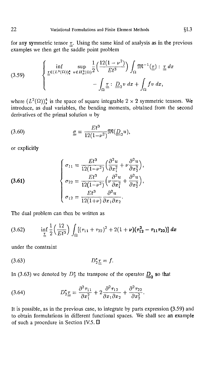
for any symmetric tensor r. Using the same kind of analysis as in the previous
examples we then get the saddle point problem
C.59)
1/12A -v2)
inf sup -I —
) fm-l(L):z
- Z" R2V dx + fv dx,
dx
where (L2(f2)), is the space of square integrable 2x2 symmetric tensors. We
introduce, as dual variables, the bending moments, obtained from the second
derivatives of the primal solution u by
C.60)
Et3
or explicitly
C.61)
r Et3
Et3
Et3
sd2u +
d2u
The dual problem can then be written as
C.62) inf i {—) j [(m + r22J + 2A + v)(t?2 - rur22)] dx
under the constraint
C.63) D*2z = /■
In C.63) we denoted by D2 the transpose of the operator D_2 so that
C.64)
d2n2 d2r22
r
dx2 dx\dx2 dx\
It is possible, as in the previous case, to integrate by parts expression C.59) and
to obtain formulations in different functional spaces. We shall see an example
of such a procedure in Section IV.5. U
§1.3 Mixed and Hybrid Finite Element Methods 23
1.3.3 Duality methods for nonsymmetric bilinear forms
In all previous examples, our variational formulations were based on a mini-
minimization problem for a functional and we were led to introduce a genuine saddle
point problem. Even if this classical framework is suitable for a first presen-
presentation, it is not the sole possibility and the techniques developed can also be
applied to problems which are not optimization problems. Let us consider for
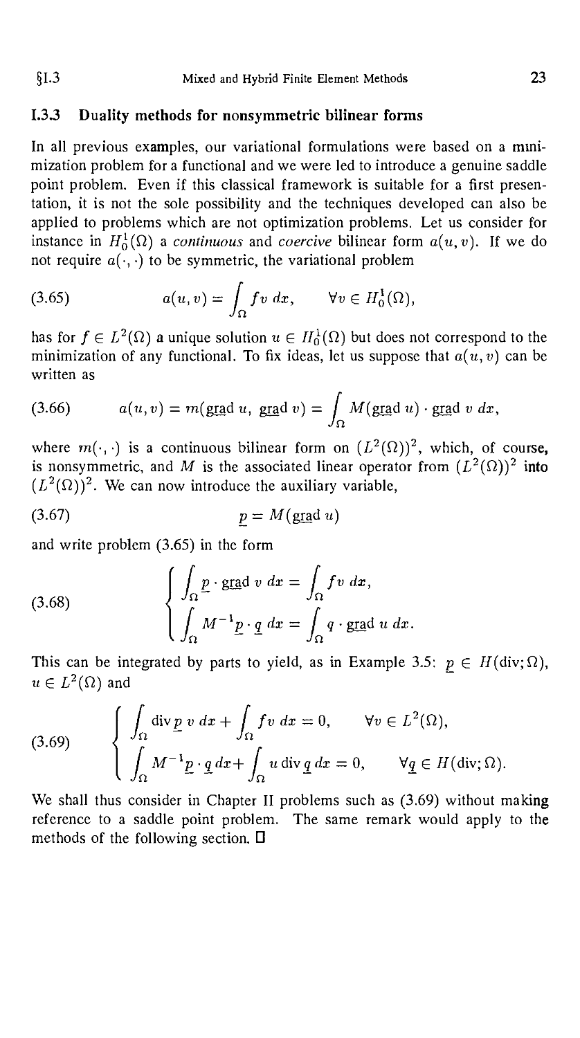
instance in Hq(Q) a continuous and coercive bilinear form a(u,v). If we do
not require a(-, ■) to be symmetric, the variational problem
C.65) a(u,v)= [ fvdx, Vv G Hl0(Q),
Jn
has for / £ L2(f2) a unique solution u £ //o(fl) but does not correspond to the
minimization of any functional. To fix ideas, let us suppose that a(u,v) can be
written as
C.66) a(u, v) = m(grad u, grad v) = / M(grad w) • grad v dx,
Ja
where m(-, ■) is a continuous bilinear form on (L2(f2)J, which, of course,
is nonsymmetric, and M is the associated linear operator from (L2(f2)J into
(L2(f2)J. We can now introduce the auxiliary variable,
C.67) p = M(grad u)
and write problem C.65) in the form
{/ P ■ glad v dx — / fvdx,
/ M~lp-qdx= I q-gradudx.
Jn. ~~ ~ Jo.
This can be integrated by parts to yield, as in Example 3.5: p e H(div;Q),
u G L2(Q) and
C.69)
/ divp v dx+ I fv dx = 0, Vd G L2(Q),
Jn Jn
/ M~lp-q_dx+ I udivqdx = 0, Vq£ H(div;Q).
Jn Jn
We shall thus consider in Chapter II problems such as C.69) without making
reference to a saddle point problem. The same remark would apply to the
methods of the following section. U
24 Variational Formulations and Finite Element Methods §1.4
1.4 Domain Decomposition Methods, Hybrid Methods
We have shown in Section 1.3 that duality techniques enable us to obtain alternate
variational formulations for some problems. The method that we shall now
describe will yield a new family of variational principles that can be more or
less grouped under the name of hybrid methods. The common point between
the examples that follow is that in all cases the variational principle will depend
explicitly, independently of any discretization, on a partition of the domain Q
into subdomains. To make clearer some of the facts that will appear later, we
first recall a very classical result.
Example 4.1: A transmission problem.
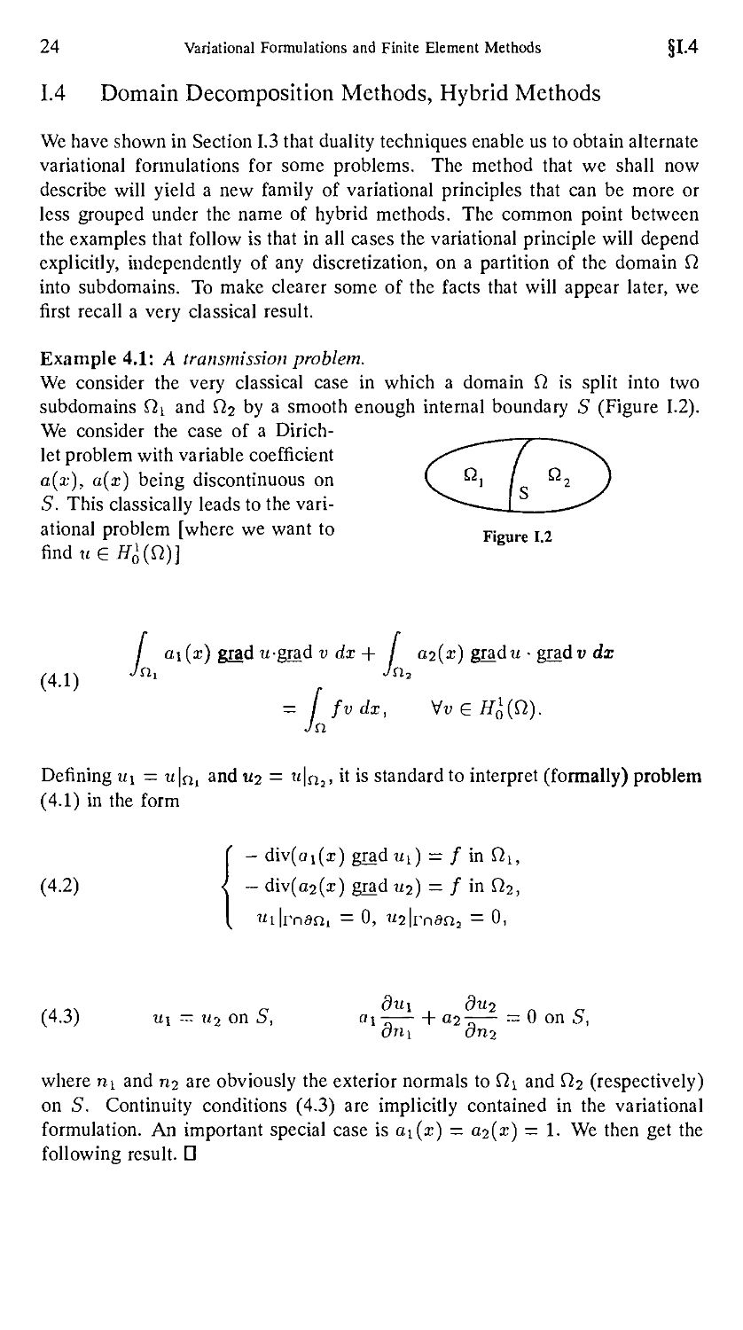
We consider the very classical case in which a domain Q is split into two
subdomains fii and 0,% by a smooth enough internal boundary 5 (Figure 1.2).
We consider the case of a Dirich-
let problem with variable coefficient
a(x), a(x) being discontinuous on
5. This classically leads to the vari-
variational problem [where we want to Figure 12
fid^(fi)]
D.1)
/ ai(x) grad w-grad v dx + I 02A) gradu • gradv dx
Jill -In?
= / fvdx, VveH^fi).
Jn.
Defining u\ — w|fi, and «2 = wln2. it is standard to interpret (formally) problem
D.1) in the form
- div(oi(x) grad «i) = / in fli,
D.2) ^ - div(a2(x) grad w2) = / in fi2,
, = 0, W2|rnan3 = 0,
D.3) «i = u^ on 5, a\— h a-2-— = 0 on S,
oii on
where n\ and ni are obviously the exterior normals to fii and Q2 (respectively)
on 5. Continuity conditions D.3) are implicitly contained in the variational
formulation. An important special case is ay[x) — a^{x) — 1. We then get the
following result. D
§1.4 Mixed and Hybrid Finite Element Methods 25
Proposition 4.1: Let u be solution of the Dirichlet problem
-Au = f,
D.4)
V ' I t«|r =
Let the internal boundary 5 split Q into fii and 0,2. Then it is equivalent to
say that u is solution of the problem
{
- Aw2 = / in fi2,
, = 0, U2|man2 = 0,
{Ki = u-i on 5,
~- + -- = 0 on S.
To show this result we would have to define properly the normal derivatives
dui/dni and du2/dri2 on 5. This would require some regularity on /, for
instance / e L2(Q). □
What we really want to do is to consider a general partition of
D.7)
We now write the classical Dirichlet functional of Example 2.1, in the following
apparently strange way.
Example 4.2: A domain decomposition method for Dirichlet problem.
Writing the Dirichlet functional as
D.8) J(v) = J2\l [ \mdv\2dx-[ fvdx}
and introducing now the functional space
D.9) X(Q) = {v\vG L\n),v\K, G Hl(K{)} ^Y[Hl(
we can extend J(v) on X(Cl). Moreover Hg(d) is a closed subspace of X(Q.)
and we may consider "v £ Hq(Q)" as a linear constraint on v £ X(Q).
This constraint states that on e,j = <9/t; n dKj we must have, in Hll2(eij),
26 Variational Formulations and Finite Element Methods §1.4
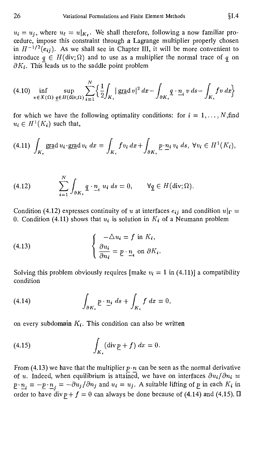
Ui = uj, where ui — u\jit. We shall therefore, following a now familiar pro-
procedure, impose this constraint through a Lagrange multiplier properly chosen
in H~ll2{eij). As we shall see in Chapter III, it will be more convenient to
introduce q £ H(div;fi) and to use as a multiplier the normal trace of q on
dK{. This leads us to the saddle point problem
N
D.10)
N r
inf sup 5^1/ |giadi>|2f/x— / q-n.vds— / fvdx\
uex(ft) q£H{&iv,n)~[ ^Vk, JdK,~ ~' Jk, '
for which we have the following optimality conditions: for i = 1,..., 7V,find
u{ e Hl(Ki) such that,
D.11) / graduj-gradDj dx = fv{dx+ / p-n{vi ds, Vd,- G Hl(Ki)}
Jk, Jk, Jbk,
N f
D.12) J2 q-n.Ui
i=i Jbk.
Condition D.12) expresses continuity of u at interfaces e,j and condition u|r =
0. Condition D.11) shows that u{ is solution in A',- of a Neumann problem
( -Am = / in K{,
D-13) <^ dui
^— -p-n on OKi-
K Orii ~ —*
Solving this problem obviously requires [make vi = 1 in D.11)] a compatibility
condition
D.14) / p-mds+ f fdx = 0,
JaK, Jk,
on every subdomain Ki. This condition can also be written
D.15) / (divp + /) da; = 0.
Jk,
From D.13) we have that the multiplier p-n can be seen as the normal derivative
of u. Indeed, when equilibrium is attained, we have on interfaces dui/dnc —
p-n. = — p-£. = —duj/dnj and u,- = uj. A suitable lifting of p in each Ki in
order to have divp+ / = 0 can always be done because of D.14) and D.15). D
§1.4 Mixed and Hybrid Finite Element Methods 27
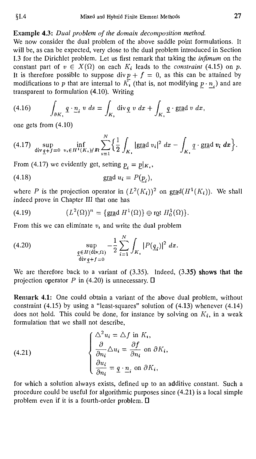
Example 4.3: Dual problem of the domain decomposition method.
We now consider the dual problem of the above saddle point formulations. It
will be, as can be expected, very close to the dual problem introduced in Section
1.3 for the Dirichlet problem. Let us first remark that taking the infimum on the
constant part of v £ X(Q) on each A', leads to the constraint D.15) on p.
It is therefore possible to suppose divp + / = 0, as this can be attained by
modifications to p that are internal to K, (that is, not modifying p- n.) and are
transparent to formulation D.10). Writing
D.16) / gn.vds= I divq v dx + I q-gradvdx,
J8K, ~ ~l Jk, ~ Jk, ~
one gets from D.10)
D.17) sup inf Y^< - / Igrad vA2 dx — / q ■ grad i>,- dx >.
div£+/=o v,£iil(K,)/njL-' 12 JK< Jk,~ '
From D.17) we evidently get, setting p. = p\k,,
D.18) grad «,- = P(p.),
where P is the projection operator in (L2(A',-)J on grad(F1(A'j)). We shall
indeed prove in Chapter III that one has
D.19) (L2(V))n = {grad Hl{Sl)}® rot/.
From this we can eliminate v, and write the dual problem
D.20) sup -=Y, \p(li)\2dx-
?eJ/(divn) z ;=1 Jk,
div^+/=o
We are therefore back to a variant of C.35). Indeed, C.35) shows that the
projection operator P in D.20) is unnecessary. D
Remark 4.1: One could obtain a variant of the above dual problem, without
constraint D.15) by using a "least-squares" solution of D.13) whenever D.14)
does not hold. This could be done, for instance by solving on A',-, in a weak
formulation that we shall not describe,
D.21)
' A2u,- = A/ in K,,
d . Of
-—Au; = on oh{,
r = !'non dl<i,
for which a solution always exists, defined up to an additive constant. Such a
procedure could be useful for algorithmic purposes since D.21) is a local simple
problem even if it is a fourth-order problem. D
28 Variational Formulations and Finite Element Methods §1.4
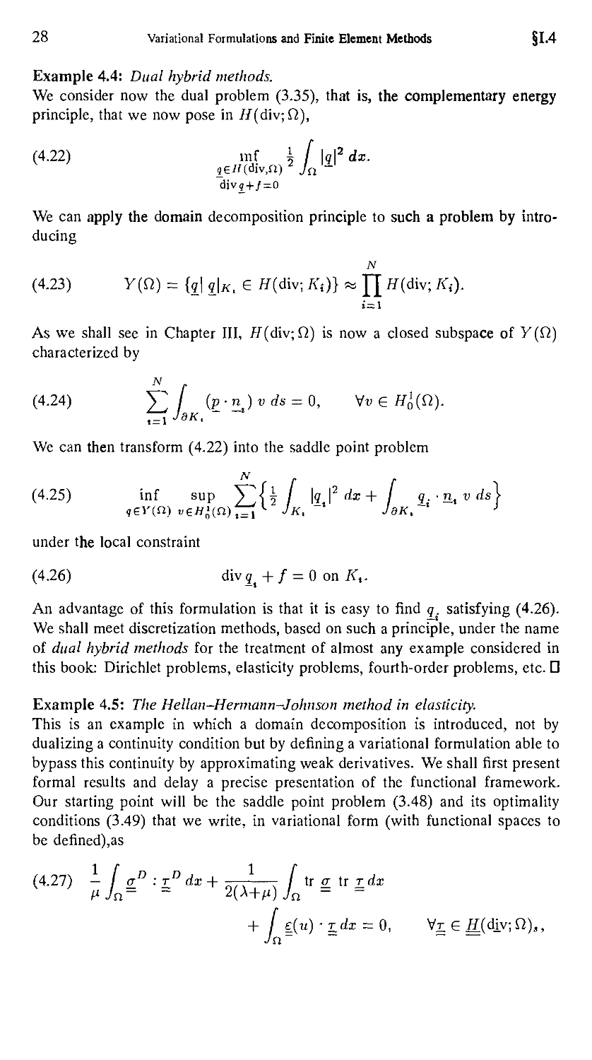
Example 4.4: Dual hybrid methods.
We consider now the dual problem C.35), that is, the complementary energy
principle, that we now pose in //(div; fi),
D.22) mf i / |?|2 dx.
We can apply the domain decomposition principle to such a problem by intro-
introducing
N
D.23) Y(Q) = {,| q\K, G tf (div; Kt)} « JJ tf (div; K{).
As we shall see in Chapter III, //(div;fl) is now a closed subspace of Y(Q)
characterized by
N r
D.24) J2 (p-nt)vds = 0, Vd G H^(Q).
We can then transform D.22) into the saddle point problem
D.25) inf sup Y]{W \q\2dx+j q{ ■ nt v ds\
under the local constraint
D.26) divg + / = 0 on Jf,.
An advantage of this formulation is that it is easy to find q. satisfying D.26).
We shall meet discretization methods, based on such a principle, under the name
of dual hybrid methods for the treatment of almost any example considered in
this book: Dirichlet problems, elasticity problems, fourth-order problems, etc. U
Example 4.5: The Hellan—Hermann-Johnson method in elasticity.
This is an example in which a domain decomposition is introduced, not by
dualizing a continuity condition but by defining a variational formulation able to
bypass this continuity by approximating weak derivatives. We shall first present
formal results and delay a precise presentation of the functional framework.
Our starting point will be the saddle point problem C.48) and its optimality
conditions C.49) that we write, in variational form (with functional spaces to
be defined),as
D.27) - / aD : td dx + * s / tr a tr r dx
+ / |(w) -zdx = 0, Vz
Jn
§1.4 Mixed and Hybrid Finite Element Methods 29
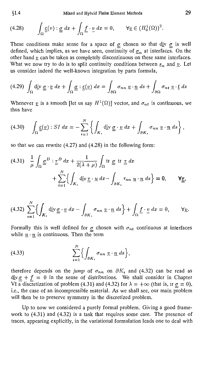
D.28) f g(v):gdx + f f_-v dx = 0, Vj; G (^(Q)J.
Jn Jn
These conditions make sense for a space of a chosen so that diy a_ is well
defined, which implies, as we have seen, continuity of g_n at interfaces. On the
other hand v_ can be taken as completely discontinuous on these same interfaces.
What we now try to do is to split continuity conditions between sn and v_. Let
us consider indeed the well-known integration by parts formula,
D.29) / djy q_ ■ v dx + I q_: e(y_) dx = I ann v_-nds+ / ant v^-tds
Jn ~ Jn~ ~ Jan Jan
Whenever y_ is a smooth [let us say Hl(Q)] vector, and ant is continuous, we
thus have
D.30)
/ g(v) :SIdx = -y2\ drv g ■ v dx + [ ann v - n ds i ,
Jn ,=1 KJk, JdK, J
so that we can rewrite D.27) and D.28) in the following form:
D.31) - [ aD :td dx + —~ / tr a tr r dx
^ vJ= = 2(X + fi)J = =
N . .
+ 2^1 / diy Z- udx— / rnn u ■ n_ ds > = 0, Vt,
i^i Jk, ~ JdK, > ~
N
D.32) V"{ / djygi-vdx- ann v_ ■ n ds\ + / / ■ v dx = 0, VV
f^i^JK, ~ JdK, J Jn~ ~
Formally this is well defined for a_ chosen with ant continuous at interfaces
while u ■ n is continuous. Then the term
D.33) Y"{ / annv-nds\,
i ^Jsk J
therefore depends on the jump of <rnn on dK, and D.32) can be read as
divo; + / = 0 in the sense of distributions. We shall consider in Chapter
VI a~discretization of problem D.31) and D.32) for X = +00 (that is, tr a = 0),
i.e., the case of an incompressible material. As we shall see, our main problem
will then be to preserve symmetry in the discretized problem.
Up to now we considered a purely formal problem. Giving a good frame-
framework to D.31) and D.32) is a task that requires some care. The presence of
traces, appearing explicitly, in the variational formulation leads one to deal with
30 Variational Formulations and Finite Element Methods §1.4
spaces Hxl2(dKi) and H~1^2(dKi) and to subtle considerations about the be-
behavior of functions in these pathological spaces. Let us define
D.34) E = HiH^Ki))*, = {g£ (L2(Q))t,
o-.-jk, G Hl{Ki), aij = aji).
This is a space of smooth tensors and we can consider ant on each interface
c,j = dl<{ n dKj (cf. Chapter III). We have ant e H1'2^) but we do not
have ani e H1/2(dKi); this would require some continuity at vertices which
cannot, in general, take place due to the change of direction of n and t. We can
nevertheless consider in J^, tensor functions <r such that ant is continuous on
e,-j. To make D.33) meaningful, we now have to choose y_ with y. • n continuous
on e,-y. We have already seen that for y_ in H(d\v\ /{,•) we can define y ■ ri
in H~xl2(dKi). Unfortunately it is not possible to restrict y-n\ei} and get a
result in H~1^2(e{j): something is lost in corners. In reality we only need an
"infinitesimal" amount of extra smoothness and this will lead us to look for y_
in (Lp(f2)J n tf(div; fi) for p > 2. This will cause some problems in applying
the theory of Chapter II and existence of a solution will have to be deduced
through special considerations. D
1.5 Augmented Variational Formulations
We shall present in this section other possible ways of defining variational
principles associated with saddle point problems. The methods that we shall
consider are known as Galerkin least-squares methods and were introduced by
FRANCA-HUGHES [A]. To fix the ideas, let us consider the simplest cases of
Examples 3.4 and 3.5, and in particular the saddle point formulations C.32) and
C.39), respectively. In both cases the Euler equations are given by C.34). It is
clear that we can always add (or substract) the square of one of these equations
to the functional without changing the min-max point. For instance, we can
take C.32) and add to it the square of the first equation of C.34) to obtain
inf sup < —-| / |<7|2f/x— / fv dx + / q • gradv dx
v£ii*(n) ?e(L2(ri)J [ Jn ~ Jn Jn~
E.1)
where a can be chosen arbitrarily provided 0 < a < 1. Similarly one can add,
instead, the square of the second equation of C.34) to the functional C.39) to
get
E.2)
inf sup | | / l^pc/x + fvdx+ I v divq dx
r(div,n) i>£L2(ri) [ Jn ~ Jn Jn ~
+ f / (div?+/Jc
inf sup \\ i \q\2dx+ I fv dx + I v div q dx
'(div.ri) vej/,5(fi)[ Jn ~ Jn Jn ~
+ f f(divq+fJdx- § /|£-gradi)|2dxL
Jn Jn
§1.5 Mixed and Hybrid Finite Element Methods 31
where C > 0 is arbitrary.
A third (reasonable) possibility is available: one might take C.39), add to
it the square of the second equation of C.34) and substract the square of the
first equation of C.34):
Note that we had to change the regularity requirements on v in order to make
the functional meaningful. Note as well that we could obtain E.3) from E.1) by
substracting (/3/2) ||div<7 + /H2^^ (and increasing the regularity requirements
on q) and by changing the sign. An easy computation shows that the Euler
equations of E.1) are
/ p • q dx + / fvdx— I p-gradvdx— I q ■ gradudx
E d\ n~ ~ n •'n" Jn~
-a I\p-gradu)-(q-gradv)dx = O, V(£, v) G (L2(Q)Jx//<5 (Q)
Jn
which are equivalent to C.34) for a ^ 1. For a = 1, we just have
/ gradu ■ grad v dx = / fvdx, \/v G II^(Q),
Jn Jn
as should be expected since E.1) reduces to C.30) in this case. Similarly, E.2)
gives
/ p ■ qdx + / fvdx+ I u div q dx + I v div p dx
E 5) n ~ ~ ~ ~
+ 13 f {div p+f )div qdx = 0, V(9, v) G H(div; Q)xL2(«),
Jn
which are again equivalent to C.34). Finally, E.3) gives
/ p ■ qdx + I fvdx+ I u div q dx + / v div p dx
Jn ~ ~ Jn Jn ~ Jn ~
E.6) + p j (divp+/)div£di - a / (p-gradu).(9-gradd)c/z = 0,
Jn Jn
Setting now ip = div p + / and <j> = p — gradw, we may rewrite E.6) as
A-a) I 4-qdx + f3 I i> div qdx = 0, V? G //(div.fi),
E.7) { f Jn ~ :n ~
a I <f> ■ grad v dx + I ipv dx = 0, Vd G /fg (f2).
Jn~ Jn
32 Variational Formulations and Finite Element Methods §1.5
But taking q = gradu, with v £ H2(Q) n Hq(Q), we get from E.7)
E.8) -A-a) / rjivdx + aP [ i>Avdx = 0, Vd G F2(Q) n #o(fi).
(For a = 1, we have —Aw = / again. In conclusion, E.6) is equivalent to
C.34).
Remark 5.1: We obtained in this way three more equivalent variational formu-
formulations for the original problem C.30). Note however that the Euler equations
C.34) constitute a system of two first-order equations in the unknowns u and p;
on the contrary E.4) is of second order in u and first order in p, whereas E.5)
is of first order in u and second order in p and finally E.6) is of second order
in both variables. D
Remark 5.2: We presented here, on an example, a quite general idea which
was presented in a general setting in FRANCA-HUGHES [A] and FRANCA
[A]. Some examples of possible uses of these ideas will be developed in the
following chapters. D
Remark 5.3: In the example presented above, Euler equations C.34) were a
system of first-order equations. This is not the case of Stokes problem C.14),
for which one of the equations is already second order. Applying the same
procedure would lead to a fourth-order problem in the variable u which would
lead to undesirable complications. Indeed the analogue of E.1) would here be
obtained from C.10) as follows:
inf sup n I \e_{v)\2dx — I f ■ v^dx — / gdiv^
., „, uef-HifST)"J ogL2(fl) Jet ~ Jci~ JCl
E.9) -
f /
Jn
|-A«+giadp-/|2dx,
which would force us to use a very regular approximation for the variable u.
A possible one could be to employ this method in connection with a domain
decomposition, Q being partitioned into subdomains as in D.7) and to change
the last integral into
E.10) -f2_,/ |-A« + giadp-/|2dx
7=i ^K<
where a will have to be suitably scaled. This is what has been done by
HUGHES-FRANCA [A]. We shall come back to this in Chapter VI. 0
§1.6 Mixed and Hybrid Finite Element Methods 33
Remark 5.4: Finally, another variant of the general idea developed above has
been considered in DOUGLAS-WANG [A]. The formulation cannot in this case
be written as a modified Lagrangian but must be introduced as a modification
of Euler equations of E.4). Indeed let us write instead of E.4)
E.11) / p-qdx+ / fvdx— / p-gradv dx — / q-gradudx
Jn Jn Jn~ Jn ~
+ a [ (p-grzdu){q+grzdv)dx = 0, W{q,v) € (L2(Q)JX^(Q).
Jn ~
This formulation cannot be obtained from a Lagrangian. It can easily be seen
that it remains valid for a > 0 arbitrary. Indeed E.11) can also be writen as
E.12)
Ul+a) [ (p-gradu) qdx = 0, V<? G (L2(n)O,
I Jn
\a I gradw-gradi; dx+(l— a) I p-gradi; dx— I fvdx —Q,
v Jn Jn~ Jn
and this is equivalent to C.34) for any a > 0. □
To end this chapter, we present a last type of variational formulation yield-
yielding weaker solutions than the formulations presented up to now.
1.6 Transposition Methods
Although we shall not consider in this book discretization methods directly
based on transposition methods, some of the properties of these methods will be
a good guide for understanding weak formulations. We present here the simplest
possible case of a transposed problem and we refer to LIONS-MAGENES [A]
for a complete discussion. Our starting point to obtain a weak formulation
of a Dirichlet problem will be, paradoxically, a regularity result (AGMON-
DOUGLIS-NIRENBERG [A], AGMON [A], NECAS [A]). It is indeed well
known that for / G L2(Q) and when the boundary <9fi is smooth enough, the
solution of the problem
- Aw = /,
satisfies a regularity property
F.2) a
and then an a priori bound
F-3)
34 Variational Formulations and Finite Element Methods §1.6
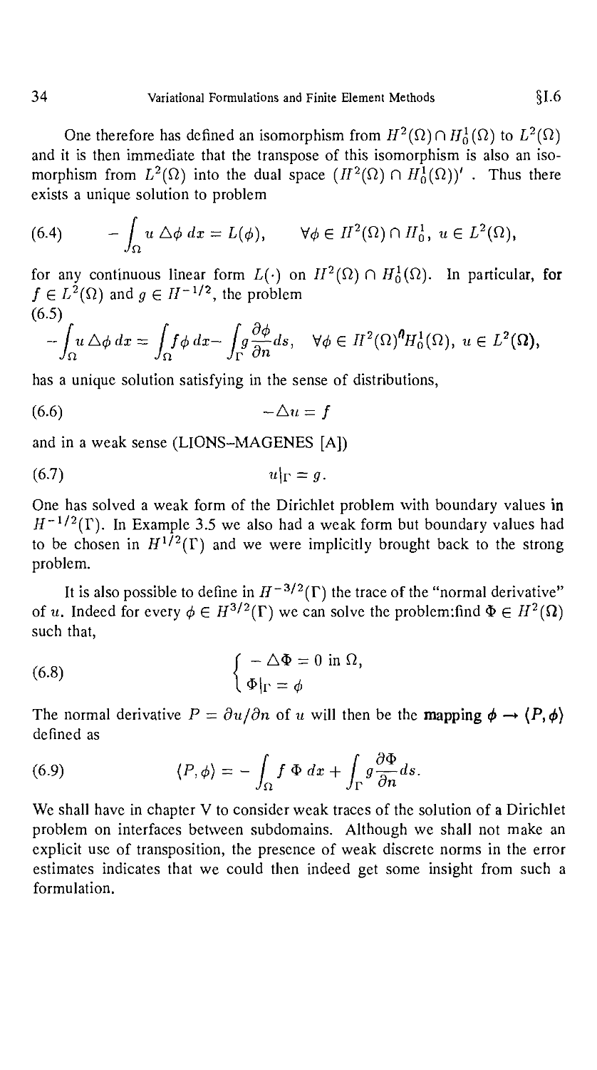
One therefore has defined an isomorphism from H2(Q)C\ Hq(£1) to L2(f2)
and it is then immediate that the transpose of this isomorphism is also an iso-
isomorphism from L2(Q) into the dual space (//2(fi) (~l H^(Q))' . Thus there
exists a unique solution to problem
F.4) - / u A<j> dx =
Jn
for any continuous linear form L(-) on J/2(fi) n Hq(Q). In particular, for
/ G L2(Q) and g G //-1/2, the problem
F.5)
f f [ d<j> 2._.fl 1/(_ 2,-,.
— I u A(f> dx = / /<^> ax— / <7——as, V</> G // (i2) /fo("), u G L (ft),
has a unique solution satisfying in the sense of distributions,
F.6) -Am = /
and in a weak sense (LIONS-MAGENES [A])
F.7) u\r = g.
One has solved a weak form of the Dirichlet problem with boundary values in
ff-1/2(r). In Example 3.5 we also had a weak form but boundary values had
to be chosen in fl'1/2(r) and we were implicitly brought back to the strong
problem.
It is also possible to define in II~3/2(T) the trace of the "normal derivative"
of u. Indeed for every <j> G H3^2(T) we can solve the problenr.find $ G H2(£l)
such that,
f - A$ = 0 in Q,
The normal derivative P — du/dn of u will then be the mapping <j> —* (P, (j>)
defined as
F.9) {P,d>) =
We shall have in chapter V to consider weak traces of the solution of a Dirichlet
problem on interfaces between subdomains. Although we shall not make an
explicit use of transposition, the presence of weak discrete norms in the error
estimates indicates that we could then indeed get some insight from such a
formulation.
§1.7 Mixed and Hybrid Finite Element Methods 35
1.7 Bibliographical Remarks
The purpose of this Chapter was to present examples which will be used later
as a standing ground for our development. It was not possible in such a context
to consider every case. We already referred the reader to DAUTRAY-LIONS
[A] where the mathematical analysis of the problem selected, and many others,
can be found in an unified setting. We also refer to more engineering oriented
presentations such as BATHE [A], HUGHES [A], KIKUCHI-ODEN [A], and
ZIENKIEWICZ [A]. In particular, nonlinear problems and their treatment are
described in these references.
II
Approximation of
Saddle Point Problems
This chapter is in a sense the kernel of the book. It sets a general framework in
which mixed and hybrid finite element methods can be studied. Even if some
applications will require variations of the general results, these could not be
understood without the basic notions introduced here. Our first concern will be
existence and uniqueness of solutions. We first consider in Section II.1.1 the
simple case of a saddle point problem corresponding to the minimization of a
linearly constrained quadratic functional. This case is extended in Section 11.1.2
to a more general case. The matter of approximating the solution will then be
considered under various (but classical) assumptions. Finally, we shall deal with
numerical properties of the discretized problems and practical computational
facts.
II. 1 Existence and Uniqueness of Solutions
In the previous chapter, we introduced a large number of saddle point problems
or generalizations of such problems. In most cases, the question of existence
and uniqueness of solutions was left aside. We now introduce an abstract frame
that is sufficiently general to cover all our needs. In order to make our pre-
presentation easier, we shall first consider the simpler case corresponding (under
symmetry assumptions) to the minimization of a quadratic functional under lin-
linear constraints. We shall follow essentially the analysis of BREZZI [A] and
FORTIN [C]. We also refer the reader to the paper of BABUSKA [A] which
was a fundamental step towards understanding mixed methods, and to the recent
work of ROBERTS-THOMAS [A] for another general presentation of mixed
methods.
§11.1 Mixed and Hybrid Finite Element Methods 37
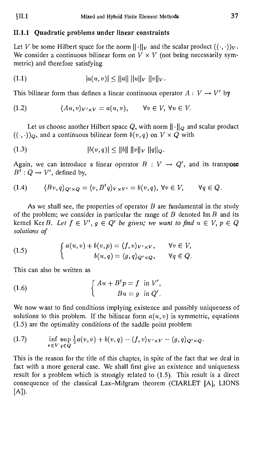
II.1.1 Quadratic problems under linear constraints
Let V be some Hilbert space for the norm || • ||y and the scalar product ((•, -))v-
We consider a continuous bilinear form on V x V (not being necessarily sym-
symmetric) and therefore satisfying
A.1) |a(«,«)|<||a|||MHM|v.
This bilinear form thus defines a linear continuous operator A : V —*• V by
A.2) (Au,v)v,xV =a(u,v), Vv£V,Vu£V.
Let us choose another Hilbert space Q, with norm || • \\q and scalar product
((■> "))q> anc' a continuous bilinear form b(v,q) on V x Q with
Again, we can introduce a linear operator B : V —» Q', and its transpose
S1 :Q-> V, defined by,
A.4) (Bv,q)Q,xQ^(v,Dtq)vxv =b(v,q), Vv £ V, Wq G Q.
As we shall see, the properties of operator B are fundamental in the study
of the problem; we consider in particular the range of B denoted Im B and its
kernel KerS. Let f G V', g G Q' be given; we want to find u G V, p G Q
solutions of
I b(u,q) - (g,q)Q'XQ, Vg G Q.
This can also be written as
Au + B'p = f in V',
1 Bu = g inQ'.
We now want to find conditions implying existence and possibly uniqueness of
solutions to this problem. If the bilinear form a(u,v) is symmetric, equations
A.5) are the optimality conditions of the saddle point problem
A.7) inf sup ^a(v,v) + b(v,q) ~ (f,v)v>xv - (<7,9)q'xq-
This is the reason for the title of this chapter, in spite of the fact that we deal in
fact with a more general case. We shall first give an existence and uniqueness
result for a problem which is strongly related to A.5). This result is a direct
consequence of the classical Lax-Milgram theorem (CIARLET [A], LIONS
[A]).
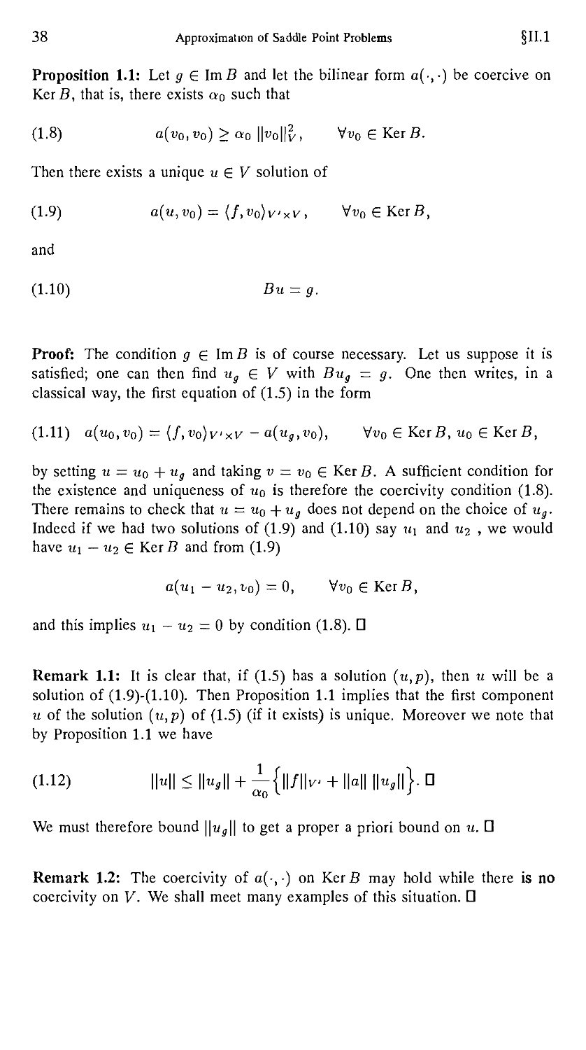
38 Approximation of Saddle Point Problems §11.1
Proposition 1.1: Let g G ImB and let the bilinear form a(-,-) be coercive on
Ker B, that is, there exists ao such that
A.8) a(vo,vo)>ao\\vo\\l, Vi>0 G Ker B.
Then there exists a unique u £ V solution of
A.9) a(u,vo) = {f,vo)vxv, Vuo
and
A.10) Bu = g.
Proof: The condition g G Im B is of course necessary. Let us suppose it is
satisfied; one can then find ug G V with Bug — g. One then writes, in a
classical way, the first equation of A.5) in the form
A.11) a(uo,vo) = (f,vo)vxv - a(ug,v0), Wv0 G Ker B, u0 G Ker B,
by setting u = w0 + ug and taking v = vo G KerS. A sufficient condition for
the existence and uniqueness of «o is therefore the coercivity condition A.8).
There remains to check that u = u0 + ug does not depend on the choice of ug.
Indeed if we had two solutions of A.9) and A.10) say u\ and «2 , we would
have «i — «2 G KerB and from A.9)
a(ui - u2,v0) = 0, Vi>oGKerB,
and this implies «i — «2 = 0 by condition A.8). D
Remark 1.1: It is clear that, if A.5) has a solution (w,p), then u will be a
solution of A.9)-A.10). Then Proposition 1.1 implies that the first component
u of the solution (u,p) of A.5) (if it exists) is unique. Moreover we note that
by Proposition 1.1 we have
We must therefore bound ||uj|| to get a proper a priori bound on u. D
Remark 1.2: The coercivity of a(,) on KerB may hold while there is no
coercivity on V. We shall meet many examples of this situation. D
§11.1 Mixed and Hybrid Finite Element Methods 39
Remark 1.3: If the bilinear form a(-, •) is symmetric, A.9) and A.10) are the
optimality conditions of the minimization problem
A.13) inf -a(v,v)-(f,v)v,xV.
Bv=g 2
The variable p will be the Lagrange multiplier associated with the constraint
Bu = g.U
We now turn to the problem of finding p. For this, we shall have to make
an additional assumption on the operator B. Precisely the range of B, imB,
will have to be closed in Q'. This will hold, in particular, in the frequently
encountered cases where B is surjective or when Im B is of finite codimension.
This assumption (that Im B is closed) enables us to extend to the infinite-
dimensional case, properties that are well-known to hold for matrices. We thus
recall the following classical result of functional analysis (cf YOSIDA [A] for
instance).
Proposition 1.2: The following statements are equivalent:
— Im B is closed in Q', that is for any sequence Vk such that Bvk converges
in Q', there exists v £ V with limji Dvk = Dv.
— Im Dt is closed in V', that is for any sequence q^ such that Bxqk converges
in V', there exists q G Q with lim^ Bxqk — Bxq.
— (Ker5)° = {v' G V'\(v', v) v,xV = 0, Vv G KerB} = ImB'.
— (KerS1H = {<?' G Q'|<<?',q)Q.xQ = 0, V? G KerS1} = ImB.
— There exists k0 > 0 such that for any jg ImB, there exists vg G V with
Bvg = g and \\vg\\v <l/ko\\g\\Q,.
— There exists ko > 0 such that for any / G Im Bx, there exists qj G Q with
B19/=/and||9/||0<l/*0||/||i".n
If one of the above properties is satisfied, one can say that B admits a
continuous lifting from Q' to V and Bx a continuous lifting from V' to Q. We
have used the dual norms, || • \\v and || • ||q/, defined by
A.14) H/llv- = sup M ^
p ,
v£V \\v\\v
where, as in the rest of the book, we assumed implicitely that sup^. <f>(x) has to
be taken for ||x|| ^ 0 if <f>(x) contains ||x|| in the denominator. The same will
be true for inf^ 4>(x). The last two statements of Proposition 1.2 can then be
written as
A.15) sup MMl>fco[ mf |
IMI LuoeKerfl
40 Approximation of Saddle Point Problems §11.1
and
A.16) sup bJf^l>k0\ inf \\q + qO\\]=ko\\q\\Q/Ke,B', V? G Q,
£V \\V\\V LgoeKerB' J
by taking into account the fact that vg can be chosen in (KerBI and qj in
(KerB')-1-, respectively. We can summarize by saying that operators with a
closed range have the well-known properties of operators in finite-dimensional
spaces (for which the range is always trivially closed). We can now proceed to
study the full problem A.5).
Proposition 1.3: Let g G Im B and let u be the solution of problem A.9) and
A.10). If ImB is closed in Q', there exists p G Q' such that (u,p) is solution
of problem A.5). Moreover, we have
Proof: Indeed, let us consider in V', the linear form
A.19) L(v) = (f,v)vxv-a(u,v).
By A.9) we have L(v0) = 0, for any v0 G KerB. By Proposition 1.2, we know
that L GlmD' - (KerBH, and there exists p G Q so that
A.20) L(v) = b(v,p), VuGV,
A.21) Hpllo/KeiB. < h\L\\v. < y(\\a\\ \\u\\y + \\f\\v>).
From Proposition 1.2, we can also choose ug in Proposition 1.1 to satisfy
A-22) IKIIv < f \\g\W-
fc0
Thus A.17) follows from A.12) and A.22) whereas A.18) is readily deduced
from A.21) and A.17). Finally, from A.20) and A.19) we have
A.23) a(u,v) + b(v,p) = (/,«), VwGV.D
§11.1 Mixed and Hybrid Finite Element Methods 41
Remark 1.4: For finite-dimensional problems we shall always have existence
of a solution (u,p) of A.5) provided we have the existence of u in A.9) and
A.10). D
Remark 1.5: If ImD is of finite codimension (and thus closed) it is possible
to build explicitly the extension of £(•). □
Remark 1.6: It is clear (from the first equation ofA.6) for instance) that p is
defined up to an arbitrary element of KerB'. We then have uniqueness of p if
and only if D is surjective. D
The proof of Proposition 1.1 shows that condition A.8) is in fact too strong.
What we really need is the condition that the restriction of A to KerB be
invertible on KerS. Equation A.11) then defines u0 in a unique way. This
condition is equivalent to the condition that Ao, the restriction of A to KerB, is
bijective and by Proposition 1.2 applied to A; this is equivalent to the conditions
A.24) inf sup
which impliesKer AQ = {0} that is, Ao is surjective, and
/1 -vcn • r a(uO,Vo) .
A.25) inf sup ' > a0,
lluo|| \\vo\\
which implies Ker Ao = {0} that is, Ao is injective. It must be pointed out that
A.25) for instance is not implied by a condition of the form
a(u,v)
mf sup \ ' > a
u£V v£V \\u\\ \\v\\
which would mean A to be injective on V. The same remark holds for A.24).
For example, we shall encounter in practice problems of the form
I A B\ GX
A.26) Dx 0
\Ci C2 0
We would then have to check that
A B\
Bx O
is invertible on Ker C = Ker{Ci, C2}. It will not be sufficient to prove invert-
ibility on V which is a problem of the type considered above and is in general
much simpler.
We can now summarize the above results in the following.
42 Approximation of Saddle Point Problems §11.1
Theorem 1.1: Let a(-, •) be a continuous linear form on V x V, let b(-, •) be a
continuous linear form on V x Q. Let us suppose that the range of the operator
B associated to &(-, •) is closed in Q', that is, there exists ko > 0 such that
A.27) sup^l >fco|MlQ/Kcr/J<.
If moreover a(-, •) is invertible on Kcr D, that is, there exists ao > 0, such that
. a(uo,vo) _
inf sup . , > ao,
ll«|| INI|
. - a(uo,vo)
inf sup v ■■■■ > ao,
llu|| \\vo\\v
then there exists a solution (w,p) to problem A.5) for any f £ V' and for any
g £ Im B. The first component u is unique and p is defined up to an element
of KerS'. Moreover one has the bounds
A.29) ||«||v< J-|
a0
^[l + ^liMio'.n
Remark 1.7: Conditions A.27)-A.28) of the theorem above are not only suf-
sufficient but necessary for the existence of a solution to the problem considered
for all g G Im B and for all f £ V (BREZZI [A]). □
To fix ideas, we shall apply the results just obtained to some of the examples
introduced in Chapter I.
Example 1.1: The Stokes problem.
Let us go back to Example 3.1 of Chapter I. We look for u £ (
V ,p £ L2(Q) = Q, solutions of
A.31)
2/< / e(u) : e_(v)dx - / p div vdx = / v ■ f_dx, \/v £ V,
Jn. - - Jn. Jn
- / qdivudx-0, Wq£Q.
Jn
Here we have g = 0. Moreover the bilinear form a(u,v) = 2fifn s(u):e_(v) dx
is coercive on V (DUVAUT-LIONS [A], TEMAM [A]). The exisTence of u in
B.27) of chapter I is therefore established.
§11.1 Mixed and Hybrid Finite Element Methods 43
On the other hand, we have
= ~ I
and B is the divergence operator from (//q(Q)J into L2(£l). One can show
(LADYZIIENSKAYA [A], TEMAM [A]) that
ImB = {q\ / qdx = 0},
and this subspace of L2(f2) is evidently closed (being of codimension one). We
then have the existence of a pressure p defined up to an additive constant, and
we can write
KerS* = Ker(-grad) = {q\ q is constant on ft}. U
Example 1.2: Mixed formulation of (he Dirichlel problem
We consider here the case of Example 3.5 of Chapter I. We look for p G
//(div; fi) = V, u G L2(Q.) = Q such that, / being given in L2(Q),
ip-q_dx+ ud\vgdx = 0, V? G//(div; Q),
r"
Jn.
There is a reversal of symbols with respect to the abstract result: this is probably
the major difficulty of this example. Here B is ihe divergence operator from
//(div; Q) into L2(Q) and it is surjective. We have
a(p,q) = / p-qdx,
Jn.
and this bilinear form is coercive on KerS, even if it is not coercive on
H(div; Q), taking into account the definition C.37) of chapter I of the norm in
Example 1.3: Domain decomposition for the Dirichlet problem.
Refering to Example 4.2 of Chapter I, we have to solve the following problem:
find u G X(Q) = V, p G //(div; fi) = Q, solutions of
/ grad «j • grad v% dx — I p ■ n.vida — I f vi dx,
Jk, JdK,~ ~' Jk,
A.33) < Vi>i G // (Ki), VA'j,
Y] I in. Ui da = 0, V? G //(div; fi)
44 Approximation of Saddle Point Problems §11.1
We thus have b(v,q) = J2, f9K 9 ' "i v'(ia' and ^e operator B associates to
v G X(Q) its jumps u; - vj on the interfaces e,-j = dKt n <9A'j. The kernel
of B is nothing but ^o'(f2) and the problem corresponding to A.9) and A.10)
is the standard Dirichlet problem. To prove the existence of p we shall have
to prove that imB is closed in (H(div;Q))' and we shall have to characterize
KerS'. This will be done in Chapter IV. U
We shall of course come back to these problems when studying more
precisely mixed and hybrid methods. Checking the closedness of ImB, even
if existence proofs can be obtained through other considerations, is a crucial
step ensuring that we have a well-posed problem and that we are working with
the right functional spaces. This last fact is essential to obtain "natural" error
estimates.
II.1.2 Extensions of existence and uniqueness results
Some applications, in particular nearly incompressible material (Section VI.6)
will require a more general formulation than problem A.5). Although the first
generalization introduced will appear to be simple, we shall see that its analysis
is rather more intricate.
Let us then introduce a new bilinear form c(-,-) on Q x Q on which we
suppose continuity and posilivity,
A.34) Kp,?)I<IM
A-35) c(q,q)>0, Vq£Q,
and let us denote by C : Q —* Q' the operator associated with c(-, •).
We now consider the following extension of problem A.5): find u £ V
and p £ Q such that
A36) (a(xi,v) + b(v,p) = {f,v)v.xV,,
Vi>e v,
V?6Q.
Whenever a(-, •) and c(-,-) are symmetric, this problem corresponds to the
saddle point problem
inf sup \a(v, v) + b(v,q) - \c{q,q) - (/, v) + {g,q)
and it is no longer equivalent to a minimization problem on u.
We now want to look for conditions on a, b, and c ensuring the existence
and uniqueness of a solution to A.36). We also want to find bounds on u and
p and we would like these bounds to be independent of the properties of c(-, •).
§11.1 Mixed and Hybrid Finite Element Methods 45
Let us first consider a special case. We assume that c(-, •) is coercive on
Q, that is,
A.37) 3T > 0 such that c(q, q) > j \\q\\l, V? G Q
and that a(-, •) is also coercive on V:
A.38) 3a > 0 such that a(v, v) > a \\v\\l, Wv G V.
Then we have the following proposition.
Proposition 1.4: If A.37) and A.38) hold, then for every / G V and g G Q'
problem A.36) has a unique solution (u,p). Moreover we have:
A-39) |lHI^ + |l|p||^<^ll/||2v- + ^l*
The proof is elementary. □
The estimate A.39) is unsatisfactory. Actually, in many applications, we
will deal with a bilinear form c(-, •) defined by
A.40) c(p,q) = X((p,q))Q, X>0,
and we would like to get estimates that provide uniform bounds on the solution
for X small (say 0 < X < 1). Clearly if c(-,-) has the form A.40), one has
7 = X in A.37) and the bound A.39) explodes for vanishing X. This fact
has practical implications, as we shall see, on the numerical approximations of
some problems, for instance nearly incompressible materials. On the other hand
Proposition 1.4 makes no assumptions on (>(•,•) [except the usual A.3)] and it
is then quite natural for the choice c = 0 to be forbidden. However in Section
II. 1.2 we were able to get proper bounds for c s 0 by using A.27). Hence we
now try to reduce the assumptions on c = 0 and to add the assumption A.27)
on &(•,•)•
We therefore assume that a(-,-) satisfies A.1), A.28), and
A.41) a(v,v)>0, WvGV.
We also assume that &(•,-) satisfies A.3) and A.27) and c(-, •) satisfies A.34)
and A.35). For the sake of simplicity we also assume that c is symmetric, that
is, c[p,q) — c(q,p) for all p and q in Q. It is easy to check that A.35), and the
symmetry imply
A-42) «p,q)J <(c(p,p))(c(q,q))
[consider the polynomial P(i) = c{p + tq,p+ tq) and remark that P(t) >
0, Vi G 1R. This implies A.42).]
46 Approximation of Saddle Point Problems §11.1
Now consider, for every e > 0, the "regularized" problem: find ue G V
and pe GQ such that
A.43) e((ut,v))v+a(ut,v) + b(v,pt)=(f,v), Vi> G V,
A.44) K««.?)-e((p
Proposition 1.4 ensures existence and uniqueness of the solution of A.43) and
A.44). If we can bound w£ andp£ independently of e, a simple limiting argument
will allow us to conclude. As a first step we take v = uc in A.43) and q = pe
in A.44) and we subtract the two equations to get
A.45) e\\ut\$ + e \\pt\\2Q + a(uc,uc) + c(pt,pt) = (f,ue) - (g,pt).
From now on, we drop, for the sake of brevity, the subscript e and we write
A.46) u = w0 + «, P = Po+P
with wo G KerS, w G (KerSI, p0 G KerS', p G (KerS'I. The first step
is to bound w and p by means of A.27). We have
and, using Proposition 1.2 (in particular A.15)),
ko||w||y < sup
A.48)
where A.42) and A.34) were also used. Next we bound wo in terms of w, using
A.28):
a(wo,i>o) ra(u,v0) - a(u,v0)'
A.49) °oW|v- SU-P ~^^ = SU.P
Collecting A.48) and A.49) we have
A.50) ||w||v < —{(||c|| c(p,p)I/2 • -"-"- ' "~" ■i/'1 ■ Hall+(^ ■ ll^'l1
On the other hand, if g G ImS we have from A.45)
A.51) e\\p\\2Q + a(u, w) + c(p,p) < ||/||v ||w||v + \\g\\Q. \\p\\Q
§11.1 Mixed and Hybrid Finite Element Methods 47
and using A.47)
A.52) e\\p\\2Q+a(u,u) + c(p,p)
\\v + llffllo'^^) \MW + YjlfWv \\9\\Q-
From A.52) and A.50) we have
A.53) e\\p\\2Q + a(«,u) + c(p,p) < K((\\c\\ c{p,p)fl2 + 1 +
where K is easily bounded by ||/||, \\g\\, \\a\\, l/fc0) l/«o-
From A.53) we deduce that c(p,p) and a/^IIpII are uniformly bounded.
Then A.48) gives the bound on 5, A.49) gives the bound on u0 and A.47)
gives the bound on p. We still have to bound po. Equation A.44) implies
A.54) e((po,?))o + c(p0,?) = -c(p,?)) V?eKerS(.
In many particular cases, A.54) provides a bound for p0 in a very natural way.
Let us consider the following general assumption.
There exists a 70 > 0 such that for every p £ (KerS'I and for
A.55) every e > 0 the solution p0 G Ker B* of equation A.54) is bounded
by to ||po||q < ||p||q.
If assumption A.55) is satisfied, we obtain that both ||w|| and ||p|| and bounded
uniformly in £ by a constant depending on ||/||, \\g\\, \\a\\, \\c\\, 1/fco, 1/ao, —.
This will imply existence and a priori bounds for the solution of A.36). Before
a deeper analysis of A.55) let us state the result which has been obtained.
Theorem 1.2. Assume that a(-, •), &(•, •) and c(-, •) are continuous bilinear forms
on V x V on V x Q, and on Q x Q respectively. Assume further that a(-,-)
is positive semidefinite [i.e. A.41)] and that c(-,-) is positive semidefinite and
symmetric. Finally assume that A.27), A.28), and A.55) are satisfied. Then for
every f £ V and every g £ ImB problem A.36) has a solution (u,p), which
is unique in V x Q/M, where
A.56) M - Ker Bl n Ker C.
Moreover we have the bound
A.57) |M|V + ||p||0/ KerB- < K{\\f\\v. + \\g\W)
with K a nonlinear function of ||a||, ||c||, 1/ao, l/^o, I/to which is bounded
on bounded subsets. □
48 Approximation of Saddle Point Problems §11.1
Remark 1.8: Theorem 1.2 assumes that g G Im B. Actually a careful look at
its proof shows that the crucial steps A.51)—A.53) can be performed under the
more general assumptions,
{9 = 9 + go,
g£lmB,
3a > 0 such that for all q GQ, \(go,q)\ < ° (c(q,qI'2).
This in particular will hold if g has the form
A-59) (g,q) = {g,<i) + c(qo,q)
with g G Im B and qo G Q, provided c(-, ■) satisfies the assumptions of Theorem
1.2 and in particular A.42). In this case, we clearly have a = (c(qo,qoI^2)-
If g has the form A.59), equation A.54) also keeps the same form, and
condition A.55) must now be written in the slightly stronger form
There exists a 70 > 0 such that for every p G Q and for every
A 60) £ > 0 the solution po G KerS* of equation A-54) is bounded by
toIIpoIIq < HpIIq. □
Let us now discuss condition A.55) in more detail, trying to find particular
instances where it stands.
Casel: c{p, q) = A((p,g)H, (A > 0).
Then A.54) reduces to
A.61) (e
hence p0 = 0 and A.55) is trivially satisfied. The result extends if g has the
form A.59), but p0 is not bounded independently of \ for a general g. U
Case 2: c(p, q) = A c(p, q), where c(-, ■) is a bilinear form onQxQ satisfying
Then A.55) is satisfied with 70 = 7/||c|| and hence independent of A for g G
Imflorj satisfying A.59). □
§11.1 Mixed and Hybrid Finite Element Methods 49
Case 3: KerB* = {0}.
Then A.55) is trivial. D
Case 4: c(-, •) is coercive on KerB*.
A.63) c(qo,qo) > 7i \\qa\\2Q, Vgo G Ker 5*.
Then A.55) holds with 70 = 7i/||c||. In this case the assumption g £ imB
becomes unnecessary. D
An assumption weaker then A.63), in the style of A.28), still ensuring
c to be invertible in Ker 5* would still be enough to get A.55) and to avoid
g GlmB.
Remark 1.9: One often has (like in Cases 1 and 2 above), Ker C = {0}, so
that the space M appearing in A.56) actually reduces to {0} and the solution
(u,p) is unique. D
Remark 1.10: A closer look to the proof of Theorem 1.2 shows that, if one
assumes a(-, -) to be coercive in V, that is, A.38), then \\u\\y is bounded directly
by (a(u,u)y^2 and A.48) is useless. Hence the symmetry of c(-, •) becomes
unnecessary if A.38) holds. D
Remark 1.11: The case c= \I was considered by ARNOLD [A]. □
Remark 1.12: Assuming that Ker B* = {0} and A.28), a continuity argument
shows that A.36) has a unique solution whenever c(-, •) is small enough, without
any further assumption. D
Remark 1.13: Another case strongly related to Theorem 1.2 will occur in
applications, (cf. Section VII.3). Let us consider a bilinear form c^(-, ■) defined
on a Hilbert space W «—► Q and satisfying
cx(p,q)<cO\\\p\\w\\q\\w, Vp,q£W
We now consider a problem of the form
a(u,v) + b(v,p) = (f,v)v,xV,
1 Kui) ~ca(p,q) = (</i,g)<?'x<? + {g2,q)wxw, V? e W.
50 Approximation of Saddle Point Problems §H.l
We now suppose, for simplicity, a(-, ■) to be coercive on V and 6(-, •) continuous
on V x Q (hence on V x W) with the range of B closed in Q'. We suppose in
A.64) that g\ £ \mB. It is then obvious that we get, instead of A.39),
A.65) a|Mft
while one still has fco|bllQ/KerB< < INI llulk + ll/lk1- Regrouping the terms
one gets the estimate
A.66) \\u\\l + ||p||2Q/KerB, + \\\P\\W < c (\\f\\2y
If we have g2 = giW with (||</2(A)||v^»/A) bounded as A —»■ 0, the solution will
become unbounded in W but will remain bounded in Q/KerB* and will con-
converge to the solution of problem A.5). We shall come back to this convergence
property in Section II.3. D
Finally, we must state here another type of generalization considered in
NICOLAIDES [A] and BERNARDI-CANUTO-MADAY [A]. They consider a
problem of type A.36) but implying two bilinear forms 4i(-,-) and b2{-,-) on
V x Q, that is,
„ (a(u,v) + b1(v,p) = {f,v)vxv, V»el/,
\h(u,q) ~c(p,q) = (g,q)Q'xQ, Vq£Q.
In fact, the above references only deal with the case C = 0. Conditions for
existence of a solution are now that both fci(-,-) and ^(t) should satisfy an
inf-sup condition of type A.27) and that a(u, v) should satisfy an invertibility
condition from KerB2 on (KerBi)', that is,
A.68) inf sup
\vo\\V
This condition is in general rather hard to check. We refer to BERNARDI-
CANUTO-MADAY [A] for details and an application to a problem arising
from spectral methods.
§11.2 Mixed and Hybrid Finite Element Methods 51
II.2 Approximation of the Problem
II.2.1 Basic results
We now turn to the approximation of problem A.5). To make this presentation
clearer, we shall first place ourselves in the simplest possible framework. Ex-
Extensions of the theory to more complex cases will be introduced later. We again
follow BREZZI [A] and FORTIN [C] while giving a more general presentation.
We suppose known the standard approximation results such as can be found in
CIARLET [A] or BABUSKA [B].
Let then Vh <—> V and Qh «—► Q be finite-dimensional subspaces of V and
Q, respectively. The index h will eventually refer to a mesh from which these
approximations are derived. We thus look for a couple {uh,ph} in Vh x Qh
solution of
, . (a(uh,vh) + b(vh,ph) - (f,vh)v'xV,
I b(uh.qh) = {g,qh)QlxQ, \% G Qh.
The problems we have to solve here concern the existence and uniqueness
of {uh,qh} and the estimation of \\u — Uh\\v and ||p — phllc?-
Remark 2.1: We can introduce, as in the continuous problem, operators Ah
from Vh to Vh' and Bh from Vh to Q'h. We identify Q'h to a subspace of
Q' extending bilinear forms on Qh to bilinear forms on Q by the canonical
"extension by zero" on Q^, the orthogonal complement of Qh in Q. We
therefore set for g'h £ Q'h,
It is also natural to define for g £ Q' its projection onto Q'h C Q' by
This being done, the operator Bh can then be interpreted as an operator from
Vh into Q' which will not be, in general, the restriction to Vh of the operator
B. In fact we shall have
, (Bhh,q}Q>xQ = (BhVh,PQhq}Q>hXQh =b(vh,PQhq)
= (Bvh,PQhq}Q>xQ-
In other words, as Pq' can be seen as (Pq^Y we can write
B.3) Bhvh = (PqJ Bvh = PQ,h Bvh, VvhG
Bh will therefore coincide with B only if BVh C Q'h- We shall meet cases
where this inclusion holds but they are far from being the rule. D
52 Approximation of Saddle Point Problems §^-2
Coming back to problem B.1), we first introduce some notation. For
g G Q', we set
B.4) Zh(g) = {vh G Vh\ b{vhlqh) = (g,qh), Wqh G Qh}.
When g = 0, we have evidently,
B.5) Zh@) = KerBh.
We shall also need constantly
B.6) KerBh = {qh G Qh\ b(th,qh) = 0, Wvh G Vh}.
It is clear that a necessary condition in order to have existence of a solution
of B.1) is
B.7) Z* (ff) 7*0.
Some of the results of Section II.1 will apply directly to the present case,
possibly with some simplifications due to the fact that we are dealing with
finite-dimensional spaces. Note that, in particular, Im Bh will always be closed.
Moreover, if we have the existence of a positive constant ah such that
B.8) mf sup v >ah,
||«|kl|u||
this will imply the existence of a positive a\ such that
for in the finite-dimensional case, surjectivity and injectivity are equivalent.
Hence we can collect the results of Theorem 1.1, applied to problem B.1).
Proposition 2.1: Assume that B.7) and B.8) are satisfied. Then B.1) has at
least one solution (uh,ph)- Moreover u/, is uniquely determined in V)> and p^
is uniquely determined in Qh/ Ker Bh. D
Remark 2.2: In most applications, condition B.8) will be a consequence of the
ellipticity of a(u,v) on KerB/,, that is,
There exists ah > 0 such that
a(vh,vh) > alh\\vh\\2v, V!7h G KerSh.
Note however that B.10) is not, in general, a consequence of A.8) since the
inclusion Ker B^ C Ker B is, in general, not true. D
Although Proposition 2.1 looks simple, its simplicity is hiding fundamental
difficulties. Indeed, a problem may arise when we shall try to get error estimates
in the Section II.3: p is defined up to an element of Ker Bx whereas ph is defined
up to an element of KerB^. In practice, cases will be met where KerB^ is
larger than KerB* (In particular when B is surjective while Bh is not). The
next result shows that this question is also related to condition B.7).
§11.2 Mixed and Hybrid Finite Element Methods 53
Proposition 2.2: The following statements are equivalent:
— For any g £ Im B, Zh(g) £ 0.
— For any u £ V, there exists Uh — Uhu £ Vh, such that b(u — IIhU,<jh) =
0, Vgh G Qh.
— Ker Bh = Ker Bx n Qh C Ker B\
The first two statements are evidently synonymous. To check equivalence
of the last one, take qOh G KerB^. Then {>(*;, go^) = 0 for any v G V as v can
be replaced by Vh by the second statement. The reciprocal is equally obvious. D
We evidently have by the same demonstration,
Proposition 2.3: The following statements are equivalent;
— For any q G Q, there exists qh = $hq G Qh, such that b(vh,q -
0, Vvh G Vh.
— Ker Bh =KerBnVh'-* Ker B U
Proposition 2.2 can be summarized by the fact that the following diagram com-
commutes.
V —?—+ Q'
-1 N
Indeed the second statement can be written
BhUhU = PQ,hBu.
Proposition 2.3 could also be summarized by a commuting diagram, that
is, Bh$hq= Pv'B'q.
Specially interesting is the case when Bh is the restriction of B to Vh', we
then have
{vh>Btq) = {Bvh,q} = (Bvh,PQhq) = {vh,BhPQkq)
for Bvh G Qh and <$h can be taken to be the projection from Q into Qh.
54 Approximation of Saddle Point Problems §H.2
Remark 2.3: A closer look to Proposition 2.2 may be worthwhile before going
further. It tells us that when KerB£ is larger than KerB', some discrete prob-
problems might not be well posed [Zh(g) = 0] even if the continuous counterpart
is (g G ImB). In such cases, additional compatibility conditions have to be
imposed and parasitic components from KerBh will pollute ph- The inclusion
Ker Bh c Ker J3* is therefore "quasi-essential" even if approximations not sat-
satisfying it are still currently used. On the other hand, inclusion Ker B^ C Ker B
will be exceptional and approximations where it holds will possess special prop-
properties. D
Remark 2.4: In practice, a very important case will be KerB£ = KerB*. This
will, in particular, be true if B and B>, are both surjective. D
II.2.2 Error estimates for the basic problem
We can now come to the essential part of this abstract theory: comparing the
discrete solution {ith,ph} of problem B.1) to the exact solution of problem
A.5). Our first result will be:
Proposition 2.4: Let (u,p) be solution of problem A.5). Assume that B.7)-
B.8) are satisfied and let (uh,ph) be solution of problem B.1). We then have
B.11) ||u_Uh||K< (l + lH!) inf Ilu-^II^ + M inf \\qh-p\\Q.
Moreover if Ker Bh C Ker B, this can be reduced to
B.12) ||u_Uh||,,<(i + iHh inf \\u~wh\\v
Proof: Let wh be any element of Zh(g). Since wh - vh £ KerB/,, we have
l,i ii ^ a(wh ~ Uh,Vh)
«hlK-«hlk< sup '-
K \\vh\\V
,, \\vh\\V
B.13) = sup °("*
K
_
V
a(wh - u,vh) -b{vh,p- ph)
If Ker Bh C Ker B, condition vh G Ker Bh implies vh G Ker B and B.13) gives
B.14) a\\\wh-uk\\v< sup
K
\\vh\\V
§11.2 Mixed and Hybrid Finite Element Methods 55
and B.12) follows from the triangle inequality. In the general case(KerBh <£
KerJ3), we still have as i'h £ KerBh, for any qh £ Qh,
\b(vh,p- Ph)\ = \b(vh,p- qh)\ < \\b\\ \\vh\\v\\p - qh\\Q,
and B.13) becomes
{!„ ,, , «('"h - u,vh) -b(vh,p-qh)
hIK ~ wh\\v < sup -i j— '-
i^eKerfl,. \\vh\\
and B.11) follows again using the triangle inequality. D
The result just proved is still very incomplete. Besides the fact that we still
have to estimate ||p — ph\\Q, we also have to study the quantity
B.16) inf \\u-wh\\v,
uih£Zh(g)
and eventually to relate it to the more standard quantity iniVkqvK \\vh — w||v ,
for which we can, using finite elements, get a mesh dependent bound.
Remark 2.5: We shall however meet cases where it will be possible, and even
simpler to use directly a bound of B.16). D
Proposition 2.5: Under the same assumptions as in Proposition 2.4, let kh be
the constant (in general dependent on h) such that
B.17) sup h' h > kh inf \\qh + qoh\\Q -
vh£Vh \\Vh\\v 9£KeBj
for every qh £ Qh- Then we have
B.18) inf |K - «j|v < fl + ~^) inf \\vh-u\\v.
wh£Zh(g) \ Kh I vh£Vh
Proof: Let v^ be any element of Vh- We look for r^ £ V such that
B.19) b(rh,qh) = b(u-Vh,qh), Wqh£Qh.
As Bu = g, assumption B.7) ensures that B.19) has at least one solution. From
Proposition 1.2 and A.15), we can in fact find a solution satisfying
B.20) \\rh\\v < ~ sup 6(»-^'gh) < l||fr|| \\u-vh\\v.
kh qh£Qh \\Qh\\Q kh
From B.19), we also know that wh — rh + vh £ Zh{g). Thus writing
\\u-wh\\v =\\u-vh-vh\\v <\W-vh\\v
we get directly B.18). D
56 Approximation of Saddle Point Problems
Remark 2.6: Note that we had, as an intermediate result [using B.20)],
\\u-wh\\v<\\u-vh\\v+\\rh\\v<\\u-vh\\v + ±- sup ^~^
\\qh\\Q
which easily implies
B.21) inf ||U - wh\\v < inf (||« - vh\\v + i- sup &(" ~ V*' qh)) .
In some cases, B.21) provides a sharper estimate than B.18). D
We now marry Propositions 2.4 and 2.5 to get the following classical results.
Proposition 2.6: Assume that problem A.5) has a solution (u,p). Assume that
B.7) and B,8) are satisfied and let (uh,ph) be a solution of B.1). Assume
moreover that there exists two positive constants a\ > 0 and ko > 0 such that
ah — ai 'n B-8) and k^ > fc0 in B.17). Then there exist two constants cj and
c2 independent of h such that
B.22) ||«-«h||v<ci inf \\u - vh\\v + c2 inf \\p
vh£Vk qh£Qh
If moreover Ker Bh C Ker B, we have
B.23) Il«-«h|k <c' ml ll«-«hlk-
The constants cj and c2 satisfy
M)A + M), C2<M.D
Remark 2.7: The condition kh > k0 > 0, will be known in the following as the
inf-sup condition. It is often referred to in the literature as the Babuska-Brezzi
condition. It is a sufficient but not a necessary condition for estimates B.22)
and B.23). For additional comments on this point, see Remark 2.11 below. D
Having now obtained error bounds for Uh, there remains to study the error
on the Lagrange multiplier pn- Here again, the properties of Bh and of its lifting
are an essential part of the discussion.
Proposition 2.7: Under the same hypotheses as in Proposition 2.4 and 2.5, we
have the error estimate
B.24) \\p-ph\\QfK«B<h< (l+l^
§11.2 Mixed and Hybrid Finite Element Methods 57
Proof: Let us subtract the first equation of B.1) from the first equation of A.5).
We get
a(u- uh,vh) + b(vh,p -ph) - 0, Vt)j, £ Vi,
so that for qh £ Q/, there comes
Kvh,qh-Ph) = -a(u-uh,vh) -b(vh,p~qh).
Using this and B.17) we have,
1 b(vh,qh - Ph)
' < SUP
< t SUP uTTT
, - . Kh vh£Vh \\vh\\V
_ J_ b(vh,p - qh) +a(u - Uh,Vh)
kh vh£Vh \\uh\W
One obtains therefore
< ^(IMI \\P ~ ?h||(? + ll«ll II" ~ «*lk),
Kh
which implies B.24) by the triangle inequality. D
Remark 2.8: Comparing estimates B.24) and B.22) one sees that the estimate
for \\p — p/,\\q depends on 1/fc^ whereas the estimate for \\u — u^Wv depends
only on 1/fch. It can thus be expected, and this is verified in practice, that a
small value of kh will have more dramatic effects on ph than on u^.U
Remark 2.9: The inf-sup condition is again crucial to estimate ||p — Ph||Q- It
must also be remarked that the error on ph is estimated up to an element of
KerB£. If the kernel of Bh is larger than the kernel of Bt, this means that some
components of p are not well approximated. However this possible imprecision
on ph might have no effect on the error ||uj, — u\)v- D
We shall come back later to variants and extensions of the above results.
Before doing so, we shall pay some special attention to the fundamental hy-
hypotheses of Proposition 2.6.
II.2.3 The inf-sup condition: criteria
We have met in Section II.1 the hypothesis,
B.26) sup^fl>to inf
which is nothing but B.17) when kh > k0 > 0. Refering to Proposition 1.2,
this hypothesis means that Bh has an uniformly continuous lifting (with respect
to h). This is classically known as the inf-sup condition.
58 Approximation of Saddle Point Problems §11-2
Going back to the estimates B.22) or B.24) we sec that the case when
kh —* 0 will mean a loss of precision and even a lack of convergence. Checking
the inf-sup condition is thus a very important point in the study of a saddle point
problem. Condition B.26) is rather abstract and is hard to check as such. We
now give criteria that can be used in many important cases.
Proposition 2.8: Assume that we are given spaces W <—* V and 5 such that
SC\Qh C Q. Let [ • | be a seminorm on S and ||- \\w be a norm on W. Suppose
that
B.27) sup ^^ > pw \sh |s, Vsh G S n Qh
and assume that there exists a family of uniformly continuous operators 11/,
from W into V satisfying
(b(Uhw-w,sh) = 0,
{ ' ' \\\Tlhw\\v<c\\w\\w.
with c independent of h. Then we have
B.29) sup M-^l > k0 \sh\s, Vsh € Sn Qh
\\Vh\\V
with ka = Pw /c
Proof: Indeed we have
b(w,sh)
oil p v ' '
\\vh\\v ~ w£W \\Ti.hw\\V w£W \\Tlhw\\v
1 b(w,sh) Av, ,
> sup -~r. > \sh\s.
w£W c \\w\\w c
Remark 2.10: In most applications, we shall take W = V, S — Q and | • |s =
II ' llQ/KerZJ1- In this case, the first condition of B.28) indeed implies from
Proposition 2.2 that Ker B*h c Ker D* and we can summarize Proposition 2.8
by saying that if the continuous inf-sup condition A.27) holds, and if we have
B.28), then the discrete inf-sup condition holds. D
In some cases, it will be convenient to choose W to be a strict subspace of
V. This will, for instance, be the case when V is not smooth enough to allow a
simple construction of the operator 11/,. Obviously, we shall then have to check
the inf-sup condition B.27) on W, usually with S = Q and \-\s = ||-||Q/KerB'-
§11.2 Mixed and Hybrid Finite Element Methods 59
The more general statement of Proposition 2.8 will also be useful for some
special cases where KerB£ is larger than KerB* and where we would like to
use | • |s = || • WQ/KsrB' ■ In those cases, B.28) will hold only for an ad hoc
choice of W and the main trouble will be to obtain B.27) for this W.
Finally, there will still be other cases in which a special choice of S is
needed. We shall meet, for example, cases where KerB£ = KerB* = {0},
where V is smooth enough to allow the construction of 11/, but where the
continuous inf-sup condition holds only if one takes a space S which is larger
than Q so that | • |s < || • \\Q,
Remark 2.11: Assume that for every w G W C V one has Zh(Bw) ^ 0,
so that the discrete problem A.5) with g = Bw and / = Aw has a solution
(uh,Ph)- If one requires that ||u/, — w||y < c||uj||vy (which is somehow a
weaker condition than requiring the convergence of u>, to w), then one can set
Uh = Uhw and B.28) is satisfied, (hence also the inf-sup condition). This shows
that the existence of an operator II /, which satisfies B.28) (hence the validity of
the inf-sup condition) is in a sense necessary if we want a reasonable behavior
of the discrete problem. However, the explicit construction of 11/, will be easy
in some cases but very difficult in others. D
There will be cases in which 11/, will be constructed in two steps. Namely,
we have the following proposition.
Proposition 2.9: Let W <—* V be a subspace of V for which B.27) holds. Let
III G C(W, Vh) and n2 G C(V, Vh) be such that
f ||n1«'||i' <Cl \\w\\w,
B.30) \ b(Tl2v-v, qh) = 0, Vqh£Qh,
Uin^z-noHk^iMk,
then B.28) holds, hence the inf-sup condition follows.
Proof: We set Uhw = U2(w - II^u) + Uiw. It is easy to check that B.28)
holds. Indeed,
b(Uhw,qh) = b(U2(w -
= b(w - Uiw,qh) + b(Usw,qh)
and
||nhu>||v < lln2O - n,w)|k + ||nito||v < (c2 + ci)|tw||w. a
60 Approximation of Saddle Point Problems §11.2
In applications, IIi will be a kind of "best approximation" operator. To
fix ideas, it will verify an estimate of type ||IIiw — w\\v < ch* \\w\\w- On
the other hand, II2 will be a local adjustment (typically by bubble functions) in
order to satisfy the first condition of B.28).
A last remark about the operator 11/,. It is sometimes possible to build it
so that an error bound is directly available on ||IIhU — u||v, independently of
the inf-sup condition. One then has
Proposition 2.10: Let u be solution of problem A.5). If one can build IlhU €
Zh(g), that is satisfying b(u - IIhM, qh) = 0, Vgh g Qh, then one has
\\u - uh\\v < ci\\u - Uhu\\v +c2 inf \\p-qh\\Q,
B.31) ^ "h£Qh
Ui = (l + |M|/«£), c2 = \\b\\/ctl
Proof: This is obvious from Proposition 2.4. D
As the above results will play an essential role throughout this book, we
shall now summarize its most usual form in the following.
Theorem 2.1: Let (u,p) g V x Q and (uh,ph) g Vh x Qh be respectively
solutions of problems,
'a(u,v)+b(v,p) = (f,v), VtieV,
and
a(uhlvh)+b(vh,ph) - (f,vh), Vt)h G Vh,
{ Ku) = (g,qh),
Assume that the inf-sup condition
B-34) inf sup 6[Py> > k0 > 0
is satisfied and let a(-, ■) be uniformly coercive on Ker Bh, that is, there exists
c*o > 0 such that
B.35) a(voh,voh) > ao\\voh\\2, Vvoh g KerBh
Then one has the following estimate, with a constant c depending on ||a||, ||6||,
k0, a0 but independent of h:
B.36) ||u-Uh||K+||p-ph||<j/Kerfl. <c( inf \\u-vh\\v+ inf ||p-
«eV q£Q
The reader may refer to the previous propositions to get more detailed
forms of this result.
§11.2 Mixed and Hybrid Finite Element Methods 61
Remark 2.12: As we have seen, condition B.35) can be replaced by the weaker
condition B.8). □
II.2.4 Extensions of error estimates
We have introduced in Section II.1.2 an extended problem in which a third
bilinear form c(-,-) appeared. We shall consider now the question of error
estimation for this problem. We shall use a discrete analogue of Theorem 1.2
and in particular of its variant provided by Remark 1.8. We first introduce the
discrete problem
{find Uh G Vh and ph G Qh such that
a(uh,vh) + b(vh,qh) = (f,vh), Vvh G Vh,
,Qh) - c(qh,qh) = (g,qh), Vgh G Qh,
where, as usual, «(•,•)■ K'i')> an^ c('>') are bilinear continuous forms on
V x V, on V x Q, and Q x Q respectively, and Vh C V and Qh C Q are
finite-dimensional subspaces.
Proposition 2.11: Assume that a(-,-) and c(-,-) are positive semidefinite [that
is A.35) and A.41), respectively]. Assume moreover that c(-,-) is symmetric,
that a(-,-) satisfies A.24) and B.8), and that ImB is closed in Q' whereas
6(-, •) satisfies B.34). Assume finally that condition A.60) holds. Then for
every / G V and g G ImB problems A.36) and B.37) have a unique solution.
Moreover we have
B.38) \\u-uh\\v + \\p-ph\\Q
< ^'(Nl. \\b\\, Ml r-> —, —)( inf" ||w — vhjlv + »nf ||p-?j,||<?)
^ fco ah To' We*' juGQii '
with /T bounded on bounded subsets.
Proof. Existence and uniqueness for both problems follow from Theorem 1.2.
In order to get the estimate B.38) we note that from A.36) and B.37) we have,
for all iih G Vh and ph £ Qh,
a(uh - uh,vh) + b(vh,ph - ph) - a(uh - u,vh) + b(vh,ph - p),
b(uh - uh,qh) - c(ph -ph,qh) — b(uh - u,qh) - c{ph - p,qh),
Vgh G Qh-
Hence (uh — Uh,ph — Ph) is the solution of a problem of type B.37) with
right-hand side F £ V^ and G £ Q'h defined by
B.40) F :vh -*a(uh - u, vh) + b(vh,ph - ph),
62 Approximation of Saddle Point Problems §11.2
B.41) G=G-Go,
B.42) G:qh-+b(uh-u,qh),
B.43) Go : qh -* c(ph - P,qh) =■ c(qo,qh).
It is clear that
B.44)
Applying Theorem 1.2 (or, rather, Remark 1.8) to B.39) and using B.44), we
obtain
B.45)
K(\\a\\, \\b\\, \\c\\, 1, —, 1) (||fih - u\\v + \\ph - p\\Q).
ko ah 70
Since Hh and p^ are arbitrarily chosen in Vj, and qh, we obtain B.38) from
B.45) and the triangle inequality. D
Remark 2.13: The above proof applies in particular to the case c(-, •) = 0. It
is more general than Theorem 2.1 by allowing coerciveness to be replaced by
B.8). In practice such a condition may well be rather hard to check. □
We can also consider the case of Remark 1.13 in which c(-, •) depends on
a parameter A and there exists constants co and j such that,
B.46) cx(p,q) < c0A ||p||(y \\q\\w, Wq G W,
B.47) cX(q,q)>j\\\q\\2w, \fq G W,
with ff^>Q. We have the following proposition:
Proposition 2.12: Let a(-,) and &(-,-) be as in Proposition 2.11 and assume
that a(-, •) is coercive on V and c(-, •) satisfies B.46), B.47). Then for every
/ G V and g G Im D we have
B.48) \\ux - uh\\2v + \\PX - PhilipKerB, + A||pA - Ph\\2w
inf \\ux-vh\\l+ inf {||pA-«h||^
The proof follows the lines of Proposition 2.11, using A.66) with {g\,qh) =
b(uh -ux,qh) and {g2,qh) = -c\ (ph -p\,qh) (instead of using Remark 1.8).
Estimate B.48) indeed breaks down in W for A small but still yields an optimal
estimate in Q. D
§11.2 Mixed and Hybrid Finite Element Methods 63
II.2.5 Various generalizations of error estimates
We have considered up to now the most basic form of mixed problems. Nu-
Numerous variations are however possible. Some of them are too special to merit
an abstract treatment and will be presented on specific examples in subsequent
chapters. We consider here some problems arising in quite a large number of
practical situations.
The first pathology that we consider is the case where coerciveness on
KerBh does not hold but can be replaced by a weaker condition. Let us suppose
V <—* H where H is also a Hilbert space. We suppose that the bilinear form
a(-, ■) satisfies the hypotheses
B.49) a{y,v)>a\\v\\2H,
B.50) |o(u, V)| < ||o|| IIuMjv ||«||jsr-
This situation arises in two kinds of examples.
— || • ||// is a norm on KerB so that B.49) implies coerciveness on KerB.
It may happen however that for a discretization of the problem one does
not have KerBj, C KerB and that the discrete problem is not coercive
on KerB/,. Condition B.49) nevertheless ensures existence of the discrete
solution by the equivalence of norms in a finite-dimensional space (see
below). Convergence properties are however likely to be altered. In the
mixed formulation of elasticity introduced in Chapter I, we have V —
(iJ(djy; fi))J whereas the bilinear form a{u,v) — J^ a \T_dx is coercive
only on (L2(fi))* = //. This is enough to have coerciveness on KerB
but not in general on KerB/, unless one is clever and builds Vh and Qh in
order to have KerB/, c KerB. In general the analysis of this problem is
difficult as we shall see in Chapter VII.
— One considers an ill-posed problem in the sense that the existence of (u,p)
cannot be obtained directly in V x Q but only for instance through a
regularity argument. Existence of a discrete solution however holds and
one would like to get error estimates. Such is the case in the ip — w
mixed formulation of the biharmonic problem that we have seen in C.54)
of chapter I. For a more detailed analysis of this case, see chapter IV.
On the finite-dimensional space Vj,, || • \\v and || • ||// are equivalent and we
thus have
B.51) \\vh\\v<S{h)\\vh\\n.
In practice, S(h) will be given, for finite element approximations, by the
inverse inequality (CIARLET [B]).
We now consider an error estimate for the simple case.
64 Approximation of Saddle Point Problems §11.2
Proposition 2.13: Let (u,p) be solution of problem A.5) and (uh,Ph) be so-
solution of problem B.1). Under hypotheses B.49)-B.50)-B.51), we have the
estimate
B.52) ||u-uh||// < (l + M
v a
The proof is the same as for Proposition 2.4, introducing the bound
b{uh - vh, qh-p)< \\b\\ S(h) \\uh - vh\\n \\qh - p\\Q.
The rest of the analysis can be continued from this point but with a loss of
accuracy coming from the S(h) factor. □
Remark 2.14: In fact, the general bound in this case would be
+ ^) inf JK-«||h
+ inf sup -±——n '-
qh vk^KeiBk a\\vh\\H
for which B.52) is a brute force bound. It is however reasonable to expect
in some cases the term b(vh,p — qh) to have for v^ £ KerBh some super-
convergence property either in general or for special types of approximation
(KIKUCHI-ANDO [A], SCAPOLLA [A]). If Ker Dh C KerJ3, this term actu-
actually vanishes. It must also be noted that we do not have in general a bound of
inf«i£Zi(j) IK - u||// by iuf^ei^ IK - ull" ■ Q
Another variant that will be useful in the study of some hybrid methods is
the following.
Let \v\v be a continuous seminorm on V and let M denote its kernel. Then
| • |v is a norm on the quotient space V/M. We suppose that we have
B.54) a(v,v) > a \v\y, V« £ V, a independent of h,
and
B-55) \a(u,v)\<\\a\\\u\v\v\v.
Let us suppose M C 14 and let us suppose that for p £ Q, one can build
qh £ Qh such that b(vh,p — qh) = 0, V^h £ M. We then have the bound
B.56) \b(vh,p-qh)\<\\b\\\vh\v\\p-qh\\Q,
and the following proposition holds.
§11.2 Mixed and Hybrid Finite Element Methods 65
Proposition 2.14: Let (u,p) be solution of problem A.5) and («h,ph) be so-
solution of problem B.1). Let
B.57) Qh(p) = {qh\ b(v,p-qh) = 0.WvG M},
If B.54) and B.55) are satisfied, then we have the estimate
B.58) \u-uh\v< [l + Ml inf \u-vh\v + \\b\\ inf \\p-qh\\Q.U
II.2.6 Perturbations of the problem, nonconforming methods
We shall now rapidly consider the effect on error estimates of changing problem
B.1) into a perturbed problem of the form
I bh(uh,qh) = (g,qh)h, Vqh^Qh,
where o,h{-,-) and bh(-,-) are, in a sense to be made precise, approximations
of a(-, •) and b(-, •), and where {-, •)>, denotes an approximation of the duality
brackets (;-)vxv or {-,-)q<xq
The reasons underlying such a study are twofold:
— Formulation of type B.59) arise when nonconforming approximations are
introduced. In this case we no longer have Vj, C V and Qh C Q so that the
problem must be imbedded in larger spaces. We shall give an alternative
treatment of nonconforming methods using domain decomposition methods
in Chapter IV. However, their importance is worth their presence in our
abstract discussion.
— Using numerical quadrature formulas also leads to problems of type B.59).
Numerical integration is a standard part of the finite element method and
it is important to be acquainted with its consequences.
Remark 2.15: The concept of numerical integration is taken here in a very
general sense and is not restricted to reduced integration methods (cf. Section
VI.7). We also mean by this any procedure where b(vh,qh) is replaced by a
(weaker) expression of the form
B-60) bh(vh,qh) = (IBvh,qh)Q'hxQk,
where 7 is a continuous operator from B{Vh) into Q'h. In practice this could
mean as in Chapter VI an interpolation operator. The usual mixed formulation
takes I to be the projection operator on Q'h and we have
{IBvh,qh)Qh = {Bvh,qh).
In general we can consider I to project Bvh with respect to a duality
product <-,-)h defined by (IBvh,qh)Q,■ xQh = {Bvh,qh))h.D
66 Approximation of Saddle Point Problems §11.2
To include the nonconforming case in our setting we suppose that there
exist spaces X and Y such that Vh and V are closed subspaces of X. In the
same way Qh and Q should be closed subspaces of Y. We suppose that ah(-, •)
and fch(-, •) satisfy
B.61) \ah(uh,vh)\<c\\uh\\x |K||x
B.62) Mvh,qh)\<c\\vh\\x \\qh\\Y
We suppose that ah(-t ■) is coercive on KerBh (where KerB/, = {vh € Vj, |
bh{vh,qh) = 0, : Wqh G Qh), that is,
B.63) ah{vQh,vah) > a \\voh\\2x, ^voh G KerBh.
We suppose that bh satisfies, with fco independent of h,
B-64) sup h^Vh'qh) > k0 \\qh\\Y
<>k£Vk \\vh\\X
that is, Bh is surjective (we consider the general case later). Finally we define
B.65) ||/||h= sup ifl^i, |M|h= sup &*$>.
«i£V/, \\vh\\X qk£Qh \\qh\\Y
We obviously have the following result.
Proposition 2.15: Under hypotheses B.61) through B.65), problem B.59) has
a unique solution and there exists a constant c independent of h such that
B.66) IMIx+|M|y <c(||/||h + |M|h).D
We now want, as in Proposition 2.12, to use this stability result to obtain
an error estimate. Let then (u,p) be the solution of problem A.5). After a few
tedious manipulations, one gets from B.59)
B.67) ah(u - uh,vh) + bh(vh,p- ph)
- [ah(u,uh) + bh(vh,p) - (f,vh)] + [(f,vh) - (f,vh)h],
B.68) bh(u - uh,qh) = [bh(u,qh) - (g,qh)] + [(g,qh) ~ (g,qh)k],
provided we can give a meaning to all the terms in B.67), B.68). For numerical
integration, this will require extra regularity whereas for nonconforming meth-
methods, ah(-,-) and bh(-,-) will be extensions of a(-,-) and fc(-, ■) to less regular
spaces. It wil therefore be impossible to state a general precise result. However,
using the same stability argument as in Proposition 2.12 we have formally
§11.2 Mixed and Hybrid Finite Element Methods 67
Proposition 2.16: Let (u,p) be the solution of problem A.5) and (uh,Ph) be
the solution of problem B.59). Assume that the hypotheses of Proposition 2.15
hold, then we have
B.69) ||«-«h||x + ||p-ph||y<
c ( inf ||u — v&||a- + inf \\p-qh\\Y
where we define the "consistency terms"
B.70)
B.71)
B.72)
B.73)
Mlh =
M2h =
M3h =
MAh =
sup
<>h£V,
sup
sup
<lh£Q
sup
\\vh\\X
\Wh\
\\Qh\\Y
Using Proposition 2.16 in practice means giving a sense to the extra terms
Mih, M2h, M3h, M4h and bounding them properly.
It is worth considering a few special cases. In many problems, it will be
natural to use a nonconforming approximation of V but a conforming one on
Q. For instance, in Stokes problem (Chapter VI) we have Q = L2(fi) and
it is rather hard to think of a nonconforming approximation to this space. If
we suppose then that bh(u,qh) = b(u,qh), which is usually the case when no
numerical integration is used, then we have M3h = 0.
The terms M2h and M$h normally come from the use of numerical quadra-
quadrature formulas for the right-hand sides, and they can be handled by standard
techniques (CIARLET [B]).
Finally an important case is the use of conforming approximations where
a(-, •) and fc(-, •) are computed by numerical quadrature. In this case, we have
(if u is smooth enough to give a sense to a^{u, vk))
B.74) a(u,vh) + b(vh,p)-(f,vh) = Q
and we can transform M\h to
B.75) Mlh = sup W»>*»)-*»(».?>£ + sup
\\v\\
\\vh\\
and M$h to
B.76) M3h= sup !»(".«*)-M
?ft£Qft \\9h\\Q
68 Approximation of Saddle Point Problems §11.2
We have assumed in the previous estimates that Bh was surjective. Let
us now see how this condition can be checked and eventually relaxed for the
case of nonconforming methods. We assume therefore that the bilinear forms
a/,(-,-) and £>/,(•,•) are now extensions of a(-,-) and fc(-,-) to X x X and
X x Y respectively. It is then natural to consider the extension B of B with
B : X -+ 7' and B' ■ Y -> X' . We thus have by the definitions of B and
Bh
B.77) Bu - Pq-(Bu),
B.78) Bhuh = PQlh(Buh).
Whenever Q — Y, this reduces to Bu — Bu and BhUh = Pqi (Bu^) that is
the standard conforming case.
Let us now make the assumption that B has a closed range in Y', that is,
In general checking B.79) requires a good choice of X and Y. Whenever
this holds we have:
Proposition 2.17: Let the bilinear form £>>,(•, •) satisfy B.79) and let there exist
a family of uniformly continuous operators 11/, : X —> Vh such that one has
B.80) bh(u,qh)
B.81)
with constant c independant of h. If, moreover, Im Bh <—* Im B, then KerBJ «-*•
KerJ3* and one has
B.82) sup bhf.Vh;.qh)>k'0\\qh\\Y/Kell!l.
vh£Vh \\Vh\\X
The proof is the same as for Proposition 2.8. □
The error estimate B.69) can then be changed to bound ||p—Phlly/KerB1 'nstead
of Ib - Ph\W■ The case Y = Q thus reduces to a standard ||p - Ph\\Q/ KerB'
and using Proposition 2.17, requires a good choice of X. In the same way when
Y ^ Q, it should be chosen in order to keep KerB* small enough, the best
situation being Ker B* = Ker Bx. These technical problems will of course have
to be solved by different ways on each particular problem.
Let us turn now to the case of conforming approximations with numerical
integration, in which Vh C V, Qh C Q but bh(-, •) is an approximation of b(-, •).
It is sometimes interesting to compare on Vh x Qh tne two operators Bh and
Bh defined respectively by b(vh,qh) = {#>>«,9h) and bh{vh,qh) - {Bhvh,qh)-
Knowing for instance that Bh satisfies the inf—sup condition, what can be said
of Bh- We have the following criterion.
§11.2 Mixed and Hybrid Finite Element Methods 69
Proposition 2.18: Let Bh and Bh be defined respectively by b{-, ■) and &*,(-, ■).
The following statements are then equivalent.
B.83)
a) KerB^cKerBj,,
b) ImBft C ImBh,
c) Vt'h, Bwh - Uhvh such that b(vh,qh) = bh(wh,qh), Vgh eQh-
The proof is a simpler version of the proof of Proposition 2.2. □
The above result is symmetrical with respect to Bh and Bh. It is then clear
that we have the criterion given by the following
Proposition 2.19: Let Bh and Bh be defined respectively by b(-, •) and 6h(-,-)
and suppose that there exists an invertible operator 11/,; Vj, —> Vj, such that
B.84) ||nhvh||^ < c0 ||wfc|k, lin^^fcllv < ci \\vh\\v
and such that
B.85)
Then, if either of Bh or Bh satisfies the inf-sup condition, both do, and we
have KerB£ = KerJ3£, Im Bh = ImJ3h. □
In practice this means that the numerical quadrature is not exact for the com-
computation of b{vh,qh) but rather integrates b(UhVh,qh) with UhVh near enough
to vh.
It is also useful to consider the following result.
Proposition 2.20: Let us suppose that Bh and Bh have the same kernel, that
Bh satisfies the inf-sup condition, and that there exists a constant C(h), with
C(h) -* 0 when h -c 0, such that
B.86) \b(vh,qh - bh(vh, qh)\ < C(h) \\vh\\v IMIc/ KerB< ■
Then for h small enough, bh(-, •) also satisfies the inf-sup condition.
Indeed one may write b(vh,qh) = bh(vh,qh) + (b(vh,qh)-bh(vh,qh)) and
thus
b(vh,qh) bh(vh,qh) , \b(vh, qh) ~ bh(vh, qh)\
sup -+—jr—^ < sup —- + sup J-i (■—n—^ ~
vk£V \\Vh\\V »»£!/ \\Vh\\V vk£V \\vh\\V
Using B.85) and the inf-sup condition for 6(-, •) we get
vr£V \\Vh\\V
that is, the desired result. □
70 Approximation of Saddle Point Problems §11-2
II.2.7 Dual error estimates
We now present, to end this section on error estimates, an extension of the
Aubin-Nitsche's duality technique (AUBIN [A], NITSCHE [A]) to the analysis
of problem A.5). We consider an abstract setting that will be general enough
to include most cases where we will like to use such techniques for instance
in Chapter VI for Stokes problem (to get L2(Cl)-estimates) or in Chapter V for
Dirichlet's problem (to get H~l-estimates). We refer to FALK-OSBORN [A]
where similar, and in some cases more general, results are presented.
Let us then consider two spaces V- and Q_ (the minus index intuitively
meaning a "less regular" space) with the dense inclusions
B.87) V^V- and Q^Q-.
We would like to estimate \\u — u/,||v_ and ||p — Ph||c?_- Let us denote
B.88) V{ = (V_)', Q'+ = (Q-)'.
We then have from B.87)
B.89) v'+<-+V', Q'+ <-> Q',
and we can thus make the following hypothesis.
Hypothesis HI: For any /+ G V{, g+ G Q'+ n Im B, the solution (w, s) of the
problem
( a(v,w) + b(v s) = (f+,v), Vv£V
B.90) 1
belongs to V++ x Q++, where V++ <—► V, Q++ °-> Q and we have the estimate
B.91) \\w\\V++ + lk||Q++/KerB< < c (||/||^ + \\g\\Q'+). D
This hypothesis evidently means in practice that we have a regularity prop-
property and that / G V+, g G Q'+ yield a more regular solution. Moreover we are
implicitly assuming that Keri?' C Q++- We then have
Theorem 2.2: Let hypothesis HI hold and let (u, p) be the solution of problem
B.32) and (ith,Ph) be the solution of problem B.33). We (hen have under the
hypotheses of Theorem 2.1
B.92) \\u — Ith||i/_ + ||p—Ph||Q_/ KerB1 < cl (llu"~uh||l/ + \\p~Phllc?/ KerB')
mf sup " + mf sup
,h£Vh \\W\\V++
§11.2 Mixed and Hybrid Finite Element Methods 71
Proof: Let us choose /+ G V{ and g+ G Q'+ n ImB with ||/+||v| = 1 and
||<7+||q' = 1 such that one has
f </+,«- uh)v'xv^ = ||«- uh\\v_,
B 93) <
[ (</PP)?;x<?_ = l|p-Ph||<?_/KerB'.
and let (w,s) G V++ x Q++ be the solution of B.90) and therefore bounded
by B.91). We may thus write
B.94) (\\w\\v++ + \\s\\v++)<£-
Making v = u — uh and q = p — ph in B.90) we thus have from B.93):
B.95) ||«-«h||io +||p
= a(u- uh,w) + b(u - Uh,s) + b(w,p- ph).
But we know that one also has, substracting B.32) and B.33)
' a(u - uh,wh) + b(wh,p~ph) = 0, Vwh G Vh,
\ b(u- uh,qh) = 0,
We may thus write in B.95),
B.97) ||u-Uh||K_ + l|p-Ph||Q_/KerB'
= a(u - uh, w - wh) + b(u -Uh,s- qh) + b(w ~ wh,p-Ph)
and B.92) follows. □
In practice we shall use the fact that w G V++ and s G Q++ are regular
to obtain bounds
B.98) inf \\w - wh\\v < m(h) \\w\\v < m(h) c,
B.99) inf \\s - qh\\Q < n(h) \\s\\Q++ < „(/,) c,
so that B.92) yields the estimate
B.100) ||«-«h||K_+ ||p
< m(h) ci (||«-«h||K + ||p-ph||<?) + n(h) c2 {\\u-uh\\v),
which will eventually be a better estimate if m(h) and n(h) are small. D
72 Approximation of Saddle Point Problems §11-2
Remark 2.16: We shall also use in Chapter V a superconvergence result that
can be extended to the abstract setting of Theorem 2.2.
Let us suppose that the approximations at hand satisfy the inclusion
KerBj, <—* KerB. From Proposition 2.3, we then know there exists ph G Qh
such that
B.101) b(vh,ph-p) = Q, Vvh£Vh,
and we now want to find an estimate on ||p~h — ph\\q ■ In order to do so, we
consider {z,<j>) the solution of the problem
(v,z) + b(v,j>) 0, \fvGV,
\
This is a well-posed problem in V x Q. It may happen (that will be the case in
the application of Chapter V) that (z, <ft) is more regular and that (z, <f>) belongs
to V++ x Q++ for properly chosen spaces. We now show that it is then possible
to estimate ||p~h — Ph||<3- Indeed from B.102) we have
B.103) \\ph - paIIq = b(z>Ph ~ Ph) ~ b(TlhZ,ph - Ph),
where TI^z is the special interpolate such that b(z — Uhz,qh) = 0 for all qh as
in B.28). (The existence of 11/, z is equivalent to say that the inf—sup condition
holds, according to Proposition 2.8 and Remark 2.11.) Using B.101) in B.103)
we then have
||Ph-Ph||Q =KUhZ,p-Ph)
B.104) =a(Uh-u,nhz)
= a(uh - u, Uhz - z) + a(uh - u,z).
Making v = uh - u in B.102) this becomes, for all qh G Qh,
B 105) "^h ~ Ph^Q ~ ^Uh ~ U> IlhZ ~z^~ b(Uh ~~ u' ^
= a(uh - u,Uhz ~ z) - b(uh -u,<j>- qh)-
Finally from B.105) we have, for all qh G Qh,
B.106) \\ph - ph||2 < ||«h - u\\v(\\z - Uhz\\v + ||0 - qh\\Q).
If IlhZ approximates z with optimal order (for z G V++) and if we have an
estimate ||z||v++ + U\\q++ < c\\ph - ph\\Q, then we get from B.98), B.99),
and B.106) the estimate:
B.107) \\ph - Ph|| < \\u - uh\\v c [m(h) + n(h)].
This result uses the strong assumption Ker Bh C Ker B and its use is rather
technical. Anyhow the above analysis shows when it can be expected to hold,
besides the example of Chapter V. □
§11.3 Mixed and Hybrid Finite Element Methods 73
II.3 Numerical Properties of the Discrete Problem
This section will present a few general facts related to numerical computations
with the previously described problem. As we are still in a rather abstract
setting, we will not be able to obtain directly usable results. However some
basic facts are common to a large number of methods and presenting them in
a unified frame may help understand the relations existing between apparently
different methods.
H.3.1 The matrix form of the discrete problem
We shall consider first problem B.1) and develop a matrix form suited to nu-
numerical computation. We shall set, for the finite-dimensional spaces Vh and
Qh,
^ ' M = dim
and we use a basis of theses spaces, namely, {v,h\ 1 < » < N} for Vh and
{<7»h| 1 < l < M} for Qh. We can now define
C.2) atl - a(v}h,vlh),
C.3) bi3 = b(v]h,qih),
C.4) ft = (f,v>h),
C-5) gt-{g,q,h)-
We denote ^x^ = ("«i)> Bmxn = Dy)» fN = (fi), gM = (ff») and by
u = {at}, P = {A} the vectors of RN and 2RM formed by the coeficients of
Uh and ph in the expressions
N
C.6) uh = ^a» t-.h,
t=i
M
C-7) Ph = ^Ag«h,
Problem B.1) can now be written in matrix form as
C.8)
74 Approximation of Saddle Point Problems §11-3
or
C-9) (A Bt
In practice, the bases {I'ih} and {qth} will be built using a finite element tech-
technique. This will impose additional structure on problem C.9). We can however
see that for a symmetric bilinear form a(-, •) we have to solve a symmetric but,
in general, indefinite linear system. The fact that we have positive and negative
eigenvalues is, of course, directly related to the fact that we discretize a saddle
point problem.
It can be seen from C.9) that the system will be singular if KerB* ^ {0}.
The right-hand side will then have to satisfy a compatibility condition: g must
belong to Im B. As we have already said, this can happen even if the continous
problem is surjective.
Finally one can eliminate the variable ufrom this linear system, at least if
matrix A is inverhble. Indeed one gets from C.8),
C.10) u= A~li- A~lBtv
and thus denoting ug any solution of Bug = g
C.11) Bu = BA'li- BA~lB*p = g = Bng.
We can then solve for p in the problem
C.12) BA~lB*p= BA~li- Bug.
This is a discrete form of the dual problem of Section 1.3. Let us consider the
matrix BA~lB*. If matrix A is positive definite, this matrix is also positive
semidefinite. Indeed one has
yj.lj) \D J\ D p, P/JftM — \f\ D p, D P) ]RM ^ C*||.D P||ff^M-
It is positive definite if KerB* = {0}. Problem C.12) is therefore easier to
solve than problem C.9), as numerical methods for positive definite systems are
more efficient and more stable.
Unfortunately this simplification of the problem cannot in general be done
in practice. The trouble comes from A which is likely to be a full matrix even
if A is sparse. The system C.12) is then too large to be stored and handled. We
shall however meet some cases where such a reduction of the problem can be
done, thus providing an efficient solution method.
§11.3 Mixed and Hybrid Finite Element Methods 75
II.3.2 Eigenvalue problem associated with the inf-sup condition
The convergence analysis of Section II.2 relied heavily on the inf—sup condition
stating that the operator B^ must have an uniformly continuous lifting. In
abstract form, this means checking that one has, with kh > k0 > 0,
C.14) sup bp^l > kh \\qh\\Qh/KetB'K, V9h G Qh.
"h£Vk \\Vh\\V V "
We shall now give an interpretation of constant k^ as a generalized singular
value of the matrix representing the operator B^ in the discrete problem. This
singular value can be identified with the square root of a generalized eigenvalue
problem. Although the following development is very elementary, it cannot
easily be found in elementary texts and we thought it was worth presenting it.
We also refer to MALKUS [A] where similar discussions can be found.
We have already defined a matrix B such that if Vh = Ylt=i a*v>>> and
qh = Z^li Pilih, one has, denoting v = {a,}, q = {/?,},
C.15) b(vh,qh) = <J3v,q)KM = <v,
We shall also need the matrices S and T associated with the scalar product of
Vh and Qh. Let us define
C-16) stj = ((q,h,qjh))Qh, 1 < i,j < M,
C.17) Uj =((vth,vjh))Vk, \<i,j<N.
One then clearly has with the same notations as above
C-18)
and
C-19)
The operators S and T can be considered as isomorphisms from the copy of
JRN and TRM representing Vh and Qh onto another copy representing the dual
spaces Vh' and Q'h. We can summarize the situation by the Diagram II.1.
Vhz
Vh*
*RN
Tt
a RM
B
B<
Diagram ]
Q'h
Qh
1.1
1
RM
s
RM
76 Approximation of Saddle Point Problems §11.3
We now consider the following generalized singular value problem. Find a
basis of T-orthonormal vectors of ffiN, {v,-| 1 < i < TV}, and a basis of S-
orthonormal vectors of RM, [qi\ 1 < i < M}, such that there exists m > 0
satisfying
C.20) B\i = mSqi, Vv,-gKerJ3,
C.21) Btqi = tiiTyi, Vq,-£KerB\
The case 5 = T = / is the standard singular value problem for matrix B. It
is easily shown that such m, Vj and q,- exist. Indeed one gets from C.20) and
C.21), denoting by r the rank of D,
C.22) BT-'B'qs = tf Sqt, 1 < i < r,
C.23) B'5~1Bv,- = ^?rv,-) 1 < i < r.
Both these problems are standard generalized eigenvalue problems. It is ele-
elementary to show that their solution yield a solution of C.20) and C.21). One
then obtains the desired bases by completing them with vectors of the kernel
subspaces. We then have
where U and P are the matrices formed from the column vectors vt- and qs and
E is the M x TV, pseudo-diagonal matrix containing the /i; on its main diagonal.
In problem C.22), zero eigenvalues correspond to eigenvectors lying in
KerB*. We shall now see that the inf-sup condition is related to the behavior
of the smallest nonzero eigenvalue. This eigenvalue is nothing but k^ and must
remain bounded away from zero when the dimensions of the spaces increase.
We shall in fact prove:
Proposition 3.1: Let kh be defined by C.14) and let ^mjn = fxr be the smallest
nonzero singular value of B, as defined by C.20) and C.21). Then kh = ^m;n.
Proof: Let us first remark that C.14) can be written as
C.25) inf sup i^n^n = k>>-
Let us write as in C.6) and C.7), v^ = Y^i ai vih and qn = YX Pi 9'h> ^ut
taking now for vih and qth the elements of Vh and Q/, associated with the
§11.3 Mixed and Hybrid Finite Element Methods 77
vectors v,- and q,- solutions of the eigenvalue problems C.22) and C.23). Then
Vh £ (KerB^)x and qh £ (KerBh)x . One has moreover
C.26)
by the S orthonormality of the qj and Bv,- = Hi Sq,-. Moreover we have
si itv II ||2 \ 2
C-28) ll?fcll«fc=E^-
We want to evaluate
V—■r n
> . iii. rvi. lii.
C.29) infsup
There is no loss in generality in taking \\vk\\ = ||?h|| = 1. Then the supremum
in ak is then clearly attained for o^ = ^ Pk{^ZlJ-\ P"i)~x^2 and its value is
A Pi- This is clearly larger than Umin- The minimum value is
r, taking j3r = 1 and all other coefficients zero. Q
Remark 3.1: We have in fact for the singular value a generalized Rayleigh's
quotient with
C.30) Hm>n = infsup
v q
and other singular values corresponding to other extremal values.
In particular, we have
C.31) |H| = sup sup <^V'^^. □
v q ^(Tv,\)/(S)
An interesting special case of the above result arises when one can identify the
matrix T, associated with the scalar product on Vh and matrix A defined by
C.2). This is the case when a(-, ■) is continuous and coercive, thus defining on
Vh a scalar product and hence a norm, equivalent to the standard norm. From
78
Approximation of Saddle Point Problems
§11.3
C.22), the n? are now the eigenvalues of the dual problem C.12) and we have
a result on the condition number of this problem (FORTIN-PIERRE [A]) which
is now given by
C.32)
or kmm on h.
and will vary, following the dependence of |
The above analysis also allows us to give a closer look to the structure of
the problem and the importance of the inf-sup condition for convergence.
II.3.3 Is the inf-sup condition so important?
One of the most frustrating things in the analysis of mixed finite element methods
is often the apparent discrepancy between experience and theory. To quote
FORTIN [D], "Computations were done (with success!) using theoretically
dubious elements or at best, using elements on which theory remained silent."
This is specially the case for Stokes problem of Chapter VI where velocity
results are generally quite good, even with elements not satisfying the inf-sup
condition, whereas reasonable pressure results can often be recovered after a
filtering posttreatment of the raw results. The singular value decomposition
introduced above allows us to get a better understanding of those disconcerting
behaviors.
Let us go back to the matrix form C.9) of our problem, which we shall
now rewrite, using the fact that there exists a basis of Vh and a basis of Qh
such that matrix B takes the pseudo-diagonal form:
/Hi ■ ■ ■ 0 ■ 0\
■ U2 ■ ■ 0-0
C.33)
B =
0
0
0 ■ 0/
where we suppose that the singular values \i% are written in decreasing order. The
solution of our problem will depend directly on the behavior of those singular
values in a way which we shall now try to describe. Let us first note that in
C.33), columns of zeros (i.e., j > r) , correspond to the kernel of B whereas
rows of zeros correspond to the kernel of of B\ Rows of zeros imply that it is
possible to solve Bu = g only if g takes the form
C.34)
92
9r
0
\ 0 /
§11.3
Mixed and Hybrid Finite Element Methods
79
that is, g has no component in KerB*. We have already discussed the impor-
importance of the dimension of KerB*. If this dimension happens to be larger than
the dimension of the kernel of the corresponding infinite-dimensional operator,
we have spurious zero energy modes in p which imply artificial (nonphysical)
constraints on g.
Another important point is the dimension of KerB, that is, the number of
zero columns. In order to get a good approximation of the infinite-dimensional
kernel, this dimension should grow when the number of degrees of freedom
increases. Whenever this growth is not occurring properly, we shall have a
locking phenomenon, which may be total, that is,
C.35)
flu = 0 implies u = 0,
or partial, u being restricted into too small a subspace. This will happen when-
whenever the space Qh is taken too large, thus overconstraining the solution. From
Proposition 2.5, such a situation implies that some of the singular values n, will
become vanishingly small when the mesh size decreases.
To complete our picture, we shall now divide the singular values of B into
three sets, writing
C.36)
B =
E,
0
0
0
0
0
0
0
where E, contains the "stable part of B" (i.e.,^, > k0 > 0), E2 contains singular
values vanishing when h gets small, and the zero singular values correspond to
KerB'. We can now write system C.9) as
C.37)
Mn
-42i
-431
Ei
0
V o
-4l2
-422
-432
0
E2
0
-4l3
-423
-433
0
0
0
Ei
0
0
0
0
0
0
£2
0
0
0
0
0
0
0
0
0)
\
Pi
P2
h
h
9\
92
If we want to solve C.37), we must first have g3 = 0, leaving p3, the component
of p in KerB', indeterminate. As we have already discussed, this condition may
imply artificial constraints if KerB' is too large: they could then eventually be
verified by suitably modifying the data. The question is then whether this can
be done without losing precision. Supposing that this point can be settled, we
can now proceed in C.37) to solve for u,, «2» and ,
C.38)
- -4
a/
80 Approximation of Saddle Point Problems §11-3
The potential trouble obviously lies in u2 which depends on the inverse of
the unstable part E2. Again, if 32 is null (or sufficiently small), u-i will be
null (or negligible) whereas u\ and 1*3 will behave correctly. This can happen
because we can set 32 to zero without loosing precision or because "normal
data" contain only a small 32 component corresponding, for example, to "high
frequency components" which are small for regular functions. In such a case,
one can expect reasonable results even if the inf-sup condition is not satisfied
and B contains an unstable part E2.
Finally, «i, «2, and 1*3 being known, we get from C.37)
Pi = -^r'^nui + A-^u2 + A^us -fi),
C 39)
\ £ ' (A + ^22 + ^23 -
Here p2 depends on the inverse of the unstable part £2, in fact> fr°m C.38), on
EJ2 if 32 is not zero. Even for 32 = 0, P2 cannot be expected to be correct but
Pi will then remain stable. If this stable part of p is rich enough to approximate
the exact infinite-dimensional solution, filtering out P2 W'H yield good results.
This is indeed what happens in many situations. One may however think that
relying on such borderline conditions is likely to lead to unreliable results at
times.
The complete analysis of an approximation should therefore identify how
well a "normal problem" can be approximated by the "good part" ui,u3,Pi
of the numerical solution. This would imply the knowledge of the singular
decomposition, which is a rather strong requirement. We shall present in Chapter
VI an example where this can partly be done. We also refer to Section V.6 where
the role of "coerciveness on the kernel" and the inf-sup condition are discussed
on a simple example.
II.4 Solution by Penalty Methods, Convergence of Regularized
Problems
We now describe a procedure that is gaining more and more popularity for the
numerical solution of some saddle point problems, specially the Stokes problem
described in Chapter VI. The method is general and we believe it is worth
presenting it in an abstract setting.
The main idea is very simple and is quite classical in the theory of mathe-
mathematical programming. Let us suppose we want to solve a constrained problem
D.1) inf J(v),
vqK
where K is a closed convex subset of the Hilbert space V. Then we can
approximate this problem by the unconstrained one
D.2) \rfvJ{v)+l-d2{v,K),
§11.4 Mixed and Hybrid Finite Element Methods 81
where d{v, K) is the distance in V from v to K. It can be proved, under fairly
general assumptions, that the solution u of D.2) converges in V to the solution
u of problem D.1) when e becomes small. This apparent simplification has to
be paid: problem D.2) is generally harder to solve when e is small due to the
ill conditioning of the functional
Let us apply this to problem C.8). When A is a positive definite symmetric
matrix, this system is equivalent to
D.3) M H(Av,v)-(f,v)}>
where (■, ■) denote the standard Euclidean scalar product in SlN. Then let S be
any positive definite matrix in MN. We can replace D.3) by
D.4) in({-(Av,v) + ^-(S~l(Bv-g,Bv-g) - (f,v]
or equivalently, writing p£ = (l/e)S~i(Bv — g)
Aue + Btpe = /,
Bu£ - g - eSp,
which is nothing but
D.6) Aut + -BtS~lBu£ — f -\—BtS~xg.
£ £
If the matrix S is "easy to invert" (in particular if S is a sparse matrix, by
preference block diagonal), this provides a way to reduce our problem to a more
standard quadratic unconstrained problem. This is a widely used technique and
it is indeed quite efficient. One should however be aware that the penalty term
1/e BtS~i B has a strong negative impact on the condition number of the linear
system D.6).
Using a penalty method is, for instance, almost impossible if an iterative
method is used for the solution of the linear system D.6), iterative methods
being is general quite sensitive to the condition number of the matrix at hand.
We now consider the problem of estimating the effect of changing a problem
with constrains to a penalized problem. We shall place ourselves in a general
setting that can be applied as well to a finite-dimensional problem as to an
infinite dimensional one. The result obtained will also show how the solution
of a problem depending on a parameter may converge in some cases to a limit
problem of mixed type. We therefore consider a problem of the form
\b(u£,q) -e((pc,q))Q = (g,q), V? G Q.
82 Approximation of Saddle Point Problems §11.4
If 5 : Q —► Q', denotes the canonical isomorphism associated with the scalar
product ((■, -))q, this problem can be written as
D.8) a(u£,v) + -{Bv,S-lBu£)Q,xQ = (f,v) + ~(Bv,S-1g)Q.XQ.
If the space Q is identified to its dual space Q', we then have S = I and D.8)
becomes
D.9) a(ue,v) + ±((Bu,,Bv))Q = {f,v) + ^((
A problem as D.9) can thus arise from a penalty method applied to a constrained
problem. We are then interested in knowing whether the solution of the penal-
penalized problem converges or not to the solution of the true problem. It is also
possible that D.9), usually with g = 0, represents a physical system in which a
parameter becomes small. This is the case for example in nearly incompress-
incompressible materials (Section I.I and Section VI.7). In this case we are interested in
knowing the relation between the solution of D.9) and the solution of the limit
problem which has the form A.5).
Both these questions are indeed solved by the same analysis. The assump-
assumption will be as usual coerciveness of a(-, ■), that is
D.10) a(v,v)>a\\v\\l,
and the closedness of Im B in Q', that is,
D.H) SUp^-^ >fco||<?o||Q/KerB'■
ve^' \\v\\v
We now prove (BERCOVIER [B], ODEN-KIKUCHI-SONG [A]), ODEN-
JACQUOTTE [B].
Proposition 4.1: Let g £ Im B, then solution of problem D.7) converges
strongly when e —* 0, in V x Q to the solution (u,p) of problem A.5) with
p £ (KerB*)-1- provided D.10) and D.11) hold. Moreovere there exists a con-
constant depending only of / and g, k0, a, and ||«|| such that
D.12) \\u-uE\\v <ce,
D-13) I|p-P.||(j<f
§11.4 Mixed and Hybrid Finite Element Methods 83
Proof: Substracting D.7) from A.5) we have
(u-uc,v) + b(v,p-pe) = 0, WvGV,
D.14)
L b(u - ue,q)+e((v,p-pe))Q - .
Then we apply Theorem 1.2 and we get the result. D
Remark 4.1: This result can of course be applied to a discretized problem.
The reader should notice that discretizing a penalized problem is not in general
equivalent to penalize a discrete problem. In this last case a choice of spaces
Vh C V and Qh C Q is explicitly done and the penalty method is to be
considered as a solution procedure. Discretizing the penalized problem is in
general equivalent to choosing Qh = BVh which is in general a poor choice.
Reduced integration penalty methods have been introduced to circumvent these
difficulties and their equivalence with mixed method will be discussed in Chapter
VI in the context of Stokes problem and in Chapter VII for moderately thick
plates a la Mindlin in the slightly more general setting discussed below. In
general, a discrete penalty method will take the form
D.15) a(uh,vh) + ^((IBuh,IBvh))Qh ={f,vh),
where I is an operator from Q into Qh. In the context of Remark 2.15 this can
be seen to be equivalent to the perturbed mixed problem
,. ,,, { a{uh,vh) + bh(vh,ph) ~ (f,vh),
D.1 o) <
I h{uh,qh) -£{(Ph,qh))Qh =0,
where bh(vh,qh) = ((IBvh,qh)) = ((Bvh,qh))h. Whenever I is not the
projection operator on Qh, a consistency error is introduced that has to be taken
into account by the method of Section II.2.6. □
Remark 4.2: Proposition 4.1 can be extended to the case where the bilinear
form a(-, ■) is coercive only on Ker B, that is,
a(vo,vo)>a\\vo\\2, \/vo£KcrB.
Indeed one still has the estimate D.12) and we must then show that p is bounded.
But this will be true by applying Proposition 2.11 to problem D.7). D
Let us now consider the case already discussed in Remark 1.13, that is a
regularization of our problem by a scalar product ((■, -))w in a dense subspace
W ^-> Q. Depending on which space is identified to its dual space, we shall
meet cases where W ^-* Q = Q' ^-> W or where Q' ^-* W = W ^-* Q. In all
cases the solution of a problem in Q is approximated by the smoother solution
84 Approximation of Saddle Point Problems §H-4
of a problem in W. We suppose as in Remark 1.13 that a(-, ■) is coercive on V
but this condition could probably be relaxed.
We thus want to compare (u,p) £ V x Q solution of problem A.5) and
{ue,pc) £V x W solution of
D 17) {
\b(uc,q) -ce(pe,q) = (g,q)Q'XQ, Vg G W,
where c£ is equivalent to e times the scalar product on W; that is, it satisfies
A.44) with A = £ and when g £ Q' is supposed to lie in Im B, which is closed
in Q' but not in W.
Using the bound of Remark 1.13, one gets
D.18) IKIk+||p,||Q/KerB< < c (\\f\\v + \\g\\<y),
and we can prove the following proposition.
Proposition 4.2: The solution of problem D.17) converges strongly in V x
Q/KerB', when e goes to zero, to the solution of problem A.5).
Proof: Weak convergence is obvious by the usual extraction of subsequences
and by uniqueness of (u,p). To prove strong convergence we use the standard
trick and write
D.19) a(u-uz,u—u£) — a(u,u) — a(u£,u) — a(u,ut) + a(uc,ue).
Using D.17) this can be written as
a(u — ue,u — u£) = a(u, u) — a(u£ , u) — a(u, u£) + {/, ue)
- {g,p£) -c£(p£,p£)
and thus by the positivity of c£(-, ■)
D.20) a(u - ue,u - ut) < a(u,u) - a(ue,u) - a(u,ue) + (f,u£) - {g,pc).
But weak convergence and equations A.5) show that the limit of the right-hand
side is zero. Thus by coerciveness of a(-, ■), we have \\ue — u\\v -»0. Moreover
one has
a(u - vt,v) + b(v,p~ pe) = 0
and hence
fco||p-P.||(?<IHIII«-«,||K
and the proof is complete. D
§11.4 Mixed and Hybrid Finite Element Methods 85
Remark 4.3: This result applies, of course, to the case W = Q. It is then a
special case of Proposition 4.1.
The problem that remains is to get an estimate on \\u — ut\\v and
Ib ~Pe||<?- We now prove
Proposition 4.3: Let (u£,pe) G V x W be the solution of problem D.17) and
(u,p) G V x Q be the solution of problem A.5). We then have
D.21) (\\u-ue\\v + \\p-pe\\Q/KelB,) <c inf
One easily sees by substracting D.17) and A.5) with q G W that one has
a(u - ue,v) + b(v,p~pe) = 0, Wv G V,
The argument of Proposition 4.1 cannot be applied for it would require (in
D.22b)) q £Q. However let pw be any element of W. We rewrite D.22) as
( a(u-Uc,v)+b(v,pw-pe)=b(v,pw -p), Vu G V,
\b(u-ue,q) - c£(pw - p£,q)- -Ct{Pw,q), Vg G W.
We can now use estimate A.44) with (<72,g) = c£ (pw,q) to get
D.24) ||u - u£\\2v + \\Pw - p£||2Q/KerZJ( < c (\\pw - p\\2Q + e \\pw\\2w).
From the triangle inequality and the arbitrariness of pw, one deduces D.21). □
Remark 4.4: The above result is not optimal. It does not for instance reduce
to Proposition 4.2 when W = Q. Let us suppose however that there exists a
space W+ dense in W (and hence in Q) such that
D.25) |c£(Pu,+ ,g)| < c£ |K+||w+ ||g||Q/KerZj', Vg G W.
W+ is then a space of more regular functions. From D.23) and A.47) taking
now pw = pw+ and g2 — 0, {gi ,g) = c£ (pw+, q), one obtains
D.26) (\\u-ue\\v+\\p-pe\\Q/KtlB,) < c
and this is now optimal for W+ = Q.Q
86 Approximation of Saddle Point Problems §11-4
Remark 4.5: We remark that the right-hand side of D.26) can be bounded
in term of e whenever p is more regular. Precisely let us suppose that p £
[W+,Q]gik for 0 < 9 < 1, then one has
D.27) inf (\\p-pw+\\Q+e\\pw+\\w+)<c«ee\\p\\e.
The space [W^+,Q]Si used here is an interpolation space between W+ and Q.
We refer the reader to BERGH-LOFSTROM [A] where inequality D.27) is
proved in Theorem 3.12. In particular if W+ = //'(ft) and Q — L2(ft) we
have [W+,Q]ttx = H\Q).U
Remark 4.6: Stabilization by a penalty method.
In the estimate of penalty error presented above, we have supposed that the
bilinear form b[v,q) satisfied the inf—sup condition and we did not distinguish
between discrete or continuous problems. It must however be said that penalty
methods are sometimes used, on discrete problems that do not satisfy the inf-
sup condition, as a stabilization procedure. We shall meet such a situation in
Section VI.5. It is however worth to introduce the idea in a general setting.
Suppose that problem B.1) is replaced by
a(u,vh)+b(vh,ph) = (f,vh),
u - uh,qh) - e((ph,qh))o - (g,qh)-
Substracting from the continuous perturbed problem D.7) we get
a(u - uh,vh) + b(vh,p - ph) - 0,
D.29)
1 b(u-uh,qh)-£((p-ph,qh))Q =
By standard techniques and without using the inf-sup condition we can easily
get the estimate
+e\\p- Ph\\q < ci inf [\\vh - u\\2v + -\\vh - u\\2v]
D.30) I Vk£V" £
c2 mf[(l + £)\\qh-p\\2Q].
The presence of the \/e term on the right-hand side forbids e going to zero.
However taking £ to be a function of h leaves a downgraded but simple error
estimate. We shall use in Section VI.5 a variant of this procedure that will not
cause a loss of accuracy at least for low-order approximations. Q
§11.5 Mixed and Hybrid Finite Element Methods 87
II.5 Iterative Solution Methods. UZAWA's algorithm
To conclude this section we present an iterative algorithm, namely Uzawa's
algorithm that is quite efficient in the solution of problems of type A.5) when
the operator A associated with a(-, ■) is invertible. In this case, we have already
seen that u can be eliminated and we get, in matrix form, problem C.12). The
matrix BA~lB* that appears in this problem is positive semi-definite and is
well suited to a solution by a descent method such as the gradient method or the
conjugate gradient method. Moreover, in many important cases, the condition
number of BA~xBl will not grow as the discretization mesh is reduced so
that convergence properties will be independent of the mesh, which is a very
desirable feature. We refer to FORTIN-GLOWINSKI [B] for more details and
convergence proofs of the algorithms described below that are nothing but a
gradient method applied to C.12) or a variant of C.12). Multigrid versions of
the method can also be found in VERFURTH [B].
II.5.1 Standard UZAWA's algorithm
A - Let p° be chosen arbitrarily,
B - pn being given, find un+1 solution of
E.1) a(u"+1,v) = b(v,pn) = {f,v), V»gl/,
C - compute pn+1 using with p small enough
E.2) ((pn + i-pn,q)) +i
D - stop whenever ||p"+1 - p"\\q is small enough, otherwise go to
step B. □
Although this algorithm behaves well by itself, it is specially well adapted to
being used in conjuction with a penaly method. In this case it can be considered
as a way to eliminate the penalty error and to obtain the true solution of the
underlying limit problem. This extension of Uzawa's algorithm is called the
augmented Lagrangian algorithm and it was introduce by HESTENES [A] and
POWELL [A]. Its properties are discussed in details in FORTIN-GLOWINSKI
[B].
II.5.2 Augmented Lagrangian algorithm
A - Let p° be chosen arbitrarily,
B - pn being given, find un+1, the solution of
E.3)
a(un+\v) + -{S-lBun+1,Bv)Q,xQ = {f,v) + -{S^
C - compute pn+1 using with p < 1/e
E.4) ((Pn+1-pn,q)) = p[b(un+\q)-{g,q)]> V9GQ.
D - stop whenever ||pn+1 — p"||q is small enough, otherwise go to step B. □
Remark 5.1: Using in E.4) the value p = 1/e which is very close to the
optimal value for e small, one can rewrite E.3) and E.4) as
b(un+1 ,q) - s ((pn+1 -pn,q))q = (g,q), Vg e Q.
Taking pn = 0, this is the standard penalty method and for £ small, pn+1 is a
good approximation of p. In general two or three interations of E.5) will be
sufficient to completely eliminate the error due to the penalty term. □
The augmented Lagrangian algorithm is a powerful tool for the numeri-
numerical solution of Stokes problem (Chapter VI). It has also been applied to a large
number of mixed problems under names or forms that are sometimes hard to rec-
recognize but nevertheless equivalent. It is also worth noting that it may converge
even for a(-,-) being coercive only on KerB as long as the matrix associated
with E.3) is invertible. This will be the case for instance if a(v,v) > a \\v\\2H
as in Section II.2.5. □
II.6 Concluding Remarks
We tried to present in this chapter the basic facts that will serve throughout this
book for the analysis of various applications. Many cases have not been treated.
We however feel that it should enable the reader to master easily the different
extensions that can be found in the literature and even to build by themselves
the variants that would be necessary to cover new problems. Some important
problems have not been treated in our presentation. This is the case in particular
of eigenvalue problems for which mixed and hybrid methods can provide an
alternate approach. We refer to the fundamental work of MERCIER-OSBORN-
RAPPAZ-RAVIART [A] for a general analysis and also to CANUTO [A,B]
where applications can be found. Other presentations of parts of the theory
or variants are given in BABUSKA-OSBORN [B], FALK [A], LEROUX [A],
ODEN-REDDY [A], Another general presentation, ROBERTS-THOMAS [A]
can also be consulted for additional for references. We must also point to the
analysis of some nonlinear problems given in PIRONNEAU-RAPPAZ [A] for
isentropic compressible flows and KIKUCHI-ODEN [A] for contact problems
in elasticity. Incompressible non-linear elasticity problems have been studied,
for instance, by BERCOVIER-HASBANI-GIBON-BATHE [A], SUSSMAN-
BATHE [A], and LE TALLEC-RUAS [A].
Ill
Function Spaces and Finite Element
Approximations
This chapter will present some properties of function spaces that will be neces-
necessary for the application of the abstract theory of Chapter II to special problems.
We also consider standard results about the finite element approximation of
Sobolev spaces and finally we consider approximations of iJ(div;fi). The re-
results of Section III.l are technical and may be skipped by a reader interested
mostly by numerical results.
III.l Properties of the Spaces Ilm(Q) and F(div; Q)
III.1.1 Basic results
We have already introduced, in Chapter I, the Sobolev spaces
A.1) Hm{Q) = {v | v G L2(fi), Dav G L2(fi), |a| < m]
where,
The most important of these spaces will be for us 7/'(Q) (and some of its
subspaces) and for fourth-order problems H2(Q).
For a general study of Sobolev spaces, we refer the reader to LIONS-
MAGENES [A], NECAS [A], ADAMS [A]. It is well known that if T = dQ
is smooth enough (for instance Lipschitzian), it is possible to define the trace
90 Function Spaces and Finite Element Approximations §111.1
ju = u\r of u £ iJ'(fi) on the boundary T. The traces of functions in -ff'(fi)
span a Hilbert space, denoted Hll2(T) that is a proper dense subspace of L2(fi).
The mapping
A.2) j: Hl(Q)
is surjective and possesses a continous lifting. The norm,
A-3) IMIi/2.r= mf |Hli.n,
is then equivalent to more standard norms on H^/2(Q) as defined in LIONS-
MAGENES [A]. If we use on fl"'(Q) the standard norm \\v\\2 n = M2n + \v\\n
where we have, as defined in Chapter I,
A-4) Hl,n= E
we can write
A-5) IMIi/2,r = Nli.n,
where v is the unique solution in //'(fi) of the Dirichlet problem,
-Av + v = 0,
A.6)
We shall denote by fl-'/2(r) the dual space of H^2(T) with the dual norm
A-7) IHI-i/2,r= suPr ytli'^-
where the bracket <-,■) denotes duality between fl"/2(r) and H1/2^). It is
easily checked that one has,
A.8) IKI|-i/2,r = ||S*||i,n,
where v* is the solution of the variational Neumann problem,
A.9) / grad v* ■ grad v dx + / v* v dx = {v* ,v), \fv £ H*(Q.).
Jn Jn
§111.1 Mixed and Hybrid Finite Element Methods 91
Remark 1.1: We shall sometimes write formally, frv*v ds instead of {v*,v),
to denote duality between fl"'/2(F) and H~ll2{T). □
We can define in the same way a trace operator 7 on H2(Q). It is now
possible to define v\r in a space denoted fl/2(F) but also traces of grad v\r G
(//'/2(r))n anci thus the trace of the normal derivative dv/dn. We then define
A.10) flo'(fi) = {v\v£ //'(«), v\r = 0},
A.11) J/2(ft) = {v\vG H2(Q), v\r = 0, g-
= 0}.D
Remark 1.2: The reader should be aware that handling Sobolev spaces H'(-)
where s = integer 1/2 requires some caution (LIONS-MAGENES [A]). In the
case of Hll2(T) it is important to recall some facts. Let Fo be a part of F ; then
4> G Hl/2(To) cannot be extended by zero outside Fo to a function in Hll2(T)
[even if paradoxically S(F0) is dense in //^(Fo)]. Dually if F = Fo U rh
one does not get the whole of H~1t2(T0) by patching functions of fl"~1/2(r0)
and fl"-'/2(Fi). Unfortunately spaces Hl/2(dK) and H~l/2(dK), with K an
element of a partition of ft, are met very often in the analysis of hybrid and
mixed methods and one must be very careful in handling them. D
Having considered standard Sobolev spaces, we now present some proper-
properties of a space specially adapted to the study of mixed and hybrid methods.
The mathematical analysis of mixed methods will use constantly
A.12) F(div; ft) = {£ I , G (L2{Q))n, div q € £2(ft)},
with the norm
It is then possible to define q ■ n\r , the normal trace of q on F.
Lemma 1.1: For q g iJ(div,ft), we can define q ■ n\r G -ff~'/2(F) and we
have Green's formula,
A.14) / div q v dx + / q • grad v dx = (q_- n, v), Vv G Hl(Q).
Jn ~ Jn~ ~ ~~
92 Function Spaces and Finite Element Approximations §111.1
Proof: For q G (£(ft))n and v G D(Q), we have the standard Green's formula
/ q ■ n v dcr — I div q v dx + / q ■ grad v dx
and therefore
| q-nv da\< |M|div,nlM|i,n-
Jr
Moreover the expression Jn div q v dx + fn q ■ grad v dx depends only on the
trace v\r G //1/2(r). The result follows by density of £>(Q) and (£>(Q))n in
H\Q) and //(div;Q), respectively. D
The trace operator defined above also satisfies a surjectivity property.
Lemma 1.2: The trace operator £ G //(div;ft) —> q ■ n\r G //~1/2(r) is
surjective.
Proof: Let g G //~1/2(r) be given. Then solving in Hl(Q)
/ grad (f> •grad v dx + / 0t; da; = (g,v), Wv G //'(^).
and making g = grad 4>, implies q ■ n|r = g- D
Let us now suppose a partition (T = D\JN) of the boundary T. We define
A.15) H^d(Q) ={v\vG II1 (Q), v\d = 0}.
In particular, we have HliD(Q) = H^(Q) if D - V and H^(Q) = Hl(Q) if
D = 0. We shall also need the space
A.16) //0,^(div,Q) = {£|iG//(divQ), (q-n,v) = 0, Vv £ H^D
Remark 1.3: This space contains functions of //(div;Q) whose normal traces
vanish on N. For reasons related to pathological properties of Hll2(D) and
H~XI2(N), it is necessary to use definition A.16) and not an expression such
zsq-n\N =0 \nH'i'2(N).U
In particular we denote i/0(div;Q) = i/0;v(div;fi) when N = Y. Finally
another important subspace of //(div; Q) will be
A.17) N°(d\v;Q)= {q\q£ //(div;Q), div q = 0}.
We then have
§111.1 Mixed and Hybrid Finite Element Methods 93
Lemma 1.3: The normal trace operator q —> q n|r is surjective from 7V°(div; Q)
onto {/i' | f G H-'I\Y), (^,1) = 0} . ~"
Proof: By Green's formula A.14) we have (q ■ n, 1) = 0 if q G 7V°(div;Q).
Reciprocally, if 3 G -ff~'/2(r) is given with {g, 1) = 0, we can solve in
Hl(Q)/R the Neumann problem
A.18)
and making g = grad 0 yields g • n = 3. D
Remark 1.4: In applications, D will be the part of T where Dirichlet's condi-
conditions are given, and TV the part with Neumann's conditions. D
III.1.2 Properties relative to a partition of fi
This section presents a short introduction to properties of some functional spaces.
We refer to RAVIART-THOMAS [A], THOMAS [B] for more details.
Partitioning Q into subdomains is an essential feature of both standard and
non-standard methods. Continuity properties at interfaces between sub-domains
are an essential part in the definition of a finite element approximation. Moreover
we shall introduce here some notations that will be used throughout the book.
Let Q = (J^Li -Kr be partioned into a family of subdomains. In practice,
the Kr will be triangles or quadrilaterals and we shall call them elements. We
shall denote by T/, a partition into triangles or into quadrilaterals (or for three-
dimensional domains, tetrahedra and hexahedra).
The edges of elements will be denoted e( (i = 1,2,3 or i — 1,2,3,4) in
the two-dimensional case. For three-dimensional elements we denote again the
faces of the elements by e( A < i < 4 or 1 < i < 6). We also denote by
A.19) e^^dlUDdKj,
the interface between element 7t',- and K3 and
A-20) $h = {Jeii{jTh = {JdK,
'j K
where I\ is the set of boundary edges or faces.
94 Function Spaces and Finite Element Approximations §111.1
Remark 1.5: The index h will of course be related to mesh size, that is, to the
size of elements. With an abuse of notation, we shall also use the symbol h for
denoting the maximum diameter of the elements of the decomposition- D
We introduce the functional space
A'(fi) = {v | v G L2{Q), v\Kt G Hl (Ki), Vi}
A.21)
with the norm
A.22)
and
Y(Q) = [g | q_ G (L2(Q))n, q \K, € tf (div;Ki), Vi}
A.23)
with the norm
A.24)
We also consider the subspace of Y(Q),
A.25) Y°(Q) = {q | £ G Y(Q), £|K, G W°(div; 71',-), Vi}.
We shall now characterize H^ D(£l) and iJ0,w(div;Q) assubspaces of X(Q) and
Y(Q), respectively. Let us first remark that for v G Hl(Q,) and £ G fl"(div;fi),
we have, denoting nr the outward normal to Fr = dKr,
A.26)
where (•, ■) denotes duality between Hll2(Tr) and H~ll2{Yr). Indeed we can
decompose the Green's formula as
V~~v ( f f
A.27) (v,q ■ n)i- = > < / div q v dx + / q ■ grad v dx >,
and apply it inside each element. We can now state
§111.1 Mixed and Hybrid Finite Element Methods 95
Proposition 1.1: H^D(Q) = {v \ v G X(Q), J2(g-1r>v)rr = 0, Vg G
HOtN(d\v;Q)}.
Proof: It is clear by definition that if v G H^ D(Q), we have by A.26) that
Y^(i ■ " >v) = 0) Vg G 77o,A'(div;fi). Let us consider the reciprocal. Using
r - —r —
Green's formula, we get
A.28) vd'wqdx = -y^ gradu -q dx, Vg G Ho N(div;Q).
This implies for all q, for instance q G
A.29) | (vd\vq_dx\<
"' r
and therefore grad u G (L2(Q))n, thus u G ff'(fi). We then have (q ■ n,v) =
0, VgGflo,;v(div;Q), so that i; GffdiD(fi).D
The same kind of proof would yield
Proposition 1.2: ffOiJV(div;fi) = {g | g G Y(fi), E(s-^.^r, = 0, Vv e
This last result states that functions of Y(Q) belong to iJ(div;Q) if their
normal traces are "continuous" at the interfaces. This will be an essential point
for finite element approximations.
III.1.3 Properties relative to a change of variables
The use of a reference element, and therefore of coordinates changes is an
essential ingredient of finite element methods, whether for convergence studies
or for practical implementation. We must therefore study the effect of a change
of variables on our function spaces. We refer to CIARLET [B] for a more
complete presentation.
Let then K C Mn. We denote by dK its boundary, by n the outward
oriented normal, by dx the Lebesgue measure on K and, by ds the superficial
measure induced by it on dK.
Let now F be a smooth (at least C1) mapping from lRn into Ft". We
define K = F(f<). We suppose that DF(x), the Jacobian matrix is invertible
for any x and that F is globally invertible on K. We then have
A.30)
\-l
96 Function Spaces and Finite Element Approximations §HI.l
An important case is F(x) = x0 + Bx, that is, F is an affine mapping. Then
DF(x) — B is a constant matrix. We define
A.31) \\DF\\OO = sup (sup
the norm in L°°(K) of the function x —» ||DF(£)||, that is, the matrix norm of
DF(x). In the same way we have,
d.32)
We write,
A.33) J(x) = |det DF(x)\,
and for x £ dK,
A.34) Jft(*) = J(*)\(DF-lyn\Rn.
If t)(£) is a function on K, we define u(i) on 7t' by
A.35) v = voF~l,
and we denote this by v = 5(?5). We then have the classical formulas
A.36) grad v = (DF~1)t grad v o F'1 = ^((DF")' grad i))
and
A.37) / 5(i) di = f v J dx,
A.38) / 3(i))<i<T= / vJnds.
JdK Jak
From this, it is immediate to deduce
Lemma 1.4: The mapping 5 is an isomorphism from L2(K) onto L2(K) and
from Hl(K) onto Hl(K), satisfying,
A.39)
A.40)
A.41)
A.42)
\v\o,K < (sup J(x)j
^ x '
\v\n j> < (inf J(x))
• \ X 1
/ \ ^ /
\v\l,K < [SUP J(x)J
\i>\. f> < (inf J(x))
' \ X /
Mo.k,
\\DF-
§111.1 Mixed and Hybrid Finite Element Methods 97
Remark 1.6: If F is an affine mapping we also have (CIARLET [A])
A.43) \v\m,K<li2l
and, similarly,
A.44) \*\m,K<
where the constant c depends only on m and on the space dimension n. D
In the general case, one must use the Leibnitz's formula and the final result
is much more complex. We refer to CIARLET-RAVI ART [A,C] for this analysis
which is beyond the scope of this presentation. D
When building approximations of -ff(div;fi) in Section III.3, we shall be
led to using the normal component of vectors as degrees of freedom. The above
transformation obviously does not preserve normal components. It does neither
map //(div; K) into //(div; K). To overcome this problem we have to introduce
a special (contravariant) transformation known as the Piola's transformation.
Let then DF(x) be the Jacobian matrix of the transformation F(x). We
consider, for q g (L2(K))n, the mapping
A.45) ®(?)(z) = Jr\DF(i) l(£)> x - F(i)-
It is then elementary to check that one has (in II2, but the result holds for
Rn)
dx dy
As the trace of a matrix is invariant by a change of variables, we have
A.47) div q = — div q.
J
More generally we have (THOMAS [B])
98 Function Spaces and Finite Element Approximations §111.1
Lemma 1.5: Let v = $(v) and g = 0(?), then
A.48) / q ■ grad v dx— / q ■ grad v dx,
Jk~ Jk"
A.49) / v ■ div q dx — I v^div qdx,
Jk " Jk
A.50) / q -nv da = q -n_v ds, D
JdK ~ ~~ Jdk "
We refer to THOMAS [B] and RAVIART-THOMAS [A] for the proof of
this result and most of the following ones.
From A.50) we see that 0 preserves the normal trace in H~ll2 and enables
us to define subspaces of //(div; K) through the reference element K . More
precisely we have
Lemma 1.6: The mapping 0 is an isomorphism of //(div; K) onto //(div; K)
and of //°(div; K) onto //°(div; K). Moreover we have
A.51) |£|Ol* < (inf
/ \l/2
A.52) |$| jj. < sup J(x)\ IIDF^Hoo \q\OlK,
I \-l/2
A.53) |di|< (if J(£)j
A.54) |div£|Oi* < sup J(x)\
1/2
It is also possible to obtain relations between |<7|m,/s: and \q\m ^ or between
|div q\m,K and |div q\m %. We refer to THOMAS [B] for details. For the sake
of completeness we shall however present the result in the case where F is an
affine transformation and q £ //m(div;Q), where
A.55) //m(div;fi) = {g|ie(//m(fi))n, div q G //
We then have
Lemma 1.7: If the mapping F is affine and if q G //m(div;Q), the following
estimates hold, with B = DF:
A.56) \q\m,K < (del B)-'/2!!/?-1!! ,
A.57) |div£|m,K < (det B)-1/2||B-1|r |div£|mjt.D
§111.2 Mixed and Hybrid Finite Element Methods 99
The reverse inequalities also hold by a simple exchange of roles between
K and K. Such results are of course essential to the proofs of error estimates.
The Piola transformation can be extended to tensor-valued functions with similar
properties (cf., for instance, BREZZI-MARINI [A], MARSDEN-HUGHES [A]
or CIARLET [A]).
III.2 Finite Element Approximations of Hl (ft) and iJ2(Q)
This section will be mainly devoted to the approximation of iJ'(fi) and its
subspaces of the form Hq D(Q). We shall however sketch the results concerning
the approximation of //2(fi). Standard approximations of Sobolev spaces can
be subdivided into two classes: conforming and nonconforming methods. Even
though nonconforming methods will be studied in the context of hybrid finite
element methods, their importance makes it useful to introduce them here. We
refer to CIARLET [A], BABUSKA-AZIZ [A] or RAVIART-THOMAS [D] for
a detailed presentation of the following results.
III.2.1 Conforming methods
Conforming methods are the most natural of finite element methods. They
yield internal approximations in the sense that they enable us to build finite
dimensional subspaces of the function space that we want to approximate.
Given a partition of the domain Q, into triangles or quadrilaterals, a con-
conforming approximation of 77'(fi) is a space of continuous functions defined by
a finite number of parameters (or degrees of freedom).
The last condition is usually met by using a space of piecewise polynomial
functions or functions obtained from polynomials by a change of variables like
(using the notations of Section III. 1)
B.1) vh\K=voF-\
where K = F(K) and v is a polynomial function on K. Continuity is obtained
by a clever choice of degrees of freedom.
Remark 2.1: For triangular elements it is usual and convenient to use piecewise
polynomial functions on K. For quadrilaterals it is essential to use B.1). It must
then be noted that vh\K is not in general a polynomial on K. This will be the
case only for affine transformations. D
To give a more precise definition of our finite element approximations we
shall need a few definitions. Let us define on an element K
B.2) Pk{K) '■ the space of polynomials of degree < k.
100 Function Spaces and Finite Element Approximations §111.2
The dimension of Pk(K) is ^(k + l)(k + 1) for n = 2, and for n = 3, it is
|(fc + l)(fc + 2)(fc + 3). It will sometimes be convenient to define (for n = 2)
B.3) Pk^k^K) = |p(n,i2) p(xi,x2) = J^ aij x\
the space of polynomials of degree < fci in ii and < k2 in x2. In the same
way we can define Pkl,k2,k3{K) for n = 3. The dimensions of these spaces are
respectively (kt + l)(/t2 + 1) and (/fci + l)(/t2 + l)(/t3 + 1). We then define
i - k k v - - , for n = 2
B.4) Qt(K)=\ *■ v ' . ,
I Pt,t,t,(-^) for " = 3.
We shall also need polynomial spaces on the edges (or faces) of the ele-
elements. Using the notations of Section III.1.2, we define
B.5) Rt(dK)= {4> | 4> G L2(dK), 0|e, G Pk(ei), VeJ,
B.6) Tt(dJ<0 = {<}> | 0 G /4(<9/i) n C°(dK)}.
Functions of Rk(dK) are polynomials of degree < k on each side (or
face) of K. They do not have to be continuous at vertices (or edges). The
dimensions of Rk(dK) and Tk(dK) are respectively for k > 1:
— 3(fc + 1) and 3/fc for triangles,
— 4(/t + 1) and 4/fc for quadrilaterals,
— 2(k + l)(k + 2) and 2(/t2 + 1) for tetrahedra.
For hexahedra, it will usually be more convenient to consider functions in Qk(f-i)
in the definition of Rk(dK) and Tk(dK).
To define a finite element, we must, following CIARLET [A], specify three
things.
— The geometry: we choose a reference element K and a change of variables
F(x), and we set K = F(K).
— A set P of polynomials on K. For p £ P we define, on K, p = po F'1.
— A set of degrees of freedom E, that is, a set of linear forms {A}KJ<dim p
on P. We say that this set is unisolvent when these linear forms are linearly
independent, i.e., the knowledge of £;(p) for all i completely defines p.
A finite element is of Lagrange type if its degrees of freedom are point values,
that is, one is given a set {a^ ^" i <* < dim p °f P°in's 'n K and one defines
B.7) £i(p) = p(ih), 1 < i < dim P.
§111.2
Mixed and Hybrid Finite Element Methods
101
For the approximation of #'(fi), Lagrange type elements will be sufficient
but approximating H2(Q) requires Hermite type elements, that is, degrees of
freedom involving derivatives.
Remark 2.2: The reader should be aware that not any choice of points will
yield an unisolvent set of degrees of freedom. Moreover the points have to be
chosen in order to ensure interelement continuity. D
Example 2.1: Affine finite elements
This is the most classical family of finite elements. The reference element is
the triangle K of Figure III.l and we use the affine transformation
B.8)
F(x) = xo + B£.
The element K is still a triangle and it is not degenerate provided det B ^ 0.
We now take P = Pk(K) and choose an appropriate set of degrees of freedom.
The standard choice for k < 3 are presented in Figure III.2.
@,1)
(PW
A,0)
K
Figure III.l
Pi(K)
Figure III.2: Standard conforming elements
One notes that this choice of points ensures continuity at interfaces. D
102 Function Spaces and Finite Element Approximations
Example 2.2: Isoparametric triangular elements
§111.2
We use the same reference element and the same set P as in the previous
example. We now take the transformation F(x) such that each of its components
F; belongs to Pk(Ii). For k = 1 nothing is changed but for k > 2, the element
K now has curved boundaries. We present the case k = 2 in Figure III.3.
Figure III.3: Isoparametric triangle of degree two
Using such curved triangles enables us to obtain a better approximation of curved
boundaries. It must be noted that the curvature of boundaries introduces addi-
additional terms in the approximation error and the curved elements should be used
only when they are really necessary (CIARLET-RAVIART [C] or CIARLET
[A]).
Example 2.3: Isoparametric quadrilateral elements
This is also a very classical family of finite elements. The reference element
is the square K =]0, l[x]0, l[. We take P = Qk{K) and a transformation F
with each component in Qk{K). We present the standard choice of degrees of
freedom for k < 2 in Figure III.4. It must be noted that we need F £ (Q\(K)J
to define a general straight-sided quadrilateral.
a2 a,
a) The Qi isoparametric element
Figure III.4
§111.2
Mixed and Hybrid Finite Element Methods
103
a1 a5
b) The Q2 isoparametric element
Figure III.4
Finally we recall that it is possible to eliminate internal nodes to get the so-called
serendipity finite elements. For instance if we take
p =
we obtain the element of Figure III.5
i=5
Figure III.5
One notices again that the degrees of freedom have been chosen in order to
ensure continuity between elements. D
Example 2.4: Hermite type elements
Approximating H2(Q) will require continuity of derivatives at interelement
boundaries and leads to the introduction of elements in which values of the
derivatives are used as degrees of freedom. The simplest Hermite type element
is the P3 triangle of Figure III.6a.
104 Function Spaces and Finite Element Approximations §111.2
a) P3-triangle b) Argyris' triangle
• value of the function
® values of the function and its first derivative
@ values of the function and its first and second derivative
— value of the normal derivative
Figure ni.6
Here the degrees of freedom are values of the function and its derivative at
vertices plus a point value at barycenter. This element does not enable us to build
an approximation of H2(Q). To do so, one must use Argyris' triangle (Figure
III.6b) where polynomials of degree 5 are used. (Composite elements may also
be used.) For quadrilaterals the analogues are easily built. The difficulty of
building approximations of H2(Q) by standard methods was one of the major
reason for the introduction of various kinds of mixed or hybrid methods for
plate problems (cf. Section IV.5 or Section VII. 1).
We now have to say a few words about the approximation of a given
function v by the finite element spaces just described or similar ones. We
shall not give proofs, for which we refer to CIARLET [A], STRANG-FIX [A],
CLEMENT [A].
We must first define the interpolate of v. For a general set of degrees of
freedom {£t} on K, we define fhv by
B.9) ii(fhv) = M,(v), 1 < i < dim P.
The operator M must be a well-defined continuous form. When the linear
forms £, are defined by B.5), it is natural to set
B.10) (fhi)(at) = v(at).
This definition makes sense only when v is a continuous function which
is not the case when v £ Hl(Q). For Lagrange type elements in El2 or JR3,
v G H2(K) is a sufficient condition for B.10) to be justified and f^v is just the
Lagrange interpolate, in the classical sense, of v. For v g iJ'(fi), CLEMENT
[A] has defined a continuous interpolate f/, using averages of u instead of
point values. This also implies a more elaborate use of reference elements. In
particular, the operator r^v is no longer defined on an element. In fact the nodal
§111.2 Mixed and Hybrid Finite Element Methods 105
values of ?hv depend on the value of v on the adjacent elements through an
averaging process.
Once fhi) is defined, we can define on K,
B.11) rhv = (rh(v o F)) o F = (fhv) of1.
We rapidly recall a few classical results. We refer the reader to CIARLET
[A] for a detailed presentation. We first consider the case of affine elements,
assuming first rh to be defined by the usual interpolate B.10).
Proposition 2.1: If the mapping F is affine, that is F(x) = x0 + Bx, and if
rhpk = pk for any pk G Pk(K), we have for v G H'(Q.), m < s, I < s < k + l
B.12) \v-rhv\m,K<c\\B-l\\m \\B\\* \v\SiK.
The proof uses A.43), its reciprocal A.44) and the classical results stated
below. D
Lemma 2.1: |- \k+\,n is a norm on Hk+1(Q)/Pk(fl), equivalent to the standard
quotient norm. D
From this one deduces another classical result:
Lemma 2.2: (Bramble-Hilbert lemma) Let L be a continuous linear form on
Hk+i(Cl) such that L{pk) = 0 for any pk £ Pk(&)- Then there exists a constant
c (depending on L and Q) such that one has
B.13) |L(«)|<c|*|t+iin.n
Results similar to B.12), although more complex, can be obtained for
general isoparametric elements (CIARLET [A], CIARLET-RAVIART [A,C]).
Let then hx be the diameter of K. Provided some classical conditions on the
shape of elements forbidding degeneracy (CIARLET [A]) are fulfilled, relation
B.12) can be converted into a relation involving a power of hx- For affine
elements one defines for instance
B.14) <tk = —,
Pk
where pk is the diameter of the largest inscribed disk (or sphere) in K.
We shall in the following always assume that the interpolation operator rh
is defined by the method of CLEMENT [A], that is, by a local projection instead
106 Function Spaces and Finite Element Approximations §111.2
of a pointwise interpolate. This allows us to get rid of the condition s > 1 of
Proposition 2.1. To state this result we define
AK = {K'\ A" 0 7? 7^0},
hAK = sup hK,,
K'£AK
vak = sup oK>-
K'£AK
We then have (CLEMENT [A]):
Proposition 2.2: If the mapping F is affine and if rhp^ — pj. for any pk £
P,t(Q), then there is a constant, depending on k and m, such that for 0 < m <
s, 1 < s < k + 1,
B.15) |rhl; - «|miK < c <tak^aT |«|..ak. Q
We then say that a family of triangulations (Th)h>0 is regular if
B.16) aK <a, VK £Th, V/i.
For the geometrical meaning of this condition, we refer to CIARLET [A]. We
may recall however that B.16) can be written as a condition on angles excluding
degenerate elements. For general curved elements there is also a condition on
the curvature of the sides.
We then have the approximation result,
Corollary 2.1: If (Th)h>o is regular family of affine partitions, there exists a
constant c depending on k and a, such that
rhv-v\m,K <ch'
For more general partitions including general isoparametric elements, the
result is qualitatively the same: we have an O(hk) approximation provided the
family of partitions is regular in a sense to be precised.
We also refer the reader to JAMET [A] where some degenerate cases are
analyzed.
From the elements described above, we can build approximations of Hl (Q)
and 7/2(Q). The idea is, of course, to use functions whose restriction to an
element belongs to a set of polynomial (or image S of polynomial) functions.
Let Sk(K) be a subspace of Pk(K). We define for a partition 7/, of Q
B.18) £'(Sk,Th) = {v | v G H'(Q), v\K G Sk(K)}.
§111.2 Mixed and Hybrid Finite Element Methods 107
Remark 2.3: In the two-dimensional case, for s = 1 and s = 2, we have
£°{Sk,Th) c C'-^Ci). although, this is not true for H'(Q) U
We shall reduce this notation when no confusion is to be feared and write
B.19) £>k=£>(Pk,Th)
when Th is built from triangles, and Sk = Pk ( = tne space of polynomials of
degree < k). In the same way we shall write
B.20) £[k] = £'(Qk,Th)
when Th is built from quadrilaterals.
We shall often use in our constructions bubble functions. For an element
K a bubble function is a function vanishing on dK. Thus we say that Sk is a
set of bubble functions if Sk C //q(A'). We then denote
B.21)
and we shall use the compact notation
B.22)
when no ambiguity will be possible.
Spaces of bubble functions will be used to build enriched spaces. For
instance the space £2 © &3 wiU be useful in Chapter VI for the approximation
of Stokes problem.
When approximating a standard elliptic problem, the finite element spaces
introduced up to now can be used directly in the variational fomulation of the
problem and error estimates follow from interpolation error estimates (CIARLET
[A]). In many cases, however, nonconforming methods have proved to yield
accurate (and sometimes easier to handle) approximations.
III.2.2 Nonconforming methods
We shall meet later nonconforming methods when studying hybrid finite element
methods. In many cases, it will however be more convenient to see them in the
frame of external approximations, which we now define.
Let us consider a variational problem (with / G V),
B.23) a(u,v) = {f,v)v,xV, \fv &V, u£ V,
where V is some Hilbert space and a(u, v) a bilinear (coercive) form on V x V.
108 Function Spaces and Finite Element Approximations §111.2
Suppose we can find a larger space S D V, such that there exists a canonical
extension 5(-, •) to S x S, satisfying
B.24) a(u,v) = a(u,v), Vu, » E K
Moreover, let 14 C 5 be a family of finite-dimensional subspaces of S
such that
B.25) v = lim vh => v G V.
h—n
Vh is said to be an external approximation to V. Assuming that / can be
extended to an element / in S', we can now approximate problem B.23) by:
find Uh G Vh, the solution of
B.26) a(uh,vh) = {f,vh)s'Xs, Vvh€Vh.
Using standard coerciveness and continuity assumptions, one gets from B.23)
and B.26) a result known as Strang's lemma (CIARLET [A], STRANG-FIX
[A]).
||U-Uh||s<c inf
B.27) Vh£Vk
< c inf
The last term can be seen as a consistency term: it measures how well the exact
solution satisfies the discrete equation. This term vanishes when Vh C V and
we then get the standard result for the conforming case.
In classical situations we have V = Hl(Q) or V — //2(f2) (or one of their
subspaces). Introducing a partition of the domain into m subdomains Kr, and
assuming V = //'(Q), we take S = X(Q) as defined in Section III.1.3. Any
bilinear form of the type
B.28) / a(i) grad u ■ grad v dx
Jn
can immediately be extended to X(Q) by writing
B.29) 5(u, v) = V^ / a(i) grad u ■ grad v dx.
7Z[Jkt
We now want to find a subspace of X(Q), approximating Hl(Q) and
such that error estimates obtained from B.27) be "optimal". Optimality is here
relative to the degree of the polynomials from which the approximation is built:
§111.2 Mixed and Hybrid Finite Element Methods 109
we would like to keep O(hk) estimates when using polynomials of degree k.
We are thus led to study the second term on the right-hand side of B.27). We
shall make this analysis later in the context of hybrid finite element methods; we
shall therefore merely state the result which is quite classical (CEA [B], IRONS-
RAZZAQUE [A], CROUZEIX-RAVIART [A], FRAEIJS DE VEUBEKE [B])
and was discovered on empirical grounds and is known as the Cea-test: the
moments up to degree k — 1, of u/, on any interface of the partition must be
continuous, that is,
B.30)
/ UhPk-i ds, Vpt_i G Pk-i(S)
Js
is continuous across S. D
A more general form was given by LASCAUX-LESAINT [A]. It states
that the consistency term Eh(u, v^) must vanish whenever u G Pr(Q). For plate
problems this implies a condition similar to B.30) for Uh and its derivatives.
To fix ideas we recall a few classical examples. D
In conformity to notation B.18) we denote by £}• NC{Sk,Th) a noncon-
forming approximation of 7/'(Q) built from functions of Sk{K). We shall
simplify this notation whenever possible as in the following example.
Example 2.4: Nonconforming elements on the triangle
Let us consider a partition of Q into straight-sided triangles and an approximation
B.31) £\-NC = {vh | vh G L2(fi), vh\K G Pk{K), VK G Th,
V f uh<t>ds = 0, \/<t>£Rk(dK)}
K JdK
It is then easy to see that the patch-test implies that the functions of £k'
should be continuous at the k Gauss-Legendre points on every side of the
triangles (Figure III.7).
a) k = 1 b)/t = 2 c)/t =
Continuity points for nonconforming elements
Figure III.7
110 Function Spaces and Finite Element Approximations §111-2
For k odd, those points, with internal points for k > 3, can be used as degrees
of freedom, but for k even it is not so. For instance the six Gaussian points
of the k = 2 case lie on an ellipse and the values at these points are not
independent. It was however shown in FORTIN-SOULIE [A] that this element
can nevertheless be used in a very simple way. This was extended to the three-
dimensional case in FORTIN [B]. It must be noted that in three-dimensional
nonconforming elements, the patch-test implies in general no point continuity. D
Nonconforming approximations of //2(fi) (CIARLET [B]) have been widely
used because of the difficulty to obtain conforming elements. We refer the
reader to LASCAUX-LESAINT [A] where many examples are given. We shall
however use in Chapters VI and VII the following nonconforming approximation
of H2(Q).
Example 2.5: Morley's triangle
In plate problems, where an approximation of H2(Q) is needed, an important
nonconforming element is Morley's triangle (Figure III.8).
• point value
— normal derivative value
Figure III.8
The functions Vh are supposed to be in P-2{K) for every K. The degrees of
freedom are point values at the vertices of the triangle and normal derivatives at
mid-side points. It can be shown by the method of LASCAUX-LESAINT [A]
that this provides a consistent approximation that will converge as O(h) in a
discrete //2(fi)-norm. We shall denote by £2,'NC the approximation of
built from such elements. D
Example 3.6: Nonconforming elements on the rectangle
We could consider a partition of Q into straight-side quadrilaterals, and an
approximation of H1^) defined by
B.32) £[^c={uh G L2(fi), uh\Kr=uhoF-\ uh G Qt(K), B.30) holds}.
§111.2 Mixed and Hybrid Finite Element Methods 111
Here again the patch-test implies continuity at the Gauss-Legendre points of
the interfaces. It is never possible to use these points as degrees of freedom.
For k = 1, the functions (£ — ^)(y — 5) S Q{K) vanishes on the four Gauss-
Legendre points of the sides that are indeed midpoints in this case. For it = 2,
the points lie on an ellipse, and so on. This explains why nonconforming
quadrilateral elements have been used so little. It is however possible to extend
the method of FORTIN-SOULIE [A] to these cases. D
The above examples are in no way exhaustive: many other nonconforming
approximations can be built and some are indeed effectively used (LESAINT
[A], HENNART-JAFFRE-ROBERTS [A]). As we shall see in the sequel, non-
conforming methods are strongly related, and often equivalent to hybrid methods
or mixed methods. We think it is preferable to delay further examples until they
are met in a proper context.
II 1.2.3 Nonpolynomial approximations: Spaces ££(<£/,)
In the applications involving hybrid methods it will be useful to consider ap-
approximation spaces built from functions that have a polynomial trace on dK but
which are not necessarily polynomials inside K. These spaces will be useful
whenever only the trace is computationally important: they can be thought of
as defined only on <£A = \JK dK (cf. A.20)). We thus define for s > 1
B.33) ££(<£*) = {v I v G ff'(n), v\aK G Tk(dK), VA'},
and for s = 0,
B.34) ££(<£„) = {v\vs L2(£h), v\aK G Rk(dK),
For s > 1, functions of ££(<£/,) are evidently approximations of #'(fi) at
optimal order with respect to k. It is also possible to get error estimates on the
traces.
III.2.4 Scaling arguments
We shall briefly recall here the basic idea of the scaling arguments of DUPONT-
SCOTT [A]. We shall do it on a very simple example, but it will be clear how
the idea applies to more general cases. Assume that we want to prove the
following inverse inequality for elements vh £ £{: there exists a constant c
depending only on k and on the minimum angle Oq in Th such that, on every
element K, we have
B-35) \vk\ltK <drKl \vh\0,K.
We construct first a new element K such that the mapping F : K -* K is
simply given by
B.36) x = hKx + b
112 Function Spaces and Finite Element Approximations §111-2
and K has a vertex in the origin. Formulas A.43) and A.44) then simply become
(in two dimensions)
B.37) v\m^ = /j™"" \v\m<K
and we easily get
B.38) \vh\UK = \v\lik < c(k,K) |6|OiJf < c(k,K) h~Kl \v\0>K.
Now we remark that c(k, K) actually depends continuously on the shape of K
(a similar argument was already used in BREZZI-MARINI [A]). In particular,
if one considers the family A'So of all the triangles having diameter = 1 , one
vertex in the origin and a minimum angle > (?o, one easily gets
B.39) sup c(k,K) < c(k,90)
by compactness (DUPONT-SCOTT [A]). Hence from B.38) and B.39) we get
B.40) K|liK <c(Mo)/*k' |t>|OlK,
that is, B.35).
Note that, in this particular case, it would have been equally easy (or even
easier) to derive directly B.35) by using A.43) and A.44) and a fixed K = unit
triangle. However B.37) is easier to use and the continuity argument B.39)
is always essentially the same in many different applications, so that using the
scaling B.36) actually results in a simplification. For instance one can easily
get by this method the inequality
B.41) f \vh\d<r = hK [ \vh\ds<c(k,90)hK\vh\oii = c(Mo)Mo,k.
JdK Jdk
In the same way, one can guess, for instance, that one has
B.42) \\dvkldn\\L-(aK) < c(k, 60) h~2 \vh\o,K,
because both sides behave like h^} in the transformation B.36) and the inequal-
inequality holds on a fixed clement of size = 1. However, Note that an inequality of
the type
is still hopeless (take Vh = 1!) unless we specify, for instance, that Vh has zero
mean value in K.
§111.3 Mixed and Hybrid Finite Element Methods 113
III.3 Approximations of i7(div; fi)
Although this section is important by itself, as we shall use H(div; fi) in
many examples throughout this book, its importance also lies in its value as
a model. The techniques introduced for the approximation of H(div; fi) can
indeed be applied to other situations and we shall meet for instance simi-
similar constructions in the discretization of the Hermann-Johnson mixed formu-
formulations (Chapter VII). Our presentation does not follow the original work of
RAVIART-THOMAS [A], and THOMAS [B] later generalized and extended
to the three-dimensional case by NEDELEC [A]. We shall rather start from an
approximation introduced by BREZZI-DOUGLAS-MARINI [B][C], BREZZI-
DOUGLAS-DURAN-FORTIN [A], and NEDELEC [B] that contains (for tri-
triangular elements) the elements of NEDELEC [A] and RAVIART-THOMAS
[A]. In the case of quadrilaterals, we introduce a general element containing the
elements of RAVIART-THOMAS [A] the BREZZI-DOUGLAS-MARINI [B]
elements and the ones of BREZZI-DOUGLAS-FORTIN-MARINI [A], thus
clarifying the relation between those two. As the triangular case is simple and
more intuitive, we shall first consider it into details. Quadrilateral elements will
be treated afterwards.
III.3.1 Simplicial approximations of H(div; K)
In this section, the element K will be either a triangle (n = 2) or a tetrahedron
(n = 3). We still denote e, (i = 1,2,3 or i= 1,2,3,4) the sides (or the faces)
of K.
Following BREZZI-DOUGLAS-MARINI [B] (for n = 2) and BREZZI-
DOUGLAS-DURAN-FORTIN [A] (for n = 3) we now introduce, to approxi-
approximate H(div; K), the space
C.1)
The dimension of BDMk is thus
2) forn = 2,
f (*
C.2) dim BDMk = < \
forn =
For q £ BDMk(K), we evidently have div q £ Pk-i(dK). Moreover, the
normal trace q ■ n on dK belongs to Rk(dK) as defined by B.5). In order
to build from BDMk an approximation of i7(div;fi), it will be necessary to
ensure continuity (up to the sign) of q • n at the interfaces. This will be made
possible by the choice of appropriate degrees of freedom. Indeed we have
Proposition 3.1: For k > 1, and for any q £ BDMk the following relations
imply q = 0.
C.3) / qnPkds = 0, Vpk<=Rk(dK),
JdK
114
C.4)
Function Spaces and Finite Element Approximations
§111.3
C
.5) f q-lk
dx = 0,
Indeed, it is easy to check that C.3) and C.4) are equivalent to q £ $&, since
we may write
C.6) / div £ div q dx = — I q ■ grad div q dx + I q ■ n div q da
Jk Jk~ ~ JdK ~
Thus C.3) and C.4) imply div q = 0. Reciprocally, it is trivial that C.3) and
C.4) hold for ^ e$t.D
To prove that C.3),C.4), and C.5) can be used to define degrees of freedom
for BDMk by choosing bases for Rk(dK), Pk-i(K) and $*, there remains to
check that the set obtained from C.3) and C.4) is linearly independent, that is,
Lemma 3.1: Let g e Rk(dK) and / e Pk-r(K) such that
C.7) / gq_-nds+ f £ • grad / dx = 0, Vq€ BDMk(K),
JaK Jk
then g = 0 and / = constant.
Proof: Using the change of variables A.45) and Lemma 1.5, it is sufficient to
prove the result on the reference element (Figure III.9). We give the construction
for n = 3 as the case n = 2 is a simple restriction of it. One first uses in C.7),
X4 being the fourth barycentric coordinate (that is, X4 = 1 — x — y — z),
df. df
ox oy
a/
@,0,1)
"A,0,0)
Figure III.9
@,1,0)
§111.3 Mixed and Hybrid Finite Element Methods 115
Then q • n\gx = 0 and we get from C.7)
/flf \ 2t
4 dx = 0
which implies grad / = 0 as all terms in the integral are positive. We now take
q± = xpk_i, q2 = 93 = 0. From this comes fe xg pk-i ds = 0. In the same
way we get /e< yg pk-i ds = /e< zg pk_l ds = 0 and as i + !/ + z = 1 on
e4i /e </ Pt-i rf« = 0. All these conditions imply g\et = 0. Finally we take
?. = a\e, = g% and C.7) implies Ya=\ /e,(ffiJ ^s = °, hence </ = 0. D
Let us now count the number of conditions thus induced:
for n = 2
h 38fc + 18 for n = 3.
From this we can deduce, by standard arguments of linear algebra,
C.10)
- 1) = dim Pk-2{K) for n = 2, k > 2,
. rdim[(Pi_2K]-dim(ft_3),
cum ^fc i 1 fti 5* /M 1/. ^\/i ^. 1 07-^0
n — o, fc > o,
[dim [(Pk-2)% n=3, fc=2.
In the two-dimensional case, the space $jt can easily be characterized.
Lemma 3.2: For n = 2, we have,
C.11) $* = {^ | $k = curl 6K Pt-2, Pk-2 S Pi_2(/O}.
where 6jf = A1A2-^3 S fl3(A') is the bubble function on 7<\
Proof: Any (f> S $* is the curl of a polynomial of degree k + 1. A simple
count of degrees of freedom terminates the proof. D
In the three-dimensional case, the construction of $& is less direct. It is still
true that <f>k £ <£& implies that <j>k is the curl of a vector function polynomial
of degree k + 1. However this representation is not, in general, unique and it is
not so easy to explicit a basis (NEDELEC [B]).
One must however make two remarks. First it must be noted that building
a basis for <£& is a simple problem of linear algebra, that is, building a basis
for the kernel of a linear operator. If one really needs it, such a basis can
be built by a simple procedure based on Gaussian elimination. But one must
also say that the degrees of freedom described above have mainly a theoretical
importance for instance in building an interpolation operator for proving the
116 Function Spaces and Finite Element Approximations §111.3
inf-sup condition. In practice, as we shall see in the applications of Chapter IV
and V, any basis of (Pk)n will be convenient and standard degrees of freedom
can be used.
Although the spaces described above may seem quite natural, they were
not, by far, the first approximations introduced to approximate //(div; fi). Other
possibilities exist and we shall see later how they are related to the previous
one. Therefore, we now introduce the approximations of RAVIART—THOMAS
[A]. We first consider the case of affine triangular or tetrahedral elements and
we use the definition introduced by NEDELEC [A].
Let K be an n-simplicial (triangular or tetrahedral) element. Then we
define
C.12) RTk(K) = (Pk(K))n + S.Pk{K).
It can easily be checked that the dimension of RTk(K) is given by
f (k+l)(k + Z) forn = 2
C.13) dim RTk(K) =< l
and that only the part of xPk(K) involving homogeneous polynomials of degree
k is important. We now prove some basic result about RT^ spaces. These spaces
have indeed been tailor designed in order to satisfy the properties we now state
in the following proposition.
Remark 3.1: The original work of RAVIART-THOMAS [A] used an expres-
expression equivalent to C.12) on the reference element K and defined RTk(K) by
the change of variable 0 of A.45). It must be noted that this definition is not
equivalent to the definition of RTk(K) given above: it depends on the orien-
orientation of space. For triangular elements, definition C.12) is more natural and
easier to handle. D
Proposition 3.2: For any n-simplicial element K we have for q S RTk(K)
\vq£Pt(K),
q-n\dK £Rk(dK).
Moreover, the divergence operator is surjective from RTk(K) onto Pjt(A').
Proof: £ e RTk(K) can be written £ = £0 + xpk with £0 e (Pk{K))n. It is
then clear that div q is a polynomial of degree k. This proves the results about
div q. On the other hand let n = {«], n2] be the normal to a side (we consider
the two-dimensional case for simplicity)
q ■ n = gp ■ n + Pkjxini + x2n2).
But on a side we have x\n\ + x2n2 constant so that q ■ n is a polynomial of
degree k. The same argument holds in K3 (or in Kn). D
§111.3 Mixed and Hybrid Finite Element Methods 117
We also have,
Proposition 3.3: For k > 0, and for any q S RTk, the following relations imply
i=0:
C.15) / q-nPkds=0,
JdK
C.16) j
This is a variant of Proposition 3.1 and the proof is left as an exercise. D
Let us now define
C.17) RT?(K) = {g£ RTk(K) | div q = 0}.
From C.12), we can easily deduce
Corollary 3.1: RT°(K) C {Pk{K))n. U
Therefore RTk(K) and BDMk(K) contain the same divergence-free vec-
vectors. We then have
Corollary 3.2: For n = 2, any qQ £ RT^(K) is the curl of a stream-function
i> e Pk+i(K). The dimension of RT%(K) is equal to (dim Pk+i{I<) - 1) =
The above result has been extended by NEDELEC [A] to the three-dimen-
three-dimensional case using
C.18) tf(curl ;fi) = {^ | £ e (L2(fi))n, curl £ e (L2(fi))n}.
In the three-dimensional space, i7(curl ;fi) will need special approximations,
whereas in the two-dimensional case, approximations can be built from RTk or
BDMk by a simple rotation of it/I, as we shall see in Chapter VII.
Propositions 3.2 and 3.3 imply that one can use as degrees of freedom for
RTk:
— the moments of order up to k of q ■ n on the sides or faces of A";
— the moments of order up to k — 1 of q on K.
Before stating approximation results, we consider a few examples.
118 Function Spaces and Finite Element Approximations
Example 3.1: The spaces RT0, RTU BDMi
§111.3
From the results above, we know that RTq is a space of dimension 3 containing
polynomials of the form
C.19)
qi(x,y) -a + cx,
. <l2(z,y) = b + cy.
We can specify it by the three normal components of q on dK as sketched in
Figure III.10. Space BDMi is of dimension 6 and RT\ is of dimension 8. It
must be noted that div BDMi = div RT0 = Po. If one considers the subset of
BDMi such that q_ ■ n\9K £ R0(dK), one easily sees that the resulting space
is RT§. In the same way, BDMi is the subset of RTi such that div q £ Po
instead of Pi.
q-n
a) RT0
♦ 1
b) BDMi
Figure 111.10
q.n
i r
c)RTi
Example 3.2: Spaces BDM2 and BDFM2
The space BDM2{K) is twelve dimensional. It is defined by nine boundary
degrees of freedom and three internal ones (Figure III.11) derived from C.3)
through C.5). It is then possible to restrict q ■ n to belong to Ri(dK) instead
of i?2(9A'). The reader may check that Proposition 3.1 would still be valid
with the appropriate change of C.3). This space is then closely related to the
Raviart-Thomas space RTi(K), with, however, one more degree of freedom.
We denote it BDFM2, as it is the triangular analogue of the reduced element
introduced in BREZZI-DOUGLAS-FORTIN-MARINI [A]. D
q.n
TTT
a) BDM2
T \
b) BDFM2
Figure III.ll
§111.3
Mixed and Hybrid Finite Element Methods
119
This last example was indeed quite general: restricting q £ BDMk(K) to have
a normal trace in Rk-i(dK) yields a space larger than RTk(K), but having
essentially the same properties, that we denote BDFMk{K). For the triangular
case we thus have the following inclusions between the spaces just defined:
RT0 C BDFMi C BDMi C RTi C BDFM2 C BDM2 C RT2.
The spaces BDM/.(K) are in a sense more natural as they use a full set of
polynomials instead of C.12). It must, however, be stated (cf. Chapter VII)
that spaces RTk(K) are more suited to certain problems, specially in elasticity.
Example 3.3: Three-dimensional elements: RTq, BDMi, RT\
The simplest cases of three-dimensional elements are depicted in Figure III. 12.
Their properties are exactly the same as in the two-dimensional case.
b) BDMi c) RTi
Figure 111.12
III.3.2 Rectangular approximations of i7(div; K)
We now consider the extension of the previous construction to rectangular ele-
elements and through the change of variables A.45) to general quadrilaterals. In
the present case, the use of a reference element is essential and we shall build
our spaces on K =] — 1, +l[n . Contrarily to the simplicial case, it will be
simpler here to first introduce the approximations of Raviart and Thomas. The
extension to the three-dimensional case is again due to NEDELEC [A].
Let us thus define, as in the previous section,
C.20) RT[k] = (Qk)n+xQk.
It can be checked that one has
Pk+i,k x Pk,k+i for n = 2
Pk+i,k,k x Pk,k+i,k x Pk,k,k+i for n = 3,
and that
• 2) for n = 2
■f 2) for n = 3.
C.21)
C.22)
dim
120 Function Spaces and Finite Element Approximations §111.3
Moreover, these spaces have been defined in order to have
C.23) div qk G Qk
and
q-n\e, S Pk(ei) for n = 2,
A24) '--■ 'QM forn =
Defining, as in the simplicial case,
C.25) RTfo = {q\q£ RT[k], div , = 0},
we have
Lemma 3.3: For n= 2, if g £ RTf^K), there exists i)> £ Qk+i(K) such that
q = curl rj). The dimension of Klfk](K) is (k + l)(k + 3). D
In order to choose an approximate set of degrees of freedom, we define
x Pk k-i(K) for n=2,
C.26) 9k(K) ^ pk_hkk(K) x Pk,k-ilk(K) x Pk,k,k-i(K) for n=3.
We can now state
Proposition 3.4: For any q £ RT[k](K), the relations
C.27) / <j>i q-n d's = 0, V& £ Qk(ei) for n = 3, V^ e Pt(e,-) for n = 2,
ie,
C.28) [ 4>qdx = Q, V^> e *t(A')
imply g = 0.
For n = 2 the proof is analogous to the proof of Proposition 3.3. For n = 3
see NEDELEC [A]. Note that, for n = 2, the sides e,- are one-dimensional, so
that actually Qk(ei) = Pk(ei) in C.27). D
The RT[k] spaces just described are based on the idea that a finite ele-
element approximation of the rectangle should use a space of type Qk. This is,
however, by no means necessary in the present case. Let us define follow-
following BREZZI-DOUGLAS-MARINI [B] and BREZZI-DOUGLAS-DURAN-
FORTIN [A], for n = 2, k > 1,
BDM[k] = {q\q = pk(x, y)+r curl (xk + iy)
+ scurl(xyk+l),pk£{PkJ}
C.30)
§111.3 Mixed and Hybrid Finite Element Methods 121
and for n = 3, fc > 1,
k
BDM[k] = {q | q = p (x, y, z) + Y^r,- curl {0, 0, xyt+1zk~'}
i=o
+ st-curl {yzt+lxk~l, 0, 0}
+ <.curl{0,*xi+y-',0}];pie(PiK}-
Those spaces have been carefully defined in order to have
divg e Pk-i{K),
q-n\e, S Pt(e,-).
It must be remarked that these last conditions are rather unusual for a rectangular
approximation. We have by a simple count,
r (fc + i)(fc + 2)n
C.32) dim BDM[k] = (t+1)(t+2)(t+3)
*- 2
For the choice of degrees of freedom, we have
(fc + l)(fc + 2)+2 = fc2 + 3fc + 4 forn = 2
-2 -,-3(fc+l) for n = 3.
Proposition 3.5: For fc > 1, the following conditions imply £ = 0,
C.33) I qnpkdcr, Vp* G Pk{ei),
Je,
C.34)
We prove the proposition for n = 3. The case n = 2 is a simpler variant. It is
sufficient to prove that C.33) implies g e (ffc)", that is, all terms introduced
through curl vanish. Indeed, if q S (Pk)n, then q • n|e_ = 0 implies qi =
A - x2)p)t-2> qi = A - y2)pk-2, ?3 = A - z2)pifc-2 and C.34) eliminates g .
Let us consider the first component qx. One has from C.30)
k k
?i =Pk(r,y,z) + J2r,(i+l)xyizk-i - ^i,xi + 1y*-"
!=0 1 = 0
C.35) * *zi
=Pk(x,y,z) - J2Ux2x"lyk-' + Y^r,(i+l)xyizk-i
1=1 1=0
+ (rk(k + 1) - to)xyk.
In order to have qi = 0 for x = ±1, all terms that are for fixed x homogeneous
polynomials of degree k in y, z must vanish. This implies
r, = 0, 0 < i < fc - 1,
rt(fc+l)-<0 = 0.
In the same way one has s,- = 0, @ < i < k - 1), sjt(fc + 1) - r0 = 0 from
component qi considered at y = ±1 and<; = 0, @ < i < fc-1), ^(fc+l)-s0 =
0 from (?3 considered at z = ±1. This completes the proof. D
122 Function Spaces and Finite Element Approximations §111.3
Remark 3.2: Definitions C.29) and C.30) have been designed in order to keep
divq in Pk-i by adding divergence-free functions to (Pk)n while providing
terms with a normal component in Pjt(et-) on each side or face e,-. In the three-
dimensional case, there is no unique way to give such a definition. For instance,
one could have used, instead of C.30),
k
i+lzk~1}
J2ri^ {0, 0, yxi+lzk~1}
i=0
C.36) +^.
i=0
k
1 = 0
<,• curl {0,z2i+y-',0}}.
We shall also show below on an example how other choices can be made. D
We would now like to see what are the relations between BDM[k](K)
and RT[k](K). For the sake of simplicity, we restrict ourselves to the case
n = 2 even though the result can easily be extended. First, one obviously
has BDM[k] C RT[k] ■ However, the space obtained by restricting the normal
component of BDM[k] to belong to Pk-i(ei) on each side has no direct relation
to RT[k_ q and is a much smaller space (providing an approximation of the same
accuracy). In order to get a pattern of inclusions, we define the space
S[k+i] R[k] + Span{curl x*+2j/,curl yxk+\
( } curl xk+\ curl /+2}.
This space obviously contains RT[k] but also contains
We can also define the space BDFM[k+i] be restricting the normal com-
component of q S BDM[k+i] to belong to P*(e,-) instead of Pfc+i(e,) on each side
(BREZZI-"DOUGLAS-FORTIN-MARINI [A]).
It can easily be checked that BDFM^ = RT[Oy To make things clear, let
us consider a few diagrams (Figure III.13)
§111.3
Mixed and Hybrid Finite Element Methods
123
k =
BDB[k+
\ ♦
i] BDFM[)fc+1]
t
+2
y t y t
+2
- —
+6
t y y t < i
MM MM
+6
y y y t
+12
y y y t
Figure 111.13
RT[k]
4
+4
y *
i 4 4
+4
y ♦ t 1 1
I \ \ MM
+12
+12
t y y y y y t
MM MAM
+24
y y y t
+24
ny h
We can then summarize the previous facts in Figure III. 14 in which arrows
indexed by b represent a reduction in boundary degrees of freedom and arrows
indexed by i represent a reduction in internal degrees of freedom
>[*+!]
BDMi
[t+i]
BDFM[k+1]
Figure HI.14
Space iiTp] plays a special role in this set of spaces. It is the simplest possible
space and it is related to the MAC scheme (HARLOW-WELSCH [A]) that has
been extensively used in fluid mechanical computations. It is clear from Figure
III.14 that both RT^\ and BDFM[k+i] are a generalization of this space with
the same order of accuracy. One uses RT^ whenever one wants div q S Qk
and BDFM[k+i] if div q £ Pk is sufficient. It is thus worth considering
BDFM[k+i] in more details. It is easy to check that one has in the two-
dimensional case
C.38)
BDFM[k+l] = (Pk+1J\{0,xk+i}\{yk+\0}.
124 Function Spaces and Finite Element Approximations §111.3
This shows that it is natural to move to BDM[k+1] and get an extra order of
accuracy whenever one is ready to pay for extra boundary nodes.
To make our presentation complete we now consider a few three-dimen-
three-dimensional elements.
Example 3.4: Spaces BDM[t] and BDFMp] for n = 3
Space BDM^ has 18 degrees of freedom. They are the moments of degree
1 on each face. Any function of BDM^ can be written in the form (using
C.30))
(a\ + b\x + c\y + d\z + rgzx + 1r\xy — toxy — t\x2,
a-i + b2x + ciy + d2z — r§yz — riy2 + soyx + 1s\yz,
a3 + b3x + c3y + d3z - sozx - s\z2 + tozy + 2t\zx.
The last terms have been generated (from C.30)) by taking the curl of six
vectors:
{0,0,xyz}, {0,0, xy2}, {yxz, 0,0}, {yz2,0,0} {0,zxy,0}, {0,2x2,0}.
A space with similar properties could be generated by taking the curl of
{0,0, xyz2}, {0,0, x2y}, {xyz, 0,0}, {y2z, 0,0}, {0,xyz,0}, {0,zz2,0}
as in C.36), or even the more symmetrical form
{0,0,xy2}, {0,0, x2y}, {z2y,0,0}, {y2z,0,0}, {0,x22,0}, {0,x22,0}.
The last case can be written in a general form; however, it is more cumbersome
than C.30).
Space BDM[2] has 39 degrees of freedom. Boundary nodes account for 36
of them and 3 internal ones remain. The space BDFMp] obtained by restricting
the normal components to Pi(et) on each face thus has 21 degrees of freedom,
18 of them on the boundary. By comparison, the space RTt has, for the same
order of accuracy, 36 degrees of freedom, 24 of them on the boundary. Again,
one has for n = 3, BDFM^ = RT[Oy D
IH.3.3 Interpolation operator and error estimates
Let now g be some function of H(div;K). Using for each of the spaces the
degrees of freedom previously described, it is possible to define an interpola-
interpolation operator pxq, provided q is slightly smoother than merely belonging to
//(div; K). Indeed the degrees of freedom used always imply the moments of
q on the faces (or sides) of an element. But the functions pk 6 Rk(dK) do not
§111.3
Mixed and Hybrid Finite Element Methods
125
belong to Hll2(dK), and it is not possible in general to compute expressions
like /g/fl'ZiP* ds as q-n is only defined in H~ll2(dK).
However it is easy to check that if q belongs to the space C.40)
C.40) W(K) = {qe (L'(K))n | div q g L2 e («)}
(for s fixed > 2), then such a construction is possible.
For the convenience of the reader we shall summarize now all the spaces
introduced in this section, and, for each of them, we shall define the correspond-
corresponding operator pk that we will always assume to be defined in W(K).
Case n = 2, triangular elements
(i) BDMk(K) = (Pk(K)J, (k > 1).
pK: W(K) -* BDMk(K) is defined by
C.41)
dK
I (q-
Jk
-curl (b1(pk-2)dx = 0,
Ci) BDFMk(K) = {£e (Pk(K)J | q-n\dK G Rk-i{dK)}, (k > 1
PK- W(K) -* BDFMk(K) is defined by
/ (9 - PKq) -QPk-i ds = 0, Vp)t_i e Rk-i(dK),
JdK
C.42)
Pk-i{K),
j (q- pKq)
JK ~
I (q~PKq) -curl (bKPk-2)dx = 0, Vpi_2ePi-2(/O (fc>2)
(iii)
. (fc >
: W(K) -» RTk(K) is defined by
C.43)
= 0,
126 Function Spaces and Finite Element Approximations §111.3
Case n = 2, K = unit square
(i) BDM[k](K) = (Pk(K)J © curl (xk+"y) © curl (zj/*+i) (ib > 1).
') is defined by
/ {q-PK^-llPkds^Q, Vpk€Rk(dK),
C.44) J'* ~
{ J (? - PK£) " Pj.j dx = 0, VPi G (Pt-2(/OJ (fc > 2).
| BDFM[k](K) = {q£ BDM[k](K), q-n\dK g flt-iE/C)}
= (Pt(/O\{y*}) x {Pt(K)\{xk}) (k > 1).
• W(K) -* flDF%](/{) is defined by
Rk-y{dK),
C-45)
= 0, Vp, ,G
(iii) RT[k](K) = Pi+i,i(/<-) x PM+1(K), (fc > 0).
Pk W(K) -* ^^(/-C) is defined by
n.Pids = 0, Vpk£Rk(dK),
{
Before discussing the cases n = 3 we recall some additional notation. For
K = tetrahedron, we set
C.47) $k(K) = {$& (Pk(K)K | div^ = 0, I -n\aK = 0}.
For K = cube, we set
C.48)
C.49) Homi«,i,)= 8^ •?*-'■,
0
C.50) %](9if) = {u G L2E/<T), He. G Qk(e:), 1 < i < 6}.
§111.3
Mixed and Hybrid Finite Element Methods
127
Case n = 3, K = tetrahedra
(i) BDMk(K) = (Pk(K)K, (fc > 1).
PK ■ W{K) -* BDMk(K) is defined by
/ (?- PK?) -UPk ds = 0, Vpjfc e Rk(dK),
JdK
f (q-pKq)
(q~pKq)-<j> dx = 0, V^, e^
C.51)
(ii) BDFMk(K) = {qe(Pk(K)K, q-n\dK G
Pk W(A') -+ BDFMk(K) is defined by
/ (£-PJC?)-n
JdK
C.52)
(iii)
(* > 1)
Rk-i(dK),
: FF(A') -+ iZTi(A') is defined by
C.53)
J (q-
Case n = 3, K = unit cube
(i)
url @, 0,xj/1
C.54)
© curl (O,x*-V+1,O)
»=o
8 curl (x'+1yk-<z,O,O)
* BDM[k)(K) is defined by
/ (q-PKq)-nPkds = o, Vpi e Rk{dK),
JdK
?-PK?)-pt , dx = o, Vp e (Pjfc_2(/
(fc > 2).
128 Function Spaces and Finite Element Approximations §111.3
(ii) BDFM[k](K) = {q e BDM[k]{K), q. n\aK g Rk-i{dK)}
= (Pk\Homk(y,z)) x (Pk\Homk(x, z))
x (Pk\Homk(x,y)), (k > 1).
pK : W{K) -» BDFMW(/C) is defined by
{( {<L-PKq)-npk-ids=:Q, Vpk-ieRt
Jbk
J {g-PKq)-Pk_2 dx = 0, Vpk_2 G (ft-2(A')J, (* > 2).
(iii) i?Tw(A') = Pt+i.i.iX^) x Pk,k+i,k(K) x ^t,t,t
pK : W(K) -+ i?T[fc](A') is defined by
R[k](dK),
C.56)
Note that for rectangular elements we used the unit square for K (or the
unit cube for n = 3). For a general A', the spaces and the interpolation operators
pK have to be modified by means of the contravariant mapping <& of A.45). In
particular, pKq = <8(p^q), where </ = 85~'(?) a"d K is the unit square or the
unit cube. As we have seen, everything works in the case of affine elements
whereas some complications may arise for general elements.
In the following, whenever it may be convenient, we will denote by the
symbol M(K) anyone of the above approximations of /^(diviA'). Since, as
we shall see, the accuracy of these approximations in the L2-norm is especially
relevant, we decided to indicate by Mk(K) anyone of the above spaces such
that (Pt(/C))" C Mk(K) but (Pk+i(K))" <£ Mk(K). Hence, in the following,
Mfc(A') will denote anyone of the following spaces: BDMk(K), BDM[k](K),
RTk(K), RT[k](K), BDFMk+i(K), BDFM[k+i](K).
Using Lemmas 1.6 and 1.7 and usual techniques (CIARLET [A]) we have
immediately the following result.
Proposition 3.6: Let K be an affine element and pk be the interpolation oper-
operator W(K) —+ Mfc(A'). There exists a constant c depending only on k and on
the shape of K, such that, for 1 < m < k + 1, for s = 0 or 1 and for any q in
(Hm(K))n, we have
C.57) h-PKq\\,,K<ciq->\q\mtK.U
§111.3 Mixed and Hybrid Finite Element Methods 129
We now want to analyze the behavior of the error in //(div; A"). For this
we need to characterize the space of the divergences of the vectors in Mk(K).
Let
C.58) Dk(K) := div(Mk(K)).
A simple analysis shows that, for affine elements, we have
div(BDMk(K)) = div(BDM[k](K)) = Pk-i{K),
div(BDFMk+i(K)) = div(BDFM[k+1](K)) = Pk(K),
div(RTk(K)) = Pk(K),
div(RT[k](K)) = 3(Qk(K)),
with {J defined in A.35). (Note that Qk is not invariant under affine transfor-
transformations.) The following result is of paramount importance in the study of these
approximations.
Proposition 3.7: Let K be an affine element and pa the interpolation opera-
operator: W{K) -+ Mk{K). Let moreover itK be the L2-projection on Dk{K) =
div{Mk{K)). Then we have, for all q £ W{K),
C.59) div(pK?) = fjf div q.
Proof: Since div^? S Dk{K) by definition, we only have to prove that
C.60) / v div(pKq) dx = j v div q dx, V» 6 Dk(K).
Jk Jk
Indeed
C.61)
/ u(div pKq — div q) dx = I (g — pKq) ■ grad v dx
Jk ~ Jk ~
~ / (?- PKg) -nv ds,
JdK
and it is easy to check that, for all the possible choices of px , the right-hand
side of C.61) vanishes. D
130 Function Spaces and Finite Element Approximations §111.3
Remark 3.3: The statement of Proposition 3.7 can also be expressed as
W(K) -^— L\K)
C.62) ,Kj ^j
Mk{K) —^-* Dk(K)
and is often called the "commuting diagram property" (DOUGLAS-ROBERTS
[A,B]). Q
From Proposition 3.7, using Lemmas 1.6 and 1.7 and usual techniques, we
easily have the following result.
Proposition 3.8: Let K be an affine element and pk the interpolation operator:
W(K) —* Mk(K). There exists a constant c depending only on k and on the
shape of K such that for 1 < m < <j>M(k) we have
C.63) ||div(j - PKq)\\o,K < c/»k Idiv q\m,K,
where <j>M{k) = k for BDMk(K) or BflMjq and 4>M{k) = k +1 for the other
choices. D
Remark 3.4: Proposition 3.8 shows that choosing RTk, RT^], BDFMk+i or
BDFM[k+i] leads to the same accuracy in H(div; K) as we have in (L2(K))n.
This is not the case for BDMk or BDM[k] where the accuracy in (L2(K))n
is of one order larger than the accuracy in //(div;/C). However, as we shall
see in the next chapter, the commuting diagram property is so strong that this
drawback can be circumvented. D
Remark 3.5: For nonaffine elements the situation is more complicated. In
particular, we now have to define Dk(K) and $(Dk(K)), where K is the
reference element and 3 is defined in A.35). On the other hand, div(Mfc(K))
will be 5(J-1 div Mk(K)). Hence, it is clear that Proposition 3.7 will not hold
anymore. However, Lemma 3.5 will still have important consequences.
For instance, if q € W(K), then
C.64) ?rKdiv q = 0 =^ div q = 0.
Moreover, for any q S W(K),
C.65) div q => div pxq = 0.
On the other hand, Proposition 3.6 still holds (at least for RT elements) in the
weaker form
C.66) ||, - pKq\\,,K < cK~' (Iffk* + hK |div q\miK)
§111.3 Mixed and Hybrid Finite Element Methods 131
(for s = 0,1 and 1 < m < k+ 1, see THOMAS [B]). This result is not optimal:
a better one can be found in GIRAULT-RAVIART [A] for the case m = 1,
in which the term divq in the rigt-hand side does not appear. It is not known
whether this better result can be obtained in the general case. Finally Proposition
3.8 does not hold (at least for .ffiT-elements; see again THOMAS [B]). D
IH.3.4 Approximation spaces for H(div; Q.)
It is clear that the spaces defined in the previous sections can be used to define
internal approximations of 77(div;fi). The choice of degrees of freedom has
obviously been done in order to ensure continuity of q ■ n at interfaces of
elements. We can then define, for each choice of Mk(K), a space
C.67) Mk(V,Th) = {q_£ tf(div;fi), q\K G Mk(K)}.
In a similar manner we have, in agreement with the notation B.18),
C.68) £°(Dk,Th) = {vG L\Q), v\K e Dk{K)}.
It is clear that for affine elements
C.69) divMk(Q,Th)c£°(Dk,Th).
Moreover, we can now define a global interpolation operator from
C.70) W - H{div; Q) n (L'(
(s fixed > 2) into Mk(Q;Th) by simply setting
By defining P/, := projection on £°(Dk,Th) we have the following commuting
diagram
C.72) n,| n|
Mk(Q,Th) -^- £°(Dk,Th)
This will imply in particular that
C.73) div Mk{Q;7h) = £°(Dk,Th).
Finally, we have from Propositions 3.6 and 3.8 the following estimates for
the interpolation operator 11/,.
132 Function Spaces and Finite Element Approximations §111.3
Proposition 3.9: Let Tft be a regular family of decompositions of fi, and let
lid be defined as in C.71). There exists a constant c independent of h such that
C-74) ||?
for 1 < m < k + 1. Moreover,
C.75) ||div(£ - nh£)||Oln < ch' |div £|s,n,
where s < k for DDMk or BDM^k] and s < fc + 1 for the other choices of
Mk.Q
III A Concluding Remarks
This chapter is evidently not a complete presentation of finite element ap-
approximation methods. It cannot be, unless it becomes a book by itself. Our aim
was therefore to present examples of the most classical cases and to consider a
construction for the less standard case i7(div;fi). Other cases have been con-
considered; for instance NEDELEC [A,B] developed approximations of the spaces
i7(curl;fi). On the other hand, approximations of elasticity problems by the
Hermann-Johnson technique will also require special spaces. They will be de-
described in due time. We, however, believe that the present chapter will then
provide a sound basis for these developments.
IV
Various Examples
This chapter will rapidly present various applications of the theory developed in
Chapter II. It will give the reader a general idea of the possibilities offered by
this theoretical framework. Many of our examples have already been considered
in Chapter I. We shall consider here existence and uniqueness proofs, when they
can be obtained, in a proper functional setting. Moreover, we shall give exam-
examples of discretizations and error estimates. Some of the problems considered
here will be presented in a more detailed treatment in future chapters: this will
be the place where special cases and exceptions will eventually be discussed; the
present analysis is, in principle, restricted to simple and straightforward cases.
We shall, therefore, successively consider non-standard methods for Dirichlct's
problem, including hybrid methods. We shall then present approximations of
the Stokes problem and of the linear elasticity problems. Fourth-order prob-
problems will also be considered either by mixed methods such as the ip-cv method
(CIARLET-RAVIART [C], MERCIER [A]) or a la MIYOSHI [A] or by dual
hybrid methods. This list of examples is obviously not exhaustive and many
applications have not been treated, in particular, equilibrium methods for which
we refer to BREZZI-MARINI-QUARTERONI-RAVIART [A], HLAVACEK
[A], HASLINGER-HLAVACEK [A]-[B] and BATOZ-BATHE-HO [A]. Other
examples can be found in ROBERTS-THOMAS [A] and the references therein.
Other applications and variants of the methods presented can also be found
in BATOZ-BATHE-HO [A], KIKUCHI [A], and QUARTERONI [A,B], RAN-
NACHER [A], and SCAPOLLA [A] for fourth-order problems. Time-dependent
problems have been treated in QUARTERONI [C] and with a quite difffrent
methodology in HUGHES-HULBERT [A]. Finally, let us point out the contribu-
contribution (e.g., WHEELER-GONZALEZ [A]) of many people working on reservoir
modeling to mixed methods.
134 Various Examples §IV.l
IV. 1 Nonstandard Methods for Dirichlet's Problem
IV.l.l Description of the problem
This section presents a unified framework for the analysis of nonstandard meth-
methods for problems involving an elliptic, Laplacian-like equation in ]Rn. Although
we shall mainly consider the case n — 2, most results can be extended to the
case n = 3 using the construction developed in Chapter III. We thus consider a
problem of the following type:
{— divyl(x)gradu = / in fi,
«|70 = gx on D,
A{x) grad u ■ n = gi on N,
where fi is a bounded domain in ]Rn and T — D U N — dfi. We assume
A(x) to be an n x n positive definite matrix and that its smallest eigenvalue is
bounded away from zero, uniformly with respect to x, that is,
A.2) {A(x)q,q)>a\q\2R., VgSiR",
with a independent of x. We have already introduced this problem in Chapter
I with A(x) = I. Restricting ourselves temporarily to the case gi = 0, the
standard variational formulation is the following minimization problem (when
A(x) is symmetric)
A.3) inf i / A grad v.grad v dx — / fvdx— / gzvds,
"^"o.dC") Jn Jn Jn
where (cf. Chapter III)
A.4) ff,U(n) = H«e H\n), v\D = o}.
It is classical that there exists a unique solution to this problem. We shall call
problem A.3) the Primal Formulation.
Using duality methods, we also transformed, in Chapter I, this problem to
get a Mixed Formulation, namely for / 6 L2(Q) and g^ — 0,
A.5) inf sup \ I A~lq.qdx
«eH0.N(div;n) uez,5(n) Jn
+ / (div q + f) v dx + / giq-nds,
Jn Jd ~ ~
where one has (cf. Section III.l.l)
A.6) i70,N(div;fi) = {q \q G i7(div;fi), q- n\N = 0},
§IV. 1 Mixed and Hybrid Finite Element Methods 135
the sense of q-n\N = 0 being defined as in Section III. 1.1. Later we shall come
back to the nonhomogeneous case q ■ n = gi ^ 0. Problem A.5) is equivalent
to the Dual Formulation
A.7) inf / A~iq.qdx + I glq-nds.
?e//o.w(div;n) Jn -- Jd ~ ~
<iivq+f=0
Problem A.7) is a constrained problem (in the sense of mathematical program-
programming). The Mixed Formulation uses the Lagrange multiplier v to deal with the
linear constraint div q + f — 0.
It must be remarked that problem A.7) is not, strictly speaking, the dual
of problem A.3). That dual problem should be written with g e L2(fi))"
and / S H~l(£l). Here we use a modified form using a stronger space for
q while the regularity of v has been weakened. It must also be said that the
approximation of this problem is not the main interest. The reason for such a
detailed study is that it provides a simple framework that will later be generalized
to other important problems.
This section will thus be entirely devoted to the study of problems A.3),
A.5), and A.7). We shall first consider approximations of problem A.5), that
is, mixed finite element methods. To work out such an approximation we shall
have to use the finite element spaces approximating /f(div;fi) built in Chapter
III.
To approximate the dual problem, we shall need to build vector functions
q satisfying the condition
A.8) divg + / = 0.
This condition is the analogue of the equilibrium condition in elasticity theory,
and approximations satisfying it will be called equilibrium methods. Finally
domain decomposition methods will lead us to hybrid finite element methods.
Hybrid methods will be called primal or dual, depending on the formulation
being used. This distinction corresponds to assumed stress or assumed displace-
displacement hybrid methods in elasticity theory. Our analysis will rely directly on the
properties of Hl(£l) and //(div;fi) and of their approximations considered in
Chapter III.
IV.1.2 Mixed finite element methods for Dirichlet's problem
We are now able to consider in details the approximation of the mixed formu-
formulation
A.9) inf sup I / A~l q.qdx + / (div q + f)v dx + / giq-nds,
g v J Jn ~ Jd ~ ~
136 Various Examples §IV.l
with q £ i7o,jv(div;fi) and v S L2(Q). We can now see, by the results of
Section IV.1.1 that the last term of A.9) makes sense if </i e H1/2(D) and
that the boundary integral must be read as a formal way of writing the duality
between H1/2 and H~1/2. Problem A.9) is a saddle point problem. With the
notation of Chapter II, we have
A.10) a(Plq) = ( A~lp.qdx
Jii
and
A.11) b(v,q) = / vdiv qdx.
Jn
The optimality conditions for A.9) can be written as
( <*(?,?) + &(?>«) = (</i,?-"), v? e Fo,jv(div,fi),
A.12)
(p,v) = - f
Jn
b(p,v) = - fvdx,
We work with the spaces V = Hojj(div;Q), Q S L2(fi). It is natural here to
identify Q and its dual space Q'. The operator B is then the divergence operator
from V into Q. This operator is surjective. Indeed if / S L2(Q) = Q is given,
we can solve the problem
-A^ = / in n,
<£|d =0,
TV u
on
to find <j) e -ff^fi). Taking p = grad^, we have found p 6 ffo,Ar(div;n) with
Remark 1.1: Note also that such a p will belong, for instance, to the space
(Z/(n)J for some s > 2. Setting
A.13) W= {g|ge(L'(fi)J, divgeL2}n//0,A'(div.fi),
we have ||p|jvv < c||/||q. Hence, B has a continuous lifting from Q into W.
Moreover we have coercivcness of a(.,.) on KerB although not on V.
Using assumption A.2) we have, in fact, whenever divg0 = 0,
A.14) a(l0'l0) ^ Qliol2z,^n))-. = «ll
The theory of Chapter II then applies in a straightforward way and we obtain
existence and uniqueness of a solution (p, u) to this problem. D
jjIV.l Mixed and Hybrid Finite Element Methods 137
Remark 1.2: Uniqueness of the Lagrange multiplier u is consequence of the
surjectivity of B which implies Ker5f = {0}. D
Remark 1.3: The reader should take care to the inversion of notations between
the general theory of Chapter II and the present application. In the present case,
p is the primal variable and u the Lagrange multiplier. D
The above results also enable us to consider a nonhomogeneous problem,
that is, the case gi ^ 0 in A.1). To do so we consider any q such that
A.15) A~1q-n = g2 on N.
This is possible and can be done explicitly by considering a classical solution
to problem A.1) with / = 0 and g\ — 0 and then taking q = gradu. We then
look forp = | + p0 with pQ £ JJ0,jv(div; fi). This leads us to the problem
£o £o22o
F
b(pn,v) = - fvdx-b(q,v),
~° Jn
This means that considering #2^0 can be reduced to changing the right-hand
side of A.12).
We are therefore ready to consider the approximation of the Mixed Formu-
Formulation.
In Chapter III, we built function spaces for the purpose of approximating
i7(div;fi). We can now use to discretize problem A.12) or A.16) anyone
of the spaces Mk{£l,Th) introduced in Section III.3.4. The approximation of
Q ~ L2(fi) is then implicitly done: Qh must be £°(SltDk). To fix ideas, we
shall use, following RAVIART-THOMAS [A] RTk(Q,Th) and we define
A.17) Vk = {qh \qh G RWn.Ti), lfi-n\N = 0}.
Such a definition is possible if the partition into elements is made in such a way
that there is no element across the interface between D and N on T. Having
chosen Vh as in A.17), we must take
A-18) Qh = £°h(fi) = {vh\vh\K G Pk(K)}-
We could replace this choice with any of the elements listed in Section 111.3.3.
In order to apply results of Chapter II without unnecessary technicalities, we
shall restrict ourselves to the case of affine elements.
We may now introduce the discrete problem
dx = (£,£A>, Vgh £ Vh,
A.19)
/
/ vhdivphdx+ (f,vh) = 0,
£ Vh x Qh,
138 Various Examples §IV.l
where / and g may include nonhomogeneous boundary conditions as in problem
A.16), that is"
(J7>?) = (flli? ' «) - a(gyg),
(/. «) = / fvdx + b(q,v).
Jn
To apply the results of Chapter II, we must check that the bilinear form a(-, •) is
coercive on KerB/, and the inf-sup condition. These properties will be an easy
consequence of the commutative diagram (III.3.72). In particular, we already
know from (III.3.73) that
A.20) div Vh = Qh-
This shows that Bh is nothing but the restriction to Vh of the divergence operator
and that it is surjective so that KerB£ = {0}. Moreover ,we have
A.21) Bh = B\Vh = div|vA
and this implies obviously that we are in the special and interesting case where
A.22) KerBhCKerB.
We can then rewrite (III.3.72) in the abstract form
W —^—+ Q = Q'
A.23) ruj ph |
Vh -^-* Qh = Q'h
with Ph the L2-projection from Q onto Qh. From Remark 1.1, we know that
B has a continuous lifting from Q to W. Since the operators Uh are uniformly
bounded from W to VJ,, we have
, , < i divYltlq)vhdx = 0, VvhGQh,
I NTT II ^ HI,
\W-
) / (div 9 - .
< Jn
ll|nh«||K<«
The first part of A.24) is a direct consequence of the commuting property of
diagram A.23). Using A.24) and Proposition II.2.8 we obtain that the discrete
inf-sup condition is satisfied with a constant independent of h.
On the other hand, A.22) implies that the coercivity of a(-,-) on K&rBh
is trivial and follows directly from A.14).
We can now apply our abstract results to get
jjlV.l Mixed and Hybrid Finite Element Methods 139
Proposition 1.1: Problem A.19) has a unique solution. Moreover, if (p, u) is
the solution of problem A.16), we have the estimates
A.25)
\\P-Ph\\v <c inf ||?-£j|v,
A.26)
Proof: A.25) is nothing but Proposition II.2.6 in the case where Ker B/, c
KerB. Then A.26) follows from Proposition II.2.7. D
This direct use of Chapter II is optimal when the spaces RT or BDFM are
used but not with BDM. This comes from the fact that in RTk{£l,T) we have
an estimate on inf? 6v ||? — qh\\o and inf? evA ||divg — div<?J|o to the same
order O(hk+1), whereas the latter is only 0{hk)'m BDMk(£l;Th) (Proposition
III.3.9). We must, however, not despair. Denoting
A.27) //= (L2(fi))n.
we have as in Section II.2.5
a.{q,q) >
and indeed ||g||// = ||?||v for any q £ KetB. We can thus apply estimate
(II.2.53) of Remark II.2~14 which yields
A.29) ||p-pJ|h<c? m^\\p-qh\\H <c\\p-Uhp\\H,
which is now optimal. It must be noted that the second term of (II.2.53) vanishes
as we have Ker Bh C KerB. Estimate A.29) is now optimal for any of the
spaces considered in Chapter III.
We can now join the above results with the approximation results (III.3.74)
and (III.3.75).
Proposition 1.2: Let Mfc(fi,T(,) be any of the spaces defined in (III.3.67) and
(III.3.41) to (III.3.46) in the two-dimensional case or (III.3.51) to A11.3.56) in
the three-dimensional case. Let Z°(Dk,Th) be the corresponding space given
by (III.3.68). Let (p, u) be the solution of problem A.16). Let (pa,«a) be the
solution in Vh x Qh = Mh{U,Th) x £°(Dk,Th) of problem A.19). Then we
have the estimates
A-30) ||p-pjo.n<cfc'||p||..n
for s < k + 1. Moreover, we also have
A-31) ll«-«fc||o.n<c/.'(||p||, + ||ti||.)
for s < k+1 for the spaces RT and BDFM and s < k for the spaces BDM. Q
140 Various Examples §IV.l
Remark 1.4: The case of non-affine elements is somewhat more tricky. In that
case the contravariant transformation <& of (III.1.45) no longer has a constant
Jacobian and we no longer have B^ = div|vA because
/divo\
A.32) didi((>5) 3(^
where $ is the standard change of variables (III. 1.35). As the Jacobian is not
constant in the general case, div<? ^ Qh- It can, however, be checked that
Ker Bh ^ Ker B. We refer to THOMAS [B] for a study of this case. D
Remark 1.5: In the affine case (where div Vh = Qh), a direct subtraction of
the second equations in problems A.16) and A.19) yields
A.33) / (divp-divp )vhdx = 0, Vvh£Qh-
This means that divp^ is the L2(fi)-projection of divp onto Qh. An estimate
of ||divp — divpj| then directly follows. D
We shall come back to this mixed method in Chapter V. We shall then
consider sharper estimates and introduce Lagrange multipliers to deal with con-
continuity of ph n at interfaces. This will allow us in particular to build an efficient
solution method and to obtain from the results a better approximation of u. This
method of Lagrange multipliers is in fact quite general and will lead to a more
standard interpretation of otherwise non-standard methods. In particular, BDM
spaces will recover in the scalar variable the same order of convergence as the
other methods.
IV.1.3 Primal hybrid methods
We now consider for the first time a nonstandard method (cf. RAVIART-
THOMAS [B]) based on domain decomposition. We place ourselves in the
frame of Example 1.3.4.
To avoid complicating unduly our presentation we shall restrict ourselves
to problem A.1) in which D = T, that is ,Dirichlet boundary conditions on
the whole of F. This restriction is in no way essential and does not diminish
the generality of our results. We thus want to find u £ 7/q (fi) solution of the
minimization problem
A.34) inf \ I A erad v grad v dx — / fvdx,
or equivalently of the variatjonal problem
A.35) / ,4gradu gradixfc= I fvdx, Vv £ Hl(Q).
Jit Jn
jjIV.l
Mixed and Hybrid Finite Element Methods
141
Introducing now a partition of fi into elements, it is natural (this is in fact one
of the basic ideas of the Finite Element Method) to define u on each element
and to impose continuity conditions at the interfaces. The standard assembly
process is based on this idea. We now follow a slightly different route. We use
X(Q) = fir H\Kr) as defined by (III. 1.21) with the product norm (III. 1.22).
i70'(fi) is then a closed subspace of X(Q.) and the fact of belonging to H^(Q,)
can be considered as a linear constraint on u. From this, we can transform
A.34) into a saddle point problem:
A.36)
inf
sup
}gH(div,n)
I / A grad v ■ grad v dx
JK
— I vq • nds — I fv dx> ,
JdK ~ ~ JK J
where we formally write fgK vq nds for the duality between H1^2(dK) and
H~i/2(dK). The optimality conditions of problem A.36) are indeed
A.37)
* I f
VJd
A grad u • grad v dx
-f vp-nds- f fvdxl =0, Vv€X(Q),
JdK Jk J
uq-nds\ = 0, V? £ (div,fi).
From Proposition III. 1.1 we then have u £ .ffd(fi) so that u satisfies A.35). Let
us now set our problem in the framework of the general theory of Chapter II.
Taking V = X(fi) and Q = H(div;Q); we then define,
A.38)
and
A.39)
a(ti,u) = Yj| / ylgrad.gradudx},
is J K
- I vq-nds\, Vv S V, Vg £ Q,
always using the formal integral notation for the duality between H~ll2{dK)
and Hll2(dK). The bilinear form b{v,q) defines an operator B from V into
Q. We have from Propositions III. 1.1 and III. 1.2
A.40)
and
KerB* = {q\qs H(div;tt),q n\dK =0, VAT G
A.41)
K
142 Various Examples §IV.l
Loosely speaking, the operator B associates to u its jumps on interelement
interfaces. We could also have defined it from V onto the space
A.42)
We thus want to check the closedness of Im B by obtaining an inequality of the
form
A-43) sup -~^=- > k \q\Q/ KerB' •
vev \\v\\v
In the present case it is obvious that one has
(L44) -PM7 =
and to obtain A.43) it is sufficient to show that one has (on each element)
A-45) inf ||? + go||H(div,JC) <l|g-n||-i/2,8JC.
But A.45) is readily obtained by solving a Neumann problem
A.46) / grad <j> ■ grad v dx + / <f>vdx= / q-nvds.
JK Jk JdK" ~
Setting g — grad^, we have q ■ n = g ■ n and div£ = <j> £ L2(K). Moreover,
we have
div,K) = \\4>\\ll' < II? -n|l-l/2,8if
and A.45) follows.
Proposition 1.3: Let / £ L2(fi) be given. There exists a solution (u,p) to
problem A.37). The first component is unique and the second one is defined up
to an element of KerBf as defined by A.41).
Proof: Assumption A.2) made on A, implies that a(-, •) is coercive on KerB =
Hq(Q). The result follows by the closedness of Im B and Theorem II. 1.1. D
jjIV.l Mixed and Hybrid Finite Element Methods 143
Remark 1.6: The first component u is of course the unique solution of problem
A.1). The second component can be chosen so that divp+/ = 0. Indeed taking
v — 1 on K and 0 elsewhere, we have from A.37a) for any solution p ,
A.47) / p .nds= f divp dx = - f f dx.
JdK ~ JK Jk
It is then possible to solve on K the Neumann problem,
The solution exists, and is defined up to an additive constant, as the right-hand
side is compatible. Then qQ = graded S Keri3f and pl — pQ -+- £<, satisfies
d / 0D
Remark 1.7: It is moreover possible to choose p = A grad u. Indeed there
comes from the first equation of A.37) that p-n\an = A grad u -n\aK on any
We are now able to consider a discretization of problem A.37). We shall
use, as an example,
A.48) Vh = £°k+1(a)cV
A.49) Qh = {qh G ff(div;n), q^-nG Rt{dK), V/f G Th).
Note that only the traces of vectors in Qh are polynomials. Our space Q^ is
in fact infinite dimensional. This is no problem in practice as only the (finite
dimensional) traces are used in computing. We then solve the discrete problem
A grad Uh ■ grad vh dx
k KJh
A.50) -/ vhp -nds- I fvhdx} = 0,
law ~n — /f J
dK ~ JK
The first step in the analysis of such a discretization is to examine the properties
of the operator Bh associated with the bilinear form i(«ft, <//,).
The first point that comes out is that we do not have (as in the previous
example), KerB>, C KerB; that is, functions in KerB>, do not belong to i70'(fi).
144 Various Examples §IV.l
It is, however, easy to see that their moments up to order k are continuous across
interelements boundaries. This in turn implies, as the traces are polynomials of
degree k + 1 that we have continuity of the functions in Ker B^ at the k + 1
Gauss-Legendre points, associated to a quadrature formula of degree k + 2,
on every interface. Eliminating the Lagrange multiplier q thus yields a non-
conforming approximation of problem A.37), namely, to find uh £ KerB/,
solution of
{ f ^grad«A-gradi;fcc/x}= /
A.51) J2{ f ^grad«A-gradi;fcc/x}= / fvhdx,
We already considered such approximations in Chapter III and their analysis
is fairly well established (STRANG-FIX [A], CIARLET [B], CROUZEIX-
RAVIART [A], CEA [B], STUMMEL [A], FRAEIJS DE VEUBEKE [B]).
One can therefore say that primal hybrid methods are another way of intro-
introducing nonconforming methods. The new point is to introduce an approximation
of p = A grad v. which is more regular than the approximation deduced directly
from uh. Moreover, this approximation can be built in order to satisfy the equi-
equilibrium conditions. Finally the convergence analysis through the saddle point
approach is simpler than the standard one and permits one to introduce correctly
the "patch test" arising in the analysis of nonconforming methods.
Before coming to this point, we first have to show existence and uniqueness
of a solution. With respect to the existence and uniqueness of the solution u^
of A.51) we fortunately have no problem It is obvious that
A.52) V'h\vh = \/a(vh,vh)
defines on Vh a continuous seminorm. The kernel of this seminorm is
A.53) M = {vh \vh G L2(V), vh\K G P0(K)} = £°0,
and we have MnKerB;, = 0 so that a(«/,,t)ft) is coercive on KerB;,:
A.54)
We do not know, however, how ah depends on h. This would require a discrete
Poincare inequality and is quite technical to prove.
We shall rather obtain an error bound in the seminorm \vk\vh using Propo-
Proposition II.2.14. In order to do so we must build an interpolate II^p of p such
that
A.55) b(vh,p-Hhp) = Q, Vwft 6 M.
But this is immediate by taking II^p as defined by A11.3.71) provided p is at
least in W defined by A.13). We thus obtain the error bound
A.56) |«-tifck<c( inf
Mixed and Hybrid Finite Element Methods
145
Such an estimate is typical of nonconforming methods. The first term is
readily estimated by standard methods, that is, by the use of some interpolation
operator. The second one has already been considered. It must be remarked
that as p is defined only up to an element of KerBf, this norm depends in fact
only on the values of p ■ n and p ■ n on the boundary of the elements. If p is
regular, we get the same order of accuracy as in the first term. We therefore
recognize here a form of the classical patch test: moments up to order k must be
continuous to get the optimal convergence rate (CEA [B]). This corresponds to
the choice of multipliers belonging to P*(ej) on interfaces and thus to the choice
A.49) for Qh- Consistency terms that appear in the analysis of nonconforming
methods are nothing but the contribution of the dual variable to error estimates.
Choosing a poorer approximation would destroy convergence properties. The
main difficulty in the present situation will be to study the convergence of ph-
To do so we now have to check the inf-sup condition. We shall try to do it
by the criterion of Proposition II.2.8, that is by building a proper interpolation
operator for u £ V: given u £ V = X(Q), one must find xth S Vh such that
—h —h
and depending continuously on u. This would prove KerB£ C KerBf and
the inf-sup condition. We must then distinguish between two cases depending
on whether k is even or odd. To make things simpler we shall restrict our
presentation to it = 1 or 2 (which are, by far, the most important in practice).
Example 1.1: Hybrid method, k = 1.
This is the simplest case of primal hybrid method (or nonconforming method).
Functions of Vh are piecewise linear and Keri?/, contains those of them that are
continuous at mid-side points on interfaces (Figure IV.l).
• continuity point
o vanishing point
Figure IV.l: Ker Bh
The space Q^/KerS' can be assimilated here to RTo(Sl). Now taking u
X(Q), one readily builds v.h by taking on each K
A.58)
/ uhds= I
Je. Je.
uds, 1 = 1,2,3.
146 Various Examples §IV.l
It is then obvious that A.57) holds; moreover, checking continuity is straight-
straightforward so that we have the error bound
A.59) Hp-pJlQ/KerB' < c(ll? ~ ?JlQ/KerB' + W ~ uh\vh), Vqh £ Qh-
In practice this means that one can extract from such a nonconforming formu-
formulation an approximation of grad u that is better than the direct one, grad u^. We
shall see later (Chapter V) how this approximation can be easily deduced from
the standard one by a simple post processing trick (MARINI [C]). D
Example 1.2:Hybrid Method, Jfc = 2.
This hybrid formulation yields the next simpler case of a nonconforming method.
Its use was long rejected because of a problem in the choice of the degrees
of freedom. Although the functions of KerBh are continuous at two Gauss-
Legendre points on each side, these points cannot be used as degrees of freedom
because their values are linked by a linear relation. Indeed, let a; A < i < 6)
be the six values of a second-degree polynomial on the six Gauss-Legendre
points of the sides of a triangle (Figure IV.2), that is, a,- = P2(^i)-
X
Figure 1V.2
One then has
A.60) (a6 - <z5) + (a4 - a3) + (a2 - ai) = / -^-ds = 0
JdK at
(FORTIN-SOULIE [A]). We shall call the nonconforming bubble the second-
degree function vanishing at the six Gauss-Legendre points (a,- = 0) and taking
value 1 at the barycenter of K. There also follows from A.60) that one cannot
define u/,|k by the six moments
A.61) / v.h<f>ids, (f>{ £ Pi(e,),
and this precludes checking A.57) by the simple method of the previous ex-
example. Considering the problem a little more thoroughly, one then sees that
KerB£ #KerB* and that A.59) cannot hold.
pv.i
Mixed and Hybrid Finite Element Methods
147
Indeed YLer B'h contains one vector g° that does not lie in Ker5f. It is
sketched in Figure IV.3, where the symbols + and - represent equal absolute
values of the normal component of qh.
Figure IV.3: The
This is the first occurrence of a pathological situation where the inf-sup condition
does not hold. In principle, this should imply some compatibility condition on
the data. However, in the present case the second equation of A.37) is always
solved with a zero right-hand side and Zh(g) = Zh@) = Ker5h is always
nonempty.
It must be noted that contrarily to other cases of spurious modes that we
shall meet, for instance in Chapter VI, the existence of g° does not depend on
the mesh. Moreover, we know that its existence does not compromise the error
estimates on «/,. One may therefore wonder if some convergence of ph could
not be obtained, modulo q°, that is, using an inf-sup condition of the form
A.62)
sup
6("/i.£/,)
From Proposition II.2.8 this will hold if, given u £ V, b(u,q°h) — 0, one can
build uh e Vh such that A.57) holds.
This can, indeed, be done, through a construction that is not local and
for which we do not know how to prove that the operation 11/, : u —» «/, is
uniformly continuous (with respect to h). We shall however be able to prove a
partial result: p will converge in a quotient space Qh/
In order to see this, we first define on every element K
with Ker5£ C
A-63) ?k=£°I*
and we denote by Q°K the one-dimensional space generated by q° . We then
define M/, = YIk Q°k and
A.64) Q*h = Qh+Mh.
148 Various Examples §IV.l
It must be noted that Q*h <£. //(div; Q,) so that we must now consider a noncon-
forming framework replacing Q by Q* = Y[k H{d\v; K) as in Section II.2.6.
Let us first remark that the proof given for Im B to be closed is directly
extended to the operator D* • V —<■ Q* now associated with the bilinear form
&(•, •) because this proof did not rely on any continuity property. It is also easy
to check that one now has
A.65) Ker B*h* = Mh + Ker Bl
where B^ is evidently defined by the extension of b(-, •) to Vh x Q\.
Considering now the problem
vh,
it is easy to see that u*h = u/,. This comes from
A.67)
which is a direct consequence of A.66). We thus have increased the indetermi-
indeterminacy of q without changing u/,. To prove convergence, we shall use Theorem
VI.5.1, which is directly suitable. Let us thus define in the noiaiions of this
theorem
Qh = Mh,
A-68) Qh = Q*h\Mh,
Vh = Vh.
From A.67) we have h{xih,q^) = 0, Vuh S V),, Vgh £ Qh, and there remains
to prove that 6(-,-) satisfies an inf—sup condition on V), x Qh-
To do so, by Proposition II.2.8, one must build in a continuous way fij, =
nh?x such that
A.69) 6(«h-u,£h) = 0, V^GQft.
Working in Q;, (from which components g° have been removed) now enables
us to do it in a local way, that is, element by element. It is indeed sufficient,
as in the previous example (k = 1) to interpolate u using its moments. This
does not determine fi/, in a unique way and a minimum norm solution has to be
chosen to get the desired uniform continuity property. We thus have the inf-sup
condition (k being independent of h)
(L70)
jjIV.l Mixed and Hybrid Finite Element Methods 149
In Chapter VI, other instances are presented where a global mode such as
q° can be transformed into a local mode Yl aKiou- From the results of Section
K
VI.5, we obtain that if the exact solution u satisfies
Ku'^h) = 0, VmA e Mh - Qh,
we have the estimate
A.71) \\p-&\\Q>h,Mk < ( inf ||p-2h||Q + ||«-«h|kJ+ inf. ||p-
Remark 1.8: It must be noted that condition A.71) is not as stringent as may
appear. Indeed, given u £ V and replacing Bu by Biih, with u^ the interpolate
of u in Vh, introduces a perturbation of the problem which now has ii^ as a
solution. This means that, by a slight modification of the data, it is possible
to switch from a noncompatible problem to a compatible one without really
changing the solution. D
Remark 1.9: Knowing that £* £ Q*h implies that q_h ■ n is continuous at
mid-points of the interfaces. It can be checked, using the results of FORTIN-
SOULIE [A], that the converging part of p_h is sometimes in fact equal to grad uh
which satisfies the same continuity properties for some right-hand sides. How-
However, the procedure sketched above can be extended to higher approximations,
the case k — 4 for instance, where this equality will no longer hold. D
Remark 1.10: In the case k — 2, it is possible to build the solution p^ of
A.58) starting from graduh £ Qh. The trick is to use a spanning tree of the
elements: starting from the root, one can then adjust ax q% on eacn element
so that q ■ n. is continuous on the interfaces with previously visited elements.
The properties of grad u^ shown in FORTIN-SOULIE [A] enable us to do so
in a unique way as ax q° can be chosen arbitrarily on the root of the spanning
tree. Tin's is obviously not a local construction. Its continuity depends on the
diameter of the spanning tree and thus of h and this leads us to believe that our
result is probably optimal. (This is not the case for the construction for k = 1,
described in Chapter V, which is local.) D
IV.1.4 Dual hybrid methods
We now turn to another use of domain decomposition, this time to solve the
dual formulation A.7) (RAVIART-THOMAS [C], THOMAS [A]), . In this
formulation, the main difficulty is to work in the affine subspace of H(div;Q),
A.72) W} = {q{ \q} G ff(divn), div£/ + / = 0}.
150 Various Examples §IV.l
When Neumann conditions are imposed on N C F, it is also necessary to ask
for q to satisfy
A.73) £^ -n\N = g2.
The idea of the dual hybrid formulation will again be to relax continuity,
this time for the normal trace q ■ n at interfaces between elements. Condition
A.73) will also be treated weakly. We thus transform problem A.7) into
A.74) inf sup - / A~1q -q dx+y~] / g,-Rvgids- 92VSlds,
lj£V/ "giGQg, l Jn ' ' x JdK ' JN
where, denoting as in Chapter III, Y(Q.) = f]K /7(div; K), one sets
A.75) Vt = {q\q£Y(Q), diVi|K+/ = 0, VA'},
A.76) Qtl={v\vEHl(n),v\D=gi}.
Taking q an arbitrary element of Vj and vSt an arbitrary element of Qgi, One
may write A.74) as
inf sup - A~l(q +q )-{q +q )dx
?oeKo vo£Qo 2 Jn -° -1 -° -/
A.77) +Y] / (qn + q.)-n(v0 + vgi)ds~ g2(vo + vgi)ds,
K JdK "' JN
where Vo and Qo are defined by A.75) and A.76) with / = 0 and gt - 0.
Denoting as in the previous section
A.78) b(l>v) = 72f i-nvds,
K JdK
problem A.77) is equivalent to finding (p0,uo) S Vo x Qo the solution of
A.79) [A'1Eotodx + b(qja,uo) =
A.80) b(p0, v0) = -Hi,. "o) + / 92 vo ds, Vu0 £ Vo.
This is now in standard form and we shall try to apply the general theory.
First note that we have
A.81) Ker B< =~[[H0(K)
jjIV.l Mixed and Hybrid Finite Element Methods 151
and
A.82) KerB = {q\q e ffo,w(div;fi), divg = 0}.
It is then clear that
A.83) a(p,q) = / A~lp-qdx
Ja
is coercive on Vo, and to apply our general existence result one must show an
inf-sup condition, that is, for all v £ Q = Qo,
b{qn,v)
A.84) sup -° > fco|MlQ/KerB<-
£oe^o H£ollH(div,n)
To obtain this, we first select, v being given, vo C Q such that
( —Ado = 0 on each element K G T/,,
I V0\dK = v\dK-
Now we take p = grad vo and we have
A.86) / |grad vo\2dx = ^J / |grad vo\2dx = ^J / vop^-nds = ^(Pq, «o).
K "n K
Moreover, divp = 0 and, using Poincare's inequality, we may write
1
(L87) Hpo|lH(div,n) = lbol|o = llgiad uo||o >
provided the domain is bounded and Dirichlet conditions are imposed on a part
of <9fi (that is: D ^ 0). From A.85) and A.87), we then have
b(p , v) b(q. v)
A-88) ||»||Q/KerB. < IKIIl.a < \\p y ^ ^ SUP
which is the desired result.
We now know that problem A.79) and A.80) has a unique solution (up to
an element of KerBf for vo). Our concern is now to introduce a discretization
and, to do so, we shall again use the spaces defined in Chapter III. We define,
in the notation of Propositions III.3.6 and III.3.7.
(i.89) v*=n^
152 Various Examples §IV.l
where Mk(K) is one of the approximations of //(div; K) introduced in Section
III.3. We suppose f\K £ Dk = div(Mk(K)) so that it is possible to find £
satisfying divg + / = 0 in each K. In general, / can be approximated on
Dk without loss of precision.
Using (III.2.6), we also set
Qh = {vh\vh g #'("). «h|8K g Tk+i(diq, vk e rh},
Qok = {«h €Qh\ vh\D=0).
We now have again the unusual situation where the approximation Qoh is infinite
dimensional. However, only the traces on K are relevant to computation and
we do not really have to worry about this. Moreover the choice
A.91) V0h = {qh G Vh,divqh\K = 0, VA' G %}.
ensures that we have no problem with coerciveness of a(-, ■). This comes from
the inclusion Vb/, C Vb. The only crucial point with respect to convergence is
to get a discrete inf-sup condition. We must now show that for any voh S Qohi
we have with k independent of h and vq\
A-92) sup Skh^l y k\\Voh\\ e[
The correct situation is of course obtained for KerB^ c KerB'. To prove
A.92) we shall try, as usual, to use Proposition II.2.8. To do so, qQ £ Vb being
given, we should be able to build qQh = Rhq0 such that
1 ll£0J|o < C\\qJ|o
with a constant C independent of h. To get this result, we shall in fact build for
any q £ V, qh = Tlhq, in such a way that Ylhq £ Voh if q S Vb, and satisfying
A.94) 6(«-«fcI«fc) = 0, Vt;hGQh.
From the definition of fc(-,-), this will, a fortiori, hold whenever one has
A.95) / (q~Tlhq)- nvhds = 0, Vvh £ Vh, VA' £ Jh.
JdK
Condition A.95) is, however, nothing but a small linear system,
A.96) / q -nvhds= I q-nvhds, Vvh £ Tk+i(dK).
JdK JdK ~
We have again the same problem as in the previous section: solving A.96)
for q depends on the degree of polynomials at hand. As we shall see, the cure
is, however, much simpler here. To fix ideas we shall therefore consider two
simple examples.
jjIV.l Mixed and Hybrid Finite Element Methods 153
Example 1.3: (k = 0 triangular elements).
This is the simplest case, and it is easily seen that system A.96) can always
be solved. Indeed the degrees of freedom of Mo(A') are the constant values
q; = (gh ■ n)i on each side e,- of lenglit l-% of K when Do = Po(K). System
A.96) taker the form (cf. Figure IV.4)
Figure IV.4
U(i2)^ + (q3y3)= f (q-n)
JdK
A.97) 5K«3)'3 + («i)'i]
dK
which can always be solved. Moreover, A.97) implies, by summing the three
equations,
A.98) ?]A + qil2 + q3e3 = f q.-nds= j q ■ n ds
J8K ~ JdK ~ ~
so that q e Vo implies q e Vah. D
Remark 1.11: Let us recall that any divergence-free function of RTk(K) is
the curl of a stream function i/v, S Pk+i- If we want to check A-96) only for
divergence-free functions, which is sufficient to get the inf— sup condition, we
can write, with dtp/dr denoting the tangential derivative of tp on dK,
A.99) / ^vhds= f
JdK <JT Jd
/ ^ f ^
dK <JT JdK Qr
where ifi is the stream function associated to q.
System A.99) is then always singular, as for v^ — constant on dK both
sides vanish. For k — 0 (and all even k) the system can always be solved. For
the case k = 1 of our next example, an extra linear dependence will appear
among the equations. We refer to Lemma 5.2, where a similar situation will be
encountered in the analysis of hybrid methods for fourth-order problems. D
154 Various Examples §IV.l
Example 1.4: Case k = 1.
We now use the space Mi(K) = RTi(K) with D\ = -Pi(A') (but this is not
the only possible choice). The degrees of freedom of q are now given by two
values (or moments) of the linear normal trace qh ■ n on each side of K, plus
two internal nodes which will be used to obtain the divergence-free condition
onqh.
When trying lo solve A.96), we are again facing the same pathology that
we had already met when studying primal hybrid methods: there exists a second-
degree polynomial <j>x , which we already called the "non-conforming bubble"
such that
A.100) / q ■ n <j>K ds = 0, V?. S Vh
JdK ~
/
JdK
This implies that system A.96) is not of maximal rank and cannot in general
be solved for a general q. Our local construction thus fails. It can, however
be checked that Ker Blh C Keri3f because no function of Qh can be built
from nonconforming bubbles, satisfying Dirichlet conditions on a part of <9fi.
However, we know of no way to prove an inf—sup condition (if one holds).
The standard cure in such a situation is to use a richer space for Vo-' we
shall add to Mi{K) one element of the next member of the family, that is,
RT2(K). Let us then define i>ZK £ Pz{K) such that
A.101) ff
We can now take iph £ Pz(K)® span (V>3k) and the system A.99) becomes of
maximal rank and always has a solution. It is not unique and we may select the
solution of minimal norm. D
Remark 1.12: Taking q = rot^^ and working in the space RT\{K)® span
q , we could have found a solution of A.96) and made it divergence free using
the internal nodes of RTi(K). 0
The above examples are quite representative of situations generally en-
encountered in hybrid methods: construction of approximations differ for odd or
even degrees. Whenever a difficulty arises, enrichment of Vh can be used to
cure the trouble. From a computational point of view, this enrichment is not
troublesome, since degrees of freedom of q are internal to the element (Y(£l)
satisfies no continuity on interfaces). The standard practice is then to use "static
condensation" and to reduce the problem to degrees of freedom in Vh. Dual
hybrid methods can then be seen as a variant of standard conforming methods
in which the shape of approximations inside K is not specified. As we shall see
§IV.2 Mixed and Hybrid Finite Element Methods 155
in a latter part of this chaper, this will be very useful for higher-order problems
where C1 continuity is required in the construction of elements.
We have still a technical point to set. To apply Proposition II.2.8, we
must show that 11/, is continuous, (uniformly in h) from V into Voh- But
this reduces to continuity in L2(K) as div£ — 0 implies div£Qh = 0. This
is easily obtained by a scaling argument or, equivalently, by transforming the
problem to a reference element. We must, however, make this through the Piola
transformation (III. 1.45) to make q divergence-free. Continuity of Uh is then
easily deduced from (III.1.51) and (III.1.52) with a standard condition on the
shape of elements.
Remark 1.13: For an application of dual hybrid methods to the problem of the
torsion of an elastic bar, the reader may refer to PIAN [A] and BREZZI [B] for
the corresponding mathematical analysis. D
IV.2 Stokes Problem
We consider now another simple application of the abstract results of Chapter II.
In particular we present a few examples of stable discretizations of the Stokes
problem introduced in A.3.11) and (II.1.31). Much more will be said on this
problem in Chapter VI. Let us recall very briefly the notation and the results
already obtained. We had
a(u,v) :- 2/t / £(u) :e(v_)dx,
Jn~
b(v.}i) '■— ~ I qdivvdx,
in
V = (H£(V.)y, Q = L\V), / e (£ (fi)) given
and we were looking for u£ V, p € Q such that
B.1)
We also saw that in this case Ker Bl is the one-dimensional subspace of constants
and that B.1) has a unique solution (u,p) in V x Q/M (that is, the pressure is
unique up to an additive constant). We have now to choose subspaces Vh C V
and Qh c Q so that some of the conditions of Chapter II can be applied. Our
first attempt would be with the easiest choice
B.2) Vh =(£,1Jn(//(j
B.3) Qh = £\.
156 Various Examples
However, it can be shown that this choke does not satisfy the inf-sup condition.
Nevertheless, we can enrich B.2) so that, in the end, the new choice will give
a stable and convergent approximation to the Stokes problem B.1). We set as
in (III.2.22)
B.4) B3 = {b(x) e H*(Q), b(x)\T G P3(T) n /^(T), VT G Th).
Hence each b(x) of B3 , on each triangle T, has the form a(T) X\ (x) .^(x)
A3(x) with a(T) constant in T. Following ARNOLD-BREZZI-FORTIN [A]
we set
B.5) Vh := {£[(Th) e B3}2
and we want to show that B.5) and B.3) is a stable and convergent approx-
approximation of B.1). For this we will apply Proposition II.2.8 with W = V and
S = Q/Ker Bl and we have therefore to construct an operator 11/, such that
B.6) / (div(u - Ilhv) qhdx = 0,Vq£Qh, Vv£V,
B.7) \\KhV\\v < c\\v\\v, Vv&V.
We shall use the technique of Proposition II.2.9 with W = V so that we first
take for TIi the operator rh of Proposition III.2.1 and Corollary III.2.1. We,
thus, set
B.8) Ul]L\K = rhv\K
which from (III.2.15) yields
B.9) l«-n,!;|mi*<
In particular, B.9) implies the first condition of (II.2.30),
We now define the operator n2 : V —> (B3J by means of
B.11) / div(n2t) - v)qh dx= I (v - U2v) ■ gradqhdx = 0, V?h e Qh.
Since gradq^ is piecewise constant, B.11) is easily satisfied by choosing, in
each K, bubbles with the same mean value as v. It is easy to check that
B.12) Pa^llr,* < clrKr |H|o,k, V« G K, r = 0,1.
§IV.2 Mixed and Hybrid Finite Element Methods 157
From B.11) it is then immediate to check that the second condition of (II. 2.30)
is fulfilled and from B.12) and B.9) we easily have the third condition.
We can thus apply Proposition II.2.9 and the inf—sup condition holds. Now
we apply Theorem II.2.1 and we obtain
B.13) \\u - uh\\v + \\p - PhWqir < ch (||u||2,n + |p|i),
that is, an optimal error estimate.
We now analyze another possible simple discretization of the linear Stokes
problem. In particular, we try to use a piecewise constant pressure field. It is
easy to see that taking
B.14) Vh=(£l2nH^)J,
B.15) Qh = £0°,
we can again apply (II.2.9) and define IT^ : V —<■ Vh by
B.16)
where IIi is still chosen as in the previous example and where II2 : V —> Vh
is defined by
B.17) U2w = 0 at the vertices; (U2w - w) ds = 0, Ve e 8h.
Je
It is now elementary to check that
B.18) / div(j; - U2v)qdx = / (v-H2v)-nqds = Q
JK J8K
for all q e £§ and that
B.19) ||na«||i,K <cVHIo,k, VA'GTh.
Hence the inf—sup condition will be satisfied and again we can apply Theorem
II.2.1 and get
B.20) \\u - uh\\v + \\p - Ph\\Q/m < ch (||M||2,n + Ip^).
A third possibility would be to use a noiiconforming approximation of V. For
instance we may choose again Qh = £q an(^
B.21)
Vh ."= {vh S (£l'NC(Pi,Th)J, vanishing at the boundary midpoints}
158 Various Examples jjIV.2
B.22) ah(uh,vh) = Y^ 8Sd^ : Eadjihdx,
K Jk
B.23) bh{vh,qh) =J2 / divvhqhdx,
K Jk
K
and consider the problem
B.24) afc(uh,2A)+Miih.p0 = (/,
B.25) bh(Uh,qh) = O,
We may now construct 11/, : V —* V), by
B.26)
dK
and again it is easy to see that
B.27)
(where as usual \vh\1 h = £ |wA|? t) and
B.28) M£
which implies, by Proposition II.2.17,
B.29) inf sup y > c> 0.
On the other hand, we also have
B.30) ah{Uk>!LH)>
We may now apply Proposition II.2.16 and get
B.31) |«-«Ji,h + IIp
where
B-32) _ sup |t)h|^V/ [(gradu) ■ n\ -vhds
so that in the end we have the optimal estimate
I" ~ «Ji,a + IIP - PhWqir < ch ||w||2,n-
We shall present many other approximations of Stokes problems in Chapter VI.
§IV.3 Mixed and Hybrid Finite Element Methods 159
IV. 3 Elasticity Problems
In our list of quick applications of the above abstract theory, we consider now
some simple applications to linear elasticity problems. If we set p = X div u,
bl,v) = / 2fie{u) :e(v)dx,
Jn
M) ?) = / div uqdx,
Jn
with the notation of Example 1.2.2, we may write A.2.21) as
<*(«,«)+ K«»P) = (/.«)> Vv£V,
C.1) 1
&() () VeQ
(for the sake of simplicity we took To = 3fi). When X is "not to large," C.1)
has obviously a unique solution by the Lax-Milgram theorem and Korn's first
inequality, that is,(cf.DUVAUT-LIONS [A])
f \e(v)\2
Jn
C.2) f \e(v)\2 dx > a\\v\\ln, V
Jn
Existence of a solution of C.1), actually, is still true for any finite value of X ;
however* it is clear that, for X larger and larger, we have to deal with a problem
of the type (II.4.7), where now I/A plays the role of e. Following the results of
Proposition 11.4.1 we see that in order to deal with a linear elasticity problem
where X is large (nearly incompressible case) we must choose spaces Vh and
Qh which satisfy the inf—sup condition. For instance with the choice B.5) and
B.3) we have
II"-ujv- + IIP-P*lk < c/i (||u||2 + |p|0
with c independent of h and X. D
We want now to see what can be done in a truly mixed approach to A.2.21),
that is using
C.3) S = £(djy; Q)Sl U= (
C.4) a(a>Z) := f \±crD : rD + —~ trfe) tr(r)] dx,
C
.5) b(r,v) := d\y(r).vdx.
Jn
160 Various Examples §IV.3
Note that here we are using (E, U) instead of (V, Q) as in Chapter II. It is
clear that, taking as in B.5),
C.6) Eh = (£\(BB3I,
C.7) Uk = (£\J,
we have
C.8) a(£i£)>__|y0
and that we may construct 11/, : E —> E/, such that
To see this last point, note that
C.10) fc(r — II/,r, v) = / djy(r — II/,r) • t) dx = — / (r — II/,r) : e(^) dx,
~~ Jn ~ ~ Jn ~ ~ ~
and that e(v) can be represented by three (independent) constants on each K.
Hence we may proceed as in B.12), defining
where TIi and II2 are defined as in B.8) and B.11). It is also clear that II h as
given in C.11) verifies
C.12) ||nfc£llo<c||r||o,
so that using C.9) and C.12) we have as usual, using Proposition II.2.8, that
h<T,4>)
C.13) inf sup r- > c > 0.
06t/k Tgs4 llrllol^li
Note that here we are using E = {L2{Sl)Ls and U = (//o'(n)J > this does not
correspond to a truly mixed approach, but is allowed here due to the choice
C.7). Now from C.8) and C.13) we have the existence and uniqueness of the
solution of the discretized problem and, from Theorem II.2.1, the usual error
bounds
C-14) ||£-£h||o + ||ii-uh||i
< c{inf ||<t-t||o+ inf ||« - tf||,} < c,h \\u\\2.
A simple duality argument (as in Section II.2.7) would also show that
C.15) ||«-«h||o<cAa||u||a.
However, as we have noticed before, the troubles arise when we have to deal
with a very large X (nearly incompressible materials). In fact, it is clear from
C.8) that the constant c which appears in C.14) goes like A when A —► +00
and the quality of the approximation is jeopardized. Actually, the situation is
not as bad as it seems, because, as in Proposition II.2.4, we do not need C.8)
to hold for every rgS (or E/,) but only for r £ KerB (respectively, KerB/,).
In particular, the continuous formulation A.3.48) does not break down when
A —> 00 because of the following proposition.
§IV.3
Mixed and Hybrid Finite Element Methods
161
Proposition 3.1: There exists a constant c > 0 such that, for every z S (L2(U)LS
satisfying
C.16)
we have
C.17)
/ tt(r)dx = 0,
Proof: It is clear that it is enough to show that
C.18) ||Mr)llo<c(||rD||o + l!divi||o).
For this, note that C.16) implies the existence of a v S (#oJ such that
C.19)
C.20)
div t) = tr(r),
INIi < c\\tr(r)\\0.
Now from C.19) and C.16) we have
||tr(r)|lo- / lr(r_) div vdx
~ Jn ~~
— / Z '■ £divndx
Jn ~~ ~
= 2 I t: (grad v - (grad v)D) dx
Jn" ~~ ~
= -2 / rD -.gigdvdx- 2 / divj- vdx
Jn Jn
C.21)
and from C.20) and C.20) we get C.18). D
It is clear that any stationary point of A.3.48) must satisfy C.16). If we
work now in the subspace
C.22) E= {t\t e
we know that the set
C.23) KerB = {r|xeE, 6(r,t)) =
is precisely made of tensors satisfying C.16) and
C.24) djyr = 0.
162 Various Examples §IV.3
Hence, from Proposition 3.1 we have
C.25) «(r,l) > cGO ||r||2 = c(^)||r|||(divn)il Vr G KerB.
If we had now KerB/, C KerB we would get in C.14) a constant c independent
of A. We might think to prove C.18) for zh S KerB/,.
Unfortunately we can construct examples of zh S £/, such that we have
ftr(zh)dx = 0 and
C.26) 6(rh,£*) = 0, V«Gtffc,
but r^ = 0 and tr(r/,) ^ 0. For instance, on a uniform mesh, take rhll — r/,22 —
±<f> (the unit bubble in each /Q and 77,12 = 0 (the sign ± of <j> changing on
any pair of adjacent triangles). Globally, one has /tr(|I/,) ^ = 0 due to the
alternating signs. It is also easy to see that C.26) is satisfied. Hence, C.17)
is not true, in our case, for rft £ KerB/,. We see again that the property
KerBh C KerB (that here is unfortunately false) is a very useful one.
The problem that we face is essentially due to the fact that the bilinear
form <z(-,-) is not coercive on the whole space H_(diy, £1)s, but only on the
subspace KerB defined by C.23). We shall now show that using the results of
Section 1.5, that is by modifying the variational formulation, we can obtain an
approximate solution with error bounds independant of A.
Let us indeed consider instead of A.3.48) the saddle-point problem,
infsup-1 [\<LD\2dx+ * x [\tra\2dx+ /(<My £+/)•« dx
2. £ 4^ Jn - 2(A+^J Ja ~ Jn
+ £ / |djyg+/|2dz, a > 0,
2 Jn
for which the optimality conditions are now
/ —aD:rDdx + - /tro; trrdx + a /(divff+/)-(divT) dx
Jsi^- (A+^)Jn ~ - Jn
{
r
+ / (divr) ■ u dx = 0, Vr S B£(djy, SI),,
Jn
C.29) I (&vg +£) ■ vdx = 0 Vw S (L2(fi)J.
Jn
But C.28) and C.29) are clearly equivalent to the original formulation. How-
However, we now have, instead of C.4),
C.30)
a(<I)Z) — 7T I —° ■ —° dx H / iT£ ttrdx + a I djy<r ■ divr dx
2^Jn- - A + fi Jn ~ ~ Jn ~ ~
§IV.3 Mixed and Hybrid Finite Element Methods 163
and from Proposition 3.1, we get the coerciveness property
where q0 depends on a, \x, and c but is independant of A. On the other hand
the bilinear form fc(r,y) defined by C.5) is unchanged but we now need the
inf-sup condition (cfi ARNOLD-DOUGLAS-GUPTA [A])
b(T,v)
C.32) inf sup - > k > 0.
«6(ia(n))a re(H'(n)); HTlli Irllo
Now, we introduce the discretization already defined by C.6) and C.7). As
we now have a coerciveness property on the whole space E, the only delicate
point is to obtain a discrete inf-sup condition. We use Proposition II.2.8 and
the operator Ylh defined by C.11). Indeed as in section IV.2, we deduce,
C.33) £
But C.32) and C.33) imply, by Proposition II.2.8, that we have
C.34) inf sup 7 , , > k0 > 0
s.k6v* res* HtJIeIjjIo
with /to independant of h. From the standard theory, we therefore obtain an
error estimate
||££Je + ||««fcl|o C | Jnf ^ ||<r-
Augmented formulations, therefore, appear as a powerful tool to overcome diffi-
difficulties associated with problems of coerciveness and enable us to bypass the in-
inclusion of kernels property which is very difficult to obtain in practice. We shall
present in Chapter V examples where one can also employ similar arguments
to avoid the inf-sup condition. Examples of applications to elasticity problems
can be found in FRANCA-STENBERG [A] and in BREZZI-FORTIN-MARINI
[A].
We shall see other examples of elements (for linear elasticity) which can
treat the nearly incompressible case in Chapter VII. Other variational formula-
formulations of the elasticity problem can be found in STENBERG [B].
164 Various Examples §IV.4
IV.4 A Mixed Fourth-Order Problem
IV.4.1 The tp — u> biharmonic problem
Let us now see, as a new example of application of the abstract results of
Chapter II, some simple cases of fourth-order problems. We shall start with
formulation A.3.54) which we may now rewrite in the form (II.2.1) by setting
D.1) V = H1(Q), Q = Hl(a),
D.2) a(w,^)= / u><f>dx, Vw, 4>g ;/'(n),
Jn
D.3) b(vi,4>)
We shall denote by (w, ip) instead of (u, p) the solution of the problem in order to
be consistent with the usual physical notations. It is easy to see that we are now
in the situation of Section II.2.5: the bilinear form a(uj,<j>) is not coercive on V
(nor is it on KerB but only on H = L2(fi)), A loss of accuracy is therefore to
be expected. Another pitfall is that we cannot use the abstract existence results
of Chapter II for the continuous problem and that we must deduce the existence
of a solution through another channel. In the present case we know that the
solution of our mixed problem: find ip S Hq(Q) and w S -ff'(fi) such that
(/ u>(/>dx+ I gradrl^-grad <j>dx = 0, ¥^Hl(fi),
Jn Jn
/ gradw.grad/*dx= / /j/dx, VpS/Jo(Q)
Jn Jn
should be a solution of a biharmonic problem
D.5) A2tf = /, ^effo2(Q).
From a regularity result on the biharmonic problem, we know, for instance if fi
is a convex polygon (LIONS-MAGENES [A], TEMAM [A], GRISVARD [A]),
that for / e -ff"~'(Q), the solution of D.5) belongs to H3(Q.), so that w = -Aip
belongs to H1(Q). It is then direct to verify that we have thus obtained a
solution of D.4). This is an example of an "ill-posed" mixed problem. It
should be remarked that the discussion of existence made above does not apply
when the right-hand side of the first equation of D.4) is not zero.
To get a discrete problem we take, in the notation of Chapter III, we set
D.6) Vh=£i, Qfc = £lnffJ(Q), k>2.
The case it = 1 requires a more special analysis (FIX-GUNZBURGER-NICO-
LAIDES [A], SCHOLZ [C], GLOWINSKI [A]). We then have that the constant
§IV.4 Mixed and Hybrid Finite Element Methods 165
S(h), appearing in (II.2.51), can now be bounded by S(h) < ch~i so that a
direct application of Proposition II.2.13 gives
Indeed, the inf-sup condition is quite straightforward. The operator B
is nothing here but the Laplace operator from Hl(£l) to i7-1(fi), which is
obviously surjective. To check the discrete condition we use the criterion of
Proposition II.2.8; given w S /J'(Q) we want to built u>/, £ Vh such that
D.8) / graduih -grad/ih dx — I gradu; -grad^/, dx, V^^ S Qh-
Jn Jn
We recall, however, that we have chosen Qh C Vh so that D.8) will, a fortiori,
hold if we take Hh S Vh. But D.8) is then nothing but a discrete Neumann
problem for which a solution exists and can be chosen (it is defined up to an
additive constant) so that
D.9) llwfcllt <c||w||i.
It must be noted that the condition Qh C Vh is essential to the above result.
In practice this is not a restriction as D.6) is a natural and efficient choice.
Result D.7) is far from optimal and may suggest at a first sight that the method
is not worth using. It can however be sharpened in two ways. First it is
possible to raise the estimate on |u> — u>/,|o by half an order (SCHOLZ [D],
FIX-GUNZBURGER-NICOLAIDES [A]) by a quite intricate analysis using
L°°-error estimates. The second way is a more direct variant of the duality
method of Section II.2.7 and shows that the expected accuracy can be obtained
for ip £ H3(£l), that is,
D.10) \\i>-i>h\V <ch\
and under a supplementary regularity assumption
D.11) M - Mo < chk+1.
We refer the reader to SCHOLZ [A,D], FALK [A], BRAMBLE-FALK [A] and
FALK-OSBORN [A] for this analysis.
On the other hand, the particular structure of problem D.4) allows the
use of sophisticated but effective techniques for the numerical resolution, (cf.
CIARLET-GLOWINSKI [A],GLOWINSKI [B], GLOWINSKI-PIRONNEAU
[A]) so that this method and its variants have a considerable practical interest.
In fact it provides a correct setting for the widely used ip — w approximations
in numerical fluid dynamics. We refer to GIRAULT-RAVIART [A] for more
informations on this subject.
166 Various Examples §IV.4
Still in the case of fourth-order problems we could also consider instead
formulation A.3.59) which is more related to plate bending problems. We now
set
D.12) V=(
and we define, following A.3.59) for g and r in V,
D.13) a(<r, r) = 12A"'/2) / [A + i/)] 2 : r - i/ tr(<r) tr(r)] dx.
&i Jn - - - -
In order to consider a weaker form of the saddle point problem A.3.59), we
introduce
D.14) b(v,r)= [(dLVT).gnLdvdx= f V^^-dx.
This enables us to look for w S #o(fi) instead of H%(Si), the second boundary
condition being implied by this variational formulation as a natural condition.
This is again an "ill-posed" mixed problem: we must obtain the existence
of a solution through a regularity result on the standard problem.
Two approaches have been followed in the approximation of this mixed
problem. One of them consists in taking (MIYOSHI [A]):
D.15) Vh = (£,\)*, Qh=£inH^(Q).
With respect to D.14) it is, however, possible lo use a second approach and to
work not in V = (i7'(fi))^ but in the weaker space A.3.43)
D.16) jl(div : fi), = {t\t,: = T}t, t,j e L2(fi), djyx e (L2(fi)J}.
Discretizations of Ihis space can be built through composite elements as we
shall see in Section VII.2 (JOHNSON-MERCIER [A], ARNOLD-DOUGLAS-
GUPTA [A]) .
In the first case the results are the same as for the ip — u> approximation
discussed above. We get, by Proposition II.2.13 an error estimate which is
(hk~l). Duality methods (FALK-OSBORN [A]) enable one to lift the estimate
on ip at the right level. For the second case we can have optimal error estimates
(see the above references).
§IV.5 Mixed and Hybrid Finite Element Methods 167
IV.5 Dual Hybrid Methods for Plate Bending Problems
We consider now as a final example an application of our general theory to
hybrid methods. We go back again to Example 3.8 of Chapter I and set, for the
sake of simplicity, v = 0 and Et3/12 — 1. The consideration of the true values
would not change the mathematical structure of the problem, but would result
in more lengthy formulas. The condition D2(z) — f in A.3.63) is, in general,
difficult to enforce directly. Hence, following PIAN-TONG [A], we may think
of working with stresses satisfying D2(x) — f inside each element of a given
decomposition. This will imply that we have to enforce some continuity of the
stresses by means of a Lagrangian multiplier; moreover it will be convenient
lo assume / £ L2(fi). In order to make the exposition clearer, we need some
Green's formula. We have indeed, on any triangle K of a triangulation T/, of
Q,
E.1) / t : D_ (v) dx = / D2(f)vdx+ / (Mnn(r)—^ - /Cn(r)u) ds
Jk ~ Jk ~ JdKv -on - /
for all z e {H2{K)I and v e H2(K), where,
E.2) Mnn{z) ~ (t n) n,
E.3) K-n(z) := ~^~ tr(r) — "[(l a) '!]> i— tangent unit vector.
~~ on — ot ~
It is essential, in the definition of Hn, to consider the derivative d/dt in
the distributional sense, that is, to take into account the jumps of (r • n) ■ / at
the corners of K (the so-called corner forces).
It is easy to check that the condition D2(z) = / in Q is equivalent to
{D2{z) = / in each K,
^ f 3» 2
K JdK — dn —
Setting
. r / F\f\ \_
\ds
E.5)
- ICn(r)v)
— / t : D_r,{v) dx — y I D2(r)v dx,
E.6) Vf(Th) ={r£ (L2(fi))t D2(z) = / in each K),
168 Various Examples §IV.5
the problem can now be written
E.7) inf sup I||r||g-6(l,«).
If now ff/ is a given clement of V; G),), that is, a particular solution of D^is.) =
/ in each K, we have
ES) ' Hg°+ ,',») = »,
where obviously <r° + 0/ •= a_. Problem E.8) has now the form (II. 1.5), where
V = Va(Th), Q = i702(fi), a(g,f) = fez), and b{r,v) is given by E.5). The
right-hand side is obviously — (<t/,t) for the first equation and —b{aj,v) for
the second equation. It is natural to use in V the L2-norm, and in Q the norm
\\v\\q = \\Q v\\v = \\D_ v\\o. It is clear that condition (II. 1.8), that is, the
ellipticity of <z(-, •), is trivially satisfied in the whole V (and not only in KerB)
with a ~ 1. A different value for E, t, and v would obviously yield a different
value for a but the V ellipticity will still be true. It is clear that KerB' cannot
be empty; indeed, any v with support in a single K will satisfy 6(r, v) = 0 for
all t , and hence is a zero energy mode. However, it is not difficult to see that
Im B is closed.
Proposition 5.1: The image of B is a closed subset of Q' = H~2(Q).
Proof: We have to show that if a sequence Xn — Bz converges to x 'n H~2,
Ihen x = Bz for some x S Vo{Th) = V. We note first that
E.9) if x S V0(Th) and <j> £ i702(fi), then b(z,<j>) = (z,M^),
which is quite obvious from E.5) and E.6). Now let ip £ Hq(£1) be such that
x and let r = ID (f> (so that D\z — x)- F°r every <f> S i?o we have
E.10) (s
Now, since Xn = Bz —► X 'n ^~2, we have
E.11) (zn,n24>) = h{zn,4>) = (Bzn,4>} = (
thai is, (zn-Z,R24>) -* 0 for all <£ e //'o(fl). This easily implies Djr = 0 in
each T, 7o that~x S Vo(Th)- Hence ,(x,^} = (z,R24>) = Kz,4>) =jBz,4>),
that is, x S Im B. D
fjIV.5 Mixed and Hybrid Finite Element Methods 169
Proposition 5.2: We have Kerflf =
K
Proof: It is obvious from E.5) that if <j>\K £ H%{K) for all K, then b{z,<l>) =
0 Vx, and hence 4> £ KerBf. Therefore we need only to prove that KerB' C
UK H%{K)- For this, let <f> £ KcrD', that is,
We want to show that <j> £ Y[T(H2K)), that is,
E.13) 4>\k G H2{K), VK.
Let tp be defined in each K by
E.14) i> £ Hg(K) and A2^ = A2<^;
clearly, (z,Q2i>) = 0 for all x in V0(Th) so that from E.12)
E.15) b(z, i>-4>) = (z,Q2(ip - <f>)) = 0, Vx G V0(Th).
But now D*2Q_rii> — 4>) — A2(V> — 4>) — 0 in each K, so lhal we can take
t = Q^ip — <j>) in E.15) and obtain Z3 (tfi — <j>) = 0. Since both ^ and 4> are
in Hq(£1), this implies tp = <j>, so that from E.14) we get E.13). D
Proposition 5.3: We have
E.16)
where ^ is the function in //o(fi) such that
E.17) <t>-4>£ H%(K) for each K,
E.18) A2^ = 0 in each A".
Proof: By definition we have
E.19)
Now from Proposition 5.2 and the definition of \\x\\q - ||J22x||o we have
E.20) 2
It is now an easy matter to check that, for each K,
for ^ defined in E.17) an E.18). Hence E.21) and E.20) prove E.16). D
170 Various Examples §IV.5
We are now able to prove the inf—sup condition
SUP || 11 II ill = SUP n n ll n Til
because <j> — ^ is the projection (in Q) of <j> onto Ker Bf so that <j> and <j> — <j>
are orthogonal in Q.
Remark 5.1: A way of getting rid of Ker Bl (which is infinite dimensional) is
to consider as a space of Lagrange multipliers the space
E.23) Q = {<j>\4> e W02(n), A2^ = 0 in each T}.
This is what has been done in BREZZI [C], BREZZI-MARINI [A]. The draw-
drawback in the choice E.23) is that the actual transversal displacement w does not
belong to Q so that, as a solution, we have the unique function w in Q that
coincides with w (with its first derivatives) at the interelement boundaries (as
in E.17) and E.18)). D
Let us continue our analysis of problem E.8). We already noted that A1.1.8)
is satisfied in our case. Hence, we have to check that the right-hand side of
the second equation in E.8) (that is, —b(a/,v)) is in Im B; this means that
we have to find a particular solution of the second equation of E.8), which is
obvious by taking <t° := Q w — a}.
We can now go to the discretization of E.8); for this we have to choose
subspaces Vk C Vo(Th) and Qk C Q. For instance, for any triple (m,r,s) of
integers we may choose
E-24) V?:=(£°m(Th))l
E.25) QY := {^ G Hi(Q), <j>\9T G TrCT),
G R.(dT),
dn
Note that Vh is made of tensor-valued polynomials of degree < m which are
completely discontinuous from one element to another and verify DJr = 0 in
each T. On ihe other hand, Qh is clearly infinile dimensional (which is quite
unusual); however this does not show up in the computations, where only the
values of <j> and d<j>/dn on £/, are considered. According to Proposition II.2.1
we now have to choose (m,r,s) in such a way that KerB^ £ KerB'. This
means, in our case, that we have to show
f if <j> e QY and 6(x, <j>) = 0, Vx S V™ (that is, if <j> e Ker B\),
\ then <f> = grad^ = 0 on Sh{ that is, <j> € KerBf).
The proof of E.26) (or, rather, the finding of sufficient conditions on m for
having E.26)) will be easier with the following characterization of V™.
§IV.5 Mixed and Hybrid Finite Element Methods 171
Lemma 5.1: We have
E.27) Vrs£2
where S_ is defined for q ■=. (a,/?)
da/dy —\{da/dx
-Uda/dx + d/3/dy) dp/dx )'
Proof: The Inclusion £[(£?„+! (T/,)J] C Vj? is trivial; the opposite inclusion
is an exercise. (See BREZZI-MARINI [A] for more details.) □
We notice now that if r = 5(?),thcn
E.28) b(r,v)
where t is the tangent to dT. We also notice that
4> £ Hn(Q) and gradd> = constant on
E.29)
( imply <f> = 0 and grad <j> = 0 on Ch ■
We may now use E.27)-{5.29) in E.26) which becomes
f if 4> £ «?;•' and V; / grad^ ~?c/s = 0, Vg £
E.30) ^ xJdK dt~
{ then grad^ = constant on ^.
Now E.30) is implied by
\ then grad </> = constant on 3K.
(but not vice versa). Now let k be the degree of grad (j> on dT, that is,
E.32) Jfc = max(s,r-1).
The following technical lemma is proved for instance in BREZZI-MARINI
[A].
Lemma 5.2: If ^ G Hl{K) and 0|e, G Pt(e,)(« = 1,2,3) and if
E.33)
172 Various Examples §IV.5
then
E.34) 0k=c4(«) + ci (i = 1,2,3),
where, on each e,-, we define l\ as the Arth Legendre polynomial (normalized
with value 1 in the second endpoint in the counterclockwise order). D
Formula E.34), for k odd, implies directly that <f> — constant on dK. We
have therefore a first result.
Proposition 5.4: If m + 1 = k — max(r — l,s) and k is odd, then E.31)
holds. □
If now m + 1 is even, we can apply Lemma 5.2 to both d<f>/dx and d<f>/dy
and get
E-35) ^ = <+Cl, g = 74+7i,
on each e,-. If now r — 1 ^ s, there must exist a combination of d<j>/dx and
d<f>/dy on each e; (to get d<j>/dn) which has degree lower than k). This easily
implies that both d<j>/dx and d<f>/dy are constants on dK. We have, therefore,
the following result:
Proposition 5.5: If m + 1 = k = max(r — l,s) and r — 1 ^ s, then E.31)
holds. □
We are finally left with the last and worst case in which r — 1 = s is even.
We have several escapes. First, brutally, we may take m + 1 = k + 1. It is
easy to see that then E.31) always holds. As a second possibility, we may take
m + 1 = k and enrich (£°m+i(Th)J into {SPm+l{Th))]nr by adding, in each
K, a pair of functions q in (Pm+iJ such that dqj/dt\et = l\ (j =1,2 and
i = 1,2,3). Again it is easy to check that E.31) is satisfied if we take the
enriched space (£m+iG/i))enr 'nstead of the original one. Then, of course, we
must consider V™enr = 5[(J2jJ,+1(T/i))gnr] instead of V/,. Finally, we might give
up E.31) and go directly to E.30). It is easy to check that in E.35) the values
of c, c\, 7, and 7i must remain constants from one K to another, due to the
continuity of grad^|e across the edges. Hence, since <j> £ Hl{£l), we must have
c=ci = 7 = 71 =0 and actually E.30) holds for m + 1 = k = max(r — 1, s)
wi any case, that is, also for r — 1 = s = even. However, we shall see in a
moment that E.31) has other basic advantages over E.30) that we are not very
willing to give up. We summarize the results in the following theorem.
Theorem 5.1: The condition KerBj; c KerB' holds whenever
E.36) m + l > k = max(r-l,s).
§IV.5 Mixed and Hybrid Finite Element Methods 173
Moreover, E.31) holds when E.36) is satisfied, unless r — 1 = s = even.
In that case E.31) is satisfied by taking m + 1 > k or by using an enriched
Vhenr (between v£~l and VJ*) as described above. D
The condition Ker B'h = KerB' implies, by Proposition II.2.1, the exis-
existence of an operator IT/, from VbG/>) to VAm such that
E.37) b{z— KhZ,v) = 0, Vu £ Q^'■
However, in view of the use of Proposition II.2.8 we would also like to
show that there exists a IT/, which satisfies E.37) and
E.38) ||nfcr||o<c||T||o, Vr£Vo(TA),
with c independent of h. (Since V™ is finite dimensional, E.38) will always
hold, but the constant might depend on h.) Now, if E.31) holds, we see that IT/,
can be defined element by element. But, the dimension of V™\k depends on m,
but not on h. A continuous dependence argument on the shape of the element
can now prove E.38) without major difficulties (but, to be honest, not quickly);
we refer to BREZZI-MARINI [A] for a detailed proof of E.38). Once we
have E.37) and E.38) we apply Proposition II.2.8 to prove the discrete inf-sup
condition. Then Theorem II.2.1 gives immediately
E'39)
where Wh is the (unique) element in Qr^' that satisfies A2^/, = / in each K
and belongs to the set of discrete solutions.
irif ||<ro-r||o+ inf
Theorem 5.2: If m + 1 > max(r — 1, s) (and m + l>sforr— 1 = s is even),
we have
E.40) \\g - gj|o + \\g2{w - wh)\\o < ch' (||H|<+2 + J2 II^H?.*)*
with t = min(m + 1, r — 1, s).
The proof is obvious from inequality E.39) and standard approximation
results. □
We end this section with a few computational remarks. First we notice that
our discretization of E.8) has obviously the matrix structure
E.41) , at
A B
B% 0 J '
174 Various Examples §IV.5
where A, corresponding to the approximation of the identity in V™, is obviously
block diagonal because V™ is made of discontinuous tensors. Hence one usually
makes an a priori inversion of A, to end with the matrix BlA~lB, which
operates on the u>h unknown and is symmetric and positive definite. However,
the computation of the right-hand side is, in general, a weak point in the use of
dual hybrid methods, unless / is very special (zero, Dirac mass, constant, etc.)
and allows the use of a simple gj. A few computational tricks for dealing with
more general cases can be found in DREZZI-MARINI [A], MARINI [A,B].
Here we recall, from BREZZI [D] a simple method that works for low-order
approximations (more precisely, when t in Theorem 5.2 is < 2). We define
first the operator R — orthogonal projection onto Vh. We remark then that the
discretizations E.24) and E.25) of E.8) may be written as
Solving a priori in <r° from the first equation and substituting into the second
equation we obtain
E.43) {RR2wh,a24>)^{SA)-{g1 -R^,R2<t>), W s Qh
Now the left-hand side of E.43) corresponds to the matrix BiA~lB acting
on the unknown iuj,. The right-hand side is actually computable because both
(/></>) — {gJ >H24>) and {R&/ i Q.2<t>) depend (looking carefully) only on the
values of <f> and its gradient at the interelement boundaries. However, the com-
computation, in general, is not easy. Therefore, in some cases, it can be convenient
to use a rough approximation of it, for instance
where the V3 are the vertices of K. It can be shown (BREZZI [D]) that this
involves an additional error of order O(h2) (essentially because Vh contains all
piecewise linear stress functions and therefore \\qj — RgJ\\o < ch2) and hence,
this procedure is recommended whenever i < 2 in E.40).
Finally, a few remarks on the choice of the degrees of freedom in V™ and
Qr,l'. As we have seen, the a°h unknown is usually eliminated a priori at the
element level due to the complete discontinuity of V™. As a consequence, the
choice of the degrees of freedom in V£x is of little relevance. In general, it is
more convenient to start from (£°l+iGh)J and to derive Vh through E.27).
When 77? is "large" (say m > 4, to fix the ideas), however, the resulting
matrix A can be severely ill-conditioned unless the degrees of freedom in Vj™
are chosen in a suitable way. We refer to MARINI [A,B] for a discussion of
PV.5
Mixed and Hybrid Finite Element Methods
175
this point. On the other hand the degrees of freedom in Qr^s are the ones that
count in the final stiffness matrix, and, besides, they have to take into account
the C1 -continuity requirements. We list in Figure IV.5 some commonly used
choices for different values of r and s.
Symbol
Values of
grad^
d2<f>/dndt
d<t>/dn
84>/dt, d<i>/dn, d2<i>ldndt
Figure IV.5
176 Various Examples §IV.5
Remark 5.2: It is impossible to say what is, in general, the best choice for r and
s. Numerical evidence shows obviously that the accuracy/number of degrees
of freedom ratio is improved for large r and s, at least when the solution is
smooth. However it is clear that the simplest (and most widely used) choice
r = 3, s = 1 allows a much easier implementation. Similar considerations also
hold with the choice of m, in particular in the case where r — 1 = s is even,
for instance for r = 3, s = 2. The use of the enriched V^ enr implies a smaller
matrix to be inverted on each element than with the "brutal" choice VA2 A1 x 11
instead of 17 x 17), but the latter may allow some simplification in writing the
program. D
Remark 5.3: We have used, so far, homogeneous Dirichlet boundary conditions
corresponding to a clamped plate. Nothing changes when considering nonhomo-
geneous Dirichlet conditions. If, instead, a part of the plate is simply supported
(w — given; Mnn — 0) or free (Mnn = 0; Kn — 0), then we have two possi-
possibilities for dealing with them. Let us discuss a simple case: let 3ft = To UTn
and assume that w = dw/dn = 0 on To and Mn = Kn = 0 on Tn. One
possibility is to choose Qr^s so that its elements vanish only on To, and to
let V™ unchanged. In this case the conditions Mn — JCn = 0 on Tn will be
satisfied only in a weak sense. A second possibility is to choose V™ in such a
way that its elements satisfy, a priori, the boundary conditions Mn = fCn = 0
on Fat. However, care must be taken in (his case to enrich conveniently the
stress field in the boundary elements, so that the inf-sup condition still holds.
Otherwise, a loss in the order of convergence is likely to occur. D
Remark 5.4: One may think of using discretizations of the dual hybrid for-
formulations other than the ones discussed here (see, for instance, the previous
remarks). In any case, the inf-sup condition should be checked. Although this
is not evident from our discussion (because we wanted to deal with many cases
at the same time), nevertheless it is true that to check the inf-sup condition in
hybrid methods is basically an easy task. What is really needed is the following:
for any element K, the only displacement modes with zero energy on K, that
is, the only modes <f> such that
/
BK
must be the rigid modes (that is, grad</> = constant on K). If this condition is
violated, one can expect troubles (minor or major, depending on the cases). D
Complements on Mixed Methods for
Elliptic Problems
V.I Numerical Solutions
V.I.I Preliminaries
In this chapter we present some additional results on the application of the mixed
finite element method to linear elliptic problems. In particular in Section V.I
we shall discuss some aspects of the numerical techniques that can be used for
solving the linear system of equations that one obtains after discretization. The
procedure suggested here is essentially due (to our knowledge) to Fraeijs de
Veubeke and, as we shall see, involves the introduction of suitable interelement
Lagrange multipliers A. Such a trick has the remarkable effect of reducing the
total number of unknowns and leads to solving a linear system for a matrix
which is symmetric and positive definite instead of the original indefinite one.
A rough analysis of the computational effort that this procedure requires for
the various elements is presented in Section V.2. Moreover, as we shall see in
Section V.3 , the new unknown A's that are obtained by such a procedure allow
the construction of a new approximation u*h of u, depending on A and Uh, which
is usually much closer to u. In a fourth section we sketch miscellaneous results
on error estimates in different norms. Section V.5 is dedicated to an example of
application to semiconductor devices simulation. Finally, Section V.6 presents,
on a very simple problem, some examples of dicretization that do not work, and
Section V.7 applications of augmented formulations introduced in Section 1.5.
178 Complements on mixed methods for elliptic problems §V.l
For the sake of simplicity we shall present the arguments on the model
case (cf. Chapter IV).
= 0 on TN,
On
although the range of generality is much wider. Similarly, we shall discuss in
detail the simplest case of the approximation by means of the RTo = BDFM\
element and give statements and references for the proofs of the other cases.
V.1.2 Interelement multipliers
As we have seen in Section IV. 1, the mixed formulation of A.1) is
(p,g) + (u,divq) = (g,g-n), V? £ flo,Ar(div; ft),
(«,divp) = (/,«), Vu£L2(ft),
where u, /, and g are the same as in A.1) and p = grad u. Assume, for the sake
of simplicity, that ft is a polygon and let T/, be a triangulation of ft. We recall,
following Section III.3.4, that the use of the RTo element for the approximation
of A.2) consists of the following steps. We had
A.3) RTo(K) = {(a + bxi,c + bx2), a,b,c£R}<Z (
A.4) m° = {q I q € (L2(V)J, q\ € RT0(K), VA' € Th],
— — IK
A.5) m = m°nHOiN(div;Q) = {?e RT0(Q,Th), gn = QonTN}.
Thus, the elements of 9?l are the elements of 9?l° such that q ■ n is continuous
across the interelement boundaries and vanishes on T^j. The discretized version
of A.2) is now
where, clearly, ph is sought in 2# and Uh in £[J . We remind the reader that
£o is the space of piecewise constant functions. The linear system of equations
associated with A.6) has the form (see (II.3.9))
IjV.l Mixed and Hybrid Finite Element Methods 179
and its matrix is indefinite. This is definitely a considerable source of trouble.
Therefore, following essentially the ideas of FRAEIJS de VEUBEKE [A] we
introduce the space
A-8) A = £g(£fc)
of functions /^ which are constant on each edge of the decomposition 7J,. For
any function x G L2(To) we consider
A.9) Ax>jD = {(ih | Hh e A, f{(ih -x)ds = 0, Ve e £h n TD}.
It will finally be convenient to set, for gh g SOI0 and pk € A,
A.10)
is
The following lemma is a direct consequence of definition A.5).
Lemma 1.1: Assume that qh g M°. Then
A.11) (c(/ifc>2A) = 0, V/ifc eA0,o)^(?A £l).D
Let now (gA, «/i) be the solution of A.6), and consider the linear mapping
A-12) <f>: lh-*{Ph<lh) + (uh,&vqh)h-{g,qh-n),
where (x, ip)h = J2k Ik ^ ^x- •" 's c^ear tliat ^dj = 0 f°r all Hh e 5^-
Therefore, A.11) implies that there exists a Xoh ? Aoo such that by Proposition
11.1.2
d-13) <t>(ih) = c(\oh,qh), Vqh£DJl°.
Let us show that such a A0/, is unique, This will be an immediate consequence
of the following lemma.
Lemma 1.2: If fih € Ao,zj and
then nh — 0.
180 Complements on mixed methods for elliptic problems §V.l
Proof: Let e* be an edge in £h and K* g Th be a triangle such that e* C dK*.
Let g*h e 9fl° be such that
A.15) ?>=0, VA'^/r
and defined on K* by
1*h " H = 0 on 'he edges e ^ e*,
I n* ■ n = 1 on e*.
—ft
Then c(///,,£*) = /e./u ds and A.14) implies that hh = 0 on e*. Since e*
was any edge in £/,, this concludes the proof. D
Let us now define X^ by means of
A.17) AjSAjiD, Xh = Xohon£h\TD.
Then A.12) and A.13) imply that
We can summarize the results obtained so far in the next theorem.
Theorem 1.1: Let (pa,«/>) be the solution of A.6) and let Xh be defined
through A.13) and A.17). Then the triple (ph,uh,Xh) is the unique solution of
the following problem: find (pA,w/>, Xh) in M° x£^x AgD such that
A-19)
The matrix associated with A.19) now has the form
A.20)
and we still do not see any improvement on A.7). However, consider that the
space 9Jl° is completely discontinuous from one element to another. This was
not the case with K>t, which required the continuity of qh -n. As a consequence,
we can choose in 2J?° a basis, made of vectors qh that are different from zero
only on one triangle (as was the vector q*h in A.15) and A.16)), Then matrix
A becomes block diagonal, each block being a 3 x 3 matrix corresponding to
jjV.l Mixed and Hybrid Finite Element Methods 181
a single element and we can eliminate the unknown P at the element level by
solving
A.21) P= A-l(G- BtU-CiK).
We are left with the system
\ / \
Recall now that £q is made of piecewise constants. This means that the ma-
matrix BA~lB* is diagonal (in a more general case it will be block diagonal,
each block corresponding again to a single element). This means that we can
eliminate the unknown U at the element level by solving
A.23) U = (BA~1Bt)~l[-BA~1CtK + BA~lG- F].
We are finally left with a system of the form
A.24) Hi = R
with
jj r* a~^ r?*{ n a~~' r*^~i d J~ic*t c* 2~i /^*
and
R= CA'1 B^BA'1 B^'^BA-1^ - F}.
It is clear that H is symmetric and positive definite. It is easy to see that the
procedure for getting from A.20) to A-24) is the most common procedure for
eliminating internal degrees of freedom, better known as static condensation.
Clearly, all that we have described so far applies to the various RT>.,
BDMk, and BDFM\. elements described in Chapter III for the mixed approxi-
approximation of elliptic problems, as well as to their corresponding elements for quadri-
quadrilaterals. More generally (and more philosophically) this procedure can be ap-
applied to systems of the form A.7) whenever the matrix A corresponds to a bilin-
bilinear continuous form on a space V which does not have continuity requirements at
the vertices. See ARNOLD-BREZZI [A], BREZZI-DOUGLAS-MARINI [B],
BREZZI-DOUGLAS-FORTIN-MARINI [A], BREZZI-DOUGLAS-DURAN-
FORTIN [A] for the corresponding proofs in cases more general than the present
one. Other examples in which the procedure applies will be presented in Chapter
VII.
182 Complements on mixed methods for elliptic problems §V.2
V.2 A Brief Analysis of the Computational Effort
As we have seen, the introduction of the interelement multiplier A/, is in general
the most effective way of solving a discrete version of A.2). This implies that a
comparison among different kinds of discretizations, as far as the computational
effort is concerned, must be done by the light of the "A-procedure."In this
respect, two basic steps must be taken into account. The first step is the work
which has to be done at the element level: basically the hard part of this work
is the inversion of the matrix A (see A.21)) and, if w/, has many degrees of
freedom per element, also the inversion of BA~xBt (see A.23)). This, in our
example, was trivial, since A, on each element, was a 3 x 3 matrix and BA~lB*
a 1 x 1 matrix (that is, a scalar). In more general cases those numbers can be
bigger. Therefore, it is always a good feature, for a space 2Jt approximating
77(div;fi), to have a basis in which the two components are independently
assumed. Let us make it clearer with a simple example. If K is a triangle, a
reasonable choice for a basis in RTo(K) is
B.1) p'=(l,0); P2 = (O,1); p3 = (x,y).
Now, since p3 has two components which are both different from zero, the
corresponding local matrix
B.2) A?,= f p'-j dxdy
Jk~ ~
will have the structure
B.3)
where <g> means, a priori, a nonzero element. On the other hand, if K is a
rectangle, one will choose as local basis for RT^(K)
B.4) pl = A,0); g2 = (se.O); p3 = @,1); p4 = @,t/).
Now each element of the basis B.4) has one component identically zero, and
the corresponding matrix AK
B.5)
is block diagonal. An elementary inspection on the spaces RTk, BDM^ and
BDFMk gives the following outcome:
for K = triangle, then BDMk(= {'PkJ) gives rise to a block
B.6) diagonal elementary matrix Ak whereas RT^ and
BDFM[k] do not;
§V.2 Mixed and Hybrid Finite Element Methods 183
for K - rectangle, then RT[k] and BDFM[k] give rise to block
^ ' ' diagonal elementary matrices whereas BDM[k) does not.
It must also be noted that the total dimension of AK also comes into play.
For instance, for K — rectangle and k = 2 then RT^.] produces a matrix AK
B4 x 24), which is block diagonal and each of the two blocks is a 12 x 12 matrix,
whereas BDM[k] produces a matrix AK which is 14 x 14 (actually made from
a A2 x 12) block-diagonal matrix with two 6x6 blocks, plus two full rows and
columns). On the other hand, BDFJWji+1] gives two 9x9 blocks. Obviously,
on a uniform mesh with constant coefficients, one just performs one inversion
once, so that the total cost is nothing. But in a general case the inversion of
AK on each K might be expensive.
As far as the matrix BA~iBt is concerned, usually one gets, on each
element, a full matrix so that the total dimension of it (that is, the number of
degrees of freedom for u/, in each K) is the only way of comparison.
Let us consider now the second step which is the solution of the final
system A.24) in the unknown A/,. It is easy to observe that the total number
of degrees of freedom for A/, equals the total number of degrees of freedom
for ph which lie on the edges in £/,. In this respect BDMk produces the same
number of A/, unknowns as RTk while BDFMk produces the same number of
Xh unknowns as RTk-\. The same is true for both triangles and rectangles.
Tables 2.1 to 2.4 summarize the computational effort for the various ele-
elements.
We have used, for the comparison, BDFMk+i rather than BDFMk
because, as we shall see in the next section, the order of convergence of
BDFMk+i is essentially the same as BDMk or RTk.
It must also be pointed out that the splitting of the vector space into two
(or three) independent components is a crucial starting point for the use of ADI
solvers. See for instance DOUGLAS-DURAN-PIETRA [A,B], DOUGLAS-
PIETRA [A], BREZZI-DOUGLAS-FORTIN-MARINI [A], and BREZZI-
DOUGLAS-DURAN-FORTIN [A].
Element
RTk
BDMk
BDFMk+l
{P-
*{P-
{P-
f- 4Jfc -
t-3/fc-
2
AK
H3)
f-2)
h3)
x{P-
P-
x{P-
f 4k
f-3/fc
2
f 5k
+ 3)
+ 2)
+ 3)
(*4
(A 4
-l)(/fc
2
(P
l)(ifc
2
+ 2) ,.
+ *)..
2 "
+ 2)..
{k
K
+
24-
2
+
\){k
2
yt)
0(*
2
+ 2)
+ 2)
A d.o.f. on dK
3k+ 3
3k + 3
3*; 4-3
00
Table V.I: /-C = triangle (* two times a system of the dimension indicated)
Element
RT{k]
BDMfi]
BDFM[k+1]
V
{P
*{p-
+ 3k
+ 3k
f 5*
2
Matrix
4-3) x
4-4) x
+ 4),,
AK
(A2 4
(*N
(*2-
-3A
-3A
h5yt
2
+ 3)
+ 4)
+ 4)
{P
{P-
Matrix (J
4-2/fc-
(P-
2
f 3/fc-
2
+•1)
hi)
f-2)
3,
X
X
X
4-1 j
(A2
3')K
4-2*4
+ *)
2
+ 3A-
2
-1)
f-2)
A d.o.f.
4Jb
4Jb
4Jt
on SX
4-4
4-4
4-4
S"
g.
■a
8-
1
Table V.2 A' = rectangle (* two times a system of the dimension indicated)
Element
RTk
BDMk
BDFMk+l
k'-tre±i4
2
6
*3+9it = + 22it-
2
AK
k
k3
it3
+7it-K4it+8
2
+6it2 + llfc + 6
6
+9fc2+22it + 16
2
it'
it3
6
k?+3k:!+2k
6
f6*» + ll* + 6
6
lBTt)K
w k -f-6fc
„ it3 + 3it
v it3 + 6A:
J + Uit+6
6
111
2+lU + 6
6
A d.o.f. on dK
2k2 + Qk+A
2k2 + Ak + 4
2yt2 + 6yt + 4
2.
Table V.3 A* = tetrahedron (* three times a system of the dimension indicated)
Element
RT[k]
BDM[k]
BDFM[k+l]
*
it3+6it2 +
2
* it3 + 9it2 +
6
yiK
+ 5*+2)x(fc
L7fc + 12 w A:
20it+12 „
3 + 4it2+5it+2)
3 + 6it2+17it+12
2
t3+9it+20it+12
6
(BA~
(k+lf
6
6
lBTt)K
x (*+!)»
.. *3+3it = + 2it
6
.. i3+6fc2 + lU + 6
X 6
A d.o.f. on 3A'
6(/t2+3it+2)
2
6(it2+3it + 2)
2
I
Table V.4 /\ = cube (* three times a system of the dimension indicated)
186 Complements on mixed methods for elliptic problems §V.2
V.3 Error Analysis for the Multiplier
Let us consider again, for the sake of simplicity, the approximation of A.2)
by means of the discretization A.6). We assume from now on that IV = 0
and g = 0 in the notation of Section IV, 1. This, if fi is for instance a convex
polygon, will ensure at least H2-regularity. We have seen in Chapter IV that
C.1) ||U - «h||0 + ||p - pj|ff(div;n) < ch (||«||2 + H/iio.
Now if we are going to solve A.6) through the introduction of the interelement
multiplier Xh, we compute the Xh unknown first, from A.24), and then Uh and
ph out of it (this is done element by element). However, we still have computed
Xh (which physically must be an approximation of u) and we seek some further
use of it. In order to do that, we first need an estimate which is somehow
better than C.1) and was proved first by DOUGLAS-ROBERTS [A]. If uh is
the L2-projection of u onto £q, then
C-2) H«*-«fc||o<cA2(|M|2 + ||/||i).
Estimates of this kind can be obtained from the abstract duality results of Chapter
II. However, we found it more convenient to sketch a direct proof. To do so,
let <p G H2(Q) n #o(fi) be the solution of A<f> = uh - uh. Clearly we have
C-3) IMl2<c||«fc-«fc||0.
Set now _z = grad <f> and let 11/,^. be the interpolate of z_ in RTq. Recall that
(div (IIh2 - z),vh) — 0, V«fc e £o (see Section III.3.4), so that, in particular,
div 11/,^ = uA — u/,- Then we have
IK -«fc||o = (divllfcz, uh - uh)~ (divllfci.w- uh)
C.4) =(£A-
= (Eh - p. n^ - ^) + (ph ~ p, siad
- (Rh ~P>n'>^-^) + (div (ph -p),^)-
Remember that (div (p — p),vh) = 0, Wvh € £q- Hence, if<^ = L2-projection
of (f> onto £g, then C.4) yields
C.5) ||«fc-«fc||o = (Pfc-P,nfc«-2) + (div(ph-p)I <j>-4>h)-
Since
C-6) \k-^hz\\o + U-k\\o <chM2,
C.2) follows from C.1), C.3), C.5), and C.6). D
§V.3 Mixed and Hybrid Finite Element Methods 187
We are now ready to get some extra information from Xh. First, if (p, u)
is the solution of A.2) and q e 9Jl°, then by Green's formula on each K we
have
dl) < 1 4- <d' 1 — V^ / d — lu )
^—'— h' * —h'' £—jj^n —h— '— h
From C.7) and the first equation of A.19) one gets
where we were allowed to use uh instead of u since div gh is constant in
each element. Let us define u*h and «/, to be the interpolate in £k' (Section
III.2.31) of Xh and w, respectively, by means of
C.9) /"(«;-Afc) <*«= /(«* - «) cte = 0, Ve€£h.
J e J e
Equation C.8) implies
Z I (^h ~ u*h) 9 ■ n ds = (p — p , q ) + (div q , u^ — w/,)/i,
C.10) V^ " "
On the other hand, we have by Green's formula
/ (uh-u*h)q -nds= grAd(uh-u"h)-q dx
C.11) JdK " Jk
+ (uh - K) div ?A dx-
Jk
A simple scaling argument shows that, for any vh g £fc and for any K in Th,
f grad Vh ■ q dx + (V C/, div o dx
C.12) ||«fc||Oi* < c sup JK h_ ~A g- —^6
so that from C.12), C.11), and C.10) we have
which together with C.1) and C.2) gives
Since \\u — u/,||o < ch2 \\u\\2 we get by the triangle inequality that
C-15) ll«-«ll|o<C/i2(||«||2+11/110-
We can now summarize the above results in a theorem.
188 Complements on mixed methods for elliptic problems §V.3
Theorem 3.1: Let (p uh, Xh) be the solution of A.19), let u be the solution
of A.1), and let u*h be the £fc interpolant of Xh defined by C.9). Then
C.16) l|u-^l|o<c/i2(|M|o + ||/||i)
with c independent of h and u. D
Remark 3.1: The proof that we have given of Theorem 3.1 is somehow "un-
conventiona.'The traditional proof (see for instance ARNOLD-BREZZI [A])
will, as an intermediate step, estimate first the distance of Xh from the L2(£h)
projection A of u onto A, defined by
ft \\
Je
In particular, in our case one would get
C-17) ||A-A,|Ui_1/2<c/i2(||U||2 +H/ll,),
where
C\ 1S1! II,, II
Then C.15) would follow from C.17) by extending Xh in the interior of each
K (in our case such an extension is u*h). D
Results of type C.17) hold in much more general cases. For instance one
has
C-19) ||A-Ah||fc>_1/2<c/»*+2
for RTk or RT[k] or BDFMk+i or BDFM[k+^, whereas for BDMk or
BDM[k] one has
C.20) ||A-A,|U,_1/2<c/lfc+2 (*>2),
C.21) l|A-Afc||fci_I/2<c/.2 (t = l).
In C.19)-C.21) Xh is still the interelement multiplier, now in A = £,°k(£h),
whereas A is the L2(^/,)-projection of u onto A. For the proofs we refer
to ARNOLD-BREZZI [A], BREZZI-DOUGLAS-MARINI [B], and BREZZI-
DOUGLAS-FORTIN-MAR1NI [A]. One has now to extend Xh in the interior
of each element in order to derive from C.19)-C.21) estimates of type C.15).
This can be done in many ways. We shall indicate here one possible choice.
§V.3 Mixed and Hybrid Finite Element Methods 189
For K = triangle and k even we can define u*h g Pk+1(K) simply by
setting
C.22)
f(u*h-\h)pk = 0, VptePt(c,), i = l,2,3,
Je,
C.23) / K - uh)Pk^2 dx = 0, Vpt-2 e Pk-2{K), (k > 2)
It is easy to check that C.22)and C.23) determine u*h g Pk+i(K) in a unique
way. In order to show this, check first that the number of conditions in C.22)
and C.23) matches correctly the dimension of Pk+i'-
C,4)
Then it is enough to show that if Xh — 0 and Uh = 0, formulas C.22) and
C.23) yield u*h = 0. First note that C.22) (for \h = 0) implies that u*h, on
each e,, coincides with /jt+1(p,), the Legendre polynomial of degree k + 1, up
to a scaling factor. The continuity of u*h at the corners and the fact that for
k + 1 odd, 4+i is antisymmetric will then give u*h\sK = 0. Hence, for k > 2,
this means u*h = b3pk_2 f°r some pk-2 € P*-2(^Q and where 63 is the cubic
bubble on K. Condition C 23) will now give easily u*h = 0.
Let us go now to the case K = triangle and k odd. Here the construction
C.22) and C.23) does not work anymore. We shall indicate another choice
that works. Other possible choices can be found in ARNOLD-BREZZl [A],
BREZZI-DOUGLAS-MARINI [B]. Let us define, for k odd > 1, <f>k+2 as the
polynomial £ Pk+2 such that <f>k+2 = 0 at the vertices of K and
C-25)
C.26) / 4>k+2 pk_x dx = 0, Vpt_! e Pt-
Note that in C.25), d/dt is the counterclockwise tangential derivative and
/jt+i(e,) is the Legendre polynomial of degree k + 1 taking the value 1 at
the endpoints. We also define i/>jt+i € Pk+i(K) by
C.27) ^+, = ^ti on dK>
C.28) / ,/»*+, pt_2dx = 0, VPS:_2 £ Pit-2(A'), * > 3.
Note that from C.25H3.27),i/>it+i|c, =4+i(e,) (i = 1,2,3). Now we can set
C.29) Sk+l=Pk+l®{<f>k+2}.
190 Complements on mixed methods for elliptic problems §V.3
Our extension u*h will be defined as the unique (we have to prove that!) element
of Sk+i such that
C.30) [ (v*h - Xh) pkds = 0, Vp*eP*(e,)(i = 1,2,3),
C.31)
C.32) [ (u*h - vh) &$k+1dx = 0.
JK
Note that the dimensional count C.24), being independent of the parity of k, still
holds since both sides are increased by one. Assume therefore that AA = uh — 0
and let us show that C.30)-C.32) imply u*h = 0. For this, first note that for
every pk+l £ Pk+\(K) we have
C-33) / pk+l ds= - I \J)k+lds = 0.
J8K oi j'dK Ot
On the contrary,
C.34) / fa+2?h±Lds = _ f
/ ^k+)s ± 0.
9K Ot JgK
Hence C.30), (with Xh = 0) will first give u*h e Pk+\{K) (by taking pjb|«,
3i/>jt+i/3(|e, and summing over i); then again C.30) will imply that
C.35) u*h = a i/>it+1 + bk+l - a Tj>k+l + b3 qk_2
(where bk+i is a bubble of degree k + 1 and 63 is the cubic bubble) for some
a e SI and some gfc_2 € Pk-2{K). Now using C.35), C.28), and C.31) with
«fc = 0 we easily get gt_2 = 0. Finally, C.32) gives a = 0. D
A different approach for reconstructing an approximation u*h g Pk+\ (K) of
w which converges to u faster than «/, can be found for instance in STENBERG
[C]. Basically one solves, in every K, a Neumann problem with p ■ n as
boundary data by using u*h in order to fix the mean value in each element.
Another approach (BRAMBLE-XU [A]) consists instead of taking uh and ph
as the first and second terms of a suitable Taylor expansion. Note, however,
that these methods will produce a completely discontinuous u*h, whereas the
previous one was simply nonconforming.
§V.4 Mixed and Hybrid Finite Element Methods 191
Remark 3.2: Let us go back to the simplest case of the lowest-order element
RT0 = BDFMi. It has been proved by MARINI [C] that if we consider the
space Z\'NC and define u*h e £]|NC to be the solution of
C.36) Y\ j grad u*h ■ grad vh dx = / fvh dx, Wvh e £?C,
y Jt Jn
then, for / piecewice constant, one can compute, a posteriori, the solution
(■Eh' U/l) °^ ^■^ trough 'he formulas
C.37) ph(x)\K = gradnj; + (z-**) {
C.38) uh\K =
where x_K is the barycenter of K. Formulas C.37) and C.38) (in particular
C.37)) are specially interesting because the principle of C.36), and therefore
its implementation and use, is much simpler that the principle of A.6). On the
other hand, experimental results show that in some applications the accuracy of
A.6), as far as ph is concerned, is superior to the accuracy of the traditional
methods (see, e.g., MARINI-SAVINI [A]) and that the correction C.37) away
from r_K (say, at dK) has a relevant improving effect on the accuracy. D
V.4 Error Estimates in Other Norms
We have seen in Chapter IV that all the families of mixed finite element methods
for the Laplace operator (and hence for more general elliptic problems) satisfy
the inf-sup condition and therefore provide optimal error estimates in the "nat-
"natural norms,"which are the 77(div;fi) norm for P — Ph and the L2(fi)-norm for
u — uh. We have also seen in this chapter that if one introduces Lagrange mul-
multipliers \h in order to solve A.6) (and in general one does want to do so), then
it is possible to obtain some additional information that allows one to construct
a new approximation u*h of u that provides some extra accuracy for u in the
Hx (fi)-norm. In this section we will present some other error estimates for
p — ph, u — uh, and u — u*h in other norms which might be interesting for
applications. In particular, we shall deal with L°°-norms and H~'(Q)-norms.
The interest of using L°°-norms (especialy for p — p ) is quite obvious in the
applications: a large stress field in a very small region can have a small L2-
norm but will be very dangerous for safety reasons. The interest of having dual
estimates, like the estimates in H~'(Q) (s > 0), can only be understood as a
prerequisite to the use of a "smoothing post-processor" (see, e.g., BRAMBLE-
SCHATZ [A,B]). We shall not present here such smoothing post-processors;
however ,we can describe their features: if you have a continuous solution (say
w) and an approximate solution (say uh) such that u — ur, is small (say O(h'+k))
192 Complements on mixed methods for elliptic problems §V.4
in some dual norm || • ||_, , then you can operate some "local" and relatively
simple averages on u/, in order to produce a new approximation u'h such that
\\u - w* ||0 = O(h'+k). We refer to BRAMBLE-SCHATZ [A,B] for a more
precise information.
Let us now list the error estimates which have been proved so far in the
L°°-norms. We shall only quote the more recent ones (and more accurate)
obtained by GASTALDI-NOCHETTO [A,B]. Previous results where obtained
by JOHNSON-THOMEE [A], DOUGLAS-ROBERTS [A,B], and SCHOLZ
[B.D.E].
Let us see, for instance, the spaces RTk or RT[k\. Then one has
D.1) ||«-«*|U~ + ||p-pJ|t~
Note that, for k = 0, D.1) holds only if/ is smooth enough inside each element.
Moreover, for k > 0, the assumption u g Wk+2'°°(Q) is obviously required.
We also have a superconvergence result for it/, — P/,u (here P^u — L2(Q)-
projection of u onto ££):
D.2) \\Phu - uh\\L- < chk+2 \log h\,
where again u is assumed in Wk+2'°°(Q) and some extra regularity for / is
needed for k = 0. Finally, for the case of rectangular elements one gets, for
k> 0,
D.3) \u(S) - uh(S)\ < chk+2 \logh\2 A1/IU.oo.n + Skfi \\f\\H>)
at the Gauss-Legendre points 5 of each element. It is also possible to study the
error u— u*h. One has, for k > 0,
D.4) ||U - «J||to. < chk+2 \logh\2 A1/IU.oo.n + MI/II//0,
and, for u e Wk+2-ca (and for smoother / if k - 0)
D.5) \\u-ul\\L~<chk+2\\ogh\.
Similar results hold for DDM and BDFM spaces and for their analogues in
three dimensions. D
As far as the dual norms are concerned we have for RTk and RT^\ or
DDFMk+i and BDFM^.+\\ elements, in two and three variables
D.6) ||W-^|| J J
whereas for BDMk or BDM[^\ elements, in two or three variables, one has
D.7) ||«-«fc||_1 + ||div(p-pk)||_,<cAt+'1 0<s<k,
§V.5 Mixed and Hybrid Finite Element Methods 193
and
D.8) Wp-EhW- <chk+>+1, 0<8<k-h
For more precise estimates involving explicitly the regularity of the solution
we refer to DOUGLAS-ROBERTS [B], BREZZI-DOUGLAS-MARINI [B],
BREZZI-DOUGLAS-FORTIN-MARINI [A], BREZZI-DOUGLAS-DURAN-
FORTIN [A]. Interior estimates can be found for instance in DOUGLAS-
MILNER [A].
V.5 Application to an Equation Arising from Semiconductor
Theory
We now consider a special case of application of mixed finite element methods
that is interesting in the simulation of semiconductor devices. Let us assume
that we have to solve an equation of the type
E.1) div(egrad ?< + ?/• grad ip) = / in fi,
and assume, for the sake of simplicity, that we have Dirichlet boundary condi-
conditions
E.2) u = g on dQ.
Note, however, that, in practice, we will always have a Neumann boundary
condition e grad u+ij-grad i/> = 0 on a part of dQ. In E.1) we may assume i/>
to be known, and in the computations we shall also assume that i/> is piecewise
linear; this is realistic since in practice i/> will be the discretized solution of
another equation (coupled with E.1)). Assume moreover that e is constant
and small. In order to present the mixed exponential fitting approximation of
E.1) and E.2), (BREZZI-MARINI-PIETRA [A,B,C]), we first introduce the
Slotboom variable
E.3) p = e^l'u
with its boundary value
E.4) x = e-f/'g.
In order to simplify the notation we shall often write
E.5) 4, = yl>/e.
Using unknown p, problem E.1) and E.2) becomes
e div(e~^grad p) = / in Q,
E.6)
1 p = X on
194 Complements on mixed methods for elliptic problems §V.5
Note that the quantity
E.7) p = tt"^ grad p = £grad u+ u ■ grad ^
(which has the physical meaning of the electric current / through the device),
is the most relevant unknown of the problem.
We now apply a mixed method to the solution of E.6). By choosing
the lowest-order Raviart-Thomas method, formulation A.19) becomes: find
(ph, Ph, \h) e 9tt° x £g x A such that
E.8)
e Ao,
where (•, •)/, and c(fi, gh) are defined as in A.19). By static condensation, E.8)
can be reduced as in A.24) to the form
E.9) H\ = R,
with 77 symmetric and positive definite. We also point out that II will be an
M-matrix (see for instance VARGA [A]) provided that the tnangulation is of
a weakly acute type. However, the scheme E.8) (and the unknown p) are not
suitable for actual computations. Indeed, one can see from E.3) and E.4) that
p can become very large or very small in different parts of the domain Q when
e is very small. Hence, we go back to the variable u. Since, as we have seen,
\h in E.8) will be an approximation of p at the interelement boundaries, we
can use the inverse transformation of E.3) in the form
E.10) vh = e*" A*
where <f>h € £o(£>>) 's defined as
E.11) I e+hds- I e*"c/s, Ve, e Sh.
Problem E.8) now becomes- find (ph, ph, Uh) € OT° x £' x A, such that
E.12) I {ah,d\vp,)h =(j,ah), V<rfc e £?,,
The static condensation procedure applied to E.12) now produces a system in
the sole unknown uh of the form
E.13) Huh = R,
§V.6 Mixed and Hybrid Finite Element Methods 195
where the unknown, the coefficients, and the right-hand side have a reasonable
size. Moreover, it is easy to check that the passage from H to H involves only
the multiplication of each row by a factor of the type e~^k, which does not
alter the M-character of the matrix. Hence, if the decomposition is of weakly
acute type, H will be an M-matrix.
The most relevant feature of this approach is, however, that the approxi-
approximation p of the current obtained by E.12) will now have continuous normal
components at the interelement boundaries. We have, therefore, a strong con-
conservation of the current.
Remark 5.1: Problem E.6) could also be discretized by dual hybrid methods.
However, in this case the conservation of the current will hold only in a weak
sense (BREZZI-MARINI-PIETRA [B]). D
Remark 5.2: It is easy to check that the one-dimensional version of this ap-
approach reproduces the celebrated Sharfetter-Gummel method, also known as
exponential fitting method. The use and the analysis of nonstandard formula-
formulations (involving the harmonic average of the coefficients) in one dimension can
be found in BABUSKA-OSBORN [A]. D
Remark 5.3: It can be checked that, for very small t, the scheme E.13) pro-
produces an up-wind discretization of E.1). See BREZZI-MARINI-PIETRA [C]
for this kind of analysis. D
Remark 5.4. If E.1) contains a zero-order term
div(e grad u + u ■ grad i/>) + en — f,
then, in general, the matrix // in E.9) will not be an M-matrix any longer, and
the same will be true for the matrix H in E.13). To circumvent this difficulty,
one can change the choice of the space 9Jl°. We refer to MARINI-PIETRA [A]
for a general theory of nonconfonning mixed methods and to MARINI-PIETRA
[B] for applications to semiconductor devices. D
V.6 How Things Can Go Wrong.
We considered so far in this chapter and in Chapter IV many examples
of mixed finite element methods that can be used for linear elleptic problems.
They are based on elements for the approximation of -ff(-r- . fi) presented in
Chapter III. As it is normal, we only restricted our attention to the cases that
work. This, together with the simplicity of the proofs, might lead the reader
to think that we are dealing with a particularly easy, albeit trivial, case. The
196 Complements on mixed methods for elliptic problems §V.6
following example shows that mixed methods for linear elliptic problems are,
in a sense, very delicate, and that one has to handle them with care. Let us
consider, to illustrate this assertion, the model problem
F.P ' - in I =M,1[,
f«" = l inJ=]-
\ «(-!) = i/(l) = 0.
It is clear that the exact solution of F.1) is given by u(x) = \{x2 — 1). By
setting, as usual,
= u' ( = x in our case),
we may write the mixed formulation of F.1) as: find a € £ and u g V such
that
^) + (v') = 0, VreE
Choosing two finite-dimensional subspaces E/,cS and 14 C V, we have the
discrete formulation: find <x/, g E/, and w/, € 14 such that
fK,O+(/.,^) 0 Vr,
It is very easy to check that, for a given uniform decomposition of I into subin-
tcrvals //,, if we choose E/, = £} and 14 = £o, that is, piecewise constants,
then F.4) has a unique solution and <x/, = a. Moreover, «/, is first-order accurate
(and second order accurate at the midpoints of the intervals).
Let us analyze this situation in the abstract framework of Chapter II. We
have here
a(a,r) = / ardx,
F-5) { Jl
h(vt r) = / vt' dx.
Jl
The operator Dr is here simply dr/dx. It is evidently surjective (hence the
inf-sup condition) from Hl(I) onto L2(I) and its kernel consists of constants.
The bilinear form a(-, •) is then coercive on the kernel of D, as needed, but not
on Hl{I).
Now with the discretization introduced above, we have exactly for the
discrete operator B^
F.6) Ker Dh = Ker B HE,, c Ker B.
§V.6 Mixed and Hybrid Finite Element Methods 197
This highly desirable inclusion of kernels makes o(-, •) coercive on KerB. The
inf-sup condition can also be checked directly: for Vh € 14 (piecewise constant)
one obviously can build f/, £ £/, such that dih/dx = Vh- Hence
In fact, if TV subintervals are used, the matrix corresponding toS/, is TV x N +1
and of maximal rank. Ker Bh is one-dimensional and consists of constants.
Note that F.6) implies, using (II.2.23), that we will have <x/, = a for our model
problem.
Now a naive idea, which is indeed correct in standard finite element for-
formulations, is that using a richer approximation should yield better results. This
would be true if one increased simultaneously the degrees of polynomials in
both £/, and 14 e.g. moving to £/, = £}2, 14 = £{". However, increasing T,h
or Vh alone may lead to strange results.
It is not surprising that we cannot increase the space 14 too much without
disatrous effects on the inf-sup condition. For example, taking £/, = £} and
Vh = £? changes the matrix associated to Bh to a 27V x TV + I matrix which is
still of rank TV. (The additional components Vh of 14 satisfy ff Vhr'h dx = 0.)
Hence, we have only created here a nonzero kernel for BTh, introducing
spurious zero energy modes in the solution. Doing so we make the matrix of
the system singular. We shall come back in Chapter VI to this question of
spurious modes.
Let us see what happens if instead we increase T,h by taking T,h =
Z\ but keeping Vh = £§•
This can be seen as adding to the previous approximation quadratic bubble
function b^{x) in each subinterval 7^. An easy computation now shows that
one has
F.8)
and that the error
does not converge to zero in L2(I) (not even weakly) when the mesh size
goes to zero. The reason for this is that, in this case, we lost the inclusion
Ker Bh C Ker B and the constant a\ appearing in (II.2.8) is now given by
F.10) a'h = h2/(h2 + 10),
198 Complements on mixed methods for elliptic problems §V.6
as one can see with a simple computation on the bk 's.
One, therefore, sees that we must keep a delicate balance between coer-
civeness on the kernel of B and the inf-sup condition which are in a sense
conflicting conditions with respect to the choice of spaces.
Finally, let us give a last look at the solution F.8). An equivalent form of
problem F.4) is the constrained minimization problem
F.11) inf | f\rh\2dx,
F.12) f vhr'h dx= [ lvh dx, Wvh € £g.
Ji Jl
But the bubbles bk(x) are transparent with respect to F.12) so that they are free
to decrease the L2-norm of r^ in any way. Indeed, the norm of r& in F.8) is
smaller than the L2-norm of the exact solution a = x, and using a richer space
spoils the solution instead of making it better.
V.7 Augmented Formulations (Galerkin Least Squares
Methods)
We have seen in the previous section the importance of both conditions of the
general theory of Chapter II, namely, the coerciveness on the kernel and the
inf-sup condition. We shall now apply the ideas of Section 1.5 to bypass one
ore both of these conditions. The methods presented should be seen as modeling
more complex situations and not as having a practical importance by themselves.
We already considered a similar idea in Section IV.3 when studying elasticity
problems.
Let us first consider the simplest modification, enabling us to obtain co-
coerciveness on the whole space and not only on the kernel. We shall use the
augmented formulation A.5.2) for which we write the optimally conditions:
)p-ldx+ udivq^dx + fi (div p+f)div qdx = 0, VgeF(div;fi),
Ja Ja Ja
I divpvdx+ I fvdx = 0, Wv £ L2(Q).
Ja Ja
The bilinear form a(p,q) is now defined by
G.2) a(p, q) — I q-qdx + P I divpdivgc/x
Ja Ja ~~ ~
and we obviously have, for any C > 0 with 7 = min(l,/?)
G.3) a(p,p) > 7
§V7 Mixed and Hybrid Finite Element Methods 199
Hence for the discretization of G.1), we only have to worry about the inf-sup
condition.
It is now obvious that, for instance, in Section V.6 we could now choose a
quadratic approximation for p, and a constant approximation for u, without any
problem.
Similarly, in more general two-dimensional cases, if we were interested in
employing a continuous approximation for p, we might choose, for instance,
the MINI element introduced for the Stokes problem or the elasticity problems
in Chapter IV or any other of the elements well suited for the Stokes problem
which we shall study in Chapter VI.
If we now want to avoid as well the problem of the inf-sup condition, we
can use formulation A.5.3) for which the optimality condition can be written as
f f ■ f
/ p^qdx+ I u divq dx + ft I (divp+f)div q dx
G.4) {Jn~~ Ja ~ Ja
- a / (p-gradw)^ = 0, Vg e H(div;Q),
Jn ~ ~~
a I (gradw—p)'gradvdx — I vdivpdx
G.5) < Ja ~ ~~ JJ?
- / fvdx = 0 Vv £ HhQ).
Jn
It is easy to check that we now have a problem of the form (II.1.36)
a(p, q) + b(u, q) = {F, q), V? € if (div; 0)
where,
G.7) a(p,g) — A - a) / p-gdx + fi J divpdivgcte,
Jn Jn ~
G.8) b(u,q) = (l-a) [ udivqdx,
Jn
G.9) c(u,v) = a / gradu'gr&dv dx.
Jn ~~ ~~
If we choose 0 < a < 1 and fi > 0, conditions (II. 1.37) and (II. 1.38) are
satisfied and stability and optimal error estimates follow.
Remark 7.1: It is obviously also possible to use the variational formulation
E.11) instead of E.6) and to obtain convergence for every a > 0 and /? > 0. D
We have rapidly presented here the basic idea of using augmented formu-
formulations. We refer for more details to BREZZI-FORTIN-MARINI [A].
VI
Incompressible Materials and Flow
Problems
Although the approximation of incompressible flows by finite element methods
has grown quite independently of the main stream of mixed and hybrid methods,
it was soon recognized that a precise analysis requires the framework of mixed
methods. In many cases, one may apply directly the techniques and results
of Chapter II. In particular, the elements used are often standard elements or
simple variants of standard elements. The specificity of Stokes problem has,
however, led to the development of special techniques; we shall present some
of them that seem particularly interesting. Throughout this study the main
point will be to make a clever choice of elements leading to the satisfaction
of the inf-sup condition. This chapter, after a summary of the problem, will
present examples of elements and techniques of proof. It will not be possible
to analyze fully all elements for which results are known; we shall try to group
them by families which can be treated by similar methods. These families
will be arbitrary and will overlap in many cases. Besides this presentation of
elements, we shall also consider solution techniques by penalty methods and
will develop the related problem of almost incompressible elastic materials. We
shall consider the equivalence of penalty methods and mixed methods and some
questions arising from it.
Finally, a section will be devoted to numerical considerations, in particular
to the construction of a divergence-free basis for the discrete problems.
§VI.l Mixed and Hybrid Finite Element Methods 201
VI. 1 Introduction
We have already considered in Chapter I (Example 3.1) the Stokes problem
or creeping flow problem for an incompressible fluid. We had written it as a
system of variational equations,
I
in
/ §.(u) : |(«) dx - I / • « dx - / p div v dx = 0, V« £ V,
Ja Ja~ Ja
q div u dx = 0, Vg £ <2,
where K = (#o(fi)J and Q = L2(f2). In this formulation, w is the velocity of
the fluid and p its pressure. An analogue problem arises for the displacement
of an incompressible elastic material.
For an elastic material we have, following Chapter I (Example 2.2), to
solve the variational equation
A.2) 2fi j g(u) ■ g(v) dx + X j div u div v dx = j / • v dx, V« £ V.
Ja Ja Ja
The case where A is large, (or, equivalently, when u = A/2(A + ft) ap-
approaches 1/2) can be considered as an approximation of A.1) by a penalty
method as in Section II.4. The limiting case is exactly A.1) up to the fact that
u is a displacement instead of a velocity. Problems where A is large are quite
common and correspond to almost incompressible materials. Equation A.2) can
be considered as a penalty approximation of A.1). Results of Chapter II can be
applied and give conditions under which error estimates can be found that do
not depend on A.
It is also worth recalling that, defining
Bu\ 1 d
y + W
that is, Au — div e(u), we have 2(x Au = p, Aii + ^i grad div u. Problems A.1)
and A.2) are then respectively equivalent to
{— 2fi Au + grad p — —fi Au + grad p = f_,
div u = 0,
«|r = 0,
and
A.5) — 2p. Au — A grad div u = — n Au — (A + /.i) grad div u = f.
202 Incompressible Materials and Flow Problems §VI.l
Remark 1.1: The problems described above are, of course, physically unrealis-
unrealistic, as they involve body forces and homogeneous Dirichlet boundary conditions.
The aim of doing so is to avoid purely technical difficulties and implies no loss
of generality. The results obtained will be valid, unless otherwise stated, for all
acceptable boundary conditions.
To approximate the Stokes problem, two approaches follow quite naturally
from the preceding considerations. The first is to use system A.1) and to dis-
cretize u and p by standard (or less standard) finite element spaces. The second
one is to use formulation A.2) with A large as a penalty approximation to system
A.1).
It rapidly became clear that both these approaches could yield strange re-
results. In particular, the first often led to nonconvergence of pressure and the
second to a locking mechanism, the numerical solution being uniformly null.
For velocity-pressure approximations, empirical cures were found by HOOD
and TAYLOR [A], HUGHES-ALLIK [A] and others. At about the same time
some elements using discontinuous pressure fields were shown to work prop-
properly (FORTIN [B], CROUZEIX-RAVIART [A]) from the mathematical point
of view.
For the penalty method, the cure was found in selective or reduced inte-
integration procedures. This consisted in evaluating terms like fn div u div v_ dx
by quadrature formulas of low order. This sometimes led to good results.
It was finally stated (HUGHES-MALKUS [A]), even if the result was
implicit in earlier works (BERCOVIER [A]), that the analysis underlying the
two approaches must be the same. Penalty methods are equivalent to some
mixed methods. A penalty method works if and only if the associated mixed
method works (BERCOVIER [B]).
We now try to develop these results. We apologize from the beginning
for not treating every aspect of the problem that is still the object of a rapidly
growing literature.
VI.2 The Stokes Problem as a Mixed Problem
VI.2.1 Mixed formulation
We shall describe in this section how the Stokes problem A.1) can be analyzed
in the general framework of Chapter II. Defining as above V = (H^(Q)J, Q =
L2(Q), and
B.1) a{u,v) -In I e(u) : e(v) dx,
Jn
B.2) b(v,q) = ~ / qdivvdx,
Jn
§ VI.2 Mixed and Hybrid Finite Element Methods 203
problem A.1) can clearly be written in the form
B.3)
and is a saddle point problem in the sense of Chapter II. Indeed, we have already
seen that p is the Lagrange multiplier associated with the incompressibility
constraint.
In the notations of Chapter II, we can write
B.4) B = -div :
and
B.5) B' = grad : L2(Q)
It is clear that the kernel Ker Bt is one dimensional and consists of constant
functions. On the other hand, we have (e.g., TEMAM [A])
B.6) Im B
={q\ f
Jn
This is a closed subspace of L2(Q) and the operator B = —div possesses a
continuous lifting. Now choosing an approximation 14 C V and Qh C Q
yields a discrete problem
< / g(«fc) •' g{ih)dx - j Ph div y_h dx — j / • v_h dx, Wvh £ V,
Jn Jn Jn
I qn div uh dx = 0, Wqh £ Qh-
Jn
B.7)
As the bilinear form fag(uh) : g(vh) dx is coercive on (H^(Q)O there is no
problem as to the existence of a solution (uh,ph) to problem B.7). We thus try
to obtain estimates of the errors \\u — uh\\ and ||p —
We can first see that the solution uh is not in general divergence-free.
Indeed the bilinear form b(vh,qh) defines a discrete divergence operator,
B.8) Bh =-d\vh : Vh - Qh.
(It is convenient here to identify Q — L2(Q) and Qh C Q with their dual
spaces). In fact, we have
B.9) (div,, uh,qh)Q = / divuh qh dx,
Jn
204 Incompressible Materials and Flow Problems §VI.2
and, thus, div/,uh is the L2-projection of div uh on Qh-
The discrete divergence operator coincides with the standard divergence
operator if div \'\ C Qh- Refering to Chapter II, we see that obtaining error
estimates requires a careful study of the properties of the operator Bh = —div&
and of its transpose that we denote by grad/,.
The first question is to characterize the kernel Kcr B[ = Ker(grad/,). It is
clear from the definition of b(tih, qh) that Ker(grad/,) is at least one-dimensional
and always contains constants. It may, however, be more than one-dimensional
and we shall meet examples where this will occur. In these cases Im Bh =
Im (div/,) will be strictly smaller than PQh (Im B); this may lead to pathologies
and may even imply trouble with the mere existence of the solution, as the
following example shows.
Example 2.1: Let us consider problem A.4) with nonhomogeneous boundary
conditions, that is, with
B.10) «|r = r,
r-nds = 0.
Jr
It is classical to reduce this case to a problem with homogeneous boundary
conditions by first introducing any function u £ (//'(fi)J such that u|r = r.
Setting u = uQ + u with u0 £ (Hq(Q)J we then have to solve, with A defined
by A.3)
B.11)
| div ?i0 = —div u — g, ujr = 0.
We thus find a problem with a constraint Bu0 = g where j / 0. We have
seen in Chapter II that the associated discrete problem may fail to have a
solution, because gh = PQhg does not necessarily belongs to Im Bh, when-
whenever KerBj; c/KerB'. Discretizations where Ker(grad/,) is more than one-
dimensional can therefore lead to ill-posed problems in particular for some
non-homogeneous boundary conditions. Examples of such conditions can be
found in GRESHO-GRIFFITHS-LEE-SANI [A]. In general, any method that
relies on extra compatibility conditions will sooner or later be a source of trouble
when applied to more complex (nonlinear, time-dependent, etc.) problems. D
We have given in Chapter II, Proposition 2.2, a criterion ensuring that
KerBj; C KerB'. We have seen that this is equivalent to the existence of an
operator IT/, from V to 14 satisfying
B.12) b(u - ITfcU, qh)= (div u - div nhu) qh dx = 0, Wqh £ Qh-
Jn
§VI.2 Mixed and Hybrid Finite Element Methods 205
We can also write this as div/1(IT/1u) = Pqh (div u). Building such an operator
will also be the key to verify the inf-sup condition, which is in the present case,
B.13) sup fnih^^dx fcfc||qfc|| kh > fco > o,
.kEVk \\V-h\\v '
where the constant kQ is independent of h. Indeed, Proposition II.2.8 tells us
that B.13) will hold if the operator defined in B.12) is continuous from V into
Vh, that is, if one has
B.14) \\nhu\\v<c\\u
u\\v.
In most cases where IT/, can be explicitly built, B.14) will also hold, thus
proving the inf-sup condition and the error estimate
+\\p-Ph\\Q/n
nf \\u-vh\\v+ inf \\p-qh\\Q/n}.
Usually, we shall use quite standard elements to approximate u and p and it will
be quite classical to evaluate the right-hand side.
Remark 2.1: We shall also meet cases in which the constant kh is not bounded
from below by kQ. We shall then try to know precisely how it depends on h
and to see whether convergence to a lower order can still be expected. When
Ker(grad/,) is more than one dimensional, we are interested in a weaker form
of B.13),
B.16) sup -^—-=^ >kh inf
l|«|| eK(
and in the dependence of k/, with respect to h. D
Several methods have also been proposed to get a more direct and intuitive
evaluation of the quality of finite element approximations to divergence-free
functions. One of them is the constraint ratio, which we shall denote Cr and
define by
B.17) Cr = (dimQh-1)/ dim Vh.
It is, therefore, the ratio of the number of linearly independent constraints
arising from the discrete divergence-free condition to the total number of degrees
of freedom of the discrete velocity.
The value of Cr has no direct interpretation, unless it is larger than 1, which
obviously means that, as the number of constraints exceeds that of variables,
208
Incompressible Materials and Flow Problems
§VI.3
Example 3.1: Pt — Po approximation
This is probably the simplest element one can imagine for the approximation
of an incompressible flow: one uses a standard Pi approximation for velocity
and a piecewise constant approximation for pressure. As the divergence of a
Pi velocity field is piecewise constant, this would lead to a divergence-free
approximation. However, it is easy to see that such an element will not work
for a general mesh. Indeed consider a triangulation of a (simply connected)
domain fi and let us denote
— t, the number of triangles,
— V;, the number of internal vertices,
— vb, the number of boundary vertices.
We shall thus have 2vj degrees of freedom (d.o.f.) for space Vh (as the
velocity must vanish on the boundary) and t d.o.f. for pressure leading to (t -1)
independent divergence-free constraints. By Euler's relations, we have
C.1) t = 2vr+vB -2
and thus
C.2) (' - 1) > 2(«, - 1).
A function uh £ V/, is thus overconstrained and a locking phenomenon will
occur: in general the only divergence-free discrete function is uh = 0. When
the mesh is built under certain restrictions, it is, however, possible that some
linear constraints become dependent: this will be the case for the cross-grid
macroelement (Figure VI.3) that will be analysed in section VI.5.2. D
Figure VI.3: The cross-grid element
Example 3.2: Rectangular approximations.
Let us consider a rectangular mesh with a Q1 approximation of velocity. Using
a Pi pressure field would yield a divergence-free velocity field. It is, however,
easy to see that this approximation is strongly overconstrained. In the same way
it is not possible to build a divergence-free approximation from a Qi velocity
field. D
§VI.3
Mixed and Hybrid Finite Element Methods
209
Example 3.3: Pi — P\ approximation.
Coming back to triangles and using a P2 velocity field, a divergence-free ap-
approximation is obtained from a P\ (discontinuous) pressure field. This can be
shown to work with a special cross-grid mesh (Section VI.3.3). On a general
mesh there exist nontrivial divergence-free discrete velocity fields. They will,
however, generate a poor approximation as the smallest representable vortices
will require a large patch of elements. For instance, on the mesh of Figure
VI.4, three divergence-free independent functions will remain from the original
74 degrees of freedom.
Figure VI.4
An analysis of such a method is, however, far from being straightforward,
although the macroelement technique of section VI.5.3 could probably be ap-
applied. It results from this, the fact that genuinely divergence-free approximations
cannot be built on a general mesh using low-degree elements. Indeed, it was
shown in FORTIN [B] that building a general divergence-free triangular element
requires fourth-degree polynomials. This was afterwards analyzed in detail by
VOGELIUS [A] and SCOTT and VOGELIUS [A]. We shall present this precise
result later.
An obvious way to circumvent this problem is to weaken the discrete
divergence-free condition by using a smaller space Qh. Thus, the discrete
divergence operator div/, = Pqk (div) will generate weaker constraints provided
div Vh tflQh- For instance, using a piecewise constant pressure field with a P2
velocity field will be shown in Example 3.6 to yield a convergent and stable
approximation.
Using continuous pressure fields is another way of weakening the discrete
divergence-free condition even if this fact was not the initial reason for their
introduction. Before coming back to the analysis of some stable discontinuous
pressure methods, we shall consider some methods of this kind.
206
Incompressible Materials and Flow Problems
SVI.2
the only discrete divergence-free function is zero. We then have a locking
phenomenon.
Conversely a small value of CV implies a poor approximation of the
divergence-free condition. It must, however, be emphasized that such a use
of the constraint ratio has only a limited empirical value.
Another heuristic evaluation can be found by looking at the smallest rep-
resentable vortex for a given mesh. This will be closely related to building a
divergence-free basis (cf. Section VI.6). The idea behind (FORTIN [D]) is that
a discrete divergence-free function can be expressed as a sum of small vortices
that are, indeed, basis functions for KerZ?/,. The size of the smallest vortices
can be thought of as the equivalent of the smallest representable wavelength in
spectral methods.
In this context, we shall refer to a regular mesh of n2 rectangles, n3 cubes
or 2n2 triangles (Figure VI. 1).
/
/
/ y / j
/ / y / /
S / / s
\
/
/
/
/
/
y
y
/
/
/
n2 rectangles
n3 cubes
Figure VI.l
2n2 triangles
We must also quote the results of ZIENKIEWICZ-QU-TAYLOR-NAKAZAWA
[A] who introduced a "patch test" to analyze similar problems. This patch test
is only heuristic and does not yield a proof of stability. Although it can provide
an intuitive indication, such a test may be misleading in several cases.
VI.3 Examples of Elements for Incompressible Materials
This section will provide a survey of elements for incompressible materials.
This implies some classification of the known elements and such a classification
necessarily contains a large part of arbitrariness. We shall base our classifica-
classification on the techniques required for their analysis rather than on the elements
themselves. A major distinction also appears between continuous pressure and
discontinuous pressure elements. Variational formulation A.1) contains no pres-
pressure derivative so that no continuity is required for the approximation of this
variable. Users of finite element methods, however, feel better at ease with
continuous approximations; this "inertial" reason, along with the desire to com-
compute pressure at boundaries, has led people to approximate pressure by standard
continuous elements.
SVI.3
Mixed and Hybrid Finite Element Methods
207
Our main task will be to check the inf-sup condition. We shall first present
the simplest examples both for continuous and discontinuous pressure elements.
From this point we shall introduce some stabilization techniques enabling us to
use some initially pathological elements. Finally, we consider special techniques,
among them the use of macroelements, permitting one to prove the inf-sup
condition.
We shall use the notations of Chapter III. In particular, (Pk-Pt), (Qk-Pt)
and (Qk-Qi) will respectively mean elements in which velocities are approx-
approximated by polynomials of degree k and pressure by polynomials of degree t
or polynomials of degree k and £ in each variable. Special notations will be
introduced for enriched versions of these elements and will be defined when
needed.
VI.3.1 Simple examples
When attempting to define a finite element approximation for problem A.1), it is
quite natural to try using standard elements as developed for problems of plane
elasticity or for thermal problems. In this respect the most natural approaches
are probably
— use a standard element for velocity and try to impose the divergence-free
condition everywhere,
— use the same standard element for both velocity and pressure ("Equal in-
interpolation methods").
The first approach leads to discontinuous pressure approximations in which
div(I4) C Qh and the second one to continuous pressure formulations. We shall
first see that both these approaches need to be altered if correct results are to
be obtained. We shall then present a few classical elements and show how they
can be analyzed.
The most standard elements, represented schematically on Figure VI.2, are
the Pi, P2, Q\, and Q2 approximations.
a) A
b)P2
Figure VI.2
We first deal with the first approach: building true divergence-free elements.
We first give a few examples showing that it is not possible with low order
elements.
210
Incompressible Materials and Flow Problems
SVI.3
Example 3.4: Equal interpolation methods.
To fix ideas let us consider a very simple case, that is, a P\ continuous interpo-
interpolation for both velocity and pressure. A simple count shows that if the number
of triangles is large enough, there exist nontrivial functions satisfying the dis-
discrete divergence-free condition. Thus, no locking will occur and a solution can
be computed. Users of such methods (for instance (P2 - P2), (Qi - Q\),
etc.) soon became aware that their results were strongly mesh dependent. In
particular, pressure exhibited a very strange instability. This comes from the
fact that for some meshes the kernel of the discrete gradient operator is more
than one dimensional and contains nonconstant functions. This means that the
solution obtained is determined only up to a given number oi spurious pressure
modes, (GRESHO-GRIFFITHS-LEE-SANI [A]) and that, at best, some filter-
filtering will have to be done before accurate results are available. We shall come
back later to this phenomenon also named checkerboarding after the behavior
of the (Qi - Pa) approximation of Example 3.8. To fully understand the nature
of spurious pressure modes, the reader may check the results of Figure VI.5 in
which different symbols denote points where functions in Ker(grad/,) must have
equal values for a (Pi — P\) approximation.
Figure VI.5
Apart from the constant pressure mode, we thus have in this case, three
spurious pressure modes. This also shows that there exists on this mesh one
nontrivial discrete divergence-free function, whereas a direct count would predict
locking. D
This unpredictable behavior of equal interpolation methods led to the intro-
introduction of more sophisticated methods. In particular, HOOD-TAYLOR [A,B]
experimentally discovered that using an approximation for pressure one degree
lower than the approximation of velocity led to acceptable results. From this
emerged the methods of the following example.
§VI.3 Mixed and Hybrid Finite Element Methods
Example 3.5: Taylor and Hood elements.
Ill
From purely experimental considerations it was soon recognized that a {P2 — P1)
or a (Q2 — Q\) approximation (Figure VI.6) yielded stable and convergent
results.
P2-P1
Q2-Q1
Figure VI.6
The analysis of these elements was first done by BERCOVIER-PIRON-
NEAU [A] and requires special techniques; it will be presented in Section VI.6.
We shall see later how the above elements can be slightly modified to make
their analysis simpler (and incidentally making them more accurate). □
Example 3.6: (P2 — Pq) and Crouzeix-Raviart elements.
Having realized that low-degree divergence-free elements could not be built (ex-
(except on special meshes and with a few difficulties), an obvious idea is to weaken
the constraint. Let us consider the case of a Pi velocity field on triangles and
a (piecewise constant) Pq pressure field. The discrete divergence-free condition
can then be written as
C.3)
/ div uh dx = uh ■ n_ ds = 0, VA' € Th,
Jli JdK
that is, as a conservation of mass on every element. This is intuitively an ap-
approximation of div 2ih — 0» directly related to the physical meaning of this
condition. It is, however, clear from error estimate B.15) and standard approxi-
approximation results (cf. Chapter III) that such an approximation will lead to the loss
212 Incompressible Materials and Flow Problems §VT.3
introducing the cure for this problem, that is, the Crouzeix-Raviart element, we
give a first glance at the analysis of the Pi — Po element as this will be the
basis for most discontinuous pressure approximations. If one tries to check the
inf-sup condition by building an operator Uh satisfying B.12) one is led, u
being given, to build uh — Hny. such that
h
C.4) / div(« - u J qh dx = 0, Sqh £ Qh
Jk
or, equivalently, as qh is constant on every element K £ Th,
C.5) / div(u-uh)dx = / (u- uh) -nds = 0.
Jk JdK
This last condition could be satisfied if uh were built in the following
way. Let us denote by M; and e,-, i = 1,2,3, the vertices and the sides of the
triangular element K (Figure VI.7); mid-side nodes are denoted M(j, We then
define
C.6) uh(Mi) = u(Mi), . = 1,2,3
C.7) jiLhds= nds, 1=1,2,3.
Condition C.7) can be fulfilled by a correct choice of uA(M,;). Moreover, this
construction can be done at element level as the choice of Uh(Mij) is compatible
on adjacent elements.
Although this is the basic idea, some technicalities must be introduced
before a real construction is obtained. Indeed, for u £ (Hq(Q)J, condition
C.6) has no sense. We shall use in Section VI.3.2 the same technique as in
Chapter IV to overcome this. We now turn our attention to the Crouzeix-
Raviart element, which is an enrichment of the previous one. If a piecewise
linear pressure is to be used, condition C.5) must be changed to
§VI.3 Mixed and Hybrid Finite Element Methods 213
The previous construction (provided it is correctly justified) enables us to choose
uh satisfying this for pi |K — constant. Moreover.this choice of uh depends only
on the values of u on dK. The idea of Crouzeix and Raviart was to increase
the number of d.o.f. of the element by adding bubble functions (that is, shape
functions vanishing on dK). Thus we use as a velocity field, a finite element
space such that
C.9) «Jk =P2+tttfA,A2A3l p2e(P2(K)J, aKsffl2,
where the A; are the barycentric coordinates of K. Writing now C.8) in the
form
C.10) / (u - uh) -gradp, dx = I (u~uh)-np{ds,
Jk Jok
it is possible to choose aK to satisfy this equation. It must be noted that uh -n,
in the right-hand side of C.10) is already specified by C.6) and C.7). It is
now easy to see that error estimate B.15) will be optimal, that is, O(h2), with
respect to the elements used. As we shall see in the next sections, adding internal
nodes to stabilize elements and permit the use of higher-degree pressure fields is
a fundamental idea that will also prove useful for continuous pressure elements
shown in the next example. D
Example 3.7: Stable continuous pressure elements (MINI and related elements).
Let us come back to the (Pi — Pi) element of Example 3.4. Following
ARNOLD-BREZZI-FORTIN [A], we add, as we have already seen in Chapter
IV, to the velocity field bubble functions
C.U) «h|K=P1+g^A1A2A3, VKeT^p^iP^K)J, aK e R2.
As the pressure field is continuous, integrating C.4) by parts reduces to
C.12) / uh -gradpi dx - / u-gradp! dx, Vpi££j,
Jn Jn
as boundary terms cancel. But C.12) will, a fortiori, be satisfied if one has
C.13) f uhdx- [ u dx, VA'.
Jk Jk
Indeed, grad/?! is piecewise constant and C.13) evidently implies C.12). It
is easily seen that a proper choice of q_K makes C.13) hold and thus adding a
bubble function to a standard element again makes it stable. The same trick will
yield an enriched version of the Taylor-Hood element: adding bubbles enables
us to use the technique sketched in C.12) and C.13). D
214
Incompressible Materials and Flow Problems
SVI.3
Remark 3.1: Let us denote by P2+ the space of P2 polynomials enriched by
bubbles. We present in Figure VI.8 a diagram of the elements introduced above.
a) P2
b) P2+ - Pi (Crouzeix-Raviart)
c) Mini
d) P2+ ~
continuous
Figure VI.8
The continuous pressure (P2+ —Pi) element can be considered as a sub-element
of the Crouzeix-Raviart element. The inf-sup condition for this element is a
direct consequence of the result for the Crouzeix-Raviart element. Both these
§VI.3 Mixed and Hybrid Finite Element Methods
practical interest of such a fact is somewhat limited. D
215
Example 3.8: The Q\ — Po element
Our previous examples of discontinuous pressure elements were built on trian-
triangles. Quadrilaterals are also widely used and among quadrilateral elements, the
Q\ - Po element (Figure VI.9 a)) is the first that comes to mind. It uses a
standard Q\ velocity field and a piecewise constant pressure field. This element
is strongly related, for rectangular meshes, to some finite-difference methods
(FORTIN-PEYRET-TEMAM [A]). Its first appearance in a finite element con-
context seems to be in HUGHES-ALLIK [A].
II—
—•-
a)Qi
b)Q2
i \
- Pi element
Q2 — Ql element
• value of velocity
X value of pressure
_ values of pressure and its first derivatives
Figure VI.9
However simple it may look, the Q\ - Po element is one of the hardest ele-
elements to analyze and many questions are still open about its properties. This
element does not satisfy the inf-sup condition: it strongly depends on the
mesh. For a regular mesh the kernel of the discrete gradient is two dimen-
dimensional. More precisely, gradA p/, — 0 implies that Vh is constant on the
216
Incompressible Materials and Flow Problems
§VL3
<i
C2
<i
Si
C,
°2
Figure VI.10
This means that two singular values (cf. Chapter II) of the operator Bh — divh
are null. Moreover, it was verified by computation (MALKUS [A]) that a
large number of nonzero singular values converge to zero when h becomes
small. JOHNSON-PITKARANTAfA] indeed proved that the constant kh is
O(h) and cannot be bounded from below (see also ODEN-JACQUOTTE [A]).
The <3i - Pq element has been the subject of a vast literature. We shall sum-
summarize some of the facts known about it in Section VI.5.4. D
Example 3.9: (Q2 - Pi) and (Q2 - Q,) elements
The Qi~P\ element is probably the most popular quadrilateral two-dimensional
element at the present time. It was apparently discovered around a blackboard at
the Banff Conference on Finite Elements in Flow Problems A979). This element
is sketched in Figure VI.9; it satisfies the inf-sup condition, the proof of this
being essentially the same as for the Crouzeix-Raviart element, besides some
technical details specific to quadrilaterals. This element is a relatively late comer
in the field; the reason for this is that using Pi pressure on a quadrilateral is not
a standard procedure. It appeared as a cure for the instability of the (Q2 — Q\)
element (also sketched in Figure VI 9) which appears quite naturally in the use
of reduced integration penalty methods (BERCOVIER [B]). This last element
is essentially related to the Q\ — Pq element and suffers the same problem
although to a lesser extent. Another cure can be obtained by adding internal
nodes (FORTIN-FORTIN [A]). 0
Example 3.10: Non-conforming elements
Another classical way (CROUZEIX-RAVIART [A]) of obtaining elements sat-
satisfying the inf-sup condition is to use a nonconforming velocity field. The
simplest element of this kind is for sure the P^c — Po element of Figure VI.11.
§VI.3 Mixed and Hybrid Finite Element Methods 217
pNC _ p
Figure VLU
Mid-side nodes enable to control the flux through the side and to build an
interpolation operator satisfying B.12) or rather a nonconforming version of it.
Other nonconforming methods of odd degrees can be found in CROUZEIX-
RAVIART [A], The second degree case has been treated in FORTIN-SOULIE
[B]. It must also be said that coerciveness may be a problem for the P^c — Pq
element as it does not satisfy the discrete version of Korn's inequality. D
Example 3.11: Three-dimensional elements.
Many of the elements presented above have a three-dimensional counterpart. For
instance, the Crouzeix-Raviart element of Example 3.6 can easily be generalized
to the three-dimensional case: one needs bubble functions at the faces of a tetra-
tetrahedron to enable control of the normal flow and internal bubbles to stabilize the
nonconstant part of pressure (Figure VI.12a). This yields an element containing
fourth-degree shape functions. A nonconforming counterpart has been built in
FORTIN [E]. In this case shape functions remain in P%{K) a"d the degrees of
freedom associated with vertices can be deleted without loosing accuracy. (Fig-
(Figure VI. 12b). The Q2 - Pi (Figure VI. 12c) element has a direct extension and
has been used numerically (BERCOVIER-ENGELMAN-SANI-GRESHO [A]).
The Taylor-Hood Pi — P\ element has also been used (Figure VI.12d). Adding
to it a bubble function as in Example 3.7 makes its stability obvious. Numerical
evidence (BERTRAND-DHATT-FORTIN-OUELLET-SOULAIMANI [A]) in-
indicates that this also improves accuracy and could, therefore, be worthwhile to
use. The MINI element of Example 3.7 is also readily extended to tetrahedra
(Figure VI.12e). It is probably the simplest stable three-dimensional element
along with the nonconforming P\ — Pq element (Figure VI.12f) which has been
studied in HECHT [A] for instance. The most popular of three-dimensional
elements up to now is probably the Qi - Po element (Figure VI.12g). It suffers
from the same problems as its two-dimensional counterpart. We shall analyze
it in detail in Section VI.5. Development of three-dimensional elements is still
an active area (FORTIN [E], RUAS [A]); implementations have been mostly
restricted to first-order elements because of computer limitations but one can
expect a shift to second-order elements in the next years.
218
Incompressible Materials and Flow Problems
§VI
a) Crouzeix-Raviart element
b) Non-conforming Pi —
•
•
O
AT •
l»^— • (
•
1 /
X-
c) Qi-P\ element
d) Tiylor-Hood
Figure VL12
§VI.4
Mixed and Hybrid Finite Element Methods
e) MINI element
<
—;*
X
t) Non-conforming Pi —
• value of velocity
0 value of velocity at barycen
X value of pressure
1 / values of pressure and
X — its first derivatives
g) Q\ — Po element
Figure VI.12: Three-dimensional elements
VI.4 Standard Techniques of Proof for the inf-sup Condition
We now consider in this section the proof of the inf-sup stability condition
a large class of elements. In the present problem, the most general way to
this is to build some interpolation operator II;, satisfying
(A 1\ / A-»,(- TT \ ! r> u - <->
220 Incompressible Materials and Flow Problems §VI.4
and
D.2) \\Uhu\\v<c\\u\\v,
where the V norm is the (Hq(&)J norm. As it is shown in Chapter II, condition
D.1) is equivalent to Ker(grad>0 C Ker(grad). An element with this property
will present no spurious pressure mode. We shall develop a technique to build
II;, for a fairly general class of elements. We shall follow, the approach of
Proposition II.2.9. We have, therefore, to build two operators IIi 6 £(V, Vh)
and n2 € £(V, Vh) satisfying
D.3) ||n,ti||v <ci \\v\\v, WvEV,
D.4) ||n2(i-- no^ll < c2 lUHv-, v»e7,
D.5) f div(« - n2v) qhdx = 0, WveV, Vqh E Qh,
Jn
where the constants c\ and c2 must be independent of h. Then the operator 11/,
satisfying D.1) and D.2) will be found as
D.6) Uhu = n,« + n2(u- IIim).
In many cases, IIi will be the interpolation operator of CLEMENT [A] (cf.
Proposition III.2.1) in Hl(Q); we then have
D.7)
K
Setting r=l in D.7), and the triangle inequality ||IIit;||v < ||«.-ni«||v +||«||v
yield D.3).
On the contrary, the choice of II2 will vary from one case to the other,
according to the choice of Vh and Qh. However, as we have already seen
in Chapter IV, the common feature of the various choices for II2 will be the
following one: the operator II2 is constructed on each element K in order to
satisfy D.5). In many cases it will be such that
D.8) HiMkjc < c(h-l\\v\\OtK + |t,|,,K).
It is clear that D.8) and D.7) imply D.4) since
D.9) ||n2(/ - n,kll?,n
K
{/*k2II(/- n.kllo.K +1(/-
K
We can summarize this in the following proposition.
§VI.4 Mixed and Hybrid Finite Element Methods 221
Proposition 4.1: Let Vh be such that a "Clement's operator": Hx : V —* Vh
exists and satisfies D.7). If we can construct an operator II2 : V —* Vh such
that D.5) and D.8) hold, then the operator Uh defined by D.6) satisfies D.1)
and D.2) and, therefore, the discrete inf-sup condition holds. D
We have already seen in Chapter IV some examples of the above procedure.
Let us briefly recall the following example.
Example 4.1: The P2 - Pq element.
As we did in Chapter IV, we define, for every K € T\ and every v_ £
(Hq(Q)J, U2v\k by the conditions
{ €
U2v\K(M) = 0, VM = vertex of K,
I U2v_ ds — I v_ds, Ve = edge of K.
J e J e
It is now elementary to check that n2, as defined in D.10), satisfies D.5) and
D.8). Actually D.5) follows from
D.11) / div(tt2v_- v) dx = / (H2v_- v) -nds = 0
JK JdK
and D.8) follows by a scaling argument (see Section III.2.4)
D.12) \n2v\iiK = \fhv\ltK < c(Mo)||i||,,tf
The above proof can easily be extended to more general cases. It can be applied
to the Qi - Po quadrilateral element provided the usual regularity assumptions
on quadrilateral meshes. A simple modification will hold for elements in which
only the normal component of velocity is used as a degree of freedom at mid-side
nodes (FORTIN M.[D], FORTIN, A. [A], BERNARDI-RAUGEL [A]). Indeed
if only the normal component of uh were used as a degree of freedom, the
Pi — Po element would become the element of Figure VI.13 in which, on each
side, the normal component of uh is quadratic, whereas the tangential is only
linear. We now define H2v in P2(K) by asking (n2«)(Af,-) = 0 (z = 1,2,3)
and
(A
/ m \ 7 /
222 Incompressible Materials and Flow Problems §VI.4
M3 »M Ml
Figure VI.13
The above proof applies directly. The same argument can be done for the
Qi — Po quadrilateral element.
For three-dimensional elements, one needs to correct some mid-face node
instead of a mid-side node in order to control the normal flow on the face. From
this point, the idea of the proof is the same. Finally, we shall present examples
in the next section in which a patch of elements (a macroelement) will have to
be used. A correction of uh at some cleverly chosen node on the boundary of
the patch will ensure that the inf-sup condition will hold for piecewise constant
pressure. □
In a certain number of situations, the operator Hh that we have constructed
here for the Pi — Po element will be used, when applying Proposition II.2.9, as
an operator IIi. We, therefore, change its name: we denote by IT j the operator
Uh constructed for the Pi — Po element and we recall its properties
iaH, < c\\v\\u
D.14)
f
/ div(«-n,«) dx = o, Vvev,vi<eTh.
J K
As an example in which this choice of IIi is convenient, let us consider the
following example.
Example 4.2: The Crouzeix-Raviart element.
We already said that we shall choose II, = ft, in applying Proposition II.2.9 .
We now choose II2. Since Vh is locally made by Pi polynomials plus bubble
functions, we choose II2 V —♦ (B3J. That means E^ in each K will be a
pair of P3-bubble functions (with coefficients to be chosen).
Actually we shall define II2.U only in the case when divt; has zero mean
value in each K. This will be sufficient since we shall use in practice Ui(T-Ui)
and ft, satisfies the second equation of D.14). For all K and for all v_ with
D.15) / div v dx = 0,
we then set 112^ as the unique solution of
§VI.4 Mixed and Hybrid Finite Element Methods 223
D.17) / div(n2£ - v) qh dx = 0, Vqh € Pi{K).
Jk
Note that D.16) and D.17) is a linear system of three equations (dim P\ (A") = 3)
in two unknowns (dim(B3(A')J = 2) that is compatible since v is assumed to
satisfy D.15) and, on the other hand, for every b g (B3(A')J we clearly have
/ div b
Jk
dx - 0
We have only to prove that
D.18) l|n2«J|,,K < c \\v\\liK
for all v_ G V satisfying D.15). Indeed D.17) can be rewritten as
D.19) / (n2u).grad qh dx = / div v_ (qh - q~h) dx,
Jk Jk
where <jh is any piecewise constant approximation of qh. A scaling argument
as in Section III.2.4 yields
D-20) fclo.K ^ UIi,kc(*o)
which easily implies D.18). D
The above proof applies quite directly, with minor changes due to the
technicalities special to quadrilaterals, to the Q2 - P\ element. It can also be
used to create nonstandard elements. For instance, in FORTIN-FORTIN [A],
bubble functions were added to a Q\ — Po element in order to use a P\ pressure
field. This element is not more, but not less, stable than the standard Qx — Po
but gives better results in some cases.
Before moving to general results, we recall the proof of the stability of
the MINI element (Example 3.7) of ARNOLD-BREZZI-FORTIN [A] already
presented in Section IV.2.
Example 4.3: Stability proof for the MINT element.
Here we use, again, the operator III of Clement as in Proposition 4.1, and we
have now to construct II2. Since in each element we have v_h £ (Pi(A')J +
(i?3(A')J, we can again build n2 . V —* S3 and define it, on each K, as the
solution of
Jik G (B3(K)J,
224 Incompressible Materials and Flow Problems §VI.4
It is clear that D.21) has a unique solution and that D.8) will hold by a simple
scaling argument On the other hand, taking advantage of the fact that now
Qh C ff'(fi),we have
D.22) / div(n2j) - v) q>, dx = - I (n2« - «).grad qh dx
Jn Jn
= J2 (n^ ~ ^ Slid qh dx = 0,
so that D.5) is also satisfied and we can apply Proposition 4.1 to obtain the
inf—sup condition.
VI.4.1 General results
This subsection will present a general framework containing the previous ex-
examples and providing a general tool for the analysis of finite element approx-
approximations to incompressible materials problems. This technique will be further
extended in Section VI.5 to the case of composite elements, but for the sake of
comprehension it is worth considering first the simpler case.
The basic idea has been used several times on particular cases, starting from
CROUZEIX-RAVIART [A] for discontinuous pressures and from ARNOLD-
BREZZI-DOUGLAS [A], and ARNOLD-BREZZI-FORTIN f A] for continuous
pressures. We are going to present it in its final general form given by BREZZI-
PITKARANTA [A]. It consists essentially in stabilizing an element by adding
suitable bubble functions to the velocity field.
In order to do that, we first associate to every finite element discretization
Qh C L2(Q) the space
D.23) {£(£
- h,K gladqh\K for some qh E Qh}-
In other words, the restriction of a j3 £ B(gx&dQh) to an element K is the
product of the P3 bubble functions b3 K times the gradient of a function of
Qh\K-
Remark 4.1: Notice that the space B(gradQh) is not defined through a basic
space B on the reference element. This can be easily done, if one wants to, in
the case of affine elements for all the reasonable choices of Qh. However, this
is clearly unnecessary: if we know how to compute qh on K we also know
how to compute grad^^ and there is no need for a reference element. D
We can now prove our basic results concerning the two cases of continuous
or discontinuous pressures.
§VI.4 Mixed and Hybrid Finite Element Methods 225
Proposition 4.2: (Stability of continuous pressure elements). Let the following
assumptions hold:
D.24) there exists II, e £(V, Vh) satisfying D.7)
D.25) Qh C II1 (Q),
D.26) Vh D B(gradQh) (defined as in D.23)).
Then the pair (Vh,Qh) is a stable element, in the sense that it satisfies the
inf-sup condition.
Proof: We shall use Proposition 4.1. We already have our operator II, by
assumption D.24). We only need to construct II2. We define U2 ' V —*
S(gradQh) on each element by requiring
Problem D.27) has obviously a unique solution. As in D.22), it is clear that II2
satisfies D.5). Finally D.8) follows by a scaling argument. Hence, Proposition
4.1 gives us the desired result. □
Corollary 4.1: Assume that Qh C Q is any space of continuous piecewise
smooth functions. If Vh D (£}J© B(gradQh), then the pair (Vh,Qh) satisfies
the inf—sup condition.
Proof: Continuity and piecewise smoothness imply D.25). The condition
(£jJ C Vh implies D.24), and condition B(gradQh) C Vh is D.25). Hence
we can apply Proposition 4.2. D
The above results apply, for instance, to the enriched Taylor-Hood element
and, if one wants, to the families (ARNOLD-BREZZI-FORTIN [A])
D.28) .-^-* + ., -
Kfc = (£j © ^it + 2J,
We turn now to the case of discontinuous nressnrp
/ (n2v-v) -gra
Jk
226 Incompressible Materials and Flow Problems §VI.4
Proposition 4.3: (Stability of discontinuous pressure elements). Let the follow-
following assumptions hold:
D.29) there exists ft, G £(V, Vh) satisfying D.14),
D.30) Vh D B(gradQft), (defined in D.23)).
Then the pair (Vh, Qh) is a stable element in the sense that it satisfies the inf-sup
condition.
Proof: We are going to proceed as in Example 4.2, that is, by essentially
applying Proposition II.2.9. We take fl\ (given by D.29)) as operator fli. As
in Example 4.2, we are not going to define II2 on all V, but only in the subspace
D.31) V° = {v\v<EV, f divvdx = 0, VA'
Jk
For every v G V° we construct Il22> G B(gradQh) by requiring that, in each
element K,
Il2«U G S(gradQh)|K = b3>K
I div(U2v-v)qhdx = O,
Jk
Note that D.32) is uniquely solvable if v, G V°, since the divergence of a bubble
function has always zero mean value (hence, the number of nontrivial equations
is equal to dim(Qh\K) - 1, which is equal to the number of unknowns; the
nonsingularity then follows easily). It is obvious that II2, as given by D.32),
will satisfy D.5) for all v G V°. We have to check that
D.33) l|n2v||i < c IJtiHi,
which actually follows by the same scaling argument as in D.19) andD.20). It
is then easy to see that the operator
D.34) nh = ni-n2(/-no
satisfies D.1) and D.2). Hence, the inf-sup condition follows from Proposition
II.2.8. □
Corollary 4.2: (Bidimensional case). Assume that Qh C Q is any space of
piecewise smooth functions. If Vh D (£.lJ(BB(gxadQh), thtn the pair (Vh,Qh)
satisfies the inf-sup condition.
§VI.4 Mixed and Hybrid Finite Element Methods 227
Proof: Condition (£2J C Vh implies D.29) as we have seen in Example 4.1.
On the other hand, the condition B(gradQh) C Vh is D.30), so that we can
apply Proposition 4.3. □
Proposition 4.1, 4.2, and 4.3 are worth a few comments. They show that
almost any element can be stabilized by using bubble functions. For a contin-
continuous pressure element this procedure is mainly useful in the case of triangular
elements. For discontinuous pressure elements it is possible to fully stabilize el-
elements which are already partially stable,that is, stable for a piecewise constant
pressure field. Examples of such a procedure can be found in FORTIN-FORTIN
[A]. Stability with respect to piecewise constant pressure implies that at least
one degree of freedom on each side or face of the element is linked to the
normal component of velocity (FORTIN [D]).
VI.4.2 Higher-order methods
In this subsection we shall recall the statement of a basic result by SCOTT-
VOGELIUS [A] which, roughly speaking, says: under minor assumptions on
the decomposition Th (in triangles) the pair Vh = (£j.J, Qh = £°_i satisfies
the inf-sup condition for k > 4. This, in a sense, settles the matter as far as
higher-order methods are concerned, and leaves only the problem of finding
stable lower-order approximations.
In order to state in a precise way the restrictions that have to be made on
the triangulation, we assume first that Q is a polygon, and that its boundary
dQ has no double points. In other words there exists two continuous piecewise
linear maps x(t), y(t) from [0,1[ into TR such that
(x(ti) — x(t2) and y(i\) — 2/(^2)) implies t\ = t2,
dQ - {(x, y) I x = x(t), y = y(t) for some t € [0, 1[}.
Clearly we will have limt_i x(t) — x@) and lim^! y(t) = t/@). Note that
we already restricted ourselves to a less general case than the one treated by
SCOTT-VOGELIUS [A]. We shall make further restrictions in what follows,
so that we are actually going to present a particular case of their results.
Let now V be a vertex of a triangulation Th of Q and let 6l,..., 6n, be
the angles, at V, of all the triangles meeting at V, ordered, for instance, in the
counterclockwise sense. If V is an internal vertex, we also set #n+i := 9\-
Now we define S(V) by
D.35) if n= 1, then S(V) = 0,
D.36) if n > 1 and V G dQ, then S(V) = max (jr - 0,- - 0i+1),
(A ^l\ if
228 Incompressible Materials and Flow Problems §VI.4
It is easy to check that S(V) = 0 if and only if all the edges of Th meeting
at V fall on two straight lines. In this case V is said to be singular (SCOTT-
VOGELIUS [A]). If S(V) is positive but very small, then V will be "almost
singular". Thus, S(V) measures how close V is to be singular.
We are now able to state the following result.
Proposition 4.4: (SCOTT-VOGELIUS [A]). Assume that there exists two pos-
positive constants c and 6 such that
ch < hK, VA' € Th,
and
D.38) S(V) > 6, WV vertex ofTh.
Then the choice Vh = (£*J, Qh = £°-\> ^ < 4> satisfies the inf-sup condi-
condition with a constant depending on c and 5 but not on /*. D
Condition D.38) is worth a few comments. The trouble is that S(V) = 0
makes the linear constraints on uh, arising from the divergence-free condition,
linearly dependent. We shall meet other instances of this case in Examples
5.1 and 5.2. When this linear dependence appears, some part of the pressure
becomes unstable. In the present case, this unstable part could be filtered out
so that condition D.38) could in reality be avoided. But this would require the
methods developed in the next section.
VI.5 Macroelement Techniques and Spurious Pressure Modes
This section will introduce two general techniques for the analysis of finite ele-
element approximations to the Stokes problem. We shall first, after some remarks
about spurious pressure modes, consider an abstract convergence result which
generalizes some results of Chapter II. On the other hand, introducing the con-
concept of macroelement enables us to extend the techniques of Section VI.4 to a
new class of approximations. Finally, the joint use of these methods will enable
us to make a partial analysis of the Q\ — Po element and some other elements
suffering from global spurious pressure modes.
VI.5.1 Some remarks about spurious pressure modes
We already introduced, in Section VI.3, the concept of spurious pressure mode,
the classical example being the checkerboard mode of the Q\ — Po element.
The underlying problem is essentially algebraic in nature; in the framework of
Chapter 11 we shall say that spurious pressure modes occur whenever,
§VI.5 Mixed and Hybrid Finite Element Methods 229
that is, when the discrete gradient operator vanishes on nonconstant functions.
From the results of Chapter II, It is clear that, in such a situation, the stan-
standard inf-sup condition (where quotient norms with respect to KerS* are used),
cannot hold. There arises the question of whether a weaker form could be ob-
obtained; such a weaker condition would explain the success of some numerical
computations using such pathological elements.
We already discussed in Example 3.8 the checkerboard pressure mode as-
associated with the Qi - Po element and in Example 3.4 some modes associated
with equal interpolation elements. We shall now present a few more examples
and distinguish between local and global spurious pressure modes. This will
lead us to the concept of macroelement or composite element that will be useful
in Section VI.5.3.
Example 5.1: Cross-grid P\ - Po element.
Let us consider a mesh of quadrilaterals divided into four triangles by
their diagonals (Figure VI. 14). It is well known that using a piecewise linear
approximation for velocity and piecewise constant pressure leads to locking,
that is, to a null velocity field. On the mesh introduced above, it is easy
to see, however, that nonzero divergence-free functions can be obtained. The
divergence is constant on each triangle. This means four linear relations between
the values of the partial derivatives. It is easily seen that one of them can be
expressed as a combination of the others, this fact being caused by equality of
tangential derivatives along the straight-sided diagonal. To make things simple
we consider the case where the diagonals are orthogonal (Figure VI.15) and
we label by A, B, C, D the subtriangles. We then have by taking locally the
coordinates axes along the diagonals and denoting uK the approximation on
element K
Figure VI.14
du* . duf
230 Incompressible Materials and Flow Problems §VL5
Figure VI.15
On the other hand, one has at point M,
ax2 ax2 oxx oxx ox2 ox2
It is easy to check that this makes one of the four conditions E.2) redundant.
The reader may check the general case by writing the divergence operator in a
nonorthogonal coordinate system.
The consequence of the above discussion is that on each composite quadri-
quadrilateral one of the four constant pressure values will be undetermined. The
dimension of Ker£?£ will be at least as large as the number of quadrilaterals.
Thus, three constraints remain on each composite quadrilateral element. If
we admit that two of them can be accounted for, using the methods of Section
VI.4, by the "internal" node M, we obtain an element that is very similar to the
Qi — Po element with respect to degrees of freedom. Indeed, it can be checked
that, on a regular mesh, an additional checkerboard mode occurs and that the
behavior of this approximation is essentially the same as that of the Q\ — Po
element that will be discussed in details in Section VI.5.3. D
The above example clearly shows the existence of two kinds of spurious
pressure modes. Let us consider an element where Ker B^ D Ker Bl and thus
where dim Ker B\ > dim Ker B*.
In the first kind of spurious pressure mode dim Ker B\ grows when h —+ 0
and there exists a basis of Ker S£ with local support (that is, the support of
each basis function can be restricted to a macroelement). Such pressure modes
can be eliminated by considering a composite mesh (in the example a mesh
of quadrilaterals instead of triangles) and using a smaller space for pressure by
deleting some degrees of freedom from the composite elements. We shall then
speak of local pressure modes.
In the second kind, the dimension of Ker B*h does not grow when h —+ 0
and no basis can be found with a local support. We then have a global pressure
mode which cannot be eliminated as easily as the local ones. Global modes
listtallv annpar nn snecial (regular) meshes and are symptoms that the behavior
§VI.5 Mixed and Hybrid Finite Element Methods 231
Some elements may generate both local and global modes as we have seen in
the above example.
It must be emphasized that local spurious modes are source of trouble only
when one prefers to work directly on the original mesh and not on the composite
mesh on which they could easily be filtered out by a simple projection on each
macroelement. We shall prove this in Section VI.5.2, where a more precise
framework will be given.
Example 5.2: Cross-grid P2 — P\ element.
Another simple example where a local mode occurs is the straightforward ex-
extension of the previous example to the case of a P2 — P\ approximation (Figure
VI.16). This yields, on each quadrilateral, 12 discrete divergence-free con-
constraints, and it is easily seen by the argument of Example 5.1, written at point
M, that one of them is redundant. Thus, one spurious mode will appear for
each composite quadrilateral. However, in this case, no global mode will ap-
appear and we shall be able to analyze this element by the macroelement tech-
technique of section 5.2. The analysis of this element is also related to the work
of CIAVALDINI-NEDELEC [A] by considering the stream function associated
with a divergence-free function.
Figure VI. 16
The presence of spurious modes can be interpreted as a signal that the pressure
field used is in some sense too rich. We, therefore, can hope to find a cure by
using a strict subspace Qh of Qh as the space of discrete pressure to obtain
a stable approximation. The question arises whether or not this stability can
be used to prove at least a partial result on the original approximation. One
can effectively get some result in this direction. We now introduce an abstract
setting that will be the key to many results of the next sections.
VI.5.2 An abstract convergence result
In this section, we shall work in the abstract framework of Chapter II. Even
if known applications of the results come from Sfntf= nmW^m ttmir —-.-.*
232
problem
E.4)
E.5)
a(uh
Incompressible
,Vh) + b(vh,Ph)
f>(uh,qh)
Materials and Flow
= (f,vh), V
= (g,qh), v
Problems
'vh G 14,
'qh G Qh,
Uh G
Ph G
Vh,
Qh,
§VI.5
for which we suppose a solution to exist. This problem is, of course, an approxi-
approximation of the corresponding infinite-dimensional problem posed in V x Q and we
suppose Vh C V and Qh C Q. We now consider cases where Ker B\ (/ Ker B*
and where the inf-sup constant kh may depend on ft. We also suppose that
a(-,-) is symmetric and V-elliptic (cf.(II.1.38)).
We now suppose that there exists subspaces Vh C V^ and Qh C Qh
defining a stable approximation of the problem. We, thus, have
E.6) sup
We recall some notation from Chapter II: then let
E.7) Z(g) = {v\b(v,q) = (g,q),Vq£Q}
and
E.8) Zh(g) = {vh | b(vh,qh) = (g,qh), V9h e Qh},
and let us introduce
E.9) Zh(g) = {wh G Vh | b{whtqh) = {g,qh), Vgh G Qh}.
Using E.6) and Proposition II.2.5, we have
E.10) inf ||u-tufc||v <c inf \\u - vh\\v.
In the context of finite element approximation, we shall usually require that the
quantities inf^gy^ \\u — ibh\\v and infWhGv\ ||u ~ wh\\v can be estimated to
the same order of accuracy.
Let us denote Qh the orthogonal complement of Qh in Qh. We shall make
the following strong hypothesis (which is nevertheless satisfied in many cases):
Condition E.11) implies, in particular, that for t)j, G KerS^ = Zj,@), one has
§VI.5 Mixed and Hybrid Finite Element Methods 233
that is
E.13) Kerflh
We would also like to have
E.14) Zh(g)cZh(g).
This will hold by E.11) provided g satisfies the condition
E.15) {g,qh) = 0, VjhGQfc.
This last condition will not be difficult to check in practical cases. It will, of
course, hold in the important case where g = 0.
We can now consider our convergence result. Let (u,p) be the solution of
the continuous problem; we can easily get from Proposition II.2.4
E.16) ||«-«a||v<c( inf ||u-u>a||v+ inf ||p -
From E.14) we have
E.17) inf ||u-u>fc||v< inf ||u-ti;fc||y.
w£Z(a) Z()
Using E.10) we have
E.18) inf Hu-iBfcHv <c inf ||u-Wfc||v,
and we finally obtain
E.19) \\u - uh\\v < c ( inf \\u - vh\\v + inf
KV qeQ
and the problem is now a standard approximation problem in Vh-
Remark 5.1: As we shall see when considering examples, it will be possible
when dealing with local pressure modes to take Vh = Vh- Estimate E.19) then
shows that local modes cause no loss in accuracy. This can, in fact, be used as
fl vrpcisp /jpfinifinn nf Inmf %-*mAnr PI
234 Incompressible Materials and Flow Problems §VI.5
We shall now try to get an estimate for pressure. As can be expected, we
shall have to consider convergence for the component (say, ph) of ph in Qh
and not for ph itself. This corresponds to the practice of filtering out spurious
pressure modes. We substract the continuous and discrete equation and write
E.20) a(u - uh,vh) + b(vh,p - qh)
+ b(qh -Ph,vh) = 0, Vi>a G Vh, Vgft £ Qh,
and we separate ph into its components
E.21) Ph=Ph+Ph, PhtQh,Ph€Qh-
By hypothesis E.6) we can find vh e Vh such that
E.22) b(vh,qh-ph) = \\qh-ph\\l, \\vh\\v <-r\\qh-ph\\Q.
This yields, using E.11) to get rid of the term b(i>h,ph),
E.23) \\qh - Ph\\Q < c (\\u - uh\\v + \\p - qh\\Q).
By the triangle inequality, we thus have
E.24) ||p-pfc||o<c(||u-«h||,,+ inf \\p - qh\\Q) + inf \\p-qk\\Q
iGQ jEQ
and no loss of accuracy will occur provided Qh approximates Q with the same
order as Qh.
We can now summarize these results in the following:
Theorem 5.1: Let Vh C Vh C V and Qh C Qh C Q satisfy hypotheses E.6)
and E.11). Let g satisfy E.15) and let (uh,ph) be the solution of E.4) and
E.5), ph denoting the projection of ph on Qh. One then has constants c\ and
c2, independent of h, such that
E.25) ||u-«h||v <cif inf ||«-wfc||v + inf \\p-qh\\o)
E.26) ||p-Pfc||o<c2(||«-«h||v+ inf \\p-qh\\Q) + inf \\p-qh\\Q.a
§ VI.5 Mixed and Hybrid Finite Element Methods 235
Remark 5.2: Let v,h and ph be the solution of the problem
E.27) a(uh,vh) + b(vh,ph) = (f,vh),
E-28) b{uh,qh) = {g,qh).
Making vf, = vh and qh — qh in E.4) and E.5) and substracting, we get
E.29) a(uh - uh,vh) + b(vh,Ph - Ph) = 0, Vt)/, G Vh,
E.30) b(uh -uh,qh) = 0, V$h G Oa•
Making i>h G Ker£?A in E.29) we have
E.31) uh=Puh,
where P is the projection operator on Zh{g) with respect to the scalar product
«(.,.).□
Remark 5.3: The key of the above result is of course hypothesis E.11). It
is possible that extensions could be obtained if one could get an estimate on
b(vh, qh) instead of requiring it to be zero. D
In order to apply Theorem 5.1 to the examples of Section VI.5.1 and to
other cases, we shall need to introduce another special technique, namely, the
use of macroelements. This will ultimately lead us to the analysis of the Q\ —Pq
element in Section VI.5.4.
VI.5.3 Macroelement techniques
This section may be considered as a generalization of Section VI.4 in which
we proved general stability results for a large class of continuous or discon-
discontinuous pressure elements through the use of internal nodes. We also refer to
BOLAND-NICOLAIDES [AJ for related results in a somewhat different set-
setting. It is, however, clear that the notion of internal node can be extended
by introducing composite elements or, in the language of STENBERG [A-EJ,
macroelements. For instance, the quadrilateral element of Figure VI.17 is built
from two quadratic triangles and node P may be considered as internal with
respect to the quadrilateral.
236 Incompressible Materials and Flow Problems §VI.5
Let us now define more precisely what a mesh of macroelements may be. We
first suppose given a standard partition of 0 into triangles or quadrilaterals.
This partition bears a more or less standard finite element approximation of the
problem at hand.
We shall denote V^ and Qh these finite element spaces. By a macroelement
we now mean the union of a fixed number of adjacent elements along a well-
defined pattern. Indeed, a macroelement M should be equivalent, through a
proper change of variables, to a reference macroelement M. (STENBERG
[C]). We now define, supposing that one has
m
E.32) M=\jK]t
the spaces
E.33) Vo,M = {v \vh G Vh, vh = 0 in Q\M},
E.34) NM = [qM\ qM = qh\M, qh £ Qh, qhdiv vh dx = 0, Vt>h G V0,m},
Jm
Supposing now that a mesh of macroelements is used, it is possible to try
building on this mesh an interpolation operator 11/, such that one would have
E.35) f(u-Tlhu)-xhdx = 0, Vx, G $„ D grad Q,
in the case of continuous pressure fields, or
E.36) / div(« - Uhu) qh dx = 0, V?h G Qh
for discontinuous pressure fields. This would prove stability provided IT/, is a
continuous operator.
It should now be clear to the reader that functions of V0M associated with
internal nodes with respect to the macro-element, will play a special role in
building the operator 11/,. Two ways are indeed open. For continous pressure
fields one may try directly to build Tlh satisfying E.35). For discontinuous
pressure fields one can split condition E.36) into local elementwise conditions.
These are again split into
E.37) / div(u - Ilhu) qM dx = 0,
Jk
and
E.38) / div(u - Ilhu) qM dx = 0, V?Af <= NM.
Jk
Condition E.37) can be handled using the internal nodes associated to
V0,m- As to E.38), it reduces in most cases to ensuring conservation of mass
by properly choosing boundary nodes.
§VI.5 Mixed and Hybrid Finite Element Methods 237
Remark 5.4: It should also be recalled that whenever stability has been proven
for a class of discontinuous pressure field elements, any element built by using a
subspace of the pressure space Qh will also be stable. In particular, a subspace
of continuous pressures can thus be shown to be stable. This is implicitly used
in the work of STENBERG [C]. D
Remark 5.5: In Section VI.4 the choice of internal nodes had been made in to
order to make the equivalent of E.35) immediate. In the present case, one has
to deal with internal nodes as they come from the building of the macroelement.
In order to prove the equivalent of Proposition 4.1, we shall have to introduce
an additional assumption. This assumption is essentially algebraic and has to
do with the rank of a small linear system. D
Proposition 5.1: Let us suppose that Vh is defined on a mesh of macroelements
and can be written as
E.39) Vh = Vh® (®V0M).
Let us moreover suppose Qh C HX(Q) (that is, we use a continuous approxima-
approximation for pressure). Suppose that on every M there is a space <&m D grad Qh \m
such that the matrix associated with
E.40)
/ Vh
Jm
has rank = dim<J>M. Let us suppose that on Vh we have an interpolation
operator III such that
E.41)
M
Then the inf-sup condition holds.
Proof: We want to build 11/, satisfying E.35). As in Proposition 4.1, one sets
E.42) nhu = n1u + n2w
where w = u — IIiu and (n^w)!^ £ Vo,M' We can then by hypothesis find
II2U! by solving (and choosing a minimal solution if uniqueness fails)
E.43) / U2w-4>,dx= I {u-Tliu) <j> dx V<f> G $M
Jm Jm ~h ~
There remains to estimate Tl2w, which uses the same scaling argument as in
PronositiVin 4 1 Fl
238 Incompressible Materials and Flow Problems §VI.5
The key is thus to check that the matrix associated with E.40) has full
rank. This may be in some cases a tedious task but is nevertheless, a priori, a
simple problem. In fact a closer look to the result shows that what we actually
need is
[., div vh at. dx
E.44) inf sup -r^f. =±-p > p > 0,
that is, in each subdomain M the choice of Vo,m for velocity fields and Qh\m
for pressure leads to a well-posed problem. This condition is strongly related
to the patch test used by engineers (cf., e.g., ZIENKIEWICZ-QU-TAYLOR-
MAKAZAWA [A]) although their counting of degrees of freedom is clearly
insufficient. It is clear that the rank condition for E.40) is a sufficient condition
for E.44) to hold.
We now turn to the case of discontinuous pressure elements. As in Propo-
Proposition 4.2 we shall have to control separately the constant part of pressure by
using nodes on M and use internal nodes for the remaining part. We refer the
reader to STENBERG [C] from which we now quote the following result.
Proposition 5.2: Let us suppose on Q, a partition into macroelements such that
E.45) Nm is one-dimensional.
Suppose, moreover, that there exists an interpolation operator Tl^ : V —► Vjj
such that one has
E.46) Jm
/ div(f\hu -u)dx = 0, VM,
Jm
Then the inf-sup stability condition is satisfied. D
This contains the case where M is built from one element and thus Propo-
Proposition 4.2. The proof is a generalization of the ideas of Section VI.4 and we
refer the reader to the work of Stenberg for details. Note that in practice, E.45)
will follow from E.44) and that E.46) means that the pair (Vh,Mh) is stable,
where Mj, is the space of piecewise constants on the macroelements.
We shall now consider on a few examples, applications of the above result.
Example 5.3: Taylor-Hood element (Q2 — Qi)-
We consider, following STENBERG [C] a patch of quadrilaterals as in Fig-
Figure VI.18. The velocity field will be approximated by a standard nine-node
§VI.5 Mixed and Hybrid Finite Element Methods 239
patch we thus have six degrees of freedom for pressure that could be matched
by the six internal velocity degrees of freedom associated with nodes Mi, M2,
and M3 to use Proposition 5.1. STENBERG [C] instead, checks that NM is
one dimensional so that boundary nodes can be, in the classical way, used to
get E.46). Proposition 5.2 then proves stability for a macrowise discontinu-
discontinuous pressure field (in this case a most "unnatural" approximation). Stability
for the continuous field is then obvious by Remark 5.1. The original proof of
convergence for this element was given by BERCOVIER-PIRONNEAU [A],
M3<
Figure VI.18
0
Example 5.4: Cross-grid divergence-free elements.
We consider elements presented in Examples 5.1 and 5.2, namely, the cross-grid
P\ —Pi and P2 — P1 elements. Taking as the macroelement M the quadrilateral,
we already checked that ATM is not one but two dimensional. We, however know,
that in the case of Example 5.2, condition E.46) holds. We thus introduce the
space Qh C Qh by deleting from the pressure the spurious mode on each
macroelement M (that is, a checkerboard patterned discontinuous function on
M). Theorem 5.1 can then be applied using Vh = Vh for E.11) is a direct
consequence of the construction (as indeed in all cases of local modes). The
same method enables us to eliminate the local mode in Example 5.1. We have
however no way to check condition E.46) and we cannot conclude from this
the stability of the element. Indeed on a regular rectangular mesh a global mode
arises and the analysis of this element will have to follow the analysis of the
Qi — Pq element in the next section. D
Example 5.5: The Union Jack element.
We consider a composite element made from piecewise linear triangular element
following the pattern of Figure VI. 19. This "Union Jack" element is used as
an approximation for velocity while pressure is taken to be linear on M (and
discontinuous). This composite element has the same degrees of freedom a<; the
240
Incompressible Materials and Flow Problems
§VI.5
direct from Proposition 5.2. In practice, such an element could be advantageous
because its elementary matrix can be computed much more economically than
the matrix associated with the Q2 — P\ element and the structure of the global
matrix is sparser. There remains to see if this is sufficient to suffer the loss of
one order in accuracy. D
Figure VI.19
VI.5.4 The bilinear velocity-constant pressure {Qx - Po) element
We now consider the analysis of what is probably the most popular of all
elements for incompressible flow problems (Figure VI.20). This is perhaps also
the hardest to analyze and as we shall see only partial results are known (at
least at the time of this writing). Origins of this element can be traced back
to finite-difference methods (FORTIN-PEYRET-TEMAM [A]) and its peculiar
properties were soon recognized. In particular, the checkerboard pressure mode
was already a familiar feature long before the scheme used was written in terms
of finite elements.
r
T
X
Figure VI.20
Let us summarize the basic facts. On a regular mesh, for a problem with Dirich-
let boundary conditions, two singular values (cf. Section II.3.2) of the matrix
associated with the discrete divergence vanish instead of one. We thus have
a pure spurious pressure mode in the terminology of GRESHO-GRIFFITHS-
LEE-SANI [A]. When the mesh is slightly distorted, or for other types of bound-
5VI.5
Mixed and Hybrid Finite Element Methods
241
thus implying an ill-conditioning of the problem. This ill-conditioning is fortu-
fortunately almost restricted to pressure: we have an impure pressure mode which
can be eventually filtered but does not seem to affect (at least substantially) the
computation of velocity. This is still not, however, the whole story. One could
indeed hope, from all this, that an inf-sup stability condition could hold for the
third singular value instead of the second and that we could have stability in
a simple quotient space. Experimental evidence showed this hope to be false:
on a regular mesh, a large number of eigenvalues converge to zero at order
h (MALKUS [A]). JOHNSON-PITKARANTA [A] indeed proved the constant
kh to be O(h) (see also ODEN-JACQUOTTE [A], BOLAND-NICOLAIDES
[B,C], MANSFIELD [A]). The standard estimates then led to the conclusion
that no convergence occurred, in complete contradiction with experience. The
paper of Johnson and Pitkaranta provided a first result by showing, on a regu-
regular mesh, that under stricter regularity assumptions than usual on the solution
convergence still takes place.
STENBERG-PITKARANTA [A] proved a convergence result, without spe-
special regularity assumptions, for a special type of mesh. We shall now consider
a new proof of these results using the technique of Section VI.5.2. To make
things simpler we shall first consider the case of a regular rectangular mesh.
We shall thus try to find subspaces Vh and Qh satisfying the stability condition
and condition E.11). For this purpose, we consider a macroelement (Figure
VI.22) M formed of four quadrilaterals. On this macroelement a piecewise
constant pressure has four degrees of freedom. We introduce a local basis on
M, 0i, 02, 03, and 04 described symbolically in the figure.
+1
+1
+ 1
+ 1
a) 01, M
-1
+1
-1
+ 1
-1
-1
+ 1
+1
b) <j>2,M
-1
+ 1
+ 1
-1
C) 03,AT d) 04,M
Figure VI.21: Pressure basis functions on M
A checkerboard mode will obviously take its roots in <j>4. We, therefore, intro-
introduce quite naturally the space
E.47)
242 Incompressible Materials and Flow Problems §VI.5
and, therefore,
E.48) Qh = ^2/O!4M <}>4,M-
M
The choice of VJ, can then be inferred from other well-known elements. We use
as degrees of freedom the two values of velocity at the vertices of M and at its
barycenter and the normal value (rather a correction to this value) at mid-side
nodes (Figure VI.22). This normal node is readily used to control the condition
E.46) and, in Qh, NM is one dimensional (= 4>\m)- Stability of Vh, Qh is,
thus, immediate from Proposition 5.2. In order to apply Theorem 5.1 we need
to check E.11) that is now
p2
p
23
P
3
]
12
K4
P,
P
4
Figure VI.22
E.49)
/ «*4M div v_h dx = 0, VM,
./A/
In order to check this, let us consider the shape function wt associated to vertex
Pi, for instance, which is the function of Q\{M) having the whole of M as its
support. A straightforward computation then shows that one has
E.50)
/ 4>4M div w1 dx = I w± • n ds — I wt • n
t • n ds
+ / w_i nds — I w± n ds — 0.
In the same way the shape function wl2 associated with node P\2 satisfies
E.51) / <t>4M div Wj2 dx = / Hli2 n ds — I Vli2 • n ds = 0
JM JdKi ~ JdK? ~
§VI.5 Mixed and Hybrid Finite Element Methods 243
and this is also true in the adjacent element because the mesh is aligned. The
shape function associated with the barycenter trivially satisfies the condition.
Condition E.11), therefore, holds and we have by Theorem 5.1
E.52) \\u-uh\)v<( inf ||«-Ch|k + inf ||p-«h|
In the present case it is clear that an error estimate in VJ, has the same or-
order as an estimate in Vh and the result is therefore almost optimal. We also
have convergence of (filtered) pressure in Qh by estimate E.26). Following
PITKARANTA-STENBERG [A] we can now extend this result to the case
where the mesh is made from super macroelements as in Figure VI.23. A gen-
general quadrilateral is divided in a regular way into sixteen quadrilaterals. (It is
well known (FORTIN [D]) that on a nonrectangular mesh at least a 4 x 4 patch
of elements is needed to generate a nontrivial discrete divergence-free function.)
We, thus, have four "submacros" similar to the previous case. The space of fil-
filtered pressures Qh is taken exactly as on the regular mesh and is still defined
by E.47). The space Vh is defined by the following degrees of freedom: the
values of velocity at the vertices of the Mt, the values at the barycenters of the
Mt, and a correction of the component of velocity parallel to the mesh at the
mid-side nodes of the M, internal to SM. It is readily checked that on SM
Proposition 5.2 applies. One can also directly build an interpolation operator
enabling us to check the inf-sup condition. Mid-side nodes of SM control the
part of pressure which is constant on the whole of SM. Internal mid-side nodes
ensure mass balance on each M, and the nodes at the barycenters of the M, end
the job. It must be remarked that the alignment of mid-side velocities along the
mesh is an essential feature of the construction.
Figure VI.23: A supermacro SM and its submacros
In order to prove condition E.11) the only difficult point is to check that E.49)
still holds on every M,. We refer the reader to PITKARANTA-STENBERG
244
Incompressible Materials and Flow Problems
§VI.5
[A] for this proof. It is then possible to use Theorem 5.1 and to get optimal
error estimates.
This is still not the whole story about this peculiar element. It is also
possible to prove stability on meshes built from macroelements like in Figure
VI.24 (STENBERG [C], LE TALLEC-RUAS [A]) without filtering or other
subterfuge. This is coherent with the known experimental fact that on a general
distorted mesh pressure modes disappear and the inf-sup constant is independent
of h. This last fact is still resisting analysis. It is our hope that the above
technique could be generalized to yield the complete result.
Figure VI.24
The above discussion can be extended to the three-dimensional case. Things
are made still more complicated by the fact that on a regular mesh (let say a
n x n x n assembly of elements to fix ideas) we do not have one spurious
pressure mode but 3n — 2 of them. (This will also mean the same number of
compatibility conditions on data so that trouble should be expected from time
to time when using apparently reasonable boundary conditions). These spurious
modes are depicted in the Figure VI.25. One of them is the genuine three-
dimensional checkerboard mode (Figure VI.25a). The other ones are built from
an assembly of two-dimensional modes. In Figure VI.25b we have sliced the
mesh in order to make apparent the internal structure of this mode. There are
3(n - 1) possible slices so that we find the number of modes stated above.
Figure VI.25: Pressure modes
b)
§V1.5
Mixed and Hybrid Finite Element Methods
245
We now sketch the extension of the above proof to the three-dimensional case.
We shall only present the rectangular case to avoid lengthening unduly this
exposition. We, thus, suppose the mesh is built from 2x2x2 macroelements
(Figure VI.26). Our pressure space Qh will be built from Qh deleting on each
macro-element four (=3x2— 2)spurious modes sketched in Figure VI.26.
b)
Figure VI.26
The mode depicted in Figure VI.26b has obviously two other symmetrical coun-
counterparts. On each macro-element we thus keep the three-dimensional analogues
of the basis functions d>lM, <^2,M,and </>apjvf of Figure VI.21 (we have obviously
four of them now). We must now introduce VJ,. This is done again by taking off
some degrees of freedom from Vj,. The remaining ones are sketched in Figure
VI.27.
Figure VI.27: Degrees of freedom for Vh
The internal node at the barycenter of the element is also used. It is now clear
that Vh, Qh is a stable pair that provides O(h) convergence. There remains
to check condition E.11), that is, that VJ, is transparent with respect to Qh-
This is done exactly as in the two-dimensional case by a simple check of flow
246 Incompressible Materials and Flow Problems §VI.5
balance at the surface of elements. Theorem 5.1 then applies and we get 0(/i)
convergence for velocities and filtered pressures.
It could be hoped that the same kind of analysis could be done for equal
interpolation continuous pressure methods such as the Qi — Q\ approximation.
Unfortunately, we could find no way in which condition E.11) could be made
to hold and an analysis of the convergence properties of these approximations
remains an open question. We can, however, introduce an alternate way of
stabilizing such approximations and this is done is the following section.
VI.5.5 Other stabilization procedures (Augmented formulations)
It is clear or should be clear from the results presented in this chapter that
the key of success in stabilizing incompressible elements is in weakening the
discrete divergence-free condition. This was done up to now by reducing the
space Qh of pressures or by enriching the space Vj, of velocity field. Another
still unexplored possibility is to explicitly weaken the condition divh uh = 0 by
changing it to
E.53) divh uh - gh
when Ph is a (well-chosen) "small" function.
One step in this direction has been done in the work of BREZZI-PITKA-
RANTA [A] who considered the relaxed condition
E.54) - / div uh qh dx + a Y] h2K / grad ph.grad qh dx = 0
Jn K Jk
in the case of a continuous pressure approximation (that is, Qh C Hl(Q)). In
E.54), a is any positive real number and can be chosen equal to 1. On a regular
mesh this is a discrete form of
E.55) -div u = -ah2 Ap.
It is easy to understand that appearance of oscillations due to spurious pressure
modes will make A^ p>, large. This will relax the divergence-free condition
thus preventing the growth of such oscillations. It is easy to understand that
appearance of oscillations due to spurious pressure modes will make Ah ph
large. This will relax the divergence-free condition thus preventing the growth
of such oscillations. It is also clear that E.55) introduces a perturbation in
the problem and that a consistency error (of order h) is unavoidable. A way of
circumventing this problem can be found, essentially, in the use of the augmented
formulations presented in Section 1.1.5. According to this section, we can now
consider the following augmented formulation:
E.56) inf sup {// / \g(vh)\2dx- / qh div v_h dx - / f_-v_hdx
v_h£Vh ghSQh Jn Jn Jn
+ifdx^-
§ VI.5 Mixed and Hybrid Finite Element Methods 247
This gives rise to the variational formulation
E.57) fi / |(uj : g(vh) dx - ph div vhdx- / }_■ y_h dx
Jn Jn Jn
+ V* a(K) [ {Auh - grad ph + /) • Avh dx = 0, Vt^ G Vh,
E.58) / qh div_uh dx
Jn
- Y^ <*(K) / (AUh - glid Ph + /) • giad 9h dx =■ °> V9fc € <9*.
It can be seen easily that, by taking
a(K) = ah\
with a > 0 small enough (in comparison to the inverse inequality constant c
which appears in (III.2.5)), we can get stability and optimal error bounds in the
norm
for any choice of the finite element spaces V\ and Qh. We refer to FRANCA-
HUGHES [A] for the details of this idea which was first introduced in a non-
symmetric form in HUGHES-FRANCA-BALESTRA [A], guided by the basic
ideas introduced in the theory of the approximation of hyperbolic equations by
HUGHES-BROOKS [A] and JOHNSON [B]. A variant of the original non-
symmetric approach can be found in BREZZI-DOUGLAS [A]. A very inter-
interesting variant of the symmetric approach E.57) and E.58) was introduced by
DOUGLAS-WANG [A]. As we have seen in A.5.11), it consists in considering,
instead of E.58),
E.61) / qh div uh dx
Jn
+ ]T a(K) j (Auj, - grad ph + /) ■ Agrad qh dx = 0, Vqh G Qh-
It can be seen (cf. DOUGLAS-WONG [A]) that the choice E.59) for a(K) now
makes the problem defined by E.57) and E.61) stable and optimally convergent
for any choice of the finite element spaces Vh, Qh, and for any choice of a > 0.
The following result is proved in FRANCA-STENBERG [A].
248 Incompressible Materials and Flow Problems §VI.5
Proposition 5.3 Assume that one of the following conditions is satisfied
(i) (£j n H^)J C Vk and Qh C C°(Q)
(ii) the pair (V//,£$) satisfies the inf-sup condition
Then the method E.57) and E.58) (for a > 0 small enough), and the
method E.57) and E.61) (for any a > 0) are stable and yield optimal error
bounds. D
An interesting aspect which is still to be investigated in an exhaustive way
is the relationship between the use of augmented formulations and the use of
suitable bubble functions to augment the velocity space. To give a simple hint,
let us consider what happens to the MINI element of Example 3.7, when the
bubbles are eliminated by static condensation, that is, by Gaussian elimination
at element level. For this, let (uf,,ph) be the discrete solution of the Stokes
problem
{a(«h.«h) + / V.h ■ gad phdx = / f_-vh dx, V?;h G Vk,
/ Uk ■ gmd <?h dx - 0, Vgh G Qh,
Jn
with the MINI clement, that is, Vk = (£j n #d(fi) © B3O, Qh - £j, and let
us split the solution uh as
We first note that, for vh G (B3J and wh G (£{J, we have
E-64) a(vh,wh) =a(wh,vh) = 0.
Therefore, if we take ?;h G (B3J in the first equation of E.62) we easily obtain
E.65) 8KC = / (/ - grad ph)fc, dx
~A Vic ""
where,
E.66) SK =11 I \g{hK)\2 dx.
Jk
If we assume now that / is pieccwise constant, we can rewrite E.65) in the
form
E-67) 6P = TAr(/-gradph),
§VI.5 Mixed and Hybrid Finite Element Methods 249
E.68) 7t = [ bK dx.
Jn
From E.67), we the get
E.69) ubh = £G*/«x)(/ - gradph).|K
Substituting the value of ubh given by E.69) into E.63), we can now rewrite the
second equation of E.62) as
E.70) / ulh ■ grad qh dx
Jn
+ V\{ik/&k)U - glad Ph)|x • / bK giad;gh dx = 0, Vgh € Qh,
or equivalently
E.71) / ulh ■ grad 9h dx
+ ]CGk/%)(/ - S2d Ph)|/f • grad ?fc = 0, V?fc € Q*
and finally
E.72) / ulh ■ grad 9h dx
/ (/ - gradph)k ■ gild 9h dx = 0, V9h G Qh
which is
E.73) / ulh • grad qh dx
Jn
with
Note that we now have, using E.64) and the first equation of E.62)
E.75) a(ul,vh)+ [ ^h.grad ph dx = f j__-vh dx,
Jn Jn
250 Incompressible Materials and Flow Problems §VI.5
and it is easy to check that E.74) and E.75) coincide with E.57) and E.58)
since Avh — 0. Hence, in a sense, we can say that the introduction of a bubble
function and its elimination by static condensation leads to the augmented for-
formulation E.56) for a suitable choice of a(K), given here by E.74), depending
on the shape of the bubble. For more details about this subject, for the MINI
element, we refer to PIERRE [A,B]. However, the relationship between bubbles
and augmented formulations is probably larger as suggested by a simple com-
comparison between Proposition 5.3 and Propositions 4.2 and 4.3. Indeed, if one of
the two conditions (i) or (ii) is satisfied, it is always possible, from Corollary
4.1 or Corollary 4.2, to stabilize the proble by adding bubble functions to the
velocity space.
As presented above, the stabilization procedure cannot be used for discon-
discontinuous pressure elements where expressions such as E.54) make no sense. This
is however not a definite obstacle. We may indeed consider two cases.
Suppose that we have an approximation V/, x Qh that does not satisfy the
inf-sup condition but that a subspace Vh x Qh does. If Qh contains piecewise
constants we could use an elementwise analogue of E.54) in the same way
as adding bubbles to stabilize. We could even manage so that the Qh part of
pressure is not affected. This could be used for instance to stabilize the Q2 — Q1
approximation that is known to suffer from spurious pressure modes.
Another possibility is offered by employing a mixed method to implement
E.54). To illustrate this point, we shall now show how Q\ — Pq approximation
(Section VI.5.4) can be stabilized.
To simplify the exposition we shall consider the case of a rectangular mesh
but the techniques of Chapters III through V could provide an obvious extension
to a general mesh. Let us then consider the Qj — Po of section VI.5.4 and let
us introduce \h G RT[o\(Sl,Th). On our rectangular mesh, we have
E.76) xAk = {(^i.^2)^1 = ao + aix, &2 — ^o + l>2y},
and we have div xhW G Po(K). We may, thus, write instead of E.54)
l'v Mh>9h) = —e(div ^h,9h), V^h G Qh,
Xh\ULh) — (Ph.div ?2Ih)> ^tHh G /2T[oj(fi).
This, of course, is a mixed approximation of div u = eAp.
Using the A-trick of Chapter V, one can eliminate \k and obtain a discrete
problem having exactly the same structure as in continuous pressure elements, its
unknown being velocities at vertices and pressure at mid-side points. This has a
major drawback: one can no longer eliminate pressure by a penalty method (cf.
Section VI.7) as this is usually done for a Qj — Pq approximation. One possible
§VI.5 Mixed and Hybrid Finite Element Methods 251
cure would be to proceed iteratively, that is, to use eApn to obtain u"+1 and
pn+l. For instance the following procedure can be shown to converge (although
slowly in practice):
E 78)
\ (d\wun+l,q) -£i(p"+\?) = -£2(gradp",grad?) -
provided £i/£2 is large enough.
As we shall see in Section VI.7 solving E.78) reduces to a penalty method.
It would from this be quite interesting to find an efficient way to compute the
solution by a more clever iterative procedure.
Finally, let us point out another way in which the Q\ — Pq approximation
can be stabilized. The idea is to consider directly E.53) and to make gu a
control variable. This supposes that we can define an objective function to be
minimized. We shall show how this can be done using the space Qh defined in
Section VI.5.4 by E.48). We can thus consider, provided the mesh is formed
of 2 x 2 macroelements
E-79)
This projection is readily computed by a local process. We can then con-
consider the control problem
E.80) i,,f j\F{ph)?dx
under the constraint
a(uh,vh)- (ph,d\vvh) = (l,vh), Vvh G Vh,
E.81)
(div uh,qh) - (gh, qh), Vgj, G Qh-
The solution of this is equivalent to the solution with ph and qh chosen in
Qh as defined by E.47), which is known to be stable. The advantage here is to
avoid manipulating the problem in Qh that requires the explicit construction of
macroelements.
A gradient method to solve E.80) and E.81) can easily be built and leads
to solving a sequence of Stokes problems (with the same matrix).
Let g'jl be chosen arbitrarily (e.g., g° = 0). Supposing g% known we solve,
\(divJ) (^) V G Qh.
252 Incompressible Materials and Flow Problems §VI.5
and then the adjoint problem
One can update gh by
E-73)
The coefficient pn can be determined in order to get a steepest descent
method. Such a procedure could be extended to other approximations where
a subspace of Qh is known to yield a stable computation but is hard to build
explicity. It must also be emphasized that E.82) and E.83) use the same matrix
and that solving a sequence may be a small increase in computing costs if this
matrix is factored once and for all.
VI.6 An Alternative Technique of Proof and Generalized Taylor-
Hood Elements
We now consider a very popular choice of element for incompressible problems.
Velocity is approximated by a standard Pk element and pressure by a standard
(continuous) Pk-\\ that is, using the notation of Chapter III, nh G (£jtJ, Ph G
£]._,. This choice has an analogue on rectangles using (£mJ for velocities and
£[k-i] f°r Pressure. Such an approximation has arisen from experimental con-
considerations. First attempts which used equal interpolation (P2 — P2, f°r instance)
yielded either locking or spurious pressures. It was realized that lowering the
approximation of pressure by one degree was a way to get good results. These
elements do not fit in the results of the previous section: it is possible to get
a proof of stability for the Pi — P\ element without adding bubble functions.
The first proof of convergence for this element was given in BERCOVIER-
PIRONNEAU [A] using a weaker form of the inf-sup condition The analysis
was subsequently improved by VERFURTH [A] who showed that the classical
inf-sup condition is indeed satisfied. We give an alternate proof below.
Proposition 6.1: Assume that every triangle K in Tj, has at most one edge
on dK. Then the choice Vh = (#<j ( £2) and Qh = £} satisfies the inf-sup
condition.
Proof: Let qh G Qh and let qh be its L2-projection onto £$ (piecewise con-
constants). Moreover, let »gff,j (ft) be such that
F.1) / div y_ qh dx = \\q~h\\0/gi, \\n\\i < c\ \\qh\\o/n-
Jn
§VI.6 Mixed and Hybrid Finite Element Methods 253
We first construct wh 6 14 as wh = Siv, with fti given by D.14). Then we
have
/ div wh qh dx = I div wh qh dx + / div wh(qh - qh) dx
Jn Jn Jn
F) = l?h|o/m + / div wh {qh - qh) dx
Jn
> H?h||o/iR - IKIll ll?h-?h||o-
Recalling D.14), we have
F3) IKHx = lin^H, < c2 HjiII, < t ||fh||o/K
so that F.2) becomes
F.4) / div wh qh > ||9h||o/m - 7 ||9h||o/m||9h - 9h||o-
We are now going to construct a 2h G Vk which takes care of the "nonconstant"
part, qh - qh- We first define z_h to be zero at all vertices of Tj,, and £h • n to
be zero at all mid-points of the edges of Th. Since z_h must be in (//(jJ, we
also need z_h ■ t (tangential component of z_h) to vanish on the mid-points on
dQ. Then for every edge e internal we define z_h 't at '^e mid-point M of e by
F.5) *h <(M)-=-|e|2(gradgh.i)(M).
An easy scaling argument shows that
F.6) INI, < ca ||gh - gh||o.
We now have , for every K in Tf,,
/ div z_h qhdx-- I £h.grad qh dx
Jk Jk
F.7) m
= £ |e|2l|i|grad9h.i(M)|2
using the fact that £.h.grad qh is in P2(K). Now, since grad qh is constant in K
and since K has at least two different mid-points M ^ d£l, we can check that
Illgradgh.|||o,jc is zero if and only if qh is constant. Another scaling argument
then shows
F-8)
254 Incompressible Materials and Flow Problems §VI.6
From F.7) and F.8), summing in K, we have
F.9) / div2h9h dx >c3||9h-gh||^n.
Jn
We look now for y_h G Vj, of the type
F.10) vk=wk+j3zk,
with /? to be chosen. We have from F.4) and F.9)
F.11) / d\vvh qh dx > \\qh\\l/R-y\\qh\\o/Bt\\qh-qh\\o + 0c3 ||?h-?h||o.
Jn
Choosing j3 = 1/2 + j2fBc3), we have
F.12) j d\vvhqh> J||?hHo/jR + f ll?h-?h||^> | m\n(l,cs)\\qh\\l/at.
On the other hand, from F.3), F.6), and F.10) we have
F.13) \\vh\U < |K||, + j3\\zh\\, < G + 0c2) ||?h||o/K,
and from F.12) and F.13)
«\\A\ Indiv^-h<Ih dx lmin(l,c3)
F4) Nh 2 GT^)Il9h|lo/K'D
2
A similar proof can be given for quadrilateral elements but this result can
be obtained in a simple way using the macroelement technique of the previous
sections. It is also worth noting that adding a bubble function to the previous
Taylor-Hood element makes stability quite straightforward. Our numerical ex-
experience has been that the bubble function does improve the accuracy of the
element.
Remark 6.1: Another element that has been used because of the simplicity
of its shape functions is the so-called "P\ iso Pi" element that is sketched in
Figure VI.28. It is a composite element assembled from four piecewise linear
elements for velocity while pressure remains linear on the macroelement. The
above analysis can extended to this case showing that the inf-sup condition
holds. One could use this subspace of a Px — Px equal approximation method
in the context of the stabilization procedure described in Section VI.5.5.
§VI.6 Mixed and Hybrid Finite Element Methods 255
Remark 6.2: The technique employed in Proposition 6.1 is quite general. It
has been extended by BREZZI-FALK [A] to show a convergence result for
the P3 — P2 element which is an obvious generalization of the Taylor-Hood
element studied above. They also show that the essential ingredients, namely,
that the space of velocities can stand a piecewise constant pressure and a clever
use of a quadrature rule, can be used to prove stability of the Q* ~ Qk~\
rectangular elements with continuous pressures for every k > 2. They also
show that Qk — Qk-\ elements with discontinuous pressure exhibit spurious
pressure modes on a regular mesh for every k > 1 which shows that a general
stability proof cannot be obtained. □
• velocity node
X pressure node
Figure VI.28: The "Pi iso P2" element
□
In some cases, the technique used in the proof of Proposition 6.1 does not
apply directly, but a variant of it, based on Verfurth's trick (VERFURTH [A]),
can be employed. We shall illustrate this by proving the stability of the three-
dimensional Hood-Taylor element. The original proof by STENBERG [D] was
done through the macroelement technique.
Verfurth's trick is essentially based on two steps. The first step is quite
general and can be summarized in the following lemma.
Lemma 6.1: Let Q be a bounded domain in RN with Lipschitz continuous
boundary. Let Vh C (H&(tt)J = V and Qh C tf'(fi) be closed subspaces.
Assume that there exists a linear operator 11^ from V into Vh and a constant c
(independent of h) such that
F.15) \\vh - n^||r,n < c
K
256 Incompressible Materials and Flow Problems §VI.6
where ft = UK and hx is the diameter of K. Then there exist two positive
constants Cj and C2 such that, for every qh G Qh
SUp . > Ci ||9h||0/]R-C2
v_hEvh llihlll K
Proof. We remark first that the inf-sup condition for the continuous problem,
F.17) inf f^f^
Hill i Il9llo/m
holds in the N-dimensional case (TEMAM [A]). This implies that for every
<7h G Qh there exists a v G V such that
/ qh div ?;h t/x- / qh div 11°C di 1 / qh div n^j; di
(O.lo)
1 J^hdivCdi 1 J qh divA1° C — v)dx
= Tc HlfK +Tc JUJh
from which we get,
jqhd\\vhdx B
sup ^—r-— >7
The second step in Verfiirth's trick is to prove a kind of inf-sup condition where
the zero norm of qh is substituted by /i|gh|i- This will be done, for the three-
dimensional Hood-Taylor element, in the next lemma. To be precise, however,
we first have to introduce the element. For this, let ft be a polyhedron in M3
and Tf, a decomposition of ft into tetrahedra K with the usual "nondegeneracy"
condition. We assume, moreover, that
F.20) every K G Th has at least three internal edges.
We now set
F.21) Vh = (£\(Th)Kn(f.
F.22) Qh = £!(Th).
§VI.6 Mixed and Hybrid Finite Element Methods 257
Lemma 6.2: Under the assumptions F.20)-F.22) there exists a positive con-
constant c3 such that, for every qh £ Qh,
F-23) sup i >c3l> il)
Proof: We shall prove F.23) by a suitable construction of vh. Let qh be given
in Qh and let A' be an element of Th. We define v\K by the following conditions
F.24) vh = 0 at the vertices of K,
F.25) iih = -2
at the midpoint of every edge e of K, where |e| is the length of e and te is the
unit unit tangent vector to e (the orientation is immaterial, but has obviously to
be chosen once and for all in Th). It is easy to check that
F-26) ||«£hlli,*<cA*|gh|i,*.
We shall use the following well-known integration formula
F.27) / P2(i) dx = [^ ^~ - 2_, i-^!-jMeas(A')
K M V
(where M and V vary over midpoints of edges and vertices respectively), for
all p2 polynomial of degree < 2 on K. We have, with the choice F.24) and
F.25) for vh,
/ Qh div vhdx = - / grad qh ■ y_h dx
Jn Jn
Meas(A')
s, i giad?h -vh dx
K Jk
F.28)
K M
%h|2,,|2Meas(A")
K M
K
where in the last inequality we used the nondcgeneracy condition |e| > crhj<
and assumption F.20). From F.26) and F.28) we obtain
F.29)
which
is
I IK
\
F.23). D
div vh
IKIli
dx
{
Eic hK l|giad 9hHo,ic
'£ /£ ||gradgh||2 )'/2
258 Incompressible Materials and Flow Problems §VI.6
The last step of Verfurth's trick is then to multiply F.16) by c3 and F.23)
by C2 and sum. We have
(c3 + c2) sup ?h|, 'V,fh X -ClC3 H
ahsvh IK Hi
that is, the inf-sup condition. D
Remark 6.3: The above proof could also be applied to the two-dimensional
case of Proposition 6.1. We presented both to make explicit the use of two
different techniques. D
VI.7 Nearly Incompressible Elasticity, Reduced Integration
Methods, and Relation with Penalty Methods
VI.7.1 Variational formulations and admissible discretizations
We have already seen in Chapter I that there are problems associated with ap-
approximations of nearly incompressible materials when using the standard varia-
variational principle. Consider, to make things simple, a problem with homogeneous
Dirichlet conditions
G.1) inf n f \e(v)\2 dx + y f Idiv v\2 dx - [ f ■ v dx.
We already noted in Section VI.1 that this problem is closely related to a penalty
method to solve the Stokes problem.
It was soon recognized in practice that a brute force use of G.1) could
lead, for large values of A, to bad results, the limiting case being the locking
phenomenon that is an identically zero solution. A cure was found in us-
using a reduced (that is inexact) numerical quadrature when evaluating the term
A Jn [div v\2 dx associated with compressibility effects. We refer the reader to
the papers of HUGHES-MALKUS [A] and BERCOV1ER [B] for a discussion
of the long history of this idea. We shall rather develop in detail on this example
the relations between reduced integrations and mixed methods and try to make
clear to what extent they may be claimed to be equivalent. For this we first re-
recall from Chapter I, that problem G.1) can be transformed by a straightforward
application of duality techniques into a saddle point problem
G.2) inf sup n f \g(v)\2 dx - — / \q\2 dx + I q div v dx - / / • £ dx
for which optimally conditions are, denoting by (u, p) the saddle point,
§VI.7 Mixed and Hybrid Finite Element Methods 259
G.3) ft f e(w) :e(v)dx + f p div v dx = / / ■ v dx, Vu g (Fox(fi)J,
in- - Ai Jn
G.4) [ div uqdx = - [ pqdx, V9 G L2(fi).
This is obviously very close to a Stokes problem and is also an example of the
problem studied in Chapter II, that is, find u G V, p G Q such that
G.5) a(u,v) + b(v,p) = (f,v), Vt/GK,
G.6) 6(«-<r)-c(p,g) = (g,g). V? g Q.
We then know from Chapter II that an approximation of G.3) and G.4)
(that is, a choice of an approximation for both u and p), leading to error esti-
estimates independent of A, must be a good approximation for the Stokes problem.
The preceding sections of this chapter, therefore, give us a good idea of what
should (or should not) be used as an approximation. What we shall now see is
that reduced integration methods correspond to an implicit choice of a mixed
approximation. The success of the reduced integration method will thus rely on
the qualities of this underlying mixed method.
VI.7.2 Reduced integration methods
Let us consider a (more or less) standard approximation of the original problem
G.1). An exact evaluation of the "penalty term" A Jn |div v]2dx means that for
A large one tries to get an approximation of u which is exactly divergence-free.
But as we have already seen few finite elements can stand such a condition
that will in most cases lead to locking phenomenon due to overconstraining. In
a mixed formulation one relaxes the incompressibility condition by the choice
of the approximation for p. Let us now see how this will be translated as
a reduced integration method at least in some cases. Let us then consider
Vh C V — (/^(ft)J, Qh C Q = L2(fi), these approximation spaces being
built from finite elements defined on a partition of Q, On each element K,
let there be given a set of k points x, and weights w, defining a numerical
quadrature formula (Figure VI.29),
Figure VI.29
260 Incompressible Materials and Flow Problems §VI.7
Remark 7.1: It will be convenient to define the numerical quadrature on a
reference element K and to evaluate integrals by a change of variables.
G.8) / f(x) dx= [ /(£) J(x) dx = YV /(£,) J(£t)
Jk Jk fr(
The presence of the Jacobian J(x) should be taken into account when discussing
the precision of the quadrature rule on K. D
Let us now make the hypothesis that for v_h G Vk and p;,, qh £ Q/i, one
has exactly
G.9) / qh div vh dx - ^ui, qh(x,)d\v v.h(xt) J(x,)
Jk «=i
and
f k
G.10) / ph qh dx = Y^o;, Ph(it) ?h(i.) /(£,).
^ ^l
Let us now consider the discrete form of G.4)
G.11) / divuh qh dx = - / ph gh di, Vgh G Qh.
^n ^ Jn
When the space Qh is built from discontinuous functions, this can be read
element by element,
G.12) / qhdi\uhdx = - / phqhdx, Vqh g Qh,
Jk * Jk
so that by using G.9) and G.10) one gets
G.13) Ph(£t) = Adiv uh(xt) or ph(xt) = Adiv uh(x,),
provided the values of qh at the quadrature points can be used as degrees of
§VI.7 Mixed and Hybrid Finite Element Methods 261
are unisolvent. Formula G.8) can, in turn, be used in the discrete form of G.3)
which now gives
In general the term YIkw2x=i'j' ^(^»)(div uh(£,)(div i>.h(ii))J *s not an
exact evaluation of Jn div uh div y_h dx and reduced integration is effectively
introduced. In the case where G.9) and G.10) hold there is a perfect equivalence
between the mixed method and the use of reduced integration. Whatever will
come from one can be reduced to the other one. It will, however, not be general
in possible to get equalities G.9) and G.10) so that a further analysis will be
needed. But we shall first consider some examples of this complete equivalence
case.
Example 7.1: Let us consider the Qx — Pq approximation on a rectangle and
a one-point quadrature rule. It is clear that div uh G Pi(K) and is integrated
exactly. In the same way a one-point rule is exact for Jn p;, gj, dx when-
whenever ph, gf, g Po(K'). There is thus a perfect equivalence between reduced
integration and the exact penalty method defined by G.11). D
Example 7.2: We now consider again the same Qi — Pq element on a general
quadrilateral (Figure VI.30). To show that we still have equivalence requires
a somewhat more delicate analysis. Indeed, at first sight the quadrature rule is
not exact for J^ div uh Jk(£) d£.
Let us however consider in detail the term div uh — duifdxi +du2/dx2.
Let B — DF be the Jacobian matrix of the transformation F from K into K.
Writing explicitly
a0 + aix + a2y + a3xy
«o + b\x + a2y + o2xy
one has
f-7-,^ n_fai+a3y
262
Incompressible Materials and Flow Problems
§VI.7
so that we get
G.17)
But
Figure VIJO
D3X
J(x) \-a2 - a3x
0x2
-h - b3y
ai + a3y
>i - b3y)) -
du2
-a2 - a3x)
J\X)
When computing f^ div uh J(x) dx, Jacobians cancel and one is left with the
integral of a function that is linear in each variable and that can be computed
exactly by a one-point formula. D
Example 7.3: Using a four-point integration formula on a straight-sided qua-
quadrilateral can be seen as in the previous example to be exactly equivalent to a
Q2 - Qi approximation (BERCOVIER [A,B]).
The above equivalence is however not the general rule. Consider the fol-
following examples.
Example 7.4: We want to use a reduced integration procedure to emulate the
Crouzeix-Raviart P2 - Pi element (cf. Section VI.3). To define a Pi pres-
pressure, we need three integration points (Figure VI.31) which can generate a
formula that will be exact for second degree polynomials (but not more). The
bubble function included in velocity however makes div uh £ f^(/f) and
JK div iih q^dx will not be evaluated exactly. D
Figure VU1
§VI.7 Mixed and Hybrid Finite Element Methods 263
Example 7.5: A full iso-parametric Q2 — Q\ element is not equivalent to its
four-point reduced integration analogue. D
Example 7.6: A Q2 — Po approximation is not, even on rectangles, equivalent
to a one-point reduced integration method, since div u^ contains second-order
terms which are not taken into account by a one-point quadrature. D
VI.7.3 Effects of inexact integration
If we now consider into more detail the cases where a perfect equivalence does
not hold between the mixed method and some reduced integration procedure we
find ourselves in the setting of Section II.2.6. In particular, 6(;uh, qh) is replaced
by an approximate bilinear form bh(v_h,qh). We shall suppose, for the sake of
simplicity, that the scalar product on Qh is exactly evaluated. Two questions
must then be answered.
— Does &;,(.,.) satisfy the inf-sup condition ?
— Do error estimates still hold without loss of accuracy ?
We have already introduced in Section II.2.6 a general setting in which
this situation can be analyzed. We shall first apply Proposition II.2.19 to the
verification of the inf-sup condition for two examples and give an example
where inexact integral changes the nature of the problem. We shall then consider
consistency error on those three examples.
Example 7.7: We in fact come back to Example 7.6 and study, on a rectangular
mesh, the Q2 — Po approximation with a one-point quadrature rule. This is not,
as we have said, equivalent to the standard Qi — Pq approximation. We now
want to check using Proposition II.2.19, that it satisfies the inf-sup condition.
We, thus, have to build a continuous operator (in //'(ft)-norm) such that
G.18) / divuh qh dx = Y][(divnhuh)(M0K)qK} area(tf),
where Mqx is the barycenter of K and qx the restriction of qh to K. We can
restrict our analysis to one element as qh is discontinuous and we study both
sides of equality G.18). We have, taking qK = 1,
n
/„:.... ,__ f
264
Incompressible Materials and Flow Problems
§VI.7
6
.. 4
Figure VU2
Using the numbering of Figure VI.32 and denoting by u, and v, the horizontal
and vertical components of velocity at node i, we can write G.19), by Simpson's
quadrature rule, in the form
G.20)
/ div uh
Jk
dx =-#
u3] -
ur]
If we write
^5 +
2
t>5 +'
lJ 6
+ u7
+ «6,
,
where u4,ue,ve, and t>2 are corrections with respect to a bilinear interpolation,
we may rewrite G.20) as
4 . , h,lr 4. ,
G.21)
/ div uh dx - y[
~u8]
4
4
On the other hand, area (A") div wh(M0|K-) can be seen to be equal to
G.22) ^[u5 + u3+ 2u4) - ^[
2fi8]
2u2].
If we split uh into a bilinear part u^ and a mid-point correction part uh, one
can define Tlhuh by setting
G.23)
Equality G.19) will then hold and G.23) is clearly continuous with a continuity
constant independent of h. D
§VI.7 Mixed and Hybrid Finite Element Methods 265
Example 7.8: We come back to Example 7.4, that is, a three-point quadrature
rule used in conjunction with the Crouzeix-Raviart element. We shall not give
the analysis in detail but only sketch the ideas. The problem again is to check
that the inf-sup condition holds through Proposition II.2.19. As the quadrature
rule is exact when qh is piecewise constant, the obvious idea is to build IIhUh by
leaving invariant the trace of uh on dK and only modifying the coefficients of the
bubble functions. This can clearly be done. Continuity is now to be checked and
the proof is essentially the same as the standard proof of the inf-sup condition
(Section VI.3). D
Example 7.9: A modified Q\ — Pq element.
We now present a puzzling example (BREZZI-MARINI [A]) of an element
which is stable but for which convergence is tricky due to a consistency error
term. We have here a case where using a one-point quadrature rule will change
the situation with respect to the inf-sup condition. In fact, it will make a stable
element from an unstable one but will also introduce an essential change in
the problem. The departure point is, thus, the standard Q\ - Po element that
was studied in Section VI.5 and that, as we know, does not satisfy the inf-sup
condition. We now make it richer by adding to velocity uh\K — {«i>U2} what
we shall call wave functions. On the reference element K =] — 1, l[x] — 1,1[,
those functions are defined by
G.24) I ?:
I w2 = y 02(x,y),
where 62B,3/) = A —£2)A —j/2) is the Q2 bubble function. If we now consider
G.25) uh\K = {«! + aKivuu2 + aKw2] = uh\K
we obtain a new element with an internal degree of freedom. The wave functions
that we added vanish on the boundary and nothing is changed for the stability
of the mixed method with exact integration. If we use a one-point quadrature
rule, things become different. We shall, indeed, check that the modified bilinear
form 6h(^hi9h) satisfies the inf-sup condition. Thus, we have to show that
G.26) sup -£ r-— > fc0 ||ph||o.
This is easily checked by posing on K (we suppose a rectangular mesh to
simplify)
G.27) uh\K ~ hKpKwK.
We then have div uh — Ap^ at the integration points, and
G-28) ||«h||i,A- = /iifPA-||ti;if||i1A-,
266 Incompressible Materials and Flow Problems §VI.7
which implies
G-29) IMi < c ||ph||o,
and G.26) follows. A remarkable point here is that even the hydrostatic mode
has disappeared. This is an indication that something incorrect has been in-
introduced in the approximation. An analysis of consistency error indeed shows
that usual error estimates fail and that we are actually approximating a con-
tinous problem in which the incompressibility condition has been replaced by
div u + kp = 0, where k = 1575/416 (UGLIETTI [A]). We then see that if in
general for the Stokes problem, making the space of velocities richer improves
(at least does not reduce) the quality of the method, this fact can become false
when numerical integration is used. D
Let us now turn our attention to the problem of error estimation. From
Propositions II.2.16 and (II.2.74) and(II.2.75), all we have to do is to estimate
the consistency terms
G.30) sup l*fo.P)-**(g
*h \hh\W
and
G.31) sup|6(ry)-MM,
We thus have to estimate quadrature errors. It is not our intent to enter here
into detail and we refer the reader to CIARLET [B] where examples of such
analysis are presented exhaustively. The first step is to transform G.30) into a
form which is sometimes more tractable. We may indeed write
G.32) b(vh,p)-bh(vh,p)
and
G.33) b(u,qh)-bh(u,qh)
- (b(iL-lLh,9h) ~ bh(u- vh,qh)) + (b(vh,qh) -bh(vh,qh)).
The first parenthesis in the right-hand sides of G.32) and G.33) can be reduced
to an approximation error. The second parentheses imply only polynomials.
Let us therefore consider G.33) for the three approximations introduced
above. For the Crouzeix-Raviart triangle taking v_h the standard interpolate
of u makes the second parentheses vanish whereas the first yields an O(h)
estimate. For the two other approximations taking y_h to be a standard bilinear
approximation of u makes the second parenthesis vanish, whereas the first yields
on O(h) estimate, which is the best that we can hope, anyway. The real trouble
is, therefore, with G.30) with or without G.32). In the case of the Crouzeix-
Raviart triangle, we can use directly G.30) and the following result of CIARLET
[B]
§VI.8 Mixed and Hybrid Finite Element Methods 267
Proposition 7.1: Let / g Wkig(Q), pk G Pk{K) and denote by Ek(fpk) the
quadrature error on element K when numerical integration is applied to fpk.
Let us suppose that Ek(<J>) — 0, V<6 G P2k-2(K), then one has for k — q/n > 0
G.34) \EK{fpk)\ < chkK (meaS(K))l'3-l^\f\t.1iK\pt\i.K 0
Taking k = 2, q = oo and using the inverse inequality to go from \pk\\ to
|pt|o one gets an 0{h2) estimate for G.30).
The two other appproximations cannot be reduced to Proposition 7.1 and
must be studied through G.32). We must study a term like
G.35)
IK 111
This can at best be bounded. For instance, in the case of the Q2 — Po ap-
approximation we can check by hand that the quadrature error on K reduces to
VI.8 Divergence-Free Basis, Discrete Stream Functions
We have dealt in this chapter with the mixed formulation of the Stokes problem
and we have built finite element approximations in which discrete divergence-
free functions approximate the continuous ones. It is sometimes useful to con-
consider directly the constrained minimization problem
(8.1) inf'i [\e_(vo)\2dx- [ f-vodx,
where Vo is the subspace of divergence-free functions. In this subspace we have
a standard minimization problem and the discrete form would lead to a positive
definite linear system. Indeed, the solution u0 £ Vo of problem (8.1) satisfies
the variational equation
(8.2)
Jn~ ~ Jn °
In the discrete problem, if one knows a basis {w0,.. , wm} of Voh, the
solution is reduced to the solution of the linear system
(8.3) Ao Uo = Fo,
where
a?y = / £(ta?) : sK°) dx, f? = [ f ■ w°.
Jn Jn
dx
268 Incompressible Materials and Flow Problems §VI.8
and
A0= {<*%}, F0 = {f?}.
Building a basis for the divergence-free subspace could therefore lead to
a neat reduction of computational costs: pressure is eliminated, along with a
certain amount of velocity degrees of freedom. System (8.3) is smaller than
the original one. It must however be noted that with respect to the condition
number, (8.3) is behaving like a fourth order problem, (VERFURTH [C]) which
makes its practical usefulness often dubious. As to pressure, it can be recovered
a posteriori (CAUSSIGNAC [A,B]).
The construction of such a basis is not, however, a very popular method
and is considered as a hard task although it has been numerically implemented
(GRIFFITHS [B], THOMASSET [A], HECHT [A]).
As we shall see the two-dimensional case is quite readily handled in many
cases. The degrees of freedom can be associated with those of a discrete stream
function. The three-dimensional problem is harder to handle: a generating
system can often easily be found but the construction of a basis requires the
elimination of some degrees of freedom in a not so obvious way.
It is also possible to define a numerical procedure, related to static conden-
condensation (FORTIN-FORTIN [A]) for the construction of a partly divergence-free
basis.
Finally, we want to emphasize that the construction that we describe will
make sense only if the finite element approximation is good so that the previous
analysis is still necessary even if it might seem to be bypassed.
We first consider a simple example of a divergence-free basis.
Example 8.1: The nonconforming P\ — Pq element.
We consider the classical non-conforming element introduced in CROUZEIX-
RAVIART [A] (cf. Section VI.3) in which mid-side nodes are used as degrees
of freedom for velocity. This generates a piecewise linear nonconforming ap-
approximation; pressure is taken constant on each element (Figure VI.33). The
restriction to an element K of u_h g Vh is then exactly divergence-free and
is, therefore, locally the curl of a quadratic polynomial. This discrete stream
function cannot be continuous on interfaces but must have continuous deriva-
derivatives ai mid-side points: it can be built from Morley's triangle (cf. Example
III.2.5). The degrees of freedom of the divergence-free basis can be associated
to the degrees of freedom of this nonconforming stream function (Figure VI.34).
This assigns a basis function to each vertex and to each mid-side node. They
are depicted schematically in Figure VI.35. One observes a general pattern:
divergence-free functions are made from small vortices. □
§VI.8
Mixed and Hybrid Finite Element Methods
269
Figure VI.33
Figure V135: Basis functions for a divergence free A — Pq non-conforming element
270
Incompressible Materials and Flow Problems
SVI.8
Remark 8.2: The kind of basis obtained m the previous example is typical
of a domain without holes with homogeneous Dirichlet boundary conditions.
Whenever a hole is present, an extra basis function must be added in order to
ensure circulation around the hole (Figure VI.36). This function is not local.
r
Figure VI.36
In the same way when the flow is entering on a part To of dQ and outgoing
on a part Fi, a basis function must be provided to link those parts and to take
into account the potential part of the flow (Figure VI.37). D
Figure VI.37
We now consider a conforming approximation, namely, the popular Q2—P1
element.
Example 8.3: The conforming Q2 — P\ element.
We shall sketch in this example the construction of a divergence-free basis
for the Q2 — P\ element. To make things simple we shall assume that the mesh
is formed of 2 x 2 macroelements. The general case can easily be deduced.
Let us first look for divergence-free (in the discrete sense, of course) functions
with their support on a macroelement. We have 18 degrees of freedom for
velocity (Figure Vl.38) linked by A2 — 1) = 11 linear constraints. This leaves
SVI.8
Mixed and Hybrid Finite Element Methods
271
7 linearly independent functions which can be described by the diagrams of
Figure VI.39.Three of them are associated with the center and one to each
mid-side node. It must be noted that internal nodes are no longer degrees of
freedom. D
Figure VI.38
V
7
T)
Figure VI.39
Remark 8.4: The "divergence-free" functions described above cannot be taken
as the curl of a stream function as they are not exactly divergence-free. However,
a discrete stream function iph can nevertheless be built. Its trace on dK can
be totally determined by integrating uh ■ n_ along the boundary As the flow is
conserved at element level this defines iph\aK that is a piecewise third degree
polynomial such that diph/dr — uh • n. This stream-function could be built
from the element of Figure VI.40 ( close to Adini's element) but uh must be
deduced by taking a discrete curl operation.
272
Incompressible Materials and Flow Problems
5VI.8
Figure VI.40
Other methods which have been studied for elasticity problems can be ex-
extended to the Stokes problem. For instance, the Hellan-Hermann-Johnson
mixed method for plate bending that will be described in Chapter VII has been
extended to the rp-w formulation for Stokes by BREZZI-LE TELLIER-OLIER
[A].D
VI. 9 Other Mixed and Hybrid Methods for Incompressible
Flows
We have considered in this chapter only the most standard applications to the
Stokes problem using primitive variables. This is not, by far, the only possi-
possibility; we already considered in Chapter IV the ip — u decomposition of the
biharmonic problem. This can clearly be applied to the Stokes problem. Indeed
any divergence-free functions u £ {Hq(H)J can be written in the form
(9.1)
From (9.1) we get
(9.2)
= curl
curl u = w = —
On the other hand, taking the curl of A.1) gives
(9.3)
-Aw = curl / =
This procedure can be extended to the Navier-Stokes equation (indeed in many
ways) including, if wanted, some upwinding procedure for the non linear terns
(FORTIN-THOMASSET [A], JOHNSON [A]). The reader will find a fairly
complete study of such procedures in GLOWINSKI-PIRONNEAU [A], and
PIRONNEAU [B]. It must be noted that the simplest case of such a procedure,
using for V"h a bilinear approximation, yields as an approximation of u the
famous MAC scheme (Figure VI.41).
§VI.9
Mixed and Hybrid Finite Element Methods
273
Figure VI.41
Indeed, this is nothing but the space RT[0] for which the subspace of divergence-
free functions can be obtained from a bilinear stream function. The Hellan-
Hermann-Johnson mixed method for elasticity described in Chapter I can also
be applied to the Stokes problem with uh chosen in some approximation of
H(di\;Q). A direct approach precludes to use a symmetric tensor and forces
to use g||d u instead of g(u) as a dual variable (ARNOLD-FALK [A]). This
difficulty has been circumvented by MGHAZLI [A] by enriching the spaces by
the trick of AMARA-THOMAS [A] or ARNOLD-BREZZI-DOUGLAS [A] or
BREZZI-DOUGLAS-MARINI [B].
Finally it must be said that dual hybrid methods have been applied by
ATLURI-YANG [A] to the Stokes problem. As in Section IV.1.5 (but in a
simpler setting), this generates elements that are defined only by the traces at
the boundaries and for which internal values can be chosen arbitrarily. This
can be seen as the ultimate case of enrichment by bubble functions: enriching
by a (potentially infinite dimensional) space enables to use exactly divergence-
free function, provided the inf-sup condition is satisfied for piecewise constant
pressure.
VII
Other Applications
In this chapter we shall present a few among the many other applications of
mixed methods. In the first section we shall describe a mixed method for linear
thin plates theory, in the second section we shall discuss some applications of
mixed methods to linear elasticity with a particular stress on the nearly incom-
incompressible case, and in the third section we shall report some recent results on the
discretization of the Mindlin-Reissner formulation for moderately thick plates.
VII.l Mixed Methods for Linear Thin Plates
Let us go back to the variational formulation of the problem discussed in Chapter
I and let us recall it here for the convenience of the reader. We had
A.1) L{g_,w) = inf sup L(z,<f>),
where
L(l> *) := I (i£e) [ K1 + "k ' Z - "(tr(x)J] dx
A.2) Km } Jn
~ / Z-R2<t>dx+ / f4>dx;
Jn Jn
A.3) E = Young's modulus,
A.4) t = thickness of the plate,
A.5) v = Poisson's ratio,
A.6) / = transversal load / unit surface,
A7) w — transversal displacement,
A.8) g_= stresses (in the Kirchoff assumption).
SjVII.l Mixed and Hybrid Finite Element Methods 275
In order to use a more compact notation we set
A.9) Cz := \Et3((l + v)z-v tr(£)|)
and write L(z, <f>) as
A.10) L{zA) = |(Cr,r)- {z,Q2<l>) + if,<f>)
Assume now that we are given a triangulation 7), of ft, and that we are willing
to discretize the stress field q_ by means of piecewise polynomials for which the
normal bending moment
(HI) Mnn{g) = (gn) n
is continuous from one element to another. We recall the following Green's
formulas:
r r c F\*,
.... x— • ~ds
f . _ .
A.12) / t D.<f> dx~- f dWT-gmd<f>dx+ f Mnn{Z)~
Jk ~ jk JaK " °n
■f Mnt{T)d-±ds,
JaK ot
A.13) - / djy t grad <j> dx = / D*2{t) <j> dx - j Qn{r)
Jk " Jk Jbk
ds
valid for all t_ and <f> smooth in K; we recall again that here i is the unit tangent
(counterclockwise) vector and
A.14) Mn1(r) = (r a) -I, Qn(L) = dlv(r) n
If now Mnn (r) is continuous and <f> is smooth we can write
A.15) L(r,*) = i(Cr,r) + y;f / div(r) - grad <f> dx
- I Mnt(r&s}+(f,<f>)
JdK - Ot )
A little functional analysis shows that every integral in A.15) makes sense
(at least as a suitable duality pairing) provided r and <f> are, respectively, in the
following spaces:
A.16) V = {z | z\k G {Hl{K)Lt, Mnn{r) continuous }
A.17) Q= Wl•"{&), p> 2
276 Other Applications §VII.l
Remark 1.1: (for mathematicians). We have to choose p > 2 in A.17) be-
because for <f> G Hl(K) we have dtj>fdi G H-vl2(dK), whereas Mnt{r) is in
Ilei #1/2(e,-) but not in Hl'2(dK). On the other hand, for <j> g Wl* we have
that d<f>/dt G W-xl'*{dK). Since Mn((r) is in H'{dK) for all s < 1/2 and
since W~1/'P''(<9A') c H~~'(dK) for s > 1/p, the boundary integral which ap-
appears in A.15) can now be interpreted as a duality pairing between H~'(dK)
and H'(dK) for 1/p < s < 1/2 (which is possible since p > 2). D
The Euler equations of A.15) can now be written as
A.18) (C<r,r) +Y { / djy(r).gracWz - / Mnt(r)^ ds) = 0, Vt £ V,
kVjk ~ JaK ~ at J -
K
f Mnt{r)^-ds\ = (-/, 4>),
JaK ~ ot '
Q,
which has the form (II.2.1) if we set
A-20) a{z,T) = (C£,r),
A.21) 6B,0) = X^{ / div(r) -grad* dz -
Unfortunately, problem A.18), A.19), as it stands, does not satisfy any of the
conditions given in Chapter II in order to have a well-posed problem. However,
we know that the original problem A.2.30) has a solution w. If £ = C~l{Dw)
is in Hl(Q), that is, if the solution w of A.2.30) is smooth enough, it is easy
to check that the pair (a, w) solves A.18) and A.19). Hence we only have to
prove the uniqueness of the solution of A.18), A.19).
Proposition 1.1: Problem A.18) and A.19) has a unique solution.
Proof: It is obvious that
A-22) a(x,x)>a||r||20, Vr G V
Now let us check a weaker inf-sup condition. For every <j> in Q, let us
define t(<j>) by
A.23) Til = T22 = <j>, T\i — T2l = 0.
§VII.l Mixed and Hybrid Finite Element Methods 277
It is immediate to check that Mnt(r)) is continuous across the interelement
boundaries, so that
A.24) W Mnt(r(<f>)&
x Jax ~ ot
and, therefore,
A.25) 6(£M,*) = l*l?,n.
It is also easy to check, using A.23) and the Poincarg's inequality A.2.7),
that
A-26) UrMllv < c
hence we have from A.25) and A.26),
Now using A.22) and A.27) we have the desired uniqueness by standard argu-
arguments.
We are now ready to discretize our problem. Following BREZZI-RAVIART
[A] and JOHNSON [A], for any integer k > 0 we set
A-28) Vh = (£°k)ir\V,
A-29) Qh - &\+l
with the notation of Chapter III. Note that the space Vh in A.28) is made of
tensors whose normal bending moment is continuous across the interelement
boundaries. The degrees of freedom for Qh will be the usual ones (see Section
III.2). As degrees of freedom for Vh we may choose, for instance the following
ones:
A.30) / Mnn(r)p(s) ds, Vp G /Me), Ve G Sh,
Je
A.31) / r-.pdx, Vp G (A_,(/O)?, Vtf G Th, {k > 1)
Jk~ =
The possibility of choosing A.30) and A.31) as degrees of freedom in V*
is shown by the following lemma and by a standard dimensional count.
278 Other Applications §VII.l
Lemma 1.1: Let z G {Pk{K))* be such that
A.32) / Mnn(r)p(s) ds = 0, Vp G Pk(e{) (i = 1,2,3),
Je,
A.33) f r-pdx = 0, Vpe(/V.,(tf))J (*>1),
Jk~ = =
then z = 0.
Proof: (Hint). From A.32) we get Mnn(r) = 0. We first show that D\ (r) = 0.
This is trivial for k < 1; for it > 1 take p = £26 with 6 = 63 D$z in A.33)
to get fK b3{Dl(r)Jdx = 0 and hence, D%(t) = 0. Now use the formula (see
Section IV.5.1)) ~
A.34) / T:D$dx= j Dt2(T)$dx+ [ [Mnn (r) ^ - Kn {t)<£\ ds
JK~ JK ~ J8K -On
for <j> g Pk+i(K); thus we get
and easily, that A^n(r) = 0. It is now simple to show that r = S_(q) (see
(IV.5.27) for the definition of S) for some q G {Pk+i{K)J with ? = 0 on
d = K. Therefore, 51 (for instance) has the form 632 with z G Pk-2{K)- Now
let us choose in A.33), pn such that dpn/dy = z and pt2 = P22 = 0; we get
0 = / mpn dx = I -rr-pndx = -/ qi z dx = - / b3z2dx
Jk Jk °y Jk jk
so that z = 0 and gt = 0. Similarly, one proves that q-i — 0. D
We are now able to define the operator 11/,. We set, for r G V,
A.35) f Mnn{UhL~r)p{s)ds = 0, Vp G A(e), Ve G fh,
A.36) / (nhr - r) • p cte = 0, Vp G (ft_,(/O)J, V/f G Th.
Lemma 1.2: Let Tlh be defined by A.35) and A.36). Then we have
0-37) \\Uhr\\v < c \\t\\v , Vi G V,
and
A.38) b(r - UhZ, $h) = 0, Vr G V, V«^ G Qfc.
§VII.l Mixed and Hybrid Finite Element Methods 279
Proof: Formula A.37) is easy to check. Let us prove A.38). From A.12) and
A.21) we have
A.39) &(r-nhr,^) = - W / (r-IIfcz) :R2<j>dx
- I Mnn(L-TlhTAs
Jax ~ — on
and from A.39), A.35), and A.36) we get A.38). D
Lemma 1.3: If r, g Vh is such that
A-40) b{zh,<j>h) = 0, V^ftGQh,
then
A.41) 6(^,^ = 0, V^eQ.
Proof: We have from A.13) and A.21)
A.42) &(r,^) = -
*2{Lh) <f>dx+f [Mn
Integrating JdK Mntd<j>/dtds by parts and recalling the definition of fCn
in (IV.5.3) we then have
A.43) b{Lh,4>) = -J2{[ ^(rj *dx- [ fCn(rh) <f> ds\.
Note that A.43) holds for any z_h and <f> piecewise smooth. If now A.40)
holds, we first have D$(zh) = 0 by choosing <f>\K = b3D*2(zh), (for k > 2,
otherwise the property is trivial). Hence, we are left with
(L44) ?/.
dK ~
Since fCn is made of Dirac measures at the vertices plus polynomials of
degree < k — 1 on each edge, it is easy to see that A.44) implies fcniZ/,) — 0.
Therefore, we have proved that if ^ e 14 satisfies A.40), then D^iz^) - 0
and /Cn(zh) — 0. Now we insert those two equations into A.43) and we get
A.41). D~
280 Other Applications §VII.l
This last property was denoted, in Chapter II, as Zh{0) C Z{0). We
have seen that, together with the existence of the operator 11/,, this property
is so important that it can provide optimal error estimates even in desperate
situations (no ellipticity, no inf-sup condition) like ours.
Actually we remark first that A.27) and Lemma 1.2 provide, through Propo-
Proposition II.2.8, the following inf-sup type condition:
b(r <j>h)
A.45) inf sup -—~——t— > c > 0 (c independent of h).
On the other hand, since Qh and Vh are finite dimensional, A.22) and
A.45) ensure that the discrete problem has a unique solution. We are now ready
for error estimates.
Proposition 1.2: If {g_,w) is the solution of A.18) and A.19) and {g.h,wh) is
the discrete solution of A.18) and A.19) through A.28) and A.29), we have
A.46) |k-gj|o<c||g-nhgj|o.
The proof is immediate from Proposition II.2.4. D
From A.46) and standard approximation results we then have
A-47) ||ff-£jo<c/.*+1||g|U+1.
Proposition 1.3: With the notation of Proposition 1.2, we have
A.48) ||w - ti;fc||i < c {hk+l\\g\\k+l + A*+1|H|i+2}.
Proof: Let <f>h £ Qh to be chosen. From A.45) we have for some zh G Vh
c\\<f>h -w/illillrjk < Hgh,<l>h -wh)
A.49) = b(zh,<j>h - w) + b(zh,w-wh)
= b(zh,<f>h - w) + a(g_-g_h,zh).
It is now elementary to see that <f>h can be chosen in such a way that
A.50)
A.51) ||i"-^||i<
With such a choice we have
b(zh, w - j>h) = Y, I div(lj •
K K
(L52) <HrJk
< chk+l \\Lh\\v\H\k+2
so that from A.49), A.52), and A.47) we get A.48). D
§ VII. 1 Mixed and Hybrid Finite Element Methods 281
Remark 1.2: Result A.48) is not optimal as far as the regularity of w is
involved. Actually it states
\\W - Wh\\l < Ch' HHI. + 2 (S<k+ 1),
while an (s + l)-norm on w should be enough for optimality. A more sophis-
sophisticated analysis (FALK-OSBORN [A], BABUSKA-OSBORN-PITKARANTA
[A]) shows that
A.53) \\w-wh\\r<ch!~r\\w\\, (s<k + 2,0<r<l)
for k > 1 and
A.54) ||u>-u;A||o<c/i2|M|4 for It = 0.
In particular, the approach of BABUSKA-OSBORN-PITKARANTA [A]
is of special interest because, by a suitable use of mesh-dependent norms in Vh
and Qh, they can show that the discretized problem (in the new norms) satisfy
the abstract assumptions (II.2.34) and (II.2.35) so that optimal error estimates
(in the new norms) can be directly obtained by Theorem II.2.1. Their approach
also works for other fourth-order mixed methods, like those analyed in Sections
IV.4 and IV.5. D
Remark 1.3: In the actual solution of the discretized problem, the most con-
convenient way is to disconnect the continuity of q^h ■ n and to enforce it back
via Lagrange multipliers A/,. Then one eliminates zh at 'he element level and
one solves a symmetric and positive definite system in the unknowns \h and
wh. The procedure is identical to the one described in Section V.I and we refer
to it for a detailed description. As far as the error estimates for the Lagrange
multipliers \h are concerned, recent results have been obtained by COMODI
[AJ.D
Remark 1.4: It is interesting to analyze the relationship between the mixed
methods described here and some nonconforming methods for fourth-order prob-
problems. For instance, the following result is proved in ARNOLD-BREZZI [A].
Let us consider the space built by means of the Morley element £2' described
in Example III.2.5 and let us define
A.55) a.h(iphy<j>h) :~
For every <f>h G £%NC, let <j>'h be the piecewise linear interpolant of <f>h (that
is, 4>'h G £{ and <j>'h = <f>h at the vertices). Consider now the modified Morley
problem: find iph in z\NC such that
A.56) ah(ih,*h) = {f Ah), V-M G £%NC.
282 Other Applications §VII.l
Then we have
A.57) £>=£*■ 1>l = wh,
where (g_h,wh) is the discrete solution of the mixed problem A.18), A.19)
through A.28), A.29) for k = 0. We note explicitly that, in the case of variable
coefficients, the equivalence is more complicated. Note also that diph/dn\e =
Xh\e for all e £ £h, where Xh is the Lagrange multiplier introduced in the
previous remark. Note also that we have from ARNOLD-BREZZI [A]
A.58) Uh-w\\lth<ch2\\w\\3
which improves on A.48) and A.54) since it requires only J/3-regularity on
w. This is particularly striking since the cost for computing ip^ is cheaper (or
equal, using A/,) than the cost for computing (a_ ,wh). D
VII.2 Mixed Methods for Linear Elasticity Problems
We shall now present some among the many mixed approximations of the two-
dimensional linear elasticity problem. For convenience of the reader we recall
here the mixed formulation which we already introduced in Chapter IV. We set
B.1) £= {re/f(djy,fi), / tr(r)cfa = 0}, U = (L2(Q)J,
Jn
B.2) a(a,z) = jf (±gD : Z° + ~^y U(g) tr(i)) dx,
B.3) b(rlv)= f dw(r)-vdx
We recall that tr(x) = rn + r22 and that z° = Z~ §.tr(f)/2. Note that
we are using (E,U) instead of (V,Q) as in the abstract theory. We recall as
well that A and fi are the Lame coefficients. Considering again, for the sake
of simplicity, the case of homogeneous Dirichlet boundary conditions, we may
write the problem as follows: find a£E and u £ U such that
It is very easy to check that
b(T,v)
B.5) inf sup = ~ > c> 0
£€t/ reE llrllilUllo
§ VII.2 Mixed and Hybrid Finite Element Methods 283
and that
B.6) a(r,r) > \ ||r||02, Vr G E
Moreover, setting (as in Chapter II)
KerS = {i£E, 6(r_, a) = 0, Vi; G t/} = {x € E, djy r = 0}
and defining
B-7) iyE = llrllo+l|dlvr||o2(<llz||?).
we have from Proposition IV.3.1 that
B.8) a(z,r) > c(^) ||t|||., Vx G Ker B.
Hence from B.5), B.7) and B.8) we know that the problem B.4) is well posed
in the sense of Chapter II.
If we now choose some finite-dimensional subspaces E/, and Uh, we must
be careful to have the discrete analogues of B.5) and B.8) verified. However
we see here a delicate point. In order to prove an inequality of type B.8) we
needed, in Proposition IV.3.1, djyr = 0. Hence, our life would be a lot easier
if we had the "inclusion of the kernels" property: KerS/, C KerS. In other
words, we must require from our spaces E/, and Uh the following property:
B9)
C KerS = {x G E, div x = 0}
At the same time, we still need the existence of an operator 11^ : E
such that
B.10) 6(x
B.H) ||nhrJ|s<C||x||S> VxGE
We saw many examples of discrete spaces satisfying B.9) , B.10) and
B.11) in Section III.3, for the approximation of spaces of type F(div,Q) and
Z2(ft). It seems, at the first sight, that we could just use a pair of vectors
in F(div;Q) to approximate E, but we should not forget the symmetry of the
tensors in 2£(djy; ft). The problem of finding subspaces of E and U satisfying
B.9), B.10)", and B.11) is actually very difficult. Let us make a few rough
computations in order to understand why: assume that we take Uh of type £°
(it is reasonable to take discontinuous functions if we are willing to get B.9)).
284 Other Applications §VII.2
Then, in each triangle, we try using polynomials of degree k + 1 for £/,. We
have, in each triangle,
unknowns. In order to obtain B.10) we try building an operator Uh such that
B.13) f[(z-nhz)-n\-pJe{s)ds^0, VpJtG(Plk(e1-)J, (i= 1,2,3),
Je,
and
B.14) J (g - nhr) : ^) dx = 0, Vpk G (P*(/OJ-
Now B.13) amounts to 3 x 2 x (k + 1) conditions and B.14) to
B dim(Pfc (A')) - 3) conditions, that is, (k + l)(k + 2) - 3 conditions. Now, we
still need Uhr_ to be in i£(djy;ft) and this requires the continuity of (n^r) • R
at the edges and introduces six additional conditions. Consider finally that, in
(Pjt+i)?, there are tensors which surely satisfy z ■ Q. = 0 and djy r = 0. They
have the form: rn = d^b/dy2, r,2 - r2t = -d7b/dxdy, r22 = d2b/dx7
with b G Pfc+3 n H02(A-). Thus, we have (k - l)(k - 2)/2(= dim(Pk+3 n F02)
tensors to throw away because they are insensitive to B.13) and B.14). We are
left with
and we do anticipate trouble. At our present knowledge there are basically three
possibilities at hand:
A) to give up the symmetry of r and enforce it back in a weaker form by
some Lagrange multiplier;
B) To give up the use of polynomial functions, for instance going for composite
elements (hence, using piecewise polynomials inside each A');
C) to employ an augmented formulation in the sense of Section 1.5
We shall present here some examples of each one of the first two possibil-
possibilities and give an hint about the third one.
Therefore, we start by giving a short idea on the approximation of B.4)
by means of discrete tensor spaces which are not symmetric. This idea, to our
knowledge, was first used by FRAEIJS DE VEUBEKE [C] and his school; it
was then used by AMARA-THOMAS [A] and more recently by ARNOLD-
BREZZI-DOUGLAS [A]. Other recent results can be found in BREZZI-
DOUGLAS-MARINI [C], MORLEY [A] and STENBERG [F,G]. The example
§VII.2 Mixed and Hybrid Finite Element Methods 285
that we are going to present here is very close to all those previous works but
has the merit to allow a shorter presentation.
We consider first the space obtained basically from the BDFMt element
(cf. Section III.3) with k = 2,
B 15) ^ ~ ^~h ' -" G ^4' Lh ' ~ continuous and
of degree < 1 on each e£fj}
and its subspace
B.16) Eh = {zh G Eft, f li(Lh) dx = 0, f as (rj p cfa = 0, Vp G £?}
where we used the notation
B.17) as (r) = T2i - rt2 (= asymmetry of r)
We note that, zh being locally of degree 2, the orthogonality of as (x) to
Pt enforces only a weak symmetry. Hence, EA tf. E (defined in B.11)) and it
must therefore be regarded as a nonconforming approximation of E. Next we
take
B.18) Uh = (£?J C U
and we consider the following discretized problem: find (gih,uh) £ Eft x Uh
such that
B
We shall first show that E>, has a local basis; then we will show that B.19)
has a unique solution and finally we will give optimal error bounds.
Proposition 2.1: Any z G (P2(K)L with r • n G ^(e,)J (i = 1,2,3), is
uniquely determined by the values of
B.20) f(r-n).pds, VpG(P1(e,.)J(i=l,2,3),
Je, ~ ~ ~
B.21) f r:e(P)dx, VpG(P1(/OJ,
Jk ~
B.22) / as (fjpdx, VpG
286 Other Applications §VII.2
Proof: Check first that B.20)-<2.22) define 18 = 12 + 3 + 3 conditions which
equals the dimension of (P2L with r • n g (P)(ej)J on each e,. Hence, we
only have to check that the homogeneous system has only the trivial solution.
Equating B.20) to zero gives T-nsOon dK while equating B.21) and B.22)
to zero gives div r = 0. This implies r = curl(^>) with (f> g (B3(K)J. Note
now that as (cyrl(^)) = —div tj> so that equating again B.22) to zero we have
} ■ grad p dx = 0, Vp g Pi (K),
K
which implies <£ = 0. D
Remark 2.1: The above results do not really imply a local basis for £/,, if
we keep fntr(z)dx — 0. We saw, however, that this condition is used only to
simplify some proofs (in this case it can be imposed a posteriori) and is not
really used on the computer unless A = +00. D
Now we will look for sufficient conditions in order to prove existence and
uniqueness of the solution of B.19). We have the following immediate result.
Proposition 2.2: Let zh g £/, satisfy
B,23) byT-LiHh*) — Oj ^—h ^ ^* *
Then zh also satisfies div zh — 0 •
The proof is obvious. D
Next we have
Proposition 2.3: For any zh G KerS/, we have
with c(n) independent of A g [0, +00).
Again the proof is an easy adaptation of Proposition IV.3.1. D
Proposition 2.4: There exists a linear operator IT/, : (F1(ft))* -+ £>, such that
B.25) b(T
B.26) ||nhr||E<c||r||,
and, moreover,
B-27) ||r-nhr||,<c/i2||r||2.
§VII.2 Mixed and Hybrid Finite Element Methods 287
Proof: Using Proposition 2.1 we define UhL by
B.28) / (nhr-r).S.£ds=0, Vp G
Jeh ~ -
B.29) f (tthT-ff:£.(p)dx = O, VpG(P,(A'))\
Jk
B.30) / as (Tlhr - r)p dx = 0, Vp G £?
Note that B.30) actually implies Jnas (IUx) p dx = 0 since Z G E im-
implies as (;r) = 0. Note also that if fntv(f)dx = 0, then B.29) implies
Jntr(IIhr) dx = 0, taking p = (s,j/) so that |(p) = |.. Now it is clear
that integrating B.29) by parts and using B.30) lind B.28) we have, for all
2
B.31) / dw(UhT-T)-vh dx
Jk
= - f (nhr- r); g(u) dx + I
Jk Jd
f g
Jk JdK
which proves B.25). Then B.26) and B.27) follow from B.28)-{2-30) with a
simple scaling argument (see Section III.2.4). D
Now, proceeding as in Proposition II.2.8 we have
Proposition 2.5: The following inf-sup condition holds:
B.32) inf sup 7,, >c>0
—ft
with c independent of h. D
From Propositions 2.3 and 2.5 and Theorem II. 1.1 we then have
Theorem 2.1: Problem B.19) has a unique solution. D
We are now ready for the error estimates.
Theorem 2.2: If (a,u) is the solution of B.4) and (gh,uh) is the solution of
B.19), we have ~ ~
B.33) Uh - g||o + \\uh - u||0 <
288 Other Applications §VII.2
Proof: We just have to pay some care to the nonconformity E/, <2 E. We have,
using B.24)
B 34) MH=*"~=llo-a(=* "" = '=*""=)
= a(gh - g ,gh - Uhg) + a(g.h - g, Uhg — g).
Now set zh ■= gh~^hg and note that from B.4), B.19), B.25), and Proposition
2.2 we have
B.35) djy gh = 0,
which implies, using B.19)
B.36) «£lt>Zh) = 0.
On the other hand, recalling the definition of a(-, •), B.2), and the relation
gD/ft + 1/2(A + ft) tr(<r)£ = |(u), we have
B.37) <£>U)
Now from B.16) and B.35) we have, for every vh G (£| n HiJ,
B.38) / r : s^) dx = [ r : grad vh dx = f -div(r ) • vh dx = 0
so that from B.37), B.38), and standard approximation theory we get
B.39) Hg,Zh)\<ch2\\u\\3\\rh\\o.
From B.34), B.27), B.36), and B.39) we have
B.40) \\gh-g\\o<c(fi)h2(\\g\\2 + \\u\\3).
\\ghg\\
Now let uh be the orthogonal projection of u onto (£?J; from B.32) we know
that there exists a rft G £/, such that
B.41) c||uh - t^llo HiJIe < b(zh, uh - uh) = b(Lh, u - uh),
the last equality following from the definition of uh. Using again the fact that
InLh ' i(^) dx ~ fnlh ' md(^f>) dx for all vh £ (£^J, we now have
B.42)
lh,u) + I Zh- t{u) dx\ = \ I [-x : gmd u + x : |(u)] dx\
Jn Jn
which combined with B.41) yields (using B.4) and B.19))
B.43) c\\uh - ujo HxJIe < ck2 ||rj|o||ti||3 + a(fffc - g.rj,
so that, from B.43), B.40), and standard estimates on ||« - uh\\0 we obtain
B.33). D
§VII.2 Mixed and Hybrid Finite Element Methods 289
Remark 2.2: If we define
2l9:Ei dx2J
and
B.45) c(x,t) := / as (r) y dx,
Jn
we may see that, in general, an approximation of B.4) with relaxed symme-
symmetry requirements corresponds to a conforming approximation of the following
continuous problem: find (a,u,ui) G (tf(div;ft)J x (L2(fi)J x L2(ft) such
that
fer) + b(z,u) + c(z,") = 0 2
B.46) J b(g<v) = (jr.a), Vug {\
[
In particular, the method described above corresponds to an approximation of
B.46) where (J/(div; ft)J is approximated by pairs of BDFM2, (L2(^)J is
approximated by (£?J, and L2(ft) by £?. Moreover, in the formulation B.19)
we did work directly in the kernel of Ch ■
B.47) KerCft = {zh \ c(zh,7h) = 0, VTh G £?}.
This was possible because we were able to construct a local basis of weakly
symmetric tensors. If we had approximated the problem in the full form B.46),
we would also obtain
B.48) ||a;-a;h||o<c/i2.
Note, however, that in our analysis we made "a wild use" of the degrees of
freedom B.20)-{2.22). At our knowledge this approach (that is, to work directly
in the kernel of Ch) cannot be used with "smaller choices" for £>,. However, if
one wants to use an element with lower degree (and less degrees of freedom),
one can go back to form B.46) which allows the use of less ambitious elements.
For instance, one can think of approximating B.46) by means of:
(i) pairs of Raviart-Thomas elements of lowest degree for g_h;
(ii) piecewise constants (= (£oJ) for uh;
(iii) piecewise linear continuous elements (= £j) for wa.
This does not work. However, we may enrich the tensor space, with cyrlF)
for 6 G (S3J (thus adding two more degree of freedom per triangle). In that
way one gets the PEERS element of ARNOLD-BREZZI-DOUGLAS [A] which
290 Other Applications § VII.2
converges with an O(h) rate (uniformly in 7 G [0, +00)). Another possibility is
to use pairs of BDM elements of degree 1 for q_h and again uh and uih G £{• It
is proved in BREZZI-DOUGLAS-MARINI [B] that, enriching again the tensor
space with curl (S3J, we have
B.49) ||£ - gjo + ||«fc - «a||o + ||w - wh||o < ch\
where uh is the projection of u onto (£oJ.
Obviously many other choices are possible. For equilibrium methods (in-
(instead of mixed; but the difference, at a second sight, is negligible) AMARA-
THOMAS [A] considered a family of elements with reduced symmetry, whose
element of lowest degree coincides (at third sight) to the one described here. In
the same framework see also STENBERG [B].
If one discretizes B.46) with continuous u and w (and discontinuous a),
one can reach (after elimination of a by static condensation) a final matrix in
the unknowns u and w. This is particularly interesting in applications to shell
problems since it makes an explicit use of the "drilling degrees of freedom" (see
HUGHES-BREZZI [A]). D
Remark 2.3: From the computational point of view, the best approach for
solving, say, B.19) (but the same holds for all the other elements of this type) is
to relax the continuity requirements on r ■ n by means of Lagrange multipliers
Aj, at the interelement boundaries. Then we can proceed as in Section V.I and
eliminate crh at the element level. In the case of B.19) we can also eliminate
uh afterwards and be left with a matrix which is symmetric and positive definite
in the unknowns Ah (generalized displacements). This would also produce an
O(h3) approximation of u. D
We turn to the second possibility considered at the begining of this chapter,
that is considering test and trial functions which are not polynomials in each
K. The simplest example would be to use, in each K, functions which are
piecewise polynomial on a given subdivision of K into subelements. We obtain
in that way the so-called composite elements which have been widely used in
particular for constructing conforming approximations of spaces like H2(Q)
requiring (essentially) C1 -continuity. To our knowledge the use of composite
elements for the mixed formulation of elasticity problems was introduced in
JOHNSON-MERCIER [A]. More recent results in this direction have been
obtained by ARNOLD-DOUGLAS-GUPTA [A]. Here we shall present first
the Johnson-Mercier element (for triangles) and then give a short idea on the
Arnold-Douglas-Gupta family of elements.
Assume then that each triangle K G Tj, is subdivided into three subtriangles
Kj (j = 1,2,3) as indicated in Figure VII.1, where, for instance, B is the
barycenter of K.
SVII.2
Mixed and Hybrid Finite Element Methods
291
4. U = 1, 2,3)}.
Figure VII.l
Now consider the space
B.50) JM,{K) = {i | r G £(div, K), z\k,
Note that in B.50), the condition r G I£(djy; K) requires that r ■ n be continuous
from one subtriangle to another. We need the following lemma.
Lemma 2.1: If £ is a function on K such that Z,\Kj be constant (j = 1,2,3)
and
B.51)
[
k
then £ = 0.
The proof is left as an exercise. D
We may now choose the degrees of freedom in JM\(K).
Proposition 2.6: An element g of JM\(K) is uniquely detennined by the
following 15 degrees of freedom
B.52) i {Z-H)-Vds, Vp G (P,(e,)J, i = 1, 2, 3,
A.
B.53) f L-.pdx, Vp G (Po(A'))?.
JK~ ~ ~
Proof: It is clear that dim(JMt(A')) > 15 (that is, 3 x dim(Pt)f minus the 12
conditions needed to enforce the continuity of r ■ n). Hence we must show that
if r is such that
B.54)
f (L n)-pds = 0, VpG(A(e,)J, i= 1,2,3,
Je,
I r-.pdx, vPe(PoW)J,
Jk~ = =
292 Other Applications JjVII.2
there follows j_ = 0. Clearly B.53) implies g • H — 0 on dK. Now for every
v G (P,(/<)J"we have£(t;) G (Po(K))t so that
/ diy I ■ 1£ dx = — / r : £(t/) dac = 0.
Jk ~ Jk~ ~
Applying Lemma 2.1 this implies djy r = 0. It is easy to see that then r must
have the form
T2 551 r
B.55) r
and that r • n = 0 implies that ip in B.55) can be chosen in such a way that
n = 0 on <9#.
Since B.55) also implies V G ^(A'i) 0' = i.2.3) and V> G C'(A'), then
we conclude that 4> — 0 (see, for instance, CIARLET [B] on the unisolvence of
the Hsieh-Clough-Tocher element). □
We are now ready to construct approximations for E and U as in B.1).
We set
'5
B.57) Uh=£°.
It is very easy to show that, from Lemma 2.1, we have KerS/, C KerS, that
is,
B.58) {zh G Eh, b(zh,!Lh) = 0. VHh G Uh} C {x | tHy x = 0}.
Now we have, from Proposition IV.3.1 that
B.59) a(zh,Lh) > c(fi) llrjlo, VrhGKerSft.
Finally, it is easy to check that the operator Uh defined by
B.60) / (tthZh - z) ■ P ds = 0. Vp G (£°(£h)J,
B.61) / (UhL -z)-pdx = 0, V£ G (£%)*„
satisfies
B.62) b(Uhz -Z,Hh) = 0, Vlth G Uh,
B.63)
and
B.64) |L
We can, therefore, use Theorem II.2.1 and get the following result.
§VII.2 Mixed and Hybrid Finite Element Methods 293
Theorem 2.3: If (a,u) is the solution of B.4) and (ffh,uh) is the solution of
the discretized problem corresponding to the choice B.56) and B.57), then
lk-£h||o + ||ti-tiA||o<c(^)[||2:-nh£||o+ inf \\u-vh\\o]
B.65) ~ ~ ^eC/"
< c(/i) h2 [\\g\\2 + \\u\\2). D
Remark 2.4: The space B.56) contains 15 degrees of freedom per triangle,
whereas the space B.16) had 18 degrees of freedom per triangle. However the
elements of B.16) are polynomials in each K and the ones in B.56) are only
piecewise polynomials in each K, and then more difficult to deal with. The
choice between them should therefore be made on a "case by case" basis. □
The composite element presented in B.56) corresponds (roughly) to the
choice k = 1. The Arnold-Douglas-Gupta families starts with k = 2 and
considers, on each K — U K}, subspaces of
B.66)
= {zh I Zh G £(djy; 70, iJK, G (P*(A';))t (j = 1,2,3),
Now we have to choose (arbitrarly, but some reasonable choice is indicated
in ARNOLD-DOUGLAS-GUPTA [A]) three tensors in Wk ■ £(h° , t^] ,z(^\
the only constraint being
B.67) dx^ + c2r« + c3if $ (Pt(K))*., V(clf c2, c3) # @, 0, 0).
The tensors £p (r = 1,2,3) clearly depend on k, and will be the only "com-
"composite" part in E^. We set now
B.68) ADGk{K) = [g[
The corresponding degrees of freedom are
B.69) f(z-n)-pds, Vp€(Pfc(ei)J(i= 1,2,3),
B.70) f r:eip)dx, Vp G (Pk^(K)J,
Jk~ ~
B.71) f r:Airy(p)dx, Vp € {Bk+2{K)f O H20{K).
Jk~ ' "
Then, we set for k > 2,
B.72) E^i^l^G^divifi),
ZhW G ADGk{K\ V/f G Tk, [tr(zh)dx = 0},
294 Other Applications §VII.2
B.73) tfi =£*-!•
In particular Arnold-Douglas-Gupta proved that if 11^ is the operator from
(Hl (fi))J into Eh naturally associated with the degrees of freedom B.69)-B.71)
and if Ph is the orthogonal projection on £$!-i> then we have the commuting
diagram
div
(tf1)? > U
B.74) ruj Pk[
div
which, as we have seen, implies all sorts of optimal error bounds. We refer to
ARNOLD-DOUGLAS-GUPTA [A] for the proofs and additional results.
Remark 2.5: The previous composite element B.56),B.57) of Johnson-Mercier
did not satisfy B.74) because, in this case, djy(Eh) (J^ft, On the other hand,
the element B.16), B.18) satisfies B.74) somehow, but T,h g E. □
Remark 2.6: We might also consider a reduced ADG element. For instance
we can define
B 75) E" = {=" ' =" G Sdiv;n)' £> G ADGk' £*•*!« G (Pi-1(e)J'
\K GTh, Ve££h}
(plus, always formally, the condition /n'r(rh) dx — 0). For k ~ 2 we obtain
an element which has, on each triangle, only 12 degrees of freedom, satisfies
B.74), and has an O(h2) accuracy (in L2(£l)) for both u_ and u.
Remark 2.7: In recent times, relevant progress has been made on this subject
by the use of stabilizing techniques such as those described in Section 1.5 and
Section VI.5.5. For the present context they correspond in adding to formulation
B.4) a term like
d™g ■ djyiefz - / / • dwg
(clearly vanishing if a_ is the continuous solution). The parameter 6 has to be
conveniently chosen. Note however that this will work for discretizations using
continuous displacements and discontinuous stresses, that is, in a functional
context which is different from B.1) (and less "mixed"). We refer to FRANCA-
HUGHES [A] (and references therein) for additional information. □
§VII.3 Mixed and Hybrid Finite Element Methods 295
VII.3 Moderately Thick Plates
VH.3.1 Generalities
We end this chapter with a hint on the theory for the so-called "Mindlin-
Reissner plates." The corresponding model stands somehow in between the
standard three-dimensional linear elasticity and the two-dimensional Kirchoff
theory for thin plates. Let us recall it briefly. Assume that we are given a
three-dimensional elastic body that, in the absence of forces, occupies the re-
region Qx] — t,t[, where Q c M2 is a bounded smooth domain and t > 0 is
" small" (but not "too small") with respect to diam(fi). This is what we call
a "moderately thick" plate. We shall assume, for the sake of simplicity, that
the plate is clamped along the entire boundary dQx] — t,t[ and acted by a
vertical load / = @, 0,/3). The Mindlin model assumes that the "in plane"
displacements «i and u2 have the form
C.1) ul(x,y,z) = -zPi{x,y)y u2{x,y,z) - -z/32(x,y)
and that the "transversal" displacement w3 has the form
C.2) u3(x,y,z) = w(x,y).
The corresponding strain field therefore takes the form:
C 3) f £"=~zdfo/dx< £22=-zdfo/dy; £33=0;
{2£i2=~z(d/3i/dy+d/32/dx); 2ei3=dw/dx-01; Zeia^dw/dy-fo,
and assuming a linear elastic material the stress field is
rn = (£11+^22) £/(l-V); a22 = (£22+ven)E/(l-i/2);
Tij = e{jE/(l+v); i,j = 1,2,3, i ? j.
If we now write the total potential energy
C.5) n = 5/ (g: g-21-u)dxdydz
in terms of /? and w through C.1)-C.4) we obtain (after some calculations)
C.6) II = — a(/?,/?) + — / |grad w - §\2 dx dy - I fawdxdydz,
2 2 in ~ Jnx]-t,t[
where
296 Other Applications §VII.3
C.8) X = ^
and k is a correction factor which is often used to account for the "nonconfor-
"nonconformity" of C.4). Indeed from C.1)-C.4) we deduce that cr13 and cr23 are constants
in z, whereas the physical problem has cr13 — cr23 = 0 on the upper and lower
face of the plate: Q x {<} and Q x {-*}; hence C.4) is often corrected by
assuming that <ri3 and cr23 behave parabolically in z, vanishing for z — ±t, and
assuming the value C.4) for z = 0. To tell the truth, this explanation is not
100% satisfactory for our mathematical minds. However, after all, it is not our
business here to discuss the validity of a model as far as its application gives
answers that are considered good enough by engineers. We however refer to
DESTUYNDER [A] and CIARLET [B] for a precise discussion. The assumed
boundary conditions lead to the kinematic constraints
C.9) pl=/32 = w = 0 on dQ.
Hence, we define the spaces
n 101 H — <H1(Q)J- W — H\(Q\- V — H x W-
the generic element of V will be denoted v — G7, <) with 77 = G7!, t/2) G H and
C G W. We finally recall the Korn's inequality,
C.11) 3a >0 such thataG?,7?) > o||t?||?, Vt? G H.
It is easy to check that, for any fixed t > 0, functional C.5) has a unique
minimizer (/?, w) on V which satisfies
C.12) t3 a(p, 7?) + M f (grad w - 0) ■ r, dx dy = 0, V17 € H,
C.13) XL I (grad w-0) ■ grad (dxdy= [ f3 < dxdydz, V< G W.
Jn Jnx]-t,t[
In particular, we have
C.14) I «(,,, 7,) + ^ f |grad C - tfdx dy > c(t) (||r,||? + ||C||?)
for any v — G?, Q € V- Note that for fixed t, C.14) always guarantees that
C.12), C.13) is a nice linear elliptic problem, so that, for instance, any reason-
reasonable conforming approximation of V will have optimal order of convergence.
The troubles start when we take a small t; then the constant in C.14) dete-
deteriorates and so does the constant in front of the optimal error bound. In practice,
§VII.3 Mixed and Hybrid Finite Element Methods 297
it is well known that if we use "any reasonable conforming approximation of
V", we will get pretty bad answers for small t. Here we shall make an analy-
analysis of the nature of the trouble. We shall also give some sufficient conditions
on the discretization so that it stays good for t smaller and smaller. The one
dimensional case was treated by ARNOLD [A], but the two dimensional case,
as we shall see, is more complicated.
The first thing that we have to do is to construct a sequence of physical
problems Vt (t > 0) that fulfill the following requirements
A) each Vt is of type C.12), C.13) and so has a unique solution /?(<), w(t);
B) there exists two constants ci, C2 with 0 < ci < C2 such that
A possible answer is to fix Q, E, and v, and to choose, for each t > 0, the
load fa(x, y, z) of the form
C-16) fz(x,y,z) :— —g(x,y)
with g(x,y) fixed (once and for all) independent of t. It is clear that C.16)
implies
C.17) / f3wdxdydz = t3 gw dxdy = t3(g,w)
Jnx]-t,t[ Jn
so that, dividing C.6) by t3 , each problem Vt will amount to minimize, in V,
1 , N t~2X f, ,9
C.18) n< = -a((l, P) H / grad w — p\ dx dy — (g,w).
2 2 J -
Proposition 3.1: Let /?(<), w(t) be the minimizer of C.18) in V. Then C.15)
holds with ci and C2 independent of t.
Proof: We obviously have
C-19) a(P,P)+r2\\\gradw-P\\l = (g,w).
Using C.11) and a little algebra we deduce from C.19) that
C.20)
which implies the boundedness of ||/?||i + ||w||i from above. Then one checks
that
C.21) ia(£,g) + ^||grad w - p\\20 - (g,w) < -c < 0
298 Other Applications §VII.3
with c independent of t (this is checked easilyy: we minimize nt on Vo =
{(^iOI7? = gild C} and we get a negative minimum independent of <). Now
from C7l9) and C.21) we deduce
2 —'— 2 — "~
which implies that ||/?||i + ||u;||i is bounded from below by a positive constant.
This completes the proof. □
It will be convenient, in order to carry on the analysis, to introduce the
auxiliary variable
C.23) £
which is related to the shear stresses but does not go to zero with t. We can
now write the Euler equations for IIt in the form
C.24) a(£,2) + G,gradC-2) = (ff,C), %,<) G V,
C.25) 7 = Ar2(grad «,-£).
This is now taking the form of the abstract problem studied in Chapter II and
it is clear that if we are going to find a uniform bound for 7(<), this will be in
the dual space of the space that is the image of V through the mapping
C.26) B:B)<)-
In what follows, we are going to use the notation:
rot:0 —>rot<£= < -£-,--£- ),
[dy dxJ
5Xi ,
rot : x —► rot x = - -^ h ^
- - oy ox
This is different from the notation we used in other parts of this book, but is
more consistent with the current literature for Reissner-Mindlin plates. Note as
well that (for the same reason) we are using here (x, y, z) instead of (x\, xi, x$).
Proposition 3.2: The mapping B is surjective from V onto the space T =
/fo(rot,fi) defined by
C.27) tf0(rot; Q) = {x|x G (L7(Q)J, rotx G L2(Q), x • t = 0 on dQ]
C-28) llxll?/o(ro.,n) •= IWI? + !|rotx!|§
(where t is the unit tangent to dQ) and admits a continuous lifting.
§VII.3 Mixed and Hybrid Finite Element Methods 299
Proof: We shall show that for every x G H0(rot;Q) there exists (>;,<) G V
such that
C.29) x = grad < - 2,
C-30) IKIli + Ilizlli <
For this we first choose v G {HiJ such that
C.31) divv = -rot x,
C-32) Hull, <c||rotx||o,
this is obviously possible because
C.33) / rot x dx dy = I Xtds = Q.
Then we set
C-34) V = (m,V2):=(-v2tVl),
so that from C.31) and C.32) we have
C.35) rot 7? = -rot x,
C-36) yit < ||rot x||o
Now choose ( as the unique solution in H^ (Q) of
C.37) A< l
we have, using C.36) and C.37)
C-38) HCII, <c(||divx||_
We now have
( div(grad C — if) = div x in fi,
C.39) < rot(grad < - rj) = rot x in fi,
[ (grad C - 2) • < = X • < = 0 on dQ,
which easily implies C.29). On the other hand, C.30) follows from C.36) and
C.38). □
From Propositions 3.2 and II. 1.2, we have the following result.
300 Other Applications §VII.3
Proposition 3.3: Let (/?,«>, 7) be the solution of C.24). Then we have
C.40) ||7(<)||r' < c,
where
r' ~(Ho(rot,n)y
C.41) =H-\div;Q)
with the norm
C-42)
Proof: From Propositions 3.2 and II.1.2, we have
C.43) inf sup ~ ~ > c> 0
||(i?Ollllx||'
and from C.43), C.24), and C.15) we have C.40). It remains to check that
the norm C.42) is equivalent to the natural dual norm induced by C.28)-C.41),
which is an exercise of functional analysis. □
Remark 3.1: In the case of beam problems, the space F' is replaced by L2,
which makes things much easier. □
We are now able to make the result of Proposition 3.1 more precise.
Theorem 3.1: Let (/?(<), w(<),7(<)) be the solution of C.24), C.25). Then we
have for t —> 0
C.44) w(t)-^ w0 in Hl0(Q),
where ^fl,w0,70 satisfy
C.45) a(£0,T?) + G0,grad <->?> = (<7,<), VB,<) € V,
C.46) £, = grad u/0,
C.47) E&2w0 = 12A - is2)g.
JjVII.3 Mixed and Hybrid Finite Element Methods 301
Proof: The weak convergences (a priori, up to a subsequence) in C.44) just
follow from C.15) and C.40). A passage to the limit in C.24) gives C.45),
whereas C.46) follows from C.25). Now putting C.46) into C.45) and using
C.7) yields C.47). 0
Remark 3.2: Additional results in this direction can be found in
DESTUYNDER [A]. 0
We can now apply the result of Proposition II.4.3 to estimate the conver-
convergence rate as a function of t2 which plays here the role of e. This leads us
to a convergence rate in \fe = t. In order to improve this bound and also to
enable us later to get sharper error estimates, we now introduce a decomposition
principle for C.24) and C.25). We shall first prove
Proposition 3.4: Every element 7 G F" can be written in a unique way as
C.48) 7 = grad ip + rot p
with 4> £ H£(Q), p G L2(Q)/R, and rot p = (dp/dy,-dp/dx). Moreover,
we may use
C.49) \\y\\2, = \W2lK{n) + \\p\\h{a)iR
as a norm on F".
Proof: Set £ = div 7 G H~l(Q.). We define rj> to be the unique solution of
—Aip — i, ip G Hq(Q), and we set a = 7 — grad rp. One has div a = 0 so
that a = rot p,and p is determined up to a constant in L2(Q). Condition C.49)
is then immediate. □
Remark 3.3: The decomposition introduced in Proposition 3.4 also holds for
(L2(Q)J, //(rot; Q), and //o(rot; Q), the difference between these spaces being
in the regularity of the p component. Indeed, taking 7 = grad ip + rot p with
rl> G J7E(fi), we have
C.50) 2e(
C.51) 7 G //(rot; Q) & p G H2(Q)/R,
C.52) 7 € //o(rot;fi)«Pe H2(Q)/]R and ~- = 0 on dQ. U
— on
It is now a simple exercise to transform problem C.24), C.25). We write
C.25) in (L2(Q)J using 7 = grad rp + rot p and we multiply by suitable test
functions. We then get the following proposition:
302 Other Applications §VII.3
Proposition 3.5: Any solution of C.24) and C.25) is a solution of the following
problem (and conversely):
C.53)
f)-(rgt p(i), 77) = (grad<£(<),t,), V77 G
,rot g) = y(rot p(i),rot „), Vg G Hl(Q)/]R,
C.54)
(grad
It must be noted that C.54) implies dp/dn\dn = 0 and p G #2(ft) so that
7 = giad V> + rot p is indeed an element of T = H0(tQt;Q). Note also that
ip(t) is actually independant off.
We have thus reduced, through Proposition 3.5 our original problem to the
following sequence
— a Dirichlet problem C.53) that is independent of t,
— a "Stokes-like" problem C.54),
— a Dirichlet problem C.55).
This decomposition shows us that it is the p component of 7 which depends on t.
Before coming back to the quantification of this dependency, we rapidly develop
the analogy between C.54) and a Stokes problem. Let us set ij1 = {-772,771}
. We can write C.54) in the form
C 56)
The limit problem (t = 0) is, thus, a standard Stokes problem and we shall
be able to rely on results of Chapter VI to build approximations. We shall not
analyze here the case t ^ 0 in too much detail . However, it is important to see
the behavior of p as t —> 0.
Proposition 3.6: Let /?(<), w(t), p{t) and ip be the solution of C.53)-C-55).
We then have
C.57) ||£(f)||2 + \\w(t)\\2 + \\rP(t)h +
where the constant c is independent of t. □
§VII.3 Mixed and Hybrid Finite Element Methods 303
We refer to BREZZI-FORTIN [A] for the proof of this result which is
based essentially on the regularity properties of the Dirichlet problem and the
Stokes problem. D
An important point is that C.57) does not improve for a more regular g
(even in a smooth domain). It is not possible to bound ||p(<)||2 uniformly in t.
The reason is that the normal derivative of p(t) vanishes although this is not
the case for the solution p@) of the limit problem. We, thus, have a boundary
layer effect which has been studied by ARNOLD-FALK [C]. Their analysis
shows that an analogue of C.57) exists for ||/?||s/2 and ||p||3/2/« but not for
more regular spaces.
Remark 3.4: We can now try to apply Remarks II.4.4 and II.4.5 to our problem.
Denoting W+ = {p | p G H2(Q)/R, dp/dn\an = 0}, it is clear that we have
C.58) l(rotp,rot?)|<c||p||w+|?||i2(n)/R.
Whenever the solution p@) of the limit problem is regular enough (this is the
case for smooth data and a smooth domain) we shall have,
C.59) p@)G[L2(Q),W+}(), V0<§.
No improvement is possible because of the fact that dp(Q)/dn ^ 0. We can
thus apply Remark II.4.5 to get for 9 < f
C.60) ||^@ - ^@)||i + ||p@ - P@)||o + |K0 -
where ||p@)||« is the norm of p@) in [L2(Q), W+]e . We can summarize C.60)
by saying that we have an O(t3/2~c) convergence. This requires, however, a
smooth domain. In the case where dQ is only Lipschitzian, the best we can get
is O(t). □
VII.3.2 Discretization of the problem
We now turn our attention to the discretization of our problem C.24), C.25).
Let us assume that we are given finite-dimensional subspaces Hh and Wh of
H and W and use Vh = Hh x Wh as a subspace of V. We also discretize
the space F = Ho(iot;Q) by I\ and we consider the discretized problenr.find
(/?\u;h,7h) such that
C 6l) l(£h.Rh) + (lh.^<»Rh) (9,<h), (,h,G) G Vh,
l(grad^J(<2A)(J 0 V G IV
Note that we do not have, in general, 7 = Af~2(grad Wh — 0 ) unless we take
precisely Th — grad Wh - Hh-
304 Other Applications §VII.3
We can also introduce the limit problem:find (/?Qfc, wOh, 70h) G Hh x Wh x
I\ such that ~
C 62)
\ (Xh, grad won - U = 0,
Thus we have a problem of the form (II.1.5). It also comes from the results
of Section II.4 that to get a good approximation of C.24) and C.25) by C.61)
(that is, with convergence properties independent of <), it is necessary for C.62)
to be a good approximation of C.45) and C.46). Therefore, we should choose
Hh, Wh, and Th so that the following properties hold.
First, we must have a coercivenes property:
C.63) «(&.2j>«o(ll2jl? + llOklli). V^.OOGKerBk,
where, of course
C.64) KerBh = {(^,0.) G Vh \ (xh, grad <h - 7^) = 0, Vxh G Th}.
Condition C.63) is the usual condition lhat «(■,-) be coercive on the kernel of
Bh. This is, here, a nontrivial condition because a(-, •) is not coercive on Vh as
this was the case in the Stokes problem of Chapter VI.
We also know from Chapter II that we must satisfy in our choices of
discrete spaces an inf-sup condition
C-65) inf sup
The constants ao and ko must obviously be independent of h if we want to get
the proper result. Now we can start to see why the problem is so nasty. If we
use the strategy of making Vh richer in order to satisfy the inf-sup condition
C.65), we will get a large Ker Bh and C.63) may fail. Making Vh smaller could
cure C.63) but then C.65) will give us trouble. It is somehow a "short cover"
problem: either your arms or your feet will freeze! Moreover, we do not like
to use one space with poorer approximation properties than the other, as errors
will sum up. Choosing spaces satisfying C.63)-C.65) is not an easy task as we
shall see below. Let us first apply the results of Chapter II to our case. We first
have
Proposition 3.7: If C.63) holds, then C.62) has at least one solution and
(Hoh'Woh^ 's um(lue- Moreover if (/?o,u;o) is the solution of C.45), C.46) we
have the estimate
C.66) ll^-^JIi
This is a direct application of Proposition II.2.4. □
§VII.3 Mixed and Hybrid Finite Element Methods 305
We are.therefore, led to the study of KerBh as this will be the key to
ellipticiy of the bilinear from a(-,-) and to error estimation. We shall first
consider the most "naive" case.
Example 3.1: The direct approach.
Let us suppose given Hh C H and Wh C W, and let us choose
C.67) Th = grad(Wh) - Hh
This choice implies that
C.68) KerBh = {(»/,,, <fc) I & = g£§d 0J C KerB,
so that C.63) evidently holds.
It is important to note that the choice C.67) is very easy to use on the
computer. Actually, in all applications, one deals with a positive thickness t
and, therefore, with problem C.24), C.25). Now condition C.67) means that
you are actually minimizing the functional ITt given by C.18) on Vj, = Hh x Wh
and that you do not even see yh (nor Fj,). Condition C.67) is then one of the
most widely used choices for F&, although, in general, one does not realize it.
Now a quick glance to KerB^ will make us understand that we have a
long way to go. Consider r/^ = {—r/2h 1 »7ifc}> 'hat 's» a rotation of ir/2 of 7?fc.
It is clear that if (r/h,<h) belongs to KerSh, we then have by C.68)
C.69) div 77^ = rot 7?h = 0.
Therefore, with choice C.67), the infimum which appears in C.66) is actually
taken on a subset of functions 77 satisfying C.69). But we have already seen in
Chapter VI, for the linear Stokes problem, that it is not recommended to work
with velocity fields which are exactly incompressible (because there are too few
of them in general). A direct application of C.67) is likely to lead to bad results
(e.g., locking) unless a very special choice of Hh and Wh has been done. D
We can also be guided by the decomposition principle of Propositions 3-4
and 3.5 in which a Stokes-like problem explicitly appears. This yields the kind
of approximation described in the following.
Example 3.2: Solution through the decomposition principle.
We shall, instead of directly approximating 7, explicitly approximate each com-
component of its decomposition into grad ipi, +rot ph. Moreover as C.54) shows us
that /? and ph are analogous to a velocity field and a pressure field in a Stokes
306 Other Applications §VII.3
problem, we shall try to use some results of Chapter VI to build a suitable
approximation.
Let then H^ be built by employing the MINI element of Chapter VI (figure
VII.2), that is, in the notation of Chapter III.
Wh =£\
Figure VII.2
These are spaces of piecewise linear polynomials enriched by a bubble function
in the case of H^. We also introduce
C.71) Th = grad(£} D H^tt)) © rot £}.
This space is then a strict subspace of piecewise constant vector functions for
which we imposed, a priori, the analogue of the decomposition principle of
Proposition 3.4 and Remark 3.3.
It is then straightforward to check that Ker B^ is made of the pairs (rjh, O>)
in Hh x Wh such that,
C.72) (Rh,rot qh) = 0, V?hG£{,
C.73) (grad Cgrad fa) = (^.grad fa), \/fa e £{ O Hl0{Q).
Now condition C.73) is especially nice as it implies
C-74) ||G||i<c||>zJk
and hence, C.63) holds from C.11) and we can apply Proposition 3.7. To get
a really usable result we, however, need to replace in C.66) the infimum on
Ker£h by an infimum over the whole space. As we have learned in Chapter
II, this amounts to checking the inf-sup condition C.65) and we can do it using
Proposition II.2.8.
Given (/?,C). we must be able to build /? ^ such that
C.75) (lh,ph - grad ^)-{lh,§_- grad <) = 0, Vt, G I\,
§VII.3 Mixed and Hybrid Finite Element Methods 307
C.76) ll£J|i + ll<*lli<
where, in C.76), c is independent of h. But from the construction of Th condi-
condition C.75) can be decomposed into
{ (j>h,/3_h - grad <h) - (grad tj>h,0- grad <) = 0,
(rot ph,ph - grad (h) - (rot ph,§_ - grad <) = 0, Vph G Z\.
To do such a construction we use the trick already introduced in Chapter
VI to deal with the inf-sup condition for the MINI element. We first build /?fc
by taking a standard interpolate of /? and then, adjusting the bubble function so
that one has for any piecewise constant rnh G (£qJ,
C-78) (£h-0,™h) = O.
We have seen in Chapter VI that this can be done in a continuous way, that is,
C.79) ||£j|i<c||£||i.
By C.78), the fact that grad <j>h is piecewise constant and that (rot pn, grad (h) =
(rot ph, grad Q = 0, C.76) reduces to
C.80) (grad <f>h, grad <h) = (grad <fih, grad <), V^G^,
and this is a discrete Dirichlet problem for which we have ||0i||i < c ||C||i,
yielding the second part of C.75). This proves the inf-sup condition and we
can, therefore, apply to problem C.62) the basic results of Chapter II. We can
summarize this in the following proposition:
Proposition 3.8: Problem C.62) with the choice C.70) and C.71) has a unique
solution. Moreover if (/? , wo>7o) is the solution of C.45) and C.46), we have
C.81) H&-&JI1 + IN-u/oMli + ll70-70J|r'
Remark 3.5: The result of Proposition 3.5 can be applied to the discrete prob-
problem in the present case. Indeed, we built, a priori, I\ in order to obtain a
decomposition principle. Problem C.61) can be written in the form
C.82) (grad ^,grad &) = (g,(h), V<h G H^Q
308 Other Applications gVII.3
f
C.83) I t2
[ -(/?h,rot qh) = j(rot
C.84) (gradwh.gradxh) = (^h,gradxh) +
These problems can be solved sequentially and C.83) is a Stokes-like prob-
problem using the MINI element of Chapter VI. This approximation has been intro-
introduced and studied for t £ 0 in BREZZI-FORTIN [A]. Using this decomposition
and Proposition 3.8, recalling that
Illllr- = MVIIi + |p|o/«,
and bringing in the regularity result of Proposition 3.6, we have, for t = 0, the
following estimate:
C.85) ||^ok-^o||i + |po-Po*|o/« < ch {IKHa + lliftolh + lbolli} < ch \\g\\0.
From a numerical point of view C.82)-C.84) can lead to an efficient
method, provided one can dispose of a Stokes solver. □
Remark 3.6: An easy duality argument would also show that we have the
estimate
C.86) ||£Q - £J|0 + |K - woh\\0 < ch2 {\\wo\\s + ||70lkdiv,n)}- D
To end this example, we rapidly show how the results of Section II.2.4
can be applied to the case t ^ 0. We consider the error estimate (II.2.48)
from Remark II.2.13, where we denote V = (H&(Q)J x H^(Q), Q - T',
and W = (L2(Q)J. The parameter A is, of course, t2 in the present case. It
is easily verified that all conditions are satisfied and that we have, taking into
account regularity properties of Remark 3.3,
f \\w(t) - qh\\2
Using the decomposition principle and the estimate C.57) we can find the result
of BREZZI-FORTIN [A]:
2 + l|u;@ - Mt)\\i
that is, an O(h) convergence. This result cannot be (much) improved because
of the boundary layer effect already described. Q
§VII.3 Mixed and Hybrid Finite Element Methods 309
The above example is, although interesting, rather remote from the actual
engineering practice in which one tries to stick as closely as possible to the
original formulation. What we have to avoid is a spurious locking of the solution
whenever, for t small, one nearly enforces the condition (grad w — /?) = 0. As
we have seen in Chapter VI, it is not, in general, possible to introduce directly
such a condition in a finite element method.
The most common escape from the troubles that we are facing is to use
some kind of numerical integration for the term Af"||grad w — /?||2 which
appears in C.18), thus weakening condition C.69). A way of formalizing it is
the following. We assume that we are given a linear operator r which maps
Hh x Wh into (for instance) L2(Q). To fix the ideas, let us consider the possible,
but not recommended, choice:
C 89) r(-C) G £° and r^'C)l* = value Of
at the barycenter of K.
Then one minimizes, instead of n( (as in C.18)), the functional
C.90) Ml := !„(£,£) + ^H|r(£, «,)||02 - (g,w)
on Hh x Wh- This corresponds to the choice
C.91) Th:=r(Hh,Wh)
and leads to the limit problem (for t = 0): find (/?fc, Wh,7h) G Hh x Wh x I\
such that
C 92) f <^Rh) + dh.^.OO) - (ff.CO = 0,
We then have implicitly defined, as in Section II.2.6, a bilinear form
C.93) b»({Rh><»}>lh) = (lH>r(Rh><»))>
where -yh is to be looked for in the range of r(jih,(,h)- We shall have to
characterize this space and to analyze
C.94) KerBh = {(vhXh)HvhXh) = 0},
which will enforce r)h = grad 0, only in a weak sense.
310 Other Applications §VII.3
Theorem 3.2: Let KerBh be defined by C.94). If C.63) holds, then C.92) has
for a unique solution (/? ft, won)- Moreover if ({3^, wo) is the solution of C.45)
and C.46) we have:
C.95)
}
where c is independent of h and a is given by C.63) (and, a priori, might
depend on h).
Proof: We have for all (vh,(h) G Ker5h,
"(IK -ionWl + IK" - «**H?) < <%-^h'Uh-^h)
<H2h-£ollilK-£<Jli
+ do'Rh-ioh)-(aXh -wah).
Moreover,
so that
(lo'Rh ~ £ah) ~ (9,<h - won) = (Jq,^ - lOh -
= (lo'Sfc - ioh ~ g&d«h - u>oh) + r{rih - §_QhXh - woh))
and C.95) follows easily. D
The above result does not require that F^, the range of K^> Ch)» be known
explicitly. On the other hand, it does not yield an estimate on the multiplier 7^
and requires one to build an error estimate in KerB^. As we know from the
results of Chapter II, the cure to this is to suppose an inf-sup condition. From
Section II.2.6, in particular Proposition II.2.16 and the remarks that follow, we
have the following result.
Theorem 3.3: If C.63) holds and if, moreover, bh(-,-) satisfies an inf-sup
condition, that is
C.96) inf sup ^'ii^'yi >*o>0,
jjVII.3 Mixed and Hybrid Finite Element Methods 311
then C.92) has a unique solution (PQhi't*>ah.,2jah)- Moreover, if (/?oiu;o,7o) is
the solution of C.45) and C.46), we have
+||70 -70J|r'
i.97)
+ sup
+ sup
SVh HChlll +l|l?hl|l
(Xh,r(i0,wo)-(mdwo-i0))
llxjlr-
This is nothing but Proposition II.2.16 using (II.2.75) and (II.2.76). To be
able to use this estimate we should be able to do some extra work, namely, ,
— make explicit the space I\;
— check the inf-sup condition C.96);
— properly estimate the two consistency terms of C.97).
Before considering an example where part of this can be done, some re-
remarks have to be made.
At least formally, formulation C.92), for this limit problem, includes all
the previous ones. In particular, any choice of I\ in C.62) can be interpreted
in the form C.92) by defining
C.98) rG7,<) = Ph(grad < - 77); Ph := projection onto I\.
However, if one starts with a Th independently assumed, it will usually be
simpler to use directly the approach C.62) instead of using C.92) and C.98).
Let us try to summarize the few results that we have obtained so far. For
any given choice of Vh (that is, Hh and Wh) we have to make a decision on the
treatment of the term Ai~*2)|grad w- P\\l in C.18). We can choose to introduce
the space Th and to look for the additional variable yh in I\ (as in C.61)) or
we may choose to make use of a reduction operator r as in C.90). The study
of the discrete kernel is a crucial step in the analysis. Then we have to
— prove that C.63) holds in KerSh possibly with a independent of h;
— estimate inf (||/? -^J|i + ||wo - Chili) (and possibly the other
term in C.95)).
Once this is done, Theorems 3.2 and 3.3 will provide the error estimate. We
recall once more that if G^, 0,) € Ker Bh, then div Rrih ~ 0 and 7?h ^ grad <h,
312
Other Applications
§ VII.3
where .R77 = 77-1- is a rotation of tt/2 of 77 as in C.69). Hence, the analysis of
Ker Bh will be, in general, related to some discrete solution of a problem of
Stokes type.
Example 3.3: A "reduced integration" approximation.
We consider now an example of application of formulation C.92). We assume
that Q is a convex polygon and that we are given a sequence {Th } of partitions
of Q into triangles. We set, with the notation of Chapter III,
C.99)
tHh = (£l2 © B3J; Wh =
Figure VIIJ
One then sees that Hh is similar to the Crouzeix-Raviart element of Chapter
VI (Figure VII.3). We now have to define the operator r. We set
C-100) rh = {2j2A€fl(iJTi)},
where R is, as previously, the tt/2 rotation operator. Note that I\ is now an
approximation of /7o(rot; Q), whereas RTi was an approximation of H(div; Q),
and that the tangential components are continuous across the interelement bound-
boundaries instead of the normal components. Now given rjh € Hh, we may consider
its interpolant rij,7?h = f) by means of
C.101) /Bk-2fc)-i/i,d<7 = 0,
C.102) / (Rh - jjj dx - 0,
We are now able to define the operator r by
V/i, €!?(
VA' € Th.
C.103)
K&.00 = glad Cfc -
€ Th.
We remark that, using essentially Proposition III.3.8, one can easily check
that rot fih is the L2-projection of rot 7?h onto £i(Th). Hence, the kernel of Bh
as defined in C.94) is now easily characterized as the set of (r)hXh) such that
C.104)
§VII.3 Mixed and Hybrid Finite Element Methods 313
C.105) / (rot Rh) qh dx = 0, V?h € %
Since ||_vj|o < Il2h||i..we clearly have
C.106) «(&,&) >c(||2j|i+116110, Vh
that is, condition C.63). We can now apply Theorem 3.2 but for this we need a
result for KerS/,. This is, however, a direct consequence of estimates obtained
in Chapter VI for the Crouzeix-Raviart element and we have
Proposition 3.9: Let /?Q, w0 be the solution of C.45), C.46) and let KerBh be
given by C.104), C.105). Then we have
C'l07) < C,^(Hfi, -ikh +IK -+k\\i)-
Proof: 0Q — grad wo and, thus, rot /? = 0. From Chapter VI we know that we
can approximate it to the right order with the Crouzeix-Raviart element by 7?h
satisfying C.105). But then 77 is equal to grad 0, and the result follows from
the continuity of the operator Uh- D
To apply Theorem 3.2, we must, however, also bound the consistency term
of C.95) that is given by
C-108) sup
(V
In the present case we have
C.109) Bo.K2h.Ck) &
Using C.102), we also see that we can write for any r/h
C.110) (Io>ZZ/i - nhRh) = (Io - 20,2* -
where 7Q is the projection of 7Q onto (£oJ. From C.110) we obtain
(lQ'Rh - nj < . j?f Hlo -20II0II2* -
C.111) 26(£°}
314 Other Applications gVII.3
so that finally we have
(O HCfclli+II2J1 ~°
Now to finish our error estimate we have to consider the approximation
errors involved in C.107). There are two of them and they are straightforward
from the results of Chapter III. Indeed we can immediately write
inf (||/9 - T) ||i + 11wo - Chili) < ch2 (\\wo\\a ■
C.113) (? ^CIA ~°
We can therefore summarize the previous results in
Theorem 3.4: Let (/?Q, w0) be the solution of C.45), C.46) and (/?ofc, wOh) be
the solution of C.92) obtained by C.99)-C.103). We then have
C 1141
K' J -" l2'" " + n^iia) + c2h2 ikjii n
As we already noted, this estimate is overoptimistic because it ignores the bound-
boundary layer effects. From the results of ARNOLD-FALK [C] an O(h3/2) conver-
convergence rate should be expected.
Remark 3.7: Similar estimates have been obtained in BATHE-BREZZI-
FORT1N [A] for the presently discussed element and related ones, including
elements defined on quadrilaterals. More refined estimates can be found in
BREZZI-FORTIN-STENBERG [A]. 0
Remark 3.8: The choice of second-order accuracy has been done only for the
sake of simplicity. Higher-order element are possible and we shall indicate at
the end of this chapter a general framework within which they could be built.
On the contrary, lower-order elements are more difficult to get; see, for instance,
BATHE-BREZZI [A] for the convergence analysis of a similar method, which is
only O(h) accurate (HUGHES-TEZDUYAR [A], BATHE-DVORKIN [A]). We
also refer to BATHE-BREZZI [A], BREZZI-FORTIN [A], ARNOLD-FALK
[B] and PITKARANTA [A] for other examples. 0
Remark 3.9: It is possible to use a duality argument to get an O(h3) estimate
for \\P0 - /?0J|0 and ||u>0 - wOh\\o- See BREZZI-FORTIN-STENBERG [A]. 0
jjVII.3 Mixed and Hybrid Finite Element Methods 315
The above result, although interesting, still leaves part of the question
unanswered as we have no estimate on the shear stress yh. Moreover, we
would like to be able to check that we indeed have an uniform bound in t > 0.
Theorem 3.3 would be a first step in that direction and we, therefore, should try
to obtain some inf-sup condition.
In order to do so, we shall need to use the following result on the structure
of I\, which is in fact nothing but the discrete analogue of Proposition 3.4.
Proposition 3.10: For any yh G Th, there exists 4>h G £\ C\ H&(Q) = Wh and
ph G £?/2R = Qh such that
C.115) (lh,6h)o = (gad <fih,6h) + (Ph,rot 6h), V& G IV
Proof: Given yh we solve in I\ a mixed problem similar to those studied in
Chapter V, namely,
(«*,&)-(Pk,rot £0 = 0, V^gIV
^ (rotah)?h) = (rot7h.?h). V«fc G Qh.
In fact, this is a "tt/2 rotation" of the problem of Chapter V and we can find
ah and ph (up to an additive constant) solution of this problem. Now, rotGfc —
ah) = 0 and Corollary III.3.2 enables us to write yh — ah — grad <j>h, which
completes the proof. □
This result will later lead us to a decomposition principle analogous to
C.82)-C.84). But we shall first proceed to prove
Proposition 3.11: The operator r defined by C.103) is surjective on I\. Given
7h G I\, one can find /?fc G Hh and n>h G Wh with
C.117)
\ ll£J| + IKIli < c (HtJIo + ||rot 2J|o) < c \
with a constant c independent of h.
Proof: Given y_h, we first solve a "Stokes-like" problem: find
Hh x Qh such that
f <L'%) - (^'rot 2*) = °- V2h g Hh,
\(lOl0q) (mtq) V?GQ
316 Other Applications gVII.3
The couple Hh x Qh is the Crouzeix-Raviart element for Stokes problem. This
makes C.118) well posed and there exists a unique /?fc. It satisfies
C.H9) II^JI^cllrotTjIo
and
C.120) rot(nh^) = rot7h.
Thus, rotGfc - IU/? ) = 0 and we can find (again from Corollary III.3.2)
wh S Wh such that yh — ^h§_h = grad Wh- In fact, wh can be obtained by
solving the discrete Dirichlet problem
(grad Wh.grad <f>h) = (yh - n/^grad fa), \lfa e Wh.
From this, C.119), and continuity of ITh, we get C.117). □
But now we have, in fact, proved a weak form of the inf-sup condition for
it comes from Proposition 3.11 that Bh coincides with the operator r. What we
have obtained is, in fact,
(/•.ihTi, — grad Wh)
C-121) sup ,,„ -"■ m — >*o||7j|ri,
where the norm ||7h||r' is the discrete dual norm
C.122) ||^||ri = sup (Tjh'-h
To apply Theorem 3.3, we would need C.121) to hold with
= sup
We are thus slightly short of an optimal result. The intuitive reason is that -yh
cannot be written yh = grad iph + rot ph but only as grad iph + roth ph where
roth is a discrete rotational operator as in C.115).
On the other hand, j_h (as any other element of H0(rcn, Q)) can be written
as
C.123) yh - grad «/> + rot p
and (see C.49))
C.124) IhJIr'
§VII.3 Mixed and Hybrid Finite Element Methods 317
whereas from C.115) and C.122) we easily get
C-125) HzJlri*IWIi+I
We shall now try to get an estimate on fa and ph and for this, we are led to
introduce a decomposition principle analogous to C.82)-C.84). This will, of
course, be based on Proposition 3.10. We consider now the full case t ^ 0 and
we start from C.90) which we rewrite as
C-126) akZW \a(&>£J + ir|gad Wh ~ n"^12 ~(M)-
where C_h and Wh are chosen as in Example 3.3 and 11^ is again defined by
C.101)~and C.102). Note that, for the sake of simplicity we set \ = 1. The
optimality conditions for the problem are
C.127) a(ih,Rh)-hRh Rh
C.128) r2(grad«;h-nh^)grad^) = (<7)^)) Vfa G Wh.
Denoting 7^ = f~2(grad Wh — ^hQh) and recalling that grad w^ — Rhfl^ is
surjective on Th, this becomes equivalent to
C.129) <ih,rih) - (Zk.IIkJ/J = 0, V7?h G Hk,
C.130) Bk.gsad^) = (ff,^), WhGWh,
Now from Proposition 3.10 we can decompose -yh into two components,
C.132) Ba,^) = (grad rph,6h) + (ph,rot 6h), V& G Th,
with iph G Wh, Ph G Qh- From C.130), we now have
C.133) (grad ^,grad fa) = (g, fa), Ifa G Wh,
so that iph is immediately known. Now we insert C.132) into C.129), recalling
that (rot nhi]h,qh) = (rot ]]h,qh), V?h G Qh- This gives
C.134) <ih<Rh) ~ (P"-rot!Zj = (giad tf*,nhJ/J.
We still have to manage with C.131). First let us take 6h = grad fa. We then
get
C.135)
(grad Wh.grad fa) = (nh/?h,grad fa) + £2(grad
318 Other Applications §VII.3
This makes it possible to compute wh whenever /? is known. Finally we take
6h in the orthogonal of grad Wh. We have in C.F31) from C.132)
C.136) (Ph,rot6h) = t-2(Ilhph,6h), V^ G (grad Wh)L.
Let now ah be the element of Th defined by
C.137) («„,<$„) = (ph)rot 6h), \/Sh G Th,
then C.136) can be written as
C.138) (ah,6^) = ~t-2(Tlhph,6h), V& G (grad Wh)L.
But for 6h G (grad Wh)l, there exists qh G Qh such that
C.139) ih,Xh) = (<lh,rolxh), VxhG(gradWh)±,
and C.138) then becomes (using again (rot Uhiih,qh) = (rot vh,qh), Vg^)
C.140) {mtah,qh) = t-2{rot(h_,qh), \/qh£Qh.
We can summarize this in
Proposition 3.11: Using the hypotheses of Theorem 3.4, the solution
{§_h, wh,Xh) °f problem C.129)—C.131) can be found by solving the following
problem:find (/^Wh, VViiPfc."*,) in Hh x Wh x Wh x Qh x Th such that,
C.141) (grad rph, grad fa) = {g,<l>h), Vfa G Wh,
C.142) Q(^h,5h) - (pk.rot 2h) = (grad ^h,nh7?J, Vr?h G Hk,
C.143) (rot^,gh) + f2(rotah,gh) = 0, Vgh G Qh,
C.144) (aA,6J - (Ph,rot 6h) = 0, V6h G Th,
C.145) (grad u;h, grad 0h) = (nh^h, grad 0h)+<2(p,^), V0h G Wh.
and setting
C.146) yh = grad t/>h + 0^.0
Now C.141) is a standard Dirichlet problem and for t = 0, C.142), C.143)
is a "Stokes problem" discretized by the Crouzeix-Raviart element (Chapter VI).
Again one must emphasize the relations between Stokes problem and Mindlin's
problem. For (/Owe have on the right-hand side of C.143) and in C.144)
a mixed formulation of the Neumann problem using the Raviart-Thomas ele-
element. This could be brought to a more computable form using the " A-trick" of
Chapter V. However, in opposition with the situation of Example 3.2, where the
decomposition principle C.82)-C.84) was the only way to solve the problem,
it is now more suitable from a computational point of view to use C.127) and
C.128). Formulation C.141), C.142) however makes it possible to easily refine
the error estimate of C.114). Following BREZZI-FORTIN-STENBERG [A]
(see also PEISKER-BRAESS [A]) we now prove the following theorem.
§vn.3
Mixed and Hybrid Finite Element Methods
319
Theorem 3.5: Let (/?(<), u/(i) and y(i) be *e solution of C.24), C.25), let
ip{t) and p{t) be defined by Proposition 3.4 (see C.48)), and set
C.147)
a(t) = rot p(t).
Let 0h{t),wh(t),iph(t),ph(t),ah(t) be the solution of C.141H3-H5). Then
there exist two constants c, c\ > 0 independent of h and t such that
C.148)
+ IMO-p(*)IIo/« + t \\<*h(t)-<*(t)\\o
inf ||/?(*)—J7j|i+ mf IW)"
+ sup
for every s G [0,2].
Proof: We remark first that
C.149) (grad r/>, grad 4>) = {g,4>),
C.150) a(/3,j])~{
is a solution of
C.151) -(rot/?,g)~i2(rota,g) = 0, Vg G L2{tt),
C.152) (a, 6) - (p, rot 6) = 0, V6 G i^o(rot; fi),
C.153) (grad u;, grad <£) = (/?, grad 0) + <2(p, 0), V^ G Hq(Q).
We now look for functions (/?£, w^, 4>'h, p'h, a^) in Hh x Wh x Wh x (
close to (/?, w,ifr,p,a). For this we set first
C.154)
(grad ip{,grad <f>h) = {g,<f>h),
320 Other Applications §VII.3
that is, actually, ip'h — tph. Then we consider the solution (/?^,p£) of the discrete
Stokes-like problem
C.155) <&,%) + (Pi, rot gj = a(£>2h), V& G Hh,
C.156) (rot tfh, qh) = (rot §, qh), Vgh G Qh
Since the pair (Hh,Qh) is a stable pair for Stokes problem (see Chapter VI)
we shall have that /?7 is an optimal approximation of /?. Now we consider the
mixed problem: find {a!h,prh) G T^ x Qh such that
C.157) (rot £,qh) + <2(rot a!h,qh) = 0, V9h G Qh,
C.158) (ai,6h) - (p[,rot 6h) = 0, Wh G Th.
Note that, from C.156), (a{,p{) will be the mixed finite element solution
of a = rot p and rot a = <~2rot C and hence an optimal approximation of
(<*>p)- Finally we can solve
Let us look now at the difference (/?fc — /?^,..., ah — aj,). It is a solution
of
C.160) (grad(^h - ip{), grad fa) = 0, Vfa G W\
C.161) a(/? — C1, T) ) — (ph—p£,rot77 ) = a(/?~/? , rj ) — (p—p
2hZh 2hJ Vr?h G £Th,
C.162) (rot(^-!0/h),gh)+<2(rot(ah-a7),gh) = O> V?i £ ft,
C.163) {ah - a[,6h) - {ph - p'h, rot 6h) = 0, V6h G Th,
C.164) (gradK - ii»{),grad <j>h) = {Uhph - nh^,grad fa), V0h G Wh.
From C.160) we have again iph — ip'h- This easily implies
C.165) ||^-^||,< inf ||ift-^||,.
Now we take 7?h - P_h~§!h in C.161), 9h = ph-p[ in C.162), S_h -t2(ah-a!h)
in C.163), and we sum the three equations. We obtain
C.166) (grad^.n -
jjVII.3 Mixed and Hybrid Finite Element Methods 321
Using now the triangle inequality, the optimality of the solutions of C.155),
C.156) and C.157), C.158) and C.165) we have
inf \\0-vh\U+
1
C.167) *"-
- (t>h\\i +
Vk€H, IIVAI
<IK-2llo<C4{ inf 1@-,, ||, + inf ||p-
C.168) T *k
+ a
Using now the inf-sup condition for Stokes problems in C.161) (and again the
triangle inequality) we have from C.161) and the previous estimates
inf ||/?_2J|1+ inf ||p-
inf 11^-^11,+ sup
Finally from the approximation properties of Dirichlet problem for the
Laplace operator we have, from C.164),
C.170) ||u,-ufc||,<Ce{ inf |k-^||i + ||/?-nh/?||o + ||/?-/?J
Collecting C.166)-C.170) we have that C.148) follows from known approxi-
approximation properties, bounding the consistency term (with the sup) as in C.110)—
C.112). Q
Remark 3.10: If the triangulation is quasi-uniform (see, e.g., CIARLET [A])
we can use an inverse inequality in C.163) and obtain
C-171) He* -fiJllo < cA-1 ||pfc -pJllo,
which, in turn, produces a bound for h||a - aj|o similar to C.148). D
322 Other Applications §VII.3
Remark 3.11: From Theorem 3.5 we have optimal error estimates for the
variable /? and w. As far as 7 is concerned, we have, on the one hand, optimal
error bounds in the norm C.125). On the other hand, the estimates on ip and a
give an estimate for i \\y — y^ \\o and for (f + h) \\y — 2JI0 f°r quasi uniform
meshes. It is not clear whether the (natural) norm in T' (see C.42) or C.49)) is
equivalent to C.125) or not. □
Now to end this lengthy section, we are in a position to present general
guidelines for the discretization of Mindlin-Reissner problems.
We must emphasize again that the decomposition principle makes apparent
a direct link with the Stokes problem. Indeed, all examples for which a satis-
satisfactory analysis could be achieved contained an already proven Stokes element.
If we distinguish the case of continuous pressure approximation and the case of
discontinuous pressure element, we get two types of strategies.
VII.3.3 Continuous pressure approximations
— Suppose one knows Hh x Qh to be a good approximation of the Stokes
problem with Qh C H1{Q).
— Choose Wh an approximation of Hq(Q) of the same order of accuracy.
— Write Th = grad Wh + rot Qh.
In this context, the definition of I\ does not lead, in general, to a standard
space and the decomposition principle C.82)-C.84) is the only way to handle
things from a computational point of view. It may, however happen, for a
clever choice of Wh and Qh, that Th turns out to be a standard polynomial
space. Such a situation has been encountered in ARNOLD-FALK [B] where,
using for Hh x Qh the MINI element as in Example 3.2, but taking Wh to be
£[' c, that is, a nonconforming Pi approximation of Ho{fi), Th comes to be
the whole space (£qJ and not a proper subspace as in Example 3.2. No such
construction is known (at the time we write this) to extend this result to (£?J
or to larger spaces.
VII.3.4 Discontinuous pressure elements
This second class of approximations to the Stokes problem has been the basis for
the "reduced integration" method of Example 3.4. We shall try to outline here
the principal features of this example in order to provide a guide for possible
extensions, some of which can be found in BATHE-BREZZI-FORTIN [A].
A) Here again our starting point is an approximation of the Stokes problem
Hh x Qh, Qh being a space of discontinous polynomial functions. This
approximation should, of course, satisfy the inf-sup condition.
B) We need to match this with an approximation Th of H0(rol;Q). More
precisely we need a couple of spaces {Th, Qh) (where Qh is the same as
§VII.3 Mixed and Hybrid Finite Element Methods 323
before) and a uniformly bounded linear operator 11^ —+ Fj, such that we
have the commuting diagram:
H
rot
I\ ► Qh ,
where H = (Hl(Q)J n Ho (rot; Q) and Ph is the L2 -projection operator.
C) We finally need a space Wh C #o (ft) such that
grad Wh = {6h G Th, rot 6h = 0}.
Ingredients A), B), C) will produce a plate element for which one can
essentially repeat the proof of Theorem 3.5 and obtain optimal error estimates
for /?, and w, and for 7 (in the norm C.125)).
326 References
BABUSKA I., OSBORN J., PITKARANTA J.
[A] Analysis of mixed methods using mesh-dependent norms, Math. Comp.,
35, 1039-1079 A980).
BARBU V., PRECUPANU T.
[A] Convexity and optimization in Banach spaces, Editura Academiei, Bu-
carest A978).
BATHE KJ.
[A] Finite Element Procedures in Engineering Analysis, Prentices-Hall, En-
glewood Cliffs, N.J. A982).
BATHE K.J., BREZZI F.
[A] The convergence of a four-node plate bending element based on Min-
dlin-Reissner plate theory and a mixed interpolation, Proceedings of the
Conference on Mathematics of Finite Elements and Applications V (J.R.
Whiteman, ed.), Academic Press, New York A985), pp. 491-503.
[B] A simplified analysis of two plate bending elements. The MITC4 and
MITC9 elements, Numerical Techniques for Engineering Analysis and De-
Design. Numeta 87, Vol 1 (G.N. Pande and J. Middleton, eds.), Martinus
Nijhoff, Amsterdam A987).
BATHE KJ., DVORKIN E.
[A] A continuum mechanics based four-node shell element for general
nonlinear analysis, /. Eng. Comp., 1, 77-78 A984).
BATHE K.J., SUSSMAN T.
[A] A Finite Element Formulation for Nonlinear Incompressible Elastic and
Inelastic Analysis,/. Comp. and Structure, 26, 357-409 A987).
BATOZ J.L., BATHE KJ., HO L.W.
[A] A study of three-node triangular plate bending elements, Int. J. Numer.
Methods Eng., 15, 1771-1812 A980).
BERCOVIER M.
[A] Regularisation duale des problemes variationnels mixtes. These de doc-
torat d'Etat, Universite de Rouen A976).
[B] Perturbation of a mixed variational problem, applications to mixed finite
element methods, R.A.I.R.O. Anal. Numer., 12, 211-236 A978).
BERCOVIER M., ENGELMAN M., GRESHO P.
[A] Consistent and reduced integration penalty methods for incompressible
media using several old and new elements. Int. J. Numer. Methods Fluids,
2, 25-42 A982).
BERCOVIER H., HASBANI Y, GITON Y, BATHE KJ.
[A] On a finite element procedure for non-linear incompressible elasticity
in Hybrid and Mixed Finite Element Methods, S.N. Attluri, R.H. Rallagher
O.C. Zienkiewicz eds, John Wiley and Sons, New York A983).
References 327
BERCOVIER M, PIRONNEAU O.A.
[A] Error estimates for finite element method solution of the Stokes problem
in the primitive variables, Numer. Math., 33, 211-224 A977).
BERGH J., LOFSTROM J.
[A] Interpolation Spaces: An Introduction, Springer-Verlag, Berlin A976).
BERNARDI C, CANUTO C, MADAY Y.
[A] Generalized Inf-Sup condition for Chebyshev approximation of the
Navier-Stokes equations, SIAM J. Numer. Anal, 25, 1237-1265 A988).
BERNARDI C, RAUGEL G.
[A] Methodes d'elements finis mixtes pour les equations de Stokes et
de Navier-Stokes dans un polygone non convexe, Calcolo, 18, 255-291
A981).
BERTRAND E, DHATT G., FORTIN M., OUELLET Y, SOULAIMANI A.
[A] Simple continuous pressure elements for two and three-dimensional
incompressible flows, Comp. Methods Appl. Mech. Eng., 62, 47-69 A987).
BOLAND J.M., NICOLAIDES
[A] Stability of finite elements under divergence constraints, SIAM J. Nu-
Numer. Anal., 20, 722-731 A983).
[B] On the stability of bilinear-constant velocity-pressure finite elements,
Numer. Math., 44, 219-222 A984).
[C] Stable and semistable low order finite elements for viscous flows, SIAM
J. Numer. Anal, 22, 474-492 A985).
BRAESS D., PEISKER P.
[A] Uniform Convergence of Mixed Interpolated elements for Reissner-
Mindlin Plates, Preprint 142 A990) Fakultat und Institut far Mathmatik
der Ruhr-Universitat Bachum Universitatsstafie 150, D-4630 Bochum.
BRAMBLE J.H.
[A] The Lagrange multiplier method for Dirichlet's problem, Math. Comp.,
37, 1-11 A981).
BRAMBLE J.H., FALK R.S.
[A] Two mixed finite element methods for the simply supported plate prob-
problem, RA.I.R.O. Anal. Numer., 17, 337-384 A983).
BRAMBLE J.H., SCHATZ A.H.
[A] Estimates for spline projections, RA.I.R.O. Anal. Numer., 10, 5-37
A976).
[B] Higher order local accuracy by averaging in the finite element method,
Math. Comp., 31, 94-111 A977).
BRAMBLE J.H., XU J.M.
[A] local post-processing technique for improving the accuracy in mixed
finite element approximations, SIAMJ. Numer. Anal. 26,1267-1275 A989).
328 References
BREZZI F.
[A] On the existence, uniqueness and approximation of saddle point prob-
problems arising from lagrangian multipliers, R.A.I.R.O. Anal. Numer., 8, 129-
151 A974).
[B] Sur une methode hybride pour l'approximation du probleme de la
torsion d'une barre elastique, 1st. Lombardo (Rend. Sc), A108, 274-300
A974).
[C] Sur la methode des elements finis hybrides pourle probleme bihar-
monique, Numer. Math., 24, 103-131 A975).
[D] Hybrid approximations of non-linear plate bending problems, Hybrid
and Mixed Finite Element Methods (S.N.Atluri, R.H.Gallagher, O.C. Zien-
kiewicz, eds.), John Wiley and Sons A983).
BREZZI E, BATHE K.J., FORTIN M.
[A] Mixed-Interpolated elements for Reissner-Mindlin plates, Int. J. Numer.
Methods Eng., 28, 1787-1801 A989).
BREZZI E, DOUGLAS J.
[A] Stabilized mixed methods for the Stokes problem, Numer. Math., 53,
225-235 A988).
BREZZI E, DOUGLAS J., DURAN R., FORTIN M.
[A] Mixed finite elements for second order elliptic problems in three vari-
variables, Numer. Math., 51, 237-250 A987).
BREZZI E, DOUGLAS J., FORTIN M., MARINI L.D.
[A] Efficient rectangular mixed finite elements in two and three space vari-
variables, Math. Model. Numer. Anal., 21, 581-604 A987).
BREZZI E, DOUGLAS J., MARINI L.D.
[A] Two families of mixed finite elements for second order elliptic prob-
problems, Numer. Math., 47, 217-235 A985).
[B] Recent results on mixed finite element methods for second order ellip-
elliptic problems, in Vistas in Applied Math., Numerical Analysis, Atmospheric
Sciences, Immunology (Balakrishanan, Dorodnitsyn, and Lions, eds.), Op-
Optimization Software Publications, New York A986).
BREZZI E, FALK R.S.
[A] Stability of a higher-order Hood-Taylor method SIAM J. Num. AnaL.
28 A991).
BREZZI E, FORTIN M.
[A] Numerical approximation of Mindlin-Reissner plates, Math. Comp.,
47, 151-158 A986).
BREZZI E, FORTIN M., STENBERG R.
[A] Quasi-optimal error bounds for approximation of shear-stresses in Mind-
Mindlin-Reissner plate models, (to appear in Math. Models and Methods in Appl.
Sci., 1) A991).
References 329
BREZZI E, LE TELLIER J., OLIER T.
[A] Mixed finite element approximation for the stationary Navier-Stokes
equations (in Russian), Meeting INRIA Novosibirsk, Paris 1988, Viceslitel-
nia Metodii V. Prikladnoi Mathematiceskie, NAUKA, Novosibirsk A982),
pp. 96-108.
BREZZI E, MARINI L.D.
[A] On the numerical solution of plate bending problems by hybrid meth-
methods, RA.I.R.O. Anal. Numer., 5-50 A975).
BREZZI E, MARINI L.D., PIETRA P.
[A] Mdthodes d'elements finis mixtes et schema de Scharfetter-Gummel,
C.RA.S. Paris, 305, I, 599-604 A987).
[B] Two dimensional exponential fitting and application to drift-diffusion
models, SIAM. J. Numer. Anal, 26, 1347-1355 A989)
[C] Numerical simulation of semi conductor devices, Comp. Math. Appl.
Mech. Eng., 75, 493-514 A989).
BREZZI E, MARINI L.D., QUARTERONI A., RAVIART PA.
[A] On an equilibrium finite element method for plate bending problems,
Calcolo, 17, 271-291 A980).
BREZZI E, PITKARANTA J.
[A] On the stabilization of finite element approximations of the Stokes
equations, in Efficient Solutions of Elliptic Systems, Notes on Numerical
Fluid Mechanics, Vol 10 (W. Hackbush, ed.), Braunschweig, Wiesbaden
A984).
BREZZI E, RAVIART P.A.
[A] Mixed finite element methods for 4th order elliptic equations, in Top-
Topics in Numerical Analysis III (J. Miller, ed.), Academic Press, New York
A978).
BROOKS A., HUGHES T.J.R.
[A] Streamline upwind/Petrov-Galerkin formulation for convection domi-
dominated flows with particular emphasis on the incompressible Navier-Stokes
equations, Comp. Methods Appl. Mech. Eng., 32, 199-259 A982).
CANUTO C.
[A] Eigenvalue approximations by mixed methods, R.A.I.R.O. Anal, . Nu-
Numer., 12, 27-50 A978).
[B] A hybrid finite element method to compute the free vibration frequen-
frequencies of a clamped plate, R.A.I.R.O. Anal. Numer., 15, 101-118 A981).
CAUSSIGNAC P.
[A] Explicit basis functions of quadratic and improved quadratic finite el-
element spaces for the Stokes problem, Comm. Appl. Numer. Methods, 2,
205-211 A986).
330 References
[B] Computation of pressure from the finite element vorticity stream-func-
stream-function approximation of the Stokes problem, Comm. Appl. Numer. Methods,
3, 287-295 A987).
CEAJ.
[A] Approximation variationnelle des problemes aux limites, Ann. Inst.
Fourier, 14, 2 A964).
[B] Approximation variationnelle et convergence des elements finis; un test,
Journees Elements Finis, Universite de Rennes, Rennes A976).
CHAVENT G., JAFFRE J.
[A] Mathematical models and finite elements for reservoir simulation ,
Studies in Mathematics and its Applications 17, North-Holland, Amsterdam
A986).
CIARLET P.G.
[A] The Finite Element Method for Elliptic Problems, North-Holland, Am-
Amsterdam A978).
[B] Mathematical Elasticity, Volume 1. Three-Dimensional Elasticity, North-
Holland, Amsterdam A988); Volume 2. Lower-Dimensional Theories of
Plates and Rods, North-Holland, Amsterdam, (to appear).
CIARLET P.G., DESTUYNDER P.
[A] A justification of the two-dimensional linear plate model,/. Mecanique,
18, 315-344 A979).
CIARLET P.G., GLOWINSKI R.
[A] Dual iterative techniques for solving a finite element approximation of
the biharmonic equation, Comp. Methods Appl. Mech. Eng., 5, 227-295
A975).
CIARLET P.G., RAVIART PA.
[A] Interpolation theory over curved elements with applications to finite
element methods, Comp. Methods Appl. Mech. Eng., 1, 217-249 A972).
[B] General Lagrange and Hermite interpolation in Stn with applications
to finite element methods., Arch. Rat. Mech. Anal, 46, 177-199 A972).
[C] A mixed finite element method for the biharmonic equation, in Mathe-
Mathematical Aspects of Finite Element in Partial Differential Equations (C. de
Boor, ed.), Academic Press, New York A974).
CIAVALDINI J.F., NEDELEC J.C.
[A] Sur l'61ement de Fraeijs de Veubeke et Sander, RA.I.R.O. Anal. Numer.,
8, 29-45 A974).
CLEMENT P.
[A] Approximation by finite element functions using local regularization,
RA.I.R.O. Anal. Numer., 9, 77-84 A975).
References 331
COMODI L.
[A] The Hellan-Hermann-Johnson method: error estimates for the La-
grange multipliers and post processing, Math. Comp., 52, 17-30 A989).
CROUZEIX M, RAVIART P.A.
[A] Conforming and non-conforming finite element methods for solving
the stationary Stokes equations, RA.I.R.O. Anal. Numer., 7, 33-76 A973).
DAUTRAY R., LIONS J.L.
[A] Analyse mathematique et calcul numerique pour les sciences et les
techniques, Collection Commissariat a l'Energie Atomique, Masson, Paris
A984).
DESTUYNDER P.
[A] Une theorie asymptotique des plaques minces en elasticite liniaire,
Masson, Paris A986).
DOUGLAS J., DURAN R., PIETRA P.
[A] Alternating-direction iteration for mixed finite element methods, Com-
Computing Methods in Applied Sciences and Engineering (R. Glowinski and
J.L. Lions, eds.), North-Holland, Amsterdam A986), p.7.
[B] Formulation of alternating-direction iterative methods for mixed meth-
methods in three space, Numerical Approximation of Partial Differential Equa-
Equations (E.L.Ortiz, ed.), North-Holland, Amsterdam A987).
DOUGLAS J., MILNER F.
[A] Interior and superconvergence estimates for mixed methods for second
order elliptic problems, Math. Modelling Numer. Anal, 19, 397-428 A985).
DOUGLAS J., PIETRA P.
[A] A description of some alternating-direction iterative techniques for
mixed finite element methods, Mathematical and Computational Methods
in Seismic Exploration and Reservoir Modeling (W.E. Fitzgibbon, ed.),
SIAM, Philadelphia A986).
DOUGLAS J., ROBERTS J.E.
[A] Mixed finite element methods for second order elliptic problems, Math.
Appl. Comp., 1, 91-103 A982).
[B] Global estimates for mixed methods for second order elliptic equations,
Math. Comp, 44, 39-52 A985).
DOUGLAS J., WANG, J.
[A] An absolutely stabilized finite element method for the stokes problem,
Math. Comput. 52, 495-508 A989).
DUPONT T, SCOTT L.R.
[A] Polynomial approximation of functions in Sobolev spaces, Math. Comp.,
34, 441-463 A980).
332 References
DUVAUT G., LIONS J.L.
[A] Les inequations en mecanique et en physique, Dunod, Paris A972).
EKELAND I., TEMAM R.
[A] Analyse convexe et problemes variationnels, Dunod Gauthier Villars,
Paris A974).
FALK R.S.
[A] A Ritz method based on a complementary variational principle,
RA.I.R.O. Anal. Numer., 10, 39-48 A976).
[B] Approximation of the biharmonic equation by a mixed finite element
method, SIAM J. Numer. Anal, 15, 556-567 A978).
FALK J., OSBORN J.
[A] Error estimates for mixed methods,
R.A.I.R.O. Anal. Numer., 4, 249-277 A980).
FIX G.J., GUNZBURGER M.D., NICOLAIDES R.A.
[A] Theory and applications of mixed finite element methods, in Construc-
Constructive Approaches to Mathematical Models (C.V. Coffman and G.J. Fix, eds.),
Academic Press, New York A979), pp. 375-393.
FORTIN A.
[A] Methodes d 'elements finis pour les equations de Navier-Stokes, Thfese,
Universite Laval A984).
FORTIN A., FORTIN M.
[A] Newer and newer elements for incompressible flow, Finite Elements
in Fluids 6 (R.H. Gallagher, G.F. Carey, J.T. Oden and O.C. Zienkiewicz,
eds.), Wiley, New York A985).
FORTIN M.
[A] Calcul numerique des ecoulements des fluides de Bingham et des flu-
ides newtoniens incompressibles par la mithode des Elements finis, These,
Universite Paris VI A972).
[B] Utilisation de la methode des elements finis en mecanique des fluides,
Calcolo, 12, 405-441 A975).
[C] An analysis of the convergence of mixed finite element methods,
RA.I.R.O. Anal. Numer., 11, 341-354 A977).
[D] Old and new finite elements for incompressible flows, Int. J. Numer.
Methods Fluids, 1, 347-364 A981).
FORTIN M., GLOWINSKI R.
[A] Methodes de Lagrangien augmente, Dunod, Paris A982).
[B] Augmented Lagrangian Methods, North-Holland, Amsterdam, A983).
FORTIN M., PEYRET R., TEMAM R.
[A] Resolution numerique des equations de Navier-Stokes pour un fluide
visqueux incompressible, Micanique, 10, 3, 357-390 A971).
References 333
FORTIN M., PIERRE R.
[A] Stability analysis of discrete generalized Stokes problems (to appear in
Mathematical Methods for Partial Differential Equations).
FORTIN M., SOULIE M.
[A] A non-conforming piecewise quadratic finite element on triangles, Int.
J. Numer. Methods Eng., 19, 505-520 A983).
FORTIN M., THOMASSET F.
[A] Mixed finite element methods for incompressible flow problems, J.
Comp. Phy., 37, 173-215 A979).
FRAEIJS de VEUBEKE B.
[A] Displacement and equilibrium models in the finite element method, in
Stress Analysis (O.C. Zienkiewicz and G. Holister, eds.), John Wiley and
Sons, New York A965).
[B] Variational principles and the patch test, Int. J. Numer. Methods Eng.,
8, 783-801 A974).
[C] Stress function approach, in World Congress on the Finite Element
Method in Structural Mechanics, Bournemouth, Dorset, England A975).
FRANCA L.P.
[A] New Mixed Finite Flement Methods, Ph. D. Thesis, Appl. Mech. Divl,
Stanford University A987).
FRAEIJS de VEUBEKE B., SANDER G.
[A] An equilibrium model for plate bending, Int. J. Solids Structures, 4,
447_468 A968).
FRANCA L.P., HUGHES T.J.R.
[A] Two classes of finite element methods, Comp. Meth. Appl. Mech. Eng.,
69, 89-129 A988).
FRANCA L.P., STENBERG R.
[A] Error Analysis of Some Galerkin Least-Squares Methods of the Elas-
Elasticity Equations, Rapport INRIA 1054, INRIA , Domaine de Voluceau,
Rocquencourt, B.P. 105, 78153, Le Chesnay, CEDEX, France A989).
GASTALDI L., NOCHETTO R.
[A] Optimal L°°-error estimates for non-conforming and mixed finite ele-
element methods of lowest order, Numer. Math., 50, 587-611 A987).
[B] Sharp maximum norm error estimates for general mixed finite element
approximations to second-order elliptic equations.^/ode/. Math. An.Numer.,
23,103-128 A989).
GIRAULT V., RAVIART PA.
[A] Finite Element Approximation of Navier-Stokes Equations, Lecture
Notes in Math. 749, Springer-Verlag, Berlin A979).
[B] Finite Element Methods for Navier-Stokes Equations, Theory and Al-
Algorithms, Springer-Verlag, Berlin A986).
334 References
GLOWINSKI R.
[A] Numerical Methods for Nonlinear Variational Problems, Springer-
Verlag, Berlin A984).
[B] Approximations externes par elements finis d'ordre 1 et 2 du probleme
de Dirichlet pour Poperateur biharmonique, Methode iterative de resolution
des problemes approches; Topics in Numerical Analysis, J. Miller ed., Aca-
Academic Press, New York A973).
GLOWINSKI R., PIRONNEAU O.
[A] Numerical methods for the first biharmonic equation and for the two-
dimensional Stokes problem, SI AM Review, 17, 167-212 A979).
GRESHO P., GRIFFITHS D., LEE R., SAM R.
[A] The cause and cure of the spurious pressures generated by certain
GFEM solutions of the incompressible Navier-Stokes equations, Int. J.
Numer. Methods Fluids, 1, (part 1), 17-44; (part 2) 171-204 A981).
GRIFFITHS D.
[A] The construction of approximately divergence-free finite elements, in
Mathematics of Finite Elements and Applications (J.R. Whiteman, ed.) Aca-
Academic Press A979).
[B] Finite elements for incompressible flow, Math. Methods Appl. Scl, 1,
16-31 A979).
GRISVARD P.
[A] Boundary Value Problem in Non-Smooth Domains, Lectures Notes, 19,
University of Maryland A980).
[B] Elliptic Problems in Non-Smooth Domains, Pitman, Marshfields, Mass.
A985).
HARLOW F.H., WELCH J.E.
[A] Numerical calculation of time dependant viscous incompressible flow,
Phys. Fluids, 8, 2182 A965).
HASLINGER J., HLAVACEK I.
[A] Convergence of an equilibrium finite element method based on the dual
variational principle, Appl. Math., 21, 43-65 A976).
[B] A mixed finite element method close to the equilibrium model, Numer.
Math., 26, 85-97 A976).
HECHT F.
[A] Construction d'une base de fontions PI non-conformes a divergence
nulle dans K3, RA.I.R.O. Anal. Numer., 15, 119-150 A981).
HELLAN K.
[A] Analysis of elastic plates in flexure by a simplified finite element
method, Ada Polytechnica Scandinavia, Civil Engineering Series, 46,
Trondheim A967).
References 335
HENNART J.P., JAFFRE J., ROBERTS J.E.
[A] A constructive method for deriving finite elements of nodal type, Nu-
mer. Math., 55, 701-738 A988).
HERRMANN L.R.
[A] Finite element bending analysis for plates, /. Eng. Mech. Div. ASCE,
93, EM5, 13-26 A967).
HESTENES M.
[A] Multiplier and gradient methods, /. Opt. Theory Appl., 4, 303-320
A969).
HLAVACEK I.
[A] Convergence of an equilibrium finite element model for plane elasto-
statics, Apt Mat, 24, 427-457 A979).
HOOD P., TAYLOR C.
[A] Numerical solution of the Navier-Stokes equations using the finite
element technique, Comput. Fluids, 1, 1-28 A973).
[B] Navier-Stokes equations using mixed interpolation, Finite Element
Methods in Flow Problems (J.T. Oden, ed.), UAH Press, Huntsville, Al-
Alabama A974).
HUGHES T.J.R.
[A] The Finite Element Method: Linear Static and Dynamic Finite Element
Analysis, Prentice-Hall, Englewood Cliffs N.J. A987).
HUGHES T.J.R., ALLIK H.
[A] Finite elements for compressible and incompressible continua, in Pro-
Proceedings of the Symposium on Civil Engineering, Vanderbilt University,
Nashville Tenn. A969), pp. 27-62.
HUGHES T.J.R, BREZZI F.
[A] On drilling degrees of freedom, Comp. Methods Appl. Mech. Eng., 72,
105-121 A989).
HUGHES T.J.R., BROOKS A. (See BROOKS A., HUGHES T.J.R.)
HUGHES T.J.R, FRANCA L.P.
[A] A new finite element formulation for computational fluid dynamics:
VII. The Stokes problem with various well-posed boundary conditions,
symmetric formulations that converge for all velocity-pressure spaces,
Comp. Methods. Appl. Mech. Eng., 65, 85-96 A987).
[B] A mixed finite element formulation for Reissner-Mindlin plate theory:
uniform convergence of all higher-order spaces, Comp. Methods. Appl.
Mech. Eng., 67, 223-240 A988).
336 References
HUGHES T.J.R., FRANCA L.P., BALESTRA, M.
[A] A new finite element formulation of computational fluid dynamics: a
stable Petrov-Galerkin formulation of the Stokes problem accommodating
equal-order interpolations, Comp. Methods. Appl. Mech. Eng., 59, 85-99
A986).
HUGHES T.J.R., HULBERT G.M.
[A] Space-time finite element methods for elastodynamics: Formulations
and error estimates, Comp. Methods Appl. Mech. Eng., 66, 339-363 A988).
HUGHES T.J.R., TEZDUYAR T.E.
[A] Finite elements based upon Mindlin plate theory with particular refer-
reference to the four-node bilinear isoparametric element, /. Appl. Mech., 48,
587-596 A981).
IRONS B.M., RAZZAQUE A.
[A] Experience with the patch-test for convergence of finite elements, in
Mathematics of Finite Element Method with Applications to Partial Differ-
Differential Equations (A.K. Aziz, ed.), Univ. of Maryland, Baltimore, A972).
JAMET P.
[A] Estimation d'erreur pour des elements finis droits presque degeneres,
R.A.I.R.O. Anal. Numer, 10, 3, 43-62 A976).
JOHNSON C.
[A] On the convergence of a mixed finite element method for plate bending
problems, Numer. Math., 21, 43-62 A973).
[B] Numerical Solution of Partial Differential Equations by the Finite El-
Element Method, Cambridge University Press, Cambridge A987).
JOHNSON C, MERCIER B
[A] Some equilibrium finite element methods for two-dimensional elasticity
problems, Numer. Math., 30, 103-116 A978).
JOHNSON C, PITKARANTA J.
[A] Analysis of some mixed finite element methods related to reduced
integration, Math. Comp., 38, 375-400 A982).
JOHNSON C, THOMEE V.
[A] Error estimates for some mixed finite element methods for parabolic
type problems, R.A.I.R.O. Anal. Numer., 15, 41-78 A981).
KIKUCH1 F.
[A] On a finite element scheme based on the discrete Kirchhoff assumption,
Numer. Math., 24, 211-231 A975).
KIKUCHI F., ANDO Y.
[A] On the convergence of a mixed finite element scheme for plate bending,
Nucl. Eng. Design, 24, 357-373 A973).
References 337
KIKUCHI N., ODEN J.T.
[A] Contact problems in Elasticity: A Study of Variational Inequalities and
Finite Element Methods, SIAM Studies in Applied Mathematics, SIAM,
Philadelphia A988).
LADYZHENSKAYA O.A.
[A] The Mathematical Theory of Viscous Incompressible Flow, Gordon and
Breach, New York A969).
LASCAUX P., LESAINT P.
[A] Some non-conforming finite elements for the plate bending problem,
RA.I.R.O. Anal. Numer., 9, 9-53 A975).
LEROUX M.-N.
[A] A mixed finite element method for a weighted elliptic problem,
RA.I.R.O. Anal. Numer., 16, 243-273 A982).
LESAINT P.
[A] Nodal methods for the transport equation, The Mathematics of Finite
Elements and Applications V, MAFELAP 984, Proc 5th Conf., Oxbridge,
England A985), pp. 563-569.
LE TALLEC P.
[A] Existence and approximation results for nonlinear mixed problems.
Application to incompressible finit elasticity, Numer. Math., 38, 365-382
A982).
LE TALLEC P., RUAS V.
[A] On the convergence of the bilinear velocity-constant pressure finite
method in viscous flow, Comp. Methods Appl. Mech. Eng., 54, 235-243
A986).
LIONS J.L.
[A] Controle optimal des systdmes gouvernes par des Equations aux deri-
vees partielles, Dunod Gauthier Villars, Paris A968).
LIONS J.L., MAGENES E.
[A] Probl&mes aux limites non-homog&nes et applications, Dunod, Paris
A968).
MALKUS D.S.
[A] Eigenproblems associated with the discrete LBB-condition for incom-
incompressible finite elements, Int. J. Eng. Sci., 19, 1299-1310 A981).
MALKUS D.S, HUGHES TJ.R.
[A] Mixed finite element methods. Reduced and selective integration tech-
techniques : a unification of concepts, Comp. Methods Appl. Mech. Eng., 15,
63-81 A978).
338 References
MANSFIELD L.
[A] On finite element subspaces on quadrilateral and hexahedral meshes for
incompressible viscous flow problems, Numer. Math., 45, 165-172 A984).
MARINI L.D.
[A] Implementation of hybrid finite element methods and associated nu-
numerical problems, part 1, Publ. 36, IAN-CNR, Pavia A976).
[B] Implementation of hybrid finite element methods and associated nu-
numerical problems, part 2, Publ. 182, IAN-CNR, Pavia A978).
[C] An inexpensive method for the evaluation of the solution of the lower
order Raviart-Thomas mixed method, SIAMJ. Numer. Anal., 22, 493-496
A985).
MARINI L.D., PIETRA P.
[A] An abstract theory for mixed approximations of second order elliptic
problems, Mat. Aplic. Comp., 8 C), 219-239 A989).
[B] New mixed finite element schemes for current continuity equations,
Compel. 9 D), 257-268 A990).
MARINI L.D., SAVINI A.
[A] Accurate computation of electric field in reverse biased semi conductor
devices: a mixed finite element approach, Compel, 3, 123-135 A984).
MARSDEN J.E., HUGHES T.J.R.
[A] Mathematical Foundations of Elasticity, Prentice-Hall, Englewood
Cliffs, N.J. A983).
MERCIER B.
[A] Numerical solution of the biharmonic problem by mixed finite elements
of class C°, Boll. U.M.I., 10, 133-149 A974).
MERCIER B., OSBORN J., RAPPAZ J., RAVIART P.A.
[A] Eigenvalue approximation by mixed and hybrid methods, Math. Comp.,
36, 427-453 A981).
MGHAZLI Z.
[A] Une methode mixte pour les equations de I'hydrodynamique, These,
Universite de Montreal A987).
MIYOSHI T.
[A] A finite element method for the solution of fourth order partial differ-
differential equations, KumamotoJ. Sci. (Math.), 9, 87-116 A973).
MORLEY M.
[A] A family of mixed finite elements for linear elasticity, Numer. Math.
55, 633-666 A989).
NECAS J.
[A] Les methodes directes en theone des equations elliptiques, Masson,
Paris A967).
References 339
NEDELEC J.C.
[A] Mixed finite elements in fit3, Numer. Math., 35, 315-341 A980).
[B] A new family of mixed finite elements in M3, Numer. Math., 50, 57-81
A986).
NICOLAIDES R.A.
[A] Existence, uniqueness and approximation for generalized saddle point
problems, SIAMJ. Numer. Anal, 19, 349-357 A982).
NITSCHE J.
[A] Ein kriterium fur die quasi-optimalitat des Ritzchen Verfahrens, Numer.
Math., 346-348 A968).
ODEN J.T., JACQUOTTE O.
[A] Stability of some mixed finite element methods for Stokesian flows,
Comp. Methods Appl. Mech Eng., 43, 231-247 A984).
[B] Stable and unstable RIP/perturbed lagrangian methods for two-dimen-
two-dimensional viscous flow problems, Finite Elements in Fluids V, John Wiley and
Sons, New York A984).
ODEN J.T, KIKUCHI N., SONG Y.J
[A] Penalty finite element methods for stokesian flows, Comp. Meth. Appl.
Mech. Eng., 31, 297-329 A982).
ODEN J.T., REDDY J.N.
[A] On mixed finite element approximations, SIAM J. Numer. Anal. 13,
393-404 A976).
PIAN T.H.H.
[A] Formulations of finite element methods for solid continua, in Recent Ad-
Advances in Matrix Methods Structural Analysis and Design (R.H.Gallagher,
Y. Yamada and J.T. Oden, eds.), The University of Alabama Press A971).
[B] Finite element formulation by variational principles with relaxed conti-
continuity requirements, in The Mathematical Foundations of the Finite Element
Method with Applications to Partial Differential Equations (A.K. Aziz, ed.),
Academic Press, New York A972).
PIAN T.H.H., TONG P.
[A] Basis of finite element methods for solid continua, Int. J. Numer. Meth-
Methods Eng., 1, 3-28 A969).
PIERRE R,
[A] Simple C°-approximations for the computation of incompressible flows,
Comp. Methods. Appl Mech. Eng. 68 205-227 A988).
[B] Regularization procedures of mixed finite element approximation of the
Stokes problem, Numerical Methods for Partial Differential Equations, 5,
241-258 A989).
[C] Convergence properties and numerical approximation of the solution
of the Mindlin plate bending problem, Math. Comp., 51, 15-25 A988).
340 References
PIRONNEAU O.A.
[A] Methodes d'elements finis pour les ftuides, Masson, Paris A988).
[B]Finite Element Methods for Fluids, John Wiley and Sons A989). (En-
(English Version of [A].)
PIRONNEAU O.A., RAPPAZ J.
[A] Numerical analysis for compressible viscous isentropic stationary flows,
Impact Comput. Sci. Eng., 1, 109-137 A989).
PITKARANTA J.
[A] Analysis of some low-order finite element schemes for Mindlin-Reis-
sner and Kirchoff plates, Numer. Math., 53, 237-254 A988).
PITKARANTA J., STENBERG R.
[A] Analysis of some mixed finite element methods for plane elasticity
equations, Math. Comp., 41, 399-423 A983).
POWELL M.J.D.
[A] A method for non-linear constraints in minimization problems, in Op-
Optimization (R. Fletcher, ed.), Academic Press, London A969).
QUARTERONI A.
[A] Error estimates for the assumed stresses hybrid methods in the ap-
approximation of fourth order elliptic equations, R.A.I.R.O. Anal. Numer., 13,
355-367 A979).
[B] On mixed methods for fourth order problems, Comp. Methods Appl.
Mech. Eng., 24, 13-24 A980).
[C] Mixed approximations of evolution problems, Comp. Methods Appl.
Mech. Eng., 24, 137-163 A980).
RANNACHER R.
[A] On nonconforming and mixed finite element methods for plate bending
problems. The linear case, RA.I.R.O. Anal. Numer., 13, 369-387 A979).
RAVIART P.A.
[A] Methode des elements finis, Universite Paris VI, Paris A972).
RAVIART P.A., THOMAS J.M.
[A] A mixed finite element method for second order elliptic problems,
Mathematical Aspects of the Finite Element Method (I. Galligani, E. Ma-
genes, eds.), Lectures Notes in Math. 606, Springer-Verlag, New York
A977).
[B] Primal hybrid finite element methods for second order elliptic equations,
Math. Comp., 31, 391—413 A977).
[C] Dual finite element models for second order elliptic problems, in Energy
Methods in Finite Element Analysis (R. Glowinski, E.Y. Rodin and O.C.
Zienkiewicz, eds.), John Wiley and Sons, Chichester A979).
[D] Introduction a l'analyse numerique des equations aux d£rivees par-
tielles, Masson, Paris A983).
References 341
REISSNER E.,
[A] On a variational theorem in elasticity, /. Math. Physics, 29, 90-95
A958).
[B] On a variational theorem for finite elastic deformations /. Math. Physics.
32, 129-135 A953).
ROBERTS J.E., THOMAS J.M.
[A] Mixed and hybrid methods, in Handbook of Numerical Analysis, (P.G.
Ciarlet and J.L. Lions, eds.), Vol.H, Finite Element Methods (Part 1), North-
Holland, Amsterdam A989).
ROCKAFELLAR R.T.
[A] Convex Analysis, Princeton University Press, Princeton, N.J. A970).
RUAS V.
[A] Finite element solution of three-dimensional viscous flow problems
using non standard degrees of freedom, Japan J. Appl. Math., 2, 415-431
A985).
SCAPOLLA T.
[A] A new abstract framework for special mixed methods with an applica-
application to plate bending problems, Math. Appl. Comp., 4, 219-244 A985).
[B] A mixed finite element method for the biharmonic problem, RA.I.R.O.
Anal. Numer., 14, 55-79 A980).
SCHOLZ R.
[A] Approximation von sattelpunkten mit finiten elementen, Banner Math-
ematischen Schriften, 89, 54-66 A976).
[B] L°°-convergence of saddle point approximations for second order prob-
problems, RA.I.R.O. Anal. Numer., 11, 209-216 A977).
[C] A mixed method for fourth order problems using linear finite elements,
RA.I.R.O. Anal. Numer., 12, 85-90 A978).
[D] A remark on the rate of convergence for a mixed finite element method
for second order problems, Numer. Funct. Anal. Optim., 4, 3, 269-277
A982).
[E] Optimal Z,°°-estimates for a mixed finite element method for elliptic
and parabolic problems, Calcolo, 20, 355-377 A983).
SCOTT L.R., VOGELIUS M.
[A] Norm estimates for a maximal right inverse of the divergence operator
in spaces of piecewise polynomials, Math. Modelling Numer. Anal, 9, 11-
43 A985).
STENBERG R.
[A] Analysis of mixed minite mlement methods for the Stokes problem: a
unified approach, Math. Comp., 42, 9-23 A984).
[B] On the construction of optimal mixed finite element methods for the
linear elasticity problem, Numer. Math., 48, 447-462 A986).
342 References
[C] On the postprocessing of mixed equilibrium finite element methods,
in Numerical Tehchniques in Continuum Mechanics (W. Hackbusch, K.
Witsch, eds.), Proceedings of the Second GAMM-Seminar, Kiel 1986, Vei-
weg, Braunschweig A987).
[D] On Some three-dimensional finite elements for incompressible media,
Comp. Methods. Appl. Mech. Eng., 63, 261-269 A987).
[E] Error Analysis of Some Finite Element Methods for the Stokes Problem,
Rapport de recherche 948, INRIA, Domaine de Voluceau, B.P.105, 78153,
Le Chesnay, France A988).
[F] A family of mixed finite elements for the elasticity problem, Numer.
Math., 53, 513-538 A988).
[G] Two low-order mixed methods for the elasticity problem, The Mathe-
Mathematics of Finite Elements and Applications VI, J.R. Whiteman ed, Academic
Press, London, pp 271-280 A988).
STRANG G., FIX GJ.
[A] An Analysis of the Finite Element Method, Prentice-Hall, New York
A973). (Now published by Wellesley-Cambridge Press.)
STUMMEL F.
[A] The generalized patch test SIAM, J. Numer. Anal., 16, 449-471 A979).
TEMAM R.
[A] Navier-Stokes Equations, North-Holland, Amsterdam A977).
THOMAS J.M
[A] Methode des elements finis hybrides duaux pour les problemes du
second ordre, RA.I.R.O. Anal. Numer., 10, 51-79 A976).
[B] Sur l'analyse numerique des methodes d'elements finis hybrides et
mixtes, These d'Etat, Universite Pierre et Marie Curie, Paris A977).
THOMASSET F.
[A] Implementation of Finite Element Methods for Navier-Stokes Equa-
Equations, Springer Series in Comp. Physics, Springer-Verlag, Berlin A981).
TONG P., PIAN T.H.H.
[A] A variational principle and the convergence of a finite element method
based on assumed stress distribution, Int. J. Solids Struct., 5, 463-472
A969).
VARGA R.
[A] Matrix Iterative Analysis, Prentice-Hall, Englewood Cliffs, N.J. A962).
VERFURTH R.
[A] Error estimates for a mixed finite element approximation of the Stokes
equation, RA.I.R.O. Anal. Numer., 18, 175-182 A984).
[B] A combined conjugate gradient multi-grid algorithm for the numerical
solution of the Stokes problem, IMA J. Numer. Anal, 4, 441-455 A984).
[C] On the preconditioning of non-conforming solenoidal finite element
approximations of the Stokes equation (to appear).
References 343
VOGELIUS M.
[A] An analysis of the p-version of the finite element method for nearly
incompresssible material - Uniformly valid, optimal error estimates, Numer.
Math., 41, 39-53 A983).
WHEELER M, GONZALEZ R.
[A] Mixed finite element methods for petroleum reservoir engineering prob-
problems, in Computing Methods in Applied sciences and Engineering VI (R.
Glowinski and J.L. Lions, eds.). North-Holland, Amsterdam A984).
YOSIDA K.
[A] Functional Analysis, Springer-Verlag, New York A966).
ZIENKIEWICZ O.C.
[A] The Finite Element Method, McGraw-Hill, London A977).
ZIENKIEWICZ O.C, QU S., TAYLOR R.L., NAKAZAWA S.
[A] The patch text for mixed formulations, Int. J. Numer. Methods Eng.,
23, 1873-1883 A986).
Index
Adini's element, 273
Admissible discretizations, 259-260
Affine elements, 107-108, 226
Affine finite elements, 104-105
Approximations
external, 110-111
internal, 102
non polynomial, 114
Argyris' triangle, 107
Arnold-Douglas-Gupta families, 295
Aubin-Nitsche duality technique, 72
B
Babuska-Brezzi condition, 58
Barycentric coordinate, 117
Basis function, 271-272
Beam problems, 302
Bending moments, 22
Bibliography, 326-344
Biharmonic problem, 65, 166
decomposition of, 20-21
Bilinear form, 46
duality methods for, 23
Bilinear velocity-constant pressure
elements, 242-248
Block diagonal matrix, 182-183
Boundary conditions
Dirichlet, 144, 196
homogeneous, 206-207
non-homogeneous, 206
Bramble-Hilbert lemma, 108
Brezzi-Douglas-Fortin-Marini space,
121
Bubble functions, 110
adding, 215
Checkerboard pressure modes, 230,
231
Clement's operator, 223
Coercive bilinear form, 23
Coercive form, 3
Coerciveness, 64
inf-sup condition and, 201
Commuting diagram property, 133
Complementary energy, 20
Complementary energy principle, 18
Composite quadrilateral elements, 232
Condition number, 89
Conforming elements, 272-273
standard, 104
Conforming methods, 102-110
Conjugate function, 13
Consistency error, 267
Consistency terms, 69
Constitutive law, 9-10
Constrained minimization problem,
268-269
Constraint ratio, 207-208
Continuous bilinear form, 23
Continuous boundary, Lipschitz, 4,
5,257
Continuous functions, 102
Continuous interpolate, 17
Continuous lifting, 40
uniformly, 59
Continuous operator, 264
Continuous pressure approximations,
324
Continuous pressure elements
stability of, 226-227
stable, 215-216
Convergence rate, 302
Convex function, 13
Corner forces, 169
Creeping flow problem, see Stokes
problem
Cross-grid divergence-free elements,
241
Cross-grid elements, 210, 231-233
Crouzeix-Raviart elements, 213-215
stability proof for, 224-225
for Stokes problem, 317
Index
345
Stokes problem discretized by,
320
Cubes, mesh of, 208
Curl, 120
Curl operation, discrete, 273
D
Decomposition principle, 307-309
Deviatoric, 8
Dirac measures, 281
Dirichlet boundary conditions, 144,196
Dirichlet conditions, non-homogeneous,
17
Dirichlet problem, 6
discrete, 309
domain decomposition for, 45
domain decomposition method
for, 25-26
dual, weak form of, 18-20
dualization of, 17-18
mixed finite element methods
for,139-144
mixed formulation of, 44
non-standard methods for,
137-158
Discontinuous pressure elements,
324-325
stability of, 227-228
Discrete curl operation, 273
Discrete Dirichlet problem, 309
Discrete divergence operator,
205-206
Discrete stream functions, 268-274
Discretization methods, 33
Discretizations
admissible, 259-260
of Mindlin-Reissner problems,
323-325
stable, of Stokes problem,
158-162
Divergence-free approximations,
211-212
Divergence-free condition, 14
Divergence-free elements, cross-grid,
241
Divergence-free subspaces, 269
Divergence-free vectors, 120
Divergence operator, 212
discrete, 205-206
standard, 206
Domain, partition of, 3
Domain decomposition method, 138
for Dirichlet problem,
25-26, 45
dual problem of, 27
Dual Formulation problem, 38
Dual hybrid methods, 28, 153-158
for plate bending problems,
169-178
Dual norm, 93
Dual problem, 13
discrete form of, 76
of domain decomposition
method, 27
for Stokes problem, 15-16
Duality methods, 12-23
for nearly imcompressible
elasticity, 16-17
for non-symmetric bilinear
forms, 23
Dualization
of Dirichlet problem, 17-18
for linear elasticity problem, 20
Eigenvalue problem, inf-sup
condition and, 77-80
Elastic body, three-dimensional,
296-297
Elasticity
Hellan-Hermann-Johnson meth
in, 28-30
linear, 7-10
nearly incompressible, 259-268
Elasticity problems, 12, 162-165
linear, see Linear elasticity
problems
Elements, 96; see also Pressure
elements
Adini's, 273
346
Index
affine, 107-108, 226
bilinear velocity-constant,
242-248
choice of, 202
conforming, see Conforming
elements
cross-grid, 210, 231-233
cross-grid divergence-free, 241
Crouzeix-Raviart, see Crouzeix-
Raviart elements
finite, see Finite elements
Hermite type, 104, 106-107
for incompressible materials,
208-221
inequality for, 114-115
isoparametric triangular, 105
Lagrange type, 104
macro-elements, see Macro-element
entries
MINI, see MINI elements
Morley, 283
non-conforming, 218-219,
270-272
quadrilateral, see Quadrilateral
elements
Raviart-Thomas, 320
reference, 98
second-order, 219
shape of, 108
Taylor-Hood, see Taylor-Hood
elements
three-dimensional, 219-221
Union-Jack, 241-242
Elliptic problems, linear, mixed
finite element method for,
179-201
Ellipticity, 53
Energy functional, 2
Equal interpolation methods, 209,
212-213
Equilibrium condition, 3
Equilibrium methods, 138
Error analysis for interelement
multipliers, 186-194
Error estimates, 194-195
Exponential fitting method, 198
External approximations, 110-111
F
Family of triangulations, 109
Finite element method, 1
Finite elements
affine, 104-105
defining, 3
mixed methods for, see Mixed
finite element methods
serendipity, 106
Flow problems, incompressible ma-
materials and, 202-275
Fourth-order problem, mixed, 166-
168
Function space, see Functional
spaces
Functional spaces, 3, 92-135
finite element approximations
of, 102-115
partitioning, 96-98
properties of, 4-6
Galerkin's method, 3
Generalized Taylor-Hood elements,
253-259
Global pressure modes, 232
Gradient method, 253
Green operator, 16
Green's formula, 94-95
H
Hellan-Hermann-Johnson method,
28-30
Hermite type elements, 104,
106-107
Higher order methods, 229-230
Homogeneous boundary conditions,
206-207
Hood elements, see Taylor-Hood
elements
Hybrid methods, 24-30, 138
dual, see Dual hybrid
methods
Index
347
primal, see Primal hybrid
methods
Incompressibility condition, 10
Incompressible elasticity, nearly,
259-268
duality method for, 16-17
Incompressible flow, viscous, Stokes
problem for, 10
Incompressible materials
almost, 203
elements for, 208-221; see also
Elements
flow problems and, 202-275
Inequality for elements,
114-115
Inexact integration effects, 264-268
inf-sup condition, 58-62
checking, 209
coerciveness and, 201
continuous, 60
discrete, 60, 155
eigenvalue problem and, 77-80
importance of, 80-82
standard techniques of proof for,
221-230
for Stokes problem, 323
Injectivity, 53
Integration effects, inexact, 264-268
Integration methods, reduced,
260-264
Interelement multipliers, 180-183
error analysis for, 186-194
Internal approximations, 102
Internal nodes, 237
choice of, 238
Interpolate, 107
Interpolation operator, 127, 221
Interpolation spaces, 5
Invertibility, 43
Isoparametric quadrilateral
elements,105-106
Isoparametric triangular elements,
105
Jacobians, 261-263
Jump, 29, 169
K
Kernel, 38
characterizing, 206
Kernels property, 285
Korn's inequality, 162, 298
Lagrange multiplier, 26
La grange type elements, 104
Lagrangian algorithm, augmented, 90
Lame coefficients, 9
Lax-Milgram theorem, 38, 162
Linear constraints, quadratic prob1
lems under, 38-45
Linear continuous operator, 38
Linear elasticity, 7-10
Linear elasticity problems, 162-165
dualization for, 20
mixed methods for, 284-296
Linear thin plates, mixed methods
for, 276-284
Lipschitz continuous boundary, 4,
5, 257
Local pressure modes, 232, 235-236
Locking mechanism, 204
Locking phenomenon, 81, 208, 210
M
MAC cells, 126, 274
Macro-element techniques, 230-253,
237-241
Macro-elements, 210
Matrix form of discrete problem,
75-76
Mesh
of cubes, 208
quasi-uniform, 250
rectangular, 208, 251-252
of triangles, 208
Mindlin model, 297
Mindlin-Reissner plates, 296-325
348
Index
Mindlin-Reissner problems,
discretization of, 323-325
MINI elements, 215-216, 219
stability proof for, 225-226
Minimization problem, 6
constrained, 268-269
Mixed approach, truly, 163-164
Mixed finite element methods, 138
forDirichlet's problem, 139-144
for linear elliptic problems,
179-21
for semi-conductor devices,
196-198
Mixed formulation, 20
of Dirichlet problem, 44
Mixed Formulation problem, 1 ST-
STBS
Mixed fourth-order problem,
166-168
Mixed methods
for finite elements, see Mixed
finite element methods
for linear elasticity problems,
284-296
for linear thin plates, 276-284
penalty methods and, 202, 204
Mixed type problem, 6
Stokes problem as, 204-208
Moderately thick plates, 296-325
Morley elements, 283
Morley's triangle, 113, 270
Multiplier(s)
interelement, see Interelement
multipliers
Lagrange, 26
N
Natural boundary conditions, 11
Natural norms, 194
Navier-Stokes equation, 274
Nearly incompressible elasticity, see
Incompressible elasticity, nearly
Neumann boundary conditions, 196
Neumann conditions, 19
Neumann problem, 7
using Raviart-Thomas elements,
320
variational, 93
Non-conforming elements, 218-219,
270-272
Non-conforming methods, 67,
110-113
Non-homogeneous boundary condi-
conditions, 206
Non-homogeneous Dirichlet
conditions, 178
Non polynomial approximations, 114
Normal trace, 18
Numerical integration concept, 67
Numerical quadrature formula,
260-261
O
Optimality, 111
Oscillations, appearance of, 249
Particular solutions, 170
Partition of domain, 3
Patch-test, 111, 208, 240
Penalty methods
mixed methods and, 202, 204
solution by, 83-89
stabilization by, 88-89
standard, 90
Penalty term, 84
exact evaluation of, 260
Piola's transformation, 100
Poincar6 inequality, 6
Point values, 104
Polynomial spaces, 103
Pressure, in Stokes problem, 13-15
Pressure approximations, continuous,
324
Pressure elements, see also Elements
bilinear, velocity-constant,
242-248
continuous, see Continuous pres
sure elements
Index
discontinuous, see Discontinu-
Discontinuous pressure elements
Pressure modes, 247
checkerboard, 230, 231
global, 232
local, 232, 235-236
spurious, 200, 212, 230-233
Primal Formulation problem, 137
Primal hybrid methods, 144-152
simplest case of, 148-149
Q
Quadratic problems under linear con-
constraints, 38-45
Quadrature errors, estimating,
267-268
Quadrature formula, numerical,
260-261
Quadrilateral elements, 217-218
composite, 232
isoparametric, 105-106
Quasi-uniform mesh, 250
Quasi-uniform triangulation, 323
R
Raviart-Thomas elements, Neumann
problem using, 320
Raviart-Thomas space, 121
Rectangular approximations, 211
Rectangular mesh, 208, 251-252
Reduced integration approximation,
313-314
Reduced integration methods,
260-264
Reference elements, 98
Regularity results, 7
Rigid modes, 178
Ritz's method, 2
S
Saddle point, 21
Saddle point condition, 3
Saddle point problems, 37-91
approximation of, 52-74
discrete, numerical properties of,
75-82
dual error estimates for, 72-74
error estimates for, 55-59
existence and uniqueness of
solutions for, 37-52
extensions of error estimates for,
62-64
generalizations of error estimates
for, 64-66
iterative solution methods,
89-90
perturbations of, 67-71
solution by penalty methods,
83-89
Scaling arguments, 114-115
Second-order elements, 219
Semi-conductor devices, mixed
finite element methods
for, 196-198
Semi-norm, 66
Serendipity finite elements, 106
Shape of elements, 108
Sharfetter-Gummel method, 198
Simple functions, 3
Singular value, generalized, 77
Singular value problem, generalized,
78
Slotboom variable, 196
Smoothing post-processors, 194
Sobolev spaces, 4-5, 92-94
of fractional order, 5
Spaces, 114
functional, see Functional spaces
interpolation, 5
polynomial, 103
Spurious pressure modes, 200, 212,
230-233
Stabilization by penalty methods,
88-89
Stabilization procedures, 248-253
Stable continuous pressure elements,
215-216
Standard conforming elements, 104
Standard divergence operator, 206
Static condensation, 183
Stokes nroblem, 43-44, 203
350
Index
approximating, 204
Crouzeix-Raviart elements for,
317
discretized by Crouzeix-Raviart
elements, 320
dual problem for, 15-16
inf-sup condition for, 323
as mixed problem, 204-208
pressure in, 13-15
specificity of, 202
stable discretizations of,
158-162
for viscous incompressible flow,
10
Strang's lemma, 111
Stream-function, 120
discrete, 268-274
Subspaces, 97
divergence-free, 269
Superconvergence property, 66
Surjective trace operator, 95-96
Surjectivity, 53
T
Tangential components, 314
Taylor-Hood elements, 213, 240
generalized, 253-259
Thin clamped plate problem, 10-11
Thin plate bending problem
decomposition of, 21-22
dual hybrid methods for,
169-178
Thin plates, linear, mixed methods
for, 276-284
Three-dimensional elastic body,
296-297
Three-dimensional elements, 219-221
Trace operator, 94
surjective, 95-96
Trace(s)
of functions, 5
normal, 18
Transmission problem, 24-25
Transposition methods, 33-35
Triangles, mesh of, 208
Triangular elements, isoparametric,
105
Triangulation(s)
family of, 109
quasi-uniform, 323
Truly mixed approach, 163-164
U
Union-Jack elements, 241-242
Uzawa's algorithm, 89-90
Variational equations, 2, 203
augmented, 30-33
Variational Neumann problem, 93
Variational principle, 3
Velocity-constant pressure elements,
bilinear, 42-248
Velocity-pressure approximations, 20
Verfurth's trick, 256-259
Viscous incompressible flow, Stokes
problem for, 10
W
Wave functions, 266
Zero eigenvalues, 78
PRINGER SERIES IN
OMPUTATIONAL
MATHEMATICS
Editorial Board R.L. Graham, J. Stoer, R. Varga
Computational Mathematics is a series of outstanding books and monographs which study the
applications of computing in numerical analysis, optimization, control theory, combinatorics, applied
function theory, and applied functional analysis The connecting link among these various
disciplines will be the use of high-speed computers as a powerful tool The following list of topics
best describes the dims of Computational Mathematics: finite element methods, multigrade
methods, partial differential equations, numerical solutions of ordinary differential equations,
numerical methods of optimal control, nonlinear programming, simulation techniques, software
packages for quadrature, and p d e solvers Computational Mathematics is directed towards
mathematicians and appliers of mathematical techniques in disicplines such as engineering,
computer science, economics, operations research and physics
Volume 1
R. Piessens, E. de Doncker-Kapenga,
C.W. Uberhuber, D.K. Kahaner
QUADPACK
A Subroutine Package for
Automatic Integration
1983 VII, 301 pp. 26 figs.
Hardcover ISBN 3-540-I2553-I
Volume 2
J.R. Rice, R.F. Boisverl
Solving Elliptic Problems
Using ELLPACK
1985 X, 497 pp. 53 figs.
Hardcover ISBN 3-540-90910-9
Volume 3
N.Z. Shor
Minimization Methods for
Non-Differentiable Functions
Translated from the Russian by
K.C. Kivviel, A. Ruszc/ynski
1985 VIII, 162 pp
Hardcover ISBN 3-540-12763-1
Volume 4
W. Hackbusch
Multi-Grid Methods and
Applications
1985 XIV, 377 pp 43 figs. 48 tabs.
Hardcover I<!RM 1 "^f1 '">-"-' r
Volume 5
V. Girault, P-A. Raviart
Finite Element Methods for
Navier-Stokes Equations
Theory and Algorithms
1986. X, 374 pp. 21 figs
Hardcover ISBN 3-540-15796-4
Volume 6
F. Robert
Discrete Iterations
A Metric Study
Translated from the French by J. Rokne
1986 XVI, 195 pp 126 figs
Hardcover ISBN 3-540-13623-1
Volume 7
D. Braess
Nonlinear Approximation
Theory
19TO. XIV,
290 pp
38 figs
Hardcover
ISBN
3-540-13625