R.R.Puri
MATHEMATICAL METHODS OF QUANTUM OPTICS
Berlin: Springer, 2001, pp. XIII+285
This book provides an accessible introduction to the mathematical methods of
quantum optics. Starting from first principles, it reveals how a given system of atoms
and a field is mathematically modelled. The method of eigenfunction expansion and the
Lie algebraic method for solving equations are outlined. Analytically exactly solvable
classes of equations are identified. The text also discusses consequences of Lie
algebraic properties of Hamiltonians, such as the classification of their states as
coherent, classical or non-classical based on the generalized uncertainty relation and the
concept of quasiprobability distributions. A unified approach is developed for
determining the dynamics of two-level and a three- level atom in combinations of
quantized fields under certain conditions. Simple methods for solving a variety of linear
and nonlinear dissipative master equations are given.
Contents
1. Basic Quantum Mechanics 1
1.1 Postulates of Quantum Mechanics 1
1.1.1 Postulate 1 1
1.1.2 Postulate 2 11
1.1.3 Postulate 3 11
1.1.4 Postulate 4 11
1.1.5 Postulate 5 13
1.2 Geometric Phase 16
1.2.1 Geometric Phase of a Harmonic Oscillator 18
1.2.2 Geometric Phase of a Two-Level System 18
1.2.3 Geometric Phase in Adiabatic Evolution 18
1.3 Time-Dependent Approximation Method 19
1.4 Quantum Mechanics of a Composite System 20
1.5 Quantum Mechanics of a Subsystem and Density Operator 21
1.6 Systems of One and Two Spin-l/2s 23
1.7 Wave-Particle Duality 26
1.8 Measurement Postulate and Paradoxes of Quantum Theory 29
1.8.1 The Measurement Problem 3 0
1.8.2 Schrodinger's Cat Paradox 31
1.8.3 EPR Paradox 32
1.9 Local Hidden Variables Theory 34
2. Algebra of the Exponential Operator 37
2.1 Parametric Differentiation of the Exponential 37
2.2 Exponential of a Finite-Dimensional Operator 38
2.3 Lie Algebraic Similarity Transformations 39
2.3.1 Harmonic Oscillator Algebra 41
2.3.2 The SUB) Algebra 42
2.3.3 The 57/A,1) Algebra 43
2.3.4 The SU(m) Algebra 45

2.3.5 The SU(m, n) Algebra 45
2.4 Disentangling an Exponential 48
2.4.1 The Harmonic Oscillator Algebra 49
2.4.2 The SU{2) Algebra 50
2.4.3 SU(\,\) Algebra 51
2.5 Time-Ordered Exponential Integral 52
2.5.1 Harmonic O scillator Algebra 52
2.5.2 SU{2) Algebra 53
2.5.3 The SU{\, 1) Algebra 53
3. Representations of Some Lie Algebras 55
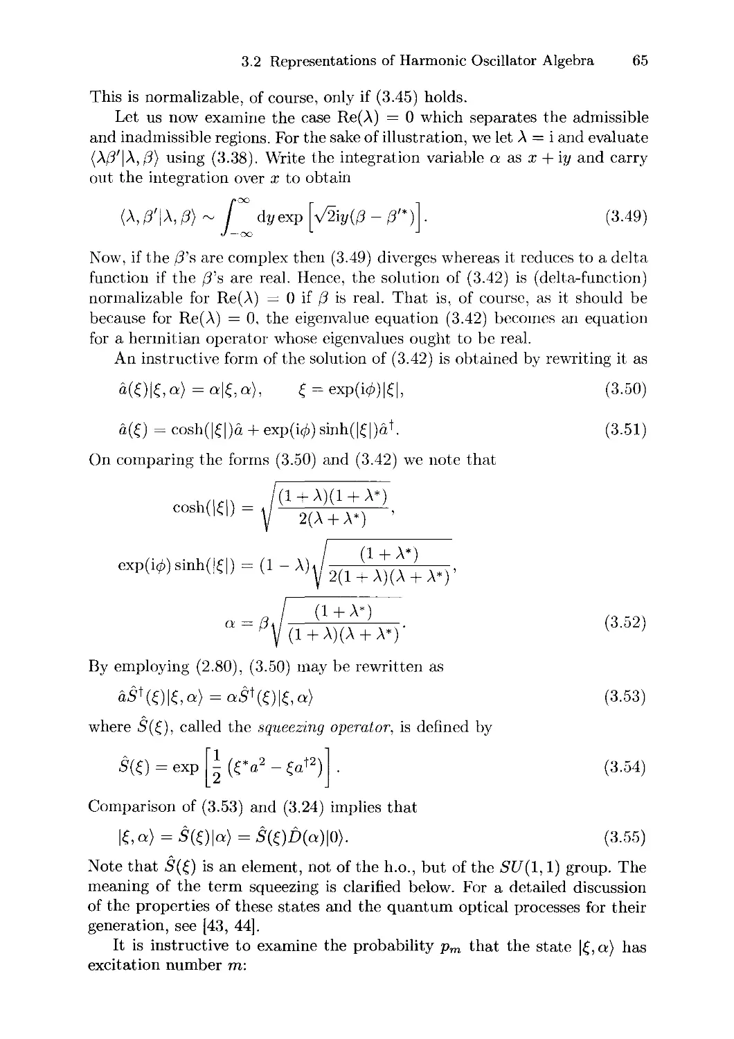
3.1 Representation by Eigenvectors and Group Parameters 55
3.1.1 Bases Constituted by Eigenvectors 55
3.1.2 Bases Labeled by Group Parameters 56
3.2 Representations of Harmonic Oscillator Algebra 60
3.2.1 Orthonormal Bases 60
3.2.2 Minimum Uncertainty Coherent States 61
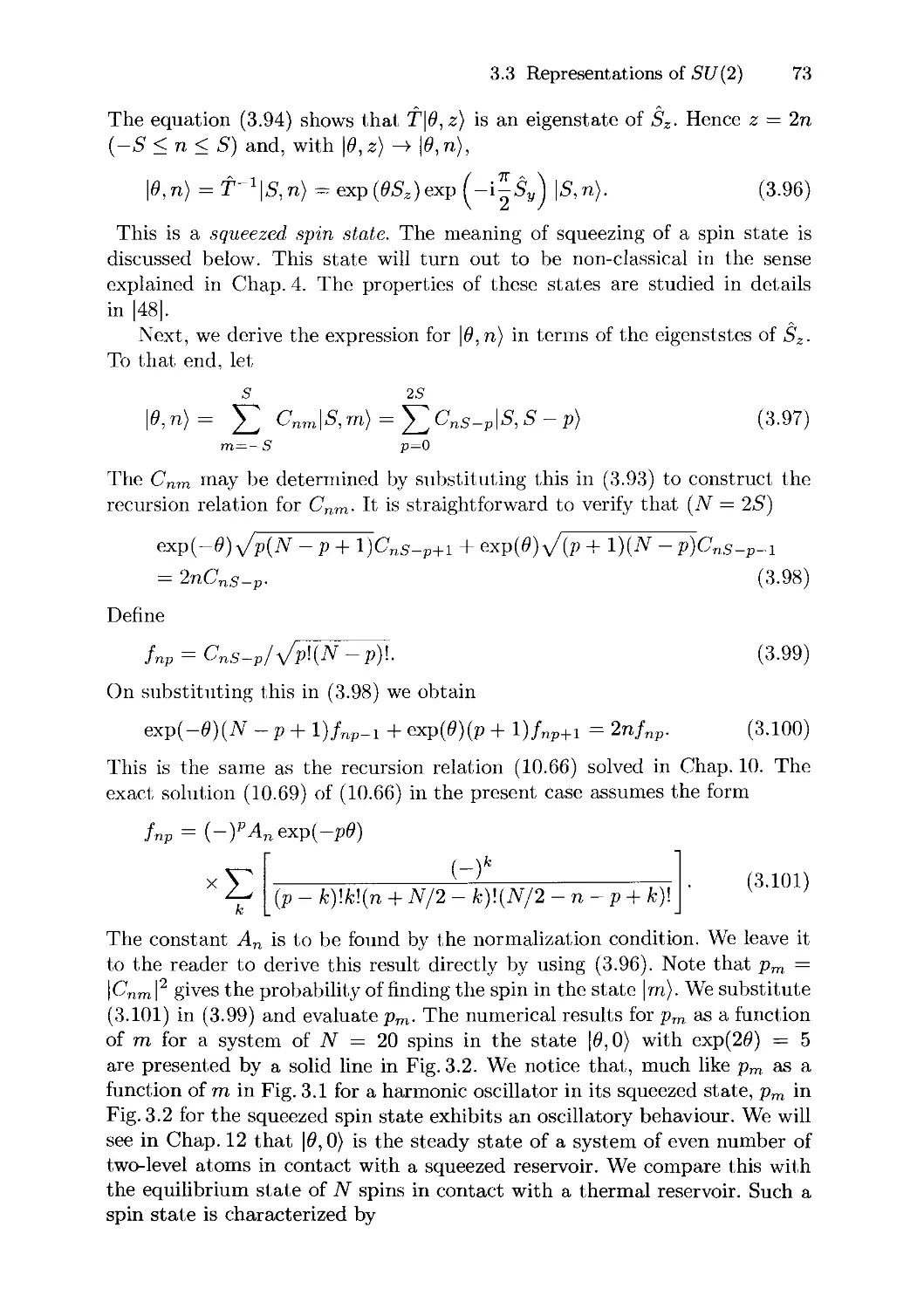
3.3 Representations of 577B) 68
3.3.1 Orthonormal Representation 68
3.3.2 Minimum Uncertainty Coherent States 70
3.4 Representations of SU{ 1, 1) 76
3.4.1 Orthonormal Bases 76
3.4.2 Minimum Uncertainty Coherent States 77
4. Quasiprobabilities and Non-classical States 81
4.1 Phase Space Distribution Functions 81
4.2 Phase Space Representation of Spins 88
4.3 Quasiprobabilitiy Distributions for Eigenvalues of Spin Components 93
4.4 Classical and Non-classical States 95
4.4.1 Non-classical States of Electromagnetic Field 95
4.4.2 Non-classical States of Spin-l/2s 97
5. Theory of Stochastic Processes 99
5.1 Probability Distributions 99
5.2 Markov Processes 102
5.3 Detailed Balance 105
5.4 Liouville and Fokker-Planck Equations 106
5.4.1 Liouville Equation 107
5.4.2 The Fokker-Planck Equation 107
5.5 Stochastic Differential Equations 109
5.6 Linear Equations with Additive Noise 110
5.7 Linear Equations with Multiplicative Noise 112
5.7.1 Univariate Linear Multiplicative Stochastic Differential Equations 113
5.7.2 Multivariate Linear Multiplicative Stochastic Differential Equations 114
5.8 The Poisson Process 115
5.9 Stochastic Differential Equation Driven by Random Telegraph Noise 116
6. The Electromagnetic Field 119

6.1 Free Classical Field 119
6.2 Field Quantization 121
6.3 Statistical Properties of Classical Field 123
6.3.1 First-Order Correlation Function 125
6.3.2 Second-Order Correlation Function 126
6.3.3 Higher-Order Correlations 126
6.3.4 Stable and Chaotic Fields 127
6.4 Statistical Properties of Quantized Field 130
6.4.1 First-Order Correlation 131
6.4.2 Second-Order Correlation 132
6.4.3 Quantized Coherent and Thermal Fields 132
6.5 Homodyned Detection 134
6.6 Spectrum 135
7. Atom— Field Interaction Hamiltonians 137
7.1 Dipole Interaction 137
7.2 Rotating Wave and Resonance Approximations 140
7.3 Two-Level Atom 144
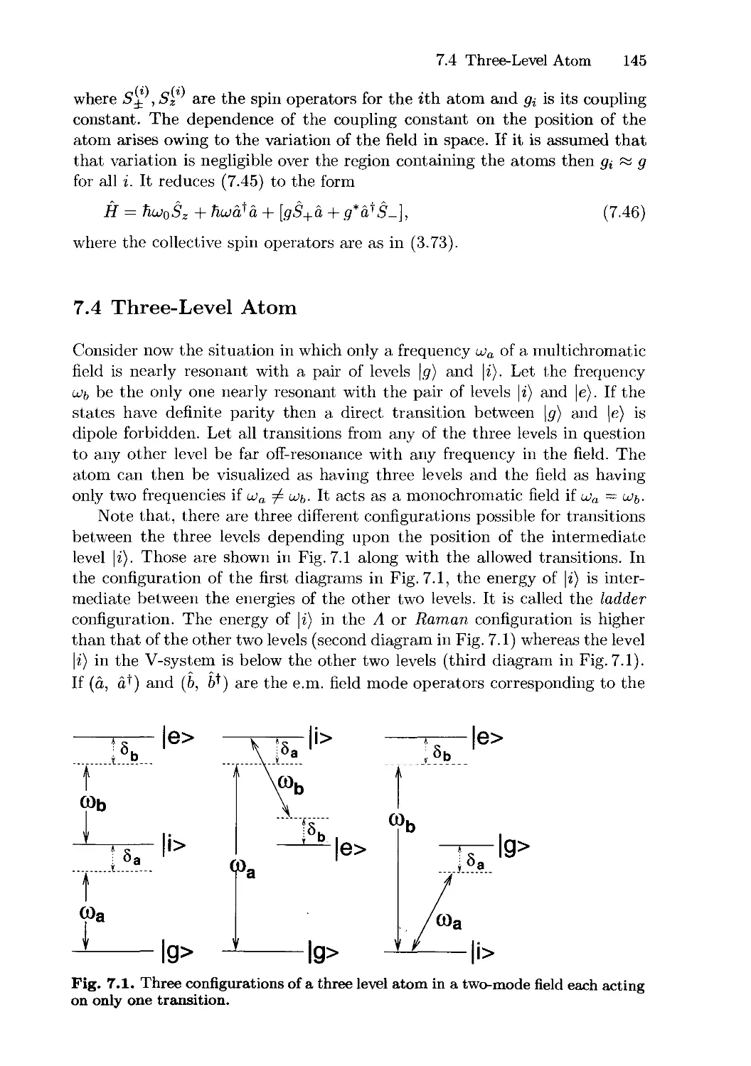
7.4 Three-Level Atom 145
7.5 Effective Two-Level Atom 146
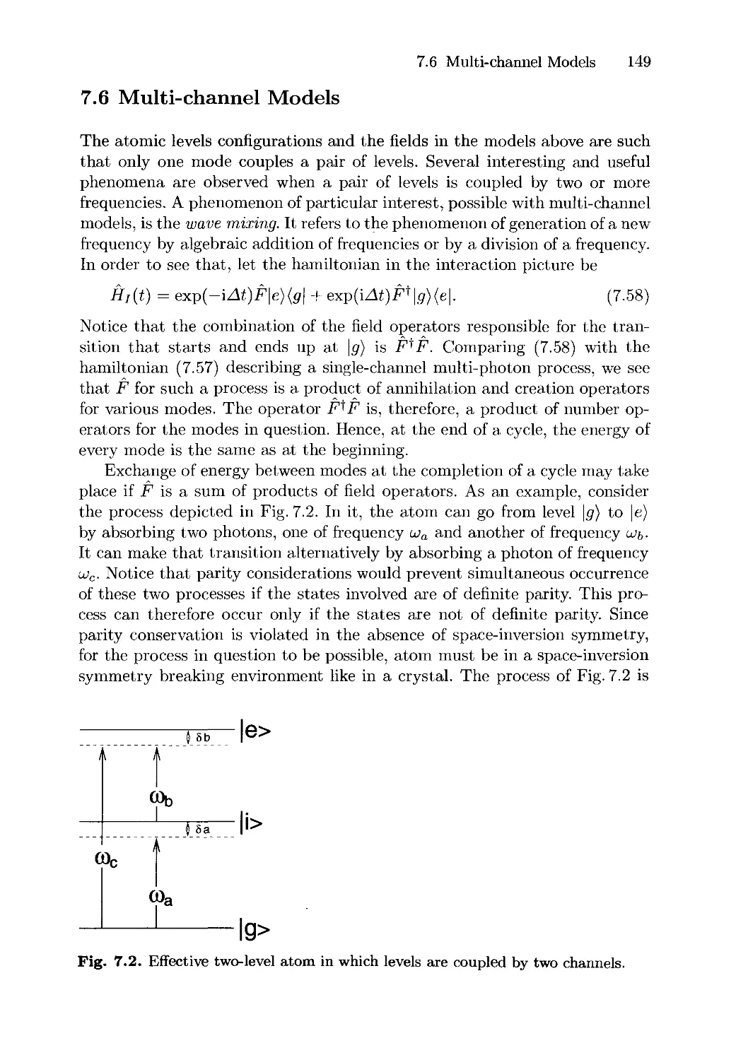
7.6 Multi-channel Models 149
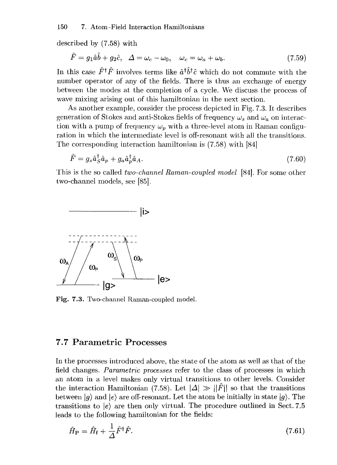
7.7 Parametric Processes 150
7.8 Cavity QED 151
7.9 Moving Atom 153
8. Quantum Theory of Damping 155
8.1 The Master Equation 155
8.2 Solving a Master Equation 160
8.3 Multi-Time Average of System Operators 162
8.4 Bath of Harmonic Oscillators 163
8.4.1 Thermal Reservoir 164
8.4.2 Squeezed Reservoir 166
8.4.3 Reservoir of the Electromagnetic Field 167
8.5 Master Equation for a Harmonic Oscillator 168
8.6 Master Equation for Two-Level Atoms 170
8.6.1 Two-Level Atom in a Monochromatic Field 171
8.6.2 Collisional Damping 172
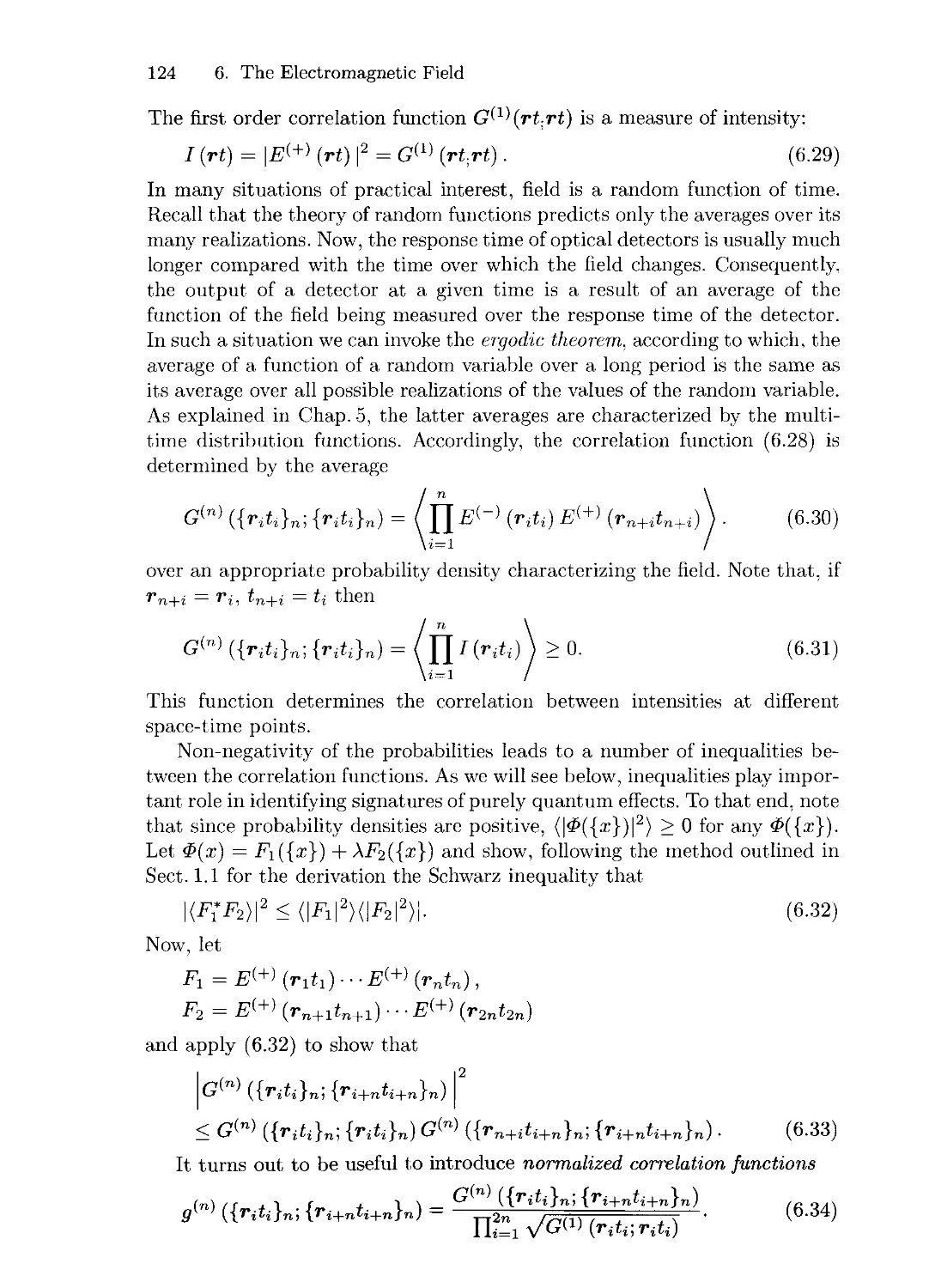
8.7 Master Equation for a Three-Level Atom 173
8.8 Master Equation for Field Interacting with a Reservoir of Atoms 174
9. Linear and Nonlinear Response of a System in an External Field 177
9.1 Steady State of a System in an External Field 177
9.2 Optical Susceptibility 179
9.3 Rate of Absorption of Energy 181
9.4 Response in a Fluctuating Field 183
10. Solution of Linear Equations: Method of Eigenvector Expansion 185
10.1 Eigenvalues and Eigenvectors 186

10.2 Generalized Eigenvalues and Eigenvectors 189
10.3 Solution of Two- Term Difference-Differential Equation 191
10.4 Exactly Solvable Two- and Three-Term Recursion Relations 192
10.4.1 Two- Term Recursion Relations 192
10.4.2 Three- Term Recursion Relations 193
11. Two-Level and Three-Level Hamiltonian Systems 199
11.1 Exactly Solvable Two-Level Systems 199
11.1.1 Time-Independent Detuning and Coupling 202
11.1.2 On- Resonant Real Time-Dependent Coupling 208
11.1.3 Fluctuating Coupling 208
11.2 N Two-Level Atoms in a Quantized Field 210
11.3 Exactly Solvable Three- Level Systems 210
11.4 Effective Two-Level Approximation 212
12. Dissipative Atomic Systems 215
12.1 Two-Level Atom in a Quasimonochromatic Field 215
12.1.1 Time-Dependent Evolution Operator Reducible to SUB) 217
12.1.2 Time-Independent Evolution Operator 219
12.1.3 Nonlinear Response in a Dichromatic Field 223
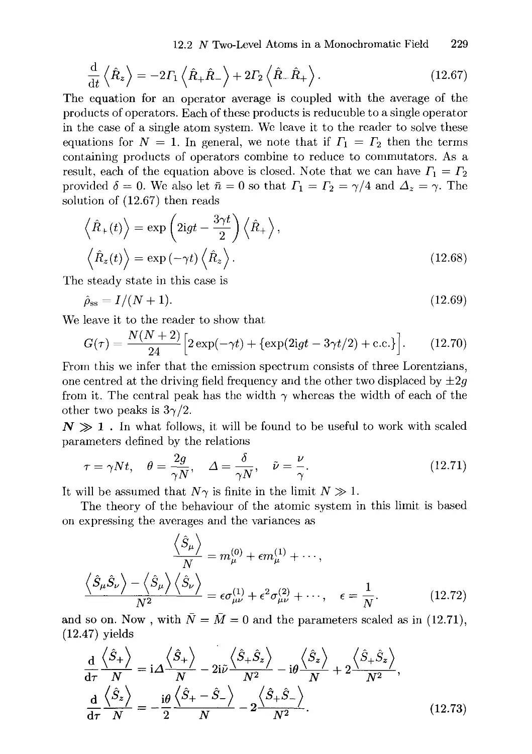
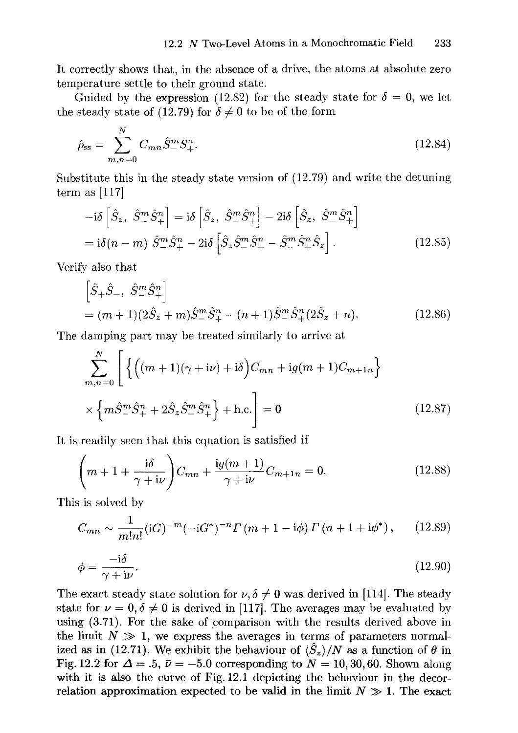
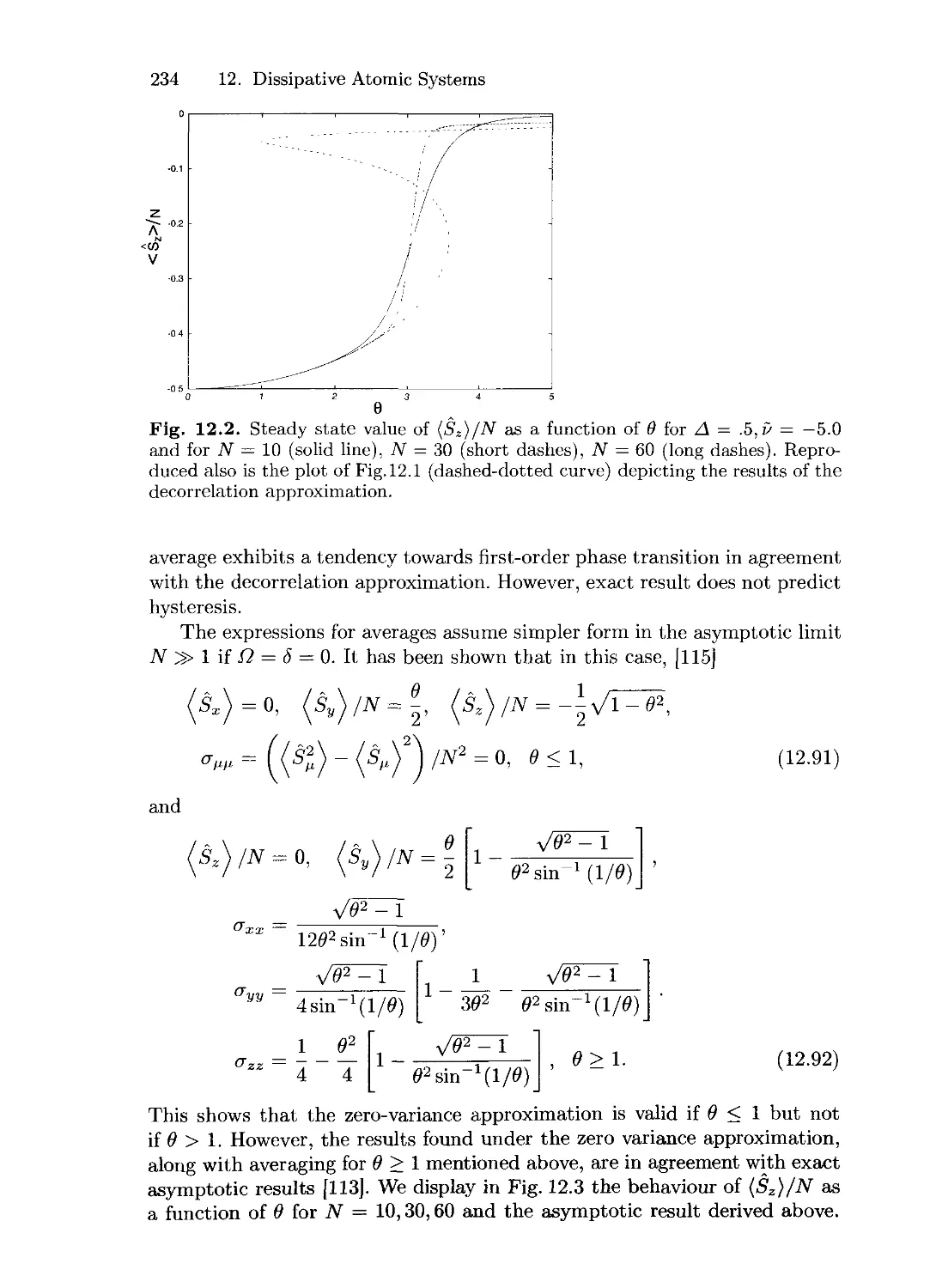
12.2 N Two-Level Atoms in a Monochromatic Field 224
12.3 Two-Level Atoms in a Fluctuating Field 236
12.4 Driven Three-Level Atom 237
13. Dissipative Field Dynamics 239
13.1 Down-Conversion in a Damped Cavity 239
13.1.1 Averages and Variances of the Cavity Field Operators 240
13.1.2 Density Matrix 242
13.2 Field Interacting with a Two-Photon Reservoir 245
13.2.1 Two-Photon Absorption 245
13.2.2 Two-Photon Generation and Absorption. 247
13.3 Reservoir in the Lambda Configuration 248
14. Dissipative Cavity QED 251
14.1 Two-Level Atoms in a Single-Mode Cavity 251
14.2 Strong Atom-Field Coupling 252
14.2.1 Single Two-Level Atom. 252
14.3 Response to an External Field 255
14.3.1 Linear Response to a Monochromatic Field 256
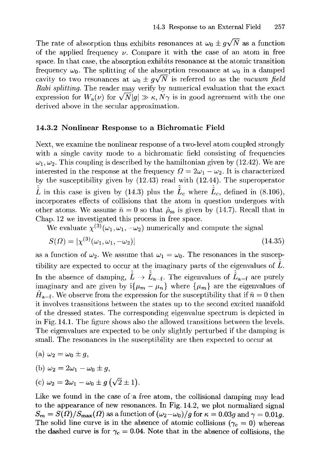
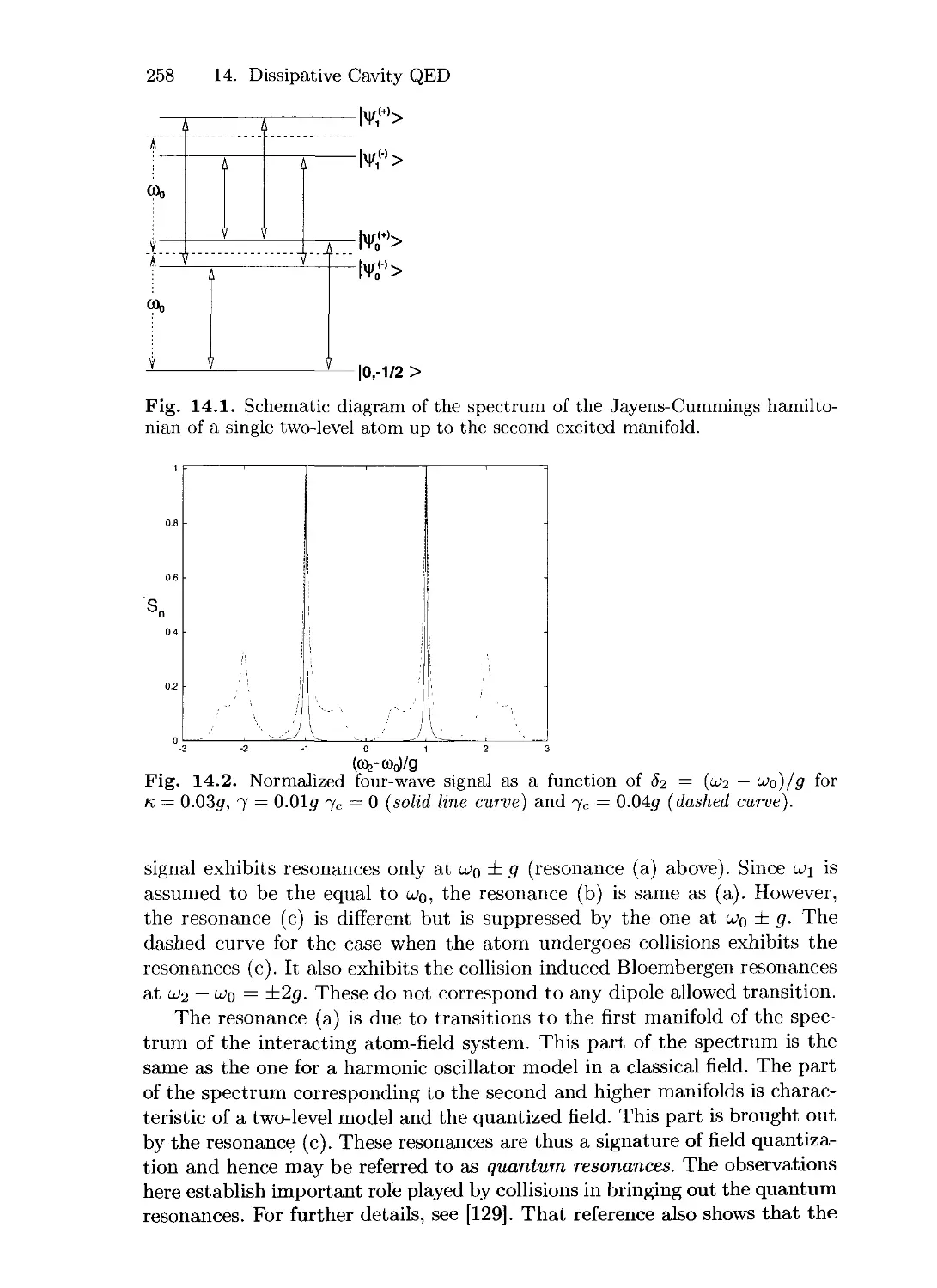
14.3.2 Nonlinear Response to a Bichromatic Field 257
14.4 The Micromaser 259
14.4.1 Density Operator of the Field 259
14.4.2 Two-Level Atomic Micromaser 263
14.4.3 Atomic Statistics 266
Appendices 267
A. Some Mathematical Formulae 267
B. Hypergeometric Equation 270
C. Solution of Two-and Three-Dimensional Linear Equations 272

D. Roots of a Polynomial
References
Index
absorption spectrum 182
ac Stark splitting 223
algebra
- harmonic oscillator 41
-SU(\,\) 43
- SUB) 42
- SU(m) 44
- SU{m,n) 45
antibunching 132
antinormal ordering 49, 83
Bargmann representation 64
Bell's inequality 35
Bloch-Siegert shift 142
Bloembergen resonances 224
Born approximation 157
bunching 134
cat paradox 31
cavity QED 151
Chapman-Kolmogorov equation 103
characteristic function 100
coherent multiphoton process 148
coherent states 58
- generalized 57
- Glauber 58,62
-ofe.m. field 58, 133
- of harmonic oscillator 62
- of spins 70
- of SU{2) 70
- pair 78, 248
- Perelomov 57
coherent states, completeness relation
57
- for harmonic oscillator 62
-for SU(\, 1O8
- for SUB) 72
coherent states, minimum uncertainty
59
- of harmonic oscillator 64
- of spins 70, 72
-of SU{\, 1O7
Index
273
277
283
coherent states, uncorrelated equal
variance minimum uncertainty 59
- of harmonic oscillator 62
- of spins 70
-of SU{\, 1O7
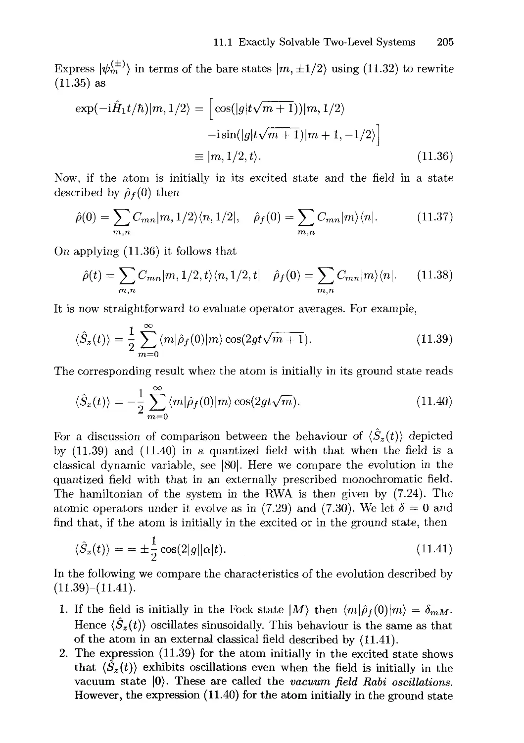
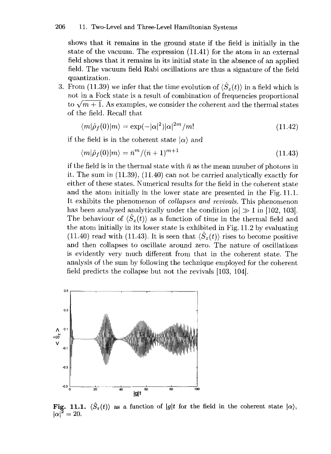
collapses and revivals 206
collisional damping 172
complementarity 12,27
cumulants 101
density operator 21
Descarte's rule 277
detailed balance 106, 108, 160, 225
differentiation, parametric 8
- of exponential operator 37
- of operator product 8
disentangling an exponential 48
- harmonic oscillator algebra 49
-SU(\,\) algebra 51
- SUB) algebra 50
down conversion 151,239
dressed states 204
e.m. field
- chaotic, classical 127
- chaotic, quantum 133
- coherence time 130
- coherent 127,133
- correlation functions, classical 123
- correlation functions, quantum 130
- quantization 121
effective two-level approximation 212
effective two-level atom 147
eigenvalue 7,186
- generalized 189
eigenvector 7,186
- generalized 189
entangled state 20, 25
EPR Paradox 32
equal variance minimum uncertainty
state 13
Fokker-Planck equation 107

four-wave mixing 223, 257
- collision induced resonances 224, 257
- quantum resonances 258
Gaussian process 102
geometric phase 16
- in adiabatic evolution 18
- of a harmonic oscillator 18
- of a two-level system 18
Hamilton-Cayley theorem 190
Heisenberg equation 14
hidden variables theory 34
- local 34
Hilbert space 1
homodyned detection 134
Hurwitz criterion 277
Husimi function 87
incompatibility 12
interaction picture 15
interference 26,27
Jaynes-Cummings model 143, 144, 204
Jordan canonical form 189
Lie algebra 40
Lie group 56
Markov approximation 158
Markov process 103
master equation 104, 105, 158
measurement problem 30
micromaser 259
- trapping condition 264
minimum uncertainty states 12, 59
- of harmonic oscillator 61, 67
- of spins 70
-of5E7(MO7
mixed state 22
moments 100
multi time joint probability 15
multi-channel models 149
noise
-additive 110
- coloured 109
- delta correlated 109
- Gaussian white 109
- multiplicative 110, 112
-white 109
non-classical states 95
- of e.m. field 95
- ofspin-l/2s 97
normal ordering 49, 83
Ornstein-Uhlenbeck process 110-112
P-function 86
- for spins 91
parametric processes 150
phase
- dynamic 16
- geometric (see geometric phase) 16
photon 122
Poisson process 115
probability amplitude 11
probability density 11,99
- conditional 103
-joint 99
pure state 22
Q-function 87
- for spins 92
quantum eraser 29
quasiprobability distribution 83
- for spins 89
Rabi frequency 142, 221
random telegraph noise 116
regression theorem 105,163
representations
- by eigenvectors 55
- equivalent 56
- labeled by group parameters 56
- of harmonic oscillator algebra 60
-of 5GA,1) algebra 76
-of 57/B) algebra 68
resonance approximation 144
resonance fluorescence 171,219
- collective 225
rotating wave approximation 143, 181
Rydberg atom 152
s-ordering 83
Schmidt decomposition 25
Schrodinger equation 13
Schwarz inequality 2
- generalized 3

secular approximation 162, 227, 253,
256
semiclassical approximation 139
similarity transformation 39
- harmonic oscillator 41
-5GA,1L3
- SUB) 42
- SU(m) 44
- SU{m,n) 45
Sneddon's formula 37
spectroscopic squeezing 75
spectrum 136
- absorption 223,256
- emission 222 spin operators
- collective 69
- lowering 23
- raising 23
squeezed reservoir 166
squeezed states
- of harmonic oscillator 67
- of spins 73, 74
squeezed vacuum 166
squeezing operator 65
Stark shift 214
stationary process 100
stochastic differential equation 109
sub-Poissonian distribution 132
superoperator 10
- adjoint 10
superposition, principle of 26
susceptibility 179
- optical 180 symmetric ordering 83
- for spins 94
thermal reservoir 164 three level atom
145
time-ordered exponential integration
- harmonic oscillator algebra 52
-SU{\,\) algebra 53
- SU{2) algebra 53
trace 6
transition probability 103
two-channel Raman-coupled model
150,207
two-level atom 144
two-photon process 146
two-photon reservoir
- in ladder configuration 245
- in Lambda configuration 248
uncertainty relation 12
uncorrelated equal variance minimum
uncertainty state 13, 62
vacuum field Rabi oscillations 205
vacuum field Rabi splitting 257
vacuum fluctuations 122
wave mixing 149, 181
wave-particle duality 26
welcher weg 28
which path 28
Wiener process 110, 111
Wiener-Khintchine theorem 136
Wigner function 87
- for spins 92
Zeno effect 16

Dedicated to
My Inspiration - My Wife
Shyama

Preface
This book is intended to provide a much needed systematic exposition of the
mathematical methods of quantum optics, something that is not found in
existing books. It is primarily addressed to researchers who are new to the
field. The emphasis, therefore, is on a simple and self-contained, yet concise,
presentation. It provides a unified view of the concepts and the methods of
quantum optics and aims to prepare a reader to handle specific situations.
A number of formulae scattered throughout the scientific literature are also
brought together in a natural manner.
The broad plan of the book is to introduce first the basic physics and
mathematical concepts, then to apply them to construct the model hamilto-
hamiltonians of the atom-field interaction and the master equation for an atom-field
system interacting with the environment, and to analyze the equations so
obtained. A brief description of the contents of the chapters is as follows.
The first chapter introduces the basic postulates of quantum mechanics,
brings out their implications and develops the associated operational tech-
techniques. It discusses the measurement problem, the paradoxes of quantum
mechanics and the local hidden variables theory, since quantum optics pro-
provides experimental means of examining these issues. Chapter 2 outlines the
algebra of the exponential operator, which plays a prominent role in mathe-
mathematical physics. The concept of Lie algebra is introduced and the standard
hamiltonians of quantum optics are treated as elements of one or the other
finite-dimensional Lie algebra. The question of representations of Lie algebras
is addressed in Chap. 3. The notion of coherent states emerges as a continuous
representation of a Lie algebra. The concept of quasiprobabilities is developed
in Chap. 4. Their usefulness as operational tools and as entities for identify-
identifying purely quantum effects is demonstrated. Chapter 5 presents the essential
elements of the theory of stochastic processes. The theory of classical and
quantized electromagnetic (e.m.) fields is outlined in Chap. 6. It describes
the characterization of the e.m. field in terms of its correlation functions and
also their role in identifying the signatures of field quantization.
By starting with the hamiltonian for an atom interacting with the e.m.
field in the dipole approximation, Chap. 7 describes ways of reducing it to
simpler, mathematically tractable forms commensurate with given physical
conditions. The standard models of quantum optics are thereby derived. The

VIII Preface
effects of the environment on an atom-field system are the subject of the
quantum theory of damping outlined in Chap. 8. Here the master equation
for the evolution of a system in contact with a reservoir is constructed and
methods of solving it are discussed.
Chapter 9 analyzes the perturbative solution of the master equation of an
atomic system in an external field. This leads to the notions of susceptibility,
multiwave mixing and the absorption spectrum.
The method of solving a set of linear equations with time-independent
coefficients in terms of generalized eigenvectors is outlined in Chap. 10. That
chapter presents the solution of a two-term recurrence relation and identifies
and solves exactly solvable quadratic three-term recurrence relations. These
recurrence relations encompass many well-known quantum optical situations.
Chapters 11-14 deal with the solution of some standard model systems.
Chapter 11 identifies the class of analytically exactly solvable models of an ef-
effective two-level atom and that of an effective three-level atom in a quantized
field. It provides a unified treatment of the exactly solvable hamiltonians of
quantum optics.
The problem of an externally driven two-level atomic system dissipating
into a squeezed reservoir is addressed in Chap. 12. The exactly solvable cases
of an arbitrary time-dependent drive are identified. The exact dynamics in
a monochromatic drive is investigated and the collective effects in a driven
two-level atomic system are highlighted. Chapter 12 also briefly discusses
the dynamical behaviour of a three-level atom dissipating into a reservoir at
absolute zero temperature and reveals the effects of almost equally spaced
pairs of energy levels.
The dynamics of a field dissipating into a linear or two-photon non-linear
reservoir is the subject of Chap. 13. The evolution of an atomic system in-
interacting with a single damped quantized cavity mode is investigated in
Chap. 14. This chapter also outlines the theory of the micromaser.
I am indebted to Girish Agarwal for teaching me the subject of quantum
optics. Valuable contributions to my understanding have been gained through
my association with Robert (Robin) Bullough, Joseph Eberly, Fritz Haake,
Shoukry Hassan, Rajiah Simon, Subhash Chaturvedi, V. Srinivasan, Subha-
sish Dattagupta, Surya Tiwari, Dinkar Khandekar and Suresh Lawande. I am
grateful to Debabrata Biswas and Aditi Ray for their valuable suggestions
and help in preparing the manuscript. I am thankful to Dinesh Sahni for his
support and encouragement. Angela Lahee of Springer-Verlag deserves a big
thank you for her careful editing.
Mumbai, Ravinder Puri
January 2001

1. Basic Quantum Mechanics
Quantum optics is the quantum theory of interaction of the electromagnetic
field with matter. In this chapter we recapitulate basic concepts and opera-
operational methods of the quantum theory essential for developing the theory of
quantum optics. We delve also in to the controversial issue of interpretation of
the quantum theory as a classical statistical theory. Quantum optics provides
means for subjecting these conceptually controversial issues to experimental
tests.
1.1 Postulates of Quantum Mechanics
In this section we state five basic postulates of Quantum Mechanics and
discuss some of their important implications.
1.1.1 Postulate 1
An isolated quantum system is described by a vector in a Hilbert space. Two
vectors differing only by a multiplying constant represent the same physical
state.
Following the notation introduced by Dirac [1], we represent a vector by
a ket, | ).
A Hilbert space is a complex linear vector space equipped with the def-
definition of a scalar product and spanned by a complete set of vectors [2].
The meaning and implications of these properties of the Hilbert space are
explained below. They are crucial for relating the theory with experimental
observations.
Linear Vector Space. A Hilbert space is a complex linear vector space. We
assume familiarity with the notion of a linear vector space over the field of
complex numbers (c-numbers) [2]. We recall that if \tpi) and \rp%) are vectors
in a complex linear vector space then a linear combination ail^i) + CK2 j2)
for arbitrary complex numbers ct\, oii is also a vector in the same space. A
set of vectors |i/>i)j • ¦ •, |i/>n) is said to be linearly independent if

2 1. Basic Quantum Mechanics
implies at = 0 for alii = 1,... , n. The maximum number of linearly inde-
independent vectors in a linear vector space is called its dimension.
Scalar Product. To say that the Hilbert space is a Euclidean or scalar
product space means that it is possible to associate with every pair of vectors
\(j>) and \ip) in it a complex number, denoted by ((j>\ip), such that
1. ((j>\tp) = {ip\(j>)*, where * denotes the operation of complex conjugation;
2. If \rl>) = ci|^i) + c2|</>2) then (<^) = ci(^i) +
3. (</#) > 0;
4. <V#) = 0 if and only if (iff) |^> = 0.
In the following we list some consequences of these axioms.
The scalar product associates with a vector | ) its dual ( | called a bra [1].
The non-zero positive number |||'0)|| = s/^PW) *s called the norm or the
length of the vector. Since two vectors differing only by a multiplication
factor represent the same physical state, we can represent a physical state
by a vector of a fixed, say unit, norm if the norm is finite. Hence, \ip) is
physically an acceptable vector if its norm is finite i.e. if
< oo. A.2)
The vector \<j>)(<j>\ip} is the projection of a vector \ip) along the vector \<p).
The scalar product {(f>\xj)) is a measure of the overlap between the vectors
\tp) and \<p). If (<p\ip) = 0 then \ip) and \<p) are said to be orthogonal to each
other.
Two sets of vectors \rpi), • • •, \xpn) and \(j>i), • • •, \<pn) are said to be orthonor-
mal to each other if
((j>i\rpj) = Sij, i,j = l,...,n. A.3)
A set \e.\), ¦ ¦ ¦ \en) of vectors is said to be orthonormal if
(ei\ej} = Sij, i,j = l,...,n. A.4)
An important consequence of the axioms defining the scalar product is the
Schwarz inequality
D#>W#> > {0|V)(^|0>, A-5)
where the equality holds if and only if the two vectors in question are
linearly dependent i.e. if
\1>)=n\4>), A.6)
/x being a complex number. In order to establish this, show that the min-
minimum value of (<F(/z)|!F(/z)), where |#) = |i/j) — /x|0), as a function of /x is
{tp\ip) — \(ip\(j>)\2/(<f)\<f)). The requirement that this value, due to axiom 3
of the scalar product, be positive leads to the Schwarz inequality in A.5).
Also, according to the axiom 4 above, (\P((j,)\\P((i)) = 0 iff |^(m)) = 0 i-e-

1.1 Postulates of Quantum Mechanics 3
iff A.6) holds. It may be verified easily that A.5) then holds with equality.
In a similar way we can derive the generalized Schwarz inequality
) > 0, A.7)
where det((^Al|^^)) is the determinant of the matrix constituted by the
elements (VvlVv)) /xj v = 1, ¦ ¦ ¦ ,n. Invoking the fact that the determinant
of a matrix is zero if its rows (or columns) are linearly dependent, it follows
that the equality in A.7) holds iff |^) are linearly dependent.
Completeness. In a scalar product vector space of finite dimension n, there
always exists a set of n linearly independent vectors A^)}, called the basis
vectors, such that any vector \ip) can be expressed as a linear combination [2],
The complex numbers {d{\ in a scalar product space may be determined
by taking the scalar product of A.8) with the vectors {|<^>i)} orthonormal to
{\ipi}} to give di = D>t\ip) so that
The vector \ip) in an n-dimensional space is thus characterized by n complex
numbers {{<pi\4>}}- The column of these numbers constitutes a representation
of the vector in the given basis. The dual (?/>[ of \ip) is then represented by the
row constituted by the numbers {{4>\<pi)} = {{<Pi\i>}*}- Thus the representa-
representation of {ip\ is obtained by the process of hermitian conjugation (interchanging
of rows and columns along with the operation of complex conjugation), de-
notedbyf, of|#M = (M)t.
The expansion A.9) in a scalar product space is guaranteed if the space
is finite-dimensional. However, such an expansion need not exist if the space
is infinite-dimensional. In quantum mechanics, we are concerned only with
those scalar product linear vector spaces in which every vector is expressible
in terms of a basis. Such a space is called a Hilbert space.
Now, on invoking the fact that A.9) is to be valid for an arbitrary \tp),
follows the completeness relation
where / is the identity operator defined below. If {|^>i)} is orthonormal, i.e.
if {\4>i)} = {Hi)} = i\ei)}, then A.10) reduces to
>te|=7. A.11)

4 1. Basic Quantum Mechanics
In our discussion so far we have assumed that the basis vectors are de-
numerable. There are, however, occasions which require us to work with a
basis labeled by a continuous parameter. Consider an orthonormal set of ba-
basis vectors |?) labeled by a real continuous parameter ?. The condition of
orthonormality then reads
5(x) being the Dirac delta function. If a < ? < b then the analog of the
expansion of a vector in terms of the basis vectors is
A vector \ip) in a continuous basis is thus represented by the function c(?) =
of a real variable ?.
Operators. The action of a force transforms the state of a system. A trans-
transformation of a state of a system may be described by a rule, called an operator.
that associates with a vector in the space another vector in the same space.
If, for example, an action transforms \tp) to \<j>) then we write
Aty) = \<P) A.14)
where the operator A defines the rule of transformation. We distinguish an
operator from a c-number variable by a caret on the former. An operator A
is linear if, for any complex numbers c\ and ci,
A.15)
We shall be concerned only with linear operators.
If A\ip) = \ip) for all \ip) then A is called the unit or identity operator,
often denoted by /. Since / acts like the scalar unity, we do not dress it with
a caret and even denote it by 1.
In order to obtain a c-number representation of an operator A, consider
an orthonormal basis {|ej)}. Rewrite A as IAI where / is the unit operator
and express / in terms the completeness relation A.11) to get
n
A.16)
The operator A may be represented by an n x n matrix constituted by the
complex numbers (ei|A|ej) (i,j = 1, ...,ra). On operating A.16) on an ar-
arbitrary vector \ip), it follows that A\ip) is represented by the product of the
matrix (ej|A|e.,) representing A with the column {ej\ip) representing |i/j). It is
straightforward also to show that a product AB is represented by the prod-
product of the matrices representing them. Thus, the correspondence between
vectors as columns and operators as matrices is not only notational but also
operational.

1.1 Postulates of Quantum Mechanics
The analog of A.16) in the continuous representation is evidently
[
J a
The function a(?, ?') = (?|.A|?') of two real variables ? and ?' now serves as a
representation of A. The rules of addition and multiplication of operators and
those for the action of an operator on a vector are same as the corresponding
ones for the discrete case with summations replaced by integrals.
Next, we enumerate some definitions and algebraic operations involving
linear operators. The treatment, though may lack rigor at times, is adequate
for our purpose. For details, see, e.g., [3].
1. The product AB denotes the action of B on a state followed by that of
A on the resulting state. This result need not be the same as that due to
the operation BA. The operator defined by
[A,B}=AB-BA A.18)
is called the commutator of A and B. If [A, B] = 0 then A and B are said
to commute.
2. If m is a positive integer then Am denotes A multiplied with itself m
times.
3. A function F{A) of an operator A may be defined by its expansion in
terms of the powers of A. Of particular interest is the exponential operator
defined by the expansion
771=0
Using this definition, the reader should verify that if [A, B] = 0 then
exp[i + B] = exp(i) exp(B) = exp(B) exp(i). A.20)
The problem of disentangling the exponential of a sum of non-commuting
operators is addressed in Chap. 2.
4. Check that we can write B(AB)m = (BA)B(AB)m~1 = ¦¦¦ = (BA)mB.
As a consequence of this it follows that if F{AB) is a function expandable
as a power series of its argument then
BF(AB) = F(BA)B. A.21)
5. If there exists a nonnegative real number C such that u |(^
Cy/{ij)\ip) for all |i/j) then A is called a bounded operator. The minimum
of the numbers C, denoted by [\A\\, is called the norm of A.
6. The adjoint of A, denoted by A*, is defined by the relation
A.22)

1. Basic Quantum Mechanics
for all |i/j) and \<f>) in the given Hilbert space. Combine this with A-16)
to show that the matrix representing the adjoint of an operator is the
adjoint of the matrix representing that operator. Verify also that
A.23)
7. If, corresponding to an operator A, there exists an operator B such that
BA = AB = I then B is called the inverse of A. The inverse of A is
denoted by A~1:
A-1A = AA~1=I. A.24)
An operator is called singular if it does not admit an inverse. It can be
shown that AB = I implies BA = I in a finite dimensional Hilbert space
but not if the space is infinite dimensional [3]. In an infinite dimensional
space, an operator A may be singular but corresponding to it there may
still exist an operator Aj^1 called the left inverse of A such that A^A = I
or an operator A^1 called its right inverse such that AA^1 = I. Clearly,
an operator which is the right as well the left inverse of A is the inverse
A^1. It is straightforward to show that
(ABC)-1 = C-lB~1A-\ A.25)
provided that A, B, and C are non-singular. Since an operator commutes
with itself, it follows from A.20) that the inverse of exp(A) is exp(—A).
Notice also that
-1
=exp(-,4m)---exp(-,41). A.26)
8. An operator H is called hermitian if H = W .
9. An operator U is called unitary if UW = UW = I. This shows that
(ipi\Tpj) = (ipi\WU\Tpj). Hence the set of states {&]&}} obtained by a
unitary transformation of the set {|t/)j)} preserves the scalar product.
Hence, the set of vectors obtained as a result of unitary transformation
of an orthonormal set of vectors is also orthonormal. If the orthonormal
set is complete then so is the set obtained by its unitary transformation.
Verify that U can be represented as U = exp(iH) where H is hermitian.
10. If an operator A commutes with its adjoint i.e. if [A, A^\ = 0 then it is
called a normal operator. Note that hermitian and unitary operators are
examples of a normal operator.
11. If (^>|A|^) > 0 for all |^) then A is said to be positive. Let \<f>) = B\ip).
Then (i/j|.BtB\ip) = <0|0> > 0. Hence &B > 0 for all B.
12. The sum of the diagonal elements of a matrix representing an operator
A is called the trace of A. It is often denoted by Tr(yl). If {\ei}} is an
orthonormal basis then, by definition,
Tr(i) = f>|A|ei>. A.27)

1.1 Postulates of Quantum Mechanics 7
The value of the trace of an operator is independent of the basis. Some
consequences of the definition of trace are:
• The complex conjugate of A-27), read with A-22), shows that
Tr(it) = [Tr(i)l* A.28)
• Invoke the definition of trace and completeness of {|ej)} to show that
5> A.29)
and
n
Tr [\xl>)(<t>\A] = ^(e^X^ih) = (<t>\A\rl,). A.30)
i=l
• Verify that the trace of a product of operators possesses the cyclic
property:
Tr(ABC) = Tr(CBA). A.31)
• If U is unitary then, due to A.31), Tt[U^AU]== Tr[UU'A] = Tr[i].
This shows that the trace of A and that of U^AU are equal.
13. If \%p) is such that
i|</>) = A|</>), A.32)
where A is a constant then |t/>) is called an eigenvector or an eigenstate
and A the corresponding eigenvalue of A. Expand F(A) in powers of A
and use A-32) repeatedly to show that
F(A)\r(>) = F(\)\r(>). A.33)
The problem of solving an eigenvalue equation is addressed in Chap. 10.
We recall from that chapter that
• The eigenvalues of a hermitian operator are real.
• Any normal operator in an n-dimensional space possesses n eigenvec-
eigenvectors which are orthonormal. Hence, if A is a normal operator and {|ai)}
the set of its orthonormal eigenvectors then (aj|A|ai) = aiSij. On com-
combining this with A.16) follows the expansion
n
i = 53oi|oi)(ai|. A.34)
of a normal operator in its eigenbasis. Apply A.33) to show that
A-35)
i=\
Now, let |a, b) be a simultaneous eigenvector of A and B such that
A\a,b) =a\a,b), B\a,b) = b\a,b). A.36)
erate first (second) of the equations above by B (A) and subtract the
lting equations to obtain
[A, B]\a,b)=0. A.37)

8 1. Basic Quantum Mechanics
This equation is trivially solved if [A, B] = 0 showing that non-
commuting operators may possess common eigenvectors. If A and B
do not commute, then no general conclusion can be drawn about the
solvability of A.37) except for special cases. For example, if [A, B] is
a non-zero constant then A-37) evidently does not admit a non-trivial
solution. This is the case for the pair of position and momentum op-
operators q and p. Hence, q and p do not have any common eigenvector.
Same result can be shown to hold for angular momentum operators. It
is generally accepted that non-commuting observables of common inter-
interest do not possess common eigenvectors. However, it can be proved that
if A and B do not commute then they do not admit a common set of
eigenvectors [3].
14. If a state \tp(t)} or an operator A(t) is a function of a scalar t then its
derivative with respect to t has the usual meaning of the calculus of c-
number functions. The rules for differentiation of a product of states or of
operators with respect to a parameter are also same as for the c-number
functions provided that in applying those rules the order of states and
operators is retained. Thus, for example,
()
^•¦•in = (^i1)-in + -- + i1--^. d.39)
Hence, verify that
15. Consider the differential equation
Its solution may be written in the form
dri(r)] |</>(to)> A-42)
where the time-ordered exponential integration is defined by
IT exp [ /" dri(r)l = 1 + / dri(r)
L Jto J Jto
+ f dr2 f 2 drii(T2)i(r1) + • • •
+ f drn fn drn_i ¦¦¦ f2 dni(rn) • • • A(n) + ¦¦¦. A.43)
Jto Jto Jto

1.1 Postulates of Quantum Mechanics 9
Here T is the so called time-ordering operator. It arranges operators in
a chronological order with time increasing from right to left. Verify by
term-by-term differentiation of A-43) that
r dri(r)l =i(t)^f exp [ / dri(r)l. A.44)
I to J lJta J
On using this it follows that A-42) indeed satisfies A.41). In the following
we list some properties of the time-ordered exponential operation.
• Take the hermitian conjugate of A-43) to show that
(*Texp [ / dri(T)])t = 7*exp [ / dri^r)]. A.45)
I ljto JJ LJto J
The operator T in the equation above arranges operator in a chrono-
chronological order with time increasing from left to right. Verify that
y i-t -, , r rt ,
/ AtA(t) =Texp / dTAMlAtt). A.46)
lJt0 J lJt0 J
A(ti), A(tj) = 0 for all U, tj then the operators under the integral
in A.43) may be shuffled at will like the c-numbers. This property leads
to the relation
ft rT-n fTi
I drn / drn_i---/ dTlA(Tn) ¦ ¦ ¦ A(n)
Jto Jto Jto
= — I" / dri(T)jn. A.47)
Substitution of this in A.43) yields
*Texp [ / dri(r)] = exp [ / dri(r)l. A.48)
Jto "to
In particular, if A is independent of t then
rt ,
dri = exp[A(t - t0)}. A-49)
/to J
If A(t) does not commute at different times then the commutator of
A(ti) and A(tj) would contribute to the integral if A(ti) and A(tj) are
interchanged. Hence, on shuffling the operators as in A.47), we can
express the nth term in the time-ordered integral in the form
dr
/ drn_i---/
Jto J to
t), A.50)
the Cn(t) being the contribution from commutators of A(t) at defferent
times. This reduces to A.47) if the commutator of A(t) at different
times vanishes.
If A is time-independent but B(t) a function of time then
d

10 1. Basic Quantum Mechanics
= exp[i(t - to)]^ exp [ I drB(r)], A.51) •
B(t) = exp[-i(t - to)]Bexp[A(t - t0)]. A.52)
The relation A.51) may be established by showing that the terms on
its two sides have the same derivative with respect to t.
The problem of evaluating a time-ordered exponential integral is ad-
addressed in Chap. 2.
Superoperators. We have so far considered the operation of linear trans-
transformation of vectors in a Hilbert space. Another important class of operations
consists of transformation of operators. A superoperator defines a rule that as-
associates an operator with another operator acting in the same Hilbert space.
The operation of transformation of an operator / to another operator g may
be expressed as
If = g. A.53)
Here the superoperator L, distinguished from operators by a double caret,
defines the rule of the transformation. We restrict our attention to linear
superoperators acting on linear operators in a given Hilbert space.
Recall from the theory of vector spaces that linear operators acting in a
vector space constitute a vector space. The relation A.53) may then be viewed
as defining a transformation in a vector space and a superoperator may be
identified as an operator in the vector space of the operators. Furthermore,
the vector space of operators may be made a scalar product space by defining
a suitable scalar product. A useful definition of scalar product is
=Tr[it?J. A.54)
(A,
It may be verified that this definition is in accordance with the axioms of the
scalar product. In analogy with operators, the definition A-54) of the scalar
it x
product leads to the following definition of the adjoint L of L:
Tr[pLg] =Tr[g^Lf] . A.55)
In order to obtain a c-number representation of superoperators, let {|ej)}
be a complete set of orthonormal vectors spanning an ./V-dimensional Hilbert
space. The transformation A.53) in this basis may be written as
N
9ij = ^2 Lij,klfkl- A.56)
k,l=l
The superoperator L is thus represented by a tensor {Lij^i} acting on a
matrix. If N x N matrices {fij} and {gtj} are represented as column Vec-
Vectors having iV2 elements then Lij^i is represented as an AT2 x iV2 matrix.
This provides a means of converting equations involving superoperators in to
matrix equations.

1.1 Postulates of Quantum Mechanics 11
1.1.2 Postulate 2
To each dynamical variable there corresponds a unique hermitian operator.
The reason for associating a hermitian operator with a dynamical variable
will become clear after the statement of the postulate 4.
1.1.3 Postulate 3
// A and B are hermitian operators corresponding to classical dynamical vari-
variables a and b then the commutator of A and B is given by
[A, B] = AB~bA = ih{a, b}, A.57)
where {a, b} is the classical Poisson bracket of a and b and h = h/2n where
h is the Planck's constant. See [1] for the rationale behind this postulate.
1.1.4 Postulate 4
Each act of measurement of an observable A of a system in state \ip) collapses
the system to an eigenstate |aj) of A with probability |(aij^)|2. The average
or the expectation value of A is given by
<i>=^aiKai|^>|2 = <^|i|^>) A.58)
i
the ai being the eigenvalue of A corresponding to the eigenstate |a;).
The complex number {a,i\ip) is called the probability amplitude. The last
equality in A.58) can be derived by (i) rewriting |(a;|^)|2 as (ip\ai)(ai\ip),
and (ii) by invoking A.34) to write the summation over i of aj|aj)(aj| as A.
An operationally useful way of evaluating the probability |(aj|^)|2 is to
use the expression A0.11) to write
^ - A). A.59)
This assumes that a%,..., an are distinct. As a consequence, the probability
of observing the eigenvalue a^ as an outcome of a measurement of A on |^)
is given by
[^ ^ (^{ )\) A.60)
In the discussion above, it is tacitly assumed that the eigenvalues are denu-
merable. Let the eigenvalues ? of the operator associated with the observable
be continuous with |?) as the corresponding eigenvectors. Then, |(^|^)|2 is
identified as the probability density so that |(?|i/>)|2 d? is the probability that
the act of measurement results in a value in the range d? around ?. Invoke
(A.I) to show that
A ^ /" A.61)

12 1. Basic Quantum Mechanics
Since, according to the postulate 2, the observables are represented by
linear hermitian operators whose eigenvalues are necessarily real, it follows
that the act of measurement would give a real number as its result as any
act of measurement does. This also explains the rationale behind associating
a hermitian operator with an observable.
In the following we list some implications of this postulate.
• As a consequence of this postulate, quantum theory predicts only the av-
average of the results of measurements on a large number of identically pre-
prepared systems. The results of all such measurements are identical only if
the observed state is an eigenstate of the measured observable. Only in
that case does the observable possess a definite value, that value being
the corresponding eigenvalue. Also, as mentioned before, non-commuting
observables do not admit common eigenvectors. Hence, non-commuting ob-
observables can not have definite values simultaneously. Simultaneous mea-
measurement of non-commuting observables to an arbitrary degree of accuracy
is thus incompatible. Non-commuting observables are complementary in the
sense that precise knowledge of one excludes that of the other.
• Since quantum predictions are probabilistic, it is important to know the
extent of the spread in the outcomes of measurements. A measure of the
spread in the values of the results of measurements of an observables A of
a system in state \ip) is the variance defined by
AA2 = <#i - (A)]2\tP) = (iP\A2\tP) - <^|i|^J. A.62)
In order to determine the relationship between variances of two observables
A and B due to measurements on a system in state \ip), let
A.63)
Invoke the Schwarz inequality A.5) to arrive at the relation
AA2AB2 > j [(FJ + (C1J] A.64)
called the uncertainty relation. Here
[A, B] = iC, F = Ab + BA-2(A){B). A.65)
Note that, as a result of assumed hermiticity of A and B, the operators
C and F are also hermitian. The operator F is a measure of correlations
between A and B. The uncertainty product is minimum i.e. the equality
in A.64) holds iff, following A.6), |^i) = — iA | -02), where A is a complex
number, i.e. iff
[A + i\B]\rP) = [{A} + i\(B)] \1>) = z\1>). A.66)
The state \tp) satisfying A.66) is called a minimum uncertainty state.
We may derive useful general results about the solvability of A.66) and
the expressions for AA2 and AB2 in the minimum uncertainty state. To

1.1 Postulates of Quantum Mechanics 13
that end, verify that A + iXB is a normal operator if Re(A) = 0. Recall
that the eigenstates of only a normal operator are orthonormal. Hence
it follows that the minimum uncertainty states A.66) for a given A are
non-orthogonal if Re(A) =/= 0.
Next, rewrite A.66) in the form
{A-(A)]\rl,) = -i\[B-(B)]\rl>). A.67)
Operate this on the left with A — (A) and take the scalar product of the
resulting vector with \ip). Repeat this procedure by operating A.67) now
with B — (B). On using A.65), the two equations so obtained read
A.68)
Set A = Ar + iAi- Compare the real and imaginary parts of each of the
equations above to get
AA2 = l-[xi{F) + Xr{C)], AB2 = ±-2AA2,
A;(G)-Ar(F)=0. A.69)
These relations imply that
1. If" | A | = 1 then A A2 = AB2 . The corresponding states may then be
referred to as equal variance minimum uncertainty states .
2. If |A| = 1 along with A; = 0 then AA2 = AB2 and (F) = 0. Since F
is a measure of correlations between A and B, the corresponding states
may be referred to as uncorrelated equal variance minimum uncertainty
states.
3. If Ar ^ 0 then
A- - ~ IAI2 - - 1 -
{r ) = \^/5 *-±sl — (O ), lalj — —r—\^/- V ' /
Ar 2XT 2Ar
The variances and the correlations in the measurement of two observables
in this case is expressible in terms of the average of their commutator C.
Clearly, those quantities are completely determined without an explicit
construction of the said state if C is a constant multiple of the identity
operator. Also, since AA2,AB2 are positive, it follows that Ar should
have the same sign as (C). Hence, if C is a positive operator then admis-
admissible solutions of A.66) are obtained only if Ar > 0. As an example, recall
that C = hi > 0 for the pair (q,p). Hence, the minimum uncertainty
states for the pair (q, p) exist only if Ar > 0. This is borne out also by
an explicit solution of A.66) carried in Sect. 3.2.
1.1.5 Postulate 5
The time evolution of a state \tp) is governed by the Schrodinger equation
ih^Mt))^Mt)Mt)), A.71)

14 1. Basic Quantum Mechanics
where H(t) is the Hamiltonian which is a hermitian operator associated with
the total energy of the system.
This postulate provides the means for determining the dynamical evolu-
evolution of a system. The Schrodinger equation A.71) is of the form A.41). Its
solution is, therefore, given by
) = Us(t, to)\^(to)). A.72)
Invoke A.45) to show that
i f" ) ^i, *„)¦ A-73)
j
If H is time-independent then, on using A.49), A-72) reads
\xP(t)) = exp f-i(t - to)H/h) |^(to)>. A-74)
Expand \ip(to)) in the basis of the eigenstates \Et) of H and apply A.33) to
reduce A.74) to
n
A.75)
Now, the quantities of physical interest are the expectation values of opera-
operators. Using A-72), the expectation value (ip(t)\A\ip(t)) of A at time t may be
expressed as
>, A-76)
where
A(t) = Ul(t,to)AUs(t,to), A.77)
now carries the time dependence. It is straightforward to see that A(t) evolves
according to the Heisenberg equation
ih±A{t) = [A, H(t)]. A.78)
The time evolution of the expectation value of an operator can thus be pic-
pictured either in the framework of the time evolution of the state, called the
Schrodinger picture or in that of the operator, called the Heisenberg picture.
Next, consider a system described by \ip(t)) evolving under the action of
a hamiltonian H decomposable as
H = H0 + H^t) A.79)
where Hq is time-independent. Define
\Mt)) = ^P (iHot/h) \rP(t)). A.80)
It is then straightforward to see that \ipi(t)) evolves according to

1.1 Postulates of Quantum Mechanics 15
Hi(t) = exp (\HQt/h\ Hi(t)exp (-iHot/h) . A.82)
The evolution A.81) is said to be in the interaction picture generated by Ho-
In many situations, it is required to know the multi time joint probability
p({\<fri), ti}) that a system in a state \(j>o{to)} at to is found in the state \(j>i) at
t = U (i = 1,..., n). To find that probability, note from A-72) that the state
of the system at time t\ is given by Us(ti,to)\<po(to)) and its projection on
|<Ai> is |0i(*i)> = \<pi){<t>i\Us(ti,to)\<po(to)). The state |0i(*i)) then evolves
till time t2 to Us(t2,ti)\<j>i(ti)) whose projection along \<j>2) is Ifcfo)) =
\<p2){<p2\Us(t2,ti)\(j)i(ti)). On continuing this argument till time tn it follows
that
| !2 A.83)
1=1
Consider now a time-independent hamiltonian so that, by virtue of A.74),
Us{ti, tj) = exp(—iH(ti—tj)/h). Also, let the observations be spaced at equal
time intervals ti — ti-\ = t/n. The probability that at each time ti the system
is observed in its initial state \<po) then reads
n¦ A.84)
Let t/n <C 1. Expand the exponential in A.84) and retain terms up to t2 to
arrive at
()|2(^J A.85)
where AH2 = {4>o\H2\(po} - (</>o|fl"|</>oJ- The joint probability that the sys-
system is observed in its initial state at the time of each of n equally spaced
observations on it in time t is then given, on substituting A.85) in A.84),
by D]
[(^J]" A-86)
Compare this with the probability p(\(po),t) that the system is found in the
initial state at time t if it is left unobserved in between. That probability is
evidently A.86) corresponding to n = 1, i.e.
p(\<f>0),t) = l-t2AH2/h2. A.87)
This shows that the probability of finding the system in its initial state at a
given time is increased if it is observed repeatedly at intermediate times com-
compared with that probability when the system is left unobserved during its evo-
evolution to that time. In fact, for n » 1, A.86) approaches exp(—t2AH2/nh2).
Hence, the probability of finding the system in its initial state tends to unity

16 1. Basic Quantum Mechanics
as the number n of observations tends to infinity. In other words, a system
continuously under observation does not evolve! This is the quantum Zeno
effect or the watchdog effect. This effect was invoked to predict the inhibi-
inhibition of decay of an unstable system [5]. An experimental demonstration of
this effect in the context of quantum optics has been reported in [6]. For a
discussion of various interpretations of the experimental results, see [7].
1.2 Geometric Phase
Yet another characteristic which exhibits distinctly quantum nature of evo-
evolution is the phase of a state. The observable effects of phase obviously can
not be exhibited by the expectation value {tp\A\ip) of an observable A as it is
independent of the phase of \ip). Effects of phase may be manifested, as we
will see in Sect. 1.7, in interference between two non-orthogonal states.
Now, consider a state \4>(t)) evolving under the action of a Hamiltonian
H(t) according to the Schrodinger equation. The state is assumed to be
normalized to unity. The phase difference between the states at two times t\
and ?2, called the total phase, is given by
A.88)
The phase is defined modulo 2n. It turns out to be useful to introduce another
phase, called dynamic phase , defined by
[ V^)dT. A.89)
The last equality above is the result of the assumption that \ip(t)) evolves
according to the Schrodinger equation and that {ip\H\ip) is real. If H is time-
independent, and if the initial state is an eigenstate of H with eigenvalue En
then, invoke A-72) to show that <j>t = 4>& = En{t\ — t-^jh, i.e. the dynamic
phase in this case is the same as the total phase. In general, the difference
) - Im / ' dr(^(r)^(r)) A.90)
J
is called, for the reason elaborated below, the geometric phase. We note first
that the definition A.90) holds even for the states which do not satisfy the
Schrodinger equation. In order to see that, consider the Gauge transformation
A-91)
where f(t) is a real smooth function of t. On substituting this for \ip(t)) in
A.90) we obtain
2 ^^). A.92)

1.2 Geometric Phase 17
This shows that <f>s remains invariant under the transformation A.91). Note
that, if \ip) satisfies the Schrodinger equation, \xp) need not. Now, the trans-
transformation A.91) defines an equivalence class of vectors. Let P be the space
obtained by projecting to the same point the states related by A.91). With
the passage of time, any state |^(i)) traverses a curve C under the action of
H. Let Co be the image of that curve in the projective space P. Let C be
another trajectory traversed by the state vector under the action of H'. If C"
projects on to the same Co in the projective space then its geometric phase is
clearly the same as that for the motion on C. It can also be verified that (pg
is reparameterization invariant, i.e. it is unchanged under the transformation
t —> t' where t' is a smooth function of t [8]. The phase 0g is thus a geometric
property of unparameterized Co in the projective space.
The freedom in the choice of f(t) may be used to cast <pg in different
instructive forms. To that end, use A.91) in the first term on the right hand
side of A.92) so that
> + f(t2) - f(h) - Im f ' cIt^(t)^(t)>. A.93)
Jt!
If fit) is chosen such that /(ii) — ffo) = arg((^(ii)|^(i2)) then the geometric
phase is the same as the dynamic phase:
<t>s = -Im / 2 dT$(T)|^(T)> = -fa. A.94)
Alternatively, use A.91) in the second term on the right hand side of A.92)
to get
</>g = axg(^(t1)|^(*2)> + f(h) - }{t2) -Im I' dr(^(T)|^(T)). A.95)
Jt!
If fit) is such that
2 dr(^(T)|^(r)) A.96)
then the geometric phase is the same as the total phase:
0g = arg(^(t1)|^(t2)). A.97)
The geometric phase signifies interesting differential-geometric properties of
evolution. For a detailed discussion of its differential geometric interpretation,
its generalization to non-hamiltonian evolution and references to experiments
on its observation, see [8, 9].
For the sake of illustration, we evaluate next the geometric phase for the
evolution generated by the hamiltonian of a harmonic oscillator and that of
a two-level system.

18 1. Basic Quantum Mechanics
1.2.1 Geometric Phase of a Harmonic Oscillator
Recall that the eigenstates of the hamiltonian of a harmonic oscillator of fre-
frequency lj are \n) with En = (n + l/2)hu>, (n = 0,1,...) as the corresponding
eigenvalues. On invoking A.75), its state at time t is given by
\iP(t)) = V Cmexp (-\hJt(m+ -) ) \m). A.98)
m=0 ^ '
Consider the evolution over the period 2n/u>. On substituting A.98) in A.90)
and on using the orthonormality of the states {|tti)} follows the well-known
result
oo
0g = 2n Y^ rn\Cm\2 = 2ir(m). A.99)
m=0
1.2.2 Geometric Phase of a Two-Level System
Consider a system having two states |±) in an external field. The state of such
a system at any time is a linear combination of |±) and hence is expressible
as
) A.100)
where the functional form of 9(t),<j)(t) is unimportant for the present. For
the sake of simplicity, assume that 9 is independent of time. On substituting
A.100) in A.90) and after a little algebra it may be shown that [8]
0g = - cos (9) A(p - tan cos (9) tan ( -^- ) A.101)
with A<p = <p(t2) -<p(h).
1.2.3 Geometric Phase in Adiabatic Evolution
The recent surge in interest in the geometric phase owes its origin to the
paper by Berry on the geometric phase in adiabatic evolution [10]. Consider
a system evolving under the action of a time-dependent hamiltonian Hit).
Let the system be initially in an eigenstate |k@)) of H@). The assumption
of adiabadicity means that the state of the system at any time t is
n Jo
\i/>(t)) = exp -r / drEn(r) \n(t)) A.102)
where \n(t)) is the eigenstate of H(t) and En(t) the corresponding eigenvalue.
Assume also that after a time T the hamiltonian returns to its form at t = 0.
On substituting A.102) in A.90) with U = 0, t2 = T and |n@)) = \n(t)) it
follows that

1.3 Time-Dependent Approximation Method 19
4n) = -Im / (n(t)\h(t))dt. A.103)
Jo
Now, if it is assumed that the time-dependence of the hamiltonian, and con-
consequently of the states \n(t)), is due to that of the parameters {Ri} then
A.103) reduces to the form
4n> = -Im / {n(t)\VRn(R(t))).R(t) A-104)
Jo
which is familiar since its introduction in [10]-
1.3 Time-Dependent Approximation Method
We have seen that the problem of studying the time-evolution of a quantum
hamiltonian system reduces to solving the Schrodinger equation. However,
more often than not, the Schrodinger equation is not exactly solvable. That
necessitates use of approximation methods for its solution. The approxima-
approximation methods are many a times useful to unveil the salient features of even
an exactly solvable problem. The approximation method to be employed de-
depends, of course, on the nature of the problem. Here we outline a method of
frequent use in quantum optics.
Consider a system whose hamiltonian is expressible as in A-79) where Ho
is time-independent whereas Hi (t) is time-dependent. Assume that no part
of Hi(t) commutes with Hq. In the interaction picture generated by Ho, the
system is described by the state vector \ipi(t)) related to the state vector
\ip(t)) in the Schrodinger picture by A.80). The formal solution of A.81)
governing its evolution is
>, Ui(t) = ^exp (-ij drH^rynj , A.105)
where Hi(t) is defined in A.82). Let Ho and H±(t) be such that
JV
ff/(t) = H J2 [A exP (~[nk t) + PI exp (iflfc ?)] . A.106)
fc=i
Substitute this in Ui(t) of A.105). Expand Ui(t) as in A.43) and express its
nth term as in A.50). It follows that if
\\h\\/nk < i (i.io7)
then the time-ordered expansion of Ui(t) is a perturbative expansion in the
smallness parameter ||Ffe||/f2fe. It may be terminated at a desired order.
A more instructive form of perturbation expansion is obtained by sep-
separating the contribution from commutators of Hr(t) at different times.
To that end, (i) express the time-ordered expansion of Ui(t) in the form

20 1. Basic Quantum Mechanics
Uj{t) = 1 + x = exp(ln(l + x)), (ii) expand A + x) in powers of x, (iii) group
together the terms having the same number of Hi(t)'s to get
17} (t) = exp
E
fc=i
Mfc(t)
A.108)
i r
Mx{t) = -- I
n Jo
( i\ , , ~ ¦¦¦,
M2(t)= [--) / dr2 / dTiifj^-ff/Ori) --M^i) A.109)
and so on. Comparison of A.108) and A.50) shows that if Hj(i) commutes
at any two times then Mfe(t) = 0 for k > 2. Hence, Mk(t) for k > 2 contain
contribution from the commutators of Hj{t) at different times.
1.4 Quantum Mechanics of a Composite System
The state vector provides a quantum theoretic description of an isolated
system. At times we need to describe the state of a system in terms of its
constituents known as its subsystems. Here we outline the approach for the
quantum theoretic description of a system in terms of its subsystems.
For the sake of simplicity, consider a system made up of two subsystems:
A and B. The state vector \)&a+b) of the combined system may then be
expressed in terms of orthonormal basis vectors {|o»)} and {\bi)} respectively
for the subsystems A and B as
A.110)
where {\ai,bj)} = {|«i)} ® (l^j)} is the direct product of the sets of vectors
{|ai)} and {|&i)}. Let \)&a+b) be normalized to unity so that
Now, if aij = a(A)a<-B) then A.110) shows that
\#a+b) = [E^M [Ea*(B)M = 1^I^), A.112)
where \ipA) (IV's)) 's the state vector only of the subsystem A (B). In this
case the state vector of the combined system factorizes in to those of its
subsystems. The state of a composite system which can not be factorized" in
to a product of the states of its subsystems is called an entangled state. The
entangled states play a crucial role in understanding purely quantum effects.

1.5 Quantum Mechanics of a Subsystem and Density Operator 21
1.5 Quantum Mechanics of a Subsystem
and Density Operator
Consider a system composed of subsystems A and B. Let it be that we are
interested in the behaviour of only one of the subsystems, say, the subsystem
A. That behaviour is determined by the expectation values of the operators
{X^} which act on the states of the subsystem A alone. On using A.110) for
the state vector of the composite system, the expectation value of XA is seen
to be given by
(XA) = {9A+B\XA\9A+B) = 52?i
k,l i,j
ij(ak\XA\at) = J2c^(ak\XA\al), A.113)
i,k
Ytj=cki. A.114)
3
In writing the first line in A.113) we have made use of the fact that XA
does not act on the vectors representing the subsystem B, and in writing the
second line we have invoked the orthonormality of the basis {|&j)}- Use of
A.111) in A.114) yields
Now, on invoking A.30), A.113) may be written as
(XA)=Tr\xApA^ A.116)
where
is called the density operator of the system A. On taking the matrix element
of A.117) it follows that
ctk = {ai\pA\ak). A.118)
The elements {{a,i\pA\aj)} constitute a matrix representation of the density
operator pA. Since it is the expectation values of operators which are the
quantities of physical interest and since all such expectation values for a
subsystem can be found by using the density operator by means of the relation
A.116), it follows that a density operator describes the state of a system
interacting with other systems in the same way as a state vector describes
the state of an isolated system.

22 1. Basic Quantum Mechanics
In the following we enumerate some properties of the density operator.
1. The expectation value of an operator X of an isolated system in state |<P)
may be written, using A.30), as {V\X\P) = Tr[X|<P)(<P|]. On comparing
this with A.116) we see that the density operator of a system in the
state \$r) is given by p = |^)(t^|. If the density operator p of a system is
expressible as p = |^)(^| then it is said to be in a pure state. Else it is
said to be in a mixed state.
2. Let TrB denote the operation of trace only over the subsystem B. Check,
using A.29), that
j|] = |ai)(afe|TVB[|6,)Fj|] = ^(a^. A.119)
Using this to carry the operation of trace over B in \&a+b)(J&a+b\ with
given by A.110) and on invoking A.114) it follows that
TrB [I^+bX^+bI] = TrB [pA+B\ = pA. A.120)
3. If the evolution of the system A is governed by the hamiltonian HA{t)
then the kets and bras of A evolve according to A.72) and A.73). Hence,
the density operator A.117) of A at time t is given by
PA(t)
=M-U'd7iM^(o)MU'
.A.121)
It is straightforward to verify that the equation of evolution of pA (t) is
foj-tMt) = [HA(t), pA(t)} • A-122)
4. On combining A.114) and A.117) we infer that pA = pA i.e. p is hermi-
tian.
5. The operation of trace over A.117) combined with A.115) leads to
i = l. A.123)
6. The probability that a system is in state 1^) is given by the expecta-
expectation value of \tpA){tpA\ which, by virtue of A.116), is {tpA\p\tpA). Since
measurable probability should be a positive number, it follows that
{'4ja\pa\'4>a) > 0. Hence pa is a positive operator.
7. As a consequence of D), we note that the eigenvalues of pa are real. If
{|Aj)} are the eigenstates of pa corresponding to eigenvalues {A»} then,
on applying A.34), pa can be represented as
/M = 5>*| Wi|. A.124)

1.6 Systems of One and Two Spin-l/2s 23
Since pa > 0, it follows that A» > 0. The equation A.124) also shows that
the trace of Pa is sum of its eigenvalues. This, along with the condition
A.123) imply that A, < 1. If one of the X^s, say, Ai = 1 then A» = 0 for all
i ^ 1. Then, pa = |Ai)(Ai| which is the density operator for the system
in pure state |Ai). On squaring A.124) and by using the orthonormality
of the states {|Ai)}, it follows that
/^- A-125)
i=\
The equality in this holds, as discussed above, only if pa describes a
pure state. Since Tr[p^] = 1, we note that Tr[/5^] = 1 if the state is
pure and that Tr[p^] < 1 if the state is mixed. Recall from the list of
properties of the trace that if U is unitary then Tr[A] = Ty[IJAU^} for
any A. Hence, if p obeys the inequalty Tr[/52] < 1 then so does UpU^
if U is unitary. A mixed state thus remains mixed and a pure state
remains pure under a unitary transformation. Note in particular that the
transformation generated by the Schrodinger evolution is unitary. Hence,
under the Schrodinger evolution, a mixed state evolves to a mixed state
and a pure state to a pure one.
Next we discuss the quantum mechanics of one and two two-state systems
which are of interest in the discussion to follow.
1.6 Systems of One and Two Spin-l/2s
Assuming familiarity with the concept of spin in quantum mechanics, we let
the vector operator S represent spin in the ordinary three-dimensional space.
Its components Sx,Sy,Sz in three orthogonal directions, say, the directions
x,y,z, obey the commutation relation (letting h = 1 for convenience)
[sx, Sy] =iSz, [Sz, Sx] =iSy, [Sy, Sz] = iSx. A-126)
It would turn out to be useful to introduce the spin raising and lowering
operators
On applying A.126), it is straightforward to verify that
H S-] = 2SZ, \SZ, S±] = ±S±. A.128)
It is a spin-1/2 if measurement on any of its components yields one of the
two values, ±1/2. In addition to the commutation relations A.126), the or-
orthogonal components of a spin-1/2 obey also the anticommutation relations
SpSv + SvSfi = 0, nJ=v = x,y,z. A.129)

24 1. Basic Quantum Mechanics
The anticommutation relation between the components of spins in two arbi-
arbitrary directions is obtained by expressing them in terms of the x, y, z com-
components. Verify that
SaSb + SbSa = ~, A.130)
the Sa and Sb being the spin components along the directions a and b.
By combining the commutation and anti-commutation relations, any
product of spin-1/2 operators may be expressed in terms of a single spin-
1/2 operator. Thus, for example,
&x&y = T^&zi &y&z = ~^&x, &z&x = ~^&y (l.lol)
Express S± in terms of Sx and Sy, (see A.127)), apply the anticommutation
relation A.129) to show that
5+5_+5_5+ = l. A.132)
By combining A.132) and A.128) we find that, for spin-1/2,
S+S_ = ± + Sz, S.S+ = ^-Sz. A.133)
Now, if |±) are the eigenstates of Sz corresponding to the eigenvalues ±1/2
then verify that
5+ = |+)<-|, 5_ =
A.134a)
=0, 5_|-) = 0, S2± = 0.
±
S+Sz = -^5+, SZS+ = ^S+ A.134b)
Next, let Se = e.S be the operator corresponding to the spin component in
direction e. Let p(±, e) be the probability that the outcome of measurement
of the component in the direction e of a spin-1/2 in state \rp) is ±1/2. On
applying A.60) it is straightforward to show that
p(±,e) = |(±|</>)|2 = U\l± Se\A ¦ A-135)
Consider next a system consisting of two spin-1/2 subsystems. Let the eigen-
eigenvectors | ±a, 1) of the component Sa of spin 1 in direction a be the basis for
the Hilbert space of that spin and let the eigenvectors | ± b, 2) of the compo-
component §1 ' of the second spin in direction b constitute the basis vectors for the
states of the second spin. A state of a system consisting of these two spins is
then a linear combination of the states | ± a, ±b) = | ± a, 1) ® | ± b, 2). This

1.6 Systems of One and Two Spin-l/2s
25
linear combination can be decomposed to express any state of two spin-1/2s
in the form
\ip(a)) = cos(a)\a,i,-a2) — sin(a)| — a,i,a2), 0<a<-. A.136)
This is known as the Schmidt decomposition [12] . This state reduces to a
product of the states for the two spins for a = 0 but is an entangled state for
a/0. The extent of entanglement may be measured by the absolute value
of the correlation function
»). A.137)
A.138)
For the state A.136), it can be verified that
\C(ai,a2)\ =sin2Ba)/4.
This shows that the maximal entanglement is achieved for a = tt/4. In what
follows, we consider the maximally entangled singlet state corresponding to
a,i = a2 = z (say) and a = tt/4 in A.136):
A.139)
where |±, ±) is the eigenstate of Sz ' and Sz ¦ The expectation value of Si
in this state is straightforwardly zero. By expressing Sx,y in terms of S± using
A.127) and on applying A.134b), we find that
1
W+ ^- / — ~o'
* ?=3
A.140)
Express the vectors in terms of their Cartesian components and use these
results to show that, in the state A.139),
a • b
0 = 0
B)
o> = o, (o
0 =-
A.141)
We now find the probability pQib (e^ ; e^ ) that the outcomes of measurements
on the component of spin 1 in the direction a and that of 2 in the direction
b are, respectively, the eigenvalues e^ 7 2 and e[ /2 (ei , e? = ±1). Note
that those two measurements are compatible as the corresponding operators,
being the operators acting on two different spins, commute. On using A.60),
that probability may be shown to be given by
A.142)
Apply A.141) to get
A.143)

26 1. Basic Quantum Mechanics
From this we infer that the probability of finding two spins in the same
direction is zero, i.e. if a • b = 1 then pa,b(+, +) = Pa,b(~, ~) = 0.
Prom the point of view of the discussion to follow, we consider the prob-
probabilities for the pairs of directions from a set of three directions a, b and c.
Use A.143), to shown that
Po,6( + , +) + P6,c(+, +) - Pa,c{+> +)
where 6ab,6bc,0ac are the angles between the directions identified by the
respective subscripts.
With this we conclude the discussion of the methods of quantum me-
mechanics relevant to us. Next we turn our attention to the important issue of
identifying the characteristic non-classical features of the quantum theory.
1.7 Wave—Particle Duality
Classical mechanics deals with two types of dynamical systems, particles and
fields. A particle is an entity localized in space and time. A field, on the other
hand, is described by a function E(x, t), called the field amplitude defined at
a continuum of points in space. An important property of the fields is that
the resultant amplitude due to two fields at a space-time point is the sum of
their amplitudes:
E(x,t)=E1(x,t) + E2(x,t). A.145)
This is the principle of superposition of the field amplitudes. The field am-
amplitude may be expressed as a Fourier series in time. Consider a field whose
amplitude has the Fourier expansion
E(x,t) = -1=\A(x)exp(-iui)+A*(x)exp(iut)\, A.146)
V 2 L J
involving only one frequency. This describes a wave of frequency uj. A quantity
of experimental interest is the intensity of the field. The intensity of the wave
of a given frequency is the average of the modulus square of its amplitude
over a period. The intensity of the wave described by A.146) is thus I(x,t) =
\A(x)\2. Consider the superposition of two waves of the same frequency. On
expressing each of the amplitudes E\{x,t) and E2{x,t) as in A.146), the
intensity of the superposed waves is seen to be given by
I = h+I2 + 2^fhh cos@(ar)), A.147)
where /» = |^4j(a;)|2, At{x) = |.4j(a;)|exp(i0j(a;)) is the intensity and ampli-
amplitude of the individual waves, and <p(x) = <j>i(x) — 4>i(x) is the phase difference
between them. This shows that the intensity / due to superposition of two
waves is not a simple sum of the intensities I\ and I2 of the superposed waves;
it is modified by the addition of an interference term which is the last term in

1.7 Wave-Particle Duality 27
A.147). There is no interference of this kind in the classical formalism if the
entities involved are particles. The phenomenon of interference in classical
mechanics is a characteristic of waves.
Now, recall that the quantum theory describes the state of motion of a
particle in terms of a state vector and, like waves, the quantities of experi-
experimental interest in quantum mechanics, the expectation values, are quadratic
in the state vector. Also, like the wave amplitudes, the state resulting from
combination of states is a linear superposition of the corresponding state vec-
vectors. Hence, like waves, the expectation values of the observables in a state
which is a linear superposition of two states may exhibit the phenomenon of
interference. In other words, in quantum theory, a system can exhibit dual
character: the particle-like character of space-time localization and the wave-
like character of interference. The wave-particle duality, however, turns out
to be complementary. It means that in an experiment a system would exhibit
either the particle-like or the wave-like character but not both. We elaborate
on these issues in the following.
For the sake of simplicity, consider a system described by the state vector
\ip) which is a superposition of the states \tpi) (i = 1, 2) i.e.
\ij>) = |</>!> + |</>2>. A.148)
The expectation value of an observable A in this state is given by
(A) = (</>|i|</>) = (^1|i|^i) + (^2|i|^2> + 2|(</>1|i|</>2)| cos@), A.149)
where <p is the phase of the complex number (tpi \A\rp2). This shows that the
expectation value of an observable A in a state \rp), which is formed by a
linear superposition of the states \xpi) and \tp2) is not a simple sum of its
expectation values in the states l^) and \tp2) alone but is modified by the
addition of an interference term (which is the last term in A.149)). Clearly,
the interference effects may be exhibited if the observable has non-zero matrix
element between the two states. The observable may, for example, be \a){a\
where \a) is an eigenstate of A with eigenvalue a. The expectation values in
A.149) are then the probabilities of observing the system in state \a).
The probability amplitudes in quantum mechanics thus exhibit the inter-
interference phenomenon of waves. In order to understand the origin of quantum
interference, note that the fact that the state \rp) is a superposition of two
states means that the system can exist in one or the other state. We will see
that interference is due to the lack of information about the state in which
the system existed at the time of observation. In order to see that, let the
system, before it is observed, pass through a detector whose state is changed
differently on interaction with the two superposed states. Let \d0) be the
state of the detector before interaction and let \di) (i = 1,2) be its state
after interaction with the state labeled i. The combined state of the observed
system (hereafter called system S) and the detector after the interaction may
be expressed as
} Wl A.150)

28 1. Basic Quantum Mechanics
We are, however, interested in the results of measurements on the system S
alone. As explained in Sect. 1.5, those results are determined by the density
operator ps = Trd[|^)(^|] where Trd denotes trace over the detector states.
Verify that
ps = |^i)<^i| + \ih){ih\ + \r/>i){rh\{<h\di) + |^><Mdi|d2>, (
The expectation value of a system observable A alone is then given by
(A) = (^i|i4|^i) + (^2|i4|^2) + 2Re((^1|i4|^2)(d1|d2)). A.152)
The interference term in this case has an additional factor (dijek)- This fac-
factor determines the overlap between the states in which the detector is left
as a result of its interaction with the two superposed states of the system.
Since Kdjc^)! < 1, the process of detection reduces the contribution of the
interference term. The two superposed states are evidently distinguishable
unambiguously if the states in which they leave the detector on interaction
with it are orthogonal, i.e. if (di\d,2) — 0. The interference term in A.152)
then vanishes. This shows that there is no interference if the superposed state
in which the system existed before the time of observation is known. In other
words, the interference is lost if we know by which path (welcher weg in Ger-
German) the system arrived at the detector. Now, in the classical mechanical
description, a particle follows a definite trajectory or path. Hence, knowing
unambiguously the path of an object is a particle-like property. From this
it may, therefore, be inferred that the interference, which is a wave-like phe-
phenomenon, is lost if the path, which is a particle-like characteristic, is known.
Hence, though what is perceived as a particle in classical mechanics, may
exhibit wave-like interference phenomenon, the wave-particle duality is com-
complementary. We will see in Chap. 5 that even what are perceived as waves in
classical mechanics may exhibit particle-like dual character.
The loss of interference due to the process of detection may at times be
attributed to a change in the observed part of the superposed states brought
about by their interaction with the detector. The details of the changes so
brought about depend upon the particular situation at hand. However, it is
at times possible to conceive detectors which reveal which-path information
by interacting with that operator of the system which commutes with the
one under observation. Such detectors, therefore, do not alter the observed
part of the state of the system. The loss of interference in that case can
not be attributed to any detector influenced state alteration mechanism. An
example of such a detector in the context of quantum optics may be found
in [13].
In the following, we refer to the states |d») of the detector resulting from
its interaction with the superposed states of the system under observation as
the which-path states.
We have seen above how the process of detection may reduce the effect
of interference exhibited by observations made on a system in a superposed

1.8 Measurement Postulate and Paradoxes of Quantum Theory 29
state. Let us now examine the possibility of observing interference in a joint
measurement of a system observable A and a detector observable D. In the
combined state of the system and the detector, given by A.150), the expec-
expectation value in question is evidently
A.153)
This implies that the joint observation of the system observable A and the
detector observable D would exhibit interference effects between the super-
superposed states |^i) and \tp2) if (V'll-^IV^) ?" 0 i-e- if -^ exhibits interference in
the absence of detection, and if {dx\D\d2) ^ 0 i.e. if D has a non-vanishing
matrix element between which-path detector states. Recall from A.152) that
if the which-path detector states are orthogonal to each other then the system
observable A alone would not exhibit interference effects. However, its joint
observation with a detector observable D may exhibit such an effect even if
(di\d,2) = 0 but if (di|D|d2) ^ 0. Since the condition (dijek) = 0 provides
which-path information, the condition {di\D\d,2) ^ 0 means that the detec-
detector observable D is an eraser, called the quantum eraser, of the which-path
information [14]. It should be emphasized that the interference in this case
is not in A but in joint observation of A with the detector observable D. For
examples of the possibility of realization of quantum eraser in the context of
quantum optics, see [14, 15].
1.8 Measurement Postulate
and Paradoxes of Quantum Theory
The validity of a postulate of a physical theory is judged, of course, by its
ability to describe the observed physical phenomena. However, in spite of its
success on this count, the postulate (postulate 4) which relates the theoretical
predictions with experimental observations, has been at the centre of contro-
controversy right since its conception. The controversy revolves mainly around the
questions involving (a) that postulate's consistency with other postulates, and
(b) its denial of the objective reality. Those issues are brought out forcefully
in the thought experiment (Gedankenexperiment in German) of Schrodinger
and that of Einstein, Podolsky and Rosen (EPR). In the following we outline
briefly first the issue of consistency of the process of measurement envisaged
by the postulate in question with other postulates of the quantum theory
and follow it up with a discussion of the two paradoxes: the Schrodinger's
Cat Paradox and the EPR Paradox.

30 1. Basic Quantum Mechanics
1.8.1 The Measurement Problem
A measurement is an outcome of interaction between the system under ob-
observation (hereafter called the object) and an apparatus designed to measure
an observable. Since there is no restriction in the postulates of the quantum
theory on the kind of physical systems that it seeks to describe, it is expected
to describe an apparatus as well as it describes the object. If that be so, the
process of measurement envisaged by the quantum theory should be consis-
consistent with its other postulates applied to the interacting system of the object
and the apparatus. In order to examine whether or not it is so, consider the
act of measurement of an observable B. Let {|&i)} be the set of orthonormal
eigenvectors of B corresponding to the eigenvalues {6j} (i = 1,... ,n) where,
for the sake of simplicity, we assume that those eigenvectors are denumerable
and the eigenvalues non degenerate (see Chap. 10). Any state of the object is
then expressible as
n
i|6i). A.154)
Similarly, let the state space of the apparatus be spanned by the orthonor-
orthonormal set {|<Xi)} and let the apparatus be initially in a pure state. Recall that,
according to the measurement postulate, the state of the object on interac-
interaction with the apparatus is reduced to one of the eigenstates, say \bk), of the
observable being measured with probability \{ip\bk)\2 = |afe|2 and that the
outcome of the measurement is the corresponding eigenvalue b^. This implies
that the state of the combined system of the object and the apparatus after
the interaction be described by the density operator
p=^2\ai\2\ai,bi){ai,bi\. A155)
i=l
For details see the papers in [11]. The density operator A.155) characterizes
a mixture of states {|ai;6i)} with probability {|ai|2}. However, recall from
Sect. 1.5 that a pure state remains pure under a unitary transformation. Since
the initial state of the combined system is a pure state whose evolution is
governed by unitary Schrodinger evolution operator, the state of the com-
combined system at any time will be pure. Note also that the state reduction
is an irreversible process whereas a unitary evolution is reversible. The mea-
measurement postulate thus seems to be out of tune with other postulates. The
non-unitary, irreversible, evolution may, however, arise in the limit of non-
denumerably infinite number of degrees of freedom of the environment with
which a system interacts (see Chap. 8).
Quantum theory thus seems to have different laws depending upon
whether a particular process is a measurement or not. What, then, distin-
distinguishes an apparatus from any other quantum mechanical system? Although
the quantum theory does not provide an answer to it, it is generally ac-
accepted that an apparatus is a macroscopic system. Each macroscopically dis-

1.8 Measurement Postulate and Paradoxes of Quantum Theory 31
tinguishable state is a statistical mixture of several microscopic states. Hence
a macroscopic state should be described, not by a state vector, but by a den-
density operator. However, even if it is assumed that the apparatus is initially
in a mixed state, the Schrodinger evolution still does not lead to the form
A.155) expected of a process of measurement [11].
The cause of the measurement paradox thus seems to be rooted in linear-
linearity (resulting from superposition principle) and the unitarity of the quantum
evolution. It would thus appear that by postulating a different kind of evo-
evolution when a quantum system interacts with an apparatus may resolve the
paradox. Indeed, a non-linear time-evolution for object-apparatus has been
advocated by some authors [11]. However, a theory whose laws depend upon
whether or not a system is an apparatus can not be regarded as satisfactory.
Finally, it may be argued that the state reduction is not a physical pro-
process, that the quantum theory predicts only the statistical average of many
observations and that state reduction postulate is needed to make statistical
predictions about the outcome of individual experiments. The state vector
provides just a means of calculating the statistical outcomes of the process
of measurement made on identically prepared systems. It describes an en-
ensemble of identically prepared systems and not any individual system. The
paradoxes discussed below indeed bring out emphatically the inadequacy of
the state vector in describing the outcome of individual measurements.
1.8.2 Schrodinger's Cat Paradox
Following Schrodinger [16], assume that a cat is pinned up in a steel chamber.
Let there be a mechanism (details of which are unimportant for the present)
which releases a poisonous gas in the chamber when hit by a spin pointing
in the +z-direction but not if the spin points in the -z-direction. The release
of the poisonous gas is assumed to kill the cat. Let the said mechanism be
hit by a spin-1/2 whose states in the ±z-directions are denoted by |±). Let
\d) denote the state of the dead cat and \l) that of the living cat. If a spin
in state |+) hits the triggering mechanism then quantum mechanics predicts
that the state of the combined system of the cat and the spin is |+, d). In any
subsequent experiment, the cat will be found dead with certainty. Similarly,
if that mechanism is hit by a spin in state |—) then the quantum mechanical
state of the combined system of the cat and the spin would be | —,/), and
in any subsequent experiment the cat will be found alive with certainty.
Those predictions agree with what is the common perception of reality or
the objective reality.
The situation is, however, different if the triggering mechanism is hit with
a spin in a superposition state, say, in the state s/l/2{\+) - |—)). According
to quantum mechanics, the state of the combined system of the cat and the
spin would be

32 1. Basic Quantum Mechanics
This state is a superposition of the states in one of which the cat is dead and
in the other in which the cat is alive with equal probability. According to the
measurement postulate, the cat in a process of measurement will be found
dead or alive with equal probability and that no statement can be made about
the state of the cat until a measurement is performed, i.e. the state of the cat
is decided by the act of measurement. The act of measurement could be the act
of looking at the cat after the event is over. Till then, the cat remains in a state
of suspended animation! This is contrary to the objective reality according
to which the state of the cat is decided according to how the spin hits the
triggering mechanism and not by any subsequent act of measurement. The
subsequent act of measurement only ascertains that state. It would, therefore,
seem that a macroscopic object, like a cat, may not exist in a superposition
state. A state that is a superposition of macroscopic states is often referred
to as a cat state. Which quantum states should we accept as macroscopic
though may be a matter of debate. However, the coherent states (introduced
in Chap. 3) of a harmonic oscillator and those of spins are widely recognized
to be macroscopic. It is because those states are most classical; in fact the
only pure states of respective systems possessing classical properties (in the
sense explained in Chap. 4). A number of models for generating coherent
superposition of field coherent states [17] and those of spin states [18] in the
context of quantum optics have been proposed.
1.8.3 EPR Paradox
Here we present experimentally important Bohm's [19] version of the EPR
paradox [20]. It considers a maximally entangled state A.139) of two spin-
l/2s. Now, let the two spins fly apart and let the z-component of spin 1 be
determined experimentally after it ceases to interact with the spin 2. Accord-
According to the measurement postulate, spin 1 then collapses to an eigenstate of
its z-component. Since the combined state of the spins is given by A.139), it
follows that if the state of spin 1 is found to be |+) (|—)) then that of spin 2
is certainly |—) (|+))- According to the measurement postulate, the state of
spin 2 in this case is reduced to an eigenstate of its z-component.
However, we can, instead, measure some other component, say, the x-
component of 1. The eigenstates |±,a;) of the ^-component of a spin-1/2 are
related with those of its z-component by the relation
A.157)
The reader may verify by expressing Sx in terms of S± that these are indeed
the eigenstates of Sx. Invert this relation to express |±) in terms of |±, x).
Substitute the resulting expression in A.139) to show that the state of th,e
spins assumes the form
A.158)

1.8 Measurement Postulate and Paradoxes of Quantum Theory 33
Hence, if the outcome of a measurement of the x-component of spin 1 is 1/2
(—1/2) then it follows that the spin 2 is certainly in the state \—,x) (|+,x)).
According to the measurement postulate, the state of spin 2 in this case is
reduced to an eigenstate of its x-component.
Observe that the state reduction of spin 2 in the example above is caused,
not by a measurement performed on it, but by the one performed on another
spin not interacting with it at the time of the measurement. This shows that
the process of state reduction of a spin may be controlled by the process of
measurement performed on another spin with which it interacted in the past
but with which it has no interaction at the time of measurement. Since none
of the spins knows while it interacts with the other, which of its component
is going to be measured by a subsequent act of measurement, the said con-
controlling influence by the process of measurement envisaged by the quantum
theory is non-local.
Moreover, an experiment can be performed to determine simultaneously
one component of spin 1 and the same or the other component of the spin
2. This is permissible because all the operators corresponding to one spin
commute with all the operators corresponding to the other and, according
to the quantum theory, the value of the observables whose corresponding
operators commute can be determined simultaneously with certainty. Let
then the z-component of spin 1 and the ^-component of spin 2 be measured
simultaneously. As discussed above, the knowledge of the z-component of spin
1 provides precise information about the state of that component of spin 2 as
well. However, the ^-component of spin 2 is also known precisely by virtue of
the measurement performed on it. We thus know simultaneously the precise
values of two non-commuting observables. That is in contradiction with the
quantum theoretical dictum that two non-commuting observables can not
possess precise values simultaneously.
This thought experiment exemplifies a situations wherein, it is possible,
in principle, to determine with certainty the values of two non-commuting
operators simultaneously. As mentioned above, this is incompatible with the
description of a system in terms of a state vector. Therefore, EPR [20] argue
that, the description in terms of a state vector is incomplete. According to
them, a necessary requirement for the description given by a theory to be
complete is that every element of the physical reality must have a counterpart
in the physical theory. Their criterion for determining the elements of physi-
physical reality is that if, without in any way disturbing a system, we can predict
with certainty (i.e. with probability unity) the value of a physical quantity,
then there exists an element of physical reality corresponding to this phys-
physical quantity. Since, in the example above, it is possible to determine with
certainty the values of two non-commuting components of a spin without dis-
disturbing it, there is an element of physical reality corresponding to those spin
components. However, according to the description of the spin in terms of a
state vector, the values of non-commuting operators can not be determined

34 1. Basic Quantum Mechanics
simultaneously with certainty. Hence, the said elements of the physical reality
have no counterpart in the description in terms of a state vector. Such a de-
description is, therefore, incomplete. They left open the question of whether or
not a complete description exists but concluded by saying that they believe
that it does.
An attempt in the direction of providing a complete description of a phys-
physical system is in terms of the hidden variables theory discussed next.
1.9 Local Hidden Variables Theory
The paradoxes discussed above may be resolved by assuming that in each re-
realization the system carries definitive value of all its observables distributed
among different realizations with the probability assigned by the measure-
measurement postulate. This is the basic premise of the hidden variables theory. It
attributes the quantum indeterminism to some 'hidden' influence analogous
to that due to microscopic constituents in a macroscopic classical statistical
system. It assumes that, with a complete knowledge of those hidden variables,
the outcome of the observations can be predicted with certainty and that the
probabilistic nature of the quantum predictions is a result of our ignorance
of such variables. If it is also assumed that the measuring devices at two
different places are neither correlated with each other nor with the object
under observation then the hidden variables theory is called a local hidden
variables theory (LHVT). We do not discuss the hidden variables theory in
all its details (for a survey, see [21]) and restrict ourselves to highlighting the
implications of the LHVT only.
The incompatibility of the LHVT with the quantum theory can be seen at
the outset. For, it implies that in each realization of an experiment the system
carries definitive information about every observable whether commuting or
not. According to quantum mechanics, a definitive information about non-
commuting observables is precluded. Thus, in the hidden variables theory,
we can define joint probability distributions involving even non-commuting
observables. In the quantum theory, there is no concept of a joint probabil-
probability distribution involving non-commuting observables. Let us, nevertheless,
investigate some observable consequences of the LHVT and compare them
with the predictions of the quantum theory.
The simplest and the most widely studied system, as regards the verifiable
consequences of the LHVT are concerned, is a system of two spin-1/2 particles
in a maximally entangled state such as A.139). For the two spins in that state,
we have in A.144) the quantum theoretic relationship between pa,b(+,+),
Pb,c(+' +) anc* Pa,c(+, +) where pa,b(ea, eb) is the probability that the outcome
of measurement on the component of spin 1 in the direction a and that of
spin 2 in the direction 6 are, respectively, the eigenvalues ea/2 and et/2
(ea>e6 = ±1)- Here we derive that relationship following the local hidden
variables theory.

1.9 Local Hidden Variables Theory 35
To that end, let P (e{a},e{b1},e{c};e{a},e{b2),e?}\ be the joint probability
that the spin 1 has the components measuring ei /2,eb /2,eil>/2 along the
directions a, 6, c and that ei '/2, eb '/2, ec /2 are the components of the spin
2 along the same directions where each of the e assumes values ±1. Now, the
probability of finding two spins in the same direction, say the direction a,
may be expressed in terms of the joint probability introduced above as
Pa,a(ea;ea) = J2 P (ea, e?\eW; ea, e<2), e<2>) , A-159)
where the summation is over all the e^'s and the eB)'s. If the spins are in
the state A.139) then, by virtue of A.143), pa,a(ea\ea) = 0. Since classical
probabilities are non-negative, it follows that paa(ea;ea) = 0 can hold only
if each of the joint probability under the summation in A.159) is zero. On
using the same argument for the probabilities in the other two directions, it
follows that the P's with the same sign at the same place on the two sides
of the semicolon is zero i.e.
A.160)
Now, note that pQ,6(ei1}; e[2)) is obtained from P (e(a\ e(b1], ei1}; e(a\ e(b\ e
by summing over all the e's other than ei and e[ '. Similar argument for
Pb,c D1};^2)) and Pa,c (ei1};42)) along with the use of A.160) yields
These lead to the relation
+ ; +) - Pa,c(+'>
, +; -, +, -) + P(-, +, -; +, -, +). A.162)
Again, positivity of the probabilities on the right hand side of A.162) implies
the inequality
Pa,&(+; +) + P6,c(+; +) - Pa,c(+; +) > o A.163)
known as Bell's inequality [22]. Its derivation given here is due to Wigner [23].
Recall that the corresponding quantum theoretic result is the equality A.144).
That equality need not respect the inequality A.163). A violation of A.163)
for any choice of directions would constitute a rebuttal of LHVT.
It is not difficult to see that if, for example, the three vectors are coplanar
and 0ab = 9bc = tt/3, 9ac = 2tt/3, then the value of A.144) is -1/4 which
violates A.163).

36 1. Basic Quantum Mechanics
It has been shown that any pure entangled state of two spin-l/2s violates
corresponding Bell's inequality [12, 24, 25]. Similar inequalities involving four
directions have also been derived [26]. A more powerful criterion for compar-
comparing the predictions of the two theories in the form of an equality is obtained
for a system of three spin-l/2s [27, 28].
Violations of Bell-type inequalities have been observed experimentally
(see the papers reprinted in [11]). They thus establish that the LHVT can
not account for quantum correlations. In other words, the nature of quantum
indeterminism is not the same as that of a classical statistical mechanical
system.
Note that the assumptions involved in deriving the results of hidden vari-
variables theory above are locality and the positivity of the probabilities. By
lifting any one of those restrictions we can make the hidden variables theory
agree with the quantum theoretic predictions. However, relaxing the require-
requirement of locality would mean that the states of the measuring devices are
correlated with the states of the object and with each other. It has the ques-
questionable feature of denying a description of isolated systems. The negative
probabilities [29] are, of course, unphysical. However, as discussed in Chap. 4,
they can be useful as calculational tools and in identifying signatures of quan-
quantum effects.

2. Algebra of the Exponential Operator
The exponential operator, i.e. the exponential function of an operator, defined
in A.19) by way of a series expansion, is of paramount interest in mathemat-
mathematical physics. In view of its importance, we discuss in this chapter some useful
algebraic operations involving an exponential operator. The operations dis-
discussed here are (i) the parametric differentiation of an exponential operator,
(ii) its reduction to a polynomial when the exponent is finite-dimensional, (ii)
similarity transformation, defined below, by an exponential operator, (iii) the
operation of disentangling an exponential, and (iv) evaluation of time-ordered
exponential integral.
2.1 Parametric Differentiation of the Exponential
Consider the exponential function exp(A(t)) of an operator which is a func-
function of a scalar t. In this section we evaluate its derivative with respect to
t. To that end, use the series expansion A.19) of the exponential and the
formula A.40) for the derivative of Am(t) with respect to t to get
Now, (i) interchange the n and k summations in B.1) using
oo n oo oo oo oo
/ , / , fn,k = 2_, ? /«.fc = ? ? fn+k,k,
n=0fe=0 k=0n=k k=0n=0
(ii) multiply and divide the resulting summand by nlk\, (iii) rewrite n\kl/(n+
k + 1)! in terms of an integral using (A.18), and finally (iv) carry the sum-
summations over n and k to arrive at the Sneddon's formula
rl - dA
ex.p[uA}—— exp[(l - w)Jl]dM. B.3)
/o dt
If A(t) = At then this yields the familiar c-number result
— exp(At) = A exp(ii) = exp(At)A. B.4)
= f

38 2. Exponential Operator
2.2 Exponential of a Finite-Dimensional Operator
In this section we show that the exponential of an n-dimensional operator X
may be expressed as a polynomial of degree at most n — 1 in X. To that end,
we recall eq.A0.24) which states that an n-dimensional operator satisfies the
equation
n
\{(X- K) = 0, B.5)
i—l
Xi being the eigenvalues of X. This is a polynomial of degree n in X. Recall
also that the equation B.5) is not necessarily the minimum polynomial equa-
equation of X. Let N < n be the degree of the minimum polynomial equation of
X. We may rewrite such an equation in the form
N-l
XN = Y, a™Xm. B.6)
m=0
Here am are known in terms of the A's. Using B.6), we can express the nth
and higher powers of X as linear combinations of its powers up to N — 1.
Consequently, we may write
N-l
exp(9X) = J2 Cm@)Xm. B.7)
m=0
Note that
Ck@) = 6k0. B.8)
To detrmine the unknown functions Cm(9), differentiate B.7) with respect
to 6 to obtain
N N-l
Y, Cm-X{0)Xm = J2 Cm@)Xm. B.9)
771=1 771=0
The dot over a quantity denotes derivative with respect to 9. Now, use B.6)
for XN and compare equal powers of X in B.9) to arrive at the equation
CkF) = akCN-1F) + Ck-1@), C_i@)=O, B.10)
The set of equations generated by B.10) for k = 0,..., N — 1 determine Ck-
Their solution, with B.8) as the initial condition, on substitution in B.7)
gives the desired expression of the exponential as a polynomial.
As an example, consider a spin-1/2. Any of its component Sa along a
direction a is a two-dimensional operator (n = 2) which can assume the
values ±1/2. The equation B.5) in this case reads
S2a = \- B.H)

2.3 Lie Algebraic Similarity Transformations 39
It is also the minimum polynomial equation for Sa. On comparing this with
B.6) we note that a0 = 1/4 and aY = 0. Since N = n = 2, the equations
B.10) reduce to
Co@) = \c1@), C1@)=COF). B.12)
The solution of these, with the condition B.8), on substitution in B.7) yields
exp@Sa) = cosh f Q + 2sinh (J\ Sa. B.13)
We leave it as an excersise for the reader to show that if Ja is a component
of a spin-1 then
exp(BJQ) = 1 + sinh@)Ja + (cosh(<2) - 1) j2a. B.14)
This may be established by noting that the eigenvalues of Ja are 0, ±1 and
that the equation B.5) in this case assumes the form Ja(J2 — 1) = 0.
2.3 Lie Algebraic Similarity Transformations
Let S be a non-singular operator. The transformation defined by
S~lAS=B B.15)
is called the similarity transformation of A by S. By invoking the definition
of the power of an operator we see that, for a positive integer m,
= S~1AmS. B.16)
As a consequence of this we note that if F(A) is a function expandable in a
power series of A then
S^F (i) S = F (^AS). B.17)
As an application of the similarity transform, note that if S^1 exists then
we can shuffle 5 to the right (left) in the product SA (AS) by means of the
relations
SA = (SAS'^S, AS = S(S~lAS) B.18)
involving a similarity transformation.
Of particular interest to us is the similarity transformation B.15) when
5 = exp(P). As an important example, recall from A.77) that if a sys-
system is described by a time-independent hamiltonian H then the time-
evolution of an operator A is determined by the similarity transformation
A(t) = exp(iHt/h)Aexp(—\Ht/%). The similarity transformation by an ex-
exponential operator may be expressed as

40 2. Exponential Operator
A F) = exp (-OP) A exp
= A-o[p,a] +
= Y^ ^—T~LpA = exp \-6Lp\ i, B.19)
LpA = A, LpA = [p, i] , • • •, Lpi = Lnp-l[P, A). B.20)
To prove B.19), show that A{8) obeys the differential equation (d/d8)AF) =
—LpA{6) whose solution is evidently B.19).
The evaluation of B.19) is generally a formidable task unless the series
terminates at a low order. A systematic approach for its evaluation may be
developed when A and P are the elements of a Lie algebra: A linear vector
space of operators is said to constitute a Lie algebra if it is closed under the
operation of commutation, i.e. if the commutator of any two operators in the
space also lies in that space. Consider a vector space spanned by a complete
set of operators Xi, ¦ • •, Xn. This space would constitute a Lie algebra if
djkXk, B.21)
fc=i
being c-numbers called the structure constants of the algebra. An algebra
is characterized by its structure constants. The operators Xi,- ¦ ¦ ,Xn are
called the generators of the algebra.
Now, consider the similarity transformation
Xt F) = exp (-0Z) Xi exp (oz\ . B.22)
Differentiation of this equation with respect to 6 yields
^Xi (9) = exp (-OZ) [&, Z] exp (oz) . B.23)
Let Z be an element of the given algebra expressible as
B-24)
i=\
o.i being c-numbers. Substitution of B.24) in B.23) and use of the commu-
commutation relation B.21) leads to a set of first order coupled ordinary linear
differential equations for •< Xi(ff) >:
E
Xk (9). B.25)

2.3 Lie Algebraic Similarity Transformations 41
Solution of B.25) gives Xi (9) in terms of a linear combination of X\@), • • •,
Xn@) = Xu---,Xn.
In the next section we solve B.25) explicitly for some algebras which en-
encompass a number of hamiltonians of frequent occurrence in quantum optics.
2.3.1 Harmonic Oscillator Algebra
The set of operators (a),a,N = a) a, i) obeying the commutation relations
[a, a*] = i, [tv, a] = -a, [tv, at] = a+ B.26)
generates the harmonic oscillator algebra. It is so called because the hamil-
tonian of a harmonic oscillator (h.o.) coupled linearly to a driving force is
expressible as a linear combination of the elements of this algebra. The last
two commutation relations in B.26) are consequences of the first relation
called the canonical or bosonic commutation relation. The operators a, a)
are also called boson operators. An element Zh in this algebra is expressible
as
, B.27)
the a's being c-numbers. Consider the similarity transformation
a{9) = exp (-0Zho) a exp (oZh^j . B.28)
It is straightforward to show that
^a@) = a3a(9) + a2. B.29)
This is solved by
a{6) = exp(a30)a + — [exp (a30) - ll. B.30)
a3 L J
Next we derive results for some frequently encountered special cases of B.30).
1. Set a3 = 0, 9 = 1 to reduce B.30) to
exp {— (ot\a + a^o^)} aexp {(aid, + a2<^)} = a + a-i. B-31)
Rearrange this to arrive at the commutation relation
[a, exp [a\a + a2a^)] = a2 exp (a\a + a2a)) . B.32)
Set a.\ = 0 and differentiate this m times with respect to a2 at a.i = 0
to get
[a, atm] =mafm-1. B.33)
2. On setting ax = a2 = 0, a3 = 1, B.30) yields
exp (—9a?a) aexp {9a)a) = exp(9)a. B.34)
The system of interest in quantum optics described by the harmonic oscillator
algebra is the electromagnetic field (see Chap. 6).

42 2. Exponential Operator
2.3.2 The SUB) Algebra
The Lie algebra generated by the spin operators Sx,Sy, Sz obeying the com-
commutation relations A.126) is called the SUB) algebra. SU stands for special
unitary. This nomenclature has its origin in the group theory. However, the
group theoretic aspects of the algebras are of no relevance to us here. Follow-
Following the notation of Sect. 1.6., we denote by Sa = a ¦ S = axSx + aySy + azSz
the spin operator along the direction a. Use this decomposition and A.126) to
show that the commutation relation between the components in two arbitrary
directions a and b is
[?„, Sb] = i(axb)-S. B.35)
Now, consider the similarity transformation
Sa(O)-exip(-idn-S\a-Se-xp(Wn-s), n-n=l. B.36)
Differentiate this with respect to 9 and use B.35) to show that
?) (q\ — (n x q\ . S@) B 37)
The equation satisfied by (to x a) • 5@), can similarly be found to read
— (to x a) • 5@) = exp (-iOn-S) [to x (to x a)] • 5 exp (iOn-S) . B.38)
d0 V / V /
Now, use the relation a x F x c) = (a • c)b — (a • b)c to rewrite B.38) as
-^ (to x a) • 5@) = -5a@) + (a • to)(to • 5). B.39)
In writing this we have made use of the fact that
exp (-i0TO • S\ to • 5exp (iOn ¦ S\ = to • 5 B.40)
is independent of 6. Solution of the coupled set B.37) and B.39) yields
exp ( — i0TO • Sja ¦ 5exp M0to • Sj
= cos @) a • 5 + (to x a) • 5 sin @) + [1 - cos@)] (to • s)(n ¦ a). B.41)
If to • a = 0 then, also on invoking B.35), the expression above reduces to
exp ( — i0TO • Sja ¦ 5exp [\6n ¦ S\
= cos @) a • S - \[n ¦ S, a ¦ S] sin @). B.42)
Some special cases of this are enumerated below.
1. If n • S = Sz, a ¦ S = Sx then
exp ( - iOS^Sx exp (ieSx) = cos @) Sz + Sysin @) . B.43)

2.3 Lie Algebraic Similarity Transformations 43
2.
S±F) = exp (-i#52} S± exp (iOS^ = exp(^i0M±. B.44)
This may be derived by noting that d5±@)/d0 = =fiS±@).
3.
SzF) = exp (-19S+) Sz exp (i6S+) = Sz + iOS+. B.45)
This may be derived by noting that dSz@)/d6 = i5+. Multiply B.45) on
the left by exp(i05+), differentiate it m times with respect to 9 at 9 = 0
and show that
[Sz,S™]=mS™ .
4.
5_ {9) = exp (-W5+) ?_ exp (i05+) = S-- 2\6SZ + 025+. B.46)
This may be derived by showing that dS~{O)/dO = -2\SZ{6) where Sz{6)
is as in B.45). Multiply B.46) on the left by exp(i05+), differentiate it
to times with respect to 9 at 9 = 0 and show that
[S_, S™} = -2ms™-1 Sz - m(m -
The system of interest in quantum optics that is an element of SUB) is
that of a collection of two-level atoms (see Chap. 7).
2.3.3 The SUA,1) Algebra
The SUA,1) algebra is generated by hermitian operators Kx, Ky, and Kz
obeying the commutation relations
kx, ky\ =-ikz, [ky, kz] =ikx, [kz, kx] =iky. B.47)
Note that the difference between the commutation relations for SUA,1) and
the relations A.126) for SUB) is in the sign of the commutator of the x
and y components. Like the case of SUB) operators, the SUA,1) operators
can also be thought of as components of a vector in a three dimensional
space. The space for SUA,1) operators, however, is not the Euclidean space
of 5GB) operators. It is the so called B+l)-dimensional Minkowski space in
which the dot and the cross products between vectors a and b are defined
by
ab = axbx + ayby — azbz, B.48a)
(axb)i = - ^2 tijkdjbk, i / z;
j,k=x,y,z
(a xbJ= ^2 ezjkajbk. B.48b)
j,k=x,y,z

44 2. Exponential Operator
Here exyz is +1 (—1) for even (odd) permutation of x,y,z; Cijk = 0 if any
two of the i,j, k are same. Note that the scalar product so defined does not
have the properties of the Euclidean scalar product as the "norm" a • a of
a vector a according to B.48a) need not be positive. Keeping in mind the
definitions B.48a) and B.48b) of the dot and the cross products, show that
\a-k, b-k] = i(axb)-K. B.49)
By following the steps outlined above for the case of 5GB), establish also
that
exp ( — \0n ¦ k) a • If exp li0n ¦ k)
= cosh@)a K +(nxa) sinh@) - [cosh@) - I](n • a)n ¦ K. B.50)
It would turn out to be useful to introduce the operators
k±=kx±iky, K+=K[_. B.51)
Apply B.47) to see that
[kz, k±\ - ±k±, [k+, kJ\ = -2kz. B.52)
Some similarity transforms involving 5GA,1) of frequent occurrence are enu-
enumerated below.
1.
K±@) = exp (~i0Kz) K±exp (\0kz\ = exp(TiO)K±. B.53)
This may be derived by noting that dK±@)/d0 = =pLK±@).
2.
Kz{0) = exp (-\0K+\ Kz exp (iOK+\ = Kz + \0K+. B.54)
This may be derived by checking that dKz{0)/d0 = \k+.
3.
-02K+. B.55)
This may be derived by verifying that dif_ @)/d0 = 2iKz{6) where Kz@)
is as in B.54).
The hamiltonian of interest in quantum optics that is an element of
5GA,1) is the one that describes the process of two-photon down-conversion
(see Chap. 7).

2.3 Lie Algebraic Similarity Transformations 45
2.3.4 The SU(m) Algebra
The algebra SU{2) introduced above is a special case of the SU(m) algebra.
It is generated by a set of to2 operators {Aij}, i,j = 1, • • ¦ ,m obeying the
commutation relations
\Aij, ifc!j =6jkAii-6iiAkj, i,j = 1,2,•••,to. B.56)
Verify that the operator
ll B.57)
commutes with all Aij. Hence the number of independent generators of
SU(m) is to2 — 1. A similarity transformation of a generator by an arbi-
arbitrary element of the algebra would involve solving a set of up to m2 — 1
coupled equations. However, it will be seen in the next subsection that, by
using the so called bosonic representation, the number of coupled equations
required to be solved for an arbitrary similarity transformation in SU(m) is
to. As a simple example, we consider the similarity transformation generated
by a linear combination of the diagonal operators An:
C
-0 Y^ OiiAu Ai:j exp 0 ^ ctiAu . B.58)
V
It is easy to verify that dAijF)/d6 = (olj — ati)Aij@) so that
Aij @) = exp {0 {olj - on)} Aij. B.59)
The hamiltonian of an m-level atom interacting with classical e.m. field and
a class of optical parametric processes constitute realizations of SU(m) [30].
2.3.5 The SU(m, n) Algebra
The SUB), SUA,1) and SU(m) algebras introduced above are special cases
of the SU(m,n) algebra with SU(m) = SU(m,0). The group theoretic as-
aspects of SU(m, n) are of no relevance to us here. For us, it is adequate to
introduce SU(m, n) in terms of what is known as its bosonic representation.
The SU(m, n) operators in this representation are bilinear combinations of
the boson operators {ak,a\; bp, bj} (k = 1,..., m;p = 1,...,n) obeying
6kl, [bp, i>i\=6pq, [afc, 6p]=0, [afc, S;]=0. B.60)
The set of (m + nJ bilinear combinations of the form
Xjk = a]ak, Ypg = blbg, Zjp = a,jbp B.61)
along with their hermitian conjugates generate SU(m,n). These operators
commute with the effective number operator

46 2. Exponential Operator
blbP- B-62)
2 = 1 p=l
Hence the number of independent generators of SU{m,ri) is (m + nJ — 1. It
should be emphasized that the representation of SU(m, n) in terms of bilinear
combinations of bosonic operators does not encompass all its representations.
Consider the similarity transformation
A{6) = exp (-0Zmn) A exp FZmn^j . B.63)
Let Zmn be an element of SU(m, n) expressed as
P.9=1 s=l P=l
Verify invoking the commutation relations that
i=i p=i
^^p(^) = -?/Ugw -E^^w- B-65)
q=l i=l
These constitute a set of m+n linear coupled equations. Since any element of
SU(m,n) is a bilinear combination of {fii}, {bp} and their hermitian conju-
conjugates, any SU(m, n) similarity transformation is determined by the solution
of m + n coupled linear equations B.65) and the property B.17). For a dis-
discussion of solution of B.65) see [30]. In the following we consider its special
cases:
1. Verify that
S+ = a\a,2, S1- = a\ai, Sz = -(a[a\ — a^^) B.66)
obey the commutation relations A.128) of SUB). Consider the similarity
transformation
Oi@) = exp (iflZ2) a* exp (-iflZ2) , B.67)
B.68)
On differentiating B.67) with respect to 6 we find that aj@) and a2F)
obey the coupled equations

2.3 Lie Algebraic Similarity Transformations 47
')+?-«i(<9)- B.69)
UP
These are easily solvable. Their solution may be used in conjunction with
B.66) and B.17) to find similarity transformation of any SUB) operator.
In particular, for u>i — u>2 = 0, B.69) are solved by
= cos
sin
0,2F) = cos
2. Verify that
M/7~ sin (
K+=a)b\ K_=ba, Kz =-(a?a
B.70)
B.71)
obey the commutation relations B.52) of SUA,1). Consider the similar-
similarity transformation
AF) = exp (i
iexp r-
B.72)
B.73)
It is straightforward to show that
i-aF) = u;aaF
These are easily solvable. Their solution may be used in conjunction
with B.71) and B.17) to find similarity transformation of any SUA,1)
operator. In particular, for uia = u>b = 0, B.74) are solved by
a{6) = cosh
-61) a - i
sinh
= cosh
|=- sinh
-61) a.
B.75)
3. Verify that the SUA,1) commutation relations B.52) are obeyed also by
the bilinear combinations
7.t2
B.76)
of a boson operator with itself. Consider the similarity transformation

48
2. Exponential Operator
AF) = exp (\6Z\ iexp (-\0Z\ ,
B.77)
B.78)
It then follows that
i±
B.79)
These are easily solvable. Their solution for toa = 0 reads
a@) = cosh (y/?+?_o\ a - 'u ~ sinh (y/?+?_o) a1. B.80)
The hamiltonians of a variety of important optical parametric processes
are realizations of the elements of SU(m,n) [30].
2.4 Disentangling an Exponential
By disentangling an exponential we mean expressing the exponential of a
sum of operators in terms of a product of the exponentials of operators. If A
and B are given operators then the problem of disentanglement consists in
finding operators C\, C%, ¦ ¦ ¦ such that
exp
+ Bj = exp
exp
exp
exp
B.81)
The Cn are combinations of repeated commutator of A and B (see [31] for
details). The expansion B.81) in general involves an infinite number of C'ns.
Finding analytical expression for the C'ns is generally a formidable task. How-
However, as elaborated below, the number of C'ns is finite if A and B are elements
of a finite-dimensional Lie algebra.
Consider a Lie algebra generated by X\, ¦ ¦ ¦, Xn. Let
exp
'?¦
= exp
---exp
fn@)Xn]
Note that
/i@) = 0.
B.82)
B.83)
Now, differentiate B.82) with respect to 0 and multiply the resulting ex-
expression on the right with the inverse of B.82) (constructed using A.26)) to
get

2.4 Disentangling an Exponential 49
+fn@){ exp [h@)Xi] • • ¦ exp [/n_i@)Xn_i] !„
x exp [-/n_i@)Xn_i] • • -exp [-/i^Xi] }. B.84)
On carrying the similarity transformations, the right hand side of this equa-
equation reduces to a linear combination of the X[s. A comparison of the coeffi-
coefficients of the X[s in the resulting equation then leads to differential equations
for the {fi(Q)}. The equations so obtained are, in general, non-linear. Their
solution determines {fi@)}-
We follow the general procedure outlined here to the algebras introduced
in previous sections.
2.4.1 The Harmonic Oscillator Algebra
Let a, a1 be the boson operators and let
exp [6 {aid, + 0.2a)a + aadf}]
= exp [/i@)a+] exp [f2{O)tfa] exp [/3@)a] exp [/4]. B.85)
The procedure outlined above alongwith the results of Sect. 2.3.1 yield
fi~ hh = ota, f2 = a2, /3 = aiexp(/2)
/4-/i/3exp(-/2)=0. B.86)
The solution of these equations reads
h = — [exp(a20) - 1], f2 = a20,
a2
/3 = ^[exp(a26»)-l], U = ^ [^P (<*20) - a20 - 1]. B.87)
OL2 OL^
In particular, for a2 = 0, 9 = 1, it follows by substituting B.87) in B.85)
that
exp [aid + a3a^] = exp [a^a1] exp [a\d] exp
= exp [aid] exp [a3d^] exp
2
1
B-88)
The last line above is obtained by invoking B.18), B.17) and B.31).
In many applications, we need to expand a function F(at, a) in powers of
a and a* such that all the a operators lie on the right of all the df operators.
Such an expansion is called normally ordered expansion. The expansion of
F(d^,d) is said to be antinormally ordered if all the at operators appear on
the right of all the a operators. Note that the first line of B.88) is in normal

50 2. Exponential Operator
ordered form whereas the second line there is its antinormally ordered form.
Next we derive those forms for the exponential of a)a. To that end, let
exp [Otfa] = J2 ^T«tm«m- B-89)
where x(9) is an unknown function. To find that function, differentiate B.89)
with respect to 6 to get
a+aexp [Otfa] = ^ ? ^Mat-+ia-+i. B.90)
m=0
Now, (i) rewrite the exponential on the left hand side using the series expan-
expansion B.89), (ii) use B.33) to write aa)m = a^a + ma^'1, and (iii) compare
the coefficients of atm+1am+1 to arrive at
Its solution for x@) = 0 reads
xF) = exp@) - 1. B.92)
On substituting this in B.89) we get
exp [6a! a] = V (eXP(g),~ ir tfmam. B.93)
ml
m=0
The antinormal form of the exponential of afa may be derived by starting
with the expansion
exp \9aa)} = V ^lamd)m. B.94)
^—' 771!
771!
m=0
Follow the steps outlined above for determining the normal ordered form of
the exponential of a) a and show that
exp [Oa^a] = exp(-0) ^J v ^ "" ama)m. B.95)
m=0
2.4.2 The SU{2) Algebra
Let the exponential of an element of SUB) be disentangled in the form
exp \ie < a+S+ + azSz
= exp (/_)_ {e)S+ j exp
= exp (V_@)?_) exp l-<j>z(e)Sz) exp (<^+@M+ ). B.96)

2.4 Disentangling an Exponential 51
We outline below a derivation of the first equation above. The second equation
follows by noting that the disentangling relation is a consequence of only the
commutation relations and that if S± —>¦ S^ then the commutation relations
of (S^,—Sz) are the same as those of (S±,SZ). Hence <f>±tZ(a+,ct-,az) =
fzf,z{a-,a+,-az).
By following the procedure outlined in the beginning of this section we
obtain non-linear differential equations
/+ -f+fz- flf- exp[-/z] = ia+, B.97a)
U + 2/+/_ exp[-fz] = u*z, B.97b)
/_exp[-/z]=ia_. B.97c)
Substitution of B.97c) in B.97a) and B.97b) gives
f+-f+fz-ifla-=ia+, B.98a)
U + 2i/+a_ = \az. B.98b)
Elimination of fz between these equations leads to the Riccati equation
\f+ + aj+~a-fl +a+ = 0. B.99)
Follow the standard method for solving a Riccati equation or verify by direct
substitution that B.99), with /+@) = 0, is solved by
J+ A cos(r16») -iazsin(r16»)/2r1' K' '
rf=a+a_ + ^-. B.101)
The function fz can now be determined by combining B.100) and B.98b).
The solution of the resulting equation yields
fz = -2 In Ls(A#) - \~ sinfAfl)] • B-102)
The expression for /_, obtained by combining B.102) and B.97c), reads
J A cos(A6')iasin(A6l)/2A' '
2.4.3 SUA,1) Algebra
Let the exponential of an element of SUA,1) be disentangled in the form
exp ^|a+A"+ + azKz + a_A"_|l
= exp[4>+F)k+} exp[4>zF)kz} exp[^@)K_}. B.104)
The procedure outlined in the beginning of this section leads to following
non-linear differential equations for unknown functions 4>±F),4>zF):

52 2. Exponential Operator
0+ — 0+0z 4" 0+0— 6Xp[—02] = Q!-)-,
02 — 20+0_ exp[—02] = a2,
0-exp[-02] =a_. B.105)
Following the method outlined in the last subsection we find that
0+ — 0 i ol— — 0+az — ol+ = 0. B.106)
The solution of this equation and its use in solving the equations for <j)z and
0_ yields
0+ = V
cosh(r20) - az sinh(r20)/2r2 '
= -21n cosh(r20) - ^- s
**™ B.107)
1 2 cosh(i 2t7) — az s
r| = ^-a+a_. B.108)
2.5 Time-Ordered Exponential Integral
We have seen in the last chapter that the study of the motion of a quantum
system governed by a time-dependent harniltonian requires evaluation of a
time-ordered exponential integral. If X\, • • •, Xn generate a Lie algebra then
we may write
/ dr > a
1 exp
= exp (/i(t)Xi) • • -exp (/„(*)!„) . B.109)
On differentiating this with respect to t and on multiplying the resulting
expression on the right by the inverse of B.109) (constructed using A.26)) we
arrive essentially at the equation B.84) (with 0 there identified for the present
as t) except that whereas the the a'ts appearing there are independent of the
differentiation parameter 0, they are now dependent on the differentiation
parameter t. Explicit results for some algebras of interest are derived below.
2.5.1 Harmonic Oscillator Algebra
In this case, let

2.5 Time-Ordered Exponential Integral 53
. r r-t
Texp / dr {ai(r)a +a2{T)a^a +a3(T)a
Uo
= exp [/i(t)ot] exp [/2(t)oto] exp [f3(t)a] exp[/4(i)]. B.110)
As argued above, the /j(t)'s are determined by solving B.86) but the aj(t)'s
appearing there are now time-dependent. The solution of those equations is,
therefore, no longer given by B.87). It may be shown that the solution of
B.86) for time-dependent a.i(t)'s is
h(t) = f dr'exp [ f a2(T)dr\a3(T'), }2{t) = [ a2(r)dr,
Jo 1Jt' j Jo
f3(t)= [ ai(T)exp[f2(T)]dT, /4(t)= [ /l(T)ai(T)dT. B.111)
Jo Jo
These may be evaluated for the a(t)'s for the problem at hand. The expres-
expressions B.111), of course, reduce to B.87) if the a^s are time-independent.
2.5.2 SUB) Algebra
Let the time-ordered integral involving an element of SUB) be expressed as
= exp [f+(t)S+] exp [fz(t)Sz] exp [/_(tM_] . B.112)
The equations obeyed by f±(t) and fz(t) are the same as B.97a)-B.97c) but
with time-dependent ai(t)'s. However, note that the steps leading to B.99)
are not influenced by the time-dependence of the a's. Hence /+ even in the
present circumstance obeys B.99) but now with time-dependent coefficients.
That equation can not be solved in general. It can be handled analytically or
numerically depending on the a(t)'s for the problem at hand.
2.5.3 The SUA,1) Algebra
Let the time-ordered integral of the exponential of an element of SUA,1) be
expressed as
^f exp [i I dT^a+(T)K+ + az(r)Kz + «
= exp [#+(<)?+] exp [<k(t)?z] exp
-(*)?_] - B.113)
The 4>±{t),4>z(t) obey B.105) but the Oi(t)'s are now time-dependent. The
<j>+, however, still obeys B.106) which can not be solved analytically for
general time-dependence of the ai(t)'s. It can be handled analytically or
numerically depending on the a(t)'s for the problem at hand.

3. Representations of Some Lie Algebras
Comparison of the quantum theory with experiments is made by evaluating
expectation values of observables. Evaluation of expectation values is carried
in a c-number representation of the vector space of the states of the system
by choosing a suitable basis. A basis that immediately suggests itself for in-
investigating time-evolution of a system is the one spanned by the eigenvectors
of the hamiltonian governing its motion. As has been pointed out in the last
chapter, hamiltonians encountered frequently in quantum optics can be clas-
classified as elements of the Lie algebras or of their direct products. Hence, the
problem of representation of a quantum optical system in terms of the eigen-
eigenvectors of its hamiltonian reduces to that of finding eigenvectors of hermitian
elements of the Lie algebras introduced in the last chapter. However, it will
be seen that there are other bases which prove to be of not only mathematical
interest but also of importance in understanding various physics aspects.
In this chapter we address the question of constructing representations of
some Lie algebras of interest in quantum optics.
3.1 Representation by Eigenvectors
and Group Parameters
The bases of a Lie algebra may be classified as (i) the bases constituted by
the eigenvectors of the elements of the algebra, (ii) the bases labeled by the
parameters characterizing the associated group to be defined in the sequel.
3.1.1 Bases Constituted by Eigenvectors
The most convenient bases are, of course, the ones formed by complete sets of
orthonormal vectors. Since the eigenvectors of a hermitian operator constitute
a complete orthonormal set of vectors, a way of constructing an orthonormal
basis of an algebra is in terms of the eigenvectors of a hermitian generator of
the algebra. Consider the eigenvalue equation
X\X) = X\X), X=& C.1)
for a hermitian element X in the algebra. The set of its eigenvectors {|A)}
constitutes an orthonormal basis. We can construct different eigenbases by

56 3. Representations of Some Lie Algebras
solving C.1) for different X in the algebra. However, not all the sets so
obtained are inequivalent in the sense discussed below.
On operating C.1) with a unitary operator U it follows that
UlXW^j U\X) = XU\X). C.2)
From this we infer that U\X) is an eigenvector of the hermitian operator
UXW with the same eigenvalue A. Now, let U be given by
"V" vt (o Q\
Ai — A ¦, F.J)
where {a} = (ai,..., an) is a set of real constants and {Xj} are the genera-
generators of the given algebra. It is not difficult to show that the set of all U {{a}),
parameterized by the set of real numbers {a}, constitute a group. It is called
the Lie group associated with the given Lie algebra. In particular, we note
the group property
U([a})u({a'}) =u({a(a,a')}) C.4)
where a (a, a') is a function of a and a'. The relation C.4) states that the
product of two group elements is also an element of the group.
Let us now reexamine C.1) and C.2). The operator U ({a}) XW ({a})
in C.2), being a similarity transform of X belongs, as discussed in Chap. 2,
to the algebra of X. The operators X and U ({a}) XW ({a}), related by
a unitary transformation in the associated group, are said to be unitarily
equivalent. Their corresponding eigenstates {|A)} and {U\X)} constitute uni-
unitarily equivalent representations. Unitarily inequivalent bases are constructed
by solving the eigenvalue problem for unitarily inequivalent generators of the
algebra.
Another instructive way of representing an algebra, discussed next, is in
terms of the bases labeled by the group parameters {a}.
3.1.2 Bases Labeled by Group Parameters
Let IV'o) be a vector in the space in which the elements of the Lie algebra
generated by {Xi} act. We show that the states
IV>o ({"})) = exp
C-5)
.7 = 1
constitute a complete set as a function of {a}. To that end, consider the
operator
A = J dM({a}) |Vo ({a})) <Vo ({a}) | C.6)

3.1 Representation by Eigenvectors and Group Parameters 57
Here dfi({a}) is an invariant measure on the parameter space of the group [32].
Now, (i) rewrite \if)Q ({a})) in C.6) as in C.5), (ii) carry the similarity trans-
transformation of the resulting expression by U({a'}), and (iii) use C.4) to arrive
at
u{{a'})AW ({a'}) = f M{a}) [u({a" ({a}, {a'}) )
)] C.7)
Next, transform the variables {a} of integration in this to new variables
{a"}. On using the fact that the measure is an invariant of the group, i.e.
d/x({a}) = d/x({a"}), the integral in C.7) reduces to the one in C.6), so that
c =
C.8)
U {{a.}), ^4 =0. Since U({a}) is an arbitrary element of an irreducible
representation of the group, it follows from the Schur's Lemma that A must
be a constant multiple of unity, i.e. A = cl where c is a constant to be
determined. This constant is fixed by taking the expectation value of C.6)
(with A = cl) in a state \SP) so that
/ d/z({a}) (•P'lV'oW) • C-9)
On redefining the measure by suitably scaling it by the constant c, emerges
the completeness relation
{<*}{= I, C-10)
for the states \tpo{a}) parameterized by {a}.
However, not all the a's need be essential for characterizing the state
\ipoict}). For, if the fiducial state \xjjq) is an eigenstate of some of the genera-
generators, say, Xm, Xm+i,... then those generators must commute and thus form
a subalgebra, say, h. The group generated by the operators in h is called
the stability group or stationary group of \ipo)- The transformation U ({a})
can then be written as a product of the stability transformation and the
transformation generated by the elements not belonging to h. The stability
transformation, acting on \xjio), gives rise to only a phase factor. Hence the
variables am,am+\.. associated with those transformations do not play any
essential role. The states C.5), without those operators in U({a}) of which
l^o) is an eigenstate, are called the Perelomov coherent states or the gen-
generalized coherent states [33]. Note also that, by virtue of the group property
C.4), the action of a group element on the coherent state results in another
coherent state.
Using the resolution of identity, C.10), any state \\P) can be expanded in
terms of the generalized coherent states as

58 3. Representations of Some Lie Algebras
{a}) \#). C.11)
J
The function {ipQ ({a}) \&) provides a representation of the state \&) in terms
of the generalized coherent states. The set of generalized coherent states is,
in fact, overcomplete in the sense that it contains subsets which are complete
(see [34] for details).
Perelomov's definition generalizes the concept of coherent states. The con-
concept that it seeks to generalize is, in fact, of the Glauber coherent states (see
Sect. 3.2) introduced by Glauber [35] as those states of the electromagnetic
field which give maximum contrast in a two-slit interference pattern (see
Chap. 6). These states and their generalizations have since played a signifi-
significant role in diverse fields [34, 36]. The guiding characteristics for identifying
similar states of other systems are that (i) the Glauber coherent state \a) is
labeled by a continuously varying parameter a, (ii) the scalar product @\a)
is continuous as a function of the labels of the states, (iii) the set of states
\a) is complete, (iv) \a) is an eigenstate of the harmonic oscillator (h.o.) an-
annihilation operator (see C.24)), (v) it is generated by the h.o. unitary group
transformation on the vacuum state (see C.27)) and, (vi) it is an uncorre-
lated equal variance minimum uncertainty state (UEVMUS)(as defined circa
A.69)) of (q, p).
The features (i)-(iii) characterize a coherent state of any system. Accord-
Accordingly, minimum requirements for a state \{z}) of any system to be called
a coherent state are that {z} be a set of continuously varying parameter;
({^'JK^}) be continuous as a function of the labels of the states and; the
set of states \{z}) as a function of {z} should be complete. While there may
be more than one set of states with these features, the tag 'coherent' can be
pinned only to a set possessing some specified properties. For example, as we
will see in Sect. 3.2, there are more than one complete sets of continuously
labeled h.o. states but the name coherent is given to the set of states in which
the two-slit interference pattern exhibits maximum contrast. However, in the
absence of a knowledge of any similar property for other systems, the prop-
properties defining the coherent states has been a debatable issue. In the case of
systems describable by the hamiltonians belonging to one or the other Lie
algebra, the definition of coherent states is extended by generalizing to other
systems one or the other methods (iv)-(vi) of construction of the Glauber
coherent states. Those methods, though equivalent for constructing h.o. co-
coherent states, are not so for other systems. For an extension of the concept
of coherent states to a general one-dimensional potential, see [37]. In the
following we restrict our attention to the coherent states of the Lie groups.
The generalization based on (iv) consists in denning a coherent state as an
eigenstate of an annihilation operator of the algebra. This approach, however,
is restrictive as not all the algebras contain an operator whose eigenvalue
problem is solved by continuously labeled states. As an example, note that
the only solution of the eigenvalue equation 5_ l^) = 0 of the SUB) algebra is

3.1 Representation by Eigenvectors and Group Parameters 59
\ip) = \S, —S) (see Sect. 3.3 for the notation). On the other hand, as we will see
in Sect. 3.4, the SUA,1) annihilation operator K_ does admit continuously
labeled eigenstates. However, as discussed in that section, those solutions do
not possess analog of the group property (v).
Perelomov's definition of a coherent state, as given above, is clearly a
generalization of the property (v). It holds for any algebra but ignores (vi).
The property (vi) contains in it the essential physics of the coherent states.
For, the notion of minimum uncertainty states is associated with the states
in which a system behaves closest to its classical counterpart. Search for such
states dates back to the early days of quantum mechanics. Schrodinger [38]
labeled the states whose wave-packets do not spread in time under the h.o.
potential as the most classical states of the h.o. Those are nothing but the
Glauber coherent states. The coherent states of the systems described by the
Lie algebras and possessing the property analogous to (vi) may be constructed
by restricting the choice of the fiducial state in Perelomov's definition to
minimum uncertainty states of the operators in the algebra in a way described
below (see also [39]-[41]). This approach unifies the properties (iv)-(vi) of the
h.o. coherent states.
In view of preceding delibrationns, let \ipo) in C.5) be a minimum uncer-
uncertainty state of a pair of non-commuting hermitian generators, say, X\, X2 in
the given algebra. Recall from A.66) that a minimum uncertainty state \xjjq)
of Xi, X2 solves
It is straightforward to verify by operating C.12) by U ({a}) that the gen-
generalized coherent state C.5) is a minimum uncertainty state of the pair
U({a}) liC/t ({a})) u ({a}) x2U] ({a}). The coherent states C.5) obtained
with \tp0) as a solution of C.12) may, therefore, be called minimum uncer-
uncertainty coherent states (MUCS). Recall from discussion circa A.69) that if
A = ±1 then Xi, X2 are uncorrelated and their variances AX\ and AX2 are
equal. The MUCS corresponding to A = ±1 may, therefore, be named uncor-
uncorrelated equal variance minimum uncertainty coherent states (UEVMUCS).
We can thus construct different sets of MUCS by choosing the minimum
uncertainty states corresponding to different pairs of non-commuting gen-
generators as the fiducial states. However, not all such sets are unitarily in-
equivalent. For, as remarked above, if |f/>0) is a minimum uncertainty state
of the pair iX\, X2\ then ?/|^/>o) 's a minimum uncertainty state of the
pair (uXilP, UX2uA. Thus the set of MUCS obtained by choosing the
minimum uncertainty states of a pair of generators ( X\, X2 j as the fiducial
state is unitarily equivalent to that constructed by choosing the minimum un-
uncertainty states of the pair of generators \JjX\tf^, tjX2U^\ as the fiducial
state. Hence, a pair of generators (Xi, X2) is said to be unitarily equivalent

60 3. Representations of Some Lie Algebras
to another pair (Xi, Xj J if there exists a unitary transformation U in the
associated group such that [X\, X2) = (UXiW, UXjU^j, i.e. if Xi and
Xj are unitarily equivalent, respectively, to X\ and X2 by the same unitary
transformation in the associated group. A complete set of MUCS of a given
algebra consists of all unitarily inequivalent MUCS.
In the following we construct inequivalent representations of some algebras
of interest in quantum optics.
3.2 Representations of Harmonic Oscillator Algebra
Recall from Chap. 2 that the harmonic oscillator algebra is generated by the
operators {a,fit,atfi,/} obeying the commutation relations B.26). Let
q = —}= (a + a/) , p = —r= (fi — fi) , fo.pl = i. C.13)
/r) V / ' L fry \ / ' La?^J V /
The set (q,p, a^a, I) constitutes hermitian generators of the h.o. algebra. Now,
by inspecting B.30) it may be verified that there does not exist any h.o. group
transformation that can transform any linear combination of (q,p) to fit a. The
set (q,p) and the operator fitfi are therefore unitarily inequivalent. Bearing
this in mind we construct below the orthonormal bases and the MUCS of the
harmonic oscillator algebra.
3.2.1 Orthonormal Bases
As a consequence of the observation above, this algebra admits two sets of
unitarily inequivalent bases: one formed by the eigenstates of fit a and the
other by the eigenstates of q or of p.
Eigenstates of aJa. Recall that the eigenstates \n) of fitfi, called the number
or Fock states, wee such that
ata\n)=n\n), n = 0,1,2,... C.14)
The completeness and orthonormality relations for these states are
i)(n\ = I, (m\n) = Smn. C.15)
n=0
Using the commutation relations, it is straightforward to show that
a\n) = y/n\n — 1), a)\n) = y/n + l\n + 1). C.16)
These, on repeated application, yield
C.17)

3.2 Representations of Harmonic Oscillator Algebra 61
The operator a (a^) thus lowers (raises) the number state and is, therefore,
called lowering or annihilation (raising or creation) operator. Note that
a|0) = 0. C.18)
The state |0) is called the vacuum state.
In applications, it is at times useful to know the expression of the product
m)(n\ in terms of the h.o. operators. We derive the desired expression first
for |0)@|. To that end, invoke A.35) to note that
oc
lim exp (—Ca)a) = lim V^ exp(—/3m)|m)(m|
/3->oo /3-s-oo ^—'
= |0){0|. C.19)
Now, express the exponential operator above in the normal ordered form
using B.93) so that
^J i-^_ (l - exp(-/3))
771=0
m=0
C.20)
This expresses |0)@| in terms of normally-ordered h.o. operators. Now, C.17)
implies that
^. C.21)
Vm\n\
Combination of this with C.20) expresses \m)(n\ in terms of normally ordered
product of the h.o. operators.
Eigenstates of q. The other set of unitarily inequivalent orthonormal basis
is formed, as stated above, by the eigenstates of q or of p. The eigenstates of
q follow as a special case of the eigenvalue equation C.42) solved in the next
subsection.
3.2.2 Minimum Uncertainty Coherent States
The inequivalent pairs of generators of inequivalent sets of minimum un-
uncertainty states of harmonic oscillator are evidently (q,p), and (q,d)a) (or
(p, a)a)). The corresponding minimum uncertainty states are constructed as
follows.
MUCS for the Pair (q,p). The MUCS for the pair (q,p) are given by
substituting for \tp) in
\{P}) = exp [-\{Pia)a + Pla + p2a)}] \tp), (ft real) C.22)
the solution |A, a) of the equation for the MUS of q,p:

62 3. Representations of Some Lie Algebras
[q + i\p] |A, a) = a\f2\\, a) C.23)
and by dropping from the exponent in C.22) the operators of which |A, a)
is an eigenstate. We construct first the UEVMUS corresponding to A = 1.
On invoking the definition C.13), C.23) for A = 1 reduces to the eigenvalue
equation (|a) = |l,a))
a\a)=a\a) C.24)
for the h.o. annihilation operator. Using B.31), this may be rewritten as
b(a)at)\a)\a) = 0. C.25)
where the unitary displacement operator D(a) is defined by
D(a) = exp(aaf - a*a). C.26)
On comparing C.25) with C.18), it follows that D^(a)\a) = |0) i.e.
\a)=D(a)\0). C.27)
Note that \a) has the structure of a Perelomov coherent state, for, it is ex-
expressible as a result of transformation of a state, in this case the vacuum state
|0), by the operator D(a) which is a unitary group element, not containing
the generator a}a of which |0) is an eigenstate. The substitution of C.27) in
C.22) leads to, by virtue of the group property, the state of the same form.
The UEVMUCS C.27) is the so called Glauber or h.o. coherent state.
On disentangling the exponential in the normal ordered form by employing
B.88), and on using C.17), C.27) leads to the expansion
00 nm
\a) = exp (->|2/2) ? -n\m), C.28)
of the coherent state in terms of the number states. The expression C.10) for
the resolution of unity in this case assumes the form
- fd2a\a)(a\ = I. C.29)
t J
Here the integration extends over the whole complex plane. This result may
be verified (i) by using in its left hand side the expansion C.28), (ii) on
carrying the integration using (A.25), and (iii) on invoking the completeness
of the number states. A useful expression for the trace of an operator A is
obtained by operating C.29) with A and carrying the operation of trace. On
applying A.30), we find that
Tr(i) = - fd2a{a\A\a). C.30)
k J
Note that, by virtue of the definition C.24),
(a\tfman\a) =a*man. C.31)
Hence, if it is given that

3.2 Representations of Harmonic Oscillator Algebra 63
mna*ma" C.32)
then the operator form of A would read
C.33)
Now, as a consequence of C.29), any state \tp) in the space of the h.o.
may be expressed as
(a[
C.34)
The complex number (a\ip) represents \ip) in the basis of the coherent states.
On using C.28) for \a), we see that
= exp (-
H
00
/2) V
*
= exp (-|a|2/2) ^(a
C.35)
The factor exp (— |a|2/2) is only a normalization factor. The state \ip) may
thus be represented by the function ij){a*):
a'
a =
This implies that
i
(m\ip) =
dm
m\
\dz
ibiz'
m=0
z=0
\fm\
m).
C.36)
C.37)
Now, on taking the matrix element of C.29) in the states \ip) and \<j>), the
scalar product between the states may be expressed as
= - f d2a@|a)(a|V>> = - /d2aexp (—
7T J IT J
This shows that |f/>) is normalizable if
i I d2a exp (-\a\2) \iP(a)\2 < oo.
C.38)
C.39)
C.40)
C.41)
Note that this requires the existence of all derivatives of tp(a*). That is en-
ensured by the requirement that tp(a*) be an entire function. Thus, in the basis
By using the definition C.36) of |a), show that
i i-t ., i i r d / i
(a\ai=a(a\, (a|o=—(a|.
Accordingly, if # (a^, a) is a function of the h.o. operators then
( * d N

64 3. Representations of Some Lie Algebras
of the coherent states, a state vector is represented by an entire function,
normalizable in the sense of C.39). The action of an operator on a vector is
represented as a differential operator on the corresponding function. This is
known as the function-space or Bargmann representation [42].
We have thus constructed the UEVMUCS by using the solution of C.23)
for A = 1. We will see that the UEVMUCS corresponding to A = -1 do not
exist.
Next, we construct the minimum uncertainty coherent states of a har-
harmonic oscillator corresponding to the solution of C.23) for A ^ 1. That
equation, rewritten in terms of a, a^ (by suitably redefining 0) reads
[A + X)a + A - A)af] |A, p) = V2p\X, /3). C.42)
On applying C.41), C.42) assumes the form
C.43)
A
This is
A)z|(
evidently solved by
X,/3) - D exp
1-
2A
z*\\,
-X
+ A)
z2
= V2/3(z
+ i + xz
*|A,
C.44)
with D as the normalization constant. Now, apply (A.29) to show that
(z*\X,/3) would satisfy the normalizability condition C.39) if
Re(A)>0. C.45)
This implies in particular that C.42) does not admit normalizable solution
if A = —1, i.e. «t does not admit normalizable right eigenvectors. If C.45)
holds then an application of (A.29) shows that
~Jd2a\(z*\\,C)f
x exp [(-/32A - A*)/{2A + A)(A + A*)}) + c.c] . C.46)
This determines the constant D. Now, by using (A.33), C.44) may be ex-
expressed in terms of the Hermite polynomials as
On combining this with C.37) it follows that the MUCS satisfying C.42) is
given in the number state representation by
/ R \
h?»>¦ C48)

3.2 Representations of Harmonic Oscillator Algebra 65
This is normalizable, of course, only if C.45) holds.
Let us now examine the case Re(A) = 0 which separates the admissible
and inadmissible regions. For the sake of illustration, we let A = i and evaluate
(X0'\X,0) using C.38). Write the integration variable a as x + \y and carry
out the integration over x to obtain
/
J —
dyexp U/2iy@ - /3'*)] • C.49)
Now, if the /3's are complex then C.49) diverges whereas it reduces to a delta
function if the /3's are real. Hence, the solution of C.42) is (delta-function)
normalizable for Re(A) = 0 if 0 is real. That is, of course, as it should be
because for Re(A) = 0, the eigenvalue equation C.42) becomes an equation
for a hermitian operator whose eigenvalues ought to be real.
An instructive form of the solution of C.42) is obtained by rewriting it as
o@l?,a>=a|?,a>, ? = exp(i0)|?|, C.50)
a(?) = cosh(|?|)a + exp(i0) sinhfl^Dat. C.51)
On comparing the forms C.50) and C.42) we note that
By employing B.80), C.50) may be rewritten as
where S(?), called the squeezing operator, is defined by
C.54)
Comparison of C.53) and C.24) implies that
\t,a)=S(O\a)=S(H)D(a)\0). C.55)
Note that S(?) is an element, not of the h.o., but of the SUA,1) group. The
meaning of the term squeezing is clarified below. For a detailed discussion
of the properties of these states and the quantum optical processes for their
generation, see [43, 44].
It is instructive to examine the probability pm that the state |?, a) has
excitation number m:

66
3. Representations of Some Lie Algebras
Pm = \(m\?,,a}\2- C.56)
This may be evaluated by using C.48) and the relations C.52) between (A, C)
and (?,cc). In Fig. 3.1 we have plotted pm as a function of m for a — 6,
sinh(|?|) = 3.5. Notice the oscillatory behaviour of pm. We compare it with
120
140
Fig. 3.1. Plot of Pm as a function of m for the oscillator in the squeezed state C.55)
with sinh(|?|) = 3.5, a = 6 (solid curve). Long dashed curve is for the coherent state
with a = 6. Short dashed curve is for the thermal state with n = 36.
pm = |(m|a)|2 in the coherent state and with pm — (m|/5th|m) in the state of
the oscillator in equilibrium with a bath at temperature T described by
Ah = exp(-/3ata)/Tr[exp(-/3ata)], C = huo/kBT, C.57)
the frequency of the oscillator. We
ke being the Boltzmann constant and
also define
exp(-/3) = -
n
C.58)
Long dashes in the Fig. 3.1 are for the coherent state \a) with a — 6 whereas
small dashes are for the thermal state corresponding to n = 36. The pm for
the coherent state is a Poissonian centered at \a\2 = 36. The pm is a mono-
tonically decreasing function for the thermal state. The oscillatory behaviour
of pm for the squeezed state is a signature of its non-classicality [45] in the
sense explained in Chap. 4.
The operator averages in state |?, a) may be found by noting that
C-59)
= (a\F(a@,*H0)\<*),

3.2 Representations of Harmonic Oscillator Algebra 67
the a(?) being given by C.51) with ? -» —?. The matrix element in the last
line above may be evaluated by expressing F in normal-ordered form in a, aJ.
For example, the average occupation number in the state |?, a) is
{tfa) = {a\ {cosh(|^|)at -exp(-i«/>)sinh(|^|)a}
x {cosh(|?|)« — exp(i0) sinh(|?|)at} \a)
- cosh(|?|) sinh(|?|) {exp(-i^)a2 + c.c.} . C.60)
Squeezed States of Harmonic Oscillator. Let
X@) = —= [exp(i(9)a + exp(-W)tf] . C.61)
Then [X@ + ir/2), X@)} = i. Using C.59), verify that
-2 cosh(|?|) sinh(|?|) cos@ + 2(9I. C.62)
A coherent state corresponds to ? = 0. Hence, in a coherent state, AX2 @) =
1/2. A state in which AX2{0) < 1/2 for some 0 is called a squeezed state. We
will see in Chap. 4 that a squeezed state is non-classical in the sense explained
there. On examining C.62) we note that it is posible to have AX2{0) < 1/2
in the MUS |?,a). For example, if 20 + 0 = 0 then AX2@) = exp(-2|?|)/2 <
1/2.
The concept of squeezing introduced above is based on an application
of the uncertainty relation. This concept, however, arises in the context of
search for minimizing error in a process of measurement imposed by the
quantum theory. For, the quantum theory assigns, through the uncertainty
relation, an inherent error to the measured value of an observable. This error
is independent of the one contributed by external factors like those due to
the limitations of the apparatus and the environment. It is, therefore, im-
imperative to know how to minimize the intrinsic quantum imprecision in a
process of measurement. By analyzing some simple measurement processes
it has been shown that if a process of measurement by means of a h.o. is
carried by finding average of an observable X@) defined in C.61) then the
fundamental quantum-theoretic error in the measurement of that average is
related directly with AX2@) [43, 46]. Hence, smaller the AX2@), better is
the sensitivity of measurement. Since AX2F) in a squeezed state is smaller
than that in a coherent state, the squeezed state provides better precision
in measurement than that in a coherent state. For detailed examples and
comparative estimates of errors in various states, see [46].
MUS for the Pair (p,^11^). Next we construct the minimum uncertainty
states for the pair (p,a^a) which is equivalent to the pair (q,a^a). The equa-
equation C.12) then reads

68 3. Representations of Some Lie Algebras
[a^a + Wp] \ip) = a\ip). C.63)
By using B.31) this may be rewritten as
f A21
exp(Ag) fitfi+y exp(-Ag)|^) = a|^>, C.64)
which is solved by
). C.65)
We leave it to the reader to check that substitution of this for \ij)) iu C.22)
results in |{/3}) in the form D(/3,X)\m) where Z)(/3, A) is an exponent of a
linear combination of a, at. The operator exp (Ag) in C.65), and consequently
D@, A), are unitary if A = ±i. The state \tpm) is then of the form D(C)\m).
These states were investigated in [47] as a generalization of the Glauber
coherent states.
We have thus constructed all the unitarily inequivalent MUCS of the
harmonic oscillator algebra. Next, we construct such states for the SUB)
algebra.
3.3 Representations of SUB)
Recall from chapter 2 that the SU{2) algebra is generated by the operators
( Sx, Sy, Sz J = S which obey the commutation relations A.126). It may
be verified by inspecting B.41) that these operators can be transformed to
each other by an SUB) unitary group element. Hence all the generators of
this algebra are unitarily equivalent. In this case, therefore, the orthonormal
representations corresponding to the eigenstates of any of the three operators
are equivalent and so are the continuous bases generated by any pair of
generators.
3.3.1 Orthonormal Representation
An SU(n) algebra admits n — 1 operators, called the Casimir operators, which
commute with all the operators of that algebra. For the SUB) there is one
Casimir operator. It is the total spin operator
S2=Sl+S2 + S2. C.66)
The vector space of the algebra is, therefore, reducible to a sum of the sub-
spaces each characterized by an eigenvalue of S2. The eigenvalues of S2 are
known to be given by S(S + 1) where S — 1/2,1,3/2,... and the eigenvalues
of any hermitian SU{2) operator, say Sz, are given by m = -S, -5+1,..., S.
Hence, simultaneous eigenstates \S,m) of S2 and Sz denned by

3.3 Representations of 517B) 69
S2\S,m)=S(S + l)\S,m), S =1/2,1,...
Sz\S,m)=m\S,m), m = -S, -S + 1,... ,S C.67)
constitute a basis for the 25 + 1 dimensional space of the spin states. The set
of states \S, m) is complete and orthonormal:
s
^T \S,m)(S,m\ = I, (S,m\S,n)=Smn. C.68)
m=-S
Consider now the operators S± defined in A.127). By expressing Sx, Sy in
terms of S± and, by using C.67) to write S2 = S(S + 1), C.66) reads
S(S + 1) = - \S+S_ + S-S+] +S2 = 5+5_ - Sz + S2. C.69)
Next, using the commutation relations A.128) of S± with Sz, verify that
S+\S,m) =
b-\b,m) = v (o + m)(o — m + l)|o, m — 1). C.70)
The operators S± thus act as raising and lowering operators of the eigenstates
of Sz. By repeated application of C.70), we find that
The action of Sx,Sy on \S,m) is determined by expressing them in terms of
S±. Note, in particular, that
S+\S,S) = 0, S-\S,-S)=0, Sf+1=0. C.72)
As stated before, there is no other unitarily inequivalent set of orthonormal
states in this algebra. The eigenstates of any hermitian operator in the algebra
can be found by constructing the transformation coupling it with Sz.
We have already encountered in Chap. 1 the case of a spin-1/2, i.e. of a
spin of total spin quantum number S = 1/2. We will have occasions to deal
also with a collection of N spin-l/2s. Such a collection is described by the
collective spin operators
5m = E-SW . C.73)
t=i
where S^' is the /jth component of the spin-1/2 labeled i. It is straight-
straightforward to verify that C.73) obey the commutation relations A.126). The
state space of such a system is evidently spanned by |toi,TO2, ...,

70 3. Representations of Some Lie Algebras
mi,TO2,... ,tojv = ±1/2. The set of these states is reducible to a sum of
sets of states such that the states in each set transform amongst each other.
Each such set is characterized by a total spin quantum number S capable of
assuming the values S = N/2, N/2 — 1,..., 0 or 1/2 depending on whether N
is even or odd. The states in a set, characterized by S, may thus be labeled
by \S, m) (m = -S1, -S + 1,..., S).
Next we construct the minimum uncertainty states of SU{2).
3.3.2 Minimum Uncertainty Coherent States
As mentioned above, there is only one pair-class in this case which is gener-
generated by any two, say (Sx,Sy), of the three generators. Its minimum uncer-
uncertainty coherent states are constructed by substituting for \ip) in
= exp [i{fixSx +fiySy + fijz}] |V), C.74)
the solution |A, z) of the equation
\sx+i\Sy]\\,z) = z\\,z) C.75)
and by dropping from the exponent in C.74) the operators of which \\,z)
is an eigenstate. The equation C.75) determines the minimum uncertainty
states of the pair Sx,Sy.
Consider first the case of UEVMUS corresponding to A = ±1. In this
case, C.75) assumes the form
S±\±,z) = z\±,z). C.76)
By virtue of C.70) and C.72), it is solvable only if z = Owith |±,0) = |5,±5).
By substituting this solution in C.74) and by dropping from the exponent
the operator Sz of which \S, ±S) is an eigenstate gives the UEVMUCS of
SU{2) called the SUB) or spin coherent state. For the sake of definiteness,
we let \S, S) be the fiducial state and rewrite C.74) as
\6,</>) = U@,4>)\S,S), C.77)
= exp
if? sm(<f>)Sx - cos(<t>)Sy , C.78)
0 < 6 < 7T, 0 < (j) < 2ir. Similar results follow if the fiducial state is chosen
instead to be the state \S, —S). On disentangling the exponential according
to B.96) and on applying C.71), C.77) leads to
2S ~~
|g's~m)' C-79)
where

3.3 Representations of 51/B) 71
- ) . C.80)
The scalar product between the spin coherent states is given by
L , ,..m* (! + "VJS ¦ C-81)
In the following we enumerate some properties of the spin coherent states.
1. The spin coherent state is an eigenstate of the spin component in the
direction @, </>). To see this, operarte the eigenvalue equation C.67) of Sz
corresponding to m = S by U and rewtrite it as
[UF,<I>)SZU\6,<I>)\ UF,</>)\S,S) = SU{6,<I>)\S,S). C.82)
Evaluate the similarity transformation above by using B.42) and invoke
the definition C.77) to get
) = S\6,4>), C.83)
= sin@) cosD>)Sx + sin@) sin(^My + cosF)Sz. C.84)
This is, of course, the component of the spin in the direction @, <j>). The
equation C.83) shows that the spin coherent state is an eigenstate cor-
corresponding to the eigenvalue S of the spin component in the direction
F,</>).
2. Expectation values of operators in a spin coherent state may be evaluated
by noting that
@, <t>\F ({?M}) |0,4>) = (S, S\tf{0,4>)F ({?„)}) UF, <f>)\S, S)
S,S), C.85)
t C.86)
The similarity transformation above may be carried using the results of
Sect. 2.3.2.
3. Consider a spin component S1- = exSx+eySy, (ex+e^ = 1), in a direction
orthogonal to the z direction. Note that
5,5) = 0. C.87)
By virtue of the fact that Sx(9,<fi) is obtained as a result of a unitary
transformation of the spin component perpandicular to 5Z, it follows that
5J-@, (f>) is perpandicular to SF,<j>), i.e. in a direction orthogonal to the
direction of the spin coherent state. The expression C.87) shows that the
average of a spin component in a direction orthogonal to the direction

72 3. Representations of Some Lie Algebras
of a spin coherent state is zero in that state. We evaluate fluctuations in
the said orthogonal components by starting with the equation
(S,S\(eJx + eySyJ\S,S)
= {S,S\S+S^+S-S+\S,S}/4 = 5/2. C.88)
In writing this we have made use of C.69). This implies that
(S,S\WF,0M^F,^11F,0I8,3) = F,<l>\S±2{6,<l>)\6,<t>)
= f • C-89)
This, together with C.87) shows that the variance AS±2 in any compo-
component orthogonal to the direction of the spin coherent state has the same
value S/2.
4. The expression for the resolution of identity in the present case reads
dQ = sm{9)d9d(j). Using this relation, a state \ip) is represented by (/J.\ip)
or by the function ip{fi*) = {l-i-\ip) of /i* where |/i) is unnorrnalized spin
coherent state:
25 ; B5)!
On invoking C.67) and C.70), it may also be verified that
vL\. C.92)
Thus, in the spin coherent states representation, vectors are represented
by a complex valued function and operators on a vector by the differential
operators. Since S^5 = 0, the expressions C.92) imply that VKa**) is a
polynomial of degree 2S in /x*.
We have thus constructed the UEVMUCS corresponding to the solution
of C.75) for A = ±1. Its solution for A ^ ±1 my be derived by writing it as
[exp(-0)S_ + expFiM'+j \6, z) = z\6, z). C.93)
Use B.44) and B.42) to reexpress this as
f ^f C.94)
where
f = exp (i|4) exp (-0&) • C.95)

3.3 Representations of 51/B) 73
The equation C.94) shows that T\9, z) is an eigenstate of Sz. Hence z = 2n
(-S <n<S) and, with \6,z) ->• \6,n),
\6,n) = f^\S,n) = expF^)exp (-i^Sy) |5,n). C.96)
This is a squeezed spin state. The meaning of squeezing of a spin state is
discussed below. This state will turn out to be non-classical in the sense
explained in Chap. 4. The properties of these states are studied in details
in [48].
Next, we derive the expression for \6,n) in terms of the eigenststes of Sz.
To that end, let
S 2S
\e,n)= J2 Cnm\S,m) = J2°nS-P\S,S ~ p) C.97)
m=~S p=0
The Cnm may be determined by substituting this in C.93) to construct the
recursion relation for Cnm. It is straightforward to verify that (JV = 2S)
-p + l)CnS-p+i + expF)^/(p + 1)(JV - p)CnS-P-i
= 2nCnS-P. C.J
Define
fnp = CnS-p/y/p\{N-p)\. C.99)
On substituting this in C.98) we obtain
exp{-6){N ~p + l)UP-i + exp@)(p + l)/np+i = 2n/np. C.100)
This is the same as the recursion relation A0.66) solved in Chap. 10. The
exact solution A0.69) of A0.66) in the present case assumes the form
x
E
k
(_)*
(p - fc)!fc!(n + N/2 - k)\(N/2 - n - p + k)\
C.101)
The constant An is to be found by the normalization condition. We leave it
to the reader to derive this result directly by using C.96). Note that pm =
\Cnm\2 gives the probability of finding the spin in the state \m). We substitute
C.101) in C.99) and evaluate pm. The numerical results for pm as a function
of m for a system of JV = 20 spins in the state |0,0) with expB#) = 5
are presented by a solid line in Fig. 3.2. We notice that, much like pm as a
function of m in Fig. 3.1 for a harmonic oscillator in its squeezed state, pm in
Fig. 3.2 for the squeezed spin state exhibits an oscillatory behaviour. We will
see in Chap. 12 that \8,0) is the steady state of a system of even number of
two-level atoms in contact with a squeezed reservoir. We compare this with
the equilibrium state of iV spins in contact with a thermal reservoir. Such a
spin state is characterized by

74 3. Representations of Some Lie Algebras
0.4,
0.35
0.3
0.25
Pm02
0.15
0.1
0.05
-20 -15 -10
a
-5 0
m
15
20
Fig. 3.2. Plot of pm as a function of m for the spins in the squeezed state C.96)
with expB6>) = 5, n = 0, N = 20 (solid curve). The dashed curve is for the thermal
state with n = 5.
/5th = exp(~/3S'2)/Tr[exp(—@SZ)}, C.102)
the C being as in C.57). The corresponding probability of occupation of the
state \S, m) is
Pm = {m\pth\m) = ex.p(-/3m)/Tr[exp(-/3Sz)},
C.103)
N
Tr{exp(-f3Sz) = exp(-/3S)
«P(ffl-i - (4)
The behaviour of pm as a function of m given by C.103) is displayed by a
dashed line in Fig. 3.2 for n = 5 (n denned as in C.58)) and N = 20. The
oscillatory behaviour of pm is a signature of non-classicality of the state in
question.
Spin Squeezing. Recall from the discussion of Sect. 3.2 that a squeezed
state of the h.o. is denned as the state in which the variance in a linear
combination of q and p is less than its value in the coherent state. Extension
of this definition to a spin, however, requires more careful considerations
because, whereas the variance of a linear combination of q and p in a h.o.
coherent \a) state is independent of a, the variance in the generators of spin
in a spin coherent state \0, <f>) depends on F, <j>).
In order to extend the concept of squeezing to a system of spins, we note
from C.89) that the variance in a spin component in any direction orthogonal

3.3 Representations of 51/B) 75
to the average direction (9,(p) of a spin in its coherent state \6,<j>) is 5/2. A
squeezed spin state may then be defined as a state in which the variance ASj^2
in a spin component in some direction orthogonal to the average direction
(S) in that state is less than 1EI/2 [49]:
(AS^J < lyi (SQ(I)). C.105)
The concept of spin squeezing may also be based on the problem of sensitivity
of measurement. Some simple processes of measurement using a spin have
been analyzed [39, 50, 51]. For an experiment on measuring the quantum
noise in a spin system, see [52]. In those processes, the measurement of a
quantity a is carried by coupling it with linear spin operators. The value
of a is related with the averages of an observable Sa associated with the
component of spin in direction a. It is then shown that the error in the
measurement of a is given by
Aa = ASa/\(S^)\ C.106)
where 5^ is the observable corresponding to the spin component in a di-
direction orthogonal to a. The actual direction depends on the details of the
interaction. It can be verified that the minimum value of (AaJ in the spin
coherent state is 1/25. Hence the parameter
t 9<?f/\<? \2/|/C-L\|2 ('\ MX7\
i^ — ^O liijja/ / \ a / [O.1UI I
is defined as a measure of sensitivity of measurements involving a spin. As
remarked before, its minimum value in a spin coherent state is ?min,coh = 1-
A squeezed spin state may be defined as the one in which ? is less than unity,
i.e. a state in which
< 1 (SQ(II)). C.108)
This criterion of squeezing is not the same as the criterion SQ(I) of C.105).
However, since the average of any spin component is less than 5, it follows
that SQ(II) implies SQ(I). The criterion SQ(II) is also referred to as spec-
troscopic squeezing. The squeezed spin state C.96) satisfies SQ(I) as well as
SQ(II) [53].
Note that U in the definition C.77) of the spin coherent state is expressible
as a product of N spin operators. The state |5,5) therein is also a product
of N spin-1/2 states. Hence the spins in the state \6,<j>) are uncorrelated.
However, although the operator T defined in C.95) is a product of individual
spins but not the state \s,n) if n ^ ±s. Hence, spins in MUS C.96) are
correlated if n ^ ±s. In general, the spins in states which satisfy SQ(I)
or SQ(II) are correlated. For details of evaluation of ? and the spin-spin
correlation function for various states, see [53].

76 3. Representations of Some Lie Algebras
3.4 Representations of SUA,1)
Recall from Chap. 2 that the SUA,1) algebra is generated by K = (Kx,
Ky,Kz) which obey the commutation relations B.47). Note from Sect. 2.3.3
that the norm of vectors in a direction which is a linear combination of x and
y directions is positive but the one in the direction z is negative. Hence, linear
combinations of directions x and y are equivalent to each other but not to
z. Accordingly, the compnents Kx,Ky are equivalent to each other but not
with Kz. A third inequivalent class is formed by combination of Kz with
Kx or Ky which gives zero norm. There are thus three classes of orthogonal
bases generated by the hermitian operators of the algebra: one equivalent to
the eigenbasis of Kz, second equivalent to that of Kx and third equivalent to
Kx + Kz. The Casimir invariant for SUA,1) is
q = kl + k2y - k\ = k+k_- k\ + kz. C.109)
The vector space of SU A,1) is, therefore, reducible to a sum of invariant
subspaces each labeled by an eigenvalue of Q. Here we are concerned only with
one-mode and two-mode bosonic realizations of SUA,1) denned in B.71)
and B.76). Verify that the Casimir operator C.109) in the two-mode bosonic
representation assumes the form
Q = KA-K), k=ha^a-tfb+l), C.110)
whereas for one-mode realization it reads
Q = ^- C-111)
The operator k in C.110) is related with the difference in the occupation
number of the two modes which, as a consequence of the fact that K is an
invariant, remains unchanged in an SUA,1) process.
3.4.1 Orthonormal Bases
As stated before, in this case there are three inequivalent representations:
one equivalent to the eigenbasis of kz, second to that of kx, and third to
kx + kz.
Consider the eigenvectors of kz. The expressions B.71) and B.76) for Kz
in the bosonic representations and the corresponding expressions C.110) and
C.111) for Q suggest that the eigenstates \x(m,K)) of Kz are such that
Q\x(m,K))=K(l-K)\x(m,K)),
m = 0,1,2,... C.112)
where, for the two-mode realization,
\x(m,K)) = \m + 2K-l,m), C.113)

3.4 Representations of 51/A,1) 77
the \m, n) being a simultaneous eigenstate of the operators a)a and wb with
m and n as respective eigenvalues. For one-mode realization,
\X(m,K)) = \2m),\2m+l). , C.114)
Also, by comparing C.112) with C.111), check that K = 1/4,3/4 for one-
mode realization. It may also be verified by invoking the definitions B.71)
and B.76) that
K+\X{m, K)) = vV + l)(m + 2K)\X{m + 1, K)). C.115)
Note that
K-\X@,K))=0. C.116)
Repeated application of C.115) yields
Note that, in the single-mode case, K± couple \m) with \m ± 2). Hence
the space of states in this case reduces to a sum of odd and even number
states. Also, from the relationship B.76) between Kz and a'a, we see that
Kz\2m) = (m + 1/4)|2m), Kz\2m + 1) = [m + 3/4)\2m +1). On comparing
these results with C.112) we infer that K = 1/4 (K = 3/4) for even (odd)
number states leading to the correspondence
|x(m,l/4)>-H2m>, |x(m,3/4)>-> |2m +1). C.118)
The eigenstates of Kx in terms of the eigenstates of Kz introduced above
are obtained as the special case A = 0 of C.119) below.
3.4.2 Minimum Uncertainty Coherent States
The classes of minimum uncertainty states of SUA,1) are: One corresponding
to the pair (Kx,Ky) and another to the pair class (KX,KZ).
MUS of the Pair (Kx, Ky). The MUS in this case are the solutions of
\kx-\\ky]\\,z)=z\\z). C.119)
Consider first the case of the UEVMUS corresponding to A = 1. The equation
C.119) in this case reduces to the eigenvalue equation (with \l,z) = \z))
K-\z) = z\z) C.120)
for the lowering operator. Let

78 3. Representations of Some Lie Algebras
oo
J2 C.121)
m=0
Substitute this in C.120) and use C.115) to arrive at the recursion relation
. I'(m _1_ 1 \(m _1_ 0K~\C -yC I'I 1 99\
-y \Tn -f- Lj\Tn -f- Zi\ jO?n_)_i — 2.Om. yo.LZZj
This is easily solvable. Its solution, on substitution in C.121) yields
" ^ :{rn,K)), C.123)
A being the normalization constant. The state
\?,r,,z) = exp kK+-eK-+ir,Kz] \z), 77 real C.124)
generated by the SUA,1) group transformation is, by definition, the SUA,1)
UEVMUCS. A special case of C.124) of particular interest is the state |?, 77,0)
corresponding to \z = 0) = \x@,K)). The \x@,K)) is an eigenstate of Kz.
The relevant part of the coherent state C.124) then is
[t-K+ - ?'?_] |X@, K)) C.125)
M) = exp
Note that for single-mode realization of SUA,1) this is the same as the
MUS |?, 0) of the harmonic osciilator defined in C.55). Now, disentangle the
exponential above using B.104) and expand the resulting exponentials. Next,
use C.116), C.112) and C.117) to obtain (with fi = exp(i0) tanh(|?|))
E
m—0
The expression C.10) for the resolution of unity in this case assumes the form
= /. C.127)
Here the integration is over the unit disc |/x|2 < 1. This relation may be
verified by expanding the states as in C.126) and on carrying the integration.
The resolution of unity is also admitted by the states \z) of C.123) [54].
The states \z) thus fulfill minimum requirements listed in Sect. 3.1 for labeling
a state as a coherent state. Note that this is an eigenstate of the annihilation
operator of SUA,1) like the Glauber coherent state is an eigenstate of the
annihilation operator of the h.o. The states \z) of C.123) have, therefore,
been recognized as the SUA,1) coherent states parameterized by z [54]. The
properties of their two-mode realization and quantum optical processes for
their generation have been identified by Agarwal [55] who named them pair
coherent states. Note, however, that the states \z) are not coherent in the
sense of Perelomov because the variable z is not a group parameter. That is
in contrast with the fact that the parameter a defining the h.o. coherent state

3.4 Representations of 51/A,1) 79
\a) is the h.o. group parameter. Recall also that the action of a h.o. group
transformation on a h.o. coherent state \a) results in another h.o. coherent
state. However, the state \z) of C.123) does not transform to another \z')
under the action of an ST/A,1) transformation. The state \z) is, therefore,
not a group parameter related coherent state.
We reserve the name SUA,1) coherent states for the UEVMUCS C.125).
The completeness relation C.127) shows that any SUA,1) state \ip) may
be represented by (n\ip) or by the function tp{^*) = (a*|) °f M* where |/x) is
the unnormalized SUA,1) coherent state:
[2lxirn>K))- C128)
On using C.127), the scalar product of two states in this representation turns
out to be given by
J
d2fi A - \n\2JK~2 4> (fi) </> (/O ¦ C.129)
This shows that \tp) is normalizable if
_1} / dV A - M2J^2 IV- (M) I2 < oo. C.130)
On using C.115) and C.128), it is easy to show that
M
C.131)
These relations are useful in converting the SU(l, 1) operator equations in
to differential equations by means of the correspondence
C-l32)
This, along with C.130), demands ip(fj,) to be analytic in the disc |/x|2 < 1 if
it is to be an admissible function.
The representation C.132) along with the analyticity requirement pro-
provides a simple means for solving SU(l, 1) equations. This method has been
used in [40, 41] to solve C.119) for A ^ 1 and to find the MUS of the other
pair class, namely, the pair (Kz, Kx). We conclude by mentioning that C.119)
admits normalizable solutions only if Re(A) > 0 and that its solution is delta-
function normalizable if Re(A) = 0. Hence C.119) does not admit acceptable
solution for A = —1. Consequently, the states C.125) corresponding to A = 1
are the only UEVMUCS of SU{1,1) for the pair (Kx, Ky). We refer to [40, 41]
for details.

4. Quasiprobabilities and Non-classical States
Recall that a classical dynamical system may be described by a phase space
probability distribution function f{{q},{p}), ({<?} = Qi,Q2,-'' >Qn', {p} =
Pi,P2, ¦ ¦ ¦ ,Pn) which is such that f({q},{p})dNqdNp gives the probability
that the system is in a volume element dNqdNp centered around ({q}, {p})-
In the quantum mechanical description of a dynamical system, however, the
phase space coordinates qi and pi can not be ascribed definite values simulta-
simultaneously . Hence the concept of phase space distribution function does not ex-
exist for a quantum system. It is, however, possible to construct for a quantum
system functions, called quasiprobability distributions (QPDs), resembling
the classical phase space distribution functions. A QPD provides insight into
quantum-classical correspondence as well as useful means of calculations.
4.1 Phase Space Distribution Functions
For the sake of simplicity, consider a one dimensional dynamical system de-
described classically by a phase space distribution function f(q,p,t). It deter-
determines the average of any function A(q,p) by means of the relation
(A(q,p))cl = JdqdpA(q,p)f(q,p,t). D.1)
The quantum mechanical description of a system, on the other hand, is con-
contained in its density operator p which determines the average of any function
A(q,p) by the relation
A(q,p)]. D.2)
Now, assume that A is a function of q alone and carry the operation of trace
in the equation above in the basis of the eigenstates \q) of q to get
= JdqA(q)(q\p\q). D.3)
This is of the form D.1) of the classical phase space average. Similar result
follows by working in the basis of the eigenstates \p) of p in case A is a
function only of p. However, as argued in Sect. 1.1, there is no state which

82 4. Quasiprobabilities and Non-classical States
is simultaneously an eigenstate of q and p. Hence the foregoing procedure
can not yield an analog of the classical phase space distribution function in
quantum mechanics.
However, through D.2), the density operator determines the average of
any function of the operators q, p. Note also that the classical distribution
function may be expressed in terms of the averages of a complete set of func-
functions of q and p. This suggests that we may be able to construct a quantum
analog of the classical distribution function by expressing the latter in terms
of the average of a suitably chosen complete set of functions and by identify-
identifying those classical averages as quantum mechanical ones. In order to explore
this possibility we rewrite a classical distribution as
f(q,p, t)= J dq'dp'5{q - q')S(p ~ p')f(q',p', t)
= —- / dq'dp'dkdlexp\i\k(q ~ q') + Up — p')}]f(q',p',t)
4?r2 J
If
4?r2 J
This expresses the distribution function f[q, p, t) in terms of the average of a
complete set of functions of q and p. Now, to construct the quantum analog
of /(^iPj t), (i) express the exponential under the average in D.4) as a sum of
products of the form qmpn, (ii) replace the c-numbers q,p by the operators
q,p, and (iii) replace the classical average by the quantum average defined as
in D.2). The basic difficulty in administering this prescription lies, however,
in the fact that, due to non-commutivity of q,p, there are several different
operator forms of a c-number product qmpn if m, n ^= 0. Those different
forms correspond to different ways of ordering q and p. For example, q2p
may be represented by any of the forms: q2p, qpq, pq2 or by their linear
combination Xiq2p + Xiqpq + x^pq2 where Xi are arbitrary subject to the
condition X\ +X2+a:3 = 1- This condition ensures that the linear combination
in question reduces to q2p when the operators are replaced by c-numbers. In
general, we formally represent a c-number product as an operator as
qmpn ->¦ Q {qmpn) D.5)
where f2(qmpn) defines a linear combination of m g's and n p's. Use the cor-
correspondence D.5) to replace the exponential of c-numbers under the average
in D.4) and follow the step (iii) above to get
f{n)(q,p,t) = -^ f
/?[exp(-iA;g)exp(-i/p)l\ . D.6)
\ L J/qm
This is a quantum analog of the classical phase space distribution function.
Different choices of the correspondence Q lead to different f^n\q,p,t), each

4.1 Phase Space Distribution Functions 83
called a quasiprobability distribution (QPD). It is designated a quasiprobabil-
ity to emphasize the fact that it is a mathematical construct and not a true
phase space distribution function as no such function exists for a quantum
system. Let us now examine the results of different ordering prescriptions.
In order to investigate various operator orderings, it is convenient to ex-
express q,p in terms of the creation and annihilation operators a, a) and to
transform suitably to complex variables so as to rewrite D.6) as
^||J D.7)
Now, let
Q {exp(i?a) exp(if af)} = i7JI1[exp(ia^a) expQ/^*af)], D.8)
where ctj, f3j are complex numbers such that ax+- ¦ -+aN = /3iH )-/3jv = 1-
This condition ensures that D.8) reduces to an identity when a —> a, a
c-number. By applying B.88) repeatedly, we may combine the product of
the exponentials in D.8) in to a single exponential. We note that each such
combination would contribute a c-number exponential whose exponent is
proportional to |?|2. As a result, we may rewrite D.8) as
77jl1[exp(ia^a)exp(i/3,rat)] =exp [-||?|2] expji^a + r^)} . D.9)
Here s is a complex number related with products of the a's and the /3's.
Although the exact expression of s in terms of the a's and the /3's may be
derived, it is inessential. The ordering for s = 0 is called the Weyl ordering.
For the reason mentioned after D.12), it is also called the symmetric order-
ordering. In applications, it is often useful to know the form of operators in the
normal or antinormal ordering introduced in Sect. 2.4. By applying B.88),
the exponential operator in D.9) may be put in the antinormal or the normal
ordering as
= exp (-^l2) exp(if a^exp^a). D.10)
The ordering corresponding to different choices of the a's and the C's in
D.8) thus reduces to the one denned in terms of just a complex number s. It
is referred to as the s-ordering [56]. The operator ordering corresponding to
a c-number form ama*n in the s-ordering may be derived by noting that

84 4. Quasiprobabilities and Non-classical States
As an example, the s-ordering of the powers of the operators in terms of the
normal ordering is obtained by expressing the exponential operator in D.11)
in the normal-ordered form using D.10) and then carrying the operation of
differentiation. We leave it to the reader to show that
D.12)
(m-fc)!(n-fc)!fc!
It may be shown that if s = 0 then the operator on the right hand side above
may be expressed as a symmetric combination (see [57] for a proof). In the
symmetric ordering, a product x\X2 ¦ ¦. xm of variables is replaced by the sum
of all possible permutations of the product divided by the total number of
such permutations.
The QPD in the s-ordering, obtained by substituting D.9), read with
D.8), in D.7) reads
D.13)
This relation may be inverted by using (A.10) and (A.11) to express p in
terms of the QPD as
Tr [exp {-i(fi? + &?*)}(>] = G (?, D exp (||?|2) , D.14)
-iK + a*r)}- D.15)
Now, disentangle the exponential under the trace in D.14) into the antinormal
form using D.10). Use the relation
Tr [exp(-i?a) exp(-i^*at)/5] = Tr [exp(-i^at)pexp(-i^*a)] D.16)
to carry the operation of trace in the resulting expression by applying C.30).
It will be found that
D.17)
This, on applying (A.10) and (A.11), leads to the expression
D.18)
for the density matrix in the coherent state representation. On invoking C.32)
and C.33), the operator form of D.18) is found to read

4.1 Phase Space Distribution Functions
85
G
exp
D.19)
This determines the relationship between the density operator and its various
phase space representations through G (?,?*) denned in D.15).
The relationship between different phase space representatives /(s) and
/(*) may be derived by substituting D.14) and D.15), with s replaced by t, in
D.13) and on carrying the ^-integration we find that, provided Re(s) > Re(?),
f{
2 f
n(s -t)Jl
/3exp U
[
D.20)
This is the desired relation between two phase space distributions.
In practical applications, we need to convert equations involving products
of p with ama^n in to c-number equations (see Chaps.13,14). The c-number
equivalent of amp is obtained by replacing p in D.13) by amp. On applying
D.10) and using the cyclic property of the trace, we note that
D.21)
= exp(-|?|2/2)Tr
Substitute this in D.13) to obtain
= a
s+1 d
2 da*
D.22)
the f(s\a, a*) being the QPD of p. The phase space equivalent of a)mp may
be derived in a similar manner but by starting with the anti-normal form of
the exponential operator under the trace in D.13). Verify that
D.23)
The relations D.22), D.23) and their hermitian conjugates may be used to
find the phase space equivalent of any combination /i(o, tf)pf2(a, a+) in terms
of a differential operator on the phase space representative of p.

86 4. Quasiprobabilities and Non-classical States
Operator Averages. The foregoing considerations for a density operator
p may be extended to construct the phase space representation A^(a, a*)
of any operator A by way of the correspondence p —> A and /(s)(a, a*) —>
A^(a,a*) in D.13) so that
A™ (a,a*) = -L J
x exp < — -|?|2 > Tr exp {—i
D.24)
The expression for A in terms of its phase space representative, obtained
similarly using D.19), reads
.(?.Oexp^-|?rJexp[i(a? + oT?*)] D-25)
with
r
2a 4(s)(a,a*)exp{-i(a? + a*?*)}- D.26)
The average of 4 may now be expressed in terms of a phase space integral
similar in appearance to the classical expression D.1). To that end, multiply
D.19) by A, substitute for G (?,?*) from D.15) and take its trace to obtain
Ti [Ap] = ^
= n fd2a f{s)(a,a*)A<--^(a,a*). D.27)
In writing the last line above, we have used the definition D.24). The expres-
expression D.27) is evidently of the form D.1) of a classical average. The function
4(~s) (a, a*) is said to be conjugate to At^ (a, a*). We thus see that the
expectation value of an operator is the phase space integral of the product
of any of its phase space function with its conjugate representative of the
density operator.
Next, we list some properties of the phase space representation for some
particular values of s of special interest.
1. Let
p = Jd2f3 P (p,0*) \0)@\. D.28)
This is known as the P-function representation of a density operator.
Substitute this in D.13) and express the exponential operator under the
trace there in the normal-ordering. Let s = — 1. Use the cyclic property
of the trace to obtain

4.1 Phase Space Distribution Functions 87
d2/3
(a - 0)? + (a* - 0*)?}]
= P(a,a*). D.29)
The phase space representative for s = — 1 is thus the P-function. The
P-function representation for an antinormally ordered product can be
found easily by using the completeness relation C.29). For, on operating
that relation with an on the left and a)m on the right we find that
ana)m = - f &2aana*m\a)(a\. D.30)
71" J
On comparing this with D.28) we see that the P-function for ana)m is
ana*m/n.
2. Next, set s = 1 in D.17) and compare it with D.15) to note that
7T
D-31)
Thus f(s\f3,f3*) for s = 1 is simply the matrix element of the operator
in the coherent states representation. It is also known as the Q-function
or the Husimi function. The Q-function of a)man is clearly a*manfix. -
As a consequence of D.29), D.31) and D.27), it follows that the trace of
a product of two operators is the phase space integral of the P-function
of one with the Q-function of the other. Thus, if the density operator is
represented by its P-function then
r)/rm/3™ = (atma"). D.32)
This shows that the phase space average of /3*m/3" with the P-function of
the density operator gives the average of normally ordered operators. On
the other hand, if the density operator is represented by its Q-function
then
,/3*)/3*m/3n = {ana)m). D.33)
This shows that the phase space average of f3*mf3n with the Q-function of
the density operator gives the average of antinormally ordered operators.
3. The phase space distribution function /(s)(/3,/3*) corresponding to s = 0
is called the Wigner function. It is usually denoted by W(/3,/3*) =
f(°\C,C*). We infer from D.27) that the trace of a product of two oper-
operators is the phase space integral of the product of their Wigner functions.

88 4. Quasiprobabilities and Non-classical States
Hence, if the density operator is represented in terms of its Wigner func-
function then
J
d2f3W(f3,C*)f3*mf3n = ±-((antfm)a), D.34)
the suffix s denotes symmeterized operator product, i.e. the sum of all
products formed by permutation of m fit's and n a's and Ns is the number
of such permutations.
The relation D.9) for an operator representation of a c-number function
may be generalized by replacing a by a linear combination b = r]\a -j- 772^:
t JI,r^t)]- D-35)
The phase space distribution functions for such a generalized rule can be
constructed by following the procedure outlined above for the special case
771 = 1,772 = 0. The theory of quasi-distributions of the canonical operators
is developed in its generality in [58].
4.2 Phase Space Representation of Spins
Consider a system of spins. The spin observables obey non canonical com-
commutation relations. As shown in Chap. 2, we can represent spin operators as
bilinear combinations of two canonical operators and thus extend the con-
considerations of the Sect. 4.1 to construct the QPD for a spin [59]. However, a
direct approach is to exploit the fact that a spin-S traverses the surface of a
sphere. Hence, a spin may be described classically by a distribution function
f(9, (j)) of the polar and the azimuthal angles. In order to construct its quan-
quantum analog, /(#,</>) is expressed in terms of the averages of a complete set
of functions. A convenient set in this case is the set of spherical harmonics
YLM{0, </>), (L=0,l,...), (M=-L,-L 11,... ,L) so that
f(O,<j>) = fsm{9')d9'd<p'S{<p-<p')S{cos(9)-cos{9'))f{9',<p')
J
** L=0M=-L
oo L
= EE YLM@,<I>)(Y?M@,4>)). D.36)
L=0M=-L
In writing the second line above we have invoked the completeness relation
(A.37) of the spherical harmonics. The QPD for a system of spins is obtained
by replacing the classical average of the spherical harmonics in this equation
by the quantum mechanical expectation value of appropriate operators. The
operators appropriate for this purpose evidently are the ones which transform
oo L

4.2 Phase Space Representation of Spins 89
under rotation in the same way as do the spherical harmonics. Now, recall
that the operators corresponding to an integral spin may be represented by
differential operators in 9, <f> on the functions of 9, <fr. We know the commuta-
commutation relations between integral spin operators in the (#, </>) representation and
the Ylm(9, 4>) [60]. The defining property of the operators we are looking for
corresponding to Ylm(9, <j>) in D.36) is that their commutation relations with
the spin operators be the same as the those between the spherical harmonics
and the spin operators in the (9, <f>) representation. Hence, the desired opera-
operators should have the form fKQ with K = 0,1,... and Q = -K, -K+l,... ,K
and they should be such that
z, TKQ\ = QfKQ,
b±, J-kq\ = V (K =F Q)\K- ± Q + l)J/f±iQ- D-37)
J
These are the commutation relations of Ykq{9, <j>) with the spin operators in
the (9, <j>) representation. We recall that, for a system of total spin quantum
number S [60],
Tkq= E (-)S-m(-y-nC^lQ\m,S){n,S\, D.38)
m,n—— S
K = 0,1,..., 2S; Q = -K, -K+1,...,K. Substitution of D.38) in D.37)
shows that C'^-^Q obey the recursion relation of Wigner or Clebsch-Gordan
coefficients[(H]. The operators Tkq, called state rnultipole operators, consti-
constitute a complete set. Their orthonormality relation is |60]
Tr [flMfKQ\ = SKLSMQ- D.39)
We note also the property
T]<Q = {-)QTk-q. D-40)
Hence, any spin operator, for example, a density operator, may be expressed
as
2S K
P=y2 y2 (Tkq^Tkq- D-41)
K=0Q=-K
Now, the QPD of spins is obtained by identifying the classical average of
Ylm(9,4>) over (9,<p) as an average of Tlm m the state described by p by
means of the relation
(YLM(9, <?)) = OlmTt [Tlmp] = fiLM (TLM) , D.42)
&lm being a free constant. Substitution of this in D.36) results in different
quasiprobability distribution functions

90 4. Quasiprobabilities and Non-classical States
2S L
D.43)
L=0M=-L
for different choices of the value of Qlm- By using the orthogonality relation
(A.36) of the spherical harmonics, D.43) may be inverted to obtain
J M0)Mtyfl"H0, 4>)Y?M(e, <f>). D.44)
Substitution of this in D.41) expresses p in terms of the
The phase space distribution D.43) is not normalized. We normalize it by
noting that
/"si
In arriving at this result, we have inserted D.43) for f(n\9,4>) and carried
the integration using (A.36) by setting K = Q = 0 in it, and used (A.35) for
Yqo(9, <j>) along with the relation
f
Now, in analogy with D.43), we may define the phase space representation
~ >) of any spin operator A as
[\ D.47)
L=0M=-L
The function A^(9, <f>) determines A through the relations
2S L
i=E E ^[tIm^Tlm, D.48a)
L=0M=-L
Tr [fiMi] = nixM Jsm(9)d9d<t> A(n\e,4>)Y?M(e,<f>). D.48b)
Next, we express the trace of a product of two operators in terms of their
phase space representation. To that end, multiply D.48a) by B and take the
trace to get
L,M
— \ " f— ^TV \T^ A Tr \T^ R (A 4Q"l
— / j\ j ii Mlm^J ±l I1 l-md\ • y'i.'n))
L,M
We have applied D.40) in writing the second line above. Use D.48b) and the
property (A.34) to reduce D.49) to the form

4.2 Phase Space Representation of Spins 91
Tr \Ab] = f sm(9)d9d(f> [ sm(9')d9'd<t>' V
I i J J ^—' QlM{2'l _m
x \YLM{9,4>)YlM{9'A')A^){9l,4>')B^'\9,4))\. D.50)
If QlmQ'l _ju = 1 then an application of the completeness relation (A.37)
to D.50) leads to
= sm(9)d9d(pA<-n')(e,(p)B(-^(9,(f>), D.51)
where B^ is the phase space functions corresponding to Qlm = 1/&L -m-
The functions B^ and ??(fi) are said to be conjugate to each other. The
equation D.51) shows that the trace of the product of two operators is the
phase space integral of the phase space representation of one with the con-
conjugate representation of the other. In particular, if one of the operators, say,
A is the density operator then D.51) determines the quantum expectation
value of B in terms of the phase space integral. Now, in analogy with the
considerations of the last section, let
p= sm(9)d9d4>P{9,(f>)\9,(t>){9,(t>\) D.52)
be the P-function representation. It implies that
It is known that [61]
{9, <p\flM\9, <f>) = !lmY?m(9, <f>) D.54)
where
Jlm = (-)L"Mv/4^ ' D.55)
Substitute D.54) in D.53) and insert the resulting expression in D.43). Set
HLM = fiLM with
42 = flh- D-56)
The summation over L,M then is simply the completeness relation (A.37).
It then follows that
>). D.57)
Thus, the QPD corresponding to the HLM given by D.56) is the P-function.
Verify that the normalization factor D.45) in this case is unity.

92 4. Quasiprobabilities and Non-classical States
Next, take the matrix element of D.41) in the spin coherent state to obtain
2S K
>> = E E
K=0Q=-K
2S K
K=0Q=-K
xf^(9', 4>')Ykq{0', <fi')YKQ(9, <?)}. D.58)
In writing the second line above we have invoked D.44) and D.54). Now, if
we let Qlm = 4m with
= ]lm D.59)
then the summation in D.58) reduces to the completeness relation (A.37)
leading to the identification
/' 'F,<fr) = (9,(f>\p\9,(f>). D.60)
Thus, the QPD for the Qlm corresponding to D.59) is the diagonal matrix
element of the density operator. The corresponding normalization factor may
be evaluated by using D.45). The normalized form of D.60), called the Q-
function is then defined by
Q(Q,(ft) = @, <ft\ p\Q, <ft). D.61)
Next, the Wigner function for spins is denned, following the deliberations
of the last section, as the function which is its own conjugate i.e. the one
corresponding to Qlm = 1:
= 1. D.62)
Let f^(O,cf>) be the corresponding QPD. Its normalization factor may be
found using D.45). The normalized form of the QPD corresponding to D.62)
reading
/25 + 1 „¦,
W(9,<j>) = \ —f^iO^) D.63)
V 4?r
is called the Wigner function for spins.
As an example, we give explicit expressions for the Q, P and the Wigner
function W for a spin-1/2. Using the expressions for the Clebsch-Gordan
coefficients [60], D.38) yields
Too = —p, T\q = \2SZ,
2
fn = -S+, Ti_i = S-. D.64)
Use of these and relevant expressions for Ylm{0, <j>) and Hlm give [61]

4.3 Quasiprobabilitiy Distributions for Eigenvalues of Spin Components 93
>) = [l
W@, <j>) = -^ [l + 2V3{S).nF, </>)] , D.65)
the nF, <j>) = (sin(#) cos(</>), sin(#) sin(</>), cos(#)) being the unit vector in the
direction F, <j>).
For a spin, it is possible to define, besides the phase space distributions
introduced above, another class of quasiprobabilities. It is the distribution of
the eigenvalues of its non-commuting components discussed next.
4.3 Quasiprobabilitiy Distributions for Eigenvalues
of Spin Components
Any component of a spin-1/2 can assume two values, namely, ±1/2. Hence,
we can construct a classical analog of a spin-1/2 by treating a spin com-
component Sa = S.a in any direction a as a two-state random variable ca-
capable of assuming the values ±1/2. The classical statistical description of
such a system is provided by the probability pm(ea, eb,. ¦ ¦, em) that the spin
components in the directions a,b,... ,m assume values ea/2, eb/2,...,em/2
where ea,eb)... ,em = ±1. The probability distribution of the spin compo-
components Sa, Sb, ¦ ¦ ¦, Sm is then given by
c i & cy \ s ( wi cy \ (f ~\ \ ( a aa\
where {e} = eo,..., em. In the spirit of the approach developed in the last
section, the quantum quasiprobabilities may be constructed from the classical
distributions expressed in terms of the averages of the spin variables. To
derive the expression for the classical distributions in terms of the averages
of the spin variables, multiply D.66) by (Saaa + l/2) • ¦ • (Smam + l/2), where
aa, cub,..., am = ±1, and integrate over Sa, Sb, ¦.., Sm to obtain
- + Saaa I I - + SbQ-b) ' " ( o + S™a™
Z J \Z J \Z
= 2^ Z^™^6^1 + e«a<l)A + ei>«&)--(l + emo:m)- D-67)
The angular brackets denote the average with respect to fm(Sa, Sb,- • •, Sm).
Now, on noting that the possible values of cjo:, are ±1, it follows that the
right hand side of D.67) is non-zero only when e,o:i = 1 for all i so that
Pm({e}) = ( Q + S«eo) Q + Sbeb^ ¦ • • Q + 5mem j ). D.68)

94 4. Quasiprobabilities and Non-classical States
This is the desired expression for the probability distribution in terms of the
averages.
The quantum analog of D.68), constructed by replacing the c-number
variables Sa, Sb, ¦ ¦ ¦, Sm by the operators Sa, Sb, ¦ ¦ ¦, Sm, may be written for-
formally as
= Tr[{
z + ^) G + ^) }co
where the suffix CO stands for 'chosen ordering' of the product of the oper-
operators and p is the quantum density operator of the spin. The p^({e}) is the
joint quasiprobability distribution for the eigenvalues of the components of
spin-1/2 in the directions a, b..., m.
The operator ordering problem, of course, does not arise if the distribution
is sought only for one component, say, the component along a direction a.
The equation D.69) then reads
Q) D.70)
Now, take the trace in this equation in the eigenstates ja, ±1/2) of Sa to
show that
(^\\±y D.71)
Since \a, |) is a spin coherent state (see Sect. 3.3), D.71) is proportional to
the Q function.
The quasiprobability for more than one component would depend upon
the chosen ordering. Here we discuss only the completely symmetric ordering
defined after D.12). It turns out to be useful in formulating a criterion for
a spin system to be labeled as classical or non classical. On using the anti
commutation relation A.130), the correspondence between some c-number
and the operator products in symmetric ordering reads
SaSb ->¦ 7;(Sa?>b + SaSb) = ——
Z 4
sasbsc -> — [(sa(sbsc + scsb) + (sbsc + scsb)sa
-H-
D.72)
Of particular interest is the quasiprobability for three orthogonal components.
On using D.72), the QPD D.69) for three orthogonal components in the
symmetric ordering reads

4.4 Classical and Non-classical States 95
pq3(ea,eb,ec) = — Tr [{- + 5aea + Sbeb + 5cec)}/5J. D.73)
The preceding considerations can be generalized to a system of N spin-
l/2s. The quasiprobability p^({e^(]),4«))'••• iemL)}) tnat tne components
of the spins, labeled 1,2..., TV, assume values {e^, e^,..., e^U)} along
the directions {a^, f>>,... ,m?} is given, on a straightforward generalization
of D.69), by
a(j)' fc6C)' • • • ' tm(j) J )
(\ + *S,.S,) • • • G + S2,,^L,) }co).
The QPD for three orthogonal components in the symmetric ordering, ob-
obtained by generalizing D.73), reads
r n [ (\+*«<" cS)+^' eS)+^^» c
By following the steps leading from D.70) to D.71) and by invoking the fact
that a spin coherent state for a system of N spin-1/2s is the product of
the spin coherent state for each of the spins, it can be established that the
Q-function for a system of N spin-l/2s is the same as P%({+}n)-
We will see below that the QPDs introduced in this section play an im-
important role in the scheme for identifying non classical states.
4.4 Classical and Non-classical States
In Chap. 1 we discussed the merits of the suggestion that the quantum inde-
terminism may be regarded as a classical statistical one arising from a lack
of any knowledge about the dynamics of some hidden variables. States ex-
exhibiting properties not attributable to any classical statistical description are
termed non-classical. Here we outline an approach for classifying the states as
classical or non-classical based on the concept of quasiprobability distribution
functions introduced earlier in this chapter.
4.4.1 Non-classical States of Electromagnetic Field
We showed in Sect. 4.1 that each QPD in phase space determines operator
averages in certain order unique to it. We found that the QPD f^ \{q,p})

96 4. Quasiprobabilities and Non-classical States
in s-ordering acts as a phase space distribution function for determining the
averages of operators in the ordering — s conjugate to s. If f^ ({q,p}) for
a state is a classical distribution function, i.e. if it is normalizable and non-
negative everywhere then the corresponding state is classical with respect to
the measurement of operator averages in — s ordering. This means that the
moments of operators in — s ordering in the said state will exhibit all the
properties of the moments of a classical distribution. If f^ ({q,p}) assumes
negative values or is non-normalizable then it is non-classical. The moments
of operators in — s ordering in that case may exhibit purely quantum char-
characteristics, i.e. the properties not expected from the moments of a classical
distribution. Such non classical characteristic are exhibited in the form of
violation of some inequalities between the moments expected of a classical
distribution.
Note that the Q-function, being the diagonal element of the density ma-
matrix, is always positive and normalizable. That function corresponds to s = 1
which characterizes the normal ordering. Hence every state is classical with
respect to measurements of anti-normally ordered products corresponding
to s = — 1. The functions f^ ({g,p}) for other orderings may become non-
classical. What value of s should one choose to classify the states? The answer
to this question is provided by the mechanism by which experimental mea-
measurements are made. Here we confine our attention to the issue of characteri-
characterization of the states of the electromagnetic (e.m.) field. We will see in Chap. 6
that the e.m. field is described by the harmonic oscillator operators and that
the experimental measurements on it consist in measuring the expectation
values of those operators in normal ordering. Since the normal order corre-
corresponds to s = 1, the QPD appropriate for classifying the states the e.m. field
as classical or non-classical is the one corresponding to s = — 1. As shown in
D.29), the QPD corresponding to s = -1 is the P-function. A state of the
e.m. field is accordingly called classical if its P-function is classical. Else it is
labeled non-classical.
In terms of this criterion, it can be proved that the coherent state is
the only pure state of the e.m. field that is classical [62]. To that end, let
p be the density operator of a pure state of the field and let P(a, a*) be
the corresponding P-function. Since p describes a pure state, p = p2. The
normalizability demands that
Tr [p2] = Tr [p] = f d2a P(a,a*) = 1. D.76)
Now, the expression D.28) of p in terms of P(a,a*) yields
Tr [p2] = Jd2a d2f3 exp [-\a - f3\2] P(a,a')P(j3,F). D.77)
If P(z,z*) is a classical distribution function then it must be non-negative
and normalizable as in D.76). However, if that be so then the right hand side
in D.77) is always less than one unless

4.4 Classical and Non-classical States 97
P(a, a*) = S(a-a')S(a* -a*'). D.78)
Since, by virtue of D.76), the left hand side of D.77) is required to be always
unity, it follows that D.76) and D.77) are consistent only if D.78) holds which
is the expression for the P-function of the coherent state |a').
The MUS may be shown to be the only pure states of the e.m. field whose
Wigner function is non-negative [63].
The experimentally measurable quantities are, of course, the moments.
Experimental observation of non-classicality of the P-function should, there-
therefore, be translated in to the properties of the moments. Some such properties
are discussed in Chap. 6.
4.4.2 Non-classical States of Spin-l/2s
In the absence of any guideline based on the method of measurement, other
considerations come in to play for classifying the states of a system of spins as
classical or non-classical. A consideration is suggested by the deliberations in
Chap. 1 regarding non-classical characteristics of a pair of spin-l/2s. We found
there that the non-classicality of a pair of spin-1/2s is linked with correlations
between them. An uncorrelated state of spin-l/2s, and hence any state of a
single spin-1/2, is classical. Recall from Chap. 3 that an uncorrelated pure
state of a system of spins is its coherent state. We may, therefore, base the
classification scheme on the premise that it should classify any uncorrelated
state as classical. However, this scheme is not helped by the phase space
distribution of a spin, introduced in the Sect. 4.2. For, D.65) shows that the
P and W functions are negative even for a spin in the eigenstate | ± 1/2)
which is a spin coherent state.
However, the QPD of the eigenvalues of spin components, introduced
in Sect. 4.3, do lead to a scheme of classification of states according to the
following criterion [25]:
A quantum state of a system of N spin-1/2s is classical if the joint quasiprob-
ability for the eigenvalues of the components of each spin in three mutually
orthogonal directions, one of which is the average direction of that spin, is
classical in the symmetric ordering of the operators. It is non-classical if any
of those. m-spin (m < N) joint quasiprobabilities is negative in the said or-
ordering.
This criterion identifies (i) the coherent states of N spin-l/2s as classical,
(ii) any state of single spin-1/2 as classical; (iii) any pure entangled state
of two spin-l/2s as non-clasgical: this is in conformity with the finding in
Chap. 1 that any such state violates Bell's inequality which is a signature of
non-classicality; (iv) squeezed spin states as non-classical. For details, see [25].

5. Theory of Stochastic Processes
In a number of situations, the forces acting on a system are non-deterministic.
The dynamical variables of the system then are random functions of time. The
behaviour of such variables can be described only statistically. The problem of
studying the statistical behaviour of random functions of time is the subject
of the theory of stochastic processes. In this chapter we summarize some
concepts and the operational techniques of the theory of stochastic processes.
For details, we refer to [64]- [67].
5.1 Probability Distributions
Consider a process described by a real valued function ?(?) of time t. If ?(?)
traces unpredictable paths as a function of t in different realizations of an
experiment then it is called a random function and the process described
by it as a stochastic process. Let ?i(t) be the functional form of the path
traced by ?(?) in the «th realization of an experiment. The set of all possible
realizations ?i (t), ?2 (t), • • • of ? (t) constitutes an ensemble of ? (?). The theory
of stochastic processes deals with the problem of determining the ensemble-
averaged values (f(?(h),---,?(tn)))-
Consider first the problem of determining (/(?(?)))• Let pi(x,t)dx be the
probability that the value of ?(?) at time t lies in the interval [x,x+dx]. The
single time probability density (henceforth also called single time probability)
Pi (x, t) is defined by
Pl{x,t) = {8(x - tit))) E.1)
where the average is over all realizations of ?(?). The average of a function of
?(?) may be determined in terms of pi(x,t) by noting that
</(?(*))> = (Jf(x)S(x - ?(t)))dx = J Pl (x, t)f(x) dx. E.2)
The integration is over the range of realizable values of ?(?). In a simi-
similar way, the average of a function of ?(*i), • • • ,€(tn) is determined by the
n-time joint probability density (henceforth also called n-time probability)
Pn{xn,tn;...;xi,t1) =Pn{{xi,U}) defined by

100 5. Theory of Stochastic Processes
Pn ({Xi,U}) = (S(X! - ?(*!)) • • • S(xn - ?(*„))) • E.3)
The pn ({xi, ti}) da;i • • ¦ dxn is the probability that ?(?) assumes values ?(?i),
• • • i?(*n) at times i1; • • • ,tn lying in the intervals [xi, X\ + dx\],...,
[xn,xn + dxn] respectively. The n-time averages are determined by the rela-
relation
, • • •, ?(*«))> = y dan • • • j dxnPn ({xjM) f(xu...,xn). E.4)
A stochastic process is completely described by the infinite hierarchy of the
probability densities pn({xi, ti}). (n = 1,2,...). However, note that
Pk(x
'n+k,tn+k;---;xn,tn)= / da;n_i ¦¦¦dxipn+k({xj,tj}). E.5)
This is the compatibility condition relating fe-time probability with n+fe-time
probabilities.
A stochastic process is called stationary if its probability densities are
invariant under time translation, i.e. if
E.6)
where T is arbitrary. On setting T = —t\ we see that
Pi{x,t) =pi(x,0), P2(xi,ti;x2,t2)=P2(xi,0;X2,t2-ti). E.7)
This shows that single time probability of a stationary process is time-
independent and that its two-time probability depends only on the time
difference.
Now, by invoking the representation (A.I) of the delta function, E.3) may
be rewritten as
Pn ({Xi,ti})
— ) / dUl-- dunCn({ui,U.})exp I-i^XjUj , E.8)
where the Fourier coefficients Cn({ui,ti}) of pn({xi,ti}),
Cn({ui,ti} = /exp I i
\ V fc=i
1 -r(i«1ri---(iun)TO"(ri(*i)---rn(*n)> E.9)
TTZi . * * * TTlvi
mi,...,mn=0
is called the characteristic function. An average (^mi (*i) • • • ^mTV(<n)) is called
a moment of ?,(t) and the number 771J + • • • + rnn its order. The concept of
characteristic function enables us to determine the probability densities in
the problems specified in terms of the moments of a random function. Note
from E.9) that the characteristic function generates the moments by means
of the relation

5.1 Probability Distributions 101
E.10)
u,=0
Now, if ?(t) assumes the same value at any time t in all its realizations with-
without any correlation between its values at different times then any moment
(Zmi(h) ¦ ¦ ¦ C"n(*«)} factorizes in to the product {?(*i)}mi ¦ • • (?(tn))m". We
may classify the stochastic processes according to the deviation of its mo-
moments from their factorized value in terms of lower order moments. A measure
of this deviation is provided by the cumulants {{?mi (t{) ¦ ¦ ¦ ?m" (tn))} denned
by
In {Cn({ui,ti})}
j=l
E.11)
U3=°
The number mi + • • • + mn is the order of the cumulant in E.11). This defi-
definition of cumulants is equivalent with the following expansion of the charac-
characteristic function in terms of the cumulants
= exp
1
Z^
mil- ¦ -run'-
"{m,=0}
mi H hmn/0. E.12)
By expressing an integral as a sum followed by the use of E.12), it may be
shown that [64]
(exp
= exp
00 •n pt
00 •n pt pt
t{ "'• ^o Jo
u(Ti) ¦ ¦ ¦ u(rn)
E.13)
It should be emphasized that the quantity inside a double angular bracket
denoting a cumulant is not an algebraic operand. It is only a symbol indi-
indicating the highest moment in the expression of a cumulant in terms of the
moments. Two lowest-order cumulants in terms of the moments are
) = a (U,tj). E.14)
The first equation above shows that the first order cumulant is the mean
whereas the second order cumulant is the variance if tj = U and a covari-
ance if tj ^ U. The covariance is a measure of correlation between the val-
values of the random function at two different times. The elements a(ti,t3)

102 5. Theory of Stochastic Processes
(i,j = 1,2, •••) constitute the correlation matrix a. It is a symmetric ma-
matrix. By virtue of the positivity of the probability densities, we can identify
the average {t;(ti)t;(tj)) as a scalar product which fulfills the axioms of a
scalar product listed in Sect. 1.1. Consequently, the generalized Schwarz's in-
inequality A.7) in this case reads det(<r) > 0 where the matrix a has a{U,tj)
(i,j = 1, 2,..., N) (N=l,2,...) as its elements. As an example, for N = 2 it
states that a(ti,ti)a(tj,tj) > a2(ti,tj).
Now, if all the moments of a process factorize in to the products of {?(?;))
then Cn({u}) = exp(mi(?(?i))) • • • exp(mn{?(?„))). Insert this in E.11) and
verify that «fmi (ii) • • • f™" (*„))) = 0 if mi + \- mn > 2. This property
characterizes a deterministic process. The cumulant expansion enables us to
define the process next to a completely factorized one as the one for which
((fmi(*i)---fmn(*n))) = 0 if mi + •¦¦ + mn > 3. It is called a Gaussian
process. On expressing {{?,{ti)(,(tj))) in terms of a(U,tj) as in E.14), the
characteristic function E.12) for a Gaussian process assumes the form
= exp I i]T]ui<f(fi)) - ^Y^aitutrfuiUj . E.15)
We can find the moments by substituting this in E.10). As an example, let
us determine single time moments assuming (?(?j)) = 0. To that end, expand
C\(ui) in E.15) in powers of u and insert it in E.10). Carry the required
differentiation to show that single time moments of a Gaussian process are
given by
Next, we derive the n-time probability distribution by inserting E.15) in
E.8). We assume a to be positive and carry the integration over {ui} by
applying (A.22) to obtain
Pn({Xi,U})
Here X and ? are columns formed by n elements x\,..., xn and ?(?i),..., ?(tn)
respectively, and AT denotes transpose of A.
Next we outline the scheme for classifying stochastic processes according
to their correlations in time. It leads to the concept of Markov processes
which encompass a large variety of processes of practical interest.
5.2 Markov Processes
We noted in Sect. 5.1 that a stochastic process is characterized by the infinite
hierarchy of the probability densities pn({zi, U}). Of considerable importance

5.2 Markov Processes 103
is also the concept of conditional probabilities. It enables us to classify the
processes according to their correlations at different times
The probability density of finding ?(?) in the intervals \xr, xr + dxr), ¦ ¦ ¦
[xn, xn+dxn] respectively at times tr,.. ¦, tn under the condition that ?(?) has
known values xi,..., a;r_i at times t±,..., tr~\ {t\ < t2 < ¦ ¦ ¦ < tn) is called
the conditional probability density p(xn,tn\ ¦ ¦ ¦ \xr, tr\xr-i,tr-i;... ;x\,ti).
We note that, for tn > ¦ ¦ ¦ > U,
Pn({Xi,U}) = p(xn,tn\Xn-l,tn-i; ¦ ¦ ¦;Xi,ti)pn-i({xi,ti}). E.18)
Consider the conditional probability p(xn,tn\xn-i,tn-i; ¦¦¦', xi,ti) for find-
finding ?(t) in the interval \xn, xn + dxn) at time tn when its value at the earlier
times tn~i, ¦ ¦ ¦ ,ti is known respectively to be xn-i,..., x\. If this probability
at any time tn is independent of its values at the earlier times then
P(Xn,tn\xn-l,tn-i; ...;Xi,t{) =Pl(xn,tn). E.19)
On inserting this in E.18) and on repeating the argument, it follows that
Pn{xn,tn;...\xi,ti) =pi(xn,tn)---p1(x1,ti). E.20)
This shows that there is no correlation between the values of the random
function at different times. However, if ?(?) is a continuous function of time,
we expect its value at a time to be correlated with its value at a time at least
infinitesimally close to it in the past.
Bearing aforementioned arguments in mind, next in the scheme of classifi-
classification based on the conditional probabilities would be the processes in which
the value of the random function at a time t is correlated only with its value
at the time immediately preceding t. Such a process, called a Markov process,
is characterized by the relation
p(xn,tn\xn-i,tn-i;. ..;xi,ti) = p(xn,tn\xn-i,tn-i), E-21)
tn > ¦ ¦ ¦ > t\. On substituting this in E.18) we find that
Pn({Xi,t}) = p(xn,tn\xn_i,tn-i)Pn-l({Xi,t}) E.22)
On using E.21) again and on repeating the argument, we obtain
Pn({Xi,U})
= PiXn^nlXn-l,^-!) ¦ • ¦ p(x2,t2\x1,ti)pi(x1,t1). E.23)
This implies that a Markov process is determined completely by its single time
probability distribution pi (x, t) and the conditional probability p(xi,ti\xj,tj)
called the transition probability. The transition probability of a Markov pro-
process obeys the condition (?3 > t2 > t\)
{) = P(x3,t3\x2,t2)p(x2,t2\xi,t1)dx2 E.24)
called the Chapman-Kolmogorov equation [64]-[67]. The rate of transition
from Xj to Xi for xi ^ Xj is defined by

104 5. Theory of Stochastic Processes
p(xi,t\xj,t) = 8{xi — Xj). Markov processes describe a variety of physical
phenomena. In practice, a process may be specified in terms of its transition
rates. If it is a Markov process, then its probability density can be shown to
evolve according to the master equation [66]
glP(xt) = / dV \w(x\y)p{yt) - w(y\x)p(xt)j. E.26)
This may be interpreted as a probability balancing equation. For, the first
term on the right hand side of E.26) represents the rate at which probability
of assuming a value x is gained at the cost of the probabilities of the other
values whereas the second term gives the rate at which the probabilities of the
other values gain at the cost of the probability of the value x. The differential
equation form of this equation is the Kramers-Moyal expansion [65]
p(xt)=L(x,t)p(xt), E.27)
^(fe E.28)
m=l ^
D
*->0"
E.29)
The equation E.27) determines the evolution of the probability in terms of
the moments of the process. Its formal solution yields
, r ft ]
p(x,t\xo,to) =Texp\ dTL(x,T)\S(x-x0). E.30)
Verify by combining this with E.25) that the rate of transition may be ex-
expressed as
iii(t\t'} — f It AA(t — t'\ f\ "it \
Now, the quantities of practical interest are the averages of functions of x.
The equation for the average of a function f(x) can be found by multiplying
E.27) by f(x) and integrating with respect to x to get
(/Or)) = J dx p{x)D (x,t) /Or), E.32)
where L^(x) is the adjoint of L(x) defined by the relation
j dx g(x)L(x)h(x) = f dx h(x)P(x)g(x), E.33)
with h(x) and g(x) obeying appropriate boundary conditions. Verify by re-
repeated partial integration that if the functions in question and their deriva-
derivatives vanish at the boundaries then

5.3 Detailed Balance 105
da; g(x) " mh{x) = (—)m / da; ft(a;) g(x). E.34)
On comparing this with E.33) we see that
dm
E.35)
/
dxm J y ' dxm'
In the foregoing, we assumed that the random function assumes contin-
continuously distributed real values. We will have occasions to deal with random
functions which assume only integral values. The master equation E.26) then
reads
—p(m, t) = ^T [w(m\n)p(n, t) - w(n\m)p(m, t)}, E.36)
n
the p(m, t) being the probability that the value of the random function at
time t is m and w{n\m) is the rate with which its value m makes a transition
to the value n.
The equation for single time probability of a Markov process enables us
to determine its multi-time correlations as well. This property is underlined
by the regression theorem. It states that if ?i(?),... ,?/v(*) are N random
functions of time described by a Markov process such that their averages
evolve according to
d N
s&(t)> = E°y-&(*)>' E-37)
where a^ are independent of time then the evolution of their two-time cor-
correlations is governed by
d N
-r,Ut)tk(t0)) = $>;&(*)&(*°)>> E-38)
1 3 = 1
This equation is the same as E.37) for single time average. See [65, 68] for
its proof.
5.3 Detailed Balance
If L(x) is time-independent then E.27) may be solved by the method of
eigenfunction expansion discussed in Chap. 10. Let zero be a non-degenerate
eigenvalue of L(x) and let the real part of all its other eigenvalues be negative.
Consequently, as t -» oo, p{xi) -> pss(x) where pss(x), called the steady state
distribution function, is the eigenfunction corresponding to the eigenvalue
zero:
pss(x) = L(x)pss(x) = 0. E.39)

106 5. Theory of Stochastic Processes
The solution of the steady state equation is greatly facilitated if the process
obeys the condition of detailed balance discussed next.
Consider a stationary Markov process described by N random functions
?i(*)> • • • >?iv(?)- Let u>({a^}|{a;i}) be the rate of transition from the values
{xi} to {x't} and let pss({xi}) be the corresponding steady state. Under the
operation of time-reversal t —> —t, let x^ —> CiX, {to} —> {e^} where {to}
denotes a set of external variables and e^ = ±1. The process is said to be in
detailed balance if
pss({xi}, {to}) = PssdeiX,}, {ci^i}), E.40a)
wtteixttHeiXiVpssdxi}, {to}) = ^({zJK^Pssd^}, {to})- E.40b)
The first of the conditions above is the statement of invariance of the steady
state distribution under the time reversal. The second condition states that
the number of transition from a state described by the values {x^ to another
state described by the values {x't} is the same as the number of transition
from {x'j} to {x^ in the reverse direction of time. Using E.31) to express
u>({?/}|{z}) in terms of L({?/}), and after a little algebra, E.40b) may be
reduced to the form [66]
Pss ({xz}, {m}) D ({elXi}, {e
= L ({Xi}, fa}) pas ({Xl}, {fit}) F ({Xi}), E.41)
the F being an arbitrary function. This is the detailed balance condition in
terms of the operator governing the evolution of the probability density of a
Markov process. We demonstrate the usefulness of this condition in the next
section for finding pss.
The detailed balance condition for the case of discretely varying random
variable described by the master equation E.36) reads
w(m\n)ps* = u>(n|m)p^. E.42)
This states that the number of transitions in unit time from the value n to
the value m in the steady state is the same as that from m to n.
5.4 Liouville and Fokker-Planck Equations
An advantage of working with the Kramers-Moyal expansion E.27) lies in
the possibility of terminating it at some finite step. However, a theorem due
to Pawula (see [66]) asserts that the solution of E.27) is everywhere non-
negative if it is truncated at the first or at the second term but not if it is
truncated at any other finite step. Since the admissible solutions of E.27)
should be non-negative, it follows that it can be terminated up to the second
step or else all its terms should be retained. This theorem holds also for a
multivariate system.

5.4 Liouville and Fokker-Planck Equations 107
5.4.1 Liouville Equation
The expansion E.28), generalized to N variables and truncated at the first
step, reduces E.27) to the Liouville equation
J2A({})({}t) E.43)
• E-44)
At
To find the solution of E.43), consider the equation
E.45)
with Zi(to) = Hi as the initial condition. Let Zi({yi},t) be the corresponding
solution of E.45). Let p({xi},to) — S({xi — ?/,}). Verify by direct substitution
that E.43) is solved by
p({xi},t\{yi},to)=8({zi-zi({yi},t)}). E.46)
This means that, for given initial conditions, the system traverses a definite
path determined by the solution of E.45). For details, see [65].
5.4.2 The Fokker-Planck Equation
The multivariate form of E.28) terminated at the second term reduces E.27)
to the Fokker-Planck equation
i>({xk}, t) = LFp({a*})p({a*}, *), E-47)
where the Fokker-Planck operator is given by
^]- E-48)
The column of the elements {^({a^})}, defined in E.44), constitutes the
drift vector whereas
E.49)
Ut + At) - &(*))(&¦(* + At) - 0
constitute the diffusion matrix. The diffusion matrix is positive. The Fokker-
Planck equation is a continuity equation for the flow of the probability as is
revealed by writing it in the form
p({40 + Er = 0
i=i °Xi
where

108 5. Theory of Stochastic Processes
{{x},t). E.51)
[1 N 8
is the probability current.
Now, if Lpp({xi}) is time-independent, then the steady state pss({xi}) of
the Fokker-Planck equation is obtained by solving
Eg-"- <»¦»>
For a univariate process, this implies J = constant, i.e.
eB(x) = C, E.53)
where C is a constant to be determined by the boundary conditions. If J is
assumed to vanish at the boundaries then G = 0. In this case
PsS(z) = j— exp^Oc)), N~l = J dx^ expOPOc)), E.54)
the $(x) being the potential function denned by
wr E-55)
E.54) shows that pss is peaked at the maxima of $(oc).
However, if the process is multivariate then E.52) does not necessarily
imply Ji = constant for each i. Solving E.52) is generally a formidable task.
This task is simplified considerably if the process satisfies the condition E.41)
of the detailed balance. In order to see that, substitute the Fokker-Planck
operator LFP of E.48) for L in E.41). Note that, by virtue of its defini-
definition, D({eiXi,€jXj}) = ei€jD({xi,Xj}). Now, equate to zero separately the
coefficients of F({xi}) and of dF({xi})/dxi to show that pss({xi}) solves
dx~- [Al^Xl^ ~ ?iAi(Ui^})]ps»({xi}) = 0,
J2 ^]»({a;i}) = 0. E.56)
The task of finding pss for a detailed-balanced process is thus reduced to
solving first-order equations. The equation to be solved in the absence of the
detailed balance is a multivariate second-order partial differential equation.
We have outlined above the way of finding the probability density of a
process described in terms of its moments. In many practical situations, a
system is described by equations of evolution of its dynamical variables. In
the next section we discuss how to extract the stochastic properties of a
system from its dynamical equations.

5.5 Stochastic Differential Equations 109
5.5 Stochastic Differential Equations
An equation of motion of a dynamical variable subject to the influence of a
random force is named a stochastic differential equation (s.d.e.). We consider
the s.d.e. written in the form
,t)rij(t), E.57)
where the first term on the right hand side is a deterministic function of time
and of {&(?)} whereas r/i(t) in the second term are random functions of time.
Given the probability distributions of r/i(t), our aim is to derive those for
fc}-
Solution of a stochastic differential equation involves integration over ran-
random functions of time. For details of the theory of integration of stochastic
differential equations, see [65]. Of several ways of defining integration involv-
involving random functions, it turns out that the definition of Stratonovich enables
one to use the rules of the theory of the calculus of ordinary functions [65].
In what follows, we treat the stochastic integration in the same way as the
integration of ordinary functions. In other words, we implicitly follow the
approach of Stratonovich.
It is known that if r/i(t) are delta correlated, i.e. if {{771 (?i) ¦ ¦ -r]n{tn))) =
D(tiM(ti -t2) ¦ ¦ ¦ S(ti — tn) then ?(?) is Markovian [64]. The equation govern-
governing the evolution of a probability density of the process described by E.57)
can be derived analytically in general if {rji(t)} is a stationary delta-correlated
Gaussian process characterized by
(Vi(t)) = 0, (Tii(t)ilj(t')) = DiSijSit - f),
((Vi(ti)---Vi(tn)))=0, n>3. E.58)
Note that the spectral density S(u), defined in F.91), is independent of u> if
the process is delta-correlated. Hence a delta-correlated process is also called
a white noise. The processes for which S(ui) exhibits dependence on u> are said
to constitute coloured noise. The process described by E.58) is the Gaussian
white noise.
Now, the definition E.1) of single time probability density of a univariate
process generalized to n random functions ?i(?), • • •, ?zv(?) reads
N
p='[[6(ti(t)-xi). E.59)
i=\
Differentiate p with respect to time and substitute E.57) for &. Use next the
property (A.7) of the delta-function to show that
N f) N
J2 \
E.60)

110 5. Theory of Stochastic Processes
Derivation of the equation for the probability density p({xi},t) is facilitated
by the following theorem:
Theorem 5.1: Let y({x}, (t)) be a vector function of variables ({x}) obey-
obeying
\,t), E.61)
fc=i J
where A({x}) and Bf,({x}) are matrices whose elements are differential op-
operators of {x}. If {rjk(t)} is a Gaussian white noise characterized by E.58)
then (y({x},t)) obeys
where the average is over the distribution of {%(?)}¦ We refer to [69] for its
proof. On applying this theorem to E.60) and on recalling from E.59) that
(p) = P{{%i},t), we nnd that p({xi},t) obeys the Fokker-Planck equation
1 N
N r) r)
Dk]—glk({xl},tOrgjk({xt},t)]p({xl},t). E.63)
OXl Oxi
If p({xi},t0) = S(xi - yi)---S(xN — yN) then the solution of E.63) gives
the transition probability p({xi}, t\{yi}, to). Since delta-correlation of {%(?)}
ensures that {^,(t)} is Markovian [64], the transition and single time proba-
probabilities determine all its multi-time correlation functions.
In the next two sections we discuss some analytically solvable cases of
E.57). To that end, it is useful to classify the equations according to how the
system is coupled to the random influence {%(?)}¦ If it is so coupled that {gtj}
are independent of {?i(?)} then the noise induced by {r]k(t)} is called additive.
Else it is termed a multiplicative noise. There are, however, situations which
permit transformation between the two types of noises [66, 67].
5.6 Linear Equations with Additive Noise
In this section we solve the linear s.d.e.
?(t) = f(t)S(t)+g(t)v(t). E.64)
If r)(t) is a Gaussian white noise then ?(t) is said to describe a Wiener process
if f(t) = 0, and an Ornstein-Uhlenbeck process (OU) if f(t) ^ 0.
The formal solution of E.64) is
= a(t,to)xo + I dr b(t,T)rj(T), x0 = ?(*<,), E.65)
Jt0

5.6 Linear Equations with Additive Noise 111
ait, t0) = exp (J dr/(r)) , &(*, t) = g(T)a(t, r). E.66)
We insert E.65) in the definition E.9) of the characteristic function to obtain
E.67)
E.68)
= exp [iuait,to)xo] ( exp iu / dr 6(t, rOj(r)
L Jt0
Apply E.13) to express this equation in the form
Ci(u) = exp [iuait, ?0)^0] exp
m=l
m\
m(,o)
= / drm--- /
Jto Jto
dri(G?(n) • ¦ ¦ r,iTm)))bit, n) ¦ ¦ ¦ bit, rm).
E.69)
Since C\(u) constructed above is under the condition that ?(?0) = xo, its
substitution in E.8) yields the conditional probability p(x,t\xo,to). The in-
integral in E.8) can be evaluated analytically exactly if C\(u) is a Gaussian,
i.e. if Km(t) = 0 for m > 2. This, in turn, requires that r](t) be Gaussian. By
assuming that to be the case and with (r}(t)) = 0 we get
pix,t\xo,to) =
K2{t,t0)
exp
(x — a{t,to)xo)
2#2(Mo)
21
E.70)
Verify by direct substitution that p(x, t\xo,to) obeys the Chapman-Kolmogoro-*
equation E.24) for a Markov process only if if rj(t) is delta-correlated. If rj(t)
is not delta-correlated then we need to construct multi time probability den-
densities for a complete characterization of the process described by ?(?). The
multi time probabilities may be derived in a manner similar to the one fol-
followed above for deriving the single time probability.
Let r}(t) be a Gaussian white noise characterized by E.58). Also, let /(?) =
0 so that ?(?) describes a Wiener process. If, in addition, g — 1 then ait, to) —
1, b{t,r) = 1, K2it,to) = Dit-to)- The equation E.70) then assumes the
form
I X — '.
p(xt\xoto) =
1
2tt D{t -;
•exp
2D{t-t0)
E.71)
Next, let f{t) = -7 G > 0), g(t) = 1 so that ?(i) describes an OU
process. On inserting these values in E.66) and E.69) we find that
ait, t0) = exp{-7(* - to)}, b^, r) = ait, t)
K2it,t0) = ^-{l-exp(-27(t-t0))}. E.72)

112 5. Theory of Stochastic Processes
The expression E.70) then assumes the form
p(x,t\xo,to) =
7
x exp
D l-exp(-27(t-t0))
In the limit * —)¦ oo it yields
p(xt\xoto) -> W -^ exp ( - Jz2), G > 0).
E.73)
E.74)
The asymptotic distribution is independent of the initial distribution.
It is straightforward to verify that E.73) obeys the Fokker-Planck equa-
equation
D92 E.75)
dp(x,t\xo,to)
dt
d
This is the same as E.63) specialized to the present situation.
Next, use E.65) to show that
x \x
Q
D / dndT-2 expG(r1 + t2)N(t1 - r2).E.76)
Jo Jo
The (^-function reduces the double integral above to single integral in which
the upper limit is the smaller of *i and *2. Assume also that 7*1,7*2 S> 1.
The expression E.76) then reduces to
(?(^i)?fe)) = ^— exp{—T'lii — *2|}- E-77)
This is the two-time correlation of an OU process in the long time limit.
Generalization of these results to multivariate systems is straightforward.
5.7 Linear Equations with Multiplicative Noise
In this section we discuss the problem of solving
E.78)
Here ? is a column vector constituted by the elements (?i(*), ¦ ¦. ,&v(*)); F(t)
and G(t) are the NxN matrices independent of {?(*)}. We discuss separately
the univariate and the multivariate cases.

5.7 Linear Equations with Multiplicative Noise 113
5.7.1 Univariate Linear Multiplicative Stochastic Differential
Equations
The univariate form of E.78) reads
Its formal solution is given by (xo = ?@))
= xoa(i)exp \j
, a(t) = exp \J /(r)dr
E.79)
E.80)
On raising this to power m and on invoking E.13) we obtain
oo ..
ra=l
ft /•*
Kn(t) = mn I dfi ¦ • • / drn( G7G-1)
If 77(t) is a Gaussian with zero mean then
<?m(*)> = x^am(t) exp \^
Substitute this in E.9) to obtain
I r -| 171 r 711
Y [(t)\ [
m=0
exp
E.81)
E.82)
E-83)
Now, rewrite the exponential in E.83) recalling (A.20) (with C = m,a =
l/2K2(t)) so that
E.84)
The summation over m can now be carried. Substitute the resulting expres-
expression in E.8). The integration over u is a delta function in x — xoa(t) exp(y).
This enables us to integrate over y and obtain the probability distribution as
1
1 1]]2f x
0) "
For an application of this result in laser physics, see [68].
}]•

114 5. Theory of Stochastic Processes
5.7.2 Multivariate Linear Multiplicative Stochastic Differential
Equations
Now we examine E.78) when ? is an TV-dimensional column vector. We as-
assume F and G to be independent of time. Define
= exp{-tF)t{t) E.86)
so that
? (t) = r}(t)G(t)?'(t), G = exp(-tF)Gexp(tF). E.87)
Its formal solution, averaged over the distribution of rj(t), is
E.88)
Recall from Sect. 1.1 that if [g(<i), G(t2)] = 0 for all h,t2 then the time-
ordered exponential integral is simply the exponential of the integral. This
condition will be satisfied if \F, G =0. Assuming this to be the case,
we invoke E.13) to perform the cumulant expansion of the average of the
exponential of the integral and transform back to ? to get
E.89)
[
n=1
- dTn
Jt0
[ 1 // 1
?-/ dn-- dTn((r,(T1).--r,(Tn)))Gn\t@)-
n J J J
F, G\ ^ 0 then E.88) can be evaluated if rj(t) is a Gaussian white
noise. For such an r)(t), we can apply theorem 5.1 to E.78) to get
). E.90)
The problem of solving E.78) for a multivariate system driven by coloured
r](t) is generally analytically formidable one. A case of coloured noise of com-
common interest is when rj(t) is a Gaussian with zero mean and the two-time
correlation given by
(V(ti)v(t2)) = ^ exp(-7|ti - t2\). E.91)
The form of the coefficient of the exponential above ensures that, in the limit
7 -> oo it reduces, by virtue of (A.8), to DS(ti—t2). The correlation in E.91)
is of the form E.77) which arises in the long-time limit of the OU process.
We, therefore, assume rj(t) to be an OU process governed by
E.92)
where a(t) is Gaussian white noise with zero mean and the two-time corre-
correlation given by

5.8 The Poisson Process 115
(a(t)a(t')) = D~f25{t -1'). E.93)
The problem now boils down to solving the coupled equations: equation E.78)
for ?(t) and E.93) for r](t). The noise in these equations is a Gaussian white
noise contributed by a(t). These equations may be combined to resemble
E.57) whose probability distribution obeys E.63) if the noise is Gaussian
white noise. To that end, we let ?jv+i = v(t) so that the set of equations
JV
3 = 1
+a(tNiN+1, E.94)
i = 1, 2,..., TV + 1, is equivalent to E.78) and E.92). If xi,..., xn and y
stand for realizable values of ?i(?),... ,?n(t) and ?jv+i then the probability
density p(x,y,t) obeys
d D72 d
dy» ' 2 dy
Our interest is in evaluating the averages
?0 = / xk p(x, y, t)dxi ¦ ¦ ¦ dxjydy = zkdy. E.96)
where
Zk= xkp(x, y, t)dxi ¦ ¦ ¦ dxN. E.97)
On multiplying E.95) by xk and by integrating over x\,...,xn we find that
Zfc obeys the equation
g [^+GH + bl+?f $}Zk- E-98)
This equation is solvable exactly for a univariate system. We have anyway
already solved the univariate problem in Sect. 5.7.1 for most general noise. For
the details of the methods of approximate analytical and numerical solution
of E.98), see [66]. In the context of quantum optics, this finds application in
the study of the dynamics of a two-level atom in a fluctuating field in which
noise is characterized by E.91) [70].
5.8 The Poisson Process
We have so far considered continuously varying random functions of time.
In this section we consider a discrete random process, the so called Poisson

116 5. Theory of Stochastic Processes
Process. This process is described by a random variable ?(t) whose value
increases randomly by one as a function of time without correlation between
any two values. The numbers m = 0,1,... are the realizations of the values of
?(?). Let p(m, t) be the probability that ?(?) = m at time t. Let R be the rate
of increase of ?(?) so that w(n\m) = R5n,m+i. The master equation E.36)
for p(m, t) then reduces to
p(m,t) = R[p(m-l,t) -p(m,t)]. E.99)
If p(m, 0) = Smo then this is evidently solved by
(Rt)m
p(m,t) = ±—}—exp(-Rt). E.100)
m!
By using the defining relation
f(m)p(m,t) E.101)
for an average, verify that
Ci{u) = (exp(ht?(f))) = exp [Wexp(ht) - l\\. E.102)
Compare this with the cumulant expansion E.12) of C\(u) and verify that
((ZN(t))) = Rt. E.103)
This states that all single time cumulants of the Poisson process are equal.
Recall from E.14) that ((?(?))) is the mean of ?(?). Hence all single time
cumulants of a Poisson process are equal to its mean.
5.9 Stochastic Differential Equation
Driven by Random Telegraph Noise
In this section we outline a method of solving
?{t) = M{q{t))i(t) E.104)
where the matrix M(rj(t)) is a function of the telegraph noise rj(t). The func-
function rj(t) is such that (i) it jumps between discretely spaced values a,b,- ••
at a rate R and remains constant between the jumps, (ii) the jumps occur
randomly without any correlation, (iii) the process is stationary. Now, let us
denote by x(fi,t) the value of ?(t) at time t in a realization in which the
value of T](t) is /j,. The value of ?(t) in different realizations in which r)(t) = /j,
need not be same. This is because evolution to time t depends on the values
of r)(t) at earlier times which are random. Let (x(fj,, t)) denote the average of
?(t) under the condition that r)(t) = fi. Clearly

5.9 Stochastic Differential Equation Driven by Random Telegraph Noise 117
Let us consider a realization in which rj(t) = /j,. We assume that rj(t) does not
change during the evolution of ?(t) till time t + dt. The solution of E-104)
gives ?(t + dt) = A + M(/j,)dt)x(iJ,,t). The r)(t) may or may not change its
value at t + dt. Let r](t + dt) = v so that the value of ?(t + dt) is denoted
by x(v, dt + t). The probable value of r](t + dt) is found by introducing the
probability that rj(t) jumps from its value jjl to v in time dt. It is given
by w(v\ij,)(dt) = Rp{v\ij)dt (p ^ v), R being the rate of transition. The
probability of transition p{v\ij) obeys
E.106)
Hence, the probability that the value of the variable does not change in time
dt is 1 - Rdt. It then follows that
= A - Rdt)(l + M(v)dt)(x(v,t))
x(fi,t)). E.107)
In the limit dt ->¦ 0, E.107) reduces to
(x(v, t)) = (M{y) - R)(x{y, t)) + R^ p{v\n)(x(n, t)). E.108)
If the number of values assumed by rj(t) are N then E.108) constitutes a set
of N equations whose elements are operators. The simplest telegraph process
is the two-state one assuming values a, b with pab = Pba = 1- As an example,
see [71] where two-state telegraph noise is used as a model of fluctuations in
the phase of a laser interacting with a two-level atom.

6. The Electromagnetic Field
In this chapter we recapitulate the classical and the quantum theories of the
electromagnetic (e.m.) field. This is followed by a discussion of the concept of
the field correlation functions and their role in characterizing the statistical
and spectral properties of the field. We highlight some signatures of non-
classical features of the field carried by the correlation functions.
6.1 Free Classical Field
The e.m. field may be described by the vector potential A(r, t) and the scalar
potential 4>(r,t) related with the electric and the magnetic fields E(r,t) and
B(r,t) by the relations
B(r,t) = \7xA(r,t), E(r,t) = -^~A(r,t) - v#M). F.1)
The potential functions corresponding to particular electric and magnetic
field vectors are not unique. They are arbitrary up to the gauge transforma-
transformation A -> A - VX> 4> —> 4> + c~1dx/dt. We may use the freedom available
within the gauge transformation to work with potentials having desired prop-
properties. The gauge convenient for developing the quantum theory of the e.m.
field is the Coulomb gauge characterized by the transversality condition on A:
V-A(r,t)=0. F.2)
The potentials in a region of charge density a and current density j under
this condition obey the equations
V20M) = -a, F.3a)
v^A(r,t)-^A(r,t) = --cJT. F.3b)
Here, j = jl + 3t with the longitudinal and the transverse currents, Jl and
jr defined by v x 3l = 0 and y.jV = 0.
Consider a region free of charges and currents. In such a region, the in-
homogenous terms in F.3a) and F.3b) vanish. We may exploit the Gauge
freedom to choose <f> = 0 as the solution of F.3a) corresponding to a = 0. In
order to solve F.3b), we note that, for the boundary conditions of interest,

120 6. The Electromagnetic Field
V2 is a hermitian operator. Hence, its eigenfunctions constitute a complete
orthonormal set. Let {uk(r)} be the eigenfunctions of V2> called the spatial
mode functions. They solve the eigenvalue equation
V2«fc(r) + \k\2uk(r) = 0, F.4)
along with appropriate boundary conditions. Their orthonormality relation
reads
f u*k{r).ui{r)d3r = Skl F.5)
Jv
where the integration is over the volume V of the region containing the field.
We may then express A(r, t) as
A{r,t) = c]T -^= [uk(r)ak(t) + u*k(r)a*k(t)}. F.6)
k
The form of the expansion coefficients above is chosen for later convenience.
Note that the mode functions, by virtue of the transversality condition F.2)
on A(r,t), should obey also the transversality condition
= 0. F.7)
For example, in a cubic region of side L = (VI^3 with periodic boundary
conditions, the mode functions are the plane-waves
uk(r) = ukt\(r) = W — e\(k) exp(ife • r), F.8)
where ?\(k) is called the polarization vector. As a result of F.7), e\(k)-k = 0.
Hence, for a given k, ?\(k) may be along any direction orthogonal to k. Let
ei(fe) and e2(fc) be the directions orthogonal to k and to each other such
that (ei(fe),e2(fe),fe/|fe|) forms a right-handed triad of mutually orthogonal
directions. The eigenvector index k on uk in this case stands for the set k, A.
We determine the expansion coefficients ak(t) in F.6) by substituting it
in F.3b) (with j = 0). We find that the ak(t) obey the equation of evolution
of a harmonic oscillator:
d2
—ak(t) + co2kak(t) = 0. wfc = c|fc|. F.9)
We work with its solution
ak(t) = exp(-liokt)ak F.10)
so that, with uk given by F.8), A is a function of k ¦ r — u>kt describing a
travelling plane wave:
77| [ u*k(r)a*k exp(iwfet)j. F.11)
The expression for the electric field, obtained by combining this with F.1),
reads

6.2 Field Quantization 121
F.12)
r,t) = i^-uk(r)akexp(-iukt) = E^* (r,t) F.13)
The E^(r,t) are the so called positive and negative frequency parts of the
field. We will see that separation of the electric field into positive and negative
frequency parts plays a central role in the theory of the e.m. field detection.
Now, we recall that the hamiltonian of the e.m. field is given by
r. F.14)
This may be evaluated using the expression F.13) for E and that for B,
obtained by combining F.11) and F.1). Using the orthogonality properties
of Uk and the boundary conditions, it may be shown that
^ F.15)
k
Refer to [73] for details. Introduce real variables qk,pk defined by
Consequently, the hamiltonian F.15) assumes the form
1 k
By treating them as canonically conjugate generalized dynamical variables,
we note that the classical Hamilton's equation of qk,pk are, in accordance
with their definition, the equations of a harmonic oscillator. The form of its
hamiltonian F.17) suggests that the free field may be regarded as a collection
of harmonic oscillators. It affords an easy passage to the quantum theory of
the radiation.
6.2 Field Quantization
The quantum theory of the e.m. field can be formulated by following the
standard method of quantizing a classical system, namely, by treating the
canonically conjugate variables qk,Pk for each mode as operators qk,pk which
obey the commutation relation
[qk,Pi] =ihSki. F.18)
The quantum analog of the classical free-field hamiltonian then is

122 6. The Electromagnetic Field
k
Define the creation and the annihilation operators
uikqk + ipk .t uikqkipk , ,
ak = —/o%— ' ak = —/ot— ' F-20
obeying, by virtue of F.18), the commutation relation
<JH. F.21)
We may rewrite the Hamiltonian F.19), after shifting the zero of the energy
of the fcth oscillator to hcuk/2, as
H = h y uikakak. F.22)
k
On comparing this with F.15), we note quantum classical correspondence
ak -s- Vhak, a*k ->¦ Vhafk. F.23)
The electric field is similarly quantized by replacing the c-number dynamical
variables in F.12) by operators. On invoking also F.20), the electric field
operator reads
E(r,t) = E{+\r,t)+Ei~)(r,t), F.24)
E(+)(r,t)=^Ei+>(r,t),
E[+) (r, t) = \xl^uk{r)ak exp(-io;fci) = E(k )f (r, t) F.25)
Now, recall that the eigenstates of a'kak are the number states \nk) (nk =
0,1, • • •. Hence energy of the field in the state \nk) is nkhu>k. Since the energy
in a field mode is an integral multiple of fiuik, it is postulated that each
unit of energy in a field mode is carried by an indestructible particle, called
photon. Accordingly, an eigenstate \{nk}) = |ni,7i2---) of F.22) represents
a collection of photons with nk photons in mode k. The ground state |{0fc}},
which describes a field having no photon in any of the modes accessible to
it, is called the vacuum state of the field. Invoke the properties of the h.o.
operators given in Chap. 3 to verify that
nk\Ek\nkJ =0,
nk\Ek ¦ Ek\nk) - (nk\Ek\nk) . (nk\Ek\nk) = ^ (nk + ^) . F.26)
This shows that the expectation value of electric field in the number state is
zero but its fluctuations are finite even when it is in the vacuum state. These
are the so called vacuum fluctuations.

6.3 Statistical Properties of Classical Field 123
Some particle-like properties of a photon are (see [73] for details):
• By invoking the expression
S x B)d3r, F.27)
it may be shown that the momentum of a photon corresponding to the
plane wave F.8) of wave vector fc is hk.
• On using the relativistic relation between mass m and energy E, namely,
me2 = y/E2 — \p\2c2 along with already noted facts that the momentum
and energy of a photon of wavevector fc are p = hk and E = fkvk = ch\k\,
it follows that the mass of a photon is zero.
• Besides energy and momentum, a photon state is characterized also by the
polarization vector e\. Since e\ transforms like a vector, a photon is viewed
as a particle whose rotational properties are those of an angular momentum
quantum number L = 1. Any component of such an angular momentum
has eigenvalues ±1,0. However, due to the transversality condition, the
eigenvalue zero is excluded.
The quantum theory thus assigns particle-like character to what is classi-
classically perceived as a wave. Recall that the quantum theory predicts wave-like
behaviour for what are perceived classically as particles. The quantum charac-
characteristics of the e.m. field are identified by comparing its statistical properties
predicted by the quantum and classical theories outlined in the next two
sections.
6.3 Statistical Properties of Classical Field
The classical electric field is expressible in terms of the spatial mode functions
as in F.13). The functions ak(t) for free fields are harmonic. The same expan-
expansion holds also in the presence of sources except that the time-dependence of
afe(i) is determined by that of the source through F.3b). The e.m. field may
thus be generally characterized by a set of complex numbers {(*&(?)}. For the
sake of simplicity, we assume that the field is polarized in one direction and
treat it as a scalar.
Detailed considerations based on the theory of atom-field interaction show
that the optical detectors are square law detectors, i.e. they respond to the
square of the field amplitude E(r, t) and that their time of resolution is orders
of magnitude longer than the time period w of optical oscillations [74]. An
optical detector, therefore, measures E2(r,t) averaged over many cycles of
oscillations. The detectors can be so arranged as to measure an nth order
correlation function [74]
n
G(n) ({viUU; {ri+nti+n}n) = n^ (TiU) #(+) (rn+itn+i)
i=\
,..., rntn; rn+1*n+1,..., r2nt2n)- F.28)

124 6. The Electromagnetic Field
The first order correlation function G^\rt-rt) is a measure of intensity:
/ (rt) = |?(+) (rt) |2 = GA) (rtrt). F.29)
In many situations of practical interest, field is a random function of time.
Recall that the theory of random functions predicts only the averages over its
many realizations. Now, the response time of optical detectors is usually much
longer compared with the time over which the field changes. Consequently,
the output of a detector at a given time is a result of an average of the
function of the field being measured over the response time of the detector.
In such a situation we can invoke the ergodic theorem, according to which, the
average of a function of a random variable over a long period is the same as
its average over all possible realizations of the values of the random variable.
As explained in Chap. 5, the latter averages are characterized by the multi-
time distribution functions. Accordingly, the correlation function F.28) is
determined by the average
n) ({rttt}n; {nU}n) = lf[E^ (nU) ?(+) (rn+itn+i)\ . F.30)
over an appropriate probability density characterizing the field. Note that, if
rn+i = rt, tn+i = U then
F.31)
This function determines the correlation between intensities at different
space-time points.
Non-negativity of the probabilities leads to a number of inequalities be-
between the correlation functions. As we will see below, inequalities play impor-
important role in identifying signatures of purely quantum effects. To that end, note
that since probability densities are positive, (|#({a;})|2} > 0 for any <&({x}).
Let ^(x) = Fi({x}) + \F2({x}) and show, following the method outlined in
Sect. 1.1 for the derivation the Schwarz inequality that
\{F;F2)\2 < (IF^XIFsl2)!. F.32)
Now, let
F, =?« (r^) ¦ ¦ ¦ E^ (rntn),
F2 = ?(+> (rn+itn+i) • ••?(+> (r2nt2n)
and apply F.32) to show that
U {ri+nti+n}n) |
< G<n> ({riUjn, {riU}n) G(n) ({rn+iti+n}n; {ri+nti+n}n). F.33)
It turns out to be useful to introduce normalized correlation functions
g™ ({rA}»; {ri+nti+n}n) = &?r)hiU\)
li=i

6.3 Statistical Properties of Classical Field 125
The correlation functions of frequent occurrence in quantum optics are the
first and the second-order ones. In the following subsections we summarize
briefly some of their important properties.
6.3.1 First-Order Correlation Function
The first order correlation function characterizes the interference effects in
wave amplitudes like in the Young's double-slit and many other interfer-
ometric experiments. In order to see it, recall that in Young's double-slit
experiment, the wave amplitude is divided in to two parts at two pinholes
at positions ri and r2 (see Fig. 6.1). The intensity of the field is measured
Fig. 6.1. Schematic diagram of Young's two-slit interference experiment.
at points r on another screen at a time t. The field E {ri) at (r, i) is due to
superposition of the fields E(ri,U) (i = 1,2) that propagated from the two
pinholes at earlier times ?j. Hence, the field intensity I(r,t) at the point of
observation is
(r, t) =
F.35)
the fi being the constants inversely proportional to \r — ri\. An important
characteristic of the interference pattern is its visibility defined by
V =
/max ~
; r2t2)) |
F.36)
On invoking F.33) and on combining it with the definition F.34) of
follows that the visibility is maximum when
it
F.37)

126 6. The Electromagnetic Field
The fields for which F.37) holds are said to be first order coherent. The field
is incoherent if g^ (ri?i;r2i2) = 0. The visibility with incoherent fields is
zero, i.e. such fields do not produce any interference pattern. The field is said
to be partially coherent if |fl^(ri?i;r2*2))| 7^ 0,1. It may be proved that
F.37) would hold for all space-time points if [74]
GA)(r1i1;r2t2) = ?*(r1i1)?(r2i2) F.38)
If, in addition, the field is stationary then G^ G*1*1; ^1*2) will be a func-
function only of ti — t2 = t. The condition F.38) for such a process implies that
?*(fiti)e(r2t2) be a function of t\ — ?2. This can hold only if e(t) ~ exp(—iwi)
implying thereby that a stationary first-order coherent field is monochro-
monochromatic.
6.3.2 Second-Order Correlation Function
We have seen that the first-order correlation function characterizes interfer-
interference effects between the field amplitudes at two space-time points. The equa-
equation F.31) shows that G'2'(ri,^i,r2,i2; T,?2,ri,?i), a second-order correla-
correlation function, is a measure of intensity correlations at two space-time points.
The forerunner of the experiments for measuring intensity correlations is the
one performed by Hanbury Brown and Twiss [75].
Consider the measurement of G^2\rt, rt + t; rt + r,rt) assuming the field
to be stationary. The correlation function in question is then a function only
of t. We denote it by G^2\t). Its normalized form is
B) = {E(-)(t)El-)(
The inequality above is a result of the fact that the intensity and the prob-
probability density are non-negative. Furthermore, the inequality F.32) with
Fi = I{t) and F2 = I(t + r) implies that
9{2){r) < ffB)@). F.40)
Next, let Fi = I(t) and F2 = 1 in F.32) to obtain
<7B)@) > 1. F.41)
This will turn out to be a useful inequality for distinguishing the quantum
nature of the field.
6.3.3 Higher-Order Correlations
The higher-order correlation functions can be similarly interpreted. Of par-
particular interest is the generalization of the definition of first-order coherence.
A field is said to be nth order coherent if [74]

6.3 Statistical Properties of Classical Field 127
9{m) ({rtti}n; {rl+ntl+n}n) | = 1 F.42)
for all m < n. It may be shown that this would hold if [74]
m 2m
G{m){{riti}n]{rl+ntl+n}n) = J\e*{rlti) ]J e(rzti). F.43)
As a consequence of F.31), we note that if the field is nth order coherent then
9(m) (Wi}n; {rttt}n) = 1, (m < n). F.44)
A field which is coherent to all orders is said to be coherent.
Next, we examine two commonly encountered examples of fields for their
coherence properties.
6.3.4 Stable and Chaotic Fields
The simplest example is of a single-mode field with constant amplitude Eo
and phase (f>:
= Eo exp[i(fc.r -ut + <j>)]. F.45)
Such a stable classical field describes approximately the output from a laser
operating far above its threshold. For this field, the condition F.42) of co-
coherence holds for all n.
Consider now the field obtained by superposition of radiation from TV
radiators. For the sake of definiteness, let the radiators be atoms each emitting
spontaneously at frequency cu0. The atoms may be colliding with each other
as well. The radiation from each atom is of constant amplitude e0 but its
phase is a random function of time. The positive frequency part of the total
field at a point of observation is
N N
?j+)(*) F-46)
The phase <pi(t) is distributed uniformly between 0 and 2tt. The corresponding
distribution function being
1 \N
±\ . F.47)
We further assume that each cfiiit) undergoes a sudden change at randomly
distributed times but remains constant between two consecutive interruptions
and that there is no correlation between the phase of radiation from different
atoms. These characteristics are adequately described by the equation
ftJ>j(t) = Hi*), F.48)

128 6. The Electromagnetic Field
where Hj(t) is a Gaussian white noise with zero mean and
F.49)
The rate 7 is related with the rate of spontaneous decay and the rate of
collisions. Note that F.48) and stationarity imply
^ exp [-i {4>i - 4>%{±t)}} = ±ifu(T) exp [-i {& - &(±t)}]. F.50)
On recalling the deliberations of Chap. 5, we find that, with r > 0,
? (exp [-i {& - &(±r)}]) = -7 (exp [-i {0, - &(±r)}]). F.51)
This proves useful in evaluating two-time averages. For,
TV
]T (exp [-i {<&(*) - <pj(t + r)}])
TV
= eg exp(-iwor)
= A^e^ exp(-iwor) (exp [-i {^(t) -<&(* + r)}])
27|r|). F.52)
In writing the second line above we have invoked the fact that the atoms
are not correlated enabling us to write the average of a product involving
different atoms as a product of the averages. Also, by virtue of F.47), the
average of exp(i0j) is zero. The property of equivalence of the radiators has
been applied in writing the third line. The final result is obtained by inserting
the solution of F.51). Verify also that, due to F.47),
=0. F.53)
We recall again the considerations of Chap. 5 now to construct single time
probability density P(E,E*) by evaluating
P(E,E*,t)= (J-\
x(exp [i(?(+)(i)? + Ei~\t)c)])• F.54)
With ?(+)(<) given by F.46), we find that
( 1 \N N
= 1 — I
/ i \ f r r n
( — I TT / d(j>i ¦¦¦d(j)Nexp \ieo\ exp(i<^ - iwot)? + c.c. [•
V27r/ +Vo JJ

6.3 Statistical Properties of Classical Field 129
17V
« exp [—7Veo|^|2] . F.55)
The last line above is the result of retaining only the first two terms in the
series in the second line and by invoking the definition of an exponential
assuming AT ^> 1. It is called the Gaussian approximation. On combining
F.54) and F.55) and on applying (A.28), follows the chaotic field distribution
P (E, E*) = -L- exp [-\E\2/Ne2] . F.56)
The average of an arbitrary product of field for this distribution is
'E{-)mE{+)n\ = Id2EEnE*mP (E,E*) = m! (Nel)m6mn. F.57)
J
The multi-time probabilities may similarly be approximated as Gaussians.
Consequently, all the cumulants except the first two vanish. We exploit this
property to evaluate {E^~\t)E^(t + rjE^(t + t)E(+^(t)) by equating the
cumulant {{{E(--'>(t)E(--'>(t + r)E^+\t + T)E^(t)}} to zero. We use the ex-
expression for the cumulant of four variables in terms of the moments (see, for
example [65]). Since all odd-order moments are zero, we find that
t)). F.58)
This relation holds for any Gaussian with zero mean. On recalling F.52),
F.58) yields
2e% [1 + exp(-27|r|)] .F.59)
Now, the normalized first-order correlation function for a stationary field at
a fixed point of observation with ti = t,t2 = t + t is given, using F.52) and
F.59), by
= exp(-iwor - 7|r|). F.60)
The normalized second-order correlation function defined in F.39), is given
by
27|r|). F.61)
Consider first the properties of g^(r).
• For 7^0, |5^(r)l 7^ 0> 1- Hence the chaotic field is partially coherent.

130 6. The Electromagnetic Field
• For r «C 7~\ \9^(t)\ « 1, which is its value for a coherent field whereas
for r 2> 7^1, <7^(r) —> 0 which is its value for an incoherent field. Hence
7 is identified as the coherence time of the field.
• ^'(O) = 1. Hence g^@) can not distinguish between a coherent and a
chaotic field.
Consider now gB\r) given by F.61). Note that
<?B)@) = 2, F.62)
which is in contrast with the value g^2\0) = 1 for a coherent field. The
chaotic and the coherent fields can thus be distinguished by a measurement
of <7'2^@). However, note from the expression F.61) for the chaotic field that
ffB)(r)^l, r>7. F.63)
Hence, on a time scale much longer than the coherence time, the chaotic and
the coherent fields are indistinguishable.
Let us now express the field as in F.13). Since we are restricting our
attention to a fixed point (r = 0) in space, we find that
C f°°
a(wfc) = —= / exp(h;kt)E^(t)dt,
V^k J-oo
F.64)
the C being a constant. This shows that (a(wfe)) = 0. Following the steps in
F.89), and on redefining the constant C, we obtain
° "' '"' * F.65)
F.66)
This shows that the frequency in a chaotic field has Lorentzian distribution.
In view of F.56), the set {«?,«?} also has a Gaussian distribution. Their
distribution function is, therefore, given by
P(ak, a*k) = [] ^([a(^)|2) exp (-|"fc|2/(l«K)|2» • F.67)
We will use this result in the next section to construct the quantum analog
of the classical chaotic field.
6.4 Statistical Properties of Quantized Field
The observable statistical properties of the e.m. field in the quantum theory
are determined by the correlation function

6.4 Statistical Properties of Quantized Field 131
(rB+1fn+1) • • • #+> (r2nt2n) ). F.68)
Bear in mind that E(+\rt) = M ^(rt) and that the average is the quan-
quantum mechanical expectation value with the density operator of the field. The
expression F.68) reduces to the corresponding classical one if operators are
replaced by corresponding c-numbers and the averages are identified as over
the distribution of those c-numbers. Since E^ is a linear combination of field
annihilation operators for different modes and Z?(~) = i?(+)t is that of field
creation operators, F.68) shows that the process of photo detection measures
the field operators in normal ordering. Recall that it is this fact that forms
the basis for classifying the field states in Chap. 4 as classical or quantum.
Now, purely quantum effects may be isolated by comparing the bounds on
correlation functions derived in the last section for the classical theory with
those predicted by the quantum theory, to be derived below. To that end,
recall from Sect. 1.1 that &C for any C is a positive operator. Since density
operator is also positive, it follows that Tr[C*tC/5] > 0. Let C = A+XB. Follow
the method outlined in Sect. 1.1 for the derivation the Schwarz inequality and
show that
2 < (A]A)(B]B). F.69)
The choice
+nti+n), F.70)
i=\ i=\
leads to the same inequality F.33) as derived for a classical field. However,
we show below that there are situations in which the quantum predictions
differ from the predictions based on classical inequalities.
6.4.1 First-Order Correlation
The normalized first-order correlation function for a quantized field at a fixed
point of observation and for a stationary process is defined as in F.60) with
the c-numbers replaced by operators. For a single-mode field it assumes the
form
g(D(r)= W)fi(*+))
9 [T)
<at(*)o(*)>
Quantum theoretical g^(r) does not lead to any inequality which is in con-
conflict with the classical theory. This amounts to saying that the first-order
correlation function does not carry any signature of field quantization.

132 6. The Electromagnetic Field
6.4.2 Second-Order Correlation
Now we examine the properties of the quantized version of the second-order
correlation function denned in F.39):
)u i _\ t?(+)u\\
F.72)
For a single-mode field it reduces to
9{2)(t) = (aUt)a(t)J ' ^6'73^
Let t = 0 and reexpress F.72) as
Ie^ I"k(+) e^~A _©(+)\
'-. F.74)
On applying F.69) with A = E^E^+\ B = 1 we see that the first term
on the right hand side above is greater than one. However, non-zero positive
values of the second term may lead to
<?B)@) < 1. F.75)
Notice that F.75) can hold only if the commutator in the second term in
F.74) is non-zero. On recalling the classical prediction F.74) viz. gB\<d) >
1, it follows that F.75) is a signature of the quantum nature of the field.
Furthermore, using the P-representation introduced in Chap. 3, we leave it
to the reader to confirm that g^ @) < 1 implies that the corresponding P-
function is non-classical. A field for which F.75) holds is called antibunched.
An example of antibunched field is the number state \m). For this state, it is
easy to see using F.73) that firB)@) = 1 for m = 0, and #B)@) = 1 - l/m
for m > 1.
Now, for a single-mode field, F.73) and F.75) imply
{(a^aJ) - (fltaJ < a]a. F.76)
The left hand side above is the variance and the right hand side the mean
of photon number distribution. Recall that variance is equal to mean if the
distribution is Poissonian. The inequality in F.76) indicates sub-Poissonian
photon number distribution. Hence, sub-Poissonian photon number distribu-
distribution is another signature of the quantum nature of the e.m. field.
6.4.3 Quantized Coherent and Thermal Fields
In this subsection we identify the quantum analogs of classical stable and
chaotic fields.

6.4 Statistical Properties of Quantized Field 133
Like in the classical description, a quantum field is said to be nth order
coherent if F.42) holds. It implies the factorization property F.43). On us-
using the operator representation of the field, it follows that the condition for
coherence to all orders can be satisfied if the field is in an eigenstate of the
annihilation operator ak of every mode k (see [74] for details). Since the op-
operators corresponding to different modes commute, it follows that the said
eigenstate is a direct product of the eigenstates of each of the annihilation
operator ak. An eigenstate \a) of the field annihilation operator a is, there-
therefore, called a coherent state of the field. This provides physics basis for the
concept of a coherent state introduced in Chap. 3 based on mainly mathe-
mathematical considerations. Recall also from Chap. 3 that a) does not admit right
eigenstates. Hence the states \a) are the only ones for which the correlation
function factorizes to all orders.
The expansion C.28) of a coherent state in terms of the number states
and the interpretation of the number state \m) as the state having m photons
shows that the photon number distribution in the coherent state is Poissonian.
Verify using F.24) that the expectation value of single-mode electric field in
the coherent state \a), (a = \a\ exp(i^)) is given by
F.77)
This expression is similar to the one for stable classical field. Also, like the
stable classical field, the field in a coherent state is coherent to all orders.
The field in a coherent state is therefore analogous to a stable classical field.
Next, we construct the quantum analog of the classical chaotic field. To
that end, we invoke the correspondence F.23) and note that the quantum
density operator analogous to the classical distribution function F.67) of the
chaotic field may be written as
p=Y{Akexp(-Cka{ak) F.78)
k
where j3k and the normalization constant Ak are determined as follows.
• Working in the basis of the eigenstates \m) of a)a we obtain
Tr[exp(-/3ata)] = ? exp(-m/3) = t _ ^^y F-79)
Hence, the normalization constant Ak is given by
Ak=n i1 - exp(-/?fe)i
k
• The expectation value of (a^a)m is similarly found to be given by
Tr[(ata)mexp(-/3ata)

134 6. The Electromagnetic Field
Using this, it is straightforward to see that
The correspondence F.23) implies that h(a^kai) = (a^ai). Use this relation,
the expressions F.65) and F.82) to show that
hnk = —S{uk). F.83)
U)k
We may now evaluate normalized first order correlation function denned in
F.60) by inserting in it the expression F.25) for the field. Bearing F.82) and
F.83) in mind, verify that
(i)/ n _ Efc Ukfik exp(i^fcr) Efc S(uk) exp(i^r)
Convert the sum to an integral over to from 0 to oo. As is the case with
optical fields, the width 7 of the Lorentzian is small compared with the op-
optical frequencies. Hence, we can extend lower limit of integration to —00.
On carrying the integration by standard contour integration, we recover the
classical result F.60). We leave it to the reader to evaluate g^(r) in the
same way and confirm that it is same as F.61) for the classical chaotic field.
In particular, g^@) = 2. The value g^iO) = 2 may now be interpreted to
indicate increased correlation or bunching of photons at a given space-time
point over what is found in a coherent state.
6.5 Homodyned Detection
In the last section we noted that a direct measurement on the field at a
given space-time point yields information only about the quantities which
are products of equal number of positive and negative frequency parts of
the field operator. The observables which are not of the said form can be
measured by the method of homodyned detection. In this method, the signal
field is mixed with a strong coherent field called the local oscillator. Photo
detection of the field so mixed can give information about the statistical
properties of certain correlation functions of the kind in question. See [76] for
details.
As an illustration, let the signal be a single mode field described by the
operators a, a^. Let frequency of the local oscillator field be the same as that
of the signal. We treat the local oscillator classically. The positive frequency
part of the mixed fields is

6.6 Spectrum 135
??(+) = [d+ \Et\ exp(-i<?)] exp(-iwi). F.85)
Here \E{\ and cfi are the amplitude and phase of the local oscillator. Perform
a measurements of the variance in the photon number distribution in the
homodyned field. Assume the local oscillator field to be very strong compared
with the signal and retain the highest non-zero power of \Ei\ to show that
F.86)
A* = -j= [exp(i0)a + exp(-ty)fflt] . F.87)
A measurement of An2 in homodyned detection of a single-mode field is a
measure of the variance in A$.
The method outlined above for a single-mode field can be extended to
multi-mode fields by means of appropriate choice of frequency of the local
oscillator. As an example, see [55].
6.6 Spectrum
A characteristic of the light fields of utmost interest has traditionally been its
spectrum. By spectrum we commonly understand the intensity of the Fourier
components of the field. Let
1 f°°
l (ii)E(+>(f)di F.88)
Assume that the field is stationary. Now,
-oo J-oo
00
1 />OO />
= — / dti /
*7T ./-oo J-
1 Z*
= — /
/
J —
i-oo
poo
x /
w2M(wi). F.89)
The second line above is obtained by changing the integration variables
to T = (ti + *2)/2, r — ti — t\ along with the use of the stationarity,
()*)<)W -*!)>, and
J —o
oo
poo
= 2Re /
poo
/ drexp(io;r)(?;(~)?;(+)(r)). F.90)
Jo

136 6. The Electromagnetic Field
The last line above is obtained by using the relation (E\))
(??(-) (r)?(+)) = <?^)?(-<-)(t))*. The function S(iv) is called the spectral
density or the spectrum of the field. The equation F.90), relating spectral
density with the two-time correlation function of a stationary process, is
the content of the Wiener-Khintchine theorem. For a plane-wave field, the
mean power per unit area carried by the field past a point of observation is
proportional to (E^E^), it follows that S(lv) is indeed a measure of the
power distribution among different frequency components of the field|77].
The definition F.90) may be extended to quantized fields by treating the
field amplitude as an operator so that
S(lv) = 2Re / dTexp([uJT)(E^->E^+)(T))\ . F.91)
L/o \ '\
Note that the definitions of spectrum given above are based on mathematical
considerations. The mathematical soundness of these definitions, their rela-
relationship with what is actually measured as also the question of generalization
to a non-stationary process have been greatly debated. We refer to [77, 78] for
a detailed account of the theory of the spectrum of classical and quantized
e.m. field. The definition F.91), however, is adequate for most commonly
encountered situations.

7. Atom-Field Interaction Hamiltonians
In this chapter we introduce the hamiltonian governing the interaction of
quantized electromagnetic (e.m.) field with free atoms. We show how the
facts of the physics of the problem can be used to reduce that hamiltonian
to mathematically manageable forms. Simple prescriptions for constructing
models conforming to frequently encountered conditions are given.
7.1 Dipole Interaction
Consider an atom consisting of Z electrons surrounding its nucleus which is
assumed to be at rest. Let the atom be irradiated by the e.m. field. Express
the hamiltonian of the combined system of the atom and the field as
H = nJ2^ka{ak+Ha + Hint. G.1)
k
The first term on the right hand side above is the free field hamiltonian,
given by F.22), Ha and H[nt are, respectively, the free-atom and atom-field
interaction hamiltonians derived below. If the wavelength of the field is large
compared with the size of the atom, which is typically of the order of 10~8
cm., then the variation of the e.m. field over the atom can be ignored. This
would be the case if the field frequency is less than about 1018 Hz. It can
then be shown that the dominant part of the atom-field interaction arises by
treating the atom as a dipole constituted by Z atomic electrons bound to
the nucleus [72]. If r, (i = 1, • • •, Z) denotes the position of the «th electron
then the quantized atom-field interaction hamiltonian in the electric dipole
approximation reads
G.2)
i=\
Here e is the electronic charge, d is the atomic dipole moment, and E(r0) is
the electric field operator at the position 7*0 of the nucleus:
G-3)

138 7. Atom-Field Interaction Hamiltonians
We assume that all but the valence electrons constitute a hard core and that
the e.m. field changes the state of only the valence electrons. We consider
atoms having single valence electron and restrict the summation in G.2) to
Z=l.
Now, let {IV^}}; i = 1, ¦ • •, N be the complete set of orthonormal energy
eigenstates accessible to the electron and let {Ei} be the corresponding energy
eigenvalues. As a result, the relevant part of the free-atom hamiltonian reads
N
Aij = \rl>i)(rl>j\, (i,j = l,---,N). G.5)
The orthogonality and completeness of the states implies that
N
Au = l. G.6)
The dipole moment operator in the basis of the energy eigenstates reads
N
G-7)
where d^ = e(ipi\r\ipj) is the dipole matrix element between the levels \ipi)
and iV'j}- In the representation spanned by the eigenstates \r) of the position
operator f, obeying r
r\r)
i:j = e I
G.8)
Verify that if the electronic states are of definite parity, i.e. if ipk(—f) =
±V'fe(T") then dij = 0 if the parity of |V>i) is same as that of \ij)j). For such
states du = 0. Each state of a free atom has a definite parity. On combining
G.2), G.3), and G.7), the interaction hamiltonian assumes the form
N
Hmt = n^2 ^2^ij [9ijkak + ^ifeaij» G.9)
the gijk being the atom-field coupling constant given by
9ijk = ~'l\J^y dij.e\exp(ik.r0) = dij.e\ek. G.10)
If the matrix element of the dipole operator between two levels vanishes then
the transition between those levels is said to be electric dipole forbidden. Else
it is an electric dipole allowed transition. The selection rules for identifying
electric dipole allowed transitions are well known.
The hamiltonian for an interacting system of an atom and the e.m. field
in dipole approximation thus assumes the form

7.1 Dipole Interaction 139
N N
H = h^2ukalak+J2EiAu + hY^ X^' [9m°k + 9ljkal] • G-n)
fc=0 i=l i,j=l k
It treats the atom as well as the field quantum mechanically. If we wish to
identify the characteristic effects of field quantization then we need to com-
compare the results of the quantized hamiltonian G.11) with those predicted
by treating the field classically. On recalling the quantum-classical corre-
correspondence F.23), we note that the classical field version of the atom-field
interaction is obtained by the replacement a,k —> ak/vh. The equations of
the field variables are then the Hamilton's equations for the pairs of con-
conjugate variables {aj.,a?}. Those equations are the same as the Maxwell's
equations. The approximation which treats the e.m. field classically but the
atoms quantum mechanically is known as the semiclassical approximation. It
is equivalent with replacing the quantum averages (a^manA), where A is an
atomic operator, by (a)m) (an) (A) in the Heisenberg equations.
The field in the semiclassical approximation is a classical dynamical vari-
variable. Further simplification is obtained by treating it as an external variable.
To see this, consider the Heisenberg equation
N
\ak = ujkak + ^2 9*jkAij G.12)
ij = l
where 'dot' over a quantity denotes derivative with respect to time. The
formal solution of G.12) reads
/t N
dTexp(iwfe-r) ^ g*jkAi:j(T)y G.13)
First term on the right hand side of this equation describes contribution
due to free evolution of the field. The second term is the reaction on the
field from atomic transitions induced by it. If the applied field is sufficiently
intense compared with what can be contributed by the atomic transitions
then the second term in G.13) can be ignored so that
afe(i)«exp(-iwfei)afe(O). G.14)
The field then is no longer a dynamical variable. The field operators at time
t may then be replaced by their averages in the initial state. We assume the
field to be in the coherent state \{ak}) (\ak\ » 1), replace the operator ak@)
in G.14) by ak and substitute it in the hamiltonian to reduce it to
N
H = Y^ EiAu + ^Y1 ^ \9ijkexp(-iwfei)afc + c.c.j. G.15)
i=l k
The atomic operators are now the only dynamical variables.

140 7. Atom-Field Interaction Hamiltonians
The solution of the dynamical problem associated with even the semiclas-
sical hamiltonians is generally a formidable task. However, there are numerous
realistic situations in which the atom-field interaction can be approximated
by manageable forms. The approximations central to quantum optics are the
rotating wave and the resonance approximations, discussed next.
7.2 Rotating Wave and Resonance Approximations
To understand the conceptual basis of these approximation, consider a sim-
simplified version of the hamiltonian G.15) in which the field is assumed to be
prescribed externally. Assume that it is a single mode field of frequency to
and that it couples only the levels |<7) and \e) (Ee > Eg). The interaction
part in G.15) may be written, assuming a and g to be real, as
Hint(t) = 2gha[S+ + S-] cos(wt), G.16)
S+ = \e)(g\, S. = \g)(e\, Sz = \ (|e)(e| - \g)(g\). G.17)
The completeness relation for the two states reads
<e| = l. G.18)
The operators S^ are the same as the spin-1/2 operators introduced in
Sect. 1.6. On using the definition of Sz along with the completeness rela-
relation G.18), and on shifting the zero of energy to (Ee + Eg)/2, the free-atom
Hamiltonian G.4) may be rewritten as
Ha = hu;0Sz, lo0 = {Ee - Eg)/n. G.19)
The hamiltonian of a two-level atom in a monochromatic external field thus
reads
H(t) = huj0Sz + 2hga \s+ + S_l cos(wi)
+ 2hga \s+ + 5_] cos(wt), G.20)
5 = (jJq — u> being the detuning between the atomic and the field frequencies.
The state |V>(*)) °f the atom under this hamiltonian evolves according to
i jf*dr?(T)] |V@)>- G.21)
Apply A.51), with A in it identified as -iu>Sz, to rewrite G.21) as
!</>(*)> = exp (-iujtSz) ^exp \~ J driJj(r)] |^@)>, G.22)

7.2 Rotating Wave and Resonance Approximations 141
= exp (iwtSz) [H - hujSz] exp (-i
= #rwa + hga expBiwi)S+ + exp(-2iwt)S_ I . G.23)
The second line above is obtained by using B.44), and
Z + ga (S+ + 5_)] . G.24)
On applying A.51) again, with A = —iHTvra/h, G.22) assumes the form
it.
|V(*)> = exp ^-iwiSzJ exp f --HIV/a
4- r i /•* i
xTexp / driJ//^) |-0(O)>, G.25)
L «Jo J
Hn(t) = hga\expBiu>t)S+{t)+exp{-2iu>t)S-(t)\, G.26)
SJt) = exp f JiJrwa^ 5, exp f--ffj . G.27)
\h J \ h J
The -SM(t) may be evaluated as in Sect. 12.2 by transforming to new set of
spin operators Rv related with 5^ by A2.59a). In the new representation,
flrwa = hf2Rz, where
S+(t) = 2-^Rz + i (l + A) exp (iQt) R+
2+52. G.28)
Recalling the results of Sect. 12.2 we note that
G.29)
Sz(t) = ^RZ-^ (exp(i/2 t)R+ -h.c.) . G.30)
Combination of these results in G.26) determines Hu(t).
The time-ordered integral G.25), read with G.26) and G.29) cannot be
performed analytically exactly even for S = 0. Its approximate value of practi-
practical interest is obtained by examining the expansion A.43) of a time-ordered
integral. It shows that each time integration contributes the factors 1/w,
l/Bw ± Q). Hence, G.25) is expressible as an expansion in powers of ga/oj,
ga/Bu; ± fi) and their products. We consider transitions between bound
state far below the ionisation limit. The strength of optical fields inducing
such transitions and the atomic dipole moments are such that
n «; uj. G.31)

142 7. Atom-Field Interaction Hamiltonians
Note from G.30) that Q is the frequency with which the atomic popualation
is exchanged between the two levels. It is known as the Rabi frequency. The
condition G.31) states that the Rabi frequency be much smaller than the
frequency of the field. For a simple argument revealing that \g\\a\ of the order
of optical frequencies would ionize an atom, see [79]. Now, due to G.31), the
terms containing ga/ui and ga/Bui + Q) are negligibly small. The terms
proportional to ga/Bu> — ft) are also small except when u « uo/3 in which
case ga/Bui — fi) ~ ui/ga which is large. However, an inspection of G.29)
reveals that the coefficient of exp(±2«(w — ?2)t), which is responsible for such
terms, contributes additional factor which is of the order of g2a2/u>2. Hence
the overall contribution even from the terms like ga/(uj — Q) is of the order
of ga/u>.
In view of the preceeding deliberations, we carry the time-ordered inte-
integration in G.25) to second-order. Now, the time scales of observation are
orders of magnitude longer than u>~1. Hence, what is observed is an average
over many cycles of oscillations at frequency u>. Consequently, the contribu-
contribution from a term oscillating at frequency of the order of ui averages to zero.
Bearing this in mind, we find that non-zero contribution in second order of
perturbation comes only from the terms containing exp(±i?i?). It follows that
j &THn{T)\ * 1 2i^^5z « exp (-i5BStS^ , G.32)
where, for the reasons elaborated below,
describes shift in the atomic frequency ujq. It is known as the Bloch-Siegert
shift. The expression G.32) may alternatively be derived by evaluating A.108)
to second order. We substitute G.32) in G.25) and invoke the smallness of
ga/u> to write the product of the exponential containing ffrwa and G.32) as
exp{—it(HIwa./h + SbsSz)}. The expression G.25) then reduces to
= exp (-iwi&) exp{-it(J?rwa/fi + SBSSz)}\ip@))
dTH(T)/h\ |-0(O)), G.34)
H = h(w0 + SBs)Sz + hga (exp(-iu>t)S+ + exp(iwiM_) . G.35)
The reader may verify that the second line in G.34) reduces to the first if
A.51) is applied with A = -icvSz. The hamiltonian G.35) shows that in the
process of making approximations, the atomic transition frequency is shifted
by Sbs- This shift is negligibly small for optical frequencies. In what follows
we ignore Sbs- We note that the terms ignored in the approximate form
G.35) of G.16) are exp(iwtM+ and exp(—iu>t)S-. It is known as the rotating

7.2 Rotating Wave and Resonance Approximations 143
wave approximation (RWA). Dropped terms are the so called counter rotating
terms. For an explanation of this nomenclature, see, for example [79].
The interaction hamiltonian is simplified still further if the detuning be-
between the field and the atomic transition frequency is large. To that end, note
that an atomic operator S^, under the action of G.35), evolves to
= exp(-iSzu!t) exp
ft 1 , fir-
/ H{tNt S^Texp - / H(t)&t
Jo J lhJo
' i 1 f i - 1
-rffrwa* 5MeXp -i?rwat
x exp(iSzu>t). G.36)
The exact analytic expressions for S^ under the action of Hrv/Si have already
been evaluated in G.29). We examine them under the condition
\S\ » go. G.37)
This states that on-resonance Rabi frequency be much smaller than the de-
detuning between the atom and the field. A perturbative expansion of the exact
Sfj,(t) shows that, to zeroth order in gce/S, Sz(t) « SZ(Q). Hence, if the atom
is initially in its ground state then the expectation value of Sz(t) is —1/2 to
zeroth order in gce/5. To this order, we may let Sz(t) « —1/2. The commu-
commutation relation [S+, S_] = 2SZ then reduces to
[5_, 5+]«l. G.38)
This suggests that the atomic operators may be approximated by the har-
harmonic oscillator operators:
S-->b, S+->b\ Mf] = l- G-39)
The foregoing considerations apply also when the field is treated quantum
mechanically. The atom-field system in this case, in terms of spin operators
introduced above, is described by the hamiltonian
H = hu>0Sz + hujtfa + h(s++ S-) (ga + g*a^). G.40)
By following the method outlined above and by using the solution A1.22) for
a two-level atom in a single-mode quantized field we find that, if
G.41)
then G.40) reduces to (ignoring the Bloch-Siegert shift)
H = hw0Sz + hwtfa + h (gS+a + g*^S-) . G.42)
This is known as the Jaynes-Cummings model [80].
Reducing G.40) to G.42) constitutes the RWA for a quantized field. In
this form, we see that RWA amounts to ignoring energy non-conserving terms

144 7. Atom-Field Interaction Hamiltonians
in which emission (absorption) of a photon is accompanied by the transition
of the atom from its lower (upper) to its upper (lower) state. In other words,
RWA ignores terms in which the atomic raising (lowering) operator multiplies
the field creation (annihilation) operator. Similarly, following the method
outlined above for a classical field, it may be shown that if
\6\^\g\/(a~U) G.43)
then the atomic evolution is adequately described by harmonic oscillator
approximation of two-level operators.
A pair of levels for which G.43) holds are said to be far off-resonant with
the field mode in question. Else they are said to be nearly-resonant with it.
The deliberations above show that if a level is coupled far off-resonantly with
one and nearly resonantly with another then the off-resonant coupling can
be discarded in comparison with the nearly resonant one. We refer to it as
the resonance approximation.
In what follows we assume the RWA to hold to rewrite G.11) as
G.44)
Based on the resonance approximation, we obtain its simplified forms for
some situations of practical interest. The issue of their solution is addressed
in Chap. 11.
7.3 Two-Level Atom
Consider an atom in a states |<7) irradiated by a multichromatic field. Let
there be a frequency w in the field for which an allowed transition from \g) to
another level |e) is nearly resonant. Let this transition be far off-resonant with
all the other frequencies present in the field. Also, let all the allowed transi-
transitions from \e) or from \g) to any other level be far off-resonant with all the
frequencies present in the field. As discussed above, the atom then interacts
dominantly only with the mode of frequency w and undergoes transitions only
between \g) and |e). The atom can then be considered as a two-level atom and
the field as monochromatic of frequency w. The corresponding hamiltonian
in RWA is obtained from G.44) by retaining in it the free-field term corre-
corresponding only to the mode of frequency ui, the free-atom term corresponding
only to the two levels and the interaction term only between those levels and
the single mode. It is the Jaynes-Cummings hamiltonian given by G.42). Its
generalization to N identical two-level atoms is described by
N
? f Yi ^ &U] G.45)

7.4 Three-Level Atom 145
where S± , ST are the spin operators for the ith atom and gt is its coupling
constant. The dependence of the coupling constant on the position of the
atom arises owing to the variation of the field in space. If it is assumed that
that variation is negligible over the region containing the atoms then <?, ~ <?
for all i. It reduces G.45) to the form
H =
where the collective spin operators are as in C.73).
7.4 Three-Level Atom
G.46)
Consider now the situation in which only a frequency uia of a multichromatic
field is nearly resonant with a pair of levels |<7) and \i). Let the frequency
u>b be the only one nearly resonant with the pair of levels \i) and |e). If the
states have definite parity then a direct transition between \g) and \e) is
dipole forbidden. Let all transitions from any of the three levels in question
to any other level be far off-resonance with any frequency in the field. The
atom can then be visualized as having three levels and the field as having
only two frequencies if u>a ^ u>b- It acts as a monochromatic field if uja — u>b-
Note that, there are three different configurations possible for transitions
between the three levels depending upon the position of the intermediate
level \i). Those are shown in Fig. 7.1 along with the allowed transitions. In
the configuration of the first diagrams in Fig. 7.1, the energy of \i) is inter-
intermediate between the energies of the other two levels. It is called the ladder
configuration. The energy of \i) in the A or Raman configuration is higher
than that of the other two levels (second diagram in Fig. 7.1) whereas the level
i) in the V-system is below the other two levels (third diagram in Fig. 7.1).
If (a, a*) and (b, b') are the e.m. field mode operators corresponding to the
e>
t
COb
I
i>
t
I
e>
Fig. 7.1. Three configurations of a three level atom in a two-mode field each acting
on only one transition.

146 7. Atom-Field Interaction Hamiltonians
frequencies u>a and u>b respectively then it is straightforward to see that the
hamiltonians for the ladder, Raman and V configurations in the RWA are
given respectively by
h [gftfAie + gbAeib} , G.47)
G.48)
h \g*btf Aie + gbAeib\ . G.49)
In the equations above, Ho = Hf + H& where
EmAmm G.50)
are the free field and the free atom hamiltonians. The problem of solving
these hamiltonians is addressed in Chap. 11.
7.5 Effective Two-Level Atom
In the processes described above, a photon mediates transitions between a
pair of levels coupled by an allowed dipole transition. This is the lowest order
process in the interaction of radiation with atoms. If there is no pair of direct
dipole-coupled levels available close to an applied frequency, higher order
processes come in to play. The process next in line is a two-photon process.
As the name suggests, it describes a situation in which transition between
two levels is mediated by simultaneous action of two photons. The action in
question may consist in simultaneous absorption or emission of two photons,
or absorption of one accompnaied by simultaneous emission of the other. The
former process takes place if the sum of two applied frequencies is close to
the frequency of transition between a pair of levels having a non zero dipole
matrix element for the said transition. The latter process applies when the
difference of two applied frequencies is close to the frequency of transition
between a pair of levels having a non zero dipole matrix element for the said
transition. For the sake of definiteness, let a and b be the field annihilation
operators for the modes of frequencies wa and Ub- If the levels |e) and \g) are
such that Tiuiq = Ee — -Eg ~ h(u>a + ojb) then the interaction between the field
and the atom is goverened by the hamiltonians
?l = fi [d<geaebab\e) (g\ + h.c] . G.51)
Here, di^) is the dipole matrix element for the process in question and ea,eb
are as in G.10).

7.5 Effective Two-Level Atom 147
In case Ee — -Eg ~ h(uia — u>b) then
, G.52)
the dig' being the dipole matrix element for the process of absorption of
one and emission of another photon. For further details see [81]-[83].
These considerations can be generalized to a multiphoton process involv-
involving m emissions and n absorptions. Such a process is described by the hamil-
tonian of the form G.57).
The strength of a multiphoton process is enhanced if there is an inter-
intermediate transition close to a field frequency participating in the multiphoton
process but still sufficiently far away enabling that transitions to be termed
far-off resonant. We elaborate this in the following.
To that end, in the three-level models introduced in the last section, let
the detunings
E\_ Sb=\3L^3l_ub G.53)
h
of each pair of levels from the frequency of their respective coupling fields be
such that l^olVWti -C |5a|, Ig^lv^b *C Sb- Here na,fib are the average number
of photons of frequency uia and u>b- In this case, the transition between \g) and
\i) as well as that between |e) and \i) are far off-resonant. We can then solve
the Heisenberg equations perturbatively with ga/8ig and gb/Sie as the per-
perturbation parameters. However, exact solutions for the three configurations
of a three-level atom are also available (see Chap. 11) under the condition
Ee - Eg = h(oja +u>b), ladder configuration, G.54a)
Ee — Eg = h\u>a — u>b\, Raman and V configurations. G.54b)
Starting with the exact solution we have carried the said perturbation ex-
expansion in Chap. 11. We find that, to the lowest order of perturbation, the
intermediate level remains unoccupied if it is unoccupied initially. The three-
level atom is thus reduced to an effective two-level atom. The dynamics of
the three configurations is found to be governed by the following effective
two-level hamiltonians
l^f) Agg ^
G.55)
Agg ( ^&h) A
G.56)
The hamiltonian in the V-configuration is similar to that in the Raman con-
configuration. Each term in the expressions above has a simple physical meaning:

148 7. Atom-Field Interaction Hamiltonians
• The operator Aegab in G.55) describes the process of the atom making
transition from its lower state \g) to its upper state |e) by absorbing simul-
simultaneously one photon of frequency uja and another of frequency Wb- The
operator a^wAge describes the reverse process. In the same way, aw Aeg
in G.56) describes transition from \g) to |e) by simultaneous absorption of
a photon of frequency uia and emission of a photon of frequency u>b- The
strength of these processes is evidently enhanced by decreasing the detun-
detuning of the intermediate level to the extent that it still qualifies to be called
far off resonance.
• The shift in the energy levels in G.55)-G.56) is the Stark shift. Note that it
depends on the intensity of the field. It arises due to virtual transitions to
the intermediate level. The atom in the lower state in the ladder configu-
configuration makes virtual transitions to the intermediate state by simultaneous
absorption and emission of a photon of frequency uia. Note that in this case
atom must absorb a photon first and then emit. This process is represented
by a)a. The atom in this process remains in the state \g). It is, therefore,
described by the part of the Stark shift term reading a^aAgg. The anal-
analogous process for the atom in the upper state |e) is, however, performed
by emission followed by simultaneous absorption of a photon of mode b.
This is represented by bw. Note the order of the operators. The atom, of
course, remains in the state |e). The process of virtual transition from the
upper state is thus represented by bw Aee. The Stark shift terms in the
other configurations can be similarly interpreted.
A process in which oja ^ u>b is termed non-degenerate. Else it is a degen-
degenerate process. The hamiltonians for the degenerate processes corresponding
to G.55), G.56) are obtained by the replacements un, —>¦ uia, b —>¦ a.
The interpretation of the effective two-level models outlined above pro-
provides a recipe for eliminating one or more off-resonant levels. If two levels
are coupled by n off-resonant dipole transitions between them which involve
absorption of m photons and emission of n in going from \g) to |e) then the
hamiltonian, in the interaction picture generated by the free hamiltonian,
will be of the form
Hi{t) = sexp(-[At) oi • • • amb\ ¦ ¦ • Vn\e)(g\ + h.c. G.57)
Here A = oj\ + ¦ • • uim — iom+\ + • • • u>n — ujq. This describes a coherent mul-
tiphoton process. The problem of solution of such a hamiltonian is addressed
in Chap. 11.

7.6 Multi-channel Models 149
7.6 Multi-channel Models
The atomic levels configurations and the fields in the models above are such
that only one mode couples a pair of levels. Several interesting and useful
phenomena are observed when a pair of levels is coupled by two or more
frequencies. A phenomenon of particular interest, possible with multi-channel
models, is the wave mixing. It refers to the phenomenon of generation of a new
frequency by algebraic addition of frequencies or by a division of a frequency.
In order to see that, let the hamiltonian in the interaction picture be
HT(t) = eXp(-iAt)F\e)(g\+exp(iAt)Fi\g)(e\. G.58)
Notice that the combination of the field operators responsible for the tran-
transition that starts and ends up at \g) is F^F. Comparing G.58) with the
hamiltonian G.57) describing a single-channel multi-photon process, we see
that F for such a process is a product of annihilation and creation operators
for various modes. The operator F^F is, therefore, a product of number op-
operators for the modes in question. Hence, at the end of a cycle, the energy of
every mode is the same as at the beginning.
Exchange of energy between modes at the completion of a cycle may take
place if F is a sum of products of field operators. As an example, consider
the process depicted in Fig. 7.2. In it, the atom can go from level 1^) to |e)
by absorbing two photons, one of frequency wQ and another of frequency uib-
It can make that transition alternatively by absorbing a photon of frequency
u)c. Notice that parity considerations would prevent simultaneous occurrence
of these two processes if the states involved are of definite parity. This pro-
process can therefore occur only if the states are not of definite parity. Since
parity conservation is violated in the absence of space-inversion symmetry,
for the process in question to be possible, atom must be in a space-inversion
symmetry breaking environment like in a crystal. The process of Fig. 7.2 is
8b
e>
(Ob
Fig. 7.2. Effective two-level atom in which levels are coupled by two channels.

150 7. Atom-Field Interaction Hamiltonians
described by G.58) with
F = giab + g2c, A = wc~ w0, wc = wQ + W&. G.59)
In this case F^F involves terms like a)we which do not commute with the
number operator of any of the fields. There is thus an exchange of energy
between the modes at the completion of a cycle. We discuss the process of
wave mixing arising out of this hamiltonian in the next section.
As another example, consider the process depicted in Fig. 7.3. It describes
generation of Stokes and anti-Stokes fields of frequency uis and uia on interac-
interaction with a pump of frequency uip with a three-level atom in Raman configu-
configuration in which the intermediate level is off-resonant with all the transitions.
The corresponding interaction hamiltonian is G.58) with [84]
F = gaa*sap+gaa])aA. G.60)
This is the so called two-channel Raman-coupled model [84]. For some other
two-channel models, see [85].
l>
Fig. 7.3. Two-channel Raman-coupled model.
7.7 Parametric Processes
In the processes introduced above, the state of the atom as well as that of the
field changes. Parametric processes refer to the class of processes in which
an atom in a level makes only virtual transitions to other levels. Consider
the interaction Hamiltonian G.58). Let \A\ » ||F|| so that the transitions
between \g) and |e) are off-resonant. Let the atom be initially in state \g). The
transitions to |e) are then only virtual. The procedure outlined in Sect. 7.5
leads to the following hamiltonian for the fields:
± G.61)

7.8 Cavity QED 151
As discussed in the last section, wave-mixing can occur if F is a sum of
products of field operators. As an example, G.61) for F given by G.59) (with
5i = 92,G = \g\\/A) reads
ab + tftfci . G.62)
Now, we assume that the mode c is initially in an intense coherent state \a),
\a\ ^> 1. On account of the procedure outlined in Sect. 7.1, we treat the mode
c classically by replacing c by aexp(—\u>ct) so that G.62) reduces to
Cabexp(iujct) + h.c. . G.63)
? = Ga. The dynamics generated by this Hamiltonian may be investigated by
recalling from B.71) that it is an element of SUA,1). An application of the
similarity transformation B.75) shows that the modes a and b grow in time.
The Hamiltonian G.63) thus transfers energy of the mode c, called the pump
to the modes a and b. The Hamiltonian G.63) thus describes the process of
down conversion of a frequency.
7.8 Cavity QED
It should be clear that the models introduced above, and their likes, rely on
the availability of a set of well-separated discrete modes. This may be achieved
only inside an appropriately constructed cavity. Recall that the possible val-
values of wavelength inside a cavity of finite volume V are discretely spaced and
that the density of modes at frequency v is proportional to (I2 + to2 + n2)
where I, to, n are integers characterizing the order of a mode. This implies
that lower order modes are better suited to meet the requirement of well-
separation of frequencies. For cavities of the size of a few millimeters, lower
order frequencies fall in the microwave region.
However, the field in a cavity loses energy due to leakage at the walls of the
cavity. The methods for accounting for such losses are outlined in Chap. 8.
The models introduced above ignore such loses. Hence, in order to realize
these models experimentally, the time of interaction tiat should be such that
*int *C k^1 where n is the rate of leakage of the field at frequency to. That
rate is usually expressed as k = lo/Q where Q is called the cavity Q-factor.
We consider a microwave cavity with high enough Q factor and find out
what kind of atoms are suitable for realizing the said models. To that end,
note that in order to enable the atoms to pass through it, the cavity has to
be open ended. The modes travelling parallel to the axis of the cavity are, of
course, discretely spaced. However, the modes entering from the open sides
form a continuum. We will see in Chap. 8 that interaction with a continuum of
modes causes an atom to decay spontaneously. It is obviously an undesirable
hurdle in the way of realization of the models in question. We, therefore, need
to restrict the time of interaction to a time scale much shorter than the time

152 7. Atom-Field Interaction Hamiltonians
scale of spontaneous decay. The time of interaction, however, should be long
enough to allow for appreciable exchange of energy between the atom and the
field. Recall that the rate of exchange of energy between a pair of atomic levels
coupled resonantly with a field mode is given by the Rabi frequency which is
proportional to the dipole moment of the transition in question. Hence, the
dipole moment of the operative transition should be high enough to make
its Rabi frequency g much larger than the spontaneous decay rate 7 from
any of the operative levels. These considerations imply that the experimental
conditions should be such that
fl~1«*int<7~1»«~1- G-64)
For experimentally meaningful interaction times in microwave cavities, such
a condition can be realized with transitions between states of high principal
quantum number n called the Rydberg states. An atom in such a state is
called a Rydberg atom. In the following we enumerate some properties of
Rydberg atoms to bring out their usefulness for the purpose in question.
1. The energy of a level of principal quantum number n is proportional to
n~2. Hence, the frequency to of transition between the levels of neigh-
neighbouring principal quantum number ~ n~3 if n is high. For n ~ 30, cu lies
in the microwave range.
2. The dipole moment d for transitions between nearby levels is proportional
to n2. Clearly, the dipole moment for n ~ 30 is almost two orders of
magnitude higher than normal optical transitions corresponding to, say,
n ~ 3. The choice of high n is thus in consonance with the aforementioned
requirement of strong atom-field coupling.
3. We will see in Chap. 8 that the rate of spontaneous emission 7 between
levels having dipole matrix element d and transition frequency cu is pro-
proportional to d2tu3. Hence, in view of the properties 1 and 2 above, 7 ~ n~5
for transition between two Rydberg levels. The rate of spontaneous decay
between two Rydberg levels is thus reduced considerably compared with
that in optical domain. For n ~ 30, 7 ~ 100 sec.
4. The spontaneous emission in 3 above is for transitions between two oper-
operative Rydberg levels. An atom may decay spontaneously to other lower
energy levels. The total rate F of such an emission may be shown to be
~ n~3 [86]. However, emission to states other than the ones in question
does not have any bearing on the model since the probability of an atom
returning to an operative level from a non-operative one is negligible.
These considerations show that the conditions appropriate to realizing
the models in question can be met by working with Rydberg atoms on a time
scale of few milliseconds.
The problem of interaction of isolated atomic transitions with isolated
e.m. field modes is thus a problem of cavity quantum electrodynamics (QED).
See [86, 87] for details of applications of cavity QED in probing fundamental
aspects of quantum mechanics and atom-field interaction.

7.9 Moving Atom 153
7.9 Moving Atom
In our treatment so far of atom-field interaction, we have tacitly assumed that
the atom is fixed at one position or, if the atom is moving, there is no spatial
variation of the field over the distance that it traverses during the duration of
its interaction with it. These conditions exclude many important situations of
interest. For example, in cavity QED, an atom enters a cavity and interacts
with a spatially varying field while in motion. An atom oscillating in a laser
cooled trap is another example which is of current interest.
The atomic motion may be included in the description of atom-field inter-
interaction by making the position vector r in the mode function in the interaction
hamiltonian a dynamical variable so that
H = ^-P2 + V(r)+Ha + H{ + Ha_{(r). G.65)
Here P is the momentum conjugate to r, m is the atomic mass, V(r) is
the external potential and Ha^f(r) is the atom-field interaction hamiltonian.
Now, the momentum of an atom changes due to the influence of V(r) and
due to the fact that it recoils to compensate for the momentum of radiation
emitted or absorbed by it. Each process of emission or absorption of radiation
of wave vector k changes the atomic momentum by 7i|fe|. If this is negligibly
small compared with the momentum of the atom then we can ignore it and
assume that the atomic momentum changes solely due to V(r). Hence, if
rm(t) is the position vector at time t due to the evolution under the mechan-
ical part P /2m + V(r) of the hamiltonian then the effect of atomic motion
on atom-field interaction is adequately described by replacing r in H (r) by
{rm(t)) so that
H = H&+H{ + H&_(((rm(t)})- G-66)
The position is thus no longer a dynamic variable. Many a times it is adequate
to describe the mechanical part classically. In this case, and for an atom
evolving freely (V = 0) with fixed momentum p, {rm(t)) —>• Tq +pt/m.
A system of current interest in which the atomic motion is coupled to its
electronic transitions is that of an atom in a laser cooled trap. The motion
in the trap is well approximated as harmonic. For a detailed review of the
quantum optics of an atom in a laser cooled harmonic trap, see [88].

8. Quantum Theory of Damping
The evolutions governed by the hamiltonians we have introduced are re-
reversible in time. However, irrevesible motions are facts of life. Spontaneous
emission from an excited atomic level, absorption of radiation etc. are some
examples of interest to us. How irreversibility arises is the issue addressed in
this chapter. We will see that irreversible evolution is generally an outcome
of a system's interaction with the environment having nondenumerably in-
infinite number of degrees of freedom. Such an evolution is described by a so
called master equation. We derive the master equation under the conditions
frequently encountered in quantum optics and specialize it to various model
systems. For further reading, see [89]-[91].
8.1 The Master Equation
Consider an isolated system composed of subsystems named S and R. We are
interested in the dynamical behaviour of the system S alone. In what follows
we refer to S as the 'system' and R as the 'reservoir'. Let the hamiltonian of
the combined system S + R be expressible as
H = HS + HR + HRS = HO + HRS. (8.1)
Here, H$ and Hr describe free evolution respectively of the system and the
reservoir, and Hrs is their interaction hamiltonian. We know from A.121)
that the density operator p(t) of the combined system at time t is given in
terms of p@) by the relation
p(t) = exp \~^Ht] /3@)exp fifftl = exp [lt\ p@), (8.2)
where Lp = (—i/K)[H, p]. On using (8.1) for H and on applying A.51), this
expression may be rewritten as
p(t) = exp \-jrHot] ^exp \~j dTfli(T)l /3@)
x 3*exp |i j drHx(r)l exp [lHot\ , (8.3)

156 8. Quantum Theory of Damping
H^t) = exp (^Hot) HRS exp (~Hot) . (8.4)
The behaviour of S alone is determined by the density operator ps(t) =
TrR [/>(?)] obtained by performing the operation of trace over the reservoir
operators in the combined density operator p(t). Let S and R be decoupled
at t = 0 so that
p@) = ps@) ® pr@), Trs/5s@) = TrR/5R@) = 1. (8.5)
Substitute this in (8.3) along with the definition Ho = H$ + i?R and perform
trace over R. Since Hs does not contain any reservoir operator, the exponen-
exponential containing it can be brought out of the trace. The cyclic property of the
trace can be applied to the reservoir operators. As a result we find that
psi(t) = b(t)ps@), (8.6)
psi(t) = exp \^Hst\ ps(t)exp\~Hst\ , (8.7)
b(t)ps@) = TrR{^exp 1-^ drH^r)] /5R(O)/5s(O)
= TrR| ^exp [-^ ^drl^r)] pR@) Us@). (8.8)
The superoperator Lj(t) in the equation above is defined by
i/(*)p=[#i(t), p]. (8.9)
Express the time-ordered integral as in A.43) to rewrite (8.8) as
D(t) = l + ?, (8.10)
i = V / drn / drn_! • • • / dnTrR L7(rn) • • • L/(ti)pr@) L
^ Jo Jo Jo l '
(8.11)
Owing to the reasons outlined circa A.108), we reexpress D(t) as
D(t) = exp [ln(l + ?)] = exp [ ^ ^Tfc(t)j, (8.12)
m=l

8.1 The Master Equation 157
—} J
--M^t), (8.13)
and so on. In writing the second step in the equation above, we have (i) ex-
expanded ln(l + x) in powers of x, and (ii) grouped together the terms having
the same number of Lj. The density operator ps(t) of the system S may now
be determined by substituting (8.12) for D(t) in (8.6). However, exact evalu-
evaluation of D(t) is generally a formidable task. Approximate expressions may be
derived by exploiting realistic conditions. A practical situation of widespread
interest is the one in which the interaction hamiltonian is much weaker than
the free hamiltonian. In this case, it is adequate to retain in (8.12) terms up
to the second order in the interaction. It is called the Born approximation.
Moreover, we assume that /3r@) is such that TrR[i?i(t)pR(O)] = 0 so that
Mi = 0. Hence, in the Born approximation,
pSi(t) = exp (m2(*)) As@). (8-14)
To derive the equation obeyed by psi(t), differentiate (8.14) with respect to
t using the identity B.3). In order to be consistent with the Born approx-
approximation, the terms only up to the second order in the interaction need be
retained. The operation of differentiation of the exponential operator is then
equivalent with that of a c-number exponential. On recalling the definition
(8.13) read with (8.9) we obtain
¦JlPsiit) = -T2 / dTTrR [#iW> [#i(* - r)> m@)ps/(*)ll • (8-15)
at fi Jq l l j j
Now, let the system-reservoir interaction hamiltonian be expressible as
JV
fc=i
Fk being a reservoir operator and Sk a system operator. Insert this in (8.4)
to obtain
JV
Hi(t) = hJ2 (sfkI(t)FkI(t) + FtMSuit)), (8.17)
fc=i
FkI(t) = exp (iHn t/h^j Fk exp (-i-fifo t/T^j . (8.18)
We assume that the system operator Sk is such that

158 8. Quantum Theory of Damping
SkI(t) = exp (^Hst\ Skexp (~^Hst\ = exp{-\Qkt)Sk. (8.19)
On combining (8.17) and (8.15) and on transforming psi(t) back to ps(t)
using (8.7) we find that (8.15) reduces to the master equation
ttPs = —t \Hs, Ps\ + Lsops = Lsps, (8.20)
dt h L J
+ (skpsSt - psStS^wt? + h.c]. (8.21)
The rates W(t)'s are related with the two-time averages of the reservoir
operators by
/>oo
Wtf = J drexp(i^r)TrR [P]u{t - r)FkI(t)pR(Q)\ dr,
lk] = J drexp(-i^r)TrR \Fu{t - T)FkI{t)pK(Q)\ dr,
= J" drexp(i^r)TrR [ift(t - r)JFfet/(^)PR@)] dr. (8.22)
In writing the expressions above, the upper limit of time-integration is re-
replaced by oo by assuming that the reservoir correlation time rc is very small
compared with the time t of observation. This usually requires the reservoir to
have non-denumerably infinite number of degrees of freedom (see Sect. 8.4).
On the said time scale of observation, the system loses all the memory of its
past. It is, therefore, called the Markov approximation. The time of observa-
observation should, however, be short compared with the time scale on which the
system evolves.
The Liouvillean L$ in (8.20) describing the evolution of S consists of two
parts. The part involving the commutator of Hs describes its free evolution
whereas the influence of the reservoir, contained in Lso, describes irreversible
motion.
Now, let the subsystem S, while interacting with the reservoir, be driven
also by an external field whose action on the system is described by Hext so
that total hamiltonian of the combined system is
(8.23)
Let us define

8.1 The Master Equation 159
(8.24)
U(t) = 7* exp |"i J {ffs + HR + ^ext(r)} drl . (8.25)
Verify that psi(t) obeys the equation
Jtf>si{t) = ~ [ffi(t), psi(t)] , (8.26)
Hl(t)=UHRSW. (8.27)
The form of Hi(t) is as in (8.17) with FkI(t) as in (8.18) but Ski(t) are now
given by
, r; ./•*
SkI(t) = Texp
exp
~f {^S + Fext(r)}drl. (8.28)
The formal solution of (8.26) is the same as in (8.6). We can follow the steps
leading from (8.6) to the master equation (8.20) by first rearranging H\{t) in
the form:
Hi(t) = h J2 (exP (>^fc *) SkFki + exp (-i6fc tj Ffe/5fe). (8.29)
fe=i
It then follows that the master equation in the present case would read
, Ps] - ^ [Hs(t), ps] + Lsops, (8.30)
with Lso given by (8.21) but with §k -> Sk, Fki —> Fki, and Qk —> fik. How-
However, if ll^sll >> ||-ffext|| then the time evolution in (8.28) may be assumed
to be solely due to Hs, i.e. Hext(ty in the exponentials in that expression may
be ignored in comparison with Hs ¦ This is the weak external field approxi-
approximation. It reduces (8.28) to (8.19). The Liouvillean Lso in (8.30) is then the
same as Lso in (8.21). In other words, the Liouvillean of the master equa-
equation of a system in a weak external field is the sum of the Liouvillean of its
evolution in that field alone and that of its evolution in its absence.
Now, compare the exact formal expression for ps(t) = Ttr[/>(?)], where
p(t) is given by (8.2), with the formal solution of the master equation (8.20)
which is in the Born-Markov approximation. Assuming, for the sake of sim-
simplicity, Ls to be time-independent we infer that, in the Born-Markov approx-
approximation,
TrR [exp (It) p@)] * exp (Lst) TrR [p@)} ¦ (8.31)
This relation will prove useful in finding multi-time averages in Sect. 8.3.

160 8. Quantum Theory of Damping
8.2 Solving a Master Equation
Consider a master equation
^P = Lp. (8.32)
It may be solved by converting it in to a c-number equation by taking its
matrix elements in an appropriately chosen basis. If L is independent of time
then the resulting equation may be solved by the method of eigenvectors
exapansion outlined in the Chap. 10. In the problems of interest to us, one of
the eigenvalues of L is zero whereas the real part of all its other eigenvalues
is negative. Then, in the limit t —> oo, the system approaches the state pss,
called its steady state. It solves
Lpss = 0. (8.33)
We assume that the solution of (8.33) is unique. The task of solving this
equation is greatly facilitated if L obeys the condition E.41) of detailed bal-
balance. Along with the requirement pss = pss (where A is time-reversed form
of A), that condition in the superoperator language may be rewritten as
PssLF = LtIpssF, (8.34)
F being an arbitrary operator, LtI is the time-reversed form of L whereas L
is related with L by
Tx{ALB] = Tt[BLA] (8.35)
for all A and B. See Chap. 12 for an application of the condition (8.34).
Alternatively, we may work with the equations for the expectation values
of the operators. These equations are obtained by multiplying the master
equation by the operator whose expectation value equation is desired, fol-
followed by performing the operation of trace. As an illustration, consider
^-p = -i \B, p] + 2ipif - A^Ap - pA]A. (8.36)
at L J
Notice that the evolution operator of any master equation is a sum of terms
of the kind appearing on the right hand side of the equation above. The
equation of motion for the expectation value (O) = Tr[O/5] of an operator O,
obtained by multiplying (8.36) by O and on using the cyclic property of the
trace reads
-j-(d) = -iTr \6 [B, p] } + Tr[J2itoi _
= -iTr{p[d, B] } + ¦&[{[it.dli
{\dtd) (8.37)

8.2 Solving a Master Equation 161
The operator in the expectation value sign on the right hand side in the
equation above may or may not be a linear combination of a constant and a
constant multiple of O. If it is not, then we need to derive equation for new
operators arising therein. This process is carried till a closed set of equations
is obtained.
The equation of motion of an operator may be put in a form suitable for
applying to multi time averages. To that end, and for the sake of simplicity,
let Ls be time-independent. On using the formal solution of (8.20) and the
definition (8.35), note that the expectation value of an operator A^ acting
in the space of S alone may be written as
= Trs
= Trs [iE) exp (lst) ps@)}
(8.38)
Note that L acting on a system operator yields a linear combination of the
system operators. We may, therefore, write
= exp (lst\ A^ = J2fm(t)A<?\ (8.39)
^ ' in
the fm(t) being c-number functions of time. On combining this with (8.38)
we find that
() () (8-40)
Thus, the average of any system operator is determined by solving a closed
set of equations for A\,A2,...
Which of the approaches outlined above should be preferred depends on
the situation at hand. For example, see Chap. 12.
However, solving a master equation analytically exactly is generally a
formidable task. We outline the approximation methods for solving master
equations for the situations encountered generally in quantum optics. Con-
Consider first a system in interaction with a reservoir and subject also to an
external field. The system is then described by (8.30). If the interaction of
the system with the external field is weak compared with its interaction with
the reservoir, then we can carry a perturbation expansion of its solution in
powers of ||//ext||- The details of this case are presented in the Chap. 9.
Consider next the case when, in an appropriate interaction picture, the
hamiltonian part of the master equation (8.20) is independent of time. Trans-
Transform the density operator ps to
p/(t) = exp ji.ffs?/7ij ps exp j-Lffs?//i j . (8.41)
The pi obeys the equation

162 8. Quantum Theory of Damping
—pi = liifypu (8.42)
x f-1- f - "I
Li(t) = exp < iHst/h > Lso exp < -iHst/h >. (8.43)
I J I J
The Lj(t) will be of the form
LI{t)=A0+A{t), (8.44)
the Aq being independent of time. The time-dependent part A(t) would in-
involve non-zero differences of the eigenvalues Aj of Hs- The contribution to
the solution of (8.42) from A(t) part would, therefore, be of the order of
||Lso||/|Ai — Aj,-1, Ai ^ Aj. Hence, if the differences in the eigenvalues is suf-
sufficiently large compared with ||iso|| then we can ignore A(t) in comparison
with Aq. The approximation wherein only the Aq in (8.44) is retained is re-
referred to as the secular approximation. As examples of its applications, see
Sect. 12.2 and Sect. 14.2.
8.3 Multi-Time Average of System Operators
So far we have discussed the problem of solving a master equation for deriving
operators averages at a single time t. The multi-time averages are also of
experimental interest like in characterizing the spectrum and determining
correlations between the dynamical variables at diferent times. Consider the
two-time average of operators A^ and B^ of S. By definition,
= Ttr+s [iE)(* + r)B^s\t)p@)] ¦ (8-45)
The operators are in the Heisenberg picture generated by the combined hamil-
tonian H. On invoking A.77), and on applying the cyclic property of trace,
(8.45) leads to
) exp
exp (
( - ^H
(s))] (8.46)
The last line above is by virtue of the definition (8.2). Use (8.31) to reduces
(8.46) in the Born-Markov approximation to

8.4 Bath of Harmonic Oscillators 163
= Trsr"~'
= Trs
= X^m(r)(^™)-^(s))- (8-47)
m
In writing the last line above, we have invoked (8.39). The two-time average
is thus expressed in terms of the functions fm{t) determined by single time
averages. This is the quantum regression theorem. It is the quantum analog of
the regression theorem E.38) for a classical Markov process. Similar results
may be derived also for multi-time averages [68].
Next, we specialise the master equation by fixing the choice of a reservoir.
8.4 Bath of Harmonic Oscillators
A reservoir of common interest is the one constituted by an infinite number
of harmonic oscillators. An example of such a reservoir is the e.m. field in
free space. Its interaction with an atom leads to the phenomenon of sponta-
spontaneous emission from an excited atomic level. The infinite system of harmonic
oscillators may even be used to model the motion of atoms in the walls of a
cavity. The system S then is a mode of the cavity field. The reservoir in this
case causes decay of the cavity modes at the walls of the cavity.
Let b\., bk be the creation and annihilation operators of a harmonic oscilla-
oscillators of frequency u>k constituting the reservoir. The free reservoir hamiltonian
is then given by
(8.48)
fc
The hamiltonian of the combined system of the reservoir and the system S
interacting with it then reads
J2 [J ] (8.49)
We assume that the reservoir operator F± appearing in the interaction hamil-
hamiltonian above is a linear function of bk and b\. Its form depends on whether or
not we choose to work in the rotating wave approximation (RWA) introduced
in Chap. 7. Assuming S» to be a lowering operator, the form of F» in the RWA
is
.kbk, (8.50)
the gjk being the system-reservoir coupling constant. Without the RWA,

164 8. Quantum Theory of Damping
k
The Fki defined in (8.18) are found by noting that
hi{t) = exp (iHR t/hj Sfcexp (~-iHR t/hj = exp(-itokt)bk. (8.52)
Now, in order to evaluate the rates defined in (8.22), we need to fix the state
of the reservoir. The reservoirs of common interest are: (i) a thermal reservoir,
and (ii) a squeezed reservoir.
8.4.1 Thermal Reservoir
Thermal reservoir is constituted by harmonic oscillators in the state of equi-
equilibrium at theinperature T. It is described by the density operator
Pth = I] A - exp(-/3fc)) exp [-#$&*] , (8.53)
Ck = hojk/kBT, fee being the Boltzmann constant. The correlation functions
needed for evaluating the rates (8.22) are easily found by applying the for-
formulae F.79)-F.81). Verify that (b(wk) = bk)
(b\u)k)b(u)i)) = n(u>k)S (u)k - ut), n(cuk) =
,
= 0. (8.54)
Consider first the case of interaction in the RWA. On using (8.18) read with
(8.50) and (8.52) we find that
- T)Fu(t)) = J29jk9
k
- T)F}j(t)) = ^5;fctoexp(iu;fcr)(n(u;fc) + 1),
{F3l{t - r)Fu{t)) = (F/7(iL(i - t)> = 0. (8.55)
Now, let the frequencies be continuously distributed and let h{ui) be the
density of oscillators at frequency u>. We can then convert a sum over k to
an integral over us by means of the correspondence
/ (( (8.56)
k Jo_
Derivation of H^1'2) involves evaluation of terms of the kind,

8.4 Bath of Harmonic Oscillators 165
¦>° k
-> / dr / dw/i(w)exp{±i(w-l2)r}/(w). (8.57)
7o Jo
On recalling (A.3), this reduces to
f°° ( ( l M
7± = / dw /i(w) /(w) <^ tt5 (w - 12) ± iP \
Jo { \uj-S2J)
= ivh(S2)f (S2) ±\P f du}h^^^\ (8.58)
J w — Si
On applying these results, (8.22) yields Wt{p = wff = 0 and
(8.59)
(860)
The i?]1 • ^ is obtained by replacing n(u>k) in i?}•' by fi(u>k) +1- Substitution of
these rates in (8.21) gives the master equation for a system interacting with
a reservoir of harmonic oscillators in thermal equilibrium at temperature T
in RWA.
Without the RWA, the reservoir operator is given by (8.51). The rates
Wt' ' are now non-zero. Note that in the interaction picture defined in
(8.7), the terms multiplying these rates in the equation for psiif) oscillate at
Qi + fij. The time t of observation is usually very large compared with \/fik-
Hence, contribution of these terms averages to zero on the time scale of ob-
observation. The terms multiplying the rates W>j ' may, therefore, be ignored.
This amounts to making the RWA on the master equation. The resulting
master equation, like the one derived by making the RWA on the hamilto-
nian, does not contain terms corresponding to Wjfe' . However, verify that
W(k' ; now involve in addition to J± defined in (8.57), the terms of the kind
/•oo
J±= I dr V exp (±i (Wfc + Si) r) fk
-> j™ dw h(w) /H |tt5 (u>+S2)± iP
= ±lPJ ^-^TTT-

166 8. Quantum Theory of Damping
These terms contribute to the principal part in W}j' . We will see in the
examples below that the principal part contributes to reversible part of the
evolution. Thus, the master equation obtained by employing the hamiltonian
without the RWA but making it on the master equation is the same as the
one obtained by using the hamiltonian in the RWA except in the modification
of frequencies of the rversible evolution.
8.4.2 Squeezed Reservoir
A squeezed reservoir is characterized by the density operator
/5sq = S(Opth&{t) (8.62)
where pth is given by (8.53), and
Sf@ = IIexP (Ch(*P - "k)b(np + wfc) - h.c.) (8.63)
k
is the so called two-mode squeezing operator. It is an element of SUA,1)
group. The correlation functions needed for evaluating the rates may be de-
derived by noting that, for any A, Tr[/5sqA] = Tr[/5th5t(C)^45'(C)]- Use the results
of Chap. 2 to show that
± Wfc) + exp(i^) sinh(|?|)St(ttp T Wfc), (8.64)
= |?| exp(i(p). It is now straightforward to verify that
<6(w,Nt(Wfc)> = (N(uk) + 1M (wfc - loi) ,
{b(wk)b(ui)) = M(iok)S (wfc + ojl - 2QP), (8.65)
JV = n(cosh2(|?|) + sinh2(|C|))
M = Bn+ 1) sinh(|C|) cosh(|^|) exp(i<p). (8.66)
Verify that
N(N + 1) = \M\2+n(n + l). (8.67)
For ? = 0 the relations (8.66) reduce to those of a thermal bath. On the
other hand if n = 0 then /9th = |{0})({0}|, i.e. pth then describes the vacuum
state. The squeezed bath is consequently in a pure state, S(?)|{0}), called
the squeezed vacuum .
We evaluate the rates by treating the interaction in the RWA. The rates
W$'2) are given by (8.59) with n -> N:
l) - iflg>. (8.68)

8.4 Bath of Harmonic Oscillators 167
Ignoring the principal part,
S] f (-2iQpt), (8.69)
The master equation of a system interacting with a squeezed bath of harmonic
oscillators is determined by substituting the rates derived above in (8.21).
8.4.3 Reservoir of the Electromagnetic Field
As stated before, a realization of a harmonic oscillator bath of particular
interest to us is the one constituted by the e.m. field in free space. The prop-
properties of the e.m. field are of paramount interest. For the sake of illustration,
we consider an oscillator of frequency ujq at To interacting with the e.m. field
in free space. Corresponding interaction hamiltonian in the RWA, by virtue
of G.44), may be written as
] (8.71)
9k = -W ^ dEx exP(ife'r°)'
the d being the electric dipole moment of the oscillator. The free evolution
of the oscillator is described by
S{t) = exp(-ito0t)S. (8.73)
The hamiltonian (8.71) is of the form (8.49) read with (8.50). Now, the solu-
solution of the Heisenberg equation for bk is
bk(t) = exp(-iwfc t)bk(O)
-i / drgt exp (-iwfc (t - r)) S (r). (8.74)
Jo
The field at any position R = r — Tq may be found by inserting (8.74)
in F.25). Recall that the summation over k in that expression stands for
summation over the wave vector and the polarization directions:
^472W
fc k X K > J X
The last expression above is the integral equivalent of the summation over k
in the continuum limit. The summation over A and integration over k yields,
to order I-Rl,

168 8. Quantum Theory of Damping
x (Rxd)\R\~3
x exp (-i/:or-.ro/|r|) S(t - |r|/c)]. (8.76)
Here fco = <^o/c- We refer the reader to [93] for the details of the derivation.
See also [89, 94].
The expression (8.76) for the field in the radiation zone determines the
field in terms of the oscillator dynamics. The dynamical prperties of the
oscillator are determined, of course, by solving the corresponding master
equation. As an application of (8.76), we note that the two-time correlation
function of the field in the far-field zone is
t - \r\/c)S(t-\r\/c + T)). (8.77)
This, on substitution in F.90) shows that the spectrum of the radiation is
determined by
/ (8.78)
/
Jo
In following two sections we derive the master equation for some atomic
systems in contact with the reservoir of the e.m. field.
8.5 Master Equation for a Harmonic Oscillator
The system treated in this section is that of a harmonic oscillator of frequency
wo described by the hamiltonian
Hs = htooa^a. (8.79)
Let its interaction with the reservoir be described by
HRS = hJ2 (?ii>la + gkarbk). (8.80)
The hamiltonian of the combined system S + R is then given by (8.49) with
Si —> a and Ft given by (8.50). The correspondibg rates are given by (8.68)
and (8.69). We assume that Qp k, ojo and invoke the fact that gu varies little
around u>q. We, therefore, have
7(wo) = 7(w0). (8.81)
The master equation (8.20) then assumes the form
}{t) = -iw [a*a, p] + 7 (N + l) [2apa) - pa^a - a)ap]
+7-/V [2a^pa — pad? — aa*p]
+7 j-M expBiQpt) [2apa - pa2 - a?p] + h.c.j. (8.82)
Here u> is renormalized to include contribution from the principal parts of
W%'2) and Af = N(w0),M = M(lj0).

8.5 Master Equation for a Harmonic Oscillator 169
The equation (8.82) is obtained by eliminating the bath variables in the
Born-Markov approximation. However, the bath variables in this model can
be eliminated exactly. In order to see it, note that the Heisenberg equations
for the system and the bath operators reading
ia = ojoa + ^2gkbk, ibk = ubk + g*ka (8.83)
k
are linear. These may be solved by the method of Laplace transformation.
Let F(z) denote the Laplace transform of F(t) defined by
/»oo
F(z) = I exp(-zt)F(t)dt. (8.84)
Jo
Then
F(t) = ^ T °° exp(zt)F(z)dz, (8.85)
where 7 is such that the singularities of f(z) lie on the left of the line at a
distance 7 parallel to the imaginary axis. Use the property
/ exp(-zt)F(t)dt = -F@) + zF(z) (8.86)
Jo
to transform (8.83) to
(z + ito0)a = a@)-i^2gkbk, (z + uok)bk = tokbk@) - \g*ka. (8.87)
Eliminate bk from these equations to express a in terms of a@) and {bk@)}.
The inverse transform of the resulting expression for a gives
a(t) = f(t)a@) + Y,fa (t)k @) (8.88)
k
where
r,(z) = z + h>0+Y.-^—- (8.90)
Clearly, any function of a(t),a^(t) may be evaluated using (8.88). For an
exact evaluation of the density operator see [92]. The nature of evolution is
determined by the nature of the time-dependence of f(t) and (j>k(t) which,
in turn, is dictated by the roots of rj(z). If the number N of oscillators in
the reservoir is finite then 7?(z) = 0 reduces to a polynomial of degree N +

170 8. Quantum Theory of Damping
1 in z. Its roots are isolated poles on the imaginary axis. The functions
f(t) and (j>k(t) are then sums of oscillatory functions of time. As a result, S
executes a reversible motion. However, in the limit of continuous distribution
of frequencies, it may be shown that
f(t) ~ exp(-iwi - -ft). (8.91)
The <pk(t), obtained by substituting (8.91) in (8.89) also acquires a damping
part. The motion is thus irrevrsible in the limit N —> oo. In this limit, the
density operator ps(t) evolves according to (8.82). For details, refer to [92].
8.6 Master Equation for Two-Level Atoms
Consider a system of N identical two-level atoms each of frequency u>q in-
interacting with the radiation field. The evolution of the combined system is
governed by the hamiltonian
N N
H = hojoJ2sil) + nJ2^ka{ak + hJ2 [s^Fi+PJS^ . (8.92)
Here S± are the raising and lowering operators for the ith atom and Fi is
given by (8.50). By identifying Si in (8.16) as Si , it turns out that Qk in
(8.19) are wq. Invoking also the (8.68) and (8.69), the master equation (8.20)
assumes the form
h.c.}]. (8.93)
The rates jij, Qij = Q\^ - Q^ are as in (8.60). The g^ in those equations
are as in (8.72) (with r$ there replaced by the position Tj of the ith atom and
9k —> 9ik)- For the details of evaluation of the rates see, for example, [89].
For a single two-level atom,
7=^12|2^, (8-94)
the |<ii21 being the dipole moment between the atomic levels in question.
The indices i,j in 7^ and fi%j indicate their dependence on the atomic
position through the factor exp(fe.(rj — Tj)). Due to the presence of the

8.6 Master Equation for Two-Level Atoms 171
delta function in the expression for 7^, the magnitude of fc is restricted to
|fco| = wo/c- Hence, if fc.(rj -rj)<l for all i and j, i.e. if the atomic sample
is confined to a region of dimensions small compared with the wavelength
corresponding to the atomic transition frequency, then 7^ become indepen-
independent of space. The master equation (8.93) in the small atomic sample size
approximation reduces to
5,+ ^%5f5W, p
+7 [(N + 1) BS-pS+
+NBS+pS- - pS-S+ - 5-
+ JMexpBiJ?pi) BS-pS- - pS-S- - S-S-pj +h.c.|j. (8.95)
Here S^ are collective atomic operators defined in C.73).
We have thus at hand the equation governing the evolution of a system
of two-level atoms interacting with the reservoir of the e.m. field. Now, let
the atoms interact also with an external field whose action is described by
Hext- As discussed in Sect. 8.1, if the field is weak then the master equations
derived above acquires an additional term reading — i[Hext/fb,p\. However,
if the field is strong then the master equation is derived by following the
procedure outlined in Sect. 8.1. We illustrate that procedure by treating the
example of a single two-level atom in a monochromatic external field.
8.6.1 Two-Level Atom in a Monochromatic Field
We consider a two-level atom in contact with the reservoir of the e.m. field
and driven also by a monochromatic field of frequency u>. This interaction
descries the phenomenon of resonance fluorescence. Let the interaction with
the applied field be described by
jF/ext = fr[aexp(-iu;t)S+ + a* exp(wt)S-}. (8.96)
We derive the atomic master equation assuming, for the sake of simplicity,
u> = wo- To that end, we need to evaluate (8.27):
[i jf dr [hs + Hext(T)}} [p}(t)S-
= exp (^extt) exp Unst\ [P}(t)S- +
x exp (-^Hstj exp (-^Hexitj , (8.97)

172 8. Quantum Theory of Damping
a*S-]. (8.98)
In writing the second line in (8.97) we have applied A.51). For simplicity, we
let a to be real. The similarity transformation in (8.97) is a special case of
G.29) corresponding to S = 0. Using that expression (or by evaluating (8.97)
directly by applying B.42)) we find that
Hi{t) = ^ \P+(t)S+ + F-(t) cosBat)S-
+iF_(t)sinBat)Sz} +h.c, (8.99)
F±(t) = Pj(t) exp(-iwoi) ± h.c. (8.100)
The Hi(t) is of the form (8.17). Assuming that the reservoir is in the state
of vacuum, the Liouvillean (8.21), ignoring the frequency shifts, assumes the
form
isoP = ~ [Hmt(t),p] + 7+ BS^pS+ - S+S-p-pS+S-)
7-[S+pS+ ~S+S+pj
+7 (szPS+ - S+Szp^j + h.c.}, (8.101)
7± = -. [27(wo) ± G(^0 + 2a) + 7(o;o - 2a)}],
4
7=2 {^(^0 + 2a) - 7(w0 - 2a)} . (8.102)
Note that if \a\ <C wo (i.e. if ||fls|| S> ||-ffext||) then the non-commutator part
in (8.101) reduces to the vacuum field version (N = M = 0) of (8.95) without
the frequency shift. It is in accordance with the assertion that the Liouvillean
of the master equation of a system in a weak external field is a sum of the
Liouvillean of its evolution in that field alone and that of its evolution in the
absence of the field.
8.6.2 Collisional Damping
The master equation (8.95) describes radiative decay of an excited atomic
level. It is caused by the resrvoir of the e.m. field. There are, however, other
mechanisms responsible for the decay of an atomic level. One such mecha-
mechanism of considerable interest is collisions of an atom with other atoms. Let
us consider the collisions that alter the phase of the atomic state but not
its population. Such collisions may be incorporated by assuming that the
evolution of the atom is governed by the hamiltonian
H = h (w0 + n(t)) Sz. (8.103)

8.7 Master Equation for a Three-Level Atom 173
The equation of motion of the atomic density operator then reads
-p(t) = -iw0 [Sz, p(t)} + Up\t) - i/x(t) [Sz, p(t)] • (8-!04)
Here Lq accounts for any other interaction that the atom may be involved
in. On assuming that fi(t) is a delta correlated Gaussian process with zero
mean, it follows by applying the methods of Chap. 5 that the density operator
averaged over collisional fluctuations obeys
-%t) = -iu [Sz, p{t)\ + lop(t) + Lcp-(t) (8.105)
where
Kj>(t) = -7c&, [Sz,p]] = 7c [2SzJjSz - S2J - j>S*} (8.106)
is the Liouvillean of collisional damping.
8.7 Master Equation for a Three-Level Atom
Consider a three-level atom described by one of the hamiltonians G.47)-
G.49) depending upon the configuration of the three levels. For the sake of
definiteness, let the levels be in the ladder configuration. The hamiltonian of
such an atom in a multimode field reads
H = Y^ EpApp+ hY^Ukalak+[AgiFl+AieF%+h.c] (8.107)
where FY (F2) are given by (8.50) with g\k (g2k) as the coupling constant
between the mode k and the levels \g) and \i) (\i) and |e)). The interaction
in (8.107) is of the form (8.16) with
S, = Agi, S2 = Aie, fij = wlg, fl2 = ujei, (8.108)
Wig = (Ei — Eg)/h, 0Jei = (Ee - Ei)/%. Assuming the bath to be thermal, the
master equation then assumes the form (ignoring frequency shifts)
P = ~
(8.109)
Here 7« = 7(J?j), fii = n(J?j). Now, if \u>ig — u>ei\t » 1 then i ^ j terms in
(8.109) can be ignored as, in the interaction picture, those terms contribute
factors oscillating at the frequency \wig — u>ei \ which average to zero on the
time scale of observation. Hence, the master equation for nearly degenerate
sets of level separations will have additional terms as compared with widely
separated sets of levels.

174 8. Quantum Theory of Damping
8.8 Master Equation for Field Interacting
with a Reservoir of Atoms
So far we have considered a system of atoms interacting with a reservoir of
the e.m. field. The field frequencies are continuously distributed whereas the
atomic system is characterized by a denumerable set of frequencies. Consider
now the situation in which the atomic frequencies are almost continuously
distributed interacting with field modes described by a set of denumerable
frequencies. Such a situation is realized, for example, by well-separated field
modes in a cavity. The atoms in the walls of the cavity then act as a reservoir
whereas each cavity mode is a small system.
A simple model to describe the atomic oscillators in the walls of a cavity
is in terms of harmonic oscillators. The hamiltonian for the combined system
of a field mode, described by the operators d, a\ and the atomic oscillators
described by the operators \bk, b'k} is then given by (8.80). The corresponding
master equation is (8.82) with N —> n, M = 0 and 7 is now the damping
constant of the field.
There are, however, situations when the reservoir of atoms can not be
modelled as a collection of harmonic oscillators. In the following we derive
master equation for the evolution of one or two field modes interacting with
a reservoir of two level or effective two level atoms.
• Let a single mode field of frequency to interact with a reservoir of two-level
atoms of frequencies u)\, u>2, ¦ • • described by
H = huotf a + h^UiS^ +hJ29iS{+ a+ h.c. (8.110)
i i
The interaction hamiltonian is of the form (8.16) with
5i=o, F1=^2giS{i). (8.111)
We assume that the atomic reservoir is in a state of thermal equilibrium
at temperature T characterized by the density operator
/Satoms = I] [exp(-ft/2) + exp(/3i/2)] exp (-&,§«), (8.112)
Pi = huji/kBT. In this state,
We see that in the same approximation as used for deriving (8.59), and on
ignoring the principal parts,

8.8 Master Equation for Field Interacting with a Reservoir of Atoms 175
where n = n(w0) and n is the same as 7@*0) of (8.60). The summation
there is converted in to an integral by applying (8.56) with h(u>) there being
the atomic lineshape function. The master equation for the field mode in
question is then the same as (8.82) with N + 1 ->• (n + l)/Bn + 1), N ->•
n/Bn + l),M = 0.
Consider a single-mode field causing two-photon transitions in a system
of two-level atoms in the ladder configuration. It is described by G.51)
rewritten in the form
S{+ab + h.c. (8.115)
This is of the form (8.16) with Si = ah, and Fx is as in (8.111). Assuming
the state of the reservoir of atoms to be (8.112), verify that the master
equation for the density operator of the field modes is
p = —iuja [a'a,p] — iujf, \b'b,p\ — ir/ \a'b ab,p
Bn + l)
+ Kn htftfpab - afcfltSV - pafta^tj . (8.116)
The r\ in the equation above comes from the principal part of the integrals.
The equation for the degenerate process is obtained by replacing b by a.
• For the levels in the Lambda configuration, the interaction is governed by
G.52), rewritten in the form
¦jO_j_ a'0 + h.c. (8.117)
For the atomic reservoir in the state (8.112) the master equation reads
p = —iuja [a^a,p] — ioub Wb,p\ — irj
Bn + l
n h - aWap - pa)Wa\ . (8.118)
J
(Zn + 1)
The equation for the degenerate process is obtained by replacing b by a.
The method of the solution of these equations is outlined in Chap. 13.

9. Linear and Nonlinear Response of a System
in an External Field
We have seen in the preceeding chapters that the problem of studying an
optical process reduces to that of solving an appropriate master equation.
However, barring the harmonic oscillator model of atoms, the master equa-
equations in question can seldom be tackled analytically exactly. This is particu-
particularly so when there are more than one frequencies coupling a transition. We
identify in Chaps. 12 and 14 analytically exactly solvable atomic systems in
which a transition is driven by only one frequency. In this chapter we discuss
a perturbative approach to solving the master equation of an atomic system
in which a transition may be driven by more than one frequency.
9.1 Steady State of a System in an External Field
Consider a system described by a density operator p whose evolution is gov-
governed by the time-independent master equation
Xt)=UP{t). (9.1)
We assume that the eigenvalues and the eigenvectors of Lq are known and
that one of the eigenvalues of Lq is zero whereas the real part of all its other
eigenvalues is negative. Hence, as t —> oo, the atomic system approaches the
steady state pss satisfying
lopss = 0. (9.2)
We assume that the solution of (9.2) is unique. Let the system be subject
to an external influence after it has attained the steady state pss. We wish
to study the properties of the system as t —> oo after the application of an
external field.
To that end, let Hext(t) be the hamiltonian of interaction between the sys-
system and the externally applied field which is treated classically. The density
operator p, after the application of the field, evolves according to
o]
(9.3)

178 9. Linear and Nonlinear Response
Let the external field be such that ||Iq|| -C Lq. Hence, (9.3) may be solved
perturbatively in powers of L\(t). This task is facilitated by applying A.51)
to rewrite the formal solution of (9.3) as
p(t) = exp (Lot) T exp
/ drij(r)
vo
Li(t) = exp (-LQtj Li(t) exp (Lotj .
(9.4)
(9.5)
The p(n^(t) in (9.4) is the nth order perturbative contribution to the density
operator. On carrying the time-ordered expansion in the first line in (9.4)
and on using (9.5) and (9.2), we find that
p<n\t) = ^11 [/ '+1driexp{(ri+1 - n) l0]
i=l '-•'0
Pss,
(9.6)
with rn+i = t > Tn-\ > ¦ • • > T\. On transforming the integration variables
successively as t — rn —> rn,t — rn — Tn-\ —> rn_i, • ¦ •, and on letting t —> oo,
(9.6) reduces to
(9.7)
Now, let the external field be a linear combination of M quasiinonochromatic
fields whose frequencies are centered at vx,..., vm ¦ Let the field-system cou-
coupling be described by
M
Hext(t) = hYJ Y. ex(yj,t)exp(ivjt)Qx(vj), (9.8)
A j--M
v~j = —fj, e\{—Vj,t) = e\{vj,t) are c-numbers, and Q\(vj) is a system
operator such that Q\(vj) = Q\{—Vj)- On inserting (9.8) in the definition
(9.3) of Li and substituting it, in turn, in (9.7) we obtain
M
x exp
(9.9)

9.2 Optical Susceptibility 179
(9.10)
Let each of the component in (9.8) be perfectly monochromatic so that
?\(yi,t) are independent of time and let ?\{vi,t) —> e\(vi). The integration
in (9.9) can then be performed formally to give
M ^T
k = -M}{\k}
J=l
-1
(9.11)
The left arrow on the product denotes that the product index number in-
increases from right to left. Note that the exponential term and the product
of the field amplitudes in (9.11) are invariant under the exchange of the sets
(Aj, Vij) and (A^, Vik) (i,j = l,..., n) but not the operator part in it. Hence,
the contribution to a particular value of v^ + • ¦ ¦ + Vin and a particular prod-
product of the field amplitudes to (9.11) arises from a sum of the operators in it
obtained by exchange of n sets of indices (Ai, vil),•••, (An, uin). Keeping this
in mind, the nth order contribution A^ = Tr(.Ap(n)(oo)) to the expectation
value Tr(.Ap) of a system operator A may be expressed as
M
(9.12)
where the so called response function of the operator A is defined by
1
(9.13)
with Sym standing for the operation of symmetrization of the product on
its right in the indices (Ai, u^), ¦ ¦ •, (An, vin). If A = Q\ then the response
function is called a susceptibility of the system.
We apply the results of this section to the problem of the response of an
atomic system to an externally applied e.m. field.
9.2 Optical Susceptibility
Let us express the hamiltonian of interaction between an atom and the field
in the form

180 9. Linear and Nonlinear Response
M
E dxiurfexWexpiiVit). (9.14)
A i=-M
If the interaction is without the RWA, then d\(v) = d\ where d\= d- e\ is
the component of the atomic dipole operator in the polarization direction ex
of the field. Recall that
N
d=J2dv\i)U\, (9.15)
i,J = l
where \i) (i = 1, 2,..., N) is an atomic state of energy Ei and dij is the electric
dipole moment component between the states \i) and \j) in the direction e.
In the RWA, and for v > 0,
d{y)= E di3\i)(Jl d{-u)= E d?il*H1. (9-16)
The label v on d\ (v) thus enables us to incorporate compactly the RWA in
the formalism.
The hamiltonian (9.14) is in the form (9.8). The nth order contribution to
(d\(~u)) in the asymptotic limit t ->• oo is, therefore, given by (9.12), with
A ->• dx(-u):
M
E,.,AnK."-.^})II^K), (9.17)
{A,} j=l
where
(n) / \
= -Sym[Tr{dA(-i/
n'
x---[Lo-wil) LxMi)pBs\\ (9-18)
is the optical susceptibility of the atomic medium and
lx{y)p = ~[dx{y), p]. (9.19)
If rid is the density per unit volume of the atoms then the dipole moment per
unit volume of such a collection of atoms is given by rid id).
Notice that if the system is symmetric under space inversion then, due to
the fact that the dipole operator is odd under space inversion, it follows that

9.3 Rate of Absorption of Energy 181
i.e. even-order susceptibilities vanish if the system is space-inversion symmet-
symmetric. This implies in particualr that even-order susceptibilities of a free atomic
system are zero. Details of the relationships between susceptibilites arising
as a result of the symmetries of the system may be found, for example, in
[96, 97].
Further simplification of the expression (9.18) for the susceptibility is
achieved by noting that |e| is usually small compared with the optical fre-
frequencies. As a result, we may ignore those denominators in (9.18) which
contain terms of the kind F + i(u> + (I), {Q > 0). It leads essentially to the
same results as are obtained by making the rotating wave approximation
(RWA) on the hamiltonian along with the use of (9.16).
The nth order susceptibility determines the contribution to the dipole
moment induced by the applied fields in the nth order of perturbation. The
induced moment is linear in the amplitudes of the applied fields in the first
order and non-linear in the higher orders. The induced moment oscillates at
linear combinations of the applied frequencies. The nth order contribution
to the dipole moment consists of all the combinations of the n v[s selected
from the set of applied frequencies i/±i, u±2, • ¦ •, v±m- The oscillations in the
first order are at the frequencies of the applied fields whereas new oscillation
frequencies appear in the higher orders of the perturbation due to linear
algebraic combination of frequencies. This is the process of wave mixing.
Note that a particular frequency may arise not in one but in several orders
of perturbation. The dominant contribution to a particular frequency comes
from the lowest order in perturbation in which it appears. Let n be the lowest
order of perturbation in which a combination Qn of the frequencies appears.
Let d^(f2n) be the lowest order component of the dipole oscillating at f2n.
The radiation at frequency Qn may be visualized as coming from a dipole of
moment d^n\f2n). Note that the field in the radiation zone from an oscillator
is given by (8.76). It shows that the intensity of field from an oscillator of
dipole moment d is proportional to \d\2. Hence the intensity of the field at
fin produced in the wave mixing is proportional to \d^n\f2n)\2. Since d(f2n)
is proportional to X\\ \ {vni""" > yin) where Vix + ¦ ¦ ¦ + Vin — f2n, the
intensity of the radiation of frequency f2n from a driven atomic system is
proportional to \x^\lt...,\n ("h, • • •, uin) ?¦
We may write explicit expression for susceptibilities of various wave-
mixing processes. We have derived such an expression in Chap. 12 for in-
investigating the process of four-wave mixing in a bichromatic field. For the
present, we derive in the next section the rate of absorption of energy by the
system from the field in the first order.
9.3 Rate of Absorption of Energy
Consider a system subject to an external field of frequency v so that the
interaction hamiltonian is given by (9.8) with M = 1 and v\ = v. Now, the

182 9. Linear and Nonlinear Response
rate of change of the mean internal energy U(t) of a system described by the
hamiltonian H is given by [96]
f ?
In the present case, the explicit time-dependence of the hamiltonian arises
only from the externally applied field. It then follows that
W& = \v Y^ [ex(u){Qx(v)) exp(i^) - c.c] . (9.22)
A
Substitute for the average in the equation above the expression (9.11) to
the first-order. Note that the resulting expression contains exponentials like
exp(±iz4), exp(±i2z4) and the terms without any ^-dependence. If the time
of observation is very long compared with v~x then the observed values are
averages over several periods of oscillations. Such an average of the oscillating
terms gives vanishing contribution. Hence, keeping only the time-independent
terms, we get
^Tv{Q(ii) * [q^) A] } + c.c.
\,f3
(-OO
[°° Y^ * /" ( ~ \\ U
J 0 x a ^ ^ ' L J J
drexp(ii/r)([QA(r, i/), Qp(-v)} ) + h.c, (9.23)
A,/3
/; \
Q(f)=expf LofjQ- (9.24)
This determines the rate at which the system absorbs energy from the field in
terms of the two-time correlation function of the system operators. Variation
of Wa(v) as a function of v gives the absorption spectrum of the field. The
first equation in (9.23) shows that the resonances in the absorption spectrum
are located at the imaginary parts of the eigenvalues of Lq.
For the case of a two-level atom in a single component monochromatic
field, the hamiltonian in the RWA is given by (9.14) with M = 1, A = 1, and
by virtue of (9.16),
d{u) = dge\g)(e\ = dgeS_, d{-v) = d*geS+. (9.25)
The expression (9.23) for the absorption spectrum then reads
W&(u) = 2v\s\2Re j dr exp(ii/T) ( [§-(?), S+j} .
= 2i/|e|2Re[Tr iS- (z,0 + u>) [s+, pss] j ] • (9.26)
This determines the absorption characteristics of a two-level atom.

9.4 Response in a Fluctuating Field 183
9.4 Response in a Fluctuating Field
We have thus far confined our attention to the asymptotic response of a sys-
system to a linear combination of discretely spaced monochromatic fields, though
we have at hand also the expression (eq.(9.9)) for the density operator when
the fields are quasimonochromatic. A situation of considerable interest con-
concerns the fields fluctuating around a mean frequency. The expectation value
of an observable A in the nth order in this case is found by first evaluating
TT[Ap(n\oo)} and then averaging it over the fluctuations:
AW =Tr [ip(")(oo)|. (9.27)
The bar denoting average over the fluctuations. This may be evaluated by
finding p(n)(oo). Now, consider the signal S(v) at the frequency v resulting
from mixing of the applied frequencie. If domonant contribution to S{y) arises
in the nth order then the signal averaged over the field fluctuations is
S(i/)~|d(»)(i/)|2, (9.28)
where S-n\u) is the average of d{y) found by applying (9.27). Clearly, S(y)
is not linear in p(n' and hence the signal average over fluctuations can not
be derived by averaging the density operator over fluctuations. Carrying the
average in (9.28) for non-linear response is generally an involved task. Cal-
Calculations for the second and the third order response for some models of
fluctuations may be found in [98]. The reference [99] draws attention to er-
erroneous conclusions arrived at by first averaging dSn) over fluctuations and
then squaring it.

10. Solution of Linear Equations:
Method of Eigenvector Expansion
We have seen in previous chapters that a variety of dynamical problems
reduce to solving a set of coupled linear first order equations expressible in
the form
^(*)> =%>(*)>, A0-1)
where \il>(t)) is a vector in an n-dimensional space and X an operator acting
on the vectors in that space. The operator X may or may not be time-
dependent. In this chapter we assume X to be independent of time. The
formal solution of A0.1) then is
A0.2)
In principle, we can evaluate A0.2) by expanding the exponential in powers of
X and by evaluating Xn|^>@)). This procedure may be simplified by express-
expressing the exponential as products of exponentials of operators whose action on
IV'(O)) is simpler to evaluate. The problem of disentangling an exponential
has been addressed in Chap. 2. Alternatively, we may express \ip(fy) in a basis
which is such that the action of X on a basis state results in a linear combina-
combination of fewer number of vectors than the dimension n of the space in question.
In other words, we would like to choose the basis vectors which are reducible
to a sum of subspaces each of which is invariant under the action of X. Smaller
the dimension of such subspaces to which a basis can be reduced, simpler it is
to handle. The most desirable choice then is the basis which can be reduced
to a sum of one-dimensional invariant subspaces. A one-dimensional subspace
invariant under the action of an operator is constituted by the eigenvector of
the operator. Hence, the set of all the eigenvectors of X is the most desirable
basis for evaluating A0.2). However, the set of eigenvectors of an arbitrary X
need not be complete. We then have to discover additional vectors to make
the set complete. These additional vectors are constructed by introducing the
concept of generalized eigenvectors. In this chapter we discuss the eigenvalue
problem of an operator to evaluate A0.2).

186 10. Method of Eigenvector Expansion
10.1 Eigenvalues and Eigenvectors
Recall from A.32) that A is an eigenvalue of X and |^) the corresponding
eigenvector if
^a)=0. A0.3)
If [X — A/] exists, then we can operate A0.3) on the left with [X — A/]
leading to the conclusion that \tp\) = 0. Thus A0.3) admits non-trivial solu-
solution only for those values of A for which X — XI is singular.
Recall from Chap. 1 that a vector in an n-dimensional space may be rep-
represented by a column of n rows and an operator by an n x n matrix. We
recall also the theorem that necessary and sufficient condition for a finite-
dimensional matrix A to be singular is that det(A) be zero [100]. Hence, the
necessary and sufficient condition for A0.3) to admit a non-trivial solution is
det(X - A7) = 0. A0.4)
This equation determines the eigenvalues A. In the following we enumerate
some properties of eigenvalues and eigenvectors. Some results are stated with-
without proof. Their proofs may be found in [3, 100].
1. The equationA0.4) is a polynomial of degree n and hence admits n roots
Ai, • • •, An. However, not all the roots need be distinct. The number of
times a root is repeated is called its multiplicity. Let Ai,---,Am be m
distinct roots. Let r$ be the multiplicity of Aj so that A0.4) may be
written as
m
(A - X,)ri • • • (A - Am)r™ =0, ^2n=n. A0.5)
Corresponding to each A^ of multiplicity r*, A0.3) admits a number rii <
rj of non-trivial solutions. The eigenvector corresponding to an eigenvalue
of multipicity one is unique. The multiplicity of a root is also called the
geometrical degeneracy of the eigenvalue and the number of independent
eigenvectors corresponding to a multiple root its dynamical degeneracy.
Since a polynomial has at least one root, A0.3) admits at least one non-
trivial solution.
2. The eigenvalues of the adjoint of an operator are complex conjugates of
the eigenvalues of the operator. To prove this, let
X^\<pli)=n\<j)li). A0.6)
This implies
@JX=/z*@J. A0.7)
The eigenvalue /x of X^ is a solution of det(Xt —/xJ) = 0. Since det(A') =
(det(A))*, it follows that fj, = A* where A is an eigenvalue of X.

10.1 Eigenvalues and Eigenvectors 187
3. Property 2 implies that the eigenvalues of a hermitian operator are real.
4. The eigenvectors of X corresponding to an eigenvalue A are orthogonal
to the eigenvectors of X^ corresponding to the eigenvalues /j, ^ A*. To
prove it, take the scalar product of the eigenvalue equation A0.3) for X
with the eigenvector |0M) of X^ to get {4>^\X — \I\ip\) = 0. On applying
A0.7) it reduces to (/x* - A)@m|^a) = 0. This implies that {<j)^\) = 0
if A^/x*.
5. The eigenvectors corresponding to distinct eigenvalues are linearly in-
independent. To see this, operate the equation a\\ipi) + ¦ ¦ ¦ + am\ipm) = 0
involving linear combination of m eigenvectors of X belonging to distinct
eigenvalues Ai, • • •, Am by (X-Ai) • • • (X-Ai_i)(X-Ai+i) • • • (X-Xm).
It leads to the equation di\ipi) = 0 which implies a, = 0 for all i. Hence,
by the definition of linear independence, \ip\), ¦ • ¦, \ipm) are linearly inde-
independent.
6. We infer from 5 that if the eigenvalues of an n-dimensional operator X are
distinct then it would admit n linearly independent eigenvectors. These
eigenvectors may be employed to serve as a basis for the vector space of
X. The set of vectors orthonormal to the set of eigenvectors of X is con-
constituted, in view of 4, by the eigenvectors of X^. If IV'Ai), • • •, \H>\n) are the
eigenvectors of X corresponding to distinct eigenvalues Ai,..., An, and
I^Ai)) • • •, \4>\n) are the eigenvectors of X^ corresponding to the eigen-
eigenvalues \\,..., A* then the orthonormality and completeness relations in-
involving these vectors read
(^xi\^xJ)=Slj, A0.8)
Operate A0.9) with f(X) and invoke A.33) to obtain
A0-10)
By setting f{X) = (X - Ai) • • • (X - Vi)^ - Ai+i) • • • (X - \n) it
follows that
On combining A0.10) and A0.11) we obtain
±fl^^. A0.12)
We exploit this result in the Appendix C to write general solution of a
set of two and three coupled linear equations.

188 10. Method of Eigenvector Expansion
7. An operator acting in an n-dimensional space may admit n linearly inde-
independent eigenvectors even when its eigenvalues are not all distinct. That
would be the case if the number of independent eigenvectors correspond-
corresponding to a multiple root is equal to its multiplicity. There is, however, no
general prescription for ascertaining the number of independent eigen-
eigenvectors corresponding to a multiple eigenvalue except in the special case
of normal operators defined in Chap. 1. It can be proved that the number
of independent eigenvectors corresponding to an eigenvalue of a normal
operator is equal to the multiplicity of the eigenvalue [100]. Hence, a nor-
normal operator in an n-dimensional space admits n lineraly independent
eigenvectors. These eigenvectors may, furthermore, be orthonormalized.
More generally, it can be proved that a necessary and sufficient condi-
condition for an ^-dimensional operator to admit n orthonormal eigenvectors
is that it be normal. Recall that the hermitian and unitary operators
are special cases of a normal operator. Hence the eigenvectors of these
operators constitute an orthonormal basis.
8. Let IV'Ai), • • •, iV'An) and \4>\t), ¦ ¦ ¦, \4>\n) be as in the item 6 above. Let
"I' be a matrix constituted by the column vectors I^Ai), • • •, \^\n), and
^ that constituted by the column vectors |</>Ai), • • • > |<AO- Using the or-
thonormality relation A0.7), it is straightforward to show that
i,. •., An), A0.13)
Dx(M, • • •, An) being a diagonal matrix with the eigenvalues Aj,..., An
of X as its diagonal elements. This shows that an n-dimensional operator
admitting n linearly independent eigenvectors can be diagonalized by a
similarity transformation. The transformation in question is generated
by the matrix formed by the eigenvectors of the operator as columns.
Now, consider the formal solution A0.2) of A0.1). Let X admit n linearly
independent eigenvectors \ip\x), • • •, IV'Ai) corresponding to the eigenvalues
Ai,..., An. Using A0.9) we represent |^0(O)) as
X)). A0-14)
On substituting this in A0.2) we obtain
This is the solution of A0.1) in case X admits n independent eigenvectors.
The eigenvectors can not constitute a basis if there is any root not having
as many independent eigenvectors as its multiplicity. The vectors required
in addition to the eigenvectors to make a complete set are then obtained by
invoking the concept of a generalized eigenvector introduced next.

10.2 Generalized Eigenvalues and Eigenvectors 189
10.2 Generalized Eigenvalues and Eigenvectors
Consider an operator X in an n-dimensional vector space. Let us assume
that it has m distinct eigenvalues, denoted by Ai, • • •, Am and that t\ is the
multiplicity of Aj. Let us assume that corresponding to an eigenvalue A^ there
is only one eigenvector, denoted by |^i»xi A)), so that
O. A0.16)
If Ti > 2 then construct IV'Ai(^)) by solving
\X - \il]\tl>x,{k)) = W\i{k ~ 1)) A0.17)
successively for k = 2,..., r;. On operating A0.17) by X — A,/ successively
for k = 1,... and on using A0.16) it follows that
[x-\il}k\^Xi(k))=0, [x-XJ^l^iW^O. A0.18)
Vector li^Xi (k)) is called a generalized eigenvector of rank k and A^ a general-
generalized eigenvalue. The eigenvector of rank 1, IV'A.(l)), is also called the ordinary
eigenvector. Note that each of the generalized eigenvectors is arbitrary to the
addition of a scalar multiple of the ordinary eigenvector. The importance of
the concept of generalized eigenvectors stems from their following properties:
1. If the eigenvalue Ai of multiplicity r, has only one ordinary eigenvector,
then its r» generalized eigenvectors, \ip\i(k)) (k = 1,... ,rt), are linearly
independent.
2. Generalized eigenvectors corresponding to different eigenvalues are lin-
linearly independent.
3. The set of generalized eigenvectors of X is orthonormal to the set of gen-
generalized eigenvectors of X^. Let !?beannxn matrix formed by the gen-
generalized eigenvectors IV'Ai(l)), • • •, I^Ai(ri));'""! I^Am(l)), • • •, \^xm(rm))
of X as columns numbered 1 to n. Let the matrix ^ be formed similarly
by the generalized eigenvectors \4>\% (&)), • • •, \4>\i(ri)) (* = 1, • • • >m) °f
X^ corresponding to the eigenvalues A*,...,A^. The orthogonality of
the generalized eigenvectors of X and X^ implies that
The definition of the generalized eigenvectors and A0.19), imply that
S^M = W'-1XW' = jx, A0.20)
Jx being the Jordan canonical form of X. It is such that (i) its elements
along the main diagonal are the eigenvalues of X, (ii) all its elements
below the main diagonal are zero, (iii) besides the main diagonal, its only
non-zero elements, if any, are in the diagonal above the main diagonal.
Each of those non-zero elements is unity. The eigenvalue Ai appears in

190 10. Method of Eigenvector Expansion
the main diagonal in the rows numbered 1 to ri followed by A2 which
appears in rows numbered r\ + 1 to 7*1 4- r-2, and so on. Unity appears
in the diagonal above the main diagonal in rows numbered 1 to r\ — 1,
ri + 1 to n + r-i — 1 and so on.
We have thus at hand n independent vectors in an n-dimensional space. We
employ it as a basis to evaluate A0.2) by expressing IV'(O)) as
Substitute this in A0.2) and invoke A0.16)-A0.18) to show that
k~1 tl
^1
A0.22)
As a consequence, we get
m ri k — 1
t=l k = l 1=0
This is the solution of A0.1) in case there is only one ordinary eigenvector
corresponding to an eigenvalue of any multiplicity. The expression A0.23)
shows that the evolution of a state involves terms which are products of an
exponential in time with a power of time. Note from A0.15) that the time-
dependence is an exponential function if the evolution operator admits as
many linearly independent eigenvectors as its dimension.
The problems that we encounter in Chaps. 12 and 13 involving multiple
eigenvalues fall in to the category discussed above. We, therefore, do not dis-
discuss the general case when an eigenvalue of multiplicity greater than two has
two or more independent eigenvectors. In the general case also we can always
find Ti independent generalized eigenvectors corresponding to an eigenvalue
A, of multiplicity r,. They possess the property A0.18). Since the maximum
value of k is ri, it follows that A0.18) holds for any generalized eigenvector
if At = r,. Now, since any vector in the given space is expressible as a linear
combination of generalized eigenvectors, it follows that
(X - X^ ¦ • • (X - Xmym = 0. A0.24)
On comparing this with A0.5) we note that an operator satisfies its own eigen-
eigenvalue equation. This is the content of the Hamilton-Cayley theorem [100].
However, A0.24) need not be the minimum polynomial equation satisfied by
X. For, if there are more than one independent eigenvectors corresponding to
an eigenvalue Aj of multiplicity two or more then the expansion A0.21) would
contain eigenvectors of lower rank corresponding to Ai. Consequently, A0.24)

10.3 Solution of Two-Term Difference-Differential Equation 191
will contain the power of X — Aj less than r,. We have used this property in
Sect. 2.2 to express the exponential of a finite-dimensional operator in terms
of a polynomial in the operator.
We solve A0.1) in the next section for a special form of X without taking
recourse to eigenvector expansion. Its eigenvalue equation, along with that of
another form, is solved in Sect. 10.4.
10.3 Solution of Two-Term Difference-Differential
Equation
In this section we solve the equation
Cm=amCm + lmCm+1 m = 0,l,...,N, A0.25)
assuming that Cjv+i = 0, and the equation
Cm = amCm + pmCm-x m = 0,l,..., A0.26)
assuming C_i = 0.
Consider first A0.25). Its Laplace transform (defined in (8.84)) yields
Cm = —^— \cm@) + lmCm+1\ . A0.27)
Set m = 7V in this and use the given condition Cjv+i — 0 to obtain
CN = —!— Cjv@). A0.28)
z-aN
Set m = N - 1, N - 2,..., successively in A0.27) to get
r JV-m k "I
Cm = — Cm@) + T Cm+k@) I] — im+i-i ¦ A0-29)
z a | z al j
m() T m+k() I]
z am |_ fc=1 l=1z am+l j
Consider next A0.26). Its Laplace transformation yields
Cm = —^— fCm(O) + {3mCm-l\ ¦ A0-30)
Set m = 0 in this and use C_i = 0 to show that
Co = —— C0@). A0.31)
Z — OLQ
Solve A0.30) recursively for m = 1,2,... to obtain
m—1 m—1
j A0.32)
m—1
The inverse Laplace transform (defined in (8.85)) of A0.29) and A0.32)
determines CTO(?). Now, if am axe all distinct, then the poles of A0.29) and

192 10. Method of Eigenvector Expansion
A0.32) are simple. The inverse Laplace transform of A0.29) and A0.32) is
then straightforward to evaluate. However, it may become an involved exer-
exercise if the poles are not simple.
As an example, let am = —(m + a). The solution of A0.25) and A0.26)
then reads, respectively,
Cm(t) =
+ ?
k-rn+l
a)t)} [Cm@)
- exp(-i))fe-rn
Imim+l ¦ ¦ ¦ 7fc-
(k-m)\
-Cfe@)], A0.33)
Cro(t)=exp{-(m
m-l
?
k=0
Cm@)
(m-k)\
A0.34)
The correctness of these solution may be verified by substituting them in
their respective equation. We use these solutions in Chap. 14 in solving the
problem of strongly coupled atom-cavity system.
10.4 Exactly Solvable Two- and Three-Term
Recursion Relations
In this section we solve the eigenvalue equations corresponding to A0.25) and
A0.26). It is followed by the solution of the eigenvalue problem reducible to
the three-term recursion relation A0.41).
10.4.1 Two-Term Recursion Relations
Consider the problem of determining Cm obeying the eigenvalue equation
amCm+lmCm+i=XCm, m = 0,l,..., A0.35)
ann 1m being known functions of m, and A is an eigenvalue. Rewrite this as
/ q0 - A 70 0 ¦ • • \ / Co \
0 ai -A 7i 0 • ¦ I
(d-AJ)|C> =
=
V
= 0
0
0
OL\ —
0
A
Q2
Yi
-A
0
72
0
Ci
c2
7 V i
A0.36)
By carrying its expansion in terms of the first column, we see that det(d - XI)
in this case is a product of the diagonal elements of a — XI. Hence, det(d —
XI) = 0 yields the expression
Xn=an, n = 0,l.... A0.37)

10.4 Exactly Solvable Two- and Three-Term Recursion Relations 193
for the eigenvalues. Let Cnm denote the solution of A0.35) corresponding to
the eigenvalue An. Solve A0.35) recursively to obtain
m
Cnm=\\ Cn0, m = 1,2, ¦ ¦ ¦ ,U
Cnm+n = 0 m=l,2,-" A0.38)
This is the exact solution of A0.35).
Consider next the equation
Cm-i=ACm, m = 0,1,... A0.39)
Invoking the preceeding arguments, it follows that the eigenvalues in this case
also are given by A0.37). Verify also that A0.39) is solved by
m „
/~i II r"n-t-' (~i if)
Cnm = 0 m = 0,1, ¦••,«-1. A0.40)
10.4.2 Three-Term Recursion Relations
We have seen in the last subsection that two-term recursion relations admit
analytical solutions in closed form. However, three-term relations are not
always exactly solvable. In this subsection we identify exactly solvable cases
of frequently encountered quadratic three-term recursion relations of the type
m(m - l)a2]Cm + [(m + 1O1 + m(m + lO2]Cm+1
+ [/30 + (m - l)/3i + (m - l)(m - 2)/32]Cm_1 = ACm, A0.41)
m = 0,1,..., M, C_i = 0, a's, /3's and 7's are fixed constants and A is an
eigenvalue. The upper limit M on the allowed values of m is finite if it is
given that CM+k = 0 for A; > 1. In case this holds, set m = M +1 in A0.41).
It results in a relation between Cm+i, Cm+2 and Cm- This equation will be
consistent with the given condition Cm+i = Cm+2 = 0 if the coefficient of
Cm in it vanishes, i.e. if
/30 + Mfa + M(M - l)/32 = 0. A0.42)
Write this as a quadratic in M and show that
A0.43)
We solve A0.41) by converting it into a differential equation for the gen-
generating function
M
f(x) = ^ Cmxm A0.44)
m=0

194 10. Method of Eigenvector Expansion
so that
iS A0.45)
m!
x=0
It is then straightforward to show that, by virtue of A0.41), (together with
A0.42) if M is finite) f(x) satisfies the second-order differential equation
r //3 2 , ,-d2 -• -> ^ d
\x(fj2x + a2x + y
+ @ox-\)]f(x)=O. A0.46)
The solution of this equation determines Cm through the relation A0.45).
Exact power series solution of a second-order differential equation, re-
reducible to a hypergeometric or a confluent hypergeometric equation, is known.
We recall from Appendix B that an ordinary second-order differential equa-
equation admits solution in terms of the hypergeometric function if it has at most
three singularities, including a singularity at x = 00, which are regular and
that its solution is expressible in terms of the confluent hypergeometric func-
function if two of the three singularities merge. The problem of solving A0.46) is
thus reduced to one of determining the nature of its singularities. Recall from
the Appendix B that the nature of the singularity at x = 00 is determined
by transforming to y = 1/x. Use (B.2) to show that the change of variable
x = 1/y transforms A0.46) to
+ ot2y + AO-j-j + {B72 - 7iJ/2 + Ba2 - a{)y
+ Bft - ft)}~ + i(/30 - Xy)]f(y) = 0. A0.47)
The nature of the singularity of this at y = 0 determines that of the point
x = oo of A0.46).
Following again the Appendix B, we find that if ft 7^ 0, 72 7^ 0 then
^^y/j^fa x = oo A0>48)
are four singular points of A0.46). However, as mentioned above, it is the
case of at most three regular singularities which is of interest. The number of
singularities reduces to three if (A) ft. = 0, 72 7^ 0, a2 7^ 0, or if (B) 72 = 0,
ft + 0, a2 ± 0, or if (C) a\ = 4ft72 + 0.
The number of singular points is two if (D) 72 7^ 0, ft = 0, a2 = 0 or if
(E) ft ? 0, 72 = 0, a2 = 0 or if (F) ft - 72 = 0.
Finally, we note that A0.46) reduces to a first-order equation if a2 = ft =
72 = 0. We discuss this below as case (G).
Case A: /32 = 0, 72 7^ 0, a2 7^ 0. In this case, the singularities of A0.46)
axe at
x = 0, 3 = - — , x = oo. A0.49)
a

10.4 Exactly Solvable Two- and Three-Term Recursion Relations 195
Verify that the first two singularities above are regular whereas the singularity
at x = oo is regular only if /?o = /3i = 0. Under these conditions, the three-
term recursion relation A0.41) reduces to a two-term relation
[max + m(m- l)a2]Cm + (m + l)^ + m-y2]Cm+1 = ACm. A0.50)
This is a special case of already solved equation A0.35).
Case B: 72 = 0, /32 7^ 0, a2 7^ 0. The singularities of A0.46) in this case
are at
ot2
x = 0, x=— —-, x = 00. A0.51)
P2
Verify that the last two singularities above are regular whereas the singularity
at x = 0 is regular only if 71 = 0. Under these conditions, A0.41) reduces to
[max + m(m - l)a2]Cm
+ [/30 + (m - l){/3i + (m - 2)/32}]Cm_1 = XCm A0.52)
This is a special case of already solved equation A0.39).
Case C: oc\ — 4/3272 7^ 0. , The singularities of A0.46) in this case are at
X = 0, X = —jr^r, X = OO. A0.53)
2/52
Verify that the first and the last singularity above are regular whereas the
second singularity is regular if the coefficient of df/dx can be factorized as
Cix2 + an + -y1=01(x+ ^) (x + K), A0.54)
i.e. if
The two equations above determining one unknown K are consistent if
/3i 2/32
The differential equation A0.46) then reduces to
[x)=Q. A0.57)
Verify that the transformation x — —a2z/2/32 reduces this equation to the
form (B.7) with p = -/3i//32, q = -2Kf32/a2, r = Po/fo, A -4 -2A/a2. A
solution of A0.57) is, therefore, given by
f{x) = A + 2/32x/a2)Q F (a, b; c; -2fox/a2), A0.58)
with c = 2KC\/oi2, and 0,6 and a determined by solving

196 10. Method of Eigenvector Expansion
^a+^ = {K0ia\), A0.59)
P2 P2 a2
a + b+l = 2a+^-, ab=—(Kfoa - \). A0.60)
P2 Ot2
Let us assume that Cm+h = 0 (k > 1) so that A0.42) holds. The f(x) in
this case should be a polynomial of degree M. Recall from Appendix B that
F(a, b; c; x) is a polynomial of degree n if either a or 6 is —n. Hence, we must
have
a=-n, a = M-n. A0.61)
On combining this with A0.60) we find that
P2
^\n). A0.62)
n+
The expression for Cm corresponding to the eigenvalue An is obtained by
substituting A0.58) in A0.45).
Case D: 72 9^ 0, «2 = @2 = 0. The singularities of A0.46) in this case are
at x = 0, x = 00. The singularity at x = 0 is regular whereas that at x = 00
is irregular. The equation A0.46) is reducible to the equation (B.13) for the
confluent hypergeometric function if, in addition, /3o = /3i = 0. Note that
this is obtained as the limit a2 —> 0 of the case A above. In this limit, the
singularity at x = — 72/02 °f case A merges with already present singularity
at 00. The recursion relation A0.41) now reads
aimCm + (m + l)Gl + m^2)Cm+i = \Cm. A0.63)
This is a special case of already solved equation A0.35).
Case E: 02 9^ 0, a2 = 72 = 0. The singularities in this case are at
x = 0 and x = 00. The singularity at x = 00 is regular whereas that at
x = 0 is always irregular. Since we are interested only in the case of a regular
singularity at x = 0, this case is not of interest.
Case F: /32 = 72 = 0. The singularities in this case are at x = 0, x = 00.
Both the singularities are irregular. However, the singularity at x = 0 becomes
regular if 71 = 0. The corresponding recursion relation assumes the form
[max + m(m - l)a2 - \}Cm + \fo + (m - \)fc]Cm-i = 0. A0.64)
This is a special case of already solved equation A0.39).

10.4 Exactly Solvable Two- and Three-Term Recursion Relations 197
Case (G) a2 = 02 = 72 = 0. The equation A0.46) in this case reduces
to a first order equation
(x) = 0. , A0.65)
The recursion relation A0.41) then assumes the form
motxCm + (m + lbiCm+i + [/30 + (m - l)/?i]Cro_i = \Cm. A0.66)
Verify that the solution of A0.65) is
f(x)~(x-x+)a(x-x-)b, A0.67)
1
x± =
2/3;
-ax ±
a = -, 0 = -r—. -. A0.68)
Let CM+n = 0 (n > 1). The f(x) in A0.67) then should be a polynomial of
degree M. This implies that a and b should be integers such that a + b = M.
We set a = n, b = M — n. Now apply A0.45) to get
We have used this result in Chap. 3 for deriving the expression for the
squeezed spin state.

11. Two-Level
and Three-Level Hamiltonian Systems
In this chapter we present exact analytical approach to studying the dynam-
dynamical behaviour of certain classes of two-level and three-level hamiltonian sys-
systems in a quantized e.m. field. These classes encompass most of commonly
encountered systems of interest in quantum optics. This chapter is based
largely on [101].
11.1 Exactly Solvable Two-Level Systems
A class of exactly solvable system of a two-level atom in a quantized field is
comprised by the hamiltonian
H, = h[ho({C},t) + 6({C},t)Sz + {g({C},t)F*§- + h.c.} ] A1.1)
in an appropriate interaction picture. Here, F, P^ are time-independent sums
of products of single mode field operators whereas {C} is a set of commuting
operators each commuting with Sz, P^S- and S+F. In other words, {C} is
a set of commuting time-independent constants. In the following we suppress
displaying explicit dependence on {C}. The Hamiltonian A1.1) describes
emission and absorption of the field quanta by the effective field operators F
and F^. The effective detuning 8(t) and the atom-field coupling constant g(t)
may be time-dependent. The properties of two-level operators are contained
in the equations A.129)-A.134b).
The time-evolution operator generated by H\ is
Ui(t)= ^exp [- ±J Jfiti-Jdr]. A1.2)
We follow the method of Chap. 2 and write the time-ordered exponential
A1.2) in terms of the products of the exponentials of all those operators
which, along with the operators Sz, P^S- and S+F constituting H\(t), are
closed under the operation of commutation. To that end, recall the properties
A.129)-A.134b) of two-level operators and show that
[SZ,F*S-] = -F*S-, [SZ,S+F] = S+F, A1.3)
A1.4)

200 11. Two-Level and Three-Level Hamiltonian Systems
Now, recall A.134b) to rewrite S+S- and S-S+ respectively as 2SZS+S-
and —2SZS-S+. Consequently, A1.4) may be rewritten as
A1.5)
A1.6)
It is straightforward to see that
By repeated use of these relations, it follows that
)S+, A1.8)
for any 0N expandable as a power series in its argument.
The reader should also verify that N commutes with S+F, F^S_ and,
of course, with Sz. Hence N commutes with each of the operators in H\(t).
It is, therefore, a time-independent constant of the motion. Hence, the time-
ordered exponential A1.2) may be written as
U1=exp[-iJ /io(r)dr] [exp (/+(iM+F) exp
= exp [ - i J Ao(t)<1t] (l + f+(t)S+F)
x (cosh(/z(i))
r /"* -
= exp -i / ho(
1 Jo
^ A1.9)
Here, f± (t) and fz (t) are time-dependent functions of time-independent op-
operator constants of the motion. The second equation above has been ob-
obtained by applying B.13) and the third by invoking the two-level operator
relations. The a's and the x's may be identified in terms of the /'s. How-
However, we do not need that relation. We write Sz as (l/2)[S+,5_], Qo(i) as
ao(t)(S+S- + S_S+), and invoke A1.7) to rewrite A1.9) as
&! = exp [ - i j /io(r)dr] [x+__(iM+5_ + z_+(i)SLS+
A1.10)
Xij (t) being the functions of the time-independent operator constants of the
motion. Note that f/i for a classically driven two-level system has the same
form as A1.10) if the quantum field operator F is replaced by a c-number.

11.1 Exactly Solvable Two-Level Systems 201
The time-dependence of the evolution is contained in the Xij(t) which are
determined next.
To derive ?ij(t), write U\ in A1.10) as in (H-2), differentiate it with
respect to t and use A1.1) for H\(t) to get
6(t)Sz+g(t)PS- +g*(t)S+F\U1
= iexp [-i f ho(r)dr
A1.11)
where 'dot' over a quantity denotes derivative with respect to time. On sub-
substituting for Ui from A1.10), A1.11) reads
i [:r+_S+S_ + X++S+F + i—F^S- + X-+S-
= [s(t)Sz + g(t)F*S- +g*(t)S+P]
.S+S. + X++S+F + x-
On applying the two-level characteristics and the relations A1.7), we express
the right hand side of A1.12) as a combination of the same operators that ap-
appear on its left hand side. On comparing the coefficients of the like operators
we arrive at two closed systems of equations
= ~Y^++ +9*(t)x-+,
?_++Ng(t)x++; A1.13)
and
S(t)
hi— =—Y
^+-^ + Ng*(t)x—. A1.14)
The sets of equations A1.13) and A1.14) are similar. They are to be solved
along with the initial condition
x++@) = ?__@) =0, x+-@) = X-+@) = 1. A1.15)
Note that, since TV is a constant operator, A1.13) and A1.14) may be treated
like c-number equations. Their solution for given time-dependent functions
g(t) and S(t) determines ?„• for any field operator F in the hamiltonian A1.1).
Dynamics of the system is thus determined by solving the c-number like
equations A1.13) and A1.14) for Xij. The xtj are functions of N which con-
contains, besides the field operators, also the atomic operators. Since Xij appear
in A1.10) only in combination with S±, we can get rid of the dependence

202 11. Two-Level and Three-Level Hamiltonian Systems
of Xij on the atomic operators by using A1.8). The iy may depend also on
other constants of motion which may, in turn, contain the atomic operators.
Such atomic operators can also be removed by using the relations A1.8) and,
possibly, other similar relations.
Assuming that the other constants, if any, do not involve field operators
in any other combination then what appears in TV", the iy turn out to be
functions of the field operators F^F and FF^. The problem of evaluating
matrix elements of U\ reduces to that of solving the eigenvalue problem of
F^F and FF^. These two eigenvalue problems are, however, not independent.
For, if \tp) is an eigenstate of F^F then it follows that F\ip) is an eigenstate of
FF^ corresponding to the same eigenvalue. Note also that F^F and FF^ are
normal operators. Hence, their eigenstates constitute a complete set which
may be used as the basis states. The eigenvalue problem in question can be
solved effortlessly for single-channel models. For, recall from Sect. 7.5 that
F then is a product of single-mode operators and hence F^F a product of
number operators. The eigenvalue problem, however, may not be simple for
multi-channel models ( see A1.47)).
Now, the time-evolution of a state of the system is determined by
A1.16)
If the system is described by a density operator p then
p(t) = U,(t)P{0)Ul{t), A1.17)
p@) being the density operator at the initial time. The dynamics may be
investigated in terms of evolution of operators by evaluating
A(t) = ulwA&iit), (n.18)
A being a system operator.
Next, we examine the equations A1.13) and A1.14). Those equations can
be solved analytically exactly if (a) 5 and g are time-independent, or if (b)
5 = 0 and g(t) is real. In the following we derive the expression for U\ (t) for
these exactly solvable cases, and for the case of (c) random time-dependence
oi5(t) and g(t).
11.1.1 Time-Independent Detuning and Coupling
The solution of equations A1.13) and A1-14) in this case is readily obtained
reading
x+- = cos(r<) - i-/7 sin(rt),
x-+ = cos(ft) + i-f-1 sin(rt),
Zi
x++ = -is*/1 sin(ri), ?__ = -igf-1 sin(ft), A1.19)

11.1 Exactly Solvable Two-Level Systems 203
A1.20)
On substituting A1.19) in A1.10) and on applying A1-8) we obtain
Ux{t) = exp(-iM){ [cos(f2t) - iS-r^ aux(f2t)\s+S-
i^ff1 sin(At)] S-S+
sin(f2t)FS+\ }, A1.21)
A2 = \ [52 + 4\9\2F1P], r\ = \ [52 + 4\g\2FFi]. A1.22)
This determines completely the dynamics generated by time-independent
form of the hamiltonian A1.1). It is also of interest to know its eigenstates
called its dressed states.
Dressed States. Let |A) be the eigenstates of FF^ corresponding to the
eigenvalue A:
FF^X) = A|A). A1.23)
Since Hi commutes with N, we may reduce the space of states to a sum of
subspaces each characterized by an eigenvalue of N. To that end, verify that
N\X,l/2) = A|A, 1/2), NF*\\,-1/2) = Ai^A,-1/2). A1.24)
Hence, the states |A, 1/2) and F^\X, —1/2) correspond to the same eigenvalue
A of N. The space of the eigenstates of Hi is thus split in to manifolds
characterized by an eigenvalue of N. Each manifold consists of two states,
|A, 1/2) and Ft|A,-1/2).
We may now express the eigenstates of time-independent form of A1.1)
as
^ A1.25)
with exp(i</>) = g/\g\. Let
H1\fi)=hfi\fi). A1.26)
Redefine the eigenvalues of Hi by absorbing in them the constant contribution
from ho to obtain
Hi|u)=ft
A1.27)
Substitute this in A1.26) to arrive at the eigenvalue equation

204 11. Two-Level and Three-Level Hamiltonian Systems
(n-6/2 -\g\V\\ fcos(9)\ _
It is now straightforward to see that the eigenvalues are
fi± = ±^\\g\2+52/4, A1.29)
and that
tan@) = f~^- A1.30)
IlA
The states \fi±) are known as the dressed states of the hamiltonian.
If 5 = 0 then tan@) = ±1. Hence A1.25) reduces to
|M±> = ^ [|A, 1/2) ± -^ exp^FtjA, -1/2)] . A1.31)
Now we specialize these results to (a) the Jaynes-Cummings model of
one-photon transitions, and (c) a two-channel Raman coupled model.
Jaynes—Cummings Model. The hamiltonian A1.1) reduces to the Jaynes-
Cummings hamiltonian G.42) of a two-level atom in a single mode field in
the interaction picture generated by hu>Sz with 5 = u>o — u>, F —> a. Note also
that in this case N = a^a + Sz + 1/2. The eigenstates and eigenvalues of a^a
are \n) and n = 0,1,.... The dressed states of this model for an arbitrary S
may be derived by using A1.25) and bearing in mind that |A) = \m) where
\m) is an eigenstate of aa) with m + 1 as the corresponding eigenvalue. The
dressed states for 5 = 0, given by A1.31), now read (assuming g to be real)
l^°> = ^ [K 1/2) ± \m + 1, -1/2)] . A1.32)
The eigenvalues corresponding to \tpm ) are
^ = ±\g\V^+l. A1.33)
The inverse of the relations A1.32) is
\m, 1/2) = -L
\m + 1, -1/2) = -L [|^+)) _ |^-))] . A1.34)
We may now investigate the dynamics by expressing an initial state in terms
of the dressed states. As an example, let the system be initially in the state
\m, 1/2). Using A1.34) we get
exp(-iHi</ft)|m,l/2) =

11.1 Exactly Solvable Two-Level Systems 205
Express \ipm ') in terms of the bare states \m, ±1/2) using A1.32) to rewrite
A1.35) as
exp(-ifl"it/n)|m, 1/2) = \cos(\g\Wm + l))|m, 1/2)
-isin(\g\tVm + l)\m + 1, —1/2I
= m,l/2,t). A1.36)
Now, if the atom is initially in its excited state and the field in a state
described by /3/@) then
, pf@) = ? Cmn\m)(n\. A1.37)
m,n
On applying A1.36) it follows that
Y/Cmn\m,l/2,t)(n,l/2,t\ pf@) = ]T Cmn\m)(n\. A1.38)
It is now straightforward to evaluate operator averages. For example,
oo
(Sz(t)) = 2 J2 Hp/(°)H cosBgtV^Tl). A1.39)
m=0
The corresponding result when the atom is initially in its ground state reads
oo
(Sz(t)) = -- 53(m|p/@)|m>cosBfftV^)- (H-40)
m=0
For a discussion of comparison between the behaviour of (Sz(t)) depicted
by A1.39) and A1.40) in a quantized field with that when the field is a
classical dynamic variable, see [80]. Here we compare the evolution in the
quantized field with that in an externally prescribed monochromatic field.
The hamiltonian of the system in the RWA is then given by G.24). The
atomic operators under it evolve as in G.29) and G.30). We let 5 = 0 and
find that, if the atom is initially in the excited or in the ground state, then
(Sz(t)) = = ±±co8B\g\\a\t). . A1.41)
In the following we compare the characteristics of the evolution described by
A1.39) A1.41).
1. If the field is initially in the Fock state \M) then (m|p/@)|m) = SmM-
Hence {Sz(t)} oscillates sinusoidally. This behaviour is the same as that
of the atom in an external classical field described by A1.41).
2. The expression A1.39) for the atom initially in the excited state shows
that (Sz(t)) exhibits oscillations even when the field is initially in the
vacuum state |0). These are called the vacuum field Rabi oscillations.
However, the expression A1.40) for the atom initially in the ground state

206
11. Two-Level and Three-Level Hamiltonian Systems
shows that it remains in the ground state if the field is initially in the
state of the vacuum. The expression A1.41) for the atom in an external
field shows that it remains in its initial state in the absence of an applied
field. The vacuum field Rabi oscillations are thus a signature of the field
quantization.
3. From A1.39) we infer that the time evolution of (Sz(t)) in a field which is
not in a Fock state is a result of combination of frequencies proportional
to \/m + 1. As examples, we consider the coherent and the thermal states
of the field. Recall that
(m\pf(O)\m) =exp(-|a
|a
2m
if the field is in the coherent state \a) and
(m\Pf@)\m)=nm/(n+ir+1
A1.42)
A1.43)
if the field is in the thermal state with n as the mean number of photons in
it. The sum in A1.39), A1.40) can not be carried analytically exactly for
either of these states. Numerical results for the field in the coherent state
and the atom initially in the lower state are presented in the Fig. 11.1.
It exhibits the phenomenon of collapses and revivals. This phenomenon
has been analyzed analytically under the condition \a\ > 1 in [102, 103].
The behaviour of (Sz(t)) as a function of time in the thermal field and
the atom initially in its lower state is exhibited in Fig. 11.2 by evaluating
A1.40) read with A1.43). It is seen that (Sz(t)) rises to become positive
and then collapses to oscillate around zero. The nature of oscillations
is evidently very much different from that in the coherent state. The
analysis of the sum by following the technique employed for the coherent
field predicts the collapse but not the revivals [103, 104].
Fig. 11.1. (Sz{t)) as a function of |<7|i for the field in the coherent state |a),
lap = 20.

11.1 Exactly Solvable Two-Level Systems 207
Fig. 11.2. (Sz{t)} as a function of \g\t for the field in the thermal state having an
average of n = 20 photons.
We can similarly study the bahaviour of any other observable. A property
of particular interest is the squeezing of the field. The coherent field is
classical. However, on interaction with the atom according to the Jaynes-
Cummings hamiltonian, it exhibits the quantum feature of squeezing. For
details, see [105].
Two-Channel Raman-Coupled Model. The hamiltonian in this case is
given by G.60). We let gs = gA = g. It corresponds to A1.1) with ho = 5 = 0,
taA. Verify that
F = apa's
= apapasa\
commutes with M and C where
M = apap
a\as
Let
aAaA, C = aAa,A ~ alas.
aap aA
A1.44)
A1.45)
\mp,mA,rn3) be an eigenstate of apap aAa,A and &Jas with mp,mA,rns
as the corresponding eigenvalues. Owing to A1.45), the state space reduces
to a sum of spaces labeled by the eigenvalues M and C of M and C. Hence,
we may employ the states \M + C — 2ms,ms,ms — C) as a set of basis states.
For the sake of illustration, let ms = tua, M -> 2M. An eigenstate |^a) of
may then be expressed as
M
\ipx) = ^2 Cm\2m, M - m,M - m).
m=0
Operate this with F^F to obtain
[2mBM - 2m + 1) + M - m] Cm
- mWBm + l)Bm + 2)Cm+1
%—l = ACm.
A1.46)
A1.47)

208 11. Two-Level and Three-Level Hamiltonian Systems
Define
/m = CTO/(M - m)VBm)!. A1.48)
On substitution in A1.47) this yields
[2mBM -2m+l)-ra]/m + Bm + l)Bm + 2)/m+1
+(M - m + lJ/m-i = (A - M)fm. A1.49)
This is the same as A0.41) with
Qi = 4M — 3, a2 = —4,
7o=O, 7i=2, 72=4. A1.50)
Verify that this falls in to the category C of classification of three-term re-
recursion relations in Sect. 10.3.2. Note that the parameters A1.50) also satisfy
A0.42) as they should because Cm+u = 0, (n > 1). Invoke A0.62) to show
that the eigenvalues are given by
A = nBn+1), n = 0,l,...,M. A1.51)
The corresponding eigenvectors are also determined by A0.45). For some
numerical results and their physical interpretation, see [84],
11.1.2 On-Resonant Real Time-Dependent Coupling
If S = 0 and g is real then verify that A1.13) are solved by
1 / rr \
x++ = x = —i—-j= sin ( V Nt I ,
?+_ = ?_+ = cos (VAV) , r = / g(t')dt'. A1.52)
A realization of particular interest is g(t) = asin(o;t). This accounts for,
for example, the effects of spatial mode structure on a moving atom in a
cavity. This effect has been studied in [106] for single-mode two-level Jaynes-
Cummings model. On inserting A1.52) in A1.10) we can recover not only
the known analytic results [106] for the said model but can also study those
effects in several other effective two-level models.
11.1.3 Fluctuating Coupling
We have thus at hand an apparatus for handling a two-level atom in a quan-
quantized field if the detuning and the coupling are deterministic functions of
time. In this section we address the question of studying the dynamics when
the said parameters are random functions of time.
In the case of fluctuating parameters, we first evaluate the expectation
value (A{t)) of an operator A and then average over the fluctuations. Note (for

11.1 Exactly Solvable Two-Level Systems 209
example from A1.18)) that calculation of an expectation value involves action
of U and W together. Hence, the task of evaluating average over fluctuations
reduces to that of finding that average over bilinear combinations of {?ij}.
However, the operator whose expectation value is being evaluated, need not
commute with N. Hence, we need to know the average over fluctuations of
the quantities of the type Xij(Ni)xki(N2), N± ^ N2. It may be determined
by constructing equations for the said products.
As an example, apply A1.13) and A1.14) to show that
, x2 = x++(N1)x*_ + (N2),
x3 = x^ + (N1)x*++(N2), Xi = x-+{N{)x*_+{N2), A1.53)
obey the following closed set of equations
i±i = -g(t)x2 + g*(t)x3,
i±2 = -N2g*(t)x1 + d(t)x2 +g*(t)x4,
i±3 = N]_g{t)x-i - 5{t)x3 - g(t)xi,
i±4 = Nig(t)x2 ~ N2g*(t)x3. A1.54)
Let us assume that 5 is a constant and the coupling is of the form
A1.55)
\g\ being a constant but the phase <j>(t) a fluctuating variable. In order to find
Xi averaged over fluctuations, define
xim = exp(im<t>(t))xi, x2m = exp(im<t>(t) - i<t>(t))x2,
x3m = exp(im<t>(t) + i<t>(t))x3, xim = exp(im<j)(t))x4. A1.56)
It then follows that
xi = xw, x2=x2i, x3=x3_i, x4 = x40. A1.57)
On invoking A1.54), it is straightforward to show that
0 0
0 0
m+1 0
0 m,
-\g\ \g\
5 0
0 -S
\g\Ni -\g\N2
Recall from Chap. 6 that analytically exact equation for the average of the
variables obeying an equation of the type A1.58) may be derived if j> is either
a delta-correlated Gaussian process or a random telegraph noise. We leave it
to the reader to derive corresponding equations. The reader may also derive
equations for other bilinear combinations of x±.

210 11. Two-Level and Three-Level Hamiltonian Systems
11.2 N Two-Level Atoms in a Quantized Field
The Hamiltonian of N atoms interacting collectively with a quantized field
may be written as in A1.1) with the understanding that S^ obey the SU{2)
commutation relations and that S = N/2 is the total spin quantum number.
The space of the atomic states is then spanned by iV + 1 states \m) (m =
—S, —S + 1,..., S. For the sake of illustration, let us assume that F = a.
The combined state of the field and the atoms is then spanned by \n,m),
n being the eigenvalue of a) a. Note that M = a) a + Sz commutes with H.
Hence, if initial state of the system is such that M\ip@)) = M\ip@)), then its
state at any time t will be a combination of states \M — m,m), where, the
positivity of the photon number M — m and the condition that —S<m< S
demand that m = -S, -S + 1,..., M if M < S, but m = -S, -S + 1,..., S
if M > S. The eigenstates corresponding to the same eigenvalue M of M
are said to constitute a manifold. Thus, the problem of iV two-level atoms
reduces to diagonalization of at most TV + 1 dimensional hamiltonian matrix.
The dimension Nj is smaller than iV+1 if M < S. For example, if M = —S+l
then m = — S1, — S1 + 1. The problem of iV two-level atoms then reduces to
solving the eigenvalue problem of only a two-dimensional matrix. Similar
considerations apply if the process is multiphoton. For example, if F = ap in
A1.1) then the constant opertator is M = a)a + pSz.
11.3 Exactly Solvable Three-Level Systems
In this section we consider a class of systems consisting of three-level atoms
in quantized field describable, in an appropriate rotating frame, by the hamil-
hamiltonian
= h\51{t)A22 + 52(t)A33 {
A1.59)
Here 5i(t),S2(t) are effective detunings, gi,g2 are the coupling constants,
Aij = \i){j\, i,j = 1,2,3 A1.60)
are the operators effecting transition between the atomic states |z) and |j),
and Fi,F2 are the sums of products of single-mode quantized field operators.
The orthogonality and completeness relations imply that
3
AijAu = An6jk, J2Aii = L AL61)
i-l
As a consequence of this, the evolution operator U2 may be expressed as
U2 = exp [ - i f H2(r)dr] = ? 0y (t)iy, A1.62)

11.3 Exactly Solvable Three-Level Systems 211
(f>ij being functions of the field operators. In order to determine these func-
functions, differentiate A1.62) with respect to time to get
3
Y^ A1-63)
On substituting A1.59) for H2 and A1.62) for U2 and on comparing the
coefficients of Aij, A1.63) leads to a closed set of equations
43i = 52{tL>3i + g*2(t)F2<t>2i, i = 1,2,3. A1.64)
These are to be solved with the initial condition
4@) = 0 for i^j, ^n@) = ^22@) = ^33@) = 1. A1-65)
Solving A1.64) analytically exactly is generally a formidable task. An ana-
analytically solvable case of widespread interest is when the 5's and the g's are
time-independent with 52 = 0. The equations A1.64) then yield
d2 d
^2^2i+Wi^i + A22^2i=0, 1 = 1,2,3, A1.66)
A22 = l5i \2FiP! + \g2\2PlP2. A1.67)
The solution of A1.66) with the initial condition A1.65) is given by
fait) = exp ( - iyt) [{ cos(n) - iS.X sm(ft)}6i2
-ij sin(ft){5iAfci +52^3}], A1-68)
Sij being the Kronecker delta, and
The rest of the fcj, found on inserting A1.68) in A1.64), read
0n = l + ltfil2^—[expf- l-±-^ (cos(ft) + i^r sm(ftfj -lJA,
12
A1.70)
031 =flril'flr2^2^-[exp^- ^-Vcos(r*)+i^rsin(/Y)) — llA,
12 "" x " ' v 2/1
A1.71)

212 11. Two-Level and Three-Level Hamiltonian Systems
0i2 = —igiF{ — exp(—iSit/2)sin(rt), A1.72)
r
i
12" i r / i^i^\ /
033 = 1 + 52 F2~— exp I — ) ( cos(rt)
A22 L v 2 A
1 ~l A1-74)
»1 Q =
* 12
\-^ [exp(-Wit/2)(cos(ft)
2f. A1.75)
We have thus determined completely the dynamics of a three-level system
corresponding to the time-independent form of the Hamilonian A1.59) with
#2 = 0. For the standard models outlined in the Chap. 7, A and Pi are single
mode operators. The corresponding F is a function of the number operators.
In such cases, the number states constitute a convenient choice as a basis.
For details of some numerical results, see [102].
Next, we discuss a frequently encountered situation in which a three-level
hamiltonian is reducible to an effective two-level one.
11.4 Effective Two-Level Approximation
Note from the expressions for the {4>ij} derived in the last section that the
rate of transition between the levels in the presence of the detuning 5i is
determined by \\F\\ denned in A1.69). That rate in the absence of 5i is
governed by ||/i2||- Now, let \Si\ ^> ||ii2||- On ignoring the terms of order
II, A1.68) and A1.70)-A1.75) reduce to
4>i2 ~ 4>2i ~ 0, 4>23 ~ 4>32 ~ 0, $22 ~ exp(—i<M), A1.76)
^11 « 1 + l^il2^"^- [exp (iA22*/*i) " l] A, A1-77)
033 « 1 + \92\2F2~ [exp (iA22*/«i) " l]H, A1-78)
l^ [exp (if^t/Si) ~ l] PI A1.79)

11.4 Effective Two-Level Approximation 213
exp
A1-80)
The equations A1.76) show that, in the limit of large detuning, the levels
|1) and |3) are decoupled from the level |2). Hence, if the atom is initially
prepared in a superposition of only the states |1) and |3) then it contin-
continues executing transitions only between those two states. In other words, the
three-level system then acts as an effective two-level one. The corresponding
effective two-level hamiltonian can be written knowing the specific forms of
the field operators Fi and F2. However, A1.77)-A1.80) on substitution in
A1.62) determine the time-evolution in effective two-level approximation for
arbitrary F\t2 without any recourse to the knowledge of the effective hamil-
hamiltonian.
A frequently encountered three-level system is the one in which each of
the two pairs of levels is coupled by only one mode. Consider, for example, the
levels arranged in a ladder configuration with both the transitions induced by
the same field mode described by the annihilation operator a. It is described
by A1.59) with Fi = F2 = a. The operator solutions A1.77)-A1.80) in this
case read
1 +|5iT^a^2 [exp
7 L
J
A1.81)
1 + |52|2aafT2
7
1
72
;5l52«2^2
exp
exp
- l
- l],
71 =
72 =
152
152
)^a -\g2\2,
A1.82)
A1.83)
A1.84)
A1.85)
In writing these expressions, we have made use of A.21). On combining
A1.85) and A1.62) we obtain the operator determining the evolution of the
levels |1) and |3) as
f/eff = exp [-ifleffA] = Yl ^l*H1- (H-86)
The Hefi satisfying A1.86) is given by
A1.87)

214 11. Two-Level and Three-Level Hamiltonian Systems
Note that this is the same as the one written in Sect. 7.5 on qualitative
considerations.
In order to show that A1.87) is the correct hamiltonian, rewrite it in
the form A1.1) and construct the corresponding evolution operator U\ as
in A1.10). The correctness of A1.87) is established by showing that U\ so
constructed is the same as the Ueg of A1.86). We leave it to the reader to
carry the suggested steps.
The term in the first brackets in A1.87) is, as already stated in Chap. 7,
the Stark shift arising due to virtual transitions to the intermediate level |2).
In practice, it is common to ignore the Stark shift either completely or ap-
approximate it by replacing the field operator acft in front of the atomic operator
|3)C| in A1.87) by a^a. This replacement amounts to ignoring spontaneous
emission from the upper level. However, the i\ and /^ in the corresponding
U\(t) of A1.21) in these cases turn out to be square roots of an imperfect
quadratic form in the number operator a^a. This implies irrational ratio of
frequencies in the number states. Correct frequencies A1.85) are, however,
linear in the number operator cJa. The expressions of /\ and P2 in agreement
with A1.85) are obtained, as already established above, by treating the Stark
shift correctly. For some numerical results in case the Stark shift is treated
approximately, see [107]- [109]. The reference [109] compares the results ob-
obtained in the effective two-level approximation with the exact results.
The effective Hamiltonians for the three levels in other configurations and
in two-mode field may similarly be derived and shown to be the ones given
in Chap. 7.

12. Dissipative Atomic Systems
In the last chapter we outlined an approach to studying lossless two- and
three-level atomic systems interacting with lossless quantized field. In this
chapter we analyze the equations governing dissipative two and three level
atomic systems driven by an external field.
12.1 Two-Level Atom in a Quasimonochromatic Field
Recall from Chap. 8 that the dynamical evolution of the density operator of
a two-level atom in an external field is governed by the master equation
^ = ~ [ffext, p] ~ ™0 [Sz, P] + Up + Up- A2.1)
Here Hext is the hamiltonian of interaction between the atoms and an external
field, assumed to be of the form
g{t)S+ exp(—icv\t) + g*(t)S-
A2.2)
The Liouvillean Lr in A2.1) describes the atomic radiative losses. It is given
by (8.95). The Liouvillean Lc governs the losses due to atomic collisions. It
is given by (8.106). We transform to the interaction picture by means of
pi{t) = exp{ioJiSzt)p{t) exp(-iwiSzt). A2.3)
The atomic dynamics in this picture is characterized by
k = -i[6Sz+g{t)S++g*(t)S-, pi]
- piS+S- - S+S-
+ {MexpBWpt) feS-piS- - piS-S- - S-S-fa) + h.c.}
+7c (pSifaSz - piSzSz - SxSxfa)]. A2.4)

216 12. Dissipative Atomic Systems
Here 5 = u>$ — uj\ is the detuning of the atomic levels from the frequency of
the driving field, 5P = Qp — uj\ is the difference in the frequency between the
driving field and that of the pump driving the squeezed bath.
Invoke (8.37) and the properties of two-level operators to show that the
atomic averages obey the equation (with M = \M\ exp(i(/>))
d (\
-|S(i)) = M|S(())-7 0 , A2.5)
\S(t)) = | (Sy(t)) , A2.6)
' -rph + rc rs~s o
M{t)=\ rs + s -rph-rc -2g(t) \. A2.7)
0 29(t) ~r
rc = 2\M\j cos{4> + Sp t), rs=2\M\jsm{4> + 5pt). A2.8)'
The coupling constant g(t) has been taken to be real for convenience.
Note from (8.67) that N(N+1) > \M\2. This implies that BJV + IJ -
4|M|2 =4^V(^V+1)-4|M|2 + 1 >0, i.e., 2iV+l-2|M| > 0. As a consequence
of this we have
rph-2|M|7>0. A2.9)
The equations A2.5) are the so called optical Block equations. Their for-
formal solution evidently is
\S(t)) = D(t,0)\S@)) ~ 1 ? D(t,r)dr lo) , A2.10)
where D(t,t') is the time-ordered integral
D(t,t')=Texpl M(r)dr . A2.11)
\Jt' )
This integral is easily evaluated if M is time-independent (see Sect. 12.1.2).
However, its explicit evaluation for general time-dependence of M(t) is not
straightforward. The complexity of the problem, and its possible simplifica-
simplifications, can be assessed by rewriting M(t) in terms of nine elementary matrices
Bpq = \p)(g\, p,q =1,2,3, A2.12)

12.1 Two-Level Atom in a Quasimonochromatic Field 217
the \p) being an elementary column vector which has unity as its only non-
nonzero element in its pth row. Consequently, Bpq has unity as its only non-zero
element at the position (p,q). Clearly
M{t) = 2g(t) [b32 - B23) + S (B21 - Bl2) - rph (fin + B22)
2|M|7{ sin(</> + 4>pt) (B12 + ?21)
-B22)}. A2.13)
Analytically tractable cases of the time-ordered integral A2.11) can be iden-
identified by looking for the cases in which M(t) reduces to a combination of a
set of a fewer number of operators closed under commutation. For example,
it can be verified that B12: B2i (l/2)(Bn — B22) obey the commutation re-
relations of the SUB) operators J±, Jz. We may similarly identify other sets
of operators obeying SUB). Now, if the values of the parameters are such
that M(t) reduces to such combinations of Bij which are closed under SUB)
then the problem of evaluating A2.11) is reduced to that of finding an SUB)
time-ordered integral. That problem has already been addressed in Chap. 2.
We discuss in the subsection below the dynamics when M is time-dependent
and reducible to SUB). In the subsection following it, we discuss the case of
time-independent M.
12.1.1 Time-Dependent Evolution Operator Reducible to SUB)
The operator M(t) reduces to an SUB) operator if: (a) there is no damping
i.e. if 7 = 7C = 0; or (b) if Tph = T , \M\ = 0; or (c) if 5 = 5p = 0, along with
<f> = nir. In the following we discuss these cases separately.
No Damping. In this case, the equation of evolution A2.5) for the averages
is homogeneous. The expression A2.13) for M reads
M(t) = 2g{t) (b32 - ?23) + S F21 - ?12)
A2.14)
where, as can be readily verified, the operators
Jx=i(B32-B23), Jy = i(B21-B12), Jz=i(B31-B13), A2.15)
obey the SUB) commutation relations. They are the generators of its three-
dimensional representation having the property J^ = J^, the J^ being any
component of J. The expression A2.11) then reads
D(t,t') = ^exp Li I Bg{r)jx + 6Jy} drl . A2.16)
The time-integral can now be performed by using the method of Sect. 2.5.2.
The time-ordered integral in A2.16) reduces to the exponential of the integral
if S = 0. In this case, apply B.14) to show that

218 12. Dissipative Atomic Systems
D(t,t') = 1 -ismBe(t,t'))Jx +{cosB9(t,t')) - 1} jj, A2.17)
0(t,t') = I g(r)dT. A2.18)
Since g(t) is proportional to the envelop function of the driving field, 9(t, t')
is proportional to the area enclosed between the field envelop and the time
axis between the times t' and t. Substitution of A2.17) in A2.10) along with
the use of matrix representation of Jx, yields
0 0
cosB6(t,0)) -sinB6(t,Q))
sinB0(i,O)) cosB0(t,O))
'(Sx@))\
(Sv{0)) . A2.19)
.(SZ(O))J
This determines the dynamics of a resonantly driven non-dissipating two-level
atom in a time-dependent field. Now, let the atom be initially in one of the
two states | ± 1/2) so that (Sx@)) = (Sy@)) = 0, (Sz@)) = ±1/2. It will be
found in the other state |=F 1/2) so that (Sx(t)} = (Sy(t)) = 0,(Sz(t)} - =f1/2.
at the time t which is such that the area 6(t, 0) = Bn + 1)tt/2. It will return
to its initial state at such time t which generates the area 6(t, 0) = n-n.
Strong Collisions and Thermal Bath. Consider the case F^ = F and
\M\ = 0. The condition \M\ = 0 means that the reservoir is thermal. The
condition Fvh = F, by virtue of A2.8), requires collisions to be so strong that
7C = F/2. This condition is, therefore, referred to as the strong collisions
limit. Since, by definition A2.12), B11+B22+B33 = I, the expression A2.13)
for M(t) in this case reduces to
M(t) = 2g(t) (B32 - ?33) + 5 (b2x - B12) - FI
= -\Bg(t)jx + SJy) - FI, A2.20)
where JM are as in A2.15). Hence, A2.11) may be rewritten as
[ft -I
-i / [2g(T)Jx+SJy) drl. A2.21)
The time-ordered integral above describes free evolution. The solution of the
homogeneous part of A2.5) in the limit of strong collisions is thus a product
of free and damped evolutions.
Resonant Squeezed Bath. Consider the case 6 = 6P = 0, <fi — rnr. This
implies that Fs'— 0, Fc = 2(-)n|M|7- Note that in this case the equation
for (Sx(t)) reading
i)> • A2.22)

12.1 Two-Level Atom in a Quasimonochromatic Field 219
gets decoupled from the equations for (Sy(t)) and (Sz(t)):
(sy(t)) = - [rph + rc] (sy(t)) - 29(t)(sz(t))
(Sz(t)) = -r(Sz(t)) + 2g(t)(Sy(t)). A2.23)
If g is independent of time then these equations can be solved by extending
the results of the Appendix C. Else, they may be handled by the method of
time-ordered SUB) integration outlined in Sect. 2.5.2.
12.1.2 Time-Independent Evolution Operator
If the envelop of the driving field is constant and its frequency the same as that
of the pump driving the squeezed bath then all the elements of M become
time-independent. The master equation then describes the phenomenon of
resonance fluorescence in a squeezed bath. The evolution operator M in this
case assumes the form
M=\ r2 + S -rph - A ~2g I , A2.24)
A = 2|M|7cos@), A = 2\M\jsm((f>), A2.25)
and i~ph is as in A2.8). The formal solution A2.10) now reads
\S(t)) = exp (Mt) \S{0)) - 7 / exp (Mt) dr I 0 1 . A2.26)
vy Jo \1 I
This may be evaluated by applying (C.7). Its application requires eigenvalues
of M. It is straightforward to verify that the equation det(M — XI) = 0
determining the eigenvalues A is the cubic
/(A) = [(A + TphJ - A2 - A? + ?2] [A + Al + 4g2 [A + Tph - A]
= A3 + a2A2 + aiA + a0 = 0, A2.27)
with
ao = T (r2h - 4|M| V + S2) + 4g2 (rph - A),
Ol = 2rphr + r2h - 4|m|272 + s2 + 4g2,
a2 = T + 2rph. A2.28)
Let Xi (i = 1,2,3) be the roots of A2.27). We invoke (C.7) to evaluate
exp(Mt) and insert it in A2.26). We get

220 12. Dissipative Atomic Systems
D (*)> = [«! + a2 (A - Tph) + a3 {(A - rphJ + A2 - J2}] D@))
+ (r2 - 6) (a2 - 2a3rph) (Sy@)) - 2ga3 (F2 - 5) D@)),
+219(r2-S) f a3(r)dr,
Jo
(Sy(t)) = (A- + S) (a2 - 2a3rph) D@))
+ ai — a2 A + 1 phj
+a3 {(A + TphJ + if - S2 - 452} ] (?„(
+275 / [a2(r) - a3(r) (A + i> + T)] dr,
Jo
A + *) (Sx{0)) + 25 [a2 - a3 (A + rph + F)} (Sy{0))
- Ta2 + a3 (r2 - 4g2)] (Sz@))
-7 / [ai(r) - ra2(r) + a3{r) (F2 - 4g2)] dr. A2.29)
Jo
This gives the atomic averages in terms of {am(t)} which are determined by
evaluating (C.8) in terms of the roots of A2.27).
The problem of studying the radiative properties of a two-level atom in
a monochromatic field thus boils down to the one of finding the roots of the
cubic in A2.27). Exact analytic expression for the roots of a cubic are known
and are reproduced in the Appendix D. However, as elaborated below, the
nature of the roots and hence the qualitative features of the evolution can be
established even without solving A2.27) explicitly.
Recall from the Appendix D that the roots of a cubic are either all real
or one of the roots is real and the other two are complex conjugates of each
other. We show that the real part of each of the roots of A2.27) is negative. To
that end, we invoke the Hurwitz criterion stated in the Appendix D and note
that the roots have a negative real part if (a) ao,ai > 0, and (b) a\a2 > a^.
Using the definitions A2.28) of the a^s and the condition A2.9), verify that
both these conditions are satisfied for any non-zero value of 7 and -yc. As a
consequence of this it follows that, as t —> 00, the atom evolves irreversibly
to a steady state. That state is determined by (C.3).
Now, following again the Appendix D, we express the roots in terms of
one unknown parameter lying in the range [0,1]. This approach reveals easily
the conditions under which a pair of roots become complex. To that end,
note that if T/2 - 7c + A > 0 then /(A) of A2.27) is such that
V - 7c + A] < 0,

12.1 Two-Level Atom in a Quasimonochromatic Field 221
/ (-rph + 2|M|7) = 62 [? + 2|M|7 - 7c]
/ 0. A2.30)
Hence, /(A) has a root, say Ai, in the interval [—rph + 2|M|7, -F]. We note
that, due to A2.9), -Fph + 2|M|7 < 0. Hence Ai < 0. We may write Ax as
Ai = B|M|7-rph)(l-o)-ra, 0<a<l. A2.31)
The other two roots, A2,3, are then the solution of the quadratic (D.5). These
roots will be complex if the discriminant of the quadratic is negative, i.e. if
(Ai + a2f - 4 [ai + A^Ai + a2)] < 0. A2.32)
This, on inserting the a[s from A2.28), acquires the form
D2 - f22F) < 0 A2.33)
where D is a combination of the damping constants and
B(8) = y/Ag2 + 62 A2.34)
is the off-resonance Rabi frequency. This shows that complex roots are ob-
obtained above a threshold value of the Rabi frequency.
We have thus at hand a complete description of the atomic dynamics.
As discussed in Chap. 8, the atomic averages determine also the statistical
properties of the radiation from the atom. We have in (8.76) the expression
for the field in the radiation zone. It shows that the positive frequency part
of the field at time time t and at the position r with respect to the atom is
proportional to S-(t — |r|/c). Hence, the problem of finding the average of a
normal order product of the field operators reduces to that of determining the
product of atomic operator in which 5_ are placed at the right of the S+. Of
particular interest are the first-order and second-order coherence functions of
the field. These are proportional respectively to
t + T)S-(t + T)S-(t)). A2.35)
Note that because of the two-level property S± = 0, G^2^@) = 0. This implies
that the radiation from a two-level atom is antibunched.
The multi-time averages may be evaluated by invoking the regression
theorems (Chap. 8). To that end, let
E+(*)> = /+„(«)+ ? f+i(t)(Si@)),
t)) = i + 0z(t)) = \ + fzo{t) + Y, fziV){Si{<>))- A2-36)
The f(t)'s can be identified by comparing these expressions with A2.29). On
using (8.47) and the properties of two-level operators it follows that

222 12. Dissipative Atomic Systems
= (I + fzo(r)) (S+(t)S.(t)} + ? MT)(S+(t)Si(t)S-(t))
= Q + /zo(r) - \fzz{r)} ((Sz{t)) + l^j • A2-37)
Consider a damped atom so that it reaches a steady state. Evaluate the
correlation functions in the limit t —>• oo. The corresponding averages are
found using (C.3). In the following we highlight some qualitative features of
the emission and the absorption spectra obtained by employing the steady
state atomic correlation functions.
Consider first the emission spectrum. The spectrum is defined in F.91).
We substitute in it the expression (8.75) for the field from the atom in the
radiation zone. We assume the free-field to be in the state of the vacuum.
We also note that we have evaluated the averages in the interaction picture
defined in A2.3). It is in a frame rotating at the driving field frequency oj\.
Hence, the expression F.91) for the spectrum in the interaction picture, with
the field given by (8.75), acquires the form
/•OO
S(w) = Re / exp{-i(w - wi)t}G(t)<1t. A2.38)
Jo
This gives the spectrum of the field from the driven atom. It is, therefore, also
referred to as the emission spectrum. This involves evaluating expressions of
the form
/•OO
I{w) = Re / dr exp{-i(w - uh)t} exp {(-AR + iAi) r} , A2.39)
Jo
Ar and Ai being the real and imaginary parts of an eigenvalue A. Note that
there also are time-independent terms in the expressions for the averages and
consequently r-independent terms in G(t). They correspond to Ar = Ai = 0.
I{oj) due to such terms is the delta function 8{u — w\). This component in the
spectrum is called the Rayleigh or coherent component. It represents elastic
scattering of radiation at its incident frequency. For r-dependent terms in
G(t), A2.39) yields
/M ~ -* — ¦ A2.40)
1 ' AR + (w - on + AiJ V ;
This is a Lorentzian of width Ar centered at w = u\ — \\. A real root con-
contributes a Lorentzian at the frequency of the driving field whereas a pair of
complex conjugate roots contribute Lorentzians at u>\ ± Ai in the spectrum. A
Lorentzian characterizes an incoherent process. It results due to absorption of

12.1 Two-Level Atom in a Quasimonochromatic Field 223
a photon from the incident field followed by the process of spontaneous emis-
emission. Recall that the roots become complex if the field is sufficiently strong.
The splitting of the fluorescent spectrum in to three components in a strong
field is referred to as ac Stark splitting.
We may similarly determine the absorption spectrum by evaluating (9.26).
In the interaction picture it assumes the form
Wa(w) ~ Re f°° exp{i(W - w,)t} ( [s_ (r), S+] ) dr. A2.41)
It consists of a Lorentzian centred at the atomic transition frequency if the
field intensity is below its threshold value for the complex roots to occur.
Lorentzian peaks displaced from the centre by ±Ai appear in a strong field.
The qualitative considerations outlined above, however, do not provide
information about the relative heights of the peaks. The roots need to be
determined explicitly for a quantitative study. As stated before, the ana-
analytic expression for the roots is generally not simple. It assumes simple form
whenever the cubic can be factored in to the product of a quadratic and a
linear form in A. Such special situations are encountered if (cl) the atom is
undamped; (c2) the atom is not driven, i.e. g = 0, (c3) \M\ = 0 and the col-
collisions are strong so that Fvh = F, (c4) the drive is on-resonance, i.e. 6 = 0,
and <p = titt. Construction of solution in these cases is a matter of simple
algebra left for the reader to carry. Simple results are obtained also when the
drive is strong, i.e. Q{6) 2> 7. This case is discussed in the next section for a
system of N two-level atoms.
12.1.3 Nonlinear Response in a Bichromatic Field
A problem of considerable interest is the nonlinear response of a two-level
atom in a bichromatic field consisting of frequencies oj\, u>2- This interaction
is characterized by
Hp-rt
exp(-iw1t)S+ + e2 exp(-iuJt)S+ + h.c.j . A2.42)
We assume that Hext may be treated perturbatively and that |ei| > |e2|. We
study the response to second order in ei and first order in e2- We are inter-
interested in the characteristics of the four-wave mixing signal at the frequency
fi = 2wi — u>2. It is characterized by %C)[ui\, u>i, —u^)- We construct it using
the definition (9.18). The summation in that formula runs over v^, v^, Vi3.
In the present situation, each of these frequencies takes values u>i,oj\, —U2-
The distinct combinations of (vix, vi2,i/i3) are (u>i,u>i, —oj2), (o>i, —a^,o>i)
and (—a>2,k>i,a;i). We recall also that L(±v)F ~ —i[5T,F]. Consequently, it
follows that
W A2.43)

224 12. Dissipative Atomic Systems
[s
[S+,Ps
[s+, t^— [S-,Pss]}}
L — i(uji — oj2) L — iwi
+ [S+,^ [S-,t^— [S-,Pss]]]}, A2.44)
L — 2iw! L — \u>i
L = Lr + Lc — iu!q[Sz,\ and pss is the steady state of L. For the sake of
illustration, we asume that N = M = 0. In this case, pss = \ — 1/2)(—1/2|.
Verify also that
2| - 1/2)A/2| = [iwo - G + 7c)] I - 1/2){1/2|,
2 = [-iw0 - G + 7c)] | -
-|-l/2)(-l/2|]. A2.45)
It is now not difficult to show that
- 2G
- 27 - i(wi -
f 1~1F I
x [ - 7 - 7c - iBwi - w2 - wo)J y ~ 7 - 7c - i(^i - w
[
- 7 - 7C + i(w2 - wo)] . A2.46)
The signal at 2wi — u>2 as a function of u>2 will, therefore, exhibit resonances
at wo, 2wi — wo and a resonance at Wj if 7C 7^ 0. The resonance at u>2 = oj\
is thus induced by collisions. It is referred to as the Bloembergen resonance.
Note that the resonance at u>i does not correspond to an atomic transition.
In Chap. 14 we will come across another important role played by collisions
in four wave mixing in a cavity. It is in their ability to bring out otherwise
suppressed resonances in non linear response of an atom in a cavity.
12.2 iV Two-Level Atoms in a Monochromatic Field
The master equation for a system of N two-level atoms in contact with a
squeezed reservoir is governed by (8.93). The Hilbert space of N two-level
atoms, being a direct product of N two-dimensional spaces, is 2N dimensional.
Its density operator has, therefore, 22N elements. The system is evidently an-
analytically intractable even for small N > 1 unless the atoms-reservoir interac-
interaction is such that it confines the evolution to some lower dimensional invariant

12.2 iV Two-Level Atoms in a Monochromatic Field 225
subspace. A case of common interest in which the evolution is confined to a
space of drastically reduced dimension is that of the atoms occupying a vol-
volume so small that all of them see the same field. Such a situation is described
by the master equation (8.95) if it is also assumed that Qij ss v for all i,j.
For, then (8.95) would involve only collective two-level operators confining
the evolution to a space of fixed total spin quantum number S. Now, for an
N two-level system, S = N/2, N/2 — 1,... ,0 or 1/2 depending on whether
N is even or odd. For a given S, the eigenvalues m of any component of the
spin vector is such that m = —S,—S+1,...,S. A possible state of two-level
atoms is the one in which all the atoms are in the ground state. This corre-
corresponds to m = —N/2. This value of m is realized only if S — N/2. Hence, we
restrict our attention to space of fixed S = N/2. Since the dimension of the
space of spin quantum number S is 25 + 1 it follows that the dimension of
the density matrix obeying (8.95) is (N + IJ. This is evidently an enormous
reduction in the dimension compared with the general equation (8.93).
In the following we confine our attention to the collective operator form
of (8.95). We let the system be driven by a monochromatic field assuming
that the frequency Qv of the pump driving the squeezed bath is the same as
the frequency oji of the field driving the atoms. The atomic density operator
in the interaction picture defined by A2.3) then reads
k = -i[sSz + gS+ + g*S-, pi] - iz/[s+S_,
+7 [(TV + 1)
L - nS-S- - S_S_pi) + h.c.}
= lPl. A2.47)
This is the master equation for the phenomenon of collective resonance fluo-
fluorescence in a squeezed bath. We may solve this equation either by taking its
matrix elements in the collective states \S,m) or by constructing the equa-
equations for averages. However, except for small values of N, these equations can
be solved only numerically. We have already discussed the case of N = 1 in
the last section. The analytical solution of A2.47) for v = M = 0 for N = 2
and its numerical solution for N up to 20 are given respectively in [110] and
[111].
Solving A2.47) even for its steady state is a non trivial task. For, it
does not obey the condition (8.34) of detailed balance. Application of that
condition requires us to construct the time-reversed form of the evolution
operator. To do that, let us denote by T the operation of time reversal. Let
|i) and A denote the state and the operator obtained by performing time-
reversal on |i) and A. The operator T is antilinear. We have, by definition,
[112]

226 12. Dissipative Atomic Systems
\i) = f\i), A = f-ltif. A2.48)
If A in the equations above is a constant c then we find that c = c*. We also
note that A2.48) implies
AB = BA. A2.49)
If A = S± then, invoking A2.48), we infer that
S±=ST, SZ=SZ. A2.50)
We use these relations to find the time-reversed form of L given by A2.47).
For the sake of illustration, we let 6 = M = v = 0, N = n. We get
LtIf = i[gS++g*S-,
+7 [(n + 1) BS-/S+ - fS+S- - S+S-/)
+nBS+fS- - fS-S+ - 5_S+/)], A2.51)
The form of L, found by invoking the definition (8.35), reads
Lf = i[gS++g*S-, f]
+7 [(n + 1) BS+JS- - fS+S- - S+S-f)
+nBS-fS+ - /S-5+ - 5_S+/). A2.52)
Substitute these relations in the detailed balance condition (8.34). It is
straightforward to see that the resulting expression would hold for any /
if
[<?S++5*S_, /)ssj =0,
[s+S_, Pss\ =0, (n + l)A*&f - nS+Pss = 0. A2.53)
These equations can not be satisfied simultaneously if g ^ 0. However, if
<? = 0 then the last two equations above are solved by C.102).
In the following we discuss the cases when analytical time-dependent and
steady state solution of A2.47) can be derived. The time-dependent solutions
can be found (a) if g = M = N = 0, (b) in the limit Q 2> 7, and (c) in the
limit N 2> 1, whereas exact steady state solution is derivable analytically for
(d) m = n = 0, and (e) for some special values of the external field if v = 0,
and \M\2 = N(N+1).
g = M = N = 0. The master equation for g = M = 0 reads
^ = -iv [S+S-, p] + 7 (n + 1) B5-,35+ - 5+5_p - pS+S-)
+7n BS+/35- - 5_5+p - /35_5+) . A2.54)

12.2 iV Two-Level Atoms in a Monochromatic Field 227
It describes collective spontaneous emission in a thermal bath. It can be
solved analytically if n = 0. We may solve it by the method of eigenvectors
expansion. To that end, take the matrix elements of A2.54) in the eigenstates
\S,m) of Sz. Define pm+p,m = {S—m — p\p\S — m), to arrive at the eigenvalue
equation
- [G - iv)Am+i + G + iv)Am+p+1] pm+P,m
+ 27 ^/' AmAm+pPm+p-l,m-l = Mp)Pm+p,m, A2.55)
Am =m(N-m+l). A2.56)
This is to be solved as a recursion relation in m for a fixed p. The method
of solving such an equation has been outlined in Sect. 10.3. We note that the
eigenvalues are
Afe(p) = ( + iv)Ak+1 + (-7 - iv)Ak+p+1, A2.57)
k = 0,1,..., N. The real part of the eigenvalues is non positive. They are non-
degenerate for any p ^L 0 if v ^ 0. The eigenvalues are two-fold degenerate if
p = 0. For, then
\k@) = -2>y(k + l)(N-k) = \N-k-1{0), A; = 0,1,..., TV. A2.58)
The eigenvalue 0 corresponding to k = N is clearly non degenerate. The solu-
solution of A2.55) in case of p = 0 is to be found by constructing its generalized
eigenvectors. It is a tedious but straightforward task. The reader may carry
it for N = 2 and compare the solution with the one derived by direct inte-
integration of the time dependent equation [89]. We have outlined that method
in Sect. 10.3.
The High-Field Limit. Recall from Sect. 8.2 that the dominant contribu-
contribution to a master equation in this limit may be extracted by applying the
secular approximation. The task at hand is to solve A2.47) in the limit when
the hamiltonian part in it is strong compared with the damping. This task
is accomplished conveniently by transforming to a new set of spin operators
defined by (assumimg g to be read)
/Sx\
A2.59a)
A2.59b)
the Q being the Rabi frequency defined in A2.34). The equation A2.47) then
reads
^ = -if2 \kz, p] + Lp. A2.60)

228 12. Dissipative Atomic Systems
The superoperator L is written, of course, in terms of the new set of operators
defined in A2.59a). Now, define
Pi(t) = exp (iQRzt\ p(t)exp (-\QRzt\ , A2.61)
so that pi(t) obeys the equation
^ = li(t)Pl(t), A2.62)
where
Li(t) = exp (iQRzt\ Lexp (-iQR.t) . A2.63)
The Li it) would contain terms some of which are independent of time and the
terms which oscillate at the Rabi frequency or its multiples. As discussed in
Sect. 8.3, if the hamiltonian part is very much strong compared with damp-
damping, i.e. if 7 <C fi then the dominant contribution to the master equation
arises from time-independent terms in -?/. This constitutes the secular ap-
approximation. It is straightforward to see that only the terms in which p occurs
in combination with equal number of R+ and i?_, and any power of Rz are
time-independent under the transformation generated by Rz. Collecting all
such terms together we find that, in the secular approximation, A2.60) re-
reduces to
= -H2 [Rz, p] - i
+A \2R_pR+ - pR+R- - R+R-p\
+r2 h,R+pR- - pR-R+ - R-R+p^
+AZ \2RzPRz - pRzRz - RzRzp\, A2.64)
A =-,{(n)+ }
r2=1{(n + l)A2_+nA2+}. A2.65)
Verify that the steady state solution of this equation is
pss = exp (- ln(ri/r2)J2z) /Tr [exp (- ln(A/r2)^)] . A2.66)
For the sake of illustration, we write the equations for averages of operators
corresponding to A2.64). If v = 0 then
^ (h+) = \n (r+) + 2 a (r+Rz) - 2r2 (rzr+)
-A

12.2 iV Two-Level Atoms in a Monochromatic Field 229
= -2A (R+R-) + 2A (R-R+) . A2.67)
The equation for an operator average is coupled with the average of the
products of operators. Each of these products is reducuble to a single operator
in the case of a single atom system. We leave it to the reader to solve these
equations for N = 1. In general, we note that if A = A then the terms
containing products of operators combine to reduce to commutators. As a
result, each of the equation above is closed. Note that we can have A = A
provided 6 = 0. We also let n = 0 so that A = A = 7/4 and Az = 7. The
solution of A2.67) then reads
\Rz{tyj = exp(--yt) {Rz} . A2.68)
The steady state in this case is
pss = I/(N+l). A2.69)
We leave it to the reader to show that
2) [2 exp(-Tt) + {expBi5* - 37i/2) + c.c.}]. A2.70)
From this we infer that the emission spectrum consists of three Lorentzians,
one centred at the driving field frequency and the other two displaced by ±2g
from it. The central peak has the width 7 whereas the width of each of the
other two peaks is 37/2.
N *^> 1 . In what follows, it will be found to be useful to work with scaled
parameters defined by the relations
4r
7-/V 7
It will be assumed that -/V7 is finite in the limit N 2> 1.
The theory of the behaviour of the atomic system in this limit is based
on expressing the averages and the variances as
em) > + •¦¦
+ ?(?$ + •¦¦, e=—.
and so on. Now , with N = M = 0 and the parameters scaled as in A2.71),
A2.47) yields
At N 2 N N2

230 12. Dissipative Atomic Systems
On using A2.72) and on retaining the terms to zeroth order in e we obtain
±mf = \Amf + {2mf A - w) - i
_ @)
dr'
-m* = -2m+ m_ - — m+ -mLM. A2.74)
To the same order in e, {S2)/N2 = 1/4 which, on using the relation S2 =
S+S- + S2-SZ gives
m+ m_ -\-mz — -. (i/./oj
By applying A2.74), it can be checked that the time derivative of this expres-
expression is indeed zero. As an illustration, we solve A2.74) for its steady state by
equating the time derivatives to zero. Show that the inversion in the steady
state solves the quartic
- 2m(%J + 4m(°Jj fi - mf2] - 02m@J = 0. A2.76)
Its solution for v = 6 = 0 yields
A2.77a)
A2.77b)
These solutions must be examined for their stability by determining how a
small disturbance of the steady state develops in time. To that end, we let
mM = mj^ ; + dmM in A2.74) and derive the equations obeyed by dm^. We
find that (A = v = Q)
6mz \ = / 4m° -10/2
dr V 6m+ ~ 6m- ) V 2{m^ - m@) - i#} 2m°
6m+ — 8m-
The nature of evolution is determined by the eigenvalues of the matrix of
evolution. It is straightforward to see that if 0 < 1 then the eigenvalues of
the matrix of evolution in A2.78) are 2m°z,4mz. The steady state is stable
if the real part of all the eigenvalues is negative. Hence, A2.77a) is a stable
solution if m°z < 0. The eigenvalues of the evolution matrix for 6 > 1 are
±i\/#2 — 1- The significance of purely imaginary eigenvalues is revealed by
comparing the approximate results with exact asymptotic results given in
A2.91) and A2.92). We note that the approximate expressions for the av-
averages above are in agreement with the exact expressions for 8 < 1. In this
range, the eigenvalues of the matrix of evolution have a negative real part.
However, the approximate results for 6 > 1 are wide off the exact results.
Thus fluctuations, ignored in obtaining the approximate results in A2.77b),

12.2 N Two-Level Atoms in a Monochromatic Field 231
seem to play important role in driving the system towards the steady state
above 9=1.
The equations A2.74) can be solved exactly for 6 = u = 0. Below 9=1,
the time-dependence is purely decaying. Above 9 = 1, the system follows a
closed trajectory around the steady state solution determined by the initial
condition. But for ignored fluctuations, the system would stay on a trajectory.
These fluctuations influence the motion on a time scale much longer than its
period. They cause the motion to diffuse on a trajectory as well as between
the trajectories. The dynamics of the system on that time scale may be
viewed as a result of averaging over the motion on all the trajectories and
the initial states. A systematic procedure for carrying such an average is
outlined in [113].
Observe that the approximate as well as the exact steady state results
show that, for S = v = 0, the steady state averages are continuous functions
of the driving field parameter 9 but their derivatives with respect to that
parameter are discontinuous at 9 = 1. This behaviour is reminiscent of a
second-order phase transition.
The nature of the steady state is entirely different if v, 5 ^ 0. In this case
A2.76) may be solved numerically. Of course, only its stable real solutions in
the range [—1/2,1/2] are physically acceptable. In order to bring out essential
features of the solution, we have plotted in Fig. 12.1 mz as a function of 9
for A = 0.5, v = —5.0. These are the values of the parameters used in [114].
A
N
V
0.1
-0.2
0.3
0.4
0.5
C
D
————— i B
^^-\ ;
\|
A
J
Fig. 12.1. Solution (Sz)/N of A2.76) as a function of 0 for A = .5, v = -5.0.
We have omitted the part of the curve corresponding to positive values of
mi as that part is unstable (see [114]). The part of the curve between points
A and C is also unstable. Let 9a and 9c be the values of 9 corresponding
to the points A and C respectively. Notice that, for the values of 9 in the
range Fc,0a), the system admits two stable steady states whereas there is
one stable state outside the said range. In order to see which of the two

232 12. Dissipative Atomic Systems
states the system exists in, let 9 increase from 9 = 0. The system would
follow the lower curve up to the the point A corresponding to 9 = 9a- As
the field is increased beyond the value corresponding to 9 = 9a, the steady
state of the system would jump on to B and follow the upper curve. This is
reminiscent of the first order phase transition. If the field is decreased while
the system is on the upper branch, the system would follow it till the point
C corresponding to 9 = 9c where it will jump to D and follow the lower
branch. Thus, transition from the upper to the lower branch takes place at a
value of 9 that is different from the value at which it jumps from the lower
to the upper branch. This exemplifies the phenomenon of hysteresis. We will
see that whereas the exact steady state solution derived below does predict
first-order phase transition, it does not predict hysteresis. The hysteresis is
thus an artifact of the decorrelation which ignores quantum fluctuations.
The Steady State for M = N = 0. The master equation in this case
reads
- iS [Sz, p] - w [S+S-, p]
+7 BS-pS+ - S+S-p - pS+Sl) . A2.79)
The steady state solution of this equation can be readily derived if S = 0 by
rewriting it in the easily verifiable form
^ = 27 (S- + iG) p (S+ - iG') - G + w) (S+ - iG') E_ + iG) p
- G - ii/) P (S+ - iG*) E_ + iG) , A2.80)
where
G=—~. A2.81)
7 + iiz
It is straightforward to see that
+ ig) (s+-iG*y1
N
(iC)"m(-iG'*)-n5'!n5'™ A2.82)
is the steady state solution of A2.80). Note that the inverse operators in the
first line above exist and that the upper limit in the second line is restricted
to N owing to the fact that §±+m = 0 for m > 1. The constant D is chosen
to have Tr(/3SS) = 1. The solution for v = 0 was derived first in [115]. In the
absence of an external drive, i.e. for g = 0, A2.82) reduces to
pss = *-*+ = | - N/2){-N/2\. A2.83)
Tr [S!?S?j

12.2 N Two-Level Atoms in a Monochromatic Field 233
It correctly shows that, in the absence of a drive, the atoms at absolute zero
temperature settle to their ground state.
Guided by the expression A2.82) for the steady state for S = 0, we let
the steady state of A2.79) for S ^ 0 to be of the form
N
PSS= J2 CmnSmSl. A2.84)
Substitute this in the steady state version of A2.79) and write the detuning
term as [117]
10 Jz, O_ O_|_ — 10 Jz, b_ i
= io(n — mj o_ o I — zio o2o_ o_|_ — o_ o,oz . (iz.oo)
Verify also that
= (m + 1)BSZ + m)S™Sl ~{n+ l)S™SlBSz + n). A2.86)
The damping part may be treated similarly to arrive at
N
E
| f(m + 1)G + \v) + iS)Cmn + \g(m + l)Cm+in
= 0 A2.87)
It is readily seen that this equation is satisfied if
| Cmn + lg(^1} Cm+ln = 0. A2.88)
iG*ynr (m + 1 _ i^,) _T (n + 1 + i^,*), A2.89)
A2.90)
The exact steady state solution for v, S ^ 0 was derived in [114]. The steady
state for v = 0,6 / 0 is derived in [117]. The averages may be evaluated by
using C.71). For the sake of comparison with the results derived above in
the limit N » 1, we express the averages in terms of parameters normal-
normalized as in A2.71). We exhibit the behaviour of {Sz)/N as a function of 9 in
Fig. 12.2 for A = .5, v = -5.0 corresponding to N = 10,30,60. Shown along
with it is also the curve of Fig. 12.1 depicting the behaviour in the decor-
relation approximation expected to be valid in the limit N » 1. The exact

234 12. Dissipative Atomic Systems
Fig. 12.2. Steady state value of {Sz)/N as a function of 6 for A = .5, v = -5.0
and for TV = 10 (solid line), TV = 30 (short dashes), TV = 60 (long dashes). Repro-
Reproduced also is the plot of Fig.12.1 (dashed-dotted curve) depicting the results of the
decorrelation approximation.
average exhibits a tendency towards first-order phase transition in agreement
with the decorrelation approximation. However, exact result does not predict
hysteresis.
The expressions for averages assume simpler form in the asymptotic limit
TV 3> 1 if fi = S = 0. It has been shown that in this case, [115]
Sx)=0,
'2\ / c
„ ) ~ ( "I
/TV2 = 0, e < i,
and
Sz)/N =
Sy)/N=l
A2.91)
02 sin A/0)
ne2 sin (i/6»)'
36>2 92 Bin-1 A/9)
°1
4
1 —
62 sin'1 {1/9)
> 1.
A2.92)
This shows that the zero-variance approximation is valid if 9 < 1 but not
if 9 > 1. However, the results found under the zero variance approximation,
along with averaging for 9 > 1 mentioned above, are in agreement with exact
asymptotic results [113]. We display in Fig. 12.3 the behaviour of (Sz}/N as
a function of 9 for TV = 10,30,60 and the asymptotic result derived above.

12.2 N Two-Level Atoms in a Monochromatic Field 235
Fig. 12.3. Steady state value of (Sz)/N as a function of 6. The curves, in order of
the lowermost to the uppermost, correspond to N = 10, 30,60 and the asymptotic
result N > 1.
The plots for finite N exhibit the expected tendency of approaching the
asymptotic one with an increase in the value of N.
Steady State for 8 = g = v = 0, M ^ 0. Finding the steady state of
A2.47) in this case is facilitated by rewriting it as
d
d
p = 7(n + 1) BRzpRl - R\RzP
BR\pRz - RzR\p
where
M = fj,i/(l + 2n) exp(i^),
|/xj2 - \u
Rz =
A2.93)
A2.94)
A2.95)
It can be solved analytically for its steady state if n = 0. Recall from Chap. 3
that the eigenvalues of Rz and hence those of R\ are m = —5, —5 + 1, ¦ ¦ ¦ ,S
with S = JV/2. This implies that zero is an eigenvalue of Rz and R\ if N is
even. The steady state of A2.93) for n = 0 then is
Ass = IV'oXV'ol) Rz\if>o) = 0. A2.96)
Since Rz is a linear combination of Sx and Sy, \rpo) is their minimum uncer-
uncertainty state. We have exhibited the behaviour of \(S,m\ipo)\2 in Fig.3.2 as a
function of m. See also the discussion following that figure.
However, if JV is odd then zero is no longer an eigenvalue. But then JJj1
exists. As a consequence
pss ~ R-iR-1*, A2.97)

236 12. Dissipative Atomic Systems
is the steady state of A2.93) for n = 0. For further details of its properties
and numerical results, see [48].
The steady state of the master equation for 5 ^ 0 and for some special
values of the driving field has been derived in [48]. Those solutions exhibit
several interesting quantum features.
12.3 Two-Level Atoms in a Fluctuating Field
So far we have treated the field as a deterministic function of time. Now, we
let the field to be fluctuating and assume that it is of the form
E(t) = exp(-i(p(t) - iuit) (Eo + e(t)) + h.c. A2.98)
where the phase <j>(t) and e(i) are fluctuating variables, and Eo is a constant.
The problem is analytically manageable if the reservoir is thermal, i.e. if
M = 0. We assume that to be the case and rewrite the master equation
A2.47) in the form
Pi = "i [Eo + g{t)) exp(-i<0(t))S+ + h.c, pi] + Lp\. A2.99)
The L in the equation above is time-independent. Define
Wm = exp {-\m<j)(t)) exp (i0(i)S2) pi(t) exp (-i0(*M2) . A2.100)
The Wm averaged over the distribution of <fi(t), denoted by Wm, provides
information about the expectation value of the operators averaged over the
distribution of <fi(t). For,
>=Tr
= Tr
exp (+im#i)) exp [-i<f>(t)Sz) Wm exp
= Tr WmSp+SqSp_+m] . A2.101)
Hence, any expectation value averaged over the phase fluctuations is deter-
determined by an appropriately chosen Wm. For example, the expectation value
of an operator that is diagonal in the eigenstates of Sz is determined by Wo
and that the expectation value of 5±, needed for evaluating the dipole mo-
moment, is governed by WTl. On substituting A2.100) in A2.99) we find that
Wm obeys the equation
^-Wm = -i4>[mWm - [Sz, Wm]] + [{go + g{t))S+ + h.c, Wm]
+lWm, A2.102)

12.4 Driven Three-Level Atom 237
The equation for Wm averaged over the fluctuations of <f>(t) can be derived if
<j)(t) is a delta-correlated Gaussian process. Let
<j>(t) = 0, <j>(t)<t>(t') = 2lp5{t - if). A2.103)
Following Chap. 5 we find that
^fm = 7P [2SzWmSz - SlWm - Wmsf\ - mlp(mWm - 2[SX, Wm])
-i[(go + g(t))S++h.c.,Wm\ +LWm. A2.104)
This may be solved analytically if g(t) is a constant. See [116] for details and
the numerical results.
The case of coloured <fi(t) can be handled by treating the equation for W
by the method outlined in Chap. 5. For some numerical results, see [70].
12.4 Driven Three-Level Atom
Consider a three-level atom in the ladder configuration interacting with the
field reservoir. Its evolution is described by the master equation (8.109). For
the sake of simplicity, we let the reservoir to be thermal at absolute zero
temperature. The evolution of the atom is then governed by (8.109) with
N = M = 0 reading
J=g,i,e
+7i 2Ag\pA\g — pAa
+72 [2iie/5iei - pAee ~ Aeep\ . A2.105)
It should be borne in mind that the term multiplying jx contributes as long
as Ei - Eg ~ Ee - E\ (see Chap. 8). The equations for the operator averages
read
(iie) = -i(Ee - ^)(iie) - G1 +72){Ae),
(ige) = -i{Ee - Eg)(Age) - 72(lge)
i i, (iee) = -272(iee). A2.106)
These equations are easily solvable. Note that the equations for (Agi) and
(Aie) are coupled only when "fx ^= 0.

238 12. Dissipative Atomic Systems
The problem of resonance fluorescence from a three level atom in external
field can also be dealt with by means of the methods developed in preceding
chapters. That problem can be handeled analytically in the secular approxi-
approximation. We refer the reader to [118] for details and further references.

13. Dissipative Field Dynamics
In this chapter we solve some standard master equations describing evolution
of a single and a two-mode field interacting linearly or non linearly with a
reservoir. The non linear absorption considered here is a two-photon process.
13.1 Down-Conversion in a Damped Cavity
Consider a nonlinear medium placed inside a cavity. Let it be pumped by an
external field of frequency 2w0 such that it causes generation of two photons of
frequency u>q each by the process of down-conversion. The hamiltonian G.63)
for the process of non degenerate two-photon down-conversion assumes the
form
Htp = - [G* expBiwoi)a2 + Gexp(-2iwo?)at2] A3.1)
when the process is degenerate. We assume the cavity to be tuned to ujq. Let
the cavity mode in question be coupled linearly also to an external drive. The
hamiltonian governing this process is
Hext = h [g* exp(iu!Ot)a + g exp(-iwo*)«t] • A3-2)
Let the cavity mode interact also with a reservoir which may possibly be
squeezed. We will see shortly how such a squeezed reservoir is generated.
The interaction with squeezed reservoir is described by (8.82). We assume
that the frequency of the pump driving the reservoir is same as the frequency
u>o of the cavity mode. In the interaction picture defined by
pi(t) = exjp(iu>oa^ at) p(t) exjp(—ki}oaJ at), A3.3)
the density operator then obeys the master equation
—pi = -i [g*a + ga\ p\] - '- [GoJ + G*a2, p\\
+k(N + 1) [2ap\a^ — p\a)a — a)ap{\
+K.N [2alp\a — p\aa^ — aa)p\]
+k [M Bapia - p\a2 - a2p\) + h.c] . A3.4)
We assume further that

240 13. Dissipative Field Dynamics
k>\G\.
A3.5)
See [119] for details of the theory of the process of down-conversion in a
thermal bath (M = 0). We solve A3.4) by converting it in to an equation for
p(a, a*) = (a\p\a) by taking its matrix element in the coherent state |a) and
by using the relations D.22)-D.23). It reads
1
+ 2
-(iG*
(iG -
pi(a,a*)
+ ?~a* + l-al Pl(a, a*)
'dada* ' da
A3.6)
We first examine the equations for the averages of a, a*.
13.1.1 Averages and Variances of the Cavity Field Operators
Using E.32) we find that
We solve these equations by applying the results of the Appendix C (C.5)
and find that (G = \G\ exp(ic/>))
iexp(-i<P)smh{\G\t) cosh(|G|t)
Note that the time evolution is governed by exp[— (k ± |G|)i]. This, by
virtue of A3.5), describes damped evolution. As a result, the system decays
towards a steady state given by the last term in A3.8).
Next we examine the evolution of the variances Aa2, Aa*2, A\a\2
a2, a*2, \a\2. It is straightforward to show that
in

13.1 Down-Conversion in a Damped Cavity 241
— Aa2 = -2kAo? - 2iGA\a\2 + iG - 2kM* ,
at
^-Aa*2 = -2kAo*2 + 2iG*A\a\2 - iG* - 2kM,
at
a
= -2k
a
\{G*Aa2 - GAa*2) + 2k{N + 1).
A3.10)
These equations can be combined to see that the equation for G*Aa2+GAa*2
obeys a first—order equation which is solved by
G*Aa2(t) + GAa*2(t) = exp(-2/rf) {G*Aa2@) + GAa*2@)}
-(l-exp(-2«t)) [G*M*+GM] . A3.11)
The equations for G* Ac? — GAa*2 and /\|aj2 are coupled reading
_d (G*Aa2 -GAa*2'
At
_ ( -2k -4i|G|2
i -2k
G*Aa2-GAa*2
( 2i\G\2 - 2k(GM - G*M*
+ \ 2k(N + 1)
We solve this set by recalling (C.5) and find that
'G*Aa2{t)-GAa*2{tY
A3.12)
= exp(—2Kt)
A\a\2(t)
coshB|G|t)
isinhB|G|0/2|G|
G*Aa2@)-GAa*2@)
a
\B) =
coshB|G|i) )
|B>] - \B),
1) + 2k2(GM -G*M*)
¦f 1)+ik(GM-G*M*)
A3.13)
A3.14)
We restrict our attention now to a thermal reservoir. This corresponds to
M —> 0 and N —>• n where n is average number of thermal photons in the
reservoir. From A3.11) and A3.13) it follows that, in the steady state,
Zia2(oo) ^ _ 1 ( -iGKBn + 1)
2«2(n+l)-|G|2
A3.15)
Note from A3.8) that if g = 0, i.e. if the cavity mode is undriven then
(a(oo)) = (a*(oo)) = 0. Assume that to be the case and compute the steady-
state value of the squeezing parameter
1
S(ip) = -((exp(—iV>)a + exp(iV>)a ) )• A3.16)
We recall that S = 1/4 in a coherent state and that S < 1/4 implies squeez-
squeezing. While evaluating S(i[>), bear it in mind that since p(a, a*) is a Q-function,

242 13. Dissipative Field Dynamics
the average (a*man) corresponds to {ana^m). Thus (|a|2) corresponds to
(aal). Verify in particular that if 2ip + (/> = n/2 then
s ~ 4(k +\c\y A3J7)
This shows that the field is definitely squeezed if n = 0, G ^ 0 and that
the presence of thermal photons spoils squeezing. Since \G\ is restricted by
A3.5), it follows that the maximum value of squeezing for n = 0 is 1/8. This
amounts to 50% squeezing over the value 1/4 of S in a coherent state.
We leave it to the reader to use the results derived above to obtain two-
time correlation functions of a and a'. It will be found that the correlations
(a(t)a(t + t)) and (a^(t)a^(t + r)) are proportional to \G\. Furthermore, use
(A.8) to show that the two-time correlations reduce to delta-functions in time
as k —>¦ oo.
We thus find that the field generated in the process of down-conversion in
an ordinary bath is squeezed provided the number of thermal photons is low
enough. The output field is also squeezed. The exact relationship between the
cavity field and the output field requires further deliberations. We refer the
reader to [93], [120]-[123] for a detailed account of the relationship between
the cavity and the outcoming fields. The correlations in the output field are
the same as in (8.65) with G —> ?.
We will see that the knowledge of the averages and the variances derived
above is sufficient to construct complete solution of the master equation.
13.1.2 Density Matrix
In this section we solve A3.6) for p(a,a*,t).
The formal solution of A3.6) is
p(a,a*,t) = exp (Li(a,a*)t) p(a,a*,0). A3.18)
Express p(a,a*,0) as
p(a,a*,0) = J d2aoP(ao,a*o,0M^(a-ao). A3.19)
On combining this with A3.18) we obtain
p(a,a*,t) = f d2a0 K(a,a*,t;af3,a*,0)p(ao,a*Q,0), A3.20)
where the kernel K is defined by
K(a, a*, t; a0, a*0,0) = exp (L^a, a*)tj 6{2\a - a0). A3.21)
On using the representation (A.2) of the delta-function, A3.21) reads
K(a,a*,t;ao,aQ,O)
B) ?a+ ?•«*)]• A3-22)

13.1 Down-Conversion in a Damped Cavity 243
Now, note that Li(a,a*) is a linear combination of the operators d/da,
ad/da, a*d/da, d2/da2, d2 jdado* and their complex conjugates and that
this set of operators is closed under the operation of commutation. Hence,
the exponential in A3.22) can be expressed as a product of the exponentials
of the said operators. The scalar coefficients in each of the exponents may
be determined by the method outlined in the Chap. 2. There is, however, no
need to follow this tortuous path! Instead, we observe that the exponentials of
the said operators acting on the exponential function on the right in A3.22)
reduce it to the form
K(a,a*,t;ao,a*o,0) = ^ J d^exp (B^*2 + B*?2 - d\^\2)
x exp [i? (fia + f2a* -ao + /„) - c.c]. A3.23)
This shows that, if the coefficients of ?,?*, |?|2 satisfy appropriate conditions
for the integral in A3.23) to exist then the kernel is a Gaussian in a, a*. Now,
recall that a Gaussian is expressible in terms of averages and correlations of
the variables as in E.17). Since the variables in that equation are real, we
apply it for the real and imaginary parts, X\ = (a+a*)/2 and x-i — (a—a*)/2i
of a and express the Gaussian kernel as
K(a,a*,t;ao,a*,0) = ^ exp - — V1 MV\ , A3.24)
"vX L °X
(/"V — lev) -\- C C
—i(a — (a) — c.c.)
A (a-a*J iA(a2-a*2)
VT being the transpose of V and
X = (A\a\2J - Aa2Aa*2. A3.26)
The averages and the variances in the expressions above are given by A3.8),
A3.11) and A3.13) with the understanding that the variables a, a* have
fixed values a0, a^ at t = 0. Hence, (a@)) = a0 in A3.8) whereas Aa2@) =
Aa*2@) = Zi|a|2@) = 0 in A3.11) and A3.13).
We have thus at hand the expression for the Q-function corresponding to
the density operator satisfying A3.4). The kernel for any other quasidistri-
bution would also have the form A3.24) except that the equations for the
averages and the variances are to be derived from the master equation corre-
corresponding to the desired quasiprobability. Alternatively, use the relationship
D.12) between the quantities in question for different quasiprobabilities. The
averages of a, a* are same for all the quasiprobabilities but the average of
\a
is different. For example, recall that (|a|2) represents {atf), (ata) and
+ oot}/2, respectively for the Q, P and the Wigner functions. Hence,
the expression for p(a,a*) stands for any ordering by assigning the value to
ZX|o;|2 appropriate to that ordering.

244 13. Dissipative Field Dynamics
Density Matrix in Number State Representation. In many applica-
applications, we need matrix elements of the density operator in the number states.
These can be derived by noting that
1 Qm+n
HPl»> = -7==75-^^exp(M2)p(a,a*) . ,, A3.27)
As an illustration, we consider a thermal bath characterized by M = 0,
N = n. We also let G = 0 and find that
(a) = da0, Aa2 = 0,
Evaluate the kernel by substituting these expressions in A3.24)-A3.26). Com-
Combine the result with A3.20) to show that
p(a,a*,t)
f
exp
a - exp(-Kt)a0
A3-29)
Now we evaluate (m\p\n) by substituting this in A3.27). The operation of
differentiation leads to
¦ exp
aod(a* - a^
da*'" - i x
= (-X)-nexpf~
dn
d~a"
Qm
^eXP|"^
X) ao".}
Q*=0
Now, rewrite p(ao,ctQ,0) as
A3.30)
A3.31)
Substitute this, along with A3.30) in A3.27). Carry the integration over
ao,ao assuming m > n. Change the summation over k in A3.30) to n — k.
Rewrite the resulting sum over k in terms of the hypergeometric function to
obtain
(™\p(t)\n) = yj^ —Lj(l - X-1T{X + d2)
<2\n—m jm—n
(m - n + 1I (m - n + l\p(Q)\l)
T\ (x + d2I
xF(m — n +1 + 1, — n; m — n+l;x)\,
A3.32)

13.2 Field Interacting with a Two-Photon Reservoir 245
-X). A3-33)
If n = 0 then we note that x = 1. The value of the hypergeometric function
F(l + 1, -m,n - m + 1,1) is given by (A.38). The expression A3.32) then
assumes the form
(m\p\m)
= exp(—2Kmt) \^ — —A — exp(—2Kt))p~m(p\p\p). A3.34)
¦^—' m\(p — my.
We have employed this expression in Chap. 14 in the context of the theory of
a micromaser.
13.2 Field Interacting with a Two-Photon Reservoir
In this section we discuss the method of solving the master equation of a single
or a two-mode field interacting with a two-photon reservoir. We consider first
the evolution of the field only under the process of two-photon absorption. We
follow it up by including a mechanism that generates the field in a two-photon
process.
13.2.1 Two-Photon Absorption
The interaction of a two-mode field with two-photon reservoir is described by
the master equations (8.116) whereas that of a single-mode field is described
by replacing b by a in that equation. By virtue of the relations B.71) and
B.76) the master equation for both the cases can be expressed in terms of
the SU(l, 1) operators K±,KZ. In the interaction picture generated by the
free-field hamiltonian, those equations are of the form
~p = -vq [K+K-, p] + n(n + 1) ]2K-pk+ - pK+K. - K+K.p}
K+pk- - pk-K+ - K-k+pj . A3.35)
It is convenient to employ the eigenstates {\x(m,K))} of kz for a fixed
eigenvalue label K of Q as a basis. However, we may require the expectation
value of such combinations of field operators that do not commute with Q.
We, therefore, need to know (x(m,K2)\p\x(n,Ki)) even for Kx ^ K2.
We also observe that if we take the matrix element of A3.35) in the states
\x{iti, Ki)) and |x(n> ^2)) then the value of m — n in each term is same.
Bearing these observations in mind, we solve A3.35) by taking its matrix
elements between the states |x(m, Ki)) and |x(m + p, K2)) where K1 and
K2 may be different. The corresponding eigenvalue equation, in terms of the
function

246 13. Dissipative Field Dynamics
p(p)
reads (k =
[c-
2(n +
2n(K
lr{Ki
1)
i»?)Mm+p
1)(#1 +
+ rr
1+]
(^2;
1)(A
i)r(x2 -
l)F(m +
» + (! +
" 1)(#2 -
fm + p)
P+l)
fm+p-
-P + DFJ
!p) _ n
A3.37)
= v/mBA' + m-l). A3.38)
On comparing this with the standard form A0.41) we find that this equation
does not fall in to any analytically solvable class unless n = 0. If n = 0 then
A3.37) reduces to the two-term recursion relation
&m+l,pPm+l,p — Pm,pPm,p = ^ Pm,p A3.39)
for pm,p = {x(m, Ki)\p\x(m + p, K2)) with
{3m,p = A - i77)M^+p(^2) + A + i??)M™(tfi). A3.40)
By following Sec. 10.3, we note that the eigenvalues are given by
A?p) = -0n,p. A3.41)
Verify also that the eigenvalues are distinct and that their corresponding
eigenvectors are
V ;
m'p (n - m)\y/m\(m+p)\r BK1 + m) F BK2 + m + p)'
for m < n, with (Cv + 2n) as the normalization factor (see A3.46) below),
Cp = Ki + K2 + p - i»?(JR'1 -K2-p). A3.43)
Note that the adjoint of A3.39) is
<Xm,pPm-l,p ~ Pm,pPm,p = A*(PVm,p A3.44)
Following Sect. 10.4, the eigenvectors p~m,p are given by
p&>, = 0, m < n - 1,
Pm+n,p \ /
x y/rBKi + m + n)r{2K2 + m + n + p). A3.45)
We ascertain the orthogonality of the sets A3.42) and A3.45) by evaluating

13.2 Field Interacting with a Two-Photon Reservoir 247
V «(") «(*) =
m=0 m=fc m=0
m
m=0
(Cp + 2n)r(Cp+n
_ (Cp
r(Cp + 2k+l)(n-k)\
xF (Cp + n + k, -n + k;Cp + 2k+ 1; 1)
= , (Cp + 2n) r (Cp + n + k)
~ (n - k)\(k - n)\r (Cp+n + k+l)
= 5kn. A3.46)
The density matrix at any time t is then given by
{X(m)\p(t)\x(m+P))= ]T [exp (-
l,n=0
x{X(m,Kl)\p(Q)\x(m+p,K2)). A3.47)
As explained above, this enables us to obtain the expectation value of any
field operator whether it is an SU(\, 1) operator or not. For a different method
for evaluating p(t) for r/ = 0, and for some numerical results, see [95, 124].
13.2.2 Two-Photon Generation and Absorption
Consider now the situation wherein the field, in addition to being absorbed
in a two-photon reservoir, is generated by another two-photon mechanism.
As discussed in [55], this situation depicts closely the experiments of [125].
Assuming that the frequency of the field driving the nonlinear medium to
produce two photons is equal to the sum of the frequencies of the photons
produced, the hamiltonian describing two-photon generation in the interac-
interaction picture is given by
H1 = -[Ga2 + G*a^% A3.48)
for the single-mode field and by
H2 = h[Gab + G*tfa% A3.49)
for the two-mode field. These hamiltonians consist only of SUA,1) operators.
The master equation for the field, with A3.35) as the damping part (with
n = 0), may be written as (k = 1)
—p = 2K^pK+ - A + irj)pk+k- - A - ir])K+K_p, A3.50)
k-=k- + -^r-=k\. A3.51)

248 13. Dissipative Field Dynamics
If there exists a state |^o) such that K~\ipo) — 0, i.e. if
A3.52)
then
pss = IVoXV'ol A3.53)
is the steady state solution of A3.50). Equation A3.52) is the same as C.120)
whose solution is given by C.121). For single-mode realization, A3.52) defines
the pair coherent states [55]. For a discussion of numerical results, see [55].
13.3 Reservoir in the Lambda Configuration
The master equation for a single-mode field interacting with a reservoir in the
Raman configuration is given by replacing b by a in (8.118). It is a function
of only the number operators ala. It is trivially solvable in the number states
representation.
We consider the two-mode case dissipating according to (8.118). Let there
be a nonlinear medium pumped by an external field such that it gnerates and
absorbs the modes in question in the Lambda configuration. The modes in
the interaction picture then evolve according to the master equation
—p = — ie <z^6+ tfa, p\ + n(n + 1) \2a^bpb^a — ptfaa^b — tfaa^bpl
at L J L J
A3.54)
We may use the eigenstates {\m,N — m)}, corresponding respectively to the
eigenvalues m and N — m of a^a and b'b as the basis states. By following
the arguments similar to the ones in the last section, we note that we need
to evaluate the matrix elements of p between states of different values of
N. We also observe that if we take matrix elements of A3.54) in the states
\m,Ni — m) and \n,N2 — n) then each term in A3.54) preserves the value of
m — n.
We, therefore, take matrix elements of A3.54) in the states \m,Ni — m)
and \m + p, N2 — m — p). By following the method of the last section, we
find that the analytical solution of A3.54) may be derived by the method
of Chap. 10 if n = 0. Assuming that to be the case, the eigenvalue equation
corresponding to A3.54) reads (e = 0, k = 1)

13.3 Reservoir in the Lambda Configuration 249
(m+p)(Ni -m+l)(N2 -m-p + l),
Ni+N2
+i?? [m (Ni -N2 + 2p)-p (N2 - p)]. A3.56)
By following Sect. 10.3 we note that the eigenvalues are given by
Aip) = -0np. A3.57)
The corresponding eigenvectors being
P^l = 0, m < n - 1,
(\m
Y (iV!-m)!(iV2-m-p)!'
where ^4n is the normalization constant and
r, N1+N2 ^
2 " ' \ 2
It may also be confirmed that the eigenvectors of the equation
m-\-lpPrn-\'^P PmpPmp n Pmpi
adjoint to A3.55) are
A3.59)
m<n. A3.61)
y m\(m+p)\
The scalar product between the eigenvectors A3.58) and A3.61) is
V P{k) P{n) = V P{n)O{k)
/ j lJm,pl-'m.,p / d rm.pl-'m.p
= An
rBk-S + p-l- iDp) (n - k)W (S - p - 1 + \DP - n - k + 2)
xF(-n +k,n + k-S + p-l- iDp; 2k - S - p - 1 - \Dp; 1)
A
This determines the normalization constant. As discussed in Chap. 10, these
eigenvectors are sufficient to determine the solution of A3.54) for a given p
if the corresponding eigenvalues are nondegenerate and that we need to find

250 13. Dissipative Field Dynamics
the generalized eigenvectors in case of degeneracy. We note that, for Ni =
N2 = N, Xn = XN_n_1 if V = 0 , i.e. the eigenvalues are two-fold degenerate.
The solution of the equation in this case requires a knowledge of the general-
generalized eigenvectors corresponding to two-fold degenerate eigenvalues. However,
we do not undertake the tedious but straightforward task of construction of
generalized eigenvectors.

14. Dissipative Cavity QED
In this chapter we illustrate the general methods developed in previous chap-
chapters by applying them to a dissipative atomic system in a dissipative cavity.
Except for atoms modeled as harmonic oscillators, this system can not gen-
generally be treated analytically exactly. In this chapter we consider a system of
two-level atoms. We pay attention to theoretically and experimentally inter-
interesting situation of strong atom-field coupling. We discuss the ways of probing
the characteristic features of such a strongly coupled atoms-cavity system by
means of an external drive. Finally, we outline the method of treating the
situation wherein atoms are pumped in to a cavity one at a time. This con-
constitutes what is known as a micromaser.
14.1 Two-Level Atoms in a Single-Mode Cavity
We consider a system of N identical two-level atoms of transition frequency
wq coupled to a cavity mode of frequency to. The corresponding hamiltonian
is
H = h \utfa + lo0Sz} + Ha-f, A4.1)
Ha-f = gh \o)S- + S+a] . A4.2)
We assume that the cavity mode in question and the atoms are coupled to a
thermal bath having an average of n photons. The master equation for the
density operator p of the combined system of the atoms and the cavity mode
in the interaction representation generated by uj(a^a + Sz) then reads (with
S = u>o — u>)
p[H0,p]+Afp + A*p,= Lp, A4.3)
Ho = SSZ + tfa_f, A4.4)
= k(v, + 1
+Kfi \2a}pa — padt — aalp] , A4-5)

252 14. Dissipative Cavity QED
ia = 7(n + 1) [25_p5+ - pS+S- - S+S-p]
+pS- - pS-S+ - S-S+p] . A4.6)
The equation A4.3) may be solved by converting it in to a c-number equation
by taking its matrix elements between the the states {\m,M)} where \m) is
a number state of the of the field and \M) (M = -N/2, -N/2 + 1, • • •, N/2)
is an eigenstate of Sz. Its steady state solution can be found by applying the
principle of detailed balance (see Sect. 12.2). Else, verify by direct substitution
that if n — 0 then the steady state is given by
pss=|0,-iV/2)<0,-iV/2|. A4.7)
The steady state for n^O reads
Pss = ex.p[-0(tfa + Sz)], exp(-/3) = ^-. A4.8)
n + 1
The time-dependent solution of A4.3) even for a single two-level atom is a
formidable task except when n = 0 and the eigenvalue of a)a + Sz in the
initial state is ±1/2 [127].
However, some situations of practical interest in quantum optics that can
be tackled much more conveniently by approximation methods include (i) the •
limit of strong atom-field coupling compared with dissipation, and (ii) weak
atomic coupling with an external drive. The former enables us to invoke the
secular approximation whereas the latter can be handled perturbatively.
14.2 Strong Atom-Field Coupling
The situations in which the reversible atom-cavity coupling is very much
stronger than irreversible dissipation are of immense interest. Recall from
Sect. 8.2 that such situations can be treated conveniently by the method of
the secular approximation. We outline this method (i) for a single two-level
atom when the atom and the field are in an arbitrary initial state, and (ii)
for N two-level atoms in particular initial state.
14.2.1 Single Two-Level Atom
Recall that the secular approximation consist in retaining only those terms
in the dissipative operator which are time-independent in the interaction
picture generated by the strong reversible part. The reversible part in the
present case is the hamiltonian Ho- We express the density operator of the
system as a linear combination of the eigenstates of Hq. For the sake of
illustration we let 5 = 0. Corresponding eigenstates \tpm ') and the eigenvalues
iffl = ±gy/m + 1 of Ho are given respectively by A1.32) and A1.33). The
density operator may then be expressed as

14.2 Strong Atom-Field Coupling 253
3,-1/2X0,-
- y y <
m,n=0a,/3=±
m=0a=±
A4.9)
We, therefore, derive the equation for \xpm )(ipn \ by letting p —> \ipm )(ipn \
in A4.3). The secular approximation consists in retaining only those terms in
[ila + ilf]|^m ){ipn | which have same time dependence as \ipm }{ipn \ under
the action of the evolution generated by Hq. This means that if \ipp )(ip<j |
is a term in the expression for [A& + Af]\ipm ){tpn \ then it may be retained
in the secular approximation if /xp — fiq' = /Xm — A*n ¦ The action of the
damping operator on a dressed state may be found by first writing the dressed
state in terms of the bare states \m, ±1/2). Use the knowledge of the action
of the operators on the bare states and rewrite the resulting bare states in
terms of the dressed states. As an illustration, we determine the action of &
' ). Using A1.32), we find that, for m = 1,2,...,
1
on
1, -1/2)]
, -1/2)]
In the same manner show that
a^lV^0) = \ [Bm
A4.10)
A4.11)
A4.12)
A4.13)
Bearing these considerations in mind, it straightforward to see that the master
equation A4.3) for n = 0 = 7 = 0, to = ojq leads to the following equations
in the secular approximation
n ¦
n and any a, /? = ± or a ^ C and any m, n,
l|0,
, A4-14)
A4.15)
A4.16)
The equations for the diagonal components read, m = 1,2,...,

254 14. Dissipative Cavity QED
d
A4.17)
m-ll
Pm-l
A4.18)
Whereas the equation A4.14) for off-diagonal elements is simple, the equa-
equations A4.17) and A4.18) constitute coupled set of recursion relations for
the diagonal elements. Their sum and difference lead to the equations (with
r = 2/rf)
and
for
A4.20)
A4.21)
The equations A4.19) and A4.20) are solved easily by following the Sect. 10.3.
The resulting expressions for F^(t), which may also be verified by direct
substitution in the respective equations, read
F+(t)=exp(-Bm
n=0
-3/2)
{ }
and
F-(<)=exp(-Bm
A4.23)
n=0
The solution of the equations above, on substitution in A4.9) provides the
description of the system in the secular approximation. For some detailed
numerical results see [103]. For a different approach to the strong-coupling
limit, see [128].

14.3 Response to an External Field 255
N Two-Level Atoms. In order to apply the secular approximation in this
case, we need to know the eigenvalues and the eigenstates of Ho for a general
value of N. As stated in Sect. 11.2, the eigenvalue problem of Ho can be
solved analytically only if the eigenvalue M of a*a + Sz is small. We let N
be arbitrary and M = -N/2, -N/2 + 1, -N/2 + 2. We also let w = lo0.
The state |0, -N/2) is the only eigenstate of H if M = -N/2. It corre-
corresponds to the eigenvalue —Nhuj/2.
For M = —N/2 + 1 there are two eigenstates of H:
|^> = -J= [|0, -N/2 + 1) ± |1, -N/2)]. A4.24)
v2
The corresponding eigenvalues of H are h(~Nto/2 + /x^-),
A4.25)
Thus, if the initial excitation is —N/2 + 1 then the iV-atom system behaves
mathematically like a two-level one.
Next, for M = —N/2 + 2, H admits three eigenstates:
3 „
l^} = 5>dj-l, --2+3-j), A4.26)
where a^ are the elements of the matrix A defined by
-1)/2BJV -
-y/N/2N-l 0 y/(N - l)/2N - 1 A4.27)
- l)/2BiV - 1) -1/V2
The eigenstates A4.26) correspond to the eigenvalues %{—Nu>/2 + fii) (i —
1,2,3) where
/ii,3 = 2o;0 ± gy/4N - 2, H2 = 2uj0. A4.28)
The inverse of the relation A4.26) is
N 3
+3j> ^|^> A4.29)
i=\
If the initial excitation of the system is M < —N/2 + 2 then it is confined
to the subspace formed by the eigenstates constructed above. We use these
results in the next section for determining the atomic response to an external
field.
14.3 Response to an External Field
A useful means of probing the characteristic features of atom-cavity interac-
interaction is by monitoring its response to a weak external drive. It is determined

256 14. Dissipative Cavity QED
by the method outlined in Chap. 9. Recall that it consists in evaluating an
appropriate susceptibility of the system. We use that approach to examine
the response of a system of two-level atoms in a cavity to (i) a monochromatic
field, and (ii) a bichromatic field.
14.3.1 Linear Response to a Monochromatic Field
We let the atoms to be driven by a monochromatic field of frequency v. Recall
from Chap. 9 that the rate of absorption of the energy by the system from
the field is given by (9.26):
Re
Tr
-i
, pss
= \/iVReTr
S-(L
-l
\0,-N/2 + l)@,-N/2\
A4.30)
where we have used the fact that pss is given by A4.7)). The expression
A4.30) can, of course, be evaluated exactly by using the results of the last
section. However, simpler expression is obtained in the secular approxima-
approximation. To apply it, we invoke A4.24) to express |0, —N/2 + 1) in terms of the'
dressed states. Then, following the procedure outlined in the last section, it
is straightforward to see that, in the secular approximation,
| At|^)<0 - N/2\ A4.31)
A4.32)
The equation A4.31) yields
N
,--
N
-|
= i [{A;1 + A-^IO, -N/2 + 1) + {A;1 - AI1}^, -N/2)] @, -iV/2|.
A4.33)
On substituting this in A4.30) it follows that the rate of absorption of energy
from the applied field is proportional to
A4.34)

14.3 Response to an External Field 257
The rate of absorption thus exhibits resonances at u>0 ± gy/N as a function
of the applied frequency v. Compare it with the case of an atom in free
space. In that case, the absorption exhibits resonance at the atomic transition
frequency ujq. The splitting of the absorption resonance at loo in a damped
cavity to two resonances at ujq ± g\^N is referred to as the vacuum field
Rabi splitting. The reader may verify by numerical evaluation that the exact
expression for W/a(i^) for v7V|<;| S> k, -/V7 is in good agreement with the one
derived above in the secular approximation.
14.3.2 Nonlinear Response to a Bichromatic Field
Next, we examine the nonlinear response of a two-level atom coupled strongly
with a single cavity mode to a bichromatic field consisting of frequencies
lo\, L02- This coupling is described by the hamiltonian given by A2.42). We are
interested in the response at the frequency f2 = 2wi — w-i- It is characterized
by the susceptibility given by A2.43) read with A2.44). The superoperator
L in this case is given by A4.3) plus the Lc where Lc, denned in (8.106),
incorporates effects of collisions that the atom in question undergoes with
other atoms. We assume n = 0 so that pss is given by A4.7). Recall that in
Chap. 12 we investigated this process in free space.
We evaluate xC)(u;i,u;i, —U2) numerically and compute the signal
5(/2) = |xC)(^1,^1,-W2)| A4.35)
as a function of u^- We assume that lo\ = loq. The resonances in the suscep-
susceptibility are expected to occur at the imaginary parts of the eigenvalues of L.
In the absence of damping, L —> La-f • The eigenvalues of ia-f are purely
imaginary and are given by i{/^m — fin} where {/^m} are the eigenvalues of
i?a-f ¦ We observe from the expression for the susceptibility that if n = 0 then
it involves trasnsitions between the states up to the second excited manifold
of the dressed states. The corresponding eigenvalue spectrum is depicted in
in Fig. 14.1. The figure shows also the allowed transitions between the levels.
The eigenvalues are expected to be only slightly perturbed if the damping is
small. The resonances in the susceptibility are then expected to occur at
(a) uj2 = uj0 ± g,
(b) lo2 = 2a;i - w0 ± g,
(c) 0J2 =2uji-ujo±g (V2 ± l).
Like we found in the case of a free atom, the collisional damping may lead
to the appearance of new resonances. In Fig. 14.2, we plot normalized signal
Sm = S(f2)/Sma.x(f2) as a function of (u>2-u>o)/g for k = 0.03# and 7 = O.Olg.
The solid line curve is in the absence of atomic collisions (-yc = 0) whereas
the dashed curve is for 7C = 0.04. Note that in the absence of collisions, the

258 14. Dissipative Cavity QED
Fig. 14.1. Schematic diagram of the spectrum of the Jayens-Cummings hamilto-
nian of a single two-level atom up to the second excited manifold.
(^jg
Fig. 14.2. Normalized four-wave signal as a function of &2 = (<^2 — ^o)/
K = 0.03<?, 7 = O.Olg 7C = 0 (solid line curve) and 7C = 0.04<? (dashed curve).
for
signal exhibits resonances only at loq ± g (resonance (a) above). Since uj\ is
assumed to be the equal to loq, the resonance (b) is same as (a). However,
the resonance (c) is different but is suppressed by the one at loq ± g. The
dashed curve for the case when the atom undergoes collisions exhibits the
resonances (c). It also exhibits the collision induced Bloembergen resonances
at LO2 — ^o = ±2g. These do not correspond to any dipole allowed transition.
The resonance (a) is due to transitions to the first manifold of the spec-
spectrum of the interacting atom-field system. This part of the spectrum is the
same as the one for a harmonic oscillator model in a classical field. The part
of the spectrum corresponding to the second and higher manifolds is charac-
characteristic of a two-level model and the quantized field. This part is brought out
by the resonance (c). These resonances are thus a signature of field quantiza-
quantization and hence may be referred to as quantum resonances. The observations
here establish important role played by collisions in bringing out the quantum
resonances. For further details, see [129]. That reference also shows that the

14.4 The Micromaser 259
results of the secular approximation in this instance are not only in quanti-
quantitative but also in qualitative disagreement with exact numerical results. The
secular approximation need not hold for evaluation of a nonlinear suscep-
susceptibility. The second of the reference [129] discusses also the case of mixing
by a collective system of N atoms. For a description of quantum effects in
four-wave mixing by a trapped atom, see [130].
14.4 The Micromaser
A setup in cavity QED that offers immense possibilities of realizing a variety
of quantum effects is the micromaser [131]-[135]. A micromaser refers to a
setup in which atoms prepared in a particular state pass through the cavity
one at a time. In these experiments, the field is too weak for measurements.
The experimentally measurable property in these experiments is the atomic
population. The statistical characteristics of the cavity field are, therefore,
required to be determined in terms of the statistics of the atomic population in
a given state. The relationship between the statistical properties of the cavity
field and that of the atomic population is, however, still an open question
even for the simple model of a two-level atom in a single-mode cavity. In the
following we outline briefly the theory of a micromaser.
14.4.1 Density Operator of the Field
Let an atom, prepared in a desired state (henceforth referred to as an active
state) described by the density operator pa pass one at a time through a
cavity. Let p{(ti) be the density operator of the field at the time the ith atom
enters the cavity. Let tint be the time taken by an atom to traverse the cavity.
If Lint is the Liouvillean describing the evolution of the combined system of
the atom and the cavity field then the state of the cavity field at the time
ti + tint when the ith atom exits the cavity is evidently given by
pt{U + tint) = Tratom [exp [LinttintJ /5a/5f(tj)J
= ^(tint)Pf(ti), A4-36)
Where F(t-mt) is the so called production Liouvillean:
F(tint) = Tratom [exp (Linttint) Pa] • A4.37)
Let the field evolve under the action of the Liouvillean L{ from the time
U + tint the ith atom exits the cavity till the time ti+i of the entry of the
(i + l)th atom. The state of the cavity field at that time is given by

260 14. Dissipative Cavity QED
Pi(U+l) = exp [Lf(ti+1 -ti- iint)) Tratom jexp (Lint*int)
Tratom |exp
where
?>(r) = exp (z,fr) A4.39)
is the damping Liouvillean. The second line in A4.38) is obtained by assum-
assuming, in accordance with the usually encountered experimental conditions, that
the time interval r = U+i — ti between the arrival of two successive atoms in
the cavity is very much longer than the time tint that an atom takes to tra-
traverse the cavity. Note that the trace of the density operator does not change
during an evolution. Hence,
Tr[bp] = Tr^], Tr[>p] = Tr[p] A4.40)
for any p.
The equation A4.38) determines the dynamics of the field in a micromaser
for fixed values of r and tint. Its formal solution reads
Pt{U)= [b(T)P(tiat)]n pt@). A4.41)
This may be evaluated, for example, by the method of expansion of p@) in
terms of the eigenvectors of ?)(r)F(iint). Let pv be an eigenvector of DF
corresponding to the eigenvalue \iv, i.e.
DFpv = iivpv. A4.42)
Let pv be the eigenvector of the adjoint of DF corresponding to the eigenvalue
/x*. Let us represent an operator / by |/). The expression A4.41) may then
be written as
A4.43)
the (A\B) denotes scalar product of A and B. We note that
1. In the problems of interest, one of the eigenvalues of DF is unity whereas
the magnitude of all its other eigenvalues is less than one. Note that the
terms in the summation in A4.43) for which \p,v\ < 1 vanish in the limit
n —> oo. Hence, as n —> oo, Pf(tn) —> pss where pss is the eigenstate of
D(T)F(tint) corresponding to eigenvalue unity i.e.
b(T)F0(tint)pss = pss. A4.44)

14.4 The Micromaser 261
2. The time scale of approach to the steady state is determined by the
eigenvalue nearest to unity in magnitude. Thus, if p,\ is the eigenvalue
nearest to unity in magnitude then the steady state will be reached when
a number n ~ l/ln(l/|//i|) of atoms have passed through the cavity. If
R is the rate of pumping then this corresponds to the time scale t ~
1/i? 111(
The relation A4.38) determines the state of the field when the time in-
interval r between the arrival of two successive atoms in to the cavity and the
time of interaction t\nt are constants. These times, however, need not be con-
constants. Consider first the time r. The spread in r arises due to the fact that
the process of preparing atoms in the desired state at the entry of the cavity
is generally a random process. For, in the experiments, the atoms are pumped
in to the cavity from a source at regular intervals of time, say, T. At the cav-
cavity, the atoms are excited to the active state by shining appropriate lasers.
The process of excitation is random. It is described adequately by assuming
that the atoms are excited to the active state with probability p and that
there is no correlation between the excitation of any two atoms. If K atoms
arrive at the cavity in time tj( = KT then the probability P(N, K) that N
of them are excited to the active state is given, under the aforementioned
assumptions, by the Binomial distribution
P(N, K) = (^)pWA " P)K~N- A4-45)
Now, let Pf(N,tpc) denote the state of the field at the time tfc of the arrival
of the Kth atom under the condition that N atoms before it got excited to
the active state. At the cavity, it may get excited to the active state with
probability p or not with probability 1 — p. If it is not excited then it passes
through the cavity leaving the state of the field unchanged. Else it interacts
with the cavity field transforming its state, by virtue of A4.36), by the action
of F on it. In either case, the field decays for time T till the arrival of the
next atom numbered K + 1. The density operator pf(N,tK+i) of the field
seen by atom number K + 1 is thus expressible as
Pt(N,tK+1) = exp (LtT) [(l-p)pt{N,tK)
+PPpt(N-l,tK)]. A4.46)
This recurrence relation may be used to determine the field density operator
Pitta) at the time tx with no regard for the number of active atoms traversing
the cavity or the field density operator pt(N) at the time of entry of the Nth
active atom without any reference to how long it takes to prepare that many
active atoms.
The density operator pt(tK) at the time tx is given by Pf(N,tK) summed
over all N. On carrying summation over N in A4.46) it follows that

262 14. Dissipative Cavity QED
= exp BfT) [A -p) + pp\ pt(tK). A4.47)
The density operator Pf(N), on the other hand, is given by pt(N, tK) summed
over all K:
pexp )
^L A4.48)
l-(l-p)exp(LtT)
Let us examine the steady state solution of the maps A4.47) and A4.48).
The steady state of the map A4.47) is the state reached in the asymptotic
limit tK —> oo whereas that of the map A4.48) is the state reached in the
limit N —>¦ oo. Those states correspond to the solutions pf(tx+i) = pf(tx),
Pi{N + 1) = Pf(N) respectively of A4.47) and A4.48). The steady state pss
of A4.47) is the solution of the operator equation
[l - exp (tfTJ (A -p) +pP)}Psa = 0. A4.49)
It is easy to see that the steady state of the map A4.48) also obeys A4.49).
Hence the steady state density operator of the cavity field is the same whether
the dynamics is described in terms of time or in terms of the number of active
atoms traversing the cavity.
An experimentally important case of random pumping is the Poisson
pumping. This corresponds to the limit p —> 0, T —»¦ 0 of binomial pumping
such that p/T —> R where the constant R is the average rate of pumping of
the active atoms. In this limit, the atoms enter the cavity continuously. In
other words, in the Poisson limit, the discrete time t^ becomes a continuous
variable t. Hence we can write p{(N,tK+1) — p{(N,tK) = T(d/dt)pf(N,t).
The equation A4.47) then reduces to
A4.50)
Finally, the density operator of the field after the passage of a fixed number N
of active atoms, irrespective of the time for the case of Poissonian pumping,
is found from A4.48) to be given by
A4.51)
The properties of the cavity field including the effect of the pumping statistics
may thus be studied for any model of atom-field interaction.
We must also account for the fact that all the atoms may not move with
the same velocity. The spread in the atomic velocities results in a spread in the
time of their interaction tint. This may be included by averaging the density
operator found above over the distribution W (tint) of tint- In realistic situ-
situations the atomic velocities follow the Maxwellian distribution. The average
over W (tint) m&y be carried knowing the functional dependence of operators
on tint- It has been computed in [132] for the two-level atomic micromaser
with a single mode cavity discussed next.

14.4 The Micromaser 263
14.4.2 Two-Level Atomic Micromaser
Consider two-level atoms pumped in to a cavity. The atoms interact reso-
resonantly with a single cavity mode by executing one-photon transitions between
its levels \g) and |e). This interaction is described by A4.1) with u> = loq. The
micromaser theory is based on determining the field superoperators defined
in A4.37) and A4.39). Assume the Q-factor of the cavity to be very high so
that the field damping is negligibly small during the time of transit of the
atom. The evolution of the combined system of the atom and the field is then
governed only by A4.1) so that
exp LLint^int I PaPf = exp I -iHtint I PaPf exp \iHtint . A4.52)
The expression for the production operator may be found by using the results
of Chap. 11. Show that if the atoms enter the cavity in their excited state
then
= cos (^int.Aj p{ cos
s (gtiatXJ
sin (stintA) sinUtintA)
+af ^ '-pi ^ '-a, A4.53)
A = s\/ata+l A4.54)
We examine the characteristics of the micromaser first by ignoring the field
damping at all times.
Undamped Micromaser. A simplified version of the micromaser is ob-
obtained by assuming that the field does not decay significantly even during
the time interval between the arrival of two atoms in to the cavity [136]. In
this case, Lfp = —icjffia, p\. Use this form of Lf and A4.53) for F in A4.38),
take the matrix element in the number state \m) of the field to obtain (with
Pmn = (m|/5f|n))
{m\pt(k + l)|n) = pmn(k + 1)
= am+ian+ipmn(k) + Pm/3nPm-in-i(k), A4.55)
am = cos(gtinty/m), /3m = sm(gtinty/m). A4.56)
The equation A4.55) gives the density operator of the field at the time of
entry of (k + l)th atom in terms of that at the time of entry of kth atom
in to the cavity. Let us examine the steady state solution of this equation.
Consider first the diagonal elements. Writing pm = pmm we see that
(k)+0lpm-1{k). A4.57)
Its steady state solves
4 O A4-58)

264 14. Dissipative Cavity QED
This shows that /3ip0 = /3fpi = • • • = 0^,+iPn = • • • = 0. Hence, a non-trivial
steady-state is possible only if
/3jv1+i=0 A4.59)
for some positive integer N\, which is such that, for an integer p,
gtinty/Ni + 1 =pn. A4.60)
In this case p^^ ?" 0 whereas pmm = 0 for m < Ni. Note that if A4.60)
holds then A4.59) is satisfied for all those positive integers JVj which satisfy
Ni = qf(Nx + 1) - 1, qx = 1. A4.61)
Hence, under the trapping condition A4.60)
pm = ^amA. A4.62)
i
In order to determine d, note from A4.57) that under the condition A4.60),
the equations for pm{k+\) for the values m > Ni + 1 are decoupled from pn(k)
n < N\. It may in fact be verified that the equations reduce to uncoupled
blocks defined by A^_i + 1 < m,n < Ni (with No = — 1). Since the equations
in each block are decoupled from each other, it implies that the trace of p in
a block remains unchanged during the evolution. Hence
Nt
C* = ? pro@), A4.63)
m=JVi_i + l
pm@) being the initial photon number distribution function. Thus, if the
cavity is initially in the vacuum state then pmm@) = 5mo and Q = 5n i.e.
the cavity field is the number state \N\). If the initial field has components in
other blocks then the steady state would be a mixture of the number states.
For the steady state of an undamped micromaser when the atoms enter the
cavity in a superposition state, see [137]. A micromaser operating with three-
level atoms in a two-mode cavity has been analyzed in [138]. A micromaser
in which atomic levels are coupled by two channels is studied in [139].
Damped Micromaser. Let us now account for the field damping during the
time interval between the arrival of successive atoms. Let the field damping
be described by Af defined in A4.5) so that Lf = A{. Let n = 0. We substitute
that form of Lf in A4.39) to evaluate the field damping superoperator D(t).
Its matrix elements in the photon number representation are given by A3.34).
It is then straightforward to show that, owing to the map A4.38), and A4.57),
the photon number distribution pm obeys
pm{U+l) = 5^
= V; Dmk [al+lPk{U) + /&>*-!(*i)] , A4.64)
k =m

14.4 The Micromaser 265
Dmk =
The equation A4.64) shows that if there is a trap at Nk then pNk+n(ti+i)
(n > 1) are no longer coupled with pm(tt) (m < Nk). The equation for
Pm(k + 1) in a block is coupled with pm(k) in higher blocks but not with the
ones in lower blocks. Hence, if pm(<o) = 0 for m in blocks higher than the
Mth then pm(U) = 0 for all U for m in a block higher than the Mth.
An interesting and useful consequence of the trapping condition is that
pm in the steady state is confined to the lowest block. In order to see that,
perform the summation over m from zero to N on the steady state form of
A4.64). Owing to (A.14), Dmk = 0 if k < m. Hence, we may extend the lower
limit of summation over k in A4.64) to zero. The summation over m then
involves only Dmk. Break the summation over k in two parts, one running
from zero to N and another from N + 1 to oo to obtain
N N N oo TV
Y,Pm = ^FkY,Dmk+ Y, FkYJDmk, A4-66)
m=0 fe=0 m=0 k=N+l m=0
the Fk being the m-independent terms under the summation in A4.64). Since
the value of k in the first sum above is less than the upper limit N of the
summation over m in it, and since Dmk = 0 for m > k, the upper limit of
summation over m there may be replaced by k. The resulting binomial sum
over m then yields unity. Change the sumation index over k —>¦ k + 1 in the
term having Ck to get
oo N
fc=TV+l m=0
We let N = Ni, which is the lowest value of N for which /3n+i = 0, to arrive
at
oc
where
N
DNk = Y, Dmk A4-69)
m=0
are positive definite if d ^ 1. The term in the parentheses in A4.68) is,
therefore, positive definite if d ^ 1. Since pk are positive semidefinite, it
follows that in order to satisfy A4.68) they should vanish if k > Ni + 1.
In case of d = 1, i.e. if the cavity damping is ignored, then E>Nlk = 0 for
k > Ni. The equation A4.68) then can be satisfied for non-zero pk. Thus,
the problem of finding the steady state reduces to solving equations only in
the first block. This is evidently a significant simplification.

266 14. Dissipative Cavity QED
The problem of determining the time-scale of approach to equilibrium,
however, requires an elaborate analysis of the eigenvalues. We refer to [140]
for the details of such an analysis. Here we quote the substance of the results.
Those results state that if e = kt <§C 1 then the population in the kth block
leaks to the lower block on the time scale ~ eNk^Nk~1. The population in
the lowest block approaches the steady state on the time scale of the cavity
damping time k^1. For a numerical study of the time-scale, see [141].
Approximation Method. Since solving even the zero temperature micro-
maser photon number distribution equation A4.64) is generally a formidable
task, approximation methods are employed to investigate its characteris-
characteristics. These methods consist in reducing the stroboscopic map A4.38) to a
continuous-time evolution by noting that [pf(ti+i) - pf(ti)]/(ti+i — ti) «
(d/d<i)pf(<i) if ti+i — ti = t <§C U. On replacing ^ by t, A4.38) in this
approximation reduces to (r = R^1)
jtpt(t) =R\n [b(T)P(tint)] Pt(t). A4.70)
This equation is further approximated by treating the logarithm of operators
as c-number logarithms to obtain
—pt(t) = [if + i?ln(F(tint))] pi it). A4.71)
Furthermore, ln(F(?int)) is expressed in powers of 1 — F(t-mt) retaining terms
to a desired order.
In the case of an atom in a single-mode field, further approximation is
introduced to treat the photon number to as a continuous variable \i. This
approximation applied to the Jaynes-Cummings model described to second
order in 1 — F(t[nt) in A4.71) then turns out to be a Fokker-Planck equation.
We refer the reader to [140, 142] for comparison of the exact and approximate
results.
14.4.3 Atomic Statistics
As mentioned before, the characteristics of a micromaser are examined exper-
experimentally by studying the statistics of the atomic population and correlation
between the population of atoms exiting the cavity at different times. The
analytical results for the variance in the observed population of atoms exiting
the cavity and correlation between atomic population at different times were
reported first in [143] by assuming the pumping mechanism to be Poissonian.
It included also the effects of finite detector efficiency. See also [144, 145] for
analysis of atomic correlations. The study of the atomic statistics has been
carried in [146] by constructing the joint distribution for observing atoms
exiting the cavity at different times in one state or the other. It is applicable
to a binomial pumping which includes Poissonian pumping as a special case.
See [147, 148] for experimental results.

Appendices
A. Some Mathematical Formulae
• The delta function is defined by
1 f°°
S(x) = — dkexp(ikx). (A.I)
27T J-oo
= ^ I exp {i(z!i + z*C)} d2z (A.2)
where the integration is over the complex plane.
f°° 1
/ dk exp(±ifcx) = nS(x) ± iP- (A.3)
Jo x
where P indicates Cauchy principal value defined by
x1-F(X). (A.4)
lim —*— =P-T ™5(x). (A.5)
e->o x ± ie x
—6(x-y) = -—6(x-y) (A.7)
dx dy
1
lim -^j= exP(-x2/a2) = <J(a:). (A.9)
• If
then
F(z,z*)= I F(C,r)exp{-i(^ + -2*D}d2C- (A.ll)

268 Appendices
• The Gamma function F{z) is defined by
/•OO
r(z) = / exp(-x)xz-1dx, Re(z) > 0. (A.12)
Jo
If to a positive integer or zero then
r(m+l)=m!, J^j^
• The beta function B(a,/3) is defined by
B(a,8) = [ xa(l-x)/3-1dx, Re(a) > 0, Re(/3) > 0. (A.18)
Jo
r(a)rC)
B(a,3)= J, ' K^' (A.19)
• If x is a real variable and Re(o:) > 0 then
/ dxexp(-ax2 + Bx) = J- exp(/32/4a), (A.20)
¦/-co V "
/°° 1 / 1\
dx x2m exp(-o;x2) = T I m + - J . (A.21)
If A is an A^ x TV symmetric matrix whose eigenvalues are positive then
det(-A) > 0 and
/•OO /.OO .
/ dx1... dxNexp (-XTAX + CTX)
J— oo J—oo
(A.22)
det(^l)
where X is a column constituted by the elements X\,..., xn, C is a column
of N constants and CT denotes the transpose of C.

A. Some Mathematical Formulae 269
Integration over complex a plane may be carried by substituting a = x+iy,
(—00 < x, y < 00) so that
//"DO />OC
d2a -> / dx / dy.
J — oc J— oc
(A.23)
It may alternatively be performed in the polar representation a = sjr exp(i0)
@ < r < oo, 0 < 0 < 2?r) so that
I d2a^\j~ dr J71d9. (A.24)
Using this representation, it may be verified that, if Re(a) > 0 then
l2a ama*n exp(-a|a|2) = -^j5mn. (A.25)
(A.26)
(A.27)
(A.28)
- f d2aexp(-\a\2 + p*a)f(a*) = f(p*).
a
- [ d2a exp(-a|aj2 +
If a2 -4|c|2 >0 then
- / d2aexp(-a\a\2
+ b2a*) = - exp (
b*a* + ca2+ c*a*2)
a2-4
a2-4|c|2
The Hermite polynomial Hn(x) is defined by
Hn(x) = (-r
(n/2)
dxr'
n-
n-2m
m\{n — 2m)!
;ion and the gi
<yn roc
In{x) = -rl (x+-it)nexp(-t2)dt,
m=0
Its integral representation and the generating functions are
rm rOC
exp (-x2 + 2xy) = ^ —Hm{y).
m=0
(A.29)
(A.30)
(A.31)
(A.32)
(A.33)

270 Appendices
• The spherical harmonics Ylm(9,(/)) are such that
*YL-M(9,<fr), (A.34)
(A.35)
r r27r
I sin@)d0 / A<J)YLm{9,<j>)Y^q{9,<j>) = SKLSMQ, (A.36)
o Jo
oc L
^ V YLMF',4>t)Y?M(e,4>)
? ?
L=0 M--L
= 5(<j> - <j>'M(cos(9) - cos(9')). (A.37)
• If F(a, b; c; z) is the Gauss hypergeometric function then
B. Hypergeometric Equation
In this Appendix we address the question of reducibility of a second-order
differential equation
to an equation for the hypergeometric or the confluent hypergeometric func-
function. For details see, for example, [149, 150].
The nature of solution of (B.I) is governed by its singularities. We recall
that if P{x) and Q(x) are analytic at a point xo then xo is called an ordinary
pointoi (B.I). The xo is a singular point of (B.I) if it is an isolated singularity
of either P(x) or Q(x) or both. The singular point Xo is called a regular
singularity if (x —xo)P(x) and (x —xoJQ(x) are analytic at x = xq. In other
words, x = xo is a regular singularity if P(x) has a pole of order no more
than one and Q(x) has a pole of order no more than two at Xq.
The nature of singularity at infinity is examined by transforming to y =
1/x. The eq.(B.l) in terms of y = 1/x reads
i
J
\ dy
The singularity of this equation at y = 0 corresponds to that of (B.I) at
x = oo.
Let x0 be a regular singular point with
lim (x - xo)P(x) = po, lim (x - xoJ<9(x) = q0. (B.3)
IVX X—*X0

B. Hypergeometric Equation 271
The equation
72-(l-pob + <7o = 0 (B.4)
is called the indicial equation and its roots -y± the exponents or indices cor-
corresponding to Xq-
The equation (B.I) is called a Riemann equation if it has three regular
singularities including the singularity at infinity. The sum of the exponents
corresponding to those singularities is unity. By an appropriate transforma-
transformation of x —» z, its three singular points can be mapped on to z = 0, l,oo.
This, followed by a transformation of f(x) ~> w(z) transforms (B.I) to the
hypergeometric equation
[z(l -z)^+{c-{a + b+ l)z}|- - ab]w{z) = 0. (B.5)
If c is not an integer then, within the unit circle \z\ < 1, linearly independent
solutions of (B.5) are F(a,b;c;z) and zl~cF[a — c+l,b — c + 1; 2 — c; z) where
F(a, 6; c; z) is the Gauss hypergeometric function
F(a,b;c;z)
_ r(c)
o r(m + c)r(m
(B.6)
Note that if a = —to or b = —to where to is a positive integer then F(a, b; c; z)
is a polynomial of degree to.
The equation (B.5) has z = 0,1,00 as its regular singular points the sum
of whose indices is 1. In addition to this, one of the indices of each of the
singularities at z = 0,1 is zero. The transformations that reduce a Riemann
equation to a hypergeometric equation are known [150]. However, we outline
below the procedure for transforming (B.I) to (B.5) only for the particular
forms of P(x), Q(x) encountered in Chap. 10.
A form of (B.I) that concerns us is
) + (rx\)]f(x)=0, (B.7)
p, q, r, A being constants. Verify that
f(x) = A - x)aw(x) (B.8)
transforms (B.7) to an equation for w(x) which is of the form (B.5) if
a(a — 1) — ap + r = apq + A, (B-9)
with a, b determined by solving
a + b+l = 2a-p, ab = a(a — 1) - pa + r, (B.10)
and
c = pq. (B.11)

272 Appendices
A solution of (B.7) thus reads
f(x) = (l-x)aF(a,b;c;x), (B.12)
with a and a, b, c determined by (B.9)-(B.ll).
Confluent Hypergeometric Function. Consider the hypergeometric equa-
equation (B.5). Rewrite it by changing the independent variable z to x = bz. The
singular points of the transformed equation are then at x = 0, b, oo. Let
b —> oo so that the singularity at x = b merges with that at x = oo. The
transformed equation
]{x) = 0> (R13)
is called the confluent hypergeometric equation. Note that this equation is
thus obtained by the confluence of two singularities at infinity. Also, x = 0 is
a regular singularity of (B.12) whereas its singularity at x = oo is irregular.
If c is not zero or a negative integer then a solution of this equation is the
confluent hypergeometric function
Note that <?(—to; c; x) is a polynomial of degree to.
C. Solution of Two-
and Three-Dimensional Linear Equations
In this Appendix we derive exact solution of a linear equation
(C.I)
when M is a ^-independent 2x2ora3x3 matrix. Its formal solution is
given by
exp(Mi) [|V@)) + J drexp(-Mr)!5(r))] . (C.2)
If the real part of all the eigenvalues of M is negative then, in the limit
t —» oo, exp(Mt) —> 0. If, in addition, \S) is independent of time then (C.2)
yields
\ip(oo)} = -M~1\S). (C.3)
Consider first the case of two-dimensional M given by
M =

D. Roots of a Polynomial 273
Let Ai and A2 be the eigenvalues of M. Assume that Ai ^ A2 and invoke
A0.12) to obtain
exp(Mi) = l \(M - A2) exp(Aii) - (M - A,) exp(A2<)l
Ai — A2 L J
1 — A2 \fJ2l{t) P22\P) )
/3n @ = (a-A2)exp(Aji) - (a - Ai)exp(A2<),
022@ = (d-A2)exp(Ai*)-(d-Ai)exp(A2?),
012@ = fr(exp(Ai<) — exp(A2<)),
021 (t) = c(exp(A1<) - exp(A2<)). (C.6)
Combination of (C.2), (C.5) and (C.6) yields the solution of (C.I). Its limit
Ai —» A2 gives the solution for Ai = A2.
Next, let M be a 3 x 3, ^-independent matrix. Let A1; A2,A3 be its eigen-
eigenvalues assumed to be distinct. Invoke A0.12) to obtain
( ' \ v~^ / \ tt M — \n
exp I M t) = > exp(Xmt) I I —
3
m-l
am(t)Mm-\ (C.7)
the am(<) being unknown functions. The second line in the equation above is
owing to the fact that the maximum power of M in the first line is two. The
am(f)'s, obtained by comparing equal powers of M in the two equations in
(C.7), are found to be given by
/ai(t)\ /A2A3(A3-A2) A1A3(A1-A3) A1A2(A2-A1)
U2(i) =- A|-A| A?-AI A|-A?
\a3(t)J U \ A3-A2 A,-A3 A2-A1
/exp(Ai t)\
x exp(A2 0 , (C.8)
\exp(A3i)/
D = (Ai - A2)(A2 - A3)(A3 - Ai). (C.9)
The exp(Mt) is determined by inserting (C.8) in (C.7). The resulting expres-
expression, on combination with (C.2), determines the solution of (C.I).
D. Roots of a Polynomial
In this Appendix we list some general properties of the roots of a polynomial
and the exact expression for the roots of a cubic. For details, see [151].

274 Appendices
1. Consider the polynomial equation
/n(A) = an\n + an_iA" H h aiA1 + a0 = 0
(D.I)
where ao,..., an are real constants. This equation admits n roots Ai,..., Xn.
The roots may be real or complex. However, if A^ is a root then, since
{afc} are real, it follows that /^(Ai) = /n(A*) = 0. Hence A* is also a
root.
2. If /(a) and f(b) are of opposite sign then /n(A) = 0 has a root in the
interval (a, b).
3. If one of the roots of a polynomial fn (A) = 0 is known to be, say, A] then
on dividing that polynomial by A — Ai we obtain the quotient which is a
plynomial <f)n~\ (A) of degree n — 1. The other roots of /n(A) = 0 are the
roots of 0n-i(A) = 0.
4. In the problems concerned with dynamical stability, it is crucial to know
whether or not the roots are positive and the conditions under which the
real part of the roots is negative. This task is helped by the following:
• Descarte 's rule of signs: If r+ is the number of positive real roots of
(D.I) and V is the number of changes of sign in the sequence of the
coefficients an, an_i, an_2,..., ao then
r+ = V - 2h, (D.2)
the h being a nonnegative integer. In other words, the maximum value
of r+ is V and, if less, always by an even number.
• Hurwitz criterion: The real part of every root of (D.I) is negative if,
and only if, ao > 0 and n determinants
ai ao 0
Dn =
a2n-i
are all positive.
5. Consider the cubic equation
a\
a3
D2
=
ai
a0
a
2
a a
to o
0
0
D3 =
a2
a5
(D.3)
/3(A) = A + a2A + aiA + ao = 0. (D-4)
If Ai is its root then, following the item number 3 above, we find that its
other two roots are the solutions of the quadratic
A2 + (Ai + a2)A + ax + AX(AX + a2) = 0.
In order to list the roots of (D.4), we define
1 , 1
(D.5)
P = «i - g
2 3
aia2 + — a2,
(D.6)
(D.7)

D. Roots of a Polynomial 275
The roots of (D.4) are
+ BV3 a1'3 -
A2 =
A2 = ^ iV3 -a2. (D.9)
Now, if A < 0 then A, ?? are complex conjugate of each other. Hence all
the three roots are real if A < 0. If A > 0 then A, B are real. Hence, if
A > 0 then one root (Ai) is real and the other two are complex conjugate
of each other.

References
1. P. A. M. Dirac: The Principles of Quantum Mechanics 3rd edn. (Oxford Uni-
University Press, London, 1947).
2. P. R. Halmos: Finite-Dimensional Vector Spaces, 2nd edn. (Von Nostrand,
Princeton, 1958); Introduction to Hilbert Space and the Theory of Multiplicity,
2nd edn. (Chelsea Publishing Co., New York, 1957).
3. G. Fano: Mathematical Methods of Quantum Mechanics (McGraw-Hill Book
Co., New York, 1971).
4. A. Peres, Am. J. Phys. 48, 931 A980).
5. B. Misra and E. C. G. Sudarshan, J. of Math. Phys. 18, 756 A977).
6. W. M. Itano, D. J. Heinzen, J. J. Bollinger, and D. J. Wideland, Phys. Rev.
A41, 2295 A990).
7. A. Peres and A. Ron, Phys. Rev. A42, 5720 A990); L. E. Ballentine, Phys.
Rev. A43, 5165 A991); W. M. Itano, D. J. Heinzen, J. J. Bollinger and D. J.
Wideland, Phys. Rev. A43, 5168 A991); T. P. Altenmuller and A. Schenzle,
Phys. Rev. A49, 2016 A994).
8. N. Mukunda and R. Simon, Ann. Phys. 228, 205 A993).
9. Geometric Phases in Physics edited by A. Shapere and F. Wilczek, (World
Scientific, Singapore, 1989).
10. M. V. Berry, Proc. Roy. Soc. Lond. A392, 45 A984).
11. Quantum Theory of Measurement edited by J. A. Wheeler and W. H. Zurek,
(Princeton University Press, Princeton, 1983).
12. B. W. Schumacher, Phys. Rev. A44, 7047 A991).
13. M. O. Scully, B.-G. Englert, and H. Walther, Nature, 351, 111 A991).
14. M. O. Scully and K. Druhl, Phys. Rev. A25, 2208 A982).
15. S. M. Tan and D. F. Walls, Phys. Rev. A47, 4663 A993).
16. E. Schrodinger, Die Naturwissenschaften 23, 807, 823, 844 A935). For English
translation (see [11]).
17. M. Brune, E. Hagley, J. Dreyer, X. Maitre, A. Maali, C. Wunderlich, J. M.
Raimond, and S. Haroche, Phys. Rev. Lett. 77, 4887 A996); M. Graf, G. S.
Agarwal, M. Orsag, M. O. Scully, and H. Walther, Phys. Rev. A49, 4077
A994); M. Brune, S. Haroche, J. M. Raimond, L. Davidovich, and N. Zagury,
Phys. Rev. A45, 5193 A992); B. Yurke and D. Stoler, Phys. Rev. Lett. 57, 13
A986); V. Buzek, H. Moya-Cessa, P. L. Knight, and S. J. D. Phoenix, Phys.
Rev. 45, 8190 A992).
18. G. S. Agarwal, R. R. Puri, and R. P. Singh, Phys. Rev. 56, 2249 A997).
19. D. Bohm: Quantum Theory (Prentice-Hall Inc., New York, 1951).
20. A. Einstein, B. Podolosky, and N. Rosen, Phys. Rev. 47, 777 A935).
21. F. J. Belinfante: A Survey of Hidden-Variables Theories (Pergamon Press,
Oxford, 1973).
22. J. S. Bell, Physics, 1, 195 A965); Rev. Mod. Phys., 38 447 A966).
23. E. P. Wigner, Interpretation of quantum mechanics, in [11].

278 References
24. N. Gisin, Phys. Lett. 154A, 201 A991).
25. R. R. Puri, J. Phys. A29, 5719 A996).
26. J. F. Clauser, M. A. Home, A. Shimony, and R. Holt, Phys. Rev. Lett. 23,
880 A969).
27. D. M. Greenberg, M. Home, and A. Zeilinger, in Bell's Theorem, Quantum
Theory and the Concepts of Universe, edited by M. Kafatos, (Kluwer, Dor-
dretch, Netherlands, 1989); D. M. Greenberg, M. Home, A. Shimony and A.
Zeilinger, Am. J. Phys. 58, 1131 A990).
28. N. D. Mermin, Physics Today, 43, 9 A990).
29. R. P. Feynman, in Quantum Implications edited by B. Hiley and F. Peat
(Routledge, London, 1987).
30. R. R. Puri, Phys. Rev. A50, 5309 A994).
31. R. M. Wilcox, J. Math. Phys. 8, 962 A967).
32. M. Hamermesh, Group Theory (Addison-Wesley Publishing Co., Reading,
Massachusetts, 1962).
33. A. M. Perelomov, Generalized Coherent States and Their Applications
(Springer, Berlin, Heidelberg 1986).
34. Coherent States edited by J. R. Klauder and Bo-Sture Skagerstam (World
Scientific, Singapore 1985).
35. R. J. Glauber, Phys. Rev. 130, 2529 A963).
36. Wei-Min Zhang, D. H. Feng, and R. Gilmore, Rev. Mod. Phys. 62, 867 A990).
37. M. M. Nieto, L. M. Simmons, Jr., and V. P. Gutschick, Phys. Rev. D23, 927
A981); M. M. Nieto and D. R. Traux, Phys. Rev. Let. 71, 2843 A993).
38. E. Schrodinger, Die Naturwissenschaften 14, 664 A926).
39. R. R. Puri, Pramana 48, 787 A997).
40. R. R. Puri and G. S. Agarwal, Int. J. Mod. Phys. 10, 1563 A996).
41. R. R. Puri and G. S. Agarwal, Phys. Rev. A53, 1786 A996).
42. V. Bargmann, Commun. Pure Appl. Maths. 14, 187 A967).
43. H. P. Yuen, Phys. Rev. A13, 2226 A976).
44. R. Loudon, P. L. Knight, J. Mod. Opt. 34, 709 A987).
45. W. Schleich and J. H. Wheeler, J. Opt. Soc. Am. B4, 1715 A987).
46. J. N. Hollenhorst, Phys. Rev. D19, 1669 A979); C. M. Caves, Phys. Rev. D23
2226 A981); D26 1817 A982).
47. M. Boiteux and A. Levelut, J. Phys. A6, 589 A973); S. M. Roy and Virendra
Singh, Phys. Rev. D25, 3413 A982).
48. G. S. Agarwal and R. R. Puri, Opt. Comm. 69, 267 A989); Phys. Rev. A41
3782 A990).
49. M. Kitagawa and M. Ueda, Phys. Rev. A47, 5138 A993).
50. B. Yurke, S. L. McCall, and J. R. Klauder, Phys. Rev. A33, 4033 A986); B.
Yurke, Phys. Rev. Lett. 56, 1515 A986); B. Yurke, Physica B151, 286 A988).
51. D. J. Wineland, J. J. Bollinger, W. M. Itano, and F. L. Moore, Phys. Rev.
A46, 6797 A992).
52. W. M. Itano, J. C. Bergquist, J. J. Bollinger, J. M. Gilligan, D. J. Heinzen, F.
L. Moore, M. G. Raizen, and D. J. Wineland, Phys. Rev. A47, 3554 A993).
53. G. S. Agarwal and R. R. Puri, Phys. Rev. A49, 4968 A994).
54. A. O. Barut and C. Girardello, Commun. Math. Phys. 21, 41 A971).
55. G. S. Agarwal, J. Opt. Soc. Am. B5, 1940 A988); Phys. Rev. Lett. 57, 827
A986).
56. K. E. Cahil and R. J. Glauber, Phys. Rev. 177, 1857 A969).
57. M. Hillery, R. F. O'Connell, M. O. Scully, and E. P. Wigner, Phys. Rep. 106,
121 A984).
58. G. S. Agarwal and E. Wolf, Phys. Rev. D2, 2161, 2187, 2206 A970).

References 279
59. V. Bargmann, Rev. Mod. Phys. 34, 829 A962); Y. Takahashi and F. Shibata,
J. Stat. Phys. 14, 49 A976).
60. L. C. Biedenharn and J. D. Louck: Angular Momentum in Quantum Physics
(Addison-Wesley Publishing Co., Reading, Massachusetts, 1981).
61. G. S. Agarwal, Phys. Rev. A24, 2889 A981); Phys. Rev. A47, 4608 A993).
62. K. E. Cahil, Phys. Rev. 138, B1566 A965).
63. R. L. Hudson, Rep. Math. Phys. 6, 249 A974); F. Soto and P. Claverie, J.
Math. Phys 24, 97 A983).
64. R. L. Stratonovich, Topics in the Theory of Random Noise (Gordon and
Breach Science Publishers, New York 1963).
65. C. W. Gardiner, Handbook of Stochastic Methods (Springer-Verlag, Heidelberg
1990).
66. H. Risken, The Fokker-Planck Equation, 2nd edn. (Springer-Verlag, Heidel-
Heidelberg 1998).
67. N. G. Van Kampen, Stochastic Processes in Physics and Chemistry (North-
Holland, Amsterdam 1981).
68. M. Lax, in Brandeis University Summer Institute in Theoretical Physics Vol.2
edited by M. Chretien, E. P. Gross, and S. Deser (Goedon and Breach Science
Publishers, New York, 1968).
69. R. F. Fox, J. Math. Phys. 13, 1196 A972).
70. S. N. Dixit, P. Zoller, and P. Lambropoulos, Phys. Rev. A21, 1289 A980); P.
Zoller, G. Alber, and R. Salvador, Phys. Rev. A24, 398 A981).
71. J. H. Eberly, K. Wodkiewicz, and B. W. Shore, Phys. Rev. A30, 2381 A984);
K. Wodkiewicz, B. W. Shore, and J. H. Eberly, ibid A30, 2390 A984).
72. R. Loudon, The Quantum Theory of Light, 2nd edn. (Clarendon Press, Oxford,
1983).
73. J. J. Sakurai, Advanced Quantum Mechanics (Addison-Wesley Publishing
Company, Reading, Massachusetts, 1967).
74. R. J. Glauber, in Quantum Optics and Electronics, edited by C. DeWitt, A.
Blandin and C. Cohen-Tannoudji (Gordon and Breach Science Publishers,
New York 1965).
75. R. Hanbury Brown and R. Q. Twiss, Nature 177, 27 A956); Proc. R. Soc.
A242, 300 A958); ibid. A243, 291 A958).
76. H. P. Yuen and J. H. Shapiro, IEEE Trans. Inf. Theory IT-26, 78 A980).
77. J. D. Cresser, Phys. Rep. 94, 47 A983).
78. J. H. Eberly and K. Wodkiewicz, J. Opt. Soc. Am. 67, 1252 A977).
79. L. Allen and J. H. Eberly: Optical Resonance and Two-Level Atoms (Dover
Publications, Inc., New York, 1987).
80. E. T. Jaynes and F. W. Cummings, Proc. IEEE 51, 89 A963).
81. Y. R. Shen, Phys. Rev. 155, 921 A966).
82. B. R. Mollow, Phys. Rev. 175, 155 A968).
83. G. S. Agarwal, Phys. Rev. Al, 1445 A970).
84. R. R. Puri, Liwei Wang, and J. H. Eberly, Laser Physics, 2, 1021 A992); Liwei
Wang, R. R. Puri, and J. H. Eberly, Phys. Rev. A46, 7192 A992).
85. Liwei Wang: Ph.D. Thesis, University of Rochester A993); K. Wodkiewicz K.,
Liwei Wang, and J. H. Eberly, Phys. Rev. A47, 3280 A993); Liwei Wang and
J. H. Eberly, Phys. Rev. A47, 4248 A993).
86. S. Haroche, in New Trends in Atomic Physics, Les Houches Summer School
Session XXXVIII, edited by G. Grynberg and R. Stora (North-Holland, Am-
Amsterdam, 1984); in Fundamental Systems in Quantum Optics, Les Houches
Summer School Session LIII, edited by J. Dalibard, J. M. Raimond, and J.
Zinn-Justin (Elsevier Science Publishers, B. V. 1992).
87. H. Walther, Phys. Rep. 219, 263 A992).

280 References
88. J. I. Cirac, A. S. Parkins, R. Blatt and P. Zoller, Adv. in At. Mol. Opt. Phys.,
37, 237 A996).
89. G. S. Agarwal, Quantum Statistical Theories of Spontaneous Emission and
Their Relation to Other Approaches, Springer Tracts in Modern Physics, Vol.
70, ed. G. Hohler (Springer-Verlag, Berlin, Heidelberg 1974).
90. F. Haake, Statistical Treatment of Open Systems by Generalized Master Equa-
Equations, Springer Tracts in Modern Physics, Vol. 66, ed. G. Hohler (Springer-
Verlag, Berlin, Heidelberg 1974).
91. W. H. Louisell, Quantum Statistical Properties Radiation, (John Wiley, New
York, 1973).
92. R. R. Puri and S. V. Lawande, Phys. Lett. 62A, 143-145 A977); ibid 69A,
161-163 A978).
93. M. O. Scully and M. S. Zubairy: Quantum Optics, (Cambridge University
Press, Cambridge, UK, 1997).
94. L. Mandel and E. Wolf, Opticxd Coherence and Quantum Optics, (Cambridge
University Press, Cambridge, UK, 1995).
95. K. J. McNeil and D. F. Walls, J. Phys. A7, 617 A971).
96. V. M. Fain and Ya. I. Khanin, Quantum Electronics Vol. I (Pergamon Press,
London, 1969).
97. Y. R. Shen, The Principles of Nonlinear Optics, (Wiley-Interscience and Sons,
New York, 1984).
98. G. S. Agarwal, Phys. Rev. A37, 4741 A988); G. S. Agarwal and C. V. Kunasz,
Phys. Rev. A27, 996 A983).
99. G. S. Agarwal, C. V. Kunasz, and J. Cooper, Phys. Rev. A36, 143 A987).
100. P. Dennery and A. Krzywicki, Mathematics for Physicists, (Harper and Row,
New York, 1967).
101. R. R. Puri, J. Mod. Opt. 46, 1465 A999).
102. H. I. Yoo and J. H. Eberly, Phys. Rep. 118, 241 A985).
103. R. R. Puri and G. S. Agarwal, Phys. Rev. A35, 3433 A987); ibid A33, 3610
A986).
104. P. L. Knight and P. M. Radmore, Phys. Lett. 90A, 342 A989).
105. P. Meystre and M. S. Zubairy, Phys. Lett. 89A, 390 A982).
106. R. R. Schlicher, Opt. Commun. 70, 97 A989).
107. R. R. Puri and R. K. Bullough, J. Opt. Soc. Am. B5, 2021 A988).
108. P. Alsing and M. S. Zubairy, J. Opt. Soc. Am. B4, 177 A987).
109. A. H. Toor and M. S. Zubairy, Phys. Rev. A45, 4951 A992).
110. G. S. Agarwal, A. C. Brown, L. M. Narducci, and G. Vetri, Phys. Rev. A15,
1613 A977).
111. L. M. Narducci, D. H. Feng, R. Gilmore, and G. S. Agarwal, Phys. Rev. A18,
1571 A978).
112. G. S. Agarwal, Z. Physik 258, 409 A973).
113. H. J. Carmichael, J. Phys. B13, 3551 A980).
114. S. Ya. Kilin, Sov. Phys. JETP 55, 38 A982).
115. R. R. Puri and S. V. Lawande, Phys. Lett. 72A, 200-202 A979); Physica
101A, 599-612 A980).
116. R. R. Puri and S. V. Lawande, Physica 120A 43-54 A983); R. R. Puri and
S. S. Hassan, Physica 120A 55-67 A983).
117. R. R. Puri, S. V. Lawande, and S. S. Hassan, Opt. Comm. 35, 179-184 A980).
118. S. V. Lawande, R. R. Puri, and R. D'Souza Phys. Rev. A33 2504 A986); S.
V. Lawande, R. D'Souza and R. R. Puri, Phys. Rev. A36 3228 A987); A.
Joshi and R. R. Puri, Phys. Rev. A45 2025-2030 A992).

References 281
119. W. H. Louisell, A. Yariv, and A. E. Siegmann, Phys. Rev. 124, 1646 A961);
J. P. Gordon, L. R. Walker, and W. H. Louisell, Phys. Rev. 130, 806 A963);
B. R. Mollow and R. J. Glauber, Phys. Rev. 160, 1076, 1097 A967).
120. B. Yurke, Phys. Rev. A29, 408 A984).
121. M. J. Collet and C. W. Gardiner, Phys. Rev. A30, 1386 A984); C. W. Gar-
Gardiner and M. J. Collet, Phys. Rev. A31, 3761 A985).
122. C. W. Gardiner: Quantum Noise (Springer-Verlag, Berlin, Heidelberg 1991).
123. D. F. Walls and G. J. Milburn: Quantum Optics (Springer-Verlag, Berlin,
Heidelberg 1994).
124. H. D. Simaan and R. Loudon, J. Phys. A8, 539 A975).
125. M. C. Malcuit, D. J. Gauthier, and R. W. Boyd, Phys. Rev. Lett. 55, 1086
A985); R. W. Boyd, M. C. Malcuit D. J. Gauthier, and K. Rzazewski, Phys.
Rev. A35, 1648 A987).
126. P. D. Drummond and C. W. Gardiner, J. Phys. A13, 2353 A980).
127. G. S. Agarwal and R. R. Puri, Phys. Rev. A33, 1757 A986).
128. S. M. Barnett and P. L. Knight, Phys. Rev. A33, 2444 A986).
129. R. R. Puri and A. Ray, J. Opt. Soc. Amer. B14 1289 A997); R. R. Puri and
A. Ray, Phys. Rev. A57 4061 A998).
130. A. Ray and R. R. Puri, Opt. Commun., 165 207 A999).
131. H. Walther, Phys. Rep. 219, 263 A992).
132. P. Filipowicz, J. Javanainen, and P. Meystre, Phys. Rev. A34, 3077 A986).
133. F. L. Kien, G. M. Meyer, M. O. Scully, H. Walther, and S. Y. Zhu, Phys. Rev.
A49, 1367 A994).
134. L. Davidovich, J. M. Raimond, M. Brune, and S. Haroche, Phys. Rev. A36,
3771 A987).
135. J. Bergou and M. Hillery, Phys. Rev. A49, 1214 A994).
136. P. Filipowicz, J. Javanainen, and P. Meystre, J. Opt. Soc. Am. B3, 906 A986).
137. J. J. Slosser, P. Meystre, and S. Braunstein, Phys. Rev. Lett. 63, 934 A989);
P. Meystre, J. J. Slosser, and M. Wilkens, Phy. Rev. A43, 4959 A991).
138. F. L. Kien, G. M. Meyer, M. O. Scully, H. Walther, and S. Y. Zhu, Phys. Rev.
A49, 1367 A994).
139. R. R. Puri, C. K. Law, and J. H. Eberly, Phys. Rev. A50, 4212 A994); C. K.
Law, R. R. Puri, and J. H. Eberly, Appl. Phys. B60, Sll A995).
140. R. R. Puri, F. Haake, and D. Forster, J. Opt. Soc. Am. B13, 2689 A996).
141. A. Joshi, A. Kremid, N. Nayak, B. V. Thompson, and R. K. Bullough, J. Mod.
Opt. 43, 971 A996).
142. S. Y. Zhu, M. S. Zubairy, C. Su, and J. Bergou, Phys. Rev. 45, 499 A992); L.
Davidovich, S. Y. Zhu, A. Z. Khoury, and C. Su, Phys. Rev. 46, 1630 A992).
143. H.-J. Briegel, B.-G. Englert, N. Sterpi, and H. Walther, Phys. Rev. A49, 2962
A994).
144. U. Herzog, Phys. Rev. A50, 783 A994).
145. H. Paul and Th. Richter, Opt. Commun. 85, 508 A991).
146. R. R. Puri, A. Kumar, and R. K. Bullough, quant-ph/9910103 A998).
147. B. T. H. Varcoe, S. Brattke, M. Weidinger, and H. Walther, Nature 403, 743
B000).
148. M. Brune, E. Hagley, J. Dreyer, X. Maitre, A. Maali, C. Wunderlich, J. M.
Raimond, and S. Haroche, Phys. Rev. Lett. 77, 4887 A996).
149. F. W. J. Olver, Asymptotics and Special Functions, (Academic Press, New
York, 1974).
150. I. S. Gradshteyn and I. M. Ryzhik, Table of Integrals and Products, (Academic
Press, New York, 1965).
151. J. V. Uspensky, Theory of Equations, (McGraw-Hill Book Co., New York,
1948).

Index
absorption spectrum 182
ac Stark splitting 223
algebra
- harmonic oscillator 41
- 5GA,1) 43
- 5GB) 42
- SU(m) 44
- SU(m,n) 45
antibunching 132
antinormal ordering 49, 83
Bargmann representation 64
Bell's inequality 35
Bloch-Siegert shift 142
Bloembergen resonances 224
Born approximation 157
bunching 134
cat paradox 31
cavity QED 151
Chapman-Kolmogorov equation 103
characteristic function 100
coherent multiphoton process 148
coherent states 58
- generalized 57
- Glauber 58,62
- of e.m. field 58, 133
- of harmonic oscillator 62
- of spins 70
- of 5GB) 70
- pair 78, 248
- Perelomov 57
coherent states, completeness relation
57
- for harmonic oscillator 62
- ioi SUA,1) 78
- for SUB) 72
coherent states, minimum uncertainty
59
- of harmonic oscillator 64
- of spins 70, 72
) 77
coherent states, uncorrelated equal
variance minimum uncertainty 59
- of harmonic oscillator 62
- of spins 70
- of 5GA,1) 77
collapses and revivals 206
collisional damping 172
complementarity 12,27
cumulants 101
density operator 21
Descarte's rule 277
detailed balance 106, 108,160, 225
differentiation, parametric 8
- of exponential operator 37
- of operator product 8
disentangling an exponential 48
- harmonic oscillator algebra 49
- SUA,1) algebra 51
- SUB) algebra 50
down conversion 151, 239
dressed states 204
e.m. field
- chaotic, classical 127
- chaotic, quantum 133
- coherence time 130
- coherent 127, 133
- correlation functions, classical 123
- correlation functions, quantum 130
- quantization 121
effective two-level approximation 212
effective two-level atom 147
eigenvalue 7, 186
- generalized 189
eigenvector 7,186
- generalized 189
entangled state 20, 25
EPR Paradox 32
equal variance minimum uncertainty
state 13

284
Index
Fokker-Planck equation 107
four-wave mixing 223, 257
- collision induced resonances
257
- quantum resonances 258
Gaussian process 102
geometric phase 16
- in adiabatic evolution 18
- of a harmonic oscillator 18
- of a two-level system 18
224,
Hamilton-Cayley theorem
Heisenberg equation 14
hidden variables theory 34
- local 34
Hilbert space 1
homodyned detection 134
Hurwitz criterion 277
Husimi function 87
190
incompatibility 12
interaction picture
interference 26,27
15
Jaynes-Cummings model 143,144,
204
Jordan canonical form 189
Lie algebra 40
Lie group 56
Markov approximation 158
Markov process 103
master equation 104, 105, 158
measurement problem 30
micromaser 259
- trapping condition 264
minimum uncertainty states 12, 59
- of harmonic oscillator 61,67
- of spins 70
-of 5GA,1) 77
mixed state 22
moments 100
multi time joint probability 15
multi-channel models 149
noise
- additive 110
- coloured 109
- delta correlated 109
- Gaussian white 109
-multiplicative 110,112
- white 109
non-classical states 95
- of e.m. field 95
- ofspin-l/2s 97
normal ordering 49, 83
Ornstein-Uhlenbeck process 110-112
P-function 86
- for spins 91
parametric processes 150
phase
- dynamic 16
- geometric (see geometric phase) 16
photon 122
Poisson process 115
probability amplitude
probability density
- conditional 103
- joint 99
pure state 22
11
11,99
Q-function 87
- for spins 92
quantum eraser 29
quasiprobability distribution
- for spins 89
83
Rabi frequency 142, 221
random telegraph noise 116
regression theorem 105, 163
representations
- by eigenvectors 55
- equivalent 56
- labeled by group parameters 56
- of harmonic oscillator algebra 60
- of 5GA,1) algebra 76
- of 5GB) algebra 68
resonance approximation 144
resonance fluorescence 171, 219
- collective 225
rotating wave approximation 143, 181
Rydberg atom 152
s-ordering 83
Schmidt decomposition 25
Schrodinger equation 13
Schwarz inequality 2
- generalized 3
secular approximation 162, 227, 253,
256
semiclassical approximation 139
similarity transformation 39
- harmonic oscillator 41
- 51/A,1) 43

Index
285
- SU{2) 42
- SU(m) 44
- SU(m,n) 45
Sneddon's formula 37
spectroscopic squeezing 75
spectrum 136
- absorption 223,256
- emission 222
spin operators
- collective 69
- lowering 23
- raising 23
squeezed reservoir 166
squeezed states
- of harmonic oscillator 67
- of spins 73, 74
squeezed vacuum 166
squeezing operator 65
Stark shift 214
stationary process 100
stochastic differential equation 109
sub-Poissonian distribution 132
superoperator 10
- adjoint 10
superposition, principle of 26
susceptibility 179
- optical 180
symmetric ordering 83
- for spins 94
thermal reservoir 164
three level atom 145
time-ordered exponential integration
- harmonic oscillator algebra 52
- SU{1,1) algebra 53
- ?77B) algebra 53
trace 6
transition probability 103
two-channel Raman-coupled model
150,207
two-level atom 144
two-photon process 146
two-photon reservoir
- in ladder configuration 245
- in Lambda configuration 248
uncertainty relation 12
uncorrelated equal variance minimum
uncertainty state 13, 62
vacuum field Rabi oscillations 205
vacuum field Rabi splitting 257
vacuum fluctuations 122
wave mixing 149, 181
wave-particle duality 26
welcher weg 28
which path 28
Wiener process 110, 111
Wiener-Khintchine theorem 136
Wigner function 87
- for spins 92
Zeno effect 16

Springer Series in
OPTICAL SCIENCES
New editions of volumes prior to volume 60
1 Solid-State Laser Engineering
By W. Koechner, 5th revised and updated ed. 1999, 472 figs., 55 tabs., XII, 746 pages
14 Laser Crystals
Their Physics and Properties
By A. A. Kaminskii, 2nd ed. 1990, 89 figs., 56 tabs., XVI, 456 pages
15 X-Ray Spectroscopy
An Introduction
By B. K. Agarwal, 2nd ed. 1991,239 figs., XV, 419 pages
36 Transmission Electron Microscopy
Physics of Image Formation and Microanalysis
By L. Reimer, 4th ed. 1997,273 figs. XVI, 584 pages
45 Scanning Electron Microscopy
Physics of Image Formation and Microanalysis
By L. Reimer, 2nd completely revised and updated ed. 1998,
260 figs., XIV, 527 pages
Published titles since volume 60
60 Holographic Interferometry in Experimental Mechanics
By Yu. I. Ostrovsky, V. P. Shchepinov, V. V. Yakovlev, 1991,167 figs., IX, 248 pages
6\ Millimetre and Submillimetre Wavelength Lasers
A Handbook of cw Measurements
By N. G. Douglas, 1989, \$ figs., IX, 278 pages
62 Photoacoustic and Photothermal Phenomena II
Proceedings of the 6th International Topical Meeting, Baltimore, Maryland,
July 31 - August 3,1989
By J. C. Murphy, J. W. Maclachlan Spicer, L. C. Aamodt, B. S. H. Royce (Eds.),
1990,389 figs., 23 tabs., XXI, 545 pages
63 Electron Energy Loss Spectrometers
The Technology of High Performance
By H. Ibach, 1991,103 figs., VIII, 178 pages
64 Handbook of Nonlinear Optical Crystals
By V. G. Dmitriev, G. G. Gurzadyan, D. N. Nikogosyan,
3rd revised ed. 1999, 39 figs., XVIII, 413 pages
65 High-Power Dye Lasers
By F. J. Duarte (Ed.), 1991, 93 figs., XIII, 252 pages
66 Silver-Halide Recording Materials
for Holography and Their Processing
By H. I. Bjelkhagen, 2nd ed. 1995, 64 figs., XX, 440 pages
67 X-Ray Microscopy III
Proceedings of the Third International Conference, London, September 3-7,1990
By A. G. Michette, G. R. Morrison, C. J. Buckley (Eds.), 1992,359 figs., XVI, 491 pages
68 Holographic Interferometry
Principles and Methods
By P. K. Rastogi (Ed.), 1994,178 figs., 3 in color, XIII, 328 pages
69 Photoacoustic and Photothermal Phenomena III
Proceedings of the 7th International Topical Meeting, Doorwerth, The Netherlands,
August 26-30,1991
By D. Bicanic (Ed.), 1992,501 figs., XXVIII, 731 pages

Springer Series in
OPTICAL SCIENCES
70 Electron Holography
By A. Tonomura, 2nd, enlarged ed. 1999,127 figs., XII, 162 pages
71 Energy-Filtering Transmission Electron Microscopy
By L. Reimer (Ed.), 1995,199 figs., XIV, 424 pages
72 Nonlinear Optical Effects and Materials
By P. Gunter (Ed.), 2000,174 figs., 43 tabs., XIV, 540 pages
73 Evanescent Waves
From Newtonian Optics to Atomic Optics
By F. de Fornel, 2001, 277 figs., XVIII, 268 pages
74 International Trends in Optics and Photonics
ICO IV
By T. Asakura (Ed.), 1999,190 figs., 14 tabs., XX, 426 pages
75 Advanced Optical Imaging Theory
By M. Gu, 2000, 93 figs., XII, 214 pages
76 Holographic Data Storage
By H.J. Coufal, D. Psaltis, G.T. Sincerbox (Eds.), 2000
228 figs., 64 in color, 12 tabs., XXVI, 486 pages
77 Solid-State Lasers for Materials Processing
Fundamental Relations and Technical Realizations
By R. Ifflander, 2001,230 figs., 73 tabs., XVIII, 350 pages
78 Holography
The First 50 Years
By J.-M. Fournier (Ed.), 2001,266 figs., XII, 460 pages
79 Mathematical Methods of Quantum Optics
By R.R. Puri, 2001,13 figs., XIV, 285 pages
80 Optical Properties of Photonic Crystals
By K. Sakoda, 2001, 85 figs., 23 tabs., X, 192 pages
81 Photonic Analog-to-Digital Conversion
By B. Shoop, 2001,252 figs., 11 tabs., XIII, 328 pages

Ravinder R. Puri
Mathematical Methods
of Quantum Optics
With 13 Figures
Springer

Contents
1. Basic Quantum Mechanics 1
1.1 Postulates of Quantum Mechanics 1
1.1.1 Postulate 1 1
1.1.2 Postulate 2 11
1.1.3 Postulate 3 11
1.1.4 Postulate 4 11
1.1.5 Postulate 5 13
1.2 Geometric Phase 16
1.2.1 Geometric Phase of a Harmonic Oscillator 18
1.2.2 Geometric Phase of a Two-Level System 18
1.2.3 Geometric Phase in Adiabatic Evolution 18
1.3 Time-Dependent Approximation Method 19
1.4 Quantum Mechanics of a Composite System 20
1.5 Quantum Mechanics of a Subsystem and Density Operator . . 21
1.6 Systems of One and Two Spin-l/2s 23
1.7 Wave-Particle Duality 26
1.8 Measurement Postulate and Paradoxes of Quantum Theory . . 29
1.8.1 The Measurement Problem 30
1.8.2 Schrodinger's Cat Paradox 31
1.8.3 EPR Paradox 32
1.9 Local Hidden Variables Theory 34
2. Algebra of the Exponential Operator 37
2.1 Parametric Differentiation of the Exponential 37
2.2 Exponential of a Finite-Dimensional Operator 38
2.3 Lie Algebraic Similarity Transformations 39
2.3.1 Harmonic Oscillator Algebra 41
2.3.2 The SU{2) Algebra 42
2.3.3 The SU A,1) Algebra 43
2.3.4 The SU(m) Algebra 45
2.3.5 The SU(m, n) Algebra 45
2.4 Disentangling an Exponential 48
2.4.1 The Harmonic Oscillator Algebra 49
2.4.2 The ?77B) Algebra 50

X Contents
2.4.3 SUA,1) Algebra 51
2.5 Time-Ordered Exponential Integral 52
2.5.1 Harmonic Oscillator Algebra 52
2.5.2 SU{2) Algebra 53
2.5.3 The SUA,1) Algebra 53
3. Representations of Some Lie Algebras 55
3.1 Representation by Eigenvectors
and Group Parameters 55
3.1.1 Bases Constituted by Eigenvectors 55
3.1.2 Bases Labeled by Group Parameters 56
3.2 Representations of Harmonic Oscillator Algebra 60
3.2.1 Orthonormal Bases 60
3.2.2 Minimum Uncertainty Coherent States 61
3.3 Representations of SUB) 68
3.3.1 Orthonormal Representation 68
3.3.2 Minimum Uncertainty Coherent States 70
3.4 Representations of SUA,1) 76
3.4.1 Orthonormal Bases 76
3.4.2 Minimum Uncertainty Coherent States 77
4. Quasiprobabilities and Non-classical States 81
4.1 Phase Space Distribution Functions 81
4.2 Phase Space Representation of Spins 88
4.3 Quasiprobabilitiy Distributions for Eigenvalues
of Spin Components 93
4.4 Classical and Non-classical States 95
4.4.1 Non-classical States of Electromagnetic Field 95
4.4.2 Non-classical States of Spin-l/2s 97
5. Theory of Stochastic Processes 99
5.1 Probability Distributions 99
5.2 Markov Processes 102
5.3 Detailed Balance 105
5.4 Liouville and Fokker-Planck Equations 106
5.4.1 Liouville Equation 107
5.4.2 The Fokker-Planck Equation 107
5.5 Stochastic Differential Equations 109
5.6 Linear Equations with Additive Noise 110
5.7 Linear Equations with Multiplicative Noise 112
5.7.1 Univariate Linear Multiplicative Stochastic Differen-
Differential Equations 113
5.7.2 Multivariate Linear Multiplicative Stochastic Differ-
Differential Equations 114
5.8 The Poisson Process 115

Contents XI
5.9 Stochastic Differential Equation
Driven by Random Telegraph Noise 116
6. The Electromagnetic Field 119
6.1 Free Classical Field 119
6.2 Field Quantization 121
6.3 Statistical Properties of Classical Field 123
6.3.1 First-Order Correlation Function 125
6.3.2 Second-Order Correlation Function 126
6.3.3 Higher-Order Correlations 126
6.3.4 Stable and Chaotic Fields 127
6.4 Statistical Properties of Quantized Field 130
6.4.1 First-Order Correlation 131
6.4.2 Second-Order Correlation 132
6.4.3 Quantized Coherent and Thermal Fields 132
6.5 Homodyned Detection 134
6.6 Spectrum 135
7. Atom—Field Interaction Hamiltonians 137
7.1 Dipole Interaction 137
7.2 Rotating Wave and Resonance Approximations 140
7.3 Two-Level Atom 144
7.4 Three-Level Atom 145
7.5 Effective Two-Level Atom 146
7.6 Multi-channel Models 149
7.7 Parametric Processes 150
7.8 Cavity QED 151
7.9 Moving Atom 153
8. Quantum Theory of Damping 155
8.1 The Master Equation 155
8.2 Solving a Master Equation 160
8.3 Multi-Time Average of System Operators 162
8.4 Bath of Harmonic Oscillators 163
8.4.1 Thermal Reservoir 164
8.4.2 Squeezed Reservoir 166
8.4.3 Reservoir of the Electromagnetic Field 167
8.5 Master Equation for a Harmonic Oscillator 168
8.6 Master Equation for Two-Level Atoms 170
8.6.1 Two-Level Atom in a Monochromatic Field 171
8.6.2 Collisional Damping 172
8.7 Master Equation for a Three-Level Atom 173
8.8 Master Equation for Field Interacting
with a Reservoir of Atoms 174

XII Contents
9. Linear and Nonlinear Response of a System
in an External Field 177
9.1 Steady State of a System in an External Field 177
9.2 Optical Susceptibility 179
9.3 Rate of Absorption of Energy 181
9.4 Response in a Fluctuating Field 183
10. Solution of Linear Equations:
Method of Eigenvector Expansion 185
10.1 Eigenvalues and Eigenvectors 186
10.2 Generalized Eigenvalues and Eigenvectors 189
10.3 Solution of Two-Term Difference-Differential Equation 191
10.4 Exactly Solvable Two- and Three-Term
Recursion Relations 192
10.4.1 Two-Term Recursion Relations 192
10.4.2 Three-Term Recursion Relations 193
11. Two-Level
and Three-Level Hamiltonian Systems 199
11.1 Exactly Solvable Two-Level Systems 199
11.1.1 Time-Independent Detuning and Coupling 202
11.1.2 On-Resonant Real Time-Dependent Coupling 208
11.1.3 Fluctuating Coupling 208
11.2 AT Two-Level Atoms in a Quantized Field 210
11.3 Exactly Solvable Three-Level Systems 210
11.4 Effective Two-Level Approximation 212
12. Dissipative Atomic Systems 215
12.1 Two-Level Atom in a Quasimonochromatic Field 215
12.1.1 Time-Dependent Evolution Operator
Reducible to SU{2) 217
12.1.2 Time-Independent Evolution Operator 219
12.1.3 Nonlinear Response in a Bichromatic Field 223
12.2 N Two-Level Atoms in a Monochromatic Field 224
12.3 Two-Level Atoms in a Fluctuating Field 236
12.4 Driven Three-Level Atom 237
13. Dissipative Field Dynamics 239
13.1 Down-Conversion in a Damped Cavity 239
13.1.1 Averages and Variances of the Cavity Field Operators . 240
13.1.2 Density Matrix 242
13.2 Field Interacting with a Two-Photon Reservoir 245
13.2.1 Two-Photon Absorption 245
13.2.2 Two-Photon Generation and Absorption 247
13.3 Reservoir in the Lambda Configuration 248

Contents XIII
14. Dissipative Cavity QED 251
14.1 Two-Level Atoms in a Single-Mode Cavity 251
14.2 Strong Atom-Field Coupling 252
14.2.1 Single Two-Level Atom 252
14.3 Response to an External Field 255
14.3.1 Linear Response to a Monochromatic Field 256
14.3.2 Nonlinear Response to a Bichromatic Field 257
14.4 The Micromaser 259
14.4.1 Density Operator of the Field 259
14.4.2 Two-Level Atomic Micromaser 263
14.4.3 Atomic Statistics 266
Appendices 267
A. Some Mathematical Formulae 267
B. Hypergeometric Equation 270
C. Solution of Two-
and Three-Dimensional Linear Equations 272
D. Roots of a Polynomial 273
References 277
Index 283