Systems & Control: Foundations & Applications
Founding Editor
Christopher I. Byrnes, Washington University
The International Institute for Applied Systems Analysis
is an interdisciplinary, nongovernmental research institution founded in 1972 by leading
scientific organizations in 12 countries. Situated near Vienna, in the center of Europe, IIASA
has been for more than two decades producing valuable scientific research on economic,
technological, and environmental issues.
IIASA was one of the first international institutes to systematically study global issues
of environment, technology, and development. IIASA's Governing Council states that
the Institute's goal is: to conduct international and interdisciplinary scientific studies to
provide timely and relevant information and options, addressing critical issues of global
environmental, economic, and social change, for the benefit of the public, the scientific
community, and national and international institutions. Research is organized around three
central themes:
- Global Environmental Change;
- Global Economic and Technological Change;
- Systems Methods for the Analysis of Global Issues.
The Institute now has national member organizations in the following countries:
Austria
The Austrian Academy of Sciences
Bulgaria
The National Committee for Applied
Systems Analysis and Management
Canada
The Canadian Committee for IIASA
Czech Republic
The Czech Committee for IIASA
Finland
The Finnish Committee for IIASA
Germany
The Association for the Advancement
of IIASA
Hungary
The Hungarian Committee for Applied
Systems Analysis
Italy
The Italian Committee for IIASA
Japan
The Japan Committee for IIASA
Kazakstan
The National Academy of Sciences
Netherlands
The Netherlands Organization for
Scientific Research (NWO)
Poland
The Polish Academy of Sciences
Russian Federation
The Russian Academy of Sciences
Slovak Republic
The Slovak Committee for IIASA
Sweden
The Swedish Council for Planning and
Coordination of Research (FRN)
Ukraine
The Ukrainian Academy of Sciences
United States of America
The American Academy of Arts and
Sciences

Alexander Kurzhanski
Istvan Valyi
Ellipsoidal Calculus
for Estimation
and Control
OH AS A
International Institute for Birkhauser
Applied Systems Analysis Boston · Basel · Berlin
A-2361 Laxenburg/Austria

Alexander В. Kurzhanski Istvan Valyi
Moscow State University Hungarian National Bank
Faculty of Computational MNB
Mathematics & Cybernetics Budapest H-1850
Moscow 119899 Hungary
Russia
Library of Congress Cataloging-in-Publication Data
Kurzhanskii, A. B.
Ellipsoidal calculus for estimation and control / Alexander
Kurzhanski and Istvan Valyi.
p. cm. -- (Systems & control)
Includes bibliographical references.
ISBN 0-8176-3699-4 (hardcover : alk. paper). - ISBN 3-7643-3699-4
(hardcover : alk. paper)
1. Control theory-Data processing. 2. Elliptic functions.
I. Valyi, Istvan, 1950- . II. Title. III. Series.
QA402.3.K773 1996
629.8312~dc20 96-5738
CIP
Printed on acid-free paper BirkhUUSer
© 1997 Birkhauser Boston and International Institute for Applied Systems Analysis
Copyright is not claimed for works of U.S. Government employees.
All rights reserved. No part of this publication may be reproduced, stored in a retrieval system,
or transmitted, in any form or by any means, electronic, mechanical, photocopying, recording,
or otherwise, without prior permission of the copyright owner.
Permission to photocopy for internal or personal use of specific clients is granted by
Birkhauser Boston for libraries and other users registered with the Copyright Clearance
Center (CCC), provided that the base fee of $6.00 per copy, plus $0.20 per page is paid directly
to CCC, 222 Rosewood Drive, Danvers, MA 01923, U.S.A. Special requests should be
addressed directly to Birkhauser Boston, 675 Massachusetts Avenue, Cambridge, MA 02139,
U.S.A.
ISBN 0-8176-3699-4
ISBN 3-7643-3699-4
Typeset by the Authors in IATeX.
987654321

Contents
Preface ix
Part I. EVOLUTION and CONTROL:
The EXACT THEORY 1
Introduction 1
1.1 The System 4
1.2 Attainability and the Solution Tubes 8
1.3 The Evolution Equation 11
1.4 The Problem of Control Synthesis:
A Solution Through Set-Valued Techniques 19
1.5 Control Synthesis Through
Dynamic Programming Techniques 28
1.6 Uncertain Systems: Attainability Under Uncertainty ... 36
1.7 Uncertain Systems: The Solvability Tubes 43
1.8 Control Synthesis Under Uncertainty 49
1.9 State Constraints and Viability 57
1.10 Control Synthesis Under State Constraints 64

vi Contents
1.11 State Constrained Uncertain Systems:
Viability Under Counteraction 69
1.12 Guaranteed State Estimation:
The Bounding Approach 72
1.13 Synopsis 80
1.14 Why Ellipsoids? 86
Part II. THE ELLIPSOIDAL CALCULUS 91
Introduction 91
2.1 Basic Notions: The Ellipsoids 93
2.2 External Approximations: The Sums
Internal Approximations: The Differences 104
2.3 Internal Approximations: The Sums
External Approximations: The Differences 121
2.4 Sums and Differences: The Exact Representation 128
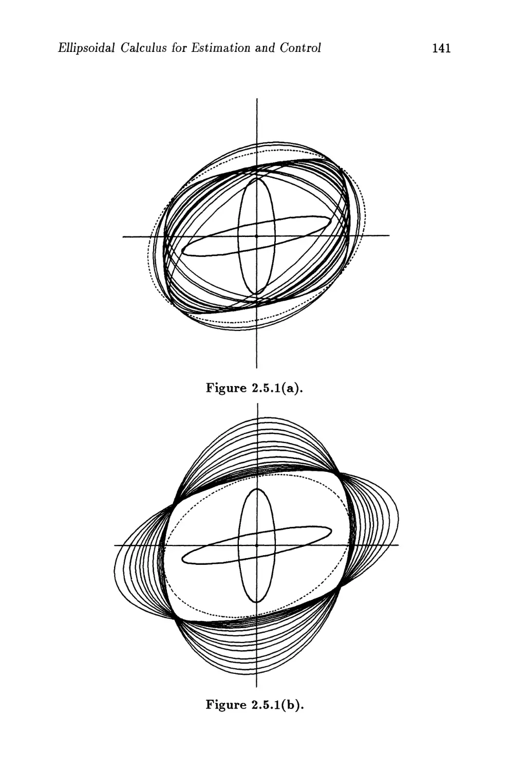
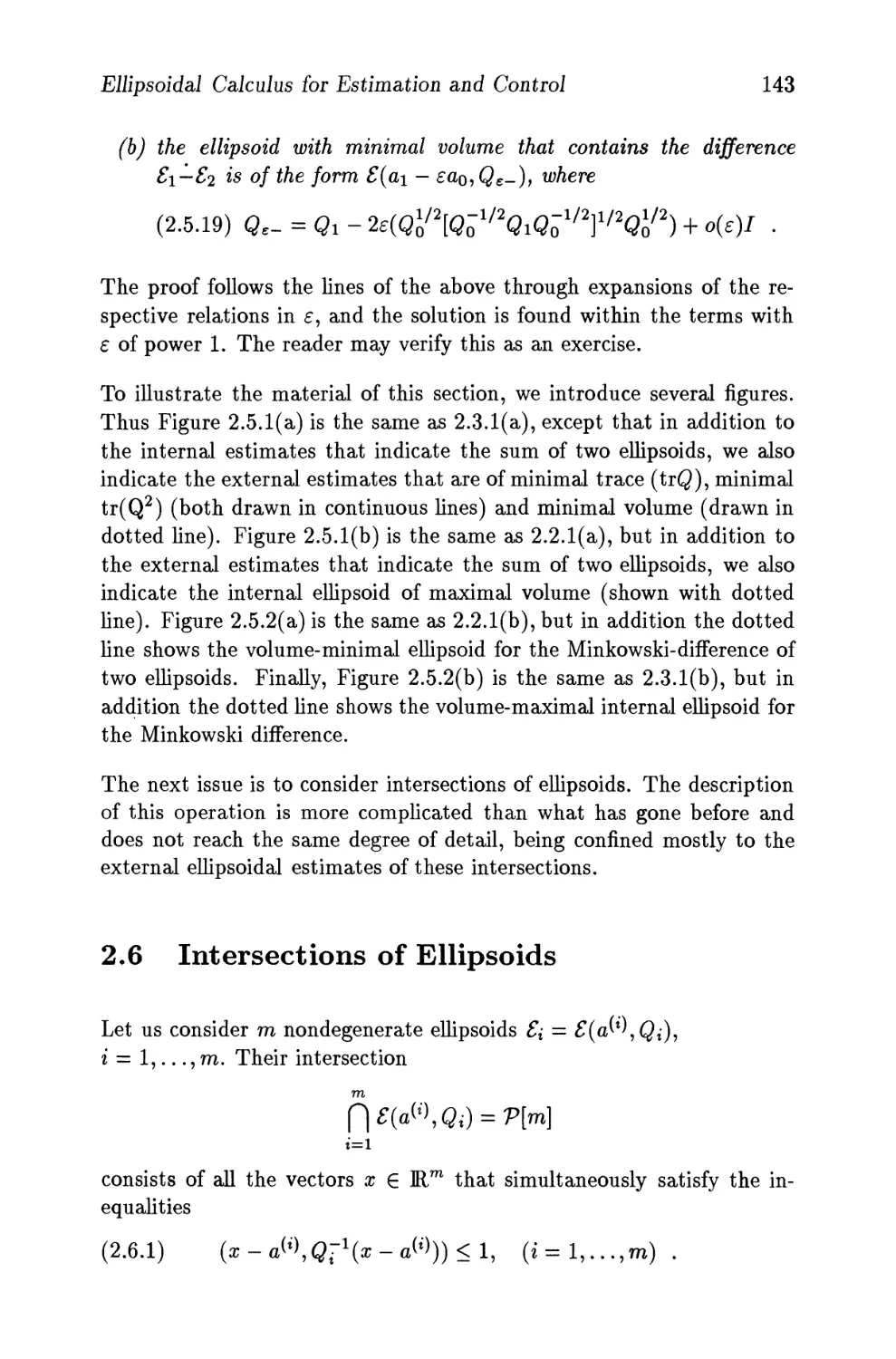
2.5 The Selection of Optimal Ellipsoids 132
2.6 Intersections of Ellipsoids 143
2.7 Finite Sums and Integrals: External Approximations ... 161
2.8 Finite Sums and Integrals: Internal Approximations . . . 170
Part III. ELLIPSOIDAL DYNAMICS:
EVOLUTION and CONTROL SYNTHESIS 177
Introduction 177
3.1 Ellipsoidal-Valued Constraints 178
3.2 Attainability Sets and Attainability Tubes:
The External and Internal Approximations 182

Contents vii
3.3 Evolution Equations with Ellipsoidal-Valued Solutions . . 190
3.4 Solvability in Absence of Uncertainty 194
3.5 Solvability Under Uncertainty 198
3.6 Control Synthesis Through Ellipsoidal Techniques .... 208
3.7 Control Synthesis: Numerical Examples 214
3.8 Ellipsoidal Control Synthesis for Uncertain Systems . . . 225
3.9 Control Synthesis for Uncertain Systems:
Numerical Examples 230
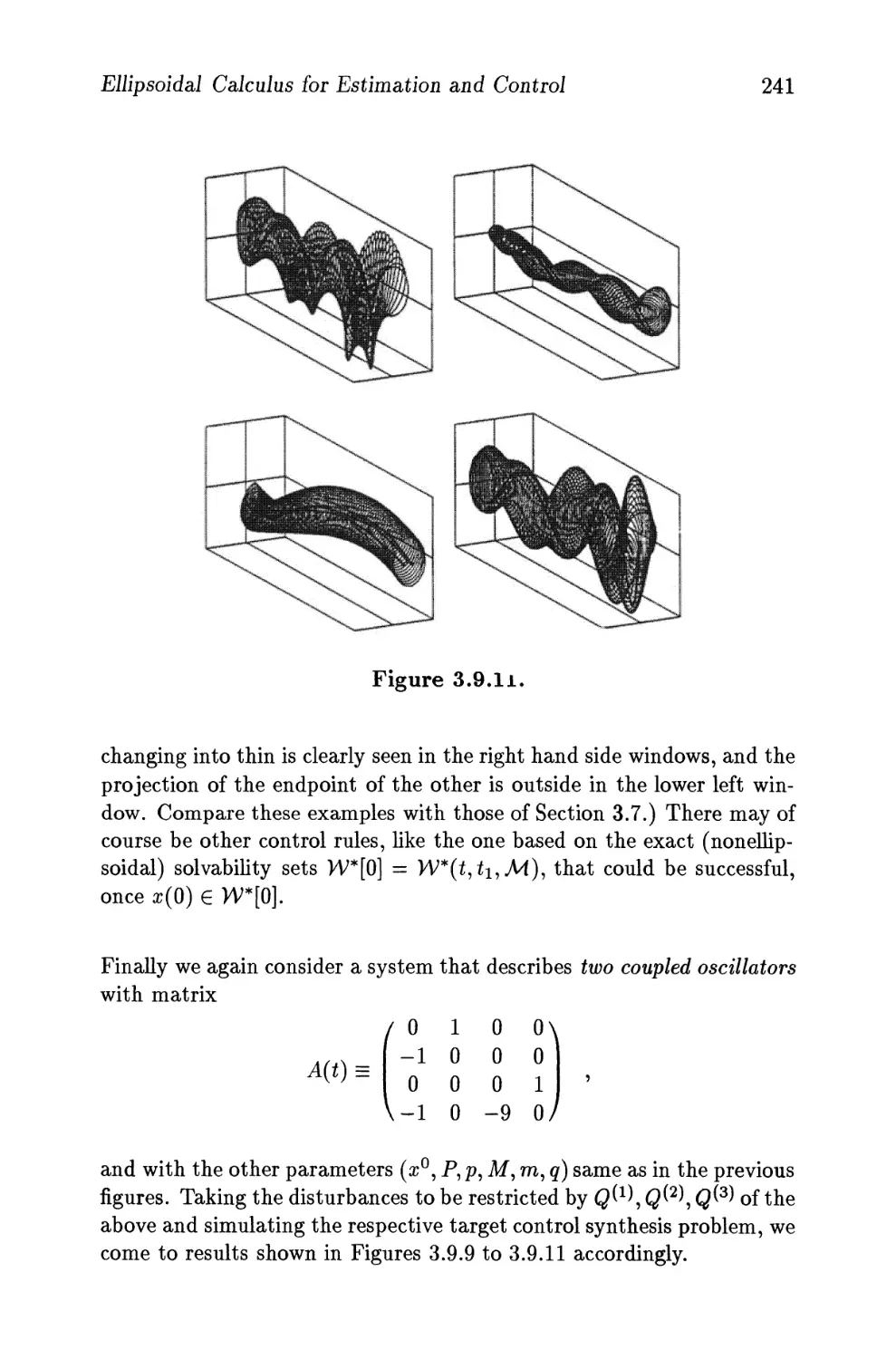
3.10 Target Control Synthesis Within Free Time Interval ... 242
Part IV. ELLIPSOIDAL DYNAMICS: STATE
ESTIMATION and VIABILITY PROBLEMS 247
Introduction 247
4.1 Guaranteed State Estimation:
A Dynamic Programming Perspective 249
4.2 From Dynamic Programming
to Ellipsoidal State Estimates 259
4.3 The State Estimates, Error Bounds, and Error Sets .... 264
4.4 Attainability Revisited:
Viability Through Ellipsoids 268
4.5 The Dynamics of Information Domains:
State Estimation as a Tracking Problem 273
4.6 Discontinuous Measurements and
the Singular Perturbation Technique 285
Bibliography 291
Index 319

Preface
It is well known that the emphasis of mathematical modelling on the
basis of available observations is first - to use the data to specify or refine
the mathematical model, then - to analyze the model through available
or new mathematical tools, and further on - to use this analysis in
order to predict or prescribe (control) the future course of the modelled
process. This is particularly done by specifying feedback control strategies
(policies) that realize the desired goals. An important component of the
overall process is to verify the model and its performance over the actual
course of events.
The given principles are also among the objectives of modern control
theory, whether directed at traditional (aerospace, mechanics,
regulation, technology) or relatively new applications (environment,
population, finances and economics, biomedical issues, communication, and
transport).
Among the specific features of the controlled processes in the mentioned
areas are usually their dynamic nature and the uncertainty in their
description.
Following this reasoning, one may claim that control theory is a science
of assigning feedback control or regulation laws for dynamic processes on
the basis of available information on the system model and its
performance goals (given both through on-line observations and through data
known in advance). It is on how to construct, in some appropriate sense,
the best or the better control laws. It is also used to indicate how the
level of uncertainty and the amount of information used for designing
the feedback control laws affects the result of the controlled process,

χ
Preface
particularly, the values of the cost functions or the aspired guaranteed
performance levels.
However, it is not any type of theory that is desired. Not the least
objective is to develop, among the possible approaches, a solution theory that
allows analytical designs that are relatively simple for practical
implementations or lead, at least, to effective numerical algorithms. These,
desirably, should match the abilities of modern computer technology,
e.g., allow parallel calculations and graphic animation.
The present book is devoted to an array of selected key problems in
dynamic modelling, state estimation, viability, and feedback control under
uncertainty. Its aim is to present a unified framework for effectively
solving these problems and their generalizations to the end through modern
computer tools.
The model of uncertainty considered here is deterministic, with set-
membership description of the uncertain items. These are taken to be
unknown but bounded with preassigned bounds and no statistical
information whatever. The set-membership model of uncertainty reflects
many actual information situations in applied problems. Particularly,
it appears relevant in estimating nonrepetitive processes, processes with
limited numbers of observations, incomplete knowledge of the problem
data and no available statistics. It is a common approach in pursuit-
evasion differential games, in robust stabilization, control and
disturbance attenuation, particularly, under unmodelled dynamics. Needless
to say, it also reflects the research preferences, interests and experiences
of the authors.1
The problems treated here are described through set-valued functions
and are thus to be treated through set-valued analysis. However, the aim
of this book is not to produce any type of set-valued technique, but a
calculus that allows effective solutions of the selected problems and their
generalizations with fairly simple control designs and the possibility of
graphic animation. The attempt is based on introducing an "ellipsoidal
1The references and some historical comments are given in the introductions to
each part and throughout the text. The authors apologize that among the enormous
literature on the subject they were able to mention only a very limited, representative,
rather than exhaustive number of publications available to them, with an emphasis
on those directly related to the topics of this publication and those that would allow,
as we hope, to pursue the further directions indicated here.

Preface
xi
calculus" that allows us to represent the exact set-valued solutions of the
respective problems through ellipsoidal-valued functions. The solutions
are thus constructed of elements that involve only ellipsoidal sets or
ellipsoidal-valued functions and operations over such sets or functions.
This further allows us to parallelize the calculations and to animate the
solutions through computer graphic tools.
It is necessary to indicate that the ellipsoidal techniques of this
particular book are not confined to approximation of convex sets by one
or several ellipsoids only as done in other publications, but indicate e/-
lipsoidal representations of the exact solutions. Namely, each convex
set or convex set-valued function considered here is represented by a
parametrized variety of ellipsoids or ellipsoidal-valued functions, which,
while their number increases, jointly allow (through their sums, unions,
or intersections), a more and more accurate representation with exact
one in the limit. The scheme includes approximations by single ellipsoids
as a particular element of the overall approach.
A particular emphasis of this book is on the possibility of computer-
graphic representations. The animation of the problems in estimation,
feedback control, and game-type dynamics not only allows us to present
the rather sophisticated mathematical solutions in visible forms (and
literally, to peer into the multidimensional spaces through computer
windows or more sophisticated computer tools). The authors believe
that it may also give new insights into the mathematical structure of
the solutions. (Thus, some assertions of a general nature proved in
this book were first noticed during the animation experiments.) The
authors also hope that though applying their techniques to a specially
selected array of problems, they also demonstrate an approach applicable
to many other situations that spread quite beyond the topics addressed
here. These are certainly not confined only to control applications, but
cover a broad variety of problems in systems modelling.
The book is divided into four parts designed along the following lines.
The first part gives exact solutions to the problems of evolution -
attainability (reachability) and solvability, as well as of estimation,
viability, and feedback terminal target control. The exact theory (both
known and new) is rewritten within a unified framework that involves
trajectory tubes and their set-valued descriptions either through
evolution equations of the "funnel type", or through the evolution of support

Xll
Preface
functions or through level sets of appropriate H-J-B (Hamilton-Jacobi-
Bellman) equations. The feedback control designs are based on using
set-valued solvability tubes which may be interpreted as "bridges"
introduced by N.N. Krasovski as a basis for further "aiming rules", as well
as on Dynamic Programming considerations. The principal schemes for
this framework are specifically directed towards the desired transition,
through ellipsoidal-valued representations, to parallelizable computation
schemes.
The second part of the book describes the ellipsoidal calculus itself. It
covers external and internal ellipsoidal representations for basic set-
valued operations-geometrical ("Minkowski") sums and differences as
well as intersections of ellipsoids and integrals of ellipsoidal-valued
functions. Though written for applications to Problems of Part I, the
text of this chapter may be also considered as a separate theory with
motivations and applications coming from topics other than discussed
here. Particularly, from optimization under uncertainty and multiob-
jective optimization, experiment planning, problems in probability and
statistics, interval analysis and its generalizations, adaptive systems and
robotics, image processing, mathematical morphology, and related areas
of theoretical and applied research.
The third and fourth parts indicate the applications of ellipsoidal
calculus to problems of Part I. Thus, the third part describes (both in forward
and backward time) the internal and external ellipsoidal representations
of attainability (reachability) tubes for systems without and with
uncertainty. In the latter case these are more complicated, of course, being
related to reachability or solvability under uncertainty or counteraction
and allowing, particularly, a direct interpretation in terms of the above
mentioned bridges - the key elements of game-theoretic feedback
control. The third part also deals with feedback control. The respective
control designs are based on applying ellipsoidal versions of the exact
solutions. This leads to a nonlinear control synthesis in the form of
analytical designs, except for a scalar parameter whose dependence on the
state space vector may be calculated in advance, through the solution
of a simple algebraic equation. These analytical designs are possible
due to the fact that the internal ellipsoidal tubes that approximate the
solvability domains under uncertainty are precisely such, that they
possess the property of being an "ellipsoidal-valued bridge". The latter
property arrives due to two basic features : the fact that the respective

Preface
xiii
ellipsoidal-valued mappings possess a semigroup property and the fact
that the internal tubes are inclusion-maximal among all other internal
ellipsoidal tubes.
The fourth part deals with state-estimation under unknown but bounded
errors, with attainability under state constraints and viability problems.
It also indicates the applicability of the suggested schemes to problems
posed within the so-called H^ approaches, when the value of the error
bound is not specified. This is due to the involvement of Dynamic
Programming techniques, particularly, of one and the same H-J-B equation
for the treatment of uncertain dynamics in both of the settings
investigated here. Other topics include new types of dynamic relations for the
treatment of information sets and vector-valued guaranteed estimators
as well as an interpretation of the state estimation problem as one of
tracking an unknown motion under unspecified but bounded errors. This
links the problem with those of viability under counteraction. The final
Section 4.6 deals with problems of state estimation under "bad noise",
which are approached through the incorporation of singular perturbation
techniques. This approach allows us to treat discontinuous observations
described by measurable functions and also to deal with viability
problems under measurable constraints. Numerical examples complement
the theoretical parts.
The narrative stops just short of control under measurement feedback
and adaptive control. These are areas which require separate serious
consideration and explanation. However, the application of ellipsoidal
techniques would be especially useful in these areas, as we believe. The
respective challenges are beyond the material of the present book.
As already mentioned, this book indicates a unified concise framework
for problems of state estimation, viability and feedback control under
set-membership uncertainty for systems with linear dynamics. It
introduces an ellipsoidal calculus to develop the solutions from theory to
algorithms and computer animation, and thus to solve the problem to
the end.
This book is not a collection of numerous facts or artifacts in set-valued
analysis or control theory. It is rather a book on basic problems and
principles for calculating their solutions through set-valued models. Whether
reached or not, our aim is also to stimulate and encourage further
investigation in the spirit of the present approach as well as implementations

xiv
Preface
in real-life modelling. (The latter issue could be the topic of a separate
monograph.)
In this text we are confined to linear-convex systems and problems.
However, the control synthesis given here is nonlinear and the
synthesized systems are nonlinear systems. Moreover, the Dynamic
Programming approaches applied here open the routes to further penetration
into generically nonlinear classes of systems. The algorithmization and
animation in these cases is certainly a worthy challenge.2
Another important aspect hardly discussed here is the accuracy and
computational complexity of the underlying algorithms.
The conceptual approaches to controlled dynamics that served as a
background for this work were influenced by the research of N.N. Krasovski
and his associates at Yekaterinburg (Sverdlovsk), where the first of the
authors had earlier worked for many years. In the necessity of studying
and applying set-valued analysis we share the views of J-P. Aubin and
his colleagues.3
The principal parts of this book and the underlying ellipsoidal
representation approach for the set-valued functions were worked out throughout
the authors participation at the SDS (Systems and Decision Sciences)
Program of HAS A - the International Institute of Applies Systems
Analysis at Laxenburg, Austria. The serious but friendly atmosphere,
pleasant working conditions, and possibility of regular contacts with a broad
spectrum of researchers certainly stimulated our work at the Institute
and the direction of our efforts. The authors are grateful to the
Directors of IIASA - Thomas Lee, Robert Pry, and Peter De Janosi and
to the Chairman of the IIASA Council in 1987-1992, the late Vladimir
Sergeevich Michalevich, for their support of methodological research at
IIASA, particularly of our own investigations.
We wish to thank our colleagues at IIASA and its Advisory
Committee on Methodology - J.P. Aubin, H. Frankowska, A. Gaivoronski,
2 The nondifferentiable version of Dynamic Programming has been substantially
developed in the recent years (see references [82], [83], [290]), becoming an effective
tool in nonlinear control theory, particularly. For covering the needs of this book we
use its simple versions that do not extend beyond the use of subdifferential calculus.
3A set-valued approach to state estimation and uncertain dynamics was
emphasized in [181].

Preface
xv
P. Kenderov, G. Pflug, R.T. Rockafellar, W. Runggaldier, K. Sigmund,
M. Thoma, V. Veliov, R. Wets, A. Wierzbicki for their stimulating
discussions and support, K. Fedra and M. Makowski for their help in
computer graphics, the SDS secretaries E. Gruber and C. Enzlberger-
Vaughan for preparing papers and manuscripts used in this book. We
thank T. Filippova, 0. Nikonov, M. Tanaka, K. Sugimoto who have
coauthored some of our IIASA Working Papers used here and also
E.K. Kostousova and O.A. Schepunova for their help in arranging the
final version of the manuscript.
Throughout the last years we had the pleasant opportunity to discuss the
topics treated in this book with Z. Artstein, J. Baras, F. Chernousko,
M. Gusev, A. Isidori, P. Kail, R. Kalman, H. Knobloch, A. Krener,
G. Leitmann, С Martin, M. Milanese, E. Mischenko, S. Mitter, J.
Norton, Yu. Osipov, B. Pschenichnyi, S. Robinson, A. Rusczynski, P. Saint-
Pierre, A. Subbotin, T. Tanino, V. Tikhomirov, P. Varaiya, S. Veres,
and J. Willems. Their valuable comments certainly helped to shape the
contents.
Our special thanks go to С. Byrnes - Editor of the Birkhauser
Series on Systems and Control: Foundations and Applications and to the
Birkhauser staff for their support, patience, and understanding of the
problems faced by the authors in preparing the manuscript.

Part I. EVOLUTION and CONTROL:
The EXACT THEORY
Introduction
The present first part of the book is a narrative on constructive
techniques for modelling and analyzing an array of key problems in
uncertain dynamics, estimation, and control. It presents a unified approach
to these topics based on descriptions involving the notions of
trajectory tubes and evolution equations for these tubes. The class of systems
treated here are linear time-variant systems
χ = A(t)x + u + /(i), x(to) = xq ,
with magnitude bounds on the controls и and the uncertain items
f(t),xo. The target control processes and the estimation problems are
considered within finite time intervals: t £ [^0^1]· This requires a rather
detailed investigation of the system dynamics. The present topic thus
differs from problems in which the objective lies only in the achievement
of an appropriate asymptotic behaviour of the trajectories with perhaps
some desired quality of the transient process.
The first step is the description of attainability (reachability) domains
X[t] for systems without uncertainty. The evolution of these in time
is naturally described by set-valued ("Aumann") integrals with variable
upper time limit. This immediately leads to set-valued "attainability
tubes" whose crossections are the attainability domains. However, it is
not unimportant to introduce some sort of evolution equation with set-
valued state-space variable that would describe the dynamics of sets X[t]
in time. The tubes X[t] could then be interpreted as trajectories of some
generalized dynamic systems. (Among the first investigations with this
emphasis are the works of E. Barbashin and E. Roxin [34], [270].) The
serious obstacle for deriving such an equation in a differential form is the
difficulty in defining an appropriate derivative for set-valued functions.
The objective is nevertheless reached through evolution equations of the
funnel type that do not involve such derivatives. Though somewhat
cumbersome at first glance, these equations indicate set-valued discrete-
time schemes important for calculations.4
4 Among the recent investigations on evolution equations for trajectory tubes are
papers [246], [299], [103], [17].
ki et.al, Ellipsoidal Calculus for Estimation and Control
Jiauser Boston and International Institute for Applied Systems Analysis

2
Alexander Kurzhanski and Istvan Valyi
The attainability tubes may be also constructed in backward time in
which case they are referred to as solvability tubes. The solvability tubes
are used here in synthesizing feedback control strategies for problems
of terminal target control. Namely, if the solvability tube ends at the
target set Μ, then the synthesized control strategy should be designed to
keep the trajectory within this tube (or bridge) throughout the process.
This idea is the essence of the "extremal aiming rule" introduced by
N.N. Krasovski [168], [169] and used in Section 1.4. A key element that
allows us to use the solvability tubes for the control synthesis problem
is that the respective multivalued maps satisfy a semigroup property
and therefore generate a generalized dynamic system with set-valued
trajectories.
A similar type of strategy may be derived through a Dynamic
Programming technique with cost function being the square of the Euclid
distance d2(x[t\],M) from endpoint x[ti] to the target set M, for
example (see Section 1.5). Selecting a starting position {t, x},x = x(t),
we may minimize the cost function by selecting an appropriate optimal
control (in the class of either open-loop or closed-loop controls).
Finding the optimal value of the cost function for any position {t, x} we
come to the value function V(i, x). One should note that in the absence
of uncertainty the value function V{t,x) is the same both for open-loop
(programmed) control and for closed-loop (positional) feedback control.
For the linear-convex problems of this Section 1.5 the function V(t,x)
may be therefore calculated through standard methods of convex
analysis used traditionally for solving related problems of open-loop control
[167], [266], [181]. The function V(t,x) then satisfies a corresponding
generalized H-J-B (Hamilton-Jacobi-Bellman) equation.
The next stage is the treatment of systems with input uncertainty f(t)
(unknown but bounded, with magnitude bounds). In this case the at-
tainability set under counteraction (in forward time) and solvability set
under uncertainty (in backward time) are in general far more
complicated than in the absence of uncertainty (see Sections 1.6-1.8). One
should now distinguish, for example, the open-loop solvability tubes from
the closed-loop solvability tubes (Section 1.6). Under some nondegener-
acy conditions, the latter ones may be again interpreted as Krasovski's
bridges (now for uncertain systems) and may be used for designing
feedback strategies through the extremal aiming rules (Sections 1.7, 1.8).
The backward procedure for solvability tubes is also similar in nature

Ellipsoidal Calculus for Estimation and Control
3
to the schemes introduced by P. Varaiya et al [308] and B. Pschenichnyi
[259]. In the linear-convex case considered here the constructive
description of solvability tubes may be given by a set-valued integral known as
L.S. Pontryagin's alternated integral [257] (Section 1.7). It is indicated
here that they also satisfy some special evolution equations of the
funnel type. There is a particular case, however, when the open-loop and
closed-loop solvability tubes coincide. This is when the system satisfies
the so-called matching condition which means that the bounds on the
controls и and the disturbances / are similar in some sense (Section
1.6). The calculation of the solvability tubes is then as simple as in the
absence of uncertainty.
One may also apply Dynamic Programming to the mentioned uncertain
systems. Taking the cost function d2(x(t\),M), for example, we note
that now it should be minimaximized over the control и and the input
disturbance / respectively. But the value of this minmax, when
calculated over closed loop controls is different, in general, from its value
calculated for open loop controls. It is the former value that may be
described through a respective H-J-B-I (Hamilton-Jacobi-Bellman-Isaacs)
equation (see [109], [171], [219], [290]). There is an exception again,
nevertheless. Namely, if the matching conditions are satisfied, then the
minmax of the cost function or, in other words, the value function V(t,x)
is the same, whether calculated over open-loop or closed4oop controls.
Having in mind the previous remarks, one may observe that the value
functions V(t,x) used in this book play the role of Liapunov functions
used in respective approaches to the design of feedback controllers for
uncertain systems (see [214], [215]). We should also emphasize that
the problem treated here is to reach the goal in finite time attenuating
the unknown disturbances. Namely, it is to ensure that the system
is steered by control и to the target set Μ (at given time ti) under
persistent disturbances / rather than to figure out the saddle points of a
positional (feedback) dynamic game between two equal players и and /
which is the emphasis of the theory of differential games (see [37], [171],
[50], [119]).
The further problems are similar to the previous ones but complicated
by state constraints (viability restrictions). Evolution funnel equations
are introduced for the dynamics of attainability sets under state
constraints (in forward time) and respective solvability sets (in backward

4
Alexander Kurzhanski and Istvan Valyi
time). The latter ones are similar to viability kernels introduced by J.P.
Aubin [15], within the framework of viability theory (Section 1.9). The
control synthesis problem is now to ensure viability (Section 1.10) or
viability under counteraction (or under persistent disturbances, in another
interpretation), while also reaching the terminal set (Section 1.11).
The last problem of the first part is the one of state estimation under
unknown but bounded errors and disturbances (Section 1.12).5
The main objects of investigation here are the information sets
consistent with the system dynamics, the available measurement and the
constraints on the uncertain items. The information sets are actually
the attainability domains under a state constraint that is induced by
the measurement equation and therefore arrives on-line, together with
the result of the measurement. The evolution equation for the
information set acts as a guaranteed filtering equation and the guaranteed
state estimate is then the "Chebyshev center" of this set (namely, the
center of the smallest ball that includes the information set). This first
part of the book gives but a general introduction to the problem, while
constructive techniques are introduced in Parts III and IV, where one
may also find some connections with other approaches to deterministic
filtering (particularly, the Я^ approach [94], in the interpretation of
J. Bar as and M. James [30]).
A synopsis of the results and some suggestions on why ellipsoids were
undertaken to be studied finish this part.
We now proceed with the main text, commencing with the basic
notions.
1.1 The System
In this book we consider dynamic models described in general by a linear
time-variant system
(1.1.1) x(t) = A(t)x(t) + u + f(t)
5 The first investigations of state estimation problems under unknown but bounded
inputs date to papers [166], [318], [178]. A systematic investigation of the set-valued
approach in continuous time seems to have started with [54], [277], [179], [181].

Ellipsoidal Calculus for Estimation and Control
5
with finite-dimensional state space vector x(t) £ Rn and inputs и (the
control) and f(t) (the disturbance or external forcing term). The η Χ η
matrix function A(t) is taken to be continuous on a preassigned interval
of time Τ = {t £ Ж : to < t < ti} within which we consider the
forthcoming problems, with u(t),f(t) assumed Lebesgue-measurable in
t £T .
The values и of the controls are assumed to be restricted for almost all
t by a magnitude or geometrical constraint
(1.1.2) ueV(t) ,
where V(t) is a multivalued function V : Τ —» convlR71, continuous in t.
Here and further on symbol convlR71 stands for the variety of closed
convex sets in finite-dimensional space Жп while complR71 stands for the
variety of convex compact sets in ]Rn.
We shall further consider two types of controls which are:
- open loop, when и = u(t) is a function of time t, measurable on Τ (a
measurable control), and
- closed loop, when и = U(t,x(t)) is a multivalued map, namely,
U : Τ χ Жп —* convRn
measurable in t and upper semicontinuous in x, being a function
of the position {t, ж} of the system.
(The definition of upper semicontinuity is standard, it may be found in
[176], [68], [20], [22] and other related publications.)
In the first case we come to a linear differential equation
(1.1.3) x(t) = A(t)x(t) + u(t) + f(t)
with u(t) £ V(t),t £ T, being an open-loop control. The class of
functions u(·) = u(t),t £ T, measurable in t £ Τ and restricted as in (1.1.2)
is further denoted as Up.

6
Alexander Kurzhanski and Istvan Valyi
In the second case we come to a nonlinear differential inclusion
(1.1.4) i(t)€A(t)x(t)+U(t,x(t)) + f(t) ,
where
(1.1.5) U(t,x)CV(t), teT ,
is a feedback (closed-loop) control strategy.
The class Щ = {U(t,x)} of feasible control strategies consists of all
convex compact-valued multifunctions that are measurable in t, upper
semicontinuous in ж, being restricted by (1.1.5) and such that equation
(1.1.4) does have a solution extensible to any finite time interval Τ for
any x° = χ (to) £ lRn. The latter means that there exists an absolutely
continuous function x(t),t £ T, that yields the inclusion
x(t)eA(t)x(t) + lt(t,x(t)) + f(t)
for almost all t £ T.
The existence of solution for system (1.1.3) is a standard property of
linear differential equations [61], [142], [167], [248].
Systems (1.1.3), (1.1.4) may be transformed into simpler relations.
Let S(t,r) stand for the matrix solution to the equation
(1.1.6) -S(i,r) = -£(*,r)A(i), S(t,t) = I ,
which also satisfies the equation
^-S(t,r) = A(r)S(t,T), S(t,t) = I .
ОТ
As it is well known, the solution to (1.1.3) with initial value
(1.1.7) x(t0) = x°
is given by the formula
x(t) = S(to,t)x° + f S(T,t)(u(r) + f(r))dT .
Jt0

Ellipsoidal Calculus for Estimation and Control
7
Taking the transformation
(1.1.8) z(i) = 5(Mi)a;(i)
and substituting χ for ζ in (1.1.3) we come to the equation
(1.1.9) z(t) = 5(Mi)ti(t) + S(Mi)/(*)
(1.1.10) z° = z(t0) = S(t0,h)x° .
Clearly, there is a one-to-one correspondence of type (1.1.6) between the
solutions x(t) and z(t) to equations (1.1.3) and (1.1.9), respectively. The
initial values for these are related through (1.1.10). Therefore, instead
of the systems (1.1.3), (1.1.4), constraint (1.1.2) and initial condition
(1.1.7), we come to
(1.1.11) z(t) = w(t) + g(t), ζ(ί0) = 5(ίο,ίι)ζ° ,
(1.1.12) z(t)eW(t,z) + g(t)
with constraint
(1.1.13) w(t)eV0(t) .
Here obviously
w(t) = S^t, <!)«(<)
g(t) = 5(ΐ,ΐα)/(ί)
W(t,z) = S(t,h)U(t, S-\t0, t)z)
Vo(t) = S(t,tx)V(t)
and the set-valued function Vo(t) remains continuous. The new feedback
strategies W(i, z) belong to the class defined by the constraint Vo(t), but
otherwise the same as before:
Without loss of generality we may therefore further treat systems
(1.1.11)—(1.1.13) rather than (1.1.2)—(1.1.4). It is compulsory however
that the constraint function Vo(t) would be time-variant. In other terms,
without loss of generality we may further follow the notations of (1.1.2)—
(1.1.4) with A(t) = 0.
One should realize, however, that the described substitution (1.1.8)
allows us to consider the forthcoming problems for A(t) = 0 within the

8
Alexander Kurzhanski and Istvan Valyi
time range {t < ii}. A similar result may be also obtained by
substitution
(1.1.14) z(t) = S(t,t0)x(t) .
Then the original system may be again, without loss of generality, taken
with A(t) = 0, but the time range for which the respective substitution
is true will be {t > t0}.
We shall often make use of the indicated facts in the sequel in the hope
that this will enable us to demonstrate the basic techniques without
overloading the text with unessential but cumbersome procedures. The
reader will always be able to return to A(t) φ 0 as a healthy exercise.
The first issue to discuss is the description of the set of states that can
be reached in finite time due to systems (1.1.3), (1.1.4) under restriction
(1.1.2) and (1.1.5).
1.2 Attainability and the Solution Tubes
Taking system (1.1.3), (1.1.2) for A(t) = 0, we have
(1.2.1) x(t) = u(t) + f(t), i6T,
with constraint (1.1.2) u(t) G V{t). We also presume that the initial
state x° = ж (ίο) is restricted by the inclusion
(1.2.2) x° G *°, X° G comp ЖЛ
One of the first questions that arise in control theory is to describe
the variety of all states χ = x(t) that can be reached by the system
trajectories that start at a prescribed set X°.
Let x[t] = x(t, to, x°) denote an isolated trajectory of system (1.2.1) that
starts at instant ίο from state xo, being driven by a certain control u(t).
We will be further interested in the union of all such isolated trajectories
over all possible initial states x° G X° and measurable controls u(t) G
V{t). Therefore we denote
Щ = X(t,t0,X°) = \J{x(t,tQ,x0) : x° G X°,u(t) G V(t),t G T].

Ellipsoidal Calculus for Estimation and Control
9
For the mapping X(t,to,·) : comp]Rn —» comp]Rn it is not difficult to
check that it satisfies the following semigroup property:
X(t,t0,X°) = X(t,T,X(T,to,X0)),
whatever are the values ί, τ with ίχ > t > τ > ίο·
Definition 1.2.1 The set X[t] = X(t,t0,X°) is referred to as the
attainability domain for system (1.1.3) or (1.2.1), (1.1.2.) at time t,
from set X°.
The attainability domain X[t] is often said to be the reachability domain.
The set-valued map
X[t] = X(t,t0,X°), iGT,
defines a solution tube to the differential inclusion
(1.2.3) x(t)eV(t) + f(t),
that starts from set X°. In other words, the set X[t] = {#*} consists of
all those vectors ж* for each of which there exists an isolated trajectory
x[t] = x(r,to,x0),to < r < i, of (1.2.3) that satisfies the boundary
conditions ж [ίο] £ A'0,a:[i] = χ*.
It is clear that the control
u(t) = x[t] - f(t)
is the one that corresponds to #[i], so that we could also indicate
(1.2A)X[t] = {x[t} : x[t] - f(r) G V(r), i0 < r < i, x[t0) G X0}.
The multivalued function ^[t], ί £ Τ, X[to] = <^° is also known as the
solution tube to system (1.2.1), under restriction (1.1.2), from set X°,
for the interval ί G [ίο, *i] = T.6
As a preliminary exercise it is not difficult to prove the following
6 Other terminology says that X\t\ is the trajectory assembly generated by system
(1.2.3) and set X[t0] = X° [181].

10
Alexander Kurzhanski and Istvan Vaiyi
Lemma 1.2.1 The multifunction X[t] is convex compact-valued (X[t] £
convlR71) and continuous on the interval T.
Remark 1.2.1 One of the popular problems studied on the subject of
attainability is the following: given X° = {0}, will the set
x = u{x[t],te[to,oo)},
coincide with the whole space Etn ?
An affirmative answer will indicate that any point in Etn may be reached
in finite time through a bounded control u(-) £ Up. Otherwise one is to
specify X as a subset of Ш71.
Exercise 1.2.1. Investigate the problem of Remark 1.2.1.
Passing to the differential inclusion
(1.2.5) x(t)eU(t,x) + f(t),
(1.2.6) H(v)et^
where the class of feasible feedback strategies Щ is as defined in Section
1.1, we come to the following questions.
Let ХцЩ = Xu(tito->x°) be the crossection of the set of all isolated
trajectories x[t] that satisfy the relation
i[t]eU(t,x[t]) + f(t), x[to] = x°,
for a given multivalued map ZY(·, ·) £ Щ. A particular element of Щ
is the set-valued map V{t) itself, so that (1.2.3) could be viewed as a
particular case of equation (1.2.5), when U(t,x) = V(t).
Denote for a fixed U of (1.2.6):
MA = Xu(t,t0,X°) = UWMo,*0): x° € A'0},
and further
X*[t] = X*(t,to,X°) = {J{Xu{t,t0,X°):U(;·) e Щ}.
Then one may want to know what is the relation between the tubes X*[t]
obtained for the closed-loop system (1.2.5), (1.2.6) and X[t] obtained for
the open-loop system (1.2.3)?

Ellipsoidal Calculus for Estimation and Control
11
Theorem 1.2.1 With X*[to] = X[to] = X° the following relation is
true:
X[t] = **[t], t G T.
To prove this assertion we observe that every single-valued function
u(t) can be treated as an element of U%>. Therefore X[t] С Λ""[ί],ί G
Т. To show the opposite assume there exists a trajectory x*[t] =
x*(t,t0,x°),x° G Л', which satisfies the inclusion x*[t] G #*[*],* G T,
namely,
i*[r]eW*(r,a:*[r]) + /(T), r<i,.
for some W(·, ·) = W*(·, ·) G i/£. Then obviously
i*[r] G W*(r, х*[т]) + /(г) С P(r) + /(r), r < i,
and due to (1.2.4) this yields x*[t] G Λ'Μ,ί G Γ.
The main conclusion given by Theorem 1.2.1 is such that with
function f(t) given (there is no uncertainty in system (1.1.1), (1.1.2)), the
solvability tube X[t] for system (1.1.1), (1.1.2) taken in the class Up of
open-loop controls u[t] is the same as the solvability tube X*[t] taken in
the class Щ of closed-loop controls U(t,x). This conclusion is also true
when the closed loop controls are selected among appropriate classes of
single-valued functions и - u(t,x) G V(t) that allow the existence and
prolongation of solutions of (1.1.1) with и — u(t,x),t G T.
The next question is whether it would be possible to describe the
evolution of sets X[t] in time t through some type of evolution equation with
set-valued states X = X[t].
1.3 The Evolution Equation
We shall now introduce an evolution equation with state space variable
X G convlR71, whose solution will be precisely the tube X[t] of Section
1.1.2.
Obviously
t t
(1.3.1) X[t] = X° + Jv(r)dr + J f(r)dr ,
to to

12
Alexander Kurzhanski and Istvan Valyi
where the second term in the right hand is the set-valued Lebesgue
integral ("the Aumann integral" [25]) for the function V. The question
is therefore whether one could construct an evolution equation for
describing X[t].
Denote S = {x : (ж, χ) < 1} to be the unit ball in ]Rn.
Definition 1.3.1 The Hausdorff semidistance h+(X,y) between sets
Х,У G conv Etn is introduced as
h+(X, У) = min{7 > 0 : X С У + 7<S}
or equivalently
h+(X,y) = maxmin{(a; - y,x - y)*\x G X,y G У} .
Я7 У
Similarly
h-(X,y) = h+(y,X) .
The following properties are true for X,y,Z 6 convEt":
(i) h+(X,y) = 0 implies X С У
(and Л_(ДГ,У) = 0 impUes J С Х).
(ii) /»+(*,£) + Л+(2,У) > h+(X,y).
Definition 1.3.2 The Hausdorff distance h(X,y) between sets Х,У €
convWC1 is introduced as
h(X,y) = max{h+(X,y),h-(X,y)} .
Obviously
(iii) Н(Х,У) = 0 implies X = y for Х,У £ convR"
As it is well known, a closed convex set X € convlR" may be described
by its support function
p{l\X) = sup{(/,z)|a: G X}

Ellipsoidal Calculus for Estimation and Control
13
which is a positively homogeneous convex function of /, namely,
p(ct\X) = ctp(l\X) for α > 0
and
p(<*1l1 + a2l2\X) <alP(h\X) + a2p(l2\X) ,
where αχ > 0, a2 > 0, αχ + a2 = 1.
For X G comp]Rn we have /9(/|^) < oo, V/ G It71. A well-known property
is given by
Lemma 1.3.1 The inclusion χ G X, X G com;]Rn, is equivalent to the
inequality
(l,x) <p(l\X\ V/GRn .
Direct calculation gives us the following formulae:
h+(X,y) = тах{р(1\Х)-р(1\У) : ||/|| < 1} ,
(1.3.2) h(X,y) = тгх{\РЩХ)-р(1\У)\ : ||/|| < 1} .
Definition 1.3.3 A function X : Τ —> conu!Rn is said ίο 6e absolutely
h-continuous on Τ if for any ε > 0 Йеге eziste a 5 > 0 swc/г //ш£
condition
г
yieWs
Σ>(*[«ί], *[ίΠ) <£ ·
г
The definition of absolute h+-continuity is given by mere substitution of
h by h+ in Definition 1.3.3.
Lemma 1.3.2 A function X : Τ —> IRn is absolutely h-continuous if
the support function p(l\X[t]) = f(l,t) is absolutely continuous int^T
uniformly in I G S.

14
Aiexander Kurzhanski and Istvaa Valyi
Now we may consider the equation
(1.3.3) lim σ_1 h(X[t + σ], X[t] + aV(t) + σ/(ί)) = 0
with initial value
(1.3.4) X[t0] = X° .
Definition 1.3.4 A multivalued function Ζ : Τ -» condR71 z's scud to be
a solution of (1.3.3), (1.3.4) if it is absolutely h-continuous and satisfies
(1.3.3) for almost all t G T, together with (1.3.4).
Let us see whether X[t] is a solution to (1.3.3) in the sense of the last
definition.
Rewriting (1.3.1) in terms of support functions, we come to
t t
(1.3.5) p(l\X[t]) = p(l\X0) + Jp(l\V(r))dT + J(l,f(r))dr .
to to
Here we made use of the fact that for a continuous map V : Τ —» convIR71,
the following is true
τ τ
p(l\Jv(r)dr) = J P(l\V(r))di
to to
To calculate
h(X[t + a],X[t] + aV(t) + af(t)) = H(a,t) ,
due to (1.3.3), (1.3.5) at first we have
R(l,a,t) = p(l\X[t + a]) - p(l\X[t]) - ap(l\V(t))-a(lj(t)) ,
t+σ
R(l,a,t) = J[(P(1\V(t)) + (l,f(r))]dr-ap(l\V(t)) - σ(/,/(ί))
t
In case of continuous f(t) and V(t) we further have
t+σ
(1.3.6) σ~ι J f{r)dr - f{t), σ - 0

Ellipsoidal Calculus for Estimation and Control
15
for all t and
t+σ
(1.3.7) σ"1 J p(l\V(r))dr - />( W))> σ -^ 0 .
ί
If f(t) is not continuous, being only measurable in t, relation (1.3.6) is
still true, but now only for almost all of the values of /, which are the
points of density of f(t) [232]. A similar remark is true for set-valued
function V(t) and thus for (1.3.7) with p{l\V{t)) measurable in t [68],
[21].
Taking into account the equality
H(a,t) = тах{|Д(/,а,<)| : ||/|| = 1}
and the relation
lim σ-1.β(/,σ,ί) = 0 ,
that follows from (1.3.6), (1.3.7), and is uniform in / £ <S, being true for
almost all ί € T, we observe
1ш1а_1Я(а,*) = 0
σ—>Ό
for almost all t £ T. This proves the following assertion:
Theorem 1.3.1 The map X : Τ —> convIR71, is α solution to the
evolution equation (1.3.3).
Theorem 1.2.1 implies the following
Corollary 1.3.1 The map X*\t] of Section 1.2.1 is a solution to the
evolution equation (1.3.3).
It is not uninteresting to write down a formal analogy of equation (1.3.3)
when A(t) φ 0.
This is as follows:
НтИедНа], (I + aA(t))X[t] + aV(i)
σ—»Ό
(1.3.8) + σ/(ί)) = 0 .

16
Alexander Kurzhanski and Istvan Valyi
A solution X[t] to (1.3.7) with given initial state X[t0] = X°,X° £
convRn is one that satisfies Definition 1.3.4, but with equation (1.3.3)
substituted by (1.3.8).
Let us now have a look at what would equation (1.3.8) be when X[t] =
{x[t]} and V(t) = {p(t)} are single-valued. Then, clearly,
h(x',x") = d(xf,x") = (xf - x",xf - x")1'2
and for almost all t £ Τ
(1.3.9) x[t + a] = (7+σΑ(ί))χ[ί] + σρ(ί) + σ/(ί) + ο(ί,σ) ,
where σ_1ο(/,σ) —*· 0 with σ —» 0. This yields
σ-!(ψ + σ]-^]) = ^(фИ+р^ + ДО + а^о^а)
for almost all t £ Г or after a limit transition σ —> 0:
(1.3.10) i[t] - A(t)x[t] + p(t) + /(t), s[i0] = ж0
for almost all ί £ Г.
Thus, equation (1.3.8) is clearly a set-valued analogy of the ordinary
differential equation (ODE) (1.3.10) that may also be presented in a
form similar to (1.3.8), which is (1.3.9).
There is no special point, however, in presenting an ODE in the form
(1.3.9). It is not so for set-valued maps, where equation (1.3.8) may
be quite convenient, particularly because here we avoid the unpleasant
operation of subtraction of sets or set-valued functions.
Equation (1.3.3) may be integrated. The integral form for its solution
X[t] is given by (1.3.1) and is described by a multivalued Lebesgue
integral [25].
The support function for a solution X[t] of (1.3.3), (1.3.4) satisfies, as
one may directly conclude from these relations, the partial differential
equation
(1.3.П) ^(WD = p(W)) + (i,/W) ,
(1.3.12) p(l\X[to]) = p(l\X°), t € Г, / € Ш"
for almost all t £ Τ and all I <E IRn, that follows due to (1.3.2). From
(1.3.11), (1.3.12) it is then not difficult to observe that X[t] is the only
solution to (1.3.3), (1.3.4):

Ellipsoidal Calculus for Estimation and Control
17
Lemma 1.3.3 The solution X[t] to equation (1.3.3), (1.3-4) ™ unique.
To conclude this paragraph we shall introduce another version of the
evolution equation (1.3.3), namely, by substituting the Hausdorff distance
hQ for a semidistance h+(). This gives
(1.3.13) lim σ-1Λ+(2[ί + σ],2[ί] + σΡ(ί) + σ/(ί)) = 0 ,
(1.3.14) Z[t0] CX° .
A solution Z[t] to (1.3.12), is specified as in Definition 1.3.4 but with
equation (1.3.3) substituted by (1.3.13).7 Here a solution Z[t] to (1.3.12)
satisfies an inclusion
Z[t + a] CZ[t] + aV{t) + σ/(ί) + o(t,a)S ,
rather than an equality, (C instead of =,) which would be the case for
(1.3.3). This directly yields a partial differential inequality (true for all
/ G IRn) and almost all t G T)
(1.3.15) ^(l\Z[t)) < p(l\V(t)) + (/,/(/))
for the solution Z[t]. The initial condition also satisfies an inequality
(1.3.16) p(l\Z[to]) < p(l\X°) .
It is not difficult to observe that (1.3.13) has a nonunique solution.
Particularly, any single valued trajectory x(i) driven by a control u(t) G V(t)
with x° G X° will be one of these.
Integrating (1.3.13), we come to
t
p(l\Z[t}) < p(l\X[to}) + j{p{l\V{r)) + (/, f(r)))dr = p(l\X[t}) ,
ίο
in view of (1.3.15) and (1.3.16). This leads us to the assertion
7 In the sequel in all the equations of the funnel type that involve Hausdorff
semidistance /i+ we shall presume that σ —► +0 without additional indication.

18
Alexander Kurzhanski and Istvan Valyi
Lemma 1.3.4 The solutions Z[t], X[t] to the evolution equations
(1.3.3) (1.3.4) and (1-3.13), (1.3.4)j respectively, satisfy the inclusion
Z(t) С X[t] ,
for all t G T.
We emphasize again that (1.3.3), (1.3.4) has a unique solution, while, in
general, the solution to (1.3.13), (1.3.4) is nonunique.
Definition 1.3.5 A solution Z°[t] to (1.3.13) is maximal if
Z[t] С Z°[t], WGT ,
for any solution Z[t] to (1.3.13) with the same initial condition (1.3.4).
As an exercise the reader may prove the following
Lemma 1.3.5 The maximal solution Z°[t] to (1.3.13), (1.3.14) exists
and coincides with the unique solution X[t] to (1.3.3), (1.3.4).
We will further use the evolution equations (1.3.3), (1.3.8), (1.3.18) and
their generalizations as an essential tool for describing the topics of this
book. Among the first of these is the problem of Control Synthesis.
We shall first present a constructive technique for Control Synthesis
based on set-valued calculus and further used here in the sections
devoted to ellipsoidal-valued dynamics. A still further Section 1.1.5 is
intended to indicate that the technique of the next Section 1.1.4 is not
an isolated approach, but allows an equivalent representation in
conventional terms of Dynamic Programming as applied in either a standard
or a nondifFerentiable version.

Ellipsoidal Calculus for Estimation and Control
19
1.4 The Problem of Control Synthesis:
A Solution Through Set-Valued
Techniques
Consider system (1.1.1)—(1.1.2) and a terminal set Μ G convIR71.
Definition 1.4.1 The problem of control synthesis consists in
specifying α solvability set W*(r,t\,M) and a feedback control strategy
и = U(t,x), £/(·,·) G Щ such that all the solutions to the differential
inclusion
(1.4.1) x(t)eU(t,x) + f(t)
that start from any given position {τ, xT}, xT = χ[τ], χΤ G
W*(r, ίι,ΛΊ), τ G [ίο?*ι)ί would reach the terminal set Μ at time ti:
x[h] eM.
The definition is nonredundant provided xT G W*(r,ii,A<) Φ 0, where
the solvability set W*(r,ii,A<) = W*[t] is the largest set of states from
which the solution to the problem of control synthesis does exist at all.
(More precisely this will be specified below).
Taking >ν*(ί,ίι,ΛΊ) for any instant t G [*o?*i]? we come to a set-valued
map W*[t] = W*(t,ti,Ai), t G T, (the solvability tube) where W*[ti] =
To describe the tube >V*[i] we first start from the following
Definition 1.4.2 The open-loop solvability set W(r,ti,M) is the set of
all states xT G lRn such that there exists a control u(i) G V{t)} τ <t <t\
that steers the system from xT to Μ due to a respective trajectory x[t]f
τ <t <ίι} so that x[t] = xT, and x[ti] G Λί.
The set W[r] = W(r,ii,Ai) is nothing more than the attainability
domain at instant r for system (1.1.1), (1.1.2), from set ΛΊ, but calculated
in backward time, namely, from ii to r. The respective map >V[t], ί G T,
yV(ti) = Μ is defined as the open-loop solvability tube for set ΛΊ, on the
interval T.
A direct consequence of Theorem 1.3.1 and the definition of W[t] is the
following

20
Alexander Kurzhanski and Istvan Valyi
Theorem 1.4.1 The set-valued function W[t] satisfies the evolution
equation
(1.4.2) )lma'4(mt-a],yV[t]-aV(t)-af(t)) = 0
σ—>Ό
(1.4.3) W[ti] = Μ
and the semi-group property
W(r,tbM) = W(r,t,W(t,h,M))
for all to < τ <t <ti.
Its solution is obviously
(1.4.4) W[t] = M- I V(r)dr- f f(r)dr .
t t
Equation (1.4.2) is the same as (1.3.3), but is treated in backward time.
The definition of the solution is, naturally, also the same.
Definition 1.4.3 The closed-loop solvability set W*(r, ίι,Λί) is the set
of all states xT € ]Rn such that there exists a control strategy и = U{t, x),
U(-, ·) € Щ that ensures every trajectory x[t] of the differential inclusion
(1.4-1) that starts at τ, х[т] = xT, to end in set Μ : x[ti] € M.
The respective map W*[t] = W*(t,ίι,Λί), t 6 Γ, W*[ti] = Μ defines
the closed-loop solvability tube W[·] for set M.
From Theorem 1.2.1 we come to
Lemma 1.4.1 With W[*i] = W*[ii] = Μ the open-loop and closed-loop
solvability tubes, which are W[t] and >V*[/], do coincide, namely,
W[t] = W*[i],; teT .

Ellipsoidal Calculus for Estimation and Control
21
Tube yV*[t] therefore satisfies the evolution equation (1.4.2), (1.4.3).
With A(t) φ 0 we have
(1.4.5)
lim σ_1Λ (W[t - σ], (I - aA(t)) W[t] - aV(t) - σ/(ί)) = 0 .
σ—*0
The solutions to (1.4.2), (1.4.3), or (1.4.5), (1.4.3) are unique and are
given by convex compact-valued functions.
Substituting Hausdorff distance h(-) for semidistance /ц(·), we come to
the equation
(1.4.6) lim σ~4+ (Z[t - σ], Z[t] - aV(t) - af(t)) = 0
σ—*0
(1.4.7) Z[h] С М
which is the same as (1.3.13), (1.3.14) but taken in backward time. The
definition of its solution and maximal solution are analogies of those
given in the previous section for direct (forward) time. By analogy with
Lemma 1.3.5 we also come to
Lemma 1.4.2 With W[ti] = M, the map W[t], t ζ Τ, is the maximal
solution to (1.4-6), (I.4.7).
This is a consequence of the definition of the solvability sets. It is
important to emphasize that the condition
>ν(τ,ί1,Μ)?έ0 ,VreT ,
is necessary and sufficient for the solvability of. the control synthesis
problem of Definition 1.4.1. An essential element in constructing the
respective strategy U — U(t,x) is the tube W[i], τ <t <t\.
Assume χ G Hn and set W[r] to be given. Let us introduce a
synthesizing function V(r,x) = d2[r, ж], where
d[r,x] = h+(x,W[r]) ,
h+(x,W[r]) = min{||a; - w|| | w e Щт]} .
Clearly,
V[t, x] = 0 implies χ G W[r] ,

22
Alexander Kurzhanski and Istvan Valyi
and
V[r, ж] > 0, implies χ g W[r]
(One may observe that
W[r] = {x :V(t,x)<0}
is the level set {от V(r, x).)
We may now investigate the derivative
lF«·*)
(1.2.1)
along the trajectories of system (1.2.1). The control set U°(t,x) will
then consist, as we shall see, of all the values u(t) £ V(t) that minimize
this derivative, namely,
li°(t,x) = argmin{— V(t,x)
(1.2.1)
:u£V(t)} .
Let us specify this in detail. A direct differentiation yields
(1.4.8)
1F«·*)
(1.2.1)
= 2d[t,x](j-d[t,x
(1.2.1)
) ,
<1} =
where
(1.4.9) d[t,x] = max{(/,a;)-p(/|W[t]) :
= (l°,x)-p(l°m}) ,
and where /° φ 0, ||/°|| = 1, is a unique maximizer for d[t,x] > 0. We
will always choose the maximizer to be /° = {0} if d[t, x] = 0.
Since W[t] is absolutely continuous, it is not difficult to prove the
following property that justifies the differentiation.
Lemma 1.4.3 Let x*[t] be an absolutely continuous function on an in-
terval e where d*(t) = Л+(ж*[<], W[t]) > 0. Then the function d*(t) is
absolutely continuous on the same interval

Ellipsoidal Calculus for Estimation and Control
23
We further need the derivative d(d[t,x])/dt when cf[t, x] > 0, due to the
system (1.2.1), which is
For this we obtain:
(1.4.10)
±d[t,x]
1.2.1
x(t) = ti(i) + f(t) .
— rf[i, ж] + (—d[t,x],x(-
= (i°,m)- §-tP(i°\w[t])
= (l°Mt) + /(*)) + P(-l°\V(t)) - (/°, /(*)),
and therefore
(1.4.П) |«*M<)] = (J°,4*)) + рП0т)) ·
Here we have used the formula
P(l\yV[t]) = p(l\M) + JP{-l\V{r))dT - J(lJ(r))dr
t t
that follows from (1.4.4) and the fact that in calculating the derivative
(1.4.10) for d[t,x] which is the maximum over / in (1.4.9), we should
avoid differentiation in /°.
Indeed, following [86], [265], [261], we observe that for a difFerentiable
function of type
h(t,x(t)) = max{#(t,a;(t),/) : ||/|| = 1} ,
with unique maximizer /° we have
dh(t,x) _ dH(t,x,l°) (dH(t,xJ°) .
dt dt + \ dx '*
where /° = arg max {H(t,x,l) : ||/|| = 1}.
Remark 1.4.1 The direct calculation of дp{l\W[t\)/dt introduced in
(1.4-10) also indicates that with Z(t) = W[t] the inequality (1.3.15)
turns out to be an equality.

24
Alexander Kurzhanski and Istvan Valyi
We now proceed with specifying the feedback strategy U°(t, x). Since /°
depends on t and ж, we further use the notation /° = /°(/,ж).
The strategy U°(t, x) has to be specified both in the domain {x $ W[t]}
(or V(t,x) > 0) and in {x e W[t]} (or V(t,x) = 0).
Assume V(t,x) > 0. Then U°(t,x) is defined as
U°(t,x) = arg mini— ф,ж] u€P(i)} =
= arg mini— V(t,x) t* € P(*)f ·
(We further omit the index (1.2.1) that indicates the system along wuose
solutions we calculate the derivative.)
Due to (1.4.11), this turns into
K°(t,x) = arg min{(i°(t,s),tO
or, what is the same,
(1.4.12) U°(t,x) = arg max{(-/°(*,x),u)
и е V(t)}
uev(t)} .
(One should observe that with V(t,x) = 0 we have /° = 0 and therefore
U°(t,x) = V(t).)
Relations (1.4.9), (1.4.10) yield the following assertion
Lemma 1.4.4 With d[t,x] > 0 the derivative
(1.4.13) -j-d[t,x] > 0 for any u6V,
(1.4.14) —d[t,x] = Q for u(t)eU°(t,x),
where U°(t,x) is defined by relation (1.4-11)-
Combining this with (1.4.8), (1.4.11), (1.4.12), we come to

Ellipsoidal Calculus for Estimation and Control
25
(1.4.15) jV(t,x)
Lemma 1.4.5 For any position {t}x}the derivative
<0 ,
UL 1(1.2.1)
provided и G U°(t, x)
The latter relations allow us to prove
Theorem 1.4.2 The strategy u(i) = U°(t,x) defined by equation
(I.4.H), does solve the problem of control synthesis specified in
Definition I.4.I.
Assume that x° € W[*o] and that the inclusion (1.4.1) is run by strategy
U = U°(t,x), which, in general, generates a tube
*[t,Z/°] = *(Mo,a0|W°) = {a°(Mo,a0)}, * € Г,
of isolated trajectories x°[t] = x°(t,t0,x°) to (1.4.1), (U = Z/°).
The proof of Theorem 1.4.2 is based on the following
Lemma 1.4.6 The tube X[t\U%t € T; X[t0\U°] = ж0, ж0 € W[*o],
satisfies the inclusion
X[t\U°] С W[t], i6T,
Йеге/оге
*[ti|W°] С Л4.
Proof. Assume x[t] = a;(i,i(b#0) is a trajectory of inclusion (1.4.1),
ZY = ZV°, with #° 6 W[*o] °r equivalently, with V(t0,x0) < 0 and x[t] €
<V[*|W°], ίίΤ. We shall prove that x[t] € W[i], or equivalently, that
^(*,ж[<]) < 0, for all t € T. Then, for any value of t 6 (*o,*i], we
observe that the integral
J dV^[T])dr = f(mM) - v(*o^N) < 0
ίο

26
Alexander Kurzhanski and Istvan Valyi
due to (1.4.15). Since ж [ίο] G W[to] , this yields
V(t,x[t])<V(to,x[to])<0
for any t G (to,ti\ and thus proves Lemma 1.4.6 from which Theorem
1.4.1 follows directly.
The same property is true if x° is substituted by a set X° С W[i°].
Corollary 1.4.1 With X° = X(t°\U°) С W[t0] the respective tube of
solutions X[t\U°] = ^(ί, ίο? Λ^°|Ζ/°) to the differential inclusion (1.4-1)
generated by strategy U{t,x) = U°(t,x), satisfies the relation
X[t\U°] С W[t], t € Г,
and therefore A^[*i|W°] С Λί.
We thus observe that if for an instant τ £ Τ the inclusion AV =
A[r|ZY°] С Щт] is true, then
(1.4.16) X[t\U°] С W[t]
will hold for all ί > r, i.e., for the whole trajectory tube <f[J|W°], J €
ΓΤ,ΓΤ = [r,ii] generated by system (1.4.1), U = ZV°.
The tube A[/|ZV°] therefore satisfies (1.4.16) as a state constraint.
According to the terminology of [17] Xr is strongly invariant relative to
tube УУ[/], / G TT, for time r. The latter means that every trajectory of
the inclusion (1.4.1), U = U° that evolves from set XT remains within
W[t]. It is now obvious that the largest strongly invariant set for time
r, relative to >V[t], t G Γτ, is Щт] itself.
The feedback strategy U°(t,x) may be rewritten in terms of the
notion of subdifferential [265], [267], [261]. We recall that a sub differential
dif(t,l°) (in the variable /, at point / = /°) of a function /(/,/) convex
in /, is the set of all vectors q such that
(1.4.17) /(«,/) - /(t,/°) > (?,/-/°), V/GHn.
Assume /(t, /) = p{l\V{t)). Then, due to the definition, a vector q G
d//(t,i°)if and only if
/>(W)) - P('°W*)) > (9,/-/°), V/бВЛ

Ellipsoidal Calculus for Estimation and Control 27
From here it follows (taking / = 2/°), that
(1.4.18) P{l>{t)) ~ (l°,q) > 0 ,
and therefore,
p(l\V(t)) - (?,/) > (l°\V(t)) - (l°,q) > 0, V/€ υ" ,
whence q £ V(t).
On the other hand, with / = 0, we come to
(1.4.19) (l°,q) > P(l°\V(t)) .
A comparison of (1.4.18), (1.4.19) and a substitution of q for и yields
Lemma 1.4.7 With f(tj) — p(l\V{t)), the respective subdifferential
dif(t,l) is given by:
dif(t,i°) = {«eiR~|(/0,«) = p(i°\V(t))} .
Clearly, for /° = 0 we have dif(t, 1°) = V{t), and therefore
tfifrx) = dif(t,-l°(t,x)) ,
where l°(t,x) is the maximizer for (1.4.9).
Summarizing the reasoning of the above, we conclude the following.
Theorem 1.4.3 The feedback strategy U°(t,x) that solves the problem
of control synthesis may be defined as
(1.4.20) U°(t,x) = dtf(t,-l0(t,x)) ,
where f(t,l) = p(l\V{t)) and l°(t,x) is the maximizer for problem
(1.4-9).
One may check, as an exercise, that the strategy U°(t,x) G Uj> belongs
to the class of feasible strategies introduced in Section 1.2.

28
Alexander Kurzhanski and Istvan Valyi
1.5 Control Synthesis Through
Dynamic Programming Techniques
For a control-theorist experienced in the methods of this theory the
geometrical techniques of set-valued calculus, as introduced in the above
and further used in the sequel, may seem, at first glance, to be somewhat
unusual. It may be demonstrated, however, that they are quite in line
with the well-known fundamentals of control theory. We therefore feel
obliged to indicate, in a very concise form, a conventional way of looking
at the problems under discussion.
Assume a position {т, ж} due to system (1.1.1) to be given together with
a terminal set Μ £ convlRJ1. (Although matrix A(t) φ 0 is present in
the first part of this section, one may always take A{t) = 0 as shown in
Section 1.2). Let us indicate a cost criterion 1'(r, x) for the problem of
control synthesis, assuming that our objective will be to find an optimal
control strategy и = u(t,x) that minimizes this criterion. We shall
further look for the solution in the class и = U(t,x) G Щ.8
More specifically, let us assume
(1.5.1) X{t,x*) = Н2+{х[Ь],М]) ,
where χ[ti] = ж(^1,т,ж*).
The optimal value
I°(r,x) = mm {Цт,х)\и(-,-)еЩ}
when taken for any position {r, x} will be further referred to as the value
function
V(T,a:) = Ι\τ,χ) .
It is obvious that V(r, x) = 0 , if x[ti] € Μ and V(r, x) > 0 if
x[h] & M.
8 The standard schemes of Dynamic Programming presume that the strategy
и = ω(/, χ) is single-valued. Following [168], we shall however allow them to be
multivalued, observing that for the classes of problems considered here the multivalued
functions appear naturally, from the same technique.

Ellipsoidal Calculus for Estimation and Control
29
Therefore, the solvability domain W[r] of Section 1.4 is actually the level
set
W[r] = {x :V(r,x) < 0} .
Let us now calculate function V(r, x) by formally writing down the H-
J-B (Hamilton-Jacobi-Bellman) equation for the problem of minimizing
cost criterion (1.5.1) along the trajectories of system (1.1.1) with и =
u(t,x) € Щ. (The respective theory may be found in [109], [53].) This
is
(1.5.2)
°ψ! + т1„{(М^1,Л(ф + . +Лт))|.е V(r)) = 0
with boundary condition
(1.5.3) V(tux) = h\{x,M)
or, more precisely,
^,^,,).^^^).,
with same boundary condition (1.5.3).
We have to check, however, whether these formal operations are justified.
We shall do that by calculating the value i(r, x) directly, through the
technique of convex analysis.
Obviously, the function
ф(х) = h\(x,M) = min{(a; - q,x - q)\q € M)
has a conjugate
ф*(1) = тъх{(1,х)-ф(х)\х£Шп} =
— тах{тах{(/,ж) - (χ - q,x - q)\x 6 lRn}|? € Μ} —
= max{(Z,?)+-(/,/)|?€ Μ}
which is
(1.5.5) φ*{1) = p(l\M) + \(l,l) .

30
Alexander Kurzhanski and Istvan Valyi
Our problem is to find
Ι°(τ,χ) = min{0(a;(ti))|tt(t) € V(t),r < t < tt}
over the trajectories of system (1.2.1), (1.1.2) with given initial position
{r, x}. We have
πάΐίφ(χ(ίι)) = minmax{(Z,a;(ii)) — </>*(/)} =
u(.) u(.) /
= max{min{(/,a;(ti)) - φ*(I)}} .
/ u(·)
The function in the brackets in the right-hand side is linear in u(·) and
concave in /, with φ(1) -» oo as ||/|| -» oo. This indicates that the
operations of min and max are interchangeable [101].
Denoting s(t,ti,/) to be the solution of the adjoint equation
8 = -sA(t) , 5(ti) = /,*<*! ,
(5 is a vector-row) and using the notations of (1.1.6), we may rewrite
h
(l,x(ti)) = (/^(Mi» + ^(/,£(ΜιΜ*)+ /(*))* =
τ
= s(r,*b/)a; + Js(t,tul)(u(t) + f(t))dt .
τ
Hence
(1.5.6) I°(r, ж) = тах{Ф(т, ж, /)|/ € Ж"},
where
Ф(г,ж,/) = 5(г,*1,/)ж —
-Jp(-s(t,tul)\V(t) + f(t))dt -ф\1) .
τ
The function Ф(г,ж,/) is concave in / (moreover, even strictly concave,
due to the quadratic term). The maximum in (1.5.6) is therefore
attained at a single vector 1° = /°(r, ж), whatever is the position {τ, x}.
Lemma 1.5.1 The maximizer /°(r, x) of (1.5.6) is continuous in {τ, χ}.

Ellipsoidal Calculus for Estimation and Control
31
This is a well-known property in convex analysis (see, for example, [261],
Chapter II.3).
Denote X°[r] = {χ : 1°(τ,χ) < 0}.
Lemma 1.5.2 For any χ G ΧΌ[τ] we have
l°(r,x) = а^тах{Ф(т,ж,/)|/ € Hn} = {0} .
This follows from the explicit expression for Φ(τ, χ J).
A direct differentiation of I°(r, x) in χ now gives
(1.5.7) ^Ii£l = S(r,ib/°(r^)).
(Recall that since /°(r, ж) is unique, the respective formula is as follows
— (тах{Ф(т,ж,/)|Ш = —Ф(г,ж,/)
) ·
/=/°(г.Д7)
Similarly, with Z = /°(^,ж),
(1.5.8) ^^ = р(-з(т,tul)\V(r) + f(r)) - s(t,hJ)A(r)x.
Taking V(i, x) — I°(t,x) and substituting into (1.5.2), we have, in view
of (1.5.7) and (1.5.8),
p(-s(r, il5 /°(r, x))\P(t)) - s(t, tu /°(r, χ))(Α(τ)χ + /(r))+
(1.5.9)тт{5(г,/1,/0(г,а;))(А(г)ж + « + /(г))|г1€РИ} = 0 .
In order to check the boundary condition (1.5.3), we may formally
observe from formula (1.5.6)
(1.5.10) I°(ib x) = max{(/, x) - p(l\M) - hi, l)\l 6 Ж1} = ψ*(χ) ,
where
φ(1) = ρ(1\Μ)+\(1,1) = φ*(1)
due to (1.5.5.). Hence ψ*(χ) = (<£*)*(ж) = ф(х) = h\(x,M). This is a
consequence of the obvious relation
2?(ti,x) = h2+(x,M) .
Therefore, the following assertion turns out to be true

32
Alexander Kurzhanski and Istvan Valyi
Theorem 1.5.1 The value function V(r, x) = I°(r, x) given by formula
(1.5.6) satisfies the Dynamic Programming (H-J-B) equation (1.5.2)
((1.5.4)) wtth boundary condition (1.5.3).
To compare this section with the previous one we further change the
variable r to t in the relations for the value function V(r, x). The
respective control и = u(t, ж) is then formally determined from (1.5.2) and
(1.5.9) as
(1.5.11) u°(t,x) = ajgmax|r^"^^\tf)|tf€ P(i)}·
Particularly, with V(t, ж) = 0, this gives
(1.5.12) u°(t,x) = P(t) .
(This reflects that dV(t,x)/dx = 0 if V(i,a;) = 0, in view of Lemma
1.5.2.)
The control u°(t,x) is thus similar to U°(t,x) defined in Section 1.4,
while (—dV(t,x)/dx) plays the role of vector l°(t,x) in (1.4.12) and
(1.4.20).
We therefore come to an equivalent of Theorem 1.4.2.
Theorem 1.5.2 The solution strategy u°(t,x) is given by by relations
(1.5.11), (1.5.12), where V(t,x) is the value function X°(t,x).
Let us now calculate the value
r[t,x] = mn{fc+(a[ti],Ai)|u(s) € P(s),t <s<tt} ,
assuming A(t) = 0. Following the scheme for calculating (1.5.6), we
have
ф,ж] = тах{Ф(*,ж,/)|||/||< 1} ,
where
t\
»(i, x, I) = (/, x)-J p(-l\V(s) + f(s))ds - p(l\M) =
t
= (l,x)-p(l\W[t])
and >V[i] is defined by (1.4.4). This yields r[t,x] = d[t,x] and therefore
leads us to

Ellipsoidal Calculus for Estimation and Control
33
Lemma 1.5.3 With A(t) = 0 the value function
I°(t,x) = V(t,x) = d2[t,x] .
Thus, under condition A(t) = 0 (which does not imply any loss of
generality, as we have seen), the solution given in Section 1.4 through set-
valued techniques is precisely the one derived in this section through
Dynamic Programming.
We shall further continue to indicate the Dynamic Programming
interpretations of the outcoming relations which, of course, shall be somewhat
more complicated in the case of uncertain systems and state constraints.
Nevertheless, in the problems of this book, aimed particularly at the
applicability of ellipsoidal calculus , the value functions will turn out to be
convex in x. They will be directionally difFerentiable and therefore allow
a more or less clear propagation of the notions of Dynamic Programming
(DP).
In the more general case of nonlinear systems and an arbitrary terminal
cost φ(χ) the main inconvenience is that there may be nondifferentiable
function V(t,x) that solves the DP (H-J-B) equation (a nonlinear
analogy of equation (1.5.2)), whereas if we look for nondifferentiable
functions, then the partial derivatives of V may not be continuous or may
not even exist at all. The solution to the DP equation should then be
interpreted in some generalized sense. Particularly, it may be interpreted
as a viscosity solution [82], [109], or its equivalent - the minmax solution
[290].
Looking at the solution (1.5.11) and (1.5.12), one may observe that for
defining u°(t, x) through DP techniques, one needs to know the following
elements:
• the level sets
W°[t] = {x :V(t,x) < 0}
• the partial derivatives dV/дх in the domain {x : V(t,x) > 0}.
For the problems treated in this book these elements may be determined
without integrating equation (1.5.4) but through direct constructive
techniques which, particularly, are those formulated in Section 1.4. One just
has to recognise that d2[t,x] = V(i, x) and therefore that the level set

34 Alexander Kurzhanski and Istvan Valyi
W°[t] is the solvability set W[t] , (W°[t] = W[t](!)), while the antigra-
dient (-dV/дх) is соШпеаг with l°(t,x) in (1.4.12).
Needless to say, the elements V(/, x), dV(t,x)/dx, may be, of course,
calculated by integrating equation (1.5.4) or its analogies (in a
generalized sense, perhaps). This integration will be an essential tool for the
treatment of those nonlinear problems for which the techniques of this
book cease to be effective.
Example 1.5.1
Let us write down equation (1.5.2), with boundary condition (1.5.3) for
the particular case when the system is autonomous, A = 0, and Μ,V(t)
are nondegenerate ellipsoids, namely,
Μ = {χ :(x-m,M-1(x-m)) < 1} = £(ra,M) ,
V(t) = {u :{u-p{t),p-\t){u-p{t))) < 1} = S(p(t),P(t)) ,
where
M, P(t) > 0
are positive definite and P(t),p(t) are continuous. We have
(1„3) ^+(^),/(1)+p)+
V ox ox J
with
(1.5.14)
V{t\,x) = (x-m,M(x-m))(l - (х-т,М(х-т))~ъ)2, χ £ £(ra,M) ,
V(tux) = 0, χ eE(m,M) .
Relation (1.5.14) follows from (1.5.10) by direct calculation.
Exercise 1.5.1. With A(t) ^ 0 indicate the cost criterion I* for which
the value function V* would be
V*(t,x) = hl(x,W[t]) ,
where >V[/] is the solvability set of Section 1.4.

Ellipsoidal Calculus for Estimation and Control
35
Let us now indicate another relation for the solvability set W[r] under
the conditions of Example 1.5.1. Taking system (1.2.1) and position
{τ,χ},τ G [to)h],x = #(r), solve the following problem: minimize the
functional
(1.5.15) »(r,x,t*(.)) = max{/T,/i},
where
l\ = (x(ti) - ra, M(x(ti) - ra)) ,
II = esssupt(ti(t) - p(t), P(t)(u(t) - p(i))), t e [r, h] .
Introduce value function
V(r, x) = πιίη{Φ(τ, x, u(-))\u(·)} .
Then, clearly
(1.5.16) W[r] = {x:V{r,x)<l} .
We shall now indicate an explicit relation for V(r, x).
First, consider set
πμ[τ] = m + μ£(0, Μ) - J ' (ρ(ί) + /(/) + μ£(0, Ρ(ΐ)))* ·
This set is similar to set W[r] of (1.4.4) with Μ = τη+μ£(0, Μ), 7>(ί) =
ρ(ΐ) + μί(0,Ρ(*))·
Its support function
ρ(1\πμ[τ}) = (1,χ*(τ)) + μ[{1,ΜΙ)^ + £\ΐ,Ρ(ί)1)1/2ά^ ,
where x*(t) is the solution to system
** = p(*) +/(*)> **(*i) = ™ ·
Second, for a given position {r, a:} find smallest μ for which ж € W^M·
We have χ G ννμ[τ] if
(/,*)< МВД), V/бБГ ,
or otherwise
(Ι,χ-χ^τ^Η^,Ι^Κμ, V/ ,
where
tf (r, /) = (/, M/)1/2 + Γ (Ζ, P{t)lfl2dt .
This immediately yields

36
Alexander Kurzhanski and Istvan Valyi
Lemma 1.5.4 The value function
(1.5.17) V(r, x) = max{(/, χ - χ*(τ))(Η(τ, 1))~г\1 е Ш/1} .
(Check that here, with Μ > 0, the maximum is attained.)
Exercise 1.5.2. Try to write a formal H-J-B equation for cost criterion
Φ(τ, χ, u(-)). Check whether this equation does have a classical solution.
In what sense could function V(r, x) be considered a solution to this
equation? Would it be a viscosity solution [109]? (See [82].)
Later, in Part IV, Sections 4.1-4.3, we shall indicate an approach for
approximating the solution of the H-J-B equation of Exercise 1.5.2, rather
than solving it explicitly.
Naturally, the description of attainability domains also allows an
application of DP. Indeed, since W[t] is similar to the attainability domain
X\t], if the latter is calculated in backward time, it is possible to
formulate an optimization problem, such that X[t] would be the level set for
the respective value function. (We ask the reader to specify the
formulation of such a problem.) Later, in Sections 4.1-4.4, we shall discuss
this issue in conjunction with ellipsoidal techniques.
Our next subject will be the issue of uncertainty in the knowledge of the
system inputs.
1.6 Uncertain Systems:
Attainability Under Uncertainty
We are returning to systems (1.1.1), (1.1.2) and (1.1.4), but now the
disturbance (or forcing term) f(t) will be taken to be unknown but bounded,
namely, the information on f(t) will be restricted to the inclusion
(1.6.1) /(ί)€β(ί) ,
where Q(t) is a given multi-valued map Q : Τ -» conv]Rn, continuous
in t.
We therefore come to the following systems:

Ellipsoidal Calculus for Estimation and Control
37
(i) the linear differential equation
(1.6.2) χ = u(t) + /(*), x(t0) G *°, teT ,
that reflects the availability of only open-loop controls u(-) G Up
and also has an unknown disturbance f(t) subject to a given
constraint (1.6.1),
(ii) the nonlinear differential inclusion
(1.6.3) xeu(t,x) + /(t), x° ex° ,
where ZV(·, ·) € Щ and /(t) is unknown, but bounded by constraint
(1.6.1). This reflects the availability of closed-loop (feedback)
controls.
What would be the notion of attainability now that the input f(t) is
unknown? It is quite obvious that the respective definitions for both
open-loop and closed-loop controls could be presented in several ways.
We shall start with the following open-loop construction that will be
used in the sequel.
Definition 1.6.1 An open-loop domain of attainability under
counteraction for system (1.6.2), (1.6.1) from set XQ — X[t0] at time t\ is
defined as the set Λ'^ι,ίο,Λ'0) = X[t\] of all states ж*, such that for
any /*(·) G Q(-) there exists a pair {ж°*,и*(.)}, ж0* G X°,u*(·) G U$,
that generates a trajectory x[t] of system
χ = u* + /*, x[t0] = x°\ teT ,
that satisfies the boundary conditions
a;°*G^0, a[ti] = a;* .
Let us further add the symbol /(·), to the notation of the attainability
domain X[t] = X(t,to,X°) of Section 1.2 emphasizing its dependence
on a given input /(·), namely,
Xf[t] = X(ttt0tX°tf) .

38 Alexander Kurzhanski and Istvan Valyi
In other terms X[t] = X(t,tQ,X°,f) is the cross-section at instant t of
the solution tube to the linear-convex differential inclusion
i € V(t) + /(t), X(t0) = X° .
The set X[t\] of Definition 1.6.1 may then be presented as
(1.6.4) X[h) = X(tuto,X°) =
= п и Ц^лдл I *° € ^°,/(o € «ο}
or
*[*i] = Π {*(«ъ*о,*°,Я I /(·).€ Q(·)}
Remark 1.6.1 ОЙег types of attainability domains than those in
Definition 1.6.1 may be defined by introducing operations of either inter-
section Π or union U over ж°,/(·), in an order other than (1.6.4)- We
invite the reader to investigate this issue.
Returning to (1.6.4) and taking X[t], for any ί 6 Г, we come to the
open-loop solution tube (under counteraction).
Let us see, whether it is possible to derive an evolution equation for the
tube X[t]. Obviously x* € X\t] if and only if
(/,**) < p(l\X(t,h,X\f)) Vier, ν/(·)€β(·)
or
(/,Ο < h(t,l) ,
with
h(t,l) = ΐηφ(/|*(Μο,*°,/)|/(·)€β(·)} ·
Here direct calculation gives
t t
h(t,l) = p(l\X°) + Jp(l[P(T))dT + inf{/(/,/(r))rfr|/(-)€ β(·)}
to to
t
(1.6.5) Λ(Μ) = ρ(/|*°) + J(P(1\V(t)) - p(-/|6(r)J)<ir .
to
The function Λ(ί, /) is positively homogeneous in /, namely, h(tj al) =
ah(t,l), for all α > 0.

Ellipsoidal Calculus for Estimation and Control
39
Assumption 1.6.1 The function
g(r,l) = p(l\V(T))-p(-l\Q(r))
is convex in I (and finite valued: g(rj) > -oo, V/,Vr G T).
Under Assumption 1.6.1 the function g(rj) is convex in /. It is also
positively homogeneous in / and therefore turns out to be the support
function for a certain set ΊΖ{τ) that evolves continuously in time. A
standard result in convex analysis consists in the following [265],
Lemma 1.6.1 Under Assumption 1.6.1 the function
g(r,l) = p(l\V(r))-p(-l\Q(r))
is the support function for set
ОД = -p(t)-(-Q(t)) ,
namely,
р(1\Щт)) = p(l\V(r)-(-Q(r))) = p(l\V(r)) - p(l\ - Q(r))
and ΤΖ(τ) φ 0. The set-valued map TZ(r) is continuous.
Here V—Q stands for the geometrical ("Minkowski") difference between
V and Q:
V-Q = {x:x + QCV} .
Following the proof of Theorem 1.4.1 we come to
Theorem 1.6.1 Under Assumption 1.6.1 the tube X[t\ satisfies the
following evolution equation
(1.6.6) Urn a^h(X[t + a]y X[t] +aU(t)) = 0, X[t0] = X° .
σ—уО
The solution X[t] = X(t,to,X°) to equation (1.6.6) satisfies the
semigroup property
X(t,r,X(T,t0,X0)) = X(t,t0,X°) ,
fort0<T<t<h.

40
Alexander Kurzhanski and Istvan Valyi
Remark 1.6.2 A typical example for Assumption 1.6.1 is when ОбР,
-Q = aV + c,0 <а<1, сеШ4, so that
P-(-Q) = (l-a)P-c .
This case is known as the matching condition for the constraints on w, /
in equation (1.2.1).
It is not difficult to formulate the necessary and sufficient condition for
X[t] to be nonvoid. This is given by
Lemma 1.6.2 The set X[t] is nonvoid (X[t\ φ 0) if and only if there
exists a vector с 6 Hn such that the function h(t, I) - (/, c) > 0, V/ € Hn.
The proof of this assertion is a standard exercise in convex analysis.
Once X° = {x0} is a singleton, the function h(tj) satisfies the condition
of Lemma 1.6.2 if the following assumption is fulfilled.
Assumption 1.6.2 The geometrical difference of the following two
integrals is not empty:
t t
Jv(r)dr- j{-Q{r))dT φ 0 .
to to
Thus the set X[t] φ 0 if and only if (coih)(tJ) φ -oo, for all Z, where
(со/Л) (ί, /) is the closed convex hull of h(t, I) in the variable I [265], [100].
Then x* e X[t] if and only if
(/,£*) < (со,Л)(*,/), V/eRn
or
(1.6.7) (со,Л)(«,/) = Р(ЦЩ) ·

Ellipsoidal Calculus for Estimation and Control
41
Therefore
t t
(1.6.8) X[t] = (X[t0] + J V(r)dr) - J Q(r)dr .
to к
It follows under Assumption 1.6.1, that the set X[t] φ 0 for any convex
compact set X[to] and any ίζΤ, since
t t t
fv(r)dr) - f Q(r)dr D f(V(r) - Q(t)) dr
to to to
(prove this inclusion).
Remark 1.6.3 The results of convex analysis imply a formal
calculation for determining the closed convex hull (co//i)(i,/). This is given by
the relation
(c0lh)(t,i) = hr(t,i) ,
where h^(tj) is the second conjugate of h(tj) in the variable I. Recall
that
k**(l) = (**)*(/) ,
where
k*(p) = sup{(/,p)-fc(/)|/GlRn} .
Remark 1.6.4 It is not difficult to check that the tube X[t] of (1.6.8)
may not satisfy the semigroup property.
Exercise. Construct an example for this remark.
Let us now define an attainability domain under counteraction in the
class of feedback (closed-loop) control strategies.
Given a strategy и = W(t,x) , W(t,x) 6 Щ, and /(·) G Q(*), we shall
define the respective solution tube to system
(1.6.9) ieU*(t,x) + f(t) ,
x(t0) = x°

42
Alexander Kurzhanski and Istvan Valyi
as X(t,t0,x°,f\li*), so that
X(t,t0,X°,f\U*) = U{*(Mo,*°,/|W*) : ^бД'0}
The union of such tubes will be
x(t,t0,x°,f) = |j{*(Mo,*0,/|w) : z/et^}
Definition 1.6.2 Л closed-loop domain of attainability under
counteraction for system (1.6.3), (1.6.1) from set X° = X[to] at time ti is
defined as the set X[h] — X(ti,to,X°) of all states x*, such that for
апУ /(·) £ Q(') there exists a vector ж0* G X°, and a strategy U* G E/|>,
such that the pair {ж°*,2У*}, generates a solution tube X{t\,to, ж0*, f\W)
to system (1.6.9) that satisfies the boundary condition
x*€X(tuto,*,f\U*) ·
In other words, X(ti,to) can be described as
(1.6.10) X(tuto,X°) =
= Пии{^(«ь*о,х°,/|г/) : x° € A ZV € ff£, /(·) € Q(·)} =
} Ы xo
= П{*(*ъ*о,*0,/) : /(-)€Q(·)}
This also means that set X[t] = X{t> ίο, Λ'0) consists, for any fixed t € 2\
of all those states ж* such that for any /(·) 6 Q(·) there exists a solution
#[r]>r £ [*(h*] to (1.6.3) generated by some x[to] € Λ'0, Μ £ Щ , such
that a?[i] = ж*.
Other types of attainability domains under feedback and counteraction
could be defined by introducing operations of intersection or union over
#°,/,ZV in an order other than in (1.6.10). This is left to the reader.

Ellipsoidal Calculus for Estimation and Control
43
1.7 Uncertain Systems:
The Solvability Tubes
An idea that is also important for control synthesis is that of the
solvability set We shall start with a respective definition for the case of
open-loop controls.
Definition 1.7.1 The open-loop solvability set under counteraction at
time t,t < i1? for terminal set Μ is the set W[t] = W{t,t\,M) of all
states ж* £ Hln, such that for every function /(r) € Q(t), t < τ < t\,
there exists an open-loop control и = w(r), u(-) £ U® that steers
system
(1.7.1) i = u(r) + f(r)
from x* = x(t) to set M, so that x{t\) £ ΛΊ.
A direct calculation similar to that of Section 1.6 (see 1.6.5) gives:
x* £ W[t]
if and only if
(/,**)<*(*,/), V/£Rn ,
where
fc(M) = p(l\M) + J (p(l\ - V(t)) - P(l\Q(r)))dr .
t
In terms of set-valued maps this allows the relation
«1. v *1.
t t
(1.7.2) W[t] =Ш + j(-V(r))drJ - j Q(r)di
If nonvoid, the function W[t] = W(t,ti,M) generates a multivalued
map with convex compact values (provided Μ £ conv Etn). For the
open-loop case considered here, it is clear that the inverse problem of
finding W[t] is precisely the one of constructing the attainability domain
of Definition 1.6.1, but when the latter is taken in backward time. This
does not mean, however, that W[t] would immediately satisfy a
semigroup property and therefore, an evolution funnel equation, since an
additional assumption is required here.

44
Alexander Kurzhanski and Istvan Valyi
Lemma 1.7.1 Under Assumption 1.6.1 the map W[t] satisfies the
evolution equation
(1.7.3) lim a-lh(W[t - σ], W[t] - a(V{t)-(-Q{t))) = 0
σ—*Ό
W[ti] = M .
This Lemma follows directly from Theorem 1.6.1. Particularly, under
the conditions of Remark 1.6.2 (namely, 0 £ V{t\ -Q(t) = ctP(t) + c,
a G (0,1)), we have
(1.7.4) V(t)-(-Q(t)) = (1 - a)V(t) + с = U(t) .
The evolution equation (1.7.3) in this case is precisely the equation
(1.6.4), but its solution is evolving in backward time, starting at ti
and moving towards given instant ί < <i.
Our aim, however, is to devise a feedback control strategy for an
uncertain system that operates under unknown but bounded input
disturbances. A precise definition of the problem as well as its solution will be
given in the next section. This solution requires some preparatory work.
Let us formally construct a set >ν*(£,£ι,ΛΊ) which shall be a certain
superposition of the open-loop sets W(i,<i,Ai) defined above.
Taking the interval t < τ < <i, introduce a subdivision Σ = {σι,..., σ^},
к
ί = ίι — 2^0»,.. .,ίι — σι,ίι »
where
к
°i > 0, Υ^σι — t\ - t .
t=l
As a first step, starting at instant <i, find the open-loop solvability set
yV[h - σι] = W(ii - σι,ίι,Λί). Due to (1.7.2) this gives
(1.7.5) W[t1-a1]=\M+ J {-V{r))dr\- J Q(r)dr .
t\-a\ ti-σχ

Ellipsoidal Calculus for Estimation and Control
45
Following the procedure, we come to
(1.7.6) W(t -σχ- a2,h - auW[h - аг}) =
ti-σι h-σι
= (yV[t1-a1]+ J (-V(T))drj- J Q(r)dr
and may finally calculate the value
(1.7.7) =J(Mi,M,E) .
The formal procedure described here presumes all the sets W(·) of type
(1.7.5)—(1.7.7) involved in the construction to be nonvoid.
Assumption 1.7.1 There exists α continuous function β(ί) >0,ίξΤ,
such that all the sets
г=1 г=1 г=1 г=1
..., W(ii - σι,ίι,Μ))...) - /?(ii - £»«S
г=1
are nonvoid with j = 1,..., k, whatever is the subdivision
к
Σ = {σι,.,.,σ*}, ^σ» = /ι-ί, σ» > 0 .
Assumption 1.7.1 clearly ensures J(t,ti,M^) φ 0 for any subdivision
Σ.
Following (1.7.2), (1.7.5)—(1.7.7), we come to the analytical expression
J(Mi,M,E) =
t\ t\ t+ak
= (...((M+ J (-V(r)dr)- J Q(r)dr)...- J Q(r)dr)) .
t\—&\ t\— σ\ t
The set J(t, t\, Μ, Σ) is convex and compact for any subdivision Σ. We
may consider the limit of these sets with max {аг- : г = 1,..., к} —► 0.

46
Alexander Kurzhanski and Istvan Valyi
Lemma 1.7.2 Under Assumption 1.7.1 there exists α Hausdorff limit
J(t,tuM):
]lmh(j(t,tuM,E), J(t,tuM)J = 0
with
к
max{at· : i = 1,..., k} —► 0, к —*· oo, 2*2 <т% = ti — t .
t=l
We shall refer to
(1.7.8) J(t,tuM) = W*(i,<bM) = W*M
as the alternated solvability domain and denote
J(t,tuM)= j ({-P{T))dT-Q(T)dr) .
ti,M
The set J(t,ti,M) is actually the value of a certain type of set-valued
integral that is known as the ήAlternated Integral of L.S. Pontryagin."
The integral was introduced and described in detail in papers [256],
[257].
Definition 1.7.2 With t varying, the set-valued function W*[t] of
(1.7.8) will be referred to as the "alternated solvability tube".
Lemma 1.7.3 Once W*[i] φ 0, t € T, the set-valued function W*[i]
satisfies for all t 6 Τ the evolution equation
(1.7.9) lim σ"1/ι+(νν[ί - σ] + σβ(ί), W[i] - σΡ(ί)) = 0 ,
σ—►()
(1.7.10) W[tt] = M .
Proof Obviously W*[ii] = ΛΊ. Taking W* at an arbitrary instant of
time t and also W*[i - σ], and following the definitions of these sets we
observe that there exists a function 7(σ), such that
(1.7.11) W*[i - σ] С W(i - σ, i, W*[i]) + 7И<$ ,

Ellipsoidal Calculus for Estimation and Control
47
where
7(σ) > Ο, σ > 0; σ_17(σ) -» 0 with σ -+ 0, (see [257]) .
Due to
(1.7.12) W(i-a,i,W*[i]) =
= (W*[t]+ J(-V(r))dT)- j Q{r)d; ,
t—σ t—σ
and to the definition of geometric difference, relation (1.7.11) yields the
following:
t
(1.7.13) (Vv*[*-a] + / Q(r)dr\ С
CW*[i]+ J (-ν(τ))άτ + Ί(σ)δ .
The continuity of 'P(r), and Q(r) implies
Jim σ^/ι Γ / V(r)dr, σΡ(τ)\ = 0 ,
lim σ-χ/ι ( / Q(r)dr, aQ(t)\ = 0
The latter relations, together with (1.7.1) give the inclusion
(1.7.14) W*[i - σ] + σβ(ί) С W*[i] - σΡ(ί) + α(σ)5 ,
where σ_1α(σ) —» 0 with σ —*· 0.
Q.E.D.
Relation (1.7.14) is equivalent to the existence of a solution to (1.7.9)
at any given instant £, particularly, at ί = ίι· The prolongability of the
solution >V*[i] towards time ίο follows from the condition y\?*[t] φ 0,
t G Τ and from the boundedness of the tube W*[£]. This justifies the
assertion of Lemma 1.7.3. Studying equation (1.7.9) it is possible to
observe that its solution in nonunique (devise an example) and moreover,
that yV*[t] satisfies the following properties.

48
Alexander Kurzhanski and Istvan Valyi
Lemma 1.7.4 The set-valued function W*[t] is a maximal solution to
equation (1.7.9).
The proof of this assertion is left to the reader. It also follows from
Lemma 1.8.3 of the next section.
Lemma 1.7.5 The set-valued map >V*(t, ίι, Λί) satisfies the semigroup
property (in backward time). Namely,
(1.7.15) W*(i, h, M) = W*(i, r, W*(r, ii, Μ)) ,
with t <r <t\.
The proof of the relation (1.7.14) follows from the additivity properties
of the alternated integral J(t, ίι, Λί) [257].
Remark 1.7.1 The assertions of this section concerning the
Alternated Solvability Tube W*[t] have been all derived under
Assumption 1.7.1. Hence, all the propositions that follow in the sequel and
involve the tube W*[i] are true only under this assumption.
For future operation it may be sometimes more convenient to use an
assumption of equivalent type
Assumption 1.7.2 The alternated solvability tube W*[t] is nondegen-
erate. Namely, there exists an absolutely continuous function x(t) and
a function β{ί) > 0, to < t < ti, such that
x(t) + fi(t)Sc W*M, tQ <t <ii .
The given assumptions are also important in the sequel in Part III for the
justification of ellipsoidal approximations of the present constructions.9
As we shall see in the next section, the tube W*[i] coincides with the
solvability tube for the problem of control synthesis under uncertainty.
9 Once Assumptions 1.7.1 or 1.7.2 are not fulfilled, there is a degenerate situation
which has to be approached separately, by means of a regularization procedure that
allows us to keep up with the basic solution scheme. Such situations are not discussed
in this book and are left for additional treatment.

Ellipsoidal Calculus for Estimation and Control
49
1.8 Control Synthesis Under Uncertainty
Consider system (1.7.1) and terminal set M.
Definition 1.8.1 The problem of control synthesis under
uncertainty consists in specifying α solvability set W*(r, t\,M) and a set-
valued feedback control strategy и = U(t,x), U(·, ·) G Uj> such that
all the solutions to the differential inclusion
(1.8.1) xeU(t,x)+Q(t)
that start from any given position {r, xT}, xT = x[r] G W*(r,ii,Ai),
τ £ [to,h)> would reach the terminal set Μ at time t\ : x(t\) G M.
Set W*[t] = W*(t,ti,M) is the set of all states xT G Hn that satisfy
the above.
Definition 1.8.1 is nonredundant if W*(r, ίι,ΛΙ) Φ 0, where, as we have
seen, W*(r, ti,M)is the solvability set, which is the largest set of states
from which the solution to the problem does exist at all.
Taking W*(Mi,A1) = VV*[i], we come to a set-valued map (the
solvability tube). We shall prove that the alternated solvability tube W*[t]
of Section 1.6 does coincide with W*[i].
Let us first try to find a tube Z(t) that would also provide solvability
of the problem of control synthesis, but would not necessarily be the
largest solvability tube as required by Definition 1.8.1. Assume Z{i) to
be a solution to the evolution equation (1.7.9) with boundary condition
Z{h) С Μ
and therefore an absolutely continuous set-valued map with convex
compact values.
For every such solution 2(t) let us assign a feedback strategy Uz(t,x)
constructed similar to the one in Section 1.4 (see (1.4.11), (1.4.14), and
(1.4.15)). Thus
(1.8.2) Uz&x) = dif(t,-Pz(t,x)) ,

50 Alexander Kurzhanski and Istvan Valyi
where /(£,/) = p('l^(0) and '° = ^(*?ж) is *he maximizer of the
expression for calculating dz[t,x] = h+(x,Z(t), which is
а2&х] = тгх{(1,х)-р(1\2(г)) : ||/|| < 1} =
= (l°,x)-p(l°\Z(t) ,
(/°={0} for dz[t,x] = Q).
Relation (1.8.2) is formally similar to the definition of the extremal
strategy (1.4.19).
Consider the derivative
—d2z[t,x} =2d2[t,x]—dz[t,x]
due to system (1.7.1). At a point {t,x} that has dz[t,x] > 0, a direct
calculation yields
Lemma 1.8.1 The following inequality is true
(1.8.4) ШШ > pm{t))-p{-l\V{t)),lt Шп
Proof. The evolution equation (1.7.9) leads to the inclusion
Z{t -σ) + σβ(ί) С Z(t) - aV(t) + o(a)S
with
σ_1ο(σ)-»0, σ-»0 ,
and further on,
p(l\Z(t - σ)) + ap(l\Q(t)) < p(l\Z(t)) + ap(-l\V(t)) + ο(σ)(/, If'2
or otherwise, the inequality
a-\p(l\Z(t) - p(l\Z(t - σ)) > p(l\Q(t)) - p(-l\V(t)) + σ^ο{σ){1,l)^

Ellipsoidal Calculus for Estimation and Control
51
which gives, after a limit transition σ -» 0, the result (1.8.4) of the
Lemma.
Q.E.D.
A consequence of Lemma 1.8.1 (see (1.8.2) and (1.8.3)) is that with
dz[t,x] > 0 for its derivative the following inequality holds:
(1.8.5) ±d2[t,x] < (l°At) + f(t))-p(l0\Q(t)) + p(-l°\V(t)),
where
<t) e V(t), /(<) e Q(t) .
Therefore, with и = u°, where
-(l°,«0) = p(-l°|P(0) ,
we will have
(1.8.6) jtdz[t,x]<0, V/(i)6Q(i).
This leads us to
Lemma 1.8.2 The derivative ^d2z[t^x] calculated due to the system
(1.8.7) χ eUz(t,x) + f(t)
satisfies the inequality
jtd%[t,x]<0, V/(i)€Q(i) .
Some further reasoning yields the next assertion
Lemma 1.8.3 With xT G Ζ[τ], τ < t\, the tube Xz[t] =
Xz(t,T,xT\f(-)) of all trajectories of system (1.8.7), χ[τ] = χΤ9 τ <
t < ti, satisfies the inclusion
(1.8.8) Xz[t] С Z[t], V/(i) G Q(i), r<t<h ,
and therefore, the boundary condition Z{t\) С ΛΊ.

52
Alexander Kurzhanski and Istvan Valyi
The proof of Lemma 1.8.3 is similar to that of Lemma 1.3.3 as the main
relation used in the proof is the inequality (1.8.4).
Lemma 1.8.3 thus indicates that Uz(t,x) is a synthesizing strategy that
solves the problem of control synthesis of Definition 1.8.1 with Ζ [τ]
being the solvability domain (but not necessarily the largest one). It is
therefore possible, in principle, to solve the problem of control synthesis
through any solution Z[t] of equation (1.7.9) with boundary condition
Z[h] С Μ .
The set of states for which the problem of Definition 1.8.1 is solvable
will then be restricted to Z[t]. Our problem, however, is to find the
maximal solvability domain W*[i] for the problem of Definition 1.8.1
and the respective strategy U{t^x).
Referring to Lemmas 1.7.3, 1.7.4, we observe that tube W*[i] is the
maximal solution to equation (1.7.9) with an equality in the boundary
condition (W*[ii] = M). The tube W*[i] generates a strategy
(1.8.9) U°(t,x) = dif(t,-l°w.(t,x)) ,
where 1° = /уу*(£,ж) is the maximizer for the problem
dw.[r,x] = max{(l,x) - p(l\W*[r])\ ||/|| < 1}
(1.8.10) dw.[T,x] = (l0,x)-p(P\W*[T]) .
The results of Lemmas 1.8.2, 1.8.3 imply
Lemma 1.8.4 Strategy U°(t,x) ensures the inclusion
(1.8.11) Xw(t,г,хт) С W*[i], τ < t < h ,
provided xr G W*[r] .
Here Xw{t)T)Xr) is the solution tube for system (1.8.1), х[т] = жт,
with U{t,x) = U°(t,x). The results of the above may be summarized
into
Theorem 1.8.1 The synthesizing strategy U°(t,x) of (1.8.9) resolves
the problem of control synthesis under uncertainty of Definition 1.8.1.

Ellipsoidal Calculus for Estima,tion and Control
53
Remark 1.8.1 It is necessary to emphasize that the last theorem is true
in the absence of matching conditions of the Assumption 1.6.1 type. The
result presumes however that the solution W*[t] to the evolution equation
(1.7.9) and (1.7.10) exists and that infW*[t] φ 0,Vt G T. The latter is
ensured by Assumption 1.7.1.
Finally, to make the ends meet, we have to answer the following question:
is the maximal solution >V*[t] to equation (1.7.9) and (1.7.10) also the
maximal solution tube for the problem of control synthesis of Definition
1.8.1? As we shall see, the answer to the question is affirmative. This
may be proved due to the inequality (1.8.4). Namely, once ж* ^ W*[r],
it is possible to select in the domain d[x*, W*[r]] > 0 a strategy
(1.8.12) V°(M) = {v\(l°,v) = P(l°\Q(t))}.
This strategy will affect the sign of the derivative d(dw*(t,x*))/dt due
to system (1.7.1).
Let us calculate this derivative solving the extremal problem
dw*[t,x*] = m<ix{(l,x*)-p(l\W*[t]) : ||/|| < 1}
rfw4^^ = (CO-p(i|w*M) ,
and
/2 = 0 for dw*[t,x*] = 0 .
This gives
±dw.[t,x*] = (i°,x*) - dP{il\w*[t])idt .
The calculation of the derivative dp(l°\W*[t])/dt can be done using the
representations (1.7.12)—(1.7.14). Thus, in view of a relation of type
(1.7.13) this further gives
t+σ t+σ
P(l\W*[t+a])-p(l\W*[t])> -p{l\ J(-V(r))dr+j Q(r)dr)+o(t,a) ,
t t
(1.8.13) ШШ>мт)-М-Р11)),

54
Alexander Kurzhanski and Istvan Valyi
or, under Assumption 1.6.1,
(1A14) ?ШЖ = тт-м-т) =
=-/»('|(-р('))-е(<)) ·
We shall first continue under this assumption so that, with Z(t) =
W*(i), the inequality (1.8.5) turns to an equality. Differentiating
dw*[t,x*] f°r #* ^ W*[*], using (1.8.13) and also the respective rule
indicated in Remark 1.4.1, we come to the following relation.
Lemma 1.8.5 Under Assumption 1.6.1 the derivative dw*[t,x*]/dt due
to system (1.7.1) is given by the relation
(1.8.15) ^dw.{t,x*] = (llu(t) + f(t)) + p(-l0JV(t))-p(l°JQ(t)) .
Selecting / G V°(t,a;), (1.8.12) and observing that
и € P(t) implies - (l^u) < p(l^\V(t)), \/u£V(t) ,
we arrive, due to (1.8.15), to the following relations
d
,-dw[t,x*]
> o, Vue v(t) ,
—dw*[t,x*}
= o, \/ueu°(t,x) .
/gv°
This implies that any solution x[t] to the differential inclusion
^eu(t,x) + f-feV°(t,x), χ[τ] = χ* ,
that starts at a point ж* £ W*[t] or in other words, with d[x*, W*[r]] =
rT > 0, does satisfy the inequality d[a;[t],>V*[t]] > *V,t G [^?*i] whatever
is the strategy ZY(·, ·) G Щ. Under Assumption 1.6.1 we have therefore
proved
Theorem 1.8.2 (i) The alternated solvability tube W*[t] coincides
with the solvability tube W*[i] of the problem of control synthesis
under uncertainty, namely,
W*[t] = W*[t], *o<*<*i .

Ellipsoidal Calculus for Estimation and Control
55
(ii) The set W*[r], τ £ [to,ti) is the largest solvability domain for this
problem.
It should be emphasized that this theorem remains true without the
Assumption 1.6.1. To prove (i) and (ii) of the last Theorem in the general
case, one has to substitute strategy V°(t,x) of (1.8.12) by another one
V* that would in some sense ensure a relation similar to the following
type (for an appropriate vector /°)
jtdw[t,x] = (t?,u + f(t)) + P(l°\(-V(t))-Q(t)) >0
/€V*(t,aO, VueV(t) .
Since in general we have
(1.8.16) P(l\(-V)-Q) = со(Л-/2)(/) ,
fi(l) = p(l\-V), f2(l) = p(l\Q) ,
the desired strategy V* may not exist in the explicit form of (1.8.12). It
exists, however, in the class of mixed strategies (also known as relaxed
controls), where V* has to be specified as a probabilistic measure
concentrated on Q. Loosely speaking, the value ν may be required to run
around a variety v^ of some extremal points of the set Q, throughout
any minor interval of time. We shall not specify the rigorous definition
and precise construction of such strategies V* as this would require us
to discuss notions that are quite beyond the scope of this book, referring
the reader to monographs [169], [170], [171], on differential games, where
these topics are discussed in detail.
Let us now pass to the DP interpretation for this section. Consider
equation (1.7.1) and target set M. Introduce the value function
V*(t,x) = minmax{I(i,a;)|W(.,0e^/(0eQ(·)}
u f
where l(t, x) is the same as in (1.5.1). Our aim is to minimaxize the cost
l(t,x) over all the strategies ZY(·,·) € Щ and disturbances /(·) € Q(·).
Here the formal H-J-B equation for the value V*(t,x) looks as follows
dV fdV \
(1.8.17) — + minmax (— ,u + f) =0
at u / \dx )

56
Alexander Kurzhanski and Istvan Valyi
with boundary condition
(1.8.18) V(tux) = h\(x,M) .
(When a minmax operation is involved, the latter H-J-B equation is often
referred to as the the H-J-B-I equation with letter /being a reference to
R. Isaacs and his contribution to differential games.)
Presuming W*[t] Φ 0, consider the function V(t,x) = d^[t,x].
Obviously
(1.8.19) V(tux) = h\(x,M) .
Then in view of Lemma 1.8.2 one may observe that V(t,x) satisfies the
inequality
(1„0) 2M + T(2g£i.. + ,) £ ο
and boundary condition (1.8.18), provided
и eUw*(t,x) = #//(*,-/yy*(t, a:))
where /(*,/) = p(i\V(t)) and l^(t,x) = d^[t,x]/dx with
dw*[t,x] > 0, /yy*(t,#) = 0 with d\y*[t,ж] = 0.
Denoting Z/w*(i,a;) = Z/*(i,a;), we may rewrite
(1.8.21) ZV*(*,a;) = aTgmm{(dV^X\u\\u eV(t)} =
-4.(-*r
Relations (1.8.20), (1.8.17) and (1.8.21), (1.8.9) then imply
Lemma 1.8.6 Suppose W*[t] 7^ 0. ГЛеп £/*e value function V*(t,x) <
V(t,x) and the strategy U*(t,x), (1.8.21), solves the problem of Control
Synthesis of Definition 1.8.1.
Indeed, inequality (1.8.20) ensures that once V(i,a?) < 0, then
V(r, x[t]) < 0 for any trajectory х[т] = ж(г,^,ж),г б [Mi]? of the
differential inclusion
(1.8.22) ^P- e U*(r,x) + /(r), ι[ί] = χ ,

Ellipsoidal Calculus for Estimation and Control
57
whatever is the disturbance f(r) that satisfies (1.6.1). The continuity of
W*[t] in τ implies the upper semicontinuity of W*(r, x) in its variables
and, therefore, the existence of solutions to the differential inclusion
(1.8.22).
Under Assumption 1.6.1 relation (1.8.20) turns into an equality and
V*(t,x) = V{t,x). In order to achieve this equality without such an
assumption one has to allow the disturbance / to be selected as indicated
in the comments after Theorem 1.8.2, namely, in the class of functions
generated by a mixed strategy which may result in sliding modes or
so-called chattering functions /. Then V(t,x) will be the value of a
respective differential game (see [171], [291]).
Our next issue is to deal with state constraints.
1·9 State Constraints and Viability
Let us return to system
(1.9.1) x(t)eV(t) + f(t), t0<t<h ,
(1.9.2) x°eX° ,
with a fixed disturbance /(£), taking it here to be continuous. We shall
now introduce an additional state constraint
(1.9.3) Gx(t) € y(t), *o < * < *ι ,
where G is a given matrix of dimensions m χ η (га < η) and y(t)
is a multivalued function continuous in t with convex compact values
(;y(0Gcomp]Rn,V*).
We shall start from
Definition 1.9.1 A trajectory x[t] = x(t,to,x°) of system (1.8.1) and
(1.8.2) is said to be viable relative to constraint (1.9.3) if it satisfies the
state constraint (1.9.3).

58
Alexander Kurzhanski and Istvan Valyi
Our interest is in describing the tube of such trajectories.10 A detailed
theory of viable trajectory tubes for differential inclusions may be found
in [17],[193].
Definition 1.9.2 A viability tube
X[t] = X(t,t0,X°)
is the union
over X° of all viable trajectories of system (1.9.1), (1.9.2) relative to
constraint (1.9.3).
It is obvious that X[to] G У (to).
Let us first calculate the support function р(^|Яф]) of the crossection
X[t] of the tube X[·] at time t. This is also the attainability domain of
system (1.9.1), (1.9.2) under a state constraint (1.9.3). The set X[t] is
generated through relations (1.9.1)-(1.9.3). For a certain instant t = i?
these relations yield
ρΰ ρΰ
(1.9.4) x(#) = x°+ u(r)dr+ / f(r)dr,
Jto Jto
(1.9.5) Gx(t) = Gx°+ f Gu(r)dT + [ Gf(j)dr ,
Jto Jto
to < t < 0 ,
with restrictions (1.9.3) and
(1.9.6) x° € X°, u(t) e V(t), t0<t<d .
It is not difficult to observe that (1.9.4) is equivalent to the equality
(1.9.7) £'χ(θ) = £'χ°+ Ι £'u(r)dT+ f if'f(r)dr
Jto Jto
10This section gives a very concise description of the subject, being only an
introduction to other parts of the book.

Ellipsoidal Calculus for Estimation and Control
59
that should be true for any vector I G Etn, while (1.9.5) is equivalent to
the equality
(1.9.8) / X'(t)Gx(t)dt = ( X'(t)Gx°dt +
ρΰ I ρΰ \ ρΰ I ρΰ \
/ / X\t)Gdt u(r)dr + / I / \'{t)Gdt f(r)di
that should be true for any continuous m-dimensional vector-valued
function λ(ί), ( λ(·) G Cm[t0J]).
On the other hand, the inclusions (1.9.6) are equivalent to the following
inequalities
(1.9.9) tx°<p(t\X°), WelRn ,
(1.9.10) l'u{t)<p(l\V{t)% WGEn, t0<t<u ,
while (1.9.3) is equivalent to
ρΰ ρΰ
(1.9.11) 0<-/ X'(t)Gx(t)dt + p(X(t)\y(t))dt ,
Jto Jto
VA(-)ecn[io,0] .
The set X[&\ will now consist of all those vectors χ[θ] that satisfy (1.9.7),
(1.9.8) under restrictions (1.9.9)—(1.9.11). In other terms, collecting
relations (1.9.7)—(1.9.11), we observe that
(1.9.12) χ(θ) G ХЩ
if and only if there exists a vector x° and a function u(t) that respectively
satisfy (1.9.9) and (1.9.10) and also the inequality
Ι'χ{θ) < (if - ( X'(t)Gdt)x° + [ 16 - [ \'(t)Gdt) u(r)dr +
Jto Jto \ Jt J
[*(£'- i\'(t)Gdt)f(T)dr+ i\(X(T)\y(r))dr ,
Jto J τ Jto
whatever are the elements I G Etn, λ(·) G Cn[*0,i?].
Following the theory of convex analysis [100], it was proved in [181], that
the latter requirement will be fulfilled if and only if
/'*(*) <Φ*(/,λ(·))

60
Alexander Kurzhanski and Istvan Valyi
for any I G Rn, λ(·) e Cm[i0,tf], where
Φύ(£, A(·)) = Ж' - / X'(t)G dt\X°) +
[ p(£'- [ X'(t)Gdt\V(r) + f(r))dT +
f P(Kr)\y{r))dr .
J to
This in its turn will be true if and only if
(1.9.13) Ι'χ{θ)< Ы{Ф#(1,Х('))\Х(')еСт[г0^]} = Ф4£] .
Function Φ#[έ] happens to be convex and positively homogenous (this
may be verified as an exercise) and, therefore, due to Lemma 1.3.1, is a
support function of some set X$. Since (1.9.13) is necessary and sufficient
for (1.9.12), we come to the equality X$ — ХЩ, having proved
Theorem 1.9.1 The support function for Χ[ΰ] is given by
(1.9.14) P(W]) = **M ·
A more detailed version of these calculations could be also found in paper
[181]. Let us now introduce an evolution equation which will prove to
be an appropriate description for X[t]. This will be
(1.9.15) Urn σ-Ύ}ι+(Ζ^ + σ], Z[t] Π y(t) + aV{t) + σ/(ί)) = 0
<7—>Ό
Z[t0]CX° .
A solution to (1.9.15) is a multifunction Z[t] that satisfies (1.9.15)
almost everywhere and is also h+ - absolutely continuous in the sense of
Definition 1.3.2.
Let X[t] = {x[i\} be the union of all trajectories of (1.9.1), (1.9.2) viable
relative to constraint (1.9.3). Then, obviously
(1.9.16) X[t] с УЩ, ^<ί<^ ,
and
X[t0] = X°ny[t0] .

Ellipsoidal Calculus for Estimation and Control
61
At the same time X[t] = {x[i\} is a collection of all solutions to (1.9.1)
and (1.9.2) and therefore, due to Lemma 1.3.5, is a solution to the
evolution equation (1.3.13). For any t £ [to,ti] , σ > Ο,σ < t\ — to this
yields the inclusion
ft+σ rt+σ
(1.9.17) X[t + σ] С Щ + / Τ(τ)άτ + /(τ)άτ
Jt Jt
С X[t] + aV{t) + σ/(ί) + o(a)S
that follows from the definition of the Hausdorff semidistance h+ as
well as from relations (1.3.6) and (1.3.7). The inclusion (1.9.17) may be
rewritten due to (1.9.16) as
(1.9.18) X[t + σ] С X[t] Π y[t] + aV(t) + σ/(ί) + o(a)S .
The latter relation indicates that (1.9.15) is true for t 6 [*ο> *ι]· From the
relations of the above it also follows that X[t] is absolutely h+ continuous
in the sense of Definition 1.3.2. We thus come to the proposition
Theorem 1.9.2 The set-valued function X[t] is a solution to the
evolution equation (1.9.15).
It is not difficult to observe that an isolated trajectory x[t] = ж(<, /о? χ0)
that is viable relative to constraint (1.9.3) is also a solution to (1.9.15).
Given X[t] and any other solution Z[t] to (1.9.15), the following assertion
is true.
Lemma 1.9.1 The set-valued function X[t] is a maximal solution to
(1.9.15)y namely,
Z[t] С X[t]
for any other solution Z[t] to (1.9.15).
We leave to the reader to verify both Lemma 1.9.1 as well as the following
assertion
Lemma 1.9.2 The mapping X[t] = X(t,t0,X0) satisfies the
semigroup property
(1.9.19) X(t,tQ,X°) = X{t,r,X(r,t0,X0)) .

62
Alexander Kurzhanski and Istvan Valyi
There is another, stronger form of an evolution equation which should
be mentioned in this context. We will precede this with a definition
Definition 1.9.3 A multivalued function y(t) G compRn is said to be
absolutely continuous on an interval Τ = [to,ti] if its support function
P(i\y(t)) = f(t,l)
is absolutely continuous on the interval T, for any I G S.
This definition ensures that f(t,i) is absolutely continuous on Τ
uniformly in I G S.
We may now formulate
Theorem 1.9.3 Assume the multifunction y(t) to be absolutely
continuous on the interval Τ. Also assume that there exists a trajectory x(t) of
system (1.8.1),(1.8.2) such that x(t) G inty(t). Then the multifunction
X[t] is the unique solution to the evolution equation
(1.9.20)
Urn σ~4(Χ[ί + σ], (X[t] + aV(t) + σ/(ί)) Π y(t + σ)) = 0
σ—>Ό
X[to] = X° ·
Equation (1.9.19) is somewhat different from (1.9.15), particularly in
having involved the Hausdorff distance h rather than the semidistance
h+. The proof of Theorem 1.9.3 is given in papers [190], [193].
Let us now formally write the equation (1.9.19) with A(t) ψ 0. This
gives
(1.9.21)
Urn a'xh{X[t + σ], ((I + aA(t))X[t] + aV(t) + σ/(ί)) Π y(t + σ)) = 0 .
σ—+0
Equation (1.9.19) can also be treated in backward time, namely, in the
following form
(1.9.22)
Urn а~Ч(Щг - σ], (W[i\ - aV(t) - σ/(ί)) Π y{t - σ)) = 0 ,
<7—►О
W[ii] = M .
Theorem (1.9.3) obviously yields

Ellipsoidal Calculus for Estimation and Control
63
Lemma 1.9.3 With y(t) absolutely continuous, equation (1.9.21) has
a unique solution defined on the interval T.
Set }V[t] allows the following interpretation.
Definition 1.9.4 A solvability set Wo[r] under state constraints
(1.9.3), is the set of all states {xT} — Wo [τ] such that there exists a
measurable function u(t) that generates a trajectory x(t,r,xT) = x[t],
r < t < t\ of system (1.9.1) that satisfies the inclusion x[t\] £ Μ
together with restriction (1.9.3).
Here Wo Μ is obviously the same as the attainability set, but is taken
in backward time and is clearly a solution to equation (1.9.21), so that
W0[r] ξ W[t]. With Μ = JRn, the set W0[r] is also known as the
viability kernel (relative to constraint (1.9.3)), [17].
An alternative version of (1.9.21) is given by the equation
(1.9.23) lim а'гк+(2[г - σ], Z[t] Π y[t] - aV(t) - af(t)) = 0
σ—>·0
z[h] с м .
A solution to (1.9.23) exists under weaker assumptions than those for
(1.9.22) (y[t] may be assumed to be merely continuous and even upper
semicontinuous). Its solution is nonunique, however. Thus any viable,
single-valued trajectory of (1.8.1) and (1.8.2), if taken in backward time,
satisfies (1.9.23), and the proof of the respective existence theorem is
similar to that of Theorem 1.9.2.
We finally emphasize the following property that could be proved
through standard procedures.
Lemma 1.9.4 The multifunction W[t] is the maximal solution to
equation (1.9.22).
Function Wo[£],£o < * < ^i generates a solvability tube that is a crucial
element for solving the problem of control synthesis under state con-
straints.

64
Alexander Kurzhanski and Istvan Valyi
Remark 1.9.1 With Μ = Жп,Х° = ]Rn, the viability set W[t] is the
collection of all positions {t,x}, from each of which there exists a control
u(-) G Uj> that keeps the respective trajectory x(t) within the state
constraint (1.9.3.). A set W[t] with such a property is referred to as weakly
invariant relative to constraint (1.8.3) (see [17]).
1.10 Control Synthesis
Under State Constraints
Given the solvability tube W[i] of the previous paragraph we may
construct a multivalued synthesizing strategy U(t, x) that solves the problem
of control synthesis under state constraints.
Definition 1.10.1 Given a terminal set Μ G compRn, the problem of
control synthesis under state constraints consists in specifying a
solvability set W(t, ^,ΛΊ) = >V°[r] and a set-valued feedback
control strategy и = ZV(£,a;),ZV(·, ·) £ /7£, such that all the solutions to
the differential inclusion
(l.io.i) x(t)eu(t,x) + f(t)
that start from any given position {т, жт}, хт = χ [τ], χτ G
УУ(т,<1,Л4), г G [<o?*i] would satisfy the restrictions
(1.10.2) x(t) G }>(*), r < t < ίι ,
(1.10.3) a?(ti)G-M .
Definition 1.9.1 is nonredundant provided >V°[r] = >V(r,ii,A<) φ 0,
where >V°[r] is the largest set of states xT, from which the solution to
the problem of Definition 1.9.1 does exist at all.
Following the same reasoning as in the absence of state constraints (see
Sections 1.3 and 1.4), it may be shown that the set W°[r] will coincide
with set Щт] of Section 1.1.9, so that W°[r] = W0[r] = W[t],t G T.
We shall further use notation >V[r] for this set and for the respective
tube (r eT).

Ellipsoidal Calculus for Estimation and Control
65
Let us now consider the tube W[r], r < t < tl9 and define a feedback
strategy
(1.10.4) U(t,x) = dif{t,-l^y{t,x))
similar to that of (1.4.20) and (1.8.9). Here, as before, /(*, I) = p{l\V(t))
and / = lyy(t,x) is the maximizer for the expression
(1.10.5) dw[t, x] = max{(/, x) - p{l\W[t\)
<1}
or
dw{t,x] = (l°,x)-p(l°\W[t])
if с/уг[*?ж] > 0 (otherwise /° = 0).
Here
(1.10.6) d\v[t,x] = mm{(x-z,x-z)\z^y\;[t\} = V(t,x) .
To prove that U{t,x) is a solution to our problem we have to calculate
the derivative
(1.10.7) ^V(t,x) = 2dw[t,x]—dw[t,x] = 2dw[t,x]—dw[t,x]
due to the inclusion
(1.10.8) i6U(t,x) + f(t) .
We assume in this section that the support function p(l\y(t)) of the
multifunction y(t) is absolutely continuous.
In order to do that, let us first calculate the left partial derivative in t
of the support function p(/|W^]), namely,
дт
where
d-p{l^[T]) = Ша-\р(1\Щт - σ]) - р(1\Щт}))
ОТ σ—>0
for a given direction / £ lRn. We will further use the relation (1.9.21),
particularly to calculate the increment
р(1\Щт-а])-р(1\Щт])

66
Alexander Kurzhanski and Istvan Valyi
through the relation
W[r - σ] = (>V[r] - σΡ(τ) - σ/(τ)) Π У(т - σ) + ν{σ)
where а~гк(г(а),0) —► 0 with σ -» 0.
Since
fc(W', W") = max{p(/|W') - p(/|W") I ||/|| = 1}
we observe that the increments
А1(а) = а-1(р(1\Щт-а])-р(1\Щт}))
and
Δ2(σ) = <Г V('I(WM - σΡ(τ) - σ/(τ)) η У (τ - σ)) - p(l\W[r]))
are such that
Ηιη|Δ1(σ)-Δ2(σ)| = 0 .
σ—>·0
Therefore it suffices to calculate the derivative
dg(a)\
da
σ=0
for the function
g(a) = р(1\(Щт]-аР(т)-а/(т))ПУ(т-а))
= тт{р{р\{Щт] - σΤ(τ) - σ/(τ))) + p(l - р\У(т - σ))\ρ 6 Ш71}
since
dg(a)
da
д-рЩЩт})
\σ=0 9τ
The calculation then follows the techniques of directional differentiation
given, for example, in [89]. This finally yields
Lemma 1.10.1 The following relation holds
д-Р(1\Щт])\
(1.10.9)
дт
T=t
д
mm{p{-p\V{t)) - (ρ, /(*)), --(p(/ - p\y(t))
\peF(t,l)} ,

Ellipsoidal Calculus for Estimation and Control
67
where
(1.10.10) F(t,l) ={peRn: fc(t,/) - fc(t,p) - p(l - р|У(*))>
fc(i,/) = /!»(Z|wM) .
Here the relations (1.10.9) and (1.10.10) reflect the fact that the infimal
convolution that defines 5(0),/ = τ, is exact, namely, the minimum in
(1.0.9) is taken over all ρ G Rn that satisfy the equality
P(p\mt}) + P(l-p\y(t)) = p(l\W[t]) .
Let us elaborate on this result. Since the properties of >V[t] imply W[t] С
y(t), we have
p(l\W[t] η y(t)) = wm{p(l\W[t]),p(W))}
and therefore the minimum of g(0) over ρ is attained at either ρ = 0
(which is when p(/|W[f]) < p(l\y(t)) or ρ = I (which is when p(l\y(t) =
/»(/|)V[<])). Formula (1.10.9) actuaUy yields
д-р(ЦЩт])\
dr \r=t
(1.10.11) min{p(-l\V(t))-(l,f(t)), ~p{l\y{t))} .
Relation (1.10.9) allows to calculate the right directional derivative
d+dw[t,x]/dt
due to system (1.9.1) through formula (1.9.5).
In view of the equality
d-P(i\w[r])
дт
we come to
= dp(l\W[r})
at at
= (/°, и + /(<)) +
min{/9(-/0|P(i
< (Ζθ,ω + /(ί)) + ρ(-Ζ°ΐηθ) + (-ί°,/ω) ,
штм-/°|я*)) - e°> /w). - J^c°iw)}

68
Alexander Kurzhanski and Istvan Valyi
which is true for almost all t. The last relation turns into an equality
d+dw[t,x]/dt = 0, if и G U(t,x), where U(t,x) is given by (1.10.4).
This conclusion produces
Lemma 1.10.2 Once и G U(t,x), where U(t,x) is defined by (1.10.4),
then almost everywhere the derivative
d+dy\?[t,x]/dt < 0 ,
and therefore
(1.10.12) ~cttV^X">
< 0 a.e.
Similar to Sections 1.1.4 and 1.1.8, it suffices to prove that strategy
U(t,x) of (1.10.4) does solve the problem 1.10.1 of control synthesis
under state constraints. We thus come to the proposition
Theorem 1.10.1 The problem of control synthesis under state
constraints of Definition 1.10.1 is solved by strategy U{t,x) of (1.10.4)-
The problem is obviously solvable if the starting position {t,x} is such
that χ 6 W[i], where >V[t] is the solvability set given by the unique
solution to equation (1.9.22) or by the unique maximal solution to equation
(1.9.23). It is not difficult to prove though that >V[t] is the largest set
from which the solution does exist at all. The respective proof is similar
to the one given in the last part of Section 1.8, so the last theorem may
be complemented by
Lemma 1.10.3 In order that the solution strategy U(t,x) of Definition
1.10.1 can be applied to position {τ, χτ}, it is necessary and sufficient
that xT eyV[r].
The results of this section may be explained through DP techniques.
Exercise 1.10.1. (a) Introducing the value function

Ellipsoidal Calculus for Estimation and Control
69
«1
V0(t,x) = mm!^ Jhl(x(r),y(r))dr + Η\{χ{ίΎ),Μ)\η{τ) G V(r)\ ,
t
check whether it satisfies the corresponding H-J-B equation for system
(1.10.8) and what would be the relations between the solutions to the
problem of Definition 1.10.1 achieved through Vo(t, x) and through
function V(t, x) of (1.10.6).
(b) Taking Example 1.5.1, complement it by a state constraint
(x(t)-n(t),N(t)(x(t)-n(t)))<l, N(t)>0 ,
and find the solvability set W°[r] of Definition 1.10.1 by following the
schemes of (1.5.15)—(1.5.17). Calculate the analogy of formula (1.5.17)
for the given state constraint.
We finally come to the next topic which incorporates all the difficulties
specific for the previous sections. This is the problem of control synthesis
under both uncertainty and state constraints.
1.11 State Constrained Uncertain Systems:
Viability Under Counteraction
Consider system (1.7.1) with terminal set ΛΊ, state constraint (1.10.2)
and constraints (1.1.2), (1.6.1) on the control и and the uncertain input
/.
Definition 1.11.1 The problem of control synthesis under
uncertainty and state constraint consists in specifying α solvability set
W[t] = W*(r,<i,Ai) and a set-valued control strategy U(t,x) such that
all the solutions x[t] = x(t,r,xT) to the differential inclusion (1.8.1) that
start at a given position {г,жт},жт = x[r] G H*(r,ii,Ai),r G fab^i)?
would reach the terminal set Μ at time t\, so that x(t\) G M, and
would also satisfy the state constraint (1.10.2), namely,
x[t] G y(t), r<t<h .

70
Alexander Kurzhanski and Istvan Valyi
Here the multivalued function y(t) with values in comp]Rn is again taken
to be absolutely continuous.
It is clearly the strategy U(t, x) that is responsible for the solution x[t] to
satisfy the state constraint (1.10.2), no matter what is the disturbance
In this section we will have to combine the schemes of Sections 1.1.7,
1.1.8 and Sections 1.1.9, 1.1.10. The technicalities of this combination
require a more or less sophisticated mathematical treatment, the details
of which are not directly relevant to the topics of this book. They are
the subject of other publications (see [194], [195]). We will however give
a concise presentation of the solution to this problem emphasizing the
substantial interrelations important for the results.
The solution strategy U{t,x) will again be determined by a relation of
type (1.10.4) and (1.10.5), where W[i] has to be substituted by W*[*] -
the solvability set of Definition 1.11.1. The basic evolution equation for
W*[t] now has the form
Urn а-гк+(2[г -σ] + σβ(ί), Z[t] Π y(t) - aV{t)) = 0 ,
2[h]CM ,
so that the following assertion holds.
Lemma 1.11.1 The solvability set W*[t] for the problem of control
synthesis under both uncertainty and state constraints as formulated in
Definition 1.11.1 is the maximal solution to equation (1.11.1) with boundary
condition Z[t\] = ΛΊ.
The proof of this assertion follows the lines of Sections 1.1.7-1.1.10. As
we have seen above, the property important for Control Synthesis is the
behavior of the directional derivative
V(t,x) = d2w^x] = hl(x,W*[t])

Ellipsoidal Calculus for Estima,tion and Control
71
along the solutions to the differential inclusion (1.10.1) with f(t)
unknown, but bounded:
(l.ii.i) f(t)eQ(t), te[*o,ii] .
Combining the calculations of Sections 1.1.8 and 1.1.10 under
Assumption 1.6.1 we come to
Lemma 1.11.2 The derivative dd(x, W*[t])/dt is given by
±d(x,m[t}) = (i°Mt) + f(t)) +
+ m\n{p(l°\(-V(t)) - Q(t)) , ~p(P\y(t))} <
(1.11.2) < (1°, u(t) + /(/)) + p(/°| - V(t)) - P(l°\Q(t)) .
The synthesizing strategy U®(t, x) may now be defined in the same way
as U°(t,x) of Section 1.1.8, that is according to (1.8.9), but with W*[t]
substituted by >V*[/] of Definition 1.11.1, (the notation U°(t,x) is also
substituted by U®(t,x)).
Similarly to Section 1.1.8 (Theorem 1.8.1), the previous Lemma implies
Theorem 1.11.1 The strategy U%{t,x) defined by (1.8.9) (with >V*[t]
substituted by W*[t]) resolves the problem of control synthesis under
uncertainty and state constraints of Definition 1.11.1.
Therefore every solution x[t] to the system
(1.11.3) ieH°(i, *) + /(«)
(1.11.4) x(t0) e W*[*o]
satisfies the constraint
(1.11.5) x[t] e W*M, to<t<h
and therefore the inclusion
x[t{\ £ Μ .

72
Alexander Kurzhanski and Istvan Valyi
In this case we will say that system (1.11.3) is viable relative to constraint
(1.10.2) under counteraction (1.11.2), provided x(t0) satisfies (1.11.6).
In other terms we may say that W*M,£o < ί < *i, is a tube of strongly
invariant sets for system (1.11.3) under counteraction (1.11.2). (The
latter term indicates that all the solutions to the differential inclusion
(1.11.3) that start in W[tfoL do satisfy the state constraint (1.10.2).)
The assertions of this section finalize the concise description of the
solutions to the problems of evolution and control synthesis in the presence
of uncertainty and state constraints. A topic for further discussion is the
application of set-valued calculus to the problem of state-estimation.
1Л2 Guaranteed State Estimation:
The Bounding Approach
One of the basic problems of modelling and control is to estimate the
state of an uncertain or incompletely defined dynamic system on the
basis of on- or off-line observations corrupted by noise. Leaving aside
the well-developed stochastic approach to these problems, and following
the emphasis of the present book, we shall again assume the set-valued
interpretations of the respective problems.
Namely, as in Section 1.6, an uncertain system is understood to be one
of the following type
(1.12.1) x(t) e A(t)x(t) + u(t) + f(t) ,
to < t < <i, x(to) = x° ,
where A(t) G £(Hn,IRn),^(/) is a given function (a preselected control)
and f(t) G Etn is the unknown but bounded input (disturbance).
It is presumed that the initial state x° € Rn is also unknown but
bounded, so that
(1.12.2) f(t) € Q(t), t0<t<h ,
(1.12.3) x°eX° ,
where the set X° С conv7£n and the continuous set-valued function
Q(t) G comp]Rn, are given in advance.

Ellipsoidal Calculus for Estimation and Control
73
Equation (1.12.1) may be complemented, as we have seen earlier, in
Section 1.9, by a state constraint
(1.12.4) G(t)x(t) G y(t), to<t<tt
with G(t) G £(Hn,lRm) and y(t) G conv Rm, m < n. The constraint
(1.12.3) may be particularly generated by a measurement equation
(1.12.5) y(t) = G(t)x(t) + v(t), *0<*<*i ,
with an unknown but bounded error
(1.12.6) v(t) G K{t), t0<t<tx
where K(t) G conv Etm, to < t\ is an absolutely continuous set-valued
map (recall Section 1.9).
With the realization y(-) being known, restriction (1.12.4), (1.12.5) turns
into
(1.12.7) G(t)x(t) e y(t) - K{t\ ίο<ί<*ι ,
so that
y(t) = {x : G(t)x e y(t) - /C(i)} ,
(however, the whole function y(-) may not be known in advance, arriving
on-line).11
Our objective will be to estimate the system output
(1.12.8) z(t) = Hx(t), zeW, r<n, ίο<ί<*ι
at any prescribed instant of time t.
More precisely, the problem is to specify the range of the output z{t)
that is consistent with relations (1.12.1)—(1.12.4) (the Attainability
Problem under State Constraints), or the set of all outputs z(t) consistent
with system (1.12.1)—(1.12.3), and measurement equation (1.12.5) and
(1.12.6), with realization y(t) of the measurement being given (the
Guaranteed State Estimation Problem).
11 The class of functions y(t) admitted here clearly depends on the class of functions
v(t) - the error noise. We shall implicitly specify theses classes along the course of
the presentation, through the properties of y(t).

74
Alexander Kurzhanski and Istvan Valyi
The solution to both problems is, therefore, given in the form of α set
representing thus the bounding approach to state estimation.
Our aim here is not to repeat the well-known information [277], [181],
[225]. on these issues, but to rewrite some theoretical results focusing
them on the main objective, which is further to devise in Part IV some
constructive algorithmic procedures based on ellipsoidal techniques that
would allow a computer simulation with graphical representations.12
Let us specify the problems considered here, starting with the
Attainability Problem. As indicated in Section 1.9, the attainability domain
X(t,t0,x°) for (1.12.1) and (1.12.2) under state constraint (1.12.4) at
time t G [^ο,^ι] from point x° G lRn is the cross-section at t G [^ο,^ι] of
the tube of all trajectories x[-] = ж(·, to, x°) that satisfy (1.12.1), (1.2.2),
and (1.12.4), namely,
(1.12.9) X(;t0,x°) = \J{x(',to,x°) | xo e X0} .
Define the map X[t] = X(t, t0, X°) as
X(t,t0,X°) = \J{X(t,t0,x0)\x0eX0} .
The multivalued map X[-] generates a generalized dynamic system.
Namely, the mapping
X : [<(b*i] x [<(b*i] x convlR71 -» conv]Rn
possesses a semigroup property, that is, whatever are the values to < t <
τ < θ < h, we have
Х(в,ЪЩ) = X(0,T,X(T,t,X[t])) .
Also, the set-valued map X, or in other words, the tube X[t], (to < t <
ti) satisfies an evolution equation, the funnel equation of type (1.9.20)
[190], [193], which is
(1.12.10)
Urn σ-4(Χ[ί + σ],((Ι+Α(ήσ)Χ[ή + σνψ))Γ\)?(ί + σ)) = 0 ,
σ—»-+0
12 The first descriptions of state estimation (observation) problems under unknown
but bounded errors may be traced to papers [166], [318], [277], [177]. The set-valued
approach to such problems in continuous time appears to have independently started
from publications [54], [178], [278], [181].

Ellipsoidal Calculus for Estimation and Control
75
to < t < <i ,
X[to\ — Xq ,
Equation (1.12.10) is correctly posed and has a unique solution that
defines the tube X[] = Χ(;ίΌ,ΧΌ) for system (1.12.1)-(1.12.4) if the
map 3^(·) is such that the support function
p(£\IC(t)) = max{(£,p)\pelC{t)}
and the function y(t) are absolutely continuous in t [193].
Using only one of the HausdorfF semi-distances in (1.12.10) leads to the
loss of uniqueness of the solutions, but allows us to relax the
requirements on the multivalued function y(t).
Consider the evolution equation of type (1.9.23) which, in our case,
transforms into
(1.12.11) Urn σ-4+(Ζ[ί + σ], ((J + A(t)a)Z[t] Π }>(*))+
+σΡ(ί)) = 0 ,
with
t0<t<h ,
and
Z[to] = Xo ■
As we have observed earlier, the solution to this equation is nonunique.
By complementing it with an extremality condition, we obtain
alternative descriptions for the multivalued map X[-].
A set-valued map Λ+[·] will be defined as a maximal solutionto (1.12.11)
if it satisfies (1.12.11) for almost all t € [to, *i] and if there exists no other
solution Z[·], such that X+[t] С Z[t] for all t G [i0,*i] and Χ+[·] φ Щ-].
Equation (1.12.11) has a unique maximal solution under relatively mild
conditions (for example, if IC(t) — y(t) is only upper semicontinuous in
t) [194]. Particularly, it allows us to treat a reasonably large class of
discontinuous set-valued functions y(t).
Under the conditions required for the existence and uniqueness of the
solutions to (1.12.10), one may also observe, that X[-] — X+[·]. As

76
Alexander Kurzhanski and Istvan Valyi
mentioned in Section 1.9, equation (1.12.11) is an alternative version
relative to (1.12.10).
The Guaranteed State Estimation Problem may now be formulated more
precisely. Namely, suppose that the measurement y(-) = ?/*(·), due to
system (1.12.1) and (1.12.4), is given and is generated by an unknown
triplet
(1.12.12) C*(*) = {^/*(*)^*(*)} ,
to<t<tt ,
that complies with the constraints (1.12.2), (1.12.3), (1.12.5), and
(1.12.6), that is:
(1.12.13) i*[t] = A(t)x*[t] + u(t) + /*(t) x*0 e Λ£,
(1.12.14) y*(t) = G(t)s*M + v*(t), to<t<h .
Then the tube X[t] = **[·] of domains **[*] = AT[i] = X(t,t0jX°)
generated by (1.12.1)-(1.12.3), (1.12.5), (1.12.6) and calculated due to
the knowledge of the measurement j/[·] = j/*[·], does always contain the
unknown actual trajectory ж*[·], generated by £*(·). Each set X*[t]
therefore gives a guaranteed estimate of the state x*[t] of system (1.12.1)
on the basis of the available measurement y*(r), to < r < t under the
constraints (1.12.2), (1.12.3), and (1.12.7).
Definition 1.12.1 The set X[t] = Λ^ί,ίο,ΛΌ)* of states χ = x(t) of
system (1.12.1) that, with given y(r),/o < τ < t , are consistent with
the constraints (1.12.2), (1.12.3), and (1.12.7) is referred to as the
information domain relative to measurement j/(·)).
The information domain X[t], [181], is also referred to as the domain
of consistency, or the feasibility domain [56], [278], [225]. As mentioned
above, it is the attainability domain X[t] for system (1.12.1), (1.12.2),
and (1.12.7).
The solution of the guaranteed estimation problem is to specify the tube
X[t] = X*[t], to < t < ίχ, defined for a given measurement y(t) = y*(t).
The results of Section 1.9 allow the following assertion.

Ellipsoidal Calculus for Estimation and Control
77
Theorem 1.12.1
(i) With /C — y(t) upper semicontinuous, the tube X*[t] is the unique
maximal solution to the evolution equation (1.2.11).
(ii) With p(l\K,(t)-y(t)) absolutely continuous in t, the tube (set-valued
function) X*[t] satisfies the evolution equation (1.12.10). It is also
the unique maximal solution to (1.2.11).
(Hi) Once X*[t] is known, the estimate of the output z(t) is the set
Z{t) = HX*[t].
To conform with the assumptions on y(t) of the above, one ought to
presume, for example, that with /C(i) = const, the function y(t) is piecewise-
continuous (from the right), if we use equation (1.12.11), or absolutely
continuous, if we use (1.12.10).
It is important to emphasize that in many applied problems the observed
measurement output y{t) is not obliged to be continuous. We shall
therefore further allow it to be only Lebesgue-measurable. In order to
imbed this situation in the given schemes, we shall apply the idea of
singular perturbation technique. But one must of course realize that this
time the object of application is a differential inclusion and that the
propagation of well-known results [295], [296] in singular perturbation
theory to trajectory tubes would require specific treatment.
Consider the system of differential inclusions (c > 0):
(1.12.15) xe A(t)x + V(t) ,
(1.12.16) ewe -G(t)x + IC(t) ,
(1.12.17) {x(t0),w(t0)} £ Zo t0<t<r .
Here w £ !Rm,£o € conv(Rn χ Etm). As in the earlier sections, by
X[t] = X(t, t0j ΛΌ), w^ denote the trajectory tube of system (1.1.16) that
consists of all those trajectories that start at Λ^ο] = %o &nd satisfy the
state constraint (1.12.4) for all t £ [^o^] ХЩ is obviously the tube of
all viable trajectories relative to constraints (1.12.4) and (1.12.3).
Following this notation, symbol Z[t] = Ζ(τ, to,Zo,e) will denote the
tube of solutions z(t) = {x(t), y(t)} to the system (1.12.15)-(1.12.17) on

78
Alexander Kurzhanski and Istvan Valyi
the interval [ίο, r]. We will also use the notation TixW for the projection
of set l^cEnx Etm onto the space Жп of variables x.
Here the constraint (1.12.4) may particularly be generated by a
measurement equation, as in (1.12.7) or (1.12.5) and (1.12.6), where function
y(t) - the realization of the observations - is allowed to be Lebesgue-
measurable. The "bad" properties of y(t) are then clearly due to the
bad measurement noise v(t) in (1.12.5).
Our aim is still to describe the tube X[t]. However, in order to achieve
this, we shall not study system (1.12.16),(1.12.4) directly, but shall
rather deal with the perturbed system (1.12.16)-(1.12.18). The
latter system may then be fully treated within the standard framework of
Sections 1.9 and 1.10, and papers [192], [193]. The following assertion
is true.
Theorem 1.12.1 Assume that
(1.12.18) ΑΌςΠ,Ζο .
Then for every trajectory x(-) £ X[·] of (1.12.15), (1.12.3), (1.12.4) there
exists a vector wq £ Жт such that {x(to),wo} £ Z0 and for every τ £
[ίο,ίι]
ζ(τ) = {z(t),W(t)} £ 2(τ,ίο,2ο,€)
for all e > 0.
Corollary 1.12.1 Assume (1.12.18) to be true. Then
X[T]CIlx(n{Z(T,to,Zo,e)\e> 0}) .
Let us now introduce another system of differential inclusions of type
(1.12.15) and (1.12.16), but with a time-dependent matrix L(t) instead
of the scalar с > 0:
(1.12.19) ie A(t)x + V(t) ,
(1.12.20) L(t)y £ -G(t)x + K(t)
(1.12.21) z0 = {x(t0),w(t0)} £ Zo, t0<t<r .
The class of all continuous invertible matrix functions L(t) £
£(Etn,]Rn),£ £ [£()^ι] will be denoted as L and the solution tube to
system (1.12.19)-(1.12.21) will be denoted as Z[t,L] = Z(t,t0jX0,L).
The following analogy of Theorem 1.12.2 is true.

Ellipsoidal Calculus for Estimation and Control
79
Theorem 1.12.2 Assume relation (1.12.18) to be true. Then for every
x(-) £ X[·] there exists a vector wq £ IRm such that
{x(t0),w0} £ Z0 ,
and for every τ £ [to,ti]
z(T) = {x(T),y(T)}£Z[T,L] ,
whatever is the function L(-) £ L.
Corollary 1.12.2 Assume relation (1.12.18) to be true. Then
(1.12.22) Х[т] С Πγ(Π{Ζ[τ, L]\L(·) £ L}) .
The principal result of the singular perturbations method applied to the
guaranteed estimation problem discussed here is formulated as follows
Theorem 1.12.3 Let us assume
Then for every r £ [<o?*i] the following inclusion is true
(1.12.23) Π*(η{Ζ[τ, L]\L(·) £ L}) С Х[т] .
This result may be proved within the techniques of Sections 1.9 and
1.10. Its details may be found in [193].
Relations (1.12.22) and (1.12.23) yield an exact description of the
set X[r] through the solution of the perturbed differential inclusions
(1.12.19)—(1.12.21) that are without any state constraints:
Theorem 1.12.4 Under the assumption
HxZo = Xq
the following formula is true
(1.12.24) X[r) = Π*(η{Ζ[τ, £]|£(·) £ L})
for any τ £ [t0,ti].

80
Alexander Kurzhanski and Istvan Valyi
The application of this theorem to the calculation of information sets
will be illustrated in Section 4.6, where it will be further modified to
suit the related ellipsoidal techniques.
The conventional theory of guaranteed state estimation as introduced in
[181], [225], may require us to find the worst-case estimate of x(t) as a
vector x°(t), which is usually taken to be the "Chebyshev center" of set
X(t), namely, as the solution to the problem
(1.12.25) max{|| x°(t) -z\\\ze X(t)} =
ζ
- minmax{|| χ - ζ || \x G X(t),z G X(t)} .
The Chebyshev center of a set X is the center of the smallest Euclidean
ball that includes X. Its calculation leads to mathematical programming
problems of special type [139], [86], [88], [69], [209]. The approximate
calculation of Chebyshev centers is generating an increasing literature
[225]. A less investigated problem is to find the Steiner center [275] of
set X[t].
The interested reader who has managed to reach these lines may be
curious to know whether the results of the last few sections could be
interpreted in some conventional way, in terms of DP, as in Section 5,
for example. These questions are discussed further in the first sections
of Part IV.
1ЛЗ Synopsis
We shall now summarize the results of the previous sections. Recall that
we have considered the system
(1.13.1) x(t) = u(t) + f(t) ,t0<t<h ,
with constraints on the controls
(1.13.2) u(t)eV(t) ,
the unknown inputs
(1.13.3) /Wea(i) ,

Ellipsoidal Calculus for Estimation and Control
81
the initial state
(1.13.4) x° G X°, x(t0) = x0 ,
and Йе state space variables
(1.13.5) G(t)a G }>(*) , G(i) G £(Rn,]Rm) ,
and with continuous in time set-valued functions
V(t) G convM4, Q(t) G conu]Rn, y(t) G corwlt771
and matrix-valued function G(t) taken to be continuous in t. (Recall
that the presumed property of Q(t) being continuous is translated into
the presumption that f(t) is continuous whenever Q(t) = f(t) is reduced
to a singleton /(£), otherwise f(t) is allowed to be measurable in t.)
Among the problems of control and estimation for this system we have
singled out five for detailed treatment to demonstrate the suggested
approach. These are the following
I System with no input uncertainty and no state constraints (Sections
1.2 and 1.3):
f(t) - given ]Q(t) = f(t) - single-valued, y(t) = Ж™.
II System with input uncertainty and with no state constraints (Sections
1.6 and 1.7):
/(*) - unknown, but bounded, due to (1.14.3), y(t) = Etm.
III System with state constraint but no uncertainty (Section 1.9):
f(t) - given; Q(t) = f(t);y(t) G convHR™ - absolutely continuous in t.
IV System with uncertainty and with state constraints (Section 1.11):
f(t) - unknown but bounded, due to (1.13.3); y(t) G convHV71 - same
as in III.
IV System with measurement output (Section 1.12), with uncertainty
in the inputs, initial states and measurement noise: control u(t) - given,
input f(t) - unknown, but bounded, due to (1.13.3), state constraint
given in the form
y(t) G G(t)x + K[t)

82
Alexander Kurzhanski and Istvan Valyi
or, particularly,
y(t) € y(t) , y(t) = y(t) - K{t) .
Here y(t) is the available measurement, JC(t) is the bound on the
measurement error.
The first issue discussed was the calculation of the attainability domains
and the attainability tubes. These were given through the solutions of the
following evolution funnel equations with set-valued solutions, namely,
for case I
lim σ~4(Χ[ί + σ], X[t] + aV(t) + af(t)) = 0 ,
σ—>·0
(1.13.6) X[t0] = X° ;
for case II
lim σ-1Λ+(*[ί + σ] - σβ(ί), X[t] + aV{t)) = 0 ,
σ—►()
or equivalently,
Urn σ-4+{Χ[1 + σ], (X[t] + aV(t))-(-Q(t))) = 0 ,
σ—»·0
under condition (1.13.6);
for case III
Urn a-xh{X[t + σ], (X[t\ + aV(t) + /(*)) Π y(t + σ)) = 0 ,
σ—>·0
or
Urn σ'4+(Χ[ί + σ], *[t] Π y(t) + σΡ(ί) + /(*)) = 0 ,
σ—>0
under (1.13.6);
for case IV
Ш a^h+(X[t + σ]- aQ(t),X[t]ny(t) + V(t) + f(t)) = 0 ,
σ—>·0
under condition (1.13.6);
for case IV
Urn σ'4(Χ[ί + σ], (X[t\ + a{u{t) + y(t)) + σβ(ί)) Π /C(i)) = 0 ,
σ—»·0

Ellipsoidal Calculus for Estimation and Control
83
(if the function y(t) — y(t) - IC(t) is absolutely continuous in t) or
lim a-lh+(X[t + σ], X[t] П (y(t) - /C(i)) + σ(«(ί) + fi(<))) = 0 ,
с—>Ό
(if the function y(t) is upper semicontinuous in £, particularly, if /C(<) is
continuous and y(t) is piecewise continuous from the right).
Both equations are considered under conditions (1.13.6).
The respective attainability domains are given through the respective
unique solutions to the evolution equations when these are written in
terms of the HausdorfF distance h(·.-) and through the maximal solutions
(with respect to inclusion) for the equations written in terms of the
HausdorfF semidistance Λ+(·, ·). The attainability domain for case IV
is the information domain for the guaranteed state estimation problem
of Section 1.12.
The second group of issues consists of problems of goal-oriented
nonlinear control synthesis. Here the objective is to reach a preassigned
terminal target set Μ at given time t = ti by selecting a feedback
control strategy U(t, χ) £ \]φ which in general turns out to be nonlinear, as
the controls are bounded here by magnitude bounds. The overall
synthesized system is then described by a nonlinear differential inclusion.
For each of the system types I-IV this strategy U = Mo(t, x) is selected
in a standard way by minimizing the derivative
(1.13.7) ±V{tjX)
= mm\—V(t,x)
u=U0 Idt
L=U
иещ\ ,
where
V(t,x) = d2(x,W[t])
and W[t] is the cross-section of the respective solvability tube.13
The strategy ZY(/, x) may also be calculated directly, without introducing
the tube W[t], but, as indicated in Sections 1.5, 1.8, 1.10, and 1.11, by
solving for the respective problems the respective H-J-B equations with
value functions
V*(t,x) = mm{hl(x(tut0,x),M)\U('r) G Щ}
13This type of solution was introduced by N.N. Krasovski under the name of
extremal aiming strategy with solution tubes W[t] being referred to as bridges, see [168],
[169] and also [171].

84
Alexander Kurzhanski and Istvan Valyi
for case I,
V\t, x) = minmax{h2+(x(tuto, х),М)Щ-,·) € Щ,/(·) € fi(·)}
for case II,
Vo(i, ж) = min^
for case III,
Уо(«,ж) = mini Ζ"hl(x(r),y{r))dr + h\{x(tut0,x),M)\u(·) € V(-)\
Vn(t,x) = min max
v ' и j
1
{/h2+(x(r),y(r))dr + hl(x(h,t0,х),МШ-,■) e Щ,/(·) 6 fi(·)}
t
for case IV,
and with further application of (1.14.6) to V = У*(£,ж) or V — Vo(t,x).
For systems of type (1.14.1) the respective solvability sets W[t] will turn
out to be level sets for the corresponding value functions, namely,
W[t] = {x: V*(t,x)<0}
for cases I, II and
W[t] = {x:Vo{t,x)<0}
for cases III, IV.
The control strategies are then determined from relation (1.13.6) taken
for the corresponding value functions.
The ability to calculate the solvability tubes W(·) eliminates the
necessity to solve the H-J-B equation. The specific emphasis is that these
tubes may be calculated through evolution equations which are
precisely the ones introduced for the attainability domains but should be
now taken in backward time. Namely, we have introduced the following
equations:
for case I
(1.13.8) Urn a-lh(W[t - a],W[t] - aV(t) - af(t)) = 0 ,
<7—► ()

Ellipsoidal Calculus for Estimation and Control
85
for case II
(1.13.9) lim σ-4+(π[ί -σ} + aQ(t), W[t] - aV{t)) = 0 ,
σ—+Ό
or
(1.13.10) lim a-xh+{W[t - σ], (W[t\ - aV(t))-(-Q(t))) = 0 ,
σ—>·0
for case III
(1.13.11) lim a~lh{W[t - σ], (W[i\ - aV(t) - σ/(ί)) Π ^(ί - σ)) = 0 ,
σ--»Ό
ΟΓ
(1.13.12) Urn а_1/ц. W " ^], И^й Π }>(*) - σΡ(ί) - σ/(ί)) = 0 ,
σ—>·0
for case IV
(1.13.13) Urn σ-4+(\ν[ί -σ] + σβ(ί), W[*] Π }>(*) - σΡ(ί)) = 0 ,
σ—»·0
All of these equations have to be solved with boundary condition
(1.13.14) W[h] = M .
The unique solutions to equations (1.13.7) and (1.13.10) with
boundary condition (1.13.13) and the maximal solutions to equations (1.13.8),
(1.13.9), (1.13.11), and (1.13.12) with the same boundary condition give
us the respective solvability tubes W[·] that produce the the crucial
elements W[t\ for calculating the required control strategies U(t,x).
Needless to say, equations (1.13.9), (1.13.10), and (1.3.12) are particular
cases of equations (1.13.13) and (1.13.8) is a particular case of (1.13.11).
The solution to (1.13.8) is also the maximal solution to a modification
of this equation which is (1.3.9), where distance h is substituted by
semidistance h+.
Now it should be probably clear that equations (1.13.7)—(1.13.12) may
serve to be the motivation and the basis for introducing discretized
schemes with set-valued elements. In other words, we may loosely
assume:
for case I
(1.13.15) W[t-a]~W[t-a]-aV(t)-af(t) ,

86
Alexander Kurzhanski and Istvan Valyi
for case II
(1.13.16) W[t-a]~(W[t]-aV(t))-(-Q(t)) ,
for case III
(1.13.17) W[t - σ] ~ (W[i\ - aV(t) - σ/(ί)) П y(t - σ)
or
(1.13.18) W[t - σ] ~ W[t] Π j;(i) - σΡ(ί) - σ/(ί) ,
for case IV
(1.13.19) И^[*-а]~(И^[*]ПУ(0-^(0)-(-2(0)-^/(*) ·
The equalities (1.13.14)—(1.13.18) are true relative to an error of order
7(σ), where σ~Ύη{σ) —» Ο,σ —> О.14
The last relations indicate that the basic set-valued operations for the
topics of this book are the geometrical (Minkowski) sums (+,—) and
differences(-) of convex compact sets as well as their intersections (fl).
Since an arbitrary convex compact set is an infinite-dimensional element
(that may be identified with its support function, for example), the
respective numerical calculations require finite-dimensional
approximations. This book indicates ellipsoidal approximations as an appropriate
technique.
1.14 Why Ellipsoids?
The aim of this book is to indicate some constructive techniques for
solving problems of estimation and feedback control under set-membership
uncertainty and state constraints with the hope that these techniques
will allow effective algorithmization and computer animation. As we
have seen in the above, the basic mathematical tool for describing the
class of problems raised here is set-valued calculus. It is probably not
unnatural, therefore, that the specific methods selected in the sequel are
based on an ellipsoidal technique that would allow us to approximate the
14 The indicated relations describe first order approximations to the exact set-valued
solutions of the above. The theory of second-order approximations to solution tubes
for differential inclusions was discussed in paper [309].

Ellipsoidal Calculus for Estimation and Control
87
set-valued solutions of the above by ellipsoidal-valued solutions.
Particularly, the set-valued attainability and solution tubes of the previous
sections will be further approximated by ellipsoidal-valued functions.
Technically one of the basic justifications for such an approach is that
the crossections <¥[*], W[i] of functions <V[-],>V[·] with convex compact
values may be presented ( for all the cases I-IV under consideration)
in the form of intersections
(1.14.1) X[t] = η4°°(*) , W[t] = nS{f(t)
over a parametrized infinite variety of ellipsoidal-valued functions
4 (0>4 (0 (which may even be assumed denumerable). Each of
these, in its turn, may be calculated by solving a system of ordinary
differential equations (ODE's). The calculation of Λ*[ί],>ν[ί] would thus
be parallelized into an array of identical problems each of which would
consist in solving an ODE that describes an ellipsoidal-valued function
€f\t) or 8f\t).
The ellipsoidal representations (1.14.1) for <V[t],>V[t] are exact and are
true for the solutions of each of the evolution equations indicated in
Section 1.14, (that is, for all the cases I—IV indicated in this section).
Moreover, in the absence of state constraints (cases I, II), the ellipsoidal
calculus used here also allows effective internal ellipsoidal
approximations in the form of
(1.14.2) X[t] = ue{j\t),W[t} = U£{_6\t) ,
where the dash stands for the closure of the respective set and where
£_(ί), £- (ί), again stands for the elements of an infinite denumerable
variety of ellipsoidal-valued functions described by ordinary differential
equations.
The ellipsoidal calculus suggested further yields, among others, the
ability to address the following issues:
(i) The exact representation and approximation of attainability domains
for linear systems with or without state constraints through both
external and internal ellipsoids.
(ii) The treatment of attainability and solvability tubes Λ*[<],>ν[ί]
under set-membership uncertainty (counteraction) in the inputs. These,

88
Alexander Kurzhanski and Istvan Valyi
for the linear systems considered here, may be particularly described by
alternated integrals of L.S. Pontryagin - an object far more complicated
than the standard set-valued (Aumann) integral that represents similar
tubes in the absence of input uncertainty. Nevertheless, the respective
tubes, given by alternated integrals or by corresponding evolution
equations of the funnel type, still allow exact internal and external ellipsoidal
representations.
(Hi) The exact ellipsoidal representation or external approximation of the
information domains for guaranteed (set-membership) state estimation
under unknown but bounded errors.
(iv) The possibility to single out individual external or internal
approximating ellipsoids that are optimal relative to some given optimality
criterion (trace, volume, diameter, etc.) or a combination of such
criteria. They also allow to apply vector-valued criteria to the approximation
problem.15
Loosely speaking, the representations of type (1.14.1) and (1.14.2) mean
that the more ellipsoids are allowed to approximate X[t], W[t] (in
practice this depends on the number of available processors), the more
accurate will be the approximation, so that, in theory, an infinite (denumer-
able) variety of ellipsoids would produce the exact relations (1.14.1) and
(1.14.2). Thus, each ellipsoidal-valued function could be treated through
a single processor which solves an ODE of fixed dimension. The
number of available processors would then determine the accuracy of the
solution.
The application of ellipsoidal techniques will further allow us to devise
relatively simple control strategies for a control synthesis that will ensure
guaranteed results for the related problems. The strategies will then be
given in the form of analytic designs rather than algorithms as it is
in the exact case. The important feature that allows such ellipsoidal-
based analytical designs is that the multivalued mappings that generate
the internal ellipsoidal tubes S8_{t) for the solvability sets >V[£] satisfy a
generalized semigroup property on one hand, and, on the other, the tubes
15 The possibility of exact representations and of vector-valued criteria for
approximating attainability domains under state constraints by external ellipsoids was
indicated in monograph [181]. The minimal volume criteria for these problems was
thoroughly studied in [278], [73].

Ellipsoidal Calculus for Estimation and Control
89
are nondominated (inclusion-maximal) among all such ellipsoidal-valued
functions. These two properties allow us to demonstrate that the tubes
£-(t) possess the property of being an ellipsoidal bridge similar to the
"Krasovski bridge" of the exact solution, (see Sections 3.5 and 3.8).
It is obvious, of course, that one of the options is to approximate the
set-valued functions <V[i],>V[i] by using boxes or, more generally, by
polyhedral-valued functions. This approach, which, of course, has its
advantages and disadvantages, lies beyond the scope of the present book.
(We address the reader to [187], [175], [225], [75].) However, it appears
that the main difficulty lies in the fact that computational complexity is
such that the number of elementary operations here increases
exponentially with the number of steps in the sampled problem. A natural desire
will then be to parallelize the polyhedral approximation into problems
of smaller dimensions.
(v) Another motivation for using ellipsoids comes from Section 4.2.
There the nondifFerentiable solution V(t,x) to the H-J-B equation (its
level set is the attainability domain) is approximated by quadratic
functions whose level sets are nondegenerate ellipsoids. At the same time,
these functions are precisely the test functions used in defining the
generalized viscosity solutions of the H-J-B equation.
(vi) The ellipsoidal approaches described in this book allow direct links
to related stochastic problems of estimation and control with Gaussian
models of uncertainty.
It also appears useful to remark that any convex compact set Q in Etn
may be presented as an intersection of ellipsoids
Q = Π£(σ)
(This fact is a consequence of an ellipsoidal separation theorem - the
property that every point χ £ Q may be separated from Q by an
ellipsoidal surface.)
The last fact justifies that we further take all the sets Λ'0, V{t), Q(t), У(£),
X° that define the preassigned constraints (1.2.1), (1.1.2), (1.6.1), and
(1.9.3) on the system to be ellipsoidal-valued.

Part II. THE ELLIPSOIDAL CALCULUS
Introduction
This part is a separate text on ellipsoidal calculus - a technique of
representing basic operations on ellipsoids. The operations treated here
are motivated by the requirements of Part I of the present book.
However, the results given here may be applied, of course, to a substantially
broader class of problems that arise in mathematical modelling,
particularly, in optimization and approximation, identification and
experiment planning, probability and statistics, stabilization, adaptive control,
mathematical morphology, and other areas.
The operations on ellipsoids are discussed in the following order. First,
these are the geometrical (Minkowski) sums and differences of two non-
degenerate ellipsoids with the difference having a nonvoid interior. Each
sum and difference is approximated - both externally and internally -
by a corresponding parametrized variety of ellipsoids. With the
number of approximating ellipsoids increasing to infinity, the approximations
converge, in the limit, to exact representations. The external
representations are given by intersections and the internal by unions (or their
closures) over the respective varieties each of which is infinite, denumer-
able, at least. Taking intersections or unions over some finite subsets of
these varieties, we come to external and internal approximations of the
sums and differences (Sections 2.2 and 2.3). Particularly, we take only
one element of the respective variety, which is optimal in some sense (an
array of possible optimality criteria is discussed at the end of Section
2.1). Then the sums and differences will be approximated (internally
or externally) by an optimal ellipsoid (Section 2.5). These criteria may
include its diameter, the sum of its axes or their squares (the trace of
the matrix defining the ellipsoid) [111], [181], [263], [225], etc. A widely
studied criterion is the volume of the ellipsoid (see [278], [73]).
A certain reciprocity consists in the fact that the external ellipsoids for
the sums and the internal ones for the differences are given by the same
type of parametrization which differs in both cases only in some signs
in the representation formula. A similar fact is true for the internal
ellipsoidal approximations of the sums and the external ones of the
differences (Sections 2.2 and 2.3).
A. Kiitzhanski et.al, Ellipsoidal Calculus for Estimation and Control
© 1997 Birkhauser Boston and International Institute for Applied Systems Analysis

92
Alexander Kurzhanski and Istvan Valyi
The obtained representations are then propagated to finite sums of non-
degenerate ellipsoids and to set-valued integrals of ellipsoidal-valued
functions S[t] (which are not obliged to be ellipsoids). These sums and
integrals are again approximated externally and internally. Moreover, if
the upper limit of the set-valued integral
X[t] = [ S[r]dr
varies, then the parameters of the ellipsoidal functions that approximate
X[t] may be described by ordinary differential equations (Sections 2.7
and 2.8). The important element here is that these ellipsoidal-valued
functions that approximate X[t] are nondominated with respect to
inclusion. Namely, they are inclusion minimal for the external ellipsoids
and inclusion-maximal for the internals.
Intersections of ellipsoids are the topic of Section 2.6. Several types of
external ellipsoidal approximations are described here with exact
representations in the limit. An indication is finally given on how to
construct varieties of internal ellipsoidal approximations of intersections of
ellipsoids. The construction of internal ellipsoidal approximations to
polyhedral and other types of convex sets are important particularly in
algorithmic problems of mathematical programming [152], [282]. The
solution to these is usually given in the form of an algorithm. (Also
note the theory of analytical centers [287].) However, to be consistent
with the approach presented here, one must be able to indicate a variety
of internal ellipsoids whose union (or its closure) would approximate a
nondegenerate intersection of ellipsoids (from inside) with any desired
degree of accuracy.
In Section 2.4 we also mention a direction toward the calculation of
approximation errors (depending on the number of approximating
ellipsoids). Effective algorithms for estimating the errors as well as the
computational complexity of these problems are among the issues that
present a further challenge. We also believe that one should not drop
the problem of finding perhaps rough but simple error estimates.

Ellipsoidal Calculus for Estimation and Control 93
2Л Basic Notions: The Ellipsoids
As we have seen in Part I, the basic set-valued operations involved in
the calculation of solutions to the control problems of the above are the
following:
• the geometrical (Minkowski) sum of convex sets,
• the geometrical (Minkowski) difference of convex sets,
• the intersection of convex sets,
• the affine transformations of convex sets.
Let us elaborate on the first two of these operations presuming that the
sets involved are convex and compact.
Definition 2.1.1 Given sets Ύίχ,Ύίι £ comp Etn, the geometrical
(Minkowski) sum Hi + H2 is defined as
Ήι+Η2= [J (J {/ίχ + Ы ·
Obviously, the support function
ρ{ί\Η1 + Η2) = ρ№ύ + Ρ(1\Κ2) ■
Definition 2.1.2 Given sets Hi,H2 G comp Etn, the geometrical
(or Minkowski or also internal) difference H1—H2 is defined as
H1-H2 = {heWLn:h + H2CHi} .
This means H1-H2 φ 0 if there is an element h £ Etn, such that
h + H2QHi .
Clearly
H1-H2 = {h G WLn : h G Hi - Λ2, for all h2 € H2} .
What follows from here are the assertions

94 Alexander Kurzhanski and Istvan Valyi
Lemma 2.1.1 The set H1—H2 тпау be presented as
(2.1.1) Ηι-Η2= Π U {bi-Ы ·
Lemma 2.1.2 The geometrical difference Τι = H1—H2 is the maximal
convex set (with respect to inclusion) among those that satisfy the
relation
(2.1.2) Н + ^СНг ,
namely,
Τι — Ή,\—Ή,2
if and only if
П + П2СП1 and H' + H2 С Hi imply Ji! С Η .
In terms of support functions the inclusion (2.1.2) yields
(2.1.3) P(l\H)<p{l\Hx)-P{l\H2) = f{l), V/eHn,
so that, if /(/) were convex, we would have
p(l\H) = P№i) - PW2)
(since Τι is the inclusion-maximal set that satisfies (2.1.3)).
Otherwise,
p{l\H) = ( со /)(/) = /«(Ο ,
where со / is the "lower envelope" of f{l) [100].
The following properties may happen to be useful
Lemma 2.1.3 With Τίι,Τί2,Τί3 6 comp]Rn we have
(2.1.4) Hi-(H2 + Пз) = (П1-П2)-П3 ,
(2.1.5) («ι + Н2)-Н3 2Пг + (W2-W3) .

Ellipsoidal Calculus for Estimation and Control
95
Let us indicate examples that would illustrate that in the last relation
both an equality and a strict inclusion are possible.
Example 2.1.1
Assume
Sr(0) = {(х,у)еШ2:х2 + у2 <r2},
Wi =«Si(0),
П2 = «Si(0),
Hz = {{x,y)<=n2:-l<x<l,y = 0} .
Then
Ht + Hi = <S2(0),
(Wi + W2)-^3 = S2{0)-H3 = Η ,
where, obviously
Η = {(*, у) € Ш2 : (χ + г)2 + j/2 < 4, |z| < 1} .
In other words, the set Η is the intersection of the sets
{(х,у)еЖ2:(х+1)2 + у2<4},
{(x,y)G]R2:(a:-l)2 + y2<4} .
On the other hand, clearly, H2—H3 = {0}, according to the definition of
the geometric difference. Therefore, Hi + (H2—H3) = Hi + {0} = <Si(0)
and
5i(0)C« ·
The relation (2.1.5) is therefore a strict inclusion.
Example 2.1.2
Take
Hi = {(x,y)eR2:x = 0,\y\<l},
П2 = «Si(O),
Нг = {(ж,2/)еИ2 :|х| < l,y = 0}.

96
Alexander Kurzhanski and Istvan Valyi
Then
Ή1+Η2 = \J{(x,y)eB2:x2 + (y + z)2<l, \z\ < 1}
and one may observe
(Hi + H2)—Hz = Hi .
On the other hand, clearly,
H2-H3 = {0} ,
and
Hi + (H2—H3) = Hi .
In this case the inclusion (2.1.5) is an equality.
The convex compact set Η — Hi -H2 is defined to be inclusion-maximal
relative to those convex compact sets that satisfy the relation
H2 + Η С Hi ,
being therefore an internal difference. It is not difficult to prove that
the internal difference is unique.
Definition 2.1.3 A set He will be defined as an external difference
He — Н1-ГН2 if it is inclusion-minimal relative to those convex compact
sets that satisfy the relation
(2.1.6) H2 + HDH1 .
The external difference may also be defined as the class Η = {Η} of all
sets Η G conv (Etn) that satisfy the inclusion (2.1.6).
Then
p('I«2) + p(/|W)>p(/|Wi)
mh e h, vz g nn
and it is possible to demonstrate that
М{р(1\П)\П б Н} = p(l\Hi) - р(1\П2) < p(t\He)
(since 7ίι,7ί2 € comp (Etn) and / G Etn is finite-dimensional).
Our further aim is to introduce an ellipsoidal calculus that allows us
to approximate the above relations for convex compact sets through
ellipsoidal-valued relations.

Ellipsoidal Calculus for Estimation and Control
97
Definition 2.1.4 An ellipsoid S(a,Q) with center a G Hn and
configuration matrix Q (symmetric and nonnegative) is defined as the set
S(a,Q) = {xeWin: (l,x) < (I,a) + (/,Q/)2 ,V/ 6 WLn} ,
where its support function p{l\E{a,Q)) is defined by the equation
p(l\8(a,Q)) = (l,a) + (l,Ql)t .
With Q nondegenerate, the ellipsoid £(α,ζ)) could also be presented
otherwise, in terms of the inequality
£(a,Q) = {хеШп :(x- a)lQ-l(x - a) < 1} .
which gives a direct, conventional description.16
We will now proceed with the following basic set-valued operations,
applying them to ellipsoids.
The geometrical (Minkowski) sum. Given two ellipsoids £i = £(αι, Qi),
£2 = £(ct2, Q2), their sum £1 + £2 may obviously not be an ellipsoid
(find an example). We will therefore be interested in ellipsoidal
approximations £+ , £+ of the sum £1 + £2 where
4+) 2 £1 + £2
is an external approximation and
4_) ς £1 + £2
is an internal approximation.
As we shall see, it is not difficult to observe that £+ ,£+ are
not unique. Therefore we shall further describe a rather complete
parametrised variety of such ellipsoids.
16This representation is also true for degenerate matrices Q but then Q г does not
exist and has to be substituted by the Moore-Penrose pseudoinverse for Q [120].

98
Alexander Kurzhanski and Istvan Valyi
Definition 2.1.5 Let Eo denote α certain variety of ellipsoids S. An
ellipsoid £q will be inclusion-maximal relative to the variety Eo , if
the inclusions So £ Eo, £o С S imply the equality So = S. Inclusion-
minimality is defined similarly.
We will further indicate the inclusion-minimal external approximations
and the inclusion-maximal internal approximations of S\ + £2·
The geometrical (Minkowski) difference. For two given ellipsoids
£i,£2 £ comp Etn the geometrical (internal) difference
S1-S2 = {x : χ + S2 Q Si}
is unique. However it may not be an ellipsoid (give an example).
Definition 2.1.6 An external ellipsoidal estimate of the difference
S1 — S2 will be defined as an ellipsoid S_ ' that satisfies the inclusion
while an internal ellipsoidal approximation of the difference S\—S2 is an
ellipsoid S_ that satisfies the inclusion
S(_~) + S2CS1 .
Obviously
s{_-)cs1-s2 .
We will further be interested in the inclusion-maximal internal and the
inclusion-minimal external ellipsoidal approximations S_ , £l ' of the
difference S1—S2.
As we shall observe in the sequel, the inclusion-maximal approximations
£_ and the inclusion-minimal approximations £1 ' are not unique.
They could also be interpreted as nondominated elements of a (partially)
ordered family. (It is now the family of sets in Etn and the ordering is
inclusion.) This interpretation naturally follows from Definition 2.1.5.

Ellipsoidal Calculus for Estimation and Control
99
The Intersections. Given £1,^2 € cornp Etn, its intersection ί\ Π £2
in general is not an ellipsoid. We are interested first of all in its
external approximations
£+ Э ft П S2
seeking, for example, the inclusion-minimal (nondominated)
ellipsoids. We will again discover that these are not unique and will
try to describe a rather complete variety of such ellipsoids.
A more difficult problem is to find an internal ellipsoidal approximation
ε~ ς Ει η ε2
to the intersection. Indeed the intersection may easily turn out to be
a convex set of rather general nature, namely, a nonsymmetrical set
relative to any point or plane or even a degenerate convex set in the
sense that if taken in Etn it will have no interior point.
A relatively simpler situation occurs when the centers of Si and £2
coincide.
Affine Transformations. As an exercise one may easily check that the
inclusion
x £ €(a,Q)
is equivalent to the following
Ax + be S(Aa + b,AQA') .
Let us now indicate two useful properties of symmetrical sets.
Lemma 2.1.4 Suppose that a set Η £ comp Etn is symmetrical,
namely, Η = -Η. Then
(a) the inclusion Η С E{a,Q) implies Η С £(0,Q) and
(b) U D S(a,Q) implies П 2 £(0,Q).

100
Alexander Kurzhanski and Istvan Valyi
Proof. Suppose Η С £(α,ζ)), but the inclusion Η С £(0,Q) does not
hold. Then there exists a set С ф 0 such that
£ = {/eRn:/9(/|ft)>(/,Q/)M/|| = l} ·
Since H, £(0,(3) are symmetrical, the property
p(l\H)>(l,Ql)l
will also hold for / £ -£.
Since 7i С £(α,ζ)), we have
/9(/|^)<(a,/) + (/,Q/)2, iGEn.
Due to the previous supposition this implies
(2.1.7) (M)>0, /G£ ,
and also the inequality
(a,/)>0, /G -C ,
which contradicts (2.1.7). The assertion (a) is thus proved.
To prove assertion (b) we observe
(2.1.8) />(/|W)>(/,a) + (Z,Q/)2, / G W1 .
Since W = -Wwe have ,o(/|W) = p(-/|W) for all / € ШЛ Therefore
Together with (2.1.8) the latter inequality yields
P(i\n)>(i,Qi)K ier.
The assertion is thus proved.
As we have already mentioned, our objective is to add and subtract
ellipsoids (in the geometrical sense) and also to intersect them and to
apply affine transformations. The results of these operations are convex
sets which may either again be ellipsoids or, what is more common, may
not be ellipsoidal at all. In the latter case we will introduce internal

Ellipsoidal Calculus for Estimation and Control
101
and external ellipsoidal approximations of these sets. Out of all the
possible approximating ellipsoids we will prefer to select the inclusion
minimal or maximal ellipsoids observing that these extremal ellipsoids
are the nondominated elements (relative to inclusion) of the respective
varieties.
Among the nondominated varieties of inclusion-minimal or inclusion-
maximal ellipsoids we may then want to single out some individual
elements that would be optimal relative to some prescribed optimality
criterion. We will therefore indicate a class Φ = {ф(£(а,Я))} of criteria
functions i/)(S(a,Q)) that would be
(a) defined on the set of all nondegenerate ellipsoids {£(a^Q)} and
nonnegati ve- valued,
(b) monotonous by increasing with respect to inclusion:
Φ(ει)<Φ(ε2)Ίΐε1€ε2 .
(We shall generally also require the monotonicity property (b) to be
invariant relative to affine transformations of ellipsoids.)
Let Q stand for a symmetric positive matrix and <pk(Q), к — 1,.. . ,n,
for the coefficient of the (n — fc)-th degree term of its characteristic
polynomial,
x(A)=f>Afc ,
A;=0
so that xk = ψη-kiQ)·
Let a(Q) = {λι,..., λη} denote the set of eigenvalues of Q.
Lemma 2.1.5 Suppose £(ai,Qi) Э S(a2^Q2)-Then for all m G N we
have
(i)<Pk(QT)><Pk№), (* = i,...,n),
(ii) max{a(Qf)} > max{a(Q^)} ,

102
Alexander Kurzhanski and Istvan Valyi
(Hi) mm{a(QT)} > mm{a(Qf)} .
Proof. From Lemma 2.1.4 it follows that if £(ab Q\) D €(0,2, Q2), then
£(0,Qi)2S(0,Q2) .
The latter inclusion yields Qi > Q2·
Having two positive η χ η matrices Q\,Q2 with respective eigenvalues
Ai1} < A^1) < -.. < A^)
and
A<2) < A<2> < ... < Al2> ,
we observe that if Q\ > Qi, then [120],
Af)>Af\ i = !,...,„.
The latter property yields the assertions of the Lemma.
Let us now indicate some common type measures
for the size of an ellipsoid 8(0, Q) .
(a) The trace:
i>[Q] = tr(Q) = ψη-iiQ) = λι +... + λη ,
is actually the sum of the squares of the semiaxes of £(0, Q).
Given 8(0,Q) = {x £ Hn : (Q~xx,x) < 1}, with support function
p(l\8(0,Q)) = (l,Ql)z, a canonic orthogonal transformation Tx =
ζ (\Τ\ φ 0) transforms 5(0,Q) into 8(0,TQT), where TQT is
diagonal, with diagonal elements Аг·. (Here the transformation
Q —► TQT keeps the eigenvalues of TQT' the same as of Q and
the lengths of the semiaxes of 8(0, TQT') the same as of 8(0, Q)).
Thus
p(l\8(0,TQTf)) = (J2\il2iY- ,
t=l

Ellipsoidal Calculus for Estimation and Control
103
so that the length of the г-th semiaxis of £(0, Q) is
p(eV\e(0,TQr)) = y/\i ,
where e^ — (4 ,.. .,βη ), ej· = <5;j, is the г-th orth in the
orthogonal coordinate space of Etn.
Therefore tr(Q) is equal to the sum of the squares of the semiaxes
of 5(0, Q).
(b) The trace of the square yields a criterion
№] = ti{Q2) = <Pn-i{Q2) ·
(c) The product φ[0\ = Αι · Аг · ... · An = <po{Q) is proportional to the
volume vol (£(0, £?)) of £(0, Q).
Indeed a direct calculation yields [213],
vol (5(0, Q)) = жЦ det φ1'2^ + l))"1 ,
where Г stands for the gamma-function (see [213], [276]). One
just has to recall that the determinant det Q of Q is equal to the
product <po(Q) = Ai ·... · An.
(d) The diameter : ф[0\ - d(S(Q,Q)). Here the value
гл m · -, , (d\2
тах{Аг G JR : г = 1,..., η] = Ι - I ,
where d = d(£(0, Q)) is the diameter of £(0, Q), so that d/2 is the
radius of the smallest n-dimensional ball that includes £(0,Q).
This follows from the fact that d/2 is equal to the length of the
largest semiaxis of £(0,Q).
It is obvious that monotonous functions of those appearing in Lemma
2.1.5 as well as their positive combinations are also monotonous with
respect to inclusion. This indicates the range of cases that we are
able to handle. However we shall formulate our results primarily for
vol £(0,Q),tr(Q), and tr(Q2).
We shall now specify some parametrized varieties of ellipsoids that allow
us to approximate the geometrical sums and differences of ellipsoids and
even to give an exact representation of these.

104
Alexander Kurzhanski and Istvan Valyi
2*2 External Approximations: The Sums
Internal Approximations: The Differences
In this section we will deal only with nondegenerate ellipsoids. Given
two such ellipsoids Si = S(a,Qi) and E2 = S(a,Q2), denote the roots of
the equation
det(Qi - \Q2) = 0
as
Amin = λι < λ2 < . . . < λη = Amax, (Ai > 0, λη < 00) .
These roots are also said to be the relative eigenvalues of the matrices
QuQ2eC(Mn,Mn).
Consider a parametric family of matrices
Q(p) = (l + p-1)Qi + (l+p)Q2 ■
We will also be interested in the family Q(—p).
Denote
π+ - γα1/2 λ1/2ι
П" = П+П(1)аШш) .
Lemma 2.2.1 (a) The ellipsoid S = £(аг + a2,Q(p))->P > 0, is prop-
erly defined and is an external approximation of the sum Si + Z2,
i.e.,
(2.2.1) S1 + S2CS(a1+a2,Q(p))
for any ρ > 0.
(b) With vector I £ Etn, ||/|| = 1, given, the equality
(2.2.2) P = (Qil,l)1/2(Q2UT1/2
defines a scalar parameter ρ £ Y\*, such that
(2.2.3) р(Щаг + α2, Q(p))) = р(Щаг, Qt) + £(α2, Q2)) .
Conversely, with parameter ρ £ f]+ given, there exists a vector I £ Rn
with \\l\\ = 1, such that equalities (2.2.2) and (2.2.3) are true.

Ellipsoidal Calculus for Estimation and Control
105
Proof. The inequality
P~4Qil, 0 + P(Q2*, 0 > 2(QiZ, /)1/2(Q2/, /)1/2
is obviously true for any ρ > 0.
Adding (Q\l,l) + (Q2IJ) to both sides, we obtain
(2.2.4) (Q(p)/, Ζ)1/2 > (Qrl, I)1'2 + (Q2l, If'2 ,
where Q{p) > 0 for any ρ > 0.
With a further addition of (/,аг + а2) to both sides this implies
р(Щаг + а2, Q(p))) > К¥(«ь Qi)) + K¥K Q2))
for any / G lRn and therefore, implies the inclusion (2.2.1).
To prove the assertion (b), with I £ Etn given, we select the parameter
ρ due to (2.2.2), observing that ρ £ Π+ (check the latter inclusion as an
exercise, using the extremal properties of matrix eigenvalues, see, e.g.,
[120]). After a substitution of (2.2.2) into (2.2.4), the latter turns into an
equality for the given / (this can be verified through direct calculation).
The equality (2.2.3) is therefore true for any given / with ρ and / related
through (2.2.2).
Conversely, with ρ £ Π+ given, there exists a vector I £ Etn,||Z|| =
1, such that (2.2.2) and therefore (2.2.3) do hold. This follows from
Theorem 7.10, Chapter X of reference [120], due to the continuity in /
of the right-hand side of (2.2.2).
Q.E.D.
A similar reasoning passes through for geometrical differences.
Lemma 2.2.2 Suppose int 5(0, Qi) D £(0,Q2). Then
(a) S = S(a\ — d2<>Q(-p)) is a nondegenerate ellipsoid if and only if
(2.2.5) peihXmin).
For these values of ρ the ellipsoid Ζ is an internal approximation
of the difference i\ — Zi, i.e.,
ε{αχ -a2,Q(-p))C Si - S2 .

106
Alexander Kurzhanski and Istvan Valyi
(b) With vector I G Ж/\ ||/|| = 1, given, the equality (2.2.2) defines a
scalar parameter p. If ρ Gil", then
p(l\S(ai - a2, Q(-p))) = p(l\€-€2) = p(/|fi) - p(l\€2) .
Conversely, with parameter ρ G Π~ given, there exists a vector
I G Rn, ||/|| = 1, such that the last equality is true together with
(2.2.2).
Proof. Consider the inclusion
intS(0,Q1)-DE(0,Q2) ,
which implies
for any / G Hn and therefore implies the condition
,-(f'W/a>i
p (/,wa *
Taking
Q(-p) = (i - p-^Qi + (i - p)<?2 = (p - lXQijr1 - Q2) ,
we observe, in view of the condition ρ > 1 that Q(—p) is positive definite
if and only if Q\P~X - Q2 > 0, which means ρ < Ащь. This yields
Ρ G (Ι,λπύη).
Following the proof along a scheme similar to that of Lemma 2.2.1 with
ρ substituted by (—p), we come to the inequality
(2.2.6) (Q(-P)l, If12 < W, If12 - W, l)1/2,
which is true for any / G Hn and equivalent to
р(Щаг - α2, Q(-p))) < р{Щаъ Qt)) - р{Щаъ Q2)) .
The latter inequality is further equivalent to the inclusion
£(аг -a2,Q(-p)) + S(a2,Q2) Q ^ObQi)

Ellipsoidal Calculus for Estimation and Control
107
which, due to the definition of the geometrical difference and the
conditions of the Lemma, implies
(2.2.7) £(αι - a2,Q(-p)) С €(аидг) - S(a2,Q2)
for any ρ € (1, Amjn). As shown above, the latter condition ensures that
Q(-p) > 0.
To prove assertion (b) with I £ Etn given, we suppose the parameter ρ to
be defined due to (2.2.2) and such that ρ € Π~· Under these conditions
a direct substitution of ρ into (2.2.6) turns the latter into an equality.
The inclusion (2.2.8) together with the relation
р(Щаг, Qx) - £(θ2, Q2)) < рШ*ъ Qi)) ~ р(Ща2, Q2))
then yields equality (2.2.6) for the given values of I and p.
On the other hand, once ρ £ Π~ 1S given, there exists a vector I £ Ж/\
such that equality (2.2.2) is fulfilled (due to Theorem 7.10, Chapter X
of [120], and the continuity of the right-hand side of (2.2.2) in /).
This also yields (2.2.6) for the given ρ and I.
Q.E.D.
Consider a positive definite, symmetric matrix С with elements {c^}
where i stands for the row and j for the column of C. Also assume the
symbol ITU = 0.
Lemma 2.2.3 Fix a vector I £ Etn, ||/|| = 1 and suppose that for some
m £ [0,n], we have
(2.2.8) lj = 0 if j £ I~ra,
lj φ 0 if j = m + 1, η .
Suppose in addition that Si = S(0,Qi),S2 = S(0,Q2) and that the
matrices Qi,Q2,Q are diagonal. Then the following implications hold:
(a) If
€(0,Q)DS(0,C)DS1 + S2

108
Alexander Kurzhanski and Istvan Valyi
and
p(l\S(0,Q)) = p(l\e1 + S2)
then
Cij = 0 for all г φ j, г G m + 1, η
β) if
S(0,Q)CE(0,C)CSi-e2
and
p(l\€(0,Q)) = Pm-€2)
then
Cij = 0 for all i Φ j, i6m-fl,n .
Proof. We shall now prove assertion (a). Assertion (b) will be left as
an exercise. Its proof is similar to that of (a).
For the given vector / define an array of vectors h^k\k G m + 1, n, where
,(*) _ ί lj ifj^k
nj -\-l3 if j = k .
By diagonality of the respective matrices and the equality of supports
we have
(2.2.9) (Qh(k\Η^ψ2 = (Qlh^k\h^2 + {Q2h^\h^fl2 .
Combined with the inclusion relations this implies
(2.2.10) №Ψ\Ψψ2 = {C Ψ\№ψ* .
Assuming
Q = diag {qn,...,qnn} ,
Qi= diag {?{?,...,?$} , j = i>2.
Define the function χ : lRn -»1R by the equality
η
X(z) = Σ(?« - cu)zf .
»=i

Ellipsoidal Calculus for Estimation and Control
109
Here we have for all к £ m + 1, η
(2.2.11) χ(1) = χ(Λ<*>)
and due to (2.2.10) we come to
η
(2.2.12) χ(1) = Σ djUlj .
Substituting / for hW with a fixed value of к into (2.2.11), (2.2.12) and
taking into account the symmetry of C, we have
η
2 Σ ckjWj = 0 .
The respective terms may now be cancelled out from the right-hand side
of (2.2.12) for the respective value of k. Taking equation (2.2.12) in its
reduced form we can cancel out similar terms for a new value к* φ к.
Repeating this procedure for all the values k* £ m + 1, η except for a
previously fixed pair r, s, r φ s, r, s £ m + 1, η, we finally come to
χ(1) = 2crslrls ,
so that the last cancellation yields χ(/) = 0. This directly implies crs =
0. Since r, s were chosen arbitrarily, what follows is that crs — 0, for any
r, s £ m + 1, щ r φ s. The proof is therefore complete for m = 0.
If m > 0, then take
(2.2.13) <K0 = \(p\z\8(0, Q)) - p2(z\€(0, C))) .
The function <p(z) has a local minimum at ζ = Ζ, г = /i(fc) for any
A; G m + l,n.
By differentiability we necessarily have
d<p(z)
dz
0, ***)
z=hW dz
= 0
2=1
For all the values of i £ 1, ra, &£m + l,n this yields
η η
Σ счкТ = °> Σ c^'= ° ·
j=m+l j=m+l

по
Alexander Kurzhanski and Istvan Valyi
Substracting the first relation from the second one for ech к = m + l,n
and recalling that hj φ 0 for any j, к G m + l,n, we conclude that
Cjj = 0, t ^ j, for any i G 1, ra, j G ra + l,n.
Q.E.D.
Lemma 2.2.4 Consider an ellipsoid £(0,(7) together with ellipsoids
Si = £(0,<2i),£2 = £(0,(?2), assuming that Qi,$2 are diagonal Fur-
ther assume the vector I G Κ/\ ||'|| — 1 to be given and the parameter ρ
to be defined due to relation (2.2.2) with given L
Then the following implications hold:
if
e(o,Q(p))D£(o,c)De1 + e2
and
p(i\e(o,Q(p))) = p№ + £2) ,
then
£(0,Q(p)) = £(0,C) and p G П+ ·
Proof. Denote Q3 = diag {q[\\.. .,?&}}, j = 1,2, Q(p) =
diag {дц,.. .,gnn}5 С = {°ij}- Also keep the notation of (2.2.9) and
the definition of h,W of the previous Lemma.
Due to the previous Lemma 2.2.3 (a) and the inclusion E(0,Q(p)) D
£(0,(7), we have
(2.2.14) cu < qa, i G m+ l,n .
The equality (2.2.3) with value of ρ from (2.2.2) yields
η η
t=ra+l t=ra+l
where /j φ 0. Together with (2.2.14) this implies сц = gt-t- for г G
m + l,n.
By the conditions of the Lemma both nonnegative functions
t(i) = P(i№Mp)))-pQ\mc))

Ellipsoidal Calculus for Estimation and Control
111
and
ζ(ΐ) = ρ(ΐ\ε(ο,ο))-Ρ(ΐ\ε1 + ε2)
have local minima at / = /&(*), к G ra + l,n with £(/&<*)) = Ο,^/ι^) = 0.
Due to the differentiability of these functions, the second order necessary
conditions of optimality imply that the matrices of the second order
partial derivatives are nonnegative, namely
m) «'>
> о
l=hW
and
d\2
JR) c(,)
> о .
l=hW
In particular, this implies that the diagonal elements of the respective
matrices are nonnegative, or, after a direct calculation,
qii СЦ \^=т+\сгЗПз j
(Q(p)h(k),h(k)y/2 ~ (Ch(k),h(k)y/2 (СЛ(*),Л(*))3/2
for all г = l,m, к G m+l,n. Here the second term on the right-
hand side disappears due to Lemma 2.2.3. If we now observe that the
denominators in the resulting inequality are equal (due to the condition
of the Lemma and being the values of the support functions at / = h^)
we may conclude that qn > сц for all i G l,ra.
Due to Lemma 2.2.3 and the definition of /i^) a similar condition for
the matrix of second derivatives of ζ yields the following inequality for
the diagonal elements i = l,m:
c- a® aW
(2-2-15) ,'*2 > Т^ТШГТШТП + ~
(ChW,h(k)y/2 ~ (QihW,h(k)y/2 (Q2h(k),h(k)y/2
Take the right-hand side of (2.2.16), multiply and divide it by
{Qxh^Mk))1'2 + (<22/i(feUW)1/2, recalling that
Q(P) = (1 + P-1)Q{1) + (1+P)Q{2) ,
where
p = (l,QWl)1'\l,QWl)-1f2, l = hW .

112
Alexander Kurzhanski and Istvan Valyi
Substituting the obtained relations into (2.2.15) and using the equality
relation for the support functions at / = hSk\ we come to the condition
QU < cu and therefore to the equality qn = сц, гб l,m.
The inclusion £(0,Q(p)) Э £(0,C) implies that the matrix Q(p) - С is
nonnegative. Since it was just established that its diagonal elements are
all equal to zero, what follows is that all the rest of the elements must
also be zero. The Lemma is thus proved.
However, before proving an assertion similar to Lemma 2.2.4, but for
the differences £i-<?2, we will first prove the following essential
Theorem 2.2.1 Suppose that for the ellipsoids E\ = £(ai,Qi), S2 =
S(a2^Q2) the matrices Qi,Q2 we positive definite and that Q(p) is
defined due to formula (2.2J),
Then the set of inclusion-minimal external estimates of the sum Si + £2
will consist of the ellipsoids of the form E{a\ + a2, Q(p)), with ρ £ Π+·
Proof. Without loss of generality, referring also to Lemma 2.1.4, we
may assume all the centers of the ellipsoids considered here to be zero,
particularly a\ = α2 = 0.
Given an ellipsoid £(0,Q) D Si + 82 let us indicate that there exists a
value ρ such that the ellipsoid S(0,Q(p)) could be squeezed in between
£(0, Q) and £1 + £2, so that we would have
Si+e2CS(0,Q(p))CS(0,Q) .
We may obviously consider £(0, Q) to be tangential to Si +£2, assuming
the existence of a vector / = Ϊ £ IRn, ||/j| = 1, such that
(2.2.16) р(Ш0,Я)) = р(1\€1+е2) ·
Let us now select an invertible matrix Τ such that the matrices Q\ =
T'QiT, Q2 = TfQ2T would both be diagonal. The existence of such a
transformation Τ follows from results in Linear Algebra and the theory
of matrices (see, for example, [120]).

Ellipsoidal Calculus for Estimation and Control
113
The transformation Τ obviously does not violate the inclusion £(0, Q) D
E\ + E2, so that with Q* = T'QT we still have
£(0,Q*)2i:(0,Qi) + £(0,Q;) .
Taking the mapping / = Tz one may transform the equality (2.2.16),
which is
(J, Ql)1'2 = (J, Qj)1'2 + (J, Q2J)1/2
into
(f, Q*zfl2 = (f, Q\z)112 + (z, Qlzf12
where ζ = Т~Ч. Following (2.2.2) we may now select
P = (z,Q*1z)1'2(z,Q*2z)-1/2
and further take
Q*(p) = (l + p-l№ + (.l + P)Q*2 ■
We then come to the relations
E(0,Qt) + E(0,Q*2)CE(0,Q*(p)) ,
(2.2.17) p{z\E{Q,Q\)) + p(z\E(0,Ql))
= p(z\E(0,Q*(p))) = p(z\E(0,Q*)).
From Lemma 2.1.4, part (a) it now follows that £(0, Q*(p)) С £(0, Q*).
Indeed with this inclusion being false, there would have existed a vector
z* such that
(2.2.18) p(z*\E(0,Q*(p)))>P(z*\E(0,Q*)) .
The vector z* is obviously noncollinear with z. Define Ζ to be the 2-
dimensional space generated by 2, z* and Sz(0, Q) to be the projection of
the ellipsoid 8(0, Q) on space Z. In view of (2.2.17) and the inequality
(2.2.18) we have
SX(Q,Q*(P))DSX(09Q*)

114
Alexander Kurzhanski and Istvan Valyi
and
p(^(0,Q*)) = p(z\Sx(09Q*(p)))
= р(г|ад,д;) + ^(о,д5)) ·
From Lemma 2.2.4 it then follows that £z(0,<2*) = £*(0,Q*(p)) is in
contradiction with (2.2.18).
Q.E.D.
The following proposition is similar to Lemma 2.2.4, but is applied to
geometrical differences.
Lemma 2.2.5 Consider α nondegenerate ellipsoid 8(0, C) together with
ellipsoids E\ = £(0,Qi), £2 = £(0,(^2), assuming that Q\,Q2 are
diagonal Further assume the vector I = /, ||/|| = 1 to be given and the
parameter ρ — ρ to be defined due to relation (2.2.2), I — Ϊ.
Then, if the ellipsoid S(0,Q(-p)) is properly defined (Q(—p) > 0), the
relations
(2.2.19) S(Q,Q(-P)) С £(0,C) С ίλ-ί2
(2.2.20) p(l\S(0,Q(-p))) = P{J\E^E2)
imply
S(0,Q(-p)) = S(0,C) and pGU" ·
Proof. Let us start with the indication that the inclusion £(0,C) С
£i-£2 implies the existence of an ε > 0 such that
ε||/|| < (/, C/)1/2 < (/, Qi01/2 - (W)1/2
and therefore
р = (Ш)1/2(ШГф>1 ■
Let us further proceed with all the formal procedures, presuming also
Ρ < Amin = min{(/, Qi/)(/, Q2I)-1 G 1R : ||/|| - 1} ,
so that altogether ρ 6 (1, Ащь) and therefore Q(—p) > 0.

Ellipsoidal Calculus for Estimation and Control
115
Suppose that p, / is the pair given in the formulation of the theorem.
Then for this pair the relations (2.2.20), (2.2.21) are fulfilled, and the
first of them is equivalent to the inequalities
Ρ(ΐ\ε(ο, Q(-p))) < Ρ(ΐ\ε(ο, с)) < p(/|£i-£2)
for any !el".
Further on, the inclusion E(0,C) С Z\-Z2 implies
€(0,C) + S2C€1 .
By Lemma 2.2.1 there exists an ellipsoid €(0,C(p)) with
(2.2.21) C(p) = (l+p-1)C + (l+p)Q2 ,
which satisfies the inclusion
(2.2.22) 5(0, C) + Z2 С 8(0, C(p))
for any ρ > 0. With / = Γ given and ρ = ρ* taken as
(2.2.23) p* = (Ci, l)1/2(Q2l 0~1/2
it also satisfies the equality
(2.2.24) p(J\€(0,C(Pm))) = P(M0,C)) + piJ\€2) ·
According to Theorem 2.2.1 we then have
(2.2.25) £(0, C) + S2 С £(0, С(р*)) С £г .
(Note that here
s(o,c)cs(o,c(p))-e2ce1-e2 ) .
Rearranging (2.2.21) and taking p° = 1 + p*, we obtain
(2.2.26) С = (1 - 0>ο)-χ№*) + (1 - p°)Q2 .
Being defined through (2.2.23), the value p* is positive (as С > 0) and
p° > 1. From (2.2.25) we also observe C(p*) < Qx and due to (2.2.23),
(2.2.24) we have

116
Alexander Kurzhanski and Istvan Valyi
p°=p* + l = ((CU)1'2 + {Q2W/2)WJ)-1/2
= ((С(Л, /, 01/2)W, 01/2 < Ш 01/2(<M ϊ)-1/2 = ρ ,
so that p° < p.
Combining (2.2.25), (2.2.26) we come to the inequality
С < Q(-p) = (l - гг)Яг + (i - P)Q2
which may be checked by direct calculation, observing that (I,CI) <
(/,Q(-p)0, V/GHn.
Together with (2.2.19) this produces
c = g(-p) .
Since С is nondegenerate, we have Q(-p) > 0 and therefore ρ indeed
lies within the domain ρ £ (Ι,λπύη).
Q.E.D.
Let us now prove the analogy of Theorem 2.2.1 for geometrical
differences.
Theorem 2.2.2 Suppose that int £(0,Qi) D E(0,Q2) holds. Then the
set of maximal internal estimates of the difference i\—i<i consists of
ellipsoids of the form
€(a1-a2jQ(-p))9peir ·
Proof. Without loss of generality suppose again that a\ — 0, a2 =
0. Given a nondegenerate ellipsoid 8(0,Q) С Z\—Z2 let us indicate
that there exists a value ρ such that the ellipsoid £(0,<2(— p)) could be
squeezed in between £(0,Q) and £i—£2? S0 that we would have
(2.2.27) £(0,д)С£(0,О(-р))С£!-£2 .

Ellipsoidal Calculus for Estimation and Control
117
We may consider 8(0, Q) to be tangential to £1—£2? assuming the
existence of a vector ί £ Etn, ||ί|| = 1, such that
(2.2.28) p(I\S(0,Q)) = p{J\e1-e2) .
Let us first define £(0,Q(-p)) with
p = (QiM)1/2(Q2M)-1/2
and prove that Q(-p) is positive definite. To do this, define the matrix
d(p*) = (i + (pT1)Q + (i + p*)Q2
or
(2.2.29) Q = (l-p-1)D(p*) + (l-p)Q2 ,
where
and
p = p* + l .
Due to Theorem 2.2.1, we further observe
or, in other words, that D(p*) < Q\. Moreover,
(2.2.30) р(Щ0, D(p*))) = p(J\S(0, Q)) + р(Щ0, Q2)) .
By (2.2.28) we have
p(J\e(0,Q)) + p(J\S2)<p(l\S1)
or
(Ш)1/2 + (Ш)1,2<{Ш)1/2 ,
so that
p = P* + i = ((ТМ1,2 + (Ш)1,2)(ШГ1/2
= {{ΐΌ{ρ*)ψ\ϊΜ)^ < (ШГ'ЧШ)-1'2 = p .
Together with (2.2.29) and the inequality ρ < ρ this yields Q < Q(-p),
also proving that Q(-p) > 0, which means ρ £ (1, Amin). On the other

118 Alexander Kurzhanski and Istvan Valyi
hand, due to Lemma 2.2.2(a), we have £(0, Q(-p)) £ £(0, <2i)-£(0, Q2)·
We thus come to the desired inclusion (2.2.27).
Q.E.D.
To conclude this section we shall summarize its results in the following
Theorem 2.2.3 Given nondegenerate ellipsoids 81,82, the following re-
lations are true
(2.2.31) S1 + S2 = f]{S(a1 + a2,Q(p)):pen+} ,
and with int Si D £2,
(2.2.32) εχ-ε2 = |j№i - 02,Q(-P)) : Ρ € Π"} ,
доЛеге ζ) stands for the closure of set Q.
Proof. It is clearly sufficient to prove the theorem for αϊ = α<ι = 0.
From Lemma 2.2.1 it follows
£i + £2Cp|{£(0,Q(p)):pen+} ·
To prove the exact equality, assume the existence of a point я* such that
(2.2.33) /ёП№^)):реП+} ,
(2.2.34) χ $ ίχ + 82 .
The last condition ensures the existence of a vector / = I* that yields
(2.2.35) (1*,χ*)>ρ(1*\ε1 + ε2) .
Selecting
p = p* = (l*,Q1n1/2(l*,Q2lT1/2
and following Lemma 2.2.1 (a), we come to
ρ(ΐ*\ε1 + ε2) = ρ(ηε(0Μρ*))) ■

Ellipsoidal Calculus for Estimation and Control
119
Together with (2.2.35) this implies x* g £(0,Q(p*)) in contradiction
with (2.2.33). The equality (2.2.31) is thus proved.
To prove (2.2.32), we recall that int (£ι-£2) φ 0 and follow Lemma
2.2.2 which immediately yields
U{£(0,Q(-p)):perTK£i-£2 ·
To indicate that there is actually an exact equality, assume the existence
of such a vector x* that
(2.2.З6) χ* g int (εχ-ε2) ,
(2.2.37) x*t{JmO,Q(-p))--P£l\-} ■
Since x* G int (£1 —£2) there exists an ε > 0 for which
S€(x*) = {(χ -χ\χ- χ*) < ε2} С int (£ι-£2) .
As Si = —£1, £2 = —£2 (these sets are symmetrical around the origin),
we obviously have £1-^2 = — (£1—£2) and therefore the whole set
S = {χ : χ G Se(z), z = -x* + 2аж*, α G [0,1]}
satisfies S С int (£1—£2). What follows is that there exists a nonde-
generate ellipsoid £(0,C*) С S С int (£1 — £2). (Give an example by
explicit calculation of C*, assuming set
X* = {z : z = -x* + 2аж*, α G [0,1]}
to be its largest axis.) From Theorem 2.2.2 it now follows that for
some p* G П~ there exists an ellipsoid £(0,<2(-p*)) that satisfies
ж* С £(0,С*) С £(0,<2(-р*)) G £i-£2 in contradiction with (2.2.36),
(2.2.37).
Q.E.D.
Theorem 2.2.3 may be illustrated on a 2-dimensional example. In the
center of Figure 2.2.1(a) we see two ellipsoids whose sum is the nonel-
lipsoidal set that is the intersection of the nondominated (inclusion-
minimal) ellipsoids that approximate it externally and are constructed

120
Alexander Kurzhanski and Istvan Valyi
Figure 2.2.1(a).
Figure 2.2.1(b).

Ellipsoidal Calculus for Estimation and Control
121
from formula (2.2.31). Figure 2.2.1(b) shows a nondegenerate geometric
difference of two ellipsoids (the set with two kinks) that also arrives as
the (closure of the) union of the nondominated (inclusion-maximal)
ellipsoids that approximate it internally and are constructed from formula
(2.2.32). In both examples the parameters ρζΠ+, S € Σ are chosen
randomly but give a good illustration of the nature of the
approximations.
2.3 Internal Approximations: The Sums
External Approximations:
The Differences
We shall now introduce a representation that will allow an
internal approximation of the sum of two nondegenerate ellipsoids by a
parametrized variety of ellipsoids, and an external approximation of the
geometrical difference of these. It will be demonstrated that this
approximation may be exact.
Given £i = £(abQi),£2 = £(^2,Q2), where Qi > 0, Q2 > 0, we
introduce a parametric family of matrices Q+[*?], where
(2.3.1) Q+[S] = S^ftSQrf')1'2 + (SQ2Sf)1'2]2S9-1
and 5ΈΣ with
Σ = {S G £(Rn,lRn) : S' = S, \S\ φ 0} .
The matrix S is therefore selected from the set Σ of symmetrical non-
degenerate matrices.
In a similar way we define the variety
(2.3.2) Q_[S] = i'MCSOiS")172 ~ (SQ2S)1'2]2S'-1
with S e Σ.
The variety Q+[£] will be used for approximating the sums Si + £2
(internally), while the variety Q-f*?] for approximating the differences
£i_£2 (externally).
Let us start from the first case.

122
Alexander Kurzhanski and Istvan Valyi
Lemma 2.3.1
(a) The ellipsoid ί = E(a\ + a2, Q+tS*]) is an internal approximation
of the (Minkowski) sum Si + S2, namely, for any S G Σ, one has
(2.3.3) S[S] = €(аг + a2, Q+[S]) CS1 + E2 .
For eac/j 5Έ Σ Йеге eiisb a vector I = /*, ||/|| = 1, suc/i ίΛαί Йе
(2.3.4) ρ (/|5Γ(α! + α2, Q+[S])) - р(/|й) + ρ(/|£2)
«5 irwe шЙ Ι = Γ. Conversely, for any I G IRn, ||'|| = 1, there
exists a matrix S* G Σ such that (2.3.4) is ^rue w^h S = S*.
(b) The ellipsoid Ζ — ί(α\ — a2, Q-[S]) is an external approximation
of the geometrical difference E\—S2, namely, for any S G Σ, one
has
S[S] = S(a1-a2,Q-[S])2S1-S2 .
For each 5ΈΣ there exists a vector I = /*, ||/|| = 1, sucu ίΛαί the
equality
p(l\S(ai - a2,Q.[S])) = p{l\S{) - p(l\S2)
is true with I = /*. Conversely, for any I € Ж.™, ||/|| = 1, there
exists a matrix S* € Σ such that the last relation is true with
S = S*.
Proof. As in the previous sections it is clearly sufficient to consider the
case, when αϊ =0, a2 = 0.
For any matrix S € £(ffi,n,ffi,n) we have
(p(l\e[S])f = (l,Q+[S]l) =
= (l,Qil) + (l,Q2l) +
+ 2((SQiS')1/2S'-1l,(SQ2S')1,2S'-1lj) .
By Holder's inequality
(p(l\€[S])f < (l,Qil) + (l,Q2l) +
+ 2 ((SQ1S,)1/2S'~4(SQiS,)1/2S''~1)1/2 ·
• {{SQ^f^S'-H^SQ.S'Y^S'-H)1'2

Ellipsoidal Calculus for Estimation and Control
123
or
(P(l\€[S))f < (/, Qxl) + (/, Q2l) + 2(1, Qxl)l'\l, Q2l)1/2 ,
which proves the inclusion (2.3.3).
To prove that for a given S there exists an / = /* that ensures the
equality (2.3.4), we observe, by direct substitution that this would be
possible if there existed a number λ > 0 and a vector / = /*, ||/*|| = 1,
that would ensure the relation
(2.3.5) [(SQiS')1/2 - \(SQ2S')1/2} S'-Ψ = 0 .
Denote
D = (QTQiQ?12)112, ζ = Q~ll2l\ Τ = SQ\12 ,
then (2.3.5) reduces to
[TDDT'Y^T'-1 ζ = λ(ΤΤ,)1/2Τ/"1^ .
Suppose, in addition, that the matrix Τ is symmetrical. Then the last
relation takes the form
(2.3.6) (TD-DT)1^-T-1z = \z .
Taking the polar decomposition [120], of the matrix TJD, we obtain an
orthogonal matrix U and a symmetrical (here also nonsingular) matrix
Η such that
(2.3.7) TD = UH .
The condition of symmetricity for Η means that
(2.3.8) TDU'1 = UDT .
Substituting (2.3.7) into (2.3.6), we finally transform the original
equation (2.3.4) to
(2.3.9) U -Dz = \z .
We now have to solve the system (2.3.8), (2.3.9) for A 6 E, U G
£(]Rn,]Rn) orthogonal and Τ e £(Rn,lRn) symmetrical and
nonsingular, where the symmetrical, positive definite matrix D € £(Rn,]Rn)
and the nonzero vector ζ € Жп are given in advance.
With vector Dz φ 0 given, there obviously exists an orthogonal matrix
U such that vector UDz is directed along with z, hence there is a λ > 0

124
Alexander Kurzhanski and Istvan Valyi
that ensures (2.3.9) with the U selected as above. What remains is to
find a solution to the equation
ТВ' = ВТ
for symmetrical and nonsingular Τ where
B = UD .
This can be done by using a well known result of matrix theory. The
proof given in Chapter VIII of [120] needs a slight modification which
we leave to the reader.
For matrix S defined by the solution Τ obtained this way, equation
(2.3.5) will hold. Using the polar decomposition theorem, we find an
orthogonal matrix О such that 5* = OS is symmetrical and therefore
S* e £· From formula (2.3.1) it follows that
Q+[S] = Q+[OS]
and in such a way also that (2.3.5) is valid for S = S*.
The proof of case (b) is analogous. Q.E.D.
The proof of Lemma 2.3.1 implies
Corollary 2.3.1 The following equality is true
^i+€2 = [j{e(a1+a2,Q+[S})\SeY/} ,
as well as
Si-S2 = [j{S(a1^a2,Q.[S])\SeJ2} .
The next step is to prove that the ellipsoids S(0,Q+[S]),S(0,Q-[S])
are the inclusion-maximal internal and the inclusion-minimal external
estimates for Si + i2 and i\-i<i, respectively.
Theorem 2.3.1 Consider the parametrized varieties of ellipsoids
ε(α\ + a2,Q+[5]), £(ai — a2-,Q-[S]), S € Σ, generated, respectively,
by the varieties of matrices Q+[S],Q-[S], due to (2.3J), (2.3.2). Then
the following assertions are true

Ellipsoidal Calculus for Estimation and Control
125
(a) the set of inclusion-maximal internal estimates of the sum Si + S2
consists of ellipsoids of the form £(a\ + a2,Q+[S]) where S G Σ.
(b) Assuming int i\ D Z2j the set of inclusion-minimal external
estimates of the difference ί\—ί2 consists of the ellipsoids of the form
E{a1-a2,Q-[S]), 5GE.
Proof. As previously, we assume ai = a2.
In order to prove the maximality of £(0,Q+[£]) we shall demonstrate
that for any ellipsoid 6(0, Q) the inclusions
s(Q9Q+[s])ce(o9Q)ce1 + e2
imply
Q+[S] = Q ■
According to Lemma 2.3.1 there is a condition in which there exists a
vector t G ]Rn, ||l|| = 1, such that (2.3.4) is true. This is actually (2.3.6)
(using the notations of the Lemma), where the matrix (TDDT)1!2 is
positive definite and symmetrical and the matrix Τ"1 is symmetrical.
It is left to the reader to prove as an exercise that, under the above
conditions, their product has simple structure, namely, a complete set
{ζι 6 Hn : г = l,n} of linearly independent eigenvectors (that are not
necessarily orthogonal). From this it follows that there is an invertible
matrix В € £(Rn,]Rn) that maps the г-th unit vector e» G Шп into
Q21,2*i € B/1, for all г G T~n.
This leads to the relation
(2.3.Ю) p(t\£(o, b'q+[s]b)) < ρ(ΐ\ε(ο, b'qb)) <
<Ρ(£\Β'ε1) + Ρ(ί\Β'ε2)
for all I G Ж71 with equality holding for I = e», г G l,n. This implies
that the diagonal elements of B'Q+[S]B and B'QB coincide.
Substituting I — ei + ej, г φ j into (2.3.10) we obtain
</i+) + 2?^ + qff < qii + 2qi3 + qij

126
Alexander Kurzhanski and Istvan Valyi
for arbitrary fixed i and j, where q\,r} and q^r denote the element in the
fc-th row and r-th column of the matrix B'Q+[S]B and BlQB,
respectively. By the equality of the diagonal elements, this implies
Carrying out the substitution of I — et· - ej into (2.3.10), we arrive at
the reverse inequality. Taken together this means
B'Q+[S]B = B'QB
and by the invertibility of 5, the equality
Q+[S] = Q ■
Part (a) is thus proved. The proof of part (b) is similar, and is left to
the reader. However, one should bear in mind that part (b) is true only
if the difference Z\—Z<i has a nonvoid interior which implies that matrix
Q-[S}>0.
Q.E.D.
The second part of the Theorem implies the following assertion
Corollary 2.3.2 The following representation is true
(2.3.11) ε1-ε2 = Γ\{ε(α1-α2,(ί-[3])\3ζΣ} .
A 2-dimensional illustration of Theorem 2.3.1 is given in Figures 2.3.1(a)
and 2.3.1(b). The first one shows the nonellipsoidal sum of two ellipsoids
and the variety of nondominated (inclusion-maximal) ellipsoids that
approximate it internally, due to formula (2.3.3). The sum then arrives
as the union of the internal ellipsoids (over all the variety of these, see
Lemma 2.3.1). The second one shows a nondegenerated geometrical
difference of two ellipsoids (the set with two kinks) and the variety of non-
dominated (inclusion-minimal) ellipsoids that approximate it externally,
due to formula (2.3.11). This difference then appears as the intersection
of the external ellipsoids (over all the variety). The parameters S € Σ
are chosen randomly but give a good illustration of the nature of the
representations.
Exercise 2.3.1. Check, whether in this section the class Σ of symmetrical
nondegenerate matrices S may be reduced to the class of only positive
matrices S > 0, S = S'.

Ellipsoidal Calculus for Estimation and Control
127
Figure 2.3.1(a).
Figure 2.3.1(b).

128
Alexander Kurzhanski and Istvan Valyi
2Λ Sums and Differences:
The Exact Representation
The results of the previous sections indicate that the sums S\ + £2 and
differences £i~£2 °f ellipsoids could be exactly represented through the
unions and intersections of the elements of certain parameterized
families of ellipsoids. Let us once more indicate this result collecting all
the facts in one proposition. When calculating i\-i<i we also assume
intCu-fc) φ 0.
Theorem 2.4.1 (The Representation Theorem).
Let Si = £(ui,<2i),£2 = £(α2,ζ?2) be a pair of nondegenerate ellipsoids.
Let Q(p) be a parameterized family of ellipsoids
Q(p) = (i + p-1)Qi + (l + p)Q2,
Ρ € Π = l^min) ^max] ,
where Amin > 0, Amax < oo are the roots of the equation
det(Qi - \Q2) = 0
(the relative eigenvalues ofQi,Q2).
Let
П" = П+П(1,АюЬ) ·
Also let Q+[S], Q-[S] denote the following parametrized families of el-
lipsoids
Q+[S] = S-1[(SQ1S')1f2 + (SQ2S'fl2\2S'-1
Q.[S] = S-^SQiS')1'2 - (SQ2S')ll2]2S'-x
where
SeJ2 = {S£ £(Rn,]Rn) :S' = S, \S\ φ 0} .
Then the following inclusions are true
(2.4.1) S1 + S2ce(a1 + a2,Q(p)), Vp € Π+ ,
(2.4.2) Sx + S2 D S(ai + α2, Q+[S]), VS € £,

Ellipsoidal Calculus for Estimation and Control
129
(2.4.3) S1-S2ce{a1-a2,Q-[S]), VS € £ ,
(2.4.4) €1-€2D€(a1-a2,Q(-p)), Vp € Π" ·
Moreover, the following exact representations are valid:
(2.4.5) €1+€2 = f]{€(a1 + a2,Q(p))\peU+} ,
(2.4.6) Si+S2 = \J{S(a1+a2,Q+[S])\Se4£} ,
(2.4.7) ίΓι-52 = nWai - а2,д-[51)|5 € X)} ,
(2.4.8) £ι-£2 = υ№ι-α2,ί?(-ρ))|ρ€ΓΓ} ·
The facts given in this theorem may be treated as being related to
integral geometry, particularly to the representations of ellipsoidal sets
(bodies) in Etn. The specific properties formulated in (2.4.1)-(2.4.4)
and (2.4.5)-(2.4.8) reflect a certain type of geometrical duality in treating
the geometrical sums and differences of ellipsoids. Namely, the external
representations (2.4.1) for approximating the sum yields, with a change
in the sign of the parameter p, the internal representation (2.4.4) for
the difference and the internal representation (2.4.2) for the sum yields,
with a change of sign (from Q+fS*] to Q_ [5]), the external representation
(2.4.3) for the difference. As it was also demonstrated in the previous
sections, Theorem 2.4.1 also indicates that the parametrized varieties
involved are also the varieties of inclusion-minimal external and inclusion-
maximal internal estimates for i\ + 82, £1—£2· This can be summarized
in
Theorem 2.4.2 (i) Given E\ + £2 and an ellipsoid ί D Si + 82, there
exists a value ρ £ Π+ suc^ ^at
(2.4.9) £1 + ε2 С £(αι + a2,Q(p)) С ί .
(ii) Given E\ + 82 and an ellipsoid ί С S\ + £2 there exists an S G Σ>
such that
(2.4.10) £C£(ai+a2,Q+[S])C£1 + £2 .
(Hi) Given £1—£2, (Int (£1—£2) Φ Φ) and an ellipsoid £ D £1—£2, there
exists an S £Σ, such that
(2.4.11) S1-e2CS(a1-a2jQ-[S])CS .

130
Alexander Kurzhanski and Istvan Valyi
(iv) Given E\-E2, (Int (^1-^2) φ Φ) and an ellipsoid S D E\-E2, there
exists an ρ G Π~, suc^ that
(2.4.12) £ С Е(аг - a2,Q(-p)) С U-& ·
The variety {£(αι + a2?Q(p))? Ρ € Π+} is therefore the set of non-
dominated (inclusion-minimal) upper ellipsoidal estimates for i\ + i2.
The variety of nondominated (inclusion-maximal) internal estimates for
£1 + £2 is therefore Щаг + a2,Q+[S]), S € £}.
Similarly, the varieties of non-dominated (inclusion-minimal) external
and nondominated (inclusion-maximal) external estimates for £1 —£2 are
£(αι - a2,£?_[£]) and Е(аг - a2,Q(-p)).
The mentioned relations allow us to say that the nondominated
ellipsoids, as described above, posses a certain type of "Pareto" property.
The important fact is that the mentioned Pareto property is invariant
under linear transformations. This means that after a linear
transformation the nondominated ellipsoids remain nondominated. It is precisely
this fact that allows us to propagate the static schemes of this section
to systems with linear dynamics.
One of the further problems in ellipsoidal approximations to be discussed
is to to estimate the number of ellipsoids that would give a desired
accuracy of approximation.
Without going into the details of this problem, we shall briefly discuss it
for the case of external approximation of the sum of two ellipsoids £1 =
€(o>i,Qi) and £2 = E(a2^Q2). Taking к arbitrary external ellipsoids
£(αι + <i2iQ(Pk)) of the tyPe given in (2.4.1), we have
£1 + £2 С η{£(αι + a2,Q(Pi))\i = 1, ...к} ,
where pi € Π+. Without loss of generality we further set a\ + a2 = 0.
Calculating the Hausdorff semidistance (i = 1,..., к)
h+(ns(o,Q(Pi))^i + ε2) = аР[к]) ,
where р[к] = {pi, ...,ρ*} is a &-dimensional vector, we come to
C(j>[*]) = max{p(/| a 5(0, Q(Pi))) - ρ{1\εχ + £2)|(/, /) < 1} ,

Ellipsoidal Calculus for Estimation and Control
131
where, in its turn,
к
P(l\ ГЦ S(Q,Q(Pi))) = min{^(/«,g(^)'W)1/2|Sii/W = /} .
t=l
Presuming that the best к ellipsoids are those that give the smallest
Hausdorff semidistance C(iffi)? we шаУ specify them by solving the
problem
(°(k) = min{C(p[*])|p[*] : Pi € П+, < = 1, ·»*} ·
The best ellipsoids are those that are generated by the optimalizing
vector p[k] = p°[k] of the previous problem. It is not difficult to observe
that C°(jfc) > (°(A; + 1) and (°(k) -» 0 if к -» oo. We thus assert the
following
Lemma 2.4.1 The minimal number of ellipsoids that approximate the
sum £i + £2 with given accuracy e > 0 may be determined as the smallest
integer к = k(e) that satisfies the inequality (°(k) < c.
The respective optimal ellipsoids are those that are generated by the vec-
tor p[k(e)] = p°[k(e)}.
It is also important, of course, to obtain the estimate in a more explicit
form or to obtain estimates that are perhaps less precise, but simpler
than the exact one, specified by the previous Lemma. An appropriate
issue is also to describe effective algorithms for calculating (°(k) or its
estimates.
A similar reasoning may be applied to the other approximation
problems. However, speaking in general, we should note that the nonsimple
problem of the accuracy and computational complexity of the ellipsoidal
approximation requires special treatment and in its full detail spreads
beyond the scope of this book.
It may be also interesting to single out, among the variety of
approximating ellipsoids, a single ellipsoid that is optimal in some sense.

132 Alexander Kurzhanski and Istvan Valyi
2.5 The Selection of Optimal Ellipsoids
We shall now proceed with describing the optimal ellipsoidal estimates
(external or internal) for E\ + £2 and Ζχ-ίϊ, selected through some cost
function (optimality criterion). If the cost function φ(€) is monotonous
by increasing with respect to inclusion {ф(Е') > ф(Еп) or ф(Е') < ф{Е")
if £' D £"), then, due to Theorem 2.4.2, the solution may be sought
only from the parametrized varieties of this theorem. Some rather simple
necessary conditions of optimality could then be applied for this purpose.
Lemma 2.5.1 Suppose the function φ(ί) is continuous and
monotonously increasing with respect to inclusion. Then
(a) The φ-minimal external ellipsoidal estimate of the sum E\ + 82 is
S(ai + a2,Q(p*)), where p* is the value for which the minimum of
the function f : (0,00) —> H,
f(p) = №(p)], реП+ ,
is attained.
(b) Suppose that int(£i) D £2 holds. Then the φ-maximal internal
estimate of the difference ίχ-ίϊ is i{a\ - a2,Q(-p**)), where p**
is the value for which the maximum of the function g : (1, Ащш) —►
Ж
д(р) = Ш-р)], р^П" ,
is attained.
Proof. By the monotonicity of φ, follows from Theorem 2.4.2. Q.E.D.
We shall now apply Lemma 2.5.1 to find the minimal external estimates
of the sum of two ellipsoids with respect to three important parameters
of ellipsoids: the volume, the sum of squares of semiaxes (or trace),
and tr(Q2), and do the same for the maximal external estimates of the
difference. Using our technique, analogous results can be obtained for
other functions, like tr(Q3), etc.

Ellipsoidal Calculus for Estimation and Control
133
Although the case of the difference is similar to the above, in our test
cases we are not in such a favorable position because the existence of a
unique stationary point cannot always be guaranteed. However, as we
shall see later, this still can be done up to o{e) in the important special
case when Q2 = £2Qo·
Lemma 2.5.2
(a) There exists a unique ellipsoid with minimal sum of squares of
semiaxes, (which is tr(Q)^ that contains the sum E\-\- £2· It is of
the form £(аг + a2?Q(i>*)), where
(trQa)1/2
(2.5.1) p*
(trQ2)V2
(b) Suppose that int(£i) Э £2 holds, and also that there exists an
internally estimating ellipsoid for the difference S\ —£2 such that its
sum of squares of semiaxes (which is tr(Q)j is maximal. Then it is
of the form £{a\ — a2,Q(—p*)). Here p* is defined by the equality
(2.5.1) andp* G П-.
Proof. The function / : (0,00) —► H
±f(p) = ^tr[Q(p)] = Atr[(l +p"1)Q1 + (l + p)Q2]
= tT^[(l + p-1)Q1 + (l+p)Q2)
has one single root at ρ — ρ*, therefore it has to be an element of Π+.
In case (b), considering the function defined by g(p) = /(— p), we have
g(p) = /(p), and therefore the root is the same as in the above case and
unique. The matrix Q(— p*) being positive definite implies p* < Amin.
Q.E.D.
Lemma 2.5.3
(a) There exists a unique ellipsoid of minimal volume that contains the
sum Si + 82. It is of the form £(аг + «2? Q(p*)) where p* 6 (0, 00)
is the unique solution of the equation
П -i
(2'5'2) Sv^ = ^TI) ·
For it we also have р*бП+.

134
Alexander Kurzhanski and Istvan Valyi
(b) Suppose that £(a2?ih) С int(£(ai,Qi)), then there exists a unique
ellipsoid S of maximal volume contained in the difference £1—£2·
It is of the form ί — ί{α\ - α2?ζ?(—Ρ**)) where p** is the single
root of equation (2.5.2) falling into the set Π~.
Proof. By Lemma 2.5.1 we only have to find p* G (0,oo) that
minimizes the volume of £(a,Q(·)). This is obviously equivalent to the
minimization of logdet(Q(·)), and det(Q(·)) depends on the product of
the eigenvalues of Q. Since the eigenvalues of Q do not change with
nondegenerate linear transformations, the minimal property of the
estimating ellipsoid is not changed if a nondegenerate-affine transformation
is applied. Because of the way Q(p) is derived from Q\ and ζ)2? so is
the value of p* G (0,oo). Therefore, we are allowed to suppose that
and hence
Q(p) = diag{?! 0),... qn(p)} .
All this means that we have to find the roots of the function / :
(0,oo) —►IR
/(p) = ^bgdet(Q(p)) ·
Using the relationship
d
d logdet(<5(p)) = tr
Q{v)-l^Q{P)
we obtain
tr[(p-1Q2-1Qi+/r1] =
P+l
By diagonality this means that
η
where Аг, г € 1,гг are the eigenvalues of the pencil Q\ - λ<22, and they
are again invariant with respect to the affine transformation used for
diagonalization.

Ellipsoidal Calculus for Estimation and Control
135
The left hand side of this equality strictly increases from 0 to η and the
right hand side strictly decreases from η to 0 while ρ increases from 0
to oo. Therefore it has one single root corresponding to a minimum, as
we have
lim det(Q(p)) = lim det(Q(p)) = oo .
ρ >·0 Ρ юо
The proof of (a) now is complete.
In the case of (b) we need the roots in (—οο,Ο). If here the parameter
ρ corresponding to the maximal volume fell onto any of the endpoints
of the interval (1, Amin) then the matrix would be semidefinite, i.e., the
ellipsoid would have zero volume. But this is excluded by the condition
we set. After having established this, a similar argument shows that
there is one single local maximum. Q.E.D.
Lemma 2.5.4
(a) There exists a unique ellipsoid with minimal tr(Q2) that contains
the sum Si + £2· It is of the form £{a\ + a2?Q(p*))^ where p* is
the unique positive root of the polynomial
(2.5.3) /0) = 722P3 + Ί12Ρ2 - Ί12Ρ - 7n
Из = ft(QiQj) ,
for г J e ТД The value p* G Π+·
(b) Suppose that int(£i) D £2 holds, and also that there exists an
internally estimating ellipsoid for the difference S\—E2 with maximal
tr(Q2). Then it is of the form £{a\ - a2,Q(-p**)). Here p** is
a root of the polynomial defined by the equality g(p) = f(—p) that
falls into Π~.
Proof. Direct calculations indicate that
2(1 + P)P~3 ■ f(p) = ^tr[Q(p)2] .
All the coefficients 7^-s are positive, as we have the equality ti(QiQj) =
tr(RjQiRj) where Rj is the square root of Qj. The right hand side is

136
Alexander Kurzhanski and Istvan Valyi
positive here, because we take the trace of a positive definite matrix.
Hence 722 > 0 and 7n > 0, implying the existence of a positive root.
The equality f(p) = 0 is equivalent to
2 = 7i2P + 7n
722P+712
Here the left hand side is a convex strictly increasing function, while
the right hand side is a continuous function with value 7ιι7["21 at ρ = 0,
which tends to 712722* with ρ —» oo. Therefore their graphs may have
no more than one intersection. The proof of (a) is complete.
The proof of the statement of part (b) is obvious. Q.E.D.
For the sake of approximating the solutions to differential inclusions
we may need to treat a particular case, when the parameters of S2 =
£(α2?ζ?2) may be presented as
α2 = εα0, Q2 = £2<2o?
so that
p№a2,Q2)) = (1>*2) + {1№)112
= ε(/,αο) + ε(/,ί?ο01/2
= ep(l\S(a0,Qo)) ,
or in other terms
£{a<2,Q2) = zS(aQjQo) ,
i.e.,
(2.5.4) Е2 = еЕ0, S0 = S(a0,Q0) .
Lemma 2.5.5 Let us have for ε > 0 the relation (2.5.4).
(a) Then the ellipsoid with minimal sum of squares of semiaxes, (which
is ti(Q)) that contains the E\ + Z2 is of the form E(a\ +a2j Q€(q*))>
where
(2.5.5) Qe(q) = Qt+ e(q-1Q1 + qQ0) + e2Q0
and
(2·5·6) q ~ ^ш ■

Ellipsoidal Calculus for Estimation and Control
137
(b) Suppose that int(^2) φ 0· Then the ellipsoid with the maximal sum
of squares of semiaxes, (which is tr(Q)) that is contained in the
difference ίχ-ίϊ is of the form Е(аг - εα0, <2ε(-?*)).
Proof. Writing formally
(2.5.7) Q(p) = (1 + р-^Яг + ε2(1 + p)Q0 ,
and calculating the optimal ρ = p* that gives tr(Q(p)) = min, we obtain
(2.5.8) ε2(ρ*)
.2/ *ч _ tTQl
trQo
Introducing the notation
(2.5.9) Q€(q) = Qiqe-1), q = ρε ,
(2.5.5) follows. By (2.5.8) now the proof of part (a) is complete.
The proof of case (b) is similar to the above; however, here we also need
the inequality
S q <L Amm = ε /Л-гшп ?
that will automatically hold for small ε. Here μ^η is the minimal relative
eigenvalue of Q\ and Qo· The Lemma is now proved for both cases.
Q.E.D.
Lemma 2.5.6 Let us have for ε > 0 the relation (2.5.4).
(a) Then the ellipsoid with minimal volume that contains the sum
So + 82 is of the form 8(аг + εαο?<2ε(?*))> with Q£(q) given by
(2.5.5) and
(2'5'10) "' - swi'
(b) Suppose that int(^) φ 0· Then the ellipsoid with maximal volume
that is contained in the difference Z\—S*i is of the form
Е(аг - εαο,<2ε(-<7*)), where q* is defined by (2.5.10).

138
Alexander Kurzhanski and Istvan Valyi
Proof. Denote by μι < μ2 < ... < μη the relative eigenvalues of
the matrices £\ and Sq. Comparing them with the relative eigenvalues
λι < λ2 < ... < λη of S\ and 82 we obviously have for all % 6 1, η
(2.5.11) ε2λί = μί .
We look for the root of equation (2.5.2) where we have to use (2.5.11)
and according to the equality q = ρε. Rewriting equation (2.5.2), into
the form
(2-5.12) T^ = ^- ,
and carrying out the substitutions, by the analytic dependence of the
roots on the parameters, we obtain for the Taylor-series expansion in ε
of equation (2.4.20)
1 η
Σ——
-1 1 + ε?"1 '
and
η-ε9*1£μΤ1 = η(1-ε(9*)-1) + ο{ε) .
t=l
From the comparison of the coefficients of ε,
η
*\2
(«*)
Σ?=ι μ]
1 '
and then (a) follows.17 For part (b) we have to take the negative sign,
and the condition of positive definiteness follows in the same way as for
Lemma 2.5.2.
Q.E.D.
Lemma 2.5.7 Assume the relation the relation (2.5.4) t° be true.
(a) Then the ellipsoid with minimal tr(Q2) that contains the sum
Si + 82 is of the form S(ai+sao,Q€(q*)), with formula Q£(q) given
by (2.5.5)
(2.5.13) f. ,r"2<«>
tr^QiQo)
17In calculating q* the terms of higher order in e have been omitted.

Ellipsoidal Calculus for Estimation and Control
139
(b) Suppose that int(^2) φ 0· Then the ellipsoid with maximal tr(Q2)
that is contained in the difference 82-£\ is of the form E(a\ —
εα0,<2ε(-?*))> where g* is defined by (2.5.13).
Proof. The notation of equation (2.5.3)
Hi = b(QiQj) ,
is now used for i,j = 1 or 0. Using the above scheme, we look for the
root again in the form of q = ρε. Substituting this into equation (2.5.3)
(2.5.14) £7oo?3 + 7io?2 - £7io? - 7n = 0
and from the comparison of coefficients in the Taylor-series expansion
in ε for this equation
(2.5.15) (q*)2= Мд?)
tr(QiQo)
The rest of the proof is analogous. Q.E.D.
Corresponding to the above, we formulate the converse statements
concerning the internal estimates of maximal volume of the Minkowski-sum
and the external estimates of minimal volume of the difference. Part (a)
of the following theorem is given in [73], but this proof is different and
appears to be more general. On the other hand, part (b) is a new result,
which is proved by the technique used there.
Lemma 2.5.8
(a) There exists a unique ellipsoid of maximal volume contained in the
sum £1 + £2· It is of the form S(a\ + a2,Q\) where
(2.5.16) Q% = Qx + Q2 + 2Q21'2[Q2-1I2Q1Q2-1I2YI2Q21I2 .
(b) There exists a unique ellipsoid of minimal volume containing the
difference Z\—Z<i. It is of the form i{a\ — a2, Q!_) where
(2.5.17) Q*_ = Qx + Q2 - IQ^Q^Q^-1'2]1'^1!2 .

140
Alexander Kurzhanski and Istvan Valyi
Proof. It is not difficult to prove, as in [73], that (a) is valid with
Ql = S-^iSQiS')1'2 + {SQ2Sl)1l2)2S'-1 ,
where S is the matrix diagonalizing both Q\ and Q2· It is also possible
to observe that although S is not unique, this expression is independent
of the choice of S. Let us select
S = NQ2-1'2 ,
where N is orthogonal. Then for a suitable N the matrix S will meet
the requirements. A substitution now yields (a).
Let us now consider (b). By the affine invariance of the volume
function, we can use again the matrix S to diagonalize Q\ and Q2? Le.,
to get SQiS' = Di = diag{rb.. .rn}. and SQ2Sl = P, where
Ρ = diag{pi,.. ,pn} is a partial identity. Our aim is to find a
minimal volume ellipsoid S(a,D) among those with the property:
р(/|£(а,Д))>р(/|£(0,/?!)-£((), P))
By the argument of the proof of Part 2 in [84], the existence and
uniqueness of such an ellipsoid follows, and the same argument implies that
a = 0 and D is diagonal. This is justified because of the inclusion
int(£i) D £2 holds. Substituting the unit coordinate-vectors into the
previous inequality we shall require
rfJ/2 > r Д/2 _ p.l/2 i€I^ .
If we define е/г·, iel,n with di = (ri' -ft1/2)2, then it can be established
by direct calculation that D is an external estimate. The statement is
thus true. Q.E.D.
Lemma 2.5.9 Let us have the relation (2.5.4) for ε > 0. Then
(a) the ellipsoid with maximal volume that is contained in the sum
£1 + £2 ^ of the form £{a\ + εαο, Qe+), where
(2.5.18) Qe+ = Qi + 2s(Ql/2[Qo1/2QiQo1/2}1/2Ql/2) + ο(ε)Ι

Ellipsoidal Calculus for Estimation and Control
141
Figure 2.5.1(a).
Figure 2.5.1(b).

142
Alexander Kurzhanski and Istvan Valyi
/ *' >^ζ5йι^>^>^χ,^
Ι ι ΓΐΜτη— Ι
^^ 1 >ИЙГ / /
^^^r^^&Z&^ .^" /
Figure 2.5.2(a).
Figure 2.5.2(b).

Ellipsoidal Calculus for Estimation and Control
143
(b) the ellipsoid with minimal volume that contains the difference
i\-i<i is of the form E(a\ - εα0,<2ε-)> where
(2.5.19) Q^=Q1-2£(Ql/2[Q^1/2Q1Q-1/Y2Ql/2) + o(£)I .
The proof follows the lines of the above through expansions of the
respective relations in ε, and the solution is found within the terms with
ε of power 1. The reader may verify this as an exercise.
To illustrate the material of this section, we introduce several figures.
Thus Figure 2.5.1(a) is the same as 2.3.1(a), except that in addition to
the internal estimates that indicate the sum of two ellipsoids, we also
indicate the external estimates that are of minimal trace (trQ), minimal
tr(Q2) (both drawn in continuous lines) and minimal volume (drawn in
dotted line). Figure 2.5.1(b) is the same as 2.2.1(a), but in addition to
the external estimates that indicate the sum of two ellipsoids, we also
indicate the internal ellipsoid of maximal volume (shown with dotted
line). Figure 2.5.2(a) is the same as 2.2.1(b), but in addition the dotted
line shows the volume-minimal ellipsoid for the Minkowski-difference of
two ellipsoids. Finally, Figure 2.5.2(b) is the same as 2.3.1(b), but in
addition the dotted line shows the volume-maximal internal ellipsoid for
the Minkowski difference.
The next issue is to consider intersections of ellipsoids. The description
of this operation is more complicated than what has gone before and
does not reach the same degree of detail, being confined mostly to the
external ellipsoidal estimates of these intersections.
2.6 Intersections of Ellipsoids
Let us consider m nondegenerate ellipsoids Si = £(a^,Qi)>
г = 1,..., m. Their intersection
m
f]e(a^,Qi) = V[m]
г=1
consists of all the vectors χ G Etm that simultaneously satisfy the
inequalities
(2.6.1) (x_a(0?g-i(x_aW))<i? (i = i,...,m) .

144
Alexander Kurzhanski and Istvan Valyi
Assuming
Л = {аеПт :^аг: = 1, аг · > О, i = l,...,m} ,
take the inequality
τη
(2.6.2) Σ<*χ(* ~ <fi\Q7\* ~ *W)) < 1 ·
The following assertion is obvious
Lemma 2.6.1 If x* € Etm «β α solution to the system (2.6.1), then x*
satisfies (2,6.2) for any a € Λ (and vice versa).
By direct calculation we may observe that for a given a 6 Λ the
inequality (2.6.2) defines an ellipsoid
(2.6.3) S[a] = {z:(z- α[α], Q[a](x - a[a])) < 1 - h2[a]} ,
where
(771 \ —1 / 771 \
t=l
771
Λ2[α] = £«,(««, Q-V'))
г=1
(τη /m \ — 1 / m \\
It is not difficult to check that h2[a] G [0,1]. In other terms
(2.6.4) S[a] = ОДа], (1 - /^И^а])"1) .
A direct consequence of Lemma 2.6.1 is
Lemma 2.6.2 The following assertion is true. The set
V[m] = {П5[а]|а € Л} .

Ellipsoidal Calculus for Estimation and Control
145
Each of the ellipsoids S[a] is therefore an external estimate for V[m], so
that Pm С £[α], for any a E A.
The intersection 7^[m] of m ellipsoids Si is now presented as an
intersection of a parametrized family of ellipsoids £[α],α G A. Among these
we may select, if necessary, an optimal external ellipsoidal estimate for
V[m].
It is clear that the variety £[a], a G Л, contains each of the ellipsoids
£;, so that
£ = £[eW]; i=l,...,m ,
where eM 6 lRm is a unit vector (an orth) along the i-th coordinate axis
and its coordinates are defined as
Sij = 1 if г = j, iij; = 0 if г φ j j = 1,..., m .
In Figure 2.6.1(a) one may observe an illustration of Lemma 2.6.2. Here
numbers 1,2 indicate the intersecting ellipsoids while the unmarked ones
are the external estimates S[a] calculated due to formula (2.6.4). The
intersecting ellipsoids 1,2 correspond to values αχ = 1,α2 = 0 and αϊ =
О, с*2 = 1 in (2.6.4). Figure 2.6.1(b) shows the two intersecting ellipsoids
and with dotted line the volume-minimal external estimate obtained by
a one-dimensional search in a\ € [0,1], (#2 > 0, ot\ + #2 = 1).
However, in general, the optimal external ellipsoidal estimate S[a°] for
V[m] (taken, for example, for one of the criteria of the above) may not be
among the ellipsoids £;. One of the questions that arise here is whether
the variety S[a] is sufficiently complete in the sense of the following
question: will the optimal external estimate S[a°] (with respect to a
function Ф(£)) chosen only among the ellipsoids £[a], a G A be the same
as the optimal ellipsoid ί (also with respect to Φ(£)) chosen among some
other class of external ellipsoids or, particularly, among all the possible
external estimates?
In the sequel of this section we shall produce some examples (see
Examples 2.6.2, 2.6.3) that give an answer to this question.

Alexander Kurzhanski and Istvan Valyi
Figure 2.6.1(a).
> I I · J
I I I '
V^— ι .-****'* /
Figure 2
.6.1(b).

Ellipsoidal Calculus for Estimation and Control
147
Meanwhile let us introduce another formula for the intersection
m
f)€{aV,Qi) = V[m]
of nondegenerate ellipsoids 8(a^l\Qi).
Assumption 2.6.1 The intersection V[m] has an interior point:
intV[m] φ 0.
We shall further proceed under this assumption. Taking the support
functions p{i\S(a(l\Qij) for the ellipsoids £(aW,Q;), we may apply the
convolution formula [265]
m m
(2.6.5) P{l\Q) = { inf Σ^ΙΟΟΙΣ*0 = 4
t=l t=l
that relates the support function p{t\Q) of an intersection Q = O^Qi
with the support functions p(i\Qi) for each set Qt·.
Then, assuming
(2.6.6) № = M®1,
where the matrix AfW G !RnXn does exist for any i,№ G Ж/\ t φ {0},
we may substitute (2.6.6) into (2.6.5), coming to
(m m "\
inf ^р(£\мМ'&)\мЮ : £(MW-J)* = 0> ,
t=l t=l J
or to the relations
771 771
/>(ί\ο)<ρ(*\ΣΜ{ί)'&)> (ΣΜ®-*)* = <> ,
t=l г=1
which should be true for any t G Hn and any array of matrices M^
that satisfy the last equality.
Otherwise this means
(2.6.8) Qcf^M^'Qi ,

148 Alexander Kurzhanski and Istvan Valyi
whatever are the matrices AfW that satisfy the equality
m
(2.6.9) ΣΜ^ = Ι .
t=l
Moreover, (2.6.7) implies
m
t=l
over all the matrices AfW that satisfy (2.6.9) (we may omit the
transpose, since are chosen arbitrarily, provided only that (2.6.9) does
hold).
In terms of ellipsoids and in view of the formula
ME(a,Q) = e(Ma,MQM')
this gives
m m
(2.6.10) V[m] С ^ДМ^аМд^д^М'), £М« = I ,
t=l t=l
and for the same class of matrices (2.6.9) we have
m m
(2.6.11) v[m] = Г\^е(м®ам,мЮ(){мЮ'), ]Гм« = ι .
t=l t=l
We therefore come to the assertion
Lemma 2.6.3 The intersection V[m] of m nondegenerate ellipsoids
S(a^\Qi) satisfies the inclusion (2.6.10), whatever are the matrices
M^ of (2.6.9). Moreover, the equality (2.6.11) is true with the in-
tersection taken over all M^ of (2.6.9).
Particularly, for m = 2 we have
(2.6.12) V[2] С
С ε(Μα^\ MQXM') + Ε{{1 - M)aW, (I - M)Q2(I - M)')

Ellipsoidal Calculus for Estimation and Control
149
for any η χ η matrix Μ G £(]Rn,]Rn).
The intersection V[m] of η ellipsoids £(aM,Qt·) is therefore
approximated from above in (2.6.10) by the sum of m ellipsoids
E{a(i\M^QiM^') restricted only by the equality (2.6.9). As we have
seen earlier, the sum of m ellipsoids may, however, be approximated
from above by one ellipsoid. Namely,
m
J^^M^a^.M^QiM^) С e(a[m,M],Q[m,p,M]) ,
i=l
where
m
α[πι,Μ] = ΣΜ{ί)α{ί) >
t=l
m m
Q{m,p,M} = (J2Pi)EPilMii)QiMiiy> Pi^° '
t=l t=l
Л< = {М<1),...,М('")}, p = {pi,...,pw> ·
Combining the results of Lemma 2.6.3 and Theorem 2.4.1 (formula
2.4.5), we conclude that the intersection V[m] may be presented through
the inclusion
(2.6.13) V[m]CS(a[m,M],Q[m,p,M]) ,
which is true for any M,p > 0, provided Μ satisfies (2.6.9), or the
equality
(2.6.14) V[m] = f)f)S(a[m,M],Q[m,p,M})
Ρ Μ
with Μ of (2.6.9), ρ > 0.
Lemma 2.6.4 The intersection V[m] satisfies the inclusion (2.6.13)
over all Μ of (2.6.9) and the equality (2.6. Ц) over all Μ of (2.6.9).
Among the ellipsoids £(a[m, A1],Q[m,p,M\) we may now select those
that are optimal relative to some criteria, taking perhaps one of the
above, defined at the end of Section 2.1.
Let us first consider two ellipsoids with centers aW = a^ = 0 so that
(2.6.15)
P[2] =

150 Alexander Kurzhanski and Istvan Valyi
= 5(0, Qi) Π 5(0, Q2) С 5(0, MQ^'J + 5(0, (J - M)Q2(/ - M)') .
The external bounding ellipsoid may be now designed through the
following schemes.
Scheme A
For a matrix Q positive symmetrical we may rewrite
MQMf = ^^М'У^^М')
and introduce the norm
\\MQM'\\2 = {Q1l2M,,Q1'2Ml) = trMQM' ,
where the scalar product (if, L) of two η χ rc-matrices K,L 6 EtnXn is
defined as
(K,L) = tTK'L .
The present scheme is now defined through minimizing
HAfQxAf'll2 + ||(/-M)Q2(/-M)'||2 =
(2.6.16) = (Ql/2M',Ql/2M'} + (Ql^I-My^l^I-M)'}
over Μ which leads to the optimal Μ = Mo:
M0 = (Qi + Q2y1Q2 ·
Further on, following (2.6.13) we have
(2.6.17) 5(0, MoQiMof) + 5(0, (/ - MQ)Q2(I - M0)')
С 5(0, (1 + p^JMoQiMj + (1 + p)(/ - M0)Q2(/ - M0)')
whatever is the ρ > 0. The bounding ellipsoid may now be optimalized
over ρ due to one of the criteria of the above (see Section 2.1).
Let us for example select an optimal ρ = Po, minimizing over ρ the trace
tr((l + p-1)510 + (l+P)^°) = /i(p) ,
where
(2.6.18) S? = MoQiMb, S$ = (I- M0)Q2(I - M0)' .

Ellipsoidal Calculus for Estimation and Control 151
Solving this problem through the equation f[(p) = 0, (check here that
what one gets is precisely a minimum), we observe
p2 = tiS°/trS$ .
The final calculation gives an upper bound for 'Pfra], which is
(2.6.19) V[m]C8(0,(l + Po1)S° + (l + Po)S%) = S(0,S°) ,
where
(2.6.20) trS° = ((trS?)1/2 + (tr^0)1/2)2 .
Consider a specific case
Example 2.6.1
Take the two-dimensional ellipsoids £i = £(0,<2i), £2 = ^(0,^2)? where
Then
Mo=№+^2=(^r2r,(1+V)·
ttM0QlM0' = 16k\l + 4k2)-2 + k2(l + k2)~2 = a2(k) ,
tr(/ - M°)Q2(I - M0)' = 4fc2(l + 4k2)-2 + к4(1 + к2)-2 = /?2(&) ,
p° = а(к)р-\к) .
Following (2.6.19), (2.6.20), we have
trS° = (а(к) + βψ))2 ,
S° = (l+lP)(jP-1S? + S%) .
Scheme В
The next option is not to minimize (2.6.16) first over M, then over p,
but to take the bounding ellipsoid £(0, S\p, М]) given by the inclusion
£(0, MQM') + £(0, (/ - M)Q2(I - M)') С

152 Alexander Kurzhanski and Istvan Valyi
С 5(0, (1 + p-^MQM1 + (1 + p)(/ - M)Q2(I - МУ) = £(0,5[p, M])
and to minimize 5(0,5[p, Af ]) directly over the pair p, Af (p > 0, Me
Rnxn) having tr5[p, Af] = min as the criterion. After a minimization of
tr£[p, Af ] over p, this leads to the problem of minimizing the function
/2(M) = ((trMQaM')1/2 + (tr(/ - M)Q2(I - M)')1/2)2
over M. Since /2(М) is strictly convex and f2(M) —► oo with Μ —»■ oo,
there exists a unique minimizer M*.
We also gather that
p* = (trM*g1M*)1/2(tr(J- M*)Q2(I- Μ*)')"1/2
so that the optimal ellipsoid
ε* = 5(ο,%*, μ*]) .
We have thus indicated two options for the bounding ellipsoid
V[m] С 5(0, S°) .
The one of Scheme A is when S° is taken due to (2.6.19). The value M°
for this case is calculated through the minimum of (2.6.16) which is
(M,Q1Mf) + ((I - MY, Q2(I - MY) =
= trMQiM' + tr(/ - M)Q2(I - MY
On the other hand, in Scheme 5, we have
%]Ci(0,5[p*,M*])
where M* is calculated by minimizing f2[M], which is equivalent to the
minimization of
(trM<2!M')1/2 + (tr(/ - M)Q2(I - MY)1'2 .
We shall now illustrate the given schemes on two-dimensional examples,
comparing on them the results given by Schemes A and B. Apart from
distinguishing these two cases, we shall also distinguish for each case
a minimization over diagonal matrices Μ only (cases AD and BD,
respectively) from a minimization over all possible matrices Μ (cases AA
and BA). In all the consecutive figures the intersecting ellipsoids are

Ellipsoidal Calculus for Estimation and Control 153
marked by numbers 1,2, while the approximating ellipsoids are marked
as A (AD,AA) and Β (Βϋ,ΒΑ).
Consider first the case when the centers of Si and £2 coincide.18
Example 2.6.2
(a) The ellipsoids 1,2 are centerd at 0. Here both schemes A A and В А
give the same external ellipsoid (Figure 2.6.2(a)). However, one may
observe, that scheme AD gives a larger one than AA. At the same time,
scheme BD does not give any other ellipsoid except 1,2.
(b) The ellipsoids 1,2 are centered at 0. Here schemes A and В give
different external ellipsoids AA and BA (Figure 2.6.2(b)). At the same
time, for each of these schemes the ellipsoids ΑΑ,ΒΑ are smaller (by
inclusion) than AD,BD (which are not shown).
The schemes A,B are now applied to ellipsoids £1, £2 with different
centers.
Example 2.6.3
(a) Here schemes ΑΑ,ΒΑ give the same external ellipsoid which clearly
is not optimal by either trace or volume. Note that scheme BD gives
nothing more than ellipsoids 1,2 (Figure 2.6.3(a)).
(b) Here schemes А,В give different external ellipsoids, but AA coincides
with AD and BA with BD (Figures 2.6.3(b) and 2.6.3(bl)).
(c) Here schemes ΑΑ,ΒΑ give the same external ellipsoid which is close
to optimal by trace or volume (Figure 2.6.3(c)). Note that AD,BD give
worse results in both cases.
Scheme С
This one is similar to Scheme 1, but instead of minimizing the trace
/ι(ίΟ? we minimize
/з(р) = tr(((l + p"1) <,? + (1 + P)S2)((1 + P-1)^0 + (1 + p)520)')
Examples 2.6.2 and 2.6.3 were calculated by S. Fefelov.

154
Alexander Kurzhanski and Istvan Valyi
Figure 2.6.2(a).
Figure 2.6.2(b).

Ellipsoidal Calculus for Estimation
and Control
Figure 2.6.3(a).
Figure 2.6.3(b).

156
Alexander Kurzhanski and Istvan Valyi
Figure 2.6.3(bl).
Figure 2.6.3(c).

Ellipsoidal Calculus for Estimation and Control
157
Equation /з(р) = 0 now yields a cubic polynomial
a>oP3 + α>ιΡ2 + a2p + a3 = 0 ,
where (£<> = S?,S$ = S$)
a0 — trS^S^, o>\ = —0,2 — teSiS® ,
a3 =-trS?S? .
It may be checked, without difficulty, that the given polynomial has a
unique positive root ρ = ρ* > 0, which turns out to be the optimalizer
and therefore may be substituted into /з(р) allowing us to write
/з(р*) = тт/3(р), Р> 0 .
ρ
The optimal circumscribed (external) ellipsoid
5(0, S°) DS(0,S°) + £(0,S2°)
is given by
5° = (l+p*-1)51° + (l+p*)S'20 .
Let us now return to the case of an arbitrary finite number m of
intersecting ellipsoids and select the external circumscribed ellipsoid as a
trace-minimal set. We have
(2.6.21) trQ[m,p] = $>iC? = ¥>(p),
where
t=l
ъ= \Σρήρ-\ с? = 1гм«д,-м«' ,
\t=l /
and
τη
(2.6.22) ΣΜ(ί) = / *
Minimizing trQ[m,p] over ρ = {ρ;,... ,pm} and assuming
£>г^0, Pi>0 ,
t=l
we come to the system
d<p
0^ = 0, » = l,...,m ,

158
Alexander Kurzhanski and Istvan Valyi
or otherwise, to the equations
/ m \ ~1 / τη \
Σ*' -сгЧ2 + Е^2=0, i = l,...,m ,
\t=l / \ t=l
the solution to which is given by
and therefore, by ct· = pt-(i = 1,..., m) so that the optimal value
m
i=l
Further on we shall briefly describe a possible approach to the calculation
of internal ellipsoidal approximations of an intersection of two nonde-
generate ellipsoids Si = €{a^x\Qi) and £2 = £{oi2\Q2)' We assume
that this intersection has an interior point: intEif)S2 Φ 0 (Assumption
2.6.1).
Consider the direct product
£1 ® ε2 = ε(α£\ qW) + £(αί2), g(2)) = η ,
where
and
a, - I 0 I , a* - I a(2)
Clearly, α1υ,α12) G B.2",^1),^2) G £(R2n,lR2n).
The set Η is the sum of two degenerate ellipsoids in R2n. Nevertheless,
since £1,82 are nondegenerate in Etn and the set 7i is assumed to have an
interior point in Et2n, it may still be approximated internally according
to formula (2.3.3) and Corollary 2.3.1 ( where one just has to take the
closure of the approximating variety). We may therefore write
HDS(a^ + a(2\Q[S]) ,

Ellipsoidal Calculus for Estimation and Control
159
where
Q[S] = S-^SQWS')1'2 + (SQ^S')1'2]2^')-1 >
and S is a symmetrical matrix of dimension 2n χ 2n.
Let us denote α = α* + α* and
where x® € ΚΛΦ^ € £(]Rn,]Rn),t, j = 1,2.
Then
(2.6.23) £(a, Q[S]) = {г : (г - a, Q^^K* - a)) < 1} =
{z : ESJ(z« - ««,Q-(^« - «^))|i,j =1,2} .
Let us now intersect sets 7i and £(a, Q[S]) with the hyperplane {a^1) =
xW = £}. Then
(2.6.24) Wn£D5(a,Q[5])n£, V5eE.
(Here Σ is the set of all symmetrical matrices in Et2n). Moreover, due
to an extension of Corollary 2.3.1, we will have
(2.6.25) HC)£ = l){S(a,Q[S])n£\S £Σ) .
The obtained relations may be now rewritten in Etn. Namely, taking
G Hn , we may observe that then
and
S(a,Q[S])ri£ = {x : Σ^(χ - oP\Qt£x - а<Я)) < 1}
We may now rearrange the previous relation and rewrite (3.6.23) as
(2.6.26) €г Π ε2 D €(q[S], (1 - h2[S])Q*[S]) ,
where
Q*[S] = (Σ^ρ-.)"1, h2[S) = E?J=1(aW,Qr.e(i))-
and
i[5] = 5«*[5] · KSl b[S] = V^iQrja® + Q-/») .
The previous reasoning results in

160
Alexander Kurzhanski and Istvan Valyi
18
16
14
12
10
8
_y1(t) 6
уад 4
V(t) 2
0
-2
-4
-6
-8
-10
Ί I I—ТГ'чТ I Г
' \
' \
/ \
' \
\
Figure 2.6.4.(a).
У1®
y2(t)
y(t)
18
16
14
12
10
8
6
4
2
0
-2
-4
-6
-8
r~
•
_ /
/
/
/
1
J.
,
-4
1
1
-1
\
- \
- \
\
\
- \
-
—ι—ι—тг^т—ι—
t \
ι \
ι \
I \
1 ч »
l s ι
! VI
!
■
\ ч I
\ ч I
\\
Λ ι
\
'\
; \
\\) :
4
4
\
4
4
S
ι—ι
A
A
A
A
A
* Ί
' -\
! -|
Figure 2.6.4.(b).

Ellipsoidal Calculus for Estimation and Control
161
Lemma 2.6.5 Suppose Assumption 2.6.1 holds: the intersection Si DS2
of two nondegenerate ellipsoids has an interior point (intSi Π S2 φ Φ)-
Then the internal ellipsoidal approximation of ί\ Π 82 may be described
due to formula (2.6.26), where S is any symmetrical matrix in Et2n.
The following relation is true
(2.6.27) £1 Π S2 = V{£(q[S),(l- h2[S])Q*[S])\S £Σ} .
The last relation follows from (2.6.25).
Remark 2.6.1 Under nondegeneracy conditions similar to those of
Lemma 2.6.5 relations analogous to (2.6.26)} (2.6.27) are true for in-
tersections of a finite number η of ellipsoids.
An interesting exercise here would be to specify some types of optimal
or extremal internal ellipsoids and also to describe some minimal variety
of internals that would nevertheless wipe out the set Si Π Ε2 from inside.
We leave this to the interested reader. However we shall finalize this
section with yet another illustration.
Example 2.6.4
Here we demonstrate some internal ellipsoids for an intersection Si Π S2
of two ellipsoids where these are marked by numbers 1,2, as before. The
internal ellipsoids, calculated due to relations (2.6.25), are unmarked
(Figures 2.6.4(a) and 2.6.4(b)).19
Exercise 2.6.1. Apply the scheme used in Lemma 2.6.5 to external
ellipsoidal approximations of the intersection Si Π^2·
2.7 Finite Sums and Integrals:
External Approximations
Consider m nondegenerate ellipsoids Si = £(<ZbQi)> qi G St71, Qi G
£(Rn,Rn), Qi > 0, г = 1,.. .,m. Let us find the external estimates of
This example was calculated by D. Potapov.

162 Alexander Kurzhanski and Istvan Valyi
their Minkowski sum
m
(2.7.1) S[m] = J2€i
г=1
which is, by definition,
ε= U ··· U {p(1) + --- + P{m)} ■
We shall try to get a hint at the type of formula required. Let us first
take three ellipsoids:
Si = £(0,Qi), S2 = £(0,Q2), S3 = £(0,Q3) ·
Applying formula (2.2.1) first to £i + £2, one comes to
Si + S2C€(p[2]) = €(0,Q(j>[2])) ,
where
Q(p[2)) = (ft + V2){P?Qi + V?Q2) ,
and parameter ρ = p[2] of (2.2.1) is presented in the form ρ = Pi/p2,
Pi > О, Р2 > 0. Applying (2.2.1) once more (now to £(p[2]) and £3), one
obtains
£(p[3]) = £(0,Q(p[3])) ,
where
Q(Pm) = (l+p-1)Q(P[2])+(l + P)Q3 ,
with parameter ρ > 0 taken as
Ρ = p3 > 0 .
Рз
This gives
(2.7.2) Q(p[Z]) = (pi + P2 + PsXp^Qi + P?Qi + P^Qz) ■
Now the general assertion is as follows:
Theorem 2.7.1 The external estimate
(2.7.3) E(p[m})

Ellipsoidal Calculus for Estimation and Control
163
of the Minkowski sum S[m] = ΣΤ^ι £% °f m nondegenerate ellipsoids
£i = £(qi,Qi) is given by
(2.7.4) i(p[m]) = i(g*[m],Q(p[m]))
where
m
(2.7.5) ?>] = Σ«
and
(2.7.6) ί2(ρΝ) = Σ«· ΣρΓ1^·
i=l \i=l /
/or еасЛ se£ of pi > 0, i = 1,..., m.
Proof. The proof is given by induction. For m = 2 the statement
clearly follows from (2.2.1). Assuming (2.7.4) - (2.7.6) to be true for
given m and applying (2.2.1) to
€(p[m]) + Sm+i
one comes to
(2.7.7) q*[m + l) = q*[m] + qm+u
(2.7.8) Q(p[m + 1]) = (l + p-1)Q[m] + (l + p)Qm+1 .
After taking ρ > 0 as
Pm+1
this gives
(m+1 \ m+1
Σ« Σργ1^· ·
i=l / i=l
Q.E.D.
In the form of recurrence relations, one has
(2.7.9) Q(p[k+1]) = {l+Pk+ip-^MW + il+PilMWQk+i,
(2.7.10) p[k + l) = p[k) + pk+u pk>0, k = l,...,m .
Direct calculations yield the following

164 Alexander Kurzhanski and Istvan Valyi
Lemma 2.7.1 // the parameter p[m] = {pb .. .,pm} of (2.7.10) is
selected as
(2.7.11) Pi = №,t*)>, г = 1,...,ш
with I € Hn, (£*,£*) = 1 /гжес?, ί/геп
(2.7.12) P(t\8(q*[m], Q(p[m])) = p(t\S[m}) .
Formula (2.7.12) implies
Lemma 2.7.2 The following relation is true
(2.7.13) S{m] = f){S(q*[m),Q(Pl™))\p[rn]eMm} .
As in the case of two ellipsoids, the finite sum S[m] may be presented
as an intersection of ellipsoids, which now belong to the parametrized
variety S(q*[m],Q(p[m]).
Although the equality (2.7.13) is true, this does not mean that the
variety £(q*[m],Q(p[m\) contains all the inclusion-minimal ellipsoids
circumscribed around S[m].
The following example illustrates that in the case of adding three (or in
general more than two) ellipsoids, the family
{f(0,Q[pi,p2,fl3]) : Pi >0, i = 1,2,3}, Q\pi,P2,Ps] = ЯШ) >
does not contain the covering ellipsoid of minimal volume.
Example 2.7.1
Consider the segments T{ — [Аг·, Д] С Ж/2, г = 1,2,3 where
Ax = (-1,0), B1 = (1,0),

Ellipsoidal Calculus for Estimation and Control
165
The Minkowski sum
^ = Σ*
г=1
is the regular hexagon, that is covered by the ball of radius 2 around the
origin, <S(0,2) С ΠΙ2, with
^•Vol2(S(0,2)) = 16
On the other hand
mm(^-Vo\28(0,Q\Pl,p2,p3]) : Pi > О, г = 1,2,3 j =
81
4
Proof. We have
Fi = S(0,Qi) i = 1,2,3
with
Qi =
<52 =
1 0
[о о
?
1 _y/3 '
Уз з
L 4 4 J
<5з =
1 ^/З "
4 4
л/3 3
4 4 -
?
•
Consider the matrix
ЯЬ>1,Р2,Рз] - (Pi +P2 + Рз)
Pi 4p2 4p3 4 VP2 P3/
. 4 \P2 Рз/ 4 \p2 T РЗ/ .
Calculating the determinant, we obtain:
det(Q[pbP2,p3]) = ^-Vol2(£(
о,
Q[Pl)P
2?
#
1чч 3 (pi+P2 +
4 V (Р1Р2Рз):
Рз
The well-known inequality between the arithmetic and geometric mean
completes the proof. Q.E.D.

166
Alexander Kurzhanski and Istvan Valyi
Exercise 2.7.1. Consider the variety
E[m] = %*[m],Q(p[m]))
by vectors p[m] > 0. Select an optimal ellipsoid among those of the form
S 6 E[ra] relative to the criterion
Ф[Я{р[т})} = min
where the function φ is one of those given in Section 2.1.1.
A further step is to approximate set-valued integrals. Assume an
ellipsoidal valued function
V(t) = S(q(t),Q(t)), ί€[ίο,«ι]
with the functions q : [t0,h] —► Htn, Q : [<0,ii] —► £(Β,η,ΙΙη)
continuous and Q(t) > 0 for all t £ [ίο,^ι] given. What would be its set-valued
integral
/[<o,*i]= / X S(q(t),Q(t))dt ?
Since the sum of a finite number of ellipsoids is not obliged to be an
ellipsoid, this, obviously is all the more true for the integral of an ellipsoidal
valued function V(·).
With the functions <?(·), Q(·) continuous, the integral J[io,*i] can be
treated as a set-valued Riemann-integral with integral sums
TV
(2.7.15) Ι(ΣΝ) = Σ £(?fr), Q{n))°i
t=l
with
Στν = {n> = *о?П = Ti-i +0"г-ъ σ% = 0,г = Ι,.,.,Ν}
and
σ(Ν) = тах{аг- : г = 1,..., Ν}
converging to /[^o? h] in the Hausdorff-metric h for any subdivision Ejy
(2.7.16) lim Λ(/(ΣΝ),/[*ο,<ι]) = 0 .
In the sequel assume σ» = (ίι - to)/-W = σ(Ν) for г = 0,.. .,iV - 1.
Applying Theorem 2.7.1 to (2.7.15) we have
(2.7.17) /(Σ7ν)ς%*(ΣΝ),ρ(Σ7ν)) ,

Ellipsoidal Calculus for Estimation and Control
167
where
TV
t=l
and
with p* > 0.
After substitution pi(N) = a_1(iV)p*(JV) the last equality transforms
into
/ N \ N
\t=l / t=l
Assuming ρ : [ίο,ίι] —> Ε to be a continuous function with positive
values, taking
Pi(N) = p(t0 + σ(Ν))
and having in view the continuity of Q we observe
(2.7.18)
^QPn) = (j£V)*-) (£ p-\r)Q{r)dT^ = Q+(i!b(·))
while
(2.7.19) lim q\VN) = / * g^dr - ^(ίχ) .
N-юо Jto
Making a limit transition in (2.7.17) in view of (2.7.16), (2.7.18), and
(2.7.19), we arrive at the inclusion
(2.7.20) /[ίο,ίι] С i(gi0(ii),Q+(iib(·)))
whatever is the function p(·) > 0. The last argument allows us to
formulate
Theorem 2.7.2 An external ellipsoidal estimate for the integral I[tо, ti]
is given by relation (2.7.20). Moreover, the following equality holds
(2.7.21) 1[к,к] = Г\{^0(.к),Я+^М-)))Ю^с+[г0,н}}
where C+[ίο,ίι] denotes the open cone of continuous, positive valued
functions over the interval [ίο,ίι].

168
Alexander Kurzhanski and Istvan Valyi
Equality (2.7.21) follows from propositions similar to Lemmas 2.7.1,
2.7.13, namely, from
Lemma 2.7.3 If the function p(·) 6 C+[t0, t{\ of (2.7.20) is selected as
p(t) = (Q(t)t,t)i, t€Mi] ,
with I* € Hn, (£*,£*) = 1, fixed, then the respective support function
verify the equality:
(2.7.22) p(t\I[t0,tl}) = p{C\S{qtSh), fi+(ii|p(·)))) ·
Proof. The proof follows from direct substitution. Q.E.D.
Let us finally indicate some differential relations for <ft0(i) and Q(t) —
Q+(*IK"))> taking p(-) to be fixed. Recalling (2.7) we have the
representation
Q+(t) = (/V)^) {j\-\r)Q{r)d?j ,
or, after differentiating both sides by t and introducing the notation
(2.7.23) ir(i) :
the differential equation
(2.7.24) Q+(t)
(2.7.25) Q+(t0)
complemented by
(2.7.26)
(2.7.27)
= p(t) (J ρ(τ)άτ^ ,
= π(ί)δ+(ί) + τ_1(0<3(0
= 0
ίίο(*) = ?(<)
?ίο(*ο) = 9ο ·
Exercise 2.7.2. Prove that for the sum
(2.7.28) S(q°,Q°) + Γ S(q(t),Q(t))dt С S{qto{h), Q+(h))
Jto

Ellipsoidal Calculus for Estimation and Control
169
the external ellipsoidal representation is still given by equations (2.7.24),
and (2.7.26), the change appearing only in the initial conditions (2.7.25)
and (2.7.27), so that Q° and q° have to be added on the respective right
hand side.
Before ending this section, let us single out some individual external
ellipsoids. We shall discuss two ways of selecting these. Integrating
relation (2.7.4), in view of (2.7.25), we have
Q+(r)= ΓF{*{t),Q+(t),Q(t))dt
По
where
(2.7.29) ^(π(ί), G+(i), C(0) = *(*)6+(*) + *~\t)Q(t) ·
Let us now minimize the matrix T[t] = Τ(π, Q+(£), Q(t)) over π ( at
each instant t 6 [to,r] ), taking, for example, the following local
optimally criteria (see Section 2.1).
(a)
ф[Щ] = ti(F[t}) ,
(b)
ф[ГЩ] = tv(F2[t]) ,
(c)
ф[Щ] = detf[t] .
Through calculations similar to those of Section 2.5 one may observe
that the respective optimalizers are
(9 7 4)\ („\ Mt\\-1 - trl/2(Q+(*))
(2.7.30) (a) (»(*)) - trV2(Q(i)) >
(2.7.31) (b) (x(t)) (0 = trl/2((Q(i))2) ,
(2.7.32) (с) (,(0Г = ^^χ^))-*) .
Summarizing these results, we come to

170
Alexander Kurzhanski and Istvan Valyi
Lemma 2.7.4 (a)The parameters Q+(r) of the external ellipsoids
^to(r,Q+(r)) = 5+[r]
singled out through the local optimality criteria (a), (b), (c) taken for each
t G [^o? t]} may be calculated due to equation (2.7.24), where the function
n(t),t £ [i0,r] has to be selected due to equalities (2.7.30)-(2.7.32),
respectively.
(b) Each of the ellipsoidal tubes £+[<],<o <t<r7 generated by equations
(2.7.24)~(2.7.27) is nondominated with respect to inclusion. (In the
sense that for each t the respective set S*[t] is an inclusion-minimal
external ellipsoidal estimate of /[ίο, t\).
One may observe that in equation (2.7.24) the functions π(ί) may treated
as (positive-valued) controls. The problem of selecting optimal ellipsoids
may then be reduced to an open-loop terminal control problem, where
the nonlocal optimality criteria to be minimized over 7r(i),i 6 [io?r]?
could be
(2.7.33) trQ+(r), tr(Q+(r))2, det(Q+(r))
accordingly.20
Exercise 2.7.3. Compare the solutions of the optimal terminal control
problem for system (2.7.24) with control 7r(i), due to optimality criteria
(2.7.33), with the solutions obtained due to local criteria (a),(b),(c), as
specified in Lemma 2.7.4.
We shall also calculate the internal ellipsoidal approximations for finite
sums of ellipsoids and for integrals of ellipsoidal-valued functions.
2.8 Finite Sums and Integrals:
Internal Approximations
Consider again the sum
m
t=l
20One should be aware, in view of Example 2.7.1, that these criteria would be
minimized only in the class of ellipsoids described by formula (2.7.24).

Ellipsoidal Calculus for Estimation and Control 171
of m nondegenerate ellipsoids Si = £(qi,Qi)· We shall introduce the
internal ellipsoidal approximation of these, assuming again , without
loss of generality, that qi = О, г — 1,..., га.
Applying formula (2.4.2) to Eq,S\, we have,
So + Sx =£(0,Qo) + £(0,Qi) 2£(0,Q[£i]) ,
where S[l] = Si and
(2.8.1) Q(S[l]) = Si1[{S1Q0S'1)1* + (S1Q1S'1)^2)2S'-1 .
Moreover , the representation of Theorem 2.4.1 yields
(2.8.2) 5(0,Q0) + €(0,Qi) = U{S(0,Q(S[1]))\S[1) € Σ} .
Continuing this procedure, we have, due to the same representations
(2.8.3) S[2] = So + Si + e22S(p,Q(SW)) ,
\/S[2) = {S1,S2}, 5,·€Σ ,
where
Q(S{2]) = S^[(S2Q(S[1])S'2Y2 + {SiQiStffSi1 .
Further on, assuming that the last relations are true for S[m — 1], we
have,
(2.8.4)
m
S[m) = J2EiDS(0,Q(S[m-l))) + £(0,Qm) D i(0,Q(%])) ,
t=l
\/S[m] = {5b...,5m} ,
where
(2.8.b)Q(S[k]) = S;1[(SkQ(S[k-l])S'k)i + (S^U)*]2^"1 ,
S[k] = {Su...,Sk},Q(S[0]) = Qo ■
Applying the representation of Theorem 2.4.1 to (2.8.3), we come to
ε0 + ε1 + ε2 = u{£(o,g(s,[i]))|51} + s(o,q2) ,

172
Alexander Kurzhanski and Istvan Valyi
£(0,Q(S[1])) + €(0,Q2) = U{S(0,Q(S[2]))\S2} ,
which gives
<S[2] = UU{S(0,Q(S[2]))\SbS2} .
Similarly, by induction,
(2.8.6) S[m] = U{e(0,Q(S[m-l]))\S[m-l)} + €(0,Qm) =
= U{e(0,Q(S[m)))\S[m]} .
Concluding the discussion, we are now able to formulate
Theorem 2.8.1 The internal ellipsoidal estimate
m
S-[m]C^2e(0,Qi) = S[m] ,
i=0
for the sum S[m] of m + 1 nondegenerate ellipsoids 8(0, Qi) is given by
the inclusion (2.8.4) w^h exact representation (2.8.6), where the union
is taken over all the sequences S[m] of symmetrical matrices Si 6Σ,ί =
l,...,ra.
The general case, with
m
t=0
is treated similarly. This allows
Corollary 2.8.1 The inclusion
(2.8.7) S[m]DS'[m] = S(q[m],Q(S[m])) ,
m
г'=1
holds for any sequence S[m]. The following representation is true
(2.8.8) S[m] = U{£(q[m],Q[m])\S[m]} .

Ellipsoidal Calculus for Estimation and Control
173
Remark 2.8.1 The last assertions were proved for the sum S[m] of
m + 1 nondegenerate ellipsoids Ei,i = 0, ...,ra. The basic relations turn
out to be also true if these are degenerate. However, the union in the
right-hand side of (2.8.8) has to be substituted by its closure.
Exercise 2.8.1. Prove the assertion of the previous remark.
Let us now pass to the internal approximation of the set-valued integral
/[*o, *i] = Γ S(q(t),Q(t))dt .
Ito
Its Riemannean integral sum is the one given in (2.7.15) with
convergence property (2.7.16). Applying Theorem 2.8.1 to (2.7.15), we observe
fc-l
(2.8.9) /(Σ*) 2^(J2^qi,Qa(S[k-l))) + S(akqk,a2Qk) D
к
5 £(£><?;,£,№])) ,
t=l
and
к
(2.8.10) /(Σ,) = {J{S(Y^atqtyQa(S[k]))\S[k]} ,
t=l
where S[k] is such that Si 6 Σ, г = 1,..., ky and
QAS[k]) = S?[(SkQ0{S[k-i\)S'k)± + akiSkQkStfFS'b-1 .
The last relations are equivalent to
Q„(S[k])-Q„(S[k-l}) =
= akS;\(SkQa(S[k-l))S'kYHSkQkS'k)i +
+ (SkQkS'k)kskQ„(S[k-l))S'k)12)Sk-1 + a2kQk .
Denoting
rk = ί,Σ* = {r0 = i0,r» = r»_i +σ»_ι, σ{ > 0, г = l,...,fc}
and
S[k] = S[t], S[i] = 5[rJ = {Sfo); j = 0,...,г},5(г,·) = 5,- ,

174 Alexander Kurzhanski and Istvan Valyi
к
?(*) = ?(τ»)>?σ(<) = Σί(Οσ<
i=l
we observe, that the previous relations may be rewritten as
(2.8.11)
QAS[t)) - Qo{S[t-o)) =
= akS-\t}{{S{t\QAS[t-ak})S\t}^{S[t}Q(t)S'[t})^ +
+ (S[t]Q(t)S'[t})1HS[t]Q(7(S[t-ak})S'[t}^)S-1[t} + a2kQ(t) ,
(2.8.12) qv(t) - qv(t-ak) = q(t)ak .
Let us assume that the values S[ri\ in the above are generated by a
measurable, matrix-valued function ί^τΙ,τ € [to,t] with values in Σ.
Passing to the limit in (2.8.11), (2.8.12) with
(2.8.13) max{ffi, г — 1,..., к} —► 0, к —► сю ,
(for an arbitrary i) and denoting
]hRqa(t) = qo(t),1imQ„(S[t]) = Q~(t)
we arrive at the differential equations
(2.8.14) dQ-(t)/dt = S-1[t]((S[t]Q-(t)S'[t])2(S[t]Q(t)S'[t])2 +
+ (sm^s'^Hsm-^s'it))^'-^},
(2.8.15) dqo(t)/dt = ?(<),
Q-(<0) = 0, ?o(io) = 0 .
The inclusion (2.8.9) and the relation
(2.8.16) lim I[Sk] = J[*o,t]
/с—>-oo
imply
Lemma 2.8.1 The inclusion
(2.8.17) /[ίο,*] 2%(f),fi"W) >
«5 £гме, whatever is the measurable function S[t] with values in Σ.

Ellipsoidal Calculus for Estimation and Control
175
Further, since (2.8.10) is true for any value of к and since (2.8.16) is true
with (2.8.13), the limit transition in (2.8.10), (2.8.16) yields
(2.8.18) I[to,t] = MS(q0(t),Q-(t))\S[t]}}
over all measurable functions £[·] of the type considered above. The
result may be summarized in
Theorem 2.8.2 The integral I[to,t] allows an internal
approximation (2.8.17) where qo(t),Q~(t) satisfy the differential equations
(2.8.14), (2.8.15) with zero initial conditions.
The representation (2.8.18) is true, where the union is taken over all
measurable functions S[t] with values in Σ.
An obvious consequence of this Theorem is
Corollary 2.8.2 The sum
£(?°, Q°) + Г £(?(*)> Q(t))dt = /[«ο, *ι]
J to
allows an internal approximation (2.8.17) and a representation of type
(2.8.18), where qo(t), Q(t) are the solutions to the differential equations
(2.8.14)j (2.8.15) with initial conditions
(2.8.19) ?0(io) = q°, Q(h) = Q° ■
We finally offer the reader to formulate and solve a problem similar to
Exercise 2.7.3, but taken for internal ellipsoids.
This section finalizes Part II. We shall now apply the results of this part
to the problems of Part I.

Part III. ELLIPSOIDAL DYNAMICS:
EVOLUTION and CONTROL SYNTHESIS
Introduction
In this part we apply the calculus of Part II to the problems of Part I. We
start from systems with no uncertainty, constructing external and
internal ellipsoidal- valued approximations of the attainability (reachability)
domains and tubes. In order to achieve these results we introduce two
corresponding types of evolution funnel equations with ellipsoidal-valued
solutions. Each of these evolution equations generates a respective
variety of ellipsoidal-valued tubes that approximate the original attainability
tubes externally or internally and finally yield, through their
intersections or unions, an exact representation of the approximated tube. This
result is similar to those achieved for static situations in Sections 2.2-
2.4, but is now given for a dynamic problem (Sections 3.2 and 3.3).
The main point, however, is that the time-varying coefficients of the
approximating ellipsoidal tubes are further described through ordinary
differential equations with right-hand sides depending on parameters.
The same result is given in backward time (Section 3.4). This gives
us the internal approximations for synthesizing the control strategies
in the target control problem. It is shown that the scheme of Section
1.4 remains true except that the the solvability tube of Definition 1.4-3
is substituted for its internal ellipsoidal approximation, and the control
strategy is constructed accordingly (Section 3.6).
The specific advantage of such solutions is that the strategies are given
(relative to the solution of a simple algebraic equation) in the form of
an analytical design.
One should realize, however, that attainability domains for linear
systems are among the relatively simpler constructions in control theory.
The problem is substantially more difficult if the system is under the
action of uncertain (unknown but bounded) inputs. The approximation
of the domains of attainability under counteraction or of the
solvability domains for uncertain systems requires, in its general setting, the
incorporation of both internal and external approximations of sums or
geometrical (Minkowski) differences of ellipsoids. The external and
internal ellipsoidal approximations of the solvability tubes for uncertain
A. Kiifzhanski et.al, Ellipsoidal Calculus for Estimation anal Control
© 1997 Birkhauser Boston and International Institute for Applied Systems Analysis

178
Alexander Kurzhanski and Istvan Valyi
systems are derived in Section 3.5 (under conventional nondegeneracy
conditions). The important point is that these ellipsoidal
approximations that reflect the evolution dynamics of uncertain or conflict-control
systems are again described through the solutions of ordinary differential
equations. Once the internal approximation of the solvability tubes are
known, it is again possible (now following the schemes of Section 1.8),
to implement an ellipsoidal control synthesis in the form of an analytical
design (relative to the solution of an algebraic equation). Moreover, the
ellipsoidal solvability tubes constructed here are such that they retain
the property of being "Krasovski bridges". Namely, once the starting
position is in a specific internal ellipsoidal solvability tube, there exists
an analytical control design that keeps the trajectory within this tube
despite the unknown disturbances.
We should emphasize the key elements that allow us to use the ellipsoidal
tubes introduced here for designing synthesizing control strategies (both
with and without uncertainty). These are, first, that the approximating
(internal) ellipsoidal tubes are nondominated with respect to inclusion,
their crossections being inclusion-maximal at each instant of time and -
second - that the respective ellipsoidal-valued mappings satisfy a
semigroup property which we call the lower and upper semigroup property
- for internal and external tubes accordingly. It is these two elements
that allow the internal ellipsoidal approximations to retain the property
of being bridges, specifically, to be the ellipsoidal-valued bridges.
The techniques of this part are illustrated in Sections 3.7 and 3.9, where
one may observe some examples on solvability tubes and ellipsoidal
control synthesis for 4-dimensional systems animated through computer
windows.
3.1 Ellipsoidal-Valued Constraints
Let us again consider system (1.1.1) and pass to its transformed version
(1.14.1), where A(t) = 0. Namely, taking
(3.1.1)
χ = и + f(t)

Ellipsoidal Calculus for Estimation and Control
179
x(to) — x°, to < t < ti ,
we shall further presume the constraints on u,f,x° to be ellipsoidal-
valued:
(3.1.2) (u-p(t),p-\t)(u-p(t))<l ,
(3.1.3) (f-q(t),Q-\t)(f-q(t))<l ,
(3.1.4) (z°-a:*,Xo~V-**))<! ,
where the continuous functions p(t),q(t) and the vector x* are given
together with continuous matrix functions P(t) > 0, Q(t) > 0 and matrix
Xo>0.
In terms of inclusions we have,
(3.1.5) и 6 €(p(t),P(t)) ,
(3.1.6) /€%(i),0(0) ,
(3.1.7) x°£€(x*,Xo)
or, in terms of support functions, the inequalities
(3.1.8) (l,u)<(l,p(t)) + (l,P(t)l)i ,
(3.1.9) (*,/)<(*,?(*)) +С Q(00* >
(3.1.10) (l,x°)<(l,x*) + (l,X0l)2 ,
With /(f) given, the attainability domain X[t] = X(t,to,S(x*,Xo)) is
defined by the set-valued integral (1.3.1), which is now
t
(3.1.11) X[t] = E{x\ X0) + J €(p(t) + /(*), P(t))dt .
to

180
Alexander Kurzhanski and Istvan Valyi
With f(t) continuous, the set-valued function X[t] satisfies the evolution
equation, based on (1.3.3) or (1.14.6)
(ЪЛА2)^ш a~lh(X[t + a],X[t] + aC(p(t) + f{t),P{t))) = 0 ,
<7—+0
with boundary condition
x[t0] = ε(χ*,χ0)
for the attainability tube X[·]. On the other hand, with terminal set Μ
being an ellipsoid,
(3.1.13) Μ = 8(т,М),теЖп,Ме £QRn,]Rn),M>0 ,
we have an evolution equation
(S.l.U^ma^hiWlt-a^Wl^-aSip^ + fit)^^))) = 0 ,
σ—»·0
W[h] = ε(πι,Μ) ,
for the solvability tube.
Passing to an uncertain system with f(t) measurable, bounded by
restriction (3.1.3), we come to the equation for the solvability tube under
uncertainty, which is21
]im a^h+iWlt - σ] + ae(q(t),Q(t)),W[t] - aE(p(t),P(t))) = 0 ,
σ—>0
(3.1.15) W[t{\ = €(m,M) .
After the introduction of an additional ellipsoidal-valued state constraint
(3.1.16) G(t)x(t)eS(y(t),K(t))
or
x(t) € y(t) = {x : G(t)x € y{t) + E{0,K(t))},
21 We recall that this equation was introduced under nondegeneracy Assumptions
1.7.1 or 1.7.2 which imply that the tube W[f],f € [ίο,^ι] contains an internal tube of
type/?(*)$+ *(*),0(*)>O.

Ellipsoidal Calculus for Estimation and Control
181
with K(t) 6 £(Κ*,Β*),ϋΤ'(ί) = K(t) > 0,y(i) € Жк, y{t),K{t)
continuous, the equation for the solvability tube under state constraints is as
follows
lim a-lh+{W[t - a], W[t] Π y(t) - a€(p(t), P(t) + /(*))) = 0
σ—*·0
(3.1.17) w[ti]==£(m,M)n;y(t) .
(The solvability tube is the maximal solution to (3.1.17).)
If the function u(t) is given, and the constraint (3.1.16) is due to a
measurement equation with observed values y(t) (assuming u(t),y(t) to
be continuous), then the attainability domain X[t] for system (3.1.1),
(3.1.6), (3.1.7), (3.1.16) is the corresponding information domain that
satisfies the evolution equation
(3.1.18) lim σ-4+(Χ[ί + a],X[t] Π y(t) +
σ—+0
+ aS(q(t) + u(t),Q(t))) = 0 ,
X[t0] = £(x\Xo) ·
(X[t] is the maximal solution to this equation.) The set X[t] gives a
guaranteed estimate of the state space vector x(t) of system (3.1.1) (u(t)
given), under unknown but bounded disturbances f(t) G £(q(t)iQ(t)),
through the measurement of vector
(3.1.19) y(t) € G(t)x(t) + £(0,#(i)) .
As we have observed in Part II, the sets ^[<],W[<] generated by the
solutions to the evolution equations of this section, are not obliged to
be ellipsoids. We shall therefore introduce external and internal
ellipsoidal approximations of these within a scheme that would generalize
the results of Part II, propagating them to continuous-time dynamic
processes. Our further subject is therefore the one of ellipsoidal-valued
dynamics. Following the sequence of topics of Part I, we start from the
simplest attainability problem.

182
Alexander Kurzhanski and Istvan Valyi
3.2 Attainability Sets and Attainability Tubes:
The External and Internal
Approximations
Our first subject is to consider the differential inclusion
(3.2.1) ieS(p(t),P(t)) + /(*), t0< t <h ,
x(t0) = x°, x° eS{x*,X0) ,
and to approximate its attainability domain X[t] = X(t,to,€(x*,Xo)),
where
t
(3.2.2) X[t] = S(x\X0) + J8(p(s) + f(s),P(s))ds .
ίο
The external ellipsoidal approximation for such a sum has been
indicated in Section 2.7, particularly, through relations (2.7.20), (2.7.24),
and (2.7.22). Applying these relations to the present situation and
changing the notations to those of (3.2.2), we have
(3.2.3) X[t] С S(x*(t),X+(t)) ,
where
(3.2.4) x*{t) = p(t) + № ,
(3.2.5) X+(t) = *(t)X+(t) + %-\t)P(t), π(ί) > 0 ,
(3.2.6) x*(t0) = x\X+(t0) = Xo .
Here X+(t) actually depends on π(·), so that if necessary, we shall also
use the notation
x+(t) = x+№(·)) .
It follows from Theorem 2.7.2 and the substitution (2.7.23) that the
inclusion
(3.2.7) X[t] С ε(χ*(ί),Χ+(ήπ(-)))
is true, whatever is the function π(<) > 0 that allows representation
(2.7.20), (2.7.23) with π(ί) > 0. Moreover, the equality
(3.2.8) X[t] = П{£Г(х*(*)^+(*к(0)к(·)}
is true if the intersection is taken over all the functions π(·) of the type
indicated above. We leave it to the reader to observe that (3.2.7) remains

Ellipsoidal Calculus for Estimation and Control
183
true if the intersection is taken over all piece-wise continuous or even
continuous functions π(ί) > 0. This finally leads to the proof of the
following assertion
Theorem 3.2.1 The external ellipsoidal approximation to the attain-
ability domain X[t] — X(t,to,£(x*,Xo)) of the differential inclusion
(3.2.1) is given by the inclusion (3.2.7) with exact representation (3.2.8),
where the intersection may he taken over all piecewise continuous (or
even continuous) functions π(ί) > 0.
Let us now return to the last Theorem, approaching it through another
scheme - the technique of funnel equations. Following Sections 1.4 and
3.1, we observe that the tube X[t] satisfies the funnel equation (3.1.12).
This allows us to write
X[t + a] С X[t] + σ£(ρ(ί),Ρ(0) + 0(σ)$ >
where σ_1ο(σ) —» 0 if σ —» 0, and S is a unit ball in Etn, as before.
With X[t] being an ellipsoid of type X[t] = E(x*(t),X+(t)), we may
apply the expansion (2.5.6), so that the external approximation to X[t +
σ] would be
(3.2.9) X[t + a] С S{x\t + a),X+(t + a)) ,
where
(3.2.10) X+(t + σ) = X+(t) + σπ-\ήΧ+(ή + σττ(ί)Ρ(ί) + a2P{t) ,
with π(ί) > 0 continuous. Relations (3.2.9) , (3.2.10) are true for any
σ > 0 and any π(ί) of the indicated type.
Dividing the interval [to,t] into subintervals with subdivision
Σ ~ {σΐι-ισ3} ,
s
To = ίο, ts = t0 + 22 σ*' * = Ts '
t=0
where
s
t=0

184
Alexander Kurzhanski and Istvan Valyi
we have:
X{n) = S(x*,X+(t0)) + <7i£(p(*o) + /(ίο),Ρ(ίο)) С
С 5(г*(г1)Д+(г1)) = 5+Ы ,
where
(3.2.11) х*(п) = χ* + σι(ρ(ί0) + /(ίο))
(3.2.12)Χ+(η) = (1 + σ17Γ-1(ί0))Χ+(ίο) + ^7r(i0)P(i0) + <т?Р(*о) .
We further have:
Х+Ы С £(ίτ*(τ*-ι),Α"+(τ*-ι)) + ^(pfa-i) + ί(η-ι),Ρ(η-ύ) С
С£(ж*(г*),Х+(т*)), (* = 1,··.,*) ,
where
(3.2.13) ж*(г*) = s*(t*-i) + σ^η-ι) + /(τ*-ι)) ,
(3.2.14) Χ+(τ*) - (1 + σΛ7Γ-1(7*_1))Χ+(τ*_1) + σ*π(7*_!)Ρ(τ*-ι) .
Dividing relations (3.2.13), (3.2.14) by σ^ and passing to the limit, with
max{afc|fc = 1,..., s} —» 0 , 5 —» oo,
and t being fixed as the end-point of the interval [^ο,ί), whatever is the
subdivision Σ and the integer 5, we again come to equations (3.2.4) and
(3.2.5) with initial condition (3.2.6). This gives an alternative proof for
the relation (3.2.7) of Theorem 3.2.1.
Let us now assume A(t) φ 0. Then Theorem 3.2.1 transforms into
Corollary 3.2.1 For every t G [^ο,^ι] the following equality is fulfilled
X(t) = n{S(x(t),X+(t\Tr(.)))\*l·)} ,
where X+(t) = Χ+(ί\π(-)), are the solutions of the following differential
equations
χ = A(t)x + p(t)] x(t0) = χ* ,
X+ = A(t)X+ + X+A'(t) + T~\t)X+ + 7r(t)P(t); X+(*o) = Xo .

Ellipsoidal Calculus for Estimation and Control 185
We shall now indicate that with a certain modification this result
remains true for the special case when S(p(t),P(t)) is α product of
ellipsoids and therefore does not fall under the requirements of Section 3.1.
Let us start from a generalization of Lemma 2.2.1.
Lemma 3.2.1 Suppose E\ — S(q\\Q\),E2 = £(<Z2iQ2) where
Ql={o1 θ)' Q2=\0 A2) '
A\(A2) is α symmetric positively defined m X m- (respectively, к χ к—)
matrix, m + к — п. Then
Ег + Е2 = f){€(qi + q2, Q(p))\p > 0} ,
(l + p-1)^ 0 \
0 (l+p)A2) *
Proof. The upper estimate
E1 + E2CE(q1 + q2;Q(p)), ρ > 0 ,
can be obtained along the lines of the proof of Lemma 2.3.1.
Consider now an arbitrary vector ν = {/,6} e Etn, I € Ж"1, b € TR,k such
that / φ 0, b φ 0. It is not difficult to demonstrate that
p(v\Ex + E2) = v'(qi + q2) + (/%/)? + (6Ά26)5 =
= v'(qi + Ы + (v'Q(p)v)^
for ρ ^il'A^/ib'Aib)*.
This yields
p{v\Ex + E2) = p(v\E(qi + q2,Q(p))) ,
for every direction ν = {l,b} with / φ 0, b φ 0. From the continuity of
the support functions of the convex compact sets E\ + E2 and of the set
<~l{£(<7i + q2,Q(p))\p > 0} we conclude that equality
p{v\Ex + E2) = p(v\ П {%! + q2,Q{p))\P > 0})
Q(p) =

186 Alexander Kurzhanski and Istvan Valyi
is true for all υ G !Rn. The last relation implies the assertion of this
Lemma.
Q.E.D.
Denote symbol Π+[ίο,ίι] to stand for the set of all continuous positive
functions from [ίο,^ι] to It.
Combining the last Lemma with Corollary 3.2.1, we come to the
conclusion
Corollary 3.2.2 Consider the differential inclusion
χ G A(t)x + V(t) ,
ж(*о)€£(ж*,Х0),*о<*<*1 ,
with
V{t) = &(*(*), £(*)) X Sm{q{t), Q(t)) ,
where ek(s(t), £(*)) С В*, £m(g(t), Q(t)) СЖт,к + т = п.
For every t G [io?^i] the following equality is true
x(t) = η№(ί),ζ(<|*(.),χ(·))Κ·),χ(·)}
where {ττ(·),χ(·)} € Π+[ί0,ίι], and
ζ : [ίο,ίι] - Ж1, Ζ : [*0, *ι] - С(ВГ,Жп)
are ί/ге solutions to differential equations
z = Az + v(t), v(t) = {s(t),q(t)}, z(t0) = x* .
Ζ = A(t)Z + ZA'(t) + X~\t)Z + X(t)Q[t] ,
(l + x-\t))S(t) 0 \
0 (l + r(t))Q(t)J
and Ζ [to) = Xq.
Q[t] = Q(t,n(t)) =

Ellipsoidal Calculus for Estimation and Control
187
In order to deal with internal approximations, we will follow the last
scheme, dealing now with funnel equation (3.1.12). This time we have
(3.2.15) X[t] +σ£(ρ(ί),Ρ(ί)) С X[t + σ] + οι(σ)β ,
where
σ_1θι(σ) -> 0 ,σ-> 0.
With X[t] being an ellipsoid of type
X[t] = S(x*(t),X-(t)) ,
we may apply formula (2.3.3) with (2.3.1). Changing the respective
notations, namely, taking
Qi = X~(t) , Q2 = σ2Ρ(ί) , S = H(t) ,
we have, in view of (3.2.15)
X[t + a] Э €(x*(t + a),X-(t + a)) ,
where
X~(t + a) = H-\t)[H(t)X-(t)H'(t) +
+ a(H(t)X-(t)H'(t))HH(t)P(t)H'(t)Y2 +
+ a(H(t)P(t)H'(t))t(H(t)X-(t)H'(t))* +
+ a2H{t)P{t)H\t)]H'-\t) ,
and
x*(t + σ) = x*(t) + σ(ρ(ί) + /(*)) .
After a discretization and a limit transition in the last equations, similar
to the one for the external approximations of the above, we come to
ordinary differential equations which are equation (3.2.4) and
dX~(t)/dt = Я-1((Я(*)Х-(/)Я'(*))2 (Я(*)Р(<)Я'(<))2 +
(3.2.16) + (Я(«)Р(0Я'(«))5(Я(0Х-(0Я(0)а)Я'-1 ,
with initial conditions
x*(t0) = x° , X~(to) = Xo ■

188
Alexander Kurzhanski and Istvan Valyi
What follows from here is the inclusion
(3.2.17) X[t] De(x*(t),X-(t)) ,
where x*(t),X(t) satisfy (3.2.4), (3.2.16) and H(t) is a continuous
function of t with values in Σ - the variety of symmetric matrices. A detailed
proof of the same inclusion follows from Theorem 2.9.1, where one just
has to change notations S(t),qo(t),Q~(t) to Я(^),ж*(^),Х~(^),
respectively. The given reasoning allows us to formulate
Theorem 3.2.2 The internal approximation of the attainability domain
X[t] = X(t,to,S(x*,Xo)) of the differential inclusion (3.2.1) is given by
the inclusion (3.2.17) }where x*(t),X~(t) satisfy the equations (3.2.4)
and (3.2.16). Moreover, the following representation is true
(3.2.18) X[t] = U{€(x*(t),X-(t))\H(-)},
where the union is taken over all measurable matrix-valued functions
with values in Σ.
Relation (3.2.18) is a direct consequence of Corollary 2.8.1.
One may remark, of course, that all the earlier conclusions of this section
were made under the assumptions that ellipsoids £(p(t), P(t)), £(ж*, Xo)
are nondegenerate. However, the given relations still remain true under
relaxed assumptions that allow degeneracy in the following sense.
Consider system
(3.2.19) χ € A(t)x + B(t)E(p(t), P(t)) ,
x(t0) - x°, x°eS(x\X0) ,
where B(t) is continuous, p(t) € Rm,P(i) € £(Rm,IRm),m < n.
The parameters of this sytem allow to generate the set-valued integral
t
(3.2.20) X*[t] = I S(t, t)B(r)S(0, Ρ(τ))άτ,
to
where matrix 5(r,i) is defined in Section 1.1, see (1.1.6).

Ellipsoidal Calculus for Estimation and Control
189
Assumption 3.2.1 There exists α continuous scalar function β(ί) >
0,t > to such that the support function
*ДО*М) >/?(*)(*,/)1/2 ,
for all t > to.
This assumption implies that the attainability domain X[t] of system
(3.2.19) has a nonempty interior (intX[t] φ 0). It is actually equivalent
to the requirement that system (3.2.19) with unrestricted control u(t)
would be completely controllable [147], [212], on every finite time interval
[*o,*l·
Under the last Assumption the analogies of Theorems 3.1, 3.2 for system
(3.2.19) still remain true. Namely, taking equations
(3.2.21) X+(t) = A(t)X+(t) + X+(t)A'(t)+
+K(t)X+(t) + T-\t)B(t)P(t)B\t) ,
(3.2.22) x*(t) = A(t)x* + B(t)p(t) + f(t) ,
we have the following assertion.
Lemma 3.2.2 Suppose Assumption 3.2.1 for system (3.2.19) is true.
Then the results of Theorems 3.2.1 and Corollary 3.2.1 (for the attain-
ability domain X[t] of this system) remain true with equations (3.2.5)
and (3.2.4) substituted by (3.2.22) and (3.2.21).
The details of the proof follow the lines of Section 2.7 and the reasoning
of the present section.
Remark 3.2.1 An assertion similar to Lemma 3.2.2 is also true for
internal ellipsoidal approximations (under the same Assumption 3.2.1).
System (3.2.16) is then substituted by
(3.2.23) dX~(t)/dt =
= А(/)Х-(/)+Х-(/)А,(/)+Я-Ч(Я(/)Х-(/)Я^))1(Я(0Р(^)Я,(/))1 +
+ (H(t)P(t)H^HHW-№(t))hH'-1 ,

190
Alexander Kurzhanski and Istvan Valyi
Exercise 3.2.1. Prove the statement of Remark 3.2.1.
Remark 3.2.2 It is now possible to single out individual ellipsoidal
tubes that approximate X[t] externally or internally. This, particularly,
may be done as described in Lemma 2.7.4 (due to a local optimality con-
dition) or due to nonlocal criteria, of types (2.7.33), for example (see
Exercise 2.7.3).
We emphasize once again that that functions r(t)^H(t) in equations
(3.2.5) and (3.2.16) may be interpreted as controls which, for example,
may be selected on an interval [to, τ] so as to optimalize the terminal
ellipsoid £(ж*(г),Х+(г)) or £(ж*(т),.Х~(т)) in the classes of ellipsoids
determined by equations (3.2.21)-(3.2.23).
The next natural step would be to introduce ellipsoidal approximations
for solvability tubes. Prior to that, however, we shall introduce some
evolution equations for ellipsoidal-valued mappings.
3.3 Evolution Equations
with Ellipsoidal-Valued Solutions
Having found the external and internal ellipsoidal approximations for the
attainability domains X[t] and recalling that X[t] satisfies an evolution
funnel equation, we come to what seems to be a natural question: do the
ellipsoidal mappings that approximate X[t] satisfy, in their turn, some
evolution equations with ellipsoidal-valued solutions? Let us investigate
this issue.
Writing down the evolution equation (3.1.12) for X[t] with the ellipsoidal
data of Section 3.1, we have
(3.3.1) lima-^OVt*+ *],#[<] + σ£(ρ(ί) +/(t),P(t))) = 0 ,
σ—►Ο
X[t0] = E(x*,Xo) ·
As indicated in the above, it should be clear that in general the solution
to (3.3.1) is not ellipsoidal-valued.

Ellipsoidal Calculus for Estimation and Control 191
Let us now introduce another equation, namely,
(3.3.2) lim h.{S[t + σ],ε[ϊ\ + aS{p(t) + f(t),P(t))) = 0 ,
σ—>0
s(t0) = ε(χ*,χ0) .
Definition 3.3.1 A function S+[t] is said to be a solution to the
evolution equation (3.3.2) if
(i) £*[t] satisfies (3.3.2) almost everywhere,
(ii) £+M is ellipsoidal-valued,
(Hi) E^[t] is the minimal solution to (3.3.2) with respect to inclusion.
From the definition of the semidistance h- and of the solution E*[i\
(points it (i),(ii)), it follows that always
e+[t]DX[t] ,
so that S+[t] is an external approximation of X[i\.
Lemma 3.3.1 The external approximation
£+[«] = £(**(*), X+(i|*(·)))
is a solution to the equation (3.3.2) in the sense of Definition 3.3.1,
provided π(τ) > 0 is selected as
(3.3.3)r(r) = (Г(г),Р(г)Г(г))* , (Г(т),1*(т)) = 1, ίο < г < ί ,
where I* (τ) is a measurable function oft.
This follows, due to (3.3.1), (3.2.7), from the inclusion
ε+(χ*(ί + σ),Χ+(ί + σ\π(·))) + ο(σ)δ D S(x*(t),X+(t\w(·))) +
+ a€(p(t),P(t)) ,

192
Alexander Kurzhanski and Istvan Valyi
that ensures the ellipsoidal-valued function £[t] to satisfy (3.3.2) and
from the equalities
P(/|£+M) = p(/|io[io,iil) ,
/ο[ίο,ίι] = ε(χ*,Χ0)+ Γ €(p(t) + f(t),P(t))dt ,
•/to
(taken for 7r(i) selected due to (3.3.3)) that ensure the minimality
property (iii) of Definition 3.3.1.
The last Lemma indicates that the solution to equation (3.3.1) is not
unique. This is all the more true due to
Corollary 3.3.1 The ellipsoidal function £+[*] = £(ж*(*),Х+(*|я-(·)))
is a solution to (3.3.2) , whatever is the measurable function π{τ) >
Ο,^ο < τ < /ι selected due to the inequalities
min{(/,P(r)/)|(/,/)= 1} < тг(г) < max{(/,P(r)/)|(/,/)= 1} .
The proof of this corollary follows from the results of Sections 2.3 and
2.7.
For a given function π(ί) and given initial pair ж*,Х*, we shall also
denote
E+(t,r,S(x*,X*)) = S(x*(t,T,x*),X+(t,r,X*)) ,
where x*(t,T,x*),X+(t,r,X*) satify (3.2.4),(3.2.16) with
x*(t,t,x*) = x*, Χ+(τ,τ,Χ*) = Χ* .
Then, obviously
E+(t, t, E{x\ X*)) D S(x*, X*) + j* S(p(s) + f(s), P(s))ds
and a direct substitution leads to
Lemma 3.3.2 The following relation is true
(3.3.4) E+(t, τ, Ε+(τ, ίο, S(x°, Χ0))) = E+(t, t0, €(x°, X0)) ,
t0<r <t .

Ellipsoidal Calculus for Estimation and Control
193
Relations (3.3.4) describe the dynamics of the external ellipsoidal
estimates E+(t,r,E(x*,X*)). They thus define an upper semigroup
property of the respective mappings. The sets E^(t,t$, £(x°, X0)) are
sometimes referred to as supperattainability domains.
Together with (3.3.2) consider equation
(3.3.5) ]ΐτησ-4+{εψ + σ],ε[ή + σε(ρ(^ + Ν),Ρ(ί))) = 0 ,
σ—ИЗ
E[to] = S(x*,X0) ·
Definition 3.3.2 A function E~\t\ is said to be a solution to the
evolution equation (3.3.5) if
(i) S~[t] satisfies (3.3.5) almost everywhere,
(ii) S~[t] is ellipsoidal-valued,
(Hi) S~[t] is the maximal solution to (3.3.5) with respect to inclusion.
From the definition of the semidistance h+ and of the solution £~[t]
(points (i), (ii)) it follows that always
ε-щсхщ .
Thus, we have
Lemma 3.3.3 Any solution S~[t] to (3.2.5) that satisfies points (i),(ii)
of Definition 3.3.2 is an internal approximation for X[t].
Moreover, representation (3.2.18) yields the fulfillment of the
requirement of point (Hi) of Definition 3.3.3 for any function £_[t] =
S(x*(t),X~(t)) generated by the solutions ж*(-),Х~(·) to equations
(3.2.4), (3.2.16). This leads to
Theorem 3.3.1 The internal approximation
e-[t} = s(x*(t),x-(t))
is a solution to the evolution equation (3.3.5), whenever x*(t),X~(t) are
the solutions to differential equations (3.2.4), (3.2.16).

194
Alexander Kurzhanski and btvan Valyi
For a given function H(t) and a given initial pair x*,X* denote
E-(t,r,S(x*,X*)) = S{xm(t),X-(t)) ,
where x*(t),X~(t) are the solutions to (3.2.4), (3.2.16) with initial
conditions
χ*{τ) = χ\χ-(τ) = Χ* .
Then, clearly,
fL(i, Г, E{x\ X*)) С £(**, Χ*) + У* S{P{S) + /(5), P(*))<fc,
and a direct substitution leads to
Lemma 3.3.4 The following relation is true
(3.3.6)E-(t,T,E-{T,to,S{x0,X0))) = £-(Mo,£(s°,*°)), *o < r < t .
The last relation describes the dynamics of the internal estimates
E-(t,r,E(x*,X*)) for the attainability domains X[t], defining thus
a lower semigroup property for the respective mappings. The sets
E-(t,to,S(x°)X0)) are sometimes referred to as subattainability
domains. A similar type of description may now be introduced for
solvability tubes.
3.4 Solvability in Absence of Uncertainty
We shall now pass to the treatment of solvability tubes for the simplest
case of systems without uncertainty and state constraints. Our aim is
to approximate these tubes by ellipsoidal-valued functions.
Returning to relation (1.4.4), we recall that in our case
(3.4.1) W[t] = S{m,M) - p S{p(t) + f(t),P{t))dt .
Then, following the approximation schemes of Sections 2.8, 2.9, 3.2, and
3.3, with obvious changes of signs, we come to the differential equations
(3.4.2)
i = КО + ДО .

Ellipsoidal Calculus for Estimation and Control 195
(3.4.3) X+(t) = -*(t)X+(t) - *-\t)P(t) ,
(3.4.4) X_(t) = -H-\t)[{H(t)X-{t)HXt))t{H(t)P(t)H'(t))b +
+ (H(t)P(t)H'(t))HH(t)X-(t)H(t))i]H'-\t) ,
with boundary conditions
(3.4.5) x(h) = m , Χ+(ίι) = Μ, Χ-(ίι) = Μ .
Denote the solutions to (3.4.2)-(3.4.4) with boundary conditions (3.4.5)
as ж(<), -Χ"+(ί), -Χ"-(ί)? respectively. Similarly to (3.1.3), ( 3.1.17), we
then come to
Theorem 3.4.1 The following inclusions are true
(3.4.6) e-(x(t),X_(t))CW[t]CS+(x(t),X+(t)) ,
whatever are the solutions to differential equations (3.4-2)-(3.4-5) with
тг(<)>0,Я(<)е Σ.
As in the previous Sections 3.2 and 3.3, the last assertion develops into
exact representations.
Theorem 3.4.2 (%) The following external representation is true
(3.4.7) W[t] = n{€+(x(t),X+{t))\*{·)} ,
where the intersection is taken over all measurable functions π(ί) that
satisfy the inequalities
(3.4.8) min{(/, P(t)l)\(l, I) = 1} < тг(<) < max{(/, P(t)l)\(l,0=1} ·
(ii) The following internal representation is true
(3.4.9) W[t] = U{£-(x(t),X.{t))\H(.)} ,
where the union is taken over all measurable functions H(t) with values
in Σ.

196
Alexander Kurzhanski and Istvan Valyi
The next issue is to write down an evolution equation with ellipsoidal-
valued solutions for each of the approximating functions £_(ί),£+(ί).
Consider equations
(3.4.10)lim a-lh_(W[t - a],W[t] - σ£(ρ(ί) + f(t),P(t))) = 0 ,
σ—*-Ό
(3.4.11) lim a-xh+(W[t - σ], W[t] - σ8(ρ(ϊ) + fit), P(t))) = 0
σ—*Ό
with boundary condition
(3.4.12) W[*i] = £(m,M) .
The solution to these equations are not obliged to be ellipsoidal-valued.
Therefore, in analogy with (3.3.2), we introduce another pair of
equations, namely,
(3.4.13) Urn Λ_(£[ί - σ],£[ί] - σ£(ρ(ί) + f(t),P(t))) = 0 ,
σ—>·0
(3.4.14) lim h+(€[t - σ], £[t] - a£(p(t) + f(t), P(t))) = 0 ,
with the same boundary condition
(3.4.15) £[<i] = £(m,M) .
Definition 3,4.1 A function £+[t] (respectively S-[t]), is said to be a
solution to the evolution equation (3.4-13) (respectively 3.4-14), if
(i)8-[t\ (respectivelyS+[t]) satisfies (3.4-13) (respectively 3.4-14)
almost everywhere,
(ii) ε+[ί] (respectivelyS-[t]) is ellipsoidal-valued,
(Hi) £+[i] (respectivelyS-[t]) is the minimal (respectively maximal)
solution to (3.4-13) (respectively 3.4-14) w^h respect to inclusion.
From the definitions of the semidistances h-, h+ and of the solutions
£+[i],£_[t], (properties (i),(ii)) it follows that always
(3.4.16) £-[*]£ W[t] C£+[t] .
It also follows that the last relations are true for any functions
£+[t],£_[t], that satisfy properties (i)9(ii) of Definition 3.4.1.
The minimality and maximality properties of the respective solutions
are described similarly to Sections 3.2 and 3.3. This gives

Ellipsoidal Calculus for Estimation and Control
197
Theorem 3.4.3 (i) The ellipsoidal-valued function E+[t] = E(x(t),X+(t))
generated by the solutions x(t),X+(t) to the differential equations
(3.4-2), (3.4-3), (3.4-5) is a solution to the evolution equation (3.4-13),
whatever is the measurable function π(·) selected due to the inequalities
(34.8).
(ii) The ellipsoidal-valued function E-[t] = 8{x{t),X_(t)) generated by
the solutions to the differential equations (3.4-2)', (3.4-4)> (3-4-5) is a
solution to the evolution equation (3.4- Ц), whatever is the measurable
function H(t) with values in Σ.
For a given pair of functions 7г(-),Я(·) and a given pair of boundary
values ra*,M* we shall denote
(3.4.17) E+(t, r, £(m*, M*)) = E(x(t, r, m*),X+(t, r, Af*)) ,
(3.4.18) £_(*, r, £(m*, Μ*)) = S(x(t, τ, m*), X_(t, τ, Μ*)) ,
where x{t,r,m), Χ+(*,τ,Μ*), Χ_(*,τ,Μ*) satisfy (3.4.2), (3.4.3),
(3.4.4), with boundary condition
χ(τ, r, m*) = m*, X+(r, r, M*) = X_(r, r, M*) = M* .
Then, obviously,
£.(i,r,i(m*,M*)) С ε(χ*,Μ*))-
- jT S(p(s), P(s))ds С Ε+(ί, r, £(m*, M*)) ,
and a direct substitution leads to
Lemma 3.4.1 The following relations are true with t < τ < ίχ:
(3.4.19) £_(*, τ, Ε(τ,<ι, £(m, Μ))) = £_(*>tx,£(m, M)) ,
(3.4.20) E+(t,tuS(m,Μ)) = E+(t,τ,Ε+(τ,*ь £(m,Μ))) .
Relations (3.4.20), (3.4.21) describe the dynamics of the ellipsoidal
estimates for W[t], respectively defining, (now, in backward time, however)

198
Alexander Kurzhanski and Istvan Valyi
the lower and upper semigroup properties of the corresponding
mappings.
Exercise 3.4-1· Assume that the original system (3.1.1) is given in the
form (1.1.1), that is with A(t) φ 0.
By direct calculations prove that equations (3.4.2)-(3.4.4) are then
substituted by
(3.4.21) χ = A(t)x + p(t) + f(t) ,
(3.4.22) X+(t) = A(t)X+(t) + X+(t)A'(t)-
-w(t)X+(t)-w-\t)P(t) ,
(3.4.23) X.(t) = Α(ί)Χ_(ί) + X-(t)A'(t)-
H-\t)[(H(t)X-(t)H'(t))t(H(t)P(t)H>(t))l·-
+ (H(t)P(t)H'(t))HH(t)X-№(t))i]H'-\t) ,
with same boundary condition (3.4.5) as before.
The next step is to proceed with the approximations of solvability tubes
for systems with uncertainty.
3-5 Solvability Under Uncertainty
In this section we discuss solvability tubes for uncertain systems with
unknown input disturbances. Taking equation (3.1.15) for the
solvability tube of such a system, we again observe that in general its set-
valued solution W[t] is not ellipsoidal-valued. How should we construct
the ellipsoidal approximations for W[t] now, that f(t) is unknown but
bounded?
Since we do not expect ellipsoidal-valued functions to be produced by
solving (3.1.15), we will try, as in the previous section, to introduce other
evolution equations than (3.1.15), constructing them such that their
solutions, on the one hand, would be ellipsoidal-valued and, on the other,
would form an appropriate variety of external and internal ellipsoidal
approximations to the solution W[t] of (3.1.15). Being interested in the
solvability set (under uncertainty), we shall further presume that W[t]

Ellipsoidal Calculus for Estimation and Control
199
is inclusion-maximal, namely, as shown in Sections 1.6 and 1.7, the one
that gives precisely the solvability set.
Indeed, relation (3.1.15), t 6 [*ο,£ι], yields22
(3.5.1) W^t -a] + aS(q(t),Q(t))CW[t]-aS(p(t),P(t)) + o(a)S .
We shall now look for an ellipsoidal-valued function S(x(t),X(t)) = S[t]
that would ensure an internal approximation for the left-hand side of
(3.5.1) and an external approximation for the right-hand side. Due to
(2.4.1) and (2.4.2), this would give
(3.5.2) W[t -σ} + aE(q(t), Q(t)) D
D €(x(t - a),X(t - σ)) + σ£(?(*),0(*)) ,
(3.5.3) S(x(t - σ), X(t - σ)) + σ£(?(ί), Q(t)) D
D S(x(t -σ) + aq(t), Н^ЦН^Х^ - a)H\t)j* +
+ а(Я(/)д(/)Я^))"]2Я'-1) ,
and
(3.5.4) W[t] - σ£(ρ(ί), P(t)) С €(x(t), X(t)) - aE(p(t), P(t)) ,
(3.5.5) S(x(t), X(t)) - σ£(ρ(ί), P(t)) С
С €{x(t) - σρ(ί), (1 + σπ(ί))Χ(ί) + σ2(1 + (σπ(ί))"χ)Ρ(ί)) .
Combining (3.5.3), (3.5.5) and requiring that the right-hand parts of
these inclusions are equal (within the terms of first order in σ), we
require the equality
(3.5.6) €(x(t - σ) + aq(t),X[t - σ] +
+ aH-\t)[(H(t)X{t-G)H'{t)^(H(t)Q{t)H'{t))^ +
+ (H(t)Q(t)H'(t)YHH(t)X(t- a)H'{t))h]H'-\t)) =
= S(x(t) - σρ(ί), (1 + aic(t))X(t) + σ2(1 + (σ7τ(ί))-χ)Ρ(ί)) ,
which is ensured if x(t),X(t) satisfy the following equalities
(3.5.7) x(t -σ) + aq(t) = x(t) - ap(t) ,
22This equation is treated under nondegeneracy Assumptions 1.7.1, 1.7.2, see
footnote for formula (3.1.15).

200
Alexander Kurzhanski and Istvan Valyi
and
(3.5.8) X(t-a)+
aH-\t)[(H(t)X(t - a)H'(t)Y2(H(t)Q(t)H'(t))h
+(H(t)Q(t)H'(t))$(H(t)X(t - a)(H'(t))^]H'-l{t) =
= (1 + σττ(ί))Χ(ί) - σ2(1 + (στφ))-1^*) .
Dividing both parts by σ and passing to the limit (σ —»· 0), we come to
the differential equations (with further notation X = X+)
(3.5.9) χ = p(t) + q(t) ,
and
(3.5.10) X+(t) = -n(t)X+(t) - 7Γ-χ(ί)Ρ(ί) +
+H-\t)[(H(t)Q(t)H'(t)YnHW+№'(t))* +
+(Я(<)Х+(<)Я'(<))^(Я(«)0(«)Я'(«))^]я'-1(«) ,
which have to be taken with boundary conditions
(3.5.11) х(Ц) = т, X+(ti) = M .
Let us introduce an evolution equation
(3.5.12) Uma_1/i_(£:[i-a]+
+σ£(?(ί), Q(t)), S[t] - <r£(p(t), P(t))) = 0 ,
with boundary condition
(3.5.13) £[ti] = £(m, M) .
Definition 3.5.1 Л solution to (3.5.12), (3.5.13) will be defined as an
ellipsoidal-valued function S\t] that satisfies (3.5.12) almost everywhere
together with boundary condition (3.5.13).
A solution to the evolution equation (3.5.12) obviously satisfies the
inclusion
(3.5.14) E[t - σ] + a€(q(t), Q{t)) + o(a)S D
DS[t]-aE(p(t),P(t))

Ellipsoidal Calculus for Estimation and Control
201
Lemma 3.5.1 The ellipsoid ε(χ(ί),Χ+(ί\π(·),Η(-))) = E+[i\ given by
equations (3.5.9)-(3.5.11) satisfies the inclusion (3.5.14)-
Introducing the support function р(/| £+[/]) and calculating its derivative
in t, we have
dP(l\€+[t])/dt = ±(X+(t)l,l)(X+(t)l,l))-i + (l,p + q) .
By equation (3.5.10) this implies
(3.5.15) dp(l\S+[t])/dt = (l,p+q)-
-\(P(t)i, i)H(x+m i)^(t)(P(t)i, i)~h
+π-1(ί)(Ρ(ί)/,/)5(Χ+(ί)/,/)4)+
From inequality a + a-1 > 2 and the inequality of Cauchy-Buniakowski
it then follows ( for all / G Rn )
(3.5.Щ dp(l\S+[t])/dt < (l,p+ q) - (l,P(t)l)2+(l,Q(t)l)2 .
Integrating this inequality within the interval [t - σ, t] and having in
view the continuity of P(t),Q(t), we come to (3.5.14) and therefore, to
the proof of the Lemma.
Lemma 3.5.2 The ellipsoid 8+[t] is an external estimate for W[t] - the
solvability set under uncertainty, whatever are the parametrizing June-
tionsT(t)> 0,H(t) G Σ.
Following the scheme of Section 1.6 and incorporating relation (3.5.1),
we have
(3.5.17) - dp(l\W[t])/dt < P(-l\€(p(t), P(t))) - p(l\S(q(t), Q(t))) ,
Together with (3.5.16), this gives
(3.5.18) -d(p(l\W[t])-p(l\S+[t]))/dt<0 ,

202
Alexander Kurzhanski and Istvan Valyi
and since the boundary conditions are W[t\] = E{m,M) = £+[<i], this
yields relation
(3.5.19) p(l\W[t])<p(l\€+[t]) = P(l\S(x(t),X+(tH-),H(-m V/ ,
or, in other terms,
w[t] сε+щ = s(x(t),x+(t\ir(.),H(.)) ,
for t\ — σ < t < ti and consequently, the same inclusion for all t G [<o? *i]5
whatever are the respective functions π(·),#(·).
We shall now indicate the inclusion-minimal solutions to (3.5.12).
Indeed, for a given vector /, take
(3.5.20) ττ(ί) = (X+(t)l, l)-2(P(t)l, 1)2 ,
and take H(t) due to a relation similar to (2.4.4), so as to ensure
(х+(/)/,/)-?((я(*)д(оя(0)"я-1/,(я(/)х+(оя(*))5Я-1/) =
(3.5.21) -{l,Q{t)l)2 .
For a given vector /, with π, Я selected due to (3.5.20), (3.5.21), the
value of the respective derivative
dp{l\£+[t])/&t = p{l\£(q(t), Q(t))) - ρ(-1\ε(ρ(ί), P(t)))
is clearly the largest among all feasible π,Η:
dp(i\s+[t])/dt > dP(i\e*+[t])/dt ,
where £* is any other external estimate. Integrating the last inequality
from t to ^i and having in view that £+[/i] = £+[*i] = £(ra,M), we
come to
p{i\e+[t]) < P(i\e*[t]) .
This means that along the direction / there is no other external ellipsoid
governed by equations (3.5.9), (3.5.10) that could be squeezed between
W[t] and E+[t] if the last one is chosen due to (3.5.20) and (3.5.21). This
implies
Lemma 3.5.3 With тг [t],#[t] selected due to (3.5.20), (3.5.21),l e Rn,
the ellipsoid E+[t] = S(x(t), Χ+(ί|π(·), Η(-))) is inclusion-minimal in the
class of all external ellipsoids governed by equations (3.5.9) and (3.5.10).

Ellipsoidal Calculus for Estimation and Control 203
The selected functions %(t)^H(t) may be treated as feedback controls
selected, as we shall see, so as to ensure a tightest external bound for
W^].23
We now note that the maximal solution W[t] to (3.1.15)
ensures an equality in (3.5.19), if for each / the ellipsoid E+[t] =
£(ж(<),Х+(<|тг(-),Я(·))) is selected to be inclusion-minimal, due to
(3.5.20) and (3.5.21). Indeed, we observe this after integrating (3.5.18)
and arriving at (3.5.19), where for each I there is its own pair of
functions π, Я.
Combining this fact with the previous assertions, we now observe that
the inclusion-minimal external ellipsoids £+[t] ensure that the
approximation of W[t] is as tight as possible.
Namely, in view of the indicated relations, we come to the conclusion
that for every vector / there exists a pair π(·), Я(·), such that
(3.5.22) P(l\W[t]) < p(l\8(x(t), Χ+(ί|π(·), Я(·)))) ,
and also
p(l\€(x(t), Χ+(ί|π(·), Η(.)))) < P(l\W[t]) + ο(σ, /) ,
for
ίι - σ < ί < ίι ,
Therefore, particularly, for the indicated values of t one has
p{l\W[t\) = inf{p(l, \S(x(t), Χ+(ί|τΓ(·), И(■))))} + ο(σ) ,
and moreover, for every vector / we have
(3.5.23) P(l\W[t]) = p(l\8(x(t),X+(t\ir(-),H(-))))
for some π(·),#(·). This yields
(3.5.24) W[t] = n{€(x(t), Χ+(ί|ττ(·),Я(.))К·), Я(·)} + o*(a)S
23The explicit relations for (3.5.20) and (3.5.21) indicate that 7γ(·),£Γ(·) are
continuous or at least measurable in t. With I = l(t) φ 0 in (3.5.20) and (3.5.21), the
respective functions 7τ(·),#(·) are still measurable, continuous or piece-wise
continuous depending on the properties of l(t).

204
Alexander Kurzhanski and Istvan Valyi
We may consequently repeat this procedure indicating (see 1.7.6) for
W(t! -σχ- σ2,Η - auW[h - аг]) =
= (W[h - σχ] + Γ ^ S(p(t), P(t))dt) - Γ"7' 8(q(t), Q(t))dt
and for a given vector / the existence of a pair π(·), Я(·) that again yield
(3.5.24), now for
t G [ίι -σι -σ2,ίι -σι] .
Continuing the procedure yet further , now for the sets defined by (1.7.7)
and passing, under Assumption 1.7.1, to the respective limit transition of
Lemma 1.7.2 and (1.7.8), we may observe that with σ —> 0 the equalities
(3.5.23), (3.5.24), (ο*(σ) = 0), are true for all t € [i0,<i]. Relations
(3.5.9)-(3.5.11) thus define an array of external ellipsoidal estimates for
the solvability set W[t]. Summarizing the results of the above, we have
Theorem 3.5.1 Under Assumption 1.7.1 there exists, for every vector
I G IR/\ a pair π(·), Я(·) of measurable functions that ensure the
following:
(i) The support function
(3.5.25) P(l\W[t}) = p(l\8(x(t),X+(t\*(.),H{.)))), * € [ίο,ίι]·
(ii) The relation (3.5.24) (ο*(σ) ξ 0^ is true for t G [io,*i].
(Hi) The external estimates S+[t] = 5(α;(ί),-Χ"+(ί|π(·),5(·))) for the
solutions W[t] to the evolution equation (3.1.15) that are generated by so-
lutions x(t),X+(t) to the differential equations (3.5.9), (3.5.10) satisfy
the evolution equation (3.5.12), (3.5.13) and are minimal with respect
to inclusion among all solutions to (3.5.12), (3.5.13).
The next stage is to arrive at a similar theorem for internal estimates.
Returning to (3.1.15), and considering the relation opposite to (3.5.1),
we shall look for an ellipsoidal function E(x(t),X(t)) = £[t] that
ensures an external approximation for its left-hand side and an internal
approximation for its right-hand side.

Ellipsoidal Calculus for Estimation and Control 205
Due to (2.4.1) and (2.4.2) this would give
(3.5.26) W[t -σ] + σ£(?(ί), Q(t)) С
С E(x(t - σ), X(t - σ)) + σ£(?(<), Q(t)) ,
and
(3.5.27) S{x{t - σ), X(t - σ) + σ£(?(ί), ЯШ) С
С S(x(t - σ) + σ?(ί), (1 + σττ(ί))Χ(ί - σ) + σ2(1 + (σπ(ί))"1)ρ(ί))) ,
together with
(3.5.28)5(*(ί), Χ(0) - σί(ρ(ί), ВД) Я Ш " ^(ίΚΟ, ^(0) ,
£(*(ί) - ар(0,Я-1(0[(Я(/)Х(0Я'(0)^ +
+ a{H{t)P{t)H'{t))hfH'-\t)) С
(3.5.29) ς£(ζ(ί),Χ(ί))-σ£(ρ(ί),Ρ(0) ·
Equalizing the right-hand side of (3.5.28) with the left-hand side of
(3.5.29), dividing both parts by σ and passing to the limit with σ -+ 0
(similarly to (3.5.6)-( 3.5.8)), we come (with further notation X = X_)
to equations (3.5.9) and
(3.5.30) X-(t) = ic(t)X-(t) + *-l{t)Q{t) -
-H-l(t)[{H(t)P(t)H'(t))b{H{t)X_{t)H\t))b +
+(H(t)X-(t)H'(t))HH(t)PW'(t))i}H'-\t) ,
which have to be taken with same boundary conditions as before,
namely,
(3.5.31) a:(ti) = m,AL(ti) = M .
Let us introduce an evolution equation
(3.5.32) lima~1/i+(i:[/-a]+
σ—>0
+a€(q(t),Q(t)) ,
S[t]-a€(p(t),P(t))) = Q
with boundary condition
(3.5.33) £[ii] = £(m,M) .

206
Alexander Kurzhanski and Istvan Valyi
A solution to the last equation is to be considered due to Definition 3.5.1,
where (3.5.32), (3.5.33) are to be taken instead of (3.5.12), (3.5.13). It
obviously satisfies the inclusion
(3.5.34) S[t-a] + a€(q(t),Q(t))+C
CS[t]-a€(p(t),P(t)) + o(a)S .
Similarly to Lemma 3.5.1 one may prove the following:
Lemma 3.5.4 The ellipsoid ε(χ(ί),Χ-(ί\π(-),Η(·))) = £-[t] given by
equations (3.5.9), (3.5.30), (3.5.31) is a solution to the evolution
equation (3.5.32)-(3.5.33).
A further reasoning is similar to the one that preceded Theorem 3.5.1,
except that the ellipsoid £_[i] is now an internal estimate for the maximal
solution W[t] to the evolution equation (3.1.15) and that the respective
representations are true relative to closures of the corresponding sets
(as in Theorem 2.5.1). We leave the details (which are not too trivial,
though) to the reader, confining ourselves to the formulation of
Theorem 3.5.2 Under Assumption 1.7.1, for every vector I £ Жп, the
following relations are true:
(i)
(3.5.35MW*]) = suj>{p(l\€(x(t),X-(W,H(-)))M-),H(-)} ,
W
(3.5.36) W[t] = U{S(x(t), Χ_(ί|π(·), Я(-)))|тг(·), Я(·)} ,
where π(ί) > 0,H(t) are measurable functions.
The internal estimates S-[t] = S(x(t),X-(t, |π(·),#(·))) for the max-
imal solutions W[t] of the evolution equation (3.1.15) that are
generated by the solutions x(t),X-(t) to the differential equations (3.5.9)
and (3.5.30), are also the maximal solutions to the evolution equation
(3.5.32) and (3.5.33).

Ellipsoidal Calculus for Estimation and Control
207
Maximality is treated here with repect to inclusion, as in the above.
Exercise 3.5.1. Under a nondegeneracy Assumption 1.7.2 (or 1.7.1)
prove that equations (3.5.9), (3.5.10), and (3.5.30) may also be derived
through the results of Part II (Theorems 2.4.1 and 2.4.2), when the
evolution equation (3.5.1) is by definition substituted by
(3.5.37) W[t - σ] С (W[t\ - σ£(ρ(ί),P(t)))-aS(q(t),Q(t)) + o(a)S
and the ellipsoidal estimates (external and internal) are taken
accordingly. The nondegeneracy assumption implies in this case that there
exist numbers e > 0, δ > 0 such that
(W[t]-aS(p(t),P(t)))-a€(q(t),Q(t))DeS, σ < 6, t € [*o,*i] ·
Exercise 3.5.2. By direct calculation prove that with A(t) φ 0, that is
with system (3.1.1) given in the form (1.1.1), equations (3.5.9), (3.5.10),
(3.5.30) will be substituted by
(3.5.38) χ = A(t)x +p(t) + q(t) ,
and
(3.5.39) X+(t) = A(t)X+(t)+
+X+(t)A'(t) - w(t)X+(t) - π"1(ί)Ρ(ί) +
+H-\t)[(H{t)Q(t)H'(t)Y2(H(t)X+(t)H'(t))i +
HH(t)x+№'(t)Y4H(t)Q№'(t))*)H'-4t) ,
(3.5.40) X.(t) = A(t)X.(t) + X.(t)A'(t)+
+π(ί)Χ_(ί) + π"α(^(ί)-
-H-\t)[(H(t)P(t)H\t))kH(t)X.(t)H'(t)Y2 +
+(H(t)X.(t)H'(t))kH(t)P(t)H'(t)Y2]H'-\t) ,
with same boundary conditions (3.5.11), (3.5.31) as in the above.
Remark 3.5.1 The external and internal ellipsoidal approximations
S+[t] and S-[t] of the solvability tubes W[t] (under uncertainty) may
be interpreted as approximations of Krasovski's bridges or Pontryagin's
alternated integrals.

208
Alexander Kurzhanski and Istvan Valyi
Remark 3.5.2 Relations (3.5.39), (3.5.40) will be simpler and reduce
to those of type (3.4.22), (3.4.23) if £(p{t),P{t)),E(q(t),Q(t)) satisfy
the matching condition of Remark 1.6.2 which means
6(p(t), P(t))-€(q(t), Q(t)) = €(p(t) - q(t)), 7i>(i))), 0 < 7 < 1 .
We finally mention an important property of the estimates £_[<],£+[<].
Using the notations of (3.4.17), (3.4.18), where now ж(/, r, m*),
X+(t,r,M% X-(t,r,M*) satisfy (3.5.9)-(3.5.10), (3.5.30) with
boundary conditions (3.4.19), one may verify that the external and internal
ellipsoidal approximation mappings ■#+(·), ■#-(·) satisfy the external and
internal semigroup properties, respectively.
Lemma 3.5.5 The external and internal approximation mappings (for
the solvability tube under counteraction W[t]), are defined through
relations (3.4.П)-(3.4.19), (3.5.9), (3.5.10), (3.5.30) and satisfy the upper
and lower semigroup properties of type (3.4-19) and (3.4-20).
Remark 3.5.3 The ellipsoids £+[ΐ],£_[ΐ] are nondominated (inclusion-
minimal and maximal, respectively). Due to this and to the semigroup
property of Lemma 3.5.5, the sets S-\t\ turn to be ellipsoidal-valued
bridges as will be indicated in Section 3.8.
We are now prepared to deal with problems of control synthesis with the
aim of using the described relations as a basis for constructive techniques
in analytical controller design.
3.6 Control Synthesis
Through Ellipsoidal Techniques
In this section we shall apply the results of the previous paragraphs to
the analytical design of synthesizing control strategies through ellipsoidal
techniques developed in the previous sections.

Ellipsoidal Calculus for Estimation and Control
209
Let us return to the Control Synthesis problem 1.1.4 of Section 1.4.
There the idea of constructing the synthesizing strategy U(t,x) for this
problem was that U{t,x) should ensure that all the solutions x[t] —
x(t, r, xr) to equation
x(t)eU(t,x(t)) + f(t), r<t<tu
with initial state x[r] = xT £ W[r], ( W[i] is the respective solvability
set described on the same section) would satisfy the inclusion
x[t] G W[t], τ < t < ti
and would therefore ensure x[ti] G M. This exact solution requires us,
as we have seen, to calculate the tube W[t] and then, for each instant
of time i, to solve an extremal problem of type (1.4.9) whose solution
finally yields the desired strategy (1.4.12) U{t,x). This strategy is thus
actually defined as an algorithm.
In order to obtain a simpler scheme, we will now substitute W[t] by one
of its internal approximations S-[t] = S(x*,X(t)). The conjecture is
that once W[t] is substituted by S-Щ, we should just copy the scheme of
Section 1.4, constructing a strategy U-{t,x) such that for every solution
x[t] = a;(i,r, жт) that satisfies equation
(3.6.1) x[t] = U-(t,x[t]) + /(t), τ < t < tu x[t] = xTJ xT G S-[r] ,
the following inclusion would be true
(3.6.2) x[t] G £-[*], r <t<tu
and therefore
x[h] G S(m,M) = M = f(a;*(ti),X-(ti)) .
It will be proven that once the approximation £_ [t] is selected
appropriately, the desired strategy U-(t,x) may be constructed again according
to the scheme of Section 1.4, except that W[t] will now be substituted
by £_[i], namely,
(3 6 3)14 (tz)-I W).^*)) if *€£-[<]

210 Alexander Kurzhanski and Istvan Valyi
where /° = l°(t,x) is the unit vector that solves the problem
(3.6.4)d[i,x] = (l°,x)-p(l°\€-[t}) = max{(l,x)- ρ(1\ε-[ί\)\\\1\\ < 1}
and
(3.6.5) d[t,x] = h+(x,S-[t]) = mm{\\x-s\\\seS-[t]} .
One may readily observe that relations (3.6.4), (3.6.3) coincide with
(1.4.9), (1.4.12) if set W[t] is substituted for for S-[t] and V(t) for
e(p(t),P(t).
Indeed, let us start with the maximization problem of (3.6.4). It may
be solved in more detail than its analogue (1.4.9) in Section 1.4 (since
S-[t] is an ellipsoid).
If s° is the solution to the minimization problem
(3.6.6) θ° = argmin{||0r - *)|||* G £_[t], χ = a?(t)},
then we can take
(3.6.7) 1° = k(x(t) - 5°), A;>0,
in (3.6.4), so that /° will be the gradient of the distance e/(#, E-[t]) with
t fixed. (This can be verified by differentiating either (3.6.4) or (3.6.5)
in x.)
Lemma 3.6.1 Consider a nondegenerate ellipsoid Ζ = S(a,Q) and a
vector χ $ S(a,Q). Then the gradient
l° = dd(x,S(a,Q))/dx
may be expressed through 1° = (x - s°)/\\x - s°\\,
(3.6.8) s° = (/ + \Q-ly\x -a) + a,
where λ > 0 is the unique root of the equation h(X) = 0, with
h(X) = ((/ + Ag-1)"1^ - a), Q~\I + Ag-1)"1^ - a)) - 1 .
Proof. Assume a = 0. Then the necessary conditions of optimality for
the minization problem
||г - θ|| = min, (s,Q~ls) < 1

Ellipsoidal Calculus for Estimation and Control
211
are reduced to the equation
-x + 8 + XQ-1s = 0
where λ is to be calculated as the root of the equation h(X) = 0, (a = 0).
Since it is assumed that χ £ £(0,Q), we have h(0) > 0. With λ —► oo
we also have
((/ + \Q-lYlx, Q~\I + XQ-l)~lx) -+ 0
This yields h(X) < 0, λ > λ* for some λ* > 0. The equation h(X) = 0
therefore has a root λ° > 0. The root λ° is unique since direct calculation
gives h'(X) < 0 with λ > 0. The case α φ 0 can now be given through a
direct shift χ -+ χ — a. Q.E.D.
Corollary 3.6.1 With parameters a,Q given and χ varying, the
multiplier X may be uniquely expressed as a function
X = X(x) .
Let us now look at relation (1.4.12). In the present case we have V(t) =
S(p(t),P(t)) and problem (1.4.12) therefore reduces to
(3.6.9) argmax{(-/V)|uG £(p(t),P(t))} = W_(t,s) .
Relation (3.6.3) now follows from the following assertion:
Lemma 3.6.2 Given ellipsoid S{p,P), the maximizer u* for the
problem
тгх{(1,и)\и G S(p,P)} = (/,«*) ,/^0,
is the vector
u* =p + Pl(l,Pl)-3 .
This Lemma is an obvious consequence of the formula for the support
function of an ellipsoid, namely,
p(i\€(p,p)) = {i,p) + (i,pi)-t .

212
Alexander Kurzhanski and Istvan Valyi
We will now prove that the ellipsoidal valued strategy U_(t,x) of (3.6.3)
does solve the problem of control synthesis, provided we start from a
point xT = x[t] £ £-[t]. Indeed, assume xT £ £-[i~] with x[t] =
x(t,r,xT) , τ <t <t\ being the respective trajectory. We will
demonstrate that once x[t] is a solution to equation (3.6.1), we will always
have the inclusion (3.6.2). (With isolated trajectory x[t] given, it is
clearly driven by a unique control u[t] = x[t] - /(£), a.e. such that
u[t]£S(p(t),P(t)).)
Calculating
d[t] = d[t,x[t]] = m*x{(l,x[t])-p{l | £-[t])|||Z|| < 1}>
for d[t] > 0, we observe
jtd[t] = jtl(l0,x[t})-p(l°\S-[t})] ,
and since /° φ 0 is a unique maximizer,
(3.6.Ю) jtd[t] = (i°,x[t])-§-tp(i°\e-{t]) =
= (l°Mt])-jt[(l0,x(t)) + (l°,X-(t)iyV}
where S-[t] = S(x(t),X-(t)). For a fixed function H(-) we have £_[t] =
S(x(t),X-(t)), where a(t), X_(t) satisfy the system (3.4.2) and (3.4.4).
Substituting these relations into (3.6.10) and remembering the rule for
differentiating a maximum over a variety of functions, we have
jtd[t] = (l°,u[t]) - (l°,p(t)) + \{l\X-{t)l0)-"2.
.(1°,Η-\ί)([Η(ί)Χ.(ί)Η(ψ2[Η(ί)Ρ(ί)Η(ψ2+
+[Η(ί)Ρ(ί)Η(ψ2[Η(ί)Χ4ί)Η(ψ2)Η-\ί)ΐ°) ,
or, due to the Bunyakovsky-Schwartz inequality,
(3.6.11) ~d[t] < -(l°,p(t)) + (l°,P(t)iy/2 + (i°, «[*]),
where
ti[i]€W_(t,i)C£(p(i),P(<)),

Ellipsoidal Calculus for Estimation and Control 213
with inequality
attained if u[t] G U-(t,x). Integrating dd2[t]/dt = dd2[t,x[t]]/dt from r
to ^i (see notations of Section 1.4), we come to the equality
е/2[т,ж[т]] = d2[tba:[ti]] = Λ+Η*ι],Λ<) = 0
which means x[ti] G ΛΊ, provided ж [т] G X_(r).
What follows is the assertion
Theorem 3.6.1 Define an internal approximation £_[<] = £_(#(/),
X_(i)) гуйЛ угиеп parametrization H(t) of (3.4-4)- Once x[r] G £-[т]
and ^Ле synthesizing strategy is U-(t,x) of (3.6.3) , the following
inclusion is true:
x[t] G £_[t], r <*<*!,
and therefore
x[h] G £(ra,M) .
The ellipsoidal synthesis described in this section thus gives a
solution strategy U-(t,x) for any internal approximation £_[t] =
E-(x(t),X-(t)). With ж £ £-[ί], the function U-(t,x) is single-valued,
while with ж G £-M it is multivalued (U-{t,x) = £-[*]), being upper-
semicontinuous in ж, measurable in t, and ensuring the existence of a
solution to the differential inclusion (3.6.1).
Remark 3.6.1 (i) Due to Theorem 3.4-2 (see (1.4-8)), each element
χ G mfly[i] belongs to a certain ellipsoid £_[<] and may therefore be
steered to the terminal set Μ by means of a certain ellipsoidal-based
strategy U-{t,x). (The assumptions of Section 3.1 imply intW[t] φ 0.J
(it) Relations (3.6.3), (3.6.7), (3.6.8) indicate that strategy U-{t,x) is
given explicitly, with the only unknown being the multiplier λ of Lemma
3.6.1 which can be calculated as the only root of equation h(X) = 0.
But in view of Corollary 3.6.1 the function λ = \(t,x) may be calculated
in advance, depending on the parameters of the internal approximation
S-[t] (which may also be calculated in advance). With this specificity, the
suggested strategy U-{t,x) may be considered as an analytical design.

214
Alexander Kurzhanski and Istvan Valyi
(Hi) The internal ellipsoids S-[t] satisfy the evolution equation (3.5.32)
and therefore the equation (1.7.9) which implies Theorem 1.8.1 and its
ellipsoidal version, Theorem 2.6.1. The given facts are particularly due
to the lower semigroup property of the respective mappings (see Lemma
2.5.3) and the inclusion-maximal property of the ellipsoids S-[t].
We shall now proceed with numerical examples that demonstrate the
constructive nature of the solutions obtained above.
3.7 Control Synthesis:
Numerical Examples
Let us take system (1.1.1), (3.1.2) to be 4-dimensional, and study it
throughout the time interval [ts,te],ts = 0,te = 5. We will seek for
graphical representations of the solutions. And as the ellipsoids
appearing in this problem are four dimensional, we we shall present them
through their two dimensional projections. The figures below are
therefore divided into four windows, and each shows projections of the
original ellipsoids onto the planes spanned by the first and second (^1,^2),
third and fourth (#3, Ж4), first and third (ж1? #з), and second and fourth
(#2i #4) coordinate axes, in a clockwise order, starting from bottom left.
The drawn segments of coordinate axes corresponding to state variables
range from —10 to 10 according to the above scheme. In some of the
figures, where we show the graph of solutions and of solvability set, the
third, skew axis corresponds to time and ranges from 0 to 5. Let the
initial position {0, xo} be given by
*o = 0 .
\0/
the target set Μ = S(m, M) by
m= l·
\0/

Ellipsoidal Calculus for Estimation and Control
215
and
at the final instant t\
is constant:
M =
5. We consider a case when the right hand side
A(t) =
I 0 1
-1 0
о о
о о
V
0 0\
о о
0 1
-4 0/
describing the position and velocity of two independent oscillators. The
restriction u(t) 6 S(p(t),P(t)) on the control u, is also defined by time
independent constraints:
P(t)
0
0
\0/
/i
0
0
\o
0
1
0
0
0
0
1
0
o\
0
0
1/
P(t)
so that the controls do couple the system. Therefore, the class of feasible
strategies is such that
Uf, = {U(t9x)}9 U(t,x)CV = S(p(t),P(t)) .
The results to be presented here we obtain by way of discretization.
We divide the interval [0,5] into 100 subintervals of equal lengths, and
use the discretized version of (3.4.22) and (3.4.23) implemented through
a standard first-order scheme (see, for example, [63], [272], [273] for
technical details). Instead of the set valued control strategy (3.6.3) we
apply a single valued selection:
(3.7.1) u(t,x) =
p(t) if ж €£-[*]
p(t) - P(t)l°(l°,P(t)l0)-1/2 if χ $ S.[t]
again in its discrete version. The use of a single-valued strategy in the
discrete version does not affect the existence of solutions to the respective
recurrence equations.

216
Alexander Kurzhanski and Istvan Valyi
We shall specify the internal ellipsoid £_[<] = S(x(t),X-(t)) of (3.4.22)
and (3.4.23) to be used here by selecting
H{t) = P'1/2(t), 0 < t < 5
in (3.4.18). The calculations give the following internal ellipsoidal
estimate €-[0] = £(ж(0),Х_(0)) of the solvability set W[0] = W(0,5,A*):
i(0)
/ 4.2371 \
1.2342
-2.6043
V-3.1370/
and
X_(0) =
0
V
/31.1385 0 0
0 31.1385 0
0 0 12.1845 2.3611
0 0 2.3611 44.1236/
Now, as it is easy to check, xq € £-[0] and therefore we may apply
Theorem 3.4.1 with an implication that the control strategy li-(t,x) of
(3.6.3) should steer every solution of
(3.7.2) x = A(t)x + U-(t,x) + f(t) ,
xQ = x(0), into M. For the discrete version this produces
/ 0.0264 \
x[5} =
4.9512
4.0457
\ -0.0830 /
as a final state. Figure 3.7.1 shows the graph of the ellipsoidal valued
map £-[ί],ί € [0,5] and of the solution of
(3.7.3) x(tk+1) - x(tk) = a-\A(tk)x(tk) + u(tk,x(tk))) ,
ts = to = 0<t<5 = two — te]
x[0] = xq : σ = tk+i - tk > 0, к = 0,..., 100,
where we use u{t,x) of (3.7.1).
Equation (3.7.3) serves as a discrete-time version of the differential
equation
(3.7.4) x[t] = A(t)x[t] + u(t,x[i\) .

Ellipsoidal Calculus for Estimation and Control
217
However, the last equation has a single-valued but discontinuous right-
hand side which leads to additional questions on the existence of
solutions to this equation. There is actually no such problem, however,
for the discrete-time system (3.7.3). We will therefore avoid the single-
valued equation (3.7.4), but will interpret the limit (σ —► oo) of solutions
to (3.7.3) as a solution to the differential inclusion (3.7.2).
Figure 3.7.2 shows the target set Μ = £(ra,M), (projections appearing
as circles), the solvability set £_[0] = £(ж(0), Х-(0)) at the initial instant
t = 0, and the trajectory of the solution of (3.7.2), which, within the
accuracy of the computation, may be treated as a solution of (3.7.2)
constructed for the same tube £_[t] as in (3.7.3), (3.7.1).
In the next example we show by way of numerical evidence, what can
happen if the initial state xo £ £.[0]. Leaving the rest of the data to be
the same, we change the initial state xo in such a way that the inclusion
xo G S40]
is hurt, but not very much, taking
x0
/4\
1
0
\2/
Though Theorem 3.6.1 cannot be used, let us still apply formulae (3.7.1)
and (3.7.3). Analogously to Figure 3.7.2, Figure 3.7.3 shows the phase
portrait of the result. The trajectory of the solution to (3.7.3) is drawn
with a thick line, as long as it is outside of the respective ellipsoidal
solvability set, and with a thin line if it is inside. The drawn projections
of the initial state are inside, except one (upper left window). As the
illustration shows, at one point in time the trajectory enters the tube
£-[<], the line changing into thin. After this happens, Theorem 3.6.1
does take effect, and the trajectory remains inside for the rest of the
time interval. In this way we obtain
x[5] =
/ 0.0255 \
4.9528
4.0215
V-0.1658/
as a final state. The above phenomenon indicates that

218
Alexander Kurzhanski and Istvan Valyi
Figure 3.7.1.
Figure 3.7.2.

Ellipsoidal Calculus for Estimation and Control
219
Figure 3.7.3.
Figure 3.7.4.

220
Alexander Kurzhanski and Istvan Valyi
• the initial state must be inside the solvability set W[0] =
W(0,5,M), that is actually
ж0€ М0,5,Л4)\£-[0],
as it was possible to steer the solution to (3.7.3),(3.7.1) into the
target set ΛΊ,
• in this particular numerical example the control rule works beyond
the tube £_[t].
In the third example, we move the initial state Xq further away, so that
the control rule does not work any more (Figure 3.7.4):
and obtain as final state
Xq =
a[5] =
f4\
1
0
?
\3/
/ 0.0460 \
4.9150
3.3668
\-
0.5i
)40/
Figures 3.7.5 and 3.7.6 show the effect of changing the target set. We
take the data of the first example except for the matrix Μ in the target
set Μ = €(m, M) by setting the radius to be 2:
M =
/4 0 0 0\
0 4 0 0
0 0 4 0
\θ 0 0 A)
resulting in a final state
x[5] =
I 0.5875 \
4.8914
3.0158
V -0.0536 /

Ellipsoidal Calculus for Estimation and Control
221
Figure 3.7.5.
Figure 3.7.6.

222
Alexander Kurzhanski and Istvan Valyi
The switching of the control, due to the specific form of (3.7.1), is clearly
seen in Figure 3.7.6 and later in Figure 3.7.8. Taking again the data of
the first example, we allow more freedom for the controls, changing the
matrix P(t) in the bounding set V — 8(p(t),P(t)) again by setting the
radius to be 2:
ith a final state
P(t) =
^4000
0 4 0 0
0 0 4 0
\0 0 0 4
*[5] =
/ 0.0235 \
4.9565
4.0536
\ -0.1308/
Numerical simulations were made on a SUN Sparc Station.
Finally we shall consider two coupled oscillators, represented by a system
with parameters
x0
/"5\
0
-10
V io /
with target set Μ = £(ra, M) defined by
m
/10\
0
0
Mo/
and
Μ
(I 0 0 0\
0 10 0
0 0 10
\0 0 0 1/
at final instant ii = 3.

Ellipsoidal Calculus for Estimation and Control
223
Figure 3.7.7.
Figure 3.7.8.

224
Alexander Kurzhanski and Istvan Valyi
Figure 3.7.9.
Figure 3.7.10.

Ellipsoidal Calculus for Estimation and Control
225
The system matrix A is constant:
A(t) =
/ 0 1 0 0\
-1 0.25 0 0
0 0 0 1
\ 16 0 -16 0/
and the constraint on the controls is defined by
p(t) =
0
0
P(t) =
/9 0 0 0 \
0 0.1 0 0
0 0 9 0
Vo о о o.i/
The target control problem is solved as before, in 100 steps, with
synthesizing strategy calculated due to (3.7.1) through a difference scheme
similar to the above. The four-dimensional ellipsoidal tubes and the
synthesized control trajectory in phase space are shown in an
appropriate scale in Figures 3.7.9 and 3.7.10 (here note the relatively small size
of the target set).
3.8 Ellipsoidal Control Synthesis
for Uncertain Systems
In this section we shall further apply the results of the previous
paragraphs to the analytical ellipsoidal design of synthesizing control
strategies, this time constructing them for uncertain systems.
Let us consider the Problem of Control Synthesis Under Uncertainty of
Section 1.8 (Definition 1.8.1). There the idea was that the respective
synthesizing control strategy U(t, x) should ensure that all the solutions
x[t] — x(t,r,xT) to the differential inclusion
x(t) £ U(t,x(t)) + S(q(t),Q(t)), T<t<tu

226
Alexander Kurzhanski and Istvan Valyi
with initial state x[r] = xT G W*[r], would satisfy the inclusion
x[t] 6УУ*М, r <t<tb
and would therefore ensure the desired terminal condition χ[ΐχ] G M.
Here >V*[/] = >V*[i] is the solvability set of Definition 1.8.2 which, under
Assumptions 1.7.1 or 1.7.2 presumed here, could be specified through
the Alternated Integral (1.7.8), so that the set-valued function >V*[i]
would satisfy the evolution equation (1.7.9), (1.7.10).
The exact solution scheme requires, as we have seen, to calculate the
tube W*[t] and then, for each instant of time £, to solve an extremal
problem of type (1.8.10) whose solution finally allows us to specify the
desired strategy U(t,x) = U°(t,x) according to (1.8.9). The strategy
W°(i,a?) is again actually defined as an algorithm which, due to the
presence of uncertain items, is more complicated, of course, than in the
absence of these.
To obtain a simpler scheme, we shall substitute >V*[<] by one of its inter-
nal ellipsoidal approximations £_[t] = E(x*,X-(t)). The conjecture is
that once >V*[i] is substituted by E-[t], we should just copy the scheme of
Section 1.8. Namely, we should construct the new approximate strategy
U-(t,x) such that for every solution x[t] = #(<, r,xT) to the system
(3.8.1) x[t] = W°(t,s[t])+ /(*), r <t<tb χ[τ] = χτ, xt € 5-[r],
the inclusion
(3.8.2) x[t] e S-[t], τ < t < ti
would be true, whatever is the function f(t) € ^(?(^),Q(^)· This would
ensure the terminal condition
x[h] eS(m,M) = M = 5[*i].
It will be proven again that once the approximation £_[t] is selected
appropriately, namely, due to relations (3.5.9), (3.5.30), (3.5.31), the
desired strategy W^(i, x) may be constructed as in Section 1.8, except
that >V*[t] should be substituted by £_[t]. Namely,
Гооол u4tx\-{ W*).n*)) iixe€.[t]

Ellipsoidal Calculus for Estimation and Control
227
where /° = l°(t,x) = dd(x,8-[t])/dx is the unit vector that solves the
problem
(3.8.4)
rfM = (l°,x) - p(l° | S-[t\) = max{(/,x) - p(/|£_[i])|||/|| < 1} ,
and as before
(3.8.5)φ,χ] = d(s,£_[*]) = h+(z,E-[i\) = min{||a? - s|||s e £-[*]} .
Remark 3.8.1 We emphasize again that the given scheme follows the
lines of Section 3.6, but the tube £_[i] = E-{t,x) taken here is
defined by relations (3.5.9), (3.5.30) rather than by (34.2), (344)
as in Section 3.6. This reflects the uncertainty (3.1.6) in the inputs
/ of the system.
The further reasoning is analogous to that of Section 3.6. Without
repeating the similar elements in the scheme, we have to underline that the
main new point here is the calculation of the derivative dd[t,x]/dt due
to the differential inclusion (3.8.1) with £_[t] = £_(a?*,X_(t)) defined
by (3.5.9), (3.5.30).
The desired solution strategy ZV£(t,x) must satisfy a relation of type
(1.8.9) which depends on vector /° = /°(t,a?), the maximizer for problem
(3.8.4), a direct analogue of problem (1.8.10) of Section 1.8. The
respective relations may now be obtained in more detail than in the general
case of Section 1.8, since £_[<] is an ellipsoid.
The properties of /° are similar to those described in (3.6.7), (3.6.8) and
in Lemma 3.6.1. Further on, we notice that again V(t) — S(p(t),P(t))
is an ellipsoid, so that problem (1.8.9) reduces to
(3.8.6) argmax{(-/°, u)\u e S(p(t), P(t))} = UQ_{t,x),
and therefore relation (3.8.3) follows from Lemma 3.6.2.
We will now prove that the ellipsoidal-based strategy U4(t,x) of (3.8.3)
does solve the problem of control synthesis of Definition 1.8.1, provided
we start from a point xr = x(r) 6 £-[τ]. Indeed, assume xr 6 S-[r] and
x[t] = x(t, r, χτ) , τ < t < ti to be the respective trajectory. We will

228 Alexander Kurzhanski and Istvan Valyi
demonstrate that once x[t] is a solution to (3.8.1), U(t,x) - ZY° (£,#), it
will always satisfy (3.8.2).
Calculating
d[t] = d[t,x[t]] = max{(/,xM)-p(/1 €-[t])\\\l\\ < 1},
we observe
jtd[t] = jt[(l0,x[t})-p(l°\E.[t})] ,
and since /° is a unique maximizer, (d[t] > 0),
(3.8.7) Αφ] = (/°,ά[ί])_|ρ(/0|£_Μ) =
= (/°, u[t] + f(t)) - ^[(/°, x(t)) + (1°, X-(i)/0)1/2],
where £_[i] = S(x(t),X-(t)). For fixed functions 7г(-),Я(·) we have
E-[t] = £(s(t),X_(t)), where s(t),X_(t) satisfy the system (3.5.9),
(3.5.30).
Substituting this into (3.8.7) and differentiating the respective function
of the maximum type due to equation
±z[t] = u[t] + /(*),
where u[t] G U{t, x[t]) is a realization of the feedback control strategy U
and f{t) is an input disturbance, we have
jtd[t] = (l°,u[t] + f(t)) - (l°,p(t) + q(t)) - l-(l\X_{t)l»y^.
.{{l°^{t)X.{t)^^-\t)Q{t))l0)-
(l°,H-\t)([H(t)X-(t)H(t)}V2[H(t)P(t)H(t)}V4
+[я(«)Р(05,(«)]1/2[я(0^-(0Я(0]1/2)я-1(*)^0)} ·
Applying inequality a2 + b2 > 2ab and the the Bunyakovsky-Schwartz
inequality to the right-hand part of the previous formula, we come to
(3.8.8) jtd[t] <
< (l°,u[t] + f(t)) - (l°,p(t) + q(t)) + (/°,P(i)/°)1/2 - {l\Q(t)iyl2 ,

Ellipsoidal Calculus for Estimation and Control
229
where
u[t]ee(p(t),P(t)), №€€(q(t),Q{t),
In other terms we have
jtd[t]<(l°,u[t} + f(t)) + p(-l°\S(p(t),P(t))) - p(l°\e(q(t),Q(t))) .
With u[t] G M-(t, x) and any feasible f(t) this yields (almost everywhere)
^φ]<0, s[i]2£L[i],
due to (3.8.6).
This also gives
jtV(t,x)<0, V(t,x) = d2[t].
Integrating dd2[t]/dt from r to <i, we come to the inequality (d[t] =
dyy«[i,a?[i]], see notation of 1.8.19)
h\{x[h],M) = d^.[tux[ti]] < rf2W*[r,x[r]] = Ηΐ(χ[τ],Χ-(τ)) ,
so that x[ti] G Μ if x[r] G -Χ-(τ). What follows is the assertion
Theorem 3.8.1 Define an internal ellipsoidal approximation £_[t] =
£-(x(t),X-(t)) to the solvability set W*[t], with given parametrization
H(t),T(t) in (3.5.30). Once x[r] G S-[r] and the synthesizing strategy
is selected asli^{t,x) of (3.8.6), (3.8.3), the following inclusion is true:
x[t] G £_[*], r <t<tu
whatever is the solution x[t] to the differential inclusion
(3.8.9) jx e U°_{t,x) + S(q(t),Q(t)),
and therefore
x[h] 6%,M),
whatever is the disturbance f(t) G S(q(t)^Q(t)) in the synthesized system
1-х = Z£(i,*) + f{t) .

230
Alexander Kurzhanski and Istvan Valyi
The ellipsoidal synthesis thus gives a solution strategy U?_(t,x) for any
internal approximation £_[<] = S-(x(t),X_(t)) of the solvability tube
W*[t]. With χ £ £-M, the function U^(t,x) is single-valued, while with
x G £-[t] it is multivalued (JA^(t,x) = £-M), being therefore upper-
semicontinuous in ж, measurable in £, and ensuring the existence of a
solution to the differential inclusion (3.8.9). Theorem 3.8.1 indicates
that each of the tubes £[t] is an ellipsoidal-valued bridge (see Remark
3.5.3).
Remark 3.8.2 (i) Due to Theorem 3.5.2 (see 3.5.36), each element
χ 6 m/W*[/] belongs to a certain ellipsoid S-[t] and may therefore be
steered to the terminal set Μ by means of a certain ellipsoidal strategy
U-{t,x). Such a strategy may be specified in explicit form except for
a scalar multiplier λ = \{t,x), which may be calculated in advance, as
indicated in Remark 3.6.2. With this reservation, the suggested strategy
U^_ may be interpreted as an analytical design.
(ii) We emphasize once more that the constructions given in Sections
3.5 and 3.8 are derived here under Assumption 1.7.1, which implies that
there exists an internal curve x(t) such that x(t) + e(t)Si(0) С W*[<] for
all t with continuous e(t) > 0. Then clearly intW*[t] φ 0.
We shall now proceed with further numerical examples (this time for
uncertain systems) that demonstrate the constructive nature of the
suggested solution schemes.
3.9 Control Synthesis for Uncertain Systems:
Numerical Examples
In this section our particular intention first is to illustrate through
simulation the effect of introducing an unknown but bounded disturbance
f(t) into the system. We shall do this by considering a sequence of three
problems where only the size of the bounding sets for the disturbances
f(t) increases from case to case, starting from no disturbance at all
(that is where the sets Q(t) = €(q(t),Q(t)), t 6 [^o?^i] are singletons )
to more disturbance allowed, so that the problem still remains solvable.

Ellipsoidal Calculus for Estimation and Control
231
The result is that in the first case we obtain a large internal ellipsoidal
estimate S-[t] of the solvability set W*[/0] = W*(/o?^i? M), while in the
last it shrinks to be small. We also indicate the behaviour of isolated
trajectories of system (3.8.1) in the presence of various specific feasible
disturbances f(t) G £(?(*)><?(*))·
For the calculations we use a standard first-order discrete scheme for
equations (3.8.9) and (3.8.30) by dividing the time interval - chosen
to be [0,5] - into 100 subintervals of equal length (the details of such
schemes may found in [63], [272], [273]. Instead of the set valued control
strategy (3.8.3) we apply a single valued selection:
(3.9.1) u(t,x) =
P(t)
p(t) if ж е €-[t]
P(t)/0(/0,P(t)*°)~1/2 ifsg £.[*].
again in its discrete version. (The discrete version obviously does not
require any additional justification for using the single-valued selection.)
We calculate the parameters of the ellipsoid £_[t] = £(ж(<),Х_(<)) by
chosing a specific parametrization which is
H(t) = P~1/2(t)
and
( . _ tr1/2(X_(/))
"V
ч -
&"№))
in equation (3.5.30). We consider a 4-dimensional system of type (1.1.1),
(3.1.2)-(3.1.4) with the initial position {0,жо} given by
( 2^
X0 -
-10
1
?
\ -6/
at the initial moment ίο = 0 and target set Μ = S(m, M) defined by
/10\
m =
0
0
\W
and
/100 0 0 0\
Μ =
0 100 0 0
0 0 100 0
l о
0
0 100 )

232
Alexander Kurzhanski and Istvan Valyi
at the final moment t\
constant:
= 5. We suppose the right hand side to be
A(t) =
( 0
-1
0
V о
1
0
0
0
0
0
0
0
1
0/
describing the position and velocity of two independent oscillators.
(Through the constraints on the control and disturbance, however, the
system becomes coupled.) The restriction u(t) G S(p(t),P(t)) on the
control and v(t) G £>{q{t),Q{t)) on the disturbance is also defined by
time independent constraints:
p(t)^
0
0
Vo/
P(t) =
/9 0 0 0\
0 10 0
0 0 9 0
\0001/
The center of the disturbance is the same in all cases:
0
0
V
q(t) =
0(1)(0 =
QV\t) Ξ
The difference between the three cases i = 1,2,3 appear in the matrices:
/0 0 0 0\
0 0 0 0
0 0 0 0
\0 0 0 0/
/1 0 0 0\
0 9 0 0
0 0 10
\0 0 0 9/
/1 0 0 0\
0 13.1 0 0
0 0 1 0
\0 0 0 13.1/
Q(3)W ^

Ellipsoidal Calculus for Estimation and Control
233
Clearly, case г = 1 is the one treated in Section 3.7, but note that in the
cases г = 2,3 the data are chosen in such a way that neither the controls,
nor the disturbances dominate the other, that is, both V — Q = 0 and
Q - V = 0.
Obviously, in these cases the problem cannot be reduced to simpler
situations without disturbances. More precisely, in these cases Assumption
1.6.1 that allows such a reduction is not fulfilled. At the same time, the
solvability set W*[t] contains an internal trajectory so that intW*[<] φ 0
(see Remark 3.8.2(H)). Its internal ellipsoidal approximations £_[t] exist
and may be calculated due to schemes of Section 3.5.
The calculations give the following internal ellipsoidal estimate £_ [0] =
€(x(0),X®(Q)) of the solvability set WW(0,M), г = 1,2,3:
/ 2.4685 \
-8.4742
1.5685
\ -5.2087 )
x(0)
and
xix)(o)
,(2)
/323.9377 30.2735
30.2735 341.4382
0 0
0 0
ЛГ'(О) =
Xi3)(0)
0 0\
о о
147.0094 61.1077
61.1077 469.5488/
0 0\
0 0
0 45.3047 28.3397
\ 0 0 28.3397 132.7509/
/ 12.2863 21.2197 0 0 \
21.2197 37.8930 0 0
0 0 33.6241 22.3911
\ 0 0 22.3911 98.7732/
/46.3661 25.5502
25.5502 66.4791
0
0
Now, as is easy to check, xq € S(x(0),X_(0)) for г = 1,2,3 and
therefore Theorem 3.8.1 is applicable, implying that the control strategy of
(3.8.3) steers the solution of (3.8.1) into Μ under any admissible
disturbance f(t) 6 €(q(t), Q^\t)) in all three cases. Also, as it can be proved
on the basis of their construction, we have the inclusions
£(x(0),xi3)(0)) С £(x(0),xi2)(0)) С €(x(0),X{2\o))

234
Alexander Kurzhanski and Istvan Valyi
holding, analogously to the corresponding inclusions between the
original (nonellipsoidal) solvability sets WM(0,5,M).
Since the ellipsoids appearing in this problem are four dimensional, and
since the objective is to describe the solutions also through graphical
representations, we present their two dimensional projections. The figures
are therefore divided into four windows, showing projections of the
original ellipsoids onto the planes spanned by the first and second ({xi, #2})?
third and fourth ({^3,^4}), first and third({xi,X3}), and second and
fourth ({#2? #4}) coordinate axes, in a clockwise order starting from
bottom left. The drawn segments of coordinate axes corresponding to
the state variables range from -30 to 30. The skew axis in Figures
3.9.1 to 3.9.3 is time, ranging from 0 to 5. Figures 3.9.1 to 3.9.3 show
the graph of the ellipsoidal valued maps £_ [i], t G [0,5], г = 1,2,3,
respectively, and of the solutions to equation
(3.9.2) x(tk+1) - x(tk) = a(A(tk)x(tk) + u(tk,x(tk)) + /(**))
x[0) = xo, 0 = t0 < t < tioo - 5, σ = tk+i - tk > 0, к = 1,..., 100 ,
which is a discrete version of the equation
i[t] = A(t)x[t] + u(t,x[t]) + f(t) .
(There may be problems with defining the existence of solutions to the
last equation , however, since function u(t,x) may turn to be
discontinuous in x. We will therefore avoid this last equation and refer only to
(3.9.2) and (3.7.1), see analogous situation in Section 3.7.)
Here u{t,x) is defined by (3.9.1) and we consider three different choices
of the disturbance /(£), one being f(t) = 0 and two other - so-called
extremal bang-bang type - feasible disturbances. The construction of
these disturbances is the following. The time interval [0,5] is divided
into subintervals of constant lengths. A value / is chosen randomly at
the boundary of S(q(t),Q^\t)) and the disturbance is then defined by
/w = /
over all the first interval and
/w = -/

Ellipsoidal Calculus for Estimation and Control
235
Figure 3.9.1.
Figure 3.9.2.

236
Alexander Kurzhanski and Istvan Valyi
Figure 3.9.3.
over the second. Then a new value for / is selected and the above
procedure is repeated for the next pair of intervals, etc. The controlled
trajectory, that is the solution to (3.9.1), (3.9.2), is drawn in a thin line
if it is inside the current ellipsoidal solvability set, and by a thick line
if it is outside. So the statement of Theorem 3.8.1 is that the control
ensures that a thin line cannot change into thick.
Figures 3.9.4 to 3.9.6 show the target set Μ = £(ra, Μ),
(projections appearing as circles of radius 10), the solvability set £_ [0] =
£(w(0), W_(0)) at t — 0, and trajectories of the same solutions of
(3.9.1), (3.9.2) in phase space.
The ellipsoids £_[0] are only subsets of the respective solvability sets
>V*(0,5, ΛΊ); therefore from Theorem 3.8.1 there does not follow a
negative statement like, if the initial state is not contained in £_[io], then
it is not true that the trajectory can be steered into the target set Μ
under any disturbance f(t) € Q(t). However, if the ellipsoidal
approximation £-[0] С W*(0,5, M) is appropriate, then it may occur that such
a behaviour can be illustrated on the ellipsoidal approximations. To

Ellipsoidal Calculus for Estimation and Control
237
Figure 3.9.5.

238
Alexander Kurzhanski and Istvan Valyi
Figure 3.9.6.
show this, we return to the parameter values of the previous examples
and change the initial state only, by moving it in such a way that
(3.9.3)
holds, taking
'(1)
x0 € fii;[0] \ S(J>[0]
(2)r
XQ -
/-12\
0
3
\ 4
In Figures 3.9.7 and 3.9.8 it can be seen that relation (3.9.3) holds indeed.
The trajectory in Figure 3.9.7 successfully hits the target set Μ at t = 5.
(This is case г = 1, so there is no disturbance.)
Figure 3.9.8 shows two trajectories under two simulated feasible
disturbances f(t) ς £(q(t)iQ(t)). In one case the control rule defined using
the ellipsoidal tube S_ }[t] steers the trajectory into the target M, while
under the other disturbance, it does not succeed. (One thick trajectory

Ellipsoidal Calculus for Estimation and Control
239
Figure 3.9.8.

240
Alexander Kurzhanski and Istvan Valyi
Figure 3.9.9.
Figure 3.9.10.

Ellipsoidal Calculus for Estimation and Control
241
Figure 3.9.H.
changing into thin is clearly seen in the right hand side windows, and the
projection of the endpoint of the other is outside in the lower left
window. Compare these examples with those of Section 3.7.) There may of
course be other control rules, like the one based on the exact (nonellip-
soidal) solvability sets W*[0] = νν*(ί,ίι,Λί), that could be successful,
once x(0) G W*[0].
Finally we again consider a system that describes two coupled oscillators
with matrix
/ 0 1 0 0\
A(t)= Г1 ° ° °
A(t) - ο ο ο ι '
\-l 0 -9 0/
and with the other parameters (ж0, Ρ, ρ, Μ, m, q) same as in the previous
figures. Taking the disturbances to be restricted by Q(l\Q(2\ Q(3) of the
above and simulating the respective target control synthesis problem, we
come to results shown in Figures 3.9.9 to 3.9.11 accordingly.

242
Alexander Kurzhanski and Istvan Valyi
3.10 Target Control Synthesis Within
Free Time Interval
Considering again the Problem of Control Synthesis Under Uncertainty
of Definition 1.8.1, we shall modify this definition by deleting the
requirement that the terminal instant ti is fixed. Thus, we shall require
that the terminal inclusion x(t) € Μ can be reached at any instant
* € (^ο,^ι] (namely, not later than at t\ rather than at fixed t1? as
before). We shall look for an ellipsoidal control synthesis solution to this
problem within a scheme similar in nature to the one of Section 3.8. We
have in view that the constraints on u, f and the target set Μ are all
ellipsoidal-valued, as in Sections 3.1 and 3.8.
We shall now briefly describe this problem without going into specific
details with the main aim to demonstrate a numerical example of a
nonconvex solvability set
Recall the solvability set of Section 1.8. For time interval [r,i] it should
be denoted, according to the respective notations, as W*(r, £,Λ4). Our
new problem with free terminal time t will then be solvable for a given
position {r, x} if and only if χ 6 W/(r, Λ4), where
W/(r,>i) = (J{W*(r,i,^):i€[r,i1]} .
Clearly, set Wj{r,M) is not bound to be convex. The results of the
previous sections allow us to formulate the following assertion, see [306].
(Here the earlier symbols Π+,Σ of Sections 3.2 to 3.5 for the classes
of functions 7г(·),#(·) are complemented by [tfo^i] that symbolizes the
interval where these functions are defined.)
Theorem 3.10.1 Fix continuous functions π(£) G Π+[/ο,^ι] and
H(t) G Σ[/ο,^ι] and define an internal approximation
ε-[τ,ί,Μ] = ε(χ(τ),χ-(τ\*(·),Η(.))·ΛΜ)
ofW(r,t,M)forT£[t0,t].24
24Here symbol £-[r, t, M] = £(x(r), Х_(г|7г(·), #(·)), t, M) stands for the internal
ellipsoid described by equations (3.5.30) or (3.5.41), but with boundary condition
(3.5.31) taken at instant t instead of t\.

Ellipsoidal Calculus for Estimation and Control
243
Once
(З.Ю.1) xT = x(r)es.[r,t,M]
for some r 6 [^ t] and x[f] = x{t', τ, xr) is a solution to ( 3.8.1), (3.8.3),
where S-[r] is substituted by £[r, t,M] , the inclusion
x[t']6S(tT,T,M)
shall be true for all t' G [τ, t] and in particular
x[t] eS(m,M) .
Hence, the strategy (3.8.3) taken for £_[r] = £[τ,ί,Λί] solves the
terminal control problem by time t, whatever is the disturbance /(<) G
€(q(t),Q(t)·
Proof. Follows from the fact that
Ц{е-[тЛМ№€[т,Ь]}С\У;{т,М) ,
where S-[r,t,M] = €(x(r),X_(r\%(-),H(-)),t,M) and the pair
7г(-),Я(·) is fixed. Q.E.D.
Denote
{J{S-[t, t, M]\t € [r, h]} = Ef(r, Μ|π(·), Я(·)) ·
Then, if
1т€Д/(г,Л<К),Я(.)) ,
there exists a minimal value t — t* among those t that ensure xr G
£[r, £, Λί]. This is due to the continuity of the distance function
d(xT, £[r, £, Λί]) = /ц.(жт, £[r, £, Λί]) = </[ят, ί]
in £ (check this assertion), so that i* is the minimal root of the equation
(3.10.2) φτ,ί] = 0 .
Denote de(xT,W*(r, ί,Λί)) = de[xT,t] and i* to be the minimal root of
equation
(3.10.3) de[xT,t] = 0 ,
(the latter function de is also continuous in t). Time t* shall then be the
exact optimal time. But since 0 < de[xT,t] < d[xT,t] , we further come
to the following fact

244 Alexander Kurzhanski and Istvan Valyi
Lemma 3.10.1 The optimal time i* < t* , whatever is the internal tube
£[r, t,M] that generates the value t*.
Remark 3.10.1 One should be aware that in general the functions
d[xr,t],de[xT,t] are not monotonous in t, so that the practical
calculation of the roots of equations (3.10.1) and (3.10.2) may lead to unstable
numerical procedures that require additional regularization.
Exercise 3.10.1. Check the the following assertion.
Fix continuous functions π(·) G Π+[ίο,ί] and #(·) G Σ[£ο,^] for
all t G [to,ti] and define an external approximation £+[r, t,M] =
S^x(r),X^t^('),H('))^M)o{W(T,t,M){oT τ e[t0^
Once
(3.10.4) xto =x[to]i€+[t0jt,M]
for all t G [ίο,ίι], ^ben the problem of target control synthesis of this
section (under uncertainty, with free target time), cannot be solved.
We shall now proceed with numerical examples. For the calculations
we use the same discrete scheme as in Section 3.9 (dividing the time
interval - chosen to be [0,5] - into 100 subintervals of equal lengths)
and the control strategy of type (3.9.1) is found here through the same
parametrization.
The parameters Α, Μ,ρ, Ρ, q are the same as in the examples of Figures
3.9.1 to 3.9.3, except that the initial position is given by
/ 0\
-20
Xo=\ 0 '
V 4
0 and for the target set Μ = S(m,M) we
/ 20 \
\-20/
at the initial instant to
have:

Ellipsoidal Calculus for Estimation and Control
245
Figure 3.10.1.
Figure 3.10.2.

246
Alexander Kurzhanski and Istvan Valyi
For the constraint £(<?, Q) on the adversary / here the matrix Q = Q^
of Section 3.9. Note that the data are chosen in such a way that neither
the controls, nor the disturbances dominate the other, that is, neither
€(p,P) = V D Q = S(q>Q) nor Q D V holds. Obviously, in
this case the problem cannot be reduced to simpler situations without
disturbances.
The numerical calculation on the basis of Theorem 3.10.1. is carried
out in the following way: after creating the internal estimate 22/(<o, Λ<),
we check whether x(to) — x° € £_(to,t,Ai), taking increasing values of
t G fab *i]· In such a way we find that this relation holds for
t = t* = 4.6
i.e.,
x0ee-[Q,4.6,M] = £[Q,t*,M] .
So i* = 4.6 is an upper estimate of t* - the closest time instant by which
the set Μ can be hit for any disturbance /.
According to Theorem 3.10.1 we keep the trajectory in the ellipsoidal
valued map starting from the above ellipsoid £(0,f ,ΛΊ).
Figure 3.10.1 shows the internal estimate of the set WffaM) at τ — 0
in the form of
|J{^[0,*,A<]|ie[0,ii]} .
In Figure 3.10.2 we see again the above set, the ellipsoidal valued map
£_[t,t*,A<],t G [0,i*], as well as the controlled trajectories under two
simulated disturbances / resulting in that the trajectories arrive to the
target set Μ at time t — t* = 4.6.
The layout of the two last figures is the same as before, with the drawn
segments of coordinate axes corresponding to the state variables ranging
from -40 to 40.

Part IV· ELLIPSOIDAL DYNAMICS:
STATE ESTIMATION and
VIABILITY PROBLEMS
Introduction
This last Part IV of the present book is concentrated around state
estimation and viability problems, emphasizing constructive techniques for
their solution worked out in the spirit of the earlier parts.
We emphasize that here the uncertain items - the initial states, system
inputs and measurement noise are assumed to be unkown in advance,
with no statistical information on them being available. The problem
may then be further treated in two possible settings. The first one is
when the bounds on the unknowns are specified in advance. This leads to
the problem of guaranteed state estimation introduced in Section 1.12.
A natural move in this setting is to use the set-membership (bounding)
approach. A key element here is the notion of information set of states
consistent with the system equations, the realization of the
measurement and the constraints on the uncertain items. The information set
always includes the unknown actual state of the system and thus gives
a set-valued guaranteed estimate of this state. It may also be useful to
find a single vector-valued state estimator, which may be selected, for
example, as the center of the smallest ball that includes the information
set (which is the so-called the Chebyshev center of this set). One of the
main problems here is to give an appropriate description of the evolution
of the information sets in time and of the dynamics of the vector-valued
estimators. A detailed description of the bounding approach can be
found in monographs [277], [181], [225], and reviews [226], [187], [186].
The calculation of information sets, even for the linear-convex problems
of this book, is not a simple problem, though. Indeed, it requires us
to describe more or less arbitrary types of convex compact sets, which
actually are infinite-dimensional elements. One may try to approximate
them by finite-dimensional elements however, particularly, by ellipsoids,
as in the present book.
The approximation of information sets by only one or few ellipsoids is
described in [278], [73]. This approximation may turn out to be useful in
A. Kiifzhanski et.al, Ellipsoidal Calculus for Estimation and Control
© 1997 Birkhauser Boston and International Institute for Applied Systems Analysis

248
Alexander Kurzhanski and Istvan Valyi
applied problems where computational simplicity stands above accuracy
of solution. On the other hand, in sophisticated applications (to some
types of pursuit-evasion games, for example), this rather rough
approximation may be misleading. As mentioned above, among the objectives
of this book is to produce an ellipsoidal approximation by α parametrized
variety of ellipsoids, which, in the limit, gives an exact representation of
the information sets.25
The parameters of the approximating external ellipsoids are described
here as solutions to systems of ordinary differential equations. Two
types of such equations are given in Sections 4.3 and 4.5. The latter
is derived through the relations of Section 2.6, while the former follows
from Dynamic Programming (DP) considerations. The DP techniques
allow to link the bounding approach with another deterministic approach
to state estimation.
This second approach to state estimation assumes that no bounds on the
uncertain items are known. Given is a measure of uncertainty for the
uncertain items and the vector-valued estimator is generated through a
system which realizes the minimal norm of a certain input-output map
or a saddle point of an appropriate dynamic game. The estimators are
then calculated through the knowledge of the information state - the
value function of a certain problem in dynamic optimization calculated
as a forward solution of an appropriate H-J-B equation. This second
scheme is often referred to as the so-called #oo approach.26
The important connection between the two approaches is that the
information sets are the level sets for the information states - the solutions
to the H-J-B equation of the Яоо approach (Section 4.3, see also [32]).
Since systems with magnitude constraints on the inputs generate H-J-
B equations with no classical solutions, the latter equations could be
analyzed within the notions of generalized solutions (of the viscosity or
minmax types, for example, [82], [290]). In this book these generalized
solutions are not calculated explicitly, but are rather approximated by
classical solutions to systems of H-J-B equations constructed for
adequate classes of linear-quadratic extremal problems. In terms of level
25The idea of such representations was indicated in [181], §§ 12.2, 15.1.
26 The #oo approach to estimation and feedback control has been studied in many
papers. Here we mention [94], [231] and especially those of J. Baras and M. James
who introduced the notion of information state [30].

Ellipsoidal Calculus for Estimation and Control
249
sets the last construction is again an ellipsoidal approximation. It is
thus observed that the connection between the two approaches to the
deterministic treatment of uncertainty in dynamics lies, basically, in the
incorporation of the same DP equations to both settings.
The DP approach may as well be applied to the calculation of
attainability domains. Particularly, if one deals with magnitude constraints on the
inputs, then the ellipsoidal approximations to these domains may again
be achieved through the construction of level sets for value functions of
appropriate linear-quadratic extremal problems. However, Section 4.4
indicates that the respective ellipsoids could be transformed to be the
same as those obtained through the purely geometrical considerations of
Parts II and III, as described in Sections 2.7 and 3.2. Similar assertions
are also proved for the calculation of viability kernels [15].
Among the problems of viability and state estimation are those, where
the viability restriction or the state constraint induced by the
measurement equation are not continuous in time. (This particularly happens,
when the noise in the observations is modelled by discontinuous
functions, that may turn to be only Lebesgue-measurable, for example.) A
possible scheme for handling such situations lies in imbedding the
original problem into one with singular perturbations (Section 4.6). The new
problem is constructed such that it is free of the inadequacies of the
original problem on one hand, and allows an approximation of the
original one, on the other. A detailed description of this scheme for state
estimation and viability problems of general type is given in references
[191], [192]. Section 4.6 presents an ellipsoidal version of the technique.
4.1 Guaranteed State Estimation:
A Dynamic Programming Perspective
We shall begin this section by discussing the two basic approaches to
the deterministic treatment of uncertainty in the dynamics of controlled
processes, as mentioned in the previous Introduction, treating them in
the context of the problem of state estimation with a further aim of
using ellipsoidal techniques.
The first of these, as we have seen in Section 1.12, is the bounding
approach based on set-membership techniques. Here the uncertain items

250
Alexander Kurzhanski and Istvan Valyi
are taken to be unknown but bounded with given bounds on the
performance range. The estimate is then sought for in the form of a set - the
information domain, which was described by funnel equations (1.12.10)
or (1.12.11).
The second one is the so-called #oo approach based in its linear
version on the calculation of the minimal-norm input-output map for the
investigated system and the error bound for the system performance
expressed through this norm.
Although formally somewhat different, these two approaches appear
to have close connections. These may be demonstrated particularly
through the techniques of Dynamic Programming that are the topic of
this section. Namely, it will be indicated that both approaches may be
handled through one and the same equation of the H-J-B type.
For the case of problems with ellipsoidal magnitude constraints on the
uncertain items that are treated in the next section and are among
the the main points of emphasis in the present book, we shall indicate
an approximation technique for solving the respective H-J-B equation.
The technique is based on an approximation of the original problem
with magnitude constraints by a parametrized variety of problems with
quadratic integral constraints. Such a scheme shall then allow a turn to
ellipsoidal approximations of attainability domains.
Let us start with a slightly more general problem than in Section 1.12.
Consider again the system (1.12.1), (1.12.5) with u(t) = 0, rewriting it
as
(4.1.1) x(t) = A(t)x(t) + /(f), x(t0) = x° ,
(4.1.2) y(t) = G(t)x(t) + v(t), f0< t <r .
We shall assume that the unknown items £(·) = {a;°,/(i),v(i),io < t <
τ} are now bounded by the inequality
(4.1.3) Ф(г,С(·)) = [ *{tj{t\v{t))dt + φ(χ°) < μ2 ,
J to
where Φ (г, £(·)) reflects the accepted uncertainty index for the unknown
items.
Particularly, the bounds may be of the quadratic inteqral type, namely,
such that
(4.1.4) φ(χ°) = (χ°-α,1(χ°-α)) ,

Ellipsoidal Calculus for Estimation and Control
251
(4.1.5) φ(ί, f(t), v(t)) = (f(t) - f*(t), M(t)(f(t) - /·(*))) +
+(v(t)-v*(t),N(t)(v(t)-v*(t))) ,
where (p,g) (p,g 6 1R*), stands for the scalar product in the respective
space is a given vector; /*(f), v*(i) are given vector functions
of respective dimensions, square-integrable in t G [ίο? τ]] M(t),N(t) are
positive definite, continuous, and L > 0.
Another common type of restriction is given by magnitude bounds, a
particular case of which is described by ellipsoidal-valued constraints -
the inequalities27
(4.1.6) I0(x°) = (x° - a, L(x° - a)) < μ2 ,
(4.1.7) h(r, /(·)) = esssupt(/(t) - /*(t), M(t)(f(t) - /*(ί)) < μ2
(4.1.8) /2(r, *(·)) = esssuptMf) - t;*(t), ΛΓ(ί)(ϋ(ί) - **(«)) < μ2
i€[i0,r] .
In this case the functional
(4.1.9) Ф(г,С(-)) = тах{/0,/1,/2} .
As we shall observe in the sequel, the number μ in the restriction (4.1.1)
may be or may not be given in advance, and the corresponding solution
will, of course, depend on this specificity of the problem. Despite of the
latter fact, the aim of the state estimation (filtering) problem could be
described as follows:
(a) determine an estimate χ°(τ) for the unknown state x{r) on the basis
of the available information:
the system parameters, the measurement y(i), t G [ίο? τ], and the
restrictions on the uncertain items ζ(·) (if these are specified in advance);
(b) calculate the error bounds for the estimate x°(r) on the basis of the
same information,
27In the coming Sections 4.1-4.3 the notations for the bounds on the unknowns are
independent of those introduced earlier, emphasizing that the treatment of the state
estimation (filtering) problem, as given here, is independent of the earlier material.
In Section 4.4 we shall synchronise these notations with the earlier ones.

252
Alexander Kurzhanski and Istvan Valyi
(c) describe the evolution of the estimate χ°(τ) and the error bound in
r, preferably through a dynamic recurrence-type relation, an ordinary
differential equation, for example, if possible.
Let us discuss the problem in some more detail. Suppose that the
constraints (4.1.1) with specified μ are given together with the available
measurement у = y(t),t G [io?^]· The bounding approach then requires
that the solution be given through the information domain X{r) of
Definition 1.12.1. With X(r) calculated, one may be certain that for the
unknown actual value x(r) we have: х(т) £ Х(т), and may therefore
find a certain point x(r) € X{j) that serves as the required estimate
x°(r). As mentioned above, at the end of the previous section, this
point x(t) may be particularly selected as the "Chebyshev center" for
X(r), defined through the relation
(4.1.10)
min max(# - z,x - z) = max(f(r) - z, x(r) - 2), ζ € Χ(τ) .
χ ζ ζ
It is obviously the center of the smallest ball that includes the domain
Χ(τ). The inclusion
x(t) £ X(t)
will be secured as X(r) is convex. (This may not be the case for the
general nonlinear problem, however, when the configuration ofX(r) may
be quite complicated.) The set Χ(τ) gives an unimprovable estimate of
the state-space variable ж(г), provided the bound on the uncertain items
(the number μ) is given in advance.
On the other hand, in the second or #00 approach, the value μ for the
bound on the uncertain items is not assumed to be known, while the
value of the estimation error
e2(r) = (x(t) - x{t),x{t) - x(r))
is then estimated, in its turn, merely through the smallest number σ2
that ensures the inequality
(4.1.11) e2(r) < а2Ф(г,С(·))
under restrictions (4.1.2) or (1.12.5).

Ellipsoidal Calculus for Estimation and Control
253
Since we deal with the linear case, the smallest number σ2 is clearly the
square of the minimal norm-type index of the input-output mapping T,
where
е(г) = ||Г(С(-))-*(г)||
with у = y(t) given. It obviously depends on the type of norm (the type
of functional Ф(((·)) selected to evaluate η(-)). The latter worst-case
estimate is less precise than in the first approach (since, as one may
observe, it actually indicates a larger error bound). However, this may
sometimes suffice for the specific problem under discussion.
We shall use the upcoming discussion in Section 4.3 to emphasize the
connections between the two approaches and to indicate, through a
Dynamic Programming (DP) technique, a general framework that
incorporates both of these, producing either of them, depending on the a priori
information, as well as on the required accuracy of the solutions.
Let us start by introducing a scheme for describing the information
domains A'(r), presuming y(-) to be given and restriction (4.1.3) to be
of the quadratic integral type (4.1.3)-(4.1.5), to start with.
Denote
and
Ф(г, i7(·)) = (*° " a, Po(z° - a)) + Γ((/(ί) - /*(*), M(t)(f(t) - /*(*))+
J to
+(у(о-ед*(мо,»?(0)^ .
Clearly,
(4.1.12) Ф(г, η(·)) = {Ф(г, COM*) = y(t)~
-G(t)x(t,t0,rii-))-v*(t)} .
Define
(4.1.13) V(r, x) = inf {Ф(г, !,(·)) \χ(τ, ίο, !?(·)) = x} .
With L,N(t) > 0 the operation "inf" in the line above may be
substituted for "min", which will be attained at a unique element r/(·) = r/°(·).

254
Alexander Kurzhanski and Istvan Valyi
Definition 4.1.1 Given measurement y{t),t G [to,r] and functional
Ф(г, η(·)) of (4-1.12), the respective function V(r, x) will be referred to
as the information state of system (4Λ.1), (4-1.2), relative to
measurement y(·) and criterion Φ.
The given Definition holds not only for the quadratic index Φ of (4.1.3)-
(4.1.5) but for any other one as well (for Φ of (4.1.9), for example.
An obvious assertion is given by
Lemma 4.1.1 The information domain X(r) is the level set
(4.1.14) X(r) = {x : V(r, χ) < μ2}
for the information state V(r, x).
It should be emphasized here that both V(r, x) > 0 and X{r) depend
on the given measurement y(t) as well as on the type of functional Φ, Φ
and that Χ(τ) φ 0, provided
(4.1.15) V°(r) = inf{V(r,χ)\χ£ϋη}<μ2 .
Since Lemma 4.1.1 indicates that the Χ(τ) is a level set for V(r, ж), the
knowledge of V(r, x) will thus allow to calculate the sets X{r).
We emphasize once more the main conclusions:
(i) the information domain X(r)is the level set for the information state
V(r, x) that corresponds to the given number μ.
(ii) the information state depends both on y(-) and on the type of
functional Φ.
The crucial difficulty here is the calculation of the sets A'(r), the function
V(r, x) and further on, of the estimate #*(r) for the unknown state x{r).
The calculations are relatively simple for an exceptional situation - the
linear-quadratic case.
As already emphasized above, apart from their separate significance,
the linear-quadratic solutions will be important in organizing ellipsoidal
approximations for systems with magnitude constraints.

Ellipsoidal Calculus for Estimation and Control
255
Let us therefore introduce a DP - type of equation, taking V(r, x) to
be the value function for the linear-quadratic problem (4.1.13) when
Ф(г, ((·)) is given by (4.1.3)-(4.1.5). The respective function Ф(г, η(·))
then obviously satisfies the Optimality Principle of Dynamic
Programming (DP) [109].
Applying standard techniques [53], [109], we may observe that the DP
equation for the value function is
^ + max{(^, A(t)x + /)-(/- /*(*),M(t)(f - /*(*)))-
-(y(t) - G(t)x - vm(t), N(t)(y(t) - G(t)x - v*(t)))) = 0
so that, after an the elimination of /, the respective forward H-J-B
equation is as follows
<4Xle> W + & A(t)x + r(i)) + \€·M"«Uf >-
-(!,(<) - G(t)i - »·((), N(t)(y(t) - G(t)x -«*(())) = 0
with boundary condition
(4.1.17) V(t0,x) = (x-a,L(x-a)) .
Its unique solution is a quadratic form
(4.1.18) V(t,x) = (x- z(t),V(t)(x - z(r))) + k2(r)
where V{t), z{t), k2(t) are the solutions to the following well-known
equations [149], [57], [277], [181].28
(4.1.19) V = -VA{t) - A\t)V - VM~\t)V + G'(t)N(t)G(t) ,
V(t0) = L ,
(4.1.20) i = A(t)z + V-lG\t)N{t)(y(t) - G(t)z - t;*(i)) + /*(*) ,
z(t0) = a ,
28Here we formally followed the standard scheme assuming V(t, x) differentiable.
The unicity of the solution V(t, x) to this linear-quadratic problem with strictly
convex cost and of the solution to the following equations (4.1.19)-(4.1.21) justify this
procedure.

256 Alexander Kurzhanski and Istvan Valyi
(4.1.21) k2 = (y(t)-G(t)z-v4t),N(t)(y(t)-G(t)z-v%t))) ,
*2(*o) = 0.
Equations (4.1.19)-(4.1.21) are derived by direct substitution of V(t,x)
into equation (4.1.16).29
An obvious consequence of the given reasoning is the following assertion
Lemma 4.1.2 Under restrictions (4-l-3)-(4-l-5) on the uncertain in-
puts £(·) = {η(-),ν(-)} the information domain X{r) for the system
(4-1-1), (4-1-2) is the level set (4-1-14) for the information state V(r, x),
being an ellipsoid Ε(ζ(τ),(μ2 — fc2(r))7:>~1(r)) given by the relation
(4.1.22) X(r) = E(z(t), (μ2 - к\т))р-\т)) =
= {*:(*- z(t),V(t)(x - ζ{τ))) <μ2- к\т)},
where z(t),V(t) > 0, &2(V) are defined through equations (4-1-19)-
(4.1.21).
Remark 4.1.1 Note that the matrix-valued function V(t) does not
depend on the measurement y(·), while the scalar function k2(t) depends
on the measurement The estimation error is given by an error set
TZ(t) — X{t) — z(t) which therefore depends only on k2(r).
Formula (4.1.21) immediately indicates the worst-case realization y*(t)
of the measurement y(t) which yields the largest set X(t) (with respect
to inclusion). Namely, if it possible to obtain the specific measurement
y*(t) through the triplet
η(.) = η*(.) = {α,η.)},ν(.) = ν*(.),
(among other possible triplets), then
y*(t) = G(t)x(t,t0,v*(-)) + v*(t)
29One may easily observe that the first two equations (4.1.19) and (4.1.20) are the
same as in stochastic "КаЬпап" filtering theory. However, the third one, (4.1.21), is
not present in stochastic theory. It is specific for the set-membership approach and
reflects the dynamics of the size of the information set.

Ellipsoidal Calculus for Estimation and Control 257
is the worst-case realization of the measurement and the respective value
v(t) = n^U·)^·) = о .
In order to check the last assertions, let us introduce an equation for the
function h(t) = x(t) - z(t), where x(t) is the realization of the actual
trajectory generated due to equation
(4.1.23) x = A(t)x + f, x(tQ) = x° .
Subtracting (4.1.23) from (4.1.20), we come to
(4.1.24) h = A(t)h(t) - K(t)(v(t) - v*(i))+
+/(ί)-/*(ί), h(t0) = x°-a ,
where
A(t) = A(t) - V-\t)G'(t)N(t)G(t), K(t) = V-\t)G'(t)N(t) .
If the actual realization x(t) is generated by x° = α,/(£) = /*(ί), so
that x(t) = x(t, to, Τ7*(·))> and the realization of the measurement noise
is v(t) = v*(i), then (4.1.24), (4.1.21) yield h{t) = 0,k2(t) = 0. We
therefore come to
Lemma 4.1.3 The worst-case realization y(t) — y*(t) of the
measurement is a function that (among other possible triplets ζ(-)) may be
generated by the triplet {x° = a,f(t) = f*(t),v(t) = v*(t)} which yields
к2(т) = О.
The worst-case error set is the ellipsoid
Щт) = Χ(τ) - z(r) = E(0,μ^1(г)) = {е : (e,V(r)e) < μ2} .
The other extreme situation is when the measurement is the best possible.
Lemma 4.1.4 There exists a function (measurement noise) ν = v(t),
such that the triplet £(·) = {α, /*(ί), v(t)} generates, due to system
(4-1.1), (4-1-2), a measurement y(-) that ensures k2(r) = μ2, so that
in this case the informational set Χ{τ) is a singleton and
ад = {s(r, to, »/*(·))} ·

258
Alexander Kurzhanski and Istvan Valyi
Returning to equation (4.1.24) and rewriting (4.1.21) in view of
measurement equation
y(t) = G(t)x(t) + v(t) ,
we come to
(4.1.25)
k\t) = (G(t)h(t) + v(t) - t;*(i), N(t)(G(t)h(t) + v(t) - v*(t))) ,
and (with f(t) = /*(i))
(4.1.26) h(t) = A(t)h(t) - K(t)(v*(t) - v(t))
we shall require that k(t), h(t) satisfy the following boundary-value
problem
(4.1.27) Ρ(ίο) = 0,Ρ(τ) = μ2; Λ(ί0) = 0,Л(г) = 0 .
The solution v(t) to this problem obviously satisfies the requirements of
the last Lemma, ensuring particularly, at instant r, the equalities
x(t) = i(r, ίο, r?*(·)) = г(г), {х(т)} = X{t) .
We leave to the reader to verify that such a solution v{t) does exist.
Finally, let us assume that there is no measurement equation, so that
we simply have the standard system
(4.1.28) χ = A(t)x + /(i), x(t0) = x° ,
with quadratic constraint (4.1.3)-(4.1.5), N(t) = 0 Then the set Х{т) is
merely the attainability domain for system (4.1.28) under the constraint
(4.1.3)-(4.1.5), N(t) = 0. We may therefore follow the calculations of
the above, setting N(t) = 0.
The procedure then automatically gives the following result
Lemma 4.1.5 Under restrictions (4.1.3)-(4-l-5), N(t) = 0 on the in-
puts η(·) = {ж°,/(·)} the attainability Х(т) for system (4-1.28) is the
level set (4-1-14) for the function
V(t,x) = (x-z(t),V-\t)(x-z(t))) ,
where V(t),z(t) are the solutions to the equations
(4.1.29) z = A(t)z + /*(<) ,

Ellipsoidal Calculus for Estimation and Control 259
z(t0) = α ,
(4.1.30) V + VA(t) + A'(t)V + VM-\t)V = 0 ,
V(t0) = L ,
being an ellipsoid E(z(r),V~l(r)) given by relation
(4.1.31) X(t) = E(z(t),V-\t)) =
= {χ:(χ-ζ(τ),ν(τ)(χ-ζ(τ)))<μ2} .
We are now prepared to extend the results of this section to problems
with magnitude constraints.
4.2 From Dynamic Programming
to Ellipsoidal State Estimates
Let us now specify the information state V(r, ж) of (4.1.13) for the case of
magnitude constraints, presuming Φ is defined through relations (4.1.6)-
(4.1.9). One may observe that Ф(г, η) again satisfies the Optimality
Principle (and is thus a positional functional in terms of [170]). One
may therefore again calculate V(r,x) through the H-J-B equation or, if
necessary, through its generalized versions that deal with nondifferen-
tiable functionals (see [83], [290], [109]). We shall not pursue the last
direction, but shall rather apply yet another scheme which will be of
direct further use in this book.
Denote
A(r, η(·), a,/?(·), 7(·)) = a(x° - a, L(x° - a))+
+ Γ(/?(ί)(/(ί) - Г(0, M{t)(№ - /*(<)))+
J to
+l(t)(y(t) - *(i, t0, i/(·)) - t;*(i), N(t)(y(t) - x(t, t0,4(.)) - v*(t)))dt .
Lemma 4.2.1 Assuming Μ\t),N(t),t € [to, τ] continuous, the
restrictions (4-l-6)-(4-l-8) are equivalent to the system of inequalities
(4.2.1) A(r,»,(.),a,/J(-),7(-))</*2

260
Alexander Kurzhanski and Istvan Valyi
whatever are the parameters
(4.2.2) <*>0,/ϊ(ί)>0,7(ί)>0
where
(4.2.3) a+ Γ(/ϊ(ί) + 7(0)Λ=1 ·
J to
The functions /?(·)?7(0 are taken to be measurable, with (4-2.2) being
true for almost all t.
We further denote the triplet {α,/?(0?7(0) = ω(') and the variety of
triplets ω that satisfy (4.2.1)-(4.2.3), as Ω = {ω(-)}.
Proof. With (4.2.1)-(4.2.3) given, take any triplet ω(·), then multiply
(4.1.6) by a, (4.1.7) by /?(i) and (4.1.8) by 7(4), then integrate the last
two relations over t € [to,τ]. Adding the results, we obtain (4.2.1) due
to (4.2.3).
Conversely, assume (4.2.1) to be true for any ω(·) € Ω. Taking a =
l,/?(i) = 0,7(i) = 0, one comes to (4.1.4). Further on , assume for
example, that (4.1.7) is false and therefore that ii(i,/(·)) > e > 0 on a
set e of measure mes(e) > O.Then taking a = 0; β{ϊ) = (mes(e)-1, ί €
e;)S(i) = 0, ί ^ e ; 7(ί) ξ 0, one comes to a contradiction with (4.2.4)
and thus (4.2.7) turns out to be true. Similarly, the third condition
(4.2.8) also follows from (4.2.1).30 Q.E.D.
Using a similar reasoning the reader may now verify the following
assertion
Lemma 4.2.2 The function Ф(г, η(-)) of (4.1.12), (4-1-9) may be ex-
pressed as
(4.2.4) Ф(г, η(-)) = sup{A(r, Ч(-),Ц·)) I «(0 € Ω} .
The proof of an analogous fact may be also found in [181].
For further calculations we emphasize the following obvious property
30With slight modifications the present Lemma 4.2.1 may as well be proved if
fi(t),y(t) are taken to be continuous.

Ellipsoidal Calculus for Estimation and Control
261
Lemma 4.2.3 The functional Л(г, η(-),ω(-)) is convex in η(-) =
{ж°,/(·)} on the set of elements η(-) restricted by the equality {x :
Φ%»7(·)) = *}·
Due to Lemma 4.2.2 we have
(4.2.5) У (г, ж) = inf {Ф(г, η(·)) | я(г, η(-)) = χ} =
= infsup{A(r,T/(-),o;(·))} ·
η Ц·)
under restriction ω(·) € Ω.
(4.2.6) я(г,77(.)) = я
The functional Л(г, η(·),α;(·)) is linear (therefore, concave) in a; and
convex in η , according to Lemma 4.1.3. In view of minmax-type theorems
(see [101], [86]), the order of operations inf, sup may be interchanged.
We therefore come to the relation
(4.2.7) 7(г,ж) = 8иршА(г,ч(.),а;(.))
ω η(·)
under restrictions ω(·) € Ω and (4.2.6).
The internal problem of finding
(4.2.8) V(r,xM-)) = πΰη{Λ(τ,»;(.),ω(·)) | ,,(.), ж(т, ??(.)) = x}
may be solved through equation (4.1.16) (see Remark 4.2.2) with V(r, ж)
substituted for V(r,x,u>(-)) and M(t),N(t) for P(t)M(t),i(t)N(t),
rmeespectively, with boundary condition being
(4.2.9) V(t0jx>u>(·)) = a(aj-a,£(i-a)) .
This leads to
Lemma 4.2.4 The information state (4-2-7) is given by
(4.2.10) V(r,x) = sup{V(r,a;,u;(·)) | Ц-) G Ω}
where V(r, ж,о;) is Йе solution to equation (4-1-16), under boundary
condition (4.2.9), with M(t),N(t) substituted for β(ήΜ(t),j(t)N(t).

262 Alexander Kurzhanski and Istvan Valyi
Solving problem (4.2.10), we observe
(4.2.11) ν(τ,χ,ω(·)) =
= (x- ζ{τ,Ί{.)),Ρ{τ,ω{.)){χ - ζ(τ,7(·))))+ *2(г,7(·)) ,
where V = V(t,u>(-)),z = 2(ί,7(·)),& = k(t,i(·)) satisfy the equations
(4.2.12) V = -VA - A!V - β~χ [t)VM-\t)V + i(t)G'(t)N(t)G(t) ,
(4.2.13)
ζ = A(t)z + l(t)V-\t)G%t)N(t)(y(t) - G(t)z - **(*)) + /*(t) ,
(4.2.14) k2(t) =
= l(t)(y(t) - G(t)z - t>*(t), JV(t)(y(t) - G{t)z - !,·(*)))
(4.2.15) P(t0) = ai, *(t0) = a, fc(t0) = 0 .
Finally this develops into the assertion
Theorem 4.2.1 For the system (4.1.1), (4-1-2) the information state
V(r, x) relative to measurement y(-) and nonquadratic (magnitude)
criterion (4-1-9), is the upper envelope
(4.2.16) V(r,x) = sup{y(r,a;,u;(.)) | ω(-) G Ω}
of a parametrized family of quadratic forms V(r, ж, <*;(·)) of type (4-2.11)
over the functional parameter ω(·) — {α, /?(·), 7(·)}, where ω(·) £ Ω.
As we have observed in the previous sections, the information domain
Χ{τ) = Ε(ζ(τ),μ2ν~1(τ)) is defined by V(t,x) through inequality
(4.1.14) with μ given. Moreover, for each of the ellipsoidal level sets
(4.2.17) Χ(τ,ω(·)) =
= Ε(ζ(τΜ·))Λμ2 ~ к2(т))Г-\тМ·)) = {* ■ V(r, *,«(■)) < μ2}
where У(г,ж,и;(·)) is a nondegenerate quadratic /orra(!), we obviously
have
х(т) с χ(τ,ω(·)) = Ε(ζ(τΜ-Μμ2- ь2(т))г-\тм-тм·) £ ω ,
so that (4.2.16) yields the following fact

Ellipsoidal Calculus for Estimation and Control 263
Theorem 4.2.2 For the system (4-1-1), (4-1-2), with criterion (4-1-9),
the information set Χ(τ) is the intersection of ellipsoids
χ(τΜ·)) = Ε(ζ(τΜ·Μμ2 - k2(r))v-\rM-)))
namely
(4.2.18)*(r) = Π{Ε(ζ(τ,ω(·Μμ2 ~ к2(т))Т-\тМ·))) I Ц0 € Ω}
where
Z(t) = z(tM-)),v(t) = v(tM-)),k2(t) = k2(t,i(-))
are defined through equations (4.2.12)-(4-2.15).
The worst case measurement y{t) — y*(t) is a function that may be
generated (among other possible triplets) by triplet £*(·) = {η*(·),ν*(-)}9
where x° = a, f(t) = f*(t), v(t) = t;*(t). This yields к2(т) = 0 and
V%r) = V°(T)\y(.)=y4.)
where
V°(t) = inf{V(r, x)\x G Hn} = 0 .
The last part of the Theorem that deals with the worst-case
measurement j/*(·) may be checked by substituting £*(·) into (4.2.13), (4.2.14)
and following the reasoning of the previous section.
Remark 4.2.1 Observe that function fc2(£,7(·)) depends upon the
measurement y(-), while V(t,u(-)) does not depend upon y(-).
Remark 4.2.2 The fact that functions /?(t),7(t) are taken measurable
does not forbid us to use equation (4-1.16) and the further schemes of
Section 4-1 for the function V(t, ж,о;(·)). This particularly is due to the
unicity of the solution to the extremal problem (4.2.8). Besides that,
α(ί),/?(<) may be assumed continuous (see footnote after Lemma 4-2.1).
In the absence of state constraints induced by the measurement (N(t) =
0), one should simply delete the restriction (4.1.8) and set 7(·) = 0 in
the previous Theorem. This also gives k(t) = 0.

264
Alexander Kurzhanski and Istvan Valyi
Corollary 4.2.1 In the absence of the state constraint (4-1-8) relations
(4.2.17) and (4.2.18) generated by equations (4.2.12)-(4.2.15) remain
true, provided η(ί) = 0. The set X(t) is then the attainability domain
of Section 1.2 for system (4-1-1) under ellipsoidal magnitude constraints
(4-1.6) and (4.1.7).
Further, in Section 4.4, we shall rearrange the results obtained here in
terms of earlier notations and compare them with those obtained in
Parts II—III. But prior to that we shall discuss the calculation of error
bounds for the estimation problems.
4.3 The State Estimates, Error Bounds,
and Error Sets
Let us now pass to the discussion of the estimates and the error bounds.
Consider the informational domain X{r) to be specified. Under the
assumptions of Sections 4.1 and 4.2, set X{r) will be closed and bounded.
Let us calculate the Chebyshev center of X(-). Following formula
(4.1.10), we have to minimaximize the function
min max (x - ζ, χ - ζ) = max (χ - χ, χ — χ)
ζ χ χχ
under the restriction
ν(τ,χ)<μ2 .
Applying the conventional generalized Lagrangian technique [69], [260],
[265] to the internal maximization problem, we have
(4.3.1) minmax{(x — z,x - z) - \2μν(τ,χ)} .
Since χ (τ) is the center of the smallest ball that includes <V(r), a convex
and compact set, the inclusion x(r) G Χ{τ) is always true.
Here the number λ^ is the Lagrange multiplier which generally depends
on μ as also does χ(τ) = χμ(τ).31 With V(r, x) being a quadratic form of
31 The multiplier λμ for the internal maximization problem should also depend on
x. However, in this section it is presumed that it is the one that corresponds to the
vector x.

Ellipsoidal Calculus for Estimation and Control
265
type (4.1.6), the solution to (4.3.1) is the center of the ellipsoid (4.1.22),
namely, x(r) = z(r), whatever is the value of μ.
Summarizing the results, we have
Lemma 4.3.1 The minmax estimate x(t) (the Chebyshev center) for
the informational domain X{r) of Section 1.12, satisfies the property
χ(τ) ex(r)
and in general depends on μ: χ(τ) = χμ(τ).
In the linear-quadratic case (4·1.3)-(4·1·5) the vector
x(r) = z(t)
is the center z(r) of the ellipsoid Ε(τ,ν~\τ)) described by the (4-1.22)
and does not depend on the number μ.
In order to compare the set-membership (bounding) and the Hoo
approaches, let us find the estimate x(r) for the Яоо approach to state
estimation. Then we have to solve the following problem:
Find the smallest number σ2 that ensures
min max{(x - ζ, χ - ζ) - σ2Φ(τ, ((·))} < О
ζ С(·)
under the conditions
*(τ,*ο,η(·))= »; G(t)x(t,torf(-)) + O(t) = y(t)\ t0<t<r .
This, however, is equivalent to the problem of finding the smallest
number σ2 = σ$ that ensures
(4.3.2) minmax {(x — z.x — z) —
ζ χ
σ2{ΜΦ(τ,η(.))\χ(τ^η(·)) = χ} < О
or, equivalently,
(4.3.3) minmax {(x - z,x - z) - a2V(r,x)} < 0 .
It is not difficult to observe the following

266
Alexander Kurzhanski and Istvan Valyi
Lemma 4.3.2 In the quadratic case (4.1.3)-(4.1.5) the Lagrange
multiplier λμ that corresponds to the maximum over χ in (4-3.1) (with ζ = χ),
satisfies the equality
and the solution x(r) to (4-3.2), (4-3.3)) satisfies
χ(τ) = χ(τ) = ζ(τ) = ζμ(τ)9 V/x.
This conclusion follows from standard calculations in quadratic
programming and linear-quadratic control theory.
As an exercise in optimization we ask the reader to check the next
proposition:
Proposition 4.3.1 In the case (4.1.3), (4.1.9) of magnitude constraints
the Lagrange multiplier λμ of (4.3.1) that corresponds to the maximum
over χ with ζ = χ and the number σ = σ0 of (4.3.2), (4.3.3) are related
as follows
with estimate
χμ{τ) -> x(r), (μ -> oo)
Remark 4.3.1 Among the recommended estimates for deterministic
state estimation problems of the above one may encounter the follow-
ing one [129]:
z*(r) = argmin{y(r,x) | χ 6 Rn} -
Such a selection of the estimate is certainly justified for the linear-
quadratic problem since then, as we have seen,
(4.3.4) z*(r) = x(t) = x(t) = z{r\
and all the estimate types coincide (!).
However, as soon as we apply a nonquadratic functional Ф(г, η(-)), like
the one given by (4-1.3), (4-1.9,), one may observe that all of the
estimates (4-3.4) ™>ay turn to be different, despite the linearity of the system.
(Provide an example for the last assertion.)

Ellipsoidal Calculus for Estimation and Control
267
One of the basic elements of the solutions to the state estimation
problem are the error bounds for the estimates. For the set-membership
(bounding) approach, when the bounds on the uncertain items £(·) are
specified in advance, these are naturally given in the form of error sets.
Here the error set may be taken as
Щт) = Χ{τ) - χ (г) .
As indicated above, the set ΊΙ will be the largest possible (with respect
to inclusion) if the realizations of the uncertain items £(·) will generate
the worst-case measurement y*(i)· As we have seen, for the problems
treated here these are ("(·) = {xq = a; v{t) = v*(i); /(f) = /*(i)}·
On the other hand, the set TZ is the smallest possible if it a singleton
TZ = {0}, in which case it is generated by the best-case measurement
For the quadratic integral constraint the best-case measurement is
described in Lemma 4.1.4. The principles for identifying such
measurements for magnitude constraints are indicated in references [186], [187].
As for the Яоо approach, the estimation error e2(r) will depend upon
the number σ2 in the inequality (4.3.2). The smallest possible value σ%
of this of number depends in general on the given measurement y(t) that
determines the restriction (4.3.2).
Among all possible measurements, the largest possible value of σ$ will be
attained again at the worst- case measurement y*(i) specified in Lemmas
4.1.3 and 4.2.2.
Exercise 4-3.1. In the R^ setting, for the case of quadratic integral
index Ф(г, C(*))? check whether the best-case function y(-) of Lemma
4.1.4 does yield the value σ$ = 0.
Remark 4.3.2 Given measurement y(-), suppose we have calculated
number σ$ for the H^ approach. If moreover, we are also given the
number μ in (4.1.3), then, in the quadratic integral case (4.1.3)-(4.1.5),
the number μσο > 0 will be the radius of the smallest sphere that
surrounds the error set ΤΖ{τ):
Щт) = X(т) - х(т) С {χ : (χ, χ) < μ2σ%} .

268
Alexander Kurzhanski and Istvan Valyi
The properties of the Chebyshev centers for the set-membership and
the Hoo solutions in the nonlinear case yield yet more diversity in the
estimates. This however leads us beyond the scope of the present book.
We shall now compare the ellipsoidal relation derived in Sections 4.1 and
4.2 with those introduced earlier, in Parts II and III.
4.4 Attainability Revisited:
Viability Through Ellipsoids
In this section we again deal with the main object of this book, namely,
with systems restricted by magnitude constraints. We shall first
rearrange the relations of Section 4.2 using the notations of the earlier parts.
Let us start with system
(4.4.1) x = A(t)x + u ,
under constraints
и e s(p(t),P(t)),x(t0) e ε(χ\χ0) .
We also take A(t) = 0, which gives no loss of generality, as indicated
in Section 1.1. Then, due to Corollary 4.2.1, the attainability
domain Х[т] = /F(r, ίο? Λ'0) at time r, from set X° = S(a,Xo) (see also
Definition 2.1) may be derived from Theorem 4.2.2 if one substitutes
A(t) = Ο,Χ"1 = X0,P(t) = M-\t),i(t) = 0.
Reformulating the Theorem for this particular case, we have, with μ = 1,
Theorem 4.4.1 The attainability domain Χ[τ] = Χ(τ, ίο, X°) is the
intersection of ellipsoids X[r] = Χ(τ,χ(·)) = i(^(r),7>_1(r,x(·))),
namely,
(4.4.2) X[t] = n№(r),7>-V,x(-)))lx(·)},
where χ(·) = {α,/?(·)},
α >0,/?(ί)>0, α+ [ P(t)dt = 1 ,
Jto

Ellipsoidal Calculus for Estimation and Control
269
and z(t),V(t) — V(t,x(·)) are defined through equations
(4.4.3) i = p(<), z(t0) = x* ,
(4.4.4) V=^-1(t)VP-\t)V, Vt0 = aX^ .
In order to compare the last result given in terms of equations
(4.4.3),(4.4.4) to the one given in Theorem 3.2.5 in terms of equation
(3.2.5), we make the substitution X(t) = V1^), using also the relation
<p-i _ _<ρ-\γγ-\ xhis gives
(4.4.5) X(t) = fi~1(t)P(t), X(t0) = (l- Γ βφά^Χο ,
J to
or, after integration from ^ to r,
(4.4.6) X(t) = (1 - Γ β^άί^Χο + Γ β-\ί)Ρ{ί)άί .
J to J to
Let us now take equation (3.2.5) of Section 3.2 and also integrate it from
ίο to τ with same initial set Xq. This gives
(4.4.7) X+(r)= Γ K(T,t)*-\t)P(t)dt + K(T,to)Xo ,
J to
where
κ(τ,ΐ) = expi / n(s)ds)
Comparing (4.4.6) and (4.4.7), one may observe, by direct calculation,
that by setting
(4.4.8) 7r(t) =/?(t)(l - j" β(8)άβ)-\ t0<t<r ,
relation (4.4.7) is transformed into (4.4.6).
Indeed, taking
expi-ί Γ\(s)ds)j =1- Γ fi(s)ds ,
and differenting both parts in i, we have
(4.4.9) K(t)exp(-([T K(s)ds\} = /?(<) ,

270
Alexander Kurzhanski and Istvan Valyi
which gives (4.4.8), on one hand, and transforms (4.4.7) into (4.4.6) on
the other.
One may observe from (4.4.9) that for any function ir(t) > 0 defined on
the interval to < t < τ there always exists a function β{ί) of the type
/?(<) > 0, *o < t < r, (1 - Γ β(ΐ)άί) > 0 ,
Jt0
Since for any /?(<) of the last type there exists a function 7г(£), due to
(4.4.8), we are in the position to formulate
Theorem 4.4.2 The attainability domain X[r] = X(r, to,X°) of
(4-4-Ю allows an equivalent representation
(4.4.10) Χ[τ] = η{ε(ζ(τ),Χ(τ))\β(·)} = ПЩх*(т),Х+(т))\ж(.)}
where ζ (τ) = ж*(г) and th>e parametrized varieties of matrices
{X(r)}, {X+(r)} are described by equivalent relations (4-4-6), (4-4-V-
The respective parameters /?(·),π(·) are related due to (4-4-8), (4-4-9)-
The respective differential equations for X[t], X+[t] to < t < τ are given
by (4.2.5), (4.2.6), and (4.4.5). These equations may be transformed one
into another through the substitutions given above, so that at instant τ
they would yield the same solutions.
Let us now pass to the discussion of Dynamic Programming techniques
for the viability problem.
Consider system (4.1.1) under constraints (4.1.2), (4.1.4) on u,xq and
viability constraint
(4.4.11) x(t) e S(q(t),Q(t)), t0<t<r ,
with function f(t) = 0. Constraint (4.4.11) follows from (4.1.2), (4.1.8)
if y(t) = 0,G(t) = I,N-\t) = Q(t),O*(t) = -q(t) (however, (4.4.11)
may now be taken to be true everywhere).
We shall look for the viability set W[r] at given instant τ which is the
set of all points χ = χ(τ) for each of which there exists a control и =

Ellipsoidal Calculus for Estimation and Control
271
u(t) that ensures the respective trajectory x(t,to,x\u(-)) to satisfy the
viability constraint:
x[t]^x(t,t0,x\u('))eS(q(t),Q(t)), r<t<tt ,
Set W[t] coincides with the solvability set \V[t] = >V(r, <i, Μ) of
Definition 1.9.4 if we take G(t) = I,y(t) = €((t),Q(t)),M = £(?(*ι),<?(*ι)).
We shall determine W[r] as Йе /eve/ sei
W[t] = {x:Vv(t9x)<1]
for Йе viability function Vv(r, ж), which we define as the solution to the
following problem:
(4.4.12) Vv(r,x) = пш{Ф(г,1*(.))|*М = *(ί,τ,*Μ)}
where
Ф(г,гл(-)) = max{J0,Ji,J2} ,
and
(4.4.13) Jo(*[*i]) = (*[*i] - ?(*i),Q(*i)(*[*i] ~ i(«i))) ,
(4.4.14) Ji(r,t*(.)) = esssupt(t*(i)-p(*)^(*)K*)-P(*))) ,
(4.4.15) J2(r,a?[*]) = max(a:M - q(t),Q(t)(x[t] - q(t)) ,
with ί G [τ,ίι] and ж[<] = ж(<,г,ж|гл(·)) being the trajectory of system
(4.4.1) that starts at position {τ, χ} and is steered by control u(t).
The solution to this problem may be described by a certain forward
dynamic programming (H-J-B) equation [109]. In order to avoid
generalized solutions of this equation, we shall follow the scheme of Section
4.4.2 by solving a linear-quadratic control problem. It is to minimize
Л(г,1,и(-),Ц·)) = j\l{t){x[t\ - q{t),Q{t)x[t] - q(t))+
+)8(<)(u(i)-p(0»^(*)(«(<)-l'(i))))*+a(a:[ii]-?(ii),i?(ii)a:[ii]-g(ii))
over «(·), with x[t] = x(t,r,x\u(·). Hereu>(·) = {a,/?(·),7(·))} and
(4.4.16) α>0,/3(ί)>0,7>0, Q + f * (β(ί) + i(t))dt = 1 .

272 Alexander Kurzhanski and Istvan Valyi
The variety of such elements ω(·) is further denoted as Ω.
Then, in analogy with the previous Section 4.2, we have
(4.4.17) Vv(t, x) = шп{Ф(г, «(·))!*[*] = x(t, r, x\u(-))} =
= minsupA(r,a:,u(-),u;(·)) .
«(·) ω(·)
The operations of min and sup may again be interchanged. Doing this,
we denote
(4.4.18) Vv(t,x) = suvVv(t,x,u(·)) ,
where
Vv(r,x,Lo(-)) = mmA.(T,x,u(-),u(·))
We again look for this function as a quadratic form
(4.4.19) νυ(τ,χ,ω(·)) =
= (x- г{т,1(-),ПтМ'Ж* ~ *(r,7(0)) .
where V[t] = V(t,u(-)),z[t] = z(t,i(-)),k = fc(i,7(0) satisfy the
equations
(4.4.20) V = -VA(t) - A\t)V + fi-x{t)VP(t)V - i(t)Q-\t) ,
(4.4.21) z = A{t)z-1(t)V-1Q-1(t)(z + q(t)) + p(t) ,
(4.4.22) k\t) = -j(t)(z + q(t), Q~\t){z + q(t))) ,
(4.4.23) V(h) = aQ-\h), z(h) = q(h), k(h) = 0 .
It may be more convenient to deal with matrix Xv{t) = 7?_1[i] which
satisfies equation
(4.4.24) Xv = A(t)Xv + XvA'(t) + Ί(ΐ)Χυρ-\ί)Χυ - fi-\t)P(t) ,
(4.4.25) Xv(h) = a-lQ{tx) .
Following the reasoning of Section 4.2, we formulate the following
assertion

Ellipsoidal Calculus for Estimation and Control
273
Lemma 4.4.1 The viability function Vv(t,x) is the upper envelope
(4.4.26) Vv(r,x) = 8νφ{νυ(τ,χ,ω(.))\ω(·) € Ω}
of a parametrized variety of quadratic forms Vv(r, χ,ω(·)) of type (4-4-19)
over the functional parameter ω(·) = {<*, β(-)),"/(-))}, where ω(·) G Ω-
Since the level sets for К(г,ж,а;(·)) are ellipsoids, namely,
\ν[τ,ω(·)} = ε(ζ[τ),(1-*2[τ))-1Χυ[τ])
and since W[r] is a level set for Vv(r, ж), we are able, due to Lemma
4.4.1, to come to
Theorem 4.4.3 The viability set W[r] is the intersection of ellipsoids,
namely,
(4.4.27) W[t) = {n€(z[r], (1 - *2[r])~ ^МЖ) € Ω},
where z,k,Xv are defined through equations (4.4·%1)~(4·4·%5)-
The set-valued function W[i], τ < t < ti is known as the viability
tube which may therefore also be approximated by ellipsoids along the
schemes of this section.
4.5 The Dynamics of Information Domains:
State Estimation as a Tracking Problem
As we have remarked before , the information domains of Section 4.1.1 or
4.1.12 are nothing else than attainability domains under state constraints
when the last are given, for example, by inequalities (4.1.8), (4.1.2).
These domains X(r) were therefore already described through Dynamic
Programming approaches in Sections (4.1.1)-(4.1.3). However, some
other types of ellipsoidal estimates and their dynamics may be derived
for X(t) directly, through the funnel equations of Sections 1.9 and 1.12
and the elementary formulae of Part II.

274 Alexander Kurzhanski and Istvan Valyi
In this section we consider the attainability domain Χ[τ] for system
(4.5.1) x = u(t) + f(t) ,
under the constraints and notations of Section 4.4 for u(t),x° and state
constraint
(4.5.2) x(t)eS(y(t),K(t)) ,
where the matrix-valued function K(t) > 0,K(t) e £(Rn,lRn) and the
function y(t) 6 Hn (the observed output in the state estimation
problem) sassumed to be continuous.32 To treat this case we shall first follow
the funnel equation of type (1.9.21). For the attainability domain X(t)
under state constraint (4.5.2) this gives
ΛΤ(ί + (τ) = (Λ'(ί) + σ№(ί),Ρ(ί))+
+f(t)))r\S(y(t + a),JC(t + a)) + o(a)S, ,σ > 0 .
Presuming X{t) = S(x(t), X(t)), we shall seek for the external ellipsoidal
estimate S(x(t+a), X(t+a)) of X(t+a). To do this we shall use relations
(2.3.1) and (2.7.14).
Namely, using (2.3.1), we first take the estimate
S(x(t), X(t)) + a(S(p(t), P(t)) + /(<)) € £(x(t), X(t)) ,
where x(t) = x(t) + ap(t) + σ/(ί), and
(4.5.3) X(t) = (l + q)X(t) + (l + q-1)a2P(t), q>0 .
Further, using (2.7.4), we have
£(*, X) П S(y(t), K{t)) € S{x{t + σ), X(t + σ)) ,
where
(4.5.4) x(t + σ) ='(/ - M){x{t) + σρ(ί) + σ/(ί)) + My(t + σ) ,
and
(4.5.5) X(t + σ) = (1 + jt)(/ - M)X(t)(I - Μ)'
32The case of measurable functions y(t) which allows more complicated
discontinuities in y(t) and is of special interest in applications is considered lower in Section
4.6.

Ellipsoidal Calculus for Estimation and Control 275
+(l + 7T-1)MK(t + a)M\ 7Γ >0 .
Making the substitutions
q = aq, π = σττ, Μ = σΜ ,
collecting (4.4.3) -(4.4.5) together and leaving the terms of order < 1 in
σ, we come to
x(t + σ) - a(t) = σρ(ί) + σ/(ί) + aM(y(i + σ) - ж(*))
and also
Χ(ί + σ)-Χ(ί) =
= σ((π + g)X(t) - MX - ΧΜ' + q~lP + *~lMK{t + σ)Μ') .
Dividing both parts of the previous equations by σ > 0 and passing
to the limit σ —► +0, we further come, in view of the continuity of
y(t),K(t)> to differential equations (deleting the bars in the notations)
(4.5.6) χ = p(t) + f(t) + M(t)(y(t) - χ) ,
(4.5.7) X = (*(*) + g(t))X + я(г)-гР - M(t)X - XM'(t)+
+*-1M(t)K(t)M'(t) ,
where
(4.5.8) x(t0) = x°, X(t0) = X0 ,
and ?r(i) > 0,g(£) > 0,M(£) are continuous functions.
What further follows from Theorem 1.3.3 (formula 1.3.31) and Lemma
2.7.3 (formula 2.7.11) is the assertion
Theorem 4.5.1 The attainability domain Χ(τ) for system (4-5.1)
under restrictions (4-1.2), (4-1-4) and s^a^e constraints (4-5.2) (with
y(t),K(t) continuous) satisfies the inclusion Χ(τ) G Е(х(т)^Х(т)),
where x(t)^X(t) satisfy the differential equations (4-5.6)-(4-5.8) within
the interval to < t < т.
Moreover, the following relation is true
(4.5.9) X(t) = n{e(x(t),X(t))\ir(-),q(-),M(-)}
where 7r(£) > 0,q(t) > 0>M(t) are continuous functions.

276
Alexander Kurzhanski and Istvan Valyi
Exercise 4-5.1. Suppose the state constraint (4.5.2) is substituted by
relation
(4.5.10) G(t)x(t)eS(y(t)J{(t))
where y(t) e WLmJ((t) £ C(Wi7n,Mm),G(t) e £(Rn,]Rw) and G(t) is
continuous.
Prove that in this case the previous relations together with Theorem
4.5.1 still hold with obvious changes. Namely, (4.1.6), (4.1.7) should be
substituted by
(4.5.11) χ = p(t) + f(t) + M(t)(y(t) - G(t)x) ,
(4.5.12) X = (π(ί) + q(t))X + q^P^)-
-M(t)G(t)X - XG'M'(t) + Tr^M^iif(*)Μ'(ί) ,
with same boundary conditions (4.5.8).
Remark 4.5.1 To obtain the equations for Χ (τ) through Dynamic
Programming, we just have to take relations (4.2.12)-(4.2.15) and set
v*(t) = Ο,ΛΓ(ί) = K-\t).
We thus have two sets of relations for X{r), namely, the one given in
Section 4.1.2 and the one given in the present section.
Then each of the approaches leads to a variety of ellipsoidal sets that
include X(r), on the one hand, and allow exact representations of types
(4.2.18) (variety 1) and (4.5.9) (variety 2), on the other.
It is not difficult to observe that variety 2 of ellipsoids given in (4.5.9)
depends on more parameters than in (4.2.18) and is therefore richer than
variety 1. This has the following implication: if among the varieties 1 or
2 we are to select an ellipsoid optimal in some conventional sense (see,
for example, Section 4.2), then we may expect that variety 2 (the richer
one) will produce a tighter optimal ellipsoid than variety 1. Elementary
examples of such kind are given above, in Section 2.6.
Remark 4.5.2 System (4.5.6)-(4.5.8) was derived under the
assumption that function y(t) is continuous. However, we may as well assume
that y(t) is allowed to be piecewise continuous (from the right). Then the
respective value in equations (4.5.6), (4.5.11) should be y(t) = y(t + 0).

Ellipsoidal Calculus for Estimation and Control
277
One could observe, that the funnel equation used earlier in the proof of
Theorem 4.5.1, is the one given in (1.12.10). A similar derivation is
possible, however, if we use funnel equation (1.12.11), which for constraint
(4.5.2) is as follows:33
Urn a-1-h+(X(t + a),X(t)i)S(y(t)J{(t)) + aS(p(t),P(t))) = 0 .
Then for the maximal solution of this equation, with X[to] = ΛΌ, we
have
X[t + σ} = X[t] Π £(y(t), K(t)) + aS{p{t), P(t)) + δο(σ) ,
and subsequently follow the operations: first take the estimate
x[t]ns(y(t),K(t))ce(x(t),x(t)) ,
then the estimate
£(i(i),X(t)) + σ£(ρ(ί), P(t)) С S(x(t + a),X(t + σ)) .
With obvious modifications the futher reasoning is similar to proof of
Theorem 4.5.1 (see (4.5.3)-(4.5.5) and following relations). The
conclusion is that finally we again come to equations (4.5.6)-(4.5.8), except
that this time we did not use the continuity of j/(t), having implicitly
used its piece wise-continuity from the right. (We have implicitly
required that at each point t we have
-i it+a
σ / y(s)ds -> y(t), σ -> +o ,
This is ensured by the latter piece wise continuity.)
Lemma 4.5.1 Theorem 4-5.1 remains true if y(t) is piecewise
continuous from the right
Exercise 4-5.la. Solve Exercise 4.5.1 under conditions of Lemma 4.5.1.
33 Though agreed in Section 3 that we do not indicate the sign + in the limit
transition σ —► +0 when h = h+, in this specific relation we emphasize the sign

278
Alexander Kurzhanski and Istvan Valyi
We shall now give a control interpretation of the state estimation
problem. Consider again the state estimation ( attainability) problem for
system (4.5.1), (4.5.10), (4.1.2), (4.1.4), f(t) = 0. Though the set X[r] may
be approximated both externally and internally by ellipsoidal-valued
functions, we shall again further deal only with the former case. (An
indication on a general scheme for internal ellipsoidal approximations of
intersections of ellipsoids is given at the end of Section 2.6.)
As in Section 3.3, let us introduce an ellipsoidal funnel equation, but
for the present problem now. In doing this we shall seek for the
external ellipsoidal approximation of the respective tube X[t]. Consider the
evolution equation
Urn σ4 · L(i(i + σ), ί(ί) П %(ί), ί(ί)) + σί(ρ(ί), Ρ(ί))) = 0 ,
σ—►+()
(4.5.13)
*ο<*<*ь ε[ίο] = ε(χ°,χ0) .
A set-valued function E+[t] will be defined as a solution to (4.5.13) if it
satisfies (4.5.13) for almost all t and is ellipsoidal-valued. Obviously the
solution E+[t] is nonunique and satisfies the inclusion
E+[t] D X[t], t0<t<tu 5+[ίο] = X[to] .
Moreover, as a consequence of Lemmas 2.2.1 and 2.6.3, one may come
to
Theorem 4.5.2 For any to <t <ti the following equality is true
X[t] = f){E+[t] | €+[·] is a solution to (15.13) } .
The ellipsoidal solutions E+[t] = £(s_(t),X-(t)) to (4.5.13) allow
explicit representations through appropriate systems of ODEs for the
centers x~(t) and the matrices X-(t) > 0 of these ellipsoids. One may check
that among these are, particularly, the solutions x(i, M), X(t, Μ, π, q) to
system (4.5.6)-(4.5.8). A more complicated problem is to find the
tightest estimates, or, in other terms, the minimal (with respect to inclusion)
ellipsoidal solutions to (4.5.13).

Ellipsoidal Calculus for Estimation and Control
279
Exercise 4-5.2. Check whether it is possible to select parameters
M(i),7r(£),g(£) in (4.5.6)-(4.5.7), so as to produce an inclusion-minimal
external ellipsoidal estimate £(#(r),X(r)) D X[t] at time r.
The indications on how to select such estimates for the static case are
given in Sections 2.3 and 2.6.
As we have earlier observed in similar situations, parameters M, 7r,g
may be interpreted as controls and the problem of specifying the best
ellipsoids as control problems. This also leads to the following
considerations.
Denote the external ellipsoid of system (4.5.11), and (4.5.12) as Εω[ί\ =
£(z(i,M),X(i,M,7r,g)), where ω = {Μ(·), *(·)>?(·)}· The center
x(t,M) of the tube £ω[ί], t0 < t < ίχ, satisfies equation (4.5.11) with
x(t0) = x°.
Let us denote the actual trajectory to be estimated, as #*(·). By
construction, the inclusions
£j[t] D X*[t] D x*(t), *o < * < *i ,
are true. Therefore the approximate estimation procedure is that the
estimator x(t,M) tracks the unknown trajectory a?*(i), and the ellipsoid
εω[ί\ around it plays the role of a guaranteed confidence region. The set
£(0,Χ(£,Μ,π,*?)) then estimates the error set {X*[i\ — x(t,M)} of the
estimation process.
The trajectory of the estimator x(t,M) depends on the measurement
output y(s),to < s < t, and therefore realizes a feedback procedure.
(The parameter Μ may be also chosen through feedback from y(·)·)
The tracking procedure described here is similar in nature to a
differential game of observation.34
Example 4.5.1
Given is a 4-dimensional system
(4.5.14) χ = A(t)x + u(t), G(t)x = y(t) + v(t) ,
34 A feedback duality theory for differential games of observation and control is
described in [179].

280
Alexander Kurzhanski and Istvan Valyi
u(t)e£(P(t),p(t)), v(t)eS(o,K(t)) ,
over the time interval [0,5]. We first describe the the attainability do-
main under state constraints (or, interpreting y(t) as the observation,
the information domain).
The initial state is bounded by the ellipsoid ΛΌ = S(x°)Xq) at the
starting time to = 0 with
x° =
0
1
\0/
and
X0 =
(I 0 0 0>
0 10 0
0 0 10
\0 0 0 1,
The matrix A(t) is constant:
A(t) =
/01 0 0\
-8 0 0 0
0 0 0 1
V 0 0-40/
It describes the position and velocity of two independent oscillators. The
unknown inputs u(t) £ E(p(t), P(t)) are bounded by constant constraints
where
p{t) =
and
P(t) =
/1 0 0 0\
0 0.01 0 0
0 0 1 0
V о oo o.oi /
(this form of the bounding sets makes the system coupled).35
The state constraint is defined by the data
0\ „,л (Ш 0
0 1 0 0>
G{t) = | 0 0 0 0
,0 0 0 1,
*(*) =
K(t) S
0 25
In Figure 4.5.1 we show the graph of external ellipsoidal estimates of
the 4-dimensional state space variable x(t) - with and without state
35Following Section 1.1, we could transform this system to an equivalent form,
where A = 0 and Ρ = P(t) is time-dependent.

Ellipsoidal Calculus for Estimation and Control
281
Figure 4.5.1.
Figure 4.5.2.

Alexander Kurzhanski and Istvan Valyi
Figure 4.5.3.
Figure 4.5.4.

Ellipsoidal Calculus for Estimation and Control 283
Figure 4.5.5.
Figure 4.5.6.

284
Alexander Kurzhanski and Istvan Valyi
constraints - presenting them in four windows, being confined to
projections onto the planes spanned by the first and second, third and fourth,
first and third, and second and fourth coordinate axes, in a clockwise
order starting from bottom left. The drawn segments of coordinate axes
corresponding to the output variables range from -30 to 30. The skew
axis in Figure 4.5.1 is time, ranging from 0 to 5.
Calculations are based on the discretized version of the system (4.5.14)
and the schemes of this section. The parameters m, π, q in each step are
selected as trace-minimal along the results of Section 2.6. Figure 4.5.2
shows the trajectory of the centers, initial sets and the ellipsoidal
estimates of the state space variables #, projected on to the planes spanned
by two coordinate axes (chosen with the same arrangement of the four
windows as in Figure 4.5.1), with drawn segments ranging from —10 to
10.
We turn now to the guaranteed state estimation problem interpreted as
a tracking problem, as described above. We keep the above parameter
values of the time interval, A(t), S(xq,Xo), £(p(tf),P(tf)), and G(t) and
the same calculation schemes.
We model the trajectory x*(t) , - the one to be tracked - by using
the following construction for the triplet £*(·) = {so,tt*(-)>v*(·)}· The
initial value Xq is a (randomly selected) element at the boundary of the
initial set ΛΌ = S(xq,Xq). The input u*(-) is of the so called extremal
bang-bang type. The time interval is divided into subintervals of constant
lengths. A value и is chosen randomly at the boundary of the respective
bounding set, that is in case of the input u*(t), of set V(t) = S{p{i), P(t))
and its value is then defined as u*(t) = и over all the first interval and as
u*(t) = —u over the second. Then a new random value for и is selected
and the above procedure is repeated for the next pair of intervals, etc.
For modelling the measurement noise v*(·) (generating together with Xq
and u*(-) the actual measurement y*(·)), we use a similar procedure.
As is well known, the size of the error set of the estimation depends on
the nature of v*(·). According to [181], if we choose it in such a way that
it takes a constant value at the boundary of £(0, K(t)) over all the time
interval under study, then it corresponds to the worst case. This means
in large confidence regions, while using, e.g., the extremal bang-bang
construction, good noises are created, reducing the confidence regions'
size.

Ellipsoidal Calculus for Estimation and Control 285
Figure 4.5.3 shows the process developing over time - the drawn
segments of coordinate axes corresponding to the output variables range
from -20 to 20. In Figure 4.5.4 the initial sets of uncertainty
(appearing as circles) are displayed in phase space, as well as the confidence
region at the final instant. Coordinate axes range here from -10 to 10.
The trajectory drawn with the thick line is the actual output x*(t). The
thin line represents the trajectory of the centers x(tyM) of the
projections of the tracking ellipsoids. Figures 4.5.5 and 4.5.6 show how much
the estimation can improve if the noise changes from worst to better -
although we obtain here only external ellipsoidal estimates of the true
error sets. Opposed to Figures 4.5.3 and 4.5.4, where the noise was
constant, we chose its range to be within [-0.5,0.05]. The range of the
coordinate axes is again [—20,20].
4-6 Discontinuous Measurements and
the Singular Perturbation Technique
The idea of applying singular perturbation techniques to the state
estimation problem of the present book is motivated by the necessity to
treat measurements y(t) that are of a bad nature, possibly discontinuous.
Indeed, in this section we shall allow Lebesgue-measurable realizations
y(t) of the measurement output.
Consider system ( 1.12.19), (1.12.3)—(1.12.5), where all the sets involved
are ellipsoids:
(4.6.1) ieA(t)x + S(p(t),P(t)) ,
(4.6.2) x(t0)eS(x°,X0),
(4.6.3) G(t)x(t) e y(t) + £(0, JBT(i)), t0<t<r .
Here
p:[io,ii]-Hn, у : [ίο,ίι] -► Ж™ ,
P(t) €£(JRn,JRn), K(t)6C(B.m,WLm), х°еЖп,
the matrices Xo,P(t),K(i) are symmetric and positively definite.
Our goal will be to find the exact external ellipsoidal estimate for the
attainable set X[r] for the system (4.6.1)-(4.6.3).

286
Alexander Kurzhanski and Istvan Valyi
After collecting the preliminary results of Sections 1.12 and 2.2, and
using the notations similar to those of Section 1.12, we are in a position
to formulate the following result:
Theorem 4.6.1 Given instant τ G [*ο>*ι]> the following exact formula
is true
(4.6.4) X[r) = X(T,t0,Xo) =
= Tlx(n{S(z(T, L), Z(t, L, π, X)\L(·), *(·), x(·)}
where
L(-)€L; ττ(ί)>0, x(t)>0, te[t0,T] .
Here z(t,L) = {x(t),s(t)} is a solution to the system
(4.6.5) χ = A(t)x + p(t) ,
(4.6.6) L(t)s = -G(t)x + y(t) ,
x(t0) = x°, s(to) = 0 ,
and Zi(t), i= 1,2,3, of
«"-a-(M)
being the solutions to the matrix differential equations
Zx = A(t)Zx + ZxA\t) + x~\t)Zx + +χ(ί)(1 + *_1(*)W) ,
L(t)Z2 = -G{t)Zx + L(t)Z2A'(t) + L{t)x-\t)Z2 ,
L(t)Z3 = -G(t)Z'2 - L{t)Z2G'L'-l{t)+
+x-l(t)L(t)Z3 + x(t)(l + *(t))K{t)L'-\t) ,
Z1(t0) = X0, Z2(to) = 0, Z3(t0) = I ,
where the identity matrix I 6 £(WLm,WLm).
Proof. Introducing the perturbed system
(4.6.7) xeA(t)x + €(p(t),P(t)) ,
(4.6.8) L(t)s € -G(t)x + €(y(t), K(t))

Ellipsoidal Calculus for Estimation and Control
287
{«ο,*ο}€ €({xo,0},Xo) ,
Xo={o ι) ■
Applying consequently theorem 1.12.5 and Corollary 3.2.2 to systems
(4.6.5), (4.6.6) and (4.6.1)-(4.6.3), we come to the equality (4.6.4).
Q.E.D.
The proposed scheme does not require the measurement y(t) to be con-
tinuous.
We shall further illustrate the procedures of this section through a
numerical example.
Example 4.6.136
To illustrate the Singular Perturbation Technique, we chose a system of
two dimensions, and a scalar measurement equation, taking right-hand
side constant:
(4.6.9) A(t) =
The unknown inputs u(t) are bounded by time independent constraints
v(t) eS(p(t),P(t)) with
(4.6.10) K*)=(o), and P(t)=[l 005) ,
and the initial state xfo) by the ellipsoid E(xo^Xo)^ there
(4.6.11) ,0=(J) and X0=(l °0) .
Further we take the measurement equation to be 1-dimensional:
G(i)s(0 1), y(i)sl, K(t) = (l) .
Additionally we suppose the initial condition:
*(0) eS0, ^o = [-10-5,10-5] .
36The calculation of this Example belongs to K. Sugimoto.

288
Alexander Kurzhanski and Istvan Valyi
Therefore, we have
Z0 = E(x0iX0) xSoCM2 xWL .
The time interval was divided into 100 subintervals of equal lengths and
the calculations were based on a discretized version of system (4.6.1)-
(4.6.3) with data (4.6.9)-(4.6.11).
We further calculate the ellipsoidal estimate
X[r] = ЕЦОДг, Z+), Z(r, Z+, π, χ)) Π S(z(r, Z_), Z(r, Z_, π, χ))) ,
for the following two choices for the function L:
(A_\ 1 if* 6 [0,3.5] τ (Λ-ί 1 if* €[0,3.5]
+ μ) ~ \ 0.3 if t € (3.5,5] , ^ ~ \ -0.3 if t € (3.5,5] ,
with the range of coordinate axes being -30 to 30.
Parameters π, χ are chosen as
_ trW(P(t)) _ tr^(Z(t))
K)~trV\K{t)Y XK) ~ trV\K{t)) '
It is useful to note that in general
(4.6.12) Π*(£ιη£2)ςΠ*(£ι)ηΠ*(£2) .
An illustration of that is given in Figure 4.6.1, where the thin lines denote
the projections of two 3-dimensional ellipsoids on the plane spanned
by the first two coordinates (upper left window), the first and third
coordinate (upper right) and second and third (lower right). The thicker
line denotes the projection of their intersection on the same planes. Here
(4.6.12) is α proper inclusiop.
Returning to our numerical example, we illustrate it in Figure 4.6.2,
where the upper left window shows the projections onto the plane
spanned by the two state variables. Here they coincide as expected.
In the upper right we see the projection of the two estimating tubes
(corresponding to X+,X_) onto the plane of the measurement variable
and the first state variable, while in the lower window, the tubes are
projected onto the plane of the measurement variable and the second state

Ellipsoidal Calculus for Estimation and Control
289
Figure 4.6.1.
Figure 4.6.2.

290
Alexander Kurzhanski and Istvan Valyi
Η
Figure 4.6.3.
variable. In Figure 4.6.3 we see the estimates (in the same arrangement
of the windows and in the same scale) at instant t = 4.25, drawn by
thin lines, and the projection of their intersection, drawn by a thicker
line. It is to be noted here, that in the space of the first two variables,
the projections of the two estimates coincide again, but the projection
of their intersection is α proper subset We leave to the reader to try
these techniques with various types of discontinuous realizations y(t).

Bibliography
[1] AGRACHEV Α.Α., GAMKRELIDZE R.V., Quadratic Mappings
and Smooth Vector-Functions: Euler Characteristics of Level Sets,
in ser.: Modern Problems of Mathematics. Newest Achievements,
Vol. 35, R.V. Gamkrelidze, ed., VINITI, Moscow, 1989, pp. 179-
239 (in Russian).
[2] ALEFELD G., HERZBERGER J., Introduction to Interval Com-
putation, Academic Press, New York, 1983.
[3] AKIAN M., QUADRAT J-P, VIOT M., Bellman Processes, 11th
International Conference on Systems Analysis and Optimization,
Sophia-Antipolis, France, 1994.
[4] ALEKSANDROV A.D., On the Theory of Mixed Volumes of
Convex Bodies, pp. I-IV, Mat.Sbornik, Vol. 2., NN5,6, 1937, Vol. 3,
NN1,2, 1938 (in Russian).
[5] ANANIEV B.I., Minimax Mean-Square Estimates in
Statistically Uncertain Systems, Differencialniye Uravneniya, N8, 1984,
pp. 1291-1297 (in Russian), translated as "Differential Equations".
[6] ANANIEV B.I., A Guaranteed Filtering Scheme for Hereditary
Systems with no Information on the Initial State, Proceedings
ECC-95, Rome, Vol. 2, pp. 966-971.
[7] ANANIEV B.I., PISCHULINA I.Ya., Minimax Quadratic
Filtering in Systems with Time-Lag, in: Differential Control Systems,
A.V. Kryazhimski, ed., Ural Sci. Cent., 1979, pp. 3-12.
[8] ANTOSIEWICZ H.A., Linear Control Systems, Archive for Rat
Mechanics and Analysis, Vol. 12, N4, 1963.

292 Bibliography
[9] ARNOLD V.I., The Theory of Catastrophes, 3rd edition, Nauka,
Moscow, 1990 (in Russian).
[10] ARTSTEIN Z., A Calculus for Set-Valued Maps and Set-Valued
Evolution Equations, Set-Valued Analysis, Vol. 3, 1995, pp. 213-
261.
[11] ATTOUCH H., AUBIN J-R, CLARKE F., EKELAND I., eds.
Analyse Nonlineaire, Gauthiers-Villars, C.R.M. Universite de
Montreal, 1989.
[12] AUBIN J-R, Motivated Mathematics, SIAM News, Vol. 18,
NN1,2,3,1985.
[13] AUBIN J-R, Differential Games: A Viability Approach, SIAM
Journal on Control and Optimization, Vol. 28,1990, pp. 1294-1320.
[14] AUBIN J-P., Fuzzy Differential Inclusions, Problems of Control
and Information Theory, Vol. 19, 1990, pp. 55-67.
[15] AUBIN J.-R, Viability Theory, Birkhauser, Boston, 1991.
[16] AUBIN J.-P., Initiation ά I'Analyse Appliquee, Masson, Paris,
1994.
[17] AUBIN J.-R, Mutational and Morphological Analysis: Tools for
Shape Regulation and Optimization, Preprint, CEREMADE,
Universite Paris-Dauphine, September 1995.
[18] AUBIN, J.-R, CELLINA Α., Differential Inclusions, Springer-
Verlag, Berlin, 1984.
[19] AUBIN J.R, DA PRATO G., Stochastic Viability and Invariance,
Annali Scuola Normale di Pisa, 27, 1990, pp. 595-694.
[20] AUBIN J.P., EKELAND I., Applied Nonlinear Analysis, Wiley-
Inter science, 1984.
[21] AUBIN J.-R, FRANKOWSKA H., Set-Valued Analysis,
Birkhauser, Boston, 1990.
[22] AUBIN J.-R, FRANKOWSKA H., Inclusions aux Derivees Par-
tielles Gouvernant des Controles de Retroaction, Comptes-Rendus
de VAcademie des Sciences, Paris, 311, 1990, pp. 851-856.

Bibliography
293
[23] AUBIN J.-R, FRANKOWSKA H., Viability Kernels of Control
Systems, in: Nonlinear Analysis, Ch. Byrnes, A. Kurzhanski, eds.,
ser. PSCT9, Birkhauser, Boston, 1990.
[24] AUBIN J-P., SIGMUND K., Permanence and Viability, Journal
of Comput. and Appl. Mathematics, Vol. 22, 1988, pp. 203-209.
[25] AUMANN R.J., Integrals of Set-valued Functions, Journal of
Math. Anal, and Appl., Vol. 12,1965.
[26] BAIER R., LEMPIO F., Computing Aumann's Integral, in:
Modeling Techniques for Uncertain Systems, Kurzhanski, А.В., Veliov,
V.M., eds., ser. PSCT18, 1994, pp. 71-92.
[27] BALAKRISHNAN A.V., Applied Functional Analysis, Springer-
Verlag, 1976.
[28] BANKS H.T., JACOBS M.Q., A Differential Calculus for Mul-
tifunctions, Journal of Math. Anal, and Appl., Vol. 29, 1970,
pp. 246-272.
[29] BARAS J.S., BENSOUSSAN Α., JAMES M.R., Dynamic
Observers as Asymptotic Limits of Recursive Filters: Special Cases,
SI AM Journal on Appl. Math., Vol. 48, N5, 1988, pp. 1147-1158.
[30] BARAS J., JAMES M., Nonlinear H^, Control, Proceedings of the
33rd IEEE, CDC, Lake Buena Vista, FL, Vol. 2, 1994, pp. 1435-
1438.
[31] BARAS J.S., JAMES M.R., ELLIOT R.J., Output-Feedback,
Risk-Sensitive Control and Differential Games for Continuous-
Time Nonlinear Systems, Proceedings of the 32nd IEEE, CDC,
San Antonio, Texas, Vol. 4., 1994, pp. 3357-3360.
[32] BARAS J.S., KURZHANSKI A.B., Nonlinear Filtering: The Set-
Membership (Bounding) and the H^ Approaches, Proceedings of
the IFAC NOLCOS Conference, Tahoe, CA, Plenum Press, 1995.
[33] BARBASHIN E.A., On the Theory of Generalized Dynamic
Systems, Scientific Notes of the Moscow University, Mathematics,
Vol. 2, N135, 1949 (in Russian).
[34] BARBASHIN E.A., Liapunov Functions, Nauka, Moscow, 1970
(in Russian).

294
Bibliography
[35] BARBASHIN E.A., ALIMOV Yu.L, On the Theory of
Dynamical Systems with Multi-Valued and Discontinuous Characteristics,
Dokl. AN SSSR, 140, 1961, pp. 9-11 (in Russian).
[36] BARBU V., DA PRATO G., Hamilton-Jacobi Equations in
Hilbert Spaces: Variational and Semigroup Approach, Annali di
Matematica Рига е Applicata, CXLII, 1985, pp. 303-349.
[37] BASAR Т., BERNHARD P., H°° Optimal Control and Related
Minimax Design Problems, ser. SCFA, Birkhauser, Boston, 1991.
[38] BASAR Т., KUMAR P.R., On Worst-Case Design Strategies,
Comput. and Math, with Appl., Vol. 13(1-3), 1978, pp. 239-245.
[39] BASAR Т., DIDINSKY G., PAN Z., A New Class of Identifiers
for Robust Parameter Identification and Control in Uncertain
Systems, Proceedings of Workshop on "Robust Control via Variable
Structure and Liapunov Techniques", Benvenetto, Italy,
September 1994.
[40] BARMISH B.R., LEITMANN G., On Ultimate Boundedness
Control of Uncertain Systems in Absence of Matching Conditions,
IEEE Trans. Aut. Control, AC-27, 1982, p. 1253.
[41] BARTOLINI G., ZOLEZZI Т., Asymptotic Linearization of
Uncertain Systems by Variable Structure Control, Syst. Cont. Letters,
Vol. 10, 1988, pp. 111-117.
[42] BASAR Т., MINTZ M., Minimax Terminal State Estimation
for Linear Plants with Unknown Forcing Functions, International
Journal of Control, Vol. 16(1), 1972, pp. 49-70.
[43] BASILE G., MARRO G., Controlled and Conditioned Invariants
in Linear Systems Theory, Prentice Hall, Englewood Cliffs, NJ,
1991.
[44] BEHREND F., Uber die kleinste umbeschriebene und die grofite
einbeschriebene Ellipse eines konvexen Bereichs, Math. Annalen,
Vol. 115, 1938, pp. 379-411.
[45] BELL D.J., Singular Problems in Optimal Control: A Survey, Int.
J. Control, 21, 1975, pp. 319-331.

Bibliography
295
[46] BELLMAN R., Dynamic Programming, Princeton University
Press, 1957.
[47] BENSOUSSAN Α., DA PRATO G., DELFOUR M.C., MITTER
S.K., Representation and Control of Infinite-Dimensional Systems,
ser. SCFA, Birkhauser, Boston, Vol. 1, 1992, Vol. 2., 1993.
[48] BERGER M., Geometrie-Z, CEDIC, Fernand Nathan, Paris, 1978.
[49] BERKOVITZ L.D., Characterization of the Values of Differential
Games, Appl. Math, and Optim., Vol. 17, 1988, pp. 177-183.
[50] BERKOVITZ L.D., Differential Games of Survival, Journal of
Math. Anal. Appl. Vol. 129,2,1988, pp. 493-504.
[51] BERNHARD P., A Discrete-Time Certainty Equivalence
Principle, Systems and Control Letters, 1994.
[52] BERNHARD P., Expected Values, Feared Values and Partial
Information Control, Preprint, INRIA, Sophia-Antipolis, January
1995.
[53] BERTSEKAS D.P., Dynamic Programming Deterministic and
Stochastic Models, Prentice Hall, Englewood Cliffs, NJ, 1987.
[54] BERTSEKAS D.P., RHODES LB., On the Minimax Reachability
of Target Sets and Target Tubes, Automatica, N7, 1971, pp. 233-
247.
[55] BERTSEKAS D.P., RHODES LB., Recursive State Estimation for
a Set-Membership Description of Uncertainty, IEEE Trans. Aut.
Control, AC-16, 1971, pp. 117-128.
[56] BERTSEKAS D.P., RHODES LB., Sufficiently Informative
Functions and the Minmax Feedback Control of Uncertain Dynamic
Systems, IEEE Trans. Aut. Control, AC-18(2), 1973, pp. 117-123.
[57] BITTANTI S., ed., The Riccati Equation in Control, Systems and
Signals, Pitagora Editrice, 1989.
[58] BIRGE J.R., WETS R.J.-B., Sublinear Upper Bounds for
Stochastic Programs with Recourse, Math. Prog., Vol. 43, 1989, pp. 131-
149.

296
Bibliography
[59] BLAGODATSKIH V.I., FILIPPOV A.F., Differential Inclusions
and Optimal Control. Trudy Mat. Inst. AN SSSR, 169, 1985,
pp. 194-252, translated as Proceedings of the Steklov Math. Inst.,
4, North Holland, Amsterdam, 1986.
[60] BONNENSEN Т., FENCHEL W., Theorie der Konvexen Korper,
Springer, Berlin, 1934.
[61] BROCKETT R.W., Finite-Dimensional Linear Systems, John
Wiley, New York, 1970.
[62] BROCKETT R.W., Pulse Driven Dynamical Systems, in:
Systems, Models and Feedback: Theory and Applications, A. Isidori,
T.J. Tarn, eds., 1992, ser. PCST 12, Birkhauser, Boston.
[63] BRYSON A.E., HO Y.-C, Applied Optimal Control, Ginn,
Waltham, MA, 1969.
[64] BURAGO Yu.D., ZALGALLER V.A., Geometrical Inequalities,
Nauka, Leningrad, 1980 (in Russian).
[65] BUSEMANN H., A Theorem on Convex Bodies of the Brunn-
Minkowski Type, Proceedings of the National Acadamy of Sciences
USA, Vol. 35, 1949, pp. 27-31.
[66] BYRNES Ch.L, ISIDORI Α., Feedback Design from the Nonzero
Dynamics Point of View Computation and Control, ser. PSCTl,
Birkhauser, Boston.
[67] BYRNES Ch.L, KURZHANSKI A.B., eds., Nonlinear Synthesis,
ser. PCST9, Birkhauser, Boston, 1989.
[68] CASTAING C, VALADIER M., Convex Analysis and Measurable
Multifunctions, Lecture Notes in Mathematics, Vol. 580, Springer-
Verlag, 1977.
[69] CEA J., Optimisation: Theorie et Algorithmes, Dunod, Paris,
1971.
[70] CELLINA Α., ORNELAS Α., Convexity and the Closure of the
Solution Set to Differential Inclusions. Preprint, SISSA, Trieste,
1988.

Bibliography
297
[71] CELLINA Α., ORNELAS Α., Representation of the Solution Set
to Lipschitzian Differential Inclusions. Preprint, SISSA, Trieste,
1988.
[72] CHERNOUSKO F.L., Optimal Guaranteed Estimates of Indeter-
minacies with the Aid of Ellipsoids, I., II., III., Izv. Acad. Nauk
SSSR, Tekhn. Kibernetika, 3,4,5,1980, (in Russian), translated as
Engineering Cybernetics.
[73] CHERNOUSKO, F.L., State Estimation for Dynamic Systems,
CRC Press, 1994.
[74] CHEUNG M-F., YURKOVICH S., PASSINO K.M., An Optimal
Volume Algorithm for Parameter Set Estimation, IEEE, Trans.
Ant. Cont., Vol. 39, N6, 1994, pp. 1268-1272.
[75] CHISCI L., GARULLI Α., ZAPPA G., Recursive State Bounding
by Parallelotopes, Preprint, Univ. Firenze, 1995.
[76] CHIKRII A.A., Conflict-Controlled Processes, Naukova Dumka,
Kiev, 1992 (in Russian).
[77] CHIKRII A.A., ZHUKOVSKII V.I., Linear-Quadratic Differential
Games, Naukova Dumka, Kiev, 1994 (in Russian).
[78] CLARKE F.H., Optimization and Nonsmooth Analysis, Wiley-
Interscience, New York, 1983.
[79] COLOMBO G., Approximate and Relaxed Solutions of
Differential Inclusions. Preprint, SISSA, Trieste, 1988.
[80] COMBA J.L.D., STOLFI J., Affine Arithmetic and its
Applications to Computer Graphics, Anais do SIBGRAPI VI, 1993, pp. 9-
18.
[81] CORLESS M., LEITMANN G., Adaptive Control for Uncertain
Dynamical Systems, Dyn. Syst. and Microphys., Contr. Theory
and Mech., Acad. Press, 1984, pp. 91-158.
[82] CRANDALL M.G., LIONS P.L., Viscosity Solutions of Hamilton-
Jacobi Equations, Trans. Amer. Math. Soc, Til, 1983, pp. 1-42.
[83] CRANDALL M.G., ISHII H., LIONS P.L., User's Guide to
Viscosity Solutions of Second Order Partial Differential Equations,
Bull, of the Amer. Math. Soc, Vol. 27, N1, 1992, pp. 1-67.

298
Bibliography
[84] DANZER L., LAUGWITZ D., LENZ H., Uber das Lownersche
Ellipsoid und sein Analogon unter den Einem Eikorper
Einbeschriebenen Ellipsoiden, Arch. Math. 8, 1957, pp. 214-219.
[85] DEIMLING K., Multivalued Differential Equations on Closed
Sets, Differential and Integral Equations, 1, 1988, pp. 23-30.
[86] DEMIANOV V.F., Minimax: Directional Differentiation,
Leningrad University Press, 1974.
[87] DEMIANOV V.F., LEMARECHAL C, ZOWE J., Approximation
to a Set-Valued Mapping, I: A Proposal, Appl. Math. Optim., 14,
1986, pp. 203-214.
[88] DEMIANOV V.F., RUBINOV A.M., Foundations of Nonsmooth
Analysis and Quasidifferential Calculus, Nauka, Moscow, 1990 (in
Russian).
[89] DEMIANOV V.F., VASILIEV L.V., Nondifferentiable
Optimization, Nauka, Moscow, 1981 (in Russian)
[90] DI MASI G., GOMBANI Α., KURZHANSKI Α., eds., Modeling,
Estimation and Control of Systems with Uncertainty, ser. PCST10,
Birkhauser, Boston, 1990.
[91] DONTCHEV A.L., Perturbations, Approximations and Sensitivity
Analysis of Optimal Control Systems, Lecture Notes in Control
and Inform. Sciences, 52, Springer-Verlag, 1986.
[92] DONTCHEV A.L., LEMPIO F., Difference Methods for
Differential Inclusions: A Survey, SI AM Rev., Vol. 34, 1992.
[93] DONTCHEV A.L., VELIOV V.M., Singular Perturbation in
Mayer's Problems for Linear Systems, SIAM Journal on Control
and Optimization, 21, 1983, pp. 566-581.
[94] DOYLE J.C., FRANCIS B.A., TANNENBAUM A.R., Feedback
Control Theory, McMillan, New York, 1992.
[95] DUBROVIN B.A., NOVIKOV S.P., FOMENKO A.T., Modern
Geometry: Methods and Applications, URSS Pub., Moscow, 1994.
[96] DUNFORD, N., SCHWARTZ, J.T., Linear Operators, Part I, In-
terscience Publishers Inc., New York, 1957.

Bibliography
299
[97] DWYER R.A., EDDY W.F., Maximal Empty Ellipsoids, in:
Proceedings of the Fifth Annual ACM-SIAM Symposium on Discrete
Algorithms, Arlington, VA, USA, New York, ACM, 1994, pp. 98-
102.
[98] EGGLESTON H., Convexity, Cambridge University Press, 1963.
[99] EFIMOV N.V., Advanced Geometry, Nauka, Moscow, 1971 (in
Russian).
[100] EKELAND L, ТЕМАМ R., Analyse Convexe et Problemes Van-
ationnelles, Dunod, Paris, 1974.
[101] FAN KY, Minmax Theorems, Proceedings of the National
Acadamy of Sciences USA, Vol. 39, N1, 1953, pp. 42-47.
[102] FILIPPOV A.F., On Some Problems of Optimal Control Theory.
Vestnik Mosk. Univ., Math., N2, 1958, pp. 25-32 (in Russian),
English version in SI AM Journal on Control and Optimization,
N1, 1962, pp. 76-84.
[103] FILIPPOV A.F., Classical Solutions of Differential Equations with
a Multivalued Right-Hand Side, SIAM Journal on Control and
Optimization, N5, 1967, pp. 609-621.
[104] FILIPPOV A.F., Differential Equations with Discontinuous Right-
hand Side, Kluwer Acad. Pub., 1988.
[105] FILIPPOVA T.F., A Note on the Evolution Property of the
Assembly of Viable Solutions to a Differential Inclusion, Computers
Math. Applic, 25, 1993, pp. 115-121.
[106] FILIPPOVA T.F., On the Modified Maximum Principle in the
Estimation Problems for Uncertain Systems, Working Paper WP-
92-32, IIASA, Laxenburg, Austria, 1992.
[107] FILIPPOVA T.F., KURZHANSKI A.B., SUGIMOTO K., VALYI
I., Ellipsoidal Calculus, Singular Perturbations and the State
Estimation Problem for Uncertain Systems, in: Bounding Approaches
to System Identification, M. Milanese, J. Norton, H. Piet-Lahanier,
E. Walter, eds., Plenum Press, 1995, also in Working Paper WP-
92-51, IIASA, Laxenburg, Austria, 1992.

300
Bibliography
[108] FLEMING W.H., RISHEL R.W., Deterministic and Stochastic
Optimal Control, Springer-Verlag, 1975.
[109] FLEMING W.H., SONER H.M., Controlled Markov Processes and
Viscosity Solutions, Springer-Verlag, 1993.
[ПО] FLEMING W.H., SOUGANIDIS P.E., On the Existence of Value
Function for a Two-Player Zero-Sum Differential Game, Indiana
Univ. Math. «/., Vol. 38, 1989, pp. 293-314.
[Ill] FOGEL E., System Identification via Membership Set Constraints
with Energy Constrained Noise, IEEE, Trans. Aut. Contr. Vol. 24,
N5, 1979, pp. 752-757.
[112] FORMALSKI A.M., On the Corner Points of the Boundaries of
Attainability Regions, Prikl. Mat. Meh., Vol. 47, 1983, translated
as Appl. Math, and Mech.
[113] FRANK M., WOLFE P., An Algorithm for Quadratic
Programming, Naval Res. Log. Quart, Vol. 3., 1956, pp. 95-110.
[114] FRANKOWSKA H., L'Equation d'Hamilton-Jacobi Contingente,
Comptes-Rendus de I'Academie des Sciences, Paris, 304, ser. 1,
1987, pp. 295-298.
[115] FRANKOWSKA H., Contingent Cones to Reachable Sets of
Control Systems, SI AM Journal on Control and Optimization, Vol. 27,
1989, pp. 170-198.
[116] FRANKOWSKA H., Lower-Semicontinuous Solutions of
Hamilton-J acobi-Bellman Equations, SI AM Journal on Control
and Optimization, Vol. 31, N1, 1993, pp. 257-272.
[117] FRANKOWSKA H., PLASCACZ M., RZEZUCHOWSKI Т.,
Measurable Viability Theorems and Hamilton-Jacobi-Bellman
Equations, J. Diff. Equal, Vol. 116, N2, 1995, pp. 265-305.
[118] FRANKOWSKA H., QUINCAMPOIX M., Viability Kernels of
Differential Inclusions with Constraints, Math. Syst., Est. and
Control, Vol. 1, N3, 1991, pp. 371-388.
[119] FRIEDMAN Α., Differential Games, Interscience, New York,
1971.

Bibliography
301
[120] GANTMACHER F.R., Matrix Theory, I-II, Chelsea Publishing
Co., New York, 1960.
[121] GRUBER P., Approximation of Convex Bodies, in: Convexity and
Applications, P. Gruber, J. Wills, eds., Birkhauser, 1993.
[122] GIARRE L., MILANESE M., TARAGNA M., H^, -
Identification and Model Quality Evaluation, Preprint, Politecnico Torino,
1995.
[123] GRAVES C.H., VERES S.M., Using MATLAB Toolbox "GBT" in
Identification and Control, in: IEE Colloquium on Identification
of Uncertain Systems, Digest No. 1994/105.
[124] GRUNBAUM В., Convex Polytopes, Interscience, London, 1967.
[125] GUSEINOV KH.G., USHAKOV V.N., Strongly and Weakly
Invariant Sets with Respect to a Differential Inclusion, Soviet
Mathematical Doklady, Vol. 38, 3, 1989 (in Russian).
[126] GUSEINOV KH.G., SUBBOTIN A.I., USHAKOV V.N.,
Derivatives for Multivalued Mappings with Applications to Game-
theoretical Problems of Control, Problems of Control and Inform.
Theory, Vol. 14, 3, 1985, pp. 155-167.
[127] HADWIGER H., Vorlesungen Uber Irihalt, Oberflache und
Isoperimetrie, Springer-Verlag, Berlin, 1957.
[128] HALE J.K., LIN X.B., Symbolic Dynamics and Nonlinear Flows,
Annali Mat Рига е Applicata, Vol. 144, 1986, pp. 229-260.
[129] HIJAB O.B., Minimum-Energy Estimation, Ph.D. Thesis, UC-
Berkeley, 1980.
[130] HINRICHSEN D., MARTINSEN В., eds., Control of Uncertain
Systems, ser. PSCT6, Birkhauser, Boston, 1990.
[131] HOFBAUER J., SIGMUND K., The Theory of Evolution and
Dynamical Systems Cambridge University Press, 1988.
[132] HONIN V.A., Guaranteed Estimation of the State of Linear
Systems by Means of Ellipsoids, in: Evolutionary Systems in
Estimation Problems, A.B. Kurzhanski, T.F. Filippova, eds., Sverdlovsk,
1980 (in Russian).

302
Bibliography
[133] IOFFE A.D., TIKHOMIROV V.M., The Theory of Extremal
Problems, Nauka, Moscow, 1979.
[134] ISAACS R., Differential Games, John Wiley, New York, 1965.
[135] ISIDORI Α., Nonlinear Control Systems, Springer-Verlag, 1989.
[136] ISIDORI Α., Attenuation of Disturbances in Nonlinear Control
Systems, in: Systems, Models and Feedback: Theory and
Applications, Isidori Α., Tarn T.J., eds., ser. PCST 12, Birkhauser,
Boston, 1992.
[137] JOHN F., Extremum Problems with Inequalities as Subsidiary
Conditions, in: K. Friedrichs, 0. Neugebauer, J.J. Stoker, eds.
Studies and Essays, Courant Anniversary Volume, John Wiley &
Sons Inc., New York, 1948.
[138] JOULIN L., WALTER E., Guaranteed Estimation of Stability
Domain via Set-Inversion, IEEE Trans. Aut. Cont, Vol. 39, N4,1994,
pp. 886-889.
[139] JUNG H.E.W, Uber die kleinste Kugel, die eine raumliche Figur
einschliefit, J. Reine Angew. Math., Vol. 123, 1901, pp. 241-257.
[140] KAC I.Ya., KURZHANSKI A.B., Minimax Estimation in
Multistage Systems, Sov. Math. Dokl., Vol. 16, N2, 1975, pp. 374-379.
[141] KAHAN W., Circumscribing an Ellipsoid About the Intersection
of Two Ellipsoids, Can. Math. Bull., Vol. 11, 1968.
[142] KAILATH Т., Linear Systems Prentice Hall, Englewood Cliffs,
NJ, 1980.
[143] KAILATH Т., The Innovations Approach to Detection and
Estimation Theory, Proceedings of the IEEE, Vol. 58, 1970, pp. 680-
695.
[144] К ALL P., Stochastic Programming with Recourse: Upper Bounds
and Moment Problems: A Review, in: Advances in Math. Op-
timization (Dedicated to Prof. F. Nozicka), J. Guddat, B. Bank,
H. Hollatz, P. Kail, D. Klatte, B. Kummer, K. Lommatzch, K.
Tammer, M. Vlach, eds. Akademie-Verlag, Berlin, 1988.

Bibliography
303
[145] KALL P., STOYAN D., Solving Stochastic Programming
Problems with Recourse Including Error Bounds, Math. Operations-
forsch. Statist, Se. Opt, Vol. 13, 1982, pp. 431-447.
[146] KALL P., WALLACE S.W., Stochastic Programming, John Wiley,
Chichester, 1994.
[147] KALMAN R.E., On the General Theory of Control Systems,
Proceedings of the 1st IFAC Congress, Vol. 1, Butterworths, London,
1960.
[148] KALMAN R.E., Nine Lectures on Identification, Lecture Notes on
Economics and Math. Systems, Springer-Verlag, 1993.
[149] KALMAN R.E., BUCY R., New Results in Linear Filtering and
Prediction Theory, Trans. AMSE, 83, D, 1961.
[150] KANTOROVICH L.V., AKILOV G.P., Functional Analysis, Perg-
amon Press, 1982.
[151] KARL W.C., VERGHESE G.C, WILLSKY A.S., Reconstructing
Ellipsoids from Projections, Graph. Mod. and Image Proc, Vol. 56,
N2, 1994, 124-139.
[152] KHACHIYAN L.D., A Polynomial Algorithm in Linear
Programming, Sov. Math. Dokl, Vol. 20, 1979, pp. 191-194.
[153] KHACHIYAN L.D., An Inequality for the Volume of Inscribed
Ellipsoids, Discr. and Comput. Geom., Vol. 5, N3, 1990, pp. 219-
222.
[154] KHACHIYAN L.D., TODD M., On the Complexity of
Approximating the Maximal Inscribed Ellipsoid for a Polytope, Cornell
Univ. Tech. Rep. N893, Ithaca, NY, 1990.
[155] KISELEV O.N., POLYAK B.T., Ellipsoidal Estimation with
Respect to a Generalized Criterion, Avtomatika г Telemekhanika,
Vol. 52, N9, 1991, pp. 133-45, translated as Automation and
Remote Control, September 1991, Vol. 52, N9, pp. 1281-92.
[156] KLEE V.L., Extremal Structure of Convex Sets, Part I, Arch.
Math., Vol. 8, 1957, pp. 234-240, Part II, Math. Zeit, Vol. 69,
1958, pp. 90-104.

304
Bibliography
[157] KLIR G.J., FOLGERT.A., Fuzzy Sets, Uncertainty and
Information, Prentice Hall, Englewood Cliffs, NJ, 1988.
[158] KNOBLOCH H., ISIDORI,A., FLOCKERZID., Topics in Control
Theory, Birkhauser, DMV-Seminar, Band 22, 1993.
[159] KOENIG H., PALLASCHKE D., On Khachian's Algorithm and
Minimal Ellipsoids, Num. Math., Vol. 36, 1981, pp. 211-223.
[160] KOKOTOVIC P., BENSOUSSAN Α., BLANKENSHIP G., eds.,
Singular Perturbations and Asymptotic Analysis in Control
Systems, Lecture Notes in Contr. and Inform. Sci., 90, Springer-
Verlag, 1986.
[161] KOLMOGOROV A.N., FOMIN S.V., Elements of Theory of
Functions and Functional Analysis, Nauka, Moscow, 1968.
[162] KOMAROV V.A., The Equation for Attainability Sets of
Differential Inclusions in the Problem with State Constraints, Trudy
Matem. Instit. Akad. Nauk SSSR, Vol. 185, 1988, pp. 116-125.
[163] KOMAROV V.A., The Estimates of Attainability Sets of
Differential Inclusions, Mat. Zametki, 37, 1985, pp. 916-925.
[164] KONSTANTINOV G.N., SIDORENKO G.V., Outer Estimates of
Reachable Sets of Controlled Systems, Izv. Akad. Nauk SSSR, Teh.
Kibernet, N3, 1986, translated as Engineering Cybernetics.
[165] KOSCHEEV A.S., KURZHANSKI A.B., On Adaptive Estimation
of Multistage Systems Under Conditions of Uncertainty, Izvestia
AN SSSR, Teh. Kibernetika, N4, 1983 (in Russian), pp. 72-93,
translated as Engineering Cybernetics, N2, 1984, pp. 57-77.
[166] KRASOVSKII N.N., On the Theory of Controllability and
Observability of Linear Dynamic Systems, Priklad. Mat. г Meh., Vol. 23,N
4, 1964 (in Russian), translated as J. of Appl. Math, and Mech.
[167] KRASOVSKI N.N., The Theory of Control of Motion, Nauka,
Moscow, 1968 (in Russian).
[168] KRASOVSKII N.N., Game-Theoretic Problems on the Encounter
of Motions Nauka, Moscow, 1970 (in Russian), English translation:
Rendezvous Game Problems, Nat. Tech. Inf. Serv., Springfield, VA,
1971.

Bibliography
305
[169] KRASOVSKII N.N., The Control of α Dynamic System, Nauka,
Moscow, 1986 (in Russian).
[170] KRASOVSKI N.N., KRASOVSKI A.N., Feedback Control Under
Lack of Information, Birkhauser, Boston, 1995.
[171] KRASOVSKI N.N., SUBBOTIN A.N., Positional Differential
Games, Springer-Verlag, 1988.
[172] KRASTANOV M., KIROV N., Dynamic Interactive System for
Analysis of Linear Differential Inclusions, in: Modeling Techniques
for Uncertain Systems, Kurzhanski, А.В., Veliov V.M., eds., ser.
PSCT18, 1994, pp. 123-130.
[173] KRENER Α., Necessary and Sufficient Conditions for Worst-Case
-ffoo Control and Estimation, Math. Syst. Estim. and Control, N4,
1994.
[174] KUMAR P.R., VARAIYA P., Stochastic Systems: Estimation,
Identification and Adaptive Control, Prentice Hall, Englewood
Cliffs, NJ, 198б!
[175] KUNTSEVICH V.M., LYCHAK M., Guaranteed Estimates,
Adaptation and Robustness in Control Systems, Letcure Notes in Contr.
Inf. Sci., Vol. 169, Springer-Verlag, 1992.
[176] KURATOWSKI R., Topology, Vols. 1,2, Academic Press, New
York, 1966.
[177] KURZHANSKI A.B., On the Duality of Problems of Optimal
Control and Observation, Prikl. Mat, Meh., Vol. 34, N3, 1970 (in
Russian), translated as J. of Appl. Math, and Mech.
[178] KURZHANSKI A.B., Differential Games of Approach Under
Constrained Coordinates, Dot Akad. Nauk SSSR, Vol. 192, N3, 1970
(in Russian), translated as Soviet Math. Doklady, Vol. 11, N3,
1970, pp. 658-672.
[179] KURZHANSKI A.B., Differential Games of Observation, Sov.
Math. Doklady, Vol. 13, N6, 1972, pp. 1556-1560.
[180] KURZHANSKI A.B., On Minmax Control and Estimation
Strategies Under Incomplete Information, Problems of Contr. Inform.
Theory, 4, 1975, pp. 205-218.

306
Bibliography
[181] KURZHANSKI A.B., Control and Observation under Conditions
of Uncertainty, Nauka, Moscow, 1977.
[182] KURZHANSKI A.B., Dynamic Decision Making Under
Uncertainty, in: State of the Art in Operations Research, N.N. Moiseev,
ed., Nauka, Moscow, 1979, pp. 197-235 (in Russian).
[183] KURZHANSKI A.B., On the Estimation of Dynamic Control
Systems Under Uncertainty Conditions, Problems of Control and
Information Theory, Part I, Vol. 9, 1980, pp. 395-406; Part II,
Vol. 10, 1981, pp. 33-42.
[184] KURZHANSKI A.B., Evolution Equations for Problems of
Control and Estimation of Uncertain Systems, in: Proceedings of
the International Congress of Mathematicians, Warszawa, 1983,
pp. 1381-1402.
[185] KURZHANSKI A.B., On the Analytical Description of the
Bundle of Viable Trajectories of a Differential System, Soviet Math,
Doklady, Vol. 33, 1986, pp. 475-478.
[186] KURZHANSKI A.B., Identification: A Theory of Guaranteed
Estimates, in: From Data to Model, J.C. Willems, ed., Springer-
Verlag, 1989.
[187] KURZHANSKI A.B., The Identification Problem: A Theory of
Guaranteed Estimates, Automation and Remote Control,
translated from "Avtomatikai Telemekhanika", Vol. 52, N4, pt.l, 1991,
pp. 447-465.
[188] KURZHANSKI A.B., Inverse Problems of Observation and Invert-
ibility for Distributed Systems, Vestnik Mosk. Univers, Vychislit.
Mat, N1, 1995 (in Russian).
[189] KURZHANSKI A.B., FILIPPOVA T.F., On the Description of the
Set of Viable Trajectories of a Differential Inclusion, Sov. Math.
Doklady, Vol. 34, 1987.
[190] KURZHANSKI A.B., FILIPPOVA T.F., On the Set-Valued
Calculus in Problems of Viability and Control for Dynamic Processes:
The Evolution Equation, Les Annales de I'Institut Henri Poincare,
Analyse Non4ineaire, 1989, pp. 339-363.

Bibliography
307
[191] KURZHANSKI A.B., FILIPPOVA T.F., On the Method of
Singular Perturbations for Differential Inclusions, Sov. Math. Doklady,
Vol. 44, 1992, pp. 705-710.
[192] KURZHANSKI A.B., FILIPPOVA T.F., Differential Inclusions
with State Constraints: The Singular Perturbation Method, Trudy
Matem. Inst. Ross. Akad. Nauk, 1995 (in Russian).
[193] KURZHANSKI A.B., FILIPPOVA T.F., On the Theory of
Trajectory Tubes: A Mathematical Formalism for Uncertain Dynamics,
Viability and Control, in: Advances in Nonlinear Dynamics and
Control: A Report from Russia, A.B. Kurzhanski,- ed., ser. PSCT
17, Birkhauser, Boston, 1993, pp. 122-188.
[194] KURZHANSKI A.B., NIKONOV O.I., On the Problem of
Synthesizing Control Strategies: Evolution Equations and Set-Valued
Integration, Doklady Akad. Nauk SSSR, 311, 1990, pp. 788-793,
Sov. Math. Doklady, Vol. 41, 1990.
[195] KURZHANSKI Α., NIKONOV O.I., Evolution Equations for
Tubes of Trajectories of Synthesized Control Systems, Russ. Acad.
ofSci. Math. Doklady, Vol. 48, N3, 1994, pp. 606-611.
[196] KURZHANSKI Α., OSIPOV Yu.S., On Optimal Control Under
Restricted Coordinates, Prikl. Mat. Meh., Vol. 33, N4,1969,
translated as Applied Math, and Mech.
[197] KURZHANSKI Α., OSIPOV Yu.S., On One Problem of Control
Under Bounded Coordinates, Izv. Akad. Nauk SSSR. Teh. Kiber.,
N5, 1970, translated as Engineering Cybernetics
[198] KURZHANSKI A.B., TANAKA M., On a Unified Framework for
Deterministic and Stochastic Treatment of Identification
Problems, Working Paper WP-89-13, IIASA, Laxenburg, Austria, 1989.
[199] KURZHANSKI A.B., PSCHENICHNYI B.N., POKOTILO V.G.,
Optimal Inputs for Guaranteed Identification, Problems of Control
and Information Theory, Vol. 20, N1, 1991, pp. 13-23.
[200] KURZHANSKI A.B., SIVERGINA I.F., On Noninvertible
Evolutionary Systems: Guaranteed Estimates and the Regularization
Problem, Sov. Math. Doklady, Vol. 42, N2, 1991, pp. 451-455.

308
Bibliography
[201] KURZHANSKI A.B., SUGIMOTO K., VALYI I., Guaranteed
State Estimation for Dynamic Systems: Ellipsoidal Techniques,
International Journal of Adaptive Contr. and Sign. Proceedings,
Vol. 8., 1994, pp. 85-101.
[202] KURZHANSKI A.B., VALYI I., Set Valued Solutions to Control
Problems and Their Approximation, in: A. Bensoussan, J.L.
Lions, eds., Analysis and Optimization of Systems, Lecture Notes in
Control and Information Systems, Vol. Ill, Springer-Verlag, 1988,
pp. 775-785.
[203] KURZHANSKI A.B., VALYI I., Ellipsoidal Techniques for
Dynamic Systems: the Problems of Control Synthesis, Dynamics and
Control, 1, 1991, pp. 357-378.
[204] KURZHANSKI A.B., VALYI I., Ellipsoidal Techniques for
Dynamic Systems: Control Synthesis for Uncertain Systems,
Dynamics and Control, 2, 1992, pp. 87-111.
[205] KURZHANSKI A.B., VELIOV V.M., eds., Set-Valued Analysis
and Differential Inclusions, ser. PCST16, Birkhauser, Boston,
1993.
[206] KURZHANSKI A.B., VELIOV V.M., eds., Modeling Techniques
for Uncertain Systems, ser. PSCT18, Birkhauser, Boston, 1994.
[207] KWAKERNAAK H., SIVAN R., Linear Optimal Control Systems,
Wiley-Interscience, New York, 1972.
[208] LAKSHMIKANTAM V., LEELA S., Nonlinear Differential
Equations in Abstract Spaces, Ser. in Nonlin. Math.: Theory, Methods,
AppL, 2, Pergamon Press, 1981.
[209] LAURENT P.J., Approximation and Optimization, Hermann,
Paris, 1972.
[210] LEDIAYEV Yu.S., Criteria for Viability of Trajectories of Nonau-
tonomous Differential Inclusions and Their Applications, Preprint,
CRM, 1573, Univ. de Montreal, 1992.
[211] LEDIAYEV Yu. S., MISCHENKO E.F., Extremal Problems in the
Theory of Differential Games, Trud. Mat. Inst. AN SSSR,Vo\. 185,
1988, pp. 147-170, 1988 (in Russian).

Bibliography
309
[212] LEE E.B., MARKUS L., Foundations of Optimal Control Theory,
Wiley, New York, 1961.
[213] LEICHTWEISS K., Konvexe Mengen, VEB Deutscher Verlag der
Wissenschaft, Berlin, 1980.
[214] LEITMANN G., Deterministic Control of Uncertain Systems via
a Constructive Use of Lyapunov Stability Theory, Proceedings of
the 14th IFIP Conference on Systems Modeling and Optimization,
Leipzig, July, 1989.
[215] LEITMANN G., One Approach to the Control of Uncertain
Dynamical Systems, Proceedings of the 6th Workshop on Dynamics
and Control, Vienna, 1993.
[216] LEMARECHAL C., ZOWE J., Approximation to a Multi-Valued
Mapping: Existence, Uniqueness, Characterization, Math.
Institute Universitat Bayreuth, 1987, Report N5.
[217] LIAPUNOV A.M., Probleme Generale de Stabilite de Mouvement,
Ann. Fac. Toulouse, Vol. 9, 1907, pp. 207-474.
[218] LIONS J-L., Controllabilite Exacte, Perturbations et Stabilization
des Systemes Distribues, Vols. 1,2, Masson, Paris, 1990.
[219] LIONS P-L., SOUGANIDIS P.E., Differential Games, Optimal
Control and Directional Derivatives of Viscosity Solutions of
Bellman's and Isaac's Equations, SIAM Journal on Control and
Optimization, Vol. 23, 1995, pp. 566-583.
[220] LOTOV A.V., Generalized Reachable Sets Method in Multiple
Criteria Problems, in: Methodology and Software for Interactive
Decision Support, Lecture Notes in Econ. and Math. Systems,
Vol. 337, Springer-Verlag, 1989.
[221] MARCHUK G.I., Methods of Numerical Mathematics, Springer-
Verlag, 1975.
[222] MARKOV S.M., ANGELOV R., An Interval Method for Systems
of ODE, Interval Mathematics 1985} Proceedings of International
Symposium Freiburg, Lecture Notes in Comput. ScL, Vol. 212,
Springer-Verlag, 1986.

310 Bibliography
[223] MELKMAN A.A., MICCHELLI C.A., Optimal Estimation of
Linear Operators in Hubert Spaces from Inaccurate Data, SIAM J.
Num. Anal., Vol. 16., N1, 1979, pp. 87-105.
[224] MILANESE M., Properties of Least-Squares Estimates in Set-
Membership Identification, Automatica, Vol. 31, N2,1995, pp. 327-
332.
[225] MILANESE M., NORTON J., PIET-LAHANIER H., WALTER
E., eds., Bounding Approaches to System Identification, Plenum
Press, 1995,
[226] MILANESE M., VICINO Α., Optimal Estimation for Dynamic
Systems with Set-Membership Uncertainty: An Overview,
Automatica, Vol. 27, 1991, pp. 997-1009.
[227] MILANESE M., VICINO Α., Information-Based Complexity
and Nonparametric Worst-Case System Identification, Journal of
Complexity Vol. 9, 1993, pp. 427-446.
[228] MOHLER R.R., Nonlinear Systems: Vol. II Application to
Bilinear Control, Prentice Hall, Englewood Cliffs, NJ, 1991.
[229] MOORE R.E., Methods and Applications of Interval Analysis,
SIAM, Phil, 1979.
[230] MOREAU J-J., Rafle par un Convexe Variable, Analyse Convexe,
Montpellier, p.I Ex.N15, 1971, p.II Ex.N3, 1972.
[231] NAGPAL K.M., KHARGONEKAR P.P., Filtering and Smoothing
in an Hoc Setting, IEEE, Trans, on Aut. Contr., Vol. 36, N2,1991,
pp. 152-166.
[232] NATANSON, LP., A Theory of Functions of the Real Variable,
Nauka, Moscow, 1972 (in Russian)
[233] NEMYTSKI V.V., STEPANOV V.A., Qualitative Theory of
Differential Equations, Princeton University Press, 1960.
[234] NESTEROV YU.N., NEMIROVSKII A.S., Selfadjustment
Functions and Polynomial Algorithms in Convex Programming, CEMI
Akad. Nauk SSSR, Moscow, 1989 (in Russian).
[235] NEUMAIER Α., Interval Methods for Systems of Equations,
Cambridge University Press, 1990.

Bibliography
311
[236] NIKOLSKI M.S., On the Approximation of the Attainability
Domain of Differential Inclusions, Vestn. Mosk. Univ., Ser. Vitchisl.
Mat. i Kibern., 4, 1987, pp. 31-34 (in Russian).
[237] NORTON J.P., Identification and Application of Bounded-
Parameter Models, Automatica, Vol. 23, N4, 1987, pp. 497-507.
[238] NURMINSKI, Ε. Α., URYASIEV, S.P., The Difference of Convex
Sets, Doklady AN Ukrainian SSR, ser. A, 1, 1985 (in Russian).
[239] OLECH C, The Characterization of Weak Closures of Certain
Sets of Integrable Functions, SIAM Journal on Control and
Optimization, Vol. 12, 1974.
[240] OSIPOV Yu.S., The Alternative in a Differential-Difference Game,
Sov. Math. Dokl., Vol. 12, N2, 1971, pp. 619-624.
L241] OSIPOV Yu.S., KRYAZHIMSKII A.V., Inverse Problems of
Ordinary Differential Equations: Dynamical Solutions, Gordon and
Breach, 1995.
[242] OVSEEVICH, A.I., Extremal Properties of Ellipsoids
Approximating Attainability Sets, Problems of Control and Information
Theory, Vol.12, N1, pp. 1-11, 1983.
[243] OVSEEVICH A.I., RESHETNYAK Yu.N., Approximation of the
Intersection of Ellipsoids in Problems of Guaranted Estimation,
Sov. J. Comput. Syst. Set., Vol. 27, N1, 1989.
[244] PANASYUK A.I., PANASYUK V.I., On an Equation Resulting
from a Differential Inclusion, Mathem. Notes, Vol. 27, N3, 1980,
pp. 213-218.
[245] PANASYUK A.I., Dynamics of Attainable Sets of Control
Systems, Diff. Eqns., Vol. 24, N12, 1988.
[246] PANASYUK A.I., Equations of Attainable Set Dynamics, pp. 1,2,
J OTA, Vol. 64, 1990, p.349.
[247] PETROSIAN L.A., Differential Games of Pursuit, Leningrad
University Press, 1977.
[248] PETROVSKI I.G., Lectures on Ordinary Differential Equations,
6th edition, Nauka, Moscow, 1970.

312
Bibliography
[249] PETTY СМ., Ellipsoids, in: Convexity and Its Applications, P.M.
Gruber, J.M. Wills, eds., Birkhauser, 1983.
[250] PISIER G., The Volume of Convex Bodies and Banach Space
Geometry, Cambridge University Press, 1989.
[251] POLOVINKIN E.S., The Theory of Multivalued Mappings, MFTI,
Moscow, 1983 (in Russian).
[252] POLOVINKIN E.S., SMIRNOV G.V., Differentiation of
Multivalued Mappings and Properties of Solutions of Differential
Inclusions, Sov. Math. Dokl, Vol. 33, 1986, pp. 662-666.
[253] POLYAK B.T., SCHERBAKOV P., SCHMULYIAN S.,
Circular Arithmetic in Robustness Analysis, in: Modeling Techniques
for Uncertain Systems, Kurzhanski, A.B., Veliov V.M., eds., ser.
PSCT18, 1994, pp. 229-243.
[254] POLYAK B.T., TSYPKIN Ya.Z., Robust Identification, Automat-
ica, Vol. 16, N1, 1980.
[255] POLYAK B.T., TSYPKIN Ya.Z., Robust Stability Under
Complex Parameter Perturbations, Autom. and Remote Control,
Vol. 52, 1991, pp. 1069-1077.
[256] PONTRYAGIN L.S., On Linear Differential Games, I., II, Soviet
Mathematical Doklady, V.8, 1967, pp. 769-771 and pp. 910-912.
[257] PONTRYAGIN L.S., Linear Differential Games of Pursuit, Mat.
Sbornik, Vol. 112 (154):3(7), 1980 (in Russian).
[258] PONTRYAGIN L.D., BOLTYANSKI V.G., GAMKRELIDZE
R.V., MISCHENKO E.F., Mathematical Theory of Optimal
Processes, Interscience, New York, 1962.
[259] PSCHENICHNYI B.N., The Structure of Differential Games, Sov.
Math. Dokl, Vol. 10, 1969, pp. 70-72.
1260] PSCHENICHNYI B.N., Necessary Conditions of Extremum,
Marcel Decker, 1972.
[261] PSCHENICHNYI B.N., Convex Analysis and Extremum
Problems, Nauka, Moscow, 1980 (in Russian).

Bibliography
313
[262] PSCHENICHNYI B.N., OSTAPENKO V.V., Differential Games,
Naukova Dumka, Kiev, 1992 (in Russian).
[263] PSCHENICHNYI B.N., POKOTILO V.G., KRIVONOS I.V., On
Optimization of the Observation Process, Prik. Mat. Meh, Vol. 54,
N3, 1990, translated as Appl. Mat. and Mech.
[264] QUINCAMPOIX M., Differential Inclusions and Target Problems,
SIAM Journal on Control and Optimization, Vol. 30, 1992.
[265] ROCKAFELLAR R.T., Convex Analysis, Princeton University
Press, 1970.
[266] ROCKAFELLAR R.T., State Constraints in Convex Problems of
Bolza, SIAM Journal on Control and Optimization, Vol. 10,1972,
pp. 691-715.
[267] ROCKAFELLAR R.T., The Theory of Subgradients and its
Application to Problems of Optimization of Convex and Nonconvex
Functions, Helderman Verlag, Berlin, 1981.
[268] ROCKAFELLAR R. Т., Linear-Quadratic Programming and
Optimal Control, SIAM Journal on Control and Optimization,
Vol. 25, 1987, pp. 781-814.
[269] ROCKAFELLAR R.T., WETS R.J.B., Generalized Linear-
Quadratic Problem of Deterministic and Stochastic Optimal
Control in Discrete Time, SIAM Journal on Control and Optimization,
Vol. 28, 1990, pp. 810-822.
[270] ROXIN E., On the Generalized Dynamical Systems Defined by
Contingent Equations, J. Diff. Eqns, 1, 1965, pp. 188-205.
[271] SAINT-PIERRE P., Approximation of the Viability Kernel,
Applied Math, and Optim., Vol. 29, 1994, pp. 187-209.
[272] SAMARSKII A.A., The Theory of Difference Schemes, Nauka,
Moscow, 1983 (in Russian).
[273] SAMARSKI A.A., GULIN A.V., Numerical Methods, Nauka,
Moscow, 1989 (in Russian).
[274] SCHLAEPFER F., SCHWEPPE F., Continuous-Time State
Estimation Under Disturbances Bounded by Convex Sets, IEEE
Trans. Autom. Contr., AC-17, 1972, pp. 197-206.

314 Bibliography
[275] SCHNEIDER R., Steiner Points of Convex Bodies, Isr. J. of
Math., Vol. 9, 1971, pp. 241-249.
[276] SCHNEIDER R., Convex Bodies: The Brunn-Minkowski Theory,
Cambridge University Press, 1993.
[277] SCHWEPPE F.C., Recursive State Estimation: Unknown but
Bounded Errors and System Inputs, IEEE, Trans. Aut. Cont.,
AC-13, 1968.
[278] SCHWEPPE F.C., Uncertain Dynamic Systems, Prentice Hall,
Englewood Cliffs, NJ, 1973.
[279] SEEGER Α., Direct and Inverse Addition in Convex Analysis and
Applications, J. Math. Anal. Appl, Vol. 148, N2, 1990, pp. 317-
349.
[280] SERRA J., Image Analysis and Mathematical Morphology,
Academic Press, 1982.
[281] SHARY P., On Controlled Solution Set to Interval Algebraic
Systems, Interval Computations, Vol. 4., N6, 1992, pp. 66-75 (in
Russian).
[282] SHOR N.Z., BEREZOVSKI O.A., New Algorithms for
Constructing Optimal Circumscribed and Inscribed Ellipsoids, Optimization
Methods and Software, Vol. 1, N4, 1992, pp. 283-299.
[283] SILJAK D.D., Decentralized Control of Complex Systems,
Academic Press, 1991.
[284] SKOWRONSKI J.M., A Competitive Differential Game of
Harvesting Uncertain Resources, in: D.F. Batten, P.F. Lesse, eds.,
New Mathematical Advances in Economic Dynamics, Croom
Helm, London, Sydney, 1985, pp. 105-118.
[285] SNYDER J.M., Interval Analysis for Computer Graphics, ACM
Computer Graphics, Vol. 26, N2, 1992, pp. 121-130.
[286] STOER J., WITZGALL C, Convexity and Optimization in Finite
Dimensions I, Springer-Verlag, 1970.
[287] SONNEVEND G., STOER J., Global Ellipsoidal Approximations
and Homotopry Methods for Solving Convex Analytical Programs,

Bibliography
315
Institut fur Angewandte Mathematik und Statistik, Universitat
Wurzburg, Report N40, 1988, also appeared as "The Theory of
Analytical Centres" in Appl. Math, and Opt, 1990.
[288] SUBBOTIN A.I., A Generalization of the Basic Equation of
Differential Games, Sov. Math. Dokl., Vol. 22, N2, 1980, pp. 358-362.
[289] SUBBOTIN A.I., Existence and Uniqueness Results for Hamilton-
Jacobi Equations, Nonlinear Analysis, Vol. 16, 1991, pp. 683-689.
[290] SUBBOTIN A.I., Generalized Solutions of First-Order PDE's:
The Dynamic Optimization Perspective, ser. SC, Birkhauser,
Boston, 1995.
[291] SUBBOTIN A.I., CHENTSOV A.G., Optimization of Guarantees
in Problems of Control, Nauka, Moscow, 1981 (in Russian).
[292] SUBBOTINA N.N., The Maximum Principle and the Superdiffer-
ential of the Value Function, Problems of Contr. and Inf. Theory,
Vol. 18, N3, 1989, pp. 151-160.
[293] TANAKA M., OSADA Α., ΤΑΝΙΝΟ Т., Ellipsoidal
Approximations in Set-Membership State Estimation of Linear Discrete-Time
Systems, Transactions of the Society of Instrument and Control
Engineers, Vol. 27, N.12, 1991, pp. 1374-1381 (in Japanese).
[294] TARASYEV A.M., Approximation Schemes for Construction of
the Generalized Solution of the Hamilton-Jacobi (Bellman-Isaacs)
Equation, Prikl. Mat. Meh., Vol. 58, 1994, pp. 22-26 (in Russian).
[295] TIKHONOV A.N., On the Dependence of the Solutions of
Differential Equations on a Small Parameter, Matem. Sbornik, Vol. 22,
1948, pp. 198-204.
[296] TIKHONOV A.N., Systems of Differential Equations Containing
a Small Parameter Multiplying the Derivative, Matem. Sbornik,
Vol. 31, 1952, pp. 575-586.
[297] TITTERINGTON D.M., Estimation of Correlation Coefficients by
Ellipsoidal Trimming, Appl. Stat, Vol. 27, N3, 1978, pp. 227-234.
[298] TODD M., On Minimum-Volume Ellipsoids Containing Part of
Given Ellipsoid, Math, of Operat Res., Vol. 7, N2, 1982, pp. 253-
261.

316
Bibliography
[299] TOLSTONOGOV A.A., Differential Inclusions in Banach Space,
Nauka, Novosibirsk, 1986.
[300] TRAUB J.F., WASILKOWSKI G.W., WOZNIAKOWSKI H.,
Information-Based Complexity, Academic Press, 1988.
[301] TSAI W.K., PARLOS A.G., VERGHESE G.C., Bounding the
States of Systems with Unknown-but-bounded Disturbances, Int.
J. of Contr., Vol. 52, N4, 1990, pp. 881-915.
[302] USORO P.B., SCHWEPPE F.C., WORMLEY D.N., GOULD
L.A., Ellipsoidal Set-Theoretic Control Synthesis, J. Dyn. Syst.
Measur. Cont, Vol. 104, 1982, pp. 331-336.
[303] USTIUZHANIN A.M., On the Problem of Matrix Parameter
Identification, Problems of Control and Inf. Theory, Vol. 15, N4, 1986,
pp. 265-274.
[304] VALENTINE F., Convex Sets, MacGrawhill, New York, 1964.
[305] VALYI I., Ellipsoidal Approximations in Problems of Control, in:
Modelling and Adaptive Control, Ch. Byrnes, A.B. Kurzhanski,
eds, Lecture Notes in Contr. and Inform. Sci., Vol. 105, Springer-
Verlag, 1988.
[306] VALYI I., Ellipsoidal Methods in Time-Optimal Control, in:
Modeling Techniques for Uncertain Systems, A.B. Kurzhanski, V.M.
Veliov, eds., ser. PCST 18, Birkhauser, Boston, 1994.
[307] VARAIYA P., On the Existence of Solutions to a Differential
Game, SIAM Journal on Control and Optimization, Vol. 5, N1,
1967, 153-162.
[308] VARAIYA P., LIN J., Existence of Saddle Points in Differential
Games, SIAM Journal on Control and Optimization, Vol. 7, 1,
1969, pp. 142-157.
[309] VELIOV V.M., Second Order Discrete Approximations to
Strongly Convex Differential Inclusions, Systems and Control
Letters, Vol. 13, 1989, pp. 263-269.
[310] VELIOV V.M., Approximations to Differential Inclusions by
Discrete Inclusions, IIASA Working Paper WP-89-17, Laxenburg,
Austria, 1989.

Bibliography
317
[311] VICINO Α., MILANESE Μ., Optimal Inner Bounds of Feasible
Parameter Set in Linear Estimation with Bounded Noise, IEEE,
Trans. Aut. Contr., Vol. 36, 1991, pp. 759-763.
[312] VINTER R.B., A Characterization of the Reachable Set for
Nonlinear Control Systems, SIAM Journal on Control and
Optimization, Vol. 18, 1980, pp. 599-610.
[313] VINTER R.B., WOLENSKI P., Hamilton-Jacobi Theory for
Optimal Control Problems with Data Measurable in Time, SIAM
Journal on Control and Optimization, Vol. 28, 1990, pp. 1404-
1419.
[314] WAZEWSKI Т., Systemes de Commande et Equations au
Contingent, Bull Acad. Pol Sci., 9, 1961, pp. 151-155.
[315] WIENER N., Extrapolation, Interpolation and Smoothing of
Stationary Time Series, MIT Press, Cambridge, MA, 1949.
[316] WILLEMS J.C., Dissipative Dynamical Systems, Part I: General
Theory, Arch. Rat Mech. Anal., Vol. 45, 1972, pp. 321-351.
[317] WILLEMS J.C., Feedback in a Behavorial Setting, in: Systems,
Models and Feedback: Theory and Applications, Isidori Α., Tarn
T.J., eds., ser. PCST 12, Birkhauser, Boston, 1992.
[318] WITSENHAUSEN H.S., Set of Possible States of Linear Systems
Given Perturbed Observations, IEEE Trans. Autom. Cont., AC-
13, 1968, pp. 556-558.
[319] WOLENSKI P.R., The Exponential Formula for the Reachable
Set of a Lipschitz Differential Inclusion, SIAM Journal on Control
and Optimization, Vol. 28, 1990, pp. 1148-1161.
[320] WONHAM W.M., Linear Multivariable Control: A Geometric
Approach, Springer-Verlag, 1985.
[321] YOUNG L.C., Lectures on the Calculus of Variations and Optimal
Control Theory, Saunders, Phil., 1969.
[322] ZADEH L.A., Fuzzy Sets, Inform, and Control, Vol. 8, 1965,
pp. 338-353.

318
Bibliography
[323] ZAGUSKIN V.L., On Circumscribed and Inscribed Ellipsoids of
the Extremal Volume, Uspekhi Mat Nauk., Vol. 13, 6(64), 1958
(in Russian), translated as Soviet Math. Surveys.

Index
H-J-B (Hamilton-Jacobi-Bellman) closed, 5
equation, 29 compact, 5
absolute h+-continuity, 13
alternated integral, 46
analytical design, 213, 229
attainability
under counteraction, 37, 41
under state constraints, 274
attainability domain, 9, 73, 269
ellipsoidal approximation
external, 183
internal, 188
attainability tubes, 82
Chebyshev center, 80, 252, 264
closed convex hull, 40
constraints
ellipsoidal, magnitude, 250
quadratic, integral, 250
control, 5
closed loop, 5, 11
open loop, 5, 11
control strategy
closed-loop, 6
feasible, 6
control synthesis, 19
under state constraints, 64
under uncertainty, 49
under uncertainty and state
constraint, 69
convex sets
difference
external, 96
internal(geometrical, 96
differential equation
linear, 5
differential game, 57
differential games
of observation, 280
differential inclusion
linear-convex, 38
nonlinear, 6
disturbance, 5
ellipsoidal approximations
external, 97
difference, 121
sum, 104
integral
external, 168
internal, 176
internal, 97
difference, 105
sum, 121
intersection
internal, 159
intersections
external estimate, 145
optimality criteria, 101
ellipsoidal represenations

320
Bibliography
geometrical duality, 129
ellipsoidal-based synthesis, 213
ellipsoidal-valued constraints, 179
ellipsoids, 97
exact representations, 128
finite sum
internal estimate, 173
finite sums
external estimates, 163
geometrical difference, 98
geometrical sum, 97
intersections, 99
nondegenerate, 97, 103
nondominated, 130
optimal, 132
error bounds, 267
error sets, 267
evolution equation, 11, 15, 38,
39,60
ellipsoidal-valued solution, 190,
193,196
uncertain system
internal estimate, 205
extremal strategy, 50
feedback control strategy, 19
feedback strategy, 27
filtering problem, 251
stochastic, 256
funnel equations, 82
generalized dynamic system, 74
geometrical constraint, 5
geometrical difference, 93
geometrical sum, 93
guaranteed estimate, 76
Hausdorff distance, 12
Hausdorff semidistance, 12
information domain, 76, 252
information state, 254
input disturbance
unknown but bounded, 44,
72
invariant set
strongly, 26
inverse problem, 43
Lebesgue integral
set-valued, 12
level set, 22, 29
linear time-variant system, 4
matching condition, 40
maximal solution, 18, 61
measurement
best-possible, 257
worst-case, 257
minmax estimate, 265
minmax theorems, 261
partial differential inequality, 17
position, 19
reachability domain, 9
relative eigenvalues, 104
relaxed controls, 55
second conjugate , 41
semigroup property, 8, 39, 61, 74
singular perturbation, 77
singular perturbation technique,
287
solution tube, 9, 38
solvability set, 19
closed-loop, 20
nonconvex, 241
open-loop, 19
under counteraction
open-loop, 43
under state constraints, 63

Bibliography
under uncertainty
external estimate, 201
under uncertainty and state
constraints, 70
solvability tube
alternated, 46
closed-loop, 20
ellipsoidal approximations,
194
open-loop, 19
under uncertainty
internal approximation, 207
state constraint, 26, 57, 58, 72
state estimate, 251
state estimation, 71
Hoo approach, 250
bounding approach, 73, 249
subattainability domain, 194
sub differential, 26
superattainability domain, 192
support function, 12
symmetrical sets, 99
synthesizing strategy
ellipsoidal, 212
ellipsoidal-based
under uncertainty, 227
system output, 73
terminal time
fixed, 241
free, 242
tracking problem, 281
trajectory
assembly, 9
isolated, 8
viable, 58
trajectory tubes, 77
uncertain system, 72
uncertainty index, 250
321
value function, 28
quadratic , 255
viability constraint, 271
viability function, 271
viability kernel, 63
viability set, 271
viscosity solution, 33

Systems & Control: Foundations & Applications
Founding Editor
Christopher I. Byrnes
School of Engineering and Applied Science
Washington University
Campus P.O. 1040
One Brookings Drive
St. Louis, MO 63130-4899
U.S.A.
Systems & Control: Foundations & Applications publishes research monographs and
advanced graduate texts dealing with areas of current research in all areas of systems and
control theory and its applications to a wide variety of scientific disciplines.
We encourage the preparation of manuscripts in TEX, preferably in Plain or AMS TEX—
LaTeX is also acceptable—for delivery as camera-ready hard copy which leads to rapid
publication, or on a diskette that can interface with laser printers or typesetters.
Proposals should be sent directly to the editor or to: Birkhauser Boston,
675 Massachusetts Avenue, Cambridge, MA 02139, U.S.A.
Estimation Techniques for Distributed Parameter Systems
H.T. Banks and K. Kunisch
Set-Valued Analysis
Jean-Pierre Aubin and Helene FrankowsL·
Weak Convergence Methods and Singularly Perturbed
Stochastic Control and Filtering Problems
Harold J. Kushner
Methods of Algebraic Geometry in Control Theory: Part I
Scalar Linear Systems and Affine Algebraic Geometry
Peter Falb
H°°-Optimal Control and Related Minimax Design Problems
Tamer Basar and Pierre Bernhard
Identification and Stochastic Adaptive Control
Han-Fu Chen and Lei Guo
Viability Theory
Jean-Pierre Aubin

Representation and Control of Infinite Dimensional Systems, Vol. I
A. Bensoussan, G. Da Prato, M. C. Delfour and S. K. Miner
Representation and Control of Infinite Dimensional Systems, Vol. II
A. Bensoussan, G. Da Prato, M. C. Delfour and S. K. Miner
Mathematical Control Theory: An Introduction
Jerzy Zabczyk
Η „-Control for Distributed Parameter Systems: A State-Space Approach
Bert van Keulen
Disease Dynamics
Alexander Asachenkov, GuriMarchuk, Ronald Mohler, Serge Zuev
Theory of Chattering Control with Applications to Astronautics,
Robotics, Economics, and Engineering
Michail I. Zelikin and Vladimir F. Borisov
Modeling, Analysis and Control of Dynamic Elastic
Multi-Link Structures
J. E. Lagnese, Gunter Leugering, E. J. P. G. Schmidt
First Order Representations of Linear Systems
Margreet Kuijper
Hierarchical Decision Making in Stochastic Manufacturing Systems
Suresh P. Sethi and Qing Zhang
Optimal Control Theory for Infinite Dimensional Systems
Xunjing Li and Jiongmin Yong
Generalized Solutions of First-Order PDEs: The Dynamical
Optimization Process
Andrei I. Subbotin
Finite Horizon Η„ and Related Control Problems
M. B. Subrahmanyam

Control Under Lack of Information
A. N. Krasovskii and N. N. Krasovskii
H°°-Optimal Control and Related Minimax Design Problems
A Dynamic Game Approach
Tamer Ba$ar and Pierre Bernhard
Control of Uncertain Sampled-Data Systems
Geir К Dullerud
Robust Nonlinear Control Design: State-Space and
Lyapunov Techniques
Randy A. Freeman and Petar V. Kokotovic
Adaptive Systems: An Introduction
hen Mareels and Jan Willem Polderman
Sampling in Digital Signal Processing and Control
Arie Feuer and Graham C. Goodwin
Ellipsoidal Calculus for Estimation and Control
Alexander KurzhansH and Istvan Valyi