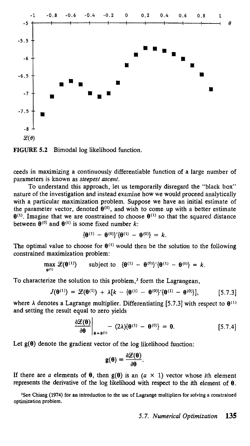
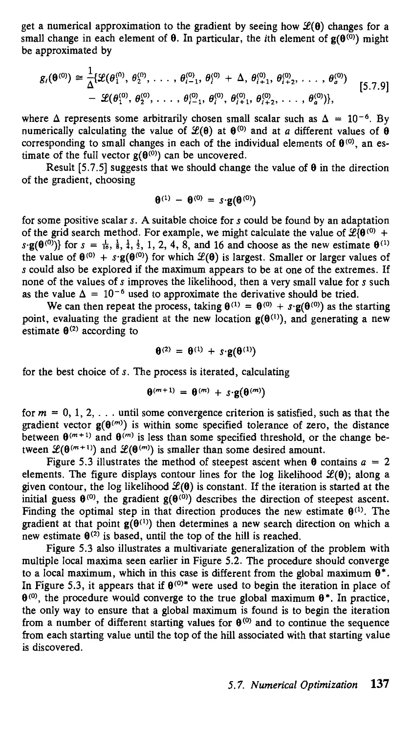
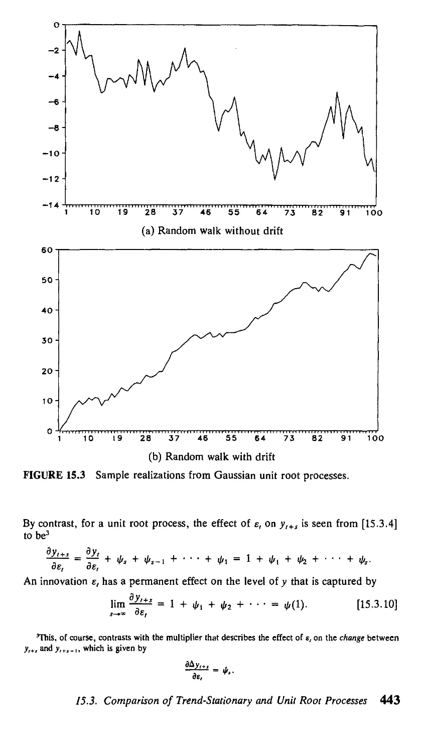
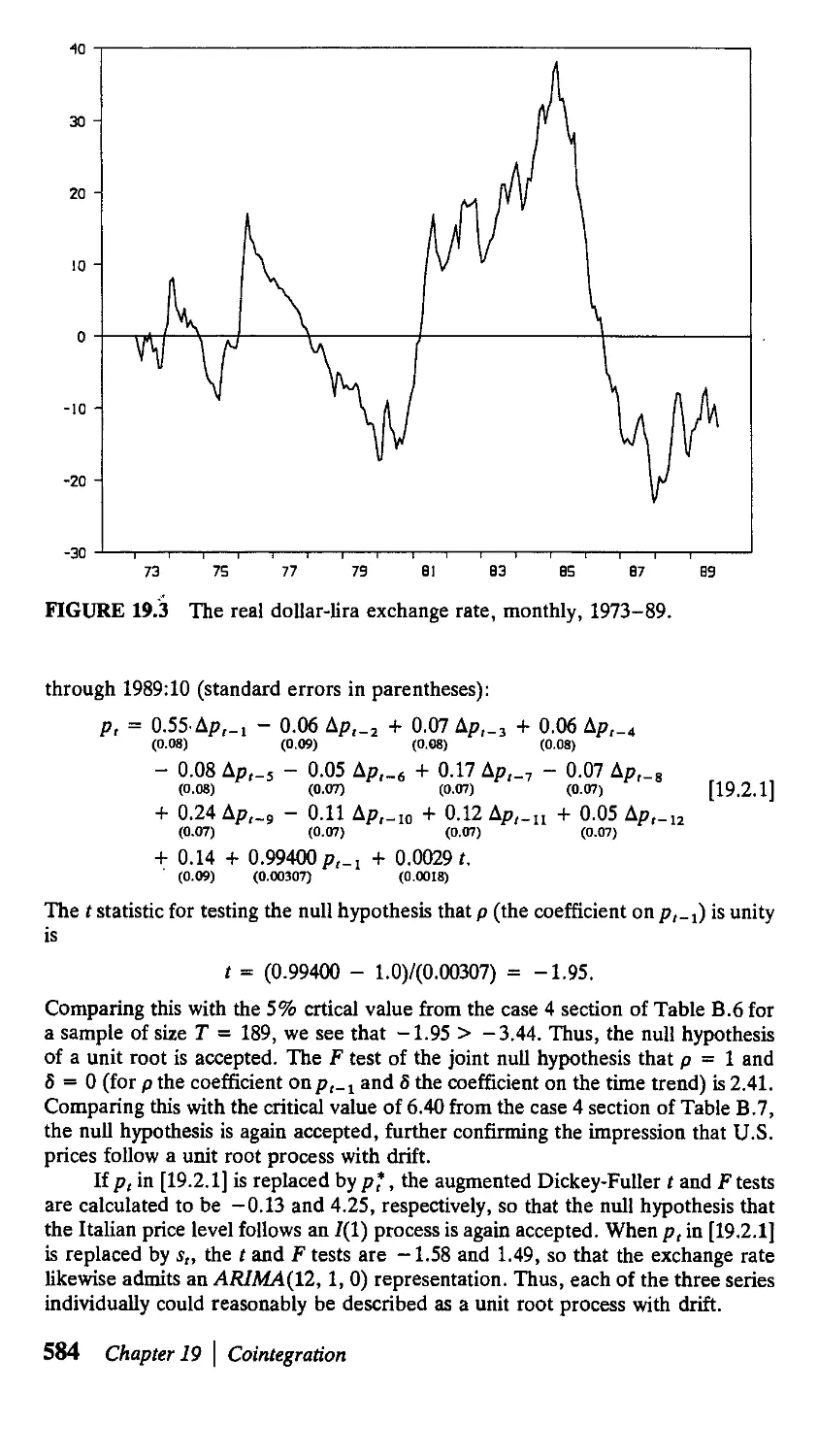
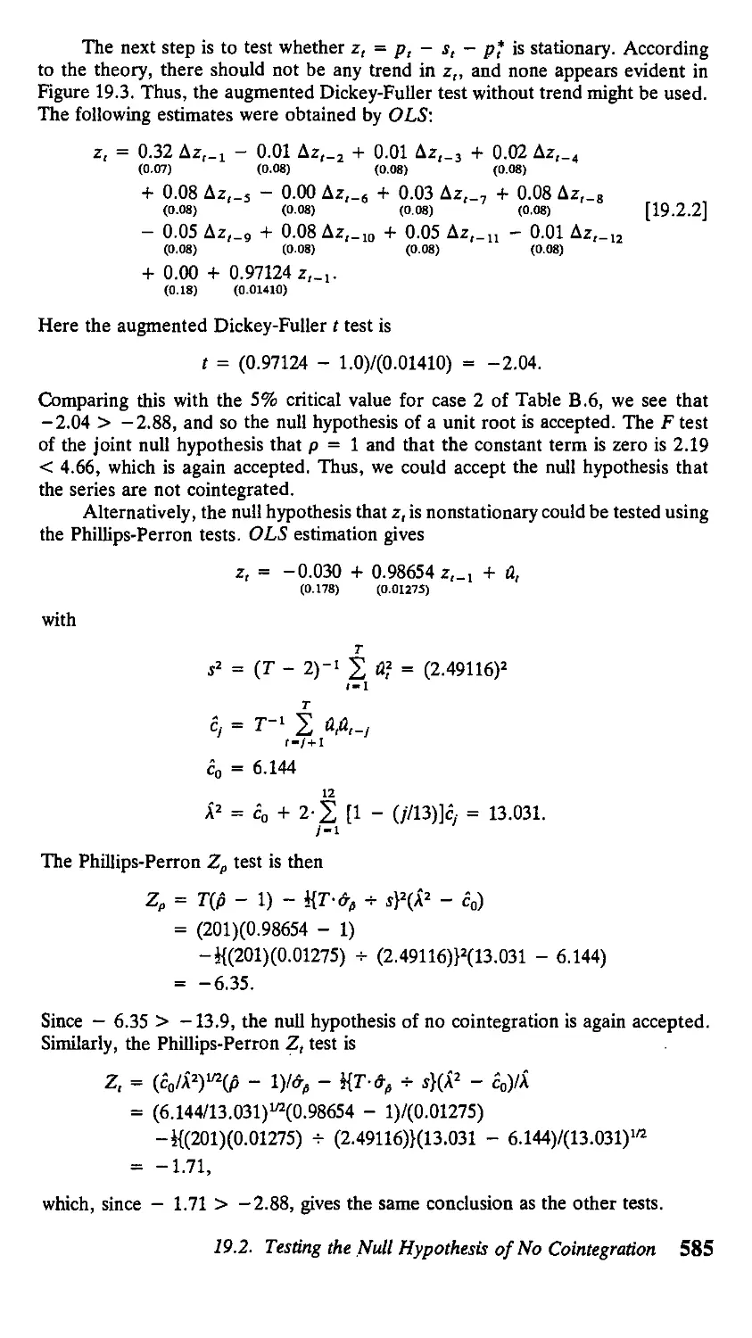
/


Author: Hamilton J.D.
Tags: mathematics mathematical analysis statistics
ISBN: 0-691-04289-6
Year: 1994


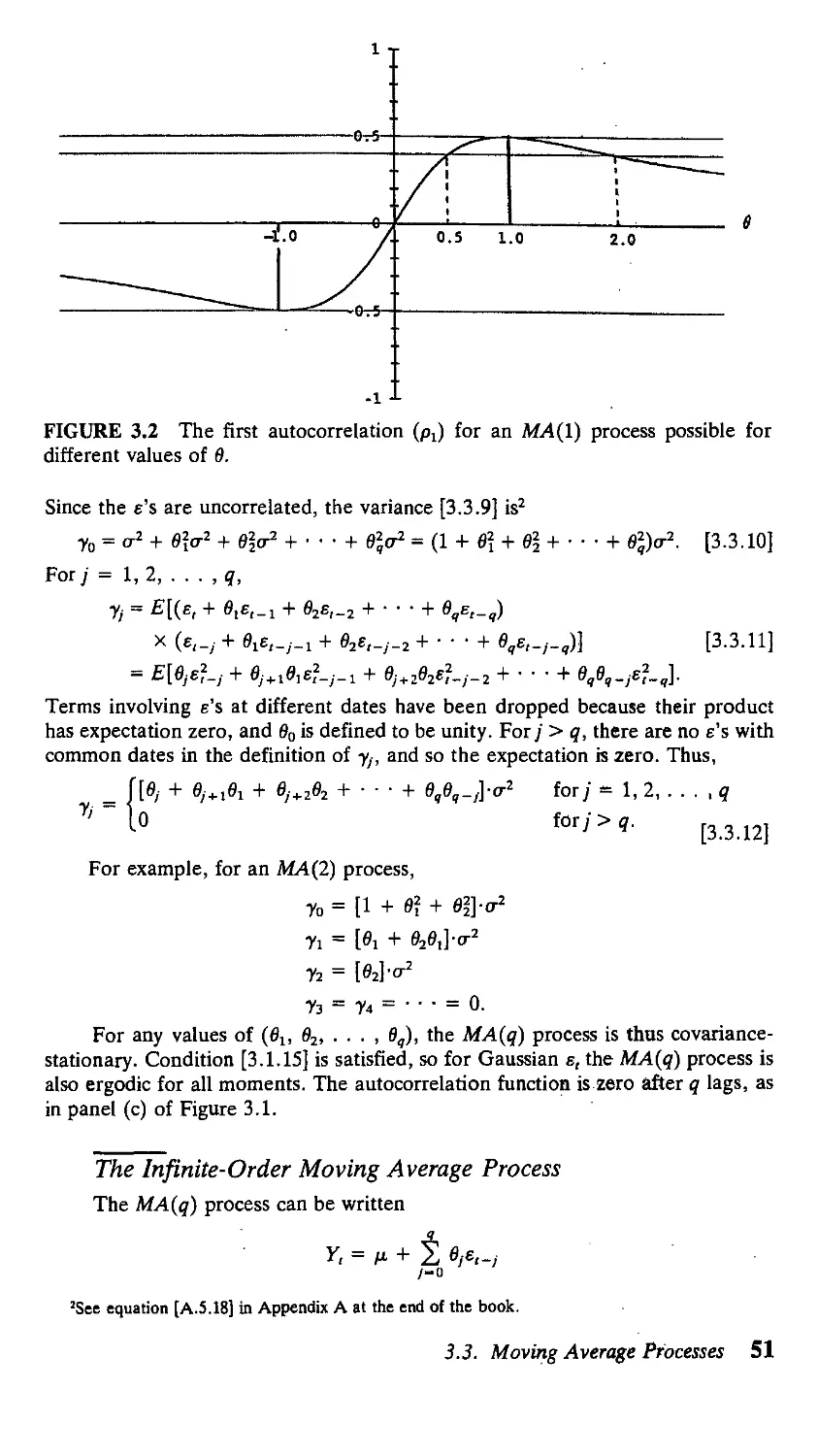
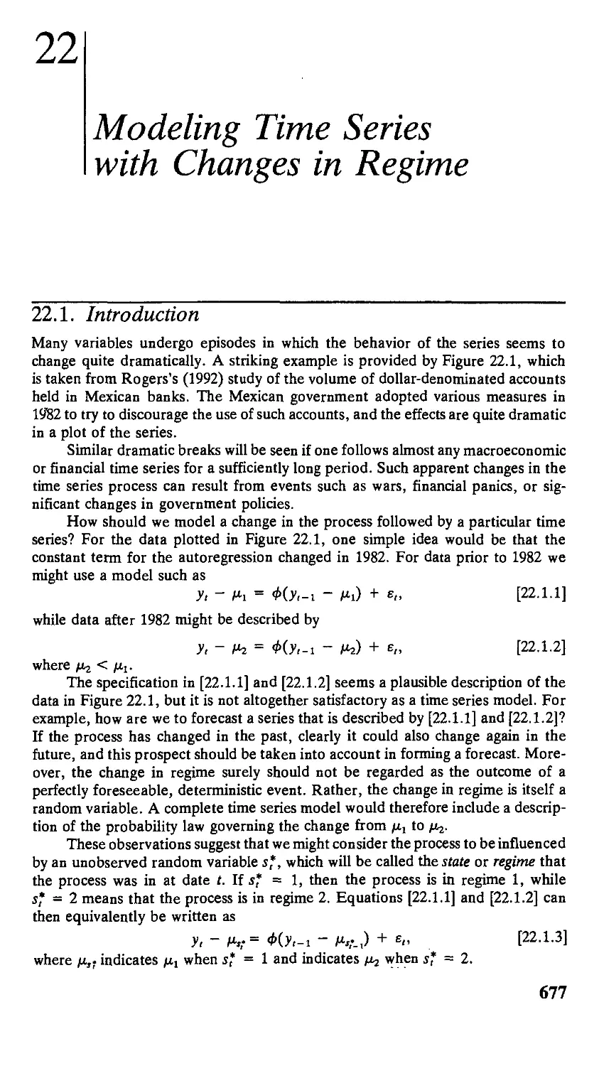
Text
Time Series Analysis
James D. Hamilton
л
PRINCETON UNIVERSITY PRESS
PRINCETON, NEW JERSEY
Copyright © 1994 by Princeton University Press
Published by Princeton University Press, 41 William St.,
Princeton, New Jersey 08540
In the United Kingdom: Princeton University Press,
Chichester, West Sussex
All Rights Reserved
Library of Congress Cataloging-in-Publication Data
Hamilton, James D. (James Douglas), A954-)
Time series analysis / James D. Hamilton,
p. cm.
Includes bibliographical references and indexes.
ISBN 0-691-04289-6
1. Time-series analysis. I. Title.
QA280.H264 1994
519.5'5—dc20 93-4958
CIP
This book has been composed in Times Roman.
Princeton University Press books are printed on acid-free paper and meet the guidelines for
permanence and durability of the Committee on Production Guidelines for Book Longevity of the
Council on Library Resources.
Printed in the United States of America
10 987654321
Contents
PREFACE xiii
1 Difference Equations
1.1. First-Order Difference Equations 1
1.2. pth-Order Difference Equations 7
APPENDIX l.A. Proofs of Chapter 1 Propositions 21
References 24
2
2.1.
2.2.
2.3.
2.4.
2.5.
Lag Operators
Introduction 25
First-Order Difference Equations 27
Second-Order Difference Equations 29
pth-Order Difference Equations 33
Initial Conditions and Unbounded Sequences 36
References 42
25
3 Stationary ARMA Processes 43
3.1. Expectations, Stationarity, and Ergodicity 43
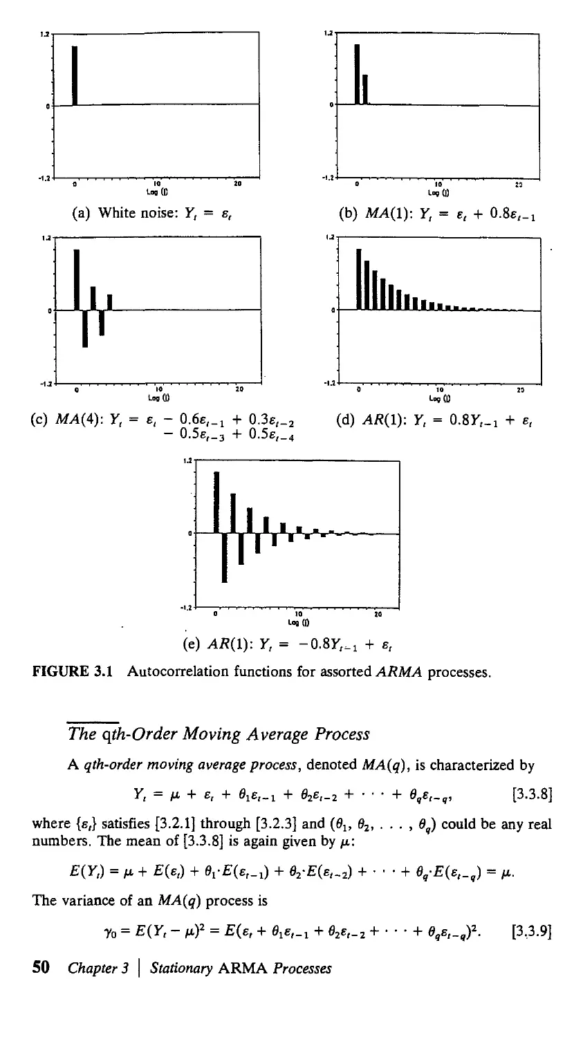
3.2. White Noise 47
3.3. Moving Average Processes 48
3.4. Autoregressive Processes 53
3.5. Mixed Autoregressive Moving Average
Processes 59
3.6. The Autocovariance-Generating Function 61
3.7. Invertibility 64
APPENDIX 3.A. Convergence Results for Infinite-Order
Moving Average Processes 69
Exercises 70 References 71
4 Forecasting 72
4.1. Principles of Forecasting 72
4.2. Forecasts Based on an Infinite Number
of Observations 77
4.3. Forecasts Based on a Finite Number
of Observations 85
4.4. The Triangular Factorization of a Positive Definite
Symmetric Matrix 87
4.5. Updating a Linear Projection 92
4.6. Optimal Forecasts for Gaussian Processes 100
4.7. Sums of ARMA Processes 102
4.8. Wold's Decomposition and the Box-Jenkins
Modeling Philosophy 108
APPENDIX 4.A. Parallel Between OLS Regression
and Linear Projection 113
APPENDIX 4.B. Triangular Factorization of the Covariance
Matrix for an MAA) Process 114
Exercises 115 References 116
5 Maximum Likelihood Estimation 117
5.1. Introduction 117
5.2. The Likelihood Function for a Gaussian ARA)
Process 118
5.3. The Likelihood Function for a Gaussian AR(p)
Process 123
5.4. The Likelihood Function for a Gaussian MA{\)
Process 127
5.5. The Likelihood Function for a Gaussian MA(q)
Process 130
5.6. The Likelihood Function for a Gaussian ARMA(p, q)
Process 132
5.7. Numerical Optimization 133
vi Contents
5.8. Statistical Inference with Maximum Likelihood
Estimation 142
5.9. Inequality Constraints 146
APPENDIX 5.A. Proofs of Chapter 5 Propositions 148
Exercises ISO References ISO
6 Spectral Analysis 152
6.1. The Population Spectrum 152
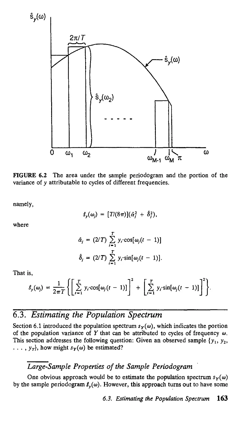
6.2. The Sample Periodogram 158
6.3. Estimating the Population Spectrum 163
6.4. Uses of Spectral Analysis 167
APPENDIX 6.A. Proofs of Chapter 6 Propositions 172
Exercises 178 References 178
7 Asymptotic Distribution Theory 180
7.1. Review of Asymptotic Distribution Theory 180
7.2. Limit Theorems for Serially Dependent
Observations 186
APPENDIX 7. A. Proofs of Chapter 7 Propositions 195
Exercises 198 References 199
8 Linear Regression Models 200
8.1. Review of Ordinary Least Squares
with Deterministic Regressors and i.i.d. Gaussian
Disturbances 200
8.2. Ordinary Least Squares Under More General
Conditions 207
8.3. Generalized Least Squares 220
APPENDIX 8. A. Proofs of Chapter 8 Propositions 228
Exercises 230 References 231
9 Linear Systems of Simultaneous Equations 233
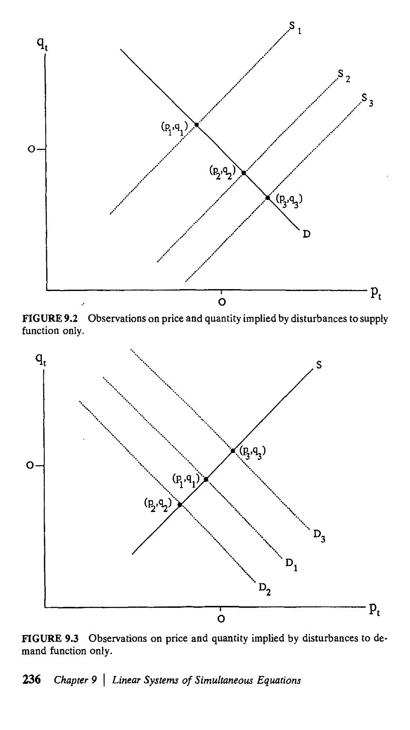
9.1. Simultaneous Equations Bias 233
9.2. Instrumental Variables and Two-Stage Least
Squares 238
Contents vii
9.3. Identification 243
9.4. Full-Information Maximum Likelihood
Estimation 247
9.5. Estimation Based on the Reduced Form 250
9.6. Overview of Simultaneous Equations Bias 252
APPENDIX 9.A. Proofs of Chapter 9 Proposition 253
Exercise 255 References 256
10 Covariance-Stationary Vector Processes 257
10.1. Introduction to Vector Autoregressions 257
10.2. Autocovariances and Convergence Results
for Vector Processes 261
10.3. The Autocovariance-Generating Function
for Vector Processes 266
10.4. The Spectrum for Vector Processes 268
10.5. The Sample Mean of a Vector Process 279
APPENDIX 10.A. Proofs of Chapter 10 Propositions 285
Exercises 290 References 290
11 Vector Autoregressions 291
11.1. Maximum Likelihood Estimation and Hypothesis
Testing for an Unrestricted Vector
Autoregression 291
11.2. Bivariate Granger Causality Tests 302
11.3. Maximum Likelihood Estimation of Restricted
Vector Autoregressions 309
11.4. The Impulse-Response Function 318
11.5. Variance Decomposition 323
11.6. Vector Autoregressions and Structural Econometric
Models 324
11.7. Standard Errors for Impulse-Response
Functions 336
APPENDIX 11. A. Proofs of Chapter 11 Propositions 340
APPENDIX П.В. Calculation of Analytic Derivatives 344
Exercises 348 References 349
viii Contents
12 Bayesian Analysis 351
12.1. Introduction to Bayesian Analysis 351
12.2. Bayesian Analysis of Vector Autoregressions 360
12.3. Numerical Bayesian Methods 362
APPENDIX 12. A. Proofs of Chapter 12 Propositions 366
Exercise 370 References 370
13 The Kalman Filter 372
13.1. The State-Space Representation of a Dynamic
System 372
13.2. Derivation of the Kalman Filter 377
13.3. Forecasts Based on the State-Space
Representation 381
13.4. Maximum Likelihood Estimation
of Parameters 385
13.5. The Steady-State Kalman Filter 389
13.6. Smoothing 394
13.7. Statistical Inference with the Kalman Filter 397
13.8. Time-Varying Parameters 399
APPENDIX 13.A. Proofs of Chapter 13 Propositions 403
Exercises 406 References 407
14 Generalized Method of Moments 409
14.1. Estimation by the Generalized Method
of Moments 409
14.2. Examples 415
14.3. Extensions 424
14.4. GMM and Maximum Likelihood Estimation 427
APPENDIX 14.A. Proofs of Chapter 14 Propositions 431
Exercise 432 References 433
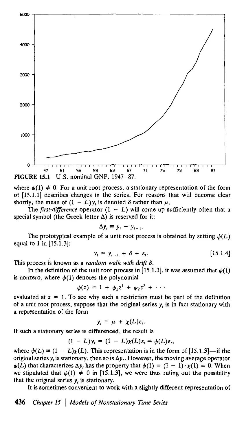
15 Models of Nonstationary Time Series 435
15.1. Introduction 435
15.2. Why Linear Time Trends and Unit Roots? 438
Contents ix
15.3. Comparison of Trend-Stationary and Unit Root
Processes 438
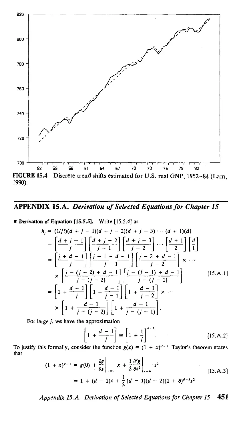
15.4. The Meaning of Tests for Unit Roots 444
15.5. Other Approaches to Trended Time Series 447
APPENDIX 15.A. Derivation of Selected Equations
for Chapter 15 451
References 452
16 Processes with Deterministic Time Trends 454
16.1. Asymptotic Distribution of OLS Estimates
of the Simple Time Trend Model 454
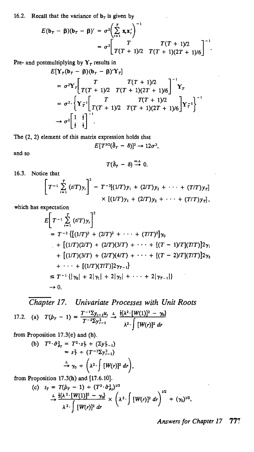
16.2. Hypothesis Testing for the Simple Time Trend
Model 461
16.3. Asymptotic Inference for an Autoregressive
Process Around a Deterministic Time Trend 463
APPENDIX 16. A. Derivation of Selected Equations
for Chapter 16 472
Exercises 474 References 474
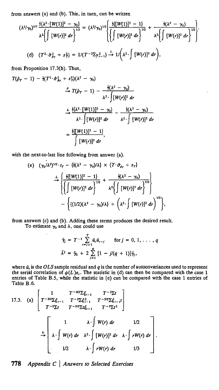
17 Univariate Processes with Unit Roots 475
17.1. Introduction 475
17.2. Brownian Motion 477
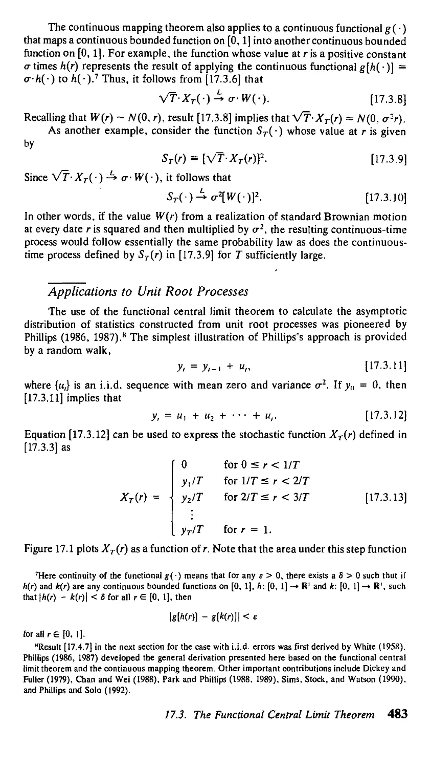
17.3. The Functional Central Limit Theorem 479
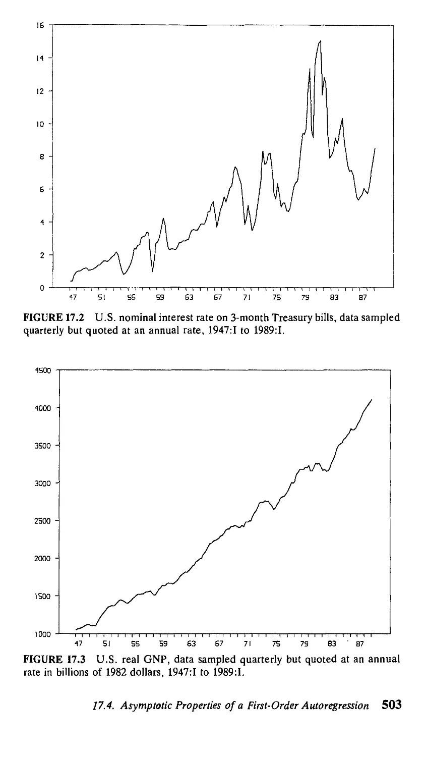
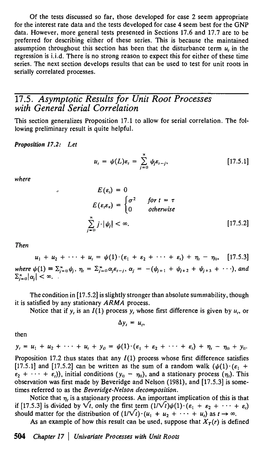
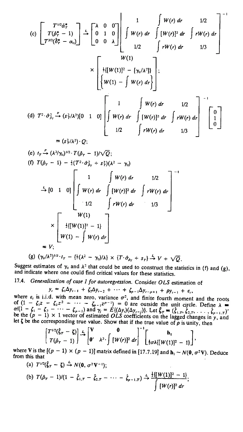
17.4. Asymptotic Properties of a First-Order
Autoregression when the True Coefficient Is
Unity 486
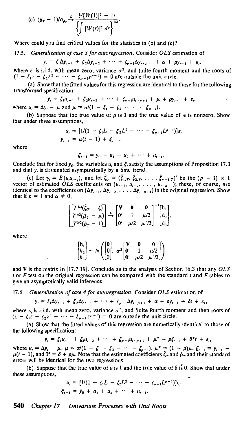
17.5. Asymptotic Results for Unit Root Processes
with General Serial Correlation 504
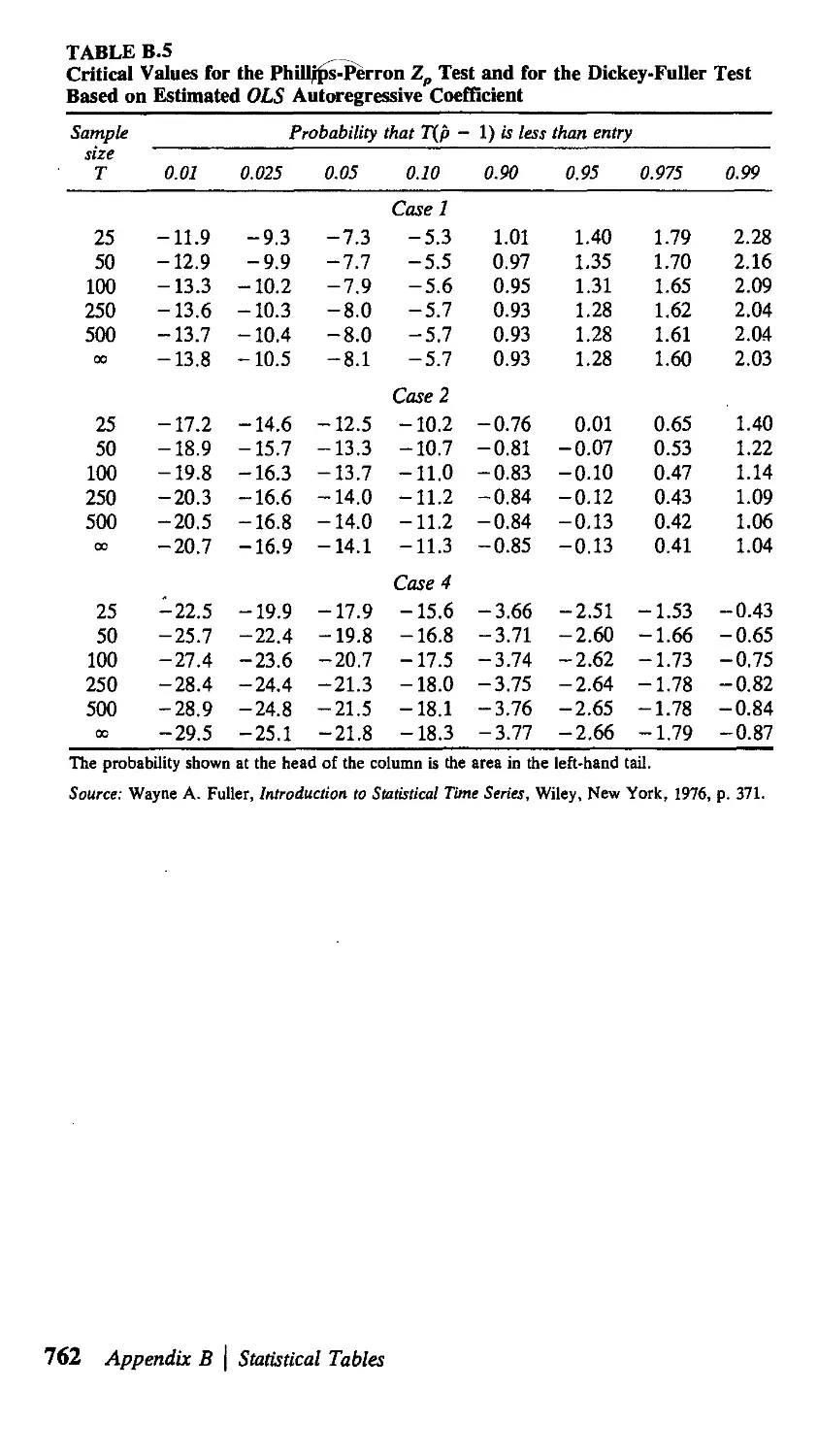
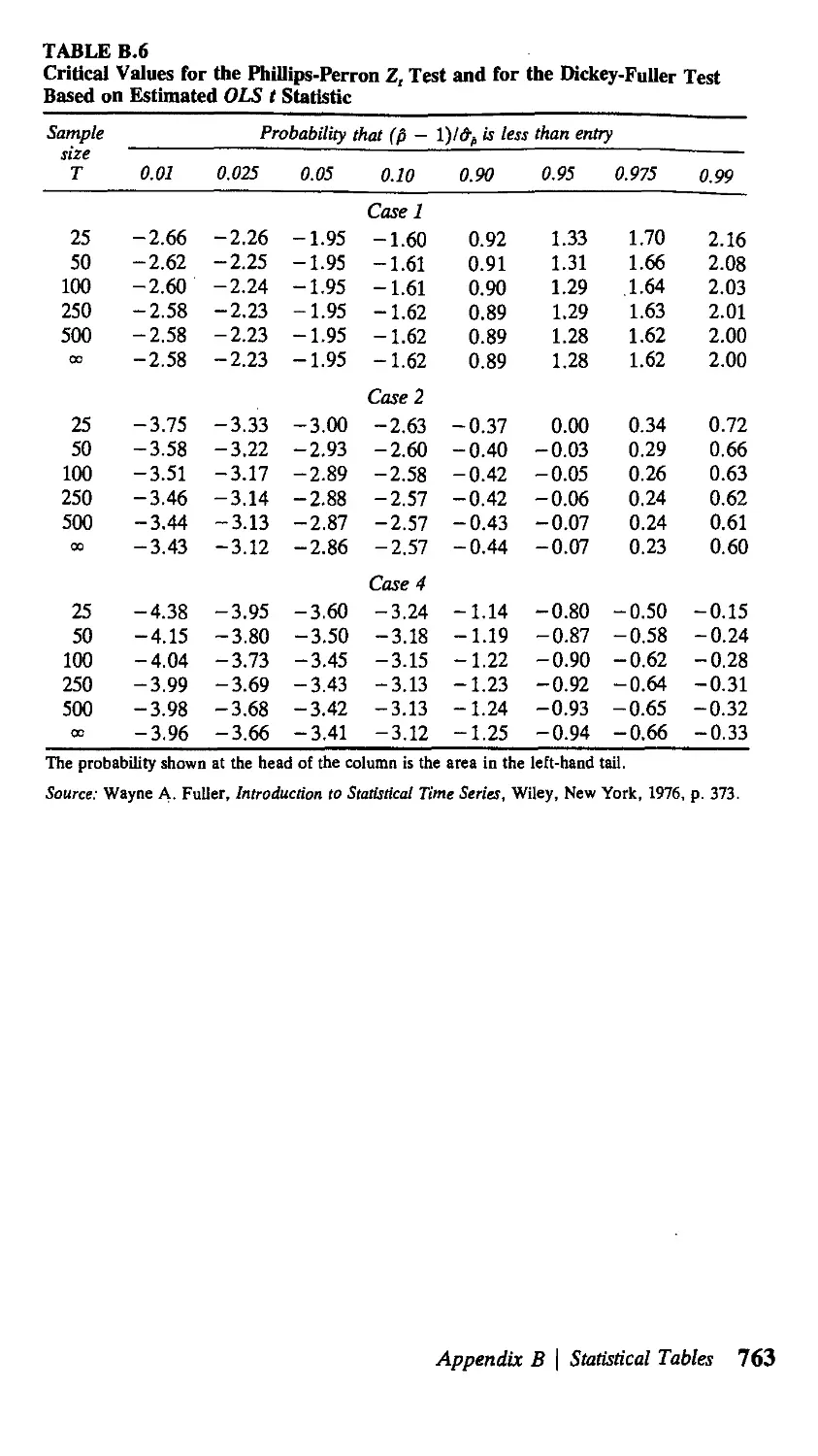
17.6. Phillips-Perron Tests for Unit Roots 506
17.7. Asymptotic Properties of a pth-Order
Autoregression and the Augmented Dickey-Fuller
Tests for Unit Roots 516
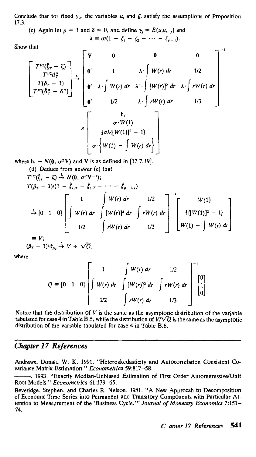
17.8. Other Approaches to Testing for Unit Roots 531
17.9. Bayesian Analysis and Unit Roots 532
APPENDIX 17.A. Proofs of Chapter 17 Propositions 534
Exercises 537 References 541
X Contents
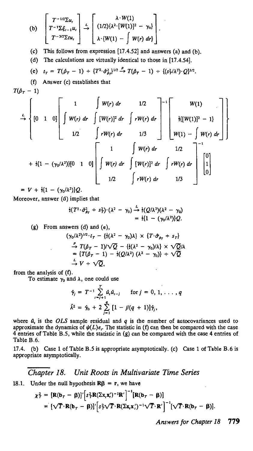
18 Unit Roots in Multivariate Time Series 544
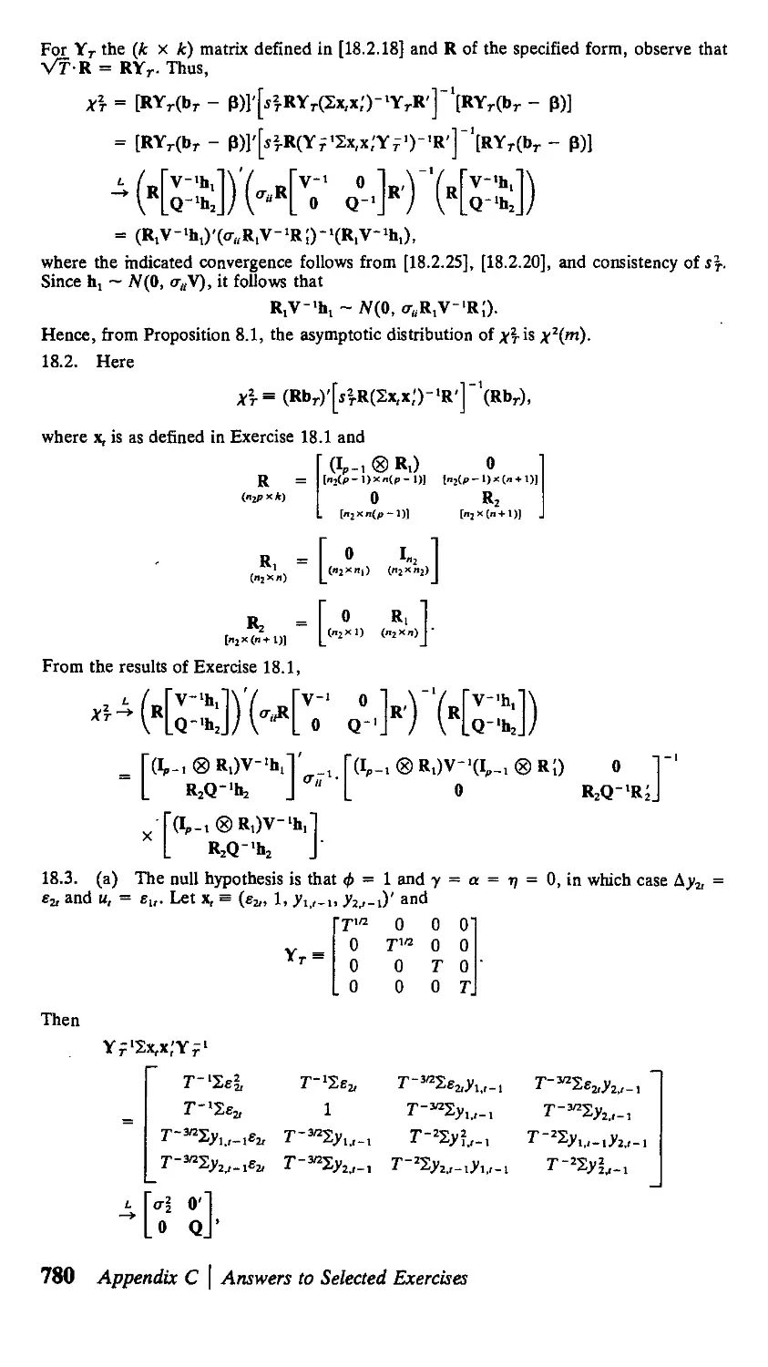
18.1. Asymptotic Results for Nonstationary Vector
Processes 544
18.2. Vector Autoregressions Containing Unit Roots 549
18.3. Spurious Regressions 557
APPENDIX 18.A. Proofs of Chapter 18 Propositions 562
Exercises 568 References 569
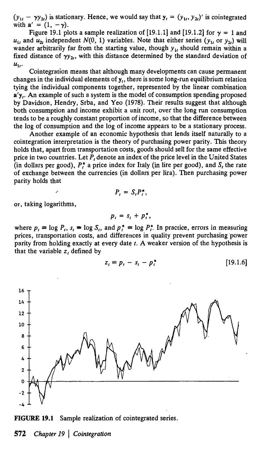
19 Cointegration 571
19.1. Introduction 571
19.2. Testing the Null Hypothesis of No
Cointegration 582
19.3. Testing Hypotheses About the Cointegrating
Vector 601
APPENDIX 19. A. Proofs of Chapter 19 Propositions 618
Exercises 625 References 627
20 Full-Information Maximum Likelihood
Analysis of Cointegrated Systems 630
20.1. Canonical Correlation 630
20.2. Maximum Likelihood Estimation 635
20.3. Hypothesis Testing 645
20.4. Overview of Unit Roots—To Difference
or Not to Difference? 651
APPENDIX 20.A. Proofs of Chapter 20 Propositions 653
Exercises 655 References 655
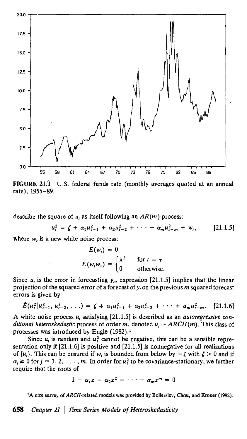
21 Time Series Models of Heteroskedasticity 657
21.1. Autoregressive Conditional Heteroskedasticity
(ARCH) 657
21.2. Extensions 665
APPENDIX 21.A. Derivation of Selected Equations
for Chapter 21 673
References 674
Contents xi
22 Modeling Time Series with Changes
in Regime 677
22.1. Introduction 677
22.2. Markov Chains 678
22.3. Statistical Analysis of i.i.d. Mixture
Distributions 685
22.4. Time Series Models of Changes in Regime 690
APPENDIX 22.A. Derivation of Selected Equations
for Chapter 22 699
Exercise 702 References 702
A Mathematical Review 704
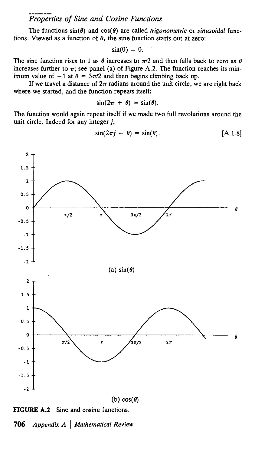
A.I. Trigonometry 704
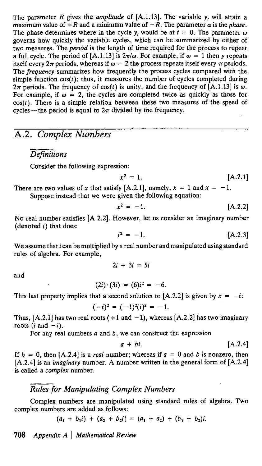
A.2. Complex Numbers 708
A.3. Calculus 711
A.4. Matrix Algebra 721
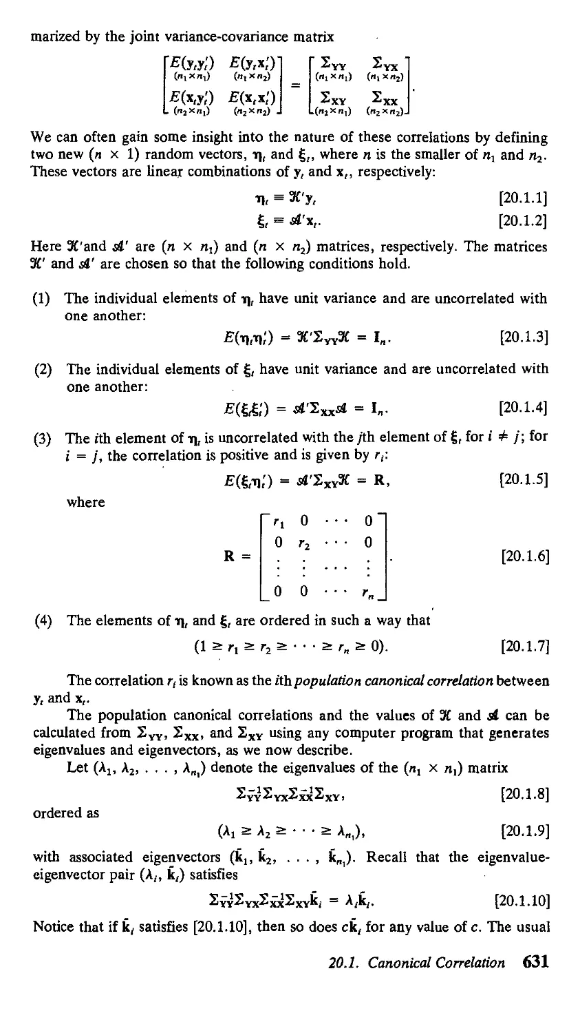
A.5. Probability and Statistics 739
References 750
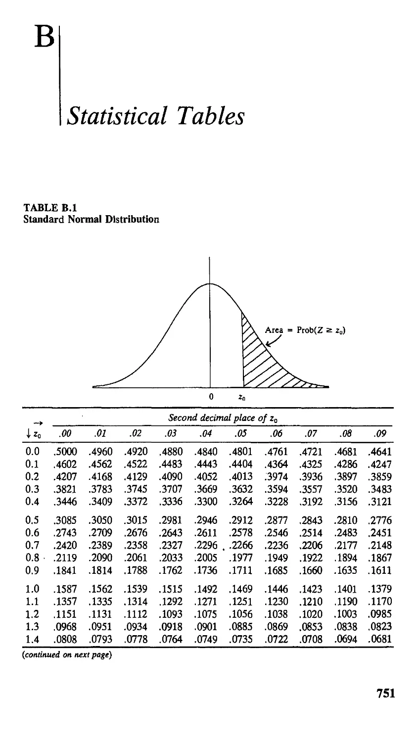
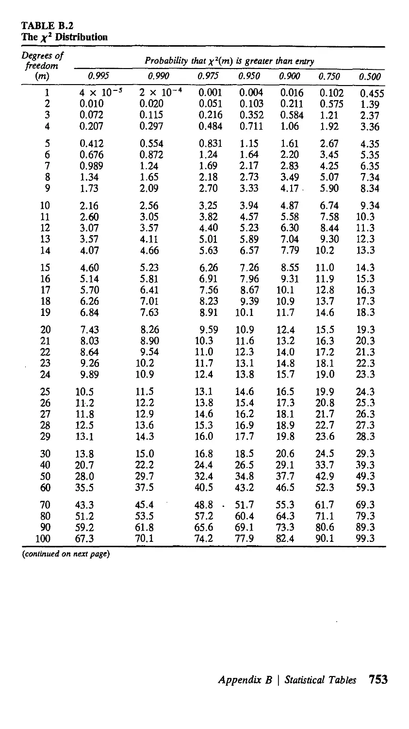
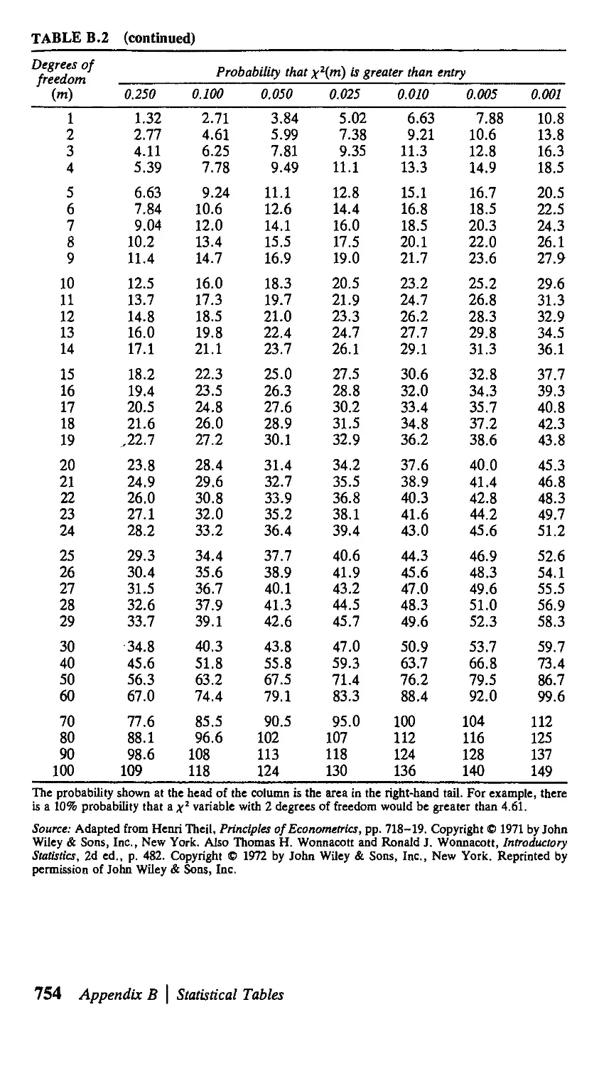
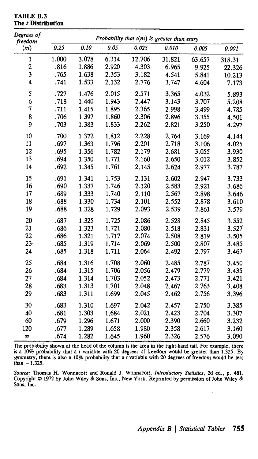
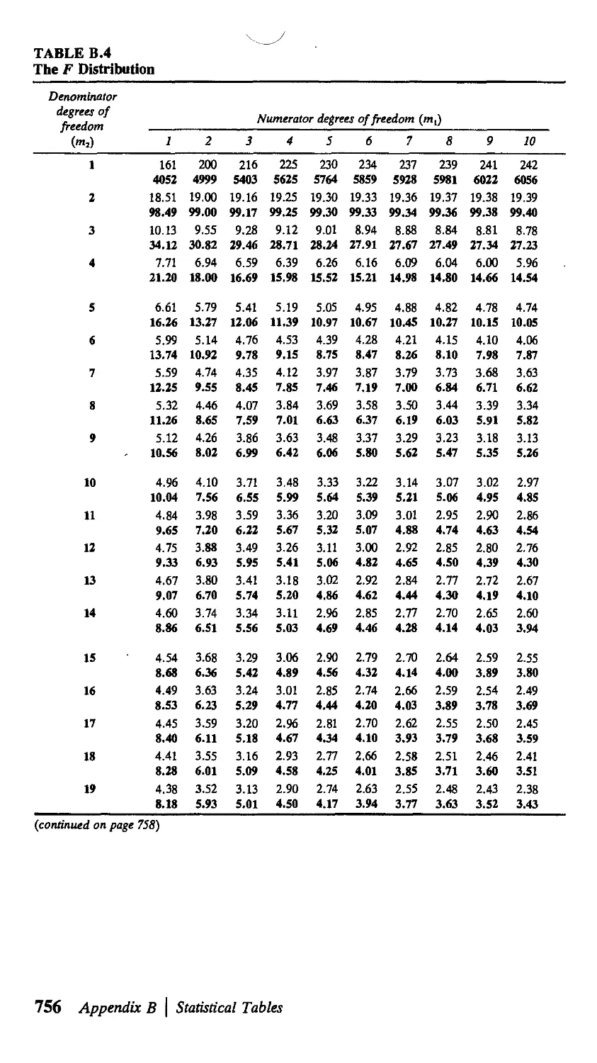
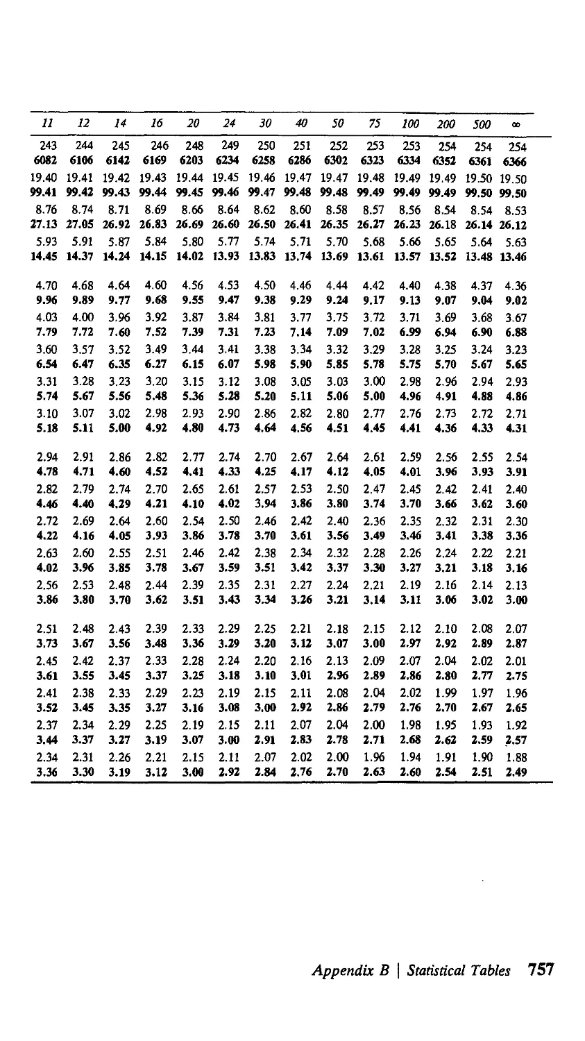
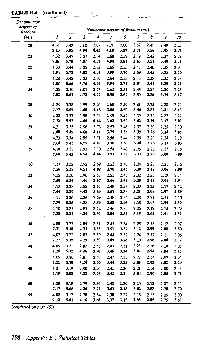
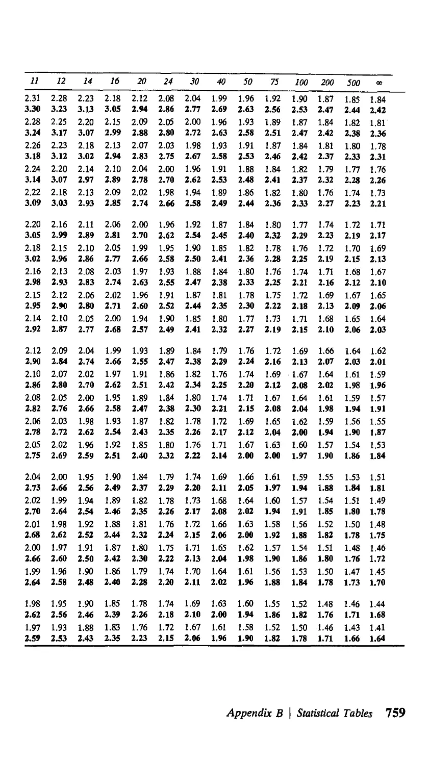
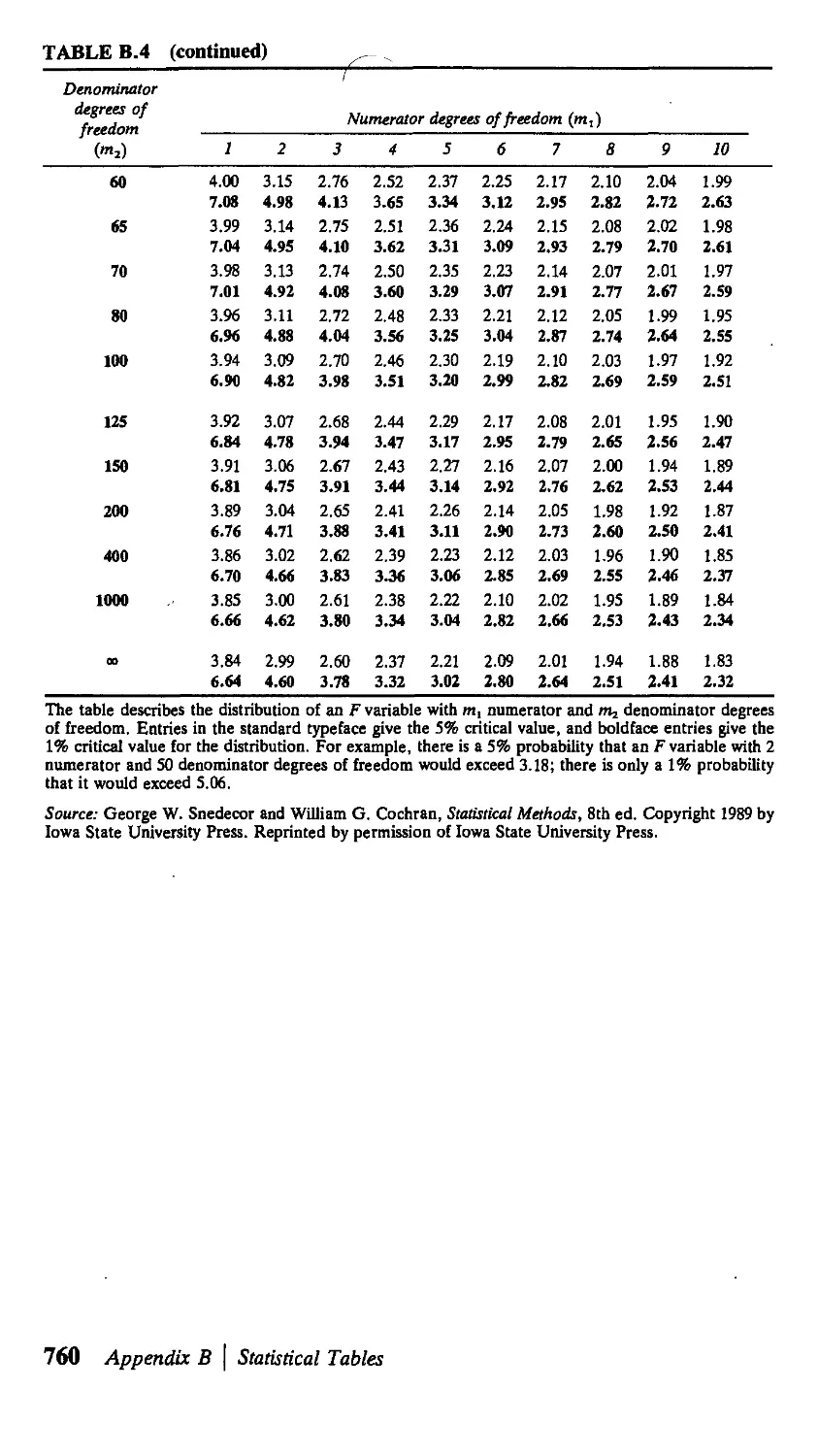
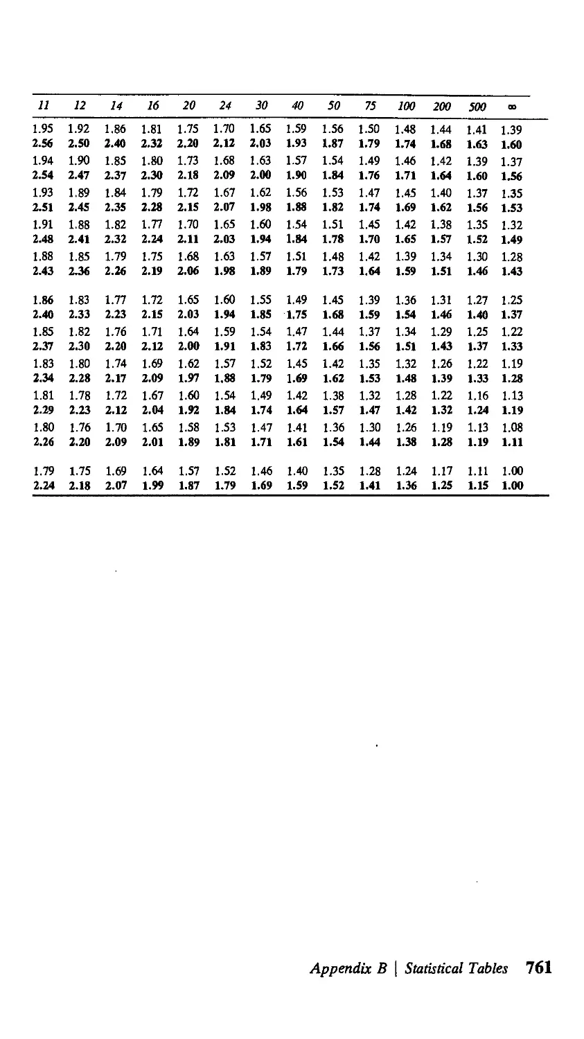
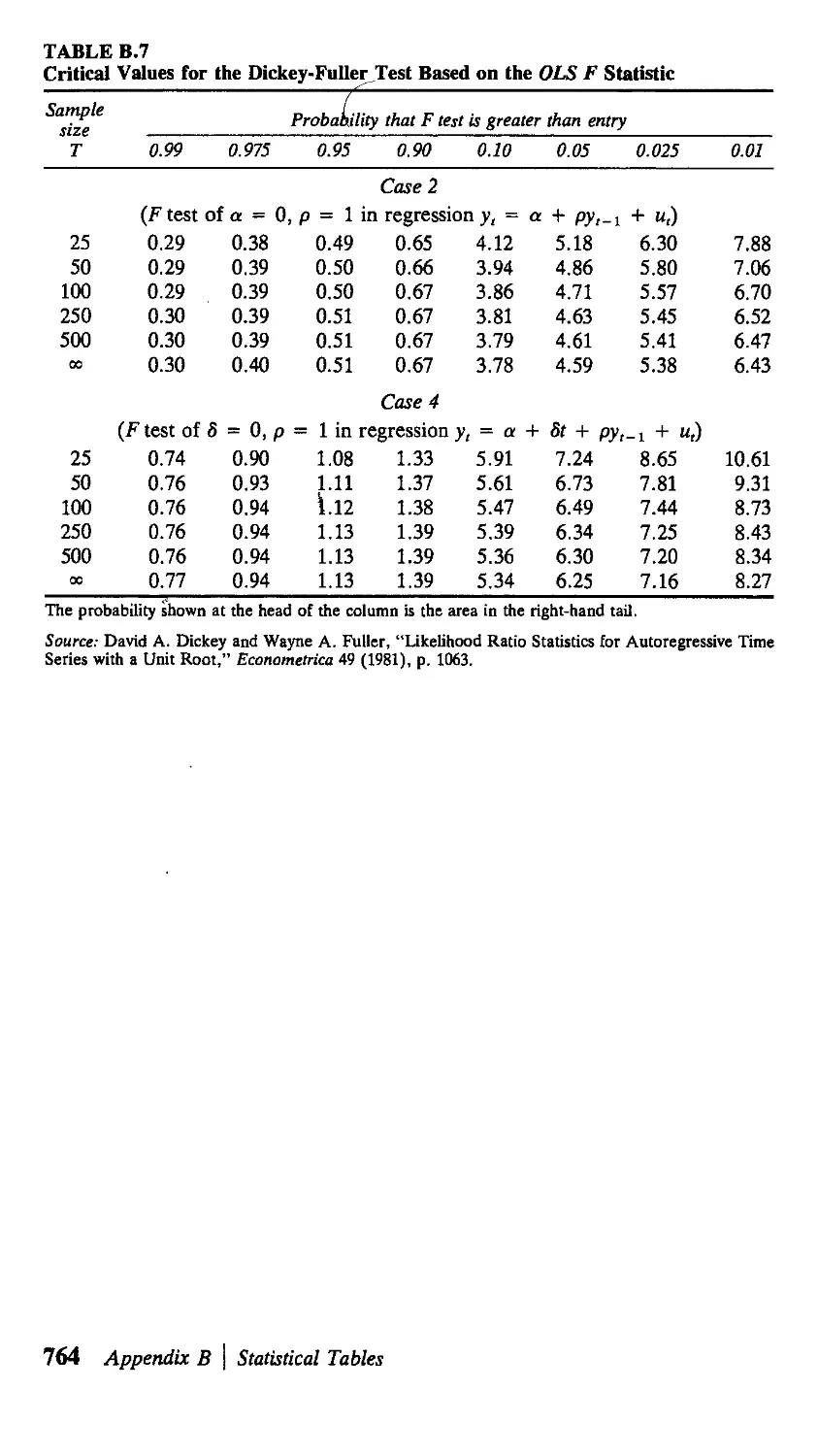
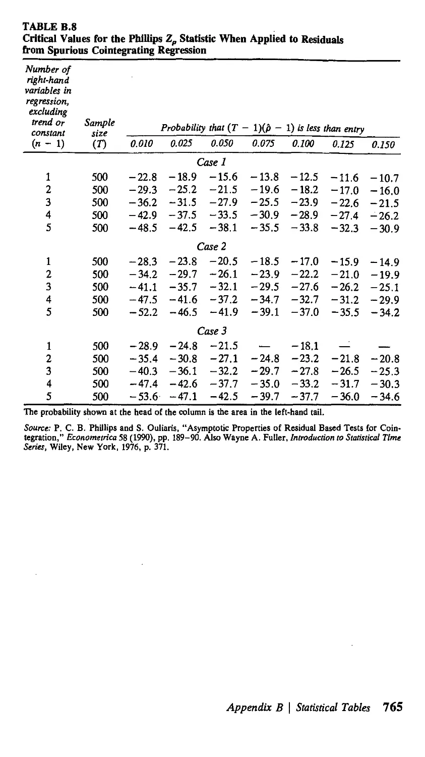
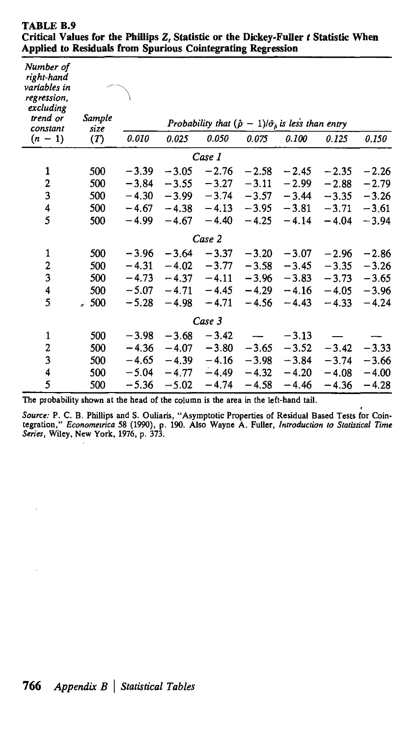
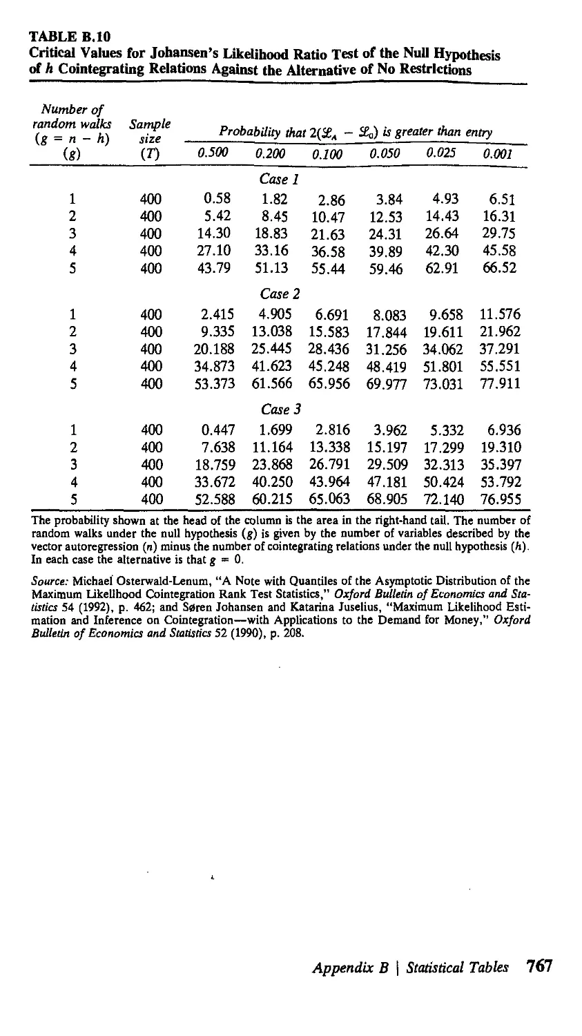
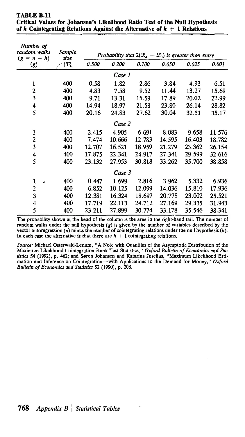
В Statistical Tables 751
Answers to Selected Exercises 769
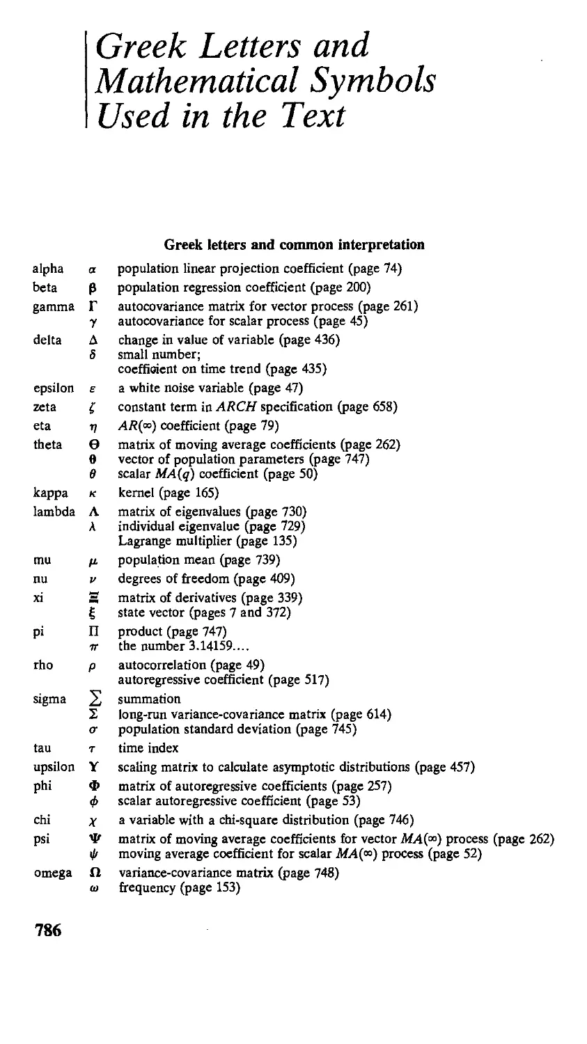
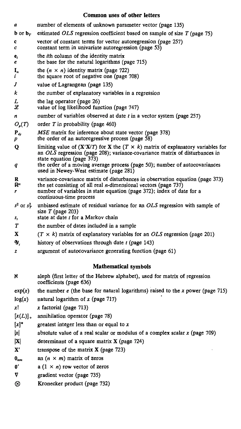
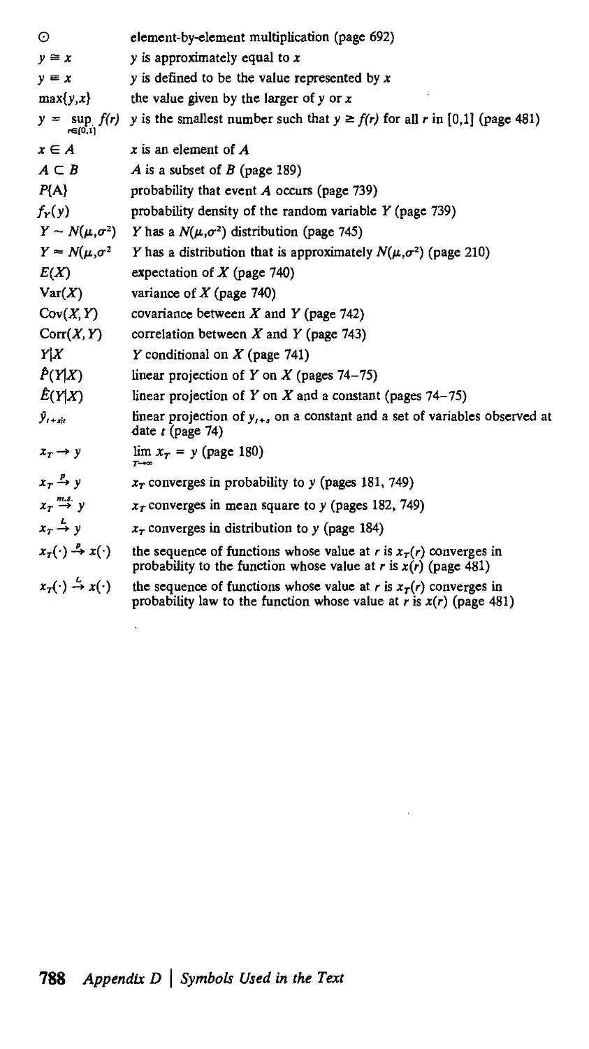
D Greek Letters and Mathematical Symbols 786
Used in the Text
AUTHOR INDEX 789
SUBJECT INDEX 792
xii Contents
Preface
Much of economics is concerned with modeling dynamics. There has been an
explosion of research in this area in the last decade, as "time series econometrics"
has practically come to be synonymous with "empirical macroeconomics."
Several texts provide good coverage of the advances in the economic analysis
of dynamic systems, while others summarize the earlier literature on statistical
inference for time series data. There seemed a use for a text that could integrate
the theoretical and empirical issues as well as incorporate the many advances of
the last decade, such as the analysis of vector autoregressions, estimation by gen-
generalized method of moments, and statistical inference for nonstationary data. This
is the goal of Time Series Analysis.
A principal anticipated use of the book would be as a textbook for a graduate
econometrics course in time series analysis. The book aims for maximum flexibility
through what might be described as an integrated modular structure. As an example
of this, the first three sections of Chapter 13 on the Kalman filter could be covered
right after Chapter 4, if desired. Alternatively, Chapter 13 could be skipped al-
altogether without loss of comprehension. Despite this flexibility, state-space ideas
are fully integrated into the text beginning with Chapter 1, where a state-space
representation is used (without any j argon or formalism) to introduce the key results
concerning difference equations. Thus, when the reader encounters the formal
development of the state-space framework and the Kalman filter in Chapter 13,
the notation and key ideas should already be quite familiar.
Spectral analysis (Chapter 6) is another topic that could be covered at a point
of the reader's choosing or skipped altogether. In this case, the integrated modular
structure is achieved by the early introduction and use of autocovariance-generating
functions and filters. Wherever possible, results are described in terms of these
rather than the spectrum.
Although the book is designed with an econometrics couse in time series
methods in mind, the book should be useful for several other purposes. It is
completely self-contained, starting from basic principles accessible to first-year
graduate students and including an extensive math review appendix. Thus the book
would be quite suitable for a first-year graduate course in macroeconomics or
dynamic methods that has no econometric content. Such a course might use Chap-
Chapters 1 and 2, Sections 3.1 through 3.5, and Sections 4.1 and 4.2.
Yet another intended use for the book would be in a conventional econo-
econometrics course without an explicit time series focus. The popular econometrics texts
do not have much discussion of such topics as numerical methods; asymptotic results
for serially dependent, heterogeneously distributed observations; estimation of
models with distributed lags; autocorrelation- and heteroskedasticity-consistent
xiii
standard errors; Bayesian analysis; or generalized method of moments. All of these
topics receive extensive treatment in Time Series Analysis. Thus, an econometrics
course without an explicit focus on time series might make use of Sections 3.1
through 3.5, Chapters 7 through 9, and Chapter 14, and perhaps any of Chapters
5, 11, and 12 as well. Again, the text is self-contained, with a fairly complete
discussion of conventional simultaneous equations methods in Chapter 9. Indeed,
a very important goal of the text is to develop the parallels between A) the tra-
traditional econometric approach to simultaneous equations and B) the current pop-
popularity of vector autoregressions and generalized method of moments estimation.
Finally, the book attempts to provide a rigorous motivation for the methods
and yet still be accessible for researchers with purely applied interests. This is
achieved by relegation of many details to mathematical appendixes at the ends of
chapters, and by inclusion of numerous examples that illustrate exactly how the
theoretical results are used and applied in practice.
The book developed out of my lectures at the University of Virginia. I am
grateful first and foremost to my many students over the years whose questions
and comments have shaped the course of the manuscript. I also have an enormous
debt to numerous colleagues who have kindly offered many useful suggestions,
and would like to thank in particular Donald W. K. Andrews, Stephen R. Blough,
John Cochrane, George Davis, Michael Dotsey, Robert Engle, T. Wake Epps,
Marjorie Flavin, John Geweke, Eric Ghysels, Carlo Giannini, Clive W. J. Granger,
Alastair Hall, Bruce E. Hansen, Kevin Hassett, Tomoo Inoue, Ravi Jagannathan,
Kenneth F. Kroner, Rocco Mosconi, Masao Ogaki, Adrian Pagan, Peter С. В.
Phillips, Peter Rappoport, Glenn Rudebusch, RaulSusmel, Mark Watson, Kenneth
D. West, Halbert White, and Jeffrey M. Wooldridge. I would also like to thank
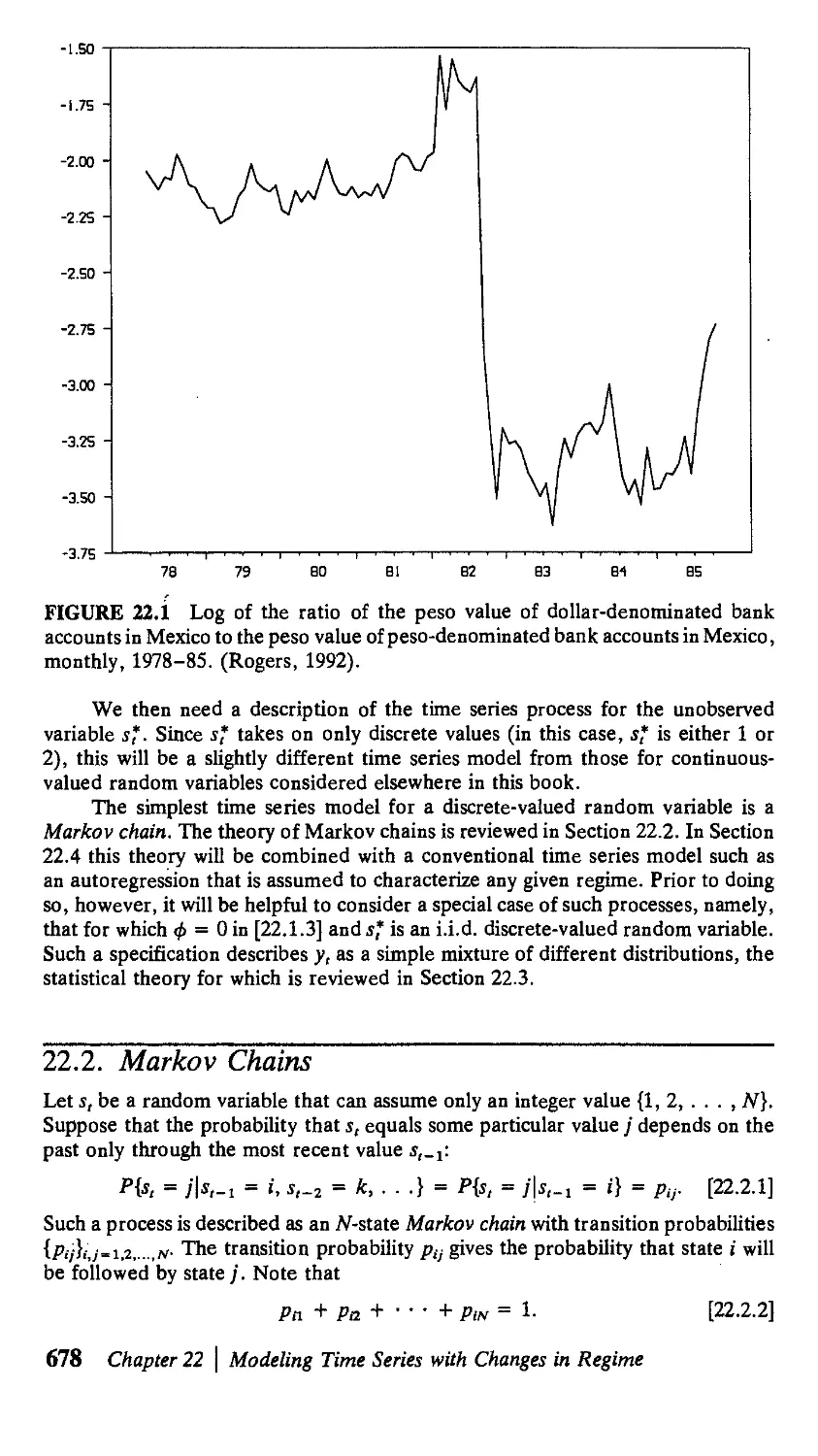
Рок-sang Lam and John Rogers for graciously sharing their data. Thanks also go
to Keith Sill and Christopher Stomberg for assistance with the figures, to Rita
Chen for assistance with the statistical tables in Appendix В, and to Richard Mickey
for a superb job of copy editing.
James D. Hamilton
xiv Preface
Time Series Analysis
Difference Equations
1.1. First-Order Difference Equations
This book is concerned with the dynamic consequences of events over time. Let's
say we are studying a variable whose value at date t is denoted y,. Suppose we are
given a dynamic equation relating the value у takes on at date t to another variable
w, and to the value у took on in the previous period:
У, = ФУ.-i + w,. [1.1.1]
Equation [1.1.1] is a linear first-order difference equation. A difference equation is
an expression relating a variable y, to its previous values. This is a first-order
difference equation because only the first lag of the variable (y,_i) appears in the
equation. Note that it expresses y, as a linear function о1у,-± and wt.
An example of [1.1.1] is Goldfeld's A973) estimated money demand function
for the United States. Goldfeld's model related the log of the real money holdings of
the public (m,) to the log of aggregate real income (/,), the log of the interest rate on
bank accounts (rb), and the log of the interest rate on commercial paper (ra):
m, = 0.27 + 0.72т,_! + 0.19/, - 0.045г„, - 0.019г„. [1.1.2]
This is a special case of [1.1.1] with у, = т„ ф = 0.72, and
w, = 0.27 + 0.19/, - 0.045г„, - 0.019г„.
For purposes of analyzing the dynamics of such a system, it simplifies the algebra
a little to summarize the effects of all the input variables (/„ rbl, and rcl) in terms
of a scalar w, as here.
In Chapter 3 the input variable w, will be regarded as a random variable, and
the implications of [1.1.1] for the statistical properties of the output series y, will be
explored. In preparation for this discussion, it is necessary first to understand the
mechanics of difference equations. For the discussion in Chapters 1 and 2, the values
for the input variable {wu w2, . . .} will simply be regarded us a sequence of deter-
deterministic numbers. Our goal is to answer the following question: If a dynamic system
is described by [1.1.1], what are the effects on у of changes in the value of w?
Solving a Difference Equation by Recursive Substitution
The presumption is that the dynamic equation [1.1.1] governs the behavior
of у for all dates t. Thus, for each date we have an equation relating the value of
у for that date to its previous value and the current value of w:
Date Equation
0 Уо = ФУ-i + Wo [1.1.3]
1 уг = фу0 + w, [1.1.4]
2 y2 = ф, + w2 [1.1.5]
' Л = #,-i+ wr. [1.1.6]
If we know the starting value of у for date t = — 1 and the value of w for
dates f = 0, 1, 2, . . . , then it is possible to simulate this dynamic system to find
the value of у for any date. For example, if we know the value of у for t = — 1
and the value of w for t = 0, we can calculate the value of у for t = 0 directly
from [1.1.3]. Given this value of y0 and the value of w for t = 1, we can calculate
the value of у for t = 1 from [1.1.4]:
У1 = фу0 + *г = ф(фу.г + w0) + tv,,
or
Уг = ф2У-г + фЩ + и»!.
Given this value of уг and the value of w for t = 2, we can calculate the value of
у for r = 2 from [1.1.5]:
У г = ФУ т. + w2 = ф(ф2у-! + фп>0 + Wj) + w2,
or
Уг = Ф3У-1 + 4?wo + фЩ + w2.
Continuing recursively in this fashion, the value that у takes on at date t can be
described as a function of its initial value y_x and the history of w between date
0 and date t.
у, = ф-^у-г + ФЧ + ф-^ + ф-2\м2 + • • • + фн>,_г + w,. [1.1.7]
This procedure is known as solving the difference equation [1.1.1] by recursive
substitution.
Dynamic Multipliers
Note that [1.1.7] expresses y, as a linear function of the initial value у _х and
the historical values of w. This makes it very easy to calculate the effect of vv0 on
y,. If w0 were to change with y_x and wb w2, . . . , w, taken as unaffected, the
effect on y, would be given by
? = * [1-1.8]
Note that the calculations would be exactly the same if the dynamic simulation
were started at date t (taking у,_х as given); then yt+j could be described as a
2 Chapter 1 | Difference Equations
function of у,_г and w,, wl+1, . . . , wl+J:
y,+j = <t>i+1y,-i + Ф'щ + «'-Ч+i + Фу"Ч+2 Г1 x
+ • • • + <*w,+y-i + w,+j.
The effect of w, on j>/+y is given by
Thus the dynamic multiplier [1.1.10] depends only on/, the length of time separating
the disturbance to the input (w,) and the observed value of the output (y,+/). The
multiplier does not depend on t; that is, it does not depend on the dates of the
observations themselves. This is true of any linear difference equation.
As an example of calculating a dynamic multiplier, consider again Goldfeld's
money demand specification [1.1.2]. Suppose we want to know what will happen
to money demand two quarters from now if current income /, were to increase by
one unit today with future income /,+ x and I,+2 unaffected:
dm,*! = dmt+2 ^ dw, = ^ dw.
dl, dw, 31, Г 31,'
From [1.1.2], a one-unit increase in /, will increase w, by 0.19 units, meaning that
dw,lal, = 0.19. Since ф = 0.72, we calculate
@.72J@.19) = 0.098.
a/,
.Because /, is the log of income, an increase in /, of 0.01 units corresponds to a 1%
increase in income. An increase in m, of @.01)'@.098) » 0.001 corresponds to
a 0.1% increase in money holdings. Thus the public would be expected to increase
its money holdings by a little less than 0.1% two quarters following a 1% increase
in income.
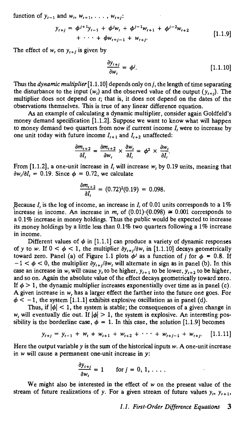
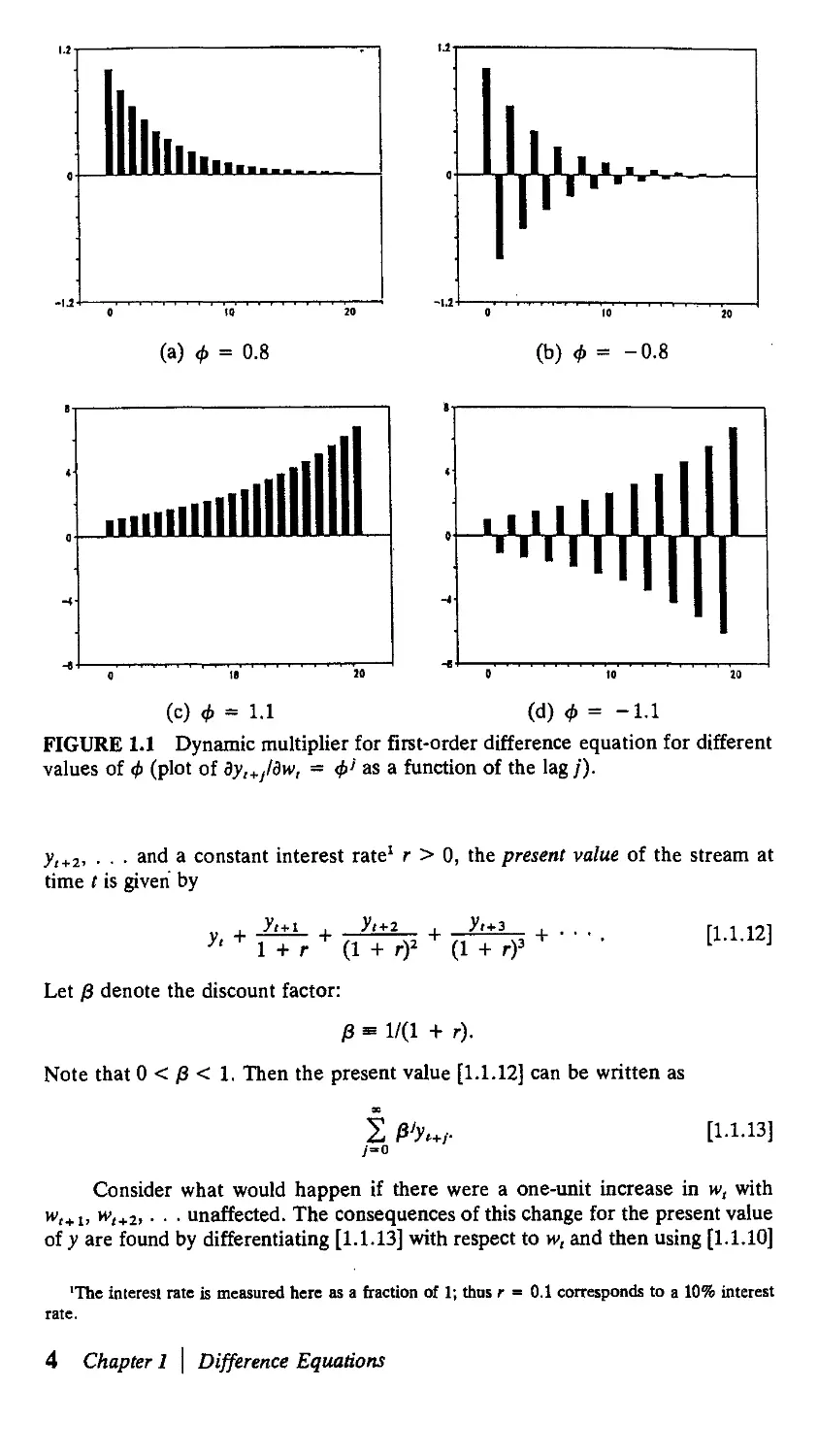
Different values of ф in [1.1.1] can produce a variety of dynamic responses
of у to w. If 0 < ф < 1, the multiplier dy,+J/dw, in [1.1.10] decays geometrically
toward zero. Panel (a) of Figure 1.1 plots ф1 as a function of/ for ф - 0.8. If
-1 < ф < 0, the multiplier dy,+j/dw, will alternate in sign as in panel (b). In this
case an increase in w, will cause y, to be higher, у,+1 to be lower, у,+1 to be higher,
and so on. Again the absolute value of the effect decays geometrically toward zero.
If ф > 1, the dynamic multiplier increases exponentially over time as in panel (c).
A given increase in w, has a larger effect the farther into the future one goes. For
ф < -1, the system [1.1.1] exhibits explosive oscillation as in panel (d).
Thus, if \ф\ < 1, the system is stable; the consequences of a given change in
w, will eventually die out. If \ф\ > 1, the system is explosive. An interesting pos-
possibility is the borderline case, ф = 1. In this case, the solution [1.1.9] becomes
yl+j = У,-! + W, + W,+ 1 + W,+2 + ¦ ¦ • + И»,+у-1 + W,+J. [1.1.11]
Here the output variable у is the sum of the historical inputs w. A one-unit increase
in w will cause a permanent one-unit increase in y:
^ = 1 for/ = 0, 1,
We might also be interested in the effect of w on the present value of the
stream of future realizations of y. For a given stream of future values y,, yl+1,
1.1. First-Order Difference Equations 3
(а) ф = 0.8
(с) ф = 1.1 (d) ф= -1.1
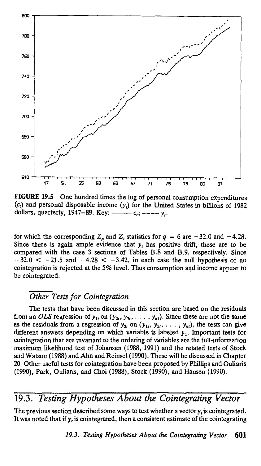
FIGURE 1.1 Dynamic multiplier for first-order difference equation for different
values of ф (plot of dy,+jldw, = ф' as a function of the lag /).
;y,+2, . . . and a constant interest rate1 r > 0, the present value of the stream at
time t is given by
v 4.
1 + r A + rJ A + rK
Let /3 denote the discount factor:
/3 - 1/A + r).
Note that 0 < /3 < 1. Then the present value [1.1.12] can be written as
i
[1.1.12]
[1.1.13]
Consider what would happen if there were a one-unit increase in w, with
wt+u wi+z, ¦ ¦ ¦ unaffected. The consequences of this change for the present value
of у are found by differentiating [1.1.13] with respect to w, and then using [1.1.10]
'The interest rate is measured here as a fraction of 1; thus r = 0.1 corresponds to a 10% interest
4 Chapter 1 \ Difference Equations
to evaluate each derivative:
[1.1.14]
provided that \/Зф\ < 1.
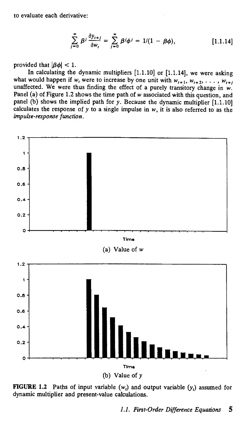
In calculating the dynamic multipliers [1.1.10] or [1.1.14], we were asking
what would happen if w, were to increase by one unit with w,+ 1, w,+2, • • . , w,+l
unaffected. We were thus finding the effect of a purely transitory change in w.
Panel (a) of Figure 1.2 shows the time path of w associated with this question, and
panel (b) shows the implied path for y. Because the dynamic multiplier [1.1.10]
calculates the response of у to a single impulse in w, it is also referred to as the
impulse-response function.
1.2
0.8
Time
(a) Value of w
Time
(b) Value of v
FIGURE 1.2 Paths of input variable (w() and output variable (y() assumed for
dynamic multiplier and present-value calculations.
1.1. First^Order Difference Equations 5
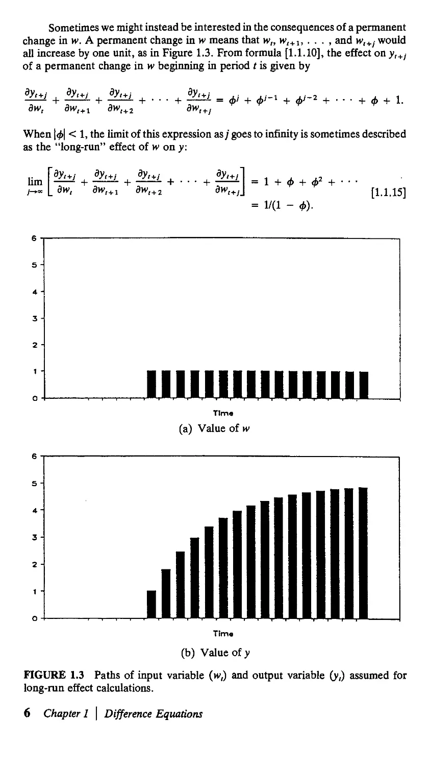
Sometimes we might instead be interested in the consequences of a permanent
change in w. A permanent change in w means that w,, w,+ b . . . , and w,+/ would
all increase by one unit, as in Figure 1.3. From formula [1.1.10], the effect on yl+l
of a permanent change in w beginning in period t is given by
dw,
dyl+j
dw,+2
+ ф + 1.
When \ф\ < 1, the limit of this expression as/ goes to infinity is sometimes described
as the "long-run" effect of w on y:
dW,+ 2
= 1 + ф + ф2 +
= 1/A - Ф)-
[1.1.15]
IIIIIIHIIIIIIII
Time
(a) Value of w
Time
(b) Value of у
FIGURE 1.3 Paths of input variable (w,) and output variable (y,) assumed for
long-run effect calculations.
6 Chapter 1 \ Difference Equations
For example, the long-ran income elasticity of money demand in the system [1.1.2]
is given by
0.19
1 - 0.72
= 0.68.
A permanent 1% increase in income will eventually lead to a 0.68% increase in
money demand.
Another related question concerns the cumulative consequences for у of a
one-time change in w. Here we consider a transitory disturbance to w as in panel
(a) of Figure 1.2, but wish to calculate the sum of the consequences for all future
values of y. Another way to think of this is as the effect on the present value of у
[1.1.13] with the discount rate /3 = 1. Setting/3 = 1 in [1.1.14] shows this cumulative
effect to be equal to
f, ^ = 1/A - ф), [1.1.16]
provided that \ф\ < 1. Note that the cumulative effect on у of a transitory change
in w (expression [1.1.16]) is the same as the long-ran effect on у of a permanent
change in w (expression [1.1.15]).
1.2. pth-Order Difference Equations
Let us now generalize the dynamic system [1.1.1] by allowing the value of у at date
t to depend on p of its own lags along with the current value of the input variable
w,:
У, =
Л-1 + ФгУг-г + • • ¦ + ФрУ,-р +
[1.2.1]
Equation [1.2.1] is a linear pth-order difference equation.
It is often convenient to rewrite the pth-order difference equation [1.2.1] in
the scalar y, as a first-order difference equation in a vector ?,. Define the (pxl)
vector ?, by
У,
yt-i
У.-2
[1.2.2]
That is, the first element of the vector ? at date t is the value у took on at date t.
The second element of g, is the value у took on at date t - 1, and so on. Define
the (p x p) matrix F by
[1.2.3]
l
0
ф2
0
l
Фз
0
0
... фр-1
0
... 0
ф1
0
0
0 0 0
0.
1.2. pth-Order Difference Equations 7
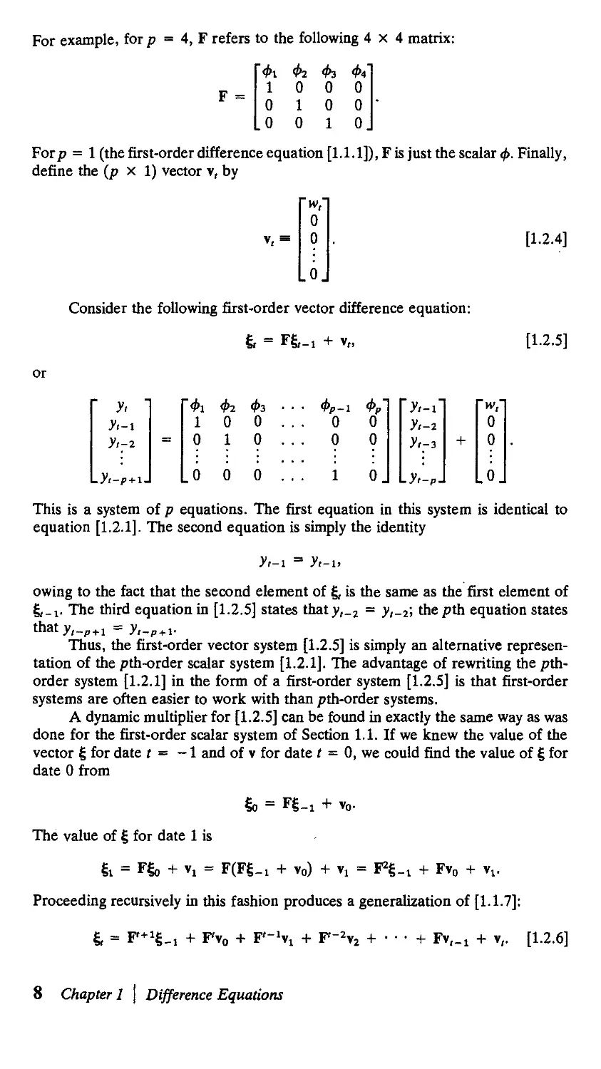
For example, for p = 4, F refers to the following 4x4 matrix:
Ф\ Фг Фз Ф*
10 0 0
0 10 0
0 0 1 0J
Forp = 1 (the first-order difference equation [1.1.1]), F is just the scalar ф. Finally,
define the (p x 1) vector v, by
о
О . [1.2.4]
Consider the following first-order vector difference equation:
& = Fg,_, + v,, [1.2.5]
or
У,
У,-\
У,7г
Фх
1
0
Фг
0
1
Фз ¦¦
0 . .
0 . .
Фр.
. 0
. 0
0 0 0
0
0
0.
"л-Г
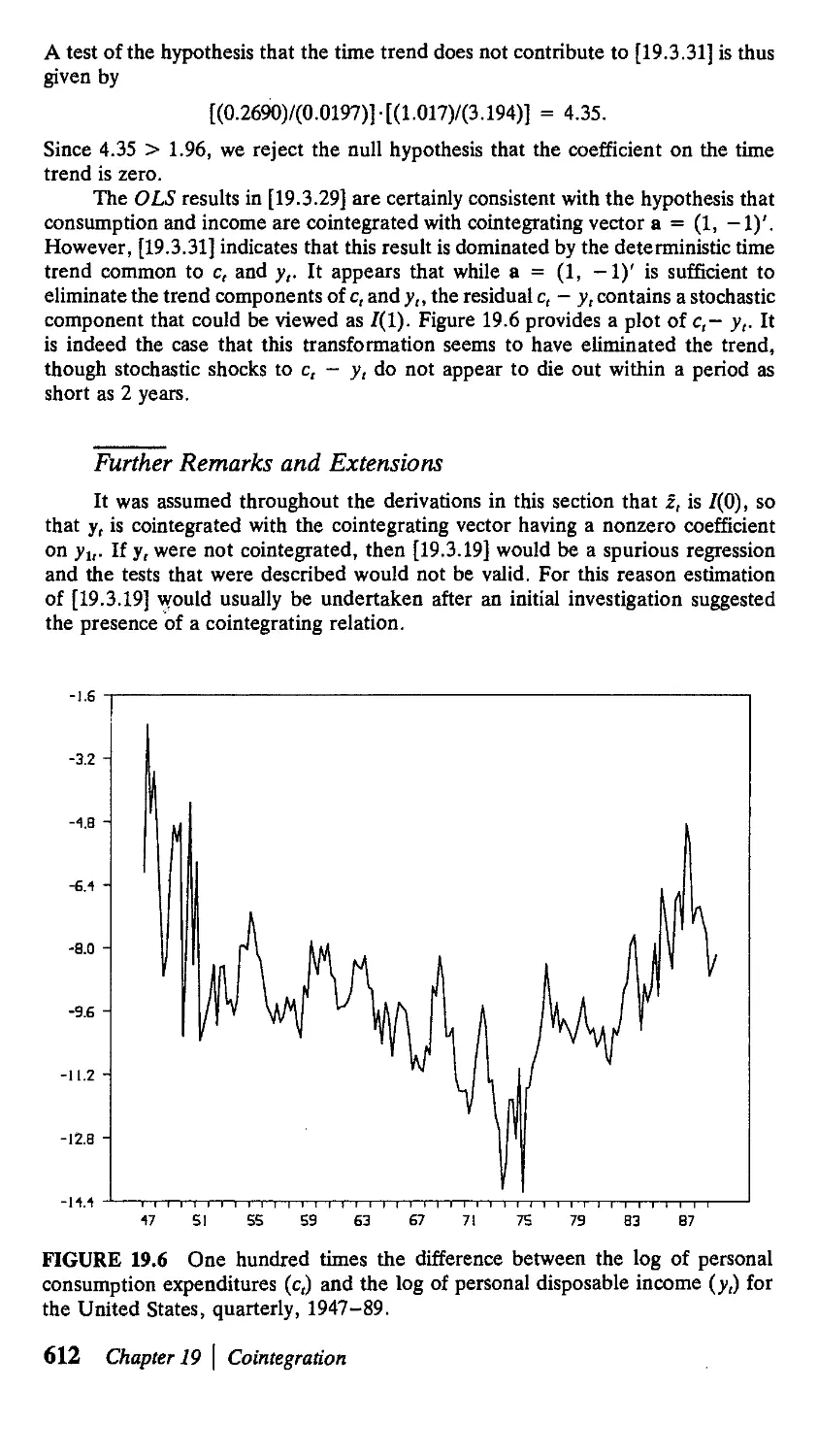
У,-г
У,-з
-У,-Р-
+
'w,'
0
0
.0.
This is a system of p equations. The first equation in this system is identical to
equation [1.2.1]. The second equation is simply the identity
yt-i = y,-i,
owing to the fact that the second element of g, is the same as the first element of
?,_!• The third equation in [1.2.5] states thaty,_2 = y,_2; the pth equation states
Thus, the first-order vector system [1.2.5] is simply an alternative represen-
representation of the pth-order scalar system [1.2.1]. The advantage of rewriting the pth-
order system [1.2.1] in the form of a first-order system [1.2.5] is that first-order
systems are often easier to work with than pth-order systems.
A dynamic multiplier for [1.2.5] can be found in exactly the same way as was
done for the first-order scalar system of Section 1.1. If we knew the value of the
vector g for date t = -1 and of v for date t = 0, we could find the value of g for
date 0 from
?„ = Fg_! + то.
The value of ? for date 1 is
g! = F& + т, = F(Fg_! + то) + Ti = F2^! + Ft0 + yx.
Proceeding recursively in this fashion produces a generalization of [1.1.7]:
& = F1*1^! + F't0 + F'-'Ti + F't2 + ¦ • • + Fr,_! + t(. [1.2.6]
8 Chapter 1 | Difference Equations
Writing this out in terms of the definitions of g and v,
0
0
6
У,
У<-1
У,-г
.У.-p + i.
_ F'+1
'У-1
У-г
У-г
-У-Р-
+ F'
+ F1
+ F'"
[1.2.7]
Consider the first equation of this system, which characterizes the value of y,. Let
/ft denote the A, 1) element of F', /g the A, 2) element of F1, and so on. Then
the first equation of [1.2.7] states that
y, =
+ ••• +/ЙЧ-1 + и-,.
[1.2.8]
This describes the value of у at date (asa linear function of p initial values of у
(y_i, у-2, • • • , У-р) and the history of the input variable w since time 0 (w0, wlt
. . . , w,). Note that whereas only one initial value for у (the value у _t) was needed
in the case of a first-order difference equation, p initial values for у (the values
y_!, y_2> ¦ • ¦ • У-р) аге needed in the case of a pth-order difference equation.
The obvious generalization of [1.1.9] is
F'v,
[1.2.9]
from which
f\'P+l)y,-p
[1.2.10]
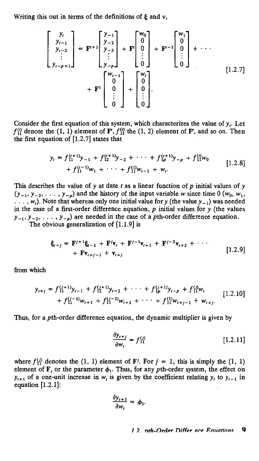
Thus, for a pth-order difference equation, the dynamic multiplier is given by
dw,
[1.2.11]
where/H' denotes the A, 1) element of F>. For/ = 1, this is simply the A, 1)
element of F, or the parameter ф^. Thus, for any pth-order system, the effect on
yt+1 of a one-unit increase in w, is given by the coefficient relating y, to yr-i in
equation [1.2.1]:
dw,
1 7 nth-Order niffer nrt> Rnuniinnx 0
Direct multiplication of [1.2.3] reveals that the A, 1) element of F2 is (ф1 + ф2),
so
dw,
= Ф1 + 4>i
in a pth-order system.
For larger values of/, an easy way to obtain a numerical value for the dynamic
multiplier 3yl+j/dw, is to simulate the system. This is done as follows. Set >_, =
у_г = • ¦ • = y_p = 0, w0 = 1, and set the value of w for all other dates to 0.
Then use [1.2.1] to calculate the value of y, for t = 0 (namely, y0 = 1). Next
substitute this value along with yt-\,yt-i> ¦ ¦ ¦ ,yt-p+i back into [1.2.1] to calculate
y,+ I, and continue recursively in this fashion. The value of у at step t gives the
effect of a one-unit change in w0 on y,.
Although numerical simulation may be adequate for many circumstances, it
is also useful to have a simple analytical characterization of Byt+i/3wt, which, we
know from [1.2.11], is given by the A,1) element of F'. This is fairly easy to obtain
in terms of the eigenvalues of the matrix F. Recall that the eigenvalues of a matrix
F are those numbers A for which
|F - AIP| = 0.
[1.2.12]
For example, for p = 2 the eigenvalues are the solutions to
Фт
O
] _ Г
j |_
а О
0 A
or
-А) фг
1 -A
= A2 - ф,\ - Фг. = 0. [1.2.13]
The two eigenvalues of F for a second-order difference equation are thus given by
A, =
A2 =
ф1 -
[1.2.14]
[1.2.15]
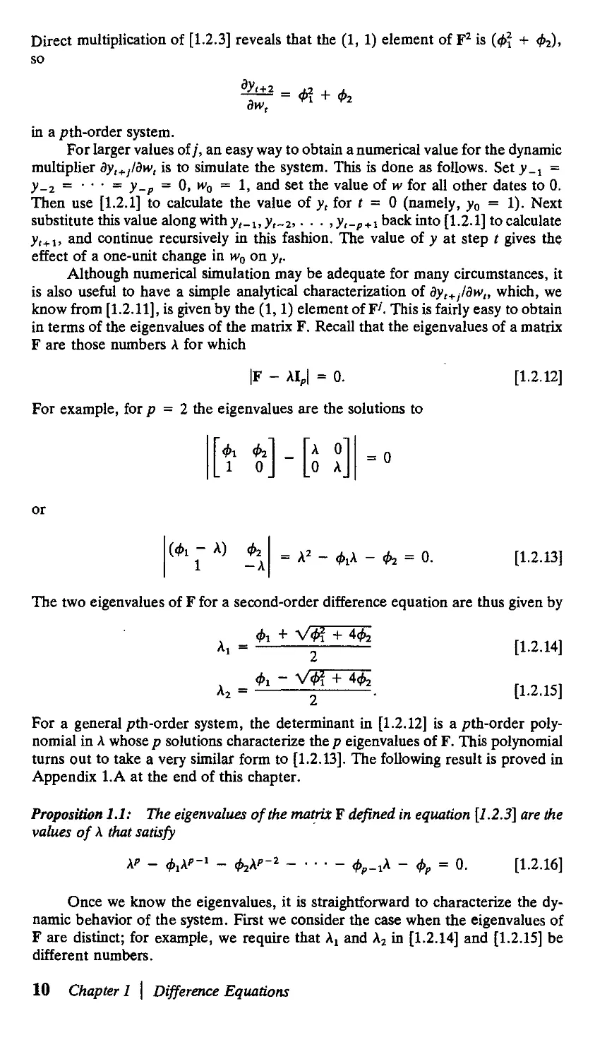
For a general pth-order system, the determinant in [1.2.12] is a pth-order poly-
polynomial in A whose p solutions characterize the p eigenvalues of F. This polynomial
turns out to take a very similar form to [1.2.13]. The following result is proved in
Appendix l.A at the end of this chapter.
Proposition 1.1: The eigenvalues of the matrix F defined in equation [1.2.3] are die
values of A that satisfy
-г _
- ф._гА - ф. = 0.
[1.2.16]
Once we know the eigenvalues, it is straightforward to characterize the dy-
dynamic behavior of the system. First we consider the case when the eigenvalues of
F are distinct; for example, we require that A! and A2 in [1.2.14] and [1.2.15] be
different numbers.
10 Chapter 1 \ Difference Equations
General Solution of a pth-Order Difference Equation
with Distinct Eigenvalues
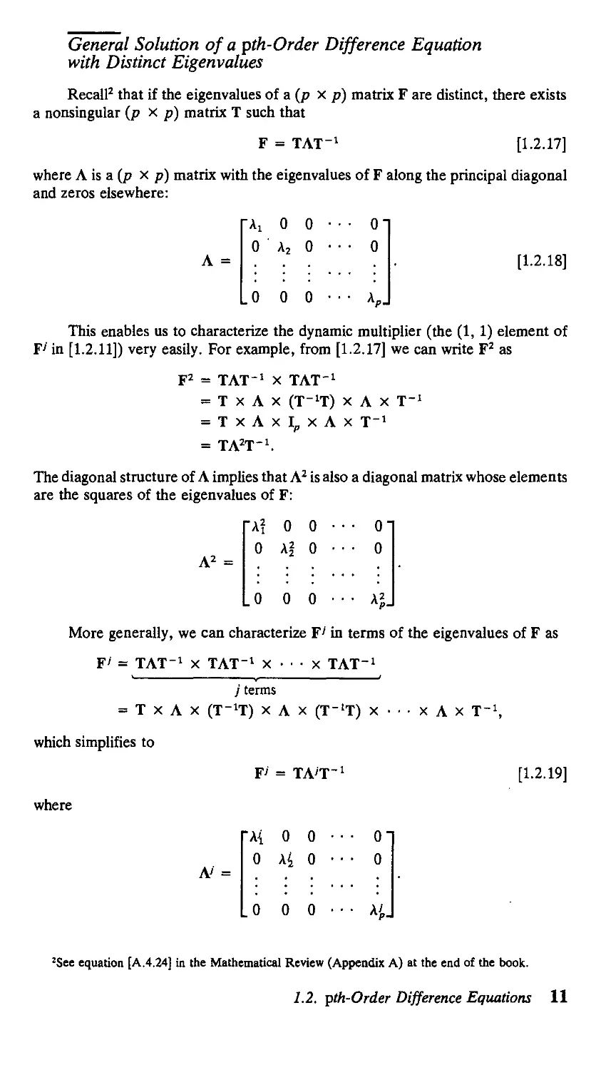
Recall2 that if the eigenvalues of a (p x p) matrix F are distinct, there exists
a nonsingular (p X p) matrix T such that
F = TAT
[1.2.17]
where Л is a (p x p) matrix with the eigenvalues of F along the principal diagonal
and zeros elsewhere:
Л =
A! 0 0
0 A2 0
.0 0 0
01
0
[1.2.18]
This enables us to characterize the dynamic multiplier (the A, 1) element of
F' in [1.2.11]) very easily. For example, from [1.2.17] we can write F2 as
F2 = ТЛТ-1 x TAT1
= T x Л x (Т-Ч) х Л х Т-1
= ТхЛх1рхЛх Т
The diagonal structure of A implies that Л2 is also a diagonal matrix whose elements
are the squares of the eigenvalues of F:
A2 =
"А2 О О
О А2 О
01
0
.0 0 0 ••• A2.
More generally, we can characterize F' in terms of the eigenvalues of F as
F' = TAT x TAT x • • • x TAT
which
where
= Т х Л
simplifies to
х A
А!
j terms
Г"Ч) х
?'
0
0
Л
X (Т-
= ТЛ'Т-
0
А4
0
0 •
0 •
0 •
"Г)
1
• •
X ¦
¦ • х Л х т-:,
0"
0
А>
[1.2.19]
2See equation [A.4.24] in the Mathematical Review (Appendix A) at the end of the book.
1.2. pth-Order Difference Equations 11
Let tij denote the row i, column ; element of T and let t1' denote the row i, column
/ element of T. Equation [1.2.19] written out explicitly becomes
F> =
<u кг ¦ ¦ ¦ kp'
'21 ^2 ' ' ' *2p
'pi 'p2 ' tpp-
¦\{ 0 0 • • • 0 "
0 A? 0 • • • 0
. 0 0 0 • • • ki
",11 ,12 ... ,lp
^21 ^22 . . . ?2p
(P* tPi ... (PP
tp2\{
tpp^ ^
tn t12
p t22
t'2
fip
tfp
from which the A, 1) element of F' is given by
/К' = ['1/ЧА4 + [^21]A4 +
or
where
[1.2.20]
[1.2.21]
Ci = [tufi].
Note that the sum of the c, terms has the following interpretation:
c1 + c2 + ¦ • • + cp = [tutn] + [tnt21] + • ¦ ¦ + [tlptPx], [1.2.22]
which is the A, 1) element of T-T. Since T-T~l is just the {p x p) identity
matrix, [1.2.22] implies that the c, terms sum to unity:
+ c2 +
+ cp = 1.
[1.2.23]
Substituting [1.2.20] into [1.2.11] gives the form of the dynamic multiplier
for a pth-order difference equation:
dw,
+ cp\'p.
[1.2.24]
Equation [1.2.24] characterizes the dynamic multiplier as a weighted average of
each of the p eigenvalues raised to the /th power.
The following result provides a closed-form expression for the constants (clt
c2, . . . , cp).
Proposition 1.2: If the eigenvalues (Al5 \2, . . . , \p) of the matrix F in [1.2.3] are
distinct, then the magnitude c, in [1.2.21] can be written
c, =
Af"
[1.2.25]
k=l
k+t
To summarize, thepth-order difference equation [1.2.1] implies that
[1.2.26]
12 Chapter 1 \ Difference Equations
The dynamic multiplier
** = * [1-2.27]
is given by the A, 1) element of F':
*i = f\S- [1-2-28]
A closed-form expression for ф1 can be obtained by finding the eigenvalues of F,
or the values of A satisfying [1.2.16]. Denoting these p values by (Ab A2, . . . , \p)
and assuming them to be distinct, the dynamic multiplier is given by
ф, = cx\{ + c2A2 + ¦ ¦ ¦ + cp\p [1.2.29]
where (c,, c2, . . . , cp) is a set of constants summing to unity given by expression
[1.2.25].
For a first-order system (p = 1), this rule would have us solve [1.2.16],
A - Фг = О,
which has the single solution
At = <fo. [1.2.30]
According to [1.2.29], the dynamic multiplier is given by
^ = c,A{. [1.2.31]
dW,
From [1.2.23], Cj = 1. Substituting this and [1.2.30] into [1.2.31] gives
^ = Ф{,
dw, V1
or the same result found in Section 1.1.
For higher-order systems, [1.2.29] allows a variety of more complicated dy-
dynamics. Suppose first that all the eigenvalues of F (or solutions to [1.2.16]) are
real. This would be the case, for example, if p = 2 and ф\ + 4<^ > 0 in the
solutions [1.2.14] and [1.2.15] for the second-order system. If, furthermore, all of
the eigenvalues are less than 1 in absolute value, then the system is stable, and its
dynamics are represented as a weighted average of decaying exponentials or de-
decaying exponentials oscillating in sign. For example, consider the following second-
order difference equation:
y, = 0.6y,_, + 0.2y,.2 + w,.
From equations [1.2.14] and [1.2.15], the eigenvalues of this system are given by
— U.84
0.6
0.6
+ V@.6J -
2
- V@.6J i
1- 4@.2)
1- 4@.2)
From [1.2.25], we have
c, = A,/(A, - A2) = 0.778
c2 = A2/(A2 - AJ = 0.222.
The dynamic multiplier for this system,
1.2. pth-Order Di erence Equations 13
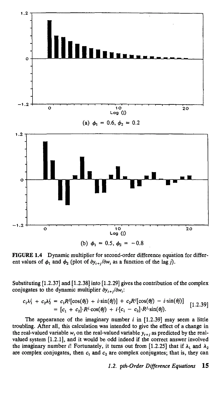
is plotted as a function of / in panel (a) of Figure 1.4.3 Note that as / becomes
larger, the pattern is dominated by the larger eigenvalue (A,), approximating a
simple geometric decay at rate A^
If the eigenvalues (the solutions to [1.2.16]) are real but at least one is greater
than unity in absolute value, the system is explosive. If Аг denotes the eigenvalue
that is largest in absolute value, the dynamic multiplier is eventually dominated by
an exponential function of that eigenvalue:
Other interesting possibilities arise if some of the eigenvalues are complex.
Whenever this is the case, they appear as complex conjugates. For example, if
p = 2 and ф2 + 4^2 < 0, then the solutions At and A2 in [1.2.14] and [1.2.15] are
complex conjugates. Suppose that A! and A2 are complex conjugates, written as
Аг = a + Ы [1.2.32]
A2 = a - Ы. [1.2.33]
For the p = 2 case of [1.2.14] and [1.2.15], we would have
a = фхП [1.2.34]
b = A/2)V-<M - 4<^. [1.2.35]
Our goal is to characterize the contribution to the dynamic multiplier с^к\
when Ai is a complex number as in [1.2.32]. Recall that to raise a complex number
to a power, we rewrite [1.2.32] in polar coordinate form:
Ai = i?-[cos@) + i-sin@)], [1.2,36]
where в and R are defined in terms of a and b by the following equations:
R = Va2 + b2
cos@) = alR
sin@) = blR.
Note that R is equal to the modulus of the complex number kv
The eigenvalue A, in [1.2.36] can be written as4
A, = R[e%
and so
A{ = R'[eie'] = R'[cos(ej) + i-sin@/)]. [1.2.37]
Analogously, if A2 is the complex conjugate of Alt then
A2 = i?[cos@) - i-sin@)],
which can be written5
A2 = R[e~"\.
Thus
A2 = R'[e-ieq = Ri[cos(ef) - i-sin@/)]. [1.2.38]
3 Again, if one's purpose is solely to generate a numerical plot as in Figure 1.4, the easiest approach
is numerical simulation of the system.
4See equation [A.3.25] in the Mathematical Review (Appendix A) at the end of the book.
5See equation [A.3.26].
14 Chapter 1 | Difference Equations
1.2
-1.2-
20
(a) & = 0.6, ф2 = 0.2
1.2
II ¦!I ¦¦¦ ¦!
-1.2 •
20
(b) ф, = 0.5, фг = -0.8
FIGURE 1.4 Dynamic multiplier for second-order difference equation for differ-
different values of ф^ and <k (plot of ду,+11дп>, as a function of the lag j).
Substituting [1.2.37] and [1.2.38] into [1.2.29] gives the contribution of the complex
conjugates to the dynamic multiplier dyIJrjldwt:
c2R'[cos(ej) - i-sin(fl/)] ^
= [c, + c2]-R'-oos(ef) + i-[ci - c2]-R'-sm(ef).
The appearance of the imaginary number i in [1.2.39] may seem a little
troubling. After all, this calculation was intended to give the effect of a change in
the real-valued variable w, on the real-valued variable yt+J as predicted by the real-
valued system [1.2.1], and it would be odd indeed if the correct answer involved
the imaginary number i! Fortunately, it turns out from [1.2.25] that if Аг and A2
are complex conjugates, then Cj and c2 are complex conjugates; that is, they can
1.2. pth-Order Difference Equations 15
be written as
cx = a + pi
c2 = a - pi
for some real numbers a and /}. Substituting these expressions into [1.2.39] yields
CiA{ + c2Ai = [(a + pi) + (a - pi)]-R'cos(ef) + i-[(a + pi) - (a - pi)]-R'siaFj)
= [2a]R'cos(ej) + i-[2pi\-R'sia(ej)
= 2aR>co&@j) - 2/3i?'sin@/),
wliich is strictly real.
Thus, when some of the eigenvalues are complex, they contribute terms
proportional to R' cos@/) and Ri sin@/) to the dynamic multiplier dy,+j/dw,. Note
that if R = 1—that is, if the complex eigenvalues have unit modulus—the mul-
multipliers are periodic sine and cosine functions of/. A given increase in w, increases
yt+J for some ranges of/ and decreases y,+i over other ranges, with the impulse
never dying out as / -* <». If the complex eigenvalues are less than 1 in modulus
(R < 1), the impulse again follows a sinusoidal pattern though its amplitude decays
at the rate R'. If the complex eigenvalues are greater than 1 in modulus (R > 1),
the amplitude of the sinusoids explodes at the rate R'.
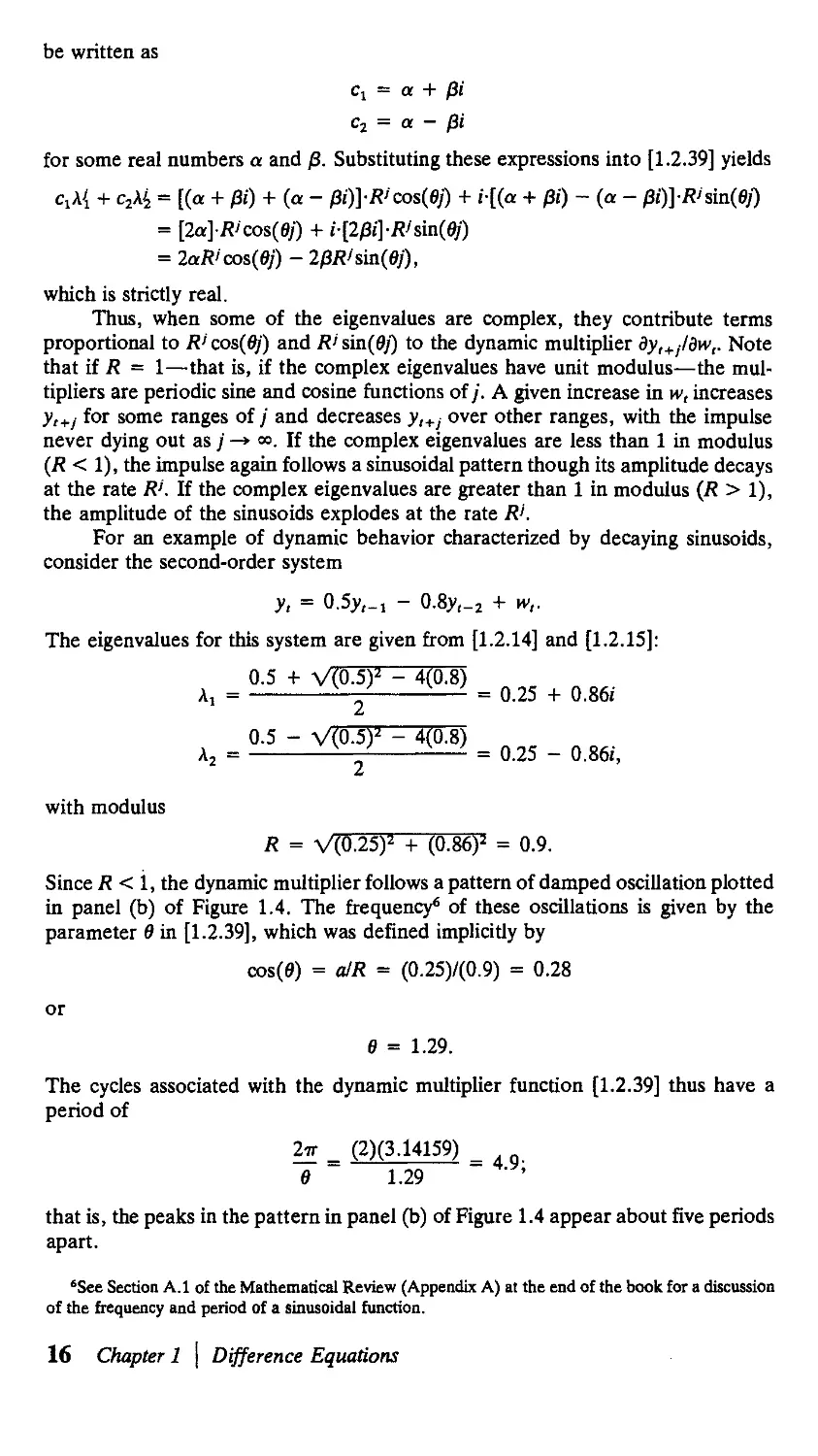
For an example of dynamic behavior characterized by decaying sinusoids,
consider the second-order system
y, = 0.5y,_, - 0.8y,_2 + w,.
The eigenvalues for this system are given from [1.2.14] and [1.2.15]:
0.25 + 0.86i
= 0.25 - 0.86i,
with modulus
R = V@.25J + @.86J = 0.9.
Since R < 1, the dynamic multiplier follows a pattern of damped oscillation plotted
in panel (b) of Figure 1.4. The frequency6 of these oscillations is given by the
parameter в in [1.2.39], which was defined implicitly by
cos@) = alR = @.25)/@.9) = 0.28
or
в = 1.29.
The cycles associated with the dynamic multiplier function [1.2.39] thus have a
period of
27Г _ B)C.14159)
в 1.29
that is, the peaks in the pattern in panel (b) of Figure 1.4 appear about five periods
apart.
'See Section A.I of the Mathematical Review (Appendix A) at the end of the book for a discussion
of the frequency and period of a sinusoidal function.
16 Chapter 1 | Difference Equations
A, :
A2 .
0.5
0.5
+ V@.5)'
2
- V@.5)'
2
- 4@.8)
- 4@.8)
Solution of a Second-Order Difference Equation
with Distinct Eigenvalues
The second-order difference equation (p = 2) comes up sufficiently often
that it is useful to summarize the properties of the solution as a general function
of фг and ф2, which we now do.7
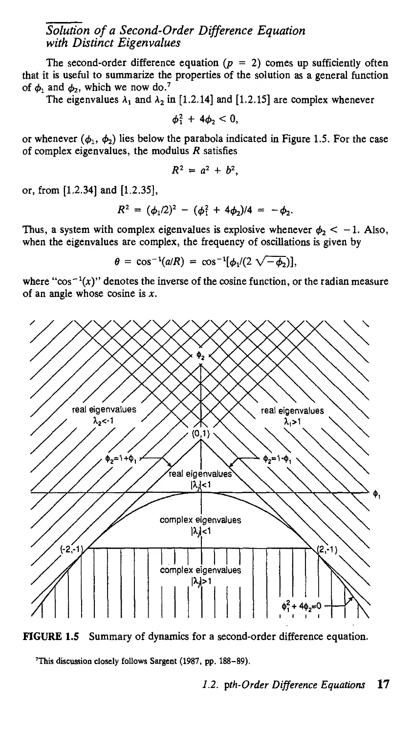
The eigenvalues Aj and A2 in [1.2.14] and [1.2.15] are complex whenever
ф\
О,
or whenever (ф1, ф^) lies below the parabola indicated in Figure 1.5. For the case
of complex eigenvalues, the modulus R satisfies
or, from [1.2.34] and [1.2.35],
R2 = a2 + b\
{ф\
Thus, a system with complex eigenvalues is explosive whenever & < — 1. Also,
when the eigenvalues are complex, the frequency of oscillations is given by
в = cos"\a/R) = сов-ЧфДг V^)],
where "cos^)" denotes the inverse of the cosine function, or the radian measure
of an angle whose cosine is x.
FIGURE 1.5 Summary of dynamics for a second-order difference equation.
This discussion closely follows Sargent A987, pp. 188-89).
1.2. pth-Order Difference Equations 17
For the case of real eigenvalues, the arithmetically larger eigenvalue (Aj) will
be greater than unity whenever
ф1 + V*} + Чг
> 1
or
V0f + Ч2 > 2 - 0,.
Assuming that \1 is real, the left side of this expression is a positive number and
the inequality would be satisfied for any value of fa > 2. If, on the other hand,
фх < 2, we can square both sides to conclude that Aj will exceed unity whenever
ф\ + 4ф2 > 4 - 40, + ф\
or
Фг
Thus, in the real region, Aj will be greater than unity either if фг > 2 or if @,, ф2)
lies northeast of the line Ф2 = 1 - 0i in Figure 1.5. Similarly, with real eigenvalues,
the arithmetically smaller eigenvalue (A2) will be less than -1 whenever
- V0f
< -1
:< -2 -
Again, if 0i < —2, this must be satisfied, and in the case when ф1 > -2, we can
square both sides:
ф\
> 4 + 40,
> 1 + Ф1-
ф\
Thus, in the real region, A2 will be less than -1 if either 0, < -2 or @!, 0j) lies
to the northwest of the line ф2 = 1 + 0, in Figure 1.5.
The system is thus stable whenever @i, 02) lies within the triangular region
of Figure 1.5.
General Solution of a pth-Order Difference Equation
with Repeated Eigenvalues
In the more general case of a difference equation for which F has repeated
eigenvalues and s < p linearly independent eigenvectors, result [1.2.17] is gener-
generalized by using the Jordan decomposition,
F = MJM-1 [1.2.40]
where M is a (p x p) matrix and J takes the form
"J, 0 • 0
J =
0
0
.0 0 • • • J,_
18 Chapter 1 | Difference Equations
with
J, =
A, 1 0
0 A,- 1
0 0 A,-
0 0
0 0
0 0
0 0 0
0 0 0
A, 1
0 A, _
[1.2.41]
for A, an eigenvalue of F. If [1.2.17] is replaced by [1.2.40], then equation [1.2.19]
generalizes to
F> = MJ'M1
[1.2.42]
where
J' =
о о
Moreover, from [1.2.41], if J, is of dimension (n, x n,), then8
ц (Оаг1 ШАГ2 ••• СЛ)ЛГ"'+
[1.2.43]
where
о о
'JU- i)Q-2) ¦••(/- я + 1)
n(n-l)--.3-2-1 **'*"
10 otherwise.
Equation [1.2.43] may be verified by induction by multiplying [1.2.41] by [1.2.43]
and noticing that (>) + („i,) = ('J1).
For example, consider again the second-order difference equation, this time
with repeated roots. Then
so that the dynamic multiplier takes the form
Long-Run and Present-Value Calculations
If the eigenvalues are all less than 1 in modulus, then F' in [1.2.9] goes to
zero as / becomes large. If all values of w and у are taken to be bounded, we can
"This expression is taken from Chiang A980, p. 444).
1.2. pth-Order Difference Equations 19
think of a "solution" of y, in terms of the infinite history of w,
y, = w, + i/w_i +. Фг^,-г + Фъ^,-ъ + • • • . [1.2.44]
where ф{ is given by the A,1) element of F' and takes the particular form of [1.2.29]
in the case of distinct eigenvalues.
It is also straightforward to calculate the effect on the present value of у of
a transitory increase in w. This is simplest to find if we first consider the slightly
more general problem of the hypothetical consequences of a change in any element
of the vector v, on any element of %t+j in a general system of the form of [1.2.5].
The answer to this more general problem can be inferred immediately from [1.2.9]:
**f = *'• [1-2.45]
The true dynamic multiplier of interest, ду,+1/дп>„ is just the A, 1) element of the
(p x p) matrix in [1.2.45]. The effect on the present value of g of a change in v
is given by
ж
i°'1L 2 fiW (I №)' [1246]
provided that the eigenvalues of F are all less than /3~4n modulus. The effect on
the present value of у of a change in w,
ж
i-o
Bw,
is thus the A, 1) element of the (p X p) matrix in [1.2.46]. This value is given by
the following proposition.
Proposition 1.3: If the eigenvalues of the (p x p) matrix F defined in [1.2.3] are
all less than p'1 in modulus, then the matrix (Ip - /3F) exists and the effect of
w on the present value of у is given by its (i, 1) element:
1/A - фф - ффг - ••• - фр.^р-1 - фррр).
Note that Proposition 1.3 includes the earlier result for a first-order system
(equation [1.1.14]) as a special case.
The cumulative effect of a one-time change in w, on y,, y,+ 1, . . . can be
considered a special case of Proposition 1.3 with no discounting. Setting /3 = 1 in
Proposition 1.3 shows that, provided the eigenvalues of F are all less than 1 in
modulus, the cumulative effect of a one-time change in w on у is given by
J) ^±-' = 1/A - фг - ф2 - ¦ ¦ ¦ - фр). [1.2.47]
Notice again that [1.2.47] can alternatively be interpreted as giving the even-
eventual long-run effect on у of a permanent change in w:
20 Chapter 1 \ Difference Equations
APPENDIX l.A. Proofs of Chapter 1 Propositions
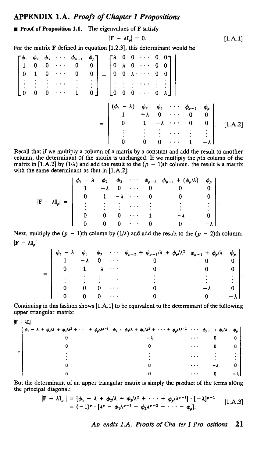
¦ Proof of Proposition 1.1. The eigenvalues of F satisfy
|F - AI,| = 0.
For the matrix F defined in equation [1.2.3], this determinant would be
Фр
0
0
0.
[1.A.1]
~Фг
1
0
0
Фг
0
1
0
Фг ••
0 • •
0 • •
0 ¦ ¦
¦ фр
¦ 0
• 0
1
"А
0
0
.0
(Ф
0
А
0
0
-
1
0
0
0
А -
0
А)
Фг
-А
1
0
0
0
0
Фг
0
-А
О"
0
0
А.
••• Ф,-
... о
¦ 0
0
0
о
о
о
1 -А
. [1.А.2]
Recall that if we multiply a column of a matrix by a constant and add the result to another
column, the determinant Of the matrix is unchanged. If we multiply the pth column of the
matrix in [1.A.2] by (I/A) and add the result to the (p - l)th column, the result is a matrix
with the same determinant as that in [1.A.2]:
IF - AI,| =
Ф\ ~
1
0
-A 0
1 -A
фр.х + (фр1\)
0
0
0 0 0 ¦• ¦ 1 -А 0
О 0 0 • • ¦ О О -А
Next, multiply the (р - l)th column by A/A) and add the result to the (p - 2)th column:
IF - AIJ
Ф\ ~ А ф2 Фг ' ' ' Фр-г + Фр-Jh + Фр/h2 Фр-t + Фр1^ ФР
1 -А 0 • ¦ ¦ О О О
О 1 -А ¦ • • О О О
О 0 0 •• • О -А О
О 0 0 ¦ • • О О -А
Continuing in this fashion shows [l.A.l] to be equivalent to the determinant of the following
upper triangular matrix:
IF - AI,|
О -Л О О
0 0 ¦ • ¦ 0 0
О О •¦•-АО
о о о -л
But the determinant of an upper triangular matrix is simply the product of the terms along
the principal diagonal:
|F - AI, | = [ф, - A + ф2/\ + ф3/А2 + • • ¦ + ф„/\"-1] ¦ [-A]' fl A 3,
= (-1)" • [A- - <M<-' - <fcA<-2 ФР].
Ad endix l.A. Proofs of Cha ter 1 Pro ositions 21
The eigenvalues of F are thus the values of A for which [1.A.3] is zero, or for which
A' - ф^К"'х - <M"-2 - • • ' - Фр = 0,
as asserted in Proposition 1.1. ¦
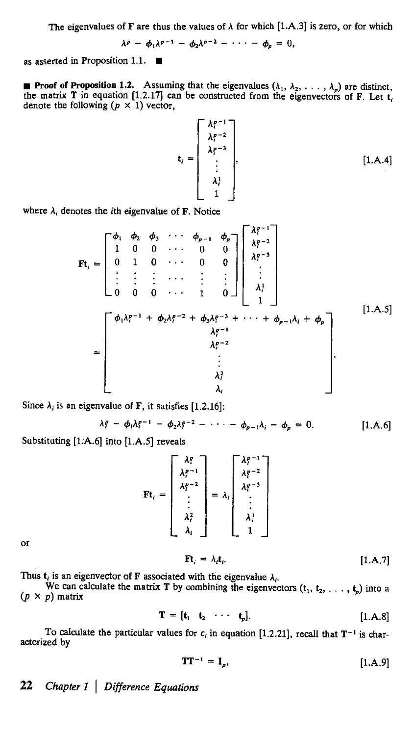
¦ Proof of Proposition 1.2. Assuming that the eigenvalues (A,, A? kp) are distinct,
the matrix T in equation [1.2.17] can be constructed from the eigenvectors of F. Let t,
denote the following (p x 1) vector,
Af
Af
Af
A/
1
where A, denotes the ith eigenvalue of F. Notice
Ft; =
'<t>i Фг Фг ' ' ' Фр-i Фр
1 0 0 • • • 0 0
0 1 0
0 0
Af
а;
1
Lo о о • • • i oJ
Af
А?
А,
Since A, is an eigenvalue of F, it satisfies [1.2.16]:
Af - <?,Af-' - <МГ2 фр-1к, - фр = 0.
Substituting [1.A.6] into [1.A.5] reveals
Ft, =
" Af ~
Af
кГг
A?
A,
= A,
Af-'~
Af
Af-3
a;
1
[1.A.4]
[1.A.5]
[1.A.6]
Ft; = A,t,.
[1.A.7]
Thus t, is an eigenvector of F associated with the eigenvalue A,-.
We can calculate the matrix T by combining the eigenvectors (t,, t2, . . . , t,,) into a
(p X p) matrix
T = [t, Ц • • • tp]. [1.A.8]
To calculate the particular values for c, in equation [1.2.21], recall that T is char-
characterized by
TT1 = I,,
22 Chapter 1 \ Difference Equations
[1.A.9]
where T is given by [1.A.4] and [1.A.8]. Writing out the first column of the matrix system
of equations [1.A.9] explicitly, we have
ЛГ1
АГ2
Ar3
A!
1
A$"
Af
A?'
A
1
t11
t21
t31
=
1
0
0
0
_0
This gives a system of p linear equations in the p unknowns (fu, r21, . . . , fl). Provided
that the A, are all distinct, the solution can be shown to be9
1
tn =
(A,
(A.
- A2)(A,
- A,)(A2
-A3)
1
-A3)
1
• • • (A,
• ¦ • (A2
-A,)
-к)
t21 =
'" (A, - A,)(A, - A2) ¦ • • (A, - A,_,)'
Substituting these values into [1.2.21] gives equation [1.2.25]. ¦
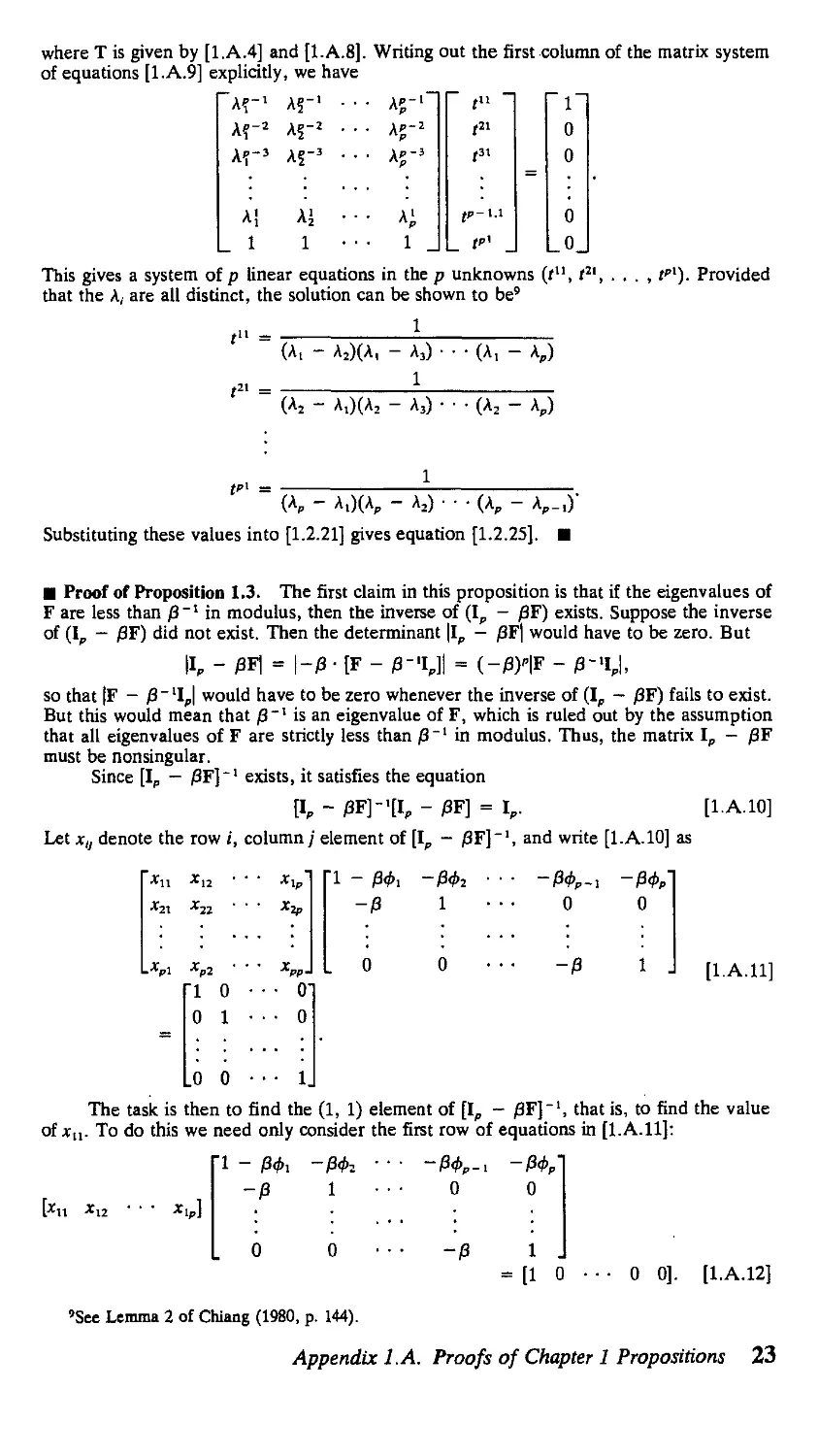
¦ Proof of Proposition 1.3. The first claim in this proposition is that if the eigenvalues of
F are less than 0 in modulus, then the inverse of (I, - 0F) exists. Suppose the inverse
of (I, - 0F) did not exist. Then the determinant \lp - 0F| would have to be zero. But
II, - 0F| = |-0 ¦ [F - p-%]\ = (-0)'|F - 0-4J,
so that |F - 0 " lI,| would have to be zero whenever the inverse of (I, - 0F) fails to exist.
But this would mean that 0" is an eigenvalue of F, which is ruled out by the assumption
that all eigenvalues of F are strictly less than 0 in modulus. Thus, the matrix Ip - 0F
must be nonsingular.
Since [Ip — 0F]~l exists, it satisfies the equation
[I, - РЩ-'[1Р - 0F] = I,. [1.A.10]
Let xu denote the row i, column/ element of [I, - 0F], and write [1.A.10] as
Г1 о
0 1
Г1 -
о
[l.A.ll]
.0 0
The task is then to find the A, 1) element of [1„ - /3F], that is, to find the value
of xu. To do this we need only consider the first row of equations in [l.A.ll]:
[*I1 *12
0
0
1 J
[1 0
• 0 0]. [1.A.12]
'See Lemma 2 of Chiang A980, p. 144).
Appendix LA. Proofs of Chapter 1 Propositions 23
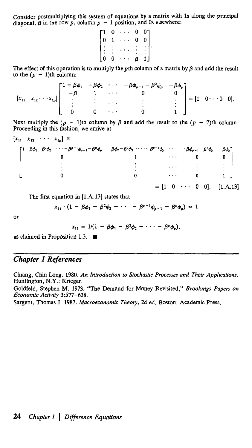
Consider postmultiplying this system of equations by a matrix with Is along the principal
diagonal, /3 in the row p, column p - 1 position, and Os elsewhere:
Г1 0
0 1
О О'
0 0
0 0
/3 1J
The effect of this operation is to multiply the pth column of a matrix by /3 and add the result
to the (p - l)th column:
= [1 О • • •0 0].
Next multiply the (p - l)th column by /3 and add the result to the (p - 2)th column.
Proceeding in this fashion, we arrive at
[xu xl2 ¦ ¦ ¦ xlp] x
= [1 0
01
0 0]. [1.A.13]
The first equation in [1.A.13] states that
хп = 1/A - /Зф, -
as claimed in Proposition 1.3. ¦
Chapter 1 References
Chiang, Chin Long. 1980. An Introduction to Stochastic Processes and Their Applications.
Huntington, N.Y.: Krieger.
Goldfeld, Stephen M. 1973. "The Demand for Money Revisited," Brookings Papers on
Economic Activity 3:577-638.
Sargent, Thomas J. 1987. Macroeconomic Theory, 2d ed. Boston: Academic Press.
24 Chapter 1 \ Difference Equations
Lag Operators
2.1. Introduction
The previous chapter analyzed the dynamics of linear difference equations using
matrix algebra. This chapter develops some of the same results using time series
operators. We begin with some introductory remarks on some useful time series
operators.
A time series is a collection of observations indexed by the date of each
observation. Usually we have collected data beginning at some particular date (say,
t = 1) and ending at another (say, t = Г):
(У1, У* ¦ ¦ ¦ . Ут)-
We often imagine that we could have obtained earlier observations (y0, y_it
У-г, . ¦ .) or later observations (ут+1, Ут+ъ ¦ ¦ ¦) had the process been observed
for more time. The observed sample {yv, y2, . . . , yT) could then be viewed as a
finite segment of a doubly infinite sequence, denoted {y,}?. _*:
{y,}7--~ = {¦ ¦ • ,У-1.Уо,У1,Уг Ут.Ут*иУт+2. ¦ ¦ ¦)¦
observed sample
Typically, a time series {у,}Г--« IS identified by describing the fth element.
For example, a time trend is a series whose value at date / is simply the date of the
observation:
У, = t-
We could also consider a time series in which each element is equal to a constant
c, regardless of the date of the observation t:
У, = c.
Another important time series is a Gaussian white noise process, denoted
У1 = e,,
where {e,}J°_ _* is a sequence of independent random variables each of which has
a N(Q, or1) distribution.
We are used to thinking of a function such as у = f(x) or у = g(x, w) as an
operation that accepts as input a number (x) or group of numbers (x, w) and
produces the output (y). A time series operator transforms one time series or group
25
of time series into a new time series. It accepts as input a sequence such as
{xjjl. _* or a group of sequences such as (fc}f_ _«,, {w,}f_ _„) and has as output a
new sequence {у}?ш _«,. Again, the operator is summarized by describing the value
of a typical element of {y}T=-~ in terms of the corresponding elements of
МТ—ш.
An example of a time series operator is the multiplication operator, repre-
represented as
У, = Px,- [2.1.1]
Although it is written exactly the same way as simple scalar multiplication, equation
[2.1.1] is actually shorthand for an infinite sequence of multiplications, one for
each date t. The operator multiplies the value x takes on at any date t by some
constant /3 to generate the value of у for that date.
Another example of a time series operator is the addition operator:
У, = x, + wt.
Here the value of у at any date t is the sum of the values that x and w take on for
that date.
Since the multiplication or addition operators amount to element-by-element
multiplication or addition, they obey all the standard rules of algebra. For example,
if we multiply each observation of {-Of»-* by /3 and each observation of
iw}T- -» by p and add the results,
px, + pw,,
the outcome is the same as if we had first added {jcJ-П--- t0 {*>}?--* and then
multiplied each element of the resulting series by /3:
p(x, + w,).
A highly useful operator is the lag operator. Suppose that we start with a
sequence {*,}*_ .^ and generate a new sequence {y,}T- -*> where the value of у for
date t is equal to the value x took on at date / — 1:
У, = x,-i. [2.1.2]
This is described as applying the lag operator to {г,},*, _*. The operation is repre-
represented by the symbol L:
IJt.--x,.i. [2.1.3]
Consider the result of applying the lag operator twice to a series:
L(Lx,) = L(x,_,) = x,_a.
Such a double application of the lag operator is indicated by "L2":
L2x, = дс,_2.
In general, for any integer k,
L% = x,_*. [2.1.4]
Notice that if we first apply the multiplication operator and then the lag
operator, as in
the result will be exactly the same as if we had applied the lag operator first and
then the multiplication operator:
26 Chapter 2 | Lag Operators
Thus the lag operator and multiplication operator are commutative:
L(pxt) = p-Lxt.
Similarly, if we first add two series and then apply the lag operator to the result,
(x,, w,) -» x, + w, -» *,_! + w,_lt
the result is the same as if we had applied the lag operator before adding:
(х„ w,) ->• (*,_!, w,_!) -> x,-! + w,_x.
Thus, the lag operator is distributive over the addition operator:
L(x, + w,) = Lx, + Lwt.
We thus see that the lag operator follows exactly the same algebraic rules as
the multiplication operator. For this reason, it is tempting to use the expression
"multiply y, by L" rather than "operate on {^,}Г__« by L." Although the latter
expression is technically more correct, this text will often use the former shorthand
expression to facilitate the exposition.
Faced with a time series defined in terms of compound operators, we are free
to use the standard commutative, associative, and distributive algebraic laws for
multiplication and addition to express the compound operator in an alternative
form. For example, the process defined by
y, = (a + bL)Lx,
is exactly the same as
y, = (aL + bL2)x, = ax,-! + bx,_2-
To take another example,
A - AiLXl - A2L)xt = A - AtL - Aji + A^L2)*,
= A - [At + A2]L + Х^гЩх, [2.1.5]
= x, - (At + A2)x,_i + (AiA2)*,_2.
An expression such as (aL + bL2) is referred to as a polynomial in the lag
operator. It is algebraically similar to a simple polynomial (яг + bz2) where z is
a scalar. The difference is that the simple polynomial (яг + bz2) refers to a
particular number, whereas a polynomial in the lag operator (aL + bL2) refers to
an operator that would be applied to one time series {-Of--- to produce a new
time series {ytf?- -«•
Notice that if {xt}~. _« is just a series of constants,
x, = с for all t,
then the lag operator applied to x, produces the same series of constants:
Lxt = x,_! = с
Thus, for example,
(aL + pL2 + yL3)c = (a + p +y)-c. [2.1.6]
2.2. First-Order Difference Equations
Let us now return to the first-order difference equation analyzed in Section 1.1:
У, = Фу.-i + у,- [2-2.1]
2.2. First-Order Difference Equations 27
Equation [2.2.1] can be rewritten using the lag operator [2.1.3] as
у, = фЬу, + w,.
This equation, in turn, can be rearranged using standard algebra,
y, - фЬу, = w,,
or
A - фЦу, = w,. [2.2.2]
Next consider "multiplying" both sides of [2.2.2] by the following operator:
A + фЬ + ф2Ь2 + ф3Ь3 + ¦ ¦ ¦ + фЧ/). [2.2.3]
The result would be
A + фЬ + ф2Ь2 + tfL3 + ¦ ¦ ¦ + ф/и){\ - фЦу,
= A + фЬ + ф2Ь2 + ф3!3 + ¦ • • + PL')w L ' ' J
Expanding out the compound operator on the left side of [2.2.4] results in
A + фЬ + ф2Ь2 + ф3^ + • • • + <?'L')A - фЬ)
= {\+фЬ + ф2Ь2 + <^L3 + • • ¦ + ф/L1)
-{\ + фЬ + ф2Ь2 + ф3!? .+ ¦•• + фЧ')фЬ г2 2 5]
= A + фЬ + ф2Ь2 + ф3!3 + ¦ ¦ ¦ + ф/и)
- {фЬ + ф2Ь2 + фэЬ3 + ¦ ¦ ¦ + ф'П + <?'+IL'+1)
= A - <?'+1L'+1).
Substituting [2.2.5] into [2.2.4] yields
A - ф1+1и+1)у, = A + фЬ + ф2Ь2 + ф3^ + ¦ ¦ ¦ + VU)w,. [2.2.6]
Writing [2.2.6] out explicitly using [2.1.4] produces
У, ~ Ф1+1У,-(.,+1) = w, + <?*,_! + <pw,_2 + ^3w,_3 + • • • + <?4_,
or
у, = Ф?+1У-1 + w, + <j>w,_i + tfw,_2 + <?Ч_з + • • • + #w0- [2-2.7]
Notice that equation [2.2.7] is identical to equation [1.1.7]. Applying the
operator [2.2.3] is performing exactly the same set of recursive substitutions that
were employed in the previous chapter to arrive at [1.1.7].
It is interesting to reflect on the nature of the operator [2.2.3] as / becomes
large. We saw in [2.2.5] that
A + фЬ + ф2Ь2 + tfL3 + • • ¦ + фЧ'){\ - фЦу, = у, - &+1y-v
That is, A + фЬ + ф2!2 + ф3Ь3 + ¦ ¦ ¦ + фЧ%\ - фЬ)у, differs from у, by
the term ф1+1у_^. If \ф\ < 1 and if у _, is a finite number, this residual ф'+1У-\
will become negligible as t becomes large:
A + фЬ + ф2Ь2 + ф3!3 + ¦ ¦ • + ф'Ь'){\ - фЦу, з у, for / large.
A sequence {y,}%, __ is said to be bounded if there exists a finite number у such
that
|y,| < у for all t.
Thus, when \ф\ < 1 and when we are considering applying an operator to a bounded
sequence, we can think of
A + фЬ + ф2Ь2 + ф3Ь3 + • • • + ф'Ь')
28 Chapter 2 \ Lag Operators
as approximating the inverse of the operator A — фЬ), with this approximation
made arbitrarily accurate by choosing/ sufficiently large:
A - фЦ-1 = lim A + фЬ + ф2!/ + фги + • • • + фШ). [2.2.8]
у—»
This operator A - фЬ)'1 has the property
A - «?L)-l(l - фЦ = 1,
where " denotes the identity operator:
iy, = y,-
The following chapter discusses stochastic sequences rather than the deter-
deterministic sequences studied here. There we will speak of mean square convergence
and stationary stochastic processes in place of limits of bounded deterministic
sequences, though the practical meaning of [2.2.8] will be little changed.
Provided that \ф\ < 1 and we restrict ourselves to bounded sequences or
stationary stochastic processes, both sides of [2.2.2] can be "divided" by A - фЬ)
to obtain
y, = A - 4>L)-lw,
or
y,= wt + ф^.г + 0Ч_2 + 4?w,_3 + • • • . [2.2.9]
It should be emphasized that if we were not restricted to considering bounded
sequences or stationary stochastic processes {w,}"_ _« and {у^„ _„, then expression
[2.2.9] would not be a necessary implication of [2.2.1]. Equation [2.2.9] is consistent
with [2.2.1], but adding a term аоф',
у, = аоф! + w, + фп,.! + ф2н>,_2 + <^w,_3 + • • • , [2.2.10]
produces another series consistent with [2.2.1] for any constant ao. To verify that
[2.2.10] is consistent with [2.2.1], multiply [2.2.10] by A - фЬ):
A - фЬ)у, = A - фЬ)ао# + A - фЩ1 - #.)-Ч
= аоф/ - ф-аоф-1 + w,
so that [2.2.10] is consistent with [2.2.1] for any constant ao.
Although any process of the form of [2.2.10] is consistent with the difference
equation [2.2.1], notice that since \ф\ < 1,
\аоф\ —> a> as t-*—<*>.
Thus, even if {wjf., — is a bounded sequence, the solution {>,},"_ _¦ given by [2.2.10]
is unbounded unless ao = 0 in [2.2.10]. Thus, there was a particular reason for
defining the operator [2.2.8] to be the inverse of A - фЬ)—namely, A - 0L)
defined in [2.2.8] is the unique operator satisfying
A - «?L)-l(l - фЬ) = 1
that maps a bounded sequence {w,}?_-x into a bounded sequence {y}7=-*-
The nature of A — фЬ)~х when \ф\ s 1 will be discussed in Section 2.5.
2.3. Second-Order Difference Equations
Consider next a second-order difference equation:
У, = ФхУ.-i + Ф2У.-2 + «V [2-3.1]
2.3. Second-Order Difference Equations 29
Rewriting this in lag operator form produces
A - ф,Ь - фгЬ^у, = wt. [2.3.2]
The left side of [2.3.2] contains a second-order polynomial in the lag operator
L. Suppose we factor this polynomial, that is, find numbers At and A2 such that
A - ф,Ь - ф2Ьг) = A - А^)A - A2L) = A - [A: + AJL + A,A2L2). [2.3.3]
This is just the operation in [2.1.5] in reverse. Given values for ф1 and ф2, we seek
numbers \Y and A2 with the properties that
and
AiA2 = -ф2.
For example, if ф1 = 0.6 and фг = —0.08, then we should choose At = 0.4 and
A2 = 0.2:
A - 0.6L + 0.08L2) = A - 0.4L)(l - 0.2L). [2.3.4]
It is easy enough to see that these values of At and A2 work for this numerical
example, but how are A! and A2 found in general? The task is to choose At and A2
so as to make sure that the operator on the right side of [2.3.3] is identical to that
on the left side. This will be true whenever the following represent the identical
functions of z:
A - ф,г - &г2) = A - V)(l - A2z). [2.3.5]
This equation simply replaces the lag operator L in [2.3.3] with a scalar z. What
is the point of doing so? With [2.3.5], we can now ask, For what values of z is the
right side of [2.3.5] equal to zero? The answer is, if either z = Af1 or z = Af1,
then the right side of [2.3.5] would be zero. It would not have made sense to ask
an analogous question of [2.3.3]—L denotes a particular operator, not a number,
and L = Af1 is not a sensible statement.
Why should we care that the right side of [2.3.5] is zero if г = Af' or if z =
A2~'? Recall that the goal was to choose Kx and A2 so that the two sides of [2.3.5]
represented the identical polynomial in z. This means that for any particular value
z the two functions must produce the same number. If we find a value of z that
sets the right side to zero, that same value of z must set the left side to zero as
well. But the values of z that set the left side to zero,
A - &z - ^z2) = 0, [2.3.6]
are given by the quadratic formula:
з7]
-2фг
_?1+ Ф2- [2-3.8]
Setting z = zt or z2 makes the left side of [2.3.5] zero, while z = Af1 or
A2~! sets the right side of [2.3.5] to zero. Thus
Af1 = xx [2.3.9]
A, = z2. [2.3.10]
30 Chapter 2 | Lag Operators
Returning to the numerical example [2.3.4] in which фг = 0.6 and фг = -0.08,
we would calculate
0.6
0.6
- л
+ 1
V@.6y -
2@.08)
^(О.б)* -
4@.08)
4@.08)
22 2@.08) " 5-°'
and so
At = 1/B.5) = 0.4
А2 = 1/E.0) = 0.2,
as was found in [2.3.4].
When ф\ + Афг < 0, the values zx and z2 are complex conjugates, and their
reciprocals At and A2 can be found by first writing the complex number in polar
coordinate form. Specifically, write
Zi = a + Ы
as
Zj = jR[cos@) + i-sin@)] = Re".
Then
Zi1 = R-1^-* = /?-'-[cos@) - i-sin@)].
Actually, there is a more direct method for calculating the values of Ai and
A2 from фг and фг. Divide both sides of [2.3.5] by z2:
(z-2 - ^z - ф2) = (z~» - AjXz - A2) [2.3.11]
and define A to be the variable z:
A-z. [2.3.12]
Substituting [2.3.12] into [2.3.11] produces
(A2 - фхХ - ф2) = (А - At)(A - A2). [2.3.13]
Again, [2.3.13] must hold for all values of A in order for the two sides of [2.3.5]
to represent the same polynomial. The values of A that set the right side to zero
are A = A! and A = A2. These same values must set the left side of [2.3.13] to zero
as well:
(A2 - &A - фг) = 0. [2.3.14]
Thus, to calculate the values of Ai and A2 that factor the polynomial in [2.3.3], we
can find the roots of [2.3.14] directly from the quadratic formula:
A, = — T-^1 [2.3.15]
For the example of [2.3.4], we would thus calculate
_ 0.6 + V(fl.6y - 4@.08)
_ 0.6 - У(О.6У - 4@.08)
A2 - 0.2.
2.3. Second-Order Difference Equations 31
It is instructive to compare these results with those in Chapter 1. There the
dynamics of the second-order difference equation [2.3.1] were summarized by
calculating the eigenvalues of the matrix Г given by
[2.3.17]
-[1 oj-
The eigenvalues of F were seen to be the two values of A that satisfy equation
[1.2.13]:
(A2 - <*>,A - ф2) = О.
But this is the same calculation as in [2.3.14]. This finding is summarized in the
following proposition.
Proposition 2.1: Factoring the polynomial A - ф-iL — ф2Ь2) as
A - ф,Ь - фгЬ2) = A - А^)A - A2L) [2.3.18]
is the same calculation as finding the eigenvalues of the matrix F in [2.3.17]. The
eigenvalues At and A2 o/F are the same as the parameters At and A2 in [2.3.18], and
are given by equations [2.3.15] and [2.3.16].
The correspondence between calculating the eigenvalues of a matrix and
factoring a polynomial in the lag operator is very instructive. However, it introduces
one minor source of possible semantic confusion about which we have to be careful.
Recall from Chapter 1 that the system [2.3.1] is stable if both A! and A2 are less
than 1 in modulus and explosive if either At or A2 is greater than 1 in modulus.
Sometimes this is described as the requirement that the roots of
(A2 - <M - фг) = О [2.3.19]
lie inside the unit circle. The possible confusion is that it is often convenient to
work directly with the polynomial in the form in which it appears in [2.3.2],
A - фхг - ф2г2) = 0, [2.3.20]
whose roots, we have seen, are the reciprocals of those of [2.3.19]. Thus, we could
say with equal accuracy that "the difference equation [2.3.1] is stable whenever
the roots of [2.3.19] lie inside the unit circle" or that "the difference equation
[2.3.1] is stable whenever the roots of [2.3.20] lie outside the unit circle." The two
statements mean exactly the same thing. Some scholars refer simply to the "roots
of the difference equation [2.3.1]," though this raises the possibility of confusion
between [2.3.19] and [2.3.20]. This book will follow the convention of using the
term "eigenvalues" to refer to the roots of [2.3.19]. Wherever the term "roots" is
used, we will indicate explicitly the equation whose roots are being described.
From here on in this section, it is assumed that the second-order difference
equation is stable, with the eigenvalues At and A2 distinct and both inside the unit
circle. Where this is the case, the inverses
A - A,L)-' = 1 + Aji + k\L2 + \{L3 + ¦ ¦ ¦
A - A2L)-' = 1 + A2L + A|L2 + AIL3 + ¦ • •
are well defined for bounded sequences. Write [2.3.2] in factored form:
A - AtL)(l - A2L)^, = w,
and operate on both sides by A — А^)~'A - A2L)~':
y, = A - AiLJ-41 - A2L)-4- [2.3.21]
32 Chapter 2 | Lag Operators
Following Sargent A987, p. 184), when Ai Ф A2, we can use the following operator:
Notice that this is simply another way of writing the operator in [2.3.21]:
"(Al"A2) I A - A,L) • A - A2L) ]
1
A - A,L) • A - A2L)"
Thus, [2.3.21] can be written as
y- - ^ - «-1 {rAz - гЛ
= I Al [1 + k^L + AfL2 + A?Z/> + ¦ ¦ •]
1*1 ~ Л2
A, - A2 l
or
y, = [cl + c2]w, + [c^
A2L + AIL2 + A|L3 + • • -]\w,
_, + [c.A, + c2A>,_2 ^^
where
c, = A,/(A, - A2) [2.3.24]
c2 = -A2/(A! - A2). [2.3.25]
From [2.3.23] the dynamic multiplier can be read off directly as
the same result arrived at in equations [1.2.24] and [1.2.25].
2.4. pth-Order Difference Equations
These techniques generalize in a straightforward way to a pth-order difference
equation of the form
У, = Ф1Л-1 + Ф2У-2 + • ¦ ¦ + V,-p + w,. [2.4.1]
Write [2.4.1] in terms of lag operators as
A - &L - <feL2 - • • • - фрЬР)у, = w,. [2.4.2]
Factor the operator on the left side of [2.4.2] as
A - фхЬ - ф2Ь2 - ¦ ¦ ¦ - фрЬ") = A - A^Xl - A2L) • • • A - ApL). [2.4.3]
This is the same as finding the values of (Ab A2, . . . , kp) such that the following
polynomials are the same for all z:
A — <?[Z — фггг — • • • — фргр) = A — Агг)A — A2z) •••(!— Арг).
2.4. Dth-Order Difference Eauations 33
As in the second-order system, we multiply both sides of this equation by z p and
define A = z~h
(A" - «M*-1 - &Л'-2 *,-iA - ФР) , ,
= (A - A,)(A - A2) ¦ • • (A - A,). l ¦ J
Clearly, setting A = A, for i = 1, 2, . . . , or p causes the right side of [2.4.4] to
equal zero. Thus the values (A1( A2, . . . , kp) must be the numbers that set the left
side of expression [2.4.4] to zero as well:
kp - fcA' - фгЬ"-2 ФР-А - ФР = 0. [2.4.5]
This expression again is identical to that given in Proposition 1.1, which charac-
characterized the eigenvalues (Ai, A2, . . . , kp) of the matrix F defined in equation [1.2.3].
Thus, Proposition 2.1 readily generalizes.
Proposition 2.2: Factoring a pth-order polynomial in the lag operator,
A — ф\1-1 — Фг^-1 — • • • — фрир*) = A — k^Ljyl — A2.L) * * * A — kpL),
is the same calculation as finding the eigenvalues of the matrix F defined in [1.2.3].
The eigenvalues (A,, A2,. . . , kp) ofF are the same as the parameters (Ab A2,. . . ,
kp) in [2.4.3] and are given by the solutions to equation [2.4.5].
The difference equation [2.4.1] is stable if the eigenvalues (the roots of [2.4.5])
lie inside the unit circle, or equivalently if the roots of
1 - ф-^z - фгг2 - • • • - фрг" = 0 [2.4.6]
lie outside the unit circle.
Assuming that the eigenvalues are inside the unit circle and that we are
restricting ourselves to considering bounded sequences, the inverses A - kxL)~l,
A - А2^)~', . . . , A - kpL)~l all exist, permitting the difference equation
A - A^Xl - A2L) • • • A - kpL)y, = w,
to be written as
y, = A - AiL)-1^ - A2L)"' • • • A - ApL)- [2.4.7]
Provided further that the eigenvalues (A1; A2, . . . , kp) are all distinct, the poly-
polynomial associated with the operator on the right side of [2.4.7] can again be ex-
expanded with partial fractions:
1
[2.4.8]
- А2г) •••(!- kp
с
A - A22) A - kpZy
Following Sargent A987, pp. 192-93), the values of (cu c2, . . ., cp) that make [2.4.8]
true can be found by multiplying both sides by A - Atz)(l — A2z) • • • A - kpz):
1 = Cl(l - А2г)A - А3г) ¦ • ¦ A - kpz)
+ c2(l - А,г)A - A3z) • • • A - kpz) + ¦ ¦ ¦ [2.4.9]
+ cp{\ - А,г)A - А2г) • • ¦ A - kp_lZ).
Equation [2.4.9] has to hold for all values of z. Since it is a (p - l)th-order
polynomial, if (c1; c2, . . . , cp) are chosen so that [2.4.9] holds for p particular
34 Chapter 2 \ Lag Operators
distinct values of z, then [2.4.9] must hold for all z. To ensure that [2.4.9] holds
at z = Af1 requires that '
1 = c,(l - A2Ar»)(l - А3АГ1) • • • A - A^Af1)
or
A?
' (Л1 - Л2>(Л1 ~ Лз) • - - (Л1 ~ *-рУ
For [2.4.9] to hold for z = Af1, A3-1, . . . , A'1 requires
(A2 - A,)(A2 - A3) • • • (A2 - A.)
[2.4.11]
K
C" = (A, - AO(AP - AJ ¦ ¦ ¦ (A, - А,.,)' [2АЛ2]
Note again that these are identical to expression [1.2.25] in Chapter 1. Recall from
the discussion there that ct + c2 + • • • + cp = 1.
To conclude, [2.4.7] can be written
L)"' + A - A2L)W' + + A - ApL) "'
Aii + k\L2 + \\L3 + ¦ ¦ -)w, + c2(l + A2L + A|L2 + A
\PL + \2pL2
or
v, = [d + c2 + • • ¦ + cp]w, + [c^! + c2A2 + • • • + cp\p]w,..x
+ [ClAf + c2A22 + • ¦ • + cp\p]w,_2 [2.4.13]
+ [ClA? + c2A| + • ¦ • + cp\3p]w,_3 + • • •
where (c1; c2, . . . , cp) are given by equations [2.4.10] through [2.4.12]. Again,
the dynamic multiplier can be read directly off [2.4.13]:
^ = [ClA{ + C2Ai + • • • + cp\p), [2.4.14]
reproducing the result from Chapter 1.
There is a very convenient way to calculate the effect of w on the present
value of у using the lag operator representation. Write [2.4.13] as
y, = ilrow, + i^w,-! + <fevf,_2 + <few,-3 + • • • [2.4.15]
where
ф, = [схА4 + c2A^ + ¦ ¦ • + cp\ip]. [2.4.16]
Next rewrite [2.4.15] in lag operator notation as
У, = *{L)w,t . [2.4.17]
where ф(Ь) denotes an infinite-order polynomial in the lag operator:
2.4. vth-Order Difference Eauations 35
Notice that ф1 is the dynamic multiplier [2.4.14]. The effect of w, on the present
value of у is given by
2)
j-0
ft
д
3y .
[24Л8]
= i р'Фг
i-o
Thinking of ф{г) as a polynomial in a real number z,
ф(г) = ф0 + фхг + ф2г2 + ф3г3 + ¦ ¦ ¦ ,
it appears that the multiplier [2.4.18] is simply this polynomial evaluated at z = p:
Э h P'y'+I = ф(Р) = Фо+ ФФ + ФгРг + ФъР3 + ¦ ¦ ¦ ¦ [2.4.19]
dW,
But comparing [2.4.17] with [2.4.7], it is apparent that
ф(Ь) = [A - А^)A - A2L) • • • A - ApL)]-\
and from [2.4.3] this means that
ф{Ь) = [1 - frL - Ф2Ь2 ФРЬ"]-К
We conclude that
ф(г) = [1 - ф1Х - Фггг фрг<-\^
for any value of z, so, in particular,
ф(р) = [1 - фгр - фгр2 ФрР]-1. [2.4.20]
Substituting [2.4.20] into [2.4.19] reveals that
reproducing the claim in Proposition 1.3. Again, the long-run multiplier obtains
as the special case of [2.4.21] with j8 = 1:
hm ' н
/— L aw, dwl+1
- Ф\~ Фг~ • • • - Фр
2.5. Initial Conditions and Unbounded Sequences
Section 1.2 analyzed the following problem. Given apth-order difference equation
У, = ФхУ.-i + ФгУ,-г + ¦¦• + Ф„У,-„ + *>„ [2.5.1]
p initial values of y,
У-iJ- b. [2-5.2]
and a sequence of values for the input variable w,
{w0, wu . . . , w,}, [2.5.3]
36 Chapter 2 | Lag Operators
we sought to calculate the sequence of values for the output variable y:
{Уо, У» ¦ ¦ ¦ , У,}-
Certainly there are systems where the question is posed in precisely this form. We
may know the equation of motion for the system [2.5.1] and its current state [2.5.2]
and wish to characterize the values that {y0, ylt. . . , y,} might take on for different
specifications of {w0, wx, . . . , w,}.
However, there are many examples in economics and finance in which a
theory specifies just the equation of motion [2.5.1] and a sequence of driving
variables [2.5.3]. Clearly, these two pieces of information alone are insufficient to
determine the sequence {y0, yu . . . , y}, and some additional theory beyond that
contained in the difference equation [2.5.1] is needed to describe fully the de-
dependence of у on w. These additional restrictions can be of interest in their own
right and also help give some insight into some of the technical details of manip-
manipulating difference equations. For these reasons, this section discusses in some depth
an example of the role of initial conditions and their implications for solving dif-
difference equations.
Let Pt denote the price of a stock and D, its dividend payment. If an investor
buys the stock at date t and sells it at t + 1, the investor will earn a yield of
DJP, from the dividend and a yield of (Pt+1 - P,)/P, in capital gains. The investor's
total return (r,+ 1) is thus
r,+1 = (Pt+1 ~
A very simple model of the stock market posits that the return investors earn on
stocks is constant across time periods:
r > 0. [2.5.4]
Equation [2.5.4] may seem too simplistic to be of much practical interest; it
assumes among other things that investors have perfect foresight about future stock
prices and dividends. However, a slightly more realistic model in which expected
stock returns are constant involves a very similar set of technical issues. The ad-
advantage of the perfect-foresight model [2.5.4] is that it can be discussed using the
tools already in hand to gain some further insight into using lag operators to solve
difference equations.
Multiply [2.5.4] by P, to arrive at
rP, = P,+i - P,+ D,
or
Л+i = A + r)P, - D,. [2.5.5]
Equation [2.5.5] will be recognized as a first-order difference equation of the form
of [1.1.1] with y, = P,+1, ф = A + r), and w, = -?>,. From [1.1.7], we know
that [2.5.5] implies that
P,+l = A + r)'+1P0 - A + r)'D0 - A + ry-'D, - A + r)-W2 p.5.6]
A + /•)?>,-! - D,
If the sequence {Do, Du . . . , D,} and the value of Po were given, then [2.5.6]
could determine the values of {Plt P2, . . . , P,+i}- But if only the values {Do, Dlt
...,?>,} are given, then equation [2.5.6] would not be enough to pin down {Plt
P2, ¦ ¦ ¦ , P,+i}- There are an infinite number of possible sequences {P1( P2, ¦ ¦ ¦ ,
Pl+1} consistent with [2.5.5] and with a given {Do, Du . . . , D,}. This infinite
number of possibilities is indexed by the initial value PQ.
2.5. Initial Conditions and Unbounded Seauences 37
A further simplifying assumption helps clarify the nature of these different
paths for {Pi, P2, ¦ . . , P,+i}. Suppose that dividends are constant over time:
D, = D for all t.
Then [2.5.6] becomes
Pl+i = A + r)'+1P0 - [A + r)' + A + r)'
+ • • • + A + r) + \]D
= A + r)l+1[P0 - (D/r)] + (D/r).
Consider first the solution in which Po = D/r. If the initial stock price should
happen to take this value, then [2.5.7] implies that
P, = D/r [2.5.8]
for all t. In this solution, dividends are constant at D and the stock price is constant
at D/r. With no change in stock prices, investors never have any capital gains or
losses, and their return is solely the dividend yield DIP = r. In a world with no
changes in dividends this seems to be a sensible expression of the theory represented
by [2.5.4]. Equation [2.5.8] is sometimes described as the "market fundamentals"
solution to [2.5.4] for the case of constant dividends.
However, even with constant dividends, equation [2.5.8] is not the only result
consistent with [2.5.4]. Suppose that the initial price exceeded D/r:
Po > D/r.
Investors seem to be valuing the stock beyond the potential of its constant dividend
stream. From [2.5.7] this could be consistent with the asset pricing theory [2.5.4]
provided that P1 exceeds D/r by an even larger amount. As long as investors all
believe that prices will continue to rise over time, each will earn the required return
r from the realized capital gain and [2.5.4] will be satisfied. This scenario has
reminded many economists of a speculative bubble in stock prices.
If such bubbles are to be ruled out, additional knowledge about the process
for {PJf- _* is required beyond that contained in the theory of [2.5.4]. For example,
we might argue that finite world resources put an upper limit on feasible stock
prices, as in
\P,\ < P for all t. [2.5.9]
Then the only sequence for {Р,}Г« _«, consistent with both [2.5.4] and [2.5.9] would
be the market fundamentals solution [2.5.8].
Let us now relax the assumption that dividends are constant and replace it
with the assumption that {D}?._x is a bounded sequence. What path for
{Р,}Г_-== in [2.5.6] is consistent with [2.5.9] in this case? The answer can be found
by returning to the difference equation [2.5.5]. We arrived at the form [2.5.6] by
recursively substituting this equation backward. That is, we used the fact that [2.5.5]
held for dates t, t — 1, t - 2,. . . , 0 and recursively substituted to arrive at [2.5.6]
as a logical implication of [2.5.5]. Equation [2.5.5] could equally well be solved
recursively forward. To do so, equation [2.5.5] is written as
P, = j±-r [P,+1 + A]. [2.5.10]
38 Chapter 2 \ Lag Operators
An analogous equation must hold for date t + V.
1 r-
[2-5Л1]
Substitute [2.5.11] into [2.5.10] to deduce
[2.5.12]
Using [2.5.10] for date t + 2,
1
and substituting into [2.5.12] gives
'. - Ш'-+Ш °«¦Ш °-+Ш*
Continuing in this fashion T periods into the future produces
Г-2
[2.5.13]
If the sequence {P,}?=-* is to satisfy [2.5.9], then
'Lm [—r\ "- " a
If {Д}Г--« is likewise a bounded sequence, then the following limit exists:
г V Г 1 T+1n
Thus, if {P,}T- _«is to be a bounded sequence, then we can take the limit of [2.5.13]
as T —* oo to conclude
which is referred to as the "market fundamentals" solution of [2.5.5] for the general
case of time-varying dividends. Notice that [2.5.14] produces [2.5.8] as a special
case when D, = D for all t.
Describing the value of a variable at time t as a function of future realizations
of another variable as in [2.5.14] may seem an artifact of assuming a perfect-
foresight model of stock prices. However, an analogous set of operations turns out
to be appropriate in a system similar to [2.5.4] in which expected returns are
constant.1 In such systems [2.5.14] generalizes to
'See Sargent A987) and Whiteman A983) for an introduction to the manipulation of difference
equations involving expectations.
2.5. Initial Conditions and Unbounded Sequences 39
where E, denotes an expectation of an unknown future quantity based on infor-
information available to investors at date t.
Expression [2.5.14] determines the particular value for the initial price Po that
is consistent with the boundedness condition [2.5.9]. Setting t = 0 in [2.5.14] and
substituting into [2.5.6] produces
- A + ry-'D, - A + r)-2D2 A + riD,., - D,
Thus, setting the initial condition Po to satisfy [2.5.14] is sufficient to ensure that
it holds for all t. Choosing Po equal to any other value would cause the consequences
of each period's dividends to accumulate over time so as to lead to a violation of
[2.5.9] eventually.
It is useful to discuss these same calculations from the perspective of lag
operators. In Section 2.2 the recursive substitution backward that led from [2.5.5]
to [2.5.6] was represented by writing [2.5.5] in terms of lag operators as
[1 - A + r)L]P,+1 = -D, [2.5.15]
and multiplying both sides of [2.5.15] by the following operator:
[1 + A + r)L + A + rJL2 + • • ¦ + A + ryu]. [2.5.16]
If A + r) were less than unity, it would be natural to consider the limit of [2.5.16]
as t —» °o;
[1 - A + r)L}-^ = 1 + A + r)L + A + rJL2 + ¦ ¦ ¦ .
In the case of the theory of stock returns discussed here, however, r > 0 and
this operator is not defined. In this case, a lag operator representation can be
sought for the recursive substitution forward that led from [2.5.5] to [2.5.13]. This
is accomplished using the inverse of the lag operator,
which extends result [2.1.4] to negative values of k. Note that L'1 is indeed the
inverse of the operator L:
L-\Lw.) = L-4-i = w,.
In general,
L~kV = L'~k,
with L° defined as the identity operator:
L°w, ш Wl.
40 Chapter 2 | Lag Operators
Now consider multiplying [2.5.15] by
[1 + A + г)-'Ь-1 + A + r)-2L~2 + ¦ ¦ ¦ + A + г)-(г-Ц?-
x [-A
to obtain
[1 + A + ry'L'1 + A + r)-2L + • ¦ • + A +
x [1 - A + r)-1!-1]?,^
= [1 + A + г)-1!. + A + r)-2L~2 + • • •
or
[rh] *•« + • • •+ [rh]д-
which is identical to [2.5.13] with t in [2.5.13] replaced with t + 1.
When r > 0 and {P,},°1 _* is a bounded sequence, the left side of the preceding
equation will approach Pl+1 as T becomes large. Thus, when r > 0 and {P,}T- _*
and {Z)J". _„ are bounded sequences, the limit of the operator in [2.5.17] exists
and could be viewed as the inverse of the operator on the left side of [2.5.15]:
[1 - A + r)L]-' = -A + г)-1/-
x [1 + A + г)-гЬ-г + A + r)-2L~2 +¦¦¦].
Applying this limiting operator to [2.5.15] amounts to solving the difference equa-
equation forward as in [2.5.14] and selecting the market fundamentals solution among
the set of possible time paths for {P,},*L _* given a particular time path for dividends
Thus, given a first-order difference equation of the form
A - фЦу, = wn [2.5.18]
Sargent's A987) advice was to solve the equation "backward" when |ф| < 1 by
multiplying by
[1 - фЦ-1 = [1 + фЬ .+ ф2!2 + ф3Ь3 + ¦ ¦ ¦] [2.5.19]
and to solve the equation "forward" when \ф\ > 1 by multiplying by
I1^-!^^ [2.5.20]
= -ф-1ь-1[\ + ф^ь-1 + ф~2ь~2 + ф-3ь~3 + ¦¦¦].
Defining the inverse of [1 - фЬ] in this way amounts to selecting an operator
[1 - фЬ]'1 with the properties that
[1 - ФЦ-1 x [1 - фЦ = 1 (the identity operator)
and that, when it is applied to a bounded sequence {w}f. _«,,
[1 - фЦ-'w,,
the result is another bounded sequence.
The conclusion from this discussion is that in applying an operator such as
[1 - фЬ]'1, we are implicitly imposing a boundedness assumption that rules out
2.5. Initial Conditions and Unbounded Sequences 41
phenomena such as the speculative bubbles of equation [2.5.7] a priori. Where
that is our intention, so much the better, though we should not apply the rules
[2.5.19] or [2.5.20] without some reflection on their economic content.
Chapter 2 References
Sargent, Thomas J. 1987. Macroeconomic Theory, 2d ed. Boston: Academic Press.
Whiteman, Charles H. 1983. Linear Rational Expectations Models: A User's Guide. Min-
Minneapolis: University of Minnesota Press.
42 Chapter 2 \ Lag Operators
Stationary
ARMA Processes
This chapter introduces univariate ARMA processes, which provide a very useful
class of models for describing the dynamics of an individual time series. The chapter
begins with definitions of some of the key concepts used in time series analysis.
Sections 3.2 through 3.5 then investigate the properties of various ARMA processes.
Section 3.6 introduces the autocovariance-generating function, which is useful for
analyzing the consequences of combining different time series and for an under-
understanding of the population spectrum. The chapter concludes with a discussion of
invertibility (Section 3.7), which can be important for selecting the ARMA rep-
representation of an observed time series that is appropriate given the uses to be made
of the model.
3.1. Expectations, Stationarity, and Ergodicity
Expectations and Stochastic Processes
Suppose we have observed a sample of size Г of some random variable Y,:
{Уи Л. ¦ • • , Ут)- Р.1.1]
For example, consider a collection of T independent and identically distributed
(i.i.d.) variables e,,
{«i, e», ¦ • • , «r}, [3.1.2]
with
e, ~ N@, a2).
This is referred to as a sample of size Г from a Gaussian white noise process.
The observed sample [3.1.1] represents Г particular numbers, but this set of
T numbers is only one possible outcome of the underlying stochastic process that
generated the data. Indeed, even if we were to imagine having observed the process
for an infinite period of time, arriving at the sequence
{>«};*- — = {••¦. У-1, Уо, Уи Уг> ¦ ¦ • > Ут> Ут+и Ут+2, ¦ ¦ ¦}>
the infinite sequence {у,}?. _„ would still be viewed as a single realization from a
time series process. For example, we might set one computer to work generating
an infinite sequence of i.i.d. N@, cr2) variates, {е,A)}Г- -«. and a second computer
generating a separate sequence, {e{2)}J°__«. We would then view these as two
independent realizations of a Gaussian white noise process.
43
Imagine a battery of / such computers generating sequences {у{1]}Г_ -»,
M2'}"- -=,••¦, {уИ1}*- -»i and consider selecting the observation associated with
date t from each sequence:
This would be described as a sample of / realizations of the random variable Y,.
This random variable has some density, denoted fY,(y,), which is called the un-
unconditional density of Y,. For example, for the Gaussian white noise process, this
density is given by
The expectation of the fth observation of a time series refers to the mean of
this probability distribution, provided it exists:
JY,{y) dy,. [3.1.3]
We might view this as the probability limit of the ensemble average:
E(Y,) = plim (Щ) 2 У{°. [3.1.4]
For example, if {Y,}f= _„ represents the sum of a constant ix plus a Gaussian white
noise process {е,}Г__,«,
Y, = м + е„ [3.1.5]
then its mean is
E(Y,) = м + ?(e,) = м- [3-1.6]
If У, is a time trend plus Gaussian white noise,
Y, = pt + e,, [3.1.7]
then its mean is
E(Y.) = fit. [3.1.8]
Sometimes for emphasis the expectation E(Y,) is called the unconditional
mean of Yr The unconditional mean is denoted /л,:
E(Y.) = M/.
Note that this notation allows the general possibility that the mean can be a function
of the date of the observation /. For the process [3.1.7] involving the time trend,
the mean [3.1.8] is a function of time, whereas for the constant plus Gaussian white
noise, the mean [3.1.6] is not a function of time.
The variance of the random variable Y, (denoted yot) is similarly defined as
yo, - E(Y, - n,f = \"_m (y, - rffvky.) dy,- [3.1.9]
44 Chapter 3 \ Stationary ARMA Processes
For example, for the process [3.1.7], the variance is
y0, = E(Y, - pty = E(ef)
Autocovariance
Given a particular realization such as {yP'Jr.-* on a time series process,
consider constructing a vector xj1' associated with date t. This vector consists of
the [/ + 1] most recent observations on у as of date t for that realization:
We think of each realization {у,}Г= _« as generating one particular value of the
vector x, and want to calculate the probability distribution of this vector x,(/) across
realizations i. This distribution is called the joint distribution of (Y,, Y,_u . . . ,
У,_;). From this distribution we can calculate the/th autocovariance of Y, (denoted
X /V,,r,-, у,-у(У<. У,-1 . У,->) <fy, <fy,-i ¦ • ¦ dyl4 [3.1.10]
= E(Y, - м,)(У,.у - м,_;).
Note that [3.1.10] has the form of a covariance between two variables X and Y:
, У) =
Thus [3.1.10] could be described as the covariance of Y, with its own lagged value;
hence, the term "autocovariance." Notice further from [3.1.10] that the Oth au-
autocovariance is just the variance of Y,, as anticipated by the notation y0, in [3.1.9].
The autocovariance yJt can be viewed as the A, / + 1) element of the variance-
covariance matrix of the vector x,. For this reason, the autocovariances are de-
described as the second moments of the process for Y,.
Again it may be helpful to think of the /th autocovariance as the probability
limit of an ensemble average:
У„ = Plim
ii, ~ M,-y].
[3.1.11]
As an example of calculating autocovariances, note that for the process in
[3.1.5] the autocovariances are all zero for/ Ф 0:
у„ = E(Y, - ri(Y.-i ~ M) = Е(е,е1Ч) = 0 for; Ф 0.
Stationarity
If neither the mean ^t, nor the autocovariances yjt depend on the date /, then
the process for Y, is said to be covariance-stationary or weakly stationary:
E(Y,) = м for all t
E(Y, - м)(Уг-/ " M) = У/ for all / and any;.
3.1. Expectations, Stationarity, and Ergodicity 45
For example, the process in [3.1.5] is covariance-stationary:
By contrast, the process of [3.1.7] is not covariance-stationary, because its mean,
fit, is a function of time.
Notice that if a process is covariance-stationary, the covariance between У,
and У,_у depends only on /, the length of time separating the observations, and
not on t, the date of the observation. It follows that for a covariance-stationary
process, ys and т_у- would represent the same magnitude. To see this, recall the
definition
V, = E{Y, - m)(Y,_,- - M). [3.1.12]
If the process is covariance-stationary, then this magnitude is the same for any
value of t we might have chosen; for example, we can replace t with t + j:
y, = E(Yl+j - /0(y[f+/w - M) - E(Y,+/ - /i)(y, - /i) =
But referring again to the definition [3.1.12], this last expression is just the definition
of y_j. Thus, for any covariance-stationary process,
yt•= T_y for all integers;'. [3.1.13]
A different concept is that of strict stationarity. A process is said to be strictly
stationary if, for any values of д, j2, . . . ,/„, the joint distribution of (У,, Yl+Jl,
Y,+h, . . . , Y,+In) depends only on the intervals separating the dates (Л,;^, . . . ,
jn) and not on the date itself (t). Notice that if a process is strictly stationary with
finite second moments, then it must be covariance-stationary—if the densities over
which we are integrating in [3.1.3] and [3.1.10] do not depend on time, then the
moments /n, and yjt will not depend on time. However, it is possible to imagine a
process that is covariance-stationary but not strictly stationary; the mean and au-
tocovariances could not be functions of time, but perhaps higher moments such as
E(Y?) are.
In this text the term "stationary" by itself is taken to mean "covariance-
stationary."
A process {У,} is said to be Gaussian if the joint density
fY,.r,4i Y,^(y-' У'+iv ¦ ¦ ¦ ' У'+j.)
is Gaussian for any ju j2, . ¦ ¦ , ]'„. Since the mean and variance are all that are
needed to parameterize a multivariate Gaussian distribution completely, a covariance-
stationary Gaussian process is strictly stationary.
Ergodicity
We have viewed expectations of a time series in terms of ensemble averages
such as [3.1.4] and [3.1.11]. These definitions may seem a bit contrived, since
usually all one has available is a single realization of size Г from the process, which
we earlier denoted {y?\ у{г\ ¦ ¦ ¦ , Уг'}- From these observations we would cal-
calculate the sample mean y. This, of course, is not an ensemble average but rather
a time average:
. [3.1.14]
46 Chapter 3 \ Stationary ARMA Processes
Whether time averages such as [3.1.14] eventually converge to the ensemble concept
E(Y,) for a stationary process has to do with ergodicity. A covariance-stationary
process is said to be ergodic for the mean if [3.1.14] converges in probability to
E(Y,) as Г-* M.1 A process will be ergodic for the mean provided that the auto-
covariance у, goes to zero sufficiently quickly as j becomes large. In Chapter 7 we
will see that if the autocovariances for a covariance-stationary process satisfy
ilrvl<», [3.1.15]
l-o
then {Y,} is ergodic for the mean.
Similarly, a covariance-stationary process is said to be ergodic for second
moments if
[У(Т-])] 2 (Y.-fi-XY.-j-^yj
t-j+i
for all j. Sufficient conditions for second-moment ergodicity will be presented in
Chapter 7. In the special case where {У,} is a stationary Gaussian process, condition
[3.1.15] is sufficient to ensure ergodicity for all moments.
For many applications, stationarity and ergodicity turn out to amount to the
same requirements. For purposes of clarifying the concepts of stationarity and
ergodicity, however, it may be helpful to consider an example of a process that is
stationary but not ergodic. Suppose the mean /u(l' for the ith realization
W'}*- -« iS generated from a N(Q, A2) distribution, say
У{« = /u<" + e,. [3.1.16]
Here {e,} is a Gaussian white noise process with mean zero and variance cr2 that
is independent of /u('>. Notice that
At, = ?(/u.<") + E(e,) = 0.
Also,
yai = ?0*0 + e,Y = A2 + <r2
and
ъ = ?(м(" + е,)(м(" + e,_,) = A2 for; Ф 0.
Thus the process of [3.1.16] is covariance-stationary. It does not satisfy the sufficient
condition [3.1.15] for ergodicity for the mean, however, and indeed, the time average
в,) = м(
converges to /n(/) rather than to zero, the mean of Y,.
3.2. White Noise
The basic building block for all the processes considered in this chapter is a sequence
{е,}Г- -x whose elements have mean zero and variance a2,
?(e.) = 0 [3.2.1]
?(e?) = a2, [3.2.2]
and for which the e's are uncorrelated across time:
'Often "ergodicity" is used in a more general sense; see Anderson and Moore A979, p. 319) or
Hannan A970, pp. 201-20).
3.2. White Noise 47
E(s,sT) = 0 for t Ф т. [3.2.3]
A process satisfying [3.2.1] through [3.2.3] is described as a white noise process.
We shall on occasion wish to replace [3.2.3] with the slightly stronger condition
that the e's are independent across time:
e,, eT independent for t Ф т. [3.2.4]
Notice that [3.2.4] implies [3.2.3] but [3.2.3] does not imply [3.2.4]. A process
satisfying [3.2.1] through [3.2.4] is called an independent white noise process.
Finally, if [3.2.1] through [3.2.4] hold along with
s, ~JV(O, a-2), [3.2.5]
then we have the Gaussian white noise process.
3.3. Moving A verage Processes
The First-Order Moving Average Process
Let {e,} be white noise as in [3.2.1] through [3.2.3], and consider the process
Y, = ix + e, + бе,.!, [3.3.1]
where /li and в could be any constants. This time series is called a. first-order moving
average process, denoted MAA). The term "moving average" comes from the fact
that Y, is constructed from a weighted sum, akin to an average, of the two most
recent values of s.
The expectation of Y, is given by
E(Y,) = ?(M + e, + бе,^) = M + E(e,) + (Ще,^) = ц. [3.3.2]
We used the symbol /li for the constant term in [3.3.1] in anticipation of the result
that this constant term turns out to be the mean of the process.
The variance of Y, is
E(Y, - MJ = E(e, + ee,^f
= ?(e? + 20s,e,_, + 02??_а) [3.3.3]
= a2 + 0 + в2а2
= A + в^а2.
The first autocovariance is
E{Y, - М)(У,-1 - м) = E(e, + Se^Xe,.! + 0e,_2)
= Eiefi,^ + 6eU + ве,е,_2 + в2е,_1е,_2) [3.3.4]
= 0 + бо-2 + 0 + 0.
Higher autocovariances are all zero:
-м) = Е(е,+ бег_1)(е,_/+ее,_/_1) = 0 for/>l. [3.3.5]
Since the mean and autocovariances are not functions of time, an MAA) process
is covariance-stationary regardless of the value of в. Furthermore, [3.1.15] is clearly
satisfied:
? \y,\ = (i + ev + M-
Thus, if {e,} is Gaussian white noise, then the MAA) process [3.3.1] is ergodic for
all moments.
48 Chapter 3 \ Stationary ARMA Processes
The y'th autocorrelation of a covariance-stationary process (denoted p;) is de-
defined as its ;'th autocovariance divided by the variance:
Pj-yjifo- [3.3.6]
Again the terminology arises from the fact that p, is the correlation between Y,
and У,_,:
_ Соу(У„ Y,.j) 22__ _
Согг(У„ У,_,) - VVi?(jrj War(yy) " Vu Wo ~ "'•
Since pj is a correlation, |p,| s 1 for all;', by the Cauchy-Schwarz inequality. Notice
also that the Oth autocorrelation p0 is equal to unity for any covariance-stationary
process by definition.
From [3.3.3] and [3.3.4], the first autocorrelation for an MA{\) process is
given by
Pl = (i + 0>2 = (ГТё5)- [3-37]
Higher autocorrelations are all zero.
The autocorrelation py can be plotted as a function of/ as in Figure 3.1. Panel
(a) shows the autocorrelation function for white noise, while panel (b) gives the
autocorrelation function for the MAA) process:
For different specifications of в we would obtain different values for the first
autocorrelation p, in [3.3.7]. Positive values of в induce positive autocorrelation
in the series. In this case, an unusually large value of Y, is likely to be followed
by a larger-than-average value for У,+1, just as a smaller-than-average У, may well
be followed by a smaller-than-average Y,+,. By contrast, negative values of в imply
negative autocorrelation—a large У, might be expected to be followed by a small
value for Y,+ i-
The values for px implied by different specifications of в are plotted in Figure
3.2. Notice that the largest possible value for p, is 0.5; this occurs if в = 1. The
smallest value for pt is -0.5, which occurs if в = — 1. For any value of p, between
-0.5 and 0.5, there are two different values of в that could produce that auto-
autocorrelation. This is because the value of 6/A + в2) is unchanged if в is replaced
by 1/0:
Pl ~
A/61) 6>2-(l/6>) в
~ 1 + (ШJ ~ 6>2[1 + A/6IJ] ~ в2 + Г
For example, the processes
and
У,= е,+ 2e,_!
would have the same autocorrelation function:
2 _ 0.5
Pl A + 22) A + 0.52)
We will have more to say about the relation between two MAA) processes that
share the same autocorrelation function in Section 3.7.
3.3. Moving Average Processes 49
1
0
(a)
И
1
10
White noise:
¦
i
20
У, = s,
Log (I!
(c) MAD): Y, = e, - 0.6e,_! + 0.3e,_2
- 0.5e,_3 + 0.5e,_4
(d) ARA): Y, = 0.8У,-! + e,
(e) A/?(l): Y, = -0.87,^ + e,
FIGURE 3.1 Autocorrelation functions for assorted ARMA processes.
The qth-Order Moving Average Process
A qth-order moving average process, denoted MA(q), is characterized by
Y, = ц + e, + e^,.! + e2e,_2 + • ¦ • + e,g,_,, [3.3.8]
where {в,} satisfies [3.2.1] through [3.2.3] and @1; 02, . . . , 0?) could be any real
numbers. The mean of [3.3.8] is again given by /n:
E(Y.) = м + E(e.) + e^Eie,.,) + 62-E(E/.2) + • • • + вд-Е(е,_я) = M.
The variance of an MA{q) process is
y0 = E(Y, - nf = E(e, + в,е,_, + в2е,_2 +¦¦¦ + ege,_qf. [3.3.9]
50 Chapter 3 \ Stationary ARMA Processes
1 •
0 5
-г'.о °/.
-1
0.5 1.0 2.0
FIGURE 3.2 The first autocorrelation (px) for an MA{\) process possible for
different values of в.
Since the e's are uncorrelated, the variance [3.3.9] is2
yo = a2 + в\стг + 6\<r2 + ¦ ¦ ¦ + e^o2 = A + в\ + 61
For; = 1,2, ... ,?,
•y, = ?[(e, + в,е,_! + 6l2g,_2 + • • • + 9,6,.,)
x (e,_y + flje,.;.! + e2g,_y_2 + • • • + вче,ч
[3.3.10]
[3.3.11]
= ЕЩе}., + ej^e^.j., + 6;+2Оге}ч-г + • • • + eqeq-tf_q].
Terms involving e's at different dates have been dropped because their product
has expectation zero, and 60 is defined to be unity. For; > q, there are no e's with
common dates in the definition of y,-, and so the expectation is zero. Thus,
<-2&2 + ¦ • • + вдвд_/]-(т2 for/ — \,2, . . . , q
fOry>9' [3.3.12]
f [в, + в/+,в1
У> = (о
For example, for an MAB) process,
Уо = [i + e? + eg-*2
Тз = У* = ¦ ¦ ¦ = 0.
For any values of @1; в2, . . . , б,), the MA{q) process is thus covariance-
stationary. Condition [3.1.15] is satisfied, so for Gaussian s, the MA(q) process is
also ergodic for all moments. The autocorrelation function is zero after q lags, as
in panel (c) of Figure 3.1.
The Infinite-Order Moving Average Process
The MA (q) process can be written
Y, = ц + ? в/в,..
l-o
2See equation [A.5.18] in Appendix A at the end of the book.
3.3. Moving Average Processes 51
with So = 1- Consider the process that results as q —* <»:
У, = M + Ё ^e,-v = M + <M, + >M<-i + ^е,-2 + • • • • [3.3.13]
/—ci
This could be described as an MA(°o) process. To preserve notational flexibility
later, we will use i^'s for the coefficients of an infinite-order moving average process
and S's for the coefficients of a finite-order moving average process.
Appendix 3.A to this chapter shows that the infinite sequence in [3.3.13]
generates a well defined covariance-stationary process provided that
ж
E Ф? < M- [3.3.14]
It is often convenient to work with a slightly stronger condition than [3.3.14]:
? Щ < »• [3-3.15]
i-o
A sequence of numbers {i/(y}f_o satisfying [3.3.14] is said to be square summable,
whereas a sequence satisfying [3.3.15] is said to be absolutely summable. Absolute
summability implies square-summability, but the converse does not hold—there
are examples of square-summable sequences that are not absolutely summable
(again, see Appendix 3.A). \
The mean and autocovariances of an MA(«>) process with absolutely sum-
summable coefficients can be calculated from a simple extrapolation of the results for
an MA{q) process:3
E(Y,) = Urn E(ji + фае, + ф1Е,_{ + ф2в,_2 + • ¦ • + фте,_т) [3.3.16]
г-»*
= М
уп = E{Y,- tf
= lim Е(фое, + i^te,_t + ф2е,-2 + ¦ • • + фге,_тJ rj 3 1?i
= lim (ф1 + ф\ + ф\ + • • • + ф\)-стг
М) р.3.18]
= <г2(Ф,Фо + Ф, + 1ф1 + Ф!+гФ2 + Ф)+ъФъ +¦•¦)•
Moreover, an MA(«>) process with absolutely summable coefficients has absolutely
summable autocovariances:
?Ы<«- [3.3.19]
Hence, an MA(°o) process satisfying [3.3.15] is ergodic for the mean (see Appendix
3.A). If the e's are Gaussian, then the process is ergodic for all moments.
'Absolute summability of ОД*_о and existence of the second moment ?(e?) are sufficient conditions
to permit interchanging the order of integration and summation. Specifically, if {XT}^., is a sequence
of random variables such that
then
See Rao A973, p. 111).
52 Chapter 3 | Stationary ARMA Processes
3.4. Autoregressive Processes
The First-Order Autoregressive Process
A first-order autoregression, denoted AR( 1), satisfies the following difference
equation:
У,= с + ф?,.1 + е,. [3.4.1]
Again, {e,} is a white noise sequence satisfying [3.2.1] through [3.2.3]. Notice that
[3.4.1] takes the form of the first-order difference equation [1.1.1] or [2.2.1] in
which the input variable w, is given by w, = с + e,. We know from the analysis
of first-order difference equations that if \ф\ > 1, the consequences of the e's for
Y accumulate rather than die out over time. It is thus perhaps not surprising that
when \ф\ 2; 1, there does not exist a covariance-stationary process for Y, with finite
variance that satisfies [3.4.1]. In the case when \ф\ < 1, there is a covariance-
stationary process for Y, satisfying [3.4.1]. It is given by the stable solution to [3.4.1]
characterized in [2.2.9]:
Y, = {c + e,) + ф-(с + e,_,) + ф2-(с + e,_2) + ф*-(с + e,_3) + ¦ • •
= [c/(l - </>)] + s, + фе,_1 + ф2е,_2 + </>Ч-з + • • • •
This can be viewed as an MA(«>) process as in [3.3.13] with ty given by ф>. When
\ф\ < 1, condition [3.3.15] is satisfied:
1-0 j-0
which equals 1/A - \ф\) provided that \ф\ < 1. The remainder of this discussion
of first-order autoregressive processes assumes that \ф\ < 1. This ensures that the
MA(°°) representation exists and can be manipulated in the obvious way, and that
the ARA) process is ergodic for the mean.
Taking expectations of [3.4.2], we see that
E(Y,) = [c/(l - ф)] + 0 + 0 + • • • ,
so that the mean of a stationary AR(l) process is
ix = c/(l - ф). [3.4.3]
[3.4.4]
The variance
while the /th
is
y0 = E(Y, - p
= E(e, + ф<
= A + ф2 4
= <T2/A - ф
autocovariance is
: E{Yr — f*-)(Y,-j ~ i
¦¦ E[e, + фе(-1 + Ф2)
+ </>' + Ч-у-2 + ' '
= [ф> + ф'+2 + ф'*4
-¦ ф'[1 + ф2 + ф* +
J
5,-1 "
¦ф<-
<2),
и.)
5,-2"
'] Х
+
Ь ф ?f-2 *^~ Ф ^i
1- ф6 + • ¦ -У(т2
!-••• + фЧ_,.
[е,^- + фе,ч_
¦•W
[3.4.5]
3.4. Autoregressive Processes 53
It follows from [3.4.4] and [3.4.5] that the autocorrelation function,
Pi = V?o = 4>>, [3-4.6]
follows a pattern of geometric decay as in panel (d) of Figure 3.1. Indeed, the
autocorrelation function [3.4.6] for a stationary AR{\) process is identical to the
dynamic multiplier or impulse-response function [1.1.10]; the effect of a one-unit
increase in s, on Yt+/ is equal to the correlation between Y, and Yt+j. A positive
value of ф, like a positive value of в for an MAA) process, implies positive cor-
correlation between Y, and Y,+ i. A negative value of ф implies negative first-order
but positive second-order autocorrelation, as in panel (e) of Figure 3.1.
Figure 3.3 shows the effect on the appearance of the time series {y,} of varying
the parameter ф. The panels show realizations of the process in [3.4.1] with с = 0
and e, ~ N@, 1) for different values of the autoregressive parameter ф. Panel (a)
displays white noise {ф = О). A series with no autocorrelation looks choppy and
patternless to the eye; the value of one observation gives no information about the
value of the next observation. For ф = 0.5 (panel (b)), the series seems smoother,
with observations above or below the mean often appearing in clusters of modest
duration. For ф =* 0.9 (panel (c)), departures from the mean can be quite pro-
prolonged; strong shocks take considerable time to die out.
The moments for a stationary ARA) were derived above by viewing it as an
МЛ(оо) process. A second way to arrive at the same results is to assume that the
process is covariance-stationary and calculate the moments directly from the dif-
difference equation [3.4.1]. Taking expectations of both sides of [3.4.1],
E(Y,) = с + ф-Е(?,-х) + E(e,). [3.4.7]
Assuming that the process is covariance-stationary,
E(Y,) = E(Y,.J = M. [3.4.8]
Substituting [3.4.8] into [3.4.7],
/li = с + фр + 0
or
/* = c/(l - ф), [3.4.9]
reproducing the earlier result [3.4.3].
Notice that formula [3.4.9] is clearly not generating a sensible statement if
\ф\ & 1. For example, if с > 0 and ф > 1, then Y, in [3.4.1] is equal to a positive
constant plus a positive number times its lagged value plus a mean-zero random
variable. Yet [3.4.9] seems to assert that Y, would be negative on average for such
a process! The reason that formula [3.4.9] is not valid when \ф\ S: 1 is that we
assumed in [3.4.8] that Y, is covariance-stationary, an assumption which is not
correct when \ф\ s 1.
To find the second moments of Y, in an analogous manner, use [3.4.3] to
rewrite [3.4.1] as
Y, = M(l - ф) + фУ,_1 + е,
or
(У, - /i) = ф^,^ - M) + e,. [3.4.10]
Now square both sides of [3.4.10] and take expectations:
E(Y, - nf = ф2?(У,_! - мJ + 2фЕ[(У,.1 - /i)ej + ?(e?). [3.4.11]
54 Chapter 3 \ Stationary ARMA Processes
1С 20 ЗС 40 SO 60 70 SO 90
(а) ф = 0 (white noise)
10 20 3C 40 SO 60 70 SO 90
10 20 30 40 SO 60 70 SO 90
FIGURE 3.3 Realizations of an ARA) process, Y, = </>У,_1 + е„ for alternative
values of ф.
3.4. Autoresressive Processes 55
Recall from [3.4.2] that (У,_! - /a) is a linear function of e,_!, e,_2,
But e, is uncorrelated with e,_1; s,_2, . . . , so e, must be uncorrelated with
(У,_1 - m)- Thus the middle term on the right side of [3.4.11] is zero:
- m)bJ = 0. [3.4.12]
Again, assuming covariance-stationarity, we have
E(Y, - MJ = E(Yt_t - mJ = y0. [3.4.13]
Substituting [3.4.13] and [3.4.12] into [3.4.11],
To = Ф2Уо + 0 + a2
or
y0 = <r7(l - <?2),
reproducing [3.4.4].
Similarly, we could multiply [3.4.10] by (У,_; - fj.) and take expectations:
E[(Y, - М)(У,_У. - м)] f, 4 14,
= ф?[(У,_, - м)(У,-у - м)] + ?[вХУ,-у - м)]. L J
But the term (У,_;- - /л) will be a linear function of e,_,-, e,_,-_,, e,_y_2, . . . ,
which, for/ > 0, will be uncorrelated with в,. Thus, for/ > 0, the last term on the
right side in [3.4.14] is zero. Notice, moreover, that the expression appearing in
the first term on the right side of [3.4.14],
E[{Y,.y -
is the autocovariance of observations on Y separated by / - 1 periods:
E[(Y,.i - м)(У|,-1МУ-ц - м)] = T/-1-
Thus, for/ > 0, [3.4.14] becomes
7, = «Ty-i. [3.4.15]
Equation [3.4.15] takes the form of a first-order difference equation,
У i = ФУ i-1 + wt,
in which the autocovariance у takes the place of the variable у and in which the
subscript/ (which indexes the order of the autocovariance) replaces t (which indexes
time). The input w, in [3.4.15] is identically equal to zero. It is easy to see that the
difference equation [3.4.15] has the solution
7, = Ф'Уо,
which reproduces [3.4.6]. We now see why the impulse-response function and
autocorrelation function for an ARA) process coincide—they both represent the
solution to a first-order difference equation with autoregressive parameter ф, an
initial value of unity, and no subsequent shocks.
The Second-Order Autoregressive Process
A second-order autoregression, denoted ARB), satisfies
Y, = с + «,У,_, + &У,_2 + е„ [3.4.16]
56 Chapter 3 | Stationary ARMA Processes
or, in lag operator notation,
A - ф,Ь - 4bL2)Y, = с + e,. [3.4.17]
The difference equation [3.4.16] is stable provided that the roots of
A - фхг - ф2гг) = О [3.4.18]
lie outside the unit circle. When this condition is satisfied, the ARB) process turns
out to be covariance-stationary, and the inverse of the autoregressive operator in
[3.4.17] is given by
A - фхЬ - ф2Ь2)~1 = ф0 + ф,Ь + ф2Ьг + фъ1? + • • • . [3.4.19]
Recalling [1.2.44], the value of i/ry can be found from the A, 1) element of the
matrix F raised to the /th power, as in expression [1.2.28]. Where the roots of
[3.4.18] are distinct, a closed-form expression for ф, is given by [1.2.29] and [1.2.25].
Exercise 3.3 at the end of this chapter discusses alternative algorithms for calculating
Multiplying both sides of [3.4.17] by i/r(L) gives
У, = ф(Ь)с + ф(Ь)е,. [3.4.20]
It is straightforward to show that
ф(Ь)с = cl{\ - ф, - ф2) [3.4.21]
and
1 W < «; [3.4.22]
y-o
the reader is invited to prove these claims in Exercises 3.4 and 3.5. Since [3.4.20]
is an absolutely summable MA(<*) process, its mean is given by the constant term:
M = c/(l - ф1 - ф2). [3.4.23]
An alternative method for calculating the mean is to assume that the process
is covariance-stationary and take expectations of [3.4.16] directly:
E(Yt) = с + ф^Г,^) + ф2Е(Г,-2) + E(e,),
implying
fi = с + ф№ + fefi + 0,
reproducing [3.4.23].
To find second moments, write [3.4.16] as
Y, = /x-(l - фх - ф2)
or
(У, - М) = фу{У,^ - М) + &(У,-2 - м) + е,. [3.4.24]
Multiplying both sides of [3.4.24] by (Y,_y - /л) and taking expectations produces
Г, = *i7f-i + «fcTy-2 for; = 1, 2, .... [3.4.25]
Thus, the autocovariances follow the same second-order difference equation as
does the process for Y,, with the difference equation for -уу indexed by the lag /.
The autocovariances therefore behave just as the solutions to the second-order
difference equation analyzed in Section 1.2. An ARB) process is covariance-
stationary provided that фг and <fc lie Within the triangular region of Figure 1.5.
3.4. Autoregressive Processes 57
When ф1 and ф2 lie within the triangular region but above the parabola in that
figure, the autocovariance function ys is the sum of two decaying exponential
functions of /. When ф1 and ф2 fall within the triangular region but below the
parabola, у,- is a damped sinusoidal function.
The autocorrelations are found by dividing both sides of [3.4.25] by y0:
Pj = фгр/.г + <fep,_2 for/ = 1, 2, [3.4.26]
In particular, setting j = 1 produces
Pi = Ф\ + ФгР\.
or
Pl = «,/A - ФгУ [3-4-27]
For/ = 2,
Рг = Ф1Р1 + <h- [3.4.28]
The variance of a covariance-stationary second-order autoregression can be
found by multiplying both sides of [3.4.24] by (Y, - /л) and taking expectations:
E{Y, - nJ = ф1-Е(У,_1 - ц)(У, - ц) + ф2Е(У,_1 - М)(У, - м)
+ E(e,)(Y, - ix),
or
Го = Фм + Ф2У2 + о-2. [3.4.29]
The last term (cr2) in [3.4.29] comes from noticing that
E(e,)(Y, - м) = Я(в,ШУ,_, - M) + Фг{У,-г - м) + ej
= <^!-0 + <fc-0 + СГ2.
Equation [3.4.29] can be written
Го = Ф1Р1У0 + Ф2Р2У0 + <r2- [3.4.30]
Substituting [3.4.27] and [3.4.28] into [3.4.30] gives
Го =
pth-Order Autoregressive Process
A pth-order autoregression, denoted AR(p), satisfies
Y,= с + ф^-t + ф2Уг-2 + • • • + фрУ,-р + в,. [3.4.31]
Provided that the roots of
1 - <M - <fcz2 - • • • - фрг" = О [3.4.32]
all lie outside the unit circle, it is straightforward to verify that a covariance-
stationary representation of the form
Y, = м + ф(Ь)е, [3.4.33]
58 Chapter 3 \ Stationary ARMA Processes
exists where
and 2JL0 \ф/\ < °°. Assuming that the stationarity condition is satisfied, one way
to find the mean is to take expectations of [3.4.31]:
/Л = С + фф + фф + • ¦ ¦ + фр1Х,
or
М = с/A - ф, - ф2 фр). [3.4.34]
Using [3.4.34], equation [3.4.31] can be written
Y, - fx = ф,(Уг_, - /x) + &(У,_2 - M) + • • •
+ *,(У,_, - м) + *, L ^
Autocovariances are found by multiplying both sides of [3.4.35] by (У,_у - fi) and
taking expectations:
= (M--i + ^Ty-2 + ¦ • ' + ^ry-p for у = 1, 2, ... 4
У UiT! + Ф2У2 + ¦¦¦ + ФРУР + о-2 for; = 0.
Using the fact that -y_y = yj7 the system of equations in [3.4.36] for j = 0, 1,
. . . , p can be solved for y0, У\, ¦ . . ,yp as functions of <r2, фъ фг, . . . , фр. It
can be shown4 that the (p x 1) vector (y0, yu . . . , ?,,_!)' is given by the first p
elements of the first column of the (p2 x p2) matrix <r2[Ipi - (F ® F)]~l where
F is the (p x p) matrix defined in equation [1.2.3] and ® indicates the Kronecker
product.
Dividing [3.4.36] by y0 produces the Yule-Walker equations:
Pj = (M/-1 + <fcP,-2 + • • • + фрр;-р for; = 1, 2, [3.4.37]
Thus, the autocovariances and autocorrelations follow the same pth-order
difference equation as does the process itself [3.4.31]. For distinct roots, their
solutions take the form
У; = gM + gzH + ¦ ¦ ¦ + gPK' [3-4-38]
where the eigenvalues (A,, . . . , Ap) are the solutions to
A" - ^A*-1 - ф2к"-г - ¦ ¦ ¦ - фр = 0.
3.5. Mixed Autoregressive Moving Average Processes
An ARMA(p, q) process includes both autoregressive and moving average terms:
Y,= с + ф1У,_1 + &У,_2 + • • • + фрУ„р + е, + eie,_, [3.5.I]
+ е2е,-2 + • • • + вче,.ч,
or, in lag operator form,
= с + A + 0tL + 62L2 + • • • + 6>,L?)e,. L ' ' J
Provided that the roots of
1 - <hz - ф2г2 - • • • - фр2" = 0 [3.5.3]
¦The reader will be invited to prove this in Exercise 10.1 in Chapter Ю.
lie outside the unit circle, both sides of [3.5.2] can be divided by A - фхЬ ~ фгЬг
- ¦ ¦ ¦ — фрЬр) to obtain
У, = M + ф(Ь)ег
where
A + в.Ь + 62L2 + ¦ ¦ ¦ + в„Ь")
' A - фхЬ - ф2Ь2 - • • • - фрьр)
2 Ш < -
у-О
IX = с/A - ф-i. - Фг - • • • - фр)-
Thus, stationarity of an ARMA process depends entirely on the autoregressive
parameters (фи ф2, . . . , фр) and not on the moving average parameters @1; в2,
. . • , eq).
It is often convenient to write the ARMA process [3.5.1] in terms of deviations
from the mean:
Y, - /л = Ьр.-г - м) + Ф2(У,-2 - м) + [3 5 4]
+ ф„{У,_р - M) + e, + 0,6,.! + в2е,_2 + ¦ • • + eqs,_q.
Autocovariances are found by multiplying both sides of [3.5.4] by (Y,_,- - /a) and
taking expectations. For j > q, the resulting equations take the form
У,= Ф1Ъ-1 + Ф2Ъ-2 + ---+ФрУ1-р forj = q + l,q + 2, [3.5.5]
Thus, after q lags the autocovariance function -у; (and the autocorrelation function
p,) follow the pth-order difference equation governed by the autoregressive
parameters.
Note that [3.5.5] does not hold fory ¦& q, owing to correlation between 0,e,_y
and У,_у. Hence, an ARMA(p, q) process will have more complicated autocovar-
autocovariances for lags 1 through q than would the corresponding AR(p) process. For
j > q with distinct autoregressive roots, the autocovariances will be given by
•y, = M(
This takes the same form as the autocovariances for an AR(p) process [3.4.38],
though because the initial conditions (y0, yu . . . , yq) differ for the ARMA and
AR processes, the parameters hk in [3.5.6] will not be the same as the parameters
gk in [3.4.38].
There is a potential for redundant parameterization with ARMA processes.
Consider, for example, a simple white noise process,
Y, = e,. [3.5.7]
Suppose both sides of [3.5.7] are multiplied by A - pL):
A - PL)Y, = A - PL)et. [3.5.8]
Clearly, if [3.5.7] is a valid representation, then so is [3.5.8] for any value of p.
Thus, [3.5.8] might be described as an ARMA{\, 1) process, with фг = р and
в1 = —p. It is important to avoid such a parameterization. Since any value of p
in [3.5.8] describes the data equally well, we will obviously get into trouble trying
to estimate the parameter p in [3.5.8] by maximum likelihood. Moreover, theo-
theoretical manipulations based on a representation such as [3.5.8] may overlook key
cancellations. If we are using an ARMAA, 1) model in which в1 is close to -фи
then the data might better be modeled as simple white noise.
60 haDter 3 I Stationary ARMA Processes
A related overparameterization can arise with an ARMA(p, q) model. Con-
Consider factoring the lag polynomial operators in [3.5.2] as in [2.4.3]:
- A2L) • • • A - \pL)(Y, - M)
• • A - r\qL)er
We assume that |A,| < 1 for all i, so that the process is covariance-stationary. If
the autoregressive operator A - фгЬ - ф2Ьг - • • • - фр№) and the moving
average operator A + вгЬ + 02L2 + • • ¦ + 6qL4) have any roots in common,
say, A, = tj; for some i and /, then both sides of [3.5.9] can be divided by
A - A,L):
ft
A - A,L)(y, - м) = ft A - r,kL)en
t-i
k+j
or
A - фХЬ - ф*2Ь2
where
ф^Ы-^У, -ix)
= A + в*Ь + в}!* + ¦ ¦ ¦ + в*я.^Ьч-1)е„ L ' ' J
- A2L) • • • A - A,_,L)A - AI + 1L) • • • A - A,L)
- t,2L) ¦ • • A - n, /
The stationary ARMA(p, q) process satisfying [3.5.2] is clearly identical to the
stationary ARMA(p -1,^-1) process satisfying [3.5.10].
3.6. The Autocovariance-Generating Function
For each of the covariance-stationary processes for Y, considered so far, we cal-
calculated the sequence of autocovariances {%¦},*= _«. If this sequence is absolutely
summable, then one way of summarizing the autocovariances is through a scalar-
valued function called the autocovariance-generating function:
gy{z) = i ?,-*'. [3.6.1]
This function is constructed by taking the /th autocovariance and multiplying it by
some number z raised to the /th power, and then summing over all the possible
values of /. The argument of this function (z) is taken to be a complex scalar.
Of particular interest as an argument for the autocovariance-generating func-
function is any value of z that lies on the complex unit circle,
z = cos(w) - i sin(w) = е~'и,
where i = V —1 and ш is the radian angle that z makes with the real axis. If the
autocovariance-generating function is evaluated at г = е~'ы and divided by 2тт,
the resulting function of w,
is called the population spectrum of Y. The population spectrum will be discussed
3.6. The Autocovariance-Generating Function 61
in detail in Chapter 6. There it will be shown that for a process with absolutely
summable autocovariances, the function sY(<a) exists and can be used to calculate
all of the autocovariances. This means that if two different processes share the
same autocovariance-generating function, then the two processes exhibit the iden-
identical sequence of autocovariances.
As an example of calculating an autocovariance-generating function, consider
the MAA) process. From equations [3.3.3] to [3.3.5], its autocovariance-generating
function is
gY(z) = Mr1 + [A + P)<t2]z? + [e&>-\zl= ^[fe + A + e2) + Oz].
Notice that this expression could alternatively be written
gY(z) = <t2A + Oz)(l + fe-1). [3.6.2]
The form of expression [3.6.2] suggests that for the MA(q) process,
Y, = n + (l + e1L + 62L2 + • • • + вчЬ")е„
the autocovariance-generating function might be calculated as
gY{z) = <t2A + e,z + e2z2 + ¦¦¦ + eqz«) [363]
x A + diZ-1 + Q2z~2 + • • • + eqz-i).
This conjecture can be verified by carrying out the multiplication in [3.6.3] and
collecting terms by powers of z:
A + 6xz + вгг2 + ¦ ¦ ¦ + вяг") x A + 0!*-1 + d2z~2 + • • • + eqz-")
= (*,)*« + (»,-i + »№<*-» + @,_2 + 0,_ A + W<«-*>
+ ¦•• + (»! + вгвг + в3в2 + ¦ ¦ ¦ + 0,0, _i) г1 [3.6.4]
+ A + 9?+01 + - ¦ • + eq)z°
+ @! + 020! + 0302 + • • • + 0,0,_1)г-1 + • • • + @,)z-«.
Comparison of [3.6.4] with [3.3.10] or [3.3.12] confirms that the coefficient on z>
in [3.6.3] is indeed the/th autocovariance.
This method for finding gY{z) extends to the AfA(oo) case. If
with
and
then
For example,
У, = M + KL)e,
ф{Ь) = фо + фхЬ + ф2Ь2 + • v
2 к/1 < ».
gy(r) = <т2ф(г)ф(г~1).
the stationary A/?(l) process can be written as
У, - fi = A - (Ш'Ч,
[3.6.5]
[3.6.6]
[3.6.7]
[3.6.8]
which is in the form of [3.6.5] with ф(Ь) = 1/A - фЬ). The autocovariance-
generating function for an ARA) process could therefore be calculated from
() [369]
62 Chapter 3 | Stationary ARMA Processes
To verify this claim directly, expand out the terms in [3.6.9]:
x A + фг-1 + ф2г~2 + ф3г-3 +¦¦¦),
from which the coefficient on z' is
<г7(ф' + ф>+хф + ф!*2ф2 +•••) = <г2ф'/A - ф2).
This indeed yields the/th autocovariance as earlier calculated in equation [3.4.5].
The autocovariance-generating function for a stationary ARMA(p, q) process
can be written
o-2(l + 0jz + Q^z2 + ¦ ¦ ¦ + eqz"){l + в^-1 + d2z'2 + ¦ ¦ ¦ + в„г-1)
8() «I* - Фг*~2 Фр*-"У
[3.6.10]
Fitters
Sometimes the data are filtered, or treated in a particular way before they
are analyzed, and we would like to summarize the effects of this treatment on the
autocovariances. This calculation is particularly simple using the autocovariance-
generating function. For example, suppose that the original data Y, were generated
from an MA{\) process,
У, = A + BL)e,, [3.6.11]
with autocovariance-generating function given by [3.6.2]. Let's say that the data
as actually analyzed, X,, represent the change in Y, over its value the previous
period:
Xt=Y,- yf_! = A - L)Y,. [3.6.12]
Substituting [3.6.11] into [3.6.12], the observed data can be characterized as the
following MAB) process,
X, = A - L){\ + вЬ)е, = [1 + (в- \)L - 6>L2]e, = [l + вгЬ + в2Ь2]е„ [3.6.13]
with 0X = (в - 1) and 02 = - в. The autocovariance-generating function of the
observed data X, can be calculated by direct application of [3.6.3]:
gx{2) = o-2(l + 0tz + d2z2)(l + fljz-1 + e2z'2). [3.6.14]
It is often instructive, however, to keep the polynomial A + 0xz + faz2) in its
factored form of the first line of [3.6.13],
A + 0xz + 62z2) = A - z)(l + вг),
in which case [3.6.14] could be written
gx(z) =
z)(i + ez) [3 6 15]
= A - z){\ - z~') ¦ gr(z).
Of course, [3.6.14] and [3.6.15] represent the identical function of z, and which
way we choose to write it is simply a matter of convenience. Applying the filter
3.6. The Autocovariance-Generating Function 63
A — L) to Y, thus results in multiplying its autocovariance-generating function by
A - z){\ - г).
This principle readily generalizes. Suppose that the original data series {Yt}
satisfies [3.6.5] through [3.6.7]. Let's say the data are filtered according to
X, = h(L)Y, [3.6.16]
with
h{L) = ? h,V
i= -'*
1IM < -.
Substituting [3.6.5] into [3.6.16], the observed data X, are then generated by
X, =
where /л* = h(l)/x and i/<*(L) = A(L)i/<(L). The sequence of coefficients associated
with the compound operator {i/r*}"=_« turns out to be absolutely summable,5 and
the autocovariance-generating function of X, can accordingly be calculated as
gx{z) = <Н*'(г)**(г-») = a*h{zWz)*(z-*yh(z-4 = h(z)h(z^)gY{z). [3.6.17]
Applying the filter h(L) to a series thus results in multiplying its autocovariance-
generating function by h(z)h(z~l).
3.7. Invertibility
Invertibility for the MAA) Process
Consider an MA{\) process,
Y, - ft, = A + вЬ)е„ [3.7.1]
with
(a2 for t = т
'Specifically,
+ h,z> + А;+,г'*' + ¦ ¦ •)(*¦*" + *iz' + ^г- + ¦•¦).
from which the coefficient on г' is
?(Е'Ет) 10 otherwise.
Then
2 Wl = 1
2 *,-,*
: 2 2 |a,-v*vI = 2 Ы 2 |A;-vl = 2 M 2 IM < »¦
64 Chapter 3 \ Stationary ARMA Processes
Provided that |0| < 1, both sides of [3.7.1] can be multiplied by A + 6L)'1 to
obtain6
A - вЬ + в2Ь2 - 03L3 + • • -)(Y, - м) = е„ [3.7.2]
which could be viewed as an AR(«>) representation. If a moving average repre-
representation such as [3.7.1] can be rewritten as an A/?(<») representation such as [3.7.2]
simply by inverting the moving average operator A + 6L), then the moving average
representation is said to be invertible. For an MA{\) process, invertibility requires
|0| < 1; if |0| a 1, then the infinite sequence in [3.7.2] would not be well defined.
Let us investigate what invertibility means in terms of the first and second
moments of the process. Recall that the MA{\) process [3.7.1] has mean /x and
autocovariance-generating function
gY{z) = <72A + dz)(\ + fe-1). [3.7.3]
Now consider a seemingly different MA{\) process,
Y, - м = A + 0L)e,, [3.7.4]
with
for t = т
Е(ёё ) =
'n otherwise.
Note that Y, has the same mean (jj.) as Y,. Its autocovariance-generating function
is
gy{z) = &\\
= ^{(«h1*-1 + l)(fe)} {0-^ + 1)(к-1)} [3.7.5]
= (&2в2){1 + e-^)(l + (Иг).
Suppose that the parameters of [3.7.4], (в, &2), are related to those of [3.7.1] by
the following equations:
в = в'1 [3.7.6]
о-2 = в2&2. [3.7.7]
Then the autocovariance-generating functions [3.7.3] and [3.7.5] would be the
same, meaning that Y, and Y, would have identical first and second moments.
Notice from [3.7.6] that if |0| < 1, then |ё| > 1. In other words, for any
invertible MA{\) representation [3.7.1], we have found a noninvertible MA{\)
representation [3.7.4] with the same first and second moments as the invertible
representation. Conversely, given any noninvertible representation with |S| > 1,
there exists an invertible representation with в - A/6) that has the same first and
second moments as the noninvertible representation. In the borderline case where
в = ±1, there is only one representation of the process, and it is noninvertible.
Not only do the invertible and noninvertible representations share the same
moments, either representation [3.7.1] or [3.7.4] could be used as an equally valid
description of any given MA(X) process! Suppose a computer generated an infinite
sequence of y's according to [3.7.4] with 6 > 1. Thus we know for a fact that the
data were generated from an MA(\) process expressed in terms of a noninvertible
representation. In what sense could these same data be associated with an invertible
MA{\) representation?
«Note from [2.2.8] that
(i + ei)-1 - [i - (-в)Ц-1 = i + (-e)z. + (~eyv + (-e)'L3 + • • •.
3.7. Invertibility 65
Imagine calculating a series {е,}Г- -= defined by
e,-(i + eL)-4?,-/0 Г3781
where б = A/6) is the moving average parameter associated with the invertible
MAA) representation that shares the same moments as [3.7.4]. Note that since
\в\ < 1, this produces a well-defined, mean square convergent series {e,}.
Furthermore, the sequence {e,} so generated is white noise. The simplest way
to verify this is to calculate the autocovariance-generating function of e, and confirm
that the coefficient on z> (the /th autocovariance) is equal to zero for any j Ф 0.
From [3.7.8] and [3.6.17], the autocovariance-generating function for e, is given
by
gjz) = A + 6z)-\l + fe-1)-1*^*)- [3.7.9]
Substituting [3.7.5] into [3.7.9],
g.{z) = (l + bz)-\\ + ez-l)
a + 02)(i + «*) f .
= &2в2, l " " J
where the last equality follows from the fact that б = в. Since the autocovariance-
generating function is a constant, it follows that e, is a white noise process with
variance в2^2.
Multiplying both sides of [3.7.8] by A + ftL),
Y, - ц = A + вЬ)в,
is a perfectly valid invertible MA(l) representation of data that were actually
generated from the noninvertible representation [3.7.4].
The converse proposition is also true—suppose that the data were really
generated from [3.7.1] with |fl| < 1, an invertible representation. Then there exists
a noninvertible representation with 0 = 1/6 that describes these data with equal
validity. To characterize this noninvertible representation, consider the operator
proposed in [2.5.20] as the appropriate inverse of A + 0L):
= 6L~l[l - 6L~l + 02L-2 - 03L~3 + •••]•
Define i, to be the series that results from applying this operator to (У, - /u.),
ё, = 0(У(+1 - /u.) - 02(У,+2 - /u.) + 6\Yt+i - /u.) , [3.7.11]
noting that this series converges for Щ < 1. Again this series is white noise:
ge(z) = {ez-41 - ez-1 + e2z~2 - e3z~3 + ¦¦¦]}
x {ez[i - ez1 + e2z2 - e3z3 + • • -]W(i
The coefficient on z> is zero for/ Ф 0, so ё, is white noise as claimed. Furthermore,
by construction,
У, - /u. = A + ёЬ)8„
so that we have found a noninvertible MAA) representation of data that were
actually generated by the invertible MAA) representation [3.7.1].
Either the invertible or the noninvertible representation could characterize
any given data equally well, though there is a practical reason for preferring the
66 Chapter 3 \ Stationary ARMA Processes
invertible representation. To find the value of e for date t associated with the
invertible representation as in [3.7.8], we need to know current and past values of
Y. By contrast, to find the value of ё for date t associated with the noninvertible
representation as in [3.7.11], we need to use all of the future values of У! If the
intention is to calculate the current value of e, using real-world data, it will be
feasible only to work with the invertible representation. Also, as will be noted in
Chapters 4 and 5, some convenient algorithms for estimating parameters and fore-
forecasting are valid only if the invertible representation is used.
The value of e, associated with the invertible representation is sometimes
called the fundamental innovation for Y,. For the borderline case when \в\ = 1,
the process is noninvertible, but the innovation e, for such a process will still be
described as the fundamental innovation for Y,.
Invertibility for the MA(q) Process
Consider now the MA(q) process,
(У, - ix) = A + eLL + 02L2 + ¦ ¦ • + в„Ь")е, [3.7.12]
(a2 for f = т
?(б'?т) Ю otherwise.
Provided that the roots of
A + <?,z + 02z2 + • • • + Bqzi) = 0 [3.7.13]
lie outside the unit circle, [3.7.12] can be written as an AR(<x>) simply by inverting
the MA operator,
A + ViL + V2L2 + rj3L3 + ¦ • -){Y, - /lc.) = e,,
where
A + TjiZ, + rJL2 + rKL3 +•••) = A + 0,L + 02L2 + ¦ ¦ ¦ + eqLi)-\
Where this is the case, the MA(q) representation [3.7.12] is invertible.
Factor the moving average operator as
A + 0,L + 02L2 + ¦ ¦ ¦ + eqL") = A - A,L)A - X2L) • • • A - \qL). [3.7.14]
If |Aj < 1 for all i, then the roots of [3.7.13] are all outside the unit circle and the
representation [3.7.12] is invertible. If instead some of the A,- are outside (but not
on) the unit circle, Hansen and Sargent A981, p. 102) suggested the following
procedure for finding an invertible representation. The autocovariance-generating
function of Y, can be written
gr(z) - a2 • {A " V)(l - A2z) ¦ • • A - A,z)}
X {A - Al2->)A - A.2-1) ¦ • • A - A,*)}- l ' ' J
Order the A's so that (Au A2, . . . , An) are inside the unit circle and (An+1, A,,+2,
. . . , A,) are outside the unit circle. Suppose a2 in [3.7.15] is replaced by a2-
A^+1-A^+2- • -\2; since complex A,- appear as conjugate pairs, this is a positive
real number. Suppose further that (An + i, An+2, . . . , A,) are replaced with their
3.7. Invertibility 67
reciprocals, (A"^, A~^2, . . . , A). The resulting function would be
{" If' 1
П a - A'z)j{,.n.1A - A'"lz)j
ft A - A|Z)]f ft [(A,z-')A - A-b
x [ft A - A'z
= cr'ffl A - A,2)}|^ft ^A.2-1 - 1)}
x f ft A - M-1)}! ft (A,z - 1)}
(., = 1 J li-n + l J
= <r2f ft A - A,z)}|ft(l - A,*)},
which is identical to [3.7.15].
The implication is as follows. Suppose a noninvertible representation for an
MA (q) process is written in the form
Y, = /* + ft A - k,L)i,, [3.7.16]
where
|A,.| < 1 for i = 1, 2, . . . , n
|A,| > 1 for i = n + 1, n + 2, . . . , q
and
_ ftr2 forf = т
[0 otherwise.
Then the invertible representation is given by
Y, = P. + f ft A - A,L)]f ft A - Xr'L)}en [3.7.17]
where
А» Ьг/-т
(.0 otherwise.
Then [3.7.16] and [3.7.17] have the identical autocovariance-generating function,
though only [3.7.17] satisfies the invertibility condition.
From the structure of the preceding argument, it is clear that there are a
number of alternative MA(q) representations of the data Y, associated with all the
possible "flips" between A,- and A,~l. Only one of these has all of the A,- on or inside
the unit circle. The innovations associated with this representation are said to be
the fundamental innovations for Y,.
68 Chapter 3 \ Stationary ARMA Processes
APPENDIX 3.A. Convergence Results for Infinite-Order Moving
Average Processes
This appendix proves the statements made in the text about convergence for the
process [3.3.13].
First we show that absolute summability of the moving average coefficients implies square-
summability. Suppose that{ф$т0 is absolutely summable. Then there exists an N < » such
that \ф,\ < 1 for all / a N, implying ф] < \ф,\ for all / г N. Then
1 ф] = "i ф} +1Ф} < i' *} + i w-
/-0 /=-0 i~N / = 0 j-N
But 2jiV i/(j is finite, since N is finite, and J.J_N Щ is finite, since Щ is absolutely summable.
Hence Sf.o i/^2 < «>, establishing that [3.3.15] implies [3.3.14].
Next we show that square-summability does not imply absolute summability. For an
example of a series that is square-summable but not absolutely summable, consider ф1 =
Vj for/ =1,2,.... Notice that I// > Vx for all x > j, meaning that
(Vx) dx
and so
2 Vj > J (Vx) dx = log(N + 1) - log(l) = log(N + 1),
which diverges to «> as N —* <*>. Hence {i//y}JL, is not absolutely summable. It is, however,
square-summable, since I//2 < Vx2 for all x < j, meaning that
Vp < j (Vx2) dx
and so
Г (l^2) dx = 1 + (-l/*)l?-i = 2 - (IW),
,?. W <
which converges to 2 as N —* °°. Hence {i^},*., is square-summable.
Next we show that square-summability of the moving average coefficients implies that
the Ш(оо) representation in [3.3.13] generates a mean square convergent random variable.
First recall what is meant by convergence of a deterministic sum such as 2*.o a, where {a,}
is just a sequence of numbers. One criterion for determining whether 2,10 a, converges to
some finite number as T —* °° is the Cauchy criterion. The Cauchy criterion states that
2*_c> a, converges if and only if, for any e > 0, there exists a suitably large integer N such
that, for any integer M > N,
M N
" < E.
In words, once we have summed N terms, calculating the sum out to a larger number M
does not change the total by any more than an arbitrarily small number e.
For a stochastic process such as [3.3.13], the comparable question is whether
I.J.U Ф/е,.1 converges in mean square to some random variable Y, as T—* <*>. In this case
the Cauchy criterion states that 27.0 Ф1е,-, converges if and only if, for any e > 0, there
exists a suitably large integer N such that for any integer M > N
["? " T
E\ У. Ф,е,_, - л Ф^,-,\ < e. [3.A.1]
In words, once N terms have been summed, the difference between that sum and the one
obtained from summing to M is a random variable whose mean and variance are both
arbitrarily close to zero.
? A Cnnveromrp Rpnalti for I ft 'te-O der Movine Average Processes 69
Now, the left side of [3.A.1] is simply
Е[фме,.м + (/<„.,?,.« + , + ¦ • ¦ + фнц
= («Й. + ФЬ-i + ¦ • • + Ф%+1)-<?2
2 Ф1 - 2 Ф}\
J-0 1-0 J
[З.А.2]
But if 5y_01//? converges as required by [3.3.14], then by the Cauchy criterion the right side
of [3.A.2] may be made as small as desired by choice of a suitably large N. Thus the infinite
series in [3.3.13] converges in mean square provided that [3.3.14] is satisfied.
Finally, we show that absolute summability of the moving average coefficients implies
that the process is ergodic for the mean. Write [3.3.18] as
У, = <72 2 Ф^кФк-
Then
М-
A key property of the absolute value operator is that
\a + b + c\*\a\ + \b\ + \c\.
Hence
Ы s «r2 2 \Фи-кФк\
к.а
and
2 Ы й ° 2 2 \Ф/*кФк\ = «^ 2 2 \Ф/*к\ ¦ Ш = о2 2 М 2 1*/+*1-
But there exists an M < =° such that S".o |i/(,| < M, and therefore 2JLO \Ф;+к\ < M for к =
0, 1, 2, . . . , meaning that
|o Ы < <^2 2в Ш ¦ м < <*№ < ».
Hence [3.1.15] holds and the process is ergodic for the mean.
Chapter 3 Exercises
3.1. Is the following MAB) process covariance-stationary?
Y, = A + 2.4L + 0.8L2)e,
fl for f = т
otherwise.
If so, calculate its autocovariances.
3.2. Is the following ARB) process covariance-stationary?
A - 1.1L + 0.18L2)y, = e,
for t - т
If so, calculate its autocovariances.
3.3. A covariance-stationary AR(p) process,
A - фхЬ - фгО
7fi Chnntpr ? I ttntinnnrv ARMA P пг.йхчй.
has an MA(<*>) representation given by
(У, - M) - ф(Ь)е,
with
ML) = 1/[1 -ф^-фгЦ- ф,1г\
or
[1 - фхЬ - фгЬг фрЩ [ф0 + ф,Ь + фги + •••] = 1.
In order for this equation to be true, the implied coefficient on V must be unity and the
coefficients on &, L2, L3, . . . must be zero. Write out these conditions explicitly and show
that they imply a recursive algorithm for generating the MA(=°) weights ф0, фх, . . . . Show
that this recursion is algebraically equivalent to setting ф, equal to the (I, 1) element of the
matrix F raised to the/th power as in equation [1.2.28].
3.4. Derive [3.4.21].
3.5. Verify [3.4.22].
3.6. Suggest a recursive algorithm for calculating the AR(<*>) weights,
A + Tj.Z. + -n2L2 + ¦ ¦ -)(Yt - ix) = e,
associated with an invertible MA(q) process,
(У, - м) = A + B,L + 62L2 + ¦ ¦ ¦ + e,L')e,.
Give a closed-form expression for т\; as a function of the roots of
(i + e,z + e2z2 + ¦ ¦ ¦ + e,z«) = o,
assuming that these roots are all distinct.
3.7. Repeat Exercise 3.6 for a noninvertible MA(q) process. (HINT: Recall equation
[3.7.17].)
3.8. Show that the MAB) process in Exercise 3.1 is not invertible. Find the invertible
representation for the process. Calculate the autocovariances of the invertible representation
using equation [3.3.12] and verify that these are the same as obtained in Exercise 3.1.
Chapter 3 References
Anderson, Brian D. O., and John B. Moore. 1979. Optimal Filtering. Englewood Cliffs,
N.J.: Prentice-Hall. •
Hannan, E. J. 1970. Multiple Time Series. New York: Wiley.
Hansen, Lars P., and Thomas J. Sargent. 1981. "Formulating and Estimating Dynamic
Linear Rational Expectations Models," in Robert E. Lucas, Jr., and Thomas J. Sargent,
eds., Rational Expectations and Econometric Practice, Vol. I. Minneapolis: University of
Minnesota Press.
Rao, С Radhakrishna. 1973. Linear Statistical Inference and Its Applications, 2d ed. New
York: Wiley.
Sargent, Thomas J. 1987. Macroeconomic Theory, 2d ed. Boston: Academic Press.
Forecasting
This chapter discusses how to forecast time series. Section 4.1 reviews the theory
of forecasting and introduces the idea of a linear projection, which is a forecast
formed from a linear function of past observations. Section 4.2 describes the fore-
forecasts one would use for ARMA models if an infinite number of past observations
were available. These results are useful in theoretical manipulations and in under-
understanding the formulas in Section 4.3 for approximate optimal forecasts when only
a finite number of observations are available.
Section 4.4 describes how to achieve a triangular factorization and Cholesky
factorization of a variance-covariance matrix. These results are used in that section
to calculate exact optimal forecasts based on a finite number of observations. They
will also be used in Chapter 11 to interpret vector autoregressions, in Chapter 13
to derive the Kalman filter, and in a number of other theoretical calculations and
numerical methods appearing throughout the text. The triangular factorization is
used to derive a formula for updating a forecast in Section 4.5 and to establish in
Section 4.6 that for Gaussian processes the linear projection is better than any
nonlinear forecast.
Section 4.7 analyzes what kind of process results when two different ARMA
processes are added together. Section 4.8 states Wold's decomposition, which
provides a basis for using an MA(°°) representation to characterize the linear
forecast rule for any covariance-stationary process. The section also describes a
popular empirical approach for finding a reasonable approximation to this repre-
representation that was developed by Box and Jenkins A976).
4.1. Principles of Forecasting
Forecasts Based on Conditional Expectation
Suppose we are interested in forecasting the value of a variable Y,+1 based
on a set of variables X, observed at date t. For example, we might want to forecast
Y,+ j based on its m most recent values. In this case, X, would consist of a constant
plus Y,, Y,-u .. . , and y,_m + I.
Let У*+1|, denote a forecast of Y,+1 based on X,. To evaluate the usefulness
of this forecast, we need to specify a loss function, or a summary of how concerned
we are if our forecast is off by a particular amount. Very convenient results are
obtained from assuming a quadratic loss function. A quadratic loss function means
choosing the forecast Y?+ ц, so as to minimize
E(YI+1 - Y,*+1|,J. [4.1.1]
72
Expression [4.1.1] is known as the mean squared error associated with the forecast
У*+ !|„ denoted
The forecast with the smallest mean squared error turns out to be the ex-
expectation of У,+1 conditional on X,:
|Х,). [4.1.2]
To verify this claim, consider basing У*+1(, on any function g(X,) other than the
conditional expectation,
17+11, = g(X,). [4.1.3]
For this candidate forecasting rule, the MSE would be
У,+1|Х,) + Е(У,+ 1|Х,) - g(X,)f
2 [4л 4]
2Е{[У,+1 - ?(У,+1|Х,)] [?(Yt+1|X,) - g(X,)]}
Write the middle term on the right side of [4.1.4] as
2?[4|+1], [4.1.5]
where
Consider first the expectation of rj,+1 conditional on X,. Conditional on X,, the
terms ?(Y, + 1|X,) and g(X,) are known constants and can be factored out of this
expectation:1
*fo,+i|X,] = [E{Yl+l\X,) - g(X,)] x E([Y,+1 - Е(У, JX,)]|X,)
= [?(y,+ 1|X,)-g(X,)]x0
= 0.
By a straightforward application of the law of iterated expectations, equation [A.5.10],
it follows that
E[v,+ i] = Ex,(Eh,+1|Xj) = 0.
Substituting this back into [4.1.4] gives
E[YI+1 - g(X,W = E[YI+1 - Е(У(+1|Х()Р + ?([?(У,+1|Х,) - g(Xr)f). [4.1.6]
The second term on the right side of [4.1.6] cannot be made smaller than zero,
and the first term does not depend on g(Xt). The function g(X,) that makes the
mean squared error [4.1.6] as small as possible is the function that sets the second
term in [4.1.6] to zero:
E(Yl+i\X,) = g(X,). [4.1.7]
Thus the forecast g(X,) that minimizes the mean squared error is the conditional
expectation ?(У,+1|Х,), as claimed.
The MSE of this optimal forecast is
YI+1 - g(X,)f = E[Y,+1 - ?(Y,+ 1|X,)]2. [4.1.8]
'The conditional expectation ?(У1Ч.,|Х,) represents the conditional population moment of the ran-
random variable Y,+ , and is not a function of the random variable Y,fl itself. For example, if KD.,|X, —
N(a'X,, O), then ?(У„,|Х,) = <х'Х„ which does not depend on K,*,.
4.1. Principles of Forecasting 73
Forecasts Based on Linear Projection
We now restrict the class of forecasts considered by requiring the forecast
У,*+1|, to be a linear function of Xr:
У,*+1„ = а'Х,. [4.1.9]
Suppose we were to find a value for a such that the forecast error (Yl+1 - a'X,)
is uncorrelated with X,:
?[(У,+1 - a'X,)X;] = 0'. [4.1.10]
If [4.1.10] holds, then the forecast a'X, is called the linear projection of У,+1 on
X,.
The linear projection turns out to produce the smallest mean squared error
among the class of linear forecasting rules. The proof of this claim closely parallels
the demonstration of the optimality of the conditional expectation among the set
of all possible forecasts. Let g'X, denote any arbitrary linear forecasting rule. Note
that its MSE is
E[Y!+1 - g'X,]2
= ?[y,+1-a'X,+ a'X,-g'X,]2
= Е[У,+1 - a'X,]2 + 2E{[Y,+ 1 - a'X,] [a'X, - g'X,]} 141UJ
+ ?[a'X, - g'X,]2.
As in the case of [4.1.4], the middle term on the right side of [4.1.11] is zero:
?([У,+1 - a'X,] [a'X, - g'X,]) = (?[У,+1 - a'X,]X,')[a - g] = 0'[a - g],
by virtue of [4.1.10]. Thus [4.1.11] simplifies to
E[YI+1 - g'X,]2 = ?[У,+ 1 - a'X,]2 + ?[a'X, - g'X,]2. [4.1.12]
The optimal linear forecast g'X, is the value that sets the second term in [4.1.12]
equal to zero:
g'X, = a'X,,
where a'X, satisfies [4.1.10].
For a'X, satisfying [4.1.10], we will use the notation
or sometimes simply
У,+1|, = а'Х„
to indicate the linear projection of У,+1 on X,. Notice that
MSE[P{YI+1\X,)]
since the conditional expectation offers the best possible forecast.
For most applications a constant term will be included in the projection. We
will use the symbol Ё to indicate a linear projection on a vector of random variables
X, along with a constant term:
Properties of Linear Projection
It is straightforward to use [4.1.10] to calculate the projection coefficient а
in terms of the moments of У,+1 and X,:
?(У,+1Х;) = а'?(Х,Х;),
74 Chapter 4 \ Forecasting
or
а'-?(У(+1х;)[Е(Х,Х;)]-1, [4.1.13]
assuming that ?(X,X,') is a nonsingular matrix. When E(X,X',) is singular, the
coefficient vector a is not uniquely determined by [4.1.10], though the product of
this vector with the explanatory variables, a'X,, is uniquely determined by [4.1.10].2
The MSE associated with a linear projection is given by
1 - а'Х,J = ?(У,+ 1J - 2?(а'Х,У,+1) + ?(a'X,X,'a). [4.1.14]
Substituting [4.1.13] into [4.1.14] produces
E(Yt+1 - a'X,J = E(Yr+1Y -
Notice that if X, includes a constant term, then the projection of (aYl+1 + b)
on X, (where a and b are deterministic constants) is equal to
P[(aY,+ l + ft)|XJ = а-*(У,+ 1|Х,) + b.
To see this, observe that я-?(У/+1|Х() + b is a linear function of X,. Moreover,
the forecast error,
[aYl+1 + b] - [a-P(Yl+1\X,) + b] = a[Y,+ 1 -
is uncorrelated with X,, as required of a linear projection.
Linear Projection and Ordinary Least Squares Regression
Linear projection is closely related to ordinary least squares regression. This
subsection discusses the relationship between the two concepts.
A linear regression model relates an observation on y,+1 to x,:
>,+1 = РЧ + и,- [4.1.16]
Given a sample of T observations on у and x, the sample sum of squared residuals
is defined as
2 (У,+1 - P'x,J- [4-1.17]
(=i
The value of p that minimizes [4.1.17], denoted b, is the ordinary least squares
(OLS) estimate of p. The formula for b turns out to be
[4-1.18]
2If E(X,X,') is singular, there exists a nonzero vector с such that c'-E(X,X,')-c = E(c'X,J = 0, so
that some linear combination c'X, is equal to zero for all realizations. For example, if X, consists of
two random variables, the second variable must be a rescaled version of the first: Хъ = с-Хь. One
could simply drop the redundant variables from such a system and calculate the linear projection of
Y,+1 on X*, where XT* is a vector consisting of the nonredundant elements of X,. This linear projection
a*'X* can be uniquely calculated from [4.1.13] with X, in [4.1.13] replaced by X*. Any linear com-
combination of the original variables a'X, satisfying [4.1.10] represents this same random variable; that is,
a'X, - a*'X; for all values of a consistent with [4.1.10].
4.1. Principles of Forecasting 75
which equivalently can be written
1 [iJ [4.1.19]
Comparing the OLS coefficient estimate b in equation [4.1.19] with the linear
projection coefficient a in equation [4.1.13], we see that b is constructed from the
sample moments A/7J,^.!Xtx,' and (VTI.J.1xlyl+1 while a is constructed from
population moments E(X,X',) and ?(X,Y,+ 1). Thus OLS regression is a summary
of the particular sample observations (хг, x2, . . . , xr) and (y2, y3, . . . , yT+i)<
whereas linear projection is a summary of the population characteristics of the
stochastic process {Х„ У,+1}Г__*.
Although linear projection describes population moments and ordinary least
squares describes sample moments, there is a formal mathematical sense in which
the two operations are the same. Appendix 4. A to this chapter discusses this parallel
and shows how the formulas for an OLS regression can be viewed as a special case
of the formulas for a linear projection.
Notice that if the stochastic process {X,, Yl+1} is covariance-stationary and
ergodic for second moments, then the sample moments will converge to the pop-
population moments as the sample size T goes to infinity.
implying
ьЛа. [4.1.20]
Thus OLS regression of yl+l on x, yields a consistent estimate of the linear
projection coefficient. Note that this result requires only that the process be ergodic
for second moments. By contrast, structural econometric analysis requires much
stronger assumptions about the relation between X and У. The difference arises
because structural analysis seeks the effect of X on У. In structural analysis, changes
in X are associated with a particular structural event such as a change in Federal
Reserve policy, and the objective is to evaluate the consequences for У. Where
that is the objective, it is very important to consider the nature of the correlation
between X and У before relying on OLS estimates. In the case of linear projection,
however, the only concern is forecasting, for which it does not matter whether it
is X that causes У or У that causes X. Their observed historical comovements (as
summarized by ?(X,yr+i)) are all that is needed for calculating a forecast. Result
[4.1.20] shows that ordinary least squares regression provides a sound basis for
forecasting under very mild assumptions.
One possible violation of these assumptions should nevertheless be noted.
Result [4.1.20] was derived by assuming a covariance-stationary, ergodic process.
However, the moments of the data may have changed over time in fundamental
ways, or the future environment may be different from that in the past. Where
this is the case, ordinary least squares may be undesirable, and better forecasts
can emerge from careful structural analysis.
76 Chapter 4 \ Forecasting
Forecasting Vectors
The preceding results can be extended to forecast an (и x 1) vector Y<+1 on
the basis of a linear function of an (m x 1) vector X,:
[4.1.21]
Then a' would denote an (n x m) matrix of projection coefficients satisfying
?[(Yr+1 - a'X,)X;] = 0; [4.1.22]
that is, each of the n elements of (Y,+1 - Y,+1|,) is uncorrelated with each of the
m elements of X,. Accordingly, the yth element of the vector Y,+1|, gives the
minimum MSE forecast of the scalar YiJ+x. Moreover, to forecast any linear com-
combination of the elements of Y,+1, say, z,+ 1 = h'Y,+ 1, the minimum MSE forecast
of z,+ 1 requires (zr+1 - 2,+i|,) to be uncorrelated with X,. But since each of the
elements of (Y,+ 1 - Y,+l|,) is uncorrelated with X,, clearly h'(Y,+1 - Y,+ ,|,) is also
uncorrelated with X,. Thus when Y,+ 1|, satisfies [4.1.22], then h'Y,+ ,|, is the min-
minimum MSE forecast of h'Yr+1 for any value of h.
From [4.1.22], the matrix of projection coefficients is given by
a' = [?(Y,+1X,')] • [?(X,X;)]-'. [4.1.23]
The matrix generalization of the formula for the mean squared error [4.1.15] is
MSE(oL'Xr) ш ?{[Y,+1 - a'XJ • [Y,+ 1 - a'X,]'}
;)] [ J
4.2. Forecasts Based on an Infinite Number
of Observations
Forecasting Based on Lagged e's
Consider a process with an MA(°°) representation
(Y, - /u.) = ф{Ь)е, [4.2.1]
with e, white noise and
/-0
SW<». И-2.2]
/-0
Suppose that we have an infinite number of observations on e through date t, {e,,
e,_1; e,_2, . . .}, and further know the values of /u. and {фи ф2, . . .}. Say we want
to forecast the value of Yl+S, that is, the value that Y will take on i periods from
now. Note that [4.2.1] implies
Y,+s = M + e,+J + i/'ie,+i-i + • • • + ф,-1е1+1 + фае, ^ ^
+ & + ie,-i +
The optimal linear forecast takes the form
Jie,, e,_1?. . .] = ix + ф$е, + ifc+ie,-i + &+2е,_2 + • • •. [4.2.4]
4.2. Forecasts Based on an Infinite Number of Observations 77
That is, the unknown future e's are set to their expected value of zero. The error
associated with this forecast is
e,,e,-i, • • •] = el+s + ф1е,+,.1 + • • • + ife-i^i- [4-2.5]
In order for [4.2.4] to be the optimal linear forecast, condition [4.1.10] re-
requires the forecast error to have mean zero and to be uncorrelated with е„ е,_у,
.... It is readily confirmed that the error in [4.2.5] has these properties, so [4.2.4]
must indeed be the linear projection, as claimed. The mean squared error associated
with this forecast is
,!«„«,_!, . . .]J = A + ф\ + ф\ + ¦ ¦ ¦ + I^-OO-2. [4.2.6]
For example, for an MA(q) process,
ф(Ь) = l + 0yL + 62L2 + • • • + eqL\
the optimal linear forecast is
«,-i,...] [4.2.7]
i + dse, + ej+1e,_! + • • • + Qqe,_q+S for s = 1,2, ... ,q
<¦ for s = q + 1, q + 2, . . .
The MSE is
o-2 fors = 1
A + 0? + e\ + • • • + flf-Ocr2 fors = 2,3,. . . , q
A + в\ + в\ + • • • + fl^cr2 fors = q + l,q + 2,. . . .
The MSE increases with the forecast horizon s up until s = q. If we try to
forecast an MA(q) farther than q periods into the future, the forecast is simply the
unconditional mean of the series (E(Yt) = /u.) and the MSE is the unconditional
variance of the series (Var(Y() = A + в\ + в\ + ¦ • ¦ + 0*.)cr2).
These properties also characterize the МЛ(») case as the forecast horizon s
goes to infinity. It is straightforward to establish from [4.2.2] that as s -* °°, the
forecast in [4.2.4] converges in mean square to /u., the unconditional mean. The
MSE [4.2.6] likewise converges to о2 1*„оф}, which is the unconditional variance
of the MA(°°) process [4.2.1].
A compact lag operator expression for the forecast in [4.2.4] is sometimes
used. Consider taking the polynomial ф{Ь) and dividing by Ls:
= L~s
The annihilation operator3 (indicated by [•] + ) replaces negative powers of L by
zero; for example,
И?1 + Ф*+1^ + ф!+21?+---. [4.2.8]
И?1 Ф* + Ф*+1^ + ф!+21?+.
L ь J +
Comparing [4.2.8] with [4.2.4], the optimal forecast could be written in lag operator
notation as
E[Y,Jen е,-ь ...] = ,*+ [^] s,. [4.2.9]
3This discussion of forecasting based on the annihilation operator is similar to that in Sargent A987).
78 Chapter 4 | Forecasting
Forecasting Based on Lagged Y's
The previous forecasts were based on the assumption that er is observed
directly. In the usual forecasting situation, we actually have observations on lagged
y's, not lagged e's. Suppose that the process [4.2.1] has an AR(<*>) representation
given by
Ч(?)(У, -/*) = ef, [4.2.10]
where rj(L) = 2JU0rj;Z,', щ = 1, and 27_0|rj;| < °°. Suppose further that the AR
polynomial rj(L) and the MA polynomial ф(ь) are related by
V(L) = [фЩ]-К [4.2.11]
A covariance-stationary AR(p) model of the form
О.-фуЬ-ф21> ФРЬ"Х?, - /u.) = е„ [4.2.12]
or, more compactly,
Ф(Ь){У, - /it) = е„
clearly satisfies these requirements, with rj(L) = ф(Ь) and ф{Ь) - [^(L)]. An
MA(q) process
Y, - /л = A + 6yL + 02L2 + • • • + 6qLq)e, [4.2.13]
or
Y, - /lc. = 6(L)e,
is also of this form, with ifi{L) = e(L) and rj(L) = [6(L)]~l, provided that [4.2.13]
is based on the invertible representation. With a noninvertible MA(q), the roots
must first be flipped as described in Section 3.7 before applying the formulas given
in this section. An ARMA(p, q) also satisfies [4.2.10] and [4.2.11] with фЩ =
в{ЬIф{Ь), provided that the autoregressive operator ф(Ь) satisfies the stationarity
condition (roots of ф{г) = О lie outside the unit circle) and that the moving average
operator 0(L) satisfies the invertibility condition (roots of 6(z) = 0 lie outside the
unit circle).
Where the restrictions associated with [4.2.10] and [4.2.11] are satisfied, ob-
observations on {Yt, У,_!, . . .} will be sufficient to construct {er, e,_u . . .}. For
example, for an ARA) process [4.2.10] would be
A - фЬ)(У, - /u.) = e,. [4.2.14]
Thus, given ф and /u. and observation of Y, and Y,-lt the value of e, can be
constructed from
e, = (Y, - ,*) -
For an MAA) process written in invertible form, [4.2.10] would be
(l+eL)-l(Yt-ri = e,.
Given an infinite number of observations on Y, we could construct e from
e, = (Y, - /u.) - 0G,.! - /u.) + d\Y,_2 - /u.)
-ew-,-/o + ---. [4-2Л5]
Under these conditions, [4.2.10] can be substituted into [4.2.9] to obtain the
forecast of Y,+s as a function of lagged y's:
E[Y,JY,, У,.!,. . •] = /^ + №1 4(Z.)(y( - ^);
L ^ J +
4.2. orecasts В ed on an Infinite Number of Observations 79
or, using [4.2.11],
E[Y,JY,, Y,.u ...} = „+ ^Щ -щ (У, - „). [4.2.16]
Equation [4.2.16] is known as the Wiener-Kolmogorov prediction formula. Several
examples of using this forecasting rule follow.
Forecasting an ARA) Process
For the covariance-stationary ARA) process [4.2.14], we have
ф(Ь) = 1/A - фЬ) = 1 + фЬ + 4P-L2 + tfU + • • • [4.2.17]
and
*Щ1 = ф*
Щ
[4.2.18]
Substituting [4.2.18] into [4.2.16] yields the optimal linear s-period-ahead forecast
for a stationary AR(Y) process:
Ky.Ay,, y,-, ...] - * + r^i (i - W, - /0 [4i2il9]
= /lc. + p(Y, - At).
The forecast decays geometrically from (Y, - /u.) toward /u. as the forecast horizon
s increases. From [4.2.17], the moving average weight ty is given by ф1, so from
[4.2.6], the mean squared s-period-ahead forecast error is
[1 + ф2 + ф* + • • • + 4?b-»]cr2.
Notice that this grows with s and asymptotically approaches cr2/(l - ф2), the
unconditional variance of Y.
Forecasting an AR(p) Process
Next consider forecasting the stationary AR(p) process [4.2.12]. The Wiener-
Kolmogorov formula in [4.2.16] essentially expresses the value of (Y,+s - /u.) in
terms of initial values {(Y, — /u.), (У,_! - /u.), . . .} and subsequent values of {e,+ 1,
fc"(+2» ¦ ¦ • . e,+s} and then drops the terms involving future e's. An expression of
this form was provided by equation [1.2.26], which described the value of a variable
subject to a pth-order difference equation in terms of initial conditions and sub-
subsequent shocks:
[4.2.20]
where
Ф/ - /Й». [4-2.21]
80 Chanter 4 I Fo ec tie
Recall that/ff denotes the A, 1) element of F',/A2> denotes the A, 2) element of
F', and so on, where F is the following (p x p) matrix:
Фу
1
0
0
Фг
0
1
0
Фз • • ¦
0
0
0 • • ¦
Фр-У
0
0
1
фр
0
0
0
The optimal s-period-ahead forecast is thus
r,+sl, = /^ + /«(Y, - ».) +
[4.2.22]
Notice that for any forecast horizon j the optimal forecast is a constant plus a linear
function of {Yf, Y,_b . . . , Y,_p + 1}. The associated forecast error is
Y,+s ~ Yl+sl, = е/+л + iKe,+,_! + <fee,+J-2 + • • • + ^-i^+i- [4.2.23]
The easiest way to calculate the forecast in [4.2.22] is through a simple re-
recursion. This recursion can be deduced independently from a principle known as
the law of iterated projections, which will be proved formally in Section 4.5. Suppose
that at date t we wanted to make a one-period-ahead forecast of Y,+,. The optimal
forecast is clearly
1 " w " [4.2.24]
т ^(.^f-p + l "" W-
Consider next a two-period-ahead forecast. Suppose that at date t + 1 we were
to make a one-period-ahead forecast of Y,+2. Replacing t with t + 1 in [4.2.24]
gives the optimal forecast as
[4.2.25]
?,_р + 2 - /Lt).
The law of iterated projections asserts that if this date t + 1 forecast of Y, + 2 is
projected on date t information, the result is the date t forecast of Y,+2. At date
f the values Y,, Y,_lt . . . , Y,_p+2 in [4.2.25] are known. Thus,
{Yt+2\, -
, -/*)+
[4.2.26]
Substituting [4.2.24] into [4.2.26] then yields the two-period-ahead forecast for an
AR(p) process:
Y,_p+2 - /u.)
on
The s-period-ahead forecasts of an АД(р) process can be obtained by iterating
[4.2.27]
4.2 F ecasts Base on an In i ite Number о Observations 81
for; = 1,2, ... ,s where
YAl = Ут for т < л
Forecasting an MAA) Process
Next consider an invertible MAA) representation,
Y, - /x = A + 6L)et [4.2.28]
with |fl| < 1. Replacing i/^L) in the Wiener-Kolmogorov formula [4.2.16] with
A + 0L) gives
[4^]г^(У,-,). [4.2.29]
To forecast an MAA) process one period into the future (s = 1),
and so
д
f'+4' = ^ + rT^Z(y'~^ ' [4.2.30]
= /u. + б(У, -/Lt)
It is sometimes useful to write [4.2.28] as
e< = ITIl <y< - ^
and view e, as the outcome of an infinite recursion,
et = (У, - /^) - №,-i. [4.2.31]
The one-period-ahead forecast [4.2.30] could then be written as
t+U, = * + 6er [4.2.32]
Equation [4.2.31] is in fact an exact characterization of e,, deduced from
simple rearrangement of [4.2.28]. The "hat" notation (e,) is introduced at this point
in anticipation of the approximations to e, that will be introduced in the following
section and substituted into [4.2.31] and [4.2.32].
To forecast an MAA) process for s = 2, 3, . . . periods into the future,
У(+,|, = /lc. for s = 2, 3, .... [4.2.33]
0 for s = 2, 3, . . . ;
and so, from [4.2.29],
Forecasting an MA(q) Process
For an invertible MA{q) process,
(У, - /u.) = A + 0,L + 02L2 + • • • + eqV)et,
82 Chapter 4 \ Forecasting
the forecast [4.2.16] becomes
О Г1 + eiL + O2L2 + ¦¦ ¦ + g,?,«1
1,+Ф = ^ + 77
L L J +
[4.2.34]
x 1 + e^ + e2L2
Now
+ OyL + 02 L2 + • ¦ ¦ + 64LQ~\
? J
= fe, + 0s+lL + 0S+2L2 + • • • + eqL"-s
[0
tors = 1,2, ... ,q
= q + 1, q + 2, . . . .
Thus, for horizons of s = 1, 2, . . . , q, the forecast is given by
?+* = /* + (», + »x+i^ + 0J+2?-2 + • • • + вяЬ«-°)ё„ [4.2.35]
where s, can be characterized by the recursion
i, = (У, - /a) - e^,.! - в2ё,_2 0че,_я. [4.2.36]
A forecast farther than q periods into the future is simply the unconditional
mean /u..
Forecasting an ARMAG, 1) Process
For an ARMAA, 1) process
A - 4>L)(Y, - p) = A + 0L)s,
that is stationary (|^| < 1) and invertible (|<J| < 1),
Here
1 + flZ, 1
L
[4.2.38]
1 - фЬ '
Substituting [4.2.38] into [4.2.37] gives
[4.2.39]
Note that for s = 2, 3, . . . , the forecast [4.2.39] obeys the recursion
it+s\, - aO = Ф(?1+!-ц, - /*)•
Thus, beyond one period, the forecast decays geometrically at the rate ф toward
the unconditional mean /u.. The one-period-ahead forecast (s = 1) is given by
This can equivalently be written
(*,¦* - ,) = ^ + ^);^-^)(У, - ,) = W - ,) + ее, [4.2.41]
where
or
У,_! - At) - вв,_ t = Y, - tu-1. [4.2.42]
Forecasting an ARMA(p, q) Process
Finally, consider forecasting a stationary and invertible ARMA(p, q) process:
A - фуЬ - фгЦ- <t>pL')(Y, - At) = A + eyL + d2L2 + ¦ ¦ ¦ + eqL")e,.
The natural generalizations of [4.2.41] and [4.2.42] are
(У.+ 11, - И) = 01(У, - /*) + Ф2(У,-1 - м) + • • •
+ ^(У,-,+ 1 " /^) + M, + M«-i + • • • + »,«»-« + !. l J
with {!,} generated recursively from
I^y.-V!. [4.2.44]
The .s-period-ahead forecasts would be
(?r+s\, ~ H) [4.2.45]
*i(y,+i-i|, - /^) + <fc(^«-2|, - At) + • • " + Фр(У,„-,к - At)
+ 6si, + в!+1ё,_1 + • • • + eqet+s-q fori = 1, 2, . . . , q
k(y,«-i|, - At) + <fc(y,+J-2|, - At) + • • • + 0„(У,«-р|, - At)
for s = 9 + 1, q1 + 2, . . . ,
where
YA,= YT fair &t.
Thus for a forecast horizon s greater than the moving average order q, the forecasts
follow a pth-order difference equation governed solely by the autoregressive
parameters.
84 Chapter 4 \ Forecasting
4.3. Forecasts Based on a Finite Number
of Observations
The formulas in the preceding section assumed that we had an infinite number of
past observations on Y, {Y,, У,_ь . . .}, and knew with certainty population pa-
parameters such as ix, ф, and в. This section continues to assume that population
parameters are known with certainty, but develops forecasts based on a finite
number of observations {У„ У,_1; . . . , Y,_m + 1}.
For forecasting an AR(p) process, an optimal s-period-ahead linear forecast
based on an infinite number of observations {Y,, Y,_!, . . .} in fact makes use of
only the p most recent values {У„ Y,_!, . . . , Y,_p+1}. For an MA or ARMA
process, however, we would in principle require all of the historical values of Y in
order to implement the formulas of the preceding section.
Approximations to Optimal Forecasts
One approach to forecasting based on a finite number of observations is to
act as if presample e's were all equal to zero. The idea is thus to use the approx-
approximation
[4.3.1]
|У,,У,-1,...,У,-я,+1,е,_м = 0,б,_т_1-0,...)-
For example, consider forecasting an MA(q) process. The recursion [4.2.36] can
be started by setting
e,_m = !,_„_! = • • - = l,_m_,+1=0 [4.3.2]
and then iterating on [4.2.36] to generate e,_m+1, e,_m + 2, . . . , ir These calcu-
calculations produce
?t-m + 3 — (Ус-ш+3 ~ p) ~ *M(-m + 2 ~~ <Mf-m+l>
and so on. The resulting values for (?„?,_!, . . . , e,_,+I) are then substituted
directly into [4.2.35] to produce the forecast [4.3.1]. For example, fors =q = 1,
the forecast would be
вСУ"/*)-^-/*)
(-lr-'ny.-.*!-/*), L ' ' J
which is to be used as an approximation to the AR(?x) forecast,
p + 6(Y, - /u.) - fl^y,., - & + d\Y,_2 - /u.) . [4.3.4]
For m large and \в\ small, this clearly gives an excellent approximation. For
|0| closer to unity, the approximation may be poorer. Note that if the moving
average operator is noninvertible, the forecast [4.3.1] is inappropriate and should
not be used.
4.3. Forecasts Based on a Finite Number of Observations 85
Exact Finite-Sample Forecasts
An alternative approach is to calculate the exact projection of Y,+1 on its m
most recent values. Let
1
У,
We thus seek a linear forecast of the form
о '" X, = «o + ai Y, + a2 У,_! + • • • + am Y,_m+1. [4.3.5]
The coefficient relating У,+ 1 to У, in a projection of Yl+1 on the m most recent
values of У is denoted с//"' in [4.3.5]. This will in general be different from the
coefficient relating Y,+1 to Y, in a projection of У,+1 on the m + 1 most recent
values of У; the latter coefficient would be denoted a*{n+1\
If У, is covariance-stationary, then ?(У,У,_у) = yt+ /uA Setting X, = A, У,,
У,_!, . . . , Y,.m + 1)' in [4.1.13] implies
a<'")' s [«("¦' a\m) ai"° • ¦ • a(m)]
(Г2
Ут-2
Го
[4.3.6
When a constant term is included in X,, it is more convenient to express
variables in deviations from the mean. Then we could calculate the projection of
(Y,+i ~ /a) oil X, = [(У, — /а), (У,_1 — /л), . . . , (У,_т+1 — a0]':
'+1' i 2 [4.3.7J
For this definition of X, the coefficients can be calculated directly from [4.1.13] to
be
v(<n)
vco
Уо У1 - ' ' Tm-i
Г1 Го - - - Ут-2
Ут-l Ут-2 - ¦ ' ГО
Г2
[4.3.8]
We will demonstrate in Section 4.5 that the coefficients (al™\a%"\ . . . ,
a^1') in equations [4.3.8] and [4.3.6] are identical. This is analogous to a familiar
result for ordinary least squares regression—slope coefficients would be unchanged
if all variables are expressed in deviations from their sample means and the constant
term is dropped from the regression.
86 Chapter 4 \ Forecasting
To generate an s-period-ahead forecast Y,+s^,, we would use
where
Уо
У1
У1
Уо
Ут-1 Ут-2
Ут-1
Ут-2
Уо
-1
Уг
%+i
yS + m-l_
[4.3.9]
Using expressions such as [4.3.8] requires inverting an (m x rri) matrix.
Several algorithms can be used to evaluate [4.3.8] using relatively simple calcula-
calculations. One approach is based on the Kalman filter discussed in Chapter 13, which
can generate exact finite-sample forecasts for a broad class of processes including
any ARMA specification. A second approach is based on triangular factorization
of the matrix in [4.3.8]. This second approach is developed in the next two sections.
This approach will prove helpful for the immediate question of calculating finite-
sample forecasts and is also a useful device for establishing a number of later
results.
1
«21
«31
0
1
«32
0 •
0 •
1 •
• • 0
• ¦ 0
• • 0
4.4. The Triangular Factorization of a Positive Definite
Symmetric Matrix
Any positive definite symmetric (n x n) matrix fl has a unique representation of
the form
n = ADA', [4.4.1]
where A is a lower triangular matrix with Is along the principal diagonal,
A =
and D is a diagonal matrix,
D =
where du > 0 for all i. This is known as the triangular factorization of (I.
4.4. Factorization of a Positive Definite Symmetric Matrix 87
О
О
О
О
dn
О
О
О ¦
О •
*зз •
0 •
• ¦ О
• • О
• • О
• • d.
To see how the triangular factorization can be calculated, consider
«11
«21
«31
«12
«22
«32
«13 • •
«23 •••
«зз • • •
«1„
«2,,
«3„
«„1 «„2
[4.4.2]
We assume that О is positive definite, meaning that x'ftx > 0 for any nonzero
(n x 1) vector x. We also assume that О is symmetric, so that fl,y = fl/;.
The matrix О can be transformed into a matrix with zero in the B,1) position
by multiplying the first row of О by ^«fi1 and subtracting the resulting row from
the second. A zero can be put in the C, 1) position by multiplying the first row
by fl^fln1 and subtracting the resulting row from the third. We proceed in this
fashion down the first column. This set of operations can be summarized as pre-
multiplying ft by the following matrix:
0 О
1 О
О 1
-«„AV 0 0
l
[4.4.3]
This matrix always exists, provided that fiu Ф 0. This is ensured in the present
case, because fiu is equal to eJOe^ where ej = [1 0 0 • • ¦ 0]. Since Cl is positive
definite, ejile! must be greater than zero.
When ft is premultiplied by Ei and postmultiplied by E; the result is
i = H,
[4.4.4]
where
A,, 0 0
0 Ar A23
0 h32 Й33
0 Кг Кг
[4.4.5]
о
о
о
We next proceed in exactly the same way with the second column of H. The
approach now will be to multiply the second row of H by Л32Л221 and subtract the
result from the third row. Similarly, we multiply the second row of H by hA2h^
and subtract the result from the fourth row, and so on down through the second
88 Chapter 4 \ Forecasting
column of H. These operations can be represented as premultiplying H by the
following matrix:
1
о
о -;
о -/
[4.4.6]
This matrix always exists provided that h^ Ф 0. But h^ can be calculated as
h22 = e2He2, where e? = [0 1 0 • • • 0]. Moreover, H = EjOEi, where Cl is
positive definite and Ej is given by [4.4.3]. Since Et is lower triangular, its deter-
determinant is the product of terms along the principal diagonal, which are all unity.
Thus Et is nonsingular, meaning that H = EiilE{ is positive definite and so h22 =
e2He2 must be strictly positive. Thus the matrix in [4.4.6] can always be calculated.
If H is premultiplied by the matrix in [4.4.6] and postmultiplied by the trans-
transpose, the result is
where
E2HE2 — К,
о
0
О Ли
К = О О Л33 -
о о л„3 -
Again, since H is positive definite and since E2 is nonsingular, К is positive
definite and in particular k33 is positive. Proceeding through each of the columns
with the same approach, we see that for any positive definite symmetric matrix О
there exist matrices E], Ej, . . . , Е„ _, such that
ея_1---е2е1ое1Е?---е;;_1 = d,
[4.4.7]
where
D =
nu
0
0
ft22-!
0
0
hv.
0
0
0
0
0
0
0
0
with all the diagonal entries of D strictly positive. The matrices Ex and Ej in [4.4.7]
are given by [4.4.3] and [4.4.6]. In general, E/ is a matrix with nonzero values in
the yth column below the principal diagonal, Is along the principal diagonal, and
zeros everywhere else.
Thus each E; is lower triangular with unit determinant. Hence E'1 exists,
and the following matrix exists:
A = (Еи_! • • • E^Ei)'1 = Ef lE2~1 ¦ ¦ ¦ E^ii. [4.4.8]
4.4. Factorization of a Positive Definite Symmetric Matrix 89
If [4.4.7] is premultiplied by A and postmultiplied by A', the result is
ft = ADA'.
[4.4.9]
Recall that Ег represents the operation of multiplying the first row of О by
certain numbers and subtracting the results from each of the subsequent rows. Its
inverse Efl undoes this operation, which would be achieved by multiplying the
first row by these same numbers and adding the results to the subsequent rows.
Thus
Ef1-
1
о о
1 О
О 1
о о
1
[4.4.10]
as may be verified directly by multiplying [4.4.3] by [4.4.10] to obtain the identity
matrix. Similarly,
1
0
0 ,
0
1
0
0
1
• ¦ ¦ 0
• • • 0
... о
0
v[^ 0
1
and so on. Because of this special structure, the series of multiplications in [4.4.8]
turns out to be trivial to carry out:
A =
1
flnlflu
[4.4.11]
That is, the /th column of A is just the /th column of E'1.
We should emphasize that the simplicity of carrying out these matrix multi-
multiplications is due not just to the special structure of the E^1 matrices but also to
the order in which they are multiplied. For example, A = Еи^Еп-г ¦ ¦ ¦ Ex
cannot be calculated simply by using the /th column of Ey- for the /th column of
A.
Since the matrix A in [4.4.11] is lower triangular with Is along the principal
diagonal, expression [4.4.9] is the triangular factorization of O.
For illustration, the triangular factorization О = ADA' of a B x 2) matrix
is
[Па Пи] Г 1 0]
lAa Пи] L^AV l]
"I Г1 nii»nu]
VnJ LO 1 ]'
[4.4.12]
while that of a C x 3) matrix is
ft3
where h12 =
@,3 - ПиП
¦ftu о
0 h22
О О
1 О О
ПгА!1 1 О
Ди^п1 ''зг^гг1 1
О
О
1 П-lf) П-1П
л. в"Ц **12 **11 ^^13
О 1 /li1/^
О О 1
— О П~^О \ QnH U —
[4.4.13]
Uniqueness of the Triangular Factorization
We next establish that the triangular factorization is unique. Suppose that
П = A1D1A^ = A2D2A2> [4.4.14]
where At and A2 are both lower triangular with Is along the principal diagonal and
Dx and D2 are both diagonal with positive entries along the principal diagonal.
Then all the matrices have inverses. Premultiplying [4.4.14] by Df xAf' and post-
multiplying by [A2] ~l yields
AitA,]-1 = Df lAflA2D2. [4.4.15]
Since A2 is upper triangular with Is along the principal diagonal, [A2]~l must
likewise be upper triangular with Is along the principal diagonal. Since A[ is also
of this form, the left side of [4.4.15] is upper triangular with Is along the principal
diagonal. By similar reasoning, the right side of [4.4.15] must be lower triangular.
The only way an upper triangular matrix can equal a lower triangular matrix is if
all the off-diagonal terms are zero. Moreover, since the diagonal entries on the
left side of [4.4.15] are all unity, this matrix must be the identity matrix:
a;[a2]-' = 1„.
Postmultiplication by A2 establishes that A; = A2. Premultiplying [4.4.14] by A
and postmultiplying by [A'] then yields Di = D2.
The Cholesky Factorization
A closely related factorization of a symmetric positive definite matrix О is
obtained as follows. Define D1/2 to be the (n x n) diagonal matrix whose diagonal
entries are the square roots of the corresponding elements of the matrix D in the
triangular factorization:
D1'2 =
о
о о о •••
Since the matrix D is unique and has strictly positive diagonal entries, the matrix
D1'2 exists and is unique. Then the triangular factorization can be written
П = AD1/2D1/2A' = AD1/2(AD1/2)'
tnriTntinn nf n Pnxitibt> Definite Svmmetric M trix 91
or
where
p = AD1/2
" 1
«21
0 0
1 0
«31 «32 1
П = PP\
«„з ¦ •
0
0
0
0
V3T2
0
0
0
Va
[4.4.16]
Expression [4.4.16] is known as the Cholesky factorization of O. Note that P, like
A, is lower triangular, though whereas A has Is along the principal diagonal, the
Cholesky factor has the square roots of the elements of D along the principal
diagonal.
4.5. Updating a Linear Projection
Triangular Factorization of a Second-Moment Matrix
and Linear Projection
Let Y = (Yu Y2, ¦ ¦ ¦ , Yn)' be an (n x 1) vector of random variables whose
second-moment matrix is given by
П = E(YY'). [4.5.1]
Let О = ADA' be the triangular factorization of O, and define
Y = A^Y. [4.5.2]
The second-moment matrix of these transformed variables is given by
E(YY') = ?(A-1YY'[A']-1) = A^EtfY'ftA']-1. [4.5.3]
Substituting [4.5.1] into [4.5.3], the second-moment matrix of Y is seen to be
diagonal:
E(YY') = А-'ЩА']-1 = A-'ADA'tA']-1 = D. [4.5.4]
That is,
f d,, for ( = j
[0 for i Ф j.
Thus the Y's form a series of random variables that are uncorrelated with
one another.4 To see the implication of this, premultiply [4.5.2] by A:
AY = Y. [4.5.6]
4Wc «ill use "Y, and Yt arc uncorrelated" to mean "E(YiY]) = 0." The terminology will be correct
if Y, and Y/ have zero means or if a constant term is included in the linear projection.
[4.5.5]
92 Chapter 4 \ Forecasting
Expression [4.4.11] can be used to write out [4.5.6] explicitly as
1 0
fijAi1 i
n3AV №'
n»Ail Jfc1
0
0
1
^пЗ^ЗЗ
• • 0
• • 0
¦ • 0
• • 1
Y1
Y2
Y3
i
=
У,
Y2
Y3
Yn
[4.5.7]
The first equation in [4.5.7] states that
Y, = Yu [4.5.8]
so the first elements of the vectors Y and Y represent the same random variable.
The second equation in [4.5.7] asserts that
^ + У2 = Y2,
or, using [4.5.8],
Y2 = Y2 - ft2Al% - У2 - «Уь [4.5.9]
where we have defined a ¦ ЦгА!1- The fact that У2 is uncorrelated with Yy
implies
E{Y2Y,) = ?[(У2 - «yjyj = 0. [4.5.10]
But, recalling [4.1.10], the value of a that satisfies [4.5.10] is defined as the coef-
coefficient of the linear projection of У2 on Yv Thus the triangular factorization of О
can be used to infer that the coefficient of a linear projection of У2 on Yt is given
by a = f^ifiu1, confirm'ng the earlier result [4.1.13]. In general, the row i, column
1 entry of A is flAfl{il, which is the coefficient from a linear projection of У, on
yi-
Since У2 has the interpretation as the residual from a projection of У2 on Уь
from [4.5.5] d^ gives the MSE of this projection:
?(У1) = 4в = Пя - ПиПГ^Пц.
This confirms the formula for the MSE of a linear projection derived earlier (equa-
(equation [4.1.15]).
The third equation in [4.5.7] states that
ПзА-i1^ + h32h2?Y2 + Y3 = У,.
Substituting in from [4.5.8] and [4.5.9] and rearranging,
Уз = Уз - ПэА!1^ " hnh^(Y2 - ПяПг^УО.
[4.5.11]
Thus У3 is the residual from subtracting a particular linear combination of Yx and
У2 from У3. From [4.5.5], this residual is uncorrelated with either Ух or У2:
Е[У3 - П3А1% " h32h^(Y2 - ПъПгЖ)]?, = 0 for/ = 1 or 2.
Thus this residual is uncorrelated with either Yx or У2, meaning that У3 has the
interpretation as the residual from a linear projection of У3 on Yx and У2. According
to [4.5.11], the linear projection is given by
P{Y3\Y2,Y,) = П,А-1% + h32h2~i\Y2 - ПиПй^х). [4.5.12]
The MSE of the linear projection is the variance of У,, which from [4.5:5] is given
by d33:
E[Y3 - P(J3\Y2,Y,)f = hi3 - h32hn%3. [4.5.13]
4.5. Updating a Linear Projection 93
Expression [4.5.12] gives a convenient formula for updating a linear projec-
projection. Suppose we are interested in forecasting the value of Y3. Let Yx be some
initial information on which this forecast might be based. A forecast of Y3 on the
basis of Yx alone takes the form
Let Y2 represent some new information with which we could update this forecast.
If we were asked to guess the magnitude of this second variable on the basis of Ух
alone, the answer would be
[4.5.14]
Equation [4.5.12] states that
P(Y,\Y2,YX) = P(Y3\Y1)
h32h2~2\Y2 -
We can thus optimally update the initial forecast P^Y^Y^) by adding to it a multiple
(Л32Л221) of the unanticipated component of the new information [У2 - P{Y2\YJ\.
This multiple {h32h^1) can also be interpreted as the coefficient on Y2 in a linear
projection of У3 on Y2 and Yv
To understand the nature of the multiplier {h32h^1), define the (n x 1) vector
Y(l) by
Y(l) ¦
[4.5.15]
where Ег is the matrix given in [4.4.3]. Notice that the second-moment matrix of
Y(l) is given by
?{YA)[YA)]'} = ?{ElYY'Ei} = ExOEJ.
But from [4.4.4] this is just the matrix H. Thus H has the interpretation as the
second-moment matrix of Y(l). Substituting [4.4.3] into [4.5.15],
Yi
V — О O~1V
¦a il^iili , 11
Yn-
The first element of Y(l) is thus just У, itself, while the fth element of Y(l) for
i = 2, 3, . . . , n is the residual from a projection of У,- on Yv The matrix H is
thus the second-moment matrix of the residuals from projections of each of the
variables on Yv In particular, h22 is the MSE from a projection of Y2 on Уг:
Л22 = ?[У2 -
while /i32 is the expected product of this error with the error from a projection of
У3 on Уг:
h32 = E{[Y3 - P(Y3\Y1)][Y2 - PiYJiY,)]}.
Thus equation [4.5.14] states that a linear projection can be updated using the
following formula:
[4.5.16]
{E[Y3 - Р(У3\У{)][У2 -
x {E[Y2 - едУО]2}-1 x [Y2 ~
94 Chapter 4 \ Forecasting
For example, suppose that Yr is a constant term, so that P(Y2\Y,) is just /x2, the
mean of У2, while P{Y3\Y1) = Д3. Equation [4.5.16] then states that
P(Y3\Y2,1) = дз + Соу(У3, Y2y[VK{Y2)\-^{Y2 - ^).
The MSE associated with this updated linear projection can also be calculated
from the triangular factorization. From [4.5.5], the MSE from a linear projection
of Y3 on Y2 and Yr can be calculated from
E[Y3 -
= d33
= h33 - h-nh^h-x.
In general, for i > 2, the coefficient on Y2 in a linear projection of Yt on Y2
and Yr is given by the fth element of the second column of the matrix A. For any
i > j, the coefficients on У,- in a linear projection of У, on У}, У}-!, . . . , Yx is
given by the row i, column / element of A. The magnitude du gives the MSE for
a linear projection of Y, on У,_1; У,_2> ¦ ¦ • . ^i-
Application: Exact Finite-Sample Forecasts for an MAA)
Process
As an example of applying these results, suppose that У, follows an MA{\)
process:
Y, = ц + e, + 9е,_„
where e, is a white noise process with variance a2 and в is unrestricted. Suppose
we want to forecast the value of У„ on the basis of the previous n - 1 values (Yu
Y2, . . . , Y,,^). Let
and let О denote the (n x n) variance-covariance matrix of Y:
"l + 92 в 0 • • ¦ 0
9 1 + 92 9 • • • 0
0 9 1 + 92 • • ¦ 0
ft = E(YY') = a2
[4.5.17]
О 0 0 • • ¦ 1 + в2
Appendix 4.B to this chapter shows that the triangular factorization of О is
1 + в2
0
1
9A + в2)
1 + в2 + в4
О
[4.5.18]
о'
О
О
9[1 + 92 + 9" + • • ¦ + 92<"-2>]
1 + 92 + 94 + • • • + 92<"-1>
4.5. Updating a Linear Projection 95
D =
[4.5.19]
1 +
О
О
О
1 + в2 + в*
1 + в2
о
о
1 +
о
о
+ в4 + в6
1 + в- + 94
1 + в2 + 0" +
1 + в2 + в' +
To use the triangular factorization to calculate exact finite-sample forecasts,
recall that У,-, the j'th element of Y = A~XY, has the interpretation as the residual
from a linear projection of У,- on a constant and its previous values:
У, = Y, -
The system of equations AY = Y can be written out explicitly as
Y^Y,-
Yi + Y2 = Y2-
?%~Y,-
l- Yn = У„ -
Solving the last equation for У„,
УИ-?(УИ|У„_1,У„_2,...,У1) = У„-м
0[1 + в2 + e4 + ¦ ¦ ¦ +
0[1
1
+
+
02 + в4 + • • ¦
в2 + 0" + • • ¦
1
0A +
1 + 02
+ 02(и-
+ 02("-
+ в2
в2)
+ в*
2)] у
I) '
i +
implying
„_!, У„-2) .... У
0Г1 + в2 + в* +
[4.5.20]
+ 02(п-2)]
+ 1 + в2 + 0" + • ¦ • + е2!"'
The MSE of this forecast is given by dn
[4.5.21]
It is interesting to note the behavior of this optimal forecast as the number
of observations (n) becomes large. First, suppose that the moving average repre-
representation is invertible (|0| < 1). In this case, as n —» «, the coefficient in [4.5.20]
tends to 0:
0[1 + 02 + g4 + • • • + 02<"-2)]
i + 02 + 04 + • • • + e2("-»
while the MSE [4.5.21] tends to a2, the variance of the fundamental innovation.
Thus the optimal forecast for a finite number of observations [4.5.20] eventually
tends toward the forecast rule used for an infinite number of observations [4.2.32].
96 Chapter 4 | Forecasting
Alternatively, the calculations that produced [4.5.20] are equally valid for a
noninvertible representation with |g| > 1. In this case the coefficient in [4.5.20]
tends toward g:
g[l + g2 + б4 + • ¦ • + 62'"-2>] = g[l - g2'"'»]/(! - g2)
1 + g2 + g4 + • • • + б2!"' ~ A - g2")/(l - в2)
' - е-2)
g" - 1
-1
= в.
Thus, the coefficient in [4.5.20] tends to S in this case, which is the moving
average coefficient associated with the invertible representation. The MSE [4.5.21]
tends to cP-b2:
[1 - 0*"+»]/(l - 0»)
* A - e*)/(l -в2) a в '
which will be recognized from [3.7.7] as the variance of the innovation associated
with the fundamental representation.
This observation explains the use of the expression "fundamental" in this
context. The fundamental innovation e, has the property that
Y, - E(Y,\Y^U Y,_2,..., У,_т) m-i s, [4.5.22]
m.s.
asm->» where —> denotes mean square convergence. Thus when |<?| > 1, the
coefficient в in the approximation in [4.3.3] should be replaced by в~1. When this
is done, expression [4.3.3] will approach the correct forecast asra->«».
It is also instructive to consider the borderline case в - 1. The optimal finite-
sample forecast for an MA(Y) process with g = 1 is seen from [4.5.20] to be given by
which, after recursive substitution, becomes
у„|у„.1; у„_2) ..., у,)
+ ^4^(у"-1 -rf- 'Чг(у"-2 ¦ ^ [4-5-23]
+ (-l)"^
The M5E of this forecast is given by [4.5.21]:
a\n + \)ln-*o-7.
Thus the variance of the forecast error again tends toward that of e,. Hence the
innovation e, is again fundamental for this case in the sense of [4.5.22]. Note the
contrast between the optimal forecast [4.5.23] and a forecast based on a naive
application of [4.3.3],
ix + (yB_! - ix) - (У„_2 - ix) + (У„_3 -it) f . 2 ,
+ (-i)«(y1-^).- l ¦ ¦ J
The approximation [4.3.3] was derived under the assumption that the moving average
representation was invertible, and the borderline case g = 1 is not invertible. For this
4.5. Updating a Linear Projection 97
reason [4.5.24] does not converge to the optimal forecast [4.5.23] as n grows large.
When в = 1, Y, = ix + e, + e,_! and [4.5.24] can be written as
ix + (?„_! + е„_2) - (е„-2 + 6„_3) + (е„_3 + е„_4)
- • • • + (-1Ж + в0) = IX + ?„_! + (-1)%.
The difference between this and У,„ the value being forecast, is е„ - (- l)"e0,
which has MSE 2a2 for all n. Thus, whereas [4.5.23] converges to the optimal
forecast as n —* «, [4.5.24] does not.
Block Triangular Factorization
Suppose we have observations on two sets of variables. The first set of var-
variables is collected in an (nx x 1) vector Yi and the second set in an (n2 x 1) vector
Y2. Their second-moment matrix can be written in partitioned form as
E(Y2Y2)\ L«2i «22
where Ou is an (nx x nr) matrix, O22 is an (n2 x n2) matrix, and the (nx x r^)
matrix Ol2 is the transpose of the (n2 x nj matrix O2i-
We can put zeros in the lower left {n2 x иг) block of О by premultiplying
О by the following matrix:
El
If О is premultiplied by Er and postmultiplied by E[, the result is
1„, 0 ] ГПп П12] Г1„, -0,141,,
-njxiixi1 1J Lou ^lio in2
[4525]
о ]
П22 -
Define
If [4.5.25] is premultiplied by A and postmultiplied by A', the result is
l"nu n12] = Г 1„, о
|_n2l n^J [а21Пп1
Гп о ]Г1И
К J [ ]
= ADA'.
This is similar to the triangular factorization О = ADA', except that D is a block-
diagonal matrix rather than a truly diagonal matrix:
D = Г1 # 1
L 0 ftjz - (Mlil'nuJ'
98 Chapter 4 | Forecasting
As in the earlier case, D can be interpreted as the second-moment matrix of
the vector Y = A^Y,
N-Г K •
Ly» j L-«2t«ril in
that is, Yi = Yi and Y2 = Y2 - О21ПП%. The rth element of Y2 is given by Уъ
minus a linear combination of the elements of Y^ The block-diagonality of
D implies that the product of any element of Y2 with any element of Yx has
expectation zero. Thus fl21flul gives the matrix of coefficients associated with the
linear projection of the vector Y2 on the vector Y^
?(Y2|Y0 = «21«П%, [4.5.27]
as claimed in [4.1.23]. The MSE matrix associated with this linear projection is
E{[Y2 - ^(YdYxNIb - P(Y2\Y1)]'} = Я(ЗД
= D22 [4.5.28]
= «22 " «ziftfi^u,
as claimed in [4.1.24].
The calculations for a C x 3) matrix similarly extend to a C x 3) block
matrix without complications. Let Yi, Y2, and Y3 be (nt x 1), (r^ x 1), and (w3 x 1)
vectors. A block-triangular factorization of their second-moment matrix is obtained
from a simple generalization of equation [4.4.13]:
[4.5.29]
'«a
«21
«31
«12
«22
«32
f
t13"
«23
«33.
X
=
"«11
0
0
fl2lflf1I
AAV
0
н22
0 H33
0
1„2
h32h2v
0
0
- H^Hii1
0
0
1
H23.
¦1Л1
0
0
nri'«i2
0
«fll«13
H211H23
1-,
where H22 = (П» - ПцП^Пп), H33 = (fl33 - fl3lfl1-11fll3), and H23 = H32
= («23 " «21«lV«13)-
This allows us to generalize the earlier result [4.5.12] on updating a linear
projection. The optimal forecast of Y3 conditional on Y2 and Yj can be read off
the last block row of A:
P(Y3\Y2,Yt) =
[4.5.30]
where
= E{[Y2 - P(Y2\Yd][Y2 -
H32 =
The MSE of this forecast is the matrix generalization of [4.5.13],
?{[Y3 - P(Y3|Y2,Yi)][Y3 - ^(Y3|Y2,Y0]'} = H33 - НяВ^'Н^, [4.5.31]
4.5. Updating a Linear Projection 99
where
H33 = E{[Y3 - P(Y3|Yx)][Y3 -
Law of Iterated Projections
Another useful result, the law of iterated projections, can be inferred im-
immediately from [4.5.30]. What happens if the projection P(Y3\Y2,Y1) is itself
projected on Уг? The law of iterated projections says that this projection is equal
to the simple projection of Y3 on Yx:
P[P(Y,|Y2,Y1)|YJ = P(Y3\Yt). [4.5.32]
To verify this claim, we need to show that the difference between P(Y3\Y2,Yl)
and P(Y3\Yl) is uncorrelated with Yv But from [4.5.30], this difference is given
by
^(YjYa.Yx) - P(Y3\YJ = H32H2-2l[Y2 - ^(YjYJ],
which indeed is uncorrelated with Yi by the definition of the linear projection
4.6. Optimal Forecasts for Gaussian Processes
The forecasting rules developed in this chapter are optimal within the class of linear
functions of the variables on which the forecast is based. For Gaussian processes,
we can make the stronger claim that as long as a constant term is included among
the variables on which the forecast is based, the optimal unrestricted forecast turns
out to have a linear form and thus is given by the linear projection.
To verify this, let Y1 be an (nt x 1) vector with mean (д.ъ and Y2 an (nj x 1)
vector with mean p^, where the variance-covariance matrix is given by
p(Yl - |4)(YX - |4)' ?CYi - I4)(Y2 - thi'l = [Пи П121
|.?(Y2 - iiaXYx - |4)' E(Y2 - ^)(Y2 - ^2)'J [п21 flj'
If Yx and Y2 are Gaussian, then the joint probability density is
-1/2
и Уг) -
1
nu n
u nl2
П21
[4.6.1]
The inverse of О is readily found by inverting [4.5.26]:
П = [ADA1]
1„, -
Likewise, the determinant of Л can be found by taking the determinant of [4.5.26]:
1Ш = |A| • |D| • |A'|.
100 Chapter 4 \ Forecasting
But A is a lower triangular matrix. Its determinant is therefore given by the product
of terms along the principal diagonal, all of which are unity. Hence |A| = 1 and
|П| |D|*
nu al2
a2l a22
п„ о
о n22 - п21пп1а [
= |П„| • |П22 - пг&п1^.
Substituting [4.6.2] and [4.6.3] into [4.6.1], the joint density can be written
1
_ — Г( у
о (n22 -
)' (y2 -
l
x expj -- [(y, -
0 (Пи -
Ч)' (Уг - т)']
•2is*n 4*ш J ЬУг mJJ
x expj -- (y, -
where
m = (ij, +
[4.6.4]
[4.6.5]
The conditional density of Y2 given Yt is found by dividing the joint density
[4.6.4] by the marginal density:
3Write О„ in Jordan form as M, J,Mf', where J, is upper triangular with eigenvalues of Ou along
the principal diagonal. Write (lu - П^Пп'Пц as MjJjMf1. Then (I = MJM"', where
Thus (I has the same determinant as J. Because J is upper triangular, its determinant is the product
of terms along the principal diagonal, or |J| = |J,| ¦ |J2|. Hence |fl| = |fl,,| - jll^ - fl^flu'fl,^.
4.6. ODtimal Forecasts for Gaussian Processes 101
The result of this division is
where
H = П22 - ПгхЛп'Ли- [4.6.6]
In other words,
Y2|Y, ~ N(m, H)
[4.6.7]
We saw in Section 4.1 that the optimal unrestricted forecast is given by the
conditional expectation. For a Gaussian process, the optimal forecast is thus
?(YjY0 = \H + ПцП1-1|(у1 - 1*0-
On the other hand, for any distribution, the linear projection of the vector Y2 on
a vector Yt and a constant term is given by
Hence, for a Gaussian process, the linear projection gives the unrestricted optimal
forecast.
4.7. Sums o/ARMA Processes
This section explores the nature of series that result from adding two different
ARM A processes together, beginning with an instructive example.
Sum of an MAA) Process Plus White Noise
Suppose that a series X, follows a zero-mean MA(\) process:
X, = u, + Su,_1; [4.7.1]
where u, is white noise:
) = H for/ = 0
' '~' [0 otherwise.
The autocovariances of X, are thus
ГA + S2)ai for/ = 0
?(*,*,_,) = < Sai for/ = ±1 [4.7.2]
LO otherwise.
Let v, indicate a separate white noise series:
[0 otherwise. L • • J
102 Chapter 4 \ Forecasting
Suppose, furthermore, that v and и are uncorrelated at all leads and lags:
E(u,v,_j) = 0 for all /,
implying
?(-*><-,-) = 0 for all/. [4.7.4]
Let an observed series Y, represent the sum of the MA{\) and the white noise
process:
Y' = X' + V' [4.7.5]
= u, + 8ur_t + v,.
The question now posed is, What are the time series properties of У?
Clearly, Y, has mean zero, and its autocovariances can be deduced from [4.7.2]
through [4.7.4]:
Y,Y,-i) = E(X, + v,)(X,_j + v,_;)
{A + S2)o?, + a2, for/ = 0 [4-7.6]
Soi for/ = ±1
0 otherwise.
Thus, the sum X, + v, is covariance-stationary, and its autocovariances are zero
beyond one lag, as are those for an MA{\). We might naturally then ask whether
there exists a zero-mean MA(\) representation for Y,
Y, = e,+ to,.,, [4.7.7]
with
_ IV for/ = 0
ч^.-j) |0 otherwiSEi
whose autocovariances match those implied by [4.7.6]. The autocovariances of
[4.7.7] would be given by
ГA + 92)а2 for/ = 0
E(Y,Y,.j) = < во2 for/ = ±1
to otherwise.
In order to be consistent with [4.7.6], it would have to be the case that
A + в2)о* = A + S2)oi + <r\ [4.7.8]
and
6a2 = So-2. [4.7.9]
Equation [4.7.9] can be solved for a2,
a2 = 8cr2je, [4.7.10]
and then substituted into [4.7.8] to deduce
A + В2)Ь = [A + S2) +
S02 - [A + S2) + {.&11а1)]в + S = 0. [4.7.11]
4.7. Sums of ARMA Processes 103
For given values of S, al, and cr2,, two values of 0 that satisfy [4.7.11] can be found
from the quadratic formula:
[A + S2) + (ai/ai)] ±
0 =
52)
2S
[4.7.12]
If &i were equal to zero, the quadratic equation in [4.7.11] would just be
862 - A + 82N + S = S@ - S)@ - S) = 0, [4.7.13]
whose solutions are 0 = S and в = S~\ the moving average parameter for-ST, from
the invertible and noninvertible representations, respectively. Figure 4.1 graphs
equations [4.7.11] and [4.7.13] as functions of 0 assuming positive autocorrelation
for X, (S > 0). For 0 > 0 and crj > 0, equation [4.7.11] is everywhere lower than
[4.7.13] by the amount (a2vla2u)e, implying that [4.7.11] has two real solutions for
9, an invertible solution 6* satisfying
0 < |<Г| < |S|, [4.7.14]
and a noninvertible solution 6* characterized by
1 < |8-4 < |0*|.
Taking the values associated with the invertible representation (в*, a-*2), let
us consider whether [4.7.7] could indeed characterize the data {У,} generated by
[4.7.5]. This would require
A + 0*L)e, = A + SL)u, + v,,
or
e, = A + e*L)~l [A + 8L)u, + v,]
= (и, - 04-1 + 0*4-2 - 0*Ч-з + • • •)
+ «(«,_! - 0Ч_, + 0*4-з - 0*4-4 + • •
+ (V, - 0*V,_! + 0*2V,-2 " 0*4-3 +•••)¦
[4.7.15]
[4.7.16]
The series e, defined in [4.7.16] is a distributed lag on past values of и and v, so
it might seem to possess a rich autocorrelation structure. In fact, it turns out to be
[4.7.13]
[4.7.11]
HGURE 4.1 Graphs of equations [4.7.13] and [4.7.11].
104 Chapter 4 \ Forecasting
white noise! To see this, note from [4.7.6] that the autocovariance-generating
function of У can be written
gY(z) = A + Sz)o-2A + Sz) + o-2, [4.7.17]
so that the autocovariance-generating function of e, = A + 0*L)~1yt is
,, A + 5z)oj(l + Sz-1) + a-l
8XZ) m A + **z)(l + «.,-!) • [4ЛЛ8]
But 0* and cr*2 were chosen so as to make the autocovariance-generating function
of A + в*Ь)е„ namely,
A + 0*z)cr*2(l + e*z),
identical to the right side of [4.7.17]. Thus, [4.7.18] is simply equal to
a white noise series.
To summarize, adding an MA(l) process to a white noise series with which
it is uncorrelated at all leads and lags produces a new MA(l) process characterized
by [4.7.7].
Note that the series e, in [4.7.16] could not be forecast as a linear function
of lagged e or of lagged У. Clearly, e could be forecast, however, on the basis of
lagged и or lagged v. The histories {«,} and {v,} contain more information than {e,}
or {У,}. The optimal forecast of У,+1 on the basis of {У„ У,_ь . . .} would be
with associated mean squared error cr*2. By contrast, the optimal linear forecast
of У,+1 on the basis of {«„ u,_x, . . . , v,, v,_1( . . .} would be
?(^r+ik> ",-ъ ¦ • ¦ . v,, v,_b . . .) = 8u,
with associated mean squared error crj + cr2,. Recalling from [4.7.14] that |0*| <
|S|, it appears from [4.7.9] that @*2)cr*2 < S2cr2, meaning from [4.7.8] that a2 >
al + <t\. In other words, past values of У contain less information than past values
of и and v.
This example can be useful for thinking about the consequences of differing
information sets. One can always make a sensible forecast on the basis of what
one knows, {У„ У,_ь . . .}, though usually there is other information that could
have helped more. An important feature of such settings is that even though e,,
и„ and v, are all white noise, there are complicated correlations between these
white noise series.
Another point worth noting is that all that can be estimated on the basis of
{Y,} are the two parameters в* and cr*2, whereas the true "structural" model [4.7.5]
has three parameters (S, cr?,, and cr2). Thus the parameters of the structural model
are unidentified in the sense in which econometricians use this term—there exists
a family of alternative configurations of S, cri, and cr2 with |S| < 1 that would
produce the identical value for the likelihood function of the observed data {У,}.
The processes that were added together for this example both had mean zero.
Adding constant terms to the processes will not change the results in any interesting
way—if AT, is an MA(l) process with mean ixx and if v, is white noise plus a constant
/av, then X, + v, will be an MA(Y) process with mean given by /лх + /av. Thus,
nothing is lost by restricting the subsequent discussion to sums of zero-mean processes.
4.7. Sums of ARMA Processes 105
Adding Two Moving Average Processes
Suppose next that X, is a zero-mean MA{qx) process:
X, = A + StL + 82L2 + • • • + S?,L«0", = S(L)m,,
with
_. JVU for/ = 0
E(B'B'->) = JO otherwise.
Let W, be a zero-mean MA(q2) process:
W, = A + «jL + k2L2 + • ¦ • + KqiL^)v, = k(L)v,,
with
?(v,v,_.) = H fOry' = °
; |_0 otherwise.
Thus, X has autocovariances y^, yf,. . . , y* of the form of [3.3.12] while W has
autocovariances y^, yY, ¦ ¦ ¦ , y? of the same basic structure. Assume that X and
W are uncorrelated with each other at all leads and lags:
E(X,W,.j) = 0 for all /;
and suppose we observe
У, = X, + W,.
Define q to be the larger of qt or q2:
q ш max{qu q2).
Then the /th autocovariance of У is given by
',_,) = E(Xt + W,)(Xl4 + W,4)
= F(Y У \ + F(WW \
(yf + yf for/ = 0, ±1, ±2, . . . , ±q
0 otherwise.
Thus the autocovariances are zero beyond q lags, suggesting that У, might be
represented as an MA(q) process.
What more would we need to show to be fully convinced that У, is indeed
an MA(q) process? This question can be posed in terms of autocovariance-gen-
autocovariance-generating functions. Since
yf = yf + yf,
it follows that
i a* = i yfzi + i yjzK
/--» ;¦--« ;--«
But these are just the definitions of the respective autocovariance-generating func-
functions,
gr(z) = gx(z) + 8w{z). [4.7.19]
Equation [4.7.19] is a quite general result—if one adds together two covariance-
stationary processes that are uncorrelated with each other at all leads and lags, the
106 Chapter 4 | Forecasting
autocovariance-generating function of the sum is the sum of the autocovariance-
generating functions of the individual series.
If Y, is to be expressed as an MA(q) process,
Y, = A + BXL + 62L2 + ¦ ¦ ¦ + вчЬч)в, = в{Ь)е,
with
IV for j = 0
?(e'?'-') [0 otherwise,
then its autocovariance-generating function would be
gY(z) = e(z)e(z->2.
The question is thus whether there always exist values of (ви в2, . . . , 6q, cr2) such
that [4.7.19] is satisfied:
в{г)в(г-1)о2 = S{z)S{z-l)ai + ^«(г)^. [4.7.20]
It turns out that there do. Thus, the conjecture turns out to be correct that if two
moving average processes that are uncorrelated with each other at all leads and
lags are added together, the result is a new moving average process whose order
is the larger of the order of the original two series:
MA(qi) + MA(q2) = MA(mBLx{qu q2}). [A.I.21}
A proof of this assertion, along with a constructive algorithm for achieving the
factorization in [4.7.20], will be provided in Chapter 13.
Adding Two Autoregressive Processes
Suppose now that X, and W, are two ARA) processes:
A - ttL)X, = u, [4.7.22]
A - pL)W, = v,, [4.7.23]
where u, and v, are each white noise with u, uncorrelated with vT for all ( and т.
Again suppose that we observe
Y, = X, + Wt
and want to forecast Y,+1 on the basis of its own lagged values.
If, by chance, X and W share the same autoregressive parameter, or
tt = p,
then [4.7.22] could simply be added directly to [4.7.23] to deduce
A - ttL)X, + A - ttL)W, = u, + v,
or
A - ттЬ)(Х, + W,) = u, + v(.
But the sum и, + v, is white noise (as a special case of result [4.7.21]), meaning
that Y, has an ARA) representation
A - ttL)Y, = e,.
In the more likely case that the autoregressive parameters it and p are dif-
different, then [4.7.22] can be multiplied by A - pL):
A - pL)(l - ttL)X, = A - pL)u,; [4.7.24]
4.7. Sums of ARMA Processes 107
and similarly, [4.7.23] could be multiplied by A - irL):
A - ttL)A - pL)W, = A - ttL)v,. [4.7.25]
Adding [4.7.24] to [4.7.25] produces
A - pL)(l - тгЩХ, + Wt) = A - PL)u, + A - ttL)v,. [4.7.26]
From [4.7.21], the right side of [4.7.26] has an MAA) representation. Thus, we
could write
A - 0,L - ф2Ь2)У1 = A + BL)et,
where
A - фгЬ - ф2Ь2) = A - pL)(l - ttL)
and
A + вЬ)е, = A - pL)u, + A - ttL)v,.
In other words,
ARA) + AR{1) = ARMAB, 1). [4.7.27]
In general, adding an AR(pt) process
tt(L)X, = щ,
to an AR(p2) process with which it is uncorrelated at all leads and lags,
P(L)W, = v,,
produces an ARMA(pt + p2, msx{pu p2}) process,
ф(Ь)У, = вЩв„
where
фЩ = tt(L)p(L)
and
6(L)et = p(L)u,+ tt{L)v,.
4.8. Wold's Decomposition and the Box-Jenkins
Modeling Philosophy
Wold's Decomposition
All of the covariance-stationary processes considered in Chapter 3 can be
written in the form
Y, = M + S ^,_;, [4.8.1]
where в, is the white noise error one would make in forecasting Y, as a linear
function of lagged У and where SJLo'/ff < °° with фа = 1.
One might think that we were able to write all these processes in the form
of [4.8.1] because the discussion was restricted to a convenient class of models.
However, the following result establishes that the representation [4.8.1] is in fact
fundamental for any covariance-stationary time series.
108 Chapter 4 \ Forecasting
Proposition 4.1: (Wold's decomposition). Any zero-mean covariance-stationary
process Y, can be represented in the form
ж
Y, = 2 ф,в,ч + к„ [4.8.2]
/-о
where ф0 = 1 and 2JL0"/'/? < °°- ^ (e>w ?< « wWte noise and represents the error
made in forecasting Y, on the basis of a linear function of lagged Y:
e, - Y, - E(Y\Y,_U Y,_2,. . .). [4.8.3]
Гйе va/ие of к, is uncorrelated with e,_; for any j, though к, can be predicted
arbitrarily well from a linear function of past values of Y:
к, = ?(kJY,_,,Y,_2,.. .).
The term к, is called the linearly deterministic component of Yn while SJLoi^,-;
is called the linearly indeterministic component. If к, = О, then the process is called
purely linearly indeterministic.
This proposition was first proved by Wold A938).6 The proposition relies on
stable second moments of У but makes no use of higher moments. It thus describes
only optimal linear forecasts of Y.
Finding the Wold representation in principle requires fitting an infinite num-
number of parameters (фг, ф2, . . .) to the data. With a finite number of observations
on (Yi, Y2, ¦ . . , YT), this will never be possible. As a practical matter, we therefore
need to make some additional assumptions about the nature of (фи ф2, . . .). A
typical assumption in Chapter 3 was that ф(Ь) can be expressed as the ratio of two
finite-order polynomials:
<^(L) 1 — Ф\1~/ ~
Another approach, based on the presumed "smoothness" of the population spec-
spectrum, will be explored in Chapter 6.
The Box-Jenkins Modeling Philosophy
Many forecasters are persuaded of the benefits of parsimony, or using as few
parameters as possible. Box and Jenkins A976) have been influential advocates of
this view. They noted that in practice, analysts end up replacing the true operators
6(L) and ф(Ь) with estimates 6(L) and $(L) based on the data. The more param-
parameters to estimate, the more room there is to go wrong.
Although complicated models can track the data very well over the historical
period for which parameters are estimated, they often perform poorly when used for
out-of-sample forecasting. For example, the 1960s saw the development of a number
of large macroeconometric models purporting to describe the economy using hundreds
of macroeconomic variables and equations. Part of the disillusionment with such efforts
was the discovery that univariate ARMA models with small values of p or q often
produced better forecasts than the big models (see for example Nelson, 1972).7 As
we shall see in later chapters, large size alone was hardly the only liability of these
large-scale macroeconometric models. Even so, the claim that simpler models provide
more robust forecasts has a great many believers across disciplines.
«See Sargent A987, pp. 286-90) for a nice sketch of the intuition behind this result.
'For more recent pessimistic evidence about current large-scale models, see Ashley A988).
4.8. Wold's Decomposition and the Box-Jenkins Modeling Philosophy 109
The approach to forecasting advocated by Box and Jenkins can be broken
down into four steps:
A) Transform the data, if necessary, so that the assumption of covariance-
stationarity is a reasonable one.
B) Make an initial guess of small values for p and q for an ARMA(p, q) model
that might describe the transformed series.
C) Estimate the parameters in ф(Ь) and 6(L).
D) Perform diagnostic analysis to confirm that the model is indeed consistent
with the observed features of the data.
The first step, selecting a suitable transformation of the data, is discussed in
Chapter 15. For now we merely remark that for economic series that grow over
time, many researchers use the change in the natural logarithm of the raw data.
For example, if X, is the level of real GNP in year (, then
Y, = log*, - logZ,_, [4.8.5]
might be the variable that an ARMA model purports to describe.
The third and fourth steps, estimation and diagnostic testing, will be discussed
in Chapters 5 and 14. Analysis of seasonal dynamics can also be an important part
of step 2 of the procedure; this is briefly discussed in Section 6.4. The remainder
of this section is devoted to an exposition of the second step in the Box-Jenkins
procedure on nonseasonal data, namely, selecting candidate values for p and q.s
Sample Autocorrelations
An important part of this selection procedure is to form an estimate p; of the
population autocorrelation p;. Recall that p;- was defined as
p,-
where
у, = E(Y, - м)(У,_;. - m).
A natural estimate of the population autocorrelation p,- is provided by the
corresponding sample moments:
where
%¦' 4 t (Л - УХУ,-; -JO for/ = 0, 1, 2, . . . , Г - 1 [4.8.6]
У "?,?/" [4-8-71
Note that even though only T — j observations are used to construct yj7 the
denominator in [4.8.6] is Г rather than T - j. Thus, for large/, expression [4.8.6]
shrinks the estimates toward zero, as indeed the population autocovariances go to
zero as / —> «, assuming covariance-stationarity. Also, the full sample of obser-
observations is used to construct y.
"Box and Jenkins refer to this step as "identification" of the appropriate model. We avoid Box and
Jenkins's terminology, because "identification" has a quite different meaning for econometricians.
110 Chapter 4 \ Forecasting
Recall that if the data really follow an MA{q) process, then p; will be zero
for/ > q. By contrast, if the data follow an AR(p) process, then p, will gradually
decay toward zero as a mixture of exponentials or damped sinusoids. One guide
for distinguishing between MA and AR representations, then, would be the decay
properties of pr Often, we are interested in a quick assessment of whether p;- = 0
foij - q + l,q + 2 If the data were really generated by a Gaussian MA(q)
process, then the variance of the estimate p; could be approximated by9
Var(p;) « \
for/ = q + l,q + 2,
[4.8.8]
Thus, in particular, if we suspect that the data were generated by Gaussian white
noise, then p, for any j Ф 0 should lie between ± 2/\/T about 95% of the time.
In general, if there is autocorrelation in the process that generated the original
data {Y,}, then the estimate p; will be correlated with p, for i Ф j.10 Thus patterns
in the estimated p"; may represent sampling error rather than patterns in the true p;-.
Partial Autocorrelation
Another useful measure is the partial autocorrelation. The mth population
partial autocorrelation (denoted a^1') is defined as the last coefficient in a linear
projection of У on its m most recent values (equation [4.3.7]):
t+i|, - M = «im) (Y, - M) + c4"° №-i " M) + • • • + «?° (Y,-m+i ~ M).
We saw in equation [4.3.8] that the vector a(m) can be calculated from
«(
Г «("¦>-]
Уо
Уо
Ут-г
Уг
_ Ут-1 Ут-2 - - - Го J L-Ут-
Recall that if the data were really generated by an AR(p) process, only the p most
recent values of У would be useful for forecasting. In this case, the projection
coefficients on y's more than p periods in the past are equal to zero:
a(m) _ о for m = p + 1, p + 2, . . . .
By contrast, if the data really were generated by an MA(q) process with }2l,
then the partial autocorrelation ajj0 asymptotically approaches zero instead of
cutting off abruptly.
A natural estimate of the mth partial autocorrelation is the last coefficient in
an OLS regression of у on a constant and its m most recent values:
yr+1 = с + <*<"">>>, + <*("¦>>>,_, +
+ ё„
where i, denotes the OLS regression residual. If the data were really generated by
an AR(p) process, then the sample estimate (a^1) would have a variance around
the true value @) that could be approximated by11
^>) s 1/Г for m = p + 1, p + 2, . . . .
'See Box and Jenkins A976, p. 35).
"Again, see Box and Jenkins A976, p. 35).
"Box and Jenkins A976, p. 65),
4.8. Wold's Decomposition and the Box-Jenkins Modeling Philosophy 111
Moreover, if the data were really generated by an AR{p) process, then af1 and
af1 would be asymptotically independent for i, j > p.
Example 4.1
We illustrate the Box-Jenkins approach with seasonally adjusted quarterly data
on U.S. real GNP from 1947 through 1988. The raw data (x,) were converted
to log changes (>>,) as in [4.8.5]. Panel (a) of Figure 4.2 plots the sample
autocorrelations of у (p;- for/ = 0, 1, ¦ ¦ • . 20), while panel (b) displays the
sample partial autocorrelations (d?° for m = 0, 1, . . . , 20). Ninety-five
percent confidence bands (±2Л/Т) are plotted on both panels; for panel (a),
these are appropriate under the null hypothesis that the data are really white
noise, whereas for panel (b) these are appropriate if the data are really gen-
generated by an AR(p) process for p less than m.
1.2
-1.2
1.2
-
11 _ _Ml__
¦ I" ¦¦ I ¦ 1 ¦
10
20
(a) Sample autocorrelations
-1.2
-
1
1
-
1
1 ¦ ¦
I
1 -
10
Lag (m)
20
(b) Sample partial autocorrelations
FIGURE 4.2 Sample autocorrelations and partial autocorrelations for U.S. quar-
quarterly real GNP growth, 1947:11 to 1988:IV. Ninety-five percent confidence intervals
are plotted as ±2Л/Т.
112 Chapter 4 \ Forecasting
The first two autocorrelations appear nonzero, suggesting that q = 2
would be needed to describe these data as coming from a moving average
process. On the other hand, the pattern of autocorrelations appears consistent
with the simple geometric decay of an ARA) process,
P, = Ф'
with ф ss 0.4. The partial autocorrelation could also be viewed as dying out
after one lag, also consistent with the AR{1) hypothesis. Thus, one's initial
guess for a parsimonious model might be that GNP growth follows an ARA)
process, with MAB) as another possibility to be considered.
APPENDIX 4.A. Parallel Between OLS Regression
and Linear Projection
This appendix discusses the parallel between ordinary least squares regression and linear
projection. This parallel is developed by introducing an artificial random variable specifically
constructed so as to have population moments identical to the sample moments of a particular
sample. Say that in some particular sample on which we intend to perform OLS we have
observed Г particular values for the explanatory vector, denoted x,, x2, . . . , xT. Consider
an artificial discrete-valued random variable ij that can take on only one of these particular
rvalues, each with probability A/Г):
P{g = x,} = 1/Г
P{g = xj = 1/Г
P{?, = xr} = 1/Г.
Thus | is. an artificially constructed random variable whose population probability distri-
distribution is given by the empirical distribution function of x,. The population mean of the
random variable \ is
Thus, the population mean of | equals the observed sample mean of the true random variable
X,. The population second moment of g is
= 42х,х,\ [4.А.1]
i r-i
which is the sample second moment of (x,, x2, . . . , xr).
We can similarly construct a second artificial variable ш that can take on one of the
discrete values (v2, v3, . . . , yT+i)- Suppose that the joint distribution of ш and | is given
by
P{g = х„ ш = v,t1} = 1/Г for f = 1,2, Г.
Then
k ?*,v,+ 1. [4.A.2]
The coefficient for a linear projection of w on i; is the value of о that minimizes
?(» - a'?J = ^ 2 (*+, - a'x,)J. [4.A.3]
This is algebraically the same problem as choosing P so as to minimize [4.1.17]. Thus,
ordinary least squares regression (choosing ? so as to minimize [4.1.17]) can be viewed as
a special case of linear projection (choosing о so as to minimize [4.A.3]). The value of о
Appendix 4. A. Parallel Between OLS Regression and Linear Projection 113
that minimizes [4.A.3] can be found from substituting the expressions for the population
moments of the artificial random variables (equations [4.A.1] and [4.A.2]) into the formula
for a linear projection (equation [4.1.13]):
Thus the formula for the OLS estimate b m [4.1.18] can be obtained as a special case of
the formula for the linear projection coefficient о in [4.1.13].
Because linear projections and OLS regressions share the same mathematical struc-
structure, statements about one have a parallel in the other. This can be a useful device for
remembering results or confirming algebra. For example, the statement about population
moments,
[E(Y)f, [4.A.4]
has the sample analog
it y2 = il (y, - yJ + OO2 [4.A.5]
1 i-i 1 <-i
with 7= (l/7)Zr.,jv
As a second example, suppose that we estimate a series of я OLS regressions, with
y,, the dependent variable for the ith regression and x, а (к x 1) vector of explanatory
variables common to each regression. Let у, = (уш уг„ . . . ,у„,)' and write the regression
model as
у, = П'х, + u,
for П' an (n x k) matrix of regression coefficients. Then the sample variance-covariance
matrix of the OLS residuals can be inferred from [4.1.24]:
if.•* ¦ Ыyj;] - Ы>ул'Ш*4Ы4 t4A-6]
where fl, = у, - Й'х, and the ith row of Й' is given by
*''¦{[?! *¦"•'] D! 4} ¦
APPENDIX 4.B. Triangular Factorization
of the Covariance Matrix for an MAA) Process
This appendix establishes that the triangular factorization of ft in [4.5.17] is given by [4.5.18]
and [4.5.19].
The magnitude a2 is simply a constant term that will end up multiplying every term
in the D matrix. Recognizing this, we can initially solve the factorization assuming that
a2 = 1, and then multiply the resulting D matrix by a2 to obtain the result for the general
case. The A, 1) element of D (ignoring the factor a2) is given by the A, 1) element of ft:
d\i = A + 92). To put a zero in the B, 1) position of ft, we multiply the first row of ft
by 9/A + в2) and subtract the result from the second; hence, a21 = S/(l + в2). This
operation changes the B, 2) element of ft to
То put a zero in the C,2) element of ft, the second row of the new matrix must be multiplied
by e/djj and then subtracted from the third row; hence,
„,, 8A + в2)
114 Chapter 4 \ Forecasting
This changes the C, 3) element to
_ A + 92)A + 92 + 94) - 92A + 92)
1 + 92 + 9"
_ A + 92 + 94) + 92A + 92 + 9") - 92A + 92)
1 + 92 + 94
_ 1 + 92 + 94 + 96
1 + 92 + 94 '
In general, for the ith row,
1 + 92 + 94 + ¦ • • + 9a
" 1 + 92 + 94 + ¦ • • + 92<'-»'
To put a zero in the (i + 1, i) position, multiply by
_ 9[1 + 92 + 9" + • • • + 92"-1']
and subtract from the (i + l)th row, producing
_ (i + e2 + e4 + • • • + в21) + e\i + в2 + a4 + ¦ • • + в21)
l + в2 + в* + ¦ ¦ ¦ + в21
_ вг[1 + в2 + 8" + ¦ ¦ ¦ + 8г('-'']
1 + в2 + в* + ¦ ¦ ¦ + въ
1 + в2 + в* + ¦ ¦ ¦ + в21' '
Chapter 4 Exercises
4.1. Use formula [4.3.6] to show that for a covariance-stationary process, the projection
of У,+1 on a constant and Y, is given by
where il = E(Y) and p, 7,70
(a) Show that for the ARA) process, this reproduces equation [4.2.19] for s = 1.
(b) Show that for the MA(V) process, this reproduces equation [4.5.20] for n = 2.
(c) Show that for an ARB) process, the implied forecast is
/i + [ф,/A - &)](У, - /i).
Is the error associated with this forecast correlated with Y,1 Is it correlated with Y,_,7
4.2. Verify equation [4.3.3].
4.3. Find the triangular factorization of the following matrix:
-2 31
-2 6 -4 .
. 3 -4 12 J
4.4. Can the coefficient on Y2 from a linear projection of У4 on Ylt Y2, and У, be found
from the D, 2) element of the matrix A from the triangular factorization of ft = ?(YY')?
4.5. Suppose that X, follows an AR(j>) process and v, is a white noise process that is
uncorrelated with X,_; for all /. Show that the sum
Y.-X.+ v,
follows an ARMA(p, p) process.
Chapter 4 Exercises 115
4.6. Generalize Exercise 4.5 to deduce that if one adds together an ARip) process with
an MA(q) process and if these two processes are uncorrelated with each other at all leads
and lags, then the result is an ARMA(p, p + q) process.
Chapter 4 References
Ashley, Richard. 1988. "On the Relative Worth of Recent Macroeconomic Forecasts."
International Journal of Forecasting 4:363-76.
Box, George E. P., and Gwilym M. Jenkins. 1976. Time Series Analysis: Forecasting and
Control, rev. ed. San Francisco: Holden-Day.
Nelson, Charles R. 1972. "The Prediction Performance of theF.R.B.-M.I.T.-PENN Model
of the U.S. Economy." American Economic Review 62:902-17.
Sargent, Thomas J. 1987. Macroeconomic Theory, 2d ed. Boston: Academic Press.
Wold, Herman. 1938 Bd ed. 1954). A Study in the Analysis of Stationary Time Series.
Uppsala, Sweden: Almqvist and Wiksell.
116 Chapter 4 \ Forecasting
Maximum Likelihood
Estimation
5.1.
Introduction
Consider an ARMA model
with ,
Y, = с + ф1У,.1
e, white noise:
I
of the
+ Ф.
E(s.)
¦Wr)
form
г"в +
= 0
10
for t = т
otherwise.
[5.1.2]
The previous chapters assumed that the population parameters (с, фи . . . , фр,
ви . . . , вя, сг2) were known and showed how population moments such as ?(Y,Y,_;)
and linear forecasts E(Yt+s\Y,, Y,_,, . . .) could be calculated as functions of these
population parameters. This chapter explores how to estimate the values of (с, фи
. . . , фр, 0и . . . , Bq, a2) on the basis of observations on Y.
The primary principle on which estimation will be based is maximum likeli-
likelihood. Let в ^ (с, фи . . . , фр, 0„ . . . , вч, a2)' denote the vector of population
parameters. Suppose we have observed a sample of size T (yit y2, ¦ • ¦ , Ут)- The
approach will be to calculate the probability density
frr.Yr., у,(Уг. Ут-i, ¦ • • > Уь-в), [5-1.4]
which might loosely be viewed as the probability of having observed this particular
sample. The maximum likelihood estimate (MLE) of в is the value for which this
sample is most likely to have been observed; that is, it is the value of в that
maximizes [5.1.4].
This approach requires specifying a particular distribution for the white noise
process e,. Typically we will assume that e, is Gaussian white noise:
e, ~ i.i.d. N@, a2). [5.1.5]
Although this assumption is strong, the estimates of в that result from it will often
turn out to be sensible for non-Gaussian processes as well.
Finding maximum likelihood estimates conceptually involves two steps. First,
the likelihood function [5.1.4] must be calculated. Second, values of в must be
found that maximize this function. This chapter is organized around these two
steps. Sections 5.2 through 5.6 show how to calculate the likelihood function for
different Gaussian ARMA specifications, while subsequent sections review general
techniques for numerical optimization.
117
5.2. The Likelihood Function for a Gaussian
ARA) Process
Evaluating the Likelihood Function
A Gaussian AR{\) process takes the form
Y, = c + ф?,_г + е„ . [5.2.1]
with в, ~ i.i.d. N@, cr2). For this case, the vector of population parameters to be
estimated consists of в ¦ (с, ф, cr2)'.
Consider the probability distribution of Yu the first observation in the sample.
From equations [3.4.3] and [3.4.4] this is a random variable with mean
E(Y,) = м = c/(l - ф)
and variance
Since {е,}Г- _« is Gaussian, Yt is also Gaussian. Hence, the density of the first
observation takes the form
/y,(yi! в) = /y,(yi; с, ф, cr2)
= 1 схрГ~{У1 ~ [c/(l ~ 4>)]}2"| [5.2.2]
Next consider the distribution of the second observation Y2 conditional on observing
Yj = yv From [5.2.1],
Y2 = с + фУ1 + ег. [5.2.3]
Conditioning on Yj = yx means treating the random variable Yt as if it were the
deterministic constant yx. For this case, [5.2.3] gives Y2 as the constant (с + фуг)
plus the N@, cr2) variable e2. Hence,
meaning
The joint density of observations 1 and 2 is then just the product of [5.2.4] and [5.2.2]:
Ai.r.te, УГ, в) = /yjy.tyjyi; в)-/у,(у,; в).
Similarly, the distribution of the third observation conditional on the first two is
from which
/у„У2,У,(Уз, У2. Уи в) = /у3|у2,у,(Уз|У2, Уи в)-/у2,у,(У2, Ух, в).
In general, the values of Yb Y2, . . . , Y,_! matter for Y, only through the
value of Y,_!, and the density of observation f conditional on the preceding f - 1
observations is given by
/^у,_„у,.2 у,(У<1Уг-1> У<-2. • • • , Уь в)
[5.2.5]
118 Chapter 5 \ Maximum Likelihood Estimation
The joint density of the first t observations is then
у,.„г,.г гг(У,-и У,-г, ¦ • ¦ , Уи в).
The likelihood of the complete sample can thus be calculated as
[5.2.6]
fyT.yT., у,(Ут, Ут-и ¦ ¦ ¦ , Уп в) = fYx{yu в)-П fy,\y,Jyt\y,-u в). [5.2.7]
r*=2
The log likelihood function (denoted ??(8)) can be found by taking logs of [5.2.7]:
2(8) = log/y.to; 8) + 2 log/r,|r.-t(y,|y,-i; в). [5.2.8]
12
Clearly, the value of 8 that maximizes [5.2.8] is identical to the value that
maximizes [5.2.7]. However, Section 5.8 presents a number of useful results that
can be calculated as a by-product of the maximization if one always poses the
problem as maximization of the log likelihood function [5.2.8] rather than the
likelihood function [5.2.7].
Substituting [5.2.2] and [5.2.5] into [5.2.8], the log likelihood for a sample
of size T from a Gaussian ARA) process is seen to be
[5.2.9]
= -JlogBir) - Hog^l - ф2)]
{y, - [c/Q. - Ф)]}2
2o-2/(l - ф2)
-[(Г-
An Alternative Expression for the Likelihood Function
A different description of the likelihood function for a sample of size T from
a Gaussian ARA) process is sometimes useful. Collect the full set of observations
in а (Г x 1) vector,
У ¦ (Уь Уг> ¦ ¦ ¦ > УтУ-
(Txl)
This vector could be viewed as a single realization from a Г-dimensional Gaussian
distribution. The mean of this (T x 1) vector is
[5.2.10]
where, as before, fi = c/(l - ф). In vector form, [5.2.10] could be written
E(Y) = Ц,
where |л denotes the (Г x 1) vector on the right side of [5.2.10]. The variance-
covariance matrix of Y is given by
?[(Y - |i)(Y - V)'] = ft, [5.2.11]
5.2. The Likelihood Function for a Gaussian ARA) Process 119
EiY2)
where
a =
?(У, -
?(У2 -
?(У, -
E(Y2 -
?(У, -
Г - /t)
1
_?(УГ -
[5.2.12]
The elements of this matrix correspond to autocovariances of Y. Recall that the
y'th autocovariance for an ARA) process is given by
E(Y, - n)(Yt4 - м) = <т2ф'/A - фг). [5.2.13]
Hence, [5.2.12] can be written as
О = <т2\, [5.2.14]
where
1 ф ф2 ¦ ¦ ¦ 07"-1"
ф 1 ф * ' * ф *
V = r-^-r; Ф2 Ф 1 ' • • Фт~3 . [5.2.15]
1 _
Viewing the observed sample у as a single draw from a N(ft, fl) distribution,
the sample likelihood could be written down immediately from the formula for the
multivariate Gaussian density:
/у(У;в) = Bir)-T/2|fl-41/2exp[-Ky - МО'Л~ЧУ ~ MO], [5.2.16]
with log likelihood
?E(8) = (-772) logBir) + Hoglfl! - Ky - И)'п~Чу ~ &)• [5.2.17]
Evidently, [5.2.17] and [5.2.9] must represent the identical function of (yi,y2, ¦ ¦ ¦ ,
yT). To verify that this is indeed the case, define
П - ф* 0 0 • • • 0 0'
-ф 1 0 • • • 0 0
0 -ф 1 • • • 0 0
L =
(TXT)
0
0 0
-Ф lJ
It is straightforward to show that1
L'L = V,
[5.2.18]
[5.2.19]
'By direct multiplication, one calculates
LV
<kVl - Ф2
A - ф*)
*Vl - Ф1
ф{\ - Ф2)
A - ф2)
- ф2)
A - Ф2)
and premultiplying this by L' produces the (Г x T) identity matrix. Thus, L'LV = lT, confirming
[5.2.19].
120 Chapter 5 Maximum Likelihood Estimation
implying from [5.2.14] that
ft = o--2L'L.
Substituting [5.2.20] into [5.2.17] results in
<g(8) = (-772) logBir) + Hog|o-2L'L| - J(y - jjt)'o-2L'L(y -
Define the (Г x 1) vector у to be
у = L(y - p.)
VI - Ф2 0 0 • • • 0 0
-Ф
[5.2.20]
). [5.2.21]
0
1 0
-ф 1
о о
0 0
0 0
Уг ~
- M
[5.2.22]
(Уз - M) -
Substituting fi = c/(l - ф), this becomes
у =
У2 - С - фу1
Уз - с - фу2
ут- с - фут_1
The last term in [5.2.21] can thus be written
КУ - n)V-*L'L(y - ц)
2
i-г
[5.2.23]
-c- ФУ.-1?-
The middle term in [5.2.21] is similarly
i log|o-2L'L| = \ log{o-2r • |L'L|}
= -Hog o-27" + i log|L'L| [5.2.24]
= (-272)logo-2 + log|L|,
where use has been made of equations [A.4.8], [A.4.9], and [A.4.11] in the Math-
Mathematical Review (Appendix A) at the end of the book. Moreover, since L is lower
triangular, its determinant is given by the product of the terms along the principal
diagonal: |L| = VI - Ф2- Thus, [5.2.24] states that
i log|o-2L'L| = (- 772) log a2 + I log(l - ф2). . [5.2.25]
Substituting [5.2.23] and [5.2.25] into [5.2.21] reproduces [5.2.9]. Thus, equations
[5.2.17] and [5.2.9] are just two different expressions for the same magnitude, as
claimed. Either expression accurately describes the log likelihood function.
5.2. The Likelihood Function for a Gaussian ARA) Process 121
Expression [5.2.17] requires inverting a (T x T) matrix, whereas [5.2.9] does
not. Thus, expression [5.2.9] is clearly to be preferred for computations. It avoids
inverting а(ГхГ) matrix by writing Y, as the sum of a forecast (c + <j>Y,_i) and
a forecast error (e,). The forecast error is independent from previous observations
by construction, so the log of its density is simply added to the log likelihood of
the preceding observations. This approach is known as a prediction-error decom-
decomposition of the likelihood function.
Exact Maximum Likelihood Estimates for the Gaussian
ARGj Process
The MLE 8 is the value for which [5.2.9] is maximized. In principle, this
requires differentiating [5.2.9] and setting the result equal to zero. In practice,
when an attempt is made to carry this out, the result is a system of nonlinear
equations in в and (yb y2, . . . , yT) for which there is no simple solution for в in
terms of (ylt y2, ¦ ¦ • , yr)- Maximization of [5.2.9] thus requires iterative or nu-
numerical procedures described in Section 5.7.
Conditional Maximum Likelihood Estimates
An alternative to numerical maximization of the exact likelihood function is
to regard the value of yi as deterministic and maximize the likelihood conditioned
on the first observation,
r
fyT,yT^ у2|у,(Уг. Ут-и ¦ ¦¦ , Уг\У1, в) = UfyAy,Jy,\y,-u в), [5.2.26]
the objective then being to maximize
!°g fyT,yT-, у^уХУт' Ут-и ¦ • ¦ . УгЬй в)
= -[(Г - 1)/2] IogBir) - [(Г - 1)/2] logCcr2) [5.2.27]
V [*(У( - с - фу.-i)
Maximization of [5.2.27] with respect to с and ф is equivalent to minimization
of
2 (У, " с - фу.-tf, [5.2.28]
1-2
which is achieved by an ordinary least squares (OLS) regression of y, on a constant
and its own lagged value. The conditional maximum likelihood estimates of с and
ф are therefore given by
И ГГ-1 Sy,.,
UJ Lsy.-, 2y?-
where 2 denotes summation over t = 2,3, . . . , T.
The conditional maximum likelihood estimate of the innovation variance is
found by differentiating [5.2.27] with respect to cr2 and setting the result equal to
zero:
-(Г-
2a2
122 Chapter 5 I Maximum Likelihood Estimation
Фу,-ЯЛ =
J U)
or
In other words, the conditional MLE is the average squared residual from the OLS
regression [5.2.28].
In contrast to exact maximum likelihood estimates, the conditional maximum
likelihood estimates are thus trivial to compute. Moreover, if the sample size Г is
sufficiently large, the first observation makes a negligible contribution to the total
likelihood. The exact MLE and conditional MLE turn out to have the same large-
sample distribution, provided that \ф\ < 1. And when \ф\ > 1, the conditional MLE
continues to provide consistent estimates, whereas maximization of [5.2.9] does
not. This is because [5.2.9] is derived from [5.2.2], which does not accurately
describe the density of Yi when \ф\ > 1. For these reasons, in most applications
the parameters of an autoregression are estimated by OLS (conditional maximum
likelihood) rather than exact maximum likelihood.
5.3. The Likelihood Function for a Gaussian
AR(p) Process
This section discusses a Gaussian AR(p) process,
Y, = c + ^У,.! + ф2?,.2 + ¦¦¦ + фр?,_р + е„ [5.3.1]
with в, ~ i.i.d. N@, cr2). In this case, the vector of population parameters to be
estimated is в = (с, ф1, ф2 фр, о2)'.
Evaluating the Likelihood Function
A combination of the two methods described for the ARA) case is used to
calculate the likelihood function for a sample of size T for an AR(p) process. The
firstp observations in the sample (уь уг yp) are collected in a (p x 1) vector
yp, which is viewed as the realization of a p-dimensional Gaussian variable. The
mean of this vector is jjtp, which denotes a (p x 1) vector each of whose elements
is given by
- ФР).
[5.3.2]
Let cr2Vp denote the (p x p) variance-covariance matrix of (Yu Y2 Yp):
?(У, - цУ E(Yt - /*)(У2 - ц) • • •
E(Y2 - д)(У, - /л) E(Y2 - p.)*
[5.3.3]
For example, for a first-order autoregression (p = 1), Vp is the scalar 1/A - ф2).
For a general pth-order autoregression,
' 7o 7i Уг • • • Ур-i'
7i 7o 7i ' • * 7„-2
o-2Vp = 72 7i 7o Ур-з
_УР-1 Ур-г Ур-з - - ' 7о _
5.3. The Likelihood Function for a Gaussian AR p Process 123
where у}, the yth autocovariance for an AR(p) process, can be calculated using the
methods in Chapter 3. The density of the first p observations is then that of a
W(jv o-2Vp) variable:
fyp.yp-, г,(УР,Ур-и ¦ ¦ ¦ , Уь»)
where use has been made of result [A.4.8].
For the remaining observations in the sample, (yp + i, yp+i, ¦ ¦ ¦ , yT), the
prediction-error decomposition can be used. Conditional on trie first t — 1 obser-
observations, the rth observation is Gaussian with mean
с + ф1у,-1 + ф2У,-2 + ¦ ¦ ¦ + ФРУ,-Р
and variance a2. Only the p most recent observations matter for this distribution.
Hence, for t > p,
Ы/-1. У,-г>
у,-„у,-,,..,у,_ДУ,1У,-1. У/-2. ¦ ¦ ¦ > У.-р' в)
'-(у, - с - ф!Уг-! - ФгУг-2 ¦
2а2
The likelihood function for the complete sample is then
Av.y,-, г[Ут, Ут-ъ ¦ ¦ ¦ . У\, в)
= /ур,у,.„....у,(УР. УР-1> • • • , Уь в)
г
X JT^/yjy,.,,*., У,.ДУ/|У/-1. У/-2, • •
and the log likelihood is therefore
= l°g/y7,yr_ у^Ут, Уг-i. • ¦ • . Уй »)
[5.3.5]
• , У,-.; в),
=~2^ 1о8B7Г) -
|logBir) -f
у (У, - с -
2о-2
rlog|V:
y,-i - ФгУ,-г ~
[5.3,6]
2<т2
Evaluation of [5.3.6] requires inverting the (p x p) matrix Vp. Denote the
row i, column/element of V by у"{р). Galbraith and Galbraith A974, equation
124 Chapter 5 I Maximum Likelihood Estimation
16, p. 70) showed that
Г'-i p+i-l
v"'(P) = 2 ФкФк+j-i ~ 2 ФкФк+1-Л for 1 sis/^p, [5.3.7]
|_*-0 k-p + l-l J
where фо ¦ -1. Values of v'/(/>) for i > j can be inferred from the fact that V^"'
is symmetric (V'Cp) = vJ'{p)). For example, for an ARA) process, V^ is a scalar
whose value is found by taking i = j = p - 1:
vr1 = [i 0*0* - 2 0*0*1 = (ф§ - Ф\) = (i - ф2).
Thus <72\1 = сг2/A - ф2), which indeed reproduces the formula for the variance
of an ARA) process. For p = 2, equation [5.3.7] implies
V2 = I,
L — (Ф1 "^~ Ф1Ф2) A — Ф1) J
from which one readily calculates
and
(У2 ~
X {A -
The exact log likelihood for a Gaussian AR{2) process is thus given by
f logM + | log{(l + ф2Щ1 - b? - ф\]}
^ [5.3.8]
- M) + A 2
_ V (У/
2a2
where /a = c/(l — ф\ — Фг)-
Conditional Maximum Likelihood Estimates
Maximization of the exact log likelihood for an AR(p) process [5.3.6] must
be accomplished numerically. In contrast, the log of the likelihood conditional on
the first p observations assumes the simple form
log/yr.yr., y,tl|y, У1{Уг> Ут-i, • ¦ • . yP + il>V' ¦ • • > Уй в)
B) [5 3 9]
v
Г
~ c ~
5.3. The Likelihood Function for a Gaussian AR p Process 125
The values of с, фи Ф2, . . . , фр that maximize [5.3.9] are the same as those that
minimize
2 (У.-С- <fiiy,-i ~ Ф2У-2 ФРУ,-РУ- [5.3.10]
(-/7 + 1
Thus, the conditional maximum likelihood estimates of these parameters can be
obtained from an OLS regression oiy, on a constant and p of its own lagged values.
The conditional maximum likelihood estimate of a2 turns out to be the average
squared residual from this regression:
1 T
&2 = ~ 2 (У,- 6- fo,-i ~ ФгУ,-г - • • • - фру<-„J.
l - p »-p+i
The exact maximum likelihood estimates and the conditional maximum likelihood
estimates again have the same large-sample distribution.
Maximum Likelihood Estimation for Non-Gaussian Time
Series
We noted in Chapter 4 that an OLS regression of a variable on a constant
and p of its lags would yield a consistent estimate of the coefficients of the linear
projection,
E{Y,\Y,_U Y,_2, ..., Y,_p),
provided that the process is ergodic for second moments. This OLS regression also
maximizes the Gaussian conditional log likelihood [5.3.9]. Thus, even if the process
is non-Gaussian, if we mistakenly form a Gaussian log likelihood function and
maximize it, the resulting estimates F, $ъ $>2> ¦ ¦ ¦ > Фр) will provide consistent
estimates of the population parameters in [5.3.1].
An estimate that maximizes a misspecified likelihood function (for example,
an MLE calculated under the assumption of a Gaussian process when the true data
are non-Gaussian) is known as a quasi-maximum likelihood estimate. Sometimes,
as turns out to be the case here, quasi-maximum likelihood estimation provides
consistent estimates of the population parameters of interest. However, standard
errors for the estimated coefficients that are calculated under the Gaussianity
assumption need not be correct if the true data are non-Gaussian.2
Alternatively, if the raw data are non-Gaussian, sometimes a simple trans-
transformation such as taking logs will produce a Gaussian time series. For a positive
random variable Y,, Box and Cox A964) proposed the general class of transfor-
transformations
fVA _ 1
' for А Ф 0
Л
log Y, for A = 0.
One approach is to pick a particular value of A and maximize the likelihood function
for yfA) under the assumption that У^А) is a Gaussian ARMA process. The value
of A that is associated with the highest value of the maximized likelihood is taken
as the best transformation. However, Nelson and Granger A979) reported dis-
discouraging results from this method in practice.
2These points were first raised by White A982) and are discussed further in Sections 5.8 and 14.4.
126 Chapter 5 \ Maximum Likelihood Estimation
Li and McLeod A988) and Janacek and Swift A990) described approaches
to maximum likelihood estimation for some non-Gaussian ARMA models. Martin
A981) discussed robust time series estimation for contaminated data.
5.4. The Likelihood Function for a Gaussian
MAA) Process
Conditional Likelihood Function
Calculation of the likelihood function for an autoregression turned out to be
much simpler if we conditioned on initial values for the Y's. Similarly, calculation
of the likelihood function for a moving average process is simpler if we condition
on initial values for the e's.
Consider the Gaussian MAA) process
Y, = /л + e, + вв,^ [5.4.1]
with e, ~ i.i.d. N@, a2). Let в = (ц, в, ст2)' denote the population parameters to
be estimated. If the value of е,_! were known with certainty, then
or
/г*-,<*к-.; в) = ^Ь^[{У>1:вЕ>'1)\ [5-4.2]
Suppose that we knew for certain that e0 = 0. Then
(У^о = 0) ~
Moreover, given observation of yu the value of ex is then known with certainty as
well:
?i = Ух ~ /">
allowing application of [5.4.2] again:
» s0 = 0; в) -
Since ?X is known with certainty, e2 can be calculated from
62 = Уг ~ V- ~ 6sv
Proceeding in this fashion, it is clear that given knowledge that e0 = 0, the full
sequence {e1; e2, . . . , eT} can be calculated from {yu y2,. . . , yT} by iterating on
e, = У,- Ц- бе,-! [5.4.3]
for t = 1, 2, . . . , Г, starting from e0 = 0. The conditional density of the rth
observation can then be calculated from [5.4.2] as
fr,\Y,.,,Y,-2 y,,.o-o(>«l>f-i,>i-2 Уи е0 = 0; в)
= fy,\c,Jyh-u в) [5.4.4]
-е?1
5.4. The Likelihood Function for a Gaussian MAA) Process 127
The sample likelihood would then be the product of these individual densities:
The conditional log likelihood is
?6F) = \оё/Гт,Гт_х у1К-о(Ут, Ут-и • • • >
= 0; в)
5 4 5]
For a particular numerical value of в, we thus calculate the sequence of e's
implied by the data from [5.4.3]. The conditional log likelihood [5.4.5] is then a
function of the sum of squares of these e's. Although it is simple to program this
iteration by computer, the log likelihood is a fairly complicated nonlinear function
of /u, and в, so that an analytical expression for the maximum likelihood estimates
of /u, and в is not readily calculated. Hence, even the conditional maximum like-
likelihood estimates for an MAA) process must be found by numerical optimization.
Iteration on [5.4.3] from an arbitrary starting value of e0 will result in
+ (-ХГ'в'-ЧЗ'! - A») + (-l)'0'eo-
If |в| is substantially less than unity, the effect of imposing e0 = 0 will quickly die
out and the conditional likelihood [5.4.4] will give a good approximation to the
unconditional likelihood for a reasonably large sample size. By contrast, if |6| > 1,
the consequences of imposing s0 = 0 accumulate over time. The conditional ap-
approach is not reasonable in such a case. If numerical optimization of [5.4.5] results
in a value of в that exceeds 1 in absolute value, the results must be discarded. The
numerical optimization should be attempted again with the reciprocal of в used as
a starting value for the numerical search procedure.
Exact Likelihood Function
Two convenient algorithms are available for calculating the exact likelihood
function for a Gaussian MAA) process. One approach is to use the Kalman filter
discussed in Chapter 13. A second approach uses the triangular factorization of
the variance-covariance matrix. The second approach is described here!
As in Section 5.2, the observations on у can be collected in а (Г х 1) vector
У = (Уъ Уг> ¦ ¦ ¦ > УтУ with mean (a = (/u, /u, . . . , /u)' and (Г х Г) variance-
covariance matrix
Л = ?(Y - ,*)(? - |i)'.
The variance-covariance matrix for Г consecutive draws from an MAA) process is
'A + в2) в 0 • • • 0
в A + в2) в ¦ ¦ ¦ 0
ft = а2 0 в A + в2) ¦ ¦ ¦ 0
0 0 0
The likelihood function is then
My; в) = B1г)-™|П|-м exp[4(y -
+ *2)J
- Ю]. [5-4.6]
128 Chapter 5 | Maximum Likelihood Estimation
A prediction-error decomposition of the likelihood is provided from the tri-
triangular factorization of ft,
ft = ADA', [5.4.7]
where A is the lower triangular matrix given in [4.5.18] and D is the diagonal matrix
in [4.5.19]. Substituting [5.4.7] into [5.4.6] gives
/Y(y;e)=-B,r)-ra|ADA'|-M [5.48]
x exp[4(y - цПАГ^-Ч-Чу - ,*)].
But A is a lower triangular matrix with Is along the principal diagonal. Hence,
|A| = 1 and
IADA'1 = |A|-|D|-|A'| = |D|.
Further defining
У = А-ЧУ-Ц), [5.4.9]
the likelihood [5.4.8] can be written
/Y(y; в) = Bтг)-га М-1'2 exp[-*y'D-iy]. [5.4.10]
Notice that [5.4.9] implies
Ay = у - ц.
The first row of this system states that y^= yt - /u, while the rth row implies that
9[i + e2 + e4 + • • ¦ + e2"-2'] .
У' = У'~ * - ! + в2 + 94 + . . . + w-x, У.-1. [5.4.11]
The vector у can thus be calculated by iterating on [5.4.11] for f = 2, 3, . . . , Г
starting from yx — yl - /л.. The variable y, has the interpretation as the residual
from a linear projection oiy, on a constant and y,_u y,^2, . . . ,yu while the rth
diagonal element of D gives the MSE of this linear projection:
Since D is diagonal, its determinant is the product of the terms along the principal
diagonal,
|D| = П d,n [5.4.13]
while the inverse of D is obtained by taking reciprocals of the terms along the
principal diagonal. Hence,
Substituting [5.4.13] and [5.4.14] into [5.4.10], the likelihood function is
My; 6) = B*r)-™[n 4,] exp|^ -i 2 |j. [5.4.15]
The exact log likelihood for a Gaussian MAA) process is therefore
2F) = log/Y(y; 6) = - JlogB*) -if log(drr) - \ 2 If. [5.4.16]
Given numerical values for /u, в, and a2, the sequence y, is calculated by iterating
on [5.4.11] starting with yt = yx - /u, while dt, is given by [5.4.12].
In contrast to the conditional log likelihood function [5.4.5], expression [5.4.16]
will be valid regardless of whether в is associated with an invertible MAA) rep-
representation. The value of [5.4.16] at в = в, о-2 = <т2 will be identical to its value
at в = в, а2 = ё2«т2; see Exercise 5.1.
5.4. The Likelihood Function for a Gaussian MAA) Process 129
5.5. The Likelihood Function for a Gaussian
MA(q) Process
Conditional Likelihood Function
For the MA{q) process,
Y, = ц + e, + e,e,_, + 02e,_2 + • ¦ • + e,e,_,,
[5.5.1]
a simple approach is to condition on the assumption that the first q values for e
were all zero:
s0 = e_, = s_q+l = 0.
From these starting values we can iterate on
- eqe,_q
[5.5.2]
[5.5.3]
for t = 1, 2, . . . , Г. Let e0 denote the (q x 1) vector (e0, е_„ . . . , е_„+,)'.
The conditional log likelihood is then
?6F) = log/yr,y7._ y1|«o-o(>r.>r-I. • • • .>iko = 0; 6)
^ e? [5.5.4]
where в = (ц, ви в2, ¦ . . , в,,, a2)'. Again, expression [5.5.4] is useful only if all
values of z for which
1 + fliz + 62z2 + ¦ ¦ ¦ + eqz« = 0
lie outside the unit circle.
Exact Likelihood Function
The exact likelihood function is given by
My, в) = Bтг)-^|П|-1Л exp[-i(y - ц)'П-!(у - ,*)], [5.5.5]
where as before у = (ylt y2,. . . , yT)' and р. = (ц,ц,. . . ,ц)'. Here ft represents
the variance-covariance matrix of Г consecutive draws from an MA(q) process:
ft =
[5.5.6]
130 Chapter 5 | Maximum Likelihood Estimation
The row ;', column / element of ft is given by У|,-л> where yk is the fcth autocovari-
ance of an MA{q) process:
\вк + efc+1e, + вк+2в2 + • • • + Bqeq_k) for к = 0, 1, . . . , q
for k> q,
[5.5.7]
where 0O = 1. Again, the exact likelihood function [5.5.5] can be evaluated using
either the Kalman filter of Chapter 13 or the triangular factorization of ft,
П = ADA', [5.5.8]
where A is the lower triangular matrix given by [4.4.11] and D is the diagonal
matrix given by [4.4.7]. Note that the band structure of ft in [5.5.6] makes A and
D simple to calculate. After the first (q + 1) rows, all the subsequent entries in
the first column of ft are already zero, so no multiple of the first row need be
added to make these zero. Hence, aa = 0 for i > q + 1. Similarly, beyond the
first (q + 2) rows of the second column, no multiple of the second row need be
added to make these entries zero, meaning that al2 = 0 for i > q + 2. Thus A is
a lower triangular band matrix with a,y = 0 for i > q + j:
A =
1
«21
«31
«J+l.l
0
0
1
«32
«„ + 1,2
«, + 2.2
0
0
1
«9+1.3 • '
«„ + 2.3 - •
0
0
0
0
0
0
0
0
0
0
о
о
о
«т.Г-1
A computer can be programmed to calculate these matrices quickly for a given
numerical value for 6.
Substituting [5.5.8] into [5.5.5], the exact likelihood function for a Gaussian
MA(q) process can be written as in [5.4.10]:
/Y(y;6) = Bir)-™|D|-ieexp[-iy'D-'y]
where
Ay = у - (л. [5.5.9]
The elements of у can be calculated recursively by working down the rows of
[5.5.9]:
Уг = (Уг - /0 ~
Ь = (Уз - V-) -
У, = (У: - м) - «,.,-iyi-i - Щ,1-гУ,-г - ¦ • • - «,,,_„>,_„.
The exact log likelihood function can then be calculated as in [5.4.16];
= log/Y(y; 6) = -|logBir) -if log(dH) - \ j) J [5.5.10]
2 2 ,_i 2 ,-i au
5.5. The Likelihood Function for a Gaussian MA(q) Process 131
5.6. The Likelihood Function for a Gaussian
ARMA(p, q) Process
Conditional Likelihood Function
A Gaussian ARMA(p, q) process takes the form
Y, = с + ф,У,_! + ф2У,_2 + ¦ ¦¦ + фрУ„
where e, ~ i.i.d. N@, cr2). The goal is to estimate the vector of population param-
parameters 6 = (с, фх, ф2, . . . , фр, 0i, 02, . . . , 0„, о-2)'.
The approximation to the likelihood function for an autoregression condi-
conditioned on initial values of the y's. The approximation to the likelihood function
for a moving average process conditioned on initial values of the e's. A common
approximation to the likelihood function for an ARMA(p, q) process conditions
on both y's and s's.
Taking initial values for y0 = (y0, y_b . . . , y-p + i)' and e0 = (e0, ?_„...,
e_,,+I)' as given, the sequence {?b e2, . . . , eT] can be calculated from \у1г у2,
¦ ¦ • - Уг) by iterating on
я [5.6.2]
for f = 1, 2, . . . , Г. The conditional log likelihood is then
т ^- °2 [5.6.3]
One option is to set initial /s and e's equal to their expected values. That
is, set ys = c/(l — ф1 — Ф2 — ¦ • • — фр) for 5 = 0, -1, . . . , — p + 1 and set
?j = 0 for s = 0, -1,. . . , - q + 1, and then proceed with the iteration in [5.6.2]
for t = 1, 2,. . . , Г. Alternatively, Box and Jenkins A976, p. 211) recommended
setting e's to zero but /s equal to their actual values. Thus, iteration on [5.6.2] is
started at date f = p + 1 with yu y2, . . . , yp set to the observed values and
ep = eP-i = ¦ ¦ ¦ = е„_„ + , = О.
Then the conditional likelihood calculated is
, • • • , У,ЛУр> • • • , ?,, e, = 0, . . . , ?„_„ + , = 0)
logp*) Ц log(<r') - 2 A
As in the case for the moving average processes, these approximations should
be used only if all values of z satisfying
1 + exz + e2z2 + • • ¦ + eqzq = 0
lie outside the unit circle.
Alternative Algorithms
The simplest approach to cal
ARMA process is to use the
132 Chapter 5 \ Maximum Likelihood Estimation
The simplest approach to calculating the exact likelihood function for a Gaus-
Gaussian ARMA process is to use the Kalman Filter described in Chapter 13. For more
details on exact and approximate maximum likelihood estimation of ARMA models,
see Galbraith and Galbraith A974), Box and Jenkins A976, Chapter 6), Hannan
and Rissanen A982), and Koreisha and Pukkila A989).
5.7. Numerical Optimization
Previous sections of this chapter have shown how to calculate the log likelihood
function
2(8) = log/yr,y,_ уХУт,Ут-1, ¦ ¦ ¦ ,Уп<>)
[5.7.1]
for various specifications of the process thought to have generated the observed
data yx, y2, ¦ ¦ ¦ , Ут- Given the observed data, the formulas given could be used
to calculate the value of !?(в) for any given numerical value of в.
This section discusses how to find the value of в that maximizes ^F) given
no more knowledge than this ability to calculate the value of ^F) for any particular
value of в. The general approach is to write a procedure that enables a computer
to calculate the numerical value of i?F) for any particular numerical values for в
and the observed data ylt y7, ¦ . ¦ , yT- We can think of this procedure as a "black
box" that enables us to guess some value of в and see what the resulting value of
2F) would be:
Input
Procedure
calculates
2F)
Output
The idea will be to make a series of different guesses for в, compare the value of
i?(e) for each guess, and try to infer from these values for ЩЪ) the value в for
which i?F) is largest. Such methods are described as numerical maximization.
Grid Search
The simplest approach to numerical maximization is known as the grid search
method. To illustrate this approach, suppose we have data generated by an AR{V)
process, for which the log likelihood was seen to be given by [5.2.9]. To keep the
example very simple, it is assumed to be known that the mean of the process is
zero (c = 0) and that the innovations have unit variance (it2 = 1). Thus the only
unknown parameter is the autoregressive coefficient ф, and [5.2.9] simplifies to
- ki - ф2)у\ - ? 2 (у, - фу,-if-
[5.7.2]
Suppose that the observed sample consists of the following Г = 5 observations:
yx = 0.8 y2 = 0.2 ^ = -1.2 yt = -0.4 y5 = 0.0.
If we make an arbitrary guess as to the value of ф, say, ф = 0.0, and plug this
guess into expression [5.7.2], we calculate that Ж(ф) = -5.73 at ф =.0.0. Trying
another guess {ф = 0.1), we calculate Щф) - —5.71 at ф = 0.1—the log likelihood
is higher at ф = 0.1 than at ф = 0.0. Continuing in this fashion, we could calculate
the value of Ш.(ф) for every value of ф between -0.9 and +0.9 in increments of
5.7. Numerical Optimization 133
0.1. The results are reported in Figure 5.1. It appears from these calculations that
the log likelihood function &(ф) is nicely behaved with a unique maximum at some
value of ф between 0.1 and 0.3. We could then focus on this subregion of the
parameter space and evaluate 2{ф) at a finer grid, calculating the value of &(ф)
for all values of ф between 0.1 and 0.3 in increments of 0.02. Proceeding in this
fashion, it should be possible to get arbitrarily close to the value of ф that maximizes
Ш.{ф) by making the grid finer and finer.
Note that this procedure does not find the exact MLE ф, but instead ap-
approximates it with any accuracy desired. In general, this will be the case with any
numerical maximization algorithm. To use these algorithms we therefore have to
specify a convergence criterion, or some way of deciding when we are close enough
to the true maximum. For example, suppose we want an estimate ф that differs
from the true MLE by no more than ±0.0001. Then we would continue refining
the grid until the increments are in steps of 0.0001, and the best estimate among
the elements of that grid would be the numerical MLE of ф.
For the simple ARA) example in Figure 5.1, the log likelihood function is
unimodal—there is a unique value в for which <Щ6)/<)в = 0. For a general
numerical maximization problem, this need not be the case. For example, suppose
that we are interested in estimating a scalar parameter 0 for which the log likelihood
function is as displayed in Figure 5.2. The value в = -0.6 is a local maximum,
meaning that the likelihood function is higher there than for any other б in a
neighborhood around в = -0.6. However, the global maximum occurs around
в = 0.2. The grid search method should work well for a unimodal likelihood as
long as i?(e) is continuous. When there are multiple local maxima, the grid must
be sufficiently fine to reveal all of the local "hills" on the likelihood surface.
Steepest Ascent
Grid search can be a very good method when there is a single unknown
parameter to estimate. However, it quickly becomes intractable when the number
of elements of в becomes large. An alternative numerical method that often suc-
-1 -0.8 -0.6 -0.4 -0.2 0 0.2 0.4 0.6 0.8 1
-5 -I 1 1 1 1 1 1 1 1 1 1 ф
-5.5 ¦¦
-6 ¦ ¦
-6.5 ¦•
-7 ¦ ¦
-7.5 ¦¦
-8 -1-
<?(ф)
Ш ¦ ¦ ¦ .
¦ ¦
¦
FIGURE S.I Log likelihood for an ARA) process for various guesses of ф.
134 Chapter 5 \ Maximum Likelihood Estimation
-1 -0.8 -0.6 -0.4 -0.2 0 0.2 0.4 0.6 0.8 1
.5
-5.5 ¦¦
" " ¦
¦ ¦
-6 + ¦
-6.5 •¦
-7 •¦
-7.5 ¦•
FIGURE 5.2 Bimodal log likelihood function.
ceeds in maximizing a continuously differentiable function of a large number of
parameters is known as steepest ascent.
To understand this approach, let us temporarily disregard the "black box"
nature of the investigation and instead examine how we would proceed analytically
with a particular maximization problem. Suppose we have an initial estimate of
the parameter vector, denoted 6@), and wish to come up with a better estimate
6A). Imagine that we are constrained to choose 6(I) so that the squared distance
between 6@) and 6@ is some fixed number k:
The optimal value to choose for 6(I) would then be the solution to the following
constrained maximization problem:
max #(в<") subject to {в'1» - в<0)}'{вA) - в<0)} = к.
о")
То characterize the solution to this problem,3 form the Lagrangean,
7@(D) = <?(9<4) + л[/к - {6(I) - 6@)}'{6A) - 6@)}], [5-7-3]
where A denotes a Lagrange multiplier. Differentiating [5.7.3] with respect to 6A)
and setting the result equal to zero yields
- BA){e<" - 6<°>} = 0. [5.7.4]
ae
Let gF) denote the gradient vector of the log likelihood function:
If there are a elements of в, then gF) is an (a x 1) vector whose ith element
represents the derivative of the log likelihood with respect to the ith element of в.
3See Chiang A974) for an introduction to the use of Lagrange multipliers for solving a constrained
optimization problem.
5.7. Numerical Optimization 135
Using this notation, expression [5.7.4] can be written as
9D - em = [i/BA)] • g(9<4). [5.7.5]
Expression [5.7.5] asserts that if we are allowed to change в by only a fixed
amount, the biggest increase in the log likelihood function will be achieved if the
change in в (the magnitude 6A) - в@)) is chosen to be a constant 1/BA) times the
gradient vector gFA)). If we are contemplating a very small step (so that к is near
zero), the value g(e<X)) will approach gF<°>). In other words, the gradient vector
gF@)) gives the direction in which the log likelihood function increases most steeply
from в<°>.
For illustration, suppose that a = 2 and let the log likelihood be
2F) = -1.501 - Щ- [5.7.6]
We can easily see analytically for this example that the MLE is given by в =
@,0)'. Let us nevertheless use this example to illustrate how the method of steepest
ascent works. The elements of the gradient vector are
^ р.,ч
двх двг
Suppose that the initial guess is 6@) = (-1, 1)'. Then
30!
Э02
= -4.
An increase in в1 would increase the likelihood, while an increase in 02 would
decrease the likelihood. The gradient vector evaluated at 6@) is
so that the optimal step 6A) - 6@) should be proportional to C, -4)'. For example,
with к = 1 we would choose
0A) _¦ 0@) = I
0,1' - 0<°> = -i;
that is, the new guesses would be 0f = -0.4 and 024 = 0.2. To increase the
likelihood by the greatest amount, we want to increase 0X and decrease 02 relative
to their values at the initial guess 6@). Since a one-unit change in 02 has a bigger
effect on i?F) than would a one-unit change in 0b the change in в2 is larger in
absolute value than the change in 0X.
Let us now return to the black box perspective, where the only capability we
have is to calculate the value of %(Q) for a specified numerical value of 6. We
might start with an arbitrary initial guess for the value of в, denoted 6@). Suppose
we then calculate the value of the gradient vector at в@):
[5.7.8]
вч ' ее
This gradient could in principle be calculated analytically, by differentiating the
general expression for i?F) with respect to в and writing a computer procedure
to calculate each element of gF) given the data and a numerical value for в. For
example, expression [5.7.7] could be used to calculate gF) for any particular value
of в. Alternatively, if it is too hard to differentiate ^F) analytically, we can always
136 Chapter 5 \ Maximum Likelihood Estimation
get a numerical approximation to the gradient by seeing how ^F) changes for a
small change in each element of 6. In particular, the ith element of gF@)) might
be approximated by
f,.... eft, e,!°> + Д, eft, eft,..., e) ?
о), e<0),..., eft, e,<°\ C\. eft. • • • > iO)
where Д represents some arbitrarily chosen small scalar such as Д = 10~6. By
numerically calculating the value of i?(8) at 6@) and at a different values of в
corresponding to small changes in each of the individual elements of 6@), an es-
estimate of the full vector gF@)) can be uncovered.
Result [5.7.5] suggests that we should change the value of в in the direction
of the gradient, choosing
9(D - em = 5-g(9<0))
for some positive scalar s. A suitable choice for 5 could be found by an adaptation
of the grid search method. For example, we might calculate the value of i?{6@) +
5-g(9<0))} for 5 = r, I, i, I, 1, 2, 4, 8, and 16 and choose as the new estimate вA)
the value of 6<0) + J-gF@)) for which 2F) is largest. Smaller or larger values of
5 could also be explored if the maximum appears to be at one of the extremes. If
none of the values of 5 improves the likelihood, then a very small value for s such
as the value Д = 10 ~6 used to approximate the derivative should be tried.
We can then repeat the process, taking 9A) = 6<°> + J-gF<°>) as the starting
point, evaluating the gradient at the new location gF(I)), and generating a new
estimate в<2' according to
for the best choice of s. The process is iterated, calculating
9(m + l) _ 9(m) + 5.g(9C"))
for m = 0, 1, 2, ... until some convergence criterion is satisfied, such as that the
gradient vector gF(m)) is within some specified tolerance of zero, the distance
between 9(m+1) and в(т) is less than some specified threshold, or the change be-
between i?(9(m+I)) and й(в(т)) is smaller than some desired amount.
Figure 5.3 illustrates the method of steepest ascent when в contains a = 2
elements. The figure displays contour lines for the log likelihood ^F); along a
given contour, the log likelihood ^F) is constant. If the iteration is started at the
initial guess в@), the gradient gF@)) describes the direction of steepest ascent.
Finding the optimal step in that direction produces the new estimate 9A). The
gradient at that point g(8(I)) then determines a new search direction on which a
new estimate вB) is based, until the top of the hill is reached.
Figure 5.3 also illustrates a multivariate generalization of the problem with
multiple local maxima seen earlier in Figure 5.2. The procedure should converge
to a local maximum, which in this case is different from the global maximum в*.
In Figure 5.3, it appears that if 6@)* were used to begin the iteration in place of
6@), the procedure would converge to the true global maximum в*. In practice,
the only way to ensure that a global maximum is found is to begin the iteration
from a number of different starting values for в@) and to continue the sequence
from each starting value until the top of the hill associated with that starting value
is discovered.
5.7. Numerical Optimization 137
FIGURE 5.3 Likelihood contours and maximization by steepest ascent.
Newton-Raphson
One drawback to the steepest-ascent method is that it may require a very
large number of iterations to close in on the local maximum. An alternative method
known as Newton-Raphson often converges more quickly provided that A) second
derivatives of the log likelihood function i?F) exist and B) the function 52F) is
concave, meaning that -1 times the matrix of second derivatives is everywhere
positive definite.
Suppose that 6 is an (a x l) vector of parameters to be estimated. Let gF<0))
denote the gradient vector of the log likelihood function at 6@):
356(8)
дв
and let Н(в@)) denote -1 times the matrix of second derivatives of the log like-
likelihood function:
(oxa)
Consider approximating 52F) with a second-order Taylor series around 6@):
56F) = #(e<°>) + [g(e<°))]'[6 - e<°>] - i[e - е<°>]'н(е<°>)[е - e<°>]. [5.7.10]
The idea behind the Newton-Raphson method is to choose в so as to maximize
[5.7.10]. Setting the derivative of [5.7.10] with respect to в equal to zero results
in
0.
[5.7.11]
138 Chapter 5 \ Maximum Likelihood Estimation
Let 6@) denote an initial guess as to the value of в. One can calculate the
derivative of the log likelihood at that initial guess (gF@))) either analytically, as
in [5.7.7], or numerically, as in [5.7.9]. One can also use analytical or numerical
methods to calculate the negative of the matrix of second derivatives at the initial
guess (HF<0))). Expression [5.7.11] suggests that an improved estimate of в (de-
(denoted вA)) would satisfy
or
ea> - e<°> = [н(в(°')]-^(в(°)). [5.7.12]
One could next calculate the gradient and Hessian at 6A) and use these to find a
new estimate 6B> and continue iterating in this fashion. The mth step in the iteration
updates the estimate of в by using the formula
ec"+i) = e<m> + [Н(в<т')]-^(в(от)). [5.7.13]
If the log likelihood function happens to be a perfect quadratic function, then
[5.7.10] holds exactly and [5.7.12] will generate the exact MLE in a single step:
If the quadratic approximation is reasonably good, Newton-Raphson should con-
converge to the local maximum more quickly than the steepest-ascent method. How-
However, if the likelihood function is not concave, Newton-Raphson behaves quite
poorly. Thus, steepest ascent is often slower to converge but sometimes proves to
be more robust compared with Newton-Raphson.
Since [5.7.10] is usually only an approximation to the true log likelihood
function, the iteration on [5.7.13] is often modified as follows. Expression [5.7.13]
is taken to suggest the search direction. The value of the log likelihood function
at several points in that direction is then calculated, and the best value determines
the length of the step. This strategy calls for replacing [5.7.13] by
ec"+D = e<m) + 5[н(в<т))]"^(в<т'), [5.7.14]
where 5 is a scalar controlling the step length. One calculates 6<m + 1> and the
associated value for the log likelihood i?F(m+1)) for various values of 5 in [5.7.14]
and chooses as the estimate в(т+1) the value that produces the biggest value for
the log likelihood.
Davidon-Fletcher-Powell
If в contains a unknown parameters, then the symmetric matrix Н(в) has
a(a + l)/2 separate elements. Calculating all these elements can be extremely time-
consuming if a is large. An alternative approach reasons as follows. The matrix of
second derivatives (- HF)) corresponds to the first derivatives of the gradient
vector (g(8)), which tell us how gF) changes as в changes. We get some inde-
independent information about this by comparing gF<1)) - gF@)) with вA) - в@).
This is not enough information by itself to estimate HF), but it is information that
could be used to update an initial guess about the value of HF). Thus, rather than
evaluate Н(в) directly at each iteration, the idea will be to start with an initial
guess about Н(в) and update the guess solely on the basis of how much gF) changes
between iterations, given the magnitude of the change in в. Such methods are
sometimes described as modified Newton-Raphson.
One of the most popular modified Newton-Raphson methods was proposed
by Davidon A959) and Fletcher and Powell A963). Since it is H rather than H
5.7. Numerical Optimization 139
itself that appears in the updating formula [5.7.14], the Davidon-Fletcher-Powell
algorithm updates an estimate of H~x at each step on the basis of the size of the
change in gF) relative to the change in в. Specifically, let 9(m) denote an estimate
of в that has been calculated at the mth iteration, and let A(m) denote an estimate
of [Щв'')]. The new estimate в<+1) is given by
есч-ч = e<m) + sAC">g(e<m>) [5.7.15]
for 5 the positive scalar that maximizes 2!{6<m) + jA<m>gF(m))}. Once 6(m+1) and
the gradient at 8(m+1) have been calculated, a new estimate A(m + 1) is found from
A<m>(Ae<m+1>VAe<'"+1)VA<m>
A ('" + 1) = AfffI) -
-DV [5.7.16]
where
In what sense should A(m + 1) as calculated from [5.7.16] be regarded as an
estimate of the inverse of HF<"' + I))? Consider first the case when в is a scalar
(a = 1). Then [5.7.16] simplifies to
-(ЯП-I)
l)-
In this case,
which is the natural discrete approximation to
More generally (for a > 1), an estimate of the derivative of g(-) should be
related to the observed change in g(-) according to
That is,
+I)) ^ gF(m') -
- в<т']
or
Hence an estimate A<m+1' of [Н(в<т + 1')]-1 should satisfy
д(т+1) Дц(т + 1) _ _Д0( + 1)_
140 Chapter 5 \ Maximum Likelihood Estimation
[5.7.17]
Postmultiplication of [5.7.16] by Ag<m+1> confirms that [5.7.17] is indeed satisfied
by the Davidon-Fletcher-Powell estimate A(m+1):
1))' A(m'(Ag(m+ 4)
= A(m) Ag<m + 1) — A(m> Ag<m + 1' — Д8(т+1'
= -Дв('" + )).
Thus, calculation of [5.7.16] produces an estimate of [HF(m+'>)]"J that is consistent
with the magnitude of the observed change between gF<m + 1)) and gF("°) given
the size of the change between 6(m+1) and 6<m).
The following proposition (proved in Appendix 5. A at the end of the chapter)
establishes some further useful properties of the updating formula [5.7.16].
Proposition 5.1: (Fletcher and Powell A963)). Consider #F), where
it: № —> M1 has continuous first derivatives denoted
g()
(a XI)
Suppose that some element of g(e(m)) is nonzero, and let A<m) be a positive definite
symmetric (a x a) matrix. Then the following hold.
(a) There exists a scalar s>0 such that #(9(m + X)) > ?e(e<m>) for
9(». + i) = eco + sA<m)g(e<m>). [5.7.18]
(b) Ifs in [5.7.18] is chosen so as to maximize i?F(m + 1)), then the first-order
conditions for an interior maximum imply that
[g(e<+1))]'[e<m+1) - e(m)] = 0. [5.7.19]
(c) Provided that [5.7.19] holds and that some element of gF('" + 1)) -
gF(m)) is nonzero, then A<"*+1) described by [5.7.26] is a positive definite
symmetric matrix.
Result (a) establishes that as long as we are not already at an optimum
(gF(m)) ф о), there exists a step in the direction suggested by the algorithm that
will increase the likelihood further, provided that Atm) is a positive definite matrix.
Result (c) establishes that provided that the iteration is begun with A@) a positive
definite matrix, then the sequence of matrices {A<m)}JJ=1 should all be positive
definite, meaning that each step of the iteration should increase the likelihood
function. A standard procedure is to start the iteration with A<°> = la, the (a x a)
identity matrix.
If the function 2!F) is exactly quadratic, so that
#F) = #(e<0>) + g'[e - e<°>] - He - е<°>]'н[е - е<°>],
with H positive definite, then Fletcher and Powell A963) showed that iteration on
[5.7.15] and [5.7.16] will converge to the true global maximum in a steps:
e<0) = bmle = e<°> + н-ig;
and the weighting matrix will converge to the inverse of -1 times the matrix of
second derivatives:
AC> = H-1.
5.7. Numerical Optimization 141
More generally, if 2?F) is well approximated by a quadratic function, then the
Davidon-Fletcher-Powell search procedure should approach the global maximum
more quickly than the steepest-ascent method,
for large N, while A(m) should converge to the negative of the matrix of second
derivatives of the log likelihood function:
-mis-
In practice, however, the approximation in [5.7.20] can be somewhat poor, and it
is better to evaluate the matrix of second derivatives numerically for purposes of
calculating standard errors, as discussed in Section 5.8.
If the function i?F) is not globally concave or if the starting value 6@) is far
from the true maximum, the Davidon-Fletcher-Powell procedure can do very badly.
If problems are encountered, it often helps to try a different starting value 6@), to
rescale the data or parameters so that the elements of в are in comparable units,
or to rescale the initial matrix A@)—for example, by setting
A(°> = A x 10-"I„.
Other Numerical Optimization Methods
A variety of other modified Newton-Raphson methods are available, which
use alternative techniques for updating an estimate of HF(m)) or its inverse. Two
of the more popular methods are those of Broyden A965,1967) and Berndt, Hall,
Hall, and Hausman A974). Surveys of these and a variety of other approaches are
provided by Judge, Griffiths, Hill, and Lee A980, pp. 719-72) and Quandt A983).
Obviously, these same methods can be used to minimize a function QF) with
respect to в. We simply multiply the objective function by — 1 and then maximize
the function -
5.8. Statistical Inference with Maximum Likelihood
Estimation
The previous section discussed ways to find the maximum likelihood estimate в
given only the numerical ability to evaluate the log likelihood function ^F). This
section summarizes general approaches that can be used to test a hypothesis about
в. The section merely summarizes a number of useful results without providing
any proofs. We will return to these issues in more depth in Chapter 14, where the
statistical foundation behind many of these claims will be developed.
Before detailing these results, however, it is worth calling attention to two
of the key assumptions behind the formulas presented in this section. First, it is
assumed that the observed data are strictly stationary. Second, it is assumed that
neither the estimate в nor the true value 60 falls on a boundary of the allowable
parameter space. For example, suppose that the first element of в is a parameter
corresponding to the probability of a particular event, which must be between 0
and 1. If the event did not occur in the sample, the maximum likelihood estimate
of the probability might be zero. Ibis is an example where the estimate в falls on
the boundary of the allowable parameter space, in which case the formulas pre-
presented in this section will not be valid.
142 Chapter 5 \ Maximum Likelihood Estimation
Asymptotic Standard Errors for Maximum Likelihood
Estimates
If the sample size Г is sufficiently large, it often turns out that the distribution
of the maximum likelihood estimate в can be well approximated by the following
distribution:
e~W(e0, Г-1.*-1), [5.8.1]
where 60 denotes the true parameter vector. The matrix $ is known as the infor-
information matrix and can be estimated in either of two ways.
The second-derivative estimate of the information matrix is
•У7
ее ее'
Here ?6F) denotes the log likelihood:
[5.8.2]
and <&, denotes the history of observations on у obtained through date t. The matrix
of second derivatives of the log likelihood is often calculated numerically. Substi-
Substituting [5.8.2] into [5.8.1], the terms involving the sample size Г cancel out so that
the variance-covariance matrix of в can be approximated by
[5.8.3]
A second estimate of the information matrix $ in [5.8.1] is called the outer-
product estimate:
$or = Г 2 [hF, %)] ¦ [h(§, %)]'. [5.8.4]
Here hF, %,) denotes the (a x 1) vector of derivatives of the log of the conditional
density of the rth observation with respect to the a elements of the parameter vector
6, with this derivative evaluated at the maximum likelihood estimate 6:
hF, <2O =
дв
In this case, the variance-covariance matrix of в is approximated by
Е(в - во)(в - в0)' ш Ц [hF, %)] ¦ [hF, <&,)]'] .
As an illustration of how such approximations can be used, suppose that the
log likelihood is given by expression [5.7.6]. For this case, one can see analytically
that
51= Г-3 °1
в' |_ 0 -4j'
36 66
and so result [5.8.3] suggests that the variance of the maximum likelihood estimate
02 can be approximated by i. The MLE for this example was 02 = 0. Thus an
5.3. Statistical Inference with Maximum Likelihood Estimation 143
approximate 95% confidence interval for 02 is given by
0 ± 2VJ = ±1.
Note that unless the off-diagonal elements of $ are zero, in general one needs
to calculate all the elements of the matrix $ and invert this full matrix in order to
obtain a standard error for any given parameter.
Which estimate of the information matrix, $2o or $op-> is it better to use in
practice? Expression [5.8.1] is only an approximation to the true distribution of
6, and $2D and $op aie in tum 0П'У approximations to the true value of $. The
theory that justifies these approximations does not give any clear guidance to which
is better to use, and typically, researchers rely on whichever estimate of the in-
information matrix is easiest to calculate. If the two estimates differ a great deal,
this may mean that the model is misspecified. White A982) developed a general
test of model specification based on this idea. One option for constructing standard
errors when the two estimates differ significantly is to use the "quasi-maximum
likelihood" standard errors discussed at the end of this section.
Likelihood Ratio Test
Another popular approach to testing hypotheses about parameters that are
estimated by maximum likelihood is the likelihood ratio test. Suppose a null hy-
hypothesis implies a set of m different restrictions on the value of the (a x 1)
parameter vector 6. First, we maximize the likelihood function ignoring these
restrictions to obtain the unrestricted maximum likelihood estimate в. Next, we
find an estimate в that makes the likelihood as large as possible while still satisfy-
satisfying all the restrictions. In practice, this is usually achieved by defining a new
[(a - m) x 1] vector X in terms of which all of the elements of в can be expressed
when the restrictions are satisfied. For example, if the restriction is that the last
m elements of в are zero, then X consists of the first a - m elements of в. Let
2F) denote the value of the log likelihood function at the unrestricted estimate,
and let 2F) denote the value of the log likelihood function at the restricted
estimate. Clearly 2F) > 2F), and it often proves to be the case that
2[2(ё) - 2(в)] - хЧт). [5.8.5]
For example, suppose that a = 2 and we are interested in testing the hy-
hypothesis that 02 = 0i + 1. Under this null hypothesis the vector @1( 02)' can be
written as (A, A + 1)', where A = 0X. Suppose that the log likelihood is given by
expression [5.7.6]. One can find the restricted MLE by replacing 02 by 0X + 1 and
maximizing the resulting expression with respect to 0X:
2@,) = -1.50? - 2@! + IJ.
The first-order condition for maximization of Й@Х) is
-30! - 4@X + 1) = 0,
or 0i = -$. The restricted MLE is thus в = (-$, ?)', and the maximum value
attained for the log likelihood while satisfying the restriction is
2F) = (Ч)МJ - Ф0O
= -{C • 4)/B • 7 • 7)}{4 + 3}
= -i
The unrestricted MLE is в = 0, at which 2F) = 0. Hence, [5.8.5] would be
2[2F) - 2F)] = ? = 1.71.
144 Chapter 5 I Maximum Likelihood Estimation
The test here involves a single restriction, so m = 1. From Table В .2 in Appendix
B, the probability that a x2(l) variable exceeds 3.84 is 0.05. Since 1.71 < 3.84, we
accept the null hypothesis that в2 = вх + 1 at the 5% significance level.
Lagrange Multiplier Test
In order to use the standard errors from [5.8.2J or [5.8.4] to test a hypothesis
about 6, we need only to find the unrestricted MLE в. In order to use the likelihood
ratio test [5.8.5], it is necessary to find both the unrestricted MLE 6 and the re-
restricted MLE в. The Lagrange multiplier test provides a third principle with which
to test a null hypothesis that requires only the restricted MLE 6. This test is useful
when it is easier to calculate the restricted estimate в than the unrestricted estimate
в.
Let в be an (a x 1) vector of parameters, and let в be an estimate of в that
maximizes the log likelihood subject to a set of m restrictions on в. Let f(y,\y,-u
y,_2> . . . ; в) be the conditional density of the rth observation, and let hF, %,)
denote the (a x 1) vector of derivatives of the log of this conditional density
evaluated at the restricted estimate в:
h(e, „,) =
ее
The Lagrange multiplier test of the null hypothesis that the restrictions are true is
given by the following statistic:
hF,«»,)j J^jjS hF, I»,)]. [5.8.6]
If the null hypothesis is true, then for large T this should approximately have a
X2(m) distribution. The information matrix $ can again be estimated as in [5.8.2]
or [5.8.4] with в replaced by в.
Quasi-Maximum Likelihood Standard Errors
It was mentioned earlier in this section that if the data were really generated
from the assumed density and the sample size is sufficiently large, the second-
derivative estimate $2d and the outer-product estimate $OP of the information
matrix should be reasonably close to each other. However, maximum likelihood
estimation may still be a reasonable way to estimate parameters even if the data
were not generated by the assumed density. For example, we noted in Section 5.2
that the conditional MLE for a Gaussian ARA) process is obtained from an OLS
regression of y, on y,_ v This OLS regression is often a very sensible way to estimate
parameters of an ARA) process even if the true innovations e, are not i.i.d. Gaus-
Gaussian. Although maximum likelihood may be yielding a reasonable estimate of в,
when the innovations are not i.i.d. Gaussian, the standard errors proposed in [5.8.2]
or [5.8.4] may no longer be valid. An approximate variance-covariance matrix for
в that is sometimes valid even if the probability density is misspecified is given by
E(U - eo)(§ - в0)' - T-W2D<f^#2D}-\ [5.8.7]
This variance-covariance matrix was proposed by White A982), who described this
approach as quasi-maximum likelihood estimation.
5.8. Statistical Inference with Maximum Likelihood Estimation 145
5.9. Inequality Constraints
A Common Pitfall with Numerical Maximization
Suppose we were to apply one of the methods discussed in Section 5.7 such
as steepest ascent to the ARA) likelihood [5.7.2]. We start with an arbitrary initial
guess, say, ф = 0.1. We calculate the gradient at this point, and find that it is
positive. The computer is then programmed to try to improve this estimate by
evaluating the log likelihood at points described by фт = фт + ,$-g(<?<0)) for
various values of s, seeing what works best. But if the computer were to try a value
for .$ such that ф™ = ф<0) + s-g@(O)) = 1.1, calculation of [5.7.2] would involve
finding the log of A - l.l2) = - 0.21. Attempting to calculate the log of a negative
number would typically be a fatal execution error, causing the search procedure
to crash.
Often such problems can be avoided by using modified Newton-Raphson
procedures, provided that the initial estimate 8<0) is chosen wisely and provided
that the initial search area is kept fairly small. The latter might be accomplished
by setting the initial weighting matrix A@) in [5.7.15] and [5.7.16] equal to a small
multiple of the identity matrix, such as A@) = A x 10~4)'Io. In later iterations,
the algorithm should use the shape of the likelihood function in the vicinity of the
maximum to keep the search conservative. However, if the true MLE is close to
one of the boundaries (for example, if фМСЕ = 0.998 in the ARA) example), it
will be virtually impossible to keep a numerical algorithm from exploring what
happens when ф is greater than unity, which would induce a fatal crash.
Solving the Problem by Reparameterizing the Likelihood
Function
One simple way to ensure that a numerical search always stays within certain
specified boundaries is to reparameterize the likelihood function in terms of an
(a x 1) vector X for which 8 = g(X), where the function g: R" —> R" incorporates
the desired restrictions. The scheme is then as follows:
Input
Procedure
Output
set в = g(X);
calculate <?(в)
For example, to ensure that ф is always between ±1, we could take
Ф = «(A) =
1 + 1АГ
[5.9.1]
The goal is to find the value of A that produces the biggest value for the log
likelihood. We start with an initial guess such as A = 3. The procedure to evaluate
the log likelihood function first calculates
ф = 3/A + 3) = 0.75
and then finds the value for the log likelihood associated with this value of ф from
[5.7.2]. No matter what value for A the computer guesses, the value of ф in [5.9.1]
will always be less than 1 in absolute value and the likelihood function will be well
146 Chapter 5 | Maximum Likelihood Estimation
defined. Once we have found the value of A that maximizes the likelihood function,
the maximum likelihood estimate of ф is then given by
This technique of reparameterizing the likelihood function so that estimates
always satisfy any necessary constraints is often very easy to implement. However,
one note of caution should be mentioned. If a standard error is calculated from
the matrix of second derivatives of the log likelihood as in [5.8.3], this represents
the standard error of A, not the standard error of ф. То obtain a standard error
for ф, the best approach is first to parameterize the likelihood function in terms
of A to find the MLE, and then to reparameterize in terms of ф to calculate the
matrix of second derivatives evaluated at ф to get the final standard error for ф.
Alternatively, one can calculate an approximation to the standard error for $ from
the standard error for A, based on the formula for a Wald test of a nonlinear
hypothesis described in Chapter 14.
Parameterizations for a Variance-Covariance Matrix
Another common restriction one needs to impose is that a variance parameter
a2 be positive. An obvious way to achieve this is to parameterize the likelihood
in terms of A which represents ± 1 times the standard deviation. The procedure to
evaluate the log likelihood then begins by squaring this parameter A:
a-2 = A2;
and if the standard deviation a is itself called, it is calculated as
<r= VA5".
More generally, let il denote an (n x n) variance-covariance matrix:
cru cr12 ¦ • • crln
Here one needs to impose the condition that il is positive definite and symmetric.
The best approach is to parameterize il in terms of the n{n + l)/2 distinct elements
of the Cholesky decomposition of il:
where
P =
ft = PP'
'Aa 0 0
A21 A22 0
[5.9.2]
О
О
No matter what values the computer guesses for An, A21, . . . , А„„, the matrix il
calculated from [5.9.2] will be symmetric and positive semidefinite.
5.9. Inequality Constraints 147
Parameterization^ for Probabilities
Sometimes some of the unknown parameters are probabilities pu p2, ¦ ¦ . ,
pK which must satisfy the restrictions
02Л<1 for i = 1,2, . . . , К
Pi + Рг + ¦ ¦ ¦ + Рк = 1.
In this case, one approach is to parameterize the probabilities in terms of Ab A2,
. . . , A*.!, where
Pi = A?/(l + X\ + \\ + ¦ ¦ • + A^O for i = 1, 2, . . . , К - 1
Рк = 1/A + A? + A| + • • • + Ai_,).
More General Inequality Constraints
For more complicated inequality constraints that do not admit a simple re-
parameterization, an approach that sometimes works is to put a branching statement
in the procedure to evaluate the log likelihood function. The procedure first checks
whether the constraint is satisfied. If it is, then the likelihood function is evaluated
in the usual way. If it is not, then the procedure returns a large negative number
in place of the value of the log likelihood function. Sometimes such an approach
will allow an MLE satisfying the specified conditions to be found with simple
numerical search procedures.
If these measures prove inadequate, more complicated algorithms are avail-
available. Judge, Griffiths, Hill, and Lee A980, pp. 747-49) described some of the
possible approaches.
APPENDIX 5. A. Proofs of Chapter 5 Propositions
¦ Proof of Proposition 5.1.
(a) By Taylor's theorem,
Substituting [5.7.18] into [5.A.1],
2(e<"+1>) - 2(в<">) = [g(e<-*)]'*A<")g(e<">) + Л,(в""\ в"" + 1>). [5.А.2]
Since A("° is positive definite and since gF("l)) Ф 0, expression [5.A.2] establishes that
where кСе*') > 0. Moreover, s-'-R^e'', в<га+") -» 0 as s -* 0. Hence, there exists an s
such that 2(e<™+") - 2(в"">) > 0, as claimed,
(b) Direct differentiation reveals
[5.А.З]
ss ~ ae, ds ae2 as ав, ss
with the last line following from [5.7.18]. The first-order conditions set [5.A.3] equal to
zero, which implies
0 = [g(e<"+l))]'jA"")g(e<'">) = [g(e("+t>)]'[e<"+1) - e<">],
with the last line again following from [5.7.18]. This establishes the claim in [5.7.19].
148 Chapter 5 | Maximum Likelihood Estimation
(с) Let у be any (e x 1) nonzero vector. The task is to show that y'A'*1^ > 0.
Observe from [5.7.16] that
[5.А.4]
Since A'™' is positive definite, there exists a nonsingular matrix P such that
Ac») = PP'.
Define
y* = P'y
x* = P'Ag<"'+1>.
Then [5.A.4] can be written as
—')'РР'У
.*-¦«, = v'PP'v - yPP4Ag
А у у ГГ у (Ag(-. + l)ypp(Ag( D)
i)) l ¦ ¦ j
У У x»v
(y*V)(»"y*)
x»v
Recalling equation [4.A.6], the first two terms in the last line of [5.A.5] represent the sum
of squared residuals from an OLS regression of y* on x*. This cannot be negative,
[5.A.6]
it would equal zero only if the OLS regression has a perfect fit, or if y* = /3x* or P'y =
/3P'Age"+1> for some p. Since P is nonsingular, expression [5.A.6] would only be zero if
у = /3Ag<"I+1> for some p. Consider two cases.
Case 1. There is no /3 such that у = /3Ag"" + l>. In this case, the inequality [5.A.6] is strict
and [5.A.5] implies
Since [у'Де'*'']2 г 0, it follows that y'A<m+I>y > 0, provided that
(Ag<">+i))'(Ae<"' + 1>) < 0. [5.A.7]
But, from [5.7.19],
(Ag('»+i))'(Ae'm+')) = [g(e('"+1») - g(e'"i>)]'(Ae<"i+1»)
= -%(e(m))'(Wm+1)) [5.A.8]
= -g(e("))'sA(")g(e"">),
with the last line following from [5.7.18]. But the final term in [5.A.8] must be negative,
by virtue of the facts that A'™' is positive definite, s > 0, and g(e<"l)) Ф 0. Hence, [5.A.7]
holds, meaning that A'*1'is positive definite for this case. • ¦
Case 2. There exists a /3 such that у = ^Ag""*". In this case, [5.A.6] is zero, so that
[5.A.5] becomes
У(де'
y } (Agt'»
()() )(e("°) > 0,
as in [5.A.8]. ¦
A Dendix .A. Proofs of Chanter 5 Pmnnxitiemx 14Q
Chapter 5 Exercises
5.1. Show that the value of [5.4.16] at в = в, <тг = &2 is identical to its value at в = в,
«г2 = §2&2.
5.2. Verify that expression [5.7.12] calculates the maximum of [5.7.6] in a single step from
the initial estimate в'0» = (-1, 1)'.
5.3. Let (y%,y2, ¦ ¦ ¦ ,Ут) be a sample of size T drawn from an i.i.d. N(ji, a-2) distribution.
(a) Show that the maximum likelihood estimates are given by
т
M = Г-'2 y,
** = T-1! (y, - AJ.
(b) Show that the matrix $2D in [5.8.2] is
» = Г1^2 ° 1
2D I 0 l/Bd-4)J'
(c) Show that for this example result [5.8.1] suggests
\&2IT
0
/U1 Г
W4
Chapter 5 References
Anderson, Brian D. O., and John B. Moore. 1979. Optimal Filtering. Englewood Cliffs,
N.J.: Prentice-Hall.
Berndt,E. K.,B. H. Hall, R. E. Hall, and J. A. Hausman. 1974. "Estimation and Inference
in Nonlinear Structural Models." Annals of Economic and Social Measurement 3:653-65.
Box, George E. P., and D. R. Cox. 1964. "An Analysis of Transformations." Journal of
the Royal Statistical Society Series B, 26:211-52.
and Gwilym M. Jenkins. 1976. Time Series Analysis: Forecasting and Control, rev.
ed. San Francisco: Holden-Day.
Broyden, C. G. 1965. "A Class of Methods for Solving Nonlinear Simultaneous Equations."
Mathematics of Computation 19:577-93.
. 1967. "Quasi-Newton Methods and Their Application to Function Minimization."
Mathematics of Computation 21:368-81.
Chiang, Alpha C. 1974. Fundamental Methods of Mathematical Economics, 2d ed. New
York: McGraw-Hill.
Davidon, W. С 1959. "Variable Metric Method of Minimization." A.E.C. Research and
Development Report ANL-5990 (rev.).
Fletcher, R., and M. J. D. Powell. 1963. "A Rapidly Convergent Descent Method for
Minimization." Computer Journal 6:163-68.
Galbraith, R. F., and J. I. Galbraith. 1974. "On the Inverses of Some Patterned Matrices
Arising in the Theory of Stationary Time Series." Journal of Applied Probability 11:63-71.
Hannan, E., and J. Rissanen. 1982. "Recursive Estimation of Mixed Autoregressive-Mov-
ing Average Order." Biametrika 69:81-94.
Janacek, G. J., and A. L. Swift. 1990. "A Class of Models for Non-Normal Time Series."
Journal of Time Series Analysis 11:19-31.
Judge, George G., William E. Griffiths, R. Carter Hill, and Tsoung-Chao Lee. 1980. The
Theory and Practice of Econometrics. New York: Wiley.
Koreisha, Sergio, and Tarmo Pukkila. 1989. "Fast Linear Estimation Methods for Vector
Autoregressive Moving-Average Models." Journal of Time Series Analysis 10:325-39.
Li, W. K., and A. I. McLeod. 1988. "ARMA Modelling with Non-Gaussian Innovations."
Journal of Time Series Analysis 9:155-68.
Martin, R. D. 1981. "Robust Methods for Time Series," in D. F. Findley, ed., Applied
Time Series, Vol. П. New York: Academic Press.
150 Chapter 5 I Maximum Likelihood Estimation
Nelson, Harold L., and С W. J. Granger. 1979. "Experience with Using the Box-Cox
Transformation When Forecasting Economic Time Series." Journal of Econometrics 10:57-
69.
Quandt, Richard E. 1983. "Computational Problems and Methods," in Zvi Griliches and
Michael D. Intriligator, eds., Handbook of Econometrics, Vol. 1. Amsterdam: North-Holland.
White, Halbert. 1982. "Maximum Likelihood Estimation of Misspecified Models." Econ-
ometrica 50:1-25.
Chapters References 151
6
Spectral Analysis
Up to this point in the book, the value of a variable Y, at date t has typically been
described in terms of a sequence of innovations {e,}*_ _x in models of the form
Yt = M + 2 4>,e<-f
The focus has been on the implications of such a representation for the covariance
between Y, and yTat distinct dates t and т. This is known as analyzing the properties
of {У,}Г- -= in 'he time domain.
This chapter instead describes the value of Y, as a weighted sum of periodic
functions of the form cos(urf) and sin(&>f), where w denotes a particular frequency:
г г
Jo Jo
Jo Jo
The goal will be to determine how important cycles of different frequencies are in
accounting for the behavior of Y. This is known as frequency-domain or spectral
analysis. As we will see, the two kinds of analysis are not mutually exclusive. Any
covariance-stationary process has both a time-domain representation and a fre-
frequency-domain representation, and any feature of the data that can be described
by one representation can equally well be described by the other representation.
For some features, the time-domain description may be simpler, while for other
features the frequency-domain description may be simpler.
Section 6.1 describes the properties of the population spectrum and introduces
the spectral representation theorem, which can be viewed as a frequency-domain
version of Wold's theorem. Section 6.2 introduces the sample analog of the pop-
population spectrum and uses an OLS regression framework to motivate the spectral
representation theorem and to explain the sense in which the spectrum identifies
the contributions to the variance of the observed data of periodic components with
different cycles. Section 6.3 discusses strategies for estimating the population spec-
spectrum. Section 6.4 provides an example of applying spectral techniques and discusses
some of the ways they can be used in practice. More detailed discussions of spectral
analysis are provided by Anderson A971), Bloomfield A976), and Fuller A976).
6.1. The Population Spectrum
The Population Spectrum and Its Properties
Let {У,}Г- -=c be a covariance-stationary process with mean E(Yt) = ц and
/th autocovariance
E(Y, - м)(У,-у " M) = Ту
152
Assuming that these autocovariances are absolutely summable, the autocovariance-
generating function is given by
*v(*)- 2?/*'. [6.1.1]
where z denotes a complex scalar. If [6.1.1] is divided by 2тг and evaluated at some
z represented by z = е~'" for i = V^-T and to a real scalar, the result is called
the population spectrum of Y:
*v(») = т-grifi-1*) =7 7ув"Н [6.1.2]
Note that the spectrum is a function of w. given any particular value of ш and a
sequence of autocovariances {yj\J- -=, we could in principle calculate the value of
sY(<o).
De Moivre's theorem allows us to write e~'"' as
Substituting [6.1.3] into [6.1.2], it appears that the spectrum can equivalently be
written
1 V
Note that for a covariance-stationary process, yt = y-.t. Hence, [6.1.4] implies
!у(и) = — To [cos(O) - i-sin(O)]
16.1.5]
. -i-sin(-o»/)]
Next, we make use of the following results from trigonometry:1
cos(O) = 1
sin(O) = 0
sin(-e) = -sin(e)
cos(-0) = cos@).
Using these relations, [6.1.5] simplifies to
^i
22 У, cos(«/) j. [6.1.6]
Assuming that the sequence of autocovariances {уу}"__» is absolutely sum-
summable, expression [6.1.6] implies that the population spectrum exists and that Sy(co)
is a continuous, real-valued function of со. It is possible to go a bit further and
show that if the y/s represent autocovariances of a covariance-stationary process,
then sy(fc>) will be nonnegative for all со.2 Since cos(&>/) = cos( — coj) for any to,
the spectrum is symmetric around w = 0. Finally, since cos[(&> + 2тгк)-]\ = cos(o)/)
for any integers к and /, it follows from [6.1.6] that sr(co + 2тгк) = sY(io) for any
integer k. Hence, the spectrum is a periodic function of w. If we know the value
of sY(o>) for all (o between 0 and тг, we can infer the value of sy(<u) for any со.
'These are reviewed in Section A.I of the Mathematical Review (Appendix A) at the end of the
book.
2See, for example, Fuller A976, p. 110).
6.1. The Population Spectrum 153
Calculating the Population Spectrum for Various Processes
Let Y, follow an MA(?°) process:
Y, = /x + МЦв„ [6.1.7]
where
/-о
м <»
Гсг2 for t = т
-•> - {о
" [О otherwise.
Recall from expression [3.6.8] that the autocovariance-generating function for Y
is given by
JrW =
Hence, from [6.1.2], the population spectrum for an MA{«>) process is given by
sY{co) = Bтг)-1-о-2|Д(е-"и)|Д(е'а'). [6.1.8]
For example, for a white noise process, ф(г) = 1 and the population spectrum
is a constant for all со:
sr(co) = сг2/2тг. [6.1.9]
Next, consider an MA{Y) process:
Y, = в, + ee,_v
Here, |Д(г) = 1 + 6z and the population spectrum is
sy(co) = Bn)-^2(l + 0e-)(l + вё")
= Bтг)-1-ст2A + Be-'» + вё" + в2).
But notice that
e~'" + еш = cos(u>) — i-sin(u>) + cos(&>) + j-sin(&>) = 2-cos(&>), [6.1.11]
so that [6.1.10] becomes
sY(co) = Bir)"l-o-2[l + в2 + 2e-cos(w)]. [6.1.12]
Recall that cos(&>) goes from 1 to -1 as со goes from 0 to тт. Hence, when
в > 0, the spectrum sY(co) is a monotonically decreasing function of со for со in
[0, tt], whereas when в < 0, the spectrum is monotonically increasing.
For an ARA) process
Yt = С + 0Jf_j + Et,
we have ф{г) = 1/A - фг) as long as \ф\ < 1. Thus, the spectrum is
, \ 1 o
)A - фё")
2тг A - фе-'ш - фё" + ф2)
J a-2
2тт [1 + ф2 ¦
[6.1.Щ
154 Chapter 6 | Spectral Analysis
When ф > 0, the denominator is monotonically increasing in to over [0, тг], meaning
that sY(io) is monotonically decreasing. When ф < 0, the spectrum sY(<o) is a
monotonically increasing function of <o.
In general, for an ARMA{p, q) process
Y, = с + ^У,.., + &,У,_2 + • • • + ф„У,_„ + e, + в,е,_,
+ 02e,_2 + • • • + e4e,_,,
the population spectrum is given by
cr2 A + 0,e~"" + в2е-л<и + ¦ ¦ ¦ + eqe-'i")
Sr@)) = br A - fce-*» - 02е-й" V"*")
+ ¦ • • + 0/«") L J
A — ф1е'" —
If the moving average and autoregressive polynomials are factored as follows:
1 + O^Z + 02Z2 + ¦ • • + eqZi = A - 7JjZ)(l - 7?2z) • ¦ • A - t)qz)
then the spectral density in [6.1.14] can be written
° П [1 + rf ~ 2»j/-cos(a»)]
sY((o) = —IJj .
2тг П [1 + A? - IXj-cosico)]
Calculating the Autocovanances from the Population Spectrum
If we know the sequence of autocovanances {y;-}"_ _», in principle we can
calculate the value of sY(<o) for any ш from [6.1.2] or [6.1.6]. The converse is also
true: if we know the value of sY(<o) for all со in [0, n], we can calculate the value
of the feth autocovanance yk for any given к. This means that the population
spectrum sY(.<») and the sequence of autocovanances contain exactly the same
information—neither one can tell us anything about the process that is not possible
to infer from the other.
The following proposition (proved in Appendix 6. A at the end of this chapter)
provides a formula for calculating any autocovariance from the population spec-
spectrum.
Proposition 6.1: Let {"yyJJL-* be an absolutely summable sequence of autocovan-
autocovanances, and define sY[(o) as in [6.1.2\ Then
sY((o)e
J-ir
)e"-kd(o = yk. [6.1.15]
Result [6.1.15] can equivalently be written as
sY(<o) cos(u)/c) d<o = yk. [6.1.16]
J -n
6 J The Pnnuintinn ЪпегЧгчуп 155
Interpreting the Population Spectrum
The following result obtains as a special case of Proposition 6.1 by setting
к = 0:
Г sY(<o) do) = y0. [6.1.17]
J -IT
In other words, the area under the population spectrum between ± тг gives y0, the
variance of Yt.
More generally—since sy(oj) is nonnegative—if we were to calculate
sY (of) do)
for any щ between 0 and тг, the result would be a positive number that we could
interpret as the portion of the variance of Y, that is associated with frequencies ш
that are less than <o1 in absolute value. Recalling that sy(oj) is symmetric, the claim
is that
Jj1 sy(oj) dot [6.1.18]
represents the portion of the variance of Y that could be attributed to periodic
random components with frequency less than or equal to o>v
What does it mean to attribute a certain portion of the variance of Y to cycles
with frequency less than or equal to «i? То explore this question, let us consider
the following rather special stochastic process. Suppose that the value of Y at date
t is determined by
Y, = 2 [ay-cos(u>yf) + 5j-sin(o>jt)]. [6.1.19]
Here, a/ and 5y are zero-mean random variables, meaning that E(Yt) = 0 for all
t. The sequences {<*y}jli and {5j}fLi are serially uncorrelated and mutually uncor-
related:
(a-j for/ = к
E{a>ak) = [0 for/ Ф к
_ i u] for/ = к
д'дк^ [0 for/ Ф к
E(otj5k) = 0 for all/ and к.
The variance of Yt is then
м
2
м Г 1
= 2 °V? c°s2(«>0 + sin2(«y0 [6.1.20]
/-1 L J
with the last line following from equation [A.1.12]. Thus, for this process, the
portion of the variance of Y that is due to cycles of frequency «y is given by a-j.
156 Chapter 6 \ Spectral Analysis
If the frequencies are ordered 0 < ш1 < a^ < ¦ ¦ ¦ < шм < тг, the portion of the
variance of У that is due to cycles of frequency less than or equal to ut is given by
(r\ + <r\ + • • • + a-j.
The feth autocovariance of Y is
E(Y,Y,.k) = f {Е{а})-&№(ш,1уа№[ш,(! - к)]
/-i
+ ?(e;2)-sm(»y0-8iii[»/(f - *)]}
м L6.1.21J
= 2 cr2{cos(w;0-cos[u»;(f - к)]
у-'
+ wa{(i)jt)-m\(aj{t - к)]}.
Recall the trigonometric identity3
cos(.A - B) = cos(A)-cos(B) + sin(A)-sin(B). [6.1.22]
For A = <O/t and В = <oj(t - k), we have A - В = (Ojk, so that [6.1.21] becomes
?(У,У,_,) = 2 o-j-cos^k). ¦ [6.1.23]
Since the mean and the autocovariances of У are not functions of time, the process
described by [6.1.19] is covariance-stationary, although [6.1.23] implies that the
sequence of autocovariances {yk}%-a is not absolutely summable.
We were able to attribute a certain portion of the variance of Y, to cycles of
less than a given frequency for the process in [6.1.19] because that is a rather special
covariance-stationary process. However, there is a general result known as the
spectral representation theorem which says that any covariance-stationary process
Y, can be expressed in terms of a generalization of [6.1.19]. For any fixed frequency
<o in [0, тг], we define random variables а(сч) and 5(u») and propose to write a
stationary process with absolutely summable autocovariances in the form
У, = fj. + I [a(<tf)-cos(utf) + d((o)-sin(<ot)] d<o.
The random processes represented by <*(•) and $(•) have zero mean and the further
properties that for any frequencies 0 < <o1 < <o2 < ш3 < щ < тг, the variable
Si] "(л() dco is uncorrelated with f%* a{ui) dia and the variable /™j 5(ш) dia is
uncorrelated with Jzt й(ш) ^ while for any 0 < щ < o^ < т and 0 < ш3 <
лL < тг, the variable /JJJ а(ш) d<o is uncorrelated with J"^ 5(*>) d(o. For such a
process, one can calculate the portion of the variance of У, that is due to cycles
with frequency less than or equal to some specified value шг through a generalization
of the procedure used to analyze [6.1.19]. Moreover, this magnitude turns out to
be given by the expression in [6.1.18].
We shall not attempt a proof of the spectral representation theorem here;
for details the reader is referred to Cramer and Leadbetter A967, pp. 128-38).
Instead, the next section provides a formal derivation of a finite-sample version of
these results, showing the sense in which the sample analog of [6.1.18] gives the
portion of the sample variance of an observed series that can be attributed to cycles
with frequencies less than or equal to <ol.
3See, for example, Thomas A972, p. 176).
6.1. The Population Spectrum 157
6.2. The Sample Periodogram
For a covariance-stationary process Y, with absolutely summable autocovariances,
we have defined the value of the population spectrum at frequency a> to be
*y(«) = TZ 2 V""'. [6-2.1]
where
and fj. = E(Yt). Note that the population spectrum is expressed in terms of
{У/}*-о. which represents population second moments.
Given an observed sample of Г observations denoted ylt y2,. . . , yr, we can
calculate up to T — 1 sample autocovariances from the formulas
r-' 2 (У, - УХу.-j - У) for/ = 0, 1, 2, . . . , T - 1
' ' ' for/ = -1, -2, . . . , -T + 1,
[6.2.2]
where у is the sample mean:
y=r-1iy,. [6.2.3]
For any given a> we can then construct the sample analog of [6.2.1], which is known
as the sample periodogram;
jy(«) = i- ?* у.е-ч [6.2.4]
As in [6.1.6], the sample periodogram can equivalently be expressed as
[6.2.5]
The same calculations that led to [6.1.17] can be used to show that the area under
the periodogram is the sample variance of y:
Sy(<o) d(o = %.
J -IT
Like the population spectrum, the sample periodogram is symmetric around
<o = 0, so that we could equivalently write
y0 = 2 Jo ty(<o) d<o.
There also turns out to be a sample analog to the spectral representation
theorem, which we now develop. In particular, we will see that given any T ob-
observations on a process (yi, y2, . . . , yT), there exist frequencies ш1г ш^, . . . , шм
and coefficients Д, d1; d2, . . . , ам, 8г, Sj, . . . , bM such that the value for у at
date t can be expressed as
м
У< = M + 2 {<fycos[w;(f - 1)] + $/sin[«,-(f - 1)]}, [6.2.6]
158 Chapter 6 | Spectral Analysis
where the variable &j-cos[uij(t - 1)] is orthogonal in the sample to dk-cos[uik(t - 1)]
for/ Ф k, the variable S/sin^^ - 1)] is orthogonal to 8k-sin[(ok(t - 1)] for/ Ф k,
and the variable d/cos[uiy(f - 1)] is orthogonal to 8k-sin[<ok(t - 1)] for all / and k.
The sample variance of у is T~12J-1(yl — yJ, and the portion of this variance
that can be attributed to cycles with frequency coj can be inferred from the sample
periodogram $y(b>j)-
We will develop this claim for the case when the sample size T is an odd
number. In this case y, will be expressed in terms of periodic functions with
M = (Г - l)/2 different frequencies in [6.2.6]. The frequencies <ou <o2, . . . , <oM
are specified as follows:
«! = 2n/T
<o2 = 4тг/Г
[6.2.7]
wM = 2Мтг/Т.
Thus, the highest frequency considered is
2(Г - 1W
шм = 2T < *¦
Consider an OLS regression of the value of y, on a constant and on the various
cosine and sine terms,
м
У, - M + 2 {«/cos[«y(r - 1)] + 5rsin[o>j(t - 1)]} + «,.
This can be viewed as a standard regression model of the form
y, = P'x, + u,, [6.2.8]
where
x, = I 1 cos[«!(f - 1)] sin[«!(t - 1)] cos[d>2(f - 1)] sin[u^(f - 1)]
• • • cos[wM(f - 1)] un[o>M(t - 1)]
P' = [ц аг 5, a2 «2 • • • ctM 5M]- [6.2.10]
Note that x, has BM + 1) = T elements, so that there are as many explanatory
variables as observations. We will show that the elements of x, are linearly inde-
independent, meaning that an OLS regression of y, on x, yields a perfect fit. Thus, the
fitted values for this regression are of the form of [6.2.6] with no error term и,.
Moreover, the coefficients of this regression have the property that \[aj + 8j)
represents the portion of the sample variance of у that can be attributed to cycles
with frequency щ. This magnitude \{af + dj) further turns out to be proportional
to the sample periodogram evaluated at Ш/. In other words, any observed series
Ун У2> • • ¦ i Ут can be expressed in terms of periodic functions as in [6.2.6], and
the portion of the sample variance that is due to cycles with frequency щ can be
found from the sample periodogram. These points are established formally in the
following proposition, which is proved in Appendix 6. A at the end of this chapter.
6.2. The Sample Periodogram 159
Proposition 6.2: Let T denote an odd integer and let M = (Г - l)/2. Let
<oj = itrjITforj = 1, 2, . . . , M, and letx, be the (Г x 1) vector in [6.2.9]. Then
т Гт 0' 1
L mi • [6.2.И]
Furthermore, let {уь у2, . . . , yr} be any T numbers. Then the following are true:
(a) The value of y, can be expressed as
м
У, = M + 2 {<*fcos[a)j(t - 1)] + 5/sin[u>;(f - 1)]},
vw'rft /u = у (f^e sample mean from [6.2.3]) and
г
&j = B/Г) 2 y,-cos[«;(f - 1)] for/ = 1, 2, . . . , M [6.2.12]
r
б; = B/Г) 2 y,-sin[«,(f - 1)] for; = 1, 2, .... M. [6.2.13]
r-l
ГАе sample variance of y, can be expressed as
У, - У)г = A/2)
and the portion of the sample variance of у that can be attributed to cycles of
frequency ft»; is given by i(aj + 8f).
(c) The portion of the sample variance of у that can be attributed to cycles of
frequency iat can equivalently be expressed as
(H2)(af + 6j) = Dтг/ГН>у). [6-2.15]
where sy((Oj) is the sample periodogram at frequency (Oj.
Result [6.2.11] establishes that 2?,jX,x,' is a diagonal matrix, meaning that
the explanatory variables contained in x, are mutually orthogonal. The proposition
asserts that any observed time series (yb y2, . . . , yr) with T odd can be written
as a constant plus a weighted sum of (Г - 1) periodic functions with (Г - l)/2
different frequencies; a related result can also be developed when T is an even
integer. Hence, the proposition gives a finite-sample analog of the spectral rep-
representation theorem. The proposition further shows that the sample periodogram
captures the portion of the sample variance of у that can be attributed to cycles
of different frequencies.
Note that the frequencies л>, in terms of which the variance of у is explained
all lie in [0, тг]. Why aren't negative frequencies a> < 0 employed as well? Suppose
that the data were actually generated by a special case of the process in [6.1.19],
Y, = a-cos(-uif) + 5-sin(-<tff), [6.2.16]
where - a> < 0 represents some particular negative frequency and where a and 5
are zero-mean random variables. Since cos(-orf) = cos(otf) and sin( - (at) = -sin(utf),
the process [6.2.16] can equivalently be written
Y, = a-cos(oit) - d-sia(wt). [6.2.17]
Thus there is no way of using observed data on у to decide whether the data are
generated by a cycle with frequency - ш as in [6.2.16] or by a cycle with frequency
160 Chapter 6 I Spectral Analysis
cOs[Cir/2)l)
-0.5 ¦
-1 • •
-1.5 ¦ •
-2 ¦ ¦
FIGURE 6.1 Aliasing: plots of cos[Gr/2)f] and cos[CTi72)t] as functions of t.
+ a> as in [6.2.17]. It is simply a matter of convention that we choose to focus only
on positive frequencies.
Why is о) = 7Г the largest frequency considered? Suppose the data were
generated from a periodic function with frequency a> > n, say, ш = Зтг/2 for
illustration:
Y, = a-cos[C7r/2)f] + 5-sin[C7r/2)f]. [6.2.18]
Again, the properties of the sine and cosine function imply that [6.2.18] is equivalent
to
Y, = <rcos[(-7r/2)t] + 5-sin[(-7r/2)f]. [6.2.19]
Thus, by the previous argument, a representation with cycles of frequency (Зтг/2)
is observationally indistinguishable from one with cycles of frequency (тг/2).
To summarize, if the data-generating process actually includes cycles with
negative frequencies or with frequencies greater than тг, these will be imputed to
cycles with frequencies between 0 and tt. This is known as aliasing.
Another way to think about aliasing is as follows. Recall that the value of
the function cos(uif) repeats itself every 2tt/w periods, so that a frequency of a> is
associated with a period of 2тг/ш.4 We have argued that the highest-frequency cycle
that one can observe is <o = тт. Another way to express this conclusion is that the
shortest-period cycle that one can observe is one that repeats itself every 2n/v =
2 periods. If ш = Зтг/2, the cycle repeats itself every I periods. But if the data are
observed only at integer dates, the sampled data will exhibit cycles that are repeated
every four periods, corresponding to the frequency a> = тг/2. This is illustrated in
Figure 6.1, which plots cos[Gr/2)f] and cos[C7r/2)f] as functions oft. When sampled
at integer values of t, these two functions appear identical. Even though the function
cos[C7r/2)f] repeats itself every time that t increases by I, one would have to observe
y, at four distinct dates (yt, yt+1, yl+2, у,+з) before one would see the value of
cos[C7r/2)f] repeat itself for an integer value of t.
•See Section A.I of the Mathematical Review (Appendix A) at the end of the book for a further
discussion of this point.
6.2. The Sample Periodogram 161
Note that in a particular finite sample, the lowest frequency used to account
for variation in yisco^ = 2тг/Г, which corresponds to a period of T. If a cycle takes
longer than Г periods to repeat itself, there is not much that one could infer about
it if one has only T observations available.
Result (c) of Proposition 6.2 indicates that the portion of the sample variance
of у that can be attributed to cycles of frequency (ot is proportional to the sample
periodogram evaluated at (Oj, with 4тг/Т the constant of proportionality. Thus, the
proposition develops the formal basis for the claim that the sample periodogram
reflects the portion of the sample variance of у that can be attributed to cycles of
various frequencies.
Why is the constant of proportionality in [6.2.15] equal to 4тг/Г? The pop-
population spectrum sY{oi) could be evaluated at any ш in the continuous set of points
between 0 and тт. In this respect it is much like a probability density fx(x), where
AT is a continuous random variable. Although we might loosely think of the value
offx(x) as the "probability" that X = x, it is more accurate to say that the integral
Si] fx(x) dx represents the probability that X takes on a value between xx and хг.
As x2 - xx becomes smaller, the probability that X will be observed to lie between
x1 and x2 becomes smaller, and the probability that X would take on precisely the
value x is effectively equal to zero. In just the same way, although we can loosely
think of the value of sY(F) as the contribution that cycles with frequency ш make
to the variance of Y, it is more accurate to say that the integral
Гш, Го.,
I sY(ui) dot = I 2sY(ui) da
represents the contribution that cycles of frequency less than or equal to щ make
to the variance of Y, and that J"?j 2sY((o) dta represents the contribution that cycles
with frequencies between щ and ш2 make to the variance of Y. Assuming that
sY(<o) is continuous, the contribution that a cycle of any particular frequency ш
makes is technically zero.
Although the population spectrum sY((o) is defined at any a> in [0, it], the
representation in [6.2.6] attributes all of the sample variance of у to the particular
frequencies щ, a^, . . . , <aM. Any variation in Y that is in reality due to cycles
with frequencies other than these M particular values is attributed by [6.2.6] to
one of these M frequencies. If we are thinking of the regression in [6.2.6]
as telling us something about the population spectrum, we should interpret
i(a? + o?) not as the portion of the variance of Y that is due to cycles with
frequency exactly equal to <о;, but rather as the portion of the variance of Y that
is due to cycles with frequency near шг Thus [6.2.15] is not an estimate of the
height of the population spectrum, but an estimate of the area under the pop-
population spectrum.
This is illustrated in Figure 6.2. Suppose we thought of \{af + Sj) as an
estimate of the portion of the variance of У that is due to cycles with frequency
between uij_1 and «y, that is, an estimate of 2 times the area under sY(<o) between
«y_i and a>j. Since (Oj = 2ttj/T, the difference «;- - «y-_i is equal to 2n/T. If Sy(fi>j)
is an estimate of sY(<Oj), then the area under sY(o)) between «y_i and <0j could be
approximately estimated by the area of a rectangle with width 2тг/Г and height
Sy(uij). The area of such a rectangle is Bтг/Г)-^(й»у). Since h{aj + 8j) is an estimate
of 2 times the area under sY(<o) between <oj_l and <иу, we have k(af + &j) =
D7r/r)if),(u(/), as claimed in equation [6.2.15].
Proposition 6.2 also provides a convenient formula for calculating the value of
the sample periodogram at frequency <n,- = 2ttjIT for / = 1, 2, . . . , (Г - l)/2,
162 Chapter 6 \ Spectral Analysis
О со1 со2
FIGURE 6.2 The area under the sample periodogram and the portion of the
variance of у attributable to cycles of different frequencies.
namely,
where
*„(«,) = [Tl(&ir)](af + if),
That is,
4у = B/ГJу,-сем[«/С- 1)]
?
t=i
б/ = B/Г) 2 y,-sin[«,(f - 1)].
6.3. Estimating the Population Spectrum
Section 6.1 introduced the population spectrum sY((o), which indicates the portion
of the population variance of У that can be attributed to cycles of frequency ш.
This section addresses the following question: Given an observed sample {yu y2,
. . . , yT}, how might sY((o) be estimated?
Large-Sample Properties of the Sample Periodogram
One obvious approach would be to estimate the population spectrum sY(oi)
by the sample periodogram Sy(<o). However, this approach turns out to have some
6.3. Estimating the Population Spectrum 163
serious limitations. Suppose that
i
1-0
where {<^}JLo is absolutely summable and where {е,}Г- -= is an i.i.d. sequence with
?(er) = 0 and ?(e?) = cr2. Let sY(w) be the population spectrum defined in [6.1.2],
and suppose that sY(<o) > 0 for all o>. Let Sy(aj) be the sample periodogram defined
in [6.2.4]. Fuller A976, p. 280) showed that for со Ф 0 and a sufficiently large
sample size T, twice the ratio of the sample periodogram to the population spectrum
has approximately the following distribution:
sY(w)
Moreover, if А Ф w, the quantity
[6.3.1]
W [>
also has an approximate X2B) distribution, with the variable in [6.3.1] approxi-
approximately independent of that in [6.3.2].
Since a *2B) variable has a mean of 2, result [6.3.1] suggests that
'
or since sY((o) is a population magnitude rather than a random variable,
Thus, if the sample size is sufficiently large, the sample periodogram affords an
approximately unbiased estimate of the population spectrum.
Note from Table B.2 that 95% of the time, a *2B) variable will fall between
0.05 and 7.4. Thus, from [6.3.1], $y(w) is unlikely to be as small as 0.025 times the
true value of sY{ui), and iy(<o) is unlikely to be any larger than 3.7 times as big as
sY(w). Given such a large confidence interval, we would have to say that sy(<o) is
not an altogether satisfactory estimate of sY((o).
Another feature of result [6.3.1] is that the estimate ?,(&>) is not getting any
more accurate as the sample size Tincreases. Typically, one expects an econometric
estimate to get better and better as the sample size grows. For example, the variance
for the sample autocorrelation coefficient щ given in [4.8.8] goes to zero as Г-»»,
so that given a sufficiently large sample, we would be able to infer the true
value of pj with virtual certainty. The estimate sy((o) defined in [6.2.4] does not
have this property, because we have tried to estimate as many parameters (y0, ylt
¦ ¦ • > Ут-i) as we had observations (ju y2, . . . , yT).
Parametric Estimates of the Population Spectrum
Suppose we believe that the data could be represented with an ARMA(p, q)
model,
У, = ц + ^У,., + ^y,_2 + • • ¦ + фрУ,.р + e, + 91e,_1 [63 3]
+ 02e,_2 + • • • + eqe,_q,
where e, is white noise with variance a-2. Then an excellent approach to estimating
the population spectrum is first to estimate the parameters ц, фи . . . , фр, в1г
164 Chapter 6 | Spectral Analysis
. . . , вд and a-2 by maximum likelihood as described in the previous chapter. The
maximum likelihood estimates (&,. . . ,фр, 01;. . . ,вд,&2) could then be plugged
into a formula such as [6.1.14] to estimate the population spectrum sY^co) at any
frequency a>. If the model is correctly specified, the maximum likelihood estimates
[фъ . . . , фр,ви . . . , dq, &г) will get closer and closer to the true values as the
sample size grows; hence, the resulting estimate of the population spectrum should
have this same property.
Even if the model is incorrectly specified, if the autocovariances of the true
process are reasonably close to those for an ARMA(p, q) specification, this pro-
procedure should provide a useful estimate of the population spectrum.
Nonparametric Estimates of the Population Spectrum
The assumption in [6.3.3] is that Y, can be reasonably approximated by an
ARMA(p, q) process with p and q small. An alternative assumption is that sy(cd)
will be close to Sy(A) when ш is close to A. This assumption forms the basis for
another class of estimates of the population spectrum known as nonparametric or
kernel estimates.
If sY(a>) is close to sY{X) when ш is close to A, this suggests that sY(a>) might
be estimated with a weighted average of the values of ^(A) for values of A in a
neighborhood around со, where the weights depend on the distance between ш and
A. Let SY(<o) denote such an estimate of sY((a) and let <Oj = IttjIT. The suggestion
is to take
*r(»y) = m2 ^(«y+m, «,)*,(«/+«)¦ [6.3.4]
Here, Л is a bandwidth parameter indicating how many different frequencies {<oj±l,
(oJ±2, . ¦ . , o)j±h} are viewed as useful for estimating sY((oj). The kernel к(ш1+т, <о;)
indicates how much weight each frequency is to be given. The kernel weights sum
to unity:
One approach is to take к(ш1+т, <oj) to be proportional to h + 1 - \m\. One
can show that5
2 [h + 1 - \m\] = {h + 1)».
Hence, in order to satisfy the property that the weights sum to unity, the proposed
kernel is
*«,+m, «,) - ^iH [6.з.5]
'Notice that
J_[h + 1 - |m|] = Jjh + 1) - J_ \m\
= BA + 1)(A + 1) - 2A(A + l)/2
= (A + iy.
6.3. Estimating the Population Spectrum 165
and the estimator [6.3.4] becomes
For example, for A = 2, this is
Recall from [6.3.1] and [6.3.2] that the estimates ?у(<о) and ?y(\) are approximately
independent in large samples for ш Ф A. Because the kernel estimate averages
over a number of different frequencies, it should give a much better estimate than
does the periodogram.
Averaging ?y(a>) over different frequencies can equivalently be represented
as multiplying the /th sample autocovariance y;- for / > 0 in the formula for the
sample periodogram [6.2.5] by a weight к*. For example, consider an estimate of
the spectrum at frequency <o that is obtained by taking a simple average of the
value of sy(k) for A between ш — v and <o + v.
I""*" SJX) dk. [6.3.7]
V
Substituting [6.2.5] into [6.3.7], such an estimate could equivalently be expressed
as
= (W)-42^)y0 + B^)-» SV/d//)^/)]^^ [6.3.8]
= Bтг)"^o + Bиг) -» 21 fy(l//)-{sin[(« + ф] - sin[(« - *);]}.
Using the trigonometric identity6
sin(A + B)- sin(A - B) = 2-cos(A)-sin(B), [6.3.9]
expression [6.3.8] can be written
sY(w) = ртг)-1-*, + (г^тг) 2 fy(l//)-[2-coe(«0-sin(W)]
1 [6.3.10]
Notice that expression [6.3.10] is of the following form:
{Г-1
Уо + 22 «*y,cos(u)»r> t6311)
where
""L
The sample periodogram can be regarded as a special case of [6.3.11] when к* = 1.
Expression [6.3.12] cannot exceed 1 in absolute value, and so the estimate [6.3.11]
essentially downweights yt relative to the sample periodogram.
'See, for example, Thomas A972, pp. 174-75).
166 Chanter 6 I Soectral Analvsis
Recall that sinGr/) = 0 for any integer/. Hence, if v = 7r, then к* — 0 for
all; and [6.3.11] becomes
!Y(f») = (гтг)^. [6.3.13]
In this case, all autocovariances other than y0 would be shrunk to zero. When v =
7г, the estimate [6.3.7] is an unweighted average of iy(k) over all possible values
of A, and the resulting estimate would be the flat spectrum for a white noise process.
Specification of a kernel function к(ш/+т, <иу) in [6.3.4] can equivalently be
described in terms of a weighting sequence {icffizl in [6.3.11]. Because they are
just two different representations for the same idea, the weight к* is also sometimes
called a kernel. Smaller values of к* impose more smoothness on the spectrum.
Smoothing schemes may be chosen either because they provide a convenient speci-
specification for к(ш/+т, w,-) or because they provide a convenient specification for к*.
One popular estimate of the spectrum employs the modified Bartlett kernel,
which is given by
for/= 1,2,. . . ,q
[6.3.14]
tor j>q.
The Bartlett estimate of the spectrum is thus
1г(ш) = B7Г) Jfo + 22 [1 - jl{q + l)ftcos(«/)}- [6.3.15]
Autocovariances y, for j > q are treated as if they were zero, or as if Y, followed
an MA(q) process. For/ =? q, the estimated autocovariances % are shrunk toward
zero, with the shrinkage greater the larger the value of/.
How is one to choose the bandwidth parameter h in [6.3.6] or q in [6.3.15]?
The periodogram itself is asymptotically unbiased but has a large variance. If one
constructs an estimate based on averaging the periodogram at different frequencies,
this reduces the variance but introduces some bias. The severity of the bias depends
on the steepness of the population spectrum and the size of the bandwidth. One
practical guide is to plot an estimate of the spectrum using several different band-
widths and rely on subjective judgment to choose the bandwidth that produces the
most plausible estimate.
6.4. Uses of Spectral Analysis
We illustrate some of the uses of spectral analysis with data on manufacturing
production in the United States. The data are plotted in Figure 6.3. The series is
the Federal Reserve Board's seasonally unadjusted monthly index from January
1947 to November 1989. Economic recessions in 1949, 1954, 1958, 1960, 1970,
1974, 1980, and 1982 appear as roughly year-long episodes of falling production.
There are also strong seasonal patterns in this series; for example, production
almost always declines in July and recovers in August.
The sample periodogram for the raw data is plotted in Figure 6.4, which
displays §y(o>j) as a function of/ where w;- = 2v]'/T. The contribution to the sample
variance of the lowest-frequency components (/ near zero) is several orders of
magnitude larger than the contributions of economic recessions or the seasonal
factors. This is due to the clear upward trend of the series in Figure 6.3. Let y,
6.4. Uses of Spectral Analysis 167
63
67
71
75
79
ВЭ
В7
FIGURE 6.3 Federal Reserve Board's seasonally unadjusted index of industrial
production for U.S. manufacturing, monthly 1947:1 to 1989:11.
30000
Z5000 -
zoooo -
isooo -
10000 -
sooo -
111 133 1SS 177 1ЭЭ 221 213
23
67
ВЭ
Value of j
FIGURE 6.4 Sample periodogram for the data plotted in Figure 6.3. The figure
plots ?y(<Oj) as a function of;, where otj = 2wj!T.
168 Cha ter 6 \ Spectral Anal sis
II 61 Bl 101 121 Ml 161 IB1 201 221
FIGURE 6.5 Estimate of the spectrum for monthly growth rate of industrial
production, or spectrum of 100 times the first difference of the log of the series in
Figure 6.3.
represent the series plotted in Figure 6.3. If one were trying to describe this with
a sine function
the presumption would have to be that <o is so small that even at date t = T the
magnitude шТ would still be less than тг/2. Figure 6.4 thus indicates that the trend
or low-frequency components are by far the most important determinants of the
sample variance of у.
The definition of the population spectrum in equation [6.1.2] assumed that
the process is covariance-stationary, which is not a good assumption for the data
in Figure 6.3. We might instead try to analyze the monthly growth rate defined by
Figure 6.5 plots the estimate of the population spectrum of X as described in
equation [6.3.6] with h = 12.
In interpreting a plot such as Figure 6.5 it is often more convenient to think
in terms of the period of a cyclic function rather than its frequency. Recall that if
the frequency of a cycle is <o, the period of the cycle is 2тг1<о. Thus, a frequency
of Wj = 2-rrjlT corresponds to a period of 2tt/<Oj = 77/. The sample size is T = 513
observations, and the first peak in Figure 6.5 occurs around/ = 18. This corresponds
to a cycle with a period of 513/18 = 28.5 months, or about 2\ years. Given the
dates of the economic recessions noted previously, this is sometimes described as
a "business cycle frequency," and the area under this hill might be viewed as telling
us how much of the variability in monthly growth rates is due to economic reces-
recessions.
6.4. Uses of Spectral Analysis 169
The second peak in Figure 6.5 occurs at; = 44 and corresponds to a period
of 513/44 = 11.7 months. This is natural to view as a 12-month cycle associated
with seasonal effects. The four subsequent peaks correspond to cycles with periods
of 6, 4, 3, and 2.4 months, respectively, and again seem likely to be picking up
seasonal and calendar effects.
Since manufacturing typically falls temporarily in July, the growth rate is
negative in July and positive in August. This induces negative first-order serial
correlation to the series in [6.4.1] and a variety of calendar patterns for x, that may
account for the high-frequency peaks in Figure 6.5. An alternative strategy for
detrending would use year-to-year growth rates, or the percentage change between
y, and its value for the corresponding month in the previous year:
*,= 100-[log(y,)-log(y,-u)].
[6.4.2]
The estimate of the sample spectrum for this series is plotted in Figure 6.6.
When the data are detrended in this way, virtually all the variance that remains is
attributed to components associated with the business cycle frequencies.
Filters
Apart from the scale parameter, the monthly growth rate x, in [6.4.1] is
obtained from log(y,) by applying the filter
Xl=(l-L)log(yt), [6.4.3]
where L is the lag operator. To discuss such transformations in general terms, let
Y, be any covariance-stationary series with absolutely summable autocovariances.
6i
Bl
101 1Z1
Volue of j
ML
161 IBI 201 ZZ1
FIGURE 6.6 Estimate of the spectrum for year-to-year growth rate of monthly
industrial production, or spectrum of 100 times the seasonal difference of the log
of the series in Figure 6.3.
170 Chapter 6 \ Spectral Analysis
Denote the autocovariance-generating function of У by gy(z), and denote the
population spectrum of У by sY(<o). Recall that
Jr(«) = Bir)-^r(e-'-). [6.4.4]
Suppose we transform У according to
X, = h(L)Y,,
where
h{L) = E h,V
and
Recall from equation [3.6.17] that the autocovariance-generating function of X can
be calculated from the autocovariance-generating function of У using the formula
gx(z) = h(z)h(z-1)gY(z). [6.4.5]
The population spectrum of X is thus
Ъ(«) = Bтг)-^(е-"") = Bir)-l*(e-'")*(«l-)gy(e-ta). [6.4.6]
Substituting [6.4.4] into [6.4.6] reveals that the population spectrum of Xis related
to the population spectrum of У according to
**(«) = h(e-'»)h(e'°)sr(<o). [6.4.7]
Operating on a series Y, with the filter h(L) has the effect of multiplying the
spectrum by the function h(e-'")h(e"°).
For the difference operator in [6.4.3], the filter is h(L) = 1 - L and the
function h{e~ia>)h(eta>) would be
= 1 - e-"° - e'« + 1 [6.4.8]
= 2 - 2-cos(w),
where the last line follows from [6.1.11]. If X, - A - L)Y,, then, to find the
value of the population spectrum of X at any frequency <o, we first find the value
of the population spectrum of У at ш and then multiply by 2 - 2'cos(w). For
example, the spectrum at frequency <o = 0 is multiplied by zero, the spectrum at
frequency со = -nil is multiplied by 2, and the spectrum at frequency ш = 7г is
multiplied by 4. Differencing the data removes the low-frequency components and
accentuates the high-frequency components.
Of course, this calculation assumes that the original process Y, is covariance-
stationary, so that sY(<o) exists. If the original process is nonstationary, as appears
to be the case in Figure 6.3, the differenced data A - L)Y, in general would not
have a population spectrum that is zero at frequency zero.
The seasonal difference filter used in [6.4.2] is h(L) = 1 - L12, for which
= 1 - е~Шш - em" + 1
= 2 - 2-cosA2u>).
6.4. Uses of Spectral Analysis 171
This function is equal to zero when 12w = 0, 27r, 47r, 67Г, 87г, 107г, or 127r; that
is, it is zero at frequencies ш = 0, 27r/12, 4W12, 6W12, 8W12, Ютг/12, and тт.
Thus, seasonally differencing not only eliminates the low-frequency (<o = 0) com-
components of a stationary process, but further eliminates any contribution from cycles
with periods of 12, 6, 4, 3, 2.4, or 2 months.
Composite Stochastic Processes
Let X, be covariance-stationary with absolutely summable autocovariances,
autocovariance-generating function gx(z), and population spectrum sx(<o). Let W,
be a different covariance-stationary series with absolutely summable autocovari-
autocovariances, autocovariance-generating function gw(z), and population spectrum sw(<o),
where X, is uncorrelated with WT for all t and т. Suppose we observe the sum of
these two processes,
У, = X, + Wt.
Recall from [4.7.19] that the autocovariance-generating function of the sum is the
sum of the autocovariance-generating functions:
= gx(z) + gw(z).
It follows from [6.1.2] that the spectrum of the sum is the sum of the spectra:
sY(<o) = sx(w) + sw(<o). [6.4.9]
For example, if a white noise series W, with variance a2 is added to a series X, and
if X, is uncorrelated with WT for all t and т, the effect is to shift the population
spectrum everywhere up by the constant а21{2тг). More generally, if X has a peak
in its spectrum at frequency ш, and if W has a peak in its spectrum at aJ, then
typically the sum X + W will have peaks at both ш^ and «Uj.
As another example, suppose that
У, = с + E hjXt4 + e,,
;=
where X, is covariance-stationary with absolutely summable autocovariances and
spectrum sx(<o). Suppose that the sequence {Л;-}*= _„ is absolutely summable and
that e, is a white noise process with variance a2 where e is uncorrelated with X at
all leads and lags. It follows from [6.4.7] that the random variable 2"_ ..у
has spectrum A(e~''°)A(e'")^(u)), and so, from [6.4.9], the spectrum of У is
sY((o) = A(e-"")A(e"»)^(u)) + a? I (lie).
APPENDIX 6.A. Proofs of Chapter 6 Propositions
¦ Proof of Proposition 6.1. Notice that
^" If""
j,,(u)e" da> = — ^ y,e-^tf^ da>
-¦я 2-7Г J-1T y_ _<e
= 7- i 7/ Г {cosKfc - /)] + i-sinMfc - /)]} A».
ZTTy—— so J-ir
[6.A.1]
172 Chapter 6 \ Spectral Analysis
Consider the integral in [6.A.1]. For fc = /, this would be
J {cos[w(fc - /)] + i-sin[a>(k - /))} dio = J {cos@) + i'-sin@)} dio
= 2ir.
For fc Ф j, the integral in [6.A.1] would be
J {cos[tu(fc - /)] + i-sin[<a(fc - /)]} dio
* - / .
(fc - ])~Чят[тг(к - /)] - sin[-ir(fc - /))
- i-cos^fe - ])] + i-cos[-w(k - ])]}.
[6.A.3]
But the difference between the frequencies ir(fc - /) and -ir{k - j) is 2ir(fc - j), which
is an integer multiple of 2ir. Since the sine and cosine functions are periodic, the magnitude
in [6.A.3] is zero. Hence, only the term for / = fc in the sum in [6.A.1] is nonzero, and
using [6.A.2], this sum is seen to be
J ^ Мш)е~* <i<" = ^ Ук J., [cos(O) + i-sin(O)) da> = yt,
as claimed in [6.1.15].
To derive [6.1.16], notice that since sY(.<^) is symmetric around ш = О,
f* f" f*
SyMe'' do> = j,.(eu)e""* deu + sY(b>)e''"k dio
J -it J —it JO
= 1 5у{-ш)е-**к da> + I j,.(eu)e'"* deu
,.((U)(e-/"* + e'"k)da>
= j Jr(eu)-2-cos(eufc) deu,
where the last line follows from [6.1.11]. Again appealing to the symmetry of ^(w),
Jj,,(eu)-2'C0s(eufc) dm = I sY(ai) cos(cufc) deu,
О J -n
so that
as claimed.
5у{ш)е'шк da) = JvM cos(eufc) deu,
¦ Derivation of Eqnation [6.2.11] in Proposition 6.2. We begin by establishing the following
result:
That [6.A.4] holds for j = 0 is an immediate consequence of the fact that exp@) = 1. To
see that it holds for the other cases in [6.A.4], define
z - exp[iBira/r». [6.A.5]
Appendix 6. A. Proofs of Chapter 6 Propositions 173
Then the expression to be evaluated in [6.A.4] can be written
? exp[iBm/T)(t - 1)] = ?
r-l i-l
We now show that for any N,
N 1 — rN
у z(,-d = I—?_
(.1 1—2
[6.A.6]
[6.A.7]
provided that z Ф 1, which is the case whenever 0 < |j| < T. Expression [6.A.7] can be
verified by induction. Clearly, it holds foi N = 1, for then
Given that [6.A.7] holds for N, we see that
Г*1 =
- 2)
1 - Z
= 1 - 2"+'
1 - 2 '
as claimed in [6.A.7].
Setting N = Tin [6.A.7] and substituting the result into [6.A.6), we see that
[6.A.8]
[6.A.9]
- D) = 717
for 0 < \s\ < T. But it follows from the definition of z in [6.A.5] that
zT = exp[iBirs/T)-T]
= cosBiri) + i-sinBirj)
= 1 for i = ±1, ±2, . . . , ±(T- 1).
Substituting [6.A.9] into [6.A.8] produces
? exp[iBW7)(« - 1)) = 0 for s = ±1, ±2 , ±(T - 1),
as claimed in [6.A.4).
To see how [6.A.4] can be used to deduce expression [6.2.11], notice that the first
column of 2,1, x,x,' is given by
[6. A. 10]
2 cos[u),(« - 1)]
2 sinftu,^ - 1))
2 cosK(i - 1)]
_ 2 sin[a.M(« - 1)]
where 2 indicates summation over t from 1 to T. The first row of ~LJ,xx,\[ is the transpose
of [6.A.10]. To show that all the terms in [6.A.10] other than the first element are zero,
174 Chapter 6 \ Spectral Analysis
we must show that
2 cos[a>,(t - 1)] = 0 for/ = 1, 2, . . . , M [6.A.11]
and
T
2 sin[«>y(/ - 1)] = 0 for/ = 1, 2, . . . , M [6.A.12]
i= i
for euy the frequencies specified in [6.2.7]. But [6. A.4] establishes that
0 = 2 ехр[/Bтг//Г)(< - 1))
'-¦ [6.A.13]
= S cos[Bwj/T)(t - 1)) + i-2 sin[Bir//T)(f - 1)]
i
for/ = 1,2 W. For [6.A.13] to equal zero, both the real and the imaginary component
must equal zero. Since euy = 2irj/T, results [6.A.11] and [6.A.12) follow immediately from
[6. A. 13].
Result [6.A.4] can also be used to calculate the other elements of ZJl,x,x,'. To see
how, note that
2[e" + ¦
and similarly
2jle" ~ e
e~'°] ~ 5[cos(9) + j-sii
= cos(9)
-"] = ^{cos(9) + i-sii
i(9) + cos(9) - i-si
i@) - [cos(e) - i-s
= sin@).
Thus, for example, the elements of 2,7LIx,x,' corresponding to products of the cosine terms
can be calculated as
r
2 cos[<u,(r - l))-cosK(r - 1)]
= 2 2 {ехр[ш,(г - 1)] + ехр[-Ц(« - 1)]}
x {exp[i(ut(« - 1)] + exp[-ieut(' - 1)]}
= 7 2 {exp[i(w, + wt)(' " 1)) + ехр[г(-Ш/ + ш4)(« - 1)]
41 ' i
x {exp[i(ut(« - 1)] + exp[-ieut(' - 1)]}
2 {exp[i(w, + wt)(' " 1)) + ехр[г(-Ш/ + ш4)(« - 1)] r* A ,,,
[6.A.16J
ехр[/(Ш/ - %)(« - 1)] + ехр[1(-Ш/ - a>k){t - 1))}
l {exp[iBWr)(/ + fc)(f - 1)) + exp[iBWT)(fc - /)(f - 1)]
exp[,BmT)(/ - k)(t - 1)] + exp[iBii/r)(-/ - *)(* - 1)]}-
For any/ = 1, 2, . . . , M and any fc = 1, 2, . . . , A/ where fc ^ /, expression [6.A.16) is
zero by virtue of [6.A.4]. For fc = /, the first and last sums in the last line of [6.A.16] are
zero, so that the total is equal to
(i/4) f, (i + i) = та.
Appendix 6.A. Proofs of Chapter 6 Propositions 175
Similarly, elements of 2,r- iX,x,' corresponding to cross products of the sine terms can
be found from
2 яп[й>Дг - l)]-sinK(r - 1)]
rl
X {exp[«ut(f -1)] - exp[-ieut(« - 1)]}
= -7 ? {exp[iB1r/T)(/ + k)(t - 1)] - exp[iBir/T)(k - j){t - 1)]
- exp[iBir/7)Q - k)(t - 1)] + ехр[гBтг/Г)(-/ - k)(t - 1)]}
Г/2 for у = к
0 otherwise.
Finally, elements of 2f,^\,\', corresponding to cross products of the sine and cosine
terms are given by
r
2 cos[eu,(« - l)]-sin[eut(« - 1))
= —.2 {ехР["";(' ~ 1)] + exp[-ieu;(« - 1)]}
x {exp[ieut(f - 1)] - exp[-i4(« - 1))}
1 v, , г.,- щ( _ jjj + ехфB7г/Т)(к - ;)(« - 1))
/ - k)(t - 1)] - exp[iB^/T)(-; - k)(t - 1)]},
which equals zero for all/ and k. This completes the derivation of [6.2.11]. ¦
¦ Proof of Proposition 6.2(a). Let b denote the estimate of fi based on OLS estimation of
the regression in [6.2.8):
Гг о' Vlf т 1
"I. (T/2),J U4 [6-A17]
-[V B/i5-ir.Jte4-
But the definition of x, in [6.2.9] implies that
2 *,У, = D У. 2 y.-cost^Cf - 1)] 2 y,-sin[<u,(f - 1)]
<-i L
2 J,-cosK(r - 1I D y,-sinK(< - 1)] • • ¦ [6.A.18]
2 y,-<»s[a>u(t - 1)) 2 j\-sinK,(r - 1)] I ,
where 2 again denotes summation over t from 1 to T. Substituting [6.A.18] into [6.A.17]
produces result (a) of Proposition 6.2. ¦
¦ Proof of Proposition 6.2(b). Recall from expression [4.A.6] that the residual sum of
squares associated with OLS estimation of [6.2.8] is
17Л Chnnter 6 I Snectral Analysis
Since there are as many explanatory variables as observations and since the explanatory
variables are linearly independent, the OLS residuals и, are all zero. Hence, [6.A.19] implies
that
2 yr = [2 >,x;J [2»,»;] [2 ».y.]• [б.А.20)
But [6. A. 17) allows us to write
[ У [6'A-21]
Substituting [6.A.21] and [6.2.11] into [6.A.20] establishes that
О' 1Г7 0' l'T7" °'
G/2)Ir.Jl.O G72)-Ir_J Lo G72)-Ir_,
b
G/2)-Ir_J
= T-fi,2 + G/2) 2 (&j + Sj)
so that
A/7) 2 yr = F + A/2) ? (a2 + ?;)• [6.A.22]
Finally, observe from [4.A.5] and the fact that fi. = у that
т т
allowing [6.A.22] to be written as
'?(>.- Я2 = A/2) 2 (<*/ + *D'
as claimed in [6.2.14]. Since the regressors are all orthogonal, the term i(aj + Bj) can be
interpreted as the portion of the sample variance that can be attributed to the regressors
cos[u);(« - 1)] and sin[<u,.(r - 1)]. ¦
¦ Proof of Proposition 6.2(c). Notice that
(af + Bj) = {&, + i-&,)(&, - Ц). [6.А.23]
But from result (a) of Proposition 6.2,
«/ - B/7) 2 >,-cos[«;(f - 1)] = B/7) 2 b. ~ y)'«*fo(f " D)- t6A-24)
(-1 r-1
where the second equality follows from [6.A.11]. Similarly,
т
B, = B/T) 2 bt ~ y)-s'nK(' ~ !)]• [6.A.25]
It follows from [6.A.24] and [6.A.25] that
(T
2 b, - y)-cos[o,y(f - 1)]
[6.A.26]
= B/T) 2 [y, - У)-ехр[|Ш/(г - 1)).
Appendix 6.A. Proofs of Chapter 6 Propositions 177
Similarly,
т
a, - i-b, = B/Г) 2 (Уг - У)-ехр[-1шДт - 1)]. [6.A.27]
Substituting [6.A.26] and [6.A.27] into [6.A.23] produces
af + Sj = D/^I^ (y, -
т
Ё (
(-2
2
К(г - т))
,*г - У)-ехр[-2|Ш/]
-2 - У)ехр[2/Ш/) + • ¦ ¦ [6.А.28]
Ьт -
[-21ш,] + у_2-ехр[2гШ/)
from \уЫсЬ equation [6.2.15] follows.
Chapter 6 Exercises
6.1. Derive [6.1.12] directly from expression [6.1.6] and the formulas for the autocovariances
of an MA(l) process.
6.2. Integrate [6.1.9] and [6.1.12] to confirm independently that [6.1.17] holds for white
noise and an MA(l) process.
Chapter 6 References
Anderson, T. W. 1971. The Statistical Analysis of Time Series. New York: Wiley.
Bloomfield, Peter. 1976. Fourier Analysis of Time Series: An Introduction. New York: Wiley.
178 Chapter 6 \ Spectral Analysis
Cramer, Harald, and M. R. Leadbetter. 1967. Stationary and Related Stochastic Processes.
New York: Wiley.
Fuller, Wayne A. 1976. Introduction to Statistical Time Series. New York: Wiley.
Thomas, George B., Jr. 1972. Calculus and Analytic Geometry, alternate ed. Reading, Mass.:
Addison-Wesley.
Chapter 6 References 179
7
Asymptotic Distribution
Theory
Suppose a sample of T observations (y,, y2, ¦ ¦ ¦ , yT) has been used to construct
в, an estimate of the vector of population parameters. For example, the parameter
vector 6 = (с, Фг, ф2, ¦ ¦ ¦ , фр, or2)' for an AR(p) process might have been
estimated from an OLS regression of y, on lagged y's. We would like to know how
far this estimate в is likely to be from the true value в and how to test a hypothesis
about the true value based on the observed sample of y's.
Much of the distribution theory used to answer these questions is asymptotic:
that is, it describes the properties of estimators as the sample size (T) goes to
infinity. This chapter develops the basic asymptotic results that will be used in
subsequent chapters. The first section summarizes the key tools of asymptotic
analysis and presents limit theorems for the sample mean of a sequence of i.i.d.
random variables. Section 7.2 develops limit theorems for serially dependent var-
variables with time-varying marginal distributions.
7.1. Review of Asymptotic Distribution Theory
Limits of Deterministic Sequences
Let {cr}f =I denote a sequence of deterministic numbers. The sequence is said
to converge to с if for any e > 0, there exists an N such that \cT - c\ < e whenever
T == N; in other words, cT will be as close as desired to с so long as Г is sufficiently
large. This is indicated as
lim cT = c, [7.1.1]
or, equivalently,
cT—* с
For example, cT = 1/T denotes the sequence {1, i,i, . . .}, for which
lim cT = 0.
A sequence of deterministic (m X n) matrices {Cr}r=i converges to С if each
element of CT converges to the corresponding element of C.
180
Convergence in Probability
Consider a sequence of scalar random variables, {XT}%1. The sequence is
said to converge in probability to с if for every e > 0 and every 8 > 0 there exists
a value N such that, for all T г N,
P{\XT - c\ > 8} < e. [7.1.2]
In words, if we go far enough along in the sequence, the probability that XT differs
from с by more than 8 can be made arbitrarily small for any 8.
When [7.1.2] is satisfied, the number с is called the probability limit, or plim,
of the sequence {XT}. This is indicated as
plim XT = с,
or, equivalently,
ХТЛС.
Recall that if {cr}r-i is a deterministic sequence converging to c, then there
exists an N such that \cT - c\ < 8 for all T > N. Then P{\cT - c\ > 8} = 0 for
all T г N. Thus, if a deterministic sequence converges to c, then we could also
say that ст-^* с
A sequence of (m X n) matrices of random variables {Xr} converges in
probability to the (m x и) matrix С if each element of Xr converges in probability
to the corresponding element of C.
More generally, if {Xr} and {Yr} are sequences of (m x n) matrices, we will
use the notation
to indicate that the difference between the two sequences converges in probability
to zero:
An example of a sequence of random variables of interest is the following.
Suppose we have a sample of Г observations on a random variable {Yj, Y2, . . . ,
Yj). Consider the sample mean,
YT - A/Г) 2 Y,, [7.1.3]
as an estimator of the population mean,
?r = YT.
We append the subscript T to this estimator to emphasize that it describes the
mean of a sample of size T. The primary focus will be on the behavior of this
estimator as T grows large. Thus, we will be interested in the properties of the
sequence {/lr}?=1.
When the plim of a sequence of estimators (such as {?r}r=i) is equal to the
true population parameter (in this case, /x), the estimator is said to be consistent.
If an estimator is consistent, then there exists a sufficiently large sample such that
we can be assured with very high probability that the estimate will be within any
desired tolerance band around the true value.
7.1. Review of Asymptotic Distribution Theory 181
The following result is quite helpful in finding plims; a proof of this and some
of the other propositions of this chapter are provided in Appendix 7.A at the end
of the chapter.
Proposition 7.1: Let {Xr} denote a sequence of {n X 1) random vectors with plim
c, and let g(c) be a vector-valued function, g: IR" -» Rm, where g(-) is continuous
at с and does not depend on T. Then g(Xr) -» g(c).
The basic idea behind this proposition is that, since g(-) is continuous, g(Xr)
will be close to g(c) provided that Xr is close to с By choosing a sufficiently large
value of T, the probability that Xr is close to с (and thus that g(Xr) is close to
g(c)) can be brought as near to unity as desired.
Note that g(Xr) depends on the value of Xr but cannot depend on the index
Г itself. Thus, g{XT, T) = T-X%is not a function covered by Proposition 7.1.
Example 7.1
If X1T A c, and X2T -^ c2, then {X1T + X2r) А (с: + c2). This follows
immediately, since g(X1T, X2T) = (X1T + X2r) is a continuous function of
\Х\т, Хгт).
Example 7.2
Let {XIr} denote a sequence of (и x n) random matrices with Х1Г А Cx, а
nonsingular matrix. Let X2T denote a sequence of (и х 1) random vectors
withX2r Д c2. Then [X1T]-lX2T -4 [С,]"^. To see this, note that the elements
of the matrix [X17.]"' are continuous functions of the elements of Xlr at
Xlr = d, since [Ci] exists. Thus, [XIr]-x A [Ci]. Similarly, the elements
of [X1T]'lX2T are sums of products of elements of [Хц-] with those of X2r.
Since each sum is again a continuous function of Xir and X2T,
plim [Х1Г]-1Х2Г = [plim Xlr]-' plim X2r = [C,]^.
Proposition 7.1 also holds if some of the elements of Xr are deterministic
with conventional limits as in expression [7.1.1]. Specifically, let X^- = (Х[т, с2Г),
where Xlr is a stochastic (и: x 1) vector and c2T is a deterministic \n2 x 1) vector.
If plim Xlr = ct and ИтГ_х с2Г = c2, then g(Xlr, c2r) -4 g(c:, c2). (See Exer-
Exercise 7.1.)
Example 7.3
Consider an alternative estimator of_the mean given by Y? s [1/(T - 1]] X
2^,7,. This can be written as c1TYT, where c1T ¦ [T/(T - 1)] and YT -
(l/T^2^Ilyt. Under general conditions detailed in Section 7.2, the sample
mean is a consistent estimator of the population mean, implying that Уг-4 (i.
It is also_easy to verify that CiT~* 1. Since c1TYT is_a. continuous function of
clr and YT, it follows that c1TYT-* 1-ц - /x. Thus, У?, like YT, is a consistent
estimator of fx.
Convergence in Mean Square and Chebyshev's Inequality
A stronger condition than convergence in probability is mean square convergence.
The random sequence {XT} is said to converge in mean square to c, indicated as
182 Chapter 7 | Asymptotic Distribution Theory
if for every e > 0 there exists a value N such that, for all T z N,
E(XT - cf < e. [7.1.4]
Another useful result is the following.
Proposition 7.2: {Generalized Chebyshev's inequality). Let Xbea random variable
with E(\X\r) finite for some r > 0. Then, for any S > 0 and any value of c,
P{\X - C[ > 8} < E]X~ С|Г. [7.1.5]
An implication of Chebyshev's inequality is that if XT ^» c, then Хт Д с. То
see this, note that if XT ~* c, then for any e > 0 and S > 0 there exists an N such
that E(XT - cf < S2e for all T > N. This would ensure that
E{XT - cf
S2
for all T & N. From Chebyshev's inequality, this also implies
P{\XT - c\ > 5} < e
for all T>N, or that Хт Л с.
Law of Large Numbers for Independent
and Identically Distributed Variables
Let us now consider the behavior of the sample mean Yj = A/7J,^\Y,
where {Y,} is i.i.d. with mean (jl and variance cr2. For this case, YT has expectation
(i and variance
_ / T \ T
E{YT - мJ = A/Г2) Var 2 Y, = A/Г2) 2 Var(Y,) = a2/T.
V-i / i-i
Since <r2IT—* 0 as Г -¦ °°, this means that Yr -4 /^,, implying also that YT^* tx.
Figure 7.1 graphs an example of the density of the sample mean/yr(yr) for
three different values of T. As Г becomes large, the density becomes increasingly
concentrated in a spike centered at fx.
The result that the sample mean is a consistent estimate of the population
mean is known as the law of large numbers.1 It was proved here for the special
case of i.i.d. variables with finite variance. In fact, it turns out also to be true of
any sequence of i.i.d. variables with finite mean (x.2 Section 7.2 explores some of
the circumstances under which it also holds for serially dependent variables with
time-varying marginal distributions.
Convergence in Distribution
Let {Xt}t= ! be a sequence of random variables, and let FXt(x) denote the
cumulative distribution function of XT. Suppose that there exists a cumulative
distribution function Fx(x) such that
lim FXt{x) = Fx{x)
'This is often described as the weak law of large numbers. An analogous result known as the strong
law of large numbers refers to almost sure convergence rather than convergence in probability of the
sample mean.
2This is known as Khinchine's theorem. See, for example, Rao A973, p. 112).
7.1. Review of Asymptotic Distribution Theory 183
FIGURE 7.1 Density of the sample mean for a sample of size T.
at any value x at which Fx{~) is continuous. Then XT is said to converge in distri-
distribution (or in law) to X, denoted
When Fx(x) is of a common form, such as the cumulative distribution function for
) variable, we will equivalently write
The definitions are unchanged if the scalar XT is replaced with an (и х 1)
vector Xr. A simple way to verify convergence in distribution of a vector is the
following.3 If the scalar (AiXlT + \2X2T + • • • + А„АГ„Г) converges in distribution
to (Ai^! + \2X2 + • • • + KnXn) for any real values of (A,, A2, . . . , А„), then
the vector XT = (X1T, X2T, . . . , XnT)' converges in distribution to the vector
X = (Xi, X2, . . . , Х„)'.
The following results are useful in determining limiting distributions.4
Proposition 73:
(a) Let {YT} be a sequence of (n X 1) random vectors with Yr —¦ Y. Suppose
that {XT} is a sequence of (n X 1) random vectors such that (XT - Yr) -» 0.
Then XT —» Y; that is, XT and YT have the same limiting distribution.
(b) Let {Xr} be a sequence of random (n X 1) vectors with ХгДс, and let {YT}
be a sequence of random (n x 1) vectors with YT —¦ Y. Then the sequence
constructed from the sum {XT + YT} converges in distribution to с + Y and
the sequence constructed from the product {X^Yj-} converges in distribution
to c'Y.
(c) Let {Xr} be a sequence of random (n x 1) vectors with XT-*X, and let g(X),
g: W —» Um be a continuous function (not dependent on T). Then the sequence
of random variables {g(Xr)} converges in distribution to g(X).
3This Is known as the Cramer-Wold theorem. See Rao A973, p. 123).
"See Rao A973, pp. 122-24).
184 Chapter 7 I Asymptotic Distribution Theory
FIGURE 7.2 Density of V?(Yr - м)-
Example 7.4
Suppose that XrAc and YT-* У, where У ~ N(ix, a2). Then, by Proposition
7.3(b), the sequence XTYT has the same limiting probability law as that of с
times a N((i, a2) variable. In other words, XTYT -i N(c/x, c2cr2).
Example 7.5
Generalizing the previous result, let {Xr} be a sequence of random (m x n)
matrices and {Yr} a sequence of random (n x 1) vectors with Хг Л С and
Yr -> Y, with Y ~ Nbi, ft). Then the limiting distribution of XrYr is the
same as that of CY; that is, XrYr-4 N(C>, CftC).
Example 7.6
Suppose that XT—* N@, 1). Then Proposition 7.3(c) implies that the square
of XT asymptotically behaves as the square of a N@, 1) variable: X\ -4
Central Limit Theorem
We have seen that the sample mean yrfor an i.i.d. sequence has a degenerate
probability density as T —» °°, collapsing toward a point mass at fx as the sample
size grows. For statistical inference we would like to describe the distribution of
YT in more detail. For this purpose, note that thejandom variable y/T(YT - p)
has mean zero and variance given by (VT}2 Var(yr) = a2 for all Г, and thus, in
contrast to YT, the random variable y/T( YT — tx) might be expected to converge
to a nondegenerate random variable as Г goes to infinity.
The central limit theorem is the result that, as T increases, the sequence
VT(YT - (i) converges in distribution to a Gaussian random variable. The most
familiar, albeit restrictive, version of the central limit theorem establishes that if
Y, is i.i.d. with mean fx and variance a2, then5
VT(YT - ix) Л iV@, a2). [7.1.6]
Result [7.1.6] also holds under much more general conditions, some of which are
explored in the next section. _
Figure 7.2 graphs an example of the density of V?( YT - /x) for three different
5See, for example, White A984, pp. 108-9).
7.1. Review о Asymptotic Distribution Theory 185
values of Т. Each of these densities has mean zero and variance a2. As T becomes
large, the density converges to that of a N@, a2) variable.
A final useful result is the following.
Proposition 7.4:L Let {X,} be a sequence of random (n x 1) vectors such that
VT(Xr - c) -*¦ X, and let g: W -» Rm have continuous first derivatives with G
denoting the (m x n) matrix of derivatives evaluated at c:
eg
3x'
Then VT[g(Xr) - g(c)] Л GX.
Example 7.7
Let {Yu Y2, ¦ ¦ • , YT} be an i.i.d. sample of size T drawn from a distribution
with mean д Ф 0 and variancejr2. Consider the distribution of the reciprocal
of the sample mean, ST = VYT, where YT = A/7J^! Y,. We know from
the central limit theorem that VT(YT - д) -» У, where Y ~ N@, a2). Also,
g(y) = \ly is continuous at у = д. Let G s« (Sg/Sy)^.^. = (-l/д2). Then
Л
- A/м)] Д G-У; in other words, VT[ST - A/м)] Л ЛГ(О,
7.2. Limit Theorems for Serially Dependent Observations
The previous section stated the law of large numbers and central limit theorem for
independent and identically distributed random variables with finite second mo-
moments. This section develops analogous results for heterogeneously distributed
variables with various forms of serial dependence. We first develop a law of large
numbers for a general covariance-stationary process.
Law of Large Numbers for a Covariance-Stationary Process
Let (Yi, Y2, ¦ ¦ ¦ , YT) represent a sample of size T from a covariance-
stationary process with
?(Y,) = м for all t [7.2.1]
E(Y, - М)(У,_У - M) = у-, for all t [7.2.2]
S Ы < »• [7-2.3]
Consider the properties of the sample mean,
YT = A/Г) 2 Y,. [7.2.4]
Taking expectations of [7.2.4] reveals that the sample mean provides an unbiased
estimate of the population mean,
E(YT) = M,
186 Chapter 7 \ Asymptotic Distribution Theory
while the variance of the sample mean is
E(YT - mJ
г
(У2 - м) + • • • + (Уг - м)]
- м) + ¦ ¦ • + (Уг - м)]}
, - м) + (У2 - м) + ¦ • • + (Уг - М)
) + (У2 - м) + • • • + (Уг - м)]
+ (Уз - м)[(У! - м) + (У2 - м) + • • • + (Уг - м)]
+ • • ¦ + (Уг - М)[(У, - м) + (У2 - м) + • • • + (уг -
= A/Г2) {[Уо + У1 + Уг + Уз + • • • + Уг-i]
+ [>i + Уо + >i + Уг + • ¦ • + Уг-г]
+ [У2 + У1 + Уо + У1 + ¦ • • + Уг-з]
+ • • • + [Уг-i + Уг-2 + Уг-з + • • ¦ + Уо]}-
Thus,
E(YT - мJ = A/П{7Уо + 2(Г - 1)У1
+ 2(Г - 2)у2 + 2(Г - 3)Уз + • • • + 2Уг_!}
or
?(УГ - мJ = A/Г){% + [(Т - 1)/Т]BУ1) + [(Г - 2)/Г|Bу2)
+ [(Г - 3)/Г]Bу3) + • • • + [1/Г1Bуг-1)}.
It is easy to see that this expression goes to zero as the sample size grows—
that is, that YT ^* д:
Г?(УГ - мJ = |y0 + [(Г - 1)/Г]BУ1) + [(Г - 2)/Г|Bу2)
+ [(Г- 3)/Г|Bу3) + • ¦ • + [1/ГК2УГ-Л
^ {|уо| + [(Т- 1)/Т]-2\У1\ + [(Г - 2)/Г]'2|у2| [7.2.6]
Hence, Г-?(УГ - мJ < °°, by [7.2.3], and so E(YT - мJ -» 0, as claimed.
It is also of interest to calculate the limiting value of Г-?(УГ - мJ. Result
[7.2.5] expresses this variance for finite Г as a weighted average of the first Г- 1
autocovariances yt. For large /, these autocovariances approach zero and will not
affect the sum. For small/, the autocovariances are given a weight that approaches
unity as the sample size grows. Thus, we might guess that
lim Г'Е(УГ - мJ = 2 Vj = Уо + 2yt + 2y2 + 2y3 + • • • . [7.2.7]
This conjecture is indeed correct. To verify this, note that the assumption [7.2.3]
means that for any e > 0 there exists a q such that
2|y,+1| + 2|y,+2| + 2|y,+3| + • • • < e/2.
7.2. Limit Theorems for Serially Dependent Observations 87
Now
= 1(Уо + 2yt + 2у2 + 2у3 + • • '}
- {% + [(Г - 1)/Л'2У1 + [(Г - 2)/Г]-2у2
- C/Г)-2|Уз| + ¦ • ¦
(q/T)-2\yq\ + 2|у,+1| + 2|у„+2| + 2|у?+3| -
B/Т)-2\у2\ + C/Г)-2|у,| + • • •
+ (Ч/Т)-2\уч\ + в/2.
Moreover, for this given q, we can find an N such that
(l/7>2|y,| + B/Г)-2Ы + C/7>2|y3| + • ¦ • + (q/T)-2\yg\ < e/2
for all T s N, ensuring that
2 y, - T-E(YT - /,
;= -»
as was to be shown.
These results can be summarized as follows.
Proposition 7.5: Let Y, be a covariance-stationary process with moments given by
[7.2.1] and [7.2.2] and with absolutely summable autocovariances as in [7.2.3]. Then
the sample mean [7.2.4] satisfies
— m.s.
(a) УГ->М
(b) lim{r-?(Yr - мJ} = %Уу
Recall from Chapter 3 that condition [7.2.3] is satisfied for any covariance-
stationary ARMA(p, q) process,
with roots of A - фуг - ф2г2 - • • • - фрг") = 0 outside the unit circle.
Alternative expressions for the variance in result (b) of Proposition 7.5 are
sometimes used. Recall that the autocovariance-generating function for Y, is defined
as
while the spectrum is given by
—g
188 Chapter 7 | Asymptotic Distribution Theory
Thus, result (b) could equivalently be described as the autocovariance-generating
function evaluated at г = 1,
or as 2ir times the spectrum at frequency at = 0,
2 У, = 27Г5У(О),
i- -*
the last result coming from the fact that e° = 1. For example, consider the MA{™)
process
Г. = /*+?*>«.-/-/*+ *(?)«,
/-o
with E(e,er) = a2 if t = т and 0 otherwise and with Sf_0|i/'/| < °°- Recall that its
autocovariance-generating fucntion is given by
gY(z) = ^)<rV(z-').
Evaluating this at г = 1,
2 у, = ^(l)trV(l) = <r2[l + фх + ф2 + ф3 + ¦ ¦ -]2. [7.2.8]
I--"
Martingale Difference Sequence
Some very useful limit theorems pertain to martingale difference sequences.
Let {F,},*.! denote a sequence of random scalars with E{Y) = 0 for all t.6 Let fi,
denote information available at date t, where this information includes current and
lagged values of У.7 For example, we might have
П, = {Yt, У,-ь . • . .YuXhX,^,.. .,Xt},
where X, is a second random variable. If
E{Y,\ut.x) = 0 for / = 2, 3, . . . , [7.2.9]
then {Y,} is said to be a martingale difference sequence with respect to {П,}.
Where no information set is specifies, Cl, is presumed to consist solely of
current and lagged values of Y:
il, — {Yt, У,_1,. . . , /j}.
Thus, if a sequence of scalars {Y,}T-i satisfied E(Y,) = 0 for all t and
„У,_2>. . .,У,)-0, [7.2.10]
for f = 2, 3, . . . , then we will say simply that {Y,} is a martingale difference
sequence. Note that [7.2.10] is implied by [7.2.9] by the law of iterated expectations.
A sequence of (и x 1) vectors {Y,}^! satisfying ?(Y,) = 0 and ?(Y,|Y,_i,
Y,_2, . . . , Yj) = 0 is said to form a vector martingale difference sequence,
'Wherever an expectation is indicated, it is taken as implicit that the integral exists, that is, that
?|yj is finite.
'More formally, {П,}Г-1 denotes an increasing sequence of <r-fields (П,_, С П,) with У, measurable
with respect to П,. See, for example, White A984, p. 56).
7.2. Limit Theorems for Serially Dependent Observations 189
Note that condition [7.2.10] is stronger than the condition that Y, is serially
uncorrelated. A serially uncorrelated sequence cannot be forecast on the basis of
a linear function of its past values. No function of past values, linear or nonlinear,
can forecast a martingale difference sequence. While stronger than absence of
serial correlation, the martingale difference condition is weaker than independence,
since it does not rule out the possibility that higher moments such as ?(Y?| Y,_x,
Yr-2, ¦ ¦ ¦ , Yi) might depend on past Y's.
Example 7.8
If e, ~ i.i.d. N@, a2), then Y, = e,e,_! is a martingale difference sequence
but not serially independent.
L.^-Mixingales
A more general class of processes known as V--m.ixinga.les was introduced by
Andrews A988). Consider a sequence of random variables {Y,}r.i with E(Y,) =
0 for t = 1,2,. . . . Let Й, denote information available at time t, as before, where
fl, includes current and lagged values of Y. Suppose that we can find sequences of
nonnegative deterministic constants {c,}*=1 and {?m}*_0 such that limm_=c ?m = 0
and
E(Yt\Ut.m)
[7.2.11]
for all f > 1 and all m > 0. Then {Y,} is said to follow an L'-mixingale with respect
to {«,}.
Thus, a zero-mean process for which the /n-period-ahead forecast ?(Y,|fi,_m)
converges (in absolute expected value) to the unconditional mean of zero is de-
described as an Z^-mixingale.
Example 7.9
Let {Y,} be a martingale difference sequence. Let c, = E\Y,\, and choose
& = 1 and ?m = 0 for m = 1, 2, . . . . Then [7.2.11] is satisfied for П, =
{Y,, Y,_i, . . . , YJ, so that {Y,} could be described as an L^mixingale
sequence.
Example 7.10
Let Y, = 2*_0i/r.e,_;-, where 2*_0|1^| < » and {e,} is a martingale difference
sequence with ?|e,| < M for all t for some M < °°. Then {Y,} is an L'-mixingale
with respect to fi, = {e,, e,_lt . . .}. To see this, notice that
«к-т,е,_т_1,. . .)
= E
Since {i^-JyLo is absolutely summable and ?|e,_;| < M, we can interchange the
order of expectation and summation:
Then [7.2.11] is satisfied with c, = M and ?m = 2f.m|^|. Moreover,
limm_sc ?„ = 0, because of absolute summability of {(/'Д'-о- Hence, {Y,} is an
L'-mixingale.
190 Chapter 7 | Asymptotic Distribution Theory
Law of Large Numbers For U-Mixingales
Andrews A988) derived the following law of large numbers for L^mixingales.8
Proposition 7.6: Let {Y,} be an L1-mixingale. If (a) {Y,} is uniformly integrable
and (b) there exists a choice for {c,} such that
т
lim A/ГJ с, < со,
then (УГ^^У,-^ 0.
To apply this result, we need to verify that a sequence is uniformly integrable.
A sequence {Y,} is said to be uniformly integrable if for every e > 0 there exists a
number с > 0 such that
[№c]) < e [7.2.12]
for all t, where в(|у^с] = 1 if |У,| s с and 0 otherwise. The following proposition
gives sufficient conditions for uniform integrability.
Proposition 7.7: (a) Suppose there exist an r > 1 and an M' < °° such that
E(\Y,\r) < M' for all t. Then {Y,} is uniformly integrable. (b) Suppose there exist an
r> 1 and an M' < °° such that E(\X\r) < M' for all t. If Y, = SJL -Л,Х,_; with
27=-* \hj\ < «, then {Y,} is uniformly integrable.
Condition (a) requires us to find a moment higher than the first that exists.
Typically, we would use r = 2. However, even if a variable has infinite variance, it
can still be uniformly integrable as long as ?|yjr exists for some r between 1 and 2.
Example 7.11
Let YT be the sample mean from a martingale difference sequence, Yr =
(l/T)S,r=1 Y, with E|Y,|r < M' for some r > 1 and M' < °°. Note that this also
implies that there exists an M < °° such that E\Y,\ < M. From Proposition
7.7(a), {Y,} is uniformly integrable. Moreover, from Example 7.9, {Y,} can be
viewed as an L'-mixingale with c, = M. Thus, limr-,^ (l/r)S,r_iC, = M < 00,
and so, from Proposition 7.6, YT Д 0.
Example 7.12
Let Y, = 2*_0i^-e,_y, where SJL0|^| < 00 and {e,} is a martingale difference
sequence with ?|e,|r < M' < °° for some r > 1 and some M' < °°. Then, from
Proposition 7.7(b), {Y,} is uniformly integrable. Moreover, from Example 7.10,
{Y,} is an I^-mixingale with c, = M, where M represents the largest value of
E|e,| for any t. Then limr_« (l/rjS^c, = M < 00, establishing again that
Proposition 7.6 can also be applied to a double-indexed array {YtT}; that is,
each sample size T can be associated with a different sequence {У1>г, Уг,г> • • • >
Уг г}. The array is said to be an Z^-mixingale with respect to an information set
fi,i7- that includes {YhT, Y2lT, ¦ ¦ • , Ут.т) «f there exist nonnegative constants fm
and ctT such that limm_sc ?m = 0 and
E\E(YtiT\n,_miT)\ < c,,r|m
"Andrews replaced part (b) of the proposition with the weaker^condition Итт-_* (\IT) 2,1, c, < <".
See Royden A968, p. 36) on the relation between "lim" and "lim."
7.2. Limit Theorems for Serially Dependent Observations 191
for all m 2 0, T s 1, and t = 1, 2, . . . , T. If the array is uniformly integrable
with limT_« (l/7"Jf_iC,,r < °°, then (l/rJ,r«iV,,r-^ 0.
Example 7.13
Let {ejf.i be a martingale difference sequence with ?|e,|r < M' for some
r > 1 and M' < °°, and define Y,jT = (t/T)e,. Then the array {K,>r} is a uniformly
integrable L'-mixingale with clT = M, where M denotes the maximal value
for E|e,|, & = 1, and ?m = 0 for m > 0. Hence, (Щг.,A/Г)е,Ло.
Consistent Estimation of Second Moments
Next consider the conditions under which
(for notational simplicity, we assume here that the sample consists of T + к
observations on Y). Suppose that Y, = Е'.о^е,-/, where 2"_0|i^| < ¦» and {er} is
an i.i.d. sequence with E\e\r < » for some r > 2. Note that the population second
moment can be written9
E{Y,Y,_k) = e(? фяв,.и) (i
\u-0 / \i-n
= Elf, 2 ^М.Л.4.,) [7.2.13]
0 0 /
Define Xuk to be the following random variable;
X,,k - Y,Y,-k - E{Y,Y,-k)
/ * " \ ( ' " \
= S I f«^e,.u?,.t.J "El '/'«'/'^(««-««(-t-v)
\u»0 v-0 / \ii»0 i'-0 /
= S S ^Л[«,-«е,-*-( - ?(e,.uet.t.,,)].
Consider a forecast of Z/>Jfc on the basis of ft,_m = {ef_m, e,_m_i, . . .} for m > к:
"Notice that
i 1 k*,i = 1 w 1 м < »
u-a v-o ij-o i—ft
and ?|е,_„е,_4_„| < <», permitting us to move the expectation operator inside the summation signs in
the last line of [7.2.13].
192 Chapter 7 | Asymptotic Distribution Theory
The expected absolute value of this forecast is bounded by
= ?
эс
*2
ie M < оо. Define
- 2
эс эс
u — m v-m-A:
' эс эе
эс
X1 1
т vm— к
2 Ш
v = m — k
2 Ш-
i
u = m v=m-k
Since {i^}f_o is absolutely summable, lim,^, 2*=m|(/fu| = 0 and limm_>=c ?m = 0.
It follows that Xlk is an L^mixingale with respect to П, with coefficient c, = M.
Moreover, Xlk is uniformly integrable, from a simple adaptation of the argument
in Proposition 7.7(b) (see Exercise 7.5). Hence,
A/7") 2 *« = (VT) 2 [У,У,-* - ЩК,У,-,)]- 0,
1 1
from which
i- [7.2.14]
It is straightforward to deduce from [7.2.14] that theyth sample autocovariance
for a sample of size Г gives a consistent estimate of the population autocovariance,
(VT) 2 (У. - 5r)(*-,-* - Yt) - ?(У, - H)(Y,-t - M), [7-2.15]
r-*+l
where YT = A/7J/".!У,; see Exercise 7.6.
Central Limit Theorem for a Martingale
Difference Sequence
Next we consider the asymptotic distribution of VT times the sample mean.
The following version of the central limit theorem can often be applied.
Proposition 7.8: (White, 1984, Corollary 5.25, p. 130). Let {Y,}T-i be a scalar
martingale difference sequence with YT = A/71J,^,1У,. Suppose that (a) E(Yj) =
or] > 0 with (l/r)S,r.!O-? -> o-2 > 0, (b) E\Y,\r < <*>for some r > 2 and all t, and
(с) A/ГJ,г.1У?Л or2. Then VTYt-^ N(Q, er2).
Again, Proposition 7.8 can be extended to arrays {Уг>г} as follows. Let
{Yt.AT-i be a martingale difference sequence with Е(У2Г) = сг2г > 0. Let
{У,|Г+1},1У be a potentially different martingale difference sequence with
?(У?,г+1) = °?,r+i > °- И (a) (l/r)S,r=i0-2,7--^ a2, (b) Е\У,,т\г < °° for some
r > 2 and all t and T, and (с) A/ГJ/т_1У?>гЛ о-2, then V? УТЛ N@, cr2).
Proposition 7.8 also readily generalizes to vector martingale difference
sequences.
7.2. Limit Theorems for Serially Dependent Observations 193
Proposition 7.9: Let {Y,}?L t be an n-dimensional vector martingale difference se-
sequence with YT = (l/TJ,r-iY,. Suppose that (a) ?(Y,Y,') = ft,, a positive definite
matrix with (l/rJtT_,ft,-> ft, a positive definite matrix; (b) E^YuY^YJ) < °°
for all t and all i, j, I, and m (including i = j = I = m), where Yu is the ith element
of the vector Y,; and (c) (l/TJT-iVtY', ^ "• Then VT УТЛ N@, ft).
Again, Proposition7.9 holds for arrays {Y,,r},r_ 2 satisfying the stated conditions.
To apply Proposition 7.9, we will often need to assume that a certain process
has finite fourth moments. The following result can be useful for this purpose.
Proposition 7.10: Let X, be a strictly stationary stochastic process with E(X^) =
M4 < oo. Let Y, = ?.f=oh:Xt_j, where SjLolfyl < °°- Then У, и a strictly stationary
stochastic process with E\Y,YjYuYv\ < oo for all t, s, u, and v.
Example 7.14
Let У, = 0,У,_1 + 02У,-2 + • ¦ • + 0рУ,-р + е„ where {e,} is an i.i.d.
sequence and where roots of A - фуг - <fcz2 - • • • - фрг") = О lie outside
the unit circle. We saw in Chapter 3 that Y, can be written as 2*.0i^-e,_y with
2f-oW < °°- Proposition 7.10 states that if e, has finite fourth moments, then
so does Y,.
Example 7.15
Let Y, = Sf.Qi/'ye,-/ with S*_0|i^| < °° and e, i.i.d. with ?(er) = 0, ?(e?) =
ar2, and E(e*) < oo. Consider the random variable X, defined by X, = e,Y,_k
for к > 0. Then X, is a martingale difference sequence with variance E(Xf) =
cr2-E{Y2) and with fourth moment ?(е?)-?(У?) < oo, by Example 7.14. Hence,
if we can show that
г
(УТ) 2 X2 Л Е(Х2), [7.2.16]
then Proposition 7.8 can be applied to deduce that
or
A/VT) 2
To verify [7.2.16], notice that
B,Y,.t Л N^O, (Г2^(У?)j. [7.2.17]
But (e2 - o^jy2.^ is a martingale difference sequence with finite second mo-
moment, so, from Example 7.11,
194 Chapter 7 \ Asymptotic Distribution Theory
It further follows from result [7.2.14] that
Thus, [7.2.18] implies
as claimed in [7.2.16].
Central Limit Theorem for Stationary Stochastic Processes
We now present a central limit theorem for a serially correlated sequence.
Recall from Proposition 7.5 that the sample mean has asymptotic variance given
by (l/7^2yL_30y;.. Thus, we would expect the central limit theorem to take the
form VT(Tr - д) —» N@, 2*__»y;-). The next proposition gives a result of this
type.
Proposition 7.11: (Anderson, 1971, p. 429). Let
wtoere {e,} и a sequence ofi.i.d. random variables with E(ej) < °° and 2*_o|<^| <
-M)^M0, 2уу). [7.2.19]
A version of [7.2.19] can also be developed for {e,} a martingale difference
sequence satisfying certain restrictions; see Phillips and Solo A992).
APPENDIX 7. A. Proofs of Chapter 7 Propositions
Ш Proof of Proposition 7.1. Let g;(c) denote the /th element of g(c), g,\ R" -» R1. We
need to show that for any 5 > 0 and e > 0 there exists an N such that for all T a N,
РЫ*т)-8М)\>8}<е. [7. A.I]
Continuity of g,(-) implies that there exists an rj such that \g,(XT) - g,(c)| > 8 only if
[{X1T - с,J + (Х„ -c2y + --- + {XnT - cnJ] > v-- [7.A.2]
This would be the case only if (XiT - c,J > r]2/n for some i. But from the fact that plim
XiT = c,, for any i and specified values of e and rj we can find a value of N such that
P{\XIT - c,\ > rj/V^} < eln
for all Г г N.
Recall the elementary addition rule for the probability of any events A and B,
P{A or B} ? P{A} + P{B},
from which it follows that
Р{(|ЛГ1Г - c,| > rj/V^) or (\Хгт - c2\ > rj/V^) or • • • or (\Х„Т - с„\ > tj/VH)}
< (sin) + (e/n) + ¦••• + {eln).
Hence,
- с,J + (X2T - c2J + ¦¦¦ + (ХпТ- с„J] >rf}<e
Appendix 7. A. Proofs of Chapter 7 Propositions 195
for all Г а N. Since [7.A.2] was a necessary condition for |g/(Xr) - g,(c)| to be greater
than 5, it follows that the probability that |#ДХГ) - g,(c)| is greater than 8 is less than e,
which was to be shown. ¦
¦ Proof of Proposition 7.2. Let 5 denote the set of all x such that \x - c\> 8, and let 5
denote its complement (all x such that \x — c\ s 6). Then, forfx(x) the density of x,
E\X -c\' = \\x- c\'fx(x) dx
= jjx - cYfx{x) dx + \.\x- c\'fx(x) dx
- c\'fx(x) dx
so that
as claimed.
. S'fx(x) dx
= 6rP{\X - c\> 8},
E\X - c|' г 8-P{\X - c| > 5},
¦ Proof of Proposition 7.4. Consider any real (m x 1) vector X., and form the function
h: R" -» R1 defined by A(x) = Vg(x), noting that /i(-) is differentiable. The mean-value
theorem states that for a differentiable function ft(-), there exists an {n x 1) vector cr
between Xr and с such that10
and therefore
r) -
VT[A(Xr) - A(c)] =
3x'
Эп(х)
ax'
Xr - c)
x VT(Xr - c).
[7.A.3]
Since cr is between Xr and с and since XT -U c, we know that ст Д с Moreover, the
derivative Bh(x)/dx' is itself a continuous function of x. Thus, from Proposition 7.1,
p a/i(x
Given that VT(Xr - с) Л X, Proposition 7.3(b) applied to expression [7.A.3] gives
VT[*(Xr)-A(c)]-i.=g
Эх'
X,
or, in terms of the original function g(),
Эх'
X.
Since this is true for any X, we conclude that
as claimed.
x,
'"That is, for any given Xr there exists a scalar ^T with 0
A - дг)с. See, for example, Marsden A974, pp. 174-75).
s 1 such that cr =
196 Chapter 7 | Asymptotic Distribution Theory
¦ Proof of Proposition 7.7. Part (a) is established as in Andrews A988, p. 463) using
Holder's inequality (see, for example, White, 1984, p. 30), which states that for r > 1, if
E[\Y\'] < °° and ?[|W|ri<'-"] < °o, then
This implies that
E(\Y,[S№c]) =? {Е[|У,Ц}"' x
Since S[IYjjs:c] 's either 0 or 1, it follows that
'-"]Yr~[)lr-
[7.A.4]
and so
lfYl(y,) dy, = P{\Y,\ a c} s Ш, [7.A.5]
E[E||Vil,c])"<'-"] = E[8m*c]]
where the last result follows from Chebyshev's inequality. Substituting [7.A.5] into [7.A.4],
Recall that E[|y,h < M' for all t, implying that there also exists an M < *> such that
Е|У,| < M for all t. Hence,
Е(|У,|-5[№е]) s (M')'" x (M/c)"->".
This expression can be made as small as desired by choosing с sufficiently large. Thus
condition [7.2.12] holds, ensuring that [Y,] is uniformly integrable.
To establish (b), notice that
Since ?[|ЛГ,_/|Г] < M' and since 8m*ci s 1, it follows that EdA'^yl-S,,^,»^} is bounded.
Since {hj}'. „» is absolutely summable, we can bring the expectation operator inside the
summation in the last expression of [7.A.7] to deduce that
к,,-,}
where the last inequality follows from the same arguments as in [7.A.6]. Hence, [7.A.7]
becomes
[7.A.8]
But certainly, Е|У,| is bounded:
Е|У,| = E 2
/--
Thus, from [7.A.8],
[7.А.9]
Since 2y", _»|/iy| is finite, [7.A.9] can again be made as small as desired by choosing с
sufficiently large. ¦
¦ Proof of Proposition 7.9. Consider У, ¦ VY, for X any real (n x 1) vector. Then У, is
a martingale difference sequence. We next verify that each of the conditions of Proposition
Appendix 7.A. Proofs of Chapter 7 Propositions 197
7.8 is satisfied, (a) E(YJ) - \'O,\ = cr? > 0, by positive definiteness of O,. Likewise,
2 cr? = Х'A/Г) 2 «A-» VflX ¦ o-2,
1
with cr2 > 0, by positive definiteness of П. (b) ?(У?) is a finite sum of terms of the form
XiXlX,AmE(Y,,Yj,Yi,Ym) and so is bounded for all t by condition (b) of Proposition 7.9;
hence, Y, satisfies condition (b) of Proposition 7.8 for r = 4. (c) Define ST ¦ A/Г) x
XJ.jYJ andSr= A/7^2,1 ,Y,Y,', noticing that ST = VSrX. Since STis a continuous function
of Sr, we know that plim 5r = к'пк = cr2, where fl is given as the plim of Sr.
Thus y,jatisfies conditions (a) through (c) of Proposition 7.8, and so V? УГЛ iV@, cr2),
or y/T YfJ* VY, where Y ~ @, П). Since this is true for any К this confirms the claim
that VTYr-4W@, П). Ш
Ш Proof of Proposition 7.10. Let У = X,X, and W = XUXV. Then Holder's inequality
implies that for r > 1,
E\X,X,XUXV\
For r = 2, this means
E\X,X,XUXU\ & {Е(Х,Х,УУ2 x {E(X,,XW s тъх{Е(Х,Х,У,
A second application of Holder's inequality with У = X} and W s X} reveals that
?(ЛГ,ЛГ,J = ?(AT?A7) s {?(АГ?/}"Г x {?(A7)"<'-'>}<'"n".
Again for r = 2, this implies from the strict stationarity of {X,} that
E{X,X,y & ?(*?).
Hence, if {X,} is strictly stationary with finite fourth moment, then
E\X,X,XUXV\ s E(X*) = д4
for all t, s, u, and v.
Observe further that
2 h,x,., 2 h,x,_, 2 h,xu., 2 hMx,_.
i-a /-о i-o m-a
t t t Ё h,hlh,hn,Xl.,X,.iXlt.lXv.,
/-0 /-0 /-0 m-0
E\Y,Y,Y,,Y,\ = E
= ?
But
2 2 2 2 IMA*J = 2 M 2 l*,l 2 W 2 К
i-0 t-0 1-0 m-a i-0 /¦(] t—0 m-0
< oo
and
for any value of any of the indices. Hence,
?|y,y.y.yj < 2 2 2 2 |Ai*yMJ>4
1-0 j-a t-0 m-0
< oo. ¦
Chapter 7 Exercises
7.1. Let {ATr} denote a sequence of random scalars with plim XT = f Let {cr} denote a
sequence of deterministic scalars with lim,-.^ cr = c. Let g: R2 -* R1 be continuous at
(ft c). Show that g(^r, ег) Л g(ft c).
198 Chapter 7 \ Asymptotic Distribution Theory
7.2. Let У, = 0.8У,_, + е, with ?(e,eT) = 1 for t = т and zero otherwise.
(a) Calculate lim^. r-Var(Tr). _
(b) How large a sample would we need in order to have 95% confidence that YT
differed from the true value zero by no more than 0.1?
7.3. Does a martingale difference sequence have to be covariance-stationary?
7.4. Let Y, = Sy-.o^e,-;, where Sf.okyl < °o and {e,} is a martingale difference sequence
with ?(e?) = cr2. Is Y, covariance-stationary?
7.5. Define X,k = 2^,02",01^„1^„[е,_„?,_4_„ - Е(е,_„е,_4_,.)], where e, is an i.i.d. se-
sequence with Е\ёу < M" for some r > 2 and M" < « with 2;,0 |i^| < «. Show that X,t is
uniformly integrable.
7.6. Derive result [7.2.15].
7.7. Let Y, follow an у4ЛМЛ(р, i?) process,
A - 4>XL - fcV- ф„С)(У, - p.) = A + 9,L + e2i2 + • • • + 9,?-«)е„
with roots of A - <j6,z - 02z2 - • • • - <$>pzp) = 0 and A + 0,z + 02z2 + • • • + в«г'<)
= 0 outside the unit circle. Suppose e, has mean zero and is independent of e, for t Ф т
with E(ef) = C7-2 and E(ef) < » for all (. Prove the following:
(а) 2Л
(b) [1/(Г-*)] 2 Y,Y,.k-^ E{Y,Y,_k).
Chapter 7 References
Anderson, T. W. 1971. The Statistical Analysis of Time Series. New York: Wiley.
Andrews, Donald W. K. 1988. "Laws of Large Numbers for Dependent Non-Identically
Distributed Random Variables." Econometric Theory 4:458-67.
Hoel, Paul G., Sidney С Port, and Charles J. Stone. 1971. Introduction to Probability
Theory. Boston: Houghton Mifflin.
Marsden, Jerrold E. 1974. Elementary Classical Analysis. San Francisco: Freeman.
Phillips, Peter С. В., and Victor Solo. 1992. "Asymptotics for Linear Processes." Annals
of Statistics 20:971-1001.
Rao, C. Radhakrishna. 1973. Linear Statistical Inference and Its Applications, 2d ed. New
York: Wiley.
Royden, H. L. 1968. Real Analysis, 2d ed. New York: Macmillan.
Theil, Henri. 1971. Principles of Econometrics. New York: Wiley.
White, Halbert. 1984. Asymptotic Theory for Econometricians. Orlando, Fla.: Academic
Press.
Chapter 7 References 199
8
Linear Regression Models
We have seen that one convenient way to estimate the parameters of an auto-
regression is with ordinary least squares regression, an estimation technique that
is also useful for a number of other models. This chapter reviews the properties
of linear regression. Section 8.1 analyzes the simplest case, in which the explanatory
variables are nonrandom and the disturbances are i.i.d. Gaussian. Section 8.2
develops analogous results for ordinary least squares estimation of more general
models such as autoregressions and regressions in which the disturbances are non-
Gaussian, heteroskedastic, or autocorrelated. Linear regression models can also
be estimated by generalized least squares, which is described in Section 8.3.
8.1. Review of Ordinary Least Squares with Deterministic
Regressors and i.i.d. Gaussian Disturbances
Suppose that a scalar y, is related to a (k x 1) vector x, and a disturbance term u,
according to the regression model
y, = x,'B + и,. [8.1.1]
This relation could be used to describe either the random variables or their real-
realization. In discussing regression models, it proves cumbersome to distinguish no-
tationally between random variables and their realization, and standard practice
is to use small letters for either.
This section reviews estimation and hypothesis tests about В under the as-
assumptions that x, is deterministic and u, is i.i.d. Gaussian. The next sections discuss
regression under more general assumptions. First, however, we summarize the
mechanics of linear regression and present some formulas that hold regardless of
statistical assumptions.
The Algebra of Linear Regression
Given an observed sample (ylt уг,. . . , yT), the ordinary least squares (OLS)
estimate of В (denoted b) is the value of В that minimizes the residual sum of
squares (RSS):
RSS= 2 (У, ~ ",'BJ. [8.1.2]
200
We saw in Appendix 4.A to Chapter 4 that the OLS estimate is given by
b=[i(x,x;)] [i(x,y,)],
[8.1.3]
assuming that the (A: x A:) matrix Е,г„,(х,х,') is nonsingular. The OLS sample
residual for observation t is
й, = у, - x,'b.
Often the model in [8.1.1] is written in matrix notation as
у = XP + u,
[8.1.4]
[8.1.5]
where
У
(ГХ1)
У1
Уг
X =
u =
G-xl)
U2
_UT_
Then the OLS estimate in [8.1.3] can be written as
b =
xT]
xT]
У1
Уг
[8.1.6]
= (X'X)-'X'y.
Similarly, the vector of OLS sample residuals [8.1.4] can be written as
fl = y-Xb = y- X(X'X)-'X'y = [Ir - X(X'X)-'X']y = Mxy, [8.1.7]
where Mx is defined as the following (Г х Т) matrix:
Mx = Ir- X(X'X)-'X'. [8.1.8]
One can readily verify that Mx is symmetric:
Mx = Mx;
idempotent:
MXMX = Mx;
and orthogonal to the columns of X:
MXX = 0. [8.1.9]
Thus, from [8.1.7], the OLS sample residuals are orthogonal to the explanatory
variables in X:
u'X = y'MxX = 0'.
[8.1.10]
The OLS sample residual (йг) should be distinguished from the population
residual (и,). The sample residual is constructed from the sample estimate b
(#, = y, - x,'b), whereas the population residual is a hypothetical construct based
on the true population value P (и, = у, - x,'P). The relation between the sample
8.1. Review of Ordinary Least Squares 201
and population residuals can be found by substituting [8.1.5] into [8.1.7]:
fl = MX(XP + u) = Mxu. [8.1.11]
The difference between the OLS estimate b and the true population parameter
P is found by substituting [8.1.5] into [8.1.6]:
b = (X'X)-'X'[Xp + u] = p + (X'X)-'X'u. [8.1.12]
The fit of an OLS regression is sometimes described in terms of the sample
multiple correlation coefficient, or R2. The uncentered R2 (denoted Rl) is defined
as the sum of squares of the fitted values (x,'b) of the regression as a fraction of
the sum of squares of y:
Rl m'-1 ' ' = ^^ = У'Х(Х'Х)-'Х'У
.? , у у у у
у v
i-1
If the only explanatory variable in the regression were a constant term (x, =
1), then the fitted value for each observation would just be the sample mean у and
the sum of squares of the fitted values would be Ту2. This sum of squares is often
compared with the sum of squares when a vector of variables x, is included in the
regression. The centered R2 (denoted R2) is defined as
Most regression software packages report the centered R2 rather than the uncen-
uncentered R2. If the regression includes a constant term, then R2 must be between zero
and unity. However, if the regression does not include a constant term, then Rl
can be negative.
The Classical Regression Assumptions
Statistical inference requires assumptions about the properties of the explan-
explanatory variables x, and the population residuals и,. The simplest case to analyze is
the following.
Assumption 8.1: (a) x, и a vector of deterministic variables (for example, x, might
include a constant term and deterministic functions of t); (b) u, is i.i.d. with mean
0 and variance а1; (с) и, is Gaussian.
To highlight the role of each of these assumptions, we first note the impli-
implications of Assumption 8.1(a) and (b) alone and then comment on the added im-
implications that follow from (c).
Properties of the Estimated OLS Coefficient Vector
Under Assumption 8.1 (a) and (b)
In vector form, Assumption 8.1(b) could be written ?(u) = 0 and ?(uu') =
*4T.
Taking expectations of [8.1.12] and using these conditions establishes that b
is unbiased,
?(b) = P + (X'X)-'X'[?(u)] = p, [8.1.15]
202 Chapter 8 \ Linear Regression Models
with variance-covariance matrix given by
?[(b - P)(b - P)'] = E[(X'X)-lX'na'X(X'X)-1]
1 [8ЛЛб]
The OLS coefficient estimate b is unbiased and is a linear function of y. The
Gauss-Markov theorem states that the variance-covariance matrix of any alternative
estimator of p, if that estimator is also unbiased and a linear function of y, differs
from the variance-covariance matrix of b by a positive semidefinite matrix.1 This
means that an inference based on b about any linear combination of the elements
of p will have a smaller variance than the corresponding inference based on any
alternative linear unbiased estimator. The Gauss-Markov theorem thus establishes
the optimality of the OLS estimate within a certain limited class.
Properties of the Estimated Coefficient Vector
Under Assumption 8.1 (a) Through (c)
When u is Gaussian, [8.1.12] implies that b is Gaussian. Hence, the preceding
results imply
b~W(p, crXX'X)). [8.1.17]
It can further be shown that under Assumption 8.1(a) through (c), no unbiased
estimator of p is more efficient than the OLS estimator b.2 Thus, with Gaussian
residuals, the OLS estimator is optimal.
Properties of Estimated Residual Variance
Under Assumption 8.1(a) and (b)
The OLS estimate of the variance of the disturbances a2 is
s2 = RSS/(T - к) = й'й/(Т - к) = u'MxMxu/(T - к) [8.1.18]
for Mx the matrix in [8.1.8]. Recalling that Mx is symmetric and idempotent,
[8.1.18] becomes
s2 = u'Mxu/(T- k). [8.1.19]
Also, since Mx is symmetric, there exists а (Г x T) matrix P such that3
Mx = PAP' [8.1.20]
and
P'P = lT, [8.1.21]
where A is а (Г X Г) matrix with the eigenvalues of Mx along the principal diagonal
and zeros elsewhere. Note from [8.1.9] that Mxv = 0 if v should be given by one
of the к columns of X. Assuming that the columns of X are linearly independent,
the к columns of X thus represent к different eigenvectors of Mx each associated
¦See, for example, Theil A971, pp. 119-20).
2See, for example, Theil A971, pp. 390-91).
'See, for example, O'Nan A976, p. 296).
8.1. Review of Ordinary Least Squares 203
with an eigenvalue equal to zero. Also from [8.1.8], Mxv = v for any vector v
that is orthogonal to the columns of X (that is, any vector v such that X'v = 0);
(Г - A:) such vectors that are linearly independent can be found, associated with
(Г - A:) eigenvalues equal to unity. Thus, Л contains к zeros and (Г - A:) Is along
its principal diagonal. Notice from [8.1.20] that
u'Mxu = u'PAP'u
= (P'u)'A(P'u) [8.1.22]
= w'Aw
= w\kl + w\k2 + ¦ ¦ •
where
w = P'u.
Furthermore,
?(ww') = ?(PWP) = P'?(uu')P = c72P'P = <r4T.
Thus, the elements of w are uncorrelated, with mean zero and variance or2. Since
к of the A's are zero and the remaining T - к are unity, [8.1.22] becomes
u'Mxu = w\ + w\ + ¦ ¦ ¦ + w\_k. [8.1.23]
Furthermore, each w2 has expectation a2, so that
?(u'Mxii) = (Г - k)cr2,
and from [8.1.19], s2 gives an unbiased estimate of a2:
E(s2) = a2.
Properties of Estimated Residual Variance Under
Assumption 8.1 (a) Through (c)
When u, is Gaussian, w, is also Gaussian and expression [8.1.23] is the sum
of squares of (Г - A:) independent N@, a2) variables. Thus,
RSS/a-2 = u'Mxu/o-2 ~ x2(T - k). [8.1.24]
Again, it is possible to show that under Assumption 8.1(a) through (c), no
other unbiased estimator of er2 has a smaller variance than does s2.4
Notice also from [8.1.11] and [8.1.12] that b and fl are uncorrelated:
?[u(b - 3)'] = ?[Mxuu'X(X'X)-1] = a2MxX(X'X)-1 = 0. [8.1.25]
Under Assumption 8.1(a) through (c), both b and u are Gaussian, so that absence
of correlation implies that b and ft are independent. This means that b and s2 are
independent.
t Tests About P Under Assumption 8.1 (a) Through (c)
Suppose that we wish to test the null hypothesis that /3,-, the Jth element of
3, is equal to some particular value /3?. The OLS t statistic for testing this null
hypothesis is given by
' [8126]
"See Rao A973, p. 319).
204 Chapter 8 | Linear Regression Models
where f" denotes the row i, column i element of (X'X) and &bl = Vs2f" is the
standard error of the OLS estimate of the ith coefficient. The magnitude in [8.1.26]
has an exact f distribution with T — к degrees of freedom so long as x, is deter-
deterministic and u, is i.i.d. Gaussian. To verify this claim, note from [8.1.17] that under
the null hypothesis, ft,- ~ N{$, a2?'), meaning that (ft, - PfyVcr2?' ~ N@, 1).
Thus, if [8.1.26] is written as
t = — "
the numerator is N@, 1) while from [8.1.24] the denominator is the square root
of a x2 (T - k) variable divided by its degrees of freedom. Recalling [8.1.25], the
numerator and denominator are independent, confirming the exact f distribution
claimed for [8.1.26].
F Tests About P Under Assumption 8.1 (a) Through (c)
More generally, suppose we want a joint test ofm different linear restrictions
about Э. as represented by
HQ: Rp = r. [8.1.27]
Here R is a known (m x A:) matrix representing the particular linear combinations
of 3 about which we entertain hypotheses and r is a known (m x 1) vector of the
values that we believe these linear combinations take on. For example, to represent
the simple hypothesis /3, = /3° used previously, we would have m = 1, R a A x A:)
vector with unity in the ith position and zeros elsewhere, and r the scalar f}°. As
a second example, consider a regression with к = 4 explanatory variables and the
joint hypothesis that @у + f32 = 1 and /33 = /34. In this case, m — 2 and
-:] и
Notice from [8.1.17] that under Ho,
Rb ~ N(r, стЩХ'Х)-1]*.'). [8.1.29]
A Wald test of Ha is based on the following result.
Proposition 8.1: Consider an (n x 1) vector z ~ N@, fl) with SI nonsingular.
Then z'&-xz~ x2{n).
For the scalar case (и = 1), observe that if z ~ N@, a2), then (z/cr) ~ N@, 1)
and z2lcr2 ~ X2(l), as asserted by the proposition.
To verify Proposition 8.1 for the vector case, since fl is symmetric, there
exists a matrix P, as in [8.1.20] and [8.1.21], such that fl = РЛР' and P'P = I,,
with Л containing the eigenvalues of SI. Since SI is positive definite, the diagonal
elements of Л are positive. Then
z'Sllz = z'(PAP')-'z
= z'pP'J-'A-1?-^
= [P-'zj'A-'P-'z
= w'A-'w [8-1.30]
8.1. Review of Ordinary Least Squares 205
where w = P h. Notice that w is Gaussian with mean zero and variance
?(W) = Е{?-ггя.'[?']-1) = Р-ЧНР'] = P-'PAP'fP']-1 = Л.
Thus [8.1.30] is the sum of squares of n independent Normal variables, each divided
by its variance A,-. It accordingly has a x2in) distribution, as claimed.
Applying Proposition 8.1 directly to [8.1.29], under #0,
(Rb - rVfo-^X'X^R'J-XRb - г) ~ x2(m). [8.1.31]
Replacing a2 with the estimate s2 and dividing by the number of restrictions gives
the Wald form of the OLS F test of a linear hypothesis:
F = (Rb - r)'[i2R(X'X)-1R'](Rb - t)lm. [8.1.32]
Note that [8.1.32] can be written
(Rb - rj'to-^X'X)-^']-1^ - r)/m
[RSS/(T
The numerator is a X2(m) variable divided by its degrees of freedom, while the
denominator is а хг{Т - к) variable divided by its degrees of freedom. Again,
since b and fl are independent, the numerator and denominator are independent
of each other. Hence, [8.1.32] has an exact F(m, T - k) distribution under Ho
when x, is nonstochastic and u, is i.i.d. Gaussian.
Notice that the t test of the simple hypothesis /3, = /3° is a special case of the
general formula [8.1.32], for which
F = (b, - РП[*ЧТ\Ь, - /3?). [8.1.33]
This is the square of the t statistic in [8.1.26]. Since an F(l, T - k) variable is just
the square of a t(T - k) variable, the identical answer results from A) calculating
[8.1.26] and using t tables to find the probability of so large an absolute value for
а t(T - k) variable, or B) calculating [8.1.33] and using F tables to find the
probability of so large a value for an F(l, T - k) variable.
A Convenient Alternative Expression for the F Test
It is often straightforward to estimate the model in [8.1.1] subject to the
restrictions in [8.1.27]. For example, to impose a constraint /3X = /3° on the first
element of p, we could just do an ordinary least squares regression of y, -
P°xu on x2t, *з,, . . . , xkt. The resulting estimates fc|, b*, . . . , b% minimize
2,г-! [(У, - P4xlt) - Ъ\хъ - bUi, btxkl]2 with respect to fc|, fc3', . . . ,
b% and thus minimize the residual sum of squares [8.1.2] subject to the constraint
that /3i = 0{. Alternatively, to impose the constraint in [8.1.28], we could regress
y, - x2l on (xu - x2l) and (x3, + xM):
У, ~ x2, = jSi(*i, - x2t) + p3(x3l + x4t) + u,.
The OLS estimates b* and b* minimize
2 1(У. - **) - f>t(xu - хъ) - bt(x3l + x,,)]2
'"' r [8.1.34]
= 2 [У, ~ btxu - A - Ь*)хъ - b*3x3, - b*xMf
i-i
and thus minimize [8.1.2] subject to [8.1.28].
Whenever the constraints in [8.1.27] can be imposed through a simple OLS
regression on transformed variables, there is an easy way to calculate the F statistic
206 Chapter 8 | Linear Regression Models
[8.1.32] just by comparing the residual sum of squares for the constrained and
unconstrained regressions. The following result is established in Appendix 8.A at
the end of this chapter.
Proposition 8.2: Let b denote the unconstrained OLS estimate [8.1.6] and let RSSt
be the residual sum of squares resulting from using this estimate:
RSS, = 2 (У, ~ x,'bJ. [8.1.35]
el
Let b* denote the constrained OLS estimate and RSS0 the residual sum of squares
from the constrained OLS estimation:
т
RSS0 = 2 (У, - x,'b*J. [8.1.36]
1-1
Then the Waldform of the OLS F test of a linear hypothesis [8.1.32] can equivalently
be calculated as
_ (RSS0 - RSSJ/m
F T-k) ¦ [8L37]
Expressions [8.1.37] and [8.1.32] will generate exactly the same number,
regardless of whether the null hypothesis and the model are valid or not.
For example, suppose the sample size is T - 50 observations and the null
hypothesis is /33 = ^4 = 0 in an OLS regression with к = 4 explanatory variables.
First regress y, on xlt, хъ, хЪп х4, and call the residual sum of squares from this
regression RSS^. Next, regress y, on just xu and x2, and call the residual sum of
squares from this restricted regression RSS0. If
(RSS0 - RSSQ/2
RSS^O - 4)
is greater than 3.20 (the 5% critical value for an FB, 46) random variable), then
the null hypothesis should be rejected.
8.2. Ordinary Least Squares Under More General
Conditions
The previous section analyzed the regression model
y, = x;p + u,
under the maintained Assumption 8.1 (x,is deterministic and u,is i.i.d. Gaussian).
We will hereafter refer to this assumption as "case 1." This section generalizes this
assumption to describe specifications likely to arise in time series analysis. Some
of the key results are summarized in Table 8.1.
Case 2. Error Term i.i.d. Gaussian and Independent
of Explanatory Variables
Consider the case in which X is stochastic but completely independent of u.
Assumption 8.2:s (a) x, stochastic and independent of usfor all t, s; (b) и, ~ i.i.d.
N@, a2).
'This could be replaced with the assumption u|X — N@, <r4T) with all the results to follow un-
unchanged.
8.2. Ordinary Least Squares Under More General Conditions 207
Many of the results for deterministic regressors continue to apply for this
case. For example, taking expectations of [8.1.12] and exploiting the independence
assumption,
?(b) = P + {Е[(Х'Х)-Ъ']}{Е(и)} = р, [8.2.1]
so that the OLS coefficient remains unbiased.
The distribution of test statistics for this case can be found by a two-step
procedure. The first step evaluates the distribution conditional on X; that is, it
treats X as deterministic just as in the earlier analysis. The second step multiplies
by the density of X and integrates over X to find the true unconditional distribution.
For example, [8.1.17] implies that
Ь|Х~ЛГ(Р, o-2(X'X)-J). [8.2,2]
If this density is multiplied by the density of X and integrated over X, the result
is no longer a Gaussian distribution; thus, b is non-Gaussian under Assumption
8.2. On the other hand, [8.1.24] implies that
RSS\X ~ a2-x2(T - k).
But this density is the same for all X. Thus, when we multiply the density of Л55|Х
by the density of X and integrate, we will get exactly the same density. Hence,
[8.1.24] continues to give the correct unconditional distribution for Assumption
8.2.
The same is true for the t and Fstatistics in [8.1.26] and [8.1.32]. Conditional
on X, {b, - $)/[сг({")ш] ~ N@, 1) and sla is the square root of an independent
[1/(Г - k)]x2(T - k) variable. Hence, conditional on X, the statistic in [8.1.26]
has a t(T - k) distribution. Since this is true for any X, when we multiply by the
density of X and integrate over X we obtain the same distribution.
Case 3. Error Term i.i.d. Non-Gaussian and Independent
of Explanatory Variables
Next consider the following specification.
Assumption 8.3: (a) x, stochastic and independent of us for all t, s; (b) u, non-
Gaussian but i.i.d. with mean zero, variance a2, and E(uf) = /u4 < »; (c) ?(x,x,')
= Q,, a positive definite matrix with (l/r)?/L,Q, -» Q, a positive definite matrix;
(d) Е(хих„х„хт1) < со for all i, j, I, m, and t; (e) (УЩ^хХ) -^ Q-
Since result [8.2.1] required only the independence assumption, b continues
to be unbiased in this case. However, for hypothesis tests, the small-sample dis-
distributions of s2 and the t and F statistics are no longer the same as when the
population residuals are Gaussian. To justify the usual OLS inference rules, we
have to appeal to asymptotic results, for which purpose Assumption 8.3 includes
conditions (c) through (e). To understand these conditions, note that if x, is co-
variance-stationary, then Е(х,х,') does not depend on t. Then Q, = Q for all t and
condition (e) simply requires that x, be ergodic for second moments. Assumption
8.3 also allows more general processes in that .E(x,x,') might.be different for dif-
different t, so long as the limit of (l/T)'SJLlE(xtx',) can be consistently estimated by
208 Chapter 8 | Linear Regression Models
TABLE 8.1
Properties of OLS Estimates and Test Statistics Under Various Assumptions
Coefficient b
Variance s2
t statistic
F statistic
Case 1
Case 2
unbiased
Case 4
unbiased
non-Gaussian
Case 3 unbiased
VT(bT- P)//(
biase
9)
unbiased
(Г- k)sVa2 ~ X2(T - k)
unbiased
(Г - k)s2/*2 ~ X\T - k)
unbiased
- o-2) -> N@, /г4 - a4)
biased
- а2) Л N@,
exact t{T - k) exact F(m, T - k)
exact t{T - k) exact F(m, T - k)
Regression model is у = X3 + n, b is given by [8.1.6], s2 by [8.1.18], i statistic by [8.1.26], and /^statistic by [8.1.32]; /it denotes ?(u?).
Case I: X nonstochastic, u ~ jV(O, o-2Ir).
Case 2: X stochastic, a ~ Af(O, <гЧТ), X independent of u.
Case 3: X stochastic, u ~ non-Gaussian @, <r2lT), X independent of u, Г~'2х,х(' Д Q.
Сак 4: Stationary autoregression with independent errors, Q given by [8.2.27].
To describe the asymptotic results, we denote the OLS estimator [8.1.3] by
br to emphasize that it is based on a sample of size T. Our interest is in the behavior
of br as T becomes large. We first establish that the OLS coefficient estimator is
consistent under Assumption 8.3, that is, that br Д p.
Note that [8.1.12] implies
[8.2.3]
= (l/n|«A' [A/7^2 ».«,]•
Consider the first term in [8.2.3]. Assumption 8.3(e) and Proposition 7.1 imply
that
[A/Г) 2 x,x;l
— X
p
Q-1. [8.2.4]
Considering next the second term in [8.2.3], notice that x,u, is a martingale dif-
difference sequence with variance-covariance matrix given by
which is finite. Thus, from Example 7.11,
UlIT) ? xr J Д 0. [8.2.5]
Applying Example 7.2 to [8.2.3] through [8.2.5],
br - P-^Q-'O - 0,
verifying that the OLS estimator is consistent.
Next turn to the asymptotic distribution of b. Notice from [8.2.3] that
vT(br - p) = [(i/г) 2 x,x;J [(i/VT) 2 *,«,]¦ [8-2.6]
We saw in [8.2.4] that the first term converges in probability to Q. The second
term is VT times the sample mean of х,ы„ where х,и, is a martingale difference
sequence with variance o-2-?(x,x,') = o^Q, and (l/rjZJLjO^Q,-» o-2Q. Notice that
under Assumption 8.3 we can apply Proposition 7.9:
^V@, <r2Q). [8.2.7]
Combining [8.2.6], [8.2.4], and [8.2.7], we see as in Example 7.5 that
Vf(br - p) Л N@, [Q-M^QVQ]) = N@, ^Q-1). [8.2.8]
In other words, we can act as if
, o-2Q-Vr), [8.2.9]
where the symbol = means "is approximately distributed." Recalling Assumption
8.3(e), in large samples Q should be close to A/ГJ,г=1х,х;. Thus Q~Vr should
be close to P/L^x,'] = (X^X,-) for Xrthe same (Г х к) matrix that was
represented in [8.1.5] simply by X (again, the subscript T is added at this point to
210 Chapter 8 | Linear Regression Models
emphasize that the dimensions of this matrix depend on Г). Thus, [8.2.9] can be
approximated by
This, of course, is the same result obtained in [8.1.17], which assumed Gaussian
disturbances. With non-Gaussian disturbances the distribution is not exact, but
provides an increasingly good approximation as the sample size grows.
Next, consider consistency of the variance estimate s\. Notice that the pop-
population residual sum of squares can be written
(Уг - ХгР)'(Уг - ХГР)
= (Уг - ХГЬГ + ХГЬГ - ХгР)'(Уг - ХГЬГ + ХГЬГ - Хгр) [8.2.10]
= (уг - ХгЬг)'(уг - ХГЬГ) + (ХГЬГ - ХГ?)'(ХГЪТ - Хгр),
where cross-product terms have vanished, since
(yr - Xrbr)'Xr(br - P) = 0,
by the OLS orthogonality condition [8.1.10]. Dividing [8.2.10] by T,
A/Г)(Уг - ХгР)'(Уг - XrP)
= A/Г)(Уг - ХтЪт)'{ут - Xrbr) + A/Г)(Ьг - Р)'Х'ТХТ(ЪТ - Р),
or
A/Г)(Уг - ХгЬг)'(уг - ХГЬГ)
= (УТ)(и'тит) - (Ьт - Р)'(Х^-ХГ/Г)(ЬГ - Р). [8.2.11]
Now, (УТ)(и'тит) = A/7J,^,uj, where {uf} is an i.i.d. sequence with mean a2.
Thus, by the law of large numbers,
For the second term in [8.2.11], we have (X'TXT/T) -4 Q and (br - P) Л 0, and
so, from Proposition 7.1,
(br - P)'(Xi-Xr/r)(br - P) Л O'QO = 0.
Substituting these results into [8.2.11],
A/Г)(Уг - Xrbr)'(yr - ХГЬГ) Л а3. [8.2.12]
Now, [8.2.12] describes an estimate of the variance, which we denote &\\
cflr m A/D(yr - Xrbr)'(yr - Xrbr). [8.2.13]
The OLS estimator given in [8.1.18],
s\ = [1/(Г - k)){yT - Xrbr)'(yr - Xrbr), [8.2.14]
differs from &\ by a term that vanishes as T—* »,
s\ = aT-&\,
where aT ¦ [T/(T - k)] with limr_, aT = 1. Hence, from Proposition 7.1,
plim s\ = l-o-2,
establishing consistency of s\.
8.2. Ordinary Least Squares Under More General Conditions 211
To find the asymptotic distribution of if-, consider first VT(o"r - a-2). From
[8.2.11], this equals
Яг - cr2) = (l/VT)(u'TuT) - VTo2
- VT(bT - p)'(xj-xr/r)(br - p). [8215]
But
(l/VT)(uJ*r) - VTa2 = (VVf) 2 (u2 - cr2),
i
where {u2 - cr2} is a sequence of i.i.d. variables with mean zero and variance
E(u2 - a2J = E(u?) - 2(т2?(и,2) + cr* = ^ - cr*. Hence, by the central limit
theorem,
(llVT)(u'TuT) - Vfa2-^N@, (M4 - cr*)). [8.2.16]
For the last term in [8.2.15], we have VT(bT - P) Л N@, o^Q), (Х^-Хг/Г)
Л Q, and (br - Р)До. Hence,
Vf(br - P)'(Xi-X^r)(br - P) -5. 0. [8.2.17]
Putting [8.2.16] and [8.2.17] into [8.2.15], we conclude
Vf{&\ - a2) -+'#@, (M4 - cr*)). [8.2.18]
To see that s\ has this same limiting distribution, notice that
VT(s2T - a2) - VTi&t - a2) = VT{[T/(T - k)]&\ - d*T}
= {{kVT)l{T - k)}&\.
But Итт-^,, [(fcVf )/(Г - к)] = 0, establishing that
Vf(s\ - cr2) - VT((H - cr2) -4 O-o-2 = 0
and hence, from Proposition 7.3(a),
VT(s]. -cr2) Л N@, О*» - er4)). [8.2.19]
Notice that if we are relying on asymptotic justifications for test statistics,
theory offers us no guidance for choosing between s2 and &2 as estimates of cr2,
since they have the same limiting distribution.
Next consider the asymptotic distribution of the OLS t test of the null hy-
hypothesis ft = jS?,
. _ (biT - ft°)
where f'f denotes the row i, column i element of (Х^-Х,-). We have seen that
Vf(bltT - /3°) Л N@, a2q"), where ?" denotes the row i, column i element of
Q. Similarly, Tf'f is the row i, column i element of (Х'тХт/Т)'1 and converges
in probability to q". Also, sT^* cr. Hence, the t statistic [8.2.20] has a limiting
distribution that is the same as a N@, cr2?") variable divided by Vcr2?'7; that is,
ИЩ1). [8-2-21]
Now, under the more restrictive conditions of Assumption 8.2, we saw that
tT would have a t distribution with (Г - к) degrees of freedom. Recall that a t
variable with N degrees of freedom has the distribution of the ratio of a N@, 1)
variable to the square root of A/N) times an independent хг(Ю variable. But a
2 variable in turn is the sum of iV squares of independent N@, 1) variables.
212 Chapter 8 \ Linear Regression Models
Thus, letting Z denote a N@, 1) variable, a t variable with N degrees of freedom
has the same distribution as
w {(Z\ + Z\ + ¦ ¦ • + 2
By the law of large numbers,
(Zl + Z\ + ¦ ¦ ¦ + Z2N)IN-^> E(Z2) = 1,
and so tN—> N@, 1). Hence, the critical value for a t variable with N degrees of
freedom will be arbitrarily close to that for a N@, 1) variable as N becomes large.
Even though the statistic calculated in [8.2.20] does not have an exact t(T - к)
distribution under Assumption 8.3, if we treat it as if it did, then we will not be
far wrong if our sample is sufficiently large.
The same is true of [8.1.32], the F test of m different restrictions:
FT = (Rbr - гУдел^ХЛ-ЧП-ЧИЬ,. - r)/m 2
= Vf(Rbr - r)'[4R(X'rXr/r)-1R']-1 Vf(Rbr - r)/m.
Here s\-2* cr2, X'TXT/T-^* Q, and, under the null hypothesis,
VT(RbT - r) = [RVT(br - P)]
-4 N@, o^RQ^R).
Hence, under the null hypothesis,
m-FT-^ [RVT(br - P)]'[o-2RQ-'R']-1[RVT(br - P)].
This is a quadratic function of a Normal vector of the type described by Proposition
8.1, from which
mFT±x\m).
Thus an asymptotic inference can be based on the approximation
(Rbr - r)'[i2rR(XJ-Xr)-1R']-1(Rbr - r) - X\m). [8.2.23]
This is known as the Wald form of the OLS x2 test.
As in the case of the t and limiting Normal distributions, viewing [8.2.23] as
X2(m) and viewing [8.2.22] as F(m, T - k) asymptotically amount to the same
test. Recall that an F(m, N) variable is a ratio of a x2(m) variable to an indepen-
independent x2(N) variable, each divided by its degrees of freedom. Thus, if Z, denotes
a N@, 1) variable and X a x2(m) variable,
P Xlm
*'" (Zl + Z\ + ¦ ¦ ¦ + Z2N)IN'
For the denominator,
(Zl + Z\ + ¦ ¦ ¦ + Z2N)IN-b E(Z2) = 1, _
implying
Fm,N j^^XIm.
Hence, comparing [8.2.23] with a x2(m) critical value or comparing [8.2.22] with
an F(m, T — k) critical value will result in the identical test for sufficiently large
Г (see Exercise 8.2).
For a given sample of size T, the small-sample distribution (the t or F dis-
distribution) implies wider confidence intervals than the large-sample distribution (the
8.2. Ordinary Least Squares Under More General Conditions 213
Normal or хг distribution). Even when the justification for using the t or F distri-
distribution is only asymptotic, many researchers prefer to use the t от F tables rather
than the Normal or x2 tables on the grounds that the former are more conservative
and may represent a better approximation to the true small-sample distribution.
If we are relying only on the asymptotic distribution, the Wald test statistic
[8.2.23] can be generalized to allow a test of a nonlinear set of restrictions on p.
Consider a null hypothesis consisting of m separate nonlinear restrictions of the
form g(P) = 0 where g: R* -* Um and g(-) has continuous first derivatives. Result
[8.2.8] and Proposition 7.4 imply that
VT[g(br) - 8(р0)] Л \?l
is.
ap-
where z ~ JV(O, o^Q) and
denotes the (m x k) matrix of derivatives of g(-) with respect to P, evaluated at
the true value p0. Under the null hypothesis that g(P0) = 0, it follows from
Proposition 8.1 that
Recall that Q is the plim of (VT)(X'TXr). Since dg/dP' is continuous and since
br-» Po, it follows from Proposition 7.1 that
1 Л FiS.
.bj Lap'
Hence a set of m nonlinear restrictions about P of the form g(P) = 0 can be tested
with the statistic
Note that the Wald test for linear restrictions [8.2.23] can be obtained as a special
case of this more general formula by setting g(P) = Rp - r.
One disadvantage of the Wald test for nonlinear restrictions is that the answer
one obtains can be different depending on how the restrictions g(P) = 0 are
parameterized. For example, the hypotheses fl^ = /32 and /^//Зг = 1 are equivalent,
and asymptotically a Wald test based on either parameterization should give the
same answer. However, in a particular finite sample the answers could be quite
different. In effect, the nonlinear Wald test approximates the restriction g(br) =
0 by the linear restriction
\>T - p0) = 0.
8(Po) + 7^7
Some care must be taken to ensure that this linearization is reasonable over the
range of plausible values for p. See Gregory and Veall A985), Lafontaine and
White A986), and Phillips and Park A988) for further discussion.
214 Chapter 8 \ Linear Regression Models
OLS
Case 4. Estimating Parameters for an Autoregression
Consider now estimation of the parameters of a pth-order autoregression by
Assumption 8.4: The regression model is
У, = с + ф^у,-! + ф2у,-г + ' • • + ФРУ,-Р + еп [8.2.24]
with roots of A - ф-^z - fcz2 - • ¦ ¦ - фргр) = 0 outside the unit circle and
with {e,} an i.i.d. sequence with mean zero, variance a2, and finite fourth moment
An autoregression has the form of the standard regression model y, =
x,'P 4- u, with x,' = A, y,^x, y,_2, . . . , yt-p) and u, = e,. Note, however, that
an autoregression cannot satisfy condition (a) of Assumption 8.2 or 8.3. Even
though u, is independent of x, under Assumption 8.4, it will not be the case that
u, is independent of x,+ 1. Without this independence, none of the small-sample
results for case 1 applies. Specifically, even if e, is Gaussian, the OLS coefficient
b gives a biased estimate of P for an autoregression, and the standard t and F
statistics can only be justified asymptotically.
However, the asymptotic results for case 4 are the same as for case 3 and are
derived in essentially the same way. To adapt the earlier notation, suppose that
the sample consists of T + p observations on у„ numbered (y_p + 1, y_p+2> • ¦ ¦ ,
Уо> Уъ ¦ ¦ ¦ t Ут)\ OLS estimation will thus use observations 1 through T. Then, as
in [8.2.6],
VT(br - P) = [A/D 2 x,x,'J [A/VT) 2 x,u,j. [8.2.25]
The first term in [8.2.25] is
Т-Ъу,_г ¦ ¦ ¦ Т-Ъу,_
p
-1У1-Р
-2У1-Р
where 2 denotes summation over / = 1 to Г. The elements in the first row or
column are of the form Г~12у,_/ and converge in probability to /n = E(y,), by
Proposition 7.5. Other elements are of the form T~tly,.iyl^l, which, from [7.2.14],
converges in probability to
,-<y,-j) = y\i-n
Hence
¦ p
IxX -Q-1 [8-2.26]
8.2. Ordinary Least Squares Under More General Conditions 215
where
70 +
71 +
7i +
7o +
7p-2
[8.2.27]
t yp_i + м 7p-2 + M • • • 7o + M
For the second term in [8.2.25], observe that х,и, is a martingale difference
sequence with positive definite variance-covariance matrix given by
E(x,u,u,x't) = E(u2)-E(x,x't) = o-2Q.
Using an argument similar to that in Example 7.15, it can be shown that
[8.2.28]
(see Exercise 8.3). Substituting [8.2.26] and [8.2.28] into [8.2.25],
VT(bT - Э) Л МО, О-Ч2-1). [8.2.29]
It is straightforward to verify further that br and s\ are consistent for this
case. From [8.2.26], the asymptotic variance-covariance matrix of VT(br - P)
can be estimated consistently by s\(X'TX.TIT)~l, meaning that standard t and F
statistics that treat bras if it were N(fi, s]-(X'rXr)~1) will yield asymptotically valid
tests of hypotheses about the coefficients of an autoregression.
As a special case of [8.2.29], consider OLS estimation of a first-order auto-
autoregression,
У, = Фу.-t + e,,
with |<?| < 1. Then Q is the scalar E(yj_i) = y0, the variance of an ARA) process.
We saw in Chapter 3 that this is given by o-2/(l - ф2). Hence, for ф the OLS
coefficient,
result [8.2.29] implies that
vT(<?r -ф)Л N@, <т2-[<т2/A -
= N(Q, 1 -
[8.2.30]
If more precise results than the asymptotic approximation in equation [8.2.29]
are desired, the exact small-sample distribution of фт can be calculated in either
of two ways. If the errors in the autoregression [8.2.24] are N@, a2), then for any
specified numerical value for фи Ф2, ¦ . . , фр and с the exact small-sample distri-
distribution can be calculated using numerical routines developed by Imhof A961); for
illustrations of this method, see Evans and Savin A981) and Flavin A983). An
alternative is to approximate the small-sample distribution by Monte Carlo meth-
methods. Here the idea is to use a computer to generate pseudo-random variables el?
. . . ,eT, each distributed N@, a-2) from numerical algorithms such as that described
in Kinderman and Ramage A976). For fixed starting values y~p+i, ¦ ¦ ¦ , yu the
216 Chapter 8 \ Linear Regression Models
values for yu y2, ¦ ¦ ¦ , Ут can then be calculated by iterating on [8.2.24].6 One
then estimates the parameters of [8.2.24] with an OLS regression on this artificial
sample. A new sample is generated for which a new OLS regression is estimated.
By performing, say, 10,000 such regressions, an estimate of the exact small-sample
distribution of the OLS estimates can be obtained.
For the case of a first-order autoregression, it is known from such calculations
that 4>Tis downward-biased in small samples, with the bias becoming more severe
as ф approaches unity. For example, for a sample of size Г = 25 generated by
[8.2.24] withp = 1, с = 0, and ф = 1, the estimate фт based on OLS estimation
of [8.2.24] (with a constant term included) will be less than the true value of 1 in
95% of the samples, and will even fall below 0.6 in 10% of the samples.7
Case 5. Errors Gaussian with Known Variance-Covariance
Matrix
Next consider the following case.
Assumption 8.5: (a) x, stochastic; (b) conditional on the full matrix X, the vector
u и N@, cr2V); (c) V и a known positive definite matrix.
When the errors for different dates have different variances but are uncor-
related with each other (that is, V is diagonal), then the errors are said to exhibit
heteroskedasticity. For V nondiagonal, the errors are said to be autocorrelated.
Writing the variance-covariance matrix as the product of some scalar a2 and a
matrix V is a convention that will help simplify the algebra and interpretation for
some examples of heteroskedasticity and autocorrelation. Note again that As-
Assumption 8.5(b) could not hold for an autoregression, since conditional on x,+ 1 =
A> Уо У(-ь ¦ ¦ ¦ < У1-Р + 1У and x,, the value of u, is known with certainty.
Recall from [8.1.12] that
(b - P) = (X'X^'X'u.
Taking expectations conditional on X,
?[(b - 3)|X] = (X'X^X'-EOi) = 0,
and by the law of iterated expectations,
E(b - Э) = Ex{E[(b - 3)|X]} = 0.
Hence, the OLS coefficient estimate is unbiased.
The variance of b conditional on X is
?{[(b - P)(b - 3)']|X} = ?{[(X'X)-1X'uu'X(X'X)-1]|X}
= o-2(X'X)-1X'VX(X'X)-1.
Thus, conditional on X,
b|X ~ nC, o-2(X'X)-1X'VX(X'X)-4.
'Alternatively, one can generate the initial values for у with a draw from the appropriate uncon-
unconditional distribution. Specifically, generate a (j> X 1) vector v — N@, lp) and set (y_,+,, . . . , y0)'
= /4-1 + P-v, where /x = c/(l - ф, - ф2 - ¦ ¦ ¦ - ф„), 1 denotes a (p x 1) vector of Is, and P is
the Cholesky factor such that PP' = Г for Г the (p X p) matrix whose columns stacked in a (p2 X 1)
vector comprise the first column of the matrix <r2[lp2 - (F ® F)], where F is the (p x p) matrix
defined in equation [1.2.3] in Chapter 1.
'These values can be inferred from Table B.S.
8.2. Ordinary Least Squares Under More General Conditions 217
Unless V = I r, this is not the same variance matrix as in [8.1.17], so that the OLS
t statistic [8.1.26] does not have the interpretation as a Gaussian variable divided
by an estimate of its standard deviation. Thus [8.1.26] will not have a t(T - k)
distribution in small samples, nor will it even asymptotically be N@, 1). A valid
test of the hypothesis that /3, = /3? for case 5 would be based not on [8.1.26] but
rather on
1 [8Z32]
where du denotes the row i, column i element of (X'X)X'VX(X'X)-1. This
statistic will be asymptotically N@, 1).
Although one could form an inference based on [8.2.32], in this case in which
V is known, a superior estimator and test procedure are described in Section 8.3.
First, however, we consider a more general case in which V is of unknown form.
Case 6. Errors Serially Uncorrelated but with General
Heteroskedasticity
It may be possible to design asymptotically valid tests even in the presence
of heteroskedasticity of a completely unknown form. This point was first observed
by Eicker A967) and White A980) and extended to time series regressions by
Hansen A982) and Nicholls and Pagan A983).
¦i
Assumption 8.6: (a) x, stochastic, including perhaps lagged values of y; (b) x,u, is
a martingale difference sequence; (c) E(ujx,s',) = il,, a positive definite matrix, with
(l/rJ,r=1ft, converging to the positive definite matrix il and A/ГJ,г_,и?х,х,' Л il;
(d) E{uUi^i^i^ml) < °°for all i, j, I, m, and t; (e) plims of{\ITJT=1ujcuxjx', and
(l/T^f^iX/fX/tXtX1, exist and are finite for all i and j and (IIT)'ZJ-Ixlx't —» Q, a
nonsingular matrix.
Assumption 8.6(b) requires u, to be uncorrelated with its own lagged values
and with current and lagged values of x. Although the errors are presumed to be
serially uncorrelated, Assumption 8.6(c) allows a broad class of conditional het-
heteroskedasticity for the errors. As an example of such heteroskedasticity, consider
a regression with a single i.i.d. explanatory variable x, with E(xj) = /j^ and
E(xf) — /u4. Suppose that the variance of the residual for date t is given by
?(и?|х() = a + bxl Then E(ujxj) = Ех[Е(.и}\х,)-х}] = Ex[(a + bx))-x}} = a^
+ Ьуц. Thus, ft, = a^ + bfit = ft for all t. By the law of large numbers,
(l/7*Jt^.1M?Jt? will converge to the population moment ft. Assumption 8.6(c) al-
allows more general conditional heteroskedasticity in that E(ufxj) might be a func-
function of t, provided that the time average of (ujxj) converges. Assumption 8.6(d)
and (e) impose bounds on higher moments of x and u.
Consistency of b is established using the same arguments as in case 3. The
asymptotic variance is found from writing
vT(br - p) = [(iit) 2 x,x;] [(l/VT) 2 ж|И,].
Assumption 8.6(e) ensures that
|A/гJ**' -
L <-i J
218 Chapter 8 | Linear Regression Models
for some nonsingular matrix Q. Similarly, x,u, satisfies the conditions of Proposition
7.9, from which
[A/VT) 2 x, J ¦!* JV(O, ft).
The asymptotic distribution of the OLS estimate is thus given by
VT(br - p) Л ЛГ(О, Q-41Q). [8.2.33]
White's proposal was to estimate the asymptotic variance matrix consistently
by substituting Or = (l/rJ,r-ix,x,' andftr = (l/rJ?.iu?x,x; into [8.2.33], where
й, denotes the OLS residual [8.1.4]. The following result is established in Appendix
8.A to this chapter.
Proposition 8.3: With heteroskedasticity of unknown form satisfying Assumption
8.6, the asymptotic variance-covariance matrix of the OLS coefficient vector can be
consistently estimated by
Qf^rQf 1-s* Q-'ftQ". [8.2.34]
Recalling [8.2.33], the OLS estimate br can be treated as if
br
where
= (x-TxT/T)-bm) 2 u?x,x;j(xj-xr/r)-» [8.2.
35]
The square root of the row i, column i element of VVT is known as a
heteroskedasticity-consistent standard error for the OLS estimate bt. We can, of
course, also use {VTIT) to test a joint hypothesis of the form Rp = r, where В is
an (m x k) matrix summarizing m separate hypotheses about p. Specifically,
(Rbr - ^'[RCV^R'l'KRbr - r) [8.2.36]
has the same asymptotic distribution as
[VT(Rbr - r)]'(RQ-InQ-1R')-1[VT(Rbr - r)],
which, from [8.2.33], is a quadratic form of an asymptotically Normal (m x 1)
vector VT(Rbr - r) with weighting matrix the inverse of its variance-covariance
matrix, (RQ^'ftQ^R'). Hence, [8.2.36] has an asymptotic x2 distribution with m
degrees of freedom.
It is also possible to develop an estimate of the asymptotic variance-covariance
matrix of br that is robust with respect to both heteroskedasticity and autocorre-
autocorrelation:
i Гi - —-nr 1 2 (жал,_уж;_, + ж,_а_а*;)](х'тхг)-\
-i |_ q + ljt_v+i J
8.2. Ordinary Least Squares Under More General Conditions 219
Here q is a parameter representing the number of autocorrelations used to ap-
approximate the dynamics for ut. The square root of the row i, column i element of
(Vr/r) is known as the Newey-West A987) heteroskedasticity- and autocorrelation-
consistent standard error for the OLS estimator. The basis for this expression and
alternative ways to calculate heteroskedasticity- and autocorrelation-consistent
standard errors will be discussed in Chapter 10.
8.3. Generalized Least Squares
The previous section evaluated OLS estimation under a variety of assumptions,
including ?(uu') Ф cr2IT. Although OLS can be used in this last case, generalized
least squares (GLS) is usually preferred.
GLS with Known Covariance Matrix
Let us reconsider data generated according to Assumption 8.5, under which
u|X — N@, cr2V) with V a known (Г х Г) matrix. Since V is symmetric and positive
definite, there exists a nonsingular (Г х Г) matrix L such that8
V = L'L. [8.3.1]
Imagine transforming the population residuals u by L:
Q = Lu.
(ГХ1)
This would generate a new set of residuals п with mean 0 and variance conditional
on X given by
?(пп'|Х) = L-?(uu'|X)L' = Lo-2VL'.
But V = [V-1] = [L'L], meaning
?(пп'|Х) = o-2L[L'L]-'L' = (T2lT. [8.3.2]
We can thus take the matrix equation that characterizes the basic regression model,
у = XP + u,
and premultiply both sides by L:
Ly = LXP + Lu,
to produce a new regression model
у = Xp + u, [8.3.3]
where
у s Ly X = LX u = Lu [8.3.4]
with п|Х ~ N@, <тЧт). Hence, the transformed model [8.3.3] satisfies Assumption
8.2, meaning that all the results for that case apply to [8.3.3]. Specifically, the
estimator
b = (X'XJ-'X'y = (X'L'LX)-1X'L'Ly = (X'V^X^X'V^y [8.3.5]
eWe know that there exists a nonsingular matrix P such that V = PP' and so V = [P']?.
Take L = P to deduce [8.3.1].
220 Chapter 8 | Linear Regression Models
is Gaussian with mean 3 and variance cr^X'X) = o-2(X'V~1X)~1 conditional
on X and is the minimum-variance unbiased estimator conditional on X. The es-
estimator [8.3.5] is known as the generalized least squares (GLS) estimator. Similarly,
*)] 2 (у. - *;ьJ
i=i
[8.3.6]
has an exact [сг2/(Г - k)]-x2(T -К) distribution under Assumption 8.5, while
(Rb - ryt^RCX'V-'X^R'l-^Rb - r)/m
has an exact F(m, T - k) distribution under the null hypothesis Rp = r.
We now discuss several examples to make these ideas concrete.
Heteroskedasticity
A simple case to analyze is one for which the variance of u, is presumed to
be proportional to the square of one of the explanatory variables for that equation,
say,
xl:
?(uu
'|X)
= a2
0
0
0
Аг
0
= o-2V.
Then it is easy to see that
L =
/|*nl 0
0 l/|xn|
0 0
0
0
l/|*irl_
satisfies conditions [8.3.1] and [8.3.2]. Hence, if we regress y,l\xi\ on x,/|xlf|, all
the standard OLS output from the regression will be valid. '
Autocorrelation
As a second example, consider
u, = pu,_i + ?„
where \p\ < 1 and e, is Gaussian white noise with variance a2. Then
[8.3.7]
?(uu'|X) =
1 -
1
= o-2V. [8.3.8]
8.3. Generalized Least Squares 221
Notice from expression [5.2.18] that the matrix
/1 - p2 0 0 •
0 ¦
0
L =
1
-p 1
0 0
0 0
0 0
0
о о
-p 1J
[8.3.9]
satisfies [8.3.1]. The GLS estimates are found from an OLS regression of у = Ly
on X = LX; that is, regress yiVl - p2 on jqVl - p2 and y, - py,^i on x, -
px,_! for t = 2, 3, . . . , T,
GLS and Maximum Likelihood Estimation
Assumption 8.5 asserts that y|X - JV(Xp, cr2V). Hence, the log of the like-
likelihood of у conditioned on X is given by
(-Г/2) 1оёBтг) - A/2) log|<r2V| - (l/2)(y - Х&)Ча*Х)-\у - XP).
[8.3.10]
Notice that [8.3.1] can be used to write the last term in [8.3.10] as
-(l/2)(y - XP)'(<T2V)-4y - ХЭ)
= -[1/B<т2)](у - Xp)'(L'L)(y - Xp)
= -[l/B<r2)](Ly - LXp)'(Ly - LXP)
= -[1/B<т2)](у - Xp)'(y - XP).
Similarly, the middle term in [8.3.10] can be written as in [5.2.24]:
-(l/2)log|<r2V| = -G72)Iog(<r2) + log|det(L)|,
where |det(L)| denotes the absolute value of the determinant of L. Substituting
[8.3.11] and [8.3.12] into [8.3.10], the conditional log likelihood can be written as
-G72) IogB7r) - G72) log(<r2) + log|det(L)|
- [l/B<r2)](y - ХР)'(У - XP). [8.3.13]
Thus, the log likelihood is maximized with respect to p by an OLS regression of
у on X,9 meaning that the GLS estimate [8.3.5] is also the maximum likelihood
estimate under Assumption 8.5.
The GLS estimate b is still likely to be reasonable even if the residuals u are
non-Gaussian. Specifically, the residuals of the transformed regression [8.3.3] have
mean 0 and variance a2lr, and so this regression satisfies the conditions of the
Gauss-Markov theorem—even if the residuals are non-Gaussian, b will have min-
minimum variance (conditional on X) among the class of all unbiased estimators that
are linear functions of y. Hence, maximization of [8.3.13], or quasi-maximum
likelihood estimation, may offer a useful estimating principle even for non-Gaussian
[8.3.11]
[8.3.12]
GLS When the Variance Matrix of Residuals Must
Be Estimated from the Data
Up to this point we have been assuming that the elements of V are known a
priori. More commonly, V is posited to be of a particular form VF), where 6 is a
This assumes that the parameters of L do not involve Э, as is implied by Assumption 8.5.
222 Chapter 8 \ Linear Regression Models
vector of parameters that must be estimated from the data. For example, with first-
order serial correlation of residuals as in [8.3.7], V is the matrix in [8.3.8] and в
is the scalar p. As a second example, we might postulate that the variance of
observation t depends on the explanatory variables according to
E(uf\xt) = <т2A + a,x\, + a2x2,),
in which case в = (aj, a2)'.
Our task is then to estimate в and 3 jointly from the data. One approach is
to use as estimates the values of в and (J that maximize [8.3.13]. Since one can
always form [8.3.13] and maximize it numerically, this approach has the appeal of
offering a single rule to follow whenever ?(uu'|X) is not of the simple form cr2lr.
However, other, simpler estimators can also have desirable properties.
It often turns out to be the case that
where VrF0) denotes the true variance of errors and 0r is any consistent estimate
of в. Moreover, a consistent estimate of в can often be obtained from a simple
analysis of OLS residuals. Thus, an estimate coming from a few simple OLS and
GLS regressions can have the same asymptotic distribution as the maximum like-
likelihood estimator. Since regressions are much easier to implement than numerical
maximization, the simpler estimates are often used.
Estimation with First-Order Autocorrelation of Regression
Residuals and No Lagged Endogenous Variables
We illustrate these issues by considering a regression whose residuals follow
the AR{\) process [8.3.7]. For now we maintain the assumption that u|X has mean
zero and variance o-2V(p), noting that this rules out lagged endogenous variables;
that is, we assume that xr is uncorrelated with u,_,. The following subsection
comments on the importance of this assumption. Recalling that the determinant
of a lower triangular matrix is just the product of the terms on the principal diagonal,
we see from [8.3.9] that det(L) = VI - p2- Thus, the log likelihood [8.3.13] for
this case is
-G72) 1оёBтг) - (Г/2) log(<r2) + A/2) Iog(l -p2)
- [A - Л/МКУ! - x;pJ [8.3.14]
( = 2
[(У, -
One approach, then, is to maximize [8.3.14] numerically with respect to 3, p, and
a-2. The reader may recognize [8.3.14] as the exact log likelihood function for an
ARA) process (equation [5.2.9]) with (y, - /jl) replaced by (y, — x,'3).
Just as in the ARA) case, simpler estimates (with the same asymptotic dis-
distribution) are obtained if we condition on the first observation, seeking to maximize
-ЦТ- 1I2] logB7r) -ЦТ- 1)/2] log(<r2)
)] ? [{y, - x,'3) - p(y,_1 - x;.^)]2. [83Л5]
2
If we knew the value of p, then the value of 3 that maximizes [8.3.15] could be
found by an OLS regression of (y, - py,-i) on (x, - px,^) for t = 2, 3, . . . ,
8.3. Generalized Least Squares 223
Г (call this regression A). Conversely, if we knew the value of p, then the value
of p that maximizes [8.3.15] would be found by an OLS regression of (y, -
x,'3) on (y,_, - x,'_!P) for t = 2, 3, . . . , T (call this regression B). We can thus
start with an initial guess for p (often p = 0), and perform regression A to get an
initial estimate of p. For p = 0, this initial estimate of P would just be the OLS
estimate b. This estimate of P can be used in regression В to get an updated
estimate of p, for example, by regressing the OLS residual ti, = y, — x,'b on its
own lagged value. This new estimate of p can be used to repeat the two regressions.
Zigzagging back and forth between A and В is known as the iterated Cochrane-
Orcutt method and will converge to a local maximum of [8.3.15].
Alternatively, consider the estimate of p that results from the first iteration
alone,
A/Г) 2 й,-А
P = '-; , [8.3.16]
A/ГJй?_,
where й, = у, — x,'b and b is the OLS estimate of p. To simplify expressions, we
have renormalized the number of observations in the original sample to T + 1,
denoted y0, yt,. . . ,yT,so that Tobservations are used in the conditional maximum
likelihood estimation. Notice that
u, = (y, - P'x, + P'x, - b'x,) = u, + (P - Ь)'х„
allowing the numerator of [8.3.16] to be written
т
A/Г) 2 «A-i
r=l
= (УТ) 2 [и, + О - ЬУхДи,-! + (P - b)'E,_d
1-1
т т [8.3.17]
= A/Г) 2 («,«,-i) + (Э - Ь)'A/Г) 2 («A-i + «.-A)
Г г
+ (p - ь)' (l/r) 2 x,x;_! (p - ь).
L '=! J
As long as b is a consistent estimate of P and boundedness conditions ensure that
plims of A1ТI,Тш1и,х,-и A/ГJ,г=1и,_1Хм and A/ГJ,г_!Х,х;_1 exist, then
= (i/г) 2 (в, + p«,-iK-i I8-3-18!
1=1
¦4 p-Var(u).
Similar analysis establishes that the denominator of [8.3.16] converges in probability
to Var(n), so that p-* p.
If u, is uncorrelated with xs for s = t — 1, f, and t + 1, one can make the
stronger claim that an estimate of p based on an autoregression of the OLS residuals
й, (expression [8.3.16]) has the same asymptotic distribution as an estimate of p
based on the true population residuals u,. Specifically, if plim[(l/7^2,r_1«,x,_1] =
224 Chapter 8 | Linear Regression Models
plim[(l/r)E,r=1M(_1x,] = 0, then multiplying [8.3.17] by VT, we find
т
1 = 1
= A/VT) 2 («*,«,-1) + VTC - Ь)'A/Г) f (иА-i + и,-А)
1
VT(p-b)j(i/r)
)|ix,x;_1jo-b)
[8.3.19]
- b)'o
VTC
- b)'plim
A/Г)
Si
(=1
Hence,
VT
(i/r) 2 й,-А
T
2 a2 ,
VT
A/Г) 2
(i/г) 2 «?-i
[8.3.20]
The OLS estimate of p based on the population residuals would have an
asymptotic distribution given by [8.2.30]:
(i/г) 2 й,_,й,
2 л?-1
, A - p2)).
[8.3.21]
Result [8.3.20] implies that an estimate of p has the same asymptotic distri-
distribution when based on any consistent estimate of p. If the Cochrane-Orcutt iter-
iterations are stopped after just one evaluation of p, the resulting estimate of p has
the same asymptotic distribution as the estimate of p emerging from any subsequent
step of the iteration.
The same also turns out to be true of the GLS estimate b.
Proposition 8.4: Suppose that Assumption 8.5(a) and (b) holds with V given by
[8.3.8] and \p\ < 1. Suppose in addition that A/ГJ,г_1Х,ы5 Л 0 for all s and that
(l/rjZ^XfX,' and A/ГJ,г.1Х,х;_! have finite plims. Then the GLS estimate b
constructed from V(p) for p given by [5.5.16] has the same asymptotic distribution
as b constructed from V(p) for the true value of p.
Serial Correlation with Lagged Endogenous Variables
An endogenous variable is a variable that is correlated with the regression
error term u,. Many of the preceding results about serially correlated errors no
8.3. Generalized Least Squares 225
longer hold if the regression contains lagged endogenous variables. For example,
consider estimation of
У, = Py,-i + УХ, + и„ [8.3.22]
where u, follows апЛДA) process as in [8.3.7]. Since A) u, is correlated with м,_1
and B) к,_! is correlated with y,-i, it follows that u, is correlated with the explana-
explanatory variable y,_i. Accordingly, it is not the case that рНт[A/ГJ^,1х,м,] = О,
the key condition required for consistency of the OLS estimator b. Hence, p in
[8.3.16] is not a consistent estimate of p.
If one nevertheless iterates on the Cochrane-Orcutt procedure, then the al-
algorithm will converge to a local maximum of [8.3.15]. However, the resulting GLS
estimate b need not be a consistent estimate of p. Notwithstanding, the global
maximum of [8.3.15] should provide a consistent estimate of p. By experimenting
with start-up values for iterated Cochrane-Orcutt other than p = 0, one should
find this global maximum.10
A simple estimate of p that is consistent in the presence of lagged endogenous
variables was suggested by Durbin A960). Multiplying [8.3.22] by A - pL) gives
у, = (р + /3)у,_! - pj8y,_2 + ух, - рул:,.! + е,. [8.3.23]
This is a restricted version of the regression model
" У> = «1Уг-1 + «2У;-2 + <*}Х, + а^х,_г + е,, [8.3.24]
where the four regression coefficients (<*!, a2, a3, a4) are restricted to be nonlinear
functions of three underlying parameters (p, /3, y). Minimization of the sum of
squared e's in [8.3.23] is equivalent to maximum likelihood estimation conditioning
on the first two observations. Moreover, the error term in equation [8.3.24] is
uncorrelated with the explanatory variables, and so the a's can be estimated con-
consistently by OLS estimation of [8.3.24]. Then - &4/a3 provides a consistent estimate
of p despite the presence of lagged endogenous variables in [8.3.24].
Even if consistent estimates of p and p are obtained, Durbin A970) empha-
emphasized that with lagged endogenous variables it will still not be the case that an
estimate of p based on (y, — x,'P) has the same asymptotic distribution as an
estimate based on (y, - x', P). To see this, note that if x, contains lagged endogenous
variables, then [8.3.19] would no longer be valid. If x, includes y,-1; for example,
then x, and u,.x will be correlated and рНт[A/ГJ,^-1м,_1х,] Ф 0, as was assumed
in arriving at [8.3.19]. Hence, [8.3.20] will not hold when x, includes lagged en-
endogenous variables. Again, an all-purpose procedure that will work is to maximize
the log likelihood function [8.3.15] numerically.
Higher-Order Serial Correlation11
Consider next the case when the distribution of u|X can be described by a
pth-order autoregression,
U, = Pl«,-i + p2U,-2 + • • • + PPU,-P + ?,•
10See Betancourt and Kelejian A981).
"This discussion is based on Harvey A981, pp. 204-6).
226 Chapter 8 \ Linear Regression Models
The log likelihood conditional on X for this case becomes
-G72) 1о8Bтг) - G72) log(<r2) - A/2) log|Vp|
- [l/Bcr2)](yp - XpP)'Vp1(yp - X,P)
{y, - x;p) -
- fh(y<-2 ~ Хг'-гР) - • • • - р„(у,_р - x/ ft)
']¦
where the (p x 1) vector yp denotes the first p observations on y, Xp is the (p x k)
matrix of explanatory variables associated with these first p observations, and
cr2Vp is the (p x p) variance-covariance matrix of (yp|Xp). The row i, column ;'
element of a-2 Vp is given by у^ _;i for yk the fcth autocovariance of an AR(p) process
with autoregressive parameters p!,p2,. ¦ • , pp and innovation variance cr2. Letting
Lp denote a (p xp) matrix such that LpLp = Vp", GLS can be obtained by
regressing yp = Lpyp on Xp = LpXp and y, = y, - Р1у,^ - Ply,_2 - ¦ ¦ ¦ -
ppy,-p on x, = x, - p1\,^1 - p2x,_2 - ¦ ¦ • - ppX,_p for t = p + \,p + 2, . . . ,
T. Equation [8.3.14] is a special case of [8.3.25] withp = 1, Vp = 1/A - p2), and
Lp = VT^T5.
If we are willing to condition on the first p observations, the task is to choose
P and p1; p2, . . . , pp so as to minimize
2 \(y,-
i-p+i L
Again, in the absence of lagged endogenous variables we can iterate as in Cochrane-
Orcutt, first taking the p,'s as given and regressing y, on x,, and then taking P as
given and regressing u, on й,-1г й,_2, . . . , й,_р.
Any covariance-stationary process for the errors can always be approximated
by a finite autoregression, provided that the order of the approximating auto-
regression (p) is sufficiently large. Amemiya A973) demonstrated that by letting
p go to infinity at a slower rate than the sample size T, this iterated GLS estimate
will have the same asymptotic distribution as would the GLS estimate for the case
when V is known. Alternatively, if theory implies an ARMA(p, q) structure for
the errors with p and q known, one can find exact or approximate maximum
likelihood estimates by adapting the methods in Chapter 5, replacing /u. in the
expressions in Chapter 5 with x,'p.
Further Remarks on Heteroskedasticity
Heteroskedasticity can arise from a variety of sources, and the solution de-
depends on the nature of the problem identified. Using logs rather than levels of
variables, allowing the explanatory variables to enter nonlinearly in the regression
equation, or adding previously omitted explanatory variables to the regression may
all be helpful. Judge, Griffiths, Hill, and Lee A980) discussed a variety of solutions
when the heteroskedasticity is thought to be related to the explanatory variables.
In time series regressions, the explanatory variables themselves exhibit dynamic
behavior, and such specifications then imply a dynamic structure for the conditional
variance. An example of such a model is the autoregressive conditional hetero-
heteroskedasticity specification of Engle A982). Dynamic models of heteroskedasticity
will be discussed in Chapter 21.
8.5. Generalized Least Squares 227
APPENDIX 8.A. Proofs of Chapter 8 Propositions
Ш Proof of Proposition 8.2. The restricted estimate b* that minimizes [8.1.2] subject to
[8.1.27] can be calculated using the Lagrangean:
f = (I'2) ? (У, ~ *<'PJ + *'(RP - «•)• [8-A.l]
/» t
Here \ denotes an (m x 1) vector of Lagrange multipliers; A, is associated with the constraint
represented by the ith row of R0 = r. The term i is a normalizing constant to simplify the
expressions that follow. The constrained minimum is found by setting the derivative of
[8.A.I] with respect to 0 equal to zero:12
dp
ь*' 2 «a' = 2 y,*l - хъ.
Taking transposes,
L'-i J '-•
b* = [2 «А1] Ц «,>.] " [f2 *,x;] R'X [8.A.2]
= b - (X'X)-'R'A.,
where b denotes the unrestricted OLS estimate. Premultiplying [8.A.2] by R (and recalling
that b* satisfies Rb* = r),
Rb - r = R(X'X)-'R'X
X = [RtX'XJ-'R'J-'CRb - г). [8.А.З]
Substituting [8.A.3] into [8.A.2],
b - b* = (X'X)-'R'[R(X'X)-1R']-1(Rb - г). [8.А.4]
Notice from [8.A.4] that
(b - b')'(X'X)(b - b*) = {(Rb - r)'[R(X'X)-1R']-IR(X'X)-1}(X'X)
X {(X'X)-1R'[R(X'X)-'R']-1(Rb - r)}
= (Rb - r)'[R(X'X)-1R']-1[R(X'X)-'R'] [8.A.5]
x [R(X'X)-'R']-4Rb - r)
= (Rb - г)'[Н(Х'Х)-гН']-'(НЬ - г).
Thus, the magnitude in [8.1.32] is numerically identical to
(b - b*)'X'X(b - b*)/m = (b - b*)'X'X(b - b*)/m
s2 RSSt/(T - k)
Comparing this with [8.1.37], we will have completed the demonstration of the equivalence
of [8.1.32] with [8.1.37] if it is the case that
RSS0 - RSS, = (b - b*)'(X'X)(b - b*). [8.A.6]
12We have used the fact that вх,'р/вр' = x,'. See the Mathematical Review (Appendix A) at the
end of the book on the use of derivatives with respect to vectors.
228 Chapter 8 | Linear Regression Models
Now, notice that
RSS0 = (y - Xb')'(y - Xb')
= (y - Xb + Xb - Xb*)'(y - Xb + Xb - Xb*) [8.A.7]
= (y - Xb)'(y - Xb) + (b - b*)'X'X(b - b*),
where the cross-product term has vanished, since (y - Xb)'X = 0 by the least squares
property [8.1.10]. Equation [8.A.7] states that
RSSa = RSS, + (b - b*)'X'X(b - b*), [8.A.8]
confirming [8.A.6]. ¦
¦ Proof of Proposition 8.3. Assumption 8.6(e) guarantees that Or~* Q. so the issue is
whether ftr gives a consistent estimate of ft. Define ft? = (l/7"M:,r,,«?x,x;, noting that
ft? converges in probability to ft by Assumption 8.6(c). Thus, if we can show that
ftr-il»A 0, then ftr A ft. Now,
ftr - ft? = A/Г) ? (u? - uf)x,x;. [8.A.9]
r-i
But
(Й? - u?) = (Й, + «,)(«, - и,)
= [(y, - bi-x,) + (y, - P'x,)][(y, - b'Tx,) - (y, - P'x,)]
= [2(y, - p'x,) - (br - P)'x,l[-(br - P)'x,]
= -2«,(br - P)'x, + [(br - P)'x,p,
allowing [8.A.9] to be written as
ftr - ft? = (-2/Г) ? и,{Ът - P)'x,(x,x,') + A/Г) ? [(br - P)'x,]2(x,x;). [8.A.10]
The first term in [8. A. 10] can be written
(-2/Г) ? u,(br - P)'x,(x,x,') = -2 ? (Ь1Т - Д)ГA/Г) ? иЛ,(х,х;I. [8.А.11]
,-1 /-i L '-• J
The second term in [8.A.11] has a finite plim by Assumption 8.6(e), and (blT - f},) A 0
for each i. Hence, the probability limit of [8.A.11] is zero.
Turning next to the second term in [8. A. 10],
? [(br - P)'x,P(x,x,') = ? ? {biT - ft)F/r - ft)|^(l/r) 2 V/,(x,x,')j,
which again has plim zero. Hence, from [8. A. 10],
ftr-ft?Ao. ¦
¦ Proof of Proposition 8.4. Recall from [8.2.6] that
VT(br - P) - [A/Г) ? *,*,'] |^A/VT) ? S
т "I
J(x, -px,_,)(x, -px,.,)' [8-A.12]
<-i J
I A/vt) ? (x, - px,.,)(«, - p",-o
x [(
We will now show that [(l/TJT.t(x, - рх,.,)(х,- рх,_,)'] has the same plim as
[A/ТJГ-Лх, ~ ^„.Kx, - px,.,)r] and that [(l/VTJ:,r-.(x, - px.-OC", - p«,.,)] has
the same asymptotic distribution as [(l/VTJ,r.,(x, - рх,_,)(и, - pu,.,)].
Appendix 8. A. Proofs of Chapter 8 Propositions 229
Consider the first term in [8.A.12]:
A/70 ? (*. ~ P*r-i)(*, ~ P*,-i)'
i-i
г
= A/70 2 [x< ~ Px,-i + (P - p)x,-,][x, - px,_, + (p - p)x,_,]'
= A/70 ? (x, - px,-,)(x, - px,.,)'
<-i
+ (p - Й-A/Г) ? (x, - рх„.,)х;_, [8.А.13]
i
But (p - р)Л 0, and the plims of (l/702,r.|X,_,x;_, and A/702,7-iX,x,'_, are assumed to
exist. Hence [8.A. 13] has the same plim as A/702,^.,(x, - px,-i)(x, - px,_,)'.
Consider next the second term in [8.A. 12]:
= A/VT) ? [x, - px,_, + (p - p)x,.,][«, - p«,_, + (p - p)«,.J [8.A.14]
= A/VT) ? (x, - px,.,)(«, - ри,_,)
/-I
+ VT(p - p)|(l/70 ? x,_,(«, - p«,_,)l
+ VT(p - P)[(l/T) ? (x, - px,.,)«,-,]
+ vT(p - pJ j A/70 ?х,-,«,.,].
But [8.3.21] established that VT(p - p) converges in distribution to a stable random vari-
variable. Since рНт[A/702,г.,х,и,] = 0, the last three terms in [8.A.14] vanish asymptotically.
Hence,
A/VT) ? (x, - px,.,)(«, - РЧ-,) -^ A/VT) ? (x, - px,.1)(«, - P«,-,),
which was to be shown.
Chapter 8 Exercises
8.1. Show that the uncentered Щ [8.1.13] can equivalently be written as
for Й, the OLS sample residual [8.1.4]. Show that the centered Щ can be written as
8.2. Consider a null hypothesis Яо involving m = 2 linear restrictions on 0. How large a
sample size T is needed before the 5% critical value based on the Wald form of the OLS
F test of Ho is within 1% of the critical value of the Wald form of the OLS x2 test of Ho?
8.3. Derive result [8.2.28].
8.4. Consider a covariance-stationary process given by
У, = /"• + ? </№-/¦
where {e,} is an i.i.d. sequence with mean zero, variance a1, and finite fourth moment and
where 2*_0 \фД < ». Consider estimating a pth-order autoregression by OLS:
y,= с + ф1у,_1 + fay,.! + • • • + ф„у,.р + и,.
Show that the OLS coefficients give consistent estimates of the population parameters that
characterize the linear projection of y, on a constant and p of its lags—that is, the coefficients
give consistent estimates of the parameters с, фи . . . , фр defined by
tt-nV!, ¦ ¦ • ,У,-р) = С + Ф%У,., + Ф2У,-2 + • • • + ФрУ,-р
(HINT: Recall that с, фи . . . , фр are characterized by equation [4.3.6]).
Chapter 8 References
Amemiya, Takeshi. 1973. "Generalized Least Squares with an Estimated Autocovariance
Matrix." Econometrica 41:723-32.
Anderson, T. W. 1971. The Statistical Analysis of Time Series. New York: Wiley.
Betancourt, Roger, and Harry Kelejian. 1981. "Lagged Endogenous Variables and the
Cochrane-Orcutt Procedure." Econometrica 49:1073-78.
Brillinger, David R. 1981. Time Series: Data Anaysis and Theory, expanded ed. San Fran-
Francisco: Holden-Day.
Durbin, James. 1960. "Estimation of Parameters in Time-Series Regression Models." Jour-
Journal of the Royal Statistical Society Series B, 22:139-53.
. 1970. "Testing for Serial Correlation in Least-Squares Regression When Some of
the Regressors Are Lagged Dependent Variables." Econometrica 38:410-21.
Eicker, F. 1967. "Limit Theorems for Regressions with Unequal and Dependent Errors."
Proceedings of the Fifth Berkeley Symposium on Mathematical Statistics and Probability,
Vol. 1, pp. 59-62. Berkeley: University of California Press.
Engle, Robert F. 1982. "Autoregressive Conditional Heteroscedasticity with Estimates of
the Variance of United Kingdom Inflation." Econometrica 50:987-1007.
Evans, G. B. A., and N. E. Savin. 1981. "Testing for Unit Roots: 1. Econometrica 49:753-
79.
Flavin, Marjorie A. 1983. "Excess Volatility in the Financial Markets: A Reassessment of
the Empirical Evidence." Journal of Political Economy 91:929-56.
Gregory, Allan W., and Michael R. Veall. 1985. "Formulating Wald Tests of Nonlinear
Restrictions." Econometrica 53:1465-68.
Hansen, Lars P. 1982. "Large Sample Properties of Generalized Method of Moments Es-
Estimators." Econometrica 50:1029-54.
Harvey, A. C. 1981. The Econometric Analysis of Time Series. New York: Wiley.
Hausman, Jerry A., and William E. Taylor. 1983. "Identification in Linear Simultaneous
Equations Models with Covariance Restrictions: An Instrumental Variables Interpretation."
Econometrica 51:1527-49.
Imhof, J. P. 1961. "Computing the Distribution of Quadratic Forms in Normal Variables."
Biometrika 48:419-26.
Judge, George G., William E. Griffiths, R. Carter Hill, and Tsoung-Chao Lee. 1980. The
Theory and Practice of Econometrics. New York: Wiley.
Kinderman, A. J., and J. G. Ramage. 1976. "Computer Generation of Normal Random
Variables." Journal of the American Statistical Association 71:893-96.
Lafontaine, Francine, and Kenneth J. White. 1986. "Obtaining Any Wald Statistic You
Want." Economics Letters 21:35-40.
Maddala, G. S. 1977. Econometrics. New York: McGraw-Hill.
Newey, Whitney K., and Kenneth D. West. 1987. "A Simple Positive Semi-Definite, Heter-
oskedasticity and Autocorrelation Consistent Covariance Matrix." Econometrica 55:703—8.
Nicholls, D. F., and A. R. Pagan. 1983. "Heteroscedasticity in Models with Lagged De-
Dependent Variables." Econometrica 51:1233-42.
O'Nan, Michael. 1976. Linear Algebra, 2d ed. New York: Harcourt Brace Jovanovich.
Phillips, P. С. В., and Joon Y. Park. 1988. "On the Formulation of Wald Tests of Nonlinear
Restrictions." Econometrica 56:1065-83.
Rao, С Radhakrishna. 1973. Linear Statistical Inference and Its Applications, 2d ed. New
York: Wiley.
Theil, Henri. 1971. Principles of Econometrics. New York: Wiley.
White, Halbert. 1980. "A Heteroskedasticity-Consistent Covariance Matrix Estimator and
a Direct Test for Heteroskedasticity." Econometrica 48:817-38.
. 1984. Asymptotic Theory for Econometricians. Orlando, Fla.: Academic Press.
9
Linear Systems
of Simultaneous Equations
The previous chapter described a number of possible departures from the ideal
regression model arising from errors that are non-Gaussian, heteroskedastic, or
autocorrelated. We saw that while these factors can make a difference for the small-
sample validity of t and F tests, under any of Assumptions 8.1 through 8.6, the
OLS estimator br is either unbiased or consistent. This is because all these cases
retained the crucial assumption that u,, the error term for observation t, is uncor-
related with x,, the explanatory variables for that observation. Unfortunately, this
critical assumption is unlikely to be satisfied in many important applications.
Section 9.1 discusses why this assumption often fails to hold, by examining a
concrete example of simultaneous equations bias. Subsequent sections discuss a
variety of techniques for dealing with this problem. These results will be used in
the structural interpretation of vector autoregressions in Chapter 11 and for under-
understanding generalized method of moments estimation in Chapter 14.
9.1. Simultaneous Equations Bias
To illustrate the difficulties with endogenous regressors, consider an investigation
of the public's demand for oranges. Let p, denote the log of the price of oranges
in a particular year and qd, the log of the quantity the public is willing to buy. To
keep the example very simple, suppose that price and quantity are covariance-
stationary and that each is measured as deviations from its population mean. The
demand curve is presumed to take the form
qi = ft, + si, [9.1.1]
with j8 < 0; a higher price reduces the quantity that the public is willing to buy.
Here e? represents factors that influence demand other than price. These are
assumed to be independent and identically distributed with mean zero and variance
The price also influences the supply of oranges brought to the market,
4s, = УР, + ef, [9.1.2]
where у > 0 and es, represents factors that influence supply other than price. These
omitted factors are again assumed to be i.i.d. with mean zero and variance oj,
with the supply disturbance e] uncorrelated with the demand disturbance ef.
Equation [9.1.1] describes the behavior of buyers of oranges, and equation
[9.1.2] describes the behavior of sellers. Market equilibrium requires qf = qst, or
PP, + ef = IP, + ej.
233
Rearranging,
ed — es
P' = у _ p-
Substituting this back into [9.1.2],
Consider the consequences of trying to estimate [9.1.1] by OLS. A regression
of quantity on price will produce the estimate
О/г) 2 рл
bT = ^ . [9.1.5]
(УТ) 2 pj
Substituting [9.1.3] and [9.1.4] into the numerator in [9.1.5] results in
I
i!/* - f I
p yerj + for?
" "* (Г - ft2 '
Similarly, for the denominator,
Hence,
OL5 regression thus gives not the demand elasticity /3 but rather an average
of j8 and the supply elasticity y, with weights depending on the sizes of the variances
cr\ and cr]. If the error in the demand curve is negligible (a2, —» 0) or if the error
term in the supply curve has a big enough variance (о-2—* °°), then [9.1.6] indicates
that OLS would give a consistent estimate of the demand elasticity /3. On the other
hand, if aj, —> 00 or a2 —> 0, then OLS gives a consistent estimate of the supply
elasticity y. In the cases in between, one economist might believe the regression
was estimating the demand curve [9.1.1] and a second economist might perform
the same regression calling it the supply curve [9.1.2]. The actual OLS estimates
would represent a mixture of both. This phenomenon is known as simultaneous
equations bias.
Figure 9.1 depicts the problem graphically.1 At any date in the sample, there
is some demand curve (determined by the value of ef) and a supply curve (deter-
(determined by eJ), with the observation on (p,, q,) given by the intersection of these
two curves. For example, date 1 may have been associated with a small negative
shock to demand, producing the curve Du and a large positive shock to supply,
producing Sj. The date 1 observation will then be (pl7 qj. Date 2 might have seen
¦Economists usualiy display these figures with the axes reversed from those displayed in Figure 9.1.
234 Chapter 9 | Linear Systems of Simultaneous Equations
o-
Average supply
s "¦
FIGURE 9.1 Observations on price and quantity implied by disturbances to both
supply functions and demand functions.
a bigger negative shock to demand and a negative shock to supply, while date 3
as drawn reflects a modest positive shock to demand and a large negative shock
to supply. OLS tries to fit a line through the scatter of points {p,, q,}J=i-
If the shocks are known to be due to the supply curve and not the demand
curve, then the scatter of points will trace out the demand curve, as in Figure 9.2.
К the shocks are due to the demand curve rather than the supply curve, the scatter
will trace out the supply curve, as in Figure 9.3.
The problem of simultaneous equations bias is extremely widespread in the
social sciences. It is rare that the relation that we would like to estimate is the only
possible reason why there might be a correlation among a group of variables.
Consistent Estimation of the Demand Elasticity
The above analysis suggests that consistent estimates of the demand elasticity
might be obtained if we could find a variable that shifts the supply curve but not
the demand curve. For example, let w, represent the number of days of below-
freezing temperatures in Florida during year t. Recalling that the supply disturbance
ef was defined as factors influencing supply other than price, w, seems likely to be
an important component of eJ. Define h to be the coefficient from a linear pro-
projection of e', on w,, and write
eJ = hw, + u\. [9.1.7]
Thus, u\ is uncorrelated with wt, by the definition of h. Although Florida weather
is likely to influence the supply of oranges, it is natural to assume that weather
9.1. Simultaneous Equations Bias 235
o-
D
FIGURE 9.2 Observations on price and quantity implied by disturbances to supply
function only.
o-
o
•Pt
FIGURE 9.3 Observations on price and quantity implied by disturbances to de-
demand function only.
236 Chapter 9 | Linear Systems of Simultaneous Equations
matters for the public's demand for oranges only through its effect on the price.
Under this assumption, both wt and u\ are uncorrelated with sf. Changes in price
that can be attributed to the weather represent supply shifts and not demand shifts.
Define p* to be the linear projection of p, on w,. Substituting [9.1.7] into
[9.1.3],
and thus
p* =
since ef and u* are uncorrelated with w,. Equation [9.1.8] can thus be written
and substituting this into [9.1.1],
where
Since u* and ef are both uncorrelated with w,, it follows that v, is uncorrelated
with p*. Hence, if [9.1.10] were estimated by ordinary least squares, the result
would be a consistent estimate of /3:
(УТ) i pTq,
,?,[p:]2
т
2 p*(Pp* + v,)
r-1
[9ЛЛ1]
2 [P,*P
1-1
(i/г) 2 p>i
The suggestion is thus to regress quantity on that component of price that is induced
by the weather, that is, regress quantity on the linear projection of price on the
weather.
In practice, we will not know the values of the population parameters A, y,
and /3 necessary to construct p* in [9.1.9]. However, the linear projection p* can
be consistently estimated by the fitted value for observation t from an OLS regres-
regression of p on w,
A - brwt, [9.1.12]
9.1. Simultaneous Equations Bias 237
where
A/Г) 2 w,p,
2 *?
The estimator [9.1.11] with p * replaced by p, is known as the two-stage least squares
BSLS) coefficient estimator:
A/Г) 2 P,q,
ri • [9.1.13]
2
Like /3?, the 25L5 estimator is consistent, as will be shown in the following section.
9.2. Instrumental Variables and Two-Stage Least Squares
General Description of Two-Stage Least Squares
A generalization of the previous example is as follows. Suppose the objective
is to estimate the vector 3 in the regression model
У, = P% + Щ, [9.2.1]
where z, is a (A: x 1) vector of explanatory variables. Some subset «stof the
variables in z, are thought to be endogenous, that is, correlated with u,. The
remaining к - n variables in z, are said to be predetermined, meaning that they
are uncorrelated with и,. Estimation of fj requires variables known as instruments.
To be a valid instrument, a variable must be correlated with an endogenous ex-
explanatory variable in z, but uncorrelated with the regression disturbance ut. In the
supply-and-demand example, the weather variable w, served as an instrument for
price. At least one valid instrument must be found for each endogenous explanatory
variable.
Collect the predetermined explanatory variables together with the instruments
in an (r x 1) vector x,. For example, to estimate the demand curve, there were
no predetermined explanatory variables in equation [9.1.1] and only a single in-
instrument; hence, r = 1, and x, would be the scalar w,. As a second example,
suppose that the equation to be estimated is
У, = ft + 02*2, + 03*3, + /V4, + fast + U,.
In this example, zM and z5, are endogenous (meaning that they are correlated with
u,), z^ and z3/ are predetermined (uncorrelated with и,), and ?1(, &« and &, are
valid instruments (correlated with z4l and z5r but uncorrelated with и,). Then r =
6 and x,' = A, z2,, z3,, ?„, ?2t> &<)• The requirement that there be at least as many
instruments as endogenous explanatory variables implies that r^-k.
Consider an OLS regression of ztt (the ith explanatory variable in [9.2.1]) on
x,:
z,, = 8,!x, + eit. [9.2.2]
The fitted values for the regression are given by
i,, = 5('х„ [9.2.3]
238 Chapter 9 | Linear Systems of Simultaneous Equations
where
&i = 2 x,x; Д x<z" •
If zu is one of the predetermined variables, then zit is one of the elements of x,
and equation [9.2.3] simplifies to
4 = zu.
This is because when the dependent variable (zft) is included in the regressors (x,),
a unit coefficient on zu and zero coefficients on the other variables produce a
perfect fit and thus minimize the residual sum of squares.
Collect the equations in [9.2.3] for i = 1, 2, . . . , к in а (к x 1) vector
equation
«, = t%, [9.2.4]
where the (к x r) matrix 8' is given by
««*;][ 2 *A'
P-2.5]
The two-stage least squares BSLS) estimate of 3 is found from an OLS regression
of y, on i,:
[9-26]
An alternative way of writing [9.2.6] is sometimes useful. Let ё„ denote the
sample residual from OLS estimation of [9.2.2]; that is, let
zu = t;x, + е„ = tu
OLS causes this residual to be orthogonal to x,:
[9.2.7]
meaning that the residual is orthogonal to f;V:
т т
2 Zfliu = t} 2 Ma = 0.
Hence, if [9.2.7] is multiplied by z/t and summed over t, the result is
т
1-1 1-1
for all i and /. This means that
т т
Z< z'zr Z< zrzi>
so that the 2SLS estimator [9.2.6] can equivalently be written as
т т
У z-z- = У
t-1 t-1
[9.2.8]
9.2. Instrumental Variables and Two-Stage Least Squares 239
Consistency o/2SLS Estimator
Substituting [9.2.1] into [9.2.8],
Гт 1 Гг 1
$2sls,t = 2 м; 2 z,(z;p + и,)
L" } Ul J [9.2.9]
where the subscript T has been added to keep explicit track of the sample size T
on which estimation is based. It follows from [9.2.9] that
,t - P = [A/г) 2 м;1 ГA/г) 2 s, J. [9.2.
10]
Consistency of the 2SLS estimator can then be shown as follows. First note
from [9.2.4] and [9.2.5] that
2<А' = вИ1/ГJ
r-l (=1
Г т "I Г г -1-1Г г I I9'211]
= I (i/г) 2 z,x; 11 (i/г) 2 x,x; I I (i/г) 2J»,«; I ¦
Assuming that the process (zr, x,) is covariance-stationary and ergodic for second
moments,
A/Г) 2 **'^ Q. P-2.12]
where
Q = [ЩмОКЦхХ)]-1^*;)]- [9.2.13]
Turning next to the second term in [9.2.10],
i,u, I = 8^
Again, ergodicity for second moments implies from [9.2.5] that
O]-1, [9.2.14]
while the law of large numbers will typically ensure that
2А = О,
under the assumed absence of correlation between x, and ut. Hence,
[(I/Г) 2t »r«,] 4. 0. [9.2.15]
Substituting [9.2.12] and [9.2.15] into [9.2.10], it follows that
$ P-?q-».0 = 0.
240 Chapter 9 \ Linear Systems of Simultaneous Equations
Hence, the 2SLS estimator is consistent as long as the matrix Q in [9.2.13] is
nonsingular.
Notice that if none of the predetermined variables is correlated with zit, then
the i'th row of E{ztx',) contains all zeros and the corresponding row of Q in [9.2.13]
contains all zeros, in which case 2SLS is not consistent. Alternatively, if zu is
correlated with x, only through, say, the first element xu and zit is also correlated
with x, only through xu, then subtracting some multiple of the ith row of Q from
the /th row produces a row of zeros, and Q again is not invertible. In general,
consistency of the 2SLS estimator requires the rows of E(z,x't) to be linearly in-
independent. This essentially amounts to the requirement that there be a way of
assigning instruments to endogenous variables such that each endogenous variable
has an instrument associated with it, with no instrument counted twice for this
purpose.
Asymptotic Distribution of2SLS Estimator
Equation [9.2.10] implies that
VT(pM?S,r - p) = [A/Г) 2 *A'] [A/VT) 2 M,], [9.2.16]
where
ui/VT) f«,«,] = Sni/VT) 2 v,.
L '=i J <-i
Hence, from [9.2.12] and [9.2.14],
S,r - p) Л Q-l-[E(z,^)][E(x,xi)]-^(l/VT) 2 *,",)• [9.2.17]
Suppose that x, is covariance-stationary and that {и,} is an i.i.d. sequence with
mean zero and variance a2 with u, independent of xs for all s ? t. Then {x,u,} is a
martingale difference sequence with variance-covariance matrix given by
o-2-E(x,x't). If u, and x, have finite fourth moments, then we can expect from
Proposition 7.9 that
? *,",) -$• N(fi, <r2-?(x,x,')). [9.2.18]
Thus, [9.2.17] implies that
- p) Л iV@, V), [9.2.19]
where
V = Q'l[E(zlt)][(l;)]^(tt)][(ll)][(lt)]Q
= ^Q-'-Q-Q [9.2.20]
= ^Q1
for Q given in [9.2.13]. Hence,
P25L5.7 = m, (VT)a2Q-1). [9.2.21]
9.2. Instrumental Variables and Two-Stage Least Squares 241
Since $2sls ls a consistent estimate of p, clearly a consistent estimate of the
population residual for observation t is afforded by
й,,г^,-^ш,^«, [9-2.22]
Similarly, it is straightforward to show that a1 can be consistently estimated by
<H = A/Г) 2 (y, ~ z^isLS,Tf [9.2.23]
l
(see Exercise 9.1). Note well that although $2sls can be calculated from an OLS
regression of y, on z,, the estimates й, and fr2 in [9.2.22] and [9.2.23] are not based
on the residuals from this regression:
и, Фу, - i;$2SLS
&2 Ф A/ГJ (У, ~ V
i
The correct estimates [9.2.22] and [9.2.23] use the actual explanatory variables zr
rather than the fitted values z,.
A consistent estimate of Q is provided by [9.2.11]:
QT = A/Г) 2 zA'
г '" ir - гт г i [92'24]
¦ = I (i/г) 2t «.ж; 11 (i/г) 2 x/X; I I (i/г) 2 ж,«; I •
Substituting [9.2.23] and [9.2.24] into [9.2.21], the estimated variance-covariance
matrix of the 2SLS estimator is
[9225]
A test of the null hypothesis Rp = r can thus be based on
(И^эдг - r)'[R(\T/T)R']-l(K$2SLS,T - r), [9.2.26]
which, under the null hypothesis, has an asymptotic distribution that is x2 with
degrees of freedom given by m, where m represents the number of restrictions or
the number of rows of R.
Heteroskedasticity- and autocorrelation-consistent standard errors for 2SLS
estimation will be discussed in Chapter 14.
Instrumental Variable Estimation
Substituting [9.2.4] and [9.2.5] into [9.2.8], the 2SLS estimator can be written as
Ё S'X,Z,' 2 &%У,
[9.2.27]
242 Chapter 9 \ Linear Systems of Simultaneous Equations
Consider the special case in which the number of instruments is exactly equal to
the number of endogenous explanatory variables, so that r = k, as was the case
for estimation of the demand curve in Section 9.1. Then 2,1 ^x,' is a (A: x k)
matrix and [9.2.27] becomes
t9-2-281
Г г -l-1!" т "I
L'-i J L'-i J
Expression [9.2.28] is known as the instrumental variable (IV) estimator.
A key property of the IV estimator can be seen by premultiplying both sides
of [9.2.28] by 2,r_1x,z,':
T ^ T
1-1 1-1
implying that
^(y, -z,'P/v) = 0. [9.2.29]
Thus, the IV sample residual (y, - z,' p/v) has the property that it is orthogonal
to the instruments x,, in contrast to the OLS sample residual (y, - z,'b), which is
orthogonal to the explanatory variables z,. The IV estimator is preferred to OLS
because the population residual of the equation we are trying to estimate (и,) is
correlated with z, but uncorrelated with x,.
Since the IV estimator is a special case of 2SLS, it shares the consistency
property of the 2SLS estimator. Its estimated variance with i.i.d. residuals can be
calculated from [9.2.25]:
[9.2.30]
9.3. Identification
We noted in the supply-and-demand example in Section 9.1 that the demand
elasticity /3 could not be estimated consistently by an OLS regression of quantity
on price. Indeed, in the absence of a valid instrument such as w,, the demand
elasticity cannot be estimated by any method! To see this, recall that the system
as written in [9.1.1] and [9.1.2] implied the expressions [9.1.4] and [9.1.3]:
E
у - /3 у - /3
P.-*
d _
9.3. Identification 243
If ef and e? are i.i.d. Gaussian, then these equations imply that the vector (q,,p,)'
is Gaussian with mean zero and variance-covariance matrix
This matrix is completely described by three magnitudes, these being the variances
of q andp along with their covariance. Given a large enough sample, the values
of these three magnitudes can be inferred with considerable confidence, but that
is all that can be inferred, because these magnitudes can completely specify the
process that generated the data under the maintained assumption of zero-mean
i.i.d. Gaussian observations. There is no way to uncover the four parameters of
the structural model (/3, y, <j\, &]) from these three magnitudes. For example, the
values (/3, у, <т\, <т]) = A, 2, 3, 4) imply exactly the same observable properties
for the data as would (/3, y, a\, a)) = B, 1, 4, 3).
If two different values for a parameter vector 6 imply the same probability
distribution for the observed data, then the vector 6 is said to be unidentified.
When a third Gaussian white noise variable w, is added to the set of obser-
observations, three additional magnitudes are available to characterize the process for
observables, these being the variance of w, the covariance between w andp, and
the covariance between w and q. If the new variable w enters both the demand
and the supply equation, then three new parameters would be required to estimate
the structural model—the parameter that summarizes the effect of w on demand,
the parameter that summarizes its effect on supply, and the variance of w. With
three more estimable magnitudes but three more parameters to estimate, we would
be stuck with the same problem, having no basis for estimation of /3.
Consistent estimation of the demand elasticity was achieved by using two-
stage least squares because it was assumed that w appeared in the supply equation
but was excluded from the demand equation. This is known as achieving identi-
identification through exclusion restrictions.
We showed in Section 9.2 that the parameters of an equation could be esti-
estimated (and thus must be identified) if A) the number of instruments for that
equation is at least as great as the number of endogenous explanatory variables
for that equation and B) the rows of Е{г,\[) are linearly independent. The first
condition is known as the order condition for identification, and the second is
known as the rank condition.
The rank condition for identification can be summarized more explicitly by
specifying a complete system of equations for all of the endogenous variables. Let
y, denote an (и х 1) vector containing all of the endogenous variables in the
system, and let x, denote an (m x 1) vector containing all of the predetermined
variables. Suppose that the system consists of n equations written as
By, + Гх, - и„ [9.3.1]
where В and Г are (и х и) and (и х m) matrices of coefficients, respectively, and
u, is an (и x 1) vector of disturbances. The statement that x, is predetermined is
taken to mean that E(x,u't) = 0. For example, the demand and supply equations
considered in Section 9.1 were
q, = 0p, + uf (demand) [9.3.2]
?< = УР1 + hw, + Mj (supply). [9.3.3]
244 Chapter 9 \ Linear Systems of Simultaneous Equations
For this system, there are и = 2 endogenous variables, with y, = (qt, p,)'\ and
m = 1 predetermined variable, so that x, = wt. This system can be written in the
form of [9.3.1] as
Suppose we are interested in the equation represented by the first row of the
vector system of equations in [9.3.1]. Let у& be the dependent variable in the first
equation, and let ylr denote an (ns x 1) vector consisting of those endogenous
variables that appear in the first equation as explanatory variables. Similarly, let
x1; denote an (m, x 1) vector consisting of those predetermined variables that
appear in the first equation as explanatory variables. Then the first equation in the
system is
У <k + B01ylr +
vector and FOi
= и,,
where Bol is a A x nt) vector and FOi is a A x mx) vector. Let y2, denote an
(n2 x 1) vector consisting of those endogenous variables that do not appear in the
first equation; thus, y,' = (y0,, y|,, y2,) and 1 + n^ + n2 = n. Similarly, let x2,
denote an (m2 x 1) vector consisting of those predetermined variables that do not
appear in the first equation, so that x^ = (x;,, x2,) and m1 + m2 = m. Then the
system in [9.3.1] can be written in partitioned form as
1
-B20
Вп
В21
0'
в12
В22.
Уо,
.Уг,.
+
Го, 0'
г г
1 11 1 12
г г
-1 21 ! 22-
г- -|
И" =
LX2j
"о/
.UZ/.
[9.3.5]
+ 1)
Here, for example, B12 is an (n1 x n2) matrix consisting of rows 2 through
and columns (nt + 2) through n of the matrix B.
An alternative useful representation of the system is obtained by moving Гх,
to the right side of [9.3.1] and premultiplying both sides by B:
where
у, = -В-Тх, + В-'u, = П'х, + v,, [9.3.6]
П' = -В-'Г [9.3.7]
v, = В-Ч. [9-3.8]
Expression [9.3.6] is known as the reduced-form representation of the structural
system [9.3.1]. In the reduced-form representation, each endogenous variable is
expressed solely as a function of predetermined variables. For the example of
[9.3.4], the reduced form is
[9.3.9]
-uf + и; J'
9.3. Identification 245
Уо1
У»
.У*.
=
'П01 Пщ
Пп П12
п21 п„
г- 1
11 +
L 2/J
~vo,~
Vl,
The reduced form for a general system can be written in partitioned form as
[9.3.10]
where, for example, П12 denotes an (nt x m2) matrix consisting of rows 2 through
(nx + 1) and columns \mx + 1) through m of the matrix IT.
To apply the rank condition for identification of the first equation stated
earlier, we would form the matrix of cross products between the explanatory var-
variables in the first equation (xlr and yu) and the predetermined variables for the
whole system (x1( and xa):
In the earlier notation, the explanatory variables for the first equation consist of
zi ~ (xin yii)'> while the predetermined variables for the system as a whole consist
of x, = (x'y, Xj,)'. Thus, the rank condition, which required the rows of E{z,x't)
to be linearly independent, amounts to the requirement that the rows of the
[(tn1 + nx) x m] matrix M in [9.3.11] be linearly independent. The rank condition
can equivalently be stated in terms of the structural parameter matrices В and Г
or the reduced-form parameter matrix П. The following proposition is adapted
from Fisher A966) and is proved in Appendix 9.A at the end of this chapter.
Proposition 9.1: If the matrix В in [9.3.1] and the matrix of second moments of the
predetermined variables E(x,x',) are both nonsingular, then the following conditions
are equivalent:
(a)
(b)
(c)
The rows of the [{mx + nj x m] matrix M in [9.3.11] are linearly independent.
The rows of the [(nt + n2) x (m2 + n2)] matrix
Tl2 Bi;
12]
j
[9.3.12]
are linearly independent.
The rows of the (nt x m2) matrix П12 are linearly independent.
For example, for the system in [9.3.4], no endogenous variables are excluded
from the first equation, and so ya, = q,, yu = pt, and y2( contains no elements.
No predetermined variables appear in the first equation, and so xu contains no
elements and \ъ = wr The matrix in [9.3.12] is then just given by the parameter
Г12. This represents the coefficient on x^ in the equation describing у и and is equal
to the scalar parameter —h. Result (b) of Proposition 9.1 thus states that the first
equation is identified provided that h Ф 0. The value of П12 can be read directly
off the coefficient on w, in the second row of [9.3.9] and turns out to be given by
ft/(/3 — y). Since В is assumed to be nonsingular, (/3 — 7) is nonzero, and so Г12
is zero if and only if П12 is zero.
Achieving Identification Through Covariance Restrictions
Another way in which parameters can be identified is through restrictions on
the covariances of the errors of the structural equations. For example, consider
246 Chapter 9 \ Linear Systems of Simultaneous Equations
again the supply and demand model, [9.3.2] and [9.3.3]. We saw that the demand
elasticity p was identified by the exclusion of w, from the demand equation. Con-
Consider now estimation of the supply elasticity y.
Suppose first that we somehow knew the value of the demand elasticity p
with certainty. Then the error in the demand equation could be constructed from
uf = q,- Pp,.
Notice that uf would then be a valid instrument for the supply equation [9.3.3],
since uf is correlated with the endogenous explanatory variable for that equation
(p,) but uf is uncorrelated with the error for that equation (u*). Since wt is also
uncorrelated with the error mJ , it follows that the parameters of the supply equation
could be estimated consistently by instrumental variable estimation with x, =
(uf, w,)':
rwl
[h*T\
[9313]
where 2 indicates summation over t = 1, 2, . . . , T.
Although in practice we do not know the true value of /3, it can be estimated
consistently by IV estimation of [9.3.2] with w, as an instrument:
p = BwlPl)-l(Zw,qt).
Then the residual uf can be estimated consistently with uf = q, — pp,. Consider,
therefore, the estimator [9.3.13] with the population residual uf replaced by the
IV sample residual:
feH
It is straightforward to use the fact that /3 -4 /3 to deduce that the difference between
the estimators in [9.3.14] and [9.3.13] converges in probability to zero. Hence, the
estimator [9.3.14] is also consistent.
Two assumptions allowed the parameters of the supply equation (y and h)
to be estimated. First, an exclusion restriction allowed /3 to be estimated consis-
consistently. Second, a restriction on the covariance between uf and mJ was necessary.
If uf were correlated with Щ, then uf would not be a valid instrument for the
supply equation and the estimator [9.3.13] would not be consistent.
Other Approaches to Identification
A good deal more can be said about identification. For example, parameters
can also be identified through the imposition of certain restrictions on parameters
such as Pi + p2 = 1. Useful references include Fisher A966), Rothenberg A971),
and Hausman and Taylor A983).
9.4. Full-Information Maximum Likelihood Estimation
Up to this point we have considered estimation of a single equation of the form
y, = p'z, + ut. A more general approach is to specify a similar equation for every
endogenous variable in the system, calculate the joint density of the vector of all
of the endogenous variables conditional on the predetermined variables, and max-
maximize the joint likelihood function. This is known as full-information maximum
likelihood estimation, or FIML.
9.4. Full-Information Maximum Likelihood Estimation 247
For illustration, suppose in [9.3.1] that the (n x 1) vector of structural dis-
disturbances u, for date t is distributed iV@, D). Assume, further, that u, is independent
of uT for t Ф т and that u, is independent of xT for all t and т. Then the reduced-
form disturbance v, = B-'u, is distributed iV@, B'^B)'), and the reduced-
form representation [9.3.6] implies that
y,|x, ~
The conditional log likelihood can then be found from
, Г, D)
= 2>g/(y,|x,;B,r,D)
= -GVi/2)logBir) - (Г/2) l
[9.4.1]
iiv,
1-Х
в-Txj.
But
[y, +
Furthermore,
-1^ + B-Tx,]
= [y, + B-irx,]'[B'D-iB][y, +
= [B(y, + B-irx,)]'D-i[B(yt +
= [By, + rx,]'D-4By, + Гх,].
-i)'| = |B-4-|D|-|B-4
Substituting [9.4.2] and [9.4.3] into [9.4.1],
J, Г, D) = -(Гп/2) logBir) + (Г/2) log|B|2
- (Г/2) log|D| - A/2) 2 [By, + rx,]'D"i[By, + Гх,].
[9.4.2]
[9.4.3]
[9.4.4]
The FIML estimates are then the values of В, Г, and D for which [9.4.4] is max-
maximized.
For example, for the system of [9.3.4], the FIML estimates of /3, y, h, cr\,
and a) are found by maximizing
ЩЗ, y, h,
= -riogBir)+-log
1 -y
~ о log
<т\ О
0 oj
2i-i I I 0
- riogBir) + riogG - /3) - (Г/2) log(o-l)
- (Г/2) log(<rj) - A/2) 2 (q, - pp,)Vri
l
<rU \_q,- yp, - hwt
[9.4.5]
- A/2) 2 (9, -yp,-
r-l
248 Chapter 9 Linear Systems of Simultaneous Equations
The first-order conditions for maximization are
T
T 2 i.q, &P,)P,
Z- + ^ = 0 [9.4.6]
у - /3 cr\ l
T
T 2 (?, - 7P, - *w,)p,
J Hi = о [9.4.7]
о-2 l J
f +
ду у - /3 о-,2
г
,„ S (?< - IP, - hw,)w,
f
T
i^ " "ад
ад
г
[9A9]
The last two equations characterize the maximum likelihood estimates of the
variances as the average squared residuals:
2 (<?- ~ PP.J [9-4'11]
i
Multiplying equation [9.4.7] by (/3 - 7)/Г results in
т
0 = -1 + 2 (<?, - 7P, - Ли;,)(/3р, - УрЖТсг])
1
[9.4.13]
г
= -i + 2 (?/ - vp, - h*№p. - q, + q,- урЖТсг])-
If [9.4.8] is multiplied by h/T and subtracted from [9.4.13], the result is
0 = -1 + E (q, ~ УР, ~ hw№p, -q, + q,- yp, - hw)l{Tcrf)
= "I + 2 (q, ~ УР, ~ hwMfip, - q,)/(Ta])
t-i
+ 2(q,- УР, - hw,L(T^)
t-i
= "I " S (q, ~ УР,- hw,)(q, - fip,)/(T*i) + 1.
1-1
by virtue of [9.4.12]. Hence, the MLEs satisfy
2 (q, -УР,- hw){q, - /3p,) = 0. [9.4.14]
(-1
.4. Full-lnfnrmatinn Mnrimum J ilreliUnn/i fi(i»i/Ti™
Similarly, multiplying [9.4.6] by (у - /3)/Г,
0 = -1 + 2 fo,
= -1 - 2 (<?, - PPM - УРЖТо% + 2 (9. - PP,LT<r2d)-
el i-i
Using [9.4.11],
2 (q. - fo,)(q, - yp.) = o. [9.4.15]
Subtracting [9.4.14] from [9.4.15],
T T
0=2 (q, - Pp,)[(qt - yp) - (qt ~ ур,- ь*>,)] = л 2 (я, - &,)*•¦
Assuming that h Ф 0, the FIML estimate of /3 thus satisfies
2 (ч, - A>>« = °;
that is, the demand elasticity is chosen so as to make the estimated residual for
the demand equation orthogonal to w,. Hence, the instrumental variable estimator
/3/y turns out also to be the FIML estimator. Equations [9.4.8] and [9.4.14] assert
that the parameters for the supply equation (y and h) are chosen so as to make
the residual for that equation orthogonal to w, and to the demand residual uf =
q, - jipt. Hence, the FIML estimates for these parameters are the same as the
instrumental-variable estimates suggested in [9.3.14].
For this example, two-stage least squares, instrumental variable estimation,
and full-information maximum likelihood all produced the identical estimates. This
is because the model is just identified. A model is said to be just identified if for
any admissible value for the parameters of the reduced-form representation there
exists a unique value for the structural parameters that implies those reduced-form
parameters. A model is said to be overidentified if some admissible values for the
reduced-form parameters are ruled out by the structural restrictions. In an over-
identified model, TV, 2SLS, and FIML estimation are not equivalent, and FIML
typically produces the most efficient estimates.
For a general overidentified simultaneous equation system with no restrictions
on the variance-covariance matrix, the FIML estimates can be calculated by iter-
iterating on a procedure known as three-stage least squares; see, for example, Maddala
A977, pp. 482-90). Rothenberg and Ruud A990) discussed FIML estimation in
the presence of covariance restrictions. FIML estimation of dynamic time series
models will be discussed further in Chapter 11.
9.5 Estimation Based on the Reduced Form
If a system is just identified as in [9.3.2] and [9.3.3] with uf uncorrelated with ust,
one approach is to maximize the likelihood function with respect to the reduced-
form parameters. The values of the structural parameters associated with these
values for the reduced-form parameters are the same as the FIML estimates in a
just-identified model.
250 Chapter 9 \ Linear Systems of Simultaneous Equations
The log likelihood [9.4.1] can be expressed in terms of the reduced-form
parameters П and ft as
ад ft) = 2i°g/(y,|x,;n,o)
1-1
= -(Tn/2) logBir) - B72) log|ft| [9.5.1]
- A/2) 2 [у, - П'х,]'О-1[у, - П'х,],
where ft = E(y,y't) = BD(B-1)'. The value of П that maximizes [9.5.1] will be
shown in Chapter 11 to be given by
Й' = I S УХ 11 Д x,x; ;
in other words, the ith row of Й' is obtained from an OLS regression of the ith
endogenous variable on all of the predetermined variables:
The MLE of ft turns out to be
[S (У, -П'х,)(у, -ft'x,)'J.
For a just-identified model, the FIML estimates are the values of (В, Г, D) for
which ft' = -B'Tandft = BD(B~1)'.
We now show that the estimates of В, Г, and D inferred in this fashion from
the reduced-form parameters for the just-identified supply-and-demand example
are the same as the FIML estimates. The estimate щ is found by OLS regression
of q, on wt, while тг2 is the coefficient from an OLS regression of p, on w,. These
estimates satisfy
T
E (q, ~ *№)*>, = 0 [9.5.2]
т
E (P, - *2*>№ = 0 [9.5.3]
and
A A I = 0-/T)
[9.5.4]
The structural estimates satisfy Bft' = -Tor
9 5 Extimntinn R/isrH nn the TiedureA Япт, tm
Multiplying [9.5.3] by /3 and subtracting the result from [9.5.2] produces
T
о = 2 (q, - rtyWt - Pp, +
1-1
= 2 to, - pp,)w, - 2 (
r-1 r=l
Г
= 2 (q< - Pp.)*,,
by virtue of the first row of [9.5.5]. Thus, the estimate of /3 inferred from the
reduced-form parameters is the same as the IV or FIML estimate derived earlier.
Similarly, multiplying [9.5.3] by у and subtracting the result from [9.5.2] gives
г
0 = 2 (?< - *iw, - yp,
т
= 2 [q, - yp, - (*i -
T
= 2 li, - yp, - hw,\w,,
by virtue of the second row of [9.5.5], reproducing the first-order condition [9.4.8]
for FIML. Finally, we need to solve D = ВЛВ' for D and у (the remaining element
of B). These equations are
= h -P~\№n Л121Г i i 1
Ш --ik--t$h-*« »M-> -
I у f U, - Pp- ~
, - Pp- ~ (*i - /з*2)^1Г?, - Pp, -
yp, -
The diagonal elements of this matrix system of equations reproduce the earlier
formulas for the FIML estimates of the variance parameters, while the off-diagonal
element reproduces the result [9.4.14].
9.6. Overview of Simultaneous Equations Bias
The problem of simultaneous equations bias is extremely widespread in the social
sciences. It is rare that the relation that we are interested in estimating is the only
possible reason why the dependent and explanatory variables might be correlated.
For example, consider trying to estimate the effect of military service on an indi-
individual's subsequent income. This parameter cannot be estimated by a regression
of income on a measure of military service and other observed variables. The error
252 Chapter 9 \ Linear Systems of Simultaneous Equations
term in such a regression represents other characteristics of the individual that
influence income, and these omitted factors are also likely to have influenced the
individual's military participation. As another example, consider trying to estimate
the success of long prison sentences in deterring crime. This cannot be estimated
by regressing the crime rate in a state on the average prison term in that state,
because some states may have adopted stiffer prison sentences in response to higher
crime. The error term in the regression, which represents other factors that influ-
influence crime, is thus likely also to be correlated with the explanatory variable.
Regardless of whether the researcher is interested in the factors that determine
military service or prison terms or has any theory about them, simultaneous equa-
equations bias must be recognized and dealt with.
Furthermore, it is not enough to find an instrument x, that is uncorrelated
with the residual и,. In order to satisfy the rank condition, the instrument x, must
be correlated with the endogenous explanatory variables г,- The calculations by
Nelson and Startz A990) suggest that very poor estimates can result if x, is only
weakly correlated with z,.
Finding valid instruments is often extremely difficult and requires careful
thought and a bit of good luck. For the question about military service, Angrist
A990) found an ingenious instrument for military service based on the institutional
details of the draft in the United States during the Vietnam War. The likelihood
that an individual was drafted into military service was determined by a lottery
based on birthdays. Thus, an individual's birthday during the year would be cor-
correlated with military service but presumably uncorrelated with other factors influ-
influencing income. Unfortunately, it is unusual to be able to find such a compelling
instrument for many questions that one would like to ask of the data.
APPENDIX 9. A. Proofs of Chapter 9 Proposition
¦ Proof of Proposition 9.1. We first show that (a) implies (c). The middle block of [9.3.10]
states that
у„ = Ппх„ + П12Х2, + v,,.
Hence,
-
[9Ai]
ft
since x, is uncorrelated with u, and thus uncorrelated with v,.
Suppose that the rows of M are linearly independent. This means that
[X' (jl']M Ф 0' for any (m, X 1) vector X and any \щ x 1) vector ц that are not both
zero, to particular, [-ц.'П„ ц.']М Ф 0'. But from the right side of [9.A.1], this implies
that
[-ц'П„ n'llJp ° \E{xX) = [С ц'П12]?(х,х,') * 0'
for any nonzero (л, х 1) vector (i. But this could be true only if ц.'П12 Ф 0'. Hence, if the
rows of M are linearly independent, then the rows of П12 are also linearly independent.
Appendix 9.A. Proofs of Chapter 9 Proposition 253
То prove that (с) implies (a), premultiply both sides of [9.A.I] by any nonzero vector
ц']. The right side becomes
[V
nj
E(x,x;) =
where r\' = [(X' + ц/П,,) ц'П12]. If the rows of П12 are linearly independent, then ц'
cannot be the zero vector unless both ц. and X are zero. To see this, note that if ц is nonzero,
then ц.'П12 cannot be the zero vector, while if ц. = 0, then ц will be zero only if X is also
the zero vector. Furthermore, since ?(x,x,') is nonsingular, a nonzero щ means that
щ'?(х,х,') cannot be the zero vector. Thus, if the right side of [9.A.I] is premultiplied by
any nonzero vector (X', ц.'), the result is not zero. The same must be true of the left side:
[X' ц']М Ф 0' for any nonzero (X', ц.'), establishing that linear independence of the rows
of П12 implies linear independence of the rows of M.
To see that (b) implies (c), write [9.37] as
П01
п„
Ln2l
п„2
п12
п22
= -В'
То,
г„
А,
0'
г,2
г22.
We also have the identity
1
0
0
0'
I
0
0'
0
1Л,
= в-1
1 В„, О''
В,0 В,, В|2
- Л! В21 ВН.
[9.А.2]
[9.А.З]
The system of equations represented by the second block column of [9.A.2] and the third
block column of [9.A.3] can be collected as
[9.A.4]
If both sides of [9.A.4] are premultiplied by the row vector [0 ц.{ 0'] where ц., is
any (л, x 1) vector, the result is
n,2
n22
0'
0
I,.,.
= B1
" 0'
-ru
0' '
в,2
B22.
[и;п12 о1] = [о ц; с]в-'
О' О'
-Г„ В,2
= [А„ К К]
О'
-г1:
0'1
В,2
-г22 в^
12 В
[9.А.5]
where
[а„ х; х2] - [о ц; с]в-',
implying
[о ц; с] = [а0 х; х2]в. [9.А.6]
Suppose that the rows of the matrix [fjj |J|] are linearly independent. Then the only
values for X, and X2 for which the right side of [9.A.5] can be zero are X, = 0 and X2 =
0. Substituting these values into [9.A.6], the only value of (i, for which the left side of
[9. A.5] can be zero must satisfy
[0 p; 0'] = [Ao 0' O']B
= [Ao A0B01 0'].
Matching the first elements in these vectors implies Ao = 0, and thus matching the second
elements requires ц., = 0. Thus, if condition (b) is satisfied, then the only value of щ for
254 Chapter 9 \ Linear Systems of Simultaneous Equations
which the left side of [9.A.5] can be zero is ц, = 0, establishing that the rows of П12 are
linearly independent. Hence, condition (c) is satisfied whenever (b) holds.
Conversely, to see that (c) implies (b), let X, and X2 denote any (л, x 1) and («j X 1)
vectors, and premultiply both sides of [9.A.4] by the row vector [0 X', X^B:
[о х;
п02
п,2
0'
0
= [о х;
ГС о!
-г,2 в12
1 77 "¦>¦>.
[Mo »*•{ nil
Пт 0'
п,2 о
-[К К]
where
[/"а и! пУ-[о x; х2]в.
Premultiplying both sides of equation [9.A.4] by В implies that
' 1 B01 0' 1
B[0 BM B12
.B2o B21 Ba
The upper left element of this matrix system asserts that
n02 + в„,п,3 = с.
Substituting [9.A.9] into [9.A.7],
[9.A.7]
[9.A.8]
По,
n12
n22
0'
0
I*,
=
0'
-г„
.-гя
0'
в12
в22.
-В0,П12 О'
П,2 О
n2
1„
Ч хаГ-г» в-
[9.A.9]
[9.A.10]
In order for the left side of [9.A. 10] to be zero, it must be the case that |i3 = 0 and that
But if the rows of П12 are linearly independent, [9.A. 11] can be zero only if
Hi = /ti,,B0,. [9. A. 12]
Substituting these results into [9.A.8], it follows that [9. A. 10] can be zero only if
[0 X; X2]B = [fi0 fiobm 0']
1 Bo, 0'
0' 0']
Bio Bu B12
[9. A. 13]
0' 0']B.
Since В is nonsingular, both sides of [9.A.13] can be postmultiplied by B'1 to deduce that
[9.A. 10] can be zero only if
[0 X; X2] = [fi0 0' 0'].
Thus, the right side of [9. A. 10] can be zero only if X, and X2 are both zero, establishing
that the rows of the matrix in [9.3.12] must be linearly independent. ¦
Chapter 9 Exercise
9.1. Verify that [9.2.23] gives a consistent estimate of a2.
Chapter 9 Exercise 255
Chapter 9 References
Angrist, Joshua D. 1990. "Lifetime Earnings and the Vietnam Era Draft Lottery: Evidence
from Social Security Administration Records." American Economic Review 80:313-36.
Errata, 1990, 80:1284-86.
Fisher, Franklin M. 1966. The Identification Problem in Econometrics. New York: McGraw-
Hill.
Hausman, Jerry A., and William E. Taylor. 1983. "Identification in Linear Simultaneous
Equations Models with Covariance Restrictions: An Instrumental Variables Interpretation."
Econometrica 51:1527-49.
Maddala, G. S. 1977. Econometrics. New York: McGraw-Hill.
Nelson, Charles R., and Richard Startz. 1990. "Some Further Results on the Exact Small
Sample Properties of the Instrumental Variable Estimator." Econometrica 58:967-76.
Rothenberg, Thomas J. 1971. "Identification in Parametric Models." Econometrica 39:577-
91.
and Paul A. Ruud. 1990. "Simultaneous Equations with Covariance Restrictions."
Journal of Econometrics 44:25-39.
256 Chapter 9 \ Linear Systems of Simultaneous Equations
10
Covariance-Stationary
Vector Processes
This is the first of two chapters introducing vector time series. Chapter 10 is devoted
to the theory of multivariate dynamic systems, while Chapter 11 focuses on em-
empirical issues of estimating and interpreting vector autoregressions. Only the first
section of Chapter 10 is necessary for understanding the material in Chapter 11.
Section 10.1 introduces some of the key ideas in vector time series analysis.
Section 10.2 develops some convergence results that are useful for deriving the
asymptotic properties of certain statistics and for characterizing the consequences
of multivariate filters. Section 10.3 introduces the autocovariance-generating func-
function for vector processes, which is used to analyze the multivariate spectrum in
Section 10.4. Section 10.5 develops a multivariate generalization of Proposition
7.5, describing the asymptotic properties of the sample mean of a serially correlated
vector process. These last results are useful for deriving autocorrelation- and het-
eroskedasticity-consistent estimators for OLS, for understanding the properties of
generalized method of moments estimators discussed in Chapter 14, and for deriving
some of the tests for unit roots discussed in Chapter 17.
10.1. Introduction to Vector Autoregressions
Chapter 3 proposed modeling a scalar time series y, in terms of an autoregression:
y, = с + ф,у,., + ф2у,-2 + ¦ ¦ ¦ + фру,.р + е„ [10.1.1]
where
Е(е,) = 0 [10.1.2]
f : [Ю.1.3]
О otherwise. L J
Note that we will continue to use the convention introduced in Chapter 8 of using
lowercase letters to denote either a random variable or its realization. This chapter
describes the dynamic interactions among a set of variables collected in an (n x 1)
vector y,. For example, the first element of y, (denoted yu) might represent the
level of GNP in year r, the second element (y2l) the interest rate paid on Treasury
bills in year f, and so on. Apth-order vector autoregression, denoted VAR(p), is
a vector generalization of [10.1.1] through [10.1.3]:
у, = с + Ф,у,_, + Ф2у,_2 + • • • + Ф„у,_„ + е,. . [10.1.4]
Here с denotes an (n х 1) vector of constants and Ф;- an (n x n) matrix of
autoregressive coefficients for j = 1, 2, . . . , p. The (n x 1) vector e, is a vector
257
generalization of white noise:
E(e,) = 0 [10.1.5]
" fOrf = T [10.1.6]
0 otherwise,
with О an (л x я) symmetric positive definite matrix.
Let c,- denote the fth element of the vector с and let ф]р denote the row i,
column j element of the matrix Ф,. Then the first row of the vector system in
[10.1.4] specifies that
У и = С, + Ф\\)у1.,-] + Ф\12)У2.,-\ + • • • + Ф\1}У„.,-,
+ *й>У,.,-2 + *Й'У2.,-2 + • • • + Ф^У„,-2 [Ю.1.7]
+ • ¦ • + Ф^У^-р + Ф\Ч}Уг.,-Р + • ¦ • + Ф\Уу«.,-р + е„.
Thus, a vector autoregression is a system in which each variable is regressed on a
constant and p of its own lags as well as on p lags of each of the other variables
in the VAR. Note that each regression has the same explanatory variables.
Using lag operator notation, [10.1.4] can be written in the form
[I,, - Ф,? - Ф7Ь2 - ¦ ¦ ¦ - Ф,,^]у, = с + e,
or
Ф(?)у, = с + e,.
Here Ф(?) indicates an (я х л) matrix polynomial in the lag operator L. The row
i, column j element of Ф(?) is a scalar polynomial in L:
ФЩ = [8,, - <?<"L' - ф^и фу»Ь'],
where Slf is unity if i = j and zero otherwise.
A vector process y, is said to be covariance-stationary if its first and second
moments (E[y,] and ?[y,y,'_y], respectively) are independent of the date t. If the
process is covariance-stationary, we can take expectations of both sides of [10.1.4]
to calculate the mean |x of the process:
|X = С + Ф^ + Ф2|Х + • • • + Фр|Л,
ОГ
ц = (I,, - Ф, - Ф2 Ф„)-'с.
Equation [10.1.4] can then be written in terms of deviations from the mean as
(у, - м.) = ф.(у,- - v) [1018]
+ Ф2(У,-2 - V) + • • • + Фр(У,-Р - M-) + с,.
258 Chapter 10 | Covariance-Stationary Vector Processes
Rewriting a VAR(p) as a VARG)
As in the case of the univariate AR(p) process, it is helpful to rewrite [10.1.8]
in terms of a VARA) process. Toward this end, define
[10.1.9]
[10.1.10]
(up x ])
F ~
("P x ,,p)
У,
Уг-1
„У»-,> +
"ф.
I,,
0
0
—
1 —
ф,
0
I,,
6
It
ф
0
0
6
з •¦¦ Фр-.
0
0
I
ф
0
0
6
(яр
The VAR(p) in [10.1.8] can then be rewritten as the following VAR{\):
fc = Ffc_, + v,.
[10.1.11]
where
and
Е(уУг) =
(up
Q
Q
0
п
0
for t = т
otherwise
0 0
0 0
о о
Conditions for Stationarity
Equation [10.1.11] implies that
&+., = v,+, + Fv,+,_, + F2v,+J._2
+ F'"'t,+ 1 + ?%,. [10.1.12]
In order for the process to be covariance-stationary, the consequences of any given
e, must eventually die out. If the eigenvalues of F all lie inside the unit circle, then
the VAR turns out to be covariance-stationary.
The following result generalizes Proposition 1.1 from Chapter 1 (for a proof
see Appendix 10. A at the end of this chapter).
Proposition 10.1: The eigenvalues of the matrix F in [10.1.10] satisfy
|I,,A" - «V-1 - Ф2А"-2 - • ¦ ¦ - Ф„| = 0. [10.1.13]
Hence, a VAR(p) is covariance-stationary as long as |A| < 1 for all values of
A satisfying [10.1.13]. Equivalently, the VAR is covariance-stationary if all values
of z satisfying
= о
lie outside the unit circle.
10.1. Introduction to Vector Autoregressions 259
Vector MA(°°) Representation
The first n rows of the vector system represented in [10.1.12] constitute a
vector generalization of equation [4.2.20]:
у,+л = ft + е,„ + *,e,tJ., + Ф2е,+.(_2 + ¦ • • + *.,_,e,+ , (
+ Fl,V(y, - |i) + 1?Й(У.-. - Ц) + • • • + Fl?(y,-,,+ , -ft).
Here Ф) = F j{> and F^f denotes the upper left block of F;, where F' is the matrix
F raised to the /th power—that is, the (n x n) matrix F1/;1 indicates rows 1 through
и and columns 1 through n of the (np x np) matrix F'. Similarly, F',4' denotes the
block of F' consisting of rows 1 through n and columns (n + 1) through 2/i, while
F(,?' denotes rows 1 through n and columns [n(p - 1) + 1] through np of F'.
If the eigenvalues of F all lie inside the unit circle, then F* —» 0 as .$ —» * and
y, can be expressed as a convergent sum of the history of e:
y, = ft + e, + *,?,_, + Ф2е,_2 + Ф3е,_, + • • • - |i + *(L)eM [10.1.15]
which is a vector M/4(=) representation.
Note that y,_;- is a linear function of e,_y, ?,_;_,, . . . , each of which is
uncorrelated with e,+ , for j = 0, 1 It follows that e,+ , is uncorrelated with
y,-,-for any j 2: 0. Thus, the linear forecast of y, +, on the basis of y,, y,_,, . . . is
given by
У1+Ц1 = V- + ф|(У- - Ц) + Фг(У,-| - Ц) + • • • + Ф,,(у,-„+| - Ц).
and e,+ | can be interpreted as the fundamental innovation for y,+ l, that is, the
error in forecasting y,+ , on the basis of a linear function of a constant andy,, y,_,,
.... More generally, it follows from [10.1.14] that a forecast of y,+ ( on the basis
the form
The moving average matrices Ф;- could equivalently be calculated as follows.
The operators <I>(L) and 4t(L) are related by
requiring
[I,, - 4>,L - Ф2Ь2 - .-• - Ф,^"][1„ + tp.L + *2L2 + ¦••]= I,,.
Setting the coefficient on Ll equal to the zero matrix, as in Exercise 3.3 of Chapter
3, produces
Similarly, setting the coefficient on
and in general for L\
Ф = Ф,Ф + Ф„Ф + • • •
, -
L2
+ ¦
Ф, =
equal
ф ^
0.
to zero gives
ЬФ2,
for* = 1, 2, . .
[10.1.
[10.1.
[10.1.
17]
18]
19]
with Ф„ = I,, and Ф, = 0 for s < 0.
Note that the innovation in the MA(°°) representation [10.1.15] is e,, the
fundamental innovation for у. There are alternative moving average representations
based on vector white noise processes other than e,. Let H denote a nonsingular
260 Chapter 10 \ Covariance-Stationary Vector Processes
(я х п) matrix, and define
u, = He,. [10.1.20]
Then certainly u, is white noise. Moreover, from [10.1.15] we could write
у, = ц + H-'He, + Ф,Н-'Не,_, + Ф2Н1Не,_2
+ Ф3Н-'Не,_3 + • • • [10.1.21]
= ц + J(,u, + J,u,_, + J2u,_2 + J,u,_, + • • • ,
where
For example, H could be any matrix that diagonalizes ft, the variance-covariance
matrix of e,:
HftH' = D,
with D a diagonal matrix. For such a choice of H, the elements of u, are uncorrelated
with one another:
?(u,u,') = E(He,e,'H') = D.
Thus, it is always possible to write a stationary VAR(p) process as a convergent
infinite moving average of a white noise vector u, whose elements are mutually
uncorrelated.
There is one important difference between the MA(*>) representations [10.1.15]
and [10.1.21], however. In [10.1.15], the leading MA parameter matrix (Ф„) is the
identity matrix, whereas in [10.1.21] the leading MA parameter matrix (J(l) is not
the identity matrix. To obtain the MA representation for the fundamental inno-
innovations, we must impose the normalization Ф„ = I,,.
Assumptions Implicit in a VAR
For a covariance-stationary process, the parameters с and Фи . . . , Фр in
equation [10.1.4] could be defined as the coefficients of the projection of y, on a
constant and y,_[ y,_p. Thus, e, is uncorrelated with у,_и . . . , y,_p by the
definition of Ф,, . . . , Ф,,. The parameters of a vector autoregression can accord-
accordingly be estimated consistently with n OLS regressions of the form of [ 10.1.7]. The
additional assumption implicit in a VAR is that the e, defined by this projection is
further uncorrelated with y,_p_,, y,_,j_2> .... The assumption that y, follows a
vector autoregression is basically the assumption that p lags are sufficient to sum-
summarize all of the dynamic correlations between elements of y.
10.2. Autocovariances and Convergence Results
for Vector Processes
The ]th Autocovariance Matrix
For a covariance-stationary n-dimensional vector process, the /th autocovar-
autocovariance is defined to be the following (n x n) matrix:
I/ = E[(y, - n)(yf_y, - ц)']. [10.2.1]
Note that although y: = ?_,- for a scalar process, the same is not true of a vector
10.2. Autocovariances and Convergence Results for Vector Processes 261
process:
Г ¦ Ф Г
/ ' -г
For example, the A, 2) element of Г,- gives the covariance between ylt and y2.,-j-
The A, 2) element of Г_;- gives the covariance between yu and y2.,+i- There is no
reason that these should be related—the response of у [ to previous movements in
y2 could be completely different from the response of y2 to previous movements
in у,.
Instead, the correct relation is
Г/ = Г.,. [10.2.2]
To derive [10.2.2], notice that covariance-stationarity would mean that t in [10.2.1]
could be replaced with t + j:
г, = ?[(y,+/ - ii)(y,,t/)-,- - ii)'] = ?[(y,+/ - (i)(y, - ii)'].
Taking transposes,
Г; = E[(y, - ц)(у,+/ - ц)'] = Г_;.,
as claimed.
Vector MA(q) Process
A vector moving average process of order q takes the form
у, = ц + e, + 0lE,_, + 02e,_2 + • ¦ • + в,е,_,, [10.2.3]
where e, is a vector white noise process satisfying [10.1.5] and [10.1.6] and 0y
denotes an (я х я) matrix of MA coefficients for/ = 1, 2, ...,</. The mean of
y, is ц, and the variance is
Г» = ?[(y, - |i)(y, - |i)']
= ?[e,e;] + 0,?[e,_,e;_,]0i + 02?[e,_2e;_2]02
+ + в?[;]в;
= n + 0,n©; + 02q©2 + • • • + 0,ft©;,
with autocovariances
for; = 1,2, ... ,q
il&'_, + 0,ft0'_y+1 + 02ft0'_/42 + • • • + 0,/+/ft0^ [10.2.5]
for/ = -1, -2, . . . , -q
0 for |/| > q,
where 0U = I,,. Thus, any vector MA(q) process is covariance-stationary. !
Vector MA(») Process
The vector AM(«) process is written
у, = ц + e, + *,?,_, + 4f2e,_2 + • ¦ ¦ [10.2.6]
for e, again satisfying [10.1.5] and [10.1.6].
A sequence of scalars {A,}*__x was said to be absolutely summable if
2.Г= -•* \hs\ < a>. For Н, an (n x m) matrix, the sequence of matrices {Hs}f_ _x is
262 Chapter 10 \ Covariance-Stationary Vector Processes
absolutely summable if each of its elements forms an absolutely summable scalar
sequence. For example, if ф(р denotes the row i, column j element of the moving
average parameter matrix Ф, associated with lag s, then the sequence {tpj^,, is
absolutely summable if
E \Фп)\ < °° for i = 1, 2 n and; = 1, 2 , n. [10.2.7]
j-ll
Many of the results for scalar MA(<*) processes with absolutely summable
coefficients go through for vector processes as well. This is summarized by the
following theorem, proved in Appendix 10. A to this chapter.
Proposition 10.2: Let y, be an (n x 1) vector satisfying
у, =
where e, is vector white noise satisfying [10.1.5] and [10.1.6] and {4?k} ?_,, is absolutely
summable. Let yu denote the ith element o/y,, and let /x, denote the ith element of
ц. Then
(a) the autocovariance between the ith variable at time t and the jth variable s
periods earlier, E{yh — м,-)(.У/.,-д - д,), exists and is given by the row i,
column j element of
Г, = 2 *, + 1ЛФ; fors = 0,1,2,...;
I--ii
(b) the sequence of matrices {Г,}*,„ is absolutely summable.
If, furthermore, {?,}*__* is an i.i.d. sequence with ?|e,,.,e,,.,e,-,,,e,4,| < » for i,, i2,
i-,, i4 - 1,2, . . . , n, then also,
(c) ?|>'/,.,1>'.-,./,>'/,./,>'/4.f4l < °°/<"- 'i. «2. 'j, «4 = 1. 2 л and/or a// f,, f2,
f.i.f4;
¦г
У*У/..-,) /о'' i, у = 1, 2, .... в and /o
Result (a) implies that the second moments of an MA(<x>) vector process with
absolutely summable coefficients can be found by taking the limit of [10.2.5] as
q—m. Result (b) is a convergence condition on these moments that will turn out
to ensure that the vector process is ergodic for the mean (see Proposition 10.5 later
in this chapter). Result (c) says that y, has bounded fourth moments, while result
(d) establishes that y, is ergodic for second moments.
Note that the vector MA(*>) representation of a stationary vector autoregres-
sion calculated from [10.1.4] satisfies the absolute summability condition. To see
this, recall from [10.1.14] that Ф, is a block of the matrix F*. If F has np distinct
eigenvalues (Ab A2,. . . , A,,p), then any element of 4?s can be written as a weighted
average of these eigenvalues as in equation [1.2.20];
*S" = Ci('\ Л'*! + C2('./)-Ai + • • ¦ + cnp(i,j)-k*tl,,
where c,.(j.-, j) denotes a constant that depends on v, i, and / but not s. Absolute
summability [10.2.7] then follows from the same arguments as in Exercise 3.5.
10.2. Autocovariances and Convergence Results for Vector Processes 263
Multivariate Filters
Suppose that the (n X 1) vector y, follows an AM(oo) process:
y, = fiY + ЩЬ)ъ,, [10.2.8]
with {Ч^}?=„ absolutely summable. Let {HjJ=_^ be an absolutely summable se-
sequence of (r x n) matrices and suppose that an (r x 1) vector x, is related to y,
according to
x, = H(L)y, = 2 Н,У,_,. [10.2.9]
*•« -*
That is,
x, = H(L)[fiY + ?(L)e,]
= НA)цу + НЩФЩе, [10.2.10]
= цх + B(L)e,,
where цх = НA)цу and B(L) is the compound operator given by
¦x.
B(L) = 2 B*L* = H(L)?(L). [10.2.11]
The following proposition establishes that x, follows an absolutely summable two-
sided MA(<*>) process.
Proposition 10.3: Let {Фк}ь=а be an absolutely summable sequence of (n x n)
matrices and let {H J^_ _ * be an absolutely summable sequence of(r x n) matrices.
Then the sequence of matrices {Bj?= _ * associated with the operator B(Z.) = H(L)*P(L)
is absolutely summable.
If {e,} in [10.2.8] is i.i.d. with finite fourth moments, then {x,} in [10.2.9] has
finite fourth moments and is ergodic for second moments.
Vector A utoregression
Next we derive expressions for the second moments for y, following a VAR(p).
Let 5, be as defined in equation [10.1.9]. Assuming that {= and у are covariance-
stationary, let X denote the variance of {=,
= ?¦
Г У/ — M-
У/-1 - M
Jl-p + l ~ ^J
[(y, - ц)' (у-i - ц)'
Г г ... Г
Г' г ... г
i * о l p ¦
_г;_! г;'_2 ••¦ г„_
264 Chapter 10 | Covariance-Stationary Vector Processes
[10.2.12]
where Г; denotes the/th autocovariance of the original process y. Postmultiplying
[10.1.11] by its own transpose and taking expectations gives
or
v,)(Ffc_, + v,)'] =
X = F2F' + Q.
[10.2.13]
A closed-form solution to [10.2.13] can be obtained in terms of the vec op-
operator. If A is an (m x ri) matrix, then vec(A) is an (mn x 1) column vector,
obtained by stacking the columns of A, one below the other, with the columns
ordered from left to right. For example, if
e22
then
vec(A) = 1 . [10.2.14]
a\2
L an J
Appendix 10.A establishes the following useful result.
Proposition 10.4: Let A, B, and С be matrices whose dimensions are such that the
product ABC exists. Then
vec(ABC) = (C® A)-vec(B)
where the symbol ® denotes the Kronecker product.
[10.2.15]
Thus, if the vec operator is applied to both sides of [10.2.13], the result is
vecB) = (F ® F)-vecB) + vec(Q) = si vecB) + vec(Q), [10.2.16]
where
st = (F®F). [10.2.17]
Let r = np, so that F is an (r x r) matrix and si is an (r2 x r2) matrix.
Equation [10.2.16] has the solution
vecB) = [I,, - si]-' vec(Q),
[10.2.18]
provided that the matrix [Ir: - si] is nonsingular. This will be true as long as unity
is not an eigenvalue of si. But recall that the eigenvalues of F ® F are all of the
form A,A;, where A, and A; are eigenvalues of F. Since |A,| < 1 for all i, it follows
that all eigenvalues of si are inside the unit circle, meaning that [Iri - si] is indeed
nonsingular.
The first p autocovariance matrices of a VAR(p) process can be calculated
10.2. Autocovariances and Convergence Results for Vector Processes 265
by substituting [10.2.12] into [10.2.18]:
vec
r0 г,
г: г„
г,.,'
= [lr- - si]-1 vec(Q). [10.2.19]
The /th autocovariance of ? (denoted 2y) can be found by postmultiplying
[10.1.11] by g,'_; and taking expectations:
Thus,
or
for/ =1,2
2y = F'2 for/ =1,2
[10.2.20]
[10.2.21]
The /th autocovariance Гу of the original process y, is given by the first n rows and
n columns of [10.2.20]:
Ф2Г,_2+
ФРТ,.Р for/= />,
2, [10.2.22]
10.3. Г/ге Autocovariance-Generating Function
for Vector Processes
Definition of Autocovariance-Generating Function
for Vector Processes
Recall that for a covariance-stationary univariate process y, with absolutely
summable autocovariances, the (scalar-valued) autocovariance-generating function
gy(z) is defined as
with
8y(z) = X
Г; = E[(y, - ix)(y,-j -
and z a complex scalar. For a covariance-stationary vector process y, with an
absolutely summable sequence of autocovariance matrices, the analogous matrix-
valued autocovariance-generating function GY(z) is defined as
Gy(z) - X T,z>,
where
ri - Е[(У, ~ У-)(У;-у - t*)']
and z is again a complex scalar.
266 Chapter 10 \ Covariance-Stationary Vector Processes
[10.3.1]
Autocovariance-Generating Function for a Vector Moving
Average Process
For example, for the vector white noise process e, characterized by [10.1.5]
and [10.1.6], the autocovariance-generating function is
Ge(z) = fl. [10.3.2]
For the vector MA(q) process of [10.2.3], the univariate expression [3.6.3] for the
autocovariance-generating function generalizes to
GY(z) = (I,, + 0,z + 02z2 + • • • + 0,г«)П [10.3.3]
x (i,, + 0jz-' + 02z~2 + • • • + 0;,z-').
This can be verified by noting that the coefficient on z' in [10.3.3] is equal to Г;
as given in [10.2.5].
For an Л/Л(=) process of the form
у, = |j. + Ф„е, + Ф,е,_, + Ф2е,_, + ¦ • • = ц + *(L)e,,
with {¦*¦(,}J.(i absolutely summable, [10.3.3] generalizes to
GY(z) = [Ф(г)]П[Ф(г -')]'. [10.3.4]
Autocovariance-Generating Function
for a Vector Auto regression
Consider the VAR{\) process |, = Fg,-i + v, with eigenvalues of F inside
the unit circle and with j, an (r x 1) vector and ?(v,v,') = Q. Equation [10.3.4]
implies that the autocovariance-generating function can be expressed as
G{(z) = [I,- Fz]-'Q[If- F'z-']-'
= [1,. + Fz + F2z2 + FV + • ¦ • ]Q [10.3.5]
x [I, + (F')z-1 + (F'Jz + (FTz-3 +¦¦•].
Transformations of Vector Processes
The autocovariance-generating function of the sum of two univariate proc-
processes that are uncorrelated with each other is equal to the sum of their individual
autocovariance-generating functions (equation [4.7.19]). This result readily gen-
generalizes to the vector case:
+ w, - цх - f-w)
E[(x, -
= Gx(z) + Gw(z).
10.3. Autocovariance-Generating Function for Vector Processes 267
Note also that if an (r x 1) vector ?, is premultiplied by a nonstochastic
(n x r) matrix H', the effect is to premultiply the autocovariance by H' and
postmultiply by H:
implying
GH.{(z) = H'G{(z)H.
Putting these results together, consider g, the r-dimensional КАЛA) process
S, = F&_, + v, and a new process u, given by u, = H'g, + w, with w, a white
noise process that is uncorrelated with ?,_y for all /. Then
Gv(z) = H'G{(z)H + Gw(z),
or, if R is the variance of w,,
Gu(z) = H'[Ir - Fz]-'Q[Ir - F'z-'J-'H + R. [10.3.6]
More generally, consider an (« x 1) vector y, characterized by
y, = nY
where e, is a white noise process with variance-covariance matrix given by fl and
where ЩЦ = 5?„„ЧГ*?* with {W*}*-,, absolutely summable. Thus, the auto-
covariance-generating function for у is
GY(z) = ЩгЩЩг-')]1. [10.3.7]
Let {HA.}J, _x be an absolutely summable sequence of (r x n) matrices, and suppose
that an (r x 1) vector x, is constructed from y, according to
x, = H(L)y, = 2 H,y,_, = vx + B(L)e,,
where px - H(l)ttY and B(L) = H(L)*(L) as in [10.2.10] and [10.2.11]. Then
the autocovariance-generating function for x can be found from
Gx(z) = В(г)П[В(г-')]' = [Н(г)Ф(г)]П[Ф(г-')]'[Н(г"')]'. [10.3.8]
Comparing [10.3.8] with [10.3.7], the effect of applying the filter H(L) to y, is to
premultiply the autocovariance-generating function by H(z) and to postmultiply
by the transpose of H(z"'):
Gx(z) = [H(z)]GY(z)[H(z "•)]'. [10.3.9]
10.4. The Spectrum for Vector Processes
Let y, be an (n x 1) vector with mean ?(y,) = }*¦ and A:th autocovariance matrix
?[(y, - ii)(y,-* - v-Y) = r*. [Ю.4.1]
'f {Г*}?„ _»is absolutely summable and if г is a complex scalar, the autocovariance-
generating function of у is given by
x
GY(z) = 2 Г***. [10.4.2]
*- -*
268 Chapter 10 \ Covariance-Stationary Vector Processes
The function GY(z) associates an (« x n) matrix of complex numbers with the
complex scalar z. If [10.4.2] is divided by 2ir and evaluated at z = e~iu>, where
w is a real scalar and i = V— 1, the result is the population spectrum of the
vector y:
sY(w) = B7r)-'GY(e-'") = Bir)-' 2 !>-'-*. [10.4.3]
The population spectrum associates an (n x n) matrix of complex numbers with
the real scalar ш.
Identical calculations to those used to establish Proposition 6.1 indicate that
when any element of sY(w) is multiplied by e'"k and the resulting function of ш is
integrated from —ir to тг, the result is the corresponding element of the Arth
autocovariance matrix of y:
-it
sY(a))eiajk du) = Гк. [10.4.4]
t
Thus, as in the univariate case, the sequence of autocovariances {Г*}?_ _к and the
function represented by the population spectrum sY(w) contain the identical in-
information.
As a special case, when к = 0, equation [10.4.4] implies
J ^sY(u>)du> = Г„. [10.4.5]
In other words, the area under the population spectrum is the unconditional var-
iance-covariance matrix of y.
The /th diagonal element of Г* is ?(>;, - /ч;)(>7.,-/< - /x;), the Arth auto-
autocovariance of^,. Thus, the/th diagonal element of the multivariate spectrum sY(w)
is just the univariate spectrum of the scalar yjr It follows from the properties of
the univariate spectrum discussed in Chapter 6 that the diagonal elements of sY(w)
are real-valued and nonnegative for all ш. However, the same is not true of the
off-diagonal elements of sY(w)—in general, the off-diagonal elements of sY(w) will
be complex numbers.
To gain further understanding of the multivariate spectrum, we concentrate
on the case of n = 2 variables, denoted
У/ =
The Arth autocovariance matrix is then
Г, = E
[10.4.6]
Recall from [10.2.2] that г; = Г_*. Hence,
[10.4.7]
[10.4.8]
[10.4.9]
10.4. The Spectrum for Vector Processes 269
For this n = 2 case, the population spectrum [10.4.3] would be
Ул-л-е 2^ Ул-ув
= -x к- -х
~ i-sin(<ok)}
L2
[10.4.10]
Using [10.4.7] and [10.4.8] along with the facts that sin(-wjfc) = -sin(wjfc) and
sin@) = 0, the imaginary components disappear from the diagonal terms:
wA) - j-sin(wfe)}
О - rsin(wA:)} 2
[10.4.11]
However, since in general yxy ф yx~yk), tne off-diagonal elements are typically
complex numbers.
The Cross Spectrum, Cospectrum, and Quadrature Spectrum
The lower left element of the matrix in [10.4.11] is known as the population
cross spectrum from X to Y:
sYX(u>) = Bir)-' 2) y(&{cos(wJt) - /•sin
k
[10.4.12]
The cross spectrum can be written in terms of its real and imaginary components
as
iqYX(u>).
[10.4.13]
The real component of the cross spectrum is known as the cospectrum between X
and Y:
СуХ(ш) = Bir)-' 2 Уух cos(wJt). [10.4.14]
One can verify from [10.4.9] and the fact that cos(-wjfc) = cos(w?) that
[10.4.15]
CyX(w) =
270 Chapter 10 \ Covariance-Stationary Vector Processes
The imaginary component of the cross spectrum is known as the quadrature spec-
spectrum from X to У:
<7v*H = -Pirr^Sy&sinOu*). [10.4.16]
One can verify from [10.4.9] and the fact that sin(-wjfc) = -sin(wfc) that the
quadrature spectrum from У to A* is the negative of the quadrature spectrum from
A" to У:
Recalling [10.4.13], these results imply that the off-diagonal elements of sY(&>) are
complex conjugates of each other; in general, the row /, column m element of
sY(w) is the complex conjugate of the row m, column / element of sY(aj).
Note that both cYX(u>) and qYX(ui) are real-valued periodic functions of ш:
cYX(ai + 2nj) = СуХ(ш) for/ = ±1, ±2, . . .
qYX(ui + 2-nj) = qYX(<o) for/ = ±1, ±2
It further follows from [10.4.14] that
cYX(-u>) = cYX(u>),
while [10.4.16] implies that
<7кл-(-ш) = -qYX{ui). [10.4.17]
Hence, the cospectrum and quadrature spectrum are fully specified by the values
they assume as ш ranges between 0 and тт.
Result [10.4.5] implies that the cross spectrum integrates to the unconditional
covariance between X and У:
da) = E(Y, - fi.Y){X, - цх).
Observe from [10.4.17] that the quadrature spectrum integrates to zero:
qYX(u>) dui = 0.
J -Т
Hence, the covariance between X and У can be calculated from the area under
the cospectrum between X and У:
CYX(o) do = ?(У, - nY)(X, - цх). [10.4.18]
The cospectrum between X and У at frequency ш can thus be interpreted as the
portion of the covariance between X and Y that is attributable to cycles with
frequency w. Since the covariance can be positive or negative, the cospectrum can
be positive or negative, and indeed, cYX{w) may be positive over some frequencies
and negative over others.
10.4. The Spectrum for Vector Processes 271
The Sample Multivariate Periodogram
To gain further understanding of the cospectrum and the quadrature spec-
spectrum, let y,, y2, . . . ,yT and x,, x2, . . . ,xT denote samples of Г observations on
the two variables. If for illustration Г is odd, Proposition 6.2 indicates that the
value of y, can be expressed as
У, = У + % {&/-cos[a),.(f - 1)] + 5;.-sin[w>(; - 1)]}, [10.4.19]
where у is the sample mean of y, M = (T - l)/2, w; = 2irjlT, and
r
af = B/T) 2 yrc°s["i(t ~ 1)] [10,4.20]
8/ = B/Г) 2 J-,-sin[w,(f - 1)]. [10.4.21]
An analogous representation for x, is
;in[aj,(f - 1)]} [10.4.22]
[10.4.23]
[10.4.24]
Recall from [6.2.11] that the periodic regressors in [10,4.19] all have sample mean
zero and are mutually orthogonal, while
X, = X + 2 {&l
й, = B/Г) 2 x,
*i = B/T) 2 x,
•cos[
¦ cos|
•sin[
io,(t -
>/(' -
1)] +
1)]
!)]¦
T T
У cos2ro (t - Ш = У
1-1 l-\
Consider the sample covariance between x and y:
= 2 sin2[W/(f - 1)] = TI2. [10.4.25]
T-'tb.-y^-x). [10,4.26]
Substituting [10.4,19] and [10.4.22] into [10.4,26] and exploiting the mutual or-
orthogonality of the periodic regressors reveal that
= Г- 2 f 2 Ц-совЦС/ - 1)] + S,-sin[W/(; - 1)]}
x 2 {d,-cosK(f - 1)] + ^.-sin[W/.(f - 1)]}} [10.4.27]
= Г 2 f 2 {a/^-cos^Cf - 1)] + S^-sin^jQ - 1)]}}
272 Chapter 10 \ Covariance-Stationary Vector Processes
Hence, the portion of the sample covariance between x and у that is due to their
common dependence on cycles of frequency w, is given by
(l/2)(d,d; + 5Д). [10.4.28]
This magnitude can be related to the sample analog of the cospectrum with
calculations similar to those used to establish result (c) of Proposition 6.2. Recall
that since
2 cos[W/(f - 1)] = 0,
t= 1
the magnitude a,- in [10.4.20] can alternatively be expressed as
&, = B/Л 2 (y,-y)-cos[ioi(t- 1)].
Thus,
(a,+ /•<},)(<*,.- i-S,)
{t т
2 (x, - x)-cos[w>(f - 1)] + «-2 (x, - x)-sui[«,(* -
,-i el
{T T 1
2 OV - >)-СО5[шДт - 1)] - /• 2 (Уг - >)-Sin[a),.(T - 1)]
T-l T-l J
{2 (x, - x)-exp[«-Wy(f - 1)]} {2r (Л " 7)-ехр[-/-«Дт - 1)]}
= D/Г2) I 2 (x, - x)(y, -y)+ 2' (x, - x)(y,+ l - 7)-exp[-«W/]
li-i i-i
T T-Z
2 (x, - x)(>,_, - y)-exp[iuij] + 2 (Л» - x)(>,+2 - y)-e\p[-2iu)t]
12 ll
2
1=2
Г
+ ¦¦¦ + (xt -x){yT-y)-exp[-(T- l)ico,]
1 = 3
+ (xr-!)(>, -7)-ехр[(Г- 1)/W/]J
D/Г) {r<1'» + y'l'-expt-^,] + y<;'>-expK]
[10.4.29]
where yj*' is the sample covariance between the value of у and the value that x
assumed к periods earlier:
¦ylA) = ¦!
A/Г) 2 (x, - x)(yl+k - y) for к = 0, 1, 2 T-l
A/Г) 2 (x, - x)(yt+k - y) for*- -1,-2, ...,'-Г+ 1.
[10.4.30]
0.4. The Spectrum for Vector Processes 273
Result [10.4.29] implies that
= Di7/T) •
[10.4.31]
where ?vv(w,) is the sample cross periodogram from x to ji at frequency w,, or the
lower left element of the sample multivariate periodogram:
2
к = - 7"+ 1
Т- I
*- -Г+1
2 №'-м
-Т '
2
Expression [10.4.31] states that the sample cross periodogram from x to у at
frequency oi, can be expressed as
= [7У(81г)] •(«/«; + <U) +
The real component is the sample analog of the cospectrum, while the imaginary
component is the sample analog of the quadrature spectrum:
where
= [7У(8,г)] ¦$««,• - d,5,).
[10.4.32]
[10.4.33]
[10.4.34]
Comparing [10.4.33] with [10.4.28], the sample cospectrum evaluated at w,
is proportional to the portion of the sample covariance between у and x that is
attributable to cycles with frequency wr The population cospectrum admits an
analogous interpretation as the portion of the population covariance between У
and X attributable to cycles with frequency ш based on a multivariate version of
the spectral representation theorem.
What interpretation are we to attach to the quadrature spectrum? Consider
using the weights in [10.4.22] to construct a new series x* by shifting the phase of
each of the periodic functions by a quarter cycle:
x* = I + % ty-cos[«v(f - 1) + (it/2)]
/-i
+ <J,-sin[a>,-(* - 1) + A7-/2)]}.
[10.4.35]
The variable x* is driven by the same cycles as х„ except that at date t = 1 each
cycle is one-quarter of the way through rather than just beginning as in the case
of x,.
Since sin[0 + (w/2)] = cos@) and since cos[0 + (ir/2)] = -sin@), the variable
x* can alternatively be described as
=x +
% {ttrcos[a,,(t - 1)] - a,-sin[»;(f - 1)]}. [10.4.36]
274 Chapter 10 \ Covariance-Stationary Vector Processes
As in [10.4.27], the sample covariance between y, and x* is found to be
Г ? (y, - У)(х? - *) = A/2) ? ("Д - 8Д).
r-l ;-]
Comparing this with [10.4.34], the sample quadrature spectrum from x to у at
frequency w, is proportional to the portion of the sample covariance between x *
and у that is due to cycles of frequency ш,. Cycles of frequency ш, may be quite
important for both x and у individually (as reflected by large values for 4л(ш) and
*1>(ш)) Уе{ fail to produce much contemporaneous covariance between the variables
because at any given date the two series are in a different phase of the cycle. For
example, the variable x may respond to an economic recession sooner than y. The
quadrature spectrum looks for evidence of such out-of-phase cycles.
Coherence, Phase, and Gain
The population coherence between X and У is a measure of the degree to
which X and Y are jointly influenced by cycles of frequency w. This measure
combines the inferences of the cospectrum and the quadrature spectrum, and is
defined as'
SYY(ai)sxx(oi)
assuming that sYY{ai) and sxx(w) are nonzero. If sYY(w) or sxx(w) is zero, the
coherence is defined to be zero. It can be shown that 0 ? hYX(u>) < 1 for all ш as
long as X and Y are covariance-stationary with absolutely summable autocovariance
matrices.2 If hYX(ai) is large, this indicates that Y and X have important cycles of
frequency w in common.
The cospectrum and quadrature spectrum can alternatively be described in
polar coordinate form. In this notation, the population cross spectrum from X to
Y is written as
sYX(u>) = cYX(u>) + i-qYX(w) = Я(ш)ехр[/-0(ш)], [10.4.37]
where
RM = {[cYX(o>)}2 + [qYxiwW2 [10.4.38]
and в(ш) represents the radian angle satisfying
sin[0(w)] qYX((»)
—L±_l± = 4yx\ I [10.4.39]
cos[fl(aO] cYX{w) l J
The function R(u>) is sometimes described as the gain while в{ш) is called the
phase.3
'The coherence is sometimes alternatively defined as the square root of this magnitude. The sample
coherence based on the unsmoothed periodogram is identically equal to 1.
2See, for example, Fuller A976, p. 156).
The gain is sometimes alternatively defined as R(<o)hxx(.<o).
10.4. The Spectrum for Vector Processes 275
The Population Spectrum for Vector MA and AR Processes
Let y, be a vector MA(*>) process with absolutely summable moving average
coefficients:
У, = f- ¦
where
П for t = т
0 otherwise.
Substituting [10.3.4] into [10.4.3] reveals that the population spectrum for y, can
be calculated as
sy(«j) = Bтг)"'[Ч'(е-'ш)]П[Ч'(е''ш)]'. [10.4.40]
For example, the population spectrum for a stationary VAR(p) as written in [10.1.4]
is
sYH = Bтг)-'{1„ - Ф,е-'" - Ф2е-2'» - ¦ ¦ ¦ - Ф^-^-'П
110.4.411
Estimating the Population Spectrum
If an observed time series y,, y2, . . . , yr can be reasonably described by a
pth-order vector autoregression, one good approach to estimating the population
spectrum is to estimate the parameters of the vector autoregression [10.1.4] by
OLS and then substitute these parameter estimates into equation [10.4.41].
Alternatively, the sample cross periodogram from x to у at frequency w; =
lirjIT can be calculated from [10.4.32] to [10.4.34], where ah 5,, й,, and d/ are as
defined in [10.4.20] through [10.4.24]. One would want to smooth these to obtain
a more useful estimate of the population cross spectrum. For example, one rea-
reasonable estimate of the population cospectrum between X and Y at frequency ш,
would be
v f* + 1 ~ H
where cyx{mj + m) denotes the estimate in [10.4.33] evaluated at frequency
oij+m = 2тг(/ + m)/7"and A is a bandwidth parameter reflecting how many different
frequencies are to be used in estimating the cospectrum at frequency w,.
Another approach is to express the smoothing in terms of weighting coeffi-
coefficients «J to be applied to tk when the population autocovariances in expression
[10.4.3] are replaced by sample autocovariances. Such an estimate would take the
form
276 Chapter 10 \ Covariance-Stationary Vector Processes
where
f* = Г"' ? (у, - y)(y,_* - у)'
r-k + i
У= 7""'iy,.
For example, the modified Bartlett estimate of the multivariate spectrum is
sYH = B*)"' |f,, + Д [l - ^77] P*'-™ + Ъе**]}. [Ю.4.42]
Filters
Let x, be an r-dimensional covariance-stationary process with absolutely
summable autocovariances and with (r x r) population spectrum denoted sx(w).
Let {Нк}ь*-х be an absolutely summable sequence of (n x r) matrices, and let
y, denote the n-dimensional vector process given by
y, = H(L)x, = (^Htx,.t.
It follows from [10.3.9] that the population spectrum of у (denoted sY(w)) is related
to that of x according to
]х()[()]'. [10.4.43]
(IIXII) (»«Г| (ГХГ| (ГХП)
As a special case of this result, let X, be a univariate stationary stochastic
process with continuous spectrum sx(w), and let u, be a second univariate stationary
stochastic process with continuous spectrum $у(ш), where X, and uT are uncorre-
lated for all t and т. Thus, the population spectrum of the vector x, = (Xn u,)' is
given by
0
Define a new series Y, according to
0 1
У, = i A**,-* + «. ш KQX, + Щ, [10.4.44]
where {кк}^._„ is absolutely summable. Note that the vector y, = {X,, Y,)' is
obtained from the original vector x, by the filter
y, = H(L)x,,
where
вд - U) °] ¦
10.4. The Spectrum for Vector Processes 277
It follows from [10.4.43] that the spectrum of у is given by
1 ОПГ^И О "|["l hie")']
«-4 iJL о w-)JLo i J [10445]
sxx(o>) sxx(u>)h(e<") 1
where
эс
A(e"'-) = 2 hke-!"k. [10.4.46]
k
2
The lower left element of the matrix in [10.4.45] indicates that when Y, and X, are
related according to [10.4.44], the cross spectrum from X to Y can be calculated
by multiplying [10.4.46] by the spectrum of A".
We can also imagine going through these steps in reverse order. Specifically,
suppose we are given an observed vector y, = (X,, Y,)' with absolutely summable
autocovariance matrices and with population spectrum given by
-v(-) - H"} SXA;]X [Ю.4.47]
Then the linear projection of Y, on {X,^k}?= _* exists and is of the form of [10.4.44],
where u, would now be regarded as the population residual associated with the
linear projection. The sequence of linear projection coefficients {hk}k. _x can be
summarized in terms of the function of w given in [10.4.46]. Comparing the lower
left elements of [10.4.47] and [10.4.45], this function must satisfy
А(е-'ш)^л-л-(ш) = syx(u>).
In other words, the function A(e~'<") can be calculated from
[10.4.48]
J
assuming that sxx(ui) is not zero. When sxx(u>) = 0, we set hie'1") = 0. This
magnitude, the ratio of the cross spectrum from A1 to У to the spectrum of X, is
known as the transfer function from X to Y.
The principles underlying [10.4.4] can further be used to uncover individual
transfer function coefficients:
= Bтг)-1 Г
J —т
In other words, given an observed vector (X,, Y,)' with absolutely summable au-
tocovariance matrices and thus with continuous population spectrum of the form
of [10.4.47], the coefficient on X,_k in the population linear projection of Y, on
{A*,_k}k= _% can be calculated from
e'^da. [10.4.49]
278 Chapter 10 \ Covariance-Stationary Vector Processes
10.5. The Sample Mean of a Vector Process
Variance of the Sample Mean
Suppose we have a sample of size Г, {yi, y2 yT}, drawn from an n-
dimensional covariance-stationary process with
,-/ - И)'] = Г,. [10.5.2]
Consider the properties of the sample mean,
t
У г = A/7) 2 у,. [Ш.5.3]
As in the discussion in Section 7.2 of the sample mean of a scalar process, it is
clear that ?(yV) = ц. and
Е[(Ут ~ |i)(yr - И)']
= A/Г)?{(у, - |i)[(y, - |i)' + (y2 - |O' + ' • • + (yr - |i)']
+ (У2 - 1*)[(У. - f*)' + (У2 - Ц)' + • • • + (yT - ц)']
+ (Уз - f*)[(yj ~ И' + (У2 - V-У + ¦ ¦ ¦ + (Уг - »«•)']
+ • ' • + (Уг - И)[(У. - I*)' + (у2 - Ц)' + • • • + (у г - И']}
= A/Г){[Г0+ Г_, + ••• + Г.(Г_„] [Ю.5.4]
+ [Г, + Г„ + Г., + • ¦ • + Г_(Т._2)]
+ [Г, + Г, + Го + Г_, + • • ¦ + Г_(Г_„]
+ • ¦ • + [1>_, + Гг_2 + Гт_, + ¦ ¦ ¦ + Г,,]}
= A/Г2){ГГ„ + (Г - 1)Г, + (Г - 2)Г2 + • • - + IV,
+ (Г- 1)Г_, + (Г-2)Г_2 + ••¦ + Г_(Г_„}.
Thus,
Г-?[(уг-
= Г„ + [(Г - 1)/Г]Г, + [(Г - 2)/Г]Г2 + ¦ ¦ • [1О.5.5]
+ [1/Г]Гг_, + [(Г - 1)/7-]Г-, + [(Г - 2)/7-]Г_,
+ ••• + [1/Г|Г_сг_„.
As in the univariate case, the weights on Tk for JAcf small go to unity as Г-* °°,
and higher autocovariances go to zero for a covariance-stationary process. Hence,
we have the following generalization of Proposition 7.5.
Proposition 10.5: Let y, be a covariance-stationary process with moments given by
[10.5.1] and [10.5.2] and with absolutely summable autocovariances. Then the sam-
sample mean [10.5.3] satisfies
(я)
(b) lira {T-E[(yT - |i)(yV - |i)']} = 2 JT,..
10.5. The Sample Mean of a Vector Process 279
The proof of Proposition 10.5 is virtually identical to that of Proposition 7.5.
Consider the following (« x n) matrix:
2_J{. ~ T-E[(yT - ц)(уг - ц)'] = ?ГГ + _2т _()(к|/Г)Г„, [10.5.6]
where the equality follows from [10.5.5]. Let у},'° denote the row i, column/element
of Г,.. The row /, column / element of the matrix in [10.5.6] can then be written
7--1
Zj Til + _ Zj \\v\i ' Oil ¦
Absolutely summability of {Г,,}*».» implies that for any e > 0 there exists a q
such that
У |y<;>| < e/2.
ЬТ>ч
Thus,
This sum can be made less than e by choosing T sufficiently large. This establishes
claim (b) of Proposition 10.5. From this result, E{yi-T ~ /a,J -* 0 for each /,
implying that y, T—> /x,-.
Consistent Estimation of T Times the Variance
of the Sample Mean
Hypothesis tests about the sample mean require an estimate of the matrix in
result (b) of Proposition 10.5. Let S represent this matrix:
S ^ lim T-E[(yT - ц)(уг - ц)']. [10.5.7]
If the data were generated by a vector MA(q) process, then result (b) would
imply
S = 2 Г,. [10.5.8]
A natural estimate then is
S = t„ + i (f,, + f;,), [10.5.9]
I'-l
where
f,. = A/Г) 2 (У, - У)(У/- - У)'- [Ю.5.10]
As long as y, is ergodic for second moments, [10.5.9] gives a consistent es-
estimate of [10.5.8]. Indeed, Hansen A982) and White A984, Chapter 6) noted that
[10.5.9] gives a consistent estimate of the asymptotic variance of the sample mean
for a broad class of processes exhibiting time-dependent heteroskedasticity and
autocorrelation. To see why, note that for a process satisfying ?(y,) = ц. with
280 Chapter 10 \ Covariance-Stationary Vector Processes
time-varying second moments, the variance of the sample mean is given by
~ V-Y]
= ЕШТ) 2 (У, ~ H)l [A/Г) 2 (y, - p.)] [10.5.11]
Suppose, first, that ?[(y, - ц.)(ул - ц)'] = 0 for |f - s\ > q, as was the case for
the vector MA(q) process, though we generalize from the MA(q) process to allow
?[(y, - n.)(ys - ц.)'] to be a function of t for \t — s\ s q. Then [10.5.11] implies
r-?[(yY-
= A/7") 2 ?[(y, -
2
у,-2 - n)(y, -
2
[10.5.12]
The estimate [10.5.9] replaces
„ - ц)'] [10.5.13]
in [10.5.12] with
A/Л 2/У» " Уг)(у,- - Уг)'. [10.5.14]
and thus [10.5.9] provides a consistent estimate of the limit of [10.5.12] whenever
[10.5.14] converges in probability to [10.5.13]. Hence, the estimator proposed in
[10.5.9] can give a consistent estimate of Г times the variance of the sample mean
in the presence of both heteroskedasticity and autocorrelation up through order q.
More generally, even if ?[(y, - ц.)(у, - ц.)'] is nonzero for all t and s, as
long as this matrix goes to zero sufficiently quickly as \t - s\ -* <*>, then there is
still a sense in which ST in [10.5.9] can provide a consistent estimate of S. Specif-
Specifically, if, as the sample size T grows, a larger number of sample autocovariances
q is used to form the estimate, then Sr-^ S (see White, 1984, p. 155).
The Newey-West Estimator
Although [10.5.9] gives a consistent estimate of S, it has the drawback that
[10.5.9] need not be positive semidefinite in small samples. If S is not positive
semidefinite, then some linear combination of the elements of у is asserted to have
a negative variance, a considerable handicap in forming a hypothesis test!
Newey and West A987) suggested the alternative estimate
S = t0 + ? |"l - -~^\ (f,, + f;,), [10.5.15]
10.5. The Sample Mean о a Vector Process 281
where f,, is given by [10.5.10]. For example, for q = 2,
S = t0 + s(f, + t[) + i(f2 + t?.
Newey and West showed that S is positive semidefinite by construction and has
the same consistency properties that were noted for S, namely, that if q and T
both go to infinity with q/Tm -* 0, then S7 A S.
Application: Autocorrelation- and Heteroskedasticity'-Consistent
Standard Errors for Linear Regressions
As an application of using the Newey-West weighting, consider the linear
regression model
y, = x;p + u,
for x, a (A: x 1) vector of explanatory variables. Recall from equation [8.2.6] that
the deviation of the OLS estimate bT from the true value P satisfies
VT(br - p) = UvT) i x,x;l [(l/VT) 2 vJ. [Ю.5.
.16]
In calculating the asymptotic distribution of the OLS estimate bT, we usually assume
that the first term in [10.5.16] converges in probability to Q~':
T
/-1 J
A/Г) 2 V,' ^Q-1. [10.5.17]
/-1 J
The second term in [10.5.16] can be viewed as VT times the sample mean of the
(k x 1) vector x,u,:
2 »,«,]-(VT,A,r,i;,. [ИЛ.1Ч
where y, ¦ %,ur Provided that ?(u,|x,) = 0, the vector y, has mean zero. We can
allow for conditional heteroskedasticity, autocorrelation, and time variation in the
second moments of y,, as long as
S= lim T-E(yTy'T)
exists. Under general conditions,4 it then turns out that
[(l/VT) 2 W = Vf-yT^N@, S).
Substituting this and [10.5.17] into [10.5.16],
VT(br - P) Л W@, Q-'SQ-'). [10.5.19]
In light of the foregoing discussion, we might hope to estimate S by
S7 = ta.T + t [l " -~^ (f,r + tl.T). [10.5.20]
4See, for example. White A984, p. 119).
282 Chapter 10 | Covariance-Stationary Vector Processes
Here,
f,.r = A/Г) 2 (х,й,.тй,-г.тх1_г),
«, у- is the OLS residual for date t in a sample of size T (uIT = y, - x;br), and q
is a lag length beyond which we are willing to assume that the correlation between
x,u, and x,_,,u,_,. is essentially zero. Clearly, Q is consistently estimated by
Qr = A/ГJ,г_,х,х;. Substituting Or and Sr into [10.5.19], the suggestion is to
treat the OLS estimate br as if
where
2 Ь - ттт 2 (х,й,и,_,.х;_,. + х,_„й,_„й,х;)
/rJ x,x;| ,
that is, the variance of bT is approximated by
(vr/r)
Гr 1 'Гr
= 2 к,*; 2 й,2х,х;
+ 2 i —^ 2+(x,d,rf,_,,x;-, + х,.„й,_,.й,х;)||2 «л;
[10.5.21]
where d, is the OLS sample residual. The square root of the row /, column /' element
of \r/T is known as a heteroskedasticity- and autocorrelation-consistent standard
error for the z'th element of the estimated OLS coefficient vector. The hope is that
standard errors based on [10.5.21] will be robust to a variety of forms of heter-
heteroskedasticity and autocorrelation of the residuals u, of the regression.
Spectral-Based Estimators
A number of alternative estimates of S in [10.5.7] have been suggested in the
literature. Notice that as in the univariate case discussed in Section 7.2, if y, is
covariance-stationary, then S has the interpretation as the autocovariance-gener-
ating function GY(z) = 2*__»I\,z" evaluated at z = 1, or, equivalently, as 2n
times the population spectrum at frequency zero:
S = 2 r. = 2ttsy@).
I'— — Ж
Indeed, the Newey-West estimator [10.5.15] is numerically identical to 2n times
the Bartlett estimate of the multivariate spectrum described in [10.4.42] evaluated
at frequency ш = 0. Gallant A987, p. 533) proposed a similar estimator based on
a Parzen kernel,
S = fB + i k[vl(q + l)](f,, + t;.),
i—i
10.5. The Sample Mean of a Vector Pr cess 83
where
forl<:<l
otherwise.
For example, for q = 2, we have
s = t „ + S(f, + f;) + *(f2 + f2).
Andrews A991) examined a number of alternative estimators and found the
best results for a quadratic spectral kernel:
I-
In contrast to the Newey-West and Gallant estimators, Andrews's suggestion makes
use of all T - 1 estimated autocovariance estimators:
4
Even though [10.5.22] makes use of all computed autocovariances, there is still a
bandwidth parameter q to be chosen for constructing the kernel. For example, for
«7 = 2,.
f0 + ? *(w3)(fv + t;.) = tu + o.85(f, + f ;>
+ 0.50(f2 + f2) + 0.14(f, + t'3) + ¦ ¦ • .
Andrews recommended multiplying the estimate by 77G" - k), where y, = x,u,
for d, the sample OLS residual from a regression with к explanatory variables.
Andrews A991) and Newey and West A992) also offered some guidance for choos-
choosing an optimal value of the lag truncation or bandwidth parameter q for each of
the estimators of S that have been discussed here.
The estimators that have been described will work best when y, has a finite
moving average representation. Andrews and Monahan A992) suggested an al-
alternative approach to estimating S that also takes advantage of any autoregressive
structure to the errors. Let y, be a zero-mean vector, and let S be the asymptotic
variance of the sample mean of y. For example, if we want to calculate hetero-
skedasticity- and autocorrelation-consistent standard errors for OLS estimation, y,
would correspond to x,tf, where x, is the vector of explanatory variables for the
regression and й, is the OLS residual. The first step in estimating S is to fit a low-
order VAR for y,,
У, = Ф.У,-( + ФаУ,-2 + • ¦ • + ФРУ,-Р + v,, [10.5.23]
where v, is presumed to have some residual autocorrelation not entirely captured
by the VAR. Note that since y, has mean zero, no constant term is included in
[10.5.23]. The jth row represented in [10.5.23] can be estimated by an OLS regres-
regression of the Jth element of y, on p lags of all the elements of y, though if any
eigenvalue of |1„А" - Ф^"' - Ф2А"~2 - • ¦ • - Ф,| = 0 is too close to the unit
circle (say, greater than 0.97 in modulus), Andrews and Monahan A992, p. 957)
recommended altering the OLS estimates so as to reduce the largest eigenvalue.
The second step in the Andrews and Monahan procedure is to calculate an
estimate S* using one of the methods described previously based on the fitted
284 Chapter 10 | Covariance-Stationary Vector Processes
residuals v, from [10.5.23]. For example,
where
f * =
](f* + f Г),
[Ю.5.24]
and where ^ is a parameter representing the maximal order of autocorrelation
assumed for v,. The matrix S* will be recognized as an estimate of 2ir-sv@), where
S\((o) is the spectral density of v:
Notice that the original series y, can be obtained from v, by applying the following
filter:
y, = [I,, - Ф,/. - Ф2С- ФР/.']"Ч.
Thus, from [10.4.43], the spectral density of у is related to the spectral density of
v according to
"vH = (P., - "V""" - "M"" Ф„<?-'"¦"]}-'sv и
x {[I,, - Ф,е'ш - Ф2е2"" - ••• - ф„е"""]'}-'.
Hence, an estimate of 2тг times the spectral density of у at frequency zero is given
by
where S? is calculated from [10.5.24]. The matrix &r in [10.5.25] is the Andrews-
Monahan A992) estimate of S, where
S = lim T-E(yTy'T).
APPENDIX 10.A. Proofs of Chapter 10 Propositions
¦ Proof of Proposition 10.1. The eigenvalues of F are the values of A for which the following
determinant is zero:
[10.A.1]
—
I,,
0
А1„)
Ф-.
-AI,
I.
Ф,
0
-AI.. •
•• Ф,,-,
0
0
Ф
0
0
I,, -AI,,
Multiply each of the final block of n columns by (I/A) and add to the previous block. Multiply
each of the n columns of this resulting next-to-final block by (I/A) and add the result to the
third-to-last block of columns. Proceeding in this manner reveals [10.A.I] to be the same
as
X, X,
0 -AI,,,.,,
where X, denotes the following (n x n) matrix:
X, m (ф, - AI,,) + (Ф2/А) + (Ф,/А
[10.A.2]
Appendix 10.A. Proofs of Chapter 10 Propositions 285
and X, is a related [n x n(p - 1)] matrix. Let S denote the following (np x np) matrix:
S =
Li,,
and note that its inverse is given by
-[ ° 4,
s-
as may be verified by direct multiplication. Premultiplying a matrix by S and postmultiplying
by S'1 will not change the determinant. Thus, [10.A.2] is equal to
IГо 1„„-„1 Гх, х2 ]Г о i.]I =
I Li. о J[o -ai^.JLw.) °J|
-А1„(„-„ 0
X, X,
[10.A.3]
Applying the formula for calculating a determinant [A.4.5] recursively, [10. A.3] is equal to
(-A)"'"-"|X,| = (-Л)"<"-"|Ф, - А1„ + (Ф2/А) + (Ф.,/А2) + • ¦ • + (Ф„/А*-')|
= (-1)"рИ„Ар - Ф^"-' - Ф2\е-- - ¦ ¦ ¦ - Ф„|.
Setting this to zero produces equation [10.1.13]. ¦
¦ Proof of Proposition 10.2. It is helpful to define z,(«, /) to be the component of ytl that
reflects the cumulative effects of the /th element of e:
2,(i, /) = $;% + «#/>*,,_, + Ф)рв,.,~2 + ¦¦ ¦ = 2 ^'Ч,-,-. [io.a.4]
v-<1
where ф'р denotes the row /', column / element of the matrix ¦,,. The actual value of the
ith variable у„ is the sum of the contributions of each of the / = 1, 2, . . . , n components
of e:
У>, = ft + 2 2,(«, 0- [Ю.А.5]
/= i
The results of Proposition 10.2 are all established by first demonstrating absolute summability
of the moments of z,(i, I) and then observing that the moments of y, are obtained from
finite sums of these expressions based on z,{i, I).
Proof of (a). Consider the random variable z,(i,l)-z,-s(i<m)> where/',/,;', and m represent
arbitrary indices between 1 and n and where s is the order of the autocovariance of у that
is being calculated. Note from [10. A.4] that
EM, D-Z...V,«» - в {[i «v_,] x [i «». _,_r]} [io д 6]
= 22 WMX-EUu-re,,,.,-,-,}.
The expectation operator can be moved inside the summation here because
2 2 |*1Г*К1 -?i Wi-kii'l = f 2 Wa] x \1 ie.ll < »•
Now, the product of e's in the final term in [10. A.6] can have nonzero expectation only if
the e's have the same date, that is, if r = s + v. Thus, although [10.A.6] involves a sum
over an infinite number of values of r, only the value at r = s + v contributes to this sum:
?{*,c о• *-.(/. m)} = i wr-vs.'}¦ ?{e,,-,_,.e } = 2t ^r•>;;>,„, [ю.а.7]
where сг,„, represents the covariance between e,, and е,„, and is given by the row I, column
m element of П.
The row /, column j element of Г, gives the value of
if = E{yu - ц,)(уы-, - ц,).
286 Chapter 10 \ Covariance-Stationary Vector Processes
Using [10.A.5] and [10.A.7], this can be expressed as
= 11 ?{2,(i,/)-2,-»(/,m)}
„ » ¦,. [10.A.8]
- 2 2t 2 ФГ •>';?<»„,
X"* V '^ > (v+И > fi'l
But 2,".i 2;;,., ф<а***ф%)а;1„ is the row i, column j element of Яг,.+,С№1. Thus, [10.A.8]
states that the row »', column j element of Г, is given by the row i, column j element of
2",„ Ф, +,ПФ,', as asserted in part (a).
Proof of (b). Define Л,( •) to be the moment in [10. A.7]:
г» и
and notice that the sequence {/?,(¦ )}/,„ is absolutely summable:
2 |/i.,(/, y, /, m)\ ? 2 2 W'"'I ¦ W«I ¦ k/J
д^О Л-II г-К
'"' ,..(, "" ,-„ " [10.А.9]
* К.\ 2 Ш 2 \ф',Г\
1 -A .1-0
Furthermore, the row /\ column / element of Гу was seen in [10. A.8] to be given by
у') = Z z. ЛД«. /- '•m)-
I - I III = I
Hence,
2 Ш ? 2u 2 2t \h.AL y. l m)\ = 2 m2 ? Мл у. л m)|. [io.a.ioj
From [10.A.9], there exists an M < x such that
? |А.(Л У, Л m)| < Л/
for any value of Л j, Л or m. Hence, [Ю.А.Ю] implies
Li It!; I <2; 2 ™ = n"M < °°.
confirming that the row /, column j element of {Г,}Д„ is absolutely summable, as claimed
by part (b).
Appendix 10. A. Proofs of Chapter 10 Propositions 287
Proof of (с). Essentially the identical algebra as in the proof of Proposition 7.10 establishes
that
"* V V V i , (i. i , f,,,i , t,.,\ . tv \i
Now,
ft, + 2 *.,&. '0
л, + 2 г„(<„ у
л -1
ft, + 2 г,4(«д, /4)
/,- i
,-,1+ 2 к(>„ wi ¦ kj + 2l^.ol •
But this is a finite sum involving terms of the form of [10.A.11]—which were seen to be
finite—along with terms involving first through third moments of z, which must also be
finite.
Proof of (d). Notice that
The same argument leading to [7.2.14] can be used to establish that
A/Г) 2 *,(/. /)¦*, ,0". Л ЕШ 0-z, ,U. »0b [10.A.12]
To see that [10.A.12] implies ergodicity for the second moments of y, notice from
[10.A.5] that
A/T) 2 ЛЛ-,- = A/T) 2 [ft + 2 *,(«". Olfft + 2 z,.,U, m)l
= ftft + ft 2 [(i/г) 2 *,.,o. m)] + nj 2 f(i/г) 2 *,('. ol
+ 22 f(i/r) 2 г,(',0л-,(;¦'
/-I „,-i L --I
"*• ftft + ft 2 ?[*,-,(/. »")] + ft 2 ?[«,(/, /)]
III-I I-1
+ 22 ?k('. 0^i-,(;¦ m)]
= E Ял + 2 ^('- ')][w + J, *,..(/. m)] J
as claimed. ¦
288 Chapter 10 | Covariance-Stationary Vector Processes
¦ Proof of Proposition 10.3. Writing out [10.2.11| explicitly,
ЩЦЩЦ = (•••+ H ,L ' + H,,Z." + H,L' + ¦ • ¦)
from which the coefficient on W is
B, = Н.Ф + H. .Ф. + H, ,4> + ¦ • • ПП А П1
Let ft;'1 denote the row /', column ; element of BA, and let /?]>' and ip'f denote the row i,
column У elements of Ht and ф-А, respectively. Then the row i, column j element of the
matrix equation [10.A. 13] states that
b)f = 2
i
Thus,
2 ICI= 2
2 2 л,1,1,, '>:;,;
But since {HJ* ., and
Thus, [10.A. 14] becomes
^ 2 2 2 Km '>:;;;i
A * г - II ,11 I
= 22 IC'I 2 K, "I
in I i Ml A t.
l .л are absolutely summable,
2 К,, "'I < м, < »
A
/ 1 t/f "^ Л/ч *C эс
^J I TIHf I "* _
2 |й!,м1< 2 м,м:<*. -
= 2 2 '>!*, 'V™!-
i
[10.A.141
¦ Proof of Proposition 10.4. Let A be (m x n), В be (» x /¦), and С be (r x c/). Let the
(»x 1) vector b, denote the /th column of B, and let c/; denote the row /, column/ element
of C. Then
'Си с.. ••¦ с,,
ABC = A[b, b, ¦ ¦ • b,] C;' C~ ' ' ' c?
= [{Ab,c,, + Ab,c,, + • • • + Ab,c,,}
{Ab.r,, + Ab:c,, + • ¦ ¦ + Abrcr,} • •
{АЬ,с„ + АЬдс„, + • ¦ • + Abrc,.,,}]
= [{c,,Ab, + c,,Ab, + • • • + снАЬЛ
Applying the vec operator gives
vec(ABC) =
|,АЬ| + C;
{c
i»Ab, +
rc,|Ab,
c,,Ab,
-Ci»Ab,
CiiA с
c,,A с
.С..Л С
,Ab, + •
c,,Ab: H
+ c,,Ab,
+ с2ЛЬ2
+ C:»Ab,
,,A ¦ • ¦
„A •¦¦
:> •••
• ¦ + СзАЬЛ ¦ •
+ ¦ • •
+ ...
+ ...
c,,A-
c,,A
<™A.
f с,.„АЬЛ
+ c,.,Ab,
+ f,-Ab,
+ 'V,,Ab
'b,l
b?
Ьг
= (С ® A)-vec(B). ¦
Appendix 10.A. Proofs of Chapter 10 Propositions 289
Chapter 10 Exercises
10.1. Consider a scalar AR(p) process (n = 1). Deduce from equation [10.2.19] that the
(px 1) vector consisting of the variance and first (p - 1) autocovariances.
can be calculated from the first p elements in the first column of the (p2 x p2) matrix
cr:[I,,: - (F ® F)] ' for F the (p x p) matrix defined in equation [1.2.3] in Chapter 1.
10.2. Let y, = (A",, Y,)' be given by
X, = e, + ве, ,
Y, = Л i A", , + н„
where (e,, »,)' is vector white noise with contemporaneous variance-covariance matrix given
by
Го-2 О"
Г E(s;) ?(Е,и,)~|
lE(u,e,) ?(m?)J
(a) Calculate the autocovariance matrices {Г4}^, _« for this process.
(b) Use equation [10.4.3] to calculate the population spectrum. Find the cospectrum
between X and Y and the quadrature spectrum from X to Y.
(c) Verify that your answer to part (b) could equivalently be calculated from expres-
expression [10.4.45]. -
(d) Verify by integrating your answer to part (b) that [10.4.49] holds; that is, show
that
(h, for к = 1
^'
=
0 for other integer k.
Chapter 10 References
Andrews, Donald W. K. 1991. "Heteroskedasticity and Autocorrelation Consistent Co-
variance Matrix Estimation." Econometrica 59:817-58.
and J. Christopher Monahan. 1992. "An Improved Heteroskedasticity and Auto-
Autocorrelation Consistent Covariance Matrix Estimator." Econometrica 60:953-66.
Fuller, Wayne A. 1976. Introduction to Statistical Time Series. New York: Wiley.
Gallant, A. Ronald. 1987. Nonlinear Statistical Models. New York: Wiley.
Hansen, Lars P. 1982. "Large Sample Properties of Generalized Method of Moments Es-
Estimators." Econometrica 50:1029-54.
Newey, Whitney K., and Kenneth D. West. 1987. "A Simple Positive Semi-Definite, Het-
Heteroskedasticity and Autocorrelation Consistent Covariance Matrix." Econometrica 55:
703-8.
and . 1992. "Automatic Lag Selection in Covariance Matrix Estimation."
University of Wisconsin, Madison, Mimeo.
Sims, Christopher A. 1980. "Macroeconomics and Reality." Econometrica 48:1-48.
White, Halbert. 1984. Asymptotic Theory for Econometricians. Orlando, Fla.: Academic
Press.
290 Chapter 10 \ Covariance-Stationary Vector Processes
11
Vector Autoregressions
The previous chapter introduced some basic tools for describing vector time series
processes. This chapter looks in greater depth at vector autoregressions, which are
particularly convenient for estimation and forecasting. Their popularity for ana-
analyzing the dynamics of economic systems is due to Sims's A980) influential work.
The chapter begins with a discussion of maximum likelihood estimation and hy-
hypothesis testing. Section 11.2 examines a concept of causation in bivariate systems
proposed by Granger A969). Section 11.3 generalizes the discussion of Granger
causality to multivariate systems and examines estimation of restricted vector au-
autoregressions. Sections 11.4 and 11.5 introduce impulse-response functions and
variance decompositions, which are used to summarize the dynamic relations be-
between the variables in a vector autoregression. Section 11.6 reviews how such
summaries can be used to evaluate structural hypotheses. Section 11.7 develops
formulas needed to calculate standard errors for impulse-response functions.
11.1. Maximum Likelihood Estimation and Hypothesis
Testing for an Unrestricted Vector Autoregression
The Conditional Likelihood Function
for a Vector Autoregression
Let y, denote an (и х 1) vector containing the values that и variables assume
at date t. The dynamics of y, are presumed to be governed by apth-order Gaussian
vector autoregression,
у, = с + Ф,у,_, + Ф2у,_2 + • ¦ • + Ф/;у,_,, + е„ [П.1.1]
with e, ~ i.i.d. N@, ft).
Suppose we have observed each of these n variables for (Г + p) time periods.
As in the scalar autoregression, the simplest approach is to condition on the first
p observations (denoted y_p+,, y_,,+2, • • . , У„) and to base estimation on the last
Г observations (denoted y,, y2, . . . , y7). The objective then is to form the con-
conditional likelihood
,,+ ,(Vr. Уг- yi|y(l. У-, y-v+ll «) [11.1.2]
/Yr.Yr-, Y,|Y,,.Y-, Y-.,,
and maximize with respect to в, where в is a vector that contains the elements of
с, Ф,, Ф2, . . . , Фр, and ft. Vector autoregressions are invariably estimated on
the basis of the conditional likelihood function [11.1.2] rather than the full-sample
291
unconditional likelihood. For brevity, we will hereafter refer to [11.1.2] simply as
the "likelihood function" and the value of в that maximizes [11.1.2] as the "max-
"maximum likelihood estimate."
The likelihood function is calculated in the same way as for a scalar auto-
regression. Conditional on the values of у observed through date t - 1, the value
of у for date t is equal to a constant,
Ф2у,_2
Ф„у,_„
[11.1.3]
plus a iV@, ft) variable. Thus,
N[(c
Ф2у,_2
Ф„у,_„), ft
[11.1.4]
It will be convenient to use a more compact expression for the conditional
mean [11.1.3]. Let x, denote a vector containing a constant term and p lags of each
of the elements of y:
1
[11.1.5]
Thus, x, is an\(np + I) x 1] vector. Let П' denote the following [л x (np + I)]
matrix:
П' = [с Ф, Ф2 ¦ • • Ф„]. [11.1.6]
Then the conditional mean [11.1.3] is equal to П'х,. The ;th row of ГГ contains
the parameters of the y'th equation in the VAR. Using this notation, [11.1.4] can
be written more compactly as
y,|y,-i. У,-2. ¦ • ¦ , У-р*. ~ N(ITx,, ft). [11.1.7]
Thus, the conditional density of the tth observation is
/y,iy,-,.y,-2 Y.^,(y,|y,-,. y,-2 у-„+(; в)
= (г*-)-'!!!-1! ехр[(-1/2)(у, - n'x,)'ft"'(y, - П'х,)]- ll'-L8J
The joint density of observations 1 through t conditioned on y0, y_,, . . . ,
y_,,+ 1 satisfies
/Y/.Y,-i Y,|Yci.Y-i У-„+|(У/> Уг-1. ¦ • • , У||УA. У-1. • • • . У-р+ь в)
= ft,-, Y,|Y,,.Y-i Y-,,,,(y/- У||УA. У- У-,,+ нв)
X /y,|Y,-i.Yi-: Y-,,*i(yH У/-I. У^-2' ¦ • • 'У-/>+|;в).
Applying this formula recursively, the likelihood for the full sample уг, уг_ i
y, conditioned on y0, У-1, • ¦ • , У-,,+1 is the product of the individual conditional
densities:
/vr.v,-, y,|y,,.y-, У-,..,
Уг-i
- У- - y-,,+ i; в)
[П.1.9]
The sample log likelihood is found by substituting [11.1.8] into [11.1.9] and taking
292 Chapter 11 \ Vector Autoregressions
logs:
|v,-,.Y,-, v,»,(y,|y,_,,y,_2, y_,) + l; 8)
= -Gn/2)IogBir) + G/2) log|ft-'| [11.1.10]
" A/2) S Г(У, - П'х,)'П-'(У, " П'х,)].
Maximum Likelihood Estimate of П
Consider first the MLE of П, which contains the constant term с and auto-
regressive coefficients Ф;. This turns out to be given by
й' = I Sy,x;l[? x(x,'l . [li.i.ii]
which can be viewed as the sample analog of the population linear projection of
y, on a constant and x, (equation [4.1.23]). The yth row of П' is
*; = Iiy,^A\ Ex,*;] ,
iix(«p+oi L'-i JL'-' J
which is just the estimated coefficient vector from an OLS regression of v/V on x,.
Thus, maximum likelihood estimates of the coefficients for the yth equation of a
VAR are found by an OLS regression of yjt on a constant term and p lags of all
of the variables in the system.
To verify [11.1.11], write the sum appearing in the last term in [11.1.10] as
= 2 (У, - П'х, + П'х, - П'х,)'П-'(у, - П'х, + П'х, - П'х,) [11.1.13]
= 2 [[*, + (П - П)'х,]'П-'[ё, + (П - П)'х,]],
where the yth element of the (и х 1) vector в, is the sample residual for observation
t from an OLS regression of yt, on x,:
6, -у, -П'х,. [11.1.14]
Expression [11.1.13] can be expanded as
2 [(У, - П'х,)'П-'(у, - П'х,)]
^ ё,'П-'(П - П)'х, [11.1.15]
Consider the middle term in [11.1.15]. Since this is a scalar, it is unchanged
11.1. Estimation and Hypothesis Testing for an Unrestricted VAR 293
by applying the "trace" operator:
2 &;il-\Tl - П)'х, = trace ? 1',Ц-1{П - П)'хг 1
,-i L'=' J
J S U-\fl - П)'х,е; [11.1.16]
ft-'(n-n)' ? x,e;1.
= trace
= trace
But the sample residuals from an OLS regression are by construction orthogo-
orthogonal to the explanatory variables, meaning that S^x,^, = 0 for all / and so
2,г=1 х,ё; = О. Hence, [11.1.16] is identically zero, and [11.1.15] simplifies to
Jj Г(у, - П'х,)'П-'(у, - П'х,)]
г
г
(-1
[11.1.17]
- П)П-'(П -
Since ft is a positive definite matrix, ft is as well.1 Thus, defining the
(« x 1) vector x,* as
x* - (П - П)'х„
the last term in [11.1.17] takes the form
2 x,'(ft - П)П-'(П - П)'х, = 2 [x;]'il-'x*-
i=i i-\
This is positive for any sequence {xf},7"., other than x,* = 0 for all t. Thus, the
smallest value that [11.1.17] can take on is achieved when xf = 0, or when П =
ft. Since [11.1.17] is minimized by setting П = ft, it follows that [11.1.10] is
maximized by setting П = П, establishing the claim that OLS regressions provide
the maximum likelihood estimates of the coefficients of a vector autoregression.
Some Useful Results on Matrix Derivatives
The next task is to calculate the maximum likelihood estimate of ft. Here
two results from matrix calculus will prove helpful. The first result concerns the
derivative of a quadratic form in a matrix. Let o,7 denote the row i, column j element
of an (и x n) matrix A. Suppose that the matrix A is nonsymmetric and unrestricted
(that is, the value of fl,y is unrelated to the value of akl when either i' Ф к or j Ф I).
Consider a quadratic form x'Ax for x an (и х 1) vector. The quadratic form can
be written out explicitly as
It П
x'Ax = X E */«//*/, [11.1.18]
from which
dx'Ax
-г— = xiXj. [11.1.19
'This follows immediately from the fact that A~' can be written as L'L for L a nonsingular matrix
as in [8.3.1].
294 Chapter 11 \ Vector Autoregressions
Collecting these и2 different derivatives into an (и x и) matrix, equation [11.1.19]
can conveniently be expressed in matrix form as
xx'. [11.1.20]
The second result concerns the derivative of the determinant of a matrix. Let
A be a nonsymmetric unrestricted (и x и) matrix with positive determinant. Then
where a1' denotes the row/, column i element of A. In matrix form,
^ - (А')-- [И.1.22]
To derive [11.1.22], recall the formula for the determinant of A (equation
[A.4.10] in the Mathematical Review, Appendix A, at the end of the book):
|A| = ? (-1)''-%|А4.|, [11.1.23]
/-I
where Af/- denotes the (и — 1) x (и — 1) matrix formed by deleting row i and
column j from A. The derivative of [11.1.23] with respect to ач is
^Г (-1)/+/|А,|, [11.1.24]
since the parameter a,, does not appear in the matrix A,y. It follows that
j
да,/
which will be recognized from equation [A.4.12] as the row y, column i element
of A, as claimed in equation [11.1.22].
The Maximum Likelihood Estimate of fl
We now apply these results to find the MLE of ft. When evaluated at the
MLEU, the log likelihood [11.1.10] is
Щп, П) = -(Ги/2) logBir) + (Г/2) Iog|ft-'|
г [11.1.25]
- A/2) 2 в/П-'в,.
Our objective is to find a symmetric positive definite matrix ft for which this is as
large as possible. It is instructive to consider first maximizing [11.1.25] by choosing
ft to be any unrestricted (и х и) matrix. For that purpose we can just differentiate
[11.1.25] with respect to the elements of ft using formulas [11.1.20] and [11.1.22]:
ae(Q. n) , aiog[ft-'| _ * at;n-'t,
aft- "( > aft- -</)i aft- [плЩ
= G72)ft' - A/2) 2 *,*;.
/=i
The likelihood is maximized when this derivative is set to zero, or when
т
ft' = A/Г) 2 M;. [11.1.27]
I
//./. Estimation and Hypothesis Testing for an Unrestricted VAR 295
The matrix О that satisfies [11.1.27] maximizes the likelihood among the class
of all unrestricted (и х и) matrices. Note, however, that the optimal unrestricted
value for ft that is specified by [11.1.27] turns out to be symmetric and positive
definite. The MLE, or the value of ft that maximizes the likelihood among the
class of all symmetric positive definite matrices, is thus also given by [11.1.27]:
П = A/Г) 2 *A'. [11.1.28]
The row i, column i element of ft is given by
*? = A/T) ? H, [И-1.29]
which is just the average squared residual from a regression of the ith variable in
the VAR ona constant term and p lags of all the variables. The row i, column j
element of ft is
fy = (I/?") t «**,. [И.1.30]
which is the average product of the OLS residual for variable i and the OLS residual
for variable j.
Likelihood Ratio Tests
To perform a likelihood ratio test, we need to calculate the maximum value
achieved for [11.1.25]. Thus, consider
#(ft, ft) = -(Ги/2) logBir) + G72) log|ft-'|
r . [11.1.31]
- A/2) 2 E,'ft-'e,
<-1
for ft given by [11.1.28]. The last term in [11.1.31] is
т Г r -|
. A/2) 2 ё,'П-'ё, = A/2) trace 2 &',&-*&,
i-i I.'-' J
= A/2) trace ? ft-'M,'
= A/2) trace[ft-'(Tft)]
= A/2) trace(T-In)
= Ги/2.
Substituting this into [11.1.31] produces
il, ft) = -(Ги/2) IogBir) + (Г/2) Iog|ft-'| - (Ги/2). [11.1.32]
This makes likelihood ratio tests particularly simple to perform. Suppose we
want to test the null hypothesis that a set of variables was generated from a Gaussian
VAR withp,, lags against the alternative specification of p, > p() lags. To estimate
the system under the null hypothesis, we perform a set of и OLS regressions of
each variable in the system on a constant term and on р„ lags of all the variables
in the system. Let ft0 = A/ГJ,1, й,(ро)[ё,(ро)]' be the variance-covariance matrix
of the residuals from these regressions. The maximum value for the log likelihood
296 Chapter 11 \ Vector Autoregressions
under Hu is then
3J = -Gn/2) 1оёBтг) + G72) log|iV| - Gn/2).
Similarly, the system is estimated under the alternative hypothesis by OLS regres-
regressions that include pt lags of all the variables. The maximized log likelihood under
the alternative is
<?f = -Gn/2)IogB7r) + G72) log|iV| - Gn/2),
where ft, is the variance-covariance matrix of the residuals from this second set
of regressions. Twice the log likelihood ratio is then
2(X* - 2S) = 2{G72) loglftf 4 - G72) log|<V'|}
= rioga/lftj) - riog(l/|n,,|)
= -riog|n,| + Г login,,!
= r{log|4.l -
Under the null hypothesis, this asymptotically has a x2 distribution with degrees
of freedom equal to the number of restrictions imposed under Ha. Each equation
in the specification restricted by Htt has (px — p0) fewer lags on each of и variables
compared with Я,; thus, #0 imposes и(р, - р()) restrictions on each equation.
Since there are и such equations, Я<> imposes и2(р, - pu) restrictions. Thus, the
magnitude calculated in [11.1.33] is asymptotically x2 with n2(pt — pn) degrees of
freedom.
For example, suppose a bivariate VAR is estimated with three and four
lags (n = 2, pf) = 3, pt = 4). Say that the original sample contains 50 obser-
observations on each variable (denoted y_,, y_2, . . . , y46) and that observations 1
through 46 were used to estimate both the three- and four-lag specifications so
that T = 46. Let e,,(p0) be the sample residual for observation t from an OLS
regression of у„ on a constant, three lags of yu, and three lags of y2r
Suppose that A/Г) 2,1, [ё„Ы]2 = 2.0, A/ГJ,г-. [ё2,(р0)]2 = 2.5, and
= 1.0. Then
1.0 2.'.
and log|n,,| = log 4 = 1.386. Suppose that when a fourth lag is added to each
regression, the residual covariance matrix is reduced to
A, = Г1"8 °-9l,
L0.9 2.2J
for which log|ft,| = 1.147. Then
2(#f - Щ) = 46A.386 - 1.147) = 10.99.
The degrees of freedom for this test are 22D - 3) = 4. Since 10.99 > 9.49 (the
5% critical value for a *2D) variable), the null hypothesis is rejected. The dynamics
are not completely captured by a three-lag VAR, and a four-lag specification seems
preferable.
Sims A980, p. 17) suggested a modification to the likelihood ratio test to take
into account small-sample bias. He recommended replacing [11.1.33] by
(Г - *){log|ftA| - login,!}, [11.1.34]
where к = 1 + np, is the number of parameters estimated per equation. The
//./. Estimation and Hypothesis Testing for an Unrestricted VAR 297
adjusted test has the same asymptotic distribution as [11.1.33] but is less likely to
reject the null hypothesis in small samples. For the present example, this test
statistic would be
D6 - 9)A.386 - 1.147) = 8.84,
and the earlier conclusion would be reversed (Hu would be accepted).
Asymptotic Distribution of П
The maximum likelihood estimates П and ft will give consistent estimates of
the population parameters even if the true innovations are non-Gaussian. Standard
errors for П can be based on the usual OLS formulas, as the following proposition
demonstrates.
Proposition 11.1: Let
у, = С + Ф,У,_, + Ф2У,_2 + • • • + ФД,-,, + Е„
where в, is independent and identically distributed with mean 0, variance ft, and
E(eilejle,,eml) < <*> for all i, j, /, and m and where roots of
|I,, - Ф,2 - Ф222 - ¦ ¦ • - фр2"| = 0 [11.1.35]
lie outside the unit circle. Let к = np + 1, and let x,' be the (I x k) vector
x; = [i y;_, y;_2 • • ¦ y;_,,].
Let тгг = vec(nr) denote the {nk x 1) vector of coefficients resulting from OLS
regressions of each of the elements of y, on x, for a sample of size T:
where
¦"i.r = |S *Л' IS *Л ;
and let it denote the {nk x 1) vector of corresponding population coefficients.
Finally, let
ft7. = A/Г) 2 *A'.
where
*#' = [ёу Ё2, • • • е,„]
ё« = Ун ~ *'<*lt-
Then
т
(а) A/Г) 2 XX -^ Q where Q = ?(x,x,');
(b) fir-?* «;
298 Chapter 11 \ Vector Autoregressions
(c) ftr^ft;
(d) VT(iiT - it) -» /V@, (ft (x) Q)), wAere ® denofei f/ie Kronecker
product.
A proof of this proposition is provided in Appendix 11.A to this chapter.
If we are interested only in тг,- r, the coefficients of the ith regression in the
VAR, result (d) implies that
VT(Tr,r - тг,) Л /V@, cr?Q-'), [11.1.36]
where 07 = ?(?,>) is the variance of the innovation of the ith equation in the VAR.
But 07 is estimated consistently by 07 = A/ГJ/=, if,, the average squared residual
from OLS estimation of this equation. Similarly, Q"' is estimated consistently by
[A/ГJ,г_, х,х,']"'. Hence, [11.1.36] invites us to treat тг, approximately as
/ Г г ~\~\
тг, = N[тг„ 67Ч S «A1 • [11.1.37]
\ L'-i J /
But this is the standard OLS formula for coefficient variances with sj =
[1/(Г — k)] 2/L, el in the standard formula replaced by the maximum likelihood
estimate erf in [11.1.37]. Clearly, sj and of are asymptotically equivalent, though
following Sims's argument in [11.1.34], the larger (and thus more conservative)
standard errors resulting from the OLS formulas might be preferred. Hence, Prop-
Proposition 11.1 establishes that the standard OLS t and F statistics applied to the
coefficients of any single equation in the VAR are asymptotically valid and can be
evaluated in the usual way.
A more general hypothesis of the form Rtt = г involving coefficients across
different equations of the VAR can be tested using a generalization of the Wald
form of the OLS x2 test (expression [8.2.23]). Result (d) of Proposition 11.1
establishes that
VT(RTrr - г) Л nU, R(ft ® Q-')R'Y
In the light of results (a) and (c), the asymptotic distribution could equivalently
be described as
irT - r) 4. nU, R(ftr ® Qf ')R').
where ftr = A/Г) S,7! 1 ё,ё,' and Qr = A/Г) 2,r=, x,x,'. Hence, the following statistic
has an asymptotic *2 distribution:
X\m) = r(R*r - ^'(КСПг® QF')R')"'(R*r - r)
= (RtV - r)'(R[ftr® GX2r)-l]R')-'(R*r - г) [Ц.1.З8]
= (R*r - r)' |R[ftr® (i xrx;) IK'} (Rtt,- - r).
The degrees of freedom for this statistic are given by the number of rows of R, or
the number of restrictions tested.
For example, suppose we wanted to test the hypothesis that the constant term
in the first equation in the VAR (c,) is equal to the constant term in the second
equation (c2). Then R is a A x nk) vector with unity in the first position, — 1 in
ILL Estimation and Hypothesis Testing for an Unrestricted V'AR 299
the (it + l)th position, and zeros elsewhere:
R = [l 00 •••0-100
0].
To apply result [11.1.38], it is convenient to write R in Kronecker product form
as
R = R,, ® Rk,
[11.1.39]
where R,, selects the equations that are involved and Rk selects the coefficients.
For this example,
R(, = [1 -1 0 0 • • • 0]
(I x,i)
Rt = [1 0 0 0 ¦ • • 0].
We then calculate
= (R,,ftR;,)
r| ft ® yi *x;J к = (R,, ® r*)| n ® (s x,x;J |(r;
I r* B xxj r; I
where <r12 is the со variance between ёи and e2, and f " is the A, 1) element of
B,7_,x,x,')~'- Since f" is a scalar, the foregoing Kronecker product is a simple
multiplication. The test statistic [11.1.38] is then
Asymptotic Distribution of П
In considering the asymptotic distribution of the estimates of variances and
covariances, notice that since ft is symmetric, some of its elements are redundant.
Recall that the "vec" operator transforms an (и х n) matrix into an (и2 х 1)
vector by stacking the columns. For example,
vec
0п
O-2I
031
0-12
022
032
0"l3
023
0зз_
=
02!
0-31
0|2
022
032
023
[11.1.40]
An analogous "vech" operator transforms an (и х n) matrix into an ([я(и + 1)/2]
x 1) vector by vertically stacking those elements on or below the principal
300 Chapter 11 \ Vector Autoregressions
diagonal. For example,
vech
cr2l cr22
"зз
<Г2|
сг2,
сг,2
[11.1.41]
Proposition 11.2: Let
у, = с + Ф,у,_, + Ф2у,_2 +
where e, ~ i.i.d. /V@, ft) and where roots of
|I,, - Ф,г - Ф223
2"| = О
lie outside the unit circle. Let тгг, ftr, and Q be as defined in Proposition 11.1.
Then
Г VT[*r - «]
LvT[vech(ftr) - vech(ft)]
Let ar,j denote the row i, column j element of ft; for example, a,, is the variance of
elr Then the element o/222 corresponding to the covariance between <r,y and &lm is
given by (<ru<rjm + 0-,,,,0-j,) for all i, j, I, m = 1,2 n, including i = j = I =
m.
For example, for и = 2, Proposition 11.2 implies that
VT
О"|2.Г ~ C|2
&22.T ~~ &2Z
/v
' 2o-2, 2o-no-l2 2cr22 '
г\\(гч ""цСгг + °"?2 2cr,2cr22
!сг22 2сГ|2сг22 2cr22
[11.1.42]
Thus, a Wald test of the null hypothesis that there is no covariance between e,,
and e2, is given by
Vf&n
A Wald test of the null hypothesis that eu and e2, have the same variance is given
by
2<r2t - 4<r?2 + 2<ri2 л vv'
where б-2, denotes the square of the estimated variance of the innovation for the
first equation.
The matrix 222 in Proposition 11.2 can be expressed more compactly using
the duplication matrix. Notice that since ft is symmetric, the и2 elements of vec(ft)
in [11.1.40] are simple duplications of the и(и + 1)/2 elements of vech(ft) in
[11.1.41]. There exists a unique [n2 x n{n + l)/2] matrix Dn that transforms vech(ft)
into vec(ft), that is, a unique matrix satisfying
D,, vech(ft) = vec(ft).
[11.1.43]
//./. Estimation and Hypothesis Testing for an Unrestricted VAR 301
For example, for и = 2, equation [11.1.43] is
0
0
0
0
1
1
0
0'
0
0
1.
_ _
021
|_022_
Cr,,
0I
О-12
_CT22_
[11.1.44]
Further, define D,f to be the following [и(я + l)/2 x n2] matrix:2
D* = (D/A^-'D,',. [11.1.45]
Notice that Dn+D,, = I,1(,, + i)/2- Thus, premultiplying both sides of [11.1.43] by D*
reveals D,+ to be a matrix that transforms vec(ft) into vech(ft) for symmetric ft:
vech(ft) = D+ vec(ft).
For example, for n = 2, equation [11.1.46] is
o-2
_o-22_
fl 0 0 ()"]
= 0 i i 0
Lo о о iJ
021
<T22
[11.1.46]
[11.1.47]
as>
It turns out that the matrix 222 described in Proposition 11.2 can be written
222 = 2D,r(ft®ft)(D,f)'.
For example, for n = 2, expression [11.1.48] becomes
[11.1.48]
2D2+(ft® ft)(D2+)' = 2
'l 0 0 0
0 { i
0 0 0
o-ncr21 crncr22
0Г[2(Гп
<Tl2a22
crz2crl2
cr2lcr22 cr22cr2|
0 0'
0 I 0
0 i 0
0 0 1
2crncrl2 сгисг22 + o
2сг22 2сг12сг22
2сг22
2crI2cr22
2cr|2
which reproduces [11.1.42].
11.2. Bivariate Granger Causality Tests
One of the key questions that can be addressed with vector autoregressions is how
useful some variables are for forecasting others. This section discusses a particular
summary of the forecasting relation between two variables proposed by Granger
A969) and popularized by Sims A972). A more general discussion of a related
question in larger vector systems is provided in the following section.
;[t can be shown that (D,',D,,) is nonsingular. For more details, see Magnus and Neudecker A988,
pp. 48-49).
'Magnus and Neudecker A988, p. 318) derived this expression directly from the information matrix.
302 Chapter 11 \ Vector Autoregressions
Definition of Bivariate Granger Causality
The question investigated in this section is whether a scalar у can help forecast
another scalar x. If it cannot, then we say that у does not Granger-cause x. More
formally, у fails to Granger-cause x if for all s > 0 the mean squared error of a
forecast of xl+s based on (x,, *,_ ) is the same as the MSE of a forecast of
jc,+v that uses both (x,, jc,_i, . . .) and (y,, y,_ ). If we restrict ourselves to
linear functions, у fails to Granger-cause x if
[1121]
= MSE[E(x,+t\x,, *,_,, . . . , у„ у,_, )].
Equivalently, we say that x is exogenous in the time series sense with respect to у if
[11.2.1] holds. Yet a third expression meaning the same thing is that у is not linearly
informative about future x.
Granger's reason for proposing this definition was that if an event Y is the
cause of another event X, then the event У should precede the event X. Although
one might agree with this position philosophically, there can be serious obstacles
to practical implementation of this idea using aggregate time series data, as will
be seen in the examples considered later in this section. First, however, we explore
the mechanical implications of Granger causality for the time series representation
of a bivariate system.
Alternative Implications of Granger Causality
In a bivariate VAR describing x and у, у does not Granger-cause x if the
coefficient matrices Ф^ are lower triangular for all /:
... 0
У i.
b,-J
РЧ + К °J Iх'-1
Ь-.J L&,1 Ф2П Ly.-2j [U22]
From the first row of this system, the optimal one-period-ahead forecast of x
depends only on its own lagged values and not on lagged y:
?(дс,+ ||дс„дс,_1, . . . ,y,,y,-u ¦ ¦ ¦) [11.2.3]
= c, + ф\\]х, + (ffix,., + ¦¦¦ + <M';V,,+I.
Furthermore, the value of xl+2 fr°m [П.2.2] is given by
x< + 2 — cl + <t>llxl+l + Ф\\Х1 + ' ' ' + ф |V xt-p + 2 + eU + 2-
Recalling [11.2.3] and the law of iterated projections, it is clear that the date t
forecast of this magnitude on the basis of (jc,,jc,_,, . . . ,y,,y,-\,- ¦ .) also depends
only on (х„ -t,_ |,. . . , x,_p+,). By induction, the same is true of an j-period-ahead
forecast. Thus, for the bivariate VAR, у does not Granger-cause x if Ф/ is lower
triangular for all j, as claimed.
Recall from equation [10.1.19] that
% = Ф,Ф,-, + Ф2*,-2 + • • • + Ф„?,-, for s = 1, 2 ,
with Фц the identity matrix and Ф, = 0 for s < 0. This expression implies that if
11.2. Bivariate Granger Causality Tests 303
Фу is lower triangular for all /, then the moving average matrices 4?s for the fun-
fundamental representation will be lower triangular for all s. Thus, if у fails to Granger-
cause x, then the MA(<*) representation can be written
И + [ыи md\ U' [1L24]
where
with i/fj = Ф22 = 1 and i/^ = 0.
Another implication of Granger causality was stressed by Sims A972).
Proposition 11.3: Consider a linear projection of y, on past, present, and future
x's,
у, = с + 2 bjxi-j + 2 dixi+i + V,, [11.2.5]
where bt- and dj are defined as population projection coefficients, that is, the values
for which
E(t),xt) = 0 for all t and т.
Then у fails to Granger-cause x if and only if dj = 0 for j = 1,2,....
Econometric Tests for Granger Causality
Econometric tests of whether a particular observed series у Granger-causes
x can be based on any of the three implications [11.2.2], [11.2.4], or [11.2.5]. The
simplest and probably best approach uses the autoregressive specification [11.2.2].
To implement this test, we assume a particular autoregressive lag length p and
estimate
x, = с, + о,дс,_, + a2*,-2 + • • • + apX,-,, + P,y,-t
¦ + fty,-2 + ¦ • ' + РРУ,.„ + u, [U2-6]
by OLS. We then conduct an F test of the null hypothesis
«o: /8, = ft = • • • = /8, = 0. [11.2.7]
Recalling Proposition 8.2, one way to implement this test is to calculate the sum
of squared residuals from [11.2.6],4
r
RSSt = 2 «?.
and compare this with the sum of squared residuals of a univariate autoregression
for x,,
RSS0 = 2 ё,2,
¦•Note that in order for / to run from 1 to 7" as indicated, we actually need T + p observations on
xzndy, namely, Jt_p4.,, д:_,+2 д:,-and у_,,+,, у_,,<., ут.
304 Chapter 11 | Vector Autoregressions
where
x, = с„ + у,дс,_, + у2х,_2 + ¦ ¦ ¦ + урх,_р + е, [11.2.8]
is also estimated by OLS. If
_ (RSS0 - RSSJ/p
St ~ RSSAT ~ 2p - 1) [1L29J
is greater than the 5% critical value for an F(p, T - 2p — 1) distribution, then
we reject the null hypothesis that у does not Granger-cause x; that is, if 5, is
sufficiently large, we conclude that у does Granger-cause x.
The test statistic [11.2.9] would have an exact F distribution for a regression
with fixed regressors and Gaussian disturbances. With lagged dependent variables
as in the Granger-causality regressions, however, the test is valid only asymptot-
asymptotically. An asymptotically equivalent test is given by
We would reject the null hypothesis that у does not Granger-cause x if S2 is greater
than the 5% critical values for a x\p) variable.
An alternative approach is to base the test on the Sims form [11.2.5] instead
of the Granger form [11.2.2]. A problem with the Sims form is that the error term
т), is in general autocorrelated. Thus, a standard F test of the hypothesis that d, = 0
for all j in [11.2.5] will not give the correct answer. One option is to use autocor-
autocorrelation-consistent standard errors for the OLS estimates as described in Section
10.5. A second option is to use a generalized least squares transformation. A third
option, suggested by Geweke, Meese, and Dent A983), is as follows. Suppose the
error term tj, in [11.2.5] has Wold representation tj, = feC^-)^- Multiplying both
sides of [11.2.5] by A(L) » [fe(L)]"' produces
У, = Ъ - S Л/Л-у + S &yVy + S «С*,*,- + Vb- [11-2.11]
i-i j-» i-\
The error term in [11.2.11] is white noise and uncorrelated with any of the ex-
explanatory variables. Moreover, d* = 0 for all j if and only if dj = 0 for ally. Thus,
by truncating the infinite sums in [11.2.11] at some finite value, we can test the
null hypothesis that у does not Granger-cause x with an F test of d* = d* =
¦ ¦ ¦ = d; = o.
A variety of other Granger-causality tests have been proposed; see Pierce
and Haugh A977) and Geweke, Meese, and Dent A983) for selective surveys.
Bouissou, Laffont, and Vuong A986) discussed tests using discrete-valued panel
data. The Monte Carlo simulations of Geweke, Meese, and Dent suggest that the
simplest and most straightforward test—namely, that based on [11.2.10]—may
well be the best.
The results of any empirical test for Granger causality can be surprisingly
sensitive to the choice of lag length (p) or the methods used to deal with potential
nonstationarity of the series. For demonstrations of the practical relevance of such
issues, see Feige and Pearce A979), Christiano and Ljungqvist A988), and Stock
and Watson A989).
Interpreting Granger-Causality Tests
How is "Granger causality" related to the standard meaning of "causality"?
We explore this question with several examples.
11.2. Bivariate Granger Causality Tests 305
Example 11.1—Granger-Causality Tests
and Forward-Looking Behavior
The first example uses a modification of the model of stock prices described
in Chapter 2. If an investor buys one share of a stock for the price P, at date
f, then at f + 1 the investor will receive Dl+, in dividends and be able to sell
the stock for P,+,. The ex post rate of return from the stock (denoted rl+,) is
defined by
A +rf+,)/»,-/»+ i +A*i- [11.2.12]
A simple model of stock prices holds that the expected rate of return for the
stock is a constant r at all dates:''
A + r)P, = E,[PI+I + Д+|]. [11.2.13]
Неге Е, denotes an expectation conditional on all information available to
stock market participants at time t. The logic behind [11.2.13] is that if investors
had information at time t leading them to anticipate a higher-than-normal return
to stocks, they would want to buy more stocks at date t. Such purchases would
drive P, up until [11.2.13] was satisfied. This view is sometimes called the
efficient markets hypothesis.
As noted in the discussion of equation [2.5.15] in Chapter 2, equation
[11.2.13] along with a boundedness condition implies
Thus, according to the theory, the stock price incorporates the market's best
forecast of the present value of future dividends. If this forecast is based on
more information than past dividends alone, then stock prices will Granger-
cause dividends as investors try to anticipate movements in dividends.
For a simple illustration of this point, suppose that
D, = d + u, + S«,_, + v,, [11.2.15]
where u, and v, are independent Gaussian white noise series and d is the mean
dividend.. Suppose that investors at time t know the values of {«,, и,_(, . . .}
and {v,, v,_[, . . .}. The forecast of Dl+j based on this information is given by
Substituting [11.2.16] into [11.2.14], the stock price would be given by
P, = dlr + Su,/A + r). [11.2.17]
5A related model was proposed by Lucas A978):
with U'(C,) the marginal utility of consumption at date /. If we define P, to be the marginal-utility-
weighted stock price P, ¦ U'(C,)P, and 6, the marginal-utility-weighted dividend, then this becomes
?-'/*, = ?,{/*,*, + O,+ ,}.
which is the same basic form as [11.2.13]. With risk-neutral investors, U'(C,) is a constant and the two
formulations are identical. The risk-neutral version gained early support from the empirical evidence
in Fama A965).
306 Chapter 11 \ Vector Autoregressions
Thus, for this example, the stock price is white noise and could not be forecast
on the basis of lagged stock prices or dividends.* No series should Granger-
cause stock prices.
On the other hand, notice from [11.2.17] that the value of «,_, can be
uncovered from the lagged stock price:
&*,_, = A + r)P,_, - A + r)dlr.
Recall from Section 4.7 that и,_, contains additional information about D,
beyond that contained in {D,_1? D,_2, . . .}. Thus, stock prices Granger-cause
dividends, though dividends fail to Granger-cause stock prices. The bivariate
VAR takes the form
p,1 |ЧН + Г о (лгл-лгад + гл
D,\ l-dlrj ll + r Oj LA-,] L «, + v, J
Hence, in this model, Granger causation runs in the opposite direction
from the true causation. Dividends fail to "Granger-cause" prices, even though
investors' perceptions of dividends are the sole determinant of stock prices.
On the other hand, prices do "Granger-cause" dividends, even though the
market's evaluation of the stock in reality has no effect on the dividend process.
In general, time series that reflect forward-looking behavior, such as stock
prices and interest rates, are often found to be excellent predictors of many key
economic time series. This clearly does not mean that these series cause GNP or
inflation to move up or down. Instead, the values of these series reflect the market's
best information as to where GNP or inflation might be headed. Granger-causality
tests for such series may be useful for assessing the efficient markets view or
investigating whether markets are concerned with or are able to forecast GNP or
inflation, but should not be used to infer a direction of causation.
There nevertheless are circumstances in which Granger causality may offer
useful evidence about the direction of true causation. As an illustration of this
theme, consider trying to measure the effects of oil price increases on the economy.
Example 11.2—Testing for Strict Econometric Exogeneity7
All but one of the economic recessions in the United States since World War
II have been preceded by a sharp increase in the price of crude petroleum.
Does this mean that oil shocks are a cause of recessions?
One possibility is that the correlation is a fluke—it happened just by
chance that oil shocks and recessions appeared at similar times, even though
the actual processes that generated the two series are unrelated. We can in-
investigate this possibility by testing the null hypothesis that oil prices do not
Granger-cause GNP. This hypothesis is rejected by the data—oil prices help
predict the value of GNP, and their contribution to prediction is statistically
significant. This argues against viewing the correlation as simply a coincidence.
To place a causal interpretation on this correlation, one must establish
that oil price increases were not reflecting some other macroeconomic influence
that was the true cause of the recessions. The major oil price increases have
'This result is due to the particular specirication of the time series properties assumed for dividends.
A completely general result is that the excess return series defined by /»,, r + ?>„, - A + r)P, (which
for this example would equal 5u,+ ,/A + r) + u,+, + v,+,) should be unforecastable. The example in
the text provides a simpler illustration of the general issues.
This discussion is based on Hamilton A983, 1985).
11.2. Bivariate Granger Causality Tests 307
been associated with clear historical events such as the Suez crisis of 1956-57,
the Arab-Israeli war of 1973-74, the Iranian revolution of 1978-79, the start
of the Iran-Iraq war in 1980, and Iraq's invasion of Kuwait in 1990. One could
take the view that these events were caused by forces entirely outside the U.S.
economy and were essentially unpredictable. If this view is correct, then the
historical correlation between oil prices and GNP could be given a causal
interpretation. The view has the refutable implication that no series should
Granger-cause oil prices. Empirically, one indeed finds very few mac-
roeconomic series that help predict the timing of these oil shocks.
The theme of these two examples is that Granger-causality tests can be a
useful tool for testing hypotheses that can be framed as statements about the
predictability of a particular series. On the other hand, one may be skeptical about
their utility as a general diagnostic for establishing the direction of causation be-
between two arbitrary series. For this reason, it seems best to describe these as tests
of whether у helps forecast x rather than tests of whether у causes x. The tests
may have implications for the latter question, but only in conjunction with other
assumptions.
Up to this point we have been discussing two variables, x and y, in isolation
from any others. Suppose there are other variables that interact with x or у as well.
How does this affect the forecasting relationship between x and yl
Example 11.3—Role of Omitted Information
Consider'the following three-variable system:
with
У и
Уг,
Ум
= '
=
1
о-2
0
_ 0
D
+
0
0
0
0
SL
0
0
0д
L
1
L
1
J
0
0
1
¦?„¦
62,
for г = j
otherwise
Thus, y3 can offer no improvement in a forecast of either y, or y2 beyond that
achieved using lagged y, and y2.
Let us now examine the bivariate Granger-causality relation between yx
and y}. First, consider the process for y,:
У i, = et, + 6e,.,_, + e2.,_,.
Notice thaty, is the sum of an MA A) process (eu + 8eu. {) and an uncorrelated
white noise process (e2.,_1). We know from equation [4.7.15] that the univariate
representation for yx is an MAA) process:
у„ = и, + 0и,_,.
From [4.7.16], the univariate forecast error u, can be expressed as
и, = (с„ - <??,.,_, + в2еи_2 - 03e,.,_3 + ¦ • •)
+ S(?l.,_, - 0eu_2 + 82e,.,_3 - 03?u_4 + ¦ • •)
308 Chapter 11 \ Vector Autoregressions
The univariate forecast error u, is, of course, uncorrelated with its own lagged
values. Notice, however, that it is correlated with y3j-\'
?(и,)(Л.,-.) = ?(«,)(ед.,-1 + e2j_2) = -8(т1
Thus, lagged y3 could help improve a forecast of y, that had been based
on lagged values of y, alone, meaning thaty. Granger-causes y, in a bivariate
system. The reason is that lagged y, is correlated with the omitted variable y2,
which is also helpful in forecasting y,.8
11.3. Maximum Likelihood Estimation of Restricted
Vector Autoregressions
Section 11.1 discussed maximum likelihood estimation and hypothesis testing on
unrestricted vector autoregressions. In these systems each equation in the VAR
had the same explanatory variables, namely, a constant term and lags of all the
variables in the system. We showed how to calculate a Wald test of linear constraints
but did not discuss estimation of the system subject to the constraints. This section
examines estimation of a restricted VAR.
Granger Causality in a Multivariate Context
As an example of a restricted system that we might be interested in estimating,
consider a vector generalization of the issues explored in the previous section.
Suppose that the variables of a VAR are categorized into two groups, as represented
by the (л, x 1) vector y,r and the (n2 x 1) vector y2,. The VAR may then be
written
у„ = с, + А;х„ + A'2x2, + e,, [11.3.1]
y2, = c, + BJx,, + B2x2, + e2,. [11.3.2]
Here xl( is an (ntp x 1) vector containing lags of y,,, and the (n2p x 1) vector
x2, contains lags of y,,:
У и-Г
У1.Г-2
.У..,-,.
*2,s
У2./-1"
У2.1-2
-Уг,,-„.
The («I x 1) and (л2 х 1) vectors c, and c2 contain the constant terms of the
VAR, while the matrices A,, A2, B,, and B2 contain the autoregressive coefficients.
The group of variables represented by y, is said to be block-exogenous in the
time series sense with respect to the variables in y2 if the elements in y2 are of no
help in improving a forecast of any variable contained in y, that is based on lagged
values of all the elements of y, alone. In the system of [11.3.1] and [11.3.2], y, is
block-exogenous when A2 = 0. To discuss estimation of the system subject to this
constraint, we first note an alternative form in which the unrestricted likelihood
can be calculated and maximized.
The reader may note thai for this example the correlation between yu and y3,_, is zero. However,
there are nonzero correlations between A) yu and >>,,_, and B) yt ,_, and y}J-,, and these account
for the conlribution of >>,,_, to a forecast of у,, that already includes y,,_r.
11.3. Estimation of Restricted Vector Autoregressions 309
An Alternative Expression for the Likelihood Function
Section 11.1 calculated the log likelihood function for a VAR using the pre-
prediction-error decomposition
2(9) = Slog/v,|x,(y,|x,;9), [11.3.3]
/-1
where у', = (у'„, y2,), x,' = (у,'_„ у;_2 у,'_„), and
л, + «2
logB?r) - 4 log
ft,, ft,2
ft2, ft22
[11.3.4]
- 1[(Уи ~ «I ~ А;х„ - A2x2,)' (y2, - c2 - BJx,, - B2
x Г^п л121"'Гу1, - с, - а;х„ - А2х2Л
|_ft2, ft22j [y2, - c2 - Bix,, - B2x2,J ¦
Alternatively, the joint density in [11.3.4] could be written as the product of a
marginal density of у„ with the conditional density of y2, given у„:
/v,ix,(y,k; 9) = /Vllix,(yi,k; e)'/Yi|v,,.x,(y2,|y,,, x,; 9). [11.3.5]
Conditional on x,, the density of y,, is
/y1,ix,(y.,|x,;e)-Bff)—«in,,!-»
x exp[-i(yIf - c, - А;х„ - A2x2/)'ftr,' [11.3.6]
x (Уи - с, - А;х„ - A2x2,)],
while the conditional density of y2, given y,, and x, is also Gaussian:
/уа|у„.х,(У2,|У|м «rl в) = Bтг)-"^2|Н|- [n 3 7]
x exp[-i(y2, - m2,)'H-'(y2, - m2,)].
The parameters of this conditional distribution can be calculated using the results
from Section 4.6. The conditional variance is given by equation [4.6.6]:
н = ft22 - ft2lft,Vft,2;
while the conditional mean (m2f) can be calculated from [4.6.5]:
m2, = ?(У2,к) + ft2lft,V[y,, - E(yu\x,)]. [11.3.8]
Notice from [11.3.1] that
?(yuk) = с, + а;х„ + а2х2„
while from [11.3.2],
?(у&к) = c2 + в;х„ + в2х2,.
Substituting these expressions into [11.3.8],
m2, = (c2 + В',х„ + B2x2,) + ftj^n'ty,, - (c, + AJx,, + A2x2,)]
= d + Diy,, + D;x1( + D2X2,,
where
d = c2 - ^.Пп'с, [11.3.9]
D(', = ПмП,-,1 [11.3.10]
d; = в; - ft21ftn'A; [11.3.И]
D2 = B2 - ft2,ft,llA2. [11.3.12]
310 Chapter 11 \ Vector Autoregressions
The log of the joint density in [11.3.4] can thus equivalently be calculated as
the sum of the logs of the marginal density [11.3.6] and the conditional density
[11.3.7]:
log/y,|x,(y,k;8) = €„ + €,„ [11.3.13]
where
€„ = (-Л./2) logB77) - *log|nM|
- Н(Уи - с, - а;х„ - A;x2,)'iV(yi, - с! - а;х„ - а2х2,)] I • • J
(ъ = (-n2/2)logB77) - 4log|H|
- Н(Уг, - d - В"Уи - Dix., - Dix2,)'H-' [11.3.15]
x (у,, - d - D,',y,, - D;X|, - D'2x2l)].
The sample log likelihood would then be expressed as
2(8) = 2 €„ + 2 <*¦ [11.3.16]
(=1 1=1
Equations [11.3.4] and [11.3.13] are two different expressions for the same
magnitude. As long as the parameters in the second representation are related to
those of the first as in [11.3.9] through [11.3.12], either calculation would produce
the identical value for the likelihood. If [11.3.3] is maximized by choice of (c,. A,,
A2, c2, B|, B2, ftu, ft|2, ft22), the same value for the likelihood will be achieved
as by maximizing [11.3.16] by choice of (c,, A,, A2, d, D(l, D,, D2, ftu, H).
The second maximization is as easy to achieve as the first. Since the parameters
(c,, A,, A2) appear in [11.3.16] only through 2,7_]f,,, the MLEs of these parameters
can be found by OLS regressions of the elements of y1( on a constant and lagged
values of y, and y2, that is, by OLS estimation of
у„ = с, + А;х„ + A,x2, + е„. [11.3.17]
The MLE of ftM is the sample variance-covariance matrix of the residuals from
these regressions, ft,, = A/TJ7_i e|,ej,. Similarly, the parameters (d, D,,, D,,
D2) appear in [11.3.16] only through 2,7,, ?2„ anc* so 'heir MLEs are obtained from
OLS regressions of the elements of y2, on a constant, current and lagged values of
y,, and lagged values of y2:
У2/ = d + D(',y,, + D;X|, + D2x2, + v2r [11.3.18]
The MLE of H is the sample variance-covariance matrix of the residuals from this
second set of regressions, H = A/T) 2 jT_, v2,v2r
Note that the population residuals associated with the second set of regres-
regressions, v2,, are uncorrelated with the population residuals of the first regressions.
This is because v2, = У2, - Е(у2,\уи, х,) is uncorrelated by construction with y,,
and x,, whereas е„ is a linear function of у„ and x,. Similarly, the OLS sample
residuals associated with the second regressions,
*2, - У2, - d - 1>оу„ - D[x,, - D2x2,,
are orthogonal by construction to у ,„ a constant term, and x,. Since the OLS sample
residuals associated with the first regressions, ё„, are linear functions of these same
elements, v2, is orthogonal by construction to ё„.
Maximum Likelihood Estimation of a VAR Characterized
by Block Exogeneity
Now consider maximum likelihood estimation of the system subject to the
constraint that A2 = 0. Suppose we view (d, D,,, D,, D2, H) rather than (c2, B,,
11.3. Estimation of Restricted Vector Autoregressions 311
B2, ft2,, ft22) as the parameters of interest for the second equation and take our
objective to be to choose values for (c,, A,, ft,,, d, D,,, D,, D2, H) so as to maximize
the likelihood function. For this parameterization, the value of A2 does not affect
the value of €2, ш [11-3.15]. Thus, the full-information maximum likelihood esti-
estimates of c,. A,, and ft,, can be based solely on a restricted version of the regressions
in [11.3.17],
у„ = с, + А;х„ + е„. [11.3.19]
Letd|@), А,@), Пц(О) denote the estimates from these restricted regressions. The
maximum likelihood estimates of the other parameters of the system (d, D,,, D,,
D2, H) continue to be given by unrestricted OLS estimation of [11.3.18], with
estimates denoted (d, 6,,, D,, D2, H).
The maximum value achieved for the log likelihood function can be found
by applying [11.1.32] to [11.3.13]:
2[8@)] = 2 «.,[?.@), A,@), «„@)] + 2 <*[&. fiu, D,, D2, H]
/-1 1=1
= [-(TnJ2) logBir) + (Г/2) log|nr,'@)| - (Гл,/2)] [П-3.20]
+ [-(Гл2/2) logBir) + (Г/2) log|H-'| - (Гл2/2)].
By contrast, when the system is estimated with no constraints on A2, the value
achieved for the log likelihood is
A,, A2, ft,,] + 2 <*[*. К D,, D2, H]
(=1
logB»r) + (Г/2) log|ftn'l - (TnJ2)] [H.3.21]
gB77) + (Г/2) log|H-'| - (Гл2/2)],
where (?,, A,, A2, ft,,) denote estimates based on OLS estimation of [11.3.17]. A
likelihood ratio test of the null hypothesis that A2 = 0 can thus be based on
2{2[9] - 2[9@)]} = r{log|<VI - log|ftr,'@)|}
= r{log|n,,@)| - login,,!}.
This will have an asymptotic x2 distribution with degrees of freedom equal to the
number of restrictions. Since A2 is an (л, х n2p) matrix, the number of restrictions
is n{n2p.
Thus, to test the null hypothesis that the л, variables represented by yi are
block-exogenous with respect to the л2 variables represented by y2, perform OLS
regressions of each of the elements of у, on a constant, p lags of all of the elements
of y,, and p lags of all of the elements of y2. Let ё„ denote the (л, х 1) vector of
sample residuals for date t from these regressions and ft,, their variance-covariance
matrix (fl,, = A/7J/1, ёиё'„). Next perform OLS regressions of each of the
elements of y, on a constant and p lags of all the elements of y,. Let ё„@) denote
the (л, x 1) vector of sample residuals from this second set of regressions and
O,,@) their variance-covariance matrix (ft,,@) = (l/TJJ_, [ё„@)][ё„@)]').
If
r{log|n,,@)| - login,,!}
is greater than the 5% critical value for а^2(л,л2/?) variable, then the null hypothesis
is rejected, and the conclusion is that some of the elements of y2 are helpful in
forecasting y,.
Thus, if our interest is in estimation of the parameters (cb A,, ft,,, d, Du,
D|, D2, H) or testing a hypothesis about block exogeneity, all that is necessary
312 Chapter 11 | Vector Autoregressions
is OLS regression on the affected equations. Suppose, however, that we wanted
full-information maximum likelihood estimates of the parameters of the likelihood
as originally parameterized (c,, A,, iln, c2, Blt B2, ft2,, «22)- F°r tne parameters
of the first block of equations (c,. A,, ft,,), the MLEs continue to be given by
OLS estimation of [11.3.19]. The parameters of the second block can be found
from the OLS estimates by inverting equations [11.3.9] through [11.3.12]:9
П21@) = Ла«и@)]
e,@) = d + [a
[6,@)]' = d; + [
[B2@)]' = D2
«22@) = H + [П2,@)][П11@)]-'[П12@)].
Thus, the maximum likelihood estimates for the original parameterization of [11.3.2]
are found from these equations by combining the OLS estimates from [11.3.19]
and [11.3.18].
Geweke's Measure of Linear Dependence
The previous subsection modeled the relation between an (л, х 1) vector y,,
and an (n2 x 1) vector y2, in terms of the /rth-order VAR [11.3.1] and [11.3.2],
where the innovations have a variance-covariance matrix given by
ft2, fl
To test the null hypothesis that у, is block exogenous with respect to y2, we proposed
calculating the statistic in [11.3.22],
r{log|ft,,@)| - Iog|fl,,|} ~ x\n,n2p), [11.3.23]
where ft,, is the variance-covariance matrix of the residuals from OLS estimation
of [11.3.1] and ft,,@) is the variance-covariance matrix of the residuals from OLS
estimation of [11.3.1] when lagged values of y2 are omitted from the regression
(that is, when A2 = 0 in [11.3.1]).
Clearly, to test the parallel null hypothesis that y2 is block-exogenous with
respect to y,, we would calculate
T{log|42@)| - log|42|} - X2(n2nlP), [11.3.24]
where ?12г is the variance-covariance matrix of the residuals from OLS estimation
of [11.3.2] and 4г@)ls the variance-covariance matrix of the residuals from OLS
estimation of [11.3.2] when lagged values of y, are omitted from the regression
(that is, when В, = О in [11.3.2]).
Finally, consider maximum likelihood estimation of the VAR subject to the
restriction that there is no relation whatsoever between y, and y2, that is, subject
"To confirm ihat the resulting estimate ?1@) is symmeteric and positive definite, notice ihat
П,,@) = ft + 6,',[П„@)]6„
and so
п„@) п,,@I = к о!Гп„(О) oik, fiJ
n,,@) n^o)J [d;, i,,J[ о Aj[o i,,,J
11.3. Esti at'on of Rrxtrirtpd V*rtnr Aiitnrtnr***!*—' 414
to the restrictions that A2 = 0, B, = 0, and ft2l = 0. For this most restricted
specification, the log likelihood becomes
= 2 ( -(«,/2) logBff) - A/2) log|ftn|
- (l/2)(ylf - c, - Aix,,)'ft1V(y1, - c, - AJx,,)
+ 2 f -(«2/2) M277) - A/2) lOg|ft22|
- (l/2)(y2, - c2 - ЩхъУПйЧуъ - с, - B2x2f)
and the maximized value is
- (Г/2) log|ft,,@)| - Gn,/2)}
+ {-(Гя2/2) logB77) - (Г/2) log|ft22@)| - (Tn2l2)}.
A likelihood ratio test of the null hypothesis of no relation at all between y, and
y2 is thus given by
- 2F@))}
[11.3.25]
log|n,,@)| ^ J2 }
=r|l
where ill2 is the covariance matrix between the residuals from unrestricted OLS
estimation of [11.3.1] and [11.3.2]. This null hypothesis imposed the (n,n2p) re-
restrictions that A2 = 0, the (n2n,p) restrictions that B| = 0, and the («2ni) restric-
restrictions that fl2, = 0. Hence, the statistic in [11.3.25] has a x2 distribution with
(«i >h) x Bp + 1) degrees of freedom.
Geweke A982) proposed A/Г) times the magnitude in [11.3.25] as a measure
of the degree of linear dependence between y, and y2. Note that [11.3.25] can be
expressed as the sum of three terms:
rflog|n,,@)| + 1о8|П22@)| - log 9" 9'2
I 1 2
= r{log|au@)| - login,,|} + r{log|n22@)| - Iog|n22|} [11.3.26]
+ rflog|nM| ¦
n21 n
The first of these three terms, T{log|flM@)| - log|ft|,|}, is a measure of the
strength of the linear feedback from y2 to y, and is the Хг(п\п2Р) statistic calculated
in [11.3.23]. The second term, T{log|fl22@)| - log|ft22lK 'S an analogous measure
of the strength of linear feedback from y, to y2 and is the х\пгп\Р) statistic in
[11.3.24]. The third term,
П,г|
i
log|n,,| + logical - log
is a measure of instantaneous feedback. This corresponds to a likelihood ratio test
of the null hypothesis that ft2, = 0 with A2 and B, unrestricted and has a X2(n\)
distribution under the null.
Thus, [11.3.26] can be used to summarize the strength of any linear relation
between y, and y2 and identify the source of that relation. Geweke showed how
these measures can be further decomposed by frequency.
314 Chapter 11 I Vector Autoregressions
Maximum Likelihood Estimation Under General
Coefficient Constraints
We now discuss maximum likelihood estimation of a vector autoregression
in which there are constraints that cannot be expressed in a block-recursive form
as in the previous example. A VAR subject to general exclusion restrictions can
be viewed as a system of "seemingly unrelated regressions" as originally analyzed
by Zellner A962).
Let х„ be а (/с, х 1) vector containing a constant term and lags of the variables
that appear in the first equation of the VAR:
У и =
+ е„.
Similarly, let x2, denote a (k2 x 1) vector containing the explanatory variables for
the second equation and х„, а (к„ х 1) vector containing the variables for the last
equation. Hence, the VAR consists of the system of equations
У и = х!,Э, + е„
У 2, =
у,„ =
[11.3.27]
е,„.
Let к = /с, + к2 + ¦ ¦ ¦ + к„ denote the total number of coefficients to be
estimated, and collect these in a (A; x 1) vector:
Э =
гэ.
p2
Lp'J
Then the system of equations in [11.3.27] can be written in vector form as
y, = 9f;p + е„
where Щ is the following (n x k) matrix:
[11.3.28]
x[,
*2,
K,
III
xi,
0'
0'
0'
0'
... о
... o'
••• x,'
Thus, X/, is defined as a A x k) vector containing the /c,- explanatory variables for
equation i, with zeros added so as to be conformable with the (к х 1) vector p.
The goal is to choose 3 and ft so as to maximize the log likelihood function
, ft) = - (Гл/2) iogBir) + (Г/2) log|ft-4
1-Х
This calls for choosing 3 so as to minimize
т
[11.3.29]
[11.3.30]
11.3. Estimation of Restricted Vt> tn
W4
If ft is written as L'L, this becomes
(y, - *;э)'
where у, = Ly, and
[11.3.31]
= 2 (у, - *;э)'(у, - *;э).
1
; = уж;
*;«
But [11.3.31] is simply
2 (у- - *;э)'(у, - *;э)
= 2
el
у.» - *!,Р"
у,„ - *;>,
"у» - *!,Р~
2
(-1
= 2 [(У.. - *!»ЭJ + (Ь - *2,ЭJ + • • • + (у,„ - е;,ЭJ].
which is minimized by an OLS regression of yit on xin pooling all the equations
(('=1,2,..., л) into one big regression. Thus, the maximum likelihood estimate
is given by
2
= I 2 [(*¦,*!,) + (*2,*2,)
-I
(*,„У„,)] [¦
J
[11.3.32]
Noting that the variance of the residual of this pooled regression is unity by
construction,1" the asymptotic variance-covariance matrix of f$ can be calculated
from
Construction of the variables y!t and х„ to use in this pooled OLS regression
requires knowledge of L and hence ft. The parameters in p and ft can be estimated
jointly by maximum likelihood through the following iterative procedure. From n
OLS regressions of у„ on x,,, form an initial estimate of the coefficient vector
'"Thai is,
E(y, - *,'P)(y, - *,'P)' = LOL' = L(L'L) 'L' = 1,,
316 Chapter 11 \ Vector Autoregressions
Э@) = (ь; ь2
matrix,
b^)'.Use this to form an initial estimate of the variance
Find a matrix L@) such that [L@)']L@) = [ft(O)], say, by Cholesky factor-
factorization, and form y,@) = L@)y, and %;(Q) = L(O)X;. A pooled OLS regression
of y,,@) on ic,,@) combining i = 1, 2, . . . , n then yields the new estimate 3A),
from which ft(l) = A/ГJ,г_, [у, - Зе,'ЭA)][у, - Зе,'ЭA)]'.А Iterating in this
manner will produce the maximum likelihood estimates (|S, ft), though the esti-
estimate after just one iteration has the same asymptotic distribution as the final
MLE (see Magnus, 1978).
An alternative expression for the MLE in [11.3.32] is sometimes used. Notice
that
(*,„*,'„)]
*,„
*;,
= *,*;
х„ О
О х
О О
'<тпхих'и
о-1'
О1
о-
а а
xl, О'
О' х'ъ
О' О'
О'
О'
а хихн1
where <j> denotes the row i, column / element of ft" '. Similarly,
ККУи) + (ХьУь) + ¦ ¦ ¦ + (хл,у„,)]
Ум
*,„]
Уг,
У,,,
Xl,
0
0
о-11
0
x2,
0
*мУи
... о '
0
••¦ ч
'а11
а21
о
+ <Г1гХиУ2, +
а12
а22
а»2
... +
... o-i..-
... аъ,
¦ ¦ ¦ а1"'
<г1"*иУп,
Уи
Уг<
У'".
[11.3.34]
<т21х2,уи + <тггхъуъ + ¦¦¦
<г*п,Ум + <гх„,Уг, + ••• + cr""xnly,,,
11.3. Estimation of Restricted Vector Autoregressions 317
[11.3.33]
Substituting [11.3.33] and [11.3.34] into [11.3.32], the MLE satisfies
a22I,x2,x2,
o-2x,,,x2,
or22x2ly2,
<тх,„уъ
а""х,„У1111
[11.3.35]
where 2 denotes summation over f = 1, 2, . . . , T.
The result from Section 11.1 was that when there are no restrictions on the
VAR, maximum likelihood estimation is achieved by OLS equation by equation.
This result can be seen as a special case of [11.3.35] by setting xl: = x2l = ••• =
х„„ for then [11.3.35] becomes
Э = [ft'1 ® Bx,x;)]-'2[(ft-'y,) ® x,]
¦Bх,х;)-' О
О Bх,х;)-'
О
О
as shown directly in Section 11.1.
Maximum likelihood estimation with constraints on both the coefficients and
the variance-covariance matrix was discussed by Magnus A978).
11.4. The Impulse-Response Function
In equation [10.1.15] a VAR was written in vector MA(«>) form as
у, = (д. + e, + Ф,е,_, + Ф2е,_2 + • ¦ • . [11.4.1]
Thus, the matrix Ф, has the interpretation
^7^ = Ф,; [11.4.2]
that is, the row i, column j element of Ф, identifies the consequences of a one-
unit increase in the /th variable's innovation at date t (e/() for the value of the ith
variable at time t + s (y,.,+.s), holding all other innovations at all dates constant.
If we were told that the first element of e, changed by 5, at the same time
that the second element changed by 52, . . . , and the «th element by 5,,, then the
318 Chapter 11 \ Vector Autoregressions
combined effect of these changes on the value of the vector y,+s would be given
by
Ду,+, = ^ «, + ~ 52 + • • • + ^ e. = *A [n.4.3]
where 8 = E,, 52, . . . , 5,,)'.
Several analytic characterizations of Ф, were given in Section 10.1. A simple
way to find these dynamic multipliers numerically is by simulation. To implement
the simulation, set y,_, = y,_2 = ¦ • • = y,_,, = 0. Set e/V = 1 and all other elements
of e, to zero, and simulate the system [11.1.1] for dates t, t + 1, t + 2, . . . , with
с and e,+ 1, e,+ 2, ... all zero. The value of the vector y,+J at date t + s of this
simulation corresponds to the /th column of the matrix Ф,. By doing a separate
simulation for impulses to each of the innovations (/ = 1,2,..., n), all of the
columns of Ф, can be calculated.
A plot of the row i, column / element of Ф„
[11.4.4]
as a function of s is called the impulse-response function. It describes the response
°f Уп+st0 a one-time impulse in y/, with all other variables dated t or earlier held
constant.
Is there a sense in which this multiplier can be viewed as measuring the causal
effect of yt on yP. The discussion of Granger-causality tests suggests that we should
be wary of such a claim. We are on surer ground with an atheoretical VAR if we
confine ourselves to statements about forecasts. Consider, therefore, the following
question. Let
X,'-l = (У/'-1,У,'-2, ¦ ¦ • . Уг'-„)
denote the information received about the system as of date f - 1. Suppose we
are then told that the date г value of the first variable in the autoregression, y[n
was higher than expected, so that elt is positive. How does this cause us to revise
our forecast of y,.,+,? In other words, what is
,|у.,.х,-,)? m451
The answer to this question is given by [11.4.4] with j = 1 only in the special case
when ?(e,E',) = ft is a diagonal matrix. In the more general case when the elements
of e, are contemporaneously correlated with one another, the fact that e,, is positive
gives us some useful new information about the values of e,,, . . . , е,„. This in-
information has further implications for the value of уи+я. То summarize these
implications, we need to calculate the vector
and then use [11.4.3] to calculate the effect of this change in all the elements of
e, on the value of yu+s.
Yet another magnitude we might propose to measure is the forecast revision
resulting from new information about, say, the second variable, y2l, beyond that
contained in the first variable, yu. Thus, we might calculate
.АУ2,,Уи, x,-i) 4 ,
11.4. The Impulse-Response Function 319
Similarly, for the variable designated number 3, we might seek
and for variable я.
У„-ь У и. x,_i)
[11.4.7]
[11.4.8]
This last magnitude corresponds to the effect of e,,, with e,,, . . . , e,,_,, constant
and is given simply by the row i, column n element of Ф,.
The recursive information ordering in [11.4.5] through [11.4.8] is quite com-
commonly used. For this ordering, the indicated multipliers can be calculated from the
moving average coefficients (Ф,) and the variance-covariance matrix of e, (ft) by
a simple algorithm. Recall from Section 4.4 that for any real symmetric positive
definite matrix ft, there exists a unique lower triangular matrix A with Is along
the principal diagonal and a unique diagonal matrix D with positive entries along
the principal diagonal such that
ft = ADA'. [11.4.9]
Using this matrix A we can construct an (я х 1) vector u, from
u, = A-'e,. [11.4.10]
Notice that since e, is uncorrelated with its own lags or with lagged values of y, it
follows that'll, is also uncorrelated with its own lags or with lagged values of y.
The elements of u, are furthermore uncorrelated with each other:
?(u,u,')
[11.4.11]
= D.
But D is a diagonal matrix, verifying that the elements of u, are mutually uncor-
uncorrelated. The (/, j) element of D gives the variance of ujt.
If both sides of [11.4.10] are premultiplied by A, the result is
Au, = ?,.
Writing out the equations represented by [11.4.12] explicitly.
1
«21
«л
_«„!
0
1
«12
«„2
у е„. The ;th
= е.
- Я
0
0
1
«п.З
row
0"
0
0
i
«2,
«.V
"„/
=
e.-v
[11.4.12]
[11.4.13]
But since Uj, is uncorrelated with «,„ u2, Uj-u, it follows that ujt has the
interpretation as the residual from a projection of et, on uu, u2l, . . . , Uj_x,:
E{ej,\uu, u2, «,_,.,) = anuu + aJ2ub + • • • + аы_,и^,_,. [11.4.14]
The fact that the u/t are uncorrelated further implies that the coefficient on
u,r in a projection of e/( on («,,, «2„ . . . , иу-_,_г) is the same as the coefficient on
320 Chapter 11 \ Vector Autoregressions
н„ in a projection of e;, on uu alone:
E(ej,\uu) = aniiu.
[11.4.15]
Recalling from [11.4.13] that eu = uu, we see that new information about the
value of eu would cause us to revise our forecast of e;V by the amount
[11.4.16]
Now eu has the interpretation asyi, — E(yu\x,^t) and Вц has the interpretation
as Vj, - Ё(у],| x,_,). From the formula for updating a linear projection [4.5.14],
the coefficient on yu in a linear projection of yjt on yu and x,_, is the same as the
coefficient on e,, in a linear projection of e;, on e,,." Hence,
Combining these equations for/ = 1, 2, . . . , n into a vector,
dE(e,\yu, x,_|)
= a,,
dyu
where a, denotes the first column of A:
[11.4.17]
[11.4.18]
Substituting [11.4.18] into [11.4.3], the consequences for y, + , of new information
about yu beyond that contained in x,_, are given by
—'У'+*1У'" *'-" = ф>в|_
Similarly, the variable иъ represents the new information in уъ beyond that
contained in (yxi, x,_,). This information would, of course, not cause us to change
our assessment of eXl (which we know with certainty from yu and х,„ i), but from
[11.4.14] would cause us to revise our estimate of eu for / = 2, 3 «by
= aj2.
Substituting this into [11.4.3], we conclude that
"Thai is
[,.,) + Cov(eA, ew)
11.4. The Impulse-Response Function 321
where
a2 =
' 0"
1
an
aA2
In general,
[п.4.19]
where ay denotes the/th column of the matrix A defined in [11.4.9].
The magnitude in [11.4.19] is a population moment, constructed from the
population parameters Ф, and ft using [11.4.9]. For a given observed sample of
size T, we would estimate the autoregressive coefficients Ф,, . . . , Ф,, by OLS and
construct Ф, by simulating the estimated system. OLS estimation would also pro-
provide the estimate ft = A/TJ,r_| &,&',, where the ith element of ё, is the OLS
sample residual for the ith equation in the VAR for date t. Matrices A and D
satisfying ft = A6A' could then be constructed from ft using the algorithm de-
described in Section 4.4. Notice that the elements of the vector fl, = A ~ '?, are then
mutually orthogonal by construction:
2 a-'m;(a-')' = а-'ща-'у = d.
1
The sample estimate of [11.4.19] is then
Ф,1У, [11.4.20]
where ay denotes the jth column of the matrix A.
A plot of [11.4.20] as a function ofs is known as an orthogonalized impulse-
response function. It is based on decomposing the original VAR innovations (e,,,
. . . , е,„) into a set of uncorrelated components («,, «,„) and calculating
the consequences for y,+i, of a unit impulse in uir These multipliers describe how
new information about yt, causes us to revise our forecast of y,+v, though the implicit
definition of "new" information is different for each variable ;.
What is the rationale for treating each variable differently? Clearly, if the
VAR is being used as a purely atheoretical summary of the dynamics of a group
of variables, there can be none—we could just as easily have labeled the second
variable)',, and the first variable y2t, in which case we would have obtained different
dynamic multipliers. By choosing a particular recursive ordering of the variables,
the researcher is implicitly asking a set of questions about forecasting of the form
of [11.4.5] through [11.4.8]. Whether we should orthogonalize in this way and how
the variables should be ordered would seem to depend on why we want to ask
such questions about forecasting in the first place. We will explore this issue in
more depth in Section 11.6.
Before leaving the recursive orthogonalization, we note another popular form
in which it is implemented and reported. Recall that D is a diagonal matrix whose
(/, /) element is the variance of ujr Let D denote the diagonal matrix whose
(/,;') element is the standard deviation of и/г Note that [11.4.9] could be written as
where
ft = AD1/2DI/2A' = PP'
P = AD.
[11.4.21]
322 Chapter 11 \ Vector Autoregressions
Expression [11.4.21] is the Cholesky decomposition of the matrix ft. Note that,
like A, the (n x n) matrix P is lower triangular, though whereas A has Is along
its principal diagonal, P has the standard deviation of u, along its principal diagonal.
In place of u, defined in [11.4.10], some researchers use
v, s p-'E, = D-1/2A-'e, = D1/2u,
Thus, Vj, is just iij, divided by its standard deviation Vd^- A one-unit increase in
vjt is the same as a one-standard-deviation increase in u/r
In place of the dynamic multiplier -дуи+л./Эи;-„ these researchers then report
ду/j+JdVj,. The relation between these multipliers is clearly
But ay \fd~j is just the /th column of AD, which is the /th column of the Cholesky
factor matrix P. Denoting the/th column of P by p;, we have
Ц^ = ^Рг [П.4.22]
Expression [11.4.22] is just [11.4.19] multiplied by the constant War(i<;,).
Expression [11.4.19] gives the consequences of a one-unit increase in y;,, where
the units are those in which yjt itself is measured. Expression [11.4.22] gives the
consequences if yjt were to increase by VVar(«,-,) units.
11.5. Variance Decomposition
Equations [10.1.14] and [10.1.16] identify the error in forecasting a VARs periods
into the future as
У,+, ~ У,+.,|, = e,+, + Ф.е^.,., + V2e,+.,_, + • • ¦ + Фл_,е,+ |. [11.5.1]
The mean squared error of this i-period-ahead forecast is thus
MSE($l+lU) = ?[(y,+, - y,+.,|,)(y,+., - У,+«|,)'] [11.5.2]
= ft + *,ft4f; + ч^пф; + • ¦ + ^v.,ft4f;_i,
where
ft = ?(e,E,'). [11.5.3]
Let us now consider how each of the orthogonaiized disturbances («|M ¦ • • ,
и,„) contributes to this MSE. Write [11.4.12] as
e, = Au, = atuu + a2u2l + • ¦ ¦ + а„«„„ [11.5.4]
where, as before, ay denotes the /th column of the matrix A given in [11.4.9].
Recalling that the «/;'s are uncorrelated, postmultiplying equation [11.5.4] by its
transpose and taking expectations produces
ft = ?(EX) [11.5.5]
= a,a;-Var(Mlr) + a2a2-Var(ub) + ¦ ¦ ¦ + a,,a,',-Var(«,,,),
where Var(uy-,) is the row/, column /element of the matrix D in [11.4.9]. Substituting
[11.5.5] into [11.5.2], the MSE of the i-period-ahead forecast can be written as the
sum of n terms, one arising from each of the disturbances щ,:
MSE(yl+sU) = 2 {Var^HaX + Ф.а^а;^;
/-1 [11.5.6]
+ v2«/*;*j + ¦¦• + *,-!¦>¦; *;.,».
11.5. Variance Decomposition 323
With this expression, we can calculate the contribution of the /th orthogonalized
innovation to the MSE of the s-period-ahead forecast:
Var(«;,)-[a/a; + W.aX*; + *2аЛ'*; + ¦ ¦¦ + *,_,aya; *,'_,].
Again, this magnitude in general depends on the ordering of the variables.
As j —» * for a covariance-stationary VAR, MSE(yl+,u) —> Г„, the uncon-
unconditional variance of the vector y,. Thus, [11.5.6] permits calculation of the portion
of the total variance of y( that is due to the disturbance ut by letting s become
suitably large.
Alternatively, recalling that ay-VVar(K/V) is equal to py, the /th column of
the Cholesky factor P, result [11.5.6] can equivalently be written as
i [p;P; + ф1Р/р;ф; 2р/Р;;
У-1 [11.5.7]
]
11.6. Vector Autoregressions and Structural
Econometric Models
Pitfalls in Estimating Dynamic Structural Models
The vector autoregression was introduced in Section 10.1 as a statistical de-
description of the dynamic interrelations between n different variables contained in
the vector y,. This description made no use of prior theoretical ideas about how
these variables are expected to be related, and therefore cannot be used to test
our theories or interpret the data in terms of economic principles. This section
explores the relation between VARs and structural econometric models.
Suppose that we would like to estimate a money demand function that ex-
expresses the public's willingness to hold cash as a function of the level of income
and interest rates. The following specification was used by some early researchers:
M,- P, = A, + /3, У, + ft./, + /3,(A/,_, - P,-t) + vf>. [11.6.1]
Here, M, is the log of the nominal money balances held by the public at date t, P,
is the log of the aggregate price level, Y, is the log of real GNP, and /, is a nominal
interest rate. The parameters /3, and f}2 represent the effect of income and interest
rates on desired cash holdings. Part of the adjustment in money balances to a
change in income is thought to take place immediately, with further adjustments
coming in subsequent periods. The parameter Д, characterizes this partial adjust-
adjustment. The disturbance vf represents factors other than income and interest rates
that influence money demand.
It was once common practice to estimate such a money demand equation
with Cochrane-Orcutt adjustment for first-order serial correlation. The implicit
assumption behind this procedure is that
v? = pvf_, + uf, [11.6.2]
where u,D is white noise. Write equation [11.6.2] as A - pL)v? = u" and multiply
both sides of [11.6.1] by A - pL):
uf>.
M, - P, = A - p)A, + /3,У, - /З.рУ,-, + /V, - 02РЛ-1 [11.6.3]
+ (ft + pHM,-, - P,-i) "
324 Chapter 11 \ Vector Autoregressions
Equation [11.6.3] is a restricted version of
M, - P, = au + a,Y,-
1 T "'" т и*1'- о [11.6.4]
where the seven parameters (a(l, a , a6) are restricted in [11.6.3] to be
nonlinear functions of the underlying five parameters (p, /3,,, /3,, ft, ft). The
assumption of [11.6.2] can thus be tested by comparing the fit of [11.6.3] with that
from unconstrained estimation of [11.6.4].
By definition, vf represents factors influencing money demand for which the
researcher has no explicit theory. It therefore seems odd to place great confidence
in a detailed specification of its dynamics such as [11.6.2] without testing this
assumption against the data. For example, there do not seem to be clear theoretical
grounds for ruling out a specification such as
v? = p.v", + p2v,D_2 + u°,
or, for that matter, a specification in which v>,D is correlated with lagged values of
Y or/.
Equation [11.6.1] further assumes that the dynamic multiplier relating money
demand to income is proportional to that relating money demand to the interest
rate:
W,
Again, it seems a good idea to test this assumption before imposing it, by comparing
the fit of [11.6.1] with that of a more general dynamic model. Finally, inflation
may have effects on money demand that are not captured by nominal interest rates.
The specification in [11.6.1] incorporates very strong assumptions about the way
nominal money demand responds to the price level.
To summarize, a specification such as [11.6.1] and [11.6.2] implicitly imposes
many restrictions on dynamics for which there is little or no justification on the
basis of economic theory. Before relying on the inferences of [11.6.1] and [11.6.2],
it seems a good idea to test that model against a more general specification such
м, = *, ЭЙЛ
} + /3'''/»,-. + /З'.УУ,-, + /3\i4-i [П.6.5]
Like equation [11.6.1], the specification in [11.6.5] is regarded as a structural money
demand equation; р%* and /3',"' are interpreted as the effects of current income
and the interest rate on desired money holdings, and uf represents factors influ-
influencing money demand other than inflation, income, and interest rates. Compared
with [11.6.1], the specification in [11.6.5] generalizes the dynamic behavior for the
error term v?, the partial adjustment process, and the influence of the price level
on desired money holdings.
11.6. Vector Autoregressions and Structural Econometric Models 325
Although [11.6.5] relaxes many of the dubious restrictions on the dynamics
implied by [11.6.1], it is still not possible to estimate [11.6.5] by OLS, because of
simultaneous equations bias. OLS estimation of [11.6.5] will summarize the cor-
correlation between money, the price level, income, and the interest rate. The public's
money demand adjustments are one reason these variables will be correlated, but
not the only one. For example, each period, the central bank may be adjusting
the interest rate /, to a level consistent with its policy objectives, which may depend
on current and lagged values of income, the interest rate, the price level, and the
money supply:
[ц.6.6]
"Г-
Here, for example, р<$ captures the effect of the current price level on the interest
rate that the central bank tries to achieve. The disturbance uf captures changes
in policy that cannot be described as a deterministic function of current and lagged
money, the price level, income, and the interest rate. If the money demand dis-
disturbance uf is unusually large, this will make M, unusually large. If /3j|' > 0, this
would cause /, to be unusually large as well, in which case uf would be positively
correlated with the explanatory variable /, in equation [11.6.5]. Thus, [11.6.5]
cannot be estimated by OLS.
Nor is central bank policy and endogeneity of /, the only reason to be con-
concerned about simultaneous equations bias. Money demand disturbances and changes
in central bank policy also have effects on aggregate output and the price level, so
that Y, and P, in [11.6.5] are endogenous as well. An aggregate demand equation,
for example, might be postulated that relates the level of output to the money
supply, price level, and interest rate:
У, = Jt, + /3.?}>М, + /З^'/», + да,
[11.6.7]
with uf representing other factors influencing aggregate demand. Similarly, an
aggregate supply curve might relate the aggregate price level to the other variables
being studied. The logical conclusion of such reasoning is that all of the date t
explanatory variables in [11.6.5] should be treated as endogenous.
Relation Between Dynamic Structural Models
and Vector Autoregressions
The system of equations [11.6.5] through [11.6.7] (along with an analogous
aggregate supply equation describing P,) can be collected and written in vector
form as
В„у, = к + B,y,_, + B2y,_2 + • • • + Bpy,_p + u,, [11.6.8]
326 Chapter 11 \ Vector Autoregressions
В„ =
where
v = (M P Y IV ¦
u, = (и,", и?, и?, и'")'
1 ~~ P12 J^I3 P14
P2I X P23 P24
P.11 P32 J^ Р34
_~^4I ""^42 ~^4.i 1 .
К ^ V f1 2» 34 4/
and B, is a D x 4) matrix whose row 1, column/ element is given by Pip for 5 =
1, 2, . . . , p. A large class of structural models for an (n x 1) vector y, can be
written in the form of [11.6.8].
Generalizing the argument in [11.6.3], it is assumed that a sufficient number
of lags of p are included and the matrices B, are defined so that u, is vector white
noise. If instead, say, u, followed an rth-order VAR, with
u, = F,u,_, + F2u,_2 + • ¦ • + Fru,_r + e,,
then we could premultiply [11.6.8] by (I,, - F, L' - F,L2 - • • • - F,.Lr) to arrive
at a system of the same basic form as [11.6.8] with p replaced by (p + r) and with
u, replaced by the white noise disturbance e,.
If each side of [11.6.8] is premultiplied by Bj, the result is
у, = с
Ф„у,-„
where
с = В,7'к
Фл = В,7'ВЛ.
е, = В,г'и,.
for 5 = 1, 2,
[11.6.9]
[11.6.10]
[11.6.11]
[11.6.12]
Assuming that [11.6.8] is parameterized sufficiently richly that u, is vector white
noise, then e, will also be vector white noise and [11.6.9] will be recognized as the
vector autoregressive representation for the dynamic structural system [11.6.8].
Thus, a VAR can be viewed as the reduced form of a general dynamic structural
model.
Interpreting Impulse-Response Functions
In Section 11.4 we calculated the impulse-response function
[11.6.13]
This magnitude describes the effect of an innovation in the y'th variable on future
values of each of the variables in the system. According to [11.6.12], the VAR
innovation eJr is a linear combination of the structural disturbances u,. For example.
11.6. Vector Autoregressions and Structural Econometric Models 327
it might turn out that
eu = 0.3и,° - 0.6j«;v + O.luf - 0.5и,с.
In this case, if the cash held by the public is larger than would have been forecast
using the VAR (eu is positive), this might be because the public's demand for cash
is higher than is normally associated with the current level of income and interest
rate (that is, и,° is positive). Alternatively, eu might be positive because the central
bank has chosen to ease credit (uf is negative), or a variety of other factors. In
general, eu represents a combination of all the different influences that matter for
any variables in the economy. Viewed this way, it is not clear why the magnitude
[11.6.13] is of particular interest.
By contrast, if we were able to calculate
this would be of considerable interest. Expression [11.6.14] identifies the dynamic
consequences for the economy if the central bank were to tighten credit more than
usual and is a key magnitude for describing the effects of monetary policy on the
economy.
Section 11.4 also discussed calculation of an orthogonalized impulse-response
function. For И = ?(?,?,'), we found a lower triangular matrix A and a diagonal
matrix D suctrthat И = ADA'. We then constructed the vector A~'e, and calcu-
calculated the consequences of changes in each element of this vector for future values
of y.
Recall from [11.6.12] that the structural disturbances u, are related to the
VAR innovations e, by
u, = В,*,. [11.6.15]
Suppose that it happened to be the case that the matrix of structural parameters
Д, was exactly equal to the matrix A "'. Then the orthogonalized innovations would
coincide with the true structural disturbances:
u, = B,,e, = A-'e,. [11.6.16]
In this case, the method described in Section 11.4 could be used to find the answers
to important questions such as [11.6.14].
Is there any reason to hope that Bo and A ~' would be the same matrix? Since
A is lower triangular, this clearly requires B,, to be lower triangular. In the example
[11.6.8], this would require that the current values of P, Y, and / do not influence
money demand, that the current value of M but not that of Y or / enters into the
aggregate supply curve, and so on. Such assumptions are rather unusual, though
there may be another way to order the variables such that a recursive structure is
more palatable. For example, a Keynesian might argue that prices respond to other
economic variables only with a lag, so that the coefficients on current variables in
the aggregate supply equation are all zero. Perhaps money and interest rates in-
influence aggregate demand only with a lag, so that their current values are excluded
from the aggregate demand equation. One might try to argue further that the
interest rate affects desired money holdings only with a lag as well. Because most
central banks monitor current economic conditions quite carefully, perhaps all the
current values should be included in the equation for /,. These assumptions suggest
ordering the variables as y, = (P,, Y,, A/,, /,)', for which the structural model would
328 Chapter 11 | Vector Autoregressions
be
у,
м,
i,
к2
к,
к4
0
0
(«)
42*
0
0
0
0
0
0
~р,
У,
М,
1,
[11.6.17]
ЭЙ* ЭЙ* ЭЙ*
^й1 эй* 13Й»
М,-„
uf
uf
uf
Suppose there exists such an ordering of the variables for which В„ is lower
triangular. Write the dynamic structural model [11.6.8] as
B,,y, = -Гх, + u,,
[11.6.18]
where
-Г
i x {up + I )|
[к В, В2
1
У,-|
У,-2
ЬУ'-Z'J
Suppose, furthermore, that the disturbances in the structural equations are serially
uncorrelated and uncorrelated with each other:
for / = т
otherwise,
[11.6.19]
where D is a diagonal matrix. The VA R is the reduced form of the dynamic structural
model [11.6.18] and can be written as
у, = П'х, + е„ [11.6.20]
where
П' = -В,7'Г [11.6.21]
e, = B(r'u,. [11.6.22]
Letting И denote the variance-covariance matrix of e,, [11.6.22] implies
П = ?(e,e,') = B,r'?A1,11; )(B0-')' = B(r'D(B(r')'- [11.6.23]
11.6. Vector Autoregressions and Structural Econometric Models 329
Note that if the only restrictions on the dynamic structural model are that Bo
is lower triangular with unit coefficients along the principal diagonal and that D is
diagonal, then the structural model is just identified. To see this, note that these
restrictions imply that B<7' must also be lower triangular with unit coefficients along
the principal diagonal. Recall from Section 4.4 that given any positive definite
symmetric matrix H, there exist a unique lower triangular matrix A with Is along
the principal diagonal and a diagonal matrix D with positive entries along the
principal diagonal such that il = ADA'. Thus, unique values BG' and D of the
required form can always be found that satisfy [11.6.23]. Moreover, any В„ matrix
of this form is nonsingular, so that Г in [11.6.21] can be calculated uniquely from
Bo and П as Г = -В„1Г. Thus, given any allowable values for the reduced-form
parameters (П and il), there exist unique values for the structural parameters (B,,,
Г, and D) of the specified form, establishing that the structural model is just
identified.
Since the model is just identified, full-information maximum likelihood (FIML)
estimates of (В„, Г, and D) can be obtained by first maximizing the likelihood
function with respect to the reduced-form parameters (П and il) and then using
the unique mapping from reduced-form parameters to find the structural param-
parameters. The maximum likelihood estimates of П are found from OLS regressions of
the elements of y, on x,, and the MLE of il is obtained from the variance-covariance
matrix of the residuals from these regressions. The estimates B,;1 and D are then
found from the triangular factorization of il. This, however, is precisely the pro-
procedure described in calculating the orthogonalized innovations in Section 11.4. The
estimate A described there is thus the same as the FIML estimate of B,7'. The
vector of orthogonalized residuals u, = A"'e, would correspond to the vector of
structural disturbances, and the orthogonalized impulse-response coefficients would
give the dynamic consequences of the structural events represented by u,, provided
that the structural model is lower triangular as in [11.6.17].
Nonrecursive Structural VARs
Even if the structural model cannot be written in lower triangular form, it
may be possible to give a structural interpretation to a VAR using a similar idea
to that in equation [11.6.23]. Specifically, a structural model specifies a set of
restrictions on Bo and D, and we can try to find values satisfying these restrictions
such that B,7lD(B,r1)' = n This point was developed by Bernanke A986), Blan-
chard and Watson A986), and Sims A986).
For illustration, consider again the model of supply and demand discussed in
equations [9.3.2] and [9.3.3]. In that specification, quantity (q,) and price (p,) were
endogeneous variables and weather (w,) was exogenous, and it was assumed that
both disturbances were i.i.d. The structural VAR approach to this model would
allow quite general dynamics by adding p lags of all three variables to equations
[9.3.2] and [9.3.3], as well as adding a third equation to describe the dynamic
behavior of weather. Weather presumably does not depend on the behavior of the
market, so the third equation would for this example just be a univariate auto-
regression. The model would then be
q, = J3p, + /З',1,»?,-! + /5',2'Л-! + Э'иЧ-i
+ /ЗЙ'9,-2 + /Зв'Л-2 + /3(,5Ч-2 + • • • [И.6.24]
+ р\?ч,-р + /5',5'Л-р + /3i54-, + «f
330 Chapter 11 | Vector Autoregressions
q, = ур, + hw, + /sy,1^, -
2 + /8ЙЧ-2 + ¦ • • [11.6.25]
w, = &!>,_, + /8g4_2 + • ¦ ¦ + №w,_p + u?. [11.6.26]
We could then take («f, и-J, и"' )' to be a white noise vector with diagonal variance-
covariance matrix given by D. This is an example of a structural model [11.6.18]
in which
B,,=
-0 0 1
1 -y -A .
0 0 1 J
[11.6.27]
There is no way to order the variables so as to make the matrix B() lower
triangular. However, equation [11.6.22] indicates that the structural disturbances
u, are related to the VAR residuals e, by e, = B,7'u,. Thus, if Bo is estimated by
maximum likelihood, then the impulse-response functions could be calculated as
in Section 11.4 with A replaced by B,7', and the results would give the effects of
each of the structural disturbances on subsequent values of variables of the system.
Specifically,
so that the effect on e, of the /th structural disturbance ut, is given by b', the yth
column of B,7'. Thus, we would calculate
for Ф, the (n x и) matrix of coefficients for the 5th lag of the MA(<*>) representation
[11.4.1].
FIML Estimation of a Structural VAR
with Unrestricted Dynamics
FIML estimation is particularly simple if there are no restrictions on the
coefficients Г on lagged variables in [11.6.18]. For example, this would require
including lagged values of p,_y and <7,_y in the weather equation [11.6.26]. Using
[11.6.23], the log likelihood function for the system [11.6.18] can be written as
, D, П) = -GW2) logpw) - (Г/2)
- A/2) 2 [У, - irxJ'lBo-'DfBo-1)']"'!*, - П'х,].
If there are no restrictions on lagged dynamics, this is maximized with respect to
П by OLS regression of y, on x,. Substituting this estimate into [11.6.28] as in
11.6. Vector Autoregressions and Structural Econometric Modeb 331
[11.1.25] produces
2(В„, D, П) = -(Tn/2) 1оёBт7) - (Г/2) loglB<7C,7')'|
т [11.6.29]
- A/2) 2 «;[В,Г'П(Во-')']-'«,¦
But
2 e;[B,7lD(BGl)']-le, = 2 trace{e;[B,71D(B(r1)']-'e,}
el <->
= 2 trace{[BG1D(BG')r'M;}
'-' [11.6.30]
= 1гасе{[В,7'О(В,71)Г'7'-П}
= Г x trace{[B,7'D(B,7l)']-|n}
= T x trace{(B,'lD-|B,,)h}.
Furthermore,
log|BG'D(B(r')'| = log{|B,7'|.|D|-|B,7'|} = -log|B,,|3 + log|D|. [11.6.31]
Substituting [11.6.31] and [11.6.30] into [11.6.29], FIML estimates of the structural
parameters are found by choosing Bo and D so as to maximize
2(В,„ D-ti) = -(Tn/2) 1о6Bтг) + (Г/2) log|B,,|2 - (TO) Iog|D|
- G72)trace{(B,',D-|B(l)n}.
Using calculations similar to those used to analyze [11.1.25], one can show
that if there exist unique matrices B,, and D of the required form satisfying
BG'D(BI71)' = ft, then maximization of [11.6.32] will produce estimates B,> and
D satisfying
6,7'6F,7')' = ft. [11.6.33]
This is a nonlinear system of equations, and numerical maximization of [11.6.32]
offers a convenient general approach to finding a solution to this system of
equations.
Identification of Structural VARs
The existence of a unique maximum of [11.6.32] requires both an order
condition and a rank condition for identification. The order condition is that В„
and D have no more unknown parameters than ft. Since ft is symmetric, it can
be summarized by n(n + l)/2 distinct values. If D is diagonal, it requires n param-
parameters, meaning that Bo can have no more than л (я - 1)/2 free parameters. For the
supply-and-demand example of [11.6.24] through [11.6.26], n = 3, and the matrix
В„ in [11.6.27] has 3C - l)/2 = 3 free parameters (/3, y, and h). Thus, that example
satisfies the order condition for identification.
Even if the order condition is satisfied, the model may still not be identified.
For example, suppose that
fl -/5 0]
B,,= 1 -y 0 .
Lo о lj
332 Chapter 11 \ Vector Autoregressions
Even though this specification satisfies the order condition, it fails the rank con-
condition, since the value of the likelihood function will be unchanged if В and у are
switched along with or2, and cr].
To characterize the rank condition, suppose that there are nB elements of В„
that must be estimated; collect these in an (nB x 1) vector вв. The identifying
assumptions can be represented as a known (n2 x nB) matrix SB and a known
(n2 x 1) vector sB for which
vec(B0) = Sses + ss. [11.6.34]
For example, for the dynamic model of supply and demand represented by [11.6.27],
1
1
0
-в
vec(B0) = -y
0
0
-h
1
0 0
0 0
0 0
-1 0
0 -1
0 0
0 0
0 0
0 0
Similarly, collect the unknown elements of D in an (nD x 1) vector 6O, with
vec(D) = SD6D + so [11.6.35]
forSD an (л2 x nD) matrix and so an (n2 x 1) vector. For the supply-and-demand
example.
0
0
0
vec(D) = a2
0
0
0
0
0
0
0
0
0
0
-1
0
Sfl =
1
1
0
0
0
0
0
0
1
1
0
0
0
0
0
0
0
0
0
0
0
0
1
0
0
0
0
0
0
0
0
0
0
0
0
1
so =
0
0
0
0
0
0
0
0
0
11.6. Vector Autoregressions and Structural Econometric Models 333
Since [11.6.33] is an equation relating two symmetric matrices, there are
n* и п(п + l)/2 separate conditions, represented by
vech(n) = vech^[B,^ee)]-1[D(eo)H[B,^ee)]-1}'j. [11.6.36]
Denote the right side of [11.6.36] by fF,,, 6D), where f: (R'"< x R"») -> R"':
vech(n) = fFn, 6D). [11.6.37]
Appendix 11.В shows that the [л* x (ne + «o)] matrix of derivatives of this
function is given by
"a vech(H) 3 vech(H)]
ae fle J [11.6.38]
where D* is the (n* x n2) matrix defined in [11.1.45].
Suppose that the columns of the matrix in [11.6.38] were linearly dependent;
that is, suppose there exists a nonzero [(nB + nD) x 1] vector A. such that JX = 0.
This would mean that if a small multiple of X were added to (вд, вд)', the model
would imply the same probability distribution for the data. We would have no basis
for distinguishing between these alternative values for (вв, вд), meaning that the
model would be unidentified.
Thus, the rank condition for identification of a structural VAR requires that
the (nB + nD) columns of the matrix J in [11.6.38] be linearly independent.12 The
order condition is that the number of rows of J (n* = n(n + l)/2) be at least as
great as the number of columns.
To check this condition in practice, the simplest approach is usually to make
a guess as to the values of the structural parameters and check J numerically.
Giannini A992) derived an alternative expression for the rank condition and pro-
provided computer software for checking it numerically.
Structural VAR with Restrictions on П
The supply-and-demand example of [11.6.24] to [11.6.26] did not satisfy the
assumptions behind the derivation of [11.6.32], because [11.6.26] imposed the
restriction that lagged values of p and q did not belong in the weather equation.
Where such restrictions are imposed, it is no longer that case that the FIML
estimates of П are obtained by OLS, and system parameters would have to be
estimated as described in Section 11.3. As an alternative, OLS estimation of [11.6.24]
through [11.6.26] would still give consistent estimates of П, and the variance-
covariance matrix of the residuals from these regressions would provide a consistent
estimate fl. One could still use this estimate in [11.6.32], and the resulting max-
maximization problem would give reasonable estimates of B,, and D.
Structural VARs and Forward-Looking Behavior
The supply-and-demand example assumed that lagged values of price and
quantity did not appear in the equation for weather. The spirit of VARs is that
'This condition characterizes local identification; it may be that even if a model satisfies both the
rank and the order condition, there are two noncontiguous values of (в ;„ в '„) for which the likelihood
has the same value for all realizations of the data. See Rothenberg A971, Theorem 6, p. 585).
334 Chapter 11 \ Vector Autoregressions
such assumptions ought to be tested before being imposed. What should we con-
conclude if, contrary to our prior expectations, the price of oranges turned out to
Granger-cause the weather in Florida? It certainly cannot be that the price is a
cause of the weather. Instead, such a finding would suggest forward-looking be-
behavior on the part of buyers or sellers of oranges; for example, it may be that if
buyers anticipate bad weather in the future, they bid up the price of oranges today.
If this should prove to be the case, the identifying assumption in [11.6.24] that
demand depends on the weather only through its effect on the current price needs
to be reexamined. Proper modeling of forward-looking behavior can provide an
alternative way to identify VARs, as explored by Flavin A981), Hansen and Sargent
A981), and Keating A990), among others.
Other Approaches to Identifying Structural VARs
Identification was discussed in previous subsections primarily in terms of
exclusion restrictions on the matrix of structural coefficients Bo. Blanchard and
Diamond A989, 1990) used a priori assumptions about the signs of structural
parameters to identify a range of values of Bo consistent with the data. Shapiro
and Watson A988) and Blanchard and Quah A989) used assumptions about long-
run multipliers to achieve identification.
A Critique of Structural VARs
Structural VARs have appeal for two different kinds of inquiry. The first
potential user is someone who is primarily interested in estimating a structural
equation such as the money demand function in [11.6.1]. If a model imposes
restrictions on the dynamics of the relationship, it seems good practice to test these
restrictions against a more general specification such as [11.6.5] before relying on
the restricted model for inference. Furthermore, in order to estimate the dynamic
consequences of, say, income on money demand, we have to take into account the
fact that, historically, when income goes up, this has typically been associated with
future changes in income and interest rates. What time path for these explanatory
variables should be assumed in order to assess the consequences for money demand
at time t + s of a change in income at time f? A VAR offers a framework for
posing this question — we use the time path that would historically be predicted
for those variables following an unanticipated change in income.
A second potential user is someone who is interested in summarizing the
dynamics of a vector y, while imposing as few restrictions as possible. Insofar as
this summary includes calculation of impulse-response functions, we need some
motivation for what the statictics mean. Suppose we find that there is a temporary
rise in income following an innovation in money. One is tempted to interpret this
finding as suggesting that expansionary monetary policy has a positive but tem-
temporary effect on output. However, such an interpretation implicitly assumes that
the orthogonalized "money innovation" is the same as the disturbance term in a
description of central bank policy. Insofar as impulse-response functions are used
to make statements that are structural in nature, it seems reasonable to try to use
an orthogonalization that represents our understanding of these relationships as
well as possible. This point has been forcefully argued by Cooley and LeRoy A985),
Learner A985), Bernanke A986), and Blanchard A989), among others.
Even so, it must be recognized that convincing identifying assumptions are
hard to come by. For example, the ordering in [11.6.17] is clearly somewhat ar-
arbitrary, and the exclusion restrictions are difficult to defend. Indeed, if there were
compelling identifying assumptions for such a system, the fierce debates among
11.6. Vector Autoregressions and Structural Econometric Models 335
macroeconomists would have been settled long ago! Simultaneous equations bias
is very pervasive in the social sciences, and drawing structural inferences from
observed correlations must always proceed with great care. We surely cannot always
expect to find credible identifying assumptions to enable us to identify the causal
relations among any arbitrary set of n variables on which we have data.
11.7. Standard Errors for Impulse-Response Functions
Standard Errors for Nonorthogonalized Impulse-Response
Function Based on Analytical Derivatives
Section 11.4 discussed how Ф,, the matrix of impulse-response coefficients
at lag s, would be constructed from knowledge of the autoregressive coefficients.
In practice, the autoregressive coefficients are not known with certainty but must
be estimated by OLS regressions. When the estimated values of the autoregressive
coefficients are used to calculate Ф„ it is useful to report the implied standard
errors for the estimates Ф,."
Adopting the notation from Proposition 11.1, let A: = np + 1 denote the
number of coefficients in each equation of the VAR and let тг = vec(II) denote
the (nk x 1) vector of parameters for all the equations; the first к elements of тг
give the constant term and autoregressive coefficients for the first equation, the
next к elements of тг give the parameters for the second equation, and so on. Let
«I», = vecD?,J)*-denote the (n2 x 1) vector of moving average coefficients associated
with lag s. The first n elements of ф,. are given by the first row of Ф, and identify
the response ofyu+s to e,. The next n elements of фл. are given by the second row
of ¦ф, and identify the response of y2j+s to e,, and so on. Given the values of the
autoregressive coefficients in тг, the VAR can be simulated to calculate фд. Thus,
ф, could be regarded as a nonlinear function of it, represented by the function
ф,(тг), ф,: R"k -> R".
The impulse-response coefficients are estimated by replacing тг with the OLS
estimates тгг, generating the estimate ф,. r = ф,(тгг). Recall that under the con-
conditions of Proposition 11.1, \/Г(тгг — тг) —» X, where
X~N\0, (ft®Q-')J. [11.7.1]
Standard errors for ф, can then be calculated by applying Proposition 7.4:
VT(&,.r ~ Ф,) -^ G,X,
where
G. -SbM. [11.7.2]
That is,
VTD,r - фд.) Л N\9, G,(n ® Q" ')gA . [11.7.3]
Standard errors for an estimated impulse-response coefficient are given by the
"Calculations related to those developed in this section appeared in Baillie A987), Liitkepohl A989,
1990), and Giannini A992). Giannini provided computer software for calculating some of these mag-
niludes.
336 Chapter 11 | Vector Autoregressions
square root of the associated diagonal element of (l/r)GvT(ftr®Qf')G; 7, where
г
Qr = (i/г) Е х,х;,
with х, and ft, as defined in Proposition 11.1.
To apply this result, we need an expression for the matrix G, in [] 1.7.2].
Appendix И.В to this chapter establishes that the sequence {G,}"L, can be cal-
calculated by iterating on
g.v = [i,,®(o,,, *;_, *;_2 •¦• *;_„)]+ (Ф,®1„)с,_| [n
Here 0,,, denotes an (я х 1) vector of zeros. The iteration is initialized by setting
Gu = G_, = •¦• = G_p+1 = 0,,:,,A. It is also understood that Ф,, = I,, and
V, = 0,,,, for s < 0. Thus, for example,
G, = [I,, ® @,,, I,, 0,,,, • • • 0,,,,)]
G2 = [I,, ® @,„ Ф; I,, ¦ ¦ • 0,,,,)] + (Ф, ® IJG,.
A closed-form solution for [11.7.4] is given by
G, = 2 [*,-i ® @,,i W,-i *.!-(-1 •'¦ ¦*,'-,¦-,, +,)]. [11.7.5]
/ -1
Alternative Approaches to Calculating Standard Errors
for Nonorthogonalized Impulse-Response Function
The matrix of derivatives G, can alternatively be calculated numerically as
follows. First we use the OLS estimates it to calculate ф^тт) for s = 1, 2
m. We then increase the value of the ith element of тг by some small amount Д,
holding all other elements constant, and evaluate ф^ет + е/Д) for 5 = 1, 2
m, where e, denotes the ith column of \llk. Then the (n1 x 1) vector
e,A) - t|/,(fr)
Л
gives an estimate of the ith column of G,. By conducting separate evaluations of
the sequence фД^йг + е,Д) for each i = 1,2,..., nk, all of the columns of G,
can be filled in.
Monte Carlo methods can also be used to infer the distribution of ф./^г).
Here we would randomly generate an {nk x 1) vector drawn from a N(it,
(l/r)(ft ® Q "')) distribution. Denote this vector by 7rA), and calculate ф,Aт(|)).
Draw a second vector itB) from the same distribution and calculate ф,.(тгB)). Repeat
this for, say, 10,000 separate simulations. If 9500 of these simulations result in a
value of the first element of фл that is between Фз1 and фг1, then (^л1, i/f,i) can be
used as a 95% confidence interval for the first element of ф,.
Runkle A987) employed a related approach based on bootstrapping. The idea
behind bootstrapping is to obtain an estimate of the small-sample distribution of
•fir without assuming that the innovations e, are Gaussian. To implement this pro-
procedure, first estimate the VAR and save the coefficient estimates fr and the fitted
residuals {ё,, ё2, . . . , ёг). Then consider an artificial random variable u that has
probability A/Г) of taking on each of the particular values {ё,, ё2, ¦ • • , ёг}. The
11.7. Standard Errors for Impulse-Response Functions 337
hope is that the distribution of u is similar to the distribution of the true population
e's. Then take a random draw from this distribution (denoted uj1'), and use this
to construct the first innovation in an artificial sample; that is, set
y(» = e + Ф,у„ + Ф2у_, + • • • + Фру_,,+ 1 + u(,",
where у„, у_,,. . . , and y_,,+, denote the presample values of у that were actually
observed in the historical data. Taking a second draw u,1', generate
у!,1» = с + Ф,у<1> + Ф2у„ + • • ¦ + Ф„у_„+2 + u2'>.
Note that this second draw is with replacement; that is, there is a (l/Г) chance
that u1,1' is exactly the same as Uj1'. Proceeding in this fashion, a full sample
{yj". у"'» • • • - Уг'} can be generated. A VAR can be fitted by OLS to these
simulated data (again taking presample values of у as their historical values),,
producing an estimate frA). From this estimate, the magnitude ф5(тгA)) can be
calculated. Next, generate a second set of T draws from the distribution of u,
denoted {u(,2), u22), . . . , u^}, fit w12» to these data by OLS, and calculate
ф,(тгB)). A series of 10,000 such simulations could be undertaken, and a 95%
confidence interval for ifc, (it) is then inferred from the range that includes 95%
of the values for ifc,(fr@).
Standard Errors for Parameters of a Structural VAR
Recall from Proposition 11.2 and equation [11.1.48] that if the innovations
are Gaussian,
vT[vech(ftr) - vech(ft)] Л N\0, 2D,f(ft ® ft)(D + )'Y
The estimates of the parameters of a structural VAR (B(, and t>) are determined
as implicit functions of ft from
ft = B.r'fyB.r1)'. [11.7.6]
As in equation [11.6.34], the unknown elements of В„ are summarized by an
(пя x 1) vector вя with vec(B,,) = Sn6n + sn. Similarly, as in [11.6.35], it is
assumed that vec(D) = SO6O + so for 6O an (nD x 1) vector. It then follows from
Proposition 7.4 that
VT(efl,r - вя) Л N\9, 2GflD,r(ft ® ft)(D,r)'GU [11.7.7]
2GoD*(ft® O)(p;)• G'D\ [11.7.8]
where
Go = °:° [11.7.10]
(nDxn*) oivecn^st^j
and n* = n(n + l)/2.
Equation [11.6.38] gave an expression for the [n* x (пя + no)] matrix:
Га vech(ft) 3 vech(ft)!
We noted there that if the model is to be identified, the columns of this matrix
must be linearly independent. In the just-identified case, n* = (nn + nD) and J~'
338 Chapter 11 \ Vector Autoregressions
exists, from which
[11.7.11]
Standard Errors for Orthogonalized
Impulse-Response Functions
Section 11.6 described calculation of the following (/г х n) matrix:
H, = ФДГ1. [11.7.12]
The row i, column j element of this matrix measures the effect of the /th structural
disturbance (ыу,) on the (th variable in the system (yLr+,) after a lag of s periods.
Collect these magnitudes in an (n2 x 1) vector hv = vec(H't). Thus, the first n
elements of h, give the effect of u, on ylJ+s., the next n elements give the effect of
u, on У2.Г+.Ч-, and so on.
Since Ф, is a function of it and since BA is a function of vech(ft), the distri-
distributions of both the autoregressive coefficients and the variances affect the asymp-
asymptotic distribution of h,. It follows from Proposition 11.2 that with Gaussian in-
innovations.
Vf(b,.T ~ K)
2D*(il
«,<»,,¦] Ш
where Appendix 11.В demonstrates that
3[vech(fl)]'
[11.7.13]
[11.7.14]
[11.7.15]
Here G, is the matrix given in [11.7.5], GB is the matrix given in [11.7.11|, and S,,
is an (n2 x nB) matrix that takes the elements of 0e and puts them in the corre-
corresponding position to construct vec(B('>):
vec(B,',) = S«.ea + sB..
For the supply-and-demand examples of [11.6.24] to [11.6.26],
S-. =
0
-1
0
0
0
0
0
0
0
0
0
0
0
-1
0
0
0
0
0
0
0
0
0
-1
0
0
0
Practical Experience with Standard Errors
In practice, the standard errors for dynamic inferences based on VARs often
turn out to be disappointingly large (see Runkle, 1987, and Liitkepohl, 1990).
11.7. Standard Errors for Impulse-Response Functions 339
Although a VAR imposes few restrictions on the dynamics, the cost of this generality
is that the inferences drawn are not too precise. To gain more precision, it is
necessary to impose further restrictions. One approach is to fit trie multivariate
dynamics using a restricted model with far fewer parameters, provided that the
data allow us to accept the restrictions. A second approach is to place greater
reliance on prior expectations about the system dynamics. This second approach
is explored in the next chapter.
APPENDIX 11. A. Proofs of Chapter 11 Propositions
¦ Proof of Proposition 11.1. The condition on the roots of [11.1.35] ensures that the MA(x)
representation is absolutely summable. Thus y, is ergodic for first moments, from Propo-
Propositions 10.2(b) and 10.5(a), and is also ergodic forsecond moments, from Proposition l().2(d).
This establishes result ll.l(a).
The proofs of results (b) and (c) are virtually identical to those for a single OLS
regression with stochastic regressors (results [8.2.5] and [8.2.12]).
To verify result (d), notice that
VT(tt, T - «,) = A/Г) 2 *Л' A/VT) 2 х,е„
L '-> J L '-i J
and so
VT(rtT - it) =
[ll.A.l]
where
Define i, to be the following (nk x 1) vector:
х,г„
X,?,,
Notice that ?, is a martingale difference sequence with finite fourth moments and variance
Е(Ш =
?(x,x,')?(ei,) ?(x,x,')-?(e,,E2,)
?(х,х,')?(^е„) ?(x,x,')?(eL)
:(е,„?„) ?(х,х;)-?(е,„?:/) ••• Е(х,х;)-Е(ет„) .
?(et,) Е{е„е,_,) ¦¦¦ ?(e,,E,
E(\,x;)
= O®Q.
It can further be shown that
A/7-) ? ts; A
340 Chapter 11 \ Vector Autoregressions
[11.A.2]
(see Exercise 11.1). It follows from Proposition 7.9 that
[11.A.31
Now, expression [11.A.I] can be written
VT{*T - it) =
Q,' 0 ••¦ О
О QT> •¦• О
о о
(l/VT) 2 x,S2,
(l/VT) 2 x,t-,,,
But result (a) implies that Qf' -» Q "'. Thus,
*7 - ir) Л (I,, ® Q
[П.А.4]
But from [11.A.3], this has a distribution that is Gaussian with mean 0 and variance
(I,,®Q-')(n®Q)(I,,®Q-') = (I,,ni,,)®(Q-'QQ-') = ft ® Q ',
as claimed. ¦
¦ Proof of Proposition 11.2. Define ft* = (l/rjX,7,, e,e,' to be the estimate of ft based
on the true residuals. We first note that ftr has the same asymptotic distribution as ft*.
To see this, observe that
Щ = A/Г) ? (у, - П'х,)(У, - ГГх,)'
= A/7") ? [у, - П'тх, + (ilT - ПУх,][у, - П'тх, + (Пт - П)'х,]'
= A/7") 2 (У, - Й;-х,)(у, - П^х,)' [I1.A.5]
/' I
+ (Пг - П)'A/Г) 2 хЛ'(П7. - П)
/= I
= ат + (пт - п)'( 2
where cross-product terms were dropped in the third equality on the right in the light of
the OLS orthogonality condition A/TIJ,,(y, - h'r\,)x; = 0. Equation [11.A.5] implies
that
'r - ilr) = (П7 - П)'
x,x;[VT(n7 - П)].
But Proposition 11.1 established that (tlT - П)' -^ 0, (УТЩ=1х,х; Л Q, and
Vf(Ur - П) converges in distribution. Thus, from Proposition 7.3, VT(?l *T - ?lT) -i 0
meaning that VT(ft? - SI) -4 Vf(Clr - П).
Recalling [11.A.4],
Г VTlTir,. - it] 1
[Vf[vech(nT) - vech(ft)]J
[11.A.6]
A/Vr) 2 К
Appendix 11.A. Proofs of Chapter 11 Propositions 341
where ?, = e, ® x, and
\, = vech
, - СГц ?„е,, - СГ,-, • • • <¦„?,„ - <Г„,
It is straightforward to show that (?J, \,')' is a martingale difference sequence that satisfies
the conditions of Proposition 7.9, from which
(i/Vr) 2 e.
i-l
А"(Н-[Ь Й)- [UA"
where
ь*21 -**22
Recall from the proof of Proposition 11.1 that
X,, = ?(?,!,') = il®Q.
A typical element of ?,2 is of the form
сг,/-?(х,)-?(е„).
which equals zero for all i,j, and /. Hence, [11.A.7] becomes
and so, from [11.A.6],
7) - vech(O)]
Hence, Proposition 11.2 will be established if we can show that ?(A.,\,') is given by the
matrix Хщ described in the proposition; that is, we must show that
?(?„?;, - ег„)(е„е„„ - ст„„) = ст,,а>„ + а1та„ [11.А.81
for all /, /', /, and m.
To derive [11. A.8], let О = PP' denote the Cholesky decomposition of O, and define
Then E(v,v,') = Р"'Я(Р"')' = I,,. Thus, vu is Gaussian with zero mean, unit variance, and
fourth moment given by ?(vj) = 3. Moreover, v,, is independent of v,, for i ф j.
Equation [11.A.9] implies
e, = Pv,. [U.A.10]
Let pa denote the row i, column / element of P. Then the ith row of [11. A.10] states that
e,, = P/iV,, + PcVj, + • ¦ • + p,,,v,,, [ll.A.ll]
and
е„Ч = (PfiV,, + pnv2, + • • • + pinv,,,) X (рл1/„ + PpyZt + • • • + ppvj. [11.A.12]
Second moments of e, can be found by taking expectations of [11.A.12], recalling that
?(vftvx) = 1 if' = / and is zero otherwise:
) = PnPn + PaPr- + • • • + Pi,,Pi,,- [11. A. 13]
342 Chapter 11 | Vector Autoregressions
Similarly, fourth moments can be found from
?(<r,,e,,e,,O = ?[(p,,v., + РпУг, + • • ¦ + P,,,O(P/ivi. + РгУг, + ' ' ' +
x (P/i"i, + РгУь + • • • + P,,,V,,,)(P,,,,»'., + P,,,2b + • • ¦
= ЩРпРпРпР»,\ + Pr.Pr-PnP,,,i + • • • + Р;„р„,Р/„р,„„)]
+ [(PnPji)(PcP,,,i + PoP,,..i + • ¦ • + P,,,P.™)
+ (Рг-РдКРпР,,,, + РвР,.* + • • ' + P,,,P ) + • ¦ •
+ (PmPj,)(Pl\P,,.l + PcP.,-2 + • • • + Plj,-lPMM l)]
+ Р,-Р,„2 + • • • + ру.„ ,P,,,.,,-i)]
+ Р,зР/з + • ' ' + P/,,p,,i)
+ (P<2P,,,l)(PflPn + PjlPo + • ¦ ¦ + РУ„Р,„) + • ¦ '
+ (Pr-iP KPiiPii + Р/зРс + ¦ ¦ • + р,.„-,р,.„-,)]
= [(P.iP/i + Р,-Р,2 + ¦ ¦ • + P,,,Pi,,){Pi>P,.,x + РсР,„г + • • • + р„,р I
+ [(Р,,Р„ + РаРп + ¦ • • + P,,,P/,,)(P>iP.,,i + Рр.Р.,,2 + ¦ ' ' + р,„р.„„)]
+ [(PfiP»i + РаР,„2 + ' ' • + РшР,„„){р,\Рп + Рг-Ра + • • ' + Р,„/Л„)]
= ОцЧш + СГ.,О>„ + (Т,,,,^,,
[II.А.14]
where the last line follows from [11.A.13]. Then
?[(«,>?,, - ^)(е„е„„ - cr,,,,)] = ?(е„е/,вАе„„) - ст,7сг,,„ = сг,,^,,, + ст,,,,^,,
as claimed in [11.A.8]. ¦
¦ Proof of Proposition 11.3. First suppose that у fails to Granger-cause л-, so that the
process can be written as in [11.2.4]. Define v,, to be the residual from a projection of f2,
on e,,, with bu defined to be the projection coefficient:
Thus, v2l and e,, are uncorrelated, and, recalling that e, is white noise, v\, must be uncorrelated
with elr for all t ф т as well. From the first row of [11.2.4], this means that v2, and xr are
uncorrelated for all t and т. With this definition of v2,, the second row of [11.2.4] can be
written as
y, = ix, + (М*,)е„ + </-::(^)K + Vi,l- [П.А. 15]
Furthermore, from the first row of [11.2.4],
e\, = [фп(Щ-'(х, - /u,). [II.A.16I
Substituting [11.A.16] into [11.A.15] gives
y, == с + b{L)x, + 17,, [II.A.17]
where we have defined b(L) = {[Ф2АЦ + Ьпф^Щ^фцЩ]'1}, с • /u, - 6(l)/u,, and
1r = feC^)^,- But 7j,, being constructed from v2l, is uncorrelated with xr for all т. Fur-
Furthermore, only current and lagged values of x, as summarized by the operator b(L), appear
in equation [11.A.17]. We have thus shown that if [11.2.4] holds, then d, = 0 for all j in
[11.2.5].
To prove the converse, suppose that dt = 0 for all / in [11.2.5]. Let
x, = p., + ф„(Це„ [tl.A.181
denote the univariate Wold representation for л,; thus, фЧ[' = 1. We will be using notation
consistent with the form of [11.2.4] in anticipation of the final answer that will be derived;
for now, the reader should view [11.A.18] as a new definition of фц(Ц in terms of the
Appendix 11.A. Proofs of Chapter 11 Propositions 343
univariate Wold representation for x. There also exists a univariate Wold representation
for the error term in [11.2.5], denoted
¦П, = feWf:,. [U.A.19]
with i/rK1 = 1. Notice that rj, as defined in [11.2.5] is uncorrected with x, for all t and s. It
follows that v-,, is uncorrelated with x, or e,T for all t and т.
Substituting [11.A.18] and [И.А.19] into [11.2.5],
у, = с
Define
for bu the coefficient on L" of b(L) and
I1-, s С
Observe that (e,,, e2,)' is vector white noise. Substituting [11.A.21] and [11.A.22] into
[11.A.20] produces
У, = V-2 ¦
Finally, define
noting that i/r1, = 0. Then, substituting this into [11.A.23] produces
This combined with [11. A.18] completes the demonstration that [11.2.5] implies [11.2.4]. ¦
APPENDIX ll.B. Calculation of Analytic Derivatives
This appendix calculates the derivatives reported in Sections 11.6 and 11.7.
¦ Derivation of [11.6.38]. Let the scalar f represent some particular element of 6B or 6,,,
and let dil/d? denote the (я2 x n1) matrix that results when each element of О is differ-
differentiated with respect to ?. Thus, differentiating [11.6.33] with respect to f results in
до/ei = (aB,rVaf)D(B,r')' + в,г'(<т/эй(в,7')' + (B,r')D[a(B,7'Oaf]. [ii.b.i]
Define
' [п.в.2]
and notice that
since D is a variance-covariance matrix and must therefore be symmetric. Thus, [11.B.I]
can be written
эп/д? = x + B,7'(aD/af)(B,7')' + x'- [а.в.з]
Recall from Proposition 10.4 that
vec(ABC) = (С ® A)'vec(B). [11.B.4]
Thus, if the vec operator is applied to [11.B.3], the result is
a vec(fl)
vec(x + X') + [(B,7') ® (B,7')l vec(aD/af).
344 Chapter 11 | Vector Autoregressions
Let D,, denote the (n1 x n*) duplication matrix introduced in [11.1.43]. Notice that
for any (и х л) matrix \, the elements of D,', vec(x) are of the form Хл for diagonal elements
of x and of the form (x</ + Хц) f°r off-diagonal elements. Hence, D,'r vec(x) = D,' vec(x').
If [11.B.5] is premultiplied by D* = (D,',D,,) 'D,',, the result is thus
= 2D,r vec(x) + D;[(B,r') ® (В,Г')] vec(aD/30, [11.B.6]
since from [11.1.46] D,* vec(«) = vech(il).
Differentiating the identity B.r'B,, = I,, with respect to ? produces
в,г'(ав„/е)?) = о„„
. [п.в.7]
Thus, [11.B.2] can be written
X = -B,r'(dB,,/e)f)Brr'D(B,,')'= -В^^
Applying the vec operator as in [11.B.4] results in
Substituting this expression into [11.B.6] gives
= _2D;(n ® ц--
[П.В.8]
Expression [11.B.8] is an (n* x 1) vector that gives the effect of a change in some
element of 6„ or 6O on each of the n* elements of vech(fl). If f corresponds to the first
element of 6„, then Вв„/д? = e,, the first column of the (nB x nB) identity matrix, and
df>n/a? = 0. If f corresponds to the second element of 6B, then 36,,/df = e2. If we stack
the vectors in [11.B.8] associated with f = в„,,, ^ = в„2, . . . , ? = в„„я side by side, the
result is
l"fl vech(ft) a vech(fl) a vech(n)"[
L B9n.i B^n.2 aee»« J [ll.B.9]
= [-2D;(n®Brr')SB][e, e2 ¦•• e,J.
That is,
Э Ve°h(n) [-2D,r(« ® В„ -)Se]. [11.B.10]
Similarly, letting the scalar fin [11.B.8] correspond to each of the elements of 6D in succession
and stacking the resulting columns horizontally results in
о;[(в,г') ® (B,r')]sn. [n.B.ii]
Equation [11.6.38] then follows immediately from [U.B.IO] and [ll.B.ll]. ¦
¦ Derivation of [11.7.4]. Recall from equation [10.1.19] that
Taking transposes,
ф; = ф.;.,ф; + ф.;_2ф; + • ¦ • + ф.;.,,ф;,. [п.влз]
Appendix 11. В. Calculation of Analytic Derivatives 345
Let the scalar ? denote some particular element of it, and differentiate [П.В.13] with
respect to 5":
= [о,„ ф: , ф; ,
эф;/э?
[п.в.14]
эф;_, аф'_, эф.;..,
_!__ : ф| ^, *—= ф^ ^ . , . _|_ :—L ф'
Гл ф' ф' . , . Л1*' 1
+ —-г1 ф; + ' " ф; + • • ¦ + —77^ ф,,-
Recall result [11 .В.4], and note the special case when A is the (n x /i) identity matrix,
В is an (n x r) matrix, and С is an (/• x q) matrix:
vec(BC) = (С ® I,,) vec(B).
[11.B.15]
For example,
/дф; ... \
I,,)
Another implication of [11.B.4] can be obtained by letting A be an (m x q) matrix,
В a (q x n) matrix, and С the (n x n) identity matrix:
vec(AB) = A„ ® A) vec(B).
For example,
[о,„ ф;_, ф;.., •¦•
= [1„®(о,„ ф;., ф;-=
= [1„®(о„, ф;., ф.:-2
[11.B.17]
\п.в.щ
Applying the vec operator to [11.B.14] and using [П.В.18] and [11.B.16] gives
I,,) (^
I.) (
Letting ? successively represent each of the elements of it and stacking the resulting
346 Chapter 11 \ Vector Autoregressions
equations horizontally as in [11.B.9] results in
as claimed in [11.7.4]. ¦
¦ Derivation of [11.7.5]. Here the task is to verify that if G, is given by [11.7.5], then
[11.7.4] holds:
g, = [1„®(о„, v'., ф;_2 ••• *;.„)] + ? (ф*®1„)с,-*. [и.в.20]
Notice that for G, given by [11.7.5],
? (Ф* ® I,,)G.,.A.
A;-I
= ? '?
t-i .-1
For any given value for к and i, define v = к + i. When / = 1, then v = к + 1; when
; = 2. then v = к + 2; and so on:
? (ф*®ug,.* - ? ? №>¦,.-*-.»№.! ¦:-, ¦:-,-. •¦¦ ¦:—,.*.)]¦
t-l *-l .--Д + 1
Recalling further that Ф,.-4_, = 0 for v = 2, 3, . . . , к, we could equally well write
?
= ?
= ?,[*.-,®(о„, г-, ¦;.,., •¦• ¦;...-,¦,)].
by virtue of [U.B.12]. If the first term on the right side of [11.B.20] is added to [11.B.2I],
the result is
[1„®(о„, *;., ф;-:
?
4-1
= [1„®(о„, ¦;., *:-з ••• ¦: „)
which is indeed the expression for G, given in [11.7.5]. ¦
¦ Derivation of [11.7.14] and [11.7.15]. Postmultiplying [11,7.12] by В„ and transposing
results in
В,',Н; = Ф;. . [11.B.22]
Let the scalar ? denote some element of it or O, and differentiate [U.B.22] with respect
tof:
+ в,',(эн;/э?) = av;/at [п.в.23]
Appendix И. В. Calculation of Analytic Derivatives 347
Applying the vec operator to [11.B.23] and using [U.B.15] and [1J.B.17],
(H, ® i,,)(a vec(B,',)/af) + (i,, ® в;,)(й vec(H;)/af) = a
implying that
яьм = - (i,, ® в,1,) - '(H, ® i,,)(a vec(B,',)/af) + (i,, ® в;,) •
щ ) fi 24
-[H,®(B,',)-'](avec(B,;)/a?) + [i,, ® (в;,) '] аф/л?
Noticing that B/, does not depend on n, if [11.B.24] is stacked horizontally for f = тг,, 7г,,
.... ir,l4, the result is
ah,/an' = [i,, ® (в;,) '] аф,/атг\
as claimed in [11.7.14]. Similarly, if ? is an element of O, then f has no effect on ЧГ,, and
its influence on B,', is given by
й vec(B,',) _ ав„
~~1*~-S" af
Stacking [11.B.24] horizontally with f representing each of the elements of vech(fl) thus
produces
a[vech(n)]< = -[П' ® (B';) ']S"- a[vech("ft)]' '
as claimed in [11.7.15]. ¦
Chapter 11 Exercises
11.1. Verify result [И.А.2].
11.2. Consider the following three-variable VAR:
У и = a^i.,-i + Ay,.,., + е„
(a) Is ^|, block-exogenous with respect to the vector (у,,, у,,)"?
(b) Is the vector (yu, y^) block-exogenous with respect to ^„?
(c) Is y}l block-exogenous with respect to the vector (.у,,, у-,,)'1?
11.3. Consider the following bivariate VAR:
У„ = а,у,.,_, + а,^,.,_, + • • • + ivy,.,.,,
+ /3,^.,-i + ft^.,-2 + • • ' + /3^,.,-,, + e,,
?(e,e;) =
otherwise.
Use the results of Section 11.3 to write this in the form
Уi, = {\У<.,-1 + iiyi.,-2 + • ' • + („у,.,-„
Уг, =
where
otherwise.
What is the relation between the parameters of the first representation (a,, ft, yf, S(, П„)
and those of the second representation (fy, tj,, Ay, §. o-f)? What is the relation between e,
and u,?
348 Chapter 11 | Vector Autoregressions
11.4. Write the result for Exercise 11.3 as
Г 1 - C(L) -r,(L) |>„"| = Гц,,!
L-Ao- ЦЦ 1 - ?(/.)] [yj [uj
or
A(L)y, = u,.
Premultiply this system by the adjoint of A(L),
A ~ LA,, + \(L) 1 - l(.L)\ '
to deduce that у„ and y2l each admit a univariate ARMABp, p) representation. Show how
the argument generalizes to establish that if the (n x 1) vector y, follows a pth-order
autoregression, then each individual element yu follows an ARMA[np, (n — l)p| process.
(See Zellner and Palm, 1974).
11.5. Consider the following bivariate VAR:
Ух, = 0.3JY,. i + 0.8^.,., + е„
у2, - 0.9y{,_ | + 0.4_y,,_. | + Ej,,
with E(euelT) = 1 for t = т and 0 otherwise, ?(e2,e2t) = 2 for t - т and 0 otherwise, and
?(?„?„) = 0 for all t and т.
(a) Is this system covariance-stationary?
(b) Calculate Ф, = Ду,+.,/йе; for i = 0, 1, and 2. What is the limit as .j -» *?
(c) Calculate the fraction of the MSE of the two-period-ahead forecast error for
variable 1,
Е[Ух.,*2 ~ Е{У\., + 2\У»У,-Х. ¦ ¦ ¦)?<
that is due to e,.,+ , and ell+2-
Chapter 11 References
Ashley, Richard. 1988. "On the Relative Worth of Recent Macroeconomic Forecasts."
International Journal of Forecasting 4:363-76.
Baillie, Richard T. 1987. "Inference in Dynamic Models Containing 'Surprise' Variables."
Journal of Econometrics 35:101-17.
Bernanke, Ben. 1986. "Alternative Explanations of the Money-Income Correlation." Car-
Carnegie-Rochester Conference Series on Public Policy 25:49-100.
Blanchard, Olivier. 1989. "A Traditional Interpretation of Macroeconomic Fluctuations."
American Economic Review 79:1146-64.
and Peter Diamond. 1989. "The Beveridge Curve." Brookings Papers on Economic
Activity 1:1989, 1-60.
and . 1990. "The Cyclical Behavior of the Gross Flows of U.S. Workers."
Brookings Papers on Economic Activity 11:1990, 85-155.
and Danny Quah. 1989. "The Dynamic Effects of Aggregate Demand and Aggregate
Supply Disturbances." American Economic Review 79:655-73.
and Mark Watson. 1986. "Are Business Cycles AH Alike?" in Robert J. Gordon,
ed.. The American Business Cycle. Chicago; University of Chicago Press.
Bouissou, M. В., J. J. Laffont, and Q. H. Vuong. 1986. "Tests of Noncausality under
Markov Assumptions for Qualitative Panel Data." Econometrica 54:395-414.
Christiano, Lawrence J., and Lars Ljungqvist. 1988. "Money Does Granger-Cause Output
in the Bivariate Money-Output Relation." Journal of Monetary Economics 22:217-35.
Cooley, Thomas F., and Stephen F. LeRoy. 1985. "Atheoretical Macroeconometrics: A
Critique." Journal of Monetary Economics 16:283-308.
Fama, Eugene F. 1965. "The Behavior of Stock Market Prices." Journal of Business 38:34-
105.
Feige, Edgar L., and Douglas K. Pearce. 1979. "The Casual Causal Relationship between
Money and Income: Some Caveats for Time Series Analysis." Review of Economics and
Statistics 61:521-33.
Chapter 11 References 349
Flavin, Marjorie A. 1981. "The Adjustment of Consumption to Changing Expectations
about Future Income." Journal of Political Economy 89:974-1009.
Gewcke, John. 1982. "Measurement of Linear Dependence and Feedback between Multiple
Time Series." Journal of the American Statistical Association 77:304-13.
, Richard Meese, and Warren Dent. 1983. "Comparing Alternative Tests of Causality
in Temporal Systems: Analytic Results and Experimental Evidence." Journal of Econo-
Econometrics 21:161-94.
Giannini, Carlo. 1992. Topics in Structural VAR Econometrics. New York: Springer-Verlag.
Granger, С W. J. 1969. "Investigating Causal Relations by Econometric Models and Cross-
Spectral Methods." Econometrica 37:424-38.
Hamilton, James D. 1983. "Oil and the Macroeconomy since World War II." Journal of
Political Economy 91:228-48.
. 1985. "Historical Causes of Postwar Oil Shocks and Recessions." Energy Journal
6:97-116.
Hansen. Lars P., and Thomas J. Sargent. 1981. "Formulating and Estimating Dynamic
Linear Rational Expectations Models," in Robert E. Lucas, Jr., and Thomas J. Sargent,
eds.. Rational Expectations and Econometric Practice, Vol. I. Minneapolis: University of
Minnesota Press.
Keating, John W. 1990. "Identifying VAR Models under Rational Expectations." Journal
of Monetary Economics 25:453-76.
Learner, Edward. 1985. "Vector Autoregressions forCausal Inference?" Carnegie-Rochester
Conference Series on Public Policy 22:255-303.
Lucas. Robert E,, Jr. 1978. "Asset Prices in an Exchange Economy." Econometrica 46:1429-
45.
Lutkepohl, Helmut. 1989. "A Note on the Asymptotic Distribution of Impulse Response
Functions of Estimated VAR Models with Orthogonal Residuals." Journal of Econometrics
42:371-76.
. 1990. "Asymptotic Distributions of Impulse Response Functions and Forecast Error
Variance Decompositions of Vector Autoregressive Models." Review of Economics and
Statistics 72:116-25.
Magnus, Jan R. 1978. "Maximum Likelihood Estimation of the GLS Model with Unknown
Parameters in the Disturbance Covariance Matrix." Journal of Econometrics 7:281-312.
and Heinz Neudecker. 1988. Matrix Differential Calculus with Applications in Sta-
Statistics and Econometrics. New York: Wiley.
Pierce, David A., and Larry D. Haugh. 1977. "Causality in Temporal Systems: Character-
Characterization and a Survey." Journal of Econometrics 5:265-93.
Rothenberg, Thomas J. 1971. "Identification in Parametric Models." Econometrica 39:577-
91.
. 1973. Efficient Estimation with a Priori Information. New Haven, Conn.: Yale
University Press.
Runkle. David E. 1987. "Vector Autoregressions and Reality." Journal of Business and
Economic Statistics 5:437-42.
Shapiro, Matthew D., and Mark W. Watson. 1988. "Sources of Business Cycle Fluctuations,"
in Stanley Fischer, ed.^NBER Macroeconomics Annual 1988. Cambridge, Mass.: MIT Press.
Sims, Christopher A. 1972. "Money, Income and Causality." American Economic Review
62:540-52.
. 1980. "Macroeconomics and Reality." Econometrica 48:1-48.
. 1986. "Are Forecasting Models Usable for Policy Analysis?" Quarterly Review of
the Federal Reserve Bank of Minneapolis (Winter), 2-16.
Stock, James H., and Mark W. Watson. 1989. "Interpreting the Evidence on Money-Income
Causality." Journal of Econometrics 40:161-81.
Theil, Henri. 1971. Principles of Econometrics. New York: Wiley.
Zellner, Arnold. 1962. "An Efficient Method of Estimating Seemingly Unrelated Regres-
Regressions and Tests for Aggregation Bias." Journal of the American Statistical Association 57:348-
68.
and Franz Palm. 1974. "Time Series Analysis and Simultaneous Equation Econo-
Econometric Models." Journal of Econometrics 2:17-54.
350 Chapter И \ Vector Autoregressions
12
Bayesian Analysis
The previous chapter noted that because so many parameters are estimated in a
vector autoregression, the standard errors for inferences can be large. The estimates
can be improved if the analyst has any information about the parameters beyond
that contained in the sample. Bayesian estimation provides a convenient framework
for incorporating prior information with as much weight as the analyst feels it
merits.
Section 12.1 introduces the basic principles underlying Bayesian analysis and
uses them to analyze a standard regression model or univariate autoregression.
Vector autoregressions are discussed in Section 12.2. For the specifications in
Sections 12.1 and 12.2, the Bayesian estimators can be found analytically. Nu-
Numerical methods that can be used to analyze more general statistical problems from
a Bayesian framework are reviewed in Section 12.3.
12.1. Introduction to Bayesian Analysis
Let в be an (я х 1) vector of parameters to be estimated from a sample of
observations. For example, if у, ~ i.i.d. N(fi, a2), then в = (/u,, or2)' is to be
estimated on the basis of у » (у,, y2, . . . , yT)''• Much of the discussion up to this
point in the text has been based on the classical statistical perspective that there
exists some true value of в. This true value is regarded as an unknown but fixed
number. An estimator в is constructed from the data, and в is therefore a random
variable. In classical statistics, the mean and plim of the random variable в are
compared with the true value в. The efficiency of the estimator is judged by the
mean squared error of the random variable, ?F - 6)(8 — в)'. A popular classical
estimator is the value в that maximizes the sample likelihood, which for this example
would be
[12.1.1]
In Bayesian statistics, by contrast, в itself is regarded as a random variable.
All inference about в takes the form of statements of probability, such as "there
is only a 0.05 probability that 0, is greater than zero." The view is that the analyst
will always have some uncertainty about в, and the goal of statistical analysis is to
describe this uncertainty in terms of a probability distribution. Any information
the analyst had about в before observing the data is represented by a prior density
351
/(в).1 Probability statements that the analyst might have made about в before
observing the data can be expressed as integrals of/(в); for example, the previous
statement would be expressed as /0/F1) dBx = 0.05 where/F,) = f'-y. /!« •••
J-»/F) dB2 rffl, ••• dB,,. The sample likelihood [12.1.1] is viewed as the density
of у conditional on the value of the random variable в, denoted/(y|6). The product
of the prior density and the sample likelihood gives the joint density of у and в:
/(У. в) =/(у|в)-/(в). [12.1.2]
Probability statements that would be made about в after the data у have been
observed are based on the posterior density of в, which is given by
Recalling [12.1.2] and the fact that/(y) = /I, /(у, в) rfe, equation [12.1.3] can
be written as
/(У|е)'/(е) , [12.1.4]
which is known as Bayes's law. In practice, the posterior density can sometimes
be found simply by rearranging the elements in [12.1.2] as
where/(у) is'a density that does not involve в; the other factor,/(в |y), is then
the posterior density.
Estimating the Mean of a Gaussian Distribution
with Known Variance
To illustrate the Bayesian approach, let у, ~ i.i.d. N(fi, a2) as before and
write the sample likelihood [12.1.1] as
. [12.1-5]
where 1 denotes а (Г х 1) vector of Is. Here /u, is regarded as a random variable.
To keep the example simple, we will assume that the variance a2 is known with
certainty. Suppose that prior information about /u, is represented by the prior
distribution ц ~ N(m, <r2lv):
^-2> = B^^еЧ-^^-]- [12Л6]
Here m and v are parameters that describe the nature and quality of prior infor-
information about /u,. The parameter m can be interpreted as the estimate of /u, the
analyst would have made before observing y, with <r2lv the MSE of this estimate.
Expressing this MSE as a multiple A/v) of the variance of the distribution for y,
turns out to simplify some of the expressions that follow. Greater confidence in
the prior information would be represented by larger values of v.
'Throughout this chapter we will omit the subscript that indicates the random variable whose density
is being described; for example./H(9) will simply be denoted/(8). The random variable whose density
is being described should always be clear from the context and the argument of/(¦).
352 Chapter 12 \ Bayesian Analysis
To make the idea of a prior distribution more concrete, suppose that before
observing у the analyst had earlier obtained a sample of Л' separate observations
{z,-, i = 1, 2, . . . , N} from the N(fi, cr2) distribution. It would then be natural to
take m to be the mean of this earlier sample (m = z = (l/AQE^z,) and a2lv to
be the variance of z, that is, to take v - N. The larger this earlier sample (N),
the greater the confidence in the prior information.
The posterior distribution for /u, after observing the sample у is described by
the following proposition.
Proposition 12.1: The product of [12.1.5] and [12.1.6] can be written in the form
/(/u,|y; cf2)-/(y; cr2), where
1 ' "* ~ '" ' ' [12.1.7]
[2ttct2I{v + Г)]1'2
> [12.1.8]
x exp] [- l/Bo-2)](y - m- l)'(Ir + 1 ¦ I'lv)- '(У - m-1)J
[12.1.9]
У =
In other words, the distribution of ц conditional on the data (_y,, y2 yT)
is N{m*, a2f(v + Г)), while the marginal distribution of у is N(m-\,
o2{lT + \-\'lv)).
With a quadratic loss function, the Bayesian estimate of /u, is the value Д that
minimizes Е(ц - ДJ. Although this is the same expression as the classical MSE,
its interpretation is different. From the Bayesian perspective, fi is a random variable
with respect to whose distribution the expectation is taken, and Д is a candidate
value for the estimate. The optimal value for /X is the mean of the posterior
distribution described in Proposition 12.1:
T \_
This is a weighted average of the estimate the classical statistician would use (y)
and an estimate based on prior information alone {m). Larger values of v correspond
to greater confidence in prior information, and this would make the Bayesian
estimate eloser to m. On the other hand, as v approaches zero, trie Bayesian
estimate approaches the classical estimate y. The limit of [12.1.6] as v-* 0 is known
as a diffuse or improper prior density. In this case, the quality of prior informa-
information is so poor that prior information is completely disregarded in forming the
estimate /2.
The uncertainty associated with the posterior estimate Д is described by the
variance of the posterior distribution. To use the data to evaluate the plausibility of
the claim that /л,, < ц < Mi> we simply calculate the probability J"?,',/(/u,|y; cr2) dp.
For example, the Bayesian would assert that the probability that /u, is within the
range /i ± 2crlVv~+~T is 0.95.
12.1. Introduction to Bayesian Analysis 353
Estimating the Coefficients of a Regression Model
with Known Variance
Next, consider the linear regression model
y, = x,'P + м,,
where M,~i.i.d. N(fi, o^J.x, is a (A: x 1) vector of exogenous explanatory variables,
and Э is а (к x 1) vector of coefficients. Let
У =
(Txl)
У\
Уг
Ут
X =
(Гх*)
Treating Э as random but cr2 as known, we have the likelihood
ft
>x ^ - ft
~Miy' - x;pJ
1
ехР\\-4Zi (У - ХЭ)'(У -
[12.1.10]
Bwo-2)r/2
Suppose that prior information about P is represented by a N(m, cr2M) distribution:
1
/(P;
B7ГО-2)*
[12.1.11]
Thus, prior to observation of the sample, the analyst's best guess as to the value
of P is represented by the (к х 1) vector m, and the confidence in this guess is
summarized by the (к х к) matrix cr2M; less confidence is represented by larger
diagonal elements of M. Knowledge about the exogenous variables X is presumed
to have no effect on the prior distribution, so that [12.1.11] also describes
/(PlX; v2).
Proposition 12.1 generalizes as follows.
Proposition 12.2: The product of [12.1.10] and [12.1.11] can be written in the form
/(P|y, Х-.^/ЫХ;^), where
/(P|y. X; a3) =
1
x expU-
X'X|I
l/Bo-2)](P - m*)'(M-' + X'X)(P
-m*)J
[12.1.12]
/(y|X; v2) =
то1жг
XMX'I
x exp1
f
[12.1.13]
m* = (M +
- Xm)'(Ir + ХМХ')-'(У - Xm)
'm + X'y).
[12.1.14]
In other words, the distribution of (i conditional on the observed data is
N(m*, cr2(M~"' + X'X)) and the marginal distribution of у given X is
N(Xm, o-2(Ir + XMX')).
354 Chapter 12 \ Bayesian Analysis
Poor prior information about p corresponds to a large variance M, or equiv-
alently a small value for M~'. The diffuse prior distribution for this problem is
often represented by the limit as M~' —* 0, for which the posterior mean [12.1.14]
becomes m* = (X'X)~'X'y, the OLS estimator. The variance of the posterior
distribution becomes cr2(X'X)~'. Thus, classical regression inference is reproduced
as a special case of Bayesian inference with a diffuse prior distribution. At the
other extreme, if X'X = 0, the sample contains no information about p and the
posterior distribution is N(m, o^M), the same as the prior distribution.
If the analyst's prior expectation is that all coefficients are zero (m = 0) and
this claim is made with the same confidence for each coefficient (M~' = A-I* for
some A > 0), then the Bayesian estimator [12.1.14] is
m* = (A-I* + X'X)-'X'y, [12.1.15]
which is the ridge regression estimator proposed by Hoerl and Kennard A970).
The effect of ridge regression is to shrink the parameter estimates toward zero.
Bayesian Estimation of a Regression Model
with Unknown Variance
Propositions 12.1 and 12.2 assumed that the residual variance cr2 was known
with certainty. Usually, both cr2 and Э would be regarded as random variables,
and Bayesian analysis requires a prior distribution for a2. A convenient prior
distribution for this application is provided by the gamma distribution. Let
{Z;},1, be a sequence of i.i.d. W@, т2) variables. Then W = 2fL,Zf is said to
have a gamma distribution with N degrees of freedom and scale parameter A,
indicated W ~ T(N, A), where A = l/т2. Thus, W has the distribution of т2 times
a X2(N) variable. The mean of W is given by
E(W) = N-E(ZJ) = Nt2 = Л7А, [12.1.16]
and the variance is
E(W2) - [E{W)f = N-{E(Zf) - [E(ZJ)]2}
= N-Ct* - т4) = 2Nt4 = 2Л7А2. ' ' J
The density of W takes the form
where Г(-) denotes the gamma function. If N is an even integer, then
ПЛИ) = 1-2-3 ••• [{N12) - 1],
with ГB/2) = 1; whereas if N is an odd integer, then
Г(Ш) = Vi-i-И • • • [(N12) - 1],
withr(i) = Vw.
Following DeGroot A970) and Learner A978), it is convenient to describe
the prior distribution not in terms of the variance cr2 but rather in terms of the
reciprocal of the variance, cr~2, which is known as the precision. Thus, suppose
that the prior distribution is specified as cr ~ T(N, A), where N and A are
parameters that describe the analyst's prior information:
12.1. Introduction to Bayesian Analysis 355
Recalling [12.1.16], the ratio MA is the value expected for a 2 on the basis of prior
information. As we will see shortly in Proposition 12.3, if the prior information is
based on an earlier sample of observations {z,, z2 zN}, the parameter N
turns out to describe the size of this earlier sample and A is the earlier sample's
sum of squared residuals. For a given ratio of MA, larger values for N imply greater
confidence in the prior information.
The prior distribution of p conditional on the value for a'2 is the same as in
[12.1.11]:
-2~5J(P - т)'М-'(Э
- m)J.
Thus, /(p, cr 2|X), the joint prior density for p and cr 2, is given by the product
of [12.1.19] and [12.1.20]. The posterior distribution/(p, cr~2|y, X) is described
by the following proposition.
Proposition 12.3: Let the prior density /(P, cr~2|X) be given by the product of
[12.1.19] and [12.1.20], and let the sample likelihood be
Then the following hold:
(a) The joint posterior density of p and a'2 is given by
/(P. a-2\y, X) = /(p|o-2, y, X)-f(a-2\y, X), [12.1.22]
where the posterior distribution of p conditional on a'2 is N(m*, cr2M*):
/(P|o-2. У, X)
[12.1.23]
with
m* = (M-' + X'XJ-'CM-'m + X'y) [12.1.24]
M* = (M-1 + X'X). [12.1.25]
Furthermore, the marginal posterior distribution of a'2 is T(N*, A*):
/(^2|y, X) = 2 Г(ДГ4) exp[-AV-2/2], [12.1.26]
with
N* = N + T [12.1.27]
A* = A + (y - ХЬ)'(У " Xb)
+ (b - m)'M-'(X'X + M-')-'X'X(b - m) l^-1^
for b = (X'X)-'X'y the OLS estimator.
{b) The marginal posterior distribution for p is a k-dimensional t distribution with
N* degrees of freedom, mean m*, and scale matrix (A*W*) -M*:
356 Chapter 12 | Bayesian Analysis
ЛР1у. X)
k + N*)l2] ¦
«/2) l( } '
[12.1.29]
- m*)'[(A*W*)M*]-'O - m*)]-<A+""
(с) Let R be a known (m x k) matrix with linearly independent rows, and define
- m*)]'[R(M-' + X'X)-'R']-'-[R(P ~ m*)]/i» Г1„ , ,nl
^ A*W* ' i1-1-^
Then Q has a marginal posterior distribution that is F(m, N*):
f(aly X) - nr^frraTHN* + тI2\д^-П
Recalling [12.1.16], result (a) implies that the Bayesian estimate of the pre-
precision is
?(o-2|y, X) = N*IK*. [12.1.32]
Diffuse prior information is sometimes represented as N = A = 0 and M~' = 0.
Substituting these values into [12.1.27] and [12.1.28] implies that N* - T and
A* = (y - Xb)'(y - Xb). For these values, the posterior mean [12.1.32] would
be
?(o-2|y, X) = 77(y - Xb)'(y - Xb),
which is the maximum likelihood estimate of <r~2. This is the basis for the earlier
claim that the parameter N for the prior distribution might be viewed as the number
of presample observations on which the prior information is based and that A might
be viewed as the sum of squared residuals for these observations.
Result (b) implies that the Bayesian estimate of the coefficient vector is
?((J|y, X) = m* = (M-1 + X'XJ-'CM-'m + X'y), [12.1.33]
which is identical to the estimate derived in Proposition 12.2 for the case where
er2 is known. Again, for diffuse prior information, m* = b, the OLS estimate.
Result (c) describes the Bayesian perspective on a hypothesis about the value
of Kp, Where the matrix R characterizes which linear combinations of the elements
of Э are of interest. A classical statistician would test the hypothesis that Rp = r
by calculating an OLS F statistic,
(Rb - r)'[R(X'X)-'R']-'(Rb - v)lm
s2
and evaluating the probability that an F(m, T - k) variable could equal or exceed
this magnitude. This represents the probability that the estimated value of Rb could
be as far as it is observed to be from г given that the true value of Э satisfies
Rp = r. By contrast, a Bayesian regards R|l as a random variable, the distribution
for which is described in result (c). According to [12.1.30], the probability that R0
would equal г is related to the probability that an F{m, N*) variable would assume
the value
(r - Rm*)'[R(M-' + X'X)-'R']-'(r - Rm*)/m
\*IN*
12.1. Introduction to Bayesian Analysis 357
The probability that an F(m, N*) variable could exceed this magnitude represents
the probability that the random variable Rp might be as far from the posterior
mean Rm* as is represented by the point Rp = r. In the case of a diffuse prior
distribution, the preceding expression simplifies to
(r - Rb)'[R(X'X)-'R']-'(r - Rb)/ffi
(y - ХЬ)'(У - ХЬ)/Г
which is to be compared in this case with an F{m, T) distribution. Recalling that
s2 = (у - ХЬ)'(У - ХЬ)/(Г - *),
it appears that, apart from a minor difference in the denominator degrees of
freedom, the classical statistician and the Bayesian with a diffuse prior distribution
would essentially be calculating the identical test statistic and comparing it with
the same critical value in evaluating the plausibility of the hypothesis represented
by R(J = r.
Bayesian Analysis of Regressions with Lagged
Dependent Variables
In describing the sample likelihood (expression [12.1.10] or [12.1.21]), the
assumption was made that the vector of explanatory variables x, was strictly ex-
exogenous. If x, contains lagged values of y, then as long as we are willing to treat
presample values of у as deterministic, the algebra goes through exactly the same.
The only changes needed are some slight adjustments in notation and in the de-
description of the results. For example, consider a pth-order autoregression with
x( = A* У/-\' Уг-2' • • • . Ут-,,У- In tms case, 'be expression on the right side of
[12.1.21] describes the likelihood of (yt,y2 Ут) conditional ony»,y-,
У-p + i', that is, it describes /(y|p, cr~2, x,). The prior distributions [12.1.19] and
[12.1.20] are then presumed to describe/(er~2|x,) and/(p|er~2, x,), and the pos-
posterior distributions are all as stated in Proposition 12.3.
Note in particular that results (b) and (c) of Proposition 12.3 describe the
exact small-sample posterior distributions, even when x, contains lagged dependent
variables. By contrast, a classical statistician would consider the usual t and F tests
to be valid only asymptotically.
Calculation of the Posterior Distribution Using
a GLS Regression
It is sometimes convenient to describe the prior information in terms of certain
linear combinations of coefficients, such as
RPk ~ W(r, o-2V). [12.1.34]
Here R denotes a known nonsingular (к х k) matrix whose rows represent linear
combinations of p in terms of which it is convenient to describe the analyst's prior
information. For example, if the prior expectation is that /3, = /32, then the first
row of R could be A, — 1, 0, . . . , 0) and the first element of г would be zero.
The A, 1) element of V reflects the uncertainty of this prior information. If p ~
yV(m, o-2M), then Rp ~ N(Rm, o-2RMR'). Thus, the relation between the parameters
for the prior distribution as expressed in [12.1.34] (R, r, and V) and the parameters
for the prior distribution as expressed in [12.1.20] (m and M) is given by
г = Rm [12.1.35]
V = RMR'. [12.1.36]
358 Cha ter 12 \ Bayesian Analysis
Equation [12.1.36] implies
V = (К')-'М-'К-1. [12.1.37]
If equation [12.1.37] is premultiplied by R' and postmultiplied by R, the result is
R'V-'R = M-'. [12.1.38]
Using equations [12.1.35] and [12.1.38], the posterior mean [12.1.33] can be re-
rewritten as
m* = (R'V-'R + X'X)-'(R'V-'r + X'y). [12.1.39]
To obtain another perspective on [12.1.39], notice that the prior distribution
[12.1.34] can be written
г = R(J + e, [12.1.40]
where e ~ N@, er2V). This is of the same form as the observation equations of
the regression model,
у = X(J + u [12.1.41]
with u ~ N@, cr2lr). The mixed estimation strategy described by Theil A971, pp.
347-49) thus regards the prior information as a set of к additional observations,
with r, treated as if it were another observation on y, and the rth row of R corre-
corresponding to its vector of explanatory variables x,'. Specifically, equations [12.1.40]
and [12.1.41] are stacked to form the system
y* = X*p + u*, [12.1.42]
where
** -\i\ x* 4x1
?(u*u") = er
The GLS estimator for the stacked system is
ь = [x*'(v*)-1xT1(x*'(v*)-'y*]
= (R'VR + X'X)-'(R'V-'r + X'y).
Thus the posterior mean [12.1.39] can be calculated by GLS estimation of [12.1.42].
For known er2, the usual formula for the variance of the GLS estimator,
gives a correct calculation of the variance of the Bayesian posterior distribution,
ег2(М-' + X'X)-'.
The foregoing discussion assumed that R was a nonsingular (к x к) matrix.
On some occasions the analyst might have valuable information about some linear
combinations of coefficients but not others. Thus, suppose that the prior distribution
12.1. Introduction to Bayesian Analysis 359
[12.1.34] is written as
v°
where R, is an {m x k) matrix consisting of those linear combinations for which
the prior information is good and R2 is a [(k - m) x k] matrix of the remaining
linear combinations. Then diffuse prior information about those linear combina-
combinations described by R2 could be represented by the limit as V2~' -* 0, for which
][R;vr' o].
The Bayesian estimate [12.1.39] then becomes
which can be calculated from GLS estimation of а [(T + m) x 1] system of the
form of [12.1.42] in which only the linear combinations for which there is useful
prior information are added as observations.
12.2. Bayesian Analysis of Vector Autoregressions
Litterman's Prior Distribution for Estimation of an Equation
of a VAR
This section discusses prior information that might help improve the estimates
of a single equation of a VAR. Much of the early econometric research with dynamic
relations was concerned with estimation of distributed lag relations of the form
у, = с + ш„х, + о),*,., + • • • + ш,,д:,_;, + и,. [12.2.1]
For this specification, w, has the interpretation as dy,ldx,_s, and some have argued
that this should be a smooth function of s; see Almon A965) and Shiller A973)
for examples. Whatever the merit of this view, it is hard to justify imposing a
smoothness condition on the sequences {w,}?_, or {<?,}?_ | in a model with auto-
regressive terms such as
У,= С + Ф,У,-, + Ф2У,-2 + • • • + ФрУ,-р
+ ш„х, + ш1х,_1 + • • • + шрх,_р + и,,
since here the dynamic multiplier Зу,/Эл:,_, is a complicated nonlinear function of
the <?'s and w's.
Litterman A986) suggested an alternative representation of prior information
based on the belief that the change in the series is impossible to forecast:
у,- у,-, = с + e,, [12.2.2]
where e, is uncorrelated with lagged values of any variable. Economic theory
predicts such behavior for many time series. For example, suppose that y, is the
log of the real price of some asset at time t, that is, the price adjusted for inflation.
Then y, - >>,_, is approximately the real rate of return from buying the asset
at t - 1 and selling it at t. In an extension of Fama's A965) efficient markets
argument described in Section 11.2, speculators would have bought more of the
asset at time f — 1 if they had expected unusually high returns, driving y,_, up in
360 Chapter 12 \ Bayesian Analysis
relation to the anticipated value of y,. The time path ior{yt) that results from such
speculation would exhibit price changes that are unforecastable. Thus, we might
expect the real prices of items such as stocks, real estate, or precious metals to
satisfy [12.2.2]. Hall A978) argued that the level of spending by consumers should
also satisfy [12.2.2], while Barro A979) and Mankiw A987) developed related
arguments for the taxes levied and new money issued by the government. Changes
in foreign exchange rates are argued by many to be unpredictable as well; see the
evidence reviewed in Diebold and Nason A990).
Write the ith equation in a VAR as
У» = с, + фЦ'уи-,
+ #fV,.,-2 + Ф^Уг.,-2 + ¦¦¦ + Ф™У,,,-2 + ¦¦¦ [12.2.3]
where ф]р gives the coefficient relating yt, to у,.,-.,- The restriction [12.2.2] requires
ФУ = 1 and all other ф)р = 0. These values @ or 1) then characterize the mean
of the prior distribution for the coefficients. Litterman used a diffuse prior distri-
distribution for the constant term c,.
Litterman took the variance-covariance matrix for the prior distribution to
be diagonal, with у denoting the standard deviation of the prior distribution
Although each equation i = 1, 2, . . . , n of the VAR is estimated separately,
typically the same number у is used for each i. A smaller value for у represents
greater confidence in the prior information and will force the parameter estimates
to be closer to the values predicted in [12.2.2]. A value of у = 0.20 means that,
before seeing the data, the analyst had 95% confidence that <?}/' is no smaller than
0.60 and no larger than 1.40.
The coefficients relating yu to further lags are predicted to be zero, and
Litterman argued that the analyst should have more confidence in this prediction
the greater the lag. He therefore suggested taking ф),2) ~ N@, (y/2J),
ф)р ~ W@, (y/3J) and <#/" ~ W@, (y/pJ), tightening the prior distribution
with a harmonic series for the standard deviation as the lag increases.
Note that the coefficients <?¦/' are scale-invariant; if each value of yn is mul-
multiplied by 100, the values of <?,•;"' will be the same. The same is not true of ф)р for
i Ф j\ if series i is multiplied by 100 but series; is not, then ф]р will be multiplied
by 100. Thus, in calculating the weight to be given the prior information about
ф\?\ an adjustment for the units in which the data are measured is necessary.
Litterman proposed using the following standard deviation of the prior distribution
for ф?>:
Here (f,/fy) is a correction for the scale of series i compared with series/. Litterman
suggested that f,- could be estimated from the standard deviation of the residuals
from an OLS regression of y,, on a constant and on p of its own lagged values.
Apart from this scale correction, [12.2.4] simply multiplies yls (which was the
standard deviation for the prior distribution for <?¦/') by a parameter w. Common
experience with many time series is that the own lagged values yu_s are likely to
12.2. Bayesian Analysis of Vector Auto regressions 361
be of more help in forecasting yu than will be values of other variables yh,-s. Hence
we should have more confidence in the prior belief that <f>fp = 0 than the prior
belief that ф{р = 0, suggesting a value for w that is less than 1. Doan A990)
recommended a value of w = 0.5 in concert with у = 0.20.
Several cautions in employing this prior distribution should be noted. First,
for some series the natural prior expectation might be that the series is white noise
rather than an autoregression with unit coefficient. For example, if _y,-, is a series
such as the change in stock prices, then the mean of <#/> should be 0 rather than 1.
Second, many economic series display seasonal behavior. In such cases, ф)р is likely
to be nonzero for s = 12 and 24 with monthly data, for example. Litterman's prior
distribution is not well suited for seasonal data, and some researchers suggest using
seasonally adjusted data or including seasonal dummy variables in the regression
before employing this prior distribution. Finally, the prior distribution is not well
suited for systems that exhibit cointegration, a topic discussed in detail in Chapter
19.
Full-Information Bayesian Estimation of a VAR
Litterman's approach to Bayesian estimation of a VAR considered a single
equation in isolation. It is possible to analyze all of the equations in a VAR together
in a Bayesian framework, though the analytical results are somewhat more com-
complicated than for the single-equation case; see Zellner A971, Chapter 8) and Roth-
enberg A973, pp. 139-44) for discussion.
12.3. Numerical Bayesian Methods
In the previous examples, the class of densities used to represent the prior infor-
information was carefully chosen in order to obtain a simple analytical characterization
for the posterior distribution. For many specifications of interest, however, it may
be impossible to find such a class, or the density that best reflects the analyst's
prior information may not be possible to represent with this class. It is therefore
useful to have computer-based methods to calculate or approximate posterior mo-
moments for a quite general class of problems.
Approximating the Posterior Mean by the Posterior Mode
One option is to use the mode rather than the mean of the posterior distri-
distribution, that is, to take the Bayesian estimate 9 to be the value that maximizes
/(9|y). For symmetric unimodal distributions, the mean and the mode will be the
same, as turned out to be the case for the coefficient vector p in Proposition 12.2.
Where the mean and mode differ, with a quadratic loss function the mode is a
suboptimal estimator, though typically the posterior mode will approach the pos-
posterior mean as the sample size grows (see DeGroot, 1970, p. 236).
Recall from [12.1.2] and [12.1.3] that the posterior density is given by
1\Р\У) = 7T~\ ' iiz.J.ij
and therefore the log of the posterior density is
log/(e|y) = log/(y|e) + log/(9) - log/(y). [12.3.2]
Note that if the goal is to maximize [12.3.2] with respect to 9, it is not necessary
362 Chapter 12 \ Bayesian Analysis
to calculate/(у), since this does not depend on 9. The posterior mode can thus be
found by maximizing
log/(9, y) = log/(y|9) + log/(9). [12.3.3]
To evaluate [12.3.2], we need only to be able to calculate the likelihood function
/(y|9) and the density that describes the prior information,/(9). Expression [12.3.2]
can be maximized by numerical methods, and often the same particular algorithms
that maximize the log likelihood will also maximize [12.3.2]. For example, the log
likelihood for a Gaussian regression model such as [12.1.21] can be maximized by
a GLS regression, just as the posterior mode [12.1.39] can be calculated with a
GLS regression.
Tierney and Kadane's Approximation
for Posterior Moments
Alternatively, Tierney and Kadane A986) noted that the curvature of the
likelihood surface can be used to estimate the distance of the posterior mode from
the posterior mean. Suppose that the objective is to calculate
6, [12.3.4]
where 9 is an (a x 1) vector of parameters and g: U"-*W is a function of interest.
For example, ifg(9) = 0,, then [12.3.4] is the posterior mean of the first parameter,
while g(9) = 0? gives the second moment. Expression [12.3.1] can be used to write
[12.3.4] as
f g(8)-/(y|9)-/(9)d9 f
Ц . [12.3.5]
Define
Л(в) « A/Г) log{g(9)-/(y|9)-/(9)} [12.3.6]
and
*(9)-(l/r)log{/(y|9)/(9)}. [12.3.7]
This allows [12.3.5] to be written
[12.3.8]
Let 9* be the value that maximizes [12.3.6], and consider a second-order
Taylor series approximation to h(9) around 9*:
/t(9) = A(»*)
Э9'
(9 - 8*)
e-e- ¦ [12.3.9]
12.3. Numerical Bayesian Methods 363
Assuming that 9* is an interior optimum of A(-), the first derivative
[3A(9)/39']|e_e- is 0. Then [12.3.9] could be expressed as
A(9) a A(9*) - (l/2)(9 - в*)'B*)"'(» ~ в*), [12.3.10]
where
1.2.,,.]
When [12.3.10] is substituted into the numerator of [12.3.8], the result is
ехр[Г-А(9)] rf9
= J _^ exp Г-А(в*) - (Г/2)(9 - 9*)'B*)-'(9 ~ »*) [ ^
= ехр[ГА(9*)] I exp (-Г/2)(9 - 9*)'B*)"'(8 - 9*I d9
J- I J [12.3.12]
= ехр[Г-А(9*)] Bir)"/2|2*/7il/2
= ехр[Г-А(9*)] Bтг)"/2|Х*/Г!1/2.
The last equality follows because the expression being integrated is a N(9*, ?*/Г)
density and therefore integrates to unity.
Similarly, the function к(в) can be approximated with an expansion around
the posterior mode 9,
- ^(9 - e)'2-'(8 - в),
where 9 maximizes [12.3.7] and
2 = -
«-«J
[39 39'
The denominator in [12.3.8] is then approximated by
J_
[12.3.13]
[12.3.14]
Tierney and Kadane's approximation is obtained by substituting [12.3.12] and
[12.3.14] into [12.3.8]:
[12.3.15]
To calculate this approximation to the posterior mean of g(9), we first find the
value 9* that maximizes (l/r)-{logg(9) + log/(y|9) + log /(9)}. Then A(9*) in
[12.3.15] is the maximum value attained for this function and X* is the negative
of the inverse of the matrix of second derivatives of this function. Next we find
the value 9 that maximizes A/Г) -{log/(y|9) + log/(9)}, with к(в) the maximum
value attained and 2 the negative of the inverse of the matrix of second derivatives.
364 Chapter 12 \ Bayesian Analysis
The required maximization and second derivatives could be calculated analytically
or numerically. Substituting the resulting values into [12.3.15] gives the Bayesian
posterior estimate of g(9).
Monte Carlo Estimation of Posterior Moments
Posterior moments can alternatively be estimated using the Monte Carlo
approach suggested by Hammersley and Handscomb A964, Section 5.4) and Kloek
and van Dijk A978). Again, the objective is taken to be calculation of the posterior
mean of g(9). Let /(9) be some density function defined on 9 with /(9) > 0 for all
9. Then [12.3.5] can be written
f g(9)-/(y|9)-/(9)d9
?[g(9)|y] = ^
/(y|9)-/(9)//(e)}/(e)rf9
The numerator in [12.3.16] can be interpreted as the expectation of the random
variable {g(9)-/(y|9)-/(9)//(9)}, where this expectation is taken with respect to
the distribution implied by the density /(9). If /(9) is a known density such as
multivariate Gaussian, it may be simple to generate N separate Monte Carlo draws
from this distribution, denoted {9"\ 9B) 9W}. We can then calculate the
average realized value of the random variable across these Monte Carlo draws:
2 (l/yV)-{g(9"))-/(y|9">)-/(9"')//(9"))}. [12.3.17]
i= i
From the law of large numbers, as N—> x, this will yield a consistent estimate of
9, [12.3.18]
provided that the integral in [12.3.18] exists. The denominator of [12.3.16] is sim-
similarly estimated from
The integral in [12.3.18] need not exist if the importance density /(9) goes
to zero in the tails faster than the sample likelihood/(y|9). Even if [12.3.18] does
exist, the Monte Carlo average [12.3.17] may give a poor estimate of [12.3.18] for
moderate N if /(9) is poorly chosen. Geweke A989) provided advice on specifying
/(9). If the set of allowable values for 9 forms a compact set, then letting /@) be
the density for the asymptotic distribution of the maximum likelihood estimator is
usually a good approach.
A nice illustration of the versatility of Bayesian Monte Carlo methods for
analyzing dynamic models is provided by Geweke A988a). This approach was
extended to multivariate dynamic systems in Geweke A988b).
12.3. Numerical Bayesian Methods 365
APPENDIX 12. A. Proofs of Chapter 12 Propositions
¦ Proof of Proposition 12.1. Note that the product of [12.1.5] and [12.1.6] can be written
where
[12.A.2]
[12.A.3]
0 cr'ljj
The goal is to rearrange a so that p appears only in the first element. Define
~vl(t> + T) -i
1
Since l'l = Г and Гу = Ту, we have
_ ГИх + Г)](/ч - m) - l'y/(»- + T) + [Tl(v
" ~ [ У - ml J
Ы(// + Г) -17(v + Г)"]'
Ly - m-l
[12.A.4]
[12.A.5]
and
Г1/(» + Г) -I7(v + ГI Г W(c + Г) l'l
~ " L vv i7. J L -1/(" + т) i J
_ [V/(»< + T) 0'
~ L 0 o--(lr+ l-lV
[12.A.6]
Thus,
a'l'a = a'A'fA'J-'X-'A-'Aa = (Aa)'(AXA') '(Aa) = a"(X*) '«". [12.A.7]
Moreover, observe that A can be expressed as
-Vl(v + ГI П 0'"]
Each of these triangular matrices has Is along the principal diagonal and so has unit deter-
determinant, implying that |A| = 1. Hence,
|X*| = |A|-|X|-|A'| = |X|. [12.A.8]
Substituting [12.A.5] through [12.A.8] into [12.A.1] gives
o-2/(v + T)
0'
0 o--(lr +
у - w
г)
y -
[12.A.9]
366 Chapter 12 | Bayesian Analysis
--(I7 + l-Vh)
Bir)IT+n>-
Г-(М - т')- (у - т-1)'A, + 1 •!'/>)-'(У ~
r:/(v + Т) 2о-:
from which the factorization in Proposition 12.1 follows immediately. ¦
¦ Proof of Proposition 12.2. The product of [12.1.10] and [12.1.11] can be written as
/(У. I
with
0 (T-I7
As in the proof of Proposition 12.1, define
_ ПА. -(М1 + X'X)-'X'] [I* 0]
_ Г(м-' + x'X)-'t
L A
-(M-
Thus, A has unit determinant and
А.
with
" "'I
- XmJ
, гнм - + x-x) ¦ о 1
L 0 o--(Ir + XMX')J
Thus, as in equation [12.A.9],
ду. p|A, о-) - ,.,,,-.,.,
X'X)-'
0
XMX')
„J 1 [p - m*]Ter=(M-' + X'X) ' 0 ITp-m'll
P[2 [у - XmJ [ 0 «r=(Ir + XMX')J Ь - XmJJ •
¦ Proof of Proposition 12.3(a). We have that
/(y, P, <7-2|X) = /(y|p, о-2, Х)-/(р|сг-', Х)-/(сг-'|Х). [12.А.10]
The first two terms on the right side are identical to [12.1.10] and [12.1.11]. Thus, Proposition
12.2 can be used to write [12.A.10] as
/(y,p,<7-=|X)
1
- m«)
lT + XMX'I""-
[12.A.11]
- Xm)'(Ir + XMX')-'(y - Xm)
f (A/2)wgo- - -"w-' -'' exp[ - Ao- 7
1 T(/V/2)
Appendix 12. A. Proofs of Chapter 12 Propositions 367
Define
А* в л + (y - Xm)'(Ir + ХМХ')"'(У ~ Xm); [12.A.12]
we will show later that this is the same as the value A* described in the proposition. For
/V* s N + T, the density [12.A.11] can be written as
/(y, p.o-^X)
Bir)r'-r(/V/2) L 2 J)
- m*)|
[12.A.13]
|
f Г(**/2)(А/2Г» +ХМХЧ-4
The second term does not involve p, and the third term does not involve p or er~2. Thus,
[12. A.13] provides the factorization
/(y. P, сг- = |Х) = {/(Эк г, у, X)H/(o-2|y. X
where /(Pk -, y, X) is a N(m*. o-'M*) density, /(o- = |y, X) is a r(/V\ A*) density, and
/(y|X) can be written as
T)l2]X"r-\lT + XMX'
(у - Xm)'(Ir + ХМХ')-'(У ~
- Xm)'[(A//V)(Ir + ХМХ')]-'(У - Xm)}
where
C ~ irTr-r(N/2)
Thus, /(y|X) is a Г-dimensional Student's / density with N degrees of freedom, mean
Xm, and scale matrix (A//V)(Ir + XM'X'). Hence, the distributions of (P|o-:, y, X) and
(o-"-|y, X) are as claimed in Proposition 12.3, provided that the magnitude A* defined in
[12.A.12] is the same as the expression in [12.1.28]. To verify that this is indeed the case,
notice that
(Ir + XMX')-1 = Ir - X(X'X + M-')-'X', [12.A.14]
as can be verified by premultiplying [12.A. 14] by (Ir + XMX'):
(Ir + XMX')[Ir - X(X'X + M-')-'X']
= Ir + XMX' - X(X'X + M-'J-'X' - XM(X'X)(X'X + M"')"'X'
= Ir + XJM(X'X + M-') - lk - M(X'X)|(X'X
- Ir-
Using [12.A.14], we see that
(y - Xm)'(Ir + XMX')-'(y - Xm)
= (y - Xm)'[I,- - X(X'X + M"')-'X'](y - Xm)
= (y - Xb + Xb - Xm)'[Ir - X(X'X + M"')-'X'](y - Xb + Xb - Xm)
= (y - Xb)'(y - Xb) + (b - m)'X'[Ir - X(X'X + M-^-'X'^b - m).
. [12.A.15]
368 Chapter 12 \ Bayesian Analysis
where cross-product terms have disappeared because of the OLS orthogonality condition
(y - Xb)'X = 0'. Furthermore,
X'fl,-- X(X'X + M-')-'X']X
~ [I* - (X'X)(X'X + M-')-']X'X
= [(X'X + M-')(X'X + М-') - (X'X)(X'X + M-')-']X'X
= M"'(X'X + M-f)-'X'X.
This allows {12.A.15] to be written as
(y -Xm)'(Ir + XMX')-'(y - Xm)
= (y - Xb)'(y - Xb) + (b - m)'M '(X'X + M ') 'X'X(b - m),
establishing the equivalence of [12.A.12] and [12.1.28].
Proof of (b). The joint posterior density of p and <г 2 is given by
/(P, o-^ly, X)
-,y. X)-/(o--|y, X)
Г[(* + N*)I2\
х expj-y-[l + (Р - m-)'(A*M*)
where/(o-2|p,y,X) will be recognized as а Г((А + ЛГ), A'fl + (P - т*)'(А*Мф)-' х
(P - m*)]) density, while/(P|y, X) can be written as
*)(P - m*)'[(A*//V*)M*]-|(P - m*)]-|tl/v ,
which is a A-dimensional t density with N* degrees of freedom, mean m*, and scale matrix
(A"W)M*.
Prw»f Qf (e). Notice that conditional on y, X, and a-2, the variable
Z = [R(p - m')]'[o-2R(M-' + X'X)-'R']-'-[R(B - m*)]
is distributed ^2(»я), from Proposition 8.1. The variable Q in [12.1.30] is equal to Z-o-'/V*/
(mA*). and so conditional On y, X, and a-2, the variable Q is distributed Г(/я, (mA*)/((rW)):
] _
Appendix 12.A. Proofs of Chapter 12 Propositions 369
The joint posterior density of q and u~- is
/(<?, o--|y, X) = f(q\a-\ y, X)-/(o--|y, X)
Г(т/2)
exp[-AV-/2]j
1 П(ЛГ +
тI2]
х a =ilc. + «-wi-ilexp[-(^ + mq)(\*/N*)<r V2\
,./2) -l|
r(m/2)r(W/2)(/V*
2\q, y, X)H/(?|y. X)},
where f((T2\q, y, X) is a l\(m + /V*). (N* + mq)(\*/N*)) density and/(9|y, X) is an
F(m, N*) density. ¦
Chapter 12 Exercise
12.1. Deduce Proposition 12.1 as a special case of Proposition 12.2.
Chapter 12 References
Almon, Shirley. 1965. "The Distributed Lag between Capital Appropriations and Expen-
Expenditures." Econometrica 33:178-%.
Barro, Robert J. 1979. "On the Determination of the Public Debt." Journal of Political
Economy 87:940-71.
DeGroot, Morris H. 1970. Optimal Statistical Decisions. New York: McGraw-Hill.
Diebold, Francis X., and James A. Nason. 1990. "Nonparametric Exchange Rate Predic-
Prediction?" Journal of International Economics 28:315-32.
Doan, Thomas A. 1990. RATS User's Manual. VAR Econometrics, Suite 612,1800 Sherman
Ave., Evanston, IL 60201.
Fama, Eugene F. 1965. "The Behavior of Stock Market Prices." Journal of Business 38:34-
105.
Geweke, John. 1988a. "The Secular and Cyclical Behavior of Real GDP in 19 OECD
Countries, 1957-1983." Journal of Business and Economic Statistics 6:479-86.
. 1988b. "Antithetic Acceleration of Monte Carlo Integration in Bayesian Inference."
Journal of Econometrics 38:73-89.
, 1989. "Bayesian Inference in Econometric Models Using Monte Carlo Integration."
Econometrica 57:1317-39.
Hall, Robert E. 1978. "Stochastic Implications of the Life Cycle-Permanent Income Hy-
Hypothesis: Theory and Evidence." Journal of Political Economy 86:971-87.
Hammersley, J. M., and D. С Handscomb. 1964. Monte Carlo Methods, 1st ed. London:
Methuen.
Hoerl, A. E., and R. W. Kennard. 1970. "Ridge Regression: Biased Estimation for Non-
orthogonal Problems." Technometrics 12:55-82.
Kloek, Т., and H. K. van Dijk. 1978. "Bayesian Estimates of Equation System Parameters:
An Application of Integration by Monte Carlo." Econometrica 46:1-19.
Learner, Edward E. 1978. Specification Searches: Ad Hoc Inference with Nonexperimental
Data. New York: Wiley.
370 Chapter 12 \ Bayesian Analysis
Litterman, Robert В. 1986. "Forecasting with Bayesian Vector Autoregressions—Five Years
of Experience." Journal of Business and Economic Statistics 4:25-38.
Mankiw, N. Gregory. 1987. "The Optimal Collection of Seigniorage: Theory and Evidence."
Journal of Monetary Economics 20:327-41.
Rothenberg, Thomas 1. 1973. Efficient Estimation with A Priori Information. New Haven,
Conn.: Yale University Press.
Shiller, Robert J. 1973. "A Distributed Lag Estimator Derived from Smoothness Priors."
Econometrica 41:775-88.
Theil, Henri. 1971. Principles of Econometrics. New York: Wiley.
Tierney, Luke, and Joseph B. Kadane. 1986. "Accurate Approximations for Posterior
Moments and Marginal Densities." Journal of the American Statistical Association 81:82-
86.
Zellner, Arnold. 1971. An Introduction to Bayesian Inference in Econometrics. New York:
Wiley.
Chapter 12 References 371
13
The Kalman Filter
This chapter introduces some very useful tools named for the contributions of
R. E. Kalman A960, 1963). The idea is to express a dynamic system in a particular
form called the state-space representation. The Kalman filter is an algorithm for
sequentially updating a linear projection for the system. Among other benefits,
this algorithm provides a way to calculate exact finite-sample forecasts and the
exact likelihood function for Gaussian ARMA processes, to factor matrix auto-
covariance-generating functions or spectral densities, and to estimate vector au-
toregressions with coefficients that change over time.
Section 13.1 describes how a dynamic system can be written in a form that
can be analyzed using the Kalman filter. The filter itself is derived in Section 13.2,
and its use in forecasting is described in Section 13.3. Section 13.4 explains how
to estimate the population parameters by maximum likelihood. Section 13.5 ana-
analyzes the properties of the Kalman filter as the sample size grows, and explains
how the Kalman filter is related in the limit to the Wold representation and factoring
an autocovariance-generating function. Section 13.6 develops a smoothing algo-
algorithm, which is a way to use all the information in the sample to form the best
inference about the unobserved state of the process at any historical date. Section
13.7 describes standard errors for smoothed inferences and forecasts. The use of
the Kalman filter for estimating systems with time-varying parameters is investi-
investigated in Section 13.8.
13.1. The State-Space Representation
of a Dynamic System
Maintained Assumptions
Let y, denote an (n x 1) vector of variables observed at date t. A rich class
of dynamic models for y, can be described in terms of a possibly unobserved
(/¦ x 1) vector (j, known as the state vector. The state-space representation of the
dynamics of у is given by the following system of equations:
I,* i = П, + v,+ 1 [13.1.1]
y, = A'x, + H'?, + w,, [13.1.2]
where F, A', and H' are matrices of parameters of dimension {r x r), (n x k),
and(n x r), respectively, and x, is а (к х 1) vector of exogenous or predetermined
variables. Equation [13.1.1] is known as the state equation, and [13.1.2] is known
372
as the observation equation. The (r x 1) vector v, and the (л х 1) vector w, are
vector white noise:
? f°^=T [13.1.3]
0 otherwise
f°:'=T [13.1.4]
otherwise, l '
where Q and R are (r x r) and (n x «) matrices, respectively. The disturbances
v, and w, are assumed to be uncorrelated at all lags:
?(vX) = 0 for all t and т. [13.1.5]
The statement that x, is predetermined or exogenous means that x, provides no
information about |,+J or w, + v for s = 0, 1, 2, . . . beyond that contained in y,_,,
у,-г, ¦ ¦ . , у,. Thus, for example, x, could include lagged values of у or variables
that are uncorrelated with |T and wT for all т.
The system of [13.1.1] through [13.1.5] is typically used to describe a finite
series of observations {у,, y2 yr} for which assumptions about the initial
value of the state vector ?, are needed. We assume that |, is uncorrelated with
any realizations of v, or w,:
?(v,g[) = 0 for t = 1, 2 T [13.1.6]
?(w,?I) = 0 for t = 1, 2, . . . , T. [13.1.7]
The state equation [13.1.1] implies that |, can be written as a linear function of
(I,, v2, v3, . . . , v,):
|, = v, + Fv,_, + F2v,-2 + ' • • + F'v2 + F'-'g, [13Л-8]
for t = 2, 3, . . . , T.
Thus, [13.1.6] and [13.1.3] imply that v, is uncorrelated with lagged values of |:
?(v,|;) = 0 for т = t - 1, t - 2, . . . , 1. [13.1.9]
Similarly,
?(w,|;) = 6 for т = 1, 2, . . . , T [13.1.10]
,y;) = ?[w,(A'xT + H'gT + wT)']
= 0 forT= t- 1, ( - 2 ,1 lU.l.iij
= 0 for т = / - 1, f - 2, . . . , 1. [13.1.12]
The system of [13.1.1] through [13.1.7] is quite flexible, though it is straight-
straightforward to generalize the results further to systems in which v, is correlated with
w,.1 The various^ parameter matrices (F, Q, A, H, or R) could be functions of time,
as will be discussed in Section 13.8. The presentation will be clearest, however, if
we focus on the basic form in [13.1.1] through [13.1.7].
'See, for example, Anderson and Moore A979, pp. 105-8).
13.1. The State-Space Representation of a Dynamic v tern 373
Examples of State-Space Representations
Consider a univariate AR(p) process,
y,+ i - M = Ф\(У, - M)
[13.1.13]
?(e,eT) =
0
for г = т
otherwise.
This could be written in state-space form as follows:
State Equation (r = p):
У1+1 ~ У
1У,-,,*2 ~
1 0
0 1
.6 6
Observation Equation (n = 1):
ФР-\ ФР
О О
о о
[13.1.14]
1
0
у, = м + [1 0
0]
У, - У-
yt-\ - M
у, - »
У,-\ -
[13.1.15]
That is, we would specify
I, =
y, = y, A'
H' = [1 0 ••
F =
Q =
х, = 1
Ф1 Фг
1 0
0 1
.6 6
"о-2 О
0 0
6 6
?-1 Ф,,'
о о
о о
1
0.
0] w, = О R = 0.
Note that the state equation here is simply the first-order vector difference equation
introduced in equation [1.2.5]; F is the same matrix appearing in equation [1.2.3].
The observation equation here is a trivial identity. Thus, we have already seen that
the state-space representation [13.1.14] and [13.1.15] is just another way of sum-
summarizing the AR(p) process [13.1.13]. The reason for rewriting an AR(p) process
in such a form was to obtain a convenient summary of the system's dynamics, and
this is the basic reason to be interested in the state-space representation of any
system. The analysis of a vector autoregression using equation [10.1.11] employed
a similar state-space representation.
As another example, consider a univariate MA(l) process,
y, = fj. + s, + 0e,_,. [13.1.16]
374 Chapter 13 | The Kalman Filter
This could be written in state-space form as follows:
Slate Equation (r = 2):
[*.:] - [; ?][.::,] ¦ [%•¦]
Observation Equation (n — 1):
[13.1.18]
that is,
4,-J '¦[?!] —[V]
H' = [1 в]
y, A' =
R = 0.
1
w, = 0
There are many ways to write a given system in state-space form. For example,
the MAA) process [13.1.16] can also be represented in this way:
State Equation (r =' 2):
1 [О
[0
Observation Equation (n = 1):
+ i + ве,1 = [О life, + ее,.,]
ft».+ i J L° Oil ве> J
4е' v,e'-
у, = м
[13.1.20]
Note that the original MA(V) representation of [13.1.16], the first state-space rep-
representation of [13.1.17] and [13.1.18], and the second state-space representation
of [13.1.19] and [13.1.20] all characterize the same process. We will obtain the
identical forecasts of the process or value for the likelihood function from any of
the three representations and can feel free to work with whichever is most con-
convenient.
More generally, a univariate ARMA(p, q) process can be written in state-
space form by defining r = max{p, q + 1}:
У, ~ M = 0i(:y,-i ~ M) + Фг(У,-2 - fi) + ¦ ¦ • + Фг{у,-г ~ M) [13.1.21]
+ e, + 0,е,_, + 02e,_2 + • • • + в,_,е,_г+1,
where we interpret $j = 0 for/ > p and <?, = 0 for у > q. Consider the following
state-space representation;
Stale Equation (r = max{p, (
6,+ i =
*f"
1
0
_6
1}):
Фг •••
0 •••
1 •••
6 •••
Фг-l
0
0
i
Ф~
0
0
o_
6,+
0
Observation Equation (л = 1):
в2
[13.1.22]
[13.1.23]
То verify that [13.1.22] and [13.1.23] describe the same process as [13.1.21], let ?,-,
denote the /th element of ?,. Thus, the second row of the state equation asserts
13.1. The State-Space Representation of a Dynamic System 375
that
The third row asserts that
and in general the y'th row implies that
Thus, the first row of the state equation implies that
or
The observation equation states that
y, = fx + A +
Multiplying [13.1.25] by A -
gives
9,L + 92L2 + ¦
- ф2Ь2 -
)?,.,+ , = e,+ l. [13.1.24]
+ *,_,//-%,. [13.1.25]
• - фгЬ') and using [13.1.24]
= A + 6tL + b2L2 + • • ¦ + er_,i'-')e,,
which indeed reproduces [13.1.21].
The state-space form can also be very convenient for modeling sums of sto-
stochastic processes or the consequences of measurement error. For example, Fama
and Gibbons A982) wanted to study the behavior of the ex ante real interest rate
(the nominal interest rate /, minus the expected inflation rate тг?). This variable is
unobserved, because the econometrician does not have data on the rate of inflation
anticipated by the bond market. Thus, the state variable for this application was
the scalar ?, = /, — Trf — /x, where /x denotes the average ex ante real interest
rate. Fama and Gibbons assumed that the ex ante real rate follows an ARA)
process:
?+¦ = Ф1 + v, + 1. [13.1.26]
The econometrician has observations on the ex post real rate (the nominal interest
rate /', minus actual inflation тг,), which can be written as
/, - it, = (/, - О + « - it,) = ц + I + w,, [13.1.27]
where w, « (rr', - тг,) is the error that people make in forecasting inflation. If
people form these forecasts optimally, then w, should be uncorrelated with its own
lagged values or with the ex ante real interest rate. Thus, [13.1.26] and [13.1.27]
are the state equation and observation equation for a state-space model with r =
n = 1, F = ф, y, = i, — тг„ A'x, = ix, H = 1, and w, = (ttJ1 - тг,).
In another interesting application of the state-space framework, Stock and
Watson A991) postulated the existence of an unobserved scalar C, that represents
the state of the business cycle. A set of n different observed macroeconomic var-
variables (yu, y2t, ¦ ¦ ¦ , y,,,) are each assumed to be influenced by the business cycle
and also to have an idiosyncratic component (denoted xu) that is unrelated
to movements in yjt for / Ф j. If the business cycle and each of the idiosyn-
idiosyncratic components could be described by univariate AR[\) processes, then the
[(л + 1) x 1] state vector would be
I, =
Xu
Хъ
[13.1.28]
376 Chapter 13 \ The Kalman Filter
with state equation
~c,+1-
X\.i*i
~фс О О
О ф1 О
О 0 фг
О О
0
0
0
Фп_
с;
Хи
Х2,
_Хш_
+
VC.I*~
V2.t+l
_""¦'+'_
[13.1.29]
and observation equation
~Уи
Уъ
_У,„_
=
Mi
М2
_м„
+
1 О
О 1
6 6
1
"с,"
Хи
Хг,
[13.1.30]
Thus, у,- is a parameter that describes the sensitivity of the /th series to the business
cycle. To allow for pth-order dynamics, Stock and Watson replaced C, and \i, ш
[13.1.28] with the (p x 1) vectors (C,, C,_, C,_, + 1)' and (*,„ *,.,_,
Л"/./-р+|)' so tnat Zt 's an [(" + 1)P x 1] vector. The scalars (^,- in [13.1.29] are
then replaced by (p x p) matrices F, with the structure of the matrixF in [13.1.14],
and [n x (p - 1)] blocks of zeros are added between the columns of H' in the
observation equation [13.1.30].
13.2. Derivation of the Kalman Filter
Overview of the Kalman Filter
Consider the general state-space system [13.1.1] through [13.1.7], whose key
equations are reproduced here for convenience:
[13.2.1]
(rxl)
y, =
(/rxl)
(rxr)(rxl)
A'-x,
(i-x I)
("XI)
?(v,v;) =
Q
(ГХГ)
0
[13.2.2]
[13.2.3]
[13.2.4]
for t = т
otherwise
for t = т
otherwise.
The analyst is presumed to have observed y,, y2, . . . , yr, x,, x2 Хт-.
One of the ultimate objectives may be to estimate the values of any unknown
parameters in the system on the basis of these observations. For now, however,
we will assume that the particular numerical values of F, Q, A, H, and R are known
with certainty; Section 13.4 will give details on how these parameters can be es-
estimated from the data.
There are many uses of the Kalman filter. It is motivated here as an algorithm
for calculating linear least squares forecasts of the state vector on the basis of data
observed through date t,
where
% s (У,\ У,'-1 У!. x,\ "/'-I , x'i)' [13.2.5]
and E(^,+ I\4lt) denotes the linear projection of |,+ 1 on 41, and a constant. The
Kalman filter calculates these forecasts recursively, generating ?ц0, |2Ц> • ¦ • >
13.2. Derivation of the Kalman Filter 377
It-It--! in succession. Associated with each of these forecasts is a mean squared
error (MSE) matrix, represented by the following (r x r) matrix:
» " i+n,)(«,*i - 4, + »|,)']. [13-2.6]
Starting the Recursion
The recursion begins with |ц„, which denotes a forecast of ?1 based on no
observations of у or x. This is just the unconditional mean of ?b
1,10
with associated MSE
P.lo = EUi ][
For example, for the state-space representation of the MA(\) system given in
[13.1.17] and [13.1.18], the state vector was
4
for which
. Je,] |0
54« = ?Ip.. I = I o |
\ Г „2 ni
[13.2.8]
where a2 = E(ef).
More generally, if eigenvalues of F are all inside the unit circle, then the
process for ?, in [13.2.1] is covariance-stationary. The unconditional mean of ?,
can be found by taking expectations of both sides of [13.2.1], producing
or, since ?, is covariance-stationary,
(Ir - F) •?(«,) = 0.
Since unity is not an eigenvalue of F, the matrix (Ir - F) is nonsingular, and this
equation has the unique solution ?(?,) = 0. The unconditional variance of ? can
similarly be found by postmultiplying [13.2.1] by its transpose and taking expec-
expectations:
Cross-product terms have disappeared in light of [13.1.9]. Letting 2 denote the
variance-covariance matrix of ?, this equation implies
2 = F2F' + Q,
whose solution was seen in [10.2.18] to be given by
vecB) = [I,, - (F®F)]-'-vec(Q).
Thus, in general, provided that the eigenvalues of F are inside the unit circle, the
Kalman filter iterations can be started with |,|0 = 0 and P,|0 the (/¦ x r) matrix
whose elements expressed as a column vector are given by
vec(P1|0) = [If, - (F®F)]-'-vec(Q).
If instead some eigenvalues of F are on or outside the unit circle, or if the
initial state & is not regarded as an arbitrary draw from the process implied by
[13.2.1], then l^o can be replaced with the analyst's best guess as to the initial
value of ?,, where P^,, is a positive definite matrix summarizing the confidence in
378 Chapter 13 \ The Kalman Filter
this guess. Larger values for the diagonal elements of P, f() register greater uncer-
uncertainty about the true value of ?,.
Forecasting yt
Given starting values |,|(> and P,|l(, the next step is to calculate analogous
magnitudes for the following date, |2|i and P2||. The calculations for t = 2, 3,
. . . , T all have the same basic form, so we will describe them in general terms
for step t\ given |,|,_, and P,|,_|, the goal is to calculate 4,+ i|, and P,+ ,|,.
First note that since we have assumed that x, contains no information about
ij, beyond that contained in <Sl, _ t,
?($,|х„ <&,-,) = E(t\%-,) = 4,|,-,.
Next consider forecasting the value of y,:
*,|,-i-?(y,|x,.«,-i).
Notice from [13.2.2] that
?(у,|х„ «,) = A'x, + H'«f,
and so, from the law of iterated projections,
y,,,_, = A'x, + Н''?(!,|х„<8/,_,) = A'x, + H'i|,_,. [13.2.9]
From [13.2.2], the error of this forecast is
У, - У,|,-. = A'x, + H'€, + w, - A'x, - Н'|,к_, = H'(S, - 4,|,-i) + w,
with MSE
*[(y,-*,„-,)&,-*,„-,)'] .
= ?[H'(«, - 4,i,-,)(«, - 4,i,-,)'H] + ?[w,w;]. l"' J
Cross-product terms have disappeared, since
?[*,(«, " 4,|,-i)'] = 0. [13.2.11]
To justify [13.2.11], recall from [13.1.10] that w, is uncorrelated with ?,. Further-
Furthermore, since |,|,_| is a linear function of1?/,.,, by [13.1.11] it too must be uncor-
uncorrelated with w,.
Using [13.2.4] and [13.2.6], equation [13.2.10] can be written
?[(У, - У",|,-,)(У, - У,,,-,)'] = H'P,|f.,H + R. [13.2.12]
Updating the Inference About ?,
Next the inference about the current value of g, is updated on the basis of
the observation of y, to produce
4,i, = ?(«,1у,.х„ «,_,)-?(«,!«,)•
This can be evaluated using the formula for updating a linear projection, equation
[4.5.30]:2
i ? 4,|,-i)(y, - У,|,-i)']} r13 2 13i
,)(y, - y,|,_,)']}"' x (y, - y,,,_,). l ' ' J
2Here ?, corresponds to У,, y, corresponds to Y,, and (x,', "Si,'.,)' corresponds to Y, in equation
[4.5.301.
13.2. Derivation of the Kalman Filter 379
But
ii,-.)(y, - уф-.)'}
= ?{[«, " |,|,-.][Н'(«, " I,,,-,) + w,]'} [13':2.14]
[(i i
by virtue of [13.2.11] and [13.2.6]. Substituting [13.2.14], [13.2.12], and [13.2.9]
into [13.2.13] gives
l|f_1H + R)-1(yl-A'x,-H'|,,,_,)- [13.2.15]
The MSE associated with this updated projection, which is denoted Р,|„ can
be found from [4.5.31]:
~ 4,|,-|)(У, - Уф-.)']} [13.2.16]
X (?[(У, -У,|,-,)(У, - Уф-,)']}
y, - y,|,-i)(«, - 4,|,-1)']}
Producing a Forecast of ?, +,
Next, the state equation [13.2.1] is used to forecast ?,+ ,:
4,*. i, = ?(«,¦.!•,)
= F-?(«,|«,) + ?(v,+ l|«,) [13.2.17]
= Fik + 0.
Substituting [13.2.15] into [13.2.17],
4,+.u = F&|,-i Г13 2 181
. + ЕР/|,_,Н(Н'Р„,_1Н + R)-'(y, - A'x, - H'4,,,-,).1 ' ' J
The coefficient matrix in [13.2.18] is known as the gain matrix and is denoted K,:
K, ^ FP,||_,H(H'P,|,_IH + К)"', {13.2.19]
allowing [13.2.18] to be written
4,*»|, = Fi|,-i + К,(У, - A'x, - H'4,|,-.).. ' [13.2.20]
The MSE of this forecast can be found from [13.2.17] and the state:equation
[13.2.1]:
4„,)(|, - ?„,)']-F' + ?[y,+ 1v,'+l]
= FP,,,F' + Q,
with cross-product terms again clearly zero. Substituting [13.2.16] into [13.2.21]
produces
P,*i|, = F[P,,,_, - Рф-ДОГРф-.Н + R)-»H'Pf|,_,]F' + Q. [13.2.22]
380 Chapter 13 | The Kalman Filter
Summary and Remarks
To summarize, the Kalman filter is started with the unconditional mean and
variance of %\.
inn = ?(«¦)
P,|(, = ?{[«, - ?(«,)][«, - ?(«,)]'}.
Typically, these are given by ?,|,, = 0 and vec(P,|()) = [lr, - (F ® F)]-' ¦ vec(Q).
We then iterate on
ж, . »ч-.,_ _ *.- _ „.fc л ПЗ.2.23]
and [13.2.22] for t = 1, 2 T. The value |,+ и, denotes the best forecast of
|,+i based on a constant and a linear function of (y,, y,_,, . . . , у,, х„ x,_ ,
x,). The matrix Р,+ (|, gives the MSE of this forecast. The forecast of y,+ , is given
by
У,*ц,-Я(У,*|к+|.«,) = A'x,* i + H'i+H, [13.2.24]
with associated MSE
y,*i - У,*.|,)(У,*1 - y,*n,)'] - H'P, + 1|,H + R. [13.2.25]
It is worth noting that the recursion in [13.2.22] could be calculated without
ever evaluating [13.2.23]. The values for P,,,_, in [13.2.22] and K, in [13.2.19] are
not functions of the data, but instead are determined entirely by the population
parameters of the process.
An alternative way of writing the recursion for P,+ ,|, is sometimes useful.
Subtracting the Kalman updating equation [13.2.20] from the state equation [13.2.1]
produces
i,*i - !,*n, = F(i, " i|,-i) - K,(y, - A'x, - H'|r|,_,) + v(+l. [13.2.26]
Further substituting the observation equation [13.2.2] into [13.2.26] results in
6,+1 - |,+ ,|, = (F - K,H')(i - |,„_,) - K,w, + v( + 1. [13.2.27]
Postmultiplying [13.2.27] by its transpose and taking expectations,
= (f - к,н')?[(«, - i,i,-i)(«, - ii,-i)'№" - hk;) + k,rk; + q;
or, recalling the definition of P,+,|, in equation [13.2.6],
p,*h, = (f - k,h')p,,,_,(f' - hk;) + k,rk; + q. [13.2.28]
Equation [13.2.28] along with the definition of K, in [13.2.19] will produce the
same sequence generated by equation [13.2.22].
13.3. Forecasts Based on the State-Space
Representation
The Kalman filter computations in [13.2.22] through [13.2.25] are normally cal-
calculated by computer, using the known numerical values of F, Q, A, H, and R along
with the actual data. To help make the ideas more concrete, however, we now
explore analytically the outcome of these calculations for a simple example.
13.3. Forecasts Based on the State-Space Representation 381
Example— Using the Kalman Filter to Find Exact
Finite-Sample Forecasts for an MAG) Process
Consider again a state-space representation for the MAA) process:
State Equation (r = 2):
ч=г?
Iе' 1 L1
Observation Equation (л = 1):
S, =
F =
v,+ i =
Q =
у, =
A' =
x, =
H' =
w, =
R =
ц + [1 9]
[v]
Го-2 О]
У|
м
1
[1 9]
0
0.
{.:¦]
[13.3.1]
[13.3.2]
[13.3.3]
[13.3.4]
[13.3.5]
[13.3.6]
[13.3.7]
[13.3.8]
[13.3.9]
[13.3.10]
[13.3.11]
[13.3.12]
The starting values for the filter were described in [13.2.7] and [13.2.8]:
il» = [oj
F'l" ~ [о о-2
Thus, from [13.2.24], the period 1 forecast is
j),|0 = ц + H'i,|o = M,
with MSE given by [13.2.25]:
E(y, - 9i\«? = H'P1|(,H + R = [1 в]Г0 ;2 J +0 = (Г2A + 92).
These, of course, are just the unconditional mean and variance of y.
To see the structure of the recursion for t = 2, 3, . . . , T, consider the basic
form of the updating equation [13.2.23]. Notice that since the first row of F consists
entirely of zeros, the first element of the vector |,+ i|, will always equal zero, for
all t. We see why if we recall the meaning of the state vector in [13.3.3]:
382 Chapter 13 | The Kalman Filter
H [13-3.13]
Naturally, the forecast of the future white noise, e,+ ,|,, is always zero. The forecast
ofy,+ l is given by [13,2.24]:
:1 м * [13.3.14]
The Kalman filter updating equation for the MSE, equation [13.2.21], for
this example becomes
Thus, P,+ ,|, is a diagonal matrix of the form
'•¦'"-[o,,°J. f13'3-16'
where the B, 2) element of P,+ 1|, (which we have denoted by ?>,+ ,) is the same as
the A, 1) element of P,|,. Recalling [13.2.6] and [13.3.13], this term has the inter-
interpretation as the MSE of s,|,:
л+| = ?(e, - I,,,J. [13.3.17]
The A, 1) element of P,+ i[, has the interpretation as the MSE of et+l\r. We have
seen that this forecast is always zero, and its MSE in [13.3.16] is cr2 for all t. The
fact that P, + ,|, is a diagonal matrix means that the forecast error (e, + , - ё,+ !|,) is
uncorrelated with (e, — e,|,).
The MSE of the forecast of yl+ , is given by [13.2.25]:
l - S,*\\,? = H'P,+ 1|,H + R
= a2 + 92pr+l.
Again, the intuition can be seen from the nature of the forecast in [13.3.14]:
which, from [13.3.17], reproduces [13.3.18].
From [13.2.23], the series for ё,\, is generated recursively from
о] Го о]Г о
or
I,,, = {<t2/[o-2 + 92/»,]}-{y, - м - ве,.,,,.,} [13.3.19]
starting from the initial value е„|„ = 0. Note that the value for e,|, differs from the
approximation suggested in equations [4.2.36] and [4.3.2],
e, = y, ~ M - 8e,_, I,, = 0,
in that [13.3.19] shrinks the inference e, toward zero to take account of the nonzero
variancep, of e,-i|,_i around the true value e,_,.
The gain matrix K, in equation [13.2.19] is given by
ил
13.3. Forecasts Based on the State-Space Representation 383
Finally, notice from [13.2.16] that
\cr2 ol __ / 1 \Го-2 olfl]r Sa2 0
The A, 1) element of P,|, (which we saw equals p, + l) is thus given by
The recursion in [13.3.21] is started with p, = a* and thus has the solution
It is interesting to note what happens to the filter as t becomes large. First
consider the case when | в\ s 1. Then, from [13.3.22],
limp,+ , = 0,
and so, from [13.3.17],
» - -
e,|, -*¦ e,.
Thus, given a sufficient number of observations on y, the Kalman fiker inference
e,|, converges to the true value e,, and the forecast [13.3.14] converges to that of
the Wold representation for the process. The Kalman gain in [13.3.20] converges
to @, 1)'.
Alternatively, consider the case when |fl| > 1. From [13.3.22}, we have
- o-202'(l ~ в2) _ o-2(l - в2)
and
o-2(l - в2) „
limprtl = 2 ' > 0.
No matter how many observations are obtained, it will not be possible to know
with certainty the value of the nonfundamental innovation e, associated with date
t on the basis of (у„ y,_,, . . . , yt). The gain is given by
а2 о-2 = J_
о- + в2р, ~" a2 - o-2(l - в2) в2'
and the recursion [13.3.19] approaches
I,,, = A/в2)-(у, - ц - 0?,_,,,_,)
or
ее,,, = (i/e)-(y, - м - ее,_,„_,).
Recalling [13.3.14], we thus have
or
Л+ц, - м = A/в)-(л - м) -
which again is the y4/?(a>) forecast associated with the invertible MA{\) represen-
representation. Indeed, the forecasts of the Kalman filter with в replaced by 9~' and cr2
replaced by $2a2 will be identical for any t; see Exercise 13.5.
Calculating s-Period-Ahead Forecasts
with the Kalman Filter
The forecast of y, calculated in [13.2.24] is an exact finite-sample forecast of
y, on the basis of x, and <!/,_, = (y,'_,, y,'_2, . . . , у I, x,'_b x,'_2, . . . , x',)'. If x,
384 Chapter 13 | The Kalman Filter
is deterministic, it is also easy to use the Kalman filter to calculate exact finite-
sample s-period-ahead forecasts.
The state equation [13.2.1] can be solved by recursive substitution to yield
«,+, = F*«, + F(-'v,+ i + F'-2vI + 2 + • • • + F'v,+,_, + v,+, з з 23J
for 5 = 1, 2, ....
The projection of |,+, on ?, and 41, is given by
?(«,+.!«,. «,) = F'«,- [13.3.24]
From the law of iterated projections,
?,+.|, - ?(«,+,!«,) = Fvl,|,- [13.3.25]
Thus, from [13.3.23] the 5-period-ahead forecast error for the state vector is
with MSE
P,«|, = FlP,|,(F')- + F-'Q(F')'-' + F'-2Q(F')' [13.3.27]
+ • • • + FQF' + Q.
To forecast the observed vector y, + v, recall from the observation equation
that
у,+л = A'x,+., + H'g,+., + w,+.v. [13.3.28]
There are advantages if the state vector is defined in such a way that x, is deter-
deterministic, so that the dynamics of any exogenous variables can be represented
through ?,. If x, is deterministic, the 5-period-ahead forecast of у is
У,+.,|, = ?(у,+„|«,) = A'x,+, + H'|,+.v|,. [13.3.29]
The forecast error is
У,+, - У,+.,\, = (A'x,+., + H'?,+, + w,.KV) - (A'x,+, + H'i+.,|,)
= h'(«,+, - i+,i,) + *,+,
with MSE
E[(J,+, - У,+л|,)(У,+, - У,+..|,)'] = H'P( + ,|(H + R. [13.3.30]
13.4. Maximum Likelihood Estimation of Parameters
Using the Kalman Filter to Evaluate
the Likelihood Function
The Kalman filter was motivated in Section 13.2 in terms of linear projections.
The forecasts |,|,_, and y,|,_! are thus optimal within the set of forecasts that are
linear in (x,, ^,_,), where <8/,_, ¦ (у,'_„ y,'_2, . . . , yj, х,'_„ x,'_2, . . . , x|)'. If
the initial state g, and the innovations {w,, v,}/l, are multivariate Gaussian, then
we can make the stronger claim that the forecasts |,|,_, and y,|,_, calculated by
the Kalman filter are optimal among any functions of (x,, *?/,_,). Moreover, if ?,
and {w,, v,},^.i are Gaussian, then the distribution of y, conditional on (x,, 4i,-\)
is Gaussian with mean given by [13.2.24] and variance given by [13.2.25]:
у,|х„ «,_, ~ tf((A'x, + H'i|,_,), (H'P,,,_,H + R));
that is.
(^-"«ЦГРф^Н + R|-
x exp{-i(y, - A'x, - Н'|,|,-,)'(Н'Рф_,Н + R)-« [1141]
x (y, - A'x, - Н'|,|,_,)} forf = 1,2, . . . , Г.
13.4. Maximum Likelihood Estimation of Parameters 385
From [13.4.1], it is a simple matter to construct the sample log likelihood,
2 log/Y.|x.*-,(y,k, «,-¦).
[13.4.2]
Expression [13.4.2] can then be maximized numerically with respect to the unknown
parameters in the matrices F, Q, A, H, and R; see Burmeister and Wall A982) for
an illustrative application.
As stressed by Harvey and Phillips A979), this representation of the likelihood
is particularly convenient for estimating regressions involving moving average terms.
Moreover, [13.4.2] gives the exact log likelihood function, regardless of whether
the moving average representation is invertible.
As an illustrative example, suppose we wanted to estimate a bivariate regres-
regression model whose equations were
Ум = «!*, + "i/
У г, = *2*, + ,.
where x, is a (A: x 1) vector of exogenous explanatory variables and a, and a2 are
(k x 1) vectors of coefficients; if the two regressions have different explanatory
variables, the variables from both regressions are included in x, with zeros appro-
appropriately imposed on a, and a2. Suppose that the disturbance vector follows a bi-
bivariate MA{\) process:
L'J Le2'J L^i "mJ Le2'-i.
with (elM еъ)' ~ i.i.d. N@, it). This model can be written in state-space form by
defining
Г0 0 0 0'
0 0 0 0
?, =
Q =
.e2.f-l-
021
0
0
0 0
о о
о о
0 OJ
[l О в„ 6l2]
[0 1 вц вгг\
0 0 0
1 0 0
А' =
R = 0,
where cr/; = ?(e,-,e;-,). The Kalman filter iteration is started from
0"
0
0
.0.
Р1|(| =
(Гц
0-2.
0
0
О-12
022
0
0
0
0
0ц
0-21
0
0
02
0-22
Maximization of [13.4.2] is started by making an initial guess as to the nu-
numerical values of the unknown parameters. One obvious way to do this is to regress
yu on the elements of x, that appear in the first equation to get an initial guess for
a,. A similar OLS regression for y2 yields a guess for a2. Setting 8U = в12 =
02i = 622 = 0 initially, a first guess for Л could be the estimated variance-covariance
matrix of the residuals from these two OLS regressions. For these initial numerical
values for the population parameters, we could construct F, Q, A, H, and R from
the expressions just given and iterate on [13.2.22] through [13.2.25] for t = 1,2,
. . . , T - 1. The sequences {|,|,_i},r=i and {Рф-,},7",., resulting from these iter-
386 Chapter 13 \ The Kalman Filter
ations could then be used in [13.4.1] and [13.4.2] to calculate the value for the log
likelihood function that results from these initial parameter values. The numerical
optimization methods described in Section 5.7 can then be employed to make better
guesses as to the value of the unknown parameters until [13.4.2] is maximized. As
noted in Section 5.9, the numerical search will be better behaved if ft is param-
parameterized in terms of its Cholesky factorization.
As a second example, consider a scalar Gaussian ARMAA, 1) process,
y, - ц = ф(у,-, - ix) + e, + 0е,_„
with e, ~ i.i.d. N@, a2). This can be written in state-space form as in [13.1.22]
and [13.1.23] with r = 2 and
" [i oj v'+l L о J y [о oj
A' = /x x, = 1 H' = [1 в] R = 0
1
2/(| _ ф2) аг/{1 _ ф2) J-
This value for Р,|„ was obtained by recognizing that the state equation [13.1.22]
describes the behavior of ?, = (z,, z,_,, . . . , z,_r + ,)', where z, = </»,z,_, +
Ф2г,-2 + •'• + <t>rz,-r + e, follows an AR(r) process. For this example, r = 2,
so that P,|0 is the variance-covariance matrix of two consecutive draws from an
ARB) process with parameters ф, = ф and фг = 0. The expressions just given
for F, Q, A, H, and R are then used in the Kalman filter iterations. Thus, expression
[13.4.2] allows easy computation of the exact likelihood function for an ARMA(p, q)
process. This computation is valid regardless of whether the moving average pa-
parameters satisfy the invertibility condition. Similarly, expression [13.3.29] gives the
exact finite-sample s-period-ahead forecast for the process and [13.3.30] its MSE,
again regardless of whether the invertible representation is used.
Typically, numerical search procedures for maximizing [13.4.2] require the
derivatives of the log likelihood. These can be calculated numerically or analytically.
To characterize the analytical derivatives of [13.4.2], collect the unknown param-
parameters to be estimated in a vector в, and write FF), QF), А(в), Н(в), and R(9).
Implicitly, then, |,|,_,(в) and Р,|,_,(в) will be functions of в as well, and the
derivative of the log of [13.4.1] with respect to the ith element of в will involve
flldz-iCeyflfy and dP,|,_|(8)/d<?,. These derivatives can also be generated recur-
recursively by differentiating the Kalman filter recursion, [13.2.22] and [13.2.23], with
respect to 0,; see Caines A988, pp. 585-86) for illustration.
For many state-space models, the EM algorithm of Dempster, Laird, and
Rubin A977) offers a particularly convenient means for maximizing [13.4.2], as
developed by Shumway and Stoffer A982) and Watson and Engle A983).
Identification
Although the state-space representation gives a very convenient way to cal-
calculate the exact likelihood function, a word of caution should be given. In the
absence of restrictions on F, Q, A, H, and R, the parameters of the state-space
representation are unidentified—more than one set of values for the parameters
can give rise to the identical value of the likelihood function, and the data give us
no guide for choosing among these. A trivial example is the following system:
13.4. Maximum Likelihood Estimation of Parameters 387
State Equation (r = 2):
*'¦' = [e2'+ll [13A3]
Observation Equation (л = 1):
у, = е„ + в„. [13.4.4]
asserts
Here, F = О, Q = К' °2 , A' = О, Н' = [1 1], and R = 0. This model
that y, is white noise, with mean zero and variance given by (a2 + cr\). The reader
is invited to confirm in Exercise 13.4 that the log of the likelihood function from
[13.4.1] and [13.4.2] simplifies to
= -G72) logB7r) - G72) log(o-2 + a\) - t yVW?] + <rVj\.
t= i
Clearly, any values for cr\ and a\ that sum to a given constant will produce the
identical value for the likelihood function.
The MA{\) process explored in Section 13.3 provides a second example of
an unidentified state-space representation. As the reader may verify in Exercise
13.5, the identical value for the log likelihood function [13.4.2] would result if в
is replaced by в'1 and a2 by в1 a1.
These two examples illustrate two basic forms in which absence of identifi-
identification can occur. Following Rothenberg A971), a model is said to be globally
identified at a particular parameter value 8n if for any value of в there exists a
possible realization ЧУ т for which the value of the likelihood at в is different from
the value of the likelihood at 8n. A model is said to be locally identified at 8,, if
there exists a 5 > 0 such that for any value of в satisfying (в — 80)'(8 — 60) < 5,
there exists a possible realization of 4lT for which the value of the likelihood at в
is different from the value of the likelihood at 80. Thus, global identification implies
local identification. The first example, [13.4.3] and [13.4.4], is neither globally nor
locally identified, while the MA{\) example is locally identified but globally un-
unidentified.
Local identification is much easier to test for than global identification. Roth-
Rothenberg A971) showed that a model is locally identified at 60 if and only if the
information matrix is nonsingular in a neighborhood around 8,,. Thus, a common
symptom of trying to estimate an unidentified model is difficulty with inverting the
matrix of second derivatives of the log likelihood function. One approach to check-
checking for local identification is to translate the state-space representation back into
a vector ARM A model and check for satisfaction of the conditions in Hannan
A971); see Hamilton A985) for an example of this approach. A second approach
is to work directly with the state-space representation, as is done in Gevers and
Wertz A984) and Wall A987). For an illustration of the second approach, see
Burmeister, Wall, and Hamilton A986).
Asymptotic Properties of Maximum Likelihood Estimates
If certain regularity conditions are satisfied, then Caines A988, Chapter 7)
showed that the maximum likelihood estimate 87- based on a sample of size T is
consistent and asymptotically normal. These conditions include the following: A)
the model must be identified; B) eigenvalues of F are all inside the unit circle; C)
388 Chapter 13 \ The Kalman Filter
apart from a constant term, the variables x, behave asymptotically like a full-rank
linearly indeterministic covariance-stationary process; and D) the true value of в
does not fall on a boundary of the allowable parameter space. Pagan A980, Theo-
Theorem 4) and Ghosh A989) examined special cases of state-space models for which
VTr2%.T(»T ~ в„) -i Щ0, 1„), [13.4.6]
where a is the number of elements of в and $2D T is the (a x a) information matrix
for a sample of size T as calculated from second derivatives of the log likelihood
function:
A common practice is to assume that the limit of $2DT as Г-» °° is the same as
the plim of
which can be calculated analytically or numerically by differentiating [13.4.2].
Reported standard errors for вг are then square roots of diagonal elements of
i
Quasi-Maximum Likelihood Estimation
Even if the disturbances v, and w, are non-Gaussian, the Kalman filter can
still be used to calculate the linear projection of y, +v on past observables. Moreover,
we can form the function [13.4.2] and maximize it with respect to в even for non-
Gaussian systems. This procedure will still yield consistent and asymptotically Nor-
Normal estimates of the elements of F, Q, A, H, and R, with the variance-covariance
matrix constructed as described in equation [5.8.7]. Watson A989, Theorem 2)
presented conditions under which the quasi-maximum likelihood estimates satisfy
VT{fiT - в„) Л N@, [»1D»bh*iD]-*), [13.4.9]
where $2d 's the plim of [13.4.8] when evaluated at the true value 0u and $nr is
the outer-product estimate of the information matrix,
»OP = plim A/Г) 2 [h(e0, (S/,)][h(ell, <*,)]',
where
в-в„
дв
13.5. The Steady-State Kalman Filter
Convergence Properties of the Kalman Filter
Section 13.3 applied the Kalman filter to an MAA) process and found that
when |в| < 1,
13.5. The Steady-State Kalman Filter 389
whereas when \0\ > 1,
It turns out to be a property of a broad class of state-space models that the sequences
{P,+ i\,}T-i and {Kr}/li converge to fixed matrices, as the following proposition
shows.
Proposition 13.1: Let F be an (r x r) matrix whose eigenvalues are all inside the
unit circle, let H' denote an arbitrary (n x r) matrix, and let Q and R be positive
semidefinite symmetric (r x r) and {n x n) matrices, respectively. Let {P,+i|,}/_i
be the sequence of MSE matrices calculated by the Kalman filter,
P,+.|, = F[P,,,_, - Рф^ЩН-Рф^Н + R)-'H'P,|,_,]F' + Q, [13.5.1]
where iteration on [13.5.1] is initialized by letting P,|0 be the positive semidefinite
(r x r) matrix satisfying
vec(P,|0) = [1,3 - (F ® F)]-'-vec(Q). [13.5.2]
Then {P,+1 \,)Jm, is a monotonically nonincreasing sequence and converges as T—> °=
to a steady-state matrix P satisfying
P = F[P - PH(H'PH + R)-'H'P]F' + Q. [13.5.3]
Moreover, the steady-state value for the Kalman gain matrix, defined by
К » FPH(H'PH + R)-', [13.5.4]
has the property that the eigenvalues of (F - KH') all lie on or inside the unit circle.
The claim in Proposition 13.1 that Р,+ ц, ? Р,|,_, means that for any real
(r x 1) vector h, the scalar inequality h'P,+ 1|,h S h'P,|,_[h holds.
Proposition 13.1 assumes that the Kalman filter is started with Рц0 equal to
the unconditional variance-covariance matrix of the state vector ?,. Although the
sequence {Р,+ц,} converges to a matrix P, the solution to [13.5.3] need not be
unique; a different starting value for P,|{) might produce a sequence that converges
to a different matrix P satisfying [13.5.3]. Under the slightly stronger assumption
that either Q or R is strictly positive definite, then iteration on [13.5.1] will converge
to a unique solution to [13.5.3], where the starting value for the iteration P,|A can
be any positive semidefinite symmetric matrix.
Proposition 13.2: Let F be an (r x r) matrix whose eigenvalues are all inside the
unit circle, let H' denote an arbitrary (n x r) matrix, and let Q and R be positive
semidefinite symmetric (r x r) and (n x n) matrices, respectively, with either Q or
R strictly positive definite. Then the sequence of Kalman MSE matrices {P,+ ц,}Т-1
determined by [13.5.1] converges to a unique positive semidefinite steady-state matrix
P satisfying [13.5.3], where the value ofPis the same for any positive semidefinite
symmetric starting value for ?ц0- Moreover, the steady-state value for the Kalman
gain matrix К in [13.5.4] has the property that the eigenvalues of(? - KH') are all
strictly inside the unit circle.
We next discuss the relevance of the results in Propositions 13.1 and 13.2
concerning the eigenvalues of (F - KH').
390 Chapter 13 | The Kalman Filter
Using the Kalman Filter to Find the Wold Representation
and Factor an Autocovariance-Generating Function
Consider a system in which the explanatory variables (x,) consist solely of a
constant term. Without loss of generality, we simplify the notation by assuming
that A'x, = 0. For such systems, the Kalman filter forecast of the state vector can
be written as in [13.2.20]:
4, + i|, = Fi|,-i + К,(У, ~ Н'|,|,_,). [13.5.5]
The linear projection of y,+ i on the observed finite sample of its own lagged values
is then calculated from
$,+ i\, = ?(y,+ i|y,, y,-i, . • • , У[) = Н'|,+ 1|„ [13.5.6]
with MSE given by [13.2.25]:
?[(У, + > - У,+ .|,)(У,и - *,¦.!,)'] = H'P,+ 1|,H + R. [13.5.7]
Consider the result from applying the Kalman filter to a covariance-stationary
process that started up at a time arbitrarily distant in the past. From Proposition
13.1, the difference equation [13.5.5] will converge to
4.+ Ч, = Ft,,., + K(y, - !!'&„_,), [13.5.8]
with К given by [13.5.4]. The forecast [13.5.6] will approach the forecast of y,, ,
based on the infinite history of its own lagged values:
?(y, + i|y,.y,-i. •• •) = H'|f+1|f. [13.5.9]
The MSE of this forecast is given by the limiting value of [13.5.7],
?{[y,+ i - ?(у,+ .1у/, y,-i, • • -Шум-i - ?(y,+i|y,, y,-!, ¦ • •)]'}
= H'PH + R, L13-5-10J
where P is given by [13.5.3].
Equation [13.5.8] can be written
6,+ 1|, = (F - KH'V-i+ii, + Ky, [13.5.11]
for L the lag operator. Provided that the eigenvalues of (F - KH') are all inside
the unit circle, [13.5.11] can be expressed as
i*.|, = [I, - (F - KH')L]-'Ky,
= [I, + (F - KH')L + (F - KH'J^2 + (F - Ktt'fL' + • ¦ -]Ky,.
[13.5.12]
Substituting [13.5.12] into [13.5.9] gives a steady-state rule for forecasting y,+ , as
a linear function of its lagged values:
?(У,+ ,|у„ У,- ) = H'[Ir - (F - KH')Z.]-'Ky,. [13.5.13]
Expression [13.5.13] implies a VAR(<*>) representation for y, of the form
y,+ 1 = H'[Ir - (F - KH')Z.]-»Ky, + el+I, [13.5.14]
where
e,+ i s Уг+i ~ ?(У/+||Ум У,-м • • •)• [13.5.15]
Thus, e,+ 1 is the fundamental innovation for y,+1. Since er+1 is uncorrelated with
y,./for any; 2 0, it is also uncorrelated with e,_y = y,_; - ?(y,_J У,-,--,, у,-/_2.
. . .) for any у г 0. The variance-covariance matrix of e,+1 can be calculated using
[13.5.15] and [13.5.10]):
E(el+Ie',+ I) = ?{[y,+ , - ?(у,+ ||у„ у,_ )]
x [y, + , - ?(У,+ 1|У„У,-,,.. ¦)]'} [13.5.16]
= H'PH + R.
13.5. The Steady-State Kalman Filter 391
Note that [13.5.14] can be written as
{I,, - H'[I, - (F - KH')L]-lKL}yl+l = e,+ 1. [13.5.17]
The following result helps to rewrite the VAR(*>) representation [13.5.17] in the
Wold MA(«=) form.
Proposition 13.3: Let F, H\ and К be matrices of dimension (г x г), (л х r), and
(r x n), respectively, such that eigenvalues of F and of (F - KH') are all inside
the unit circle, and let z be a scalar on the complex unit circle. Then
{I,, + H'(If - Fz)-»Kz}{I, - H'[If - (F - KH')z]~'Kz} = I,,.
Applying Proposition 13.3, if both sides of [13.5.17] are premultiplied by
(I,, + H'(Ir - FL)-'KL), the result is the Wold representation for y:
y/+1 = {I,, + H'(I, - FL)->KL}el+l. [13.5.18]
To summarize, the Wold representation can be found by iterating on [13.5.1]
until convergence. The steady-state value for P is then used to construct К in
[13.5.4]. If the eigenvalues of (F - KH') are all inside the unit circle, then the
Wold representation is given by [13.5.18].
The task of finding the Wold representation is sometimes alternatively posed
as the question of factoring the autocovariance-generating function of y. Applying
result [10.3.7] to [13.5.16] and [13.5.18], we would anticipate that the autocovar-
autocovariance-generating function of у can be written in the form
Gv(z) = {I,, + H'(I, - Fz)-'Kz}{H'PH + R}
x {I,, + K'(I, - F'z-V'Hz-1}. U -5- У]
Compare [13.5.19] with the autocovariance-generating function that we would have
written down directly from the structure of the state-space model. From [10.3.5],
the autocovariance-generating function of ? is given by
Gt(z) = [I,- Fz]-'Q[Ir- F'z-']-',
while from [10.3.6] the autocovariance-generating function of y, = H'?, + w, is
GY(z) = H'[I, - Fz]-'Q[Ir - F'z-']-'H + R. [13.5.20]
Comparing [13.5.19] with [13.5.20] suggests that the limiting values for the Kalman
gain and MSE matrices К and P can be used to factor an autocovariance-generating
function. The following proposition gives a formal statement of this result.
Proposition 13.4: Let F denote an {r x r) matrix whose eigenvalues are all inside the
unit circle; let Q and R denote symmetric positive semidefmite matrices of dimension
(r x r) and (n x n), respectively; and let H' denote an arbitrary (л х r) matrix. Let
P be a positive semidefvnite matrix satisfying [13.5.3] and let К be given by [13.5.4].
Suppose that eigenvalues of (F - KH') are all inside the unit circle. Then
H'[If - Fz]-'Q[If - F'z-']-'H + R
Г13 5 211
+ K'(IF'z-1)-1Hz-1} L '' '
A direct demonstration of this claim is provided in Appendix 13. A at the end
of this chapter.
As an example of using these results, consider observations on a univariate
ARA) process subject to white noise measurement error, such as the state-space
system of [13.1.26] and [13.1.27] with /x = 0. For this system, F = ф, Q = a\,
A = 0, H = 1, and R = a\,. The conditions of Proposition 13.2 are satisfied as
long as \ф\ < 1, establishing that \F — KH\ = \ф - K\ < 1. From equation
392 Chapter 13 | The Kalman Filter
[13.5.14], the AR(<*>) representation for this process can be found from
y,+ i = [!-«>- K)L]-lKy, + e,+1,
which can be written
[1 - (ф - K)L]y,^ = Ky, + [1 - (ф - K)L]el+l
or
?,+i = ФУ, + e,+ 1 - (ф - K)e,. [13.5.22]
This is an ARMA{\, 1) process with AR parameter given by ф and MA parameter
given by -{ф — K). The variance of the innovation for this process can be cal-
calculated from [13.5.16]:
ОД+,) = <r$, + P. [13.5.23]
The value of P can be found by iterating on [13.5.1]:
pl+iu = Фг[Р,^ - р%
+ J [13.5.24]
starting from Plltt = сг^/A - ф2), until convergence. The steady-state Kalman
gain is given by [13.5.4]:
К = фР1{а\, + Р). [13.5.25]
As a second example, consider adding an MA(qt) process to an MA(q2)
process with which the first process is uncorrelated at all leads and lags. This could
be represented in state-space form as follows:
State Equation (r = q, + q2 + 2):
",+
u,
1
-1
0'
0'
0
0
0
0
0
-2)
0'
0
0'
x(,;, +
0
0
0
0
42 +
2)
и '
u,'_,n
v,
_V'-4,_
0+'
6
",+1
0
6
Observation Equation (n = 1):
y,= [1 5, 6a ¦•• S4l 1 к,
"r-l
[13.5.26]
. [13.5.27]
Note that all eigenvalues of F are equal to zero. Write equation [13.5.18] in the
form
y, + l = ft, + H'(Ir " FL)-'KL}el+1 [13.5.28]
= {I,, + H'(Ir + FL + F2L2 + F3L3 + • ¦ -)KL}el+l.-
Let q = max(9i, ^2}. an<l notice from the structure of F that F'+/ = 0 for/ = 1,
2, .... Furthermore, from [13.5.4], F'K = F' + 1PH(H'PH + R) = 0. Thus
13.5. The Steady-State Kalman Filter 393
[13.5.28] takes the form
y,+ , = {1 + H'(Ir + VL+ F2L2 + F3L3
1 [13.5.29]
where
0, = H'F'-'K for; = 1,2, q.
This provides a constructive demonstration of the claim that an MA(q{) process
plus an MA{q2) process with which it is uncorrelated can be described as an
MA(ma\{qi, q2}) process.
The Kalman filter thus provides a general algorithm for finding the Wold
representation or factoring an autocovariance-generating function—we simply it-
iterate on [13.5.1] until convergence, and then use the steady-state gain from [13.5.4]
either in [13.5.14] (for the AR(<x) form) or in [13.5.18] (for the MA(<*) form).
Although the convergent values provide the Wold representation, for any
finite t the Kalman filter forecasts have the advantage of calculating the exact
optimal forecast of y,+ , based on a linear function of {y,, y,_b . . . , y,}.
13.6. Smoothing
The Kalman filter was motivated in Section 13.2 as an algorithm for calculating a
forecast of the state vector Jj, as a linear function of previous observations,
4,i,-,-?(«,|«,-,). [13.6.1]
where <5/,_, = (у,'_„ y,'_z y\, x,'_,, x,'_2, . . . , x,)'. The matrix Рф_, rep-
represented the MSE of this forecast:
- i|,_,)F# - I,,,-,)']. [13.6.2]
For many uses of the Kalman filter these are the natural magnitudes of interest.
In some settings, however, the state vector ?, is given a structural interpretation,
in which case the value of this unobserved variable might be of interest for its own
sake. For example, in the model of the business cycle by Stock and Watson, it
would be helpful to know the state of the business cycle at any historical date t.
A goal might then be to form an inference about the value of Jj, based on the full
set of data collected, including observations on y,, y,+ 1, . . . , yr, x,, x,+ 1, . . . ,
xr. Such an inference is called the smoothed estimate of ?,, denoted
4,ir-?«,l«7-). [13.6.3]
For example, data on GNP from 1954 through 1990 might be used to estimate the
value that ? took on in 1960. The MSE of this smoothed estimate is denoted
P»|r s ?[(*, - lirXSi - lir)']. [13.6.4]
In general, P,|r denotes the MSE of an estimate of ?, that is based on observations
of у and x through date т.
For the reader's convenience, we reproduce here the key equations for the
Kalman filter:
I,,, = !,„_, + Р,|,_1Н(Н'Р,|,_,Н + R)-'(y, - A'x, - H'i,,_,) [13.6.5]
i+H, = H,\, [13.6.6]
P»|, = *V. " Р,|,-,Н(Н'Рф_,Н + R)-'H'P,|,_, [13.6.7]
P#+,|, = FP,,,F' + Q. [13.6.8]
394 Chapter 13 | The Kalman Filter
Consider the estimate of |, based on observations through date t, |,|,. Suppose
we were subsequently told the true value of ?,+ i. From the formula for updating
a linear projection, equation [4.5.30], the new estimate of ?, could be expressed
,+1 - 4,+ h,)F,+ i - i.,1,)']} [13.6.9]
x №,+ . - i,+ n,).
The first term in the product on the right side of [13.6.9] can be written
by virtue of [13.2.1] and [13.6.6]. Furthermore, v,+, is uncorrelated with ?, and
i,,.Thus,
?.|,)(«, - 1|,)'F'] = P,,,F'. [13.6.10]
Substituting [13.6.10] and the definition of P,+ li, into [13.6.9] produces
?(«,l«,+ i.«,) = i|, + РфР'РГ+'игЙ,*. - 1+.|,).
Defining
J, - P^F'Pf+V [13.6.11]
we have
?«/l«,+i.«,) = 4ф + J,F,+ i - 4,+n,). [13.6.12]
Now, the linear projection in [13.6.12] turns out to be the same as
?(S,lS,+ i.«r); [13.6.13]
that is, knowledge of y,+; or x,+/-for/ > 0 would be of no added value if we already
knew the value of |,+ i- To see this, note that y,+/- can be written as
y,+/ = A'x,+/ + H'(F'-'g,+ , + F'-2v,+2 + F>-3v/+3 + • • • + yl+l)+ w,+/.
But the error
«, - ?(S,lS,+ i.«,) [13.6.14]
is uncorrelated with ?/+1. by the definition of a linear projection, and uncorrelated
with x,+/, w,+/, vl+j, v,+;_,, . . . , v,+2 under the maintained assumptions. Thus,
the error [13.6.14] is uncorrelated with yt+j or x,+/- for; > 0, meaning that [13.6.13]
and [13.6.12] are the same, as claimed:
?(«,l«,+i. «r) = i|. + J,«,+ i - i+n,). [13.6.15]
It follows from the law of iterated projections that the smoothed estimate,
?E,|Ч/y), can be obtained by projecting [13.6.15] on 4)T. In calculating this pro-
projection, we need to think carefully about the nature of the magnitudes in [13.6.15].
The first term, |,|„ indicates a particular exact linear function of ЧУ,; the coefficients
of this function are constructed from population moments, and these coefficients
should be viewed as deterministic constants from the point of view of performing
a subsequent projection. The projection of |,|, on 4)r is thus still |,^, this same
"Here, Y, = {„ Y2 = {,„.„ and Y, - «,.
13.6. Smoothing 395
linear function of <S/,—we can't improve on a perfect fit!4 The term J, in [13.6.11]
is also a function of population moments, and so is again treated as deterministic
for purposes of any linear projection. The term ?,+, |, is another exact linear function
of <?/,. Thus, projecting [13.6.15] on "Uj- turns out to be trivial:
or
Lir= Li, + J,(L+nr- L-..I,)- [13.6.16]
Thus, the sequence of smoothed estimates {Lirb^-i 's calculated as follows.
First, the Kalman filter, [13.6.5] to [13.6.8], is calculated and the sequences
{|ф}Г.|- {|,+цЛ,г-Ъ', {P,|,},r-i. and {P,+ 1|,};'.V are stored. The smoothed estimate
for the final date in the sample, ?T]r, is just the last entry in{L|,}7"-1- Next, [13.6.11]
is used to generate {J,},1~t'. From this, [13.6.16] is used for t - T — 1 to calculate
ьт-цг = ёг-i|r-1 + 3r-i(.Ur\T ~ €r|r-1)-
Now that |т-_||г has been calculated, [13.6.16] can be used for / = T - 2 to
evaluate
?г-2|Г = 1г-2|Г-2 + 1т-2(.ЪТ-ЦТ ~ ЪТ-\\Т-2)-
Proceeding backward through the sample in this fashion permits calculation of the
full set of smoothed estimates, {?,\T}T= i-
Next, consider the mean squared error associated with the smoothed estimate.
Subtracting both sides of [13.6.16] from ?, produces
5/ ~ %1\Г = Ъ1 ~ S/|l ~ Jl?,+ I|7' + J,S/+1|,
or
%t - ?/|7- + J,S,+ [|7- ~ ^l ~ %,\, + J,?,+ l|/-
Multiplying this equation by its transpose and taking expectations,
*.irLVnr)Jj;
, - Li,)'] + j,?[(L*.i,Lv.i,)]j;. l J
The cross-product terms have disappeared from the left side because |, + i|r 's a
linear function of <?/r and so is uncorrelated with the projection error ?, - Lir-
Similarly, on the right side, |,+ i|i 's uncorrelated with g, - |,|,
Equation [13.6.17] states that
LL + E[(L+.|'L'+n.)]}J;- [13.6.18]
4The law of iterated projections states that
The law of iteraled projections thus allows us to go from a larger information set to a smaller. Of
course, the same operation does not work in reverse:
?(S,|»r) * ?[?F,|*,)|*,.].
We cannot go from a smaller information set to a larger.
An example may clarify this point. Let v, be an i.i.d. zero-mean sequence with
Then
and
396 Chapter 13 \ The Kalman Filter
The bracketed term in [13.6.18] can be expressed as
[13.6.19]
The second-to-last equality used the fact that
since the projection error (?,+ , - ?, + ,|7) is uncorrelated with ?, + 1|т-. Similarly,
EF»+it'+H') = ?(i + i|i,'+1|')- Substituting [13.6.19] into [13.6.18] establishes that
the smoothed estimate |,|.r has MSE given by
P,|7- = P,|, + J,(P,+ ,|7- - P, + ,|')J;- [13.6.20]
Again, this sequence is generated by moving through the sample backward starting
with t = T - 1.
13.7. Statistical Inference with the Kalman Filter
The calculation of the mean squared error
PT)f = ?[«T - |T,,)«T - ?T|,)']
described earlier assumed that the parameters of the matrices F, Q, A, H, and R
were known with certainty. Section 13.4 showed how these parameters could be
estimated from the data by maximum likelihood. There would then be some sam-
sampling uncertainty about the true values of these parameters, and the calculation of
PT|, would need to be modified to obtain the true mean squared errors of the
smoothed estimates and forecasts.5
Suppose the unknown parameters are collected in a vector 8. For any given
value of 8, the matrices F(8), Q(8), А(в), Н(в), andR(8) could be used to construct
|t|t-F) and Рт|т-(в) in the formulas presented earlier; for т ? 7", these are the
smoothed estimate and MSE given in [13.6.16] and [13.6.20], respectively; while
for т > T, these are the forecast and its MSE in [13.3.25] and [13.3.27]. Let
^т s (Уг. Уг-м • • • < У(> хт< хг-н • . . , x,')' denote the observed data, and let
On denote the true value of 8. The earlier derivations assumed that the true value
of 8 was used to construct |т|Г(во) and Рг|Г(в0).
Recall that the formulas for updating a linear projection and its MSE, [4.5.30]
and [4.5.31], yield the conditional mean and conditional MSE when applied to
Gaussian vectors; see equation [4.6.7]. Thus, if {v,}, {w,}, and g, are truly Gaussian,
then the linear projection |т|т-(80) has the interpretation as the expectation of ?T
conditional on the data,
i|r(80) = ?«T|*r); [13.7.1]
while Pr|7.(8()) can be described as the conditional MSE:
PT|r(80) = ?{[{r - |т|Г(в„)]Кт - kirOWri*,.}. [13.7.2]
Let 8 denote an estimate of 8 based on % T, and let |T| r(8) denote the estimate
that results from using в to construct the smoothed inference or forecast in [13.6.16]
This discussion is based on Hamilton A986).
13.7. Statistical Inference with the Kalman Filter 397
or [13.3.25]. The conditional mean squared error of this estimate is
r - 4T|r(*)lKr - M*)]'!^}
[13.7.3]
Cross-product terms have disappeared from [13.7.3], since
= [i|r(e,,) - |т|г(в)]
= [1г|г(в0) - 4r|r(*)l x 0'.
The first equality follows because |т|Г(вц) and |т|т-(в) are known nonstochastic
functions of 4)r, and the second equality is implied by [13.7.1]. Substituting [13.7.2]
into [13.7.3] results in
= Рт|г(в0) + ?{[|т|7-(во) - 1нт-(*)][4г|г(в„) - 4т|Г(*)]'|«г}- 1 '
Equation [13.7.4] decomposes the mean squared error into two components.
The first component, Рг|т-(в()), might be described as the "filter uncertainty." This
is the term calculated from the smoothing iteration [13.6.20] or forecast MSE
[13.3.27] and represents uncertainty about %T that would be present even if the
true value 6,, were known with certainty. The second term in [13.7.4],
E{[L\r(%) ~ lr|r(*)][lr|r(e0) - 4r|7-(*)]'}.
might be called "parameter uncertainty." It reflects the fact that in a typical sample,
6 will differ from the true value 60.
A simple way to estimate the size of each source of uncertainty is by Monte
Carlo integration. Suppose we adopt the Bayesian perspective that в itself is a
random variable. From this perspective, [13.7.4] describes the MSE conditional on
в = в„. Suppose that the posterior distribution of в conditional on the data 4lT is
known; the asymptotic distribution for the MLE in [13.4.6] suggests that в\Ч1т
might be regarded as approximately distributedN(8, (VT)-9 "'), where в denotes
the MLE. We might then generate a large number of values of в, say,
в<", в<2», . . . , в<20""», drawn from a W(8, A/T)-.?-') distribution. For each draw
(;), we could calculate the smoothed estimate or forecast ?т|т-(в("). The devia-
deviations of these estimates across Monte Carlo draws from the estimate |т|т-(в)
can be used to describe how sensitive the estimate |т|г(в) is to parameter uncer-
uncertainty about в:
2000 /= i
This affords an estimate of
where this expectation is understood to be with respect to the distribution of в
conditional on <&T.
For each Monte Carlo realization 6(>), we can also calculate Рт|Г(в(У)) from
[13.6.20] or [13.3.27]. Its average value across Monte Carlo draws,
398 Chapter 13 \ The Kalman Filter
provides an estimate of the filter uncertainty in [13.7.4],
Again, this expectation is with respect to the distribution of
The sum of [13.7.5] and [13.7.6] is then proposed as an MSE for the estimate
|т|Т(в) around the true value ?T.
13.8. Time-Varying Parameters
State-Space Model with Stochastically Varying Coefficients
Up to this point we have been assuming that the matrices F, Q, A, H, and
R were all constant. The Kalman filter can also be adapted for more general state-
space models in which the values of these matrices depend on the exogenous or
lagged dependent variables included in the vector x,. Consider
?, + 1 = F(x,){, + v,+ , [13.8.1]
y, = a(x,) + [H(x,)]'i + w,. [13.8.2]
Here F(x,) denotes an (r x r) matrix whose elements are functions of x,; a(x,)
similarly describes an (n x 1) vector-valued function, and H(x,) an (r x n) matrix-
valued function. It is assumed that conditional on x, and on data observed through
date t — 1, denoted
41,-1 = (y('-t.y,'-2 у!- х;_,,х;_2, • • •, x',)\
the vector (v,'+1, w,')' has the Gaussian distribution
Note that although [13.8.1] to [13.8.3] generalize the earlier framework by allowing
for stochastically varying parameters, it is more restrictive in that a Gaussian dis-
distribution is assumed in [13.8.3]; the role of the Gaussian requirement will be
explained shortly.
Suppose it is taken as given that ^l^,., ~ W(|,|,_i, P,|,-i)- Assuming as
before that x, contains only strictly exogenous variables or lagged values of y, this
also describes the distribution of ?,|x,, E/,_1. It follows from the assumptions in
[13.8.1] to [13.8.3] that
К1-Ч
\ *'!'-« I Г P'l<-> P,,,-,H(x,) 1\
а(х,) + [H(x,)]'?,|,-J ' |.H'(x,)P,|,-i [H(x,)]'P,,,_,H(x,) + R(x,)J/ '
[13.8.4]
Conditional on x,, the terms a(x,), H(x,), and R(x,) can all be treated as deter-
deterministic. Thus, the formula for the conditional distribution of Gaussian vectors
[4.6.7] can be used to deduce that6
&\у„ х„ <*,_, - t\% ~ Mil,, P,|,). [13-8.5]
"Here Y, = y,, Y, = |„ ,1, = a(x,) + [Н(х,)]'|,|(.„ щ - |,|г.„ Пп = {[Н(х,)]'Р„,.1Н(х,) +
,)}, П,, - Р,|,_„ and П2, = P,|,_,H(x,).
13.8. Time-Varying Parameters 39S
where
L -1 [13.8.6]
x [у, - a(x,) - [H(xf)]'|f|,-,]j
Р,„ = P,|,_, - |p,|,_,H(x,)
I [13.8.7]
x
It then follows from [13.8.1] and [13.8.3] that i+i|%, ~ N(i + i|,. Р, + ц,), where
4, + i|, = F(x/L,|, [13.8.8]
P, + ,|, = F(x,)P,|,[F(x,)]' + Q(x,). [13.8.9]
Equations [13.8.6] through [13.8.9] are just the Kalman filter equations [13.2.15],
[13.2.16], [13.2.17], and [13.2.21] with the parameter matrices F, Q, A, H, and R
replaced by their time-varying analogs. Thus, as long as we are willing to treat the
initial state ?, as N(|,|0, Рф,), the Kalman filter iterations go through the same as
before. The obvious generalization of [13.4.1] can continue to be used to evaluate
the likelihood function.
Note, however, that unlike the constant-parameter case, the inference [13.8.6]
is a nonlinear function of x,. This means that although [13.8.6] gives the optimal
inference if the disturbances and initial state are Gaussian, it cannot be interpreted
as the linear projection of ?, on %, with non-Gaussian disturbances.
Linear Regression Models with Time-Varying Coefficients
One important application of the state-space model with stochastically varying
parameters is a regression in which the coefficient vector changes over time. Con-
Consider
y, = x;p, + w,, [13.8.10]
where x, is а (к x 1) vector that can include lagged values of у or variables that
are independent of the regression disturbance wT for all т. The parameters of the
coefficient vector are presumed to evolve over time according to
(P,+ , - P) = F(p, - p) + v,+ 1. [13.8.11]
If the eigenvalues of the (k x k) matrix F are all inside the unit circle, then p~ has
the interpretation as the average or steady-state value for the coefficient vector.
If it is further assumed that
then [13.8.10] to [13.8.12] will be recognized as a state-space model of the form
of [13.8.1] to [13.8.3] with state vector g, = p, - p. The regression in [13.8.10]
can be written as
y, = x,'p + x,'{, + w,, [13.8.13]
which is an observation equation of the form of [13.8.2] with a(x,) = x,'f$,
H(x,) = x,, and R(x,) = o-2. These values are then used in the Kalman filter
iterations [13.8.6] to [13.8.9]. A one-period-ahead forecast for [13.8.10] can be
calculated from [13.8.4] as
?(у,|х„ <*,_,) = x,'p + x;i|,_,,
400 Chapter 13 | The Kalman Filter
where {?,,,_,}/_, is calculated from [13.8.6] and [13.8.8]. The MSE of this forecast
can also be inferred from [13.8.4]:
where {P',|,_,}7L, is calculated from [13.8.7] and [13.8.9]. The sample log likelihood
is therefore
? Iog/Ov|x,, <*,_,) = -{TIT) 1о8Bтг) - A/2) ? log(x;P,,,_,x, + a2)
T
- (i/2) 2 (y, - *;p - x;I,i,-iJ/(x;p,i,-ix, + o-
The specification in [13.8.11] can easily be generalized to allow for a pth-
order VAR for the_ coefficient vector p, by defining ?', = [(P, - P)\ (P,_, - P)',
. . . , (&_,, + , - Э)'] and replacing [13.8.11] with
h
0
0
Ф,
0 •••
h ¦ ¦ ¦
0 •••
0
0
I.
фр
0
0
b
?/ +
v/+1
0
0
0
Estimation of a VAR vwYA Time-Varying Coefficients
Section 12.2 described Litterman's approach to Bayesian estimation of an
equation of a vector autoregression with constant but unknown coefficients. A
related approach to estimating a VAR with time-varying coefficients was developed
by Doan, Litterman, and Sims A984). Although efficiency might be improved by
estimating all the equations of the VAR jointly, their proposal was to infer the
parameters for each equation in isolation from the others.
Suppose for illustration that equation [13.8.10] describes the first equation
from a VAR, so that the dependent variable (y,) is yu and the (к х I) vector of
explanatory variables is x, = A, y,'_,, y,'_2 y,'.,)', where у, - (уи,Уг,
ym)' and к = np + 1. The coefficient vector is
P, =
Ф
Ф\'!!п Ф\р2!,
where ф\*>, is the coefficient relating y,, to у,.,-.,- This coefficient is allowed to be
different for each date t in the sample.
Doan, Litterman, and Sims specified a Bayesian prior distribution for the
initial value of the coefficient vector at date 1:
p, ~ ЛЧЭ, Piio). [13.8.14]
The prior distribution is independent across coefficients, so that P^,, is a diagonal
matrix. The mean of the prior distribution, p, is that used by Litterman A986) for
a constant-coefficient VAR. This prior distribution holds that changes in yu are
probably difficult to forecast, so that the coefficient on y,,_, is likely to be near
unity and all other coefficients are expected to be near zero:
P = @, 1,0, 0 ,0)'. [13.8.15]
As in Section 12.2, let у characterize the analyst's confidence in the prediction that
<?!!!, is near unity:
*i'.!i ~ Ml, Г2)-
Smaller values of у imply more confidence in the prior conviction that «^Vi'.i 'B near
unity.
The coefficient ф\^л relates the value of variable 1 at date 1 to its own value
13.8. Time-Varying Parameters 401
s periods earlier. Doan, Litterman, and Sims had more confidence in the prior
conviction that ф$л is zero the greater the lag, or the larger the value of s. They
represented this with a harmonic series for the variance,
Ф\1., ~ W@, yVs) tors = 2,3, ... ,p.
The prior distribution for the coefficient relating variable 1 to lags of other
variables was taken to be
-Mo,
¦y2-
/= 2, 3, .... и
s = 1,2 р-
[13.8.16]
As in expression [12.2.4], this includes a correction (if/if) for the scale of yu
relative to yjr where fj is the estimated variance of the residuals for a univariate
fixed-coefficient AR(p) process fitted to series/. The variance in [13.8.16] also
includes a factor w2 < 1 representing the prior expectation that lagged values of
у I tor j Ф 1 are less likely to be of help in forecasting yx than would be the lagged
values of yt itself; hence, a tighter prior is used to set coefficients on yt to zero.
Finally, let g describe the variance of the prior distribution for the constant
term:
То summarize, the matrix P,|() is specified to be
0'
(B ® C)J
"" L 0 (B®C)J'
[13.8.17]
where
В =
с =
(/IX/,)
0
y2/2
о
о
о
у2/3
о
о
о
о
о о
0
y2ip_
О 0 0 ••• w2r2/f
For typical economic time series, Doan, Litterman, and Sims recommended using
y2 = 0.07, w2 = 1/74, and g = 630. This last value ensures that very little weight
is given to the prior expectation that the constant term is zero.
Each of the coefficients in the VAR is then presumed to evolve over time
according to a first-order autoregression:
ft+i = ^sP, + A ~ Ts)P + v,+ ,. [13.8.18]
Thus, the same scalar irg is used to describe a univariate ARA) process for each
element of p,; Doan, Litterman, and Sims recommended a value of щ = 0.999.
The disturbance v, is assumed to have a diagonal variance-covariance matrix:
?(v,v,') = Q. [13.8.19]
For all coefficients except the constant term, the variance of the jth element of v,
was assumed to be proportional to the corresponding element of P,|(). Thus, for
i = 2, 3, . . . , k, the row i, column i element of Q is taken to be it-, times the row
i, column i element of P,|0. The A, 1) element of Q is taken to be it-, times the
B, 2) element of P^,. This adjustment is used because the A, 1) element of P,|(,
represents an effectively infinite variance corresponding to prior ignorance about
402 Chapter 13 \ The Kalman Filter
the value for the constant term. Doan, Litterman, and Sims recommended тг7 =
10 as a suitable value for the constant of proportionality.
Equation [13.8.18] can be viewed as a state equation of the form
&+l = 4, + v, + 1, [13.8.20]
where the state vector is given by g, = (p, - p) and F = тг„-1А.. The observation
equation is
yu = x;p + x,'g, + w,,. [13.8.21]
The one parameter yet to be specified is the variance of wu, the residual in the
VAR. Doan, Litterman, and Sims suggested taking this to be 0.9 times if.
Thus, the sequence of estimated state vectors {%,\,}J=, is found by iterating
on [13.8.6] through [13.8.9] starting from |,|,L= 0 and P,,,, given by [13.8.17], with
F(x,) = 7vI*, Q(x,) = тг7-Р a(x,) = x;p with P given by [13.8.15],_H(x,)_ =
x,, and R(x,) = 0.9-rf. The estimated coefficient vector is then p,|, = P + |,|,.
Optimal one-period-ahead forecasts are given by yt., + i|, = x',0,|,.
Optimal 5-period-ahead forecasts are difficult to calculate. However, Doan,
Litterman, and Sims suggested a simple approximation. The approximation takes
the optimal one-period-ahead forecasts for each of the n variables in the VAR,
y, + ,l,, and then treats these forecasts as if they were actual observations on y, + I.
Then?(y,+2|y,,y,_, y,) is approximated by E(y,+2\y,+ l,yn . . . ,y,) eval-
evaluated at y,+ | = ?(у, + ||у„ У/-| У])- The law of iterated expectations does
not apply here, since ?(у,+г|у,+ i> У, У1) is a nonlinear function of y, + 1.
However, Doan, Litterman, and Sims argued that this simple approach gives a
good approximation to the optimal forecast.
APPENDIX 13.A. Proofs of Chapter 13 Propositions
¦ Proof of Proposition 13.1.7 Recall that P, + 1|, has the interpretation as the MSE of the
linear projection of |,+ , on <S/, — (y,\ y,'_,, . . . , yj, x,', x,'_, x;)',
P,+ l|, = *«?[?({, ,.,|<S/,)]. [13.A.1]
Suppose for some reason we instead tried to forecast ?,t, using only observations 2, 3, ....
t. discarding the observation for date t = 1. Thus, define <S/,* ш (у,', у,'_ у,, х,',
x,'_,, . . . , x'-,)', and let
Pr+1|I-MS?f?({,+ 1|«;)]. [13.A.2]
Then clearly, [13.A.2] cannot be smaller than [13.A.1], since the linear projection
^(IchI*/) made optimal use of <S/* along with the added information in (y;, x[)'. Specif-
Specifically, if h is any (rxl) vector, the linear projection of z,,., = h'| +, on <S/, has MSE given
by
?[2,+ l - ?B, E
Similarly, the linear projection of г/4., on 4/* has MSE h'Pf+i^h, with
h'P,,,|,h< h'P,*+,|,h. [13.A.3]
But for a system of the form of [13.2.1] and [13.2.2] with eigenvalues of F inside the unit
circle and time-invariant coefficients, it will be the case that
AfS?[?(S,+ l|y,, y,_, у,, х„ x,_ x,)]
= MSE[E(t\y,-,. y,_2, • . . , y,, x,.„ x,_2 x,)],
that is,
РДи, = «V,-
Hence, [13.A.3] implies that
Ь'Р^фЬггЬ'Рф-.Н
The arguments in the proofs of Propositions 13.1 and 13.2 are adapted from Anderson and Moore
A979, pp. 76-82).
Appendix 13.A. Proofs of Chapter 13 Propositions 403
for any (r x 1) vector h. The sequence of scalars {h'P,, n,h}/l, is thus monotonically
nonincreasing and is bounded below by zero. It therefore converges to some fixed non-
negative value. Since this is true for any (r x 1) vector h and since the matrix P,,, (, is symmet-
symmetric, it follows that the sequence {P,, и,},г i converges to some fixed positive semidefinite ma-
matrix P.
To verify the claims about the eigenvalues of the matrix (F - KH'), note that if P is
a fixed point of [13.5.3], then it must also be a fixed point of the equivalent difference
equation [13.2.28]:
P = (F - KH')P(F - KH')' + KRK' + Q. [13.A.41
Let x denote an eigenvector of (F - KH')' and A its eigenvalue:
(F - KH')'x = Ax. [13.A.5]
Although F, K, and H are all real, the eigenvalue A and eigenvector x could be complex.
If x" denotes the conjugate transpose of x, then
x"(F - KH')P(F - KH')'x = [(F - KH')'x]"P[(F - KH')'x]
= [Ax]"P[Ax]
= |A|'x"Px.
Thus, if [13.A.4] is premultiplied by x" and postmultiplied by x, the result is
x"Px = |A|VPx + x"(KRK' + Q)x.
or
A - |A|-)x"Px = x"(KRK' 4- Q)x. ЦЗ.А.6]
Now, (KRK' + Q) is positive semidefinite, so the right side of [13. A.6] isnonnegative.
Likewise, P is positive semidefinite, so x"Px is nonnegative. Expression [13.A.6] then
requires |A| s I, meaning that any eigenvalue of (F - KH') must be on or inside the unit
circle, as claimed. ¦
¦ Proof of Proposition 13.2. First we establish the final claim of the proposition, concerning
the eigenvalues of (F - KH'). Let P denote any positive semidefinite matrix that satisfies
[13.A.4], and let К be given by [13.5.4]. Notice that if Q is positive definite, then the right
side of [13.A.6] is strictly positive for any nonzero x, meaning from the leftside of [13. A.6]
that any eigenvalue A of (F - KH') is strictly inside the unit circle. Alternatively, if R is
positive definite, then the only way that the right side of [13.A.6] could fail to be strictly
positive would be if K'x = 0. But from [13. A.5], this would imply that F'x = Ax, that is,
that x is an eigenvector and A is an eigenvalue of F'. This, in turn, means that A is an
eigenvalue of F, in which case |A| < 1, by the assumption of stability of F. Thus, there
cannot be an eigenvector x of (F - KH')' associated with an eigenvalue whose modulus is
greater than or equal to unity if R is positive definite.
Turning next to the rest of Proposition 13.2, let {P, щ,} denote the sequence that
results from iterating on [13.5.1] starting from an arbitrary positive semidefinite initial value
Pi!,,. We will show that there exist two other sequences of matrices, to be denoted
{?,,,,,} and {PIM|,}, such that
P,*iu-P'nu- P.-и, for all r,
where
lim P,+ M, = lim P,^, = P
and where P does not depend on Рц„. The conclusion will then be that {P, + M,} converges
to P regardless of the value of Рц„.
To construct the matrix Р,(,|, that is to be offered as a lower bound on P,, ц„
consider the sequence {PM,|,} that results from iterating on [13.5.1] starting from the
initial value P,|U = 0. This would correspond to treating the intial state J, as if known
with certainty:
P = *«?[?«,,,!•„ {.)]¦ [13.A.7]
Note that y, and x, are correlated with ?,,, for t = 1,2,... only through the value of J,,
which means that we could equally well write
p,tl|, = *«?[?«„ .l*;,!,)]. [13.A.8]
where 4l* = (y', y,'_, y'2, x,', x,'_,, . . . , x'2)'. Added knowledge about |, could not
hurt the forecast:
|«Г.*.)]. [13.А.9]
404 Chapter 13 | The Kalman Filter
and indeed, |, is correlated with g,+ l for t = 2, 3, . . . only through the value of g,:
Mffi[?({,til«,'. fe. {.)] = we[?«,+1|«;, fe)]. [13.a. 101
Because coefficients are time-invariant,
Thus, [13.A.10] and [13.A.11] establish that the left side of [13.A.9] is the same as P,,, ,,
while from [13.A.8] the right side of [13.A.9] is the same as P,tl]l. Thus, [13.A.9] states
that
so that {P,+ i|,} is a monotonically nondecreasing sequence; the farther in the past is the
perfect information about ?,, the less value it is for forecasting |,+ l.
Furthermore, a forecast based on perfect information about {,, for which P,, M,
gives the MSE, must be better than one based on imperfect information about g,, for which
P,,,l, gives the MSE:
P < P,,,|, for all л
Thus. P, ,,|, puts a lower bound on P, M|1. as claimed. Moreover, since the sequence
{P,, ||,} is monotonically nondecreasing and bounded from above, it converges to a fixed
value P satisfying [13.5.3] and [13.A.4].
To construct an upper bound on Plt ,|„ consider a sequence {Рм ц,} that begins with
PiM, = Р||„, the same starting value that was used to construct {P,+ i|,}- Recall that P,, ,|,
gave the MSE of the sequence ?,, и, described in equation [13.2.20]:
i.,i, = Fii. i + К-(У. - A'*. - H'g,,,.,).
Imagine instead using a sequence of suboptimal inferences {|, + ,|,}defined by the recursion
I, mi, = Ft,, , + K(y, - A'x, - H'l,,,.,), [13.A. 121
where К is the value calculated from [13.5.4] in which the steady-state value for P is taken
to be the limit of the sequence {P,, 4,}. Note that the magnitude |,, ,|, so defined is a
linear function of <S/, and so must have a greater MSE than the optimal inference |,,,,,:
P,+ ,i,-?f(«,+ 1 - l.uM,,, - 1м,„)']гР,+ 1„.
Thus, we have established that
? = P-.i,sP,+ 1|,
and that P,hl|,-> P. The proof will be complete if we can further show that P,, M, -• P.
Parallel calculations to those leading to [13.2.28] reveal that
P,H|, = (F - KH')P,|,.,(F - KH')' + KRK' + Q. [13.A. 13]
Apply the vec operator to both sides of [13. A.13] and recall Proposition 10.4:
vec(P, + l|() = 9& vec(P,|, ,) + с = [I,.: 4- Ж 4- Ж2 + •¦• + g&'-']e + Я' vecfP,,,,),
where
Ж = (F - KH') ® (F - KH')
с = vec(KRK' + Q).
Recall further that since either R or Q is positive definite, the value of К has the
property that all eigenvalues of (F - KH') are strictly less than unity in modulus. Thus, all
eigenvalues of Я are also strictly less than unity in modulus, implying that
lim vec(P,tll,) = (I,, - 9&)-'e,
the same value regardless of the starting value for P,,,,. In particular, if the iteration on
[13. A. 13] is started with P,,,, = P, this being a fixed point of the iteration, the result would
beP, + l|, = Pfor all t. Thus,
lim P,+ 1|, = P,
regardless of the value of P,,,, = P,,,, from which the iteration for Р14.ц, is started. ¦
Appendix 13. A. Proofs of Chapter 13 Propositions 405
Proof of Proposition 13.3. Observe that
{I,, + H'(I, - F2)-'Kz}{In - H'[I, - (F - KH')z]-'Kz}
= I,, - H'[Ir - (F - KH')z]-'Kz + H'(I, - Fz)"'Kz
- {H'(Ir - Fz)-'Kz}{H'[I, - (F - KH')z]-'Kz} [13.A. 14]
= I,, + H' -[I, - (F - KH')z]"' + [I, - Fz]"'
- [Ir - Fz]"'KH'z[I, - (F - KH')z]-' Кг.
The term in curly braces in the last line of [13.A. 14] is indeed zero, as may be verified by
taking the identity
-[I, - Fz] + [I, - (F - KH')z] - KH'z = 0
and premultiplying by [I, - Fz]"' and postmultiplying by [I, - (F - KH')z]-':
-[I, - (F - KH')z]-' + [Ir - Fz]-'
- [lr - Fz]-'KH'z[I, - (F - KH')z]"' = 0. ¦ [13.A.15]
¦ Proof of Proposition 13.4. Notice that
{I,, + H'(I, - Fz)-'Kz}{H'PH + R}{I,, + K'(Ir - F'z-')-'Hz-'}
= {H'PH + R} + H'(Ir - Fz)"'K{H'PH + R}z [13.A. 16]
+ {H'PH + R}K'(I, - F'z-')-'Hz-'
+ H'(Ir - Fz)-'K{H'PH + R}K'(I, - F'z-')-'H.
Now [13.5.4] requires that
K{H'PH + R} = FPH [13.A.17]
{H'PH + R}K' = H'PF' [13.A.18]
K{H'PH + R}K' = FPHfH'PH + R} 'H'PF'
= FPF' - P + Q, 113.А.1У)
with the last equality following from [13.5.3]. Substituting [13.A.17] through [13.A.19] into
[13.A.16] results in
{I,, + H'(Ir - Fz)~'Kz}{H'PH + R}{I,, + K'(I, - F'z-')-'Hz-'}
= {H'PH + R} + H'(Ir - Fz) 'FPHz + H'PF'(Ir - F'r'J-'Hr1
+ H'(I,. - Fz) - '{FPF' - P + Q}(Ir - F'z"') - 'H
г [13.А.20]
= R + H'JP + (Ir- Fz)"'FPz + PF'(Ir- F'z-')-'z-'
|
+ (I,- Fz)-'{FPF' - P ¦
The result in Proposition 13.4 follows provided that
P + (I, - Fz)-'FPz + PF'(I, - F'z-')-'z-' [13.A.21]
+ (I, - Fz)"{FPF' - P}(I, - F'z"')-' = 0.
To verify that [13.A.21] is true, start from the identity
(I, - Fz)P(I, - F'z-1) + FPz(Ir - F'z-') [13.A.22]
+ (I, - Fz)PF'z' + FPF' - P = 0.
Premultiplying [13.A.22] by (Ir - Fz) and postmultiplying by (I, - F'z-')"' confirms
[13.A.21]. Substituting [13.A.21] into [13.A.20] produces the ciaim in Proposition 13.4. ¦
Chapter 13 Exercises
13.1. Suppose we have a noisy indicator у on an underlying unobserved random variable
У = i + e.
406 Chapter 13 | The Kalman Filter
Suppose moreover that the measurement error (e) is /V@, т2), while the true value
N(n. a2), with e uncorrelated with f. Show that the optimal estimate of f is given by
ШУ) = M + 7-775 (У ~ У-)
with associated MSE
Discuss the intuition for these results as т- —» » and т2 —» 0.
13.2. Deduce the state-space representation for an AR(p) model in [13.1.14] and [13.1.15]
and the state-space representation for an MA(l) model given in [13.1.17] and [13.1.18] as
special cases of that for the ARMA(r, r - 1) model of [13.1.22] and [13.1.23].
13.3. Is the following a valid state-space representation of an MA(\) process?
State Equation:
Observation Equation:
13.4. Derive equation [13.4.5] as a special case of [13.4.1] and [13.4.2] for the model
specified in [13.4.3] and [13.4.4] by analysis of the Kalman filter recursion for this case.
13.5. Consider a particular MA(l) representation of the form of [13.3.1] through [13.3.12]
parameterized by @, a-2) with | 0| < 1. The noninvertible representation for the same process
is parameterized by @, a2) with 0 = 1/0 and &- = 0V-. The forecast generated by the
Kalman filter using the noninvertible representation satisfies
Лщ, = A'x, + i + H'i, + M, = fj. + вё,и,
where в,,, = {(т7[а- + в2р,]}-{у, - /л - 6>ё,_,,,_,}. The MSE of this forecast is
E(y,n ~ У.-щ,J = H'P,M,,H + R = d- + 0-p,+ l,
where plh, = (а302')/A + в2 + вл + ¦¦¦ + в11). Show that this forecast and MSE are
identical to those for the process as parameterized using the invertible representation
(в, or). Deduce that the likelihood function given by [13.4.1] and [13.4.2] takes on the same
value at (в, er2) as it does at @, &2).
13.6. Show that e, in equation [13.5.22] is fundamental fory,. What principle of the Kalman
filter ensures that this will be the case? Show that the first autocovariance of the implied
MAA) error process is given by
-(ф- K)E(ef) = -фаь
while the variance is
[1 + (ф - KY-]E(e2) = A + фг)<т%, + a2v.
Derive these expressions independently, using the approach to sums of ARMA processes
in Section 4.7.
13.7. Consider again the invertible MA(\) of equations [13.3.1] to [13.3.12]. We found
that the steady-state value of P,|,_, is given by
P " ' О О
From this, deduce that the steady-state value of P,|,+J = 0 for s = 0, 1, 2 Give the
intuition for this result.
Chapter 13 References
Anderson, Brian D. O., and John B. Moore. 1979. Optimal Filtering. Englewood Cliffs,
N.J.: Prentice-Hall.
Burmeister, Edwin, and Kent D. Wall. 1982. "Kalman Filtering Estimation of Unobserved
Rational Expectations with an Application to the German Hyperinflation." Journal of Econ-
Econometrics 20:255-84.
Chapter 13 References 407
, , and James D. Hamilton. 1986. "Estimation of Unobserved Expected Monthly
Inflation Using Kalman Filtering." Journal of Business and Economic Statistics 4:147-60.
Caines, Peter E. 1988. Linear Stochastic Systems. New York: Wiley.
Dempster, A. P., N. M. Laird, and D. B. Rubin. 1977. "Maximum Likelihood from In-
Incomplete Data via the EM Algorithm." Journal of the Royal Statistical Society Series B,
39:1-38.
Doan, Thomas, Robert B. Litterman, and Christopher A. Sims. 1984. "Forecasting and
Conditional Projection Using Realistic Prior Distributions." Econometric Reviews 3:1-100.
Fama, Eugene F., and Michael R. Gibbons. 1982. "Inflation, Real Returns, and Capital
Investment." Journal of Monetary Economics 9:297-323.
Gevers, M., and V. Wertz. 1984. "Uniquely Identifiable State-Space and ARMA Param-
eterizations for Multivariable Linear Systems." Automatica 20:333-47.
Ghosh, Damayanti. 1989. "Maximum Likelihood Estimation of the Dynamic Shock-Error
Model." Journal of Econometrics 41:121-43.
Hamilton, James D. 1985. "Uncovering Financial Market Expectations of Inflation." Journal
of Political Economy 93:1224-41.
. 1986. "A Standard Error for the Estimated State Vector of a State-Space Model."
Journal of Econometrics 33:387-97.
Hannan, E. J. 1971. "The Identification Problem for Multiple Equation Systems with Moving
Average Errors." Econometrica 39:751-65.
Harvey, Andrew, and G. D. A. Phillips. 1979. "Maximum Likelihood Estimation of Regres-
Regression Models with Autoregressive-Moving Average Disturbances." Biometrika 66:49-58.
Kalman, R. E. 1960. "A New Approach to Linear Filtering and Prediction Problems."
Journal of Basic Engineering, Transactions of the ASME Series D, 82:35-45.
. 1963. "New Methods in Wiener Filtering Theory," in John L. Bogdanoff and Frank
Kozin, eds., Proceedings of the First Symposium of Engineering Applications of Random
Function Theory and Probability, 270-388. New York: Wiley.
Litterman, Robert B. 1986. "Forecasting with Bayesian Vector Autoregressions—Five Years
of Experience." Journal of Business and Economic Statistics 4:25-38.
Meinhold, Richard J., and Nozer D. Singpurwalla. 1983. "Understanding the Kalman Filter."
American Statistician 37:123-27.
Nicholls, D. F., and A. R. Pagan. 1985. "Varying Coefficient Regression," in E. J. Hannan,
P. R. Krishnaiah, and M. M. Rao, eds., Handbook of Statistics, Vol. 5. Amsterdam: North-
Holland.
Pagan, Adrian. 1980. "Some Identification and Estimation Results for Regression Models
with Stochastically Varying Coefficients." Journal of Econometrics 13:341-63.
Rothenberg, Thomas J. 1971. "Identification in Parametric Models." Econometrica 39:577-
91.
Shumway, R. H., and D. S. Stoffer. 1982. "An Approach to Time Series Smoothing and
Forecasting Using the EM Algorithm." Journal of Time Series Analysis 3:253-64.
Sims, Christopher A. 1982. "Policy Analysis with Econometric Models." Brookings Papers
on Economic Activity 1:107-52.
Stock, James H., and Mark W. Watson. 1991. "A Probability Model of the Coincident
Economic Indicators," in Kajal Lahiri and Geoffrey H. Moore, eds.. Leading Economic
Indicators: New Approaches and Forecasting Records. Cambridge, England: Cambridge
University Press.
Tanaka, Katsuto. 1983. "Non-Normality of the Lagrange Multiplier Statistic for Testing the
Constancy of Regression Coefficients." Econometrica 51:1577-82.
Wall,. Kent D. 1987. "Identification Theory for Varying Coefficient Regression Models."
Journal of Time Series Analysis 8:359-71.
Watson, Mark W. 1989. "Recursive Solution Methods for Dynamic Linear Rational Ex-
Expectations Models." Journal of Econometrics 41:65-89.
and Robert F. Engle. 1983. "Alternative Algorithms for the Estimation of Dynamic
Factor, MIMIC, and Varying Coefficient Regression Models." Journal of Econometrics
23:385-400.
White, Halbert. 1982. "Maximum Likelihood Estimation of Misspecified Models." Econ-
Econometrica 50:1-25.
408 Chapter 13 | The Kalman Filter
14
Generalized Method
of Moments
Suppose we have a set of observations on a variable y, whose probability law
depends on an unknown vector of parameters 6. One general approach to estimating
6 is based on the principle of maximum likelihood—we choose as the estimate 6
the value for which the data would be most likely to have been observed. A
drawback of this approach is that it requires us to specify the form of the likelihood
function.
This chapter explores an alternative principle for parameter estimation known
as generalized method of moments (GMM). Although versions of this approach
have been used for a long time, the general statement of GMM on which this
chapter is based was only recently developed by Hansen A982). The key advantage
of GMM is that it requires specification only of certain moment conditions rather
than the full density. This can also be a drawback, in that GMM often does not
make efficient use of all the information in the sample.
Section 14.1 introduces the ideas behind GMM estimation and derives some
of the key results. Section 14.2 shows how various other estimators can be viewed
as special cases of GMM, including ordinary least squares, instrumental variable
estimation, two-stage least squares, estimators for systems of nonlinear simulta-
simultaneous equations, and estimators for dynamic rational expectations models. Exten-
Extensions and further discussion are provided in Section 14.3. In many cases, even
maximum likelihood estimation can be viewed as a special case of GMM. Section
14.4 explores this analogy and uses it to derive some general asymptotic properties
of maximum likelihood and quasi-maximum likelihood estimation.
14.1. Estimation by the Generalized Method
of Moments
Classical Method of Moments
It will be helpful to introduce the ideas behind GMM with a concrete example.
Consider a random variable Y, drawn from a standard t distribution with v degrees
of freedom, so that its density is
where Г(') is the gamma function. Suppose we have an i.i.d. sample of size T(y,,
Л. • • ¦ . Ут) аПA want to estimate the degrees of freedom parameter v. One
approach is to estimate v by maximum likelihood. This approach calculates the
409
sample log likelihood
y,; v)
and chooses as the estimate v the value for which i?(e) is largest.
An alternative principle on which estimation of v might be based reasons as
follows. Provided that v > 2, a standard t variable has population mean zero and
variance given by
Ma - E(Y}) = vl{v- 2). [14.1.2]
As the degrees of freedom parameter (v) goes to infinity, the variance [14.1.2]
approaches unity and the density [14.1.1] approaches that of a standard N@, 1)
variable. Let (t^T denote the average squared value of у observed in the actual
sample:
For large 7", the sample moment (/u2 r) should be close to the population moment
0*0= ' p
М2.Г-» M2-
Recalling [14.1.2], this suggests that a consistent estimate of v can be obtained by
finding a solution to
vl{v - 2) = fa [14.1.4]
or
2-/12т
Pr = "Г -. [14.1.5]
М2.Г ~ i
This estimate exists provided that /Яг.г > 1. that is, provided that the sample seems
to exhibit more variability than the N@, 1) distribution. If we instead observed
/u2.r — 1. the estimate of the degrees of freedom would be infinity—a N@, 1)
distribution fits the sample second moment better than any member of the t family.
The estimator derived from [14.1.4] is known as a classical method of moments
estimator. A general description of this approach is as follows. Given an unknown
(a x 1) vector of parameters 6 that characterizes the density of an observed variable
y,, suppose that a distinct population moments of the random variable can be
calculated as functions of 0, such as
E{Y[) = /1,@) for С = („ i2, . . . , ia. [14.1.6]
The classical method of moments estimate of 6 is the value §7- for which these
population moments are equated to the observed sample moments; that is, §r is
the value for which
An early example of this approach was provided by Pearson A894).
Generalized Method of Moments
In the example of the t distribution just discussed, a single sample moment
(?2.7-) was use(l to estimate a single population parameter (v). We might also have
made use of other moments. For example, if v > 4, the population fourth moment
of a standard t variable is
- (,-?,- 4)'
410 Chapter 14 I Generalized Method of Moments
and we might expect this to be close to the sample fourth moment,
We cannot choose the single parameter v so as to match both the sample second
moment and the sample fourth moment. However, we might try to choose v so as
to be as close as possible to both, by minimizing a criterion function such as
Q(v, Ут, Ут-i ?i)sg'Wg, [14.1.7]
where
(v - 2){v -
[14.1.8]
Here W is a B x 2) positive definite symmetric weighting matrix reflecting the
importance given to matching each of the moments. The larger is the A,1) element
of W, the greater is the importance of being as close as possible to satisfying [14.1.4].
An estimate based on minimization of an expression such as [14.1.7] was
called a "minimum chi-square" estimator by Cramer A946, p. 425), Ferguson
A958), and Rothenberg A973) and a "minimum distance estimator" by Malinvaud
A970). Hansen A982) provided the most general characterization of this approach
and derived the asymptotic properties for serially dependent processes. Most of
the results reported in this section were developed by Hansen A982), who described
this as estimation by the "generalized method of moments."
Hansen's formulation of the estimation problem is as follows. Let w, be an
(h x 1) vector of variables that are observed at date t, let 6 denote an unknown
(a x 1) vector of coefficients, and let hF, w,) be an (r x 1) vector-valued function,
h: (W x U1') -* Ur. Since w, is a random variable, so is hF, w,). Let 6„ denote
the true value of 6, and suppose this true value is characterized by the property
that
Я{Ь(в0, w,)} = 0. [14.1.9]
The r rows of the vector equation [14.1.9] are sometimes described as orthogonality
conditions. Let <&T = (y/'T, w^-i, • . . , w|)' be a (Th x 1) vector containing all
the observations in a sample of size T, and let the (r x 1) vector-valued function
gF; <?/r) denote the sample average of hF, w,):
gF; <3/r) - A/Г) 2 hF, w,). [14.1.10]
i™ i
Notice that g: IR" —» Rr. The idea behind GMM is to choose 6 so as to make the
sample moment gF; Ф7-) as close as possible to the population moment of zero;
that is, the GMM estimator §r is the value of 6 that minimizes the scalar
6@; «r) = \g(fi; <?/r)]'Wr[g(e; <9/r)], [14.1.11]
where {Wr}r-1 is a sequence of (r x r) positive definite weighting matrices which
may be a function of the data Фт-. Often, this minimization is achieved numerically
using the methods described in Section 5.7.
The classical method of moments estimator of v given in [14.1.5] is a special
case of this formulation with w, = y,, 6 = v, Wr = 1, and
*(•. w,) = yf - vl{v - 2)
gF; <9/r) = A/Г) 2 yf - vl{v - 2).
14.1. Estimation by the Generalized Method of Moments 411
Here, r = a = 1 and the objective function [14.1.11] becomes
?" v/(k-2)}
The smallest value that can be achieved for Q(-) is zero, which obtains when v is
the magnitude given in [14.1.5].
The estimate of v obtained by minimizing [14.1.7] is also a GMM estimator
with r = 2 and
hF, w,) =
(v - 2){v
1
- 4)J
Here, gF; <HT) and Wr would be as described in [14.1.7] and [14.1.8].
A variety of other estimators can also be viewed as examples of GMM,
including ordinary least squares, instrumental variable estimation, two-stage least
squares, nonlinear simultaneous equations estimators, estimators for dynamic ra-
rational expectations models, and in many cases even maximum likelihood. These
applications will be discussed in Sections 14.2 through 14.4.
If the number of parameters to be estimated (a) is the same as the number
of orthogonality conditions (r), then typically the objective function [14.1.11] will
be minimized by setting
g(*r;«7-) = 0- [14.1.12]
If a = r, then the GMM estimator is the value 6r that satisfies these r equations.
If instead there are more orthogonality conditions than parameters to estimate
(r > a), then [14.1.12] will not hold exactly. How close the ith element of
gFr; <?/r) is to zero depends on how much weight the ith orthogonality condition
is given by the weighting matrix Wr.
For any value of 6, the magnitude of the (/¦ x 1) vector gF; ЧУ r) is the sample
mean of T realizations of the (r x 1) random vector hF, w,). If w, is strictly
stationary and h(-) is continuous, then it is reasonable to expect the law of large
numbers to hold:
g@; <3/r) Л ?{hF, w,)}.
The expression ?{hF, w,)} denotes a population magnitude that depends on the
value of 6 and on the probability law of w,. Suppose that this function is continuous
in 6 and that 60 is the only value of в that satisfies [14.1.9]. Then, under fairly
general stationarity, continuity, and moment conditions, the value of §r that min-
minimizes [14.1.11] offers a consistent estimate of в0; see Hansen A982), Gallant and
White A988), and Andrews and Fair A988) for details.
Optimal Weighting Matrix
Suppose that when evaluated at the true value 6„, the process {hF0, w,)},'--*
is strictly stationary with mean zero and vth autocovariance matrix given by
г„ = ?{[це(„ w,)][b(e0, *,_„)]'}. [14.1.13]
Assuming that these autocovariances are absolutely summable, define
S = 2 Г... [14.1.14]
412 Chapter 14 \ Generalized Method of Moments
Recall from the discussion in Section 10.5 that S is the asymptotic variance of the
sample mean of hFn, w,):
S = lim r?{[g(eo;<9/r)][g(e,,;<8M]'}.
The optimal value for the weighting matrix Wr in [14.1.11] turns out to be
given by S~', the inverse of the asymptotic variance matrix. That is, the minimum
asymptotic variance for the GMM estimator 67- is obtained when 6r is chosen to
minimize
r) = [gF; «r)]'S-'[s@; VT)). [14.1.15]
To see the intuition behind this claim, consider a simple linear model in which we
have г different observations (y,, y2 yr) with a different population mean
for each observation (ju,, ц2 цг). For example, y{ might denote the sample
mean in a sample of 7", observations on some variable, y2 the sample mean from
a second sample, and so on. In the absence of restrictions, the estimates would
simply be /i,- = y( for i = 1, 2, .... r. In the presence of linear restrictions across
the m's, the best estimates that are linear functions of the y's would be obtained
by generalized least squares. Recall that the GLS estimate of |a is the value that
minimizes
(y - !л)'П-1(у - |i), [14.1.16]
where у = (yt, y2 yr)', (a = (mi. Мг> • ¦ • . Mr)'. ar|d ft is the variance-
covariance matrix of у — ц.:
ft = E[(y - |i)(y - |i)'].
The optimal weighting matrix to use with the quadratic form in [14.1.16] is given
by ft. Just as ft in [14.1.16] is the variance of (у - ц.), so S in [14.1.15] is the
asymptotic variance of VT'gO)-
If the vector process {hF,?, w,)},*.-* were serially uncorrelated, then the ma-
matrix S could be consistently estimated by
S*r = A/T) 2 [Ь(в,„ w,)][b(e0, w,)]'. [14.1.17]
Calculating this magnitude requires knowledge of в0, though it often also turns out
that
Sr - A/Г) 2 [h(er, W,)][h(9r, w,)]' Д S [14.1.18]
1-1
for 6r any consistent estimate of 6(), assuming that h(e0, w,) is serially uncorrelated.
Note that this description of the optimal weighting matrix is somewhat cir-
circular—before we can estimate 6, we need an estimate of the matrix S, and before
we can estimate the matrix S, we need an estimate of 6. The practical procedure
used in CMM is as follows. An initial estimate в??1 is obtained by minimizing
[14.1.11] with an arbitrary weighting matrix such as Wr = I,. This estimate of в
is then used in [14.1.18] to produce an initial estimate S^-1'. Expression [14.1.11]
is then minimized with Wr = [S*] to arrive at a new GMM estimate в^1. This
process can be iterated until в'/1 з в(/+1), though the estimate based on a single
iteration в У has the same asymptotic distribution as that based on an arbitrarily
large number of iterations. Iterating nevertheless offers the practical advantage
that the resulting estimates are invariant with respect to the scale of the data and
to the initial weighting matrix for Wr.
On the other hand, if the vector process {Ь(в„, w,)}^,_^ is serially correlated,
14.1. Estimation by the Generalized Method of Moments 413
the Newey-West A987) estimate of S could be used:
Sr = fo.r + i {1 - [v/(q + l)]}(f,,r + t;,,r), [14.1.19]
where
г
f,r=(l/T) 2 [Ц6, w,)][hF, w,_,.)]', [14.1.20]
1=14-1
with в again an initial consistent estimate of в„. Alternatively, the estimators
proposed by Gallant A987), Andrews A991), or Andrews and Monahan A992)
that were discussed in Section 10.5 could also be applied in this context.
Asymptotic Distribution of the GMM Estimates
Let 6r be the value that minimizes
[gF; *г)]'^г'[8(в;*г)]. [14.1.21]
with Sr regarded as fixed with respect to 6 and Sr -*¦ S. Assuming an interior
optimum, this minimization is achieved by setting the derivative of [14.1.21] with
respect to 6 to zero. Thus, the GMM estimate 6r is typically a solution to the
following system of nonlinear equations:
x Sr1 x [g(er;%r)] = 0. [14.1.22]
!&
^
Here [3gF;(?/7-)/3e'] | e,e,-denotes the (r x a) matrix of derivatives of the function
gF; <&T), where these derivatives are evaluated at the GMM estimate §r.
Since gF0; 4tfr) is the sample mean of a process whose population mean is
zero, g(-) should satisfy the central limit theorem given conditions such as strict
stationarity of w,, continuity of hF, w,), and restrictions on higher moments. Thus,
in many instances it should be the case that
Not much more than this is needed to conclude that the GMM estimator 9r is
asymptotically.Gaussian and to calculate its asymptotic variance. The following
proposition, adapted from Hansen A982), is proved in Appendix 14.A at the end
of this chapter.
Proposition 14.1: Let gF; <%T) be differentiable in в for all <%T, and let §r be the
GMM estimator satisfying [14.1.22] with r>a. Let {§r} г„ i be a sequence of positive
definite (r x r) matrices such thatST-^* S, withS positive definite. Suppose, further,
that the following hold:
(c) for any sequence {вЦт- \ satisfying 6* —» 60, it is the case that
»=e',J I ae e-eJ <'*")
[14.1.23]
with the columns of Hi' linearly independent.
Then
VT(er - e()) -^ N@, V), [14.1.24]
414 Chapter 14 | Generalized Method of Moments
where
V = {DS-'D'}-1.
Proposition 14.1 implies that we can treat §r approximately as
вг » NF0, Vr/T), [14.1.25]
where
The estimate §r can be constructed as in [14.1.18] or [14.1.19], while
(rx«)
Testing the Overidentifying Restrictions
When the number of orthogonality conditions exceeds the number of param-
parameters to be estimated (/• > a), the model is overidentified, in that more orthogonality
conditions were used than are needed to estimate 6. In this case, Hansen A982)
suggested a test of whether all of the sample moments represented by g(er; ^r)
are as close to zero as would be expected if the corresponding population moments
?{hF|b w,)} were truly zero.
From Proposition 8.1 and condition (b) in Proposition 14.1, notice that if the
population orthogonality conditions in [14.1.9] were all true, then
[Vr-g(eo;^r)]'S-l[Vr-g(eA;<9/r)]-^A<2(r). [14.1.26]
In [14.1.26], the sample moment function gF; <?/r) is evaluated at the true value
of 60. One's first guess might be that condition [14.1.26] also holds when [14.1.26]
is evaluated at the GMM estimate 6r. However, this is not the case. The reason
is that [14.1.22] implies that a different linear combinations of the (r x 1) vector
g(§r; <?/r) are identically zero, these being the a linear combinations obtained when
g(er; %)T) is premultiplied by the (a x r) matrix
ГВ(
{ дв'
i-в, J
For example, when a = r, all linear combinations of gFr; <5/г) are identically zero,
and if 60 were replaced by §r, the magnitude in [14.1.26] would simply equal zero
in all samples.
Since the vector g(9r; <Ут) contains (r - a) nondegenerate random variables,
it turns out that a correct test of the overidentifying restrictions for the case when
r> a can be based on the fact that
[Vf -g(er; «rM'SF'tVT-gtfr; VT)] - x\r - a). [14.1.27]
Moreover, this test statistic is trivial to calculate, for it is simply the sample size T
times the value attained for the objective function [14.1.21] at the GMM estimate
6r.
Unfortunately, Hansen's x2 test based on [14.1.27] can easily fail to detect a
misspecified model (Newey, 1985). It is therefore often advisable to supplement
this test with others described in Section 14.3.
14.2. Examples
This section shows how properties of a variety of different estimators can be ob-
obtained as special cases of Hansen's results for generalized method of moments
14.2. Examples 415
estimation. To facilitate this discussion, we first summarize the results of the pre-
preceding section.
Summary of GMM
The statistical model is assumed to imply a set of r orthogonality conditions
of the form
?{h(e,,, w,)} = 0, [14.2.1]
(/•Xl) (ГХ1)
where w, is a strictly stationary vector of variables observed at date t, 6,, is the true
value of an unknown (a x 1) vector of parameters, and h(-) is a differentiable
r-dimensional vector-valued function with r s a. The GMM estimate §r is the
value of 6 that minimizes
(lXr) 1ГХГ) (ГХ1)
where
g@; «r) - A/Г) 2 hF, w,) [14.2.3]
(rxl) ,-l (rxl)
and Sr is an estimate of
S = lim A/Г) 2 S ?{[hF0, w,)][h(e0, w,.,,)]'}. [14.2.4]
(rxr) 7"-~* /=| |. = —x |rxl) |lxr)
The GMM estimate can be treated as if
Йг = N(%, VT/T), [14.2.5]
1Л XI) («XI) (ЯХП)
where
Vr = {Dr -Sf 'D^)} [14.2.6]
(ox«) («x^) (rxr) irxo)
and
[14.2.7]
(i-xii) av
We now explore how these results would be applied in various special cases.
Ordinary Least Squares
Consider the standard linear regression model,
У, = x,'P + «„ [14.2.8]
for x, a (A: X 1) vector of explanatory variables. The critical assumption needed
to justify OLS regression is that the regression residual u, is uncorrelated with the
explanatory variables:
E{x,u,) = 0. [14.2.9]
'Under strict stationarity, the magnitude
?{[h(e,,,w,)][h(eI1,w, ..)]'} = Г,.
does not depend on t. The expression in the text is more general than necessary under the staled
assumptions. This expression is appropriate for a characterization of GMM that does not assume strict
stationarity. The expression in the text is also helpful in suggesting estimates of S that can be used in
various special cases described later in this section.
416 Chapter 14 \ Generalized Method of Moments
In other words, the true value p(, is assumed to satisfy the condition
E[x,(y, - x;Po)] = 0. [14.2.10]
Expression [14.2.10] describes к orthogonality conditions of the form of [14.2.1],
in which w, = (у„ х,')', 6 = p, and
h(e, W/) = x,(y, - x;p). [14.2.П]
The number of orthogonality conditions is the same as the number of unknown
parameters in p, so that r = a = k. Hence, the standard regression model could
be viewed as a just-identified GMM specification. Since it is just identified, the
GMM estimate of p is the value that sets the sample average value for [14.2.11]
equal to zero:
0 = g(*r; «r) = (VT) 2 ж,(у, - x;pr). [14.2.12]
Rearranging [14.2.12] results in
2 ЪУ, = \ 2 x,x,' [pr
or
Pr = {S M,'} {? x,y,j, [14.2.13]
which is the usual OLS estimator. Hence, OLS is a special case of GMM.
Note that in deriving the GMM estimator in [14.2.13] we assumed that the
residual u, was uncorrelated with the explanatory variables, but we did not make
any other assumptions about heteroskedasticity or serial correlation of the residuals.
In the presence of heteroskedasticity or serial correlation, OLS is not as efficient
as GLS. Because GMM uses the OLS estimate even in the presence of hetero-
heteroskedasticity or serial correlation, GMM in general is not efficient. However, recall
from Section 8.2 that one can still use OLS in the presence of heteroskedasticity
or serial correlation. As long as condition [14.2.9] is satisfied, OLS yields a con-
consistent estimate of p, though the formulas for standard errors have to be adjusted
to take account of the heteroskedasticity or autocorrelation.
The GMM expression for the variance of p7 is given by [14.2.6]. Differen-
Differentiating [14.2.11], we see that
ae'
1 5X'4o, X'P) {Ы.2.Щ
'-i ар р„рг
= -(i/г) 2 «*'.
Substituting [14.2.11] into [14.2.4] results in
S = lim A/Г) 2 2 ?{и,«,-ЛХ,'-,.}- [14.2.15]
Suppose that u, is regarded as conditionally homoskedastic and serially un-
uncorreiated:
, . fcr2?(x,x,') for v = 0
(.0 for v Ф 0.
.2. Examples 417
In this case the matrix in [14.2.15] should be consistently estimated by
Sr = О-М1/Г) ? x,x,', [14.2.16]
i-1
where
&2r = A/7) ? Й?
(-1
for u, = y, - x,'pr the OLS residual. Substituting [14.2.14] and [14.2.16] into
[14.2.6] produces a variance-covariance matrix for the OLS estimate prof
(i/r)v7- = (vtI(vt) 2 ж,х; \&hvt) ? wj (i/r> ? x/X;]
Г г I-'
= аЦ D x,x,' ¦
Apart from the estimate of a2, this is the usual expression for the variance of the
OLS estimator under these conditions.
On the other hand, suppose that u, is conditionally heteroskedastic and serially
correlated. In this case, the estimate of S proposed in [14.1.19] would be
Sr = f,,r + i {1 - [v/(q + l)]}(f,..r + f\',r),
where
Under these assumptions, the GMM approximation for the variance-covariance
matrix of pr would be
f ? x,x; Sf' (i/г) ? x,x;
-1
which is the expression derived earlier in equation [10.5.21]. White's A980) het-
eroskedasticity-consistent standard errors in [8.2.35] are obtained as a special case
when q = 0.
Instrumental Variable Estimation
Consider again a linear model
y, = z,'P + «,, [14.2.17]
where z, is a (A: x 1) vector of explanatory variables. Suppose now that some of
the explanatory variables are endogenous, so that E(z,u,) Ф 0. Let x, be an
(r x 1) vector of predetermined explanatory variables that are correlated with z,
but uncorrelated with u,:
E{x,u,) = 0.
The r orthogonality conditions are now
E[x,(y, - г', Ml = 0. [14.2.18]
This again will be recognized as a special case of the GMM framework in which
w/ = (Уп zi. ",')', 6 = p, a = k, and
hF,w,) = x,{y, ~z;p). [14.2.19]
418 Chapter 14 \ Generalized Method of Moments
Suppose that the number of parameters to be estimated equals the number
of orthogonality conditions (a = к = г). Then the model is just identified, and
the С MM estimator satisfies
0 = gFr; 41T) = A/Г) 2 x,(>, - z,'pr) [14.2.20]
or
which is the usual instrumental variable estimator for this model. To calculate the
standard errors implied by Hansen's A982) general results, we differentiate [14.2.19]
to find
= A/Г)
36'
? dx,(y, - z;i
/-1
Э-Эг
[14.2.21]
The requirement in Proposition 14.1 that the plim of this matrix have linearly
independent columns is the same condition that was needed to establish consistency
of the IV estimator in Chapter 9, namely, the condition that the rows of ?(z,x,')
be linearly independent. The GMM variance for p\- is seen from [14.2.6] to be
(VT)Vr = A/Г)|ГA/Г) S^'W'Ul/rjS^;]} . [14.2.22]
where S T is an estimate of
S = lim A/Г) 2 2 ?{и,и,-,х,х;_,.}. [14.2.23]
If the regression residuals {u,} are serially uncorrelated and homoskedastic with
variance cr1, the natural estimate of S is
Sr = *2r(UT) 2 x,x; [14.2.24]
ford-f = A/ГI,г=, (у, - z,'PrJ. Substituting this estimate into [14.2.22] yields
[i ]}
s ][ ] [i }
Гг 1~'Гг 1Гr I
b-i J L'-i JL'-' J
the same result derived earlier in [9.2.30]. On the other hand, a heteroskedasticity-
and autocorrelation-consistent variance-covariance matrix for IVestimation is given
by
- P)'] * t[? x,z;] §^| z,x;j , [14.2.25]
14.2. Examples 419
where
ч
ST = fo.r + 2 {1 - [v/(q + 1)]}(Г,,Г + f ;,r), [14.2.26]
Г
2 й,й,_„х,х;_„
Two-Stage Least Squares
Consider again the linear model of [14.2.17] and [14.2.18], but suppose now
that the number of valid instruments r exceeds the number of explanatory variables
k. For this overidentified model, GMM will no longer set ail the sample orthog-
orthogonality conditions to zero as in [14.2.20], but instead will be the solution to [14.1.22],
0 =
fag(O; 3/r
I
-{-
»=irJ
F' x [g(§r; «г)
[14.2.27]
(=1 J L '-'
with the last line following from [14.2.21] and [14.2.20]. Again, if u, is serially
uncorrelated and homoskedastic with variance ar2, a natural estimate of S is given
by [14.2.24]. Using this estimate, [14.2.27] becomes
г т -i г г 1"'f' "I
(i/*?-) x 2«,»; 2 x,x; 2 «,(* - ^;pr) = o. [14.2.2s]
I'-1 J L'-i J l'=> J
As in expression [9.2.5], define
г
Thus, S' is a (/t x r) matrix whose ith row represents the coefficients from an
OLS regression of z,, on x,. Let
z, - 5'x,
be the (к х 1) vector of fitted values from these regressions of z, on x,. Then
[14.2.28] implies that
2 K(y, - z;pr) = 0
ОГ
Thus, the GMM estimator for this case is simply the two-stage least squares esti-
estimator as written in [9.2.8]. The variance given in [14.2.6] would be
(i/r)vr = (i/г) {ГA/г) 2 z,x;]sf|(i/r) 2 ж,«;1 J
-*{й"";] [I «Til "']}"'•
420 Chapter 14 \ Generalized Method of Moments
as earlier derived in expression [9.2.25]. A test of the overidentifying assumptions
embodied in the model in [14.2.17] and [14.2.18] is given by
(i/г) 2 \(y, - *;Pv)} f*f-(i/r) 2 x,x;
I)
с т лет -I -<г г -1
- А-2 \ У IJM'il У YV'I JYxhI
- <тт \ Zi ut*i n Z, х(", г ] Z, X(«ff-
This magnitude will have an asymptotic x1 distribution with (r - k) degrees of
freedom if the model is correctly specified.
Alternatively, to allow for heteroskedasticity and autocorrelation for the re-
residuals и,, the estimate §rin [14.2.24] would be replaced by [14.2.26]. Recall the
first-order condition [14.2.27]:
I A/Г) 2 *,x;)sf '(A/Г) 2 *,(У, - *Ят)] = 0- [14.2.29]
If we now define
z, = 8'x,
then [14.2.29] implies that the GMM estimator for this case is given by
2 z,z; \ 2 г,у,\-
This characterization of $T is circular—in order to calculate ($7-, we need to know
i, and thus S,-, whereas to construct S,- from [14.2.26] we first need to know $r.
The solution is first to estimate p using a suboptimal weighting matrix such as
Sr = A/ГJ,г_|Х,х,', and then to use this estimate of S to reestimate p. The
asymptotic variance of the GMM estimator is given by
r - PXPr - P)'] *
Nonlinear Systems of Simultaneous Equations
Hansen's A982) GMM also provides a convenient framework for estimating
the nonlinear systems of simultaneous equations analyzed by Amemiya A974),
Jorgenson and Laffont A974), and Gallant A977). Suppose that the goal is to
estimate a system of n nonlinear equations of the form
y, = f (в, г,) + u,
for z, a (k x 1) vector of explanatory variables and 6 an (a x 1) vector of unknown
parameters. Let xt, denote a vector of instruments that are uncorrelated with the
ith element of u,. The r orthogonality conditions for this model are
hF, w,) =
_[у„, -
14.2. Examples 421
where /,F, z,) denotes the ith element of fF, z,) and w, = (y,', z,', x,')'. The
GMM estimate of 6 is the value that minimizes
6F; <9/r) = [A/Г) 2 hF, w,)j ^fl[(l/T) J hF, w,)j, [14.2.30]
where an estimate of S that could be used with heteroskedasticity and serial cor-
correlation of u, is given by
г,,г = (ьт) 2
: {l-[v/(q + 1)]}(Г,,Г +
i
г
hi
Minimization of [14.2.30] can be achieved numerically. Again, in order to evaluate
[14.2.30], we first need an initial estimate of S. One approach is to first minimize
[14.2.30] with Sr = lr, use the resulting estimate § to construct a better estimate
of Sr, and recalculate 6; the procedure can be iterated further, if desired. Iden-
Identification requires an order condition (r > a) and the rank condition that the columns
of the piim of D^ be linearly independent, where
b'r = (i/D
Standard errors for 6r are then readily calculated from [14.2.5] and [14.2.6].
Estimation of Dynamic Rational Expectation Models
People's behavior is often influenced by their expectations about the future.
Unfortunately, we typically do not have direct observations on these expectations.
However, it is still possible to estimate and test behavioral models if people's
expectations are formed rationally in the sense that the errors they make in fore-
forecasting are uncorrelated with information they had available at the time of the
forecast. As long as the econometrician observes a subset of the information people
have actually used, the rational expectations hypothesis suggests orthogonality
conditions that can be used in the GMM framework.
For illustration, we consider the study of portfolio decisions by Hansen and
Singleton A982). Let c, denote the overall level of spending on consumption goods
by a particular stockholder during period t. The satisfaction or utility that the
stockholder receives from this spending is represented by a function u(cr), where
it is assumed that
>0 <Ош
3c, 3c;
The stockholder is presumed to want to maximize
2 pE{u(cl+T)\x?}, [14.2.31]
where x* is a vector representing ail the information available to the stockholder
at date t and ;8 is a parameter satisfying 0 < )8 < 1. Smaller values of ;8 mean that
the stockholder places a smaller weight on future events. At date t, the stockholder
contemplates purchasing any of m different assets, where a dollar invested in asset
i at date t will yield a gross return of A + ru+,) at date t + 1; in general this rate
of return is not known for certain at date t. Assuming that the stockholder takes
a position in each of these m assets, the stockholder's optimal portfolio will satisfy
u\c,) = pE{(l + rIJ+I)«'(c/+I)|x;} for i = 1, 2, . . . , m, [14.2.32]
422 Chapter 14 \ Generalized Method of Moments
where u'(c,) = ди/дс,. То see the intuition behind this claim, suppose that condition
[14.2.32] failed to hold. Say, for example, that the left side were smaller than the
right. Suppose the stockholder were to save one more dollar at date t and invest
the dollar in asset i, using the returns to boost period t + 1 consumption. Following
this strategy would cause consumption at date t to fall by one dollar (reducing
[14.2.31] by an amount given by the left side of [14.2.32]), while consumption at
date t + 1 would rise by A + r,.,+ ,) dollars (increasing [14.2.31] by an amount
given by the right side of [14.2.32J). If the left side of [14.2.32] were less than the
right side of [14.2.32], then the stockholder's objective [14.2.31] would be improved
under this change. Only when [14.2.32] is satisfied is the stockholder as well off
as possible.2
Suppose that the utility function is parameterized as
for у > 0 and у Ф 1
u{c.) =
1 - у
log c, for у = 1.
The parameter у is known as the coefficient of relative risk aversion, which for this
class of utility functions is a constant. For this function, [14.2.32] becomes
с,-у = /8?{A + r,,+ ,)c,-/,|x,*}. [14.2.33]
Dividing both sides of [14.2.33] by c,'y results in
1 = ;8?{A + n,+ l)(c, + i/c,)-y\x*}, [14.2.34]
where c, could be moved inside the conditional expectation operator, since it rep-
represents a decision based solely on the information contained in x*. Expression
[14.2.34] requires that the random variable described by
1 - /8{A + riJ+l)(c,+ l/c,)-y} [14.2.35]
be uncorrelated with any variable contained in the information set x,* for any asset
i that the stockholder holds. It should therefore be the case that
?{[1 - /8{A + r,,,,,)(c,+ l/c,)-?}]x,} = 0, [14.2.36]
where x, is any subset of the stockholder's information set x," that the econome-
trician is also able to observe.
Let 6 = (J3, y)' denote the unknown parameters that are to be estimated,
and let w, = (rt ,+ l, r2 l+l,. . . , rnu+l, c,+ llc,, x',)' denote the vector of variables
that are observed by the econometrician for date t. Stacking the equations in
[14.2.36] for i = 1, 2, . . . , m produces a set of r orthogonality conditions that
can be used to estimate 6:
h(e,W,)= L± "u± T '2,+ mw+i'w; /J*, [1423?]
+ rmJ+1)(ct+1/c,)-y}]xL
The sample average value of hF, w,) is
r
gF; <3/r) = A/Г) 2 Кб, w,),
i=i
and the GMM objective function is
GW = [g(8; "«Ml'Sf'teCe; «г)]. [14.2.38]
This expression can then be minimized numerically with respect to 6.
According to the theory, the magnitude in [14.2.35] should be uncorrelated
with any information the stockholder has available at time t, which would include
2For further details, see Sargent A987).
14.2. Examples 423
lagged values of [14.2.35]. Hence, the vector in [14.2.37] should be uncorrelated
with its own lagged values, suggesting that S can be consistently estimated by
2
where 6 is an initial consistent estimate. This initial estimate 6 could be obtained
by minimizing [14.2.38] with §r = Ir.
Hansen and Singleton A982) estimated such a model using real consumption
expenditures for the aggregate United States divided by the U.S. population as
their measure of c,. For r,,, they used the inflation-adjusted return that an investor
would earn if one dollar was invested in every stock listed on the New York Stock
Exchange, while гъ was a value-weighted inflation-adjusted return corresponding
to the return an investor would earn if the investor owned the entire stock of each
company listed on the exchange. Hansen and Singleton's instruments consisted of
a constant term, lagged consumption growth rates, and lagged rates of return:
X, = A, C,IC,..U C,_!/C,_2, . . . , C,_t + 1/C,_f, Ги, r,.,_i, . . . ,
rU-t + l< r2.n r2./-l. ¦ • • . r2.l-C+l)'-
When t lags are used, there are 3^ + 1 elements in x,, and thus r = 2Ct + 1)
separate orthogonality conditions are represented by [14.2.37]. Since a = 2 pa-
parameters are estimated, the x2 statistic in [14.1.27] has 6t degrees of freedom.
14.3. Extensions
GMM with Nonstationary Data
The maintained assumption throughout this chapter has been that the (A x 1)
vector of observed variables w, is strictly stationary. Even if the raw data appear
to be trending over time, sometimes the model can be transformed or reparame-
terized so that stationarity of the transformed system is a reasonable assumption.
For example, the consumption series {c,} used in Hansen and Singleton's study
A982) is increasing over time. However, it was possible to write the equation to be
estimated [14.2.36] in such a form that only the consumption growth rate (c,+ ,/c,)
appeared, for which the stationarity assumption is much more plausible. Alter-
Alternatively, suppose that some of the elements of the observed vector w, are presumed
to grow deterministically over time according to
w, = a + bt + w,*, [14.3.1]
where a and 8 are (A x 1) vectors of constants and w,* is strictly stationary with
mean zero. Suppose that the orthogonality conditions can be expressed in terms
ofw? as
?{f@,,, w')} = 0.
Then Ogaki A993) recommended jointly estimating 6, a and 5 using
to construct the moment condition in [14.2.3].
Testing for Structural Stability
Suppose we want to test the hypothesis that the (a x 1) parameter vector 6
that characterizes the first Г„ observations in the sample is different from the value
424 Chapter 14 | Generalized Method of Moments
that characterizes the last T - T,, observations, where To is a known change point.
One approach is to obtain an estimate 6ln based solely on the first Tt) observations,
minimizing
,; wr,,, wr,,_,, . . . , w,)
r,,) 2 ь(в„ w,)j s,:f,|(i/r0) 2 Кб w)j [14-3-2]
where, for example, if {hF0, w,)} is serially uncorrelated,
Гц
Si.r,, = A/Г,,) 2) [Ь(в,.г„, w,)][h(eir,,, w,)]'.
/= i
Proposition 14.1 implies that
V7o(ei.r,, ~ в,) -^ N@, V,) [14.3.3]
as r0 —» oo, where V[ can be estimated from
for
Similarly, a separate estimate вг.^-г,, can be based on the last 7" — Т„ observations,
with analogous measures S2 y-_r,,, V2.r_r,,, ^2.т-т„> anc*
1.Т-П- e2)->N@,\2) [14.3.4]
as T - r0 -¦ oo. Let тг = Го/ Т denote the fraction of observations contained in
the first subsample. Then [14.3.3] and [14.3.4] state that
Ji.r,, - »i) -^ N@, \ilir)
I-^W(O, V2/(l - it))
as Г -» oo. Andrews and Fair A988) suggested using a Wald test of the null
hypothesis that 6, = 62, exploiting the fact that under the stationarity conditions
needed to justify Proposition 14.1, 6, is asymptotically independent of 62:
Аг = Г(в,,г„ - 62.r_7ii)'
x {r'-V,.,, + A - ir)-1-^.,-.,,,}-1^!.*, - вг.г.т-,,).
Then Ar-* x2ia) under the null hypothesis that в! = в2.
One can further test for structural change at a variety of different possible
dates, repeating the foregoing test for all Г(, between, say, 0.15Г and 0.85Г and
choosing the largest value for the resulting test statistic Ar. Andrews A993) de-
described the asymptotic distribution of such a test.
Another simple test associates separate moment conditions with the obser-
observations before and after Г„ and uses the x2 test suggested in [14.1.27] to test the
validity of the separate sets of conditions. Specifically, let
for t :? Го
for t > To.
If hF, w,) is an (r x 1) vector whose population mean is zero at 60, define
The a elements of в can then be estimated by using the 2r orthogonality conditions
given by ?{h*F0, w,, d^)} = 0 for t = 1, 2, . . . , T, by simply replacing hF, w,)
14.3. Extensions 425
in [14.2.3] with h*F, w,, du) and minimizing [14.2.2] in the usual way. Hansen's
X1 test statistic described in [14.1.27] based on the h*(-) moment conditions could
then be compared with a ^2Br - a) critical value to provide a test of the hypothesis
that 6[ = 62.
A number of other tests for structural change have been proposed by Andrews
and Fair A988) and Ghysels and Hall A990a, b).
GMM and Econometric Identification
For the portfolio decision model [14.2.34], it was argued that any variable
would be valid to include in the instrument vector x,, as long as that variable was
known to investors at date t and their expectations were formed rationally. Essen-
Essentially, [14.2.34] represents an asset demand curve. In the light of the discussion of
simultaneous equations bias in Section 9.1, one might be troubled by the claim
that it is possible to estimate a demand curve without needing to think about the
way that variables may affect the demand and supply of assets in different ways.
As stressed by Garber and King A984), the portfolio choice model avoids
simultaneous equations bias because it postulates that equation [14.2.32] holds
exactly, with no error term. The model as written claims that if the econometrician
had the same information x,* used by investors, then investors' behavior could be
predicted with an R2 of unity. If there were no error term in the demand for oranges
equation [9.1.1], or if the error in the demand for oranges equation were negligible
compared with the error term in the supply equation, then we would not have had
to worry about simultaneous equations bias in that example, either.
It is hard to take seriously the suggestion that the observed data are exactly
described by [14.2.32] with no error. There are substantial difficulties in measuring
aggregate consumption, population, and rates of return on assets. Even if these
aggregates could in some sense be measured perfectly, it is questionable whether
they are the appropriate values to be using to test a theory about individual investor
preferences. And even if we had available a perfect measure of the consumption
of an individual investor, the notion that the investor's utility could be represented
by a function of this precise parametric form with у constant across time is surely
hard to defend.
Once we. acknowledge that an error term reasonably ought to be included in
[14.2.32], then it is no longer satisfactory to say that any variable dated tor earlier
is a valid instrument. The difficulties with estimation are compounded by the
nonlinearity of the equations of interest. If one wants to take seriously the possibility
of an error term in [14.2.32] and its correlation with other variables, the best
approach currently available appears to be to linearize the dynamic rational ex-
expectations model. Any variable uncorrelated with both the forecast error people
make and the specification error in the model could then be used as a valid in-
instrument for traditional instrumental variable estimation; see Sill A992) for an
illustration of this approach.
Optimal Choice of Instruments
If one does subscribe to the view that any variable dated t or earlier is a valid
instrument for estimation of [14.2.32], this suggests a virtually infinite set of possible
variables that could be used. One's first thought might be that, the more orthog-
orthogonality conditions used, the better the resulting estimates might be. However,
Monte Carlo simulations by Tauchen A986) and Kocherlakota A990) strongly
suggest that one should be quite parsimonious in the selection of x,. Nelson and
426 Chapter 14 \ Generalized Method of Moments
Startz A990) in particular stress that in the linear simultaneous equations model
y, = z/p + u,, a good instrument not only must be uncorrelated with и„ but must
also be strongly correlated with z,. See Bates and White A988), Hall A993), and
Gallant and Tauchen A992) for further discussion on instrument selection.
14.4. GMM and Maximum Likelihood Estimation
In many cases the maximum likelihood estimate of 6 can also be viewed as a GMM
estimate. This section explores this analogy and shows how asymptotic properties
of maximum likelihood estimation and quasi-maximum likelihood can be obtained
from the previous general results about GMM estimation.
The Score and Its Population Properties
Let y, denote an (n x 1) vector of variables observed at date t, and let <ty, =
(Ум Уг'-i' • • • i У'О' denote the full set of data observed through date f. Suppose
that the conditional density of the fth observation is given by
Ay,l«,-i;e). [h.4.1]
Since [14.4.1] is a density, it must integrate to unity:
_[/(y,|<9/,-,;e)rfy, = 1, [14.4.2]
where si denotes the set of possible values that y, could take on and / dy, denotes
multiple integration:
j A(y,) dy, = J J • • • j h(yu, yb, . . . , ym) dyu dy2, ¦ ¦ ¦ dy,u.
Since [14.4.2] holds for all admissible values of 6, we can differentiate both sides
with respect to 6 to conclude that
I
¦ dy, = 0. [14.4.3]
The conditions under which the order of differentiation and integration can be
reversed as assumed in arriving at [14.4.3] and the equations to follow are known
as "regularity conditions" and are detailed in Cramer A946). Assuming that these
hold, we can multiply and divide the integrand in [14.4.3] by the conditional density
ofy,:
or
/а'ое/у-;е)/(у,1%-,;е).у^о. [14.4.4]
Let hF, <?/,) denote the derivative of the log of the conditional density of the
fth observation:
^IOg/y-;e). [14.4.5]
If there are a elements in в, then [14.4.5] describes an (a x 1) vector for each
date (that is known as the score of the fth observation. Since the score is a function
of1?/,, it is a random variable. Moreover, substitution of [14.4.5] into [14.4.4] reveals
14.4. GMM and Maximum Likelihood Estimation 427
that
hF, Ф,)/(у,|Ф,_|; в) dy, = 0. [14.4.6]
Equation [14.4.6] indicates that if the data were really generated by the density
[14.4.1], then the expected value of the score conditional on information observed
through date t - 1 should be zero:
?{hF, <?/,) | <?/,-,} = 0. [14.4.7]
In other words, the score vectors {hF,<?/,)} Г-i should form a martingale difference
sequence. This observation prompted White A987) to suggest a general specifi-
specification test for models estimated by maximum likelihood based on whether the
sample scores appear to be serially correlated. Expression [14.4.7] further implies
that the score has unconditional expectation of zero, provided that the uncondi-
unconditional first moment exists:
?{hF, <?/,)} = 0. [14.4.8]
Maximum Likelihood and GMM
Expression [14.4.8] can be viewed as a set of a orthogonality conditions that
could be used to estimate the a unknown elements of 6. The GMM principle
suggests using as an estimate of 0 the solution to
0 = (УТ) X hF, <?/,). [14.4.9]
But this is also the characterization of the maximum likelihood estimate, which is
based on maximization of
the first-order conditions for which are
f-;e) = 0, [14.4.10]
assuming an interior maximum. Recalling [14.4.5], observe that [14.4.10] and [14.4.9]
are identical conditions—the MLE is the same as the GMM estimator based on
the orthogonality conditions in [14.4.8].
The GMM formula [14.2.6] suggests that the variance-covariance matrix of
the MLE can be approximated by
E[(hT - e(,)(er - e())'] * (i/d0tSf'Di-}-', [14.4.П]
where
laxa)
80'
-вг
[14.4.12]
,_i ав' ,_вг
= (i/г) i:
двдв'
428 Chapter 14 \ Generalized Method of Moments
Moreover, the observation in [14.4.7] that the scores are serially uncorrelated
suggests estimating S by
ST = A/Г) E [hF, <3/,)][h(e, «,)]'. [14.4.13]
i
The Information Matrix Equality
Expression [14.4.12] will be recognized as — 1 times the second derivative
estimate of the information matrix. Similarly, expression [14.4.13] is the outer-
product estimate of the information matrix. That these two expressions are indeed
estimating the same matrix if the model is correctly specified can be seen from
calculations similar to those that produced [14.4.6]. Differentiating both sides of
[14.4.6] with respect to 6' reveals that
0 =
or
? [hF, «,)][h(e, «,)]У(у,|«,_,; в) dy, = - ? ^.^/(y,!"»,-; в)
This equation implies that if the model is correctly specified, the expected value
of the outer product of the vector of first derivatives of the log likelihood is equal
to the negative of the expected value of the matrix of second derivatives:
ti4-4-i4]
Expression [14.4.14] is known as the information matrix equality. Assuming that
A/ГJ,1| .?, Л $, a positive definite matrix, we can reasonably expect that for
many models, the estimate ST in [14.4.13] converges in probability to the infor-
information matrix $ and the estimate D^- in [14.4.12] converges in probability to
-t. Thus, result [14.4.11] suggests that if the data are stationary and the estimates
do not fall on the boundaries of the allowable parameter space, it will often be the
case that
VT(QT - в„)Л NF, ¦*-'), [14.4.15]
where the information matrix $ can be estimated consistently from either — 6V in
[14.4.12] or Sr in [14.4.13].
In small samples, the estimates -D^- and Sr will differ, though if they differ
too greatly this suggests that the model may be misspecified. White A982) devel-
developed an alternative specification test based on comparing these two magnitudes.
The Wald Test for Maximum Likelihood Estimates
Result [14.4.15] suggests a general approach to testing hypotheses about the
value of a parameter vector в that has been estimated by maximum likelihood.
14.4. GMM and Maximum Likelihood Estimation 429
Consider a null hypothesis involving m restrictions on 6 represented as gF) = 0
where g: W -» Rm is a known differentiable function. The Waid test of this hy-
hypothesis is given by
(|X/II| (iiiXo) (»x«) (r/Xm) (iiixl)
which converges in distribution to a x2(.m) variable under the null hypothesis.
Again, the estimate of the information matrix $T could be based on either -Ь'т
in [14.4.12] or Sr in [14.4.13].
The Lagrange Multiplier Test
We have seen that if the model is correctly specified, the scores
{hF,b *?/,)}Г-| often form a martingale difference sequence. Expression [14.4.14]
indicates that the conditional variance-covariance matrix of the fth score is given
by $,. Hence, typically,
2 hF0, «,)] *f'[(l/7) 2 hF0, «,)] Д x». [14.4.17]
Expression [14.4.17] does not hold when 6,, is replaced by 67-, since, from [14.4.9],
this would cause [14.4.17] to be identically zero.
Suppose; however, that the likelihood function is maximized subject to m
constraints on 6, and let 6r denote the restricted estimate of 6. Then, as in the
GMM test for overidentifying restrictions [14.1.27], we would expect that
г[A/Г) ? hFr, «,)] if'[A/Г) 2 hFr, «,)] - ^2(«)- [14.4.18]
The magnitude in [14.4.18] was called the efficient score statistic by Rao A948)
and the Lagrange multiplier test by Aitchison and Silvey A958). It provides an
extremely useful class of diagnostic tests, enabling one to estimate a restricted
model and test it against a more general specification without having to estimate
the more general model. Breusch and Pagan A980), Engle A984), and Godfrey
A988) illustrated applications of the usefulness of the Lagrange multiplier principle.
Quasi-Maximum Likelihood Estimation
Even if the data were not generated by the density /(y,|*?/,_,; 6), the or-
orthogonality conditions [14.4.8] might still provide a useful description of the pa-
parameter vector of interest. For example, suppose that we incorrectly specified that
a scalar series y, came from a Gaussian AR(l) process:
log/Ы*,-,; в) = -i logBir) - 4 log@ - (y, - Фу,^
with в = (ф, a2)'. The score vector is then
which has expectation zero whenever
E[(y,~ ФУ.-^У.-Л = 0 [14.4.19]
ФУ,-д2] = <r2- [14.4.20]
430 Chapter 14 \ Generalized Method of Moments
The value of the parameter ф that satisfies [14.4.19] corresponds to the coefficient
of a linear projection of y, on >,_| regardless of the time series process followed
by y,, while cr2 in [14.4.20] is a general characterization of the mean squared error
of this linear projection. Hence, the moment conditions in [14.4.8] hold for abroad
class of possible processes, and the estimates obtained by maximizing a Gaussian
likelihood function (that is, the values satisfying [14.4.9]) should give reasonable
estimates of the linear projection coefficient and its mean squared error for a fairly
general class of possible data-generating mechanisms.
However, if the data were not generated by a Gaussian ARA) process, then
the information matrix equality no longer need hold. As long as the score vector
is serially uncorreiated, the variance-covariance matrix of the resulting estimates
could be obtained from [14.4.11]. Proceeding in this fashion—maximizing the like-
likelihood function in the usual way, but using [14.4.11] rather than [14.4.15] to cal-
calculate standard errors—was first proposed by White A982), who described this
approach as quasi-maximum likelihood estimation.3
APPENDIX 14. A. Proof of Chapter 14 Proposition
¦ Proof of Proposition 14.1. Let g,(8; <HT) denote the ith element of gF; 4)T), So that
g,: R" -> R1. By the mean-value theorem,
8,Фт\ %) = «Л».» *r) + [ЧКт; 1>т)]'Фт ~ в„), [14.А.1]
where
эе
9-Bl'r
for some 6*r between 6,, and вт; notice that df: R" -» R". Define
D'T
Stacking the equations in [14.A.I] in an (r x 1) vector produces
g(e,; *r) = g(e,,; 4>T) + d'tFt - в„).
If both sides of [14.A.3] are premultiplied by the (a x r) matrix
fag(e; %
[14.A.2]
[14.A.3]
the result is
[14.A.4]
'For further discussion, see Gourieroux, Monfort, and Trognon A984), Gallant and White A988),
and Wooldridge A991a, b).
Appendix 14.A. Proof of Chapter 14 Proposition 431
But equation [14.1.22] implies that the left side of [14.A.4] is zero, so that
[14.A.5]
Now, 8*r in [14.A.1] is between 8,, and 8r, so that 8,*г-> в„ for each i. Thus, condition
(c) ensures that each row of D'T converges in probability to the corresponding row of D'.
Then [14.A.5] implies that
V?(er - 8„) Л -{DS-'D'}-1 x {DS-'V
С = -{DS-'D1} ' x DS,
т)}.
[14.А.6]
Define
so that [14.A.6] becomes
VT(er - 8,,) A CVf-8(8,,; «,.).
Recall from condition (b) of the proposition that
VT-*(«,,-, ът)-^ "(в, s).
It follows as in Example 7.5 of Chapter 7 that
VT(8r - 8„) Л /V@, V),
where
V = CSC = {DS-'D'}-'DS-' x S x S 'D'fDS-'D'} = {DS-'D'},
as claimed. ¦
[14.A.7]
Chapter 14 Exercise
14.1. Consider the Gaussian linear regression model,
y, = x;p + u,,
with u, ~ i.i.d. N@, a-2) and u, independent of xT for all / and т. Define 8 = O', a-1)'. The
log of the likelihood of (yt, y2, . . . , yT) conditional on (X|, x,, . . . , xT) is given by
= -G72) 1о8Bтг) - (Г/2)
o-J) - % (y, - x,'
(a) Show that the estimate Di in [14.4.12] is given by
1 T
where й, = (у, - х,'Р,) and pr and a\ denote the maximum likelihood estimates,
(b) Show that the estimate S,- in [14.4.13] is given by
(c) Show that plin^Sj-) = -plim(Dr) = 9, where
[Q/cr- 0 I
$ = \
L 0' l/Bo-J)J
forQ = plim(l/7O27".,x,x;.
432 Chapter 14 | Generalized Method of Moments
(d) Consider a set of m linear restrictions on Э of the form RP = г for R a known
(m x k) matrix and г a known (m x 1) vector. Show that for $T = -6r, the Wald test
statistic given in [14.4.16] is identical to the Wald form of the OLS x2 test in [8.2.23] with
the OLS estimate of the variance s% in [8.2.23] replaced by the MLE a\.
(e) Show that when the lower left and upper right blocks of UT are set to their plim
of zero, then the quasi-maximum likelihood Wald test of Rp = г is identical to the hetero-
skedasticity-consistent form of the OLS x2 test given in [8.2.36].
Chapter 14 References
Aitchison, J., and S. D. Silvey. 1958. "Maximum Likelihood Estimation of Parameters
Subject to Restraints." Annals of Mathematical Statistics 29:813-28.
Amemiya, Takeshi. 1974. "The Nonlinear Two-Stage Least-Squares Estimator." Journal of
Econometrics 2:105-10.
Andrews. Donald W. K. 1991. "Heteroskedasticity and Autocorrelation Consistent Co-
variance Matrix Estimation." Econometrica 59:817-58.
. 1993. "Tests for Parameter Instability and Structural Change with Unknown Change
Point." Econometrica 61:821-56.
and Ray С Fair. 1988. "Inference in Nonlinear Econometric Models with Structural
Change." Review of Economic Studies 55:615-40.
and J. Christopher Monahan. 1992. "An Improved Heteroskedasticity and Auto-
Autocorrelation Consistent Covariance Matrix Estimator." Econometrica 60:953-66.
Bates, Charles, and Halbert White. 1988. "Efficient Instrumental Variables Estimation of
Systems of Implicit Heterogeneous Nonlinear Dynamic Equations with Nonspherical Er-
Errors," in William A. Barnett, Ernst R. Berndt, and Halbert White, eds., Dynamic Econ-
Econometric Modeling. Cambridge, England: Cambridge University Press.
Breusch, T. S., and A. R. Pagan. 1980. "The Lagrange Multiplier Test and Its Applications
to Model Specification in Econometrics." Review of Economic Studies 47:239-53.
Cramer, H. 1946. Mathematical Methods of Statistics. Princeton, N.J.: Princeton University
Press.
Engle, Robert F. 1984. "Wald, Likelihood Ratio, and Lagrange Multiplier Tests in Econ-
Econometrics," in Zvi Griliches and Michael D. Intriligator, eds., Handbook of Econometrics,
Vol. 2. Amsterdam: North-Holland.
Ferguson, T. S. 1958. "A Method of Generating Best Asymptotically Normal Estimates
with Application to the Estimation of Bacterial Densities." Annals of Mathematical Statistics
29:1046-62.
Gallant, A. Ronald. 1977. "Three-Stage Least-Squares Estimation for a System of Simul-
Simultaneous, Nonlinear, Implicit Equations." Journal of Econometrics 5:71-88.
. 1987. Nonlinear Statistical Models. New York: Wiley.
and George Tauchen. 1992. "Which Moments to Match?" Duke University. Mimeo.
and Halbert White. 1988. A Unified Theory of Estimation and Inference for Nonlinear
Dynamic Models. Oxford: Blackwell.
Garber, Peter M., and Robert G. King. 1984. "Deep Structural Excavation? A Critique of
Euler Equation Methods." University of Rochester. Mimeo.
Ghysels, Eric, and Alastair Hall. 1990a. "A Test for Structural Stability of Euler Conditions
Parameters Estimated via the Generalized Method of Moments Estimator." International
Economic Review 31:355-64.
and . 1990b. "Are Consumption-Based Intertemporal Capital Asset Pricing
Models Structural?" Journal of Econometrics 45:121-39.
Godfrey, L. G. 1988. Misspecification Tests in Econometrics: The Lagrange Multiplier Prin-
Principle and Other Approaches. Cambridge, England: Cambridge University Press.
Gourieroux, C, A. Monfort, and A. Trognon. 1984. "Pseudo Maximum Likelihood Meth-
Methods: Theory." Econometrica 52:681-700.
Hall, Alastair. 1993. "Some Aspects of Generalized Method of Moments Estimation," in
С R. Rao, G. S. Maddala, and H. D. Vinod, eds., Handbook of Statistics, Vol. 11,
Econometrics. Amsterdam: North-Holland.
Chapter 14 References 433
Hansen, Lars P. 1982. "Large Sample Properties of Generalized Method of Moments Es-
Estimators." Econometrica 50:1029-54.
and Kenneth J. Singleton. 1982. "Generalized Instrumental Variables Estimation of
Nonlinear Rational Expectations Models." Econometrica 50:1269-86. Errata: Econometrica
52:267-68.
Jorgenson, D. W., and J. Laffont. 1974. "Efficient Estimation of Nonlinear Simultaneous
Equations with Additive Disturbances." Annals of Economic and Social Measurement 3:615-
40.
Kocherlakota, Narayana R. 1990. "On Tests of Representative Consumer Asset Pricing
Models." Journal of Monetary Economics 26:285-304.
Malinvaud, E. 1970. Statistical Methods of Econometrics. Amsterdam: North-Holland.
Nelson, Charles R., and Richard Startz. 1990. "Some Further Results on the Exact Small
Sample Properties of the Instrumental Variable Estimator." Econometrica 58:967-76.
Newey, Whitney K. 1985. "Generalized Method of Moments Specification Testing." Journal
of Econometrics 29:229-56.
and Kenneth D. West. 1987. "A Simple Positive Semi-Definite, Heteroskedasticity
and Autocorrelation Consistent Covariance Matrix." Econometrica 55:703-8.
Ogaki, Masao. 1993. "Generalized Method of Moments: Econometric Applications," in
G. S. Maddala, С R. Rao, and H. D. Vinod, eds., Handbook of Statistics, Vol. 11,
Econometrics. Amsterdam: North-Holland.
Pearson, Karl. 1894. "Contribution to the Mathematical Theory of Evolution." Philosophical
Transactions of the Royal Society of London, Series A 185:71-110.
Rao, С R. 1948. "Large Sample Tests of Statistical Hypotheses Concerning Several Pa-
Parameters with Application to Problems of Estimation." Proceedings of the Cambridge Phil-
Philosophical Society 44:50-57.
Rothenberg, Thomas J. 1973. Efficient Estimation with A Priori Information. New Haven,
Conn.: Yale University Press.
Sargent, Thomas J. 1987. Dynamic Macroeconomic Theory. Cambridge, Mass.: Harvard
University Press.
Sill, Keith. 1992. Money in the Cash-in-Advance Model: An Empirical Implementation.
Unpublished Ph.D. dissertation, University of Virginia.
Tauchen, George. 1986. "Statistical Properties of Generalized Method-of-Moments Esti-
Estimators of Structural Parameters Obtained from Financial Market Data." Journal of Business
and Economic Statistics 4:397-416.
White, Halbert. 1980. "A Heteroskedasticity-Consistent Covariance Matrix Estimator and
a Direct Test for Heteroskedasticity." Econometrica 48:817-38.
. 1982. "Maximum Likelihood Estimation of Misspecified Models." Econometrica
50:1-25.
. 1987. "Specification Testing in Dynamic Models," in Truman F. Bewley, ed.,
Advances in Econometrics, Fifth World Congress, Vol. II. Cambridge, England: Cambridge
University Press.
Wooldridge, Jeffrey M. 1991a. "On the Application of Robust, Regression-Based Diag-
Diagnostics to Models of Conditional Means and Conditional Variances." Journal of Econo-
Econometrics 47:5-46.
. 1991b. "Specification Testing and Quasi-Maximum Likelihood Estimation." Journal
of Econometrics 48:29-55.
434 Chapter 14 \ Generalized Method of Moments
15
Models
of Nonstationary
Time Series
Up to this point our analysis has typically been confined to stationary processes.
This chapter introduces several approaches to modeling nonstationary time series
and analyzes the dynamic properties of different models of nonstationarity. Con-
Consequences of nonstationarity for statistical inference are investigated in subsequent
chapters.
15.1. Introduction
Chapters 3 and 4 discussed univariate time series models that can be written in the
form
y, = ix + e, + iA,e,_, + ф2е,_2 + • • • = /x + ф(Ь)е„ [15.1.1]
where 2jL,,|i/f,| < =», roots of ф{г) = 0 are outside the unit circle, and {e,} is a
white noise sequence with mean zero and variance a-2. Two features of such proc-
processes merit repeating here. First, the unconditional expectation of the variable is
a constant, independent of the date of the observation:
Second, as one tries to forecast the series farther into the future, the forecast
y,+i.|, = E(y,+S\y,, y,-i, ¦ ¦ .) converges to the unconditional mean:
These can be quite unappealing assumptions for many of the economic and
financial time series encountered in practice. For example, Figure 15.1 plots the
level of nominal gross national product for the United States since World War II.
There is no doubt that this series has trended upward over time, and this upward
trend should be incorporated in any forecasts of this series.
There are two popular approaches to describing such trends. The first is to
include a deterministic time trend:
y, = a + St + ф(Ь)е,. [15.1.2]
Thus, the mean ju.of the stationary1 process [15.1.1] is replaced by a linear function
of the date t. Such a process is sometimes described as trend-stationary, because if
one subtracts the trend a + St from [15.1.2], the result is a stationary process.
The second specification is a unit root process,
A - L)y, = S + ф(Ь)е„ [15.1.3]
'Recall that "stationary" is taken to mean "covariance-stationary."
435
5000
•1000 -
3000 -
2000 -
1000 -
47 51 55 53 63 67 71
FIGURE 15J U.S. nominal GNP, 1947-87.
87
where фA) Ф 0. For a unit root process, a stationary representation of the form
of [15.1.1] describes changes in the series. For reasons that will become clear
shortly, the mean of A - L)y, is denoted 5 rather than /x.
The first-difference operator A - L) will come up sufficiently often that a
special symbol (the Greek letter Д) is reserved for it:
The prototypical example of a unit root process is obtained by setting ф(Ь)
equal to 1 in [15.1.3]:
У, = У,^+8 + е,. [15.1.4]
This process is known as a random walk with drift S.
In the definition of the unit root process in [15.1.3], it was assumed that фA)
is nonzero, where i/r(l) denotes the polynomial
ф(г) = 1 + iM1 + ф2г2 + • • •
evaluated at 2 = 1. To see why such a restriction must be part of the definition
of a unit root process, suppose that the original series y, is in fact stationary with
a representation of the form
У, = M + x(Qe,-
If such a stationary series is differenced, the result is
A - L)y, = A - LML)e, - ф(Це„
where i/r(L) = A - L)x(L). This representation is in the form of [15.1.3]—if the
original seriesy, is stationary, then so is Ay,. However, the moving average operator
ф(Ц that characterizes Ay, has the property that i/r(l) = A - 1) -^A) = 0. When
we stipulated that |ДA) Ф 0 in [15.1.3], we were thus ruling out the possibility
that the original series y, is stationary.
It is sometimes convenient to work with a slightly different representation of
436 Chapter 15 \ Models of Nonstationary Time Series
the unit root process [15.1.3]. Consider the following specification:
y, = a+ 8t + u,, [15.1.5]
where u, follows a zero-mean ARMA process:
аЛ. Г j Г2 _
= A + B,L + 62L2 + • • • + e4L4)e, t15-1-6'
and where the moving average operator A + BXL + 62L2 + • • • + вчЬч) is
invertible. Suppose that the autoregressive operator in [15.1.6] is factored as in
equation [2.4.3]:
at r i r 2 ... A. I P\ (\ l П/1 \ Y \ . . . {] \ I \
If all of the eigenvalues A,, A2 \p are inside the unit circle, then [15.1.6] can
be expressed as
1 + fl,L + 62L2 + ¦ ¦ ¦ + 6qL"
- A2L) ¦ ¦ • A - XpL) '•
with 2/L0|i/,r;| < =o and roots of ф(г) = О outside the unit circle. Thus, when
|A,| < 1 for all i, the process [15.1.5] would just be a special case of the trend-
stationary process of [15.1.2].
Suppose instead that A, = 1 and | A,| < 1 for i = 2, 3, . . . , p. Then [15.1.6]
would state that
A - L)(l - A,L)A - \jL) • • • A - KpL)u,
= A + e,L + в2Ьг + • • • + 6qL«)en l ' ' J
implying that
1 + 0xL + 62L2 + • • • + 0,,L'i
A L) ^L)
A L)"' A - A2L)A - A,L) •••(!- K,,L) S< ^L)S"
with 2*_(,|(Jr*| < » and roots of ф*(г) = О outside the unit circle. Thus, if [15.1.5]
is first-differenced, the result is
A - L)y, = A - L)a + [St - 8(t - 1)] + A - L)u, = 0 + 5 + ф*(Це„
which is of the form of the unit root process [15.1.3].
The representation in [15.1.5] explains the use of the term "unit root process."
One of the roots or eigenvalues (At) of the autoregressive polynomial in [15.1.6]
is unity, and all other eigenvalues are inside the unit circle.
Another expression that is sometimes used is that the process [15.1.3] is
integrated of order 1. This is indicated as у, ~ /A). The term "integrated" comes
from calculus; if dyldt = x, then у is the integral of x. In discrete time series, if
Ду, = х„ then у might also be viewed as the integral, or sum over t, of x.
If a process written in the form of [15.1.5] and [15.1.6] has two eigenvalues
A, and A2 that are both equal to unity with the others all inside the unit circle,
then second differences of the data have to be taken before arriving at a stationary
time series:
A - Lfy, = к + ф(Це,.
Such a process is said to be integrated of order 2, denoted у, ~ 1B).
A general process written in the form of [15.1.5] and [15.1.6] is called an
autoregressive integrated moving average process, denoted ARlMA(p, d, q). The
first parameter (/?) refers to the number of autoregressive lags (not counting the
unit roots), the second parameter (d) refers to the order of integration, and the
third parameter (#) gives the number of moving average lags. Taking rfth differences
of an ARIMA(p, d, q) produces a stationary ARMA(p, q) process.
15.1. Introduction 437
15.2. Why Linear Time Trends and Unit Roots?
One might wonder why, for the trend-stationary specification [15.1.2], the trend
is specified to be a linear function of time (dt) rather than a quadratic function
(8t + yt2) or exponential (e5'). Indeed, the GNP series in Figure 15.1, like many
economic and financial time series, seems better characterized by an exponential
trend than a linear trend. An exponential trend exhibits constant proportional
growth; that is, if
У, = «*, [15.2.1]
then dyldt = Sy,. Proportional growth in the population would arise if the number
of children born were a constant fraction of the current population. Proportional
growth in prices (or constant inflation) would arise if the government were trying
to collect a constant level of real revenues from printing money. Such stories are
often an appealing starting point for thinking about the sources of time trends, and
exponential growth is often confirmed by the visual appearance of the series as in
Figure 15.1. For this reason, many economists simply assume that growth is of the
exponential form.
Notice that if we take the natural log of the exponential trend [15.2.1], the
result is a linear trend,
log(y,) = St.
Thus, it is common to take logs of the data before attempting to describe them
with the model in [15.1.2].
Similar arguments suggest taking natural logs before applying [15.1.3]. For
small changes, the first difference of the log of a variable is approximately the same
as the percentage change in the variable:
A - L) log(y,) =
= log{l + [(y, -
where we have used the fact that for x close to zero, log(l + a:) = x? Thus, if the
logs of a variable are specified to follow a unit root process, the assumption is that
the rate of growth of the series is a stationary stochastic process. The same argu-
arguments used to justify taking logs before applying [15.1.2] also suggest taking logs
before applying [15.1.3].
Often the units are slightly more convenient if log(y,) is multiplied by 100.
Then changes are measured directly in units of percentage change. For example,
if A - L)[100 x log(y,)] = 1.0, then y, is 1% higher than y,_y.
15.3. Comparison of Trend-Stationary
and Unit Root Processes
This section compares a trend-stationary process [15.1.2] with a unit root process
[15.1.3] in terms of forecasts of the series, variance of the forecast error, dynamic
multipliers, and transformations needed to achieve stationarity.
-See result [A.3.36] in the Mathematical Review (Appendix A) at the end of the book.
438 Chapter 15 \ Models of Nonstationary Time Series
Comparison of Forecasts
To forecast a trend-stationary process [15.1.2], the known deterministic com-
component (a + 8t) is simply added to the forecast of the stationary stochastic com-
component:
j/,+s|, = a + 8(t + s) + ф,е, + iA,+ ,s,_, + ф5+2е,_2 + ¦ ¦ ¦ . [15.3.1]
Here p,+s\, denotes the linear projection of yl+i. on a constant and у„ y,_,,....
Note that for nonstationary processes, we will follow the convention that the "con-
"constant" term in a linear projection, in this case a + 8(t + s), can be different for
each date t + s. As the forecast horizon (s) grows large, absolute summability of
{ф/} implies that this forecast converges in mean square to the time trend:
E[y,+S\, - a - 8(t + s)]2-* 0 as s-> oo.
To forecast the unit root process [15.1.3], recall that the change Ду, is a
stationary process that can be forecast using the standard formula:
У,+* ~ y,+,-i)\y,-y,-\, • ¦ • ] П5 3 21
= 8 + ф,е, + <K+Ie,_, + ф„ + 2е,_2 + ¦ ¦ ¦ .
The level of the variable at date t + s is simply the sum of the changes between t
and t + s:
У,+* = (У,+, ~ .Ум-л-i) + (Л+.-i - yi+,-2) + • • •
+ Cv,+ i - У,) + У, [15.3.3]
= &,yl+s + Ду,+.,-1 + • • • + Д.у,+1 + у,-
Taking the linear projection of [15.3.3] on a constant and у„ y,_t, . . . and sub-
substituting from [15.3.2] gives
y,*,\i = дй+*|< + A&+»-ik + • • • + ДЛ+н, + у,
= {8 + ф„е, + ф1+1е,_1 + ф, + 2е,-2 + • • •}
+ {8 + 1^_,е, + i/,se,_, + i/f,+ ie,_2 + • • •}
+ • ¦ • + {5 + ф,е, + фге,_у + фге,-г +¦¦¦} + у,
or
9t+,\, = s8 + у, + (^ + ф.-i + ¦ ¦ ¦ + ф,)е, з
+ Ok+i + ф* + ¦ ¦ ¦ + Фт)в,-1 + • • • •
Further insight into the forecast of a unit root process is obtained by analyzing
some special cases. Consider first the random walk with drift [15.1.4], in which
ф{ = ф2 = ¦ • • = 0. Then [15.3.4] becomes
9,+,\i = s8 + y,.
A random walk with drift 5 is expected to grow at the constant rate of 5 per period
from whatever its current value y, happens to be.
Consider next an ARIMA@, 1, 1) specification (ф{ = в, ф2 = фъ = • • •
= 0). Then
y,+sU = s8 + у, + ве,. [15.3.5]
Here, the current level of the series y, along with the current innovation e, again
defines a base from which the variable is expected to grow at the constant rate 5.
15.3. Comparison of Trend-Stationary and Unit Root Processes 439
Notice that e, is the one-period-ahead forecast error:
e, = У1 ~ 9i\i-\-
It follows from [15.3.5] that for 8 = 0 and s = 1,
Л+Ц/ = У. + НУ, -Л1.-1) [15.3.6]
or
Л+ii/ = (i + e)y,- V,i,-i. [15.3.7]
Equation [15.3.7] takes the form of a simple first-order difference equation, relating
9,+ l\, to its own lagged value and to the input variable A + ff)y,. Provided that
\6\ < 1, expression [15.3.7] can be written using result [2.2.9] as
0J[A + 0)^-2] + (-0K[A + e)yf_3] + • • • [15.3.8]
x
о) 2 (-
Expression [15.3.7] is sometimes described as adaptive expectations, and its impli-
implication [15.3.8] is referred to as exponential smoothing; typical applications assume
that -1 < в < 0. Letting y, denote income, Friedman A957) used exponential
smoothing to construct one of his measures of permanent income. Muth A960)
noted that adaptive expectations or exponential smoothing corresponds to a rational
forecast of future income only if y, follows an AR1MA(O, 1, 1) process and the
smoothing weight (- в) is chosen to equal the negative of the moving average
coefficient of the differenced data @).
For an ARIMA@, 1, q) process, the value of y, and the q most recent values
of e, influence the forecasts p,+ i\,, 9t+i\i-> ¦ ¦ ¦ . &+4|/. but thereafter the series is
expected to grow at the rate S. For an ARIMA(p, 1, q), the forecast growth rate
asymptotically approaches S.
Thus, the parameter S in the unit root process [15.1.3] plays a similar role to
that of S in the deterministic time trend [15.1.2]. With either specification, the
forecast y,+1], in [15.3.1] or [15.3.4] converges to a linear function of the forecast
horizon s with slope 8; see Figure 15.2. The key difference is in the intercept of
the line. For a trend-stationary process, the forecast converges to a line whose
intercept is the same regardless of the value of y,. By contrast, the intercept of the
limiting forecast for a unit root process is continually changing with each new
observation on y.
Comparison of Forecast Errors
The trend-stationary and unit root specifications are also very different in
their implications for the variance of the forecast error. For the trend-stationary
process [15.1.2], the s-period-ahead forecast error is
- {a + 8(f + s)
= et
440 Chapter 15 \ Models of Nonstationary Time Series
The mean squared error (MSE) of this forecast is
ф\
~ 9,+s\,]2 =
Фг
The MSE increases with the forecasting horizon s, though as s becomes large, the
added uncertainty from forecasting farther into the future becomes negligible:
lira E[y,+S - pl+sU]2 = {1 + ф\ + ф1 + • ¦ -W.
Note that the limiting MSE is just the unconditional variance of the stationary
component ф(Ь)е,.
By contrast, for the unit root process [15.1.3], the j-period-ahead forecast
error is
forecast
95% confidence interval
Time
(a) Trend-stationary process
forecast.
.95% confidence interval
Time
(b) Unit root process
FIGURE 15.2 Forecasts and 95% confidence intervals.
15.3. Comparison of Trend-Stationary and Unit Root Processes 441
у>*, - 9i+>\t = {дУ/+« + byt+,-i + • • • + Ду,+ 1 + у,}
- {&y,+s\, + ДУг+5-ц< + • • • + Ду,+ц, + у}
= e,+s + {1 + |/чК+*-1 + 0
+ {1 + «b + «Aa + • • ' + i
with MSE
The M5? again increases with the length of the forecasting horizon s, though in
contrast to the trend-stationary case, the MSE does not converge to any fixed value
as s goes to infinity. Instead, it asymptotically approaches a linear function of s
with slope A + ф{ + ф2 + ¦ ¦ -Jo-2. For example, for an ARIMA@,1,1) process,
E[yt+S - y,+sU]2 = {1 + (s - 1)A + еу)сг2. [15.3.9]
To summarize, for a trend-stationary process the MSE reaches a finite bound
as the forecast horizon becomes large, whereas for a unit root process the MSE
eventually grows linearly with the forecast horizon. This result is again illustrated
in Figure 15.2.
Note that since the MSE grows linearly with the forecast horizon s, the
standard deviation of the forecast error grows with the square root of s. On the
other hand, if 5 > 0, then the forecast itself grows linearly in s. Thus, a 95%
confidence interval for yl+s expands more slowly than the level of the series,
meaning that data from a unit root process with positive drift are certain to exhibit
an upward trend if observed for a sufficiently long period. In this sense the trend
introduced by a nonzero drift 5 asymptotically dominates the increasing variability
arising over time due to the unit root component. This result is very important for
understanding the asymptotic statistical results to be presented in Chapters 17 and
18.
Figure 15.3 plots realizations of a Gaussian random walk without drift and
with drift. The random walk without drift, shown in panel (a), shows no tendency
to return to its starting value or any unconditional mean. The random walk with
drift, shown in panel (b), shows no tendency to return to a fixed deterministic
trend line, though the series is asymptotically dominated by the positive drift term.
Comparison of Dynamic Multipliers
Another difference between trend-stationary and unit root processes is the
persistence of innovations. Consider the consequences fory,+I if e, were to increase
by one unit with e's for all other dates unaffected. For the trend-stationary process
[15.1.2], this dynamic multiplier is given by
de, *•
For a trend-stationary process, then, the effect of any stochastic disturbance even-
eventually wears off:
lim 0.
,-.« de,
442 Chapter 15 \ Models of Nonstationary Time Series
1 10 19 28 37 46 55 64 73 82 91 100
(a) Random walk without drift
1 10 19 28 37 46 55 64 73 82 91 100
(b) Random walk with drift
FIGURE 15.3 Sample realizations from Gaussian unit root processes.
By contrast, for a unit root process, the effect of e, on yl+s is seen from [15.3.4]
to be3
as,
Фг + ' • ' + ф,-
An innovation e, has a permanent effect on the level of у that is captured by
lim
Be,
[15.3.10]
This, of course, contrasts with the multiplier that describes the effect of s, on the change between
y,+, and y,t,.\, which is given by
3s, = *"
15.3. Comparison of Trend-Stationary and Unit Root Processes 443
As an illustration of calculating such a multiplier, the following ARIMAD,
1, 0) model was estimated for y, equal to 100 times the log of quarterly U.S. real
GNP (/ = 1952:11 to 1984: IV):
b.y, = 0.555 + 0.312 Ay,-! + 0.122 Д.у,_2 - 0.116 Ду,_3 - 0.081 Ду,_4 + e,.
For this specification, the permanent effect of a one-unit change in e, on the level
of real GNP is estimated to be
</,(!) = 1/фA) = 1/A - 0.312 - 0.122 + 0.116 + 0.081) = 1.31.
Transformations to Achieve Stationarity
A final difference between trend-stationary and unit root processes that de-
deserves comment is the transformation of the data needed to generate a stationary
time series. If the process is really trend stationary as in [15.1.2], the appropriate
treatment is to subtract 8t from y, to produce a stationary representation of the
form of [15.1.1]. By contrast, if the data were really generated by the unit root
process [15.1.3], subtracting St from y, would succeed in removing the time-de-
time-dependence of the mean but not the variance. For example, if the data were generated
by [15.1.4], the random walk with drift, then
y, - St = ya + (e, + e2 + ¦ ¦ • + 6,) = y0 + и,.
The variance of the residual u, is to-2; it grows with the date of the observation.
Thus, subtracting a time trend from a unit root process is not sufficient to produce
a stationary time series.
The correct treatment for a unit root process is to difference the series, and
for this reason a process described by [15.1.3] is sometimes called a difference-
stationary process. Note, however, that if one were to try to difference a trend-
stationary process [15.1.2], the result would be
by, = 5 + A - ЦфЩе,.
This is a stationary time series, but a unit root has been introduced into the moving
average representation. Thus, the result would be a noninvertible process subject
to the potential difficulties discussed in Chapters 3 through 5.
15.4. The Meaning of Tests for Unit Roots
Knowing whether nonstationarity in the data is due to a deterministic time trend
or a unit root would seem to be a very important question. For example, mac-
roeconomists are very interested in knowing whether economic recessions have
permanent consequences for the level of future GNP, or instead represent tem-
temporary downturns with the lost output eventually made up during the recovery.
Nelson and Plosser A982) argued that many economic series are better character-
characterized by unit roots than by deterministic time trends. A number of economists have
tried to measure the size of the permanent consequences by estimating ф(\) for
various time series representations of GNP growth.4
Although it might be very interesting to know whether a time series has a
unit root, several recent papers have argued that the question is inherently un-
4See, for example, Watson A986). Clark A987), Campbell and Mankiw A987a, b), Cochrane A988),
Gagnon A988), Stock and Watson A988), Durlauf A989), and Hamilton A989).
444 Chapter 15 \ Models of Nonstationary Time Series
answerable on the basis of a finite sample of observations.5 The argument takes
the form of two observations.
The first observation is that for any unit root process there exists a stationary
process that will be impossible to distinguish from the unit root representation for
any given sample size Г. Such a stationary process is found easily enough by setting
one of the eigenvalues close to but not quite equal to unity. For example, suppose
the sample consists of Г = 10,000 observations that were really generated by a
driftless random walk:
y, = y,-i + s, true model (unit root). [15.4.1]
Consider trying to distinguish this from the following stationary process:
у, = фу,-1 + e, \ф\ < 1 false model (stationary). [15.4.2]
The s-period-ahead forecast of [15.4.1] is
Л«|, = У, [15.4.3]
with MSE
E(y,+s ~ y,+J|,J = scr2. [15.4.4]
The corresponding forecast of [15.4.2] is
Л+Ф = Ф'У, [15.4.5]
with MSE
E(y,+S - Л+,|,J = A + Ф2 + Ф* + ¦ ¦ ¦ + tf>2(s-")-<r2- [15.4.6]
Clearly there exists a value of ф sufficiently close to unity such that the observable
implications of the stationary representation ([15.4.5] and [15.4.6]) are arbitrarily
close to those of the unit root process ([15.4.3] and [15.4.4]) in a sample of size
10,000.
More formally, the conditional likelihood function for a Gaussian process
characterized by [15.1.7] is continuous in the parameter A,. Hence, given any fixed
sample size Г, any small numbers r) and e, and any unit root specification with
A, = 1, there exists a stationary specification with A, < 1 with the property that
the probability is less than e that one would observe a sample of size Г for which
the value of the likelihood implied by the unit root representation differs by more
than 7} from the value of the likelihood implied by the stationary representation.
The converse proposition is also true—for any stationary process and a given
sample size Г, there exists a unit root process that will be impossible to distinguish
from the unit root representation. Again, consider a simple example. Suppose the
true process is white noise:
y, = e, true model (stationary). [15.4.7]
Consider trying to distinguish this from
A - L)y, = A + 8L)e, |0| < 1 false model (unit root) [15.4.8]
У» = ?(i = 0-
The ^-period-ahead forecast of [15.4.7] is
i 9,+s\, = о
with MSE
'See Blough A992a, b), Cochrane A991), Christiano and Eichenbaum A990), Stock A990), and
Sims A989). The sharpest statement of this view, and the perspective on which the remarks in the text
are based, is that of Blough.
15.4. The Meaning of Tests for Unit Roots 445
The forecast of [15.4.8] is obtained from [15.3.5]:
$,+s\i = У, + Oe,
= {Ду, + Ду,_ ! + ••• + Ду2 + у,} + ве,
= {(б, + fle,_,) + (е,_, + fle,_2) + • • • + (е2 + 0et) + (б,)} + ве,
= A + 0){е, + е,_, + ¦ • • + е,}.
From [15.3.9], the MSE of the s-period-ahead forecast is
Again, clearly, given any fixed sample size Г, there exists a value of в sufficiently
close to -1 that the unit root process [15.4.8] will have virtually the identical
observable implications to those of the stationary process [15.4.7].
Unit root and stationary processes differ in their implications at infinite time
horizons, but for any given finite number of observations on the time series, there
is a representative from either class of models that could account for all the observed
features of the data. We therefore need to be careful with our choice of wording—
testing whether a particular time series "contains a unit root," or testing whether
innovations "have a permanent effect on the level of the series," however inter-
interesting, is simply impossible to do.
Another way to express this is as follows. For a unit root process given by
[15.1.3], the autocovariance-generating function of A - L)y, is
gAY(z) = ^)<rV(z"').
The autocovariance-generating function evaluated at z = 1 is then
g*v(l) = [*A)]V. [15.4.9]
Recalling that the population spectrum of Ду at frequency o> is defined by
W") = — Яду(е"'"),
expression [15.4.9] can alternatively be described as 2n times the spectrum at
frequency zero:
By contrast, if the true process is the trend-stationary specification [15.1.2],
the autocovariance-generating function of Ду can be calculated from [3.6.15] as
gMz) = A - z)*(z)^(z-')(l - г-'),
which evaluated at г = 1 is zero. Thus, if the true process is trend-stationary, the
population spectrum of Ду at frequency zero is zero, whereas if the true process
is characterized by a unit root, the population spectrum of Ду at frequency zero
is positive.
The question of whether y, follows a unit root process can thus equivalently
be expressed as a question of whether the population spectrum of Ду at frequency
zero is zero. However, there is no information in a sample of size T about cycles
with period greater than Г, just as there is no information in a sample of size T
about the dynamic multiplier for a horizon s > T.
These observations notwithstanding, there are several closely related and very
interesting questions that are answerable. Given enough data, we certainly can ask
446 Chapter 15 \ Models of Nonstationary Time Series
whether innovations have a significant effect on the level of the series over a
specified finite horizon. For a fixed time horizon (say, s = 3 years), there exists
a sample size (say, the half century of observations since World War II) such that
we can meaningfully inquire whether dyl+s/ds, is close to zero. We cannot tell
whether the data were really generated by [15.4.1] or a close relative of the form
of [15.4.2], but we can measure whether innovations have much persistence over
a fixed interval (as in [15.4.1] or [15.4.2]) or very little persistence over that interval
(as in [15.4.7] or [15.4.8]).
We can also arrive at a testable hypothesis if we are willing to restrict further
the class of processes considered. Suppose the dynamics of a given sample {yt,
. . . , yT} are to be modeled using an autoregression of fixed, known order p. For
example, suppose we are committed to using an ARA) process:
у, = фу,-х + е,. [15.4.10]
Within this class of models, the restriction
//„: ф = 1
is certainly testable. While it is true that there exist local alternatives (such as
ф = 0.99999) against which a test would have essentially no power, this is true of
most hypothesis tests. There are also alternatives (such as ф = 0.3) that would
lead to certain rejection of Ha given enough observations. The hypothesis "{y,} is
an AR(l) process with a unit root" is potentially refutable; the hypothesis "{y,} is
a general unit root process of the form [15.1.3]" is not.
There may be good reasons to restrict ourselves to consider only low-order
autoregressive representations. Parsimonious models often perform best, and au-
toregressions are much easier to estimate and forecast than moving average proc-
processes, particularly moving average processes with a root near unity.
If we are indeed committed to describing the data with a low-order auto-
autoregression, knowing whether the further restriction of a unit root should be imposed
can clearly be important for two reasons. The first involves a familiar trade-off
between efficiency and consistency. If a restriction (in this case, a unit root) is
true, more efficient estimates result from imposing it. Estimates of the other coef-
coefficients and dynamic multipliers will be more accurate, and forecasts will be better.
If the restriction is false, the estimates are unreliable no matter how large the
sample. Researchers differ in their advice on how to deal with this trade-off. One
practical guide is to estimate the model both with and without the unit root imposed.
If the key inferences are similar, so much the better. If the inferences differ, some
attempt at explaining the conflicting findings (as in Christiano and Ljungqvist,
1988, or Stock and Watson, 1989) may be desirable.
In addition to the familiar trade-off between efficiency and consistency, the
decision whether or not to impose unit roots on an autoregression also raises issues
involving the asymptotic distribution theory one uses to test hypotheses about the
process. This issue is explored in detail in later chapters.
15.5. Other Approaches to Trended Time Series
Although most of the analysis of nonstationarity in this book will be devoted to
unit roots and time trends, this section briefly discusses two alternative approaches
to modeling nonstationarity: fractionally integrated processes and processes with
occasional, discrete shifts in the time trend.
15.5. Other Approaches to Trended Time Series 447
Fractional Integration
Recall that an integrated process of order d can be represented in the form
A - LYy, = ф(Цвп [15.5.1]
with 2JLO|i^| < °°. The normal assumption is that d = 1, or that the first difference
of the series is stationary. Occasionally one finds a series for which d = 2 might
be a better choice.
Granger and Joyeux A980) and Hosking A981) suggested that noninteger
values of d in [15.5.1] might also be useful. To understand the meaning of [15.5.1]
for noninteger d, consider the MA(<*>) representation implied by [15.5.1]. It will
be shown shortly that the inverse of the operator A - L)d exists provided that
d < i. Multiplying both sides of [15.5.1] by A - L)~d results in
y, = A - L)-'KL)e,. [15.5.2]
For z a scalar, define the function
/(z)-(l - г)"".
This function has derivatives given by
0= (d+j- l)-(d + j- 2) •¦¦(«/ + l)-rf-0 - z
A power series expansion for Дг) around г = 0 is thus given by
-z)-
z)-W@) +|
+ —
\_52f
2! dz2
•2 4- — •
¦Zl +
3! dz3
= 1 + dz + (l/2!)(rf + l)dz2 + (l/3!)(rf + 2)(rf + l)dz* + ¦ ¦ ¦ .
This suggests that the operator A - L)~d might be represented by the filter
A - L)~d = 1 + dL + (l/2!)(rf + V)dL2
+ (l/3!)(rf + 2)(rf + l)dL3 + ¦ ¦ ¦ [15.5.3]
where ft,, = 1 and
h, - (l//!)(rf + / - l)(d + / - 2)(rf + у - 3) • • • (d + l)(rf). [15.5.4]
Appendix 15.A to this chapter establishes that if d < 1, ht can be approximated
for large / by
Л/-0Ч-1)'-'. . [15.5.5]
448 Chapter 15 | Models of Nonstationary Time Series
Thus, the time series model
y, = A - L)-rf6, = hos, + A,e,_, + A26,_2 + ¦ • • [15.5.6]
describes an MA(*>) representation in which the impulse-response coefficient ht
behaves for large/ like (/ + l)rf~'. For comparison, recall that the impulse-response
coefficient associated with the AR{\) process y, = A - фЬ)~*е, is given by ф1.
The impulse-response coefficients for a stationary ARM A process decay geomet-
geometrically, in contrast to the slower decay implied by [15.5.5]. Because of this slower
rate of decay, Granger and Joyeux proposed the fractionally integrated process as
an approach to modeling long memories in a time series.
In a finite sample, this long memory could be approximated arbitrarily well
with a suitably large-order ARM A representation. The goal of the fractional-dif-
fractional-difference specification is to capture parsimoniously long-run multipliers that decay
very slowly.
The sequence of limiting moving average coefficients {A;-}*_0 given in [15.5.4]
can be shown to be square-summable provided that d < г'.ь
¦x.
2 hj < oo for d < 4.
Thus, [15.5.6] defines a covariance-stationary process provided that d < i. If d >
J, the proposal is to difference the process before describing it by [15.5.2]. For
example, if d = 0.7, the process of [15.5.1] implies
A - L)-"-3(l - L)y, = фЩв,;
that is, Ду, is fractionally integrated with parameter d = — 0.3 < i.
Conditions under which fractional integration could arise from aggregation
of other processes were described by Granger A980). Geweke and Porter-Hudak
A983) and Sowell A992) proposed techniques for estimating d. Diebold and Ru-
debusch A989) analyzed GNP data and the persistence of business cycle fluctuations
using this approach, while Lo A991) provided an interesting investigation of the
persistence of movements in stock prices.
Occasional Breaks in Trend
According to the unit root specification [15.1.3], events are occurring all the
time that permanently affect the course of y. Perron A989) and Rappoport and
Reichlin A989) have argued that economic events that have large permanent effects
'Reasoning as in Appendix 3.A to Chapter 3.
1)И#М-' - 1],
which converges to 1 - [l/Bd - 1)] as ЛГ-» °°, provided that d < {.
15.5. Other Approaches to Trended Time Series 449
are relatively rare. The idea can be illustrated with the following model, in which
y, is stationary around a trend with a single break:
fa, + 8t + e, for t<Ta
У' = Ц + * + ., for t - r0. [1557]
The finding is that such series would appear to exhibit unit root nonstationarity
on the basis of the tests to be discussed in Chapter 17.
Another way of thinking about the process in [15.5.7] is as follows:
Д.У, = 6 + S + e, - e,_,, [15.5.8]
where f, = (a2 - a,) when t = T(l and is zero otherwise. Suppose ? is viewed as
a random variable with some probability distribution—say,
{a2 - a, with probability p
0
with probability 1 — p.
Evidently, p must be quite small to represent the idea that this is a relatively rare
event. Equation [15.5.8] could then be rewritten as
Ду, = M + 4,. [15.5.9]
where
M = P(a2 - a,) + S
V, = & ~ P(a2 ~ ai) + e, - e,_,.
But t), is the sum of a zero-mean white noise process [f, - p(a2 ~ a\)\ and an
independent MA{\) process [e, - s,_,]. Therefore, an MA{\) representation for
t), exists-. From this perspective, [15.5.9] could be viewed as an AR1MA(O, 1, 1)
process,
Сьу, = /X + v, + flv,_,,
with a non-Gaussian distribution for the innovations v,:
v, = У, ~ E^y,\y,_i,y,_2, . . .).
The optimal linear forecasting rule,
?(У,+ЛУ„ У,-\ ) = fis + y,+ Ov,,
puts a nonvanishing weight on each date's innovation. This weight does not dis-
disappear as s —¦ oo, because each period essentially provides a new observation on
the variable ? and the realization of ? has permanent consequences for the level
of the series. From this perspective, a time series satisfying [15.5.7] could be
described as a unit root process with non-Gaussian innovations.
Lam A990) estimated a model closely related to [15.5.7] where shifts in the
slope of the trend line were assumed to follow a Markov chain and where U.S.
real GNP was allowed to follow a stationary third-order autoregression around this
trend. Results of his maximum likelihood estimation are reported in Figure 15.4.
These findings are very interesting for the question of the long-run consequences
of economic recessions. According to this specification, events that permanently
changed the level of GNP coincided with the recessions of 1957, 1973, and 1980.
450 Chapter 15 \ Models of Nonstationary Time Series
820
BOO -
780 -
760 -
710 "
720 -
700
S2 SS S8 6) 6-1 67 70 73 76 79 82
FIGURE 15.4 Discrete trend shifts estimated for U.S. real GNP, 1952-84 (Lam,
1990).
APPENDIX 15. A. Derivation of Selected Equations for Chapter 15
¦ Derivation of Equation [15.5.5]. Write [15.5.4] as
h, - (l//!)(d + j - l)(rf + / - 2)(rf + / - 3) • • ¦ (d +
Г/ - (/ - 2) + d - 1] Г/ - (/ - 1) + d - l]
L / - (/ - 2) J L / " (/ - 1) J
For large /, we have the approximation
[15.A.2]
To justify this formally, consider the function g(x) = A + x)'1'1. Taylor's theorem states
that
A + *)'-' = g@) + &
[15.A.31
Appendix 15. A. Derivation of Selected Equations for Chapter 15 451
1 + (rf - 1)* + - (d - l)(d - 2)A +
for some 5 between zero and x. For x > —I and d < 1, equation [15.A.3] implies that
A + *)"-'& 1 + (d - l)x.
Letting x = 1/j gives
for all у > 0 and d < 1, with the approximation [15.A.2] improving as j —»°°. Substituting
[15.A.4] into [15.A.I] implies that
^] И И
-«¦¦'
Chapter 15 References
Blough, Stephen R. 1992a. "The Relationship between Power and Level for Generic Unit
Root Tests in Finite Samples." Journal of Applied Econometrics 7:295-308.
. 1992b. "Near Observational Equivalence of Unit Root and Stationary Processes:
Theory and Implications." Johns Hopkins University. Mimeo.
Box, G. E. P., and Gwilym M. Jenkins. 1976. Time Series Analysis: Forecasting and Control,
rev. ed. San Francisco: Holden-Day.
Campbell, John Y., and N. Gregory Mankiw. 1987a. "Permanent and Transitory Compo-
Components in Macroeconomic Fluctuations." American Economic Review Papers and Proceedings
77:Ш-17.
and . 1987b. "Are Output Fluctuations Transitory?" Quarterly Journal of
Economics 102:857-80.
Christiano, Lawrence J., and Martin Eichenbaum. 1990. "Unit Roots in Real GNP: Do We
Know and Do We Care?" in Allan H. Meltzer, ed., Unit Roots, Investment Measures, and
Other Essays, 7-61. Carnegie-Rochester Conference Series on Public Policy, Vol. 32. Am-
Amsterdam: North-Holland.
and Lars Ljungqvist. 1988. "Money Does Granger-Cause Output in the Bivariate
Money-Output Relation." Journal of Monetary Economics 22:217-35.
Clark, Peter K. 1987. "The Cyclical Component of U.S. Economic Activity." Quarterly
Journal of Economics 102:797-814.
Cochrane, John H. 1988. "How Big Is the Random Walk in GNP?" Journal of Political
Economy 96:893-920.
. 1991. "A Critique of the Application of Unit Root Tests." Journal of Economic
Dynamics and Control 15:275-84.
Diebold, Francis X., and Glenn D. Rudebusch. 1989. "Long Memory and Persistence in
Aggregate Output." Journal of Monetary Economics 24:189-209.
Durlauf, Steven N. 1989. "Output Persistence, Economic Structure, and Choice of Stabi-
Stabilization Policy." Brookings Papers on Economic Activity 2:1989, 69-116.
Friedman, Milton. 1957. A Theory of the Consumption Function. Pfinceton, N.J.: Princeton
University Press.
Gagnon, Joseph E. 1988. "Short-Run Models and Long-Run Forecasts: A Note on the
Permanence of Output Fluctuations." Quarterly Journal of Economics 103:415-24.
Geweke, John, and Susan Porter-Hudak. 1983. "The Estimation and Application of Long
Memory Time Series Models." Journal of Time Series Analysis 4:221—38.
Granger, C. W. J. 1980. "Long Memory Relationships and the Aggregation of Dynamic
Models." Journal of Econometrics 14:227-38.
and Roselyne Joyeux. 1980. "An Introduction to Long-Memory Time Series Models
and Fractional Differencing." Journal of Time Series Analysis 1:15-29.
Hamilton, James D. 1989. "A New Approach to the Economic Analysis of Nonstationary
Time Series and the Business Cycle." Econometrica 57:357-84.
452 Chapter 15 | Models of Nonstationary Time Series
Hosking, J. R. M. 1981. "Fractional Differencing." Biometrika 68:165-76.
Lam, Pok-sang. 1990. "The Hamilton Model with a General Autoregressive Component:
Estimation and Comparison with Other Models of Economic Time Series." Journal of
Monetary Economics 26:409-32.
Lo, Andrew W. 1991. "Long-Term Memory in Stock Market Prices." Econometrica 59' 1279-
1313.
Muth, John F. 1960. "Optimal Properties of Exponentially Weighted Forecasts." Journal
of the American Statistical Association 55:299-306.
Nelson, Charles R., and Charles I. Plosser. 1982. "Trends and Random Walks in Macro-
economic Time Series: Some Evidence and Implications." Journal of Monetary Economics
10:139-62.
Perron, Pierre. 1989. "The Great Crash, the Oil Price Shock, and the Unit Root Hypothesis."
Econometrica 57:1361-1401.
Rappoport, Peter, and Lucrezia Reichlin. 1989. "Segmented Trends and Nonstationary Time
Series." Economic Journal supplement 99:168-77.
Sims, Christopher A. 1989. "Modeling Trends." Yale University. Mimeo.
Sowell, Fallaw. 1992. "Maximum Likelihood Estimation of Stationary Univariate Fraction-
Fractionally Integrated Time Series Models." Journal of Econometrics 53:165-88.
Stock, James H. 1990. "'Unit Roots in Real GNP: Do We Know and Do We Care?" A
Comment," in Allan H. Meltzer, ed., Unit Roots, Investment Measures, and Other Essays.
63-82. Carnegie-Rochester Conference Series on Public Policy, Vol. 32. Amsterdam: North-
Holland.
and Mark W. Watson. 1988. "Variable Trends in Economic Time Series." Journal
of Economic Perspectives vol. 2, no. 3, 147-74.
and . 1989. "Interpreting the Evidence on Money-Income Causality. "Journal
of Econometrics 40:161-81.
Watson, Mark W. 1986. "Univariate Detrending Methods with Stochastic Trends." Journal
of Monetary Economics 18:49-75.
Chnnter IS
16
Processes
with Deterministic
Time Trends
The coefficients of regression models involving unit roots or deterministic time
trends are typically estimated by ordinary least squares. However, the asymptotic
distributions of the coefficient estimates cannot be calculated in the same way as
are those for regression models involving stationary variables. Among other dif-
difficulties, the estimates of different parameters will in general have different asymp-
asymptotic rates of convergence. This chapter introduces the idea of different rates of
convergence and develops a general approach to obtaining asymptotic distributions
suggested by Sims, Stock, and Watson A990).' This chapter deals exclusively with
processes involving deterministic time trends but no unit roots. One of the results
for such processes will be that the usual OLS t and F statistics, calculated in the
usual way, have the same asymptotic distributions as they do for stationary regres-
regressions. Although the limiting distributions are standard, the techniques used to verify
these limiting distributions are different from those used in Chapter 8. These
techniques will also be used to develop the asymptotic distributions for processes
including unit roots in Chapters 17 and 18.
This chapter begins with the simplest example of i.i.d. innovations around a
deterministic time trend. Section 16.1 derives the asymptotic distributions of the
coefficient estimates for this model and illustrates a rescaling of variables that is
necessary to accommodate different asymptotic rates of convergence. Section 16.2
shows that despite the different asymptotic rates of convergence, the standard OLS
tand F statistics have the usual limiting distributions for this model. Section 16.3
develops analogous results for a covariance-stationary autoregression around a
deterministic time trend. That section also introduces the Sims, Stock, and Watson
technique of transforming the regression model into a canonical form for which
the asymptotic distribution is simpler to describe.
16.1. Asymptotic Distribution o/OLS Estimates
of the Simple Time Trend Model
This section considers OLS estimation of the parameters of a simple time trend,
y, = a + St + 6,, [16.1.1]
for в, a white noise process. If e, ~ /V@, cr2), then the model [16.1.1] satisfies the
classical regression assumptions2 and the standard OLS torF statistics in equations
'A simpler version of this theme appeared in the analysis of a univariate process with unit roots by
Fuller A976).
-See Assumption 8.1 in Chapter 8.
454
[8.1.26] and [8.1.32] would have exact small-sample t or F distributions. On the
other hand, if e, is non-Gaussian, then a slightly different technique for finding the
asymptotic distributions of the OLS estimates of a and S would have to be used
from that employed for stationary regressions in Chapter 8. This chapter introduces
this technique, which will prove useful not only for studying time trends but also
for analyzing estimators for a variety of nonstationary processes in Chapters 17
and 18.3
Recall the approach used to find asymptotic distributions for regressions with
stationary explanatory variables in Chapter 8. Write [16.1.1] in the form of the
standard regression model,
y, = x;p + 6/, [16.1.2]
where
x; ^[i t) [16.1.3]
Э -|Y|. [16-1.4]
Bx1) L°J
Let Ьг denote the OLS estimate of 3 based on a sample of size T:
[1бл-5]
Recall from equation [8.2.3] that the deviation of the OLS estimate from the true
value can be expressed as
(Ьг- Э) = |x,x; [Ем,]-
To find the limiting distribution for a regression with stationary explanatory var-
variables, the approach in Chapter 8 was to multiply [16.1.6] by VT, resulting in
2 x,x;J
VT(br - p) = [(i/r) 2 x,x;J [(i/VT) i x,6,j. [16.1.7]
The usual assumption was that A/Г) ?/_, x,x,' converged in probability to a non-
singular matrix Q while AЛ/Г) E/l, x,e, converged in distribution to a /V@, cr2Q)
random variable, implying that VT(br - 3) -4 /V@, сгЧ2~').
To see why this same argument cannot be used for a deterministic time trend,
note that for x, and p given in equations [16.1.3] and [16.1.4], expression [16.1.6]
would be
[16L8]
"The general approach in these chapters follows Sims, Stock, and Watson A990).
16.1. OLS Estimates of the Simple Time Trend Model 455
where 2 denotes summation for t = 1 through Г. It is straightforward to show by
induction that4
т
2 t = T(T + l)/2 [16.1.9]
2 t2 = T(T + 1)BГ + 1)/6. [16.1.10]
Thus, the leading term in 1J=it is Г2/2; that is,
т
A/Г2) 2 / = A/Г2)[(Г2/2) + (Г/2)] = 1/2 + 1/BГ)-> 1/2. [16.1.11]
Similarly, the leading term in 2?, t2 is Г-73:
т
A/Г3) ^B= A/Г)[BГ/6) + (ЗГ2/6) + Г/6]
= 1/3 + 1/BГ) + 1/FГ2) [16.1.12]
-н> 1/3.
For future reference, we note here the general pattern—the leading term in
2/1, f is P + 1/(v + 1):
A/Г' + 1) 2 f-»l/(v + 1). [16.1.13]
To verify [16.1.13], note that
г т
A/Г' + 1) 2 Г = A/Г) 2 (f/Г)". [16.1.14]
The right side of [16.1.14] can be viewed as an approximation to the area under
the curve
№ = r-
for r between zero and unity. To see this, notice that A/Г)- (f/ГI' represents
the area of a rectangle with width A/Г) and height r1' evaluated at r = tIT (see
Figure 16.1). Thus, [16.1.14] is the sum of the area of these rectangles evaluated
¦•Clearly, [16.1.9] and [16.1.10] hold for T = I, Given that [16.1.9] holds for T,
/¦+1 r
S ' = S ' + (.T + 1) = 7X7- + l)/2 + (Г + I) = (T + l)[G72) + 1] = (T + l)(T + 2)/2,
establishing that [16.1.9] holds for T + 1. Similarly, given that [16.1.10] holds for T,
r* i
2 '- = ЦТ + 1)BT + l)/6 + (T + I)-
= (Г + 1){[Ц2Т + l)/6] + (Г + 1)}
= (T + l)BT- + 7Г + 6)/6
= (Г+ \)(T + 2)[2G-+ 1) + l]/6,
establishing that [16.1.10] holds for T + 1.
456 Chapter 16 | Processes with Deterministic Time Trends
0 12 3 T-l 1 Г
FIGURE 16.1 Demonstration that A/Г) 2,г-, (t/ТУ -» /,', rv dr = l/(v + 1).
at r = 1/Г, 2/Г, . . . , 1. As T-* °°, this sum converges to the area under the
curve/(/•):
A/Г) 2 (Г/Г)"-» f /¦•¦ dr = r"+1/(v + l)|'_(l = l/(v + 1). [16.1.15]
,-i Jo
For x, given in [16.1.3], results [16.1.9] and [16.1.10] imply that
T Г(Г+1)/2
L J
In contrast to the usual result for stationary regressions, for the matrix in [16.1.16],
A/Г)Х,г_iX,x/ diverges. To obtain a convergent matrix, [16.1.16] would have to
be divided by T3 rather than T:
Unfortunately, this limiting matrix cannot be inverted, as A/Г) ??., x,x,' can be
in the usual case. Hence, a different approach from that in the stationary case will
be needed to calculate the asymptotic distribution of br.
It turns out that the OLS estimates aT and ёт have different asymptotic rates
of convergence. To arrive at nondegenerate limiting distributions, aris multiplied
by VT, whereas ST must be multiplied by Tm\ We can think of this adjustment
as premultiplying [16.1.6] or [16.1.8] by the matrix
\Vf о
о т312]
я], [16.1.17]
16.1. OLS Estimates of the Simple Time Trend Model 457
resulting in
j |J [16.1.18]
Consider the first term in the last expression of [16.1.18]. Substituting from
[16.1.17] and [16.1.16],
A]}
Г-'SI
Thus, it follows from [16.1.11] and [16.1.12] that
where
Jl. [16.1-20]
Turning next to the second term in [16.1.18],
Г' 1 \T' 0 ]Г2в|] Г (l/VT)Se, 1
Yf [,?,H - L о r-JUJ= L(i/vT)sa/r)eJ- [16Л-211
Under standard assumptions about e,, this vector will be asymptotically Gaussian.
For example, suppose that e, is i.i.d. with mean zero, variance a1, and finite fourth
moment. Then the first element of the vector in [16.1.21] satisfies
A/VT) 2 в, Л N@, о-2),
by the central limit theorem.
For the second element of the vector in [16.1.21], observe that {{tlT)e,\ is a
martingale difference sequence that satisfies the conditions of Proposition 7.8.
Specifically, its variance is
of = E[(t/T)e,f = o-2-(f2/T2),
where
458 Chapter 16 \ Processes with Deterministic Time Trends
Furthermore, A/Г) 2,1, [(t/T)e,]2 -4 cr2/3. To verify this last claim, notice that
2 l(t/T)e,]2
2
= A/ГJ 2 WT)'E(e? - cr2J.
But from [16.1.13], T times the magnitude in [16.1.22] converges to
A/Г) 2 (t'TWef - cr2J-* (l/5)-?(e2 ~ <^2J-
meaning that [16.1.22] itself converges to zero:
But this implies that
A/Г) 2 [(t/T)e,\2 Л сг2/3,
as claimed. Hence, from Proposition 7.8, (l/VTjS,7., (tlT)e, satisfies the central
limit theorem:
A/VT) 2 A/Т)е,Л N@, o-2/3).
Finally, consider the joint distribution of the two elements in the Bx1)
vector described by [16.1.21]. Any linear combination of these elements takes the
form
A/VT) 2 [A, + A,(f/r)]e,.
Then [A, + \2(t/T)]e, is also a martingale difference sequence with positive variance'
given by cr2[A2 + 2А,А2(ЛТ) + \2(tlTJ] satisfying
г
2 o-2[A? + 2A,A2(f/r) + А^/ГJ] - <72[A2 + 2A,A2(i) + \\
for \ = (A,, A2)' and Q the matrix in [16.1.20]. Furthermore,
v
A/Г) 2 [A, + A2(f/r)]2e2 4. a2k'Qk; [16.1.23]
see Exercise 16.1. Thus any linear combination of the two elements in the vector
in [16.1.21] is asymptotically Gaussian, implying a limiting bivariate Gaussian dis-
'More accurately, a given nonzero A, and A, will produce a zero variance for [A, + A,((/7")]e, for
at most a single value of I, which does not affect the validity of the asymptotic claim.
16.1. OLS Estimates of the Simple Time Trend Model 459
tribution:
г
[16Л.24]
L(V)()J
From [16.1.19] and [16.1.24], the asymptotic distribution of [16.1.18] can be
calculated as in Example 7.5 of Chapter 7:
[ 1
Тш(к — S\ I "^ "*¦"' L^ " v v iJ ~ "v"' " v ;' [16-1-25]
These results can be summarized as follows.
Proposition 16.1: Let y, be generated according to the simple deterministic time
trend [16.1.1] where e, is i.i.d. with E(e2) = a2 and E(e?) < °o. Then
Note that the resulting estimate of the coefficient on the time trend (Sr) is
superconsistent—not only does 8T —* 5, but even when multiplied by T, we still
have
Цёт - 5)Д0; [16.1.27]
see Exercise 16.2.
Different rates of convergence are sometimes described in terms of order in
probability. A1 sequence of random variables {X^j— i is said to be ОД Т ~[n) if for
every e > 0, there exists an M > 0 such that
P{\XT\ > M/VT} < e [16.1.28]
for all Г; in other words, the random variable Vf-XT is almost certain to fall within
±M for any T. Most of the estimators encountered for stationary time series are
Op(T~in). For example, suppose that XT represents the mean of a sample of size Г,
Хт = A/Г) 2 Уп
where {y,} is i.i.d. with mean zero and variance cr2. Then the variance of XT is
<t2IT. But Chebyshev's inequality implies that
p{\xT\ > m/Vt} ^
for any M. By choosing M so that (cr/MJ < e, condition [16.1.28] is guaranteed.
Since the standard deviation of the estimator is cr/VT, by choosing M to be a
suitable multiple of cr, the band XT ± M/VT can include as much of the density
as desired.
As another example, the estimator aT in [16.1.26] would also be said to be
Of{T~ m). Since VT times (aT — a) is asymptotically Gaussian, there exists a band
±M/Vr around aT that contains as much of the probability distribution as desired.
In general, a sequence of random variables {A^r-i is said to be Op(T~k) if
for every e > 0 there exists an M > 0 such that
P{\XT\ > M/(T")} < e. [16.1.29]
Thus, for example^the estimator hT in [16.1.26] is Op(T~ V2), since there exists a band
±M around T^Sj- - 5) that contains as much of the probability distribution as
desired.
460 Chapter 16 \ Processes with Deterministic Time Trends
16.2. Hypothesis Testing for the Simple Time
Trend Model
If the innovations e, for the simple time trend [16.1.1] are Gaussian, then the OLS
estimates aT and ST are Gaussian and the usual OLS t and F tests have exact small-
sample t and F distributions for all sample sizes T. Thus, despite the fact that aT
and Ьт have different asymptotic rates of convergence, the standard errors cr& and
ogr evidently have offsetting asymptotic behavior so that the statistics such as
(Sr - Sa)/a-sT are asymptotically N@, 1) when the innovations are Gaussian. We
might thus conjecture that the usual t and F tests are asymptotically valid for non-
Gaussian innovations as well. This conjecture is indeed correct, as we now verify.
First consider the OLS t test of the null hypothesis a = a(>, which can be
written as
Here s\ denotes the OLS estimate of a2:
s\ = [1/(Г - 2)] 2 (У, -&т- VJ; [16.2.2]
l
and (X'TXT) = E/li x,x/ denotes the matrix in equation [16.1.16]. The numerator
and denominator of [16.2.1] can further be multiplied by VT, resulting in
- g,,)
Note further from [16.1.17] that
[VT 0] = [1 0]Yr. [16.2.4]
Substituting [16.2.4] into [16.2.3],
j_Oj
But recall from [16.1.19] that
It is straightforward to show that s\ -Д a2. Recall further that y/T(aT - a0) -^
N@, <tV') for <j>" the A, 1) element of Q. Hence, from [16.2.5],
But this is an asymptotically Gaussian variable divided by the square root of its
variance, and so asymptotically it has a N@, 1) distribution. Thus, the usual OLS
t test of a = a,, will give an asymptotically valid inference.
Similarly, consider the usual OLS t test of 5 = Su:
16.2. Hypothesis Testing for the Simple Time Trend Model 461
Multiplying numerator and denominator by Tm,
0 - 5,,)
tr =
~ 5»)
- g,,)
which again is asymptotically a N@, 1) variable. Thus, although aT and 8Tconverge
at different rates, the corresponding standard errors &&r and &gT also incorporate
different orders of Г, with the result that the usual OLS t tests are asymptotically
valid.
It is interesting also to consider a test of a single hypothesis involving both
a and 5,
Hu: rta + r2S = r,
where /-,, r2, and r are parameters that describe the hypothesis. A t test of Н„ can
be obtained from the square root of the OLS F test (expression [8.1.32]):6
(r,dr + r28T - r)
It —
In this case we multiply numerator and denominator by VT, the slower rate of
convergence among the two estimators aT and Ьт:
Vfir.&T + r28T - r)
- Г)
r2] Y r' Yr (X TXT) ~' Yr Y f' ^J V?}'
+ r2bT - r)
where
Г,Л Г г 1 ГгЛ
[16.2.8]
Similarly, recall from [16.1.27] that 8T is superconsistent, implying that
V?(r,dr + ^Sy - ;•) Л VT(r,dj- + r2S - r), [16.2.9]
"With a single linear restriction as here, m = I and expression [8.1.32] describes an F(l, T - k)
variable when the innovations are Gaussian. But an F(l, T — k) variable is the square of a (G" - k)
variable. The test is described here in terms of a ( test rather than an F test in order to facilitate
comparison with the earlier results in this section.
462 Chapter 16 \ Processes with Deterministic Time Trends
where 5 is the true population value for the time trend parameter. Again applying
[16.2.6], it follows that
r2S - r) VTir^&T + r2S - r)
0]Q
-И}1
But notice that
\rf{rlaT + r2S - r) = Vflr^&T ~ a) + rta + гг8 - г]
= y/1t[ri(aT - a)]
under the null hypothesis. Hence, under the null,
„ у/тЫат - a)] VT(aT - a)
which asymptotically has a N@, 1) distribution. Thus, again, the usual OLS t test
of Hu is valid asymptotically.
This last example illustrates the following general principle: A test involving
a single restriction across parameters with different rates of convergence is dom-
dominated asymptotically by the parameters with the slowest rates of convergence.
This means that a test involving both a and 5 that employs the estimated value of
5 would have the same asymptotic properties under the null as a test that employs
the true value of 5.
Finally, consider a joint test of separate hypotheses about a and 5,
ча-м-
or, in vector form,
Э = Po-
The Wald form of the OLS x2 test of //,, is found from [8.2.23] by taking R = I2:
Х2т = Q>r ~ РоУИ-СХгХгГГ'СЬг " Po)
= (bT - p,O'YI.[Yr»KXl-X7.)-1Y7-]-|Y7.(b7- - P.,)
Л [Yr(br - MVQ-'j-'tYrCbr - pA)].
Recalling [16.1.25], this is a quadratic form in a two-dimensional Gaussian vector
of the sort considered in Proposition 8.1, from which
X2r^X2B).
Thus, again, the usual OLS test is asymptotically valid.
16.3. Asymptotic Inference for an Autoregressive Process
Around a Deterministic Time Trend
The same principles can be used to study a general autoregressive process around
a deterministic time trend:
y, = a + St + ф1у,.1 + фгу,-.г + ¦ ¦ ¦ + фру,.р + e,. [16.3.1]
16.3. An Autoregressive Process Around a Deterministic Time Trend 463
It is assumed throughout this section that e, is i.i.d. with mean zero, variance cr2,
and finite fourth moment, and that roots of
1 - ф,х - <fh_z2 ф„г» = О
lie outside the unit circle. Consider a sample of T + p observations on y, {y_,,+ ],
У-l,+2^ • • • . Ут)< and letctr, $r, 4>\.Ti ¦ ¦ • * Фр.т denote coefficient estimates based
on ordinary least squares estimation of [16.3.1] for t = 1, 2, . . . , T.
A Useful Transformation of the Regressors
By adding and subtracting ф^а + 8(t - /)] for/ = 1, 2, . . . , p on the right
side, the regression model [16.3.1] can equivalently be written as
y, = a(l + ф1 + ф2 + ¦ ¦ ¦ + ф„) + 5A + ф, + ф2 + ¦ ¦ ¦ + ф„)с
- 8(ф, + 2ф2 + ¦ • • + рф„) + фх[у,_, - а - S(t - 1)] f163.2]
+ Ф2[У,-2 - а - S(t - 2)] + ¦ ¦ ¦
+ фр[у,-„ - а - 8A - р)] + е,
or
у, = а* + 8*t + ФГуГ-i + Ф$уГ-2 + ¦¦¦ + ф;уТ~, + в„ [16-3.3]
where
а* = [аA + ф1 + ф2 + ¦ ¦ ¦ + фп) - 8(ф, + 2ф2+ ¦ ¦ ¦ + рф,,)}
8* - 5A + ф, + ф2 + ¦ ¦ ¦ + ф„)
ф*^ф] for/ =1,2 ,р
and
уГч - У,-! - a- 8(t- /) for/ = 1, 2, . . . , p. [16.3.4]
The idea of transforming the regression into a form such as [16.3.3] is due
to Sims, Stock, and Watson A990).7 The objective is to rewrite the regressors of
[16.3.1] in terms of zero-mean covariance-stationary random variables (the terms
yf-i for / = 1,2,..., p), a constant term, and a time trend. Transforming the
regressors in this way isolates components of the OLS coefficient vector with
different rates of convergence and provides a general technique for finding the
asymptotic distribution of regressions involving nonstationary variables. A general
result is that, if such a transformed equation were estimated by OLS, the coefficients
on zero-mean covariance-stationary random variables (in this case, ф*.т, Ф2т,
¦ ¦ ¦ , фр. т) would converge at rate VT to a Gaussian distribution. The coefficients
&У- and 5* from OLS estimation of [16.3.3] turn out to behave asymptotically
exactly like aT and S7- for the simple time trend model analyzed in Section 16.1
and are asymptotically independent of the $*'s.
It is helpful to describe this transformation in more general notation that will
also apply to more complicated models in the chapters that follow. The original
regression model [16.3.1] can be written
У, = *;p + en [16.3.5]
7A simpler version of this theme appeared in the analysis of a univariate process with unit roots by
Fuller A976).
464 Chapter 16 \ Processes with Deterministic Time Trends
where
У,-г
•
У,-р
1
t _
Рх -
"*.
Фг
i
Фг
а
8
[16.3.6]
The algebraic transformation in arriving at [16.3.3] could then be described as
rewriting [16.3.5] in the form
y, = x,'G'[G']-'P + e, = [x,*]'P* + е„
where
G'
[G']-
2^
0 0
0 0
0 0
-a + S -a + 28
-S -S
1 0 0
-a + p8 1 0
-5 0 1
0 0'
0 0
[16.3.7]
[16.3.8]
0 0
a - 8 a - 28
8 8
1 6 6
a - p8 1 0
5 0 1
x,* = Gx, =
У
*
1- 1
УГ-2
У
*
1
t
[16.3.9]
ФГ
[16.3.10]
The system of [16.3.7] is just an algebraically equivalent representation of
the regression model [16.3.5]. Notice that the estimate of p* based on an OLS
regression of y, on x* is given by
'x;)g'] 4? x'y
?,
g-'g
(I x'y)
[16.3.11]
16.3. An Autoregressive Process Around a Deterministic Time Trend 465
where b denotes the estimated coefficient vector from an OLS regression of y, on
x,. Thus, the coefficient estimate for the transformed regression (b*) is a simple
linear transformation of the coefficient estimate for the original system (b). The
fitted value for date t associated with the transformed regression is
Thus, the fitted values for the transformed regression are numerically identical to
the fitted values from the original regression.
Of course, given data only on {y,}, we could not actually estimate the trans-
transformed regression by OLS, because construction of x* from x, requires knowledge
of the true values of the parameters a and 5. It is nevertheless helpful to summarize
the properties of hypothetical OLS estimation of [16.3.7], because [16.3.7] is easier
to analyze than [16.3.5]. Moreover, once we find the asymptotic distribution of b*,
the asymptotic distribution of b can be inferred by inverting [16.3.11]:
b = G'b*.
[16.3.12]
The Asymptotic Distribution of OLS Estimates
for the Transformed Regression
Appendix 16. A to this chapter demonstrates that
YT{K- p»)-^N@, o-2[Q*]-'),
where
Q*
VT о о
о Vr о
о
о
о
'yS
о
о
о
уГ
vS
о
о
о
VT о
о VT
о о
72*
Ур-2 Ур-з
0 0
0 0
У*.'2
у!
0
0
[16.3.13]
о
о
6
о
Г3/2_
о о'
0 о
1 i
i i
[16.3.14]
[16.3.15]
for у* ш E(y*y*_/). In other words, the OLS estimate b* is asymptotically Gauss-
Gaussian, with the coefficient on the time trend E*) converging at rate Tm and all other
coefficients converging at rate VT. The earlier result [16.1.26] is a special case of
[16.3.13] with p = 0.
The Asymptotic Distribution of OLS Estimates
for the Original Regression
What does this result imply about the asymptotic distribution of b, the esti-
estimated coefficient vector for the OLS regression that is actually estimated? Writing
466 Chapter 16 \ Processes with Deterministic Time Trends
out [16.3.12] explicitly using [16.3.8], we have
ф2
a
1
0
0
-a + 8
-8
0
1
0
-a+ 28 ¦¦¦
-8
0
0
1
-a + p8
-5
0
0
0
1
0
0
0
0
0
1
>
i;
a*
[16.3.16]
The OLS estimates ф} of the untransformed regression are identical to the corre-
corresponding coefficients of the transformed regression $*, so the asymptotic distri-
distribution of ф/ is given immediately by [16.3.13]. The estimate aT is a linear com-
combination of variables that converge to a Gaussian distribution at rate y/T, and so
&т behaves the same way. Specifically, aT = g^bf, where
-a + 25
-a + pS 1 0],
g'as[-a
and so, from [16.3.13],
Vf(aT -а) Л /V@, o-2g;t[Q*]-'ga). [16.3.17]
Finally, the estimate 8r is a linear combination of variables converging at different
rates:
5r = gibf + 8*T,
where
g;-[-a -s ¦•¦ -s о o].
Its asymptotic distribution is governed by the variables with the slowest rate of
convergence:
VT(ST - 8) = у/Т(ё'т + g'M - 8* - g'S*)
Л VTE* + g'M - 8* - gip*)
= givT(bf - P*)
Thus, each of the elements of br individually is asymptotically Gaussian and
Op{T~m). The asymptotic distribution of the full vector VT(br - p) is multi-
variate Gaussian, though with a singular variance-covariance matrix. Specifically,
the particular linear combination of the elements of br that recovers 5*, the time
trend coefficient of the hypothetical regression,
H = -Bib? + 8r = 8фит + 8фгт + ¦ ¦ • + 8ф*„.т + 8T<
converges to a point mass around 5* even when scaled by V7T
VTEf - 5*) АО.
However, [16.3.13] establishes that
ТШ{Ь*Т - 8*) Л Л/@, a2(q*)"+2"+2)
for (q*)p+2.P+2 the bottom right element of [Q*].
Hypothesis Tests
The preceding analysis described the asymptotic distribution of b in terms of
the properties of the transformed regression estimates b*. This might seem to imply
16.3. An Autoregressive Process Around a Deterministic Time Trend 467
that knowledge of the transformation matrix G in [16.3.8] is necessary in order to
conduct hypothesis tests. Fortunately, this is not the case. The results of Section
16.2 turn out to apply equally well to the general model [16.3.1]—the usual t and
F tests about p calculated in the usual way on the untransformed system are all
asymptotically valid.
Consider the following null hypothesis about the parameters of the untrans-
untransformed system:
H(): R|J = r. [16.3.18]
Here R is a known [m x (p + 2)] matrix, r is a known (m x 1) vector, and m
is the number of restrictions. The Wald form of the OLS \2 test of Я<> (expression
[8.2.23]) is
X\ = (Rbr - O'L^-R^i x,x,') R'J (Rbr - r). [16.3.19]
Here br is the OLS estimate of p based on observation of {y-p+1, У-р+2, • • • ,
Л- Ух Ут) and s\ = [1/G - p - 2)] 2Г_, {у, ~ ж,'ЬгJ.
Under the null hypothesis [16.3.18], expression [16.3.19] can be rewritten
X\ = [R(br - P)]'U2rR(j? XA') R'J [R(br - P)]
= [RG'(G')-'(br- P)]'
x ^RGXO-'^S x,x;J (G)-'GR'J [RG'(G')-'(br- Э)]-
[16.3.20]
Notice that
(G')-'(j; x,x;) (g)-' = [g(s x,x,')g'] = (^ x;[x;]')
for x,* given by [16.3.9]. Similarly, from [16.3.10] and [16.3.11],
(bf- p*) = (G')-'(br- Э).
Defining
R* = RG',
expression [16.3.20] can be written
x\ = [R*(bf - p*)
x [R*(b? - P*)].
Expression [16.3.21] will be recognized as the x2 test that would be calculated
if we had estimated the transformed system and wanted to test the hypothesis that
R*P* = r (recall that the fitted values for the transformed and untransformed
regressions are identical, so that sf will be the same value for either representation).
Observe that the transformed regression does not actually have to be estimated in
order to calculate this statistic, since [16.3.21] is numerically identical to the x2
statistic [16.3.20] that is calculated from the untransformed system in the usual
way. Nevertheless, expression [16.3.21] gives us another way of thinking about the
distribution of the statistic as actually calculated in [16.3.20].
468 Chapter 16 | Processes with Deterministic Time Trends
Expression [16.3.21] can be further rewritten as
o2d*v-iv I V v*Tv*i' I v v-irp*i'
S 7-K I 7- Y 7-1 2j X, [X, J I I r V r |K J
I
v I o2d*V-1V I V v*Tv*l' 1 V V-irP*l' MA 4 T31
X | Sj-K I 7- I 7"l Zl X( |Л J J 'Г'Г lK I I 110.J.ZZJ
for Yj-the matrix in [16.3.14]. Recall the insight from Section 16.2 that hypothesis
tests involving coefficients with different rates of convergence will be dominated
by the variables with the slowest rate of convergence. This means that some of the
elements of R* may be irrelevant asymptotically, so that [16.3.22] has the same
asymptotic distribution as a simpler expression. To describe this expression, con-
consider two possibilities.
Case 1. Each of the m Hypotheses Represented
by R*p* = г Involves a Parameter that Converges
at Rate VT
Of course, we could trivially rewrite any system of restrictions so as to involve
Op(T~[fl) parameters in every equation. For example, the null hypothesis
Я„: ф$ = О, 5* = 0 [16.3.23]
could be rewritten as
Я„: ф\ = 0, 5* = ф\, [16.3.24]
which seems to include ф* in each restriction. For purposes of implementing a
test of ЯA, it does not matter which representation of Яо is used, since either
will produce the identical value for the test statistic* For purposes of analyzing
the properties of the test, we distinguish a hypothesis such as [16.3.23] from a
hypothesis involving only ф\ and ф%. For this distinction to be meaningful, we
will assume that Я,, would be written in the form of [16.3.23] rather than [16.3.24].
"More generally, let H be any nonsingular (m x m) matrix. Then the null hypothesis Rp = r can
equivalent^ be written as Rp = f. where R - HR and f s Hr. The x~ statistic construcicd from the
second parameterization is
*-* = (Rb - r)' j3.RB xa'| R' (Rb - f)
L \'-i / J
= (Rb - r)'H'[H']-'\s-tr{2 "A'J R' H-'H(Rb - r)
= (Rb - гI Ы«B XA'J R' (Rb - r),
which is identical to the x~ statistic constructed from the first parameterization. The representation
[16.3.24J is an example of such a transformation of [16.3.23). with
-[-'.!]¦
16.3. An Autoregressive Process Around a Deterministic Time Trend 469
In general terms, this means that R* is "upper triangular."9 "Case 1" describes
the situation in which the first p + 1 elements of the last row of R* are not all
zero.
For case 1, even though some of the hypotheses may involve &*-, a test of the
null hypothesis will be asymptotically equivalent to a test that treated 5* as if known
with certainty. This is a consequence of $*- being superconsistent. To develop this
result rigorously, notice that
R*Yf' =
>fi/vT
rl,,+2/Tm
r*fl/vT
and define
Yr -VTI,,,
)
f * f* ... Г* r'* IT'
rU r\2 "l.p+1 't.p+2'1
r* r* ... r* r* IT
'21 '22 r2,p-?\ '2.P + 2' l
r* r* ••• r* r* IT
L'/iil '»/2 rm.p+\ rm.p + 2> ' J
These matrices were chosen so that
R*Yf' = Yr'R*T-
The matrix R^. has the further property that
Rf^R*, [16.3.26]
where R* involves only those restrictions that affect the asymptotic distribution:
[16.3.25]
г r* r*
* .*
R* =
rtP+i о
rtP+, о
t> * t> * .. . t> * Л
.'ml 'ш2 'm.p + l «.
'"Upper triangular" means that If the set of restrictions in Н„ involves parameters ft*, fSf2, . . . ,
0J with /, < ь < • ¦ ¦ < /'„, then elements of R* in rows 2 through m and columns 1 through i, are all
zero. This is simply a normalization—any hypothesis R*p* = r can be written in such a form by
selecting a restriction involving /3* to be the first row of R* and then multiplying the first row of this
system of equations by a suitable constant and subtracting it from each of the following rows. If the
system of restrictions represented by rows 2 through m of the resulting matrix involves parameters
P'.Pf, P* with ji < jz< ¦¦• < if, then it is assumed that the elements in rows 3 through m and
columns 1 through Л are all zero. An example of an upper triangular system is
R' =
"О гГ.,, rf.(j 0
0 0 0 rJA
0 0 0 0
470 Chapter 16 \ Processes with Deterministic Time Trends
Substituting [16.3.25] into [16.3.22],
Yr[Yf'R*r]'J [Y?'RfYr(b^ -
= [R*TYr(.K - P*)]'Yf'
x yJ^RJY^S «.'[«Г]') Y7[R?.]'J YrYV[R*Yr(b*r - P*)]
= [R?Y7(b? - P*)]'
[R*Yr(b|- - РЧГ
r[RH'J [R?Yr(b* - P*)]
'РИ']''^^?- - p*)]
[16.3.27]
by virtue of [16.3.26] and [16.A.4].
Now [16.3.13] implies that
R*Y,(b?- - p*)-^ N@, RV2[Q']-'[R4]'),
and so [16.3.27] is a quadratic form in an asymptotically Gaussian variable of the
kind covered in Proposition 8.1. It is therefore asymptotically x2(m)- Since [16.3.27]
is numerically identical to [16.3.19], the Wald form of the OLS \2 test, calculated
in the usual way from the untransformed regression [16.3.1], has the usual x2(m)
distribution.
Case 2. One of the Hypotheses Involves Only
the Time Trend Parameter 5*
Again assuming for purposes of discussion that R* is upper triangular, for
case 2 the hypothesis about 5* will be the sole entry in the mth row of R":
R* =
For this case, define
r'u
rm-\.\ rm-\.2
;
r*
'2./J + I
' l.p+2
*
r* r*
' rn- \,p + \ ' tn- I,/)+ 2
0 C
~VT о
о VT
VT о
о Tm
and
г*
'I ./7
Г* /T
' l./»+2' l
*
г/н -1.1 rm - 1.2
0 0
'm - 1,/» +1 rm-l.p + 2f I
0
ftt.p + 2 _
16.3. An Autoregressive Process Around a Deterministic Time Trend 471
Notice that these matrices again satisfy [16.3.25] and [16.3.26] with
R* =
'/и-1.1 'ш-1.2
О О
"l.p+1
r*
'2.P+1
rm-l.u+l
The analysis of [16.3.27] thus goes through for this case as well with no change.
Summary
Any standard OLS x2 test of the null hypothesis R|J = r for the regression
model [16.3.1] can be calculated and interpreted in the usual way. The test is
asymptotically valid for any hypothesis about any subset of the parameters in p.
The elements of R do not have to be ordered or expressed in any particular form
for this to be true.
APPENDIX 16. A. Derivation of Selected Equations for Chapter 16
m Derivation of [16.3.13]. As in [16.1.6],
ь? - э* - [i *,•[*;]'] [i ж,ч], [i6.A.i]
since the population residuals e, are identical for the transformed and untransformed rep-
representations. As in [16.1.18], premultiply by YT to write
{ } [16.А.2]
From [16.3.9],
21
so.;.,
Ъу*
It
2Г-
and
Y-i V v*Fv*l'V-i
I-1
Т-ЪуГ-2
Т-Ч.У*.,, Г-'-Г T-2-2t
Т-221уГ.р T---1t Т-3-2Г-
[16.A.3]
472 Chapter 16 \ Processes with Deterministic Time Trends
For the first p rows and columns, the row <", column / element of this matrix is
2
But yf follows a zero-mean stationary AR(p) process satisfying the conditions of Exercise
7.7. Thus, these terms converge in probability to У|*_,|. The first p elements of row p + 1
(or the first p elements of column p + 1) are of the form
which converge in probability to zero. The first p elements of row p + 2 (or the first p
elements of column p + 2) are of the form
T" 2 {ЧТ)у7_„
which can be shown to converge in probability to zero with a ready adaptation of the
techniques in Chapter 7 (see Exercise 16.3). Finally, the B x 2) matrix in the bottom right
corner of [16.A.3] converges to
[si]-
Thus
forQ* the matrix in [16.3.15].
Turning next to the second term in [16.A.2],
where
S'ITK
But |, is a martingale difference sequence with variance
[16.А.4]
[16.А.5]
where
Q,*
yf у?
yf
у;-, у;-г у;-;
ооо
ооо
у;-, о о
у,:- о о
у,: о о
о 1 иг
0 f/Г »2/Г2
Appendix 16. A. Derivation of Selected Equations for Chapter 16 473
and
A/Г) 2 Qf - <Г.
Applying the arguments used in Exercise 8.3 and in [16.1.24], it can be shown that
Vf' 2) x,*e, -^ /V@, cr2Q'). [16.A.6]
I» i
It follows from [16.A.4], [16.A.6], and [16.A.2] that
Yr(b? - p*L.N@, [Qi-'^Q'IQ*]-') = N@,cr=[Q•]"'),
as claimed in [16.3.13]. ¦
Chapter 16 Exercises
16.1. Verify result [16.1.23].
16.2. Verify expression [16.1.27].
16.3. Let y, be covariance-stationary with mean zero and absolutely summable autoco-
variances:
Jjr,l<-
for y, = E(y,y,.1). Adapting the argument in expression [7.2.6], show that
? , '^ 0.
Chapter 16 References
Fuller, Wayne A. 1976. Introduction to Statistical Time Series. New York: Wiley.
Sims. Christopher A., James H. Stock, and Mark W. Watson. 1990. "Inference in Linear
Time Series Models with Some Unit Roots." Econometrica 58:113-44.
474 Chapter 16 | Processes with Deterministic Time Trends
17
Univariate Processes
with Unit Roots
This chapter discusses statistical inference for univariate processes containing a
unit root. Section 17.1 gives a brief explanation of why the asymptotic distributions
and rates of convergence for the estimated coefficients of unit root processes differ
from those for stationary processes. The asymptotic distributions for unit root
processes can be described in terms of functionals on Brownian motion. The basic
idea behind Brownian motion is introduced in Section 17.2. The technical tools
used to establish that the asymptotic distributions of certain statistics involving unit
root processes can be represented in terms of such functionals are developed in
Section 17.3, though it is not necessary to master these tools in order to read
Sections 17.4 through 17.9. Section 17.4 derives the asymptotic distribution of the
estimated coefficient for a first-order autoregression when the true process is a
random walk. This distribution turns out to depend on whether a constant or time
trend is included in the estimated regression and whether the true random walk is
characterized by nonzero drift.
Section 17.5 extends the results of Section 17.3 to cover unit root processes
whose differences exhibit general serial correlation. These results can be used to
develop two different classes of tests for unit roots. One approach, due to Phillips
and Perron A988), adjusts the statistics calculated from a simple first-order au-
autoregression to account for serial correlation of the differenced data. The second
approach, due to Dickey and Fuller A979), adds lags to the autoregression. These
approaches are reviewed in Sections 17.6 and 17.7, respectively. Section 17.7 further
derives the properties of all of the estimated coefficients for a pth-order auto-
autoregression when one of the roots is unity.
Readers interested solely in how these results are applied in practice may
want to begin with the summaries in Table 17.2 or Table 17.3 and with the empirical
applications described in Examples 17.6 through 17.9.
17.1. Introduction
Consider OLS estimation of a Gaussian AR(l) process,
y, = py,_! + u,, [17.1.1]
where u, ~ i.i.d. N@, a2), and y() = 0. The OLS estimate of p is given by
[П.1.2]
475
We saw in Chapter 8 that if the true value of p is less than 1 in absolute value,
then
VT(pr - p) Л N(p, A - p2)). [17.1.3]
If [17.1.3] were also valid for the case when p = 1, it would seem to claim that
VT(py - p) has zero variance, or that the distribution collapses to a point mass
at zero:
VT(pr - 1) Л 0. [17.1.4]
As we shall see shortly, [17.1.4] is indeed a valid statement for unit root processes,
but it obviously is not very helpful for hypothesis tests. To obtain a nondegenerate
asymptotic distribution for pT in the unit root case, it turns out that we have to
multiply pT by T rather than by у/Т. Thus, the unit root coefficient converges at
a faster rate (Г) than a coefficient for a stationary regression (which converges at
VT), but at a slower rate than the coefficient on a time trend in the regressions
analyzed in the previous chapter (which converged at Tm).
To get a better sense of why scaling by T is necessary when the true value
of p is unity, recall that the difference between the estimate pT and the true value
can be expressed as in equation [8.2.3]:'
2 y,\,
(p> - 1) = !Ц , [17.1.5]
so that
A/ГJ У,-,".
Прт - 1) = ^7 ¦ [17.1.6]
Consider first the numerator in [17.1.6]. When the true value of pis unity, equation
[17.1.1] describes a random walk with
>, = и, + и,_, + •••+«,, [17.1.7]
since у„ = О. It follows from [17.1.7] that
у, ~ Щ0, a2t). [17.1.8]
Note further that for a random walk,
yf = (Л-i + "/J = yf-t + 2>,_,и, + и?,
implying that
>,_,«, = A/2M>? - >?., - «?}• [17.1.9]
If [17.1.9] is summed over t = 1, 2, . . . , T, the result is
2 y,-xu, = A/2H* - yg} - A/2) 2 «?• [17.1.Ю]
i 1
Recalling thaty,, = 0, equation [17.1.10] establishes that
A/Г) 2 >,-!«, = A/2)-A/Г)у|. - A/2)-A/Г) 2 "?. [17.1.11]
/-i i-i
'This discussion is based on Fuller A976. p. 369).
476 Chapter 17 \ Univariate Processes with Unit Roots
and if each side of [17.1.11] is divided by a-2, the result is
But [17.1.8] implies that yT/(aVf) is a N@,1) variable, so that its square is *2A):
[уАал/Т)]2 ~ *2A). [17.1.13]
Also, 2/"_ | u2 is the sum of Ti.i.d. random variables, each with mean <r2, and so,
by the law of large numbers,
(l/7>2 «?-^o-2- [17.1.14]
t-\
Using [17.1.13] and [17.1.14], it follows from [17.1.12] that
[1/(сг2Г)] ? >,_,«, 4. A/2) (X - 1), [17.1.15]
where X — *2A).
Turning next to the denominator of [17.1.6], consider
2 >?-.• [17-1.16]
Г-1
Recall from [17.1.8] thaty,_, ~N@,a2(l - 1)), so ?(>?_,) = <r\t - 1). Consider
the mean of [17.1.16],
Г "I 7"
2 >?-i = o-2 2 С " 1) = °(Г - 1O72.
In order to construct a random variable that could have a convergent distribution,
the quantity in [17.1.16] will have to be divided by T2, as was done in the denom-
denominator of [17.1.6].
To summarize, if the true process is a random walk, then the deviation of
the OLS estimate from the true value (pr - 1) must be multiplied by T rather
than VTto obtain a variable with a useful asymptotic distribution. Moreover, this
asymptotic distribution is not the usual Gaussian distribution but instead is a ratio
involving a x2A) variable in the numerator and a separate, nonstandard distribution
in the denominator.
The asymptotic distribution of T(pT — 1) will be fully characterized in Sec-
Section 17.4. In preparation for this, the idea of Brownian motion is introduced in
Section 17.2, followed by a discussion of the functional central limit theorem in
Section 17.3.
17.2. Brownian Motion
Consider a random walk,
y, = >,_, + e,, [17.2.1]
in which the innovations are standard Normal variables:
e, ~ i.i.d Щ0, 1).
If the process is started withy,, = 0, then it follows as in [17.1.7] and [17.1.8] that
y, = e, + e2 + • • • + e,
У, ~ W@, 0.
17.2. Brownian Motion 477
Moreover, the change in the value of у between dates t and s,
Л - У, = e,+ t + e,+2 + • • • + e,,
is itself /V@, E - t)) and is independent of the change between dates r and q for
any dates t < s < r < q.
Consider the change between y,_ t and y,. This innovation e, was taken to be
/V@, 1). Suppose we view e, as the sum of two independent Gaussian variables:
?< = eu + e2l,
with е„ ~ i.i.d. /V@, i). We might then associate е„ with the change between y,_,
and the value of у at some interim point (say, y,-iV2)),
>/-d/2) - >/-i = e.i. [17.2.2]
and еъ with the change between у,-{1Г2) and y,:
У, ~ У.-0/2) = «2/- [17.2.3]
Sampled at integer dates t = 1, 2, . . . , the process of [17.2.2] and [17.2.3] will
have exactly the same properties as [17.2.1], since
У, - У,-\ = eu + ez, ~ i.i.d. N(fi, 1).
In addition, the process of [17.2.2] and [17.2.3] is defined also at the noninteger
dates {t + i}"_0 and retains the property for both integer and noninteger dates that
ys - y, ~ /V@, s - t) with ys - y, independent of the change over any other
nonoverlapping" interval.
By the same reasoning, we could imagine partitioning the change between
1 — 1 and 1 into N separate subperiods:
with e,, ~ i.i.d. /V@, UN). The result would be a process with all the same properties
as [17.2.1], defined at a finer and finer grid of dates as we increase N. The limit
as N —» 00 is a continuous-time process known as standard Brownian motion. The
value of this process at date t is denoted W(t).2 A continuous-time process is a
random variable that takes on a value for any nonnegative real number t, as distinct
from a discrete-time process, which is only defined at integer values of t. To
emphasize the distinction, we will put the date in parentheses when describing the
value of a continuous-time variable at date t (as in W(t)) and use subscripts for a
discrete-time variable (as in y,). A discrete-time process was represented as a
countable sequence of random variables, denoted {>,}Г-1. A realization of a con-
continuous-time process can be viewed as a stochastic function, denoted W{ ¦), where
W:te[0, *>)-+W.
A particular realization of Brownian motion turns out to be a continuous
function of t. To see why it would be continuous, recall that the change between
/ and t + Д is distributed N@, Д). Such a change is essentially certain to be
arbitrarily small as the interval Д goes to zero.
Definition: Standard Brownian motion W( ¦) is a continuous-time stochastic proc-
process, associating each date t E [0, 1] with the scalar W(t) such that:
(a) W@) = 0;
-Brownian motion is sometimes also referred to as a Wiener process.
478 Chapter 17 \ Univariate Processes with Unit Roots
(b) For any dates 0 < ^ < t2 < ¦ ¦ ¦ < tk s l, the changes [W(t2) - W(<,)],
[W(t3) - W(t2)],. . . ,[W(tk) - W(tk_t)] are independent multivariate Gauss-
Gaussian with [W(s) - W(t)] ~ N@, s - t);
(c) For any given realization, W(t) is continuous in t with probability 1.
There are advantages to restricting the analysis to dates ( within a closed
interval. All of the results in this text relate to the behavior of Brownian motion
for dates within the unit interval (t E [0, 1]), and in anticipation of this we have
simply defined W(-) to be a function mapping t ? [0, 1] into R1.
Other continuous-time processes can be generated from standard Brownian
motion. For example, the process
Z(t) = <r-W(t)
has independent increments and is distributed /V@, cr2t) across realizations. Such
a process is described as Brownian motion with variance <r2. Thus, standard Brown-
Brownian motion could also be described as Brownian motion with unit variance.
As another example,
Z(t) = [W(t)]2 [17.2.4]
would be distributed as t times a *2A) variable across realizations.
Although W(t) is continuous in t, it cannot be differentiated using standard
calculus; the direction of change at t is likely to be completely different from that
at ( + Д, no matter how small we make Д.3
17.3. The Functional Central Limit Theorem
One of the uses of Brownian motion is to permit more general statements of the
central limit theorem than those in Chapter 7. Recall the simplest version of the
central limit theorem: if и, ~ i.i.d. with mean zero and variance a2, then the sample
mean п, = (l/7")S/_, u, satisfies
VTutA W@, <r2).
Consider now an estimator based on the following principle: When given a
sample of size T, we calculate the mean of the first half of the sample and throw
out the rest of the observations:
\TI2\-
Щтщ- = (l/[772]*) 2 «,•
Here [772]* denotes the largest integer that is less than or equal to 772; that is,
[my = 772 for Г even and [772]* = {T - l)/2 for Г odd. This strange estimator
would also satisfy the central limit theorem:
0, a2). [17.3.1]
Moreover, this estimator would be independent of an estimator that uses only the
second half of the sample.
More generally, we can construct a variable XT{r) from the sample mean of
'For an introduction to differentiation and integration of Brownian motion, see Malliaris and Brock
A982, Chapter 2).
17.3. The Functional Central Limit Theorem 479
the first rth fraction of observations, r ? [0, 1], defined by
\Tr\'
XT(r) = A/Г) 2 »,•
For any given realization, XT(r) is a step function in r, with
'0 for 0 s r < 1/T
u,/T fotl/Tsr<2/T
(и, + иЛ1Т for 2/Tsr< 3/T
[17.3.2]
(m, + u2 + ¦ ¦ ¦ + uT)IT for r = 1.
Then
But
17VJ* \Tr\-
VT-XT(r) = A/VT) 2 "- = (Vf7>f/V7;)(l/VrT>f) S и,.
|7>Г
[17.3.3]
[17-3.4]
A/V[7>f) 2 и, - /V@, o-2).
by the central limit theorem as in [17.3.1], while (V[Tr]*/Vf) -> Vr. Hence, the
asymptotic distribution of Vf-XT(r) in [17.3.4] is that of Vr times a /V@, cr2)
random variable, or
Vf-X,{r)-±> /V@, гст2)
and
T^O, r). [17.3.5]
If we were similarly to consider the behavior of a sample mean based on
observations [7>,]* through [Tr2]* for r, > r,, we would conclude that this too is
asymptotically Normal,
VT[XT(r2) - Хт(Г1)]/<тЛ /V@, r2 - r,),
and is independent of the estimator in [17.3.5], provided that r < r,. It thus should
not be surprising that the sequence of stochastic functions {vT-AV(-)Mv--i
has an asymptotic probability law that is described by standard Brownian motion
Vf-XT{-)l4-k W(-). [17.3.6]
Note the difference between the claims in [17.3.5] and [17.3.6]. The expression
XT() denotes a random function while XT{f) denotes the value that function
assumes at date r; thus, XT{-) is a function, while XT(r) is a random variable.
Result [17.3.6] is known as the functional centrallimit theorem. The derivation
here assumed that u, was i.i.d. A more general statement will be provided in Section
17.5.
Evaluated at r = 1, the function XT(r) in [17.3.2] is just the sample mean:
Thus, when the functions in [17.3.6] are evaluated at r = 1, the conventional
central limit theorem [7.1.6] obtains as a special case of [17.3.6]:
VfXT(l)/a = [l/(cr VT)] 2 и A W(l) ~ N{0, 1). [17.3.7]
480 Chapter 17 \ Univariate Processes with Unit Roots
We earlier defined convergence in law for random variables, and now we
need to extend the definition to cover random functions. Let S(-) represent a
continuous-time stochastic process with S(r) representing its value at some date r
for r ? [0, 1]. Suppose, further, that for any given realization, 5( •) is a continuous
function of r with probability 1. For {ST(-)}^xi a sequence of such continuous
functions, we say that ST(-) -4 S(-) if all of the following hold:4
(a) For any finite collection of к particular dates,
the sequence of fc-dimensional random vectors {yr}r-1 converges in distri-
distribution to the vector y, where
~ST(r,)
Ут!
(b) For each e > 0, the probability that 5т-(г,) differs from ST(r2) for any
dates r, and r2 within 5 of each other goes to zero uniformly in T as 5 —» 0;
(c) /MIS^O)! > A} -> 0 uniformly in T as A -> °°.
This definition applies to sequences of continuous functions, though the func-
function in [17.3.2] is a discontinuous step function. Fortunately, the discontinuities
occur at a countable set of points. Formally, ST(-) can be replaced with a similar
continuous function, interpolating between the steps (as in Hall and Heyde, 1980).
Alternatively, the definition of convergence of random functions can be generalized
to allow for discontinuities of the type in [17.3.2] (as in Chapter 3 of Billingsley,
1968).
It will also be helpful to extend the earlier definition of convergence in prob-
probability to sequences of random functions. Let {St-( •)}?_! and {Vt-(-)}?-i denote
sequences of random continuous functions with ST: r ? [0, 1] -» R1 and VT: r ?
[0, I]-* R1. Let the scalar YTrepresent the largest amount by which ST(r) differs
from VT(r) for any r:
sup |
re[o.i|
- Vr(r)
Thus, {VY}^! is a sequence of random variables, and we could talk about its
probability limit using the standard definition given in [7.1.2]. If the sequence of
scalars {YT}^-=I converges in probability to zero, then we say that the sequence of
functions ST(-) converges in probability to V-,-{¦). That is, the expression
js interpreted to mean that
sup | Sr(r) - Vr(r)|4.0.
re[«.il
With this definition, result (a) of Proposition 7.3 can be generalized to apply
The sequence of probability measures induced by {5, (•)}?., weakly converges (in the sense of
Billingsley, 1968) to the probability measure induced by S( ¦) if and only if conditions (a) through (c)
hold; see Theorem A.2, p. 275, in Hall and Heyde A980).
17.3. The Functional Central Limit Theorem 481
to sequences of functions. Specifically, if {ST( ¦ )}?_ i and {VT( ¦ )}f= i are sequences
of continuous functions with VT(-) -^ ST(-) and ST(-) -4 S(-) for S(-) a con-
continuous function, then VT(-) -4 5(-); see, for example, Stinchcombe and White
A993).
Example 17.1
Let {xt)t. i be a sequence of random scalars with xr -^ 0, and let {5r( • )}^_,
be a sequence of random continuous functions, Sr: r E [0, 1] —» R1 with
5Г(-) Л ?(•)• Then the sequence of functions {Vr(-)}r=, defined by VT(r) =
5г(г) + xT has the property that VT{-) -4 S(-). To see this, note that
Кт-(г) - ST(r) = xr for all r, so that
sup|57-(r) - Vr(r)| = |лгг|.
reio.n
which converges in probability to zero. Hence, VT{')-^* ST(-), and therefore
Example 17.2
Let r;, be a strictly stationary time series with finite fourth moment, and let
ST(r) = (l/V?)-77l7>r. Then St-(-) -4 0. To see this, note that
sup |Sr(r)l>[
Р{[|A/\^)-г,,|>5] or [|A/VT).7,2|>«] or
or [|(l/Vf)-4rl>e]}
Е{A/УТ)-г,,У
54
TS4 '
where the next-to-last line follows from Chebyshev's inequality. Since E(rfi)
is finite, this probability goes to zero as T—»<*>, establishing that 5r(-) -4 0,
as claimed.
Continuous Mapping Theorem
In Chapter 7 we saw that if {хт)т-\ is a sequence of random variables with
xT-^* x and if g: R' —» R1 is a continuous function, then g(*7-) -4 g(x). A similar
result holds for sequences of random functions. Here, the analog to the function
g(-) is a continuous functional, which could associate a real random variable у
with the stochastic function 5( •). For example, у = Si S(r) dr and у = /,', [5(r)]2 dr
represent continuous functionals.5 The continuous mapping theorem6 states that if
5t-()-4 5() and g(-) is a continuous functional, then gEr(-))-4 g(S(-))-
¦'Continuity of a functional #(•) in this context means that for any e > 0, there exists a S > 0 such
that if h(r) and k(r) are any continuous bounded functions on [0, 1], A: [0, 1] -> R1 and *: [0, 1] ->¦
R1. such that \h(r) - k(r)\ < S for all r e [0, 1], then
!«[*(•)]-g[*(-)ll<«.
"See, for example. Theorem A.3 on p. 276 in Hall and Heyde A980).
482 Chapter 17 \ Univariate Processes with Unit Roots
The continuous mapping theorem also applies to a continuous functional g (•)
that maps a continuous bounded function on [0,1] into another continuous bounded
function on [0, 1]. For example, the function whose value at г is a positive constant
a times h(r) represents the result of applying the continuous functional g[h( ¦)] =
o-A(-) to A(-)-7 Thus, it follows from [17.3.6] that
Vf-XT(-)^a-W(-). [17.3.8]
Recalling that W(r) ~ /V@, r), result [17.3.8] implies that Vf-Xr(r) = N@, <r2r).
As another example, consider the function ST(-) whose value at r is given
by
SAO - [VTXT(r)Y. [17.3.9]
Since Vf-XT(-) Л о- W(-), it follows that
±Y. [17.3.10]
In other words, if the value W(r) from a realization of standard Brownian motion
at every date r is squared and then multiplied by cr2, the resulting continuous-time
process would follow essentially the same probability law as does the continuous-
time process defined by Sr(r) in [17.3.9] for T sufficiently large.
Applications to Unit Root Processes
The use of the functional central limit theorem to calculate the asymptotic
distribution of statistics constructed from unit root processes was pioneered by
Phillips A986, 1987)." The simplest illustration of Phillips's approach is provided
by a random walk,
У, =У,-\ + "„ [17.3.11]
where {u,} is an i.i.d. sequence with mean zero and variance a2. If yu = 0, then
[17.3.11] implies that
у, = и, + «, + ••• + и,. [17.3.12]
Equation [17.3.12] can be used to express the stochastic function XT(r) defined in
[17.3.3] as
0 for 0 s r < \IT
y,lT for VT < r < 2/Г
y2/T for 2/Г<г< 3/Г [17.3.13]
yTIT for г = 1.
Figure 17.1 plots XT{f) as a function of r. Note that the area under this step function
'Here continuity of the functional g() means that for any e > 0, there exists a S > 0 such thut if
ft(r) and k(r) are any continuous bounded functions on [0, 1], ft: [0, 1] —» R' and k: [0, 1] —» R', such
that \h(r) - k(r)\ < д for all r ? [0, 1], then
for all re [0, I].
"Result [17.4.7] in the next section for the case with i.i.d. errors was first derived by White A958).
Phillips A986, 1987) developed the general derivation presented here based on the functional central
limit theorem and the continuous mapping theorem. Other important contributions include Dickey and
Fuller A979), Chan and Wei A988), Park and Phillips A988. 1989), Sims, Stock, and Watson A990),
and Phillips and Solo A992).
17.3. The Functional Central Limit Theorem 483
ХТ(Г)
1
T
2
T
т т
FIGURE 17.1 Plot of XT{r) as a function of r.
is the sum of'T rectangles. The tth rectangle has width 1/Г and height y,_, IT, and
therefore has area y,_,/T2. The integral of XT(f) is thus equivalent to
Xr[f) dr = yJT2 + y2/T2 + ¦¦¦ + yr_,/T2. [17.3.14]
Multiplying both sides of [17.3.14] by Vf establishes that
[ Vf-XT(r) dr = Г"» 2 >,-.• [17.3.15]
But we know from [17.3.8] and the continuous mapping theorem that as T—> <*>,
implying from [17.3.15] that
ГМ^НД(Г'| W(r)dr. [17.3.16]
It is also instructive to derive [17.3.16] from first principles. From [17.3.12],
we can write
T-312 2 У.-1 = T-3l2[ut + (и, + u2) + (и, + и2 + и3) + • ¦ •
Г= 1
+ («I + + «3 + • • • + "Г- l)]
= T-3I2[(T - 1)и, + (Г - 2)и2 + (Г - 3)и, + • • •
+ [T - (Т - l)]iir_,] [17.3.17]
= Г'2 2 (Г - 0«,
т т
_ Х- V и — Т-3/2 V /,,
484 Chapter 17 J Univariate Processes with Unit Roots
Recall from [16.1.24] that
T'112 2 u,
т-т 2 ш,
Thus, [17.3.17] implies that Т'ш EJ., y,_t is asymptotically Gaussian with mean
zero and variance equal to
o-2{l - 2-A/2) + 1/3} = o-2/3.
Evidently, cr• /,!, W(r)dr in [17.3.16] describes a random variable that has a
N@, o-2/3) distribution.
Thus, if y, is a driftless random walk, the sample mean T~4,J^ty, diverges
but r~V2EJ"_i>, converges to a Gaussian random variable whose distribution can
be described as the integral of the realization of Brownian motion with variance
<r2.
Expression [17.3.17] also gives us a way to describe the asymptotic distribution
of T'yn EJ_| tu, in terms of functionals on Brownian motion:
cr-W(l) -
(-1
W(r) dr,
[17.3.19]
with the last line following from [17.3.7] and [17.3.16]. Recalling [17.3.18], the
random variable on the right side of [17.3.19] evidently has a /V@, cr2/3) distribution.
A similar argument to that in [17.3.15] can be used to describe the asymptotic
distribution of the sum of squares of a random walk. The statistic ST(r) defined in
[17.3.9],
ST(r)= T-[XT(r)]2, [17.3.20]
can be written using [17.3.13] as
0 for 0 s r < 1/7/
y\IT for 1/Г < r < 2IT
y\IT for 2IT < r < 3/T
y\IT for г = 1.
It follows that
ST(r) dr = уУТ2 + уУТ2
+ yl-JT2.
Thus, from [17.3.10] and the continuous mapping theorem,
>?_, - <*г- f [W(r)]2 rfr.
Two other useful results are
2 ^-. = 7-3/2 2
,_) r-l
[17.3.21]
[17.3.22]
,_, Д cr- f' rlV(r) rfr [17.3.23]
77.5. The Functional Central Limit Theorem 485
for г = tIT and
T-3 2 tyU = T-* 2 {tlT)yU ^ °2- f r-[W(r)Y dr. [17.3.24]
(-1 /-1 J0
As yet another useful application, consider the statistic in [17.1.11]:
Г'1 2 У,-,и, = A/2)-(llT)y\ - A/2)-A/Г) 2 и2.
i 1
Recalling [17.3.21], this can be written
T-1 2 Л-1«, = (l/2Mr(l) - A/2)A/Г) 2 и?. [17.3.25]
el i-\
But (l/rjSJL^? Л о-2, by the law of large numbers, and 5r(l) -^ o-2[W(l)]2,
by [17.3.10]. It thus follows from [17.3.25] that
2 A . [17.3.26]
Recall that W(l), the value of standard Brownian motion at date r = 1, has a
Л/@,1) distribution, meaning that [W(l)]2 has a*2(l) distribution. Result [17.3.26]
is therefore just another way to express the earlier result [17.1.15] using a functional
on Brownian motion instead of the x2 distribution.
17.4. Asymptotic Properties of a First-Order
Autoregression when the True Coefficient Is Unity
We are now in a position to calculate the asymptotic distribution of some simple
regressions involving unit roots. For convenience, the results from Section 17.3 are
collected in the form of a proposition.
Proposition 17.1: Suppose that ?, follows a random walk without drift,
Z, = 6-1 + «M
where ?0 = 0 and {и,} is an i.i.d. sequence with mean zero and variance a2. Then
(a) T'1'2 2. и A o-W(l) [17.3.7];
i
т
(.Ь) Г'2 6_,и,Л A/2)<t2{[WA)]2 - 1} [17.3.26];
T n
(c) T- 2 tu,-*o-W(l) - а- Щг) dr [17.3.19];
(-1 J»
{d) T-™ 2 ?-. -^ о- Г Щг) dr [17.3.16];
(«) Г2 ^i-^^-f [W(r)]2dr [17.3.22];
,.| JO
(/) 7-« 2 ffi_, Л о- f rW(r) dr [17.3.23];
<*) Г"-1 2 «?-i -^ ^2- f' r-[WW]2 dr [17.3.24];
г
(А) Г-<' + 1> 2 tv-* l/(f + 1) /or f = 0, 1 [16.1.15].
486 Chapter 17 | Univariate Processes with Unit Roots
The expressions in brackets indicate where the stated result was earlier de-
derived. Though the earlier derivations assumed that the initial value g, was equal
to zero, the same results are obtained when ?0 is any fixed value or drawn from a
specified distribution as in Phillips A987).
The asymptotic distributions in Proposition 17.1 are all written in terms of
functional on standard Brownian motion, denoted W(r). Note that this is the same
Brownian motion W(r) in each result'(a) through (g), so that in general the mag-
magnitudes in Proposition 17.1 are all correlated. If we are not interested in capturing
these correlations, then there are simpler ways to describe the asymptotic distri-
distributions. For example, we have seen that (a) is just a N@, a2) distribution, (b) is
(l/2)o-2- [*2A) - 1], and (c) and (d) are Л/@, о-2/3). Exercise 17.1 gives an example
of one approach to calculating the covariances among random variables described
by these functionals on Brownian motion.
Proposition 17.1 can be used to calculate the asymptotic distributions of
statistics from a number of simple regressions involving unit roots. This section
discusses several key cases.
Case 1. No Constant Term or Time Trend in the Regression;
True Process Is a Random Walk
Consider first OLS estimation of p based on an Л/?A) regression,
y, = py,_, + un [17.4.1]
where u, is i.i.d. with mean zero and variance cr2. We are interested in the properties
of the OLS estimate
2У/
Рт = Щ [П.4.2]
2 У?-,
when the true value of p is unity. From [17.1.6], the deviation of the OLS estimate
from the true value is characterized by
Т(рт - 1) = Щ . [17.4.3]
Т~г У v2 ,
I-1
If the true value of p is unity, then
y, = vn + и, + Uj + • • • + u,. [17.4.4]
Apart from the initial term yu (which does not affect any of the asymptotic distri-
distributions), the variable y, is the same as the quantity labeled ? in Proposition 17.1.
From result (b) of that proposition,
T-1 2 У.-vA A/2)<t2{[WA)P - 1}, [17.4.5]
while from result (e),
r-22y?-iJ^-/0V(r)]2*'. . [П.4.6]
Since [17.4.3] is a continuous function of [17.4.5] and [17.4.6], it follows from
Proposition 7.3(c) that under the null hypothesis that p = 1, the OLS estimate
17.4. Asymptotic Properties of a First-Order Autoregression 487
pT is characterized by
Recall that [W(l)]2 is a *2A) variable. The probability that a *2A) variable
is less than unity is 0.68, and since the denominator of [17.4.7] must be positive,
the probability that pT - 1 is negative approaches 0.68 as T becomes large. In
other words, in two-thirds of the samples generated by a random walk, the estimate
pT will be less than the true value of unity. Moreover, in those samples for which
[W(l)]2 is large, the denominator of [17.4.7] will be large as well. The result is that
the limiting distribution of T(pT - 1) is skewed to the left.
Recall that in the stationary case when |p| < 1, the estimate pT is downward-
biased in small samples. Even so, in the stationary case the limiting distribution
of VT(pT - p) is symmetric around zero. By contrast, when the true value of p
is unity, even the limiting distribution of T(pT — 1) is asymmetric, with negative
values twice as likely as positive values.
In practice, critical values for the random variable in [17.4.7] are found by
calculating the exact small-sample distribution of T(fiT - 1) for given T, assuming
that the innovations {и,} are Gaussian. This can be done either by Monte Carlo, as
in the critical values reported in Fuller A976), or by using exact numerical pro-
procedures described in Evans and Savin A981). Sample percentiles for T(pT - 1)
are reported in the section labeled Case 1 in Table B.5 of Appendix B. For finite
T, these are exact only under the assumption of Gaussian innovations. As T be-
becomes large, these values also describe the asymptotic distribution for non-Gaussian
innovations.
It follows from [17.4.7] that pT is a superconsistent estimate of the true value
(p = 1). This is easily seen by dividing [17.4.3] by Vf:
VT(pr - 1) = ^ . [17.4.8]
From Proposition 17.1(b), the numerator in [17.4.8] converges to T шA/2)сг2 times
{X - 1), where A' is a *2A) random variable. Since a *2A) variable has finite
variance, the variance of the numerator in [17.4.8] is of order 1/Г, meaning that
the numerator converges in probability to zero. Hence,
Vf{PT- 1L.0.
Result [17.4.7] allows the point estimate pT to be used by itself to test the
null hypothesis of a unit root, without needing to calculate its standard error.
Another popular statistic for testing the null hypothesis that p = 1 is based on the
usual OLS t test of this hypothesis,
where &pT is the usual OLS standard error for the estimated coefficient,
т 1Ш
488 Chapter 17 j Univariate Processes with Unit Roots
and sf denotes the OLS estimate of the residual variance:
Although the t statistic [17.4.9] is calculated in the usual way, it does not have a
limiting Gaussian distribution when the true process is characterized by p = 1. To
find the appropriate limiting distribution, note that [17.4.9] can equivalently be
expressed as
tT = T{pT - \)\ T-* 2, y?-i \ - {s2rYa, [17.4.10]
or, substituting from [17.4.3],
г
h = 7 r'"' 'Cm • [17-4.11]
As in Section 8.2, consistency of pT implies s\-^* <r2. It follows from [17.4.5] and
[17.4.6] that as 7"-» »,
(mW{[W(l)Y - 1} №{[W(l)]2 - 1}
- [17.4.12]
Statistical tables for the distribution of [17.4.11] for various sample sizes T are
reported in the section labeled Case 1 in Table B.6; again, the small-sample results
assume Gaussian innovations.
Example 17.3
The following ARA) process for the nominal three-month U.S. Treasury bill
rate was fitted by OLS regression to quarterly data, t « 1947:11 to 1989:1:
i, = 0.99694 i,_t, [17.4.13]
@.010592)
with the standard error of p in parentheses. Here T = 168 and
T(p - 1) = A68)@.99694 - 1) = -0.51.
The distribution of this statistic was calculated in [17.4.7] under the assumption
that the true value of p is unity. The null hypothesis is therefore that p = 1,
and the alternative is that p < 1. From Table B.5, in a sample of this size,
95% of the time when there really is a unit root, the statistic T(p - 1) will
be above -7.9. The observed value (-0.51) is well above this, and so the null
hypothesis is accepted at the 5% level and we should conclude that these data
might well be described by a random walk.
In order to have rejected the null hypothesis for a sample of this size,
the estimated autoregressive coefficient p would have to be less than 0.95:
168@.95 - 1) = -8.4.
The OLS t test of Яо: p = 1 is
t = @.99694 - l)/0.010592 = -0.29.
This is well above the 5% critical value from Table B.6 of -1.95, so the null
17.4. Asymptotic Properties of a First-Order Autoregression 489
hypothesis that the Treasury bill rate follows a random walk is also accepted
by this test.
The test statistics [17.4.7] and [17.4.12] are examples of the Dickey-Fuller test
for unit roots, named for the general battery of tests proposed by Dickey and Fuller
A979).
Case 2. Constant Term but No Time Trend Included
in the Regression; True Process Is a Random Walk
For case 2, we continue to assume, as in case 1, that the data are generated
by a random walk:
У, = У,-1 + «,,
with u, i.i.d. with mean zero and variance a2. Although the true model is the same
as in case 1, suppose now that a constant term is included in the AR(l) specification
that is to be estimated by OLS:
y, = a + py,_, + u,. [17.4.14]
The task now is to describe the properties of the OLS estimates,
f-rl Л Т 2*-ГГ ^ 1
IaJ Lsy,-, sy?-,J Uy,_,y,J'
under the null hypothesis that a = 0 and p = 1 (here 2 indicates summation over
t = 1, 2, . . . , T). Recall the familiar characterization in [8.2.3] of the deviation
of an estimated OLS coefficient vector (br) from the true value (Э),
br - Э = [i x,x;] [?*'«,], [17.4.16]
or, in this case,
L J
As in case 1, y, has the same properties as the variable ?, described in Prop-
Proposition 17.1 under the maintained hypothesis. Thus, result (d) of that proposition
establishes that the sum 2y,_, must be divided by T312 before obtaining a random
variable that converges in distribution:
T-MI.y,_l Л о-? W(r) dr. [17.4.18]
In other words,
Syf_, = ОДТ*2).
Similarly, results [17.4.5] and [17.4.6] establish that
2у,_,и, = OP(T)
and from Proposition 17.1(a),
lu, = ОДГ).
490 Chapter 17 | Univariate Processes with Unit Roots
Thus, the order in probability of the individual terms in [17.4.17] is as follows:
&т
ор(Т)
It is clear from [17.4.19] that the estimates &T and pT have different rates
of convergence, and as in the previous chapter, a scaling matrix Yr is helpful in
describing their limiting distributions. Recall from [16.1.18] that this rescaling is
achieved by premultiplying [17.4.16] by Yr and writing the result as
From [17.4.19], for this application Yr should be specified to be the following
matrix:
Yr-
>* о
о r
j -
[17.4.21]
for which [17.4.20] becomes
\тш О] Г &T ~\=\\т-ш 0 1 Г Т 2у,_,1 Гг~ О
[О 7"J[pr-lJ Ц 0 НЬ,-, Sy?_J L ° Г~'
or
T*Ar l.f 1
-i)J Lr-^sy,-.
Consider the first term on the right side of [17.4.22]. Results [17.4.6] and
[17.4.18] establish that
[г-
L
1
1
o-J W(r)dr
"l О]
0 «rj
i
У?-1 J
o-J W(r)dr
a2-) [W(r)]2dr
J W(r) dr
) dr J [W(r)]2 dr
[17.4.23]
1 o
where the integral sign denotes integration over r from 0 to 1. Similarly, result (a)
of Proposition 17.1 along with [17.4.5] determines the asymptotic distribution of
17.4. Asymptotic Properties of a First-Order Autoregression 491
the second term in [17.4.22]:
-J-
Substituting [17.4.23] and [17.4.24] into [17.4.22] establishes
Г r°aT ]l h ol"
l.7Wr " 0.Г ° "J
Idr
jw(r)dr \[W(r)Ydr
[l 0l"Tl О] Г
L° Л L° dL
¦[;?
J W(r) dr
W(r)V dr
Notice that
1 J W(r) d
j\V(r)dr \[W{r)Ydr
= Д-'
-j\V(r)dr
-j W(r)
dr
where
[17.4.24]
[17.4.25]
, [17.4.26]
д = j [W(r)]2 dr - J W(r) dr . [17.4.27]
Thus, the second element in the vector expression in [17.4.25] states that
- 1}- W{\)-\w{r)dr
T(pt ~
[W(r)f dr - [{ W(r) dr
rj
[17.4.28]
Neither estimate &T nor pT has a limiting Gaussian distribution. Moreover,
the asymptotic distribution of the estimate of p in [17.4.28] is not the same as the
asymptotic distribution in [17.4.7]—when a constant term is included in the dis-
distribution, a different table of critical values must be used.
The second section of Table B.5 records percentiles for the distribution of
T(j>T - 1) for case 2. As in case 1, the calculations assume Gaussian innovations,
though as T becomes large, these are valid for non-Gaussian innovations as well.
492 Chapter 17 \ Univariate Processes with Unit Roots
Notice that this distribution is even more strongly skewed than that for case 1, so
that when a constant term is included in the regression, the estimated coefficient
on y,_, must be farther from unity in order to reject the null hypothesis of a unit
root. Indeed, for T > 25, 95% of the time the estimated value pT will be less than
unity. For example, if the estimated value pT is 0.999 in a sample of size T = 100,
the null hypothesis of p = 1 would be rejected in favor of the alternative that
p > 1! If the true value of p is unity, we would not expect to obtain an estimate
as large as 0.999.
Dickey and Fuller also proposed an alternative test based on the OLS t test
of the null hypothesis that p = 1:
tT =
pT-
where
[17.4.29]
[17.4.30]
Notice that if both sides of [17.4.30] are multiplied by T2, the result can be written
as
T]
for Yrthe matrix in [17.4.21]. Recall from [17.4.23] that
t s
[О о-
Thus, from [17.4.31],
{ |_2у,_, 2y,*_,J
[1 T'312^,^
Т~уг1.у,-.х Г~22у,2_,
1 I W(r) dr
J W(r) dr | [W(r)P dr
r-&l,As\[Q a-1]
(r) dr
[17.4.31]
[17.4.32]
0
_, . [17.4.33]
W(r) dr J [W(r)]2 dr
It is also easy to show that
52ГД о-2, [17.4.34]
i7.4. Asymptotic Properties of a First-Order Autoregression 493
from which [17.4.33] becomes
\r) dr "
J W(r
Jw(r)dr \[W(r)fdr_
[17.4.35]
\ [W(r)Y dr - [j W(r)
Thus, the asymptotic distribution of the OLS t test in [17.4.29] is
W(r) drJY
[17.4.36]
f| [Щг)]2 dr - N W(r) dr\ j
Sample percentiles for the OLS t test of p = 1 are reported for case 2 in the
second section of Table B.6. As Г grows large, these approach the distribution in
the last line of [17.4.36].
Example 17.4
When a constant term is included in the estimated autoregression for the
interest rate data from Example 17.3, the result is
i, = 0.211 + 0.96691 ;,_,, [17.4.37]
@.112) @.019133)
with standard errors reported in parentheses. The Dickey-Fuller test based on
the estimated value of p for this specification is
T(p - 1) = A68)@.96691 - 1) = -5.56.
From Table B.5, the 5% critical value is found by interpolation to be -13.8.
Since -5:56 > -13.8, the null hypothesis of a unit root (p = 1) is accepted
at the 5% level based on the Dickey-Fuller p test. The OLS t statistic is
@.96691 - l)/0.019133 = -1.73,
which from Table B.6 is to be compared with -2.89. Since -1.73 > -2.89,
the null hypothesis of a unit root is again accepted.
These statistics test the null hypothesis that p = 1. However, a maintained
assumption on which the derivation of [17.4.25] was based is that the true value
of a is zero. Thus, it might seem more natural to test for a unit root in this
specification by testing the joint hypothesis that a = 0 and p = 1. Dickey and
Fuller A981) used Monte Carlo to calculate the distribution of the Wald form of
the OLS Ftest of this hypothesis (expression [8.1.32] or [8.1.37]). Their values
are reported under the heading Case 2 in Table B.7.
Example 17.5
The OLS Wald F statistic for testing the joint hypothesis that a = 0 and p = 1
for the regression in [17.4.37] is 1.81. Under the classical regression assump-
494 Chapter 17 \ Univariate Processes with Unit Roots
tions, this would have an FB, 166) distribution. In this case, however, the
usual statistic is to be compared with the values under Case 2 in Table B.7,
for which the 5% critical value is found by interpolation to be 4.67. Since 1.81
< 4.67, the joint null hypothesis that a = 0 and p = 1 is accepted at the 5%
level.
Case 3. Constant Term but No Time Trend Included
in the Regression; True Process Is Random Walk with Drift
In case 3, the same regression [17.4.14] is estimated as in case 2, though now
it is supposed that the true process is a random walk with drift:
y,= <* + y,-t+ ч„ [17.4.38]
where the true value of a is not zero. Although this might seem like a minor change,
it has a radical effect on the asymptotic distribution of a and p. To see why, note
that [17.4.38] implies that
y, = yu + at + (и, + u2 + • • • + u,) = yu + at + $„ [17.4.39]
where
?, = и, + u2 + ¦ ¦ ¦ + u, for t = 1, 2, . . . , T
with ?> = 0.
Consider the behavior of the sum
2 У,-> = 2 [y0 + «(' - 1) + 6-,]. [17.4.40]
The first term in [17.4.40] is just Tyu, and if this is divided by T, the result will be
a fixed value. The second term, t.a(t - 1), must be divided by T2 in order to
converge:
by virtue of Proposition 17.1(h). The third term converges when divided by Tm:
W{r)dr,
from Proposition 17.1(d). The order in probability of the three individual terms in
[17.4.40] is thus
?>,-. = 2>o+ 2 «С" 1) + 2 6-.-
o,,G-> ot.a-) о,,(т-«)
The time trend a(t — 1) asymptotically dominates the other two components:
T-2 2 л-i = т-1Уо + T-* 2 *{t - i) + 7-«*f r-» 2 fc-i
,=i (-i L '-i
A 0 + all + 0.
[17.4.41]
17.4. Asymptotic Properties of a First-Order Autoregression 495
Similarly, we have that
2tf-i =2 [Уо + аО- 1) + 6_,
= 2 yl + 2 «2C - iJ +
г т т
2 2>,,a(f - 1) + 2 2y,,f_, + 2 2a(' ~ 1N-1-
When divided by 7"\ the only term that does not vanish asymptotically is that due
to the time trend a2(t - IJ:
[17.4.42]
Finally, observe that
г г
г г г
= Уо 2 и, + 2 «с - iK + 2 ^-1«м
1-Х (-1 Г- I
from which
T-*2 2 >,-,«, "^ T~m 2 «С - 1)и,- [17.4.43]
Results [17.4.41] through [17.4.43] imply that when the true process is a
random walk with drift, the estimated OLS coefficients in [17.4.15] satisfy
Гйг-а ГОДГ)
LPt ~ U \_OP(T2)
Thus, for this case, the Sims, Stock, and Watson scaling matrix would be
Гтч/г Л 1
Y_. s I
T [ 0 T3/2J'
for which [17.4.20] becomes
0 1 Г«г - а
о ¦¦-
= ГГг- о 1Г т 2>,_,1 Гг-
Ц о т-™\ [2>,_, zy?_J L о
»{[V А] [,Г;Л
496 Chapter 17 \ Univariate Processes with Unit Roots
or
\Tm(&T - a)
, ]
lMJ- L 1ЛЛ
From [17.4.41] and [17.4.42], the first term in [17.4.44] converges to
From [17.4.43] and [17.3.18], the second term in [17.4.44] satisfies
- \)и,\
- -])
= Л/@, o-2Q).
Combining [17.4.44] through [17.4.46], it follows that
ГГ'2(аг - «
*~ltT2QQ-1) = N{0, <t2Q-). [П.4.47]
Thus, for case 3, both estimated coefficients are asymptotically Gaussian. In
fact, the asymptotic properties of aT and pr are exactly the same as those for &T
and bT in the deterministic time trend regression analyzed in Chapter 16. The
reason for this correspondence is very simple: the regressor>,_, is asymptotically
dominated by the time trend a ¦ (t - 1). In large samples, it is as if the explanatory
variable >,_ | were replaced by the time trend a(t — 1). Recalling the analysis of
Section 16.2, it follows that for case 3, the standard OLS t and F statistics can be
calculated in the usual way and compared with the standard tables (Tables B.3 and
B.4, respectively).
Case 4. Constant Term and Time Trend Included
in the Regression; True Process Is Random Walk
With or Without Drift
Suppose, as in the previous case, that the true model is
y, = a + y,_ | + и„
where u, is i.i.d. with mean zero and variance a2. For this case, the true value of
a turns out not to matter for the asymptotic distribution. In contrast to the previous
case, we now assume that a time trend is included in the regression that is actually
estimated by OLS:
y,= a + py,.l + 8t + u,. [17.4.48]
If а Ф 0, y,_i would be asymptotically equivalent to a time trend. Since a time
trend is already included as a separate variable in the regression, this would make
the explanatory variables collinear in large samples. Describing the asymptotic
17.4. Asymptotic Pronerties nf a Firtt-ПгИег Л ,,m™»«...'». ЛОП
distribution of the estimates therefore requires not just a rescaling of variables but
also a rotation of the kind introduced in Section 16.3.
Note that the regression model of [17.4.48] can equivalently be written as
y, = A - p)a + p[y,_t - a(t - 1)] + {8 + pa)t + u,
и„
[17.4.49]
where a* = A - p)a, p* = p, 8* s (8 + pa), and ?, » y, - at. Moreover, under
the null hypothesis that p = 1 and 6 = 0,
6
и2 + • • • + и,;
that is, ?, is the random walk described in Proposition 17.1. Consider, as in Section
16.3, a hypothetical regression of y,on a constant, ?,_,, and a time trend, producing
the OLS estimates
p*
26 -,?,
[17.4.50]
The maintained hypothesis is that a = a,,, p = 1, and 6 = 0, which in the
transformed system would mean a* = 0, p* = 1, and 6* = a0. The deviations of
the OLS estimates from these true values are given by
[17.4.51]
Consulting the rates of convergence in Proposition 17.1, in this case the scaling
matrix should be
- dj.
Р*т-
U-
1
«0-
=
¦ 2и, "
26-,и,
2m,
О О
т о
о о гм
о
and [17.4.20] would be
Tm 0 0 1
о г о
о о тзп
&*T
T-m 0
0 Г
0
0
¦T-m 0 0
0 T~l 0
о о т~т
7--1/2 о 0
0 Г 0
о о r-3/2
498 Chapter 17 | Univariate Processes with Unit Roots
or
T
T(p*T -
T~2s.t
[17.4.52]
The asymptotic distribution can then be found from Proposition 17.1:
о'т- 1)
-ф - «о)
1
<r-jw(r)dr i
o-l W(r)dr a--\ [W(r)]2 dr o-\rW(r)dr
i a^rW(r)dr i
\w{r)dr}_
~1
0
0
0
a
0
0
0
1
- |
(r)dr
j W(r) rfr I [W(r)]2 A- j /W(r) dr
i J rW(r) dr i
[17.4.53]
"l
0
0
0
a
0
0
0
1
-i
1
0
0
0
a
0
0
0
1
U[W(i)]2 -
- J W(
dr
<T
0
0
0
1
0
0
0
W(r) ^
rfr j [W(rj\2 dr J
J rW(r) dr
- I W(r) dr
17.4. Asymptotic Properties of a First-Order Autoregression 499
Note that pf, the OLS estimate of p based on [17.4.49], is identical to pr,
the OLS estimate of p based on [17.4.48]. Thus, the asymptotic distribution of
T(pr - 1) is given by the middle row of [17.4.53]. Note that this distribution does
not depend on either a or a; in particular, it does not matter whether or not the
true value of a is zero.
The asymptotic distribution of &fT, the OLS standard error for pr, can be
found using similar calculations to those in [17.4.31] and [17.4.32]. Notice that
T 26-i 2* I"' ГО
26-, 2f?_, 26_,t 1
¦ 2*6-, 2*2 0
¦&%.,. = T2-s2T[Q 1 0]
= s2T[0 1
TM Q Q
о г о
о о тм
tr2[0
1
0]
"l
0
0
0
<T
0
0
0
1
[17.4.54]
\2dr
rW(r) dr
/-VV(r) rfr
i
-1
1
0
0
0
<T
0
0
0
1
-1
"o~
1
0
= [0 10]
-G.
J
j W(r) dr \
j[W(r)]2dr jrW(r)dr
J rW(r) dr L,
From this result it follows that the asymptotic distribution of the OLS t test
of the hypothesis that p = 1 is given by
tT = T(pT - 1) + (Г2-*2,.) 4. Г(р> - 1) + VG. [17.4.55]
Again, this distribution does not depend on a or a. The small-sample distribution
of the OLS t statistic under the assumption of Gaussian disturbances is presented
under case 4 in Table B.6. If this distribution were truly t, then a value below -2.0
would be sufficient to reject the null hypothesis. However, Table B.6 reveals that,
because of the nonstandard distribution, the t statistic must be below -3.4 before
the null hypothesis of a unit root could be rejected.
500 ChaDter 17 I Univariate Processes with Unit Roots
The assumption that the true value of 8 is equal to zero is again an auxiliary
hypothesis upon which the asymptotic properties of the test depend. Thus, as in
case 2, it is natural to consider the OLS F test of the joint null hypothesis that
3=0 and p = 1. Though this F test is calculated in the usual way, its asymptotic
distribution is nonstandard, and the calculated F statistic should be compared with
the value under case 4 in Table B.7.
Summary of Dickey-Fuller Tests in the Absence
of Serial Correlation
We have seen that the asymptotic properties of the OLS estimate pT when
the true value of p is unity depend on whether or not a constant term or a time
trend is included in the regression that is estimated and on whether or not the
random walk that describes the true process for y, includes a drift term. These
results are summarized in Table 17.1.
Which is the "correct" case to use to test the null hypothesis of a unit root?
The answer depends on why we are interested in testing for a unit root. If the
analyst has a specific null hypothesis about the process that generated the data,
then obviously this would guide the choice of test. In the absence of such guidance,
one general principle would be to fit a specification that is a plausible description
of the data under both the null hypothesis and the alternative. This principle would
suggest using the case 4 test for a series with an obvious trend and the case 2 test
for series without a significant trend.
For example. Figure 17.2 plots the nominal interest rate series used in the
examples in this section. Although this series has tended upward over this sample
period, there is nothing in economic theory to suggest that nominal interest rates
should exhibit a deterministic time trend, and so a natural null hypothesis is that
the true process is a random walk without trend. In terms of framing a plausible
alternative, it is difficult to maintain that these data could have been generated by
i, = pi,_, + u, with \p\ significantly less than 1. If these data were to be described
by a stationary process, surely the process would have a positive mean. This argues
for including a constant term in the estimated regression, even though under the
null hypothesis the true process does not contain a constant term. Thus, case 2 is
a sensible approach for these data, as analyzed in Examples 17.4 and 17.5.
As a second example, Figure 17.3 plots quarterly real GNP for the United
States from 1947:1 to 1989:1. Given a growing population and technological im-
improvements, such a series would certainly be expected to exhibit a persistent upward
trend, and this trend is unmistakable in the figure. The question is whether this
trend arises from the positive drift term of a random walk:
Ho: y, = a + у,., + и, а > 0,
or from a deterministic time trend added to a stationary AR(l):
HA: y, = a + 5t + py,_, + u, \p\ < 1.
Thus, the recommended test statistics for this case are those described in case 4.
The following model for 100 times the log of real GNP (denoted y,) was
estimated by OLS regression:
y, = 27.24 + 0.96252 y,_x + 0.02753 Л [17.4.56]
AЛ.53) @.A193A4) @.01521)
(standard errors in parentheses). The sample size is T - 168. The Dickey-Fuller
17.4. Asymptotic Properties of a First-Order Autoregression 501
p test is
T(p - 1) = 168@.96252 - 1.0) = -6.3.
Since -6.3 > -21.0, the null hypothesis that GNP is characterized by a random
walk with possible drift is accepted at the 5% level. The Dickey-Fuller t test,
0.96252- 1.0
0.019304
exceeds the 5% critical value of -3.44, so that the null hypothesis of a unit root
is accepted by this test as well. Finally, the F test of the joint null hypothesis that
8 = 0 and p = 1 is 2.44. Since this is less than the 5% critical value of 6.42 from
Table B.7, this null hypothesis is again accepted.
TABLE 17.1
Summary of Dickey-Fuller Tests for Unit Roots in the Abseuce
of Serial Correlation
Cose 1:
Estimated regression: y, = py,_t + u,
True process: y, = y,-{ + и, и, ~ i.i.d. N(Q, a2)
T(Pt — О has the distribution described under the heading Case 1 in Table
B.5.
(Pr ~ ty<*tr has the distribution described under Case 1 in Table B.6.
Case 2:
Estimated regression: y, = a + py,-\ + u,
True process: y, = y,-, + u, u, ~ i.i.d. Л/@, о-2)
Т(Рт ~ 1) has the distribution described under Case 2 in Table B.5.
(pr - l)/<v,. has the distribution described under Case 2 in Table B.6.
OLS F test of joint hypothesis that a = 0 and p = 1 has the distribution
described under Case 2 in Table B.7.
Case 3:
Estimated regression: y, = a + py,-\ + u,
True process: y, = a + y,_, + и, а Ф 0, и, ~ i.i.d. @, a2)
(pr- l)/&tT±N{0,l)
Case 4:
Estimated regression: y, = a + py,-\ + St + u,
True process: y, = a + y,_x + u, a any, и, ~ i.i.d. N@, a2)
T{pT - 1) has the distribution described under Case 4 in Table B.5.
(pr - l)/<^.,. has the distribution described under Case 4 in Table B.6.
OLS F test of joint hypothesis that p = 1 and 6 = 0 has the distribution
described under Case 4 in Table B.7.
Notes to Table 17.1
Estimated regression indicates the form in which the regression is estimated, using observations
( = 1,2 Tand conditioning on observation / = 0.
True process describes the null hypothesis under which the distribution is calculated.
p, is the OLS estimate of p from the indicated regression based on a sample of size T.
(p, - \)l&fr is the OLS t test of p = 1.
OLS Ftest of a hypothesis involving two restrictions is given by expression [17.7.39].
If и, ~ i.i.d. N{0, a--), then Tables B.5 through B.7 give Monte Carlo estimates of the exact
small-sample distribution. The tables are also valid for large Г when u, is non-Gaussian i.i.d. as well
as for certain heterogeneously distributed serially uncorrelated processes. For serially correlated «,. see
Table 17.2 or 17.3.
502 Chapter 17 | Univariate Processes with Unit Roots
47 SI SS 59 S3 67 71 75 79 83 87
FIGURE 17.2 U.S. nominal interest rate on 3-month Treasury bills, data sampled
quarterly but quoted at an annual rate, 1947:1 to 1989:1.
1S00
1000 -
3500 -
3000 -
2500 -
2000 -
)S00 -
1000
17 SI SS 59 63 S7 71 75 79 B3 ' 87
FIGURE 17.3 U.S. real GNP, data sampled quarterly but quoted at an annual
rate in billions of 1982 dollars, 1947:1 to 1989:1.
17.4. Asymptotic Properties of a First-Order Autoregression 503
Of the tests discussed so far, those developed for case 2 seem appropriate
for the interest rate data and the tests developed for case 4 seem best for the GNP
data. However, more general tests presented in Sections 17.6 and 17.7 are to be
preferred for describing either of these series. This is because the maintained
assumption throughout this section has been that the disturbance term u, in the
regression is i.i.d. There is no strong reason to expect this for either of these time
series. The next section develops results that can be used to test for unit roots in
serially correlated processes.
17.5. Asymptotic Results for Unit Root Processes
with General Serial Correlation
This section generalizes Proposition 17.1 to allow for serial correlation. The fol-
following preliminary result is quite helpful.
Proposition 17.2: Let
и, = ф^)е, = 2 Ф;ег~/, [17.5.1]
where
E(e,) = 0
_ (a2 fort = т
10 otherwise
Then
щ + u2 + ¦¦¦ + u,= фA)-(е1 + e2 + ¦¦¦ + e,) + г), - щ, [17.5.3]
where i/f(l) = Sf.,,^, ¦»?, = 2f_(laye,_,., a, = -(<^+i + ф/+2 + ф1+3 + • • •), and
2К|
The condition in [17.5.2] is slightly stronger than absolute summability, though
it is satisfied by any stationary ARMA process.
Notice that if y, is an /A) process y, whose first difference is given by и„ or
then
У, = "i + + • • • + ", + Уо = «M1)-(E| + e2 + ¦¦¦ + e,) + щ- 71,, + у„.
Proposition 17.2 thus states that any /A) process whose first difference satisfies
[17.5.1] and [17.5.2] can be written as the sum of a random walk (фA)-(е1 +
e2 + ¦ ¦ ¦ + e,)), initial conditions (y(l - ¦»}„), and a stationary process (¦»},). This
observation was first made by Beveridge and Nelson A981), and [17.5.3] is some-
sometimes referred to as the Beveridge-Nelson decomposition.
Notice that r\, is a stationary process. An important implication of this is that
if [17.5.3] is divided by Vt, only the first term (l/Vf)i/f(l)-(gI + e2 + ¦ ¦ ¦ + e,)
should matter for the distribution of A/Vt) • (и, + u2 + ¦• - + u,) as t -> ».
As an example of how this result can be used, suppose that XT(r) is defined
504 Chapter 17 \ Univariate Processes with Unit Roots
as in [17.3.2]:
XT(r) - A/Г) ? «,. [17.5.4]
I- I
where u, satisfies the conditions of Proposition 17.2 with e, i.i.d. and Е(в*) < °=.
Then the continuous-time process л/т-Хт(г) converges to cr- </f(l) times standard
Brownian motion:
To derive [17.5.5], note from Proposition 17.2 that
|7V|-
2
vr-xT(r) = (i/VT)-
i= i
\Tr\-
2
2
/=¦ I
[7V|*
2
where we have defined 5r(r) = A/л/Т)¦ (т?(Г/|* ~ Ч»)- Notice as in Example 17.2
that
5r(-)-0 [17.5.7]
as T-* =». Furthermore, from [17.3.8],
e,-*o-W(r). [17.5.8]
Substituting [17.5.7] and [17.5.8] into [17.5.6] produces [17.5.5].
Another implication is found by evaluating the functions in [17.5.5] at
r = 1:
i [17.5.9]
Since W(l) is distributed N@, 1), result [17.5.9] states that
which is the usual central limit theorem of Proposition 7.11.
The following proposition uses this basic idea to generalize the other results
from Proposition 17.1; for details on the proofs, see Appendix 17.A.
Proposition 17.3: Let и, - фЩе, = ^„иф/е,-/, where 2*_0/' I "A/I < °° anc^ {eA
is an i.i.d. sequence with mean zero, variance cr2, and finite fourth moment. Define
у- ш Е{и,и1Ч) = о-2 2о ф,ф,+, for] = 0, 1, 2, ... [17.5.10]
2 */
/-o
^, ¦ wt + и2 + ¦ • • + и, fort = 1,2, ... ,T [17.5.11]
with f0 » 0. Then
17.5. Unit Root Processes with General Serial Correlation 505
(a) r-i>,4
(-1
(b) T-*a2ul_,eAN@,o*yJ for j =1,2,...;
(c) T-l2uM.-,J>y, for) = 0,1,2, ...;
id) Г"' 2 &-.в,-^ A/2)<г'А-{^A)]2 - 1};
„ + Г, + 72 + • • •
forj= 1,2,...;
W(r)dr,
г Г n "I
(g) J--3/2 ^ f« Л л-| W(l) - W(/-) dr[ /or/ = 0, 1, 2,
(A) r-2i^2_,^A
,_|
(О ^«^^..Л
l/(v +1) /o/- v = 0, 1
Again, there are simpler ways to describe individual results; for example, (a)
is a N@, A2).distribution, (d) is (l/2)crA-[^2(l) - 1], and (f) and (g) are both
N@, A2/3) distributions.
These results can be used to construct unit root tests for serially correlated
observations in two ways. One approach, due to Phillips A987) and Phillips and
Perron A988), is to continue to estimate the regressions in exactly the form indi-
indicated in Table 17.1, but to adjust the test statistics to take account of serial cor-
correlation and potential heteroskedasticity in the disturbances. This approach is de-
described in Section 17.6. The second approach, due to Dickey and Fuller A979), is
to add lagged changes of у as explanatory variables in the regressions in Table
17.1. This is described in Section 17.7.
17.6. Phillips-Perron Tests for Unit Roots
Asymptotic Distribution for Case 2 Assumptions with Serially
Correlated Disturbances
To illustrate the basic idea behind the Phillips A987) and Phillips and Perron
A988) tests for unit roots, we will discuss in detail the treatment they propose for
the analog of case 2 of Section 17.4. After this case has been reviewed, similar
506 Chapter 17 \ Univariate Processes with Unit Roots
results will be stated for case 1 and case 4, with details developed in exercises at
the end of the chapter.
Case 2 of Section 17.4 considered OLS estimation of a and p in the regression
model
y, = a + py,_y + u, [17.6.1]
under the assumption that the true a = 0, p = 1, and u, is i.i.d. Phillips and Perron
A988) generalized these results to the case when u, is serially correlated and possibly
heteroskedastic as well. For now we will assume that the true process is
У: - У,- 1 = Щ = Ф{Цв„
where i)t(L) and e, satisfy the conditions of Proposition 17.3. More general con-
conditions under which the same techniques are valid will be discussed at the end of
this section.
If [17.6.1] were a stationary autoregression with \p\ < 1, the OLS estimate
p rin [17.4.15] would not give a consistent estimate of p when u, is serially correlated.
However, if p is equal to 1, the rate T convergence of pT turns out to ensure that
pT^> 1 even when u, is serially correlated. Phillips and Perron A988) therefore
proposed estimating [17.6.1] by OLS even when u, is serially correlated and then
modifying the statistics in Section 17.4 to take account of the serial correlation.
Let aT and pT be the OLS estimates based on [17.6.1] without any correction
for serial correlation; that is, &T and pr are the magnitudes defined in [17.4.15].
If the true values are a = 0 and p = 1, then, as in [17.4.22],
Tinar 1 Г 1 T'*2*
_ Г 1
" lT-™Zy,_,
where 2 denotes summation over t from 1 to T. Also, under the null hypothesis
that a = 0 and p = 1, it follows as in [17.4.4] that
У, = Уа + «i + «2 + ' ' ¦ + "r
Ни, = i/f(L)e, as in Proposition 17.3, then y, is the variable labeled ? in Proposition
17.3, plus the inconsequential value ya. Using results (f) and (h) of that proposi-
proposition,
1 7'"'^,_i"]
[17.6.3]
1 о
1 \-jW(r)dr
W(r)dr A2-j [W(r)]2di
1 J W(r) dr
jw(r)dr \{W{r)fdr
where the integral sign denotes integration over r from 0 to 1. Similarly, results
(a) and (e) of Proposition 17.3 give
Г A-W(l) 1
|_HA2[WA)]2 - yo}J
I'fwV1* i1 + [ma2° J
0
[17.6.4]
w{1)
1
- 1}J
+
17.6. Phillips-Perron Tests for Unit Roots 507
Substituting [17.6.3] and [17.6.4] into [17.6.2] produces
1 j W(r) dr
W(r) dr
\J
1 01
о aJ
c [o!] "Hi I] I
\щг)
j W(r) dr J [W(r)]
1 J W(r) rfr
|w(r)rfr \[W{,r)fdr
'-J1
Г
1
Li{A2 - Tuj/Aj
[17.6.5]
The second element of this vector states that
T(pT - 1)
1
[W(l) ]
i{[W(l)]2 - 1}J
+ A/2)
Jw(r)rfr \[W{r)fdr
1 J W(r) rfr
\w{r)dr \[W{r)fdr
W(r) dr
{A2 ~ y,,}
A2
[0 1]
[17.6.6]
Н1Щ1)]2 ~ 1} -
A/2)-(A2 - yu)
]2 dr - U W(r) dr] A2 J/ [W(r)f dr - [/ W(r) drl j
The first term of the last equality in [17.6.6] is the same as [17.4.28], which
described the asymptotic distribution that T(pT - 1) would have if u, were i.i.d.
The final term in [17.6.6] is a correction for serial correlation. Notice that if u, is
serially uncorrelated, then фа = 1 and ф/ = 0 for / = 1, 2, .... Thus, if u, is
serially uncorrelated, then A2 = <т2-[фA)]2 = or1 and y(, = E(uj) = a2. Hence
[17.6.6] includes the earlier result [17.4.28] as a special case when u, is serially
uncorrelated.
It is easy to use &fr, the OLS standard error for pT, to construct a sample statistic
that can be used to estimate the correction for serial correlation. Let Yr be the matrix
defined in [17.4.21], and let s2- be the OLS estimate of the variance of u,:
S2T= (T- 2)"' 2 (Л- &T- РтУ.-iJ-
Then the asymptotic distribution of T2-a\T can be found using the same approach
as in [17.4.31] through [17.4.33]:
508 Chapter 17 \ Univariate Processes with Unit Roots
¦'«¦
r)dr
*¦
= (*2r/A2)[0 1]
J
A-
[17.6.7]
H
J [W(r)]2 rfr -
It follows from [17.6.6] that
T(pr- 1) - >i{T1-&
- yu)
(A2 - Г„)
\ [W(r)f dr - N W(r) dr\ [17.6.8]
W(r) dr
J [W(r)]2 * - N W(r) dr\
Thus, the statistic in [17.6.8] has the same asymptotic distribution [17.4.28] as the
variable tabulated under the heading Case 2 in Table B.5.
Result [17.6.8] can also be used to find the asymptotic distribution of the
OLSuestofp = 1:
(P, - 1)
,dr
I [W(r)]2 dr - N W(r) drj
ir2-^}
- 1} - W(l) j W(r) dr
T2-*lr/Sf)<\2 - To)
\ [W{r)f dr - M W(r) d
- ya)} X {Г2-<7|Г4.^Г}^
77.6. Phillips-Perron Tests for Unit Roots 509
W(r) dr
\ [W(r)f dr - U W(r) dr]
fr Гг I2!
x j j [W(r)f dr - J W(r) dr \
+ {A/2)(Шг)(А2 - у»)} x {T2-&1 * j^ [17-691
with the last convergence following from [17.6.7]. Moreover,
г
.s2r = (Г - 2) 2 (^ ~ «г - Pr^-iJ-^ ?("?) = Го- [17.6.10]
Hence, [17.6.9] implies that
j J [W(r)]2 dr - J W(r) rfr | 117.6.11]
+ U(A2 - yo)/k) x {Г-^.,. * 5Г}.
Thus,
x {T-&tT + sT}
J W(r) dr [17.6.12]
[/ [W(r)]2 dr - [J lf(r) rfrj j
which is the same limiting distribution [17.4.36] obtained for the random variable
tabulated for case 2 in Table B.6.
The statistics in [17.6.8] and [17.6.12] require knowledge of the population
parameters y0 and A2. Although these moments are unknown, they are easy to
estimate consistently. Since yu = E(u2), one consistent estimate is given by
ъ = T-1 i a}, [17.6.13]
where tf, = y, - aT - pTy,-{ is the OLS sample residual. Phillips and Perron
A988) instead used the standard OLS estimate yu = (Г - 2)" 'Ей2 = sf. Similarly,
from result (a) of Proposition 17.3, A2 is the asymptotic variance of the sample
mean of u:
VT-k = Г'2 2 uAN(Q, A2). [17.6.14]
Recalling the discussion of the variance of the sample mean in Sections 7.2 and
10.5, this magnitude can equivalently be described as
A2 = <r2-[</,(l)]2 = у,, + 2 S у, = 2тгс„@), [17.6.15]
У-1
where у, is the /th autocovariance of u, and i,,@) is the population spectrum of u,
at frequency zero. Thus, any of the estimates of this magnitude proposed in Section
510 Chapter 17 \ Univariate Processes with Unit Roots
10.5 might be used. For example, if only the first q autocovariances are deemed
relevant, the Newey-West estimator could be used:
A2 = % + 2 i [1 - jl{q + 1)}% [17.6.16]
/-i
where
У) = T-' S d,d,_y [17.6.17]
t-i+1
andtf, = y, - dr - pTy,-i-
To summarize, under the null hypothesis that the first difference of y, is a
zero-mean covariance-stationary process, the Phillips and Perron9 approach is
to estimate equation [17.6.1] by OLS and use the standard OLS formulas to cal-
calculate p and its standard error &(, along with the standard error of the regression
i. The/th autocovariance of d, = y, - a - py,-t is then calculated from [17.6.17].
The resulting estimates yu and A2 are then used in [17.6.8] to construct a statistic
that has the same asymptotic distribution as does the variable tabulated in the case
2 section of Table B.5. The analogous adjustments to the standard OLS t test of
p = 1 described in [17.6.12] produce a statistic that can be compared with the case
2 section of Table B.6
Example 17.6
Let tf, denote the OLS sample residual for the interest rate regression [17.4.37]
of Example 17.4:
й, = i, - 0.211 - 0.96691 i,_, for t = 1, 2, . . . , 168.
@.112) @.0191.13)
The estimated autocovariances of these OLS residuals are
т т
% = (ут) 2 К = о.бзо у, = (i/г) ? ад_, = o.ii4
,-[ 1-2
Ь = A/Г) 2 й,й,-2 = -0.162 уз = A/Г) 2 "Л-з = 0.064
(-3 ¦ 1-4
% = A/г) 2 йА-4 = о-047-
"The procedure recommended by Phillips and Perron differs slightly from that in the text. To see
the relation, write the first line of [17.6.7] as
I
T"-2yf., - r-'Bv,-,)-
1
where у., в Г"^I,-, and the last equality follows from [4.A.5]. Instead of this expression, Phillips
and Perron used
r--2(v, - yf
The advantage of the formula in the text is that it is trivial to calculate from the output produced by
standard regression packages and the identical formula can be used for cases 1, 2, and 4.
17.6. Phillips-Perron Tests for Unit Roots 511
Thus, if the serial correlation of u, is to be described with q = 4 autocovariances,
A2 = 0.630 + 2(H)@.114) + 2($)(-0.162) + 2(?)@.064) + 2(*)@.047)
= 0.688.
The usual OLS formula for the variance of the residuals from this regression
is
т
s1 = (T - 2)"' 2 й? = 0.63760.
Hence, the Phillips-Perron p statistic is
T{p- 1) - A/2)-(Г2-*?/*2)-(A2- %)
= 168@.96691 - 1) - i{[A68)@.019133)]2/@.63760)}@.688 - 0.630)-
= -6.03.
Comparing this with the 5% critical value for case 2 of Table B.5, we see that
-6.03 > -13.8. We thus accept the null hypothesis that the interest rate data
could plausibly have been generated by a simple unit root process.
Similarly, the adjustment to the t statistic from Example 17.4 described
in [17.6.12] is
W'\y*t- 0(A2- %)(T-&fi/s) + t]
= {@.630)/@.688)}1/2@.96691 - l)/0.019133
-{¦(l/2)@.688 - 0.630)[[A68)@.019133)/V@.63760)] + V@.688)}
= -1.80.
Since -1.80 > -2.89, the null hypothesis of a unit root is again accepted at
the 5% level.
Phillips-Perron Tests for Cases 1 and 4
The asymptotic distributions in [17.6.8] and [17.6.12] were derived under the
assumption that the true process for the first difference of y, is serially correlated
with mean zero. Even though the true unit root process exhibited no drift, it was
assumed that the estimated OLS regression included a constant term as in case 2
of Section 17.4.
The same ideas can be used to generalize case 1 or case 4 of Section 17.4,
and the statistics [17.6.8] and [17.6.12] can be compared in each case with the
corresponding values in Tables B.5 and B.6. These results are summarized in Table
17.2. The reader is invited to confirm these claims in exercises at the end of the
chapter.
Example 17.7
The residuals from the GNP regression [17.4.56] have the following estimated
autocovariances:
% = 1.136 y, = 0.424 y7 = 0.285
-y3 = 0.006 74 = -0.110,
from which
A2 = 1.136 + 2{Л@.424) + f@.285) + 1@.006) - i@.H0)} = 2.117.
512 Chapter 17 \ Univariate Processes with Unit Roots
Also, s2 = 1.15627. Thus, for these data the Phillips-Perron p test is
Щ - 1) - *(Г-<г?/*2)(А2 - y0)
- 168@.96252 - 1) - ,
= -10.76.
Since -10.76 > -21.0, the null hypothesis that log GNP follows a unit root
process with or without drift is accepted at the 5% level.
The Phillips-Perron t test is
(YoM2)' - №2 - ШТ-^ls) + A}
= {A.136)/B.117)}1/2@.96252 - l)/0.019304
- 0B.117 - 1.136)[[A68)@.019304)]/Vl.15627)] - VBlT7)}
= -2.44.
Since —2.44 > —3.44, the null hypothesis of a unit root is again accepted.
More General Processes for u,
The Newey-West estimator A2 in [17.6.16] can provide a consistent estimate
of A2 for an Л/Л(оо) process, provided that q, the lag truncation parameter, goes
to infinity as the sample size Г grows, and provided that q grows sufficiently slowly
relative to T. Phillips A987) established such consistency assuming that qr —» °°
and qTIViat -* 0; for example, qT = Л-Г satisfies this requirement. Phillips's
results warrant using a larger value of q with a larger data set, though they do not
tell us exactly how large to choose q in practice. Monte Carlo investigations have
been provided by Phillips and Perron A988), Schwert A989), and Kim and Schmidt
A990), though no simple rule emerges from these studies. Andrews's A991) pro-
procedures might be used in this context.
Asymptotic results can also be obtained under weaker assumptions about u,
than those in Proposition 17.3. For example, the reader may note from the proof
of result 17.3(e) that the parameter yu appears because it is the plim of Г х
2,*L, u1. Under the conditions of the proposition, the law of large numbers ensures
that this plim is just the expected value of u2, which expected value was denoted
y0. However, even if the data are heterogeneously distributed with ?(u2) = To.,,
it may still be the case that Г~' 2?, y0.» converges to some constant. If
T~{ 2J=t uj also converges to this constant, then this constant plays the role of y(l
in a generalization of result 17.3(e).
Similarly, let пт denote the sample mean from some heterogeneously dis-
distributed process with population mean zero:
т
йт= T-1 X и,;
and let A?r denote T times the variance of пт:
A?,= T'Var(ur) = T-'E{u{ + u2 + ¦ ¦ ¦ + uTf.
The sample mean пт may still satisfy the central limit theorem:
, A2)
17.6. Phillips-Perron Tests for Unit Roots 513
TABLE 17.2
Summary of Phillips-Perron Tests for Unit Roots
Case 1:
Estimated regression: y, = py,-, + u,
True process: y, = y,_{ + u,
Zp has the same asymptotic distribution as the variable described under the
heading Case 1 in Table B.5.
Z, has the same asymptotic distribution as the variable described under Case
1 in Table B.6.
Case 2:
Estimated regression: y, = a + ду,_, + и,
True process: y, = y,_{ + u,
Zp has the same asymptotic distribution as the variable described under Case
2 in Table B.5.
Z, has the same asymptotic distribution as the variable described under Case
2 in Table B.6.
Case 4:
Estimated regression: y, = a + py,_, + St + u,
True process: y, = a + y,^{ + u, a any
Zp has the same asymptotic distribution as the variable described under Case
4 in Table B.5.
Z, has the same asymptotic distribution as the variable described under Case
4 in Table B.6.
Notes lo Table 17.2
Estimated regression indicates the form in which the regression is estimated, using observations
( = 1. 2 T and conditioning on observation ( = 0.
True process describes the null hypothesis under which the distribution is calculated. In each
case, it, is assumed to have mean zero but can be heterogeneously distributed and serially correlated
with
UmT-'t E(uf) = r,,
lim T'[E(u, + u, + ¦¦• + urJ = A-.
Z(, is the following statistic
where
%t-t-> 2 «и-/
й, = OLS sample residual from the estimated regression
& = *,.,¦ + 2-1 [1 -//(<?+ l)]f,,r
i i
1
i- i
к = number of parameters in estimated regression
&fr = OLS standard error for p.
Z, is the following statistic:
&f.,. + sr).
514 Chapter 17 \ Univariate Processes with Unit Roots
or
where
A2^ lim \2T, [17.6.18]
t—»«
providing a basis for generalizing result 17.3(a).
If u, were a covariance-stationary process with absolutely summable auto-
covariances, then Proposition 7.5(b) would imply that ИтТ-,*, A7- = S"...^-.
Recalling [7.2.8], expression [17.6.18] would in this case just be another way to
describe the parameter A2 in Proposition 17.3.
Thus, the parameters y0 and A2 in [17.6.8] and [17.6.12] can more generally
be defined as
yo« lim Г ??(«?) [17.6.19]
A2 = lim Г-'-Е(ы, + u2 + • • • + urJ. [17.6.20]
Phillips A987) and Perron and Phillips A988) derived [17.6.8] and [17.6.12] as-
assuming that u, is a zero-mean but otherwise heterogeneously distributed process
satisfying certain restrictions on the serial dependence and higher moments. From
this perspective, expressions [17.6.19] and [17.6.20] can be used as the definitions
of the parameters y0 and A2. Clearly, the estimators [17.6.13] and [17.6.16] continue
to be appropriate for this alternative interpretation.
On the Observational Equivalence of Unit Root
and Covariance-Stationary Processes
We saw in Section 15.4 that given any /@) process ioiy, and any finite sample
size Г, there exists an /A) process that will be impossible to distinguish from the
/@) representation on the basis of the first and second sample moments of y. Yet
the Phillips and Perron procedures seem to offer a way to test the null hypothesis
that the sample was generated from an arbitrary /A) process. What does it mean
if the test leads us to reject the null hypothesis that y, is /A) when we know that
there exists an /A) process that describes the sample arbitrarily well?
Some insight into this question can be gained by considering the example in
equation [15.4.8],
A - L)y, = A + 0L)e,, [17.6.21]
where в is slightly larger than -1 and e, is i.i.d. with mean zero and variance <r2.
The model [17.6.21] implies that
y, = (e, + 0?,_,) + (e,_, + 0e,_2) + • • • + (e, + ве0) + y0
= e, + A + 6)e,_, + A + 0)e,_2 + • • • + A + 0)e, + 6ea + y0
= e, + A + 0)?,_! + ds0 + y0,
where
?_, = st + e2 + • ¦ • + e,_,.
17.6. Phillips-Perron Tests for Unit Roots 515
For large t, the variable y, is dominated by the unit root component, A + 0)?,_i,
and the asymptotic results are all governed by this term. However, if в is close to
-1, then in a finite sample y, would behave essentially like the white noise series
e, plus a constant Fe0 + y0). In such a case the Phillips-Perron test is likely to
reject the null hypothesis of a unit root in finite samples even though it is true.10
For example, Schwert A989) generated Monte Carlo samples of size T = 1,000
according to the unit root model [17.6.21] with в = -0.8. The Phillips-Perron test
that is supposed to reject only 5% of the time actually rejected the null hypothesis
in virtually every sample, even though the null hypothesis is true! Similar results
were reported by Phillips and Perron A988) and Kim and Schmidt A990).
Campbell and Perron A991) argued that such false rejections are not nec-
necessarily a bad thing. If в is near — 1, then for many purposes an /@) model may
provide a more useful description of the process in [17.6.21] than does the true
/A) model. In support of this claim, they generated samples from the process
[17.6.21] and estimated by OLS both an autoregressive process in levels,
У, = с + фху,-х + ф2у,-2 + • • • + фрУ,-р + е„
and an autoregressive process in differences,
Ly, = a + gl&y,.l + &Ьу,-г + ¦ ¦ • + ?рЬу,-р + е,.
They found that for в close to — 1, forecasts based on the levels y, tended to
perform better than those based on the differences by,, even though the true data-
generating process was /A).
A related issue, of course, arises with false acceptances. Clearly, if the true
model is
У, = РЛ-i + e, [17.6.22]
with p slightly below 1, then the null hypothesis that p = 1 is likely to be accepted
in small samples, even though it is false. The value of accepting a false null hy-
hypothesis in this case is that imposing the condition p = 1 may produce a better
forecast than one based on an estimated pr, particularly given the small-sample
downward bias of pT. Furthermore, when p is close to 1, the values in Table B.6
might give a better small-sample approximation to the distribution of (pT - 1) -=¦
&6t than the traditional t tables.''
This discussion underscores that the goal of unit root tests is to find a par-
parsimonious representation that gives a reasonable approximation to the true process,
as opposed to determining whether or not the true process is literally /A).
17.7. Asymptotic Properties of a pth-Order
Autoregression and the Augmented
Dickey-Fuller Tests for Unit Roots
The Phillips-Perron tests were based on simple OLS regressions of y, on its own
lagged value and possibly a constant or time trend as well. Corrections for serial
correlation were then made to the standard OLS coefficient and t statistics. This
section discusses an alternative approach, due to Dickey and Fuller A979), which
controls for serial correlation by including higher-order autoregressive terms in the
regression.
'"For more delailed discussion, see Phillips and Perron A988, p. 344).
"See Evans and Savin A981, 1984) for a description of the small-sample distributions.
516 Chapter 17 \ Univariate Processes with Unit Roots
An Alternative Representation of an AR(p) Process
Suppose that the data were really generated from an AR(p) process,
A - 0,L - <fcX2 - • • • - ф„1Р)у, = е„ [17.7.1]
where {e,} is an i.i.d. sequence with mean zero, variance <r2, and finite fourth
moment. It is helpful to write the autoregression [17.7.1] in a slightly different
form. To do so, define
P = 0i + Фг + ¦ ¦ ¦ + Фр [17.7.2]
(i s ~[Ф1+1 + Ф/+2 + • • ' + Фр] for/ = 1, 2, . . . , p - 1. [17.7.3]
Notice that for any values of 0Ь ф2, . . - , фр, the following polynomials in L are
equivalent:
- PL) - (f,L + ?2L2 + ¦¦¦ + f,,_,L"-')(l - L)
= 1 - PL - f,L + f,L2 - ?2L2 + &L3
= 1 - [@1 + 02 + • ¦ • + Фр) - @2 + 03 + ¦ ' • + Фр)]Ь
~ [-@3 + 04 + • ' ' + Фр) + @2 + 03 + ¦ ' • + Фр№
-[-(Фр) + («р.. + W - WLp
= 1 - ф,Ь - фг1? 0,-,L"-' - 0,L". [17.7.4]
Thus, the autoregression [17.7.1] can equivalently be written
{A - PL) - {C,L + {2L2 + ¦ ¦ ¦ + f,,-1L"-1)(l - L))y, = e, [17.7.5]
or
У, = РУ,-1 + САУ,-\ + &Ьу,-г + ¦ • • + С-АУ^р + х + er [17.7.6]
Suppose that the process that generated y, contains a single unit root; that
is, suppose one root of
A - 0,7 - ф2г2 фрг") = 0 [17.7.7]
is unity,
1 - 0i - 02 - • • ¦ - Фр = 0, [17.7.8]
and all other roots of [17.7.7] are outside the unit circle. Notice that [17.7.8] implies
that the coefficient p in [17.7.2] is unity. Moreover, when p = 1, expression [17.7.4]
would imply
A - *z - 02z2 ,,*)
= A - (lZ - Czz1 ?р-1*р-')A - *)•
Of the p values of z that make the left side of [17.7.9] zero, one is z = 1 and all
other roots are presumed to be outside the unit circle. The same must be true of
the right side as well, meaning that all roots of
A - (lZ - ^ f,-!*'-1) = 0
17.7. Asymptotic Properties of a pth-Order Autoregression 517
lie outside the unit circle. Under the null hypothesis that p = 1, expression [17.7.5]
could then be written as
or
by, = u,, [17.7.10]
where
u, = A - CxL - &L2 C^ls-1)-1*,-
Equation [17.7.10] indicates that y, behaves like the variable ?, described in Prop-
Proposition 17.3, with
One of the advantages of writing the autoregression of [17.7.1] in the equiv-
equivalent form of [17.7.6] is that only one of the regressors in [17.7.6], namely, y,_t,
is /A), whereas all of the other regressors (Д.У,-,, Ду,_2, • • • , ky,-.p+l) are
stationary. Thus, [17.7.6] is the Sims, Stock, and Watson A990) canonical form,
originally proposed for this problem by Fuller A976). Since no knowledge of
any population parameters is needed to write the model in this canonical form,
in this case it is convenient to estimate the parameters by direct OLS estimation of
[17.7.6].
Results generalizing those for case 1 in Section 17.4 are obtained when the
regression is estimated as written in [17.7.6] without a constant term. Cases 2 and
3 are generalized by including a constant term in [17.7.6], while case 4 is generalized
by including a constant term and a time trend in [17.7.6]. For illustration, the case
2 regression is discussed in detail. Comparable results for case 1, case 3, and case
4 will be summarized in Table 17.3 later in this section, with details developed in
exercises at the end of the chapter.
Case 2. The Estimated Autoregression Includes a Constant
Term, but the Data Were Really Generated by a Unit Root
Autoregression with No Drift
Following the usual notational convention for OLS estimation of autoregres-
sions, we assume that the initial sample is of size T + p, with observations numbered
{.V-p+i' У-р+2< • • • . у A, ancl condition on the first p observations. We are inter-
interested in the properties of OLS estimation of
У, = SAy,-i + Cz^y,-z + • • • + C,,-Ayl-ll+\ + a + ру,_х + е,
where p = (f,, ?,, ?,_„ a, p)' and x, = (Ду,_„ Д.у,_2, ДЛ-„ + 1, 1,
y,-x)'. The deviation of the OLS estimate b7from the true value ft is given by
Ът - P = [E x*'J [S vU • [17.7.12]
518 Chapter 17 \ Univariate Processes with Unit Roots
Letting и, = у, - >»,_,, the individual terms in [17.7.12] are
т
1, *,*; =
[17.7.13]
2j,_ ,«,_„ + , 2,у,_,
5*?-,
2e,
[17.7.14]
VT
0
6
0
о •••
VT •¦•
0 ••¦
0 •••
0
0
VT
0
0
0
0
T
Premultiplying [17.7.12] by YT as in [17.4.20] results in
with 2 denoting summation over t = 1, 2, . . . , Г.
Under the null hypothesis that a = 0 and p = 1, we saw in [17.7.10] that y,
behaves like ?, = Uj + «2 + • • • + u, in Proposition 17.3. Consulting the rates
of convergence in Proposition 17.3, for this case the scaling matrix should be
[17.7.15]
[П.7.16]
Consider the matrix Yf l2x,x,'Yf'. Elements in the upper left (p x p) block of
2x,x,' are divided by Г, the first p elements of the (p + l)th row or (p + l)th
column are divided by Г3", and the row (p + 1), column (p + 1) clement of
2x,x,' is divided by T2. Moreover,
r~'2K,_,K,_y Д у|,_л from result (c) of Proposition 17.3
Г~12и,_у А ?(к,_у) = О from the law of large numbers
Г-3/22^,_1«,_у-н. О from Proposition 17.3(e)
T-3<2ly,_, Д A • J W(r) rfr from Proposition 17.3(f)
J
J
Г-22>,2_, Д A2-J [W(r)]2 rfr from Proposition 17.3(h),
where
у, =
- f, - 6 -
[17.7.17]
17.7. Asymptotic Properties of a pth-Order Autoregression 519
and the integral sign denotes integration over r from 0 to 1. Thus,
Уо
У|
У,,-2
0
0
У\
Уо
у,,'-., •
0 •
0
•¦ Ур-г
¦¦ Ур-у
Уо
0
0 Л
0
0
0
1
¦ 1 W(r) dr
Л-
А2-
0
0
0
\ W(r) dr
f [W(r)f dr
v el
o qJ-
where
Го
У\
У1
То
7„-2
Го
/(r)dr A2-J [W(f)fdr
Next, consider the second term in [17.7.16],
Yf '[Sx,e|] =
[17.7.18]
[17.7.19]
[17.7.20]
[17.7.21]
The first p - 1 elements of this vector are VT times the sample mean of a martin-
martingale difference sequence whose variance-covariance matrix is
u,_2e,
У1 Уо
Lyp_2
•'¦ Уо J
[17.7.22]
= o-2V.
520 Chapter 17 \ Univariate Processes with Unit Roots
Thus, the first p - 1 terms in [17.7.21] satisfy the usual central limit theorem,
Г-'«2и,_р+1в|.
h, ~ /V@, <r2V).
[17.7.23]
The distribution of the last two elements in [17.7.21] can be obtained from results
(a) and (d) of Proposition 17.3:
[17-7-241
Substituting [17.7.18] through [17.7.24] into [17.7Л6] results in
Coefficients on Ayt_j
The firstp - 1 elements of p are f,, &> • • • . fP-i» which are the coefficients
on zero-mean stationary regressors (Д.у,-1, Ду,^ • • • . ^Уг-р + \)- The block con-
consisting of the first p - 1 elements in [17.7.25] states that
Vf
b/)- I.Г ~~ Cii-\
V-'h,.
[17.7.26]
Recalling from [17.7.23] that h, ~ /V@, <r2V), it follows that V-'h, ~ N@, or2\~'),
or
fi.r -
Уо
У\
LTo-2
7»
Ур-2
7„-з
Уо J
[17.7.27]
where 7, /
This means that a null hypothesis involving the coefficients on the stationary
regressors (f,, f2, • ¦ • > (p-i) in [17.7.11] can be tested in the usual way, with the
standard t and F statistics asymptotically valid. To see this, suppose that the null
hypothesis is Ho: Rp = r for R a known [m x (p + 1)] matrix where m is the
number of restrictions. The Wald form of the OLS x2 test [8.2.23] is given by
j
x\ = (Rb7 - г)'^
= [RVT(b7 -
x [R-VT(br- P)]
br - r)
"' I [17.7.28]
77.7. Asymptotic Properties of a pth-Order Autoregression 521
where
st = lT ~ (.P + ]
Д ?(e?) = a*.
-V ^,-o2 [17-7-291
If none of the restrictions involves a or p, then the last two columns of R contain
all zeros:
R = R, 0 .
|mx(p + l)| |_l'"x<p-l>i ("ix2)J
[17.7.30]
In this case, RV7 = RY7 for YT the matrix in [17.7.15], so that [17.7.28] can be
written as
X\ = [RYr(b7 - P)]'|i2rRY^S x,x;j YrR'j [RY7(br - p)].
From [17.7.18], [17.7.25], [17.7.29], and [17.7.30], this converges to
[17.7.31]
But since h, - ^@, <r2V), it follows that the (m x 1) vector [R,V~ lh,] is distributed
N(fi, [o^RtV'RJ]). Hence, expression [17.7.31] is a quadratic form in a Gaussian
vector that satisfies the conditions of Proposition 8.1:
This verifies that the usual t or F tests applied to any subset of the coefficients
fii &!••¦> f*>-i nave ^e standard limiting distributions.
Note, moreover, that [17.7.27] is exactly the same asymptotic distribution
that would be obtained if the data were differenced before estimating the auto-
regression:
Thus, if the goal is to estimate ?,, f2» ¦ • ¦ » fP-i or test hypotheses about these
coefficients, there is no need based on asymptotic distribution theory for differ-
differencing the data before estimating the autoregression. Many researchers do rec-
recommend differencing the data first, but the reason is to reduce the small-sample
bias and small-sample mean squared errors of the estimates, not to change the
asymptotic distribution.
Coefficients on Constant Term and yt_,
The last two elements of p are a and p, which are coefficients on the constant
term and the /A) regressor, _у,_,. From [17.7.25], [17.7.20], and [17.7.24], their
522 Chapter 17 \ Univariate Processes with Unit Roots
limiting distribution is given by
>1Я 0
1
\k-\w(r)
-\w{r)
dr
dr
W(r) dr
W(r) dr | [W{r)f dr
mo
Г *-w(i)
|>А-{[ИЧ1)Г- -
Г1 о]
[o aJ
[17.7.32]
l О] Г W(l) 1
o aJ [u[wow - i}J
tr/A
W(r) dr
mo
-,»]¦
The second element of this vector implies that (A/cr) times T(pT - 1) has the same
asymptotic distribution as [17.4.28], which described the estimate of pin a regression
without lagged Ду and with serially uncorrelated disturbances:
Г-(А/о-)-(р7-- 0-
[W{r)Y dr - [I W(r)
-. [17.7.33]
Recall from [17.7.17] that
Л/о- = A - f, - fc - • ¦ • - fp-i)-1. [17.7.34]
This magnitude is clearly estimated consistently by
A - l.T- 1г.т U-1.T-)-1.
where fyr denotes the estimate of f, based on the OLS regression [17.7.11]. Thus,
the generalization of the Dickey-Fuller p test when lagged changes in у are included
in the regression is
[17.7.35]
This is to be compared with the case 2 section of Table B.5.
Consider next an OLS t test of the null hypothesis that p = 1:
t-r =
- 0
\~l-i
[17.7.36]
where ep+1 denotes a [(p + 1) x 1] vector with unity in the last position and zeros
elsewhere. Multiplying the numerator and denominator of [17.7.36] by T re-
17.7. Asymptotic Properties of a pth-Order Autoregression 523
suits in
[17.7.37]
But
«7>+l
L , IV1 0 1
^e" + l[ 0 Q-lJe"+l
¦{j
A2" [W{r)fdr-
by virtue of [17.7.18] and [17.7.20]. Hence, from [17.7.37] and [17.7.33],
- 1} - WQ.)-fw(r)dr
tT->(dX)
| [W{r)f dr - N W(r) dr
dr -
dr]
[17.7.38]
{/
[W(r)f dr - У W{r) dr
r] j
This is the same distribution as in [17.4.36]. Thus, the usual t test of p = 1 for
OZ.5 estimation of [17.7.11] can be compared with the case 2 section of Table B.6
without any corrections for the fact that lagged values of Ду are included in the
regression.
A similar result applies to the Dickey-Fuller F test of the joint hypothesis
that a = 0 and p = 1. This null hypothesis can be represented as Rp = r, where
R = 0 I2 I
|2x(p+l)l Ll2*(p-I)l Bx2)J
and г = @, 1)'. The Ftest is then
FT = (br - РУК'М-КСЕкл')-1*! R(b,- - P)/2.
Define YT to be the following B x 2) matrix:
Гг ol
*г-[0 Ц-
524 Chapter 17 \ Univariate Processes with Unit Roots
[17.7.39]
[17.7.40]
Notice that [17.7.39] can be written
(oT WKir'rr.r»r.w « хГ, [17.7.41]
x YTfL(bT - P)/2.
The matrix in [17.7.40] has the property that
YrR = RYr
forR = [0 IJ and Yr the (p + 1) x (p + 1) matrix in [17.7.15]. From [17.7.25],
RYr(b7 - P) Д Q~lh2. Thus, [17.7.41] implies that
Ft = (br - P)'(RYr)'{*?-RY7B:x,x;)-'Y7R'j RY7(br -
P)/2
¦[
2 _
a-W(l) Ic
1 \-jW(r)dr
k-jw(r)dr A2-1 [W{r)fdr
[
<r-W(l)
(r)dr
1 01Г
о aJ [i
Jw(r)dr \ [W(r)Y dr
1 О]"
0 Aj
w(i)
1 I W(r)
J W(r)dr
dr
-J-
[17.7.42]
This is identical to the asymptotic distribution of the F test when the regression
does not include lagged Д_у and the disturbances are i.i.d. Thus, the F statistic in
[17.7.41] based on OLS estimation of [17.7.11] can be compared with the case 2
section of Table B.7 without corrections.
Finally, consider a hypothesis test involving a restriction12 across ?t, ?2> ¦ ¦ • .
Cp-\ and p,
Ни- 'ifi + Г2?2 + • ¦ • + Vifp-l + °'a + re + iP = r
'-Since the maintained assumption is that p = 1, this is a slightly unnatural way to write a hypothesis.
Nevertheless, framing the hypothesis this way will shortly prove useful in deriving the asymptotic
distribution of an autoregression estimated in the usual form without the Dickey-Fuller transformation.
17.7. Asymptotic Properties of a pth-Order Autoregression 525
r'p = г. [17.7.43]
The distribution of the t test of this hypothesis will be dominated asymptotically
by the parameters with the slowest rate of convergence, namely, f,, B, • • • ,SP-i-
Since these are asymptotically Gaussian, the test statistic is asymptotically Gaussian
and so can be compared with the usual t tables. To demonstrate this formally, note
that the usual t statistic for testing this hypothesis is
t rbr r T(r'br - r)
г у12 г V l '
1 о уГ y^iXfXf) Г г л S f l Г yZiXfX/ f TI f
Define rT to be the vector that results when the last element of г is replaced by
fr-h r2 •¦• г„_, О r,,+ l/VT], [17.7.45]
and notice that
Г1/2г = YTfr [17.7.46]
for Y,- the matrix in [17.7.15]. Using [17.7.46] and the null hypothesis that r =
r'p, expression [17.7.44] can be written
[17.7.47]
Notice from [17.7.45] that
fT-»f,
where
f'-[r, r2 ¦¦¦ rp_, 0 0].
Using this result along with [17.7.18] and [17.7.25] in [17.7.47] produces
1ТЛ
- 0 l.l [17.7.48]
Jr)
rp_,]V-'h,
W2[r{ r2 •¦¦ r
Since h, ~ ^@, cr2V), it follows that
where
h = a2[r{ r2 ¦¦¦ ^..IV-'Ir, r2 •¦• /¦„_,]'.
Thus, the limiting distribution in [17.7.48] is that of a Gaussian scalar divided by
its standard deviation and is therefore iV@, 1). This confirms the claim that the t
test of r'p = r can be compared with the usual t tables.
526 Chapter 17 \ Univariate Processes with Unit Roots
One interesting implication of this last result concerns the asymptotic prop-
properties of the estimated coefficients if the autoregression is estimated in the usual
levels form rather than the transformed regression [17.7.11]. Thus, suppose that
the following specification is estimated by OLS:
y,= a + ф1у,_1 + ф2у,_2 + ¦ ¦¦ + фру,_р + e, [17.7.49]
for some p s= 2. Recalling [17.7.2] and [17.7.3], the relation between the estimates
(fi. 1г* ¦ ¦ ¦ . lP-\i P) investigated previously and estimates (ф\, ф2, . . . , фр)
based on OLS estimation of [17.7.49] is
<t>p = -Cp-i
ф\ = ?-?_, for/-2,3, ...,/> - 1
4>i = P + lv
Thus, each of the coefficients ф,, ф2,. . . , ф,, is a linear combination of the elements
of (fh ?2, ¦ ¦ ¦ . fp-н P)- The analysis of [17.7.43] establishes that any individual
estimate ф; converges at rate VT to a Gaussian random variable. Recalling the
discussion of [16.3.20] and [16.3.21], an OLS t or F test based on [17.7.49] is
numerically identical to the equivalent t or F test expressed in terms of the rep-
representation in [17.7.11]. Thus, the usual t tests associated with hypotheses about
any individual coefficients ф,, ф2, . . . , ф;, in [17.7.49] can be compared with
standard t or N@, 1) tables. Indeed, any hypothesis about linear combinations of
the </>'s other than the sum ф, + ф2 + ¦ • • + фр satisfies the standard conditions.
The sum ф, + ф\ + ¦ ¦ ¦ + фр, of course, has the nonstandard distribution of the
estimate p described in [17.7.33].
Summary of Asymptotic Results for an Estimated
Autoregression That Includes a Constant Term
The preceding analysis applies to OLS estimation of
y, = f,A>,-i + &Ду,-2 + • • • + (p-Ay,-p+l + « + py,-i + e,
under the assumption that the true value of a is zero and the true value of p is 1.
The other maintained assumptions were that e, is i.i.d. with mean zero, variance
cr2, and finite fourth moment and that roots of
A - [хг - &* f,.,*'-1) = 0
are outside the unit circle. It was seen that the estimates I,, ?2> • • • > lP-1 converge
at rate VT to Gaussian variates, and standard t or F tests for hypotheses about
these coefficients have the usual limiting Gaussian or*2 distributions. The estimates
a and p converge at rates Vj and T, respectively, to nonstandard distributions.
If the difference between the OLS estimate p and the hypothesized true value of
unity is multiplied by the sample size and divided by A - A - B - ¦•• - (p-1),
the resulting statistic has the same asymptotic distribution as the variable tabulated
in the case 2 section of Table B.5. The usual t statistic of the hypothesis p = 1
does not need to be adjusted for sample size or serial correlation and has the same
asymptotic distribution as the variable tabulated in the case 2 section of Table B.6.
The usual F statistic of the joint hypothesis a = 0 and p = 1 likewise does not
have to be adjusted for sample size or serial correlation and has the same distri-
distribution as the variable tabulated in the case 2 section of Table B.7.
When the autoregression includes lagged changes as here, tests for a unit root
based on the value of p, t tests, or F tests are described as augmented Dickey-Fuller
tests.
17.7. Asymptotic Properties of a pth-Order Autoregression 527
Example 17.8
The following model was estimated by OLS for the interest rate data described
in Example 17.3 (standard errors in parentheses):
i, = 0.335 Д/,_, - 0.388 Дг,_2 + 0.276 Ai,_3
@.0788) @.0808) @.0800)
- 0.107 Ai,_4 + 0.195 + 0.96904 /,_,.
@.0794) @.109) @.018604)
Dates t - 1948:11 through 1989:1 were used for estimation, so in this case the
sample size is T = 164. For these estimates, the augmented Dickey-Fuller p
test [17.7.35] would be
1 - 0.335 + О.ЗвГ- 0.276 + 0.107
Since -5.74 > -13.8, the null hypothesis that the Treasury bill rate follows
a fifth-order autoregression with no constant term, and a single unit root, is
accepted at the 5% level. The OLS t test for this same hypothesis is
@.96904 - Щ0.018604) = -1.66.
Since -1.66 > -2.89, the null hypothesis of a unit root is accepted by the
augmented Dickey-Fuller t test as well. Finally, the OLS F test of the joint
null hypothesis that p = 1 and a = 0 is 1.65. Since this is less than 4.68, the
null hypothesis is again accepted.
The null hypothesis that the autoregression in levels requires only four
lags is based on the OLS t test of f4 = 0:
-0.107/0.0794 = -1.35.
From Table B.3, the 5% two-sided critical value for a t variable with 158 degrees
of freedom is -1.98. Since -1.35 > -1.98, the null hypothesis that only four
lags are needed for the autoregression in levels is accepted.
Asymptotic Results for Other Autoregressions
Up to this point in this section, we have considered an autoregression that is
a generalization of case 2 of Section 17.4—a constant is included in the estimated
regression, though the population process is presumed to exhibit no drift. Parallel
generalizations for cases 1, 3, and 4 can be obtained in the same fashion. The
reader is invited to derive these generalizations in exercises at the end of the chapter.
The key results are summarized in Table 17.3.
TABLE 17.3
Summary of Asymptotic Results for Autoregressions Containing a Unit Root
Case 1:
Estimated regression:
У, = ?|Д?,-| + &Д?,-2 + • • • + Ср-АУ>-р+1 + РУ1-1 + e,
True process: same specification as estimated regression with p = 1
Any t or Ftest involving flt f2, . . . , fp_, can be compared with the usual t
or F tables for an asymptotically valid test.
528 Chapter 17 \ Univariate Processes with Unit Roots
TABLE 17.3 (continued)
ZDF has the same asymptotic distribution as the variable described under the
heading Case 1 in Table B.5.
OLS t test of p = 1 has the same asymptotic distribution as the variable
described under Case 1 in Table B.6.
Case 2:
Estimated regression:
У, = ?Ayt-i + ЬАу,-г + • • ' + {р-АУ,-р + 1 + a + РУ.-1 + e,
True process: same specification as estimated regression with a - 0 and
P= 1
Any t or F test involving ?,, &,..., CP-\ car> be compared with the usual t
or F tables for an asymptotically valid test.
ZDFhas the same asymptotic distribution as the variable described under Case
2 in Table B.5.
OLS t test of p — 1 has the same asymptotic distribution as the variable
described under Case 2 in Table B.6.
OLS F test of joint hypothesis that a = 0 and p = 1 has the same asymptotic
distribution as the variable described under Case 2 in Table B.7.
Case 3:
Estimated regression:
У, = ?Ayi-i + ?гЬу,-2 + • • • + (p-Ay,-p+i + a + py,_x + e,
True process: same specification as estimated regression with а Ф 0 and
P= 1
pT converges at rate Тш to a Gaussian variable; all other estimated coeffi-
coefficients converge at rate Г to Gaussian variables.
Any t or Ftest involving any coefficients from the regression can be compared
with the usual t or F tables for an asymptotically valid test.
Case 4:
Estimated regression:
У, = SAy,-i + ?2Д^-2 + • • • + lp-Ayl-P+i + a + py,_, + St + e,
True process: same specification as estimated regression with a any value,
p = 1, and S = 0
Any t or F test involving ?|, &,..., Cp-1 can be compared with the usual t
or F tables for an asymptotically valid test.
ZD/rhas the same asymptotic distribution as the variable described under Case
4 in Table B.5.
OLS t test of p = 1 has the same asymptotic distribution as the variable
described under Case 4 in Table B.6.
OLS Ftest of joint hypothesis that p = 1 arid S = 0 has the same asymptotic
distribution as the variable described under Case 4 in Table B.7.
Nates to Table 17.3
Estimated regression indicates the form in which the regression is estimated, using observations
( = 1. 2, . . . , 7" and conditioning on observations t = 0, -1, . . . , — p + 1.
True process describes the null hypothesis under which the distribution is calculated. In each
case it is assumed that roots of
"A - (,z- Bz- &-,*"-') = 0
are all outside the unit circle and that e, is i.i.d. with mean zero, variance cr2, and finite fourth moment.
ZUH in each case is the following statistic:
Zo,« T{Pr - О/О - l.r ~ Lt &-,.r),
where pT, (IT, ?,.r (p-i.t are the OLS estimates from the indicated regression.
OLS I test of p = 1 is {pT - 1)/а-„г, where d^ is the OLS standard error of pT.
OLS F lest of a hypothesis involving two restrictions is given by expression [17.7.39].
17.7. Asymptotic Properties of a pth-Order Autoregression 529
Example 17.9
The following autoregression was estimated by OLS for the GNP data in Figure
17.3 (standard errors in parentheses):
y, = 0.329 Ду,_, + 0.209 Ду,_2 - 0.084 Ду,_3
@.0777) @.0SI3) @.0818)
- 0.075 Ду,-4 + 35.92 + 0.94969 >,_, + 0.0378 t.
@.07SH) A3.57) @.019386) @.0152)
Here, T = 164 and the augmented Dickey-Fuller p test is
164
1 - 0.329 - 0.209 + 0.084 + 0.075
@.94969 - 1) = -13.3.
Since -13.3 > -21.0, the null hypothesis that the log of GNP is ARIMAD,
1, 0) with possible drift is accepted at the 5% level. The augmented Dickey-
Fuller t test also accepts this hypothesis:
@.94969 - l)/@.019386) = -2.60 > -3.44.
The OLS F test of the joint null hypothesis that p = 1 and S = 0 is 3.74 <
6.42, and so the augmented Dickey-Fuller F test is also consistent with the unit
root specification.
Unit Root AR(p) Processes with p Unknown
Various suggestions have been proposed for how to proceed when the process
is regarded as ARIMA(p, 1, 0) with p unknown but finite. One simple approach
is to estimate [17.7.11] with p taken to be some prespecified upper bound p. The
OLS l test of f^_ | =0 can then be compared with the usual critical value for a t
statistic from Table B.3. If the null hypothesis is accepted, the OLS F test of the
joint null hypothesis that both Cp-\ = 0 and ^_2 = 0 can be compared with the
usual FB, T - k) distribution in Table B.4. The procedure continues sequentially
until the joint null hypothesis that ?_, = 0, ^_2 = 0, . . . , (p_c - 0 is rejected
for some (. The recommended regression is then
У, = ?АУ,-1 + ?ЛУ,-2 + ¦ ¦ ¦ + ?р-АУ,-р + е + а + py,-x + St.
If no value of ( leads to rejection, the simple Dickey-Fuller test of Table 17.1 is
used. Hall A991) discussed a variety of alternative strategies for estimating p.
Just as in the Phillips-Perron consideration of the MA(<*>) case, the researcher
might want to choose bigger values for p, the autoregressive lag length, the larger
is the sample size T. Said and Dickey A984) showed that as long as p goes to
infinity sufficiently slowly relative to Г, then the OLS t test of p = 1 can continue
to be compared with the Dickey-Fuller values in Table B.6.
Again, it is worthwhile to keep in mind that there always exists a p such
that an ARIMA{p, 1, 0) representation can describe a stationary process arbi-
arbitrarily well for a given sample. The Said-Dickey test of p = 1 might therefore
best be viewed as follows. For a given fixed p, we can certainly ask whether an
ARIMA(p - 1, 1, 0) describes the data nearly as well as an ARIMA(p, 0, 0).
Imposing p = 1 when the true value of p is close to unity may improve forecasts
and small-sample estimates of the other parameters. The Said-Dickey result permits
the researcher to use a larger value of p on which to base this comparison the
larger is the sample size T.
530 Chapter 17 | Univariate Processes with Unit Roots
17.8. Other Approaches to Testing for Unit Roots
This section briefly describes some alternative approaches to testing for unit roots.
Variance Ratio Tests
Let
Д)>, = a + u,;
where
2 /i Ф(),
/-о
for e, a white noise sequence with variance cr2. Recall from expression [15.3.10]
that the permanent effect of e, on the level of y,+s is given by
lim ^
\fy, is stationary or stationary around a deterministic time trend, an innovation e,
has no permanent effect on y, requiring i/<A) = 0.
Cochrane A988) and Lo and MacKinlay A988) proposed a test for unit roots
that exploits this property. Consider the change in у over s periods,
Ун-, ~ У, = ocs + u,+s + u,+t_, + • • • + u,+ 1, [17.8.1]
and notice that
(yt+s ~ y,)/s = a + s~l(ul+1 + u,+s._, + • • • + и,+ 1). [17.8.2]
The second term in [17.8.2] could be viewed as the sample mean of s observations
drawn from the process followed by u. Thus, Proposition 7.5(b) and result [7.2.8]
imply that
lim j-Var[s-'(«,¦, + H|+,_, + • • • + ut+l)] = ^-[^(l)]2. [17.8.3]
Let dT denote the average change in у in a sample of T observations:
Consider the following estimate of the variance of the change in у over its value j
periods earlier:
Ы*) = Г-' 2* (Л« 'У,- &т*J- [П.8.4]
f-0
This should converge in probability to
J(s) = E(y,+S - y, - asJ = ?(hi+i + н,+ж_, + • • • + ul+lf [17-8.5]
as the sample size T becomes large. Comparing this expression with [17.8.3],
lim *"'•/(*) = ст2-[фA)]2.
5-»эе
Cochrane A988) therefore proposed calculating [17.8.4] as a function of j. If
the true process for y, is stationary or stationary around a deterministic time trend,
17.8. Other Approaches to Testing for Unit Roots 531
this statistic should go to zero for large s. If the true process for y, is /A), this
statistic gives a measure of the quantitative importance of permanent effects of e
as reflected in the long-run multiplier <AA). However, the statistic in [17.8.4] is
not reliable unless s is much smaller than T.
If the data truly followed a random walk so that >p(L) = 1, then J(s) in
[17.8.5] would equal s • cr2 for any s, where cr2 is the variance of u,. Lo and MacKinlay
A988) exploited this property to suggest tests of the random walk hypothesis based
on alternative values of j. See Lo and MacKinlay A989) and Cecchetti and Lam
A991) for evidence on the small-sample properties of these tests.
Other Tests for Unit Roots
The Phillips-Perron approach was based on an MA(<*>) representation for Ay,,
while the Said-Dickey approach was based on an AR(c°) representation. Tests based
on a finite ARMA(p, q) representation for Ay, have been explored by Said and
Dickey A985), Hall A989), Said A991), and Pantula and Hall A991).
A number of other approaches to testing for unit roots have been proposed,
including Sargan and Bhargava A983), Solo A984), Bhargava A986), Dickey and
Pantula A987), Park and Choi A988), Schmidt and Phillips A992), Stock A991),
and Kwiatkowski, Phillips, Schmidt, and Shin A992). See Stock A993) for an
excellent survey. Asymptotic inference for processes with near unit root behavior
has been discussed by Chan and Wei A987), Phillips A988), and Sowell A990).
17.9. Bayesian Analysis and Unit Roots
Up to this point in the chapter we have adopted a classical statistical perspective,
calculating the distribution of p conditional on a particular value of p such as p = 1.
This section considers the Bayesian perspective, in which the true value of p is
regarded as a random variable and the goal is to describe the distribution of this
random variable conditional on the data.
Recall from Proposition 12.3 that if the prior density for the vector of unknown
coefficients E and innovation precision cr~2 is of the Normal-gamma form of [12.1.19]
and [12.1.20], then the posterior distribution of E conditional on the data is mul-
tivariate t. This result holds exactly for any finite sample and holds regardless of
whether the process is stationary. Thus, in the case of the diffuse prior distribution
represented by N = A = 0 and M = 0, a Bayesian would essentially use the
usual t and F statistics in the standard way.
How can the classical distribution of p be strongly skewed while the Bayesian
distribution of p is that of a symmetric t variable? Sims A988) and Sims and Uhlig
A991) provided a detailed discussion of this question. The classical test of the null
hypothesis p = 1 is based only on the distribution of p when the true value of p
is unity. By contrast, the Bayesian inference is based on the distribution of p|pfor
all the possible values of p, with the distribution of p[p weighted according to the
prior probability for p. If the distribution of p|p had the same skew and dispersion
for every p as it does at p = 1, then we would conclude that, having observed any
particular p, the true value of p is probably somewhat higher. However, the dis-
distribution of p|p changes with p—the lower the true value of p, the smaller the
skew and the greater the dispersion, since from [17.1.3] the variance of y/T(p - p)
is approximately A - p2). Because lower values of p imply greater dispersion for
/3, in the absence of skew we would suspect that a given observation p = 0.95 was
more likely to have been generated by a distribution centered at p = 0.90 with
532 Chapter 17 \ Univariate Processes with Unit Roots
large dispersion than by a distribution centered at p = 1 with small dispersion.
The effects of skew and dispersion turn out to cancel, so that with a uniform prior
distribution for the value of p, having observed p = 0.95, it is just as likely that
the true value of p is greater than 0.95 as that the true value of p is less than 0.95.
Example 17.10
For the GNP regression in Example 17.9, the probability that p>l conditional
on the data is the probability that a t variable with T - 164 degrees of freedoml3
exceeds A - 0.94969)/0.019386 = 2.60. From Table B.3, this probability is
around 0.005. Hence, although the value of p must be large, it is unlikely to
be as big as unity.
The contrast between the Bayesian inference in Example 17.10 and the clas-
classical inference in Example 17.9 is one of the reasons given by Sims A988) and
Sims and Uhlig A991) for preferring Bayesian methods. Note that the probability
calculated in Example 17.10 will be less than 0.025 if and only if a classical 95%
confidence interval around the point estimate p does not contain unity. Thus, an
alternative way of describing the finding of Example 17.10 is that the standard
asymptotic classical confidence region around p does not include p = 1. Even so,
Example 17.9 showed that the null hypothesis of a unit root is accepted by the
augmented Dickey-Fuller test. The classical asymptotic confidence region centered
at p = p seems inconsistent with a unit root, while the classical asymptotic con-
confidence region centered at p = 1 supports a unit root. Such disconnected confidence
regions resulting from the classical approach may seem somewhat troublesome and
counterintuitive.14 By contrast, the Bayesian has a single, consistent summary of
the plausibility of different values of p, which is that implied by the posterior
distribution of p conditional on the data.
One could, of course, use a prior distribution that reflected more confidence
in the prior information about the value of p. As long as the prior distribution was
in the Normal-gamma class, this would cause us to shift the point estimate 0.94969
in the direction of the prior mean and reduce the standard error and increase the
degrees of freedom as warranted by the prior information, but a t distribution
would still be used to interpret the resulting statistic.
Although the Normal-gamma class is convenient to work with, it might not
be sufficiently flexible to reflect the researcher's true prior beliefs. Sims A988, p.
470) discussed Bayesian inference in which a point mass with positive probability
is placed on the possibility that p = 1. DeJong and Whiteman A991) used numerical
methods to calculate posterior distributions under a range of prior distributions
defined numerically and concluded that the evidence for unit roots in many key
economic time series is quite weak.
Phillips A991a) noted that there is a prior distribution for which the Bayesian
inference mimics the classical approach. He argued that the diffuse prior distri-
distribution of Proposition 12.3 is actually highly informative in a time series regression
and suggested instead a prior distribution due to Jeffreys A946). Although this
prior distribution has some theoretical arguments on its behalf, it has the unusual
property in this application that the prior distribution is a function of the sample
size T—Phillips would propose using a different prior distribution for/(p) when
"Recall from Proposition 12.3(b) that the degrees of freedom are given by N' = N. + T. Thus,
the Bayesian interpretation is not quite identical to the classical t statistic, whose degrees of freedom
would be T - k.
'¦"Stock A991) has recently proposed a solution to this problem from the classical perspective.
Another approach is to rely on the exact small-sample distribution, as advocated by Andrews A993).
17.9. Bayesian Analysis and Unit Roots 533
the analyst is going to obtain a sample of size 50 than when the analyst is going to
obtain a sample of size 100. This would not be appropriate if the prior distribution
is intended to represent the actual information available to the analyst before seeing
the data. Phillips A991b, pp. 468-69) argued that, in order to be truly uninfor-
mative, a prior distribution in this context would have this property, since the larger
the true value of p, the more rapidly information about p contained in the sample
{Уи Уг* ¦ • • ¦> Ут) is going to accumulate with the sample size T. Certainly the
concept of what it means for a prior distribution to be "uninformative" can be
difficult and controversial.15
The potential difficulty in persuading others of the validity of one's prior
beliefs has always been the key weakness of Bayesian statistics, and it seems
unavoidable here. The best a Bayesian can do may be to take an explicit stand on
the nature and strength of prior information and defend it as best as possible. If
the nature of the prior information is that all values of p are equally likely, then
it is satisfactory to use the standard OLS t and F tests in the usual way. If one is
unwilling to take such a stand, then Sims and Uhlig urged that investigators report
both the classical hypothesis test of p = 1 and the classical confidence region
around p and let the reader interpret the results as he or she sees fit.
APPENDIX 17.A. Proofs of Chapter 17 Propositions
¦ Proof of Proposition 17.2. Observe that
-f- I .v= I yell
= {*,?, + Ф,е,-, + фге,-г + ••¦ + ФА, + 0,+ ,?-, + "•}
+ {iA,e,_i + ф,е,.2 + ^е,-., + ••¦ + 0,-,е„ + 0,e_, + ••¦}
+ {ф„е,.2 + 0,e,_., + ф2е,_л + ••• + ф,_2еи + 0,-,е_ | + •¦•}
+ '•• + {1A.E1 + Ф^и + ifce-i + •••}
= ф„е, + @„ + ф,)е,_, + (ф„ + ф, + ,fe)e,-2 + '••
+ (фи + ф, + ф,+ ¦¦¦ + ф,.,)е, + (ф, + ф2+ •¦¦ + ф,)е„
+ (Фг + Фз + ••• + Л+|)е-1 + •••
' = (ф0 + ф, + ф2 + •¦¦)?, - (ф, + ф, + ф, + •••)?,
+ @1, + 0, + 0, + ¦¦¦)?,., - @, + 0, + •••)?,-,
+ @„ + 0, + ф2 + ¦¦•К-2 - @3 + 04 + ¦¦¦)е,-2 + ¦¦¦
+ @0 + 0, + 02 + ¦••)«! - (Ф, + Ф,+ 1 + "О*,
+ @1 + Фг + 0л + -"К - @,+ , + ф, + 2 + •••)?()
+ @2 + 03 + *. + •••)?-1 ~ (Ф' + 2 + 0, + 3 + "Oe-I + •••
^ + 1,-%. [П. АЛ]
л « 1 s - 1
where
V, - -@. + 0д + 0з + "¦к - @2 + 0.1 + 04 + •••)е.-1
- (Ф, + 04 + 05 + ¦¦•)е,.2 - •••
% = -@1 + 02 + 0.1 + "•К - @2 + 03 + 04 + ¦••)«-!
" @3 + 04 + 05 + •••JS-S - ••••
"See the many comments accompanying Phillips A991a).
534 Chapter 17 \ Univariate Processes with Unit Roots
Notice that 17, = 2Д,><*,?,_;, where at = -(i/»/+, + ф1+2 + "О. witn Ц}Д.<> absolutely
summable:
r.
Sk-I = I *i + fc + fc + •••! + life + Ф3 + Ф* + •••! + \Ф> + Ф, + Ф> + •••! + ••¦
/¦-"
^Ш + Ш + Ш + •¦¦} + Ш + Ш + Ш + •••}
+ Ш + Ш + Ш + •¦•} + •¦¦
which is bounded by the assumptions in Proposition 17.2. ¦
¦ Proof of Proposition 17.3.
(a) This was shown in [17.5.9].
(b) This follows from [7.2.17] and the fact that E(u;) = ytl.
(c) This is implied by [7.2.14].
(d) Since ? = 2;_,«,, Proposition 17.2 asserts that
I = Ф0) 2 e. + 4 ~ Пи- [17.А.2]
Hence,
T' 2 ? = Г-' 2 U(l) 2 e + т,,_, - т,„)в,
,.2
(e, + e3 + ••• + в,.,)., [17.А.З]
But [17.3.26] established that
Г E (e, + s2 + ••¦ + e,.,)e,4. A/2)<t2-{[1VA)]2 - 1}. [17.A.4|
Furthermore, Proposition 17.2 ensures that {(т(,_, - tj,,)s,},1| is a martingale difference
sequence with finite variance, and so, from Example 7.11,
r-idfc-, " т,„)в,Д0. [17.А.5]
Substituting [17.A.4] and [17.A.5] into [17.A.3] yields
2 ± - 1}, [17.A.6]
as claimed in (d).
(e) For/ = 0 we have from [17.1.11] that
7-' E ?-.«. = A/2O—^ - A/2O-'(«? + «1 + ••• + u?.). [17.A.7]
/-1
But
r-'f2r = [Г-'^и, + u2 + ••• + ur)]2-4A2-[W(l)]3 • [17.A.8]
from result (a). Also,
Л pendix 17.A. Proofs of Chapter 17 Propositions 53
from result (с). Thus, [17.A.7] converges to
T-1 2 1-,и,Л A/2){A=-[WA)]2 - г„}, [17.А.9]
which establishes result (e) for j = 0.
For/ > 0, observe that
f,.i = ?_,_, + и,_у + и,_,+ , + ••¦ + и,.,,
implying that
T T
T-' 2 ?-,«,-, = ?""' 2 (?-/-> + «.-/ + «.-/¦! + ••• + «,-lK-y
+l /H
i-/+i
But
Г 2 6-y-i«,-> = [(?" - J)'T]-(T - JY^t-xU,^
as in [17.A.9]. Also,
from result (с). This, [17.A. 10] converges to
7"-'( 2 ?-,«,-,-^ A/2){A--[WA)]2 - %} + {% + y, + y2 + ¦¦¦ + y,..,}.
Clearly, T~l 2/,, f,.,!/,.^ has the same asymptotic distribution, since
(f) From the definition of f, in [17.5.11] and XT(r) in [17.5.4], it follows as in [17.3.15]
that
f' VTXT(r) dr = r-»2
Result (f) then follows immediately from [17.5.5].
(g) First notice that
т-ш 2 *,-, = т-ш
2 ««,¦
(-1
- A- [' W(r) rfr,
by virtue of (a) and (f).
(h) Using the same analysis as in [17.3.20] through [17.3.22], for f, defined in [17.5.11]
536 Chapter 17 \ Univariate Processes with Unit Roots
where j-T KJ'.| u,_,
But from [17.3.19],
r-« 2 oi, -
/-1
^¦0.
2"
Hence,
!2«,-
M 2
r-l
r-.v2
(.-УК.
and XT(r) defined in [17.5.4], we have
Т-Ч&/Т+ &JT+-- + ft.t/T} = ? lVT-ХЛг)]2 dr Л [<т>A)]2-? [W(r)Y dr,
by virtue
(i)
J
of [17
As in
.5.5].
[17.3
T
= i
.23],
T
/- 1
= Г* ? {([7V]* + 1)/ГН(«, + «, + .-.+ и|7>|.)/Г} dr
from [17.5.5] and the continuous mapping theorem,
(j) From the same argument as in (i),
l)IT}-[XT(r)f dr
(к) This is identical to result (h) from Proposition 17.1, repeated in this proposition
for the reader's convenience. ¦
Chapter 17 Exercises
17.1. Let {и,} be an i.i.d. sequence with mean zero and variance v1, and let у, = и, +
u2 + ¦¦¦ + u, withy,, = 0. Deduce from [17.3.17] and [17.3.18] that
чен; ш-
where 2 indicates summation over t from 1 to T. Comparing this result with Proposition
17.1, argue that
where the integral sign denotes integration over r from 0 to 1.
17.2. Phillips A987) generalization of case 1. Suppose that data are generated from the
processy, = >,-, + и„ where u, = ip(L)e,, 2Д„/-]Я-| < <*>, and e, is i.i.d. with mean zero,
variance a-2, and finite fourth moment. Consider OLS estimation of the autoregression y,
= py,_, + и,. Let pT = By,2_,)-'By,_1.y,) be the OLS estimate of p, s$ = G" - 1)-' x
2й? the 0Z.S estimate of the variance of the regression error, &jT = s2T- (S,yf-,)"' the OLS
estimate of the variance of fiT, and tT = (pr - l)/o-,r the OZ-5 f test of p = 1, and define
С anter 77 Exercises 537
A = сг-фA). Use Proposition 17.3 to show that
(a) T(pT - 1) Л i?
м <-.
(b)
(с)
(d)
(e) (%/A2)-^ -
Vu
- у»)
r=-<^r + *»(as - -л)л
"—-;
dr
P - 1}
[w(r)
Y л-J
Suggest estimates of % and A- that could be used to construct the statistics in (d) and (e),
and indicate where one could find critical values for these statistics.
17.3. Phillips and Perron A988) generalization of case 4. Suppose that data are generated
from the process y, = a + y,., + u,, where u, = i/»(Z-)e,, 2Д„у-||/»,| < », and e, is i.i.d.
with mean zero, variance cr-, and finite fourth moment, and where a can be any value,
including zero. Consider OLS estimation of
y, = a + py,_, + St + u,.
As in [17.4.49], note that the fitted values and estimate of p from this regression are identical
to those from an OLS regression of y, on a constant, time trend, and f,_, — y,_, - a(t - 1):
y, = a* + p*?_, + S*t + u,,
where, under the assumed data-generating process, f, satisfies the assumptions of Proposition
17.3. Let (a*, fc, S*T)' be the OLS estimates given by equation [17.4.50], Sf = (Г - 3)-' x
2(i; the OLS estimate of the variance of the regression error, o-|- the OLS estimate of
the variance of p? given in [17.4.54], and t*T = (fir - l)/&fl-T the OLS t test of p = 1.
Recall further that p*, &%•., and t\ are numerically identical to the analogous magnitudes
for the original regression, p,, <xjjr, and /,¦. Finally, define A » cr- фA). Use Proposition 17.3
to show that
"l
0
_0
0
A
0
0~|
0
lj
\щ
r) dr
1/2
jw(r)dr j[W(r)fdr jrW(r)dr
J rW(
r) dr
1/3
1/2
~1 0 0
W(l) - | W(r) dr
538 Chapter 17 | Univariate Processes with Unit Roots
T-^Ztu,
1 0 0
0 A p
0 0 1
(с)
1
1)
«„)_
~A
0
0
0
1
0
°1
о
W(r) dr 1/2
jw(r)dr \[W(r)fdr jrW(r)dr
1/2 | rW(r) dr 1/3
- f W{r)
dr
(d)
1 0]
1/2
1/2
\\W{r)Ydr jrW(r)dr
j rW(r) dr 1/3
(f) T(pT- 1) -+G-2-*3r-^r)(A2-%)
1 | W(r) dr 1/2
Л[0 1 0] \\V(r)dr jlW(r)]!d,
1/2 j rW(r) dr 1/3
(g) ЫЛ2)|п-'г - {+(A:
Suggest estimates of у„ and A- that could be used to construct the statistics in (f) and (g),
and indicate where one could find critical values for these statistics.
17.4. Generalization of case 1 for autoregression. Consider OLS estimation of
у, = ?Ау,-1 + ?Ау,-2 + ••• + й,-|Ду,-Р+, + py,-, + е„
where e, is i.i.d. with mean zero, variance o-2, and finite fourth moment and the roots
of A - i,z - f,z2 - ••• - 4-iz''~') = ° are outside the unit circle. Define A ¦
0/A - f. - ?. f,-i) and Г/ = ?{(Ду,)(Д^,.;)}. Let ^ - (?,.r, f2.T, . . . , f;).,.,.)'
be the (p - 1) x 1 vector of estimated OLS coefficients on the lagged changes in y, and
let 5 be the corresponding true value. Show that if the true value of p is unity, then
fV 0
- 0
T(fir -
0'
where Vis the [(p - 1) x (p - 1)] matrix defined in [17.7.19] and h, ~ /V@, o-2V). Deduce
from this that
(a)
(b)
; - l}.
r)]= rfr
(c) (pT -
y
Where could you find critical values for the statistics in (b) and (c)?
17.5. Generalization of case 3 for autoregression. Consider OLS estimation of
y, = (Ay,-, + ?iby,-i + ¦¦¦ + ?р-,Ау,-рч + о + ДО,-1 + «,.
where s, is i.i.d. with mean zero, variance cr2, and finite fourth moment and the roots of
A - ?,z - ?zz2 - ••• - ?p_lzl>'1) = 0 are outside the unit circle.
(a) Show that the fitted values for this regression are identical to those for the following
transformed specification:
У, = ?.«,-i + ?3«,-2 + ••• + &-i«,-,, + i + M + РУ,-, + «„
where и, = Ду, - /i and /i = a/(l - f, - f2 - •¦¦ - ?p-x).
(b) Suppose that the true value of p is 1 and the true value of a is nonzero. Show
that under these assumptions,
u, = [1/A - (,L - ?,L2 ?„. ,/,"-')]?,
where
f,_, =yB + и, + и2 + ••• + ",-.-
Conclude that for fixed y0, the variables u, and f, satisfy the assumptions of Proposition 17.3
and that y, is dominated asymptotically by a time trend.
(c) Let 7, = Е{им,-,), and let ?r = (f,.^ f27. fp.,.,-)' be the (p - 1) x 1
vector of estimated OL5 coefficients on (и,-,, и,_2, • • . , ",-,,+1); these, of course, are
identical to the coefficients on (Ду,-,, Ду,_2, • • - , Ду,_,) + 1IП the original regression. Show
that if p = 1 and а Ф 0,
|
Г - n)\
1
о
1
рЛ
0
1/2
3/3
— 1
Аз
Л,,
where
~ /V
V 0
0' 1
0' /n/2
0
fill
and V is the matrix in [17.7.19]. Conclude as in the analysis of Section 16.3 that any OLS
t or F test on the original regression can be compared with the standard t and F tables to
give an asymptotically valid inference.
17.6. Generalization of case 4 for autoregression. Consider OLS estimation of
where e, is i.i.d. with mean zero, variance cr2, and finite fourth moment and then roots of
A - ?,z - f,z- - ••• - f,,_|Z''~') = 0 are outside the unit circle.
(a) Show that the fitted values of this regression are numerically identical to those of
the following specification:
У, - f,M,-| + ?>",-2 + ••¦ + Cp- l«,-,,+ l + /i* + Pf,-i + S*t + ?,,
where u, - Ay, - ц, ц * a/(l - I, - ?2 - ¦¦¦ - ?„-,), p.* = A - p)p, f,-i = У,-\ ~
p{t - 1), and 5* ¦ S + pp.. Note that the estimated coefficients ?r and pT and their standard
errors will be identical for the two regressions.
(b) Suppose that the true value of p is 1 and the true value of 5 is 0. Show that under
these assumptions,
u, = [1/A - ?,L - ?ZL* f,_1L'-1)]e,
6-1 = Уо + «1 + «г + •¦• + ",-¦•
540 Chapter 17 \ Univariate Processes with Unit Roots
Conclude that for fixed y,,, the variables и, and f, satisfy the assumptions of Proposition
17.3.
(c) Again let p = 1 and 5 = 0, and define ту = E(u,u,.j) and
A = cr/A - f, - Сг in-d-
Show that
г"Чт - 5)
Т(рт - 1)
»2(8*т - S*)
О' \-jw(r)dr A2
l-J W(r) dr
0'
1/2
h,
cr-W(l)
A- rW{r)dr
О
1/2
\-j rW(r)dr
1/3
- | W(r)
where h, - /V@, cr-V) and V is as defined in [17.7.19].
(d) Deduce from answer (c) that
Tin(XT- О-^АЧО, cr2V-');
1 0]
W(r) dr
1/2
W(r) dr j [W(r)]z dr j rW(r) dr
1/2
j r\V(r) dr
1/3
- | W(r) dr
V;
_
(fir- Wfr-iv* VO,
where
G-[0 1 0]
1/2
J rW(z-) dr
1/2
1/3
Notice that the distribution of V is the same as the asymptotic distribution of the variable
tabulated for case 4 in Table B.5, while the distribution of V/VQ is the same as the asymptotic
distribution of the variable tabulated for case 4 in Table B.6.
Chapter 17 References
Andrews, Donald W. K. 1991. "Heteroskedasticity and Autocorrelation Consistent Co-
variance Matrix Estimation." Econometrica 59:817-58.
. 1993. "Exactly Median-Unbiased Estimation of First Order Autoregressive/Unit
Root Models." Econometrica 61:139-65.
Beveridge, Stephen, and Charles R. Nelson. 1981. "A New Approcah to Decomposition
of Economic Time Series into Permanent and Transitory Components with Particular At-
Attention to Measurement of the 'Business Cycle.'" Journal of Monetary Economics 7:151-
74.
С aDter 17 References 541
Bhargava, Alok. 1986. "On the Theory of Testing for Unit Roots in Observed Time Series."
Review of Economic Studies 53:369-84.
Billingsley, Patrick. 1968. Convergence of Probability Measures. New York: Wiley.
Campbell, John Y., and Pierre Perron. 1991. "Pitfalls and Opportunities: What Macroe-
conomists Should Know about Unit Roots." NBER Macroeconomics Annual. Cambridge,
Mass.: MIT Press.
Cecchetti, Stephen G., and Рок-sang Lam. 1991. "What Do We Learn from Variance Ratio
Statistics? A Study of Stationary and Nonstationary Models with Breaking Trends." De-
Department of Economics, Ohio State University. Mimeo.
Chan, N. H., and С Z. Wei. 1987. "Asymptotic Inference for Nearly Nonstationary ARA)
Processes." Annals of Statistics 15:1050-63.
and . 1988. "Limiting Distributions of Least Squares Estimates of Unstable
Autoregressive Processes." Annals of Statistics 16:367-401.
Cochrane, John H. 1988. "How Big Is the Random Walk in GNP?" Journal of Political
Economy 96:893-920.
DeJong, David N., and Charles H. Whiteman. 1991. "Reconsidering 'Trends and Random
Walks in Macroeconomic Time Series.'" Journal of Monetary Economics 28:221-54.
Dickey, David A., and Wayne A. Fuller. 1979. "Distribution of the Estimators for Auto-
regressive Time Series with a Unit Root." Journal of the American Statistical Association
74:427-31.
and . 1981. "Likelihood Ratio Statistics for Autoregressive Time Series with
a Unit Root." Econometrica 49:1057-72.
and S. G. Pantula. 1987. "Determining the Order of Differencing in Autoregressive
Processes." Journal of Business and Economic Statistics 5:455-61.
Evans, G. B. A.,andN. E. Savin. 1981. "Testing for Unit Roots: 1." Econometrica 49:753-
79.
and . 1984. "Testing for Unit Roots: 2." Econometrica 52:1241-69.
Fuller, Wayne A. 1976. Introduction to Statistical Time Series. New York: Wiley.
Hall, Alastair. 1989. "Testing for a Unit Root in the Presence of Moving Average Errors."
Biometrika 76:49-56.
. 1991. "Testing for a Unit Root in Time Series with Pretest Data Based Model
Selection." Department of Economics, North Carolina State University. Mimeo.
Hall, P., and С. С. Heyde. 1980. Martingale Limit Theory and Its Application. New York:
Academic Press.
Hansen, Bruce E. 1992. "Consistent Covariance Matrix Estimation for Dependent Heter-
Heterogeneous Processes." Econometrica 60:967-72.
Jeffreys, H. 1946. "An Invariant Form for the Prior Probability in Estimation Problems."
Proceedings of the Royal Society of London Series A, 186:453-61.
Kim, Kiwhan, and Peter Schmidt. 1990. "Some Evidence on the Accuracy of Phillips-Perron
Tests Using Alternative Estimates of Nuisance Parameters." Economics Letters 34:345-50.
Kwiatkowski, Denis, Peter С. В. Phillips, Peter Schmidt, and Yongcheol Shin. 1992. "Test-
"Testing the Null Hypothesis of Stationarity against the Alternative of a Unit Root: How Sure
Are We That Economic Time Series Have a Unit Root?" Journal of Econometrics 54:159-
78.
Lo, Andrew W., and A. Craig MacKinlay. 1988. "Stock Prices Do Not Follow Random
Walks: Evidence from a Simple Specification Test." Review of Financial Studies 1:41-66.
and . 1989. "The Size and Power of the Variance Ratio Test in Finite Samples:
A Monte Carlo Investigation." Journal of Econometrics 40:203-38.
Malliaris, A. G., and W. A. Brock. 1982. Stochastic Methods in Economics and Finance.
Amsterdam: North-Holland.
Pantula, Sastry G., and Alastair Hall. 1991. "Testing for Unit Roots in Autoregressive
Moving Average Models: An Instrumental Variable Approach." Journal of Econometrics
48:325-53.
Park, Joon Y., and B. Choi. 1988. "A New Approach to Testing for a Unit Root." Cornell
University. Mimeo.
Park, Joon Y., and Peter С. В. Phillips. 1988. "Statistical Inference in Regressions with
Integrated Processes: Part 1." Econometric Theory 4:468-97.
542 Chapter 17 \ Univariate Processes with Unit Roots
and . 1989. "Statistical Inference in Regressions with Integrated Processes:
Part 2." Econometric Theory 5:95-131.
Phillips, P. С. В. 1986. "Understanding Spurious Regressions in Econometrics." Journal of
Econometrics 33:311-40.
. 1987. "Time Series Regression with a Unit Root." Econometrica 55:277-301.
. 1988. "Regression Theory for Near-Integrated Time Series." Econometrica 56:1021-
43.
. 1991a. "To Criticize the Critics: An Objective Bayesian Analysis of Stochastic
Trends." Journal of Applied Econometrics 6:333-64.
. 1991b. "Bayesian Routes and Unit Roots: De Rebus Prioribus Semper Est Dis-
putandum." Journal of Applied Econometrics 6:435-73.
and Pierre Perron. 1988. "Testing for a Unit Root in Time Series Regression."
Biometrika 75:335-46.
and Victor Solo. 1992. "Asymptotics for Linear Processes." Annals of Statistics
20:971-1001.
Said, Said E. 1991. "Unit-Root Tests for Time-Series Data with a Linear Time Trend."
Journal of Econometrics 47:285-303.
and David A. Dickey. 1984. "Testing for Unit Roots in Autoregressive-Moving
Average Models of Unknown Order." Biometrika 71:599-607.
and . 1985. "Hypothesis Testing in ARIMA(p, 1, q) Models." Journal of the
American Statistical Association 80:369-74.
Sargan, J. D., and Alok Bhargava. 1983. "Testing Residuals from Least Squares Regression
for Being Generated by the Gaussian Random Walk." Econometrica 51:153—74.
Schmidt, Peter, and Peter С. В. Phillips. 1992. "LM Tests for a Unit Root in the Presence
of Deterministic Trends." Oxford Bulletin of Economics and Statistics 54:257-87.
Schwert, G. William. 1989. "Tests for Unit Roots: A Monte Carlo Investigation." Journal
of Business and Economic Statistics 7:147-59.
Sims, Christopher A. 1988. "Bayesian Skepticism on Unit Root Econometrics." Journal of
Economic Dynamics and Control 12:463-74.
, James H. Stock, and Mark W. Watson. 1990. "Inference in Linear Time Series
Models with Some Unit Roots." Econometrica 58:113-44.
and Harald Uhlig. 1991. "Understanding Unit Rooters: A Helicopter Tour." Econ-
Econometrica 59:1591-99.
Solo, V. 1984. "The Order of Differencing in ARIMA Models." Journal of the American
Statistical Association 79:916-21.
Sowell, Fallaw. 1990. "The Fractional Unit Root Distribution." Econometrica 58:495-505.
Stinchcombe, Maxwell, and Halbert White. 1993. "An Approach to Consistent Specification
Testing Using Duality and Banach Limit Theory." University of California, San Diego.
Mimeo.
Stock, James H. 1991. "Confidence Intervals for the Largest Autoregressive Root in U.S.
Macroeconomic Time Series." Journal of Monetary Economics 28:435-59.
. 1993. "Unit Roots and Trend Breaks," in Robert Engle and Daniel McFadden,
eds., Handbook of Econometrics, Vol. 4. Amsterdam: North-Holland.
White, J. S. 1958. "The Limiting Distribution of the Serial Correlation Coefficient in the
Explosive Case." Annals of Mathematical Statistics 29:1188-97.
Chapter 17 References 543
18
Unit Roots
in Multivariate
Time Series
The previous chapter investigated statistical inference for univariate processes con-
containing unit roots. This chapter develops comparable results for vector processes.
The first section develops a vector version of the functional central limit theorem.
Section 18.2 uses these results to generalize the analysis of Section 17.7 to vector
autoregressions. Section 18.3 discusses an important problem, known as spurious
regression, that can arise if the error term in a regression is /A). One should be
concerned about the possibility of a spurious regression whenever all the variables
in a regression are /A) and no lags of the dependent variable are included in the
regression.
18.1. Asymptotic Results
for Nonstationary Vector Processes
Section 17.2 described univariate standard Brownian motion W(r) as a scalar con-
continuous-time process (W: r e [0, 1] —* IRl). The variable W(r) has a N@, r) dis-
distribution across realizations, and for any given realization, W(r) is a continuous
function of the date r with independent increments. If a set of n such independent
processes, denoted W^r), W2(r), . . . , Wn(r), are collected in an (n x 1) vector
W(r), the result is n-dimensional Standard Brownian motion.
Definition: n-dimensional standard Brownian motion W(-) is a continuous-time
process associating each date r e [0, 1] with the (n x 1) vector W(r) satisfying the
following:
(a) W@) = 0;
(b) For any dates 0 < rt < r2 < ¦ ¦ ¦ < rk < 1, the changes [Щг2) - Щъ)],
[W(r3) - W(r2)],. . . ,[W(rt) - Wfo-O] are independent multivariate Gaus-
Gaussian with [W(s) - W(r)] ~ N(Q, (s - r)-ln);
(c) For any given realization, W(r) ?s continuous in r with probability 1.
Suppose that {v,}?,1 is a univariate i.i.d. discrete-time process with mean zero
and unit variance, and let
X*r(r) - T~\Vl + v2 + ¦¦¦ + vm.),
where [7У]* denotes the largest integer that is less than or equal to Tr. The func-
544
tional central limit theorem states that as Г—» °°,
Л w()
This readily generalizes. Suppose that {vr},*_ t is an n-dimensional i.i.d. vector proc-
process with ?(v,) = 0 and ?(v,v,') = 1„, and let
- Г-ЧУг + v2 + • • • + vGV,.).
Then
VTX*(.) Д W(). [18.1.1]
Next, consider an i.i.d. n-dimensional process {е,}Г=1 with mean zero and
variance-covariance matrix given by ft. Let P be any matrix such that
ft = PP'; [18.1.2]
for example, P might be the Cholesky factor of Л. We could think of e, as having
been generated from
e, = Pv,, [18.1.3]
for v, i.i.d. with mean zero and variance 1„. То see why, notice that [18.1.3] implies
that et is i.i.d. with mean zero and variance given by
?(e,e,') = P-?(v,v,')-P' = P 1„Р' = ft.
Let
X*(r) = Г-'(е, + e2 + • • • + e[rr].)
= Р-Г-1^, + v2 + ¦ • • + vG>].)
= p-x?W-
It then follows from [18.1.1] and the continuous mapping theorem that
Vf-ХЦ-) Л P-W(-). [18.1.4]
For given r, the variable P-W(r) represents P times a N@, r\n) vector and so has
a N@, 7-PP') = N@, r-П,) distribution. The process P-W(r) is described as
n-dimensional Brownian motion with variance matrix ft.
The functional central limit theorem can also be applied to serially dependent
vector processes using a generalization of Proposition 17.2.' Suppose that
u, = 2 Фа_„ [18.1.5]
j-0
where if ф^ denotes the row i, column j element of 4?,,,
for each i,j = 1, 2, . . . , n. Then algebra virtually identical to that in Proposition
17.2 can be used to show that
tI + T|,-T|0, [18.1.6]
where Щ1) = (90 + Ф, + *P2 + • • •) and x\, = S;_o a.e,., for a, =
'This is the approach used by Phillips and Solo A992).
18.1. Asymptotic Results for Nonstationary Vector Processes 545
-(**+i + *i+2 + **+э + ••')» and {<*,}"„„ is absolutely summable. Expression
[18.1.6] provides a multivariate generalization of the Beveridge-Nelson decom-
decomposition.
If u, satisfies [18.1.5] where e, is i.i.d. with mean zero,.variance given by
(I = PP', and finite fourth moments, then it is straightforward to generalize to
vector process the statements in Proposition 17.3 about univariate processes. For
example, if we define
Xr(r) - A/Г) f Щ, [18.1.7]
then it follows from [18.1.6] that
VT-Xr(r) = Г-м(*A) 'J! es + чрц. -
As in Example 17.2, one can show that
sup r-1/2|7ja7>]. - 77,,0|ЛО.
tol]
It then follows from [18.1.4] that
Vf-X-ji-) Л 4r(l)-P-Vf-X*T(-) Д *A)-P-W(-), [18.1.8]
where *A)-P-W(r) is distributed N@, г[ФA)]-П-[ФA)]') across realizations. Fur-
Furthermore, for |, = u2 + u2 + • ¦ ¦ + u,, we have as in [17.3.15] that
T~3a S |,-i = Г VT-XT(r) dr Л ФA)-Р-Г Щг) dr, [18.1.9]
f^\ JO J0
which generalizes result (f) of Proposition 17.3.
Generalizing result (e) of Proposition 17.3 requires a little more care. Consider
for illustration the simplest case, where v, is an i.i.d. (n x 1) vector with mean
zero and E(v,v,') = 1„. Define
+ v2 + - ¦ + v, for t = 1, 2, . . . , T
[О for t = 0;
we use the symbols v, and gf here in place of u, and g, to emphasize that v, is i.i.d.
with variance matrix given by 1„. For the scalar i.i.d. unit variance case (n = 1,
A = y0 = 1), result (e) of Proposition 17.3 stated that
Г S f,*-iv,4. H[W(l)f - 1}. [18.1.10]
The corresponding generalization for the i.i.d. unit variance vector case (n > 1)
turns out to be
T-1 S {g,*-!v; + v^J-^ [WA)]-[WA)]' - 1„; [18.1.11]
»-i
see result (d) of Proposition 18.1, to follow. Expression [18.1.11] generalizes the
scalar result [18.1.10] to an (n x n) matrix. The row i, column i diagonal element
of this matrix expression states that
T-1 2 Ш,-Л + vlV?,-i}^ [W;A)P - 1, [18.1.12]
where ?,*, v,,, and W,(r) denote the ith elements of the vectors gf, v,, and W(r),
546 Chapter 18 \ Unit Roots in Multivariate Time Series
respectively. The row i, column; off-diagonal element of [18.1.11] asserts that
i iv,, + veft-j -^ [W,A)]-[W,.A)] for i Ф j. [18.1.13]
r-i
Thus, the sum of the random variables T'^Y-iiti-ib and T'^Y-iVitiili-i
converges in distribution to the product of two independent standard Normal variables.
It is sometimes convenient to describe the asymptotic distribution of
T-^Y^tfj-iVj, alone. It turns out that
T-1 2 6%.v,,Л Г W,(r) dVf,{r). [18.1.14]
(-1 JQ
This expression makes use of the differential of Brownian motion, denoted dW^r).
A formal definition of the differential dWj(r) and derivation of [18.1.14] are some-
somewhat involved—see Phillips A988) for details. For our purposes, we will simply
regard the right side of [18.1.14] as a compact notation for indicating the limiting
distribution of the sequence represented by the left side. In practice, this distribution
is constructed by Monte Carlo generation of the statistic on the left side of [18.1.14]
for suitably large T.
It is evident from [18.1.13] and [18.1.14] that
W,.(r) dWj(r) + J W,-(r) dTV,(r) = TV,-A)-W,.A) fori ?= /,
whereas comparing [18.1.14] with [18.1.12] reveals that
TV,-(r) dTV,(r) = i{[Wi(l)]2 - 1}. [18.1.15]
The expressions in [18.1.14] can be collected for i, j = 1, 2, . . . , n in an
(n x n) matrix:
T-1 S tf-.v; - Г [W(r)] [dV/(r)]\ [18.1.16]
r-i Jo
The following proposition summarizes the multivariate convergence results
that will be used in this chapter.2
Proposition 18.1: Let u, be an (n x 1) vector with
u,
s-0
where {s-*jb*_o is absolutely summable, that is, Sf_0 *-|i/'{')| < °°/or each i, j = 1,
2, . . . , n for ф^ the row i, column j element of Ф,. Suppose that {e,} is an i.i.d.
sequence with mean zero, finite fourth moments, andE(zle'l) = П a positive definite
matrix. Let ft = PP' denote the Cholesky factorization of Cl, and define
(Tij = E(suBjt) = row i, column j element of U,
Г, ^ E(u,u;_,) = 2 Ф1+„ПФ; Jots = 0, 1, 2, ...
) 0
U«-2
)
u,_v
K-0
for arbitrary v s 1 [18.1.17]
'These or similar results were derived by Phillips and Durlauf A986), Park and Phillips A988,1989),
Sims, Stock, and Watson A990), and Phillips and Solo A992).
18.1. Asymptotic Results for Nonstationary Vector Processes 547
V - E(z,z',) =
)
Го Г,
Г_! Го
Го J
Л = ФA)-Р = (Фо + *i + *2 + • ¦ -)'Р
(их,О
|, = и2 + и2 + •¦•.+ u, fort = 1,2, ... ,Т
l)
with g0 = 0.
(а)
(-1
»,eft 4. iV@,
i = 1, 2, .... и;
(с) Г 2 и,и;_, Л Г, /br * = 0, 1, 2, . . . ;
[18.1.18]
[18.1.19]
'-A' - Го
A-[WA)]-[WA)]'-A' +
fors = О
fors- 1,2,...;
2
[dW(r)]'J-A' + i ri;
j-P';
(h) Т~ш
(О
0)
2 <и,_,Л A-j
W(l) - IJ Щг) dr\ fors = 0, 1, 2
2
' rfrJ-Л';
(О Г-<"+1> 2 Г-> l/(v + 1) for v = 0,1,2,
548 Chapter 18 \ Unit Roots in Multivariate Time Series
18.2. Vector Autoregressions Containing Unit Roots
Suppose that a vector y, could be described by a vector autoregression in the
differences Ду,. This section presents results developed by Park and Phillips A988,
1989) and Sims, Stock, and Watson A990) for the consequences of estimating the
VAR in levels. We begin by generalizing the Dickey-Fuller variable transformation
that was used in analyzing a univariate autoregression.
An Alternative Representation of a VAR(p) Process
Let y, be an (n x 1) vector satisfying
(I, - Ф^ - Ф2Ь2 ФрЬ")у, = a + е„ [18.2.1]
where Ф5 denotes an (n x n) matrix for s = 1, 2, . . . , p and a and er are
(n x 1) vectors. The scalar algebra in [17.7.4] works perfectly well for matrices,
establishing that for any values of Фь Ф2, . . . , Фр, the following polynomials
are equivalent:
= A„ - pL) - (t,L + ?2L* + • • • + C.jL'-^l - L),
where
p = ф1 + ф2 + + фр [18.2.3]
L - -[*.+1 + Ф*+2 + • • • + Ф,] for s = 1, 2, . . . , р - 1. [18.2.4]
It follows that any VAR(p) process [18.2.1] can always be written in the form
A„ - PL)y, - ({,L + ?2L2 + • • ¦ + S^L'-'Xl - L)y, = a + e,
or
У, = EiAy,-i + E2Ay<-2 + ¦ ' • + EP-iAy,-p + i + « + py,_! + e,. [18.2.5]
The null hypothesis considered throughout this section is that the first dif-
difference of у follows a VAR(p — 1) process;
ДУ, = ?iAy,-i + ЕгДу.-г + • ¦ ¦ + Е„-1Ду,-„ + 1 + « + e,, [18.2.6]
requiring from [18.2.5] that
p = 1„ [18.2.7]
or, from [18.2.3],
Фу + Ф2+ + Ф„ = 1„. [18.2.8]
Recalling Proposition 10.1, the vector autoregression [18.2.1] will be said to
contain at least one unit root if the following determinant is zero:
|1„ - Фх - Ф2 Ф,| = 0. [18.2.9]
Note that [18.2.8] implies [18.2.9] but [18.2.9] does not imply [18.2.8]. Thus, this
section is considering only a subset of the class of vector autoregressions containing
a unit root, namely, the class described by [18.2.8]. Vector autoregressions for
which [18.2.9] holds but [18.2.8] does not will be considered in Chapter 19.
This section begins with a vector generalization of case 2 from Chapter 17.
18.2. Vector Autoregressions Containing Unit Roots 549
A Vector Autoregression with No Drift in Any
of the Variables
Here we assume that the VAR [18.2.1] satisfies [18.2.8] along with a = 0
and consider the consequences of estimating each equation in levels by OLS using
observations t = 1,2,. . . , T and conditioning on y0, у _ь . . . , у _р + 1. A constant
term is assumed to be included in each regression. Under the maintained hypothesis
[18.2.8], the data-generating process can be described as
A„ - foL - ?2L2
Assuming that all values of z satisfying
[18.2.10]
lie outside the unit circle, [18.2.10] implies that
Ay, = "„
where
[18-2.11]
If e, is i.i.d. with mean zero, positive definite variance-covariance matrix fl =
PP', and finite fourth moments, then u, satisfies the conditions of Proposition 18.1
with
— r r2 — . . . — г тp-1}-1 мот ш
*2^ bp-1^ / ¦ [io.Z.iZJ
= (I, - foL
Also from [18.2.11], we have
Уг = Уо +
+ U2 +
+ ",.
so that y, will have the same asymptotic behavior as ?, in Proposition 18.1.
Recall that the fitted values of a VAR estimated in levels [18.2.1] are identical
to the fitted values for a VAR estimated in the form of [18.2.5]. Consider the ith
equation in [18.2.5], which we write as
У и = ?n««-i + EaU,_2 + ¦ • • + E;.p-iU,_p+1 + a, + p;y,_x + ?,„ [18.2.13]
where u, = Ду, and (,'ь denotes the ith row of ?, for s = 1,2,. . . , p - 1. Similarly,
p,' denotes the ith row of p. Under the null hypothesis [18.2.7], p/ = e,\ where
e,; is the ith row of the (n x n) identity matrix. Recall the usual expression [8.2.3]
for the deviation of the OLS estimate br from its hypothesized true value:
br - Э = (Sx.xO-^SXfS,), [18.2.14]
where 2 denotes summation over t = 1 through Г. In the case of OLS estimation
of [18.2.13],
br- P =
Ел Ел
la ~ Co
P, " e,
[18.2.15]
550 Chapter 18 | Unit Roots in Multivariate Time Series
[18.2.16]
[18.2.17]
Our earlier convention would append a subscript T to the estimated coeffi-
coefficients ?й in [18.2.15]. For this discussion, the subscript T will be suppressed to
avoid excessively cumbersome notation.
Define Yr to be the following matrix:
0'
0
0 0
о ri
[18.2.18]
Premultiplying [18.2.14] by Yr and rearranging as in [17.4.20] results in
Yr(br - P) = (Y^SxA'Yf1)-1^?1**). [18.2.19]
Using results (a), (c), (d), (g), and (i) of Proposition 18.1, we find
n^^.n;., r-1sn,_,+1u;_2
r-1sn,_2B;_,+1
a- [i8-2-201
2S.2. Vector Autoregressions Containing Unit Roots 551
where
Го Г,
Г-! Го
Г, - Е(Ду,)(Ду,_,)'
1
Щг) dr
г„_
р-г
'р-3
[18.2.21]
W(r) rfr
] -Л'
Also, the integral sign denotes integration over r from 0 to 1, and
A - (I, - ti - Ь Sp-i)"*
. [18.2.22]
[18.2.23]
with E(e,e,') = PP'. Similarly, applying results (a), (b), and (f) from Proposition
18.1 to the second term in [18.2.19] reveals
where
[18.2.24]
~ iV@, <ruV)
e;PW(l)
2
[«(P-I)xl]
h2 =
]
for e, the ith column of 1„. Results [18.2.19], [18.2.20], and [18.2.24] establish that
[18.2.25]
The first n(p - 1) elements of [18.2.25] imply that the coefficients on Ay,_j,
У(-2. • ¦ • . Ayt-p+i converge at rate VTto Gaussian variables:
in - Li
Ca - in
[18.2.26]
This means that the Wald form of the OLS x1 test °i апУ linear hypothesis that
involves only the coefficients on Ду,_, has the usual asymptotic x2 distribution, as
the reader is invited to confirm in Exercise 18.1.
552 Chapter 18 \ Unit Roots in Multivariate Time Series
Notice that [18.2.26] is identical to the asymptotic distribution that would
characterize the estimates if the VAR were estimated in differences:
Ду*. =«/ + E/'iду,-1 + ?;2Ду,-2 + • • • + ?;,„_!ду,_р+1 + «„. [is.2.27]
Thus, as in the case of a univariate autoregression, if the goal is to estimate the
parameters ?A, t,a, . . . , ?,-,p_i or test hypotheses about these coefficients, there
is no need based on the asymptotic distributions for estimating the VAR in the
difference form [18.2.27] rather than in the levels form,
У,; = &ДУ/-1 + &гДу,-2 + • • ¦ + ?;,p-iAy,-p+i [18.2.28]
+ a,- + P.'y,-i+ ви.
Nevertheless, the small-sample distributions may well be improved by estimating
the VAR in differences, assuming that the restriction [18.2.8] is valid.
Although the asymptotic distribution of the coefficient on у,_, is non-Gaussian,
the fact that this estimate converges at rate Г means that a hypothesis test involving
a single linear combination of p,- and ?n, ?,2, . . . , ?,-,,,_i will be dominated asymp-
asymptotically by the coefficients with the slower rate of convergence, namely, ?,i, {,2,
. . . , t,-,p-i, and indeed will have the same asymptotic distribution as if the true
value of p = 1„ were used. For example, if the VAR is estimated in levels form
[18.2.1], the individual coefficient matrices Ф, are related to the coefficients for
the transformed VAR [18.2.5] by
Ф, = -t-i [18.2.29]
Ф, = I ~ L-i for s = 2, 3, p - 1 [18.2.30]
Ф1 = p + {,. [18.2.31]
Since Vf(is- ?,) is asymptotically Gaussian and since p is Op{T~x), it follows
that y/T(&s — фг) is asymptotically Gaussian for s = 1, 2, . . . , p assuming that
p 2:2. This means that if the VAR is estimated in levels in the standard way, any
individual autoregressive coefficient converges at rate VT to a Gaussian variable
and the usual t test of a hypothesis involving that coefficient is asymptotically valid.
Moreover, an F test involving a linear combination other than <&j + Ф2 + • ¦ • +
Фр has the usual asymptotic distribution.
Another important example is testing the null hypothesis that the data follow
a VAR(p0) with p0 г 1 against the alternative of a VAR(p) with p > p0. Consider
OLS estimation of the ith equation of the VAR as represented in levels,
ytl = a, + Ф^у,-! + Фпу,_2 + • • • + Ф;„у,-„ + в„, [18.2.32]
where Ф^ denotes the ith row of Ф,. Consider the null hypothesis
Ho: Ф,.л+1 = Ф,-„0+2 = ФФ = 0. [18.2.33]
The Wald form of the OLS x2 test of this hypothesis will be numerically identical
to the test of
Ho: ?,,„„ = Ь.л+1 = • • • = {,.,_, = 0 [18.2.34]
for OLS estimation of
+ а,- + Р,'У,-1 + е„.
Since we have seen that the usual F test of [18.2.34] is asymptotically valid and
since a test of [18.2.33] is based on the identical test statistic, it follows that the
usual Wald test for assessing the number of lags to include in the regression is
perfectly appropriate when the regression is estimated in levels form as in [18.2.32].
18.2. Vector Autoregressions Containing Unit Roots 553
Of course, some hypothesis tests based on a VAR estimated in levels will not
have the usual asymptotic distribution. An important example is a Granger-causality
test of the null hypothesis that some of the variables in y, do not appear in the
regression explaining ylt. Partition y, = (y((, уУ, where y2, denotes the subset of
variables that do not affect yu under the null hypothesis. Write the regression in
levels as
Ун = **iyi,<-i + МУ2.Г-1 + «й^у!,,_2 + A.2y2,,_2 + • • •
+ ЧУ1,г-р + КУ2.,-р + «, + e» ' '
and the transformed regression as
У it = ЭхДуи-i + ?1ДУ2,,-1 + ЭгДУи-г + YzAyz,,-! + • • •
+ Р;-1ДУи-Р+1 + 7р-1Ду2.г-Р+1 + «f + Ч'У1.«-1 [18.2.37]
+ »'У2,,-1 + е„.
The F test of the null hypothesis X.J = A.2 = • • • = ^p — 0 based on OLS estimation
of [18.2.36] is numerically identical to the F test of the null hypothesis yt = y2 =
• ' ' = 7P-i = 8 = 0 based on OLS estimation of [18.2.37]. Since § has a non-
standard limiting distribution, a test for Granger-causality based on a VAR esti-
estimated in levels typically does not have the usual limiting xz distribution (see Ex-
Exercise 18.2 and Toda and Phillips, 1993b, for further discussion). Monte Carlo
simulations by Ohanian A988), for example, found that if an independent random
walk is added to a vector autoregression, the random walk might spuriously appear
to Granger-cause the other variables in 20% of the samples if the 5% critical value
for a x1 variable is mistakenly used to interpret the test statistic. Toda and Phillips
A993a) have an analytical treatment of this issue.
A Vector Autoregression with Drift in Some of the Variables
Here we again consider estimation of a VAR written in the form
Уг = EiAy,-i + ?2Ду,-2 + • • • + ?p-iAy,-p + i + <* + py,-i + e,. [18.2.38]
As before, it is assumed that roots of
|1„ - {,r - ?2z2 ^-i**-1! = 0
are outside the unit circle, that e, is i.i.d. with mean zero, positive definite variance
ft, and finite fourth moments, and that the true value of p is the (n x n) identity
matrix. These assumptions imply that
Ду, = 8 + u, [18.2.39]
where
» - 0. - ti - Ь tp-i)-1" [18-2.40]
u, = *(L)e, [18.2.41]
ЩЦ - A„ - fcL - ?2L2 t-iL'-1).
In contrast to the previous case, in which it was assumed that 8 = 0, here we
suppose that at least one and possibly all of the elements of 8 are nonzero.
Since this is a vector generalization of case 3 for the univariate autoregression
considered in Chapter 17, one's first thought might be that, because of the nonzero
drift in the /A) regressors, if all of the elements of 8 are nonzero, then all the
coefficients will have the usual Gaussian limiting distribution. However, this turns
out not to be the case. Any individual element yjt of the vector y, is dominated by
554 Chapter 18 \ Unit Roots in Multivariate Time Series
a deterministic time trend, and if j/;-, appeared alone in the regression, the asymptotic
results would be the same as if yJt were replaced by the time trend t. Indeed, as
noted by West A988), in a regression in which there is a single /A) regressor with
nonzero drift and in which all other regressors are /@), all of the coefficients would
be asymptotically Gaussian and F tests would have their usual limiting distribution.
This can be shown using essentially the same algebra as in the univariate auto-
regression analyzed in case 3 in Chapter 17. However, as noted by Sims, Stock,
and Watson A990), in [18.2.38] there are n different /A) regressors (the n elements
of y,_i), and if each of these were replaced by б;(Г - 1), the resulting regressors
would be perfectly collinear. OLS will fit n separate linear combinations of y, so
as to try to minimize the sum of squared residuals, and while one of these will
indeed pick up the deterministic time trend t, the other linear combinations cor-
correspond to /A) driftless variables.
To develop the correct asymptotic distribution, it is convenient to work with
a transformation of [18.2.38] that isolates these different linear combinations. Note
that the difference equation [18.2.39] implies that
У, = Уо + Ь-t + щ + u2 +
+ u,.
[18.2.42]
Suppose for illustration that the nth variable in the system exhibits nonzero drift
(8„ Ф 0); whether in addition 8, Ф 0 for i = 1, 2, . . . , n - 1 then turns out to
be irrelevant, assuming that [18.2.8] holds. Define
y*i ¦ У и ~ W8n)yn,
У*-и-Уп-и ~ E—i/e»)y«
У nt ~ Уп1'
Thus, for i = 1, 2, . . . , n - 1,
yt, = [Ую + S^ + ua + ua + • • • + и,,]
- («А,)[.У„о + S,,t + ип1 + u,a + •
where we have defined
ylo - [л, - (Wyn0\
й - «я + «a + • • ¦ + «;
и* = и„ - E,/5„)и„,.
Collecting м*„ и?, . . . , и*_1; in an [(n - 1) х 1] vector u,*, it follows from
[18.2.41] that
uf = ¦•(L)e,,
where **(L) denotes the following [(n - 1) x n] matrix polynomial:
*•(?,)
for
'l 0 0 • • ¦ 0 -(VSJ
0 1 0 • • ¦ 0 -(S2/SJ
H
_о о о • • • 1 -(вя_А).
18.2. Vector Autoregressions Containing Unit Roots 555
Since {$•*,}*_(, is absolutely summable, so is {$-Ф*}Г-о- Hence, the [(n - 1)
x 1] vector y* = (yj, y},, . . . , y*-i,i)' has the same asymptotic properties as
the vector g, in Proposition 18.1 with the matrix ФA) in Proposition 18.1 replaced
ЬуФ*A).
If we had direct observations on y* and ut, the fitted values of the VAR as
estimated from [18.2.38] would clearly be identical to those from estimation of
У, =
Р*У*-х + УУп,,-\
[18.2.43]
where p* denotes an [n x (n - 1)] matrix of coefficients while 7 is an (n x 1)
vector of coefficients. This representation separates the zero-mean stationary re-
gressors (u,_, = Ду,_, - 8), the constant term (a*), the driftless /@) regressors
(y*-i)> and a term dominated asymptotically by a time trend (ynJ-\). As in Section
16.3, once the hypothetical VAR [18.2.43] is analyzed, we can infer the properties
of the VAR as actually estimated ([18.2.38] or [18.2.1]) from the relation between
the fitted values for the different representations.
Consider the ith equation in [18.2.43],
У* =
af
+ Р*'У«*-1 + У;Уп4-\ + в„,
where t,'is denotes the ith row of ?, and p*' is the ith row of p*. Define
[18.2.44]
x*
(u,'_!, u;_2, . . . , u;_,+1, 1, у^иУп.,-1)'
0'
0
0'
*A)-р,
) °
•fl/2
0
0
0
0'
Г-1„_!
0'
0
0
0
Г
[18.2.45]
where Е(е,е,') = РР'. Then, from Proposition 18.1,
V 0 0
0' 1 И V/(r)dr\ -Л"
[18.2.46]
0
ЪЛ
0 Л*-| W(r)dr Л*
0'
Л*' 6„-Л*-| гЩг) dr
Ьп\\ гЩг) dr\-\*' 81/3
where
Го Г,
Г., Го
-р + 2 1 -р + 3 -
Lo J
[18.2.47]
556 Chapter 18 | Unit Roots in Multivariate Time Series
and W(r) denotes и-dimensional standard Brownian motion while the integral sign
indicates integration over r from 0 to 1. Similarly,
X,'?,,
hi
К
h3
[18.2.48]
where hj ~ N@, tr,,\). The variables h2 and A4 are also Gaussian, though h3 is
non-Gaussian. If we define w to be the vector of coefficients on lagged Ду,
then the preceding results imply that
Тт{<лт - ю) '
Г1/2(а?г - a?)
Yr(br - p ) - T{pfr _ pr)
У-1.
[18.2.49]
where ц = (A2, h3, A4)' and Q is the [{n + 1) x (и + 1)] lower right block of the
matrix in [18.2.46]. Thus, as usual, the coefficients on u,_, in [18.2.43] are asymp-
asymptotically Gaussian:
VT(d>,,r - Ю/) Л
These coefficients are, of course, numerically identical to the coefficients on Ду,-.,
in [18.2.38]. Any F tests involving just these coefficients are also identical for the
two parameterizations. Hence, an Ftest about ?i. ?2, . . . , ?p_i in [18.2.38] has
the usual limiting x2 distribution. This is the same asymptotic distribution as if
[18.2.38] were estimated with p = I,, imposed; that is, it is the same asymptotic
distribution whether the regression is estimated in levels or in differences.
Since p ? and 77- converge at a faster rate than й>г, the asymptotic distribution
of a linear combination of ur, p*, and -уг that puts nonzero weight on &T has the
same asymptotic distribution as a linear combination that uses the true values for
p and 7. This means, for example, that the original coefficients Ф, of the VAR
estimated in levels as in [18.2.1] are all individually Gaussian and can be interpreted
using the usual t tests. A Wald test of the null hypothesis of p0 z. 1 lag against the
alternative of p > p0 lags again has the usual \г distribution. However, Granger-
causality tests typically have nonstandard distributions.
18.3. Spurious Regressions
Consider a regression of the form
y, = x,'P + ut,
for which elements of y, and x, might be nonstationary. If there does not exist some
population value for p for which the residual u, = y, - x,'p is /@), then OLS is
quite likely to produce spurious results. This phenomenon was first discovered in
Monte Carlo experimentation by Granger and Newbold A974) and later explained
theoretically by Phillips A986).
A general statement of the spurious regression problem can be made as
follows. Let y, be an (n x 1) vector of /A) variables. Define g ¦ (n - 1), and
18.3. Spurious Regressions 557
partition y, as
Ы,]
where y2, denotes a(jxl) vector. Consider the consequences of an OLS regression
of the first variable on the others and a constant,
yu = a + ?'y2, + u,. [18.3.1]
The OLS coefficient estimates for a sample of size T are given by
where 2 indicates summation over f from 1 to T. It turns out that even if yu is
completely unrelated to y^, the estimated value of 7 is likely to appear to be
statistically significantly different from zero. Indeed, consider any null hypothesis
of the form Ho: Ry = г where R is a known (m x g) matrix representing m
separate hypotheses involving 7 and г is a known (m x 1) vector. The OLS F test
of this null hypothesis is
x {R7r - г} Ч- m,
where
[18.3.4]
Unless there is some value for 7 such that yu - у 'у2, is stationary, the OLS estimate
7T will appear to be spuriously precise in the sense that the Ftest is virtually certain
to reject any null hypothesis if the sample size is sufficiently large, even though
7r does not provide a consistent estimate of any well-defined population constant!
The following proposition, adapted from Phillips A986), provides the formal
basis for these statements.
Proposition 18.2: Consider an (n x 1) vector y, whose first difference is described
by
Ay, = *(L)e, = 2 *A_,
i-O
for e, an i.i.d. {n x l) vector with mean zero, variance E(e,e't) = PP', and finite
fourth moments and where {s-i'JJLo is absolutely summable. Let g = (n — 1) and
Л = ФA)-Р. Partition у, as у, = (yu, y^)', and partition ЛЛ' as
ЛЛ' =
(»*») 221
AX1)
?21
[18.3.5]
.(«XI) («X;
Suppose that ЛЛ' is nonsingular, and define
<7*)z = Bц — 2.21^22 2*2l)- [lo.J.OJ
Let L^ denote the Cholesky factor o/S^1; f/шг is, L22 и t^e /ower triangular matrix
558 Chapter 18 | t/«it /foots m Multivariate Time Series
satisfying
Then the following hold.
(a) The OLS estimates aT and yr in [18.3.2] are characterized by
[18.3.7]
Г Т-^ат Л L Г «rffc, 1
where
[WJ(r)]'
[18.3.9]
and the integral sign indicates integration over r from 0 to 1, Wf(r) denotes
scalar standard Brownian motion, and Wj(r) denotes g-dimensional standard
Brownian motion with WJ(r) independent of W*(r).
(b) The sum of squared residuals RSSTfrom OLS estimation of [18.3.1] satisfies
T-2RSST-h. (atJ-H, [18.3.10]
where
H=\ [Wf(r)]2dr- | I Wf(r)dr J [Wf(r)]-[W2(r)]'dr
jwt(r)dr
J[W*2(r)]-[WUr)]dr
[/W|(r)dr \[Щ{г)]-[Щ{г)\ dr
(c) The OLS F test [18.3.3] satisfies
[18.3.11]
Tl-FT-=> W-R*h2 - r*}' x I (о-ГJ-Я[0 R*]
Г f
J Yfi(r)dr I [W2*(>
x {o-f-R*h2 - r*} -=- m,
[18.3.12]
where
R* - R-L
Г*-Г -
iS.J. Spurious Regressions 559
The simplest illustration of Proposition 18.2 is provided when yu and)>2, are
scalars following totally unrelated random walks:
Уи = Уи-i + "i. [18.3.13]
У г, = У 2,,-, + «2м [18.3.14]
where su is i.i.d. with mean zero and variance a\, e^ is i.i.d. with mean zero and
variance a\, and su is independent of e2t for all t and т. For y, = (yu, y2t)', this
specification implies
Ё;
Gf =
L22 = l/cr2.
Result (a) then claims that an OLS regression of yu on уъ and a constant,
>i, = « + Wa + «„ ( [18.3.15]
produces estimates dr and yT characterized by
Note the contrast between this result and any previous asymptotic distribution
analyzed. Usually, the OLS estimates are consistent with br -A 0 and must be
multiplied by some increasing function of T in order to obtain a nondegenerate
asymptotic distribution. Here, however, neither estimate is consistent—different
arbitrarily large samples will have randomly differing estimates yT. Indeed, the
estimate of the constant term aT actually diverges, and must be divided by Tm to
obtain a random variable with a well-specified distribution—the estimate aT itself
is likely to get farther and farther from the true value of zero as the sample size
T increases.
Result (b) implies that the usual OLS estimate of the variance of ut,
s\= (T - nyi-RSSr,
again diverges as Г-» °°. To obtain an estimate that does not grow with the sample
size, the residual sum of squares has to be divided by T2 rather than T. In this
respect, the residuals й, from a spurious regression behave like a unit root process;
if g, is a scalar /A) series, then T-'Sf? diverges and Г~22?? converges. To see
why й, behaves like an /A) series, notice that the OLS residual is given by
й, = у и ~ &т - УтУи,
from which
Дй, = Lylt - УгЬуъ = [1 -»й[дЛ'1 "^ [1 -ЬГ]Ду„ [18-3.16]
where hj ^ S^S^ + o-fL^lv This is a random vector [1 -hj'] times the /@)
vector Ду,.
560 Chapter 18 | Unit Roots in Multivariate Time Series
Result (с) means that any OLS t or F test based on the spurious regression
[18.3.1] also diverges; the OLS F statistic [18.3.3] must be divided by Г to obtain
a variable that does not grow with the sample size. Since an F test of a single
restriction is the square of the corresponding t test, any t statistic would have to
be divided by Tm to obtain a convergent variable. Thus, as the sample size T
becomes larger, it becomes increasingly likely that the absolute value of an OLS
t test will exceed any arbitrary finite value (such as the usual critical value of
t = 2). For example, in the regression of [18.3.15], it will appear that yu and y^
are significantly related whereas in reality they are completely independent.
In more general regressions of the form of [18.3.1], &yu and Lyb may be
dynamically related through nonzero off-diagonal elements of P and 4?(L). While
such correlations will influence the values of the nuisance parameters a*, 1^lt and
2з2, provided that the conditions of Proposition 18.2 are satisfied, these correlations
do not affect the overall nature of the results or rates of convergence for any of
the statistics. Note that since W*(r) and W*(r) are standard Brownian motion, the
distributions of Aj, h2, and H in Proposition 18.2 depend only on the number of
variables in the regression and not on their dynamic relations.
The condition in Proposition 18.2 that Л-Л' is nonsingular might appear
innocuous but is actually quite important. In the case of a single variable (y, = yu
with Lyb = ф(Ь)ви), the matrix Л-Л' would just be the scalar [iKl)-^]2 and the
condition that Л-Л' is nonsingular would come down to the requirement that фA)
be nonzero. To understand what this means, suppose that yit were actually sta-
stationary with Wold representation:
у lt = su + Qs!,,.! + C2elif_2 + • • ¦ = C(L)eb.
Then the first difference &yu would be described by
Ayu = A - L)C(L)eu - HL)bu,
where ty(L) = A -L)C(L), meaning i/<1) = A - l)'C(l) = 0. Thus, if yu were
actually /@) rather than /A), the condition that Л-Л' is nonsingular would not be
satisfied.
For the more general case in which y, is an (n x 1) vector, the condition that
Л-Л' is nonsingular will not be satisfied if some explanatory variable у„ is /@) or
if some linear combination of the elements of y, is /@). If y, is an /A) vector but
some linear combination of y, is /@), then the elements of y, are said to be coin-
tegrated. Thus, Proposition 18.2 describes the consequences of OLS estimation of
[18.3.1] only when all of the elements of y, are /A) with zero drift and when the
vector y, is not cointegrated. A regression is spurious only when the residual u, is
nonstationary for all possible values of the coefficient vector.
Cures for Spurious Regressions
There are three ways in which the problems associated with spurious regres-
regressions can be avoided. The first approach is to include lagged values of both the
dependent and independent variable in the regression. For example, consider the
following model as an alternative to [18.3.15]:
yu = a + фуи.1 + ууъ + Sj/j,,! + и,. [18.3.17]
This regression does not satisfy the conditions of Proposition 18.1, because there
exist values for the coefficients, specifically ф = 1 and у — 8 = 0, for which
the error term u, is /@). It can be shown that OLS estimation of [18.3.17]
yields consistent estimates of all of the parameters. The coefficients уT and 8 T each
18.3. Spurious Regressions 561
individually converge at rate VT to a Gaussian distribution, and the t test of the
hypothesis that у = 0 is asymptotically N@, 1), as is the t test of the hypothesis
that 6 = 0. However, an F test of the joint null hypothesis that у and 8 are both
zero has a nonstandard limiting distribution; see Exercise 18.3. Hence, including
lagged values in the regression is sufficient to solve many of the problems associated
with spurious regressions, although tests of some hypotheses will still involve non-
standard distributions.
A second approach is to difference the data before estimating the relation,
as in
&yu = a + у\У2, + щ. [18.3.18]
Clearly, since the regressors and error term u, are all /@) for this regression under
the null hypothesis, aT and yT both converge at rate VT to Gaussian variables-.
Any t or F test based on [18.3.18] has the usual limiting Gaussian or x2 distribution.
A third approach, analyzed by Blough A992), is to estimate [18.3.15] with
Cochrane-Orcutt adjustment for first-order serial correlation of the residuals. We
will see in Proposition 19.4 in the following chapter that if й, denotes the sample
residual from OLS estimation of [18.3.15], then the estimated autoregressive coef-
coefficient pT from an OLS regression of й, on u,_1 converges in probability to unity.
Blough showed that the Cochrane-Orcutt GLS regression is then asymptotically
equivalent to the differenced regression [18.3.18].
Because the specification [18.3.18] avoids the spurious regression problem as
well as the nonstandard distributions for certain hypotheses associated with the
levels regression [18.3.15], many researchers recommend routinely differencing
apparently nonstationary variables before estimating regressions. While this is the
ideal cure for the problem discussed in this section, there are two different situations
in which it might be inappropriate. First, if the data are really stationary (for
example, if the true value of ф in [18.3.17] is 0.9 rather than than unity), then
differencing the data can result in a misspecified regression. Second, even if both
уi, and уъ are truly /A) processes, there is an interesting class of models for which
the bivariate dynamic relation between yt and y2 will be misspecified if the re-
researcher simply differences both y^ and y2- This class of models, known as coin-
tegrated processes, is discussed in the following chapter.
APPENDIX 18. A. Proofs of Chapter 18 Propositions
¦ Proof of Proposition 18.1.
(a) This follows from [18.1.7] and [18.1.8] with r = 1.
(b) The derivation is identical to that in [11.A.3].
(c) This follows from Proposition 10.2(d).
(d) Note first in a generalization of [17.1.10] and [17.1.11] that
2 «,«; = 2 (*.-. + ».)(&-1 + «,)' = f, (I,-,?;., + &-,u; + u,$;_, + u,u;),
1-1 Г-l /-1
so that
2 к,.,»; + и,*;.,) = 2 № - 2 (i-t'-i) - 2 («Ж)
1-1 I-I (-1 1-1
= ьл'т - «о?; - 2 (»,»;) [и.a.i]
= м'т - 2 Омо.
562 Chapter 18 \ Unit Roots in Multivariate Time Series
Dividing by T,
T-1 ? tt,-,u; + »,{;_,) = r-'^r - r- ? u,u;. [w.a.2]
<-i i-i
But from [18.1.7], Ij-= Г-ХгA). Hence, from [18.1.8] and the continuous mapping theorem,
Г-'«г«г = [VT-Xr(l)] [Vr-Xr(l)]' -4 A-[WA)]-[WA)]'-A'. [18.A.3]
Substituting this along with result (c) into [18.A.2] produces
Г- ? (i-,u; + u,$;.,) -4 A-[WA)]-[WA)]'-A' - Г„, [18.А.4]
which establishes result (d) for s = 0.
For s > 0, we have
г-' ? и,.,»;., + »,-,«;-,)
?
+ [Го + Г, + • • ¦ + Г,., + Г„ + Г., + • • • + Г.,+ 1],
by virtue of [18.A.4] and result (с).
(e) See Phillips A988).
(f) Define J? в e, + 8, + • • • + 8, and ?(e,e,') = PP'. Notice that result (e)
implies that
T-1 ? {•-,«; -^ P"[/o' [W(r)] [rfW(r)]'}-P'. [18.A.5]
For |, = u, + u2 + • ¦ • + u,, equation [18.1.6] establishes that
T-1 ? Ь-.е/ = Г'1 ? {ФA)-«,*., + ц,., - ц„}-е;
i
[18.A.6]
т т
Z Sr-i8| + Т ' 2, A1,-1 - •Пп)-Е,-
But each column of {(ii,_i - Чо)"^,'},7!, is a martingale difference sequence with finite
variance, and so, from Example 7.11 of Chapter 7,
T Ё Cn,-i ~ 4o)"8i'-^ 0. [18.A.7]
Substituting [18.A.5] and [18.A.7] into [18.A.6] produces
as claimed.
(g) This was shown in [18.1.9].
(h) As in [17.3.17^, we have
T-* ? {,_, = Г-» ? u, - Г"« ? (o,
I-I J»l (-1
Appendix 18.Л. Proofs of Chapter 18 Propositions 563
or
Г-» 2 '». = T'ia 2 u- - г"зл- f, *-i -^ A-W(l) - Л-Г W(r) rfr, [18.A.8]
Г-1 <-l J-l JO
from results (a) and (g). This establishes result (h) for s = 0. The asymptotic distribution
is the same for any s, from simple adaptation of the proof of Proposition 17.3(g).
(i) As in [17.3.22],
Г-2 ? {,_,{,'_, = Г [VT-XT(r)]iVT'XT(r)]' dr
,-i Jo
Л А-Ц1 !W(r)]-[W(r)]' *j-A'.
0), (к), and A) parallel Proposition 17.3(i), (j), and (k). ¦
¦ Proof of Proposition 18.2. The asymptotic distributions are easier to calculate if we work
with the following transformed variables:
К-У.,-S^Sjb'y* [18.A.9]
yj - L22y2,. [18.A.10]
Note that the inverses 2й', ((т*)'\ and L2l all exist, since ЛЛ' is symmetric positive
definite. An OLS regression of y*, on a constant and yj,
yl = a* + 7*'У? + «Г, [18.А.11]
would yield estimates
Clearly, the residuals from OLS estimation of [18.A.11] are identical to those from OLS
estimation of [18.3.1]:
У и ~ &т- ТтУа = Ух, ~ &т ~ Тг'Уа
The OLS estimates for the transformed regression [18. A. 11] are thus related to those of
the original regression [18.3.1] by
&T-A}
Yr = Lz>Y? + 22-2'221, [18.A.13]
implying that
The usefulness of this transformation is as follows. Notice that
y? J"L о l^ JUJ Ly'
for
L = L о ^
564 Chapter 18 | t/mr /?oo?s w Multivariate Time Series
Moreover,
L'AA'L = [A/<тГ) (-^D-S^lp,, Si,]!" (IK) 0'
L ° lh JL-^21 222JL(-l/cr1*)-2i21221 L2
ГA/о-г)-B„ -:
ГA/<7Г)-B„ - 2^%,) 0' if A/o-f) 0'
L LJA, Li
O/KJ 0
[18.A.15]
But [18.3.7] implies that
2a = (L2l;2)- = (L22)-L2V,
from which
Substituting this and [18.3.6] into [18.A.15] results in
Ь'ЛЛХ = 1„. [18.А.16]
One of the implications is that if W(r) is и-dimensional standard Brownian motion,
then the и-dimensional process W*(r) defined by
W*(r) - L'A-W(r) [18.A.17]
is Brownian motion with variance matrix L'AA'L = 1„. In other words, W*(r) could also
be described as standard Brownian motion. Since result (g) of Proposition 18.1 implies that
it follows that
r-4y. ' J - Г"И 2 Ь'У'Л L'AJ0 WW dr =
Similarly, result (i) of Proposition 18.1 gives
= L'-Г-2 2 y,y;-L
'-' [18.A.19]
Л L'A-Ц' [W(r)]-[W(r)]' drJ-A'
[W(r)]-[W*(r)]' dr.
It is now straightforward to prove the claims in Proposition 18.2.
Proof of (a). If [18. A.12] is divided by erf and premultiplied by the matrix
[Г" O'l
Appendix 18.A. Proofs of Chapter 18 Propositions 565
the result is
[Г" О']Г«?/<тГ
L о ijb^r
_ Гг-« с]Г г syj' 1"'Гг-м о'
L О iJLSyJ, Zy?,yJ'J L 0 T-4
= (\т-™ о' ]Г г 2yj' ]Гг О'
о'
fl8A201
Partition W*(r) as
W(r) =
WJ(r)
L |J4) J
Applying [18. A. 18] and [18. A. 19] to [18.A.20] results in
r. .„.„ ,-, 1 I [WJ(r)]'dr
/wj(r)dr |[WI(r)]-[WJ(r)]'dr
j\VUr)-Wt(r)dr
[18.A.21]
Recalling the relation between the transformed estimates and the original estimates given
in [18.A.14], this establishes that
Premultiplying by
and recalling [18.3.7] produces [18.3.8].
r 1
0 «r?LBJ
Proof of (b). Again we exploit the fact that OLS estimation of [18. A.11] would produce
the identical residuals that would result from OLS estimation of [18.3.1]. Recall the expres-
expression for the residual sum of squares in [4.A.6]:
{
т-™ о' ]Г г 2у- 1ГГ оЛу'Гг-3» с ]Г 2К 11
о r-4fJLiyS Zyjyj'JL о ijy L о r-4fJ[2o>!ysJj-
[18.А.22]
566 Chapter 18 \ Unit Roots in Multivariate Time Series
If both sides of [18.A.22] are divided by (T-o-fJ, the result is
T-2-RSST/(o-tJ
Г 1 Г-^SyJ'Г
Л j[W!(r))* dr - [fwi(r) dr f[W!(r))-[wUr)]' dr]
Jw?(r) dr J[WJ(r)]-[WJ(r)]' dr
Г(г) dr
dr
Proof of (c). Note that an F test of the hypothesis Ho: Ry = г for the original regression
[18.3.1] would produce exactly the same value as an Ftest of R*?* = r* for OLSestimation
of [18.A.11], where, from [18.A.13],
for
R? - г = R{L227* + 22V221} - г = R V - r*
R* ^ R L22
The OLS Ftest of R*7* = r* is given by
Ft = {R*7? - r*}'
from which
[18.A.23]
[18.A.24]
m,
Vyr - г*} + m
R*]
[18.A.25]
But
^]2 = (T - «)"' X WT = (?" - n)-1 2 «?,
«-I i.i
Appendix 18. A. Proofs of Chapter 18 Propositions 567
and so, from result (b),
Moreover, [18.A.18] and [18.A.19] imply that
1 J [WJ(r)]< dr
^ m(r)dr
while from [18.A.21],
1
' dr
[18.A.26]
, [18.A.27]
[18.A.28]
Snbstituting [18.A.26] through [18.A.28] into [18.A.25], we conclude that
r-lvFr-i{trf«*h2 - r'}' x |(<т*JЯ[0 R*]
1 |[WJ(r)]' dr
]' dr
'[.-¦]}"
{o-f-R*h2 - г*} -г m.
Chapter 18 Exercises
18.1. Consider OLS estimation of
е<„
where yft is the <th element of the (n x 1) vector y, and s,, is the <th element of the
(n x 1) vector e,. Assume that e, is i.i.d. with mean zero, positive definite variance ft, and
finite fourth moments and that Ду, = Ф(Ь)е„ where the sequence of (л х n) matrices
{s-4?,}?.0 is asolutely summable and ФA) is nonsingular. Let к = np + 1 denote the number
of regressors, and define
x, = (ду;.,, ду;_2,..., Ду,'-р+1,1, у,1.,)'.
Let br denote the (fe x 1) vector of estimated coefficients:
br = (S^xO-'fSx,^),
where 2 denotes summation over t from 1 to Г. Consider any null hypothesis Ho: Rp = г
that involves only the coefficients on Ду,-,—that is, R is of the form
R = [ R, 0 1.
- r),
Let хгт be the Wald form of the OLS x2 test of Ho:
X2T™ (Rbr - ryfimtSx.xO-'R'l-'
where
*?.-(Г- к)-Ъ(у„ - Ъ'тх,J.
Under the maintained hypothesis that a, = 0 and p,' = e,' (where e,' denotes the ith row
of 1„), show that x\ ¦** X2(">)-
18.2. Suppose that the regression model
Уъ = 5пДу,-1 + ?оДу,-2 + • • • + ?,V-iAy,-p+i + о, + p,'y,-i+ е„
568 Chapter 18 | Unit Roots in Multivariate Time Series
satisfies the conditions of Exercise 18.1. Partition this regression as in [18.2.37]:
У i, = Р{ДУ1,-1 + ?;ДУ2,,-1 + Р5ДУи-г
+ 8'у^.,+ е„,
where у„ is an (л, х 1) vector and уь is an (n2 х 1) vector with и, + и2 = л. Consider
the null hypothesis 7, = уг = ¦ ¦ ¦ = ?,,_, =8 = 0. Describe the asymptotic distribution
of the Wald form of the OLS x2 test of this null hypothesis.
18.3. Consider OLS estimation of
where yu and у 2, are independent random walks as specified in [18.3.13] and [18.3.14]. Note
that the fitted valnes of this regressionare identical to those for [18.3.17] with aT, yT, and
фт the same for both regressions and ST = fjT - yT.
(a) Show that
т»ч
ЦФТ - i)
. Tr,T .
.v4.
where vx~ N@, <г\1о\) and {уг, v3, vt)' has a nonstandard limiting distribution. Conclude that
ут, ат, фт, and -qT are consistent estimates of 0, 0, 1, and 0, respectively, meaning that all
of the estimated coefficients in [18.3.17] are consistent.
(b) Show that the t test of the null hypothesis that у = 0 is asymptotically
N@, 1).
(c) Show that the t test of the null hypothesis that 5 = 0 in the regression model of
[18.3.17] is also asymptotically N@, 1).
Chapter 18 References
Blough, Stephen R. 1992. "Spurious Regressions, with ARA) Correction and Unit Root
Pretest." Johns Hopkins University. Mimeo.
Chan, N. H., and С Z. Wei. 1988. "Limiting Distributions of Least Squares Estimates of
Unstable Autoregressive Processes." Annals of Statistics 16:367-401.
Granger, C. W. J., and Paul Newbold. 1974. "Spurious Regressions in Econometrics."
Journal of Econometrics 2:111-20.
Ohanian, Lee E. 1988. "The Spurious Effects of Unit Roots on Vector Autoregressions: A
Monte Carlo Study." Journal of Econometrics 39:251-66.
Park, Joon Y., and Peter С. В. Phillips. 1988. "Statistical Inference in Regressions with
Integrated Processes: Part 1." Econometric Theory 4:468-97.
and . 1989. "Statistical Inference in Regressions with Integrated Processes:
Part 2." Econometric Theory 5:95-131.
Phillips, Peter С. В. 1986. "Understanding Spurious Regressions in Econometrics." Journal
of Econometrics 33:311-40.
. 1988. "Weak Convergence of Sample Covariance Matrices to Stochastic Integrals
via Martingale Approximations." Econometric Theory 4:528-33.
and S. N. Durlauf. 1986. "Multiple Time Series Regression with Integrated Proc-
Processes." Review of Economic Studies 53:473-95.
and Victor Solo. 1992. "Asymptotics for Linear Processes." Annals of Statistics
20:971-1001.
Sims, Christopher A., James H. Stock, and Mark W. Watson. 1990. "Inference in Linear
Time Series Models with Some Unit Roots." Econometrica 58:113-44.
Toda, H. Y., and P. С. В. Phillips. 1993a. "The Spurious Effect of Unit Roots on Exogeneity
Chapter 18 References 569
Tests in Vector Autoregressions: An Analytical Study." Journal of Econometrics 59:229-
55.
and . 1993b. "Vector Autoregressions and CausaKty." Econometrica forth-
forthcoming.
West, Kenneth D. 1988. "Asymptotic Normality, When Regressors Have a Unit Root."
Econometrica 56:1397-1417.
570 Chapter 18 \ Unit Roots in Multtvariate Time Series
19
Cointegration
This chapter discusses a particular class of vector unit root processes known as
cointegrated processes. Such specifications were implicit in the "error-correction"
models advocated by Davidson, Hendry, Srba, and Yeo A978). However, a formal
development of the key concepts did not come until the work of Granger A983)
and Engle and Granger A987).
Section 19.1 introduces the concept of cointegration and develops several
alternative representations of a cointegrated system. Section 19.2 discusses tests of
whether a vector process is cointegrated. These tests are summarized in Table 19.1.
Single-equation methods for estimating a cointegrating vector and testing a hy-
hypothesis about its value are presented in Section 19.3. Full-information maximum
likelihood estimation is discussed in Chapter 20.
19.1. Introduction
Description of Cointegration
An (n x 1) vector time series y, is said to be cointegrated if each of the series
taken individually is /A), that is, nonstationary with a unit root, while some linear
combination of the series a'y, is stationary, or /@), for some nonzero (n x 1)
vector a. A simple example of a cointegrated vector process is the following bi-
variate system:
У и = УУъ + и„ [19.1.1]
Уъ = Уг.,-1 + и*, [19.1.2]
with щ, and иь uncorrelated white noise processes. The univariate representation
for у2, is a random walk,
АЛ, = «2„ [19.1.3]
while differencing [19.1.1] results in
Ayu = уАуъ + Ащ, = уи2, + uu - mu_i. [19.1.4]
Recall from Section 4.7 that the right side of [19.1.4] has an MAA) representation:
Ayu = v, + <?v,_1( [19.1.5]
where v, is a white noise process and в Ф -1 as long as у Ф 0 and E{u%)
> 0. Thus, both у i, and у2, are /A) processes, though the linear combination
571
(Уи — УУ21) is stationary. Hence, we would say that y, = (yu, уь)' is cointegrated
with a' = A, -y).
Figure 19.1 plots a sample realization of [19.1.1] and [19.1.2] for у = 1 and
uu and «2, independent N@, 1) variables. Note that either series (ylt or уъ) will
wander arbitrarily far from the starting value, though yu should remain within a
fixed distance of ууъ, with this distance determined by the standard deviation of
и„.
Cointegration means that although many developments can cause permanent
changes in the individual elements of y,, there is some long-run equilibrium relation
tying the individual components together, represented by the linear combination
a'yr. An example of such a system is the model of consumption spending proposed
by Davidson, Hendry, Srba, and Yeo A978). Their results suggest that although
both consumption and income exhibit a unit root, over the long run consumption
tends to be a roughly constant proportion of income, so that the difference between
the log of consumption and the log of income appears to be a stationary process.
Another example of an economic hypothesis that lends itself naturally to a
cointegration interpretation is the theory of purchasing power parity. This theory
holds that, apart from transportation costs, goods should sell for the same effective
price in two countries. Let P, denote an index of the price level in the United States
(in dollars per good), P* a price index for Italy (in lire per good), and S, the rate
of exchange between the currencies (in dollars per lira). Then purchasing power
parity holds that
P, = S,P',
or, taking logarithms,
p, = s, + p*,
where p, = log Р„ s, = log 5,, and p* = log P*. In practice, errors in measuring
prices, transportation costs, and differences in quality prevent purchasing power
parity from holding exactly at every date t. A weaker version of the hypothesis is
that the variable z, defined by
z,-p,-s,-pt [19.1.6]
FIGURE 19.1 Sample realization of cointegrated series.
572 Chapter 19 \ Cointegration
is stationary, even though the individual elements (p,, s,, or p*) are all /A).
Empirical tests of this version of the puchasing power parity hypothesis have been
explored by Baillie and Selover A987) and Corbae and Ouliaris A988).
Many other interesting applications of the idea of cointegration have been
investigated. Kremers A989) suggested that governments are forced politically to
maintain their debt at a roughly constant multiple of GNP, so that log(debt) —
log(GNP) is stationary even though each component individually is not. Campbell
and Shiller A988a, b) noted that if уъ is /A) and yu is a rational forecast of future
values of y2, then yt and y2 will be cointegrated. Other interesting applications
include King, Plosser, Stock, and Watson A991), Ogaki A992), Ogaki and Park
A992), and Clarida A991).
It was asserted in the previous chapter that if y, is cointegrated, then it is not
correct to fit a vector autoregression to the differenced data. We now verify this
claim for the particular example of [19.1.1] and [19.1.2]. The issues will then be
discussed in terms of a general cointegrated system involving n different variables.
Discussion of the Example of [19.1.1] and [19.1.2]
Returning to the example in [19.1.1] and [19.1.2], notice that e2, ¦ м2, is the
error in forecasting уъ on the basis of lagged values of j>, and y2 while elr =
уиъ + щ, is the error in forecasting ylr The right side of [19.1.4] can be written
(yuz + uu) - mu_! = e1( - (?i,_i - ye2.,-i) = A - L)bx, + уЬеъ.
Substituting this into [19.1.4] and stacking it in a vector system along with [19.1.3]
produces the vector moving average representation for (&yu, Ду^У,
where
[1~L 7] [19L8]
A VAR for the differenced data, if it existed, would take the form
<&(L)Av, = e,,
where Ф(Ь) = [Ф(Ь,)]~1. But the matrix polynomial associated with the moving
average operator for this process, Ф(г), has a root at unity,
A ~ X) y = 0
0 1
Hence the matrix moving average operator is noninvertible, and no finite-order
vector autoregression could describe Ду,.
The reason a finite-order VAR in differences affords a poor approximation
to the cointegrated system of [19.1.1] and [19.1.2] is that the level of y2 contains
information that is useful for forecasting y{ beyond that contained in a finite number
of lagged changes in y2 alone.
If we are willing to modify the VAR by including lagged levels along with
lagged changes, a stationary representation similar to a VAR for Ду, is easy to find.
Recalling that m1j(_, = yu-i - УУ2,,-1, notice that [19.1.4] and [19.1.3] can be
written as
fe] -
19.1. Introduction 573
The general principle of which [19.1.9] provides an illustration is that with a
cointegrated system, one should include lagged levels along with lagged differences
in a vector autoregression explaining Ду,. The lagged levels will appear in the form
of those linear combinations of у that are stationary.
General Characterization of the Cointegrating Vector
Recall that an (n x 1) vector y, is said to be cointegrated if each of its elements
individually is /A) and if there exists a nonzero (n x 1) vector a such that a'y, is
stationary. When this is the case, a is called a cointegrating vector.
Clearly, the cointegrating vector a is not unique, for if a'yr is stationary, then
so is fca'y, for any nonzero scalar b; if a is a cointegrating vector, then so is Ья. In
speaking of the value of the cointegrating vector, an arbitrary normalization must
be made, such as that the first element of a is unity.
If there are more than two variables contained in y,, then there may be two
nonzero (n x 1) vectors at and a2 such that ajy, and a^y, are both stationary, where
aj and a2 are linearly independent (that is, there does not exist a scalar b such that
&2 = Ьаг). Indeed, there may be A < n linearly independent (л х 1) vectors (an
a2,. . . , ал) such that A'y, is a stationary (A x 1) vector, where A' is the following
(h x n) matrix:1
[19.1.10]
Again, the vectors (a,, aj, . . . , aA) are not unique; if A'y, is stationary, then for
any nonzero A x A) vector b', the scalar b'A'y, is also stationary. Then the
(n x 1) vector tt given by тг' = b'A' could also be described as a cointegrating
vector.
Suppose that there exists an (A x n) matrix A' whose rows are linearly
independent such that A'y, is a stationary (A x 1) vector. Suppose further that if
c' is any A x n) vector that is linearly independent of the rows of A', then c'y, is
a nonstationary scalar. Then we say that there are exactly h cointegrating relations
among the elements of y, and that (a,, a2, . . . , ал) form a basis for the space of
cointegrating vectors.
Implications of Cointegration
for the Vector Moving Average Representation
We now discuss the general implications of cointegration for the moving
average and vector autoregressive representations of a vector system.2 Since it is
assumed that Ду, is stationary, let 8 = ?(Ду,) and define
u, = Ду, - 8. [19.1.11]
Suppose that u, has the Wold representation
u, = e, + *,?,_, + Ф2е,_2 + • • •
Hi h = n such linearly independent vectors existed, then y, would itself be /@). This claim will
become apparent in the triangular representation of a cointegrated system developed in [19.1.20] and
[19.1.21].
Tbese results were first derived by Engle and Granger A987).
574 Chapter 19 \ Cointegration
where Е(г,) = 0 and
for t = т
,.:, - ft
?(EfL" ' « otherwise.
Let ФA) denote the (л х и) matrix polynomial *P(z) evaluated at z = 1; that is,
ФA) = 1„ + *! + Ф2 + Ф3 +
We first claim that if A'y, is stationary, then
А'ФA) = О. [19.1.12]
To verify this claim, note that as long as {г-Ф,}Г_о is absolutely summable, the
difference equation [19.1.11] implies that
У, = Уо + St + щ + u2 + • • • + u,
= Уо + St + ФA)-(«| + e» + • • • + «,) + 4, - Чо,
where the last line follows from [18.1.6] for i), a stationary process. Premultiplying
[19.1.13] by A' results in
A'y, = A'(y0 - Tic) + A'8 * + A'*(l)-(«i + e2 + • • • + e,) + А'т,, [19.1.14]
If Е(г,г[) is nonsingular, then c'{zx + e2 + • • • + e,) is 7A) for every nonzero
(л x 1) vector с However, in order for y, to be cointegrated with cointegrating
vectors given by the rows of A', expression [19.1.14] is required to be stationary.
This could occur only if A'^l) = 0. Thus, [19.1.12] is a necessary condition for
cointegration, as claimed.
As emphasized by Engle and Yoo A987) and Ogaki and Park A992), con-
condition [19.1.12] is not by itself sufficient to ensure that A'y, is stationary. From
[19.1.14], stationarity further requires that
A'8 = 0. [19.1.15]
If some of the series exhibit nonzero drift (8 Ф 0), then unless the drift across
series satisfies the restriction of [19.1.15], the linear combination A'y, will grow
deterministically at rate A'8. Thus, if the underlying hypothesis suggesting the
possibility of cointegration is that certain linear combinations of y, are stable, this
requires that both [19.1.12] and [19.1.15] hold.
Note that [19.1.12] implies that certain linear combinations of the rows of
ФA), such as ai4r(l), are zero, meaning that the determinant |Ф(г)| = О at
2=1. This in turn means that the matrix operator Ф(Ь) is noninvertible. Thus,
a cointegrated system can never be represented by a finite-order vector auto-
regression in the differenced data Ду,.
For the example of [19.1.1] and [19.1.2], we saw in [19.1.7] and [19.1.8] that
and
_ Г1 " z V*]
-[ о ij
r
This is a singular matrix with А'Щ1) = 0 for A' = [1 -y].
19.1. Introduction 575
Phillips's Triangular Representation
Another convenient representation for a cointegrated system was introduced
by Phillips A991). Suppose that the rows of the (A x n) matrix A' form a basis
for the space of cointegrating vectors. If the A, 1) element of A' is nonzero, we
can conveniently normalize it to unity. If, instead, the A,1) element of A' is zero,
we can reorder the elements of y, so that yu is included in the first cointegrating
relation. Hence, without loss of generality, we take
A' =
If a21 times the first row of A' is subtracted from the second row, the resulting row
is a new cointegrating vector that is still linearly independent of a1; a3, . . . , an.3
Similarly we can subtract a31 times the first row of A' from the third row, and ahl
times the first row from the Ath row, to deduce that the rows of the following
matrix also constitute a basis for the space of cointegrating vectors:
¦i
a2
a*_
=
1
a21
a,2
«22
«*2
«13 • ¦ ' «i«
fl23 ' ' " a2n
flA3 - ' ' flAn_
1
0
0
«2*2
**2
a13 • • •
«b ¦•¦
ЙА*3 ¦•¦
ain
at
Next, suppose that a22 is nonzero; \l a\\ = 0, we can again switch уъ with some
variable y3l, y^, . . . , ym that does appear in the second cointegrating relation.
Divide the second row of AJ by a22. The resulting row can then be multiplied by
a12 and subtracted from the first row. Similarly, a32 times the second row of Ai can
be subtracted from the third row, and at2 times the second row can be subtracted
from the Ath. Thus, the space of cointegrating vectors can also be represented by
A2 =
1
0
0
0
1
0
а*з
ah*
a*h3*
¦¦¦ at;
¦¦¦ aZ
••• <f
3Since the first and second moments of the (Л х 1) vector
do not depend on time, neither will the first and second moments of
Furthermore, the assumption that ab a7, . . . , ak are linearly independent means that no linear com-
combination of a,, a2, . . . , a* is zero, and so no linear combination of a,, a2 — a21a,, . . . , a* can be zero
either. Hence a,, a2 — a21a, a* also constitute a basis for the space of cointegrating vectors.
576 Chapter 19 \ Cointegration
Proceeding through each of the A rows of A' in this fashion, it follows that
given any (л x 1) vector y, that is characterized by exactly A cointegrating relations,
it is possible to order the variables [yu, y^, ¦ ¦ . , ynl) in such a way that the
cointegrating relations can be represented by an (A x n) matrix A' of the form
A' =
1 О
О 1
о о
0 -7i,a + i -7i,a+2 ¦ ¦ ¦ -71л
0 -72.A + 1 -72.A + 2 - ' - ~Уг,п
"~Ул,А +
?A,A
[19.1.16]
where Г' is an (A x g) matrix of coefficients for g = n - h.
Let z, denote the residuals associated with the set of cointegrating relations:
z, =А'уг.
(А XI)
Since z, is stationary, the mean |xf = E(z,) exists, and we can define
Partition y, as
zf = г, -
У, =
(л xl)
[19.1.17]
[19.1.18]
[19.1.19]
Substituting [19.1.16], [19.1.18], and [19.1.19] into [19.1.17] results in
or
Ун = Г' ¦ у2, + ц* + г* ¦
(Axl) (Axg)($xl) (Axl) (Axl)
A representation for y2, is given by the last g rows of [19.1.11]:
[19.1.20]
[19.1.21]
where 82 and u2, represent the last g elements of the (и х 1) vectors 8 and u,,
respectively. Equations [19.1.20] and [19.1.21] constitute Phillips's A991) triangular
representation of a system with exactly h cointegrating relations. Note that z* and
Ц2, represent zero-mean stationary disturbances in this representation.
If a vector y, is characterized by exactly h cointegrating relations with the
variables ordered so that [19.1.20] and [19.1.21] hold, then the (g x 1) vector y2,
is /A) with no cointegrating relations. To verify this last claim, notice that if some
linear combination c'y2t were stationary, this would mean that @', c')y, would be
stationary or that @\ c') would be a cointegrating vector for y,. But @', c') is
linearly independent of the rows of A' in [19.1.16], and by the assumption that the
rows of A' constitute a basis for the space of cointegrating vectors, the linear
combination @', c')yt cannot be stationary.
Expressions [19.1.1] and [19.1.2] are a simple example of a cointegrated
system expressed in triangular form. For the purchasing power parity example
19.1. Introduction 577
[19.1.6], the triangular representation would be
Pt = УЛ + JiPt + M* +
As, = 8S+ us,
Apf = Sp. + mpV,
where the hypothesized values are yx = y2 = 1.
The Stock-Watson Common Trends Representation
Another useful representation for any cointegrated system was proposed by
Stock and Watson A988). Suppose that an (л x 1) vector y, is characterized by
exactly ft cointegrating relations with g ш п - ft. We have seen that it is possible
to order the elements of y, in such a way that a triangular representation of the
form of [19.1.20] and [19.1.21] exists with (z,*\ a'2l)' a stationary (л х 1) vector
with zero mean. Suppose that
Г.;] = а Гц.-,-.]
Lu2J i-o|_J,e,-J
for e, an (n x 1) white noise process, with {s-H,}"_0 and {i'JJf-o absolutely
summable sequences of (h x n) and (g x n) matrices, respectively. Adapting the
result in [181.6], equation [19.1.21] implies that
У2,о + 82-f + J(l)-(e, + e2 + • ¦ • + e,)
where J(l) ¦ (Jo + Jt + J2 +•••). 4v - ^T-o^-s, and a2j= -(JJ+1 +
Jj+2 + Jj+з + ••¦)• Since the (и x 1) vector e, is white noise, the (g x 1) vector
J(l)-e, is also white noise, implying that each element of the (g x 1) vector fe,
defined by
fc,-J(lK"i + e2+ ••• + ",) [19-1-23]
is described by a random walk.
Substituting [19.1.23] into [19.1.22] results in
У2, = A2 + ^t + g2,+ *ь [19.1.24]
for jl2 = (y20 - тц20). Substituting [19.1.24] into [19.1.20] produces
y1( = Ai + T'(82-f + fa,) + -nlt [19.1.25]
for A, = M-i + Г'Аг and -nlr s z* + Г'^г,.
Equations [19.1.24] and [19.1.25] give Stock and Watson's A988) common
trends representation. These equations show that the vector y, can be described as
a stationary component,
L42,J
plus linear combinations of up to g common deterministic trends, as described by
the (g x 1) vector 82 • (, and linear combinations of g common random walk variables
as described by the (g x 1) vector ^ь-
578 Chapter 19 \ Cointegration
Implications of Cointegration
for the Vector Autoregressive Representation
Although a VAR in differences is not consistent with a cointegrated system,
a VAR in levels could be. Suppose that the level of y, can be represented as a
nonstationary pth-order vector autoregression:
y, = a + Ф,у,_! + Фгу,^ + • • • + Фру,_р + г„ [19.1.26]
or
Ф(Ь)у, = a + е„ [19.1.27]
where
Ф(Ь) = 1„ - Ф^ - Ф2Ь2 - • ¦ ¦ - фрЦ>. [19.1.28]
Suppose that Ду, has the Wold representation
A - L)y, = 8 + *(L)er. [19.1.29]
Premultiplying [19.1.29] by Ф(L) results in
A - LL>(L)y, = ФA)8 + Ф{Ь)^{Ь)г,. [19.1.30]
Substituting [19.1.27] into [19.1.30], we have
A - L)e, = ФA)8 + Ф(Ь)ЩЬ)г„ [19.1.31]
since A - L)a = 0. Now, equation [19.1.31] has to hold for all realizations of e,,
which requires that
ФA)8 = О [19.1.32]
and that A - L)ln and Ф(Ьу9(Ц) represent the identical polynomials in L. This
means that
A - z)ln = Ф(г)ФB) [19.1.33]
for all values of z. In particular, for z = 1, equation [19.1.33] implies that
ФA)ФA) = О. [19.1.34]
Let ¦n' denote any row of ФA). Then [19.1.34] and [19.1.32] state that тг'ФA)
= 0' and тг'8 = 0. Recalling [19.1.12] and [19.1.15], this means that тг is a
cointegrating vector. If al7 a2, . . ¦ , aA form a basis for the space of cointegrating
vectors, then it must be possible to express it as a linear combination of a^ a2,
. . . , ал—that is, there exists an (h x 1) vector b such that
¦n = [&! a2 • • • aA]b
or
it' = b'A'
for A' the (A x n) matrix whose rth row is a/. Applying this reasoning to each of
the rows of ФA), it follows that there exists an (и х ft) matrix В such that
ФA) = BA'. [19.1.35]
Note that [19.1.34] implies that ФA) is a singular (и х n) matrix—linear
combinations of the columns of ФA) of the form ФA)х are zero for x any column
of ФA). Thus, the determinant |Ф(г)| contains a unit root:
|1„ - Ф^1 - Ф2г2 - ¦ ¦ ¦ - ФргР\ = 0 at z = 1.
19.1. Introduction 579
Indeed, in the light of the Stock-Watson common trends representation in [19.1.24]
and [19.1.25], we could say that Ф(г) contains g = n - h unit roots.
Error-Correction Representation
A final representation for a cointegrated system is obtained by recalling from
equation [18.2.5] that any VAR in the form of [19.1.26] can equivalently be written
as
У, = ?iAy,-i + ?2Ду,-2 + • • • + Ср^Ду,.^, + a + py,.! + e,, [19.1.36]
where
p = ф, + ф2 + • • + фр [19.1.37]
(, - -[Ф.+i + *J+2 + • • ¦ + Фр] for j - 1, 2, p - 1. [19.1.38]
Subtracting y,_i from both sides of [19.1.36] produces
Ду, = ?iAy,-i + ?2Ду,-2 + • • • + Ср_!Ду,_р + 1 + а + {„у,.! + е„ [19.1.39]
where
io s P - ln = ~A„ - *i - *2 Ф„) = -ФA). [19.1.40]
Note that if у, has h cointegrating relations, then substitution of [19.1.35] and
[19.1.40] into [19.1.39] results in
ДУ, = (i Ду,-! + Ь Ду,-2 + ' • • + C-i Ду,-Р+1 + « - BA'y,.! + e,. [19.1.41]
Define z, ¦ A'yr, noticing that г, is a stationary {h x 1) vector. Then [19.1.41] can
be written
Ду, = ^Ду,-! + ?2Ду,_2 + • • • + Ср_!Ду,_р + 1 + а - Bz,^ + e,. [19.1.42]
Expression [19.1.42] is known as the error-correction representation of the
cointegrated system. For example, the first equation takes the form
+ «1 - bnzlt_1 -
where tff indicates the row i, column / element of the matrix ?,, by indicates the
row i, column / element of the matrix B, and zit represents the ith element of z,.
Thus, in the error-correction form, changes in each variable are regressed on a
constant, (p - 1) lags of the variable's own changes, (p — 1) lags of changes in
each of the other variables, and the levels of each of the A elements of z,.l.
For example, recall from [19.1.9] that the system of [19.1.1] and [19.1.2] can
be written in the form
[1 п г 1 г , п
-1 У Уи-i , У, + "к
О 0jb2,,-J L , J"
Note that this is a special case of [19.1.39] withp = 1,
г -Г ?1
5o"|.0 Oj'
ei« = 7/ + ««. ?ь ~ U2t> and 8U other parameters in [19.1.39] equal to zero.
580 Chapter 19 | Cointegration
The error-correction form is
where z, = yu - yy2l.
An economic interpretation of an error-correction representation was pro-
proposed by Davidson, Hendry, Srba, and Yeo A978), who examined a relation
between the log of consumption spending (denoted cr) and the log of income (y,)
of the form
A - L*)c, = jSxCl - L*)y, + /32A - L4)^, + ft(c,_4 - j>,_4) + и,. [19.1.43]
This equation was fitted to quarterly data, so that A - L4)c, denotes the percentage
change in consumption over its value in the comparable quarter of the preceding
year. The authors argued that seasonal differences A - L4) provided a better
description of the data than would simple quarterly differences A - L). Their
claim was that seasonally differenced consumption A - L*)c, could not be de-
described using only its own lags or those of seasonally differenced in-
income. In addition to these factors, [19.1.43] includes the "error-correction" term
j83(c,_4 - j\_4). One could argue that there is a long run, historical average ratio
of consumption to income, in which case the difference between the logs of con-
consumption and income, c, - y,, would be a stationary random variable, even though
log consumption or log income viewed by itself exhibits a unit root. For /33 < 0,
equation [19.1.43] asserts that if consumption had previously been a larger-than-
normal share of income (so that c,_4 - y,-A is larger than normal), then that causes
c, to be lower for any given values of the other explanatory variables. The term
(ci-4 ~ У1-л) is viewed as the "error" from the long-run equilibrium relation, and
j83 gives the "correction" to c, caused by this error.
Restrictions on the Constant Term
in the VAR Representation
Notice that all the variables appearing in the error-correction representation
[19.1.42] are stationary. Taking expectations of both sides of that equation results
in
О. - Ci - Ь ?,-i)8 - « - ВцГ, [19.1.44]
where 8 = E(Ay,) and nf = E(z,). Assuming that the roots of
II. - Cl* - ilZ2 С-!*'" Ч = 0
are all outside the unit circle, the matrix (In - ?t - ?2 ~ ' ' ' ~ iP -1) 's nonsingular.
Thus, in order to represent a system in which there is no drift in any of the variables
(8 = 0), we would have to impose the restriction
a = Вц.!*. [19.1.45]
In the absence of any restriction on a, the system of [19.1.42] implies that there
are g separate time trends that account for the trend in y,.
Granger Representation Theorem
For convenience, some of the preceding results are now summarized in the
form of a proposition.
19.1. Introduction 581
Proposition 19.1: (Granger representation theorem). Consider an (n x 1) vector
y, where Ду, satisfies [19.1.29] for e, white noise with positive definite variance-
covariance matrix and {s- Ws}?-o absolutely summable. Suppose that there are exactly
h cointegrating relations among the elements of yr. Then there exists an (ft x n)
matrix A' whose rows are linearly independent such that the (ft x 1) vector z, defined
by
z, 3 A'y,
is stationary. The matrix A' has the property that
= О.
//, moreover, the process can be represented as the pth-order VAR in levels as in
equation [19.1.26], then there exists an (n x h) matrix В such that
ФA) = BA',
and there further exist (n x n) matrices t,lt ?2> • • ¦ , ?p-i such that
ДУ, = ?iAy,-i + СгДУг-г + • • • + Cp.iAy,-^! + a - Bz,_, + e,.
19.2. Testing the Null Hypothesis
of No Cointegration
This section discusses tests for cointegration. The approach will be to test the null
hypothesis that there is no cointegration among the elements of an (и х 1)
vector y,; rejection of the null is then taken as evidence of cointegration.
Testing for Cointegration When
the Cointegrating Vector Is Known
Often when theoretical considerations suggest that certain variables will be
со integrated, or that a'y, is stationary for some (n x 1) cointegrating vector a, the
theory is based on a particular known value for a. In the purchasing power parity
example [19.1.6], a = A, -1, -1)'. The Davidson, Hendry, Srba, and Yeo
hypothesis A978) that consumption is a stable fraction of income implies a co-
cointegrating vector of a = A, -1)', as did Kremers's assertion A989) that govern-
government debt is a stable multiple of GNP.
If the interest in cointegration is motivated by the possibility of a particular
known cointegrating vector a, then by far the best method is to use this value
directly to construct a test for cointegration. To implement this approach, we first
test whether each of the elements of y, is individually /A). This can be done using
any of the tests discussed in Chapter 17. Assuming that the null hypothesis of a
unit root in each series individually is accepted, we next construct the scalar z, =
a'y,. Notice that if a is truly a cointegrating vector, then a'y, will be /@). If a is
not a cointegrating vector, then a'y, will be /A). Thus, a test of the null hypothesis
that z, is /A) is equivalent to a test of the null hypothesis that y, is not cointegrated.
If the null hypothesis that z, is /A) is rejected, we would conclude that z, = a'y,
is stationary, or that y, is cointegrated with cointegrating vector a. The null hy-
hypothesis that z, is /A) can also be tested using any of the approaches in Chap-
Chapter 17.
For example, Figure 19.2 plots monthly data from 1973:1 to 1989:10 for the
consumer price indexes for the United States (p,) and Italy (p*), along with the
582 Chapter 19 \ Cointegration
-100 -
-ISO
73 7S 77 73 81
FIGURE 19.2 One hundred times the log of the price level in the United States
(p,), the dollar-lira exchange rate (s,), and the price level in Italy (p,*)> monthly,
1973-89. Key: p,; s,- p*.
exchange rate (s,), where s, is in terms of the number of U.S. dollars needed to
purchase an Italian lira. Natural logs of the raw data were taken and multiplied
by 100, and the initial value for 1973:1 was then subtracted, as in
p, = 100-[log(P,) - log(PI973:1)].
The purpose of subtracting the constant log(PI973:1) from each observation is to
normalize each series to be zero for 1973:1 so that the graph is easier to read.
Multiplying the log by 100 means thatp, is approximately the percentage difference
between P, and its starting value P1973:i. The graph shows that Italy experienced
about twice the average inflation rate of the United States over this period and
that the lira dropped in value relative to the dollar (that is, s, fell) by roughly this
same proportion.
Figure 19.3 plots the real exchange rate,
z.tp.-s,- p*.
It appears that the trends are eliminated by this transformation, though deviations
of the real exchange rate from its historical mean can persist for several years.
To test for cointegration, we first verify thatp,, p*, and s, are each individually
/A). Certainly, we anticipate the average inflation rate to be positive (?(Др,) >
0), so that the natural null hypothesis is thatp, is a unit root process with positive
drift, while the alternative is thatp, is stationary around a deterministic time trend.
With monthly data it is a good idea to include at least twelve lags in the regression.
Thus, the following model was estimated by OLS for the U.S. data for t = 1974:2
19.2. Testing the Null Hypothesis of No Cointegration 583
73 75 77 79 81 83 85 87 B9
FIGURE 19.3 The real dollar-lira exchange rate, monthly, 1973-89.
through 1989:10 (standard errors in parentheses):
p, = 0.55Др,_! - 0.06 Др,_2 + 0.07 Др,_3 + 0.06 Др,_4
@.08) @.09) @.08) @.08)
- 0.08 Др,_5 - 0.05 Др,_6 + 0.17 Др,_7 - 0.07 Др,_8
@.08) @.07) @.07) @.07) [19.2.1]
+ 0.24 Др,_„ - 0.11 Др,_10 + 0.12 Др,_п + 0.05 Др,_12
@.07) @.07) @.07) @.07)
+ 0.14 + 0.99400 р,_, + 0.0029 г.
@.09) @.00307) @.0018)
The t statistic for testing the null hypothesis that p (the coefficient on p,_,) is unity
is
t = @.99400 - 1.0)/@.00307) = -1.95.
Comparing this with the 5% crtical value from the case 4 section of Table B.6 for
a sample of size T = 189, we see that -1.95 > -3.44. Thus, the null hypothesis
of a unit root is accepted. The F test of the joint null hypothesis that p = 1 and
S = 0 (for p the coefficient onp,_! and S the coefficient on the time trend) is 2.41.
Comparing this with the critical value of 6.40 from the case 4 section of Table B.7,
the null hypothesis is again accepted, further confirming the impression that U.S.
prices follow a unit root process with drift.
If p, in [19.2.1] is replaced by p*, the augmented Dickey-Fuller t and F tests
are calculated to be -0.13 and 4.25, respectively, so that the null hypothesis that
the Italian price level follows an /A) process is again accepted. When p, in [19.2.1]
is replaced by s,, the t and F tests are -1.58 and 1.49, so that the exchange rate
likewise admits an ARIMAA2,1, 0) representation. Thus, each of the three series
individually could reasonably be described as a unit root process with drift.
584 Chapter 19 \ Cointegration
The next step is to test whether z, = p, - s, — p* is stationary. According
to the theory, there should not be any trend in zr, and none appears evident in
Figure 19.3. Thus, the augmented Dickey-Fuller test without trend might be used.
The following estimates were obtained by OLS:
z, = 0.32 Дг,_! - 0.01 Дг,_2 + 0.01 Дг,_3 + 0.02 Дг,_4
@.07) @.08) @.08) @.08)
+ 0.08 Az,_s - 0.00 Дг,_6 + 0.03 Дг,_7 + 0.08 Дг,_„
@.08) @.08) @.08) @.08) [19.2.2]
- 0.05 Az,_g + 0.08 Дг,_ю + 0.05 Az,_u - 0.01 Дг,_12
@.08) @.08) @.08) @.08)
+ 0.00 + 0.97124 z,_!.
@.18) @.01410)
Here the augmented Dickey-Fuller t test is
t = @.97124 - 1.0)/@.01410) = -2.04.
Comparing this with the 5% critical value for case 2 of Table B.6, we see that
-2.04 > -2.88, and so the null hypothesis of a unit root is accepted. The F test
of the joint null hypothesis that p = 1 and that the constant term is zero is 2.19
< 4.66, which is again accepted. Thus, we could accept the null hypothesis that
the series are not cointegrated.
Alternatively, the null hypothesis that z, is nonstationary could be tested using
the Phillips-Perron tests. OLS estimation gives
with
z, =
= (Г
в Т~
-0.030
@.178)
-2)-
1 2 ч
Г-/+1
+
г
i-i
0.98654
@.01275)
й? = B
z,_, + й,
.49116J
c0 = 6.144
12
A2 = c0 + 2-2 [1 - (//13)]c/ = 13.031.
/-i
The Phillips-Perron Zp test is then
Zp = T(p - 1) - ЦТ-&, + 42(A2 - c0)
= B01)@.98654 - 1)
-§{B01)@.01275) -r B.49116)}2A3.031 - 6.144)
= -6.35.
Since - 6.35 > -13.9, the null hypothesis of no cointegration is again accepted.
Similarly, the Phillips-Perron Z, test is
Z, = (co/A2)w(p - V)l&, - ЦТ-*, + *}(A2 - co)/A
= F.144/13.031)ш@.98654 - l)/@.01275)
-i{B01)@.01275) H- B.49116)}A3.031 - 6.144)/A3.031)I/2
= -1.71,
which, since — 1.71 > -2.88, gives the same conclusion as the other tests.
19.2. Testing the Null Hypothesis of No Cointegration 585
Clearly, the comments about the observational equivalence of /@) and /A)
processes are also applicable to testing for cointegration. There exist both /@) and
/A) representations that are perfectly capable of describing the observed data for
z, plotted in Figure 19.3. Another way of describing the results is to calculate how
long a deviation from purchasing power parity is likely to persist. The regression
of [19.2.2] implies an autoregression in levels of the form
Z, = a + «kz,-! + <Mr-2 + • • •
for which the impulse-response function,
' де,
can be calculated using the methods described in Chapter 1. Figure 19.4 plots the
estimated impulse-response coefficients as a function of/. An unanticipated increase
in z, would cause us to revise upward our forecast of z,+j by 25% even 3 years into
the future (tfe6 = 0.27). Hence, any forces that restore z, to its historical value
must operate relatively slowly. The same conclusion might have been gleaned from
Figure 19.3 directly, in that it is clear that deviations of z, from its historical norm
can persist for a number of years.
Estimating the Cointegrating Vector
If the theoretical model of the system dynamics does not suggest a particular
value for the cointegrating vector a, then one approach to testing for cointegration
is first to estimate a by OLS. To see why this produces a reasonable initial estimate,
-0.2
FIGURE 19.4 Impulse-response function for the real dollar-lira exchange rate.
Graph shows ф, = d(p,+j - 5r+/ - p,*+/)/e, as a function of/.
586 Chapter 19 | Cointegration
note that if z, = a'y, is stationary and ergodic for second moments, then
T-1 Szf= Г 2 (»'У<J А E(z2). [19.2.3]
f-i
By contrast, if a is not a cointegrating vector, then z, = a'y, is /A), and so, from
result (h) of Proposition 17.3,
-2 2 О»'*J -^
[WWp
[19.2.4]
where W(r) is standard Brownian motion and A is a parameter determined by the
autocovariances of A - L)z,. Hence, if a is not a cointegrating vector, the statistic
in [19.2.3] would diverge to +°o.
This suggests that we can obtain a consistent estimate of a cointegrating vector
by choosing a so as to minimize [19.2.3] subject to some normalization condition
on a. Indeed, such an estimator turns out to be superconsistent, converging at rate
T rather than T12.
If it is known for certain that the cointegrating vector has a nonzero coefficient
for the first element of у, (ах Ф 0), then a particularly convenient normalization
is to set «! = 1 and represent subsequent entries of a (a2, a3, . . . , а„) as the
negatives of a set of unknown parameters (y2, y3, . . . , у„):
[19.2.5]
In this case, the objective is to choose (yz, y3, ¦ . . , yn) so as to minimize
T-1 2 (а'У.J = T-1 2 (Ук - ЪУт, ~ УМ. УпУпJ- [19.2.6]
el i-i
This minimization is, of course, achieved by an OLS regression of the first element
of y, on all of the others:
a2
«3
=
~ 1
-72
~7э
— у
Уи = УгУъ + УзУз, + • • • + у„Уш + и,-
[19.2.7]
Consistent estimates of y2, y3, . ¦ ¦ , у„ are also obtained when a constant term is
included in [19.2.7], as in
и = a + У2У2, + 73^3, + • • • + УЯУ„, + U,
[19.2.8]
or
yu= a
и„
where у' ¦ (y2 y3, . . . , yn) and уъ = (y2l, yit, . . . , ynt)'.
These points were first analyzed by Phillips and Durlauf A986) and Stock
A987) and are formally summarized in the following proposition.
Proposition 19.2: Let yu be a scalar and уъ be a (g X 1) vector. Let n ¦ g + 1,
and suppose that the (n x 1) vector (yu, yi,)' is characterized by exactly one
cointegrating relation (h = 1) that has a nonzero coefficient on ylt. Let the triangular
19.2. Testing the Null Hypothesis of No Cointegration 587
representation for the system be
Уи = <* +
Дуг, = Иг,.
Suppose that
[19.2.9]
[19.2.10]
[19.2.11]
where e, is an (n X 1) i.i.d. vector with mean zero, finite fourth moments, and
positive definite variance-covariance matrix E(e,e',) = PP'. Suppose further that the
sequence of (n X n) matrices {«•'Ф'ЛГ-о и absolutely summable and that the rows
of Ф*A) are linearly independent. Let aT and yT be estimates based on OLS esti-
estimation of [19.2.9],
Ы
[19.2.12J
where 2 indicates summation over tfrom 1 to T. Partition Ф*A)-Р as
(<»¦)
A!
Then
¦лг
-{{
[W(r)].[W(r)]'drJ-Ar
ca-
[19.2.13]
where W(r) й n-dimensional standard Brownian motion, the integral sign denotes
integration over r from 0 to 1, and
h2 -
[W(r)]
-Xf + f, E(a2lzf+V).
v-0
Note that the OLS estimate of the cointegrating vector is consistent even
though the error term u, in [19.2.8] may be serially correlated and correlated with
Ауъ, &y3t, . . . , Aym. The latter correlation would contribute a bias in the limiting
distribution of T(yT - y), for then the random variable h2 would not have mean
zero. However, the bias in yT is ОР(Т~Х).
Since the OLS estimates are consistent, the average squared sample residual
converges to
whereas the sample variance of yln
u " У1J,
588 Chapter 19 | Cointegration
diverges to +°°. Hence, the R2 for the regression of [19.2.8] will converge to unity
as the sample size grows.
Cointegration can be viewed as a structural assumption under which certain
behavioral relations of interest can be estimated from the data by OLS. Consider
the supply-and-demand example in equations [9.1.2] and [9.1.1]:
«*•№.+ e? [19.2.14]
qi = ft», + ef. [19.2.15]
We noted in equation [9.1.6] that if ef and ef are i.i.d. with Var(ef) finite, then
as the variance of ef goes to infinity, OLS estimation of [19.2.14] produces a
consistent estimate of the supply elasticity у despite the potential simultaneous
equations bias. This is because the large shifts in the demand curve effectively trace
out the supply curve in the sample; see Figure 9.3. More generally, if e* is /@)
and e? is /A), then [19.2.14] and [19.2.15] imply that (qlt p,)' is cointegrated with
cointegrating vector A, -у)'. In this case the cointegrating vector can be consis-
consistently estimated by OLS for essentially the same reason as in Figure 9.3. The
hypothesis that a certain structural relation involving /A) variables is characterized
by an 1@) disturbance amounts to a structural assumption that can help identify
the parameters of the structural relation.
Although the estimates based on [19.2.8] are consistent, there often exist
alternative estimates that are superior. These will be discussed in Section 19.3.
OLS estimation of [19.2.8] is proposed only as a quick way to obtain an initial
estimate of the cointegrating vector.
It was assumed in Proposition 19.2 that Ду^ had mean zero. If, instead,
ДДУа) = 82, it is straightforward to generalize Proposition 19.2 using a rotation
of variables as in [18.2.43]; for details, see Hansen A992). As long as there is no
time trend in the true cointegrating relation [19.2.9], the estimate yr based on OLS
estimation of [19.2.8] will be superconsistent regardless of whether the /A) vector
У2, includes a deterministic time trend or not.
The Role of Normalization
The OLS estimate of the cointegrating vector was obtained by normalizing
the first element of the cointegrating vector a to be unity. The proposal was then
to regress the first element of y, on the others. For example, with n = 2, we would
regress yu on уъ:
Уи = а + УУъ + «г
Obviously, we might equally well have normalized az = 1 and used the same
argument to suggest a regression of уъ on yu:
Уъ = в + Kyu + v.
The OLS estimate N is not simply the inverse of y, meaning that these two regres-
regressions will give different estimates of the cointegrating vector:
Only in the limiting case where the R2 is 1 would the two estimates coincide.
Thus, choosing which variable to call yx and which to call y2 might end up
making a material difference for the estimate of a as well as for the evidence one
finds for cointegration among the series. One approach that avoids this normali-
19.2. Testing the Nidi Hypothesis of No Cointegration 589
zation problem is the full-information maximum likelihood estimate proposed by
Johansen A988, 1991). This will be discussed in detail in Chapter 20.
What Is the Regression Estimating When There Is More
Than One Cointegrating Relation?
The limiting distribution of the OLS estimate in Proposition 19.2 was derived
under the assumption that there is just one cointegrating relation (h = 1). In the
more general case with h > 1, OLS estimation of [19.2.8] should still provide a
consistent estimate of a cointegrating vector by virtue of the argument given in
[19.2.3] and [19.2.4]. But which cointegrating vector is it?
Consider the general triangular representation for a vector with h cointe-
cointegrating relations given in [19.1.20] and [19.1.21]:
У1, = M-i* + Г'у* + z? [19.2.16]
ДУа = 62 + u,,, [19.2.17]
where the (h X 1) vector y1( contains the first h elements of y, and y2, contains the
remaining g elements. Since z* = (z*,, z*,, . . . , z?,)' is covariance-stationary with
mean zero, we can define jS2, j33, . . . , j3A to be the population coefficients asso-
associated with a linear projection of zf, on zj, zj,, . . . , z%,\
z*u = ft*? + fat + ¦ ¦¦ + /3,,z? + u,, [19.2.18]
where u, by construction has mean zero and is uncorrelated with z*,, z*t, . . . ,
The following proposition, adapted from Wooldridge A991), shows that the
sample residual й, resulting from OLS estimation of [19.2.8] converges in proba-
probability to the population residual u, associated with the linear projection in [19.2.18].
In other words, among the set of possible cointegrating relations, OLS estimation
of [19.2.8] selects the relation whose residuals are uncorrelated with any other /(I)
linear combinations of (y2l, y3l, . . . , ynl).
Proposition 19.3: Let y, = (y'ln yi,)' satisfy [19.2.16] and [19.2.17] with y1( an
(h X 1) vector with h > 1, and let /Иг, j33, . . . , j3A denote the linear projection
coefficients in [19.2.18]. Suppose that
[f 1 = 2 ¦;.,-.,
LU2lJ *-0
where {5-Ф/}Г«о и absolutely summable and e, is an i.i.d. (n X 1) vector with mean
zero, variance PP', and finite fourth moments. Suppose further that the rows of
Ф*A)-Р are linearly independent. Then the coefficient estimates associated with
OLS estimation of
converge
where
Уи = а
in probability to
+ УгУъ
P
(h -1) x 1
+ УзУз, + • •
-Ml -p>
s (ft, ft, • •
• +
I*,
• .A
I/
[19.2.19]
[19.2.20]
590 Chapter 19 \ Cointegration
and
where
Уг,т
Уз.т
L%..rJ
> =Г
[19.2.21]
Proposition 19.3 establishes that the sample residuals associated with OLS
estimation of [19.2.19] converge in probability to
Уи ~ &т ~ Уг.тУъ ~ Ь.тУз, - • • • -
¦Уи-П -Р'К - Р'
Уг,
Уз,
[1 -Р'ЫУи-
[1 -Р']-»Г,
«•Г - Г'у2,}
-[1 -Р']
Ун
with the last equality following from [19.2.16]. But from [19.2.18] these are the
same as the population residuals associated with the linear projection of z*, on
Z1f> Z3<> ¦ • • > Zhf
This is an illustration of a general property observed by Wooldridge A991).
Consider a regression model of the form
У, = a + x,'P + и,.
[19.2.22]
If y, and x, are 1@), then a + x,' p was said to be the linear projection of y, on x,
and a constant if the population residual u, = y, - a - x,'P has mean zero and
is uncorrelated with x,. We saw that in such a case OLS estimation of [19.2.22]
would typically yield consistent estimates of these linear projection coefficients. In
the more general case where y, can be /@) or /A) and elements of x, can be /@)
or /A), the analogous condition is that the residual u, = y, - a - xjp is a zero-
mean stationary process that is uncorrelated with all /@) linear combinations of
x,. Then a + xr'p can be viewed as the /A) generalization of a population linear
projection of y, on a constant and x,. As long as there is some value for p such
that y, - x,'p is /@), such a linear projection a + x,'P exists, and OLS estimation
of [19.2.22] should give a consistent estimate of this projection.
What Is the Regression Estimating When There Is No
Cointegrating Relation?
We have seen that if there is at least one cointegrating relation involving yu,
then OLS estimation of [19.2.19] gives a consistent estimate of a cointegrating
vector. Let us now consider the properties of OLS estimation when there is no
cointegrating relation. Then [19.2.19] is a regression of an /A) variable on a set
of (n — 1) 1A) variables for which no coefficients produce an /@) error term. The
19.2. Testing the Null Hypothesis of No Cointegration 591
regression is therefore subject to the spurious regression problem described in
Section 18.3. The coefficients aT and yT do not provide consistent estimates of any
population parameters, and the OLS sample residuals d, will be nonstationary.
However, this last property can be exploited to test for cointegration. If there is
no cointegration, then a regression of d, on d,_! should yield a unit coefficient. If
there is cointegration, then a regression of й, on йг_х should yield a coefficient that
is less than 1.
The proposal is thus to estimate [19.2.19] by OLS and then construct one of
the standard unit root tests on the estimated residuals, such as the augmented
Dickey-Fuller t test or the Phillips Zp or Z, test. Although these test statistics are
constructed in the same way as when they are applied to an individual series yt,
when the tests are applied to the residuals d, from a spurious regression, the critical
values that are used to interpret the test statistics are different from those employed
in Chapter 17.
Specifically, let y, be an (n x 1) vector partitioned as
У, =
Уи
(i*D
Уг,
[19.2.23]
for g « (n - 1). Consider the regression
Уи = <* + 7'Уг, + и,. [19.2.24]
Let й, be the sample residual associated with OLS estimation of [19.2.24] in a
sample of size T:
й, = Уг. ~ &т ~ ГтУг, for t = 1,2, . . . , Т, [19.2.25]
where
ГаЛ = Г Г 2yi Г
UrJ Ыг, 2y2,yJ
and where 2 indicates summation over t from 1 to T. The residual d, can then be
regressed on its own lagged value u,_l without a constant term:
й, = pu,_! + e, for t = 2, 3, . . . , T, [19.2.26]
yielding the estimate
2 Й.-1Й,
/>r = ^ . [19.2.27]
1-2
Let s\ be the OLS estimate of the variance of e, for the regression of [19.2.26]:
4 = (Г - 2) 2 № " Ргй,-!J. [19.2.28]
1-2
and let <70r be the standard error of pT as calculated by the usual OLS formula:
«3r=4+{i2^-i}. [19-2-29]
592 Chapter 19 \ Cointegration
Finally, let clT be the /th sample autocovariance of the estimated residuals asso-
associated with [19.2.26]:
г
- I)-1 2
c.T = (Г - I)-1 2 ё,ё,_, for/ = 0, 1, 2, . . . , T - 2 [19.2.30]
t-i + 2
for ?, «¦ й, - frfut-u ai>d let the square of AT be given by
А2г = Чг + 2-1 [1 - //(<? + 1)]с,,г, [19.2.31]
where # is the number of autocovariances to be used. Phillips's Zp statistic A987)
can be calculated just as in [17.6.8]:
ZP.T = (Г - l)(pr - 1) - A/2) -{(Г - 1Jд*т ^ 4}-{A2r - co,r}. [19.2.32]
However, the asymptotic distribution of this statistic is not the expression in [17.6.8]
but instead is a distribution that will be described in Proposition 19.4.
К the vector y, is not cointegrated, then [19.2.24] will be a spurious regression
and pT should be near 1. On the other hand, if we find that pT is well below 1—
that is, if calculation of [19.2.32] yields a negative number that is sufficiently large
in absolute value—then the null hypothesis that [19.2.24] is a spurious regression
should be rejected, and we would conclude that the variables are cointegrated.
Similarly, Phillips's Z, statistic associated with the residual autoregression
[19.2.26] would be
( 7" = (Cg f/A]"J 'If — yxf*-)'\\l x)'(Ta ~ •^7"/'\Л7" — Cq ff/Л. у [17.Z.JJJ
for tT the usual OLS t statistic for testing the hypothesis p = 1:
h= (fir- Ц/а-,,.-
Alternatively, lagged changes in the residuals could be added to the regression of
[19.2.26] as in the augmented Dickey-Fuller test with no constant term:
й, = <ГгДй,-1 + <Г2Дй,_2 + ¦ • • + ?„.№,-„+1 + Рй,-, + <?,. [19.2.34]
Again, this is estimated by OLS for t = p + 1, p + 2, . . . , T, and the OLS t
test of p = 1 is calculated using the standard OLS formula [8.1.26]. If this t statistic
or the Z, statistic in [19.2.33] is negative and sufficiently large in absolute value,
this again casts doubt on the null hypothesis of no cointegration.
The following proposition, adapted from Phillips and Ouliaris A990), provides
a formal statement of the asymptotic distributions of these three test statistics.
Proposition 19.4: Consider an (n X 1) vector yt such that
ду, = i ?,е,_,
for e, an i.i.d. sequence with mean zero, variance E(e,e',) = PP', and finite fourth
moments, and where {*-^}Г.о " absolutely summable. Let g = n - 1 and Л ¦
ФA)-Р. Suppose that the (n X n) matrix ЛЛ' is nonsingular, and let L denote the
Cholesky factor of (AA1):
(ЛЛ') = LI/. [19.2.35]
19.2. Testing the Null Hypothesis of No Cointegration 593
Then the following hold:
(a) The statistic pT defined in [19.2.27] satisfies
[19.2.36]
Here, W*(r) denotes n-dimensional standard Brownian motion partitioned
as
W*(r)
()
Wf(r)
(lxl)
WJ(r)
)
dr
hxis a scalar and h2 a (g X 1) vector given by
r -i -1
1 J [Wf (r)]' dr
J Wf (r) dr \ [Wf (r)] • [Wf (r)]' dr
where the integral sign indicates integration over r from 0 to 1; and
Hn^ \ [Wt(r)]2 dr - f W?(r) dr I [Wf (/•)]• [Wf (r)]' dr * .
L J L^J
(b) Ifq-*«>asT-*<» but qlT -* 0, then the statistic ZpT in [19.2.32] satisfies
Zp,
zn,
w/tere
'[-'Jl
[19.2.37]
[19.2.38]
+ Я„.
(c) // q -* <x> as T
0, Леп fAe statistic ZtJ in [19.2.33] satisfies
Z,,r Л Zn-V^ + A + h^hjI'2. [19.2.39]
(d) //, ш addition to the preceding assumptions, Ду, follows a zero-mean stationary
vector ARMA process and ifp-*<*>as T-* » butpIT™ -*¦ 0, Леи tAe augmented
Dickey-Fuller t test associated with [19.2.34] has the same limiting distribution
Zn 05 the test statistic Zf>T described in [19.2.37].
Result (a) implies that рт Л 1. Hence, when the estimated "cointegrating"
regression [19.2.24] is spurious, the estimated residuals from this regression behave
594 Chapter 19 \ Cointegration
like a unit root process in the sense that if й, is regressed on «,_!, the estimated
coefficient should tend to unity as the sample size grows. No linear combination
of y, is stationary, and so the residuals from the spurious regression cannot be
stationary.
Note that since Wf (r) and W?(r) are standard Brownian motion, the distri-
distributions of the terms hu h2, #„, and Zn in Proposition 19.4 depend only on the
number of stochastic explanatory variables included in the cointegrating regression
(n - 1) and on whether a constant term appears in that regression but are not
affected by the variances, correlations, and dynamics of Ду,.
In the special case when Ду, is i.i.d., then Ф(?) = 1„ and the matrix ЛЛ' =
?[(Ду«)(Ду;)]- Since LL' = (ЛЛ')-\ it follows that (ЛЛ') = (L')-\L)-\ Hence,
for this special case,
}Ь = L'(AA')L = Ь'{(Ь')-ЧЬ)-% = 1„. [19.2.40]
If [19.2.40] is substituted into [19.2.36], the result is that when Ду, is i.i.d.,
(Г - l)(pr -l)iz,
for Zn defined in [19.2.38].
In the more general case when Ду, is serially correlated, the limiting distri-
distribution of T(pT - 1) depends on the nature of this correlation as captured by the
elements of L. However, the corrections for autocorrelation implicit in Phillips's
Zp and Z, statistics or the augmented Dickey-Fuller t test turn out to generate
variables whose distributions do not depend on any nuisance parameters.
Although the distributions of Zp, Z,, and the augmented Dickey-Fuller t test
do not depend on nuisance parameters, the distributions when these statistics are
calculated from the residuals й, are not the same as the distributions these statistics
would have if calculated from the raw data y,. Moreover, different values for n — 1
(the number of stochastic explanatory variables in the cointegrating regression of
[19.2.24]) imply different characterizations of the limiting statistics hu Ь2, Н„, and
Zn, meaning that a different critical value must be used to interpret Zp for each
value of n - 1. Similarly, the asymptotic distributions of h2, #„, and Zn are different
depending on whether a constant term is included in the cointegrating regression
[19.2.24].
The section labeled Case 1 in Table B.8 refers to the case when the cointe-
cointegrating regression is estimated without a constant term:
Ух, = УгУъ + УъУъ, + • • • + у„У„, + и,. [19.2.41]
The table reports Monte Carlo estimates of the critical values for the test statistic
Zp described in [19.2.32], for й, the date t residual from OLSestimation of [19.2.41].
The values were calculated by generating a sample of size T = 500 for yu, y^,
. . . , ynt independent Gaussian random walks, estimating [19.2.41] and [19.2.26]
by OLS, and tabulating the distribution of (T — l)(pr — !)• F°r example, the
table indicates that if we were to regress a random walk yu on three other random
walks (уъ, y3t, and y^), then in 95% of the samples, (T - l)(pr - 1) would be
greater than -27.9, that is, pT should exceed 0.94 in a sample of size T = 500. If
the estimate pT is below 0.94, then this might be taken as evidence that the series
are cointegrated.
The section labeled Case 2 in Table B.8 gives critical values for ZPtT when a
constant term is included in the cointegrating regression:
Уи = a + угУъ + угу3, + • • • + упУп, + и,. [19.2.42]
For this case, [19.2.26] is estimated with й, now interpreted as the residual from
19.2. Testing the Null Hypothesis of No Cointegration 595
OLS estimation of [19.2.42]. Note that the different cases A and 2) refer to whether
a constant term is included in the cointegrating regression [19.2.42] and not to
whether a constant term is included in the residual regression [19.2.26]. In each
case, the autoregression for the residuals is estimated in the form of [19.2.26] with
no constant term.
Critical values for the Z, statistic or the augmented Dickey-Fuller t statistic
are reported in Table B.9. Again, if no constant term is included in the cointegrating
regression as in [19.2.41], the case 1 entries are appropriate, whereas if a constant
term is included in the cointegrating regression as in [19.2.42], the case 2 entries
should be used. If the value for the Z, or augmented Dickey-Fuller t statistic is
negative and large in absolute value, this is evidence against the null hypothesis
that y, is not cointegrated.
When the corrections for serial correlation implicit in the Zp, Zr, or augmented
Dickey-Fuller test are used, the justification for using the critical values in Table
B.8 or B.9 is asymptotic, and accordingly these tables describe only the large-
sample distribution. Small-sample critical values tabulated by Engle and Yoo A987)
and Haug A992) can differ somewhat from the large-sample critical values.
Testing for Cointegration Among Trending Series
It was assumed in Proposition 19.4 that Е(Ду,) = О, in which case none of
the series would exhibit nonzero drift. Bruce Hansen A992) described how the
results change if instead ?(Ду,) contains one or more nonzero elements.
Consider first the case n = 2, a regression of one scalar on another:
У и = « + УУг, + и,. [19.2.43]
Suppose that
&>Уъ = 8г + м2,
with §2^0. Then
t
УТЛ = Уг.О + V + E «2*>
s-1
which is asymptotically dominated by the deterministic time trend §2-f. Thus,
estimates aT and yT based on OLS estimation of [19.2.43] have the same asymptotic
distribution as the coefficients in a regression of an /A) series on a constant and
a time trend. If
(where 5t may be zero), then the OLS estimate yT based on [19.2.43] gives a
consistent estimate of (SJS2), and the first difference of the residuals from that
regression converges to ult - (V^)^! see Exercise 19.1.
If, in fact, [19.2.43] were a simple time trend regression of the form
yu = a + yt + щ,
then an augmented Dickey-Fuller test on the residuals,
Щ = &ДЯ«-1 + Г2Ай,_2 + • • • + ?р.^й,.р+1+ рй,_! + е„ [19.2.44]
would be asymptotically equivalent to an augmented Dickey-Fuller test on the
original series yu that included a constant term and a time trend:
^i» = fiA?u-i + ЬЬуи-г + ••• + fp-^i,,-p+i r19 2 45I
+ « + РУи-i + St + u,.
596 Chapter 19 | Cointegration
Since the residuals from OLS estimation of [19.2.43] behave like the residuals from
a regression of [yu - (81/82)у2,] on a time trend, Hansen A992) showed that when
У2, has a nonzero trend, the t test of p = 1 in [19.2.44] for и, the residual from
OLS estimation of [19.2.43] has the same asymptotic distribution as the usual
augmented Dickey-Fuller t test for a regression of the form of [19.2.45] with yu
replaced by [yv - (S1/S2)y2,]- Thus, if the cointegrating regression involves a single
variable уъ with nonzero drift, we estimate the regression [19.2.43] and calculate
the Z, or augmented Dickey-Fuller t statistic in exactly the same manner that was
specified in equation [19.2.33] or [19.2.34]. However, rather than compare these
statistics with the (n — 1) = 1 entry for case 2 from Table B.9, we instead compare
these statistics with the case 4 section of Table B.6.
For convenience, the values for a sample of size T = 500 for the univariate
case 4 section of Table B.6 are reproduced in the (n — 1) = 1 row of the section
labeled Case 3 in Table B.9. This is described as case 3 in the multivariate tabu-
tabulations for the following reason. In the univariate analysis, "case 3" referred to a
regression in which the single variable y, had a nonzero trend but no trend term
was included in the regression. The multivariate generalization obtains when the
explanatory variable y^ has a nonzero trend but no trend is included in the regres-
regression [19.2.43]. The asymptotic distribution that describes the residuals from that
regression is the same as that for a univariate regression in which a trend is included.
Similarly, if уъ has a nonzero trend, we can estimate [19.2.43] by OLS and
construct Phillips's Zf statistic exactly as in equation [19.2.32] and compare this
with the values tabulated in the case 4 portion of Table B.5. These numbers are
reproduced in row (n — 1) = 1 of the case 3 section of Table B.8.
More generally, consider a regression involving n — 1 stochastic explanatory
variables of the form of [19.2.42]. Let 5, denote the trend in the ith variable:
Е(Ду„) = 5,.
Suppose that at least one of the explanatory variables has a nonzero trend com-
component; for illustration, call this the nth variable:
Sn 4 0.
Whether or not other explanatory variables or the dependent variable also have
nonzero trends turns out not to matter for the asymptotic distribution; that is, the
values of 51; §2, . . . , 5„_[ are irrelevant given that Sn Ф 0.
Note that the fitted values of [19.2.42] are identical to the fitted values from
OLS estimation of
yl = «* + 72 У4 + 7э У* + • • • + У„*-!?„*-!,, + У*пУп, + Щ, [19.2.46]
where
У и s У и ~ E,/5„)у„, for i = 1, 2, . . . , п - 1.
As in the analysis of [18.2.44], moments involving ynl are dominated by the time
trend Snt, while the y? are driftless /A) variables for i = 1, 2, . . . , n - 1. Thus,
the residuals from [19.2.46] have the same asymptotic properties as the residuals
from OLS estimation of
Vl* = a* + y*yl + у*3у*3, + • • • + yl-tfLu + y*Snt + щ. [19.2.47]
The appropriate critical values for statistics constructed when й, denotes the residual
from OLS estimation of [19.2.42] can therefore be calculated from those for an
OLS regression of an 1A) variable on a constant, (n - 2) other /A) variables, and
a time trend. The appropriate critical values are tabulated under the heading Case
3 in Tables B.8 and B.9.
19.2. Testing the Null Hypothesis of No Cointegration 597
Of course, we could instead imagine including a time trend directly in the
regression, as in
У и = a + УгУъ+ УгУъ, + •¦¦ + УпУп, + St + и,. [19.2.48]
Since [19.2.48] is in the same form as the regression of [19.2.47], critical values for
such a regression could be found by treating this as if it were a regression involving
(n + 1) variables and looking in the case 3 section of Table B.8 or B.9 for the
critical values that would be appropriate if we actually had (n + 1) rather than n
total variables. Clearly, the specification in [19.2.42] has more power to reject a
false null hypothesis than [19.2.48], since we would use the same table of critical
values for [19.2.42] or [19.2.48] with one more degree of freedom used up by
[19.2.48]. Conceivably, we might still want to estimate the regression in the form
of [19.2.48] to cover the case when we are not sure whether any of the elements
of y, have a nonzero trend or not.
Summary of Residual-Based Tests for Cointegration
The Phillips-Ouliaris-Hansen procedure for testing for cointegration is sum-
summarized in Table 19.1.
To illustrate this approach, consider again the purchasing power parity ex-
example where p, is the log of the U.S. price level, s, is the log of the dollar-lira
exchange rate, and pf is the log of the Italian price level. We have already seen
that the vector a = A, — 1, -1)' does not appear to be a cointegrating vector for
У< = 0?<> st, pf)'. Let us now ask whether there is any cointegrating relation among
these variables.
The following regression was estimated by OLS for t = 1973:1 to 1989:10
(standard errors in parentheses):
p, = 2.71 + 0.051 st + 0.5300 pf + й,. [19.2.49]
@.37) @.012) @.0067)
The number of observations used to estimate [19.2.49] is T = 202. When the
sample residuals й, are regressed on their own lagged values, the result is
й, = 0.98331 й,_! + e,
@.01172)
T
s2 = (Г - 2) 2 tl = @.40374J
r-2
c0 = 0.1622
с, = (Г - I) 2 «A-;
l-j+Z
A2 = c0 + 2-2 [1 - (//13)]c; = 0.4082.
The Phillips-Ouliaris Zp test is
Z, = (Г - l)(p - 1) - A/2){(Г - !)¦&, + s}2^2 - c0)
= B01)@.98331 - 1)
- MB01)@.01172) 4- @.40374)}2@.4082 - 0.1622)
= -7.54.
Given the evidence of nonzero drift in the explanatory variables, this is to be
compared with the case 3 section of Table B.8. For (n - 1) =¦ 2, the 5% critical
598 Chapter 19 \ Cointegration
TABLE 19.1
Summary of Phillips-Ouliaris-Hansen Tests for Cointegration
Case 1:
Estimated ««integrating regression:
У и = УгУг, + УъУг. + • • • + ynynt + и,
True process for у, = (уи, уъ, . . . , yn,)'\
Zp has the same asymptotic distribution as the variable described under the
heading Case 1 in Table B.8.
Z, and the augmented Dickey-Fuller t test have the same asymptotic distri-
distribution as the variable described under Case 1 in Table B.9.
Case 2:
Estimated cointegrating regression:
Ух, = « + У2У2, + УгУъ, + • • • + у„ут + Щ
True process for y, = (yln yZl, . . . , у„,)':
Zp has the same asymptotic distribution as the variable described under Case
2 in Table B.8.
Z, and the augmented Dickey-Fuller t test have the same asymptotic distri-
distribution as the variable described under Case 2 in Table B.9.
Case 3:
Estimated cointegrating regression:
Vi, = a + У2У21 + УгУъ, + ¦ • • + Упуп, + и,
True process for y, = (ylt, уъ, . . . , у„,)':
Ду, = 8 + 2 Ф,е,_,
j-0
with at least one element of 82, S3, . . . , Sn nonzero.
Zp has the same asymptotic distribution as the variable described under Case
3 in Table B.8.
Z, and the augmented Dickey-Fuller t test have the same asymptotic distri-
distribution as the variable described under Case 3 in Table B.9.
Notes to Table 19.1
Estimated cointegrating regression indicates the form in which the regression that could describe
the cointegrating relation is estimated, using observations r = 1, 2, . . . , 7".
True process describes the null hypothesis under which the distribution is calculated. In each
case, e, is assumed to be i.i.d. with mean zero, positive definite variance-covariance matrix, and finite
fourth moments, and the sequence {j*,}f-o is absolutely summable. The matrix *A) is assumed to
be nonsingular, meaning that the vector v, is not cointegrated under the null hypothesis. If the test
statistic is below the indicated critical value (that is, if Ze, Z,, or t is negative and sufficiently large in
absolute value), then the null hypothesis of no cointegration is rejected.
Zp is the following statistic,
Z, - (Г - \){рт - 1) -
where fiT is the estimate of p based on OLS estimation of й, = pu,_, + e, for u, the OL51 sample residual
19.2. Testing the Null Hypothesis of No Cointegration 599
value for Zp is - 27.1. Since - 7.54 > - 27.1, the null hypothesis of no cointegration
is accepted. Similarly, the Phillips-Ouliaris Z, statistic is
Z, = (Co/A2I^ - l)/d> - A/2){(Г - I)-*, + s}(k* - co)/A
= {@.1622)/@.4082)}1/2@.98331 - l)/@.01172)
- i{B01)@.01172) + @.40374)}@.4082 - 0.1622)/@.4082)
= - 2.02.
Comparing this with the case 3 section of Table B.9, we see that - 2.02 > -3.80,
so that the null hypothesis of no cointegration is also accepted by this test. An
OLS regression of й, on й,_ [ and twelve lags of Дм,_; produces an OLS t test of
p = 1 of -2.73, which is again above -3.80. We thus find little evidence thatp,,
s,, and p* are ««integrated. Indeed, the regression [19.2.49] displays the classic
symptoms of a spurious regression—the estimated standard errors are small relative
to the coefficient estimates, and the estimated first-order autocorrelation of the
residuals is near unity.
As a second example, Figure 19.5 plots 100 times the logs of real quarterly
aggregate personal disposable income (yt) and personal consumption expenditures
(c,) for the United States over 1947:1 to 1989:111. In a regression of y, on a constant,
a time trend, y,-lt and Ду,_;- for/ = 1,2,. . . ,6, the OLS t test that the coefficient
on ^,_! is unity is -1.28. Similarly, in a regression of c, on a constant, a time
trend, c,_!, and Дс,_; for/ = 1, 2, . . . , 6, the OLS t test that the coefficient on
c,_! is unity is -1.88. Thus, both processes might well be described as /A) with
positive drift.
The OLS estimate of the cointegrating relation is
c, = 0.67 + 0.9865 у, + и,. [19.2.50]
B.35) @.0032)
A first-order autoregression fitted to the residuals produces
Й, = 0.782 й,.! + ё„
@.048)
Notes to Table 19.1 (continued).
from the estimated regression. Here,
• = (Г - 2)-2 «?,
where i, = й, - pTu,_t is the sample residual from the autoregression describing й, and &t is the
standard error for fiT as calculated by the usual OLS formula:
Also,
c,,r = (Г - I) 2 if,-,
k\ = г„.г + 2-2t [1 - )l(q + Щ.Т-
Z, is the following statistic:
Augmented Dickey-Fuller t statistic is the OLS t test of the null hypothesis that p - 1 in the
regression
Й, = i№,-x + l№,-i + • • • + ?,-,Дй,_,+1 + pu,-,+ e,.
600 Chapter 19 | Cointegration
800
780 -
760 -
710 -
720 -
700 -
680 -
660 -
610 ¦
17 51 SS 59 63 67 71 75 79 83 87
FIGURE 19.5 One hundred times the log of personal consumption expenditures
(ct) and personal disposable income (y,) for the United States in billions of 1982
dollars, quarterly, 1947-89. Key: с,; y,.
for which the corresponding Zp and Z, statistics for q = 6 are -32.0 and -4.28.
Since there is again ample evidence that y, has positive drift, these are to be
compared with the case 3 sections of Tables B.8 and B.9, respectively. Since
-32.0 < -21.5 and —4.28 < -3.42, in each case the null hypothesis of no
cointegration is rejected at the 5% level. Thus consumption and income appear to
be cointegrated.
Other Tests for Cointegration
The tests that have been discussed in this section are based on the residuals
from an OLS regression of yu on (y^, y3l, ¦ ¦ ¦ , ynt)- Since these are not the same
as the residuals from a regression of уъ on (yu, y3l, . . . , ynt), the tests can give
different answers depending on which variable is labeled yx. Important tests for
cointegration that are invariant to the ordering of variables are the full-information
maximum likelihood test of Johansen A988, 1991) and the related tests of Stock
and Watson A988) and Ahn and Reinsel A990). These will be discussed in Chapter
20. Other useful tests for cointegration have been proposed by Phillips and Ouliaris
A990), Park, Ouliaris, and Choi A988), Stock A990), and Hansen A990).
19.3. Testing Hypotheses About the Cointegratmg Vector
The previous section described some ways to test whether a vector y, is cointegrated.
It was noted that if y, is cointegrated, then a consistent estimate of the cointegrating
19.3. Testing Hypotheses About the Cointegrating Vector 601
vector can be obtained by OLS. This section explores further the distribution theory
of this estimate and proposes several alternative estimates that simplify hypothesis
testing.
Distribution of the OLS Estimate for a Special Case
Let yu be a scalar and уъ be a (g X 1) vector satisfying
У и = « + 1'Уг, + *,* [19.3.1]
У* = У2,,-1 + ,- [19.3.2]
If ylt and уз, are both /A) but z* and из, are 1@), then, for n = (g + 1), the n-
dimensional vector (yu, у'21)' is cointegrated with ««integrating relation [19.3.1].
Consider the special case of a Gaussian system for which Уз, follows a random
walk and for which zf is white noise and uncorrelated with и2т for all t and т:
[19.3.3]
Then [19.3.1] describes a regression in which the explanatory variables (уз,) are
independent of the error term (z*) for all t and т. The regression thus satisfies
Assumption 8.2 in Chapter 8. There it was seen that conditional on (y21, y^,. . . ,
y2r), the OLS estimates have a Gaussian distribution:
"T X2; 1
where S indicates summation over t from 1 to Г.
Recall further from Chapter 8 that this conditional Gaussian distribution is
all that is needed to justify small-sample application of the usual OLS t or F tests.
Consider a hypothesis test involving m restrictions on a and у of the form
Raa + Ryy = r,
where Ro and г are known (m x 1) vectors and RY is a known (m x g) matrix
describing the restrictions. The Wald form of the OLS F test of the null hypothesis
- * {.да. [?
X (Ra«Jr + RyyT - г) -н m,
where
52r = (Г - n) 2 (Уи - *r - 7^J.
(-1
Result [19.3.4] implies that conditional on (y21, y^, . . . , y2r), under the null
hypothesis the vector (Raar + RY7r - r) has a Gaussian distribution with mean
0 and variance
602 Chapter 19 \ Cointegration
It follows that conditional on (y21, y^, . . . , У2Г), the term
(Rodr + R./Yr - Г
[19.3.6]
x (Radr + R^r - r)
is a quadratic form in a Gaussian vector. Proposition 8.1 establishes that conditional
on (Угь Ум. • • • . Угг), the magnitude in [19.3.6] has a X2(m) distribution. Thus,
conditional on (y21, yM, . . . , y2r), the OLS F test [19.3.5] could be viewed as the
ratio of a X2(m) variable to the independent x\T — n) variable (Г - n)s\la\,
with numerator and denominator each divided by its degree of freedom. The OLS
F test thus has an exact F(m, T — ri) conditional distribution. Since this is the
same distribution for all realizations of (y21, y22, . . . , y2r), it follows that [19.3.5]
has an unconditional F(m, T - n) distribution as well. Hence, despite the /A)
regressors and complications of cointegration, the correct approach for this example
would be to estimate [19.3.1] by OLS and use standard t or F statistics to test any
hypotheses about the cointegrating vector. No special procedures are needed to
estimate the cointegrating vector, and no unusual critical values need be consulted
to test a hypothesis about its value.
We now seek to make an analogous statement in terms of the corresponding
asymptotic distributions. To do so it will be helpful to rescale the results in [19.3.4]
and [19.3.5] so that they define sequences of statistics with nondegenerate asymp-
asymptotic distributions. If [19.3.4] is premultiplied by the matrix
rjn/2 0, "I
Lo r-ij'
the implication is that the distribution of the OLS estimates conditional on (y21,
У». • • • . Угг) 's given by
[т -a)
- y)
KM? ж ли
i r-»syi]l
ит
To analyze the asymptotic distribution, notice that [19.3.1] through [19.3.3]
are a special case of the system analyzed in Proposition 19.2 with **(L) = 1„ and
where P22 is the Cholesky factor of О22:
4*22 =
For this special case,
[19-3-8]
19.3. Testing Hypotheses About the Cointegrating Vector 603
The terms Xf' and Af referred to in Proposition 19.2 would then be given by
ХГ = Г °i 0' 1
(lxn) I (ixl) (ixg)J
AJ = Г 0 PB ]
(gxn) |^(sxi) («x«)J"
Thus, result [19.2.13] of Proposition 19.2 establishes that
[0
(r)«?r [0 Pd
[о-, O']WA)
[0
[19.3.9]
where the integral sign indicates integration over r from 0 to 1. If the n-dimensional
standard Brownian motion W(r) is partitioned as
W(r) =
(nxl)
then [19.3.9] can be written
ГГ1'2(аг - a) 1
L Пут - y) J
(I xl)
W2(r)
()
[W2(r)]' drjP2
Ри W2(r) dr PM [W2(r)][W2(r)]' dr P22
' drjp22
[19.3.10]
Pol f [W2(r)]
where
1 ^ I tW2(r)]'
P22 I W2(r) dr PM.j I [W2(r)]-[W2(r)]' dr^P22
[19.3.11]
604 Chapter 19 \ Cointegration
Since W^-) is independent of W2(), the distribution of (vb v2)' conditional
on W2(-) is found by treating W2(r) as a deterministic function of r and leaving the
process Wx{-) unaffected. Then J[W2(r)] dWM nas a simple Gaussian distribution,
and [19.3.11] describes a Gaussian vector. In particular, the exact finite-sample
result for Gaussian disturbances [19.3.7] implied that
L
-a)
- у)
(У21'
1
Comparing this with the limiting distribution [19.3.10], it appears that the vector
(«>!, v2)' has distribution conditional on W2(-) that could be described as
~N
[W2(r)]'
||
Ри W2(r) dr P22 [W2(r)]-[W2(r)]'
[19.3.12]
Expression [19.3.12] allows the argument that was used to motivate the usual
OLSt and F tests on the system of [19.3.1] and [19.3.2] with Gaussian disturbances
satisfying [19.3.3] to give an asymptotic justification for these same tests in a system
with non-Gaussian disturbances whose means and autocovariances are as assumed
in [19.3.3]. Consider for illustration a hypothesis that involves only the cointegrating
vector, so that RQ = 0. Then, under the null hypothesis, m times the F test in
[19.3.5] becomes
m-FT=
2У2/У2,
r " V)]
IV
2у2,
[0 RJ
W2(r) dr Ри|/ [W2(r)]-[W2(r)]' drjpi,
19.3. Testing Hypotheses About the Cointegrating Vector 60S
ГГП
Lr;J
iy
1 [/[W2(r)]'rfr}p22
, f W2(r) dr p J | [Wa(r)]-[Wa(r)]' rfrjp22
[19.3.13]
Result [19.3.12] implies that conditional on W2(-), the vector RyV2 has a Gaussian
distribution with mean 0 and variance
[0 R,]
[Wa(r)]'
P22 / Wa(r) dr P22|/ [Wa(r)]-[Wa(r)]'
Since Sj provides a consistent estimate of erf, the limiting distribution of m-FT
conditional on W2(') is thus x2(m)> and so the unconditional distribution is x2(m)
as well. This means that OLS t or F tests involving the cointegrating vector have
their standard asymptotic Gaussian or x2 distributions.
It is also straightforward to adapt the methods in Section 16.3 to show that
the OLS x2 test of a hypothesis involving just a, or that for a joint hypothesis
involving both a and 7, also has a limiting x2 distribution.
The analysis to this point applies in the special case when yu and У2, follow
random walks. The analysis is easily extended to allow for serial correlation in
z* or u2,, as long as the critical condition that z* is uncorrelated with u2t for all
( and т is maintained. In particular, suppose that the dynamic process for
(z*, ui,)' is given by
f 1 - *
L»2,J
¦•(*.)*,.
with {«•'ФЛГ.о absolutely summable, ?(e,) = 0, E(e,e'r) = PP' if t= т and 0
otherwise, and fourth moments of e, finite. In order for zf to be uncorrelated with
u2r for all t and т, both **(L) and P must be block-diagonal:
implying that the matrix Ф*A)-Р is also block-diagonal:
Гаг el
*J)J
[19.3.14]
606 Chapter 19 \ Cointegration
Noting the parallel between [19.3.14] and [19.3.8], it is easy to confirm that if
А* Ф 0 and the rows of Л22 are linearly independent, then the analysis of [19.3.10]
continues to hold, with <тх replaced by A* and P22 replaced by Л?:
rr*(dr-a)U
L Чуг-у) J
1
[W2(r)]-dr АЙ
A? / Wa(r) dr /iAj [Wa(r)]-[W2(r)]' rfrW
[19.3.15]
[W2(r)]
Conditional on W2(-), this again describes a Gaussian vector with mean zero and
variance
(A*)
Wa(r) dr
[W2(r)]-[W2(r)]'
The same calculations as in [19.3.13] further indicate that m times the OLS F test
of m restrictions involving a or 7 converges to (AJ1J/^ times a variable that is
X2(m) conditional on W2(-). Since this distribution does not depend on W2(-), the
unconditional distribution is also [(AfJ/^]- x2(m) ¦
Note that the OLS estimate s\ provides a consistent estimate of the variance
otzf:
4 s (Г - n)-1 2 bu -&T- У'тУъI ** E{z*f.
However, if z* is serially correlated, this is not the same magnitude as (A*J.
Fortunately, this is simple to correct for. For example, s\ in the usual formula for
the F test [19.3.5] could be replaced with
(АГ
for
т
r-2
[19.3.16]
[19.3.17]
with й, = (yu — &T — у'тУь) the sample residual resulting from OLS estimation
of [19.3.1]. If q -> 00 but qlT-* 0, then Ajy-^ A?. It then follows that the test
statistic given by
[19.3.18]
X (Ra&T
- r)
has an asymptotic ^(m) distribution.
19.3. Testing Hypotheses About the Cointegrating Vector 607
The difficulties with nonstandard distributions for hypothesis tests about the
cointegrating vector are thus due to the possibility of nonzero correlations between
z* and u2t. The basic approach to constructing hypothesis tests will therefore be
to transform the regression or the estimates so as to eliminate the effects of this
correlation.
Correcting for Correlation by Adding Leads
and Lags of Ду2
One correction for the correlation between z* and u2t, suggested by Saikkonen
A991), Phillips and Loretan A991), Stock and Watson A993), and Wooldridge
A991), is to augment [19.3.1] with leads and lags of Ду^,. Specifically, since z* and
Uj, are stationary, we can define z, to be the residual from a linear projection of
Z* ОП {U2,_p, Il2,,_p + i, • • • , U2,,-U /. U2,r + 1. • • • . u2,<+p}:
Z* = 2j P>2.,-. + Z,,
j- -p
where lt by construction is uncorrelated with u2,_., for s = -p, —p + 1, . . . ,
p. Recalling from [19.3.2] that u2, = Ду^, equation [19.3.1] then can be written
Ун = a + У'Уъ + Zi &ДУ2,,-, + ^,. [19.3.19]
i--p
If we are willing to assume that the correlation between z* and u2,,_, is zero for
|s| > p, then an Ftest about the true value of 7 that has an asymptotic x2 distribution
is easy to construct using the same approach adopted in [19.3.18].
For a more formal statement, let yu and yj, satisfy [19.3.19] and [19.3.2] with
*'] = У *e
u2j A ' -"
where {з-ЯГ,}'т0 is an absolutely summable sequence of (n x n) matrices and
{e,K°_ _» is an i.i.d. sequence of (n x 1) vectors with mean zero, variance PP', and
finite fourth moments and with ^l)-? nonsingular. Suppose that z, is uncorre-
uncorrelated with u2t for all t and т, so that
P « Г1 "I [19.3.20]
L ° r22j
*(L) =
where Ргг and Ф-п^Ь) are (g x g) matrices for g « n - 1. Define
Wr = D<-p> «Ь-р + 1. ¦ • • . ,,-l, r. ,, + l. ¦ • • , ,«+p)'
p - o;, p;_,,..., pip)\
so that the regression model [19.3.19] can be written
у u = P'w, + a + 7'у„ + z(. [19.3.22]
The reader is invited to confirm in Exercise 19.2 that the OLS estimates of [19.3.22]
608 Chapter 19 \ Cointegration
satisfy
Т1/2(аг - а)
Цут - y) .
[19.3.23]
where Q = ?(w,w,'),
—> hj, Ац = o"j¦ '/'ii(l), and
i {/ [wa(r)]- drJA;
Wi(.r)dr A22ff[W2@]-[W2(r)]'
[W2(r)]
Here A22 = ФггС^'Ргг' ^i(r) ^s univariate standard Brownian motion, W2(r) is
g-dimensional standard Brownian motion that is independent of Wi(-). and the
integral sign denotes integration over r from 0 to 1. Hence, as in [19.3.12],
[19.3.24]
[Wa(r)]'
Wa(r) dr A22|J [Wa(r)]-[W2(r)]' dr|A22
Moreover, the Wald form of the OLS x2 test of the null hypothesis R77 = r,
where R7 is an (m x g) matrix and r is an (m x 1) vector, can be shown to satisfy
X\ =
s*T[0 0 RJ
,w; Ew, Ew,y2,
,' Ey2, Sy2,y2/.
x {R7-yr - r}
[0 R,]
1 [J [Wa(r)]'
, f W2(r) dr aJ f [Wa(r)]-[Wa(r)]' drJA22
[19.3.25]
79.3. Testing Hypotheses About the Cointegrating Vector 609
see Exercise 19.3. But result [19.3.24] implies that conditional on W2(-), the expres-
expression in [19.3.25] is (k\ils\) times a x2im) variable. Since this distribution is the
same for all W2(-), it follows that the unconditional distribution also satisfies
Л-5-А (Ab/4)-^(m). [19.3.26]
Result [19.3.26] establishes that in order to test a hypothesis about the value
of the cointegrating vector 7, we can estimate [19.3.19] by OLS and calculate a
standard F test of the hypothesis that R7y = г using the usual formula. We need
only to multiply the OLS F statistic by a consistent estimate of far/A n), and the
F statistic can be compared with the usual F(m, T — k) tables for к the number
of parameters estimated in [19.3.19] for an asymptotically valid test. Similarly, the
OLS t statistic could be multiplied by (s\IK\^m and compared with the standard
t tables.
A consistent estimate of Аи is easy to obtain. Recall'that Atl = cr1-i^11(l),
where z, = i^h(L)eu and E(e\,) - cr\. Suppose we approximate i^u(L) by an
AR(p) process, and let й, denote the sample residual resulting from OLS estimation
of [19.3.19]. If й, is regressed on p of its own lags:
й, = ф1й,_1 + ф2й,_2 + • • • + фрй,_р + е„
then a natural estimate of Au is
Яп = <ty(l - Фг- Ф\ ФР), [19.3.27]
where
i-p+i
and where Vindicates the number of observations actually used to estimate [19.3.19].
Alternatively, if the dynamics implied by tjin(L) were to be approximated on the
basis of q autocovariances, the Newey-West estimator could be used:
A'ii = c0 + 2- i [1 - jl(q + l)]?j, [19.3.28]
where
Bj = r-1 i ад,-,..
These results were derived under the assumption that there were no drift
terms in any of the elements of y2l. However, it is not hard to show that the same
procedure works in exactly the same way when some or all of the elements of уг,
involve deterministic time trends. In addition, there is no problem with adding a
time trend to the regression of [19.3.19] and testing a hypothesis about its value
using this same factor applied to the usual F test. This allows testing separately
the hypotheses that A) yu - 7'y^ has no time trend and B) ylt - 7'y^ is /@),
that is, testing separately the restrictions [19.1.15] and [19.1.12]. The reader is
invited to verify these claims in Exercises 19.4 and 19.5.
Illustration—Testing Hypotheses About the Cointegrating
Relation Between Consumption and Income
As an illustration of this approach, consider again the relation between con-
consumption c, and income yt, for which evidence of cointegration was found earlier.
610 Chapter 19 \ Cointegration
The following regression was estimated for t = 1948:11 to 1988:111 by OLS, with
the usual OLS formulas for standard deviations given in parentheses:
c, = -4.52 + 0.99216 y, + 0.15 Д>>,+4 + 0.29 Ду,+3 + 0.26 Ду,+2
B.34) @.00306) @.12) @.12) @.11)
+ 0.49 Д>>,+1 - 0.24 Ду, - 0.01 Д^_, + 0.07 Д>>,_2
@.12) @.12) (о.и) (о.п) [19.3.29]
+ 0.04 Д>>,_з + 0.02 Д>>,_4 + й,
@.11) @.11)
s2 = (т - п)-1 J а? = A.516J.
i-i
Here T, the number of observations actually used to estimate [19.3.29], is 162. To
test the null hypothesis that the reintegrating vector is a = A, -1)', we start with
the usual OLS t test of this hypothesis,
t = @.99216 - l)/0.00306 = -2.562.
A second-order autoregression fitted to the residuals of [19.3.29] by OLS produced
й, = 0.7180 fl,_,+ 0.2057 й,_2+ Й„ [19.3.30]
where
т
д\ = (Г - 2) 2 «? = 0.38092.
;-3
Thus, the estimate of A,, suggested in [19.3.27] is
ln = @.38092I/2/(l - 0.7180 - 0.2057) = 8.089.
Hence, a test of the null hypothesis that a = A, -1)' can be based on
t-(s/ln) = (-2.562)A.516)/(8.089) = -0.48.
Since —0.48 is above the 5% critical value of -1.96 for a N@, 1) variable, we
accept the null hypothesis that a = A, -1)'.
To test the restrictions implied by cointegration for the time trend and sto-
stochastic component separately, the regression of [19.3.29] was reestimated with a
time trend included:
c, = 198.9 + 0.6812 y, + 0.2690 / + 0.03 Ay,+A + 0.17 Ду,+3
A5.0) @.0229) @.0197) @.08) @.08)
+ 0.15 byl+2 + 0.40 Ayl+1 - 0.05 Ал + 0.13 Д^
@.08) @.08) @.08) @.08) [19.3.31]
+ 0.23 Ly,_2 + 0.20 Ду(_з + 0.19 Ly,.t + й,
@.08) @.08) @.07)
T
s2 = (Г - 12) -1 2 й1 = A.017J.
r-1
A second-order autoregression fitted to the residuals of [19.3.31] produced
й, = 0.6872 flt_,+ 0.1292 й,_2+ ё„
where
&i = (Г - 2)-1 ? ё2 = 0.34395
/-3
and
ln = @.34395I/2/(l - 0.6872 - 0.1292) = 3.194.
19.3. Testing Hypotheses About the Cointegrating Vector 611
A test of the hypothesis that the time trend does not contribute to [19.3.31] is thus
given by
[@.2690)/@.0197)HA.017)/C.194)] = 4.35.
Since 4.35 > 1.96, we reject the null hypothesis that the coefficient on the time
trend is zero.
The OLS results in [19.3.29] are certainly consistent with the hypothesis that
consumption and income are cointegrated with «(integrating vector a = A, -1)'.
However, [19.3.31] indicates that this result is dominated by the deterministic time
trend common to c, and y,. It appears that while a = A, -1)' is sufficient to
eliminate the trend components of c, and y,, the residual с, - у, contains a stochastic
component that could be viewed as /A). Figure 19.6 provides a plot of c,— yt. It
is indeed the case that this transformation seems to have eliminated the trend,
though stochastic shocks to с, - у, do not appear to die out within a period as
short as 2 years.
Further Remarks and Extensions
It was assumed throughout the derivations in this section that z, is 1@), so
that y, is cointegrated with the cointegrating vector having a nonzero coefficient
on yu. If y, were not cointegrated, then [19.3.19] would be a spurious regression
and the tests that were described would not be valid. For this reason estimation
of [19.3.19] \yould usually be undertaken after an initial investigation suggested
the presence of a cointegrating relation.
-1.6
-3.2 -
-1.8 -
-6.1 -
-8.0 -
-9.6 -
-П.2 -
-12.8 -
-11.1
SS
59
63
67
79
83
87
FIGURE 19.6 One hundred times the difference between the log of personal
consumption expenditures (c,) and the log of personal disposable income (y,) for
the United States, quarterly, 1947-89.
612 Chapter 19 \ Cointegration
It was also assumed that Л22 is nonsingular, meaning that there are no coin-
tegrating relations among the variables in y^. Suppose instead that we are interested
in estimating h > 1 different cointegrating vectors, as represented by a system of
the form
У1, = Г' ¦ Уг, + p.* + г*, [19.3.32]
(Лх1) (Axj) (gxl) (Axl) (Axl)
ДУг, = 82 + Uj, [19.3.33]
(jxl) (gxl) (gxl)
with
and Ф*A) nonsingular. Here the generalization of the previous approach would
be to augment [19.3.32] with leads and lags of ,*•¦ •
Ук = М.? + Г'у„ + 1 В;Ду2,,_5 + z,, [19.3.34]
I- -р
where Bj denotes an [h x g) matrix of coefficients and it is assumed that z, is
uncorrelated with u2t for all t and т. Expression [19.3.34] describes a set of h
equations. The ith equation regresses yit on a constant, on the current value of all
the elements of y2,, and on past, present, and future changes of all the elements
of уг,. This equation could be estimated by OLS, with the usual F statistics mul-
multiplied by [j§?/A$]2, where s$ is the standard error of the regression and A$ could
be estimated from the autocovariances of the residuals ift for the regression.
The approach just described estimated the relation in [19.3.19] by OLS and
made adjustments to the usual r or F statistics so that they could be compared with
the standard t and F tables. Stock and Watson A993) also suggested the more
efficient approach of first estimating [19.3.19] by OLS, then using the residuals to
construct a consistent estimate of the autocorrelation of u, as in [19.3.27] or [19.3.28],
and finally reestimating the equation by generalized least squares. The resulting
GLS standard errors could be used to construct asymptotically x1 hypothesis tests.
Phillips and Loretan A991, p. 424) suggested that instead autocorrelation of
the residuals of [19.3.19] could be handled by including lagged values of the residual
of the cointegrating relation in the form of
Ф,(Уи-, ~ у'Уъ-s) + eu. [19.3.35]
J" -p S"l
Their proposal was to estimate the parameters in [19.3.35] by numerical minimi-
minimization of the sum of squared residuals.
Phillips and Hansen's Fully Modified OLS Estimates
A related approach was suggested by Phillips and Hansen A990). Consider
again a system with a single cointegrating relation written in the form
Уи = а + 7'У2, + *Г [19.3.36]
Дуг, = Uj, [19.3.37]
?(e,e,') = PP',
19.3. Testing Hypotheses About the Cointegrating Vector 613
where уъ is a (g x 1) vector and e, is an (n x 1) i.i.d. zero-mean vector for
" = (g + !)• Define
2» =Л*-[А*]'
(п xn)
E» У»'
11 ^21
(lxl) (lxj)
, [19.3.38]
with A* as always assumed to be a nonsingular matrix.
Recall from equation [10.3.4] that the autocovariance-generating function for
(z*, ui,)' is given by
Thus, 2* c»uld alternatively be described as the autocovariance-generating function
G(z) evaluated at г = 1:
The difference between the general distribution for the estimated cointe-
grating vector described in Proposition 19.2 and the convenient special case in-
investigated in [19.3.15] is due to two factors. The first is the possibility of a nonzero
value for 2^, and the second is the constant term that might appear in the variable
h2 described in Proposition 19.2 arising from a nonzero value for
[19.3.40]
, from both sides
[19.3.41]
The first issue can be addressed by subtracting E *i (
of [19.3.36], arriving at
y\,= a + ?'У2, + z],
where
Notice that since Ду^ = u^, the vector (z], u^)' can be written as
»2I
for
L' =
1 -2^B^-4
o is J
i
(lxn)
[19.3.42]
[19.3.43]
Suppose we were to estimate a and 7 with an OLS regression of y\, on a constant
and Уг,:
614 Chapter 19 \ Cointegration
The distribution of the resulting estimates is readily found from Proposition 19.2.
Note that the vector XJ" used in Proposition 19.2 can be written as eJA* for ej the
first row of 1„, while the matrix A* in Proposition 19.2 can be written as ЦА* for
Ц the last g rows of L'. The asymptotic distribution of the estimates in [19.3.44]
is found by writing AJ in [19.2.13] as ЦА*, replacing X{" = e[A* in [19.2.13] with
t[\*, and replacing E(u2,z*+V) with E(u2lz]+V):
||[W(r)]'drjA"
А\* \ Щг) dr Ца4 J
L2
'JA-f, +
where W(r) denotes n-dimensional standard Brownian motion and
[19.3.45]
Z( + v ~ 2*lB22) U2,/ + v]} [19.3.46]
L l**22j **21 J
Now, consider the (n x 1) vector process defined by
B(r) = ) A*-W(r). [19.3.47]
From [19.3.43] and [19.3.38], this is Brownian motion with variance matrix
1 _y»'p
1 z2i ^
(°"iJ °'
0 2?j'
21 sJ
where
Partition B(r) as
[19.3.48]
[19.3.49]
B(r) =
(lxl)
B2(r)
(l
/9.3. Testing Hypotheses About the Cointegrating Vector 615
Then [19.3.48] implies that B^r) is scalar Brownian motion with variance (crjJ
while B2(r) is g-dimensional Brownian motion with variance matrix 2^, with Bi(-)
independent of B2(-)- The process B(r) in turn can be viewed as generated by a
different standard Brownian motion Yfr(r), where
.Wl = Ы o'
2(r)J Lo Ps
for PJjPj; = 2? the Cholesky factorization of 2J2. The result [19.3.45] can then
equivalently be expressed as
|(df - a)
L ПГт ~ 7) J
[w«r)j'
ГЬ\ I [WJ(r)]-[Wl(r)J'
[19.3.50]
WJ(r)
If it were not for the presence of the constant Hr, the distribution in [19.3.50]
would be of the form of [19.3.11], from which it would follow that conditional on
Wl(-), the variable in [19.3.50] would be Gaussian and test statistics that are
asymptotically x2 could be generated as before.
Recalling [19.3.39], one might propose to estimate 2* by
1 {i -
where
Г„ = Г
+ i)]}(f\. + f;.), [19.3.51]
[19.3.52]
for f(* the sample residual resulting from estimation of [19.3.36] by OLS and
«2* = дУг<- То arrive at a similar estimate of №, note that [19.3.46] can be written
гСиТ
This suggests the estimator
616 Chapter 19 \ Cointegration
The fully modified OLS estimator proposed by Phillips and Hansen A990) is then
L
d?] Г Г
-Y^J Uy
for f\, = >i, - EJiO^zz^'Aya- This analysis implies that
IT^d? - «)] Г 1
L П*? " 7) J
к _t
where
/ WIW * PJ.JI
[Wj(r)]-[Wj(r)]'
[p^J w|(OdWi(oj
It follows as in [19.3.12] that
for
1 {/ [Wj(r)]'
Wj(r) rfr P{
Furthermore, [19.3.49] suggests that a consistent estimate of (<г{J is provided by
(&\Y = if, - i&cs&r'zii.
with 2| given by [19.3.51]. Thus, if we multiply the usual Wald form of the x1 test
of m restrictions of the form R7 = г by (sT/&lJ, the result is an asymptotically
X2(m) statistic under the null hypothesis:
«-у)}'шт* r]
(Rv2)
~x
x\m).
19.3. Testing Hypotheses About the Cointegrating Vector 617
This description has assumed that there was no drift in any elements of the
system. Hansen A992) showed that the procedure is easily modified if Е(Ду2г) =
82 Ф 0, simply by replacing й^ = Ду^, in [19.3.52] with
where
к =
Hansen also showed that a time trend could be added to the cointegrating relation,
as in
St + z*,
for which the fully modified estimator is
7?
2y2, It
Zt
It1
Collecting these estimates in a vector bp = (d^, [??]', $?)', a hypothesis in-
involving m restrictions on Э of the form R0 = г can be tested by
T Zyi, Ef
{Rb?-r}'
It
R'
Park's Canonical Cointegrating Regressions
A closely related idea has been suggested by Park A992). In Park's procedure,
both the dependent and explanatory variables in [19.3.36] are transformed, and
the resulting transformed regression can then be estimated by OLS and tested using
standard procedures. Park and Ogaki A991) explored the use of the VAR pre-
whitening technique of Andrews and Monahan A992) to replace the Bartlett es-
estimate in expressions such as [19.3.51].
APPENDIX 19. A. Proofs of Chapter 19 Propositions
¦ Proof of Proposition 19.2. Define fv = zf + zj + • • • + z* for / = 1, 2, . . . , T and
Л о ¦ 0. Then
where
*
-№
Hence, result (e) of Proposition 18.1 establishes that
|]'ГА*' + ? г*' [19-А.1]
618 Chapter 19 \ Cointegration
for
Л* = ?•(!)-P
It follows from [19.A.1] that
r- 2 Mw uy = r- 2 PHw uy + r- i [z*][r; »y
Similarly, results (a), (g), and (i) of Proposition 18.1 imply
rBirUA''W(l) [19.A.3]
-1 L»2.J
Г"» 2 Г " I "^ A* • Г W(r) dr [19.A.4]
Г 2 [yJtVu yU -^ A»-JJJ [W(r)]-[W(r)]' dr}-A". [19.A.5]
Observe that the deviations of the OLS estimates in [19.2.12] from the population
values a and 7 that describe the cointegrating relation [19.2.9] are given by
from which
(dr-«)l = Ijr-" с
7T--7) J U ° Г"Л.
[
7
But from [19. A.2],
~* L" -fj-- ||, i-vur-v/i i -- | n | qq . у.
Similar use of [19.A.3] to [19.A.5] in [19.A.6] produces [19.2.13]. ¦
¦ Proof of Proposition 19.3. For simplicity of exposition, the discussion is restricted to the
case when ?(Дуа) = 0, though it is straightforward to develop analogous results using a
rescaling and rotation of variables similar to that in [18.2.43].
Appendix 19. A. Proofs of Chapter 19 Propositions 619
Consider first what the results would be from an OLS regression of z? on z? ¦•
zl, . . . , zj)\ a constant, and jv
z\, = P'zJ + a* + К"У21 + и,.
[19.A.8]
If this regression is evaluated at the true values a* = 0, N* = 0, and p a= (/32, /33
/3„)' the vector of population projection coefficients in [19.2.18], then the disturbance и, will
be the residual defined in [19.2.18]. This residual had mean zero and was uncorrelated with
z?. The OLS estimates based on [19.A.8] would be
fcJ
[19.A.9]
The deviations of these estimates from the corresponding population values satisfy
Pi-- P
IV. о
О' 1
о о
0
0'
SzJ/
I*-t
0'
0
0
т
0
0
0'
т*ч.
0'
0
0
г
0
0
0'
Г!
Г-»2У2,
[19. A. 10]
Recalling that ?(zj«,) = 0, one can show that Г-'2л?ы, А 0 and T-'Su, 4. 0 by
the law of large numbers. Also, T-^Sy^, -4 0, from the argument given in [19.A.7].
Furthermore,
"E(zX') 0
О' 1
{J
[W(r)]'
, [19.A.11]
where W(r) is л-dimensional standard Brownian motion and A* is a (g x л) matrix con-
constructed from the last g rows of ^*A)-Р. Notice that the matrix in [19. A.U] is almost surely
nonsingular. Substituting these results into [19. A.10] establishes that
рт — р
&т
Tll2ki
р
0
0
0.
so that OLS estimation of [19.A.8] would produce consistent estimates of the parameters
of the population linear projection [19.2.18].
An OLS regression of yu on a constant and the other elements of y, is a simple
transformation of the regression in [19. A.8]. To see this, notice that [19.A.8] can be written
as
[1 -p']zf = a* + К"У2, + и,.
[19.A.12]
620 Chapter 19 \ Cointegration
Solving [19.2.16] for z* and substituting the result into [19. A.12] gives
[1 -Р'](У„ - i*f - Г'уа) = a* + К*'У2, + и„
or, since у„ = (у,,, yv, . . . , уи,У, we have
>« = &>* + /33>з, + • • • + /3*>ta + a + X'yj, + и,, [19. A. 13]
where a = a* + [1 -p']|i,* and X' = X" + [1 -р']Г.
OLS estimation of [19. A.8] will produce identical fitted values to those resulting from
OLS estimation of [19.A.13], with the relations between the estimated coefficients as just
given. Since OLS estimation of [19.A.8] yields consistent estimates of [19.2.18], OLS es-
estimation of [19.A.13] yields consistent estimates of the corresponding transformed param-
parameters, as claimed by the proposition. ¦
¦ Proof of Proposition 19.4. As in Proposition 18.2, partition ЛЛ' as
[19. A. 14]
Г 2„ SJ, 1
АЛ' = <lxl> с»») ,
<"*"> S,, 2И
and define
L, ГA/<) (-iKl-ttj [19A15]
where
K)> - B„ - %адад [19.A. 16]
and L22 is the Cholesky factor of S^1:
2й1 = L,2L22. [19. A. 17]
Recall from expression [18.A.16] that
L'AA'L = 1„, [19.А.18]
implying that AA' = (L')-'(L) and (ЛЛ') = LL'; thus, L is the Cholesky factor of
(ЛЛ') referred to in Proposition 19.4.
Note further that the residuals from OLS estimation of [19.2.24] are identical to the
residuals from OLS estimation of
У'х, = a* + 7*% + «,* [19.A.19]
for >f, = yu - Х^Хй'Уа and Уа ¦ Ь^Уа- Recall from equation [18.A.21] that
L «/<»? J Lh2J
Finally, for the derivations that are to follow,
T* m T - 1.
Proof of (a). Since the sample residuals й* for OLS estimation of [19. A.19] are identical
to those for OLS estimation of [19.2.24], we have that
- 1) = Г
2 ЛГ-1ЙГ
Г
.-2( "lJ J [19.A.21]
(Г) 2 (й,*.,)
1-2
Appendix 19.A. Proofs of Chapter 19 Propositions 621
But
й* = orf-{(yt,l(rt) - A/с*)"Уг'Уь ~ (APef)}
for
& s Г ^Г*I = L'y,. [19.A.23]
L У2, J
Differencing [19.A.22] results in
(й* - й,*.,) = <rf-[l —у?7<г,*]Д?,*. [19.А.24]
Using [19.A.22] and [19.A.24], the numerator of [19.A.21] can be written
= Ю2-(П- i {[1 -»r/oT]fc*-i - (й*/<т*)}{(л|'*')[-4/(г1*
is a scalar and accordingly equals its own transpose:
) [l -Jf/
2
But from result (d) of Proposition 18.1,
2
2
622 Chapter 19 \ Cointegration
[19.A.25]
Notice that the expression
A/2)
+ [i -Jf'tofl-fcn-1 2
A/2) [l -Гт1^][сг)-1 2 ( )}[
[19.A.26]
- 2 («?-i(Afc") )
{- 2 (у-,(ду;) + (Ay.)(y;-i))}-L [w.A.27]
for W*(r) = L'A-W(r) the л-dimensional standard Brownian motion discussed in equation
[18.A.17]. Substituting [19.A.27] and [19.A.20] into [19.A.26] produces
[19.A.28]
Similar analysis of the second term in [19. A.25] using result (a) of Proposition 18.1 reveals
that
Substituting [19.A.28] and [19.A.29] into [19.A.25], we conclude that
-» 2 <V-iW - Й?-.
/-2
ю2Ы
[19.A.30]
The limiting distribution for the denominator of [19. A.21] was obtained in result (b)
of Proposition 18.2:
(Г) 2 *?-, "^ KJ'Wn. [19.A.31]
(-2
Substituting [19.A.30] and [19.A.31] into [19.A.21] produces [19.2.36].
Proof of (b). Notice that
lj.r = (П- 2 «A-y
= (П- 2 w - №?-Ж-1 - м:-м) [19.А.32]
= cn- 2 {дйг - tfi- - 1)л;.,}-{дй;-, - tfi- -1)*»:-/-.}.
J-/ + 2
But [19.A.22] and [19.A.24] can be used to write
-1 2 (Рт- - ЦЙГ-гАЙ,*-,
»;2
[19.A.33]
But result (a) implies that (T*)m(pT - 1) Л 0, while the other terms in [19.A.33] have
convergent distributions in the light of [19.A.20] and results (a) and (e) of Proposition 18.1.
Appendix 19.A. Proofs of Chapter 19 Propositions 623
Hence,
(Г)"^ ^(р,. - \)йГ.№Г-, А 0. [19.A.34]
Similarly,
x If:,-! (Г*)ш][1 -»?'/< -(П-^а^Г]' [19 A 35]
x [1 -yf'/o-f -(r*)-lndf/o-f]'
АО,
given that (Tt)-x27.,+2V-i-V-i-i and (Г)-»2|;_, are 0,A) by results (i) and (g) of
Proposition 18.1. Substituting [19.A.34], [19.A.35], and then [19.A.24] into [19.A.32] gives
[19.A.36]
KJ-[i -K]
It follows that for given q,
Thus, if q -* <*> with д/Г-> О,
[19.A.37]
by virtue of [19.A.18].
624 Chapter 19 \ Cointegration
But from [19.2.29] and [19.A.31],
'-2 '"' [19.A.38]
Wy-н;
It then follows from [19.A.36] and [19.A.37] that
[19.A.39]
+ Я„.
Subtracting {times [19.A.39] from [19.2.36] yields [19.2.37].
Proof of (c). Notice from [19.2.33] that
'^г + s%}-{PT- c07-}}.
[19.A.40]
But since
i&M) = (T ~ 2)/(Г -
it follows that
with the last Une following from [19.A.37], [19.A.38], and [19.2.37].
Proof of (d). See Phillips and Chilians A990). ¦
[Z"] = M + [«"]'
Chapter 19 Exercises
19.1. Let
where Sj Ф 0 and 5, may or may not be zero. Let u, = (и,,, и^)', and suppose that u, =
ЩЦ)е, for 8, an i.i.d. B x 1) vector with mean zero, variance PP', and finite fourth
moments. Assume further that {з-Ф^%0 is absolutely summable and that ^(lJ-P is non-
singular. Define ?„ = 1's-1uu, fj, = 2j.i«2,. and Уо = 8,/S;,.
(a) Show that the OLS estimates of
Уи = a + УУъ + Щ
Chapter 19 Exercises 625
satisfy
г-™*, 1 , Г 1 гугГ'Г т
tfr-To)] L^/2 51/3J Lr-
т-»*цеи - ?„&,)
Conclude that dr and 77- have the same asymptotic distribution as the coefficients
from a regression of (?„- Tq&i) °n a constant and &, times a time trend.:
(b) Show that first differences of the OLS residuals converge to
Дй, A uu - Toiij,.
19.2. Verify [19.3.23].
19.3. Verify [19.3.25].
19.4. Consider the regression model
Уи = P'W/ + a + 7'Уг<+ * + «,.
where
w, = (Дуг,,-,, Дуг.,-,+1. • ¦ ¦ > Дуг.,-1. ДУ^> ДУг.,+1. • • • . Дуг./+,)'-
Let Дуг, = Па, where
and where e, is i.i.d. with mean zero, finite fourth moments, and variance
_, ,, f«r, O'lTcr, O'l
?(E'E')=[o PJLO id"
Suppose that {^-Ф,}Г,0 's absolutely summable, Au = о-\'ФпA) ^ 0, and Ла2
is nonsingular. Show that the OLS estimates satisfy
T - a)
~ У)
r- S).
L
Q"
Au
A'11
-An
V
•
v2
¦V3.
where Q = plim r-'2w,w,', T-
ti,, and
H
1 {/ [W2(r)]'
J W2(r) dr Ли|| [W2(r)]-[W
1/2 IJ r[W2(r)]'
1/2
rW2(r) dr
1/3
Reason as in [19.3.12] that conditional on W2(-), the vector (>»,, v2, v3)' is Gaussian with
mean zero and variance H. Use this to show that the Wald form of the OLS x2 test of
any m restrictions involving a, y, or 5 converges to (An/if) times a x\m) variable.
19.5. Consider the regression model
626 Chapter 19 \ Cointegration
where
Suppose that
where at least one of the elements of 82 is nonzero. Let u, and u^ satisfy the same conditions
as in Exercise 19.4.
Let уз, = (У21, у}„ . . . , yj' and 82 = C2, 83, . . . , 3„)', and suppose that the
elements of y^ are ordered so that ?(Д>>„,) = Sn Ф 0. Notice that the fitted values for the
regression are identical to those of
where
w,* = [(Ду2,,-„ -
У» ~
Уъ, ~
yu = P'wf + a* + y*'y* + S*ynl + u,,
(Ду2.,., + 1 - 82)', . . . , (Ду2,+, =
У1
Уг
Тз
а* = а + Р'A ® 82),
with I a [Bp + 1) х 1] column of Is.
Show that the asymptotic properties of the transformed regression are identical to
those of the time trend regression in Exercise 19.4. Conclude that any F test involving 7 in
the original regression can be multiplied by (s2T/\2u) and compared with the usual F tables
for an asymptotically valid test.
Chapter 19 References
Ahn, S. K., and G. C. Reinsel. 1990. "Estimation for Partially Nonstationary Multivariate
Autoregressive Models." Journal of the American Statistical Association 85:813-23.
Anderson, T. W. 1958. An Introduction to Multivariate Statistical Analysis. New York: Wiley.
Andrews, Donald W. K., and J. Christopher Monahan. 1992. "An Improved Heteroske-
dasticity and Autocorrelation Consistent Covariance Matrix Estimator." Econometrica 60:953-
66.
Baillie, Richard Т., and David D. Selover. 1987. "Cointegration and Models of Exchange
Rate Determination." International Journal of Forecasting 3:43-51.
Campbell, John Y., and Robert J. Shiller. 1988a. "Interpreting Cointegrated Models."
Journal of Economic Dynamics and Control 12:505-22.
and . 1988b. "The Dividend-Price Ratio and Expectations of Future Dividends
and Discount Factors." Review of Financial Studies 1:195-228.
Clarida, Richard. 1991. "Co-Integration, Aggregate Consumption, and the Demand for
Imports: A Structural Econometric Investigation." Columbia University. Mimeo.
Corbae, Dean, and Sam Ouliaris. 1988. "Cointegration and Tests of Purchasing Power
Parity." Review of Economics and Statistics 70:508-11.
Chapter 19 References 627
Davidson, James E. H., David F. Hendry, Frank Srba, and Stephen Yeo. 1978. "Econo-
"Econometric Modelling of the Aggregate Time-Series Relationship between Consumers' Expend-
Expenditure and Income in the United Kingdom." Economic Journal 88:661-92.
Engle, Robert F., and С W. J. Granger. 1987. "Co-Integration and Error Correction:
Representation, Estimation, and Testing." Econometrica 55:251-76.
and Byung Sam Yoo. 1987. "Forecasting and Testing in Co-Integrated Systems."
Journal of Econometrics 35:143-59.
Granger, С W. J. 1983. "Co-Integrated Variables and Error-Correcting Models." Unpub-
Unpublished University of California, San Diego, Discussion Paper 83-13.
and Paul Newbold. 1974. "Spurious Regressions in Econometrics." Journal of Econ-
Econometrics 2:111-20.
Hansen, Bruce E. 1990. "A Powerful, Simple Test for Cointegration Using Cochrane-
Orcutt." University of Rochester. Mimeo.
. 1992. "Efficient Estimation and Testing of Cointegrating Vectors in the Presence
of Deterministic Trends." Journal of Econometrics 53:87-121.
Haug, Alfred A. 1992. "Critical Values for the ^„-Phillips-Ouliaris Test for Cointegration."
Oxford Bulletin of Economics and Statistics 54:473-80.
Johansen, S0ren. 1988. "Statistical Analysis of Cointegration Vectors." Journal of Economic
Dynamics and Control 12:231-54.
. 1991. "Estimation and Hypothesis Testing of Cointegration Vectors in Gaussian
Vector Autoregressive Models." Econometrica 59:1551-80.
King, Robert G., Charles I. Plosser, James H. Stock, and Mark W. Watson. 1991. "Sto-
"Stochastic Trends and Economic Fluctuations." American Economic Review 81:819-40.
Kremers, Jeroen J. M. 1989. "U.S. Federal Indebtedness and the Conduct of Fiscal Policy."
Journal of Monetary Economics 23:219-38.
Mosconi, Rocco, and Carlo Giannini. 1992. "Non-Causality in Cointegrated Systems: Rep-
Representation, Estimation and Testing." Oxford Bulletin of Economics and Statistics 54:399-
417.
Ogaki,Masao. 1992. "Engel'sLawandCointegration." Journal of Political Economy 100:1027-
46.
and Joon Y. Park. 1992. "A Cointegration Approach to Estimating Preference
Parameters." Department of Economics, University of Rochester. Mimeo.
Park, Joon Y. 1992. "Canonical Cointegrating Regressions." Econometrica 60:119-43.
and Masao Ogaki. 1991. "Inference in Cointegrated Models Using VAR Prewhi-
tening to Estimate Shortrun Dynamics." University of Rochester. Mimeo.
, S. Chilians, and B. Choi. 1988. "Spurious Regressions and Tests for Cointegration."
Cornell University. Mimeo.
Phillips, Peter С. В. 1987. "Time Series Regression with a Unit Root." Econometrica 55:277-
301.
. 1991. "Optimal Inference in Cointegrated Systems." Econometrica 59:283-306.
and S. N. Durlauf. 1986. "Multiple Time Series Regression with Integrated Proc-
Processes." Review of Economic Studies 53:473-95.
and Bruce E. Hansen. 1990. "Statistical Inference in Instrumental Variables Regres-
Regression with 1A) Processes." Review of Economic Studies 57:99-125.
and Mico Loretan. 1991. "Estimating Long-Run Economic Equilibria." Review of
Economic Studies 58:407-36.
and S. Ouliaris. 1990. "Asymptotic Properties of Residual Based Tests for Coin-
Cointegration." Econometrica 58:165-93.
Saikkonen, Pentti. 1991. "Asymptotically Efficient Estimation of Cointegration Regres-
Regressions." Econometric Theory 7:1—21. 4-
Sims, Christopher A., James H. Stock, and Mark W. Watson. 1990. "Inference in Linear
Time Series Models with Some Unit Roots." Econometrica 58:113-44.
Stock, James H. 1987. "Asymptotic Properties of Least Squares Estimators of Cointegrating
Vectors." Econometrica 55:1035-56.
. 1990. "A Class of Tests for Integration and Cointegration." Harvard University.
Mimeo.
628 Chapter 19 \ Cointegration
Stock, James H., and Mark W. Watson. 1988. "Testing for Common Trends." Journal of
the American Statistical Association 83:1097-1107.
and . 1993. "A Simple Estimator of Cointegrating Vectors in Higher Order
Integrated Systems." Econometrica 61:783-820.
Wooldridge, Jeffrey M. 1991. "Notes on Regression with Difference-Stationary Data."
Michigan State University. Mimeo.
Chapter 19 References 629
20
Full-Information
Maximum Likelihood
Analysis
of Cointegrated Systems
An (n x 1) vector y, was said to exhibit h cointegrating relations if there exist h
linearly independent vectors a1( a2, . . . , ал such that a,'y, is stationary. If such
vectors exist, their values are not uniquely defined, since any linear combinations
of a,, a2,. . . , aft would also be described as cointegrating vectors. The approaches
described in the previous chapter sidestepped this problem by imposing normali-
normalization conditions such as an = 1. For this normalization we would put yu on the
left side of a regression and the other elements of y, on the right side. We might
equally well have normalized a12 = 1 instead, in which case уъ would be the variable
that belongs on the left side of the regression. The results obtained in practice can
thus depend on an essentially arbitrary assumption. Furthermore, if the first var-
variable does not appear in the cointegrating relation at all (an = 0), then setting
an = 1 is not a harmless normalization but instead results in a fundamentally
misspecified model.
For these reasons there is some value in using full-information maximum
likelihood (FIML) to estimate the linear space spanned by the cointegrating vectors
a,, a2, . . . , aft. This chapter describes the solution to this problem developed by
Johansen A988, 1991), whose work is closely related to that of Ahn and Reinsel
A990), and more distantly to that of Stock and Watson A988). Another advantage
of FIML is that it allows us to test for the number of cointegrating relations. The
approach of Phillips and Ouliaris A990) described in Chapter 19 tested the null
hypothesis that there are no cointegrating relations. This chapter presents more
general tests of the null hypothesis that there are h0 cointegrating relations, where
h0 could be 0, 1, . . . , or и - 1.
To develop these ideas, Section 20.1 begins with a discussion of canonical
correlation analysis. Section 20.2 then develops the FIML estimates, while Section
20.3 describes hypothesis testing in cointegrated systems. Section 20.4 offers a brief
overview of unit roots in time series analysis.
20.1. Canonical Correlation
Population Canonical Correlations
Let the (n, x 1) vector y, and the (n2 x 1) vector x, denote stationary random
variables. Typically, y, and x, are measured as deviations from their population
means, so that E(y,y',) represents the variance-covariance matrix of y,. In general,
there might be complicated correlations among the elements of y, and х„ sum-
630
marized by the joint variance-covariance matrix
?(x,y,') ?(x,x,')
() ()
We can often gain some insight into the nature of these correlations by defining
two new (л x 1) random vectors, ц, and (¦„ where и is the smaller of nt and n2.
These vectors are linear combinations of y, and x,, respectively:
4 - «'у. [20.1.1]
I, - A%. [20.1.2]
Here 3C'and si' are (и х И]) and (n x n2) matrices, respectively. The matrices
X and si' are chosen so that the following conditions hold.
A) The individual elements of i\, have unit variance and are uncorrelated with
one another:
1„. [20.1.3]
B) The individual elements of (-, have unit variance and are uncorrelated with
one another:
?(S&) = -st'SxxSt = In. [20.1.4]
C) The ith element of in, is uncorrelated with the /th element of ?, for i Ф j; for
i = j, the correlation is positive and is given by r,:
¦¦ R, [20.1.5]
where
R =
¦r, 0
0 r2
0 0 ¦•• rn
D) The elements of i\, and g, are ordered in such a way that
A > n 2 r2 s • • • г г„ 2= 0).
[20.1.6]
[20.1.7]
The correlation /7 is known as the ithpopulation canonical correlation between
y, and x,.
The population canonical correlations and the values of Ж and d can be
calculated from S-yy, 2xx> and SXY using any computer program that generates
eigenvalues and eigenvectors, as we now describe.
Let (Ab A2 Ani) denote the eigenvalues of the (л, х nt) matrix
2-уу51ух2хх2ху, [20.1.8]
ordered as
(A, 2 A2 2 • ¦ ¦ 2 А„,), [20.1.9]
with associated eigenvectors (k,, k2, . . . , кП]). Recall that the eigenvalue-
eigenvector pair (A,-, ?,) satisfies
2^2та2?х2ХУк, = A^. [20.1.10]
Notice that if k, satisfies [20.1.10], then so does ck, for any value of с The usual
20.1. Canonical Correlation 631
normalization convention for choosing с and thus for determining "the" eigenvector
k, to associate with A,- is to set k;'k; = 1. For canonical correlation analysis, however,
it is more convenient to choose с so as to ensure that
k'Svyk; =1 for i = 1, 2, . . . , ni. [20.1.11]
If a computer program has calculated eigenvectors (k1; k2,. . . , ?„,) of the matrix
in [20.1.8] normalized by (k|k;) = 1, it is trivial to change these to eigenvectors
(kj, k2, . . . , kni) normalized by the condition [20.1.11] by setting
k/ = k, -s- Vk^YvkY
We further may multiply k,- by -1 so as to satisfy a certain sign convention to be
detailed in the paragraphs following the next proposition.
The canonical correlations (rx, r2, . . . , rn) turn out to be given by the square
roots of the corresponding first и eigenvalues (A,, A2, . . . , А„) of [20.1.8]. The
associated (rtj x 1) eigenvectors kt, k2, . . . , к„, when normalized by [20.1.11]
and a sign convention, turn out to make up the rows of the (и х n^) matrix 3C'
appearing in [20.1.1]. The matrix si' in [20.1.2] can be obtained from the normalized
eigenvectors of a matrix closely related to [20.1.8]. These results are developed in
the following proposition, proved in Appendix 20.A at the end of this chapter.
Proposition 20.1: Let
be a positive definite symmetric matrix and let (A1, A2, . . . , АЯ1) be the eigenvalues
of the matrix in [20.1.8], ordered Хг 2 A2 s • • ¦ г Ani. Let (к1( k2, . . . , к„,) be
the associated (rtj x 1) eigenvectors as normalized by [20.1.11]. Let (/x,, y^, . . . ,
/x,,2) be the eigenvalues of the (n2 x n2) matrix
^-XX^XY^YY^YX. [20.1.12]
ordered /xt s ^ 2: ¦ • ¦ 2 /х„2. Let (a,, a2 а„,) be the eigenvectors of
[20.1.12]:
2x"x2xY2YV2vxa, = MA. [20.1.13]
normalized by
а,;2хха, = 1 for i = 1, 2, . . . , n2. [20.1.14]
Let n be the smaller of nx and n2, and collect the first n vectors k, and the first n
vectors Я/ in matrices
Ж = [к, к2 ¦ • • к„]
(n,x/j)
si = [a, a2 • • • а„].
(х")
Assuming that A1; A2, . . . , An are distinct, then
(a) 0 < A,- < 1 for i = 1, 2 rtj and 0 s /xy < 1 for j = 1, 2, . . . , z^;
(b) A; = njori = 1, 2, . . . ,n;
(c) 3C'2YY3C = In onrf st'Sxxd = 1„:
R,
where R is a diagonal matrix whose squared diagonal elements correspond to the
632 Chapter 20 | Maximum Likelihood Analysis of Cointegrated Systems
eigenvalues of [20.1.8]:
~Aj 0
0 A2
0 0
R2 =
If 2 denotes the variance-covariance matrix of the vector (yr', x,')', then results
(c) and (d) are the characterization of the canonical correlations given in [20.1.3]
through [20.1.5]. Thus, the proposition establishes that the squares of the canonical
correlations (rf, r\,. . . , r\) can be found from the first n eigenvalues of the matrix
in [20.1.8]. Result (b) states that these are the same as the first n eigenvalues of
the matrix in [20.1.12]. The matrices Ж and si that characterize the canonical
variates in [20.1.1] and [20.1.2] can be found from the normalized eigenvectors of
these matrices.
The magnitude a,'2XYk, calculated by the algorithm described in Proposition
20.1 need not be positive—the proposition only ensures that its square is equal to
the square of the corresponding canonical correlation. If a,2XYk, < 0 for some i,
one can replace k, as calculated with -k,-, so that the ith diagonal element of R
will correspond to the positive square root of A;.
As an illustration, suppose that y, consists of a single variable (nj = л = 1).
In this case, the matrix [20.1.8] is just a scalar, a A x 1) "matrix" that is equal
to its own eigenvalue. Thus, the squared population canonical correlation between
a scalar y, and a set of rij explanatory variables x, is given by
2 _
1 ~
To interpret this expression, recall from equation [4.1.15] that the mean squared
error of a linear projection of y, on x, is given by
MSE = lyy - SyxSxx^xy,
and so
1 - rf - - -= . [zu. 1.1Э)
~УГ ^YY "YY
Thus, for this simple case, r\ is the fraction of the population variance that is
explained by the linear projection; that is, r\ is the population squared multiple
correlation coefficient, commonly denoted R2.
Another interpretation of canonical correlations is also sometimes helpful.
The first canonical variates i\u and (u can be interpreted as those linear combi-
combinations of y, and x,, respectively, such that the correlation between rj1( and f1( is
as large as possible (see Exercise 20.1). The variates т\ъ and &, give those linear
combinations of y, and x, that are uncorrelated with r\u and f1( and yet yield the
largest remaining correlation between 172, and §%, and so on.
Sample Canonical Correlations
The canonical correlations r, calculated by the procedure just described are
population parameters—they are functions of the population moments 2те, 2YX,
and Sxx. Here we describe their sample analogs, to be denoted r,-.
20.1. Canonical Correlation 633
Suppose we have a sample of T observations on the (n^ x 1) vector y, and
the (n2 x 1) vector x,, whose sample moments are given by
= (i/г) 2 ух!
т
= A/г) 2 ух
[20.1.16]
[20.1.17]
= A/Г) 2 «А'-
[20.1.18]
Again, in many applications, y, and x, would be measured in deviations from their
sample means.
To calculate sample canonical correlations, the objective is to generate a set
of T observations on a new (и х 1) vector r^,, where и is the smaller of n-y and n2.
The vector i\, is a linear combination of the observed value of y,:
¦П, = ЭС'у,, [20.1.19]
for Ж an (л] x n) matrix to be estimated from the data. The task will be to choose
Ж so that the ith generated series A7,,) has unit sample variance and is orthogonal
to the /th generated series:
т
A/Г) 2 ЧА' = I*- [20.1.20]
/-1
Similarly, we will generate an (и x 1) vector ?, from the elements of x,:
fc = d%. [20.1.21]
Each of the variables ?„ has unit sample variance and is orthogonal to ?,-, for
i Ф j:
2 ii;
t-l
[20.1.22]
Finally, г),, is orthogonal to \lt for i Ф j, while the sample correlation between
rj,t and lu is called the sample canonical correlation coefficient:
for
R =
2
r, 0
0 f2
0 0
[20.1.23]
[20.1.24]
Finding matrices Ж, si, and ft satisfying [20.1.20], [20.1.22], and [20.1.23]
involves exactly the same calculations as did finding matrices Ж, si, and R satisfying
[20.1.3] through [20.1.5]. For example, [20.1.19] allows us to write [20.1.20] as
г г
„ — (ill) Zj Ч141 * v-»'-'J 2j У(У< л — л ZYY-t, [zu.i.zjj
where the last line follows from [20.1.16]. Expression [20.1.25] is identical to
634 Chapter 20 | Maximum Likelihood Analysis of Cointegrated Systems
[20.1.3] with hats placed over the variables. Similarly, substituting [20.1.21] into
[20.1.22] gives d^txxd = h, which corresponds to [20.1.4]. Equation [20.1.23]
becomes d'lXY^C = R, as in [20.1.5]. Again, we can replace k, with -k, if any
of the elements of R should turn out negative.
Thus, to calculate the sample canonical correlations, the procedure described
in Proposition 20.1 is simply applied to the sample moments (?YY, 2YX, and
2xx) rather than to the population moments. In particular, the square of the ith
sample canonical correlation (fj) is given by the ith largest eigenvalue of the matrix
f A/Г) S УА')
[20.1.26]
The ith column of 3C is given by the eigenvector associated with this ith eigenvalue,
normalized so that
The ith column of d is given by the eigenvector associated with the eigen-
eigenvalue A,- for the matrix Sxx^xy^yy^'yx normalized by the condition that
Й/'^хх*; = 1.
For example, suppose that y, is a scalar (л = л, = 1). Then [20.1.26] is a
scalar equal to its own eigenvalue. Hence, the sample squared canonical correlation
between the scalar y, and a set of n2 explanatory variables x, is given by
„ {r- 'Sy.x,'Hr- 'at,*;}" х{т- »ь,у J
r WZTM
which is just the squared sample multiple correlation coefficient R2.
20.2. Maximum Likelihood Estimation
We are now in a position to describe Johansen's approach A988, 1991) to full-
information maximum likelihood estimation of a system characterized by exactly
h cointegrating relations.
Let y, denote an (и х 1) vector. The maintained hypothesis is that y, follows
a VAR(p) in levels. Recall from equation [19.1.39] that any /?th-order VAR can
be written in the form
with
Е(в,) = 0
fft for t = т
?(EfE;) " ' 0 otherwise.
20.2. Maximum Likelihood Estimation 635
Suppose that each individual variable yu is /A), although h linear combinations of
y, are stationary. We saw in equations [19.1.35] and [19.1.40] that this implies that
fo can be written in the form
So = -BA' [20.2.2]
for В an (и x h) matrix and A' an (A x n) matrix. That is, under the hypothesis
of h cointegrating relations, only h separate linear combinations of the level of y,_ x
(the h elements of z,_, = A'y,_i) appear in [20.2.1].
Consider a sample of T + p observations on y, denoted (y_p+i, y_p+2, ¦ • • ,
yr). If the disturbances e, are Gaussian, then the log likelihood of (yb y2, . . . ,
yr) conditional on (y_p+1, y_p+2, • • ¦ . Уо) is given by
2(П, 5„ Ь, . . . , S,-i, а, 50)
= (- Гп/2) 1оёBтг) - (Г/2) log|ft|
- A/2) 2 (Ду, - ^ДУг-i - ?2Ду,-2 SP-iAy«-P + i - а - Soy<-i)'
i-il
х П-'(Ду, - SiAy,-i - ?гДу,-2 Sp-iAy.-p+i - а - SoXr-i)
[20.2.3]
The goal is to chose (fl, Si, ?2, ¦ • • , SP-i> a> to) so as to maximize [20.2.3] subject
to the constraint that So can be written in the form of [20.2.2].
We will first summarize Johansen's algorithm, and then verify that it indeed
calculates the maximum likelihood estimates.
Step 1: Calculate Auxiliary Regressions
The first step is to estimate a (p— l)th-order VAR for Ду,; that is, regress
the scalar Д>>„ on a constant and all the elements of the vectors Ду,_1, Ду,_2, ¦ ¦ ¦ ,
Ду«-р+1 by OLS. Collect the i = 1, 2, . . . , n OLS regressions in vector form as
Ду, = «о + П^у,,! + П2Ду,_2 + • • • + П^Ду,.,.,., + й„ [20.2.4]
where П,- denotes an (л х л) matrix of OLS coefficient estimates and u, denotes
the (n x 1) vector of OLS residuals. We also estimate a second battery of regres-
regressions, regressing the scalar >;,,_i on a constant and Ду,_1, Ду,_2, . . . , Ду,-р+1
for i = 1, 2, . . . , и. Write this second set of OLS regressions as1
y,_, = в + ft.Ay,., + !*2Ду,_2 + • • • + ftp-iAy,-,+, + *„ [20.2.5]
with v, the (и х 1) vector of residuals from this second battery of regressions.
•Johansen A991) described Ms procedure as calculating ¦, in place of *„ where *, is the OLS residual
from a regression of y,_p on a constant and Ду,.„ Ду,-2, . . . , Ду,-,*!. Since у,., = у,., - Ду,_, -
Ду,_2 - • • • - Ду,.,*,, the residual *, is numerically identical to *, described in the text.
636 Chapter 20 | Maximum Likelihood Analysis of Cointegrated Systems
Step 2: Calculate Canonical Correlations
Next calculate the sample variance-covariance matrices of the OLS residuals
u, and *,:
2w - A/Г) 2 v,v,' [20.2.6]
2 "г"; [20.2.7]
A/Г) ? M,' [20.2.8]
r-l
From these, find the eigenvalues of the matrix
with the eigenvalues ordered Aj > A2 > • • • > А„. The maximum value attained
by the log likelihood function subject to the constraint that there are h cointegrating
relations is given by
<?* = -(Tn/2) logB7r) - (ТШ2) - G72) log|ij [20.2.10]
- (ГД) ? log(l - A,).
/-1
Step 3: Calculate Maximum Likelihood Estimates
of Parameters
If we are interested only in a likelihood ratio test of the number of cointe-
cointegrating relations, step 2 provides all the information needed. If maximum likelihood
estimates of parameters are also desired, these can be calculated as follows. Let
a1; a2, . . . , ah denote the (n х 1) eigenvectors of [20.2.9] associated with the h
largest eigenvalues. These provide a basis for the space of cointegrating relations;
that is, the maximum likelihood estimate is that any cointegrating vector can be
written in the form
for some choice of scalars (bu b2,. . . , bh). Johansen suggested normalizing these
vectors &, so that a/Syv^, = 1. For example, if the eigenvectors a, of [20.2.9] are
calculated from a standard computer program that normalizes a,'a, = 1, Johansen's
estimate is a; -^ a,- ¦*• Va/ZwaV Collect the first h normalized vectors in an
(и x h) matrix A:
A = [4, S2 •• • &„]. [20.2.11]
Then the MLE of ?<, is given by
Ьо АцуАА . [20.2.12]
The MLE of 5, for i = 1, 2, . . . , p - 1 is
g, = П, - ?<&-, [20.2.13]
and the MLE of a is
& = *0 - ?ов. [20.2.14]
20.2. Maximum Likelihood Estimation 637
The MLE of П is
= A/Г) S [(ft, - ?>,)(й, - Ь,*,)']. [20.2.15]
i-i
We now review the logic behind each of these steps in turn.
Motivation for Auxiliary Regressions
The first step involves concentrating the likelihood function.2 This means
taking О and ?0 as given and maximizing [20.2.3] with respect to (a, ?i, ?2, • ¦ . ,
t,p-i). This restricted maximization problem takes the form of seemingly unrelated
regressions of the elements of the (л х 1) vector Ду, - ?оУ<-1 on a constant and
the explanatory variables (Ду,_1; Ду,_2, . . . ,Ду,_р+1). Since each of the и regres-
regressions in this system has the identical explanatory variables, the estimates of (a, ?i,
?2 ?P-i) would come from OLS regressions of each of the elements of
Ду« ~ ?оУ<-1 on a constant and (Ду,_!, Ду,_2, • • • , Ayi-P+i)- Denote the values
of (a, ?1, ?2, • • • > ?P-i) that maximize [20.2.3] for a given value of ?0 by
These values are characterized by the condition that the following residual vector
must have sample mean zero and be orthogonal to Ду,_1, Ду,_2, • ¦ • , &yi-P+i'-
[Ду, - toy,-J - {&*«<,)
But notice that the OLS residuals ft, in [20.2.4] and v, in [20.2.5] each satisfy this
orthogonality requirement, and therefore the vector ft, - ?ov, also has sample mean
zero and is orthogonal to Ду,_1, Ду,_2 Ay<-P+i- Moreover, ft, — ?ov, is of
the form of expression [20.2.16],
u, ~ ?c& = (Лу, - *o - Г^Ду,-! - П2Ду,_2 - • • • - П^Ду,.,,^)
- ?о(У,-1 ~ » - ^Ay(_! - Й2Ду,_2 - ••• - ^.jAy^p+O,
with
&*(?„) = *0 - ?ов [20.2.17]
5#*EО) = П, - ?Д. for i = 1, 2, . . . , р - 1. [20.2.18]
Thus, the vector in [20.2.16] is given by ft, - ?ovr.
The concentrated log likelihood function (to be denoted M) is found by
replacing (a, {,, ?2, . . . , $,_,) in [20.2.3] with [&*(?„), ?>(?„), feft,), . . . ,
E;(S)]
= -GW2)logBir) - (Г/2Iоё|П| [20.2.19]
The idea behind concentrating the likelihood function in this way is that if we can
find the values of fl and ?0 for which M is maximized, then these same values
(along with &*(?<,) and ?,*(L)) wil1 maximize [20.2.3].
2See Koopmans and Hood A953, pp. 156-58) for more background on concentration of likelihood
functions.
638 Chapter 20 | Maximum Likelihood Analysis of Cointegrated Systems
Continuing the concentration one step further, recall from the analysis of
[11.1.25] that the value of ft that maximizes [20.2.19] (still regarding ?0 as fixed)
is given by
[20.2.20]
As in expression [11.1.32], the value obtained for [20.2.19] when evaluated at
[20.2.20] is then
Що) ^ M{Cl*(i0), У
= -(Гп/2IоёBтг) - (Г/2) 1о8|П*E0)| - (Гп/2)
= -G>i/2)logBir) - (Гл/2) [20.2.21]
- (Г/2) log
A/Г) 2 [(u, - Cov,)(u, - &,«,)']
Expression [20.2.21] represents the biggest value one can achieve for the log
likelihood for any given value of ?0. Maximizing the likelihood function thus comes
down to choosing ?0 so as to minimize
A/Г) 2 [(u, - ?ov,)(u, - W,)']
subject to the constraint of [20.2.2].
[20.2.22]
Motivation for Canonical Correlation Analysis
To see the motivation for calculating canonical correlations, consider first a
simpler problem. Suppose that by an astounding coincidence, fl, and V, were already
in canonical form,
' = *
with
A/1)
2 ii1 = i-
(i/г) 2 iv1,
R
h о
о о
[20.2.23]
[20.2.24]
[20.2.25]
[20.2.26]
Suppose that for these canonical data we were asked to choose ?o so as to minimize
j; [a - Soi
[20.2.27]
20.2. Maximum Likelihood Estimation 639
subject to the constraint that ?o|, could make use of only h linear combinations of
?,. If there were no restrictions on ?0 (so that \ = и), then expression [20.2.27]
would be minimized by OLS regressions of щ on |, for i = 1,2,. . . , n. Conditions
[20.2.24] and [20.2.25] establish that the ith regression would have an estimated
coefficient vector of
where e,- denotes the ith column of 1„. Thus, even if all и elements of |, appeared
in the regression, only the ith element |л would have a nonzero coefficient in the
regression used to explain r\it. The average squared residual for this regression
would be
ш}
= 1 -
Moreover, conditions [20.2.23] through [20.2.25] imply that the residual for the ith
regression, 7},-, - г,?й, would be orthogonal to the residual from the/th regression,
rj/, — f/ij,, for i Ф j. Thus, if {0 were unrestricted, the optimal value for the matrix
in [20.2.27] would be a diagonal matrix with A - r?) in the row i, column i position
and zero elsewhere.
Now suppose that we are restricted to use only h linear combinations of §,
as regressors. From the preceding analysis, we might guess that the best we can
do is use the h elements of |, that have the highest correlations with elements of
i\t, that is, choose (|lt, |2r ikt) as regressors.3 When this set of regressors is
used to explain ijft for i s h, the average squared residual will be A - rj), as
before. When this set of regressors is used to explain 7jrt for i > h, all of the
regressors are orthogonal to tj* and would receive regression coefficients of zero.
The average squared residual for the latter regression is simply (l/rjS^Tj?, = 1
for i = h + 1, h + 2, . . . , n. Thus, if we are restricted to using only h linear
combinations of |„ the optimized value of [20.2.27] will be
У On,
1 -;
0
0
0
- ВЫ']
¦ °
1-;
0
0
0
0
• • • 1 - r2h
0
0
0
0
1
... о
... о
... о
... о
о о
[20.2.28]
-Да-*)-
3See Johansen A988) for a more formal demonstration of mis claim.
640 Chapter 20 | Maximum Likelihood Analysis of Cointegrated Systems
Of course, the actual data u, and v, will not be in exact canonical form.
However, the previous section described how to find (и х и) matrices Ж and si
such that
Vir = &'", [20.2.29]
i = d'y,. [20.2.30]
The columns of si are given by the eigenvectors of the matrix in [20.2.9], normalized
by the condition si'^vvsi = In. The eigenvalues of [20.2.9] give the squares of
the canonical correlations:
A, = rj. [20.2.31]
The columns of Ж correspond to the normalized eigenvectors of the matrix
2m}2uV2vv2!vu, though it turns out that Ж does not actually have to be calculated
in order to use the following results. Assuming that Ж and si are nonsingular,
[20.2.29] and [20.2.30] allow [20.2.22] to be written
S Ш, -
(VT) 2
']
?
2
- nip, - nil
-]
where
[20.2.32]
[20.2.33]
Recall that maximizing the concentrated log likelihood function for the actual
data [20.2.21] is equivalent to choosing ?0 so as to minimize the expression in
[20.2.32] subject to the requirement that ?0 can be written as BA' for some (n x h)
matrices В and A. But ?0 can be written in this form if and only if П in [20.2.33]
can be written in the form p-?( for some (и x h) matrices В and y. Thus, the task
can be described as choosing П so as to minimize [20.2.32] subject to this condition.
But this is precisely the problem solved in [20.2.28]—the solution is to use as
regressors the first h elements of |,. The value of [20.2.32] at the optimum is given
by
П A - ff) *
i-i
Moreover, the matrix Ж satisfies
? ™; =
i
[20.2.34]
[20.2.35]
20.2. Maximum Likelihood Estimation 641
Taking determinants of both sides of [20.2.35] establishes
i = |*'| |iuu| |x|
or
1/|*P = |2J.
Substituting this back into [20.2.34], it appears that the optimized value of [20.2.32]
is equal to
|2uul x П (i - ;?).
Comparing [20.2.32] with [20.2.21], it follows that the maximum value achieved
for the log likelihood function is given by
?* = jr(to) = -GW2)logB*r) - (Гп/2) - (Г/2Iоё||2ш| х Д A - #)J,
as claimed in [20.2.10].
Motivation for Maximum Likelihood Estimates
of Parameters
We have seen that the concentrated log likelihood function [20.2.21] is max-
maximized by selecting as regressors the first h elements of ?,. Since |, = s&'\,,
this means using А'Ф, as regressors, where the (л х h) matrix A denotes the first
h columns of the (и х и) matrix d. Thus,
?of, = -ВАЧ, [20.2.36]
for some (n x h) matrix B. This verifies the claim that A is the maximum likelihood
estimate of a basis for the space of cointegrating vectors.
Given that we want to choose w, = A'v, as regressors, the value of В for
which the concentrated likelihood function will be maximized is obtained from
OLS regressions of u, on w,:
¦ [20.2.37]
But \V, is composed of h canonical variates, meaning that
Moreover,
[A/Г) 2 *,*;] = I/.- [20.2.38]
г
2., ., j
'-1 I [20.2.39]
Substituting [20.2.39] and [20.2.38] into [20.2.37],
В = -SuvA,
and so, from [20.2.2], the maximum likelihood estimate of ?o is given by
to = SyyAA'
as claimed in [20.2.12].
642 Chapter 20 \ Maximum Likelihood Analysis of Cointegrated Systems
Expressions [20.2.17] and [20.2.18] gave the values of a and ?,¦ that maximized
the likelihood function for any given value of ?0. Since the likelihood function is
maximized with respect to ?0 by choosing ?0 according to [20.2.12], it is maximized
with respect to a and ?, by substituting ?0 into [20.2.17] and [20.2.18], as claimed
in [20.2.14] and [20.2.13]. Finally, substituting ?0 into [20.2.20] verifies [20.2.15].
Maximum Likelihood Estimation in the Absence
of Deterministic Time Trends
The preceding analysis assumed that a, the (и х 1) vector of constant terms
in the VAR, was unrestricted. The value of a contributes h constant terms for the
h cointegrating relations, along with g = n - h deterministic time trends that are
common to each of the и elements of y,. In some applications it might be of interest
to allow constant terms in the cointegrating relations but to rule out deterministic
time trends for any of the variables. We saw in equation [19.1.45] that this would
require
a = BK, [20.2.40]
where В is the (n x h) matrix appearing in [20.2.2] while ц? is an (A x 1) vector
corresponding to the unconditional mean of z, = A'y,. Thus, for this restricted
case, we want to estimate only the h elements of nf rather than all и elements of
a.
To maximize the likelihood function subject to the restrictions that there are
h cointegrating relations and no deterministic time trends in any of the series,
Johansen's A991) first step was to concentrate out ?t, ?2, . . . , and ?,,_! (but not
a). For given a and ?0, this is achieved by OLS regression of (Ду, - a - {оУ^-О
on (Ду,_ь Ду,_2, ¦ • • , Ду,-р+1)- The residuals from this regression are related to
the residuals from three separate regressions:
A) A regression of Ду, on (Ду,_1, Ду,_2. ¦ • • . Ay<-p + i) with no constant term,
Ду, = П^у,.! + П2Ду,_2 + • • • + Пр^Ду,.^! + п,; [20.2.41]
B) A regression of a constant term on (Ay,_!, Ду,_2, • • ¦ , Ay,-P + i),
1 = «1Ду,_! + <*>2Ду,-2 + • ¦ • + «p-iAy,_P+i+ w,; [20.2.42]
C) A regression of y,_! on (Ду,_1, Ду,_2, ¦ ¦ ¦ , Ayi-P+i) with no constant term,
y,-i = KiAy,-i + *2Ay,-2 + • • • + *„-№,.„+! + v,. [20.2.43]
The concentrated log likelihood function is then
Л(П, a, Co) = -(Ги/2) logBir) - (Г/2) log|fl|
- A/2) 2 [(п,- a*, - Ш'П-Ч*. - aw, - ?>,)].
t™ l
Further concentrating out О results in
*(«, to)
= -G>»/2)logBir) - (Ги/2) [20.2.44]
- (Г/2) log 2 A/Г)|(п, - aw, - Cov,)(u, - aw, - ?ov,)'j
Imposing the constraints a = B|if and to = -BA\ the magnitude in [20.2.44]
20.2. Maximum Likelihood Estimation 643
can be written
Л"(а, Co) = -(ТпП) logB7r) - (Гп/2)
- (Г/2) log
г
ВА'*,)(п, + BA'w,)'}
[20.2.45]
where
Г*-1
(n + l)xl LvrJ
A' =[-|if A']. [20.2.46]
* x (л + 1)
But setting {о = -BA' in [20.2.21] produces an expression of exactly the same
form as [20.2.45], with A in [20.2.21] replaced by A and ¦, replaced by w,. Thus,
the restricted log likelihood is maximized simply by replacing v, in the analysis of
[20.2.21] with w,.
To summarize, construct
т
sww = (l/r) 2 *,*;
and find the eigenvalues of the (и + 1) x (и + 1) matrix
^ww^'wu^'uu^'uw» [20.2.47]
ordered A, > A2 > • • • > А„ +1. The maximum value achieved for the log likelihood
function subject to the constraint that there are h cointegrating relations and no
deterministic time trends is
= -(Ги/2) 1оёBтг) - (Гп/2) - (Г/2) 1оё|2ш| [20.2.48]
- (Г/2) ? log(l - A#).
Let a1; a2, . . . , an+I denote the eigenvectors of [20.2.47] normalized by
a,'2wwa, = 1. Then the maximum likelihood estimate of A is given by the matrix
[а\. й2 " ' ¦ *a]- The maximum likelihood estimate of BA' is
В A' = -SuwAA'. [20.2.49]
Recall from [20.2.46] that
BA' = [-B^f BA'] po.2.50]
= [-« -U
Thus, [20.2.49] implies that the maximum likelihood estimates of a and ?0 are
given by
[o ?0] = SuwAA'.
The MLE of ?, is
I = П, - aw; - Iji, for i = 1, 2, . . . , p - 1,
644 Chapter 20 \ Maximum Likelihood Analysis of Cointegrated Systems
while the MLE of ft is
г
К*.
20.3. Hypothesis Testing
We saw in the previous chapter that tests of the null hypothesis of no cointegration
typically involve nonstandard asymptotic distributions, while tests about the value
of the cointegrating vector under the maintained hypothesis that cointegration is
present will have asymptotic x2 distributions, provided that suitable allowance is
made for the serial correlation in the data. These results generalize to FIML
analysis. The asymptotic distribution of a test of the number of cointegrating re-
relations is nonstandard, but tests about the cointegrating vector are often x2.
Testing the Null Hypothesis ofh Cointegrating Relations
Suppose that an (и х 1) vector y, can be characterized by a VAR(p) in levels,
which we write in the form of [20.2.1]:
Лу, = CiAy.-i + fcAy,-2 + • • • + iP-Ay,-p + i + a + &#,_,+ e,. [20.3.1]
Under the null hypothesis Ho that there are exactly h cointegrating relations among
the elements of у„ this VAR is restricted by the requirement that ?0 can be written
in the form ?0 = —BA', for Ban (л x h) matrix and A' an (A x ri) matrix.
Another way of describing this restriction is that only h linear combinations of the
levels of y,_! can be used in the regressions in [20.3.1]. The largest value that can
be achieved for the log likelihood function under this constraint was given by
[20.2.10]:
22 = -Gn/2) logB7r) - (Гп/2) - (Г/2) 1оё|2ш|
* [20.3.2]
Consider the alternative hypothesis HA that there are и cointegrating rela-
relations, where и is the number of elements of y,. This amounts to the claim that
every linear combination of y, is stationary, in which case y,_t would appear in
[20.3.1] without constraints and no restrictions are imposed on ?0. The value for
the log likelihood function in the absence of constraints is given by
%*A = -Gn/2)logBir) - (Ги/2) - G72) log|ioo|
[20.3.3]
- G72) 2 log(l - A,)-
i-l
A likelihood ratio test of Ho against HA can be based on
2 log(l - Af).
Л 1
If the hypothesis involved just /@) variables, we would expect twice the log like-
likelihood ratio,
2(Z*A - 20*) = -T 2 log(l - A,), [20.3.4]
i-A-t-l
20.3. Hypothesis Testing 645
to be asymptotically distributed as x2- In tne case of #0, however, the hypothesis
involves the coefficient on y,_1; which, from the Stock-Watson common trends
representation, depends on the value of g = (л - h) separate random walks. Let
W(r) be g-dimensional standard Brownian motion. Suppose that the true value of
the constant term a in [20.3.1] is zero, meaning that there is no intercept in any
of the cointegrating relations and no deterministic time trend in any of the elements
of y,. Suppose further that no constant term is included in the auxiliary regressions
[20.2.4] and [20.2.5] that were used to construct ii, and v,. Johansen A988) showed
that under these conditions the asymptotic distribution of the statistic in [20.3.4]
is the same as that of the trace of the following matrix:
W(r) rfW(r)'1 Nj W(r)W(r)' dr\ \fQ W(r) rfW(r)'j. [20.3.5]
Percentiles for the trace of the matrix in [20.3.5] are reported in the case 1 portion
of Table B.10. These are based on Monte Carlo simulations.
If the number of cointegrating relations (A) is 1 less than the number of
variables (и), then g = 1 and [20.3.5] describes the following scalar:
W(r),
Q = ^77, Г" = ~777 T^-. Р°-3-61
{X
where the second equality follows from [18.1.15]. Expression [20.3.6] will be rec-
recognized as the square of the statistic [17.4.12] that described the asymptotic dis-
distribution of the Dickey-Fuller test based on the OLS t statistic. For example, if
we are considering an autoregression involving a single variable (n = 1), the null
hypothesis of no cointegrating relations (A = 0) amounts to the claim that f0 = 0
in [20.3.1] or that Ду, follows an AR(p — 1) process. Thus, Johansen's procedure
provides an alternative approach to testing for unit roots in univariate series, an
idea explored further in Exercise 20.4.
Another approach would be to test the null hypothesis of h cointegrating
relations against the alternative of h + 1 cointegrating relations. Twice the log
likelihood ratio for this case is given by
2B* - 20*) = -riog(l - A/1 + 1). [20.3.7]
Again, under the assumption that the true value of a = 0 and that no constant
term is included in [20.2.4] or [20.2.5], the asymptotic distribution of the statistic
in [20.3.7] is the same as that of the largest eigenvalue of the matrix Q defined in
[20.3.5]. Monte Carlo estimates of this distribution are reported in the case 1 section
of Table B. 11.
Note that if g = 1, then n = h + 1. In this case the statistics [20.3.4] and
[20.3.7] are identical. For this reason, the first row in Table B.10 is the same as
the first row of Table B.ll.
Typically, the cointegrating relations could include nonzero intercepts, in
which case we would want to include constants in the auxiliary regressions [20.2.4]
and [20.2.5]. As one might guess from the analysis in Chapter 18, the asymptotic
distribution in this case depends on whether or not any of the series exhibit de-
deterministic time trends. Suppose that the true value of a is such that there are no
deterministic trends in any of the series, so that the true a satisfies a = Вц* as
in [20.2.40]. Assuming that no restrictions are imposed on the constant term in the
646 Chapter 20 \ Maximum Likelihood Analysis of Cointegrated Systems
estimation of the auxiliary regressions [20.2.4] and [20.2.5], then the asymptotic
distribution of [20.3.4] is given in the case 2 section of Table B.10, while the
asymptotic distribution of [20.3.7] is given in the case 2 panel of Table B.ll. By
contrast, if any of the variables exhibit deterministic time trends (one or more
elements of a - Вц* are nonzero), then the asymptotic distribution of [20.3.4] is
that of the variable in the case 3 section of Table B.10, while the asymptotic
distribution of [20.3.7] is given in the case 3 section of Table B.ll.
When g = 1 and а Ф Вц*, the single random walk that is common to y, is
dominated by a deterministic time trend. In this situation, Johansen and Juselius
A990, p. 180) noted that the case 3 analog of [20.3.6] has a*2(l) distribution, for
reasons similar to those noted by West A988) and discussed in Chapter 18. The
modest differences between the first row of the case 3 part of Table B.10 or B.ll
and the first row of Table B.2 are presumably due to sampling error implicit in
the Monte Carlo procedure used to generate the values in Tables B.10 and B.ll.
Application to Exchange Rate Data
Consider for illustration the monthly data for Italy and the United States
plotted in Figure 19.2. The systems of equations in [20.2.4] and [20.2.5] were
estimated by OLS for у, = (р„ s,, p,*)', where p, is 100 times the log of the U.S.
price level, s, is 100 times the log of the dollar-lira exchange rate, and p* is 100
times the log of the Italian price level. The regressions were estimated over t =
1974:2 through 1989:10 (so that the number of observations used for estimation
was T = 189); p = 12 lags were assumed for the VAR in levels.
The sample variance-covariance matrices for the residuals u, and v, were
calculated from [20.2.6] through [20.2.8] to be
0.0435114 -0.0316283 0.0154297
-0.0316283 4.68650 0.0319877
0.0154297 0.0319877 0.179927
427.366 -370.699 805.812'
-370.699 424.083 -709.036
805.812 -709.036 1525.45 .
Г-0.484857 0.498758 -0.837701'
-1.81401 -2.95927 -2.46896
-1.80836 1.46897 -3.58991 .
2UV —
The eigenvalues of the matrix in [20.2.9] are then4
A\ = 0.1105
A2 = 0.05603
A3 = 0.03039
with
Tlog(l - A,) = -22.12
Tlog(l - A2) = -10.90
Tlog(l - A3) = -5.83.
^Calculations were based on more significant digits than reported, and so the reader may find slight
discrepancies in trying to reproduce these results from the figures reported.
20.3. Hypothesis Testing 647
The likelihood ratio test of the null hypothesis of h = 0 cointegrating relations
against the alternative of h = 3 cointegrating relations is then calculated from
[20.3.4] to be
2B% - 20*) = 22.12 + 10.90 + 5.83 = 38.85. [20.3.8]
Here the number of unit roots under the null hypothesis is g = n - h = 3. Given
the evidence of deterministic time trends, the magnitude in [20.3.8] is to be com-
compared with the case 3 section of Table B.10. Since 38.85 > 29.5, the null hypothesis
of no cointegration is rejected at the 5% level. Similarly, the likelihood ratio test
[20.3.7] of the null hypothesis of no cointegrating relations (h = 0) against the
alternative of a single cointegrating relation (h = 1) is given by 22.12. Comparing
this with the case 3 section of Table B.ll, we see that 22.12 > 20.8, so that the
null hypothesis of no cointegration is also rejected by this test.
This differs from the conclusion of the Phillips-Ouliaris test for no cointe-
cointegration between these series, on the basis of which the null hypothesis of no
cointegration for these variables was found to be accepted in Chapter 19.
Searching for evidence of a possible second cointegrating relation, consider
the likelihood ratio test of the null hypothesis of h = 1 cointegrating relation
against the alternative of h = 3 cointegrating relations:
2(%\ - 20*) = 10.90 + 5.83 = 16.73.
For this test, g = 2. Since 16.73 > 15.2, the null hypothesis of a single cointegrating
relation is rejected at the 5% level. The likelihoocf ratio test of the null hypothesis
of h = 1 cointegrating relation against the alternative of h = 2 relations is 10.90
< 14.0; hence, the two tests offer conflicting evidence as to the presence of a second
cointegrating relation.
The eigenvector dt of the matrix in [20.2.9] associated with Ai, normalized
so that alSvva, = 1, is given by
a; = [-0.7579 0.02801 0.4220]. [20.3.9]
It is natural to renormalize this by taking the first element to be unity:
a; = [1.00 -0.04 -0.56].
This is virtually identical to the estimate of the cointegrating vector based on OLS
from [19.2.49].
Likelihood Ratio Tests About the Cointegrating Vector
Consider a system of n variables that is assumed (under both the null and
the alternative) to be characterized by h cointegrating relations. We might then
want to test a restriction on these cointegrating vectors, such as that only q of the
variables are involved in the cointegrating relations. For example, we might be
interested in whether the middle coefficient in [20.3.9] is zero, that is, in whether
the cointegrating relation involves solely the U.S. and Italian price levels. For this
example h = 1, q = 2, and n = 3. In general it must be the case that h :S q =? n.
Since h linear combinations of the q variables included in the cointegrating relations
are stationary, if q = h, then all q of the included variables would have to be
Stationary in levels. If q = n, then the null hypothesis places no restrictions on the
cointegrating relations.
648 Chapter 20 \ Maximum Likelihood Analysis of Cointegrated Systems
Consider the general restriction that there is a known (q x n) matrix D' such
that the cointegrating relations involve only D'y,. For the preceding example,
D'-[5 о !]• [2O-3io]
Hence, the error-correction term in [20.3.1] will take the form
?оУ,_! = -BA'D'y,_!,
where В is now an (n x h) matrix and A' is an (h x q) matrix. Maximum likelihood
estimation proceeds exactly as in the previous section, where v, in [20.2.5] is re-
replaced by the OLS residuals from regressions of D'y,_! on a constant and Ду,_!,
Ду<-2. • • • . Ay<-p + i- This is equivalent to replacing 2w in [20.2.6] and 2иу
in [20.2.8] with
2VV SE D'SvyD [20.3.11]
2UV = 2uvD. [20.3.12]
Let A,- denote the fth largest eigenvalue of
2" -IT T-lT ПП Ъ 1 1
The maximized value for the restricted log likelihood is then
20* = -(Гл/2) logBir) - (Tn/2) - (Г/2) logli^l - G72) 2 log(l - A,).
A likelihood ratio test of the null hypothesis that the h cointegrating relations only
involve D'y, against the alternative hypothesis that the h cointegrating relations
could involve any elements of y, would then be
A A
2B% - 25) = -Г 2 log(l - A,) + Г 2 M1 - *,)¦ [20.3.14]
In this case, the null hypothesis involves only coefficients on /@) variables
(the error-correction terms z, = A'y,), and standard asymptotic distribution theory
turns out to apply. Johansen A988, 1991) showed that the likelihood ratio statistic
[20.3.14] has an asymptotic x2 distribution with h-(n - q) degrees of freedom.
For illustration, consider the restriction represented by [20.3.10] that the
exchange rate has a coefficient of zero in the cointegrating vector [20.3.9]. From
[20.3.11] and [20.3.12], we calculate
- _ [427.366 805.8121
w ~ 1.805.812 1525.45 J
-0.484857 -0.8377011
-1.81401 -2.46896
-1.80836 -3.58991
The eigenvalues for the matrix in [20.3.13] are then
A, = 0.1059 A2 = 0.04681,
with
Tlog(l - A,) = -21.15 riog(l - A2) = -9.06.
20.3. Hypothesis Testing 649
The likelihood ratio statistic [20.3.14] is
2B\ - 20*) = 22.12 - 21.15
= 0.97.
The degrees of freedom for this statistic are
h-(n - q) = l-C - 2) = 1;
the null hypothesis imposes a single restriction on the cointegrating vector. The
5% critical value for a *2A) variable is seen from Table B.2 to be 3.84. Since
0.97 < 3.84, the null hypothesis that the exchange rate does not appear in the
cointegrating relation is accepted. The restricted cointegrating vector (nonnalized
with the coefficient on the U.S. price level to be unity) is
a; = [1.00 0.00 -0.54].
As a second example, consider the hypothesis that originally suggested interest
in a possible cointegrating relation between these three variables. This was the
hypothesis that the real exchange rate is stationary, or that the cointegrating vector
is proportional to A, -1, -1)'. For this hypothesis, D' = A, -1, -1) and
iw = 88.5977
'-0.145914"
lvv = 3.61422 .
[ 0.312582.
m
In this case, the matrix [20.3.13] is the scalar 0.0424498, and so A, = 0.0424498
and riog(l - A,) = -8.20. Thus, the likelihood ratio test of the null hypothesis
that the cointegrating vector is proportional to A, -1, -1)' is
2(?*A - 20*) = 22.12 - 8.20
= 13.92.
In this case, the degrees of freedom are
h-(n - q) = l-C - 1) = 2.
The 5% critical value for a x2B) variable is 5.99. Since 13.92 > 5.99, the null
hypothesis that the cointegrating vector is proportional to A, — 1, — 1)' is rejected.
Other Hypothesis Tests
A number of other hypotheses can be tested in this framework. For example,
Johansen A991) showed that the null hypothesis that there are no detenninistic
time trends in any of the series can be tested by taking twice the difference between
[20.2.10] and [20.2.48]. Under the null hypothesis, this likelihood ratio statistic is
asymptotically x2 with g = n — h degrees of freedom. Johansen also discussed
construction of Wald-type tests of hypotheses involving the cointegrating vectors.
Not all hypothesis tests about the coefficients in Johansen's framework are
asymptotically x2- Consider an error-correction VAR of the form of [20.2.1] where
Eo = -BA'. Suppose we are interested in the null hypothesis that the last n3
elements of y, fail to Granger-cause the first nx elements of y(. Toda and Phillips
(forthcoming) showed that a Wald test of this null hypothesis can have a nonstand-
ard distribution. See Mosconi and Giannini A992) for further discussion.
650 Chapter 20 | Maximum Likelihood Analysis of Cointegrated Systems
Comparison Between FIML and Other Approaches
Johansen's FIML estimation represents the short-run dynamics of a system
in terms of a vector autoregression in differences with the error-correction vector
z,_! added. Short-run dynamics can also be modeled with what are sometimes
called nonparametric methods, such as the Bartlett window used to construct the
fully modified Phillips-Hansen A990) estimator in equation [19.3.53]. Related non-
parametric estimators have been proposed by Phillips A990, 1991a), Park A992),
and Park and Ogaki A991). Park A990) established the asymptotic equivalence of
the parametric and nonparametric approaches, and Phillips A991a) discussed the
sense in which any FIML estimator is asymptotically efficient. Johansen A992)
provided a further discussion of the relation between limited-information and full-
information estimation strategies.
In practice, the parametric and nonparametric approaches differ not just in
their treatment of short-run dynamics but also in the normalizations employed.
The fact that Johansen's method seeks to estimate the space of cointegrating re-
relations rather than a particular set of coefficients can be both an asset and a liability.
It is an asset if the researcher has no prior information about which variables appear
in the cointegrating relations and is concerned about inadvertently normalizing
an = 1 when the true value of an = 0. On the other hand, Phillips A991b) has
stressed that if the researcher wants to make structural interpretations of the sep-
separate cointegrating relations, this logically requires imposing further restrictions on
the matrix A'.
For example, let r, denote the nominal interest rate on 3-month corporate
debt, i, the nominal interest rate on 3-month government debt, and it, the 3-month
inflation rate. Suppose that these three variables appear to be /A) and exhibit two
cointegrating relations. A natural view is that these cointegrating relations represent
two stabilizing relations. The first reflects forces that keep the risk premium sta-
stationary, so that
r, = nil + 7ih + *Г„ [20.3.15]
with z*, ~ /@). A second force is the Fisher effect, which tends to keep the real
interest rate stationary:
ir, = /*?i + V2i, + zl, [20.3.16]
with z?, ~ /@). The system of [20.3.15] and [20.3.16] will be recognized as an
example of Phillips's A991a) triangular representation [19.1.20] for the vector y, =
(/•„ it,, i,)'. Thus, in this example theoretical considerations suggest a natural or-
ordering of variables for which the normalization used by Phillips would be of par-
particular interest for structural inference—the coefficients /j.^ and yt tell us about
the risk premium, and the coefficients /xfi and y2 tell us about the Fisher effect.
20.4. Overview of Unit Roots—To Difference
or Not to Difference?
The preceding chapters have explored a number of issues in the statistical analysis
of unit roots. This section attempts to summarize what all this means in practice.
Consider a vector of variables y, whose dynamics we would like to describe
and some of whose elements may be nonstationary. For concreteness, let us assume
that the goal is to characterize these dynamics in terms of a vector autoregression.
One option is to ignore the nonstationarity altogether and simply estimate
the VAR in levels, relying on standard t and F distributions for testing any hy-
20.4. Overview of Unit Roots—To Difference or Not to Difference? 651
potheses. This strategy has the following features to recommend it. A) The pa-
parameters that describe the system's dynamics are estimated consistently. B) Even
if the true model is a VAR in differences, certain functions of the parameters and
hypothesis tests based on a VAR in levels have the same asymptotic distribution
as would estimates based on differenced data. C) A Bayesian motivation can be
given for the usual t or F distributions for test statistics even when the classical
asymptotic theory for these statistics is nonstandard.
A second option is routinely to difference any apparently nonstationary var-
variables before estimating the VAR. If the true process is a VAR in differences, then
differencing should improve the small-sample performance of all of the estimates
and eliminate altogether the nonstandad asymptotic distributions associated with
certain hypothesis tests. The drawback to this approach is that the true process
may not be a VAR in differences. Some of the series may in fact have been
stationary, or perhaps some linear combinations of the series are stationary, as in
a cointegrated VAR. In such circumstances a VAR in differenced form is misspe-
cified.
Yet a third approach is to investigate carefully the nature of the nonstation-
arity, testing each series individually for unit roots and then testing for possible
cointegration among the series. Once the nature of the nonstationarity is under-
understood, a stationary representation for the system can be estimated. For example,
suppose that in a four-variable system we determine that the first variable yu is
stationary while the other variables (уъ, y3l, and y4l) are each individually /A).
Suppose we,further conclude that y2l, y3t, and y4, are characterized by a single
cointegrating relation. For y2r ¦ {уъ, у3п y4,)', this implies a vector error-correction
representation of the form *
= M
Lea-1» йг4ду,,-Р+J
where the D х 3) matrix [j|>)j is restricted to be of the form ba' where b is D x 1)
and a' is A x 3). Such a system can then be estimated by adapting the methods
described in. Section 20.2, and most hypothesis tests on this system should be
asymptotically x2-
The disadvantage of the third approach is that, despite the care one exercises,
the restrictions imposed may still be invalid—the investigator may have accepted
a null hypothesis even though it is false, or rejected a null hypothesis that is actually
true. Moreover, alternative tests for unit roots and cointegration can produce
conflicting results, and the investigator may be unsure as to which should be fol-
followed.
Experts differ in the advice offered for applied work. One practical solution
is to employ parts of all three approaches. This eclectic strategy would begin by
estimating the VAR in levels without restrictions. The next step is to make a quick
assessment as to which series are likely nonstationary. This assessment could be
based on graphs of the data, prior information about the series and their likely
cointegrating relations, or any of the more formal tests discussed in Chapter 17.
Any nonstationary series can then be differenced or expressed in error-correction
form and a stationary VAR could then be estimated. For example, to estimate a
VAR that includes the log of income (yt) and the log of consumption (c(), these
two variables might be included in a stationary VAR as Ay, and (с, — у,). If the
VAR for the data in levels form yields similar inferences to those for the VAR in
652 Chapter 20 \ Maximum Likelihood Analysis of Cointegrated Systems
stationary form, then the researcher might be satisfied that the results were not
governed by the assumptions made about unit roots. If the answers differ, then
some attempt to reconcile the results should be made. Careful efforts along the
lines of the third strategy described in this section might convince the investigator
that the stationary formulation was misspecified, or alternatively that the levels
results can be explained by the appropriate asymptotic theory. A nice example of
how asymptotic theory could be used to reconcile conflicting findings was provided
by Stock and Watson A989). Alternatively, Christiano and Ljungqvist A988) pro-
proposed simulating data from the estimated levels model, and seeing whether incor-
incorrectly fitting such simulated data with the stationary specification would spuriously
produce the results found when the stationary specification was fitted to the actual
data. Similarly, data could be simulated from the stationary model to see if it could
account for the finding of the levels specification. If we find that a single specifi-
specification can account for both the levels and the stationary results, then our confidence
in that specification increases.
APPENDIX 20. A. Proof of Chapter 20 Proposition
Ш Proof of Proposition 20.1.
(a) First we show that A, < 1 for i = 1, 2, . . . , и,. Any eigenvalue A of [20.1.8]
satisfies
РЗДг™^^ - Ai.j = o.
Since 2YY is positive definite, this will be true if and only if
|AZYY - SvxS^Zxvl = 0. [20.A.1]
But from the triangular factorization of 2 in equation [4.5.26], the matrix
Sw - SvxZxjiZxv [20.A.2]
is positive definite. Hence, the determinant in [20.A.I] could not be zero at A = 1. Note
further that
AZYY - Z^Z^Zxv = (A - 1)ZYY + [2YY - 2YX2^2XY]. [20.A.3]
If A > 1, then the right side of expression [20. A.3] would be the sum of two positive definite
matrices and so would be positive definite. The left side of [20. A.3] would then be positive
definite, implying that the determinant in [20.A.1] could not be zero for A > 1. Hence,
A a 1 is not consistent with [20.A.I].
To see that А, г 0, notice that if A were less than zero, then A2YY would be a negative
number times a positive definite matrix so that ASyy. - 2YX2^2XV would also be a negative
number times a positive definite matrix. Hence, the determinant in [20.A.1] could not be
zero for any value of A < 0.
Parallel arguments establish that 0 s /x.; < 1 for; = 1, 2, . . . , n2.
(b) Let k, be an eigenvector associated with a nonzero eigenvalue A, of [20.1.8]:
Z^ZvxZi^k, = A,k,. [20.A.4]
Premultiplying both sides of [20.A.4] by 2XY results in
[2XY2Ysf2YX2ix][2]tYki] = A,[ZXYk;]. [20.A.5]
But Рзгук,] cannot be zero, for if [2xvk,] did equal zero, then the left side of [20.A.4]
would be zero, implying that A, = 0. Thus, [20. A.5] implies that A, is also an eigenvalue of
the matrix PxySyySyxSxx] associated with the eigenvector [2етк;]. Recall further that
eigenvalues are unchanged by transposition of a matrix:
which is the matrix [20.1.12]. This proves that if A, is a nonzero eigenvalue of [20.1.8], then
it is also an eigenvalue of [20.1.12]. Exactly parallel calculations show that if fi{ is a nonzero
eigenvalue of [20.1.12], then it is also an eigenvalue of [20.1.8].
Appendix 20. A. Proof of Chapter 20 Proposition 653
(c) Premultiply [20.1.10] by k|Xn:
k/ZvxZxx'Zxvk, = A,k;2YYk(. [20.A.6]
Similarly, replace i with/in [20.1.10]:
Z^Zv^Z^k, = А,к„ [20.A.7]
and premultiply by k,'2YV;
k/SvxS^S^k; = А,к;2„к,. [20.A.8]
Subtracting [20.A.8] from [20.A.6], we see that
0 = (A, - A^'Z^k,. [20.A.9]
If i Ф j, then А, Ф Ay and [20.A.9] establishes that k;2YYk, = 0 for i Ф j. For i = /, we
normahzed k.'S^k, = 1 in [20.1.11]. Thus we have established condition [20.1.3] for the
case of distinct eigenvalues.
Virtually identical calculations show that [20.1.13] and [20.1.14] imply [20.1.4].
(d) Transpose [20.1.13] and postmultiply by 2XYk;:
a/ZxvZfvZv^ZxA = А,а;2,„к,. [20. A. 10]
Similarly, premultiply [20.A.7] by a,'2XY:
Subtracting [20.A.11] from [20.A.10] results in
0 = (A,- - A,.)a;ZXYkr
This shows that a,'2XYky = 0 for А, Ф A,, as required by [20.1.5].
To find the value of a,'2xvk; for i = j, premultiply [20.1.13] by a.'Sxx, making use
of [20.1.14]:
а;2ХуВД2уХа, = A,. [20. A. 12]
Let us suppose for illustration that n, is the smaller of n, and n2; that is, n = nx.s Then the
matrix of eigenvectors Ж is (n x n) and nonsingular. In this case, [20.1.3] implies that
or, taking inverses,
ад = ЭОС'- [20. A. 13]
Substituting [20.A.13] into [20.A.12], we find that
а^хуЗСЗС'Хуха, = А,, [20.А.14]
Now,
a;ZXY9C = а^^к, к, ••• к„]
= [a;2XYk, a;ZXYk2 ¦ • • a;2XYk, • • • а/2хук„] [20.А.15]
= [0 0 • • • а/2етк,. • • • 0].
Substituting [20.A.15] into [20.A. 14], it follows that
(a;ZXYk()* = A,.
Thus, the ith canonical correlation,
г, я а;2етк,.,
is given by the square root of the eigenvalue A,, as claimed:
if-A,. ¦
'In the converse case when л = л2, a parallel argument can be constructed using the fact that
= A,.
654 Chapter 20 | Maximum Likelihood Analysis of Cointegrated Systems
Chapter 20 Exercises
20.1. In this problem you are asked to verify the claim in the text that the first canonical
variates т;„ and ?,, represent the linear combinations of y, and x, with maximum possible
correlation. Consider the following maximization problem:
max ?(kiy,x,'a,)
{k,.a,}
subject to
?(kly.y.'k,) = 1
?(a;x,x,'a,) = 1.
Show that the maximum value achieved for this problem is given by the square root of the
largest eigenvalue of the matrix 2х^2ху2^2УХ, and that a, is the associated eigenvector
normalized as stated. Show that k, is the normalized eigenvector of ZfyZyx^xx^xY! as~
sociated with this same eigenvalue.
20.2. It was claimed in the text that the maximized log likelihood function under the null
hypothesis of h cointegrating relations was given by [20.3.2]. What is the nature of the
restriction on the VAR in [20.3.1] when h = 0? Show that the value of [20.3.2] for this case
is the same as the log likelihood for a VAR(p - 1) process fitted to the differenced data
Ay,-
20.3. It was claimed in the text that the maximized log likelihood function under the
alternative hypothesis of n cointegrating relations was given by [20.3.3]. This case involves
regressing Ду, on a constant, y,_,, and Ду,_,, Ду,-2, . . . , Ду,-,+1 without .restric-
.restrictions. Let |, denote the residuals from this unrestricted regression, with 2GG =
A/Г)Х,т., й,й',- Equation [11.1.32] would then assert that the maximized log likelihood
function should be given by
2J = -(Гл/2) logBir) - (Г/2) log|iGC| - (T/i/2).
Show that this number is the same as that given by formula [20.3.3].
20.4. Consider applying Johansen's likelihood ratio test to univariate data (n = 1). Show
that the test of the null hypothesis that y, is nonstationary (h = 0) against the alternative
that y, is stationary (h = 1) can be written
where &l is the average squared residual from a regression of Ay, on a constant and Ay,.t,
Ду,_2 Ьу,-р-и while a\ is the average squared residual when y,_, is added as an
explanatory variable to this regression.
Chapter 20 References
Ann, S. K., and G. С Reinsel. 1990. "Estimation for Partially Nonstationary Multivariate
Autoregressive Models." Journal of the American Statistical Association 85:813-23.
Christiano, Lawrence J., and Lars Ljungqvist. 1988. "Money Does Granger-Cause Output
m the Bivariate Money-Output Relation." Journal of Monetary Economics 22:217-35.
Johansen, S0ren. 1988. "Statistical Analysis of Cointegration Vectors." Journal of Economic
Dynamics and Control 12:231-54.
. 1991. "Estimation and Hypothesis Testing of Cointegration Vectors in Gaussian
Vector Autoregressive Models." Econometrica 59:1551-80.
. 1992. "Cointegration in Partial Systems and the Efficiency of Single-Equation Anal-
Analysis." Journal of Econometrics 52:389-402.
and Katarina Juselius. 1990. "Maximum Likelihood Estimation and Inference on
Cointegration—with Applications to the Demand for Money." Oxford Bulletin of Econom-
Economics and Statistics 52:169-210.
Koopmans, TjalUng C, and William С Hood. 1953. "The Estimation of Simultaneous
Linear Economic Relationships," in William С Hood and Tjalling С Koopmans, eds.,
Studies in Econometric Method. New York: Wiley.
Chapter 20 References 655
Mosconi, Rocco, and Carlo Giannini. 1992. "Non-Causality in Cointegrated Systems: Rep-
Representation, Estimation and Testing," Oxford Bulletin of Economics and Statistics. 54:399-
417.
Park, Joon Y. 1990. "Maximum Likelihood Estimation of Simultaneous Cointegrated Models."
University of Aarhus. Mimeo.
. 1992. "Canonical Cointegrating Regressions." Econometrica 60:119-43.
and Masao Ogaki. 1991. "Inference in Cointegrated Models Using VAR Prewhi-
tening to Estimate Shortrun Dynamics." University of Rochester. Mimeo.
Phillips, Peter С. В. 1990. "Spectral Regression for Cointegrated Time Series," in William
Barnett, James Powell, and George Tauchen, eds., Nonparametric and Semiparametric
Methods in Economics and Statistics. New York: Cambridge University Press.
. 1991a. "Optimal Inference in Cointegrated Systems." Econometrica 59:283-306.
. 1991b. "Unidentified Components in Reduced Rank Regression Estimation of
ECM's." Yale University. Mimeo.
and Bruce E. Hansen. 1990. "Statistical Inference in Instrumental Variables Regres-
Regression with 1A) Processes." Review of Economic Studies 57:99-125.
and S. Ouliaris. 1990. "Asymptotic Properties of Residual Based Tests for Coin-
tegration." Econometrica 58:165-93.
Stock, James H., and Mark W. Watson. 1988. "Testing for Common Trends." Journal of
the American Statistical Association 83:1097-1107.
and . 1989. "Interpreting the Evidence on Money-Income Causality." Journal
of Econometrics 40:161-81.
Toda, H. Y., and Peter С. В. Phillips. Forthcoming. "Vector Autoregression and Causality."
Econometrica.
West, Kenneth D. 1988. "Asymptotic Normality, When Regressors Have a Unit Root."
Econometrica 56:1397-1417.
656 Chapter 20 | Maximum Likelihood Analysis of Cointegrated Systems
21
Time Series Models
of Heteroskedasticity
21.1. Autoregressive Conditional
Heteroskedasticity (ARCH)
An autoregressive process of order p (denoted AR(p)) for an observed variable
y, takes the form
where и,
У,
is white
= с +
noise:
4>iy,-i +
?(«,)
Е(и,ит)
Ф2У,-г ¦
= 0
0
? ¦¦¦ + фр
for t = т
otherwise.
У,-р + и„
[21.
[21.
[21.
1.1]
1.2]
1.3]
The process is covariance-stationary provided that the roots of
1 - ф,г - <fcz2 - • • • - фр2р = О
are outside the unit circle. The optimal linear forecast of the level of y, for an
AR(p) process is
&ЫУ.-1.У1-2, • • •) = с + «foy,.! + ф2у,.г + ¦ ¦ ¦ + фру,.р, [21.1.4]
where Ё(у,\у,-1, yt-i, • ¦ •) denotes the linear projection of y, on a constant and
(y,-i, y,-2, ¦ ¦ •)• While the conditional mean of y, changes over time according
to [21.1.4], provided that the process is covariance-stationary, the unconditional
mean of y, is constant:
E(y,) = c/(l - ф1 - фг фр).
Sometimes we might be interested in forecasting not only the level of the
series y, but also its variance. For example, Figure 21.1 plots the federal funds
rate, which is an interest rate charged on overnight loans from one bank to another.
This interest rate has been much more volatile at some times than at others. Changes
in the variance are quite important for understanding financial markets, since
investors require higher expected returns as compensation for holding riskier assets.
A variance that changes over time also has implications for the validity and effi-
efficiency of statistical inference about the parameters (с, ф1, $2, . . . , фр) that
describe the dynamics of the level of y,.
Although [21.1.3] implies that the unconditional variance of u, is the constant
a2, the conditional variance of u, could change over time. One approach is to
20.0
17.5 -
15.0 -
12.5 -
10.0 -
55
58
FIGURE 21.1 U.S. federal funds rate (monthly averages quoted at an annual
rate), 1955-89.
amuj-n
describe the square of и, as itself following an AR(m) process:
M2 = ? + aluf_l + a2u}_2 + ¦
where w, is a new white noise process:
E{w.) = 0
w,,
[21.1.5]
E{w,wT) =
for t = т
otherwise.
Since и, is the error in forecasting yn expression [21.1.5] implies that the linear
projection of the squared error of a forecast of y, on the previous m squared forecast
errors is given by
?(k,2|«?-i> uj_2, ...) = ?+ alUf^ + a2u?-2 + • ¦ • + amuf_m. [21.1.6]
A white noise process u, satisfying [21.1.5] is described as an autoregressive con-
conditional heteroskedastic process of order m, denoted и, ~ ARCH(m). This class of
processes was introduced by Engle A982).'
Since u, is random and к? cannot be negative, this can be a sensible repre-
representation only if [21.1.6] is positive and [21.1.5] is nonnegative for all realizations
of {к,}. This can be ensured if w, is bounded from below by - ? with ? > 0 and if
щ г 0 for/ = 1, 2,. . . , m. In order for u] to be covariance-stationary, we further
require that the roots of
- axz - a2z
2 -
amzm = 0
¦A nice survey of ЛЛСЯ-related models was provided by Bollerslev, Chou, and Kroner A992).
658 Chapter 21 I Time Series Models of Heteroskedasticity
lie outside the unit circle. If the a;- are all nonnegative, this is equivalent to the
requirement that
«I + a2 + - ' - + «m < 1- [21.1.7]
When these conditions are satisfied, the unconditional variance of к, is given by
a2 = E(u2) = f/(l - a, - a2 - • • • - am). [21.1.8]
Let u?+J|, denote an s-period-ahead linear forecast:
This can be calculated as in [4.2.27] by iterating on
(й?+,|, - о-2) = «duLi-iu " о-2) + «2(й?+у-2|, - о-2)
+ • • • + am(u2+j_mU - о-2)
for/ = 1, 2, . . . , s where
й% = и2 for т < f.
The i-period-ahead forecast u2+.,|, converges in probability to a2 as s —> °°, assuming
that w, has finite variance and that [21.1.7] is satisfied.
It is often convenient to use an alternative representation for an ARCH(m)
process that imposes slightly stronger assumptions about the serial dependence of
и,. Suppose that
и, = y/K,-v,, [21.1.9]
where {v,} is an i.i.d. sequence with zero mean and unit variance:
E(v.) = 0 E(y2) = 1.
If h, evolves according to
h, = С + alu2^l + <x2u2_2 + • • • + amu2_m, [21.1.10]
then [21.1.9] implies that
?(k,2|«,-i. b,_2, ...) = ?+ alu2.l + a2u2_2 + • • • +.аши2_,„. [21.1.11]
Hence, if u, is generated by [21.1.9] and [21.1.10], then u, follows an ARCH(m)
process in which the linear projection [21.1.6] is also the conditional expectation.
Notice further that when [21.1.9] and [21.1.10] are substituted into [21.1.5],
the result is
h,-vj = h, + w,.
Hence, under the specification in [21.1.9], the innovation w, in the AR(m) rep-
representation for u2 in [21.1.5] can be expressed as
w, = V(w?-l). " [21.1.12]
Note from [21.1.12] that although the unconditional variance of w, was assumed
to be constant,
E(w2) = A2, [21.1.13]
the conditional variance of w, changes over time.
The unconditional variance of w, reflects the fourth moment of и,, and this
fourth moment does not exist for all stationary ARCH models. One can see this
by squaring [21.1.12] and calculating the unconditional expectation of both sides:
E(w2) = E(h2)-E(v2 - IJ. [21.1.14]
21.1. Autoregressive Conditional Heteroskedasticity (ARCH) 659
Taking the ARCHA) specification for illustration, we find with a little manipulation
of the formulas for the mean and variance of an ARA) process that
= E(( + cxrf.tf
= E{{a\-uU) + Vaxl-uf-i) + ?)
= ^.[Var^?.,) + [E{uU)f\ + ЪхгС-EiuU) + С [21.1.15]
Substituting [21.1.15] and [21.1.13] into [21.1.14], we conclude that A2 (the un-
unconditional variance of w,) must satisfy
Even when \аъ\ < 1, equation [21.1.16] may not have any real solution for
A. For example, if v, ~ N(Q, 1), then E(v2 - IJ = 2 and [21.1.16] requires that
A ~ 3a2)A2 2^
1 - a2 A - а,У
This equation has no real solution for A whenever a\ s \. Thus, if и, ~ ARCH{1)
with the innovations v, in [21.1.9] coming from a Gaussian distribution, then the
second moment of w, (or the fourth moment of к,) does not exist unless a\ < \.
Maximum Likelihood Estimation with Gaussian vt
Suppose that we are interested in estimating the parameters of a regression
model with ARCH disturbances. Let the regression equation be
y, = x;p + щ. [21.1.17]
Here x, denotes a vector of predetermined explanatory variables, which could
include lagged values of y. The disturbance term u, is assumed to satisfy [21.1.9]
and [21.1.10]. It is convenient to condition on the first m observations (t =
— m + 1, -m + 2,. . . , 0) and to use observations t = 1,2,. . . , Г for estimation.
Let /, denote the vector of observations obtained through date t:
Otm ^^— / »* »* till 11 ЧГ Ж? ^F Ж? ЧГ 1
™Г ~ \У1' У1-1' • • • г Уи У01 • • • 1 У-т + Ъ Xt > X,_i, . . . , Xl, XQ, . . . , X_m + 1) .
If v, ~ i.i.d. N@, 1) with v, independent of both x, and •?/,_!, then the conditional
distribution of y, is Gaussian with mean x,'P and variance h,:
where
h, = С + «i(y,-i - x,'_,pJ + а2(Л-2 ~ x,'_2pJ + ¦ • •
+ в«(Л-« - x,'_mpJ [21.1.19]
- [z,(P)]'8
660 Chapter 21 \ Time Series Models of Heteroskedasticity
fOr
8 = (?, alt a2, . . . , am)'
Collect the unknown parameters to be estimated in an (a x 1) vector в:
в-(Р',в')'.
The sample log likelihood conditional on the first m observations is then
= -G72) logBir) - A/2) ? log(A,) [21.1.20]
" A/2) ? (У. ~ *'.V?lh.-
For a given numerical value for the parameter vector в, the sequence of conditional
variances can be calculated from [21.1.19] and used to evaluate the log likelihood
function [21.1.20]. This can then be maximized numerically using the methods
described in Section 5.7. The derivative of the log of the conditional likelihood of
the rth observation with respect to the parameter vector 9, known as the fth score,
is shown in Appendix 21. A to be given by
(o x i) аи
[21.1.21]
««? - да?»
Г(х,м,)/лЛ
The likelihood function can be maximized using the method of scoring as in Engle
A982, p. 997) or using the Bemdt, Hall, Hall, and Hausman A974) algorithm as
inBollerslev A986,p. 317). Alternatively, the gradient of the log likelihood function
can be calculated analytically from the sum of the scores,
V<?F) = ? *,(в),
or numerically by numerical differentiation of the log likelihood [21.1.20]. The
analytically or numerically evaluated gradient could then be used with any of the
numerical optimization procedures described in Section 5.7.
Imposing the stationarity condition BJ xar^ < 1) and the nonnegativity con-
condition (a;- s 0 for all j) can be difficult in practice. Typically, either the value of
m is very small or else some ad hoc structure is imposed on the sequence {at}fl. j
as in Engle A982, equation C8)).
Maximum Likelihood Estimation with Non-Gaussian vt
The preceding formulation of the likelihood function assumed that v, has a
Gaussian distribution. However, the unconditional distribution of many financial
time series seems to have fatter tails than allowed by the Gaussian family. Some
of this can be explained by the presence of ARCH; that is, even if v, in [21.1.9]
21.1. Autoregressive Conditional Heteroskedasticity (ARCH) 661
has a Gaussian distribution, the unconditional distribution of u, is non-Gaussian
with heavier tails than a Gaussian distribution (see Milh0j, 1985, or Bollerslev,
1986, p. 313). Even so, there is a fair amount of evidence that the conditional
distribution of u, is often non-Gaussian as well.
The same basic approach can be used with non-Gaussian distributions. For
example, Bollerslev A987) proposed that v, in [21.1.9] might be drawn from a t
distribution with v degrees of freedom, where v is regarded as a parameter to be
estimated by maximum likelihood. If u, has a t distribution with v degrees of
freedom and scale parameter M,, then its density is given by
1 к" (irv)mT{vl2) '
where Г( •) is the gamma function described in the discussion following equation
[12.1.18]. If v > 2, then v, has mean zero and variance2
?(м2) = Mtvl{v - 2).
Hence, a t variable with v degrees of freedom and variance h, is obtained by taking
the scale parameter M, to be
M, = h,(v - 2I v,
for which the density [21.1.22] becomes
ht{v - 2)J
This density can be used in place of the Gaussian specification [21.1.18] along with
the same specification of the conditional mean and conditional variance used in
[21.1.17] and [21.1.19]. The sample log likelihood conditional on the first m ob-
observations then becomes
- т Ц^гД?(" - 2)"a] - A/2) ,1, l08("J [21'L241
where
л_2 - x,'_2pJ + ••• + am(y,_m - x,'_mpJ
The log likelihood [21.1.24] is then maximized numerically with respect to v, p,
and 8 subject to the constraint v > 2.
The same approach can be used with other distributions for v,. Other distri-
distributions that have been employed with АЛС/f-related models include a Normal-
Poisson mixture distribution (Jorion, 1988), power exponential distribution (Baillie
and Bollerslev, 1989), Normal-log normal mixture (Hsieh, 1989), generalized ex-
exponential distribution (Nelson, 1991), and serially dependent mixture of Normals
(Cai, forthcoming) or t variables (Hamilton and Susmel, forthcoming).
2See, for example, DeGroot A970, p. 42).
662 Chapter 21 | Time Series Models of Heteroskedasticity
Quasi-Maximum Likelihood Estimation
Even if the assumption that v, is i.i.d. N@, 1) is invalid, we saw in [21.1.6]
that the ARCH specification can still offer a reasonable model on which to base a
linear forecast of the squared value oiv,. As shown in Weiss A984,1986), Bollerslev
and Wooldridge A992), and Glosten, Jagannathan, and Runkle A989), maximi-
maximization of the Gaussian log likelihood function [21.1.20] can provide consistent
estimates of the parameters ?, alt a2, . . . , am of this linear representation even
when the distribution of u, is non-Gaussian, provided that v, in [21.1.9] satisfies
Ы*,, «,_0 = 0
and
However, the standard errors have to be adjusted. Let dT be the estimate that
maximizes the Gaussian log likelihood [21.1.20], and let 9 be the true value that
characterizes the linear representations [21.1.9], [21.1.17], and [21.1.19]. Then even
when v, is actually non-Gaussian, under certain regularity conditions
Vf (9r - 9) -^ N@, D-'SD-1),
where
S =
for s,(9) the score vector as calculated in [21.1.21], and where
[21.1.25]
' ' '
2 -2^-,ж;_у wwr] + (ш,)[х'х' j»]!,
where
^ = (Л.Л-i, • • • ,УиУо, ¦ ¦ ¦ ,y-m+u x;,x;_1; . . . ,x[,Xo, . ¦ . , x'_m + 1)'.
The second equality in [21.1.25] is established in Appendix 21.A. The matrix S
can be consistently estimated by
where s,(9r) indicates the vector given in [21.1.21] evaluated at вг. Similarly, the
matrix D can be consistently estimated by
T - г- 2 f PA2A J! -^
21.1. Autoregressive Conditional Heteroskedastidty (ARCH) 663
Standard errors for 9T that are robust to misspecification of the family of densities
can thus be obtained from the square root of diagonal elements of
Recall that if the model is correctly specified so that the data were really
generated by a Gaussian model, then S = D, and this simplifies to the usual
asymptotic variance matrix for maximum likelihood estimation.
Estimation by Generalized Method of Moments
The ARCH regression model of [21.1.17] and [21.1.19] can be characterized
by the assumptions that the residual in the regression equation is uncorrelated with
the explanatory variables,
E[(y, - x;p)x,] = 0,
and that the implicit error in forecasting the squared residual is uncorrelated with
lagged squared residuals,
?[(u? - h,)z,] = 0.
As noted by Bates and White A988), Mark A988), Ferson A989), Simon A989),
or Rich, Raymond, and Butler A991), this means that the parameters of an ARCH
model could be estimated by generalized method of moments,3 choosing 9 =
(P', 6')' so as to minimize
[g(9; «r)]'Sf 4gF; ад],
where
т
T~l 2 (.У, - Xr'PK
g(9; ад = T
T-1 2 {(У, ~ x,'PJ - [z,(p)]'8}z,(P)
The matrix §r, standard errors for parameter estimates, and tests of the model can
be constructed using the methods described in Chapter 14. Any other variables
believed to be uncorrelated with u, or with (uj — h,) could be used as additional
instruments.
Testing for ARCH
Fortunately, it is simple to test whether the residuals u, from a regression
model exhibit time-varying heteroskedasticity without actually having to estimate
the ARCH parameters. Engle A982, p. 1000) derived the following test based on
the Lagrange multiplier principle. First the regression of [21.1.17] is estimated by
OLS for observations t=-m + l, -m + 2, ...,T and the OLS sample
residuals й, are saved. Next, йг, is regressed on a constant and m of its own lagged
values:
fl? = I + a,uU + a2uU + • • • + атй1т + е„ [21.1.26]
for t = 1,2,. . . , T. The sample size Ttimes the uncentered R\ from the regression
'As noted in Section 14.4, maximum likelihood estimation can itself be viewed as estimation by
GMM in which the orthogonality condition is that the expected score is zero.
664 Chapter 21 \ Time Series Models of Heteroskedasticity
of [21.1.26] then converges in distribution to a*2 variable with mdegrees of freedom
under the null hypothesis that u, is actually i.i.d. N@, a2).
Recalling that the ARCH(m) specification can be regarded as an AR{m)
process for u2, another approach developed by Bollerslev A988) is to use the Box-
Jenkins methods described in Section 4.8 to analyze the autocorrelations of u2.
Other tests for ARCH are described in Bollerslev, Chou, and Kroner A992, p. 8).
21.2. Extensions
Generalized Autoregressive Conditional
Heteroskedasticity (GARCH)
Equations [21.1.9] and [21.1.10] described an ARCH(m) process (u,) char-
characterized by
м, = Vh,-vn
where v, is i.i.d. with zero mean and unit variance and where h, evolves according
to
h, = С + «i-i + «2«2-2 + • • • + ara"?-m-
More generally, we can imagine a process for which the conditional variance de-
depends on an infinite number of lags of u2_/;
h, = С + "Щи?, [21.2.1]
where
tt(L) = 2 t,V.
/-i
A natural idea is to parameterize ir(L) as the ratio of two finite-order polynomials:
a(L) a.L1
where for now we assume that the roots of 1 - 5(z) = 0 are outside the unit
circle. If [21.2.1] is multiplied by 1 - S(L), the result is
[1 - S(L)]h, = [1 - 5(l)]f + a(L)M2
or
h, = к + 5Л-1 + §2А,_2 + • • • + 5Д_Г [21.2.3]
+ a1u^l + агиг,_г + • • • + amM?_m
for к ш [1 - ъх - §2 - • • • - 8r]{. Expression [21.2.3] is the generalized au-
autoregressive conditional heteroskedasticity model, denoted и, ~ GARCH(r, m),
proposed by Bollerslev A986).
One's first guess from expressions [21.2.2] and [21.2.3] might be that S(L)
describes the "autoregressive" terms for the variance while a(L) captures the
"moving average" terms. However, this is not the case. The easiest way to see
why is to add к2 to both sides of [21.2.3] and rewrite the resulting expression as
h, + uf = к - S^u]^ - А,_0 - 52(k2_
22 -
2
- 5г(м2_г - h,.r) + ^м2.! + 52м2_2
21.2. Extensions 665
a,M2_, + a2M2_2 + • • • + amM2_m
or
и? = к + (Si + <*>?_! + (82 + a2)u?_2 + ¦¦¦ [21 2 4j
+ (8P + ap)u2_p + w,~ 81w,_1 - 82wt_2 Srw,_r,
where wt = u2 - A, and p = max{m, r}. We have further defined S;- = 0 for/ > r
and a; = 0 for / > m. Notice that h, is the forecast of u2 based on its own lagged
values and thus w, = uj — h, is the error associated with this forecast. Thus, wt is
a white noise process that is fundamental for uj. Expression [21.2.4] will then be
recognized as an ARMA{p, r) process for uf, in which the /th autoregressive
coefficient is the sum of S;- plus a,- while the /th moving average coefficient is the
negative of 8/. If u, is described by a GARCH(r, m) process, then u2 follows an
ARMA(p, r) process, where p is the larger of r and m.
The nonnegativity requirement is satisfied if к > 0 and at г 0, S;- г 0 for
/ = 1, 2, . . . , p. From our analysis of ARM A processes, it then follows that иг,
is covariance-stationary provided that w, has finite variance and that the roots of
1 - (81 + at)z - {82 + a2)z2 - ¦ ¦ ¦ - (8p + ap)z" = 0
are outside the unit circle. Given the nonnegativity restriction, this means that
u? is covariance-stationary if
(«i + <*i) + (82 + a2) + ¦¦¦ + (8p + ap) < 1.
Assuming that this condition holds, the unconditional mean of uj is
?(«?),= o* = k/[1 - (в, + a,) - (в, + a2) (в, + а,)].
Nelson and Cao A992) noted that the conditions a; > 0 and 5; > 0 are sufficient
but not necessary to ensure nonnegativity of h,. For example, for a GARCHA, 2)
process, the ir(L) operator implied by [21.2.2] is given by
tt(JL) = A - e^)-1^ + a2L2)
= A + 8tL + 8\L2 + 8\L3 + ¦ ¦ -)(aiL + a2L2)
= a^L + (81a1 + a2)L2
The ttj coefficients are all nonnegative provided that 0 s 8L < 1, a: a 0, and
(8la1 + «г) a 0. Hence, a2 could be negative as long as —a2 is less than 81a1.
The forecast of u?+i based on u?, u?_1(. . . , denoted u2+s\n can be calculated
as in [4.2.45] by iterating on
-i|, - o-2) + (82 + <x2)(u2+s_2U - a2)
+ • • • + (8p + ap)(fl?+J_pU - a2) - 8S#, - в,,.!*,.!
- • • • - S,*,+J_r forj= 1,2,. . . ,r
(в, + в,)^,.!,, - «Г2) + (в, + «2)(U?+J_2|, - О2)
+ ¦•• + (§„ + ар)(й?+,_р|, - о-2) forj = г + 1,г + 2,. . . ,
й?|, = и2. for т s t
#т = U2 - U?|T_! for Т = t, t - 1, . . . , t - Г + 1.
See Baillie and Bollerslev A992) for further discussion of forecasts and mean
squared errors for GARCH processes.
Calculation of the sequence of conditional variances {ht}J^l from [21.2.3]
requires presample values for A_p+1, . . . , hQ and u2_p+1, . . . , u2,. If we have
666 Chapter 21 \ Time Series Models of Heteroskedasticity
observations on у, and x, for t = 1, 2, . . . , T, Bollerslev A986, p. 316) suggested
setting
h, = uj = a2 for; = -p + 1, . . . , 0,
where
** = T-1 2 (л - x;pJ.
The sequence {/i,}<^=i can be used to evaluate the log likelihood from the
expression given in [21.1.20]. This can then be maximized numerically with respect
to P and the parameters к, Su . . . , Sr, au . . . , am of the GARCH process; for
details, see Bollerslev A986).
Integrated GARCH
Suppose that u, = y/h,vt, where v, is i.i.d. with zero mean and unit variance
and where h, obeys the GARCH(r, m) specification
h, = к + 8Д-1 + 82h,_2 + • • • + 8rh,-r
+ a^i + a2u}_2 + • • • + amuf.m.
We saw in [21.2.4] that this implies an ARMA process for u] where the /th au-
toregressive coefficient is given by (S;- + af). This ARMA process for uj would
have a unit root if
2 «, + 2 *, = 1- Pl.2.5]
/-1 /-i
Engle and Bollerslev A986) referred to a model satisfying [21.2.5] as an integrated
GARCH process, denoted IGARCH.
If u, follows an IGARCH process, then the unconditional variance of u, is
infinite, so neither u, nor u? satisfies the definition of a covariance-stationary proc-
process. However, it is still possible for u, to come from a strictly stationary process in
the sense that the unconditional density of u, is the same for all t; see Nelson A990).
The ARCH-in-Mean Specification
Finance theory suggests that an asset with a higher perceived risk would pay
a higher return on average. For example, let r, denote the ex post rate of return
on some asset minus the return on a. safe alternative asset. Suppose that r, is
decomposed into a component anticipated by investors at date t - 1 (denoted /x,)
and a component that was unanticipated (denoted u,):
r, = ix, + u,.
Then the theory suggests that the mean return (/u,) would be related to the variance
of the return (A,). In general, the ЛЛСЯ-in-mean, or ARCH-M, regression model
introduced by Engle, Lilien, and Robins A987) is characterized by
y, = x,'p + Sh, + u,
u, = Vh,-v,
h, = ? + «!«?_! + a2u?_2 + • • • + ати?_ш
for v, i.i.d. with zero mean and unit variance. The effect that higher perceived
variability of u, has on the level of y, is captured by the parameter S.
21.2. Extensions 667
Exponential GARCH
As before, let u, = Vh~,-v, where v, is i.i.d. with zero mean and unit variance.
Nelson A991) proposed the following model for the evolution of the conditional
variance of u,:
эе
log h, = e + 2 ir/-{|v,-/l - E\v<-i\ + *W- [21.2.6]
Nelson's model is sometimes referred to as exponential GARCH, or EGARCH. If
ttj > 0, Nelson's model implies that a deviation of |v,_J from its expected value
causes the variance of u, to be larger than otherwise, an effect similar to the idea
behind the GARCH specification.
The N parameter allows this effect to be asymmetric. If N = 0, then a positive
surprise (v,_j > 0) has the same effect on volatility as a negative surprise of the
same magnitude. If -1 < X < 0, a positive surprise increases volatility less than
a negative surprise. If N < -1, a positive surprise actually reduces volatility while
a negative surprise increases volatility. A number of researchers have found evi-
evidence of asymmetry in stock price behavior—negative surprises seem to increase
volatility more than positive surprises.4 Since a lower stock price reduces the value
of equity relative to corporate debt, a sharp decline in stock prices increases cor-
corporate leverage and could thus increase the risk of holding stocks. For this reason,
the apparent finding that N < 0 is sometimes described as the leverage effect.
One of-the key advantages of Nelson's specification is that since [21.2.6]
describes the log of h,, the variance itself (h,) will be positive regardless of whether
the itj coefficients are positive. Thus, in contrast to the GARCH model, no re-
restrictions need to be imposed on [21.2.6] for estimation. This makes numerical
optimization simpler and allows a more flexible class of possible dynamic models
for the variance. Nelson A991, p. 351) showed that [21.2.6] implies that log A,, A,,
and u, are all strictly stationary provided that S"_iir; < °°.
A natural parameterization is to model ir(L) as the ratio of two finite-order
polynomials as in the GARCH{r, m) specification:
log A, = к + 5: log A,_! + S2 bg Л,_2 + • • •
+ Sr\ogh,.r + o^k.J - Eli^l + Nvr_j} [21.2.7]
+ a2{|v«-2l - E\v,_2\ + Hv,-J + • • •
+ «m{k_m| - E\v,_m\ + Nv,_J.
The EGARCH model can be estimated by maximum likelihood by specifying
a density for v,. Nelson proposed using the generalized error distribution, normal-
normalized to have zero mean and unit variance:
Уехр[-A/2)К/А|Ч
П '' ~ А-2«-+1"ГA/»/) " L 8]
Неге Г( ¦) is the gamma function, A is a constant given by
f2(-2/.
"See Pagan and Schwert A990), Engle and Ng A991), and the studies cited in Bollerslev, Chou,
and Kroner A992, p. 24).
668 Chapter 21 \ Time Series Models of Heteroskedasticity
and v is a positive parameter governing the thickness of the tails. For v = 2, the
constant A = 1 and expression [21.2.8] is just the standard Normal density. If
v < 2, the density has thicker tails than the Normal, whereas for v > 2 it has
thinner tails. The expected absolute value of a variable drawn from this distribution
A-2"TB/,)
For the standard Normal case {v = 2), this becomes
E\v,\ = V2hr.
As an illustration of how this model might be used, consider Nelson's analysis
of stock return data. For r, the daily return on stocks minus the daily interest rate
on Treasury bills, Nelson estimated a regression model of the form
r, = a + br,_i + 8ht + u,.
The residual u, was modeled as \fh,-v,, where v, is i.i.d. with density [21.2.8] and
where h, evolves according to
log A, - C, = ^(log/i,-! - ?_,) + a*(logA,_a - C-2)
+ а,{К_,| - ?|v,_,| + Hv,.,} [21.2.9]
+ aJL\v,.2\ - E\v,_2\ + Kw.,2}.
Nelson allowed ?, the unconditional mean of log h,, to be a function of time:
C, = С + log(l + рЛО.
where iV, denotes the number of nontrading days between dates t - 1 and t and
f and p are parameters to be estimated by maximum likelihood. The sample log
likelihood is then
= r{log(v/A) - A + »'-1)logB) - log[r(l/«0]}
- A/2) S \(r, ~ « - *r,-i - ttt)/(A-VRU|" " A/2) 2 log(A,).
1 i
i
The sequence {h,}f..1 is obtained by iterating on [21.2.7] with
v, = (r, - a - br,_i - 8h,)/Vhr
and with presample values of log h, set to their unconditional expectations ?,.
Other Nonlinear ARCH Specifications
Asymmetric consequences of positive and negative innovations can also be
captured with a simple modification of the linear GARCH framework. Glosten,
Jagannathan, and Runkle A989) proposed modeling u, = y/h~,-vt, where i>,is i.i.d.
with zero mean and unit variance and
h, = к + S^,.! + a^i + Nu?_! ¦/,_!. [21.2.10]
Here, /,_! = 1 if u,_! г 0 and /,_! = 0 if u,_: < 0. Again, if the leverage effect
holds, we expect to find N < 0. The nonnegativity condition is satisfied provided
that S: > 0 and a: + N г 0.
A variety of other nonlinear functional forms relating h, to {u,_lt u,_2, . . .}
have been proposed. Geweke A986), Pantula A986), and Milhtfj A987) suggested
21.2. Extensions 669
a specification in which the log of A, depends linearly on past logs of the squared
residuals. Higgins and Bera A992) proposed a power transformation of the form
h, = [f + !*,(«?_,)• + «2(«?-2)s + ¦ • • + am(u?_m)T's,
with f > 0, S > 0, and а,- г 0 for i = 1, 2, . . . , m. Gourieroux and Monfort
A992) used a Markov chain to model the conditional variance as a general stepwise
function of past realizations.
Multivariate GARCH Models
The preceding ideas can also be extended to an (n x 1) vector y,. Consider
a system of n regression equations of the form
у, = П' • x, + u,,
(nxl) (nx*) (Ы) (nxl)
where x, is a vector of explanatory variables and u, is a vector of white noise
residuals. Let Ht denote the (n x n) conditional variance-covariance matrix of the
residuals:
H, = ?(u,u;|y,_b y,_2, . . . , х„ х,_ь . . .).
Engle and Kroner A993) proposed the following vector generalization of a
GARCH(r, m) specification:
н, = к + дд^д; + д2н,_2д2 + • • • + дгн,_гд; + а^,.^;.^;
+ A2u,_2u,'_2A2 + ¦ • • + Amu,_mu,'_mA^.
Here К, Д,, and A, for s = 1, 2, ... denote (и х n) matrices of parameters. An
advantage of this parameterization is that H, is guaranteed to be positive definite
as long as К is positive definite, which can be ensured numerically by parameterizing
К as PP', where P is a lower triangular matrix.
In practice, for reasonably sized n it is necessary to restrict the specification
for H, further to obtain a numerically tractable formulation. One useful special
case restricts As and A.s to be diagonal matrices for s - 1, 2,.... In such a model,
the conditional covariance between uit and ujt depends only on past values of
u,,;-* ¦"/,<-*> and not on the products or squares of other residuals.
Another popular approach introduced by Bollerslev A990) assumes that the
conditional correlations among the elements of u, are constant over time. Let
A}/> denote the row i, column i element of H,. Thus, A]jp represents the conditional
variance of the t'th element of u,:
A}?' = E(u?,|y,_i, y,_2, • • • , x,, x,,!, . . .).
This conditional variance might be modeled with a univariate GARCHA,1) process
driven by the lagged innovation in variable i:
h$ = к, + bht" + «мЬ-i-
We might postulate n such GARCH specifications (i = 1, 2,. . . , n), one for each
element of u,. The conditional covariance between uit and Uj,, or the row i, column
/ element of H,, is then taken to be a constant correlation pVl times the conditional
standard deviations of u;, and ujt:
A<;> = ?(и|1Иу||у,_„ y,_2, ...,*,, x,-i, • • •) = Pa' VAf-VAf.
Maximum likelihood estimation of this specification turns out to be quite tractable;
see Bollerslev A990) for details.
670 Chapter 21 \ Time Series Models of Heteroskedasticity
Other multivariate models include a formulation for vech(H,) proposed by
Bollerslev, Engle, and Wooldridge A988) and the factor ARCH specifications of
Diebold and Nerlove A989) and Engle, Ng, and Rothschild A990).
Nonparametric Estimates
Pagan and Hong A990) explored a nonparametric kernel estimate of the
expected value of uf. The estimate is based on an average value of those u\ whose
preceding values of ur_,, uT_2,. . . , uT_m were "close" to the values that preceded
h, = 2 и-ЛО-и?.
T-l
T + t
The weights {wt@}-T-i,t#< are a set °f i? ~ 1) numbers that sum to unity. If the
values of uT_i, ur_2, . . . , ur_m that preceded uT were similar to the values u,_b
u,_2> • • • . ut-m that preceded u,, then u\ is viewed as giving useful information
about h, = Е(и}\и,_и u,_2, . . . , u,_m). In this case, the weight wT(t) would be
large. If the values that preceded uT are quite different from those that preceded
u,, then u* is viewed as giving little information about h, and so wr(t) is small. One
popular specification for the weight wT(t) is to use a Gaussian kernel:
кт@ = П P^-WA,-1 exp[-(ur_y - u,4y/B\f)].
The positive parameter A; is known as the bandwidth. The bandwidth calibrates
the distance between uT_; and u,_t—the smaller is A;, the closer ur_y must be to
u,_; before giving the value of u\ much weight in estimating h,. To ensure that the
weights wr(t) sum to unity, we take
The key difficulty with constructing this estimate is in choosing the bandwidth
parameter Ay. One approach is known as cross-validation. To illustrate this ap-
approach, suppose that the same bandwidth is selected for each lag (A; = A for/ =
1, 2, . . . , m). Then the nonparametric estimate of h, is implicitly a function of
the bandwidth parameter imposed, and accordingly could be denoted A,(A). We
might then choose A so as to minimize
2 ["? - A,(A)P.
l
Semiparametric Estimates
Other approaches to describing the conditional variance of u, include general
series expansions for the function h, = h(u,_u u,_2, . . .) as in Pagan and Schwert
A990, p. 278) or for the density f{v,) itself as in Gallant and Tauchen A989) and
Gallant, Hsieh, and Tauchen A989). Engle and Gonzalez-Rivera A991) combined
a parametric specification for h, with a nonparametric estimate of the density of v,
in [21.1.9].
21.2. Extensions 671
Comparison of Alternative Models
of Stock Market Volatility
A number of approaches have been suggested for comparing alternative ARCH
specifications. One appealing measure is to see how well different models of het-
eroskedasticity forecast the value of u?. Pagan and Schwert A990) fitted a number
of different models to monthly U.S. stock returns from 1834 to 1925. They found
that the semiparametric and nonparametric methods did a good job in sample,
though the parametric models yielded superior out-of-sample forecasts. Nelson's
EG ARCH specification was one of the best in overall performance from this com-
comparison. Pagan and Schwert concluded that some benefits emerge from using par-
parametric and nonparametric methods together.
Another approach is to calculate various specification tests of the fitted model.
Tests can be constructed from the Lagrange mutiplier principle as in Engle, Lilien,
and Robins A987) or Higgins and Bera A992), on moment tests and analysis of
outliers as in Nelson A991), or on the information matrix equality as in Bera and
Zuo A991). Related robust diagnostics were developed by Bollerslev and Woold-
ridge A992). Other diagnostics are illustrated in Hsieh A989). Engle and Ng A991)
suggested some particularly simple tests of the functional form of h, related to
Lagrange multiplier tests, from which they concluded that Nelson's EGARCH
specification or Glosten, Jagannathan, and Runkle's modification of GARCH de-
described in [21.2.10] best describes the asymmetry in the conditional volatility of
Japanese stock returns.
Engle and Mustafa A992) proposed another approach to assessing the use-
usefulness of a given specification of the conditional variance based on the observed
prices for security options. These financial instruments give an investor the right
to buy or sell the security at some date in the future at a price agreed upon today.
The value of such an option increases with the perceived variability of the security.
If the term for which the option applies is sufficiently short that stock prices can
be approximated by Brownian motion with constant variance, a well-known formula
developed by Black and Scholes A973) relates the price of the option to investors'
perception of the variance of the stock price. The observed option prices can then
be used to construct the market's implicit perception of A,, which can be compared
with the specification implied by a given time series model. The results of such
comparisons are quite favorable to simple GARCH and EGARCH specifications.
Studies by Day and Lewis A992) and Lamoureux and Lastrapes A993) suggest
that GARCHA,1) or EGARCH{\, 1) models can improve on the market's implicit
assessment of h,. Related evidence in support of the GARCHA, 1) formulation
was provided by Engle, Hong, Kane, and Noh A991) and West, Edison, and Cho
A993).
APPENDIX 21. A. Derivation of Selected Equations for Chapter 21
This appendix provides the details behind several of the assertions in the text.
¦ Derivation of [21.1.21]. Observe that
8log/(y,|x.,1(,_1;8) 1 д log h,
ae 2 ae [21. a. l]
1 fi a(y, -x;pJ (y. - x'.py aht]
2[h, ae л? aej'
672 Chapter 21 \ Time Series Models ofHeteroskedasticity
But
and
эе
[21.A.2]
Эй,
ae :
"о"
1
0
JO.
1.
+
г,
О
О
"?-,
. О .
0)
+ •¦¦ +
-'
о
0
0
U?-m
[21.A.3]
Substituting [21.A.2] and [21.A.3] into [21.A.I] produces
3 log/(?.
;\\, %-й e) = _ f_i_ _ _«f_"l
ae 1.2/1, 2й?|
-2alu,.lx,.i
L о J'
as claimed.
Derivation of [21.1.25]. Expression [21.A.I] can be written
a log h, 1 Эк2
эе 2Л, ae'
from which
¦.(•) = * IT"
3s,(e) = l a log h, fI au? _ и? эй,"! l fu? _ 1 a2 log /i,
эе' 2 эе {л, эе' л?эе'/ 2|л j эоэе'
1 Э2к? Эк2 1 Э/|,
2л, эеэе' + эо 2й2эе''
pi.A.4]
From expression [21.A.2],
J!«L Г-гжЛаь
ли до' I П I дО'
= f2x,x,' o]
L » °J'
Substituting this and [21.A.2] into [21.A.4] results in
as,(e) _ laiog*. fi и2э/.,1 l [и? 1a2log/z,
ae' 2 ae \h,[ '' J л,гэе'| z\h, Jaeae'
_ _1_ [2x,x; Ol Г-2х,и,1 J_ ЭЛ,
2Л, l о oj [ о J 2л2эе''
Recall that conditional on x, and on %-.lt the magnitudes h, and x, are nonstochastic
and
?(«?|х„ *,_,) = h,.
Appendix 21. A. Derivation of Selected Equations for Chapter 21 673
[21.A.5]
Thus, taking expectations of [21.A.5] conditional on x, and <8/,_, results in
a, \ - _ I э *°S h'д '°ё ni _ 1 Гх>х,' °1
X" '"'] 2 Э6 Эв' й, L 0 oj
_i[x,x; ol
К L о oj'
where the last equality follows from [21.A.3].
Chapter 21 References
Baillie, Richard Т., and Tim Bollerslev. 1989. "The Message in Daily Exchange Rates: A
Conditional Variance Tale." Journal of Business and Economic Statistics 7:297-305.
and . 1992. "Prediction in Dynamic Models with Time-Dependent Conditional
Variances." Journal of Econometrics 52:91-113.
Bates, Charles, and Halbert White. 1988. "Efficient Instrumental Variables Estimation of
Systems of Implicit Heterogeneous Nonlinear Dynamic Equations with Nonspherical Er-
Errors," in William A. Barnett, Ernst R. Berndt, and Halbert White, eds., Dynamic Econ-
Econometric Modeling. Cambridge, England: Cambridge University Press.
Bera, Anil K., and X. Zuo. 1991. "Specification Test for a Linear Regression Model with
ARCH Process." University of Illinois at Champaign-Urbana. Mimeo.
Bemdt, E. K., B. H. Hall, R. E. Hall, and J. A. Hausman. 1974. "Estimation and Inference
in Nonlinear Structural Models." Annals of Economic and Social Measurement 3:653-65.
Black, Fischer, and Myron Scholes. 1973. "The Pricing of Options and Corporate Liabili-
Liabilities." Journal of Political Economy 81:637-54.
Bollerslev, Tim. 1986. "Generalized Autoregressive Conditional Heteroskedasticity." Jour-
Journal of Econometrics 31:307-27.
. 1987. "A Conditionally Heteroskedastic Time Series Model for Speculative Prices
and Rates of Return." Review of Economics and Statistics 69:542-47.
. 1988. "On the Correlation Structure for the Generalized Autoregressive Conditional
Heteroskedastic Process." Journal of Time Series Analysis 9:121-31.
. 1990. "Modelling the Coherence in Short-Run Nominal Exchange Rates: A Mul-
tivariate Generalized ARCH Model." Review of Economics and Statistics 72:498-505.
, Ray Y. Chou, and Kenneth F. Kroner. 1992. "ARCH Modeling in Finance: A
Review of the Theory and Empirical Evidence." Journal of Econometrics 52:5-59.
, Robert F. Engle, and Jeffrey M. Wooldridge. 1988. "A Capital Asset Pricing Model
with Time Varying Covariances." Journal of Political Economy 96:116-31.
and Jeffrey M. Wooldridge. 1992. "Quasi-Maximum Likelihood Estimation and Infer-
Inference in Dynamic Models with Time Varying Covariances." Econometric Reviews 11:143—
72.
Cai, Jun. Forthcoming. "A Markov Model of Unconditional Variance in ARCH." Journal
of Business and Economic Statistics.
Day, Theodore E., and Craig M. Lewis. 1992. "Stock Market Volatility and the Information
Content of Stock Index Options." Journal of Econometrics 52:267-87.
DeGroot, Morris H. 1970. Optimal Statistical Decisions. New York: McGraw-Hill.
Diebold, Francis X., and Mark Nerlove. 1989. "The Dynamics of Exchange Rate Volatility:
A Multivariate Latent Factor ARCH Model." Journal of Applied Econometrics 4:1-21.
Engle, Robert F. 1982. "Autoregressive Conditional Heteroscedasticity with Estimates of
the Variance of United Kingdom Inflation." Econometrica 50:987-1007.
and Tim Bollerslev. 1986. "Modelling the Persistence of Conditional Variances."
Econometric Reviews 5:1-50.
674 Chapter 21 \ Time Series Models of Heteroskedasticity
and Gloria Gonzalez-Rivera. 1991. "Semiparametric ARCH Models." Journal of
Business and Economic Statistics 9:345-59.
, Ted Hong, Alex Kane, and Jaesun Noh. 1991. "Arbitration Valuation of Variance
Forecasts Using Simulated Options Markets." Advances in Futures and Options Research
forthcoming.
and Kenneth F. Kroner. 1993. "Multivariate Simultaneous Generalized ARCH."
UCSD. Mimeo.
, David M. Lilien, and Russell P. Robins. 1987. "Estimating Time Varying Risk
Premia in the Term Structure: The ARCH-M Model." Econometrica 55:391-407.
and Chowdhury Mustafa. 1992. "Implied ARCH Models from Options Prices."
Journal of Econometrics 52:289-311.
and Victor K. Ng. 1991. "Measuring and Testing the Impact of News on Volatility."
University of California, San Diego. Mimeo.
, Victor K. Ng, and Michael Rothschild. 1990. "Asset Pricing with a FACTOR-
ARCH Covariance Structure: Empirical Estimates for Treasury Bills." Journal of Econo-
Econometrics 45:213-37.
Ferson, Wayne E. 1989. "Changes in Expected Security Returns, Risk, and the Level of
Interest Rates." Journal of Finance 44:1191-1218.
Gallant, A. Ronald, David A. Hsieh, and George Tauchen. 1989. "On Fitting a Recalcitrant
Series: The Pound/Dollar Exchange Rate 1974-83." Duke University. Mimeo.
and George Tauchen. 1989. "Semi Non-Parametric Estimation of Conditionally
Constrained Heterogeneous Processes: Asset Pricing Applications." Econometrica 57:1091-
1120.
Geweke, John. 1986. "Modeling the Persistence of Conditional Variances: A Comment."
Econometric Reviews 5:57-61.
Glosten, Lawrence R., Ravi Jagannathan, and David Runkle. 1989. "Relationship between
the Expected Value and the Volatility of the Nominal Excess Return on Stocks." North-
Northwestern University. Mimeo.
Gourieroux, Christian, and Alain Monfort. 1992. "Qualitative Threshold ARCH Models."
Journal of Econometrics 52:159-99.
Hamilton, James D., and Raul Susmel. Forthcoming. "Autoregressive Conditional Het-
Heteroskedasticity and Changes in Regime." Journal of Econometrics.
Higgins, Mi L., and A. K. Bera. 1992. "A Class of Nonlinear ARCH Models." International
Economic Review 33:137-58.
Hsieh, David A. 1989. "Modeling Heteroscedasticity in Daily Foreign-Exchange Rates."
Journal of Business and Economic Statistics 7:307-17.
Jorion, Philippe. 1988. "On Jump Processes in the Foreign Exchange and Stock Markets."
Review of Financial Studies 1:427-45.
Lamoureux, Christopher G., and William D. Lastrapes. 1993. "Forecasting Stock Return
Variance: Toward an Understanding of Stochastic Implied Volatilities." Review of Financial
Studies 5:293-326.
Mark, Nelson. 1988. "Time Varying Betas and Risk Premia in the Pricing of Forward Foreign
Exchange Contracts." Journal of Financial Economics 22:335-54.
Milh0j, Anders. 1985. "The Moment Structure of ARCH Processes." Scandinavian Journal
of Statistics 12:281-92.
. 1987. "A Multiplicative Parameterization of ARCH Models." Department of Sta-
Statistics, University of Copenhagen. Mimeo.
Nelson, Daniel B. 1990. "Stationarity and Persistence in the GARCHA, 1) Model." Econ-
Econometric Theory 6:318-34.
. 1991. "Conditional Heteroskedasticity in Asset Returns: A New Approach." Econ-
Econometrica 59:347-70.
and Charles Q. Cao. 1992. "Inequality Constraints in the Univariate GARCH Model."
Journal of Business and Economic Statistics 10:229-35.
Pagan, Adrian R., and Y. S. Hong. 1990. "Non-Parametric Estimation and the Risk Pre-
Premium," in W. Barnett, J. Powell, and G. Tauchen, eds., Semiparametric and Nonparametric
Methods in Econometrics and Statistics. Cambridge, England: Cambridge University Press.
Pagan, Adrian R., and G. William Schwert. 1990. "Alternative Models for Conditional
Stock Volatility." Journal of Econometrics 45:267-90.
Chapter 21 References 675
Pagan, Adrian R., and Aman Ullah. 1988. "The Econometric Analysis of Models with Risk
Terms." Journal of Applied Econometrics 3:87-105.
Pantula, Sastry G. 1986. "Modeling the Persistence of Conditional Variances: A Comment."
Econometric Reviews 5:71-74.
Rich, Robert W., Jennie Raymond, and J. S. Butler. 1991. "Generalized Instrumental
Variables Estimation of Autofegressive Conditional Heteroskedastic Models." Economics
Letters 35:179-85.
Simon, David P. 1989. "Expectations and Risk in the Treasury Bill Market: An Instrumental
Variables Approach." Journal of Financial and Quantitative Analysis 24:357-66.
Weiss, Andrew A. 1984. "ARMA Models with ARCH Errors." Journal of Time Series
Analysis 5:129-43.
. 1986. "Asymptotic Theory for ARCH Models: Estimation and Testing." Econo-
Econometric Theory 2:107-31.
West, Kenneth D., Hali J. Edison, and Dongchul Cho. 1993. "A Utihty Based Comparison
of Some Models of Foreign Exchange Volatility." Journal of International Economics,
forthcoming.
676 Chapter 21 \ Time Series Models of Heteroskedasticity
22
Modeling Time Series
with Changes in Regime
22.1. Introduction
Many variables undergo episodes in which the behavior of the series seems to
change quite dramatically. A striking example is provided by Figure 22.1, which
is taken from Rogers's A992) study of the volume of dollar-denominated accounts
held in Mexican banks. The Mexican government adopted various measures in
1982 to try to discourage the use of such accounts, and the effects are quite dramatic
in a plot of the series.
Similar dramatic breaks will be seen if one follows almost any macroeconomic
or financial time series for a sufficiently long period. Such apparent changes in the
time series process can result from events such as wars, financial panics, or sig-
significant changes in government policies.
How should we model a change in the process followed by a particular time
series? For the data plotted in Figure 22.1, one simple idea would be that the
constant term for the autoregression changed in 1982. For data prior to 1982 we
might use a model such as
У, ~ Hi = <Ky,-i ~ Hi) + е„ [22.1.1]
while data after 1982 might be described by
У,- Нг = Ф(У,-х ~ Hi) + ?,, [22.1.2]
where ^ < ^.
The specification in [22.1.1] and [22.1.2] seems a plausible description of the
data in Figure 22.1, but it is not altogether satisfactory as a time series model. For
example, how are we to forecast a series that is described by [22.1.1] and [22.1.2]?
If the process has changed in the past, clearly it could also change again in the
future, and this prospect should be taken into account in forming a forecast. More-
Moreover, the change in regime surely should not be regarded as the outcome of a
perfectly foreseeable, deterministic event. Rather, the change in regime is itself a
random variable. A complete time series model would therefore include a descrip-
description of the probability law governing the change from цх to ^.
These observations suggest that we might consider the process to be influenced
by an unobserved random variable s*, which will be called the state or regime that
the process was in at date t. If s* = 1, then the process is in regime 1, while
s* = 2 means that the process is in regime 2. Equations [22.1.1] and [22.1.2] can
then equivalently be written as
y, - txs.= ф(у,_г - ixs._) + et, [22.1.3]
where /u,,. indicates /u,j when sf = 1 and indicates ^ when sf = 2.
677
-1.S0
-I.7S -
-2.00 -
-2.2S -
-2.S0 -
-2.7S -
-3.00 -
-3.2S -
-3.S0 -
-3.7S
78
79
ВО
Bl
BS
FIGURE 22.1 Log of the ratio of the peso value of dollar-denominated bank
accounts in Mexico to the peso value of peso-denominated bank accounts in Mexico,
monthly, 1978-85. (Rogers, 1992).
We then need a description of the time series process for the unobserved
variable sf. Since s* takes on only discrete values (in this case, sf is either 1 or
2), this will be a slightly different time series model from those for continuous-
valued random variables considered elsewhere in this book.
The simplest time series model for a discrete-valued random variable is a
Markov chain. The theory of Markov chains is reviewed in Section 22.2. In Section
22.4 this theory will be combined with a conventional time series model such as
an autoregression that is assumed to characterize any given regime. Prior to doing
so, however, it will be helpful to consider a special case of such processes, namely,
that for which ф = 0 in [22.1.3] and sf is an i.i.d. discrete-valued random variable.
Such a specification describes y, as a simple mixture of different distributions, the
statistical theory for which is reviewed in Section 22.3.
22.2. Markov Chains
Let s, be a random variable that can assume only an integer value {1,2,..., N}.
Suppose that the probability that s, equals some particular value / depends on the
past only through the most recent value s^^.
P{s, = j\s,-i = «, *,-2 = k, . . .} = P{s, = /|s(_! = j} = Pij. [22.2.1]
Such a process is described as an ЛГ-state Markov chain with transition probabilities
{Pij}i,i-\,2 n- The transition probability ptj gives the probability that state i will
be followed by state /. Note that
Pa + Pa + ¦ ¦ ¦ + Pin = 1. [22.2.2]
678 Chapter 22 \ Modeling Time Series with Changes in Regime
It is often convenient to collect the transition probabilities in an (N x N)
matrix P known as the transition matrix:
P =
Pn Ргг ' ' ' Pm
Pit Ргг " " ' Pttz
_P\n
Pnn_
[22.2.3]
The row /, column i element of P is the transition probability ptj\ for example, the
row 2, column 1 element gives the probability that state 1 will be followed by
state 2.
Representing a Markov Chain with a Vector Autoregression
A useful representation for a Markov chain is obtained by letting ?, denote
a random (N x 1) vector whose /th element is equal to unity if s, = j and whose
/th element equals zero otherwise. Thus, when s, = 1, the vector ?, is equal to the
first column of lK (the N x N identity matrix); when st = 2, the vector ?, is the
second column of lN; and so on:
A, 0, 0, . . . , 0)'
@, 1,0,..., 0)'
when s, = 1
when s, = 2
@, 0, 0, . . . , 1)' when*, = N.
If s, = j, then the ;th element of ?,+i is a random variable that takes on the
value unity with probability ptj and takes on the value zero otherwise. Such a
random variable has expectation p,t. Thus, the conditional expectation of ?,+1 given
s, = i is given by
'Pa
= 0
Pa
Pin
[22.2A]
This vector is simply the t'th column of the matrix P in [22.2.3]. Moreover, when
s, = i, the vector ?, corresponds to the j'th column of 1^, in which case the vector
in [22.2.4] could be described as P?,. Hence, expression [22.2.4] implies that
and indeed, from the Markov property [22.2.1], it follows further that
?(fc+ilfc,fc-i,---) = Pt- [22.2.5]
Result [22.2.5] implies that it is possible to express a Markov chain in the
form
fc+i = P& + t«+i. [22.2.6]
where
v,+ 1 - fc+i - ?(fc+,|fc, fc-i, • • •)• [22.2.7]
Expression [22.2.6] has the form of a first-order vector autoregression for ?,; note
that [22.2.7] implies that the innovation v, is a martingale difference sequence.
Although the vector v, can take on only a finite set of values, on average v, is zero.
Moreover, the value of v, is impossible to forecast on the basis of previous states
of the process.
22.2. Markov Chains 679
Forecasts for a Markov Chain
Expression [22.2.6] implies that
i+m = v,+m + Pv,^., + P2v,+m_2 + ¦ • • + P""'v,+1 + P«fc, [22.2.8]
where Pm indicates the transition matrix multiplied by itself m times. It follows
from [22.2.8] that m-period-ahead forecasts for a Markov chain can be calculated
from
E(Z,+JZt, t-i, • • •) = Pmi- [22.2.9]
Again, since the /th element of ?,+ m will be unity if st+m = / and zero otherwise,
the/th element of the (N x 1) vector ?(?,+т|?,, &_,, • • .) indicates the probability
that i,+ m takes on the value/, conditional on the state of the system at date t. For
example, if the process is in state i at date t, then [22.2.9] asserts that
P{s,+m = Ik, = «}"
*'+т . *' ' = р-»-е„ [22.2.10]
P{sl+m = N\s, = j}_
where e, denotes the ith column of lN. Expression [22.2.10] indicates that the m-
period-ahead'transition probabilities for a Markov chain can be calculated by mul-
multiplying the matrix P by itself m times. Specifically, the probability that an obser-
observation from regime / will be followed m periods later by an observation from regime
/, P{s,+m = j\s, = i}, is given by the row/, column i element of the matrix Pm.
Reducible Markov Chains
For a two-state Markov chain, the transition matrix is
P = \. yn F22\. [22.2.11]
Suppose that pu = 1, so that the matrix P is upper triangular. Then, once the
process enters state 1, there is no possibility of ever returning to state 2. In such
a case we would say that state 1 is an absorbing state and that the Markov chain
is reducible. ;
More generally, an Af-state Markov chain is said to be reducible if there exists
a way to label the states (that is, a way to choose which state to call state 1, which
to call state 2, and so on) such that the transition matrix can be written in the form
P = C
r [0 Dj'
where В denotes a (K x K) matrix for some 1 s К < N. If P is upper block-
triangular, then so is Pm for any m. Hence, once such a process enters a state /
such that / s K, there is no possibility of ever returning to one of the states
К + 1, К + 2, . . . , N.
A Markov chain that is not reducible is said to be irreducible. For example,
a two-state chain is irreducible if pn < 1 and p^ < 1.
680 Chapter 22 \ Modeling Time Series with Changes in Regime
Ergodic Markov Chains
Equation [22.2.2] requires that every column of P sum to unity, or
P'l = 1, [22.2.12]
where 1 denotes an {N x 1) vector of Is. Expression [22.2.12] implies that unity
is an eigenvalue of the matrix P' and that 1 is the associated eigenvector. Since a
matrix and its transpose share the same eigenvalues, it follows that unity is an
eigenvalue of the transition matrix P for any Markov chain.
Consider an Af-state irreducible Markov chain with transition matrix P. Sup-
Suppose that one of the eigenvalues of P is unity and that all other eigenvalues of
P are inside the unit circle. Then the Markov chain is said to be ergodic. The
(N x 1) vector of ergodic probabilities for an ergodic chain is denoted тг. This
vector тг is defined as the eigenvector of P associated with the unit eigenvalue;
that is, the vector of ergodic probabilities тг satisfies
Ртг = тг. [22.2.13]
The eigenvector тг is normalized so that its elements sum to unity A'тг = 1). It
can be shown that if P is the transition matrix for an ergodic Markov chain, then
lim Pm = ТГ-1'. [22.2.14]
m—*¦*
We establish [22.2.14] here for the case when all the eigenvalues of P are
distinct; a related argument based on the Jordan decomposition that is valid for
ergodic chains with repeated eigenvalues is developed in Cox and Miller A965,
pp. 120-23). For the case of distinct eigenvalues, we know from [A.4.24] that P
can always be written in the form
P = TAT, [22.2.15]
where T is an (N x N) matrix whose columns are the eigenvectors of P while Л
is a diagonal matrix whose diagonal contains the corresponding eigenvalues of P.
It follows as in [1.2.19] that
pm = тд«т-1. [22.2.16]
Since the A, 1) element of Л is unity and all other elements of Л are inside the
unit circle, Лт converges to a matrix with unity in the A, 1) position and zeros
elsewhere. Hence,
lim Pm = x-y', [22.2.17]
m—»»:
where x is the first column of T and y' is the first row of T.
The first column of T is the eigenvector of P corresponding to the unit ei-
eigenvalue, which eigenvector was denoted тг in [22.2.13]:
x = тг. [22.2.18]
Moreover, the first row of T, when expressed as a column vector, corresponds
to the eigenvector of P' associated with the unit eigenvalue, which eigenvector was
seen to be proportional to the vector 1 in [22.2.12]:
у = a I. [22.2.19]
To verify [22.2.19], note from [22.2.15] that the matrix of eigenvectors T of the
matrix P is characterized by
PT = ТЛ. [22.2.20]
22.2. Markov Chains 681
Transposing [22.2.15] results in
P' = (Т-^'АГ,
and postmultiplying by (T)' yields
P'CT)' = (T-^'A. [22.2.21]
Comparing [22.2.21] with [22.2.20] confirms that the columns of (T)' correspond
to eigenvectors of P'. In particular, then, the first column of (T)' is proportional
to the eigenvector of P' associated with the unit eigenvalue, which eigenvector was
seen to be given by 1 in equation [22.2.12]. Since у was defined as the first column
of (T)'. this establishes the claim made in equation [22.2.19].
Substituting [22.2.18] and [22.2.19] into [22.2.17], it follows that
Urn Pm = it-al'.
Since Pm can be interpreted as a matrix of transition probabilities, each column
must sum to unity. Thus, since the vector of ergodic probabilities тг was normalized
by the condition that Гтг = 1, it follows that the normalizing constant a must be
unity, establishing the claim made in [22.2.14].
Result [22.2.14] implies that the long-run forecast for an ergodic Markov
chain is independent of the current state, since, from [22.2.9],
fc, fc-i, • • •) - Р"Ь^ я-1'fc = «.
where the final equality follows from the observation that \% - 1 regardless of
the value of &. The long-run forecast of ?,+m is given by the vector of ergodic
probabilities тг regardless of the current value of ?,.
The vector of ergodic probabilities can also be viewed as indicating the un-
unconditional probability of each of the N different states. To see this, suppose that
we had used the symbol ir; to indicate the unconditional probability P{s, - j}.
Then the vector тг = (iru n2, . . . , irN)' could be described as the unconditional
expectation of &:
[22.2.22]
If one takes unconditional expectations of [22.2.6], the result is
Assuming stationarity and using the definition [22.2.22], this becomes
ТГ = Р-ТГ,
which is identical to equation [22.2.13] characterizing тг as the eigenvector of P
associated with the unit eigenvalue. For an ergodic Markov chain, this eigenvector
is unique, and so the vector of ergodic probabilities тг can be interpreted as the
vector of unconditional probabilities.
An ergodic Markov chain is a covariance-stationary process. Yet [22.2.6] takes
the form of a VAR with a unit root, since one of the eigenvalues of P is unity.
This VAR is stationary despite the unit root because the variance-covariance matrix
of v, is singular. In particular, since 1% = 1 for all t and since l'P = 1', equation
[22.2.6] implies that l'v, = 0 for all t. Thus, from [22.2.19], the first element of
the (N x 1) vector Т~Ч, is always zero, meaning that from [22.2.16] the unit
eigenvalue in Pmv, always has a coefficient of zero.
682 Chapter 22 \ Modeling Time Series with Changes in Regime
Further Discussion of Two-State Markov Chains
The eigenvalues of the transition matrix P for any Af-state Markov chain are
found from the solutions to |P - Alj = 0. For the two-state Markov chain, the
eigenvalues satisfy
0
- A 1 - p22
~ Pn Pn ~ A
= (Pll ~ *)(/>22 - A) - A -
= PllP22 - (Pll + Pn)* + A2 - 1 + р„ + Р22 - pnPn
= A2 - (pu + Ргг)А - 1 + pn + P22
= (A - 1)(A + 1 - pu - pn).
Thus, the eigenvalues for a two-state chain are given by A, = 1 and A2 = - 1 +
Pn + P22- The second eigenvalue, A2, will be inside the unit circle as long as 0 <
Pn + P22 < 2- We saw earlier that this chain is irreducible as long as pu < 1
and P22 < 1- Thus, a two-state Markov chain is ergodic provided that pu < 1,
P22 < 1, and pn + P22 > 0.
The eigenvector associated with Aj for the two-state chain turns out to be
Р22УB "
Рп)/B -
- Р22Ц
- p22)\
(the reader is invited to confirm this and the claims that follow in Exercise 22.1).
Thus, the unconditional probability that the process will be in regime 1 at any given
date is given by
P{s, = 1} =
~ P22
2 ~ Pn ~ P22
The unconditional probability that the process will be in regime 2, the second
element of тг, is readily seen to be 1 minus this magnitude. The eigenvector as-
associated with A2 is
Thus, from [22.2.16], the matrix of m-period-ahead transition probabilities for an
ergodic two-state Markov chain is given by
~ Pn.
2 - Pn - Pn
1 ~ Pn
2 - Pn ~ Pn
A ~ Ргг) ¦
-1
1
1 ol
0 A?J
2 - Pn - />22
- Pii) - A?(l -
2 ~ Pn - P22
"(I ~ Pn)
1
~ Pn.
2 - Pn - Pn 2 —
~ Pu) A ~ Ргг) ~ Ь-гО- ~ Ргг)
B - Pll - Pll)
- pn) + A?(l -
2 - p,i - P22
22.2. Martfcov Chains 683
Thus, for example if the process is currently in state 1, the probability that m
periods later it will be in state 2 is given by
1 - Pn - Pn.
where A2 = -1 + pn + p^.
A two-state Markov chain can also be represented by a simple scalar ARA)
process, as follows. Let t-u denote the first element of the vector ?,; that is, t-u is
a random variable that is equal to unity when s, = 1 and equal to zero otherwise.
For the two-state chain, the second element of ?, is then 1 - ?u. Hence, [22.2.6]
can be written
[22.223]
Г ^;i 1 = Г Pn 1 - fell" (u 1
The first row of [22.2.23] states that
fu+i = A ~ P22) + (-1 + Pn + Р22Ж, + vu+I. [22.2.24]
Expression [22.2.24] will be recognized as an ARA) process with constant term
A - P22) and auto regressive coefficient equal to (-1 + pn + р2г)- Note that this
autoregressive coefficient turns out to be the second eigenvalue A2 of P calculated
previously. When pu + p^ > 1, the process is likely to persist in its current state
and the variable flf would be positively serially correlated, whereas when pn +
p22 < 1, the process is more likely to switch out of a state than stay in it, producing
negative serial correlation. Recall further from equation [3.4.3] that the mean of
a first-order autoregression is given by c/(l - ф). Hence, the representation [22.2.24]
implies that
2 - Pn - P22'
which reproduces the earlier calculation of the value for the ergodic probabil-
ity *nx
Calculating Ergodic Probabilities
for an N-state Markov Chain
For a general ergodic Af-state process, the vector of unconditional probabilities
represents a vector тг with the properties that Ртг = тг and 1'тг = 1, where 1
denotes an (N x 1) vector of Is. We thus seek a vector тг satisfying
Атг = е„+1. [22.2.25]
where ew+1 denotes the (N + l)th column of lN+1 and where
A
(/V+ 1) x N
Such a solution can be found by premultiplying [22.2.25] by (A'A)-1A':
тг = (A'A^A'e^!. [22.2.26]
In other words, тг is the (Af + l)th column of the matrix (A'A)"^'.
684 Chapter 22 | Modeling Time Series with Changes in Regime
Periodic Markov Chains
If a Markov chain is irreducible, then there is one and only one eigenvalue
equal to unity. However, there may be more than one eigenvalue on the unit circle,
meaning that not all irreducible Markov chains are ergodic. For example, consider
a two-state Markov chain in which pn = pa = 0:
p =
The eigenvalues of this transition matrix are \t - 1 and A2 = — 1, both of which
are on the unit circle. Thus, the matrix Pm does not converge to any fixed limit of
the form тг • 1' for this case. Instead, if the process is in state 1 at date t, then
it is certain to be there again for dates t + 2, t + 4, t + 6, . . . , with no ten-
tendency to converge as m —> °°. Such a Markov chain is said to be periodic with
period 2.
In general, it is possible to show that for any irreducible Af-state Markov
chain, all the eigenvalues of the transition matrix will be on or inside the unit circle.
If there are К eigenvalues strictly on the unit circle with К > 1, then the chain is
said to be periodic with period K. Such chains have the property that the states
can be classified into К distinct classes, such that if the state at date t is from class
a, then the state at date t + 1 is certain to be from class a + 1 (where class a + 1
for a = К is interpreted to be class 1). Thus, there is a zero probability of returning
to the original state s,, and indeed zero probability of returning to any member of
the original class a, except at horizons that are integer multiples of the period (such
as dates t + K, t + 2K, t + 3K, and so on). For further discussion of periodic
Markov chains, see Cox and Miller A965).
22.3. Statistical Analysis of i.i.d. Mixture Distributions
In Section 22.4, we will consider autoregressive processes in which the parameters
of the autoregression can change as the result of a regime-shift variable. The regime
itself will be described as the outcome of an unobserved Markov chain. Before
analyzing such processes, it is instructive first to consider a special case of these
processes known as i.i.d. mixture distributions.
Let the regime that a given process is in at date (be indexed by an unobserved
random variable s,, where there are N possible regimes (s, = 1, 2, . . . , or N).
When the process is in regime 1, the observed variable y, is presumed to have been
drawn from a N(/x1, o-f) distribution. If the process is in regime 2, then y, is drawn
from a N(/Jb, o-f) distribution, and so on. Hence, the density of y, conditional on
the random variable s, taking on the value / is
*!*• "/; e) "
for; = 1,2, ... ,N. Here 9 is a vector of population parameters that includes
filt . . . ,/л,, and a\, . . . , о%.
The unobserved regime {s,} is presumed to have been generated by some
probability distribution, for which the unconditional probability that s, takes on
the value ;' is denoted ttj-.
P{s, = /; 9} = ir, for; = 1, 2, . . . , N. [22.3.2]
22.3. Statistical Analysis of i.i.d. Mixture Distributions 685
The probabilities щ, . . . , irN are also included in 9; that is, 9 is given by
9 = (/*„ . . . , iiN, (t\, . . . , a%, щ, . . . , irN)'.
Recall that for any events A and B, the conditional probability of A given В
is defined as
assuming that the probability that event В occurs is not zero. This expression implies
that the joint probability of A and В occurring together can be calculated as
P{A and 6} = P{A\B}-P{B}.
For example, if we were interested in the probability of the joint event that s, = j
and that y, falls within some interval [c, d\, this could be found by integrating
piy» s, = /; •) = /M*. = /'; »)-Лл = я »} рг.з.з]
over all values of y, between с and d. Expression [22.3.3] will be called the joint
density-distribution function of y, and st. From [22.3.1] and [22.3.2], this
function is given by
P2.3.4]
The unconditional density of y, can be found by summing [22.3.4] over all
possible values for /':
N
f(y,; •) = 2 piy,,', = /; •)
[22.3.5]
Since the regime s, is unobserved, expression [22.3.5] is the relevant density de-
describing the actually observed data y,. If the regime variable s, is distributed i.i.d.
across different dates t, then the log likelihood for the observed data can be cal-
calculated from [22.3.5] as
2(9)= ?log/(y,;9). [22.3.6]
(-1
The maximum likelihood estimate of 9 is obtained by maximizing [22.3.6] subject
to the constraints that щ + ir2 + ¦ ¦ ¦ + irN = 1 and ir; a 0 for/ = 1, 2, . . . ,
N. This can be achieved using the numerical methods described in Section 5.7, or
using the EM algorithm developed later in this section.
Functions of the form of [22.3.5] can be used to represent a broad class of
different densities. Figure 22.2 gives an example for N - 2. The joint density-
distribution р(у„ s, = 1; 9) is я-! times a Nbj.lt o-f) density, while р(у„ s, = 2; 9)
is n2 times а Щ^, al) density. The unconditional density for the observed variable
/(y,; 9) is the sum of these two magnitudes.
686 Chapter 22 \ Modeling Time Series with Changes in Regime
J
FIGURE 22.2 Density of mixture of two Gaussian distributions with y,\s, =
1 ~ ЛГ(О, 1), y,\s, = 2 ~ АГD, 1), and pfo = 1} = 0.8.
A mixture of two Gaussian variables need not have the bimodal appearance
of Figure 22.2. Gaussian mixtures can also produce a unimodal density, allowing
skew or kurtosis different from that of a single Gaussian variable, as in Figure
22.3.
Inference About the Unobserved Regime
Once one has obtained estimates of 9, it is possible to make an inference
about which regime was more likely to have been responsible for producing the
FIGURE 22.3 Density of mixture of two Gaussian distributions with y,\st =
1 ~ ЛГ(О, 1), y,\s, = 2 ~ ЛГB, 8), and P{s, = 1} = 0.6.
22.3. Statistical Analysis of i.i.d. Mixture Distributions 687
date t observation of y,. Again, from the definition of a conditional probability, it
follows that
_, .. ax р(у„ s, = j; e) *r/(y,k = ;; Д) rrj,71
Given knowledge of the population parameters в, it would be possible to use
[22.3.1] and [22.3.5] to calculate the magnitude in [22.3.7] for each observation y,
in the sample. This number represents the probability, given the observed data,
that the unobserved regime responsible for observation twas regime j. For example,
for the mixture represented in Figure 22.2, if an observation y, were equal to zero,
one could be virtually certain that the observation had come from a iV@, 1) dis-
distribution rather than a ND, 1) distribution, so that P{s, = l|y,; 9} for that date
would be near unity. If instead y, were around 2.3, it is equally likely that the
observation might have come from either regime, so that P{s, = l|yr; 9} for such
an observation would be close to 0.5.
Maximum Likelihood Estimates and the EM Algorithm
It is instructive to characterize analytically the maximum likelihood estimates
of the population parameter 9. Appendix 22.A demonstrates that the maximum
likelihood estimate 6 represents a solution to the following system of nonlinear
equations:
[22.3.8]
2 Pis
t-i
2(y,-
2
г
r->2
, = /ly,
Pfo =
/|y,; 6
/|y,; в]
for/ =
i\y,> e}
'}
[ for/
1, 2, . . . ,
for/ - 1,
= 1, 2, . .
N. [22.3.10]
r-l
Suppose we were virtually certain which observations came from regime /
and which did not, so that P{s, = /|y,; 9} equaled unity for those observations that
came from regime / and equaled zero for those observations that came from other
regimes. Then the estimate of the mean for regime / in [22.3.8] would simply be
the average value of y, for those observations known to have come from regime /.
In the more general case where P{s, = /|y(; 9} is between 0 and 1 for some
observations, the estimate Д;- is a weighted average of all the observations in the
sample, where the weight for observation y, is proportional to the probability that
date f*s observation was generated by regime /. The more likely an observation is
to have come from regime /, the bigger the weight given that observation in esti-
estimating fij. Similarly, &f is a weighted average of the squared deviations of y, from
jX/, while fij is essentially the fraction of observations that appear to have come
from regime /.
Because equations [22.3.8] to [22.3.10] are nonlinear, it is not possible to
solve them analytically for 9 as a function of {yi, y2, . . . , yT}- However, these
equations do suggest an appealing iterative algorithm for finding the maximum
688 Chapter 22 \ Modeling Time Series with Changes in Regime
likelihood estimate. Starting from an arbitrary initial guess for the value of 9,
denoted в@), one could calculate P{s, = j\y,; 6@)} from [22.3.7]. One could then
calculate the magnitudes on the right sides of [22.3.8] through [22.3.10] with в@)
in place of в. The left sides of [22.3.8] through [22.3.10] would then produce a
new estimate 9A> This estimate вA) could be used to reevaluate P{s, = j\y,\ вA)}
and recalculate the expressions on the right sides of [22.3.8] through [22.3.10]. The
left sides of [22.3.8] through [22.3.10] then can produce a new estimate вB). One
continues iterating in this fashion until the change between 9<m+1} and в(т> is smaller
than some specified convergence criterion.
This algorithm turns out to be a special case of the EM principle developed
by Dempster, Laird, and Rubin A977). One can show that each iteration on this
algorithm increases the value of the likelihood function. Clearly, if the iterations
reach a point such that в<'"> = в(т+1), the algorithm has found the maximum
likelihood estimate 9.
Further Discussion
The mixture density [22.3.5] has the property that a global maximum of the
log likelihood [22.3.6] does not exist. A singularity arises whenever one of the
distributions is imputed to have a mean exactly equal to one of the observations
(Mi = У и say) with no variance (a\ -* 0). At such a point the log likelihood
becomes infinite.
Such singularities do not pose a major problem in practice, since numerical
maximization procedures typically converge to a reasonable local maximum rather
than a singularity. The largest local maximum with o, > 0 for all / is described as
the maximum likelihood estimate. Kiefer A978) showed that there exists a bounded
local maximum of [22.3.6] that yields a consistent, asymptotically Gaussian estimate
of 9 for which standard errors can be constructed using the usual formulas such as
expression [5.8.3]. Hence, if a numerical maximization algorithm becomes stuck
at a singularity, one satisfactory solution is simply to ignore the singularity and try
again with different starting values.
Another approach is to maximize a slightly different objective function such
as
2F) = 2(9) - 2 (a//2) l°g(CT/) " 2 tyBof)
„ /ml '¦* [22.3.11]
- 2 Ci(m, - n,Y/Bnf),
where ??F) is the log likelihood function described in [22.3.6]. If a, = c/( then
expression [22.3.11] is the form the log likelihood would take if, in addition to the
data, the analyst had a; observations from regime / whose sample mean was rrij and
whose sample variance was bjlas. Thus, m;- represents the analyst's prior expectation
of the value of pt, and bj/a, represents the analyst's prior expectation of the value
of of. The parameters at and Cj represent the strength of these priors, measured
m terms of the confidence one would have if the priors were based on at or c; direct
observations of data known to have come from regime /. See Hamilton A991) for
further discussion of this approach.
Nice surveys of i.i.d. mixture distributions have been provided by Everitt and
Hand A981) and Titterington, Smith, and Makov A985).
22.3. Statistical Analysis of Li.d. Mixture Distributions 689
22.4. Time Series Models of Changes in Regime
Description of the Process
We now return to the objective of developing a model that allows a given
variable to follow a different time series process over different subsamples. As an
illustration, consider a first-order autoregression in which both the constant term
and the autoregressive coefficient might be different for different subsamples:
У. = c,, + <fc,y,_, + e,, [22.4.1]
where e, ~ i.i.d. N@, cr2). The proposal will be to model the regime s, as the
outcome of an unobserved N-state Markov chain with s, independent of eT for all
t and т.
Why might a Markov chain be a useful description of the process generating
changes in regime? One's first thought could be that a change in regime such as
that in Figure 22.1 is a permanent event. Such a permanent regime change could
be modeled with a two-state Markov chain in which state 2 is an absorbing state.
The advantage of using a Markov chain over a deterministic specification for such
a process is that it allows one to generate meaningful forecasts prior to the change
that take into account the possibility of the change from regime 1 to regime 2.
We might also want a time series model of changes in regime to account for
unusual short-lived events such as World War II. Again, it is possible to choose
parameters for a Markov chain such that, given 100 years of data, it is quite likely
that we would have observed a single episode of regime 2 lasting for about 5 years.
A Markov chain specification, of course, implies that given another 100 years we
could well see another such event. One might argue that this is a sensible property
to build into a model. The essence of the scientific method is the presumption that
the future will in some sense be like the past.
While the Markov chain can describe such examples of changes in regime, a
further advantage is its flexibility. There seems some value in specifying a prob-
probability law consistent with a broad range of different outcomes, and choosing
particular parameters within that class on the basis of the data alone.
In any case, the approach described here readily generalizes to processes in
which the probability that s, = /' depends not only on the value of s,_1 but also on
a vector of other observed variables—see Filardo A992) and Diebold, Lee, and
Weinbach (forthcoming).
The general model investigated in this section is as follows. Let y, be an
(n x 1) vector of observed endogenous variables and x, а (к x 1) vector of observed
exogenous variables. Let <3/, = (y,\ y^ y'_m, x,', х,'_„ . . . , x'_m)' be a
vector containing all observations obtained through date t. If the process is governed
by regime s, = / at date t, then the conditional density of y, is assumed to be given
by
/(У,к = /. x,,Vi;«). [22.4.2]
where a is a vector of parameters characterizing the conditional density. If there
are N different regimes, then there are N different densities represented by [22.4.2]
for/ = 1, 2,. . . , N. These densities will be collected in an (N x 1) vector denoted
ТЧ,-
For the example of [22.4.1], y, is a scalar (n = 1), the exogenous variables
consist only of a constant term (xr = 1), and the unknown parameters in a consist
of съ . . . , cN, ф1г . . . , <I>N, and о-2. With N = 2 regimes the two densities
690 Chapter 22 \ Modeling Time Series with Changes in Regime
represented by [22.4.2] are
|7(Угк=1.У,-1;«I =
ly,l*/ = 2,y,_,;«)J
¦exp
y,-iJl
It is assumed in [22.4.2] that the conditional density depends only on the
current regime s, and not on past regimes:
,_bs, =j,s,-i = i,s,-2 = k,. . . ;<*),
[22.4.3]
though this is not really restrictive. Consider, for example, the specification in
[22.1.3], where the conditional density of y, depends on bothi,* andi,*_! and where
st is described by a two-state Markov chain. One can define a new variable s, that
characterizes the regime for date (in a way consistent with [22.4.2] as follows:
s, =
its* = 1 andi,*.! = 1
if s* = 2and$*_1 = 1
ifs,* = lands?^ = 2
if s* = 2andi,*_! = 2.
If pfj denotes P{sf = /|i,*_i = i\, then s, follows a four-state Markov chain with
transition matrix
P =
0 pf, 0
0 p?2 0
p2*! 0 pjt
pb о p|2
Hence, [22.1.3] could be represented as a special case of this framework with
N = 4, a = (дь д2, 0, f2)' and with [22.4.2] representing the four densities
~[(У.-Mi) ~
It is assumed that s, evolves according to a Markov chain that is independent
of past observations on y, or current or past x,:
P{st =j\s,_1 = M,-2 = *,... ,ж,,«,-1} = Pis, =j\s,-i = Pl^
[22.4.4]
For generalizations of this assumption, see Lam A990), Durland and McCurdy
A992), Filardo A992), and Diebold, Lee, and Weinbach (forthcoming).
22.4. Time Series Models of Changes in Regime 691
Optimal Inference About Regimes and Evaluation
of the Likelihood Function
The population parameters that describe a time series governed by [22.4.2]
and [22.4.4] consist of a and the various transition probabilities pif. Collect these
parameters in a vector 9. One important objective will be to estimate the value of
9 based on observation of 4)T. Let us nevertheless put this objective on hold for
the moment and suppose that the value of 9 is somehow known with certainty to
the analyst. Even if we know the value of в, we will not know which regime the
process was in at every date in the sample. Instead the best we can do is to form
a probabilistic inference that is a generalization of [22.3.7]. In the i.i.d. case, the
analyst's inference about the value of s, depends only on the value of yr In the
more general class of time series models described here the inference typically
depends on all the observations available.
Let P{s, = /|ty,; 9} denote the analyst's inference about the value of s, based
on data obtained through date t and based on knowledge of the population pa-
parameters 9. This inference takes the form of a conditional probability that the
analyst assigns to the possibility that the rth observation was generated by regime
/. Collect these conditional probabilities P{s, = j\%; 9} for ; = 1, 2, . . . , N
in an (N x 1) vector denoted |,|,.
One could also imagine forming forecasts of how likely the process is to be
in regime / in period t + 1 given observations obtained through date t. Collect
these forecasts in an (N x 1) vector |,+i|,, which is a vector whose jth element
represents P{4,+ i = /|%,;9}.
The optimal inference and forecast for each date t in the sample can be found
by iterating on the following pair of equations:
fc+i|, = P-fc|«- [22.4.6]
Here тг), represents the (N x 1) vector whose /th element is the conditional density
in [22.4.2], P represents the (N x N) transition matrix defined in [22.2.3], 1
represents an (N x 1) vector of Is, and the symbol О denotes element-by-element
multiplication. Given a starting value I^q and an assumed value for the population
parameter vector 9, one can iterateon [22.4.5] and [22.4.6] for t = 1, 2, . . . , T
to calculate the values of |,|, and |,+i|, for each date t in the sample. The log
likelihood function ??(9) for the observed data 4iT evaluated at the value of 9 that
was used to perform the iterations can also be calculated as a by-product of this
algorithm from
?€(9) - 2 log/CyJx,,^,^), [22.4.7]
where
/(У«к.Ф«-1;в) = I'Cil'-i©^)- [22.4.8]
We now explain why this algorithm works.
Derivation of Equations [22.4.5] Through [22.4.8]
To see the basis for the algorithm just described, note that we have assumed
that x, is exogenous, by which we mean that x, contains no information about s,
692 Chapter 22 \ Modeling Time Series with Changes in Regime
beyond that contained in <8lr_1. Hence, the /th element of |,|,_i could also be
described as P{s, = j\x,, <%,_и в}. The/th element of -»i,is/(y,|i, = /, х„ %^; в).
The /th element of the (N x 1) vector (?,|,_i О i\,) is the product of these two
magnitudes, which product can be interpreted as the conditional joint density-
distribution of y, and s,:
\M f(U,=J>x»%-i,Q) [22.4.9]
)
The density of the observed vector y, conditioned on past observables is the sum
of the N magnitudes in [22.4.9] for/ = 1, 2, . . . , N. This sum can be written in
vector notation as
as claimed in [22.4.8]. If the joint density-distribution in [22.4.9] is divided by the
density of y, in [22.4.8], the result is the conditional distribution of st:
p(yl,s, = j\xl,%.1;Q)= ,
Hence, from [22.4.8],
^Г/|х*';е>. [22.4.10]
But recall from [22.4.9] that the numerator in the expression on the right side of
[22.4.10] is the/th element of the vector (|,|,_, О т],), while the left side of [22.4.10]
is the /th element of the vector |,|, Thus, collecting the equations in [22.4.10] for
/ = 1, 2, . . . , N into an (N x 1) vector produces
as claimed in [22.4.5].
To see the basis for [22.4.6], take expectations of [22.2.6] conditional on
?(v,+1|%(). [22.4.11]
Note that vf+1 is a martingale difference sequence with respect to I!/,, so that
[22.4.11] becomes
as claimed in [22.4.6].
Starting the Algorithm
Given a starting value l^o, one can use [22.4.5] and [22.4.6] to calculate
|ф for any t. Several options are available for choosing the starting value. One
approach is to set I^q equal to the vector of unconditional probabilities тг described
in equation [22.2.26]. Another option is to set
Cilo = P. [22.4.12]
22.4. Time Series Models of Changes in Regime 693
where p is a fixed (JVx 1) vector of nonnegative constants summing to unity, such
as p = N-1-l. Alternatively, p could be estimated by maximum likelihood along
with 9 subject to the constraint that l'p = 1 and p; > 0 for/ = 1, 2, . . . , N.
Forecasts and Smoothed Inferences for the Regime
Generalizing the earlier notation, let |,|T represent the (N x 1) vector whose
/th element is P{s, = j\^r\ 6}- For t> т, this represents a forecast about the regime
for some future period, whereas for t < т it represents the smoothed inference
about the regime the process was in at date t based on data obtained through some
later date т.
The optimal m-period-ahead forecast of g,+m can be found by taking expec-
expectations of both sides of [22.2.8] conditional on information available at date t:
or
i+m(, = P"-i|,, [22.4.13]
where |,|, is calculated from [22.4.5].
Smoothed inferences can be calculated using an algorithm developed by Kim
A993). In vector form, this algorithm can be written as
&|r= i|,O{P'-[i+.|r(-)i+1|J}, [22.4.14]
where the sign (-r) denotes element-by-element division. The smoothed proba-
probabilities §,|Г are found by iterating on [22.4.14] backward for < = T — 1, T - 2,
. . . , 1. This iteration is started with |Г|Г, which is obtained from [22.4.5] for
t = T. This algorithm is valid only when s, follows a first-order Markov chain as
in [22.4.4], when the conditional density [22.4.2] depends on s,, s,_lt . . . only
through the current state s,, and when x,, the vector of explanatory variables other
than the lagged values of y, is strictly exogenous, meaning that x, is independent
of sr for all t and т. The basis for Kim's algorithm is explained in Appendix 22. A
at the end of the chapter.
Forecasts for the Observed Variables
From the conditional density [22.4.2] it is straightforward to forecast y,+1
conditional on knowing I!/,, x,+i, and s,+ v For example, for the AR(l) specification
У<+1 = cir+1 + ф1^1у, + el+1, such a forecast is given by
ik+i = /. %; ») = cy + ф,у,. [22.4.15]
There are N different conditional forecasts associated with the N possible values
for sl+l. Note that the unconditional forecast based on actual observable variables
is related to these conditional forecasts by
= J Уг+г/(У,+1|х,+1, %;Q)dyl+1
= J У/+1 j % p(y,+u s,+i = /k+i, %; в) \ dy,+i
694 Chapter 22 \ Modeling Time Series with Changes in Regime
= J Угч-i [ 2 [/(y,*ik+i = /, x,+ 1, %,; e)P{s,+ 1 = /|x,+1, %,; 9}]I dyl+l
N Г
= 2 ^fe+i = /k+i. %,; 9} y,+1-/(y,+ik+I = /, xr+1, %,; в) dy,+1
i-\ J
,+il*r+i = У. х.н-1. «» в).
У-1
Thus, the forecast appropriate for the /th regime is simply multiplied by the prob-
probability that the process will be in the /th regime, and the resulting N dif-
different products are added together. For example, if the/ = 1, 2, . . . , N forecasts
in [22.4.15] are collected in a A x Л0 vector h,\ then
Note that although the Markov chain itself admits the linear representation
[22.2.6], the optimal forecast of y,+ 1 is a nonlinear function of observables, since
the inference g,|, in [22.4.5] depends nonlinearly on %,. Although one may use
a linear model to form forecasts within a given regime, if an observation seems
unlikely to have been generated by the same regime as preceding observations,
the appearance of the outlier causes the analyst to switch to a new rule for forming
future linear forecasts.
The Markov chain is clearly well suited for forming multiperiod forecasts as
well. See Hamilton A989, 1993b, 1993c) for further discussion.
Maximum Likelihood Estimation of Parameters
In the iteration on [22.4.5] and [22.4.6], the parameter vector 9 was taken
to be a fixed, known vector. Once the iteration has been completed for ( = 1,2,
. . . , T for a given fixed 9, the value of the log likelihood implied by that value
of 9 is then known from [22.4.7]. The value of 9 that maximizes the log likelihood
can be found numerically using the methods described in Section 5.7.
If the transition probabilities are restricted only by the conditions that pif s 0
and (pa + pa + ¦ ¦ ¦ + ptN) = 1 for all i and /', and if the initial probability
i^o is taken to be a fixed value p unrelated to the other parameters, then it is
shown in Hamilton A990) that the maximum likelihood estimates for the transition
probabilities satisfy
P» = ?=2-? -. [22.4.16]
2 p{s,-i = /|«r; *}
r-2
where 6 denotes the full vector of maximum likelihood estimates. Thus, the esti-
estimated transition probability ptj is essentially the number of times state i seems to
have been followed by state /' divided by the number of times the process was in
state i. These counts are estimated on the basis of the smoothed probabilities.
If the vector of initial probabilities p is regarded as a separate vector of
parameters constrained only by l'p = 1 and p > 0, the maximum likelihood estimate
of p turns out to be the smoothed inference about the initial state:
P = l.ir- [22.4.17]
22.4. Time Series Models of Changes in Regime 695
The maximum likelihood estimate of the vector a that governs the conditional
density [22.4.2] is characterized by
0.
[22.4.18]
Here к), is the (N x 1) vector obtained by vertically stacking the densities in [22.4.2]
for j = 1,2,... ,N and (Э log t\,)/da' is the (N x k) matrix of derivatives of the
logs of these densities, where к represents the number of parameters in a. For
example, consider a Markov-switching regression model of the form
y, = 2,'P,, + «„ [22.4.19]
where в, ~ i.i.d. N@, a-2) and where z, is a vector of explanatory variables that
could include lagged values of y. The coefficient vector for this regression is p,
when the process is in regime 1, p2 when the process is in regime 2, and so on.
For this example, the vector tj, would be
¦П/ =
and for a ='(P{, Pi, ....
1
exp
-(y« -
:exp{~°V'P"J}
!)', condition [22.4.18] becomes
(y, - z'Afa-Pis, = /|%r; 6} = 0 for/= 1,2, ...,N [22.4.20]
(У, -
ri »}.
[22.4.21]
Equation [22.4.20] describes (J;- as satisfying a weighted OLS orthogonality con-
condition where each observation is weighted by the probability that it came from
regime /. In particular, the estimate 0y- can be found from an OLS regression of
ДО") on z,(/).:
P/ =
where
Ui) = y,-
r; в}.
Р2.4.22]
[22.4.23]
The estimate of o-2 in [22.4.21] is just A/Г) times the combined sum of the squared
residuals from these N different regressions.
Again, this suggests an appealing algorithm for finding maximum likelihood
estimates. For the case when p is fixed a priori, given an initial guess for the
parameter vector 6@> one could evaluate [22.4.16], [22.4.22], and [22.4.21] to
generate a new estimate 9A). One then iterates in the same fashion described in
equations [22.3.8] through [22.3.10] to calculate вB), вC>, .... Ibis again turns
out to be an application of the EM algorithm. Alternatively, if p is to be estimated
by maximum likelihood, equation [22.4.17] would be added to the equations that
are reevaluated with each iteration. See Hamilton A990) for details.
696 Chapter 22 \ Modeling Time Series with Changes in Regime
Illustration: The Behavior of U.S. Real GNP
As an illustration of this method, consider the data on U.S. real GNP growth
analyzed in Hamilton A989). These data are plotted in the bottom panel of Figure
22.4. The following switching model was fitted to these data by maximum likeli-
likelihood:
У, ~
ФгЬх-г ~
Фз(У,-з -
[22.4.24]
with e, ~ i.i.d. N@, <т2) and with s* presumed to follow a two-state Markov chain
with transition probabilities p*j. Maximum likelihood estimates of parameters are
reported in Table 22.1. In the regime represented by s* = 1, the average growth
rate is ^ = 1.2% per quarter, while when s* - 2, the average growth rate is
fi^ = -0.4%. Each regime is highly persistent. The probability that expansion will
be followed by another quarter of expansion is p\x = 0.9, so that this regime will
persist on average for 1/A - p*:) = 10 quarters. The probability that a contraction
will be followed by contraction is p*2 = 0.75, which episodes will typically persist
for 1/A - P22) = 4 quarters.
52 55 58 61 61 67 70 73
79 82
(a) Probability that economy is in contraction state, or P{.s* = 2\у„ y,_i, . . . ,
у _4; 6} plotted as a function of t.
-2.1
52 55 58 61 61 67 70 73 76 79 82
(b) Quarterly rate of growth of U.S. real GNP, 1952-84.
FIGURE 22.4 Output growth and recession probabilities.
22.4. Time Series Models of Changes in Regime 697
TABLE 22.1
Maximum Likelihood Estimates of Parameters for Markov-Switching Model
of U.S. GNP (Standard Errors in Parentheses)
jX1 = 1.16 #2 = -0.36 рЪ = 0.90 pj, = 0.75 &2 = 0.59
@.07) @.26) @.04) @.10) @.10)
fa = 0.01 fa = -0.06 fa= -0.25 фл = -0.21
@,12) @.14) @.11) @.11)
In order to write [22.4.24] in a form where y, depends only on the current
value of the regime, a variable s, was defined that takes on one of 32 different
values representing the 32 possible combinations for s*, s,*_i, . . . , s*-4- For ex-
example, st = 1 when s*, s*-i, . . . , and s*-4 allequal 1, s, = 2 when s* = 2 and
i?_! = • • • = ij_4 = 1, and so on. The vector |,|, calculated from [22.4.5] is thus
a C2 x 1) vector that contains the probabilities of each of these 32 joint events
conditional on data observed through date t.
The inference about the value of s? for a single date (is obtained by summing
together the relevant joint probabilities. For example, the inference
P{'T =2|yltyl_1, ...,y_4;*}
2 2 2 2
= E E.-E E PW = 2. **-i = h, s*-2 = h, s?-3 = «3. «Г-4 = h\y,,
•l = l '2 = 1 h=1 '4-1
>,_„ ...,y_4;ft} [22.4.25]
is obtained by iterating on [22.4.5] and [22.4.6] with 9 equal to the maximum
likelihood estimate 9. One then sums together the elements in the even-numbered
rows of i|, to obtain P{s* = 2\yr, y,_i, . . . , y_4; 9}.
A probabilistic inference in the form of [22.4.25] can be calculated for each
date t in the sample. The resulting series is plotted as a function of t in panel (a)
of Figure 22.4. The vertical lines in the figure indicate the dates at which economic
recessions were determined to begin and end according to the National Bureau of
Economic Research. These determinations are made informally on the basis of a
large number of time series and are usually made some time after the event.
Although these business cycle dates were not used in any way to estimate param-
parameters or form inferences about s?, it is interesting that the traditional business cycle
dates correspond fairly closely to the expansion and contraction phases as described
by the model in [22.4.24].
Determining the Number of States
One of the most important hypotheses that one would want to test for such
models concerns the number of different regimes N that characterize the data.
Unfortunately, this hypothesis cannot be tested using the usual likelihood ratio
test. One of the regularity conditions for the likelihood ratio test to have an asymp-
asymptotic x2 distribution is that the information matrix $ be nonsingular. This condition
fails to hold if the analyst tries to fit an iV-state model when the true process has
N — 1 states, since under the null hypothesis the parameters that describe the Mh
state are unidentified. Tests that get around the problems with the regularity con-
conditions have been proposed by Davies A977), Hansen A993), Andrews and Plo-
berger A992), and Stinchcombe and White A993). Another approach is to take
698 Chapter 22 | Modeling Time Series with Changes in Regime
the (N - l)-state model as the null and conduct a variety of tests of the validity
of that specification as one way of seeing whether an iV-state model is needed;
Hamilton A993a) proposed a number of such tests. Studies that illustrate the use
of such tests include Engel and Hamilton A990), Hansen A992), and Goodwin
A993).
APPENDIX 22. A. Derivation of Selected Equations for Chapter 22
m Derivation of [22.3.8] throngh [22.3.10]. The maximum likelihood estimates are obtained
by forming the Lagrangean
/(в) = 2F) + A(l - щ - щ - • • • - ttn) [22.A.1]
and setting the derivative with respect to в equal to zero. From [22.3.6], the derivative of
the log likelihood is given by
Ч?~=,?, що) * Чв^- [22-А-2]
Observe from [22.3.5] that
2tr? I
Bvt V2mr/ [ 2<rj J [22.A.3]
while
^f = ^*P(^ = /;e) [22.A.4]
and
Thus, [22.A.2] becomes
Recalling [22.3.7], the derivatives in [22.A.6] through [22.A.8] can be written
V?%=/I>,;e} [22.A.9]
12"ul
Setting the derivative of the Lagrangean in [22.A.1] with respect to д, equal to zero
means setting [22.A.10] equal to zero, from which
т т
2 y,-P{s, - i\y,\ в} = ду X pk, = j\y,; 9}.
Appendix 22. A. Derivation of Selected Equations for Chapter 22 699
Equation [22.3.8] follows immediately from this condition. Similarly, the first-order con-
conditions for maximization with respect to erf are found by setting [22. A.11] equal to zero:
E {~°f + (У. ~ HJ}Pis, = j\y,\ 0} = 0,
from which [22.3.9] follows. Finally, from [22.A.9], the derivative of [22.A.I] with respect
to iTj is given by
from which
? P{s, = j\y,; 6} = Xttj. [22.A. 12]
Summing [22.A.12] over; = 1, 2, . . . , N produces
T
[P{s, = l\y,- 6} + ¦•¦ + Pis, = N\y,; в}] = \(щ + ттг
or
2 m = a-a).
implying that T = A. Replacing A with T in [22.A.12] produces [22.3.10]. ¦
¦ Derivation of [22.4.14]. Recall first that under the maintained assumptions, the regime
s, depends on'past observations ty,^ only through the value of s,_,. Similarly, s, depends
on future observations only through the value of s,+,:
Pis, = /k+I = i, «г; в} = P{s, = /k+1 = i, %; в}. [22.А.13]
The validity of [22.A. 13] is formally established as follows (the implicit dependence
on в will be suppressed to simplify the notation). Observe that
Pte, = jU,+ i = «,*,+ i}
= P{s, = y|j,+1 = i, y,+I, х,+„ Ч)}
= P(y,*ut, = jfo+i = i,x,+u%) [22. A. 14]
/(k *)
which simplifies to
Pis, = /k+t = '. *,+i} = Pis. = /k+i = '. *,+» *-}. [22.A.15]
provided that
/(y,+ik = j, s,+i = i, x,+ 1, *,) = /(y,+1|j,+, = (', x,+1, <5/,), [22.А.16]
which is indeed the case, since the specification assumes that y,+ 1 depends on fc+,,
s,, . . .} only through the current value j,+i. Since x is exogenous, [22.A.15] further implies
that
Pis, = /k+1 = i, *,+,} = Pis. = j\s,+ , = i, %}. [22.A.17]
By similar reasoning, it must be the case that
P{s, = /k+, = «, *,+2}
= Pis, = /k+1 = /, y,+2, x,+2, <5/,+1}
_- /(У>^гк, = j, s,+, = i, x,+1, <Hl+l)-P{s, = /k+t = г, x,+2, <
/(y,+2k,+l = '. x,+2, *,+!)
700 Chapter 22 | Modeling Time Series with Changes in Regime
which simplifies to
Pis, = /k+i = i, *,+2} = Pis, = /к-м = /, x,+2, %<.,},
provided that
/(У.+гк = j, s,+ , = i, x,+2, <5/,+ 1) = /(y,+2|j,+1 = i, x,+2, <5/,+1).
In this case, [22.A.19] is established from the fact that
N
~ Zj Р\У,+2* si+2 = k\St = /, J,+ i = /, x,+2, Sy,+l)
N
~ 2-i 1/(Уг + 2|^1 + 2 ~ ^, S, — J, Sl + i = /, X, + 2, ™,+ i)
[22.A.18]
[22.A.19]
Again, exogeneity of x means that [22. A. 18] can be written
P{s, = ;k+1 = i, %Л = Pis, = ;>,+i = «. *.*i} = Pfe = i\s,+i = ',
where the last equality follows from [22.A. 17].
Proceeding inductively, the same argument can be used to establish that
Pis, = ;k+, = i, *,+J = Pis, = j\s,+l = i, %}
for m = 1, 2, . . . , from which [22.A.13] follows.
Note next that
№ - /If - i <&} - P[S' = >' *'+¦ = <|Ц
P{s, = ЛЦ
[22.A.20]
_ РЦ-PJS, = j\%)
It is therefore the case that
Pis, = j, sl+l - «|ад
s, = /k+1 =i,<5/,}
[22.A.21]
where the second equality follows from [22.A.13] and the third follows from [22.A.20].
The smoothed inference for date t is the sum of [22.A.21] over i = 1, 2, . . . , N:
Pis, = /
[22A22]
Pin]
= Pis,
Appendix 22.A. Derivation of Selected Equations for Chapter 22 701
where the A x Л0 vector pj denotes theyth row of the matrix P' and the sign ( + ) indicates
element-by-element division. When the equations represented by [22.A.22] for j = 1, 2,
. . . , N are collected in an (N x 1) vector, the result is
as claimed.
Chapter 22 Exercise
22.1. Let s, be described by an ergodic two-state Markov chain with transition matrix P
given by [22.2.11]. Verify that the matrix of eigenvectors of this matrix is given by
with inverse
T-
T '" - РиУB -pu-.
[-(I-P^-Pn-P,) d-^-pn-pj-
Chapter 22 References
Andrews, Donald W. K., and Werner Ploberger. 1992. "Optimal Tests When a Nuisance
Parameter Is Present Only under the Alternative." Yale University. Mimeo.
Cox, D. R., and H. D. Miller. 1965. The Theory of Stochastic Processes. London: Methuen.
Davies, R. B. 1977. "Hypothesis Testing When a Nuisance Parameter Is Present Only under
the Alternative." Biometrika 64:247-54.
Dempster, A. P., N. M. Laird, and D. B. Rubin. 1977. "Maximum Likelihood from In-
Incomplete Data via the EM Algorithm." Journal of the Royal Statistical Society Series B,
39:1-38.
Diebold, Francis X., Joon-Haeng Lee, and Gretchen С Weinbach. Forthcoming. "Regime
Switching with Time-Varying Transition Probabilities," in C. Hargreaves, ed., Nonstationary
Time Series Analysis and Cointegration. Oxford: Oxford University Press.
Durland, J. Michael, and Thomas H. McCurdy. 1992. "Modelling Duration Dependence
in Cyclical Data Using a Restricted Semi-Markov Process." Queen's University, Kingston,
Ontario. Mimeo.
Engel, Charles, and James D. Hamilton. 1990. "Long Swings in the Dollar: Are They in
the Data and Do Markets Know It?" American Economic Review 80:689-713.
Everitt, B. S., and D. J. Hand. 1981. Finite Mixture Distributions. London: Chapman and
Hall.
Filardo, Andrew J. 1992. "Business Cycle Phases and Their Transitional Dynamics." Federal
Reserve Bank of Kansas City. Mimeo.
Goodwin, Thomas H. 1993. "Business Cycle Analysis with a Markov-Switching-Model."
Journal of Business and Economic Statistics 11:331-39.
Hamilton, James D. 1989. "A New Approach to the Economic Analysis of Nonstationary
Time Series and the Business Cycle." Econometrica 57:357-84.
. 1990. "Analysis of Time Series Subject to Changes in Regime." Journal of Econ-
Econometrics 45:39-70.
'—. 1991. "A Quasi-Bayesian Approach to Estimating Parameters for Mixtures of Nor-
Normal Distributions." Journal of Business and Economic Statistics 9:27-39.
. 1993a. "Specification Testing in Markov-Switching Time Series Models." University
of California, San Diego. Mimeo.
. 1993b. "Estimation, Inference, and Forecasting of Time Series Subject to Changes
in Regime," in G. S. Maddala, C. R. Rao, and H. D. Vinod, eds., Handbook of Statistics,
Vol. 11. New York: North-Holland.
. 1993c. "State-Space Models," in Robert Engle and Daniel McFadden, eds., Hand-
Handbook of Econometrics, Vol. 4. New York: North-Holland.
702 Chapter 22 | Modeling Time Series with Changes in Regime
Hansen, Bruce E. 1992. "The Likelihood Ratio Test under Non-Standard Conditions: Test-
Testing the Markov Switching Model of GNP." Journal of Applied Econometrics 7:S61-82.
. 1993. "Inference When a Nuisance Parameter Is Not Identified under the Null
Hypothesis." University of Rochester. Mimeo.
Kiefer, Nicholas M. 1978. "Discrete Parameter Variation: Efficient Estimation of a Switching
Regression Model." Econometrica 46:427-34.
Kim, Chang-Jin. 1993. "Dynamic Linear Models with Markov-Switching." Journal of Econ-
Econometrics, forthcoming.
Lam, Pok-sang. 1990. "The Hamilton Model with a General Autoregressive Component:
Estimation and Comparison with Other Models of Economic Time Series." Journal of
Monetary Economics 26:409-32.
Rogers, John H. 1992. "The Currency Substitution Hypothesis and Relative Money Demand
in Mexico and Canada." Journal of Money, Credit, and Banking 24:300-18.
Stinchcombe, Maxwell, and Halbert White. 1993. "An Approach to Consistent Specification
Testing Using Duality and Banach Limit Theory." University of California, San Diego.
Mimeo.
Titterington, D. M., A. F. M. Smith, and U. E. Makov. 1985. Statistical Analysis of Finite
Mixture Distributions. New York: Wiley.
Chapter 22 Refe ences 703
A
Mathematical Review
This book assumes some familiarity with elementary trigonometry, complex num-
numbers, calculus, matrix algebra, and probability. Introductions to the first three topics
by Chiang A974) or Thomas A972) are adequate; Marsden A974) treated these
issues in more depth. No matrix algebra is required beyond the level of standard
econometrics texts such as Theil A971) or Johnston A984); for more detailed
treatments, see O'Nan A976), Strang A976), and Magnus and Neudecker A988).
The concepts of probability and statistics from standard econometrics texts are also
sufficient for getting through this book; for more complete introductions, see Lind-
gren A976) от Hoel, Port, and Stone A971).
This appendix reviews the necessary mathematical concepts and results. The
reader familiar with these topics is invited to skip this material, or consult sub-
subheadings for desired coverage.
A.I. Trigonometry
Definitions
Figure A.I displays a circle with unit radius centered at the origin in (x, y)-
space. Let (x0, y0) denote some point on this unit circle, and consider the angle в
between this point and the *-axis. The sine of в is defined as the ^-coordinate of
the point, and the cosine is the ^-coordinate:
sin@) = yo [A.1.1]
cos@) = x0. [A. 1.2]
This text always measures angles in radians. The radian measure of the angle
в is defined as the distance traveled counterclockwise along the unit circle starting
at the дс-axis before reaching (x0, y0). The circumference of a circle with unit radius
is 2ir. A rotation one-quarter of the way around the unit circle would therefore
correspond to radian measure of в = iBir) = it/2. An angle whose radian measure
is ir/2 is more commonly described as a right angle or a 90° angle. A 45° angle has
radian measure of ir/4, a 180° angle has radian measure of ir, and so on.
Polar Coordinates
Consider a smaller triangle—say, the triangle with vertex (xlt yt) shown in
Figure A.I—that shares the same angle в as the original triangle with vertex
704
— — '— - X
FIGURE A.I Trigonometric functions as distances in (x, y)-space.
(*o> Уо>- The ratio of any two sides of such a smaller triangle will be the same as
that for the larger triangle:
yjci = VI [A.1.3]
x,/c, = xo/l. [A. 1.4]
Comparing [A.1.3] with [A.I.I], the y-coordinate of any point such as (xu y^ in
(x, y)-space may be expressed as
yi = c,-sin@), [A. 1.5]
where c^ is the distance from the origin to (xu y{) and в is the angle that the point
(xu yt) makes with the x-axis. Comparing [A.I.4] with [A. 1.2], the x-coordinate
of (Xi, yi) can be expressed as
Recall further that the magnitude c1; which represents the distance from the origin
to the point (xi, y{), is given by the formula
[АЛЛ]
ex =
Taking a point in (x, y)-space and writing it as (c-cos@), c-sin@)) is called de-
describing the point in terms of its polar coordinates с and в.
A.I. Trigonometry 705
Properties of Sine and Cosine Functions
The functions sin@) and cos@) are called trigonometric or sinusoidal func-
functions. Viewed as a function of в, the sine function starts out at zero:
sin(O) = 0.
The sine function rises to 1 as в increases to irll and then falls back to zero as в
increases further to ir; see panel (a) of Figure A.2. The function reaches its min-
minimum value of -1 at в = Ъ-irtl and then begins climbing back up.
If we travel a distance of 2ir radians around the unit circle, we are right back
where we started, and the function repeats itself:
sinB7T + 0) = sin@).
The function would again repeat itself if we made two full revolutions around the
unit circle. Indeed for any integer/,
sinB7r/ + 0) = sin@).
[A. 1.8]
-2 J-
(a) sin@)
(b) cos@)
FIGURE A.2 Sine and cosine functions.
706 Appendix A \ Mathematical Review
The sine function is thus periodic and is for this reason often useful for describing
a time series that repeats itself in a particular cycle.
The cosine function starts out at unity and falls to zero as 0 increases to
tr/2; see panel (b) of Figure A.2. It turns out simply to be a horizontal shift of the
sine function:
[A.1.9]
cos@) = sin( 0 + -
The sine or cosine function can also be evaluated for negative values of 6,
defined as a clockwise rotation around the unit circle from the дг-axis. Clearly,
sin(-0) = -sin@) [A. 1.10]
cos(-0) = cos@J. [A. 1.11]
For (x0, y0) a point on the unit circle, [A. 1.7] implies that
or, squaring both sides and using [A. 1.1] and [A. 1.2],
1 = [cos@)]2 + [sin@)]2.
[A. 1.12]
Using Trigonometric Functions to Represent Cycles
Suppose we construct the function g@) by first multiplying в by 2 and then
evaluating the sine of the product: y
g@) = sinB0).
This doubles the frequency at which the function cycles. When 0 goes from 0 to
¦n, 20 goes from 0 to 2тг, and so g@) is back to its original value (see Figure A.3).
In general, the function sin(&0) would go through к cycles in the time it takes sin@)
to complete a single cycle.
We will sometimes describe the value a variable у takes on at date / as a
function of sines or cosines, such as
y, = R-cos((ot + a).
[A.I. 13]
FIGURE A.3 Effect of changing frequency of a periodic function.
A.I. Trigonometry 707
The parameter R gives the amplitude of [A. 1.13]. The variable y, will attain a
maximum value of + R and a minimum value of - R. The parameter a is the phase.
The phase determines where in the cycle y, would be at t = 0. The parameter ш
governs how quickly the variable cycles, which can be summarized by either of
two measures. The period is the length of time required for the process to repeat
a full cycle. The period of [A. 1.13] is lirlm. For example, if w = 1 then у repeats
itself every 2тг periods, whereas if w = 2 the process repeats itself every it periods.
The frequency summarizes how frequently the process cycles compared with the
simple function cos(f); thus, it measures the number of cycles completed during
lit periods. The frequency of cos(f) is unity, and the frequency of [A.1.13] is ш.
For example, if ш = 2, the cycles are completed twice as quickly as those for
cos(f). There is a simple relation between these two measures of the speed of
cycles—the period is equal to 2тг divided by the frequency.
A.2. Complex Numbers
Definitions
Consider the following expression:
x2 = I. [A.2.1]
There are two values of x that satisfy [A.2.1], namely, x = 1 and x = -1.
Suppose instead that we were given the following equation:
x2 = -1. [A.2.2]
No real number satisfies [A.2.2]. However, let us consider an imaginary number
(denoted i) that does:
i2 = -1. [A.2.3]
We assume that i can be multiplied by a real number and manipulated using standard
rules of algebra. For example,
2/ + 3i = Si
and
Bi) -Ci) = F)P= -6.
This last property implies that a second solution to [A.2.2] is given by x = - i:
(-02 = (-iJ@2= -l.
Thus, [A.2.1] has two real roots ( +1 and — 1), whereas [A.2.2] has two imaginary
roots (i and — i).
For any real numbers a and b, we can construct the expression
a + Ы. [A.2.4]
If b = 0, then [A.2.4] is a real number; whereas if a = 0 and b is nonzero, then
[A.2.4] is an imaginary number. A number written in the general form of [A.2.4]
is called a complex number.
Rules for Manipulating Complex Numbers
Complex numbers are manipulated using standard rules of algebra. Two
complex numbers are added as follows:
(a, + 6,i) + (a2 + b2i) = (a, + a2) + (b, + b2)i.
708 Appendix A \ Mathematical Review
Complex numbers are multiplied this way:
(a1 + b1i)-(a2 + b2i) = а^аг +
bLa2i
bjb2i2
+ bxa2)i.
Note that the resulting expressions are always simplified by separating the real
component (such as [ага2 - bib2]) from the imaginary component (such as
[аф2 + МгЮ-
Graphical Representation of Complex Numbers
A complex number (a + bi) is sometimes represented graphically in an
Argand diagram as in Figure A.4. The value of the real component (a) is plotted
on the horizontal axis, and the imaginary component (b) is plotted on the vertical
axis. The size, or modulus, of a complex number is measured the same way as the
distance from the origin of a real element in (x, y)-space (see equation [A.1.7]):
bi\
[A.2.5]
The complex unit circle is the set of all complex numbers whose modulus is
1. For example, the real number + 1 is on the complex unit circle (represented by
Imaginary Axis
_Real
Axis
FIGURE A.4 Argand diagram and the complex unit circle.
A.2. Complex Numbers 709
the point A in Figure A.4). So are the imaginary number —i (point B) and the
complex number (-0.6 - 0.8f) (point C).
We will often be interested in whether a complex number is less than 1 in
modulus, in which case the number is said to be inside the unit circle. For example,
(-0.3 + 0.4г) has modulus 0.5, so it lies inside the unit circle, whereas C + 4i),
with modulus 5, lies outside the unit circle.
Polar Coordinates
Just as a point in (x, y)-space can be represented by its distance с from the
origin and its angle в with the x-axis, the complex number a + Ы can be represented
by the distance of (a, b) from the origin (the modulus of the complex number),
R = Ve2 + b2,
and by the angle в that the point (a, b) makes with the real axis, characterized by
cos@) = alR
sin@) = b/R.
Thus, the complex number a + bi is written in polar coordinate form as
[K'cos@) + i-R-sin(e)] = R[cos(e) + i-sin(O)]. [A.2.6]
Complex Conjugates
The complex conjugate of (a + bi) is given by (a - bi). The numbers (a +
bi) and (a — bi) are described as a conjugate pair. Notice that adding a conjugate
pair produces a real result:
(a + bi) + (a - Ы) = 2a.
The product of a conjugate pair is also real:
(a + bi)-(a - bi) = a2 + b2. [A.2.7]
Comparing this with [A.2.5], we see that the modulus of a complex number (a +
bi) can be thought of as the square root of the product of the number with its
complex conjugate:
|a + bi\ = V(a + bi)(a - bi). [A.2.8]
Quadratic Equations
A quadratic equation
ax1 + px + у = 0 [A.2.9]
with a Ф 0 has two solutions:
-» + <^- 4°r>" [A.2.101
-, - » 'С '"'Г [A-2.11]
When (/32 - 4ay) s 0, both these roots are real, whereas when (/32 - 4ay) < 0,
the roots are complex. Notice that when the roots are complex they appear as a
710 Appendix A \ Mathematical Review
conjugate pair:
xx = {-/3/[2a]} + {(l/[2a])Day -
x2 = {-/3/[2a]} - {(l/[2a])Dey -
A.3. Calculus
Continuity
A function f(x) is said to be continuous at x = с if /(c) is finite and if for
every e > 0 there is a 5 > 0 such that \f(x) - f(c)\ < e whenever \x - c\ < 8.
Derivatives of Some Simple Functions
The derivative of /(•) with respect to x is defined by
? _ Iim /(* + A) - /(*)
, — 11Ш ~ ,
dx д-»о Д
provided that this limit exists.
If/(-) is linear in x, or
/(*) = a + px,
then the derivative is just the coefficient on x:
? m Цт [a + & + A)] - [a + fie] m UmeA =
dx д-,0 Д д—о Д
For a quadratic function
№ = *2,
the derivative is
dx
,. [л:2 + 2хД + Д2] - x2
- hm A '
д—о Д
= Iim {2x + Д}
д—о
= 2x,
and in general, ,,
dxk
=?¦ = kxk-K [A.3.1]
For the trigonometric functions, it can be shown that when x is measured in radians,
d sinf*) . . ,,,.,
—-т^-1 = cos(*) [A.3.2]
= -sinW. [A.3.3]
A.3. Calculus 111
The derivative df{x)ldx is itself a function of x. Often we want to specify the
point at which the derivative should be evaluated, say, с This is indicated by
dfix)
dx
For example,
dx
= 2*U3 = 6.
Note that this notation refers to taking the derivative first and then evaluating the
derivative at a particular point such as x = 3.
Chain Rule
The chain rule states that for composite functions such as
g(x) = /(«(*)),
the derivative is
For example, to evaluate
= df_du
dx du dx
d(a + px)k
dx
we let/(и) = и* and u(x) = a + px. Then
du dx
Thus,
d(a
dx
[A.3.4]
Higher-Order Derivatives
The second derivative is defined by
dx2
d \df(x)l
dx[ dx у
For example,
and
d2xk d[kxk~l] ...
— = ^ = *(* -
dx1
dx
d2 sin(A:) _ d cos(^)
dx2 ~ die
[A.3.5]
In general, the yth-order derivative is the derivative of the (;' — l)th-order
derivative.
712 Appendix A \ Mathematical Review
Geometric Series
Consider the sum
sT = 1 + ф + ф2 + ф3 + ¦ ¦ ¦ + фт.
Multiplying both sides of [A.3.6] by ф,
ф*г = ф + ф2 + ф3 + ¦ ¦ ¦ + фт + фт+\
Subtracting [А.3.7] from [А.3.6] produces
A - ф)зт = 1 - фт+\ [А.3.8]
For any ф Ф 1, both sides of [A.3.8] can be divided by A - ф). Hence, the sum
in [A.3.6] is equal to
[А.3.6]
[А.3.7]
- фг+1
ф
ф Ф 1
sT=
[A.3.9]
From [A.3.9],
lim sT =
Г+ 1 ф = 1.
\4>\<L
1 — ф
and so
A + ф + ф2 + ф3 + • ¦ •)
1 - ф
\ф\ < 1. [A.3.10]
Taylor Series Approximations
Suppose that the first through the (r + l)th derivatives of a function/(*)
exist and are continuous in a neighborhood of c. Taylor's theorem states that the
value off(x) at x = с + Д is given by
•Д 4
' Д^ *
1
h2!
d2f
dx2
+
1
r\
•Л
LI
С
d'f
dxr
f(c + Д) = № + ?
where r\ denotes r factorial:
r\ -r(r - \)-{r - !)¦
The remainder Rr(c, x) is given by
I dr+1f
[A.3.11]
Rr(c, x) =
(r + 1)! dxr+1
where б is a number between с and x. Notice that the remainder vanishes for small
Д:
lirn ^ = 0.
A.3. Calculus 713
Setting Rr{c, x) = Oandx = с + Д in [A.3.11] produces an rth-order Taylor series
approximation to the function/(*) in the neighborhood of x = c:
¦(x - с?
[A.3.12]
¦(x-cy.
Power Series
If the remainder Rr(c, x) in [A.3.11] converges to zero for all x as r—* <*>, a
power series can be used to characterize the function/(*). To find a power series,
we choose a particular value с around which to center the expansion, such as с =
0. We then use [A.3.12] with r—* ». For example, consider the sine function. The
first two derivatives are given by [A.3.2] and [A.3.5], with the following higher-
order derivatives:
d3 sin(*)
dx3
d* sinfx) . , .
P = sm(*)
= -cos(;t)
and so on. Evaluated at л: = 0, we have
/@) = sin@) = 0
й.
dx ,.
dx2
~dx~3
dP
~d?
cos@) = 1
= -sin@) = 0
= -cos@) = -1
= sin@) = 0
= cos@) = 1.
Substituting into [A.3.12] with с = 0 and letting r —» °o produces a power series
for the sine function:
sin(*) = x - j]X* + j-]X* - I*' + • • • . [A.3.13]
Similar calculations give a power series for the cosine function:
cos(je) = 1 - ^ ± i
[A.3.14]
Exponential Functions
A number у raised to the power x,
№ = Vх,
714 Appendix A \ Mathematical Review
is called an exponential function of x. The number у is called the base of this
function, and x is called the exponent. To multiply two exponential functions that
share the same base, the exponents are added:
yy) = /*+>>. [A.3.15]
For example,
G2H?3) = (ГУНУ-ГУ) = У5-
To raise an exponential function to the power k, the exponents are multiplied:
[y*f = y'k. [A.3.16]
For example,
[y2]3 = [rWH?2] = у6-
Exponentiation is distributive over multiplication:
(а-Д* = (а*)-0*). [А.3.17]
Negative exponents denote reciprocals:
y~k = A/У0-
Any number raised to the power 0 is taken to be equal to unity:
y° = 1. [A.3.18]
This convention is sensible, since if у = —x in [A.3.15],
and
The Number e
The base for the natural logarithms is denoted e. The number e has the
property that an exponential function with base e equals its own derivative:
— = ex. [A.3.19]
dx
Clearly, all the higher-order derivatives of ex are equal to e* as well:
^ = e*. [A.3.20]
We sometimes use the expression "exp[*]" to represent "e raised to the power
x":
exp[*] = e*.
If u(x) denotes a separate function of x, the derivative of the compound
function e"w can be evaluated using the chain rule:
—^ = T"'T = e"ix) T- [A.3.21]
dx du dx dx
A.3. Calculus 715
To find a power series for the function f(x) = e", notice from [A.3.20] that
IP = e*'
and so, from [A.3.18],
dxr
= e° = 1 [A.3.22]
for all r. Substituting [A.3.22] into [A.3.12] with с = О yields a power series for
the function/(*) = ex:
Г- Ле* = 1+Х + ^ + Х^ + %+-.-. [А.3.23]
Setting x = 1 in [A.3.23] gives a numerical procedure for calculating the
value of e:
Euler Relations and De Moivre's Theorem
Suppose we evaluate the power series [A.3.23] at the imaginary number* =
i6, where i = V~l and в is some real angle measured in radians:
2! 3! 4! 5!
[A3.24]
Reflecting on [A.3.13] and [A.3.14] gives another interpretation of [A.3.24]:
eie = cos@) + i-sin(O). [A.3.25]
Similarly,
To raise a complex number (a + Ы) to the kth power, the complex number
is written in polar coordinate form as in [A.2.6]:
a + Ы = R[cos(e) + i-sin@)].
Using [A.3.25], this can then be treated as an exponential function of в:
a + Ы = R-e". [A.3.27]
Now raise both sides of [A.3.27] to the kth power, recalling [A.3.17] and [A.3.16]:
(a + bif = Rk-[e">]k = Rk-e"*. [A.3.28]
Finally, use [A.3.25] in reverse,
i-sin(ek),
716 Appendix A \ Mathematical Review
to deduce that [A.3.28] can be written
(a + bif - Rk-[cos{6k) + i-sin(ftfc)]. [A.3.29]
Definition of Natural Logarithm
The natural logarithm (denoted throughout the text simply by "log") is the
inverse of the function ex:
log(e') ~ x.
Notice from [A.3.18] that e° = 1 and therefore log(l) = 0.
Properties of Logarithms
For any x > 0, it is also the case that
x = elos<*>. [A. 3.30]
From [A.3.30] and [A.3.15], we see that the log of the product of two numbers is
equal to the sum of the logs:
log(a-fc) = log[(ePos<">)-(e'°s<*>)] = lOg[e<to*<">+">*<*»] = log(a) + logF).
Also, use [A.3.16] to write
I • • J
xa
Taking logs of both sides of [A.3.31] reveals that the log of a number raised to the
a power is equal to a times the log of the number:
log(*°) = a-log(x).
Derivatives of Natural Logarithms
Let u(x) = log(x), and write the right side of [A.3.30] as e"M. Differentiating
both sides of [A.3.30] using [A.3.21] reveals that
dx dx
or
d 1оё(^)
1 ,.
dx :
Thus,
d-^& = i. [A.3.32]
dx x
Logarithms and Elasticities
al to diffi
te/Was
u(x) = exp[log(x)].
It is sometimes also useful to differentiate a function f(x) with respect to the
variable log(^). To do so, write f(x) as/(w(;t:)), where
A.3. Calculus 111
Now use the chain rule to differentiate:
df(x) = df du
d log(x) du d log(x)'
du
But from [A.3.21],
Substituting [A.3.34] into [A.3.33] gives
df(x)
d log(x)
1Ш
df
[A.3.33]
[A.3.34]
d log(;t) dx'
It follows from [A.3.32] that
d logfjx) = 1 df [f(x + Д) - f(x)]/f(x)
dlogx f dx [(x + Д) - *]/* '
which has the interpretation as the elasticity of/with respect to x, or the percent
change in/resulting from a 1% increase in x.
Logarithms and Percent
An approximation to the natural log function is obtained from a first-order
Taylor series around с = 1:
log(l + Д) = log(l) +
d log(*)
dx
•Д.
[A.3.35]
But log(l) = 0, and
d logpt)
dx
= 1.
Thus, for Д close to zero, an excellent approximation is provided by
log(l + Д) = Д. [А.3.36]
An implication of [A. 3.36] is the following. Let г denote the net interest rate
measured as a fraction of 1; for example, г = 0.05 corresponds to a 5% interest
rate. Then A + r) denotes the gross interest rate (principal plus net interest).
Equation [A.3.36] says that the log of the gross interest rate A + r) is essentially
the same number as the net interest rate (r).
Definition of Indefinite Integral
Integration (indicated by / dx) is the inverse operation from differentiation.
For example,
J xdx = x2/2,
718 Appendix A \ Mathematical Review
[A.3.37]
because
The function x2l2 is not the only function satisfying [A.3.38]; the function
(x2l2) + С
also works for any constant C. The term С is referred to as the constant of inte-
integration.
Some Useful Indefinite Integrals
egn
| xkdx = f—- + С * * -1
The following integrals can be confirmed from [A.3.1], [A.3.32], [A.3.2],
[A.3.3], and [A.3.21]:
[А.З
[А.З
[А.З
[А.З
[А.З
.39]
.40]
.41]
.42]
.43]
к + 1
.-1Л= Aоё(*) + С х>0
llog(-*) + С х<0
cos(x) dx = sin(;t) + С
sin(;t) dx = -cos(x) + С
j eaxdx = (l/a)-e« + C.
It is also straightforward to demonstrate that for constants a and b not de-
depending on x,
\ [a-f(x) + b-g(x)] dx = a j f(x) dx + b \g(x) dx + С
Definite Integrals
Consider the continuous function f(x) plotted in Figure A.5. Define the
function A(x; a) to be the area under f(x) between a and x, viewed as a function
of x. Thus, A(b;a) would be the area between a and b. Suppose we increase b by
a small amount Д. This is approximately the same as adding a rectangle of height
f(b) and width Д to the area A(b; a):
A(b + L; a) = A{b; a) + f(b)-b,
or
A(b + Д; д) - A(b;a)
Д
In the limit as Д —» 0,
dA(x; a)
= f(b). [A.3.44]
x-b
Now, [A.3.44] has to hold for any value of b > a that we might have chosen,
A.3. Calculus 719
f(x)
FIGURE A.5 The definite integral as the area under a function,
implying that the area function A(x; a) is the inverse of differentiation:
where
A(x; a) = F(x) + C,
dF(x)
[A.3.45]
dx
= /«•
To find the value of C, notice that A (a; a) in [A.3.45] should be equal to zero:
A(a; a) = 0 = F(a) + С
For this to be true,
С = -F(a). [A.3.46]
Evaluating [A.3.45] at x = b, the area between a and b is given by
A(b;a) = F(b) + C;
or using [A.3.46],
A(b; a) = F(b) - F(a), [A.3.47]
where F(x) satisfies dFldx = f(x):
F(x) = jf(x) dx.
Equation [A.3.47] is known as the fundamental theorem of calculus.
The operation in [A.3.47] is known as calculating a definite integral:
f(x)
f{x) dx
- IJ f{x)
For example, to find the area under the sine function between в = 0 and
в = тг/2, we use [A.3.42]:
720 Appendix A | Mathematical Review
]|,.^ - [-cos(x)]|,_0
= [-cos(ir/2)] + [cos(O)]
= 0 + 1
= 1.
To find the area between 0 and 2ir, we take
J sin(*) dx = [ - cosBir)] + cos(O)
= -1 + 1
= 0.
The positive values for sin(x) between 0 and ir exactly cancel out the negative
values between ir and 2ir.
A.4. Matrix Algebra
Definitions
An (m x n) matrix is an array of numbers ordered into m rows and n columns:
A =
«12
«22
«lit
«2л
.«ml «ш2 - - • «л
If there is only one column (n = 1), then A is described as a column vector, whereas
with only one row (m = 1), A is called a row vector. A single number (л = 1 and
m = 1) is called a scalar.
If the number of rows equals the number of columns (m = л), the matrix is
said to be square. The diagonal running through (au, аи, . . . , а„„) in a square
matrix is called the principal diagonal. If all elements off the principal diagonal
are zero, the matrix is said to be diagonal.
A matrix is sometimes specified by describing the element in row i, column
A = [alt].
Summation and Multiplication
Two (m x n) matrices are added element by element:
«11 «12
«21 «22
«mi ami
аи
a%n
b2
bln
«21 + ^21 «22 + ^22
ami + bml am2 + bm2
аи
<hn
A 4 MntrU Al~*U-~
or, more compactly,
A + В = [alt + bti].
(m X n) (m X n)
The product of an (m x n) matrix and an (n x q) matrix is an (m x q) matrix:
A x В = С ,
(m xn) (nxq) (™*<l)
where the row i, column; element of С is given by 2%=1a,kb^. Notice that mul-
multiplication requires that the number of columns of A be the same as the number
of rows of B.
To multiply A by a scalar a, each element of A is multiplied by a:
a x A = С ,
(lxl) (тхл) (тхп)
with
С = [eav].
It is easy to show that addition is commutative:
A + В = В + A;
whereas multiplication is not:
AB Ф BA.
Indeed, the pr6duct BA will not exist unless m = q, and even where it exists, AB
would be equal to BA only in rather special cases.
Both addition and multiplication are associative:
(A + В) + С = A + (B + C)
(AB)C = A(BC).
Identity Matrix
The identity matrix of order n (denoted I,,) is an (n x n) matrix with Is along
the principal diagonal and Os elsewhere:
In =
Г1 о • • • 01
0 1 • • • 0
.0 0
For any (m x n) matrix A,
A x I,, = A
and also
Iffl x A = A.
Powers of Matrices
For an (n x n) matrix A, the expression A2 denotes A • A. The expression
A* indicates the matrix A multiplied by itself к times, with A0 interpreted as the
(n x n) identity matrix.
722 Appendix A \ Mathematical Review
Transposition
Let аи denote the row i, column/ element of a matrix A:
A = [a,,].
The transpose of A (denoted A') is given by
A' = Ы-
For example, the transpose of
'2 4 61
3 5 7
1 2 3
2 3 1
4 5 2
6 7 3.
The transpose of a row vector is a column vector.
It is easy to verify the following:
(A')' = A [A.4.1]
(A + B)' = A' + В' [А.4.2]
(AB)' = B'A'. [A.4.3]
Symmetric Matrices
A square matrix satisfying A = A' is said to be symmetric.
Trace of a Matrix
The trace of an (n x n) matrix is defined as the sum of the elements along
the principal diagonal:
trace(A) = an + a22 + • • • + am.
If A is an (m x n) matrix and В is an (n x m) matrix, then AB is an (m x
m) matrix whose trace is
n n n m n
trace(AB) = 2 «vfe/i + 2 «vh + • • • + 2 «».Am = E E «*A*-
y-i j-i j-i k-ij-i
The product BA is an (n x n) matrix whose trace is
tti tn m n m
trace(BA) = ? bikakl + 2 buak2 + • • • + ^ bnkakn = E E bjkakJ.
k-\ k-\ k-l J-l k-\
Thus,
trace(AB) = trace(BA).
If A and В are both (n x n) matrices, then
trace(A + B) = trace(A) + trace(B).
A.4. Matrix Algebra 723
If A is an (n x h) matrix and A is a scalar, then
trace(AA) =
au = A-trace(A).
Partitioned Matrices
A partitioned matrix is a matrix whose individual elements are themselves
matrices. For example, the C x 4) matrix
[«И «12 «13 «14 "I
«21 «23 «23 «24
«31 «32 «33 «34J
could be written as
where
А =
;
= Г«П «12] Д = Г«13 «141
1 La2i «22J 3 \_a-a «24J
ai s [«31 «32] a2 = [a33 aM].
Partitioned matrices are added or multiplied as if the individual elements were
scalars, provided that the row and column dimensions permit the appropriate matrix
operations. For example.
A3 A4
L(m2xn,) (njlib
(mi
B2
B4
Similarly,
A4
j i 2 2
(ffl|Xn,j (m,xn2)
A3 + B3 A4 + B4
А2ВЭ А^з + A2B4
A4B3 A3B2 + A4B4
(
Definition of Determinant
The determinant of a 2 x 2 matrix is given by the following scalar:
j |A| = вцвгг - «ua2i. [A.4.4]
The determinant of an n x n matrix can be defined recursively. Let Aiy denote
the (n — 1) x (n - 1) matrix formed by deleting row i and column/ from A. The
determinant of A is given by
S
[A.4.5]
For example, the determinant of a 3 x 3 matrix is
«11 «12 «13
«21 «22 «23
«31 «32 «33
= an
«22
«32
«23
«33
— /7
«12
«21
«31
«23
«33
+ a13
«21
«31
«22
«32
724 Appendix A \ Mathematical Review
Properties of Determinants
A square matrix is said to be lower triangular if all the elements above the
principal diagonal are zero (a,7 = 0 for/ > i):
A =
The determinant of a lower triangular matrix is simply the product of the terms
along the principal diagonal:
|A| = вцви • • • а„„. [А.4.6]
That [A.4.6] holds tor n = 2 follows immediately from [A.4.4] Given that it holds
for a matrix of order я - 1, equation [A.4.5] implies that it holds for n:
«11
«21
.«„1
0
«22
ЯЛ2
0 • •
0 • •
«лЗ • •
• 0 "
• 0
¦ а ,
|A| = «п
a-22 О О
«32 «33 О
0-|Ао|
0-|А1п|.
An immediate implication of [A.4.6] is that the determinant of the identity
matrix is unity:
III = 1- [A.4.7]
Another useful fact about determinants is that if an и x п matrix A is mul-
multiplied by a scalar a, the effect is to multiply the determinant by a":
|«A| = a"|A|. [A.4.8]
Again, [A.4.8] is immediately apparent for the n = 2 case from [A.4.4]:
аап аа-я
аа21 аа22
- (aa12aa2i)
Given that it holds for и — 1, it is simple to verify for n using [A.4.5].
By contrast, if a single row of A is multiplied by the constant a (as opposed
to multiplying the entire matrix by a), then the determinant is multiplied by a. If
the row that is multiplied Ъу a is the first row, then this result is immediately
apparent from [A.4.5]. If only the ith row of A is multiplied by a, the result can
be shown by recursively applying [A.4.5] until the elements of the ith row appear
explicitly in the formula.
Suppose that some constant с times the second row of a 2 x 2 matrix is added
to the first row. This operation has no effect on the determinant:
an + ca21 a12 + c
«21 «22
ca22)a2
Similarly, if some constant c times the third row of a 3 x 3 matrix is added to the
A.4. Matrix Algebra 725
second row, the determinant will again be unchanged:
ca33
«21
«11
+ ca31
«31
«22
«12
022 + CO32
«32
+ Св32 023
«32
«1
«23 +
«3
+ ca33
«33
a21
ca31 a23 + ca33
u «зз
Г7,-
•*13
«21 +
C«31
«31
^22 ^23
«32 «33
С
«22 + CO32
«32
12
«21 «23
^31 ^33
_L
T
«13
«21
«31
«22
«32
In general, if any row of an и x n matrix is multiplied by с and added to another
row, the new matrix will have the same determinant as the original. Similarly,
multiplying any column by с and adding the result to another column will not
change the determinant.
This can be viewed as a special case of the following result. If A and В are
both n x n matrices, then
|AB| =
[A.4.9]
Adding с times, the second column of a 2 x 2 matrix A to the first column can be
thought of as postmultiplying A by the following matrix:
В
-t !]¦
Since В is lower triangular with Is along the principal diagonal, its determinant is
unity, and so, from [A.4.9],
|AB| = |A|.
Thus, the fact that adding a multiple of one column to another does not alter the
determinant can be viewed as an implication of [A.4.9].
If two rows of a matrix are switched, the determinant changes signs. To switch
the ith row with the /th, multiply the ith row by — 1; this changes the sign of the
determinant. Then subtract row 1 from row/, add the new/ back to i, and subtract
i from j once again. These last operations complete the switch and do not affect
the determinant further. For example, let A be a D x 4) matrix written in par-
partitioned form as
A =
where the A x 4) vector a,- represents the ith row of A. The determinant when
rows 1 and 4 are switched can be calculated from
ai
a2
a3
ai
-a;
a2
a3
ai
-a[
a2
a3
ai + ai
ai
a2
a;
ai + ai
a4
a2
аз
¦I
726 Appendix A \ Mathematical Review
This result permits calculation of the determinant of A in reference to any
row of an (n x n) matrix A:
[A.4.10]
To derive [A.4.10), define A* as
a,
¦/-I
Then, from [A.4.5],
|A*| =
2
J-l
2
/-1
Moreover, A* is obtained from A by (i - 1) row switches, such as switching j' with
i - 1, i - 1 with (' - 2, . . . , and 2 with 1. Hence,
| ) У .iy4|j
as claimed in [A.4.10].
An immediate implication of [A.4.10] is that if any row of a matrix contains
all zeros, then the determinant of the matrix is zero.
It can also be shown that the transpose of a matrix has the same determinant
as the original matrix:
|A'| = |A|. [A.4.11]
This means, for example, that if the kth column of a matrix consists entirely of
zeros, then the determinant of the matrix is zero. It also implies that the determinant
of an upper triangular matrix (one for which atj = 0 for all j < i) is the product of
the terms on the principal diagonal.
Adjoint of a Matrix
Let A denote an (n x n) matrix, and as before let Ay,- denote the [(л - 1) x
(n - 1)] matrix that results from deleting row / and column i of A. The adjoint of
A is the (n x n) matrix whose row i, column/ element is given by (-1)'+/|Ay,|.
Inverse of a Matrix
If the determinant of an n x n matrix A is not equal to zero, its inverse (an
n x n matrix denoted A) exists and is found by dividing the adjoint by the
determinant:
A = A/|А|)-[(-1У+>|А„|]. [А.4.12]
A.4. Matrix Algebra 111
For example, for n = 2,
°21 aZ2j L
[A.4.13]
A matrix whose inverse exists is said to be nonsingular. A matrix whose detenninant
is zero is singular and has no inverse.
When an inverse exists,
A x A = In. [A.4.14]
Taking determinants of both sides of [A.4.14] and using [A.4.9] and [A.4.7],
so
|А"Ч = 1/|A|. [A.4.15]
Alternatively, taking the transpose of both sides of [A.4.14] and recalling
[A.4.3],
(A-')'A' = In,
which means that (A)' is the inverse of A':
(A)' = (A')"».
For a a^nonzero scalar and A a nonsingular matrix,
Also, for A, B, and С all nonsingular (л х n) matrices,
[AB]-1 = B-'A-1
and
[ABC] = C-'B-'A.
Linear Dependence
Let x,, x2, . . . , xk be a set of к different (л х 1) vectors. The vectors are
said to be linearly dependent if there exists a set of к scalars (cu c2, . . . , ck), not
all of which are zero, such that
If no such set of nonzero numbers (c1; c2, . . . , ck) exists, then the vectors (xls
x2, . . . , xk) are said to be linearly independent.
Suppose the vectors (x^ x2, . . . , xk) are collected in an (n x k) matrix T,
written in partitioned form as
T = [Xl x2 • • • x*].
If the number of vectors (k) is equal to the dimension of each vector (л), then
there is a simple relation between the notion of linear dependence and the deter-
determinant of the (n x n) matrix T; specifically, if (xlf x2, . . . , xn) are linearly
dependent, then |T| = 0. To see this, suppose that x: is one of the vectors that
have a nonzero value of ct. Then linear dependence means that
728 Appendix A \ Mathematical Review
Then the determinant of T is equal to
|T| = |[-(c2/c,)x2 - (c3/c,)x3 - ¦ ¦ • - (cn/Cl)xJ x2 • • • xj
But if we add (cjcx) times the nth column to the first column, (ся_,/с,) times the
(n - l)th column to the first column, . . . , and (cj/q) times the second column
to the first column, the result is
= 0.
The converse can also be shown to be true: if |T| = 0, then (x^ x2, . . . ,
xn) are linearly dependent.
Eigenvalues and Eigenvectors
Suppose that an и x и matrix A, a nonzero n x 1 vector x, and a scalar A
are related by
Ax = Ax. [A.4.16)
Then x is called an eigenvector of A and A the associated eigenvalue. Equation
[A.4.16] can be written
Ax - А1„х = О
or
(A - AIn)x = 0. [A.4.17]
Suppose that the matrix (A - AIn) were nonsingular. Then (A - AI,,) would
exist and we could premultiply [A.4.17) by (A - AI,,) to deduce that
x = 0.
Thus, if a nonzero vector x exists that satisfies [A.4.16], then it must be associated
with a value of A such that (A - AI,,) is singular. An eigenvalue of the matrix A
is therefore a number A such that
|A - AIJ = 0. [A.4.18]
Eigenvalues of Triangular Matrices
Notice that if A is upper triangular or lower triangular, then A - AIn is as
well, and its determinant is just the product of terms along the principal diagonal:
|A - AIJ = (an - A)(O22 - A) • • • (ann - A).
Thus, for a triangular matrix, the eigenvalues (the values of A for which this
expression equals zero) are just the values of A along the principal diagonal.
Linear Independence of Eigenvectors
A useful result is that if the eigenvalues (\lt A2, . . . , An) are all distinct,
then the associated eigenvectors (xu x2,. . . , х„) are linearly independent. To see
this for the case n = 2, consider any numbers c-l and c2 such that
с^ + c2X2 = 0. [A.4.19]
A.4. Matrix Algebra 729
Premultiplying both sides of [A.4.19) by A produces
c,Ax! + c2Ax2 = c1A1x, + c2A2x2 = 0. [A.4.20]
If [A.4.19) is multiplied by A: and subtracted from [A.4.20], the result is
C2(A2 - A,)x2 = 0. [A.4.21]
But x2 is an eigenvector of A, and so it cannot be the zero vector. Also, A2 - A!
cannot be zero, since A2 Ф \t. Equation [A.4.21] therefore implies that c2 = 0.
A parallel set of calculations show that cL = 0. Thus, the only values of cl and c,
consistent with [A.4.19) are c, = 0 and c2 = 0, which means that xl and x2 are
linearly independent. A similar argument for л > 2 can be made by induction.
A Useful Decomposition
Suppose an n x n matrix A has n distinct eigenvalues (A,, A2,
Collect these in a diagonal matrix A:
A,,).
Л =
A! 0
0 A2
.0 0 • • • An
Collect the eigenvectors (xb x2, . . . , xn) in an (n x h) matrix T:
T = [xt x2 • • • х„).
Applying the formula for multiplying partitioned matrices,
AT = [Axx Ax2 ¦ • • Ах„].
But since (Xj, x2, . . . , х„) are eigenvectors, equation [A.4.16) implies that
AT = [АЛ А2х2 • • • А„хл]. [А.4.22]
A second application of the formula for multiplying partitioned matrices shows
that the right side of [A.4.22] is in turn equal to
A2x2
= [»i «2
= ТЛ.
Thus, [A.4.22] can be written
Л„х„)
Ai 0
0 A2
01
0
0 0
AT = ТА.
[A.4.23]
Now, since the eigenvalues (Ab A2, . . . , An) are taken to be distinct, the
eigenvectors (x1; x2, . . . , х„) are known to be linearly independent. Thus, |T| Ф 0
and T exists. Postmultiplying [A.4.23] by T reveals a useful decomposition of
A:
A = ТЛТ
[A.4.24]
The Jordan Decomposition
The decomposition in [A.4.24] required the (n x n) matrix A to have n
linearly independent eigenvectors. This will be true whenever A has n distinct
730 Appendix A | Mathematical Review
eigenvalues, and could still be true even if A has some repeated eigenvalues. In
the completely general case when A has s < n linearly independent eigenvec-
eigenvectors, there always exists a decomposition similar to [A.4.24], known as the
Jordan decomposition. Specifically, for such a matrix A there exists a nonsingular
(n x n) matrix M such that
A = MJM1,
where the (л x n) matrix J takes the form
J =
J, 0
0 J2
0 0
Jj
with
J, =
A,-
0
0
1
A,
0
0
1 ¦ • •
A/ • ••
0
0
0
0 0 0
A,-
[A.4.25]
[A.4.26]
[A.4.27]
Thus, J,- has the eigenvalue A,- repeated along the principal diagonal and has unity
repeated along the diagonal above the principal diagonal. The same eigenvalue A,
can appear in two different Jordan blocks J, and Jk if it corresponds to several
linearly independent eigenvectors.
Some Further Results on Eigenvalues
Suppose that A is an eigenvalue of the (л x n) matrix A. Then A is also an
eigenvalue of SAS -1 for any nonsingular (л х n) matrix S. To see this, note that
implies that
(A - AI,,)x = 0
S(A - AIJS^Sx = 0
(SAS - AIJx* = 0 [A.4.28]
for x* = Sx. Thus, A is an eigenvalue of SAS associated with the eigenvec-
eigenvector x*.
From [A.4.25), this implies that the determinant of any (n x n) matrix A is
the same as the determinant of its Jordan matrix J defined in [A.4.26). Since J is
upper triangular, its determinant is the product of terms along the principal di-
diagonal, which were just the eigenvalues of A. Thus, the determinant of any matrix
A is given by the product of its eigenvalues.
It is also clear that the eigenvalues of A are the same as those of A'. Taking
the transpose of [A.4.25],
A' = (M'^J'M',
we see that the eigenvalues of A' are the eigenvalues of J'. Since J' is lower
A.4. Matrix Algebra 731
triangular, its eigenvalues are the elements on its principal diagonal. But J' and J
have the same principal diagonal, meaning that A' and A have the same eigenvalues.
Matrix Geometric Series
The results of [A.3.6] through [A.3.10] generalize readily to geometric series
involving square matrices. Consider the sum
Sr = ln + A + A2 + A3 + • • • + Аг [А.4.29]
for A an (л x n) matrix. Premultiplying both sides of [A.4.29] by A, we see that
ASr = A + A2 + A3 + ¦ • • + Ar + Ar+1. [A.4.30]
Subtracting [A.4.30] from [A.4.29], we find that
ft, - A)Sr = ln - A™. [A.4.31]
Notice from [A.4.18] that if |1„ - A| = 0, then A = 1 would be an eigenvalue of
A. Assuming that none of the eigenvalues of A is equal to unity, the matrix
(In - A) is nonsingular and [A.4.31] implies that
Sr = ft, - А)-Ч1Л - Ar+1) [A.4.32]
if no eigenvalue of A equals 1. If all the eigenvalues of A are strictly less than 1
in modulus, it can be shown that Ar+1 —» 0 as T—* «=, implying that
ft, + A + A2 + A3 + • • •) = (I,, - A) [A.4.33]
assuming that the eigenvalues of A are all inside unit circle.
Kronecker Products
For A an (m x n) matrix and В а (р х q) matrix, the Kronecker product of
A and В is defined as the following (mp) x (nq) matrix:
"яиВ я12В • • • я1лВ'
a®b= °2.iB °22B ;;; °2r
em,B aj& • • • aj
The following properties of the Kronecker product are readily verified. For any
matrices A, B, and C,
(A® B)' = A'®B' [A.4.34]
(A ® В) ® С = А ® (В ® С). [А.4.35]
Also, for A and В both (m x n) matrices and С any matrix,
(A + В) ® С = (А ® С) + (В ® С) [А.4.36]
С ® (А + В) = (С ® А) + (С ® В). [А.4.37]
Let A be (m x л), В be (p x q), С be (n x k), and D be (q x r). Then
(A ® B)(C ® D) = (AC) ® (BD); [A.4.38]
732 Appendix A \ Mathematical Review
я12В
that is,
япВ
я21В
amlB ят2В
cuD c12D
c21D cnD
.c^D cn2D
S a2jcnBD 2 a2/cy2BD
ycy2BD ••• ^ amjcjkBD_
For A (n x n) and В (p x p) both nonsingular matrices we can set С =
A and D = B in [A.4.38] to deduce that
(A
= 1„ ® lp = lnp.
Thus,
(A ® В) = (А'1 ® В").
[А.4.39]
Eigenvalues of a Kronecker Product
For A an (n x n) matrix with (possibly nondistinct) eigenvalues (Ab A2, . . . ,
А„) and В (p x p) with eigenvalues (/*„ /Aj, . . . , /ip), then the (np) eigenvalues
of A ® В are given by A,/*y for i = 1, 2, . . . , n and / = 1, 2, . . . , p. To see
this, write A and В in Jordan form as
A = m^m;1
В = MeJeMs1.
Then (M^ ® Me) has inverse given by (Mj1 ® M51). Moreover, we know from
[A.4.28] that the eigenvalues of (A ® B) are the same as the eigenvalues of
® Me) = (M
= 3A ® Je.
But JA and JB are both upper triangular, meaning that (JA ® Je) is upper triangular
as well. The eigenvalues of (A ® B) are thus just the terms on the principal diagonal
of (J,4 ® Je), which are given by k,^.
Positive Definite Matrices
An (n x n) real symmetric matrix A is said to be positive semidefinite if for
any real (л х 1) vector x,
x'Ax > 0.
We make the stronger statement that a real symmetric matrix A is positive definite
if for any real nonzero (л х 1) vector x,
x'Ax > 0;
hence, any positive definite matrix could also be said to be positive semidefinite.
A A. Matrix Algebra 733
Let A be an eigenvalue of A associated with the eigenvector x:
Ax = Ax.
Premultiplying this equation by x' results in
x'Ax = Ax'x.
Since an eigenvector x cannot be the zero vector, x'x > 0. Thus, for a positive
semidefinite matrix A, any eigenvalue A of A must be greater than or equal to
zero. For A positive definite, all eigenvalues are strictly greater than zero. Since
the determinant of A is the product of the eigenvalues, the determinant of a positive
definite matrix A is strictly positive.
Let A be a positive definite (n x n) matrix and let В denote a nonsingular
(n x n) matrix. Then B'AB is positive definite. To see this, let x be any nonzero
vector. Define
x = Bx.
Tlien x cannot be the zero vector, for if it were, this equation would state that
there exists a nonzero vector x such that
Bx = 0-x,
in which case zero would be an eigenvalue of В associated with the eigenvector x.
But since В is nonsingular, none of its eigenvalues can be zero. Thus, x = Bx
cannot be the zero vector, and
x'B'ABx = x'Ax >0,
establishing that the matrix B'AB is positive definite.
A special case of this result is obtained by letting A be the identity matrix.
Then the result implies that any matrix that can be written as В 'В for some non-
singular matrix В is positive definite. More generally, any matrix that can be written
as B'B for an arbitrary matrix В must be positive semidefinite:
x'B'Bx = x'x = x\ + x\ + ¦ ¦ ¦ + xl a 0, [A.4.40]
where x = Bx.
The converse propositions are also true: if A is positive semidefinite, then
there exists a matrix В such that A = B'B; if A is positive definite, then there
exists a nonsingular matrix В such that A = B'B. A proof of this claim and an
algorithm for calculating В are provided in Section 4.4.
Conjugate Transposes
Let A denote an (m x n) matrix of (possibly) complex numbers:
A =
bni
b21i
bmli
hn + bui
hn + b2ni
¦nn + bnJ.
The conjugate transpose of A, denoted A.", is formed by transposing A and replacing
each element with its complex conjugate:
'au - bni ¦ ¦ ¦ aml - bmli'
Ан _ en ~ b12i ¦ ¦ ¦ am2 -
¦ain ~ blni • • ¦ a^, -
Thus, if A is real, then A" and A' would denote the same matrix.
734 Appendix A | Mathematical Review
Notice that if an (л x 1) complex vector is premultiplied by its conjugate
transpose, the result is a nonnegative real scalar:
(а„- bni)]
a2 + b2i
= 2 («? + b}) s 0.
For В a real (m x n) matrix and x a complex (л х 1) vector,
(Bx)H = x"B'.
More generally, if both В and x are complex,
(Bx)" = x"B".
Notice that if A is positive semidefinite, then
xHB'Bx = x"x,
with x = Bx. Thus, x"Ax is a nonnegative real scalar for any x when A is positive
semidefinite. It is a positive real scalar for A positive definite.
Continuity of Functions of Vectors
A function of more than one argument, such as
У = /(*i> x2, . . . , х„),
[A.4.41]
is said to be continuous at (с1г c2, . . . , с„) if f(cu c2, . . . , cn) is finite and for
every e > 0 there is a S > 0 such that
whenever
\f(xu x2, . . . , xn) - f(cu c2, . . . , с„)| < е
(x, - Clf + (x2 - c2f + • • • + (*„ - cnf < 8
Partial Derivatives
The partial derivative of / with respect to Xj is defined by
j- = lim Д-1 •{/(*!, x2 x,_j, X/ + Д, x,+1, . . . , xn)
дх, д-,о [А.4.42]
!» X2> • • • > Xi-V xh xi + \' • • • > xn)r
Gradient
If we collect the n partial derivatives in [A.4.42] in a vector, we obtain the
gradient of the function /, denoted V:
V
'df/dx,
bflbx2
UfbxJ
[A.4.43]
A A. Matrix Algebra 735
For example, suppose/is a linear function:
f(xlt x2, . . . , xn) = axxx + a2x2 +
Define a and x to be the following (« x 1) vectors:
Then [A.4.44] can be
The partial derivative
written
of/0)
a =
x =
/«
«2
an.
Xn.
= a'x.
with respect to the ith argument is
df
and the gradient is
V =
= a.
[A.4.44]
[A.4.45]
[A.4.46]
Second-Order Derivatives
A second-order derivative of [A.4.41] is given by
. d2f(xv . . . , xn) _ _^ \df{xu ¦ . . , x.)
dx.
dx,
Where second-order derivatives exist and are continuous for all i and /, the order
of differentiation is irrelevant:
J_ ГЭЯХ!, *„)] _ J_ |"y(xlt ¦ ¦ ¦ , xn)l
дХ,\_ dXj J dXj[ дХ, У
Sometimes these second-order derivatives are collected in an n x n matrix H called
the Hessian matrix:
We will also use the notation
Э2/
Эх Эх'
to represent the matrix H.
736 Appendix A \ Mathematical Review
Derivatives of Vector-Valued Functions
Suppose we haveaset of m functions/^-), /2(-),. . . , /„,(¦)> each of which
depends on the n variables (xb x2, ¦ . . , х„). We can collect the m functions into
a single vector-valued function:
We sometimes write
f(x) =
(mxl)
f:
"Л0О
L/m(x)J
to indicate that the function takes n different real numbers (summarized by the
vector x, an element of U") and calculates m different new numbers (summarized
by the value of f, an element of Rm). Suppose that each of the functions Д(-),
h('), ¦ ¦ ¦ > /m(") has derivatives with respect to each of the arguments дгь х2,
. . . , xn. We can summarize these derivatives in an (m x n) matrix, called the
Jacobian matrix of f and indicated by df/dx':
'dfJdXy ЭД/дДГз • • • dfjdxn'
df ЭД/ЭДГ! df2/dx2 ¦ ¦ ¦ df2/dxn
dx' : : • • • :
<тХП) [dfjdx, dfjdx2 ¦ ¦ ¦ dfjdxj
For example, suppose that each of the functions /,(x) is linear:
/i(x) = an*i + anx2 + • • ¦ + а1пх„
Л(х) = a21Xi + a22x2 + ¦ ¦ ¦ + а2„х„
/«(*) = emlx, + am2x2 +
We could write this system in matrix form as
f(x) = Ax,
where
A =
(m xn)
а2г
amnxn.
.aml am2 ' " " "mt
and x is the (« x 1) vector defined in [A.4.46]. Then
3f
Эх'
= A.
Taylor's Theorem with Multiple Arguments
Let/: R" -> U1 as in [A.4.41], with continuous second derivatives. A first-
order Taylor series expansion of /(x) around с is given by
/W = /W + ~
•(X - C) + «!(C, X).
[A.4.47]
A.4. Matrix Algebra 737
Here df/дх' denotes the A x n) vector that is the transpose of the gradient, and
the remainder Rx{ •) satisfies
1 2 ,-i y-1 Эх,- dxj
for 8(i, j) an (« x 1) vector, potentially different for each i and j, with each
8(i, /) between с and x, that is, 8(i, /) = A(i, /)c + [1 - A(i, /)]x for some
A(?, j) between 0 and 1. Furthermore,
[(x - c)'(x
- <Л11Я
= 0.
An implication of [A.4.47] is that if we wish to approximate the consequences
for/of simultaneously changing д^ by Д1; x2 by Д2, . . . , and xn by Д„, we could
use
1; ДГ2 + Д2, . . . , Xn + Дл) - /(*„ X2, . . . , Хп)
[А.4.48]
К/(¦) has continuous third derivatives, a second-order Taylor series expan-
expansion of/(x) around с is given by
= /(c) + ?;
\ (x - c)'
¦(x-c)
Эх Эх'
[A.4.49]
(x - с) + Й2(с, x),
where
n n n
••2V-> "/ T| ^J ^J ^J д fa
with 8((, у, к) between с and x and
lim
(x - c)'(x - c)
= 0.
Xj ~ Cj)(xk - Ck)
Multiple Integrals
The notation
\\f(x,y)dydx
indicates the following operation: first integrate
l Я*. У) dy
with respect to y, with x held fixed, and then integrate the resulting function with
respect to x. For example,
1 2
jj xAy dydx = ? лг4[B2/2) - (ff72)] dx = 2[l5/5 - O3^] = 2/5.
о о
738 Appendix A \ Mathematical Review
Provided that f(x, y) is continuous, the order of integration can be reversed. For
example,
г l
jj x'y dxdy = Jo A5/5)у dy = (l/5)-B2/2) = 2/5.
A.5. Probability and Statistics
Densities and Distributions
A stochastic or random variable X is said to be discrete-valued if it can take
on only one of К particular values; call these xlt x2, . . . , xK. Its probability
distribution is a set of numbers that give the probability of each outcome:
P{X = xk} = probability that X takes on the value xk, к = 1, . . . , К.
The probabilities sum to unity:
2 p{x = xk) = i.
Assuming that the possible outcomes are ordered x1 < x2 < ¦ • • < xK, the
probability that X takes on a value less than or equal to the value xt is given by
If X is equal to a constant с with probability 1, then X is nonstochastic.
The probability law for a continuous-valued random variable X can often be
described by the density function fx(x) with
fx(x)dx = 1. [A.5.1]
The subscript X in fx(x) indicates that this is the density of the random variable
X; the argument x of fx(x) indexes the integration in [A.5.1]. The cumulative
distribution function of X (denoted Fx(a)) gives the probability that X takes on a
value less than or equal to a;
Fx(a) ш P{X s a}
r. [A.5.2]
= \_Jx(x)dx.
Population Moments
The population mean /a of a continuous-valued random variable X is given
by
M = J_xx-fx(x)dx,
provided this integral exists. (In the formulas that follow, we assume for simplicity
of exposition that the density functions are continuous and that the indicated
A.5. Probability and Statistics 739
integrals all exist.) The population variance is
Var(Z) = f {x-tf-fx{x)dx.
J -ж
The s^uare^root of the variance is called the population standard deviation.
In general, the rth population moment is given by
The population mean could thus be described as the first population moment.
Expectation
The population mean /a is also called the expectation of X, denoted E(X) or
sometimes simply EX. In general, the expectation of a function g(X) is given by
E(gVO) - /". *(*) '/*(*) Л, [А.5.3]
where fxix) is the density of X. For example, the rth population moment of Xis
the expectation of Xr.
Consider the random variable a + bX for constants a and b. Its expectation
is
, E(a + bX) = j'ja + bx)-fx{x)
dx
Ax) dx + b \\ x-fx(x) dx
= a + b-E(X).
The variance of a + bX is
Var(a + bX) = J_ [(a + bx) - (a + Ьц)J-/Х(х) dx
x- nJ-fx(x)dx [A.5.4]
Another useful result is
E(X2) = E[(X - /* +
= Var(Z) + 0 + [E(X)f.
To simplify the appearance of expressions, we adopt the convention that
exponentiation and multiplication are carried out before the expectation op-
operator. Thus, we will use E(X - /a + /aJ to indicate the same operation as
E[(X — /a + /aJ). The square of Е(Х — /a + /a) is indicated by using additional
parentheses, as [E(X - /a + /a)]2.
Sample Moments
A sample moment is
ibserved set of data, :
740 Appendix A \ Mathematical Review
A sample moment is a particular estimate of a population moment based on
an observed set of data, say, {xlt x2, ¦ ¦ ¦ , xr}. The first sample moment is the
sample mean,
Х = A/Г)-(Х! + Хг + • • • + XT),
which is a natural estimate of the population mean /a. The sample variance,
*2-(Ш>2 (x, -x)\
r-l
affords an estimate of the population variance cr1. More generally, the rth sample
moment is given by
(VT)-(x\ + x'2 + • • • + x'r),
where xr, denotes x, raised to the rth power.
Bias and Efficiency
Let 8 be a sample estimate of a vector of population parameters 9. For
example, в could be the sample mean x and в the population mean /a. The estimate
is said to be unbiased if ?(8) = в.
Suppose that в is an unbiased estimate of 9. The estimate в is said to be
efficient if it is the case that for any other unbiased estimate в*, the following
matrix is positive semidefinite:
P - ?[(в* - в)-(в* - в)') - ?[(в - в) (в - в)'].
Joint Distributions
For two random variables X and Y with the joint density fx,v(x, y), we
calculate the probability of the joint event that both X < a and Y s. b from
P{X *a,Y?b}= \" f fXtY(x, y) dy dx.
J — oe J — ас
This can be represented in terms of the joint cumulative distribution function:
FXtY(a, b) = P{X^a,Y^ b).
The probability that Zsaby itself can be calculated from
P{X ?a,Y any} = |*_ [?_ />,y(x, y) dy\ dx. [A.5.5]
Comparison of [A.5.5) with [A.5.2) reveals that the marginal density fx(x) is ob-
obtained by integrating the joint density fx,y(x< y) with respect to y:
fxW = [|1 /*.r(*. У) dy] ¦ [A.5.6]
Conditional Distributions
The conditional density of У given X is given by
и/(г)>0
[А-5Л]
0 otherwise.
A.5. Probability and Statistics 741
Notice that this satisfies the requirement of a density [A.5.1]:
I
dy
A further obvious implication of the definition in [A.5.7) is that a joint density
can be written as the product of the marginal density and the conditional density:
fxA*, У) = fy\x(y\x)-fx(x). [A.5.8]
The conditional expectation of Y given that the random variable X takes on
the particular value x is
E(Y\X = x) = \[j-fnx{y\x) dy. [A.5.9J
Law of Iterated Expectations
Note that the conditional expectation is a function of the value of the random
variable X. For different realizations of X, the conditional expectation will be a
different number. Suppose we view E(Y\X) as a random variable and take its
expectation with respect to the distribution of X:
Ex[EYix(Y\X)) = ? |Д у/тЫ*) rfyj Ш dx.
Results [A.5.8] and [A.5.6) can be used to express this expectation as
J j yfrjciy, x)dydx = \j-fY{y) dy.
— ж. —ж
Thus,
EX[Ey\x(Y\X)) = EY(Y). [A.5.10]
In words, the random variable E(Y\X) has the same expectation as the random
variable У. This is known as the law of iterated expectations.
Independence
The variables Y and X are said to be independent if
fxA^y)=fxix)-fY{y). [A.5.11]
Comparing [A.5.11) with [A.5.8], if Y and X are independent, then
fy\x(y\x) = fy(y). [A.5.12]
Covariance
Let (лх denote E(X) and fnY denote E(Y). The population covariance between
X and Y is given by
Cov(Z, Y)* j f (х- цх)(у - iiY)-fx.y(*, У) dy dx. [A.5.13J
742 Appendix Л \ Mathematical Review
Correlation
The population correlation between X and Y is given by
. Cov(Z, У)
) ^
If the covariance (or correlation) between X and Y is zero, then X and У are said
to be uncorrelated.
Relation Between Correlation and Independence
Note that if X and У are independent, then they are uncorrelated:
Cov(Z, Y)- j j (х-
Furthermore,
(У " ^'Му) *4 = f-.yfr(y) dy ~ ^vjljy(y) dy
= 0.
Thus, if X and У are independent, then Cov(X, У) = 0, as claimed.
The converse proposition, however, is not true—the fact that X and У are
uncorrelated is not enough to deduce that they are independent. To construct a
counterexample, suppose that Z and У are independent random variables each
with mean zero, and let X = Z-Y. Then
E(X - МлгХУ - py) = E[(ZY)-Y)
= E(Z)-E(Y2) = 0,
and so X and У are uncorrelated. They are not, however, independent—the value
of ZY depends on У.
Orthogonality
Consider a sample of size T on two random variables, {xlt x2, ¦ ¦ ¦ , xT} and
{yl7 y2, . . . , yT}. The two variables are said to be orthogonal if
т
S *.y» = o.
1-1
Thus, orthogonality is the sample analog of absence of correlation.
For example, let x, = 1 denote a sequence of constants and let y, = w, -
w, where Tv = (l/^S^iW, is the sample mean of the variable w. Then x and у
are orthogonal:
A.5. Probability and Statistics 743
Population Moments of Sums
Consider the random variable aX + bY. Its mean is given by
E{aX + bY)= | | (ax + by)-fx,y(x, y) dy dx
Ж Ж ЭС ЭС
= a\ \ x-fxAx> y)dydx + b) J yfx,Y(x, y) dy dx
and so
E(aX + bY) = a-E(X) + b-E(Y). [A.5.14]
The variance of (aZ + ЬУ) is
Var(aZ + ЬУ) = j J [(ox + by) - (аМд- + b^f-f^yQc, y) dy dx
ж ж
= J J [(ox - a/u*J + 2(ax - ацх)(Ьу - Ь/лу)
+ (by - ЬцуJ) -fx,Y(x, у) dy dx
(х-
Ax' У) аУ dx
Thus,
Var(aZ + ЬУ) = e2-Var(Z) + 2ab-Cov(Z, У) + Ь2-Уаг(У). [А.5.15]
When X and У are uncorrelated,
Var(aZ + ЬУ) = a2-Var(Z) + b2-Var(y).
It is straightforward to generalize results [A.5.14) and [A.5.15). If {Xu
X2, . . . , Х„) denotes a collection of n random variables, then
+ a2X2 + • • • + anXn)
= a.-Ei.X,) + a2-E(X2) + • • • + а„-Е(Хп) J
+ e^ + • • • +
al-Vai(X2)
и X2) + 2а&-Со\(Хъ Z3) + • ¦ • [A.5.17]
^„) + ^-CovC*;,, ^3) + Ъ^си-Cov(Z2, Z4)
+ ¦• • +2en_1an-Cov(Zn_1,Zn).
744 Appendix A | Mathematical Review
If the X's are uncorrelated, then [A.5.17) simplifies to
a|-Var(Z2) + ¦ ¦ • + a2/ Var(Zn).
Cauchy-Schwarz Inequality
The Cauchy-Schwarz inequality states that for any random variables X and
Y whose variances and covariance exist, the correlation is no greater than unity in
absolute value:
-1 <Corr(X, Y) < 1. [A.5.19)
To establish the far right inequality in [A.5.19], consider the random variable
= VVar(Z) ~ VVar(Y)'
The square of this variable cannot take on negative values, so
[-i2
VVar(Z) " VVar(Y)J ~ '
Recognizing that Var(.X') and Var(Y) denote population moments (as opposed to
random variables), equation [A.5.15) can be used to deduce
E(X ~ Рх)г _ 2Г?[(Х - /jlx)(Y - fj.Y)]l E{Y - цуJ ^
Var(Z) [ VVar(Z) VVar(Y) J Var(Y) ~ '
Thus,
1 - 2-Corr(Z, У) + 1 > 0,
meaning that
Corr(Z, Y) < 1.
To establish the far left inequality in [A.5.19), notice that
/Var(Z) VVar(Y)J
implying that
1 + 2-Corr(Z, Y) + 1 >0,
so that
Corr(Z, Y) s - 1.
The Normal Distribution
The variable У, has a Gaussian, or Normal, distribution with mean /л and
variance a2 if
We write
Y,
to indicate that the density of Y, is given by [A.5.20).
A.5. Probability and Statistics 745
Centered odd^ordered population moments for a Gaussian variable are zero:
E(Y, - /j.y = 0 forr = 1,3,5,
The centered fourth moment is
E(Y, - /г)* = 3<r\
Skew and Kurtosis
The skewness of a variable Y, with mean д is represented by
[Var(Y,)P'
A variable with a negative skew is more likely to be far below the mean than it is
to be far above the mean. The kurtosis is
E(Y, - „y
[Var(Y,)f '
A distribution whose kurtosis exceeds 3 has more mass in the tails than a Gaussian
distribution with the same variance.
Other Useful Univariate Distributions
Let (Xi, X2, ¦ ¦ ¦ , Xn) be independent and identically distributed (i.i.d.)
N@, 1) variables, and consider the sum of their squares:
Y = X\ + XI + • ¦ • + XI
Then Y is said to have a chi-square distribution with n degrees of freedom, denoted
Y~X\n).
Let X - N@, 1) and Y ~ *2(«) with X and Y independent. Then
2
is said to have a t distribution with n degrees of freedom, denoted
Z ~ t(n).
Let Yx ~ *2(«i) and Y2 ~ *2(n2) witf» Y1 and Y2 independent. Then
is said to have an F distribution with nt numerator degrees of freedom and n2
denominator degrees of freedom, denoted
Z ~ F(nlt n2).
Note that if Z ~ t(n), then Z2 ~ F(l, n).
Likelihood Function
Suppose we have observed a sample of size T on some random variable Y(.
Let fYuYl YT(yu y2, . . . , yT; 9) denote the joint density of Yu Y2, . . . , YT.
746 Appendix A | Mathematical Review
The notation emphasizes that this joint density is presumed to depend on a vector
of population parameters 9. If we view this joint density as a function of 9 (given
the data on Y), the result is called the sample likelihood function.
For example, consider a sample of Ti.i.d. variables drawn from a N(jjl, cr2)
distribution. For this distribution, 9 = (ji, cr2)', and from [A.5.11] the joint density
is the product of individual terms such as [A.5.20]:
г
fruY2 гЛУи Уъ ¦ ¦ ¦ , Ут> М. о-2) = П fr,(y» M. о-2)-
/-1
The log of the joint density is the sum of the logs of these terms:
^.n уАУъУъ ¦ ¦ ¦ ,Ут, М, о)
M,<r2) [A.5.21]
= (-772) logB^) - (Г/2) log(<72) - 2 (У'2^аМJ'
Thus, for a sample of Г Gaussian random variables with mean ц and variance cr2,
the sample log likelihood function, denoted &(ji, cr2; yx, y2, . . . , yT), is given by:
, а2; У1, у2,...,Ут) = к- (Г/2) log(<72) - J) (У'''J^''. [A.5.22]
In calculating the sample log likelihood function, any constant term that does not
involve the parameter д or cr2 can be ignored for most purposes. In [A.5.22], this
constant term is
*"-G72)logBir).
Maximum Likelihood Estimation
For a given sample of observations (yu y2, . . . , yT), the value of 9 that
makes the sample likelihood as large as possible is called the maximum likelihood
estimate (MLE) of 9. For example, the maximum likelihood estimate of the pop-
population mean д for an i.i.d. sample of size Г from а ЛГ(д, cr2) distribution is found
by setting the derivative of [A.5.22] with respect to fi equal to zero:
or
A = A/Г) 2 У>- [А.5.23]
The MLE of cr2 is characterized by
as г
Substituting [A.5.23] into [A.5.24] and solving for cr2 gives
&2 = A/Г) 2 (У, ~ AJ- [A.5.25]
A.5. Probability and Statistics 747
Thus, the sample mean is the MLE of the population mean and the sample
variance is the MJuE of the population variance for an i.i.d. sample of Gaussian
variables. V
Multivariate Gaussian Distribution
Let
Y = (Yu Y2, . . . , YJ
be a collection of n random variables. The vector Y has a multivariate Normal, or
multivariate Gaussian, distribution if its density takes the form
/v(y) = B^)-1ft|-^ exp[(-l/2)(y - ц)'П"Чу - I»)]- [A-5.26]
The mean of Y is given by the vector ji:
and its variance-covariance matrix is ft:
E(Y - ,i)(Y - ц)' = «¦
Note that (Y - ji)(Y - ji)' is symmetric and positive semidefinite for any
Y, meaning that any variance-covariance matrix must be symmetric and positive
semidefinite; the form of the likelihood in [A.5.26] assumes that ft is positive
definite.
Result [A.4.15] is sometimes used to write the multivariate Gaussian density
in an equivalent form:
/v(y) = B77)-"я|Ц-1|1/2ехр[(-1/2)(у - |»)'П-»(У - |»)].
If Y ~ N(\jl, ft), then for any nonstochastic (r x n) matrix H' and (r x 1)
vector b,
H'Y + b ~ ЛГ((Н> + b), H'ftH).
Correlation and Independence for Multivariate
Gaussian Variates
If Y has a multivariate Gaussian distribution, then absence of correlation
implies independence. To see this, note that if the elements of Y are uncorrelated,
then E[(Y, - fi)(Yj - fi)] = 0 for i Ф j and the off-diagonal elements of ft are
zero:
ft =
For such a diagonal matrix ft,
|ft| =
ft =
fo-f 0
0 <r\
6 6
"I/O-2! 0
0 1/o-i
6 6
748 Appendix A | Mathematical Review
о ¦
0
Vai.
[A.5.27]
[A.5.28]
Substituting [A.5.27] and [A.5.28] into [A.5.26] produces
/v(y) = Р»)-*^ ¦¦¦riV112
x «РК-1У2ХО»! - M:J/c7? + (y2 - HP/at +
= ft Bт7)-
i-i
which is the product of n univariate Gaussian densities. Since the joint density is
the product of the individual densities, the random variables (Y1; Y2, . . . , Yn)
are independent.
Probability Limit
Let {Xu X2, . . . , XT} denote a sequence of random variables. Often we are
interested in what happens to this sequence as T becomes large. For example, XT
might denote the sample mean of T observations:
XT = A/ГИУ: + Y2 + ¦¦¦ + YT), [A.5.29]
in which case we might want to know the properties of the sample mean as the
size of the sample T grows large.
The sequence {ЛГ1; X2, . . . , XT} is said to converge in probability to с if for
every e > 0 and 5 > 0 there exists a value N such that, for all T> N,
P{\XT - c\ > 6} < e. [A.5.30]
When [A.5.30] is satisfied, the number с is called the probability limit, or
plim, of the sequence {Xlt X2, • . . , XT}. This is sometimes indicated as
Law of Large Numbers
Under fairly general conditions detailed m Chapter 7, the sample mean [A.5.29]
converges in probability to the population mean:
{\IT){YX + Y2 + ¦¦¦ + УГ)Л E(Y,). [A.5.31]
When [A.5.31] holds, we say that the sample mean gives a consistent estimate of
the population mean.
Convergence in Mean Square
A stronger condition than convergence in probability is mean square conver-
convergence. The sequence {Xlt X2, . . . , XT} is said to converge in mean square if for
every e > 0 there exists a value N such that, for all Ts: N,
E(XT - cf < e. [A.5.32]
We indicate that the sequence converges to с in mean square as follows:
ХттЛ с.
Convergence in mean square implies convergence in probability, but con-
convergence in probability does not imply convergence in mean square.
A.5. Probability and Statistics 749
Appendix A References
Chiang, Alpha С 1974r~Fundamental Methods of Mathematical Economics, 2d ed. New
York: McGraw-Hill. \
Hoel, Paul G., Sidney С Port, and Charles J. Stone. 1971. Introduction to Probability
Theory. Boston: Houghton.Mifflin.
Johnston, J. 1984. Econometric Methods, 3d ed. New York: McGraw-Hill.
Lindgren, Bernard W. 1976. Statistical Theory, 3d ed. New York: Macmillan.
Magnus, Jan R., and Heinz Neudecker. 1988. Matrix Differential Calculus with Applications
in Statistics and Econometrics. New York: Wiley.
Marsden, Jerrold E. 1974. Elementary Classical Analysis. San Francisco: Freeman.
O'Nan, Michael. 1976. Linear Algebra, 2d ed. New York: Harcourt Brace Jovanovich.
Strang, Gilbert. 1976. Linear Algebra and Its Applications. New York: Academic Press.
Theil, Henri. 1971. Principles of Econometrics. New York: Wiley.
Thomas, George В., Jr. 1972. Calculus and Analytic Geometry, alternate ed. Reading, Mass.:
Addison-Wesley Publishing Company, Inc.
750 Appendix A I Mathematical Review
в
Statistical Tables
TABLE B.I
Standard Normal Distribution
Area » Prob(Z г za)
u
0.0
0.1
0.2
0.3
0.4
0.5
0.6
0.7
0.8
0.9
1.0
1.1
1.2
1.3
1.4
.00
.5000
.4602
.4207
.3821
.3446
.3085
.2743
.2420
.2119
.1841
.1587
.1357
.1151
.0968
.0808
.01
.4960
.4562
.4168
.3783
.3409
.3050
.2709
.2389
.2090
.1814
.1562
.1335
.1131
.0951
.0793
.02
.4920
.4522
.4129
.3745
.3372
.3015
.2676
.2358
.2061
.1788
.1539
.1314
.1112
.0934
.0778
0
Second decanal place of z0
.03
.4880
.4483
.4090
.3707
.3336
.2981
.2643
.2327
.2033
.1762
.1515
.1292
.1093
.0918
.0764
.04
.4840
.4443
.4052
.3669
.3300
.2946
.2611
.2296
.2005
.1736
.1492
.1271
.1075
.0901
.0749
.05
.4801
.4404
.4013
.3632
.3264
.2912
.2578
.2266
.1977
.1711
.1469
.1251
.1056
.0885
.0735
.06
.4761
.4364
.3974
.3594
.3228
.2877
.2546
.2236
.1949
.1685
.1446
.1230
.1038
.0869
.0722
.07
.4721
.4325
.3936
.3557
.3192
.2843
.2514
.2206
.1922
.1660
.1423
.1210
.1020
.0853
.0708
.08
.4681
.4286
.3897
.3520
.3156
.2810
.2483
.2177
.1894
.1635
.1401
.1190
.1003
.0838
.0694
.09
.4641
.4247
.3859
.3483
.3121
.2776
.2451
.2148
.1867
.1611
.1379
.1170
.0985
.0823
.0681
(continued on next page)
751
TABLE B.I
iz0 .00
(continued)
.01 .Of
Second decimal place of z0
.03 .04 .05 .06
.07
.08
.09
1.5 .0668 .0655 .0643 .0630 .0618 .0606 .0594 .0582 .0571 .0559
1.6 .0548 .0537 .0526 .0516 .0505 .0495 .0485 .0475 .0465 .0455
1.7 .0446 .0436 .0427 .0418 .0409 .0401 .0392 .0384 .0375 .0367
1.8 .0359 .0352 .0344 .0336 .0329 .0322 .0314 .0307 .0301 .0294
1.9 .0287 .0281 .0274 .0268 .0262 .0256 .0250 .0244 .0239 .0233
2.0 .0228 .0222 .0217 .0212 .0207 .0202 .0197 .0192 .0188 .0183
2.1 .0179 .0174 .0170 .0166 .0162 .0158 .0154 .0150 .0146 .0143
2.2 .0139 .0136 .0132 .0129 .0125 .0122 .0119 .0116 .0113 .0110
2.3 .0107 .0104 .0102 .0099 .0096 .0094 .0091 .0089 .0087 .0084'
2.4 .0082 .0080 .0078 .0075 .0073 .0071 .0069 .0068 .0066 .0064
2.5 .0062 .0060 .0059 .0057 .0055 .0054 .0052 .0051 .0049 .0048
2.6 .0047 .0045 .0044 .0043 .0041 .0040 .0039 .0038 .0037 .0036
2.7 .0035 .0034 .0033 .0032 .0031 .0030 .0029 .0028 .0027 .0026
2.8 .0026 .0025 .0024 .0023 .0023 .0022 .0021 .0021 .0020 .0019
2.9 .0019 .0018 .0017 .0017 .0016 .0016 .0015 .0015 .0014 .0014
3.0
3.5
4.0
4.5
5.0
.00135
.000 233
.000 031 7
.000 003 40
.000 000 287
Table entries give the probability that a Jv*@, 1) variable takes on a value greater than or equal to zo.
For example, if Z — N@, 1), the probability that Z > 1.96 = 0.0250. By symmetry, the table entries
could also be interpreted as the probability that a /V@, 1) variable takes a value less than or equal to
-z0.
Source: Thomas H. Wonnacott and Ronald J. Wonnacott, Introductory Statistics, 2d ed., p. 480.
Copyright © 1972 by John Wiley & Sons, Inc., New York. Reprinted by permission of John Wiley &
Sons, Inc.
752 Appendix В | Statistical Tables
table в.;
I
The x1 Distribution
Degrees of
freedom
(m)
1
2
3
4
5
6
7
8
9
10
11
12
13
14
15
16
17
18
19
20
21
22
23
24
25
26
27
28
29
30
40
50
60
70
80
90
100
0.995
4 x 10
0.010
0.072
0.207
0.412
0.676
0.989
1.34
1.73
2.16
2.60
3.07
3.57
4.07
4.60
5.14
5.70
6.26
6.84
7.43
8.03
8.64
9.26
9.89
10.5
11.2
11.8
12.5
13.1
13.8
20.7
28.0
35.5
43.3
51.2
59.2
67.3
Probability
0.990
2 x 10⁻⁴
0.020
0.115
0.297
0.554
0.872
1.24
1.65
2.09
2.56
3.05
3.57
4.11
4.66
5.23
5.81
6.41
7.01
7.63
8.26
8.90
9.54
10.2
10.9
11.5
12.2
12.9
13.6
14.3
15.0
22.2
29.7
37.5
45.4
53.5
61.8
70.1
thatx\m)
0.975
0.001
0.051
0.216
0.484
0.831
1.24
1.69
2.18
2.70
3.25
3.82
4.40
5.01
5.63
6.26
6.91
7.56
8.23
8.91
9.59
10.3
11.0
11.7
12.4
13.1
13.8
14.6
15.3
16.0
16.8
24.4
32.4
40.5
48.8 -
57.2
65.6
74.2
й greater than entry
0.950
0.004
0.103
0.352
0.711
1.15
1.64
2.17
2.73
3.33
3.94
4.57
5.23
5.89
6.57
7.26
7.96
8.67
9.39
10.1
10.9
11.6
12.3
13.1
13.8
14.6
15.4
16.2
16.9
17.7
18.5
26.5
34.8
43.2
51.7
60.4
69.1
77.9
0.900
0.016
0.211
0.584
1.06
1.61
2.20
2.83
3.49
4.17
4.87
5.58
6.30
7.04
7.79
8.55
9.31
10.1
10.9
11.7
12.4
13.2
14.0
14.8
15.7
16.5
17.3
18.1
18.9
19.8
20.6
29.1
37.7
46.5
55.3
64.3
73.3
82.4
0.750
0.102
0.575
1.21
1.92
2.67
3.45
4.25
5.07
5.90
6.74
7.58
8.44
9.30
10.2
11.0
11.9
12.8
13.7
14.6
15.5
16.3
17.2
18.1
19.0
19.9
20.8
21.7
22.7
23.6
24.5
33.7
42.9
52.3
61.7
71.1
80.6
90.1
0.500
0.455
1.39
2.37
3.36
4.35
5.35
6.35
7.34
8.34
9.34
10.3
11.3
12.3
13.3
14.3
15.3
16.3
17.3
18.3
19.3
20.3
21.3
22.3
23.3
24.3
25.3
26.3
27.3
28.3
29.3
39.3
49.3
59.3
69.3
79.3
89.3
99.3
(continued on next page)
Appendix В \ Statistical Tables 753
TABLE B.2 (continued)
Degrees of
freedom
(m)
1
2
3
4
5
6
7
8
9
10
11
12
13
14
15
16
17
18
19
20
21
22
23
24
25
26
27
28
29
30
40
50
60
70
80
90
100
0.250
1.32
2.77
4.11
5.39
6.63
7.84
9.04
10.2
11.4
12.5
13.7
14.8
16.0
17.1
18.2
19.4
20.5
21.6
,22.7
23.8
24.9
26.0
27.1
28.2
29.3
30.4
31.5
32.6
33.7
34.8
45.6
56.3
67.0
77.6
88.1
98.6
109
Probability that X2(m) & greater than
0.100
2.71
4.61
6.25
7.78
9.24
10.6
12.0
13.4
14.7
16.0
17.3
18.5
19.8
21.1
22.3
23.5
24.8
26.0
27.2
28.4
29.6
30.8
32.0
33.2
34.4
35.6
36.7
37.9
39.1
40.3
51.8
63.2
74.4
85.5
96.6
108
118
0.050
3.84
5.99
7.81
9.49
11.1
12.6
14.1
15.5
16.9
18.3
19.7
21.0
22.4
23.7
25.0
26.3
27.6
28.9
30.1
31.4
32.7
33.9
35.2
36.4
37.7
38.9
40.1
41.3
42.6
43.8
55.8
67.5
79.1
90.5
102
113
124
0.025
5.02
7.38
9.35
11.1
12.8
14.4
16.0
17.5
19.0
20.5
21.9
23.3
24.7
26.1
27.5
28.8
30.2
31.5
32.9
34.2
35.5
36.8
38.1
39.4
40.6
41.9
43.2
44.5
45.7
47.0
59.3
71.4
83.3
95.0
107
118
130
0.010
6.63
9.21
11.3
13.3
15.1
16.8
18.5
20.1
21.7
23.2
24.7
26.2
27.7
29.1
30.6
32.0
33.4
34.8
36.2
37.6
38.9
40.3
41.6
43.0
44.3
45.6
47.0
48.3
49.6
50.9
63.7
76.2
88.4
100
112
124
136
entry
0.005
7.88
10.6
12.8
14.9
16.7
18.5
20.3
22.0
23.6
25.2
26.8
28.3
29.8
31.3
32.8
34.3
35.7
37.2
38.6
40.0
41.4
42.8
44.2
45.6
46.9
48.3
49.6
51.0
52.3
53.7
66.8
79.5
92.0
104
116
128
140
0.001
10.8
13.8
16.3
18.5
20.5
22.5
24.3
26.1
27.9
29.6
31.3
32.9
34.5
36.1
37.7
39.3
40.8
42.3
43.8
45.3
46.8
48.3
49.7
51.2
52.6
54.1
55.5
56.9
58.3
59.7
73.4
86.7
99.6
112
125
137
149
The probability shown at the head of the column is the area in the right-hand tail. For example, there
is a 10% probability that a x2 variable with 2 degrees of freedom would be greater than 4.61.
Source: Adapted from Henri Theil, Principles of Econometrics, pp. 718-19. Copyright © 1971 by John
Wiley & Sons, Inc., New York. Also Thomas H. Wonnacott and Ronald J. Wonnacott, Introductory
Statistics, 2d ed., p. 482. Copyright © 1972 by John Wiley & Sons, Inc., New York. Reprinted by
permission of John Wiley & Sons, Inc.
754 Appendix В \ Statistical Tables
TABLE B.3
The t Distribution
Degrees of
freedom
(m)
1
2
3
4
5
6
7
8
9
10
11
12
13
14
15
16
17
18
19
20
21
22
23
24
25
26
27
28
29
30
40
60
120
00
0.25
1.000
.816
.765
.741
.727
.718
.711
.706
.703
.700
.697
.695
.694
.692
.691
.690
.689
.688
.688
.687
.686
.686
.685
.685
.684
.684
.684
.683
.683
.683
.681
.679
.677
.674
0.10
3.078
1.886
1.638
1.533
1.476
1.440
1.415
1.397
1.383
1.372
1.363
1.356
1.350
1.345
1.341
1.337
1.333
1.330
1.328
1.325
1.323
1.321
1.319
1.318
1.316
1.315
1.314
1.313
1.311
1.310
1.303
1.296
1.289
1.282
Probability
0.05
6.314
2.920
2.353
2.132
2.015
1.943
1.895
1.860
1.833
1.812
1.796
1.782
1.771
1.761
1.753
1.746
1.740
1.734
1.729
1.725
1.721
1.717
1.714
1.711
1.708
1.706
1.703
1.701
1.699
1.697
1.684
1.671
1.658
1.645
that t(m) is greater than
0.025
12.706
4.303
3.182
2.776
2.571
2.447
2.365
2.306
2.262
2.228
2.201
2.179
2.160
2.145
2.131
2.120
2.110
2.101
2.093
2.086
2.080
2.074
2.069
2.064
2.060
2.056
2.052
2.048
2.045
2.042
2.021
2.000
1.980
1.960
0.010
31.821
6.965
4.541
3.747
3.365
3.143
2.998
2.896
2.821
2.764
2.718
2.681
2.650
2.624
2.602
2.583
2.567
2.552
2.539
2.528
2.518
2.508
2.500
2.492
2.485
2.479
2.473
2.467
2.462
2.457
2.423
2.390
2.358
2.326
entry
0.005
63.657
9.925
5.841
4.604
4.032
3.707
3.499
3.355
3.250
3.169
3.106
3.055
3.012
2.977
2.947
2.921
2.898
2.878
2.861
2.845
2.831
2.819
2.807
2.797
2.787
2.779
2.771
2.763
2.756
2.750
2.704
2.660
2.617
2.576
0.001
318.31
22.326
10.213
7.173
5.893
5.208
4.785
4.501
4.297
4.144
4.025
3.930
3.852
3.787
3.733
3.686
3.646
3.610
3.579
3.552
3.527
3.505
3.485
3.467
3.450
3.435
3.421
3.408
3.396
3.385
3.307
3.232
3.160
3.090
The probability shown at the head of the column is the area in the right-hand tail. For example, there
is a 10% probability that a ( variable with 20 degrees of freedom would be greater than 1.325. By
symmetry, there is also a 10% probability that a ( variable with 20 degrees of freedom would be less
than -1.325.
Source: Thomas H. Wonnacott and Ronald J. Wonnacott, Introductory Statistics, 2d ed., p. 481.
Copyright © 1972 by John Wiley & Sons, Inc., New York. Reprinted by permission of John Wiley &
Sons, Inc.
Appendix В \ Statistical Tables 755
TABLE B.4
The F Distribution
Denominator
degrees of Numerator degrees of freedom (m.)
freedom 2 _ ч '
(m2) 123456789 10
1 161 200 216 225 230 234 237 239 241 242
4052 4999 5403 5625 5764 5859 5928 5981 6022 6056
2 18.51 19.00 19.16 19.25 19.30 19.33 19.36 19.37 19.38 19.39
98.49 99.00 99.17 99.25 99.30 99.33 99.34 99.36 99.38 99.40
3 10.13 9.55 9.28 9.12 9.01 8.94 8.88 8.84 8.81 8.78
34.12 30.82 29.46 28.71 28.24 27.91 27.67 27.49 27.34 27.23
4 7.71 6.94 6.59 6.39 6.26 6.16 6.09 6.04 6.00 5.96
21.20 18.00 16.69 15.98 15.52 15.21 14.98 14.80 14.66 14.54
5 6.61 5.79 5.41 5.19 5.05 4.95 4.88 4.82 4.78 4.74
16.26 13.27 12.06 11.39 10.97 10.67 10.45 10.27 10.15 10.05
6 5.99 5.14 4.76 4.53 4.39 4.28 4.21 4.15 4.10 4.06
13.74 10.92 9.78 9.15 8.75 8.47 8.26 8.10 7.98 7.87
7 5.59 4.74 4.35 4.12 3.97 3.87 3.79 3.73 3.68 3.63
12.25 9.55 8.45 7.85 7.46 7.19 7.00 6.84 6.71 6.62
8 5.32 4.46 4.07 3.84 3.69 3.58 3.50 3.44 3.39 3.34
11.26 8.65 7.59 7.01 6.63 6.37 6.19 6.03 5.91 5.82
9 5.12 4.26 3.86 3.63 3.48 3.37 3.29 3.23 3.18 3.13
10.56 8.02 6.99 6.42 6.06 5.80 5.62 5.47 5.35 5.26
10
11
12
13
14
15
16
17
18
19
{continued on page 758)
4.96
10.04
4.84
9.65
4.75
9.33
4.67
9.07
4.60
8.86
4.54
8.68
4.49
8.53
4.45
8.40
4.41
8.28
4.38
8.18
4.10
7.56
3.98
7.20
3.88
6.93
3.80
6.70
3.74
6.51
3.68
6.36
3.63
6.23
3.59
6.11
3.55
6.01
3.52
5.93
3.71
6.55
3.59
6.22
3.49
5.95
3.41
5.74
3.34
5.56
3.29
5.42
3.24
5.29
3.20
5.18
3.16
5.09
3.13
5.01
3.48
5.99
3.36
5.67
3.26
5.41
3.18
5.20
3.11
5.03
3.06
4.89
3.01
4.77
2.96
4.67
2.93
4.58
2.90
4.50
3.33
5.64
3.20
5.32
3.11
5.06
3.02
4.86
2.96
4.69
2.90
4.56
2.85
4.44
2.81
4.34
2.77
4.25
2.74
4.17
3.22
5.39
3.09
5.07
3.00
4.82
2.92
4.62
2.85
4.46
2.79
4.32
2.74
4.20
2.70
4.10
2.66
4.01
2.63
3.94
3.14
5.21
3.01
4.88
2.92
4.65
2.84
4.44
2.77
4.28
2.70
4.14
2.66
4.03
2.62
3.93
2.58
3.85
2.55
3.77
3.07
5.06
2.95
4.74
2.85
4.50
2.77
4.30
2.70
4.14
2.64
4.00
2.59
3.89
2.55
3.79
2.51
3.71
2.48
3.63
3.02
4.95
2.90
4.63
2.80
4.39
2.72
4.19
2.65
4.03
2.59
3.89
2.54
3.78
2.50
3.68
2.46
3.60
2.43
3.52
2.97
4.85
2.86
4.54
2.76
4.30
2.67
4.10
2.60
3.94
2.55
3.80
2.49
3.69
2.45
3.59
2.41
3.51
2.38
3.43
756 Appendix В \ Statistical Tables
11 12 14 16 20 24 30 40 SO 75 100 200 500 °°
243 244 245 246 248 249 250 251 252 253 253 254 254 254~
6082 6106 6142 6169 6203 6234 6258 6286 6302 6323 6334 6352 6361 6366
19.40 19.41 19.42 19.43 19.44 19.45 19.46 19.47 19.47 19.48 19.49 19.49 19.50 19.50
99.41 99.42 99.43 99.44 99.45 99.46 99.47 99.48 99.48 99.49 99.49 99.49 99.50 99.50
8.76 8.74 8.71 8.69 8.66 8.64 8.62 8.60 8.58 8.57 8.56 8.54 8.54 8.53
27.13 27.05 26.92 26.83 26.69 26.60 26.50 26.41 26.35 26.27 26.23 26.18 26.14 26.12
5.93 5.91 5.87 5.84 5.80 5.77 5.74 5.71 5.70 5.68 5.66 5.65 5.64 5.63
14.45 14.37 14.24 14.15 14.02 13.93 13.83 13.74 13.69 13.61 13.57 13.52 13.48 13.46
4.70 4.68 4.64 4.60 4.56 4.53 4.50 4.46 4.44 4.42 4.40 4.38 4.37 4.36
9.96 9.89 9.77 9.68 9.55 9.47 9.38 9.29 9.24 9.17 9.13 9.07 9.04 9.02
4.03 4.00 3.96 3.92 3.87 3.84 3.81 3.77 3.75 3.72 3.71 3.69 3.68 3.67
7.79 7.72 7.60 7.52 7.39 7.31 7.23 7.14 7.09 7.02 6.99 6.94 6.90 6.88
3.60 3.57 3.52 3.49 3.44 3.41 3.38 3.34 3.32 3.29 3.28 3.25 3.24 3.23
6.54 6.47 6.35 6.27 6.15 6.07 5.98 5.90 5.85 5.78 5.75 5.70 5.67 5.65
3.31 3.28 3.23 3.20 3.15 3.12 3.08 3.05 3.03 3.00 2.98 2.96 2.94 2.93
5.74 5.67 5.56 5.48 5.36 5.28 5.20 5.11 5.06 5.00 4.96 4.91 4.88 4.86
3.10 3.07 3.02 2.98 2.93 2.90 2.86 2.82 2.80 2.77 2.76 2.73 2.72 2.71
5.18 5.11 5.00 4.92 4.80 4.73 4.64 4.56 4.51 4.45 4.41 4.36 4.33 4.31
2.94 2.91 2.86 2.82 2.77 2.74 2.70 2.67 2.64 2.61 2.59 2.56 2.55 2.54
4.78 4.71 4.60 4.52 4.41 4.33 4.25 4.17 4.12 4.05 4.01 3.96 3.93 3.91
2.82 2.79 2.74 2.70 2.65 2.61 2.57 2.53 2.50 2.47 2.45 2.42 2.41 2.40
4.46 4.40 4.29 4.21 4.10 4.02 3.94 3.86 3.80 3.74 3.70 3.66 3.62 3.60
2.72 2.69 2.64 2.60 2.54 2.50 2.46 2.42 2.40 2.36 2.35 2.32 2.31 2.30
4.22 4.16 4.05 3.93 3.86 3.78 3.70 3.61 3.56 3.49 3.46 3.41 3.38 3.36
2.63 2.60 2.55 2.51 2.46 2.42 2.38 2.34 2.32 2.28 2.26 2.24 2.22 2.21
4.02 3.96 3.85 3.78 3.67 3.59 3.51 3.42 3.37 3.30 3.27 3.21 3.18 3.16
2.56 2.53 2.48 2.44 2.39 2.35 2.31 2.27 2.24 2.21 2.19 2.16 2.14 2.13
3.86 3.80 3.70 3.62 3.51 3.43 3.34 3.26 3.21 3.14 3.11 3.06 3.02 3.00
2.51 2.48 2.43 2.39 2.33 2.29 2.25 2.21 2.18 2.15 2.12 2.10 2.08 2.07
3.73 3.67 3.56 3.48 3.36 3.29 3.20 3.12 3.07 3.00 2.97 2.92 2.89 2.87
2.45 2.42 2.37 2.33 2.28 2.24 2.20 2.16 2.13 2.09 2.07 2.04 2.02 2.01
3.61 3.55 3.45 3.37 3.25 3.18 3.10 3.01 2.96 2.89 2.86 2.80 2.77 2.75
2.41 2.38 2.33 2.29 2.23 2.19 2.15 2.11 2.08 2.04 2.02 1.99 1.97 1.96
3.52 3.45 3.35 3.27 3.16 3.08 3.00 2.92 2.86 2.79 2.76 2.70 2.67 2.65
2.37 2.34 2.29 2.25 2.19 2.15 2.11 2.07 2.04 2.00 1.98 1.95 1.93 1.92
3.44 3.37 3.27 3.19 3.07 3.00 2.91 2.83 2.78 2.71 2.68 2.62 2.59 2.57
2.34 2.31 2.26 2.21 2.15 2.11 2.07 2.02 2.00 1.96 1.94 1.91 1.90 1.88
3.36 3.30 3.19 3.12 3.00 2.92 2.84 2.76 2.70 2.63 2.60 2.54 2.51 2.49
Appendix В \ Statistical Tables 757
TABLE В.4 (continued)
Denominator
degrees of
freedom
(m2)
20
21
22
23
24
25
26
27
28
29
30
32
34
36
38
40
42
44
46
48
50
55
1
4.35
8.10
4.32
8.02
4.30
7.94
4.28
7.88
4.26
7.82
4.24
7.77
4.22
7.72
4.21
7.68
4.20
7.64
4.18
7.60
4.17
7.56
4.15
7.50
4.13
7.44
4.11
7.39
4.10
7.35
4.08
7.31
4.07
7.27
4.06
7.24
4.05
7.21
4.04
7.19
4.03
7.17
4.02
7.12
2
3.49
5.85
3.47
5.78
3.44
5.72
3.42
5.66
3.40
5.61
3.38
5.57
3.37
5.53
3.35
5.49
3.34
5.45
3.33
5.42
3.32
5.3»
3.30
5.34
3.28
5.29
3.26
5.25
3.25
5.21
3.23
5.18
3.22
5.15
3.21
5.12
3.20
5.10
3.19
5.08
3.18
5.06
3.17
5.01
Numerator degrees of freedom (m
3
3.10
4.94
3.07
4.87
3.05
4.82
3.03
4.76
3.01
4.72
2.99
4.68
2.98
4.64
2.96
4.60
2.95
4.57
2.93
4.54
2.92
4.51
2.90
4.46
2.88
4.42
2.86
4.38
2.85
4.34
2.84
4.31
2.83
4.29
2.82
4.26
2.81
4.24
2.80
4.22
2.79
4.20
2.78
4.16
4
2.87
4.43
2.84
4.37
2.82
4.31
2.80
4.26
2.78
4.22
2.76
4.18
2.74
4.14
2.73
4.11
2.71
4.07
2.70
4.04
2.69
4.02
2.67
3.97
2.65
3.93
2.63
3.89
2.62
3.86
2.61
3.83
2.59
3.80
2.58
3.78
2.57
3.76
2.56
3.74
2.56
3.72
2.54
3.68
5
2.71
4.10
2.68
4.04
2.66
3.99
2.64
3.94
2.62
3.90
2.60
3.86
2.59
3.82
2.57
3.79
2.56
3.76
2.54
3.73
2.53
3.70
2.51
3.66
2.49
3.61
2.48
3.58
2.46
3.S4
2.45
3.51
2.44
3.49
2.43
3.46
2.42
3.44
2.41
3.42
2.40
3.41
2.38
3.37
6
2.60
3.87
2.57
3.81
2.55
3.76
2.53
3.71
2.51
3.67
2.49
3.63
2.47
3.59
2.46
3.56
2.44
3.53
2.43
3.50
2.42
3.47
2.40
3.42
2.38
3.38
2.36
3.35
2.35
3.32
2.34
3.2»
2.32
3.26
2.31
3.24
2.30
3.22
2.30
3.20
2.29
3.18
2.27
3.15
7
2.52
3.71
2.49
3.65
2.47
3.59
2.45
3.54
2.43
3.50
2.41
3.46
2.39
3.42
2.37
3.3»
2.36
3.36
2.35
3.33
2.34
3.30
2.32
3.25
2.30
3.21
2.28
3.18
2.26
3.15
2.25
3.12
2.24
3.10
2.23
3.07
2.22
3.05
2.21
3.04
2.20
3.02
2.18
2.98
,)
8
2.45
3.56
2.42
3.51
2.40
3.45
2.38
3.41
2.36
3.36
2.34
3.32
2.32
3.29
2.30
3.26
2.29
3.23
2.28
3.20
2.27
3.17
2.25
3.12
2.23
3.08
2.21
3.04
2.19
3.02
2.18
2.99
2.17
2.96
2.16
2.94
2.14
2.92
2.14
2.90
2.13
2.88
2.11
2.85
9
2.40
3.45
2.37
3.40
2.35
3.35
2.32
3.30
2.30
3.25
2.28
3.21
2.27
3.17
2.25
3.14
2.24
3.11
2.22
3.08
2.21
3.06
2.19
3.01
2.17
2.97
2.15
2.94
2.14
2.91
2.12
2.88
2.11
2.86
2.10
2.84
2.09
2.82
2.08
2.80
2.07
2.78
2.05
2.75
10
2.35
3.37
2.32
3.31
2.30
3.26
2.28
3.21
2.26
3.17
2.24
3.13
2.22
3.09
2.20
3.06
2.19
3.03
2.18
3.00
2.16
2.98
2.14
2.94
2.12
2.89
2.10
2.86
2.09
2.82
2.07
2.80
2.06
2.77
2.05
2.75
2.04
2.73
2.03
2.71
2.02
2.70
2.00
2.66
(continued on page 760)
758 Appendix В \ Statistical Tables
и
2.31
3.30
2.28
3.24
2.26
3.18
2.24
3.14
2.22
3.09
2.20
3.05
2.18
3.02
2.16
2.98
2.15
2.95
2.14
2.92
2.12
2.90
2.10
2.86
2.08
2.82
2.06
2.78
2.05
2.75
2.04
2.73
2.02
2.70
2.01
2.68
2.00
2.66
1.99
2.64
1.98
2.62
1.97
2.59
12
2.28
3.23
2.25
3.17
2.23
3.12
2.20
3.07
2.18
3.03
2.16
2.99
2.15
2.96
2.13
2.93
2.12
2.90
2.10
2.87
2.09
2.84
2.07
2.80
2.05
2.76
2.03
2.72
2.02
2.69
2.00
2.66
1.99
2.64
1.98
2.62
1.97
2.60
1.96
2.58
1.95
2.56
1.93
2.53
14
2.23
3.13
2.20
3.07
2.18
3.02
2.14
2.97
2.13
2.93
2.11
2.89
2.10
2.86
2.08
2.83
2.06
2.80
2.05
2.77
2.04
2.74
2.02
2.70
2.00
2.66
1.98
2.62
1.96
2.59
1.95
2.56
1.94
2.54
1.92
2.52
1.91
2.50
1.90
2.48
1.90
2.46
1.88
2.43
16
2.18
3.05
2.15
2.99
2.13
2.94
2.10
2.89
2.09
2.85
2.06
2.81
2.05
2.77
2.03
2.74
2.02
2.71
2.00
2.68
1.99
2.66
1.97
2.62
1.95
2.58
1.93
2.54
1.92
2.51
1.90
2.49
1.89
2.46
1.88
2.44
1.87
2.42
1.86
2.40
1.85
2.39
1.83
2.35
20
2.12
2.94
2.09
2.88
2.07
2.83
2.04
2.78
2.02
2.74
2.00
2.70
1.99
2.66
1.97
2.63
1.96
2.60
1.94
2.57
1.93
2.55
1.91
2.51
1.89
2.47
1.87
2.43
1.85
2.40
1.84
2.37
1.82
2.35
1.81
2.32
1.80
2.30
1.79
2.28
1.78
2.26
1.76
2.23
24
2.08
2.86
2.05
2.80
2.03
2.75
2.00
2.70
1.98
2.66
1.96
2.62
1.95
2.58
1.93
2.55
1.91
2.52
1.90
2.49
1.89
2.47
1.86
2.42
1.84
2.38
1.82
2.35
1.80
2.32
1.79
2.29
1.78
2.26
1.76
2.24
1.75
2.22
1.74
2.20
1.74
2.18
1.72
2.15
30
2.04
2.77
2.00
2.72
1.98
2.67
1.96
2.62
1.94
2.58
1.92
2.54
1.90
2.50
1.88
2.47
1.8-7
2.44
1.85
2.41
1.84
2.38
1.82
2.34
1.80
2.30
1.78
2.26
1.76
2.22
1.74
2.20
1.73
2.17
1.72
2.15
1.71
2.13
1.70
2.11
1.69
2.10
1.67
2.06
40
1.99
2.69
1.96
2.63
1.93
2.58
1.91
2.53
1.89
2.49
1.87
2.45
1.85
2.41
1.84
2.38
1.81
2.35
1.80
2.32
1.79
2.29
1.76
2.25
1.74
2.21
1.72
2.17
1.71
2.14
1.69
2.11
1.68
2.08
1.66
2.06
1.65
2.04
1.64
2.02
1.63
2.00
1.61
1.96
50
1.96
2.63
1.93
2.58
1.91
2.53
1.88
2.48
1.86
2.44
1.84
2.40
1.82
2.36
1.80
2.33
1.78
2.30
1.77
2.27
1.76
2.24
1.74
2.20
1.71
2.15
1.69
2.12
1.67
2.00
1.66
2.05
1.64
2.02
1.63
2.00
1.62
1.98
1.61
1.96
1.60
1.94
1.58
1.90
75
1.92
2.56
1.89
2.51
1.87
2.46
1.84
2.41
1.82
2.36
1.80
2.32
1.78
2.28
1.76
2.25
1.75
2.22
1.73
2.19
1.72
2.16
1.69
2.12
1.67
2.08
1.65
2.04
1.63
2.00
1.61
1.97
1.60
1.94
1.58
1.92
1.57
1.90
1.56
1.88
1.55
1.86
1.52
1.82
100
1.90
2.53
1.87
2.47
1.84
2.42
1.82
2.37
1.80
2.33
1.77
2.29
1.76
2.25
1.74
2.21
1.72
2.18
1.71
2.15
1.69
2.13
¦1.67
2.08
1.64
2.04
1.62
2.00
1.60
1.97
1.59
1.94
1.57
1.91
1.56
1.88
1.54
1.86
1.53
1.84
1.52
1.82
1.50
1.78
200
1.87
2.47
1.84
2.42
1.81
2.37
1.79
2.32
1.76
2.27
1.74
2.23
1.72
2.19
1.71
2.16
1.69
2.13
1.68
2.10
1.66
2.07
1.64
2.02
1.61
1.98
1.59
1.94
1.57
1.90
1.55
1.88
1.54
1.85
1.52
1.82
1.51
1.80
1.50
1.78
1.48
1.76
1.46
1.71
500
1.85
2.44
1.82
2.38
1.80
2.33
1.77
2.28
1.74
2.23
1.72
2.19
1.70
2.15
1.68
2.12
1.67
2.09
1.65
2.06
1.64
2.03
.61
.98
.59
1.94
.56
1.90
.54
.86
1.53
1.84
1.51
1.80
1.50
1.78
1.48
1.76
1.47
1.73
1.46
1.71
1.43
1.66
00
1.84
2.42
1.81
2.36
1.78
2.31
1.76
2.26
1.73
2.21
1.71
2.17
1.69
2.13
1.67
2.10
1.65
2.06
1.64
2.03
1.62
2.01
1.59
1.96
1.57
1.91
1.55
1.87
1.53
1.84
1.51
1.81
1.49
1.78
1.48
1.75
1.46
1.72
1.45
1.70
1.44
1.68
1.41
1.64
Appendix В \ Statistical Tables 759
TABLE B.4 (continued)
Denominator
degrees of
freedom
60
65
70
80
100
125
150
200
400
1000
oo
1
4.00
7.08
3.99
7.04
3.98
7.01
3.96
6.96
3.94
6.90
3.92
6.84
3.91
6.81
3.89
6.76
3.86
6.70
3.85
6.66
3.84
6.64
2
3.15
4.98
3.14
4.95
3.13
4.92
3.11
4.88
3.09
4.82
3.07
4.78
3.06
4.75
3.04
4.71
3.02
4.66
3.00
4.62
2.99
4.60
1
Numerator degrees of freedom (m,)
3
2.76
4.13
2.75
4.10
2.74
4.08
2.72
4.04
2.70
3.98
2.68
3.94
2.67
3.91
2.65
3.88
2.62
3.83
2.61
3.80
2.60
3.78
4
2.52
3.65
2.51
3.62
2.50
3.60
2.48
3.56
2.46
3.51
2.44
3.47
2.43
3.44
2.41
3.41
2.39
3.36
2.38
3.34
2.37
3.32
5
2.37
3.34
2.36
3.31
2.35
3.29
2.33
3.25
2.30
3.20
2.29
3.17
2.27
3.14
2.26
3.11
2.23
3.06
2.22
3.04
2.21
3.02
6
2.25
3.12
2.24
3.09
2.23
3.07
2.21
3.04
2.19
2.99
2.17
2.95
2.16
2.92
2.14
2.90
2.12
2.85
2.10
2.82
2.09
2.80
7
2.17
2.95
2.15
2.93
2.14
2.91
2.12
2.87
2.10
2.82
2.08
2.79
2.07
2.76
2.05
2.73
2.03
2.69
2.02
2.66
2.01
2.64
8
2.10
2.82
2.08
2.79
2.07
2.77
2.05
2.74
2.03
2.69
2.01
2.65
2.00
2.62
1.98
2.60
1.96
2.55
1.95
2.53
1.94
2.51
9
2.04
2.72
2.02
2.70
2.01
2.67
1.99
2.64
1.97
2.59
1.95
2.56
1.94
2.53
1.92
2.50
1.90
2.46
1.89
2.43
1.88
2.41
10
1.99
2.63
1.98
2.61
1.97
2.59
1.95
2.55
1.92
2.51
1.90
2.47
1.89
2.44
1.87
2.41
1.85
2.37
1.84
2.34
1.83
2.32
The table describes the distribution of an F variable with m, numerator and m2 denominator degrees
of freedom. Entries in the standard typeface give the 5% critical value, and boldface entries give the
1% critical value for the distribution. For example, there is a 5% probability that an F variable with 2
numerator and 50 denominator degrees of freedom would exceed 3.18; there is only a 1% probability
that it would exceed 5.06.
Source: George W. Snedecor and William G. Cochran, Statistical Methods, 8th ed. Copyright 1989 by
Iowa State University Press. Reprinted by permission of Iowa State University Press.
760 Appendix В \ Statistical Tables
и
1.95
2.56
1.94
2.54
1.93
2.51
1.91
2.48
12
1.92
2.50
1.90
2.47
1.89
2.45
1.88
2.41
14
1.86
2.40
1.85
2.37
1.84
2.35
1.82
2.32
16
1.81
2.32
1.80
2.30
1.79
2.28
1.77
2.24
20
1.75
2.20
1.73
2.18
1.72
2.15
1.70
2.11
24
1.70
2.12
1.68
2.09
1.67
2.07
1.65
2.03
30
1.65
2.03
1.63
2.00
1.62
1.98
1.60
1.94
40
1.59
1.93
1.57
1.90
1.56
1.88
1.54
1.84
50
1.56
1.87
1.54
1.84
1.53
1.82
1.51
1.78
75
1.50
1.79
1.49
1.76
1.47
1.74
1.45
1.70
100
1.48
1.74
1.46
1.71
1.45
1.69
1.42
1.65
200
1.44
1.68
1.42
1.64
1.40
1.62
1.38
1.57
500
1.41
1.63
1.39
1.60
1.37
1.56
1.35
1.52
оо
1.39
1.60
1.37
1.56
1.35
1.53
1.32
1.49
1.88 1.85 1.79 1.75 1.68 1.63 1.57 1.51 1.48 1.42 1.39 1.34 1.30 1.28
2.43 2.36 2.26 2.19 2.06 1.98 1.89 1.79 1.73 1.64 1.59 1.51 1.46 1.43
1.86
2.40
1.85
2.37
1.83
2.34
1.81
2.29
1.80
2.26
1.79
2.24
1.83
2.33
1.82
2.30
1.80
2.28
1.78
2.23
1.76
2.20
1.75
2.18
1.77
2.23
1.76
2.20
1 74
2.17
1.72
2.12
1.70
2.09
1.69
2.07
1.72
2.15
1.71
2.12
1.69
2.09
1.67
2.04
1.65
2.01
1.64
1.99
1.65
2.03
1.64
2.00
1.62
1.97
1.60
1.92
1.58
1.89
1.57
1.87
1.60
1.94
1.59
1.91
1 57
1.88
1.54
1.84
1.53
1.81
1.52
1.79
1.55
1.85
1.54
1.83
1 52
1.79
1.49
1.74
1.47
1.71
1.46
1.69
1.49
1.75
1.47
1.72
145
1.69
1.42
1.64
1.41
1.61
1.40
1.59
1.45
1.68
1.44
1.66
1.42
1.62
1.38
1.57
1.36
1.54
1.35
1.52
1.39
1.59
1.37
1.56
1 35
1.53
1.32
1.47
1.30
1.44
1.28
1.41
1.36
1.54
1.34
1.51
132
1.48
1.28
1.42
1.26
1.38
1.24
1.36
1.31
1.46
1.29
1.43
1.26
1.39
1.22
1.32
1.19
1.28
1.17
1.25
1.27
1.40
1.25
1.37
1.22
1.33
1.16
1.24
1.13
1.19
1.11
1.15
1.25
1.37
1.22
1.33
1 19
1.28
1.13
1.19
1.08
1.11
1.00
1.00
Appendix В \ Statistical Tables 761
TABLE B.5
Critical Values for the Phillips-Perron Zp Test and for the Dickey-Fuller Test
Based on Estimated OLS Autoregressive Coefficient
Sample
size
T
25
50
100
250
500
00
25
50
100
250
500
oo
25
50
100
250
500
oo
0.01
-11.9
-12.9
-13.3
-13.6
-13.7
-13.8
-17.2
-18.9
-19.8
-20.3
-20.5
-20.7
-22.5
-25.7
-27.4
-28.4
-28.9
-29.5
Probability
0.025
-9.3
-9.9
-10.2
-10.3
-10.4
-10.5
-14.6
-15.7
-16.3
-16.6
-16.8
-16.9
-19.9
-22.4
-23.6
-24.4
-24.8
-25.1
0.05
-7.3
-7.7
-7.9
-8.0
-8.0
-8.1
-12.5
-13.3
-13.7
-14.0
-14.0
-14.1
-17.9
-19.8
-20.7
-21.3
-21.5
-21.8
that T\p -
0.10
Casel
-5.3
-5.5
-5.6
-5.7
-5.7
-5.7
Case 2
-10.2
-10.7
-11.0
-11.2
-11.2
-11.3
Case 4
-15.6
-16.8
-17.5
-18.0
-18.1
-18.3
1) is less than entry
0.90
1.01
0.97
0.95
0.93
0.93
0.93
-0.76
-0.81
-0.83
-0.84
-0.84
-0.85
-3.66
-3.71
-3.74
-3.75
-3.76
-3.77
0.95
1.40
1.35
1.31
1.28
1.28
1.28
0.01
-0.07
-0.10
-0.12
-0.13
-0.13
-2.51
-2.60
-2.62
-2.64
-2.65
-2.66
0.975
1.79
1.70
1.65
1.62
1.61
1.60
0.65
0.53
0.47
0.43
0.42
0.41
-1.53
-1.66
-1.73
-1.78
-1.78
-1.79
0.99
2.28
2.16
2.09
2.04
2.04
2.03
1.40
1.22
1.14
1.09
1.06
1.04
-0.43
-0.65
-0.75
-0.82
-0.84
-0.87
The probability shown at the head of the column is the area in the left-hand tail.
Source: Wayne A. Fuller, Introduction to Statistical Time Series, Wiley, New York, 1976, p. 371.
762 Appendix В | Statistical Tables
TABLE B.6
Critical Values for the Phillips-Perron Z, Test and for the Dickey-Fuller Test
Based on Estimated OLS t Statistic
Sample
size
T
25
50
100
250
500
oo
25
50
100
250
500
oo
25
50
100
250
500
OO
0.01
-2.66
-2.62
-2.60
-2.58
-2.58
-2.58
-3.75
-3.58
-3.51
-3.46
-3.44
-3.43
-4.38
-4.15
-4.04
-3.99
-3.98
-3.96
Probability
0.025
-2.26
-2.25
-2.24
-2.23
-2.23
-2.23
-3.33
-3.22
-3.17
-3.14
-3.13
-3.12
-3.95
-3.80
-3.73
-3.69
-3.68
-3.66
0.05
-1.95
-1.95
-1.95
-1.95
-1.95
-1.95
-3.00
-2.93
-2.89
-2.88
-2.87
-2.86
-3.60
-3.50
-3.45
-3.43
-3.42
-3.41
that (p -
0.10
Case 1
-1.60
-1.61
-1.61
-1.62
-1.62
-1.62
Case 2
-2.63
-2.60
-2.58
-2.57
-2.57
-2.57
Case 4
-3.24
-3.18
-3.15
-3.13
-3.13
-3.12
l)l&p is less than entry
0.90
0.92
0.91
0.90
0.89
0.89
0.89
-0.37
-0.40
-0.42
-0.42
-0.43
-0.44
-1.14
-1.19
-1.22
-1.23
-1.24
-1.25
0.95
1.33
1.31
1.29
1.29
1.28
1.28
0.00
-0.03
-0.05
-0.06
-0.07
-0.07
-0.80
-0.87
-0.90
-0.92
-0.93
-0.94
0.975
1.70
1.66
1.64
1.63
1.62
1.62
0.34
0.29
0.26
0.24
0.24
0.23
-0.50
-0.58
-0.62
-0.64
-0.65
-0.66
0.99
2.16
2.08
2.03
2.01
2.00
2.00
0.72
0.66
0.63
0.62
0.61
0.60
-0.15
-0.24
-0.28
-0.31
-0.32
-0.33
The probability shown at the head of the column is the area in the left-hand tail.
Source: Wayne A. Fuller, Introduction to Statistical Time Series, Wiley, New York, 1976, p. 373.
Appendix В \ Statistical Tables 763
TABLE B.7
Critical Values for the Dickey-Fuller Test Based on the OLS F Statistic
Sample
size
T
25
50
100
250
500
X
25
50
100
250
500
X
0.99
(F test
0.29
0.29
0.29
0.30
0.30
0.30
(F test of
0.74
0.76
0.76
0.76
0.76
0.77
0.975
of a = 0
0.38
0.39
0.39
0.39
0.39
0.40
8 = 0,p
0.90
0.93
0.94
0.94
0.94
0.94
Probakility
0.95
, p = 1 in
0.49
0.50
0.50
0.51
0.51
0.51
that F test is greater than entry
0.90
Case 2
0.10
regression y, =
0.65
0.66
0.67
0.67
0.67
0.67
Case 4
4.12
3.94
3.86
3.81
3.79
3.78
= 1 in regression у, = а
1.08
1.11
1.12
1.13
1.13
1.13
1.33
1.37
1.38
1.39
1.39
1.39
5.91
5.61
5.47
5.39
5.36
5.34
0.05
« + РУ-1 ¦
5.18
4.86
4.71
4.63
4.61
4.59
+ St + py,_
7.24
6.73
6.49
6.34
6.30
6.25
0.025
f- и,)
6.30
5.80
5.57
5.45
5.41
5.38
1 + ",)
8.65
7.81
7.44
7.25
7.20
7.16
0.01
7.88
7.06
6.70
6.52
6.47
6.43
10.61
9.31
8.73
8.43
8.34
8.27
The probability shown at the head of the column is the area in the right-hand tail.
Source: David A. Dickey and Wayne A. Fuller, "Likelihood Ratio Statistics for Autoregressive Time
Series with a Unit Root," Econometrica 49 A981), p. 1063.
764 Appendix В \ Statistical Tables
TABLE B.8
Critical Values for the Phillips Zp Statistic When Applied to Residuals
from Spurious Cointegrating Regression
Number of
light-hand
variables in
regression,
excluding
trend or
constant
(и- 1)
1
2
3
4
5
1
2
3
4
5
1
2
3
4
5
Sample
size
(Г)
500
500
500
500
500
500
500
500
500
500
500
500
500
500
500
0.010
-22.8
-29.3
-36.2
-42.9
-48.5
-28.3
-34.2
-41.1
-47.5
-52.2
-28.9
-35.4
-40.3
-47.4
-53.6
Probability that (T
0.025
0.050
Case 1
-18.9
-25.2
-31.5
-37.5
-42.5
-15.6
-21.5
-27.9
-33.5
-38.1
Case 2
-23.8
-29.7
-35.7
-41.6
-46.5
-20.5
-26.1
-32.1
-37.2
-41.9
Case3
-24.8
-30.8
-36.1
-42.6
-47.1
-21.5
-27.1
-32.2
-37.7
-42.5
- 1)(P -
0.075
-13.8
-19.6
-25.5
-30.9
-35.5
-18.5
-23.9
-29.5
-34.7
-39.1
—
-24.8
-29.7
-35.0
-39.7
1) is less
0.100
-12.5
-18.2
-23.9
-28.9
-33.8
-17.0
-22.2
-27.6
-32.7
-37.0
-18.1
-23.2
-27.8
-33.2
-37.7
than entry
0.125
-11.6
-17.0
-22.6
-27.4
-32.3
-15.9
-21.0
-26.2
-31.2
-35.5
'.
-21.8
-26.5
-31.7
-36.0
0.150
-10.7
-16.0
-21.5
-26.2
-30.9
-14.9
-19.9
-25.1
-29.9
-34.2
-20.8
-25.3
-30.3
-34.6
The probability shown at the head of the column is the area in the left-hand tail.
Source: P. С. В. Phillips and S. Ouliaris, "Asymptotic Properties of Residual Based Tests for Coin-
tegration," Econometrica 58 A990), pp. 189-90. Also Wayne A. Fuller, Introduction to Statistical Time
Series, Wiley, New York, 1976, p. 371.
Appendix В | Statistical Tables 765
TABLE B.9
Critical Values for the Phillips Z, Statistic or the Dickey-Fuller * Statistic When
Applied to Residuals from Spurious Cointegrating Regression
Number of
right-hand
variables in ^~ ~~-\
regression, \
excluding
trend or Sample
constant size
1
2
3
4
5
1
2
3
4
5
1
2
3
4
5
Probability that (p - !)/&/, is less than entry
0.010 0M25 0M50 0M75 0МЮ 0~U5 0.150
500
500
500
500
500
500
500
500
500
500
500
500
500
500
500
Casel
-3.39 -3.05 -2.76 -2.58 -2.45 -2.35 -2.26
-3.84 -3.55 -3.27 -3.11 -2.99 -2.88 -2.79
-4.30 -3.99 -3.74 -3.57 -3.44 -3.35 -3.26
-4.67 -4.38 -4.13 -3.95 -3.81 -3.71 -3.61
-4.99 -4.67 -4.40 -4.25 -4.14 -4.04 -3.94
Case 2
-3.96 -3.64 -3.37 -3.20 -3.07 -2.96 -2.86
-4.31 -4.02 -3.77 -3.58 -3.45 -3.35 -3.26
-4.73 -4.37 -4.11 -3.96 -3.83 -3.73 -3.65
-5.07 -4.71 -4.45 -4.29 -4.16 -4.05 -3.96
-5.28 -4.98 -4.71 -4.56 -4.43 -4.33 -4.24
Case 3
-3.98 -3.68 -3.42 — -3.13 — —
-4.36 -4.07 -3.80 -3.65 -3.52 -3.42 -3.33
-4.65 -4.39 -4.16 -3.98 -3.84 -3.74 -3.66
-5.04 -4.77 -4.49 -4.32 -4.20 -4.08 -4.00
-5.36 -5.02 -4.74 -4.58 -4.46 -4.36 -4.28
The probability shown at the head of the column is the area in the left-hand tail.
Source: P. С. В. Phillips and S. Ouliaris, "Asymptotic Properties of Residual Based Tests for Coin-
tegration," Economeirica 58 A990), p. 190. Also Wayne A. Fuller, Introduction to Statistical Time
Series, Wiley, New York, 1976, p. 373.
766 Appendix В \ Statistical Tables
TABLE В. 10
Critical Values for Johansen's Likelihood Ratio Test of the Null Hypothesis
of h Cointegrating Relations Against the Alternative of No Restrictions
Number of
random walks
{g~ n h)
(«)
1
2
3
4
5
1
2
3
4
5
1
2
3
4
5
Sample
size
(Г)
400
400
400
400
400
400
400
400
400
400
400
400
400
400
400
Probability that 2(?A -
0.500
0.58
5.42
14.30
27.10
43.79
2.415
9.335
20.188
34.873
53.373
0.447
7.638
18.759
33.672
52.588
0.200
Casel
1.82
8.45
18.83
33.16
51.13
Case 2
4.905
13.038
25.445
41.623
61.566
Case3
1.699
11.164
23.868
40.250
60.215
0.100
2.86
10.47
21.63
36.58
55.44
6.691
15.583
28.436
45.248
65.956
2.816
13.338
26.791
43.964
65.063
2o) is greater than
0.050
3.84
12.53
24.31
39.89
59.46
8.083
17.844
31.256
48.419
69.977
3.962
15.197
29.509
47.181
68.905
0.025
4.93
14.43
26.64
42.30
62.91
9.658
19.611
34.062
51.801
73.031
5.332
17.299
32.313
50.424
72.140
entry
0.001
6.51
16.31
29.75
45.58
66.52
11.576
21.962
37.291
55.551
77.911
6.936
19.310
35.397
53.792
76.955
The probability shown at the head of the column is the area in the right-hand tail. The number of
random walks under the null hypothesis (g) is given by the number of variables described by the
vector autoregression (л) minus the number of cointegrating relations under the null hypothesis (Л).
In each case the alternative is that g = 0.
Source: Michael Osterwald-Lenum, "A Note with Quantiles of the Asymptotic Distribution of the
Maximum likelihood Cointegration Rank Test Statistics," Oxford Bulletin of Economics and Sta-
Statistics 54 A992), p. 462; and Seren Johansen and Katarina Juselius, "Maximum Likelihood Esti-
Estimation and Inference on Cointegration—with Applications to the Demand for Money," Oxford
Bulletin of Economics and Statistics 52 A990), p. 208.
Appendix В | Statistical Tables 767
TABLE В. 11
Critical Values for Johansen's Likelihood Ratio Test of the Null Hypothesis
of h Cointegrating Relations Against the Alternative of h + 1 Relations
Number of
random walks
(g - n h)
Or)
1
2
3
4
5
1
2
3
4
5
1 -•
2
3
4
5
Sample
size
400
400
400
400
400
400
400
400
400
400
400
400
400
400
400
Pr
0.500
0.58
4.83
9.71
14.94
20.16
2.415
7.474
12.707
17.875
23.132
0.447
6.852
12.381
17.719
23.211
obability that 2(<?л -
0.200
Case 1
1.82
7.58
13.31
18.97
24.83
Case 2
4.905
10.666
16.521
22.341
27.953
Case3
1.699
10.125
16.324
22.113
27.899
0.100
2.86
9.52
15.59
21.58
27.62
6.691
12.783
18.959
24.917
30.818
2.816
12.099
18.697
24.712
30.774
Xo) is greater than entry
0.050
3.84
11.44
17.89
23.80
30.04
8.083
14.595
21.279
27.341
33.262
3.962
14.036
20.778
27.169
33.178
0.025
4.93
13.27
20.02
26.14
32.51
9.658
16.403
23.362
29.599
35.700
5.332
15.810
23.002
29.335
35.546
0.001
6.51
15.69
22.99
28.82
35.17
11.576
18.782
26.154
32.616
38.858
6.936
17.936
25.521
31.943
38.341
The probability shown at the head of the column is the area in the right-hand tail. The number of
random walks under the null hypothesis (g) is given by the number of variables described by the
vector autoregression (л) minus the number of cointegrating relations under the null hypothesis (h).
In each case the alternative is that there are h + 1 cointegrating relations.
Source: Michael Osterwald-Lenum, "A Note with Quantiles of the Asymptotic Distribution of the
Maximum Likelihood Cointegration Rank Test Statistics," Oxford Bulletin of Economics and Sta-
Statistics 54 A992), p. 462; and S0ren Johansen and Katarina Juselius, "Maximum Likelihood Esti-
Estimation and Inference on Cointegration—with Applications to the Demand for Money," Oxford
Bulletin of Economics and Statistics 52 A990), p. 208.
768 Appendix В \ Statistical Tables
с
Answers
to Selected Exercises
Chapter 3. Stationary ARMA Processes
3.1. Yes, any MA process is covariance-stationary. Autocovariances:
y0 = 7.4
y±i = 4.32
У*2 = 0.8
ji = 0 for |/| > 2.
3.2. Yes, the process is covariance-stationary, since
A - Liz + O.I822) = A - 0.9z)(l - 0.2z);
the eigenvalues @.9 and 0.2) are both inside the unit circle. The autocovariances are as
follows:
Уо = 7.89
у, = 7.35
у, = 1.1»-, - 0.18y,_, for; = 2, 3, . ..
. У-i = Ъ-
3.3. Equating coefficients on:
L° gives ф„ = 1
Ll gives -ф,|//0 + фх = 0
Lz gives -фгф0 - ф^ + ifc = 0
gives -фрф,.р - фр-хф1-р + , - ¦ • ¦ - ф,|//;_, + ^ = 0,
for; = p, p + 1
These imply
= 1
|/»2 = Ф? + Фг
ф{ = ф]|//;_1 + фг'Ау-г "^~ ' ' ' ^" ФаФ/~р for/ ¦= /7, /7 Н- 1, ....
Thus the values of ф1 are the solution to a pth-order difference equation with starting values
i//0 = 1 and i//_, = i//_2 = • • • = i//_p+1 = 0. Thus, from the results on difference equations,
Г
0
769
that is
Ф, = /V?-
3.4. From [2.1.6],
ф{Цс = (i//0 + фх + фг + ф3 + • • •)•<:¦
But the sum (i//0 + ф, + ф2 + фъ + • • •) can be viewed as the polynomial i//(z) evaluated
at 2 = 1:
ф{Цс = ф{\)с.
Moreover, from [3.4.19],
ф{\) = 1/A - 0, - &).
3.5. Let A, and A2 satisfy A - ф,г - фггг) = A - A,z)(l - Агг), noting that A, and A2
are both inside the unit circle for a covariance-stationary ARB) process.
^ Consider first the case where A, and A2 are real and distinct. Then from [1.2.29],
1-0 /-О
< V \r V I -I- V \r \i\
/j IL1 ll ' ?t |С2Л21
y-0 7-0
- |A2|)
Consider next the case where A, and A2 are distinct complex conjugates. Let R = |A,|
denote the modulus of A, or A2. Then 0 s R < 1, and from [1.2.39],
• 2
l-o
Finally, for the case
iw =
But
and
i I/am = i
i
7-0
= 2 см +
7-0
C2A2|
= 2 \2aR'cos(ej) - 2j3R'sin(e/)|
l-o
s |2«| 2 R'
s |2«| t Л>
7-0
= 2(|a| + |/3
< oo.
Df a repeated
|*,A> + kJM
I*.I2JA|'
+¦ 2lA| + 3|А!2 +
cos(e/)| + |2j3| 2 «y|sin(e/
+ i20i i л>
У-0
real root |A| < 1,
-4=sN2olA|' + |t,l2
4|A|' + ---
t I
= A + |A| + |A|* + |A|» + •••) + (|A| + |A|2 +
+ (|Ap+|A|3 + ---)
= 1/A - |A|) + |A|/A - |A|) + |A|VA - |A|) +
= 1/A - |A|J
< oo.
3.8. A + 2.4z + 0.8z2) = A + 0.4г)A + 2z).
770 Appendix С \ Answers to Selected Exercises
The invertible operator is
A + 0.4z)(l + 0.5z) = A + 0.9r + 0.2z2),
so the invertible representation is
У, = A + 0.9L + 0.2L*)e,
?(??) = 4.
Chapter 4. Forecasting
1
-2
. 3
0
1
1
0
0
1
x
0
0
0
2
0
0
0
1
1
0
0
— 2
1
0
3
1
1
4.3.
4.4. No. The projection of У, on У3, Y2, and У, can be calculated from
P(Yt\Y3, Y2, У,) = Я41У, + а„2[У2 - P{Y,\Y,)] + aa[Y3 - P(Y,\Y2,
The projection Р(У3|У2, У,), in turn, is given by
P(Y3\Y,, Г.) - «,,Г, + 2[Y2 - P{Y2\Yt)].
The coefficient on У2 in ?(У4|У3, У2, У,) is therefore given by aa - а„а32.
Chapter 5. Maximum Likelihood Estimation
5.2. The negative of the matrix of second derivatives is
so that [5.7.12] implies
««" - [I J].
-¦[-.']¦№.№]¦
Chapter 7. Asymptotic Distribution Theory
7.1. By continuity, \g(XT, cT) - g(f, c)\ > S only if \XT - ?\ + \cT - c\ > -q for some
7j. But ст-* с and XT—*?means that we can find an N such that \cT — c\ < tj/2 for all
T г N and such that P{\XT - f| > 77/2} < e for all T г N. Hence P{\XT - ?\ +
\cT - c\ > 77} is less than e for all T г N, implying that P{\g{XT, cT) - g(f, c)\ > 8} < e.
7.2. (a) For an ARA) process, i//(z) = 1/A - фг) and gK(r) = <72/(l - фг)A - фг"'),
with
= 25.
6YK ' A - ф){\ - ф) A - 0.8J
Thus limr_» r-Var(Fr) = 25.
(b) T = 10,000 (V25/10.000 = 0.05). •
7.3. No, the variance can be a function of time.
7.4. Yes, ?, has variance a2 for all t. Since e, is a martingale difference sequence, it has
mean zero and must be serially uncorrelated. Thus {e,} is white noise and this is a covariance-
stationary M4(«) process.
7.7. From the results of Chapter 3, Y, can be written as У, = ц + "Zj.^.e,., with
^¦*-о\Ф/\ < °°- Then (a) follows immediately from Proposition 7.5 and result [3.3.19]. For
(b), notice that E\e,\r < °° for r = 4, so that result [7.2.14] establishes that
[I/O"-*)]
E(Y,Y,-*),
Answers for Chapter 7 111
where Y,^Y,- fi. But
[1/(Г - к)] ? Y,Y,-k = [V(T - k)] ? (У, +
2 W-*
Л ?(?,?,_*) + 0 + 0 +
= Е(У, + М)(У,^ + /х)
у, + м2
Chapter 8. Linear Regression Models
gl = У'Х(Х'Х)-Х'У
y'y
_ У'У - y'Pr - X(X'X)-X']y
y'y
= 1 - [(у'МхМху)/(у'у)]
= 1 - [(fl'fl)/(y'y)].
У'у, - y'M^y - Туг
and
„2 =
y'y -
y'y -
= 2 (у, - уу.
8.2. The 5% critical value for a *2B) variable is 5.99. An FB, iV) variable will thus have
a critical value that approaches 5.99/2 = 3.00 as N -* «. One needs ./V of around 300
observations before the critical value of an FB, N) variable reaches 3.03, or within 1% of
the limiting value.
8.3. Fourth moments of хм, are of the form ?(??)• fi(y,_,v,_/v,.,v,_m). The first term is
bounded under. Assumption 8.4, and the second term is bounded as in Example 7.14.
Moreover, a typical element of A/ГJ/1,и?х,х,' is of the form
? (в? -
?
Hence, the conditions of Proposition 7.9 are satisfied.
8.4. Proposition 7.5 and result [7.2.14] establish
г
k.r
Уо +
• • • y,-i
p-i + I* • • • % + P* J Lyp + M2.
which equals a1»1 given in [4.3.6].
772 Appendix С \ Answers to Selected Exercises
{\ITIy,
{\1ТIу,_,у,\
Chapter 10. Covariance-Stationary Vector Processes
_ [A + 02K2 A,0o-2
10.2. (а) Го - у
Г - f ^ °
1 " [/1,A + 02K2 A20<72
Гз " ' м°-2 0J
г., = г; г_2 = г2
Гк = О forfc = ±3, ±4, ....
(b)
ju = A + 02)<72 + Bale'1" + 0<72e""
e2)o-2e-" + A,0<72
= A2(l + 02)<7«2
+ A + 02)-cos(eu) + 0}
qYX{a>)= -{2ir)-%crl{8-smBb>) + A + 02)-sin(a>)}.
(c) The variable X, follows an MA{\) process, for which the spectrum is indeed sn.
The terra j2, is su times A(e-'") = A,-e"'". Multiplying s2i in turn by A(e") = A,-e"" and
adding o-2 produces ^22-
(d) Bit) Г Ц^е'-Чи = Bir)-' Г А, • e-"e"* do..
When fc = 1, this is simply
Bir)-' Г A, da. = A,,
as desired. When fc ^ 1, the integral is
Bir)-' Г A,-e«*-1)<-<fa»
J -IT
= B7Г)-1 Г A^cosK* - l)w] dto + i-Bw)-! Г A,-sin[(ifc - l)w] da>
= [(fc - 1J*]- 'A,
= 0.
sin[(fc -
- [(fc - 1Jтг]-'А,
cos[(fc - l)cu]
Chapter 11. Vector Autoregressions
11.1. A typical element of [11.A.2] states that
But
where
2
2
Notice that 2, is a martingale difference sequence whose variance is finite by virtue of
Answers for Chapter 11 773
Proposition 7.10. Hence, A/ГJ,г.,2,Л 0. Moreover,
r
by virtue of Proposition 10.2(d).
11.2. (a) No. (b) Yes. (c) No.
11.3. a, = d for; = 1, 2, . . . ,p
Pi = Vi for; = 1,2, . . . ,p
л, = 7i ~ ЛгЛ^'ву for j = 1,2, ... ,p
f, = 5, - ПцПг,1^ for / = 1, 2, . . . , p
11.4. Premultiplying by A*(L) results in
Г|А(Ц| О
L 0
[1 - ?(L)K, +
, + A(L)]u,, + [1
и-
Thus,
= v».
Now the determinant |A(L)| is the following polynomial in the lag operator:
|А(Ц| = [1 - f(t)][l - t[L)\ - [17(Ц][А„ + А(Ц].
The coefficient on V in this polynomial is unity, and the highest power of L is L^, which
has coefficient (?,?, - ^„A,,):
atL + аг1? + • • • + a^L*.
Furthermore, vlt is the sum of two mutually nncorrelated MA(p) processes, and so v,, is
itself MA(p). Hence, yu follows an ARMABp, p) process; a similar argument shows that
y-u follows an ARMABp, p) process with the same autoregressive coefficients but different
moving average coefficients.
In general, consider an л-variable VAR of the form
*a)y, = e,
with
_ f
- |
ft if t = т
0 otherwise.
Find the triangular factorization of ft = ADA' and premultiply the system by A, yielding
А(Цу, = u,,
where
A(t) = A-'«>(?.)
u, = A-'e,
?(u,u,') = D.
774 Appendix С | Answers to Selected Exercises
Thus, the elements of u, are mutually uncorrelated and A@) has Is along its principal
diagonal. The adjoint matrix A*(?.) has the property
Premultiplying the system by A*(L),
|A(L)|-y, = A«(L)u,.
The determinant |A(?.)| is a scalar polynomial containing terms up to order ?."*, while
elements of A*(L) contain terms up to order L <"-•>». Hence, the ith row of the system takes
the form
|А(Ц|-у. - v,,
where vu is the sum of n mutually uncorrelated MA[(n - l)p] processes and is therefore
itself MA[{n - \)p]. Hence, yu ~ ARMA[np, (n - l)p\.
11.5. (a) |I2 - Ф,г| = A - 0.3r)(l - 0.4r) - @.8z)@.9z)
= 1 - 0.7r - О.бг2
= A - 1.2r)(l + 0.5r).
Since r* = 1/1.2 is inside the unit circle, the system is nonstationary.
гы ф - Г1 °1 * - Г0-3 °-8l nr - Г081 a56l
(b) * | j V | J V j j
4fs diverges as j -¦ <».
(c) Уи+г ~ ?(Уи+2\у„ У,-1. • • •) = в|..+г + 0.3е,.,+1 + 0.8е2.,+ 1
MSE = 1 + @.3J + @.8JB) = 2.37.
The fraction due to ^ = 1.09/2.37 = 0.46.
Chapter 12. Bayesian Analysis
12.1. Take к = 1, X = 1, Э = fi, and M = l/i/, and notice that l'l = T and l'y
Ту.
Chapter 13. The Kalman Filter
13.3. No, because v, is not white noise.
13.5. Notice that
or Chapter 13 775
Furthermore, from [13.3.19],
ёё„, = {в&У[&2 + в2р,]}{у, - у. - её,.,,,.,}
= {e-W2/[o-2 + е>р,]}-{у, - ?. - её,.,,,.,}
= {ваЧ[а2 + е2р,]}-{у, - р. - вё,.,,,.,},
which is the same difference equation that generates {вёг|,}, with both sequences, of course,
beginning with вё0H = вёщ = 0. With the sequences (Н'Р,+ ц,Н + R) and A'x,+, +
H'|,+,|, identical for the two representations, the likelihood in [13.4.1] to [13.4.3] must be
identical.
13.6. The innovations, in [13.5.22] will be fundamental when \ф - K\ < 1. From [13.5.25],
we see that
ф - К = фо-у(<7-^ + P).
Since P is a variance, it follows that P г 0, and so \ф — К\^\ф\, which is specified to be
less than unity. This arises as a consequence of the general result in Proposition 13.2 that
the eigenvalues of F — KH' lie inside the unit circle.
From [13.5.23] and the preceding expression for ф - К,
-(ф- K)E(sj) = ~{ф - K)(<t2w + P) = -ф*\„
as claimed. Furthermore,
[1 + (ф - KJ]E&) = (o-?, + P) + (ф - К)ф*\,
= A + фг)аг„ + P - Кфа\,.
But from [13.5.24] and [13.5.25],
P = Кфа% + crl,
and so
[1 + (ф -
To understand these formulas from the perspective of the formulas in Chapter 4, note
that the rrlodel adds an AR{\) process to white noise, producing an ARMA{\, 1) process:
The first autocovariance of the MA{\) process on the right side of this expression is
— фа2**, while the variance is A + ф2)^ + а2,.
Chapter 16. Processes with Deterministic Time Trends
I ? ? \2
16.1. ? A/ГУ 2 [A, + А2((/Г)]2?? - A/Г) 2 <Л*\ + 2А,А2(//Г) + А2((/ГJ]
r
= 0-IT2) 2 [Af + 2А,А2((/Г) + А|((/ГJ]2-?(е,2 - о-2J.
But
A/Г) 2 [A? + 2А,А2((/Г) + А2((/ГJ]2-» М < ос,
(-1
and thus
I Т Т \2
Г-?| A/Г) 2 [At + А2((/Г)]2?? - A/Г) 2 о-2[А? + 2А!А2((/Т) + А1((/ГJ] I
-¦ М-Е(е? - о-2J < «.
Thus
A/Г) 2 [А. + А2(г/Г)]2Е?
-¦' QJT) 2 °-2[А2 + 2А,А,(Г/Г)
-»<72 XQX.
776 Appendix С \ Answers to Selected Exercises
16.2. Recall that the variance of bT is given by
?(br - p)(br - p)' = ^2 )
Т Г(Г+1)/2 ]
+ l)/2 T(T+ 1)BГ+ l)/6j
Pre- and postmultiplying by Yr results in
?[Yr(br - P)(br - p)'Yr]
Т T(T+l)/2 I'1
Г + l)/2 Г(Г + 1)BГ + 1)/6J r
fY ,Г т nr+i)/2 lr1
I r Lr(r + l)/2 T(T + 1)BT + l)/6j T J
= <r2-
The B, 2) element of this matrix expression holds that
Е[ТШ(ЬТ - S)]2 -¦ 12<72,
and so
nsT - s) m-i o.
16.3. Notice that
[V1 2
which has expectation
е[г- 2
= Г {[A/ГJ + BУГJ + • • • + (TITy]y0
. + [A/Г)B/Г) + BУГ)C/Г) + • • • + [(Г -
B/Г)D/Г) + • • • + [(Г - 2)/Г](Г/Г)]2у2
[A/Г)(Г/Г)]2уг_1}
¦ 2|у,| + • • • + 2|уг_,|}
Chapter 17. Univariate Processes with Unit Roots
17.2. (a) T(pT - 1) = ^fg;'"' -^ —
from Proposition 17.3(e) and (h).
(b) Г2-*^ = Г2-^ + (Zyl_i)
from Proposition 17.3(h) and [17.6.10].
(c) tT = Прт - i) + (r2-a-jr)
A*-J[W(r)Pdr
r C/iap«r 77 77?
from answers (a) and (b). This, in turn, can be written
у
о)
(d)
A2[J
ш ~ tA' YoJ
- Yo)
[w(r)p
from Proposition 17.3(h). Thus,
- Yo)
A*-j[W(r)p<fr
- Yo) i(A2 ~ Yo)
A2 ¦ \[W{r)f dr A2 • | [W{r)f dr
•)]2 dr
with the next-to-last line following from answer (a).
(e) (у<Д2IП-'г - Й(А2 - Yo)/A} x {T&iT •*¦ sT)
- 1} i(A2 - yo)
d?j J,
- yo)/A} +
from answers (c) and (b). Adding these terms produces the desired result.
To estimate y0 and A, one could use
Г-/ + 1
*2 = Yo+ 2 i
for/= 0,1,...,
where u, is the OLS sample residual and q is the number of autocovariances used to represent
the serial correlation of <//(?.)?,. The statistic in (d) can then be compared with the case 1
entries of Table B.5, while the statistic in (e) can be compared with the case 1 entries of
Table B.6.
1 ;
1/2
17.3. (a)
1 k-jW(r)dr
A • | W(r) dr A2 • | [ W{r)f dr A • J rW{r) dr
1/2 A-J rW(r)dr 1/3
778 Appendix С | Answers to Selected Exercises
A-W(l)
(b)
- jw(r)dr]
(c) This follows from expression [17.4.52] and answers (a) and (b).
(d) The calculations are virtually identical to those in [17.4.54].
(e) tT = T{pT - 1) + {T2-&jT}ln-^ T(pT - 1) -r- {(jVA2)-Q}1/2.
(f) Answer (c) establishes that
- 1)
[0 1 0]
1
J Щг) i
1/2
H{i-(#io i
0]
j W(r) dr
[W(r)f dr
rW(r) dr
1
J»w*
1/2
J'
J
J
1/2
W(r)
1/3
W(r)
W(r)]
dr
dr
2dr
dr
/
Щ1)
in
rW(r)
1/3
-
dr
W
-1}
%r) dr
о
о
Moreover, answer (d) implies that
(g) From answers (d) and (e),
- ya)
sT]
( - 1)/VQ - {4(A2 - у„)/А} x
{T(pT - 1) - HQ/A2) (A* - %)} +
from the analysis of (f).
To estimate yo and A, one could use
%= Г 2 й,й,ч for/= 0,1,
A2 = *, + 2 t [1 - jl{q + Щ,
I-'
where u, is the OZ-S sample residual and q is the number of autocovariances used to
approximate the dynamics of ф(Ь)е,. The statistic in (f) can then be compared with the case
4 entries of Table B.5, while the statistic in (g) can be compared with the case 4 entries of
Table B.6.
17.4. (b) Case 1 of Table B.5 is appropriate asymptotically, (c) Case 1 of Table B.6 is
appropriate asymptotically.
Chapter 18. Unit Roots in Multivariate Time Series
18.1. Under the null hypothesis Rp = r, we have
X\ = [R(br - p)]'[*2rRBx,x;)-'R']~'[R(br - p)]
= [VT-R(br - p)]'[j2rVT-R(Sx,x,')-1VT-R']"'[VT-R(br - P)].
Answers for Chapter 18 779
For Yr the (к х к) matrix defined in [18.2.18] and R of the specified form, observe that
Vf-R = RYr. Thus,
X\ = [RVr(br - p)]'[5*rRYr(Zx,x;)-YrR']~l[RYr(br - p)]
= [RYr(br - p)]'[HRCYf 2x,x,'YFI)-1R']"l[RYr(br - P)]
where the indicated convergence follows from [18.2.25], [18.2.20], and consistency of s\.
Since h, ~ N@, <t>,V), it follows that
R.V-'h, ~ N@, ^R.V-Ri).
Hence, from Proposition 8.1, the asymptotic distribution of ^^-is Х2(т).
18.2. Here
- (Rbr)'[^rRBx,x;)-R']""(Rbr),
where x, is as defined in Exercise 18.1 and
(I,.
R = [(
0
R2
t
Сгх1-) ~ I1" (><>
From the results of Exercise 18.1,
Xr-
(Ip-.OR.JV-'h,]' _, r(I,_1®R1)V-'(t-,®R0 0 1
R2Q-h2 J " 1 0 R2Q->R2J
R2Q-h2
18.3. (a) The null hypothesis is that 0=1 and у = a = i) = 0, in which case Ду^ =
е-ь and и, = eu. Let x, = (в^, 1, уи^„ y2j-\)' and
ГГШ 0 0 0"
0 Г 0 0
0 ОГО'
О О О Г.
Then
» q
780 Appendix С \ Answers to Selected Exercises
where
dr
,(r)p dr
'2-jw2(r)dr
[W2(r)]dr
and
Yf'Sx.u, =
and where hx ~ N@, <r\<rl) and the second and third elements of the C x 1) vector h2
have a nonstandard distribution. Hence,
t\Pt — P/ — 1*7" ^**r*r *¦ т ) {.*¦ т ^\*^t)
(b) Let e, denote the first column of the D x 4) identity matrix. Then
tT=
!
0 QJ е'
~ N@, 1).
(c) Recall that Sr = fjr - yr, where fjris OP(T-1) and rris ОДГ"Ш). Under the
null hypothesis, all three values are zero; hence,
ТпЬт^* -Tll2yr,
which is asymptotically Gaussian. The (test of S = 0 is asymptotically equivalent to the t
test of у = 0.
Chapter 19. Cointegration
19.1. (a) The OLS estimates are given by
T
№2,
from which
R;H
T
r Chapter 19 781
and
Гг-« о
] - г;,
Гг-и
х
L о
- {[Т
«[7
0
7
,][:
0
0
0
Т 2у:
к
d[7
2 ° T
-)J
T-»JJ
,)J
и - УпУ21)
But
and thus Г-'Syj,-^
more,
8J2. Similarly, T~32yl-?* Т-Щ-2Р -» в|/3. Further-
Further= 7XJ-1.0 - У»У2.о) + Щи ~ У<Лг),
establishing that Г-^2(у„ - уауъ)
). Similarly,
and Г-'^^Су,, - у»?*)
(Ь) Дй, = (у„ -
since уг -^ Уо-
19.2. Proposition 18.1 is used to show that
Г*(ат - a)
ЦУт - У) J
Г-'Sw,
1
{/ [W.
(r)]'
h,
as claimed.
782 Appendix С | Answers fo Selected Exercises
19.3. Notice as in [19.3.13] that under the null hypothesis,
0 RJ
0
0'
[r;j
[RyXuv2]'<sH0 -в RJ
"Q 0
0' 1
0 A
[ j[W2(r)]' dr
from which [19.3.25] follows immediately.
19.4.
--ЭЛ
-7)
-y)}
F
ki
L
Q
0'
0
0'
X
as claimed.
0
1
Ли J W2(r) dr A
1/2
h,
Aa| J [W2(r)] dW
_A11^,A)
0
{/ [W2(r)]' drJAi,
aj/ [W2(r)]-[W2(r)]' drjAi
{/ '[W2(r)]' drjAj,
1
>
0
1/2
A* | rW2(r)
1/3
Chapter 20. Full-Information Maximum Likelihood Analysis
of (Jointegrated Systems
20.1. Form the Lagrangean
783
with pi,t and fj^ Lagrange multipliers. First-order conditions are
(a)
(b)
Premultiply (a) by k", and (b) by a; to deduce that
2fLk = 2pi.e = r,.
Next, premultiply (a) by rj^-jj and substitute the result into (b):
or
Thus, r? is an eigenvalue of Six1 Sxy-Syy^yxwith a, the associated eigenvector, as claimed.
Similarly, premultiplying (b) by rr'^xx an^ substituting the result into (a) reveals
that
20.2. The restriction when h = 0 is that ?0 = 0. In this case, [20.3.2] would be
X! = -GЫ2) logBir) - (Гл/2) - G72) log|?oo|,
where 2Ш is the variance-covariance matrix for the residuals of [20.2.4]. This will be
recognized from expression [11.1.32] as the maximum value attained for the log likelihood
for the model
Ду, = щ + ЩДу,., + П2Ду,_2 + ••• + Пр_,Ду,.р + 1 + u,,
as claimed.
20.3. The residuals g, are the same as the residuals from ал unrestricted regression of u,
on v,. The MSE matrix for the latter regression is given by 5,vl} - tvvi,y^tvv. Thus,
11« ""
where в, denotes the i th eigenvalue of 1„ - SjdSuvi^Svu- Recalling that A, is an eigenvalue
of SihjiiuvSYifivu associated with the eigenvector k,, we have that
ln — 2uuZ<uv2<vv^vu I f = ' ~ K)*i)
so that в, = A - A,) is an eigenvalue of 1„ - 2ui52uv2vvSvu anc'
I Sec I - lSotil-Па - М-
Hence, the two expressions are equivalent.
20.4. Here, A, is the scalar
and the test statistic is
-riog(l - A,) = -
But й, is the residual from a regression of Ду, on a constant and Ду,-!, Ду,-2. • ¦ ¦ . Д.У|-,,+1.
meaning that 2ut, = rfj Likewise, C, is the residual from a regression of y,.t on Ду,-1,
Ду,_2, . . . , Ду,-р+1. The residual from a regression of й, on <>„ whose average squared
value is given by (?au - 2ОТ2^2№), is the same as the residual from a regression of y,
onaconstant, v,_,, and Ду,_,, Ду,_2,. . . ,Ду,_„+1, whose average squared value is denoted
*?:
Hence, the test statistic is equivalent to r[log(df) - log(tff)], as claimed.
784 Appendix С \ Answers to Selected Exercises
Chapter 22. Modeling Time Series with Changes in Regime
22.1. FT- Г »" i-Pn]x\V-*№-P«-PJ "Л
Ll - Pn Ph J L(l - PnVB - Pn - P22) 1 J
(Pn 1 ~" Pn \
Z + Z ) 1 - P11 ~ P:
2 - Pn - Pn 2 - p,, - Pn/
(! - Pn) B -p/-d
- РпУО- ~ Pn ~ I
L(l - p,,VB -Pn- I
= ТЛ.
— Pll ~
aJ
r Chapter 22 785
Greek Letters and
Mathematical Symbols
Used in the Text
alpha
beta
gamma
delta
epsilon
zeta
eta
theta
kappa
lambda
mu
nu
xi
Pi
rho
sigma
tau
upsilon
phi
chi
psi
omega
a
P
Г
У
д
5
E
?
V
в
e
в
к
Л
А
М
V
S
i
п
IT
Р
2
0"
т
Y
Ф
X
Greek letters and common interpretation
population linear projection coefficient (page 74)
population regression coefficient (page 200)
autocovariance matrix for vector process (page 261)
autocovariance for scalar process (page 45)
change in value of variable (page 436)
small number;
coeffioient on time trend (page 435)
a white noise variable (page 47)
constant term in ARCH specification (page 658)
ЛЛ(») coefficient (page 79)
matrix of moving average coefficients (page 262)
vector of population parameters (page 747)
scalar MA(q) coefficient (page 50)
kernel (page 165)
matrix of eigenvalues (page 730)
individual eigenvalue (page 729)
Lagrange multiplier (page 135)
population mean (page 739)
degrees of freedom (page 409)
matrix of derivatives (page 339)
state vector (pages 7 and 372)
product (page 747)
the number 3.14159....
autocorrelation (page 49)
autoregressive coefficient (page 517)
summation
long-run variance-covariance matrix (page 614)
population standard deviation (page 745)
time index
scaling matrix to calculate asymptotic distributions (page 457)
matrix of autoregressive coefficients (page 257)
scalar autoregressive coefficient (page 53)
a variable with a chi-square distribution (page 746)
matrix of moving average coefficients for vector MA(°°) process (page 262)
moving average coefficient for scalar AfA(°°) process (page 52)
variance-covariance matrix (page 748)
frequency (page 153)
786
Common uses of other letters
a number of elements of unknown parameter vector (page 135)
b or br estimated OLS regression coefficient based on sample of size T (page 75)
с vector of constant terms for vector autoregression (page 257)
с constant term in univariate autoregression (page 53)
e, the ith column of the identity matrix
e the base for the natural logarithms (page 715)
1„ the (л x л) identity matrix (page 722)
i the square root of negative one (page 708)
/ value of Lagrangean (page 135)
к the number of explanatory variables in a regression
L the lag operator (page 26)
Ж value of log likelihood function (page 747)
л number of variables observed at date f in a vector system (page 257)
OP(T) order T in probability (page 460)
PA, MSE matrix for inference about state vector (page 378)
p the order of an autoregressive process (page 58)
Q limiting value of (Х'Х/Г) for X the (Г х к) matrix of explanatory variables for
an OLS regression (page 208); variance-covariance matrix of disturbances in
state equation (page 373)
q the order of a moving average process (page 50); number of autocovariances
used in Newey-West estimate (page 281)
R variance-covariance matrix of disturbances in observation equation (page 373)
U" the set consisting of all real л-dimensional vectors (page 737)
r number of variables in state equation (page 372); index of date for a
continuous-time process
s2 or Sr unbiased estimate of residual variance for an OLS regression with sample of
size T (page 203)
s, state at date t for a Markov chain
T the number of dates included in a sample
X (T x k) matrix of explanatory variables for an OLS regression (page 201)
4/, history of observations through date t(page 143)
z argument of autocovariance generating function (page 61)
Mathematical symbols
X aleph (first letter of the Hebrew alphabet), used for matrix of regression
coefficients (page 636)
exp(*) the number e (the base for natural logarithms) raised to the x power (page 715)
log(;t) natural logarithm of x (page 717)
x\ x factorial (page 713)
[*(?)] + annihilation operator (page 78)
[x]* greatest integer less than or equal to x
\x\ absolute value of a real scalar or modulus of a complex scalar x (page 709)
|X| determinant of a square matrix X (page 724)
X' transpose of the matrix X (page 723)
0„т an (л x m) matrix of zeros
0' a A x л) row vector of zeros
V gradient vector (page 735)
® Kronecker product (page 732)
о
у = х
у - х
тах{у,х}
у = sup f(r)
rSfO.l]
хВА
АСВ
Р{А}
МУ)
У ~ Мм.о-2)
У - N(fi,or2
Е(Х)
Vai(X)
Cov(X,Y)
Corr(X,Y)
Y\X
P(Y]X)
E(Y]X)
9,+*
Хт-^У
хт "% У
ХТЛ у
element-by-element multiplication (page 692)
у is approximately equal to x
у is defined to be the value represented by x
the value given by the larger of у or x
у is the smallest number such that у г f(r) for all r in [0,1] (page 481)
x is an element of A
Л is a subset of В (page 189)
probability that event A occurs (page 739)
probability density of the random variable Y (page 739)
У has a iV(/i,<r2) distribution (page 745)
У has a distribution that is approximately N(fi,or2) (page 210)
expectation of X (page 740)
variance of X (page 740)
covariance between X and Y (page 742)
correlation between X and Y (page 743)
У conditional on X (page 741)
linear projection of Y on X (pages 74-75)
linear projection of Y on X and a constant (pages 74-75)
Knear projection of y,+, on a constant and a set of variables observed at
date ((page 74)
lim xT = у (page 180)
xT converges in probability to у (pages 181, 749)
xT converges in mean square to у (pages 182, 749)
xT converges in distribution to у (page 184)
the sequence of functions whose value at r is xT(r) converges in
probability to the function whose value at r is x(r) (page 481)
the sequence of functions whose value at r is xT(r) converges in
probability law to the function whose value at r is x(r) (page 481)
788 Appendix D \ Symbols Used in the Text
Author Index
Ahn, S. K., 601, 630
Almon, Shirley, 360
Amemiya, Takeshi, 227, 421
Anderson, Brian D. O., 47, 373, 403
Anderson, T. W., 152, 195
Andrews, Donald W. K., 190, 191, 197, 284,
285, 412, 425, 513, 533, 618, 698
Angrist, Joshua D., 253
Ashley, Richard, 109
В
Baillie, Richard Т., 336, 573, 662, 666
Barro, Robert J., 361
Bates, Charles, 427, 664
Bendt, E. K., 142, 661
Bera, A. K.,670, 672
Bernanke, Ben, 330, 335
Betancourt, Roger, 226
Beveridge, Stephen, 504
Bhargava, A., 532
Billingsley, Patrick, 481
Black, Fischer, 672
Blanchard, Olivier, 330, 335
Bloomfield, Peter, 152
Blough, Stephen R., 445, 562
BoUerslev, Tim, 658, 661, 662, 663, 665, 666,
667, 668, 670, 671, 672
Bouissou, M. В., 305
Box, George E. P., 72, 109-10, HI, 126, 132,
133
Brock, W. A., 479
Broyden, С G., 142
Burmeister, Edwin, 386, 388
Butler, J. S., 664
Cai, Jun, 662
Caines, Peter E., 387, 388
CampbeU, John Y., 444, 516, 573
Cao, Charles Q., 666
Cecchetti, Stephen G., 532
Chan, N. H., 483, 532
Chiang, Alpha C, 135, 704
Chiang, Chin Long, 19n, 23n
Cho, Dongchul, 672
Choi, В., 532, 601
Chou, Ray Y., 658, 665, 668
Christiano, Lawrence J., 305, 445, 447, 653
Clarida, Richard, 573
Clark, Peter K., 444
Cochrane, John H., 444, 445, 531
Cooley, Thomas F., 335
Corbae, Dean, 573
Cox, D. R., 126,681,685
Cramer, Harald, 157, 184, 411, 427
D
Davidon, W. C, 139-42
Davidson, James E. H., 571, 572, 581
Davies, R. В., 698
Day, Theodore E., 672
DeGroot, Morris H-, 355, 362
DeJong, David N., 533
Dempster, A. P., 387, 689
Dent, Warren, 305
Diamond, Peter, 335
Dickey, David A., 475, 483, 493, 506, 516,
530, 532
Diebold, Francis X., 361, 449, 671, 690, 691
Doan, Thomas A., 362, 402-3
Durbin, James, 226
Durland, J. Michael, 691
Durlauf, Steven N., 444, 547, 587
E
Edison, HaliJ., 672
Eichenbaum, Martin, 445
Eicker, F., 218
Engle, Robert F., 227, 387, 571, 575, 596, 661,
664, 667, 668, 670, 671, 672, 698
Evans, G. B. A., 216, 488, 516
Everitt, B. S., 689
Fair, Ray C, 412, 425, 426
Fama, Eugene F., 306, 360, 376
Feige, Edgar L., 305
Ferguson, T. S., 411
Ferson, Wayne E., 664
Filardo, Andrew J., 690
Fisher, Franklin M., 246, 247
Flavin, Marjorie A., 216, 335
Fletcher, R., 139-42
Friedman, Milton, 440
Fuller, Wayne A., 152, 153, 164, 275, 454,
464, 475, 476, 483, 488, 493, 506, 516
Gagnon, Joseph E., 444
Galbraith, J. I., 124,133
789
Galbraith, R. F., 124, 133
Gallant, A. Ronald, 283, 412, 421, 427, 431,
672
Garber, Peter M., 426
Gevers, M., 388
Geweke, John, 305, 313-14, 365, 449, 670
Ghosh, Damayanti, 389
Ghysels, Eric, 426
Giannini, Carlo, 334, 336, 650
Gibbons, Michael R., 376
Glosten, Lawrence R., 663, 669, 672
Goldfeld, Stephen M., 1,3
Gonzalez-Rivera, Gloria, 672
Goodwin, Thomas H., 698
Gourieroux, C, 431, 670
Granger, С W. J., 126, 291, 302-9, 448, 449,
557, 571, 581-82
Gregory, Allan W., 214
Griffiths, William E., 142, 148, 227
Я
Hall, Alastair, 426, 427, 530, 532
Hall, В. Н., 142, 661
Hall, P., 481, 482
Hall, R. E., 142, 361, 661
Hamilton, James D., 307, 388, 397, 444, 662,
689, 695, 698
Hammersley, J. M., 365
Hand, D. J., 689
Handscomb, D. C, 365
Hannan, E. J., 47/133, 388
Hansen, Bruce E., 589, 596, 601, 613-18, 651,
698
Hansen, Lars P., 67, 218, 280, 335, 409, 411,
412, 414, 415, 419, 421, 422, 424
Harvey, A. G, 226, 386
Haug, Alfred A., 596
Haugh, Larry D., 305
Hausman, J. A., 142, 247, 661
Hendry, David F., 571, 572, 581
Heyde, С. С, 481, 482
Higgins, M. L., 670, 672
Hill, R. Carter, 142, 148, 227
Hoel, Paul G., 704
Hoerl, A. E., 355
Hong, Y. S., 671,672
Hood, William G, 638
Hosking, J. R. M., 448
Hsieh, David A., 662, 672
Imhof, J. P., 216
Jagannathan, R., 663, 669, 672
Janacek, G. J., 127
Jeffreys, H.,533
Jenkins, Gwilym M., 72, 109-10, 111, 132,
133
Johansen, S0ren, 590, 601, 635-36, 640, 646,
649, 650, 651
Johnston, J., 704
Jorgenson, D. W., 421
Jorion, Philippe, 662
Joyeux, Roselyne, 448
Judge, George G., 142, 148, 227
К
Kadane, Joseph В., 363-65
Kalman, R. E.,372
Kane, Alex, 672
Keating, John W., 335
Kelejian, Harry, 226
Kennard, R. W., 355
Kiefer, Nicholas M., 689
Kim, K., 513, 516
Kinderman, A. J., 216
King, Robert G., 426, 573
Kloek, Т., 365
Kocherlakota, N. R., 426
Koopmans, Т. G, 638
Koreisha, Sergio, 133
Kremers, J. J. M., 573
Kroner, Kenneth F., 658, 665, 668, 670
Kwiatkowski, Denis, 532
Laffont, J. J., 305, 421
Lafontaine, Francine, 214
Laird, N. M., 387, 689
Lam, Pok-sang, 450, 532, 691
Lamoureux, Christopher G., 672
Lastrapes, William D., 672
Leadbetter, M. R., 157
Learner, Edward, 335, 355
Lee, Joon-Haeng, 690, 691
Lee, Tsoung-Chao, 142, 148, 227
LeRoy, Stephen F., 335
Lewis, Craig M., 672
Li, W. K., 127
Lilien, David M., 667, 672
Litterman, Robert В., 360-62, 402-3
Ljungqvist, Lars, 305, 447, 653
Lo, Andrew W., 449, 531, 532
Loretan, Mico, 608, 613
Lucas, Robert E., Jr., 306
Liitkepohl, Helmut, 336, 339
M
McCurdy, Thomas H., 691
MacKinlay, A. Craig, 531, 532
McLeod, A. I., 127
Maddala, G. S., 250
Magnus, Jan R., 302, 317, 318, 704
Makov, U. E., 689
Malinvaud, E., 411
MalUaris, A. G., 479
Mankiw, N. Gregory, 361, 444
Mark, Nelson, 664
Marsden, Jerrold E., 196, 704
Martin, R. D., 127
Meese, Richard, 305
Milh0j, Anders, 662, 670
Miller, H. D., 681, 685
Monahan, J. Christopher, 284, 285, 618
Monfort, A., 431, 670
Moore, John В., 47, 373, 403
Moscorri, Rocco, 650
Mustafa, C, 672
Muth, John F., 440
N
Nason, James A., 361
Nelson, Charles R., 109, 253, 426, 444, 504
Nelson, Daniel В., 662, 666, 667, 668, 672
Nelson, Harold L., 126
Nerlove, Mark, 671
Neudecker, Heinz, 302, 704
Newbold, Paul, 557
Newey, Whitney K., 220, 281-82, 284, 414
790 Author Index
Ng, Victor К., 668, 671, 672
Nichotls, D. F., 218
Noh, Jason, 672
О
Ogaki, Masao, 424, 573, 575, 618, 651
Ohanian, LeeE., 554
O'Nan, Michael, 203, 704
Ouliaris, Sam, 573, 593, 601, 630
Pagan, A. R., 218, 389, 668, 671, 672
Pantula, S. G.,532, 670
Park, Joon Y., 214, 483, 532, 547, 549, 573,
575, 601, 618, 651
Pearce, Douglas K., 305
Perron, Pierre, 449, 475, 506-16
Phillips, G. D. A., 386
Phillips, Peter С. В., 195, 214, 475, 483, 487,
506-16, 532, 533, 534, 545, 547, 549,
554, 557, 576-78, 587, 593, 601, 608,
613-18,630,650,651
Pierce, David A., 305
Ploberger, Werner, 698
Plosser, Charles I., 444, 573
Port, Sidney С, 749
Porter-Hudak, Susan, 449
Powell, M. J. D., 139-42
Pukkila, Tarmo, 133
Q
Quah, Danny, 335
Quandt, Richard E., 142
R
Ramage, J. G., 216
Rao, С R., 52, 183, 184, 204
Rappoport, Peter, 449
Raymond, Jennie, 664
Reichlin, Lucrezia, 449
Reinsel, G. C, 601, 630
Rich, Robert W., 664
Rissanen, J., 133
Robins, Russell P., 667, 672
Rogers, John H., 677
Rothenberg, Thomas J., 247, 250, 334, 362,
388, 411
Rothschild, Michael, 671
Royden, H. L., 191
Rubin, D. В., 387, 689
Rudebusch, Glenn D., 449
Runkle, David E., 337, 339, 663, 669, 672
Ruud, Paul A., 250
Said, Said E., 530, 532
Satkkonen, Pentti, 608
Sargan, J. D., 532
Sargent, Thomas J., 33, 34, 39, 41, 67, 78,
109, 335, 423
Savin, N. E., 216, 488, 516
Schmidt, Peter, 513, 516, 532
Scholes, Myron, 672
Schwert, G. William, 513, 516, 668, 672
Selover, David D., 573
Shapiro, Matthew D., 335
Shiller, Robert J., 360, 573
Shin, Y., 532
Shumway, R. H., 387
Sill, Keith, 426
Simon, David P., 664
Sims, Christopher A., 291, 297, 302, 304, 330,
402-3, 445, 454, 455, 464, 483, 532-34,
547, 549, 555
Singleton, Kenneth J., 422, 424
Smith, A. F. M.,689
Solo, Victor, 195, 483, 532, 545, 547
Sowell, Fallaw, 449, 532
Srba, Frank, 571, 572, 581
Startz, Richard, 253, 427
Stinchcombe, Maxwell, 482, 698
Stock, James H., 305, 376, 444, 445, 447, 454,
455, 464, 483, 532, 533, 547, 549, 555,
573, 578, 587, 601, 608, 613, 630, 653
Stoffer, D. S., 387
Stone, Charles J., 704
Strang, Gilbert, 704
Susmel, Raul, 662
Swift, A. L., 127
Tauchen, George, 426, 427, 671
Taylor, William E., 247
Theil, Henri, 203, 359, 704
Thomas, George В., Jr., 157, 166, 704
Tierney, Luke, 363-65
Titterington, D. M., 689
Toda, H. Y., 554, 650
Trognon, A., 431
и
Uhlig, Harald, 532-34
V
vanDijk, H. K, 365
Veall, Michael R., 214
Vuong, Q. H., 305
W
WaU, Kent D., 386, 388
Watson, Mark W., 305, 330, 335, 376, 387,
389, 444, 447, 454, 455, 464, 483, 547,
549, 555, 573, 578, 601, 608, 613, 630,
653
Wei, С Z., 483, 532
Weinbach, Gretchen C, 690, 691
Weiss, Andrew A., 663
Wertz, V., 388
West, Kenneth D., 220, 281-82, 284, 414,
555, 647, 672
White, Halbert, 126, 144, 145, 185, 189, 193,
196, 218, 280, 281, 282, 412, 418, 427,
428, 429, 431, 482, 664, 698
White, J. S., 483
White, Kenneth J., 214
Whiteman, Charles H., 39, 533
Wold, Herman, 108-9,184
Wooldridge, Jeffrey M., 431, 590, 591, 608,
663, 671, 672
Yeo, Stephen, 571, 572, 581
Yoo, Byung Sam, 575, 596
z
Zellner, Arnold, 315, 362
Zuo, X., 672
Author Index 791
Subject Index
Absolute summability, 52, 64
autocovariances and, 52
matrix sequences and, 262, 264
Absorbing state, 680
Adaptive expectatbns, 440
Adjoint, 727
Aliasing, 161
Amplitude, 708
Andrews-Monahan standard errors, 285
Annihilation operator, 78
AR. See Autoregression
ARCH. See Autoregressive conditional
heteroske elasticity
Argand diagram, 709
ARIMA. See Autoregressive integrated
moving average
ARMA. See Autoregressive moving average
Asset prices, 360, 422, 667
Asymptotic distribution. See also Convergence
autoregression and, 215
GMM and, 414-15
limit theorems for serially dependent
observations, 186-95
review of, 180-86
time trends and, 454-60
of 2SLS estimator, 241-42
unit root process and, 475-77, 504-6
vector autoregression and, 298-302
Autocorrelation:
of a covariance-stationary process, 49
GLS and, 221-22
partial, 111-12
sample, 110—11
Autocovariance, 45
matrix, 261
population spectrum and, 155
vector autoregression and, 264-66
Autocovariance-generating function, 61-64
factoring, 391
Kalman filter and, 391-94
of sums of processes, 106
vector processes and, 266-69
Autoregression (AR). See also Unit root
process; Vector autoregression
first order, 53-56, 486-504
forecasting, 80-82
maximum likelihood estimation for
Gaussian, 118-27
parameter estimation, 215-17
pth order, 58-59
second order, 56-58
sums of, 107-8
Autoregressive conditional heteroskedasticity
(ARCH):
ARCH-M, 667
comparison of alternative models, 672
EGARCH, 668-69
GARCH, 665-67
Gaussian disturbances, 660-61
generalized method of moments, 664
IGARCH, 667
maximum likelihood, 660-62
multivariate models, 670-71
Nelson's model, 668-69
non-Gaussian disturbances, 661-62
nonlinear specifications, 669-70
nonparametric estimates, 671
quasi-maximum likelihood, 663-64
semiparametric estimates, 672
testing for, 664-65
Autoregressive integrated moving average
(ARIMA), 437
Autoregressive moving average (ARMA):
autocovariance-generating function, 63
autoregressive processes, 53-59
expectations, stationarity, and ergodicity,
43-47
forecasting, 83-84
invertibility, 64-68
maximum likelihood estimation for Gaussian
ARMA process, 132-33
mixed processes, 59-61
moving average processes, 48-52
non-Gaussian, 127
parameter estimation, 132, 387
population spectrum for, 155
sums of, 102-8
white noise and, 47-48
В
Bandwidth, 165, 671
Bartlett kernel, 167, 276-77
Basis, comtegrating vectors and, 574
Bayesian analysis:
diffuse/improper prior, 353
estimating mean of Gaussian distribution,
352-53
792
estimating regression model with lagged
dependent variables, 358
estimating regression model with unknown
variance, 355-58
introduction to, 351-60
mixture distributions, 689
Monte Carlo, 365-66
numerical methods, 362-66
posterior density, 352
prior density, 351-52
regime-switching models, 689
unit roots, 532-34
vector autoregression and, 360-62
Bayes's law, 352
Beveridge-Nelson decomposition, 504
Bias, 741
simultaneous equations, 233-38
Block exogeneity, 309, 311-13
Block triangular factorization, 98-100
Bootstrapping, 337
Box-Сох transformation, 126
Box-Jenkins methods, 109-10
Brownian motion, 477-79
differential, 547
standard, 478, 544
Bubble, 38
Business cycle frequency, 168-69
Calculus, 711-21
Canonical cointegration, 618
Canonical correlation:
population, 630-33
sample, 633-35
Cauchy convergence, 69-70
Cauchy-Schwarz inequality, 49, 745
Central limit theorem, 185-86
functional, 479-86
Martingale difference sequence, 193-95
stationary stochastic process, 195
Chain rule, 712
Chebyshev's inequality, 182-83
Chi-square distribution, 746, 753
Cholesky factorization, 91-92, 147
Cochrane-Orcutt estimation, 224, 324
Coefficient of relative risk aversion, 423
Coherence, population, 275
Cointegrating vector, 574, 648-50
Cointegration, 571
basis, 574
canonical, 618
cointegrating vector, 574, 648-50
common trends representation (Stock-
Watson), 578
description of, 571-82
error-correction representation, 580-81
Granger representation theorem, 581-82
hypothesis testing, 601-18
moving average representation, 574-75
Phillips-Ouliaris-Hansen tests, 598-99
testing for, 582-601, 645
triangular representation (Phillips), 576-78
vector autoregression and, 579-80
Cointegration, full-information maximum
likelihood and:
hypothesis testing, 645-50
Johansen's algorithm, 635-38
motivation for auxiliary regressions, 638-39
motivation for canonical correlations,
639-42
motivation for parameter estimates,
642-43
parameter estimates, 637-38
population canonical correlations, 630-33
sample canonical correlations, 633-35
without deterministic time trends, 643-45
Complex:
congugate, 710
numbers, 708-11
unit circle, 709
Concentrated likelihood, 638
Conditional distributions, 741-42
Conditional expectation, 742
for Gaussian variables, 102
Conditional likelihood, vector autoregression
and, 291-93
Conjugate pair, 710
Conjugate transposes, 734-35
Consistent, 181, 749
Consumption spending, 361, 572, 600-1,
610-12, 650
Continuity, 711
Continuous function, 711, 735
Continuous mapping theorem, 482-83
Continuous time process, 478
Convergence:
Cauchy criterion, 69-70
in distribution, 183-85
Kalman filter and, 389-90
limits of deterministic sequences, 180
in mean square, 182-83, 749
for numerical optimization, 134, 137
in probability, 181-82, 749
of random functions, 481
ordinary, 180
weak,183
Correlation:
canonical, 630-35
population, 743
Cosine, 704, 706-7
Cospectrum, 271-72
Covariance:
population, 742
triangular factorization and, 114-15
Covariance restrictions, identification and,
246-47
Covariance-stationary, 45-46, 258
law of large numbers and, 186-89
Cramer-Wold theorem, 184
Cross spectrum, 270
Cross validation, 671
D
Davidon-Fletcher-Powell, 139-42
De Moivre's theorem, 153, 716-17
Density/ies, 739. See also Distribution
unconditional, 44
Derivative(s):
of matrix expressions, 294, 737
partial, 735
second-order, 712, 736
of simple functions, 711-12
of vector-valued functions, 737
Determinant, 724-27
of block diagonal matrix, 101
Deterministic time trends. See Time trends
Subject Index 793
Dickey-FuUer test, 490, 502, 528-29, 762-64
augmented, 516, 528
F test, 494, 524
Difference equation:
dynamic multipliers, 2-7
first-order, 1-7, 27-29
pth-order, 7-20, 33-36
repeated eigenvalues, 18-19
second-order, 17, 29-33
simulating, 10
solving by recursive substitution, 1-2
Difference stationary, 444
Distributions, 739. See also Asymptotic
distribution
chi-square, 746, 753
conditional, 741-42
convergence in, 183-85
F, 205-7, 357, 746, 756-60
gamma, 355
Gaussian, 745-46, 748-49, 751-52
generalized error, 668
joint, 741
joint density-, 686
marginal, 741
mixture, 685-89
Normal, 745-46, 748-49, 751-52
posterior, 352
prior, 351-52
probability, 739
r, 205, 356-57, 409-10, 746, 755
Duplication matrix, 301
Dynamic multipliers, 2-7, 442-44
calculating by simulation, 2-3
Efficient estimate, 741
Efficient markets hypothesis, 306
Eigenvalues, 729-32
Eigenvectors, 729-30
Elasticity, logarithms and, 717-18
EM algorithm, 688-89, 696
Endogenous variables, 225-26
Ergodicity, 46-47
Ergodic Markov chain, 681-82
Error-correction representation, 580-81
Euler equations, 422
Euler relations, 716-17
Exchange rates, 572, 582-86, 598, 647-48
Exclusion restrictions, 244
Expectation, 740
adaptive, 440
conditional, 72-73, 742
of infinite sum, 52
stochastic processes and, 43-45
Exponential functions, 714-15
Exponential smoothing, 440
F distribution, 205-7, 357, 746, 756-60
Filters, 63-64, 169-72, 277-79. See also
Kalman filter
multivariate, 264
FIML. See Full-information maximum
likelihood
First-difference operator, 436
First-order autoregressive process, 53-56
asymptotic distribution and, 215, 486-504
First-order difference equations, 1-7
lag operators and, 27-29
First-order moving average, 48-49
Fisher effect, 651
Forecasts/forecasting:
ARMA processes, 83-84
AR process, 80-82
Box-Jenkins methods, 109-10
conditional expectation and, 72-73
finite number of observations and, 85-87
for Gaussian processes, 100-102
infinite number of observations and, 77-84
Kalman filter and, 381-85
linear projection and, 74-76, 92-100
macroeconomic, 109
MA process, 82-83, 95-98
Markov chain and, 680
for noninvertible MA, 97
nonlinear, 73, 109
unit root process and, 439-41
vectors, 77
Fractional integration, 448-49
Frequency, 708
Frequency domain. See Spectral analysis
Full-information maximum likelihood (FIML),
247-50, 331-32. See also Cointegration,
full-information maximum likelihood
and
Functional central limit theorem, 479-86
Fundamental innovation, 67, 97, 260
Gain, 275
Kalman, 380
Gamma distribution, 355
Gamma function, 355
Gaussian:
distribution, 745-46, 748-49, 751-52
forecasting, 100-102
kernel, 671
maximum likelihood estimation for Gaussian
ARMA process, 132-33
maximum likelihood estimation for Gaussian
AR process, 118-27
maximum likelihood estimation for Gaussian
MA process, 127-31
process, 46
white noise, 25, 43, 48
Gauss-Markov theorem, 203, 222
Generalized error distribution, 668
Generalized least squares (GLS):
autocorrelated disturbances, 221-22
covariance matrix and, 220-21
estimator, 221
heteroskedastic disturbances, 221
maximum likelihood estimation and, 222
Generalized method of moments (GMM):
ARCH models, 664
asymptotic distribution of, 414-15
estimation by, 409-15
estimation of dynamic rational expectation
models, 422-24
examples of, 415-24
extensions, 424-27
identification (econometric) and, 426
information matrix equality, 429
instrumental variable estimation, 418-20
instruments of choice for, 426-27
maximum likelihood estimation and, 427-31
nonlinear systems of simultaneous equations,
421-22
nonstationary data, 424
optimal weighting matrix, 412-14
794 Subject Index
ordinary least squares and, 416-18
orthogonality conditions, 411
overidentifying restrictions, 415
specification testing, 415, 424-26
testing for structural stability, 424-26
two-stage least squares and, 420-21
Geometric series, 713, 732
Global identification, 388
Global maximum, 134, 137, 226
GLS. See Generalized least squares
GMM. See Generalized method of moments
GNP. See Gross national product
Gradient, 735-36
Granger causality test, 302-9
Granger representation theorem, 582
Grid search, 133-34
Gross national product, 112, 307, 444, 450,
697-98. See also Business cycle
frequency; Industrial production;
Recessions
H
Hessian matrix, 139, 736
Heteroskedastidty, 217-20, 227. See also
Autoregressive conditional
heteroskedasticity (ARCH); Newey-
West estimator
consistent standard error, 219, 282-83
GLS and, 221
HSlder's inequality, 197
Hypothesis tests:
cointegration and, 601-18, 645-50
efficient score, 430
Lagrange multiplier, 145, 430
likelihood ratio, 144-45, 296-98
linear restrictions, 205
nonlinear restrictions, 214, 429-30
time trends and, 461-63
Wald, 205, 214, 429-30
l(d). See Integrated of order d
Idempotent, 201
Identification, 110, 243-46
covariance restrictions, 246-47
exclusion restrictions, 244
global, 388
GMM and, 426
just identified, 250
Kalman filter and, 387-88
local, 334, 388
order condition, 244, 334
overidentified, 250
rank condition, 244, 334
structural VAR, 332
Identity matrix, 722
i.i.d., 746
Imaginary number, 708
Impulse-response function:
calculating by simulation, 10
orthogonalized, 322
standard errors, 336-40
univariate system, 5
vector autoregression and, 318-23
Independence:
linear, 728, 729-30
random variables, 742
Industrial production, 167
Inequalities:
Cauchy-Schwarz, 49, 745
Chebyshev's, 182-83
Hdlder, 197
triangle, 70
Inequality constraints, 146-48
Infinite-order moving average, 51-52
Information matrix, 143-44
equality, 429
Innovation, fundamental, 67
Instrumental variable (IV) estimation, 242-43,
418-20
Instruments, 238, 253, 426-27
Integrals:
definite, 719-21
indefinite, 718-19
multiple, 738-39
Integrated of order d, 437, 448
Integrated process, 437. See also Unit root
process
fractional, 448-49
Integration, 718
constant of, 719
Interest rates, 376, 501, 511-12, 528, 651
Invertibility, 64-68
IV. See Instrumental variable (IV) estimation
Jacobian matrix, 737
Johansen's algorithm, 635-38
Joint density, 741
Joint density-distribution, 686
Jordan decomposition, 730-31
К
Kalman filter:
autocovariance-generating function and,
391-94
background of, 372
derivation of, 377-81
estimating ARMA processes, 387
forecasting and, 381-85
gain matrix, 380
identification, 387-88
MAA) process and, 381-84
maximum likelihood estimation and,
385-89
parameter uncertainty, 398
quasi-maximum likelihood and, 389
smoothing and, 394-97
state-space representation of dynamic
system, 372-77
statistical inference with, 397-98
steady-state, 389-94
time-varying parameters, 399-403
Wold representation and, 391-94
Kernel estimates, 165-67. See also
Nonparametric estimation
Bartlett, 167, 276-77
Gaussian, 671
Parzen, 283
quadratic spectral, 284
Khinchine's theorem, 183
Kronecker product, 265, 732-33
Kurtosis, 746
Lag operator:
first-order difference equations and, 27-29
initial conditions and unbounded sequences,
36-42
polynomial, 27
Subject Index 795
pth-order difference equations and, 33-36
purpose of, 26
second-order difference equations and,
29-33
Lagrange multiplier, 135, 145, 430
Law of iterated expectations, 742
Law of iterated projections, 81, 100
Law of large numbers, 183, 749
covariance-stationary processes, 186-89
mixingales, 190-92
Leverage effect, 668
Likelihood function, 746-47. See also
Maximum likelihood estimation (MLE)
concentrating, 638
vector autoregression and, 291-94, 310-11
Likelihood ratio test, 144-45, 296-98, 648-50
Limit. See Convergence
Linear dependence, 728-29
Geweke's measure of, 313-14
Linearly deterministic, 109
Linearly indeterministic, 109
Linear projection:
forecasts and, 74-76, 92-100
multivariate, 75
ordinary least squares regression and,
75-76,113-14
properties of, 74-75
updating, 94
Linear regression. See also Generalized least
squares (GLS); Generalized method of
moments (GMM); Ordinary least
squares (OLS)
algebra of, 200-202
review of OLS and i.i.d., 200-207
Local identification, 334, 388
Local maximum, 134, 137, 226
Logarithms, 717-18
Long-run effect, 6-7
Loss function, 72
M
MA. See Moving average
Markov chain, 678
absorbing state, 680
ergodic, 681-82
forecasting, 680
periodic, 685
reducible, 680
transition matrix, 679
two-state, 683-84
vector autoregressive representation, 679
Martingale difference sequence, 189-90,
193-95
Matrix/matrices:
adjoint, 727
conjugate transposes, 734-35
determinant, 724-27
diagonal, 721
duplication, 301
gain, 380
geometric series, 732
Hessian, 139, 736
idempotent, 201
identity, 722
information, 143-44, 429
inverse, 727-28
Jacobian, 737
Jordan decomposition, 730-31
lower triangular, 725
nonsingular, 728
optimal weighting, 412-14
partitioned, 724
positive definite, 733-34
positive semidefinite, 733
power of, 722
singular, 728
square, 721
symmetric, 723
trace of, 723-24
transition, 679
transposition, 723
triangular, 729
triangular factorization, 87
upper triangular, 727
Maximum likelihood estimation (MLE), 117,
747. See also Quasi-maximum likelihood
asymptotic properties of, 142-45, 429-30
concentrated, 638
conditional, 122, 125-26
EM algorithm and, 688-89
full-information maximum likelihood,
247-50
Gaussian ARMA process and, 132-33
Gaussian AR process and, 118-27
Gaussian MA process and, 127-31
general coefficient constraints and, 315-18
global maximum, 134, 137
GLS and, 222
GMM and, 427-31
Kalman filter and, 385-89
local, 134, 137
prediction error decomposition, 122, 129
regularity conditions, 427, 698
standard errors for, 143-44, 429-30
statistical inference with, 142-45
vector autoregression and, 291-302, 309-18
Wald test for, 429-30
Mean:
ergodic for the, 47
population, 739
sample, 186-95, 279-85, 740-41
unconditional, 44
Mean square, convergence in, 182-83, 749
Mean squared error (MSE), 73
of linear projection, 74, 75, 77
Mean-value theorem, 196
Mixingales, 190-92
Mixture distribution, 685-89
MLE. See Maximum likelihood estimation
(MLE)
Modulus, 709
Moments. See also Generalized method of
moments (GMM)
population, 739-40, 744-45
posterior, 363-65
sample, 740-41
second, 45, 92-95, 192-93
Money demand, 1, 324
Monte Carlo method, 216, 337, 365-66, 398
Moving average (MA):
cointegration and, 574-75
first order, 48-49
forecasting, 82-83, 95-98
infinite order, 51-52
maximum likelihood estimation for
Gaussian, 127-31, 387
parameter estimation, 132, 387
population spectrum for, 154-55, 276
gth order, 50-51
796 Subject Index
sums of, 102-7
vector, 262-64
MSE. See Mean squared error (MSE)
N
Newey-West estimator, 220, 281-82
Newton-Raphson, 138-39
Nonparametric estimation. See also Kernel
bandwidth, 165, 671
conditional variance and, 671
cross validation, 671
population spectrum, 165-67
Nonsingular, 728
Nonstochastic, 739
Normal distribution, 745-46, 748-49, 751-52
Normalization, cointegration and, 589
Numerical optimization:
convergence criterion, 134, 137
Davidon-Fletcher-Powell, 139-42
EM algorithm, 688-89, 696
grid search, 133-34
inequality constraints, 146-48
Newton-Raphson, 138-39
numerical maximization, 133, 146
numerical minimization, 142
steepest ascent, 134-37
О
Observation equation, 373
Oil prices, effects of, 307-8
OLS. See Ordinary least squares
Op. See Order in probability
Operators:
annihilation, 78
first-difference, 436
time series, 25-26
Option prices, 672
Order in probability, 460
Ordinary least squares (OLS). See also
Generalized least squares (GLS);
Hypothesis tests; Regression
algebra of, 75-76, 200-202
autocorrelated disturbances, 217, 282-83
chi-square test, 213
distribution theory, 209, 432-33
estimated coefficient vector, 202-3
F test, 205-7
GMM and, 416-18
heteroskedasticity, 217, 282-83
linear projection and, 75-76, 113-14
non-Gaussian disturbances, 209
time trends and, 454-60
t test, 204, 205
Orthogonal, 743
Orthogonality conditions, 411
Orthogonalized impulse-response function, 322
Outer-product estimate, 143
Partial autocorrelation:
population, 111-12
sample, 111-12
Parzen kernel, 283
Period, 708
Periodic, 707
Markov chain, 685
Periodogram:
multivariate, 272-75
univariate, 158-63
Permanent income, 440
Phase, 275, 708
Phillips-Ouliaris-Hansen tests, 599
Phillips-Perron tests, 506-14, 762-63
Phillips triangular representation, 576-78
Plim, 181, 749
Polar coordinates, 704-5, 710
Polynomial m lag operator, 27, 258
Population:
canonical correlations, 630-33
coherence, 275
correlation, 743
covariance, 742
moments, 739-40, 744-45
spectrum, 61-62, 152-57, 163-67, 269,
276-77
Posterior density, 352
Power series, 714
Precision, 355
Predetermined, 238
Prediction error decomposition, 122, 129, 310
Present value, 4, 19-20
Principal diagonal, 721
Prior distribution, 351
Probability limit, 181, 749
pth-order autoregressive process, 58-59
pth-order difference equations, 7-20, 33-36
Purchasing power parity. See Exchange rates
Q
«yth-order moving average, 50-51
Quadratic equations, 710-11
Quadratic spectral kernel, 284
Quadrature spectrum, 271
Quasi-maximum likelihood estimate, 126, 145,
430-31
ARCH, 663-64
GLS, 222
GMM and, 430-31
Kalman filter and, 389
standard errors, 145
R
Radians, 704
Random variable, 739
Random walk, 436. See also Unit root process
OLS estimation, 486-504
Rational expectations, 422
efficient markets hypothesis, 306
Real interest rate, 376
Real number, 708
Recessions, 167-68, 307-8, 450, 697-98
Recursive substitution, 1-2
Reduced form, 245-46, 250-52
VAR, 327, 329
Reducible Markov chain, 680
Regime-switching models:
Bayesian estimation, 689
derivation of equations, 692-93
description of, 690-91
EM algorithm, 696
maximum likelihood, 692, 695-96
singularity, 689
smoothed inference and forecasts, 694-95
Regression. See also Generalized least squares
(GLS); Generalized method of
moments (GMM); Ordinary least
squares (OLS)
classical assumptions, 202
time-varying parameters, 400
Regularity conditions, 427, 698
Subject Index 797
Residual sum of squares (RSS), 200
Ridge regression, 355
RSS. See Residual sum of squares
R2, 202
Sample autocorrelations, 110-11
Sample canonical correlations, 633-35
Sample likelihood function, 747
Sample mean:
definition of, 741
variance of, 188, 279-81
Sample moments, 740-41
Sample periodogram, 158-63, 272-75
Scalar, 721
Score, 427-28
Seasonality, 167-69
Second moments, 45, 92-95
consistent estimation of, 192-93
Second-order autoregressive process, 56-58
Second-order difference equations, 17, 29-33
Seemingly unrelated regressions, 315
Serial correlation, 225-27
Sims-Stock-Watson:
scaling matrix, 457
transformation, 464, 518
Simultaneous equations. See also Two-stage
least squares
bias, 233-38, 252-53
estimation based on the reduced form,
250-52 *
full-information maximum likelihood
estimation, 247-50
identification, 243-47
instrumental variables and two-stage least
squares, 238-43
nonlinear systems of, 421-22
overview of, 252-53
Sine, 704, 706-7
Singular, 728
Singularity, 689
Sinusoidal, 706
Skew, 746
Small-sample distribution, 216-17, 516
Smoothing, Kalman filter and, 394-97
Spectral analysis:
population spectrum, 152-57, 163-67, 269
sample periodogram, 158-63, 272-75
uses of, 167-72
Spectral representation theorem, 157
Spectrum. See also Kernel estimates;
Periodogram
coherence, 275
cospectrum, 271-72
cross, 270
estimates of, 163-67, 276-77, 283-85
frequency zero and, 189, 283
gain, 275
low-frequency, 169
phase, 275
population, 61-62, 152-57, 163-67, 269,
276-77
quadrature, 271
sample, 158-63, 272-75
sums of processes and, 172
transfer function, 278
vector processes and, 268-78
Spurious regression, 557-62
Square summable, 52
Standard deviation, population, 740
State equation, 372
State-space model. See Kalman filter
State vector, 372
Stationary/stationarity:
covariance, 45-46
difference, 444
strictly, 46
trend-stationary, 435
vector, 258-59
weakly, 45-46
Steepest ascent, 134-37
Stochastic processes:
central limit theorem for stationary, 195
composite, 172
expectations and, 43-45
Stochastic variable, 739
Stock prices, 37-38, 306-7, 422-24, 668-69,
672
Structural econometric models, vector
autoregression and, 324-36
Student's r distribution. See t distribution
Summable:
absolute, 52, 64
square, 52
Sums of ARMA processes, 102-8
autocovariance generating function of, 106
AR, 107-8
MA, 102-7
spectrum of, 172
Superconsistent, 460
Sup operator, 481
Taxes, 361
Taylor series, 713-14, 737-38
Taylor theorem, 713, 737-38
r distribution, 205, 213, 356-57, 409-10, 746,
755
Theorems (named after authors):
Cramer-Wold, 184
DeMoivre, 153,716-17
Gauss-Markov, 203, 222
Granger representation, 582
Khinchine's, 183
Taylor, 713, 737-38
Three-stage least squares, 250
Time domain, 152
Time series operators, 25-26
Time series process, 43
Time trends, 25, 435. See also Trend-stationary
approaches to, 447-50
asymptotic distribution of, 454-60
asymptotic inference for autoregressive
process around, 463-72
breaks in, 449-50
hypothesis testing for, 461-63
linear, 438
OLS estimation, 463
Time-varying parameters, Kalman filter and,
398-403
Trace, 723
Transition matrix, 679
Transposition, 723
Trends representation (Stock-Watson),
common, 578
Trend-stationary, 435
comparison of unit root process and, 438-44
forecasts for, 439
Triangular factorization:
block, 98-100
798 Subject Index
covariance matrix and, 114-15
description of, 87-91
maximum likelihood estimation and, 128-29
of a second-moment matrix and linear
projection, 92-95
Triangular representation, 576-78
Trigonometry, 157, 166, 704-8
r statistic, 204
2SLS. See Two-stage least squares
Two-stage least squares BSLS):
asymptotic distribution of, 241-42
coefficient estimator, 238
consistency of, 240-41
general description of, 238-39
GMM and, 420-21
instrumental variable estimation, 242-43
и
Unconditional density, 44
Unconditional mean, 44
Uncorrelated, 92, 743
Unidentified, 244
Uniformly integrable, 191
Unimodal, 134
Unit circle, 32, 709
Unit root process, 435-36. See also
Cointegration; Dickey-Fuller test
asymptotic distribution, 475-77, 504-6
Bayesian analysis, 532-34
Beveridge-Nekon decomposition, 504,
545-46
comparison of trend-stationary and, 438-44
difference versus not to difference, 651-53
dynamic multipliers, 442-44
forecasts for, 439-41
functional central limit theorem and, 483-86
Johansen's test, 646
meaning of tests for, 444-47, 515-16
multivariate asymptotic theory, 544, 547
observational equivalence, 444-47, 515-16
OLS estimation of autoregression, 527
Phillips-Perron tests, 506-14
small-sample distribution, 516
spurious regression, 557-62
variance ratio test, 531-32
vector autoregression, 549-57
decomposition, 323-24
population, 740
of sample mean, 188, 279-81
Variance ratio test, 531-32
Vech operator, 300-301
Vec operator, 265
Vector autoregression. See also Cointegration;
Impulse-response function
autocovariances and convergence results for,
264-66
autocovariance generating function and, 267
Bayesian analysis and, 360-62
cointegration and, 579-80
impulse-response function and, 318-23
introduction to, 257-61
likelihood ratio test, 296-98
Markov chain and, 679
maximum likelihood estimation and,
291-302, 309-18
restricted, 309-18
spectrum for, 276
standard errors, 298, 301, 336-340
stationarity, 259
structural econometric models and, 324-36
time-varying parameters, 401-3
unit roots, 549-57
univariate representation, 349
Vector martingale difference sequence, 189
Vector processes, asymptotic results for
nonstationary, 544-48
Vectors, forecasting, 77
w
Wald form, 213, 299
Wald test, 205, 214
for maximum likelihood estimation, 429-30
White noise:
Gaussian, 25, 43, 48
independent, 48
process, 47-48
Wiener process, 478
Wiener-Kolmogorov prediction formula, 80
Wold's decomposition, 108-9
Kalman filter and, 391-94
VAR. See Vector autoregression
Variance, 44-45, 740
Yule-Walker equations, 59
Subject Ind x 799