DERIVATIVES


dau du
1. dx a dx


d arccos u
19.


dx


1 du
-V I u 2 dx
1 du
1 + u 2 dx
1 du
1 + u 2 dx
1 du
u -v u 2 I dx
1 du
-v u 2 1 dx
du
cosh u
dx
. du


2 d(u + v)
· dx
d(uv)
dx
d(u n )
5.
dx


du dv
dx + dx
dv du
u dx + v dx
v(dujdx) u(dvjdx)
v 2


d arctan u
20.
dx


d arccot u
21.


dx


d arcsec u
22.


dx


· dx
d(e U )
7.
dx
d ( e au )
8. dx


n-l du
nu dx
du dv
vu v - l + u V (log u)
dx dx


d arccsc u
23.


dx


u du
e dx


d sinh u
dx
d cosh u
25.
dx


24.


au du
ae dx


d tanh u
26.
dx


du


da u du d coth u du
9. aU (log a) 27. (csch 2 u)
dx dx dx dx
1 d(1og u) 1 du d sech u du
O. dx - 28.
u dx dx
d(loga u) 1 du d csch u du
11. 29. (csch u)(coth u)
dx u(loga) dx dx dx


d sin u du d sinh- l u 1 du
12. cosu 30. dx -V I + u 2 dx
dx dx
d cos u du d cosh- l U 1 du
13. . 31.
sIn u dx dx -v u 2 1 dx
dx
dtanu du d tanh- l u 1 du
14. sec 2 u 32. dx u 2 dx
dx dx 1
d cot u du d coth- l u 1 du
15. csc 2 u 33. dx u 2 1 dx
dx dx


d see u du d sech- l u 1 du
16. tan usee u dx 34. u -V I u 2 dx
dx dx
d csc u du d csch- l U 1 du
17. ( cot u )( csc u ) 35. u -V I + u 2 dx
dx dx dx
d arcsin u 1 du
18. dx -V I u 2 dx




INTEGRALS (An arbitrary constant may be added to each integral.)
1.
x n dx
1
xn+l (n -# I)
n+l
log Ix
2.
1
-dx
x
3.
eX dx
eX
4.
aX dx
aX
log a
5.
sin x dx
cosx
6.
COS x d x
.
SInx
7.
tan x dx
log I cosx
8.
cot x dx
log I sin x I
9.
secx dx log I secx + tan x I
lo g tan lx + l;r
2 4
10. cscx dx log cscx cot xl log tan x
11.
. x
arCSIn dx
a
x
arccos d x
a
x
arctan - d x
a
x
.
x arCSIn +
a
x
x arccos -
a
x
x arctan
a
a 2 x 2 (a > 0)
12.
a 2 x 2 (a > 0)
13.
a
- log(a 2 + x 2 ) (a > 0)
2
14.
sin 2 mx dx
1
(mx sinmx cosmx)
2m
1 .
(mx + slnmx cos mx)
2m
15.
cos 2 mx dx
16.
sec 2 x dx
tan x
17.
csc 2 X dx
cotx
sinn x dx sin n - l x cos x n 1 sin n - 2 x dx
18. +
n n
cos n x dx cos n - 1 X sin x n 1 cosn- 2 X dx
19. +
n n
tan n x dx tan n - 1 x tan n - 2 x dx
20. (n -# I)
1
n
cot n x dx cot n - I x cot n - 2 x dx
21. (n -# I)
1
n
tan x sec n - 2 x n 2 sec n - 2 x dx
22. seen x dx + (n -# I)
1 1
n n
csc n x dx cot x csc n - 2 X n 2 csc n - 2 X dx
23. + (n -# I)
1 1
n n
(Continued on next page)

24. sinh x dx cosh x
25. cosh x dx sinh x
26. tanhxdx Ioglcoshxl
27. cothx dx log I sinh x I
28. sech x d x arctan (sinh x )
29.
x
log tanh
2
1 1 cosh x + 1
- og
2 coshx 1
csch x dx
30.
sinh 2 x dx
 sinh 2x
lx
2
31. cosh 2 x dx  sinh 2x + x
32. sech 2 x dx tanh x
33.
sinh- l  dx
a
x 2 + a 2 (a > 0)
x sinh- l x
a
x
x cosh- l
a
cosh- l x
a
x 2 a 2
34.
X
cosh- l dx
a
x x
X cosh- l + x 2 a 2 cosh- l
a a
x a
x tanh- l + - log la 2 x 2 1
a 2
35.
x
tanh- l dx
a
36.
1
log (x + a 2 + x 2 )
X
sinh- l (a > 0)
a
dx
a 2 + x 2
I dx
a 2 + x 2
1 x
- arctan (a > 0)
a a
x a 2 x
a 2 x 2 + arcsin (a > 0)
2 2 a
x 3a 4 . x
.. (5a 2 2X2) a 2 x 2 + arcsIn
8 8 a
37.
38.
a 2 x 2 dx
39.
(a 2 X 2 )3/2 dx
40.
1
41.
d · x
x arCSIn (a > 0)
a 2 x 2 a
1 dx 1 a +x
log
a 2 x 2 2a
1
x
x 2 :i: a 2 dx
x 2 :i: a 2 1
42.
a
x
x
a 2 ,J a 2 x 2
a 2
x 2 :i: a 2 ::l:: log Ix +
2 2
43.
44.
1
dx
-J x 2 a 2
I dx
x(a + bx)
x ,J a + bx dx
(a > 0)
x
cosh -1
a
45.
log Ix + x 2 a 2 1
1 x
-log
a a + bx
2(3bx 2a )(a + bx )3/2
15b 2
46.
47.
2 -J a + bx + a
I dx
x -J a + bx
x
(Continued at the back of the book)
> 0, a > 0
< 0, a > 0
(a > 0)

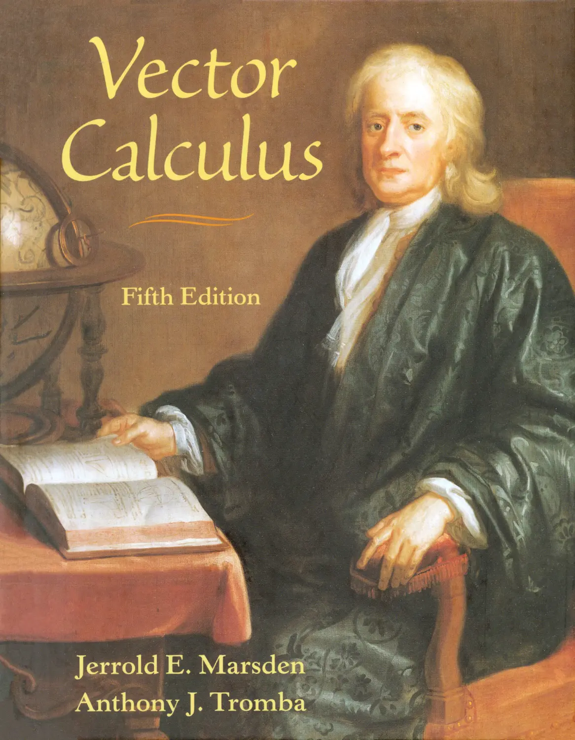
Vector Calculus
Fifth Edition
...- ---
Jerrold E. Marsden
California Institute of Technology, Pasadena
Anthony J. Tromba
University of California, Santa Cruz
rn
(f!!) W. H. Freeman and Company
New York

Executive Editor: Craig Bleyer
Acquisitions Editor: Terri Ward
Marketing Manager: Jeffrey Rucker
Project Editor: Vivien Weiss
Cover and Text Designer: Diana Blume
Production Manager: Julia DeRosa
Editorial Assistant: Kristy Cates
Media and Supplements Editor: Brian Donnellan
Illustration Coordinator: Shawn Churchman
Illustrations: The GTS Companies/York, PA Campus
Compositor: The GTS Companies/York, PA Campus
Manufacturer: RR Donnelly & Sons Company
Cover Photo: Isaac Newton (1642-1727). Painting by 1. Vanderbank (1725). London,
National Portrait Gallery.
Politics is for the moment.
An equation is for eternity.
A. EINSTEIN
Some calculus tricks are quite easy.
Some are enormously difficult. The fools
who write the textbooks of
advanced mathematics seldom take the trouble
to show you how easy the easy calculations are.
SILVANUS  THOMPSON, CALCULUS MADE EASY, MACMILLAN (1910)
Library of Congress Cataloging-in-Publication Data
Marsden, JerroldE.
Vector calculus/Jerrold E. Marsden, Anthony 1. Tromba.-5th ed.
p. cm.
Includes bibliographical references and index.
ISBN-I0: 0-7167-4992-0 ISBN-13: 978-0-7167-4992-9
1. Calculus. 2. Vector analysis. I. Tromba, Anthony. II. Title.
QA303.M338 2003
515'.63-dc21
2003049184
@1976, 1981, 1988, 1996, and 2003 by W. H. Freeman and Company
All rights reserved.
Printed in the United States of America
Fourth printing

(f()  -h -a -
Preface VII
Historical Introduction XIII
1 The Geometry of Euclidean Space 1
1.1 Vectors in Two- and Three-Dimensional Space 1
1.2 The Inner Product, Length, and Distance 23
1.3 Matrices, Determinants, and the Cross Product 38
1.4 Cylindrical and Spherical Coordinates 65
1.5 n-Dimensional Euclidean Space 74
Review Exercises for Chapter 1 88
2 Differentiation 94
2.1 The Geometry of Real-Valued Functions 94
2.2 Limits and Continuity 107
2.3 Differentiation 127
2.4 Introduction to Paths and Curves 141
2.5 Properties of the Derivative 150
2.6 Gradients and Directional Derivatives 163
Review Exercises for Chapter 2 173
3 Higher-Order Derivatives; Maxima and Minima 181
3.1 Iterated Partial Derivatives 182
3.2 Taylor's Theorem 193
3.3 Extrema of Real-Valued Functions 203
3.4 Constrained Extrema and Lagrange Multipliers 225
3.5 The Implicit Function Theorem 246
Review Exercises for Chapter 3 255
111

.
IV
Contents
4 Vector-Valued Functions 261
4.1 Acceleration and Newton's Second Law 261
4.2 Arc Length 274
4.3 Vector Fields 285
4.4 Divergence and Curl 294
Review Exercises for Chapter 4 313
5 Double and Triple Integrals 317
5.1 Introduction 317
5.2 The Double Integral Over a Rectangle 327
5.3 The Double Integral Over More General Regions 341
5.4 Changing the Order of Integration 349
5.5 The Triple Integral 354
Review Exercises for Chapter 5 365
6 The Change of Variables Formula and
Applications of Integration 368
6.1 The Geometry of Maps from ffi.2 to ffi.2 369
6.2 The Change of Variables Theorem 376
6.3 Applications 393
6.4 Improper Integrals 406
Review Exercises for Chapter 6 417
7 Integrals Over Paths and Surfaces 421
7.1 The Path Integral 421
7.2 Line Integrals 429
7.3 Parametrized Surfaces 451
7.4 Area of a Surface 461
7.5 Integrals of Scalar Functions Over Surfaces 474
7.6 Surface Integrals of Vector Fields 483
7.7 Applications to Differential Geometry, Physics, and Forms of Life 500
Review Exercises for Chapter 7 514

Contents
v
8 The Integral Theorems of Vector Analysis 518
8. 1 Green's Theorem 518
8.2 Stokes' Theorem 532
8.3 Conservative Fields 550
8.4 Gauss'Theorem 561
8.5 Some Differential Equations of Mechanics and Technology 576
8.6 Differential Forms 588
Review Exercises for Chapter 8 605
Answers to Odd-Numbered Exercises 609
Index 668
Illustration Credits 676

'f 0 cf3arbara and Inga for all their love and support

J[e
T his text is intended for a one-semester course in the calculus of functions of
several variables and vector analysis, which is normally taught at the sophomore
level. In addition to making changes and improvements throughout the text, in this new
edition we have added considerable material that presents the historical development
of the subject and have also attempted to convey a sense of excitement, relevance,
and importance of the subject matter.
Prerequisi tes
Sometimes courses in vector calculus are preceded by a first course in linear alge-
bra, but this is not an essential prerequisite. We require only the bare rudiments of
matrix algebra, and the necessary concepts are developed in the text. If this course
is preceded by a course in linear algebra, the instructor will have no difficulty en-
hancing the material. However, we do assume a knowledge of the fundamentals of
one-variable calculus-the process of differentiation and integration and their geo-
metric and physical meaning as well as a knowledge of the standard functions, such
as the trigonometric and exponential functions.
The Role of Theory
The text includes much of the basic theory as well as many concrete examples
and problems. Some of the technical proofs for theorems in Chapters 2 and 5
are given in optional sections that are readily available on the book's Web site at
www.whfreeman.com/MarsdenVC5e (see the description on the next page). Section
2.2, on limits and continuity, is designed to be treated lightly and is deliberately brief.
More sophisticated theoretical topics, such as compactness and delicate proofs in in-
tegration theory, have been omitted, because they usually belong to a more advanced
course in real analysis.
Concrete and Student-Oriented
Computational skills and intuitive understanding are important at this level, and we
have tried to meet this need by making the book concrete and student-oriented. For
example, although we formulate the definition of the derivative correctly, it is done by
using matrices of partial derivatives rather than abstract linear transformations. We
also include a number of physical illustrations such as fluid mechanics, gravitation,
. .
VII

VIII
Preface
and electromagnetic theory, and from economics as well, although knowledge of these
subjects is not assumed.
Order of T opies
A special feature of the text is the early introduction of vector fields, divergence, and
curl in Chapter 4, before integration. Vector analysis often suffers in a course of this
type, and the present arrangement is designed to offset this tendency. To go even fur-
ther, one might consider teaching Chapter 3 (Taylor's theorems, maxima and minima,
Lagrange multipliers) after Chapter 8 (the integral theorems of vector analysis).
This fifth edition was completely reset, but retains and improves on the balance
between theory, applications, optional material, and historical notes that was present
in earlier editions.
Supplelllents
One of the main changes in this edition is in the supplement. They are as follows:
1. Web Site. The book's Web site contains the following materials:
· Internet Supplement, a PDF file containing additional material suitable for
projects as well as technical proofs and sample examinations with complete
solutions.
· PowerPoint and KeyNote SUdes for instructors to use in presentations of the
text's figures, as well as section-by-section summaries.
· LaTeX and PDF Files of Sample Exams (on instructor's protected site)
· Updates
It is available to everyone and can be found at www.whfreeman.com/
Marsden VC5e.
2. Student Study Guide with Solutions. This student guide, written by Karen Pao
and Fred Soon, contains helpful hints and summaries for the material in each
section, contains the solutions to selected problems, and contains sample exams
to help students in exam preparation. Problems whose solutions appear in the
Student Study Guide have a colored number in the text, for easy reference. The
guide has been revised and reset for the Fifth Edition of Vector Calculus. ISBN
0-7167 -0528-1
3. Instructor's Manual with Solutions. This supplement contains material
available only to instructors. This includes summaries of material and additional
worked-out examples that are helpful in the preparation of lectures. It also
contains additional solutions to problems and sample exams (some of them with
complete solutions). ISBN 0-7167-0646-6
Final Exalll Questions
There are practice exams available in the Student Study Guide, the Internet supple-
ment, as well as in the Instructor's Manual. We also include some final exam ques-
tions (some of them challenging) for the reader's convenience on the book's Web site.

Preface
.
IX
Of course, the level and choice of topics and the lengths of final exams will vary from
instructor to instructor. Working these problems requires a knowledge of most of the
main material of the book, and solving 10 of these problems should take the reader
about 3 hours to complete. Some solutions are also given on the book's Web site.
We are excited about this new edition of Vector Calculus, especially the inclusion
of the new historical material as well as the new discussions of interesting applications
of vector analysis, both mathematical and physical. We hope that the reader will be
equally pleased.
Jerry Marsden and Tony Tromba,
Caltech and UC Santa Cruz, Summer 2003.

dh()w&d e"ht-e tA.-a -
M any colleagues and students in the mathematical community have made valu-
able contributions and suggestions since this book was begun. An early draft of
the book was written in collaboration with Ralph Abraham. We thank him for allowing
us to draw upon his work. It is impossible to list all those who assisted with this book,
but we wish especially to thank Michael Hoffman and Joanne Seitz for their help on
earlier editions. We also received valuable comments from Mary Anderson, John Ball,
Patrick Brosnan, Andrea Brose, David Dresin, Gerald Edgar, Michael Fischer, Frank
Gerrish, Mohammad Gohmi, Jenny Harrison, Jan Hogendijk, Jan-Jaap Oosterwijk,
and Anne van Weerden (Uterecht), David Knudson, Richard Kock, Andrew Lenard,
William McCain, Gordon McLean, David Merriell, Jeanette Nelson, Dan Norman,
Keith Phillips, Anne Perleman, Oren Walter Rosen, Kenneth Ross, Ray Sachs, Diane
Sauvageot, Joel Smoller, Francis Su, Melvyn Tews, Ralph and Bob Tromba, Steve
Wan, Alan Weinstein, John Wilker, and Peter Zvengrowski. The students and faculty
of Austin Community College deserve a special note of thanks, as do our students at
both Caltech and UC Santa Cruz.
We owe a very special thanks to Stefan Hildebrandt for his historical advice.
We are grateful to the following instructors who provided detailed reviews of
the manuscript. Dr. Michael Barbosu, SUNY Brockport; Brian Bradie, Christopher
Newport University; Mike Daven, Mount Saint Mary; Elias Deeba, University of
Houston-Downtown; John Feroe, Vassar; David Gurari, Case Western Reserve; Alan
Horowitz, Penn State; Rhonda Hughes, Bryn Mawr; Frank Jones, Rice University;
Richard Laugesen, University of Michigan; Namyong Lee, Minnesota State Uni-
versity; Tanya Leiese, Rose Hullman Institute; John Lott, University of Michigan;
Gerald Paquin, Universite du Quebec a Montreal; Joan Rand Moschovakis, Occiden-
tal College; A. Shadi Tahvildar-Zadeh, Princeton University; Howard Swann, San
Jose State University; Denise Szecsei, Stetson University; Edward Taylor, Wesleyan;
and Chaogui Zhang, Case Western Reserve. For the fifth edition, we want to thank
all the reviewers, but especially Andrea Brose, UCLA, for her detailed and valuable
comments. Most important of all are the readers and users of this book whose loyalty
for over a quarter of a century has made the fifth edition possible.
A final word of thanks goes to those who helped in the preparation of the
manuscript and the production of the book. For the earlier editions, we thank Connie
Calica, Nora Lee, Marnie McElhiney, Ruth Suzuki, lkuko Workman, and Esther Zack
.
Xl

. .
XII
Acknowledgements
for their excellent typing of various versions and revisions of the manuscript; Herb
Holden of Gonzaga University and Jerry Kazdan of the University of Pennsylvania
for suggesting and preparing early versions of the computer-generated figures; Jerry
Lyons and Holly Hodder for their roles as our previous mathematics editors; Christine
Hastings for editorial supervision; and Trumbull Rogers for his expert copyediting.
For this fifth edition, we thank Matt Haigh and Wendy McKay for their help with TeX
and Mathematica preparation of the material and also Terri Ward, the Mathematics
Acquisitions Editor at W H. Freeman for her excellent stewardship of the project, and
Vivien Weiss for her excellent handling of production matters.
We will be maintaining an up-to-date web-based list of corrections and sugges-
tions for the fifth edition and will be happy to receive any additional suggestions
and corrections from our readers. Please send your request to either Jerrold Marsden
(marsden@cds.caltech.edu) or Anthony Tromba (tromba@cats.ucsc.edu).

, ,
 6 -bift lec. t
,
 atJ dU l tLtJ tA. :
A Brief Account
This, therefore, is l\lathematics; she reminds you of the invisible form of
the soul; she gives life to her own discoveries; she awakens the mind and
purifies the intellect; she brings light to our intrinsic ideas; she abolishes
oblivion and ignorance which is ours by birth.
(j>roclus, c. 450
Cum Deus Calculat Fit J\lundus.
(As God calculates, so the world is created).
[gibniz, c. 1700
T he word mathematics derives from the Greek word mathema, meaning knowl-
edge, cognition, understanding, or perception, suggesting that the study of what
we now call mathematics began by asking questions about the world. In fact, the his-
torical evidence suggests that mathematics began about 2700 years ago as an attempt
to comprehend nature. Unfortunately, in most mathematical expositions, historical
motivations and contexts are often sacrificed. In this new edition, the authors con-
tinue to address this problem by increasing the discussion of historical and contextual
material where appropriate. Therefore, before we dive into the mathematics of Vector
Calculus, we briefly discuss the development of mathematics prior to and including
the discovery of calculus.
Egyptian, Babylonian, and Greek Mathelllatics
It is generally acknowledged that mathematics developed in the seventh and sixth
centuries B.C., somewhat after the Greeks had developed a uniform alphabet. This is not
to say, however, that mathematical knowledge did not exist before the Greeks. In fact,
the Egyptians and Babylonians knew many empirical facts centuries before the rise
of the Greek civilization. For example, they could solve quadratic equations, compute
the areas of certain geometric figures, such as squares, rectangles, and triangles, and
they possessed a reasonably good formula for the area of a circle, using the value of
3.16 for 1f. They also knew how to compute certain volumes like the size of cubes,
rectapgles, rectangular solids, cones, cylinders, and (not surprisingly) pyramids. The
ancients were also acquainted with the pythagorean theorem (at least empirically).
XIII

.
XIV
Historical In trod uction
The Greeks, who settled throughout the Mediterranean, must have played an
important role in preserving and spreading the mathematical knowledge of the Egyp-
tians and the Babylonians. However, the Greeks were aware that there were different
formulas for the same area or volumes. For example, the Babylonians had one formula
for the volume of a frustum of a pyramid with a square base, and the Egyptians had
another (see Figure 1).
L
f
h
1
Figure 1 Volume of a frustum of a pyramid with a
square base: V == h(a2 + ab + b 2 ).
It is not surprising that the Egyptians (with the experience in pyramid construc-
tion) had the correct formula. Now, given two formulas, it was clear that only one
could be correct. But how could one decide such an answer? Certainly it is not a
question for debate, as would be the question of the quality of works of art. It is
likely that the necessity to determine the answers to such questions is what led to the
development of mathematical proof and to the method of deductive reasoning.
The person usually credited for the invention of rigorous mathematical proof
was a merchant named Thales of Miletus (624-548 B.C.). It is Thales who is said
to be the creator of Greek geometry, and it was this geometry (earth measure) as an
abstract mathematical theory (rather than a collection of empirical facts) supported
by rigorous deductive proofs that was one of the turning points of scientific thinking.
It led to the creation of the first mathematical model for physical phenomena.
For example, one of the most beautiful geometric theories developed during
antiquity was that of conic sections. See Figure 2.
Conics include the straight line, circle, ellipse, parabola, and hyperbola. Their
discovery is attributed to Menaechmus, a member of the school of the great Greek
philosopher Plato. Plato, a student of Socrates, founded his school The Academy (see
Figure 3) in a sacred area of the ancient city of Athens, called Hekadameia (after
the hero Hekademos). All later academies obtained their name from this institution,
which existed without interruption for about 1000 years until it was dissolved by the
Roman Emperor Justinian in A.D. 529.
Plato suggested the following problem to his students:
Explain the motion of the heavenly bodies by some geometrical theolY.
Why was this a question of interest and puzzlement for the Greeks? Observed
from the Earth, these motions appear to be quite complicated. The motions of the
sun and the moon can be roughly described as circular with constant speed, but
the deviations from the circular orbit were troublesome to the Greeks and they felt
challenged to find an explanation for these irregularities. The observed orbits of the

Historical Introduction
xv
Figure 2 The conic sections: (A) hyperbola,
(B) parabola, (C) ellipse, (D) circle.
planets are even more complicated, because as they go through a revolution, they
appear to reverse direction several times.
The Greeks sought to understand this apparently wild motion by means of
their geometry. Eudoxus, Hipparchus, and then Apollonius of Perga (262-190 B.C.)
:::: ".:;
Figure 3 Plato s Academy (mosaic
found in Pompeii, Villa of T. Siminius
Stephanus, 86 x 85 cm, Naples,
Archaeological Museum). With certainty
the seven men have been identified as
Plato (third from the left) and six other
philosophers, who are talking about the
universe, the celestial spheres, and the
stars. The mosaic shows Plato's Academy,
with the city of Athens in the background.
It is probably a copy (from the first
century B.C.) of a Hellenistic painting.

.
XVI
Historical Introduction
suggested that the celestial orbits could be explained by combinations of circular mo-
tion (that is, through the construction of curves called epicycles traced out by circles
moving on other circles). This idea was to become the most important astronomical
theory of the next two thousand years. This theory, known by us through the writings
of the Greek astronomer Ptolemy of Alexandria, ultimately becomes known as the
"Ptolemaic theory." See Figures 4 and 5.
..... . "":";"'". -- -:---
. . ... 
IW." \k%}"'\:\",':,\"'''.' '
. A!::<....',:,
Figure 4 Woodcut from Georg von Peurbach's
Theoricae novae planetarum, edited by Oronce Fine as a
teaching text for the University of Paris (1515). It was the
canonical description of the heavens until the end of the
sixteenth century, and even Copernicus was to a large
extent under the influence of this work. Peurbach
described the solid sphere representations of Ptolemaic
planetary models, which he probably based on Ibn
al-Haytham's work "On the configuration of the world"
(translated into Latin in the thirteenth century). The same
frontispiece was used for the Sacrosbosco edition of the
first four books of Euclid's Elements (in excerpts), which
appeared under the title Textus de Sphaera in Paris
(1521).
Figure 5 Ptolemy observing the stars with a quadrant,
together with an allegoric Astronomia. (From Gregorius
Reish, Margarita Philosophica nova, Strasbourg, 1512,
an early compendium of philosophy and science.) In
those days, Ptolemy was often depicted as a king, because
he was erroneously thought to be descended from the
Ptolemaic dynasty that ruled Egypt after Alexander.

Historical Introduction
. .
XVII
Most of Greek geometry was codified by Euclid in his Elements (of Mathematics).
Actually the Elements consist of thirteen books, in which Euclid collected most of
the mathematical knowledge of his age (circa 300 B.C.), transforming it into a lucid,
logically developed masterpiece. In addition to the Elements, some of Euclid's other
writings were also handed down to us, including his Optics and the Catoptrica (theory
of mirrors).
The success of Greek mathematics had a profound effect on views of nature.
The Platonists, or followers of Plato, distinguished between the world of ideas and
the world of physical objects. Plato was the first to propose that ultimate truth or
understanding could not come from the material world, which is constantly subject to
change, but only from mathematical models or constructs. Thus, infallible knowledge
could be attained only through mathematics. Plato not only wished to use mathematics
in the study of nature, but he actually went so far as to attempt to substitute mathematics
for nature. For Plato, reality lies only within the realm of ideas, especially mathematical
ideas.
Not everyone in antiquity agreed with this point of view. Aristotle, a student of
Plato, criticized Plato's reduction of science to the study of mathematics. Aristotle
thought that the study of the material world was one's primary source of reality.
Despite Aristotle's critique, the view that mathematical laws governed the universe
took a firm hold on classical thought. The search for the mathematical laws of nature
was underway.
After the death of Archimedes in 212 B.C., Greek civilization went into a period of
slow decline. The final blow to Greek civilization came in 640 A.D. with the Moslem
conquest of Egypt. The remaining Greek texts housed in the great library in Alexandria
were burned. Those scholars who survived migrated to Constantinople (now part of
Turkey), which had become the capitol of the Eastern Roman Empire. It was in this
great city that what survived of Greek civilization was preserved for its rediscovery
by European civilization some five hundred years later.
Indian and Arabian Mathelllatics
Mathematical activity did not, however, cease with the decline of Greek civilization. In
the middle of the sixth century, somewhere in the Ganges Valley in India, our modern
system of numeration evolved. The Indians developed a nUlnber system based on ten,
with ten rather abstract symbols from zero to nine looking "roughly" as they do today.
They developed rules for addition, multiplication, and division (as we have today), a
system infinitely superior to the Roman abacus, which was used (by a special class
of servants called arithmeticians) throughout Europe until the fifteenth century. See
Figure 6.
After the fall of Egypt, came the rise of Arab civilization centered in Baghdad.
Scholars from Constantinople and India were invited to study and to share their
knowledge. It was through these contacts that the Arabs came to acquire the learning of
the ancients as well as the newly discovered Indian system of numeration. See Figure 7.
It was the Arabs who gave us the name Algebra, which comes from the book by
the astronomer Mohammed ibn Musa al-Khuwarizmi titled "AI-Jabr w'al muqabola,"

XVIII
Historical Introduction
..
Figure 6 Arithmetician performing
a calculation on a counter-abacus.
which means "restoring" or "balancing" (equations). AI-Khuwarizmi is also respon-
sible for a second profoundly influential book entitled "Kitab al jami' wa'l tafriq bi
hisab al hind" (Indian Technique of Addition and Subtraction), which described and
clarified the Indian decimal place value system.
AI-Khuwarizmi also gave us another name for a fundamental branch of science,
the word algorithm. Latinized, his name became Algorism, then Algorismus, and
finally Algorithm. The term initially represented the Indian system of numeration,
but ultimately came to be used in its modern computational sense.
The decline of Arab civilization coincided with the rise of European civilization.
The dawn of the modern age began when Richard the Lionhearted reached the walls
of Jerusalem. From approximately 1192 through around 1270, the Christian knights
brought the learning of the "infidels" back to Europe. Around 1200-1205, Leonardo
of Pisa (also known as Fibonacci), who had traveled extensively in Africa and Asia
Minor, wrote his interpretation (in Latin) of Arabic and Greek mathematics. His
.
J
tI""' l"ln'oof' fu\,..J,«.*l'"f'\u lu. if. I
fAf lrtCllhIa¥'I.1"  ,r t.l
.r*"rLrtt{ . -: tICttI4m I(Cl,,1...
rf 1Q1fL,.'tI U1IU'-' ..,...
b"" j""".1.4futl«"
w'- .¥.--'!i_ --  ;;W-"'t -;:_ '_"::t",",,,, <:.:;;0,--:1\;.& . ..;-'---:-1
I ' J ;._.._-"Q,'l'  -_-._-..- ¥ .-.-' t ::_'-- . 7 -- _ I i II  -
u u I ';119- .__.- -. -- _ f.
. . .. ., ".' . .
. "." -' .. -.." . . - .
- - :,. _ w... .,: ""!' J._ :.: __. - .- - , , ._ :.''':'. ;;_ - ,,-,., -
Figure 7 Detail from the Codex Vigilanus (976 A.D. northern Spain). The
first known occurrence of the nine Indo-Arabic numerals in Western Europe.
(Escurial Library, Madrid.)

Historical Introduction
.
XIX
historic texts brought the work of al-Khuwarizmi and Euclid to the attention of a
large audience in Europe.
European Mathematics
Around 1450 Johann Gutenberg invented the printing press with movable type. This,
combined with the advent of linen and cotton paper obtained from the Chinese,
dramatically increased the rate of the dissemination of knowledge. The steep rise in
trade and manufacturing fueled the growth of wealth and dramatic change in European
societies from feudal to city-states. In Italy, the mother of the Renaissance, we see the
rise of extraordinarily wealthy states such as Venice under the Doges and Florence
under the Medicis.
The needs of the rising merchant class accelerated the adoption of the Indian
system of numeration. The teachings of the Catholic Church, which rested on absolute
authority and dogma, began to be challenged by the ideas of Plato. From Plato, scholars
learned that the world was rational and could be understood, and that the means of
understanding nature was through mathematics. But this sharply contradicted the
teachings of the church, which taught that God designed the universe. The only
possible resolution of this apparent contradiction was that "God designed the universe
mathematically" or that "God is a mathematician."
It is perhaps surprising how much this point of view inspired the work of many
sixteenth- to eighteenth-century mathematicians and scientists. For if this were indeed
the case, then by understanding the mathematical laws of the universe, one could come
closer to an understanding of the Creator himself. Believe it or not, this point of view
survives to this day. The following is a quote from Paul Dirac, a Nobel Prize-winning
physicist and a creator of modern quantum mechanics.
It seems to be one of the fundamental features of nature that fundamental
physical laws are described in terms of a mathematical theory of great beauty
and power, needing quite a high standard of mathematics for one to understand
it. You may wonder: Why is nature constructed along these lines? One can only
answer that our present knowledge seems to show that nature is so constructed.
We simply have to accept it. One could perhaps describe the situation by saying
that God is a mathematician of a very high order, and He used very advanced
mathematics in constructing the universe. Our feeble attempts at mathematics
enable us to understand a bit of the universe, and as we proceed to develop higher
and higher mathematics we can hope to understand the universe better.
Mathematics began to see further advances and applications. In the sixteenth and
seventeenth centuries, al-Khuwarizmi's algebra was significantly advanced by Car-
dano, Vieta, and Descartes. The Babylonians had solved the quadratic equation, but
now two thousand years later, del Ferro and Tartaglia solved the cubic equation,
which in turn led to the discovery of imaginary numbers. These imaginary numbers
were later to playa fundamental role, as we shall see, in the development of vector
calculus. In the early seventeenth century, Descartes, perhaps motivated by the grid
technique used by Italian fresco painters to locate points on a wall or canvas, created,
in a moment of great mathematical inspiration, coordinate (or analytic) geometry.

xx
Historical Introduction
This new mathematical model enables one to reduce Euclid's geometry to algebra
and provides a precise and quantitative method to describe and calculate with space
curves and surfaces.
Early on, Archimedes' great work in statics and equilibrium (centers of gravity,
the principle of the lever-which we study in this book) was absorbed and improved
upon, leading to dramatic engineering achievements. In a building spree that remains
astonishing to this day, engineering advances made possible the rise of an incredible
number of cathedrals throughout Europe, including the stunning Duomo in Florence,
Notre Dame in Paris, and the Great Cathedral in Cologne, to mention a few. See
Figure 8.
.......,,'.;,.{.,.,...,'i.,-'..'.,. .:.. :,.'. .:..,.::...,.. .'.."":: ,:.:, .,...,... _ ....""" _-_--%;, "g.....- -w . = <"'-'__.'..' ,.. .
.,
Iii;
-
 .:4>
W j
:1[< u'
, .... ", . ,... . ., . . '.. , ' ,.. ., ... . ,.,
. ".'

.
"':." '.I'ojo<.
"'.'
..
. ':"..::. .."; ._:,,x;.
: *'
..
· t
181. t.'
.
"
Figure 8 Duomo.
Filippo Brunelleschi (1377-1446) studied the works of Euclid and Hipparchus and
was the first artist to employ mathematics extensively. The mathematical principles of
perspective were eventually completed by Piero della Francesca (1410-1492). Math-
ematicians and engineers were recruited by warring princes to fuel the development
of advanced weapons and ballistic science. The most famous among these was none
other than Leonardo da Vinci, who in the last years of his life was employed by the
Duke of Milan. It was in these final years that he painted the "Mona Lisa," now housed
in the Louvre in Paris. See Figure 9.
However, as in Greek times, it was astronomy that was to give mathematics its
greatest impetus. It is not surprising that the Greek astronomers placed the Earth and
not the sun at the center of our universe, because on a daily basis we see the sun
both rise and set. Still, it is interesting to ask if the Greeks, who were such marvelous
thinkers, at least tested the heliocentric theory, which places the sun at the center of the

Historical Introduction
. .  .::::
, -"""-; ,-;--- .,

,
ffi,;",,"

. t
..
'"
l
,
.-:...
'A;
::,:-
.
XXI
_.....-.
it.
E
.'.-
¥.
tj'
. 1
I
if

r

-.

r
,
+
I:
r
Figure 9 Leonardo, self portrait.
universe. In fact, they did. In the third century B.C., Aristarchus of Samus taught that
the Earth and other planets move in circular orbits around a fixed sun. His hypotheses
were, for severa] reasons, rejected. First, the opposing astronomers reasoned that if
the Earth were indeed moving, one should be able to sense it. Second, how would
objects, circulating with us, be able to stay on a moving Earth? Third, why are the
clouds not lagging behind the moving Earth?
Such arguments were to be used again in the sixteenth century against the Polish
astronomer Nicolas Copernicus (see Figure 10), who in 1543 introduced the helio-
centric theory (the planets move in orbit around the sun). His book Revolutionibus
Orbium Coelestium (On the Revolution of the Heavenly Orbits) was to initiate the
"Copernican revolution" in science and to give the world a new word, revolutionary.
In 1619, the German astronomer Johannes Kepler (see Figure 11), using the astro-
nomical calculations of the Danish astronomer Tycho Brahe, showed that the planetary
. ..:....::/'f ::""-:.: . .
Figure 10 Nicolaus Copernicus (1473-1543).

. .
XXII
Historical Introduction
orbits were in fact elliptical, the same ellipses that the Greeks had studied as abstract
forms some 2000 years earlier (see Figure 12).
But Kepler's law of elliptical orbits was only one of three laws he discovered
governing planetary motion. Kepler's second law states that if a planet moves from
a point A to another point B in a certain amount of time T , and also moves from A'
to B' in the same time, and if S is a focus of the orbital ellipse, then the sections SAB
are SA'B' have equal areas (see Figure 13). Kepler's third law was that the square of
time T a planetary body requires to complete an orbit is proportional to a 3 , where a
is the great axis of the elliptical orbit. In equation form, T 2 == K a 3 , where K is some
constant (we shall derive this law for circular orbits in Chapter 4).
. .,{j<: :;;"i0
i:;
Figure 11 Johannes Kepler
(1571-1630).
Figure 12 The motion of Mars. From
Kepler's Astronomia Nova (1609).
A'
B
A
Figure 13 Kepler's second law.
Profound as these observations were, an explanation of why these laws held was
lacking. However, by the middle of the seventeenth century, it was fully understood that
a change of velocity requires the action of forces, but how these forces influenced mo-
tion was not at all clear. In 1674 Robert Hooke, in an attempt to explain Kepler's laws,

Historical Introduction
XXIII
assumed the existence of an attractive force the sun must exert on the planets, a force
that decreased with planetary distance. Hooke's theory, however, was only qualitative.
Newton
What was also seriously lacking was a quantitative, precise definition of both velocity
and acceleration. This was ultimately solved by the invention of calculus by both
Isaac Newton and Gottfried Wilhelm Leibniz (see Figure 14). Hooke was never able
to achieve an understanding of the profound ideas behind the infinitesimal calculus.
However, during the period of 1679-1680 Hooke discussed his ideas with Newton,
including his conjecture that the force the sun exerts on the planets was actually
inversely proportional to the square of the planetary distance.
, . " .' '. )
. -.'-" .
.: iii; .)" ". .
<  ':;':" " 'J . '"
 , . '. 4 . ' ' . . ' ".
"'' .,,,\,
-, .:
, >
Figure 14 Gottfried Wilhelm Leibniz (1646-1716).
,
,
After Sir Christopher Wren, amateur astronomer, architect of the city of London
and London's magnificent St. Paul's Cathedral, issued a public challenge to "theo-
retically determine" the orbits of the planets, Isaac Newton took a serious interest in
the problem. Perhaps acting on rumors, the great British astronomer Edmund Halley
(1656-1743) in August 1684 visited Newton in Cambridge and asked him directly
what the orbit of a planet would be under an inverse square force. Newton answered
that it had to be an ellipse. As the stunned Halley asked him how he knew this, New-
ton's famous reply was" Why I have calculated it." Halley ultimately urged Newton to
publish his results as a book, and these appeared in 1686 in Newton's now legendary
Principia. See Figure 15.
This book, often and justly referred to as the foundation of modern science, had
an immediate dramatic impact. Alexander Pope wrote:
Nature and nature s laws lay hid at night,
God said, "Let Newton be" and all was light.
On the front cover of this text, we see Newton holding open a copy of his Principia.
Although Newton did not use calculus in the Principia, convincing arguments
have been put forward that Newton originally used his calculus to derive the

,
,I,
\
.
l' XXIV
Historical Introduction
d
'I
?
1
/
I
I
,
/,
i'
I '
"
,I'
PHILOSOPHIlE
NATURALIS
PRINCIPIA
Figure 15 The frontispiece of the
two-lines print of the Principia, carrying
the imprint "Prostat apud plures
Bibliopolas," which is sometimes called
the "first issue" of the first edition. The
"export copy" (with the three lines
"Prostant Venales apud Sam Smith...
aliosq; nonnullos Bibliopolas") is called
the second issue of the first edition. This
distinction between the first and second
issues seems to be quite unfounded. It has
been suggested that Halley made an
agreement with Smith concerning foreign
sales; in fact, most of Smith's fifty copies
were apparently sold on the continent.
MATHEMA TICA.
J
Autore 1 s. NEWTo N, Trin. oll. antab. oc. athefeos
ProfefTore Lucaftano, & SocIetatIs RegalJs Sodah.
IMPRIMATUR.
s. PEP Y S, Keg. Soc. P R .IE S E S.
Jtdii S. 1686.
LON DIN I,
]uiTu SocietatjJ' Kegi. ac Typis ]ofephi Streater. Profiat apud
plures Bibliopolas. Anno MDCLXXXVII.
trajectories of the planetary orbits from the inverse square law. * The Principia pro-
vided profound evidence that the universe, as the early Greeks had understood, was
indeed designed mathematically. Incidentally, it was Newton who first conceptualized
force as a vector, although he provided no formal definition of what a vector was.
Such a formal definition had to wait for William Rowan Hamilton, a century and a
half after the Principia. It was for this achievement and his creation of calculus itself
that we chose Newton for our cover.
The invention of the calculus and the subsequent development of vector calcu-
lus was the true beginning of modern science and technology, which has changed
our world so dramatically. From the mathematics ofNewton' m chanics to the pro-
found intellectual constructs of Maxwell's electrodynamics, Einstein's relativity, and
Heisenberg's and Schrodinger's quantum mechanics, we have seen the discoveries
of radio, television, wireless communications, flight, computers, space travel, and
countless engineering marvels.
Underlying all these developments was mathematics, an exciting adventure of the
mind and a celebration of the human spirit. It is in this context that we begin our
account of Vector calculus.
*We shall study the problem of planetary orbits in Section 4.1 and further in the Internet supplement.

,"
J[eJ[e
, ,
ut.6 t.IT6
dtA..d
,
(){d fLtJ tA..
We assume that students have studied the calculus of functions of a real variable,
including analytic geometry in the plane. Some students may have had some exposure
to matrices as well, although what we shall need is given in Sections 1.3 and 1.5.
We also assume that students are familiar with functions of elementary calculus,
such as sin x, cos x , eX, and log x (we write log x or In x for the natural logarithm,
which is sometimes denoted loge x). Students are expected to know, or to review as the
course proceeds, the basic rules of differentiation and integration for functions of one
variable, such as the chain rule, the quotient rule, integration by parts, and so forth.
We now summarize the notations to be used later. Students can read through these
quickly now, then refer to them later if the need arises.
The collection of all real numbers is denoted JR. Thus JR includes the integers, . . . ,
-3, -2, -1,0, 1,2,3, ...; the rational numbers, p/q, where p and q are integers
(q #- 0); and the irrational numbers, such as -/2,1f, and e. Members ofJR may be
visualized as points on the real-number line, as shown in Figure  1.
- .. .. .. . . . . .. . .
-3 -2 -1 0 1 1 n 2 e 3 1t
T
Figure P.l The geometric representation of points on the real-number line.
When we write a E JR we mean that a is a member of the set JR, in other words, that
a is a real number. Given two real numbers a and b with a < b (that is, with a less than
b), we can form the closed interval [a, b], consisting of all x such that a < x < b,
and the open interval (a, b), consisting of all x such that a < x < b. Similarly, we
can form half-open intervals (a, b] and [a, b) (F igure 2).
a
b
c
d
e
f
___a
n
0.
.
(),
..
Closed
Open
Half open
i /
Figure P.2 The geometric representation of the intervals [a, b], (c, d), and [e, f).
xxv

.
XXVI
Prerequisites and Notation
The absolute value of a number a E IR is written la I and is defined as
lal == { a
-a
if a > 0
if a < O.
For example, 131 == 3,1-31 == 3,101 == 0, and 1-61 == 6. The inequality la + bl <
lal + Ibl always holds. The distance from a to b is given by la - bl. Thus, the
distance from 6 to 10 is 4 and from - 6 to 3 is 9.
If we write A c IR, we mean A is a subset of IR. For example, A could equal the set
of integers {. . . , -3, -2, -1, 0, 1, 2, 3, . . .}. Another example of a subset ofIR is the
set Q of rational numbers. Generally, for two collections of objects (that is, sets) A
and B, A c B means A is a subset of B; that is, every member of A is also a member
of B.
The symbol A U B means the union of A and B, the collection whose members
are members of either A or B (or both). Thus,
{..., -3, -2, -1,0} U {-1,0, 1,2, ...} == {..., -3, -2, -1,0,1,2, ...}.
Similarly, A n B means the intersection of A and B; that is, this set consists of those
members of A and B that are in both A and B. Thus, the intersection of the two sets
above is {- 1, O}.
We shall write A \ B for those members of A that are not in B. Thus,
{..., -3, -2, -1, 0}\{-1, 0,1,2,...} == {..., -3, -2}.
We can also specify sets as in the following examples:
{a E IR I a is an integer} == {. . . , - 3, - 2, -1, 0, 1, 2, . . .}
{a E IR I a is an even integer} == {. . . , -2, 0, 2, 4, . . .}
{x EIRla < x < b}==[a,b].
Afunction I: A -+ B is a rule that assigns to each a E A one specific member f(a)
of B. We call A the domain of I and B the target of I. The set {I (x) I x E A}
consisting of all the values of I(x) is called the range of I. Denoted by I(A), the
range is a subset of the target B. It may be all of B, in which case I is said to be
onto B. The fact that the function I sends a to I(a) is denoted by a  I(a). For
example, the function I(x) == x 3 /(1 - x) that assigns the number x 3 /(1 - x) to each
x #- 1 in IR can also be defined by the rule x  x 3 /(1 - x). Functions are also called
mappings, maps, or transformations. The notation f: A c IR -+ IR means that A is
a subset ofJR and that I assigns a value I(x) in IR to each x E A. The graph of I
consists of all the points (x, I(x)) in the plane (Figure 3).

Prerequisites and Notation
. .
XXVII
y
Graph of f
(x. f;J
I
I
I
I
I
I
I
I
X
Figure P.3 The graph of a function with the
half-open interval A as domain.
x
A = domain
The notation E7 = 1 ai means a 1 + . . . + an, where aI, . . . , an are given numbers.
The sum of the first n integers is
n n(n + 1)
1+2+...+n==Li== .
i=1 2
The derivative of a function f(x) is denoted f' (x), or
df
dx'
and the definite integral is written
I b f(x)dx.
If we set y == f(x), the derivative is also denoted by
dy
dx
Readers are assumed to be familiar with the chain rule, integration by parts, and
other basic facts from the calculus of functions of one variable. In particular, they
should know how to differentiate and integrate exponential, logarithmic, and trigono-
metric functions. Short tables of derivatives and integrals, which are adequate for the
needs of this text, are printed at the front and back of the book.
The following notations are used synonymously: eX == exp x , In x == log x, and
sin- 1 x == arcsin x .
The end of a proof is denoted by the symbol., while the end of an example or
remark is denoted by the symbol..

1
The Geometry of
Euclidean Space
Quaternions came from Hamilton. . . and have been an unmixed evil to
those who have touched them in any way. Vector is a use less survival . . .
and has never been of the slightest use to any creature.
£grd JCelvin
I n this chapter we consider the basic operations on vectors in two- and three-
dimensional space: vector addition, scalar multiplication, and the dot and cross
products. In Section 1.5 we generalize some of these notions to n-space and review
properties of matrices that will be needed in Chapters 2 and 3.
1.1 Vectors in Two- and Three-DiInensional Space
Points P in the plane are represented by ordered pairs of real numbers (at, a2); the
numbers al and a2 are called the Cartesian coordinates of  We draw two perpen-
dicular lines, label them as the x and y axes, and then drop perpendiculars from P to
these axes, as in Figure 1.1.1. After designating the intersection of the x and y axes
as the origin and choosing units on these axes, we produce two signed distances a 1
and a2 as shown in the figure; al is called the x component of and a2 is called the
y component.
Points in space may be similarly represented as ordered triples of real numbers.
To construct such a representation, we choose three mutually perpendicular lines
that meet at a point in space. These lines are called x axis, y axis, and z axis, and the
point at which they meet is called the origin (this is our reference point). We choose
a scale on these axes, as shown in Figure 1.1.2.
1

2
The Geometry of Euclidean Space
y
a2
- - .. P = (a p a 2 )
I
I
I
I
I
I
I
I
Figure 1.1.1 Cartesian coordinates in the plane.
x
'--v---.J
a}
z
3
2
1
Figure 1.1.2 Cartesian coordinates in space.
y
x
The triple (0, 0, 0) corresponds to the origin of the coordinate system, and the
arrows on the axes indicate the positive directions. For example, the triple (2, 4, 4)
represents a point 2 units from the origin in the positive direction along the x axis,
4 units in the positive direction along the y axis, and 4 units in the positive direction
along the z axis (Figure 1.1.3).
z
-----71
/
(2,4,4)/ I
---, I
I I
I I
I
2: //4
----_..:/
Figure 1.1.3 Geometric representation of the point (2, 4, 4)
in Cartesian coordinates.
y
x
Because we can associate points in space with ordered triples in this way, we often
use the expression "the point (aI, a2, a3)" instead of the longer phrase "the point P

1.1 Vectors in Two- and Three-Dimensional Space
3
that corresponds to the triple (aI, a2, a3)." We say that al is the x coordinate (or first
coordinate), a2 is the y coordinate (or second coordinate), and a3 is the z coordinate
(or third coordinate) of It is also common to denote points in space with the letters
x, y, and z in place of aI, a2, and a3. Thus, the triple (x, y, z) represents a point whose
first coordinate is x, second coordinate is y, and third coordinate is z.
We employ the following notation for the line, the plane, and three-dimensional
space:
(i) The real number line is denoted}R1 or simply}R.
(ii) The set of all ordered pairs (x, y) of real numbers is denoted }R2.
(iii) The set of all ordered triples (x, y, z) of real numbers is denoted }R3 .
When speaking of }R I , }R2, and }R3 simultaneously, we write }Rn, where n = 1, 2,
or 3; or }Rm, where m = 1,2,3. Starting in Section 1.5 we will also study }Rn for
n = 4, 5, 6, . . ., but the cases n = 1, 2, 3 are closest to our geometric intuition and
will be stressed throughout the book.
Vector Addition and Scalar Multiplication
The operation of addition can be extended from}R to}R2 and}R3. For}R3, this is done
as follows. Given the two triples (aI, a2, a3) and (hI, h 2 , h 3 ), we define their sum to be
(aI, a2, a3) + (hI, h 2 , h 3 ) = (al + hI, a2 + h 2 , a3 + h 3 ).
. .1
(1,1,1) + (2, -3,4) = (3, -2,5),
(x , y, z) + (0, 0, 0) = (x, y, z),
(1, 7,3)+(a,h,c) = (1 +a, 7+h,3+c). ...
The element (0,0,0) is called the zero element (or just zero) of}R3. The element
(-at, -a2, -a3) is the additive inverse (or negative) of (a I , a2, a3), and we will write
(a I , a2, a3) - (hI, h 2 , h 3 ) for (a I , a2, a3) + (-hI, -h 2 , -h 3 ).
The additive inverse, when added to the vector itself, of course produces zero:
(a I , a2, a3) + (-aI, -a2, -a3) = (0,0,0).
There are several important product operations that we will define on }R3. One
of these, called the inner product, assigns a real number to each pair of elements of
}R3. We shall discuss it in detail in Section 1.2. Another product operation for}R3 is
called scalar multiplication (the word "scalar" is a synonym for "real number"). This
product combines scalars (real numbers) and elements of}R3 (ordered triples) to yield
elements of}R3 as follows: Given a scalar a and a triple (a I , a2, a3), we define the
scalar"multiple by
a(al, a2, a3) = (aal, aa2, aa3).

4
The Geometry of Euclidean Space
.  .
2(4, e, 1) = (2.4,2. e, 2.1) = (8, 2e, 2),
6( 1, 1, 1) = (6, 6, 6),
l(u, v, w) = (u, v, w),
O(p, q, r) = (0, 0, 0). .
Addition and scalar multiplication of triples satisfy the following properties:
(i) (afJ)(al, a2, a3) = a[fJ(al, a2, a3)] (associativity)
(ii) (a + fJ)(al, a2, a3) = a(al, a2, a3) + fJ(al, a2, a3) (distributivity)
(iii) a[(al, a2, a3) + (hi, h 2 , h 3 )] = a(al, a2, a3) + a(h l , h 2 , h 3 ) (distributivity)
(property of zero)
(property of zero)
(property of the
unit element)
The identities are proven directly from the definitions of addition and scalar
multiplication. For instance,
(iv) a(O, 0, 0) = (0, 0, 0)
(v) O(al, a2, a3) = (0, 0, 0)
(vi) l(al, a2, a3) = (ai, a2, a3)
(a + fJ)(al, a2, a3) = ((a + fJ)al, (a + fJ)a2, (a + fJ)a3)
= (aal + fJal, aa2 + fJ a 2, aa3 + fJa3)
= a(al, a2, a3) + fJ(al, a2, a3).
For }R2, addition and scalar multiplication are defined just as in }R3, with the third
component of each vector dropped off. All the properties (i) to (vi) still hold.
I ..  · Interpret the chemical equation 2NH 2 + H 2 = 2NH 3 as a relation
in the algebra of ordered pairs.
SOLUTION We think of the molecule NxHy (x atoms of nitrogen, y atoms of
hydrogen) as represented by the ordered pair (x, y). Then the chemical equation given
is equivalent to 2(1, 2) + (0, 2) = 2(1, 3). Indeed, both sides are equal to (2, 6). .
Geometry of Vector Operations
Let us turn to the geometry of these operations in}R2 and}R3 . For the moment, we define
a vector to be a directed line segment beginning at the origin, that is, a line segment
with specified magnitude and direction, and initial point at the origin. Figure 1.1.4
shows several vectors, drawn as arrows beginning at the origin. In print, vectors are

1.1 Vectors in Two- and Three-Dimensional Space
5
usually denoted by boldface letters such as a. By hand, we usually write them as a or
simply as a, possibly with a line or wavy line under it.
z
Figure 1.1.4 Geometrically, vectors are thought of as
arrows emanating from the origin.
y
x
U sing this definition of a vector, we associate with each vector a the point
(al, a2, a3) where a terminates, and conversely, we can associate a vector a with
each point (a I , a2, a3) in space. Thus, we shall identify a with (a I , a2, a3) and write
a == (a I , a2, a3). For this reason, the elements of}R3 not only are ordered triples of
real numbers, but are also regarded as vectors. The triple (0, 0, 0) is denoted o.
We call aI, a2, and a3 the components of a, or when we think of a as a point, its
coordinates.
Two vectors a == (a I , a2, a3) and b == (hI, h 2 , b 3 ) are equal if and only if al == hI,
a2 == h 2 , and a3 == h3. Geometrically this means that a and b have the same direction
and the same length (or "magnitude").
Geometrically, we define vector addition as follows. In the plane containing the
vectors a == (a I , a2, a3) and b == (hI, h 2 , h 3 ) (see Figure 1.1.5), form the parallelogram
having a as one side and b as its adjacent side. The sum a + b is the directed line
segment along the diagonal of the parallelogram.
z
Figure 1.1.5 The geometry of vector addition.
x
This geometric view of vector addition is useful in many physical situations, as
we shall see in the next section. For an easily visualized example, consider a bird or
an airplane flying through the air with velocity v I, but in the presence of a wind with
velocity V2. The resultant velocity, VI + V2, is what one sees; see Figure 1.1.6.

6
The Geometry of Euclidean Space
z

x
Figure 1.1.6 A physical interpretation of vector addition.
To show that our geometric definition of addition is consistent with our alge-
braic definition, we demonstrate that a + b == (a I + b I , a2 + b 2 , a3 + b 3 ). We shall
prove this result in the plane and leave the proof in three-dimensional space to the
reader. Thus, we wish to show that if a == (a I , a2) and b == (b I , b2), then a + b ==
(a I + b I , a2 + b 2 ).
In Figure 1.1.7 let a == (a I , a2) be the vector ending at the point A, and let
b == (b I , b 2 ) be the vector ending at point B. By definition, the vector a + bends
at the vertex C of parallelogram OBCA. To verify that a + b == (a I + b I , a2 + b 2 ),
it suffices to show that the coordinates of Care (a I + b I , a2 + b 2 ). The sides of
the triangles OAD and BCG are parallel, and the sides OA and BC have equal
lengths, which we write as OA == BC. These triangles are congruent, so BG == OD;
since BGFE is a rectangle, EF == BG. Furthermore, OD == al and OE == b l . Hence,
EF == BG == OD == al. Since OF == EF + OE, it follows that OF == al + b l . This
shows that the x coordinate of a + b is al + b l . The proof that the y coordinate
is a2 + b 2 is analogous. This argument assumes A and B to be in the first quadrant,
but similar arguments hold for the other quadrants.
y
c
Figure 1.1.7 The construction used to prove that
(aI, a2) + (b I , b2) == (al + b I , a2 + b 2 ).
o
x
D
E
F
Figure 1.1.8(a) illustrates another way of looking at vector addition: in terms
of triangles rather than parallelograms. That is, we translate (without rotation) the
directed line segment representing the vector b so that it begins at the end of the
vector a. The endpoint of the resulting directed segment is the endpoint of the vector

1.1 Vectors in Two- and Three-Dimensional Space
7
a + b. We note that when a and b are collinear, the triangle collapses to a line segment,
as in Figure 1.1.8(b).
y
y
x
x
a+b
a
(a)
(b)
Figure 1.1.8 (a) Vector addition may be visualized in terms of triangles as well
as parallelograms. (b) The triangle collapses to a line segment when a and bare
co llinear.
In Figure 1.1.8 we have placed a and b head to tail. That is, the tail ofb is placed
at the head of a, and the vector a + b goes from the tail of a to the head ofb. Ifwe do
it in the other order, b + a, we get the same vector by going around the parallelogram
the other way. Consistent with this figure, it is useful to let vectors "glide" or "slide,"
keeping the same magnitude and direction. We want, in fact, to regard two vectors
as the same if they have the same magnitude and direction. When we insist on vec-
tors beginning at the origin, we will say that we have bound vectors. If we allow
vectors to begin at other points, we will speak of free vectors or just vectors.
Vectors Vectors (also called free vectors) are directed line segments in [the
plane or] space represented by directed line segments with a beginning (tail)
and an end (head). Directed line segments obtained from each other by parallel
translation (but not rotation) represent the same vector.
The components (a 1 , a2, a3) of a are the (signed) lengths of the proj ections
of a along the three coordinate axes; equivalently, they are defined by placing
the tail of a at the origin and letting the head be the point (aI, a2, a3). We write
a == (aI, a2, a3).
Two vectors are added by placing them head to tail and drawing the vectors
from the tail of the first to the head of the second, as in Figure 1.1.8.
Scalar multiplication of vectors also has a geometric interpretation. If a is a scalar
and a a vector, we define aa to be the vector that is lal times as long as a, with the
same direction as a if a > 0, but with the opposite direction if a < O. Figure 1.1.9
illustrates several examples.

8
The Geometry of Euclidean Space
y
y
1
y
y
J
la
2
-x
x
1
--a
4
-x
1-a
4
.x
Figure 1.1.9 Some scalar multiples of a vector a.
Using an argument based on similar triangles, one finds that if a = (aI, a2, a3),
and a is a scalar, then
aa = (aal, aa2, aa3).
That is, the geometric definition coincides with the algebraic one.
Given two vectors a and b, how do we represent the vector b - a geometrically,
that is, what is the geometry of vector subtraction? Because a + (b - a) = b, we
see that b - a is the vector that one adds to a to get b. In view of this, we may
conclude that b - a is the vector parallel to, and with the same magnitude as, the
directed line segment beginning at the endpoint of a and terminating at the endpoint
of b when a and b begin at the same point (see Figure 1.1.10).
y
A
a l
B
Figure 1.1.10 The geometry of vector subtraction.
x
· 4 Let u and v be the vectors shown in Figure 1.1.11. Draw the two
vectors u + v and -2u. What are their components?

1.1 Vectors in Two- and Three-Dimensional Space
9
y
2
1
-----------------------
I
I
I
U I
I
I
I
I
I
V I
Figure 1.1.11 Find u + v and -2u.
x
2 3
SOLUTION Place the tail of v at the tip of u to obtain the vector shown in
Figure 1.1.12.
y
v
x
Figure 1.1.12 Computing u + v and
-2u.
-6
-1
1 v 2 3 4 5
-2u
-2
-3
-4
The vector -2u, also shown, has length twice that ofu and points in the opposite
direction. From the figure, we see that the vector u + v has components (5, 2) and
-2u has components (-6, -4). .
I EXAMPLE 5
(a) Sketch -2v, where v has components (-1, 1,2).
(b) Ifv and ware any two vectors, show that v -1w and 3v - ware parallel.
SOLUTION
(a) The vector -2v is twice as long as v, but points in the opposite direction (see
Figure 1.1.13).
(b) v - w == (3v - w); vectors that are multiples of one another are parallel. .

10
The Geometry of Euclidean Space
z
(-1,1,2)
y
Figure 1.1.13 Multiplying (-1, 1, 2)
by -2.
x
(2,-2,-4)
The Standard Basis Vectors
To describe vectors in space, it is convenient to introduce three special vectors along
the x, y, and z axes:
i: the vector with components (1, 0, 0)
j: the vector with components (0, 1, 0)
k: the vector with components (0, 0, 1).
These standard basis vectors are illustrated in Figure 1.1.14. In the plane one has the
standard basis i and j with components (1, 0) and (0, 1).
z
Lo,o, I)
(I,
x
Figure 1.1.14 The standard basis vectors.
. Y
Let a be any vector, and let (aI, a2, a3) be its components. Then
a = ali + a2j + a3k,
because the right-hand side is given in components by
aI(I, 0, 0) + a2(0, 1,0) + a3(0, 0, 1) = (at, 0, 0) + (0, a2, 0) + (0, 0, a3)
= (aI, a2, a3).

1 1 Vectors in Two- and Three-Dimensional Space
11
Thus, we can express every vector as a sum of scalar multiples of i, j, and k.
The Standard Basis Vectors
1. The vectors i, j, and k are unit vectors along the three coordinate axes, as
shown in Figure 1.1.14.
2. If a has components (ai, a2, a3), then
a=a l i+a2j+a3 k .
EXAMPLE 6 Express the vector whose components are (e, Jr, -.J3) in the stan-
dard basis.
SOLUTION Substituting al = e, a2 = Jr, and a3 = -.J3 into a = ali + a2j +
a3k gives
v = ei + Jrj - .J3k. .
EXAMPLE 7 The vector (2, 3,2) equals 2i + 3j + 2k, and the vector (0, -1,4)
is -j + 4k. Figure 1.1.15 shows 2i + 3j + 2k; the student should draw in the vector
-j+4k. .
z
Figure 1.1.15 Representation of (2, 3, 2) in terms
of the standard basis vectors i, j, and k.
)L Y
x
Addition and scalar multiplication may be written in terms of the standard basis
vectors as follows:
(ali + a2j + a3 k ) + (bli + b2j + b 3 k) = (al + bl)i + (a2 + b 2 )j + (a3 + b 3 )k
and
a(ali + a2j + a3 k ) = (aal)i + (aa2)j + a(a3)k.

12
The Geometry of Euclidean Space
The Vector Joining Two Points
To apply vectors to geometric problems, it is useful to assign a vector to a pair of
points in the plane or in space, as follows. Given two points P and P', we can draw

the vector v with tail P and head P', as in Figure 1.1.16, where we write PP' for v.
pp'
p'

Figure 1.1.16 The vector from P to P' is denoted PP'.
p
If P == (x, y, z) and P' == (x', y' , z'), then the vectors from the origin to P and P'

are a == xi + yj + zk and a' == x'i + y'j + z'k, respectively, so the vector pp' is the
difference a' - a == (x' - x)i + (y' - y)j + (z' - z)k. (See Figure 1.1.17.)
y
a' - a p'
p ----------
j a'
-+, -+, 
Figure 1.1.17 PP == OP - OPe
x
o
The Vector Joining Two Points If the point P has coordinates (x, y, z) and

P' has coordinates (x', y', z'), then the vector PP' from the tip of P to the tip of
P' has components (x' - x, y' - y, z' - z).
. .
.
(a) Find the components of the vector from (3, 5) to (4, 7).
(b) Add the vector v from (-1,0) to (2, -3) and the vector w from (2, 0) to (1, 1).
(c) Multiply the vector v in (b) by 8. If the resulting vector is represented by the
directed line segment from (5, 6) to Q, what is Q?
SOLUTION
(a) As in the preceding box, we subtract the ordered pairs: (4,7) - (3, 5) == (1,2).
Thus the required components are (1, 2).
(b) The vector v has components (2, -3) - (-1, 0) == (3, -3), and w has com-
ponents (1, 1) - (2, 0) == (-1, 1). Therefore, the vector v + w has compo-
nents (3, -3) + (-1, 1) == (2, -2).

1.1 Vectors in Two- and Three-Dimensional Space
13
(c) The vector 8v has components 8(3, -3) == (24, -24). If this vector is rep-
resented by the directed line segment from (5, 6) to Q, and Q has coordi-
nates (x, y), then (x, y) - (5, 6) == (24, -24), so (x, y) == (5,6) + (24, -24) ==
(29, -18). ..
EXAMPLE 9 Let P == (-2, -1), Q == (-3, -3), and R == (-1, -4) in the xy
plane.
(a) Draw these vectors: v joining P to Q; w joining Q to R; ujoining R to 
(b) What are the components of v, w, and u?
(c) What is v + w + u?
SOLUTION
(a) See Figure 1.1.18.
y
x
Figure 1.1.18 The vector v joins P to Q; w joins Q to R;
and ujoins R to 
p
v
u
Q.
R
-3
-4
  ---+
(b) Because v == PQ, w == QR, and u == RP, we get
v == (-3, -3) - (-2, -1) == (-1, -2),
w == (-1, -4) - (-3, -3) == (2, -1),
u == -(-1, -4) + (-2, -1) == (-1,3).
(c) v + w + u == (-1, -2) + (2, -1) + (-1, 3) == (0,0). ..
Geometry Theorems by Vector Methods
Many of the theorems of plane geometry can be proved by vector methods Here is
one example.

14
The Geometry of Euclidean Space
EXA1PLE 10 Use vectors to prove that the diagonals of a parallelogram bisect
each other.
SOLUTION Let OPRQ be the parallelogram, with two adjacent sides represented
 
by the vectors a = OP and b = OQ. Let M be the midpoint of the diagonal OR, N
the midpoint of the other diagonal, PQ. (See Figure 1.1.19.)
p
p
R
R
Figure 1.1.19 If the midpoints M and N
coincide, then the diagonals OR and PQ
bisect each other.
o
o
Q
Q
  
Observe that OR = OP + OQ = a + b by the parallelogram rule for vector ad-
 
dition, so OM = !OR = !(a + b). On the other hand,
  
PQ = OQ - OP = b - a,
so
 1 1
PN = 2: P Q = 2:(b - a),
and hence
  
ON = OP + PN = a + !(b - a) = 4(a + b).
 
Because OM and ON are equal vectors, the points M and N coincide, so the diagonals
bisect each other. .
Equations of Lines
Planes and lines are geometric objects that can be represented by equations. We shall
defer until Section 1.3 a study of equations representing planes. However, using the
geometric interpretation of vector addition and scalar multiplication, we will now
find the equation of a line I that passes through the endpoint of the vector a, with the
direction of a vector v (see Figure 1.1.20).
As t varies through all real values, the points of the form tv are all scalar
multiples of the vector v, and therefore exhaust the points of the line passing through
the origin in the direction of v. Because every point on I is the endpoint of the diagonal
of a parallelogram with sides a and tv for some real value of t, we see that all the
points on I are of the form a + tv. Thus, the line I may be expressed by the equation
let) = a + tv. We say that I is expressed parametrically, with t the parameter. At
t = 0, let) = a. As t increases, the point let) moves away from a in the direction ofv.

1.1 Vectors in Two- and Three-Dimensional Space
15
tv
I
Figure 1.1.20 The line I, parametrically
given by I(t) = a + tv, lies in the direction
v and passes through the tip of a.
a
As t decreases from t = 0 through negative values, I(t) moves away from a in the
direction of -v.
Point- Direction Form of a Line The equation of the line I through the tip of a
and pointing in the direction of the vector v is I(t) = a + tv, where the parameter
t takes on all real values. In coordinate form, the equations are
X=XI+at,
Y=YI+bt,
Z=ZI+ct,
where a = (XI, YI, ZI) and v = (a, b, c). For lines in the xy plane, one simply
drops the Z component.
XAMPLE 1 Determine the equation of the line I passing through (1, 0, 0) in
the direction j. See Figure 1.1.21.
z
j
y
Figure 1.1.21 The line I passes
through the tip of i in the direction j.
I
I(t)
x

16
The Geometry of Euclidean Space
SOLUTION The desired line can be expressed parametrically as I(t) == i + tj. In
terms of coordinates,
I(t) == (1,0,0) + t(O, 1,0) == (1, t, 0). .
XAMPLE 12
( a) Find the equations of the line in space through the point (3, -1, 2) in the direction
2i - 3j + 4k.
(b) Find the equation of the line in the plane through the point (1, -6) in the direction
of 5i - nj.
(c) In what direction does the line x == -3t + 2, y == -2(t - 1), z == 8t + 2 point?
SOLUTION
(a) Here a == (3, -1,2) == (x], y], z]) and v == 2i - 3j + 4k, soa == 2, b == -3, and
c == 4. From the box above, the equations are
x == 3 + 2t,
y==-1-3t,
z == 2 + 4t.
(b) Here a == (1, -6) and v == 5i - n j, so the required line is
I(t) == (1, -6) + (5t, -nt) == (1 + 5t, -6 - nt);
that is,
x == 1 + 5t,
y == -6 - nt.
(c) Using the preceding box, we construct the direction v == ai + bj + ck from the
coefficients of t: a == -3, b == -2, c == 8. Thus, the line points in the direction
ofv == -3i - 2j + 8k. .
. ·  · Do the two lines (x, y, z) == (t, -6t + 1, 2t - 8) and (x, y, z) ==
(3t + 1, 2t, 0) intersect?
SOLUTION If the lines intersect, there must be numbers t] and t2 such that the
corresponding points are equal:
(t], -6t] + 1, 2t] - 8) == (3t2 + 1, 2t2, 0);
that is, all three of the following equations hold:
t] == 3t2 + 1,
-6t] + 1 == 2t2,
2t] - 8 == O.

1.1 Vectors in Two- and Three-Dimensional Space
17
From the third equation, tl == 4. The first equation then becomes 4 == 3t2 + 1; that is,
t2 == 1. We must check whether these values satisfy the middle equation:
?
-6t] +] . 2t2.
Since tl == 4 and t2 == 1, this reads
?
-24 + 1 . 2,
which is false, so the lines do not intersect. .
Notice that there can be many equations of the same line. Some may be obtained
by choosing instead of a, a different point on the given line, and forming the parametric
equation of the line beginning at that point and in the direction of v. For example, the
endpoint of a + v is on the line I( t) == a + tv, and thus, I} (t) == (a + v) + tv represents
the same line. Still other equations may be obtained by observing that if a i= 0, the
vector av has the same (or opposite) direction as v. Thus, 1 2 (t) == a + tav is another
equation ofl(t) == a + tv.
For example, both I(t) == (1,0,0) + (t, t, 0) and I](s) == (0, -1,0) + (s, s, 0)
represent the same line since both are in the direction i + j and both pass through
the point (1, 0, 0); I passes through (1, 0, 0) at t == 0 and 11 passes through (1, 0, 0) at
s == 1.
Therefore, the equation of a line is not uniquely determined. Nevertheless, it
is customary to use the term "the" equation of a line. Keeping this in mind, let us
derive the equation of a line passing through the endpoints of two given vectors a
and b. Because the vector b - a is parallel to the directed line segment from a to b,
we calculate the parametric equation of the line passing through a in the direction of
b - a (Figure 1.1.22). Thus,
I(t) == a + t(b - a);
that is,
I(t) == (1 - t)a + tb.
Figure 1.1.22 The line I, parametrically given
by I(t) == a + t(b - a) == (1 - t)a + tb, passes
through the tips of a and b.
o
As t increases from 0 to 1, t(b - a) starts as the zero vector and increases in length
(remaining in the direction of b - a) until at t == 1 it is the vector b - a. Thus, for

18
The Geometry of Euclidean Space
I(t) == a + t(b - a), as t increases from 0 to 1, the vector I(t) moves from the endpoint
of a to the endpoint of b along the directed line segment from a to b.
If P == (Xl, YI, Zl) is the tip of a and Q == (X2, Y2, Z2) is the tip of b, then v ==
(X2 - xI)i + (Y2 - YI)j + (Z2 - zl)k, and so the equations of the line are
X == Xl + (X2 - XI)t,
Y == YI + (Y2 - YI)t,
Z == Zl + (Z2 - Zl)t.
By eliminating t, these can be written as
X - Xl Y - YI Z - Zl
X2 - Xl Y2 - YI Z2 - Zl
Parametric Equation of a Line: Point-Point Form The parametric equa-
tions of the line I through the points P == (Xl, YI, Zl) and Q == (X2, Y2, Z2) are
X == Xl + (X2 - XI)t,
Y == YI + (Y2 - YI)t,
Z == Zl + (Z2 - Zl)t,
where (X, y, z) is the general point of I, and the parameter t takes on all real
values.
EXAMPLE 14 Find the equation of the line through (2, 1, -3) and (6, -1, -5).
SOLUTION Using the preceding box, we choose (Xl,YI,ZI) == (2,1, -3) and
(X2, Y2, Z2) == (6, -1, -5), so the equations are
X == 2 + (6 - 2)t == 2 + 4t ,
Y == 1 + (-1 - l)t == 1 - 2t,
Z == -3 + (-5 - (-3))t == -3 - 2t. .
EXAlPL 15 Find the equation of the line passing through (-1, 1, 0) and
(0, 0, 1) (see Figure 1.1.23).
SOLUTION Letting a == -i + j and b == k represent the given points, we have
I(t) == (1 - t)( -i + j) + tk == -(1 - t)i + (1 - t)j + tk.

1.1 Vectors in Two- and Three- Dimensional Space
19
z
I
b
(0,0,1)
(-1, 1, 0)
-------.
/-
/
a /
/
/
/
Figure 1.1.23 Finding the
equation of the line through
two points.
y
x
The equation of this line may thus be written as
I(t) == (t - l)i + (1 - t)j + tk,
or, equivalently, ifl(t) == xi + yj + zk,
x==t-l
,
y==l-t,
z == t. .
The description of a line segment requires that the domain of the parameter t be
restricted, as in the following example.
XAMPLE 16 Find the equation of the line segment between (1, 1, 1) and
(2, 1, 2).
SOLUTION The line through (1, 1, 1) and (2, 1, 2) is described in parametric
form by (x, y, z) == (1 + t, 1, 1 + t), as t takes on all real values. When t == 0, the
point (x, y, z) is (1, 1, 1), and when t == 1, the point (x, y, z) is (2, 1, 2). Thus, the
point (x, y, z) lies between (1, 1, 1) and (2, 1, 2) when 0 < t < 1, so the line segment
is described by the equations
x==l+t,
y == 1,
z==l+t,
together with the inequalities 0 < t < 1. .
We can also give parametric descriptions of geometric obj ects other than lines.
EXAMPLE 1 Describe the points that lie within the parallelogram whose ad-
jacent sides are the vectors a and b based at the origin ("within" includes points on
the edges of the parallelogram).

20
o tb
x
The Geometry of Euclidean Space
SOLUTION Consider Figure 1.1.24. If P is any point within the given parallel-
ogram and we construct lines 11 and 1 2 through P parallel to the vectors a and b,
respectively, we see that I] intersects the side of the parallelogram determined by the
vector b at some point tb, where 0 < t < 1. Likewise, 1 2 intersects the side determined
by the vector a at some point sa, where 0 < s < 1.
h
Figure 1.1.24 Describing points within the
parallelogram formed by vectors a and b, with vertex O.
b
Note that P is the endpoint of the diagonal of a parallelogram having adjacent

sides sa and tb; hence, if v denotes the vector OP, we see that v == sa + tb. We
conclude that all the points in the given parallelogram are endpoints of vectors of
the form sa + tb for 0 < S < 1 and 0 < t < 1. Reversing our steps, we see that all
vectors of this form end within the parallelogram. .
As two different lines through the origin determine a plane through the origin,
so do two nonparallel vectors. If we apply the same reasoning as in Example 17, we
see that the entire plane formed by two nonparallel vectors v and w consists of all
points of the form sv + tw where sand t can be any real numbers, as in Figure 1.1.25.
z
p
w
Figure 1.1.25 Describing points P in
the plane formed from vectors v and w.
tw
 -""'--
. y
We have thus described the points in the plane by two parameters. For this reason,
we say the plane is two-dimensional. Similarly, a line is called one-di/lIensional
whether it lies in the plane or in space or is the real number line itself.

xz plane

x
1.1 Vectors in Two- and Three-Dimensional Space
21
The plane determined by v and w is called the plane spanned by v and w. When v
is a scalar multiple ofw and w i= 0, then v and w are parallel and the plane degenerates
to a straight line. When v = w = 0 (that is, both are zero vectors), we obtain a single
point.
There are three particular planes that arise naturally in a coordinate system and
that will be useful to us later. We call the plane spanned by vectors i and j the xy
plane, the plane spanned by j and k the yz plane, and the plane spanned by i and k
the xz plane. These planes are illustrated in Figure 1.1.26.
Z
1
yz plane
Figure 1.1.26 The three coordinate planes.
y
"
"
"
,-
.::r. 0 "-
«d;
,,-
f>
"" _ _ .,""__,_ _ -- _ __ , "_ , "__, ' ''' . v
"C
xy plane
-4
EXERCISES
(Exercises with colored numbers are solved in the Study Guide.)
Complete the computations in Exercises 1 to 4.
1. (-21,23) - (7, 6) = (-25,7)
2. 3(133, -0.33,0) + (-399,0.99,0) = (7,7,7)
3. (8a, -2b, 13c) = (52, 12, 11) + 4(7,7,7)
4. (2,3,5) - 4i + 3j = (7,7,7)
In Exercises 5 to 8, sketch the given vectors v and w. On your sketch, draw in -v, v +-w, and
v-w.
5. v=(2,I)andw=(1,2)
6. v = (0, 4) and w = (2, -1)
7. v = (2, 3, -6) and w = (-1, 1, 1)
8. v = (2,1,3) and w = (-2,0, -1)

22
The Geometry of Euclidean Space
9. What restrictions must be made on x, y, and z so that the triple (x, y, z) will represent a
point on the y axis? On the z axis? In the xz plane? In the yz plane?
10. (a) Generalize the geometric construction in Figure 1.1.7 to show that if VI == (x, y, z)
and V2 == (x', y', z'), then VI + V2 == (x + x', y + y', z + z').
(b) Using an argument based on similar triangles, prove that av == (ax, ay, az) when
v==(x,y,z).
In Exercises 11 to 17, use set theoretic or vector notation or both to describe the points that
lie in the given configurations.
11. The plane spanned by VI == (2, 7, 0) and V2 == (0,2, 7)
12. The plane spanned by VI == (3, -1,1) and V2 == (0,3,4)
13. The line passing through ( -1, -1, -1) in the direction of j
14. The line passing through (0,2, 1) in the direction of 2i - k
15. The line passing through (-1, -1, -1) and (1, -1, 2)
16. The line passing through (-5,0,4) and (6, -3,2)
17. The parallelogram whose adjacent sides are the vectors i + 3k and -2j
18. Find the points of intersection of the line x == 3 + 2t, Y == 7 + 8t, z == - 2 + t, that is,
let) == (3 + 2t, 7 + 8t, -2 + t), with the coordinate planes.
19. Show that there are no points (x , y, z) satisfying 2x - 3 y + z - 2 == 0 and lying on the
linev==(2,-2,-I)+t(l, 1, 1).
20. Show that every point on the line V == (1, -1, 2) + t(2, 3, 1) satisfies the equation
5x - 3y - z - 6 == O.
21. Determine whether the lines x == 3t + 2, y == t - 1, z == 6t + 1, and x == 3s - 1,
Y == s - 2, z == s intersect.
22. Do the lines (x, y, z) == (t + 4, 4t + 5, t - 2) and (x, y, z) == (2s + 3, s + 1, 2s - 3)
intersect?
In Exercises 23 to 25, use vector methods to describe the given configurations.
23. The parallelepiped with edges the vectors a, b, and c emanating from the origin.
24. The points within the parallelogram with one corner at (xo, Yo, zo) whose sides extending
from that corner are equal in magnitude and direction to vectors a and b.
25. The plane determined by the three points (xo, Yo, zo), (Xl, YI, ZI), and (X2, Y2, Z2).

1.2 The Inner Product, Length, and Distance
23
Prove the statements in Exercises 26 to 28.
26. The line segment joining the midpoints of two sides of a triangle is parallel to and has
half the length of the third side.
27. IfPQR is a triangle in space and b > 0 is a number, then there is a triangle with sides
parallel to those ofPQR and side lengths b times those ofPQR.
28. The medians of a triangle intersect at a point, and this point divides each median in a
ratio of 2 : 1.
Problems 29 and 30 require some knowledge of chemical notation.
29. Write the chemical equation CO + H 2 0 = H 2 + CO 2 as an equation in ordered triples
(Xl, X2, X3) where Xl, X2, X3 are the number of carbon, hydrogen, and oxygen atoms,
respectively, in each molecule.
30. (a) Write the chemical equation pC 3 H 4 0 3 + q02 = rC0 2 + sH 2 0 as an equation in
ordered triples with unknown coefficients p, q, r, and s.
(b) Find the smallest positive integer solution for p, q, r, and s.
(c) Illustrate the solution by a vector diagram in space.
31. Find a line that lies entirely in the set defined by the equation x2 + y2 - Z2 = 1.
1.2 The Inner Product, Length, and Distance
In this section and the next we shall discuss two products of vectors: the inner prod-
uct and the cross product. These are very useful in physical applications and have
interesting geometric interpretations. The first product we shall consider is called the
inner product. The name dot product is often used instead.
The Inner Product
Suppose we have two vectors a and b in ffi.3 (Figure 1.2.1) and we wish to determine
the angle between them, that is, the smaller angle subtended by a and b in the plane
Z
Figure 1.2.1 e is the angle between the vectors a and b.
)I y
x

24
The Geometry of Euclidean Space
that they span. The inner product enables us to do this. Let us first develop the concept
formally and then prove that this product does what we claim. Let a = ali + a2j + a3k
and b = b I i + b 2 j + b 3 k. We define the inner product of a and b, written a · b, to be
the real number
a. b = aIb I + a2b2 + a3b3.
Note that the inner product of two vectors is a scalar quantity. Sometimes the inner
product is denoted (a, b); thus, (a, b) and a. b mean exactly the same thing.
EXAMPLE 1
(a) If a = 3i + j - 2k and b = i - j + k, calculate a · b.
(b) Calculate (2i + j - k) · (3k - 2j).
SOLUTION
(a) a · b = 3 · 1 + 1 · (-1) + (-2) · 1 = 3 - 1 - 2 = o.
(b) (2i + j - k). (3k - 2j) = (2i + j - k) · (Oi - 2j + 3k)
= 2 · 0 - 1 · 2 - 1 · 3 = -5. .
Certain properties of the inner product follow from the definition. If a, b, and c
are vectors in IR 3 and a and f3 are real numbers, then
(i) a. a > 0;
a.a=O
if and only if
a = o.
(ii) aa. b = a( a · b) and
(iii) a. (b + c) = a · b + a · c
(iv) a. b = b · a.
a · f3b = f3( a · b).
and (a+b).c=a.c+b.c.
To prove the first of these properties, observe that if a = al i + a2j + a3k, then
a · a = af + a + a. Because aI, a2, and a3 are real numbers, we know af > 0,
a > 0, a > O. Thus, a. a > O. Moreover, if af + a + a = 0, then al = a2 =
a3 = 0; therefore, a = 0 (zero vector). The proofs of the other properties of the inner
product are also easily obtained.
It follows from the Pyth agorean theorem that the length of the vector a = ali +
a2j + a3 k is J af + a + a (see Figure 1.2.2). The length of the vector a is denoted
by II a II. This quantity is often called the norm of a. Because a · a = af + a + a, it
follows that
II a II = (a · a) I /2 .

1.2 The Inner Product, Length, and Distance
25
z
v ai + a + a
a 3
Figure 1.2.2 The length of the vector a == (aI, a2, a 3)
is given by the Pythagorean formula: J af + a + a.
"
y
x
Unit Vectors
Vectors with norm 1 are called unit vectors. For example, the vectors i, j, k are unit
vectors. Observe that for any nonzero vector a, a/ II a II is a unit vector; when we divide
a by II a II, we say that we have normalized a.
I XAMPLE 21
(a) Normalize v == 2i + 3j - !k.
(b) Find unit vectors a, b, and c in the plane such that b + c == a.
SOLUTION
(a) We have IIvll == J 22 + 3 2 + (1/2)2 == (1/2),J53, so the normalization ofv is
1 4 6 1
u = IIvll v = ,J53 i + ,J53 j - ,J53 k.
(b) Because all three vectors are to have length 1, a triangle with sides a, b, and c
must be equilateral, as in Figure 1.2.3. Orienting the triangle as in the figure, we
take a == i, then necessarily
1. .
b == 21+ 2J,
and
1. .
c == -I - -J.
2 2
Note that indeed II a II == II b II == II c II == 1 and that b + c == a. .
y
Figure 1.2.3 The vectors a, b, and c are represented by the sides of an
equilateral triangle.
. x
a

26
The Geometry of Euclidean Space
In the plane, define the vector ie == (cos e)i + (sin e)j, which is the unit vector
making an angle e with the x axis (see Figure 1.2.4).
y
ie
Figure 1.2.4 The coordinates ofie are cos e and sin e; it is a unit
vector because cos 2 e + sin 2 e == 1.
sin e
I'-----v---J
cos e
x
Distance
If a and b are vectors, we have seen that the vector b - a is parallel to and has the
same magnitude as the directed line segment from the endpoint of a to the endpoint
ofb. It follows that the distance from the endpoint of a to the endpoint ofb is lib - all
(see Figure 1.2.5).
z
Figure 1.2.5 The distance between the tips of a and b is II b - a II.
y
x
Inner Product, Length, and Distance Letting a == a1i + a2j + a3k and
b == b I i + b 2 j + b 3 k, their inner product is
a. b == aIb I + a2b2 + a3b3,
while the length of a is
II a II == va:a == J af + a + a .
To normalize a vector a, form the vector
a
II all
The distance between the endpoints of a and b is II a - b II, and the distance

between P and Q is II PQ II.

1.2 The Inner Product, Length, and Distance
27
Xf\ !P __ Find the distance from the endpoint of the vector i, that is, the
point (1, 0, 0), to the endpoin t of the vector j, that is, the poi nt (0, 1, 0).
SOLUTION IIj - ill = J (O - 1)2 + (1 - 0)2 + (0 - 0)2 =. ..
The Angle Between Two Vectors
Let us now show that the inner product does indeed measure the angle between two
vectors.
THEOREM 1 Let a and b be two vectors in}R3 and let e, where 0 < e < 1T:,
be the angle between them (Figure 1.2.6). Then
a · b = II a 1111 b II cos e.
It follows from the equation a. b = II all lib II cos e that if a and b are nonzero, we
may express the angle between them as
( a.b )
() = COS -I II a 1111 b II .
z
I
I
I
I
I ,,)i Y
I //
I /
_ _ _ _ _ _ _ _ _ _ _v/
Figure 1.2.6 The vectors a, b, and the angle e between them;
the geometry for Theorem 1 and its proof.
x
PROOF If we apply the law of cosines from trigonometry to the triangle with one
vertex at the origin and adjacent sides determined by the vectors a and b (as in the
figure), it follows that
II b - a 11 2 = II a 11 2 + II b 11 2 - 211 a 1111 b II cos e .

28
The Geometry of Euclidean Space
Because lib - all 2 == (b - a). (b - a), lIall 2 == a. a, and IIbll 2 == b. b, we can rewrite
the above equation as
(b - a) · (b - a) == a · a + b · b - 211 a 1111 b II cos e.
We can also expand (b - a). (b - a) as follows:
(b - a) · (b - a) == b · (b - a) - a · (b - a)
==b.b-b.a-a.b+a.a
== a. a + b · b - 2a · b.
Thus,
a · a + b · b - 2a · b == a · a + b · b - 211 a 1111 b II cos e.
That is,
a · b == II a 1111 b II cos e. .
XAMPLE 4 Find the angle between the vectors i + j + k and i + j - k
(see Figure 1.2.7).
z
x
l+j+k
Figure 1.2.7 Finding the angle between a == i + j + k
and b == i + j - k.
.....- .. y
.....
SOLUTION Using Theorem 1, we have
(i + j + k) · (i + j - k) == II i + j + klill i + j - kll cos e,
and so
1 + 1 - 1 == (J3)(J3)cose.

1.2 The Inner Product, Length, and Distance
29
Hence,
cose = 1.
That is,
e = COS- 1 (1)  1.23 radians (71°). .
The Cauchy-Schwarz Inequality
Theorem 1 shows that the inner product of two vectors is the product of their lengths
times the cosine of the angle between them. This relationship is often of value in
problems of a geometric nature. An important consequence of Theorem 1 is:
COROLLARY: Cauchy-Schwarz Inequality For any two vectors a and b,
we have
la-bl < II all lib II
with equality if and only if a is a scalar multiple ofb, or one of them is O.
PROOF If a is not a scalar multiple of b, then e, the angle between them, is not
zero or 1T:, and so I cos e I < 1, and thus the inequality holds; in fact, if a and bare
both nonzero, strict inequality holds in this case. When a is a scalar multiple of b,
then e = 0 or 1T: and Icos e I = 1, so equality holds in this case. .
XAMPLE" Verify the Cauchy-Schwarz inequality for a = -i + j + k and
b = 3i + k.
SOLUTION The dot product is a- b = -3 + 0 + 1 = -2, so la - bl = 2.
Also, lIall = -J l + 1 + 1 = -J3 and IIbll = -J 9 + 1 =,JIO, and it is true that
2 < -J3 - ,JIO because -J3 - ,JIO > -J3 - -J3 = 3 > 2. .
If a and b are nonzero vectors in }R3 and e is the angle between them, we see
that a - b = 0 if and only if cos e = O. Thus, the inner product of two nonzero vec-
tors is zero if and only if the vectors are perpendicular. Hence, the inner product
provides us with a convenient method for determining whether two vectors are per-
pendicular. Often we say that perpendicular vectors are orthogonal. The standard basis
vectors i, j, and k are mutually orthogonal and of length 1; any such system is called
orthonormal. We shall adopt the convention that the zero vector is orthogonal to
all vectors.

30
The Geometry of Euclidean Space
I The vectors ie == (cose)i + (sine)j andje == -(sine)i + (cose)j
are orthogonal, because
ie · je == -cose sine + sine cose == 0
(see Figure 1.2.8). ..
y
Figure 1.2.8 The vectors ie and je are orthogonal and of unit
length, that is, they are orthonormal.
x
T · . L .., Let a and b be two nonzero orthogonal vectors. If c is a vector in
the plane spanned by a and b, then there are scalars a and fJ such that c == aa + fJb.
Use the inner product to determine a and fJ (see Figure 1.2.9).
z
Figure 1.2.9 The geometry for finding a
and fJ, where c == aa + fJb.
y
lIeli cas () = II all
x
SOLUTION Taking the inner product of a and c, we have
a · c == a. (aa + fJb) == aa. a + fJa · b.

1.2 The Inner Product, Length, and Distance
31
Because a and b are orthogonal, a - b == 0, and so
a-e a-e
a----
- a-a - lIall 2 .
Similarly,
b-e b-e
f3= b o b = IIb1l 2 . .&
Orthogonal Projection
In the preceding example, the vector aa is called the projection of e along a, and ,Bb
is its projection along b. Let us formulate this idea more generally. If v is a vector,
and I is the line through the origin in the direction of a vector a, then the orthogonal
projection ofv on a is the vector p whose tip is obtained by dropping a perpendicular
line to I from the tip of v, as in Figure 1.2.10.
J\q
v  a
':!
p
Figure 1_2.10 P is the orthogonal projection of v on a.
Referring to the figure, we see that p is a multiple of a and that v is the sum of p
and a vector q perpendicular to a. Thus,
v == ca + q,
wherep == caanda - q == O. Taking the dot product ofa with both sides of v == ca + q,
we find a - v == ca - a, so c == (a - v)j(a - a), and hence
a-v
p == II a 112 a.
The length of p is
la-vi la-vi
II p II == 2 II a II == == II v II cos e.
II all II all
Orthogonal Projection The orthogonal projection of v on a is the vector
a-v
p == lIall 2 a.

32
The Geometry of Euclidean Space
I EXAMPLE : Find the orthogonal projection of i + j on i - 2j.
SOLUTION With a = i - 2j and v = i + j, the orthogonal projection of v on a
IS
a.v 1-2 1
- a = (i - 2j) = - - (i - 2j)
a.a 1+4 5
(see Figure 1.2.11). .
v
\
\
Figure 1.2.11 The orthogonal projection of v on a equals -a.
/
Orthogonal
projection
of v on a
The Triangle Inequality
A useful consequence of the Cauchy-Schwarz inequality, which is called the triangle
inequality, relates the lengths of vectors a and band of their sum a + b. Geometrically,
the triangle inequality says that the length of any side of a triangle is no greater than
the sum of the lengths of the other two sides (see Figure 1.2.12).
p
a /
Q
 '
a+ b
Figure 1.2.12 This geometry shows that
IIOQII < IIORII + IIRQII or, in vector notation, that
II a + b II < II a II + II b II, which is the triangle inequality.
o
b
R
THEOREM 2: Triangle Inequality For vectors a and b in space,
lIa + bll < lIall + lib II.

1.2 The Inner Product, Length, and Distance
33
PROOF While this result may be clear geometrically, it is useful to give a proof
using the Cauchy-Schwarz inequality, as it will generalize to n-dimensional vectors.
We consider the square of the left-hand side:
II a + b 11 2 == (a + b) · (a + b) == II a 11 2 + 2a · b + II b 11 2 .
By the Cauchy-Schwarz inequality, we have
lIall 2 + 2a. b + IIbll 2 < lIall 2 + 211allllbil + IIbll 2 == (liall + lib 11)2 .
Thus,
II a + b 11 2 < (II a II + II b II )2 ;
taking square roots proves the result. .
· L. ·
( a) Verify the triangle inequality for a == i + j and b == 2i + j + k.
(b) Prove that lIu - vII < lIu - wll + IIw - vII for any vectors u, v, and w. Illustrate
with a figure in which u, v, and w have the same base point.
SOLUTION
(a) We have a + b == 3i + 2j + k, so lIa + bll == -J 9 + 4 + 1 ==.JI4. On the
other hand, II a II == ,J2 and II b II == -J6, so the triangle inequality asserts that
.JI4 < ,J2 + -J6. The numbers bear this out: .JI4  3.74, while ,J2 + -J6 
1.41 + 2.45 == 3.86.
(b) We find that u - v == (u - w) + (w - v), so the result follows from the triangle
inequality with a replaced by u - wand b replaced by w - v. Geometrically,
we are considering the shaded triangle in Figure 1.2.13. .
Figure 1.2.13 Illustrating the inequality
lIu - vII < lIu - wll + IIw - vII.
Physical Applications of Vectors
A simple example of a physical quantity represented by a vector is a displacement.
Suppose that, on a part of the earth's surface small enough to be considered flat, we
introduce coordinates so that the x axis points east, the y axis points north, and the
unit of length is the kilometer. If we are at a point P and wish to get to a point Q,

34
The Geometry of Euclidean Space
----*
the displacement vector d == PQ joining P to Q tells us the direction and distance we
have to travel. If x and yare the components of this vector, the displacement of P to
Q is "x kilometers east, y kilometers north."
EXA/IPLE 11 Suppose that two navigators who cannot see one another but can
communicate by radio wish to determine the relative position of their ships. Explain
how they can do this if they can each determine their displacement vector to the same
lighthouse.
SOLUTION Let PI and P 2 be the positions of the ships, and let Q be the position
of the lighthouse. The displacement of the lighthouse from the i th ship is the vector
d i joining Pi to Q. The displacement of the second ship from the first is the vector d
joining PI toP 2 . Wehaved + d 2 == d] (Figure 1.2.14),andsod == d] - d 2 . That is, the
displacement from one ship to the other is the difference between the displacements
from the ships to the lighthouse. ..
PI
d 2
 =l
Figure 1.2.14 Vector methods can be used to locate objects.

I / " I
We can also represent the velocity of a moving object as a vector. For the moment,
we will consider only objects moving at uniform speed along straight lines. Suppose,
for example, that a boat is steaming across a lake at 10 kilometers per hour (km/h) in
the northeast direction. After 1 hour of travel, the displacement is (10/,J2, 10/,J2) 
(7.07, 7.07); see Figure 1.2.15.
Position after 1 h
,
1
110
1-
__t_jv'2
Initial 10
position v'2
Figure 1.2.15 If an object moves northeast at 10 km/h, its velocity
vector has components (10/,J2, 10/,J2) == 10(1/,J2, 1/,J2), where
(1/,J2, 1/,J2) is the unit vector of the northeast direction.
The vector whose components are (10/,J2, 10/,J2) is called the velocity vec-
tor of the boat. In general, if an object is moving uniformly along a straight line,
its velocity vector is the displacement vector from the position at any moment to
the position 1 unit of time later. If a current appears on the lake, moving due
eastward at 2 km/h, and the boat continues to point in the same direction with its

1.2 The Inner Product, Length, and Distance
35
engine running at the same rate, its displacement after 1 hour will have components
given by (10 /  + 2, 101 ); see Figure 1.2.16. The new velocity vector, therefore,
has components (10/ + 2, 10/). We note that this is the sum of the original
velocity vector (10/, 10/) of the boat and the velocity vector (2, 0) of the
current.
Disp lacement due
to current
Displacement
due to
engIne
Figure 1.2.16 The total displacement is the sum of the
displacements due to the engine and the current.
Total displacement
Displacement and Velocity If an object has a (constant) velocity vector v,
then in t units of time the resulting displacement vector of the object is d = tv;
thus, after time t = 1, the displacement vector equals the velocity vector. See
Figure 1.2.17.
Figure 1.2.17 Displacement = time x velocity.
EXANIPLE 11 A bird is flying in a straight line with velocity vector 10i + 6j + k
(in kilometers per hour). Suppose that (x, y) are its coordinates on the ground and z
is its height above the ground.
(a) If the bird is at position (1,2,3) at a certain moment, what is its location 1 hour
later? 1 minute later?
(b) How many seconds does it take the bird to climb 10 meters?
SOLUTION (a) The displacement vector from (1, 2, 3) after 1 hour is given by
10i + 6j + k, so the new position is (1, 2, 3) + (10, 6, 1) = (11, 8, 4). After 1 minute,
the displacement vector from (1, 2,3) is io (10i + 6j + k) = i + /o j + 610 k, and so
the new position is (1, 2, 3) + (, /0 ' io ) = (, ib , 16 8 0 1 ).
(b) After t seconds (= t 13 600 hours), the displacement vector from (1, 2, 3) is
(t 13600) (10i + 6j + k) = (t 1360)i + (t 1600)j + (t 13600)k. The increase in altitude
is the i component, namely, t 13600. This will equal 1 0 m (= Ibo km) when t 13600 =
lbo ' that is, when t = 36 s. A

36
The Geometry of Euclidean Space
·  · Physical forces have magnitude and direction and may thus be
represented by vectors. If several forces act at once on an object, the resultant force
is represented by the sum of the individual force vectors. Suppose that forces i + k
and j + k are acting on a body. What third force F must we impose to counteract the
two-that is, to make the total force equal to zero?
SOLUTION The force F should be chosen so that (i + k) + (j + k) + F == 0;
that is, F == -(i + k) - (j + k) == - i - j - 2k. (Recall that 0 is the zero vector, the
vector whose components are all zero.) .
EXERCISES
1. Calculate (3i + 2j + k) · (i + 2j - k).
2. Calculate a. b where a = 2i + 10j - 12k and b = -3i + 4k.
3. Find the angle between 7j + 19k and -2i - j (to the nearest degree).
4. Compute u. v, where u = ,J3i - 315j + 22k and v = u/llull.
5. Is 118i - 12kll · 116j + kll - 1(8i - 12k). (6j + k)1 equal to zero? Explain.
In Exercises 6 to 11, compute lIull, IIvll, and u. v for the given vectors in JR.3.
6. u = 15i - 2j + 4k, v = ni + 3j - k
7. u = 2j - i, v = - j + i
8. u = 5i - j + 2k, v = i + j - k
9. u = -i + 3j + k, v = -2i - 3j - 7k
10. u = -i + 3k, v = 4j
11. u = -i + 2j - 3k, v = -i - 3j + 4k
12. Normalize the vectors in Exercises 6 to 8. (Only the solution corresponding to Exercise 7
is in the Student Guide.)
13. Find the angle between the vectors in Exercises 9 to 11. If necessary, express your
answer in terms of cos -1 .
14. Find the projection ofu = -i + j + k onto v = 2i + j - 3k.
15. Find the projection of v = 2i + j - 3k onto u = -i + j + k.
16. What restrictions must be made on the scalar b so that the vector 2i + bj is orthogonal to
(a) -3i + 2j + k and (b) k?
17. Find two nonparallel vectors both orthogonal to (1, 1, 1).

1.2 The Inner Product, Length, and Distance
37
18. Find the line through (3, 1, -2) that intersects and is perpendicular to the line
x = -1 + t, Y = -2 + t, Z = -1 + t. [HINT: If (xo, Yo, zo) is the point of intersection, find
its coordinates.]
19. A ship at position (1, 0) on a nautical chart (with north in the positive y direction) sights
a rock at position (2, 4). What is the vector joining the ship to the rock? What angle () does
this vector make with due north? (This is called the bearing of the rock from the ship.)
20. Suppose that the ship in Exercise 19 is pointing due north and traveling at a speed of 4
knots relative to the water. There is a current flowing due east at 1 knot. The units on the chart
are nautical miles; 1 knot = 1 nautical mile per hour.
( a) If there were no current, what vector u would represent the velocity of the ship
relative to the sea bottom?
(b) If the ship were just drifting with the current, what vector v would represent its
velocity relative to the sea bottom?
(c) What vector w represents the total velocity of the ship?
(d) Where would the ship be after 1 hour?
(e) Should the captain change course?
(f) What if the rock were an iceberg?
21. An airplane is located at position (3, 4,5) at noon and traveling with velocity
400i + 500j - k kilometers per hour. The pilot spots an airport at position (23, 29, 0).
(a) At what time will the plane pass directly over the airport? (Assume that the plane is
flying over flat ground and that the vector k points straight up.)
(b) How high above the airport will the plane be when it passes?
22. The wind velocity VI is 40 miles per hour (mi/h) from east to west while an airplane
travels with air speed V2 of 100 mi/h due north. The speed of the airplane relative to the
ground is the vector sum VI + V2.
(a) Find VI + V2.
(b) Draw a figure to scale.
23. A force of 50 Ib is directed 50° above horizontal, pointing to the right. Determine its
horizontal and vertical components. Display all results in a figure.
24. Two persons pull horizontally on ropes attached to a post, the angle between the ropes
being 60°. Person A pulls with a force of 150 Ib, while B pulls with a force of 110 lb.
(a) The resultant force is the vector sum of the two forces. Draw a figure to scale that
graphically represents the three forces.
(b) Using trigonometry, determine formulas for the vector components of the two forces
in a conveniently chosen coordinate system. Perform the algebraic addition, and find the
angle the resultant force makes with A.
25. A I-kilogram (I-kg) mass located at the origin is suspended by ropes attached to the two
points (1, 1, 1) and ( -1, -1, 1). If the force of gravity is pointing in the direction of the
vector -k, what is the vector describing the force along each rope? [HINT: Use the symmetry
of the problem. A I-kg mass weighs 9.8 newtons (N).]

38
The Geometry of Euclidean Space
26. Suppose that an object moving in direction i + j is acted on by a force given by the
vector 2i + j. Express this force as a sum of a force in the direction of motion and a force
perpendicular to the direction of motion.
27. A force of 6 N (newtons) makes an angle of Jr /4 radian with the y axis, pointing to the
right. The force acts against the movement of an object along the straight line connecting
(1, 2) to (5, 4).
(a) Find a formula for the force vector F.
(b) Find the angle e between the displacement direction D = (5 - l)i + (4 - 2)j and
the force direction F.
(c) The work done is F. D, or equivalently, IIFIlIiDIl cos e. Compute the work from both
formulas and compare.
1.3 Matrices, Determinants, and the Cross Product
In Section 1.2 we defined a product of vectors that was a scalar. In this section we
shall define a product of vectors that is a vector; that is, we shall show how, given two
vectors a and b, we can produce a third vector a x b, called the cross product of a and
b. This new vector will have the pleasing geometric property that it is perpendicular
to the plane spanned (determined) by a and b. The definition of the cross product is
based on the notions of the matrix and the determinant, and so these are developed
first. Once this has been accomplished, we can study the geometric implications of
the mathematical structure we have built.
2 X 2 Matrices
We define a 2 x 2 matrix to be an array
[:: :]
where all, a12, a21, and a22 are four scalars. For example,
[ l
[ -1 0 ]
1 l'
and
[ 1 6 3 7 ]
11
are 2 x 2 matrices. The determinant
all al2
a21 a22
of such a matrix is the real number defined by the equation
all
a21
al2
== all a22 - a12 a 21.
a22
(1)

1.3 Matrices, Determinants, and the Cross Product
39
XA PLE 1
1
1
1
= 1 - 1 = 0;
1
1
3
2
= 4 - 6 = -2;
4
5 6
7 8 = 40 - 42 = -2. A
3 X 3 Matrices
A 3 x 3 matrix is an array
[ all
a2l
a3l
: : ]
a32 a33
where, again, each aij is a scalar; aij denotes the entry in the array that is in the ith
row and the }th column. We define the determinant of a 3 x 3 matrix by the rule
all
a2l
a3l
a12
a22
a32
a13
a22
a23 = all
a32
a33
a23 a2l
- a12
a33 a3l
a23 a2l
+ a13
a33 a3l
a22
a32
(2)
Without some mnemonic device, formula (2) would be difficult to memorize. The rule
to learn is that you move along the first row, multiplying alj by the determinant of
the 2 x 2 matrix obtained by canceling out the first row and the jth column, and then
you add these up, remembering to put a minus in front of the a12 term. For example,
the determinant multiplied by the middle term of formula (2), namely,
a2l a23
a3l a33
is obtained by crossing out the first row and the second column of the given 3 x 3
matrix:
[:: :l
EXAMPLE 2
1 0 0 1 0 0 0 0 1
0 1 0 =1 -0 +0 -1
0 1 0 1 0 0 - .
0 0 1
1 2 3 5 6 4 6 4 5
4 5 6 =1 -2 +3 = -3 + 12 - 9 = O.
8 9 7 9 7 8 A
7 8 9

40
The Geometry of Euclidean Space
Properties of Determinants
An important property of determinants is that interchanging two rows or two columns
results in a change of sign. For 2. x 2 determinants, this is a consequence of the
definition as follows: For rows, we have
all
a21
al2 a21 a22
== alla22 - a2l a l2 == -(a2I a I2 - alla22) == -
a22 all al2
and for columns,
all
a21
al2 al2 all
== -(aI2 a 21 - alla22) == -
a22 a22 a21
We leave it to the reader to verify this property for the 3 x 3 case.
A second fundamental property of determinants is that we can factor scalars out
of any row or column. For 2 x 2 determinants, this means
aall
aa21
al2
a22
all
a21
aal2
aa22
all
==a
a21
al2
a22
aall
a21
aal2
a22
all
aa21
al2
aa22
Similarly, for 3 x 3 determinants we have
aall
a21
a31
aal2
a22
a32
aal3
a23
a33
all
== a a21
a31
al2
a22
a32
al3
a23
a33
all
a21
a31
aal2
aa22
aa32
al3
a23 ,
a33
and so on. These results follow from the definitions. In particular, if any row or column
consists of zeros, then the value of the determinant is zero.
A third fundamental fact about determinants is the following: If we change a row
(or column) by adding another row (or, respectively, column) to it, the value of the
determinant remains the same. For the 2 x 2 case, this means that
al a2 al + b l a2 + b 2 al a2
b l b 2 b l b 2 b l + al b 2 + a2
al + a2 a2 al al + a2
b l + b 2 b 2 b l b l + b 2

1.3 Matrices, Determinants, and the Cross Product
41
For the 3 x 3 case, this means
al a2 a3 al + b I a2 + b 2 a3 + b 3 al + a2 a2 a3
b I b 2 b 3 b I b 2 b 3 b I + b 2 b 2 b 3 ,
CI C2 C3 CI C2 C3 CI + C2 C2 C3
and so on. Again, this property can be proved using the definition of the determinant.
·  · Suppose
a = ab + fJc;
that is, a = (aI, a2, a3) = a(b I , b 2 , b 3 ) + fJ(CI, C2, C3).
Show that
a I a2 a3
b I b 2 b 3 = O.
C I C2 C3
SOLUTION We shall prove the case a :I 0, fJ :I O. The case a = 0 = fJ is trivial,
and the case where exactly one of a, fJ is zero is a simple modification of the case we
prove. Using the fundamental properties of determinants, the determinant in question
IS
ab I + fJcI ab 2 + fJ c 2 ab 3 + fJ c 3
b I b 2 b 3
CI C2 C3
1 ab I + fJcI ab 2 + fJ c 2 ab3 + fJ c 3
-ab I -ab 2 -ab 3
a
CI C2 C3
(factoring -1/a out of the second row)
=(-  )(-  ) ab I + fJcI ab 2 + fJ c 2 ab 3 + fJ c 3
-ab I -ab 2 - ab 3
- fJcI -fJ c 2 -fJ c 3
(factoring -1/ fJ out of the third row)
1 fJcI fJ c 2 fJ c 3
- -ab I -ab 2 -ab 3
afJ - fJcI -fJ c 2 -fJ c 3
1 0 0 0
- -ab I -ab 2 -ab 3
afJ - fJcI -fJ c 2 -fJ c 3
 o. .
(adding the second row to the first row)
(adding the third row to the first row)

42
The Geometry of Euclidean Space
Closely related to these properties is the fact that we can expand a 3 x 3 determi-
nant along any row or column using the signs in the following checkerboard pattern:
+ +
+
+ +
For instance, the reader can check that we can expand "by minors" along the middle
row:
all al2 al3 al2 al3 all al3 all al2
a21 a22 a23 = -a21 +a22 - a23
a31 a32 a33 a32 a33 a31 a33 a31 a32
Let us redo the second determinant in Example 2 using this formula:
1 2 3 2 3 1 3 1 2
4 5 6 = -4 +5 -6 = (-4)(-6) + (5)(12) + (-6)(6) = O.
7 8 9 8 9 7 9 7 8
& {/Jjz t-ed1 JYil -
Determinants appear to have been invented and first used by Leibniz in
1693, in connection with solutions of linear equations. Maclaurin and
Cramer developed their properties between 1729 and 1750; in particular,
they showed that the solution of the system of equations
all Xl + al2 x 2 + a13 X 3 = b l
a21 x l + a22 x 2 + a23 X 3 = b 2
a3l x l + a32 x 2 + a33 X 3 = b 3
IS
1 b l al2 al3 1 all b l a13
Xl=- b 2 a22 a23 , x2=- a2l b 2 a23 ,
 b 3  b 3
a32 a33 a3l a33
where
1 all a12 b l
X3 = - a2l a22 b 2

a3l a32 b 3
all al2 a13
 = a2l a22 a23,
a3l a32 a33
a fact now known as Cramer's rule. While this method is rather inefficient
from a numerical point of view, it is of theoretical importance in matrix
theory. Later, Vandermonde (1772) and Cauchy (1812), treating

1.3 Matrices, Determinants, and the Cross Product
43
determinants as a separate topic worthy of special attention, developed the
field more systematically, with contributions by Laplace, Jacobi, and others.
Formulas for volumes of parallelepipeds in terms of determinants are due to
Lagrange (1 775). We shall study these later in this section. Although during
the nineteenth century mathematicians studied matrices and determinants,
the subjects were considered separate. For the full history up to 1900, see
T. Muir, The Theory of Determinants in the Historical Order of Development
(reprinted by Dover, New York, 1960).
Cross Products
Now that we have established the necessary properties of determinants and discussed
their history, we are ready to proceed with the cross product of vectors.
DEFINITION: The Cross Product Suppose that a = ali + a2j + a3k and
b = bli + b 2 j + b 3 k are vectors in ffi.3. The cross product or vector product of
a and b, denoted a x b, is defined to be the vector
axb= a2 a3 i- al a3 j+ al a2 k,
b 2 b 3 b I b 3 b I b 2
or, symbolically,
i j k
axb= al a2 a3
b I b 2 b 3
Even though we only defined determinants for arrays of real numbers, this formal
expression involving vectors is a useful memory aid for the cross product.
· .  I Find (3i - j + k) x (i + 2j - k).
SOLUTION
i
j k
-1 1 = -i + 4j + 7k. .
2 -1
(3i - j + k) x (i + 2j - k) = 3
1
Certain algebraic properties of the cross product follow from the definition. If a,
b, and c are vectors and a, f3, and yare scalars, then
(i) a x b = -(b x a)
(ii) a x (f3b + yc) = f3(a x b) + yea x c) and (a a + f3b) x c =
a(a x c) + f3(b x c).

44
The Geometry of Euclidean Space
Note that a x a == -(a x a), by property (i). Thus, a x a == O. In particular,
· · 0 j x j == 0, k x k == O.
I X I == ,
Also,
i x j == k, j x k == i, k x i == j,
which can be remembered by cyclicly permuting i, j, k like this:
(i)
k .
J
To give a geometric interpretation of the cross product, we first introduce the
triple product. Given three vectors a, b, and c, the real number
(axb).c
is called the triple product of a, b, and c (in that order). To obtain a formula for it, let
a == ali + a2j + a 3 k, b == bli + b 2 j + b 3 k, and c == cli + c2j + c 3 k. Then
(a x b).c = ( a2 a3 i- al a3 j+ al a2 k) · (c1i + C2j + C3 k )
b 2 b 3 b l b 3 b l b 2
a2 a3 al a3 C2 + al a2
b 2 b 3 CI - b l b 3 b l b 2 C3.
This is the expansion by minors of the third row of the determinant, so
al
(a x b).c == b l
CI
a2 a3
b 2 b 3 .
C2 C3
If c is a vector in the plane spanned by the vectors a and b, then the third row in the
determinant expression for (a x b) · c is a linear combination of the first and second
rows, and therefore (a x b) · c == O. In other words, the vector a x b is orthogonal to
any vector in the plane spanned by a and b, in particular to both a and b.
Next, we calculate the length of a x b. Note that
222
lIa x bll 2 == a2 a3 al a3 al a2
b 2 b 3 + b l b 3 + b l b 2
== (a2b3 - a3b2)2 + (a l b 3 - bla3)2 + (a l b 2 - b l a 2)2.

1.3 Matrices, Determinants, and the Cross Product
45
If we expand the terms in the last expression, we can recollect them to give
(ai + ai + a;)(bf + bi + b) - (al b l + a2b2 + a3 b 3)2,
which equals
II a 11 2 11 b 11 2 - (a · b)2 == II a 11 2 11 b 11 2 - II a 11 2 11 b 11 2 cos 2 e == II a 11 2 11 b 11 2 sin 2 e
where e is the angle between a and b, 0 < e < 1T:. Taking square roots and using
-Jfi == I k I, we find that II a x b II == II a 1111 b III sin e I.
Combining our results, we conclude that a x b is a vector perpendicular to the
plane P spanned by a and b with length II a 1111 b III sin e I. We see from Figure 1.3.1 that
this length is also the area of the parallelogram (with base II a II and height II b sin ell)
spanned by a and b. There are still two possible vectors that satisfy these conditions,
because there are two choices of direction that are perpendicular (or normal) to P.
This is clear from Figure 1.3.1, which shows the two choices 0 I and - 0 I perpendicular
to P, with IInlll == 11-0111 == II all lib III sine I.
0,
):  II
I a
-0}=02
o
p
Figure 1.3.1 01 and 02 are the two possible vectors orthogonal
to both a and b, and with norm II a II II b II I sin e I.
Which vector represents a x b, 01 or-ol?Theanswerisol. Try a few cases such
as k == i x j to verify this. The following "right-hand rule" determines the direction
of a x b in general. Take your right hand and place it so your fingers curl from a
toward b through the acute angle e, as in Figure 1.3.2. Then your thumb points in the
direction of a x b.
axb

Figure 1.3.2 The right-hand rule for determining in which of the two
possible directions a x b points.

46
The Geometry of Euclidean Space
The Cross Product
Geometric definition: a x b is the vector such that:
(1) II a x b II == II a 1111 b II sin e, the area of the parallelogram spanned by a and b
(e is the angle between a and b; 0 < e < n); see Figure 1.3.3.
(2) a x b is perpendicular to a and b, and the triple (a, b, a x b) obeys the
right-hand rule.
Component formula:
i j k
(a Ii + a2j + a3 k ) x (bli + b 2 j + b 3 k) == al
b l
a2 a3
b 2 b 3
== (a2 b 3 - a3 b 2)i - (a l b 3 - a3 b l)j + (a l b2 - a2 b l)k.
Algebraic rules:
1. a x b == 0 if and only if a and b are parallel or a or b is zero.
2. a x b == -b x a.
3. a x (b + c) == a x b + a x c.
4. (a + b) x c == a x c + b x c.
5. (aa) x b == a(a x b).
Multiplication table:
Second factor
x i j k
i 0 k -j
First j -k 0 i
factor k j -i 0
z
length = Ilbll Isin 01
Figure 1.3.3 The length of a x b is the area of
the parallelogram formed by a and b.
y
x

1.3 Matrices, Determinants, and the Cross Product
47
XAMPLE 5 Find the area of the parallelogram spanned by the two vectors
a == i + 2j + 3k and b == -i - k.
SOLUTION We calculate the cross product of a and b by applying the com-
ponent or determinant formula, with al == 1, a2 == 2, a3 == 3, b I == -1, b 2 == 0,
b3 == - 1 :
a x b == [(2)(-1) - (3)(0)]i + [(3)(-1) - (1)( -1)]j + [(1)(0) - (2)( -1)]k
== - 2i - 2j + 2k.
Thus, the area is
lIa x bll == J ( -2)2 + (-2)2 + (2)2 == 2-J3. .
· . . Find a unit vector orthogonal to the vectors i + j and j + k.
SOLUTION A vector perpendicular to both i + j and j + k is their cross product,
namely, the vector
i j k
(i + j) x (j + k) == 1 1 0 == i - j + k.
o 1 1
Because IIi - j + kll == -J3, the vector
1
-(i - j + k)

is a unit vector perpendicular to i + j and j + k. .
EXAMP E 7 Derive an identity relating the dot and cross products from the
formulas
II u x vII == II u 1111 v II sin e
and
u · v == II u 1111 v II cos e
by eliminating e.
SOLUTION Seeing sin e and cos e multiplied by the same expression suggests
squaring the two formulas and adding the results. We get
lIu x vll 2 + (u · V)2 == lIull 2 l1vll 2 (sin 2 e + cos 2 e) == lIull 2 l1vll 2 ,
so
II u x V 11 2 == II u 11 2 11 V 11 2 - (u · V)2 .
This identity is interesting because it establishes a link between the dot and cross
products. .

48
The Geometry of Euclidean Space
Geometry of Determinants
Using the cross product, we may obtain a basic geometric interpretation of 2 x 2
and 3 x 3 determinants. Let a = Gli + G2j and b = bli + b 2 j be two vectors in the
plane. If e is the angle between a and b, we have seen that II a x b II = II a 1111 b III sin e I
is the area of the parallelogram with adjacent sides a and b. The cross product as a
determinant is
i
a x b = GI
b I
j k
G2 0
b 2 0
GI
b I
G2
k.
b 2
Thus, the area II a x b II is the absolute value of the determinant
GI
b I
a2
= G I b 2 - G2 b I.
b 2
Geometry of 2 X 2 Determinants The absolute value of the determinant
I:  I is the area of the parallelogram whose adjacent sides are the vectors
a = Gli + G2j and b = bli + b 2 j. The sign of the determinant is + when, ro-
tating in the counterclockwise direction, the angle from a to b is less than Jr.
XAMPLE 81 Find the area of the triangle with vertices at the points (1, 1), (0, 2),
and (3, 2) (Figure 1.3.4).
y
 k"
1
:::..: -m_: no:-:.:m m:_:._.m::::::E::::: :--__.....:-:_-.._.....A.._:
y
t
2.
w,.....
c
1
b
a
c -a
x
.. x
o
1
2
(a)
3
-1
o
1
(b)
2
Figure 1.3.4 (a) Find the area A of the shaded triangle by expressing the sides as
vector differences (b) to get A = lI(b - a) x (c - a)II/2.
SOLUTION Let a = i + j, b = 2j, and c = 3i + 2j. It is clear that the triangle
whose vertices are the endpoints of the vectors a, b, and c has the same area as the
triangle with vertices at 0, b - a, and c - a (Figure 1.3.4). Indeed, the latter is merely a

1.3 Matrices, Determinants, and the Cross Product
49
translation of the former triangle. Because the area of this translated triangle is one-half
the area of the parallelogram with adjacent sides b - a = -i + j, and c - a = 2i + j,
we find that the area of the triangle with vertices (1, 1), (0,2), and (3,2) is the absolute
value of
1 -1 1 3
2 2 1 2'
that is, 3/2. .
There is an interpretation of determinants of 3 x 3 matrices as volumes that is
analogous to the interpretation of determinants of 2 x 2 matrices as areas.
Geometry of 3 X 3 Determinants The absolute value of the determinant
al
D = b l
a2 a3
b 2 b 3
C I C2 C3
is the volume of the parallelepiped whose adjacent sides are the vectors
a=a l i+a2j+a3 k ,
b = bli + b 2 j + b 3 k,
and
c = cli + c2j + C3 k .
To prove the statement in the box above, we refer to Figure 1.3.5 and note that the length
of the cross product, namely, II a x b II, is the area of the parallelogram with adjacent
sides a and b. Moreover, (a x b) · c = II a x b 1111 c II cos l/f, where l/f is the angle that
c makes with the normal to the plane spanned by a and b. Because the volume of the
parallelepiped with adjacent sides a, b, and c is the product of the area of the base
II a x b II and the altitude II c III cos l/f I, it follows that the volume is I (a x b) · c) I. We
saw earlier that (a x b) · c = D, so the volume equals the absolute value of D.
z
axb
Figure 1.3.5 The volume of the parallelepiped
spanned by a, b, c is the absolute value of the
determinant of the 3 x 3 matrix having a, b, c
as its rows.
y
x

50
The Geometry of Euclidean Space
I  . . Find the volume of the parallelepiped spanned by the three vectors
i + 3k,2i + j - 2k, and 5i + 4k.
SOLUTION The volume is the absolute value of
1 0 3
2 1 -2.
5 0 4
If we expand this determinant by minors by going down the second column, the only
nonzero term is
1 3
5 4 (1) = -11,
so the volume equals 11. .
Equations of Planes
Let P be a plane in space, Po = (xo, Yo, zo) a point on that plane, and suppose that n =
Ai + Bj + Ck is a vector normal to that plane (see Figure 1.3.6). Let P = (x, y, z)

be a point in}R3. Then P lies on the plane P ifand only if the vector PoP = (x - xo)i +

(y - Yo)j + (z - zo)k is perpendicular to D, that is, PoP · n = 0, or, equivalently,
(Ai + Bj + Ck) · [(x - xo)i + (y - Yo)j + (z - zo)k] = o.
z
p
.p
"
.B
o
Figure 1.3.6 The points P of the plane through Po and

perpendicular to n satisfy the equation PoP · n = O.
y
x
Thus,
A(x - xo) + B(y - Yo) + C(z - zo) = O.

1.3 Matrices, Determinants, and the Cross Product
51
Equation of a Plane in Space The equation of the plane P through (xo, Yo, zo)
that has a normal vector n == Ai + Bj + Ck is
A(x - xo) + B(y - Yo) + C(z - zo) == 0;
that is, (x, y, z) E P if and only if
Ax + By + Cz + D == 0
where D == -Axo - Byo - Cz o .
The four numbers A, B, C, and D are not determined uniquely by the plane P. To
see this, note that (x, y, z) satisfies the equation Ax + By + Cz + D == 0 if and only
if it also satisfies the relation
(AA)x + (AB)y + (AC)Z + (AD) == 0
for any constant A i= o. Furthermore, if A, B, C, D and A', B', C', D' determine the
same plane P, then A == AA', B == AB', C == AC', D == AD' for a scalar A. Conse-
quently, A, B, C, D are determined by P up to a scalar multiple.
L _ · MPLE 10 Determine an equation for the plane that is perpendicular to the
vector i + j + k and contains the point (1, 0, 0).
SOLUTION Using the general form A(x - xo) + B(y - Yo) + C(z - zo) == 0,
the plane is 1 (x - 1) + 1 (y - 0) + 1 (z - 0) == 0; that is, x + y + z == 1. .
XAMPLE 11 Find an equation for the plane containing the three points
(1, 1, 1), (2, 0, 0), and (1, 1, 0).
SOLUTION Method 1. This is a "brute force" method that you can use if
you have forgotten the vector methods. The equation for any plane is of the form
Ax + By + Cz + D == O. Because the points (1, 1, 1), (2, 0, 0), and (1, 1, 0) lie in
the plane, we have
A + B + C + D == 0,
2A + D == 0,
A+B
+ D == O.
Proceeding by elimination, we reduce this system of equations to the form
2A + D == 0 (second equation)
2B + D == 0 (2 x third - second),
C == 0 (first - third).

52
The Geometry of Euclidean Space
Because the numbers A, B, C, and D are determined only up to a scalar multiple, we
can fix the value of one of them, say A == 1, and then the others will be determined
uniquely. We get A == 1, D == -2, B == 1, C == O. Thus, an equation of the plane that
contains the given points is x + Y - 2 == O.
Method 2. Let P == (1,1,1), Q == (2,0,0), R == (1,1,0). Any vector normal to
 ---+
the plane must be orthogonal to the vectors QP and RP, which are parallel to the
 ---+
plane, because their endpoints lie on the plane. Thus, 0 == QP x RP is normal to the
plane. Computing the cross product, we have
i j
0== -1 1
o 0
k
1 ==i+j.
1
Because the point (2, 0, 0) lies on the plane, we conclude that the equation is given
by (x - 2) + (y - 0) + 0 · (z - 0) == 0; that is, x + y - 2 == O. .
Two planes are called parallel when their normal vectors are parallel. Thus,
the planes Alx + Bly + Clz + DI == 0 and A 2 x + B 2 y + C 2 z + D 2 == 0 are par-
allel when 01 == Ali + Blj + Clk and 02 == A2i + B 2 j + C 2 k are parallel; that is,
01 == a02 for a constant a. For example, the planes
x - 2y + z == 0
and
-2x + 4y - 2z == 10
are parallel, but the planes
x - 2y + z == 0
and
2x - 2y + z == 10
are not parallel.
Distance: Point to Plane
Let us now determine the distance from a point E == (XI, YI, 21) to the plane P
described by the equation A(x - xo) + B(y - Yo) + C(z - zo) == Ax + By + Cz +
D == O. To do so, consider the unit normal vector
Ai + Bj + Ck
0==
,J A2 + B2 + C2 '
which is a unit vector normal to the plane. Drop a perpendicular from E to the
plane and construct the triangle REQ shown in Figure 1.3.7. The distance d ==
 
IIEQII is the length of the projection of v == RE (the vector from R to E) onto 0;

1.3 Matrices, Determinants, and the Cross Product
53
Z E = (XbYI,ZI)
v
p
n

R = (xo,Yo,zo)
Figure 1.3.7 The geometry for determining the
distance from the point E to plane P.
Y
x
thus,
Distance == Iv. 01 == I[(XI - xo)i + (Yl - yo)j + (Zl - zo)k] · 01
IA(xl - xo) + B(yl - Yo) + C(ZI - zo)1
-J A2 + B2 + C2
If the plane is given in the form Ax + By + Cz + D == 0, then for any point
(xo, Yo. zo) on it, D == -(Axo + Byo + Cz o ). Substitution into the previous formula
gives the following:
Distance from a Point to a Plane The distance from (Xl, Yl, Zl) to the plane
Ax + By + Cz + D == 0 is
. IAxl + BYI + CZ l + DI
DIstance == .
-J A2 + B2 + C2
· j · Find the distance from Q == (2,0, -1) to the plane 3x - 2y +
8z + 1 == O.
SOLUTION We substitute into the formula in the preceding box the values Xl == 2
Yl == 0, Zl == -1 (the point) and A == 3, B == -2, C == 8, D == 1 (the plane) to
gIve
Distance== 13.2+(-2).0+8(-1)+11 == 1-1/ ==. .
J 3 2 +(-2)2 +8 2 m m

54
The Geometry of Euclidean Space
& {{)JL t-t?<t Jrdi -
The Origins of the Vector, Scalar, Dot, and Cross Products
QUADRATIC EQUATIONS CUBIC EQUATIONS AND IMAGINARY
NUMBERS. We know from Babylonian clay tablets that this great
civilization possessed the quadratic formula, enabling them (in verbal form)
to solve quadratic equations. Because the concept of negative numbers had to
wait until the sixteenth century to see the light of day, the Babylonians did
not consider either negative (or imaginary) solutions.
With the Renaissance and the rediscovery of ancient learning, Italian
mathematicians began to wonder about the solutions of cubic equations,
x 3 + ax 2 + bx + e == 0, where a, b, and c are positive numbers.
Around 1500, Scipione del Ferro, a professor in Bologna (the oldest
European university) was able to solve cubics of the form x 3 + b x == e, but
kept his discovery secret. Before his death, he passed his formula to his
successor, Antonio Fior, who for a while also kept the formula to himself. It
remained a secret until a brilliant, self-taught mathematician named Nicolo
Fontana, also known as Tartaglia (the stammerer), appeared on the scene.
Tartaglia claimed he could solve the cubic, and Fior felt he needed to protect
the priority of del Ferro, and so in response challenged Tartaglia to a public
competition.
We are told that Tartaglia was able to solve all of the thirty cubic
equations posed by Fior. Amazingly, some scholars believe that Tartaglia
discovered the formula for solutions to x 3 + ex == d only days before the
contest was to take place.
The greatest mathematician of the sixteenth century, Gerolamo
Cardano (1501-1576 )-a Renaissance scholar, mathematician,
physician, and fortuneteller-gave the first published solution of the general
cubic. Although born of modest means, he (like Tartaglia) rose, through
effort and natural brilliance, to great fame. Cardano is the author of
the first book on games of chance (marking the beginning of modern
probability theory) and also of Ars Magna (the Great Art), which marks
the beginning of modern algebra. It was in this book that Cardano
published the solution to the general cubic x 3 + ax 2 + bx + e == o.
How did he get it?
While working on his algebra book, and aware that Tartaglia was able to
solve forms of cubic, Cardano, in 1539, wrote to Tartaglia asking for a
meeting. After some cajoling, Tartaglia agreed. It was at this meeting that, in
exchange for a pledge of secrecy (and we know how these generally go),
Tartaglia revealed his solution, from which Cardano was able to derive a
solution to the general equation, which then appeared in Ars Magna. Feeling
betrayed, Tartaglia led a scathing attack on Cardc:tno, leading to a small soap
opera.

1.3 Matrices, Determinants, and the Cross Product
ss
What is important for us, at the moment, is that as a consequence of the
method of solution, something very strange occurred. Consider the cubic
x 3 - 15x == 4. Its only positive root is 4. However, the Tartaglia-Cardano
sol u tion formula yields
x = J 2 + J-121 + J 2 - J -121
(1)
as the positive root. Thus, this number must be equal to 4. Yet this must be
nonsense, because inside the cube root we are taking the square root of a
negative number-at the time, an absolute impossibility. This was a real
shock. Over 100 years later, in 1702, when Leibniz, codiscoverer of calculus,
showed the great Dutch scientist Christian Huygens the formula
J6= J l+ R + J l- R
(2)
Huygens was completely flabbergasted, and remarked that this equality
 defies all human understanding. " [Try, informally, to verify both formulas
( 1) and (2) for yourself. ]
Whether nonsense or not, Tartaglia and Cardano'sformula forced
mathematicians to confront square roots of negative numbers (or imaginary
numbers, as they are called today). This historical incident is another
example that negates the (widespread) view that mathematics is Hmade
up" by mathematicians. As is often the case, it is the mathematics itself that
speaks to us.
THE MATURING OF COMPLEX NUMBERS. For well over two centuries,
numbers like i == .J=1 were looked at with great suspicion. The square root
of any neg ative nu mber can be written in terms of i; for example,
H == J (a)( -1) == ,Ja .J=1 . In the middle of the eighteenth century, the
Swiss mathematician Leonhard Euler connected the universal cosmic
numbers e and n with the imaginary number i. Whatever i was or meant, it
necessarily follows that
em == -1,
that is, e Hraised to the power ni equals -1. Thus, these cosmic numbers,
reflecting perhaps some deeper mystery, are in fact connected to each other
by a very simple formula.
At the beginning of the nineteenth century, the German mathematician
Karl Friedrich Gauss was able to prove thefundamental theorem of algebra,
which says that any nth-degree polynomial has n roots (some or all of which
may be imaginary; that is, the roots have the form a + bi, where, as earlier,
i == .J=1 and where a and b are real numbers).
By the middle of the nineteenth century, the French mathematician
Augusten-Louis Cauchy and the German mathematician Bernhard
Riemann had developed the differential calculus for functions of one
complex variable. An example of such a function is F(z) == zt, where

56
The Geometry of Euclidean Space
z == a + bi. In this case, the usual formula for the derivative, F'(z) == nzn-l,
still holds. However, by introducing imaginary numbers, Cauchy was able to
evaluate "real integrals" that heretofore could not be evaluated. For example,
it is possible to show that
roo sin x dx == ]f
10 x 2
and that
in log sin x dx = -J( log 2,
These were stunning results.
In summary, the solution of the cubic equation, the fundamental
theorem of algebra, and the evaluation of real integrals proved how valuable
it was to consider imaginary numbers a + bi, even though they were not (at
least not yet) on terrafirma. Did they really exist or were they simply
phantoms of our imagination, and thus truly imaginary?
HAMILTON'S DEFINITION OF COMPLEX NUMBERS. Many
mathematicians after Cardano made important contributions to imaginary
(or complex) numbers, including Argand, Wessel, and Gauss-all of whom
represented them geometrically. However, the modern, intellectually
rigorous definition of a complex number is due to the great Irish
mathematician William Rowan Hamilton (see Figure 1.3.8). After Newton,
who created the vector concept through his invention of the notion of force,
Hamilton was, beyond any doubt, the most important and singular figure in
,J
fi\
Figure 1.3.8 Sir William Rowan
Hamilton (1805-1865).
,
-:.,;  ....
"... . . .. '. .;w f,.. . .:
. . " "
. ;,.

"."$::: .:.:.

1.3 Matrices, Determinants, and the Cross Product
57
the development of vector calculus. It was Hamilton who gave us the terms
vector and scalar quantity.
William Rowan Hamilton was born in Dublin, Ireland, at midnight on
August 3, 1805. In 1823, he entered Trinity College, Dublin. His university
career, by any standard, was phenomenal. By his third year, Trinity offered
him a professorship, the Andrew's Chair of Astronomy, and the State named
him Royal Astronomer of Ireland. These honors were based on his
theoretical prediction (in 1824) of two entirely new and unexpected optical
phenomena, namely, internal and external conical refraction.
By 1827 he had become interested in imaginary numbers. He wrote that
"the symbol .J=1 is absurd, and denotes an impossible extraction. . ." He set
out to put the idea of a complex number on a firm logical foundation. His
solution was to define a complex number a + bi as a point (a, b) in the plane
}R2, much as we do today. Thus, the imaginary number bi for Hamilton was
simply the point (0, b) on the y axis. The difference between complex
numbers and the Cartesian plane was that Hamilton followed the proforma
multiplication of complex numbers:
(a + bi)(c + di) == (ac - bd) + (ad + bc)i,
and defined a new multiplication on the complex plane:
(a, b). (c, d) == (ac - bd, ad + bc).
Thus, i == .J=1 just disappears into the point (0,1), and the mystery and
confusion over complex numbers disappears along with it.
FROM COMPLEX NUMBERS TO QUATERNIONS. From Hamilton's
interpretation, complex numbers are nothing more than the extension of real
numbers into a new dimension, two dimensions. Hamilton, however, also did
fundamental work in mechanics, and he knew well that two dimensions were
too limiting for the space analysis necessary for understanding the physics of
the three-dimensional world. Therefore, Hamilton set out to find a triplet
system; that is, an acceptable 1 multiplication scheme on points (a,b,c) in}R3,
or, as it were, on vectors ai + bj + ck.
By 1843, Hamilton realized that his quest was hopeless. But then, on
October 16,1843, Hamilton discovered that what he could not achieve for
}R3 he could achieve for }R4; he discovered quaternions, an entirely new
number system.
.
1 For him, "acceptable" meant that the associative law of multiplication would hold

58
The Geometry of Euclidean Space
Let us revisit the important historical moment in Hamilton's own
words:
But on the 16 th day of the same month-which happened to be a
Monday, and a Council Day of the Royal Irish Academy-I was
walking in to attend and preside, and your mother was walking
with me, along the Royal Canal, to which she had perhaps driven;
and although she talked with me now and then, yet another
under-current of thought was going on in my mind, which gave at
last a result, whereof it is not too much to say that I felt at once the
importance. An electric circuit seemed to close; and a spark flashed
forth, the herald (as Iforesaw, immediately) of many long years to
come of definitely directed thought and work, by myself if spared,
and at all events on the parts of others, if I should even be allowed to
live long enough to distinctly communicate the discovery. Nor could
I resist the impulse-un philosophical as it may have been-to cut
with a knife on a stone of Brougham Bridge, as we passed it, the
fundamental formula with the symbols i,j ,k; namely
if>
.2 .2 k 2 · . k 1
1 == J == == IJ == - ,
which contains the Solution of the Problem, but of course, as an
inscription, has long since moldered away. 2
Hamilton had realized that the multiplication he had been searching for
could be introduced on 4-tuples (a, b, c, d), which he had denoted by
a + bi + cj + dk.
The a was called the scalar part and bi + cj + dk was called the vector
part, which in reality, as with complex numbers, meant the point (a, b, c, d)
in ffi.4. The multiplication table he introduced was
ij == k == -ji
ki == j == - ik
jk == i == - kj
i 2 == j2 == k 2 == ijk == -1.
Hamilton continued to passionately believe in his quaternions until the
end of his life. Unfortunately, historical development went in another
direction.
2North British Review 14 (1858): 57.

1.3 Matrices, Determinants, and the Cross Product
59
The first step away from the quaternions was in fact taken by a
firm believer in the importance of quaternions, namely, Peter Guthrie Tait,
who was born in 1831 near Edinburgh, Scotland. In 1860, T ait was
appointed to the Chair of Natural Philosophy at Edinburgh University,
where he remained until his death in 1901. In 1867, he wrote his Elementary
Treatises on Quaternions, a text stressing physical applications. His third
chapter was most significant. It was here that Tait looked at the quaternionic
product of two vectors:
v == ai + bj + ck
and
,. b '. ' k
w==al+ J+c .
Then the product VW, as defined by Hamilton, yields:
(ai + bj + ck)(a'i + b'j + c'k)
== -(aa' + bb' + cc') + (bc' - cb')i + (ac' - ca')j + (ab' - ba')k
or, in modern form:
vw == -(v · w) + v x w,
where · is the modern dot or inner product of vectors and x is the cross
product. Tait discovered the formulas
v · w == IIvllllwll cos e
and
II v x w II == II v 1111 w II sin e ,
where e is the angle formed by v and w. Moreover, he showed that v x w was
orthogonal to v and w, therefore giving a geometric interpretation of the
quaternionic product of two vectors.
This began the move away from the study of quaternions and back to
Newton'svectors, with the quaternionic product eventually being replaced
by two separate products, the inner product and the cross product.
By the way, you might wonder why Hamilton did not at first discover the
cross product, since it is a product on }R3. The reason is that it did not have a
fundamental property that he required-namely, it was not associative: 3
o == (i x i) x k :I i x (i x k) == - k
3Interestingly, if one is willing to continue to live with nonassociativity, there is also a vector product with most
of the properties of the cross product in ffi? ; this involves yet another number system called the octonians, which
exists in IRs. The nonexistence of a cross product in other dimensions is a result that goes beyond the scope
of this text. For further information, see the American Mathematical Monthly, 74 (1967), pp. 188-194, and 90
(1983), p. 697, as well as J. Baez, "The Octonians," Bulletin of the American Mathematical Society, 39 (2002),
pp. 145-206. One can show that systems like the quaternions and octonians occur only in dimension 1 (the reals
IR), dimension 2 (the complex numbers), dimension 4 (the quaternions), and dimension 8 (the octonians). On
the other hand, the "right"way to extend the cross product is to introduce the notion of differential forms, which
exists in any dimension. We discuss their construction in Section 8.6.

60
The Geometry of Euclidean Space
THE MOVE AWAY FROM QUATERNIONS. The scientists ultimately
responsible for the demise of quaternions were James Clerk Maxwell
(see Figure 1.3.9), Oliver Heaviside, and Josiah Willard Gibbs, a founder of
statistical mechanics. In the 1860s, Maxwell wrote down his monumental
equations of electricity and magnetism. No vector notation was used (it did
not exist). Instead, Maxwell wrote out his equations in what we would now
call "component form." Around 1870, Tait began to correspond with
Maxwell, piquing his interest in quaternions.
ill

Figure 1.3.9 James Clerk
Maxwell (1831-1879).
H
f\"
t;
f:;.:.
In 1873, Maxwell published his epic work, Treatise on Electricity and
Magnetism. Here (as we shall do in Chapter 8), Maxwell wrote down the
equations of the electromagnetic field using quaternions, thus motivating
physicists and mathematicians alike to take a closer look at them. From this
manuscript many have concluded that Maxwell was a supporter of the
"quaternionic approach" to physics. The truth, however, is that Maxwell
was reluctant to use quaternions. It was Maxwell, in fact, who began the
process of separating the vector part of a product of two quaternions (the
cross product) from its scalar part (the dot product).
It is known that Maxwell was troubled by the fact that the scalar part of
the "square"of a vector (v v) was always negative (-v. v), which in the case
of a velocity vector could be interpreted as negative kinetic energy-an
unacceptable idea!
It was Heaviside and Gibbs who made the final push away from
quaternions. Heaviside, an independent researcher interested in electricity
and magnetism, and Gibbs, a professor of mathematical physics at Yale,
almost simultaneously-and independently-created our modern system of
vector analysis, which we have just started to study.

1.3 Matrices, Determinants, and the Cross Product
61
In 1879, Gibbs taught a course at Yale in vector analysis with
applications to electricity and magnetism. This treatise was clearly motivated
by the advent of Maxwell's equations, which we will be studying in Chapter
8. In 1884, he published his Elements of Vector Analysis, a book in which
all the properties of the dot and cross products are fully developed.
Knowing that much of what Gibbs wrote was in fact due to Tait, Gibbs's
contemporaries did not view his book as highly original. However, it is one of
the sources from which modern vector analysis has come into existence.
Heaviside was also largely motivated by Maxwell's brilliant work. His
great Electromagnetic Theory was published in three volumes. Volume I
(1893) contained the first extensive treatment of modern vector analysis.
We all owe a great debt to E. B. Wilson's 1901 book Vector Analysis: A
Textbookfor the Use of Students of Mathematics and Physics Founded upon the
Lectures of J. Willard Gibbs. Wilson was reluctant to take Gibbs's course,
because he had just completed a full-year course in quaternions at Harvard
under J. M. Pierce, a champion of quaternionic methods; but he was forced
by a dean to add the course to his program, and he did so in 1899. Wilson
was later asked by the editor of the Yale Bicentennial Series to write a book
based on Gibbs's lectures. For a picture of Gibbs and for additional
historical comments on divergence and curl, see the Historical Note in
Section 4.4.
EXERCISES
1. Verify that interchanging the first two rows of the 3 x 3 determinant
1 2 1
3 0 1
2 0 2
changes the sign of the determinant.
2. Evaluate the determinants
(a) 2 -I 0 (c) 1 4 9
4 3 2 4 9 16
3 0 1 9 16 25
(b) 36 18 17 (d) 2 3 5
45 24 20 7 11 13
3 5 -2 17 19 23
3. Compute a x b, where a == i - 2j + k, b == 2i + j + k.
4. Compute a. (b x c), where a and b are as in Exercise 3 and c == 3i - j + 2k
5 Find the area of the parallelogram with sides a and b given in Exercise 3.

62
The Geometry of Euclidean Space
6. A triangle has vertices (0, 0, 0), (1, 1, 1), and (0, -2, 3). Find its area.
7. What is the volume of the parallelepiped with sides 2i + j - k, 5i - 3k, and i - 2j + k?
8. What is the volume of the parallelepiped with sides i, 3j - k, and 4i + 2j - k?
In Exercises 9 to 12, describe all unit vectors orthogonal to both of the given vectors.
9. i, j
10. -5i+9j-4k,7i+8j+9k
11. -5i + 9j - 4k, 7i + 8j + 9k, 0
12. 2i - 4j + 3k, -4i + 8j - 6k
13. Compute u + v, u. v, Ilull, IIvll, and u x v, where u = i - 2j + k, v = 2i - j + 2k.
14. Repeat Exercise 13 for u = 3i + j - k, v = -6i - 2j - 2k.
15. Find an equation for the plane that
( a) is perpendicular to v = (1, 1, 1) and passes through (1, 0, 0).
(b) is perpendicular to v = (1, 2, 3) and passes through (1, 1, 1).
(c) is perpendicular to the line let) = (5,0, 2)t + (3, -1, 1) and passes through
(5,-1,0).
(d) is perpendicular to the line let) = (-1, -2, 3)t + (0, 7, 1) and passes through
(2,4, -1).
16. Find an equation for the plane that passes through
(a) (0, 0, 0), (2, 0, -1), and (0, 4, - 3).
(b) (1,2,0),(0,1, -2), and (4, 0, 1).
(c) (2, -1,3), (0, 0, 5), and (5,7, -1).
17. (a) Show that two parallel planes are either identical or they never intersect.
(b) How do two nonparallel planes intersect?
18. Find the intersection of the planes x + 2y + z = 0 and x - 3y - z = O.
19. Find the intersection of the planes x + (y - 1) + z = 0 and -x + (y + 1) - z = O.
20. Find the intersection of the two planes with equations 3(x - 1) + 2y + (z + 1) = 0 and
(x - 1) + 4y - (z + 1) = O.
21. (a) Prove the two triple-vector-product identities
(3 X b) x c = (3 · c)b - (b · C)3
and
3 x (b x c) = (a · c)b - (3 · b )c.
(b) Prove (u x v) x w = u x (v x w) if and only if (u x w) x v = o.

1.3 Matrices, Determinants, and the Cross Product
63
(c) Also prove that (u x v) x w + (v x w) x u + (w x u) x v == 0 (called the Jacobi
identity).
22. (a) Prove, without recourse to geometry, that
u · (v x w) == v. (w x u) == w. (u x v) == -u · (w x v)
== -w. (v x u) == -v. (u x w).
(b) Use part ( a) and Exercise 21 ( a) to prove that
(u x v) · (u' x v') == (u · u')(v . v') - (u · v')(u' . v) ==
u . u'
u'. v
u. v'
v.v' .
23. Verify Cramer's rule.
24. Find an equation for the plane that passes through the point (2, -1,3) and is
perpendicular to the line v == (1, -2, 2) + t(3, -2, 4).
25. Find an equation for the plane that passes through the point (1,2, -3) and is
perpendicular to the line v == (0, -2, 1) + t(l, -2,3).
26. Find the equation of the line that passes through the point (1, -2, -3) and is
perpendicular to the plane 3x - y - 2z + 4 == O.
27. Find an equation for the plane containing the two (parallel) lines
VI == (0, 1, -2) + t(2, 3, -1)
and
V2 == (2, -1,0) + t(2, 3, -1).
28. Find the distance from the point (2, 1, -1) to the plane x - 2y + 2z + 5 == O.
29. Find an equation for the plane that contains the line v == (-1, 1,2) + t(3, 2, 4) and is
perpendicular to the plane 2x + y - 3z + 4 == O.
30. Find an equation for the plane that passes through (3, 2, -1) and (1, -1, 2) and that is
parallel to the line v == (1, -1, 0) + t(3, 2, -2).
31. Redo Exercises 19 and 20 of Section 1.1 using the dot product and what you know about
normals to planes.
32. Given vectors a and b, do the equations x x a == b and x · a == lIall determine a unique
vector x? Argue both geometrically and analytically.
33. Determine the distance from the plane 12x + 13 Y + 5z + 2 == 0 to the point (1, 1, - 5).
34. Find the distance to the point (6, 1, 0) from the plane through the origin that is
perpendicular to i - 2j + k.
35. ( a) In mechanics, the moment M of a force F about a point 0 is defined to be the
magnitude of F times the perpendicular distance d from 0 to the line of action of F. The
vector moment M is the vector of magnitude M whose direction is perpendicular to the plane

64
The Geometry of Euclidean Space
of 0 and F, determined by the right-hand rule. Show that M = R x F, where R is any vector
from 0 to the line of action ofF. (See Figure 1.3.10.)
o
" d
,
»
,
Line of action
Figure 1.3.10 Moment of a force.
F
(b) Find the moment of the force vector F = i - j + 2k newtons about the origin if the
line of action is x = 1 + 1, Y = 1 - 1, z = 21.
36. Show that the plane that passes through the three points A = (aI, a2, a3), B =
(b l , b 2 , b 3 ), and C = (CI, C2, C3) consists of the points P = (x, y, z) given by
al -x
b l - X
CI - X
a2 - Y a3 - z
b 2 - Y b 3 - Z = o.
C2 - Y C3 - Z
(HINT: Write the determinant as a triple product.)
37. Two media with indices of refraction nl and n2 are separated by a plane surface
perpendicular to the unit vector N. Let a and b be unit vectors along the incident and
refracted rays, respectively, their directions being those of the light rays. Show that
n I (N x a) = n2(N x b) by using Snell s law, sin (h / sin (h = n2/ n I, where BI and B 2 are the
angles of incidence and refraction, respectively. (See Figure 1.3.11.)
N light ray
 /

"
I \
I \
I \
I
I
Figure 1.3.11 Snell's law.

1.4 Cylindrical and Spherical Coordinates
65
38. Justify the steps in the following computation:
1 2 3 1 2 3 1 2 3 -3 -6
4 5 6 0 -3 -6 0 -3 -6 == 33 - 36 == -3.
-6 -11
7 8 10 7 8 10 0 -6 -11
39. Show that adding a multiple of the first row of a matrix to the second row leaves the
determinant unchanged; that is,
al
a2 + Aa I
a3
b I
b 2 + Ab I
b 3
CI
C2 + ACI
C3
al b I Cl
a2 b 2 C2.
a3 b 3 C3
[In fact, adding a multiple of any row (column) of a matrix to another row (column) leaves the
determinant unchanged.]
1.4 Cylindrical and Spherical Coordinates
A standard way to represent a point in the plane JR.2 is by means of rectangular
coordinates (x, y). However, as the reader has probably learned in elementary calculus,
polar coordinates in the plane can be extremely useful. As portrayed in Figure 1.4.1,
the coordinates (r, e) are related to (x, y) by the formulas
x == r cos e
and
y == r sin e ,
where we usually take r > 0 and 0 < e < 2n:.
y
(x,y)
.
r
Figure 1.4.1 The polar coordinates of (x, y) are (r, e).
x
Readers not familiar with polar coordinates are advised to study the relevant
section of their calculus texts. We now set forth two ways of representing points in
space other than by using rectangular Cartesian coordinates (x, y, z). These alternative
coordinate systems are particularly well suited for certain types of problems, such as
the evaluation of integrals using a change of variables.

66
The Geometry of EuclIdean Space
dI:.{{)jz a't?<t uY;l - -
In 1671, Isaac Newton wrote a manuscript entitled The Method of Fuxions
and Infinite Series, which contains many uses of coordinate geometry to
sketch the solutions of equations. In particular, he introduces the polar
coordinate system, among various other coordinate systems.
In 1691, Jacob Bernoulli published a paper also containing polar
coordinates. Because Newton's manuscript was not published until after his
death in 1727, credit for the discovery of polar coordinates is usually
attributed to Bernoulli.
Cylindrical Coordinates
z
x
DEFINITION The cylindrical coordinates (r, e, z) of a point (x, y, z) are
defined by (see Figure 1.4.2)
x = r cos e ,
y = r sin e ,
z = z.
(1)
/
I
/
(x, Y, z)
z
Figure 1.4.2 Representing a point (x, y, z) in terms of its
cylindrical coordinates r, e, and z.
:.. Y
r
"
To express r, e, and z in terms of x, y, and z, and to ensure that e lies between 0 and
2n:, we can write
tan -1 (y I x)
e = n: + tan -1 (y I x)
2n: + tan- 1 (y Ix)
z = z,
if x > 0 and y > 0
if x < 0
if x > 0 and y < 0,
r = Jx 2 + y2 ,

1.4 Cylindrical and Spherical Coordinates
67
where tan-ley/x) is taken to lie between -n/2 and n/2. The requirement that 0 <
e < 2n uniquely determines e and r > 0 for a given x and y. If x == 0, then e == n /2
for y > 0 and 3n /2 for y < O. If x == y == 0, e is undefined.
In other words, for any point (x, y, z), we represent the first and second co-
ordinates in terms of polar coordinates and leave the third coordinate unchanged.
Formula (1) shows that, given (r, e, z), the triple (x, y, z) is completely determined,
and vice versa, if we restrict e to the interval [0, 2n) (sometimes the range (-n, n]
is convenient) and require that r > O.
To see why we use the term cylindrical coordinates, note that if the conditions
o < e < 2n, -00 < z < 00 hold and if r == a is some positive constant, then the
locus of these points is a cylinder of radius a (see Figure 1.4.3).
z
.,,..--L-.-
.". I .....,

/ 7
). y
Figure 1.4.3 The graph of the points whose cylindrical
coordinates satisfy r == a is a cylinder.
r=a
x
x.  · (a) Find and plot the cylindrical coordinates of (6, 6, 8). (b) If a
point has cylindrical coordinates (8, 2n /3, -3), what are its Cartesian coordinates?
Plot.
SOLUTION For part (a), we have r == -J 6 2 + 6 2 == 6 and e == tan- l (6/6) ==
tan- I (I) == n /4. Thus, the cylindrical coordinates are (6, n /4,8). This is point P
in Figure 1.4.4. For part (b), note that 2n /3 == n /2 + n /6 and compute
2n 8
x == r cos e == 8 cos - == - - == -4
3 2
and
. . 2n  h
Y == r SIn e == 8 SIn - == 8 - == 4v 3.
3 2
Thus, the Cartesian coordinates are (-4, 4,J3, -3). This is point Q in the figure. .

68
The Geometry of Euclidean Space
z
8
\
6 \
\
\
4 \ P(6, 6, 8)
.
1
1 --------:::"
2 V-4 _--- /
- / 1
1 _--- / 1
_I- - n/6 / 1
\ - I / -I Y
2 \ 12 4 / 6 8 .
n/4 \ 1 6 -12 / / / Q(-4, 4{3, -3)
4 \ 1 /
-3 \ 1 / /
6 ---__ _
Figure 1.4.4 Some examples of
the conversion between Cartesian
and cylindrical coordinates.
x
Spherical Coordinates
Cylindrical coordinates are not the only possible generalization of polar coordinates
to three di mension s. Recall that in two dimensions the magnitude of the vector xi + yj
(that is, j x 2 + y2) is the r in the polar coordinate system. For cylindrical coordinates,
the length of the vector xi + yj + zk, namely,
p == vi x 2 + y2 + z2 ,
is not one of the coordinates of that system-instead, we used the magnitude
r == vi x 2 + y2, the angle e, and the "height" z.
We now modify this by introducing the spherical coordinate system, which does
use p as a coordinate. Spherical coordinates are often useful for problems that possess
spherical symmetry (symmetry about a point), whereas cylindrical coordinates can
be applied when cylindrical symmetry (symmetry about a line) is involved.
Given a point (x, y, z) E }R3, let
p == vi x 2 + y2 + z2
and represent x and y by polar coordinates in the xy plane:
x == r cos e,
y == r sin e
(2)
where r == vlx 2 + y2 and e is determined by formula (1) [see the expression for e
following formula (1)]. The coordinate z is given by
z == p cos (jJ,

x
1.4 Cylindrical and Spherical Coordinates
69
where (jJ is the angle (chosen to lie between 0 and Jr , inclusive) that the radius vector
v == xi + yj + zk makes with the positive z axis, in the plane containing the vector v
and the z axis (see Figure 1.4.5). Using the dot product, we can express (jJ as follows:
v.k
cos4> = M'
( V.k )
4> = cos- 1 M .
that is,
z
z
Figure 1.4.5 Spherical coordinates (p, e, (jJ); the
graph of points satisfying p == a is a sphere.
y
()  "'-
r "-.., t:i
We take as our coordinates the quantities p, e, (jJ. Because
r == p sin (jJ ,
we can use formula (2) to find x, y, z in terms of the spherical coordinates p, e, (jJ.
DEFINITION The spherical coordinates of (x , y, z) is the triple (p, e, (jJ),
defined as follows:
x == p sin (jJ cos e, y == p sin (jJ sin e , z == p cos (jJ (3)
where
p > 0, 0 < e < 2Jr, o < (jJ < Jr.
& {lJjz L;t?<t  -
In 1773, Joseph Louis Lagrange was working on Newton's gravitational
theory as it applied to ellipsoids of revolution. In attempting to calculate the
total gravitational attraction of such an ellipsoid, he encountered an integral
that was difficult to evaluate. Motivated by this application, he introduced
spherical coordinates, which allowed him to calculate the integral. We will be
discussing the method of changing coordinates as it applies to multiple

70
The Geometry of Euclidean Space
integrals in Section 6.2, and applications to gravitation in Section 6.3, where
we show how the inverse square law of gravity allowed Newton to consider
spherical masses as point masses.
Spherical coordinates are also closely connected to navigation by latitude
and longitude. To see the connection, first note that the sphere of radius a
centered at the origin is described by a very simple equation in spherical
coordinates, namely, p = a. Fixing the radius a, the spherical coordinates 8
and 4J are similar to the geographic coordinates of longitude and latitude if we
take the earth's axis to be the z axis. There are differences, though: The
geographical longitude is 18 I and is called east or west longitude, according to
whether 8 is a positive or negative measure from the Greenwich meridian;
the geographical latitude is 11T /2 - 4J1 and is called north or south latitude,
according to whether 1T /2 - (jJ is positive or negative.
XAMPLE
(a) Find the spherical coordinates of the Cartesian point (1, -1, 1) and plot.
(b) Find the Cartesian coordinates of the spherical coordinate point (3, 1T /6, 1T /4)
and plot.
( c) Let a point have Cartesian coordinates (2, - 3, 6). Find its spherical coordinates
and plot.
(d) Let a point have spherical coordinates (1, -1T /2, 1T /4). Find its Cartesian coor-
dinates and plot.
SOLUTION
(a) p = jx 2 + y2 +z2 = J 12 + (-1)2 + 1 2 =,J3,
e = 2n + tan-I C ) = 2n + tan-I ( / ) = 2n _ : = 7:
4> = cos- I ( ; ) = COS-I(  )  0.955  54.74°.
See Figure 1.4.6(a) and the formula for 8 following formula (1).
(b) x = p sin 4> cose = 3 sin( : ) cos( : ) = 3(  )  =  ,
.. . ( 1T ) . ( 1T ) ( 1 ) ( 1 ) 3
y = psm4>sme = 3sm "4 sm 6" = 3 ..[i 2" = 2..[i '
( 1T ) 3 3..[i
z = pcos4> = 3cos "4 = ..[i = T.
See Figure 1.4.6(b).

1.4 Cylindrical and Spherical Coordinates
71
(a)
z
(b)
z
x
1t
4
1t
-
'Y - -
1
p=3
(1, -1,1)
/

.., y
, 7n /4
y
Figure 1.4.6 Finding (a) the
spherical coordinates of the
point (1, -1, 1), and (b) the
Cartesian coordinates of
(3,17:/6,17:/4).
(c) p = Jx 2 + y2 +z2 = J 22 + (-3)2 + 6 2 =,J49 = 7,
() = 2n + tan-I C ) = 2n + tan- I ( 2 3 )  5.3004 radians  303.69°,
tP=cos- I ( ; ) =COS-I() 0.541 31.0°.
See Figure 1.4.7(a).
(a)
z
(b)
z
y
Figure 1.4.7 Finding (a) the
spherical coordinates of the point
(2, -3, 6), and (b) the Cartesian
coordinates of (1, -17: /2, 17: /4).
y
x
(d) x = psintPcos(} = 1 sin( : ) cos( -  ) = (  ). 0 = 0,
o 0 ( 17: ) . ( 17: ) (  ) 
Y = p sin cp sin e = 1 sin 4" sin -"2 = 2 ( -1) = - 2'
z = pcostP = 1 cos( : ) =  .
See Figure 1.4.7(b) .

72
The Geometry of Euclidean Space
& L · Express (a) the surface xz == 1 and (b) the surface x 2 + y2 -
z2 == 1 in spherical coordinates.
SOLUTION From formula (3), x == p sin (jJ cos e, and z == p cos (jJ, and so the
surface x z == 1 in ( a) consists of all (p, e, (jJ) such that
p2 sin (jJ cos e cos (jJ == 1,
that is,
p2 sin 2(jJ cos e == 2.
For part (b), we can write
x 2 + y2 _ z2 == x 2 + y2 + z2 _ 2z2 == p2 _ 2 p 2 cos 2 (jJ,
so that the surface is p2 (1 - 2 cos 2 (jJ) == 1; that is, - p2 cos (2(jJ) == 1. .
Associated with cylindrical and spherical coordinates are unit vectors that are the
counterparts ofi, j, and k for rectangular coordinates. They are shown in Figure 1.4.8.
For example, e r is the unit vector parallel to the xy plane and in the radial direction, so
that e r == (cos e)i + (sin e)j. Similarly, in spherical coordinates, ell> is the unit vector
tangent to the curve parametrized by the variable (jJ with the variables p and e held
fixed. We shall use these unit vectors later when we use cylindrical and spherical
coordinates in vector calculations.
z
(a)
z
e z
(b)
ep
ea
ea
e r
y
y
x
x
Figure 1.4.8 (a) Orthonormal vectors e r , ee, and e z associated with cylindrical
coordinates. The vector e r is parallel to the line labeled r. (b) Orthonormal vectors
e p , ee, and ell> associated with spherical coordinates.
EXERCISES
1. (a) The following points are given in cylindrical coordinates; express each in
rectangular coordinates and spherical coordinates: (1, 45°, 1), (2, n /2, -4), (0, 45°, 10),
(3, n /6, 4), (1, n /6, 0), and (2, 3n /4, -2). (Only the first point is solved in the Study
Guide. )
(b) Change each of the following points from rectangular coordinates to spherical
coordinates and to cylindrical coordinates: (2,1, -2), (0, 3,4), (,J2, 1, 1), (-2J3, -2,3).
(Only the first point is solved in the Study Guide.)

1.4 Cylindrical and Spherical Coordinates
73
2. Describe the geometric meaning of the following n1appings in cylindrical coordinates:
(a) (r, e, z)  (r, e, -z)
(b) (r, e, z)  (r, e + n, -z)
( c ) (r, e, z)  (- r, e - n 14, z)
3. Describe the geometric meaning of the following mappings in spherical coordinates:
(a) (p, e, f/J)  (p, e + n, f/J)
(b) (p, e, f/J)  (p, e, n - f/J)
( c ) (p, e, f/J)  (2 p, e + n 12, f/J)
4. ( a) Describe the surfaces r == constant, e == constant, and z == constant in the
cylindrical coordinate system.
(b) Describe the surfaces p == constant, e == constant, and f/J == constant in the spherical
coordinate system.
5. Show that to represent each point in IR 3 by spherical coordinates it is necessary to take
only values of e between 0 and 2n, values of f/J between 0 and n, and values of p > O. Are
coordinates unique if we allow p < O?
6. Using cylindrical coordinates and the orthonormal (orthogonal normalized) vectors
e r , eo, and e z (see Figure 1.4.8),
( a) express each of e r , eo, and e z in terms of i, j, k and (x, y, z); and
(b) calculate eo x j both analytically, using part ( a), and geometrically.
7. Using spherical coordinates and the orthonormal (orthogonal normalized) vectors e p' eo,
and e(jJ (see Figure 1.4.8(b )),
(a) express each of e p , eo, and e(jJ in terms ofi, j, k and (x, y, z); and
(b) calculate eo x j and elf> x j both analytically and geometrically.
8. Express the plane z == x in (a) cylindrical, and (b) spherical coordinates.
9. Show that in spherical coordinates:
(a) p is the length of xi + yj + zk.
(b) f/J == cos- l (v · kl IIvll), where v == xi + yj + zk.
(c) e == cos- l (n. i/llnll), where n == xi + yj.
10. Two surfaces are described in spherical coordinates by the two equations p == f(e, f/J) and
p == -2f{e, f/J), where fee, f/J) is a function of two variables. How is the second surface
obtained geometrically from the first?
11. A circular membrane in space lies over the region x 2 + y2 < a 2 . The maximum z
component of points in the membrane is b. Assume that (x, y, z) is a point on the membrane.
Show that the corresponding point (r, e, z) in cylindrical coordinates satisfies the conditions
o < r < a, 0 < e < 2n, Iz I < b.
12. A tank in the shape of a right-circular cylinder of radius 10 ft and height 16 ft is half
filled and lying on its side. Describe the air space inside the tank by suitably chosen
cylindrical coordinates.

74
The Geometry of Euclidean Space
13. A vibrometer is to be designed that withstands the heating effects of its spherical
enclosure of diameter d, which is buried to a depth d/3 in the earth, the upper portion being
heated by the sun (assume the surface is flat). Heat conduction analysis requires a description
of the buried portion of the enclosure in spherical coordinates. Find it.
14. An oil filter cartridge is a porous right-circular cylinder inside which oil diffuses from
the axis to the outer curved surface. Describe the cartridge in cylindrical coordinates, if the
diameter of the filter is 4.5 inches, the height is 5.6 inches, and the center of the cartridge is
drilled (all the way through) from the top to admit a -inch-diameter bolt.
15. Describe the surface given in spherical coordinates by p = cos 2().
1.5 n-DiII1ensional Euclidean Space
Vectors in n -space
In Sections 1.1 and 1.2 we studied the spaces }R = }R I , }R2, and}R3 and gave geometric
interpretations to them. For example, a point (x, y, z) in}R3 can be thought of as a geo-
metric object, namely, the directed line segment or vector emanating from the origin
and ending at the point (x, y, z). We can therefore think of }R3 in either of two ways:
(i) Algebraically, as a set of triples (x, y, z) where x, y, and z are real numbers
(ii) Geometrically, as a set of directed line segments
These two ways of looking at}R3 are equivalent. For generalization it is easier to
use definition (i). Specifically, we can define }Rn , where n is a positive integer (possibly
greater than 3), to be the set of all ordered n-tuples (XI, X2, . . . , x n ), where the Xi are
real numbers. For instance, (1, -J5, 2, .J3) E }R4.
The set}Rn so defined is known as Euclidean n-space, and its elements, which we
write as x = (XI, X2, . . . , x n ), are known as vectors or n-vectors. By setting n = 1,2,
or 3, we recover the line, the plane, and three-dimensional space, respectively.
We launch our study of Euclidean n-space by introducing several algebraic op-
erations. These are analogous to those introduced in Section 1.1 for}R2 and }R3. The
first two, addition and scalar multiplication, are defined as follows:
(i) (x I , X 2, . . . , X n) + (y I , Y2, . . . , y n) = (X I + Y I , X 2 + Y2, . . . , X n + Y n );
and
(ii) for any real number a,
a(XI, X2, ..., x n ) = (axI, aX2,..., ax n ).
The geometric significance of these operations for }R2 and }R3 was discussed in
Section 1. 1.
The n vectors
el = (1, 0, 0, . . . , 0), e2 = (0, 1, 0, . . . , 0), . . . , en = (0, 0, . . . , 0, 1)

1.5 n-Dimensional Euclidean Space
75
are called the standard basis vectors of}Rn, and they generalize the three mutually
orthogonal unit vectors i, j, k of }R3. The vector x = (Xl, X2, . . . , X n ) can then be
written as x = XICI + X2C2 +... + XnCn.
For two vectors x = (Xl, X2, X3) and y = (YI, Y2, Y3) in}R3, we defined the dot or
inner product x. y to be the real number x. y = XIYI + X2Y2 + X3Y3. This definition
easily extends to }Rn; specifically, for x = (Xl, X2, . . . , X n ), Y = (YI, Y2, . . . , Yn), we
define the inner product of x and y to be x · y = XIYI + X2Y2 + . . . + XnYn. In }Rn,
the notation (x, y) is often used in place of x · y for the inner product.
Continuing the analogy with }R3, we are led to define the notion of the length or
norm of a vector x by the formula
Length of x = IIxll =  = Jx f +xi +... +x;.
Ifx and yare two vectors in the plane (}R2) or in space (}R3), then we know that
the angle e between them is given by the formula
cose =
x.y
IIxlillyll
The right side of this equation can be defined in }Rn as well as in }R2 or }R3. It still
represents the cosine of the angle between x and y; this angle is geometrically well
defined, because x and y lie in a two-dimensional subspace of}Rn (the plane determined
by x and y) and our usual geometry ideas apply to such planes.
It will be useful to have available some algebraic properties of the inner product.
These are summarized in the next theorem [compare with properties (i), (ii), (iii), and
(iv) of Section 1.2].
THEOREM 3 For x, y, Z E }Rn and a, {J, real numbers, we have
(i) (ax + (Jy) · Z = a(x · z) + (J(y. z).
(ii) x. y = y · x.
(iii) x. x > o.
(iv) x. x = 0 if and only if x = O.
PROOF Each of the four assertions can be proved by a simple computation. For
example, to prove property (i) we write
(ax + (Jy). z = (axI + {JYI, aX2 + {JY2,..., aX n + (JYn). (Zl, Z2,..., zn)
= (axI + {JYI)ZI + ( ax 2 + {JY2)Z2 + . . . + (axn + {JYn)zn
= aXIZI + {JYIZI + aX2z2 + {JY2 Z 2 + . . . + aXnZ n + {JYnzn
= a (x · z) + {J (y · z).
The other proofs are similar. .

76
The Geometry of Euclidean Space
In Section 1.2, we proved an interesting property of dot products, called the
Cauchy-Schwarz inequality.4 For}R2 our proof required the use of the law of cosines.
For }Rn we could also use this method, by confining our attention to a plane in }Rn .
However, we can also give a direct, completely algebraic proof.
THEOREM 4: Cauchy-Schwarz Inequality in ]Rn Let x, y be
vectors in }Rn. Then
Ix · YI < IIxIiIlYIi.
PROOF Let a = y. Y and b = -x. y. If a = 0, the theorem is clearly valid, be-
cause then y = 0 and both sides of the inequality reduce to O. Thus, we may suppose
a :I O. By Theorem 3 we have
o < (ax + by) - (ax + by) = a 2 x · x + 2abx · y + b 2 y · Y
= (y.y)2x-x - (y.y)(x.y)2.
Dividing by y. y gives 0 < (y - y)(x - x) - (x. y)2, that is, (x. y)2 < (x. x)(y. y) =
II x 11 2 11 Y 11 2 . Taking square roots on both sides of this inequality yields the desired
resul t. .
There is a useful consequence of the Cauchy-Schwarz inequality in terms of
lengths. The triangle inequality is geometrically clear in }R3 and was discussed in
Section 1.2. The analytic proof of the triangle inequality that we gave in Section 1.2
works exactly the same in}Rn and proves the following:
COROLLARY: Triangle Inequality in}Rn Let x, y be vectors in }Rn. Then
IIx + yll < IIxll + IIYII.
If Theorem 4 and its corollary are written out algebraically, they become the
following useful inequalities:
n ( n ) 1/2 ( n ) 1/2
8 XiYi < 8 x ; 8 Y ;
( ) 1/2 ( ) 1/2 ( ) 1/2
il: (Xi + yd < il> ; + il> ; .
4 Sometimes called the Cauchy-Bunyakovskii-Schwarz inequality, or simply the CBS inequality, became it was indepen-
dently discovered in special cases by the French mathematician Cauchy, the Russian mathematician Bunyakovskii, and
the German mathematician Schwarz.

1.5 n-Dimensional Euclidean Space
77
XAMPLE Let x == (1,2,0, -1) and y == (-1, 1, 1,0). Verify Theorem 4 and
its corollary in this case.
SOLUTION
IIxll == J12 + 2 2 + 0 2 + (-1)2 == 
II Y II == J ( -1)2 + 1 2 + 1 2 + 0 2 == ,J3
X · Y == 1 ( -1) + 2 · 1 + 0 · 1 + ( -1)0 == 1
x+y==(0,3,1,-I)
IIx + yll == J 02 + 3 2 + 1 2 + (-1)2 == m.
We compute x. y == 1 < 4.24  .J6,J3 == IIxIiIlYII, which verifies Theorem 4. Simi-
larly, we can check its corollary:
IIx + yll == m  3.32
< 4.18 == 2.45 + 1.73   +,J3 == IIxll + lIylI. .
By analogy with ffi.3, we can define the notion of distance in ffi. n ; namely, if x and
yare points in ffi.n , the distance between x and y is defined to be II x - yll, or the length
of the vector x - y. We do not attempt to define the cross product on ffi.n except for
n == 3.
General Matrices
Generalizing 2 x 2 and 3 x 3 matrices (see Section 1.3), we can consider m x n
matrices, which are arrays of mn numbers:
all al2
a21 a22
A==
amI a m 2
aln
a2n
a mn
We shall also write A as [aij]. We define addition and multiplication by a scalar
componentwise, just as we did for vectors. Given two m x n matrices A and B, we
can add them to obtain a new m x n matrix C == A + B, whose ijth entry cij is the
sum of aij and bij. It is clear that A + B == B + A.
XAMPLE
(a) [  ] + [ -   ;] = [  J

78
The Geometry of Euclidean Space
(b) [1 2] + [0 - 1] == [1 1].
(c) [ ;J - [ n = D l A
Given a scalar "A and an m x n matrix A, we can multiply A by "A to obtain a new
m x n matrix"AA == C, whose ijth entry cij is the product "Aaij.
.  .
[ 1 -1 2 ] [ 3 - 3
3 0 1 5 == 0 3
1 0 3 3 0
ll A
Next we turn to matrix multiplication. If A == [aij], B == [bij] are n x n matrices,
then the product A B == C has entries given by
n
cij == L aikbkj,
k=I
which is the dot product of the ith row of A and the jth column of B:
ith row
jth column
j
@l]
all
aln bII". blj.. ... bIn
= I t'",n, ...."""'" din I
:
anI ann bnI". bnj. ... b nn
EXAMPLE 4 Let
A = [ 0 ] B = [! 1 l
1 and 0
0 1
Then
[0 4 ] BA = [! 1 l
AB == 1 2 and 0
o 1 1
Observe that AB i= BA. .

1.5 n-Dimensional Euclidean Space
79
Similarly, we can multiply an m x n matrix (m rows, n columns) by an n x p
matrix (n rows, p columns) to obtain an m x p matrix (m rows, p columns) by the
same rule. Note that for AB to be defined, the number of columns of A must equal
the number of rows of B.
.. .4 · Let
A = [ 0 ] [ 0 :].
and B== 2
1
1
Then
AB = [; 1 ;].
4
and B A is not defined. .
.. .. . . Let
1
A== 2 and B == [2 2 1 2].
1
3
Then
2 2 1 2
AB == 4 4 2 4 and BA == [13].
2 2 1 2 .
6 6 3 6
Any m x n matrix A determines a mapping of}Rn to }Rm defined as follows: Let
x == (Xl, . . . , X n ) E }Rn; consider the n x 1 column matrix associated with x, which
we shall temporarily denote x T
Xl
x T ==
X n
and multiply A by x T (considered to be an n x 1 matrix) to get a new m x 1 matrix:
all
aln
Xl
YI
Ax T ==
_ y T
- ,
amI
a mn
X n
Ym

80
The Geometry of Euclidean Space
corresponding to the vector y = (YI, . . . , Ym).5 Thus, although it may cause some
confusion, we will write x = (Xl, . . . , x n ) and y = (YI, . . . , Ym) as column matrices
Xl YI
x= y=
X n Ym
when dealing with matrix multiplication; that is, we will identify these two forms of
writing vectors. Thus, we will delete the T on x T and view x T and x as the same.
Thus, Ax = y will "really" mean the following: Write x as a column matrix,
multiply it by A, and let y be the vector whose components are those of the resulting
column matrix. The rule x  Ax therefore defines a mapping of ffi.n to ffi. m . This
mapping is linear; that is, it satisfies
A(x + y) = Ax + Ay
A(ax) = a(Ax), a a scalar,
as may be easily verified. One learns in a linear algebra course that, conversely, any
linear transformation of ffi.n to ffi.m is representable in this way by an m x n matrix.
If A = [aij] is an m x n matrix and e j is the }th standard basis vector of ffi.n,
then Aej is a vector in ffi.m with components the same as the }th column of A. That
is, the ith component of Ae j is aij. In symbols, (Ae j)i = aij.
XAMPLE 7 If
A=
103
-1 0 1
2 1 2 '
-1 2 1
then x  Ax of ffi. 3 to ffi.4 is the mapping defined by
[ ] r+
Xl + 3X3
-Xl + X3
2XI + X2 + 2X3
-Xl + 2X2 + X3
. .
5To use a matrix A to get a mapping from vectors x = (Xl. . . . . x n ) to vectors y = (YI. . . . . Yn) according to the equation
Ax T = yT, we write the vectors in the column form x T instead of the row form (X] , . . . , x n ). This sudden switch from
writing x as a row to writing x as a column is necessitated by standard conventions on matrix multiplication.

1.5 n-Dimensional Euclidean Space
81
EXAMPLE 81 The following illustrates what happens to a specific point when
mapped by a 4 x 3 matrix:
4 2 9 [!] 2
A C2 == 3 5 4 5 == 2nd column of A. .
1 2 3 2
0 1 2 1
Properties of Matrices
Matrix multiplication is not, in general, commutative: If A and Bare n x n matrices,
then generally
AB :I BA,
as Examples 4, 5, and 6 show.
An n x n matrix is said to be invertible if there is an n x n matrix B such that
AB == BA == In,
where
1 0 0 0
o 1 0 0
In == 0 0 1 0
o 0 0 1
is the n x n identity matrix: In has the property that In C == C In == C for any n x n
matrix C. We denote B by A-I and call A-I the inverse of A. The inverse, when it
exists, is unique.
. j .
· If
[ 2 4
A== 0 2
3 0
!l
then
1 [ 4
A-I = 20 _
-8
4
12
-l
because A A-I == I3 == A -1 A, as may be checked by matrix multiplication. .
Methods of computing inverses are learned in linear algebra; we won't require
these methods in this book. If A is invertible, the equation Ax == y can be solved for
the vector x by multiplying both sides by A-I to obtain 6 x == A-ly.
6]n fact Cramer's rule from Section 1.3 provides one way to invert matrices. Numerically more efficient methods based
on elimination methods are learned in linear algebra or computer science.

82
The Geometry of Euclidean Space
In Section 1.3, we defined the determinant of a 3 x 3 matrix. This can be gen-
eralized by induction to n x n determinants. We illustrate here how to write the
determinant of a 4 x 4 matrix in terms of the determinants of 3 x 3 matrices:
all al2 al3 al4
a22 a23 a24 a21 a23 a24
a21 a22 a23 a24
= all a32 a33 a34 - al2 a31 a33 a34
a31 a32 a33 a34
a42 a43 a44 a41 a43 a44
a41 a42 a43 a44
a21 a22 a24 a21 a22 a23
+a13 a31 a32 a34 - al4 a31 a32 a33
a41 a42 a44 a41 a42 a43
[see formula (2) of Section 1.3; the signs alternate +, -, +, -].
The basic properties of 3 x 3 determinants reviewed in Section 1.3 remain valid
for n x n determinants. In particular, we note the fact that if A is an n x n matrix and
B is the matrix formed by adding a scalar multiple of one row (or column) of A to
another row (or, respectively, column) of A, then the determinant of A is equal to the
determinant of B (see Example 10).
A basic theorem of linear algebra states that an n x n matrix A is invertible if and
only if the determinant of A is not zero. Another basic property is that the determinant
is multiplicative: det (AB) = (det A)(det B). In this text, we shall not make use of
many details of linear algebra, and so we shall leave these assertions unproved.
XAMPLE 10 Let
1
A = 1
2
1
010
111
101
102
Find det A. Does A have an inverse?
SOLUTION Adding (-1) x first column to the third column, we get
1
detA = 
1
o
1
1
1
o 0 1
o 1 _ 1 1
-2 1 - 1
-1 2
o 1
-2 1.
-1 2
Adding ( -1) x first column to the third column of this 3 x 3 determinant gives
1
det A = 1
1
o 0
-2 0
-1 1
-2 0
-1 1 = -2.
Thus, det A = -2 i= 0, and so A has an inverse. .

1.5 n-Dimensional Euclidean Space
83
If we have three matrices A, B, and C such that the products A Band B Care
defined, then the products (AB)C and A(BC) are defined and are in fact equal (that
is, matrix multiplication is associative). We call this the triple product of matrices
and denote it by ABC.
·  I Let
A = [;J.
B = [1 1],
and
C=[;].
Then
ABC = A(BC) = [;] [3] = [5]. ...
EXAMPLE 1
[ ] D ] [ -] = [ ] D ] = [i ]. ...
& {{)k l-t?<t JYil€ - -
The founder of modern (coordinate) geometry was Rene Descartes (see
Figure 1.5.1), a great physicist, philosopher, and mathematician, as well as a
founder of modern biology.
Born in Touraine, France, in 1596, Descartes had a fascinating life. After
studying law, he settled in Paris, where he developed an interest in mathe-
matics. In 1628, he moved to Holland, where he wrote his only mathematical
work, La Geometrie, one of the origins of modern coordinate geometry.
Descartes had been highly critical of the geometry of the ancient Greeks,
with all their undefined terms and with their proofs requiring ever newer and
more ingenious approaches. For Descartes, this geometry was so tied to
geometrical figures "that it can exercise the understanding only on condition
of greatly fatiguing the imagination." He undertook to exploit, in geometry,
the use of algebra, which had recently been developed. The result was La
Geometrie, which made possible analytic or computational methods in
geometry.
Remember that the Greeks were, like Descartes, philosophers as well as
mathematicians and physicists. Their answer to the question of the meaning
of space was "Euclidean geometry." Descartes had therefore succeeded in
"algebrizing"the Greek model of space.
Gottfried Wilhelm Leibniz, cofounder (with Isaac Newton) of calculus,
was also interested in "space analysis," but he did not think that Descartes'

84
The Geometry of Euclidean Space
Figure 1.5.1 Rene Descartes
(1596-1650).
algebra went far enough. Leibniz called for a direct method of space analysis
(analysis situs) that could be interpreted as a call for the development of
vector analysis.
On September 8,1679, Leibniz outlined his ideas in a letter to Christian
Huygens:
I am still not satisfied with algebra, because it does not give the
shortest methods or the most beautiful constructions in geometry.
This is why I believe that, so far as geometry is concerned, we need
still another analysis which is distinctly geometrical or linear and
which will express situation (situs) directly as algebra expresses
magnitude directly. And I believe that I have found the way and that
we can represent figures and even machines and movements by
characters, as algebra represents numbers or magnitudes. I am
sending you an essay which seems to me to be important.
In the essay, Leibniz described his ideas in greater detail:
I have discovered certain elements of a new characteristic which is
entirely different from algebra and which will have great advantages
in representing to the mind, exactly and in a way faithful to its
nature, even without figures, everything which depends on sense
perception. Algebra is the characteristic for undetermined numbers
of magnitudes only, but it does not express situation, angles, and

1.5 n-Dimensional Euclidean Space
85
motion directly. Hence it is often difficult to analyze the properties
of a figure by calculation, and still more difficult to find very
convenient geometrical demonstrations and constructions, even
when the algebraic calculation is completed. But this new
characteristic, which follows the visual figures, cannot fail to give
the solution, the construction, and the geometric demonstration all
at the same time, and in a natural way and in one analysis, that is,
through determined procedure.
Leibniz's ideas influenced Hamilton and others. In the middle of the
nineteenth century, Bolyai and Lobachevsky developed their "non - Euclidean"
geometry, and Gauss studied and developed a theory of curved surfaces
in three-dimensional space. Gauss developed two measures of curvature,
the mean curvature and the Gauss curvature. For example, soap bubbles
and soap films have constant mean curvature, whereas only soap bubbles
have constant Gauss curvature. We discuss these ideas further in Section 7.7.
Bernhard Riemann (see Figure 1.5.2), possibly the greatest
mathematical genius of all time, gave an inaugural address in 1854 before the
faculty of Gottingen University, entitled "On the Hypotheses Which Lie at
the Foundation of Geometry." It was this monumental work that would lay
the foundation, 50 years later, of Einstein's general theory of relativity.
Riemann, like Leibniz and the early Greeks, was interested in space,
especially its metric (or distance) properties.
Figure 1.5.2 Bernhard Riemann
(1826-1866).

86
The Geometry of Euclidean Space
Riemann called for the study of n -dimensional spaces and surfaces. He
showed how to measure the curvature of three-, four-, ..., n-dimensional
surfaces and (incredibly) showed that in order to be called "curved," a
surface need not be "curving" inside anything else; curvature was simply a
consequence of the intrinsic "metric properties of space." Once Riemann
demonstrated that mathematical models permitted us to think of spaces
of any dimension, the question naturally arose as to why our space is
three-dimensional and not four-, five-, or more dimensional. Surprisingly, .-
no one has yet put forth a convincing explanation why, at the moment of
creation, space became three-dimensional.
Around 1 91 0, Albert Einstein realized that gravity could be explained as
a consequence of the curvature of a four-dimensional space-time (matter and
energy curve space and time), and, thanks to Riemann, Einstein's space-time
need not be enclosed in an ambient universe. Exactly how matter and energy
curve space-time is the essence of Einstein's field equations in general
relativity. In Section 7.7, we will discuss the ideas of curvature in greater
depth and will indicate some of the ideas behind general relativity. The idea
of n-dimensions also began to creep into mathematics from another, very
different direction-from matrices.
The definition of a matrix, as an isolated abstract object, is due to the
English mathematician Arthur Cayley. Cayley was born in 1821, and in 1863
was appointed Sedlesian Professor of Mathematics at Cambridge University.
Around 1855, one year after Riemann's inaugural address, Cayley, in an
effort to simplify notation for his study of linear equations (as we saw in
Section 1.5), introduced the abstract idea of a matrix of m columns and n
rows. Naturally, a 1 x n matrix could also be viewed as a vector in an
"n-dimensional space."
After this concept took hold, mathematicians realized that they lost
little in working in general dimensions, and the subject of modern linear
algebra was off and running. Again, physics was to be a major impetus.
Modern, abstract, linear algebra, including abstract vector spaces, began to
turn up in textbooks after the appearance in 1918 of Hermann Weyl's
Space- Time-Matter.
EXERCISES
1. Calculate the dot product of x = (1, -1, 0, 2) E IR 4 and y = (1, 2, 3, 4) E IR 4 .
2. In IRn show that
(a) 211xll 2 + 211Yl12 = IIx + Yll2 + IIx - YII 2 (This is known as the parallelogram law.)
(b) II x - y 1111 x + y II < II X 11 2 + II y 11 2
(c) 4(x, y) = IIx + Yll2 - IIx - YII 2 (This is called the polarization identity.)
Interpret these results geometrically in terms of the parallelogram formed by x and y

1.5 n- Dimensional Euclidean Space
87
Verify the Cauchy-Schwarz inequality and the triangle inequality for the vectors in Exercises
3 to 6.
3. x = (2,0, -1), Y = (4,0, -2)
4. x = (1,0,2,6), Y = (3,8,4, 1)
5. x = (1, -1,1, -1,1), Y = (3,0,0,0,2)
6. x = (1, 0, 0, 1), y = (-1, 0, 0, 1)
7. Compute AB, det A, det B, det (A B), and det (A + B) for
A = [ -1 n [-2 0 -!l
3 and B = - 1
1 4
8. Compute AB, det A, det B, det (AB), and det (A + B) for
A = [! 0 -i] B = [ 0 -1]
2 and 0 1 .
0 1 0
9. Use induction on k to prove that if x I, . . . , Xk E IRn, then
II x I + . . . + Xk II < II x III + .. . + II Xk II.
10. Prove using algebra, the identity of Lagrange: For real numbers XI, . . . , X n and
YI, . . . , Yn.
( tXiYi ) 2 = ( t x ; ) ( ty; ) - (XiYj - Xjy;)2.
1=1 1=1 1=1 1 <)
Use this to give another proof of the Cauchy-Schwarz inequality in IRn ,
11. Prove that if A is an n x n matrix, then
(a) det (AA) = An det A; and
(b) if B is a matrix obtained from A by multiplying any row or column by a scalar A,
then det B = A det A.
In Exercises 12 to 14, A, B, and C denote n x n matrices.
12. Is det (A + B) = det A + det B? Give a proof or counterexample.
13. Does (A + B)(A - B) = A 2 - B 2 ?
14. Assuming the law det (AB) = (det A)(det B), prove that det (ABC) =
(det A)(det B)(det C).

88
The Geometry of Euclidean Space
15. (This exercise assumes a knowledge of integration of continuous functions of one
variable.) Note that the proof of the Cauchy-Schwarz inequality (Theorem 4) depends only
on the properties of the inner product listed in Theorem 1. Use this observation to establish
the following inequality for continuous functions f, g: [0, 1]  IR:
l' f(x)g(x) dx < l' [f(x)F dx [[g(X)F dx.
Do this by
(a) verifying that the space of continuous functions from [0, 1] to IR forms a vector
space; that is, we may think of functions f, g abstractly as "vectors" that can be added to each
other and multiplied by scalars.
(b) introducing the inner product of functions
f. g = [ f(x)g(x) dx
and verifying that it satisfies conditions (i) to (iv) of Theorem 3.
16. Define the transpose AT of an n x n matrix A as follows: the ijth element of AT is aji
where aij is the ijth entry of A. Show that A T is characterized by the following property: For
all x, y in IR n ,
(A T x) · Y == x · (Ay).
17. Verify that the inverse of
[: ]
IS
1 [ d -b ]
ad - bc -c a.
18. Use your answer in Exercise 17 to show that the solution of the system
ax + by == e
cx + dy == f
IS
[;] = adbC [-: -:][;l
19. Assuming the law det (AB) == (det A)(det B), verify that (det A)(det A-I) == 1 and
conclude that if A has an inverse, then det A i= O.
REVIEW EXERCISES FOR CHAPTER 1
1. Let v == 3i+4j + 5k and w == i - j + k. Compute v + w, 3v, 6v + 8w, -2v, v. w,
v x w. Interpret each operation geometrically by graphing: the vectors.
2. Repeat Exercise 1 with v == 2j + k and w == -i - k.

Review Exercises
89
3. (a) Find the equation of the line through (-1,2, -I) in the direction ofj.
(b) Find the equation of the line passing through (0,2, -I) and (-3, 1,0).
(c) Find the equation for the plane perpendicular to the vector ( - 2, I, 2) and passing
through the point ( -I, I, 3).
4. (a) Find the equation of the line through (0, 1,0) in the direction of 3i + k.
(b) Find the equation of the line passing through (0, I, I) and (0, I, 0).
(c) Find an equation for the plane perpendicular to the vector ( -I, I, -I) and passing
through the point (I, 1, 1).
5. Compute v · w for the following sets of vectors:
(a) v == - i + j; w == k.
(b) v == i + 2j - k; w == 3 i + j.
(c) v == -2i - j + k; w == 3i + 2j - 2k.
6. Compute v x w for the vectors in Exercise 5. [Only part (b) is solved in the Study Guide.]
7. Find the cosine of the angle between the vectors in Exercise 5. [Only part (b) is solved in
the Study Guide.]
8. Find the area of the parallelogram spanned by the vectors in Exercise 5. [Only part (b) is
solved in the Study Guide.]
9. Use vector notation to describe the triangle in space whose vertices are the origin and the
endpoints of vectors a and b.
10. Show that three vectors a, b, c lie in the same plane through the origin if and only if there
are three scalars a, fJ, y, not all zero, such that aa + fJb + yc == o.
11. For real numbers aI, a2, a3, b I , b 2 , b 3 , show that
(a I b I + a2 b 2 + a3 b 3)2 < (ai + a + aj)(bi + b + bj).
12. Let u, v, w be unit vectors that are orthogonal to each other. If a == au + fJv + yw, show
that
a == a . u,
fJ == a.v,
y == a. w.
Interpret the results geometrically.
13. Let a, b be two vectors in the plane, a == (aI, a2). b == (b I , b 2 ), and let "A be a real
number. Show that the area of the parallelogram determined by a and b + "Aa is the same as
that determined by a and b. Sketch. Relate this result to a known property of determinants.
14. Find the volume of the parallelepiped determined by the vertices (0, 1, 0), (1, I, 1),
(0, 2, 0), (3, I, 2).
15. Given nonzero vectors a and b in }R3 , show that the vector v == II a II b + II b II a bisects the
angle between a and b.

90
The Geometry of Euclidean Space
16. Use vector methods to prove that the distance from the point (XI, YI) to the line
ax + by == c is
laxI + bYI - cl
,J a 2 + b 2
17. Verify that the direction of b x c is given by the right-hand rule, by choosing b, c to be
two of the vectors i, j, and k.
18. (a) Suppose a. b == a' . b for all b. Show that a == a'.
(b) Suppose a x b == a' x b for all b. Is it true that a == a'?
19. (a) Using vector methods, show that the distance between two nonparallel lines /1 and /2
is given by
I(V2 - vJ). (al x a2)1
d== ,
lIal x a211
where VI, V2 are any two points on /1 and 1 2 , respectively, and al and a2 are the directions of /,
and h. [HINT: Consider the plane through /2 that is parallel to It. Show that the vector
(al x a2)/lial x a211 is a unit normal for this plane; now project V2 - V, onto this normal
direction. ]
(b) Find the distance between the line /1 determined by the points ( -1, -1, 1) and
(0, 0, 0) and the line /2 determined by the points (0, -2, 0) and (2, 0, 5).
20. Show that two planes given by the equations Ax + By + Cz + DI == 0 and
Ax + By + C z + D 2 == 0 are parallel, and that the distance between them is
IDI - D 2 1
,J A2 + B2 + C2
21. (a) Prove that the area of the triangle in the plane with vertices (XI, YJ)' (X2, Y2), (X3, Y3)
is the absolute value of
1 1 1 1
"2 XI X2 X3.
YI Y2 Y3
(b) Find the area of the triangle with vertices (1, 2), (0, 1), (-1, I).
22. Convert the following points from Cartesian to cylindrical and spherical coordinates and
plot:
(a) (0, 3, 4)
(b) (--J2, 1, 0)
(c) (0, 0, 0)
(d) (-1, 0, 1)
(e) (-2y1, -2, 3)
23. Convert the following points from cylindrical to Cartesian and spherical coordinates and
plot:
(a) (1, n/4, 1)
(b) (3, n /6, -4)

Review Exercises
91
(c) (0, n /4, 1)
(d) (2, -n /2, 1)
(e) (-2, -n/2, 1)
24. Convert the following points from spherical to Cartesian and cylindrical coordinates and
plot:
(a) (1, n/2, n)
(b) (2,-n/2,n/6)
(c) (0, n /8, n /35)
(d) (2, -n /2, -n)
( e) (- 1, n, n / 6)
25. Rewrite the equation z = x 2 - y2 using cylindrical and spherical coordinates.
26. U sing spherical coordinates, show that
 = cos- 1 G )
where u = xi + yj + zk. Interpret geometrically.
27. Verify the Cauchy-Schwarz and triangle inequalities for
x=(3,2,1,0)
and
y = (1, 1, 1, 2).
28. Multiply the matrices
A = [  i]
and
B = [i ! l
Does AB = BA?
29. (a) Show that for two n x n matrices A and B, and x E IRn,
(AB)x = A(Bx).
(b) What does the equality in part (a) imply about the relationship between the
composition of the mappings x  Bx, y  Ay, and matrix multiplication?
30. Find the volume of the parallelepiped spanned by the vectors
(1,0,1), (1, 1,1), and
(-3, 2, 0).
31. (For students with some know ledge of linear algebra.) Verify that a linear mapping T of
IRn to }Rn is determined by an n x n matrix.
32. Find an equation for the plane that contains (3, -1, 2) and the line with equation
v = (2, -1, 0) + t(2, 3, 0).
33. The work W done in moving an object from (0, 0) to (7, 2) subject to a constant force F
is W = F. r, where r is the vector with its head at (7, 2) and tail at (0, 0). The units are feet
and pounds.

92
2m Is
e
2g
The Geometry of Euclidean Space
(a) Suppose the force F = 10 cos ei + 10 sin ej. Find W in terms ofe.
(b) Suppose the force F has magnitude of 6 Ib and makes an angle of Jr / 6 rad with the
horizontal, pointing right. Find W in foot-pounds.
34. If a particle with mass m moves with velocity v, its momentum is p = m v. In a game of
marbles, a marble with mass 2 grams (g) is shot with velocity 2 meters per second (m/s), hits
two marbles with mass 1 g each, and comes to a dead halt. One of the marbles flies off with
a velocity of 3 mls at an angle of 45° to the incident direction of the larger marble as in
Figure I.R.I. Assuming that the total momentum before and after the collision is the same
(according to the law of conservation of momentum), at what angle and speed does the
second marble move?
3 mls "
\11 19 nl4
) '/  '
"/ ,,'"
Ig
Figure 1.R.1 Momentum and marbles.
35. Show that for all x, y, z,
x+2 y z y x+2 z
z y+l 10 =-1 z-x-2 10 - z .
5 5 2 5 5 2
36. Show that
1 x x 2
1 Y y2 #0
1 Z z2
if x , y, and z are all different.
37. Show that
66 628 246 68 627 247
88 435 24 86 436 23 .
2 -1 1 2 -1 1
38. Show that
n n+I n+2
n+3 n+4 n+5
n+6 n+7 n+8
has the same value no matter what n is. What is this value?

Review Exercises
93
39. The volume of a tetrahedron with concurrent edges a, b, c is given by V == ia. (b x c).
(a) Express the volume as a determinant.
(b) Evaluate V when a == i + j + k, b == i - j + k, c == i + j.
Use the following definition for Exercises 40 and 41: Let rl, . . . , r n be vectors in JR.3 from 0 to
the masses m I, . . . , m n. The center of In ass is the vector
L7= 1 m;r;
c == ,"",n .
L;=I m;
40. A tetrahedron sits in xyz coordinates with one vertex at (0, 0, 0), and the three edges
concurrent at (0, 0, 0) are coincident with the vectors a, b, c.
(a) Draw a figure and label the heads of the vectors a, b, c.
(b) Find the center of mass of each of the four triangular faces of the tetrahedron if a
unit mass is placed at each vertex.
41. Show that for any vector r, the center of mass of a system satisfies
n n
L m; IIr - r; 11 2 == L m; IIr; - cll 2 + m IIr - c1l 2 ,
;=1 ;=1
where m == L7 = 1 m; is the total mass of the system.
In Exercises 42 to 47, find a unit vector that has the given property.
42. Parallel to the line x == 3t + 1, Y == 16t - 2, z == -(t + 2).
43. Orthogonal to the plane x - 6y + z == 12.
44. Parallel to both the planes 8x + y + z == 1 and x - y - z == o.
45. Orthogonal to i + 2j - k and to k.
46. Orthogonal to the line x == 2t - 1, Y == -( - 1, z == t + 2, and the vector i - j.
47. At an angle of 30° to i and making equal angles with j and k.

2
Differentiation
I turn away with fright and horror from the lamentable evil of functions
which do not have derivatives.
CharlesJIermite,
in a letter to Thomas fan Stieltjes
T his chapter extends the principles of differential calculus for functions of one
variable to functions of several variables. We begin in Section 2.1 with the ge-
ometry of real-valued functions and study the graphs of these functions as an aid
in visualizing them. Section 2.2 gives some basic definitions relating to limits and
continuity. This subj ect is treated briefly, because it requires time and mathematical
maturity to develop fully and is therefore best left to a more advanced course. For-
tunately, a complete understanding of all the subtleties of the limit concept is not
necessary for our purposes; the student who has difficulty with this section should
bear this in mind. However, we hasten to add that the notion of a limit is central to
the definition of the derivative, but not to the computation of most derivatives in spe-
cific problems, as we already know from one-variable calculus. Sections 2.3 and 2.5
deal with the definition of the derivative, and establish some basic rules of calculus:
namely, how to differentiate a sum, product, quotient, or composition. In Section 2.6,
we study directional derivatives and tangent planes, relating these ideas to those in
Section 2.1. Finally, the Internet supplement gives some of the technical proofs.
In generalizing calculus from one dimension to several, it is often convenient
to use the language of matrix algebra. What we shall need has been summarized in
Section 1.5.
2.1 The Geoll1etry of Real-Valued Functions
We launch our investigation of real-valued functions by developing methods for vi-
sualizing them. In particular, we introduce the notions of a graph, a level curve, and
a level surface of such functions.
94

2.1 The Geometry of Real- Valued Functions
95
Functions and Mappings
Let I be a function whose domain is a subset A of}Rn and with a range contained
in }Rm. By this we mean that to each x == (Xl, . . . , X n ) E A, I assigns a value I(x),
an m-tuple in }Rm. Such functions I are called vector-valued functions! if m > 1,
and scalar-valued functions if m == 1. For example, the scalar-valued function
I(x, y, z) == (x 2 + y2 + z2)-3/2 maps the set A of (x, y, z) :I (0,0,0) in}R3 (n == 3
in this case) to}R (m == 1). To denote I we sometimes write
I: (x, y, z)  (x 2 + y2 + z2)-3/2.
Note that in }R3 we often use the notation (x, y, z) instead of (Xl, X2, X3). In general,
the notation x  I(x) is useful for indicating the value to which a point x E }Rn is
sent. We write I: A c }Rn --* }Rm to signify that A is the domain of I(a subset of}Rn)
and the range is contained in }Rm . We also use the expression I maps A into }Rm . Such
functions I are called functions of several variables if A C }Rn, n > 1.
As another example we can take the vector-valued function g: }R6  }R2 defined
by the rule
g(x) = g(Xl, X2, X3, X4, X5, X6) = (XIX2 X 3 X 4 X 5 X 6, Jx f + x).
The first coordinate of the value of g at x is the product of the coordinates of x.
Functions from }Rn to }Rm are not just mathematical abstractions, they arise natu-
rally in problems studied in all the sciences. For example, to specify the temperature
T in a region A of space requires a function T: A C }R 3 --* }R (n == 3, m == 1); thus,
T (x, y, z) is the temperature at the point (x, y, z). To specify the velocity of a fluid
moving in space requires a map V: }R4 --* }R3, where V(x, y, z, t) is the velocity
vector of the fluid at the point (x, y, z) in space at time t (see Figure 2.1.1). To
Figure 2.1.1 A fluid in motion defines a
vector field V by specifying the velocity of
the fluid particles at each point in space
and time.
I Some mathematicians would write such an f in boldface, using the notation f(x), because the function is vector-valued.
We did not do so, as a matter of personal taste. We use boldface primarily for mappings that are vector fields, introduced
later. The noticn of function was developed over many centuries, with the definition extended to cover more cases as
they arose. For example, in 1667 James Gregory defined a function as "a quantity obtained from other quantities by a
succession of algebraic operations or by any other operation imaginable." In 1755 Euler gave the following definition:
"If some 'quantities depend on others in such a way as to undergo variation when the latter are varied then the former are
called functions of the latter."

96
Differentiation
specify the reaction rate of a solution consIstIng of six reacting chemicals
A, B, C, D, E, F in proportions x, y, z, w, u, v requires a map a: U C IR 6 ---* IR,
where a (x , y, z, w, u, v) gives the rate when the chemicals are in the indicated pro-
portions. To specify the cardiac vector (the vector giving the magnitude and di-
rection of electric current flow in the heart) at time t requires a map c: IR ---* IR 3 ,
t  c(t).
When I: U c IRn ---* IR, we say that I is a real-valuedfunction ofn variables
with domain U. The reason we say "n variables" is simply that we regard the co-
ordinates of a point x == (x}, . . . , x n ) E U as n variables, and I(x) == I(x} , . ."'. , x n )
depends on these variables. We say "real-valued" because I(x}, . . . , x n ) is a real
number. A good deal of our work will be with real-valued functions, so we give them
special attention.
Graphs of Functions
For I: U C IR ---* IR (n == 1), the graph of I is the subset of IR 2 consisting of all
points (x, I(x)) in the plane, for x in U. This subset can be thought of as a curve in
IR 2 . In symbols, we write this as
graphl == {(x, I(x)) E IR 2 I x E U},
where the curly braces mean "the set of all" and the vertical bar is read "such that."
Drawing the graph of a function of one variable is a useful device to help visualize
how the function actually behaves. (See Figure 2.1.2.) It will be helpful to generalize
y
z
Graph off
Graph off

x
.y
u
I I
I ..., . I
I .. ",J
(' TJ.?'r- '
... ....,..:.- .:"t..<:i ,:X/ .
x
(a)
(b)
Figure 2.1.2 The graphs of (a) a function of one variable, and (b) a function of two
variables.

2.1 The Geometry of Real- Valued Functions
97
the idea of a graph to functions of several variables. This leads to the following
definition:
DEFINITION: Graph of a Function Let I: V c JRn -+ JR. Define the
graph of I to be the subset of JRn+ I consisting of all the points
(Xl, . . . , X n , I(XI, . . . , X n ))
in JRn+l for (Xl, . . . , x n ) in V. In symbols,
graph I == {(Xl,..., X n , I(XI'...' X n )) E JRn+1 I (Xl,..., X n ) E V}.
For the case n == 1 the graph is a curve in JR2, while for n == 2 it is a surface in
JR3 (see Figure 2.1.2). For n == 3 it is difficult to visualize the graph, because, since
we are humans living in a three-dimensional world, it is hard for us to envisage sets
in JR4. To help overcome this handicap, we introduce the idea of a level set.
Level Sets, Curves, and Surfaces
Suppose I(x, y, z) == x2 + y2 + z2. A level set is a subset of JR3 on which I is
constant; for instance, the set where x2 + y2 + z2 == 1 is a level set for I. This we can
visualize: It is just a sphere of radius 1 in JR3 . Formally, a level set is the set of (x, y, z)
such that I(x, y, z) == c, where c is a constant. The behavior or structure of a function
is determined in part by the shape of its level sets; consequently, understanding these
sets aids us in understanding the function in question. Level sets are also useful for
understanding functions of two variables I(x, y), in which case we speak of level
curves or level contours.
The idea is similar to that used to prepare contour maps, where one draws lines
to represent constant altitudes; walking along such a line would mean walking on a
level path. In the case of a hill rising from the xy plane, a graph of all the level curves
gives us a good idea of the function h (x, y), which represents the height of the hill at
point (x, y) (see Figure 2.1.3).
h=50
i --
- - - -
 
--------- \.
- - --
f
h
(a)
(b)
Figure 2.1.3 Level contours of a function are defined in the same manner as
contour lines for a topographical map.

98
Differentiation
" I The constant function I: IR 2  IR, (X, y) 1-* 2, that is, the func-
tion I(x, y) = 2, has as its graph the horizontal plane z = 2 in IR 3 . The level curve
of value c is empty if c :I 2, and is the whole xy plane if c = 2. .
EXAMPLE 2 The function I: IR 2  IR, defined by I(x, y) = x + y + 2 has as
its graph the inclined plane z = x + y + 2. This plane intersects the xy plane (z = 0)
in the line y = -x - 2 and the z axis at the point (0, 0, 2). For any value c E IR, the
level curve of value c is the straight line y = -x + (c - 2); or in symbols, the set
Lc = {(x, y) I y = -x + (c - 2)} C IR 2 .
We indicate a few of the level curves of the function in Figure 2.1.4. This is a contour
map of the function I.
Line of
intersection of
plane z = x + y + 2
and the xy plane
Figure 2.1.4 The level curves of I(x, y) = x + y + 2
show the sets on which I takes a given value.
From level curves labeled with the value or "height" of the function, the shape of
the graph may be inferred by mentally elevating each level curve to the appropriate
height, without stretching, tilting, or sliding it. If this procedure is visualized for all
level curves, L c, that is, for all values c E IR, they will assemble to give the entire
graph of I, as indicated by the shaded plane in Figure 2.1.5. If the graph is visualized
z
-::::-A
j,y
-::::-
j,y
Level curve lifted
to surface
Level curve lifted
to surface
-
/ / _ _ Level curve x + y + 2 = 0
/ - -
-2 - -,-
_ _ - -  + y + 2 = 2 in xy plane
-
y
Figure 2.1.5 The relationship
of level curves of Figure 2.1.4
to the graph of the function
I(x, y) = x + y + 2, which is
the plane z = x + y + 2.
-
- -:"2 - -
- -
- -
-- - --
-
- - 2
,
x + y + 2 = 4 in xy plane
-
x
-
-

2.1 The Geometry of Real- Valued Functions
99
using a finite number of level curves, a contour model is produced. If I is a smooth
function, its graph will be a smooth surface, and so the contour model, mentally
smoothed over, gives a good impression of the graph. .
DEFINITION: Level Curves and Surfaces Let I: U C IRn -+ IR and
let c E IR. Then the level set of value c is defined to be the set of those points
x E U at which I(x) == c. If n == 2, we speak of a level curve (of value c);
and if n == 3, we speak of a level surface. In symbols, the level set of value
c is written
{x E U I I(x) == c} C IR n .
Note that the level set is always in the domain space.
·  · Describe the graph of the quadratic function
I: IR 2 -+ IR, (X, y) 1-+ X 2 + y2.
SOLUTION The graph is the paraboloid of revolution z == x 2 + y2, oriented
upward from the origin, around the z axis. The level curve of value c is empty for
c < 0; for c > 0 the level curve of value c is the set {(x, y) I x 2 + y2 == c}, a circle
of radius JC centered at the origin. Thus, raised to height c above the xy plane, the
level set is a circle of radius JC, indicating a parabolic shape (see Figures 2.1.6 and
2.1.7). .
y
-x
Figure 2.1.6 Some level curves for the function
I(x, y) == x 2 + y2.
x 2 + y2 = 1 2
x 2 + y2= 2 2
x 2 + y2 = 3 2
x 2 + y2= 4 2

100
Differentiation
z
I
I
I
I
I
I
_--1---_
,.,.,..,.,.,...-- I --................
/ 9 . X 2 + y2 = 3 2
I
I
I
_L_
,..--- I --.....
4' x2 + y2 = 2 2
x 2 + y2 = 4 2
Figure 2.1.7 Level curves in Figure 2.1.6 raised to the
graph.
y
x
The Method of Sections
By a section of the graph of f we mean the intersection of the graph and a (vertical)
plane. For example, if PI is the xz plane in IR 3 , defined by y == 0, then the section of
f in Example 3 is the set
PI n graph f == {(x, y, z) I y == 0, z == x2},
which is a parabola in the xz plane. Similarly, if P 2 denotes the yz plane, defined by
x == 0, then the section
P 2 n graph f == {(x, y, z) I x == 0, z == y2}
is a parabola in the yz plane (see Figure 2.1.8). It is usually helpful to compute at
least one section to complement the information given by the level sets.
.. ul. The graph of the quadratic function
f: IR 2 --* IR, (x, y)  x 2 _ y2
is called a hyperbolic paraboloid, or saddle, centered at the origin. Sketch the graph.
SOLUTION To visualize this surface, we first draw the level curves. To de-
termine the level curves, we solve the equation x 2 - y2 == c. Consider the values
c == 0, :i: 1, :i:4. For c == 0, we have y2 == x 2 , or y == :i:x, so that this level set consists
of two st raight l ines through the origin. For c == 1, the level curve is x 2 - y2 == 1, or
y == :i: -J x 2 - 1, which is a hyperbola that passes vertically through the x axis at the
points ( :i: 1, 0) ( see Figure 2.1.9). Similarly, for c == 4, the level curve is defined by
y == :i: -Jx 2 - 4, the hyperbola passing vertically through the x axis at (:i:2, 0). For

2.1 The Geometry of Real- Valued Functions
101
z
I . 8 : z = x 2 , y = 0
I'. 1
:J
.; J
I
8 2 : z = y2, X = 0

Figure 2.1.8 Two sections of the graph
of I(x, y) == x 2 + y2.
"
./
. ./
# "
,
---
- y
x
c == -1, we obtain the curve x 2 - y2 == -1, that is, x == :::t: Jy 2 - 1, the hyperbola
passing horizontally through the y axis at (0, :::t: 1). And for c == -4, the hyperbola
through (0, :::t:2) is obtained. These level curves are shown in Figure 2.1.9. Because it
is not easy to visualize the graph of I from these data alone, we shall compute two
sections, as in the previous example. For the section in the xz plane, we have
PI n graph of I == {(x, y, z) I y == 0, z == x2},
which is a parabola opening upward; and for the yz plane,
P 2 n graph I == {(x, y, z) I x == 0, z == _y2},
which is a parabola opening downward. The graph may now be visualized by lifting the
level curves to the appropriate heights and smoothing out the resulting surface. Their
y
'l"-
\

\\

x
Figure 2.1.9 Level curves for the function
I(x, y) == x 2 _ y2.

102
Differentiation
placement is aided by computing the parabolic sections. This procedure generates
the hyperbolic saddle indicated in Figure 2.1.10. Compare this with the computer-
generated graphs in Figure 2.1.11 (note that the orientation of the axes has been
changed). A
z

z = x 2 , y = 0
't-
....... x 2 - y2 = 12; z = 1
Figure 2.1.10 Some level curves on the
graph of I(x, y) = x 2 - y2.
6 2
4
1
2
U)
0 "><
ro
-2 
-4 -1
-6
-2 -2
-1
o "
'\s -2 -1 0 1 2
i
x aXIs
Figure 2.1.11 The graph of z = x 2 - y2 and its level curves.
4 t..J · Describe the level sets of the function
I: JR.3  JR., (x, y, z)  x 2 + y2 + z2 .
SOLUTION This is the three-dimensional analogue of Example 3. In this context,
level sets are surfaces in the three-dimensional domain JR.3. The graph, in JR.4, cannot
be visualized directly, but sections can nevertheless be computed.
The level set with value c is the set
Lc = {(x, y, z) I x 2 + y2 + z2 = c},

2.1 The Geometry of Real- Valued Functions
103
which is the sphere centered at the origin with radius  for c > 0, is a single point
at the origin for c = 0, and is empty for c < O. The level sets for c = 0, 1, 4, and 9
are indicated in Figure 2.1.12. A
z
x 2 + y2 + z2 = 1 2
x 2 + y2 + z2 = 0 2
x 2 + y2 + z2 = 2 2
X2+y2+Z2=32
Figure 2.1.12 Some level surfaces for
I(x, y, z) = x 2 + y2 + z2.
y
x
XAMPLE. Describe the graph of the function 1:}R3 }R defined by
I(x, y, z) = x 2 + y2 - z2, which is the three-dimensional analogue of Example 4,
and is also called a saddle.
SOLUTION Formally, the graph of I is a subset of four-dimensional space. Ifwe
denote points in this space by (x, y, z, t), then the graph is given by
{ (x , y, z, t) ! t = X 2 + y2 - z2}.
The level surfaces of I are defined by
Lc = {(x, y, z) I x 2 + y2 - z2 = c}.
For c = 0, this is the cone z = :i:Jx 2 + y2 c entered on the z axis. For c negative,
say, c = -a 2 , we obtain z = :i: J x 2 + y2 + a 2 , which is a hyperboloid of two sheets
around the z axis, passing through the z axis at the points (0, 0, :i:a). For c positive,
say, c = b 2 , the level surface is the single- sheeted hyperboloid of revolution around
the z axis defined by z = :i: J x 2 + y2 - b 2 , which intersects the x y plane in the circle
of radius !bl. These level surfaces are sketched in Figure 2.1.13.
Another view of the graph may be obtained from a section. For example, the
subspace Sy=o = {(x, y, z, t) I y = O} intersects the graph in the section
Sy=O n graph/={(x,y,z,t)!y=0,t=x 2 -z 2 },
that is, the set of points of the form (x, 0, z, x 2 - z2), which may be considered to be
a surface in xzt space (see Figure 2.1.14). A

104
Differentiation
z
1
I
.'  I
 I
I
2-t
1 t
)-
/
/
/
/ rll!!!!!'r-
, L' ..", --
y 
x 2 + y2-z2=-22
x2 + y2 - z2 = -1 2
' x 2 +y2-z2=02
I  X2+y2-Z2=12
 ,- x2+y2-z2=22
.IJIIII"
Figure 2.1.13 Some level surfaces of the
function I(x, y, z) = x 2 + y2 - z2.
-- .
1 2
.. y
-.. 
-.....-: ............ --.

I
x
1
L
.......
__x 2 -z 2 =1
... -
....
I
I
,
I
I
,
gure 2.1.14 The y = 0 section
the graph of I(x, y, z) =
+ y2 _ z2 .
x 2 - z2 == -1
1-
--z2
,xo
We have seen how the methods of sections and level sets can be used to understand
the behavior of a function and its graph; these techniques can be quite useful to
people who desire comprehensive visualization of complicated data. There are many
computer programs available to do this, and we show the results of one such program
in Figure 2.1.15.

2.1 The Geometry of Real- Valued Functions
3
2
1
o
3
2
1
o
105
(a)
2
1
y aXIS 0
-1
-2
-2 -1 0 1 2
x aXIS
(c)
..J' a "" .
"1.18
(b)
Figure 2.1.15 Computer-generated graph of z == (x 2 + 3 y2) exp (1 - x 2 _ y2)
represented in three ways: (a) by sections, (b) by level curves on a graph, and
(c) by level curves in the xy plane.
EXERCISES
1. Sketch the level curves and graphs of the following functions:
(a) f: IR 2  IR, (x,y)  x - y +2
(b) f: IR 2  IR, (x, y)  x 2 + 4y2
(c) f: IR 2  IR, (x, y)  -xy
2. Describe the behavior, as c varies, of the level curve f(x, y) = c for each of these
functions:
(a) f(x,y) = x 2 + y2 + 1
(b) f (x, y) = 1 - x 2 - y2
( c) f(x, y) = x 3 - X
3. For the functions in Examples 2, 3, and 4, compute the section of the graph defined by
the plane
Se = {(x, y, z) I y = x tan e}
for a given constant e. Do this by expressing z as a function of r, where x = r cos e, y =
r sin e. Determine which of these functions f have the property that the shape of the section
Se n graph f is independent of e. (The solution for Example 3 only is in the Study Guide.)

106
Differentiation
In Exercises 4 to 10, draw the level curves (in the x y plane) for the given function f and
specified values of c. Sketch the graph of z = f(x, y).
4. f(x,y)=4-3x+2y,c=0, 1,2,3,-1,-2,-3
5. f(x, y) = (100 - x 2 - y2)1/2, C = 0, 2, 4, 6, 8, 10
6. f(x, y) = (x 2 + y2)1/2, C = 0, 1, 2, 3, 4, 5
7. f(x,Y)=X 2 +y2,C=0, 1,2,3,4,5
8. f(x, y) = 3x - 7y, c = 0,1,2,3, -1, -2, -3
9. f(x, y) = x 2 + xy, c = 0,1,2,3, -1, -2, -3
10. f(x, y) = xjy, c = 0,1,2,3, -1, -2, -3
In Exercises 11 to 13, sketch or describe the level surfaces and a section of the graph of each
function.
11. f: IR 3  IR, (x,y,z)  -x 2 - y2 -z2
12. f: IR 3  IR, (x, y, z)  4x 2 + y2 + 9z2
13. f: IR 3  IR, (x, y, z)  x 2 + y2
In Exercises 14 to 18, describe the graph of each function by computing some level sets and
sections.
14. f: IR 3  IR, (x, y, z)  xy
15. f: IR 3  IR, (x, y, z)  xy + yz
16. f: IR 3  IR, (x, y, z)  xy + z2
17. f: IR 2  IR, (x, y)  Iyl
18. f: IR 2  IR, (x, y)  max (Ix I, Iyl)
Sketch or describe the surfaces in IR 3 of the equations presented in Exercises 19 to 31.
19. 4x 2 + y2 = 16 20. x+2z=4
21. z2 = y2 + 4 22. x 2 + y2 - 2x = 0
23. X y2 z2 24. y2 z2 x 2
-=-+- -+-=1+-
449 9 4 16
25. z =x 2 26. y2 + z2 = 4

2.2 Limits and Continuity
107
y2 x 2 28. y2 = x 2 + z2
27. Z=---
4 9
29. 4x 2 - 3y2 + 2z2 = 0 30. x 2 y2 z2
-+-+-=1
9 12 9
31. x 2 + y2 + z2 + 4x - by + 9z - b = 0, where b is a constant
32. Using polar coordinates, describe the level curves of the function defined by
f(x, y) = 2xyj(x 2 + y2) if (x, y) =I (0,0) and f(O, 0) = O.
33. Let f: IR 2 \{0}  IR be given in polar coordinates by f(r, e) = (cos2e)jr 2 . Sketch a
few level curves in the xy plane. Here, IR 2 \{0} = {x E IR 2 I x =I OJ.
34. Show that in Figure 2.1.15, the level "curve" z = 3 consists of two points.
2.2 Limits and Continuity
This section develops the concepts of open sets, limits, and continuity; open sets are
needed to understand limits, and limits are in turn needed to understand continuity
and differentiability.
As in elementary calculus, it is not necessary to completely master the limit
concept in order to work problems in differentiation. For this reason, instructors may
treat the following material with varying degrees of rigor. The student should consult
with the instructor about the depth of understanding required.
Open Sets
We begin formulating the concept of an open set by defining an open disk. Let Xo E IRn
and let r be a positive real number. The open disk (or open ball) of radius r and center
Xo is defined to be the set of all points x such that II x - Xo II < r. This set is denoted
Dr(xo), and is the set of points x in IRn whose distance from Xo is less than r. Notice
that we include only those x for which strict inequality holds. The disk Dr(xo) is
illustrated in Figure 2.2.1 for n == 1, 2, 3. For the case n == 1 and Xo E IR, the open
disk Dr(xo) is the open interval (xo - r, Xo + r), which consists of all numbers x E IR
strictly between Xo - r andxo + r. For the case n == 2, Xo E IR 2 , Dr (xo) is the "inside"
of the disk of radius r centered at Xo. For the case n == 3, Xo E IR 3 , Dr(xo) is the part
strictly "inside" of the ball of radius r centered at Xo.
DEFINITION: Open Sets Let U C IRn (that is, let U be a subset of IRn).
We call U an open set when for every point Xo in U there exists some r > 0
such that Dr(xo) is contained within U; symbolically, we write Dr(xo) C U (see
Figure 2.2.2).

I
I
,
\
,
' ''''--
108
Differentiation
y
r
Dr (Xo)
o
. 0
)I x
Xo -r
Xo Xo + r
n=l
(a)
z
----,
"
,
\
, Dr(xO)
. .
I
r
.
Xo
Dr (xo)
r
Xo
-+-- y
n=2
x
n=3
(b)
(c)
Figure 2.2.1 What disks Dr (XO) look like in ( a) one, (b) two, and ( c) three
dimensions.
The number r > 0 can depend on the point Xo, and generally r will shrink as
Xo gets closer to the "edge" of U. Intuitively speaking, a set U is open when the
"boundary" points of U do not lie in U. In Figure 2.2.2, the dashed line is not
included in U.
We establish the convention that the empty set 0 (the set consisting of no ele-
ments) is open.
We have defined an open disk and an open set. From our choice of terms it would
seem that an open disk should also be an open set. A little thought shows that this
fact requires some proof. The following theorem does this.
y
....--.."
, '-
, -.....
 *,--.., "
'" , " . \
,' . Xo ,Dr(Xo) :
" ,
, ....._ ,
I '
, "
....----
, *'
I 
 U "
, 
'--
Figure 2.2.2 An open set U is one that completely
encloses some disk Dr (xo) about each of its points Xo.
x

2.2 Limits and Continuity
109
THEOREM 1 For each Xo E ]Rn and r > 0, Dr(xo) is an open set.
PROOF Let x E Dr (Xo), that is, let IIx - Xo II < r. According to the definition of an
open set, we must find an s > 0 such that Ds(x) C Dr(xo). Referring to Figure 2.2.3,
we see that s = r - II x - Xo II is a reasonable choice; note that s > 0, but that s
becomes smaller if X is nearer the edge of Dr(xo).
r
d = IIx-xoll
s = r - IIx-xoll
Figure 2.2.3 The geometry of the proof that
an open disk is an open set.
.".-
.,'
,
,
,
,
I
I
,
I
I
I
,
\
\,
,
,
,
--
--...
,
,
,
.". - -.
. s 
y
,
x II
, I
--- I
Xo d ,
I
I
,
,
,
,
'... ,"
.... - - - - .".
To prove that Ds(x) C Dr(xo), let y E Ds(x); that is, let lIy - xII < s. We want
to prove that Y E Dr(xo) as well. Proving this, in view of the definition of an r-disk,
entails showing that II y - Xo II < r. This is done by using the triangle inequality for
vectors in ]R n :
II y - Xo II = II (y - x) + (x - xo) II < II y - x II + II x - Xo II < s + II x - Xo II = r.
Hence, II y - Xo II < r. .
The following example illustrates some techniques that are useful in establishing
the openness of sets.
EXAMPLE 1 Prove that A = {(x, y) E ]R2 I x > O} is an open set.
SOLUTION The set is pictured in Figure 2.2.4.
Intuitively, this set is open, because no points on the "boundary," x = 0, are
contained in the set. Such an argument will often suffice after one becomes accustomed
to the concept of openness. At first, however, we should give details. To prove that
A is open, we show that for every point (x, y) E A there exists an r > 0 such that
Dr(x, y) C A. If (x, y) E A, then x > o. Choose r = x. If (Xl, YI) E Dr(x, y), we
have
IXI -xl = J (XI -x)2 < J (XI -x)2 +(YI - y)2 < r =X,
and so Xl - X < X and X - X] < x. The latter inequality implies X] > 0, that is,
(Xl, YI) E A. Hence Dr (X , y) C A, and therefore A is open (see Figure 2.2.5). .

110
Differentiation
y
t
A
Figure 2.2.4 Show that A is an open set.
) x
y
t
I
: J{ XI - X)2+(yl- y)2
I /  ;;:Yl'"
I'
( J!,r(X, y)
\ (-\;y) , '
i' lXI-xi /'
I '" ..... _ .....
I
I A
I
I
Figure 2.2.5 The construction of a disk about a point in A
that is completely enclosed in A.
x
It is useful to have a special name for an open set containing a given point x,
because this idea arises often in the study of limits and continuity. Thus, by a neigh-
borhood ofx E JRn we merely mean an open set U containing the point x. For example,
Dr(xo) is a neighborhood ofxo for any r > o. The set A in Example 1 is a neighbor-
hood of the point Xo == (3, -10).
Boundary
Let us formally introduce the concept of a boundary point, which we alluded to in
Example 1.
DEFINITION: Boundary Points Let A C JRn. A point x E JRn is called a
boundary point of A if every neighborhood of x contains at least one point in A
and at least one point not in A.
In this definition, x itself mayor may not be in A; if x E A, then x is a boundary
point if every neighborhood of x contains at least one point not in A (it already
contains a point of A, namely, x). Similarly, if x is not in A, it is a boundary point if
every neighborhood of x contains at least one point of A.

2.2 Limits and Continuity
111
We shall be particularly interested in boundary points of open sets. By the defi-
nition of an open set, no point of an open set A can be a boundary point of A. Thus,
a point x is a boundary point of an open set A if and only ifx is not in A and every
neighborhood of x has a nonempty intersection with A.
This expresses in precise terms the intuitive idea that a boundary point of A is a
point just on the "edge" of A. In many examples it is perfectly clear what the boundary
points are.
EXAMPLE (a) Let A == (a, b) in IR. Then the boundary points of A consist
of the points a and b. A consideration of Figure 2.2.6 and the definition will make
this clear. [The reader will be asked to prove this in Exercise 20(c).]
{ Boundary points
o
a

o
b
)I x
Figure 2.2.6 The boundary points of the interval (a, b).
(b) Let A == Dr(xo, Yo) be an r-disk about (xo, Yo) in the plane. The boundary
consists of points (x, y) with (x - xO)2 + (y - YO)2 == r 2 (Figure 2.2.7).
y
Boundary
,-1
, ,
, . )
\(x o ' Yo)
',_., Dr (xo,Yo) =A
Figure 2.2.7 The boundary <?f A consists of points on the edge
of A.
x
(c) Let A == {(x, y) E IR 2 I x > OJ. Then the boundary of A consists of all points
on the y axis (the student should draw a figure).
(d) Let A be Dr(xo) minus the point Xo (a "punctured" disk about xo). Then Xo is a
boundary point of A. A
Limits
We now turn our attention to the concept of a limit. Throughout the following discus-
sions the domain of definition of the function f will be an open set A. We are interested
in finding the limit of f as x E A approaches either a point of A or a boundary point
of A.
The reader should appreciate the fact that the limit concept is a basic and use-
ful tool for the analysis of functions; it enables us to study derivatives, and hence

112
Differentiation
maxima and minima, asymptotes, improper integrals, and other important features of
functions, as well as being useful for infinite series and sequences. We will present a
theory of limits for functions of several variables that includes the theory for functions
of one variable as a special case.
In one-variable calculus, the student has encountered the notion oflimitf(x) == I
xxo
for a function f: A c }R  }R from a subset A of the real numbers to the real
numbers. Intuitively, this means that as x gets closer and closer to xo, the val-
ues f(x) get closer and closer to (the limiting value) I. To put this intuitiye idea
on a firm, mathematical foundation, either the "epsilon (e) and delta (8) method"
or the "neighborhood method" is usually introduced. The same is true for func-
tions of several variables. In what follows we develop the neighborhood approach
to limits. The epsilon-delta approach is left for optional study at the end of this
section.
DEFINITION: Limit Let I: A c }Rn  }Rm, where A is an open set. Let
Xo be in A or be a boundary point of A, and let N be a neighborhood of b E }Rm.
We say f is eventually in N as x approaches Xo if there exists a neighborhood
U of Xo such that x #- Xo, x E U, and x E A imply f(x) E N. [The geometric
meaning of this assertion is illustrated in Figure 2.2.8; note that Xo need not be
in the set A, so that I(xo) is not necessarily defined.] We say f(x) approaches
b as x approaches Xo, or, in symbols,
limit f(x) == b
xxo
or
I(x)  b as x  Xo,
when, given any neighborhood N of b, f is eventually in N as x approaches Xo
[that is, "/(x) is close to b if x is close to xo"]. It may be that as x approaches
Xo, the values f(x) do not get close to any particular number. In this case, we say
that limitf(x) does not exist.
xxo
Henceforth, whenever we consider the notion limit f(x), we shall always assume
xxo
that Xo either belongs to some open set on which f is defined or is on the boundary
of such a set.
One reason we insist on x #- Xo in the definition of limit will become clear if we
remember from one-variable calculus that we want to be able to define the derivative
I' (xo) of a function I at a point Xo by
f ' ( ) 1 ° ° t f(x) - f(xo)
Xo == Iml ,
x  xo X - Xo
and this expression is not defined at x == Xo.

2.2 Limits and Continuity
113
z
tN
/--
(
\ ..... - "" ......
,

,
, A .,.--
'--.--j
y
Xo
u
x
Figure 2.2.8 Limits in terms of neighborhoods; if x is in U, then f(x) will be in N.
(The little open circle denotes that the point does not lie on the graph.) In the figure,
f: A == {(x, y) I x 2 + y2 < I}  IR. (The dashed line is not in the graph of f.)
EXAMPLE 3 (a) This example illustrates a limit that does not exist. Consider
the function f: IR  IR defined by
f(x) = {_
if x > 0
if x < o.
The limitf(x) does not exist, since there are points Xl arbitrarily close to 0 with
xo
f(XI) == 1 and also points X2 arbitrarily close to 0 with f(X2) == -1; that is, there
is no single number that f is close to when x is close to 0 (see Figure 2.2.9). If
f is restricted to the domain (0, 1) or (-1,0), then the limit does exist. Can you
say why?
(b) This example illustrates a function whose limit does exist, but whose limiting
value does not equal its value at the limiting point. Define f: IR  IR by
f(x) = {
if x -# 0
if x == o.
It is true that limitf(x) == 0, since for any neighborhood U of 0, x E U and x -# 0
xo
implies that f(x) == O. One sees from the graph in Figure 2.2.10 that f approaches 0
as x  0; we do not care that f happens to take on some other value at o. .

114
Differentiation
y
!(XI) = 1
1
I
I
I
X2 I
.X
Xl
Figure 2.2.9 The limit of this function as
x  0 does not exist.
!(X2) = -1
y
(0, 1)
Figure 2.2.10 The limit of this function as x  0 is zero.
.X
XAMPLE 4 Use the definition to verify that the "obvious" limit x = Xo holds,
xxo
where x and Xo E }Rn.
SOLUTION Let I be the function defined by I(x) = x, and let N be any neigh-
borhood ofxo. We must show that I(x) is eventually in N as x  Xo. According to the
definition, we must find a neighborhood U of Xo with the property that if x #- Xo and
x E U, then I(x) E N. Pick U = N. Ifx E U, then x E N; because x = I(x), it fol-
lows that I(x) E N. Thus, we have shown that limit x = Xo. In a similar way, we have
xxo
limit x = Xo,
(x ,Y)(Xo,Yo)
etc. .
In what follows, the student may assume, without proof, the validity of limits from
one-variable calculus. For example, limit -JX = ,Jl = 1 and limit sin e = sin 0 = 0
xl eo
may be used.
EXAMPLE (This example demonstrates another case in which the limit cannot
simply be "read off" from the function.) Find limitg(x) where
xl
x-I
g: x 1---+
,JX-l.

2.2 Limits and Continuity
115
SOLUTION This function is graphed in Figure 2.2.1 1 (a).
y
y
g*: x .-- -{X + 1
1
1
x
x
1
(a)
(b)
Figure 2.2.11 These graphs are the same except that in part ( a), g is undefined at
x = 1, whereas in part (b), g* is defined for all x > o.
We see that g( 1 ) is not defined, because division by zero is not defined. However,
if we multiply the numerator and denominator of g(x) by"fi + 1, we find that for all
x in the domain of g we have
x-I
g(x) = "fi = "fi + 1,
x-I
x -# 1.
The expression g*(x) = "fi + 1 is defined and takes the value 2 at x = 1; from
one-variable calculus, g*(x)  2 as x  1. But because g*(x) = g(x) for all x > 0,
x -# 1, we must have as well that g(x)  2 as x  1. .
We will consider other examples in two variables shortly.
Properties of Limits
To properly speak of the limit, we should establish that I can have at most one limit
as x ---+ Xo. This is intuitively clear and we now state it formally. (See the Internet
supplement for the proof.)
THEOREM 2: Uniqueness of Limits
If
limit I(x) = b I
xxo
and
limit I(x) = b 2 ,
xxo
then
b I = b 2 .
To carry out practical computations with limits, we require some rules for limits,
for example, that the limit of a sum is the sum of the limits. These rules are summarized
in the following theorem (see the Internet supplement for Chapter 2 for the proof).

116
Differentiation
THEOREM 3: Properties of Limits Let I: A C }Rn ---* }Rm, g: A C
}Rn  }Rm, Xo be in A or be a boundary point of A, b E }Rm, and c E }R; then
(i) Iflimit/(x) == b, then limitc/(x) == cb, where c/: A ---*}Rm is defined by
xxo xxo
x  c(/(x)).
(ii) If limit I(x) == b l and limitg(x) == b z , then limit (I + g)(x) == b I + b z ,
xxo xxo xxo
where (I + g): A ---* }Rm is defined by x  I(x) + g(x).
(iii) If m == 1, limit I(x) == b l , and limit g(x) == b z , then limit (I g)(x) == b I b z ,
xxo xxo xxo
where (/g): A ---* }R is defined by x  I(x)g(x).
(iv) If m == 1, limit I(x) == b #- 0, and I(x) #- 0 for all x E A, then
xxo
limit 1/1(x) == lib, where III: A ---* }R is defined by x  1/1(x).
xxo
(v) If I(x) == (11 (x), . . . , 1m (X)) where fi: A ---* }R, i == I, . . . , m, are the com-
ponent functions of I, then limit I(x) == b == (b l , . . . , b m ) if and only if
xxo
limit Ji(x) == b i for each i == 1, . . . , m.
xxo
These results ought to be intuitively clear. For instance, rule (ii) says that if
I(x) is close to b l and g(x) is close to b z when x is close to Xo, then I(x) + g(x)
is close to b I + b z when x is close to Xo. The following example illustrates how this
works.
EXAMPLE 6 Let I: }Rz  }R, (x, y)  xZ + yZ + 2. Compute the limit
limit I(x, y).
(x,y) (0,1)
SOLUTION Here I is the sum of the three functions (x, y)  xZ, (x, y)  yZ,
and (x, y)  2. The limit of a sum is the sum of the limits, and the limit of a product
is the product of the limits (Theorem 3). Hence, using the fact that limit x == Xo
. (x ,y)(xO,YO)
(Example 4), we obtaIn
limit xZ == ( limit x ) ( limit x ) == x5
(x,y)(xo,Yo) (x ,y)(xo,Yo) (x,y)(xo,Yo)
and, using the same reasoning, limit y2 == Y5. Consequently,
(x ,y)(xO,YO)
limit I(x, y) == OZ + l z + 2 == 3. A
(x,y)(o, I)

2.2 Limits and Continuity
117
Continuous Functions
In single-variable calculus we learned that the idea of a continuous function is based
on the intuitive notion of a function whose graph is an unbroken curve, that is, a curve
that has no jumps, or the kind of curve that would be traced by a particle in motion or
by a moving pencil point that is not lifted from the paper.
To perform a detailed analysis of functions, we need concepts more precise than
this rather vague notion. An example may clarify these ideas. Consider the specific
functionf: JR  JRdefinedby f(x) == -1 if x < Oandf(x) == 1 if x > O. The graph
of f is shown in Figure 2.2.12(a). [The little open circle denotes the fact that the point
(0, 1) does not lie on the graph of f]' Clearly, the graph of f is broken at x == o.
Consider also the function g: x  x 2 . This function is pictured in Figure 2.2. 12(b).
The graph of g is not broken at any point.
y
y
x
)
g: x ....-- x 2
-1
-x
(a)
(b)
Figure 2.2.12 The function f in part (a) is not continuous, because its value jumps
as x crosses 0, whereas the function g in part (b) is continuous.
If one examines examples of functions like f, whose graphs are broken at some
point xo, and functions like g, whose graphs are not broken, one sees that the principal
difference between them is that for a function like g, the values of g(x) get closer to
g(xo) as x gets closer and closer to Xo. The same idea works for functions of several
variables. But the notion of closer and closer does not suffice as a mathematical
definition; thus, we shall formulate these concepts precisely in terms of limits.
Because the condition limit f(x) == f(xo) means that f(x) is close to f(xo) when
xxo
x is close to xo, we see that this limit condition does indeed correspond to the require-
ment that the graph of f be unbroken (see Figure 2.2.13, where we illustrate the
case f: JR  JR). The case of several variables is easiest to visualize if we deal with
real-valued functions, say f: JR2  JR. In this case, we can visualize f by drawing
its graph, which consists of all points (x, y, z) in JR3 with z == f(x, y). The continuity
of f thus means that its graph has no "breaks" in it (see Figure 2.2.14).

118
Differentiation
y
y
f(x)
",- .............
- - - - - -..--.
: ,.
.
.
.
.
f(x) ---- -,
f(x o } ----t\..,
. .
. .
. .
f(x o ) ----------
f
x
x
x Xo
x Xo
(a)
(b)
Figure 2.2.13 (a) Discontinuous function for which limitxxo I(x) does not exist.
(b) Continuous function for which this limit exists and equals I(xo).
z
z
Break in the
surface z = fix, y)
f{ xo)
,
,
,
,
,
,
.
I
-y
. ...... >" .. ..... ,,:...: .\t..
t.J
.(fh
. :" ''"::::"'::"."."'.' ., . ': .. :
x
x
Set of discontinuities off;
i.e., the set of points
where f is discontinuous
(a)
z=f{x,y)
y
.
Xo
(b)
Figure 2.2.14 ( a) A discontinuous function of two variables. (b) A continuous
function.
DEFINITION: Continuity Let I: A C }Rn --+ }Rm be a given function with
domain A. Let Xo E A. We say I is continuous at Xo if and only if
limit I(x) = I(xo).
XXo
If we just say that I is continuous, we shall mean that I is continuous at each
point Xo of A. If I is not continuous at Xo, we say I is discontinuous at Xo. If I
is discontinuous at some point in its domain, we say I is discontinuous.

2.2 Limits and Continuity
119
·  · Any polynomial p(x) == ao + atX + . . . + anx n IS continuous
from}R to }R. Indeed, from Theorem 3 and Example 4,
limit (ao + atX + . . . + anX n ) == limit ao + limit atX + . . . + limit anx n
xxo xxo xxo xxo
== ao + at Xo + . . . + anxg ,
because the limit of a product is the product of the limits, which gives
limit x n == ( limit X ) n == xg. A
xxo xxo
XAMPLE : Let f: }R2  }R, f(x, y) == xy. Then f is continuous, because, by
the limit theorems and Example 4,
limit x y == ( limit X ) ( limit Y ) == xoYo. A
(x ,y)(xo,Yo) (x ,y)---+(xo,Yo) (x ,y)(xo,Yo)
One can see by the same method that any polynomial p(x, y) [for example,
p(x, y) == 3x 2 - 6 xy 2 + y3] in x and y is continuous.
· u · · The function f: }R2  }R defined by
f(x, y) = g
if x < 0 or y < 0
otherwise
is not continuous at (0, 0) or at any point on the positive x axis or positive y axis.
Indeed, if (xo, Yo) == u is such a point (i.e., Xo == 0 and Yo > 0, or Yo == 0 and Xo > 0)
and 8 > 0, there are points (x, y) E D 8 (u), a neighborhood of u, with f(x, y) == 1
and other points (x, y) E D 8 (u) with f(x, y) == o. Thus, it is not true that f(x, y) 
f(xo, Yo) == 1 as (x, y)  (xo, Yo). A
To prove that specific functions are continuous, we can avail ourselves of the
limit theorems (see Theorem 3 and Example 7). Ifwe transcribe those results in terms
of continuity, we are led to the following:
THEOREM 4: Properties of Continuous Functions Suppose that
f: A C }Rn  }Rm, g: A C }Rn  }Rm, and let c be a real number.
(i) If f is continuous at xo, so is cf, where (cf)(x) == c[f(x)].
(ii) If f and g are continuous at xo, so is f + g, where the sum of f and g is
defined by (f + g)(x) == f(x) + g(x).

120
Differentiation
(iii) If I and g are continuous at Xo and m == 1, then the product function Ig
defined by (/g)(x) == I(x)g(x) is continuous at Xo.
(iv) If I: A C IRn  IR is continuous at Xo and nowhere zero on A, then the
quotient 1/1 is continuous at Xo, where (1/ I)(x) == 1/ I(x).
(v) If I: A C IRn  IRm and I(x) == (11 (x), . . . , 1m (X)), then I is continuous
at Xo if and only if each of the real-valued functions 11, . . . , 1m is continuous
at xo.
A variant of (iv) is often used: If I(xo) #- 0 and I is continuous, then I(x) #- 0
in a neighborhood of Xo and so 1/1 is defined in that neighborhood, and 1/1 is
continuous at Xo.
XAMPLE 11 Let I: IR 2  IR 2 , (x, y) t--+ (x 2 y, (y + x 3 )/(1 + x 2 )). Show that
I is continuous.
SOLUTION To see this, it is sufficient, by property (v) of Theorem 4, to show
that each component is continuous. As we have mentioned, any polynomial in two
variables is continuous; thus, the map (x, y) t--+ x 2 y is continuous. Because 1 + x 2
is continuous and nonzero, by property (iv), we know that 1/(1 + x 2 ) is continu-
ous; hence, (y + x 3 )/(1 + x 2 ) is a product of continuous functions, and by (iii) is
continuous. A
Similar reasoning applies to examples like the function c: IR  IR 3 given by
c(t) == (t 2 , 1, t 3 /(1 + t 2 )) to show they are continuous as well.
Composition
Next we discuss composition, another basic operation that can be performed on func-
tions. If g maps A to B and I maps B to C, the composition of g with I, or of I on
g, denoted by log, maps A to C by sending x t--+ I(g(x)) (see Figure 2.2.15). For
example, sin (x 2 ) is the composition of x t--+ x 2 with y t--+ sin y.

....1:
C
'. g
.
B
f

A
Figure 2.2.15 The composition of I on g.
fog

2.2 Limits and Continuity
121
THEOREM 5: Continuity of Compositions Let g: A c jRn ---* jRm
and let f: B C jRm ---* jRP. Suppose g(A) C B, so that fog is defined on A.
If g is continuous at xo E A and f is continuous at Yo == g( xo), then fog is
continuous at xo.
The intuition behind this is easy; the formal proof in the Internet supplement
follows a similar pattern. Intuitively, we must show that as x gets close to xo, f(g(x))
gets close to f(g(xo)). But as x gets close to Xo, g(x) gets close to g(xo) (by continuity
of gat xo); and as g(x) gets close to g(xo), f(g(x)) gets close to f(g(xo)) [by continuity
of f at g(xo)].
EXAMPLE 11 Let f(x, y, z) == (x 2 + y2 + z2)30 + sin z3. Show that f is
continuous.
SOLUTION Here we can write f as a sum of the two functions (x 2 + y2 + z2)30
and sin z3, so it suffices to show that each is continuous. The first is the composite
of (x, y, z) 1---+ (x 2 + y2 + z2) with U 1---+ u 30 , and the second is the composite of
(x, y, z) 1---+ z3 with U 1---+ sin u, and so we have continuity by Theorem 5. A
Limits in Terms of £'sand 8's
We now state a theorem (proved in the Internet supplement for Chapter 2) giving
a useful formulation of the notion of limit in terms of epsilons and deltas that is
often taken as the definition of limit. This is, in fact, another way of making precise
the intuitive statement that "f(x) is close to b when x is close to xo." To help understand
this formulation, the reader should consider it with respect to each of the examples
already presented.
THEOREM 6 Let f: A C jRn ---* jRm and let Xo be in A or be a boundary point
of A. Then limit f(x) == b if and only if for every number 8 > 0 there is a 8 > 0
xxo
such that for any x E A satisfying 0 < IIx - xoll < 8, we have IIf(x) - bll < 8 (see
Figure 2.2.16).
To illustrate the methodology of the epsilon-delta technique in Theorem 6, we
consider the following examples.
·  · Show that limit x == 0 using the 8-8 method.
(x ,y)(O,O)
SOLUTION Note th at if 8 > 0, lI(x, y) - (0,0)11 == J x 2 + y2 < 8 implies
Ix - 01 == Ix I == R < Jx 2 + y2 < 8. Thus, if lI(x,y) - (0, 0)11 < 8, then Ix - 01
is also less than 8. Given 8 > 0, we are required to find a 8 > 0 (generally depending
on 8) with the property that 0 < II (x , y) - (0,0)11 < 8 implies Ix - 01 < 8. What are
we to pick as our 8? From the preceding calculation, we see that if we choose 8 == 8,

Differentiation
y
y
A
f

f(A)
-....,
,
,
Xo  DB(x O )
,
,
,
\
\
I
" Dl b )
,
./
Image of DB (x 0)
x
x
Figure 2.2.16 The geometry of the £-8 definition of limit.
then II (x , y) - (0,0)11 < 8 implies Ix - 01 < £. This shows that limit x == O. Given
(x ,y)(O,O)
£ > 0, we could have also chosen 8 == £12 or £ 13, but it suffices to find just one 8
satisfying the requirements of the definition of a limit. A
I .-. .. . r 1 I Consider the function
sin (x 2 + y2)
f(x,y)== 2 2 .
x +y
Even though f is not defined at (0, 0), determine whether f(x, y) approaches some
number as (x, y) approaches (0, 0).
SOLUTION From one-variable calculus or H6pital's rule we know that
sIn a
limit == 1.
aO a
Thus, it is reasonable to guess that
. . . . sin II v 11 2
lImIt f(v) == lImIt == 1.
v(O,O) v(O,O) IIvll 2
Indeed, because limit (sin a)la == 1, given £ > 0 we are able to find a 8 > 0, with
aO
0<8 < 1, such that 0 < lal < 8 implies that I(sin a)la - 11 < £. If 0 < Ilvll < 8,
then 0 < IIvll 2 < 8 2 < 8, and therefore
If(v) - 11 = sin IIvf - 1
IIvll 2
< £.
Thus, limit f(v) == 1. If we plot [sin (x 2 + y2)]/(x 2 + y2) on a computer, we get a
V (0, 0)
graph that is indeed well behaved near (0, 0) (Figure 2.2.17). A

2.2 Limits and Continuity
123
z
x
Figure 2.2.17 Graph of
the function I(x, y) =
[sin (x 2 + y2)]/(x 2 + y2).
.. j · Show that
x 2
limit = O.
(x ,y)(O,O) J x 2 + y2
SOLUTION We must show that x 2 / J x 2 + y2 is small when (x, y) is close to the
origin. To do this, we use the following inequality:
x 2 x2 + y2
o < < (because y2 > 0)
- J x 2 + y2 - J x 2 + y2
= J x 2 + y2.
Given c > 0, choose 8 = c. Then II (x , y) - (0, 0)11 = II (x , y)1I = Jx 2 + y2, and so
II (x, y) - (0, 0) II < 8 implies that
x 2
x 2
-0
J x 2 + y2
< Jx 2 + y2 = lI(x,y) - (0, 0)11 < 8 = c.
Jx 2 + y2
Thus, the conditions of Theorem 6 have been fulfilled and the limit is verified. A
..  · (a) Does
limit x 2 /(x 2 + y2)
(x,y)(O,O)
exist? [See Figure 2.2.18(a).]
(b) Prove that [see Figure 2.2. 18(b)]
2x2y
limit = O.
(x,y)  (0,0) x 2 + y2

124
Differentiation
As (x, y) approaches Z
(0, 0) along this
ridge, Z  1

z

Y As (x, y) approaches
(0, 0) in this
(a) valley, Z  0 (b)
Figure 2.2.18 (a) The function z == x 2 j(x 2 + y2) has no limit at (0, 0). (b) The
function z == (2x 2 y)j(x 2 + y2) has limit 0 at (0, 0).
y
x
SOLUTION (a) If the limit exists, x 2 j(x 2 + y2) should approach a definite
value, say a, as (x, y) gets near (0, 0). In particular, if (x, y) approaches zero along
any given path, then x 2 j(x 2 + y2) should approach the limiting value a. If (x, y)
approaches (0, 0) along the line y == 0, the limiting value is clearly 1 (just set y == 0
in the preceding expression to get x 2 jx 2 == 1). If (x, y) approaches (0,0) along the
line x == 0, the limiting value is
lim
yo
0 2
2 2 ==0#1.
o +y
Hence, limit x 2 j(x 2 + y2) does not exist.
(x ,y)(O,o)
(b) Note that
2x2y 2x2y
< - == 21yl.
x 2 + y2 x2
Thus, given 8 > 0, choose 8 == 8j2; then 0 < lI(x, y) - (0,0)11 == J x 2 + y2 < 8
implies Iyl < 8, and thus
2x2y
- 0 < 28 == 8. A
x2 + y2
U sing the 8-8 notation, we are led to the following reformulation of the definition
of continuity.
THEOREM 7 Let I: A c }Rn  }Rm be given. Then I is continuous at Xo E A
if and only if for every number 8 > 0 there is a number 8 > 0 such that
XEA
and
II x - Xo II < 8
implies
II I(x) - l(xo)1I < 8.
The proof is almost immediate. Notice that in Theorem 6 we insisted that
o < II x - Xo II, that is, x # Xo. That is not imposed here; indeed, the conclusion of
Theorem 7 is certainly valid when x == Xo, and so there is no need to exclude this

2.2 Limits and Continuity
125
case. Here we do care about the value of f at Xo; we want f at nearby points to be
close to this value.
EXERCISES
In the following exercises the reader may assun1e that the exponential, sine, and cosine
functions are continuous and may freely use techniques from one-variable calculus, such as
L'Hopital s rule.
Show that the subsets of the plane in Exercises ]-4 are open:
1. A = {(x,y) 1-1 <x < 1,-1 <y < I}
2. B = {(x, y) I y > O}
3. C = {(x, y) I 2 < x 2 + y2 < 4}
4. D = {(x, y) I x =I- 0 and y =I- O}
5. Compute the limits:
(a) limit x 3 y
(x,y) --+ (0,1)
cos x-I
(b) limit 2
x--+o X
e h - 1
(c) limit .
h--+O h
6. Compute the following limits:
(a) limit eX y
(X ,y) --+ (0.1)
. . sin 2 x
(b) hmlt-
x--o x
, , sin 2 x
(c) hmlt 2
x--+o X
7. Compute the following limits:
(a) limit(x 2 - 3x + 5)
x--+3
(b) limit sin x
x--+o
I , , (x + h)2 - x 2
(c) lmlt h
h--+O
8. Compute the following limits if they exist:
(a) limit (x + y)2 - (x - y)2
(x,y)--+ (0.0) xy
.. slnxy
(b) hmlt
(x,y)--+(O,O) y
x3 _ y3
(c) limit
(x,y)--+ (0,0) x 2 + y2
9. Compute the following limits if they exist:
e XY - 1
(a) limit
. (x,y)--+(O.O) y
.. cos(xy) - 1
(b) hmlt
(x,y)--+(O,O) x 2 y2
I , . xy
(c) lmlt
(x,y)--+ (0,0) x 2 + y2 + 2

126
Differentiation
10. Compute the following limits, if they exist:
e XY
(a) limit
(x,y)(O,o) x + 1
cosx - 1 - (x 2 /2)
(lJ) limit
(x,y) (0,0) x 4 + y4
(c) limit (x - y)2
(x,y) (0.0) x 2 + y2
11. Compute the following limits if they exist:
(a) limit slnxy
(x,y) (0,0) xy
(lJ) limit sin (xyz)
(x.y,z) (0.0,0) xyz
(c) limit f(x, y, z), where f(x, y, z) = (x 2 + 3 y 2)/(x + 1).
(x,y,z) (0,0,0)
12. Compute the following limits if they exist:
sin2x - 2x
(a) limit 3
x---+o X
1- ) I .. sin 2x - 2x + Y
( u Imlt
(x,y) (0.0) x 3 + y
2x2y cosz
(c) limit 2 2
(x,y,z) (0,0.0) X + Y
13. Compute limit f(x), if it exists, for the following cases:
xxo
(a) f: IR  IR,x  Ixl,xo = 1
(lJ) f: IRn  IR, x  IIxll, arlJitrary Xo
(c) f: IR  IR 2 , X  (x 2 , eX), Xo = 1
(d) f: IR 2 \{(0,0)}  IR 2 ,(x,y)  (sin (x - y),ex(y+l) -x -1)/II(x,y)lI,xo = (0,0).
14. Let A C IR 2 lJe the open unit disk Dl (0, 0) with the point Xo = (1,0) added, and let
f: A  IR, x  f(x) lJe the constant function f(x) = 1. Show that limit f(x) = 1.
xxo
15. If f: IRn  IR and g: IRn  IR are continuous, show that the functions
f2g: IR n  IR, x  [f(X)]2 g (X)
and
f2 + g: IR n  IR, x  [f(x)f + g(x)
are continuous.
16. (a) Show that f: IR -+ IR, x  (1 - X)8 + cos (1 + x 3 ) is continuous.
(lJ) Show that the map f: IR -+ IR, x  x 2 e x 1(2 - sinx) is continuous.
17. (a) Can [sin (x + y)]/(x + y) lJe made continuous lJy suitalJly defining it at (0, O)?
(lJ) Can x y 1 (x 2 + y2) lJe made continuous lJy suitalJly defining it at (0, O)?
(c) Prove that f: IR 2 -+ IR, (x, y)  ye X + sinx + (xy)4 is continuous.
18. Using either £'s and 8's or spherical coordinates, show that
limit xyz = O.
(x,y,z)  (0,0,0) x 2 + y2 + z2

2.3 Differentiation
127
19. Use the £-8 formulation of limits to prove that x 2  4 as x  2. Give another proof
using Theorem 3.
20. (a) Prove that for x E IRn and s < t, Ds(x) C Dt(x).
(b) Prove that if U and V are neighborhoods of x E IRn, then so are U n V and U U V.
( c) Prove that the boundary points of an open interval (a, b) c IR are the points a and b.
21. Suppose x and yare in IRn and x =f. y. Show that there is a continuous function
f: IRn  IR with f(x) == I, fey) == 0, and 0 < fez) < 1 for every z in IRn.
22. Let f: A C jRn  IR be given and let Xo be a boundary point of A. We say that
limit f (x) == 00 if for every N > 0 there is a 8 > 0 such that 0 < II x - Xo II < 8 and x E A
xxo
implies f(x) > N.
(a)
(b)
(c)
Prove that limit (x - 1 )-2 == 00.
xl .
Prove that limit 1/1xl == 00. Is it true that limit llx == oo?
xo xo
Prove that limit I/(x 2 + y2) == 00.
(x,y)  (0,0)
23. Let b E IR and f: IR\[b]  jR be a function. We write limit f(x) == L and say that L
xb-
is the left-hand limit of fat b, if for every £ > 0, there is a 8 > 0 such that x < band
o < Ix - bl < 8 implies If(x) - LI < £.
(a) Formulate a definition of right-hand limit, or limit f(x).
xb+
(b) Find limit 1/(1 + e l / x ) and limit 11(1 + e l / x ).
xo- xo+
(c) Sketch the graph of 1/(1 + e l / x ).
24. Show that f is continuous at Xo if and only if
limit IIf(x) - f(xo) II == O.
xxo
25. Let f: A C IR n  IRm satisfy IIf(x) - f(y)1I < K IIx - yW for all x and y in A for
positive constants K and a. Show that f is continuous. (Such functions are called
Holder-continuous or, if a == 1, Lipschitz-continuous.)
26. Show that f: IR n  IRm is continuous at all points if and only if the inverse image of
every open set is open.
27. (a) Find a specific number 8 > 0 such that if lal < 8, then la 3 + 3a 2 + al < 1/100.
(b) Find a specific number 8 > 0 such that if x 2 + y2 < 8 2 , then
Ix 2 + y2 + 3xy + 180xy 5 1 < 1/10,000.
2.3 Differentiation
In Section 2.1 we considered a few methods for graphing functions. By these methods
alone it may be impossible to compute enough information to grasp even the general
features of a complicated function. From elementary calculus we know that the idea

128
z
t
x
Differentiation
of the derivative can greatly aid us in this task; for example, it enables us to locate
maxima and minima and to compute rates of change. The derivative also has many
applications beyond this, as the student surely has discovered in elementary calculus.
Intuitively, we know from our work in Section 2.2 that a continuous function is
one that has no "breaks" in its graph. A differentiable function from IR 2 to IR ought to
be such that not only are there no breaks in its graph, but there is a well-defined plane
tangent to the graph at each point. Thus, there must not be any sharp folds, comers,
or peaks in the graph (see Figure 2.3.1). In other words, the graph must be smooth.
z
z = fix, y)
peak
comer
fold
.)" y
pit
.- y
(a)
x
(b)
Figure 2.3.1 (a) A smooth graph and (b) a nonsmooth one.
Partial Derivatives
To make these ideas precise, we need a sound definition of what we mean by the
phrase "f(XI' . . . , x n ) is differentiable at x == (XI, . . . , x n )." Actually, this definition
is not quite as simple as one might think. Toward this end, however, let us introduce
the notion of the partial derivative. This notion relies only on our knowledge of one-
variable calculus. (A quick review of the definition of the derivative in a one-variable
calculus text might be advisable at this point.)
DEFINITION: Partial Derivatives Let U C IRn be an open set and suppose
f: U C IRn  IR is a real-valued function. Then af/axI, . . . , af/ax n , the par-
tial derivatives of f with respect to the first, second, . . . , nth variable, are the
real-valued functions of n variables, which, at the point (XI, . . . , x n ) == x, are
defined by
af ) _ 1 . f(XI,X2,... ,x} +h,... ,x n ) - f(XI'... ,x n )
(x I, . . . , X n - 1m
a hO h
== lim f(x + he}) - f(x)
hO h

2.3 Differentiation
129
if the limits exist, where 1 < j < nand e j is the jth standard basis vector defined
by e j == (0, . . . , 1, . . . , 0), with 1 in the jth slot (see Section 1.5). The domain
of the function a 1/ ax j is the set of x E ]Rn for which the limit exists.
In other words, a 1/ ax j is just the derivative of I with respect to the variable
x j, with the other variables held fixed. If I: ]R3  ]R, we shall often use the notation
ai/ax, al/ay, al/azinplaceofal/axl, al/aX2, al/ax3.lf/: U c]Rn  ]Rm,then
we can write
I (x 1, . . . , X n) == (11 (X 1, . . . , X n), . . . , 1m (X 1, . . . , X n)),
so that we can speak of the partial derivatives of each component; for example,
alm/ax n is the partial derivative of the mth component with respect to x n , the nth
variable.
XAMPLE
If I(x, y) == x 2 y + y3, find ai/ax and al/ay.
SOLUTION To find ai/ax we holdy constant (think of it as some number, say 1)
and differentiate only with respect to x; this yields
al d(x 2 y + y3)
- == == 2xy.
ax dx
Similarly, to find al/ay we hold x constant and differentiate only with respect to y:
af = d(x 2 y + y3) = x 2 + 3 y 2. .&
ay dy
To indicate that a partial derivative is to be evaluated at a particular point, for
example, at (xo, Yo), we write
al
ax (xo, Yo)
or
al
ax
X=Xo,Y=Yo
or
al
ax (Xo,Yo)
When we write z == I(x, y) for the dependent variable, we sometimes write az / ax
for a 1/ a x. Strictly speaking, this is an abuse of notation, but it is common practice
to use these two notations interchangeably.
XAMPLE If z == cosxy + x cos Y == I(x, y), find the two partial derivatives
(az/ax) (xo, Yo) and (az/ay)(xo, Yo).
SOLUTION First we fix Yo and differentiate with respect to x, giving
az d(cosxyo + x cosYo)
ax (xo, Yo) == dx
x=xo
== (-Yo sinxyo + cosYo)lx=xo
== -Yo sinxOYO + cosyo.

130
Differentiation
Similarly, we fix xo and differentiate with respect to y to obtain
az x ) _ d(cos x oY + xo cos y)
ay ( 0, Yo - dy
y=Yo
== (-xo sinxoY - xo siny)ly=yo
. .
== -xo slnxoyo - Xo sIn Yo. ...
XAMPLE
Find af/ax if f(x, y) == xy/ Jx 2 + y2.
SOLUTION By the quotient rule,
af yJx 2 + y2 - xy(x/Jx 2 + y2)
ax x 2 + y2
y(x 2 + y2) _ x2y
(x2 + y2)3/2
y3
...
(x2 + y2)3/2 .
A definition of differentiability that requires only the existence of partial deriva-
tives turns out to be insufficient. Many standard results, such as the chain rule for
functions of several variables would not follow, as Example 4 shows. Below, we shall
see how to rectify this situation.
£ . "1 Letf(x,y)==xI/3yI/3.Bydefinition,
af (0 0) = limit f(h, 0) - f(O, 0) = limit 0 - 0 = 0
ax' h-+O h h-+O h '
and, similarly, (af/ay)(O, 0) == 0 (these are not indeterminate forms!). It is necessary
to use the original definition of partial derivatives, because the functions x 113 and y 1 13
are not themselves differentiable at O. Suppose we restrict f to the line y == x to get
f(x, x) == x 2/3 (see Figure 2.3.2). We can view the substitution y == x as the compo-
sition fog of the function g: R  R 2 , defined by g(x) == (x, x), and f: R 2  R,
defined by f(x, y) == X 1/3 y1/3.
Thus, the composite fog is given by (f 0 g)(x) == x 2/3 . Each component of g is
differentiable in x, and f has partial derivatives at (0, 0), but fog is not differentiable
at x == 0, in the sense of one-variable calculus. In other words, the composition of f
with g is not differentiable in contrast to the calculus of functions of one variable, where
the composition of differentiable functions is differentiable. Below, lNe shall give a
definition of differentiability that has the pleasant consequence that the composition
of differentiable functions is differentiable.
There is another reason for being dissatisfied with the mere existence of partial
derivatives of f(x , y) == X 113 Y I 13: There is no plane tangent, in any reasonable sense,
to the graph at (0, 0). The xy plane is tangent to the graph along the x and y axes
because I has slope zero at (0,0) along these axes; that is, ai/ax == 0 and al/ay == 0

2.3 Differentiation
131
z
Figure 2.3.2 The portion of the graph of
x 1/3 yl/3 in the first quadrant.
y
-...---
---
---
---
---x=y
x
at (0, 0). Thus, if there is a tangent plane, it must be the xy plane. However, as is
evident from Figure 2.3.2, the xy plane is not tangent to the graph in other directions,
because the graph has a severe crinkle, and so the xy plane cannot be said to be
tangent to the graph of I. .
The Linear Approximation
To "motivate" our definition of differentiability, let us compute what the equation of
the plane tangent to the graph of I: JR.2 ---* JR., (x, y)  I(x, y) at (xo, Yo) ought to
be if I is smooth enough. In JR.3, a nonvertical plane has an equation of the form
z == ax + by + c.
If it is to be the plane tangent to the graph of I, the slopes along the x and y axes
must be equal to allax and allay, the rates of change of I with respect to x and y.
Thus, a == all ax , b == allay [evaluated at (xo, Yo)]. Finally, we may determine the
constant c from the fact that z == I(xo, Yo) when x == Xo, Y == Yo. Thus, we get the
linear approximation:
z = f(xo, Yo) + [ : (xo, yo)]<x - xo) + [ : (xo, yo)]<y - Yo), (1)
which should be the equation of the plane tangent to the graph of I at (xo, yo), if I
is "smooth enough" (see Figure 2.3.3).
Our definition of differentiability will mean in effect that the plane defined by
the linear approximation (1) is a "good" approximation of I near (xo, Yo). To get an
idea of what one might mean by a good approximation, let us return for a moment to

132
/
x
z
Differentiation
Tangent plane
of graph j at
(XO,YO,j(xo,yo))

.-
Figure 2.3.3 For points (x, y) near (xo, Yo), the
graph of the tangent plane is close to the graph of f.
I
I
I
I (x, y)
_+ ;'f4
(XO,Yo) 'h-=
)I y
one-variable calculus. If f is differentiable at a point xo, then we know that
1 . . t f(xo + x) - f(xo) f ' ( )
Iml = Xo.
xo x
Let x = Xo + x and rewrite this as
1 . . t f(x) - f(xo) f ' ( )
Iml = Xo.
xxo X - Xo
Using the trivial limit limit f'(xo) = f'(xo), we can rewrite the preceding equation as
xxo
limit f(x} - f(xo} = limit f' (xo);
xxo X - Xo xxo
that is,
1 . . t [ f(x) - f(xo) f ' ( )] 0
Iml - Xo = ;
xxo X - Xo
that is,
limit f(x) - f(xo) - f'(xo)(x - xo) = O.
xxo X - Xo
Thus, the tangent line I through (xo, f(xo)) with slope f'(xo) is close to f in the sense
that the difference between f(x) and lex) = f(xo) + f'(xo)(x - xo), the equation of
the tangent line goes to zero even when divided by x - Xo as x goes to Xo. This is the
notion of a "good approximation" that we will adapt to functions of several variables,
with the tangent line replaced by the tangent plane [see equation (1), given earlier].

2.3 Differentiation
133
Differentiability for Functions of Two Variables
U sing the linear approximation, we are ready to define the notion of differentiability.
DEFINITION: Differentiable: Two Variables Let I: JR2 ---* JR. We say I
is differentiable at (xo, Yo), if ai/ax and al/ay exist at (xo, Yo) and if
f(x, y) - f(xo, Yo) - [ : (xo, yo)}x - xo) - [ : (xo, yo)}y - Yo)
---*0
II (x , y) - (xo, Yo) II
(2)
as (x, y) ---* (xo, Yo). This equation expresses what we mean by saying that
f(xo, Yo) + [ : (xo, yo)] (x - xo) + [ : (xo, yo)] (y - Yo)
is a good approximation to the function I.
It is not always easy to use this definition to see whether I is differentiable, but
it will be easy to use another criterion, given shortly in Theorem 9.
Tangent Plane
We have used the informal notion of the plane tangent to the graph of a function
to motivate our definition of differentiability. Now we are ready to adopt a formal
definition of the tangent plane.
DEFINITION: Tangent Plane Let I: JR2 ---* JR be differentiable at xo ==
(xo, yo). The plane in JR3 defined by the equation
z = f(xo, Yo) + [ : (xo, yo)] (x - xo) + [ : (xo, yo)] (y - Yo),
is called the tangent plane of the graph of I at the point (xo, Yo).
XAMPLE Compute the plane tangent to the graph of z == x 2 + y4 + e XY at
the point (1, 0, 2).
SOLUTION Use formula (1), with Xo == 1, Yo == 0, and Zo == I(xo, Yo) == 2. The
partial derivatives are
az
- == 2x + ye xy
ax
and
az
- == 4 y 3 + xe xy .
ay

134
Differentiation
At (1, 0, 2), these partial derivatives are 2 and 1, respectively. Thus, by formula (1),
the tangent plane is
z == 2(x - 1) + ley - 0) + 2,
that is,
z==2x+y. A
Let us write D/(xo, Yo) for the row matrix
[ a I
ax (xo, Yo)
al ]
ay (xo, Yo) ,
so that the definition of differentiability asserts that
[ X - X O ]
I(xo, Yo) + D/(xo, Yo)
y - Yo
= f(xo, Yo) + [ : (xo, yo)}x - xo) + [ : (xo, YO)}y - Yo) (3)
is our good approximation to I near (xo, Yo). As earlier, "good" is taken in
th e sense that express ion (3) differs from I(x, y) by something smal1 times
J (x - xO)2 + (y - YO)2. We say that expression (3) is the best linear approxima-
tion to I near (xo, Yo).
Differentiability: The General Case
Now we are ready to give a definition of differentiability for maps I of}Rn to]Rm, using
the preceding discussion as motivation. The derivative D/{xo) of I == (11, . . . ,1m)
at a point xo is a matrix T whose elements are tij == ajj /aXj evaluated at xO.2
DEFINITION: Differentiable, n Variables, m Functions Let U be an open
set in}Rn and let I: U c }Rn  }Rm be a given function. We say that I is differ-
entiable at Xo E U if the partial derivatives of I exist at xo and if
1 . . II I(x) - I(xo) - T(x - xo) II
Imlt == 0,
xxo IIx - Xo II
(4)
where T == D/(xo) is the m x n matrix with matrix elements afi/axj evaluated
at Xo and T(x - xo) means the product of T with x - Xo (regarded as a column
matrix). We call T the derivative of I at Xo.
2 It turns out that we need to postulate the existence of only some matrix giving the best linear approximation near Xo E Rn,
because in fact this matrix is necessarily the matrix whose i jth entry is a fi / ax j (see the Internet supplement for Chapter 2).

2.3 Differentiation
135
We shall always denote the derivative T of f at Xo by D f(xo), although in some
books it is denoted df(xo) and referred to as the differential of f. In the case where
m = 1, the matrix T is just the row matrix
[ af
-(xo)
aXI
af ]
-(xo) .
aX n
(Sometimes, when there is danger of confusion, we separate the entries by commas.)
Furthermore, setting n = 2 and putting the result back into equation (4), we see that
conditions (2) and (4) do agree. Thus, if we let h = x - Xo, a real-valued function f
of n variables is differentiable at a point Xo if
1 .. 1 f )  af
Imlt - (xo + h - f(xo) -  -(xo)h j = 0,
hO IIhll j=l aXj
because
n af
Th = Lhj-(xo).
j=l ax j
For the general case of f mapping a subset of}Rn to }Rm, the derivative is the
m x n matrix given by
afl afl
aXI aX n
Df(xo) =
a fm a fm
aXI aX n
where afi/axj is evaluated at Xo. The matrix Df(xo) is, appropriately, called the
matrix of partial derivatives of f at Xo.
XAMPLE 6 Calculate the matrices of partial derivatives for these functions.
(a) f(x,y) = (e x + y + y,y2x)
(b) f(x,y) = (x 2 +cosy,ye X )
(c) f(x, y, z) = (ze X , -ye Z )
SOLUTION
(a) Here f: }R2 }R2 is defined by fl (x, y) = e X + Y + y and f2(X, y) = y2x.
Hence, Df(x, y) is the 2 x 2 matrix
[ eX+Y
Df(x,y)= y2
e X + Y + 1 ]
2xy .

136
Gradients
Differentiation
(b) We have
[ 2x
D/(x,y)== x
ye
-sin Y ]
x .
e
( c ) In this case,
[ ze X
D/(x, y, z) == 0
o
eX ]
Z . ·
-ye
-e Z
For real-valued functions we use special terminology for the derivative.
DEFINITION: Gradient Consider the special case I: U c IRn  IR.
Here D/(x) is a 1 x n matrix:
[ al
D/(x) == -
ax}
: l
We can form the corresponding vector (a 1/ a x}, . . . , a 1/ a x n), called the gradient
of I and denoted by \I I or grad I.
From the definition, we see that for I: IR 3  IR,
Vf = af i + a f j + af k,
ax ay az
while for I: IR 2  IR,
Vf = af i + af j.
ax ay
The geometric significance of the gradient will be discussed in Section 2.6. In
terms of inner products, we can write the derivative of I as
D/(x)(h) == \I I(x) · h.
EXAMPLE 7 Let I: IR 3  IR, I(x, y, z) == xe Y . Then
\I f == ( a I al al ) == ( e Y xeY 0 ) . .
ax' ay' az "

2.3 Differentiation
137
EXAMPLE 8 If I: ]R2  ]R is given by (x, y) 1--* e XY + sinxy, then
v I(x, y) == (ye xy + y cos xy)i + (xe xy + x cosxy)j
==(exY+cosxy)(yi+xj). A
In one-variable calculus it is shown that if I is differentiable, then I is continuous.
We will state in Theorem 8 that this is also true for differentiable functions of several
variables. As we know, there are plenty of functions of one variable that are continuous
but not differentiable, such as I(x) == Ix I. Before stating the result, let us give an
example of a function of two variables whose partial derivatives exist at a point, but
which is not continuous at that point.
.
. I.
.
Let I: ]R2  ]R be defined by
f(x, y) = g
if x == 0 or if y == 0
otherwise.
Because I is constant on the x and y axes, where it equals 1,
af (0, 0) = 0
ax
and
al
-(0, 0) == O.
ay
But I is not continuous at (0, 0), because limit I(x, y) does not exist. A
(x ,y)  (0.0)
Some Basic Theorems
The first of these basic theorems relates differentiability and continuity.
THEOREM 8 Let I: V C ]Rn  ]Rm be differentiable at Xo E U. Then I is
continuous at Xo.
This result is very reasonable, because "differentiability" means that there is
enough smoothness to have a tangent plane, which is stronger than just being contin-
uous. Consult the Internet supplement for Chapter 2 for the formal proof.
As we have seen, it is usually easy to tell when the partial derivatives of a function
exist using what we know from one-variable calculus. However, the definition of dif-
ferentiability looks somewhat complicated, and the required approximation condition
in equation (4) may seem, and sometimes is, difficult to verify. Fortunately, there is
a simple criterion, given in the following theorem, that tells us when a function is
differentiable.
THEOREM 9 Let I: U C]Rn  ]Rm. Suppose the partial derivatives aJi/ax}
of I all exist and are continuous in a neighborhood of a point x E U. Then I is
differentiable at x.

138
Differentiation
We give the proof in the Internet supplement for Chapter 2. Notice the following
hierarchy:
Theorem 9
Definition
of derivative
 
Continuous partials =} Differentiable =} Partials exist
Each converse statement, obtained by reversing an implication, is invalid. [For a
counterexample to the converse of the first implication, use f(x) == x 2 sin (ljx),
f(O) == 0; for the second, see Example 1 in the Internet supplement for Chapter 2 or
use Example 4 in this section.]
A function whose partial derivatives exist and are continuous is said to be of class
C 1 . Thus, Theorem 9 says that any C 1 function is differentiable.
· . I Let
cosx + e XY
f(x,y)== 2 2 .
x +y
Show that f is differentiable at all points (x, y) #- (0, 0).
SOLUTION Observe that the partial derivatives
af (x 2 + y2)(yl!Y - sin x) - 2x(cosx + e XY )
ax (x 2 + y2)2
Bf (x 2 + y2)xe xy - 2y(cosx + e XY )
ay (x 2 + y2)2
are continuous except when x == 0 and y == 0 (by the results in Section 2.2). Thus, f
is differentiable by Theorem 9. .
In the Internet supplement we show that f(x,y)==xyj Jx 2 +y2 [with
f(O, 0) == 0] is continuous, has partial derivatives at (0, 0), yet is not differentiable
there. See Figure 2.3.4. By Theorem 9, its partial derivatives cannot be continuous at
(0, 0).

2.3 Differentiation
139
z
Figure 2.3.4 This function is not differentiable
at (0, 0), because it is "crinkled."
EXERCISES
1. Find aflax, aflay if
(a) f(x, y) = xy
(b) f(x, y) = e XY
(c) f(x, y) = x cosx cosy
(d) f(x, y) = (x 2 + y2) log (x 2 + y2)
2. Evaluate the partial derivatives az I ax, az lay for the given function at the indicated
points.
(a) z = J a 2 - x 2 - y2; (0,0), (aI2, a12)
(b) z = log ,J 1 + xy; (1, 2), (0, 0)
(c) z = e ax cos(bx + y); (2nlb, 0)
3. In each case following, find the partial derivatives awlax, awlay.
2 2
(a) w = xe X +y
x2 + y2
(b) w = 2 2
X -y
(c) w = e XY log(x 2 + y2)
(d) w = xly
(e) w = cos (ye xy ) sinx
4. Show that each of the following functions is differentiable at each point in its domain.
Decide which of the functions are C 1 .
2xy
(a) f(x, y) = (x 2 + y2)2
x y
(b) f(x,y) = - +-
Y x
(c) fer, fJ) = r sin2fJ, r > 0
d f x _ xy
() ('Y)- .J2 2
X +y
x 2 y
(e) f(x, y) = 4 + 2
x y

140
Differentiation
5. Find the equation of the plane tangent to the surface z = x 2 + y3 at (3, 1, 10).
6. U sing the respective functions in Exercise 1, compute the plane tangent to the graphs at
the indicated points.
(a) (0, 0)
(b) (0, 1)
(c) (0, n)
(d) (0,1)
7. Compute the matrix of partial derivatives of the following functions:
(a) f: IR 2 -+ IR 2 , f(x,y) = (x,y)
(b) f: IR 2 -+ IR 3 , f(x, y) = (xe Y + cosy, x, x + e Y )
(c) f: IR 3 -+ IR 2 , f(x, y, z) = (x + e Z + y, yx 2 )
(d) f: IR 2 -+ IR 3 , f(x, y) = (xye XY , x siny, 5xy2)
8. Compute the matrix of partial derivatives of
(a) f(x, y) = (eX, sinxy)
(b) f(x, y, z) = (x - y, y + z)
(c) f(x,y)=(x+y,x-y,xy)
(d) f(x,y,z)=(x+z,y-5z,x-y)
9. Where does the plane tangent to z = e X - Y at (I, 1, 1) meet the z axis?
10. Why should the graphs of f(x, y) = x 2 + y2 and g(x, y) = -x 2 - y2 + xy3 be called
"tangent" at (0, O)?
11. Let f(x, y) = e XY . Show that x(aflax) = y(aflay).
12. Use the linear approximation to approximate a suitable function f(x, y) and thereby
estimate the following:
(a) (0.9geo.0 2 )8
(b) (0 .99)3 + (2.01)3 - 6(0.99)(2 .01)
(c) J (4.01)2 + (3.98)2 + (2.02)2
13. Compute the gradients of the following functions:
(a) f(x, y, z) = x exp (-x 2 - y2 - z2) (Note that exp u = e U .)
xyz 2
(b) f(x, y, z) = 2 2 2 (c) f(x, y, z) = z eX cosy
x +y +z
14. Compute the tangent plane at (I, 0, 1) for each of the functions in Exercise 13. [The
solution to part (c) only is in the Study Guide.]
15. Find the equation of the tangent plane to z = x 2 + 2y3 at (1, 1, 3).
16. Calculate V h(l, 1, 1) if h(x, y, z) = (x + z)e x - y .
17. Let f(x, y, z) = x 2 + y2 - z2. Calculate Vf(O, 0, 1).
18. Evaluate the gradient of f(x, y, z) = log(x 2 + y2 + z2) at (1,0,1).

2.4 Introduction to Paths and Curves
141
]9. Describe all Holder-continuous functions with a > 1 (see Exercise 25, Section 2.2).
(HINT: What is the derivative of such a function?)
20. Suppose I: IRn -+ IRm is a linear map. What is the derivative of I?
2.4 Introduction to Paths and Curves
In this section, we introduce some of the basic geometry and computational methods
for paths in the plane and space. This will be an important ingredient for the chain
rule treated in the next section. We will return to paths with additional topics in
Chapter 4.
Paths and Curves
x
One often thinks of a curve as a line drawn on paper, such as a straight line, a circle,
or a sine curve. It is useful to think of a curve C mathematically as the set of values
of a function that maps an interval of real numbers into the plane or space. We shall
call such a map apath. We usually denote a path by c. The image C of the path then
corresponds to the curve we see on paper (see Figure 2.4.1). Often we write t for the
independent variable and imagine it to be time, so that c(t) is the position at time t of
a moving particle, which traces out a curve as t varies. We also say c parametrizes
C. Strictly speaking, we should distinguish between c(t) as a point in space and as a
vector based at the origin.
z
c (b)
'- curve C = image of c
c(a)
Figure 2.4.1 The map c is the path; its
image C is the curve we "see."
y
c = path
. .
a
b
·  · The straight line L in IR 3 through the point (xo, Yo, zo) in the
direction of vector v is the image of the path
c(t) = (xo, Yo, zo) + tv
for t E IR (see Figure 2.4.2). Thus, our notion of curve includes straight lines as special
cases.. ...

142
Differentiation
z
(Xo,Yo, Zo)
L
Figure 2.4.2 L is the straight line in space through
(xo, Yo, zo) and in direction v; its equation is
c(t) == (xo, Yo, zo) + tv.
y
x
x · MPL 2 The unit circle C: x 2 + y2 == 1 in the plane is the image of the
path
c: IR  IR 2 ,
c(t) == (cos t, sin t),
o < t < 21T,
(see Figure 2.4.3). The unit circle is also the image of the path c(t) == (cos2t, sin2t),
o < t < 1T. Thus, different paths may parametrize the same curve. A
y
Figure 2.4.3 c(t) == (cos t, sin t) is a path whose image C is the
x unit circle.
Paths and Curves Apath in IRn is a map c: [a, b]  IRn; it is apath in the
plane if n == 2 and a path in space if n == 3. The collection C of points c(t) as t
varies in [a, b] is called a curve, and c(a) and c(b) are its endpoints. The path c
is said to parametrize the curve C. We also say c( t) traces out C as t varies.
If c is a path in IR 3 , we can write c(t) == (x(t), yet), z(t)) and we call x(t), yet),
and z(t) the component functions of c. We form component functions similarly
in IR 2 or, generally, in IRn.
· E The path c(t) == (t, t 2 ) traces out a parabolic arc. This curve coin-
cides with the graph I(x) == x 2 (see Figure 2.4.4). A

2.4 Introduction to Paths and Curves
143
y
c( -1) = (-1, 1)
/ Y = x 2
( 1, 1) = c( 1 )
Figure 2.4.4 The image of c(t) == (t, t 2 ) is the
parabola y == x 2 .
x
c(O) = (0, 0)
EXA P 4 A wheel of radius R rolls to the right along a straight line at speed
v. Use vector methods to find the path c(t) of the point on the wheel that initially lies
at a distance r below the center.
SOLUTION We place the wheel in the xy plane with its center initially at (0, R),
so that the position of the center at time t is given by the path C(t) == (vt, R). (Refer
to Figure 2.4.5.)

dC = v i
dt
 (O)
d( 0 ) ........
c(O)
Figure 2.4.5 The vector d(t) points from the wheel's center, C(t), to the position
c(t) of a point on the wheel and rotates in the clockwise direction while the wheel
moves to the right.
The position of the point c(t) relative to the center is given by the vector d(t) ==
c(t) - C(t) that has the initial value -rj and rotates in the clockwise direction. The
rate of rotation is such that the wheel makes a full rotation after the center has moved
a distance 2nR (equal to the circumference of the wheel). This takes a time 2nRjv,
so the angular velocity de j dt of the wheel is v j R. Because the rotation is clockwise,
the vector function d(t) is of the form
d(t) = r ( cos[ -  t + e ]i + sin [ -  t + e ]i)

144
Differentiation
for some initial angle e. Because d(O) == -rj, we have cos e == 0 and sin e == -1, so
e == -Jr /2, and hence
( [ V Jr ] . . [ V Jr ] . )
d(t) == r cos - R t - 2" I + SIn - R t - 2" J .
Using cos (qJ - Jr /2) == sin qJ and sin (qJ - Jr /2) == - cos qJ, along with cos ( -qJ) ==
cos qJ and sin (-qJ) == -sin qJ, we get
( vt vt )
d(t) == r -sin R i - cos R j .
Finally, the path c(t) is given by adding the components of the vector function d(t) to
the coordinates of the path C(t); the result is
( . vt vt )
c( t) == v t - r SIn R ' R - r cos R .
In the special case v == R == r == 1, we get c(t) == (t - sin t, 1 - cos t). The image
curve C of this path c is shown in Figure 2.4.6; it is called a cycloid. .&
y
c (t ) = ( t - sin t, 1 - cos t )
I
Figure 2.4.6 The curve traced by a
point moving on the rim of a rolling
circle is called a cycloid.
x
2n
The preceding example considered the path of a point not necessarily on the rim
of a wheel rolling along a straight line. When the wheel rolls on a circle, the resulting
curve is called an epicycle. These are the epicycles discussed in the Ptolemaic theory
in the introduction. If the wheel is outside the circle and the point is on the rim, the
curve is called an epicycloid, and when the wheel is inside the circle it is a hypocycloid.
An example of the latter is shown in Figure 2.4.7.
Figure 2.4.7 An example of a hypocycloid.

2.4 Introduction to Paths and Curves
145
& ({)Jt L&t Jrile -
The French mathematician Blaise Pascal studied the cycloid in 1649 as a
way of distracting himself at a time when he was suffering from a painful
toothache. When the pain disappeared, he took it as a sign that God was
not displeased with his thoughts. Pascal's results stimulated other
mathematicians to investigate this curve, and subsequently numerous
remarkable properties were found. One of these was discovered by the
Dutchman Christian Huygens, who used it in the construction of a
Hperfect"pendulum clock.
Velocity and Tangents to Paths
If we think of c(t) as the curve traced out by a particle and t as time, it is reasonable
to define the velocity vector as follows.
DEFINITION: Velocity Vector If c is a path and it is differentiable, we say
c is a differentiable path. The velocity of c at time t is defined by3
, . c(t + h) - c(t)
c (t) == 11m .
hO h
We normally draw the vector c'(t) with its tail at the point c(t). The speed of
the path c(t) is s == IIc'(t)lI, the length of the velocity vector. If c(t) == (x(t), yet))
in }R2, then
c' (t) == (x' (t), y' (t)) == x' (t)i + y' (t)j
and if c(t) == (x(t), yet), z(t)) in }R3, then
c'(t) == (x'(t), y'(t), z'(t)) == x'(t)i + y'(t)j + z'(t)k.
Here, x' (t) is the one-variable derivative dx / dt. If we accept limits of vectors inter-
preted componentwise, the formulas for the velocity vector follow from the definition
of the derivative. However, the limit can be interpreted in the sense of vectors as well.
In Figure 2.4.8, we see that [c(t + h) - c(t)]/ h approaches the tangent to the path as
h  o.
3If t lies at the endpoint of an interval, one should, as in one-variable calculus, take right- or left-handed limits.

146
Differentiation
z
c' (t)
L:- c  : c(t)
! c(t)
c(t + h)
)
Figure 2.4.8 The vector c'(t) is
tangent to the path c(t).
c
y
x
Tangent Vector The velocity c'(t) is a vector tangent to the path c(t) at time
t. If C is a curve traced out by c and if c' (t) is not equal to 0, then c' (t) is a vector
tangent to the curve C at the point c(t).
Ifwe think of the derivative Dc(t) as a matrix, it will be a column vector with the
entries x'(t), y'(t), and z'(t). Thus, the derivative here is consistent with our earlier
notion.
XA PLE Compute the tangent vector to the path c(t) = (t, t 2 , e t ) at t = o.
SOLUTION Here c'(t) = (1, 2t, e t ), and so at t = 0 we obtain the tangent vector
(1,0,1). .
EXA PLE 6 Describe the path c(t) = (cos t, sin t, t). Find the velocity vector
at the point on the image curve where t = n 12.
SOLUTION For a given t, the point (cos t, sin t, 0) lies on the circle x 2 + y2 = 1
in the xy plane. Therefore, the point (cos t, sin t, t) lies t units above the point
(cos t, sin t, 0) if t is positive and -t units below (cos t, sin t, 0) if t is negative. As
t increases, (cos t, sin t, t) wraps around the cylinder x 2 + y2 = 1 with the z coordi-
nate increasing. The curve this traces out is called a helix, which is depicted in Figure
2.4.9. At t = n12, c'(nI2) = (-sinnI2, cosnl2, 1) = (-1,0,1) = -i + k. .
EXAMPLE 7 The cycloidal path of a particle on the edge of a wheel of radius
R with velocity v is given by c(t) = (vt - R sin (vt I R), R - R cos (vt I R)). (See
Example 4.) Find the velocity c'(t) of the particle as a function of t. When is the
velocity zero? Is the velocity vector ever vertical?

2.4 Introduction to Paths and Curves
147
z
x 2 + y2 = 1

""
e'(n /2) = -j + k
I
......
"
""
(cos t, sin t, t)
Y
(cos t, sin t, 0)
Figure 2.4.9 The helix c(t) = (cos t, sin t, t)
wraps around the cylinder x 2 + y2 = 1.
r---- - 
, I
,
......
'"
x
SOLUTION To find the velocity, we differentiate:
, ( d ( . vt ) d ( vt ))
C (t) = dt vt - R SIn Ii ' dt R - R cos Ii
( vt. vt )
= v - v cos Ii' v SIn R .
In vector notation, c'(t) = (v - v cos (vt / R))i + (v sin (vt / R))j. The component in
the direction of i is v(1 - cos (vt / R)), which is zero whenever vt / R is an integer
multiple of 21T. For such values of t, sin (vt / R) is zero as well, so the only times at
which the velocity is zero are when t = 21TnR/v for some integer n. At such times,
c(t) = (21TnR, 0), so the moving point is touching the ground. These moments occur
at time intervals of 21TR/v (more frequently for small wheels, as well as for rapidly
ro lling ones).
The velocity vector is never vertical, because the horizontal component vanishes
only when the vertical one does as well. A
Figure 2.4.10 shows some velocity vectors superimposed on the cycloidal path of
Figure 2.4.6.
y
Figure 2.4.10 Velocity vectors for the curve
traced out by a point on the rim of a rolling wheel.
x

148
Differentiation
Tangent Line
The tangent line to a path at a point is the line through the point in the direction
of the tangent vector. Using the point -direction form of the equation of a line, we
obtain the parametric equation for the tangent line.
Tangent Line to a Path If c(t) is a path, and if c'(to) #- 0, the equation of its
tangent line at the point c(to) is
I(t) == c(to) + (t - to)c' (to).
If C is the curve traced out by c, then the line traced out by I is the tangent line
to the curve C at c(to).
Notice that we have written the equation in such a way that I goes through the
point c(to) at t == to (rather than t == 0). See Figure 2.4.11.
Figure 2.4.11 The tangent line to a path.
XAMPLE 8 A path in}R3 goes through the point (3, 6, 5) at t == 0 with tangent
vector i - j. Find the equation of the tangent line.
SOLUTION The equation of the tangent line is
I(t) == (3, 6, 5) + t(i - j) == (3, 6, 5) + t( 1, -1, 0) == (3 + t, 6 - t, 5).
In (x, y, z) coordinates, the tangent line is x == 3 + t, Y == 6 - t, z == 5. A
Physically, we can interpret motion along the tangent line as the path that a
particle on a curve would follow if it were set free at a certain moment.
EXAMPLE 9 Suppose that a particle follows the path c(t) == (e t , e- t , cos t) until
it flies off on a tangent at t == 1. Where is it at t == 3?

2.4 Introduction to Paths and Curves
149
SOLUTION The velocity vector is (e t , -e- t , -sin t), which at t == 1 is the vector
(e, -1/ e, -sin 1). The particle is at (e, 1/ e, cos I) at t == 1. The equation of the tangent
line is let) == (e, 1/ e, cos 1) + (t - 1 )(e, -1/ e, -sin 1). At t == 3, the position on this
line is
l( 3) = (e, , cos 1) + 2 (e, - , - sin 1) = (3e, - , cos 1 - 2 sin 1 )
r-v (8.155, -0.368, -1.143). A
EXERCISES
Sketch the curves that are the images of the paths in Exercises 1 to 4.
1. x == sin t, Y == 4 cos t, where 0 < t < 2][
2. x == 2 sin t, Y == 4 cos t, where 0 < t < 2][
3. e(t) == (2t - 1, t + 2, t)
4. e(t)==(-t,2t,1/t),wherel < t < 3
In Exercises 5 to 8, determine the velocity vector of the given path.
5. e(t) == 6ti + 3t 2 j + t 3 k
6. e(t) == (sin3t)i + (cos3t)j + 2t 3 / 2 k
7. r(t)==(cos 2 t,3t-t 3 ,t)
8. r(t) == (4e t , 6t 4 , cos t)
In Exercises 9 to 12, compute the tangent vector to the given path.
9. e(t) == (e t , cos t)
10. e(t) == (3t 2 , t 3 )
11. e(t) == (t sin t, 4t)
12. e(t) == (t 2 , e 2 )
13. When is the velocity vector of a point on the rim of a rolling wheel horizontal? What is
the speed at this point?
14. If the position of a particle in space is (6t, 3t 2 , t 3 ) at time t, what is its velocity vector at
t == O?

150
Differentiation
In Exercises 15 and 16, determine the equation of the tangent line to the given path at the
specified value oft.
15. (sin 3t, cas 3t, 2t 5 / 2 ); t = 1
16. ( cas 2 t 3t - t 3 t ) . t = 0
, "
In Exercises 17 to 20, suppose that a particle following the given path e(t)flies off on a
tangent at t = to. Compute the position of the particle at the given time t}.
17. e(l) = (t 2 , t 3 - 4t, 0), where to = 2, t} = 3
18. e(t) = (e t , e- t , cas t), where to = 1, t} = 2
19. e(t) = (4e t , 6t 4 , cas t), where to = 0, tl = 1
20. e(t) = (sine t , t, 4 - t 3 ), where to = 1, t} = 2
2.5 Properties of the Derivative
In elementary calculus, we learn how to differentiate sums, products, quotients, and
composite functions. We now generalize these ideas to functions of several variables,
paying particular attention to the differentiation of composite functions. The rule for
differentiating composites, called the chain rule, takes on a more profound form for
functions of several variables than for those of one variable.
If f is a real-valued function of one variable, written as z == f(y), and y is a
function of x, written y == g(x), then z becomes a function of x through substitution,
namely, z == f(g(x)), and we have the familiar chain rule:
dz dz dy , ,
- == -- == f(g(x))g(x).
dx dy dx
If f is a real-valued function of three variables u, v, and w, written in the form
z == feu, v, w),andthevariablesu, v, wareeachfunctionsofx, u == g(x), v == hex),
and w == k(x), then by substituting g(x), hex), and k(x) for u, v, and w, we obtain z
as a function of x: z == f(g(x), h(x), k(x )). The chain rule in this case reads:
dz az du az dv az dw
- == --+--+--.
dx au dx av dx aw dx
One of the goals of this section is to explain such formulas in detail.

2.5 Properties of the Derivative
151
Sums, Products, Quotients
These rules work just as they do in one-variable calculus.
THEOREM 10: Sums, Products, Quotients
(i) Constant Multiple Rule. Let f: U C ]Rn ]Rm be differentiable at Xo
and let c be a real number. Then hex) == cf(x) is differentiable at Xo and
Dh(xo) == cDf(xo)
(equality of matrices).
(ii) Sum Rule. Let f: U C ]Rn  ]Rm and g: U C ]Rn  ]Rm be differentiable
at Xo. Then hex) == f(x) + g(x) is differentiable at Xo and
Dh(xo) == Df(xo) + Dg(xo)
(sum of matrices).
(iii) Product Rule. Let f: U C ]Rn  ]R andg: U C ]Rn  ]R be differentiable
at Xo and let hex) == g(x)f(x). Then h: U C ]Rn  ]R is differentiable at Xo
and
Dh(xo) == g(xo)Df(xo) + f(xo)Dg(xo).
(N ote that each side of this equation is a 1 x n matrix; a more general
product rule is presented in Exercise 29 at the end of this section.)
(iv) Quotient Rule. With the same hypotheses as in rule (iii), let hex) ==
f(x)/g(x) and suppose g is never zero on U. Then h is differentiable at
Xo and
g(xo)Df(xo) - f(xo)Dg(xo)
Dh(xo) == 2 .
[g(xo)]
PROOF The proofs of rules (i) through (iv) proceed almost exactly as in the one-
variable case with a slight difference in notation. We shall prove rules (i) and (ii),
leaving the proofs of rules (iii) and (iv) as Exercise 25.
(i) To show that Dh(xo) == cDf(xo), we must show that
. . IIh(x) - h(xo) - cDf(xo)(x - xo)1I
lImIt == 0,
xxo IIx - Xo II
that is, that
. . IIcf(x) - cf(xo) - cDf(xo)(x - xo)1I
lImIt == 0,
xxo IIx - Xo II

152
Chain Rule
Differentiation
[see equation (4) of Section 2.3]. This is certainly true, since f is differentiable
and the constant c can be factored out [see Theorem 3(i), Section 2.2].
(ii) By the triangle inequality, we may write
IIh(x) - h(xo) - [Df(xo) + Dg(xo)](x - xo)1I
II x - Xo II
Ilfex) - f(xo) - [Df(xo)](x - xo) + g(x) - g(xo) - [Dg(xo)]ex - xo)11
II x - Xo II
IIf(x) - f(xo) - [Df(xo)](x - xo)1I IIg(x) - g(xo) - [Dg(xo)](x - xo)1I
< + ,
- II x - Xo II II x - Xo II
and each term approaches 0 as x  Xo. Hence, rule (ii) holds. .
I EXAMPLE 1 Verify the formula for Dh in rule (iv) of Theorem 10 with
f(x, y, z) == x 2 + y2 + z2 and g(x, y, z) == x 2 + 1.
SOLUTION Here
x 2 + y2 + z2
h(x,y,z)== 2 '
X + 1
so that by direct differentiation
Dhx z == [ Bh Bh Bh ] == [ (X2+1)2X-(X2+y2+z2)2X 2y 2Z ]
( .y,) ax' ay' az (x 2 +1}l ' x 2 +1 ' x 2 +1
[ 2X(1 - y2 - z2) 2y 2Z ]
- (x 2 + 1)2 ' X 2 + 1 ' x 2 + 1 .
By rule (iv), we get
gDf - fDg (x 2 + 1)[2x, 2y, 2z] - (x 2 + y2 + z2)[2x, 0, 0]
Dh == == ,
g2 (x 2 + 1)2
which is the same as what we obtained directly. .
As we mentioned earlier, it is in the differentiation of composite functions that we
meet apparently substantial alterations of the formula from one-variable calculus
However, if we use the D notation, that is, matrix notation for derivatives, the chain
rule for functions of several variables looks similar to the one-variable rule.

2.5 Properties of the Derivative
153
THEOREM 11: Chain Rule Let U C JRn and V C JRm be open sets. Let
g: U C JRn  JRm and I: V C JRm  JRP be given functions such that g maps
U into V, so that log is defined. Suppose g is differentiable at Xo and I is
differentiable at Yo = g(xo). Then log is differentiable at Xo and
D(I 0 g)(xo) = D/(yo)Dg(xo).
(1)
The right-hand side is the matrix product of D I(yo) with Dg(xo).
We shall now give a proof of the chain rule under the additional assumption
that the partial derivatives 01 I are continuous, building up to the general case by
developing two special cases that are themselves important. (The complete proof of
Theorem 11 without the additional assumption of continuity is given in the Internet
supplement for Chapter 2.)
First Special Case of the Chain Rule
Suppose c: JR  JR3 is a differentiable path and I: JR3  JR. Let h(t) = I(c(t)) =
I(x(t), yet), z(t)), where c(t) = (x(t), yet), z(t)). Then
dh al dx al dy al dz
- = --+--+--.
dt ax dt ay dt az dt
(2)
That is,
dh
- = V'/(c(t). c'(t),
dt
where c'(t) = (x'(t), y'(t), z'(t)).
This is the special case of Theorem 11 in which we take c = g and I to be
real-valued, and m = 3. Notice that
v I( c(t)) · c' (t) = D/( c(t))Dc(t),
where the product on the left-hand side is the dot product of vectors, while the product
on the right-hand side is matrix multiplication, and where we regard D/(c(t)) as a row
matrix and Dc(t) as a column matrix. The vectors V/(c(t)) and c'(t) have the same
components as their matrix equivalents; the notational change indicates the switch
from matrices to vectors.
PROOF OF EQUATION (2). By definition,
dh .. h(t) - h(to)
-(to) = lImIt .
dt tto t - to

154
Differentiation
Adding and subtracting two terms, we write
h(t) - h(to) f(x(t), yet), z(t)) - f(x(to), y(to), z(to))
t- t-
f(x(t), yet), z(t)) - f(x(to), yet), z(t))
t - to
f(x(to), yet), z(t)) - f(x(to), y(to), z(t»)
+
t - to
f(x(to), y(to), z(t)) - f(x(to), y(to), z(to))
+ .
t - to
Now we invoke the mean-value theorem from one-variable calculus, which states:
If g: [a, b]  JR is continuous and is differentiable on the open interval (a, b), then
there is a point c in (a, b) such that g(b) - g(a) == g'(c)(b - a). Applying this to f
as a function of x, we can assert that for some c between x and xo,
f(x, y, z) - f(xo, y, z) = [ : (c, y, Z)]<x - xo).
In this way, we find that
h(t) - h(to) == [ a f (c, y(t), Z(t» ] x(t) - x(to) + [ af (x(to), d, Z(t» ] yet) - y(to)
t - to ax t - to ay t - to
+ [ af (x (to), y(to), e) ] z(t) - z(to) ,
az t - to
where c, d, and e lie between x(t) and x(to), between yet) and y(to), and between z(t)
and z(to), respectively. Taking the limit t  to, using the continuity of the partials
af/ax, af/ay, af/az, and the fact that c, d, and e converge to x(to), y(to), and z(to),
respectively, we obtain formula (2). .
Second Special Case of the Chain Rule
Let f: JR3  JR and let g: JR3  JR3. Write
g( x , y, z) == (u (x , y, z), v (x , y, z), w (x , y, z)
and define h: JR 3  JR by setting
hex, y, z) == f(u(x, y, z), vex, y, z), w(x, y, z)).
In this case, the chain rule states that
au au au
- -
ax ay az
[ ah ah ah ] = [ af af a f ] av av av
- - - - (3)
ax ay az au av aw ax ay az
aw aw aw
- -
ax ay az

2.5 Properties of the Derivative
155
In this special case, we have taken n == m == 3 and p == 1 for concreteness,
and U == JR.3 and V == JR.3 for simplicity, and have written out the matrix prod-
uct [Df(Yo)][Dg(xo)] explicitly (with the arguments Xo and Yo suppressed in the
matrices).
PROOF OF THE SECOND SPECIAL CASE OF THE CHAIN RULE. By
definition, ah/ax is obtained by differentiating h with respect to x, holding Y and z
fixed. But then (u(x , y, z), v(x, y, z), w(x, Y, z)) may be regarded as a vector function
of the single variable x. The first special case applies to this situation and, after the
variables are renamed, gives
ah af au af av af aw
- == --+--+--.
ax au ax av ax aw ax
(3')
Similarly,
ah af au af av af aw
-==--+--+--
ay au ay av ay away
(3")
and
ah af au af av af aw
- == -- + -- +--.
az au az av az aw az
(3"')
These equations are exactly what would be obtained by multiplying out the matrices
in equation (3). .
P ROO F OF THE 0 REM 11. The general case in equation (1) may be proved in
two steps. First, equation (2) is generalized to m variables; that is, for f(XI' . . . , x m )
and c(t) == (Xl (t), . . . , Xm(t)), one has
dh _  af dx;
----,
dt ;=1 ax; dt
where h(t) == f(XI (t), . . . , xm(t)). Second, the result obtained in the first step is used
to obtain the formula
ah j _  ajj aYk
ax; - b aYk ax; ,
where f == (fl, . . . , fp) is a vector function of arguments YI, . . . , Ym; g(XI' . . . , x n ) ==
(YI (Xl, ... , X n ), . . . , Ym(X], . . . , x n )); and h j(XI, . . . , x n ) == jj(YI (Xl, . . . , X n ), . . . ,
Ym(XI, . . . , x n )). (Using the letter Y for both functions and arguments is an abuse of
notation, but it can help one remember the formula.) This formula is equivalent to
formula (1) after the matrices are multiplied out. .

156
Differentiation
The pattern of the chain rule will become clear once the student has worked some
additional examples. For instance,
a af au af av af aw af az
- f(u(x,y), v(x,y), w(x,y),z(x,y)) == -- + -- + -- + --,
ax au ax av ax aw ax az ax
with a similar formula for aflay.
The chain rule can help us understand the relationship between the geometry of a
mapping f: ]R2 -+ ]R2 and the geometry of curves in ]R2. (Similar statements may be
made about]R3 or, generally, ]Rn .) If e(t) is a path in the plane, then as we saw in Section
2.4, e'(t) represents the tangent (or velocity) vector of the path e(t), and this tangent
(or velocity) vector is thought of as beginning at e(t). Now let pet) == f( e(t)), where
f: ]R2 -+ ]R2. The path p represents the image of the path e(t) under the Inapping f.
The tangent vector to p is given by the chain rule:
j
p'(t) = Df(c(t)) c'(t).
I I I I
matrix column
vector
matrix
multiplication
In other words, the derivative matrix of f maps the tangent (or velocity) vector of
a path e to the tangent (or velocity) vector of the corresponding image path p (see
Figure 2.5.1). Thus, points are mapped by f, while tangent vectors to curves are
mapped by the derivative of f, evaluated at the base point of the tangent vector in
the domain.
y
y
e(t)
p'(t) = Dj{e(t))e'(t)
Figure 2.5.1 Tangent vectors
are mapped by the derivative
matrix.
x
x
pet) is the image of e(t) under!
EXAMPLE 2 Verify the chain rule in the form of formula (3') for
feu, v, w) == u 2 + v 2 - w,
where
u(x, y, z) == x 2 y,
v(x, y, z) == y2,
( ) -xz
W x, y, z == e .

2.5 Properties of the Derivative
157
SOLUTION Here
hex, y, z) == f(u(x, y, z), vex, y, z), w(x, y, z))
== (x 2 y)2 + y4 _ e- XZ == x4y2 + y4 _ e-XZ.
Thus, differentiating directly,
ah
- == 4x 3 y2 + ze- XZ .
ax
On the other hand, using the chain rule,
ah af au af av af aw -xz
- == -- + -- + -- == 2u(2xy) + 2v. 0 + (-I)(-ze )
ax au ax avax aw ax
== (2x 2 y)(2xy) + ze- XZ ,
which is the same as the preceding equation. A
XAMPLE 3
Given g(x, y) == (x 2 + 1, y2) and feu, v) == (u + v, u, v 2 ), com-
pute the derivative of fog at the point (x, y) == (1, 1) using the chain rule.
SOLUTION The matrices of partial derivatives are
Df(u, v) ==
afl
au
af2
au
af3
au
afl
av
af2
av
ah
av
== [   ]
o 2v
and
[ 2X 0 ]
Dg(x,y)== 0 2y.
When (x, y) == (1, 1), note that g(x, y) == (u, v) == (2,1). Hence,
D(f 0 g)(1, 1) = Df(2, I)Dg(1, 1) = [i ] [ ] = [ ]
is the required derivative. A
·  · Let f(x, y) be given and make the substitution x == r cos e, y ==
r sin e (polar coordinates ). Write a formula for a f / a e .
SOLUTION By the chain rule,
af afax af ay
ae == ax ae + ay ae

158 Differentiation
that is,
al . al al
- = -r SIn e - + r cos e -. ..
ae ax ay
·  · Let I(x,y) = (cosy+x 2 ,e x + y ) and g(u,v)=(e U2 ,u-sinv).
(a) Write a formula for log. (b) Calculate D(I 0 g)(O, 0) using the chain rule.
SOLUTION (a) We have
(I 0 g)(u, v) = l(e U2 , u - sin v)
= (cos (u - sin v) + e 2u2 , ee u2 +u-sinv).
(b) By the chain rule,
D(I 0 g)(O, 0) = [D/(g(O, O))][Dg(O, 0)] = [D/(I, O)][Dg(O, 0)].
Now
Dg(O, 0) = [ 2u l e U2 0 ] [ 0 0 ]
-cos v (u,v)=(Q,Q) = 1 -1
and
D+(l 0 ) = [ 2x -sin y ] = [ 2 0 ] .
'J, eX+Y eX+Y e e
(x ,y)=(1 ,0)
[Remember that DI is evaluated at g(O, 0), not at (0, O)!] Thus,
D(I 0 g)(O, 0) = [ 2 0 ] [ 0 0 ] = [ 0 0 ] . ..
eel -1 e-e
· . . Let I: U c }Rn -+ }Rm be differentiable, with I = (I., . . . ,1m),
and let g(x) = sin [/(x) · I(x)]' Compute Dg(x).
SOLUTION By the chain rule, Dg(x) = cos [/(x) · l(x)]Dh(x), where hex) =
[/(x). I(x)] = 1. 2 (x) + . . . + I(x). Then
[ ah ah ]
Dh(x) = - -
ax. aX n
[ a/. aim
= 2/1 - + . . . + 21m -
ax. aXl
a/. a t n ]
. . . 2/. - + . . . + 21m - ,
aX n aX n

2.5 Properties of the Derivative
159
which can be written 2/(x)D/(x), where we regard I as a row matrix,
all all
aXI aX n
I == [II
1m]
and
D/==
aim aim
aXI aX n
Thus, Dg(x) == 2[cos (/(x). l(x))]/(x)D/(x). .
EXERCISES
1. If f: U C jRn  IR is differentiable, prove that x  f2(X) + 2f(x) is differentiable as
well, and compute its derivative in terms of Df(x).
2. Prove that the following functions are differentiable, and find their derivatives at an
arbitrary point:
(a) f: IR 2  IR, (x, y)  2
(b) f: IR 2  IR, (x,y)  x + y
(c) f: IR 2  IR, (x,y)  2 +x + Y
(d) f: IR 2  IR, (x, y)  x 2 + y2
(e) f: IR 2  IR, (x, y)  e XY
(f) f: U  IR, (x, y) r-+ J I - x 2 - y2, where V = {(x, y) I x 2 + y2 < I}
(g) f: IR 2  IR, (x, y) r-+ x 4 _ y4
3. Write out the chain rule for each of the following functions and justify your answer in
each case using Theorem 11.
(a) ah/ax
(b) dh/dx
(c) ah/ax
where
where
where
hex, y) = f(x, u(x, y»
h(x) = f(x, u(x), v(x»
hex, y, z) = f(u(x, y, z), vex, y), w(x»
4. Verify the chain rule for ah/ax, where h(x, y) = f(u(x, y), v(x, y)) and
u 2 + v 2
f(u,v)= 2 2 '
U - v
u(x, y) = e- X - Y ,
vex, y) = e XY .
5. Verify the first special case of the chain rule for the composition foe in each of the
cases:
(a) f(x, y) = xy, e(t) = (e t , cos t)
(b) f(x, y) = e XY , e(l) = (31 2 , (3)
(c) f(x,y) = (x 2 + y2)log Jx 2 + y2, e(l) = (e l , e- t )
(d) f(x, y) = x exp(x 2 + y2), e(l) = (I, -I)
6. What is the velocity vector for each path e(l) in Exercise 5? [The solution to part (b) only
is in the Study Guide to this text.]

160
Differentiation
7. Let f: jR3  jR and g: jR3  jR be differentiable. Prove that
V(fg) = fVg + gVf
8. Let f: lR 3  lR be differentiable. Making the substitution
x = p cos e sin </> ,
y = p sine sin </>,
z = p cos ljJ
(spherical coordinates) into f(x, y, z), compute aflap, aflae, and afla</> in terms of
aflax, aflay, and aflaz.
9. Let feu, v) = (tan (u - 1) - e V , u 2 - v 2 ) and g(x, y) = (e x - y , x - y). Calculate fog
and D(f 0 g)(I, I).
10. Let feu, v, w) = (e U - W , cos(v + u) + sin(u + v + w» andg(x,y) =
(eX, cos (y - x), e- Y ). Calculate fog and D(f 0 g)(O, 0).
11. Find (alas)(f 0 T)(I , 0), wh ere feu, v) = cos u sin v and T: lR 2  jR2 is defined by
T(s, t) = (COS(t2 S ), log -J I +S2).
12. Suppose that the temperature at the point (x, y, z) in space is T(x, y, z) = x 2 + y2 + z2.
Let a particle follow the right -circular helix IT( t) = (cos t, sin t, t) and let T (t) be its
temperature at time t.
(a) What is T'(t)?
(b) Find an approximate value for the temperature at t = (n 12) + 0.01.
13. Suppose that a duck is swimming in the circle x = cos t, Y = sin t and that the water
temperature is given by the formula T = x 2 e Y - xy3. Find dT Idt, the rate of change in
temperature the duck might feel: (a) by the chain rule; (b) by expressing T in terms of t and
differentiating.
14. Let f: jRn  lR m be a linear mapping so that (by Exercise 20, Section 2.3) Df(x) is the
matrix of f. Check the validity of the chain rule directly for linear mappings.
15. Let f: lR 2  lR 2 ; (x, y)  (e x + y , e X - Y ). Let e(t) be a path with e(O) = (0,0) and
e/(O) = (I, 1). What is the tangent vector to the image of e(t) under f at t = O?
16. Let f(x, y) = I/ Jx 2 + y2. Compute Vf(x, y).
17. (a) Lety(x) be defined implicitly by G(x, y(x)) = 0, where G is a given function of two
variables. Prove that if y(x) and G are differentiable, then
dy
dx
aGlax
aGlay
if
aG
- i= o.
ay
(b) Obtain a formula analogous to that in part (a) if YI, Y2 are defined implicitly by
G1(x, YI(X), Y2(X)) = 0,
G 2 (x, YI (x), Y2(X)) = o.

2.5 Properties of the Derivative
161
( c ) Let y be defined implicitly by
x 2 + y3 + e Y == O.
Compute dy I dx in terms of x and y.
18. Thermodynamics texts 4 use the relationship
G ) G; ) G: ) =-1.
Explain the meaning of this equation and prove that it is true. [HINT: Start with a relationship
F(x, y, z) == 0 that defines x == I(y, z), y == g(x, z), and z == h(x, y) and differentiate
implicitly. ]
19. Dieterici's equation of state for a gas is
P(V - b)eajRVT == RT,
where a, b, and R are constants. Regard volume V as a function of temperature T and
pressure P and prove that
av ( a )/( RT a )
aT == R + T V V - b - V2 .
20. This exercise gives another example of the fact that the chain rule is not applicable if I is
not differentiable. Consider the function
I xy2
f(x,y) = 2 + y2
(x, y) # (0, 0)
(x, y) == (0, 0).
Show that
(a) allax and allay exist at (0, 0).
(b) Ifg(t) == (at, bt) for constants a and b, then log is differentiable and (f 0 g)'(O) ==
ab 2 /(a 2 + b 2 ), but \11(0, 0). g'(O) == o.
21. Prove that if I: U c }Rn -+ }R is differentiable at Xo E U, there is a neighborhood V of
o E }Rn and a function R 1 : V -+ }R such that for all h E V, we have Xo + h E U,
I(xo + h) == f(xo) + [D/(xo)]h + RI (h)
4S ee s. M. Binder, "Mathematical Methods in Elementary Thermodynamics," J. Chem. Educ. 43 (1966): 85-92. A
proper understanding of partial differentiation can be of significant use in applications; for example, see M. Feinberg,
"Constitutive Equation for Ideal Gas Mixtures and Ideal Solutions as Consequences of Simple Postulates," Chem. Eng.
Sci. 32 (1977): 75-78.

162
Differentiation
and
RI (b)  0 as b  o.
IIbll
22. Suppose Xo E IRn and 0 < rl < r2. Show that there is a C l function f: IRn  IR such
that f(x) = 0 for IIx - xoll > r2; 0 < f(x) < I for rl < IIx - xoll < r2; and f(x) = ] for
IIx - Xo II < rl. [HINT: Apply a cubic polynomial with g(r?) = ] and g(ri) = g'(ri) =
g'(r?) = 0 to IIx - Xo 11 2 when rl < IIx - Xo II < r2.]
23. Find a C l mapping f: IR 3  IR 3 that takes the vector i + j + k emanating from the
origin to i - j emanating from (I, I, 0) and takes k emanating from (I, I, 0) to k - i
emanating from the origin.
24. What is wrong with the following argument? Suppose w = f(x, y, z) and z = g(x, y).
By the chain rule,
aw aw ax away aw az aw aw az
-=--+--+--=-+--.
ax ax ax a y ax az ax ax az ax
Hence, 0 = (awjaz)(azjax), and so awjaz = 0 or azjax = 0, which is, in general,
absurd.
25. Prove rules (iii) and (iv) of Theorem 10. (HINT: Use the same addition and subtraction
tricks as in the one-variable case and Theorem 8.)
26. Show that h: IRn  IRm is differentiable if and only if each of the m components
hi: IRn  IR is differentiable. (HINT: Use the coordinate projection function and the chain
rule for one implication and consider
[ IIh(x) - h(xo) - Dh(xo)(x - xo)1I ] 2
II x - Xo II
L=l [h;(x) - hi(xo)Dhi(xo)(x - xo)]2
IIx - Xo 11 2
to obtain the other.)
27. Use the chain rule and differentiation under the integral sign, namely,
d l b l b af
dx a f(x, y)dy = a ax (x, y)dy,
to show that
d l x l x af
- f(x,y)dy=f(x,x)+ -(x,y)dy.
dx 0 0 ax
28. For what integers p > 0 is
f(x) = {P sin (l/x)
x#O
x=o
differentiable? For what p is the derivative continuous?

2.6 Gradients and Directional Derivatives
163
29. Suppose f: IRn  IR and g: IRn  IRm are differentiable. Show that the product function
h(x) == f(x)g(x) from IRn to IRm is differentiable and that if Xo and yare in IRn, then
[Dh(xo)]Y == f(xo){[Dg(xo)]Y} + {[Df(xo)]y}g(xo).
2.6 Gradients and Directional Derivatives
In Section 2.1 we studied the graphs of real-valued functions. Now we take up this
study again, using the methods of calculus. Specifically, gradients will be used to
obtain a formula for the plane tangent to a level surface.
Gradients in JR3
Let us recall the definition.
DEFINITION: The Gradient Iff: U c IR 3 -* IR is differentiable, thegra-
dient of f at (x, y, z) is the vector in space given by
v _ ( a f af a f )
f - ax' ay' az .
This vector is also denoted Vf(x, y, z). Thus, Vf is just the matrix of the deriva-
tive Df, written as a vector.
XAMPIJE 1 Let f(x, y, z) == J x 2 + y2 + z2 == r, the distance from 0 to
(x, y, z). Then
Vf(x,y,z) == ( ai , ai , a l )
ax ay az
( x y z ) r
== Jx 2 + y2 +z2' J x 2 + y2 +z2' Jx 2 + y2 +z2 ==;:'
where ris the point (x, y, z). Thus, Vf is the unit vector in the direction of (x, y, z). A
XAMPLE.2 If f(x, y, z) == xy + z, then
Vf(x, y, z) == ( af , a f , a f ) == (y, x, 1). A
ax ay az
Suppose f: IR 3 -* IR is a real-valued function. Let v and x E IR 3 be fixed vectors
and consider the function from IR to IR defined by t  f(x + tv). The set of points
of the form x + tv, t E IR, is the line L through the point x parallel to the vector v
(see Figure 2.6.1).

164
Differentiation
z
L
Figure 2.6.1 The equation of L is let) == x + tv.
y
x
Directional Derivatives
The function t 1---+ I(x + tv) represents the function I restricted to the line L. For
example, if a bird flies along this line with velocity v so that x + tv is its position at
time t, and if I represents the temperature as a function of position, then I(x + tv)
is the temperature at time t. We may ask: How fast are the values of I changing
along the line L at the point x? Because the rate of change of a function is given by a
derivative, we could say that the answer to this question is the value of the derivative
of this function of t at t == 0 (when t == 0, x + tv reduces to x). This would be the
derivative of I at the point x in the direction of L, that is, of v. We can formalize this
concept as follows.
DEFINITION: Directional Derivatives If I: IR 3  IR, the directional
derivative of I at x along the vector v is given by
d
- I(x + tv)
d t t=O
if this exists.
In the definition of a directional derivative, we normally choose v to be a
unit vector. In this case we are moving in the direction v with unit speed and we
refer to :t I(x + tv)lt=o as the directional derivative of I in the direction v.
We now elaborate on why a unit vector is chosen in the definition of the directional
derivative. Suppose that I measures the temperature in degrees and that we are
interested in how fast the temperature changes as we move in a particular direction.
If we are measuring distance in meters, then the rate of change of temperature will
be measured in degrees per meter. Suppose, for simplicity, that the temperature is
changing at a constant rate-say, two degrees per meter-as we move in a given

2.6 Gradients and Directional Derivatives
165
direction v starting at x. Thus, when we go one meter ahead, the temperature changes
by two degrees. That is,
I(x + v) - I(x) = 2
Such a relation is going to hold only when v is a unit vector, reflecting the fact that
we are going ahead by one meter. More generally, the definition of the directional
derivative is going to truly measure only the rate of change of I with respect to
distance along a line in a given direction if v is a unit vector.
From the definition, we can see that the directional derivative can also be defined
by the formula
1 . . I(x + hv) - I(x)
lIIllt .
hO h
THEOREM 12 If I: }R3  }R is differentiable, then all directional derivatives
exist. The directional derivative at x in the direction v is given by
Df(x)v = gradf(x). v = Vf(x). v = [ : (X)] VI + [ : (X)]V2 + [  (X)]V3,
where v = (VI, V2, V3).
PROOF Let c(t) = x + tv, so that I(x + tv) = I(c(t)). By the first special case
of the chain rule, (d/dt)/(c(t)) = V/(c(t)). c'(t). However, c(O) = x and c'(O) = v,
and so
d
- I(x + tv) = V/(x). v,
d t 1=0
as we were required to prove. .
Notice that one does not have to use straight lines when computing the rate of
change of I in a specific direction v. Indeed, for a general path c(t) with c(O) = x and
c'(O) = v, we have from the chain rule,
d
- I(c(t)) = V/(c(t)). c'(t)
dt 1=0
= V/(x). v.
1=0
· .4 · Let I(x, y, z) = x 2 e- Yz . Compute the rate of change of I in the
direction of the unit vector
( 1 1 1 )
v=  '  ' 
at the point
(1,0,0).

166
Differentiation
SOLUTION The required rate of change is, using Theorem 12,
Y z 2 Y z 2 Y z ( 1 1 1 )
Vf · v = (2xe- · -x ze- ,-x ye- ). .)3 ' .)3 ' .)3 ,
which, at the point (1, 0, 0), becomes
( 1 1 1 ) 2
(2.0,0)' .)3 ' .)3 ' .)3 = .)3 0 io
Directions of Fastest Increase
From Theorem 12 we can also obtain the geometrical significance of the gradient:
THEOREM 13 Assume V/(x) #- O. Then V/(x) points in the direction along
which I is increasing the fastest.
PROOF If D is a unit vector, the rate of change of I in direction D is given
by Vf(x). D = II Vf(x) II cose, where e is the angle between D and Vf(x). This is
maximum when e = 0; that is, when n and V I are parallel. [If V I(x) = 0 this rate of
change is 0 for any D.] .
In other words, if one wishes to move in a direction in which I will increase most
quickly, one should proceed in the direction V I(x). Analogously, if one wishes to move
in a direction in which f decreases the fastest, one should proceed in the direction
-V/(x).
I AMPLE"I In what direction from (0, 1) does f(x, y) = x 2 - y2 increase the
fastest?
SOLUTION The gradient is
Vf = 2xi - 2yj,
and so at (0, 1) this is
V/I(o,l) = -2j.
By Theorem 13, I increases fastest in the direction -j. (Can you see why this answer
is consistent with Figure 2.1.9?) A
Gradients and Tangent Planes to Level Sets
Now we find the relationship between the gradient of a function f and its level
surfaces. The gradient points in the direction in which the values of I change most
rapidly, whereas a level surface lies in the directions in which they do not change

N
/
x
2.6 Gradients and Directional Derivatives
167
at all. If f is reasonably well behaved, the gradient and the level surface will be
perpendicular.
THEOREM 14: The Gradient is Normal to Level Surfaces Let
f: JR.3  JR. be a C I map and let (xo, Yo, zo) lie on the level surface S defined
by f(x, y, z) = k, for k a constant. Then Vf(xo, Yo, zo) is normal to the level
surface in the following sense: Ifv is the tangent vector at t = 0 of a path c(t) in
S with c(O) = (xo, Yo, zo), then V f(xo, Yo, zo) · v = 0 (see Figure 2.6.2).
z
vJtxo,yo, zo)
v!(xo,Yo, zo)
parallel translated so
that it begins
at (xo, Yo, zo)
v translated
{
Figure 2.6.2 Geometric significance of
the gradient: Vf is orthogonal to the
surface S on which f is constant.
0;..
..........
.....
-...- y
e(t)
s
(xo, Yo, zo)
PROOF Let c(t) lie in S; then f(c(t) = k. Let v be as in the hypothesis; then
v = c'(O). Hence, the fact that f(c(t)) is constant in t, and the chain rule give
d
o = - f(c(t)) = Vf(c(O)). v. .
d t l=O
If we study the conclusion of Theorem 14, we see that it is reasonable to define
the plane tangent to S as the orthogonal plane to the gradient.
DEFINITION: Tangent Planes to Level Surfaces Let S be the surface
consisting of those (x, y, z) such that f(x, y, z) = k, for k a constant. The tan-
gent plane of S at a point (xo, Yo, zo) of S is defined by the equation
Vf(xo, Yo, zo). (x - xo, y - Yo, z - zo) = 0
(1)
if Vf(xo, Yo, zo) -# O. That is, the tangent plane is the set of points (x, y, z) that
satisfy equation (1).

168
Differentiation
This extends the definition we gave earlier for the tangent plane of the graph of
a function (see Exercise 11 at the end of this section).
·  · Compute the equation of the plane tangent to the surface defined
by 3xy + z2 == 4 at (1, 1, 1).
SOLUTION Here f(x,y,z)==3xy+z2 and Vf==(3y,3x,2z), which at
(1, 1, 1) is the vector (3, 3, 2). Thus, the tangent plane is
(3, 3, 2) · (x - 1, y - 1, z - 1) == 0;
that is,
3x + 3y + 2z == 8. A
In Theorem 14 and the definition following it, we could just as well have worked
in two dimensions as in three. Thus, if we have f: IR 2  IR and consider a level curve
c == {(x, y) I f(x, y) == k},
then V f(xo, Yo) is perpendicular to C for any point (xo, Yo) on C. Likewise, the tangent
line to C at (xo, Yo) has the equation
Vf(xo, Yo). (x - Xo, Y - Yo) == 0
(2)
ifVf(xo, Yo) #- 0; that is, the tangent line is the set of points (x, y)thatsatisfyequation
(2) (see Figure 2.6.3).
y
v f translated
Tangent line to C
)
Figure 2.6.3 In the plane, the gradient V f is
orthogonal to the curve f = constant.
x
The Gradient Vector Field
We often speak of V f as a gradient vector field. The word "field" means that V f
assigns a vector to each point in the domain of f. In Figure 2.6.4 we describe the
gradient Vf not by drawing its graph, which, if f: IR 3  IR, would be a subset of

2.6 Gradients and Directional Derivatives
169
]R6, that is, the set of tuples (x, V I(x)), but by representing V I(P), for each point P,
as a vector emanating from the point P rather than from the origin. Like a graph, this
pictorial method of depicting V I contains the point P and the value V I(P) in the same
picture.
z
v f( P 4)
i"'-
I P 4
I
Vf(P 3 )
: vf(P 1 )
I :
: PI I V f( P 2 )
I
. I I I
P 3 I P 2 I I
I I I
I I I
_ _  \ 1-L'"'  7
--- -..,. /
/
// f:JR 3 -JR
--------_/
vf(Ps)
Figure 2.6.4 The gradient VI of a function I: ]R3  ]R
is a vector field on ]R3; at each point Pi, V I(P i ) is a vector
emanating from Pi.
y
x
The gradient vector field has important geometric significance. It shows the
direction in which I is increasing the fastest and the direction that is orthogonal to
the level surfaces (or curves in the plane) of I. That it does both of these at once is
quite plausible. To see this, imagine a hill as shown in Figure 2.6.5(a). Let h be the
height function, a function of two variables. If we draw level curves of h, these are
just level contours of the hill. We could imagine them as level paths on the hill [see
Figure 2.6.5(b)]. One thing should be obvious to anyone who has gone for a hike: To
get to the top of the hill the fastest, we should walk perpendicular to level contours. 5
This is consistent with Theorems 13 and 14, which state that the direction of fastest
increase (the gradient) is orthogonal to the level curves.
A . . The gravitational force on a unit mass m at (x, y, z) produced by
a mass M at the origin in]R3 is, according to Newton's law of gravitation, given by
GmM
F = - D,
r 2
where G is a constant; r = II r II = J x 2 + y2 + z2, which is the distance of (x, y, z)
from the origin; and D = r /r, the unit vector in the direction of r = xi + yj + zk,
which is the position vector from the origin to (x, y, z).
Note that F = V(GmM/r) = -VV, that is, F is the negative of the gradient
of the gravitational potential V = -GmM/r. This can be verified as in Example 1.
5This discussion assumes that one walks at the same speed in all directions. Of course, hikers know that this is not
necessarily realistic.

170
Differentiation
--....--
- 
f
h
h = 100 ---.......
('))

.
- --
....::::.. ::>

.",.".-------....
-
------
",.
,
A curve of
steepest ascent
up the hill
Contour map of a hill
250 feet high
(a)
(b)
Figure 2.6.5 A physical illustration of the two facts (a) Vf is the direction of
fastest increase of f, and (b) V 1 is orthogonal to the level curves.
Notice that F is directed inward toward the origin. Also, the level surfaces of V are
spheres. The gradient vector field F is normal to these spheres, which confirms the
result of Theorem 14. A
I · J · j Find a unit vector normal to the surface S given by z == x 2 y2 +
y + 1 at the point (0, 0, 1).
SOLUTION Let f(x, y, z) == x 2 y2 + y + 1 - z, and consider the level surface
defined by f(x, y, z) == O. Because this is the set of points (x, y, z) with z == x 2 y2 +
y + 1, we see that this level set coincides with the surface S. The gradient is given by
af. af . af . .
Vf(x, y, z) == -I + -J + -k == 2xy21 + (2x2y + I)J - k,
ax ay az
and so
V/(O, 0, 1) == j - k.
This vector is perpendicular to S at (0, 0, 1), and so to find a unit normal n we divide
this vector by its length to obtain
Vf(O, 0, 1) 1.
n = II V 1(0, 0, 1 )11 = .J2 (J - k). ...
I · . : I Consider two conductors, one charged positively and the other
negatively. Between them, an electric potential is set up. This potential is a function
QJ: }R3 ---* }R (an example of a scalar field). The electric field is given by E == - VQJ.
From Theorem 14 we know that E is perpendicular to level surfaces of QJ. These level
surfaces are called equipotential surfaces, because the potential is constant on them
(see Figure 2.6.6). A

2.6 Gradients and Directional Derivatives
171
Lines of constant <!>
Figure 2.6.6 Equipotential surfaces (the dotted lines)
are orthogonal to the electric force field E.
EXERCISES
1. Show that the directional derivative of f(x, y, z) = z2 X + y3 at (1, 1, 2) in the direction
(I/,J5)i + (21,J5)j is 2,J5.
2. Compute the directional derivatives of the following functions at the indicated points in
the given directions:
(a) f(x, y) = x + 2 xy - 3y 2, (xo, Yo) = (1,2), v = i + j
(b) f(x, y) = log J x 2 + y2, (xo, yo) = (1,0), v = (1/,J5)(2i + j)
(c) f(x, y) = eX cos(ny), (xo, Yo) = (0, -1), v = -(I/,J5)i + (21,J5)j
(d) f(x, y) = xy2 + x 3 y, (xo, Yo) = (4, -2), v = (1/-JIO)i + (3/-JIO)j
3. Compute the directional derivatives of the following functions along unit vectors at the
indicated points in directions parallel to the given vector:
(a) f(x, y) = x Y , (xo, Yo) = (e, e), d = 5i + I2j
(b) f(x, y, z) = eX + yz, (xo, Yo, zo) = (1,1,1), d = (1, -1,1)
(c) f(x, y, z) = xyz, (xo, Yo, zo) = (1,0,1), d = (1,0, -1)
4. Find the planes tangent to the following surfaces at the indicated points:
(a) x 2 + 2y2 + 3xz = 10, at the point (1, 2, })
(b) y2 - x 2 = 3, at the point (1, 2,8)
(c) xyz = 1, at the point (1,1,1)
5. Find the equation for the plane tangent to each surface z = f(x, y) at the indicated
point:
(a) z = x 3 + y3 - 6xy, at the point (1,2, -3)
(b) z = (cos x)( cos y), at the point (0, n 12, 0)
(c) z = (cosx)(siny), at the point (0, n12, 1)
6. Compute the gradient V f for each of the following functions:
(a) f(x, y, z) = I/ Jx 2 + y2 + z2
(b) f(x,y,z)=xy+yz+xz
1
(c) f(x, y, z) = 2 2 2
X + y +z

172
Differentiation
7. For the functions in Exercise 6, what is the direction of fastest increase at (1, I, I)? [The
solution to part (c) only is in the Study Guide to this text.]
8. Show that a unit normal to the surface x 3 y3 + Y - z + 2 = 0 at (0, 0, 2) is given by
n = (1/ ,J2)(j - k).
9. Find a unit normal to the surface cos(xy) = e Z - 2 at (1, Jr, 0).
10. Verify Theorems 13 and 14 for f(x, y, z) = x 2 + y2 + z2.
11. Show that the definition following Theorem 14 yields, as a special case, the formula for
the plane tangent to the graph of f(x, y) by regarding the graph as a level surface of
F(x, y, z) = f(x, y) - z (see Section 2.3).
12. Let f(x, y) = -(1 - x 2 - y2)1/2 for (x, y) such that x 2 + y2 < 1. Show that the plane
tangent to the graph of fat (xo, Yo, f(xo, Yo» is orthogonal to the vector with components
(xo, Yo, f(xo, Yo». Interpret this geometrically.
13. For the following functions f: 1R 3  1R and g: 1R  1R 3 , find V f and g' and evaluate
(f 0 g)' ( I).
(a) f (x, y, z) = x z + Y z + x y, g( t) = (e t , cos t, sin t)
(b) f(x, y, z) = e XYz , g(t) = (6t, 3t 2 , t 3 )
(c) f(x, y, z) = (x 2 + y2 + z2) log Jx 2 + y2 + z2, g(t) = (e t , e- t , t)
14. Compute the directional derivative of f in the given directions v at the given points 
(a) f(x, y, z) = xy2 + y2z3 + z 3 x, P = (4, -2, -1), v = I/-JI4(i + 3j + 2k)
(b) f (x, y, z) = x yz , P = (e, e, 0), v =  i + 1 3 3 j + l k
15. Let r = xi + yj + zk and r = IIrli. Prove that
V (  ) = -.
r r 3
16. Captain Ralph is in trouble near the sunny side of Mercury. The temperature of the ship's
hull when he is at location (x, y, z) will be given by T(x, y, z) = e-x2-2y2-3z2, where x, y,
and z are measured in meters. He is currently at (1, 1, 1).
( a) In what direction should he proceed in order to decrease the temperature most
rapidly?
(b) If the ship travels at e 8 meters per second, how fast will be the temperature decrease
if he proceeds in that direction?
(c) Unfortunately, the metal of the hull will crack if cooled at a rate greater than -JI4e 2
degrees per second. Describe the set of possible directions in which he may proceed to bring
the temperature down at no more than that rate.
17. A function f: 1R 2  1R is said to be independent of the second variable if there is a
function g: 1R  ffi. such that f(x, y) = g(x) for all x in ffi.. In this case, calculate V f in
terms of g'.

Review Exercises
173
18. Let I and g be functions from JR3 to JR. Suppose f is differentiable and Vf(x) = g(x)x.
Show that spheres centered at the origin are contained in the level sets for I; that is, I is
constant on such spheres.
19. A function I: IRn  IR is called an even function if I(x) = I( -x) for every x in IRn. If
I is differentiable and even, find D I at the origin.
20. Suppose that a mountain has the shape of an elliptic paraboloid z = c - ax 2 - by2,
where a, b, and c are positive constants, x and yare the east-west and north-south map
coordinates, and z is the altitude above sea level (x, y, z are all measured in meters). At the
point (I, I), in what direction is the altitude increasing most rapidly? If a marble were
released at (I, I), in what direction would it begin to roll?
21. An engineer wishes to build a railroad up the mountain of Exercise 20. Straight up the
mountain is much too steep for the power of the engines. At the point (I, I), in what
directions may the track be laid so that it will be climbing with a 3% grade-that is, an
angle whose tangent is 0.03? (There are two possibilities.) Make a sketch of the situation
indicating the two possible directions for a 3% grade at (I, I).
22. In electrostatics, the force P of attraction between two particles of opposite charge is
given by P = k(r/llrIl 3 ) (Coulomb's law), where k is a constant and r = xi + yj + zk. Show
that P is the gradient of I = - k / II r II.
23. The electrostatic potential V due to two infinite parallel filaments with linear charge
densities "A and -"A is V = ("A/2n £0) In (r2/rt), where r? = (x - XO)2 + y2 and ri =
(x + xO)2 + y2. We think of the filaments as being in the z direction, passing through the xy
plane at (-xo, 0) and (xo, 0). Find V V(x, y).
24. For each of the following, find the maximum and minimum values attained by the
function I along the path c(t):
(a) I(x, y) = xy; c(t) = (cos t, sin t); 0 < t < 2n.
(b) I(x, y) = x 2 + y2; c(t) = (cos t, 2 sin t); 0 < t < 2n.
25. Suppose that a particle is ejected from the surface x 2 + y2 - z2 = -I at the point
(I, I, ,J3) along the normal directed toward the xy plane to the surface at time t = 0 with a
speed of 10 units per second. When and where does it cross the xy plane?
26. Let I: IR 3  IR and regard D/(x, y, z) as a linear map ofJR3 to IR. Show that the kernel
(that is, the set of vectors mapped to zero) ofDf is the plane in JR3 orthogonal to VI.
REVIEW EXERCISES FOR CHAPTER 2
1. Describe the graphs of:
(a) I(x,y) = 3x 2 + y2
(b) I(x, y) = xy + 3x
2. Describe some appropriate level surfaces and sections of the graphs of:
(a) I(x, y, z) = 2X2 + y2 + Z2

174
Differentiation
(b) I(x, y, z) = x 2
(c) I(x,y,z)=xyz
3. Compute the derivative D/(x) of each of the following functions:
(a) I(x,y) = (x 2 y, e- xy )
(b) I (x) = (x, x)
( c) I (x, y, z) = eX + e Y + e Z
(d) I(x,y,z)=(x,y,z)
4. Suppose I(x, y) = I(y, x) for all (x, y). Prove that
(al/ax)(a, b) = (al/ay)(b, a).
5. Let I(x, y) = (1 - x 2 - y2)1/2. Show that the plane tangent to the graph of I at
(xo, Yo, I(xo, Yo» is orthogonal to the vector (xo, Yo, I(xo, Yo». Interpret geometrically.
6. Let F(u, v) and u = h(x, y, z), v = k(x, y, z) be given (differentiable) real-valued
functions and let I(x, y, z) be defined by I(x, y, z) = F(h(x, y, z), k(x, y, z». Write a
formula for the gradient of I in terms of the partial derivatives of F, h, and k.
7. Find an equation for the tangent plane of the graph of I at the point (xo, Yo, I(xo, Yo»
for:
(a) I: IR 2  IR, (x, y)  x - y + 2, (xo, Yo) = (1,1)
(b) I: JR.2  JR., (x, y)  x 2 + 4y2, (xo, Yo) = (2, -1)
(c) I: IR 2 -+ IR, (x, y)  xy, (xo, Yo) = (-1, -1)
(d) I(x, y) = lo g (x + y ) + x cosy + arctan(x + y), (xo, Yo) = (1,0)
(e) I(x, y) = Jx 2 + y2, (xo, Yo) = (1,1)
(f) I (x , y) = x y , (xo, Yo) = (2, 1)
8. Compute an equation for the tangent planes of the following surfaces at the indicated
points.
(a) x 2 + y2 + z2 = 3,
(b) x 3 - 2 y 3 + z3 = 0,
(c) (cosx)(cosy)e = 0,
(d) e XYZ = 1,
(1,1,1)
(1,1,1)
(nj2, 1,0)
(1,1,0)
9. Draw some level curves for the following functions:
(a) I(x, y) = Ijxy
(b) I(x,y) = x 2 -xy - y2
10. Consider a temperature function T (x, y) = x sin y. Plot a few level curves. Compute V T
and explain its meaning.
11. Find the following limits if they exist:
1 .. cos x Y - 1
(a) Imlt
(x,y)(O,o) X
(b) limit J I(x + y)/(x - y)l, x =f. y
(x,y)(O,o)

Review Exercises
175
12. Compute the first partial derivatives and gradients of the following functions:
(a) f(x, y, z) = xe Z + y cosx
(b) f (x, y, z) = (x + y + z) 10
(c) f(x, y, z) = (x 2 + y)jz
a
13. Compute -[xexp(l +X2 + y2)]
ax
14. Lety(x) be a differentiable function defined implicitly by F(x, y(x») = O. From Exercise
17(a), Section 2.5, we know that
dy aFjax
dx aF jay
Consider the surface z = F(x, y), and suppose F is increasing as a function of x and as a
function of y; that is, aF jax > 0 and aF jay> O. By considering the graph and the plane
z = 0, show that for z fixed at z = 0, y should decrease as x increases and x should decrease
as y increases. Does this agree with the minus sign in the formula for dy j dx?
15. (a) Consider the graph of a function f(x, y) [Figure 2.R.l(a)]. Let (xo, Yo) lie on a level
curve C, so Vf(xo, Yo) is perpendicular to this curve. Show that the tangent plane of the
graph is the plane that (i) contains the line perpendicular to V f(xo, Yo) and lying in the
horizontal plane z = f(xo, Yo), and (ii) has slope IIVf(xo, Yo) II relative to the xy plane. (By
the slope of a plane P relative to the xy plane we mean the tangent of the angle fJ, 0 < fJ < 1f,
between the upward-pointing normal p to P and the unit vector k.)
(b) Use this method to show that the tangent plane of the graph of f(x, y) =
(x + cos y)x 2 at (1, 0, 2) is as sketched in Figure 2.R.l (b).
z
( Slope of tangent plane = IIV III
Level curve raised to graph
i C-: :   .r':YO»
I
..... I /"
.." I ./
I ) Y
/ O )
Level curve
VI (xo' Yo)
z
f
(1,0,2).
,,---- "/f-------
/ I
(1,0,0)
y
x
(a)
(b)
Figure 2.R.l (a) The relationship between the gradient of a function and the
tangent plane to the graph [Exercise 15(a)]. A specific instance of the plane in
(b) for Exercise 15 (b).

176
Differentiation
16. Find the plane tangent to the surface z = x 2 + y2 at the point (I, -2, 5). Explain the
geometric significance, for this surface, of the gradient of I(x, y) = x 2 + y2 (see
Exercise 15).
17. In which direction is the directional derivative of I(x, y) = (x 2 - y2)/(x 2 + y2) at (1,1)
equal to zero?
18. Find the directional derivative of the given function at the given point and in the direction
of the given vector.
(a) I(x, y, z) = eX cos(yz),
(b) I(x, y, z) = xy + yz + zx,
Po = (0, 0, 0),
Po = (1,1,2),
v = (2, 1, -2)
v=(10,-1,2)
19. Find the tangent plane and normal to the hyperboloid x 2 + y2 - z2 = 18 at (3, 5, -4).
20. Let (x(t), yet» be a path in the plane, 0 < t < 1, and let I(x, y) be a C l function of
two variables. Assume that (dx/dt).h + (dy/dt)ly < O. Show that I(x(l), y(I» <
l(x(O), y(O».
21. A bug finds itself in a toxic environment. The toxicity level is given by T(x, y) =
2X2 - 4 y2. The bug is at (-1, 2). In what direction should it move to lower the toxicity the
fastest?
22. Find the direction in which the function w = x 2 + x y increases most rapidly at the
point ( -1, 1). What is the magnitude of V w at this point? Interpret this magnitude
geometrically.
23. Let I be defined on an open set S in IRn. We say that I is homogeneous of degree P over
S if I(AX) = A P I(x) for every real A and for every x in S for which AX E S.
(a) If such a function is differentiable at x, show that x. V I(x) = pl(x). This is known
as Euler's theorem for homogeneous functions. [HINT: For fixed x, define g(A) = I(AX) and
compute g' (I ).]
(b) Find p and check Euler's theorem for the function I(x, y, z) = x - 2y - ,jXZ, on
the region where xz > o.
24. If z = [/(x - y )]/ y (where I is differentiable and y "# 0), show that the identity
z + y(az/ax) + y(az/ay) = 0 holds.
25. Given z = I«x + y)/(x - y» for I a C l function, show that
az az
x-+y-=O.
ax ay
26. Let I have partial derivatives a I ( x) / a Xi, where i = 1, 2, . . . , n, at each point x of an
open set U in IRn. If I has a local maximum or a local minimum at the point Xo in U, show
that al(xo)/aXj = 0 for each i.

Review Exercises
177
27. Consider the functions defined in ]R2 by the following formulas:
(i) f(x, y) = xy j(x 2 + y2) if (x, y) # (0,0),
(ii) f(x, y) = x 2 y2 j(x 2 + y4) if (x, y) # (0, 0),
f(O, 0) = 0
f(O, 0) = 0
(a) In each case, show that the partial derivatives af(x, y)jax and af(x, y)jay exist for
every (x, y) in ]R2, and evaluate these derivatives explicitly in terms of x and y.
(b) Explain why the functions described in (i) and (ii) are or are not differentiable at
(0, 0).
28. Compute the gradient vector V f(x , y) at all points (x, y) in ]R2 for each of the following
functions:
(a) f(x, y) = x 2 y 2 log (x 2 + y2) if (x, y) # (0,0),
(b) f(x,y)=xysin(lj(x 2 +y2)] if (x,y) # (0,0),
f(O, 0) = 0
f(O, 0) = 0
29. Find the directional derivatives of the following functions at the point (1, 1) in the
direction (i + j)j,J2:
(a) f(x, y) = x tan- l (x jy)
(b) f(x,y)=cos( Jx 2 +y2)
(c) f(x, y) = exp (-x 2 - y2)
30. (a) Let u = i - 2j + 2k and v = 2i + j - 3k. Find: lIull, u. v, u x v, and a vector in the
same direction as u, but of unit length.
(b) Find the rate of change of e XY sin(xyz) in the direction u at (0, 1, 1).
31. Let h(x, y) = 2e- x2 + e- 3y2 denote the height on a mountain at position (x, y). In what
direction from (1, 0) should one begin walking in order to climb the fastest?
32. Compute an equation for the plane tangent to the graph of
eX
f(x,y}= 2+ 2
x y
at x = 1, y = 2.
33. (a) Give a careful statement of the general form of the chain rule.
(b) Let f(x, y) = x 2 + y and h(u) = (sin3u, cos 8u). Let g(u) = f(h(u». Compute
dg j du at u = 0 both directly and by using the chain rule.
34. (a) Sketch the level curves of f(x, y) = -x 2 - 9y2 for c = 0, -1, -10.
(b) On your sketch, draw in V f at (1, 1). Discuss.
35. At time t = 0, a particle is ejected from the surface x 2 + 2y2 + 3z2 = 6 at the point
(1, 1, 1) in a direction normal to the surface at a speed of 10 units per second. At what time
does it cross the sphere x 2 + y2 + z2 = 103?

178
Differentiation
36. At what point( s) on the surface in Exercise 35 is the normal vector parallel to the line
x = y = z?
37. Compute azlax and azlay if
U 2 + v 2
z= 2 2'
U - v
-X-Y
U = e ,
v = e XY
(a) by substitution and direct calculation, and (b) by the chain rule.
38. Compute the partial derivatives as in Exercise 37 if z = U v, U = x + y, and v = x - y.
39. What is wrong with the following argument? Suppose that w = f(x, y) and y = x 2 . By
the chain rule,
aw aw ax away aw aw
-=--+ =-+2x-.
ax ax ax ayax ax ay
Hence, 0 = 2x(awlay), and so awlay = O. Choose an explicit example to really see that this
is incorrect.
40. A boat is sailing northeast at 20 km/h. Assuming that the temperature drops at a rate of
0.2°C/km in the northerly direction and 0.3°C/km in the easterly direction, what is the time
rate of change of temperature as observed on the boat?
41. Use the chain rule to find a formula for (d 1 dt) exp [f(t)g(t)].
42. Use the chain rule to find a formula for (d 1 dt)(f(t)g(t»).
43. Verify the chain rule for the function f(x, y, z) = [In (1 + x 2 + 2z2)]/(1 + y2) and the
path c(t) = (t, 1 - t 2 , cos t).
44. Verify the chain rule for the function f(x, y) = x 2 /(2 + cos y) and the path x = e t ,
y = e- t .
45. Suppose that u(x, t) satisfies the differential equation U t + UU x = 0 and that x, as a
function x = f(t) of t, satisfies dx 1 dt = u(x, t). Prove that u(f(t), t) is constant in t.
46. The displacement at time t and horizontal position on a line x of a certain violin string is
given by u = sin (x - 6t) + sin (x + 6t). Calculate the velocity of the string at x = 1 when
1
t = 3.
47. The ideal gas law P V = nRT involves a constant R, the number n of moles of the gas,
the volume V, the Kelvin temperature T, and the pressure P.
( a) Show that each of n, P, T, V is a function of the remaining variables, and determine
explicitly the defining equations.
(b) Calculate a via T, a T 1 a P, a Pia V and show that their product equals -1.

Review Exercises
179
48. The potential temperature e is defined in terms of temperature T and pressure p by
( ) 0.286
1000
e==T - .
p
The temperature and pressure may be thought of as functions of position (x, y, z) in the
atmosphere and also of time t.
(a) Find formulas for ae lax, ae lay, ae laz, ae lat in terms of partial derivatives of T
and p.
(b) The condition ae I az < 0 is regarded as an unstable atmosphere, for it leads to large
vertical excursions of air parcels from a single upward or downward impetus. Meteorologists
use the formula
ae e ( a T g )
az == T az + C p
where g == 32.2 and C p is a positive constant. How does the temperature change in the
upward direction for an unstable atmosphere?
49. The specific volume V, pressure P, and temperature T of a van der Waals gas are related
by P == RT I(V - fJ) - al V 2 , where a, fJ, and R are constants.
(a) Explain why any two of V, P, and T can be considered independent variables that
determine the third variable.
(b) Find aT I a P, a Pia V, a V I aT. Identify which variables are constant, and interpret
each partial derivative physically.
(c) Verify that (a T la p)(ap la v)(a via T) == -I( not + l!).
50. The height h of the Hawaiian volcano Mauna Loa is (roughly) described by the function
h(x, y) == 2.59 - 0.00024 y 2 - 0.00065x 2 , where h is the height above sea level in miles and
x and y measure east-west and north-south distances in miles from the top of the mountain.
At (x, y) == (-2, -4):
(a) How fast is the height increasing in the direction (I, I) (that is, northeastward)?
Express your answer in miles of height per mile of horizontal distance traveled.
(b) In what direction is the steepest upward path?
51. (a) In what direction is the directional derivative of f(x, y) == (x 2 - y2)/(x 2 + y2) at
(1, 1) equal to zero?
(b) How about at an arbitrary point (xo, Yo) in the first quadrant?
(c) Describe the level curves of f. In particular, discuss them in terms of the result
of part (b).
52. (a) Show that the curve x 2 - y2 == c, for any value of c, satisfies the differential
equation dyldx == xly.
(b) Draw in a few of the curves x 2 - y2 == c, say for c == 1:1. At several points (x, y)
along each of these curves, draw a short segment of lope x I y; check that these segments
appear to be tangent to the curve. What happens when y == O? What happens when c = O?

180
Differentiation
53. Suppose that f is a differentiable function of one variable and that a function
u = g(x, y) is defined by
( X + Y )
u=g(x,y)=xyf xy .
Show that u satisfies a (partial) differential equation of the form
2 au 2 au
X --y -=G(x,y)u
ax ay
and find the function G(x, y).
54. ( a) Let F be a function of one variable and f a function of two variables. Show that the
gradient vector of g(x, y) = F(f(x, y» is parallel to the gradient vector of f(x, y).
(b) Let f(x, y) and g(x, y) be functions such that Vf = "AVg for some function "A(x, y).
What is the relation between the level curves of f and g? Explain why there might be a
function F such that g(x, y) = F(f(x, y».

3
Higher-Order Derivatives:
Maxima and Minima
.."
All that is superfluous displeases God and Nature
All that displeases God and Nature is evil.
C/Jantefilighieri, circa 1300
:.....-.."" '-
,
;:,,,.
...-
."
'.
, , 
. . . namely, because the shape of the whole universe is most perfect, and,
in fact, designed by the wisest creator, nothing in all of the world will
occur in which no maximum or minimum rule is somehow shining forth.
Leonhard Euler
(by Emanuel
Handman)
(1707-1783).
£.gonhard GuIer
I n one-variable calculus, to test a function f(x) for a local maximum or minimum,
one often uses the second derivative. We look for critical points Xo, that is, points Xo
for which f' (xo) = 0, and at each such point we check the sign of the second derivative
f"(xo). If f"(xo) < 0, f(xo) is a local maximum of f; if f"(xo) > 0, f(xo) is a local
minimum of f; if f"(xo) = 0, the test fails.
This chapter extends these methods to real-valued functions of several variables.
We begin in Section 3.1 with a discussion of iterated and higher-order partial deriva-
tives, and in Section 3.2 we discuss the multivariable form of Taylor's theorem; this
is then used in Section 3.3 to derive tests for maxima, minima, and saddle points.
As with functions of one variable, such methods help one to visualize the shape of
a graph.
In Section 3.4, we study the problem of maximizing a real-valued function subject
to supplementary conditions, also referred to as constraints. For example, we might
181

182
Higher-Order Derivatives: Maxima and Minima
wish to maximize I (x , y, z) among those (x , y, z) constrained to lie on the unit sphere,
x 2 + y2 + z2 = 1. Section 3.5 discusses a technical theorem (the implicit function
theorem) useful for studying constraints. It will also be useful later in our study of
surfaces.
3.1 Iterated Partial Derivatives
The preceding chapter developed considerable information concerning the derivative
of a map and investigated the geometry associated with the derivative of real-valued
functions by making use of the gradient. In this section, we proceed to study higher-
order derivatives, with the goal of proving the equality of the "mixed second partial
derivatives" of a function. We begin by defining the necessary terms.
Let 1:]R3 ---* ]R be of class C 1 . Recall that this means that all ax , allay, and
a I I a z exist and are continuous. If these derivatives, in turn, have continuous partial
derivatives, we say that I is of class C 2 , or is twice continuously differentiable.
Likewise, if we say I is of class C 3 , we mean I has continuous iterated partial
derivatives of third order, and so on. Here are a few examples of how second-order
derivatives are written:
a 2 1 a ( a l )
ax 2 - ax ax '
a 2 1 a ( a l )
ax ay = ax ay ,
a 2 1 a ( a l )
az ay = az ay ,
etc.
The process can, of course, be repeated for third-order derivatives, and so on. If I is
a function of only x and y and all ax , allay are continuously differentiable, then by
taking second partial derivatives we get the four functi ons
a 2 1
ax 2 '
a 2 1
ay2 '
a 2 1
,
ax ay
and
a 2 .f
ayax
All of these are called iterated partial derivatives, while a 2 11ax ay and a 2 11ay ax
are called mixed partial derivatives.
 MPLE I Find all second partial derivatives of I(x, y) = xy + (x + 2y)2.
SOLUTION The first partials are
al
- = y + 2(x + 2y),
ax
al
- = x + 4(x + 2y).
ay
Now differentiate each of these expressions with respect to x and y:
a 2 1 a 2 1
 =2, -=8
ax ay2
a 2 1 = 5, a 2 1 = 5. .
ax ay ayax

3.1 Iterated Partial Derivatives
183
XAMPLE 2 Find all second partial derivatives of f(x, y) == sin x sin 2 y.
SOLUTION We proceed just as in Example 1:
af = cosx sin 2 y.
ax
a 2 f .. 2
-- == - sIn x SIn Y
ax 2 '
a 2 f
== cos x sin 2 y ,
ax ay
af 2 .. .. 2
- == SIn x sIny COS y == sIn x SIn y;
ay
a 2 f
 == 2 sin x cos 2 y;
ay
a 2 f
== 2 cosx siny cosy == cosx sin2y. A
ayax
  · Let f (x , y, z) == eX Y + z cos x. Then
af X y .
- == Y e - z SIn x
ax '
a 2 f .
== - SIn x ,
azax
af == xe XY
ay ,
a 2 f .
== - SIn x ,
ax az
af
- == cosx,
az
etc. A
The Mixed Partials are Equal
In all these examples note that the pairs of mixed partial derivatives, such as a 2 f/ax ay
and a 2 f/ayax, or a 2 f/az ax and a 2 f/ax az, are equal. It is a basic and perhaps
surprising fact that this is always the case for c 2 functions. We shall prove this in
the next theorem for functions f(x, y) of two variables, but the proof can be readily
extended to functions of n variables.
THEOREM 1: Equality of Mixed Partials If f(x, y) is of class C 2 (is
twice continuously differentiable), then the mixed partial derivatives are equal;
that is,
a 2 f a 2 f
ax ay ayax
PROOF Consider the following expression (see Figure 3.1.1):
S(x, y) == f(xo + x, Yo + y) - f(xo + x, Yo)
- f(xo, Yo + y) + f(xo, Yo).
Holding Yo and y fixed, define
g(x) == f(x,yo + y) - f(x,yo),

184
Y
Higher-Order Derivatives: Maxima and Minima
(Xo, Yo + Y)
c. -
A
(xo + &-, Yo + Y)
+ -D
+
Figure 3.1.1 The algebra behind the equality
of mixed partials: writing the difference of
differences in two ways.
- B
-
(xo+ &-, Yo)
(xo, Yo)
x
so that S(x, y) = g(XO + X) - g(xo), which expresses S as a difference of differ-
ences. By the mean-value theorem for functions of one variable, g(xo + x) - g(xo)
equals g'(i)x for some i between Xo and Xo + x. Hence,
[ a f a f ]
S(x,y)= -(i,yo+y)--(i,yo) x.
ax ax
Applying the mean-value theorem again, there is a y between Yo and Yo + y such
that
a 2 f
S(x,y)= (i,y)xy.
ayax
Because a 2 f/ay ax is continuous, it follows that
a 1
(xo, Yo) = limit [S(x, y)].
ay ax (x,y)(O,O) x y
Noting that S is symmetric in x and y, one shows in a similar way that a 2 f/ax ay
is given by the same limit formula, which proves the result. .
& Jz Ldt Jrill! -
The equality of mixed partial derivatives is one of the most important results
of multivariable calculus. It will reappear on several occasions later in the
book, when we study vector identities.
In the next historical note, we will discuss the role of partial derivatives
in the formulation of many of the basic equations governing physical
phenomena. One of the giants in this era was Leonhard Euler (1707-1783),
who developed the equations of fluid mechanics that bear his name-the
Euler equations. It was in connection with the needs of this development that
he discovered, around 1 734, the equality of mixed partial derivatives. Euler
was about 27 years old at the time.

3.1 Iterated Partial Derivatives
185
In Exercise 11 we ask the reader to deduce from Theorem 1 that for a C 3 function
of x , y, and z,
a 3 f
ax ayaz
a 3 f
az ay ax
a 3 f
,
ay az ax
etc.
In other words, we can compute iterated partial derivatives in any order we please.
EXAMPLE A Verify the equality of the mixed second partial derivatives for the
function
f(x, y) == xe Y + yx 2 .
SOLUTION Here
af
- == e Y + 2x y
ax '
a 2 f
== e Y + 2x ,
ayax
af
- == xeY + x 2
ay ,
a 2 f
== e Y + 2x ,
ax ay
and so we have
a 2 f a 2 f
- .
ayax - ax ay .
Sometimes the notation fx, fy, fz is used for the partial derivatives: fx == af/ax,
and so on. With this notation, we write fxy == (fx)y, and so equality of the mixed
partials is denoted by fxy == fyx. Notice that fxy == a 2 f/ay ax, so the order of x and
y is reversed in the two notations; fortunately, the equality of mixed partials makes
this potential ambiguity irrelevant. The following example illustrates this subscript
notation.
EXAMPLE 5 Let
z == f(x, y) == eX sinxy
and write x == g(s, t), Y == h(s, t) for certain functions g and h. Let
k(s, t) == f(g(s, t), h(s, t)).
Calculate kst.
SOLUTION By the chain rule,
ks == fxgs + fyhs == (eX sin yy + ye X cosxy)gs + (xe X cosxy)h s .

186
Higher-Order Derivatives: Maxima and Minima
Differentiating in t using the product rules gives
kst == (fx)tgs + fx(gs)t + (IY)ths + Iy(hs),.
Applying the chain rule again to (fx)t and (/Y)t gives
(fx)t == fxxgt + Ixyht
and
(IY)t == Iyxg, + Iyyht,
and so kst becomes
kst == (Ixxgt + Ixyht)gs + Ixgst + (Iyxgt + Iyyht)hs + Iyhst
== fxxgtgs + fxy(htg s + hsg t ) + Iyyhths + Ixgst + Iyhst.
Notice that this last formula is symmetric in (s, t), verifying the equality kst == kts.
Computing lxx, Ixy, and Iyy, we get
kst == (eX sinxy + 2ye X cosxy - y 2 e x sinxy)gtgs
+ (x eX cosxy + eX cosxy - xye X sinxy)(h,gs + hsg t )
- (x 2 e x sinxy)hths + (eX sinxy + ye X cosxy)gst + (xe X cosxy)h st ,
in which it is understood that x == g(s, t) and y == h(s, t). ..
& Jz L;dt Jrill! .
Some Partial Differential Equations
Philosophy [nature] is written in that great book which ever is
before our eyes-I mean the universe-but we cannot understand it
if we do not first learn the language and grasp the symbols in which
it is written. The book is written in mathematical language, and the
symbols are triangles, circles and other geometrical figures, without
whose help it is impossible to comprehend a single word of it;
without which one wanders in vain through a dark labyrinth.
GALILEO
This quotation illustrates the Greek belief, again popular in the time of
Galileo, that much of nature could be described using mathematics. In the
latter part of the seventeenth century this thinking was dramatically
reinforced when Newton used his law of gravitati0n to derive Kepler's three
laws of celestial motion (see Section 4.1) to explain the tides, and to show that

3.1 Iterated Partial Derivatives
187
the earth was flattened at the poles. The impact of this philosophy on
mathematics was substantial, and rnany mathematicians sought to
"mathematize"nature. The extent to which mathematics pervades the
physical sciences today (and, to an increasing amount, economics and the
social and life sciences) is testament to the success of these endeavors.
Correspondingly, the attempts to mathematize nature have often led to new
mathematical discoveries.
Many of the laws of nature were described in terms of either ordinary
differential equations (ODEs, equations involving the derivatives of
functions of one variable alone, such as the laws of planetary motion) or
partial differential equations (PDEs), that is, equations involving partial
derivatives of functions. To give the reader some historical perspective and
offer motivation for studying partial derivatives, we present a brief
description of three of the most famous partial differential equations: the
heat equation, the potential equation (or Laplace's equation), and the wave
equation. (Further information on some PDEs is given in Section 8.5.)
THE HEAT EQUATION. In the early part of the nineteenth century the
French mathematician Joseph Fourier (1768-1830) took up the study of heat.
Heat flow had obvious applications to both industrial and scientific
problems: A better understanding of it would, for example, make possible
more efficient smelting of metals and would enable scientists to determine
the temperature of a body given the temperature at its boundary, and to
approximate the temperature of the earth's interior.
Let a homogeneous body B C }R3 (Figure 3.1.2) be represented by some
region in 3-space. Let T(x, y, z, t) denote the temperature of the body at the
z
.
(x, y, z)
y
x
Figure 3.1.2 A homogeneous body in space.

188
Higher-Order Derivatives: Maxima and Minima
point (x, y, z) at time t. Fourier proved, on the basis of physical principles
(described in Section 8.5), that T must satisfy the partial differential equation
called the heat equation,
k ( a 2 T + a 2 T + a 2 T ) = aT ,
ax 2 ay2 az 2 at
(1)
where k is a constant whose value depends on the conductivity of the material
comprising the body.
Fourier used this equation to solve problems in heat conduction. In fact,
his investigations into the solutions of equation (1) led him to the discovery
of Fourier series.
THE POTENTIAL EQUATION. Consider the gravitational potential V (often
called Newton's potential) of a mass m at a point (x, y, z) caused by a point
mass M situa ted at the ori gin. This potential is given by V = -GmM/r,
where r = vi x 2 + y2 + z2. The potential V satisfies the equation
a 2 v a 2 v a 2 v
-+-+-=0
ax 2 ay2 az 2
(2)
everywhere except at the origin, as we will check in the next chapter (see also
Exercise 23). This equation is known as Laplace's equation. Pierre-Simon de
Laplace (1749-1827) had worked on the gravitational attraction of nonpoint
masses and was the first to consider equation (2) with regard to gravitational
attraction. He gave arguments (later shown to be incorrect) that equation (2)
held for any body and any point whether inside or outside that body.
However, Laplace was not the first person to write down equation (2). The
potential equation appeared for the first time in one of Euler's major papers
in 1752, "Principles of the Motions of Fluids," in which he derived the
potential equation with regard to the motion of (incompressible) fluids. Euler
remarked that he had no idea how to solve equation (2). Poisson later showed
that if (x, y, z) lies inside an attracting body, then V satisfies the equation
a 2 v a 2 v a 2 v
ax2 + ay2 + azZ = -4np,
(3)
where p is the mass density of the attracting body. Equation (3) is now called
Poisson's equation. Poisson was also the first to point out the importance
of this equation for problems involving electric fields. Notice that if the
temperature T is constant in time, then the heat quation (1) reduces to
Laplace's equation (2).

3.1 Iterated Partial Derivatives
189
Laplace's and Poisson's equations are fundamental to many fields
besides fluid mechanics, gravitational fields, and electrostatic fields. For
example, they are useful for studying soap films and liquid crystals (see The
Parsimonious Universe: Shape and Form in the Natural World by S.
Hildebrandt and A Tromba, Springer-Verlag, New York/Berlin, 1995).
THE WAVE EQUATION. The linear wave equation in space has the form
B2f B2f a 2 f 2 a 2 f
-+-+-==c -.
ax 2 By2 Bz2 at 2
(4)
The one-dimensional wave equation
a 2 f 2 a 2 f
-==c -
Bx2 Bt 2
( 4')
was derived in about 1727 by Johann II Bernoulli and several years later by
Jean Le Rond d'Alembertin the study of how to determine the motion of a
vibrating string (such as a violin string). Equation (4) became useful in the
study of both vibrating bodies and elasticity. As we shall see when we
consider Maxwell's equations for electromagnetism in Section 8.5, this
equation also arises in the study of the propagation of electromagnetic
radiation and sound waves.
I  . .j The partial differential equation Ut + U xxx + UU x == 0, called the
Korteweg-de Vries equation (or KdV equation, for short), describes the motion of
water waves in a shallow channel.
( a) Show that for any positive constant c, the function
U(x, t) == 3c sech 2 [(x - ct)JC]
is a solution of the Korteweg-de Vries equation. (This solution represents a
traveling "hump" of water in the channel and is called a soliton.)l
(b) How do the shape and speed of the soliton depend on c?
SOLUTION (a) We compute Ut, u x , U xx , and U xxx using the chain rule and the
differentiation formula (d / dx) sech x == - sech x tanh x from one-variable calculus.
I Solitons were first observed by 1. Scott Russell around 1840 in barge canals near Edinburgh. He reported his results in
Trans. R. Soc. Edinburgh 14 (1840): 47-109.

190
Higher-Order Derivatives: Maxima and Minima
Letting a == (x - ct),JCj2,
. a aa
Ut == 6c sech a- sech a == -6c sech 2 a tanh a-
at at
== 3c 5 / 2 sech 2 a tanh a == c 3 / 2 u tanh a.
Also,
aa
U x == -6c sech 2 a tanha-
ax
== _3c 3 / 2 sech 2 a tanh a == -,JC U tanh a,
and so Ut + CU x == 0 and
[ ,JC ] u2
U xx = -,JC U x tanh a + u(sech 2 a)T = -,JC(tanha)u x - 6
u 2 u 2
== c(tanh 2 a)u - - == c(1 - sech 2 a)u - -
6 6
U 2 u 2 u 2
== CU - - - - == cu - -.
3 6 2
Thus,
U xxx == cu x - uu x ;
that is,
U xxx + uu x == cu x .
Hence,
Ut + U xxx + UU x == Ut + CU x == O.
(b) The speed of the soliton is c, because u(x + ct, t) == u(x, 0). The soliton is higher
and thinner when c is larger. Its shape at time t == 10 is shown in Figure 3.1.3. A
u
u
0.7
J
0.6
0.5
0.4
0.3
0.2
0.1
.
0.7
0.6
0.5
0.4
I
0.3
I
0.2
0.1
x
x
-10
-5
5
10
-10
-5
5
10
(a) (b)
Figure 3.1.3 The graph of u(x, t) == 3 sech 2 (,JC(x - ct)j2) for c ==  at times
(a) t == 0 and (b) t == 10.

3.1 Iterated Partial Derivatives
191
EXERCISES
In Exercises 1 to 6, compute the second partial derivatives a 2 f/ax 2 , a 2 f/ax ay, a 2 f/ay ax,
a 2 fjay2 for each ofthefollowingfunctions. Verify Theorem 1 in each case.
1. f(x, y) == 2xy j(x 2 + y2)2, on the region where (x, y) =f. (0, 0)
2. f(x, y, z) == e Z + (ljx) + xe- Y , on the region where x =f. 0
3. f(x, y) == cos (xy2)
4. f(x, y) == e- xy2 + y3 x 4
5. f(x, y) == Ij(cos 2 x + e- Y )
6. f(x, y) == log (x - y)
7. Find a 2 zjax 2 , a 2 zjax ay, a 2 zjay ax, and a 2 zjay2 for
(a) z == 3x 2 + 2y2
(b) z == (2x 2 + 7x 2 y)j3xy, on the region where x =f. 0 and y =f. 0
8. Find all the second partial derivatives of
(a) z == sin (x 2 - 3xy)
(b) z == x2y2e2xy
9. Find fxy, fyz, hx, and fxyz for
f(x, y, z) == x 2 y + xy2 + yz2.
10. Let z == x 4 y3 - x 8 + y4.
(a) Compute a 3 zjay ax ax, a 3 zjax ay ax, and a 3 zjax ax ay (also denoted a 3 zjax 2 ay).
(b) Compute a 3 zjax ay ay, a 3 zjay ax ay, and a 3 zjay ay ax (also denoted a 3 zjay 2 ax).
11. Use Theorem 1 to show that if f(x, y, z) is of class C 3 , then
a 3 f
ax ayaz
a 3 f
a y az ax
12. Verify that
a 3 f
ax a y az
a 3 f
az ay ax
for f(x, y, z) == ze XY + yz 3 x 2 .
13. Verify that fxzw == hwx for f(x, y, z, w) == e XYZ sin (xw).

192
Higher-Order Derivatives: Maxima and Minima
14. If f(x, y, z, w) is of class C 3 , show that fxzw = hwx.
15. Evaluate all first and second partial derivatives of the following functions:
(a) f(x, y) = x arct an (x Iy)
(b) f(x, y) = cos Jx 2 + y2
( c) f( x, y) = exp ( - x 2 - y2)
16. Let w = f(x, y) be a function of two variables and let x = u + v, Y = u - v. Show
that
a 2 w
au av
a 2 w a 2 w
---
ax 2 ay2 .
17. Let f: IR 2 -+ IR be a C 2 function and let c(t) be a C 2 curve in IR 2 . Write a formula for
the second derivative (d 2 Idt 2 )«f 0 c)(t)) using the chain rule twice.
18. Let f(x, y, z) = e Xz tan (yz) and let x = g(s, t), Y = h(s, t), z = k(s, t), and define the
function m(s, t) = f(g(s, t), h(s, t), k(s, t)). Find a formula for mst using the chain rule and
verify that your answer is symmetric in sand t.
19. A function u = f(x, y) with continuous second partial derivatives satisfying Laplace's
equation
a 2 u a 2 u
-+-=0
ax 2 ay2
is called a harmonic function. Show that the function u(x, y) = x 3 - 3 xy 2 is harmonic.
20. Which of the following functions are harmonic? (See Exercise 19.)
(a) f(x,y)=x 2 _y2
(b) f(x, y) = x 2 + y2
(c) f(x, y) = xy
(d) f(x, y) = y3 + 3x 2 y
(e) f(x, y) = sin x coshy
(f) f(x, y) = eX siny
21. Let f and g be C 2 functions of one variable. Set (jJ = f(x - t) + g(x + t).
(a) Prove that (jJ satisfies the wave equation: a 2 (jJlat 2 = a 2 (jJlax 2 .
(b) Sketch the graph of (jJ against t and x if f(x) = x 2 and g(x) = o.
22. (a) Show that function g(x, t) = 2 + e- t sinx satisfies the heat equation: gt = gxx.
[Here g(x, t) represents the temperature in a metal rod at position x and time t.]
(b) Sketch the graph of g for t > O. (HINT: Look at sections by the planes t = 0, t = 1,
and t = 2.)
(c) What happens to g(x, t) as t -+ oo? Interpret this limit in terms of the behavior of
heat in the rod.

3.2 Taylor'sTheorem
193
23. Show that Newton's potential V = -GmM /r satisfies Laplace's equation
a 2 V a 2 V a 2 V
-+-+-=0
ax 2 ay2 az 2
for
(x, y, z) =I- (0,0,0).
24. Let
{ x Y (X 2 _ y2)/(X2 + y2),
I(x,y)= 0
,
(x, y) =I- (0, 0)
(x, y) = (0,0)
(see Figure 3.1.4).
(a) If (x, y) =I- (0, 0), calculate ai/ax and al/ay.
(b) Show that (al/ax)(O, 0) = 0 = (al/ay)(O, 0).
(c) Show that (a 2 1/ax ay)(O, 0) = 1, (a 2 1/ay ax)(O, 0) = -1.
( d) What went wrong? Why are the mixed partials not equal?
2
1
o
-1
-2
Figure 3.1.4 The graph of the function
in Exercise 24.
y aXIS
x aXIS
2
3.2 Taylor's Theorell1
When we introduced the derivative in Chapter 2, we saw that the linear approximation
of a function played an essential role for a geometric reason-finding the equation
of a tangent plane-as well as an analytic reason-finding approximate values of
functions. Taylor's theorem deals with the important issue of finding quadratic and
higher-order approximations.
Taylor's theorem is a central tool for finding accurate numerical approxi-
mations of functions, and as such plays an important role in many areas of
applied and computational mathematics. We shall use it in the next section to de-
velop the second derivative test for maxima and minima of functions of several
variables.
The strategy used to prove Taylor's theorem is to reduce it to the one-variable
case by probing a function of many variables along lines of the form let) == Xo + th

194
Higher-Order Derivatives: Maxima and Minima
emanating from a point Xo and heading in the direction h. Thus, it will be useful for
us to begin by reviewing Taylor's theorem from one-variable calculus.
Single- Variable Taylor Theorem
When recalling a theorem from an earlier course, it is helpful to ask these basic
questions: What is the main point of the theorem? What are the key ideas in the
proof? Can I understand the result better the second time around?
The main point of the single-variable Taylor theorem is to find approximations
of a function near a given point that are accurate to a higher order than the linear
approximation. The key idea in the proof is to use the fundamental theorem of calculus,
followed by integration by parts. In fact, just by recalling these basic ideas, one can
reconstruct the entire proof. Thinking in this way will help organize all the pieces that
need to come together to develop a mastery of Taylor approximations of functions of
one and several variables.
For a smooth function f: IR  IR of one variable, Taylor's theorem asserts
that:
, f" (xo) 2 f(k)(xo) k
f(xo + h) = f(xo) + f (xo) · h + 2 h +... + k! h + Rk(XO, h), (1)
where
l XO + h ( X + h i ) k
Rk(xo,h) = 0 - fk+l(i)di
Xo k!
is the remainder. For small h, this remainder is small to order k in the sense that
lim Rk(XO, h) = o.
hO h k
(2)
In other words, Rk(XO, h) is small compared to the already small quantity h k .
The preceding is the formal statement of Taylor's theorem. What about the proof?
As promised, we begin with the fundamental theorem of calculus, written in the
form:
l xo + h
f(xo + h) = f(xo) + f'(i) di.
Xo

3.2 Taylor'sTheorem
195
Next, we write dT == -d(xo + h - T) and integrate parts 2 to give:
j XO+h
f(xo + h) == f(xo) + f'(xo)h + f"(T)(XO + h - T) dT,
XO
which is the first-order Taylor formula. Integrating by parts again:
j XO+h
f"(T)(XO + h - T) dT
Xo
1 j XO+h
== -- f"(T) d(xo + h - T)2
2 Xo
1 1 j XO+h
== - f"(xo)h 2 + - f"'(T)(XO + h - T)2 dT,
2 2 XO
which, when substituted into the preceding formula, gives the second-order Taylor
fornlula:
1 1 l xo + h
f(xo + h) == f(xo) + f'(xo)h + - f"(xo)h 2 + - f"'(T)(XO + h - T)2 dT.
2 2 Xo
This is Taylor's theorem for k == 2.
Taylor's theorem for general k proceeds by repeated integration by parts. The
statement (2) that Rk(XO, h)/ h k  0 as h  0 is seen as follows. For T in the interval
[xo, Xo + h], we have Ixo + h - T I < I h I and fk+ I ( T), being continuous, is bounded;
say, Ifk+I(T)1 < M. Then:
j XO+h ( X + h T ) k I h l k+l
IRk(XO. h)1 = Xo ° k! - fk+'(-r:) dT < k! M
and, in particular, IRk(XO, h)/ hkl < Ih 1M / k! ---* 0 as h ---* O.
2Recall that integration by parts (the product rule for the derivative read backwards) reads as:
l b U dv = uvl -l b vdu.
Here we choose u = f'(T) and v = Xo + h - T.

196
Higher-Order Derivatives: Maxima and Minima
Taylor's Theorem for Many Variables
Our next goal in this section is to prove an analogous theorem that is valid for functions
of several variables. We already know a first-order version, that is, when k == 1. Indeed,
if f: }Rn  }R is differentiable at Xo and we define
Rl (xo, h) == f(xo + h) - f(xo) - [Df(xo)](h),
so that
f(xo + h) == f(xo) + [Df(xo)](h) + Rl (xo, h),
then by the definition of differentiability,
IRI (xo, h)1
O
II hI!
as
h  0,
that is, Rl (xo, h) vanishes to first order at Xo. In summary, we have:
THEOREM 2: First-Order Taylor Formula Let f: U C }Rn  }R be
differentiable at Xo E U. Then
n af
f(xo + h) == f(xo) + L h; -(xo) + Rl (xo, h),
;=1 ax;
where R1(xo, h)/lIhll  0 as h  0 in}Rn.
The second-order version is as follows:
THEOREM 3: Second-Order Taylor Formula Let f: U C}Rn 
}R have continuous partial derivatives of third order. 3 Then we may write
n af 1 n a 2 f
f(xo + h) == f(xo) + L h; -(xo) + - L h;h j (xo) + R 2 (xo, h),
;=1 ax; 2 ;,j=l ax; ax j
where R 2 (xo, h)/lIhIl 2  0 as h  0 and the second sum is over all i's and j's
between 1 and n (so there are n 2 terms).
3 For the statement of the theorem as given here, f actually needs only to be of class C 2 , but for a convenient form of the
remainder we assume f is of class C 3 .

3.2 Taylor'sTheorem
197
Notice that this result can be written in matrix form as
( al al )
I(xo + h) = I(xo) + -,...,-
aXl aX n
a 2 1 a 2 1 a 2 1
aXl ax] aXl aX2 aXl aX n hI
1 a 2 1 a 2 1 a 2 1 h 2
+ -(h 1, . . . , h n ) aX2 aXl aX2 a X 2 aX2 aX n
2
a 2 1 a 2 1 a 2 1 h n
aX n aXl aX n aX2 aX n aX n
+ R2(XO, h),
where the derivatives of I are evaluated at Xo.
In the course of the proof of the Theorem 3, we shall obtain a useful explicit
formula for the remainder, as in the single-variable theorem.
PROOF OF THEOREM 3 Let get) = I(xo + th) with Xo and h fixed, which is
a C 3 function of t. Now apply the single-variable Taylor theorem (1) to g, with k = 2
to obtain
g" (0)
g(l) = g(O) + g'(O) + 2! + R 2 ,
where
(3)
1 1 ( t 1 ) 2
R 2 = 0 2! gll1(t) dt.
By the chain rule,
n al
g'(t) = L -(XO + th)h;;
;=1 ax;
n a 2 1
g"(t) = L (xo+th)h;h j ,
;,j=1 ax; ax j
and
gll1(t) = t a 3 f (xo + th)hih jhk.
. . k = l ax; aXj aXk
I,) ,

198
Higher-Order Derivatives: Maxima and Minima
Writing R2 == R 2 (xo, h) we have thus proved:
n af 1 n a 2 f
f(xo + h) == f(xo) + L h; -(xo) + - L h;h j (xo) + R 2 (xo, h),
;=1 ax; 2 ;,j=1 ax; ax j
where
(4)
n 1 1 (t - 1)2 a 3 f.
R2(XO, h) == L xo + th)h;h jh k dt.
" . k - I 0 2 a x; a x j a x k
I,J, -
The integrand is a continuous function of t and is therefore bounded by a positive
constant C on a small neighborhood of Xo (because it has to be close to its value at
xo). Also note that I h; I < II h II, for II h II small, and so
I R 2 (xo , h) I < II h 11 3 C.
In particular,
I R 2(XO, h)1 < IIhllC --+ 0
IIhll 2 -
as
h ---* 0,
as required by the theorem.
The proof of Theorem 2 follows analogously from the Taylor formula (1) with
k == 1. A similar argument for R 1 shows that I R 1 (xo, h) I / II h II ---* 0 as h ---* 0, although
this also follows directly from the definition of differentiability. .
Forms of the Remainder In Theorem 2,
n 1 1 a2f n 1 a 2 f
RI (xo, h) == L (1 - t) (xo + th)h;h j dt == L - (cij)h;h j,
""- I 0 aX;aXj " "_ 1 2 aX;aXj
I,J- I,J-
(5)
where cij lies somewhere on the line joining Xo to Xo + h.
In Theorem 3,
n 1 1 (t - 1)2 ay
R 2 (xo, h) == L (xo + th)h;h jhk dt
" " k - I 0 2 a X; a x j a x k
I,J, -
n 1 ay
- " - ( C"" k) h"h "h k
-  3 ' a " a " a IJ I J '
" " k - I . X I X J X k
I,J, -
(5')
where C;jk lies somewhere on the line joining Xo to Xo + h.

3.2 Taylor'sTheorem
199
The formulas involving cij and C;jk (called Lagrange's form of the remainder) are
obtained by making use of the second mean-value theoremfor integrals. This states
that
l b h(t)g(t)dt = h(c) l b g(t)dt,
provided hand g are continuous and g > 0 on [a, b]; here c is some number between
a and b. 4 This is applied in formula (5) for the explicit form of the remainder with
h (t) = (a 2 f / a x; a x j )( Xo + t h) and g( t) = 1 - t.
The third-order Taylor formula is
n af 1 n a 2 f
f(xo + h) = f(xo) + L h;-(xo) + - L h;hj (xo)
"- I ax; 2 " "- I ax; aX J "
1- I,J-
1 n a 3 f
+ - L h;h jh k (xo) + R3(XO, h),
3! " " k - I a x; a x j a x k
I,J, -
where R 3 (xo, h)/llhI1 3  0 as h  0, and so on. The general formula can be proved
by induction, using the method of proof already given.
· I.. Compute the second-order Taylor formula for the function
f(x, y) = sin (x + 2y), about the point Xo = (0,0).
SOLUTION Notice that
f(O, 0) = 0,
af (O,O)=COS(O+2.0) = 1, a f (O,O)=2cos(O+2.0)=2,
ax ay
a 2 f a 2 f a 2 f
_ 2 (0,0) = 0, _ 2 (0,0) = 0, (0,0) = o.
ax ay axay
Thus,
f(h) = f(h I, h 2 ) = hI + 2h 2 + R 2 (0, h),
4 Proof If g = 0, the result is clear, so we can suppose g i= 0; thus, we can assume J: g(t) dt > O. Let M and m be the
maximum and minimum values of h, achieved at tM and t m , respectively" Because g(t)  0,
m l b g(t)dt ::: l b h(t)g(t)dt ::: M l b g(t)dt.
Thus, (J: h(t)g(t) dt) / ( J: g(t) dt) lies between m = h(tm) and M = h(tM) and therefore, by the intermediate-value
theorem, equals h (c) for some intermediate c" .

200
Higher-Order Derivatives: Maxima and Minima
where
R2(O, h)
---*0
I/hl/ 2
as
h ---* O. A
EXAM Compute the second-order Taylor formula for f(x, y) == eX cos y
about the point Xo == 0, Yo == o.
SOLUTION Here
f(O, 0) == 1,
af
-(0,0) == 1,
ax
a 2 f
(O, 0) == -1,
ay
af
-(0, 0) == 0,
ay
a 2 1
(0, 0) == 0,
ax ay
a 2 f
(O,O)== 1,
ax
and so
I(h) == f(h I , h 2 ) == 1 + hI + hi - h + R2(O, h),
where
R2(O, h)
---*0
I/hl/ 2
as
h ---* O. A
In the case of functions of one variable, one can expand I(x) in an infinite power
series, called the Taylor series:
f" (x )h 2 f(k)(x )h k
f(xo+h)=f(xo)+f'(xo)h+ 2 0 +...+ k!o +...,
provided one can show that Rk(XO, h) ---* 0 as k ---* 00. Similarly, for functions of
several variables the preceding terms are replaced by the corresponding ones involving
partial derivatives, as we have seen in Theorem 3. Again, one can represent such a
function by its Taylor series provided one can show that Rk ---* 0 as k ---* 00. This
point is examined further in Exercise 7.
I. ..... i Find the first- and second-order Taylor approximations to
f(x, y) == sin(xy) at the point (xo, Yo) == (1, n /2).
SOLUTION Here
f(xo, Yo) == sin (xoYo) == sin (n /2) == 1
n
fx(xo, Yo) == Yo cos (xoYo) == "2 cos (n /2) == 0
fy(xo, Yo) == Xo cos (xoYo) == cos (n /2) == 0

3.2 Taylor's Theorem
201
2
fxx(xo,yo) = -Y sin (xoYo) = - sin (n/2) = -n 2 /4
4
fxy(xo, Yo) = cos (xoYo) - XoYo sin (XOYo) = - n sin (n /2) = -n /2
2
fyy(xo, yo) = -x sin (xoyo) = -sin (n/2) = -1.
Thus, the linear (first-order) approximation is
lex, y) = f(xo, yo) + fx(xo, yo)(x - XO) + fy(xo, yo)(y - yo)
=1+0+0=1,
and the second-order (or quadratic) approximation is
g(x, y) = 1 + 0 + 0 +  ( - :2 )(X - Ii + ( -  )(X - I)(Y -  )
+  (-l)(y -  y
n 2 2 n ( n ) 1 ( n ) 2
= 1 - g(X - 1) - 2(x - 1) Y - 2 -"2 Y - 2 .
See Figure 3.2.1. .
1
0.5
o
-0.5
-1
I: / · /z = I
y
g: z = quadratic
?Ff.( A
x
Figure 3.2.1 The linear and quadratic approximations to z = sin (xy) near (1, n /2).
E APE" Find linear and quadratic approximations to the expreSSIon
(3.98 - 1)2/(5.97 - 3)2. Compare with the exact value.

202
Higher-Order Derivatives: Maxima and Minima
SOLUTION Let f(x, y) == (x - 1)21(Y - 3)2. The desired expression is close to
f( 4, 6) == 1. To find the approximations, we differentiate:
2(x - 1)
/x = (y - 3)2 ,
-2(x - 1)2
fy = (y _ 3)3
-4(x - 1)
/xy = fyx = (y _ 3)3 '
2
/xx = (y _ 3)2 ,
6(x - 1)2
fyy = (y _ 3)4 .
At the point of approximation, we have
2
1x(4, 6) == -,
3
2
fy == -3'
4
Ix y == fyx == -9'
2
Ixx == 9'
2
hy == -.
3
The linear approximation is then
2 2
1 + -(-0.02) - -(-0.03) == 1.00666.
3 3
The quadratic approximation is
2 2 2 (-0.02)2 4 2 ( -0.03)2
1 + -(-0.02) - -(-0.03) + - - -(-0.02)( -0.03) + -
3 3 92 9 32
== 1.00674.
The "exact" value using a calculator is 1.00675. .
EXERCISES
In each of Exercises I to 6, deternzine the second-order Taylor fornzula for the given function
about the given point (xo, Yo).
1. f(x, y) == (x + y)2, where Xo == 0, Yo == 0
2. f(x,y) == 1/(x 2 + y2 + 1), wherexo == 0, Yo == 0
3. f(x, y) == +y, where Xo == 0, Yo == 0
2 2
4. f(x, y) == e- x -Y cos (xy), where Xo == 0, Yo == 0
5. f(x, y) == sin (xy) + cos (xy), where Xo == 0, Yo == 0
6. f(x, y) == e(x-I)2 cos y, where Xo == 1, Yo == 0
7. (Challenging) A function f: rn: --+ rn: is called an analytic function provided
f(k) (x )
f(x+h)==f(x)+f'(x)h+...+ k! h k +...
[i.e., the series on the right-hand side converges and equals f(x + h)].

3.3 Extrema of Real- Valued Functions
203
(a) Suppose f satisfies the following condition: On any closed interval [a, b], there is a
constant M such that for all k = 1,2,3, ..., I f(k) (x) I < M k for all x E [a, b]. Prove that f is
analytic.
{ -l/x
(b) Let f{x) = 
x>o
x < O. .
Show that f is a Coo function, but f is not analytic.
( c) Give a definition of analytic functions from rn: n to rn:. Generalize the proof of part ( a)
to this class of functions.
(d) Develop f(x, y) = e X + Y in a power series about Xo = 0, Yo = O.
3.3 Extrellla of Real- Valued Functions
& {{)Jz l-t'A.t JYil(! - -
As we saw in the book's Historical introduction, the early Greeks sought to
mathematize nature and to find, as in the geometric Ptolemaic model of
planetary motion, mathematical laws governing the universe. With the
revival of Greek learning during the Renaissance, this point of view again
took hold and the search for these laws recommenced. In particular, the
question was raised as to whether there was one law, one mathematical
principle that governed and superseded all others, a principle that the
Creator used in His Grand Design of the Universe.
MAUPERTUIS'S PRINCIPLE. In 1744, the French scientist Pierre-Louis de
Maupertuis (see Figure 3.3.1) put forth his grand scheme of the world. The
IImetaphysical principle" of Maupertuis is the assumption that nature always
operates with the greatest possible economy. In short, physical laws are a
consequence of a principle of II economy of means"; nature always acts in
such a way as to minimize some quantity that Maupertuis called the action.
Action was nothing more than the expenditure of energy over time, or
energy x time. In applications, the type of energy changes with each case.
For example, physical systems often try to IIrearrange themselves" to have a
minimum energy-such as a ball rolling from a mountain peak to a valley,
or the primordial irregular Earth assuming a more nearly spherical shape.
As another example, the spherical shape of soap bubbles is connected
with the fact that spheres are the surfaces of least area containing a fixed
volume.
We state Maupertuis'sprinciple formally as: Nature always minimizes
action. Maupertuis saw in this principle an expression of the wisdom of the
Supreme Being, of God, according to which everything in nature is

204
Higher-Order Derivatives: Maxima and Minima
:
;'
.. u d . .. '. . .
'.'r....:j. .
«1:vv
:j {:
,.
L..:i'h . '
::;r." ''_ ,
 . -11;: '." ,.
: ''.  :.
.:.:i::: .''
.,
,t j .
.'il J i'.' ,.'
,=;- f :,,:'
',,-
.- -Go:
.
.j<
Figure 3.3.1 Pierre-Louis de Maupertuis (1698-1759).
performed in the most economical way. He wrote:
What satisfaction for the human spirit that, in contemplating these
laws which contain the principle of motion and of rest for all bodies
in the universe, he finds the proof of existence of Him who governs
the world.
Maupertuis indeed believed that he had discovered God's fundamental law,
the very secret of Creation itself, but he was actually not the first person to
pose this principle.
In 1 707, Leibniz wrote down the principle of least action in a letter to
Johann Bernoulli, which became lost until 1913, when it was discovered
in Germany's Gotha library. For Leibniz, this principle was a natural
outgrowth of his great philosophical treatise The Theodicy, in which he
argues that God may indeed think of all possible worlds, but would want to

3.3 Extrema of Real- Valued Functions
205
create only the best among them; and hence our world is necessarily the best
of all possible worlds.
Action, as defined by Leibniz, was motivated by the following
reasoning, used in his letter. Think of a hiker walking along a road, and
consider how to describe his action. Ifhe travels 2 kilometers in 1 hour, you
would say that he has carried out twice as much action as he would if he
traveled 2 kilometers in 2 hours. However, you would also say that he carries
out twice as much action in traveling 2 kilometers in 2 hours as he would in
traveling 1 kilometer in 1 hour. Altogether then, our hiker, by walking 2
kilometers in 1 hour, carries out 4 times as much action as he would in
traveling 1 kilometer in 1 hour.
Using this intuitive idea, Maupertuis defined action as the product of
distance, velocity, and mass:
Action = Mass x Distance x Velocity.
Mass is included in this definition to account for the hiker's backpack.
Moreover, according to Leibniz, the kinetic energy E is given by the formula:
E =  x Mass x (Velocityf
2
So action has the same physical dimension as
Energy x Time,
because velocity is distance divided by time.
PRINCIPLE OF LEAST ACTION. In the 250 years after Maupertuis
formulated his principle, this principle of least action has been found to be a
"theoretical basis" for Newton's law of gravity, Maxwell's equations for
electromagnetism, Schrodinger's equation of quantum mechanics, and
Einstein's field equation in general relativity.
Max Planck (see Figure 3.3.2), one of the greatest scientists of the modern
era and the discoverer of the" quantization" of nature, was also a profound
believer in the mathematical design of the universe. On June 29, 1922, on
"Leibniz Day" in Berlin, Germany, just a few years after World War I, with all
its terrible carnage, Planck delivered an address honoring this great scholar.
What follows are some excerpts from Planck's remarks:
The Theodicy culminates with the statement that whatever occurs in
our world, in the large as in the small, in nature as in spiritual life, is
once and for all regulated by divine reason, and in such a way that
our world is the best among possible worlds.
Would Leibniz reaffirm this statement even today, in view of
the misery of the present time, in view of the bitter failure of many
efforts not immediately aimed at material gain, in view of the

206
Higher-Order Derivatives: Maxima and Minima

". {)
Figure 3.3.2 Max Planck
(1858-1947).
undeniable fact that the imagined general harmony of people today
seems to be further away from its realization than ever? No doubt, we
should have to answer this question in the affirmative, even if we did
not know that Leibniz never ceased to earnestly occupy himself until
his last years despite an adverse fate and disappointments of all kinds,
and we shall hardly err in assuming that it was exactly the Theodicy
that gave him support and comfort in the most sorrowful days of his
life. This once again is a touching example of the old truth that our
most profound and most sacred principles are firmly rooted in our
innermost soul, independent of experiences in the outer world.
Modern science, in particular under the influence of the
development of the notion of causality, has moved far away from
Leibniz's teleological point of view. Science has abandoned the
assumption of a special, anticipating reason, and it considers each
event in the natural and spiritual world, at least in principle, as
reducible to prior states. But still we notice a fact, particularly in the
most exact science, which, at least in this context, is most surprising.
Present-day physics, as far as it is theoretically organized, is
completely governed by a system of space-time differential
equations which state that each process in nature is totally
determined by the events which occur in its immediate temporal
and spatial neighborhood. This entire rich system of differential
equations, though they differ in detail, since they refer to
mechanical, electric, magnetic, and thermal processes, is now

3.3 Extrema of Real- Valued Functions
207
completely contained in a single dictum-the principle of least
action. This, in short, states that, of all possible processes, the
only ones that actually occur are those that involve minimum
expenditure of action. As we can see, only a short step is required to
recognize in the preference for the smallest quantity of action the
ruling of divine reason, and thus to discover a part of Leibniz's
teleological ordering of the universe. 5
In present-day physics the principle of least action plays a
relatively minor role. It does not quite fit into the framework of
present theories. Of course, admittedly it is a correct statement; yet
usually it serves not as the foundation of the theory, but as a true but
dispensable appendix, because present theoretical physics is entirely
tailored to the principle of infinitesimal local effects, and sees
extensions to larger spaces and times as an unnecessary and
uneconomical complication of the method of treatment. Hence,
physics is inclined to view the principle of least action more as a
formal and accidental curiosity than as a pillar of physical knowledge.
There is much more to the story of the least action principle, which we
will revisit in Section 4.1.
5 For more information and history, consult S. Hildebrandt and A. J. T romba, The Parsimonious Universe: Shape
and Form in the Natural World, Springer-Verlag, New York/Berlin, 1995.
Maxima and Minima for Functions of n- Variables
As the previous remarks show, for Leibniz, Euler, and Maupertuis, and for much
of modern science as well, all in nature is a consequence of some maximum or
minimum principle. To make such grand schemes-as well as some that are more
down to earth-effective, one must first learn the techniques of how to find maxima
and minima of functions of n variables.
Extreme Points
Among the most basic geometric features of the graph of a function are its extreme
points, at which the function attains its greatest and least values. In this section, we
derive a method for determining these points. In fact, the method locates local extrema
as well. These are points at which the function attains a maximum or minimum value
relative only to nearby points. Let us begin by defining our terms.
DEFINITION If f: U C jRn --+ jR is a given scalar function, a point Xo E U is
called a local minimum of f if there is a neighborhood V ofxo such that for all points
x in V, f(x) > f(xo). (See Figure 3.3.3.) Similarly, Xo E U is a local maximum
if there is a neighborhood V ofxo such that f(x) < f(xo) for all x E V. The point

208
Higher-Order Derivatives: Maxima and Minima
z
z
t
Graph off
r
Graph off
,
I
I Y I Y ,
I I
I I
. .
Xo Xo
Local minimum Local maximum
x x
(a) (b)
Figure 3.3.3 (a) Local minimum and (b) local maximum points for a function of
two variables.
Xo E U is said to be a local, or relative, extremum if it is either a local minimum or
a local maximum. A point Xo is a critical point of f if either f is not differentiable
at Xo, or if it is, Df(xo) == O. A critical point that is not a local extremum is called a
saddle point. 6
First Derivative Test for Local Extrema
The location of extrema is based on the following fact, which should be familiar from
one-variable calculus (the case n == 1): Every extremum is a critical point.
THEOREM 4: First Derivative Test for Local Extrema If U c IR n
is open, the function f: U C IRn --+ IR is differentiable, and Xo E U is a local
extremum, then Df(xo) == 0; that is, Xo is a critical point of f.
PROOF Suppose that f achieves a local maximum at Xo. Then for any h E IRn,
the function get) == f(xo + th) has a local maximum at t == o. Thus, from one-
variable calculus g' (0) == 0. 7 On the other hand, by the chain rule,
g' (0) == [Df(xo)]h.
Thus, [Df(xo)]h == 0 for every h, and so Df(xo) == O. The case in which f achieves
a local minimum at Xo is entirely analogous. .
6The term "saddle point" is sometimes not used this generally; we shall discuss saddle points further in the subsequent
development.
7Recall the proof from one-variable calculus: Because g(O) is a local maximum, g(t) ::S g(O) for small t > 0, so g(t) -
g(O) ::S 0, and hence g' (0) = limit (g(t) - g(O»j t ::S 0, where limit means the limit as t --+ 0, t > O. For small t < 0, we
tO+ tO+
similarly have g'(O) = limit (g(t) - g(O»jt  O. Therefore, g'(O) = O.
tO-

3.3 Extrema of Real- Valued Functions
209
If we remember that D/(xo) = 0 means that all the components of D/(xo) are
zero, we can rephrase the result of Theorem 4: Ifxo is a local extremum, then
al
-(xo) = 0,
ax;
i=I,...,n;
that is, each partial derivative is zero at Xo. In other words, VI (xo) = 0, where V I is
the gradient of I.
If we seek to find the extrema or local extrema of a function, then Theorem 4
states that we should look among the critical points. Sometimes these can be tested
by inspection, but usually we use tests (to be developed below) analogous to the
second-derivative test in one-variable calculus.
XAMPLE 1 Find the maxima and minima of the function I: IR 2 --+ IR, defined
by I(x, y) = x 2 + y2. (Ignore the fact that this example can be done by inspection.)
SOLUTION We first identify the critical points of I by solving the two equations
allax = 0 and allay = 0, for x and y. But
al
-=2x
ax
and
al
- = 2y,
ay
so the only critical point is the origin (0, 0), where the value of the function is zero.
Because I(x, y) > 0, this point is a relative minimum-in fact, an absolute, or global,
minimum-of I. Because (0, 0) is the only critical point, there are no maxima. .
XAMPLE 2 Consider the function I: IR 2 --+ IR, (x, y) r-+ x 2 - y2. Ignoring
for the moment that this function has a saddle and no extrema, apply the method
of Theorem 4 for the location of extrema.
SOLUTION As in Example 1, we find that I has only one critical point, at the
origin, and the value of I there is zero. Examining values of I directly for points near
the origin, we see that I(x, 0) > 1(0, 0) and 1(0, y) < 1(0, 0), with strict inequalities
when x =1= 0 and y =1= O. Because x or y can be taken arbitrarily small, the origin cannot
be either a relative minimum or a relative maximum (so it is a saddle point). Therefore,
this function can have no relative extrema (see Figure 3.3.4). .
XAMPLE 3 Find all the critical points of z = x 2 y + y2 x .
SOLUTION Differentiating, we obtain
az
_ = 2xy + y2,
ax
az
- = 2xy +x 2 .
ay
Equating the partial derivatives to zero yields
2xy + y2 = 0,
2xy + x 2 = o.

210
Higher-Order Derivatives: Maxima and Minima
z
Graph off
'-
.;
.;
.;
"
.;
""
"
"
"
Figure 3.3.4 A function of two variables
with a saddle point.
, ,
"
.;" I
.; I
I
I
x
Subtracting, we obtain x 2 = y2. Thus, x = ::f:y. Substituting x = +y in the first of
the two preceding equations, we find that
2 y 2 + y2 = 3y2 = 0,
so that y = 0 and thus x = O. If x = -y, then
_2 y 2 + y2 = _y2 = 0,
so y = 0 and therefore x = O. Hence, the only critical point is (0, 0). For x = y,
z = 2x 3 , which is both positive and negative for x near zero. Thus, (0,0) is not a
relative extremum. A
.  · Refer to Figure 3.3.5, a computer-drawn graph of the function
z = 2(x 2 + y2) e- x2 - y2 . Where are the critical points?
y aXIS
x aXIS
2
2
Figure 3.3.5 The volcano: z = 2(x 2 + y2) exp (-x 2 _ y2).

3.3 Extrema of Real- Valued Functions
211
SOLUTION Because z == 2(x 2 + y2)e- x2 - y2 , we have
az 2 2 2 2 2 2
- == 4x(e- X -y ) + 2(x + y )e- X -y (-2x)
ax
== e- x2 - y2 [4x _ 4x(x2 + y2)]
== 4x(e- x2 - y2 )(1 _ x2 _ y2)
and
az 2 2 2 2
- == 4y(e- X -y )(1 - x - y ).
ay
These both vanish when x == y == 0 or when x 2 + y2 == 1. This is consistent with the
figure: Points on the crater's rim are maxima and the origin is a minimum. A
Second Derivative Test for Local Extrema
The remainder of this section is devoted to deriving a criterion, depending on the
second derivative, for a critical point to be a relative extremum. In the special case
n == 1, our criterion will reduce to the familiar condition from one-variable calculus:
f"(xo) > 0 for a minimum and f"(xo) < 0 for a maximum. But in the general con-
text, the second derivative is a fairly complicated mathematical object. To state our
criterion, we will introduce a version of the second derivative called the Hessian,
which in turn is related to quadratic functions. Quadratic functions are functions
g: JRn --+ JR that have the form
n
g( hI, . . . , h n) == L aij h i h j
i,j=I
for a n x n matrix [aij]. In terms of matrix multiplication, we can write
all aI2
aln
hI
g( hI, . . . , h n) == [h I . . . h n ]
an I a n 2
ann
h n
For example, if n == 3,
g(hl,h2,h3)=hi-2hlh2+h=[hlh2h3] [-i - ] [::]
is a quadratic function.
We can, if we wish,. assume that [aij] is symmetric; in fact, g is unchanged if
we replace [aij] by the symmetric matrix [bij], where bij == 1(aij +aji), because

212
Higher-Order Derivatives: Maxima and Minima
h; h j == h j h; and the sum is over all i and j. The quadratic nature of g is reflected in
the identity
g( Ah I, . . . , Ah n) == A 2 g( hI, . . . , h n),
which follows from the definition.
Now we are ready to define Hessian functions (named after Ludwig Otto Hesse,
who introduced them in 1844).
DEFINITION Supposethatf: U C JRn -+ JRhassecond-ordercontinuousderiva-
tives (a 2 f/ ax; aXj)(xo), for i, j == 1,..., n, at a point Xo E U. The Hessian of fat
Xo is the quadratic function defined by
1 n a 2 f
Hf(xo)(h) == - L (xo)h;h j
2 . . I ax; ax j
l,j=
a 2 f
aXI aXI
a 2 f
aXI aX n
hI
1
== -(h I, . . . , h n )
2
a 2 f
aX n aXI
a 2 f
aX n aX n
h n
Notice that, by equality of mixed partials, the second derivative matrix is
symmetric.
This function is usually used at critical points Xo E U. In this case, Df(xo) == 0,
so the Taylor formula (see Theorem 2, Section 3.2) may be written in the form
f(xo + h) == f(xo) + Hf(xo)(h) + R 2 (xo, h).
Thus, at a critical point the Hessian equals the first nonconstant term in the Taylor
series of f.
A quadratic function g: JRn -+ JR is called positive-definite if g(h) > 0 for all
h E JRn and g(h) == 0 only for h == o. Similarly, g is negative-definite if g(h) < 0
and g(h) == 0 for h == 0 only. Note that if n == 1, Hf(xo)(h) == f"(xo)h2, which is
positive-definite if and only if f"(xo) > o.
THEOREM 5: Second Derivative Test for Local Extrema If
f: U C JRn -+ JR is of class C 3 , Xo E U is a critical point of f, and the Hessian
Hf(xo) is positive-definite, then Xo is a relative minimum of f. Similarly, if
Hf(xo) is negative-definite, then Xo is a relative maximum.

3.3 Extrema of Real- Valued Functions
213
Actually, we shall prove that the extrema given by this criterion are strict. A
relative maximum Xo is said to be strict if f(x) < f(xo) for nearby x =1= Xo. A strict
relative minimum is defined similarly. Also, the theorem is valid even if f is only C 2
but we have assumed C 3 for simplicity.
The proof of Theorem 5 requires Taylor's theorem and the following result from
linear algebra.
LEMMA 1 If B == [bij] is an n x n real matrix, and if the associated quadratic
function
1 n
H:}Rn}R,(hl,...,hn)r-+ - Lbijh;hj
2 . . 1
l,j=
is positive-definite, then there is a constant M > 0 such that for all h E }Rn,
H(h) > Mllhll 2 .
PROOF For IIhll == 1, set g(h) == H(h). Then g is a continuous function of h for
IIhll == 1 and so achieves a minimum value, say M. 8 Because H is quadratic, we have
H(h) = H( ":" "h") = H( 11:11 ) IIhll 2 = g( 11:11 ) IIhll 2 > Mllhll 2
for any h =1= O. (The result is obviously valid ifh == 0). .
Note that the quadratic function associated with the symmetric matrix
4(a2f/ax; ax j) is exactly the Hessian.
PROOF OF THEOREM 5 Recall that if f: U C }Rn  }R is of class C 3 and
Xo E U is a critical point, Taylor's theorem may be expressed in the form
f(xo + h) - f(xo) == Hf(xo)(h) + R 2 (xo, h),
where (R2(XO, h))/lIhIl 2  0 as h  O.
Because Hf(xo) is positive-definite, lemma 1 assures us of a constant M > 0
such that for all h E }Rn
Hf(xo)(h) > Mllhll 2 .
8Here;';e are using, without proof, a theorem analogous to a theorem in calculus that states that every continuous function
on an interval [a, b] achieves a maximum and a minimum; see Theorem 7.

214
Higher-Order Derivatives: Maxima and Minima
Because R 2 (xo, h)/lIhIl 2  0 as h  0, there is a 8 > 0 such that for 0 < Ilhl! < 8
IR 2 (xo, h) I < Mllhll 2 .
Thus, 0 < HI(xo)(h) + R 2 (xo, h) == I(xo + h) - I(xo) for 0 < IIhll < 8, so that Xo
is a relative minimum, in fact, a strict relative minimum.
The proof in the negative-definite case is similar, or else follows by applying the
preceding to - I, and is left as an exercise. .
XAMPLE Consider again the function I: IR 2  IR, (x, y) t--* x 2 + y2. Then
(0, 0) is a critical point, and I is already in the form of Taylor's theorem:
1((0, 0) + (h 1, h 2 )) == 1(0, 0) + (hT + h) + o.
We can see directly that the Hessian at (0,0) is
HI(O)(h) == hT + h,
which is clearly positive-definite. Thus, (0, 0) is a relative minimulTI. This simple case
can, of course, be done without calculus. Indeed, it is clear that I(x, y) > 0 for all
(x,y) # (0,0). A
For functions of two variables I(x, y), the Hessian may be written as follows:
HI(x, y)(h) == 4 [h 1, h 2 ]
a 2 1
ax 2
a 2 1
ax ay
a 2 1
ayax
a 2 1
ay2
[l
Now we shall give a useful criterion for when a quadratic function defined by such a
2 x 2 matrix is positive-definite. This will be useful in conjunction with Theorem 5.
LEMMA 2 Let
B=[ ]
and
I [ hI ]
H(h) = :z[h], h 2 ]B h 2 .
Then H(h) is positive-definite if and only if a > 0 and det B == ac - b 2 > o.
PROOF We have
1 [ ah 1 +bh2 ] I 2 2
H(h) == :2 [h 1, h 2 ] == "2(ah I + 2bh I h 2 + ch 2 ).
bh 1 + ch 2

3.3 Extrema of Real- Valued Functions
215
Let us complete the square, writing
( b ) 2 1 ( b 2 )
H(h)==!a h 1 +-h 2 +- c-- h 2 .
2 a 2 a 2
Suppose H is positive-definite. Setting h 2 == 0, we see that a > o. Setting hI ==
-(bfa)h 2 , we get c - b 2 fa > 0 or ac - b 2 > o. Conversely, if a > 0 and c - b 2 fa > 0,
H(h) is a sum of squares, so that H(h) > O. If H(h) == 0, then each square must
be zero. This implies that both hI and h 2 must be zero, so that H(h) is positive-
definite. .
Similarly, one can see that H(h) is negative-definite if and only if a < 0 and
ac - b 2 > o. We note that an alternative formulation is that H(h) is positive- (respec-
tively, negative-) definite if a + c == trace B > 0 (respectively, < 0) and det B > o.
Determinant Test for Positive Definiteness
There are similar criteria for an n x n symmetric matrix B. Consider the n square
submatrices along the diagonal (see Figure 3.3.6). B is positive-definite (that is, the
quadratic function associated with B is positive-definite) if and only if the determi-
nants of these diagonal submatrices are all greater than zero. For negative-definite B,
the signs should be alternately < 0 and> o. We shall not prove this general case here. 9
In case the determinants of the diagonal submatrices are all nonzero, but the matrix
is not positive- or negative-definite, the critical point is of saddle type; in this case,
one can show that the point is neither a maximum nor a minimum in the manner of
Example 2.

Figure 3.3.6 "Diagonal" submatrices are used in the criterion for
positive definiteness; they must all have determinant> o.
.
.
.
9This is proved in, for example, K. Hoffman and R. Kunze, Linear Algebra, Prentice Hall, Englewood Cliffs, N.J., 1961,
pp. 249":"-251. For students with sufficient background in linear algebra, it should be noted that B is positive-definite when
all of its eigenvalues (which are necessarily real, because B is symmetric) are positive.

216
Higher-Order Derivatives: Maxima and Minima
Second Derivative Test
Lemma 2 and Theorem 5 imply the following result:
THEOREM 6: Second Derivative Maximum-Minimum Test
for Functions of Two Variables Let I(x,y) be of class C 3 on an open
set U in }R2. A point (xo, YO) is a (strict) local minimum of I provided the
following three conditions hold:
( i ) a I ( ) a I ( ) 0
ax Xo, Yo = ay Xo, Yo =
a 2 f
(ii) ax 2 (xo, YO) > 0
(iii) D = ( a2 ) ( a2 ) _ ( a21 ) 2 > 0 at (XO. YO)
ax ay ax ay
(D is called the discriminant of the Hessian.) If in (ii) we have < 0 instead of
> 0 and condition (iii) is unchanged, then we have a (strict) local maximum.
XAMPLE 6 Classify the critical points of the function I: }R2 --+ }R, defined by
(x , y) t--* X 2 - 2x y + 2 y2 .
SOLUTION As in Example 5, we find that 1(0,0) = 0, the origin is the only
critical point, and the Hessian is
HI(O)(h) = hi - 2h}h 2 + 2h = (hI - h 2 )2 + h,
which is clearly positive-definite. Thus, I has a relative minimum at (0, 0). Al-
ternatively, we can apply Theorem 6. At (0, 0), a 2 1/ax 2 = 2, a 2 1/a y 2 = 4, and
a 2 1/ax ay = -2. Conditions (i), (ii), and (iii) hold, so I has a relative minimum
at (0, 0) .
If D < 0 in Theorem 6, then we have a saddle point. In fact, one can prove that
I(x, y) is larger than I(xo, Yo) as we move away from (xo, Yo) in some direction and
smaller in the orthogonal direction (see Exercise 26). The general appearance is thus
similar to that shown in Figure 3.3.4. The appearance of the graph near (xo, YO) in the
case D = 0 must be determined by further analysis.
We summarize the procedure for dealing with functions of two variables: After
all critical points have been found and their associated Hessians computed, some of
these Hessians may be positive-definite, indicating relative minima; some may be
negative-definite, indicating relative maxima; and some may be neither positive- nor
negative-definite, indicating saddle points. The shape of the graph at a saddle point

3.3 Extrema of Real- Valued Functions
217
where D < 0 is like that in Figure 3.3.4. Critical points for which D =1= 0 are called
nondegenerate critical points. Such points are maxima, minima, or saddle points.
The remaining critical points, where D == 0, may be tested directly, with level sets
and sections or by some other method. Such critical points are said to be degenerate;
the methods developed in this chapter fail to provide a picture of the behavior of a
function near such points, so we examine them case by case.
l _ ._ _ PLE J Locate the relative maxima, minima, and saddle points of the
function
I(x, y) == log (x 2 + y2 + 1).
SOLUTION We must first locate the critical points of this function; therefore,
according to Theorem 3, we calculate
D/' ( ) 2x . + 2y .
VJ x,y ==x 2 +y2+1 1 x 2 +y2+1 J .
Thus, V I(x, y) == 0 if and only if (x, y) == (0, 0), and so the only critical point of I is
(0, 0). Now we must determine whether this is a maximum, a minimum, or a saddle
point. The second partial derivatives are
ay 2(x 2 + y2 + 1) - (2x)(2x)
ax 2 (x 2 + y2 + 1)2
ay 2(x 2 + y2 + 1) - (2y)(2y)
ay2 (x 2 + y2 + 1)2
and
a 2 1 -2x(2y)
ax ay (x 2 + y2 + 1)2 .
Therefore,
a 2 f a 2 f
(o, 0) == 2 == (o, 0)
ax ay
and
a 2 f
(0, 0) == 0,
ax ay
which yields
D == 2 · 2 == 4 > o.
Because (a 2 1/ax 2 )(0, 0) > 0, we conclude by Theorem 6 that (0, 0) is a local min-
imum. (Can you show this just from the fact that log t is an increasing function of
t > O?) .

218
Higher-Order Derivatives: Maxima and Minima
· y · The graph of the function g(x, y) == 1/ x y is a surface S in JR.3.
Find the points on S that are closest to the origin (0,0,0). (See Figure 3.3.7.)
o
2
Figure 3.3.7 The surface z == l/xy in the
first quadrant. (There are similar figures in
the other quadrants, but notice that z < 0
in the second and fourth quadrants.)
15
10
5
1.5
1
2
SOLUTION Each point on S is of the form (x, y, l/xy). The distance from this
point to the origin is
d(x,y)==
22 1
x +y +.
xy
It is easier to work with the square of d, so let I(x, y) == x 2 + y2 + (l/x2y2), which
will have the same minimum point. Notice that I(x, y) becomes very large as x and
y get larger and larger; I(x, y) also becomes very large as (x, y) approaches the x
or y axis where I is not defined, so I must attain a minimum at some critical point.
The critical points are determined by:
al 2
-==2x--==0
ax x 3 y2'
al 2
- == 2y - - == 0
ay y 3 x 2 '
that is, x 4 y2 - 1 == 0, andx 2 y4 - 1 == O. From the first equation we gety2 == l/x 4 ,
and, substituting this into the second equation, we obtain
x 2 I
"8 == 1 == 6.
x x

3.3 Extrema of Real-Valued Functions
219
Thus, x == ::l: 1 and y == ::l: 1, and it therefore follows that I has four critical points,
namely, (1, 1), (1, -1), (-1, 1), and (-1, -1). Note that I has the value 3 for all
these points, so they are all minima. Therefore, the points on the surface closest to
the point (0,0,0) are (1,1,1), (1, -1, -1), (-1,1, -1), and (-1, -1,1) and the
minimum distance is ,J3. Is this consistent with the graph in Figure 3.3. 7? A
" . ... Analyze the behavior of z == x 5 y + xy5 + xy at its critical points.
SOLUTION The first partial derivatives are
az
_ == 5x 4 y + y5 + y == y(5x 4 + y4 + 1)
ax
and
az
- == x( 5y 4 + x 4 + 1).
ay
The terms 5x 4 + y4 + 1 and 5 y 4 + x 4 + 1 are always greater than or equal to 1, and
so it follows that the only critical point is (0, 0).
The second partial derivatives are
a 2 z
 == 20x 3 y,
ax
a 2 z
 == 20 xy 3,
ay
and
a 2 z
==5x 4 +5y4+1.
ax ay
Thus, at (0,0), D == -1, and so (0, 0) is a nondegenerate saddle point and the graph
of z near (0,0) looks like the graph in Figure 3.3.4. A
Global Maxima and Minima
We end this section with a discussion of the theory of absolute, or global, maxima
and minima of functions of several variables. Unfortunately, the location of absolute
maxima and minima for functions on JRn is, in general, a more difficult problem than
for functions of one variable.
DEFINITION Suppose I: A --+ JR is a function defined on a set A in JR2 or JR3. A
point Xo E A is said to be an absolute maximum (or absolute minimum) point of I
if I(x) < I(xo) [or I(x) > I(xo)] for all x E A.
In one-variable calculus, one learns-but often does not prove-that every con-
tinuous function on a closed intervall assumes its absolute maximum (or minimum)
value at some point Xo in I. A generalization of this theoretical fact also holds in JRn.

220
Higher-Order Derivatives: Maxima and Minima
Such theorems guarantee that the maxima or minima one is seeking actually exist;
therefore, the search for them is not in vain.
DEFINITION A set D E }Rn is said to be bounded if there is a number M > 0
such that II x II < M for all xED. A set is closed if it contains all its boundary points.
Thus, a set is bounded if it can be strictly contained in some (large) ball. The
appropriate generalization of the one-variable theorem on maxima and minima is the
following result, stated without proof.
THEOREM 7: Global Existence Theorem for Maxima and Minima
Let D be closed and bounded in}Rn and let f: D ---+ }R be continuous. Then f assumes
its absolute maximum and minimum values at some points Xo and x 1 of D.
Simply stated, Xo and x I are points where f assumes its largest and smallest
values. As in one-variable calculus, these points need not be uniquely determined.
Suppose now that D = U U au, where U is open and au is its boundary. If
D C }R2, we suppose that a U is a piecewise smooth curve; that is, D is a region
bounded by a collection of smooth curves-for example, a square or the sets depicted
in Figure 3.3.8.
y
y
au
au
D = u u au
x
x
Figure 3.3.8 D = U u au: Two examples of regions whose boundary is a
piecewise smooth curve.
If Xo and Xl are in U, we know from Theorem 4 that they are critical points of
f. If they are in au, and au is a smooth curve (i.e., the image of a smooth path c
with c' :j:. 0), then they are maximum or minimum points of f ewed as a function
on au. These observations provide a method of finding the absolute maximum and
minilnum values of f on a region D.

3.3 Extrema of Real- Valued Functions
221
Strategy for Finding the Absolute Maxima and Minima on a Region
with Boundary Let I be a continuous function of two variables defined on
a closed and bounded region D in JR2, which is bounded by a smooth closed
curve. To find the absolute maximum and minimum of Ion D:
(i) Locate all critical points for I in V.
(ii) Find the maximum and minimum of I viewed as a function only on av.
(iii) Compute the value of I at all of these critical points.
(iv) Compare all these values and select the largest and the smallest.
If D is a region bounded by a collection of smooth curves (such as a square),
then one follows a similar procedure, but including in step (iii) the points where the
curves meet (such as the corners of the square).
All the steps except step (ii) should now be familiar to the student. To carry out
step (ii) in the plane, one way is to find a smooth parametrization of au; that is, we find
a path c: I  av, where I is some interval, which is onto av. Second, we consider
the function of one variable t 1---+ f(c(t)), where t E I, and locate the maximum and
minimum points to, tl E I (remember to check the endpoints!). Then c(to), C(tl) will
be maximum and minimum points for I as a function on av. Another method for
dealing with step (ii) is the Lagrange multiplier method, to be presented in the next
section.
I A,,' I I Find the maximum and mInImum values of the function
I(x, y) == x 2 + y2 - X - y + 1 in the disk D defined by x 2 + y2 < 1.
SOLUTION (i) To find the critical points we set all ax == allay == o. Thus,2x-
1 == 0, 2y - 1 == 0, and hence (x, y) == (4, 4) is the only critical point in the open
disk V == {(x,y) I x 2 + y2 < I}.
(ii) The boundary a V can be parametrized by c(t) == (sin t, cos t), 0 < t < 2TC.
Thus,
I(c(t)) == sin 2 t + cos 2 t - sin t - cos t + 1 == 2 - sin t - cos t == get).
To find the maximum and minimum of I on a v, it suffices to locate the maximum
and minimum of g. Now g'(t) == 0 only when
sin t == cos t ,
that is, when
TC 5TC
t-- -
- 4' 4 .
Thus, the candidates for the maximum and minimum for I on a V are the points
C(TC 14), C(5TC 14) and the endpoints c(O) == C(2TC).

222
Higher-Order Derivatives: Maxima and Minima
(iii) The values of I at the critical points are: 1(4, 4) == 4 from step (i) and, from
step (ii),
f(C( : )) =f(  ,  ) =2-h,
f(c( 5; )) = f(-  ,-  ) =2+h,
and
l(c(O)) == l(c(2Jr)) == 1(0,1) == 1.
(iv) Comparing all the values 4,2 - h, 2 + h, 1, it is clear that the absolute mini-
mum occurs at(1/2, 1/2) and the absolute maximum occurs ate --Ji12, --Ji12). A
In Section 3.4, we shall consider a generalization of the strategy for finding the
absolute maximum and minimum to regions D in ]Rn .
EXERCISES
In Exercises 1 to 16, find the critical points of the given function and then determine whether
they are local maxima, local mininza, or saddle points.
1. f(x, y) == x 2 - y2 + x y
2. f(x,Y)==X 2 +y2-xy
3. f(x, y) == x 2 + y2 + 2xy
4. f(x, y) == x 2 + y2 + 3xy
1 2 2
5. f(x, y) == e +x -y
6. f(x, y) == x 2 - 3xy + 5x - 2y + 6y2 + 8
7. f(x,y)==3x 2 +2xy+2x+y2+ y +4
8. f(x, y) == sin (x 2 + y2) [consider only the critical point (0, 0)]
9. f(x, y) == cos (x 2 + y2) [consider only the three critical points (0, 0), ( ,.jn /2 , ,.jn /2) ,
and (0, ,Jii)]
10. f(x,y)==y+xsiny
11. f(x,y) == eX cosy
12. f(x, y) == (x - y)(xy - 1)
1 1
13. f(x,y) == xy + - +-
x Y

3.3 Extrema of Real- Valued Functions
223
14. f(x, y) == log (2 + sinxy)
15. f(x, y) == x siny
16. f(x, y) == (x + y)(xy + 1)
17. Find the local maxima and minima for z == (x 2 + 3y2) el-x2-y2. (See Figure 2.1.15.)
18. Let f(x, y) == x 2 + y2 + kxy. If you imagine the graph changing as k increases, at what
values of k does the shape of the graph change qualitatively?
19. An examination of the function f: rn: 2  rn:, (x, y) r-+ (y - 3x 2 )(y - x 2 ) will give an
idea of the difficulty of finding conditions that guarantee that a critical point is a relative
extremum when Theorem 6 fails. 1O Show that
( a) the origin is a critical point of f;
(b) f has a relative minimum at (0, 0) on every straight line through (0, 0); that is, if
g(t) == (at, bt), then fog: rn:  rn: has a relative minimum at 0, for every choice of a and b;
(c) the origin is not a relative minimum of f.
20. Let f(x, y) == AX2 + E where A and E are constants. What are the critical points of f?
Are they local maxima or local minima?
21. Let f(x, y) == x 2 - 2xy + y2. Here D == O. Can you say whether the critical points are
local minima, local maxima, or saddle points?
22. Find the point on the plane 2x - y + 2z == 20 nearest the origin.
23. Show that a rectangular box of given volume has minimum surface area when the box is
a cube.
24. Show that the rectangular parallelepiped with fixed surface area and maximum volume is
a cube.
25. Write the number 120 as a sum of three numbers so that the sum of the products taken
two at a time is a maximum.
26. Show that if (xo, Yo) is a critical point of a quadratic function f(x, y) and D < 0, then
there are points (x, y) near (xo, Yo) at which f(x, y) > f(xo, Yo) and, similarly, points for
which f(x, y) < f(xo, Yo).
27. Determine the nature of the critical points of the function
f (x, y, z) == x 2 + y2 + z2 + x Y .
28. Let n be an integer greater than 2 and set f(x, y) == ax n + cyn, where ac -=1= o.
Determine the nature of the critical points of f.
IOThis interesting phenomenon was first pointed out by the famous mathematician Giuseppe Peano (1858-1932). Another
curious "pathology" is given in Exercise 41.

224
Higher-Order Derivatives: Maxima and Minima
29. Determine the nature of the critical points of f(x, y) == x 3 + y2 - 6xy + 6x + 3y.
30. Find the absolute maximum and minimum values of the function f(x, y) == (x 2 + y2)4
on the disk x 2 + y2 < 1. (You do not have to use calculus.)
31. Repeat Exercise 30 for the function f(x, y) == x 2 + xy + y2.
32. A curve C in space is defined inzplicitly on the cylinder x 2 + y2 == 1 by the additional
equation x 2 - xy + y2 - z2 == 1. Find the point or points on C closest to the origin.
33. Find the absolute maximum and minimum values for f(x, y) == sinx + cosy on the
rectangle R defined by 0 < x < 2](, 0 < y < 2](.
34. Find the absolute maximum and minimum values for the function f(x, y) == xy on the
rectangle R defined by -1 < x < 1, -1 < Y < 1.
35. Determine the nature of the critical points of f(x, y) == xy + l/x + 81y.
In Exercises 36 through 40, D denotes the unit disk.
36. Let u be a C 2 function on D which is "strictly subharmonic"; that is, the following
inequality holds: V 2 u == (a 2 ulax 2 ) + (a 2 ula y 2) > O. Show that u cannot have a maximum
point in D\aD (the set of points in D, but not in aD).
37. Let u be a harmonic function on D; that is, V 2 u == 0 on D\aD and be continuous on
D. Show that if u achieves its maximum value in D \ aD, it also achieves it on aD. This is
sometimes called the "weak maximum principle" for harmonic functions. [HINT: Consider
V 2 (u + Ee X ), E > O. You can use the following fact, which is proved in more advanced texts:
Given a sequence {Pn}, n == 1, 2, . . . , of points in a closed bounded set A in rn: 2 or rn: 3 , there
exists a point q such that every neighborhood of q contains at least one member of {PnJ.]
38. Define the notion of a strict superharmonic function u on D by mimicking Exercise 36.
Show that u cannot have a minimum in D\aD.
39. Let u be harmonic in D as in Exercise 37. Show that if u achieves its minimum value in
D\aD, it also achieves it on aD. This is sometimes called the "weak minimum principle" for
harmonic functions.
40. Let qy: aD  rn: be continuous and let T be a solution on D to V 2 T == 0, continuous on
D and T == qy on aD.
(a) Use Exercises 36 to 39 to show that such a solution, if it exists, must be unique.
(b) Suppose that T(x, y) represents a temperature function that is independent of time,
with qy representing the temperature of a circular plate at its boundary. Can you give a
physical interpretation of the principle stated in part (a)?
41. (a) Let f be a C l function on the real line rn:. Suppose that f has exactly one critical
point Xo that is a strict local minimum for f. Show that Xo is also an absolute minimum for f,
that is, that f(x) > f(xo) for all x.

3.4 Constrained Extrema and Lagrange Multipliers
225
(b) The next example shows that the conclusion of part ( a) does not hold for functions
of more than one variable. Let f: JR2 ---+ JR be defined by
f(x, y) = _y4 - e- x2 + 2y2 J eX + e- x2 .
(i) Show that (0, 0) is the only critical point for f and that it is a local minimum.
(ii) Argue informally that f has no absolute minimum.
42. Suppose that a pentagon is composed of a rectangle topped by an isosceles triangle (see
Figure 3.3.9). If the length of the perimeter is fixed, find the maximum possible area.
x
Figure 3.3.9 Maximize the area for fixed perimeter.
y
3.4 Constrained ExtreIIla and Lagrange Multipliers
/;--
([
x
Often one is required to maximize or minimize a function subject to certain constraints
or side conditions. For example, we might need to maximize I(x, y) subject to the
condition that x 2 + y2 == 1; that is, that (x, y) lie on the unit circle. More generally,
we might need to maximize or minimize I(x, y) subject to the side condition that
(x, y) also satisfies an equation g(x, y) == c where g is some function and c equals a
constant [in the preceding example, g(x, y) == x 2 + y2, and c == 1]. The set of such
(x, y) is a level curve for g.
The purpose of this section is to develop some methods for handling this sort
of problem. In Figure 3.4.1 we picture a graph of a function I(x, y). In this picture,
z
z = f(x,y)
z = f(x, y) subject
to the constraint
x 2 + y2 = 1
Figure 3.4.1 The geometric meaning of
maximizing I subject to the constraint
x 2 + y2 == 1.
y
Point on x 2 + y2 = 1 where f is maximized

226
Higher-Order Derivatives: Maxima and Minima
the maximum of I might be at (0, 0). However, suppose we are not interested in
this maximum but only the maximum of I(x, y) when (x, y) belongs to the unit
circle; that is, when x 2 + y2 == 1. The cylinder over x 2 + y2 == 1 intersects the graph
of z == I(x, y) in a curve that lies on this graph. The problem of maximizing or
minimizing I(x, y) subject to the constraint x 2 + y2 == 1 amounts to finding the
point on this curve where z is the greatest or the least.
The Lagrange Multiplier Method
In general, let I: U C JRn -* JR and g: U C JRn -* JR be given C 1 functions, and let
S be the level set for g with value c [recall that this is the set of points x E JRn with
g(x) == c].
When I is restricted to S we again have the notion of local maxima or local
minima of I (local extrema), and an absolute maximum (largest value) or absolute
minimum (smallest value) must be a local extremum. The following method provides
a necessary condition for a constrained extremum:
THEOREM 8: The Method of Lagrange Multipliers Suppose that
I: U C JRn  JR and g: U C JRn  JR are given C l real-valued functions. Let
Xo E U and g(xo) == c, and let S be the level set for g with value c (recall that
this is the set of points x E JRn satisfying g(x) == c). Assume Vg(xo) i= O.
If II S, which denotes "I restricted to S," has a local maximum or minimum
on S at xo, then there is a real number A such that
V/(xo) == AVg(XO).
(1)
In general, a point Xo where equation (1) holds is said to be a critical point
of liS.
PROOF We have not developed enough techniques to give a complete proof, but
we can provide the essential points. (The additional technicalities needed are discussed
in Section 3.5 and in the Internet supplement.)
In Section 2.6 we learned that for n == 3 the tangent space or tangent plane of S
at Xo is the space orthogonal to Vg(xo). For arbitrary n we can give the same definition
for the tangent space of S at xo. This definition can be motivated by considering
tangents to paths c(t) that lie in S, as follows: If c(t) is a path in Sand c(O) == Xo, then
c'(O) is a tangent vector to S at Xo, but
d d
-g(c(t)) == - d c == 0,
dt t

3.4 Constrained Extrema and Lagrange Multipliers
227
and on the other hand, by the chain rule,
d I '
-g(c(t») == Vg(xo) · c (0),
dt 1=0
so that Vg(XO). C'(O) == 0; that is, c'(O) is orthogonal to Vg(xo).
If flS has a maximum at Xo, then f(c(t») has a maximum at t == O. By one-
variable calculus, df(c(t))/dtlt=o == O. Hence, by the chain rule,
d I '
o == - f( c(t)) == V f(xo) · c (0).
dt (=0
Thus, V f( xo) is perpendicular to the tangent of every curve in S and so is perpendicular
to the whole tangent space to S at Xo. Because the space perpendicular to this tangent
space is a line, V f(xo) and Vg(xo) are parallel. Because Vg(xo) =1= 0, it follows that
Vf(xo) is a multiple ofVg(xo), which is the conclusion of the theorem. .
Let us extract some geometry from this proof.
THEO REM 9 Iff, when constrained to a surface S, has a maximum or minimum
at Xo, then Vf(xo) is perpendicular to S at Xo (see Figure 3.4.2).
z
gradfixo, Yo, zo) = vfixo, Yo, zo)
r
/ Plane tangent to S
I / Surface S
(-
(x o ' Yo' zo)
Figure 3.4.2 The geometry of constrained
extrema.
--
)I Y
x
These results tell us that in order to find the constrained extrema of f, we must
look among those points Xo satisfying the conclusions of these two theorems. We
shall give several illustrations of how to use each.
When the method of Theorem 8 is used, we look for a point Xo and a constant
A, called a Lagrange multiplier, such that Vf(xo) == AVg(XO). This method is more
analytic in nature than the geometric method of Theorem 9. Surprisingly, Euler in-
troduced these multipliers in 1744, some 40 years before Lagrange!

228
Higher-Order Derivatives: Maxima and Minima
Equation (1) says that the partial derivatives of I are proportional to those of g.
Finding such points Xo at which this occurs means solving the simultaneous equations
al ag
-(XI, . . . , x n ) == A-(XI, . . . , x n )
aXI aXI
al ag
-(XI, . . . , x n ) == A-(X], . . . , x n )
aX2 aX2
(2)
al ag
-(XI, . . . , x n ) == A-(XI, . . . , x n )
aX n aX n
g( X I, . . . , X n) == C
for XI, . . . , X n and A.
Another way of looking at these equations is as follows: Think of A as an addi-
tional variable and form the auxiliary function
h (x I, . . . , X n, A) == I (x I, . . . , X n) - A [g( X I, . . . , X n) - C].
The Lagrange multiplier theorem says that to find the extreme points of liS, we
should examine the critical points of h. These are found by solving the equations
ah al ag
o == - == - - A-
aX I aX I aXI
ah al ag
o == - == - - A-
aX n aX n aX n
(3)
ah
o == - == g( X I, . . . , X n) - C
aA
which are the same as equations (2) above.
Second derivative tests for maxima and minima analogous to those in Section 3.3
will be given in Theorem 10 later in this section. However, in many problems it is pos-
sible to distinguish between maxima and minima by direct observation or by geometric
means. Because this is often simpler, we consider examples of the latter type first.
I EXAMPLE Let S C JR.2 be the line through (-1, 0) inclined at 45°, and let
I: JR.2 --+ JR., (x, y) r-+ x2 + y2. Find the extrema of liS.
SOLUTION Here S == {(x, y) I y - x - I == O}, and therefore we set g(x, y) ==
y - x-I and C == o. We have Vg(x, y) == -i + j =1= O. The relative extrema of liS
must be found among the points at which V I is orthogonal to S, that is, inclined at
-45°. But V'/(x, y) == (2x, 2y), which has the desired slope only when x == -y, or
when (x, y) lies on the line L through the origin inclined at -45°. This can occur

3.4 Constrained Extrema and Lagrange Multipliers
229
in the set S only for the single point at which Land S intersect (see Figure 3.4.3).
Reference to the level curves of I indicates that this point, (-1/2, 1/2), is a relative
minimum of liS (but not of I).
Notice that in this problem, I on S has a minimum but no maximum. A
Y S
L"
(- t, t )
x
Figure 3.4.3 The geometry associated with
finding the extrema of I(x, y) == x 2 + y2
restricted to S == {(x, y) I y - x-I == OJ.
Level set f = t
XAMPLE 2 Let I: JR.2  JR., (x, y)  x 2 - y2, and let S be the circle of
radius 1 around the origin. Find the extrema of liS.
SOLUTION The set S is the level curve for g with value 1, where g: JR.2  JR.,
(x, y)  x 2 + y2. Because both of these functions have been studied in previous
examples, we know their level curves; these are shown in Figure 3.4.4. In two dimen-
sions, the condition that VI == A Vg at Xo, that is, that V I and Vg are parallel at Xo is
the same as the level curves being tangent at Xo (why?). Thus, the extreme points of
liS are (0, :i:l) and (:i:l, 0). Evaluating I, we find (0, :i:l) are minima and (:i:l, 0)
are maXIma.
Figure 3.4.4 The geometry associated with the problem of
finding the extrema ofx2 - y2 on S == {(x, y) I x 2 + y2 == I}.
x
g=l

230
Higher-Order Derivatives: Maxima and Minima
Let us also do this problem analytically by the method of Lagrange multipliers.
Clearly,
( a I al )
\ll(x,y)== -,- ==(2x,-2y)
ax ay
and
\lg(x, y) == (2x, 2y).
Note that \lg(x, y) =1= 0 if x 2 + y2 == 1. Thus, according to the Lagrange multiplier
theorem, we must find a A such that
(2x, -2y) == A(2x, 2y)
and
(X,y)ES,
. 2 2 1
I.e., x + y == .
These conditions yield three equations, which can be solved for the three un-
knowns x, y, and A. From 2x == A2x we conclude that either x == 0 or A == 1 If x == 0,
then y == :1::1 and -2y == A2y implies A == -1. If A == 1, then y == 0 and x == :1::1.
Thus, we get the points (0, :I:: 1) and (:I:: 1, 0), as before. As we have mentioned, this
method only locates potential extrema; whether they are maxima, minima, or nei-
ther must be determined by other means, such as geometric arguments or the second
derivative test given below. 11 A
II Maximizethefunction/(x, y, z) == x + z subject to the constraint
x 2 + y2 + z2 == 1.
SOLUTION By Theorem 7 we know that the function I restricted to the unit
sphere x 2 + y2 + z2 == 1 has a maximum (and also a minimum). To find the maximum,
we again use the Lagrange multiplier theorem. We seek A and (x, y, z) such that
1 == 2XA,
o == 2YA,
and
1 ==2ZA,
and
x 2 + y2 + z2 == 1.
From the first or the third equation, we see that A =1= O. Thus, from the second equation,
we get y == O. From the first and third equations, x == z, and so from the fourth,
x == :I:: 1 / J2 == z. Hence, our points are (1/ J2, 0, 1/ J2) and (-1/ J2, 0, -1/ J2).
Comparing the values of I at these points, we can see that the first point yields the
maximum of I (restricted to the constraint) and the second the minimum. A
I ....  f Assume that among all rectangular boxes with fixed surface area
of 10 square meters there is a box of largest possible volume. Find its dimensions.
SOLUTION If x, y, and z are the lengths of the sides, x > 0, y > 0, z > 0, respec-
tively, and the volume is I(x, y, z) == xyz. The constraint is 2(xy + xz + yz) == 10;
11 In these examples, V g(xo) =I- 0 on the surface S, as required by the Lagrange multiplier theorem. If Vg(xo) were zero
for some Xo on S, then it would have to be included among the possible extrema.

3.4 Constrained Extrema and Lagrange Multipliers
231
that is, xy + xz + yz = 5. Thus, the Lagrange multiplier conditions are
yz = A(Y +z)
xz = A(X +z)
xy = A(Y +x)
xy + xz + yz = 5.
First of all, x =1= 0, because x = 0 implies yz = 5 and 0 = AZ, so that A = 0 and we get
the contradictory equation yz = O. Similarly, y =1= 0, Z =1= 0, x + y =1= O. Elimination
of A from the first two equations gives yz/(y + z) = xz/(x + z), which gives x = y;
similarly, y = z. Substituting these values into the last equation, we obtain 3x 2 = 5,
or x = J5/3 . Thus, we get the solution x = y = z = J5/3 , and xyz = (5/3)3/2.
This (cubical) shape must therefore maximize the volume, assuming there is a box of
maximum volume. .
Existence of Solutions
We should note that the solution to Example 4 does not demonstrate that the cube is
the rectangular box of largest volume with a given fixed surface area; it proves that
the cube is the only possible candidate for a maximum. We shall sketch a proof that
it really is the maximum later. The distinction between showing that there is only one
possible solution to a problem and that, in fact, a solution exists is a subtle one that
many (even great) mathematicians have overlooked.
Queen Dido (ca. 900 B.C.) realized that among all planar regions with fixed
circumference, the disc is the region of maximum area. It is not difficult to prove
this fact under the assumption that there is a region of maximum area; however,
proving that such a region of maximum area exists is quite another ( difficult) matter.
A complete proof was not given until the second half of the nineteenth century by the
German mathematician Weierstrass.
Let us consider a nonmathematical parallel to this situation. Put yourself in the
place of Lord Peter Wimsey, Dorothy Sayers' famous detective:
"Undoubtedly," said Wimsey, "but if you think that this identification is
going to make life one grand, sweet song for you, you are mistaken. . . .
Since we have devoted a great deal of time and thought to the case on the
assumption that it was murder, it's a convenience to know that the
assumption is correct."
Wimsey has found the body of a dead man, and after some time has located
ten suspects. He is sure that no one else other than one of the suspects could be the
murderer. By collecting all the evidence and checking alibis, he then reduces the
number of suspects one by one, until, finally, only the butler remains; hence he is
the murderer! But wait, Peter is a very cautious man. By checking everything once
again, he discovers that the man died by suicide; so there is no murder. You see the

232
Higher-Order Derivatives: Maxima and Minima
point: It does not suffice to find a clear and uniquely determined suspect in a criminal
case where murder is suspected; you must prove that a murder actually took place.
The same goes for our cube; the fact that it is the only possible candidate for a
maximum does not prove that it is maximum. (For more information see The Parsi-
monious Universe: Shape and Form in the Natural World, by S. Hildebrandt and A.
Tromba, Springer-Verlag, New York/Berlin, 1995.)
The key to showing that I(x, y, z) == xyz really has a maximum lies in the fact
that I is a continuous function that is defined on the unbounded surface S: x y + xz +
yz == 5, and not on a bounded set, which includes its boundary, where Theorem 7 of
Section 3.3 would apply. We have already seen problems of this sort for functions of
one and two variables.
The way to show that I( x, y, z) == x yz > 0 does indeed have a maximum on
xy + yz + xz == 5 is to show that if either x, y, or z tend to 00, then I(x, y, z)  O.
We may then conclude that the maximum of I on S must exist by appealing to
Theorem 7 (the student should supply the details). So, suppose (x, y, z) lies in Sand
x -* 00, then y  0 and z  0 (why?). Multiplying the equation defining S by z
we obtain the equationxyz + xz 2 + yz2 == 5z  0 as x  00. Because x, y, z > 0,
xyz == I(x, y, z)  o. Similarly, I(x, y, z)  0 if either y or z tend to 00. Thus, a
box of maximum volume must exist.
Some general guidelines may be useful for maximum and minimum problems
with constraints. First of all, if the surface S is bounded (as an ellipsoid is, for ex-
ample), then I must have a maximum and a minimum on S. (See Theorem 7 in the
preceding section.) In particular, if I has only two points satisfying the conditions
of the Lagrange multiplier theorems or Theorem 9, then one must be a maximum
and one must be a minimum. Evaluating I at each point will tell the maximum from
the minimum. However, if there are more than two such points, some can be saddle
points. Also, if S is not bounded (for example, if it is a hyperboloid), then I need not
have any maxima or minima.
Several Constraints
If a surface S is defined by a number of constraints, namely,
g I (x I, . . . , X n) == C I
g2(XI, ..., X n ) == C2
(4)
gk(XI, ..., X n ) == Ck
then the Lagrange multiplier theorem may be generalized as follows: If I has a
maximum or a minimum at Xo on S, there must exist constants AI, . . . , Ak such that I2
\l I(xo) == A l\lgi (xo) + . . . + Ak Vgk(XO).
(5)
12 As with the hypothesis Vg(xo) =I- 0 in the Lagrange multiplier theorem, here one must assume that the vectors
Vg 1 (xo). . . ., Vgk(xo) are linearly independent; that is, each Vgi(xo) is not a linearcombinationofthe otherVgj(xo), j =I- i.

3.4 Constrained Extrema and Lagrange Multipliers
233
This case may be proved by generalizing the method used to prove the Lagrange
multiplier theorem. Let us give an example of how this more general formulation is
used.
XAMPLE Find the extreme points of I(x, y, z) == x + y + z subject to the
two conditions x 2 + y2 == 2 and x + z == 1.
SOLUTION Here there are two constraints:
gl (x, y, z) == x 2 + y2 - 2 == 0
and
g2 (x , y, z) == x + z - 1 == o.
Thus, we must find x, y, z, AI, and A2 such that
VI (x , y, z) == Al Vg I (x, y, z) + A2 Vg 2 (x, y, z),
gl (x, y, z) == 0, and g2(X, y, z) == o.
Computing the gradients and equating components, we get
1 == A I · 2x + A 2 · 1,
1 == A I · 2y + A2 · 0,
1 == A I · 0 + A2 · 1,
x 2 + y2 == 2, and x + z == 1.
These are five equations for x, y, z, A I, and A2. From the third equation, A2 == 1, and
so 2XAI == 0, 2YAI == 1. Because the second implies Al =1= 0, we have x == O. Thus,
y == :f:J2 and z == 1. Hence, the possible extrema are (0, :f:J2, 1). By inspection,
(0, J2, 1) gives a relative maximum, and (0, -J2, 1) a relative minimum.
The condition x 2 + y2 == 2 implies that x and y must be bounded. The condition
x + z == 1 implies that z is also bounded. If follows that the constraint set S is closed
and bounded. By Theorem 7 it follows that I has a maximum and minimum on S
that must therefore occur at (0, J2, 1) and (0, -J2, 1), respectively. .
The method of Lagrange multipliers provides us with another tool to locate the
absolute maxima and minima of differentiable functions on bounded regions in ]R2
(see the strategy for finding absolute maximum and minimum in Section 3.3).
XAMPLE 6 Find the absolute maximum of I(x, y) == xy on the unit disk D,
where D is the set of points (x, y) with x 2 + y2 < 1.
SOLUTION By Theorem 7 of Section 3.3, we know the absolute maximum
exists. First, we find all the critical points of I in U, the set of points (x, y) with

234
Higher-Order Derivatives: Maxima and Minima
x 2 + y2 < 1. Because
al
- ==y
ax
and
al
- ==x
ay ,
(0, 0) is the only critical point of I in U. Now consider I on the unit circle, the level
curve g(x, y) == 1, where g(x, y) == x 2 + y2. To locate the maximum and minimum
of I on C, we write down the Lagrange multiplier equations: \l I(x, y) == (y, x) ==
A \lg(x , y) == A(2x, 2 y) and x 2 + y2 == 1. Rewriting these in component form, we get
y == 2AX,
x == 2AY,
x 2 + y2 == 1.
Thus,
y == 4A2y,
or A == :I:: 1 /2 and y == :l::x, which means that x 2 + x 2 == 2x2 == 1 or x == :I:: 1;.J2,
y == :l::l/-J2. On C we compute four candidates for the absolute maximum and min-
imum, namely,
(-  ,-  ),
(-  ,  ),
(  ,  ),
(  , -  ).
The value of I at both (-I/-J2, -1/-J2) and (1/-J2, 1/-J2) is 1/2. The value of I
at (-I/-J2, 1/-J2) and (1/-J2, -1/-J2) is -1/2, and the value of I at (0, 0) is o.
Therefore, the absolute maximum of I is 1/2 and the absolute minimum is -1/2,
both occurring on C. At (0,0), a 2 1/ax 2 == 0, a 2 1/a y 2 == 0 and a 2 1/ax ay == 1, so the
discriminant is -1 and thus (0, 0) is a saddle point. A
x " MPLE Find the absolute maximum and minimum of I(x, y) == x2 +
y2 in the elliptical region D defined by x2 + y2 < 1.
SOLUTION Again by Theorem 7, Section 3.3, the absolute maximum exists. We
first locate the critical points of I in U, the set of points (x, y) with  x 2 + y2 < 1.
Because
al
- ==x
ax '
al
ay == y,
the only critical point is the origin (0, 0).
We now find the maximum and minimum of Ion C, the boundary of U, which
is the level curve g(x, y) == 1, where g(x, y) ==  x 2 + y2. The Lagrange multiplier

3.4 Constrained Extrema and Lagrange Multipliers
235
equations are
V/(x, y) = (x, y) = AVg(X, y) = A(X, 2y)
and (x 2 /2) + y2 = 1. In other words,
x = AX
y = 2AY
X 2
_ + y2 = 1.
2
Ifx = 0, theny =::i:l and A = !. Ify = 0, then x =::i:J2 and A = 1. Ifx =1= 0 and
y =1= 0, we get both A = 1 and 1/2, which is impossible. Thus, the candidates for
the maxima and minima of f on Care (0, ::i:l), (::i:J2, 0) and for I inside D, the
candidate is (0, 0). The value of I at (0, ::i: 1) is 1/2, at (::i:J2, 0) it is 1, and at (0, 0)
it is o. Thus, the absolute minimum of I occurs at (0, 0) and is O. The absolute
maximum of f on D is thus 1 and occurs at the points (::i:J2, 0). .
Global Maxima and Minima
The method of Lagrange multipliers enhances our techniques for finding global max-
ima and minima. In this respect, the following is useful.
DEFINITION Let U be an open region in jRn with boundary au. We say that
a U is smooth if a U is the level set of a smooth function g whose gradient Vg never
vanishes (i.e., Vg =1= 0). Then we have the following strategy.
Lagrange Multiplier Strategy for Finding Absolute Maxima and
Minima on Regions with Boundary Let I be a differentiable function on
a closed and bounded region D = U U au, U open in jRn, with smooth
boundary au.
To find the absolute maximum and minimum of f on D:
(i) Locate all critical points of I in U.
(ii) Use the method of Lagrange multiplier to locate all the critical points of
IlaU.
(iii) Compute the values of I at all these critical points.
(iv) Select the largest and the smallest.
XA PLE 8 Find the absolute maximum and mInImum of the function
I(x, y, z) = x + y + z on the set D = {(x, y, z) I x 2 + y2 + z2 < I}.

236
Higher-Order Derivatives: Maxima and Minima
SOLUTION As in the previous examples, we know the absolute maximum and
minimum exists. Now D = U U au, where
u = {(x, y, z) I x 2 + y2 + z2 < I}
and
au = {(x,y,z)lx 2 + y2 +z2 = I}.
The gradient of I is VI = (1, 1, 1), and so I has no critical points in U. Therefore,
the maximum and minimum values of I must occur on au.
Let g(x, y, z) = x 2 + y2 + z2. Then au is the level set g(x, y, z) = 1. By the
method of Lagrange multipliers, the maximum and minimum must occur at a critica]
point of II au, that is, at a point Xo where VI(xo) = AVg(XO) for some scalar A.
Thus,
(1, 1, 1) = A(2x, 2 y, 2z);
that is,
1
x=-
2A'
1
y = 2A '
1
z--
- 2A.
Because x 2 + y2 + z2 = 1, we obtain A = -:1:.,)3/2 and so Xo = -:1:.(1/,)3, 1/,)3,
1/,)3). Clearly, -(1/,)3, 1/,)3, 1/,)3) is the point where I assumes its absolute
minimum (namely, -,)3) and (1/,)3, 1/,)3, 1,)3), the point where I assumes its
maximum value,)3. .
Two Additional Applications
We now present two further applications of the mathematical techniques developed in
this section to geometry and to economics. We shall begin wth a geometric example.
XAMPLE 9 Suppose we have a curve defined by the equation
ljJ(x, y) = Ax2 + 2Bxy + Cy2 - 1 = O.
Find the maximum and minimum distance of the curve to the origin. (These are the
lengths of the semimajor and the semiminor axis of this quadric.)
SOLUTION The problem is equivalent to finding the extreme values of I(x, y) =
x 2 + y2 subject to the constraining condition ljJ(x, y) = o. Using the Lagrange mul-
tiplier method, we have the following equations:
2x + A(2Ax + 2By) = 0
2y + A(2Bx + 2Cy) = 0
Ax 2 + 2Bxy + Cy2 = 1.
(6)
(7)
(8)

3.4 Constrained Extrema and Lagrange Multipliers
237
Adding x times equation (6) to y times equation (7), we obtain
2(x 2 + y2) + 2A(Ax 2 + 2Bxy + Cy2) == o.
By equation (8), it follows that x 2 + y2 + A == O. Let t == -1/A == Ij(x 2 + y2) [the
case A == 0 is impossible, because (0, 0) is not on the curve ljJ(x, y) == 0]. Then
equations (6) and (7) can be written as follows:
2(A - t)x + 2By == 0
2Bx + 2(C - t)y == o.
(9)
If these two equations are to have a nontrivial solution [remember that (x, y) == (0,0)
is not on our curve and so is not a solution], it follows from a theorem of linear algebra
that their determinant vanishes: 13
A - t
B
B == o.
C -t
Because this equation is quadratic in t, ther e are two solutions, whic h we sha ll call
tl and t2. Because -A == x 2 + y2, we have J x 2 + y2 == N . Now Jx 2 + y2 is the
distance from the point (x, y) to the origin. Therefore, if (Xl, YI) and (X2, Y2) denote
the nontrivial solu tions to equation (9) co rrespond ing to tl and t2, and if tl and t2 are
positive, we get J x i + yi == 1/-Jl2 and J x i + yi == Ij,jt}. Consequently, iftl > t2,
the lengths of the semiminor and semimajor axes are Ij,jt} and 1/-Jl2, respectively.
If the curve is an ellipse, both tl and t2 are, in fact, real and positive. What happens
with a hyperbola or a parabola? .
Finally, we discuss an application to economics.
XAMPLE 10 Suppose that the output of a manufacturing firm is a quantity Q
of a certain product, where Q is a function I( K, L), where K is the amount of capital
equipment (or investment) and L is the amount of labor used. If the price of labor is
p, the price of capital is q, and the firm can spend no more than B dollars, how can
we find the amount of capital and labor to maximize the output Q?
SOLUTION We would expect that if the amount of capital or labor is increased,
then the output Q should also increase; that is,
aQ > 0
aK -
and
aQ > o.
aL -
13The matrix of coefficients of the equations cannot have an inverse, because this would imply that the solution is zero
Recall that a matrix that does not have an inverse has determinant zero.

238
B
p
L
t
\
Higher-Order Derivatives: Maxima and Minima
We also expect that as more labor is added to a given amount of capital equipment,
we get less additional output for our effort; that is,
a 2 Q
aL2 < o.
Similarly,
a 2 Q
aK2 < o.
With these assumptions on Q, it is reasonable to expect the level curves of out-
put (called isoquants) Q(K, L) = c to look something like the curves sketched in
Figure 3.4.5, with c} < C2 < C3.
Figure 3.4.5 What is the largest
value of Q in the shaded triangle?
Q =C3
Q =C2
Q =Cl
-
K
B
q
We can interpret the convexity of the isoquants as follows: As one moves to the
right along a given isoquant, it takes more and more capital to replace a unit of labor
and still produce the same output. The budget constraint means that we must stay
inside the triangle bounded by the axes and the line p L + q K = B. Geometrically, it
is clear that we produce the most by spending all our money in such a way as to pick
the isoquant that just touches, but does not cross, the budget line.
Because the maximum point lies on the boundary of our domain, we apply the
method of Lagrange multipliers to find the maximum. To maximize Q = f(K, L)
subject to the constraint pL + qK = B, we look for critical points of the auxiliary
function,
h(K, L, A) = f(K, L) - A(pL + qK - B).

3.4 Constrained Extrema and Lagrange Multipliers
239
Thus, we want
aQ
--)... q
aK - ,
aQ
--)... p
aL - ,
and
pL+qK=B.
These are the conditions we must meet in order to maximize output. (The reader is
asked to work out a specific case in Exercise 31.) .
In the preceding example, )... represents something interesting. Let k = q K and
I = pL, so that k is the dollar value of the capital used and I is the dollar value of the
labor used. Then the first two equations become
aQ 1 aQ 1 aQ aQ
- - )... - -
- -- ---
ak - q aK - - p aL - a I.
Thus, at the optimum production point the marginal change in output per dollar's
worth of additional capital investment is equal to the marginal change of output per
dollar's worth of additional labor, and)... is this common value. At the optimum point,
the exchange of a dollar's worth of capital for a dollar's worth of labor does not change
the output. Away from the optimum point the marginal outputs are different, and one
exchange or the other will increase the output.
A Second Derivative Test for Constrained Extrema
In Section 3.3, we developed a second derivative test for extrema of functions of several
variables by looking at the second-degree term in the Taylor series of f. If the Hessian
matrix of second partial derivatives is either positive-definite or negative-definite at
a critical point of f, this point is a relative minimum or maximum, respectively.
The question naturally arises as to whether there is a second derivative test for
maximum and minimum problems in the presence of constraints. The answer is yes
and the test involves a matrix called a bordered Hessian. We will first discuss the test
and how to apply it for the case of a function f(x, y) of two variables subject to the
constraint g(x, y) = c.
THEOREM 10 Let f: U C IR 2 --+ IR and g: U C IR 2 --+ IR be smooth (at least
C 2 ) functions. Let Vo E U, g(vo) = c, and S be the level curve for g with value c.
Assume that Vg(vo) =1= 0 and that there is areal number)... such that Vf(vo) = )"'Vg(vo).
Form the auxiliary function h = f - )...g and the bordered Hessian determinant
0 ag ag
-- --
ax ay
ag a 2 h a 2 h
IHI= -- - evaluated at Vo.
ax ax 2 ax ay
ag a 2 h a 2 h
-- -
ay ax ay av 2
01'

240
Higher-Order Derivatives: Maxima and Minima
(i) If IHI > 0, then Vo is a local maximum point for liS.
(ii) If IHI < 0, then Vo is a local minimum point for liS.
(iii) If IHI == 0, the test is inconclusive and Vo may be a minimum, a maximum, or
neither.
This theorem is proved in the Internet supplement for this section.
XAMPLE 1 Find extreme points of I(x, y) == (x - y)n subject to the con-
straint x 2 + y2 == 1, where n > 1.
SOLUTION We set the first derivatives of the auxiliary function h defined by
h(x, y, A) == (x - y)n - A(X 2 + y2 - 1) equal to 0:
n(x - y)n-l - 2AX == 0
-n(x - y)n-l - 2AY == 0
_(x 2 + y2 - 1) == O.
From the first two equations we see that A(X + y) == O.lfA == 0, then x == y == -:1:.-Ji12.
If A =1= 0, then x == - y. The four critical points are represented in Figure 3.4.6 and
the corresponding values of I(x, y) are listed below:
(A) x == -Ji12 y == -Ji12 A==O .{(x, y) == 0
(B) x == -Ji12 y == --Ji12 A == n( -Ji)n-2 J(x, y) == (-Ji)n
(C) X == --Ji12 y == --Ji12 A==O f(x, y) == 0
(D) x == --Ji12 y == -Ji12 A == (-1 )n-2n( -Ji)n-2 I(x, y) == (--Ji)n.
y
D
x
Figure 3.4.6 The four critical points in Example 11.
B
By inspection, we see that if n is even, then A and C are minimum points and B
and D are maxima. If n is odd, then B is a maximum point, D is a minimum, and A and
C are neither Let us see whether Theorem 10 is consistent with these observations.

3.4 Constrained Extrema and Lagrange Multipliers
241
The bordered Hessian determinant is
o -2x
IHI = -2x n(n - 1)(x - y)n-2 - 2A
-2y -n(n - 1)(x - y)n-2
-2y
-n(n - 1)(x - y)n-2
n(n - 1)(x - y)n-2 - 2A
= -4n(n - 1)(x - y)n-2(x + y)2 + 8A(X 2 _ y2).
- -
If n = 1 or if n > 3, IHI = 0 at A, B, C, and D. If n = 2, then IHI = 0 at Band D
and - ] 6 at A and C. Thus, the second-derivative test picks up the minima at A and C,
but is inconclusive in testing the maxima at Band D for n = 2. It is also inconclusive
for all other values of n . A
Just as in the unconstrained case, there is also a second-derivative test for functions
of more than two variables. Ifwe are to find extreme points for I(x}, . . . , x n ) subject
to a single constraint g( x}, . . . , X n) = c, we first form the bordered Hessian for the
auxiliary function h(x}, . . . , x n ) = I(x}, . . . , x n ) - A(g(X}, . . . , x n ) - c) as follows:
0 -ag -ag -ag
- - -
ax} aX2 aX n
-ag a 2 h a 2 h a 2 h
-
ax} ax 2 ax} aX2 ax} aX n
}
-ag a 2 h a 2 h a 2 h
-
aX2 ax} aX2 ax 2 aX2 aX n
2
-ag a 2 h a 2 h a 2 h
aX n ax} aX n aX2 aX n ax 2
n
Second, we examine the determinants of the diagonal submatrices of order > 3 at the
critical points of h. If they are all negative, that is, if
0 ag ag ag
-- -- --
ag ag ax} aX2 aX3
0 -- --
ax} aX2 ag a 2 h a 2 h a 2 h
--
ag a 2 h a 2 h ax} ax 2 ax} aX2 ax} aX3
}
-- < 0, < 0, . . . ,
ax} ax 2 ax} aX2 ag a 2 h a 2 h a 2 h
}
--
ag a 2 h a 2 h aX2 ax} aX2 ax 2 aX2 aX3
2
--
aX2 ax} aX2 ax 2 ag a 2 h a 2 h a 2 h
2
--
aX3 ax} aX3 aX2 aX3 ax 2
3
then we are at a local minimum of liS. If they start out with a positive 3 x 3 subde-
terminant and alternate in sign (that is, >0, <0, >0, <0, . . .), then we are at a local

242
Higher-Order Derivatives: Maxima and Minima
maximum. If they are all nonzero and do not fit one of these patterns, then the point
is neither a maximum nor a minimum (it is said to be of the saddle type). 14
XAMPLE 12 Study the local extreme points of I(x, y, z) = xyz on the surface
of the unit sphere x 2 + y2 + z2 = 1 using the second-derivative test.
SOLUTION Setting the partial derivatives of the auxiliary function
hex, y, z, A) = xyz - A(X 2 + y2 + z2 - 1) equal to zero gives
yz = 2AX
xz = 2AY
xy = 2AZ
x 2 + y2 + z2 = 1.
Thus, 3xyz = 2A(X 2 + y2 + z2) = 2A. If A = 0, the solutions are (x, y, z, A) =
(:i: 1, 0, 0, 0), (O,:i: 1, 0, 0), and (0, 0, :i: 1, 0). If A =1= 0, then we have 2A = 3xyz =
6AZ 2 and so z2 = t. Similarly, x 2 = y2 = t. Thus, the solutions are given by
A = xyz = :i:-J3/6. The critical points of h and the corresponding values of I
are given in Table 3.1. From it, we see that points E, F, G, and K are minima. Points
D, H, I, and J are maxima. To see whether this is in accord with the second-derivative
Table 3.1 The critical points A, B, . . . , J, K of h and corresponding values off
x y z A f(x,y, z)
:i:A :i:l 0 0 0 0
:i:B 0 :i:l 0 0 0
:i:C 0 0 :i:l 0 0
D -J3/3 -J3/3 -J3/3 -J3/6 -J3/9
E --J3/3 -J3/3 -J3/3 --J3/6 --J3/9
F -J3/3 --J3/3 -J3/3 --J3/6 --J3/9
G -J3/3 -J3/3 --J3/3 --J3/6 --J3/9
H -J3/3 --J3/3 --J3/3 -J3/6 -J3/9
I --J3/3 -J3/3 --J3/3 -J3/6 -J3/9
J --J3/3 --J3/3 -J3/3 -J3/6 -J3/9
K --J3/3 --J3/3 --J3/3 --J3/6 --J3/9
14For a detailed discussion, see c. Caratheodory, Calculus of Variations and Partial Difjerential Equations, Holden-Day,
San Francisco, 1965; Y. Murata, Mathematics for Stability and Optimization of Economic Systems, Academic Press, New
York, 1977, pp. 263-271; or D. Spring, Am. Math. Mon. 92 (1985): 631-643.

3.4 Constrained Extrema and Lagrange Multipliers
243
test, we need to consider two determinants. First, we look at the following:
0 -agjax -agjay 0 -2x -2y
IH 2 1 = -agjax a 2 hjax 2 a 2 jax ay -2x -2A z
-agjay a 2 hjax ay a 2 hja y 2 -2y z -2A
= 8AX 2 + 8 Ay 2 + 8xyz = 8A(X 2 + y2 + 2z2).
Observe that sign (IH 2 1) = sign A = sign (xyz), where the sign of a number is 1 if
that number is positive, or is -1 if that number is negative. Second, we consider
0 -agjax -agjay -agjaz
- -agjax a 2 hjax 2 a 2 hjax ay a 2 hjax az
IH 3 1 = -agjay a 2 hjax ay a 2 hja y 2 a 2 hjayaz
-agjaz a 2 hjax az a 2 hjayaz a 2 hjaz 2
0 -2x -2y -2z
-2x -2A z y
-2y z -2A x
-2z y x -2A
which works out to be +4 at points ::l:A, ::l:B, and ::l:C and - 13 6 at the other eight
- -
points. At E, F, G, and K, we have IH 21 < 0 and IH 31 < 0, and so the test indicates
- -
these are local minima. At 0, H, I, and J we have IH 21 > 0 and IH 31 < 0, and so the
test says these are local maxima. Finally, the second-derivative test shows that ::l:A,
::l:B, and ::l:C are saddle points. .
EXERCISES
In Exercises 1 to 5 find the extrenza of f subject to the stated constraints.
1.' f{x,y,z) = x - Y +z, subjecttox 2 + y2 +z2 = 2
2. f{x, y) = x - y, subject to x 2 - y2 = 2
3. f(x, y) = x, subject to x 2 + 2y2 = 3
4. f(x, y, z) = x + y + z, subject to x 2 - y2 = 1, 2x + z = 1
5. f(x, y) = 3x + 2y, subject to 2x2 + 3y2 = 3
Find the relative extrenza of fl S in Exercises 6 to 9.
6. f: rn: 2 -4 rn:, (x, y) r-+ x 2 + y2, S = {(x, 2) I x Ern:}
7. f: rn: 2  rn:, (x, y) r-+ x 2 + y2, S = {{x, y) I y > 2}

244
Higher-Order Derivatives: Maxima and Minima
8. I: lR 2 -4 lR, (x,y) r-+ X 2 - y2, S = {(x, COsX) I x E lR}
9. I: lR 3 ---+ lR, (x,y,z) r-+ X2 + y2 +Z2, S = {(X,y,Z) I z > 2 +X2 + y2}
10. Use the method of Lagrange multipliers to find the absolute maximum and minimum
values of I(x, y) = x 2 + y2 - X - y + I on the unit disk (see Example 10 of Section 3.3).
11. Consider the function I(x, y) = x 2 + xy + y2 defined on the unit disk, namely,
D = {(x, y) I x 2 + y2 < I}. Use the method of Lagrange multipliers to locate the maximum
and minimum points for Ion the unit circle. Use this to determine the absolute maximum
and minimum values for I on D.
12. A rectangular box with no top is to have a surface area of 16 m 2 . Find the dimensions
that maximize its volume.
13. Design a cylindrical can (with a lid) to contain 1 liter (= 1000 cm 3 ) of water, using the
minimum amount of metal.
14. Show that solutions of equations (4) and (5) are in one-to-one correspondence with the
critical points of
h(XI'... ,x n , AI,..., Ak) = l(xI,... ,X n ) - AI[gl(Xl,... ,Xn)-cIJ
- . . . - Ak[gk(XI, . . . , X n ) - Ck].
15. Find the absolute maximum and minimum for the function I(x, y, z) = x + y - z on
the ball B = {(x, y, z) I X2 + y2 + z2 < I}.
16. Repeat Exercise 15 for I(x, y, z) = x + yz.
17. A rectangular mirror with area A square feet is to have trim along the edges. If the trim
along the horizontal edges costs p cents per foot and that for the vertical edges costs q cents
per foot, find the dimensions that will minimize the total cost.
18. An irrigation canal in Arizona has concrete sides and bottom with trapezoidal cross
section of area A = y(x + y tan (}) and wetted perimeter P = x + 2y / cos (), where x =
bottom width, y = water depth, () = side inclination, measured from vertical. The best design
for a fixed inclination () is found by solving P = minimum subject to the condition
A = constant. Show that y2 = (A cos (})/(2 - sin ()).
19. Apply the second-derivative test to study the nature of the extrema in Exercises 1 and 5.
20. A light ray travels from point A to point B crossing a boundary between two media (see
Figure 3.4.7). In the first medium its speed is VI, and in the second it is V2. Show that the trip
is made in minimum time when Snells law holds:
sin (}l VI
sin (}2 V2

3.4 Constrained Extrema and Lagrange Multipliers
245
A.
y

I
I
I
I
I
I
x
Figure 3.4.7 Snell's law of refraction.
B
21. A parcel delivery service requires that the dimensions of a rectangular box be such that
the length plus twice the width plus twice the height be no more than 108 inches (l + 2w+
2h < 108). What is the volume of the largest-volume box the company will deliver?
22. Let P be a point on a surface Sin rn: 3 defined by the equation I(x, y, z) == 1, where I is
of class C 1 . Suppose that P is a point where the distance from the origin to S is maximized.
Show that the vector emanating from the origin and ending at P is perpendicular to S.
23. Let A be a nonzero symmetric 3 x 3 matrix. Thus, its entries satisfy aij == a ji. Consider
the function I(x) == 1(Ax). x.
(a) What is VI?
(b) Consider the restriction of I to the unit sphere S == {(x, y, z) I x 2 + y2 + z2 == I} in
rn: 3 . By Theorem 7 we know that I must have a maximum and a minimum on S. Show that
there must be an XES and a A =1= 0 such that Ax == AX. (The vector x is called an eigenvector,
while the scalar A is called an eigenvalue.)
(c) What are the maxima and minima for I on B == {(x, y. z) I x 2 + y2 + z2 < I}?
24. Suppose that A in the function I defined in Exercise 23 is not necessarily symmetric.
(a) What is VI?
(b) Can one conclude the existence of an eigenvector and eigenvalues as in Exercise 23?
25. (a) Find the critical points of x + y2 subject to the constraint 2x2 + y2 == 1.
(b) Use the bordered Hessian to classify the critical points.
26. Answer the question posed in the last line of Example 9.
27. Try to find the extrema of xy + yz among points satisfying xz == 1.
28. A company's production function is Q(x, y) == xy. The cost of production is C(x. y) ==
2x + 3 y. If this company can spend C(x, y) == 10, what is the maximum quantity that can be
produced?
29. Find the point on the curve (cos t, sin t, sin(t /2» that is farthest from the origin.

246
Higher-Order Derivatives: Maxima and Minima
30. A firm uses wool and cotton fiber to produce cloth. The amount of cloth produced is
given by Q(x, y) = xy - x - y + 1, where x is the number of pounds of wool, y the number
of pounds of cotton, x > 1, and y > 1. If wool costs p dollars per pound, and cotton q dollars
per pound and the firm can spend B dollars on material, what should the ratio of cotton and
wool be to produce the most cloth?
31. Carry out the analysis of Example 10 for the production function Q(K, L) = AKa L l - a ,
where A and a are positive constants and 0 < a < 1. This is called a Cobb-Douglas
production function and is sometimes used as a simple model for the national economy.
Q is then the aggregate output of the economy for a given input of capital and labor.
3.5 The Illlplicit Function Theorelll
In this section, we state two versions of the implicit function theorem, arguably the
most important theorem in all of mathematical analysis. The entire theoretical basis
of the idea of a surface as well as the method of Lagrange multipliers depends on
it. Moreover, it is a cornerstone of several fields of mathematics, such as differential
topology and geometry.
The One- Variable Implicit Function Theorem
In one-variable calculus, we learn the importance of the inversion process. For exam-
ple, x = In y is the inverse of y = eX, and x = sin -I y is the inverse of y = sin x. The
inversion process is also important for functions of several variables; for example, the
switch between Cartesian and polar coordinates in the plane involves inverting two
functions of two variables.
Recall from one-variable calculus that if y = f(x) is a C I function and f' (xo) =1= 0,
then locally near Xo we can solve for x to give the inverse function: x = f- I (y). We
learn that (f-I)'(y) = l/f'(x); that is, dx/dy = 1/(dy/dx). That y = f(x) can be
inverted is plausible because f' (xo) =1= 0 means that the slope of y = f(x) is nonzero,
so that the graph is rising or falling near Xo. Thus, if we reflect the graph across the line
y = x, it is still a graph near (xo, Yo) where Yo = f(xo). For example, in Figure 3.5.1,
we can invert y = f(x) in the shaded box, so in this range, x = f- I (y) is defined.
y
Yo
y = I(x) is invertible
near (Xo, Yo)
Figure 3.5.1 If f'(xo) =1= 0, then
y = f(x) is locally invertible.
... x

3.5 The Implicit Function Theorem
247
A Special Result
We next turn to the situation for real-valued functions of variables Xl, . . . , X n and z.
THEOREM 11: Special Implicit Function Theorem Suppose that
F: JRn+1 ---+ JR has continuous partial derivatives. Denoting points in JRn+1 by (x, z),
where x E JRn and z E JR, assume that (xo, zo) satisfies
F(xo, zo) = 0
and
aF
-(xo, zo) =1= o.
az
Then there is a ball U containing Xo in JRn and a neighborhood V of Zo in JR such that
there is a unique function z = g(x) defined for x in U and z in V that satisfies
F(x, g(x)) = O.
Moreover, if x in U and z in V satisfy F(x, z) = 0, then z = g(x). Finally, z = g(x)
is continuously differentiable, with the derivative given by
1
Dg(x) = - aF DxF(x, z)
-(x, z) z=g(x)
az
where DxF denotes the (partial) derivative of F with respect to the variable x, that
is, we have DxF = [aF laxI, . . . , aF lax n ]; in other words,
ag
ax;
aF lax;
aF laz '
i=I,...,n.
(1)
A proof of this theorem is given in the Internet supplement.
Once it is known that z = g(x) exists and is differentiable, formula (1) may be
checked by implicit differentiation; to see this, note that the chain rule applied to
F(x, g(x)) = 0 gives
DxF(x, g(x)) + [  (x, g(X))] [Dg(x)] = 0,
which is equivalent to formula (1).
XAMPLE 1 In the special implicit function theorem, it is important to recog-
nize the necessity of taking sufficiently small neighborhoods U and V. For example,
consider the equation
X2 + z2 - 1 = 0,
that is, F(x, z) = x 2 + z2 - 1, with n = 1. Here (aF laz)(x, z) = 2z, and so the spe-
cial implicit function theorem applies to a point (xo, zo) satisfying x5 + z6 - 1 = 0
and Zo =1= O. Thus, near such points, z is a unique function of x. This function is

248
Higher-Order Derivatives: Maxima and Minima
z == ,J l - X 2 ifzo > Oandz == - ,J l - x 2 ifzo < O. Notethatz is defined for Ix I < 1
only (U must not be too big) and z is unique only if it is near Zo (V must not be too
big). These facts and the nonexistence of azjax at Zo == 0 are, of course, clear from
the fact that x 2 + z2 == 1 defines a circle in the xz plane (Figure 3.5.2). A
z
i Z = V I-X 2
\
g does not exist here
x
Figure 3.5.2 It is necessary to take small
neighborhoods in the implicit function
theorem.

z = - V 1 - x 2
The Implicit Function Theorem and Surfaces
Let us apply Theorem 11 to the study of surfaces. We are concerned with the level
set of a function g: U c IRn --+ IR, that is, with the surface S consisting of the set of
x satisfying g( x) == Co, where Co == g( xo) and where Xo is given. Let us take n == 3
for concreteness. Thus, we are dealing with the level surface of a function g(x, y, z)
through a given point (xo, Yo, zo). As in the Lagrange multiplier theorem, assume
that Vg(xo, Yo, zo) :j:. O. This means that at least one of the partial derivatives of
g is nonzero. For definiteness, suppose that (agjaz)(xo, Yo, zo) :j:. O. By applying
Theorem 11 to the function (x, y, z) t---+ g(x, y, z) - Co, we know there is a unique
function z == k(x, y) satisfying g(x, y, k(x, y) == Co for (x, y) near (xo, yo) andz near
zoo Thus, near Zo the surface S is the graph of the function k. Because k is continuously
differentiable, this surface has a tangent plane at (xo, Yo, zo) given by
z = Zo + [ :: (xo, yo)]<x - xo) + [ :; (xo, yo)]<y - Yo). (2)
But by formula (1),
ag
ak ax (xo, Yo, zo)
-(xo, yo) == -
ax ag
az (xo, Yo, zo)
and
ag
ak ay (xo, Yo, zo)
-(xo, Yo) == - a .
ay g
az (xo, Yo, zo)

3.5 The Implicit Function Theorem
249
Substituting these two equations into the equation for the tangent plane gives this
equivalent description:
ag ag ag
o == (z - zo)-(xo, Yo, zo) + (x - xo)-(xo, Yo, zo) + (y - yo)-(xo, Yo, zo);
az ax ay
that is,
(x - xo, y - Yo, z - zo). V g(xo, Yo, zo) == o.
Thus, the tangent plane to the level surface of g is the orthogonal complement to
Vg(xo, Yo, zo) through the point (xo, Yo, zo). This agrees with our characterization of
tangent planes to level sets from Chapter 2.
We are now ready to complete the proof of the Lagrange multiplier theorem. To
do this, we must show that every vector tangent to Sat (xo, Yo, zo) is tangent to a curve
in S. By Theorem 11, we need only show this for a graph of the form z == k(x, y).
However, if v == (x - Xo, Y - Yo, z - zo) is tangent to the graph [that is, if it satisfies
equation (2)], then v is tangent to the path in S given by
c(t) == (xo + t(x - xo), Yo + t(y - yo), k(xo + t(x - xo), Yo + t(y - Yo)))
at t == O. This can be checked by using the chain rule. (See Figure 3.5.3.)
2
(x o ' Yo' 2 0 )
\
I
t
s: 2 = k(x,y)
The path c( t)
Figure 3.5.3 The construction of
a path c(t) in the surface S whose
tangent vector is v.
y

The line (xo+ t(x - xo), Yo + t(y - Yo))
x
" · Near what points may the surface
x 3 + 3y2 + 8xz 2 - 3z3y == 1
be represented as a graph of a differentiable function z == k(x, y)?

250
Higher-Order Derivatives: Maxima and Minima
SOLUTION Here we take F(x, y, z) = x 3 + 3y2 + 8xz 2 - 3z3y - 1 and at-
tempt to solve F(x, y, z) = 0 for z as a function of (x, y). By Theorem 11, this
may be done near a point (xo, Yo, zo) if (aF /az)(xo, Yo, zo) =1= 0, that is, if
zo( 16x o - 9z o yo) =1= 0,
which means, in turn,
Zo =1= 0
and
16xo =1= 9z o yo. .
General Implicit Function Theorem
Next we shall state, without proof, the general implicitfunction theorem. 15 Instead of
attempting to solve one equation for one variable, we attempt to solve m equations
for m variables Zl, . . . , Zm:
FI (x I, . . . , X n, Z I, . . . , Z m) = 0
F 2 (x I, . . . , X n, Z I, . . . , Z m) = 0
(3)
Fm(XI' ...,Xn,ZI, ...,zm) = o.
In Theorem 11 we had the condition aF jaz =1= O. The condition appropriate to the
general implicit function theorem is that  =1= 0,16 where  is the determinant of the
m x m matrix
a FI a FI
aZ I aZ m
aF m aF m
- ...-
aZ I aZ m
15 For three different proofs of the general case, consult:
(a) E. Goursat, A Course in Mathematical Analysis, I, Dover, New York, 1959, p. 45. (This proof derives the general
theorem by successive application of Theorem II.)
(b) T. M. Apostol, Mathematical Analysis, 2d ed., Addison-Wesley, Reading, Mass., 1974.
(c) 1. E. Marsden and M. Hoffman, Elementary Classical Analysis, 2d ed., Freeman, New York, 1993.
Of these sources, the last two use more sophisticated ideas that are usually not covered until a junior-level course in
analysis. The first, however, is easily understood by the reader who has some knowledge of linear algebra.
16For students who have had linear algebra: The condition 6. =f:. 0 has a simple interpretation in the case that F is linear;
namely, 6. =f:. 0 is equivalent to the rank of F being equal to m, which in turn is equivalent to the fact that the solution
space of F = 0 is m-dimensional.

3.5 The Implicit Function Theorem
251
evaluated at the point (xo, zo); in the neighborhood of such a point, we can uniquely
solve for z in terms of x.
THEOREM 12: General Implicit Function Theorem If  =1= 0, then
near the point (xo, zo), equation (3) defines unique (smooth) functions
Zi == ki(Xl,..., x n )
(i==l,...,m).
Their derivatives may be computed by implicit differentiation.
XAMPL
Show that near the point (x. y, u, v) == (1, 1, 1, 1), we can solve
xu + yvu 2 == 2
xu 3 + y 2 v 4 == 2
uniquely for u and v as functions of x and y. Compute au/ax at the point (1, I).
SOLUTION To check solvability, we form the equations
F1(x, y, u, v) == xu + yvu 2 - 2
F 2 (x, y, u, v) == xu 3 + y 2 v 4 - 2
and the determinant
==
aF 1
au
aF2
au
aF 1
av
aF 2
av
at
(1,1, I, I)
x + 2yuv
3u 2 x
yu 2
4y 2 v 3
at
(1,1,1,1)
= I  I = 9.
Because  =1= 0, solvability is assured by the general implicit function theorem. To
find au /ax, we implicitly differentiate the given equations in x using the chain
rule:
au av au
x-+u+y-u 2 +2yvu- ==0
ax ax ax
au av
3xu 2 - + u 3 + 4y 2 v 3 - == o.
ax ax

252
Higher-Order Derivatives: Maxima and Minima
Setting (x, y, u, v) == (1, 1, 1, 1) gives
au av
3- + - == -1
ax ax
au av
3- +4- == -1.
ax ax
Solving for au / ax by multiplying the first equation by 4 and subtracting gives
au/ax == -1. ·
Inverse Function Theorem
A special case of the general implicit function theorem is the inverselunction theorem.
Here we attempt to solve the n equations
Il(Xl, ..., x n ) == Yl
(4)
In (Xl, ..., X n ) == Yn
for Xl, . . . , X n as functions of Yl, . . . , Yn; that is, we are trying to invert the equa-
tions of system (4). This is analogous to forming the inverses of functions like
sin x == Y and eX == Y, with which the reader should be familiar from elementary
calculus. Now, however, we are concerned with functions of several variables. The
question of solvability is answered by the general implicit function theorem applied
to the functions Yi - fi(Xl, . . . , x n ) with the unknowns Xl, . . . , X n (called Zl, . . . , Zn
earlier). The condition for solvability in a neighborhood of a point Xo is  1= 0, where
11 is the determinant of the matrix DI(xo), and I == (11, . . . , In). The quantity  is
denoted by a(ll, . . . , In)/a(Xl, . . . , x n ), or a(YI, . . . , Yn)/a(Xl, . . . , x n ) or J(I)(xo)
and is called the Jacobian determinant of I. Explicitly,
all a/]
-(xo) -(xo)
a(II, . . . , In) aX] aX n
== J(I)(xo) == (5)
a (x 1, . . . , X n ) X=Xo
afn al n
-(XO) -(xo)
ax] aX n
The reader should note that in the case when I is linear, for example I(x) == Ax,
where A is an n x n matrix, the condition 11 i= 0 is equivalent to the fact that the
determinant of A, det A 1= 0, and from Section 1.5 we know that A, and therefore I,
has an inverse.
The Jacobian determinant will play an important role in our work on integration
(see Chapter 5). The following theorem summarizes this discussion:

3.5 The Implicit Function Theorem
253
THEOREM 13: Inverse Function Theorem Let U C IRn be open and let
11: U  IR, . . . , In: U  IR have continuous partial derivatives. Consider the equa-
tions (4) near a given solution xo, Yo. If J(I)(xo) [defined by equation (5)] is nonzero,
then equation (4) can be solved uniquely as x == g(y) for x near Xo and y near Yo.
Moreover, the function g has continuous partial derivatives.
EXAMPLE 41 Consider the equations
x4 + y4
== u,
sin x + cos y == v.
x
N ear which points (x, y) can we solve for x , y in terms of u, v?
SOLUTION Here the functions are u == .ft(x, y) == (x 4 + y4)/x and v ==
12 (x , y) == sinx + cos y. We want to know the points near which we can solve for x, y
as functions of u and v. According to the inverse function theorem, we must first com-
pute the Jacobian determinant a(I., 12)/a(X, y). We take the domain of I == (11,12)
to be U == {(x, y) E IR 2 I x =1= o}. Now
all all 3x4 _ y4 4 y 3
- - .4 3
a(II,12) ax ay x 2 SIn y 4 4 Y
X ==-(y -3x)--cosx.
a(x, y) al2 al 2 x 2 x
- - cosx -sIny
ax ay
Therefore, at points where this does not vanish we can solve for x , y in terms of u
and v. In other words, we can solve for x, y near those x, y for which x =1= 0 and
(siny)(y4 - 3x 4 ) =1= 4 xy 3 cosx. Such conditions generally cannot be solved explic-
itly. For example, if Xo == 1f /2, Yo == 1f /2, we can solve for x, y near (xo, Yo) because
there, a(ll, 12)/ a(x , y) =1= o. .
EXERCISES
1. Let F(x, y) = 0 define a curve in the xy plane through the point (xo, Yo), where F is ct.
Assume that (aF lay) (xo, Yo) =1= o. Show that this curve can be locally represented by the
graph of a function y = g(x). Show that (i) the line orthogonal to VF(xo, Yo) agrees with
(ii) the tangent line to the graph of y = g(x).
2. Show that xy + z + 3xz 5 = 4 is solvable for z as a function of (x, y) near (1, 0, 1).
Compute azlax and azlay at (1, 0).
3. (a) Check directly (i.e., without using Theorem 11) where we can solve the equation
F(x, y) = y2 + Y + 3x + 1 = 0 for y in terms ofx.
(b) Check that your answer in part ( a) agrees with the answer you expect from the
implicit function theorem. Compute dy I dx.

254
Higher-Order Derivatives: Maxima and Minima
4. Repeat Exercise 3 with F(x, y) = xy2 - 2y + x 2 + 2 = o.
5. Show that x 3 z2 - z3 yx = 0 is solvable for z as a function of (x, y) near (1, 1, 1), but not
near the origin. Compute azjax and azjay at (1, 1).
6. Discuss the solvability in the system
3x + 2 y + z2 + u + v 2 = 0
4x + 3y + z + u 2 + v + w + 2 = 0
x + z + w + u 2 + 2 = 0
for u, v, w in terms of x, y, z near x = y = z = 0, u = v = 0, and w = -2.
7. Discuss the solvability of
y + x + uv = 0
uxy + v = 0
for u, v in terms of x, y near x = y = u = v = 0 and check directly.
8. Investigate whether or not the system
u(x, y, z) = x + xyz
v(x, y, z) = y + xy
w(x, y, z) = z + 2x + 3z2
can be solved for x, y, z in terms ofu, v, w near (x, y, z) = (0,0,0).
9. Consider f(x, y) = ((x 2 - y2)j(X2 + y2), xy j(x 2 + y2)). Does this map ofJR 2 \(0, 0) to
JR2 have a local inverse near (x, y) = (0, I)?
10. (a) Define x: JR2 ---+ JR by x(r, e) = r cose and define y: JR2 ---+ JR by y(r, e) = r sine.
Show that
a(x, y)
= roo
a(r, e) (ro,(;10)
(b) When can we form a smooth inverse function (r(x, y), e(x, y))? Check directly and
with the inverse function theorem.
( c) Consider the following transformations for spherical coordinates (see Section 1.4):
x(p, cp, e) = p sin cp cos e
x (p, cp, e) = p sin cp sin e
z(p, cp, e) = p cos cpo

Review Exercises
255
Show that the Jacobian determinant is given by
a(x,y,z) 2.
== P SIn l/J .
a(p, l/J, e)
(d) When can we solve for (p, l/J, e) in terms of (x, y, z)?
11. Let (xo, Yo, zo) be a point of the locus defined by z2 + xy - a == 0, z2 + x 2 -
y2 - b == 0, where a and b are constants.
(a) Under what conditions may the part of the locus near (xo, Yo, zo) be represented in
the form x == fez), y == g(z)?
(b) Compute f'(z) and g'(z).
12. Is it possible to solve the system of equations
xy2 +xzu + yv 2 == 3
u 3 yz + 2xv - u 2 V 2 == 2
for u(x, y, z), vex, y, z) near (x, y, z) == (I, I, I), (u, v) == (I, I)? Compute avjay at
(x, y, z) == (I, I, I).
13. The problem of factoring a polynomial x n + an_lX n - 1 + . . . + ao into linear factors is, in
a sense, an "inverse function" problem. The coefficients aj may be thought of as functions of
the n roots r j. We would like to find the roots as functions of the coefficients in some region.
With n == 3, apply the inverse function theorem to this problem and state what it tells you
about the possibility of doing this.
REVIEW EXERCISES FOR CHAPTER 3
1. Analyze the behavior of the following functions at the indicated points. [Your answer in
part (b) may depend on the constant C.]
(a) z == x 2 - y2 + 3xy,
(b) Z ==x 2 - y2 +Cxy,
(x,y) ==(0,0)
(x,y) == (0,0)
2. Find and classify the extreme values (if any) of the functions on lR 2 defined by the
following expressions:
(a) y2 - x 3
(b) (X-I)2+(x-y)2
(c) x 2 +xy2 + y4
3. (a) Find the minimum distance from the origin in lR 3 to the surface z == ..../x 2 - 1.
(b) Repeat part (a) for the surface z == 6x y + 7.
4. Find the first few terms in the Taylor expansion of f(x, y) == e XY cos x about x == 0,
y == O.
5. Prove that
z==
3x 4 - 4x 3 - 12x2 + 18
12(1 + 4y2)

256
Higher-Order Derivatives: Maxima and Minima
has one local maximum, one local minimum, and one saddle point. (The graph is shown in
Figure 3 .R.I.)
2
1
o
-1
y aXIs
x aXIs
Figure 3.R.l Graph of z ==
(3x 4 - 4x 3 - 12x2 + 18)/12(1 + 4y2).
6. Find the maxima, minima, and saddles of the function z == (2 + cos n x )( sin n y), which
is graphed in Figure 3.R.2.
3
2
1
o
-1
-2
-3
x aXIs
Figure 3.R.2 Graph of z ==
(2 + cos n x) (sin ny).
7. Find and describe the critical points of f(x, y) == y sin (nx) . (See Figure 3.R.3.)
2
1
o
-1
-2
x aXIs
Figure 3.R.3 Graph of z == y sin(nx).

Review Exercises
257
8. A graph of the function z == sin(nx)/(1 + y2) is shown in Figure 3.R.4. Verify that this
function has alternating maxima and minima on the x axis, with no other critical points.
1
0.5
o
-0.5
-......'" '" ././,'........"
" ,.,. ..........
y aXIs
2
-1
o
Figure 3.R.4 Graph of
z == sin(nx )/(1 + y2).
x aXIs
2
In Exercises 9 to 14 find the extrenza of the given functions subject to the given constraints.
9. f(x, y) == x 2 - 2xy + 2 y 2, subject to x 2 + y2 == 1
10. f(x, y) == xy - y2, subject to x 2 + y2 == 1
11. f(x, y) == cos(x 2 - y2), subject t6 x 2 + y2 == 1
x2 _ y2
12. f(x, y) == 2 2 ' subject to x + y == 1
x +y
13. z == xy, subject to the condition x + y == 1.
14. z == cos 2 x + cos 2 y, subject to the condition x + y == n /4.
15. Find the points on the surface z2 - X Y == 1 nearest to the origin.
16. Use the implicit function theorem to compute dy/dx for
(a) x/y == 10
(b) x 3 - siny + y4 == 4
(c) e+ y2 + y3 == 0
17. Find the shortest distance from the point (0, b) to the parabola x 2 - 4y == o. Solve this
problem using the Lagrange multiplier method and also without using Lagrange's method.
18. Solve the following geometric problems by Lagrange's method.
(a) Find the shortest distance from the point (a I , a2, a3) in lR 3 to the plane whose
equation is given by bIxI + b2X2 + b3X3 + b o == 0, where (b I , b 2 , b 3 ) -:j:; (0, 0, 0).
(b) Find the point on the line of intersection of the two planes aIXI + a2X2 + a3X3 == 0
and bIxI + b2X2 + b3X3 + b o == 0 that is nearest to the origin.
( c) Show that the volume of the largest rectangular parallelepiped that can be inscribed
in the ellipsoid
x 2 y2 z2
-+-+-==1
a 2 b 2 c 2
is 8abc/3,J3.

258
Higher-Order Derivatives: Maxima and Minima
19. A particle moves in a potential V(x, y) = x 3 - y2 + x 2 + 3xy. Determine whether (0,0)
is a stable equilibrium point-that is, whether or not (0, 0) is a strict local minimum of V.
20. Study the nature of the function f(x, y) = x 3 - 3 xy 2 near (0,0). Show that the point
(0, 0) is a degenerate critical point, that is, D = O. This surface is called a monkey saddle.
21. Find the maximum of f(x, y) = xy on the curve (x + 1)2 + y2 = 1.
22. Find the maximum and minimum of f(x, y) = xy - y + x-Ion the set x 2 + y2 < 2.
23. The Baraboo, Wisconsin, plant of International Widget Co., Inc., uses aluminium,
iron, and magnesium to produce high-quality widgets. The quantity of widgets that may
be produced using x tons of aluminum, y tons of iron, and z tons of magnesium is
Q(x, y, z) = xyz. The cost of raw materials is aluminum, $6 per ton; iron, $4 per ton; and
magnesium, $8 per ton. How many tons each of aluminum, iron, and magnesium should be
used to manufacture 1000 widgets at the lowest possible cost? (HINT: Find an extreme value
for what function subject to what constraint?)
24. Let f: rn: --* rn: be of class C l and let
u = f(x)
v = -y + xf(x).
If f'(xo) =f. 0, show that this transformation ofrn: 2 to rn: 2 is invertible near (xo, Yo) and its
inverse is given by
x = f-I(U)
Y = -v + Uf-I(U).
25. Show that the pair of equations
x 2 - y2 _ u 3 + v 2 + 4 = 0
2xy + y2 - 2u 2 + 3v 4 + 8 = 0
determine functions u(x, y) and v(x, y) defined for (x, y) near x = 2 and y = -1 such that
u(2, -1) = 2 and v(2, -1) = 1. Compute au/ax at (2, -1).
26. Show that there are positive numbers p and q and unique functions u and v from the
interval (-1 - p, - 1 + p) into the interval (1 - q, 1 + q) satisfying
xeU(X) + u(x)ev(x) = 0 = xev(x) + v(x)eu(x)
for all x in the interval (-1 - p, -1 + p) with u( -1) = 1 = v( -1).
27. To work this exercise, the reader should be familiar with the technique of diagonalizing a
2 x 2 matrix. Let a(x), b(x), and c(x) be three continuous functions defined on U u au,

Y
(Xb YI)
Review Exercises
259
where U is an open set and au denotes its set of boundary points (see Section 2.2). Use the
notation of Lemma 2 in Section 3.3, and assume that for each x E U U au the quadratic form
defined by the matrix
[ ]
is positive-definite. For a C 2 function v on U u au, we define a differential operator L by
Lv = a(a 2 vjax 2 ) + 2b(a 2 vjaxay) + c(a 2 vjay2). With this positive-definite condition, such
an operator is said to be elliptic. A function v is said to be strictly subharmonic relative to L
if Lv> o. Show that a strictly subharmonic function cannot have a maximum point in U.
28. A function v is said to be in the kernel of the operator L described in Exercise 27 if
Lv = 0 on U u au. Arguing as in Exercise 37 of Section 3.3, show that if v achieves its
maximum on U it also achieves it on au. This is called the weak maximum principle for
elliptic operators.
29. Let L be an elliptic differential operator as in Exercises 27 and 28.
(a) Define the notion of a strict superharmonic function.
(b) Show that such functions cannot achieve a minimum on U.
( c) If v is as in Exercise 28, show that if v achieves its minimum on U it also achieves it
on au.
The following method of least squares should be applied to Exercises 30 to 35.
It sometimes happens that the theory behind an experiment indicates that the
experimental data should lie approximately along a straight line of the form y = mx + b. The
actual results, of course, never match the theory exactly. We are then faced with the problem
of finding the straight line that bestfits some set of experimental data (Xl, YI), ..., (Xn, Yn) as
in Figure 3.R.5. Ifwe guess at a straight line Y = nzx + b to fit the data, each point will
deviate vertically from the line by an amount d i = Yi - (nZXi + b).
(X3, Y3)
d 3 [1
I d2
.
(x2, Y2)
Figure 3.R.S The method of least squares
tries to find a straight line that best
approximates a set of data.
x
We would like to choose nz and b in such a way as to make the total effect of these
deviations as small as possible. However, because some are negative and some positive, we

260
Higher-Order Derivatives: Maxima and Minima
could get a lot of cancellations and still have a pretty bad fit. This leads us to suspect that a
better measure of the total error might be the sum of the squares of these deviations. Thus, we
are led to the problem of finding the nz and b that minimize the function
n
S == f(nz, b) == d + di + . .. + d; == :L (y; - mx; - b)2,
;=1
where Xl, . . . , X n and Yl, . . . , Yn are the given data.
30. For each set of three data points, plot the points, write down the function f(m, b) from
the preceding equation, find nz and b to give the best straight-line fit according to the method
of least squares, and plot the straight line.
(a) (Xl, y.) == (1,1)
(X2, Y2) == (2, 3)
(x 3, Y3) == (4, 3)
(b) (Xl, y.) == (0, 0)
(X2, Y2) == (1, 2)
(X3, Y3) == (2, 3)
31. Show that if on]y two data points (Xl, y.) and (X2, Y2) are given, this method produces the
line through (Xl, Yi) and (X2, Y2).
32. Show that the equations for a critical point, as lab == 0 and as lam == 0, are equivalent to
m(:LXi) + nb = (:LYi)
and
m(:Lx;) + b(:LXi) = (:LXiYi),
where all the sums run from i == 1 to i == n.
33. If Y == nzx + b is the best-fitting straight line to the data points (XI, y.), . . . , (x n , Yn)
according to the least-square method, show that
n
:L (y; - nzx; - b) == 0;
;=1
that is, the positive and negative deviations cancel (see Exercise 32).
34. Use the second derivative test to show that the critical point of f is a minimum.
35. Use the method of least squares to find the straight line that best fits the points
(0, 1), (1, 3), (2, 2), (3, 4), and (4, 5). Plot the points and line. I?
17The method of least squares may be varied and generalized in a number of ways. The basic idea can be applied to
equations of more complicated curves than the straight line. For example, this might be done to find the parabola that best
fits a given set of data points. These ideas also formed part of the basis for the development of the science of cybernetics
by Norbert Wiener. Another version of the data is the following problem ofleast-square approximation: Given a function
f defined and integrable on an interval [a, b], find a polynomial P of degree ::;:.n such that the mean square error
l b If(x) - P(x )1 2 dx
is as small as possible.

4
Vector- Valued Functions
. . . who by vigor of mind almost divine, the motions and figures of the
planets, the paths of comets, and the tides of the seas first demonstrated.
J'fewton'8 pitaph
C hapters 2 and 3 focused on real-valued functions. This chapter is largely con-
cerned with vector-valued functions. We begin in the first section with a con-
tinuation of our study of paths, adding applications of Newton's second law. Then
we study arc length of paths. Following this, we introduce the divergence and curl
of a vector field which, in addition to the gradient, are basic operations in vector
differential calculus. The basic geometry and calculus of the divergence and curl are
studied. The associated integral calculus will be given in Chapter 8.
4.1 Acceleration and Newton's Second Law
In Section 2.4, we studied the basic geometry of paths, learning how to sketch curves
(the images of paths) and compute tangent lines. We also learned to think of, as the
name suggests, a path as the trajectory of a particle and to regard the derivative of the
path as its velocity vector. In this section, we continue our study of paths, including
additional topics, especially acceleration and Newton's second law.
Differentiation of Paths
Recall that a path in JRn is a map c of JR or an interval in JR to JRn . If the path is differen-
tiable, its derivative at each time t is an n x 1 matrix. Specifically, if Xl (t), . . . , Xn(t)
are the component functions of c, the derivative matrix is
dXI/dt
dX2/ dt
c'(t) =
dXn/ dt
261

262
Vector - Valued Functions
which can also be written in vector form as
(dxI/dt, ..., dXn/ dt )
or as
(X (t), . . . , x:,(t)).
Recall from Section 2.4 that e'(t) is the tangent vector to the path at the point
e(t). Also recall that if e represents the path of a moving particle, then its velocity
vector is
v == e' (t),
and its speed is s == IIvll.
The differentiation of paths is facilitated by the following rules.
Differentiation Rules Let bet) and e(t) be differentiable paths in JR.3 and pet)
and q(t) be differentiable scalar functions:
Sum Rule:
Scalar Multiplication Rule:
Dot Product Rule:
Cross Product Rule:
Chain Rule:
d
dt [bet) + e(t)] == b'(t) + e'(t)
d
dt [p(t)e(t)] == p'(t)e(t) + p(t)e'(t)
d
dt [b(t). e(t)] == b'(t). e(t) + b(t). e'(t)
d
dt [bet) x e(t)] == b'(t) x e(t) + bet) x e'(t)
d
d t [ e( q ( t ) )] == q' ( t )c' ( q ( t ) ).
These rules follow by applying the usual differentiation rules to the components.
EXf\ MPLE l Show that if e( t) is a vector function such that II e( t) II is constant,
then e' (t) is perpendicular to e( t) for all t.
SOLUTION Because lIe(t)1I is constant, so is its square lIe(t)1I 2 == e(t). e(t). The
derivative of this constant is zero, so by the dot product rule,
o = [e(t). e(t)] = e'(t). e(t) + e(t). e'(t) = 2e(t). e'(t);
dt
thus, e(t). e'(t) == 0; that is, e'(t) is perpendicular to c(t). .
For a path describing uniform rectilinear motion, the velocity vector is constant. In
general, the velocity vector is a vector function v == e'(t) that depends on t. The
derivative a == dv/dt == c"(t) is called the acceleration of the curve. If the curve is

4.1 Acceleration and Newton's Second Law
263
(x(t), yet), z(t)), then the acceleration at time t is given by
aCt) == x" (t)i + y" (t)j + z" (t)k.
·  · A particle moves in such a way that its acceleration is constantly
equal to -k. If the position when t == 0 is (0, 0, 1) and the velocity at t == 0 is i + j,
when and where does the particle fall below the plane z == O? Describe the path
traveled by the particle (assume t > 0).
SOLUTION Let (x(t), yet), z(t)) be the path traced out by the particle, so that
the velocity vector is c'(t) == x'(t)i + y'(t)j + z'(t)k. The acceleration c"(t) is -k,
so x"(t) == 0, y"(t) == 0, and z"(t) == -1. It follows that x'(t) and y'(t) are constant
functions, and z'(t) is a linear function with slope -1. Because c'(O) == i + j, we
get c'(t) == i + j - tk. Integrating again and using the initial position (0, 0, 1), we
find that (x(t), yet), z(t)) == (t, t, 1 - 4t2). The particle drops below the plane z == 0
when 1 - 4 t 2 == 0; that is, t == -Jj. (because t > 0). At that instant, the position is
(-Jj., -Jj., 0). The path traveled by the particle is a parabola in the plane y == x (see
Figure 4.1.1), because in this plane the equation is described by z == 1 - 4x2. A
z
Figure 4.1.1 The path of the particle with initial position
(0, 0, 1), initial velocity i + j, and constant acceleration - k
· Y is a parabola in the plane y == x.
x
The image ofa C l path is not necessarily "very smooth"; indeed, it may have sharp
bends or changes of direction. For instance, the cycloid c(t) == (t - sin t, 1 - cos t)
shown in Figure 2.4.6 has cusps at all points where c touches the x axis (that is, when
1 - cost == 0, which happens when t == 2nn, n == 0, ::l:1,.. .).Anotherexampleisthe
hypocycloid offour cusps, c: [0, 2n]  }R2, t r-+ (cos 3 t, sin 3 t), which has cusps at
four points (Figure 4.1.2). At all such points, however, c'(t) == 0, and the tangent line
is not well defined. Evidently, the direction of c'(t) may change abruptly at points
where it slows to rest.
A differentiable path c is said to be regular at t == to if c'(to) =1= O. If c'(t) =1= 0 for
all t, we say that c is a regular path. In this case, the image curve looks smooth.
EXAMPLE
A particle moves along a hypocycloid according to the equations
3
X == cos t,
y == sin 3 t,
a < t < b.
What are the velocity and speed of the particle?

264
Vector- Valued Functions
y
Image of c
\
c' (t)
c(t)
'"
Figure 4.1.2 The image of the smooth path
e(t) == (cos 3 t, sin 3 t), a hypocycloid, does not
"look smooth."
x
SOLUTION The velocity vector of the particle is
d x . d y · (3 . 2 ) . (3 . 2 ) ·
v == -I + - J == - SIn t cos t 1 + cos t SIn t J,
dt dt
and its speed is
s == IIvll == (9 sin 2 t cos 4 t + 9 cos 2 t sin 4 t)I/2 == 3 I sin t I Icos t I. A
Newton's Second Law
Ifa particle of mass m moves in}R3, the force F acting on it at the point e(t) is related
to the acceleration aCt) by Newton's second law: I
F(e(t)) == ma(t).
In particular, if no forces act on a particle, then aCt) == 0, so e'(t) is constant and the
particle follows a straight line.
Acceleration and Newton's Second Law The acceleration of a path e(t) is
a(t) == e" (t).
If F is the force acting and m is the mass of the particle, then
F == ma.
1 Most scientists acknowledge that F = ma is the single most important equation in all of science and engineering.

m.
""F
/
x
4.1 Acceleration and Newton's Second Law
265
In the problem of determining the path c(t) of a particle under the influence of a
given force field, F, Newton's law becomes a differential equation (i.e., an equation
involving derivatives) for c(t).
For example, the motion of a planet moving along a path r(t) around the sun
(considered to be located at the origin in JR3) obeys the law
" GmM
mr = - 3 r,
r
where M is the mass of the sun, m that of the planet, r = II r II, and G is the grav-
itational constant. The relation used in determining the force, F = -GmMrjr 3 , is
called Newton's law of gravitation (see Figure 4.1.3). We shall not make a general
study of such equations in this book, but content ourselves with the special case of cir-
cular orbits. (More general orbits-the conic sections-are discussed in the Internet
supplement.)
z
1
I
I M
I
I
I
I
r------ 
/
/
/
/
/
:. y
Figure 4.1.3 A mass M attracts a mass m with a
force F given by Newton's law of gravitation:
F = -GmMrjr 3 .
Circular Orbits
Consider a particle of mass m moving at constant speed s in a circular path of radius
roo Supposing that it moves in the xy plane, we can suppress the third component and
write its location as
( st st )
r(t) = ro cos -, ro sin - .
ro ro
Note that this is a circle of radius ro and that its speed is given by IIr'(t)1I = s. The
quantity s j ro is called the frequency and is denoted w. Thus,
r(t) = (ro cos wt, ro sin wt).
The acceleration is given by
( s2 st s2 st ) s2
aCt) = r"(t) = -- cos -, -- sin - = -2"r(t) = -w 2 r(t).
ro ro ro ro r 0

266
Vector- Valued Functions
Thus, the acceleration is in a direction opposite to r(t); that is, it is directed toward the
center of the circle (see Figure 4.1.4). This acceleration multiplied by the mass of the
particle is called the centripetalforce. Even though the speed is constant, the direction
of the velocity is continuously changing and therefore the acceleration, which is a
rate of change in either speed or direction or both, is nonzero.
y
Figure 4.1.4 The position, velocity, and acceleration of a
particle in circular motion.
x
Newton's law helps us discover a relationship between the radius of the orbit of a
revolving body and the period, that is, the time it takes for one complete revolution.
Consider a satellite of mass m moving with a speed s around a central body with mass
M in a circular orbit of radius ro (distance from the center of the spherical central
body). By Newton's second law F == ma, we get
s 2 m GmM
-7 r (t) == - r 3 r(t).
o 0
The lengths of the vectors on both sides of this equation must be equal. Hence,
2 GM
s ==-
ro
If T denotes the period, then s == 2TC ro / T; substituting this value for s in the preceding
equation and solving for T, we obtain the following:
Kepler's Law
2 3 (2TC)2
T == ro .
GM
Thus, the square of the period is proportional to the cube of the radius.
We have defined two basic concepts associated with a path; its velocity and its accel-
eration. Both involve differential calculus. The basic concept of the length of a path,
which involves integral calculus, will be taken up in the next section.
  · Suppose that a satellite is to be in a circular orbit about the earth
such that it stays fixed in the sky over one point on the equator. What is the radius of

4.1 Acceleration and Newton's Second Law
267
such a geosynchronous orbit? (The mass of the earth is 5.98 x 10 24 kilograms and
G = 6.67 X 10- 11 in the meter-kilogram-second system of units.)
SOLUTION The period of the satellite should be 1 day, so T = 60 x 60 x 24 =
86,400 seconds. From the formula r 2 = rJ(2n)2jGM, we get rJ = r 2 GMj(2n)2,
and so
3 T 2 G M (86,400)2 x (6.67 X 10- 11 ) x (5.98 X 1024) 22 3
ro = 2 = 2  7.54 x 10 m.
(2n) (2n)
Thus, ro = 4.23 x 10 7 m = 42,300km  26,200 mi. .
Supplement to Section 4.1: Planetary Orbits, Hamilton's Principle,
and Spacecraft Trajectories
In this section, we have been studying paths in space and Newton's second law.
Hopefully, the student realizes that these ideas apply to the real world-the motion of
our earth around the sun, for example, is governed by these laws. But there is more
to the story, and we will try to convey some of it here.
& {{)Jz L&t JIib -
Kepler, Newton, and Hamilton
As we discussed in the historical introduction, the law of planetary motion
stating that the square of the period is proportional to the cube of the radius
of an orbit is one of the three that Kepler observed before Newton formulated
his laws of motion, known more generally as Newton's mechanics. These
mechanics enable one to compute the period of a satellite about the earth or a
planet about the sun (when the radius of its orbit is given), and, as we will
indicate shortly, trajectories of space missions.
Kepler discovered and used results like this not only for circular orbits
but more generally for elliptical orbits. Newton was able to derive Kepler's
three celestial laws from his own law of gravitation. The neat mathematical
order of the universe that these laws provided had a great impact on
eighteenth -century thought.
Newton never wrote down his laws of mechanics as differential
equations. This was first done by Euler around 1730. Newton made most of
his deductions (at least those in published form) by geometric methods.
Euler also showed how Newton's equations followed from Maupertuis's
action principle. The clearest version of the action principle in mechanics,
now known as Hamilton's principle, is due to William Rowan Hamilton
arqund 1830, who, as we all should now know, happens to also be the father
of vector calculus. Hamilton's version of Maupertuis' s principle was
elegantly presented by Richard Feynman, as we discuss next.

268
Vector - Valued Functions
Feynman and Hamilton's Principle
In his legendary Caltech Lectures on Physics, Nobel Prize-winning physicist Richard
Phillips Feynman (see Figure 4.1.5) included what he called a "Special Lecture" on a
topic clearly very close to his heart-one that he first heard about from his New York
high school teacher, Mr. Bader. Mr. Bader told his (apparently bored) student Feynman
how principles of maxima and minima apply to the trajectories of moving objects and
in particular how the action principle ofMaupertuis, Leibniz, and Hamilton (discussed
in Section 3.3) applies to Newton's mechanics, governed by F == ma.
-:
Figure 4.1.5 Richard  Feynman (1918-1988).
i',i
Professor Feynman, at the end of his lecture, notes that "a physicist, a student
of Mr. Bader, in 1942 showed how this action principle applied to quantum me-
chanics." That student was Feynman himself, who received the Nobel Prize for his
insights, which also included the discovery of Feynman integrals. The moral here is
pay attention to your teachers-especially the best ones!
We include the first part of Feynman's lecture here and more of it in the Internet
supplement; see Volume II, Lecture 19, of the Feynman Lectures on Physics for the
entire lecture.
The Principle of Least Action, by Richard Feynman
When I was in high school, my physics teacher-whose name was Mr.
Baderalled me down one day after physics class and said, "You look
bored; I want to tell you something interesting." Then he told me

St}lJti'
\Z i:,
r..., , ! _
-
· t(j,l<IJ' f f,Jjtll./J/i
LJ¥
K(ttjj'  e 
l'
fit iff). 
/"
4. 1 Acceleration and Newton's Second Law
269
t '
4.(
..at ,.
....
.

At
,
J;A'"
......
,'.
: .
:' "
.. , ,
.::.;.".... 
, "
Figure 4.1.6 Feynman lecturing at Caltech.
something which I found absolutely fascinating, and have, since then,
always found fascinating. Every time the subject comes up, I work on it. In
fact, when I began to prepare this lecture I found myself making more
analyses on the thing. Instead of worrying about the lecture, I got involved
in a new problem. The subject is this-the principle of least action.
Mr. Bader told me the following: Suppose you have a particle (in a
gravitational field, for instance) which starts somewhere and moves to
some other point by free motion-you throw it, and it goes up and comes
down [see Figure 4.1.7].
There
1 2
Figure 4.1.7
Here .-
II
It goes from the original place to the final place in a certain amount of
time. Now, you try a different motion. Suppose that to get from here to
there, it went like this [see Figure 4.1.8], but got there in just the same
amount of time.

270
Vector- Valued Functions
Figure 4.1.8
Here
II
Then he said this: "If you calculate the kinetic energy at every moment
on the path, take away the potential energy, and integrate it over the time
during the whole path, you'll find that the number you'll get is bigger than
that for the actual motion."
In other words, the laws of Newton could be stated not in the form
F = ma but in the form: The average kinetic energy less the average
potential energy is as little as possible for the path of an object going from
one point to another.
Let me illustrate a little better what this means. If you take the case of
the gravitational field, then if the particle has the path x (t) (let's just take
one dimension for a moment; we take a trajectory that goes up and down
and not sideways), where x is the height above the ground, the kinetic
energy is !m(dx/dt)2, and the potential energy at any time is mgx. Now I
take the kinetic energy minus the potential energy at every moment along
the path and integrate that with respect to time from the initial time to the
final time. Let's suppose that at the original time t} we started at some
height and at the end of the time t2 we are definitely ending at some other
place [see Figure 4.1.9].
x
Figure 4.1.9
I
11
1 2

4.1 Acceleration and Newton's Second Law
271
Then the integral is
1 t2 [ 1 ( dX ) 2 ]
11 2m dt - mgx dt.
The actual motion is some kind of curve-it's a parabola if we plot against
the time-and gives a certain value for the integral. But we could imagine
some other motion that went very high and came up and down in some
peculiar way [ see Figure 4.1.10].
x
Figure 4.1.10
,
I
I
I
11
1 2
We can calculate the kinetic energy minus the potential energy and
integrate for such a path . . . or for any other path we want. The miracle is
that the true path is the one for which that integral is least.
Real-Life Trajectories
Interesting paths in]R3 that obey Newton's second law occur in our own solar system
and are used by NASA to plan space missions. One such mission, the Genesis Dis-
covery Mission, launched from earth August 8, 200 1 (and is due to return to earth in
September 2004), has a particularly interesting trajectory, as shown in Figure 4.1.11.
More information about this trajectory and the mission objectives can be found at
http:// genesismission.jpl.nasa.gov/.
The points denoted L 1 and L 2 in this figure denote places of balance (discovered
by Euler) between the earth and the sun. A motionless spacecraft positioned there
will remain there. There are periodic orbits about these points that we have (loosely)

272
Vector- Valued Functions
Halo
orbit
]'
'-'
N
/sun
j.
z
yl X

p
Ll
Figure 4.1.11 Trajectory of the Genesis spacecraft from the earth to a periodic
orbit about a million and a half kilometers from earth and the interesting return
trajectory to earth.
called halo orbits. The main dynamics of the spacecraft is governed by the pull of both
the earth and the sun (and to a very small extent the moon) on the spacecraft. This
is thus part of the famous three-body problem studied and made famous by Poincare
around 1890. 2
Emmy Noether and Hamilton's Principle
Emmy Noether (1882-1935) (see Figure 4.1.12) is perhaps best known for her
work in algebra, but she made a significant contribution to Hamilton's principle as
well. 3 For planetary motion, the angular momentum vector J = r(t) x mr(t) is time-
independent (so is a conserved quantity), as one can readily see by computing the time
derivative of J and using F = m3 (see Exercise 20). What Noether discovered was
a deep connection between such conserved quantities and symmetries in Hamilton's
principle-in the case of angular momentum, this is rotational symmetry. Noether's
discoveries have had a profound influence on the study of mechanical systems, from
classical to quantum, ever since.
2For more information about Poincare, see F. Diacu and  Holmes, Celestial Encounters. The Origins of Chaos and
Stability, Princeton University Press: Princeton, NJ, 1996.
3"lnvariante Variationsprobleme," Gottingen Math. Phys. 2 (1918): 235-257.

4.1 Acceleration and Newton's Second Law
273
...:i
.1. .
Figure 4.1.12 Emmy Noether (1882-1935).
'"
:::. 1" .
\,
f 1, , "
.... 4 
w'
j <':;} ....
. '>>'31
" . f .
'..
..
.
..
.n
,:.:.\
. .
... t i...;,
EXERCISES
In Exercises 1 to 4, find the velocity and acceleration vectors and the equation of the tangent
line for each of the following curves, at the given value oft.
1. r(t) = (cos t)i + (sin 2t)j, at t = 0
3. r(t) = .J2ti + etj + e-tk, at t = 0
4. c(t) = ti + tj + t3/2k, at t = 9
2. c(t)=(t sint,t cost,.J3t), att =0
In Exercises 5 to 8, let CI (t) = eti + (sin t)j + t 3 k and C2(t) = e-ti + (cos t)j - 2t 3 k. Find
each of the stated derivatives in two different ways to verify the rules in the box preceding
Exanzple 1.
d
5. -[CI(t) + C2(t)]
dt
d
6. -[CI(t). C2(t)]
dt
d
7. -[CI(t) x C2(t)]
dt
d
8. -{c.(t). [2C2(t) + CI(t)]}
dt
9. Ifr(t) = 6ti + 3t 2 j + t 3 k, what force acts on a particle of mass m moving along r at t = O?

274
Vector- Valued Functions
10. Let a particle of mass 1 gram (g) follow the path in Exercise 1, with units in seconds and
centimeters. What force acts on it at t = O? (Give the units in your answer.)
11. A body of mass 2 kilograms moves on a circle of radius 3 meters, making one
revolution every 5 seconds. Find the centripetal force acting on the body.
12. Find the centripetal force acting on a body of mass 4 kilograms, moving on a circle of radius
10 meters with a frequency of 2 revolutions per second.
13. Show that if the acceleration of an object is always perpendicular to the velocity, then the
speed of the object is constant. (HINT: See Example 1.)
14. Show that, at a local maximum or minimum of IIr(t)lI, the vector r/(t) is perpendicular
to r(t).
15. A satellite is in a circular orbit 500 miles above the surface of the earth. What is the period
of the orbit? (You may take the radius of the earth to be 4000 miles, or 6.436 x 1 0 6 meters).
16. What is the acceleration of the satellite in Exercise I5? The centripetal force?
17. Find the path e such that e(O) = (0, -5,1) and e/(t) = (t, e t , t 2 ).
18. Let e be a path in lR 3 with zero acceleration. Prove that e is a straight line or a point.
19. Find paths e(t) that represent the following curves or trajectories.
(a) {(x,y)ly=e X }
(b) {(x, y) I 4x 2 + y2 = I}
( c) A straight line in lR 3 passing through
the origin and the point (a, b, c)
(d) {(x, y) I 9x 2 + I6 y 2 = 4}
20. Let e(t) be a path, vet) its velocity, and aCt) the acceleration. Suppose F is a C 1 mapping
oflR 3 to lR 3 , m > 0, and F(e(t) = ma(t) (Newton's second law). Prove that
d
-[meet) x vet)] = e(t) x F(e(t»)
dt
(i.e., "rate of change of angular momentum = torque"). What can you conclude ifF(e(t)) is
parallel to e(t)? Is this the case in planetary motion?
21. Continue the investigations in Exercise 20 to prove Kepler's law that a planet moving
under the influence of gravity about the sun does so in a fixed plane.
4.2 Arc Length
Definition of Arc Length
What is the length of a path c(t)? Because the speed IIc'(t)1I is the rate of change of
distance traveled with respect to time, the distance traveled by a point moving along
the curve should be the integral of speed with respect to the time over the interval

4.2 Arc Length
275
[to, tl] of travel time; that is, the length of the path, also called its arc length, is
l t1
L(e) = lIe'(t)lIdt.
to
There is the question as to whether or not this formula actually corresponds to
the true arc length. For example, suppose we take a curve in space and glue a string
tightly to it, cutting the string so it exactly fits the curve. Ifwe then remove the string,
straighten it out and measure it with a straight edge, we surely should obtain the length
of the curve. That our formula for arc length agrees with such a process is justified
in the supplement at the end of this section.
XAMPLE 1 The arc length of the path e(t) = (r cos t, r sin t), for t lying in
the interval [0, 2n]; that is, for 0 < t < 2n, is
(2n
L(e) = 10 J (-r sint)2 +(r costfdt = 2Jrr,
which is the circumference of a circle of radius r. If we had allowed 0 < t < 4n, we
would have obtained 4n r, because the path traverses the same circle twice (Figure
4.2.1). A
Figure 4.2.1 The arc length of a circle traversed twice
is 4nr.
Arc Length The length of the path e(t) = (x(t), yet), z(t)) for to < t < tl, is
l t1
L(e) = J [x'(t)]2 + [y'(t)]2 + [z'(t)]2 dt.
to
For planar curves, one omits the z' (t) term, as in Example 1. Here is an example
in IR 3 .
&  · Find the arc length of (cos t, sin t, t 2 ), 0 < t < n.
SOLUTION The path e(t) = (cos t, sin t, t 2 ) has the velocity vector given by
v = (-sin t, cos t, 2t). Because
IIvll = J sin 2 t + cos 2 t + 4t 2 = Jl + 4t 2 = 2 J t 2 + G )2,

276
V ector- Valued Functions
the arc length is
L(e) = i 7r 2 /2 + (r dt.
This integral may be evaluated using the following formula from the table of integrals:
f .../x 2 + a 2 dx = [X .../ x2 + a 2 + a 2 log (x + .../ x2 + a 2 )] + c.
Thus,
L(e) = 2.  [t Jt 2 + (r + (  r log (t + Jt 2 + ()) ] =o
=n R +lOg(n+ R) - lOg(/I)
= n .../ 1 + 4n 2 +  log (2n + .../ 1 + 4n 2 )  10.63.
2 4
As a check on our answer, we may note that the path c connec ts the points (1, 0, 0)
and (-1,0, Jr2). The distance between these points is y' 4 + Jr2  3.72, which is less
than 10.63, as it should be. A -
If a curve is made up of a finite number of pieces each of which is C l (with
bounded derivative), we compute the arc length by adding the lengths of the compo-
nent pieces. Such curves are called piecewise C 1 . Sometimes we just say "piecewise
smooth."
EXAMPLE 3 A billiard ball on a pool table follows the path c: [-1, I] -* }R3
defined by c(t) = (x(t), yet), z(t)) = (It I, It - 41, 0). Find the distance traveled by the
ball.
SOLUTION This path is not smooth, because x(t) = It I is not differentiable at
0, nor is yet) = It - ! I differentiable at 4. However, if we divide the interval [-1, 1]
into the pieces [-1,0], [0, !], and [4,1], we see that x(t) and yet) have continuous
derivatives on each of the intervals [-1,0], [0,4], and [!, 1]. (See Figure 4.2.2.)
On [-1,0], x(t) = -t, yet) = -t + !, and z(t) = 0, so IIc'(t)1I = . Hence,
the arc lengthofc between -1 and 0 is Jl  dt = . Similarly, on [0, !], x(t) = t,
yet) = -t +, z(t) = 0, and again IIc'(t)1I = ,sothatthearclengthofcbetweenO

2
3
2
1
i <0)
c(1/2) 1 2
y
4.2 Arc Length
277
e( -I)
. e(l)
Figure 4.2.2 A piecewise smooth path.
x
and i is iJ2. Finally, on [4, 1] we have x(t) = t, yet) = t - i, z(t) = 0, and the arc
length of c between 4 and 1 is i J2. Thus, the total arc length of c is 2J2. Of course,
one can also compute the answer as the sum of the distances from c( -1) to c(O) to c(1)
to c( 1). .
&  · Consider the point with position function
c(t) = (t - sin t, 1 - cos t),
which traces out the cycloid discussed in Section 2.4 (see Figure 2.4.6). Find the
velocity, the speed, and the length of one arch.
SOLUTION The velocity vector is c'(t) = (1 - cos t, sint), so the speed of the
point c(t) is
IIc'(t)1I = J (1 - cos t)2 + sin 2 t = -J 2 - 2 cos t.
Hence, c(t) moves at variable speed although the circle rolls at constant speed. Fur-
thermore, the speed of c(t) is zero when t is an integral multiple of2n . At these values
of t, the y coordinate of the point c(t) is zero and so the point lies on the x axis. The
arc length of one cycle is
{2n (2n 
L(c) = 10 ,J 2-2costdt=2 10 vdt
{2n t ( t t )
= 2 10 sin 2 dt because 1 - cost = 2 sin 2 2" and sin 2 > 0 on [0, 2n]
( t ) 2n
=4 -cos 2 0 =8. ..

278
V ector- Valued Functions
The Differential of Arc Length
The arc-length formula suggests that one introduce the following notation, which will
be useful in Chapter 7 in our discussion of line integrals.
Arc- Length Differential An infinitesimal displacement of a particle follow-
ing a path c(t) = x(t)i + y(t)j + z(t)k is
( dX dy dZ )
ds = dxi + dyj + dzk = -i + -j + -k dt,
dt dt dt
and its length
ds = Jdx 2 +dy2 +dz 2 = (  r + ( d: r + ( ; r dt
is the differential of arc length. See Figure 4.2.3.
-1-------b
// I I
f--f---- I
I I I
: I _!_ 
dy
z
d s = II ds II = J dx 2 + dy2 + dz 2
y
x
Figure 4.2.3 Differential of arc length.
These formulas help us remember the arc-length formula as
1 tl
arc length = ds.
to
As we have done before with such geometric concepts as length and angle, we can
extend the notion of arc length to paths in n-dimensional space.

4.2 Arc Length
279
Arc Length in]Rn Let e: [to, tl] ---+ ]Rn be a piecewise C l path. Its length is
defined to be
i tl
L(e) = lIe'(t)1I dt.
to
The integrand is the square root of the sum of the squares of the coordinate
functions of e'(t): If
e(t) = (Xl (t), X2(t), . . . , Xn(t)),
then
i tl
L( e) = V (x (t))2 + (X(t))2 + . . . + (X(t))2 dt.
to
I ·  · I Find the length of the path e(t) = ( cos t, sin t, cos 2t, sin 2t)
in ]R4, defined on the interval from 0 to 1f .
SOLUTION We have e'(t) = (-sint, cost, -2 sin2t, 2 cos2t), and so
lIe'(t)1I = V sin 2 t + cos 2 t + 4 sin 2 2/ + 4 cos 2 2t = ) 1 + 4 = -J5,
a constant, so the length of the path is
L Tr -J5 dt = -J51f. ...
It is common to introduce the arc-length function set) associated to a path e(t)
given by
set) = 1/ II e' (u)1I du,
so that (by the fundamental theorem of calculus)
s' (t) = II e' (t ) II
and
l b s'(t)dt = s(b) - sea) = s(b).
XAMPLE . Consider the graph of a function of one variable y = I(x) for X
in the interval [a, b]. We can consider it to be a curve parametrized by t = x, namely,
e(x) = (x, I(x)) for x ranging from a to b. The arc-le ngth formula gives
L(e) = l b V I + [f'(x)fdx,
which agrees with the formula for the length of a graph from one-variable calculus. A

280
V ector- Valued Functions
Justification for the Arc-Length Formula
The following discussion assumes an acquaintance with the definite integral defined
in terms of Riemann sums. If your background in this topic needs reinforcement, the
material may be postponed until after Chapter 5.
In]R3 there is another way to justify the arc-length formula based on polygonal
approximations. We partition the interval [a, b] into N subintervals of equal length:
a = to < tl < . . . < tN = b;
t;+l - t; =
b-a
N
for
O < i < N-l.
We then consider the polygonal line obtained by joining the successive pairs of
points c(t;), C(t;+l) for 0 < i < N - 1. This yields a polygonal approximation to c as
in Figure 4.2.4. By the formula for distance in ]R3, it follows that the line segment
from c(t;) to C(t;+l) has length
IIC(t;+I) - c(t;) II = J [X(t;+I) - x(t;)]2 + [y(t;+l) - y(t;)]2 + [Z(t;+l) - z(t;)]2,
where c(t) = (x(t), yet), z(t)). Applying the mean-value theorem to x(t), yet), and
z(t) on [t;, t; + 1], we obtain three points tt, tt*, and tt** such that
X(t;+l) - x(t;) = x'(t;*)(t;+l - t;),
y(t;+l) - yeti) = y'(t;**)(t;+l - t;),
z
c
((tN)=C(b)
.
c(tN-l) 
......
a = to tl t2 t3
.
t N =b
c ( t3)
(
c (t 2 )- .\
. c (tl)
.
.. y
.
c(to) = c(a)
x
Figure 4.2.4 A path c may be approximated by a polygonal path obtained by
joining each c(t;) to C(ti+l) by a straight line.

4.2 Arc Length
281
and
Z(t;+l) - Z(t;) = Z'(t;***)(t;+1 - t;).
Thus, the line segment from c( t;) to c( t; + 1) has length
V [X'(t;*)]2 + [y'(t;**)]2 + [z'(t;***)]2(t;+1 - t;).
Therefore, the length of our approximating polygonal line is
N-I
SN = L J [x'(t;*)]2 + [y'(t;**)]2 + [z'(t;***)]2(t;+1 - t;).
;=0
As N  00, this polygonal line approximates the image of c more closely. There-
fore, we define the arc length of c as the limit, if it exists, of the sequence S N as
N  00. Because the derivatives x', y', and z' are all assumed to be continuous on
[a, b], we can conclude that, in fact, the limit does exist and is given by
limit SN = l b V[x'(t)]2 + [y'(t)]2 + [z'(t)]2 dt.
Noo a
(The theory of integration relates the integral to sums by the formula
l b N-I
J(t) dt = limit L J(t;*)(t;+1 - t;),
a Noo ;=0
where to, . . . , tN is a partition of [a, b], t;* E [t;, t;+I] is arbitrary, and J is a continuous
function. Here we have possibly different points t;*, t;**, and t;***, and so this formula
must be extended slightly.)
EXERCISES
Find the arc length of the given curve on the specified interval in Exercises 1 to 6. 4
1. (2 cos t, 2 sin t, t), for 0 < t < 2n
2. (1, 3t 2 , t 3 ), for 0 < t < 1
3. (sin 3t, cos 3t, 2t 3 / 2 ), for 0 < t < 1
4 Several of these problems make use of the formula
J ";x 2 + a 2 dx = 4 [x ";x 2 + a 2 + a 2 log(x + ";x 2 + a 2 )] + C
from the table of integrals in the back of the book.

282
Vector- Valued Functions
4. (t + 1, 2"!!- t 3 / 2 + 7, t2), for 1 < t < 2
5. (t, t, t 2 ), for 1 < t < 2
6. (t, t sint, t cost), for 0 < t < n
7. Find the length of the path e(t), defined by e(t) = (2 cost, 2 sint, t), if 0 < t < 2n and
e(t) = (2, t - 2n, t), if 2n < t < 4n.
8. Let e be the path e(t) = (t, t sin t, teas t). Find the arc length of e between the two
points (0, 0, 0) and (n, 0, -n).
9. Let e be the path e(t) = (2t, (2, log t), defined for t > O. Find the arc length of e between
the points (2, 1, 0) and (4, 4, log 2).
10. The arc-length function s(t) for a given path e(t), defined by s(t) = f: lIe'(T)1I dT,
represents the distance a particle traversing the trajectory of e will have traveled by time t
if it starts out at time a; that is, it gives the length of e between e(a) and e(t). Find the
arc-length functions for the curves a(t) = (cosh t, sinh (, t) and (3(t) = (cas t, sin t. t),
with a = O.
11. Let e(t) be a given path, a < t < b. Let s = a(t) be a new variable, where a is a strictly
increasing C l function given on [a, b]. For each s in [a(a). a(b)] there is a unique t with
a(t) = s. Define the function d: [a(a), a(b)]  rn: 3 by d(s) = e(t).
(a) Argue that the image curves of e and d are the same.
(b) Show that e and d have the same arc length.
(c) Let s = a(t) = f: lIe'(T)1I dT. Define d as above by d(s) = e(t). Show that
d
-d(s) = 1.
ds
The path s r-+ d(s) is said to be an arc length reparametrization of e (see also Exercise 13).
Exercises 12 to 17 develop sonze of the classic differential geometry of curves.
12. Let e: [a, b]  rn: 3 be an infinitely differentiable path (derivatives of all orders exist).
Assume e'(t) i- 0 for any t. The vector e'(t)1 lIe'(t)II = T(t) is tangent to e at c(t), and,
because IIT(t)1I = 1, T is called the unit tangent to e.
(a) Show that T'(t). T(t) = O. [HINT: Differentiate T(t) · T(t) = 1.]
(b) Write down a formula for T'(t) in terms of e.
13. (a) A path e(s) is said to be parametrized by arc length or, what is the same thing, to
have unit speed if lie' (s) II = 1. For a path parametrized by arc length on [a, b], show that
l(e) = b - a.
(b) The curvature at a point c(s) on a path is defined by k = IIT'(s)1I when the path is
parametrized by arc length. Show that k = II e" (s) II.
(c) If e is given in terms of some other parameter t and e'(t) is never 0, show that
k = lIe'(t) x e"(t)lI/lIe'(t)1I3.

z
x
4.2 Arc Length
283
(d) Calculate the curvature of the helix e(t) == (1/.J2)(cost, sint, t). (This e is a scalar
multiple of the right-circular helix.)
14. IfT'(I) i- 0, it follows from Exercise 12 that N(t) == T'(t)/IIT'(t)II is normal (i.e.,
perpendicular) to T(t); N is called the principal normal vector. Let a third unit vector that is
perpendicular to both T and N be defined by B == T x N; B is called the binormal vector.
Together, T, N, and B form a right-handed system of mutually orthogonal vectors that may
be thought of as moving along the path (Figure 4.2.5). Show that
dB
(a) - · B == o.
dt
dB
(b) - · T == O.
dt
(c) dB/dt is a scalar multiple ofN
e(l)
B
N, I/T

Figure 4.2.5 The tangent T, principal normal N, and
binormal B.
.y
15. [f e(s) is parametrized by arc length, we use the result of Exercise 14( c) to define a
scalar-valued function T, called the torsion, by
dB
- == -TN.
ds
(a) Show that T == [e'(s) x e"(s)]. e"'(s)/IIe"(s)II 2 .
(b) Show that if e is given in terms of some other parameter t,
T==
[ e' (t) x e" (t )] · e'" (t)
II e' (t) x e" ( t ) II 2
Compare with Exercise 13(c).
(c) Compute the torsion of the helix e(t) == (1/.J2)( cost, sint, t).
16. Show that if a path lies in a plane, then the torsion is zero. Do this by demonstrating that
B is constant and is a normal vector to the plane in which e lies. (If the torsion is not zero, it
gives a measure of how fast the curve is twisting out of the plane ofT and N.)
17. (a) Use the results of Exercises 13, 14, and 15 to prove the following Frenetformulas
for a up-it-speed curve:
dT
- == kN;
ds
dN
- == -kT + TB;
ds
dB
- == -TN.
ds

284
Vector- Valued Functions
(b) Reexpress the results of part (a) as
 () = w x (;)
for a suitable vector w.
18. In special relativity, the proper time of a path c: [a, b]  lR 4 with components given by
C(A) = (X (A), Y(A), Z(A), t(A)) is defined to be the quantity
lb J -[X'(A)F - [y'(A)F - [Z'(A)]2 + C 2 [t'(A)F dA,
where c is the velocity of light, a constant. In Figure 4.2.6, show that, using self-explanatory
notation, the "twin paradox inequality" holds:
proper time (AB) + proper time (BC) < proper time (AC).
x = - ct
t
ct
\
eB
Figure 4.2.6 The relativistic triangle inequality.
x=ct
./
./
;'
./
/'
;'
/'
/'
./
/'
. /'
A ./
, T ',
"
"
.....
.....
"
)r x
19. The early Greeks knew that a straight line was the shortest possible path between two
points. Euclid, in his book Optics, stated the "principle of the reflection oflight"-that is,
light traveling in a plane travels in a straight line, and when it is reflected across a mirror, the
angle of incidence equals the angle of reflection.
The Greeks could not have had a proof that straight lines provided the shortest path
between two points because they, in the first place, had no definition of the length of a path.
They saw this property of straight lines as more or less "obvious."
U sing the justification of arc length in this section and the triangle inequality of Section
1.5, argue that if Co is the straight-line path co(t) = tP + (1 - t)Q between P and Q in lR 3 , then
L(co) < L(c)
for any other path c joining P and Q.

4.3 Vector Fields
285
4.3 Vector Fields
The Concept of a Vector Field
In Chapter 2, we introduced a particular kind of vector field, the gradient. In this section
we study general vector fields, discussing their geometric and physical significance.
Vector Fields A vector field in]Rn is a map F: A C ]Rn ---+ ]Rn that assigns to
each point x in its domain A a vector F(x). Ifn == 2, F is called a vector field in
the plane, and if n == 3, F is a vector field in space.
Picture F as attaching an arrow to each point (Figure 4.3.1). By contrast, a map
f: A C ]Rn ---+ ]R that assigns a number to each point is a scalar field. A vector field
F(x, y, z) on]R3 has three component scalar fields F I , F 2 , and F 3 , so that
F(x, y, z) == (FI(x, y, z), F 2 (x, y, z), F 3 (x, y, z)).
Similarly, a vector field on ]Rn has n components F I , . . . , Fn. If each component is a
C k function, we say the vector field F is of class C k . Vector fields will be assumed to
be at least of class C I unless otherwise noted.
z
! /'
.. · F(x)
/
.
.
Figure 4.3.1 A vector field F assigns a vector F(x) to
each point x of its domain.
y
x
In many applications, F(x) represents a physical vector quantity (force, velocity, etc.)
associated with the position x, as in the following examples.
E A PLE 1 The flow of water through a pipe is said to be steady if, at each
point inside the pipe, the velocity of the fluid passing through that point does not
change with time. (Note that this is quite different from saying that the water in the
pipe is not moving.) Attaching to each point the fluid velocity at that point, we obtain
the velocity field V of the fluid (see Figure 4.3.2). Notice that the length of the arrows
(the speed), as well as the direction of flow, may change from point to point. A

286
Vector- Valued Functions
1//
1/1
I I I
-r--r---
\ \ \
\ \ \
\\"-.
Figure 4.3.2 A vector field describing the
velocity of flow in a pipe.
£ M. E Some forms of rotary motion (such as the motion of particles on
a turntable) can be described by the vector field
V(x, y) == -yi + xj.
See Figure 4.3.3, in which we have shown instead of V the shorter vector field * V
so that the arrows do not overlap. This is a common convention in drawing pictures
of vector fields. A
//"
//
J
, \
'"
,,
y
r
-,- ,," '\ \ \
T"\\\
I " \ , \ Lx
T I I t I I
]""//1/1
r////I
Figure 4.3.3 A rotary vector field.
. £ .. .
I In the plane, ]R2, let the vector field x be defined by
yi xj ( y X )
Vex y) == - == -
, x 2 + y2 x2 + y2 x2 + y2 ' x2 + y2
(except at the origin, where V is not defined). This vector field is a good approximation
to the planar part of the velocity of water flowing toward a hole in the bottom of a tub
(Figure 4.3.4). Notice that the velocity becomes larger as you approach the hole. A
Gradient Vector Fields
In Section 2.6 we introduced the gradient of a function by
af . af . af
V f(x, y, z) == -(x, y, Z)l + -(x, y, Z)J + -(x, y, z)k.
ax ay az

4.3 Vector Fields
287
Figure 4.3.4 The vector field describing circular flow in a tub.
Now we want to think of this as an example of a vector field-it assigns a vector to
each point (x, y, z). As such, we refer to V f as a gradient vector field. Gradient fields
come up in a variety of situations, as the next two examples show.
l XAMPLE ..I A piece of material is heated on one side and cooled on another.
The temperature at each point within the body is described at a given moment by a
scalar field T (x, y, z). The flow of heat may be marked by a field of arrows indicating
the direction and magnitude of the flow (Figure 4.3.5). This energy or heatflux vector
field is given by J == -kVT, where k > 0 is a constant called the conductivity and
V T is the gradient of the real-valued function T. Level sets of T are called isotherms.
Note that the heat flows from hot regions toward cold ones, since - V T points in the
direction of decreasing T. ...
Heat flux vector
Figure 4.3.5 A vector field describing the
direction and magnitude of heat flow.
£   · The force of attraction of the earth on a mass m can be described
by a vector field called the gravitational force field. Place the origin of a coordinate
system at the center of the earth (assumed spherical). According to Newton's law of
gravity, this field is given by
mMG
F == - 3 r,
r

.
\ z
x \ t
288
m .", F
.--.,..
..
/ /
./
x I
.
Vector- Valued Functions
where r(x,y,z) == (x,y,z), and r == IIrli (see Figure 4.3.6). The domain of this
vector field consists of those r for which II r II is greater than the radius of the earth.
As we saw in Example 6, Section 2.6, F is a gradient field, F == - V V, where
mMG
V==-
r
is the gravitational potential. Note again that F points in the direction of decreasing
V. Writing F in terms of components, we see that
( -mMG -mMG -mMG )
F(x, y, z) == r 3 x, r 3 y, r 3 z. A
.
f
.
I
.

I
I
I
I
I
-----
/
/
/
/
M .
/
. y
Figure 4.3.6 The vector field F given by Newton's
law of gravitation.
,
.
f
.
t
\ '.
.
.
\
.
I £  · I According to Coulomb's law, the force acting on a charge e at
position r due to a charge Q at the origin is
cQe
F == -r == -V V,
r 3
where V == cQe/r and c is a constant that depends on the units used. For Qe > 0
(like charges) the force is repulsive [Figure 4.3.7(a)], and for Qe < 0 (unlike charges)
the force is attractive [Figure 4.3.7(b)]. Because the potential V is constant on the
level surfaces of V, they are called equipotential surfaces. Note that the force field is
orthogonal to the equipotential surfaces (the force field is radial and the equipotential
surfaces are concentric spheres). A
The next example shows that not every vector field is a gradient.

4. 3 Vector Fields
289
t .
\ . 
. I \ .
. I .
". . .
. 
Figure 4.3.7 The vector fields
. . ---.. . . .
. '-. associated with (a) like charges
.  (Qe > 0), and (b) unlike charges
I  (Qe < 0).
\
t
.
.
(a) (b)
.. £  .- I Show that the vector field V on}R2 defined by V(x, y) = yi - xj
is not a gradient vector field; that is, there is no C 1 function I such that
V(x,y) = Vf(x,y) = af i + a f j .
ax ay
SOLUTION Suppose that such an I exists. Then allax = y and allay = -x.
Because these are C 1 functions, I itself must have continuous first- and second-order
partial derivatives. But, a 2 1 lax ay = -1, and a 2 11ayax = 1, which violates the
equality of mixed partials. Thus, V cannot be a gradient vector field. A
Conservation of Energy and Escaping the Earth's Gravitational Field
Consider a particle of mass m moving in a force field F that is a potential field. That is,
assume F = - V V for a real-valued function V, and that the particle moves according
to F = ma. Thus, if the path is r(t), then
mr(t) = - V V(r(t)).
(1)
A basic fact about such motion is the conservation 01 energy. The energy E of the
particle is defined to be the sum of the kinetic and potential energies, defined as
1
E = -m IIr(t)1I 2 + V(r(t)).
2
(2)
The principle of conservation 01 energy states that if Newton's second law holds,
then E is independent of time; that is, dE I dt = O. The proof of this fact is a simple
calculation; we use equation (2), the chain rule, and equation (1):
dE
- = m r · r + (V V) · r
dt
= r.(-VV + VV) = O.

290
Vector- Valued Functions
Escape Velocity
As an application of conservation of energy, we compute the velocity required for a
rocket to escape the earth's gravitational influence. Assume the rocket has mass m
and is at a distance Ro from the center of the earth (or another planet) when its escape
velocity V e has been reached, and that it will coast thereafter. The energy at this time is
1 2 mMG
Eo == -mv -
2 e Ro
(3)
By conservation of energy, Eo will equal the energy at a later time, which we write as
1 2 mMG
Eo == E == -mv -
2 R
(4)
where v is the velocity and R is the distance from the center of the earth (or the other
planet). What we mean by the term escape velocity is that V e is chosen such that the
rocket gets to great distances, at which time it is barely moving. That is, v is close
to zero and R is very large. Thus, from equation (4), we see that E == 0 and hence
Eo == 0; solving Eo == 0 for V e using equation (3) gives:
V e = .j2MG .
Ro
Now GM/ R6 is exactly g, the acceleration due to gravity at the distance Ro from the
center of the planet. Thus, we can write:
V e == J 2g R o.
For the earth, if the escape velocity were to be achieved at the surface of the earth
(of course, this is a bit unrealistic), this would give
V e == J 2 · 9.8 mls 2 . 6,371,000 m == 11,127 mls.
However, this is a good approximation to the velocity that a satellite in low earth
orbit needs in order to escape the earth's gravitational field.
Flow Lines
An important concept related to general (not necessarily gradient) vector fields is that
of a flow line, defined as follows.
Flow Lines If F is a vector field, a flow line for F is a path c( t) such that
c' (t) == F( c(t)).
That is, F yields the velocity field of the path c(t).

4. 3 Vector Fields
291
In the context of Example 1, a flow line is the path followed by a small particle
suspended in the fluid (Figure 4.3.8). Flow lines are also appropriately called
streamlines or integral curves.
Velocity vector
Flow line
Figure 4.3.8 The velocity vector of a fluid is
tangent to a flow line.
Geometrically, a flow line for a given vector filed F is a curve that threads its
way through the domain of the vector field in such a way that the tangent vector of
the curve coincides with the vector field, as in Figure 4.3.9.
/
.
\ 1 !
\ /
. tJ
--- - y
.
. .
Xo
I
..
Figure 4.3.9 A flow line threading its way through
a vector field in the plane.
.
)
.
)
(/
.
A flow line may be viewed as a solution of a system of differential equations.
Indeed, we can write the definition c'(t) == F(c(t)) as
x' (t) == P(x(t), yet), z(t)),
y' (t) == Q(x(t), yet), z(t)),
z'(t) == R(x(t), yet), z(t)),
where c(t) == x(t)i + y(t)j + z(t)k, and where
F == Pi + Qj + Rk.
One learns about such systems in courses on differential equations, but we are not
presuming such a course has been taken.

292
Vector- Valued Functions
· : Show that the path c(t) = (cos t, sin t) is a flow line of the vector
field F(x, y) = - yi + x j. Can you find others?
SOLUTION We must verify that c'(t) = F(c(t)). The left side is (-sint)i+
(cos t)j, while the right side is F( cos t, sin t) = (-sin t)i + (cos t)j, so we have a
flow line. As suggested by Figure 4.3.3, the other flow lines are also circles. They
have the form
c(t) = (r cos (t - to), r sin (t - to))
for constants r and to. .
In many cases, explicit formulas for flow lines are not available, so one must
resort to numerical methods. Figure 4.3.10 shows some output from a program that
computes flow lines numerically and plots them on the screen.
y
Figure 4.3.10 Computer-generated integral curves of
the vector field F(x, y) = (sin'y)i + (x 2 - y)j. This
figure was created using 3D-XplorMath, available from
Richard Palais' Web site at rsp.math.brandeis.edu/
3D-XplorMath.
x
& {IJ1t Lt'A.t JYi'te - -
The Field Concept
The concept of a "field, "such as a vector field, has had an enormous impact
on the development of conceptual frameworks for physics and engineering. It
is truly one of the great breakthrough ideas in the history of human thought.
It is the notion that allows one to describe, in a systematic way, influences on
objects and between objects that are spatially separated.
The idea of a field began with Newton's concept of the gravitational
field. In this case, the gravitational field describes the attractive influence
of one body or group of bodies on one another. Similarly, the electric field
produced by a charged object or group of objects creates, according to

4. 3 Vector Fields
293
Coulomb'slaw, a force on another charged object. Using vector fields to
describe these sorts of forces has led to a deeper understanding of attractive
and repulsive forces in nature.
However, it was the monumental discovery of the Maxwell field
equations, which describe the propagation of electromagnetic energy, that
cemented the concept of "field"in scientific thought. This example is
particularly interesting because these fields can propagate. The contrast
between the electromagnetic field that can propagate and the gravitational
field that involves instantaneous action at a distance has caused great interest
among philosophers of science.
Einstein's idea is that gravitation can be described in terms of the metric
properties of space-time and that in this theory the associated field can also
propagate, just like the electromagnetic field, thus providing profound
philosophical evidence that Einstein's version of gravity may be correct.
These ideas have also led to modern efforts to detect gravitational waves. For
a further discussion of Einstein's work, see Section 7.7.
The idea of a field is also used in engineering to describe elastic systems
and interesting microstructural properties of materials. In modern theoretical
physics, the field concept is used to describe elementary particles and is
central to attempts by modern theoretical physicists to unify gravity with the
quantum mechanical physics of elementary particles. It is impossible to
imagine a modern theoretical framework that does not incorporate some sort
of field concept as a central ingredient.
EXERCISES
In Exercises 1 to 8, sketch the given vector field or a small nzultiple of it.
1. F(x, y) == (2, 2)
2. F(x,y) ==(4,0)
3. F(x,y)==(x,y)
4. F(x, y) == (-x, y)
5. F(x, y) == (2y, x)
6. F(x, y) == (y, -2x)
7. F (X,y)== ( , )
Jx 2X + y2 Jx/+ y2
8. F(x, y) == ( , )
Jx/+ y2 Jx 2x + y2

294
V ector- Valued Functions
In Exercises 9 to 12, sketch a few flow lines of the given vector field.
9. F(x, y) = (y, -x)
10. F(x, y) = (x, -y)
11. F(x, y) = (x, x 2 )
12. F(x, y, z) = (y, -x, 0)
In Exercises 13 to 16, show that the given curve e(t) is aflow line of the given velocity vector
field F(x, y, z).
13. e(t) = (e 2t , log It I, Ijt), t =1= O;F(x,y,z) = (2x,z, -z2)
14. e(t) = (t 2 , 2t - 1, ..Ji), t > 0; F(x, y, z) = (y + 1,2, I/2z)
15. e(t) = (sint, cost,et);F(x,y,z) = (y, -x,z)
( 1 t 1 ) 4 2
16. e(t) = t 3 ,e, t ;F(x,y,z) = (-3z ,y, -z)
17. Show that it takes half as much energy to launch a satellite into an orbit just above the
earth as it does to escape the earth. (Ignore the rotation of the earth.)
18. Let e(t) be a flow line ofa gradient field F = -VV. Prove that V(e(t» is a decreasing
function of t .
19. Suppose that the isotherms in a region are all concentric spheres centered at the origin.
Prove that the energy flux vector field points either toward or away from the origin.
20. Sketch the gradient field - V V for V(x, y) = (x + y)j(x 2 + y2) and the equipotential
surface V = 1.
4.4 Divergence and Curl
For each of the divergence and curl operations, we will make use of the del operator,
defined by
a a a
v =i- +j- +k-.
ax ay az
For functions of one variable, taking a derivative can be thought of as an operation or
process; that is, given a function y = f(x), its derivative is the result of operating on
y by the derivative operator d / dx. Similarly, we can write the gradient as
V f= ( i+j ) f=i af +j af
ax ay ax ay

4.4 Divergence and Curl
295
for functions of two variables, and
( . a . a a ) . af . af af
v f == 1- +J- + k- f == 1- +J- +k-
ax ay az ax ay az
for three variables. In operational terms, the gradient of f is obtained by taking the
V operator and applying it to f.
Definition of Divergence
We define the divergence of a vector field F by taking the dot product of V with F.
Divergence IfF == F 1 i + F2j + F3k, the divergence ofF is the scalar field
. aR a a
dlV F == V · F == - + - + -.
ax ay az
Similarly, if F == (F 1 , . . . , Fn) is a vector field on jRn , its divergence is
. a aR a a
dlV F ==  - == - + - + . . . + -.
;=1 ax; aXl aX2 aX n
XAMPLE 11 Compute the divergence of
F == x 2 yi + zj + xyzk.
SOLUTION
d . a 2 ) a a
IV F == -(x y + -(z) + -(xyz) == 2xy + 0 + xy == 3xy. A
ax ay az
Interpretation
The divergence has an important physical interpretation. If we imagine F to be the
velocity field of a gas (or a fluid), then div F represents the rate of expansion per
unit volume under the flow of the gas (or fluid). If div F < 0, the gas (or fluid) is
compressing. For a vector field F(x, y) == F 1 i + F2j on the plane, the divergence
a F 1 a F 2
V.F==-+-
ax ay
measures the rate of expansion of area.

296
Vector- Valued Functions
This interpretation is explained graphically, as follows. Choose a small region W
about a point Xo. For each point x in W, let x(t) be the flow line emanating from x
The set of points x(t) describe how the set W flows after time t (see Figure 4.4.1).
y
Figure 4.4.1 Flowing a region Walong
the flow lines of a vector field.
z
Call the region that results after time t has elapsed Wet), and let V(t) be its
volume (or area in two dimensions). Then the relative rate of change of volume is the
divergence; more precisely,
1 d
- - Vet)  div F(xo),
V(O) dt (=0
with the approximation being more exact as W shrinks to Xo. A direct proof of this is
given in the Internet supplement, but a more natural argument is given in Chapter 8,
in the context of the integral theorems of vector calculus.
EXA P E 2 Consider the vector field in the plane given by V(x, y) = xi.
Relate the sign of the divergence of V with the rate of change of areas under the
flow.
SOLUTION We think of V as the velocity field of a fluid in the plane. The vector
field V points to the right for x > 0 and to the left if x < 0, as we see in Figure 4.4.2.
The length of V gets shorter toward the origin. As the fluid moves, it expands (the area
of the shaded rectangle increases), so we expect div V > o. Indeed, div V = 1. A
£ ...- The flow lines of the vector field F = xi + yj are straight lines
directed away from the origin (Figure 4.4.3).

4.4 Divergence and Curl
297
y
II( -+-  
II( -+-  
D-+ I Figure 4.4.2 This fluid is expanding.
x
II( -+-  
II(   
y
t //
" " , t I /
, '- " " / /'
Figure 4.4.3 The vector
c c c  ) --+- ) . x field F(x, y) = xi + yj.
 / )/ , , 
// / I \  ,
If these flow lines are those of a fluid, the fluid is expanding as it moves out from the
origin, so div F should be positive. In fact,
a a
V. F = -x + -y = 2 > o. .
ax ay
EXAM · 4 Consider the vector field F = -xi - yj. Here the flow lines point
toward the origin instead of away from it (see Figure 4.4.4). Therefore, the fluid is
compressing, so we expect (div F) < o. Calculating, we see that
a a
V. F = -(-x) + -(-y) = -1 - 1 = -2 < o. .
ax ay

298
Vector- Valued Functions
y
. /..
. ./ .
. .
· ./ r \\ \ ·
x
Figure 4.4.4 The vector field
F(x,y)=-xi-yj.
. .
" · . j As we saw in the last section, the flow lines of F = - yi + x j
are concentric circles about the origin, moving counterclockwise (see Figure 4.4.5).
From this figure, it appears that the fluid is neither compressing nor expanding. This
is confirmed by calculating
a a
V.F=-(-y)+-(x)=O+O=O. .
ax ay
1//
1/1
-LL
y
" " \ \ \
" \ \ ,__x
\ \ \ \" I I t I I
\\\"' 1 // 1 //
\\"""1//// 1
//"
//
I
Figure 4.4.5 The vector field
F(x, y) = -yi + xj has zero
divergence.
· u · . Some flow lines of F = xi - yj are shown in Figure 4.4.6. Here
our intuition about expansion or compression is less clear. However, it is true that the
shaded regions shown have the same area, and we calculate that
a a
V.F=-x+-(-y)=I+(-I)=O. .
ax ay

4.4 Divergence and Curl
299
y Fluid particles move from
/ I I + shaded region to shaded
/ I I , region after a fixed time
interval. The two areas
/ y I I are the same.
/Y' y {
 / jI "-   --.....
x
   " If ,K  
" , " " I ,If /' 
Figure 4.4.6 The vector field F(x, y) = xi - yj.
Curl
To calculate the curl, the second basic operation performed on vector fields, we take
the cross product of V with F.
Curl of a Vector Field If F = F1i + F 2 j + F3k, the curl of F is the vector
field
curl F = V x F =
i j k
a a a
---
ax ay az
Fl F 2 F3
= ( aF 3 _ aF 2 ) i + ( aFl _ aF 3 ) j + ( aF 2 _ aF 1 ) k.
ay az az ax ax ay
If we write F = Pi + Qj + Rk, which is alternative notation, the same formula
for the curl reads
i j k
a a a
curl F = - - -
ax ay az
P Q R
= ( aR _ aQ ) i _ ( aR _ ap ) j + ( a Q _ ap ) k.
By Bz ax az ax ay

300
Vector - Valued Functions
EXAMPLE 7 Let F(x, y, z) == xi + xyj + k. Find V x F.
SOLUTION We use the preceding formula:
VxF==
i j k
a a a
ax - - == (0 - O)i - (0 - O)j + (y - O)k.
ay az
x xy 1
Thus, V x F == yk. .
EXAMPLE 8 Find the curl of xyi - sinzj + k.
SOLUTION Letting F == xyi - sinzj + k,
i j k
a a a
VxF== -
ax ay az
xy -Slnz 1
a a a a a a
- -- -
ay az i- ax az j+ ax ay k
-Slnz 1 xy 1 xy -Slnz
== coszi - xk. .
Unlike the divergence, which can be defined in ]Rn for any n, we define the
curl only in three-dimensional space (or for planar vector fields, regarding their third
component as zero).
The Curl and Rotations
The physical significance of the curl will be discussed in Chapter 8, when we study
Stokes' theorem. However, we can now consider a specific situation, in which the curl
is associated with rotations.
4 . . Consider a solid rigid body B rotating about an axis L. The rota-
tional motion of the body can be described by a vector w along the axis of rotation,
the direction being chosen so that the body rotates about w, as in Figure 4.4.7. We
call w the angular velocity vector. The length w == IIwll is taken to be the angular
speed of the body B, that is, the speed of any point in B divided by its distance from
the axis L of rotation. The motion of points in the rotating body is described by the
vector field v whose value at each point is the velocity at that point. To find v, let Q
be any point in B and let ex be the distance from Q to L.
Figure 4.4.7 shows that ex == IIrll sin e, where r is the vector whose initial point
is the origin and whose terminal point is Q and e is the angle between r and the axis
L of rotation. The tangential velocity v of Q is directed counterclockwise along the

- - - ://- --
// 
/ I Q _
B
x
4.4 Divergence and Curl
301
z
:/
Figure 4.4.7 The velocity v and angular velocity w of a
rotating body are related by v == w x r.
Y
v
Q
tangent to a circle parallel to the x y plane with radius ex and has magnitude
II v II == w ex == w II r II sin e == II w 1111 r II sin e.
The direction and magnitude ofv imply that v == w x r. Selecting a coordinate system
in which L is the z axis, we can write w == wk and r == xi + yj + zk. Thus,
v == w x r == - wyi + wx j,
and so
i j k
a a a
curl v == - == 2wk == 2w.
ax ay az
-wy wx 0
Hence, for the rotation of a rigid body, the curl of the velocity vector field is a vector
field whose value is the same at each point. It is directed along the axis of rotation
with magnitude twice the angular speed. .
The Curl and Rotational Flow
If a vector field represents the flow of a fluid, then the value of V x F at a point is
twice the angular velocity vector of a rigid body that rotates as the fluid does near
that point. In particular, V x F == 0 at a point P means that the fluid is free from rigid
rotations at P; that is, it has no whirlpools. Another justification of this idea depends
on Stokes' theorem from Chapter 8. However, we can say informally that curl F == 0
means that if a small rigid paddle wheel is placed in the fluid, it will move with the
fluid but will not rotate around its own axis. Such a vector field is called irrotational.
For example, it has been determined from experiments that fluid draining from a tub
is usually irrotational except right at the center, even though the fluid is "rotating"

302
Vector- Valued Functions
around the drain (see Figure 4.4.8). In Example 10, theflow lines of the vector field V
are circles about the origin, yet we show that the flow is irrotational. Thus, the reader
should be warned of the possible confusion the word "irrotational" can cause.
w
Figure 4.4.8 Looking at a paddle
wheel from above a moving fluid.
The velocity field Vex, y, z) =
(yi - xj)j(x 2 + y2) is irrotational;
the paddle wheel does not rotate
around its axis w.
4 . I Verify that the vector field
yi - xj
V(x,y,z) = 2 2
X +y
is irrotational when (x, y) i- (0, 0) (i.e., except where V is not defined).
SOLUTION The curl is
i j k
a a a
-
VxV= ax ay az
y -x
x2 + y2 x2 + y2 0
. . [ a ( -x ) a ( y )]
= 01 + OJ + - - - k
ax x 2 + y2 ay x 2 + y2
[ _(x2 + y2) + 2x2 -(x 2 + y2) + 2 y2 ]
= + k=O .
(x 2 + y2)2 (x2 + y2)2 .
Gradients are Curl Free
The following identity is a basic relation between the gradient and curl, which should
be compared with the fact that for any vector v, we have v x v = O.

Scalar Curl
4.4 Divergence and Curl
303
THEOREM 1: Curl of a Gradient For any C 2 function f,
V x (Vf) ==0.
That is, the curl of any gradient is the zero vector.
PROOF Because Vf == (a flax, aflay, aflaz) we have, by definition,
i j k
a a a
--
v x v f == ax ay az
af af af
---
ax ay az
( a2f a 2 f ) _ ( a2f a 2 f ) _ ( a2f a 2 f )
== - 1+ - J+ - k
ayaz az ay az ax ax az ax ay ayax .
Each component is zero because of the equality of mixed partial derivatives. .
The converse to this theorem (a vector field with zero curl is a gradient, under
suitable hypotheses) will be discussed in Chapter 8.
... · J ·
Let V(x, y, z) == yi - xj. Show that V is not a gradient field.
SOLUTION If V were a gradient field, then it would satisfy curl V == 0 by The-
orem 1. But
i j k
curl V == a a a
--- == -2k # 0,
ax ay az
y -x 0
so V cannot be a gradient. .
There is an operation on vector fields in the plane that is closely related to the curl.
If F == P(x, y)i + Q(x, y)j is a vector field in the plane, it can also be regarded as a
vector field in space for which the k component is zero and the other two components
are independent of z. The curl ofF then reduces to
v x F == ( a Q _ ap ) k
ax ay

304
Vector - Valued Functions
and always points in the k direction. The function
aQ ap
---
ax ay
of x and y is called the scalar curl of F.
XAMPLE 1
Find the scalar curl ofV(x, y) == -y 2 i + xj.
SOLUTION The curl is
i j k
a a a
v x V == - az == (1 + 2y) k,
ax ay
- y2 X 0
so the scalar curl, which is the coefficient of k, is 1 + 2 y . A
Curls are Divergence Free
A basic relation between the divergence and curl operations is given next.
THEOREM 2: Divergence of a Curl For any C 2 vector field F,
div curl F == V · (V x F) == O.
That is, the divergence of any curl is zero.
As with the curl of a gradient, the proof rests on the equality of the mixed partial
derivatives. The student should write out the details. A converse will be discussed in
Chapter 8.
"   · I Show that the vector field V(x, y, z) == xi + yj + zk cannot be
the curl of some vector field F; that is, there is no F with V == curl F.
SOLUTION If this were so, then div V would be zero by Theorem 2. But
. ax ay az
dlV V == - + - + - == 3 #- 0,
ax ay az
so V cannot be curl F for any F. A

Laplacian
4.4 Divergence and Curl
305
The Laplace operator V 2 , which operates on functions I, is defined to be the diver-
gence of the gradient:
a 2 f a2 f a2 f
V 2 I = V. (V I) = - + - + -.
ax 2 ay2 az 2
This operator plays an important role in many physical laws, as we have mentioned
in Section 3.1.
EXAMPLE 14 Show that V 2 I = 0 for
1 1
I(x,y,z) = =-
Jx 2 +y2+z2 r
and
(x, y, z) i- (0,0,0),
where r = xi + yj + zk and r = IIrli.
SOLUTION The first derivatives are
al -x al
ax (x 2 + y2 + z2)3/2' ay
-y al
(x 2 + y2 + z2)3/2 ' az
-z
(x 2 + y2 + z2)3/2 .
Computing the second derivatives, we find that
a 2 1 3x 2 1
-
ax 2 (x 2 + y2 + z2)5/2 (x 2 + y2 + z2)3/2 '
a 2 1 3y2 1
-
ay2 (x 2 + y2 + z2)5/2 (x2 + y2 + z2)3/2 '
a 2 1 3z2 1
-
az 2 (x 2 + y2 + z2)5/2 (x2 + y2 + z2)3/2 .
Thus,
a 2 1 a 2 1 a 2 1 3(x 2 + y2 + z2)
-+-+-=
ax 2 ay2 az 2 (x 2 + y2 + z2)5/2
3
(x2 + y2 + z2)3/2
3 3
- - -0 .
- (x 2 + y2 + z2)3/2 (x2 + y2 + z2)3/2 - .

306
Vector - Valued Functions
Vector Identities
We now have these basic operations on hand: gradient, divergence, curl, and the
Laplace operator. The following box contains some basic general formulas that are
useful when computing with vector fields.
Basic Identities of Vector Analysis
1. V(I + g) = V I + Vg
2. V(c/) = cV I, for a constant c
3. V(/g) = IVg + gV I
4. V(lfg) = (gV I - IVg)fg2, at points x where g(x) i- 0
5. div (F + G) = div F + div G
6. curl (F + G) = curl F + curl G
7. div (I F) = I div F + F · V I
8. div (F x G) = G · curl F - F · curl G
9. div curl F = 0
10. curl (IF) = Icurl F + V I x F
11. curl V I = 0
12. V 2 (/g) = IV 2 g + gV 2 I + 2(V I. Vg)
13. div (V I x Vg) = 0
14. div (/Vg - gV I) = IV 2 g - gV 2 I
XAMPLE 15 Prove identity 7 in the preceding box.
SOLUTION The vector field I F has components I F i , for i = 1, 2, 3, and so
a a a
div (I F) = -(I F l ) + -(I F2) + -(I F 3 ).
ax ay az
However, (a fax )(1 F l ) = laFl fax + Fl alfax by the product rule, with similar ex-
pressions for the other terms. Therefore,
( aF l aF2 aF 3 ) al al al
div (I F) = I - + - + - + Fl - + F 2 - + F 3 -
ax ay az ax ay az
= I(V · F) + F · V f A
Let us use these identities to redo Example 14.

4.4 Divergence and Curl
307
· . Show that for r i- 0, V 2 (I/r) == O.
SOLUTION As in the case of the gravitational potential, V(I/r) == -r/r 3 . In
general, V(r n ) == nr n - 2 r (see Exercise 30). By the identity V · (I F) == IV · F +
V I · F, we get
V · (  ) ==  V · r + r · V (  )
r 3 r 3 r 3
== 2- + r. ( - 3r ) == 2- _ 2- == O. .
r 3 r 5 r 3 r 3
& {tJ1i t.dt JIile - -
Divergence and Curl
William Rowan Hamilton, in his investigation of quaternions (discussed in
Section 1.3) introduced the del operator, defined formally as
a. a. a k
v == -I + -J + - .
ax ay az
Hamilton firmly believed in the significance of this operator. If
f(x, y, z) is a scalar function on JR3, then "multiplication" by V gives the
gradient of f:
f af · af · af k
V == -I + -J + - ,
ax ay az
which, of course, gives the direction of steepest ascent (see Section 2.6). If
V(x,y,z) == Vi (x,y,z)i + \f2(x,y,z)j + (x,y,z)k
is a vector field, then the" quaternionic multiplication" of V with V yields
VV == -div V + curl V.
Thus, what we now call the divergence of V is the negative of the scalar part
of this product, and curl V is the vector part (c.f. the quaternion discussion in
Section 1.3).
As far as we are aware, Hamilton never gave a physical interpretation
of divergence and curl, but he surely believed that, as a consequence of his
faith in them, they must have an important physical interpretation. His faith
in his mathematical formalism was justified, but a physical explanation of
divrgence and curl had to wait for James Clerk Maxwell's Treatise on
Electricity and Magnetism. Here, Maxwell used both the divergence and the

308
Vector- Valued Functions
curl in his equations for the interaction of electric and magnetic fields (the
Maxwell equations are discussed in Chapter 8).
Curiously, Maxwell referred to divergence as convergence and to curl as
rotation, a term still used in the literature. It was Josiah Gibbs (Figure 4.4.9)
who renamed convergence and rotation as the more familiar terms we use
today-divergence and curl.
y/
Figue 44.9 Josiah Willard
Gibbs (1839-1903).
i
Maxwell gave a physical interpretation of the divergence using the
Gauss divergence theorem, as we do in Section 8.4. His physical
interpretation of the curl as a rotation was rather brief. Gibbs provided a
more elementary interpretation of divergence, as we do in this section. In the
spirit of Leibniz (who believed in infinitesimal quantities dx,dy,dz), Gibbs
imagined placing a small cube of dimensions dx by dy by dz in a fluid. The
faces of this cube have areas dx dy, dy dz, and dx dz.
At this point, students may be interested to hear Gibbs through the
words of his student E. B. Wilson:
Consider the amount of fluid which passes through those faces of
the cube which are parallel to the YZ plane, i.e., perpendicular to the
X axis [see Figure 4.4.10].
The normal to the face whose x coordinate is the lesser, that is,
the normal to the left-hand face of the cube is -i. The flux of
substance through this face is
-i. V(x, y, z) dy dz.

4.4 Divergence and Curl
309
y
-idy _-+- i
...L . x
Figure 4.4.10 Cube with faces
parallel to the YZ plane.
z
The normal to the opposite face, the face whose x coordinate is
greater by the amount dx, is +i, and the flux through it is therefore
i. V(x + dx, y, z) dy dz = i. [ V(x, y, z) + : dx ] dy dz
= i. V(x,y,z)dydz+i. av dxdydz.
ax
The total flux outward from the cube through these two faces is
therefore the algebraic sum of these quantities. This is simply
. av a \11
1. - dxdydz = - dxdydz.
ax ax
In like manner the fluxes through the other pairs of faces of the cube
are
j. av dxdydz
ay
and
av
k. - dx dy dz.
az
The total flux out from the cube is therefore
( . av · av k av ) d d d
1 · - + J · - + · - x y z.
ax ay az
This is the net quantity of fluid that leaves the cube per unit time.
The quotient of this by the volume dx dy dz of the cube gives the

310
Vector- Valued Functions
rate of diminution of density. This is
. av . av av aVi a\t2 a\13
V.V=l.- +J. - +k.- = - + - +-.
ax ay az ax ay az
Because V · V thus represents the diminution of density or the
rate at which matter is leaving a point per unit volume per unit time,
it is called the divergence. Maxwell employed the term convergence to
denote the rate at which fluid approaches a point per unit volume
per unit time. This is the negative of the divergence. In the case that
the fluid is incompressible, as much matter must leave the cube as
enters it. The total change of contents must therefore be zero. For
this reason, the characteristic differential equation that any
incompressible fluid must satisfy is
V · V = 0,
where V is the velocity of the fluid. This equation is often known as
the hydrodynamic equation. It is satisfied by any flow of water, since
water is practically incompressible. The great importance of the
equation for work in electricity is due to the fact that according to
Maxwell's hypothesis, electric displacement obeys the same laws as
an incompressible fluid. If, then, D is the electric displacement,
div D = V · D = o.
Gibbs' interpretation of curl was much like the one we gave in Example 9 for
the rotation of a rigid body. Wilson remarks that an analysis of the meaning
of curl for fluid motion was "rather difficult." It remains a bit elusive, even
today, as can be seen from our discussion following Example 9. We provide
another interpretation in Chapter 8.
EXERCISES
Find the divergence of the vector fields in Exercises 1 to 4.
1. V(x, y, z) = eXYi - eXYj + eYZk
2. V(x, y, z) = yzi + xzj + xyk
3. V(x, y, z) = xi + (y + cosx)j + (z + eXY)k
4. V(x, y, z) = x 2 i + (x + y)2j + (x + y + z)2k
5. Figure 4.4.11 shows some flow lines and moving regions for a fluid moving in the plane
field velocity field V. Where is div V > 0, and also where is div V < O?

4.4 Divergence and Curl
311
y
\
£)
'-... 0 \ \
'....
t ! ()
;(/'
110 
 .-JJ'
x
Figure 4.4.11 The flow lines of a fluid moving in
the plane.
-
-
¥'" 
::- ))/1 \\<) "-
/ () J? 
III \ 0 V
6. Let V (x, y, z) == xi be the velocity field of a fluid in space. Relate the sign of the
divergence with the rate of change of volume under the flow.
7. Sketch a few flow lines for F(x, y) == yi. Calculate V · F and explain why your answer is
consistent with your sketch.
8. Sketch a few flow lines for F(x, y) == -3xi - yj. Calculate V · F and explain why your
answer is consistent with your sketch.
Calculate the divergence of the vector fields in Exercises 9 to 12.
9. F(x, y) == x 3 i - x sin (xy)j
10. F(x,y)==yi-xj
11. F(x, y) == sin (xy)i - cos (x 2 y)j
12. F(x, y) == xeYi - [y I(x + y)]j
Compute the curl, V x F, of the vector fields in Exercises 13 to 16.
13. F(x, y, z) == xi + yj + zk
14. F(x, y, z) == yzi + xzj + xyk
15. F(x, y, z) == (x 2 + y2 + z2)(3i + 4j + 5k)
yzi - xzj + xyk
16. F(x,y,z)== 2 2 2
X + y +z

312
Vector- Valued Functions
Calculate the scalar curl of each of the vector fields in Exercises 17 to 20.
17. F(x, y) == sinxi + cosxj
18. F(x, y) == yi - xj
19. F(x, y) == xyi + (x 2 _ y2)j
20. F(x, y) == xi + yj
Verify that V x (V f) == 0 for the functions in Exercises 2 J to 24.
21. f(x,y,z) == Jx 2 + y2 +z2
22. f(x, y, z) == xy + yz + xz
23. f(x, y, z) == I/(x 2 + y2 + z2)
24. f(x, y, z) == x 2 y2 + y2z2
25. Show that F == y(cosx)i + x(siny)j is not a gradient vector field.
26. Show that F == (x 2 + y2)i - 2xyj is not a gradient field.
27. Prove identity 10 in the list of vector identities.
28. Suppose that V. F == 0 and V · G == O. Which of the following necessarily have zero
divergence?
(a) F + G
(b) F x G
29. Let F == 2xz 2 i + j + y3zxk and f == x 2 y. Compute the following quantities:
(a) V f
(b) V x F
(c) F x V f
(d) F. (V f)
30. Let rex, y, z) == (x, y, z) andr == Jx 2 + y2 + z2 == IIrli. Prove the following identities.
(a) V(llr) == -rlr 3 , r #- 0; and, in general, V(r n ) == nr n - 2 r and V(logr) == rlr 2 .
(b) V 2 ( 1 I r) == 0, r #- 0; and, in general, V 2 r n == n(n + 1) rn-2 .
(c) V. (rlr 3 ) == 0; and, in general, V. (rnr) == (n + 3)r n .
(d) V x r == 0; and, in general, V x (rnr) == O.
31. Does V x F have to be perpendicular to F?
32. Let F(x, y, z) == 3x 2 yi + (x 3 + y3)j.
(a) Verify that curl F == O.
(b) Find a function f such that F == V f. (Techniques for constructing f in general are
given in Chapter 8. The one in this problem should be sought by trial and error.)

Review Exercises
313
33. Show that the real and imaginary parts of each of the following complex functions
form the components of an irrotational and incompressible vector field in the plane;
here i = -J=T .
(a) (x - zy)2
(b) (x - iy)3
(c) e x - iy = eX (cos y - i siny)
REVIEW EXERCISES FOR CHAPTER 4
For Exercises 1 to 4, at the indicated point, compute the velocity vector, the acceleration
vector, the speed, and the equation of the tangent line.
1. c(t) = (t 3 + 1, e- t , cos (nt 12)), at t = 1
2. c(t) = (t 2 - I, cos (t 2 ), t 4 ), at t = ,Jii
3. c(t) = (e t , sint, cost), at t = 0
(2
4. c(t) = 1 + t 2 i + tj + k, at t = 2
5. Calculate the tangent and acceleration vectors for the helix c(t) = (cos t, sin t, t) at
t=nI4.
6. Calculate the tangent and acceleration vector for the cycloid c(t) = (t - sin t, 1 - cos t)
at t = n 14 and sketch.
7. Let a particle of mass m move on the path c( t) = (t 2 , sin t, cos t). Compute the force
acting on the particle at t = o.
8. (a) Let c(t) be a path with lIe(t)1I = constant; that is, the curve lies on a sphere. Show
that c'(t) is orthogonal to e(t).
(b) Let e be a path whose speed is never zero. Show that e has constant speed if and only
if the acceleration vector e" is always perpendicular to the velocity vector e'.
9. Express the arc length of the curve x 2 = y3 = z5 between x = 1 and x = 4 as an
integral, using a suitable parametrization.
10. Find the arc length of c(t) = ti + (log t)j + 2,J2tk for I < t < 2.
11. A particle is constrained to move around the unit circle in the xy plane according to the
formula (x, y, z) = (cos (t 2 ), sin (t2), 0), t > O.
(a) What are the velocity vector and speed of the particle as functions of t?
(b) At what point on the circle should the particle be released to hit a target at (2, 0, O)?
(Be careful about which direction the particle is moving around the circle.)
( c) At what time t should the release take place? (Use the smallest t > 0 that will work.)
( d) What are the velocity and speed at the time of release?
( e) At what time is the target hit?

314
Vector - Valued Functions
12. A particle of mass m moves under the influence of a force F = -kr, where k is a
constant and r(t) is the position of the particle at time t.
(a) Write down differential equations for the components of r(t).
(b) Solve the equations in part (a) subject to the initial conditions reO) = 0,
r'CO) = 2j + k.
13. Write the curve described by the equations x-I = 2y + 1 = 3z + 2 in paral11etric form.
14. Write the curve x = y3 = z2 + 1 in parametric form.
15. Show that e(t) = (1/(1 - t), 0, e t /(1 - t)) is a flow line of the vector field defined by
F(x, y, z) = (x 2 , 0, z(l + x)).
16. Let F(x, y) = f(x 2 + y2)[ -yi + xj] for a function f of one variable. What equation
must g( t) satify for
e(t) = [cosg(t)]i + [sing(t)]j
to be a flow line for F?
Compute V · F and V x F for the vector fields in Exercises 17 to 20.
17. F=2xi+3yj+4zk
18. F = x 2 i + y2j + z 2 k
19. F=(x+y)i+(y+z)j+(z+x)k
20. F = xi + 3xyj + zk
Compute the divergence and curl of the vector fields in Exercises 21 and 22 at the points
indicated.
21. F(x, y, z) = yi + zj + xk, at the point (1, 1, 1)
22. F(x, y, z) = (x + y)3i + (sinxy)j + (cosxyz)k, at the point (2, 0, 1)
Calculate the gradients of the functions in Exercises 23 to 26, and verify that V x V f = o.
23. f(x, y) = e XY + cos (xy)
x 2 - v 2
24. f(x, y) = 2  2
X +y
25. f(x, y) = e x2 - cos (xy2)
26. f(x, y) = tan- I (x 2 + y2)

Review Exercises
315
27. (a) Let I(x, y, z) = xyz2; compute V I.
(b) Let F(x, y, z) = xyi + yzj + zyk; compute V x F.
( c ) Compute V x (IF) using identity 10 of the list of vector identities. Compare with a
direct computation.
28. (a) Let F = 2xye Z i + e z x2j + (x2ye z + z2)k. Compute V · F and V x F.
(b) Find a function I(x. y, z) such that F = V I.
29. Let F(x, y) = l(x 2 + y2)[ -yi + xj], as in Exercise 16. Calculate div F and curl F and
discuss your answers in view of the results of Exercise 16.
30. Let a particle of mass m move along the elliptical helix e(t) = (4 cos t, sin t, t).
(a) Find the equation of the tangent line to the helix at t = J( /4.
(b) Find the force acting on the particle at time t = J( /4.
(c) Write an expression (in terms of an integral) for the arc length of the curve e(t)
between t = 0 and t = J( /4.
31. (a) Let g(x, y, z) = x 3 + 5yz + z2 and let h(u) be a function of one variable such that
h'(!) = 1/2. Let I = hog. Starting at (1, 0, 0), in what directions is I changing at 50% of
its maximum rate?
(b) For g(x, y, z) = x 3 + 5yz + z2, calculate F = V g, the gradient of g, and verify
directly that V x F = 0 at each point (x, y, z).
32. (a) Write in parametric form the curve that is the intersection of the surfaces
x 2 + y2 + z2 = 3 and y = 1.
(b) Find the equation of the line tangent to this curve at (1, 1, 1).
(c) Write an integral expression for the arc length of this curve. What is the value of this
integral?
33. In meteorology, the negative pressure gradient G is a vector quantity that points from
regions of high pressure to regions of low pressure, normal to the lines of constant pressure
(isobars).
(a) In an xy coordinate system,
ap . ap .
G=--I--J.
ax ay
Write a formula for the magnitude of the negative pressure gradient.
(b) If the horizontal pressure gradient provided the only horizontal force acting on the
air, the wind would blow directly across the isobars in the direction of G, and for a given
air mass, with acceleration proportional to the magnitude of G. Explain, using Newton's
second law.
( c) Because of the rotation of the earth, the wind does not blow in the direction that part
(b) would suggest. Instead, it obeys Buys-Ballot's law, which states: "If in the Northern
Hemisphere, you stand with your back to the wind, the high pressure is on your right and the
low pressure is on your left." Draw a figure and introduce x y coordinates so that G points in
the proper direction.
(d) State and graphically illustrate Buys-Ballot's law for the Southern Hemisphere, in
which the orientation of high and low pressure is reversed.

316
Vector- Valued Functions
34. A sphere of mass m, radius a, and uniform density has potential u and gravitational force
F, at a distance r from the center (0, 0, 0), given by
3m mr 2
u==---
2a 2a 3 '
m
F == --r
a 3
(r < a);
m
u ==-,
r
m
F == --r
r 3
(r > a).
Here, r == IIrll, r == xi + yj + zk.
(a) Verify that F == Vu on the inside and outside of the sphere.
(b) Check that u satisfies Poisson's equation: a 2 ujax 2 + a 2 ujay2 + a 2 ujaz 2 ==
constant inside the sphere.
(c) Show that u satisfies Laplace's equation: a 2 ujax 2 + a 2 ujay2 + a 2 ujaz 2 == 0
outside the sphere.
35. A circular helix that lies on the cylinder x 2 + y2 == R 2 with pitch p may be described
parametrically by
x == R cos e,
y == R sin e,
z == pe,
e > o.
A particle slides under the action of gravity (which acts parallel to the z axis) without friction
along the helix. If the particle starts out at the height Zo > 0, then when it reaches the height z
along the helix, its speed is given by
ds
- == J (zo - z)2g,
dt
where s is arc length along the helix, g is the constant of gravity, t is time, and 0 < z < zoo
(a) Find the length of the part of the helix between the planes z == Zo and
z == ZI, 0 < ZI < zoo
(b) Compute the time To it takes the particle to reach the plane z == o.
36. A sphere of radius 10 centimeters (cm) with center at (0, 0, 0) rotates about the z axis
with angular velocity 4 in such a direction that the rotation looks counterclockwise from the
positive z axis.
(a) Find the rotation vector w (see Example 9, in Section 4.4).
(b) Find the velocity v == w x r when r == 5,J2(i - j) is on the "equator."
(c) Find the velocity of the point (0, 5,J3, 5) on the sphere.
37. Find the speed of the students in a classroom located at a latitude 49°N due to the
rotation of the earth. (Ignore the motion of the earth about the sun, the sun in the galaxy,
etc.; the radius of the earth is 3960 miles.)

5
.--
Double and Triple
Integrals
It is to Archimedes himself (c. 225 B.C.) that we owe the nearest approach
to actual integration to be found among the Greeks. His first noteworthy
advance in this direction was concerned with his proof that the area of a
parabolic segment is four thirds of the triangle with the same base and
vertex, or two thirds of the circumscribed parallelogram.
cfJ. c. Smith, History of Mathematics
I n this chapter and the next we study the integration of real-valued functions of
several variables; this chapter treats integrals offunctions of two and three variables,
or double and triple integrals. The double integral has a basic geometric interpretation
as volume, and can be defined rigorously as a limit of approximating sums. We shall
present several techniques for evaluating double and triple integrals and consider
some applications.
5.1 Introduction
This section discusses some geometric aspects of the double integral, deferring a
more rigorous discussion in terms of Riemann sums until Section 5.2.
Double Integrals as Volumes
Consider a continuous function of two variables f: R C }R2 ---+ }R whose domain R is
a rectangle with sides parallel to the coordinate axes. The rectangle R can be described
in terms of the two closed intervals [a, b] and [c, d], representing the sides of R along
the x and y axes, respectively, as in Figure 5.1.1. In this case, we say that R is the
Cartesian product of [a, b] and [c, d] and write R == [a, b] x [c, d].
317

I
I
I
I
I
I C
----,.--
I /
a - - - - -Y_ - - - - -
/
/ R
/
318
x
Double and Triple Integrals
Assume that I(X, y) > 0 on R, so that the graph ofz == I(x, y) is a surface lying
above the rectangle R. This surface, the rectangle R, and the four planes x == a, x ==
b, y == c, and y == d form the boundary of a region V in space (see Figure 5.1.1).
z
Graph of
z = f(x,y)
/
regioJ
V
d
Figure 5.1.1 The region V in space is bounded by
the graph of I, the rectangle R, and the four
vertical sides indicated.
y
/
The problem of how to rigorously define the volume of V has to be faced, and
we shall solve it in Section 5.2 by the classic method of exhaustion, or rather, in more
modern terms, the method of Riemann sums. To gain an intuitive grasp of the double
integral, we provisionally assume that the volume of a region has been defined.
Double Integrals The volume of the region above R and under the graph of a
nonnegative function I is called the (double) integral of lover R and is denoted
by
fLI(x,y)dA,
or
f L I(x, y)dx dy.
I XAMPLE
then
( a) If I is defined by I (x, y) == k, where k is a positive constant,
f L I(x, y)dA = k(b - a)(d - c),
because the integral is equal to the volume of a rectangular box with base Rand
height k.
(b) If I(x, y) == 1 - x and R == [0, 1] x [0, 1], then
f L f(x, y)dA = ,
because the integral is equal to the volume of the triangular solid shown in Figure
5.1.2. A
PLE Suppose z == I(x,y) == x 2 + y2 and R == [-1, 1] x [0,1]. Then
the integral JJR(X 2 + y2) dx dy is equal to the volume of the solid sketched in
Figure 5.1.3. We shall compute this integral in Example 3. A

5.1 Introduction
319
z
I
I
I
I
I
z=l-x
I
I
-----
;
;
;
(1, 0, 0) ;


x
Figure 5.1.2 Volume under the graph z == 1 - x and
over R == [0, 1] x [0, 1].
R
.
(0, 1, 0)
), y
.
(1, 1,0)
z
2 2
z=j(x,y)=x +y \
;1
; ,
," ,
,
,
,
,
Figure 5.1.3 Volume under z == x2 + y2
and over R == [- 1, 1] x [0, 1].
. (-1, 1, 0)
.. y
:7
(1, 1,0)
These ideas are similar to those for a single integral J: I(x) dx, which represents
the area under the graph of I if I > 0; see Figure 5.1.4. 1
Single integrals J: I(x) dx can be rigorously defined, without recourse to the
area concept, as a limit of Riemann sums. The idea is to approximate J: I(x) dx
by choosing a partition a == Xo < Xl < . . . < X n == b of [a, b], selecting points Ci E
[Xi, Xi+l], and forming the Riemann sum
n-l J h
L I(ci)(xi+l - Xi)  I(x)dx
i=O a
I Readers not already familiar with this idea should review the appropriate sections of their introductory calculus text.

320
Double and Triple Integrals
Y.
Figure 5.1.4 Area under the graph of a nonnegative
continuous function I from x == a to x == b is J: I(x) dx.
x
a
b
(see Figure 5.1.5). We examine the analogous process for double integrals in the next
section.
Y.

i\..
Y = J(x)
Figure 5.1.5 The sum of the areas of the
shaded rectangles is a Riemann sum,
which approximates the area under I from
x == a to x == b.
x
a = Xo Co Xl CI Xz Cz X3 C3 X4 = b
Cavalieri's Principle
There is a useful method for computing volumes, known as Cavalieri s principle.
Suppose we have a solid body and we let A(x) denote its cross-sectional area in a
plane Px measured at a distance x from a reference plane (Figure 5.1.6).

b
Figure 5.1.6 A solid body with
cross-sectional area A(x) at distance x
from a reference plane.
X

5.1 Introduction
321
According to Cavalieri's principle, the volume of the body is given by
volume = l b A(x)dx,
where a and b are the minimum and maximum distances from the reference plane.
This can be made intuitively clear as follows. If we partition [a, b] into a == Xo <
Xl < . . . < X n == b, then an approximating Riemann sum for the preceding inte-
gral is
n-l
L A(Ci)(Xi+1 - Xi).
i=O
But this sum also approximates the volume of the body, because A(x) X is the vol-
ume of a slab with cross-sectional area A(x) and thickness X (Figure 5.1.7). There-
fore, it is reasonable to accept the preceding formula for the volume. A more
careful justification of this method is given in the Internet supplement for Chap-
ter 5.
Ax(
"--A (x)
Figure 5.1.7 Volume of a slab with cross-sectional area A(x) and thickness
x equals A(x)x. The total volume of the body is J: A(x)dx.
The Slice Method - Cavalieri's Principle Let S be a solid and, for X sat-
isfying a < X < b, let Px be a family of parallel planes such that:
1. S lies between Pa and Ph;
2. The area of the slice of S cut by Px is A(x).
Then the volume of S is equal to
l b A(x)dx.

322
Double and Triple Integrals
& ({)jz Ldt JrQe - -
Bonaventura Cavalieri (1598-1647) was a pupil of Galileo and a professor in
Bologna. His investigations into area and volume were important building
blocks of the foundations of calculus. Although his methods were criticized by
his contemporaries, similar ideas had been used by Archimedes in antiquity,
and were later taken up by the "fathers" of calculus, Newton and Leibniz.
Reduction to Iterated Integrals
We now use Cavalieri's principle to evaluate double integrals. Consider the solid
region under a graph z == f(x, y) defined on the region [a, b] x [c, d], where f is
continuous and greater than zero. There are two natural cross-sectional area functions:
one obtained by using cutting planes perpendicular to the x axis, and the other obtained
by using cutting planes perpendicular to the y axis. The cross section determined
by a cutting plane x == xo, of the first sort, is the plane region under the graph of
z == f(xo, y) from y == c to Y == d (Figure 5.1.8).
z
I. z=f(x,y)
/
/
>- y
Figure 5.1.8 Two different cross
sections sweeping out the volume under
z == f(x, y).
d
x
When we fix x == Xo, we obtain the functiony H- f(xo, y), which is continuous on
[c, d]. The cross-sectional area A (xo) is, therefore, equal to the integral Je d f(xo, y) dy.
Thus, the cross-sectional area function A has domain [a, b], and is given by the rule
A: x H- Je d f(x, y) dy. By Cavalieri's principle, the volume V of the region under
z == f(x, y) must be equal to
V = l b A(x)dx = l b [[d f(x, y)dy ] dx.
The integral J: [Je d f(x, y) dy ] dx is known as an iterated integral because it is
obtained by integrating with respect to y and then integrating the result with respect
to x. Because JJR f(x, y) d A is equal to the volume V, we get the following result.

5.1 Introduction
323
Double and Iterated Integrals
flf(x,y)dA = l b [i d f(X,Y)dY]dX.
(1)
If we use cutting planes perpendicular to the y axis, we obtain
fl f(x,y)dA = i d [l b f(X,Y)dX] dy.
(2)
The expression on the right of formula (2) is the iterated integral obtained by
integrating with respect to x and then integrating the result with respect to y.
Thus, if our intuition about volumes is correct, formulas (1) and (2) ought to be
valid. This is in fact true when the concepts we are discussing are defined rigorously,
and is known as Fubini s theorem. We give a proof of this theorem in the next section.
As the following examples illustrate, the notion of the iterated integral and equa-
tions (1) and (2) provide a powerful method for computing the double integral of a
function of two variables.
A  · Evaluate the integral
f l (x 2 + y2)dx dy,
where R == [-1, 1] x [0, 1].
SOLUTION By equation (2),
fl (x 2 + y 2 )dxdy = 1 1 [I: (x 2 + y2)dX] dy.
To find JI (x 2 + y2)dx, we treat y as a constant and integrate with respect to x.
Because x 3 /3 + y2 x is an anti derivative of x 2 + y2 with respect to x, we can integrate,
using the fundamental theorem of calculus, to obtain
1 1 [ 3 ] 1 2
(x 2 +y2)dx== +y2x ==_+2y2.
-I 3 x=-I 3
N ext, we integrate  + 2 y2 with respect to y from 0 to 1, to obtain
{I ( 2 + 2i ) dy == [ y + y3 ] 1
10 3 3 3 y=o
4
3
Hence, the volume of the solid we saw in Figure 5.1.3 is 4/3.

324
Double and Triple Integrals
For completeness, let us evaluate JJR(x 2 + y2) dx dy using equation (I)-that
is, integrating with respect to y first and then with respect to x. We have
Il (x 2 + y2)dxdy = L: [1 1 (X 2 + y2)dy ]dX.
Treating x as a constant in the y integration, we obtain
1 1 [ 3 ] 1 1
(x 2 +y2)dy= x2y+ =x 2 +-.
o 3 y=o 3
Next, we evaluate J1 (x2 + 1) dx to obtain
1 ] ( 1 ) [ x3 X ] 1
x 2 + - dx = - + -
-1 3 3 3 x=-1
4
3 '
which agrees with our previous answer. .
I .. . .. I Compute the double integral JJs cos x sin y dx dy, where S is the
square [0, 7T: /2] x [0, 7T: /2] (see Figure 5.1.9).
z
z = cos x SIn y
(
(0,  ' 1)
/
-.-1'- - - - -
/,
/
/
/
/
/
-----.---iIo-- Y
Figure 5.1.9 Volume under z = cosx siny
and over the rectangle [0, 7T: /2] x [0, 7T: /2].
x
SOLUTION By equation (2),
Ii cosx sinydxdy = 1](/2 [1](/2 cosx sinydx ]d y
= 1](/2 Sin y [1](/2 cosxdx ]d Y = 1](/2 sinydy = 1. ...

5.1 Introduction
325
In the next section, we shall use Riemann sums to rigorously define the double
integral for a large class of functions of two variables without recourse to the notion
of volume. Although we shall drop the requirement that I(x, y) > 0, equations (1)
and (2) will remain valid. Therefore, the iterated integral will again provide the key to
computing the double integral. In Section 5.3, we treat double integrals over regions
more general than rectangles.
Finally, we remark that it is common to delete the brackets in iterated integrals
such as equations (1) and (2) and write
l b l d f(x,y)dydx in place of l b [l d f(x,y)d Y ] dx
and
l d l b f(x, y)dx dy in place of l d [l b f(x,Y)dX] dy.
EXERCISES
1. Evaluate the following iterated integrals:
(a) f1 fol (x 4 y + y2) dy dx
(b) fo Jr / 2 fOl (y cos x + 2) dy dx
(c) fol fo 1 (xye x + y ) dy dx
(d) f] f12( -x logy) dy dx
2. Evaluate the integrals in Exercise 1 by integrating with respect to x and then with respect
to y [The solution to part (b) only is in the Study Guide to this text]
3. Use Cavalieri's principle to show that the volumes of two cylinders with the same base
and height are equal (see Figure 5.1.10).
--r-
h
__1_________
Figure 5.1.10 Two cylinders
with the same base and height
have the same volume.
4. Using Cavalieri's principle, compute the volume of the structure shown in Figure 5.1.11;
each cross section is a rectangle of length 5 and width 3.

326
Double and Triple Integrals
I
7
1
Figure 5.1.11 Compute this volume.
r-- 5 --7
5. A lumberjack cuts out a wedge-shaped piece W of a cylindrical tree of radius r obtained
by making two saw cuts to the tree's center, one horizontally and one at an angle e. Compute
the volume of the wedge W using Cavalieri's principle. (See Figure 5.1.12.)
x
'"
Figure 5.1.12 Find the volume of W
6. (a) Show that the volume of the solid of revolution shown in Figure 5.1.13(a) is
7r l b [f(x)]2dx.
(b) Show that the volume of the region obtained by rotating the region under the graph
of the parabola y == - x 2 + 2x + 3, -1 < x < 3, about the x axis is 512T( / 15 [see Figure
5.1.13(b )].
y
y
-1
y = -x 2 + 2x + 3
x
x
Figure 5.1.13 The solid of
revolution (a) has volume
1T J:[f(x)]2 dx. Part (b) shows
the region between the graph of
y == -x 2 + 2x + 3 and the x
axis rotated about the x axis.
(a)
(b)

5.2 The Double Integral Over a Rectangle
327
Evaluate the double integrals in Exercises 7 to 9, where R is the rectangle [0,2] x [-1, 0].
7. Ii (x 2 y2 + x) dydx
8. I i (Iyl COS JTX ) dy dx
9. Ii (-xc! sin JTY) dy dx
10. Find the volume bounded by the graph of f(x, y) = I + 2x + 3 y, the rectangle
[1,2] x [0, 1], and the four vertical sides of the rectangle R, as in Figure 5.1.1.
11. Repeat Exercise 10 for the function f(x, y) = x 4 + y2 and the rectangle
[-1,1] x [-3, -2].
5.2 The Double Integral Over a Rectangle
We are ready to give a rigorous definition of the double integral as the limit of a
sequence of sums. This will then be used to define the volume of the region under
the graph of a function I(x, y). We shall not require that I(x, y) > 0; but if I(x, y)
assumes negative values, we shall interpret the integral as a signed volume, just as for
the area under the graph of a function of one variable. In addition, we shall discuss
some of the fundamental algebraic properties of the double integral and prove Fubini's
theorem, which states that the double integral can be calculated as an iterated integral.
To begin, let us establish some notation for partitions and sums.
Definition of the Integral
Consider a closed rectangle R C ]R2; that is, R is a Cartesian product of two inter-
vals: R == [a, b] x [c, d]. By a regular partition of R of order n we mean the two
ordered collections of n + 1 equally spaced points {x j lj=o and {Yk lk=o, that is, the
points satisfying
a == Xo < Xl < . . . < X n == b,
c == Yo < YI < . .. < Yn == d
and
b-a
Xj+l -Xj ==
n
d-c
Yk+l - Yk ==
n
(see Figure 5.2.1).
A function I(x, y) is said to be bounded if there is a number M > 0 such that
-M < I(x,y) < M for all (x,y) in the domain of I. A continuous function on a
closed rectangle is always bounded, but, for example, I(x, y) == l/x on (0, 1] x [0, 1]
is continuous but is not bounded, because 1/ x becomes arbitrarily large for x near o.
The rectangle (0, 1] x [0, 1] is not closed, because the endpoint 0 is missing in the
first factor.

328
Double and Triple Integrals
Y
d = Y4 I
Y3
Yz - -R
y J I

c = Yo
- x
--
a = Xo Xl Xz X3 X4= b
Figure 5.2.1 A regular partition ofa
rectangle R, with n == 4.
Let Rjk be the rectangle [Xj, Xj+l] x [Yk, Yk+l], and let Cjk be any point in Rjk.
Suppose f: R ---* IR is a bounded real-valued function. Form the sum
n-l n-l
Sn == L f(Cjk) x Y == L f(Cjk) A,
j,k=O j,k=O
(1)
where
b-a
X == Xj+l - Xj ==
n
d-c
Y == Yk+l - Yk ==
n
and
A == X y.
This sum is taken over all j's and k's from 0 to n - 1, and so there are n 2 terms. A
sum of this type is called a Riemann sum for f.
DEFINITION: Double Integral If the sequence {Sn} converges to a limit
S as n ---* 00 and if the limit S is the same for any choice of points C j k in the
rectangles R jk , then we say that f is integrable over R and we write
Il f(x, y)dA,
Il f(x, y)dx dy,
or
Il fdxdy
for the limit S.
Thus, we can rewrite integrability in the following way:
 I: f(Cjk) !::"x !::"y = f ' [ f dx dy
j,k=O J R
for any choice of Cjk E Rjk.

5.2 The Double Integral Over a Rectangle
329
Properties of the Integral
The proof of the following basic theorem is presented in the Internet supplement for
Chapter 5.
z
x
THEOREM 1 Any continuous function defined on a closed rectangle R IS
integrable.
If I(x, y) > 0, the existence of limitnoo Sn has a straightforward geometric
meaning. Consider the graph of z == I(x, y) as the top of a solid whose base is the
rectangle R. Ifwe take each Cjk to be a point where I(x, y) has its minimum value 2
on Rjk, then I(cjk) x y represents the volume of a rectangular box with base Rjk.
The sum L,kO I(cjk) x y equals the volume of an inscribed solid, part of which
is shown in Figure 5.2.2.
.
r
f(Cjk)
-J
Figure 5.2.2 The sum of inscribed boxes
approximates the volume under the graph of
z == I(x, y).
Rjk
/
/
y
d
Similarly, if Cjk is a point where I(x, y) has its maximum on Rjk, then the sum
L,kO I(cjk) x y is equal to the volume of a circumscribed solid (see Figure
5.2.3).
Therefore, iflimitnoo Sn exists and is independent of Cjk E R jk , it follows that
the volumes of the inscribed and circumscribed solids approach the same limit as
n ---+ 00. It is therefore reasonable to call this limit the exact volume of the solid
under the graph of I. Thus, the method of Riemann sums supports the concepts
introduced on an intuitive basis in Section 5.1.
There is a theorem guaranteeing the existence of the integral of certain discon-
tinuous functions as well. We shall need this result in the next section in order to
discuss the integrals of functions over regions more general than rectangles. We shall
be specifically interested in functions whose discontinuities lie on curves in the x y
plane. Figure 5.2.4 shows two functions defined on a rectangle R whose discontinuities
2Such Cjk exist by virtue of the continuity of f on R; see Theorem 7 in Section 3.3.

330
Double and Triple Integrals
z
.
1
f ( Cjk)
-J
Figure 5.2.3 The volume of circumscribed boxes
also approximates the volume under z == I(x, y).
IYk
d
y
x
z
z
A "broken surface"
z = f(x,y)
I
I
Break in the
surface
,/!(x'Y)
; II
: .. 1_  ;7 _
I -( I
I I .,;V
x/L -. _1';-
Set of discontinuities off
.... y
y

R.;.
x
..  -:> }i.;:
L.
, r""" .
Set of discontinuities off
Figure 5.2.4 What the graphs of discontinuous functions of two variables might
look like.
lie along curves. In other words, I is continuous at each point that is in R, but not
necessarily on the curve.
Useful curvesaregraphsoffunctions suchasy == (jJ(x), a < x < b,orx == ljJ(y),
c < y < d, or finite unions of such graphs. Some examples are shown in Figure 5.2.5.
The next theorem provides an important criterion for determining whether a
function is integrable. The proof is discussed in the Internet supplement.
THEOREM 2: Integrability of Bounded Functions Let I: R --+ IR
be a bounded real-valued function on the rectangle R, and suppose that the set
of points where I is discontinuous lies on a finite union of graphs of continuous
functions. Then I is integrable over R.

5.2 The Double Integral Over a Rectangle
331
y
y = <Pix)
y
d
x = 1/11 (y)
X = 1/12(y)
T
I
I c
I
x x
b
,
I
I
I
I
I
a
Figure 5.2.5 Curves in the plane represented as graphs.
U sing Theorem 2 and the remarks preceding it, we see that the functions sketched
in Figure 5.2.4 are integrable over R, because these functions are bounded and con-
tinuous except on graphs of continuous functions.
From the definition of the integral as a limit of sums and the limit theorems,
we can deduce some fundamental properties of the integral ffR I(x, y) d A; these
properties are essentially the same as for the integral of a real-valued function of a
single variable.
Let I and g be integrable functions on the rectangle R, and let c be a constant.
Then I + g and cl are integrable, and
(i) Linearity
Ii (f(x,y) + g(x, y)] dA = Ii f(x,y)dA + Ii g(x,y)dA.
(ii) Homogeneity
Ii cf(x,y)dA =c Ii f(x,y)dA.
(iii) Monotonicity If I(x, y) > g(x, y), then
Ii f(x, y)dA > Ii g(x, y)dA.
(iv) Additivity If R i , i = 1, . . . , m, are pairwise disjoint rectangles such that I
is bounded and integrable over each R i and if Q = RI U R2 U . . . U Rm is a
rectangle, then I: Q ---* IR is integrable over Q and
f '{ f(x,y)dA = t f '{ f(x,y)dA.
J Q 1=1 J R,

332
Double and Triple Integrals
Properties (i) and (ii) are a consequence of the definition of the integral as a limit
of a sum and the following facts for convergent sequences {Sn} and {Tn}, which are
proved as with the limit theorems in Chapter 2:
limit (Tn + Sn) == limit Tn + limit Sn
n ---+ 00 n ---+ 00 n ---+ 00
limit (c Sn) == c limit Sn.
n ---+ 00 n ---+ 00
To demonstrate monotonicity, we first observe that if h (x, y) > 0 and {Sn} is a
sequence of Riemann sums that converges to JJR h(x, y) dA, then Sn > 0 for all n, so
that JJR h(x, y) d A == limitn---+ooS n > O. If f(x, y) > g(x, y) for all (x, y) E R, then
(f - g )(x , y) > 0 for all (x, y), and, using properties (i) and (ii), we have
Ilf(x,y)dA- Ilg(x,y)dA = Il[f(x,y)-g(x,y)]dA > O.
This proves property (iii). The proof of property (iv) is more technical and a special
case is proved in the Internet supplement. It should be intuitively obvious.
Another important result is the inequality
Il fdA < Illfl dA .
(2)
To see why formula (2) is true, note that, by the definition of absolute value,
-If I < f < If I ;
therefore, from the monotonicity and homogeneity of integration (with c == -1),
- Illfl dA < Ii fdA < lilfldA,
which is equivalent to formula (2).
Fubini's Theorem
Although we have noted the integrability of a variety of functions, we have not yet
established rigorously a general method of computing integrals. In the case of one
variable, we avoid computing J: f(x) dx from its definition as a limit of a sum by
using the fundamental theorem of integral calculus. This important theorem tells us
that iff is continuous, then
l b f(x)dx = F(b) - F(a),
where F is an antiderivative off; that is, F' == f.

5.2 The Double Integral Over a Rectangle
333
This technique will not work as stated for functions f(x, y) of two variables.
However, as we indicate in Section 5.1, we can often reduce a double integral over a
rectangle to iterated single integrals; the fundamental theorem then applies to each
of these single integrals. Fubini's theorem, which was mentioned in the last section,
establishes this reduction to iterated integrals rigorously, by using Riemann sums. As
we saw in Section 5.1, the reduction,
11 f(x,y)dA = 1 b [l d f(X,Y)d Y ] dx = I d [l b f(X,Y)dX] dy,
is a consequence of Cavalieri's principle, at least if f(x, y) > o. In terms of Riemann
sums, it corresponds to the following equality:
jO f(Cjk) t.x t.y =  (f(Cjk) t.y ) t.x =  (f(Cjk) t.x ) t.y,
which may be proved more generally as follows: Let [ajk] be an n x n matrix,
where 0 < j < n - 1 and 0 < k < n - 1. Let L:ko ajk be the sum of the n 2 matrix
entries. Then
I: ajk = I: ( I:a jk ) = I: ( I:a jk ) .
j,k=O j=o k=O k=O j=o
(3)
In the first equality, the right-hand side represents summing the matrix entries
first by rows and then adding the results:
aOO
aOI
a02
aOk
)
aO(n-l)
n-l
LaOk
k=O
a jO a jl
ajk
)
aj(n-l)
n-l
Lajk
k=O
a(n-I)O a(n-l)l
a(n-l)k
)
a(n-l)(n-l)
n-l
L a(n-l)k
k=O
I: ( I: ajk ) .
j=O k=O
Clearly, this is equal to L,kO a jk, that is, the sum of all the a jk. Similarly, the
sum L:6 (L:6 ajk) represents a summing of the matrix entries by columns This
establishes equation (3) and makes the reduction to iterated integrals quite plausible

334
Double and Triple Integrals
if we remember that integrals can be approximated by the corresponding Riemann
sums. The actual proof of Fubini's theorem exploits this idea.
THEOREM 3: Fubini's Theorem Let I be a continuous function with
a rectangular domain R = [a, b] x [c, d]. Then
l b l d f(x,y)dydx = l d l b f(x,y)dxdy = lif(X,y)dA. (4)
PROOF We shall first show that
l b l d f(x,y)dydx = Ii f(x,y)dA.
Let c = Yo < YI < . . . < Yn = d be a partition of [c, d] into n equal parts. Define
F(x) = l d f(x,y)dy.
Then
n-I l Yk + 1
F(x) =  Yk f(x,y)dy.
Using the integral version of the mean-value theorem,3 for each fixed x and for each
k we have
l Yk+ I
I(x,y)dy = I(x, Yk(X))(Yk+I - Yk)
Yk
(see Figure 5.2.6), where the point Yk(X) belongs to [Yk, Yk+I] and may depend on
x, k, and n.
We have thus shown that
n-I
F(x) = LI(x, Yk(X))(Yk+I - Yk).
k=O
(5)
3This states that if g(x) is continuous on [a, b], then J: g(x) dx = g(c)(b - a) for some point c E [a, b]. The more general
second mean-value theorem was proved in Section 3.2.

5.2 The Double Integral Over a Rectangle
335
zr
z =f(x,y)
, f( Cij)
I
I
I
I
: Y3(X)
Y21 Y3 Y4 Ys Y6 Y7 d= Ys
Y
Figure 5.2.6 The notation
needed in the proof of
Fubini's theorem; n == 8.
a=xo
Xl
x2
P4 x3
4
Xs
x6
x7
b=xs
/
X
By the definition of the integral in one variable as a limit of Riemann sums,
l b l b [f d ] n-l
F(x)dx = f(x,y)dy dx = LF(pj)(Xj+l -Xj),
a a C J =0
where a == Xo < Xl < . . . < X n == b is a partition of the interval [a, b] into n equal
parts and Pj is any point in [Xj, Xj+l]. Setting Cjk == (Pj, Yk(Pj)) E R jk , we have
[substituting P j for X in equation (5)]
n-l
F(pj) == Lf(cjk)(Yk+l - Yk).
k=O
Therefore,
l b f d l b n-l
a c f(x,y)dydx = a F(x)dx = iF(Pj)(Xj+l -Xj)
n-l n-l
== limit"" f(Cjk)(Yk+1 - Yk)(Xj+1 - Xj)
n--+oo  
j =0 k=O
= fl f(x,y)dA.

336
Double and Triple Integrals
Thus, we have proved that
l b [d f(x,y)dydx = Ii f(x,y)dA.
By the same reasoning we can show that
[d l b f(x,y)dxdy = Ii f(x,y)dA.
These two conclusions are exactly what we wanted to prove. .
Fubini's theorem can be generalized to the case where I is not necessarily contin-
uous. Although we shall not present a proof, we state here this more general version.
THEOREM 3': Fubini's Theorem Let I be a bounded function with do-
main a rectangle R = [a, b] x [c, d], and suppose the discontinuities of I lie on a
finite union of graphs of continuous functions. If the integral Je d I (x, y) d y exists for
each x E [a, b], then
l b [[d f(X,y)d Y ] dx
exists and
l b [d f(x,y)dydx = Ii f(x,y)dA.
Similarly, if J: I(x, y) dx exists for each y E [c, d], then
[d [l b f(X,y)dX] dy
exists and
[d l b f(x,y)dxdy = Ii f(x,y)dA.
Thus, if all these conditions hold simultaneously,
l b [d f(x,y)dydx = [d l b f(x, y)dx dy = Ii f(x,y)dA.

5.2 The Double Integral Over a Rectangle
337
The assumptions made for this version of Fubini 's theorem are more complicated
than those we made in Theorem 3. They are necessary because if I is not continuous
everywhere, for example, there is no guarantee that fed I(x, y) dy will exist for each x .
&  · Compute ffR (x 2 + y) dA, where R is the square [0, 1] x [0, 1].
SOLUTION By Fubini's theorem,
11 (x 2 + y)dA = 111\x 2 + y)dxdy = 1 1 [1 1 (x 2 + Y)dX] dy.
By the fundamental theorem of calculus, the x integration may be performed:
1 1 [ 3 ] 1 1
(x 2 +y)dx= +yx =-+y.
o 3 x=o 3
Thus,
11 (x 2 + y)dA = 1 1 [  + y] dy = [y + 2 l
5
6
What we have done is hold y fixed, integrate with respect to x, and then evaluate the
result between the given limits for the x variable. Next, we integrated the remaining
function (of y alone) with respect to y to obtain the final answer. .
.& &  · A consequence of Fubini's theorem is that interchanging the order
of integration in the iterated integrals does not change the answer. Verify this for
Example 1.
SOLUTION We carry out the integration in the other order:
t [\x 2 + y) dydx = t [ x 2y + y2 ] 1 dx = [1 [ x 2 +  ] dx
10 10 10 2 y=o 10 2
= [ x 3 3 +  l  ·
We have seen that when I(x,y) > 0 on R = [a,b] x [c,d], the integral
ffR I(x, y) d A can be interpreted as a volume. If the function also takes on nega-
tive values, then the double integral can be thought of as the sum of all volumes
lying between the surface z = I(x, y) and the plane z = 0, bounded by the planes
x = a, x = b, y = c, and y = d; here the volumes above z = 0 are counted as posi-
tive and those below as negative. However, Fubini's theorem as stated remains valid in
the case where I(x, y) is negative or changes sign on R; that is, there is no restriction
on the sign of I in the hypotheses of the theorem.

338
Double and Triple Integrals
" · Let R be the rectangle [-2, I] x [0, 1] and let I be defined by
I(x, y) = y(x 3 - 12x); I(x, y) takes on both positive and negative values on R.
Evaluate the integral JJR I(x, y) dx dy = JJR y(x 3 - 12x) dx dYe
SOLUTION By Fubini's theorem, we may write
Ii y(x 3 - 12x)dxdy = 1 1 [L y(x 3 - 12X)dX] dy = 5; 1 1 ydy = 5; .
Alternatively, integrating first with respect to y, we find
Ii y(x 3 - 12x)dydx = L [1 1 (X 3 -12x)ydy ]dX
1 1 1 1 [ X 4 ] 1
= - (x 3 - 12x)dx = - - - 6x 2
2 -2 2 4 -2
57
8
..
& {{)Jz L&t Jrile - -
The Riemann Integral
The first time most mathematics students encounter the name of Bernhard
Riemann is in their calculus courses, where they read about the Riemann
integral. Leibniz had thought of the integral of a function of one variable as
an infinite sum (the J standing for a sum) of infinitesimal areas f(x)dx,
where dx is an Hinfinitesimal width" and f(x) is the height of the
corresponding Hinfinitesimally thin" rectangle. This intuitive approach
sufficed for most purposes because the fundamental theorem
l b f(x)dx = F(b) - F(a)
showed how to evaluate this (nebulously defined) integral when one knows
the antiderivative F of f.
However, Riemann was interested in applying integration to functions
of one variable where the antiderivative was not known, and to functions in
number theory or in general to those functions that Hone need not find in
nature. "
Cauchy had already known that all continuous functions could be
integrated and that the fundamental theorem was valid-that is, every
continuous function had an antiderivative. However, his proofs were not
entirely rigorous. For applications to number theory and to certain series

5.2 The Double Integral Over a Rectangle
339
(called Fourier series), Riemann needed a clear, precise definition of the
integral, which he presented in a paper in 1854. In this paper he defines his
integral and gives necessary and sufficient conditions for a bounded function
f to be integrable over an interval [a, b ].
In 1876, the German mathematician Karl J. Thomae generalized
Riemann's integral to apply to functions of several variables, as we do in this
chapter. We further develop this approach in the Internet supplement.
In the first half of the nineteenth century, Cauchy had observed that for
continuous function of two variables, Fubini's theorem was valid. But
Cauchy also gave an example of an unbounded function of two variables for
which the iterated integrals were not equal. In 1878, Thomae gave the first
example of a bounded function of two variables where one iterated integral
exists and the other does not. In these examples, the functions were not
"Riemann integrable" in the sense described in this section. Cauchy and
Thomae's examples demonstrated that one must apply caution and not
necessarily assume that iterated integrals are always equal.
In 1902, the French mathematician Henri Lebesgue developed a truly
sweeping generalization of the Riemann integral. Lebesgue's theory allowed
integration of vastly more functions than did Riemann's approach. Perhaps,
unforeseen by Lebesgue, his theory was to have a profound impact on the
development of many areas of mathematics in the twentieth century-in
particular the theory of partial differential equations. Mathematics students
go into more depth about the Lebesgue integral in their first year of graduate
study.
In 1907, the Italian mathematician Guido Fubini used the-Lebesgue
integral to state the most general form of the theorem on the equality of
iterated integrals, the form that is studied today and used by working
mathematicians and scientists in their research.
EXERCISES
1. Evaluate each of the following integrals if R = [0, I] x [0, 1].
(a) Ii (x 3 + y2) dA (c) Ii (xyi cosx 3 dA
(b) Ii yc!Y dA (d) Ii In [(x + I)(y + I)] dA
2. Evaluate each of the following integrals if R = [0, I] x [0, 1].
(a) Ii (xmy")dxdy, wherem,n > 0 (c) Ii sin (x + y)dxdy
(b) Ii (ax + by + c)dx dy (d) Ii (x 2 + 2xy + y-Jx)dxdy

340
Double and Triple Integrals
3. Compute the volume of the region over the rectangle [0, 1] x [0, 1] and under the graph
ofz=xy.
4. Compute the volume of the solid bounded by the xz plane, the yz plane, the xy plane,
the planes x = 1 and y = 1, and the surface z = x 2 + y4.
5. Let I be continuous on [a, b] and g continuous on [c, d]. Show that
Ji[f(x)g(Y)]dXd Y = [l b f(X)dx][l d g(Y)d Y ].
where R = [a, b] x [c, d].
6. Compute the volume of the solid bounded by the surface z = sin y, the planes x = 1,
x = 0, y = 0, and y = J( /2, and the xy plane.
7. Compute the volume of the solid bounded by the graph z = x 2 + y, the rectangle
R = [0, 1] x [1, 2], and the "vertical sides" of R.
8. Let I be continuous on R = [a, b] x [c, d]; for a < x < b, c < y < d, define
F(x,y) = l x l Y f(u,v)dvdu.
Show that a 2 F / ax ay = a 2 F / ay ax = I(x, y). Use this example to discuss the relationship
between Fubini's theorem and the equality of mixed partial derivatives.
9. Let I: [0, 1] x [0, 1]  IR be defined by
I(x, y) = { I
2y
x rational
x irrational.
Show that the iterated integral fo' [ fo' f (x, y) dy ] dx exists but that f is not integrable.
10. Express ffR cosh xy dx dy as a convergent sequence, where R = [0, 1] x [0,1].
11. Although Fubini's theorem holds for most functions met in practice, one must still
exercise some caution. This exercise gives a function for which it fails. By using a
substitution involving the tangent function, show that
1 1 1 1 X2 - y2 J(
o 0 (x 2 + y2 )2 dy dx = 4"'
yet
1 1 1 1 X2 - y2 J(
dx d ---
o 0 (x 2 + y2)2 y - 4.
Why does this not contradict Theorem 3 or 3'?
12. Let I be continuous, I > 0, on the rectangle R. If ffR IdA = 0, prove that I = 0 on R.

5.3 The Double Integral Over More General Regions
341
5.3 The Double Integral Over More General Regions
Our goal in this section is twofold: First, we wish to define the double integral of a
function I(x, y) over regions D more general than rectangles; second, we want to
develop a technique for evaluating this type of integral. To accomplish this, we shall
define three special types of subsets of the x y plane, and then extend the notion of
the double integral to them.
Elementary Regions
Suppose we are given two continuous real-valued functions CPl: [a, b] ---+ ]R and
CP2: [a, b]  ]R that satisfy CPl(X) < CP2(X) for all x E [a, b]. Let D be the set of
all points (x, y) such that x E [a, b] and CPl (x) < y < CP2(X). This region D is said to
be y-simple. Figure 5.3.1 shows various examples of y-simple regions. The curves
and straight-line segments that bound the region together constitute the boundary
of D, denoted aD. We use the phrase y-simple because the region is described in a
relatively simple way, using y as a function of x .
y
y = c1J2 (x)
y
y
D
y = c1J2(X)
y = cIJl (x)
y = c1J2(x) I
D
D
y = cIJl (x)
a y = cIJl (x) b
Figure 5.3.1 Some y-simple regions.
a
b
x
x
.x
a
b
We say that a region D is x-simple if there are continuous functions 0/1 and 0/2
defined on [c, d] such that D is the set of points (x, y) satisfying
Y E. [c, d]
and
o/l(Y) < x < 0/2(Y)
where 0/1 (y) < 0/2(Y) for all y E [c, d]. Again, the curves that bound the region
D constitute its boundary aD. Some examples of x-simple regions are shown in
Figure 5.3.2. In this situation, x is the distinguished variable, given as a function of
y. Thus, the phrase x-simple is appropriate.
Finally, a simple region is one that is both x - and y-simple; that is, a simple region
can be described as both an x-simple region and a y-simple region. An example of a
simple region is a unit disk (see Figure 5.3.3).
Sometimes we will refer to any of the regions as elementary regions. Note that
the boundary a D of an elementary region is the type of set of discontinuities of a
function allowed in Theorem 2.

342
Double and Triple Integrals
y
y
y
d
x= = 0/ 2 (y)
0/ 1 (y) D
c
x = 0/1 (y)
\
d
x = 0/2 (y)
D x = 0/2(y)
c
c
x = 0/1 (y)
x
x
x
Figure 5.3.2 Some x-simple regions.
y
y
y = 4>2 (x) == v/ l -X 2
1 _E;:CY)= .,/ l-y2
x
-I
1
x
y = 4>1 (x)
= - v/ 1 - x 2
_I j  x = 0/1 (Y)
= _ v/ l-y2
(a)
(b)
Figure 5.3.3 The unit disk, a simple region: (a) as a y-simple region, and (b) as an
x -simple region.
The Integral over an Elementary Region
We can now use an interesting "trick" to extend the definition of the integral from
rectangles to elementary regions.
DEFINITION: Integral over an Elementary Region If D is an elementary
region in the plane, choose a rectangle R that contains D. Given I: D ---+ IR,
where I is continuous (and hence bounded), define lID I(x, y) d A, the integral
of lover the set D as follows: Extend I to a function 1* defined on all of
Rby
f*(x, y) = {(x, y)
if (x,y) E D
if (x, y) f/. D and (x, y) E R.
Note that 1* is bounded (because I is) and continuous except possibly on the
boundary of D (see Figure 5.3.4). The boundary of D consists of graphs of

5.3 The Double Integral Over More General Regions
343
continuous functions, and so 1* is integrable over R by Theorem 2, Section 5.2.
Therefore, we can define
Ii j(x,y)dA = lij*(X,y)dA.
When I(x, y) > 0 on D, we can interpret the integral JJ D I(x, y) d A as the volume
of the three-dimensional region between the graph of I and D, as is evident from
Figure 5.3.4.
Z f
( Graph of z = I(x, y)
Z.
f Graph of/*
-(
__n_.-n "-""-.".M..
- ..,.-.
vit"'" ;w..

I
I
I
/
/ 1;':'''lJ .....'
- -, 
x Elementary region
----.;:. ....-:-.
.''7....''...!r
d
x :;' :;:':"':::::}::::.\::''::.::::;":'::;' ';":.,=,";",' '.':',::'::.:::::::.::..;.::.::::::\::;::::::::;'.::.::;;:,:::;;":;.::::::;:,;:":
y
c
I
I d
: /
".  tl //
)J y
D
(a)
(b)
Figure 5.3.4 (a) Graph ofz = I(x, y) over an elementary region D. (b) Shaded
region shows graph of z = 1* (x , y) on some rectangle R containing D. From this
picture we see that boundary points of D may be points of discontinuity of 1*,
because the graph of z = 1* (x , y) can be broken at these points.
We have defined JJD I(x, y) dx dy by choosing a rectangle R that encloses D.
It should be intuitively clear that the value of JJD I(x, y) dx dy does not depend on
the particular R we select; we shall demonstrate this fact at the end of this section.
Reduction to Iterated Integrals
If R = [a, b] x [c, d] is a rectangle containing D, we can use the results on iterated
integrals in Section 5.2 to obtain
Ii j(x,y)dA = Ii j*(x,y)dA = l b l d j*(x,y)dydx
= l d l b j*(x, y) dx dy,
where 1* equals I in D and zero outside D, as before. Assume that D is a
y-simple region determined by functions CPt: [a, b] --+ IR and CP2: [a, b] --+ IR.

344
y
d ---
c
Double and Triple Integrals
Consider the iterated integral
l b I d f*(x,y)dydx
and, in particular, the inner integral fed f*(x, y) dy for some fixed x (Figure 5.3.5).
By definition, f*(x, y) == 0 if y < CPl (x) or y > CP2(X), so we obtain
f d 1 4>2(X) 1 4>2 (x)
f*(x, y)dy == f*(x, y)dy == f(x, y)dy.
e 4>1 (x) 4>1 (x)
R
D
Figure 5.3.5 The region between two graphs-a y-simple
regIon.
Y = cpi x )
Y = CPl(x)
x
a x b
We summarize what we have obtained in the following.
THEOREM 4: Reduction to Iterated Integrals If D is a y-simple
region, as shown in Figure 5.3.5, then
/1 l b 1 4>2(X)
f(x,y)dA== f(x,y)dydx.
D a 4>1 (x)
(1)
In the case f(x, y) == 1 for all (x, y) E D, ffD f(x, y)dA is the area of D. On
the other hand, in this case, the right-hand side of formula (1) becomes:
l b 1 4>2(X) l b
f(x, y) dy dx == [CP2(X) - CPt (x)] dx == A(D),
a 4>1 (x) a
which is the formula for the area of D learned in one-variable calculus. Thus, formula
(1) checks in this case.

5.3 The Double Integral Over More General Regions
345
· I. Find ffT (x 3 y + cos x) d A, where T is the triangle consisting of
all points (x, y) such that 0 < x < Jr12, 0 < y < x.
SOLUTION Referring to Figure 5.3.6 and formula (1), we have
Ii (x 3 y + cosx)dA = L Ir / 2 1 x (x 3 y + cosx)dydx
1 77:/2 [ x3y2 ] x 1 77:/2 ( X5 )
= 0 2 + y cos x y=o dx = 0 2 + x cos x dx
[ x 6 ] 77:/2 1 77:/2 Jr6
== - + (x cosx)dx == + [x sinx + cosx]/2
12 0 0 (12)(64)
Jr6 Jr
== 768 + "2 - 1. ·
y
(T 1)
ifJ2 (x) = x
T
Figure 5.3.6 A triangle T represented as a y-simple
regIon.
x
Q>I(X) = 0 0' 0)
In the next example, we use formula (1) to find the volume of a solid whose base
is a nonrectangular region D.
XAMPLE Find the volume of the tetrahedron bounded by the planes
y == 0, z == 0, x == 0, and y - x + z == 1 (Figure 5.3.7).
SOLUTION We first note that the given tetrahedron has a triangular base D whose
points (x, y) satisfy -1 < x < 0 and 0 < y < 1 + x; hence, D is a y-simple region.
In fact, D is a simple region; see Figure 5.3.8.
For any point (x, y) in D, the height of the surface z above (x, y) is 1 - y + x.
Thus, the volume we seek is given by the integral
Ii (l-y+x)dA.

346
z
x
ct>2 (x) = x + 1
(-1, 0)
Double and Triple Integrals
(0, 0, 1)
y-x+z=l
I
Figure 5.3.7 A tetrahedron bounded by the planes
y == 0, z == 0, x == 0, and y - x + z == 1.
(-1,0,0)
(0, 1, 0)
y
! Y
(0, 1)
Figure 5.3.8 The base of the tetrahedron in Figure 5.3.7
represented as a y-simple region.
D
x
ct>l(X) = 0
(0, 0)
Using formula (1) with 4>1 (x) == 0 and 4>2 (x ) == x + 1, we have
1 0 1 1+x 1 0 [ 2 ] I+X
f 'r (1 - Y +x)dA = (1- y +x)dydx = (1 +x)y -  dx
J D -1 0 -1 2 y=O
= L [ (1 xi ]dX = [ (1 :X)3 I 1
1
6
..
·  · Let D be a y-simple region. Describe its area A(D) as a limit of
Riemann sums.
SOLUTION If we recall the definition, A(D) == lID dx dy is the integral over
a containing rectangle R of the function f == 1. A Riemann sum Sn for this in-
tegral is obtained by dividing R into subrectangles and forming the sum Sn ==
L,kO f*(Cjk)/),.X/),.y, as in formula (1) of Section 5.2. Now f*(Cjk) is 1 or 0, de-
pending on whether or not C j k is in D. Consider those subrectangles R j k that have
nonvoid intersection with D, and choose Cjk in D n Rjk. Thus, Sn is the sum of the
areas of the subrectangles that meet D and A(D) is the limit of these as n  00.

5.3 The Double Integral Over More General Regions
347
Thus, A(D) is the limit of the areas of the rectangles "circumscribing" D. The reader
should draw a figure to accompany this discussion. .
The methods for treating x -simple regions are entirely analogous. Specifically,
we have the following.
THEOREM 4': Iterated Integrals for x-Simple Regions Suppose
that D is the set of points (x, y) such thaty E [c, d] and 1/11(Y) < X < 1/12(Y). If
f is continuous on D, then
f 'r f(x,y)dA = f d [1 1/F2(Y) f(X,y)dX ] dYe
J D c 0/1 (y)
(2)
To find the area of D, we substitute f == 1 in formula (2); this yields
Ii dA = [\'h(Y) - l/J1(y))dy.
Again, this result for area agrees with the results of single-variable calculus for the
area of a region between two curves.
Either the method for y-simple or the method for x-simple regions can be used
for integrals over simple regions.
It follows from formulas (1) and (2) that lID f dA is independent of the choice
of the rectangle R enclosing D used in the definition of lID fdA, because, if we had
picked another rectangle enclosing D, we would have arrived at the same formula (1).
EXERCISES
1. Evaluate the following iterated integrals and draw the regions D determined by the
limits. State whether the regions are x-simple, y-simple, or simple.
(a) [l X2 dydx
1 2 1 3x + I
(b) dy dx
I 2x
(c) 1 1 1e"(x+ Y )d Y dx
I x2
(d) { 1 ydydx
10 x3
2. Evaluate the following integrals and sketch the corresponding regions.
2 y2
(a) 131 (x 2 + y)dx dy
j l j lXI
(b) e X + Y dy dx
-I -21xl
1 1 1 (I-X2)1/2
(c) dy dx
o 0
(d) 17C/21coSX y sinx dy dx
(e) l I l Y (xn+ym)dxdy, m,n>O
o y2
j o 1 2(1-X2)1/2
(f) xdydx
-I 0

348
Double and Triple Integrals
3. Use double integrals to compute the area of a circle of radius r.
4. Using double integrals, determine the area of an ellipse with semiaxes of length a and b.
5. What is the volume of a barn that has a rectangular base 20 ft by 40 ft, vertical walls 30 ft
high at the front (which we assume is on the 20-ft side of the barn), and 40 ft high at the rear?
The barn has a flat roof. Use double integrals to compute the volume.
6. Let D be the region bounded by the positive x and y axes and the line 3x + 4y = 10.
Compute
Ii (x 2 + y2)dA.
7. Let D be the region bounded by the y axis and the parabola x = -4 y2 + 3. Compute
Ii x 3 ydxdy.
1 x 2
8. Evaluate 11 (x 2 + xy - y2) dy dx. Describe this iterated integral as an integral over
a certain region D in the xy plane.
9. Let D be the region given as the set of (x, y) where 1 < x 2 + y2 < 2 and y > O. Is D an
elementary region? Evaluate JJD f(x, y) d A where f(x, y) = 1 + xy.
10. Use the formula A(D) = lID dx dy to find the area enclosed by one period of the sine
function sin x, for 0 < x < 2n, and the x axis.
11. Find the volume of the region inside the surface z = x 2 + y2 and between z = 0 and
z = 10.
12. Set up the integral required to calculate the volume of a cone of base radius rand
height h.
13. Evaluate JJD y dA where D is the set of points (x, y) such that 0 < 2x/n < y, y < sinx.
14. From Exercise 5, Section 5.2, l b I d f(x)g(y)dydx = (l b f(X)dx) (l d g(y)d Y ).
Is it true that lID f(x)g(y) dx dy = (l b f(x) dx ) (ia;) g(y) dy ) for y-simple regions?
15. Let D be a region given as the set of (x, y) with -<jJ(x) < y -< <jJ(x) and a < x < b,
where <jJ is a nonnegative continuous function on the interval [a, b]. Let f (x, y) be a function
on D such that f(x, y) = - f(x, - y) for all (x , y) ED. Argue that JJ D f(x, y) d A = O.
16. Use the methods of this section to show that the area of the parallelogram D determined
by two planar vectors a and b is la 1 b 2 - a2bll, where a = a1i + a2j and b = b1i + b 2 j.
17. Describe the area A(D) of a region as a limit of areas of inscribed rectangles, as in
Example 3.

5.4 Changing the Order of Integration
349
5.4 Changing the Order of Integration
Suppose that D is a simple region-that is, it is both x-simple and y-simple Thus, it
can be given as the set of points (x, y) such that
a<x<b
- - ,
CPI (x) < y < CP2(X),
and also as the set of points (x, y) such that
c < y < d,
o/I(y) < X < o/2(Y).
Hence, we have the formulas
/1 l b l c1>2(X) f d l o/2(Y)
f(x,y)dA == f(x,y)dydx == f(x,y)dxdy.
D a cl>1(X) c o/l(Y)
If we are required to compute one of the preceding iterated integrals, we may
do so by evaluating the other iterated integral; this technique is called changing the
order of integration. It can be useful to make such a change when evaluating iterated
integrals, because one of the iterated integrals may be more difficult to compute than
the other.
XAMPLE
By changing the order of integration, evaluate
l a 1(a 2 -x 2 )'/2 (a 2 _ /)1/2 dy dx.
SOLUTION Note that x varies between 0 and a, and for each such fixed x , we have
o < y < (a 2 - x 2 )1/2. Thus, the iterated integral is equivalent to the double integral
f L (a 2 - y2)1/2 dydx,
where D is the set of points (x, y) such that 0 < x < a and 0 < y < (a 2 - x 2 )1/2. But
this is the representation of one quarter (the positive quadrant portion) of the disk of
radius a; hence, D can also be described as the set of points (x, y) satisfying
o < y < a,
o < x < (a 2 _ y2)1/2
(see Figure 5.4.1). Thus,
l a 1(a 2 -x 2 )'/2 (a 2 _ y2)1/2 dy dx = l a [1(a 2 - y2 )'/2 (a 2 _ y2)1/2 dx ] dy
fa ( a 2 2 ) 1/2
= 10 [x(a 2 - y2F2]x=Y dy
= l a (a 2 - y2)dy = [a 2y - y; I
2a 3
3
.

350
Double and Triple Integrals
y
(0, a)
x = ,Ja 2 - y2
or
Figure 5.4.1 The positive-quadrant portion of a disk of
radius a.
x
(a, 0)
We could have evaluated the initial iterated integral directly, but, as the reader can
easily verify, changing the order of integration makes the problem simpler. The next
example shows that it may not be obvious how to evaluate an iterated integral, and
yet it may be relatively simple to evaluate the iterated integral obtained by changing
the order of integration.
i EXAMPLE 2 Evaluate
1 2 {logx
1 10 (x - l) .J l + e 2y dydx.
SOLUTION It will simplify matters if we first inte rchange the order of integration.
First notice that the integral is equal to lID (x - 1) ,J l + e 2Y dA, where D is the set
of (x , y) such that
l < x < 2
and
o < y < logx.
The region D is simple (see Figure 5.4.2) and can also be described by
o < y < log 2
and
e Y < x < 2.
y
x
Figure 5.4.2 D is the region of integration for Example 2.

5.4 Changing the Order of Integration
351
Thus, the given iterated integral is equal to
1 10g2 1 2 1 10g2 [ 1 2 ]
o e Y (x - I) .J I + e 2y dx dy = 0 .J I + e 2y e Y (x - I)dx dy
1 10g2 [ X2 ] 2
== .J l + e 2y - - x dy
o 2 e Y
1 10g2 ( e2Y )
= - 0 2 - eY .J I + e 2y dy
1 1 10g2 1 10g2
== -- e 2y .J l + e 2y dy + e Y .J l + e 2y dYe
200
(1)
In the first integral in expression (1), we substitute u == e 2y , and in the second, v == e Y .
Hence, we obtain
1 1 4 1 2
-- .J l+udu+ J l+v 2 dv.
4 1 1
(2)
Both integrals in expression (2) are easily found with techniques of one-variable
calculus (or by consulting the table of integrals at the back of the book). For the first
integral, we get
 1 4 .vI + u du = [ (1 + U)3/2 ] 4 = [(1 + 4)3/2 - 23/2] = [53/2 - 23/2]. (3)
4 1 6 1 6 6
The second integral is
1 2 1 [ ] 2
I J I+v 2 dv=2" v .J I+v2+log( .J I+v2+v)]
=  [2.J5+10g(.J5+2)] -  [h+log(h+ 1)] (4)
(see formula 43 in the table of integrals at the back of the book). Finally, we subtract
equation (3) from equation (4) to obtain the answer
1 ( .J5 h .J5 + 2 ) 1 3/2 3/2
2" 2 5 - 2 + log h + I - 6[5 - 2 ]. ...

352
Double and Triple Integrals
Mean Value Inequality
We conclude with an inequality that helps us estimate integrals. Suppose there are
numbersmandMsuchthatforall(x,y) E D,andm < f(x,y) < M,thenintegrating
over D, we get
m · A(D) < f l f(x, y)dA < M. A(D),
(5)
where A(D) is the area of the region D. Even though this inequality is obvious, it can
help us estimate integrals that we cannot easily evaluate exactly.
·  · Consider the integral
fl 1
dx dy,
D J l + x 6 + y8
where D is the unit square [0, 1] x [0, 1]. Because the integrand satisfies, for x and
y between 0 and 1,
1 1
- < < 1
,J3 - J l + x 6 + y8 - ,
and because the square has area 1, we get:
 < f 'r 1 dx dy < 1. ...
,J3 - J D J l + x 6 + y8 -
Mean Value Equality
The mean value inequality can be turned into an equality when f is continuous. Here
is the formal statement.
THEOREM 5: Mean Value Theorem: Double Integrals Suppose
f: D ---+ IR is continuous and D is an elementary region. Then for some point
(xo, YO) in D we have
f l f(x, y) dA = f(xo, yo)A(D),
where A(D) denotes the area of D.
PROOF We cannot prove this theorem with complete rigor, because it requires
some concepts about continuous functions not proved in this course; but we can
sketch the main ideas that underlie the proof.
Because f is continuous on D, it has a maximum value M and a minimum
value m. Thus, m < f(x,y) < M for all (x,y) E D. Furthermore, f(XI,YI) == m
and f(X2, Y2) == M for some pairs (Xl, YI) and (X2, Y2) in D.

5.4 Changing the Order of Integration
353
Dividing through inequality (5) by A(D), we get
m < A() f l f(x, y)dA < M.
(6)
Because a continuous function on D takes on every value between its max-
imum and minimum values (this is the two-variable intermediate value theorem
proved in advanced calculus; see also Review Exercise 32), and because the number
[1/ A(D)] lID f(x, y) dA is, by inequality (6), between these values, there must be a
point (xo, YO) E D with
f(xo, YO) = A() f l f(x, y)dA,
which is precisely the conclusion of Theorem 5. .
EXERCISES
1. In the following integrals, change the order of integration, sketch the corresponding
regions, and evaluate the integral both ways.
(a) 1 1 l' xydydx
(b) 1"/21 0088 cose dr de
(c) 1 1 1 2 - Y (x + yf dx dy
(d) l b 1 Y f(x, y) dx dy (express your answer in terms of anti derivative s ).
2. Find
(a) j l l l(x+yfdxdY
-I Iyl
(b) j l j .J(9-y2) X2 dx dy
-3 - ,J(9-y2)
(c) 1 4 1 2 c?2 dx dy
o y/2
1 1 1 71:/4
(d) (sec 5 x)dx dy
o tan- l y
3. If f(x, y) == eSin(x+y) and D == [-Jr, Jr] X [-Jr, Jr], show that
 < -\ 1 { f(x,y)dA < e.
e 4Jr JD
4. Show that
1 11 sinx
- (1 - cos 1) < 4 dx dy < 1.
2 [O.I]x[O.I] 1 + (xy)
5. If D == [-1, 1] x [-1, 2], show that
1 < 1  { dx dy < 6.
- J D x 2 + y2 + 1

354
Double and Triple Integrals
6. U sing the mean value inequality, show that
1 11 dA 1
-< <-
6- Dy-x+3-4'
where D is the triangle with vertices (0, 0), (1, 1), and (1, 0).
7. Compute the volume of an ellipsoid with semiaxes G, b, and c. (HINT: Use symmetry and
first find the volume of one half of the ellipsoid.)
8. Compute J i f(x, y) d A, where f(x, y) = y2 "fi and D is the set of (x, y) where x > 0,
y > x 2 , and y < 10 - x 2 .
9. Find the volume of the region determined by x 2 + y2 + z2 < 10, z > 2. Use the disk
method from one-variable calculus and state how the method is related to Cavalieri's principle.
10. Evaluate J i (!"-y dx dy, where D is the interior ofthe triangle with vertices (0, 0),
(1, 3), and (2, 2).
11. Evaluate J i y3(x 2 + y2)-3/2 dx dy, where D is the region determined by the conditions
 < y < 1 and x 2 + y2 < 1.
12. Given that the double integral J i f(x, y) dx dy of a positive continuous function f
equals the iterated integral 1 1 [1 f(x, y)d Y ] dx, sketch the region D and interchange the
order of integration.
13. Given that the double integral J i f(x, y) dx dy of a positive continuous function f
equals the iterated integral 1 1 [i .J 2 - Y2 f(x, Y)dX] dy, sketch the region D and
interchange the order of integration.
14. Prove that 21 b l b f(x)f(y)dydx = (l b f(X)dX) 2. [HINT: Notice that
(l b f(X)dX ) 2 == 1 [ f(x)f(y)dxdy.]
a J'[a.b]x[a,b]
15. Show that (see Exercise 27, Section 2.5)
: l x l d f(X,y,Z)dZdy= l d f(X,y,Z)dz+ l x l d fx(x,y,z)dzdy.
x ace a c
5.5 The Triple Integral
Triple integrals are needed for many physical problems. For example, if the temper-
ature inside an oven is not uniform, determining the average temperature involves
"summing" the values of the temperature function at all points in the solid region
enclosed by the oven walls and then dividing the answer by the total volume of the
oven. Such a sum is expressed mathematically as a triple integral.

5.5 The Triple Integral
355
Definition of the Triple Integral
Our objective now is to define the triple integral of a function I(x, y, z) over a box
(rectangular parallelepiped) B == [a, b] x [c, d] x [p, q]. Proceeding as in double
integrals, we partition the three sides of B into n equal parts and form the sum
n-l n-l n-l
Sn == LLLI(Cijk)V,
i=O j=O k=O
where Cijk is a point in B ijk , the ijkth rectangular parallelepiped (or box) in the
partition of B, and  V is the volume of B ijk (see Figure 5.5.1).
z
q
,.
,. I
,.
,.
,.
,.
I
I
B --...... : /).x ;I' I Bijk
\. P  ;!- - - - - - - - t  / /
,. I
II 
I I
I I
I I
I I
I I
I
y
Figure 5.5.1 A partition of a box B into n 3
subboxes B ijk .
d
,.
,.
y
b
x
DEFINITION: Triple Integrals Let I be a bounded function of three vari-
ables defined on B. If limitnoo Sn == S exists and is independent of any choice
of Cijk, we call I integrable and call S the triple integral (or simply the integral)
of lover B and denote it by
Iii fdV,
Iii f(x,y,z)dV
or
Iii f(x, y, z)dx dydz.
Properties of Triple Integrals
As before, one can prove that continuous functions defined on B are integrable. More-
over, bounded functions whose discontinuities are confined to graphs of continuous
functions [such as x == a(y, z), y == fJ(x, z), or z == y(x, y)] are integrable. The other
basic properties (such as the fact that the integral of a sum is the sum of the integrals)

356
Double and Triple Integrals
for double integrals also hold for triple integrals. Especially important is the reduction
to iterated integrals:
Reduction to Iterated Integrals Let I(x, y, z) be integrable on the box B =
[a, b] x [c, d] x [p, q ]. Then any iterated integral that exists is equal to the triple
integral; that is,
fflj(X,y,Z)dXdydZ = i q l d l b j(x,y, z)dx dydz
= i q l b l d j(x, y, z)dydxdz
= l b i q l d j(x,y,z)dydzdx,
and so on. (There are six possible orders altogether.)
·  · (a) Let B be the box [0, 1] x [-, 0] x [0, i]. Evaluate
f f l (x + 2y + 3zi dx dydz.
(b) Verify that we get the same answer if the integration is done in the order y first,
then z, and then x .
SOLUTION (a) According to the principle of reduction to iterated integrals, this
integral may be evaluated as
1 1/3 1 0 1 1(x+2Y+3zidxdYdz
o -1/2 0
= 1 1/3 1 0 [ (X + 2y + 3z)3 I ] dydz
o -1/2 3 x=O
= 1 1/3 1 0  [ (1 + 2y + 3z)3 - (2y + 3z)3 ] dy dz
o -1/2 3
1 1/3 1 [ ] 1 0
= - (1 + 2y + 3z)4 - (2y + 3z)4 dz
o 24 y=-1/2
1 1/3 1 [ ]
= 0 24 (3z + It - 2(3z)4 + (3z - 1)4 dz
= 1 [ (3z + 1)5 _ 2(3z)5 + (3z _ 1)5 ] 1 1/3
24 · 15 z=O
15 1
( 2 - 2 ) - -
24 · 15 - 12.

5.5 The Triple Integral
357
(b)
I Ii (x + 2y + 3zi dydzdx
= {I { I/3 j O (x+2y+3zidydzdx
10 10 -1/2
= {I {I/3 [ (X + 2y + 3Z)3 0 ] dzdx
10 10 6 y=-I/2
= 1 1 1 1 / 3 [(X + 3z)3 - (x + 3z - 1)3] dzdx
= {I  1[ (X+3z)4 _ (X+3Z-1)4 ] I /3 j dx
10 6 12 12 z=o
= 1 1 7 1 2 [(x + 1)4 + (x - 1)4 - 2x 4 ] dx
1 1 [ 5 5 5 ] 1 1
= 72 5 (x + 1) + (x - 1) - 2x x=o = 12 . ·
"  · Integrate e X + Y + z over the box [0, 1] x [0, 1] x [0, 1].
SOLUTION We perform the integrations in the standard order:
1 1 1 1 1 1 l?+Y+ZdXd Y dZ = 1111(ex+y+ZI=o)dYdZ
= t t (eI+y+z _ £?'+Z) dy dz = t [ eI+Y+Z _ e Y + Z ] 1 dz
10 10 10 y=o
= 1 1 [e2+Z - 2eI+z + e z ] dz = [e 2 + Z - 2eI+z + £! t
=e 3 -3e 2 +3e-l=(e-l)3. .
As in the two-variable case, we define the integral of a function f over a bounded
region W by defining a new function f*, equal to f on Wand zero outside W, and
then setting
Illw f(x, y, z)dx dydz = Iii f*(x, y, z)dx dydz,
where B is any box containing the region W.
Elementary Regions
As before, we restrict our attention to particularly simple regions. An elementary re-
gion in three-dimensional space is one defined by restricting one of the variables to be

358
Double and Triple Integrals
between two functions of the remaining variables, the domains of these functions be-
ing an elementary (i.e., an x-simple or a y-simple) region in the plane. For example, if
D is an elementary region in the xy plane and if YI (x, y) and Y2(X, y) are two functions
with Y2(X, y) > YI (x, y), an elementary region consists of all (x, y, z) such that (x, y)
lies in D and YI(X, y) < Z < Y2(X, y). Figure 5.5.2 shows two elementary regions.
z
i Z = Yix,y)
I
I
/
z
t Z = y 2 (x,y)
-}f,--y
/ ./
_..,u X = 1/1 1 (y)
D
Y
x = 1/1 2 (Y)
x
(
Z = Y1(X, y)
x
Figure 5.5.2 Two elementary regions in space. The domain D in the figure on the
left is y-simple, while on the right it is x -simple.
AMPLE Describe the unit ball x 2 + y2 + z2 < 1 as an elementary region.
SOLUTION This can be done in several ways. One, in which D is y-simple, is:
-1 < x < 1
- - ,
-VI -x 2 < y < Vl-x 2 ,
- V i - x 2 - y2 < Z < V i - x 2 - y2.
In doing thi s, we first w rite the top and bottom hemispheres as z = V i - x 2 - y2
and z = -V i - x 2 - y2, re spectively, where x and y vary over the unit disk (that is,
- .v I - x 2 < Y < .v I - x 2 and x varies between -1 and 1). (See Figure 5.5.3.) We
can describe the region in other ways by interchanging the roles of x , y, and z in the
defining inequalities. .
Z
y z= Y 2 (x,y) = "' I-x2 - y2
Y = cIJ 1 (x) = - "' I - x 2 "-.
""".,-- -
./
x/ / .
y = c1J 2 (x) = 1 1 - x 2
y
. Y
Figure 5.5.3 The unit ball as an
elementary region in space.
"-- z=y1(x,Y)=- 1 1-x2 _y2

5.5 The Triple Integral
359
Integrals over Elementary Regions
As with integrals in the plane, any function of three variables that is continuous over
an elementary region is integrable on that region. An argument like that for double
integrals shows that a triple integral over an elementary region can be rewritten as
an iterated integral in which the limits of integration are functions. The formulas for
such iterated integrals are given in the following box.
Triple Integrals by Iterated Integration Suppose that W is an elementary
region described by bounding z between two functions of x and y. Then either
III l b l c1>2(X) l Y2(X,Y)
j(x,y,z)dxdydz = j(x,y,z)dzdydx
W a 4>1 (x) Yl (x ,y)
[see Figure 5.5.2 (left)] or
III f d 1 0/2(Y) l Y2(X,Y)
j(x,y,z)dxdydz = j(x,y,z)dzdxdy
W c 0/1 (y) Yl (x ,y)
[see Figure 5.5.2 (right)].
If j = 1, we get the integral JJJ w dx dy dz, which is the volume of the region W.
·  · Verify the volume formula for the ball of radius 1:
fffw dxdydz= lf,
where W is the set of (x , y, z) with x 2 + y2 + z2 < 1.
SOLUTION We use the description of the unit ball from Example 3. From the
first formula in the preceding box, the integral is
1 1 1  I .J I-X2-y2
dzdydx.
-1 - .Jl-x2 - .J l-x2-y2
Holding y and x fixed and integrating with respect to z yields
1 1 1  [ .J l x2 y2 ] 1 1 [1  ]
Z l - - dydx=2 (l_x 2 _y2)1/2dy dx.
-1 - .Jl-x 2 - .J l-x 2 -y2 -1 - .Jl-x 2
Because x is fixed in the y-integral, it can be expressed as Ja(a2 - y2)1/2 dy,
where a = (1 - x 2 )1/2. This integral is the area of a semicircular region of radius

360
Double and Triple Integrals
a, so that
l a a2
(a 2 - y2)1/2 dy == -n.
-a 2
(We could also have used a trigonometric substitution or a table of integrals.) Thus,
1 .J 1 - x2 1 - x 2
(1 - x 2 - y2)1/2 dy == n,
- .Jl-x2 2
and so
1 1 l .Jl-x2 1 1 1 x 2
2 (1 - x 2 - y2)1/2 dy dx == 2 n - dx
-1 - .Jl-x 2 -1 2
==n l 1(1-x2)dx=n ( x- X3 ) 1 =n..&
-I 3 x=-I
Other types of elementary regions are shown in Figure 5.5.4. For instance, in the
second region, (y, z) lies in an elementary region in the yz plane and x lies between
two graphs:
PI(y, z) < x < P2(y, z).
z
z
z
y
. y
.. y
x
x
x
Top and bottom are
surfaces z =y(x,y)
Front and rear are
surfaces x = p(y, z)
Left and right are
surfaces y = <S(x, z)
Figure 5.5.4 Types of elementary regions in space.
As shown in Figure 5.5.5, some elementary regions can be simultaneously described
in all three ways. We shall call these regions symmetric elementary regions.
Corresponding to each description of a region as an elementary region is an
integration formula. For instance, if W is expressed as the set of all (x, y, z) such that
c < y < d,
0/1 (y) < Z < 0/2(Y),
PI (y, z) < x < P2 (y , z),

5.5 The Triple Integral
361
z
. y
Figure 5.5.5 A symmetric
elementary region can be
described in three overall ways.
x
then
111 j d 1 0/2(Y) I p2(Y,Z)
j(x,y,z)dxdydz = j(x,y,z)dxdzdy.
W c 0/1 (y) PI (y,z)
" · Let W be the region bounded by the planes x = 0, y = 0, and
z = 2, and the surface z = x 2 + y2 and lying in the quadrant x > 0, y > o. Compute
f f fw x dx dy dz and sketch the region.
SOLUTION Method 1. The region W is sketched in Figure 5.5.6. As indicated
in the figure, we may describe this region by the inequalities
o < x < h,
o < y < J 2 - x 2 ,
x 2 + y2 < Z < 2.
Therefore,
fffwXdXdydZ = 1 [1 (1:+Y2 XdZ) d Y ] dx
1  1 
= 0 0 x(2 - x 2 - y2)dydx
= 1 x [(2 - x 2 )3/2 _ (2 - ;2)3/2 ] dx
1  2x -2 ( 2 - x 2 ) 5/2 
= -(2 - x 2 )3/2 dx =
o 3 15 0
2 5 / 2 8,J2
=2- 15 =15.

362
Double and Triple Integrals
z
y=o
x=o
Z=X2+y2
Figure 5.5.6 W is the region below the plane z = 2,
above the paraboloid z = x 2 + y2, and on the positive
sides of the planes x = 0, y = o.
y
y = --V 2 - x 2
x
Method 2. We can also place limits on x first and describe W by 0 < x <
(z - y2)1/2 and (y, z) in D, where D is the subset of the yz plane with 0 < z < 2
and 0 < y < zl/2 (see Figure 5.5.7).
Z
y=o
y='JZ
x = z _ y2
Figure 5.5.7 A different description of the region in
Example 5.
y
Therefore,
f  { ( (z y2)1/2 )
fJwXdXdydZ = fll- xdx dydz
1 2 [ 1 z1/2 ( l (Z-Y2)1/2 ) ]
= x dx dy dz
o 0 0
1 2 1 z1/2 ( z - y2 )
= dy dz
o 0 2
1 1 2 ( z3/2 ) 1 1 2 2
= - z3/2 - - dz = - -z3/2dz
2 0 3 2 0 3
= [ z5/2 ] 2 = 25/2 = 8-J2
15 0 15 15 '
which agrees with our previous answer. A

5.5 The Triple Integral
363
"  · .1 Evaluate
{I {X 1 2 dzdydx.
10 10 x 2 +y2
Sketch the region W of integration and interpret.
SOLUTION
{I {X 1 2 dzdydx = [1 r (2 _ x 2 _ y2)dydx
10 10 x2+y2 10 10
= 1 1 (2X - x 3 - X; ) dx = 1 -  - 1 = .
This integral is the volume of the region sketched in Figure 5.5.8. .
z
z=2
Figure 5.5.8 The region W lies between the
paraboloid z == x 2 + y2 and the plane z == 2,
and above the region D.
y
EXERCISES
In Exercises 1 to 4, peiform the indicated integration over the given box.
1. JJi x 2 dxdydz, B = [0,1] x [0,1] x [0,1]
2. J J i e- xy y dx dy dz, B = [0, 1] x [0, 1] x [0, 1]
3. J J i (2x + 3y + z)dxdydz, B = [0,2] x [-1, 1] x [0,1]
4. J J i zex+y dx dy dz, B = [0, 1] x [0, 1] x [0, 1]
In Exercises 5 to 8, describe the given region as an elementary region.
5. The region between the cone z = J x 2 + y2 and the paraboloid z = x 2 + y2.

364
Double and Triple Integrals
6. The region cut out of the ball x 2 + y2 + z2 < 4 by the elliptic cylinder 2x2 + z2 == 1,
that is, the region inside the cylinder and the ball.
7. The region inside the sphere x 2 + y2 + z2 == 1 and above the plane z == o.
8. The region bounded by the planes x == 0, y == 0, z == 0, x + y == 4, and x == z - y - 1.
Find the volume of the region in Exercises 9 to 12.
9. The region bounded by z == x 2 + y2 and z == 10 - x 2 - 2 y 2.
10. The solid bounded by x 2 + 2 y 2 == 2, z == 0, and x + y + 2z == 2.
11. The solid bounded by x == y, z == 0, y == 0, x == 1, and x + y + z == o.
12. The region common to the intersecting cylinders x 2 + y2 < a 2 and x 2 + z2 < a 2 .
Evaluate the integrals in Exercises 13 to 21.
13.1 1 [21 3 cos[n(x+y+z)]dxdydz
14. 1 1 l x l Y (y +xz)dzdydx
15. f f L (x 2 + y2 + Z2) dx dy dz; W is the region bounded by x + y + z = a (where
a > 0), x == 0, y == 0, and z == o.
16. f f L z dx dy dz; W is the region bounded by the planes x = 0, y = 0, z = 0, z = I,
and the cylinder x 2 + y2 == 1, with x > 0, y > o.
17. f f fw x 2 cosz dx dy dz; W is the region bounded by z = 0, z = n, y = 0,
y == 1, x == 0, and x + y == 1.
18. 1 2 1 x l x + y dz dy dx
19. f f fw (1 - z2) dx dy dz; W is the pyramid with top vertex at (0, 0, 1) and base vertices
at (0, 0, 0), (1, 0, 0), (0, 1, 0), and (1, 1, 0).
20. f f L (x 2 + y2) dx dy dz; W is the same pyramid as in Exercise 19.
21. {I (2x j x+ y dzdydx.
10 10 x 2 +y2
22. (a) Sketch the region for the integral 1 1 l x l Y f(x, y, z)dz dy dx.
(b) Write the integral with the integration order dx dy dz.

Review Exercises
365
For the regions in Exercises 23 to 26, find the appropriate limits <PI (x), <P2(X), YI(X, y), and
Y2 (x, y), and write the triple integral over the region W as an iterated integral in the form
ifl l b { l (!>2(X) [ j Y2(X,y) ] }
fdV = f(x,y,z)dz dy dx.
w a 4Jl (X) Y1 (x ,y)
23. W = {(x,y,z) I Jx 2 + y2 < Z < I}
24. W = {(x, y, z) I ! < z < I and x 2 + y2 + z2 < I}
25. W = {(x, y, z) I x 2 + y2 < 1, z > 0 and x 2 + y2 + z2 < 4}
26. W = {(x, y, z) I Ix I < I, Iy I < I, z > 0 and x 2 + y2 + z2 < I}
27. Show that the formula using triple integrals for the volume under the graph of a positive
function f(x, y), on an elementary region D in the plane, reduces to the double integral of f
over D.
28. Let W be the region bounded by the planes x = 0, y = 0, z = 0, x + y = I, and
z = x + y.
(a) Find the volume of W.
(b) Evalute ffJwx dx dydz.
(c) Evalute ffJw y dx dy dz.
29. Let f be continuous and let Be be the ball of radius E centered at the point (xo, Yo, zo).
Let vol (Be) be the volume of Be. Prove that
lim I if "[ f(x,y,z)dV = f(xo,yo,zo).
eO vol (Be) J B£
REVIEW EXERCISES FOR CHAPTER 5
Evaluate the integrals in Exercises 1 to 4.
1. 1 3 j X 2 +1 xy dy dx
o -x2+1
2. l l j ' (x + yf dydx
o 
I e 2x
3. 11 x lnydydx
o eX
4. 1 1 1 2 1 3 COS [JT(X + Y + z)] dx dy dz.
Reverse the order of integration of the integrals in Exercises 5 to 8 and evaluate.
5. The integral in Exercise 1.
6. The integral in Exercise 2.
7. The integral in Exercise 3.
8. The integral in Exercise 4.

366
Double and Triple Integrals
9. Evaluate the integral Jo 1 J; J; (y + xz) dz dy dx.
1 2
10. Evaluate Jo J: e X / Y dx dYe
11. Evaluate Jo 1 Jo(arCSiny)/y y cos xy dx dy.
12. Change the order of integration and evaluate
{2 1 1 (x + y)2 dx dy.
10 y/2
13. Show that evaluating JJD dx dy, where D is a y-simple region, reproduces the formula
from one-variable calculus for the area between two curves.
14. Change the order of integration and evaluate
{I l l (x2 + y3 x )dxdy.
10 y 1 /2
15. Let D be the region in the xy plane inside the unit circle x 2 + y2 == 1. Evaluate
JJD f(x, y) dx dy in each of the following cases:
(a) f(x, y) == xy (b) f(x, y) == x 2 y2 (c) f(x, y) == x 3 y3
16. Find JJD y[l - COS (Jrx /4)] dx dy, where D is the region in Figure 5.R.1.
Y.
y=2
y=vx
Figure S.R.1 The region of integration for Exercise 16.
x
Evaluate the integrals in Exercises 17 to 24. Sketch and identify the type of the region
(corresponding to the way the integral is written).
17.
(n 1 3sinx x(1 + y) dy dx
10 sm x
(] l x cos(nx/2)
10 x-I (x 2 +xy+l)dydx
1 ] 1 (2-y)2 ( 3 )
---IX - 2y dx dy
-1 y2/3 2
1 2 1 3()/2 ( 5 )
+ y3 dydx
o -3( -J4-x2) /2 -J 2 + x
{I x2
10 1 (x 2 +xy - y2)dydx
4 y3
11 3dxdy
2 y2 -1
18.
19.
20.
21.
22.

Review Exercises
367
23. l 1 1 x (x + y)2 dy dx
o x 2
24.
1 1 1 3Y
o 0 e'+Y dxdy
In Exercises 25 to 27, integrate the given function f over the given region D.
25. f(x, y) == x - y; D is the triangle with vertices (0, 0), (1, 0), and (2, 1).
26. f(x, y) == x 3 y + cosx; D is the triangle defined by 0 < x < n12, 0 < y < x.
27. f{x, y) == x 2 + 2 xy 2 + 2; D is the region bounded by the graph ofy == -x 2 + x, the x
axis, and the lines x == 0 and x == 2.
In Exercises 28 and 29, sketch the region of integration, interchange the order, and evaluate.
28. 1 4 1.JX(X 2 + y2)dydx
2 9. 1 1 1 1 (x+y2)dxdy
o I-y
30. Show that
4e 5 < f " { e x2 + y2 d A < 4e 25 .
J[I,3]X[2,4]
31. Show that
4n < f L (x 2 + y2 + l)dx dy < 20n,
where D is the disk of radius 2 centered at the origin.
32. Suppose W is a path-connected region, that is, given any two points of W there is a
continuous path joining them. If f is a continuous function on W, use the intermediate-value
theorem to show that there is at least one point in W at which the value of f is equal to the
average of f over W, that is, the integral of f over W divided by the volume of W. (Compare
this with the mean-value theorem for double integrals.) What happens if W is not connected?
33. Prove: f;[f F(u)du]dt == f;(x - u)F(u)du.
Evaluate the integrals in Exercises 34 to 36.
34. l' l z l Y xy2z3 dxdydz
35. l l l Y l x/,/3 2 x 2 dzdx dy
o 0 0 x +z
36. 1 2 1 z 1 2 yz2 dx dy dz
1 1 I/y
37. Write the iterated integral fOl f/-x fxl f(x, y, z) dz dy dx as an integral over a region in
}R3 and then rewrite it in five other possible orders of integration.

6
The Change of Variables
Formula and Applications
of Integration
If you are stuck in a calculus problem and don't know what else to do, try
integrating by parts or changing variables.
Jerry Jeazdan
If that fails, go away, have a cup of coffee, and think!
CUte Muller
T he change of variables formula is one of the most powerful integration methods
in single-variable calculus; it enables us to evaluate integrals such as
i l xe x2 dx
by using the substitution, or change of variables u = x 2 , which reduces the problem
to the easy task of integrating e U with respect to u. In this chapter, we develop the
multidimensional change of variables formula, which is especially important and
useful in evaluating multiple integrals in polar, cylindrical, and spherical coordinates.
One of the key ingredients in the change of variables formula is how to change
variables in multidimensions. This involves the notion of mapping, which occurs
in various interesting situations. For example, consider a deforming object, such
as a swimming fish. As it changes its shape, one can imagine the instantaneous
correspondence between points on the fish in its rest state and in its current shape.
This type of correspondence is, in fact, the main idea behind a change of variables,
in this case, of one three-dimensional region (the fish in its rest state) to another (the
fish in its current shape).
368

6.1 The Geometry of Maps from JR.2 to JR.2
369
The first section in this chapter describes the key concepts for mappings between
regions of the plane. It goes on to develop the change of variables technique for double
and then triple integrals. The chapter also includes some of the important physical
applications of the integral.
6.1 The Geometry of Maps from JR2 to JR2
In this section, we shall be interested in maps from subsets of JR.2 to JR.2. The resulting
geometric understanding will be useful in the next section, when we discuss the change
of variables formula for multiple integrals.
Maps of One Region to Another
Let D* be a subset of JR.2; suppose we consider a continuously differentiable map
T: D* ---* JR.2, so T takes points in D* to points in JR.2. We denote the set of image
points by D or by T (D*); hence, D == T (D*) is the set of all points (x, y) E JR.2 such
that
(x,y) == T(x*,y*)
for some
(x*, y*) E D*.
One way to understand the geometry of a map T is to see how it deforms or changes
D*. For example, Figure 6.1.1 illustrates a map T that takes a slightly twisted region
into a disk.
y
y
T

x
x
Figure 6.1.1 A function T from a region D* to a disk D.
XAMPLE Let D* C JR.2 be the rectangle D* == [0, 1] x [0, 21r]. Then all
points in D* are of the form (r, e), where 0 < r < 1, 0 < e < 21r. Let T be the
polar coordinate "change of variables" defined by T(r, e) == (r cos e, r sin e). Find
the image set D.
SOLUTION Let (x, y) == (r cos e, r sin e). Because of the identity x 2 + y2 ==
r 2 cos 2 e + r 2 sin 2 e == r 2 < 1, we see that the set of points (x, y) E JR.2 such that
(x, y) E D has the property that x 2 + y2 < 1, and so D is contained in the unit disk.
In addition, any point (x, y) in the unit disk can be written as (r cos e, r sin e) for
some 0 < r < 1 and 0 < e < 21r. Thus, D is the unit disk (see Figure 6.1.2). .

370
The Change of Variables Formula and Applications of Integration
B
y

2n
D*

x
T: (r, B)  (r cos B, r sin B) = (x, y)
(r,B) ·
;.. r
1
Figure 6.1.2 T gives a change of variables between Euclidean and polar
coordinates. The unit circle is the image of a rectangle.
.& A  · Let T be defined by T(x, y) == ((x + y)/2, (x - y)/2) and let
D* == [-1, 1] x [-1, 1] C }R2 be a square with side of length 2 centered at the origin.
Determine the image D obtained by applying T to D*.
SOLUTION Let us first determine the effect of T on the line c} (t) == (t, 1), where
-1 < t < 1 (see Figure 6.1.3). We have T( c} (t)) == (t + 1 )/2, (t - 1 )/2). The map
t  T(c}(t)) is aparametrizationoftheliney == x-I, 0 < x < 1, because(t - 1)/
2 == (t + 1 )/2 - 1. This is the straight line segment joining (1, 0) and (0, -I).
v
(-1,1)
tCl
(1, 1)
C4
I
I
I D*
I
- .-,----
I C2
La I
I
u
Figure 6.1.3 Domain for the transformation T of
Example 2.
(-1, -1)
C3
(1, -1)
Let
C2(t) == (1, t),
c3(t)==(t,-I),
C4 ( t) == (- 1, t),
-1 < t < 1
-1 < t < 1
-1 < t < 1
be parametrizations of the other edges of the square D*. Using the same argument
as before, we see that T 0 C2 is a parametrization of the line y == 1 - x, 0 < x < 1

6.1 The Geometry of Maps from }R2 to }R2
371
[the straight line segment joining (0, 1) and (1, 0)]; T 0 C3 is the line y == x + 1, -1 <
x < 0 joining (0, 1) and (-1,0); and To C4 is the line y == -x - 1, -1 < x < 0
joining (-1, 0) and (0, -1). By this time it seems reasonable to guess that T "flips"
the square D* over and takes it to the square D whose vertices are (1, 0), (0, 1),
(-1, 0), (0, -1) (Figure 6.1.4).
y
(al , a;l)
x
Figure 6.1.4 The effect of T on the region D*.
To prove that this is indeed the case, let -1 < a < 1 and let La (Figure 6.1.3) be
a fixed line parametrized by c(t) == (a, t), -1 < t < 1; then T( c(t)) == ((a + t)/2,
(a - t)/2) is a parametrization of the line y == -x + a, (a - 1)/2 < x < (a + 1)/2.
This line begins, for t == -1, at the point ((a - 1)/2, (1 + a)/2) and ends at the point
((1 + a)/2, (a - 1)/2); as is easily checked, these points lie on the lines T 0 C3 and
T 0 c 1, respectively. Thus, as a varies between -1 and 1, L a sweeps out the square D*
while T(La) sweeps out the square D determined by the vertices (-1,0), (0, 1), (1,0),
and (0, -1). .
Images of Maps
The following theorem is a useful way to describe the image T(D*).
THEOREM 1 Let A be a 2 x 2 matrix with det A i- 0 and let T be the linear
mapping of}R2 to}R2 given by T(x) == Ax (matrix multiplication). Then T transforms
parallelograms into parallelograms and vertices into vertices. Moreover, if T(D*) is
a parallelogram, D* must be a parallelogram.
The proof of Theorem 1 is left as Exercise 10 at the end of this section. This
theorem simplifies the result of Example 2, because we need only find the vertices of
T(D*) and then connect them by straight lines.
One-to-One Maps
Although we cannot visualize the graph of a function T: }R2 -+ }R2, it does help
to consider how the function deforms subsets. However, simply looking at these

372
e
21T
L
D*
The Change of Variables Formula and Applications of Integration
deformations does not give us a complete picture of the behavior of T. We may
characterize T further by using the notion of a one-to-one correspondence.
DEFINITION A mapping T is one-to-one on D* if for (u, v) and (u', v') E D*,
T(u, v) == T(u', v') implies that u == u' and v == v'.
This statement means that two different points of D* are not sent into the same
point of D by T. For example, the function T(x, y) == (x 2 + y2, y4) is not one-to-one,
because T ( 1, - 1) == (2, 1) == T ( 1, 1) and yet (1, - 1) i= (1, 1).
EXAMPLE 3 Consider the polar coordinate mapping function T: }R2 --+ }R2
described in Example 1, defined by T(r, e) == (r cos e, r sin e). Show that T is not
one-to-one if its domain is all of}R2.
SOLUTION Ife l i= e 2 , then T(O, e l ) == T(O, e2), and so T cannot be one-to-one.
This observation implies that if L is the side of the rectangle D* == [0, 1] x [0, 2n]
where 0 < e < 2n and r == 0 (Figure 6.1.5), then T maps all of L into a single point,
the center of the unit disk D. However, if we consider the set S* == (0, 1] x [0, 2n),
then T: S* --+ S is one-to-one (see Exercise 1). Evidently, in determining whether a
function is one-to-one, the domain chosen must be carefully considered. .
y
T

x
Figure 6.1.5 The
polar-coordinate
transformation T takes
the line L to the point
(0, 0).
1
r
1
· u · Show that the function T: }R2 --+ }R2 of Example 2 is one-to-one.
SOLUTION Suppose T(x,y) == T(x',y'); then
( x + y x - y ) == ( x' + y' x' - y' )
2 ' 2 2 ' 2
and we have
, ,
x+y==x +y,
, ,
x-y==x -yo

Onto Maps
6.1 The Geometry of Maps from JR.2 to JR.2
373
Adding, we have
2x = 2x'.
Thus, x = x' and, similarly, subtracting gives y = y', which shows that T is one-to-
one (with domain all ofJR.2). Actually, because T is linear and T(x) = Ax, where A
is a 2 x 2 matrix, it would also suffice to show that det A#-O (see Exercise 8). ..
In Examples 1 and 2, we have been determining the image D = T(D*) of a region
D* under a mapping T. What will be of interest to us in the next section is, in part,
the inverse problem: Namely, given D and a one-to-one mapping T ofJR.2 to JR.2, find
D* such that T(D*) = D.
Before we examine this question in more detail, we introduce the notion of "onto."
DEFINITION The mapping T is onto D ifforeverypoint (x, y) E D there exists
at least one point (u, v) in the domain of T such that T (u, v) = (x, y).
Thus, if T is onto, we can solve the equation T (u, v) = (x, y) for (u, v), given
(x, y) ED. If T is, in addition, one-to-one, this solution is unique.
For linear mappings T of JR.2 to JR.2 (or JR.n to JR.n) it turns out that one-to-one and
onto are equivalent notions (see Exercises 8 and 9).
If we are given a region D and a mapping T, the determination of a region D*
such that T ( D*) = D will be possible only when for every (x , y) E D there is a (u, v)
in the domain of T such that T(u, v) = (x, y) (that is, T must be onto D). The next
example shows that this cannot always be done.
I · u · I Let T: JR.2 ---* JR.2 be given by T(u, v) = (u, 0). Let D be the
square, D = [0, 1] x [0, 1]. Because T takes all ofJR.2 to one axis, it is impossible to
find a D* such that T(D*) = D. ..
Let us revisit Example 2 using these methods.
XAMPLE .6 Let T be defined as in Example 2 and let D be the square whose
vertices are (1, 0), (0, 1), (-1, 0), (0, -1). Find a D* with T(D*) = D.
SOLUTION Because T is linear and T(x) = Ax, where A is a 2 x 2 matrix
satisfying det A #- 0, we know that T: JR.2 ---* JR.2 is onto (see Exercises 8 and 9),
and thus D* can be found. By Theorem 1, D* must be a parallelogram. In order
to find D*, it suffices to find the four points that are mapped onto vertices of D;
then, by connecting these points, we will have found D*. For the vertex (1,0) of
D, we must solve T(x, y) = (1, 0) = ((x + y)/2, (x - y)/2), so that (x + y)/2 = 1,
(x - y)/2 = o. Thus, (x, y) = (1, 1) is a vertex of D*. Solving for the other vertices,
we find that D* = [-1, 1] x [-1, 1]. This is in agreement with what we found more
laboriously in Example 2. ..

374
The Change of Variables Formula and Applications of Integration
·  · Let D be the region in the first quadrant lying between the arcs
of the circles x 2 + y2 == a 2 , x 2 + y2 == b 2 , 0 < a < b (see Figure 6.1.6). These cir-
cles have equations r == a and r == b in polar coordinates. Let T be the polar-
coordinate transformation given by T(r, e) == (r cos e, r sin e) == (x, y). Find D* such
that T(D*) == D.
y
Figure 6.1.6 We seek a region D* in the er plane whose image
under the polar-coordinate mapping is D.
x
(a, 0) (b, 0)
SOLUTION In the region D, a 2 < x 2 + y2 < b 2 ; and because r 2 == x 2 + y2, we
see that a < r < b. Clearly, for this region e varies between 0 < e < n 12. Thus, if
D* == [a, b] x [0, nI2], we have T(D*) == D and T is one-to-one. .
REMARK The inverse function theorem discussed in Section 3.5 is relevant to the
material here. It states that if the determinant ofDT(uo, vo) [which is the matrix of
partial derivatives of T evaluated at (uo, vo)] is not zero, then for (u, v) near (uo, vo)
and (x, y) near (xo, yo) == T(uo, vo), the equation T(u, v) == (x, y) can be uniquely
solved for (u, v) as functions of (x, y). In particular, by uniqueness, T is one-to-one
near (uo, vo); also, T is onto a neighborhood of (xo, yo), because T(u, v) == (x, y) is
solvable for (u, v) if (x, y) is near (xo, yo).
However, even if T is one-to-one near every point, and also onto, T need not be
globally one-to-one. Thus, one must exercise caution (see Exercise 12).
Surprisingly, if D* and D are elementary regions and T: D* ---+ D has the prop-
erty that the determinant of D T (u, v) is not zero for any (u, v) in D* and if T maps
the boundary of D* in a one-to-one and onto manner to the boundary of D, then T is
one-to-one and onto from D* to D. (This proof is beyond the scope of this text.)
In summary, we have:
One-to-One and Onto Mappings A mapping T: D* ---+ D is one-to-one
when it maps distinct points to distinct points. It is onto when the image of
D* under T is all of D.
A linear transformation of}Rn to }Rn given by multiplication by a matrix A
is one-to-one and onto when and only when det A #- O.

6.1 The Geometry of Maps from}R2 to}R2
375
EXERCISES
1. Let S* == (0, I] x [0, 2n) and define T (r, e) == (r cos e, r sin e). Determine the image
set S. Show that T is one-to-one on S*.
2. Define
* * ( x* - y* x* + y* )
T(x,y)== -J2 ' -J2 .
Show that T rotates the unit square, D* == [0, 1] x [0, 1].
3. Let D* == [0, 1] x [0, 1] and define T on D* by T(u, v) == (-u 2 + 4u, v). Find the
image D. Is T one-to-one?
4. Let D* be the parallelogram bounded by the lines y == 3x - 4, y == 3x, y == ! x, and
y == !(x + 4). Let D == [0, 1] x [0, 1]. Find a T such that D is the image of D* under T.
5. Let D* == [0, 1] x [0, 1] and define T on D* by T(x*, y*) == (x*y*, x*). Determine the
image set D. Is T one-to-one? If not, can we eliminate some subset of D* so that on the
remainder T is one-to-one?
6. Let D* be the parallelogram with vertices at (-1, 3), (0, 0), (2, -1), and (1, 2), and D be
the rectangle D == [0, 1] x [0, 1]. Find a T such that D is the image set of D* under T.
7. Let T: }R3 -+ }R3 be the spherical coordinate mapping defined by (p, <jJ, e) .-+ (x, y, z),
where
x == p sin <jJ cos e,
y == p sin <jJ sine,
z == p cos l/J.
LetD*bethesetofpoints(p,<jJ,e)suchthat<jJ E [O,n],e E [0,2JT],p E [0, 1]. Find
D == T (D*). Is T one-to-one? If not, can we eliminate some subset of D* so that, on the
remainder, T will be one-to-one?
In Exercises 8 and 9, let T(x) == Ax, where A is a 2 x 2 matrix.
8. Show that T is one-to-one if and only if the determinant of A is not zero.
9. Show that det A =f. 0 if and only if T is onto.
10. Suppose T: }R2 -+ }R2 is linear and is given by T(x) == Ax, where A is a 2 x 2 matrix.
Show that if det A =f. 0, then T takes parallelograms onto parallelograms. [HINT: The general
parallelogram in}R2 can be described by the set of points q == p + AV + {tW for A, {t E (0, 1)
where p, V, ware vectors in }R2 with v not a scalar multiple of w.]
11. Suppose T: }R2 -+ }R2 is as in Exercise 10 and that T(P*) == P is a parallelogram. Show
that P* is a parallelogram.
12. Consider the map T: D -+ D, where D is the unit disk in the plane, given by
T(r cos e, r sin e) == (r 2 cos 2e, r 2 sin 2e).

376
The Change of Variables Formula and Applications of Integration
Using complex notation, z = x + iy, the map T can be written as T(z) = z2. Show that the
Jacobian determinant of T vanishes only at the origin. Thus, away from the origin, T is
locally one-to-one. However, show that T is not globally one-to-one on}R2 minus the origin.
6.2 The Change of Variables TheoreIll
Given two regions D and D* in JR2, a differentiable map T on D* with image D, that
is, T(D*) = D, and any real-valued integrable function I: D ---* JR, we would like
to express JJ D I(x, y) d A as an integral over D* of the composite function loT. In
this section we shall see how to do this.
Assume that D* is a region in the uv plane and that D is a region in the xy plane.
The map T is given by two coordinate functions:
T(u, v) = (x(u, v), y(u, v))
for
(u, v) E D*.
At first, one might conj ecture that
Ii f(x, y)dx dy ? li.f(X(U, v),y(u, v»dudv,
(1)
where 1 0 T(u, v) = I(x(u, v), y(u, v)) is the composite function defined on D*.
However, if we consider the function I: D ---* JR2 where I(x, y) = 1, then equation
(1) would imply
A(D) = Ii dx dy ? I i. du dv = A(D*).
(2)
But equation (2) will hold for only a few special cases and not for a general map T.
For example, define T by T(u, v) = (-u 2 + 4u, v). Restrict T to the unit square; that
is, to the region D* = [0, 1] x [0,1] in the uv plane (see Figure 6.2.1). Then, as in
Exercise 3, Section 6.1, T takes D* onto D = [0, 3] x [0, 1]. Clearly, A(D) #- A(D*),
and so formula (2) is not valid.
v
y
}
J
D*
T
 (0,1)
(0, 1)
D
P' - u
;: - x
(l, 0)
(3, 0)
Figure 6.2.1 The map T: (u, v) 1---+ (-u 2 + 4u, v) takes the square D* onto the
rectangle D.

6.2 The Change of Variables Theorem
377
Jacobian Determinants
To rectify the incorrect formula (1), we need a measure of how a transformation
T: }R2 ---+ }R2 distorts the area of a region. This is given by the Jacobian determinant,
which is defined as follows.
DEFINITION: Jacobian Determinant Let T: D* C }R2 ---+ }R2 be a C l
transformation given by x == x(u, v) and y == y(u, v). The Jacobian determi-
nant of T, written a(x, y)ja(u, v), is the determinant of the derivative matrix
DT(u, v) of T:
a(x, y)
a(u, v)
ax ax
au av
ay ay
au av
I · . I The function from }R2 to }R2 that transforms polar coordinates into
Cartesian coordinates is given by
x == r cos e,
y == r sin e
and its Jacobian determinant is
a(x, y)
a(r, e)
cose
sine
-r sin e
== r( cos 2 e + sin 2 e) == r. ..
r cos e
Under suitable restrictions on the function T, we will argue below that the
area of D == T(D*) is obtained by integrating the absolute value of the Jacobian
a(x, y)ja(u, v) over D*; that is, we have the equation
A(D)== f '{ dxdy = f "{ a(x,y) dudv.
J D J D* a (u, v)
(3)
To illustrate: From Example 1 in Section 6.1, take T: D* ---+ D, where D ==
T(D*) is the set of (x, y) withx 2 + y2 < 1 and D* == [0, 1] x [0, 21T], and T(r, e) ==
(r cos e, r sin e). By formula (3),
A(D) = fl. :::; drde= fl.rdrde
(4)

378
The Change of Variables Formula and Applications of Integration
(here rand e play the role of u and v). From the preceding computation it follows
that
11 1 21r 1 1 1 21r [ r2 ] 1 1 1 21r
r dr de == r dr de == - de == - de == 1f
D* 0 0 0 2 0 2 0
is the area of the unit disk D, confirming formula (3) in this case. In fact, we may
recall from first-year calculus that equation (4) is the correct formula for the area of
a region in polar coordinates.
It is not so easy to rigorously prove assertion (3). However, looked at in the
proper way, it becomes quite plausible. Recall that A(D) == lID dx dy was obtained
by dividing up D into little rectangles, summing their areas, and then taking the limit
of this sum as the size of the subrectangles tended to zero. The problem is that T may
map rectangles into regions whose area is not easy to compute. The solution is to
approximate these images by simpler regions whose area we can compute. A useful
tool for doing this is the derivative of T, which we know (from Chapter 2) gives the
best linear approximation to T.
Consider a small rectangle D* in the uv plane as shown in Figure 6.2.2. Let T'
denote the derivative of T evaluated at (uo, vo), so T' is a 2 x 2 matrix. From our
work in Chapter 2, we know that a good approximation to T(u, v) is given by
T(uo, vo) + T'( ),
v
y
T(uo, Vo) + T' (D*)
vj t D*
.
(uo, vo) ui
A ax. + A ay.
LlV av I LlV av J "'\
T(D*)
(x 0' Yo )
= T(uo, vo)
\. ax. + A ay.
LlU- I LlU- J
au au
U
x
Figure 6.2.2 The effect of the transformation T on a small rectangle D*.
where u == u - Uo and  v == v - Vo. This mapping T' takes D* into a parallelogram
with vertex at T(uo, vo) and with adjacent sides given by the vectors
ax ax ax
- - [ u ] = u -
T'(ui) == au av au == uTu
ay ay ay
- - -
au av au

6.2 The Change of Variables Theorem
379
and
T'(vj) ==
ax ax
au av
ay ay
au av
[:v] = v
ax
av
ay
av
== vT v,
where
ax . ay .
Tu == -I+-J
au au
and
ax . ay .
Tv == -I+-J
av av
are evaluated at (uo, vo).
Recall from Section 1.3 that the area of the parallelogram with sides equal to the
vectors ai + bj and ci + dj is equal to the absolute value f the determinant
a b a c
c d b d
Thus, the area of T(D*) is approximately equal to the absolute value of
ax
-u
au
ay
-u
au
ax
-v
av
ay
-v
av
ax
au
ay
au
ax
av
ay
av
a(x, y)
u v == u v
a(u, v)
evaluated at (uo, vo).
This fact and a partitioning argument should make formula (3) plausible. In-
deed, if we partition D* into small rectangles with sides of length u and  v, the
images of these rectangles are approximated by parallelograms with sides T u u
and Tvv, and hence with area la(x,y)ja(u,v)luv. Thus, the area of D*
is approximately L u v, where the sum is taken over all the rectangles R in-
side D* (see Figure 6.2.3). Hence, the area of T(D*) is approximately the sum
v
y
T
u
x
Figure 6.2.3 The area of the little rectangle R is u  v. The area of T (R) is
approximately la(x, y)ja(u, v)luv.

380
The Change of Variables Formula and Applications of Integration
L la(x, y)ja(u, v)lu v. In the limit, this sum becomes
/1 a(x,y) d d
u v.
D* a (u, v)
Let us give another informal argument for the special case (4) of formula (3),
that is, the case of polar coordinates. Consider a region D in the x y plane and a
grid corresponding to a partition of the rand e variables (Figure 6.2.4). The area
of the shaded region shown is approximately (r)(rjk e), because the arc length
of a segment of a circle of radius r subtending an angle ep is rep. The total area is
then the limit ofL rjk r e; that is, ffD* r dr de. The key idea is thus that the jkth
"polar rectangle" in the grid has area approximately equal to rjk r e. (For n large,
the j kth polar rectangle will look like a rectangle with sides of lengths r j k e and
r). This should proide some insight into why we say the "area element dx dy" is
transformed into the "area element rdr de. "
8
y
kV
MI
T
r
x
1-+---+1
'lk !1r
Figure 6.2.4 D* is mapped to D under the polar-coordinate mapping T.
I .. j. ·  Let the elementary region D in the xy plane be bounded by the
graph of a polar equation r == fee), where eo < e < e l and fee) > 0 (see Fig-
ure 6.2.5). In the re plane we consider the r-simple region D* where eo < e < e l
8
y
8}
\
D*
T


D \(8)
 < '
8 8 0
) x
r = f (8)
8 0
,
r
Figure 6.2.5 The effect on the region D* of the polar-coordinate mapping.

6.2 The Change of Variables Theorem
381
and 0 < r < fee). Under the transformation x == r cos e, y == r sin e, the region D*
is carried onto the region D. Use equation (4) to calculate the area of D.
SOLUTION
A(D) = fl dxdy = fl. ::;; drdO
= fl. r dr dO = i:' [1 j(&) r dr] dO
1 8 1 [ r2 ] /(8) 1 81 [f(e)]2
== - de == de
8 0 2 0 80 2
This formula for A(D) should be familiar from one-variable calculus. .
Change of Variables Formula
Before stating the two-variable change of variables formula, which is the culmination
of this discussion, let us recall the corresponding theorem from one-variable calculus
that goes under the name the method of substitution:
l b dx l X (b)
f(x(u))- du == f(x)dx,
a du x(a)
(5)
where f is continuous and u  x(u) is continuously differentiable on [a, b].
PROOF Let F be an anti derivative of f; that is, F' == f, whose existence is guar-
anteed by the fundamental theorem of calculus. The right-hand side of equation (5)
becomes
l X (b)
f(x)dx == F(x(b)) - F(x(a)).
x(a)
To evaluate the left-hand side of equation (5), let G(u) == F(x(u)). By the chain rule,
G'(u) == F'(x(u))x'(u) == f(x(u))x'(u). Hence, again by the fundamenta] theorem,
l b f(x(u»x'(u)du = l b G'(u)du = G(b) - G(a) = F(x(b» - F(x(a»,
as required. .
Suppose now that we have a C 1 function u  x(u) that is one-to-one on [a, b].
Thus, we must have either dx/ du > 0 on [a, b] or dx/du < 0 on [a, b].l Let I*
denote the interval [a, b], and let I denote the closed interval with endpoints x (a)
1 If dx/du is positive and then negative, the function x = x(u) rises and then falls, and thus is not one-to-one; a similar
statement applies if dx / du is negative and then positive.

382
The Change of Variables Formula and Applications of Integration
and x(b). (Thus, I = [x(a), x(b)] if u r-+ x(u) is increasing and I = [x(b), x(a)] if
u r-+ x (u) is decreasing.) With these conventions we can rewrite formula (5) as
J f(x(u)) dx du = J I(x) dx.
1* du I
This formula generalizes to double integrals, as was already given informally in for-
mula (3): 1* becomes D*, I becomes D, and Idxjdul is replaced by la(x, y)ja(u, v)l.
Let us state the result formally (the technical proof is omitted).
THEOREM 2: Change of Variables: Double Integrals Let D and
D* be elementary regions in the plane and let T: D* ---+ D be of class C 1 ; suppose
that T is one-to-one on D*. Furthermore, suppose that D = T(D*). Then for
any integrable function I: D ---+ JR, we have
f { f { B(x, y)
JDf(x,y)dxd y = JD.f(x(u,v),y(u,v)) a(u,v) dudv.
(6)
One of the purposes of the change of variables theorem is to supply a method
by which some double integrals can be simplified. One might encounter an integral
lID I dA for which either the integrand I or the region D is complicated and for
which direct evaluation is difficult. Therefore, a mapping T is chosen so that the
integral is easier to evaluate with the new integrand loT and with the new region
D* [defined by T(D*) = D]. Unfortunately, the problem may actually become more
complicated if T is not selected carefully.
XAMPLE 3 Let P be the parallelogram bounded by y = 2x, y = 2x - 2,
y = x, and y = x + 1 (see Figure 6.2.6). Evaluate IIp xy dx dy by making the
v
y
. (3, 4)
y=x+l
y=2x-2
T

(1, 2)
· p . (2, 2)
)I U
)a. . x
Figure 6.2.6 The
effect of T(u, v) =
(u - v, 2u - v) on
the rectangle P*.
y=2x
(0,0) (1, 0)
y=x
- .
I p* I
(0, -2) i - · (1, -2)
(0, 0)

6.2 The Change of Variables Theorem
383
change of variables
x == u - v,
y == 2u - v,
that is, T(u, v) == (u - v, 2u - v).
SOLUTION The transformation T has nonzero determinant and so is one-to-
one (see Exercise 8, Section 6.1). It is designed so that it takes the rectangle P*
bounded by v == 0, v == -2, u == 0, u == 1 onto P. The use of T simplifies the region
of integration from P to P*. Moreover,
a (x , Y) == det [ 1
a(u, v) 2
-1 ]
-1 == 1.
Therefore, by the change of variables formula,
Ii xydxdy= li.(U-V)(2U-V)dUdv= i:l l (2U 2 -3vu+v 2 )dUdV
1 0 [ 2 3u2v ] 1 1 0 [ 2 3 ]
== -u 3 - - + v 2 u dv == - - -v + v 2 dv
-2 3 2 ° -2 3 2
== [ v - v2 + V 3 ] O = - [ (-2) - 3 _  ]
3 4 3 -2 3 3
=_[_ 13 2 -3]=7 0 ..
Integrals in Polar Coordinates
Suppose we consider the rectangle D* defined by 0 < e < 21T, 0 < r < a in the
re plane. The transformation T given by T(r, e) == (r cose, r sine) takes D* onto
the disk D with equation x 2 + y2 < a 2 in the xy plane. This transformation repre-
sents the change from Cartesian coordinates to polar coordinates. However, T does
not satisfy the requirements of the change of variables theorem, because it is not
one-to-one on D*: In particular, T sends all points with r == 0 to (0, 0) (see Figure
6.2.7 and Example 3 of Section 6.1). Nevertheless, the change of variables theorem is
valid in this case. Basically, the reason for this is that the set of points where T is not
one-to-one lies on an edge of D*, which is the graph of a smooth curve and therefore,
for the purpose of integration, can be neglected. In summary, the formula
Change ofVariables---Polar Coordinates
I l f(x, y)dx dy = I l. fer cas e, r sine)r dr de (7)

384
21T
r=O
e 
.II. .
2
e
The Change of Variables Formula and Applications of Integration
y
x 2 + y2  a2
Figure 6.2.7 The image
of the rectangle D* under
the polar-coordinate
transformation is the
disk D.
D*
T

x
r
a
is valid when T sends D* onto D in a one-to-one fashion except possibly for points
on the boundary of D*.
XA PL  Evaluate lID log (x 2 + y2) dx dy, where D is the region in the first
quadrant lying between the arcs of the circles x 2 + y2 = a 2 and x 2 + y2 = b 2 , where
o < a < b (Figure 6.2.8).
y
D*
T

Figure 6.2.8 The
polar-coordinate mapping
takes a rectangle D* onto
part of an annulus D.
x
.- - r
a
b
(a, 0)
(b, 0)
SOLUTION These circles have the simple equations r = a and r = b in polar
coordinates. Moreover, r 2 = x 2 + y2 appears in the integrand. Thus, a change to
polar coordinates will simplify both the integrand and the region of integration. From
Example 7, Section 6.1, the polar-coordinate transformation
x = r cos e ,
y = r sin e

6.2 The Change of Variables Theorem
385
sends the rectangle D* given by a < r < b, 0 < e < 1f /2 onto the region D. This
transformation is one-to-one on D* and so, by formula (7), we have
IL log(x 2 + y2)dxdy = l b 1](/2 rlogr 2 d()dr
1f l b 1f l b
= - r logr 2 dr = - 2r logr dr.
2 a 2 a
Applying integration by parts, or using the formula
I x2 x 2
X log x dx = - log x - -
2 4
from the table of integrals at the back of the book, we obtain the result
1f l b 1f [ 1 ]
- 2r logr dr = - b 2 10gb - a 2 10ga - _(b 2 - a 2 ) .
2 a 2 2
..
·   · -I The Gaussian Integral One of the most beautiful applications
of the change of variables formula, polar coordinates, and the reduction to iterated
integrals is their application to the following formula, known as the Gaussian integral:
1 00 e-x2 dx = -J]i.
-00
Not only is this formula very attractive in its own right, but it is also useful in areas
such as statistics. It also illustrates the unity of the transcendental numbers e and 1f
nearly as well as does the classic formula e ilr = -1.
To carry out the integration of the Gaussian integral, 2 we first evaluate the double
integral
I La e-(x 2 +y2) dx dy,
2The method that follows is admittedly not straightforward but requires a trick. The trick is to start with the desired formula
and square both sides. You will then observe that the left-hand side resembles an iterated integral. There are several
other ways to evaluate the Gaussian integral, but all of them require some nonobvious method For the use of complex
variables to evaluate it, see, for example, 1. Marsden and M. Hoffman, Basic Complex Analysis, 3rd ed., W H. Freeman,
New York; 1998.

386
The Change of Variables Formula and Applications of Integration
where Da is the disk x 2 + y2 < a 2 . Because r 2 == x 2 + y2, and dx dy == r dr de, the
change of variables formula gives
f La e-e x2 +l") dx dy = i 2K i a e- r2 r dr de = i 2K (_e-r2) : de
1 1 27r
-a 2 -a 2
== -- (e -1) de == Jr(I-e ).
2 0
If we let a  00 in this expression, we give meaning to the improper integral
and get
f L2 e-e x2 +l") dx dy = 7L
Assuming (as shown in the Internet supplement) that we can also evaluate this im-
proper integral as the limit of the integrals over the rectangles Ra == [-a, a] x [-a, a]
as a  00, we get
lim f ' ( e-e x2 +y2) dx dy = 7L
a-+oo J Ra
By reduction to iterated integrals, we can write this as
a [I: e- x2 dx i: e- y2 dy ] = [}i i: e- x2 dx r = 7L
That is,
[I: e- x2 dx r = n.
Thus, taking square roots, we arrive at the desired result.
Here is a variant of the Gaussian integral. Evaluate
i: e- 2x2 dx.
To do this, use the change of variables formula y == -J2x to reduce the problem to the
Gaussian integral just computed:
1 00 2 . l a 2 . l ,j2a 2 d y
e- 2x dx == hm e- 2x dx == hm e- Y -
-00 a-+oo -a a-+oo -,j2a -J2
1 1 00 2 1 {iT
= -J2 -00 e- Y dy = -J2 -Jii = V 2' ...

6.2 The Change of Variables Theorem
387
Change of Variables Formula for Triple Integrals
To state this formula, we first define the Jacobian of a transformation from }R3 to
}R3 -it is a simple extension of the two-variable case.
DEFINITION Let T: W C }R3 ---* }R3 be a C l function defined by the equations
x == x(u, v, w), y == y(u, v, w), z == z(u, v, w). Then the Jacobian of T, which is
denoted a (x , y, z) / a (u, v, w), is the determinant
ax ax ax
au av aw
ay ay ay
au av aw
az az az
au av aw
The absolute value of this determinant is equal to the volume of the parallelepiped
determined by the three vectors
ax . ay . az
T u == -I + - J + - k,
au au au
ax . ay . az
Tv == -I + - J + - k,
av av av
ax . ay . az
Tw == -1+ -J + -k.
aw aw aw
Just as in the two-variable case, the Jacobian measures how the transformation T
distorts the volume of its domain. Hence, for volume (triple) integrals, the change of
variables formula takes the following form:
Change of Variables Formula: Triple Integrals
II Iw f(x, y, z)dx dydz
111 a(x,y,z)
== W* f(x(u, v, w), y(u, v, w), z(u, v, w)) du dv dw,
a(u, v, w)
(8)
where W* is an elementary region in u v w space corresponding to W in x yz space,
underan1apping T: (u, v, w) r-+ (x(u, v, w), y(u, v, w), z(u, v, w)),provided T
is of class C 1 and is one-to-one, except possibly on a set that is the union of graphs
of functions of two variables.

388
The Change of Variables Formula and Applications of Integration
Cylindrical Coordinates
Let us apply formula (8) to cylindrical and then to spherical coordinates. First, we
compute the Jacobian for the map defining the change to cylindrical coordinates.
Because
x == r cos e,
y == r sin e ,
z==z,
we have
a(x,y,z)
a (r, e, z)
cose
sine
o
-r sine 0
r cos e 0 == r.
o 1
Thus, we obtain the formula
Change ofVariables---Cylindrical Coordinates
Illw f(x, y, z)dx dy dz = Illw. fer cosO, r sinO, z)r dr dO dz. (9)
Spherical Coordinates
Next we consider the spherical coordinate system. Recall that it is given by
x == p sin cp cos e ,
y == p sin cp sin e ,
z == p cos cp.
Therefore, we have
a(x,y,z)
a (p, e, cp)
sin cp cos e
sin cp sin e
cos cp
- p sin cp sin e
p sin cp cos e
o
p cos cp cos e
p cos cp sin e
- p sin cp
Expanding along the last row, we get
a(x, y, z) <p -p sin <p sin 0 peDs <p CDS 0
a(p, e, cp) == cos p sin cp cos e p cos cp sin e
. sin cp cos e - p sin cp sin e
- p SIn cp . ,h . e .,h e
sIn 'P sIn p sIn 'P cos
== - p2 cos 2 cp sin cp sin 2 e - p2 cos 2 cp sin cp cos 2 e
- p2 sin 3 cp cos 2 e - p2 sin 3 cp sin 2 e
== _ p2 cos 2 cp sin cp _ p2 sin 3 cp == _ p2 sin cp.

6.2 The Change of Variables Theorem
389
Thus, we arrive at the formula:
Change ofVariables--Spherical Coordinates
f f fw f(x, y, z)dx dydz
= f f fw. f(p sin cjJ CDS e, p sin cjJ sin e, p CDS cjJ )p2 sin cjJ dp de dcjJ.
(10)
To prove formula (10), one must show that the transformation S on the set W* is
one-to-one except on a set that is the union of finitely many graphs of continuous
functions. We shall leave this verification as Exercise 34.
EXAMPLE. Evaluate
f f fw exp (x 2 + y2 + z2)3/2 d V,
where W is the unit ball in]R3.
SOLUTION First note that we cannot easily integrate this function using iterated
integrals (try it!). Hence (employing the strategy in the quote that opened this chapter),
let us try a change of variables. The transformation into spherical coordinates seems
appropriate, because then the entire quantity x 2 + y2 + z2 can be replaced by one
variable, namely, p2. If W* is the region such that
o < p < 1,
0<e<2n
- - ,
o < (jJ < n,
we may apply formula (10) and write
fffw exp(x 2 + y2 + z2)3/2dV = fffw. p 2 e P3 sincjJdpde dcjJ.
This integral equals the iterated integral
{I {K { {I {K
10 10 10 e P3 p2 sincjJ de dcjJ dp = 2n 10 10 e P3 p2 sin cjJ dcjJ dp
= -2n 1 1 p2eP3[CDScjJ] dp
1 1 4 1 1
== 4n e P3 p2 dp == -n e P3 (3 p2) dp
o 3 0
[ 4 ] 1 4
== _ne P3 == -nee - 1). ..
3 0 3

390
The Change of Variables Formula and Applications of Integration
XAMPLE 7 Let W be the ball of radius R and center (0, 0, 0) in }R3. Find the
volume of W.
SOLUTION The volume of W is JJJ w dx dy dz. This integral may be evaluated
by reducing it to iterated integrals or by regarding W as a volume of revolution but
let us evaluate it here by using spherical coordinates. We get
!f  { {Ir {2Ir {R R 3 {Ir {2Ir
1w dx dy dz = 10 10 10 p2 sinifJ dp de difJ = 3 10 10 sinifJ de difJ
2n R3 1 Ir 2n R 3 4n R 3
== sin cp dcp == {-[ cos(n) - cos(O)]} == ,
3 0 3 3
which is the standard formula for the volume of a solid sphere. .
EXERCISES
1. Let D be the unit disk: x 2 + y2 < I. Evaluate
11 exp(x 2 + y2)dxdy
by making a change of variables to polar coordinates.
2. Let D be the region 0 < y < x and 0 < x < I. Evaluate
11 (x + y)dxdy
by making the change of variables x = u + v, y = u - v. Check your answer by evaluating
the integral directly by using an iterated integral.
3. Let T(u, v) = (x(u, v), y(u, v)) be the mapping defined by T(u, v) = (4u, 2u + 3v). Let
D* be the rectangle [0, I] x [1,2]. Find D = T(D*) and evaluate
(a) 11 xydxdy (b) 11 (x - y)dxdy
by making a change of variables to evaluate them as integrals over D*.
4. Repeat Exercise 3 for T(u, v) = (u, v(1 + u)).
5. Evaluate
f { dx dy
J D ,J I + x + 2y ,
where D = [0, I] x [0, I], by setting T(u, v) = (u, v/2) and evaluating an integral over D*,
where T(D*) = D.
6. Define T(u, v) = (u 2 - v 2 , 2uv). Let D* be the set of(u, v) with u 2 + v 2 < I, u > 0, -
v > O. Find T(D*) = D. Evaluate lID dx dYe

6.2 The Change of Variables Theorem
391
7. Let T(u, v) be as in Exercise 6. By making a change of variables, "formally" evaluate the
"improper" integral
j "{ dxdy
JD Jx 2 + y2.
[N OTE: This integral (and the one in the next exercise) is improper, because the integrand
1/ J x 2 + y2 is neither continuous nor bounded on the domain of integration. (The theory of
improper integrals is discussed in Section 6.4.)]
8. Calculate j " ( 1 dy dx, where R is the region bounded by x = 0, y = 0, x + y = 1,
JR x + Y
x + y = 4, by using the mapping T(u, v) = (u - uv, uv).
9. Evaluate J L (x 2 + y2)3/2 dx dy where D is the disk x 2 + y2 < 4.
10. Let D* be a v-simple region in the uv plane bounded by v = g(u) and v = h(u) < g(u)
for a < u < b. Let T: }R2 -+ }R2 be the transformation given by x = u and y = l/J(u, v),
where l/J is of class C 1 and al/J/av is never zero. Assume that T(D*) = D is ay-simple
region; show that if f: D -+ }R is continuous, then
j "{ f(x,y)dXdy= j "{ f(u,l/J(u,v)) al/J dudv.
J D J D* a v
11. Use double integrals to find the area inside the curve r = 1 + sin e.
12. (a) Express 10 1 1;2 xy dy dx as an integral over the triangle D*, which is the set of (u, v)
where 0 < u < 1, 0 < v < u. (HINT: Find a one-to-one mapping T of D* onto the given
region of integration.)
(b) Evaluate this integral directly and as an integral over D*.
13. Integrate ze x2 + y2 over the cylinder x 2 + y2 < 4,2 < z < 3.
14. Let D be the unit disk. Express J L (l + x 2 + y2)3/2 dx dy as an integral over
[0, 1] x [0, 2n] and evaluate.
15. Using polar coordinates, find the area bounded by the lemniscate (x 2 + y2)2 =
2a 2 (x2 _ y2).
16. Redo Exercise 11 of Section 5.3 using a change of variables and compare the effort
involved in each method.
17. Calculate J L (x + yie x - y dx dy where R is the region bounded by x + y = 1,
x + y = 4, x - y = -1, and x - y = 1.
18. Let T: }R3 -+ }R3 be defined by
T(u, v, w) = (u cos v cos w, u sin v cos w, u sin w).

392
The Change of Variables Formula and Applications of Integration
(a) Show that T is onto the unit sphere; that is, every (x, y, z) with x 2 + y2 + z2 = I
can be written as (x, y, z) = T(u, v, w) for some (u, v, w).
(b) Show that T is not one-to-one.
19. Integrate x 2 + y2 + z2 over the cylinder x 2 + y2 < 2, -2 < z < 3.
20. Evaluate fo oo e- 4x2 dx.
21. Let B be the unit ball. Evaluate
ff { dxdydz
J B J 2 + x 2 + y2 + z2
by making the appropriate change of variables.
22. Evaluate f L [1/(x 2 + y2)2] dx dy where A is determined by the conditions x 2 + y2 < I
andx+y > 1.
23. Evaluate ff ' { 2 dx y dZ 2 3/2 ' where W is the solid bounded by the two spheres
J w (x + y + z )
x 2 + y2 + z2 = a 2 and x 2 + y2 + z2 = b 2 , where 0 < b < a.
24. Evaluate f 1 x 2 dx dy where D is determined by the two conditions 0 < x < y and
x 2 + y2 < 1. D
25. Integrate J x 2 + y2 + z2 e-(x 2 +y2+ z 2) over the region described in Exercise 23.
26. Evaluate the following by using cylindrical coordinates.
(a) f f L z dx dy dz where B is the region within the cylinder x 2 + y2 = I above the
xy plane and below the cone z = (x 2 + y2)1/2.
(b) f f fw (x 2 + y2 + Z2)-1/2 dx dy dz where W is the region determined by the
conditions! < z < I and x 2 + y2 + z2 < I.
27. Evaluate f L (x + y) dx dy where B is the rectangle in the xy plane with vertices at
(0, I), (I, 0), (3, 4), and (4, 3).
28. Evaluate f i (x + y)dx dy where D is the square with vertices at (0,0), (1,2), (3, I),
and (2, -I).
29. Let E be the ellipsoid (x 2 Ia 2 ) + (y2Ib 2 ) + (z2/c 2 ) < I, where a, b, and c are positive.
(a) Find the volume of E.
(b) Evaluate f f L [(X 2 /0 2 ) + (/ /b 2 ) + (z2/C 2 )] dx dy dz. (HINT: Change variables
and then use spherical coordinates.)
30. Using spherical coordinates, compute the integral of f(p, cp, e) = II p over the region in
the first octant of}R3, which is bounded by the cones cp = J( 14, cp = arctan 2 and the sphere
p=.

6.3 Applications
393
31. The mapping T(u, v) = (u 2 - v 2 , 2uv) transforms the rectangle 1 < u < 2, 1 < v < 3
of the uv plane into a region R of the xy plane.
(a) Show that T is one-to-one.
(b) Find the area of R using the change of variables formula.
32. Let R denote the region inside x 2 + y2 = 1, but outside x 2 + y2 = 2y with
x > 0, y > o.
(a) Sketch this region.
(b) Let u = x 2 + y2, V = x 2 + y2 - 2y. Sketch the region D in the uv plane, which
corresponds to R under this change of coordinates.
(c) Compute J L xeY dx dy using this change of coordinates.
33. Let D be the region bounded by x 3 / 2 + y3/2 = a 3 / 2 , for x > 0, y > 0, and the coordinate
axes x = 0, y = O. Express J L f(x, y) dx dy as an integral over the triangle D*, which is
the set of points 0 < u < a, 0 < v < a - u. (Do not attempt to evaluate.)
34. Show that S(p, e, <p) = (p sin <p cos e, p sin <p sin e, p cos <p), the spherical change-of-
coordinate mapping, is one-to-one except on a set that is a union of finitely many graphs of
continuous functions.
6.3 Applications
In this section, we shall discuss average values, centers of mass, moments of inertia,
and the gravitational potential as applications.
Averages
If Xl, . . . , X n are n numbers, their average is defined by
Xl + . . . + X n 1 
[Xi]av = = - Xi.
n n i=l
Notice that if all the Xi happen to have a common value c, then their average, of
course, also equals c.
This concept leads one to define the average values of functions as follows.
Average Values The average value of a function of one variable on the interval
[a, b] is defined by
[nay = J: f(x) dx .
b-a
Likewise, for functions of two variables, the ratio of the integral to the area of D,
lID I(x, y)dx dy
[f]av = JJD dx dy ,
(1)

394
The Change of Variables Formula and Applications of Integration
is called the average value of lover D. Similarly, the average value of a function
I on a region W in three space is defined by
fffw I(x, y, z)dx dydz
[nay = JJJ w dx dy dz .
Again, notice that the denominator is chosen so that if I is a constant, say c, then
[I ]av == c.
XAMPLE Find the average value of I(x, y) == x sin 2 (xy) on the region D ==
[0, n] x [0, n].
SOLUTION First, we compute
fLf(x,y)dXd y = l Jr l Jr xsin 2 (xy)dxdy
= l Jr [l Jr 1 - C(2XY) x dy ] dx
== fIr [ y _ S in(2X Y ) ] x Ir dx
10 2 4x y=o
== fIr [ nx _ S in(2nX) ] dx == [ JTX 2 + COS(2JTX) ] Ir
10 2 4 4 8n 0
n 3 cos(2n 2 ) - 1
==-+ .
4 8n
Thus, the average value of I, by formula (1), is
n 3 /4 + [cos(2n 2 ) - 1]/8n n cos(2n 2 ) - 1
n2 == 4" + 8n 3  0.7839. ·
& "  · The temperature at points in the cube W == [-1, I] x [-1, 1] x
[ -1, 1] is proportional to the square of the distance from the origin.
(a) What is the average temperature?
(b) At which points of the cube is the temperature equal to the average temperature?
SOLUTION (a) Let c be the constant of proportionality so T == c(x 2 + y2 + z2)
and the average temperature is [T]av == i fffw T dx dy dz,because the volume of the

6.3 Applications
395
cube is 8. Thus,
[T]av ==  1 1 1 1 1 1 (x2 + y2 +z2)dxdydz.
8 -1 -1 -1
The triple integral is the sum of the integrals of x 2 , y2, and z2. Because x, y, and z
enter symmetrically into the description of the cube, the three integrals will be equal,
so that
[T]av = 3c 1 1 1 1 1 1 z2dxdydz = 3c 1 1 z2 (1 1 1 1 dXdy ) dz.
8 -1 -1 -1 8 -1 -1-1
The inner integral is equal to the area of the square [-1, 1] x [-1, I]. The area of
that square is 4, and so
[T]av = 3c 1 1 4z2dz = 3c ( z3 ) I = c.
8 -1 2 3 -1
(b) The temperature is equal to the average temperature at all points satisfying c(x 2 +
y2 + z2) == c, that is, which lie on the sphere x 2 + y2 + z2 == 1, which is inscribed in
the cube W. ..
Centers of Mass
If masses m 1, . . . , m n are placed at points Xl, . . . , X n on the X axis, their center of
mass is defined to be
'" m .x-
-  1 1
x== '" .
mi
(2)
This definition arises from the following observation: If one is balancing masses on a
lever (Figure 6.3.1), the balance point i occurs where the total moment (mass times
distance from the balance point) is zero, that is, where L mi(xi - i) == O. A physical
principle, going back first to Archimedes and then in this generality to Newton, states
that this condition means there is no tendency for the lever to rotate.
X3 X2
- Xl
X Figure 6.3.1 The lever is
 ,-A-,   balanced if L(Xi - i)m; == o.
m3 ml m2
For a continuous mass density 8(x) along the lever (measured in, say, grams/cm),
the analog of formula (2) is
_ J x8(x)dx
x==
J 8(x)dx .
(3)

396
The Change of Variables Formula and Applications of Integration
For two-dimensional plates, this generalizes to:
The Center of Mass of Two-Dimensional Plates
_ JJDx8(X, y)dx dy
x==
JJD 8(x, y)dx dy
and
_ JJDy8(x, y)dx dy
y-
- JJD 8 (x,y)dxdy'
(4)
where again 8(x, y) is the mass density (see Figure 6.3.2).
Center of mass Plate
Figure 6.3.2 The plate balances when supported at its center of mass.
" · Find the center of mass of the rectangle [0, 1] x [0, 1] if the mass
density is e-+ y .
SOLUTION First we compute the total mass:
Ii l!"+Y dxdy = 1 1 1 1 e X + Y dxdy = 1 1 (l!"+YI=o)dy = 1 1 (e l + Y - eY)dy
== (e 1 + y - eY)I=o == e 2 - e - (e - 1) == e 2 - 2e + 1.
The numerator in formula (4) for i is
1 1 1 1 xl!"+Y dx dy = 1 1 (Xl!"+Y - eX+Y)I=o dy = 1 1 [e1+ Y - el+ y - (OeY - e Y )] dy
= 1 1 eY dy = eYI=o = e - 1,
so that
_ e - 1
x==
e 2 - 2e + 1
e - 1
(e - 1)2
1
e-l
 0.582.
The roles of x and y may be interchanged in all these calculations, so that y ==
I/(e - 1)  0.582 as well. .

6.3 Applications
397
For a region W in space with mass density 8(x, y, z), we know that
volume = f f fw dx dy dz,
mass = fffw 8(x,y,z)dxdydz.
(5)
(6)
If one denotes the coordinates of the center of mass by (x, y, z), then the generalization
of the formulas in the preceding box are as follows.
Coordinates for the Center of Mass of Three-Dimensional Regions
_ JJJw x8 (x,y,z)dxdydz
x=
,
mass
_ JJJwy8(x,y,z)dxdydz
y= ,
mass J
(7)
_ JJJw z8 (x,y,z)dxdydz
z= .
mass
EXAMPLE 4 The cube [1,2] x [1,2] x [1,2] has mass density gIven by
8(x, y, z) = (1 + x)eZy. Find the total mass of the box.
SOLUTION The mass of the box is, by formula (6),
1 2 1 2 1 2(1 +x)eZydxdydz = 1 2 1 2 [( x + X 2 ) ezy ] X=2 dydz
1 1 1 1 1 2 x= 1
1 2 1 2 5 1 2 15 [ 15 ] Z=2 15
= -eZydydz = _e z dz = _e z = _(e 2 - e). .
1 1 2 1 4 4 z= 1 4
If a region and its mass density are reflection-symmetric across a plane, then the
center of mass lies on that plane. For example, in formula (7) for x, if the region and
mass density are symmetric in the yz plane, then the integrand is odd in x, and so
x = O. This kind of use of symmetry is illustrated in the next example.
EXAMPLE 5 Find the center of mass of the hemispherical region W defined by
the inequalities x 2 + y2 + z2 < 1, z > O. (Assume that the density is unity.)
SOLUTION By symmetry, the center of mass must lie on the z axis, and
so x-= y = O. To find z, we must compute, by formula (7), the numera-
tor I = JJJ w z dx dy dz. The hemisphere is an elementary region, and thus the

398
The Change of Variables Formula and Applications of Integration
integral becomes
l 1 j v'1=z2 j -J 1-y2-Z2
I== zdxdydz.
o - .J1-z2 - -J 1-y2-z2
Because z is a constant for the x and y integrations, we can remove it from the first
two integral signs, to obtain
1 1 (j v'1=z2 j -J 1-Y2_Z2 )
I == z dxdy dz.
o - .J1-z2 - -J 1-y2-z2
Instead of calculating the inner two integrals explicitly, we observe that they equal the
double integral lID dx dy over the disk x 2 + y2 < 1 - z2, considered as an x-simple
region in the plane. The area of this disk is n(1 - z2), and so
1 1 1 1 [ Z2 z4 ] 1
I == n z(1 - z2)dz == n (z - z3)dz == n - - -
o 0 2 4 0
n
4
The volume of the hemisphere is  n , and so z == (n /4) / (  n) == . .
& I{)fL Ldt JyQ - -
It is common knowledge that Archimedes observed the principle of the lever.
Perhaps less known is that he was also responsible for discovering the
concepts of center of mass and center of gravity. Only two of his works on
mechanics have been handed down to us: On Floating Bodies and On the
Equilibrium and Centers of Mass of Plane Figures. Both were translated into
Latin by Niccolo Tartaglia, circa 1543.
In Equilibrium. . . , Archimedes began the field of applied mathematics,
doing for mechanics what Euclid had accomplished for geometry. In this
work he describes the principles behind all the machines of antiquity,
including the lever, inclined plane, and pulley system.
Surprisingly, Archimedes never carefully defined the center of mass; the
first proper definition was given by Pappus of Alexandria in 340 C.E. The
concept of equilibrium was to have a profound effect on the development of
mechanical engineering (through the introduction of gears), architecture,

6.3 Applications
399
and in art, permitting the construction of complex machines, large-scale
buildings, and sculptures. Figure 6.3.3 shows sketches by Leonardo
Da Vinci, illustrating equilibrium positions of the human body.
i  >.f
. ... . . ..," ...
. u u ;'. f
:l'fl$R';i .
._%... : .:.:-
.....nnn... . . .
..... .
Ai
,s.,
¥('.

. ". )
. .. .:..'. . u . ..
::  . I;'< ,,«i¥,
...- . . . .. . .
.". :.(" ..j . ." ,
.,fWJ!l$. .
: .  .. .r. .
u m .
J?f.
1
I:
l'
:x
r
.'
1
i
I
i.:?:
I
I,
'"
h:'
". f.
rQ'
t
1
t
I
I
t.,
..n:.' .
....
i.
.
1('
'"
:1:
!
I: .
Figure 6.3.3 Equilibrium positions of the human body, to be observed by
the painter. The center of mass should be supported to maintain equilibrium.

400
The Change of Variables Formula and Applications of Integration
Moments of Inertia
Another important concept in mechanics, one that is needed in studying the dynamics
of a rotating rigid body, is that of moment of inertia. If the solid W has uniform density
8, the moments of inertia Ix, Iy, and Iz about the x, y, and z axes, respectively, are
defined by:
Moments of Inertia About the Coordinate Axes
lx= fffw(y2+ z 2)8dXd Y dZ, ly= fffw(X 2 +z 2 )8dXd Y dZ,
lz = f f fw (x2 + y2)8dx dydz.
(8)
The moment of inertia measures a body's response to efforts to rotate it; for example,
as when one tries to rotate a merry-go-round. The moment of inertia is analogous to
the mass of a body, which measures its response to efforts to translate it. In contrast to
translational motion, however, the moments of inertia depend on the shape and not just
the total mass. It is harder to spin up a large plate than a compact ball of the same mass.
For example, Ix measures the body's response to forces attempting to rotate it
about the x axis. The factor y2 + z2, which is the square of the distance to the x axis,
weights masses farther away from the rotation axis more heavily. This is in agreement
with the intuition just explained.
& .  · . Compute the moment of inertia Iz for the solid above the xy plane
bounded by the paraboloid z == x 2 + y2 and the cylinder x 2 + y2 == a 2 , assuming a
and the mass density to be constants.
SOLUTION The paraboloid and cylinder intersect at the plane z == a 2 . Using
cylindrical coordinates, we find from equation (8),
lz = {a {2n (2 8r 2 . r dz de dr = 8 r {2n (2 r 3 dz de dr = :rr8a 6 . ...
10 10 10 10 10 10 3
Gravitational Fields of Solid Objects
Another interesting physical application of triple integration is the determination of
the gravitational fields of solid objects. Example 6, Section 2.6, showed that the
gravitational force field F(x, y, z) of a particle is the negative of the gradient of a
function V (x, y, z) called the gravitational potential. If there is a point mass M at
(x, y, z), then the gravitational potential acting on a mass m at (Xl, Y1, Zl) due to this
mass is -GmM[(x - X1)2 + (y - Y1)2 + (z - Zl)2]-1/2, where G is the universal
gravitational constant.

dM
:
w
6.3 Applications
401
.
If our attracting object occupies a domain W with mass density 8(x, y, z), we
may think of it as made of infinitesimal box -shaped regions with masses d M
8(x, y, z) dx dy dz located at points (x, y, z). The total gravitational potential V for
W is then obtained by "summing" the potentials from the infinitesimal masses. Thus,
we arrive at the triple integral (see Figure 6.3.4):
V(X1, Y1, Zl)
8(x, y, z)dx dy dz
X1)2 + (y Y1)2 + (z
Zl)2
Gm
(9)
.
w (x
(XI,YI,ZI)
r
Figure 6.3.4 The gravitational potential that produces a force
acting on a mass m at (Xl, Y1, Zl) arising from the mass dM
8(x, y, z) dx dy dz at (x, y, z) is [Gm8(x, y, z) dx dy dz]jr.
(x, Y, z)
--
-
-
. ,
-
e -
-
'-6 {)Jz '-ld
The theory of gravitational force fields and gravitational potentials was
developed by Sir Isaac Newton (1642 . 1727). Newton withheld publication
of his gravitational theories for quite some time. The result that a spherical
planet has the same gravitational field as it would have if its mass were all
concentrated at the planet's center first appeared in his famous Philosophiae
N aturalis Principia Mathematica, the first edition of which appeared in 1687.
Using multiple integrals and spherical coordinates, we shall solve Newton's
problem here; remarkably, Newton's published solution used only Euclidean
geometry.
·  · Let W be a region of constant density and total mass M. Show that
the gravitational potential is given by
1
V(X1, Y1, Zl)
GMm,
r av
where [1 j r ]av is the average over W of
j(x,y,z)
1
X1)2 + (y Y1)2 + (z
Zl)2
.
(X

402
z
-
--
-- -
.
-"
.-
,.
!
/..
I
f
;:.
. P2
x
The Change of Variables Formula and Applications of Integration
SOLUTION According to formula (9),
V(Xl, Yl, Zl) Gm
8 dx dy dz
w (x Xl)2 + (y Yl)2 + (z Zl)2
dx dy dz
W (x Xl)2 + (y Yl)2 + (z Zl)2
dx dy dz
W (x Xl)2 + (y Yl)2 + (z zl )2
volume(W)
Gm8
Gm[8 volume (W)]
GmM
1
r av
are required. ...
Let us now use formula (9) and spherical coordinates to find the gravitational
potential V(Xl, Yl, Zl) for a region W with constant density between the concentric
spheres P PI and P P2, assuming the density is constant. Before evaluating the
integral in formula (9), we make some observations that will simplify the computation.
Because G, m, and the density are constants, we may ignore them at first. Because
the attracting body, W, is symmetric with respect to rotations about the origin, the
potential V(Xl, Yl, Zl) should itself be symmetric thus, V(Xl, Yl, Zl) depends only
on the distance R xf + Yf + zI from the origin. Our computation will be simplest
if we look at the point (0, 0, R) on the z axis (see Figure 6.3.5). Thus, we need to
evaluate the integral
V(O, 0, R)
dx dy dz
x2 + y2 + (z
R)2
.
W
(0, 0, R)
-
(Xb Yb zl)
.
Figure 6.3.5 The gravitational potential at (Xl, Yl, Zl) is the same
as at (0, 0, R), where R xf + Yf + zI .
!i_
111';'&tiJt' .. -_._.-:.:J"-_._9_._._._----_'W"I._----
-)I. Y

6.3 Applications
403
In spherical coordinates, W is described by the inequalities PI < P < P2, 0 < () < 2n,
and 0 < cP < 1T, and so
V(O, 0, R)
P2 1T 21T
p2 sin cP d() dcP dp
.
PI 0  0
p2 sin 2 cP( cos 2 () + sin 2 ()) + (p cos cP R)2
Replacing cos 2 () + sin 2 () by 1, so that the integrand no longer involves (), we may
integrate over () to get
PI 0
p2 sin cP dcP dp
p2 sin 2 cP + (p cos cP
R)2
V(O, 0, R)
21T
P2 1T
P2
2n p2
PI
1T
o
p2
sin cP d cP
2Rp cos cP + R2
dp.
The inner integral over cP may be evaluated using the substitution u
We get
2Rp cos cP.
2 2Rp
(p2 + u + R2)I/2
2Rp -2Rp
1
[(p2 + 2Rp + R2)I/2 (p2 2Rp + R2)I/2
Rp
1
{[(p + R)2] 1/2 [(p R)2]1/2}
Rp
1
(p+R Ip RI).
Rp
1
2Rp
2Rp
(p2 + u + R 2 )-I/2 du
-2Rp
The expression p + R is always positive, but p R may not be, so we must keep the
absolute value sign. Substituting into the formula for V, we get
V(O, 0, R)
P2 p2
2n (p + R
PI Rp
Ip Rl)dp
2n
R PI
P2
pep + R
Ip Rl)dp.
We consider two possibilities for R, corresponding to the gravitational potential for
objects outside and inside the hollow ball W.
Case 1. If R > P2 [that is, if (XI, YI, ZI) is outside W], then Ip RI R p for all
p in the interval [PI, P2], so that
R PI
P2
p 2 dp
1 4n 3
pf).
.
V(O, 0, R)
2n
R PI
P2
P [p + R
(R p)] dp
41T

404
The Change of Variables Formula and Applications of Integration
The factor(41T 13) pi pf equals the volume of W. Putting back the constants G, m,
and the mass density, we find that the gravitational potential is GmMI R, where M
is the mass of W. Thus, V is just as it would be if all the mass of W were concentrated
at the central point.
Case 2. If R < PI [that is, if (Xl, YI, ZI) is inside the hole], then Ip RI p R
for p in [PI, P2], and so
R
P2
p[p + R
(p
R)] dp
P2
(Gm)41T p dp
PI
V(O, 0, R)
PI
(Gm)21T(p pi).
The result is independent of R, and so the potential V is constant inside the hole.
Because the gravitational force is minus the gradient of V, we conclude that there is
no gravitational force inside a uniform hollow planet!
We leave it to the reader to compute V(O, 0, R) for the case PI < R < fJ2.
A similar argument shows that the gravitational potential outside any spherically
symmetric body of mass M (even if the density is variable) is V G M m 1 R, where
R is the distance to its center (which is its center of mass).
x " MPLE : Find the gravitational potential acting on a unit mass of a spherical
star with a mass M 3.02 x 10 30 kg at a distance of2.25 x lOll m from its center
(G 6.67 x 10- 11 N · m 2 lkg 2 ).
SOLUTION The negative potential is
V
GM
R
6.67 X 10- 11 x 3.02 X 10 30
2.25 X 1011
8.95 x 10 8 m 2 /s2. ...
EXERCISES
1. Find the average of f(x, y) y sinxy over D [0, n] x [0, n].
2. Find the average of f(x, y) e X + Y over the triangle with vertices (0, 0), (0, 1), and (I, 0).
3. Find the center of mass of the region between y x 2 and y x if the density is x + y.
4. Find the center of mass of the region between y 0 and y x 2 , where 0 < x < 4.
5. A sculptured gold plate D is defined by 0 < x < 2n and 0 < y < n (centimeters) and
has mass density 8(x, y) y2 sin 2 4x + 2 (grams per square centimeter). If gold sells for $7
per gram, how much is the gold in the plate worth?
6. In Exercise 5, what is the average mass density in grams per square centimeter?

6.3 Applications
405
7. (a) Find the mass of the box [0, ] x [0, 1] x [0,2], assuming the density to be uniform.
(b) Same as part (a), but with a mass density 8(x, y, z) x 2 + 3y2 + z + 1.
8. Find the mass of the solid bounded by the cylinder x 2 + y2 2x and the cone
z2 x 2 + y2 if the density is 8 x 2 + y2.
9. Find the center of mass of the region bounded by x + y + z 2, x 0, y 0, and
z 0, assuming the density to be uniform.
10. Find the center of mass of the cylinder x 2 + y2 < 1, 1 < z < 2 if the density is
8 (x 2 + y2)z2.
11. Find the average value of sin 2 JrZ cos 2 nx over the cube [0, 2] x [0, 4] x [0, 6].
12. Find the average value of e- z over the ball x 2 + y2 + z2 < 1.
13. A solid with constant density is bounded above by the plane z a and below by the cone
described in spherical coordinates by cp k, where k is a constant 0 < k < n /2. Set up an
integral for its moment of inertia about the z axis.
14. Find the moment of inertia around the y axis for the ball x 2 + y2 + z2 < R 2 if the mass
density is a constant 8.
15. Find the gravitational potential on a mass m of a spherical planet with mass
M 3 x I 0 26 kg, at a distance of 2 x 1 0 8 m from its center.
16. Find the gravitational force exerted on a 70-kg object at the position in Exercise 15.
17. A body W in xyz coordinates is called symmetric with respect to a given plane if for
every particle on one side of the plane there is a particle of equal mass located at its mirror
image through the plane.
(a) Discuss the planes of symmetry for an automobile shell.
(b) Let the plane of symmetry be the xy plane, and denote by W+ and W- the portions
of W above and below the plane, respectively. By our assumption, the mass density 8(x, y, z)
satisfies 8(x, y, z) 8(x, y, z). Justify the following steps:
8(x, y, z) dx dy dz
w
z8(x, y, z) dx dy dz
w
z8(x, y, z) dx dy dz +
w+
z8(x, y, z) dx dy dz
w-
z8(x, y, z)dx dydz +
w+
w8(u, v, w) du dv dw
w+
o.
( c ) Explain why part (b) proves that if a body is s
then its center of mass lies in that plane.
etrical with respect to a plane,

406
The Change of Variables Formula and Applications of Integration
(d) Derive this law of mechanics: If a body is symmetric with respect to two planes, then
its center of mass lies on their line of intersection.
18. A uniform rectangular steel plate of sides a and b rotates about its center of mass with
constant angular velocity w.
(a) The kinetic energy equals (mass)(velocity)2. Argue that the kinetic energy of any
element of mass 8 dx dy (8 constant) is given by 8(w 2 j2)(x 2 + y2) dx dy, provided the
origin (0, 0) is placed at the center of mass of the plate.
(b) Justify the formula for kinetic energy:
w 2
K.E. 8 (x 2 + y2) dx dy.
plate 2
(c) Evaluate the integral, assuming that the plate is described by the inequalities
aj2 < x < aj2, bj2 < y < bj2.
19. As is well kno\vn, the density of a typical planet is not constant throughout the planet.
Assume that planet C.M.W. has a radius of 5 x 10 8 cm and a mass density (in grams per
cubic centimeter)
3 x 1 0 4
p(x, y, z)
,
r > 1 0 4 em,
r < I 0 4 cm,
r
3,
where r
x 2 + y2 + z2. find a formula for the gravitational potential outside C.M. W.
lllproper ntegra s
.
In this section, we study improper integrals that is, integrals in which the function
may be unbounded or the region of integration is unbounded. We shall first recall the
situation for functions of one variable.
ne- Variable Improper Integrals
In the study of integrals of functions of one variable, one encounters various types of
"improper" integrals; that is, integrals of unbounded functions defined on intervals
or integrals of functions over unbounded intervals. For example,
I I
and
00 dx
dx
o x
]
x 2
are improper integrals. They are evaluated using a limiting process; for instance,
1 1
dx
o x
1 1
lim dx
a > 0 a X
lim 2 xl
aO a
lim (2 2 a ) 2
a > 0

6.4 Improper Integrals
407
and
CX) dx
X 2
lim
b > 00
b dx
1 x 2
lim
bCX)
I b
lim
b ) (X)
1
1 .
1
b
1
X 1
If, in such a limiting process, the limit does not exist (or is infinite), we say that the
integral does not exist (or that the integral diverges).
Improper Integrals in the Plane
Next, we describe three types of improper integrals of two variables over a region
D. The first two types are described in the text below, and the third type (integrals
over unbounded regions) is left to the exercises. We will evaluate all integrals using
a limiting process, as in the one-variable case.
For simplicity of exposition, we first restrict ourselves to nonnegative functions
f that is, f(x, y) > 0 for all points (x , y) E D and to y-simple regions described
as the set of (x , y) such that
a < x < b,
4>1 (x) < y < 4>2 (x ),
as in Figure 6.4.1.
y
y = l/J2(x)
D
Figure 6.4.1 A y-simple domain.
Y = CPl(x)
x
a
b
In the first case we wish to consider, let's assume that f: D   is continuous
except for points on the boundary of D. Consider, for example,
1
I x 2 y2 '
f(x, y)
where D is the unit disk D {(x, y)lx 2 + y2 < I}. Clearly, f is not defined on the
boundary of D, where x 2 + y2 I; yet it will be of practical interest to be able
to evaluate D f(x, y) dA, because this integral represents the area of the upper
hemisphere of the unit sphere in three space.

408
The Change of Variables Formula and Applications of Integration
Exhausting Regions
Our basic idea will be to integrate such an f over a smaller region D', where we
know the integral exists, and then let D' "tend" to D; that is, "exhaust" D and see
if D f dA tends to some limit. With this in mind, we pick a special kind of D', as
follows.
Let 1] > 0 be small enough so that a + 1] < b 1]. Let 8 > 0 be small enough so
that cPt (x) + 8 < cP2(X) 8 for all x, a < x < b (see Figure 6.4.2). If cP2(X) cPt (x)
for some x, no such 8 will exist, but we shall worry about this minor issue when it
arises in our later examples. Then the region
DTj,lJ {(x, y)la + 1] < x < b 1] and cPt (x) + 8 < Y < cP2(X) 8}
is a subset of D, and as (1], 8) > 0, DTj,lJ tends to D.
y
Y = CP2(x)
D
Figure 6.4.2 A shrunken domain DTj.lJ for improper
integrals.
D1},fJ
IIIJt--
-.1:1
Y = CPI (x)
CPl(x) + fJ
a a+TJ b-TJ b
x
Improper Integrals as Limits
Because f is continuous and bounded on DTj,lJ, the integral DTj,8f dA exists. We
can now ask what happens as the region DTj.lJ expands to fill the region, D that is,
as (1], 8) > (0, 0). Provided that
lim f dA
(1],8) > (0,0) D
T}.
exists, we say that the integral of f over D is convergent or that f is integrable over
D, and we define D f dx dy to be equal to this limit.
EXAMPLE
Evaluate
1
dA,
D 3 xy
where D is the unit square [0, 1] x [0, 1].

6.4 Improper Integrals
409
SOLUTION D is clearly a y-simple region. Choose rJ > 0 and 8 > 0 so that
D TJ ,8 C D, as in Figure 6.4.3. Then, by Fubini's theorem:
f1 1 l 1 - TJ 1 1-8 1
- dA = -dydx
D 17 .fJ  TJ 8 
l 1 - TJ 1 1 1-8 1
= -dx -dy
TJ 8-W
=  ((1 - 17i/ 3 - 17 2 / 3 ) ·  ((1 - /)i/ 3 - /)2/3).
y
8
17
17
Figure 6.4.3 The slightly shrunken unit square.
8
x
1
Letting (rJ, 8)  (0, 0), we see that
lim f or dydx = 33 = 2. .&
(TJ,8)-4(O,O) J D fJ  2 2 4
17.
Unfortunately, it may not always be possible to evaluate such limits so directly
and simply. This is often the case in the most interesting examples, as with the surface
area of the hemisphere, mentioned earlier. It's as if the "real world" always presents
the greatest challenges to the mathematician! So let us expand a bit on our theoretical
discussion.
Improper Integrals as Limits of Iterated Integrals
Suppose I is integrable over DTJ,8. We can then apply Fubini's theorem to obtain
f1 l b-TJ 1 <p2(X)-8
I dA = I(x, y)dydx.
D 17 .fJ a+TJ <PI (x)+8

410
The Change of Variables Formula and Applications of Integration
Hence, if I is integrable over D,
/1 l b-1] 1 4J2(X)-l>
IdA= lim I(x,y)dydx.
D (1],l»--+(O, 0) a+1] 4JI (x )+l>
(1)
Now F(r], 8) = JJD I dA is a function of two variables, r] and 8, because as we
7],8
change r] and 8, we get another number. Now if I is integrable, then
lim F(r], 8) = L
(1], l»--+ 0
exists. It follows that the iterated limits
lim lim F(r], 8)
1]--+0 l>--+O
and
lim lim F(r], 8)
l>--+O 1]--+0
also exist and are both equal to L, which in our case is JJ D IdA. Thus, the iterated
limit
l b -1] 1 4JI(X)-l>
limlim I(x,y)dydx
1]--+0 l>0 a+1] 4JI (x )+l>
also exists. Conversely, if the iterated limits exist, it does not generally follow that the
limit lim F(r], 8) exists.
(1],l»(0,0)
For example, if it were to turn out in some way that F(r], 8) == r]81(r]2 + 8 2 ), then
lim lim F(r], 8) = lim lim F(r], 8) = 0; yet lim F(r],8) does not exist, because
1]--+0 l>--+O l>--+O 1]0 (1],l»--+O
F(r], r]) = 1/2 (see Section 2.2).
In view of this, consider expression (1) again. If I is integrable, then
/1 l b-1] 1 4J2(X)-l>
l(x,y)dA = lim I(x,y)dydx
D (1],l»--+(O,O) a+1] 4JI(X)+l>
l b -1] 1 4J2(X)-l>
= lim lim I(x,y)dydx.
1]--+(0) l>--+O a+1] 4JI (x)+l>
Now suppose that for each x,
1 4J2(X )-l>
lim I(x, y) dy
l>0 4JI (x )+l>
exists. Denote this by J) I(x, y) dYe Suppose further that
l b -1] 1 4J2(X)
lim I(x, y) dy
1]--+0 a+1] 4JI (x)
also exists. We denote this limit by fb J:2 « X ) ) I(x, y) dy dx. Then if all limits exist, all
a 'f'l x
limits must be equal. Thus, I is integrable and the iterated improper integral exists,

6.4 Improper Integrals
411
then necessarily
/1 I b 1 4J2(X)
l(x,y)dA== I(x,y)dydx.
D a 4J1(X)
However, is it possible that the existence of just the iterated integrals implies the
integrability of I? We turn to this important question next.
Fubini'sTheorem for Improper Integrals
For integrals, something truly remarkable happens. Unlike the case for iterated
limits (as in the counterexample considered earlier), the existence of the iterated
limits does imply the integrability of I as long as I > O. Thus, if I > 0 and if
J: J2() I(x, y) dy dx exists as an iterated limit, then I is integrable and
/1 I b 1 4J2(X)
l(x,y)dA== I(x,y)dydx.
D a 4J1 (x)
If D is an x -simple region with the x coordinate lying between two functions 1/1'1 and
1/1'2, and if
[ d 1 1/12(Y)
I(x,y)dxdy
c 1/11 (Y)
exists as an improper integral, it again follows that I is integrable and
/1 [ d 1 1/12(Y)
l(x,y)dA == I(x,y)dxdy.
D c 1/11 (Y)
All these results, which are the improper analogues of Theorems 4 and 4' in Section
5.3, are known as Fubini s theorem for improper integrals, which we formally state.
THEOREM 3: Fubini's Theorem Let D be an elementary region in the
plane and I > 0 a function continuous except for points possibly on the boundary of
D. If either of the integrals
f l f(x, y) dA,
I b 1 4J2(X)
I(x, y) dy dx,
a 4J1 (x)
[ d 1 1/12(y)
I(x, y)dx dy
c 1/11 ( Y)
for y-simple regions
for x-simple regions
exist as improper integrals, I is integrable and they are all equal.

412
y
1
...... ..... 1]
The Change of Variables Formula and Applications of Integration
The proof of this involves advanced concepts of analysis, so we omit it here. This
result can be quite useful in calculation, as the next example shows.
XAMPE Let I(x, y) = 1/ V i - x 2 - y2. Show that I is integrable and
that liD I(x, y) dA = 2n:, half the surface area of the unit sphere.
SOLUTION For -1 < x < 1, we have
j -J 1 - X2 dy . j -J 1 + X2 -8 dy
=hm
- -J1-x2 V i - x 2 - y2 80 - .J1-x 2 +8 V i - x 2 - y2
( ) -8
I " . -1 Y
= 1m sIn
8--+0 -.J 1 - x 2 - .J1-x2 +8
= lim { sin- 1 ( 1- 8 ) _ sin-] ( -1 + 8 )}
8--+0 -.J l-x 2 .v l-x 2
n: ( -n: )
. -1 (1) . -1 ( 1)
= SIn - sIn - = - - = n:.
2 2
Clearly,
lim j 1-1] j .J l - x2 dydx =lim j l-'1 ndx=limn(2-21J)=2n.
1]--+0 -1+1] - .J1-x 2 v I - x 2 - y2 1]--+0 -1+1] 1]--+0
Thus, I is integrable. To see why this theorem is so useful, try to show directly from
the definition that I is integrable. It is not easy to do so! A
EXAMPLE Let I(x, y) = 1/(x - y) and let D be the set of (x, y) satisfying
o < x < 1 and 0 < y < x. Show that I is not integrable over D.
SOLUTION Because the denominator of I is zero on the line y = x, I is un-
bounded on part of the boundary of D. Let 0 < r] < 1 and 0 < 8 < r], and let D1],8
be the set of (x, y) with r] < x < 1 - r] and 8 < y < x - 8 (Figure 6.4.4).
1] Figure 6.4.4 The shrunken domain D1],8 for a triangular domain D.
x
1
8
Here the region D is y-simple with (jJ1 (x) = 0, (jJ2(X) = x, and (jJ] (0) = (jJ2(0).
To ensure that D1],8 C D and is depicted in the figure, we must choose 8 a bit more

6.4 Improper Integrals
413
carefully. A little geometry shows that we should choose 28 < rJ. Consider
f or fdA = 1 1-'1 r-8 1 dydx
J DTJ,8 rJ J l> X - Y
1 1 - rJ
= 'I [-log (x - Y)]I:dx
1 1 - rJ
= 'I [-log (8) + log (x - 8)] dx
1 1 - rJ 1 1-rJ
= [- log 8] 'I dx + 'I log (x - 8) dx
= -(1 - 2rJ) log 8 + [(x - 8) log (x - 8) - (x - 8)]I-rJ.
In the last step, we used the fact that J log u du = u log u - u. Continuing the pre-
ceding set of qualities, we have
f or f dA = -(1- 21]) log 8 + (1 -I] - 8)log(1 - I] - 8)
J DTJ,8
- 1 (1 - rJ - 8) - (rJ - 8) log (rJ - 8) + (rJ - 8).
As (rJ, 8) --+ (0,0), the second term converges to 1 log 1 = 0, and the third and
fifth terms converge to -1 and 0, respectively. Let v = rJ - 8. Because v log v --+ 0
as v --+ 0 (a limit established by using VHopital's rule from calculus 3 ), we see that
the fourth term goes to zero as (rJ, 8) --+ (0, 0). It is the first term that will give us
trouble. Now:
-(1 - 2rJ) log 8 = -log 8 + 2rJ log 8,
(2)
and it is not hard to see that this does not converge as (rJ, 8) --+ (0, 0). For example,
let rJ = 28; then expression (2) becomes - log 8 + 48 log 8. As before, 48 log 8 --+ 0
as 8 --+ 0, but - log 8 --+ +00 as 8 --+ 0, which shows that expression (2) does not
converge. Hence, lim JJD f dA does not exist and so f is not integrable. .
(rJ,l»--+(O,O) TJ,8
Functions Unbounded at Isolated Points
We now consider nonnegative functions f that become "infinite" or are undefined
at isolated points in an x-simpl e or y-simple region D. For example, consider the
function f(x,y) = I/ Jx 2 + y2 on the unit disk D = {(x,Y)lx 2 + y2 < I}. Again,
f > 0, but f is unbounded and is not defined at the origin.
3 V Hopital's rule was discovered by Bernoulli and was reported in V Hopital 's textbook.

414
The Change of Variables Formula and Applications of Integration
Let (xo, Yo) be a point of a general region D where a nonnegative function I is
undefined. Further, let D/j == D/j(xo, Yo) be the disk of radius 8 centered at (xo, Yo)
and let D\D/j denote the region D with D/j removed. Assume that I is continuous at
every point of D except (xo, yo). Then IID\D 8 I dA is defined. We say that lID I dA
is convergent, or that I is integrable over D if
lim / . r f dA
/j--+O J D\D8
exists.
XA MPLE  I Show that I(x, y) == 1/ J x 2 + y2 is integrable over the unit disk
D and evaluate lID IdA.
SOLUTION Let D/j be the disk of radius 8 centered at the origin. Then I is
continuous everywhere on D except at (0, 0). Thus, IID\D8 I dA exists. To evaluate
this integral, we change variables to polar coordinates, x == r cos e, y == r sin e. Then
I (r cos e, r sin e) == 1 / r, and
/1 1 1 1 27r 1 1 1 1 27r
I dA == - I de dr == de dr == 2n(] - 8).
D\D8 /j 0 r /j 0
Thus,
/ 'r f dA = lim / 'r f dA = 2n. &
J D /j--+O J D\D8
More generally, one can, in an analogous manner, define the integral of nonnega-
tive functions I that are continuous except at a finite number of points in D. One can
also combine both types of improper integrals; that is, one may consider functions that
are continuous except at a finite number of points on D or at points on the boundary
of D, and define lID I dA appropriately.
If I takes both positive and negative values, one can use a more advanced inte-
gration theory, called the Lebesgue integral, to generalize the notion of convergent
integral lID IdA. Using this theory, it is possible to show that if lID I dA exists, it
can then be evaluated as an iterated integral. This latter fact is also known as Fubini's
theorem.
Unbounded Regions
As was mentioned previously, we will leave consideration of unbounded regions to
the exercise section. However, we must point out that we have already addressed the
main idea in Example 5 of Section 6.2 on the Gaussian integral. In that example, we
integrated exp( -x 2 - y2) over all of JR? by integrating first over a disk of radius a
and then letting a ---* 00.

6.4 Improper Integrals
415
EXERCISES
/n Exercises 1 to 4, evaluate thefollowing integrals if they exist (discuss how you define the
integral if it was not given in the text).
1. f L )xy dA, where D = [0, I] x [0, I]
2. f L v"/- yl dxdy, where D = {(x,y) I 0 < x < 1,0 < Y < I,y < x}
3. f L (y/x)dx dy, where D is bounded by x = I, x = y, and x = 2y
1 1 1 ev
4. 0 0 log x dx dy
5. (a) Evaluate
f i (x 2 :2)2/3 '
where D is the unit disk in IR 2
(b) Determine the real numbers A for which the integral
f i (x 2 :A y2y
is convergent, where again D is the unit disk.
6. ( a) Discuss how you would define II D f dA if D is an unbounded region, for example,
the set of (x, y) such that a < x < 00 and 4Jl(X) < y < 4J2(X), where 4Jl < 4J2 are given
(Figure 6.4.5).
(b) Evaluate lID xye-e x2 +y2) dx dy if x > 0, 0 < y < 1.
Y.
:,
.
a
D
/
---
Figure 6.4.5 An unbounded region D.

Y = 4> 1 (x)
., x
7. Using Exercise 6, integrate e- XY for x > 0, I < y < 2 in two ways. Assuming Fubini's
theorem can be used, show that
1 00 -x -2x
e -e
dx = log 2.
o x

416
The Change of Variables Formula and Applications of Integration
8. Show that the integral
1 1 1 a (x/ Ja 2 - y2 )dydx
exists, and compute its value.
9. Discuss whether the integral
1 "{ x + Y d d
J D x 2 + 2xy + y2 x y
exists where D == [0, 1] x [0, 1]. If it exists, compute its value.
10. One can also consider improper integrals of functions that fail to be continuous on entire
curves lying in some region D. For example, by breaking D == [0, 1] x [0, 1] into two
regions, define and then discuss the convergence of the integral
11 1
dx dy.
D -J lx - yl
11. Let W be the first octant of the ball x 2 + y2 + z2 < a 2 , where x > 0, y > 0, z > o.
Evaluate the improper integral
111 (X2 + y2 + z2)1/4
dx dy dz
w Jz + (x 2 + y2 + Z2)2
by changing variables.
12. Let I be a nonnegative function that may be unbounded and discontinuous on the
boundary of an elementary region D. Let g be a similar function such that I(x, y) < g(x, y)
whenever both are defined. Suppose lID g(x, y) dA exists. Argue informally that this implies
the existence of lID I(x, y) dA.
13. Use Exercise 12 to show that
I/, sin2(x - y)
dydx
D J l - x 2 - y2
exists where D is the unit disk x 2 + y2 < 1.
14. Let I be as in Exercise 12 and let g be a function such that 0 < g(x, y) < I(x, y)
whenever both are defined. Suppose that lID g(x, y) dA does not exist. Argue informally that
lID I(x, y) dA cannot exist.
15. Use Exercise 14 to show that
11 ex2+y2
dydx
DX-y
does not exist, where D is the set of (x, y) with 0 < x < 1 and 0 < y < x.

Review Exercises
417
16. Let D be the unbounded region defined as the set of (x , y, z) with x 2 + y2 + z2 > 1. By
making a change of variables, evaluate the improper integral
if " { dxdydz
1 D (x 2 + y2 + z2)2.
17. Evaluate
1 1 l y x
- dx dy
o 0 Y
and
1 1 1 1 X
- dy dx
o x Y
Does Fubini's theorem apply?
18. In Exercise 11 of Section 5.2 we showed that
1 1 1 1 X2 y2 1 1 1 1 X2 y2
2 2 2 dy dx :j:. 2 2 2 dx dy.
o 0 (x + y ) 0 0 (x + y )
Thus, Fubini's theorem does not hold here, even thought the iterated improper integrals both
exist. What went wrong?
REVIEW EXERCISES FOR CHAPTER 6
1. (a) Find a linear transformation taking the square S = [0, 1] x [0, 1] to the
parallelogram P with vertices (0, 0), (2, 0), (1, 2), (3, 2).
(b) Write down a change of variables formula appropriate to the transformation you
found in part (a).
2. (a) Find the image of the square [0,1] x [0,1] under the transformation T(x, y) =
(2x, x + 3 y ).
(b) Write down a change of variables formula appropriate to the transformation and the
region you found in part (a).
3. Let B be the region in the first quadrant bounded by the curves x y = 1, x y = 3,
x 2 - y2 = 1, and x 2 - y2 = 4. Evaluate JJB(X 2 + y2) dx dy using the change of variables
u = x 2 - y2, V = xy.
4. In parts ( a) to (d), make the indicated change of variables. (Do not evaluate.)
(a) t 1 1 1 -'/(1- y2) (x 2 + y2) I 12 dx d y dz, cylindrical coordinates
10 -1 _ -JO-y2)
1 1 1 -J(1_y2) 1 -J {4-X2_y2)
(b) xyz dz dx dy, cylindrical coordinates
-1 _ -J(1_y2) - -J { 4-x 2 _y2)
1 vf2 1 -J{2-y2) l -J {4-X2_y2)
(c) z2 dz dx dy, spherical coordinates
-vf2 - -J{2-y2) -J {x 2 +y2)
(d) .1' 1" 141m p3 sin 2cjJ d () d cjJ d p, rectangular coordinates

418
The Change of Variables Formula and Applications of Integration
5. Find the volume inside the surfaces x 2 + y2 = z and x 2 + y2 + z2 = 2.
6. Find the volume enclosed by the cone x 2 + y2 = z2 and the plane 2z - y - 2 = O.
7. A cylindrical hole of diameter 1 is bored through a sphere of radius 2. Assuming that the
axis of the cylinder passes through the center of the sphere, find the volume of the solid that
remaIns.
8. Let C 1 and C 2 be two cylinders of infinite extent, of diameter 2, and with axes on the x
and y axes, respectively. Find the volume of their intersection, C 1 n C 2 .
9. Find the volume bounded by x/a + y / b + z / c = 1 and the coordinate planes.
10. Find the volume determined by z < 6 - x 2 - y2 and z > Jx 2 + y2.
11. The tetrahedron defined by x > 0, y > 0, z > 0, x + y + z < 1 is to be sliced into n
segments of equal volume by planes parallel to the plane x + y + z = 1. Where should the
slices be made?
12. Let E be the solid ellipsoid E = {(x, y, z) I (x 2 /a 2 ) + (y2/b 2 ) + (z2/c 2 ) < I} where
a > 0, b > 0, and c > O. Evaluate
III xyzdxdydz
(a) over the whole ellipsoid; and
(b) over that part of it in the first quadrant:
x > 0,
y > 0,
and
z > 0,
X 2 y2 z2
-+-+-<1.
a 2 b 2 c 2 -
13. Find the v olume of the "ice cream cone" defined by the inequalities x 2 + y2 <  z2, and
o < z < 5 + J 5 - x 2 - y2.
14. Let p, e, 4J be spherical coordinates in IR 3 and suppose that a surface surrounding the
origin is described by a continuous positive function p = f(e, 4J). Show that the volume
enclosed by the surface is
1 1 2][ 1 ][
V = - [f(e, 4J )]3 sin 4J d4J de.
3 0 0
15. Using an appropriate change of variables, evaluate
I Is exp [(y - x)/(y + x)] dx dy
where B is the interior of the triangle with vertices at (0, 0), (0, 1), and (1, 0).
16. Suppose the density of a solid of radius R is given by (1 + d 3 )-I where d is the distance
to the center of the sphere. Find the total mass of the sphere.

Review Exercises
419
17. The density of the material of a spherical shell whose inner radius is 1 m and whose
outer radius is 2 m is O.4d 2 g/cm 3 , where d is the distance to the center of the sphere in
meters. Find the total mass of the shell.
18. If the shell in Exercise 17 were dropped into a large tank of pure water, would it float?
What if the shell leaked? (Assume that the density of water is exactly 1 g/cm 3 .)
19. The temperature at points in the cube C == {(x, y, z) I -1 < x < 1, -1 < Y < 1, and
-1 < z < I} is 32d 2 , where d is the distance to the origin.
(a) What is the average temperature?
(b) At what points of the cube is the temperature equal to the average temperature?
20. Use cylindrical coordinates to find the center of mass of the region defined by
1
Y 2 + z2 < _
- 4'
(x - 1)2 + y2 + z2 < 1,
x > 1.
21. Find the center of mass of the solid hemisphere
v == {(x, y, z) I x 2 + y2 + z2 < a 2 and z > O}
if the density is constant.
22. Evaluate ffB e- x2 - y2 dx dy where B consists of those (x, y) satisfying x 2 + y2 < I and
y < o.
23. Evaluate
if " { dxdydz
is (x 2 + y2 + z2)3/2 '
where S is the solid bounded by the spheres x 2 + y2 + z2 == a 2 and x 2 + y2 + z2 == b 2 , where
a > b > O.
24. Evaluate f f L (x 2 + y2 + z2)xyz dx dy dz over each of the following regions.
(a) The sphere D == {(x, y, z) I x 2 + y2 + z2 < R2}
(b) The hemisphere D == {(x, y, z) I x 2 + y2 + z2 < R 2 and z > O}
( c) The octant D == {(x, y, z) I x > 0, y > 0, z > 0, and z2 + y2 + z2 < R2}
25. Let C be the con e-shape d region {(x, y, z) I J x 2 + y2 < Z < I} in }R3 and evaluate the
integral f f [ (1 + .J x 2 + y2) dx dy dz.
26. Find f f L3 I(x, y, z) dx dy dz where I(x, y, z) = exp [-(x 2 + y2 + z2)3/2].
27. Theflexural rigidity EI of a uniform beam is the product of its Young's modulus of
elasticity E and the moment of inertia I of the cross section of the beam with respect to a

420
The Change of Variables Formula and Applications of Integration
horizontal line I passing through the center of gravity of this cross section. Here
1 = Ii [d(x,y)fdxdy,
where d(x, y) = the distance from (x, y) to I and R = the cross section of the beam being
considered.
(a) Assume that the cross section R is the rectangle -1 < x < 1, -I < y < 2, and I is
the line y = 1/2. Find I.
(b) Assume the cross section R is a circle of radius 4 and I is the x axis. Find J, using
polar coordinates.
28. Find, fffR3 I(x, y, z)dx dy dz where
1
I(x, y, z) = [1 + (x 2 + y2 + z2)3/2P/2 .
29. Suppose D is the unbounded region ofIR 2 given by the set of (x, y) with 0 < x < 00,
o < y < x. Let I(x, y) = x-3/2eY-x . Does the improper integral ffD Itx, y)dx dy exist?
30. If the world were two-dimensional, the laws of physics would predict that the
gravitational potential of a mass point is proportional to the logarithm of the distance
from the point. Using polar coordinates, write an integral giving the gravitational
potential of a disk of constant density.
31. (a) Evaluate the improper integral
1 00 1 Y xe- y3 dx dy.
(b) Evaluate
lis (x 4 + 2x2y2 + y4)dx dy,
where B is the portion of the disk of radius 2 [centered at (0, 0) in the first quadrant].
32. Let I be a nonnegative function on an x-simple or a y-simple region D C IR 2 , and that is
continuous except for points on the boundary of D and at most finitely many points interior to
D. Give a suitable definition of ffD IdA.
33. Evaluate ffR2 I(x,y)dxdy where I(x,y) = 1/(1 +X2 + y2?12. (HINT: You may
assume that changing variables and Fubini's theorem are valid for improper integrals.)

7
Integrals Over Paths
and Surfaces
I hold infact: (1) That small portions of space are of a nature analogous
to little hills on a surface which is on the average flat. (2) That this
property of being curved or distorted is continually passed on from one
portion of space to another after the manner of a wave. (3) That this
variation of curvature of space is really what happens in that phenomenon
which we call the motion of matter whether ponderable or ethereal. (4)
That in this physical world nothing else takes place but this variation,
subject, possibly, to the law of continuity.
W J(. Clifford (1870)
I n Chapter 5, we studied integration over regions in ffi.2 and ffi.3. In this chapter,
we study integration over paths and surfaces. This is basic to an understanding of
Chapter 8, in which we discuss the basic relation between vector differential calculus
(Chapter 4) and vector integral calculus (this chapter), a relation that generalizes the
fundamental theorem of calculus to several variables. This generalization is summa-
rized in the theorems of Green, Gauss, and Stokes.
7.1 The Path Integral
This section introduces the concept of a path integral; this is one of the several ways in
which integrals of functions of one variable can be generalized to functions of several
variables. Besides those in Chapter 5, there are other generalizations, to be discussed
in later sections.
Suppose we are given a scalar function f: ffi.3 ---* ffi., so that f sends points in ffi.3
to real numbers. It will be useful to define the integral of such a function f along a path
421

422
Integrals Over Paths and Surfaces
c: I = [a, b] --+ JR3, where c(t) = (x(t), yet), z(t)). To relate this notion to something
tangible, suppose that the image of c represents a wire. We can let I(x, y, z) denote
the mass density at (x, y, z) and the integral of I will be the total mass of the wire.
By letting I(x, y, z) indicate temperature, we can also use the integral to determine
the average temperature along the wire. We first give the formal definition of the path
integral and then, after the following example, further motivate it.
DEFINITION: Path Integrals The path integral, or the integral of
I(x, y, z) along the path c, is defined when c: I = [a, b] --+ JR3 is of class C l
and when the composite function t 1--+ I(x(t), yet), z(t)) is continuous on I. We
define this integral by the equation
1 f ds = l b f(x(t), yet), z(t)) II c'(t) II dt.
Sometimes Ie I ds is denoted
I f (X, y, z)ds
or
l b f(c(t)) II c'(t) II dt.
If c(t) is only piecewise C l or I( c(t)) is piecewise continuous, we define
Ie I ds by breaking [a, b] into pieces over which l(c(t))lIc'(t)1I is continuous,
and summing the integrals over the pieces.
When I = 1, we recover the definition of the arc length of c. Also note that I need
only be defined on the image curve C of c and not necessarily on the whole space in
order for the preceding definition to make sense.
XAMPLE Let c be the helix c: [0, 2n:] --+ JR3, t 1--+ (cos t, sin t, t) (see Fig-
ure 2.4.9), and let I(x, y, z) = x 2 + y2 + z2. Evaluate the integral Ie I(x, y, z) ds.
SOLUTION First we compute II c'(t) II :
II c' (t) II =
[ d ( cos t) ] 2 [ d ( sin t) ] 2 [ d t ] 2 -vi . 2 2 r,;
+ + - = sIn t + cos t + 1 = y 2.
dt dt dt
Next, we substitute for x, y, and z in terms of t to obtain
I(x, y, z) = x 2 + y2 + z2 = cos 2 t + sin 2 t + t 2 = 1 + t 2

7.1 The Path Integral
423
along c. Inserting this information into the definition of the path integral yields
I f (X, y, z)ds = [21f (1 + t 2 )-Jidt = -Ji [ t + t 3 ] 21f = 2-Jin (3 + 4n 2 ). ..
c 10 3 0 3
To motivate the definition of the path integral, we shall consider "Riemann-like"
sums SN in the same general way we did to define arc length in Section 4.2. For
simplicity, let c be of class C I on I. Subdivide the interval I = [a, b] by means of a
parti tion
a = to < tl < . . . < tN = b.
This leads to a decomposition ofc into paths Ci (Figure 7.1.1) defined on [ti, ti+l] for
o < i < N - 1. Denote the arc length of Ci by /),.Si; thus,
/').Sj = j t i+l II c' (t) II dt.
Z.
c(t N )
c
a = to t 1 t 2 t i t i + 1
t N =b

C (ti + 1)
C (t i ) 

. . . . . . . . . . .
y
c (tl)
x
Figure 7.1.1 Breaking C into smaller Ci.
When N is large, the arc length /),.Si is small and I(x, y, z) is approximately constant
for points on Ci. We consider the sums
N-I
S N = L I (x i , Yi , Z i) /),.s i ,
i=O
where (Xi, Yi, Zi) = c(t) for some t E [ti, ti+l]. By the mean-value theorem we know
that /),.Si = II c'(tt) II /),.ti, where ti < tt < ti+l and /),.ti = ti+l - ti. From the theory of

424
Integrals Over Paths and Surfaces
Riemann sums, it can be shown that
N-I 1
limit SN == limit L I(x;, y;, z;)lIc'(tt)lIt; == I(x(t), yet), z(t)) IIc'(t)II dt
N---+oo N---+oo ;=0 I
= [ f(x,y,z)ds.
The Path Integral for Planar Curves
An important special case of the path integral occurs when the path c describes a
plane curve. Suppose that all points c(t) lie in the xy plane and f is a real-valued
function of two variables. The path integral of I along c is
[ f(x, y)ds = l b f(x(t), y(t)) Jx '(t)2 + y'(t)2 dt.
When I(x, y) > 0, this integral has a geometric interpretation as the "area of a fence."
We can construct a "fence" with base the image of c and with height I(x, y) at (x, y)
(Figure 7.1.2). If c moves only once along the image of c, the integral fe I(x, y) ds
represents the area of a side of this fence. Readers should try to justify this interpre-
tation for themselves, using an argument like the one used to justify the arc-length
formula.
z
f(x (t), Y (t»
c(t) = (x (t), y (t»
y
Figure 7.1.2 The path integral as the area
of a fence.
x
I
.. j · Tom Sawyer's aunt has asked him to whitewash both sides of the
old fence shown in Figure 7.1.3. Tom estimates that for each 25 ft 2 of whitewashing
he lets someone do for him, the willing victim will pay 5 cents. How much can Tom
hope to earn, assuming his aunt will provide whitewash free of charge?
SOLUTION From Figure 7.1.3, the base of the fence in the first quadrant is the path
c: [0, Jr /2] ---* ffi.2, t t-+ (30 cos 3 t, 30 sin 3 t), and the height of the fence at (x, y) is
I(x, y) == 1 + y /3. The area of one side of the half of the fence is equal to the integral
fe I(x, y) ds == fe(1 + y /3) ds. Because c' (t) == (-90 cos 2 t sin t, 90 sin 2 t cos t), we

7.1 The Path Integral
425
z
f(x,y) = 1 + 
/(
I uulill .......y
"\
c: t ....... (30 cos 3 t, 30 sin 3 t)
Figure 7.1.3 Tom Sawyer's fence.
x
have lie' (t) II == 90 sin t cos t. Thus, the integral is
1( Y ) 1 7r/2 ( 30sin3t )
c 1 +"3 ds = 0 1 + 3 90sintcostdt
1 7r / 2
= 90 0 (sint + 10 sin 4 t) cos t dt
[ sin 2 t ] 7r /2 ( 1 )
= 90 2 + 2 sin 5 t 0 = 90 2 + 2 = 225,
which is the area in the first quadrant. Hence, the area of one side of the fence is
450 ft 2 . Because both sides are to be whitewashed, we must multiply by 2 to find the
total area, which is 900 ft 2 . Dividing by 25 and then multiplying by 5, we find that
Tom could realize as much as $1.80 for the job. .
This concludes our study of integration of scalar functions over paths. In the
next section we shall turn our attention to the integration of vector fields over paths,
and we shall see many further applications of the path integral in Chapter 8, when we
study vector analysis.
Supplement to Section 7.1: The Total Curvature of a Curve
Exercises 12 to 17 of Section 4.2 described the notions of curvature K and torsion T
of a smooth curve C in space. If c: [a, b]  C C ffi.3 is a unit-speed parametrization of
C, so that IIc'(t)1I == 1, then the curvature K(p) at p E C is defined by K(p) == IIc"(t)lI,
where p == c(t). A result of differential geometry is that two unit-speed curves with
the same curvature and torsion can be obtained from one another by a rigid rotation,
translation, or reflection.

426
Integrals Over Paths and Surfaces
The curvature K: C ---+ ffi. is a real-valued function on the set C, so we define the
total curvature as its path integral over c: Ie K ds. There are some surprising facts
that mathematicians have been able to prove about the total curvature. For one thing,
if C is a closed [that is, c( a) = c( b )] planar curve, then
L K ds > 2:rr,
and equals 2n only when C is a circle. If C is a closed space curve with
LKdS < 4:rr,
then C is "unknotted"; that is, C can be continuously deformed (without ever inter-
secting itself) into a planar circle. Therefore, for knotted curves,
L Kds > 4:rr.
See Figure 7.1.4.
Figure 7.1.4 A knotted curve in ffi. 3 .
The formal statement of this fact is known as the Fary-Milnor theorem. Legend
has it that John Milnor, a contemporary of John Nash'sl at Princeton University, was
asleep in a math class as the professor wrote three unsolved knot theory problems
on the blackboard. At the end of the class, Milnor (still an undergraduate) woke up
and, thinking the blackboard problems were assigned as homework, quickly wrote
I John Nash is the subject of Sylvia Nasar's best-selling biography, A Beautiful Mind, a fictionalized version of which was
made into a movie in 2001.

7.1 The Path Integral
427
them down. The following week he turned in the solution to all three problems-
one of which was a proof of the Fary-Milnor theorem! Some years later, he was
appointed a professor at Princeton, and in 1962 he was awarded (albeit for other work)
a Fields medal, mathematics' highest honor, generally regarded as the mathematical
Nobel Prize.
EXERCISES
1. Let f(x, y, z) = y and e(t) = (0,0, t), 0 < t < 1. Prove that Ie f ds = O.
2. Evaluate the following path integrals Ie f(x, y, z) ds, where
(a) f(x, y, z) = x + y + z and e: t  (sint, cost, t), t E [0,2n]
(b) f(x, y, z) = cosz, e as in part (a)
3. Evaluate the following path integrals Ie f(x, y, z)ds, where
(a) f(x,y,z) = exp,JZ,ande: t  (1,2,t 2 ),t E [0, 1]
(b) f(x, y, z) = yz, and e: t  (t, 3t, 2t), t E [1,3]
4. Evaluate the integral of f(x, y, z) along the path e, where
(a) f(x,y,z)=xcosz,e:t  ti+t 2 j,t E [0,1]
(b) f(x, y, z) = (x + y)/(y +z), and c: 1 1-+ (I, 13/2, 1),1 E [1,2]
5. Let f: jR3\{xz plane} --+ jR be defined by f(x, y, z) = Ij y 3. Evaluate Ie f(x, y, z)ds,
where e: [1, e] --+ jR3 is given by e(t) = (logt)i + tj + 2k.
6. (a) Show that the path integral of f(x, y) along a path given in polar coordinates by
r = reO), OJ < 0 < O 2 , is
l (h ( d ) 2
f(rcosO,rsinO) r 2 +  dO.
Bl dO
(b) Compute the arc length of the path r = 1 + cos 0, 0 < 0 < 2n.
7. Let f (x, y) = 2x - y, and consider the path x = t 4 , Y = t 4 , -1 < t < 1.
(a) Compute the integral of f along this path and interpret the answer geometrically.
(b) Evaluate the arc-length function set) and redo part (a) in terms of s (you may wish to
consult Exercise 2, Section 4.2).
Exercises 8 to 11 are concerned with the application of the path integral to the problem of
defining the average value of a scalar function along a path. Define the number
1: f(x, y, z)ds
lee)

428
Integrals Over Paths and Surfaces
to be the average value of f along e. Here I (e) is the length of the path:
l(c) = f.llc/(t)1I dt.
(This is analogous to the average of a function over a region defined in Section 6.3.)
8. (a) Justify the formula LJ: f(x, y, z)ds]/ lee) for the average value of f along e using
Riemann sums.
(b) Show that the average value of f along e in Example I is (1 + 1JT2).
( c) In Exercise 2( a) and (b) above, find the average value of f over the given curves.
9. Find the average y coordinate of the points on the semicircle parametrized by
e: [0, JT] --+ IR 3 , e  (0, a sin e, a cos e); a > o.
10. Suppose the semicircle in Exercise 9 is made of a wire with a uniform density of 2 grams
per unit length.
(a) What is the total mass of the wire?
(b) Where is the center of mass of this configuration of wire? (Consult Section 6.3.)
11. Let e be the path given by e(t) = (t 2 , t, 3) for t E [0,1].
(a) Find I ( e), the length of the path.
(b) Find the average y coordinate along the path e.
12. If f: [a, b] --+ IR is piecewise continuously differentiable, let the length of the graph of
f on [a, b] be defined as the length of the path t  (t, f(t)) for t E [a, b].
( a) Show that the length of the graph of f on [a, b] is
l b Vi + [f'(x)F dx.
(b) Find the length of the graph of y = log x from x = 1 to x = 2.
13. Find the mass of a wire formed by the intersection of the sphere x 2 + y2 + z2 = 1 and
the plane x + y + z = 0 if the density at (x, y, z) is given by p(x, y, z) = x 2 grams per unit
length of wire.
14. Evaluate Ie f ds where f(x, y, z) = z and e(t) = (t cost, t sint, t) for 0 < t < to.
15. Write the following limit as a path integral of f(x, y, z) = xy over some path eon [0, 1]
and evaluate:
1 . .  2 ( 2 2 )
1m It  t i t i + 1 - t i '
N-+oo
i=1
where tl, . . . , tN is a partition of [0, 1].

7.2 Line Integrals
429
16. Consider paths that connect the points A = (0, 1) and B = (1, 0) in the xy plane, as in
Figure 7.1.5. 2
Yt
A (0,1)
Figure 7.1.5 A curve joining the points A and B.
x
B
Galileo contemplated the following question: does a bead falling under the influence of
gravity from a point A to a point B along a curve do so in the least possible time if that curve
is a circular arc? For any given path, the time of transit T is a path integral
T= f  ,
where the bead's velocity is v = .j2gy , where g is the gravitational constant. In 1697,
Johann Bernoulli challenged the mathematical world to find the path in which the bead
would roll from A to B in the least time. This solution would determine whether Galileo's
considerations had been correct.
(a) Calculate T for the straight -line path y = 1 - x .
(b) Write a formula for T for Galileo's circular path, given by (x - 1)2 + (y - 1)2 = 1.
Incidentally, Newton was the first to send his solution [which turned out to be a cycloid-the
same curve (inverted) that we studied in Example 2.4.4], but he did so anonymously.
Bernoulli was not fooled, however. When he received the solution, he immediately knew its
author, exclaiming, "I know the Lion from his paw." While the solution of this problem is a
cycloid, it is known in the literature as the brachistrochrone. This was the beginning of the
important field called the calculus of variations.
7.2 Line Integrals
We now consider the problem of integrating a vector field along a path. We will begin
by considering the notion of work to motivate the general definition.
Work Done by Force Fields
IfF is a force field in space, then a test particle (for example, a small unit charge in an
electric force field or a unit mass in a gravitational field) will experience the force F.
2We thank Tanya Leise for suggesting this exercise.

430
Integrals Over Paths and Surfaces
Suppose the particle moves along the image of a path c while being acted upon by
F. A fundamental concept is the work done by F on the particle as it traces out the
path c. If c is a straight-line displacement given by the vector d and if F is a constant
force, then the work done by F in moving the particle along the path is the dot
product F · d:
F · d == (magnitude of force) x (displacement in direction of force).
If the path is curved, we can imagine that it is made up of a succession of infinitesimal
straight-line displacements or that it is approximated by a finite number of straight-
line displacements. Then (as in our derivation of the formulas for the path integral in
the preceding section) we are led to the following formula for the work done by the
force field F on a particle moving along a path c: [a, b] ---* ]R3:
work done by F = l b F(c(t)). c'(t) dt.
We can further justify this derivation as follows. As t ranges over a small interval
t to t + t, the particle moves from c(t) to c(t + t), a vector displacement of
s == c(t + t) - c(t) (see Figure 7.2.1).
z

c
)I Y
.
a
. .
t t + /).,t
.
b
x
Figure 7.2.1 For small t, s == c(t + t) - c(t)  c'(t)t.
From the definition of the derivative, we get the approximation s  c'(t)t.
The work done in going from c(t) to c(t + t) is therefore approximately
F(c(t)). s  F(c(t)). c'(t)t.

7.2 Line Integrals
431
If we subdivide the interval [a, b] into n equal parts a == to < tl < . . . < t n == b, with
t == t;+l - t;, then the work done by F is approximately
n-l n-I
L F(c(t;)). s  L F(c(t;)). c'(t;)t.
;=0 ;=0
As n ---+ 00, this approximation becomes better and better, and so it is reasonable to
take as our definition of work to be the limit of the sum just given as n ---+ 00. This
limi t is given by the integral
l b F(c(t)).c'(t)dt.
Definition of the Line Integral
The previous discussion of work motivates the following definition.
DEFINITION: Line Integrals Let F be a vector field on ffi.3 that is con-
tinuous on the C 1 path c: [a, b] ---+ ffi.3. We define Ie F · ds, the line integral of
F along c, by the formula
1 F.ds = l b F(c(t)).c'(t)dt;
that is, we integrate the dot product of F with c' over the interval [a, b].
As is the case with scalar functions, we can also define Ie F. ds if
F(c(t)). c'(t) is only piecewise continuous.
For paths c that satisfy c'(t) #- 0, there is another useful formula for the line
integral: Namely, ifT(t) == c'(t)/lIc'(t)1I denotes the unit tangent vector, we have
f F.ds = l b F(c(t)).c'(t)dt
== l b [ F(C(t)). c'(t) ] II c'(t) II dt
a II c' ( t ) II
= l\F(C(t)). T(t)] II c'(t) II dt.
(by definition)
(canceling II c' (t) II)
(1)

432
Integrals Over Paths and Surfaces
This formula says that Ie F · d s is equal to something that looks like the path integral of
the tangential component F( c(t)) · T(t) ofF along c. In fact, the last part offormula (1)
is analogous to the path integral of a scalar function f along c. 3
To compute a line integral in any particular case, one can either use the origi-
nal definition or integrate the tangential component of F along c, as prescribed by
formula (1), whichever is easier or more appropriate.
t ". J Let c(t) == (sin t, cos t, t) with 0 < t < 2n. Let the vector field F
be defined by F(x, y, z) == xi + yj + zk. Compute Ie F · ds.
SOLUTION Here, F(c(t)) == F(sin t, cos t, t) == (sin t)i + (cos t)j + tk, andc'(t) ==
( cos t)i - (sin t)j + k. Therefore,
F( c( t)) · c' (t) == sin t cos t - cos t sin t + t == t,
and so
1 F.ds = 12:Jr tdt = 2n 2 . &
Another common way of writing line integrals is
1 F. ds = 1 F) dx + F 2 dy + F3 dz,
where F 1 , F 2 , and F3 are the components of the vector field F. We call the expression
Fl dx + F 2 dy + F3 dz a differentialform. 4 By definition, the integral of a differential
form along a path c, where c(t) == (x(t), yet), z(t)), is
1 l b ( dx dy dZ ) 1
Fl dx + F 2 dy + F3 dz == Fl - + F 2 - + F3 - dt == F · ds.
e a dt dt dt e
Note that we may think of ds as the differential form ds == dxi + dyj + dzk.
Thus, the differential form Fl dx + F 2 dy + F3 dz may be written as the dot product
F · ds.
XAMPLE
Evaluate the line integral
1 x 2 dx +xydy+ dz,
where c: [0, 1] ---* ffi.3 is given by c(t) == (t, t 2 , 1) == (x(t), yet), z(t)).
3If e does not intersect itself (that is, if e(tt) = e(t2) implies tl = t2), then each point P on C (the image curve of c) can
be written uniquely as e(t) for some t. Ifwe define I(P) = I(e(t)) = F(e). T(t), I is a function on C; by definition, its
path integral along e is given by formula (1) and there is no difficulty in literally interpreting Ie F. ds as a path integral.
If e intersects itself, we cannot define I as a function on C as before (why?); however, in this case it is still useful to think
of the right side of formula (1) as a path integral.
4S ee Section 8.6 for a brief discussion of the general theory of differential forms.

7.2 Line Integrals
433
SOLUTION We compute dx/dt == 1, dy/dt == 2t, dz/dt == 0; therefore,
l x2 dx + xy dy + dz = t ( [X(t)]2 dx + [x(t)y(t)] d Y ) dt
c 10 dt dt
1 1 [ 1 2 ] 1 11
== (t 2 + 2t 4 ) dt == -t 3 + -t 5 A
o 3 5 0 15
Evaluate the line integral
XAMPLE
1 coszdx + l? dy + e Y dz,
where the path c is defined by c(t) == (1, t, e t ) and 0 < t < 2.
SOLUTION We compute dx/dt == 0, dy/dt == 1, dz/dt == e t , and so
1 coszdx + eX dy + e Y dz = 1 2 (0 + e + e 2t )dt
= [et+e2tJ: =2e+e4_. &
XAMPLE 4 Let c be the path
7n
x = cos 3 e, y = sin 3 e, z = e, 0 < e < 2
(see Figure 7.2.2). Evaluate the integral fc(sinz dx + cosz dy - (xy)I/3 dz).
z
, --
I
I
I
I
I
I
I
I
I
I
I
I.......... I t
I I
I I
I I
I I
I I
I I I
I I  I
/  .
I
I
I
I
-/
I
I
I
I
I
I
/i
I
I
Figure 7.2.2 The image of the path
x == cos 3 8, y == sin 3 8, z == 8; 0 < 8 < 7n:/2.
y
x

434
Integrals Over Paths and Surfaces
SOLUTION In this case, we have
dx .
- = -3 cos 2 () sIn(),
d()
dy 3 . 2
- = SIn () cos (),
d()
dz
- = 1,
d()
So the integral is
1 sinzdx + coszdy - (xy)1/3 dz
{ 77r /2
= 10 ( - 3 cos 2 0 sin 2 0 + 3 sin 2 0 cos 2 0 - cos 0 sin 0) dO.
The first two terms cancel, and so we get
[77r/2 [ 1 ] 77r/2
- 10 cosO sin OdO = - "2sin20 0
1
2
A
I  . I Suppose F is the force vector field F(x, y, z) = x 3 i + yj + zk.
Parametrize the circle of radius a in the yz plane by letting c(()) have components
x=O
,
y = a cos () ,
z = a sin () ,
o < () < 2n:.
Because F(c(())). c / (()) = 0, the force field F is normal to the circle at every point
on the circle, so F will not do any work on a particle moving along the circle
(Figure 7.2.3).
z
F
F
Figure 7.2.3 A vector field F normal to a circle in the
Y yz plane.
"-
F
We can verify by direct computation that the work done by F is zero:
w = 1 F. ds = 1 x 3 dx + y dy + z dz
= 1 2 ]( (0 - a 2 coso sinO + a 2 cosO sinO)dO = o. &

7.2 Line Integrals
435
XAMPL . If we consider the field and curve of Example 4, we see that the
work done by the field is - , a negative quantity. This means that the field impedes
movement along the path. A
Reparametrizations
The line integral Ic F · d s depends not only on the field F but also on the path
c: [a, b]  ffi. 3 . In general, if c 1 and C2 are two different paths in ffi. 3 , r F. d s #
JCI
r F. ds. On the other hand, we shall see that it is true that r F. ds = ::I: r F. ds for
JC2 JCI JC2
every vector field F if CI is what we call a reparametrization of C2; roughly speaking,
this means that c] and C2 are different descriptions of the same geometric curve.
DEFINITION Let h: I ---* II be a C I real-valued function that is a one-to-one
map of an interval I = [a, b] onto another interval/I = [a 1 , b I ]. Let c: II  ffi.3 be
a piecewise C I path. Then we call the composition
p = c 0 h: I ---* ffi.3
a reparametrization of c.
This means that pet) = c(h(t)), and so h changes the variable; alternatively, one
can think of h as changing the speed at which a point moves along the path. Indeed,
observe that p'(t) = c'(h(t))h'(t), so that the velocity vector for p equals that for c
but is multiplied by the scalar factor h'(t).
It is implicit in the definition that h must carry endpoints to endpoints; that is,
either h(a) = al and h(b) = b I , or h(a) = b I and h(b) = al. We thus distinguish two
types of reparametrizations. If c 0 h is a reparametrization of c, then either
(c 0 h)(a) = c(aI) and (c 0 h)(b) = c(b I )
or
(c 0 h)(a) = c(b I ) and (c 0 h )(b) = c(aI).
In the first case, the reparametrization is said to be orientation-preserving, and a
particle tracing the path c 0 h moves in the same direction as a particle tracing c. In
the second case, the reparametrization is described as orientation-reversing, and a
particle tracing the path c 0 h moves in the opposite direction to that of a particle
tracing c (Figure 7.2.4).
For example, if C is the image of a path c, as shown in Figure 7.2.5, that is,
C = c([aI, b] ]), and if h is orientation-preserving, then c 0 h(t) will go from c(a])
to c(b I ) as t goes from a to b; and if h is orientation-reversing, c 0 h(t) will go from
c(b I ) to c(aI) as t goes from a to b.

436
.
a
Integrals Over Paths and Surfaces
-----1
I
I
I
I
I
Y.
b I
al
"1
a .
h
.x
a
b
Graph of h
. b
al .
. b I
h preserves orientation
(a)
Y
b I
x
al
a
b
Graph of h
al .
. b I
h reverses orientation
(b)
Figure 7.2.4 Illustrating (a) an orientation-preserving reparametrization, and (b) an
orientation-reversing reparametrization.
z
x
h
.
t
.
al
.
b
c
p(b)=c(b I )
. c(h(t)) = pet)
.. Y
c
.
h(t)
Figure 7.2.5 The path p = c 0 h
is a reparametrization of c.
.
b I

7.2 Line Integrals
437
x.. LE 7 Let c: [a, b] --+ ffi.3 be a piecewise C l path. Then:
(a) The path cop: [a, b] --+ ffi.3, t t---+ c(a + b - t), is reparametrization of c corre-
sponding to the map h: [a, b] --+ [a, b], t t---+ a + b - t; we call cop the opposite
path to c. This reparametrization is orientation-reversing.
(b) The path p: [0,1] --+ ffi.3, t t---+ c(a + (b - a)t), is an orientation-preserving
reparametrization of c corresponding to a change of coordinates h: [0, 1] --+
[ a, b ], t t---+ a + (b - a)t. A
THEOREM 1: Change of Parametrization for Line Integrals
Let F be a vector field continuous on the C l path c: [aI, b l ] --+ ffi.3, and let
p: [a, b] --+ ffi.3 be a reparametrization of c. If p is orientation-preserving, then
i F.ds = 1 F.ds,
and if p is orientation-reversing, then
i F.ds = -1 F.ds.
PROOF By hypothesis, we have a map h such that p = co h. By the chain rule,
p' (t) = c' (h(t))h' (t),
and so
iF. ds = l\F(C(h(t»). c'(h(t»]h'(t)dt.
Changing variables with s = h(t), this becomes
l h (b)
F(c(s)) - c'(s) ds
h(a)
l b' F(c(s».c'(s)ds = i F- ds
a} c
r l F(c(s».c'(s)ds = _ i F. ds
b} c
if p is orientation-
preservIng
if p is orientation-
reversing. .

438
Integrals Over Paths and Surfaces
Theorem 1 also holds for piecewise C 1 paths, as may be seen by breaking up the
intervals into segments on which the paths are of class C 1 and summing the integrals
over the separate intervals.
Thus, if it is convenient to reparametrize a path when evaluating an integral,
Theorem 1 assures us that the value of the integral will not be affected, except possibly
for the sign, depending on the orientation.
I XAMPLE: f Let F(x, y, z) == yzj + xzj + xyk and c: [-5,10] ---* JR3 be de-
fined by t r-+ (t, t 2 , t 3 ). Evaluate Ic F · ds and Ic op F · ds.
SOLUTION Forthepathc,wehavedx/dt==l, dy/dt==2t, dz/dt==3t 2 , and
F( c(t)) == t 5 j + t 4 j + t 3 k. Therefore,
1 j l0 ( dx dy dZ ) j l0
F. ds == F 1 - + F 2 - + F3 - dt == (t 5 + 2t 5 + 3t 5 ) dt == [t6]05 == 984, 375.
c -5 dt dt dt -5
On the other hand, for
Cop: [-5,10] --+ JR3, t r-+ c(5 - t) == (5 - t, (5 - t)2, (5 - t)3),
we have dx/dt == -1, dy/dt == -10 + 2t == -2(5 - t), dz/dt == -75 + 30t-
3t 2 == -3(5 - t)2, and F(cop(t)) == (5 - t)5j + (5 - t)4j + (5 - t)3k. Therefore,
1 F. ds == j 10 [-(5 - t)5 - 2(5 - t)5 - 3(5 - t)5] dt = [(5 - t)6]05 = -984, 375. ....
Cop -5
We are interested in reparametrizations, because if the image of a particular c can
be represented in many ways, we want to be sure that path and line integrals depend
only on the image curve and not on the particular parametrization. For example, for
some problems the unit circle may be conveniently represented by the map p given
by
x(t) == cos 2t,
yet) == sin 2t,
O < t < lr.
Theorem 1 guarantees that any integral computed for this representation will be the
same as when we represent the circle by the map c given by
x(t) == cos t,
yet) == sin t,
o < t < 2n
- - ,

7.2 Line Integrals
439
because p == c 0 h, where h(t) == 2t, and thus p is an orientation-preserving
reparametrization of c. However, notice that the map y given by
y ( t) == (cos t, sin t),
o < t < 4n
is not a reparametrization of c. Although it traces out the same image (the circle), it
does so twice. (Why does this imply that y is not a reparametrization of c?)
The line integral is an oriented integral, in that a change of sign occurs (as
we have seen in Theorem 1) if the orientation of the curve is reversed. The path
integral does not have this property. This follows from the fact that changing t to - t
(reversing orientation) just changes the sign of c'(t), not its length. This is one of the
differences between line and path integrals. The following theorem, which is proved
by the same method as Theorem 1, shows that path integrals are unchanged under
reparametrizations--even orientation-reversing ones.
THEOREM 2: Change of Parametrization for Path Integrals
Let c be piecewise C 1 , let f be a continuous (real-valued) function on the image
of c, and let p be any reparametrization of c. Then
I f (X,y,z)ds = if(x,y,Z)dS.
(2)
Line Integrals of Gradient Fields
We next consider a useful technique for evaluating certain types of line integrals.
Recall that a vector field F is a gradient vector field if F == V 1 for some real-valued
function I. Thus,
F = af i + af j + af k.
ax ay az
Suppose g and G are real-valued continuous functions defined on a closed interval
[ a, b ], that G is differentiable on (a, b), and that G' == g. Then by the fundamental
theorem of calculus
l b g(x)dx = G(b) - G(a).
Thus, the value of the integral of g depends only on the value of G at the endpoints
of the interval [a, b ]. Because V 1 represents the derivative of I, one can ask whether
Ie Vf. ds is completely determined by the value of 1 at the endpoints c(a) and c(b).
The answer is contained in the following generalization of the fundamental theorem
01 calculus.

440
Integrals Over Paths and Surfaces
THEOREM 3: Line Integrals of Gradient Vector Fields Suppose
that I: JR3 ---* JR is of class C 1 and that e: [a, b] ---* JR3 is a piecewise C 1 path.
Then
1 Vf .ds = f(c(b» - f(c(a».
PROOF Apply the chain rule to the composite function
F: t r-+ I(e(t))
to obtain
F'(t) == (I 0 e)'(t) == V/(e(t)). e'(t).
The function F is a real-valued function of the variable t, and so, by the fundamental
theorem of single-variable calculus,
l b F'(t)dt = F(b) - F(a) = f(c(b» - f(c(a».
Therefore,
1 Vf. ds = l b Vf(c(t». c'(t) dt = l b F'(t)dt = F(b) - F(a)
== I(e(b)) - I(e(a)). .
XAMPLE 9 Let e be the path e(t) == (t 4 /4, sin 3 (tJr /2),0), t E [0, 1]. Evaluate
lydX +xdy
(which means Ie y dx + X dy + 0 dz).
SOLUTION We recognize y dx + x dy, or equivalently, the vector field yi +
xj + Ok, as the gradient of the function I(x, y, z) == xy. Thus,
l YdX +xdy = f(c(I» - f(c(O» = .1 - 0 =. &
e 4 4
Obviously, if one can recognize the integrand as a gradient, then evaluation of
the integral becomes much easier. For example, the reader should try to work out the
integral in Example 9 directly. In one-variable calculus, every integral is, in principle,

7.2 Line Integrals
441
obtainable by finding an anti derivative. For vector fields, however, this is not always
true, because a given vector field need not be a gradient. This point will be examined
in detail in Section 8.3, where we derive a test to determine when a vector field F is
a gradient; that is, when F = Vf for some f.
Line Integrals Over Geometric Curves
We have seen how to define path integrals (integrals of scalar functions) and line
integrals (integrals of vector functions) over parametrized curves. We have also seen
that our work is simplified if we make a judicious choice of parametrization. Because
these integrals are independent of the parametrization (except possibly for the sign), it
seems natural to express the theory in a way that is independent of the parametrization,
and that is thereby more "geometric." We do this briefly and somewhat informally in
the following discussion.
DEFINITION We define a simple curve C to be the image ofa piecewise C l map
c: I  ffi.3 that is one-to-one on an interval I; c is called aparametrization of C. Thus,
a simple curve is one that does not intersect itself (Figure 7.2.6). If I = [a, b], we
call c( a) and c( b) endpoints of the curve.
c(a) c( a) .
c/ c/
. . . .
a b a b .
c(b) c(b)
Simple curve Not a simple curve
Figure 7.2.6 A simple curve that has no self-intersections is shown on the left. On
the right is a curve with a self-intersection, so it is not simple.
Each simple curve C has two orientations or directions associated with it. If P and Q
are the endpoints of the curve, then we can consider C as directed either from P to
Q or from Q to P. The simple curve C together with a sense of direction is called an
oriented simple curve or directed simple curve (Figure 7.2.7).
Q
P.
eQ
Figure 7.2.7 There are two possible senses of direction
on a curve joining P and Q.
P.

442
Integrals Over Paths and Surfaces
DEFINITION: Simple Closed Curves By a simple closed curve we mean
the image of a piecewise C 1 map c: [a, b]  JR3 that is one-to-one on [a, b) and
satisfies c(a) == c(b) (Figure 7.2.8). If c satisfies the condition c(a) == c(b), but
is not necessarily one-to-one on [a, b), we call its image a closed curve. Simple
closed curves have two orientations, corresponding to the two possible directions
of motion along the curve (Figure 7.2.9).
c(a) = c(b)

c(
c(
,
Figure 7.2.8 A simple closed curve
(left) and a closed curve that is not
simple (right).
.-.
a b
.-.
a b
c
c
Figure 7.2.9 Two possible orientations for a
simple closed curve C.
If C is an oriented simple curve or an oriented simple closed curve, we may
unambiguously define line integrals along them.
Line Integrals and Path Integrals Over Oriented Simple Curves and
Simple Closed Curves C:
[ F. ds = 1 F. ds
and
[fdS = 1 fds,
(3)
where c is any orientation-preserving parametrization of C.
These integrals do not depend on the choice of c as long as c is one-to-one
(except possibly at the endpoints) by virtue of Theorems 1 and 2. 5 The point we want
to make here is that although a curve must be parametrized to make integration along
it tractable, it is not necessary to include the parametrization in our notation for the
integral.
5 We have not proved that any two one-to-one paths c and p with the same image must be reparametrizations of each other,
but this technical point will be omitted.

7.2 Line Integrals
443
EXAMPLE 10 If I == [a, b] is a closed interval on the x axis, then I, as a curve,
has two orientations: one corresponding to motion from a to b (left to right) and the
other corresponding to motion from b to a (right to left). If f is a real-valued function
continuous on I, then denoting I with the first orientation by I+ and I with the second
orientation by /-, we have
1 f(x)dx == l b f(x)dx = - r f(x)dx = _ 1 f(x)dx. .
/+ a Jrb /-
A given simple closed curve can be parametrized in many different ways. Figure
7.2.10 shows C represented as the image of a map p, with pet) progressing in a
prescribed direction around an oriented curve C as t ranges from a to b. Note that
p'(t) points in this direction also. The speed with which we traverse C may vary from
parametrization to parametrization, but as long as the orientation is preserved, the
integral will not, according to Theorems 1 and 2.
 p(t z )
P(r- c
) = p(b) p(t,)
9 )
p(to) p' (to)
Figure 7.2.10 As t goes from a to b, pet)
moves around the curve C in some fixed
direction.
.... .-. -e-.
a to t 1 t 2 t 3 b
The following precaution should be noted in regard to these remarks. It is possible
to have two mappings c and p with the same image, and inducing the same orientation
on the image, such that
1 F · ds =1= iF. ds.
For an example, let c(t) == (cos t, sin t, 0) and pet) == (cos 2t, sin 2t, 0), 0 < t < 2n,
wi th F( x , y, z) == (y, 0, 0). Then Fl (x , y, z) == y, F2 (x , y, z) == 0, and F3 (x , y, z) == 0,
so
1 1 2:rr dx 1 2 :rr
F. ds == Fl(C(t)) - dt == - sin 2 t dt == -n.
e 0 dt 0
But I p F · d s == - 2 I02:rr sin 2 2t d t == - 2n. Clearly, c and p have the same image,
namely, the unit circle in the x y plane. Moreover, they traverse the unit circle in
the same direction; yet Ie F. ds #- I p F. ds. The reason for this is that c is one-to-one,
but p is not (p traverses the unit circle twice in a counterclockwise direction); there-
fore, p is not a parametrization of the unit circle as a simple closed curve.

444
Integrals Over Paths and Surfaces
As a consequence of Theorem 1 and generalizing the notation in Example 10,
we introduce the following convention:
Line Integrals Over Curves with Opposite Orientations Let C- be the
same curve as C, but with the opposite orientation. Then
1 F. ds = _ 1 F. ds.
c c-
We also have:
Line Integrals Over Curves Consisting of Several Components Let C be
an oriented curve that is made up of several oriented component curves C;, i =
1,..., k, as in Figure 7.2.11. Then we shall write C = CI + C 2 +... + C k .
Because we can parametrize C by parametrizing the pieces C 1, . . . , Ck separately,
one can prove that
1 F. ds = 1 F. ds + 1 F. ds + . . . + 1 F. ds. (4)
c C} C2 Ck
r
.
QC 3
.
C 2 Figure 7.2.11 A curve can be made up of several
components.
.
.
One reason for writing a curve as a sum of components is that it may be easier to
parametrize the components C; individually than it is to parametrize C as a whole. If
that is the case, formula (4) provides a convenient way of evaluating Ic F. ds.
The dr Notation for Line Integrals
Sometimes one writes, as we occasionally do later, the line integral using the notation
1 F. dr.
The reason is that we think of describing a C 1 path c in terms of a moving position
vector based at the origin and ending at the point c(t) at time t. Position vectors are

y
(0, 1)
C 4
<D1
7.2 Line Integrals
445
often denoted by r= xi + yj + zk, and so the curve is described using the notation
r(t) = x(t)i + y(t)j + z(t)k in place of c(t). By definition, the line integral is given by
l b F(r(t)). dr dt.
a dt
Formally canceling the dt's, and using the parametrization independence to replace
the limits of integration with the geometric curve C, we arrive at the notation
Ie F · dr.
·  · Consider C, the perimeter of the unit square in ffi.2, oriented in
the counterclockwise sense (see Figure 7.2.12). Evaluate the line integral
L x 2 dx +xydy.
C 3
I(
(1, 1)
C 2
Figure 7.2.12 The perimeter of the unit square,
parametrized in four pieces.
x
C 1
(1, 0)
SOLUTION We evaluate the integral using a convenient parametrization of C
that induces the given orientation. For example:
c: [0, 4]  ]R2,
(t, 0)
(l,t-l)
(3 - t, 1)
(0, 4 - t)
O < t < 1
l < t < 2
2 < t < 3
3 < t < 4.
t t--+
Then
Lx 2 dX+X Y d Y = 1 1 (t 2 +O)dt+ f\O+(t-l)]dt
+ 1 3 [-(3 - ti + 0] dt + 1 4 (0 + 0) dt
=  +  + (-) + 0 = .

446
Integrals Over Paths and Surfaces
Now let us reevaluate this line integral, using formula (4) and parametrizing the
C i separately. Notice that C = C] + C 2 + C 3 + C 4 , where C i are the oriented curves
pictured in Figure 7.2.12. These can be parametrized as follows:
C 1: Cl (t) = (t, 0), 0 < t < 1
C 2: C2 (t) = (1, t), 0 < t < 1
C 3 : c3(t)=(I-t,I),0 < t < 1
C 4: C4 (t) = (0, 1 - t), 0 < t < 1,
and so
1 x2dx +xydy = t t 2 dt = !
Cl 10 3
1 x2dx +xydy = t tdt =!
C2 10 2
1 x 2 dx+xydy = t-(1-tidt=-!
C3 10 3
1 x2dx +xydy = t Odt = o.
C4 10
Thus, again,
1 2 1 1 1 1
x dx + xy dy = - + - - - + 0 = -.
C 3 2 3 2
.
XAMPLE 1 An interesting application of the line integral is the mathematical
formulation of Ampere's law, which relates electric currents to their magnetic effects. 6
Suppose H denotes a magnetic field in JR3, and let C be a closed oriented curve in
JR3. In appropriate physical units, Ampere's law states that
L H. ds = I,
where I is the net current that passes through any surface bounded by C (see
Figure 7.2.13). .
Finally, let us mention that the line integral has another important physical mean-
ing, specifically, the interpretation of Ic V · ds as circulation, where V is the velocity
6The discovery that electric currents produce magnetic effects was made by Haas Christian Oersted circa] 820. See any
elementary physics text for discussions of the physical basis of these ideas.

7.2 Line Integrals
447
Figure 7.2.13 The magnetic field H surrounding a
wire carrying a current I satisfies Ampere's law:
Ie H · ds = I.
Current 1
field of a fluid, as we shall discuss in Section 8.2. Thus, a wide variety of physical
concepts, from the notion of work to electromagnetic fields and the motions of fluids,
can be analyzed with the help of line integrals.
EXERCISES
1. Let F(x, y, z) = xi + yj + zk. Evaluate the integral ofF along each of the following
paths:
( a ) e( t) = (t, t, t), 0 < t < I
(b) e(t) = (cost, sint, 0), 0 < t < 2n
(c) e(t) = (sin t, 0, cos t),
(d) e(t) = (t 2 ,3t,2t 3 ),
o < t < 2n
-1 < t < 2
2. Evaluate each of the following line integrals:
(a) lex dy - ydx, e(t) = (cost, sint), 0 < t < 2n
(b) fcx dx + ydy, e(t) = (cosnt, sinnt), 0 < t < 2
(c) Ie yz dx + xz dy + xy dz, where e consists of straight-line segments joining
( I , 0, 0) to (0, I, 0) to (0, 0, 1)
(d) Ie x 2 dx - xy dy + dz, where e is the parabola z = x 2 , Y = 0 from (-1,0,1) to
(1,0,1).
3. Consider the force field F(x, y, z) = xi + yj + zk. Compute the work done in moving a
particle along the parabola y = x 2 , Z = 0, from x = -1 to x = 2.
4. Let e be a smooth path.
(a) Suppose F is perpendicular to e/(t) at the point e(t). Show that
[ F. ds = O.
(b) IfF is parallel to e/(t) at e(t), show that
[ F. ds = [IIFII ds.
[By parallel to e/(t) we mean that F(e(t)) = A(t)e/(t), where A(t) > 0.]

448
Integrals Over Paths and Surfaces
5. Suppose the path c has length I, and II F II < M. Prove that
1 F. ds < Mi.
6. Evaluate Ie F. ds where F(x, y, z) == yi + 2xj + yk and the path c is defined by
c(t) == ti + t 2 j + t 3 k, 0 < t < 1.
7. Evaluate
1 ydx + (3 y 3 - x)dy + zdz
for each of the paths c(t) == (t, tn, 0), 0 < t < 1, where n == 1,2,3, ....
8. This exercise refers to Example 12. Let L be a very long wire, a planar section of
which (with the plane perpendicular to the wire) is shown in Figure 7.2.14. Suppose this
plane is the xy plane. Experiments show that H is tangent to every circle in the xy plane
whose center is the axis of L, and that the magnitude of H is constant on every such circle
C. Thus, H == HT, where T is a unit tangent vector to C and H is some scalar. Using this
information, show that H == I /2nr, where r is the radius of circle C and I is the current
flowing in the wire.
y
H
T
(x, y)
Figure 7.2.14 A planar section of a long wire and a
curve C about the wire.
x
9. The image of the path t  (cos 3 t, sin 3 t), 0 < t < 2n in the plane is shown in Figure
7.2.15. Evaluate the integral of the vector field F(x, y) == xi + yj around this curve.
10. Suppose CI and C2 are two paths with the same endpoints and F is a vector field. Show
that r F. ds == r F. ds is equivalent to r F. ds == 0, where C is the closed curve obtained
J CI J J c
by first moving along CI and then moving along C2 in the opposite direction.
11. Let c(t) be a path and T the unit tangent vector. What is Ie T. ds?
12. Let F == (z3 + 2xy)i + x 2 j + 3xz 2 k. Show that the integral ofF around the
circumference of the unit square with vertices (::!: 1, ::!: 1) is zero.

7.2 Line Integrals
449
y 1 (0, 1) = c (1 )
--
(-1,0) = c(n)
\ C ,
2 )
. )0 x
Figure 7.2.15 The hypocycloid
c(t) == (cos 3 t, sin 3 t) (Exercise 9).
(1,0) = c(O) = c(2n)
(0, -1) = c (3;)
13. Using the path in Exercise 9, observe that a C l map c: [a, b] -4 IR 3 can have an image
that does not "look smooth." Do you think this could happen if c/(t) were always nonzero?
14. What is the value of the integral of a gradient field around a closed curve C?
15. Evaluate the line integral
L 2xyzdx +x 2 zdy +x 2 ydz,
where C is an oriented simple curve connecting (I, I, 1) to (I, 2, 4).
16. Suppose V/(x, y, z) = 2xyze X2 i + ze X2 j + ye X2 k. If 1(0,0,0) = 5, find 1(1,1,2).
17. Consider the gravitational force field (with G = m = M = 1) defined [for (x, y, z) =I
(0, 0, 0)] by
1
F(x, y, z) = - 2 2 2 3/2 (xi + yj + zk).
(x + y + z )
Show that the work done by the gravitational force as a particle moves from (Xl, YI, zd
to (X2, Y 2, Z2) along a ny path depends only on the radii RI = Jx f + yf + zi and
R 2 = Jx i + yi +z.
18. A cyclist rides up a mountain along the path shown in Figure 7.2.16. She makes one
complete revolution around the mountain in reaching the top, while her vertical rate of climb
is constant. Throughout the trip she exerts a force described by the vector field
F(x, y, z) = yi + xj + k.
What is"the work done by the cyclist in traveling from A to B? What is unrealistic about this
model of a cyclist?

450
Integrals Over Paths and Surfaces
z
B
......
....
2 2
x +y +z=21t 
,...,
}
Figure 7.2.16 How much work is done in
cycling up this mountain?
.y
19. Let c: [a, b] --+ IR 3 be a path such that c/(t) #- O. Recall from Section 4.1 that when
this condition holds, c is said to be regular. Let the function I be defined by the formula
I(x) = I: IIc/(t) II dt.
(a) What is dljdx?
(b) Using the answer to part (a), prove that I: [a, b] --+ [0, L], where L is the length of
c, has a differentiable inverse g: [0, L] --+ [a, b] satisfying I 0 g(s) = s, g 0 I(x) = x. (You
may use the one-variable inverse function theorem stated at the beginning of Section 3.5.)
(c) Compute dgjds.
(d) Recall that a path s  b(s) is said to be of unit speed, or parametrized by arc length,
if II b ' (s) II = 1. Show that the reparametrization of c given by b(s) = c 0 g(s) is of unit speed.
Conclude that any regular path can be reparametrized by arc length. (Thus, for example, the
Frenet formulas in Exercise 17 of Section 4.2 can be applied to the reparametrization b.)
20. Along a "thermodynamic path" C in (V, T, P) space,
(i) The heat gained is Ie Av dV + Kv dT, where Av, Kv are functions of (V, T, P),
depending on the particular physical system.
(ii) The work done is Ie P d v.
For a van der Waals gas, we have
RT a
P(V, T) = - 2'
V-b V
RT
JA v =
V - b'
and
K v = constant,
where R, b, a, and J are known constants. Initially the gas is at a temperature To and volume
V o .
(a) An adiabatic process is a thermodynamic motion (V(t), T(t), pet)) for which
dT dTjdt Av
dV dVjdt Kv
If the van der Waals gas undergoes an adiabatic process in which the volume doubles to 2 V o ,
compute
(1) the heat gained;
(2) the work done; and
(3) the final volume, temperature, and pressure.

7.3 Parametrized Surfaces
451
(b) After the process indicated in part (a), the gas is cooled (or heated) at constant
volume until the original temperature To is achieved. Compute
(1) the heat gained;
(2) the work done; and
(3) the final volume, temperature, and pressure.
( c) After the process indicated in part (b), the gas is compressed until the gas returns to
its original volume V o . The temperature is held constant throughout the process. Compute
(1) the heat gained;
(2) the work done; and
(3) the final volume, temperature, and pressure.
( d) For the cyclic process described in parts ( a), (b), (c), compute
(1) the total heat gained; and
(2) the total work done.
7.3 Parall1etrized Surfaces
In Sections 7.1 and 7.2, we studied integrals of scalar and vector functions along
curves. Now we turn to integrals over surfaces and begin by studying the geometry
of surfaces themselves.
Graphs Are Too Restrictive
We are already used to one kind of surface, namely, the graph of a function f(x, y).
Graphs were extensively studied in Chapter 2, and we know how to compute their
tangent planes. However, it would be unduly limiting to restrict ourselves to this case.
For example, many surfaces arise as level surfaces of functions. Suppose our surface
S is the set of points (x, y, z) where x - z + z3 = O. Here S is a sheet that (relative
to the xy plane) doubles back on itself (see Figure 7.3.1). Obviously, we want to
z
(xo, Yo, 0)
- -- ----- :-,- y
Figure 7.3.1 A surface that is not the
graph of a function z = f(x, y).
x

452
Integrals Over Paths and Surfaces
call S a surface, because it is just a plane with a wrinkle. However, S is not the graph
of some function z = I(x, y), because this means that for each (xo, Yo) E }R2 there
must be one Zo with (xo, Yo, zo) E S. As Figure 7.3.1 illustrates, this condition is
violated.
Another example is the torus, or surface of a doughnut, which is depicted in
Figure 7.3.2. Anyone would call a torus a surface; yet, by the same reasoning as
before, a torus cannot be the graph of a differentiable function of two variables. These
observations encourage us to extend our definition of a surface.
Z.
-y
Figure 7.3.2 The torus is not the graph of a
function of the form z = I(x, y).
The motivation for the extended definition that follows is partly that a surface can
be thought of as being obtained from the plane by "rolling," "bending," and "pushing."
For example, to get a torus, we take a portion of the plane and roll it (see Figure 7.3.3),
then take the two "ends" and bring them together until they meet (Figure 7.3.4).
- : J
J - (
()
Figure 7.3.3 The first step in obtaining a torus from a rectangle is to make a
cy linder.
(
()
-cs

)  3)
Ends glued
Figure 7.3.4 Bend the cylinder and glue the ends to get a torus.

7.3 Parametrized Surfaces
453
Parametrized Surfaces as Mappings
In our study of differential calculus we dealt with mappings f: A c ]Rn ---* ]Rm. Taking
n == 2 and m == 3 corresponds to the case of a two-dimensional surface in 3-space.
With surfaces, just as with curves, we want to distinguish a map (a parametrization)
from its image (a geometric object). This leads us to the following definition.
DEFINITION: Parametrized Surfaces A parametrization of a surface is
a function -1>: D C ]R2 ---* ]R3, where D is some domain in ]R2. The surface S
corresponding to the function -I> is its image: S == -I>(D). We can write
-I>(u, v) == (x(u, v), y(u, v), z(u, v)).
If -I> is differentiable or is of class C 1 [which is the same as saying that
x(u, v), y(u, v), and z(u, v) are differentiable or C 1 functions of(u, v)], we call
S a differentiable or a c 1 surface.
We can think of -I> as twisting or bending the region D in the plane to yield the
surface S (see Figure 7.3.5). Thus, each point (u, v) in D becomes a label for a point
(x(u, v), y(u, v), z(u, v)) on S.
Z1
)I y
\
s =  (D)
u
x
Figure 7.3.5 -I> "twists" and "bends" D onto the surface S == -1>( D).
Of course, surfaces need not bend or twist at all. In fact, planes are flat, as shown in
our first, and simplest, example.
,,. ] In Section 1.3 we studied the equation of a plane P. We did so in
terms of graphs and level sets. Now we examine the same notion using a parametri-
zation..

454
Integrals Over Paths and Surfaces
Let P be a plane that is parallel to two vectors Q and {3 and that passes through
the tip of another vector" as in Figure 7.3.6.
(XO'YO'Z 
 0:
/
/
/
Figure 7.3.6 Describing a plane
parametrically.
1
y
x
Our goal in this example is to find a parametrization of this plane. Notice that
the vector Q x {3 == N, which we also write as Ai + Bj + Ck, is normal to P. If the
tip of, is the point (xo, Yo, zo), then the equation of P as a level set (as discussed in
Section 1.3) is given by:
A(x - xo) + B(y - yo) + C(z - zo) == O.
However, the set of all points on the plane P can also be described by the set of all
vectors that are, plus a linear combination of Q and {3. Using our preferred choice
of real parameters u and v, we arrive at the parametric equation of the plane P:
(u,v)==Qu+{3v+,. .
Tangent Vectors to Parametrized Surfaces
Suppose that  is a parametrized surface that is differentiable at (uo, vo) E ffi.2. Fixing
u at uo, we get a map ffi. ---+ ffi.3 given by t t--+ (uo, t), whose image is a curve on the
surface (Figure 7.3.7). From Chapters 2 and 4 we know that the vector tangent to this
curve at the point (uo, vo), which we denote by Tv, is given by
a ax ay az
Tv == - == -(uo, vo)i + -(uo, vo)j + -(uo, vo)k.
av av av av
Similarly, if we fix v and consider the curve t t--+ (t, vo), we obtain the tangent
vector to this curve at (uo, vo), given by
a ax . ay . az
Tu == - == -(uo, VO)I + -(uo, vo)J + -(uo, vo)k.
au au au au

7.3 Parametrized Surfaces
455
z
 (uo,vo)
--..... y
u = constant
\TV
D
s= (D)
u
I'
v = constant
x
Figure 7.3.7 The tangent vectors T u and Tv that are tangent to the curve on a
surface S, and hence tangent to S.
Regular Surfaces
Because the vectors T u and T v are tangent to two curves on the surface at a given
point, the vector Tux T vought to be normal to the surface at the same point.
We say that the surface S is regular or smooth 7 at (uo, vo), provided that
Tux Tv =1= 0 at (uo, vo). The surface is called regular if it is regular at all points
(uo, vo) E S. The nonzero vector Tux Tv is normal to S (recall that the vector
product ofTu and Tv is perpendicular to the plane spanned by Tu and Tv); the fact
that it is nonzero ensures that there will be a tangent plane. Intuitively, a smooth
surface has no "corners."g
XAMPLE 2 Consider the surface given by the equations
x = u cos v,
y=uslnv,
Z = U,
U > o.
Is this surface differentiable? Is it regular?
SOLUTION These equations describe the surface z = Jx 2 + y2 (square the
equations for x, y, and z to check this), which is shown in Figure 7.3.8. This sur-
face is a cone with a "point" at (0, 0, 0); it is a differentiable surface because each
component function is differentiable as a function of u and v. However, the surface
7S tr ictly speaking, regularity depends on the parametrization 4> and not just on its image S. Therefore, this terminology
is somewhat imprecise; however, it is descriptive and should not cause confusion. (See Exercise 15.)
8In Section 3.5, we showed that level surfaces f(x, y, z) = 0 were in fact graphs of functions of two variables in some
neighborhood of a point (xo, Yo, zo) satisfying V f(xo, Yo, zo) =1= O. This united two concepts of a surface-graphs and
level sets. Again, using the implicit function theorem, it is likewise possible to show that the image of a parametrized
surface 4> in the neighborhood of a point (uo, vo) where Tu x Tv =1= 0 is also the graph of a function of two variables.
Thus, all definitions of a surface are consistent. (See Exercise 16.)

456
Integrals Over Paths and Surfaces
z
Figure 7.3.8 The surface z == J x 2 + y2 is a cone. It is not
regular at its tip.
//
x
JI
Y
is not regular at (0,0,0). To see this, compute Tu and Tv at (0,0) E JR2:
a-l> ax ay az
Tu == - == -(0, O)i + -(0, O)j + -(0, O)k == (cosO)i + (sinO)j + k == i + k,
au au au au
and similarly,
a-l>
Tv == - == 0(- sin O)i + O( cos O)j + Ok == O.
av
Thus, Tux Tv == 0, and so, by definition, the surface is not regular at (0, 0, 0). A
Tangent Plane to a Parametrized Surface
We can use the fact that n == Tux Tv is normal to the surface to both formally define
the tangent plane and to compute it.
DEFINITION: The Tangent Plane to a Surface Ifa parametrized surface
-1>: D C JR2  JR3 is regular at -I>(uo, vo), that is, ifTu x Tv#- 0 at (uo, vo), we
define the tangent plane of the surface at -I>(uo, vo) to be the plane determined
by the vectors T u and Tv. Thus, n == Tux Tv is a normal vector, and an equation
of the tangent plane at (xo, Yo, zo) on the surface is given by
(x - Xo, Y - Yo, z - zo) · n == 0,
(1)
where n is evaluated at (uo, vo); that is, the tangent plane is the set of (x, y, z)
satisfying (1). Ifn == (nt, n2, n3) == n1i + n2j + n3k, then formula (1) becomes
nt(x - xo) + n2(Y - Yo) + n3(z - zo) == o.
(1')

7.3 Parametrized Surfaces
457
A  · Let -1>: JR2 ---+ JR3 be given by
x = u cos v,
y = u SIn v,
z = u 2 + v 2 .
Where does a tangent plane exist? Find the tangent plane at -1>(1, 0).
SOLUTION We compute
Tu = (cos v)i + (sin v)j + 2uk
and
Tv = -u(sin v)i + u(cos v)j + 2vk,
so the tangent plane at the point -I>(uo, vo) is the set of vectors through -I>(uo, vo)
perpendicular to
(Tu x Tv)(uo, vo) = (-2ucosvo +2vosinvo, -2usinvo - 2vocosvo, uo)
if this vector is nonzero. Because Tux Tv is equal to 0 at (uo, vo) = (0, 0), we cannot
find a tangent plane at -1>(0, 0) = (0, 0, 0). However, we can find an equation of the tan-
gent plane at all the other points, where Tux Tv#- O. At the point -1>(1, 0) = (1, 0, 1),
n = (Tu x T v )(I, 0) = (-2,0,1) = -2i + k.
Because we have the vector n normal to the surface and a point (1, 0, 1) on the surface,
we can use formula (1') to obtain an equation of the tangent plane:
-2(x - 1) + (z - 1) = 0; that is, z = 2x - 1. A
XA PLE  Suppose a surface S is the graph of a differentiable function
g: JR2 ---+ JR. Write S in parametric form and show that the surface is smooth at
all points (uo, Vo, g(uo, vo)) E JR3.
SOLUTION Write S in parametric form as follows:
x = u,
y = v,
z = g(u, v),
which is the same as z = g(x, y). Then at the point (uo, vo),
ag
Tu = i + -(uo, vo)k
au
and
. Bg
Tv = J + -(uo, vo)k,
av
and for (uo, vo) E JR2,
ag ag
n = Tu x Tv = --(uo, vo)i - -(uo, vo)j + k #- O.
au Bv
(2)

458
Integrals Over Paths and Surfaces
This is nonzero because the coefficient of k is 1; consequently, the parametrization
(u, v) t---+ (u, v, g( u, v)) is regular at all points. Moreover, the tangent plane at the point
(xo, Yo, zo) = (uo, Vo, g(uo, vo)) is given, by formula (1), as
( Bg Bg )
(x - Xo, Y - Yo, z - z 0). - B u ' - B v ' 1 = 0,
where the partial derivatives are evaluated at (uo, vo). Remembering that x = u and
y = v, we can write this as
z - Zo = ( : )(X - xo) + ( : )(Y - Yo),
(3)
where BgjBx and BgjBy are evaluated at (xo, Yo). A
This example also shows that the definition of the tangent plane for parametrized
surfaces agrees with the one for surfaces obtained as graphs, because equation (3) is
the same formula we derived (in Chapter 2) for the plane tangent to S at the point
(xo, Yo, zo) E S.
It is also useful to consider piecewise smooth surfaces, that is, surfaces com-
posed of a certain number of images of smooth parametrized surfaces. For exam-
ple, the surface of a cube in ]R3 is such a surface. These surfaces are considered in
Section 7.4.
I XA PLE
Find a parametrization for the hyperboloid of one sheet:
x 2 + y2 _ z2 = 1.
SOLUTION Because x and y appear in the combination x 2 + y2, the surface is
invariant under rotation about the z axis, and so it is natural to write
x = r cos e ,
y = r sin e.
Then x 2 + y2 - z2 = 1 becomes r 2 - z2 = 1. This we can conveniently parametrize
by9
r = cosh u,
z = sinh u.
Thus, a parametrization is
x = (cosh u)(cos e),
y = (cosh u )(sin e),
z = sinh u,
where 0 < e < 2IT, -00 < u < 00. A
9Recall from one-vanable calculus that cosh u = (e U + e- U )/2 and sinh u = (e U - e- U )/2 One easily verifies from these
definitions that cosh 2 u - sinh 2 u = 1.

7.3 Parametrized Surfaces
459
EXERCISES
In Exercises 1 to 3, find an equation for the plane tangent to the given surface at the specified
point.
1. x = 2u,
y = u 2 + v,
z = v 2 ,
at (0, 1, 1)
2. x = u 2 - v 2 ,
y = u + v,
z = u 2 + 4v,
at(-,!,2)
3. x = u 2 ,
y = u sin e V ,
z = 1 u cos e V ,
at(13, -2,1)
4. At what points are the surfaces in Exercises 1 and 2 regular?
5. Find an expression for a unit vector normal to the surface
x = cos v SInu,
Y = SIn v sIn u,
z = cos u
at the image of a point (u, v) for u in [0, n] and v in [0, 2n]. Identify this surface.
6. Repeat Exercise 5 for the surface
x = 3 cos 0 sin cp ,
y = 2 sin 0 sin cp ,
z = cos cp
for 0 in [0, 2n] and cp in [0, n].
7. Repeat Exercise 5 for the surface
x = SIn v,
Y = u,
z = cos v
for 0 < v < 2n and -1 < u < 3.
8. Repeat Exercise 5 for the surface
x = (2 - cos v) cos u,
y = (2 - cos v) sinu,
Z = SIn v
for -n < u < n, -n < v < n. Is this surface regular?
9. (a) Develop a formula for the plane tangent to the surface x = h(y, z).
(b) Obtain a similar formula for y = k(x, z).
10. Find the equation of the plane tangent to the surface x = u 2 , Y = v 2 , Z = u 2 + v 2 at the
point u = 1, v = 1.
11. Find a parametrization of the surface z = 3x 2 + 8xy and use it to find the tangent plane
at x = 1, y = 0, z = 3. Compare your answer with that using graphs.
12. Find a parametrization of the surface x 3 + 3xy + z2 = 2, z > 0, and use it to find the
tangent plane at the point x = 1, Y = 1/3, z = O. Compare your answer with that using level
sets.
13. C?nsider the surface in IR 3 parametrized by
(r, 0) = (r cosO, r sinO, 0),
O < r < 1
and
o < 0 < 4n.

460
Integrals Over Paths and Surfaces
( a) Sketch and describe the surface.
(b) Find an expression for a unit normal to the surface.
(c) Find an equation for the plane tangent to the surface at the point (xo, Yo, zo).
(d) If (xo, Yo, zo) is a point on the surface, show that the horizontal line segment of unit
length from the z axis through (xo, Yo, zo) is contained in the surface and in the plane tangent
to the surface at (xo, Yo, zo).
14. Given a sphere of radius 2 centered at the origin, find the equation for the plane that is
tangent to it at the point (1, 1, "Ji) by considering the sphere as:
(a) a surface parametrized by «(), qy) = (2 cos () sin qy, 2 sin () sin qy, 2 cos l/J );
(b) a level surface of f(x, y, z) = x 2 + y 2 + z2; and
(c) the graph of g(x, y) = J 4 - x 2 - y2.
15. (a) Find a parametrization for the hyperboloid x 2 + y2 - z2 = 25.
(b) Find an expression for a unit normal to this surface.
(c) Find an equation for the plane tangent to the surface at (xo, Yo, 0), where
x5 + Y5 = 25.
(d) Show that the lines (xo, Yo, 0) + t(-yo, Xo, 5) and (xo, Yo, 0) + t(yo, -Xo, 5) lie in
the surface and in the tangent plane found in part (c).
16. A parametrized surface is described by a differentiable function : }R2  }R3.
According to Chapter 2, the derivative should give a linear approximation that yields a
representation of the tangent plane. This exercise demonstrates that this is indeed the case.
(a) Assuming Tu x Tv "# 0, show that the range of the linear transformation D(uo, vo)
is the plane spanned by Tu and Tv. [Here Tu and Tv are evaluated at (uo, vo).]
(b) Show that w .1. (Tux Tv) if and only if w is in the range of D(uo, vo).
( c) Show that the tangent plane as defined in this section is the same as the
"parametrized plane"
[ u -uo ]
(u, v)  (uo, vo) + D(uo, vo) .
v - Vo
17. Consider the surfaces I(U, v) = (u, v, 0) and 2(U, v) = (u 3 , v 3 , 0).
(a) Show that the image of l and of 2 is the xy plane.
(b) Show that  1 describes a regular surface, yet 2 does not. Conclude that the notion
of regularity of a surface S depends on the existence of at least one regular parametrization
for S.
( c) Prove that the tangent plane of S is well defined independently of the regular
( one-to-one) parametrization (you will need to use the inverse function theorem from
Section 3.5).
(d) After these remarks, do you think you can find a regular parametrization of the cone
of Figure 7.3.7?
18. Let  be a regular surface at (uo, vo); that is,  is of class C l and Tux Tv"# 0 at (uo, vo).
(a) Use the implicit function theorem (Section 3.5) to show that the image of  near
(uo, vo) is the graph of a C l function of two variables. If the z component ofTu x Tv is
nonzero, we can write it as z = f(x, y).
(b) Show that the tangent plane at (uo, vo) defined by the plane spanned by Tu and Tv
coincides with the tangent plane of the graph of z = f(x, y) at this point.

7.4 Area of a Surface
461
7.4 Area of a Surface
Before proceeding to general surface integrals, let us first consider the problem of
computing the area of a surface, just as we considered the problem of finding the arc
length of a curve before discussing path integrals.
Definition of Surface Area
In Section 7.3, we defined a parametrized surface S to be the image of a function
-1>: D C ffi.2 --+ ffi.3, written as -I>(u, v) == (x(u, v), y(u, v), z(u, v)). The map -I> was
called the parametrization of Sand S was said to be regular at -1>( u, v) E S provided
that Tu x Tv #- 0, where
ax ay az
Tu == -(u, v)i + -(u, v)j + -(u, v)k
au au au
and
ax . ay . az
Tv == -(u, V)I + -(u, v)J + -(u, v)k.
av av av
Recall that a regular surface (loosely speaking) is one that has no corners or breaks.
In the rest of this chapter and in the next one, we shall consider only piecewise
regular surfaces that are unions of images of parametrized surfaces -I> i: D i --+ ffi.3 for
which:
(i) D j is an elementary region in the plane;
(ii) -I>i is of class C 1 and one-to-one, except possibly on the boundary of D i ; and
(iii) Si, the image of -I>i is regular, except possibly at a finite number of points.
DEFINITION: Area of a Parametrized Surface We define the surface
area 10 A(S) of a parametrized surface by
A(S) = flliTu x Tv II dud v (1)
where IITu x Tv II is the norm ofTu x Tv. If S is a union of surfaces Si, its area
is the sum of the areas of the Si.
10 As we have not yet discussed the independence of parametrization, it may seem that A(S) depends on the parametrization
. We shall discuss independence of parametrization in Section 7.6; the use of this notation here should not cause
confusion.

462
Integrals Over Paths and Surfaces
As the reader can easily verify, we have
IITu x Tv II =
[ a(x,y) ] 2 + [ a(Y,Z) ] 2 + [ a(X,Z) ] 2,
a(u, v) a(u, v) a(u, v)
(2)
where
a(x, y)
a(u, v)
ax ax
au av
ay ay
au av
and so on. Thus, formula (1) becomes
A(S) = 11
[ a(x,y) ] 2 [ a(y,z) ] 2 [ a(x,z) ] 2
+ + dudv.
a(u, v) a(u, v) a(u, v)
(3)
Justification of the Area Formula
We can justify the definition of surface area by analyzing the integral JJ D II Tux
T v II du dv in terms of Riemann sums. For simplicity, suppose D is a rectangle; con-
sider the nth regular partition of D, and let Rij be the ijth rectangle in the partition,
with vertices (Ui, Vj), (Ui+l, Vj), (Ui, Vj+l), and (Ui+l, Vj+l), 0 < i < n - 1,0 <
j < n - 1. Denote the values ofTu and Tv at (Ui, Vj) by Tu; and T Vj. We can think of
the vectors uTu; and vTvj as tangent to the surface at (Ui, Vj) = (xij, Yij, zij),
where u = Ui+l - Ui, v = Vj+l - Vj. Then these vectors form a parallelogram
Pij that lies in the plane tangent to the surface at (xij, Yij, zij) (see Figure 7.4.1).
v
Z
( Xij' Yij' Zij )
\  ;( Pij
/' -:<.----
/ ...,.,.;;::«..
"e.:k i
«;:(<::.)I"".. · 
, '.:.,'.:'::./;; '''i <I> (R I} 0.) \
'-1'  \
. r}: \
., \
Vo
J
<I>
V n
( U i , V j ) l.i:1 + 11 v
. t
Vo --,
I
I
U
Uo U. un
I
Y
x
Figure 7.4.1 IITu; x TVj II  u v is equal to the area of a parallelogram that
approximates the area of a patch on a surface S = (D).

7.4 Area of a Surface
463
We thus have a "patchwork cover" of the surface by the Pij. For n large, the area
of Pij is a good approximation to the area of -1>( Rij). Because the area of the par-
allelogram spanned by two vectors VI and V2 is IIvI x v211 (see Chapter 1), we see
that
A(Pij) = lIuTui x vTvj II = IITui X TVj lIu v.
Therefore, the area of the patchwork cover is
n-I n-I n-I n-I
An = L L A(Pij) = L L IITui X TVj II u v.
i=O j=O i=O j=O
As n ---+ 00, the sums An converge to the integral
f tUTu x TvU du dv.
Because An should approximate the surface area better and better as n ---+ 00, we are
led to formula (1) as a reasonable definition of A(S).
XA · LE Let D be the region determined by 0 < e < 2n:, 0 < r < 1 and let
the function -1>: D ---+ ffi.3, defined by
x = r cos e,
y = r sin e,
z=r
be a parametrization of a cone S (see Figure 7.3.8). Find its surface area.
SOLUTION In formula (3),
a(x, y) = I cse
a(r, e) SIn e
a(y, z) = I Sine
a(r, e) 1
-r sine I = r
r cos e '
r cos e I
o = -r cose,
and
a(x,z) = I cose
a(r, e) 1
- r sin e I . e
o = r SIn ,
so the area integrand is
IITr x To II = Jr 2 + r 2 cos 2 e + r 2 sin 2 e = rh.

464
Integrals Over Paths and Surfaces
Clearly, IITr x To II vanishes for r == 0, but (O, e) == (0,0,0) for any e. Thus,
(0,0,0) is the only point where the surface is not regular. We have
f { 1 27r 1 1 1 27r 1
JDJlTrxTelldrd8= 0 0 -J"2rdrd8= 0 "2-J"2d8=-J"2n,
To confirm that this is the area of (D), we must verify that  is one-
to-one (for points not on the boundary of D). Let DO be the set of (r, e) with
o < r < 1 and 0 < e < 2n. Hence, DO is D without its boundary. To see that
: DO ---* JR3 is one-to-one, assume that (r, e) == (r', e') for (r, e) and (r', e') E
DO. Then
r cos e = r' cos e' ,
r sin e == r' sin e' ,
,
r==r.
From these equations it follows that cos e == cos e' and sin e == sin e'. Thus, either
e == e' or e == e' + 2nn. But the second case is impossible for n a nonzero integer,
because both e and e' belong to the open interval (0, 2n), and thus cannot be more than
2n radians apart. This proves that off the boundary,  is one-to-one. (Is: D ---* JR3
one-to-one?) In future examples, we shall not usually verify that the parametrization
is one-to-one when it is intuitively clear. A
.. ..  .
A helicoid is defined by : D ---* JR 3 , where
x == r cos e,
y == r sin e,
z==e
and D is the region where 0 < e < 2n and 0 < r < 1 (Figure 7.4.2). Find its area.
z
Figure 7.4.2 The helicoid
x == r cos e, y == r sin e, z == e.
y

7.4 Area of a Surface
465
SOLUTION We compute a(x, y)ja(r, e) = r as in Example 1, and
a(y, z) = I sine
a(r, e) 0
a(x, z) = I cos e
a(r, e) 0
r cos e I . e
1 = SIn ,
-r sine I e
1 = cos .
The area integrand is therefore ,J r 2 + 1, which never vanishes, so the surface is
regular. The area of the helicoid is
IL IITr x Tell dr de = 1 2 11" 1 1 .J r 2 + I drde = 211: 1 1 .J r 2 + I dr.
After a little computatin (using the table of integrals), we find that this integral is
equal to
n[,J2 + log (1 + ,J2)]. ..
Surface Area of a Graph
A surface S given in the form z = g(x, y), where (x, y) E D, admits the parametri-
zation
x = u,
y = v,
z = g(u, v)
for (u, v) ED. When g is of class C 1 , this parametrization is smooth, and the formula
for surface area reduces to
A(S) = IL ( ( : r + ( : r + I ) dA,
(4)
after applying the formulas
. ag
T u = ) + - k,
au
. ag
Tv=J+-k,
av
and
ag. ag. ag. ag.
TuX Tv = - -) - - J + k = - -) - - J + k,
au av ax ay
as noted in Example 4 of Section 7.3.

466
Integrals Over Paths and Surfaces
Surfaces of Revolution
In most books on one-variable calculus, it is shown that the lateral surface area
generated by revolving the graph of a function y == f(x) about the x axis is given by
A = 2n l b (If(x)l .Jl + [f'(x)]2 )dx.
(5)
If the graph is revolved about the y axis, the surface area is
A = 2n l b (,x ' .J 1 + [f'(x)F )dx.
(6)
We shall derive formula (5) by using the methods just developed; one can obtain
formula (6) in a similar fashion (Exercise 10).
To derive formula (5) from formula (3), we must give a parametrization of S.
Define the parametrization by
x == u,
y == feu) cos v,
z == feu) sin v
over the region D given by
a < U < b,
o < v < 2n.
This is indeed a parametrization of S, because for fixed u, the point
(u, feu) cos v, feu) sin v)
traces out a circle of radius If(u)1 with the center (u, 0, 0) (Figure 7.4.3).
y
I I(x) I
 '.
(
- - - - - - - - -\- x
x
Figure 7.4.3 The curve y == f(x) rotated
about the x axis.
Circumference = 21tlf(x)1
We calculate
a(x,y) .
== - feu) sIn v,
a(u, v)
a(y, z) = f(u)f'(u),
a(u, v)
a(x, z)
== feu) cos v,
a(u, v)

7.4 Area of a Surface
467
and so by formula (3)
A(S) = ! ( D [ a(X,y) ] 2 + [ a(Y,Z) ] 2 + [ a(x,z) ] 2 dudV
iT a(u, v) a(u, v) a(u, v)
= f l J [f(u )F sm 2 v + [f (u)]2[f'(u)F + [f(u)F cos 2 v du dv
= f llf(U)I V 1 + [f'(u)]2 du dv
= l b 1 2n If(u)l v1 + [f'(u)F dvdu
= 2n l b If(u)I ;1 + [f'(u)]2 du,
which is formula (5).
If S is the surface of revolution, then 2n If(x)1 is the circumference of the vertical
cross section to S at the point x (Figure 7.4.3). Observe that we can write
2n l b If(x)l v 1 + [f'(x)F dx = 1 2n'f (X),dS,
where the expression on the right is the path integral of2n If(x)1 along the path given
bye: [a, b] --+ ffi.2, t t-+ (t, f(t)). Therefore, the lateral surface of a solid of revolution
is obtained by integrating the cross-sectional circumftrence along the path that is the
graph of the given function.
& {t)jl( _;(Xt c/Yil€ - -
The most famous mathematician in ancient times was Archimedes. In
addition to being an extraordinarily gifted mathematician, he was also an
engineering genius on a scale never before seen and was greatly admired by
his contemporaries and by later writers for his insights into mechanics. It was
these talents that helped the people of the city of Syracuse in 214 B.C. to
defend their city against the onslaught of the Roman legions under their
commander Marcellus.
When the Romans besieged the city, they encountered an enemy whom
Archimedes had supplied-totally unexpectedly-with powerful weapons,
including artillery and burning mirrors, which, as legend has it, incinerated
the Roman fleet.
_ The siege of Syracuse lasted two years, and the city finally fell as a result
of acts of treason. In the aftermath of the assault, the old scientist was slain

468
Integrals Over Paths and Surfaces
by a Roman soldier, even though the commander had asked his men to spare
Archimedes' life. As the story goes, Archimedes was sitting in front of his
house studying some geometric figures he had drawn in the sand. When a
Roman soldier approached, Archimedes shouted out, HDon'tdisturb my
figures!" The ruffian, feeling insulted, slew Archimedes.
To honor this great man, Marcellus erected a tomb for Archimedes on
which, according to Archimedes's own wishes, were depicted a cone, a
sphere, and a cylinder (Figure 7 .4.4).
1:2:3=
Figure 7.4.4 Archimedes' theorem: The ratios of the volumes of a cone, a
halfball, and a cylinder, all of the same height and radius, are 1 :2:3.
Archimedes was incredibly proud of his calculation of the volume and
surface area of the sphere, which justifiably were seen as truly outstanding
accomplishments for their time. As in his works on centers of gravity, for
which he provided no clear definition, Archimedes was able to compute the
surface area of the sphere without having a clear definition of precisely what
it was. However, as with many mathematical works, one knows the answer
long before a proof or even the correct definition can be found.
The problem of properly defining surface areas is a difficult one. To
Archimedes' credit, a careful theory of surface areas was not achieved until
the twentieth century, after a long development that began in the seventeenth
century with the discovery of calculus.
Christiaan Huygens (1629-1695) was the first person since Archimedes
to give results on the areas of special surfaces beyond the sphere, and he
obtained the areas of portions of surfaces of revolution, such as the
paraboloid and hyperboloid.
The brilliant and prolific mathematician Leonhard Euler (1707-1783)
presented the first fundamental work on the theory of surfaces in 1760
with Recherches sur La courbure des surfaces. However, it was in 1728, in a
paper on shortest paths on surfaces, that Euler defined a surface as a graph
z = f(x,y). Euler was interested in studying the curvature of surfaces, and in
1771 he introduced the notion of the parametric surfaces that are described in
this section.
After the rapid development of calculus in the early eighteenth century,
formulas for the lengths of curves and areas of surfaces were developed.
Although we do not know when all the area formulas presented in this section

7.4 Area of a Surface
469
first appeared, they were certainly common by the end of the eighteenth
century. The underlying concepts of the length of a curve and the area of a
surface were understood intuitively before this time, and the use of formulas
from calculus to compute areas was considered a great achievement.
Augustin-Louis Cauchy (1789-1857) was the first to take the step of
defining the quantities of length and surface areas by integrals as we have
presented in this book. The question of defining surface area independent of
integrals was taken up somewhat later, but this posed many difficult
problems that were not properly resolved until this century.
We end this section by describing the fascinating classic area problem
of Plateau, which has enjoyed a long history in mathematics. The Belgian
physicist Joseph Plateau (1801-1883) carried out many experiments from
1830 to 1869 on surface tension and capillary phenomena, experiments that
had enormous impact at the time and were repeated by notable nineteenth-
century physicists, such as Michael Faraday (1791-1867). The
corresponding collection of mathematical problems relating to soap
films was named in 1904 after Plateau by the great French mathematician
Henri Lebesgue (1875-1941).
If a wire is dipped into a soap or glycerine solution, then one usually
withdraws a soap film spanning the wire. Some examples are given in
Figure 7.4.5, although readers might like to perform the experiment for
themselves. Plateau raised the mathematical question: For a given boundary
(wire), how does one prove the existence of such a surface (soap film) and
how many surfaces can there be? The underlying physical principle is that
nature tends to minimize area; that is, the surface that forms should be a
surface of least area among all possible surfaces that have the given curve as
their boundary. This again is another example of the action principle of
Maupertuis and Leibniz (c.f. Section 3.3).
/'
\
'.
/l..
.
..,.;...,
Figure 7.4.5 Two soap films spanning wires.

470
Integrals Over Paths and Surfaces
For soap film surfaces that are disklike, the problem can be formulated
in the following way. Let D C ffi.2 be the unit disk defined to be the set
{( x, y) I x 2 + y2 < 1} and let aD be its boundary. Furthermore, suppose that
the image r of c: [0, 2n] ---+ ffi.3 is a simple closed curve, r representing a
wire in ffi. 3 .
Let S be the set of all maps -1>: D ---+ ffi.3 such that -I>(aD) = r, -I> is of
class C 1 , and -I> is one- to-one on aD. Each -I> E S represents a parametric Cl
U disklike" surface U spanning" the wire r.
The soap films in Figure 7.4.5 are not disklike, but represent a system of
multiple disklike surfaces. Figure 7.4.6 shows a contour that bounds two
disklike surfaces and one nondisklike surface.
(a)
(b)
(c)
Figure 7.4.6 Soap film surfaces; (b) and (c) are disklike surfaces, but (a)
is not.
For each -I> E S, consider the area of the image surface, namely, A(-I» =
JJ D II Tux T v II dud v. This area is a function that assigns to each parametric
surface its area. Plateau asked whether A has a minimum on S; that is, does
there exist a -1>0 such that A( -1>0) < A( -1» for all -I> E S? Unfortunately, the
methods of this book are not adequate to solve this problem. We can tackle
questions of finding minima of real-valued functions of several variables, but
in no way can the set S be thought of as a region in ffi.n for any n!
In his own study of surfaces of least area, Weierstrass showed that if a
mInImum
-I>o(u, v) = (x(u, v), y(u, v), z(u, v))
existed at all, it would have to satisfy (after suitable normalizations) the
partial differential equations
(i) V 2 -1>o = 0
(ii) ao . ao = 0
au av
( iii )
a-l>o
au
a -1>0
av

7.4 Area of a Surface
471
where IIwll denotes the "norm" or length of the vector w. This example
illustrates the intimate connections between problems of maxima and
minima (the calculus of variations) and the subject of partial differential
equations.
For well over 70 years, mathematicians such as Riemann, Weierstrass,
H. A. Schwarz, Darboux, and Lebesgue puzzled over the challenge posed by
Plateau. In 1931 the question was finally settled when J esse Douglas showed
that such a.po existed. However, many questions about soap films remain
unsolved, and this area of research is still active today. 11
EXERCISES
1. Find the surface area of the unit sphere S represented parametrically by tP: D -+
S C IR 3 , where D is the rectangle 0 < () < 2n, 0 < cP < nand tP is given by the
equations
x = cos () sin cp,
y = sin () sin cp ,
z = cos cp.
Note that we can represent the entire sphere parametrically, but we cannot represent it in the
form z = f(x, y).
2. In Exercise 1, what happens if we allow cp to vary from -n /2 to n /2? From 0 to 2n?
Why do we obtain different answers?
3. Find the area of the helicoid in Example 2 if the domain D is 0 < r < 1 and 0 < () < 3n.
4. The torus T can be represented parametrically by the function <1»: D -+ }R3, where <I» is
given by the coordinate functions x = (R + cos CP) cos () , y = (R + cos CP) sin (), z = sin cp; D
is the rectangle [0, 2n] x [0, 2n], that is, 0 < () < 2n, 0 < cp < 2n; and R > 1 is fixed (see
Figure 7.4.7). Show that A(T) = (2n)2 R, first by using formula (3) and then by using
formula (6).
5. Let <I»(u, v) = (u - v, u + v, uv) and let D be the unit disk in the uv plane. Find the area
of'l>(D).
6. Find the area of the portion of the unit sphere that is cut out by the cone z > J x 2 + y2
(see Exercise 1).
7. Show that the surface x = 1/ J y 2 + z2, where 1 < x < 00, can be filled but not painted!
8. Find a parametrization of the surface x 2 - y2 = 1, where x > 0, -1 < y < 1 and
o < z < 1. Use your answer to express the area of the surface as an integral.
] 1 For more information on this fascinating subject, the reader may consult The Parsimonious Universe: Shape and Form
in the Natural World, by S. Hildebrandt and A. Tromba, Springer-Verlag, New York/Heidelberg, 1995.

472
Integrals Over Paths and Surfaces
z
Figure 7.4.7 A cross section of a torus.
y
9. Represent the ellipsoid E:
x 2 y2 z2
-+-+-=1
a 2 b 2 c 2
parametrically and write out the integral for its surface area A (E). (Do not evaluate the
integral. )
10. Let the curve y = f(x), a < x < b, be rotated about the y axis. Show that the area of the
surface swept out is given by equation (6); that is,
A = 2n l b Ixl Jl + [f'(x)F dx.
Interpret the formula geometrically using arc length and slant height.
11. Find the area of the surface obtained by rotating the curve y = x 2 , 0 < x < 1, about the
y aXIS.
12. Use formula (4) to compute the surface area of the cone in Example 1.
13. Find the area of the surface defined by x + y + z = 1, x 2 + 2 y 2 < 1.
14. Show that for the vectors T u and Tv, we have the formula
IITu x Tv II =
[ a(x,y) ] 2 + [ a(y,z) ] 2 + [ a(x,z) ] 2.
a(u, v) a(u, v) a(u, v)
15. Compute the area of the surface given by
x = r cos () ,
y = 2r cos () ,
z = (),
o < r < 1,
o < () < 2n.
Sketch.
16. Prove Pappus' theorem: Let c: [a, b]  }R2 be a C l path whose image lies in the right
half plane and is a simple closed curve. The area of the lateral surface generated by rotating

7.4 Area of a Surface
473
the image of c about the y axis is equal to 2n i I ( c), where i is the average value of the x
coordinates of points on c and I (c) is the length of c. (See Exercises 8 to 11, Section 7.1,
for a discussion of average values.)
17. The cylinder x 2 + y2 = x divides the unit sphere S into two regions SI and S2, where SI
is inside the cylinder and S2 outside. Find the ratio of areas A(S2)j A(SI).
18. Suppose a surface S that is the graph of a function z = I(x, y), where (x, y) E D C IR 2
can also be described as the set of (x , y, z) E IR 3 with F(x, y, z) = 0 (a level surface). Derive
a formula for A(S) that involves only F.
19. Calculate the area of the frustum shown in Figure 7.4.8 using (a) geometry alone and,
second, (b) a surface area formula.
y
y=mx+q
Figure 7.4.8 A line segment revolved around the y axis
becomes a frustum of a cone.
rl
.x
a b
20. A cylindrical hole of radius 1 is bored through a solid ball of radius 2 to form a ring
coupler, as shown in Figure 7.4.9. Find the volume and outer surface area of this coupler.
z
........-....
--- .....
" .....
:. y
Figure 7.4.9 Find the outer surface area and volume of
the shaded region.
1
1
I 1
)- - - - - 1- _
, I 1
/ I 1
, I 1
I _/- - T - - - I
---, .....
I
."
----
x

474
Integrals Over Paths and Surfaces
21. Find the area of the graph of the function I(x, y) =  (X 3 / 2 + y3/2) that lies over the
domain [0, 1] x [0, 1].
22. Express the surface area of the following graphs over the indicated region D as a double
integral. Do not evaluate.
(a) (x + 2 Y )2; D = [- 1, 2] x [0, 2]
(b) xy+x/(y+ 1);D = [1,4] x [1,2]
( c ) X y3 e x2 y2 ; D = unit circle centered at the origin
(d) y3 cos 2 x; D = triangle with vertices (-1,1), (0, 2), and (1,1)
23. Show that the surface area of the upper hemisphere of radius R, z = J R2 - x 2 - y2,
can be computed by formula (4), evaluated as an improper integral.
7.5 Integrals of Scalar Functions Over Surfaces
Now we are ready to define the integral of a scalar function f over a surface S.
This concept is a natural generalization of the area of a surface, which corresponds
to the integral over S of the scalar function f(x, y, z) == 1. This is quite analogous to
considering the path integral as a generalization of arc length. In the next section we
shall deal with the integral of a vector function F over a surface. These concepts will
playa crucial role in the vector analysis treated in the final chapter.
Let us start with a surface S parametrized by a mapping: D ---* S C ]R3, where
D is an elementary region, which we write as <I>(u, v) == (x(u, v), y(u, v), z(u, v)).
DEFINITION: The Integral of a Scalar Function Over a Surface If
f(x, y, z) is a real-valued continuous function defined on a parametrized surface
S, we define the integral of f over S to be
Ii f(x, y, z)dS = Ii f dS = Ii f(<I>(u, v))IITu x Tv II du dv. (1)
Written out, equation (1) becomes
I if dS = Ii f(x(u, v), y(u, v), z(u, v))
[ B(X,y) ] 2 + [ B(Y,Z) ] 2 + [ B(X,Z) ] 2dUdvo
B(u, v) B(u, v) B(u, v)
(2)

7.5 Integrals of Scalar Functions Over Surfaces
475
Thus, if f is identically 1, we recover the area formula (3) of Section 7.4. Like
surface area, the surface integral is independent of the particular parametrization used.
This will be discussed in Section 7.6.
We can gain some intuitive knowledge about this integral by considering it as
a limit of sums. Let D be a rectangle partitioned into n 2 rectangles Rij with areas
u v. Let Sij == -P(Rij) be the portion of the surface -P(D) corresponding to Rij
(see Figure 7.5.1), and let A (Sij) be the area of this portion of the surface. For large
n, f will be approximately constant on Sij, and we form the sum
n-l n-l
Sn == L L f(-P(Ui, vj))A(Sij),
; =0 j =0
(3)
where (u;, Vj) E Rij. From Section 7.4 we have a formula for A(Sij):
A(Sij) = flij IITu x Tvll dudv ,
which, by the mean-value theorem for integrals, equals II T u x Tv": II u  v for some
I J
point (u;, vj) in Rij. Hence, our sum becomes
n-l n-l
Sn == L L f(-P(u;, vj))IITu; x Tvj lIu v,
;=0 j=O
which is an approximating sum for the last integral in formula (1). Therefore,
limit Sn == f 'r f dS.
n---+oo J s
v
z
D
<I>
R..
l}
.,......
s
s..
l}
u
)r y
"""'--
x
Figure 7.5.1 -P takes a portion Rij of D to a portion of S.

476
Integrals Over Paths and Surfaces
Note that each term in the sum in formula (3) is the value of I at some point
-I>(Ui, v j) times the area of Sij. Compare this with the Riemann-sum interpretation of
the path integral in Section 7.1.
If S is a union of parametrized surfaces Si, i = 1, . . . , N, that do not intersect
except possibly along curves defining their boundaries, then the integral of lover S
is defined by
N
f or fdS=  f orfds,
is l=1 is,
as we should expect. For example, the integral over the surface of a cube may be
expressed as the sum of the integrals over the six sides.
XAMP E.l Suppose a hel icoid is desc ribed as in Example 2, Section 7.4, and
let I be given by I(x, y, z) = Jx 2 + y2 + 1. Find lIs IdS.
SOLUTION As in Examples 1 and 2 of Section 7.4,
a(x, y)
=r
a(r, e) ,
a(y,z) . e
= SIn ,
a(r, e)
a(x, z)
= cos e.
a (r, e)
Also, I(r cos e, r sin e, e) = -J r 2 + 1. Therefore,
f l f(x, y, z) dS = f Iv f(fI>(r, O))IITr x Tell dr dO
= 1 27r 1 1 Jr 2 + I Jr 2 + IdrdO = 1 2K dO = Jr. ..
o 0 0 3 3
Surface Integrals Over Graphs
Suppose S is the graph of a C 1 function z = g(x, y). Recall from Section 7.4 that we
can parametrize S by
x = U,
y = v,
z = g(u, v),
and that in this case
IITu x Tv II = 1 + ( : y + ( : y,

7.5 Integrals of Scalar Functions Over Surfaces
477
so
Ilf(x,y,Z)dS= Il f(x, y,g(x, y)) 1 + ( : r + ( : r dxdy. (4)
XA  PL Let S be the surface defined by z = x 2 + y, where D is the region
o < x < 1, -1 < y < 1. EvaluateffsxdS.
SOLUTION If we let z = g(x, y) = x 2 + y, formula (4) gives
IlxdS= Ilx l+( : r +( : rdXdY= i:11x Jl+4X2+1 dXdY
1 / 1 [1 1 ] 21 / 1
= - (2 + 4x2)1/2(8x dx) dy = - · - [(2 + 4x 2 )3/2]lb dy
8 -1 0 3 8 -1
1 / 1 1 -J2
= - (6 3 / 2 - 2 3 / 2 ) dy = _(6 3 / 2 - 2 3 / 2 ) = -J6 - -
12 -1 6 3
= h(  -  ). .
XAMPLE
Evaluate fIs z2 d S, where S is the unit sphere x 2 + y2 + z2 = 1.
SOLUTION For this problem, it is convenient to use spherical coordinates
and to represent the sphere parametrically by the equations x = cos e sin l/J, y =
sin e sin l/J, z = cos l/J, over the region D in the el/J plane given by the inequalities
o < l/J < JT:, 0 < e < 2IT. From equation (1) we get
I l z2 dS = I 1 (cos<jJiIiT o x T",II de d<jJ.
A little computation [use formula (2) of Section 7.4; see Exercise 6] shows that
liTe x T Q> II = sin l/J .
(Note that for 0 < l/J < IT, we have sinl/J > 0). Thus,
Il z 2 dS = 1 2 1< 11< cos 2 <jJsin<jJd<jJde
1 1  2 1  
= - [-cos3l/J] de = - de = -. A
3 0 3 0 3

478
Integrals Over Paths and Surfaces
This example also shows that on a sphere of radius R,
f if ds = i 2 n: in: f(rfJ, e)R 2 sinrfJ drfJ de,
or, for short, the area element on the sphere is given by
d S == R 2 sin cp dcp d().
Integrals Over Graphs
x/
z
We now develop another formula for surface integrals when the surface can be repre-
sented as a graph. To do so, we let S be the graph of z == g(x, y) and consider formula
(4). We claim that
f or f(X,y'Z)ds= f "r f(x,y,g(x,y)) dxdy,
is iD cos()
(5)
where () is the angle the normal to the surface makes with the unit vector k at the point
(x, y, g(x, y)) (see Figure 7.5.2). Describing the surface by the equation cp(x, y, z) ==
z - g(x, y) == 0, a normal vector N is 'Vcp; that is,
Bg . Bg .
N == --)- -J + k
Bx By
(6)
z=g(x,y)
t
k l -e.......
V /';.S cos 6 = /';.A
I1S
Figure 7.5.2 The area of a patch of area S
over a patch A is S == A / cos (), where ()
is the angle the unit normal n makes with k.
)I y
I1A
D

7.5 Integrals of Scalar Functions Over Surfaces
479
[see Example 4 of Section 7.3, or recall that the normal to a surface with equation
g(x, y, z) == constant is given by V g]. Thus,
N.k 1
cose == - ==
IINII J (BgjBx)2 + (BgjBy)2 + 1
Substitution of this formula into equation (4) gives equation (5). Note that
cos e == n · k, where n == N j II N II is the unit normal. Thus, we can write
dx dy
dS ==
n.k
The result is, in fact, obvious geometrically, for if a small rectangle in the xy plane
has area A, then the area of the portion above it on the surface is S == A j cos e
(Figure 7.5.2). This intuitive approach can help us to remember formula (5) and to
apply it in problems.
&  · Compute lIs x d S, where S is the triangle with vertices (1, 0, 0),
(0,1,0), (0,0,1) (see Figure 7.5.3).
z
I
: 
I .
- -)f;i----- ( O 1 0 )
; I ' ,
(1,0,0) I
n
Figure 7.5.3 In computing a specific surface integral,
one finds a formula for the unit normal n and computes
the angle e in preparation for formula (5).
), y
x
SOLUTION This surface is the plane described by the equation x + y + z == 1.
Because the surface is a plane, the angle e is constant and a unit normal vector is
n == (1 j..;3, 1 j..;3, 1 j ..;3). Thus, cos e == n · k == 1 j..;3, and by equation (5),
flxdS= fLxdXd y ,
where D is the domain in the xy plane. But
f { {I {l-X {I ..;3
 1D xdxdy =  10 10 xdydx =  10 x(1-x)dx = 6° ..
Integrals of functions over surfaces are useful for computing the mass of a surface
when the mass density function m is known. The total mass of a surface with mass

480
Integrals Over Paths and Surfaces
density (per unit area) m is given by
M(S) = Ii m(x, y, z)dS.
(7)
EXAMPLE. Let: D --+ ffi.3 be the parametrization of the helicoid S == (D)
of Example 2 of Section 7.4. Recall that (r,e) == (rcose,rsine,e), where 0 <
e < 2n, and 0 < r < 1. Suppose S has a mass density at (x, y, z) E S equal to twice
the distanc e of (x, y, z) from the central axis (see Figure 7.4.2), that is, m(x, y, z) ==
2 J x 2 + y2 == 2r, in the cylindrical coordinate system. Find the total mass of the
surface.
SOLUTION Applying formula (7),
M(S) = Ii 2 Jx 2 +y 2 dS= Il2rds= Il2rllTr x Tolldrd8.
From Example 2 of Section 7.4, we see that IITr x To II == ,J l + r 2 . Thus,
M(S) = Ii 2r J I +r 2 drd8 = 1 21C 1 1 2r J I +r 2 drd8
1 27r [ 2 ] 1 1 277: 2 4n
== -(1 + r 2 )3/2 de == - (2 3 / 2 - 1) de == _(2 3 / 2 - 1).
o 3 0 0 3 3
.
EXERCISES
1. Compute lIs xy d S, where S is the surface of the tetrahedron with sides z = 0, y = 0,
x + z = 1, and x = y.
2. Evaluate lIs xyz dS, where S is the triangle with vertices (1,0,0), (0,2,0), and (0, I, 1).
3. Evalua te lIs z d S, w here S is the upper hemisphere of radius a, that is, the set of (x, y, z)
with z = J a 2 - x 2 - y2.
4. Evaluate IIs(x + y + z) dS, where S is the boundary of the unit ball B; that is, S is the
set of (x, y, z) with x 2 + y2 + z2 = 1. (HINT: Use the symmetry of the problem.)
5. (a) Compute the area of the portion of the cone x 2 + y2 = z2 with z > 0 that is inside
the sphere x 2 + y2 + z2 = 2Rz, where R is a positive constant.
(b) What is the area of that portion of the sphere that is inside the cone?
6. Verify that in spherical coordinates, on a sphere of radius R,
IITq, x To II dcp de = R 2 sincp dcp de.
7. Evaluate lIs z d S, where S is the surface z = x 2 + y2, x 2 + y2 < 1.

7.5 Integrals of Scalar Functions Over Surfaces
481
8. Evaluate the surface integral lIs z2 d S, where S is the boundary of the cube
C = [- 1, 1] x [-1, 1] x [- 1, 1]. (HINT: Do each face separately and add the results.)
9. Find the mass of a spherical surface S of radius R such that at each point (x, y, z) E S
the mass density is equal to the distance of (x, y, z) to some fixed point (xo, Yo, zo) E S.
10. A metallic surface S is in the shape of a hemisphere z = J R2 - x 2 - y2, where (x, y)
satisfies 0 < x 2 + y2 < R 2 . The mass density at (x, y, z) E S is given by m(x, y, z) =
x 2 + y2. Find the total mass of S.
11. Let S be the sphere of radius R.
(a) Argue by symmetry that
ffsx 2 dS= ffs y 2 dS = ffs z 2 dS .
(b) Use this fact and some clever thinking to evaluate, with very little computation, the
integral
f fs x 2 dS.
( c ) Does this help in Exercise 10?
12. (a) Use Riemann sums to justify the formula
 f { f(x,y,z)dS
A(S) 1s
for the average value of f over the surface S.
(b) In Example 3 of this section, show that the average of f(x, y, z) = z2 over the
sphere is 1/3.
(c) Define the center of gravity (i, y, z) of a surface S to be such that i, y, and z are the
average values of the x, y, and z coordinates on S. Show that the center of gravity of the
triangle in Example 4 of this section is (, , ).
13. Find the x, y, and z coordinates of the center of gravity of the octant of the solid sphere
of radius R and centered at the origin determined by x > 0, y > 0, z > O. (HINT: Write this
octant as a parametrized surface-see Example 3 of this section and Exercise 12.)
14. Find the z coordinate of the center of gravity (the average z coordinate) of the surface of
a hemisphere (z < 0) with radius r (see Exercise 12). Argue by symmetry that the average x
and y coordinates are both zero.
15. Let <1»: D C 2 --+ 3 be a parametrization of a surface S defined by
x = x(u, v),
y = y(u, v),
z = z(u, v).

482
Integrals Over Paths and Surfaces
( a) Let
a _ ( ax ay az )
-- -,-,-
au au au au
and
a _ ( ax ay az )
- - -, -, - ,
av av av av
that is, a/au = Tu and a/av = Tv, and set
E=
a 2
au
a a
F = - · -,
au av
a 2
G=
av
Show that
J E G - F2 = II Tux Tv II ,
and that the surface area of S is
A(S) = J L J EG - F 2 dudv.
In this notation, how can we express J Js f dS for a general function of f?
(b) What does the formula for A(S) become if the vectors a/au and a/av are
orthogonal?
(c) Use parts (a) and (b) to compute the surface area ofa sphere of radius a.
16. Dirichlet'sfunctional for a parametrized surface: D -4 IR 3 is defined by12
1 11 ( a 2 a 2 )
J() = - - + - dudv.
2 D au av
Use Exercise 15 to argue that the area A() < J() and equality holds if
(a)
a 2
au
a 2
av
and
a a
(b) au . a v = o.
Compare these equations with Exercise 15 and the remarks at the end of Section 7.4. A
parametrization  that satisfies conditions (a) and (b) is said to be conformal.
17. Let D C IR 2 and: D -4 IR 2 be a smooth function (u, v) = (x(u, v), y(u, v))
satisfying conditions ( a) and (b) of Exercise 16 and assume that
ax ax
- -
au av
det > o.
ay ay
- -
au av
12Dirichlet's functional played a major role in the mathematics of the nineteenth century. The mathematician Georg
Friedrich Bernhard Riemann (1826-1866) used it to develop his complex function theory and to give a proof of the
famous Riemann mapping theorem. Today it is still used extensively as a tool in the study of partial differential equations.

7.6 Surface Integrals of Vector Fields
483
Show that x and y satisfy the Cauchy-Riemann equations ax jau = ay jav, ax jav =
- a y j au. Conclude that V 2  = 0 (i.e., each component of  is harmonic).
18. Let S be a sphere of radius rand p be a point inside or outside the sphere (but not on it).
Show that
f { 1 dS- { 4nr
1s IIx - pil - 4nr 2 jd
if p is inside S
if p is outside S,
where d is the distance from p to the center of the sphere and the integration is over the sphere.
19. Find the surface area of that part of the cylinder x 2 + z2 = a 2 that is inside the cylinder
x 2 + y2 = 2ay and also in the positive octant (x > 0, y > 0, z > 0). Assume a > o.
20. Let a surface S be defined implicitly by F(x, y, z) = 0 for (x, y) in a domain D ofIR 2 .
Show that
Ii az
aF
dS = I i
( aF ) 2 ( aF ) 2 ( aF ) 2
- + - + - dx dYe
ax ay az
Compare with Exercise 18 of Section 7.4.
7.6 Surface Integrals of Vector Fields
The goal of this section is to develop the notion of the integral of a vector field over a
surface. Recall that the definition of the line integral of a vector field was motivated
by the fundamental physical notion of work. Similarly, there is a basic physical notion
of flux that motivates the definition of the surface integral of a vector field.
For example, if the vector field is the velocity field of a fluid (perhaps the velocity
field of a flowing river), and one puts an imagined mathematical surface into the fluid,
one can ask: "What is the rate at which fluid is crossing the given surface (measured
in, say, cubic meters per second)?" The answer is given by the surface integral of the
fluid velocity vector field over the surface.
We shall come back to the physical interpretation shortly and reconcile it with
the formal definition that we give first.
Definition of the Surface Integral
We now define the integral of a vector field, denoted F over a surface S. We first
give the definition and later in this section give its physical interpretation. This can
also be used as a motivation for the definition if the reader so desires. Also, we shall
start with a parametrized surface -I> and later study the question of independence of
parametrization.

484
Integrals Over Paths and Surfaces
D EFINITI ON: The Surface Integral of Vector Fields Let F be a vector
field defined on S, the image of a parametrized surface . The surface integral
of F over , denoted by
f L F. dS,
is defined by (see Figure 7.6.1))
f L F .dS = f Iv F. (Tu x Tv)dudv.
v
z
F.(T u x Tv)
II TuX Tv II
\ tT.-T--- F
<Jr(D) = S
-
D
S
Tu
Tv
u
... y
x
Figure 7.6.1 The geometric significance of F · (Tux Tv).
EXAMPLE
Let D be the rectangle in the ecp plane defined by
o < e < 2n, 0 < cp < n,
and let the surface S be defined by the parametrization : D ---* JR3 given by
x == cos e sin cp,
y == sin e sin cp ,
z == cos cp.
(Thus, e and cp are the angles of spherical coordinates, and S is the unit sphere
parametrized by .) Let r be the position vector r(x, y, z) == xi + yj + zk. Compute
JJr.dS.
SOLUTION First we find
T e == (-sin cp sin e)i + (sin cp cos e)j
T 4> == (cos e cos cp )i + (sin e cos cp)j - (sin cp )k,
and hence
T exT 4> == (-sin 2 cp cos e)i - (sin 2 cp sin e)j - (sin cp cos cp )k.

7.6 Surface Integrals of Vector Fields
485
Then we evaluate
r-(To x T4» = (xi + yj +zk)-(To x T4»
= [( cos e sin cp)i + (sin e sin cp)j + (cos cp)k]
- (-sin cp )[(sin cp cos e)i + (sin cp sin e)j + (cos cp )k]
= (- sin cp )( sin 2 cp cos 2 e + sin 2 cp sin 2 e + cos 2 cp) = - sin cp.
Thus,
IL r. dS = Il -sinrfJdrfJd8 = 1 2TC <_2)d8 = -41f. ..
Orientation
An analogy can be drawn between the surface integral II F - dS and the line integral
Ie F - ds. Recall that the line integral is an oriented integral. We needed the notion of
orientation of a curve to extend the definition of Ie F - ds to line integrals Ie F - ds over
oriented curves. We extend the definition of II F - dS to oriented surfaces in a similar
fashion; that is, given a surface S parametrized by a mapping -I>, we want to define
lIs F - dS = II F - dS and show that it is independent of the parametrization, except
possibly for the sign. To accomplish this, we need the notion of orientation of a surface.
DEFINITION: Oriented Surfaces An oriented surface is a two-sided sur-
face with one side specified as the outside or positive side; we call the other
side the inside or negative side. 13 At each point (x, y, z) E S there are two unit
normal vectors 01 and 02, where 01 = -02 (see Figure 7.6.2). Each of these two
normals can be associated with one side of the surface. Thus, to specify a side
of a surface S, at each point we choose a unit normal vector 0 that points away
from the positive side of S at that point.
°1
s
.
I
1 02
1

Figure 7.6.2 The two possible unit normals to a
surface at a point.
13 We use the term "side" in an intuitive sense. This concept can be developed rigorously, but this will not be done here.
Also, th choice of the side to be named the "outside" is often dictated by the surface itself, as, for example, is the case
with a sphere. In other cases, the naming is somewhat arbitrary (see the piece of surface depicted in Figure 7.6.2, for
instance ).

486
Integrals Over Paths and Surfaces
This definition assumes that our surface does have two sides. In fact, this is nec-
essary, because there are examples of surfaces with only one side! The first known
example of such a surface was the Mobius strip (named after the German mathemati-
cian and astronomer A. F. Mobius, who, along with the mathematician 1. B. Listing,
discovered it in 1858). Pictures of such a surface are given in Figures 7.6.3 and 7.6.4.
At each point of M there are two unit normals, OJ and 02. However, 01 does not
determine a unique side of M, and neither does 02. To see this intuitively, we can
slide 02 around the closed curve C (Figure 7.6.3). When 02 returns to a fixed point p
on C it will coincide with OJ, showing that both 01 and 02 point away from the same
side of M and, consequently, that M has only one side.
M
 ------,
(  ----- ,
\
", I °2
"
'.... ,
....-
--7.
Figure 7.6.3 The Mobius strip: Slide 02 around C once;
when 02 returns to its initial point, it will coincide with
01 == -02.
Figure 7.6.4 is a Mobius strip as drawn by the well-known twentieth-century
mathematician and artist M. C. Escher. It depicts ants crawling along the Mobius
band. After one trip around the band (without crossing an edge) they end up on the
"opposite side" of the surface.
Figure 7.6.4 Ants walking on a Mobius strip.
Let <1>: D ---* ffi.3 be a parametrization of an oriented surface S and suppose
S is regular at <I>(uo, vo), (uo, vo) E D; thus, the vector (T Uo x T vo)/ liT Uo x T Vo II
is defined. If o(<I>(uo, vo)) denotes the unit normal to S at <I>(uo, vo), it follows

7.6 Surface Integrals of Vector Fields
487
that
(T Uo x T vo)/ liT Uo x T Vo II == ::!:n( (uo, vo)).
The parametrization  is said to be orientation-preserving if we have the +
sign; that is, if (Tux T v)/IIT u x Tv II == n((u, v)) at all (u, v) E D for which S is
smooth at (u, v). In other words,  is orientation-preserving if the vector Tux Tv
points to the outside of the surface. If Tux Tv points to the inside of the surface at all
points (u, v) E D for which S is regular at (u, v), then  is said to be orientation-
reversing. Using the preceding notation, this condition corresponds to the choice
(Tu x T v)/IiT u x Tv II == -n((u, v)).
It follows from this discussion that the Mobius band M cannot be parametrized
by a single parametrization for which n == Tux Tv#- 0 and n is continuous over
the whole surface 14 (if there were such a parameterization, then M would indeed
have two sides, one determined by n and one determined by -n). The sphere in
Example 1 can be parametrized by a single parametrization, but not by one that is
everywhere one-to-one-see the discussion at the beginning of Section 7.4.
Thus, any one-to-one parametrized surface for which Tux Tv never vanishes can
be considered as an oriented surface with a positive side determined by the direction
ofTu x Tv.
.
EXAMPLE I We can give the unit sphere x 2 + y2 + z2 == 1 in}R3 (Figure 7.6.5)
an orientation by selecting the unit vector n(x, y, z) == r, where r == xi + yj + zk,
which points to the outside of the surface. This choice corresponds to our intuitive
notion of outside for the sphere.
z
(0, 0, 1) 1
n
I
I
I
I
I
1/
-+-----
/1
/
(0, 1, 0)
.
)I Y
Figure 7.6.5 The unit sphere oriented by its
outward normal n.
.
/
/
/
(1,/-
x
.
n
Now that the sphere S is an oriented surface, consider the parametrization  of
S given in Example 1. The cross product of the tangent vectors T e and T 4>-that is,
14There is a single parametrization obtained by cutting a strip of paper, twisting it, and gluing the ends, but it produces a
discontinuous n on the surface.

488
Integrals Over Paths and Surfaces
a normal to S is given by
(-sin cp )[( cos e sin cp)i + (sin e sin cp)j + (cos cp )k] = -r sin cp.
Because -sin cp < 0 for 0 < cp < n:, this normal vector points inward from the sphere.
Thus, the given parametrization .p is orientation-reversing. By swapping the order of
e and cp, we would get an orientation-preserving parametrization. .
Orientation and the Vector Surface Element of a Sphere
Consider the sphere of radius R, namely, x 2 + y2 + z2 = R 2 . It is standard practice
to orient the sphere with the outward unit normal. In terms of the position vector r =
xi + yj + zk, the outward unit normal is given by
r
n- -
- R.
The order of spherical coordinates that goes along with this orientation, as is evident
from Example 2, is given by the order (cp, e). The computation in Example 2 shows
that the surface-area element is then given by
dS = n · (T4> x To) dcp de = r R sincp dcp de = nR 2 sincp dcp de.
The Orientation of Graphs
The next example discusses the orientation conventions for graphs. We shall compute
the area element on graphs later in this section.
. " · Let S be a surface described by z = g(x, y). As in equation (6),
Section 7.5, there are two unit normal vectors to S at (xo, Yo, g(xo, Yo)), namely, xn,
where
Bg Bg
--(xo, yo)i - -(xo, yo)j + k
Bx By
[ : (XO,yo)r + [ : (XO,Yo)r + 1
We can orient all such surfaces by taking the positive side of S to be the side
away from which n points (Figure 7.6.6). Thus, the positive side of such a surface is
n=
z
n
outside
(
./ inside

y
Figure 7.6.6 n points away from the outside
of the surface.
x

7.6 Surface Integrals of Vector Fields
489
determined by the unit normal n with positive k component-that is, it is upward-
pointing. If we parametrize this surface by -I>(u, v) == (u, v, g(u, v)), then -I> will be
orientation-preserving. A
Independence of Parametrization
We now state without proof a theorem showing that the integral over an oriented
surface is independent of the parametrization. The proof of this theorem is analogous
to that of Theorem 1 (Section 7.2); the heart of the proof is again the change of
variables formula-this time applied to double integrals.
THEOREM 4: Independence of Surface Integrals on Parame-
trizations Let S be an oriented surface and let -1>1 and -1>2 be two regular
orientation-preserving parametrizations, with F a continuous vector field defined
on S. Then
I Lt F. dS = I L2 F. dS.
If -I> 1 is orientation-preserving and -1>2 orientation-reversing, then
I Lt F. dS = - I L2 F. dS.
If f is a real-valued continuous function defined on S, and if -1>1 and -1>2 are
parametrizations of S, then
ILl IdS = I L2 IdS.
Note that if f == 1, we obtain
A(S) = ILldS= IL2dS,
thus showing that area is independent of parametrization.
We can therefore unambiguously use the notation
11 F.dS = IL F.dS
( or a sum of such integrals, if S is a union of parametrized surfaces that intersect only
along their boundary curves) where -I> is an orientation-preserving parametrization.

490
Integrals Over Paths and Surfaces
Theorem 4 guarantees that the value of the integral does not depend on the selection
of.
Relation with Scalar Integrals
Recall from formula (1) of Section 7.2 that a line integral Ie F · d s can be thought of
as the path integral of the tangential component of F along c (although for the case
in which c intersects itself, the integral obtained is technically not a path integral).
A similar situation holds for surface integrals, because we are assuming that the
mappings  defining the surface S are one-to-one except perhaps on the boundary of
D, which can be ignored for the purposes of integration. Thus, in defining integrals
over surfaces, we assume in this book that the surfaces are nonintersecting.
For an oriented smooth surface S and an orientation-preserving parametrization
 of S, we can express lIs F · dS as an integral of a real-valued function f over the
surface. Let D == (Tux Tv) / II Tux Tv II be the unit normal pointing to the outside of
S. Then
fi FodS = fLFodS= fLFo(TuXTv)dUdV
/1 ( Tu x Tv )
== F. IITuxTvlldudv
D IITu x Tv II
= fL(F 0 n)IITu X Tvlldudv = fi(Fon)dS= fi fdS ,
where f == F · D. We have thus proved the following theorem.
THEOREM 5 lIs F · dS, the surface integral of F over S, is equal to the integral
of the normal component of F over the surface. In short,
f i F 0 dS = f i F 0 n d S.
The observation in Theorem 5 can often save computational effort, as Example 4
demonstrates.
The Physical Interpretation of Surface Integrals
The geometric and physical significance of the surface integral can be understood by
expressing it as a limit of Riemann sums. For simplicity, we assume D is a rectangle.
Fix a parametrization  of S that preserves orientation and partition the region D
into n 2 pieces Dij, 0 < i < n - 1, 0 < j < n - 1. We let u denote the length of the
horizontal side of Dij and  v denote the length of the vertical side of Dij. Let (u, v)
be a point in Dij, and (x, y, z) == (u, v) the corresponding point on the surface. We
consider the parallelogram with sides u T u and  v Tv lying in the plane tangent to
S at (x , y, z) and the parallelepiped formed by F, u T u, and  v Tv. The volume of

7.6 Surface Integrals of Vector Fields
491
the parallelepiped is the absolute value of the triple product
F.(uTu x vTv) = F.(Tu x Tv)u v.
The vector Tux Tv is normal to the surface at (x, y, z) and points away from the out-
side of the surface. Thus, the number F · (Tux Tv) is positive when the parallelepiped
lies on the outside of the surface (Figure 7.6.7).
v
z
s
f1u
..( )
vtDDij
<I>

f1itT u
u
. .y
x
Figure 7.6.7 F. (Tu x Tv) > 0 when the parallelpiped formed by v Tv, u Tu,
and F lies to the "outside" of the surface S.
In general, the parallelepiped lies on that side of the surface away from which F
is pointing. If we think of F as the velocity field of a fluid, F(x, y, z) is pointing in
the direction in which fluid is moving across the surface near (x, y, z). Moreover, the
number
IF. (Tu u x Tv v)1
measures the amount of fluid that passes through the tangent parallelogram per unit
time. Because the sign of F · (u Tux  v Tv) is positive if the vector F is pointing
outward at (x , y, z) and negative if F is pointing inward, Li,j F · (Tux Tv) u  v
is an approximate measure of the net quantity of fluid to flow outward across the
surface per unit time. (Remember that "outward" or "inward" depends on our choice
of parametrization. Figure 7.6.8 illustrates F directed outward and inward, given T u
and Tv.) Hence, the integral lIs F · dS is the net quantity of fluid to flow across the
surface per unit time, that is, the rate of fluid flow. This integral is also called the flux
ofF across the surface.
In the case where F represents an electric or a magnetic field, lIs F · dS is also
commonly known as the flux. The reader may be familiar with physical laws (such
as Faraday So law) that relate flux of a vector field to a circulation (or current) in a
bounding loop. This is the historical and physical basis of Stokes's theorem, which
we will discuss in Section 8.2. The corresponding principle in fluid mechanics is
called Kelvin So circulation theorem.

492
Integrals Over Paths and Surfaces
F
Tv
t
n
Figure 7.6.8 When F. (Tu x Tv) > 0
(left), F points outward; when
F. (Tu x Tv) < 0 (right), F points
inward.
Tu
V" ........... T v
Tu

F
Surface integrals also apply to the study of heat flow. Let T (x , y, z) be the temper-
ature at a point (x, y, z) EWe JR3, where W is some region and T is a C 1 function.
Then
aT aT aT
VT = -i + -j + -k
ax ay az
represents the temperature gradient, and heat "flows" with the vector field -k V T = F,
where k is a positive constant (see Section 8.5). Therefore, lIs F · dS is the total rate
of heat flow or flux across the surface S.
t · . .4 Suppose a temperature function is given in JR3 by the formula
T(x, y, z) = x 2 + y2 + z2, and let S be the unit sphere x 2 + y2 + z2 = 1 oriented
with the outward normal (see Example 2). Find the heat flux across the surface S if
k = 1.
SOLUTION We have
F = -VT(x, y, z) = -2xi - 2yj - 2zk.
On S, the vector n(x, y, z) = xi + yj + zk is the unit "outward" normal to S at
(x, y, z), and I(x, y, z) = F. n = _2x2 - 2 y 2 - 2z2 = -2 is the normal component
of F. From Theorem 5 we can see that the surface integral of F is equal to the integral
of its normal component I = F · n over S. Thus,
f 1 F. dS = f 1 f dS = -2 f 1 dS = -2A(S) = -2(4n) = -8n.
The flux of heat is directed toward the center of the sphere (why toward?). Clearly,
our observation that lIs F. dS = lIs IdS has saved us considerable computational
time.
In this example, F(x, y, z) = -2xi - 2yj - 2zk could also represent an electric
field, in which case lIs F. dS = -8n would be the electric flux across S. .

7.6 Surface Integrals of Vector Fields
493
XAMPLE 5 Gauss'Law There is an important physical law, due to the great
mathematician and physicist K. F. Gauss, that relates the flux of an electric field E
over a "closed" surface S (for example, a sphere or an ellipsoid) to the net charge Q
enclosed by the surface, namely (in suitable units),
/ 1 E. dS = Q
(1)
(see Figure 7.6.9). Gauss' law will be discussed in detail in Chapter 8. This law is
analogous to Ampere's law (see Example 12, Section 7.2).
E

S = closed surface
.
Figure 7.6.9 Gauss' law: lIs E · dS = Q,
where Q is the net charge inside S.
E = electric field
.
Suppose that E = En; that is, E is a constant scalar multiple of the unit normal
to S. Then Gauss' law, equation (1) in Example 5, becomes
/1 E.dS= /1 EdS=E /1 dS= Q
because E = E · n. Thus,
E= Q
A(S)
(2)
In the case where S is the sphere of radius R, equation (2) becomes
E= Q
4nR2
(3)
(see Figure 7.6.10).
Now suppose that E arises from an isolated point charge, Q. From symmetry it
is reasonable that E = En, where n is the unit normal to any sphere centered at Q.
Hence, equation (3) holds. Consider a second point charge, Qo, located at a distance

494
Integrals Over Paths and Surfaces
\ tIE
" /
( . . . )
/ Q "-
I\
Figure 7.6.10 The field E due to a point charge Q is
E = Qnf4n:R 2 .
R from Q. The force F that acts on this second charge, Qo, is given by
QQo
F=EQo=EQon= 2 n .
4n:R
If F is the magnitude ofF, we have
F = QQo
4n:R2 '
which is Coulomb's law for the force between two point charges. ] 5 .
Surface Integrals Over Graphs
Finally, let us derive the surface-integral formulas for vector fields F over surfaces S
that are graphs of functions. Consider the surface S described by z = g(x, y), where
(x, y) E D, where S is oriented with the upward pointing unit normal:
n=
Bg Bg
--i- -j +k
Bx By
( : y + ( : y + 1
We have seen that we can parametrize S by -1>: D ---* ffi.3 given by -I> (x , y) =
(x, y, g(x, y)). In this case, lIs F · dS can be written in a particularly simple form.
We have
. Bg
Tx = 1+ -k,
Bx
. Bg
T y = J + - k.
By
15 Sometimes one sees the formula F = (l/4JT80)QQo/ R 2 . The extra constant 80 appears when MKS units are used for
measuring charge. We are using CGS, or Gaussian, units.

7.6 Surface Integrals of Vector Fields
495
Thus, Tx x Ty == -(BgjBx)i - (BgjBy)j + k. IfF == F1i + F2j + F3k is a continu-
ous vector field, then we get
The Surface Integral of a Vector Field Over a Graph S
IL F.dS = Il F.(Tx x Ty)dxdy
= Il [Fl( - : ) + F2( - : )+ F 3 ]dXd Y .
(4)
XAMPLE . The equations
z == 12,
x 2 + y2 < 25
describe a disk of radius 5 lying in the plane z == 12. Suppose r is the vector field
r(x, y, z) == xi + yj + zk.
Compute lIs r - dS.
SOLUTION We shall do this in three ways. First, we have BzjBx == BzjBy == 0,
because z == 12 is constant on the disk, so
r(x,y,z)-(T x x Ty) == r(x,y,z)-(i x j) == r(x,y,z)-k == z.
U sing the original definition at the beginning of this section, the integral becomes
IL r. dS = Il zdx dy = I l 12dx dy = 12(area of D) = 300n.
A second solution: Because the disk is parallel to the xy plane, the outward unit
norma] is k. Hence, n(x, y, z) == k and r · n == z. However, II T x x T y II == II kll == 1,
and so we know from the discussion preceding Theorem 5 that
ILr.dS= ILr.ndS= ILzdS= Il 12dxdy=300n.

496
Integrals Over Paths and Surfaces
Third, we may solve this problem by using formula (4) directly, with g(x, y) == 12
and D the disk x 2 + y2 < 25:
Iirods= Il(x o o+ yo O+12)dXd y = 1 2 (area of D) = 300n. ....
Summary: Formulas for Surface Integrals
1. Parametrized Surface: (u, v)
(a) Integral of a scalar function f:
lif dS = Ilf(fI>(U,V))IIT u x Tvlldudv
(b) Scalar surface element:
dS == IITu x Tv II du dv
(c) Integral of a vector field F:
Ii FodS = Il Fo(Tu x Tv)dudv
(d) Vector surface element:
dS == (Tu x Tv)du dv == n dS
2. Graph: z == g(x, y)
(a) Integral of a scalar function f:
If f dS == I " ( f(x, y, g(x, y)) dx dy
s J D cos e
(b) Scalar surface element:
dS= :sd: = ( : r + ( : r + Idxdy,
where cos e == n · k, and n is a unit normal vector to the surface.

7.6 Surface Integrals of Vector Fields
497
(c) Integral of a vector field F:
f L F · dS = f 1 ( - Fl : - F 2 : + F3 ) dx dy
( d) Vector surface element:
( ag ag )
dS = n. dS = --j - -j + k dx dy
ax ay
3. Sphere: x 2 + y2 + z2 = R 2
( a) Scalar surface element:
dS = R 2 sincjJ dcjJ de
(b) Vector surface element:
dS = (xi + yj + zk)R sin cjJ dcjJ de = r R sin cjJ dcjJ de = nR 2 sin cjJ dcjJ de
EXERCISES
1. Let the temperature of a point in IR 3 be given by T(x, y, z) = 3x 2 + 3z2. Compute the
heat flux across the surface x 2 + z2 = 2, 0 < y < 2, if k = 1.
2. Compute the heat flux across the unit sphere 8 if T(x, y, z) = x. Can you interpret your
answer physically?
3. Let 8 be the closed surface that consists of the hemisphere x 2 + y2 + z2 = 1, z > 0,
and its base x 2 + y2 < 1, z = O. Let E be the electric field defined by E(x, y, z) =
2xi + 2yj + 2zk. Find the electric flux across 8. (HINT: Break S into two pieces 8 1 and
8 2 and evaluate lIs] E · dS and IIs 2 E · dS separately.)
4. Let the velocity field of a fluid be described by F = .JYi (measured in meters per
second). Compute how many cubic meters of fluid per second are crossing the surface
x 2 + z2 = 1, 0 < y < 1, 0 < x < 1.
5. Evaluate lIs (\7 x F) · dS, where 8 is the surface x 2 + y2 + 3z2 = 1, z < 0, and F is the
vector field F = yi - x j + zx 3 y2 k. (Let D, the unit normal, be upward pointing.)
6. Evaluate IIs(\7 x F) · dS where F = (x 2 + Y - 4)i + 3xyj + (2xz + z2)k and 8 is the
surface x 2 + y2 + z2 = 16, z > O. (Let D, the unit normal, be upward pointing.)

498
Integrals Over Paths and Surfaces
7. Calculate the integral lIs F. dS, where S is the entire surface of the solid half ball
x 2 + y2 + z2 < 1, z > 0, and F = (x + 3y5)i + (y + 10xz)j + (z - xy)k. (Let S be oriented
by the outward pointing normal.)
8. * A restaurant is being built on the side of a mountain. The architect's plans are shown in
Figure 7.6.11.
z
x 2 + y2+z = 4R 2
"
2 ) 2 2
x + (y -R = R
,u - Restaurant
X 2 +y2=4R2
"
-y
y
Side view
x
x
Top view
Figure 7.6.11 Restaurant plans.
( a) The vertical curved wall of the restaurant is to be built of glass. What will be the
surface area of this wall?
(b) To be large enough to be profitable, the consulting engineer informs the developer
that the volume of the interior must exceed nR 4 /2. For what R does the proposed structure
satisfy this requirement?
(c) During a typical summer day, the environs of the restaurant are subject to a
temperature field given by
T(x, y, z) = 3x 2 + (y - R)2 + 16z2.
A heat flux density V = -k V T (k is a constant depending on the grade of insulation to be
used) through all sides of the restaurant (including the top and the contact with the hill)
produces a heat flux. What is this total heat flux? (Your answer will depend on Rand k.)
9. Find the flux of the vector field Vex, y, z) = 3xy 2 i + 3x 2 yj + z 3 k out of the unit sphere.
10. Evaluate the surface integral lIs F. ndA, where F(x, y, z) = i + j + z(x 2 + y2)2k and S
is the surface of the cylinder x 2 + y2 < 1, 0 < z < 1.
*The solution to this problem may be somewhat time-consuming.

7.6 Surface Integrals of Vector Fields
499
11. Let S be the surface of the unit sphere. Let F be a vector field and Fr its radial
component. Prove that
J  ( F. dS == 1 27f i 7f Fr sin cp dcp dO.
J s 8=0 l/>=O
What is the corresponding formula for real-valued functions I?
12. Prove the following mean-value theorem for surface integrals: If F is a continuous vector
field, then
f L F. ndS = [F(Q). n(Q)]A(S)
for some point Q E S, where A(S) is the area of S. [HINT: Prove it for real functions first, by
reducing the problem to one of a double integral: Show that if g > 0, then
f i fg dA = f(Q) fig dA
for some QED (do it by considering (lID Ig dA)/(IID g dA) and using the intermediate
value theorem).]
13. Work out a formula like that in Exercise 11 for integration over the surface of a cylinder.
14. Let S be a surface in IR 3 that is actually a subset D of the xy plane. Show that the integral
of a scalar function I(x, y, z) over S reduces to the double integral of I(x, y, z) over D.
What does the surface integral of a vector field over S become? (Make sure your answer is
compatible with Example 6.)
15. Let the velocity field of a fluid be described by F == i + xj + zk (measured in meters per
second). Compute how many cubic meters of fluid per second are crossing the surface
described by x 2 + y2 + z2 == 1, z > o.
16. (a) A uniform fluid that flows vertically downward (heavy rain) is described by the
vector field F(x, y, z) == (0, 0, -1). Find the total flux through the cone z == (x 2 + y2)1/2,
x 2 + y2 < 1.
(b) The rain is driven sideways by a strong wind so that it falls at a 45° angle, and it is
described by F(x, y, z) == -(,.Ji12, 0, ,.Ji12). Now what is the flux through the cone?
17. For a > 0, b > 0, c > 0, let S be the upper half ellipsoid
{ X2 y2 z2 }
S == (x, y, z) 2" + 2" + 2" == 1, z > 0 ,
a b c
with orientation determined by the upward normal. Compute lIs F. dS where F(x, y, z) ==
(x 3 , 0., 0).

500
Integrals Over Paths and Surfaces
18. If S is the upper hemisphere {(x, y, z) I x 2 + y2 + z2 = 1, z > O} oriented by the normal
pointing out of the sphere, compute lIs F · dS for parts (a) and (b).
(a) F(x, y, z) = xi + yj
(b) F(x, y, z) = yi + xj
( c) For each of these vector fields, compute lIs (\7 x F). dS and Ie F. d s where C is
the unit circle in the x y plane traversed in the counterclockwise direction (as viewed from the
positive z axis). (Notice that C is the boundary of S. The phenomenon illustrated here will be
studied more thoroughly in the next chapter, using Stokes' theorem.)
7.7 Applications to Differential GeoInetry, Physics, and
ForIns of Life*
In the first half of the nineteenth century, the great German mathematician Karl
Friedrich Gauss developed a theory of curved surfaces in JR3. More than a century
earlier, Isaac Newton had defined a measure of the curvature of a space curve, and
Gauss was able to find extensions of this idea of curvature that would apply to surfaces.
In so doing, Gauss made several remarkable discoveries.
Curvature of Surfaces
For paths c: [a, b] --+ JR3 that have unit speed-that is, IIc'(t)1I = I-the curvature K
of the image curve K( c(t)) at the point c(t) is defined to be the length of the acceleration
vector. That is, IIc"(t)1I = K(C(t)). For paths c in space, the curvature is a true measure
of the curvature of the geometric image curve C. As we saw at the end of Section
7.1, the "total curvature" J K ds over C has "topological" implications. The same,
and even more, will hold for Gauss' definition of the total curvature of a surface. We
begin with some definitions.
Let : D --+ JR3 be a smooth parametrized surface. Then, as we know,
a
Tu=-
au
and
a <I>
Tv=-
av
are tangent vectors to the image surface S = (D) at the point (u, v). We will also
assume that there is a well-defined normal vector; that is, we assume the surface is
regular: Tux Tv =1= o.
Let
E=
a 2
au
a a
P --.-
- ,
au av
a 2
G=
av
In Exercise 15 of Section 7.5, we saw that
IITu x Tvll 2 = EG - p2.
*This section can be skipped on a first reading without loss of continuity.

7.7 Applications to Differential Geometry, Physics, and Forms of Life 501
For notational reasons, we denote EG F 2 by W. Furthermore, we let
N
Tu x Tv
IITu x Tv II
Tu x Tv
W
denote the unit normal vector to the image surface at p (u, v). Next we will define
two new measure-s of the curvature of a surface at p the "Gauss curvature," K (p ),
and the "mean curvature," H(p). Both of these curvatures have deep connections to
the curvature of space curves, which illuminate the meaning of their definitions, but
we do not explore these here.
To define these two curvatures, we first define three new functions .e, m, n on S
as follows:
.e(p)
a2
N(u, v) · 2
au
a2
N(u, v). uu
m(p)
N(u, v). uv
(1)
n(p)
a2
N(u, v) · 2
av
N(u, v) · vv.
The Gauss curvature K (p) of S at p is given by
K(p)
.en m 2
W
,
(2)
and the mean curvature H(p) of S at p is defined by16
H(p)
G.e + En
2W
2Fm
,
(3)
where the right-hand sides of both expressions are calculated at the point p (u, v).
&  · Planes Have Zero Curvature Let (u, v) au + {3v +"
(u, v) E JR2, where a, {3" are vectors in JR3. According to Example 1 of Section
7 .3, this determines a parametrized plane in JR3. Show that at every point, both the
Gauss and mean curvatures are zero, and hence K and H vanish identically.
SOLUTION Because uu uv vv 0, the functions .e, m, n vanish
everywhere, and so do Hand K. Thus, a plane has "zero" curvature. Hence, at
least in this example, we ought to be convinced that Hand K actually do measure
theflatness of the plane. Conversely, one can show that if Hand K vanish identically,
then S is part of a plane (see Exercise 10). .
16Technically speaking, K(p) and H(p) could, in principle, depend on the parametrization -I> of S, but one can show that
they are, in fact, independent of -I> .

502
Integrals Over Paths and Surfaces
.
XAMPLE
Curvature of a Hemisphere Let
(u, v) (u, v, g(u, v)),
where g( u, v) R2 u 2 v 2 is a parametrization of the "upper hemisphere" of
radius R. Show that the Gauss curvature at every point is 1 / R 2 and the mean curvature
is 1 / R.
SOLUTION We must first calculate the following quantities:
Tu, Tv, Tu x Tv, uu, vv, uv, E, G, F, f, m, n.
.
First of all, we have
k
R2 u 2 v 2
u
u
Tu
.
I
k.
R2 v 2 v 2
v
v
Tv
.
J
From formula (2) in Section 7.3, we have
ag e
au I av J
Tu x Tv
U
R2 u 2
i+
v 2
V
R2 u 2
j +k.
v 2
Therefore,
u 2
u 2
R 2
R2
v 2
u 2 v 2
E
lIull2
v 2
G
II v 11 2
R 2
R2
u 2
u 2 v 2
F u. v
UV
R2 u 2 v 2 .
From Exercise 15 of Section 7.5, we know that
IITu X Tv 11 2 EG F 2 (R 2 v 2 )( R 2 u 2 ) u 2 v 2
(R2 u 2 v 2 )2
R 4 R 2 u 2 R 2 v 2 R 2
(R2 u 2 v 2 )2 (R2 u 2 v 2 ) w.

7.7 Applications to Differential Geometry, Physics, and Forms of Life 503
Now a direct calculation shows that
(R2
R 2
u 2
v 2
k
v 2 )3/2
u 2
k
v 2 )3/2
uu
(R2
R 2
u 2
vv
(R2
uv
u 2
2 3 / 2 k.
V )
uv
Furthermore,
N
Tu x Tv
IITu x Tv II
Tu x Tv
W
R2 u 2
R
v 2
U
R2 u 2
i+
v 2
V
R2 u 2
· +k
2 J
v
.
1
R2
u 2
v 2 k .
Thus,
f
N · uv
1
R
1
R
I
R
R 2
R2
v 2
u 2 v 2
R 2
R2
u 2
u 2 v 2
n
N · vv
R2
uv
u 2
v 2
.
m
N · uv
Therefore,
u 2 ) u 2 v 2
v 2 )2
in
m 2
1
R2
(R 2
v 2 )(R2
(R2 u 2
1
R2 u 2 v 2 ·
Dividing this by W yields K 1 / R 2 . Thus, the Gauss curvature does not change
from point to point on the hemisphere; that is, it is constant. This conforms to our
intuition that the sphere is perfectly symmetrical and that its curvature is eve here
equal.. Hence, the mean curvature should also be constant. This is verified by the

504
Integrals Over Paths and Surfaces
following calculation:
H
Gl + En 2Fm
2W
1
2W
R 2
R2
u 2
u 2 v 2
1
R
R 2
R2
v 2
u 2 v 2
R 2
v 2
u 2 v 2
1
R
R 2
R2
2
(R2
U 2 V 2
u 2
V 2 )2
u 2
u 2 v 2
1
W
R2
R
u 2
1
R
. .
v 2
Surfaces of Constant Curvature
Surfaces of constant Gauss and mean curvature are of great interest to mathematicians.
It was known in the nineteenth century that the only closed and bounded smooth
surfaces with "no boundary" and with constant Gauss curvature were spheres. In the
twentieth century, the Russian mathematician Alexandrov showed that the only closed
and bounded smooth surfaces without a boundary that do not intersect themselves
and that have constant mean curvature must also be spheres. Mathematicians believed
that Alexandrov's result held even if the surface was allowed to intersect itself, but no
one could find a proof. In 1984, Professor Henry Wente (Toledo, Ohio) startled the
world by finding a self-intersecting torus of constant mean curvature.
Surfaces of constant mean curvature are physically relevant and occur throughout
nature. Soap bubble formations have constant nonzero mean curvature (see Figure
7.7.1), and soap film formations (containing no air) have constant mean curvature
zero (see Figures 7.7.2 and 7.7.3).
-...:-.'
.
.' ..4
'.
. '.
. .
. .
. .- ..:-
.. ..-
I:
. ..- ...... .....
. .
. ooOO ..::::: _. -:- . 
. oo.......
. . .
.. ...
.. .
.. ... .
.. -. .
. ..
.. .
... ..
........ ".-  '
.. ......
'O' ..-: .........
"

.-.. ..
, ..
...
.
.'
.: ..
. .:
. ..
.....
.:-......
4...
.:::w-:-=:
. ..
. ,
. .
. .
. ..
.. .
.. .....
.. .. -..
.. .:. :...
.
- .... ..
. ;.... , . .::
.. . .. ..
- .... ..
.. -. ..
-. ..
.. -. ..
. .
. .
. . .
.. .. .. ..
. ..
. ..
.. .
, .
. .. .. ..
.. .. ....
... ....-
..
.J'.
......
.... ::: .._.::.:t ."',
::,...... ."'.
.....:.&
::::.
-..
.-.;. ..
..
Figure 7. 7 .1 Soap bubble formation; H
constant.
: -- .
.
. .
....:..: .
'';'.': .:
1".', ..
.:.....
... 'Y
<:". .. ;.- .:::."'.= ":. ..
-, .. -.:".: ...:..:.:...= .;. ..---:
.. .. . ,'.-. .. "'. .--. p'
" .. . ::'.: '. : .:..:.........,. ....-. . .. .
. :-:.. -...-. ....... ..:.. ..
'. ....._ ,,:::_._ .0
\«:t: ,"  .
'::.:.:. ..:...;.
.. .. .:
.."
:.::  .:..-,.. ...
:":.... .... .
.o. ... '." . - .. ..
c.."... ..-.o ._:.",.
.:..-: ..
: ... :: .:.--
..
.o: <= ._.".
.'. '.
-:.:.
".'. ,.
.'.'
.
. .
..
.'
.

7.7 Applications to Differential Geometry, Physics, and Forms of Life 505
. '''\IV . . ..:' :
'..  "':....,
.., J   .,
. - -." .. ..
.'. . _. .-: "-r' o '",-.' . . '-
.. .. -.-..-...
oo, "'y'
.. .....
.. .. ..

:
,
.. .. ..-.
. .
.. .-..-
..-....
.. .-
... ....
.. -. ........
-.: .....
,'J'
..:-...:_.
... .,.: ,
.. ......
. ...
. ..;:
....:
" .....
.....
.:...........
.. .. -.. .
-:-.. .. .- ..
.... .. - ...
.... .. ..
. , .'. --:' :'."=". .'
.....:-
.....
".,...., "....
. ..
. .0;-.
. .
.. "tJ-.
'. ..
.. . 
.
". =:
.. -".:
001
r,.:::,-,.,.. ..o!:'- ' """
::, :'-»h._ . :" _':: :'oo=- _
: :::r
-:.-

-::
.
..
.....
..
, ,
. . .::: .. 
I_.
'....... ..!, ,,! I
"", . ,, }. "
....... ...
.. -0 .....H?:. _ '". .. .."
f., ,-J".1 .',. '
....:.. ......... .i'"" ":' ......
. .
, .
.....v"' .:
.... -.... ..
..... __r6tI.. _.... ..
.lll""Wlr"'jII .. ..
...:- :', ,
.
.. .. .. ... -.....
..:ie.:'Y"':'. 00 =-.. 00 __, oo oo n oo : "
. ....   y.-: ..... . ._--:---.:.:. ... ,,:.
" ,:' ,..': - . - :-: '"-.
 - ,-- -"':/ ::,.
-: " :
. .
- .
..", . ""
-A"
" -....v
.. ... ..
.... -;.-.
...... .-
." .....
" ..... .": "..:
. .
. .. -.. "
- ,
: ,. ":_'
f ___oon 00 ,
-0.". ..
.. ... ..
.. ...
. ,
.. .-
(:'::.
,
.....--
,
,.
"'-
...
.'" '.
, G "
.. . .. .... -.-
.. .. ..- - -
. - -. .-. .' - .. ---.
. ... ... ... - ...
" ' '" .. .... ..oo,
, .....  ' 'n,. » '.,... .... ..._.'
. - '- .. . -.... -......
-... . -...... .
.. -.. ........
- .- - - -
.
... _..-
. .
'  '
--. .-
.. ...
.::) .' .".'
- .--
. ,
. -.- -. - _e. . - . -. . . - _. _.. _. - __.
. ... . .... u. . :. ..:. :.-: -: .:. :-...-.: ===--_. .. _  _ _
. .:. .. ....  .-y-..-: -. . :-.:=-. y"r: ._:. :.
. ....-
- . .:.._-.- -. . .
,
-: --.....
. I . -. _:::' _ _. .-_-. _-. :::=::: .
-.- _. _. ... .-.. .-:.... . ..-:-. - .,:... .  '.:.:' .
. .-. -.. ....... .
"..
"'.'
{.. .
.:.:. .
.....:... ..-:.-.
. ...:;
_ _ 0\:..-
..
. , .";:::.', \::'. .}: . :..:: ,y.... .:::.:.; ';:. . :',::' .:,.-.: ,':'.' ,: :"', , "':::0_:::,,:' '.:::."--. "';',.:-==-,::',: .. ::.;..., -':J'".>:':'y"
. .-.- .. -. . ............ .. ..... .... _.
... . .
.-- :: :=. .. -
, .
. .
'...................;, ,
--""-),:
-. ..
-
. . . .
,
:::::: ' " ,,' ',' :': ''';::. . -==-:'::=:
: :::: , : , :  &: . ..... . .... ,.,.. ...,.,...::....,......., .,:t',..'. . ... . ...,.. . . .i . :.:. . >:i;.::ri
-or .... . .' ---. - ."....... .. ...... . - ..-. .. ......  t-. .
..... .:{.' "'::..:; . :.::.-; -,-, ""-::;-:-;.. .,:';:" ".:. '.' . ..: . I': "': :':"':.: ":": :.: ........... : '.:. .:.. .. ':::. '..:. _...::.. ...:. . .i: -.. :::. :.::.::=::::: .. ..-..::..:-
.'.: -. :.. '.-.-.- . , . . . ..,. .. -., ,...... "',:;" ,.: " .:""'" '. . :::::::":".': : . '. ,O:-;:: . .: ,':':': , ": ,., -& ::::,.,
.:". . VrI' . - . .. .- -. . .."'. .-. . - .... - -. ...... .: .:- ..."'.. t(._ __.-....-. ..
..- -:. : _..1. .:. -.. .x. .- ..: .. . - ..:_."'... . .:..  _.. :.y -.
:, :... -. ,=t:: '..'.. .'''' ".' .... '..fib. ' , ..
 - .'*. . . . ..,.,.." ""6t.. ':'.', oo " ,.:.  ., " .
... ::.- '-':': - ... -;-.- ._.. . . ... -...
. . .. .-- - "<-" .:." ..:-:-..: . _:. -;-: -_:..-
;Ii , '.... '. ';':"--:' ,:... ':
V. .."-:- .-- -
;-:--:: ....:...-_...... - -- .
 .--..-...--:-:-:. -..... -....::...-.. .. . _..'1-..-.--_
..............,..-:.v.. .:.-:-. :__.
. I ._........_._ ._.._ _.__.-
',' '. . .'-.-.' -.:-..--
.. : ":"''. _:..._:- :_=.:_=:.
:.:".'-.. ...:----=1
.....: "--!:fj:
--. '" :.........
. _..
- ...
. . ..:.. .'
. . .." '.'  .
: :..
:. ..
..
:-:-
v'
.
"".
J
.... ".
-. ,
rI'rI'. ...
.,r. ......
".
;ix:-:'"
/# . oo
''''c-.  . _ :_
-... . ......
I . .. ._
:-A-'
,.. ':.c:
- . ..
,,> -. ''-'
:: ...." ':'
. '  '
-.- . .
.. -- .-.. . . .
'..-... .. ..,
:& . . .
::;........
.......... ...:...:::.:
. .:. :-:.:-:-:.
. ... ..
...._.y
Figure 7.7.2 A helicoid,
H o.
Figure 7.7.3 A soap film, H 0, spanning two
circular wires; this one is the catenoid.
In the early nineteenth century, the French mathematician Delaunay discovered
all surfaces of revolution that have constant mean curvature. They are the cylinder,
sphere, catenoid, unduloid, and nodoid. The catenoid exists as a soap film surface
spanning two circular contours.
Optimal Shapes in Nature
Throughout the ages, people have speculated on why things are shaped the way they
are. Why are the earth and the stars "round" and not cubical? Why are life forms
shaped the way they are?
In 1917, the British natural philosopher D' Arcy Thompson published a provoca-
tive work entitled On Growth and Form, in which he investigated the forces behind
the creation of living forms in nature. He wrote:
In an organism, great or small, it is not merely the nature of the motions of
the living substance which we must interpret in terms of force (according
to kinetics), but also the conformation of the organism itself, whose
permanence or equilibrium is explained by the interaction or balance of
forces, as described in statics.
Surprisingly, Thompson discovered all of Delaunay's surfaces in the form of un ice 1-
lular organisms (see Figure 7.7.4). The constant mean curvature of these organisms

506
Integrals Over Paths and Surfaces
..
can be explained by minimum principles similar to those described in the Historica]
Note in Section 3.3. In 1952, Watson and Crick determined that the structure of DNA
is that of a double helix, a discovery that set the stage for the genetic revolution. We
know from soap films, as in Figure 7 .2.2, that nature likes helicoid forms, and nature
tends to repeat patterns. A better understanding of the scientific principles underly-
ing life may ultimately help mathematics playa more prominent role in this area of
theoretical biology.
K '''''-';''  .........."'.. ................,..,.". ""......... "".. un.......,.. ,..,,'" "'. h _.. on. __ h h n" d n h n h n _h _ _n_u_ _. _. _0._ nd n _ n hu n. _o..,..,_ n_o._n d n n '" n h nO. n n n n __ n n n n n n nn n n n nu n _nn_ _n_ _ _ n __ _ _. _ _n._...._._....,. _ ___u n n n _nn_. __n
..Y .. .. _.-.. _  _ .... _A. -:..-.-Nrh.:'X"'-.:.----.""- -----.-....---.:__:::(:::jX:r---.-. ..-.--.-. --..-.--------: :*X:x:::.. :::.::m::(::::*.-.- .....-_"':::::::::='»:: :== ::(-.-....-...-0l\I\o-..-_-.-.-..-.-..-.-..-.-.-.-..-.-.-.-.-..-........- .....::::."A =: :: :: :==:=:x-=o{== .:::=2: .._._:=t::::=. ::::::.:.- :: :.:-:-:X:: :-X
 . . . . . ««oX ................. ....... ......_... .... _... -......... U...................... ....... U........ ........ .............. ..:-;v:.:.::.:.:-: ' ._.._. ............,, .. ..-.-....-....-.-.-......... .""... ...-......-...-...............
 .. __.... ..-.. _. __-...-.-.-..........................J'.-......-.-.-.-...-rI'"..... J".-.-.......-.-....... ........-.-...-.-.-..........-........:-......."rl'rl\._..-...-.......,...-.......v.V VoI't."oI't."-.....r!".-h..-.-...... ...........,....... ...................._....... ....-.r...oIItI'rI'......y. .......-...:. R.J"............_,............-.r............""".JI
t _ :. :.-:. .-.... .:..:.. .. .:..: . :.... - ....:. :.'":. ... .. .: :.. .:: :.. ..... ..' .::. ... ::::: ::::_
&.: . .-.' 
m 
m . ...
= $
 . . ...V
 ......... .... ................ 
fl ._-,. . . 
J"....... ..... ..:.. 
 ... - - M
 . . . ::::: .::-....:= 
 .;-:.: ...: - .-...: . . ....- -- . --.. .. W
m 
'«.. . . :.. ..... ... -- . .:'. . . :i'j;:
 .. -. .
g _ _ 0
- ::::: .::::z,: .. .. 
 -- -- :«
.;. --
..lli -.- .".. .-. . 
 ---
- --- te:.
:Y.:x ....
 ,,-
-- 
 ::::: .. 
@ ... .......... ... .... .N
ID . _.. ......... _ _ _. - ......... 
-.- 
 
 . ::::: $
......-. ......
 
::* .. . ..-.-.
=m ::: .. . . ... . .. .. : . .... . . . 
i ,. .  ... : -. _::... ;: ..,.. :.,U ...:, ."u.,u. i
@ - . . ",,",:, _. 1 -.- .- ...., ::;P.:
J't."rl't." :: . .. .:.. . . . ....... -. ' ... . ... :. .. . .. ...:.. . -.v
 
m  
 
«=:; -»
-« 
.;.; :.:_..,:_;. N:
 
:;::» t -......... ..------- -. ::::.:
 =
   *
:. :oX
.-J'.-.. _ . ...-- ... . _n
 .......... -:.:.:. :.. -. .-..... . *
=*« . . _.:. .... :
 - - . . ... - - .. ===
-x« ... ..... ..... ". . . ... ... .....' .. :v:
- .. _..:: ...::.:: ... ::::: :::\::: ::.:::: -.. :..: :. :. j
& .... < -:..; : . ..  '..-:'. .- ... .... i
»:.-.: . ...... .  .. -.. - - - .. (.
mt . .-;. ..:::- ,. :-: ... ..,::: .co .... ' . .. . 
-- - --.. ,w. . ..... ..:0:-
'V:.;. . . . ' .. __ n . ..... ...-. '!)90
::::   n  . 8BB a  """""''''':::::''. ..... ..,.".,.".,...,..".... .,....,. n .. ....... . d h d.. -.. --- - --. n__ h -. - -'. -. - - - - ---. - h     - -  --- -----'-. . - - - --- --- ---- 0;-;;- -- - : -:.:-: - ------- --- ---'- -._;.- --- ---x- -:>"-:-:-:-;;;:-:--.'--.'.-- -:-..-:-:,;;;-.-;;....<:- -:-.!fjfj
... - __ "",::0: ,o-o c' o:-.,- ". : ::.:.:-:.::..:::-:-:-:-:-:-:-:-:--.....:-.,,-::;'::&:="::-:-''' ::=*.::...: : %:««=: , ::::.:):-=:: :::_ :=::::::::::=:.::««-:.:=*:.:_=t:.;:::.:_: X*:.::::%:::::'::::-.:-::
w  wllw .i;ii . -u..............I\r\.o"V'A ..  ..._ _ """""V"o: _... . ...... _ __._ .. _ _.. :.nI"__ ...._._......._-.r___._____......._...__..__.__._______ .......v.___.._._.._........._...._._......ii"Iiii"liOo"'l,;.................i(IIi..................-......-....
Figure 7.7.4 Surfaces of revolution of
constant mean curvature as unicellulars.
Curvature and Physics
The theory of curved surfaces, initiated by Gauss, has had a profound effect on
physics. Gauss realized that the Gauss curvature K of a surface depended only on the
measure of distance on the surface itself, that is, curvature was intrinsic to the surface.
This is not true of the mean curvature H. Thus, beings "living" on the surface would
be able to tell that the surface was curving, without any reference to an "external"
world. Gauss himself found this mathematical result to be so striking that he named it
theorema egregium, or "remarkable theorem." Gauss' theory was generalized by his
student Bernhard Riemann to n -dimensional surfaces for which one could describe a
notion of curvature.
Recall that Newton created the idea of a gravitational force acting over vast
galactic distances, pulling galaxies together as well as pushing them apart (see
Figure 7. 7 .5). In the early 1900s, Albert Einstein used Riemann's ideas to develop
the general theory of relativity, a theory of gravitation that eliminated the need to
consider forces (as Newton did) acting over great distances. Einstein's theory
explained the bending of light by the sun, black holes, the expansion of the uni-
verse, the formation of galaxies, and the Big Bang itself. For most applications,
including the dynamics of our solar system, Newton's theory suffices and is com-
monly used today by NASA to plan space missions, as we saw in Section 4.1. But for

7.7 Applications to Differential Geometry, Physics, and Forms of Life 507
.......& ... '"
. ,.
.
,
, .
,
'. '
..
.
.
,
'. 
I' 11 .... ....
..
..
,
...
.
.
  ,
..
.. ,..
. ...
. .
.
.
.. 
..
,
,
....
,
i
....
 ,
..
.
''11
f,.

....
,
....
- ..
".. :.
.. 
.
..',..
",'
, -.
.
...
'M',. ".:t.;.
..  -.-. .... .'
..... .-""... -;"".
:.' .' . -c. ':'
.,, ."
::...J... ,'". ..
. .-=. .: .. ..'
-&f
 - :
.".. . .....;. ..
.: ..  ..
c
...
, .
. , -.: "
.
...
.'
.
. :qr
. .
. .
....:. ..
..':-:r-. ....:.
.
.1
-tI'
. \. fI"t,
.. .
, .
. .
,
... t.f.
.,. .
,. .
....,. .:::
.... ..
..
:-. .. .........
.1... ......
::-.: . . ".::.--:
::.:...:
--.'
. . .
,'", .
K.
."
"
. "'.:.:....:
, ,...."J..
, -:.:y,.
1:0:..........
oAIo .......
,gr. ..."
. .. .
;:.:.-:. :-.;-=-: "* -..:.
... ».:"
.;. ............. .". " . : ..."" ",
.. .-."v..... ..' .' """" ....'
lI' ""':--.: 1'- .... .. ." ... 1). ..
." i :.:(.(l-:' : .' ':  .. ....'f'..
...... ..1'.....   "':=".' ,.' . ..... "... 
....". .... ".  .A ..,..: .. .-. -.t;-
;<.:'.': 'I:,," ." Jr... ..0. ".,:.- -::-:.=:: '.;(. tJ ':
.;.: '-:-;':':''... ,'. .:.'-' . .'" ,
, " >'." . .'Y,. . ..--. .. '  ' ,
"........... ... ....-...". - .-. -A-" ..
, :y',;r" ,.. W . ',. "".'. ""." "
c.- -." .. .. .. JI
..:.. .. . -. .  '\, ..-
.;)!:')..... . , .....
. . _a -.. ...
. -. : '. : :'t;.
'''' .
-c' "". ."
 ..
.: ,.....:.. ;;.: 
" . ..'.: ,,' ...... ..:'"
.... ... ...,...,$.':. ..- .. :. =:-. .  \:
..' "". ..., . .' .,
' .... .. j.- .
.. ..... .
.. .. ..
.;", .-'w, .' '.'.
-':...:. .. ...._:JII.
... -..-: .
.(.-. -: .
::..;,;, :::: ... = - ..:..
.....,... ':w":........ . . ...-:,: ..:.
.... ... .. . . oil _.. _. .. -.... ...1-. '.' .
... ."... -.:. v:.: . :. .."...-...
....,:: -.. ...;! . :....)':. .........
... . .:" :.c:...Y.
....... .-'; ... ...J5:. . -.........- .....
.. ,  ,..:. , ..... .. '.','. ::?'....
""" _.. o. . ....:. -.....::.-:-:.
". <. )0.. . ..""'..... ........
::'- ..'... ....:,... .,,",:
. .:--. - : ....... .a:.
.. ...... iIo..--.._....-
'''"I ..
..:  .:;i.. . ..:
"'. ,. .
'i . "'..J' .. "
. ........ - . ......
. .,
.
.
,
,

+
T: . .:t...t."
., .. "':-:...
. .. ' >. '" '......
. . . .
.. .. .
. .
... .. . .

'. .
.,.
... . .
.' .. ...
.
....
.. .
..
...
iI
.....#' .
'...:+ .
...
.... ::

'.
r' .
if , .. ..:.. ",
..)':.
. :;.:: .
..... '..
"» ... J'..:.,:
.. .. ...........
,:....- ..::
. ...i ..
.:''')(,
.';-:. ff.:: .
. ".:-'.,. ..:..
. -. .:..: ..
:.--.:-::.  
.'"" .....;..
.:... .....':':;t.
............
.:::: .'.'
.  ..... ':.'
 '.'' . .....
.':+ ..
.
,
.
:.
i'.
, . .
. .'
.
. .....
;-:.: ... -.
.... -.. ..
"'t
... .
..
1/1; .... ":it
 ., .':.
.;:.: ,. .."
. ::....  ..: ....
 :j" Y,. . . - .
:r'" .
.t... "':' :.-:
,'7/'
..- .ti" ";...(
,. . '
,
..
:  ....
-:. . -:.:
, ..
y,' '.
.
,,+
.

. ,
. .
.. .
.
..:...
..
I' ..
" .
. .
.. ,
.
.
,
,
f
, ,
,
. ,
. w, 
.
Figure 7. 7.5 The Andromeda Galaxy. It will collide with the Milky Way in roughly
2 billion years.
cosmological applications on the grand scale, Einstein's theory replaced that of Isaac
Newton, published in his Principia in 1687.
As a testament to his genius, and despite the astounding success of this theory,
Newton was nevertheless disturbed by questions about how this gravitational force
acted. He could give no other explanation than to say, "I have not been able to de-
duce from phenomena the reason for these properties of gravitation, and I do not
invent hypotheses; for anything which cannot be deduced from phenomena should
be called an hypothesis." Moreover, in a letter to his friend, Richard Bentley, Newton
wrote:
That gravity should be innate, inherent and essential to matter, so that one
body may act upon another at a distance, through which their action may be
conveyed from one to another, is to me so great an absurdity that I believe
no man, who has in philosophical matters a competent faculty of thinking,
can ever fall into it.
Newton coined the term action at a distance (which means "force acting at a
distance") to describe the mysterious effect of gravitation over large distances. This
effect is as difficult to understand today as it was in Newton's time.
Johann Bernoulli found it difficult to believe in the concept of a force that acts
through a vacuum of space over distances of even hundreds of millions of miles.
He viewed this force as a concept revolting to minds unaccustomed to accepting

508
Integrals Over Paths and Surfaces
.
. ..... ..
.. .
-.. - .:-::'::: .:':-. ::: .:..:' . : :::';):-:. .-.-:
  ..:.:.:::: .... . .. : :: .. ::. .. :-.:
-."'... ..... ..... .... ..
.. .- .::::::'::: :-::::/ ':::.::
.-.:=:::::':'. ..:..-..
.. .. ..
.... .. ..
.. .....
.. .  .
. ...... ..
..': ::''-:":..". .', .: '0' I': ',' _ .-..:. .::. : ;::::..
. :j;r :. :: .:: - : ':' -' .'. _u_. . -::-;::\:::: ::::::;:;::: __
.. .. . :=- :.:::: :"'..:: :.:"'.
.. -.,:.... ...... .'.
-'.' :.i:::' -:.; ::.: .
.. -,,:.- -: ::;.: :::::.:
.. .... 0°
.... "
I .' .
. .....
. . .- .... .... .... .... .
:-:::.:- ;:;:'-:":'.:.. .. . .. ..-..--:-:.' <.::: :::;.::
. .'. '"0 or..-. _ ._. __.. _ .. '\ I,- '.'.' ..
. :.: .:.:.:.:.... .. :.. ....- u.:-:_:. -.: :.: I"..
:::: ": .(:.:;::::. .::.-. - .. -:: :.- ..:: '.:. ):,:..1'-
I.:.:....... '.::._...:.:=-:: :-: ..: :: -:."'. :: .: .:. :>a:::':
:.:.....:-:-)"(-::-:-: :-:_' :..: -::-:
- ."f!.:::::-_.:-:::-..-:::.::..-: - -.. .:' ::=_'::=:::::
-c,.... .. .....r.. ... . .-.. .....
",0: .:::'::".-- ::::.
-: .:: : :-
. .':: ..:..::' .-::.- . - .
Figure 7.7.6 Albert Einstein (1879
1955) at his desk in the Patent Office,
Bern, 1905.
.
. 
. .
- . ,,"
..: ..:';:.'  "
. .... .A
. .
. .........-  . - .'-.
.. .... .  - "..' '"
. _ N.'V' . ._' . 'I
:: :.:. ': .:_: \ ". . .
.... .. ...
......v.<..-.... :: :.
: .:. ;'-::: ..Y- .:..<::::   . .....:
.... . '" ...: i-"
..  ..
.   .'
...... :" '17. :. - .
. ,. ,.. ..
:....-..:..... . :..:.
. -- --.. -.. . '. .':«' ..
. .... ..........
.:.' '. '. '.-'.:.;:..'*. Yo .,V.
-. . . - - . .. -. ..;x. .-:
.  u-_.' . -'....¥l . '.:"
.:u-'" _..-_.' ::-... -_ '.) ....
......-.. . .
.:.:....:=-.--:-. -:. ..
. :':::' : '.: :-. ::.:-. 'I), :.....::. -:. '.
.... .. .. -
. d: .:. .:;":;- : ::.:- _ :: _ ..:.
....u. :. ...:;';;£1':..:. :; , ::. 
_ _ ......-.. .. f:.;-:,.:..
_Y8888Qlr -- u... r :-. ,::.:X' ... .
..': :... :.- . :-.:=: :.-
-.l'L.- -. -. -. - -.- .. _ .... .
N.: :.::. ....... ...
.-j. -:-, '-;
. .-......:.
.'-. ..- .'. ..... .
::'::7:::: :':_:.::.r:'.-.. ___........ ...._:_=_.  :_::-: ::-. "
..' ... '".. ..-" '-"'" - . ... . - ---- _". - .:-:.:.:-:.:
:.:.:...,........:......... ... '.'-- '.:
I "",.. ..... . .......... '. ..' _. '.
::':::.:::':- .:::....:.. '.'
 . . .
. . . . . . .. . 
.. ... .....
. .
- - - 
.  . . . . .  r. . ... . r . . . _ . .
............; :::::;:::;.......;.: .....":....
:: "')j. - .::..: .
-..............-.....-...-..................... :.:.:::..... _....-
....-..:.
...:
::
... ..
;..
..
.;.

.
.
'-:
:-;-
.x
it
»
;:.
:
. . -..... - . .. . '.'
. rI" ....."".. 'rI" . .. :..... :-: .'., .'
any principle in physics, save those that are incontestable and evident. Additionally,
Leibniz considered gravitation to be an incorporeal and inexplicable power, philo-
sophically void.
It was perhaps Albert Einstein's greatest inspiration (see Figure 7.7.6) to re-
place Newton's model of gravitation with a model that would have thrilled the early
Greeks a geometric model of gravitation. In Einstein's theory, the concept of a force
acting through great distances has been replaced by the curvature of a space time 17
world. As the quote at the beginning of the chapter illustrates, W. K. Clifford had
a premonition of events to come! In order to elucidate Einstein's scheme, we shall
present an oversimplified model that conveys some of his basic ideas.
We represent space by a surface that we imagine as an originally flat trampoline
(the vacuum state), which is at some point strongly deformed by the weight of a
gigantic steel ball (the sun). A tiny steel ball rolling on the trampoline is our planet
Earth (see Figure 7. 7 . 7)
Ifwe roll the small steel ball across the flat trampoline, it will travel in a straight-
line path. However, if we now place the gigantic steel ball in the center, it will cause
the trampoline to bend, or "curve," even "far away" from the large ball. If we then
give our little ball a push, it will no longer travel in a straight line but in a curved
17 Space-time is locally like R 4 with three space coordinates and one time coordinate.

7.7 Applications to Differential Geometry, Physics, and Forms of Life 509
A
/'

.;'

r-
. ....
. "::::r :, .
_h_.:__
.- .:::"f=:;.:. :",
___ n.:-:.Jill . .
.IIfIlIAJ  _V .'
- .
- -.-
. .
. .
. . .
.. .
. .
. .
-' . .
-.
4t} " y.....
...... .. .
..-- ...
- _ --:::::::::oC*"" ::-".
-.--x.:-:.:-:-:.;.;:... .
«:-:-:-NN .
,,'. '-:';,:=:;:;:a.". .'
. w '.
A
.  ..... ..
---- .".
(a)
(b)
(c)
Figure 7.7.7 (a) A particle on a taut trampoline moves in a straight line. (b) A
heavy steel ball distorts the trampoline. (c) A particle on the distorted trampoline
follows a curved path.
path. The big ball affects the trajectory of the little ball by curving the space around
it. With just the right push, the little ball might even orbit the big one for a while.
This trampoline model explains how a large body could, by curving space, influence
a small one over great distance.
Einstein stated that space time is curved by matter and energy. In this curved
space time, even light rays are bent as they pass near massive objects like our sun.
Thanks to Gauss and Riemann, the curvature of space time requires no external
"universe" in which it curves.
The equations that tell one how much space and time are curved by matter and
energy are known as Einstein s field equations. A description of them is beyond the
scope of this book, but the mathematical kernel from which these equations arise is
not; this kernel is based on another remarkable result of the research of Gauss and
Bonnet.
Gauss Bonnet Theorem
In Example 2, we computed the Gauss curvature K of the sphere x 2 + y2 + z2 R 2
of radius R and found it to be the constant 1 / R 2 . The Gauss curvature K is a scalar-
valued function over the surface, and as such we can integrate it over the surface. We
wish to consider a constant times this surface integral, namely,
1
211:
K dA.
s
For the sphere of radius R, this quantity becomes
-
1
21T R2
dA
s
41T R 2
21T R2
2.

510
Integrals Over Paths and Surfaces
What Gauss and Bonnet discovered was that if S is any "sphere-like" closed surface
(closed and bounded, but with no boundary, as in Figure 7.7.8), then
1
2n
KdA 2
s
still holds. 18
:J
"0.
. .
s
Figure 7.7.8 A deformed sphere. 1/2n s K dA 2.
Thus, the integral
1
2n
KdA
s
always equals the integer 2, and is therefore a topological invariant of the surface.
That the integral of curvature should be an interesting quantity should be already
clear from the discussion at the end of Section 7.1.
N ow consider a torus, or doughnut. The torus can be considered as coming from
the sphere by cutting out two disks and gluing in a handle (see Figure 7.7.9).
Moreover, we can continue this process adding 1, 2, 3, ..., g handles to the
sphere. If g handles are attached, we call the resulting surface a surface of genus g,
as in Figure 7. 7 .1 0 . Notice that the torus has genus 1.
If two surfaces have a different genus, they are topologically distinct, and thus
cannot be obtained from one another by bending or stretching. Interestingly, even two
surfaces with the same genus can sit in space in quite different and complex ways,
as in Figure 7.7.11. Astonishingly, even though the integral (or total curvature) given
by (lj2n) s K dA depends on the genus, it does not depend on how the surface sits
in space (and thus not on K).
18Roughly speaking, this means that S can be obtained from the sphere by bending and stretching (like with a balloon)
but not tearing (the balloon bursts!)

7.7 Applications to Differential Geometry, Physics, and Forms of Life 511
Handle
+
:
Torus
Figure 7.7.9 Gluing a handle to a sphere to obtain a torus.
Figure 7. 7 .10 A sphere
with 0, 1, 2, 3 handles
attached.
)---
)---
Gauss and Bonnet proved that
1
21r
K dA 2 2g.
s
Thus, for the sphere (g 0), it is always 2 (already verified); for the torus, it is always
o (see Exercise 8).
There is something even more remarkable connected to the theorem of Gauss
Bonnet, observed by the great German mathematician David Hilbert (Figure
7.7.12).
.

512
Integrals Over Paths and Surfaces
..
"-_ ,..._......_.. -. --,...- .,..1._-..,..r-.- --.- - Jl.'t'1'IJJ 1. ..... t\......,..__ - -- .. --:;._ _ 'm
...-11.. '" 
1-
\
-

. .
Simple double doughnut
Baker's pretzel
Figure 7.7 .11 Two manifestations of a surface S in ]R3 of genus 2.
. .' ).. .:.
. .-. _.- '''';' -.--. .-.--
.... ...
. . -.: .... ,>.-.
v:... ._'
m"t': ....
.
.o.o ..
u .
..... .'.
-..v.
.. :._..._. .
. ...o.o
- -...o
.
t:.. -
...-
A.' .
....
-. ....' :;::-..-: .-:
.- .;=- -:. : :- :.. :- ,::-.: .
. . "\1':-.- .. -.-.: ...: . . ;-:;, --.-. ,-..'" -.
'"_.. ..........". ...o A .-.
'". :;,;::-,'.-::..;;..y ...:.... . ,,'".... ....:...: ..... - ::::.
-.-.)... ... =..' "0 '.' . .. ..: ...... .:- ......
.. ';10 ..... - ....... w-.: u .._u
'. ;-":-' ":':: _: ':" :-. -: -:..': .. .:. '.. -.::-;.
.. :-t -. .:.....:: '0 ..:-.:.. J...: . -_- _'" -... -.
. . Xc. . 1'....... .... ..
'0. .0. . -.'"... ........ .- -.
.. ':. . -::": :<....:: K-:;:. - :.,..:=..
..QT -. ...... .. .....W: .. ......"... .
'-'. . _:;.: {  ;.::: '__".:;:..:. u:. :.... -
..' '-'. . .: .;-;. '.'. :-- -' :::.-. .. ': .
.  :
.. :. -.. .. :: -.:.-
". .' ,: .- : .....
.J:..:;i.......
. '. _ 'x _ . -.... u  _:_....:-......
--.).- , ....... . ."-)0-__ '" .."......
.. -(- .. .. ... ..V .-. ....
. .... "0: :-.. ..... -:- .
, '. ":" f; ....  -:1::; : . '.'
: :-_-.... -....: - - 'c-.:' :
. 0: ::"' .»;.=:-= u': :.. '.' .
.::.j  _.-=:}:::- . -::_. ..t. :
.0 ... .. .. ._.. ...... . .. .... ...
-y,:.... .]0.. .. '.' "-:;c'" .....
...- .::".. .. ...... .. . '0 /... .-....: .
:" : ::;:,  :  .... .. .:..:y- -';,.... ::-.::.,
· - ..... .... . . , ' -
.. -.- ,'.o..." _.......
. '<-.. -... ..- -. . .=
: -;-
-.
Figure 7.7.12 David Hilbert (1862 1943) was a leading
mathematician of his time.
=-
.
.
.-:
.
.
-.
.;'-.'
.. .. -:.-.
.: ..V:= «.
...........:..
.."'... -:::
'-")'- .
- _..» -. --
u'_ .: --: '-"  . - ir;:.V ....
........::-. ..:. _ .. .....o!
 _._.:-. ..... _._ - .-
....... - # .- . . . ....
..........-.... .... .... '\0....
. -.... '.-.'-' .... ....,
 :..:::: ct .::: - .-0":.-..-., .:'  _:.:...-.....:- .:- -'.
.. .. ::.. --:; ..":.. : .... .. :-u
-J'''. .. "..." .. .. :.:".. .. ... ......:..
:10. .  . -.
\
.'
.'
Hilbert observed that the Gauss Bonnet theorem is, in effect, a two-dimensional
version of Einstein's field equations. In the physics literature, this fact is known as
Hilbert s action principle in general relativity.19 Not surprisingly, similar geometric
ideas are being employed by contemporary researchers in an effort to unify gravity
and quantum mechanics to "quantize" gravity, so to speak.
19S ee C. Misner, K. Thorne, and A. Wheeler, Gra'itation, Freeman, New York, ] 972.

7 . 7 Applications to Differential Geometry, Physics, and Forms of Life 513
EXERCISES
1. The helicoid can be described by
(u, v) (u cos v, u sin v, bv), where b =1= o.
Show that H 0 and that K b 2 /(b 2 + u 2 )2. In Figures 7.7.1 and 7.7.5, we see that the
helicoid is actually a soap film surface. Surfaces in which HOare called minimal surfaces.
2. Consider the saddle surface z xy. Show that
K
1
(1 + x 2 + y2)2 '
and that
H
xy
(1 + x 2 + y2)3/2 ·
3. Show that (u, v) (u, v, logcos v
minimal surface; see Exercise 1).
log cos u) has mean curvature zero (and is thus a
4. Find the Gauss curvature of the elliptic paraboloid
z
x2 y2
a 2 + b 2 .
5. Find the Gauss curvature of the hyperbolic paraboloid
z
x 2
a 2
y2
b 2 .
6. Compute the Gauss curvature of the ellipsoid
x 2 y2 z2
2 + b2 + 2
a c
1.
7. Show that Enneper's surface
(u, v)
u
u 3
+ uv 2 , v
3
v 3
+ U2 v u 2 v 2
3 '
is a minimal surface (H 0).
8. Consider the torus T given in Exercise 4, Section 7.4. Compute its Gauss curvature and
verify the theorem of Gauss-Bonnet. [HINT: Show that II To x T<J> 11 2 (R + cos 4»2 and
K cos4>/(R + cos4».]
9. Let (u, v) (u, h(u) cos v, h(u) sin v), h > 0, be a surface of revolution. Show that
K h" / h{ 1 + (h')2}2.

514
Integrals Over Paths and Surfaces
.
10. A parametrization clJ of a surface 8 is said to be conformal (see Section 7.4), provided
that E G, F = O. Assume that clJ conformally parametrizes 8. 20 Show that if H and K
vanish identically, then S must be part of a plane in }R3 .
REVIEW EXERCISES FOR CHAPTER 7
1. Integrate f(x, y, z) xyz along the following paths:
(a) c(t)
(b) c(t)
(c) c(t)
(d) c(t)
(e t cos t, e t sin t, 3), 0 < t < 2n
( cos t, sin t, t), 0 < t < 2n
t2i + 2t 2 j + tk, 0 < t < 1
ti + (II 2)t 2 j + t3k, 0 < t < I
2. Compute the integral of f along the path c in each of the following cases:
(a) f(x, y, z)
(b) f(x, y, z)
(c) f(x, y, z)
x + Y + yz; c(t)
x + cos 2 z; c(t)
x + y + z; c(t)
(sint, cost, t), 0 < t < 2n
(sin t, cos t , t), 0 < t < 2n
( t t2 ?:. t 3 ) 0 < t < 1
, , 3 '
3. Compute each of the following line integrals:
(a) c(sinnx)dy (cosny)dz, where C is the triangle whose vertices are (1, 0, 0),
(0, 1, 0), and (0, 0, 1), in that order
(b) c(sinz) dx + (cosz) dy (xy)I/3 dz, where C is the path c(O) (cos 3 0, sin 3 0,0),
0 < 0 < 7n/2
4. IfF(x) is orthogonal to c'(t) at each point on the curve x c(t), what can you say about
F. ds?
c ·
5. Find the work done by the force F(x, y) (x 2 y2)i + 2xyj in moving a particle
counterclockwise around the square with corners (0, 0), (a, 0), (a, a), (0, a), a > O.
6. A ring in the shape of the curve x 2 + y2 a 2 is formed of thin wire weighing Ix I + Iy I
grams per unit length at (x, y). Find the mass of the ring.
7. Find a parametrization for each of the following surfaces;
(a) x 2 + y2 +Z2 4x 6y 12
(b) 2X2 + y2 + z2 8x 1
(c) 4x 2 + 9y2 2z2 8
8. Find the area of the surface defined by clJ: (u, v) I > (x, y, z), where
x
h(u, v) u + v,
y g(u, v) u,
z f(u, v)
V.
,
o < u < 1, 0 < v < 1. Sketch.
20Gauss proved that conformal parametrization of a surface always exists. The result of this exercise remains valid even
if  is not conformal, but the proof is more difficult.

Review Exercises
515
9. Write a formula for the surface area of <1>: (r, 0) I  (x, y, z), where
x
r cos 0 ,
y
2r sinO,
z
r-
,
o < r < 1, 0 < 0 < 2n. Describe the surface.
10. Suppose z f(x, y) and (af/ax)2 + (af/ay)2 c, c > o. Show that the area of the
graph of f lying over a region D in the xy plane is -J l + c times the area of D.
11. Compute the integral of f (x , y, z) x 2 + y2 + z2 over the surface in Review
Exercise 8.
12. Find s f d S in each of the following cases:
(a) f(x, y, z) x; S is the part of the plane x + y + z 1 in the positive octant
defined by x > 0, y > 0, z > 0
(b) f(x, y, z) x 2 ; S is the part of the plane x z inside the cylinder x 2 + y2 1
(c) f(x, y, z) x; S is the part of the cylinder x 2 + y2 2x with 0 < z < x 2 + y2
13. Compute the integral of f(x, y, z) xyz over the rectangle with vertices (1, 0, 1),
(2, 0, 0), (1, I, 1), and (2, 1, 0).
14. Compute the integral of x + y over the surface of the unit sphere.
15. Compute the surface integral of x over the triangle with vertices (1, 1, I), (2, 1, 1), and
(2, 0, 3).
16. A paraboloid of revolution S is parametrized by <1>( u, v) (u cos v, u sin v, u 2 ),
o < U < 2, 0 < v < 2n.
(a) Find an equation in x, y, and z describing the surface.
(b ) What are the geometric meanings of the parameters u and v?
( c) Find a unit vector orthogonal to the surface at <1>( u, v).
(d) Find the equation for the tangent plane at <1>(uo, vo) (1,1,2) and express your
answer in the following two ways:
(i) parametrized by u and v; and
(ii) in terms of x, y, and z.
(e) Find the area of S.
17. Let f(x, y, z) xe Y cos nz.
(a) Compute F \If.
(b) Evaluate c F. ds where c(t) (3 cos 4 t, 5 sin 7 t, 0),0 < t < Jr.
18. Let F(x, y, z) xi + yj + zk. Evaluate sF. dS where S is the upper hemisphere of
the unit sphere x 2 + y2 + Z2 1.
19. Let F(x, y, z) xi + yj + zk. Evaluate c F · ds where c(t) (e t , t, t 2 ), 0 < t < 1.

516
Integrals Over Paths and Surfaces
-
20. Let F
Show that
v f for a given scalar function. Let c( t) be a closed curve, that is, c( b )
F · ds o.
c
c(a).
21. Consider the surface (u, v) (u 2 cos v, u 2 sin v, u). Compute the unit normal at
u 1, v O. Compute the equation of the tangent plane at this point.
22. Let S be the part of the cone z2
pointing out of the cone. Compute
x 2 + y2 with z between 1 and 2 oriented by the normal
sF. dS where F(x, y, z) (x 2 , y2, z2).
23. Let F xi + x 2 j + yzk represent the velocity field of a fluid (velocity measured in
meters per second). Compute how many cubic meters of fluid per second are crossing the xy
plane through the square 0 < x < 1, 0 < Y < 1.
24. Show that the surface area of the part of the sphere x 2 + y2 + z2 1 lying above the
rectangle [ a, a] x [ a, a], where 2a 2 < 1, in the xy plane is
A
a
2 sin -1
-a
a
-J I x 2
dx.
25. Let S be a surface and C a closed curve bounding S. Verify the equality
(V x F) · dS
s
F.ds
c
if F is a gradient field (use Review Exercise 20).
26. Calculate sF. dS where F(x, y, z) (x , y , y) and S is the cylindrical surface
defined by x 2 + y2 1, 0 < z < 1, with normal pointing out of the cylinder.
27. Let S be the portion of the cylinder x 2 + y2 4 between the planes z 0 and
z x + 3. Compute the following:
(a)
x 2 dS
s
(b)
sy 2 dS
(c)
z 2 dS
s
28. Let r be the curve of intersection of the plane z ax + by with the cylinder
x 2 + y2 1. Find all values of the real numbers a and b such that a 2 + b 2 1
and
ydx + (z x)dy ydz O.
r
29. A circular helix that lies on the cylinder x 2 + y2 R 2 with pitch p may be described
parametrically by
x R cos 0 ,
y R sinO,
z pO ,
o > o.

Review Exercises
517
A particle slides under the action of gravity (which acts parallel to the z axis) without friction
along the helix. If the particle starts out at the height Zo > 0, then when it reaches the height
z,O < z < Zo, along the helix, its speed is given by
.
ds
dt
(ZO z)2g,
where s is arc length along the helix, g is the constant of gravity, and t is time.
(a) Find the length of the part of the helix between the planes z Zo and z Zl,
o < Zl < Zo0
(b) Compute the time To it takes the particle to reach the plane Z o.
..

1
::1
-
!
.
[
"
"
.
.:
:,.
''',
,
r-
I
J
:
'.
:.

I
,.
J
r

:
f:
':
--
.
.
:
,
.
i
.
:
{


I
I
:
:
:
:
I
I
:
,
...
.
.
'/
I
I
:
:
!
J
I
:
.
.
.
. .
r
:
I
:
:
.
i
:
.
J ,
.
518
I
I
:
All the theory of the motion of fluids has just been reduced to the solution
of analytic formulas.
eon hard culer
Fluids are a lot easier to drink than they are to understand.
Ian ewe 11
e are now prepared to tie together vector differential calculus and vector integral
calculus. This will be done by means of the important theorems of Green,
Gauss, and Stokes. We shall also point out some of the physical applications of these
theorems to the study of electricity and magnetism, hydrodynamics, heat conduction,
and differential equations.
The basic integral theorems in vector analysis had their origins in applications. For
example, Green's theorem, discovered about 1828, arose in connection with potential
theory (this includes gravitational and electrical potentials). Gauss' theorem the
divergence theorem arose in connection with the study of capillarity (this theorem
should be jointly credited to the Russian mathematician Ostrogradsky, who discovered
the theorem around the same time as Gauss). Stokes' theorem was first suggested in
a letter to Stokes from the physicist Lord Kelvin in 1850 and was used by Stokes on
the examination for the Smith Prize in 1854.
,
reen s
eorelll
Green's theorem relates a line integral along a closed curve C in the plane JR2 to a
double integral over the region enclosed by C. This important result will be generalized
in the following sections to curves and surfaces in JR3. We shall be referring to line

8 .1 Green's Theorem
519
integrals around curves that are the boundaries of elementary regions (see Section 5.3).
To understand the ideas in this section, you may also need to refer to Section 7 .2.
A simple closed curve C that is the boundary of an elementary region has two
orientations c ounterclockwise (positive) and clockwise (negative). We denote C
with the counterclockwise orientation as C+, and with the clockwise orientation as
C- (Figure 8.1.1).
c+
c-
Figure 8.1.1 (a) Positive orientation of C, and
(b) negative orientation of C .
Positive orientation
Negative orientation
(a)
(b)
The boundary C of a y-simple region can be decomposed into bottom and top
portions, C 1 and C 2 , and (if applicable) left and right vertical portions, B 1 and B 2 .
Following Figure 8.1.2, we write,
C+ ci + Bi + Ci + Bl '
where the pluses denote the curves oriented in the direction of left to right or bottom to
top, and the minuses denote the curves oriented from right to left or from top to bottom.
y
.
c+=ct+Bi+Ci+ B }
y
.." .. .
y = QJ2 (x) . ...
o 0
""
' c
" :.:.", .:0 i
Bi
c+= ct+ B !+ Ci
Y = QJ2 (x)
.. -. ..
-. ................-.
Ci
Y = QJI (x)
.. ...-.
-
B!
D
I
..of D
. . -",
I I _
-.-
I
I
I
- --. - - ct
I
I
I B}
I
:.:.....;:.....
. . I ""0 "-.::.:.. c 1 +
-. .:-;--;... ...
, '
'0
o .
". ... j.

00
.
.
..
-.=
Y = QJl (x).."
-.
... -.-.
I
x
x
a
b
a
b
Figure 8.1.2 Two examples showing how to break the positively oriented boundary
of a y-simple region D into oriented components.
We may make a similar decomposition of the boundary of an x-simple region
into left and right portions, and upper and lower horizontal portions (if applicable)
.
(Figure 8.1.3).

520
d
c
y
x = 1frl (y)
The Integral Theorems of Vector Analysis
c+ = C!+ B 2 - + C 1 -+ Bt
B 2
-c
x = 1fr2 (y)
Figure 8.1.3 An example showing how to break the
positively oriented boundary of an x-simple region D into
oriented components.
-
C{
C-
1 
....
Bt
x
Similarly, the boundary of a simple region has two decompositions o ne into
upper and lower halves, the other into left and right halves.
reen's Theorem
We shall now prove two lemmas in preparation for Green's theorem.
LEMMA 1 Let D be a y-simple region and let C be its boundary. Suppose
P: D   is of class C 1 . Then
ap
dx dYe
D ay
Pdx
c+
(The left-hand side denotes the line integral c+ P dx + Q dy where Q 0.)
PROOF Suppose D is described by
a<x<b
411 (x) < y < 412 (x ).
We decompose C+ by writing C+ Ci + Bi + C:; + Bl (see Figure 8.1.2). By
Fubini's theorem, we may evaluate the double integral as an iterated integral and then
use the fundamental theorem of calculus:
ap
(x, y)dx dy
D ay
b
a
<P2(X) a P
(x, y)dydx
<PI (x) ay
b
[P(X,412(X)) P(x, 411 (x))] dx.
a

8.1 C}reen'sllheorenn
521
However, because ct can be parametrized by x J--* (x, cPl(X)), a < x < b, and ci
can be parametrized by x I >- (x, cP2(X)), a < x < b, we have
b
P(x, cPl (x)) dx
P(x, y)dx
c+
1
a
and
b
P(x, cP2(X)) dx
P(x, y)dx.
c+
2
a
Thus, by reversing orientations,
b
P(x, cP2(X)) dx
P(x, y) dx .
c-
2
a
Hence,
8P
dxdy
D ay
Pdx
Pdx.
c-
2
c+
I
Because x is constant on Bi and B 1 , we have
Pdx 0
Bi
Pdx,
B-
1
so
Pdx
c+
Pdx+
c+
1
Pdx+
B+
2
Pdx+
c-
2
Pdx
B-
1
Pdx+
c+
1
Pdx.
c-
2
Thus,
Pdx
c+
I
Pdx
c-
2
P dx . .
c+
D ay
We now prove the analogous lemma with the roles of x and y interchanged.
LEMMA 2 Let D be an x-simple region with boundary C. Then if Q: D  1R
is C 1
,
Qdy
c+
aQ
dx dYe
D ax
The negative sign does not occur here, because reversing the role of x and y corre-
sponds to a change of orientation for the plane.

522
The Integral Theorems of Vector Analysis
PROOF Suppose D is given by
1/fl (y) < X < 1/f2(Y),
c < y < d.
Using the notation of Figure 8.1.3, and noting that y is constant on Bt and B:;, we
have
Qdy
c+
Qdy
Qdy + Qdy,
c+ c-
2 1
c 1 + Hi +ci + Hi
where C:[ is the curve parametrized by y H- (1/12(Y), y), c < y < d, and ct is the
curve y I > (1/fl (y), y), c < y < d. Applying Fubini's theorem and the fundamental
theorem of calculus, we obtain
d
l/12(Y) a Q
dxdy
1?1 (y) ax
d
[Q(1/f2(Y), y)
Q( 1/fl (y), y)] dy
D ax
c
c
Qdy
c+
2
Qdy
Qdy + Qdy
c+ c-
2 I
Q dy. .
c+
c+
1
Adding the results of Lemmas 1 and 2 proves the following important theorem.
THEOREM 1: Green's Theorem Let D be a simple region and let C
be its boundary. Suppose P: D > 1R and Q: D > 1R are of class Cl. Then
Pdx + Qdy
c+
D
8Q
ax
8P
ay
dx dy.
The correct (positive) orientation for the boundary curves of region D can be
remembered by the following device: If you walk along the curve C with the correct
orientation, the region D will be on your left (see Figure 8.1.4).
I
'
=",-. .
1.....I-1-"","'-'.J"111'",.I. I ' .''''..''..t'.'.'IU'41''''
Ult'-l.......... . - -. .-.. " .-"..": :. -.0 ......Itf"'..&
....J.1....1- - I " - - - UUII.I.. . ...:
.. .. ,.J. r .."f.'"
..... " - "-
......'-....... .0 ° I I -
....... 0
..,.
 . I
,...,."
 I
, I
 !
/ :
 !
. r
 I
... I
i I
..
; D


,
4".-
....,
...
""
"i>
--.
,
'P
""#;
I.,
'11
"'"
ft.,#)
I."
.,..,.,., .
'r..,.i"" - ...'-.'1'" I
J''-'''r... . .-"
n'.n-'ih.. . -
.n.......... . . .- : _. _. .. _ _. Inll.lt..lh"
· ' ....II.r...i...lrI4.llllil.I.,II,.II.jf..'Ir.)...'I...1
.
""
f.....
041"
.....6..,
_ 'A.,.."
""
."".
.
f:
° '.
1'.
"t,
-

.0:.
-c
.
--'"
-
-
..
..
..


Figure 8.1.4 The correct
orientation for the boundary of a
region D.
.... C
,ct'
....
..,,,
...,
-, ..
- 0 . ,......
- ° iI"'"
.,,,,

8.1 (}reen'sllheorenn
523
Generalizing Green's Theorem
Green's theorem actually applies to any "decent" region in JR2. For instance, Green's
theorem applies to regions that are not simple, but that can be broken up into pieces,
each of which is simple. An example is shown in Figure 8.1.5. The region D is
an annulus; its boundary consists of two curves C C 1 + C2 with the indicated
orientations. (Note that for the inner region the correct orientation to ensure the validity
of Green 's theorem is clockwise; the device in Figure 8.1.4 still works for remembering
the orientation!) If Theorem 1 is applied to each of the regions D 1 , D 2 , D 3 , and D4 and
the results are summed, the equality of Green's theorem will be obtained for D and its
boundary curve C. This works because the integrals along the interior lines in opposite
directions cancel. This trick, in fact, shows that Green's theorem holds for virtually all
regions with reasonable boundaries that one is likely to encounter (see Exercise 8).
D .::.
. 3
. .
. .
. . .
. .....
.. .. .-....... ........ --..
".0 _.. ..............
..... .. ...... .. ..
..
. . .
- ..
..... .
.. ....
.. ..... .
.. .
.. .
. .
.. .... .
-
. ..
Q4
.
. - .
.- .
.  .
.... ..
.. .. ..
.. ........ .... ..

.. ............. 
C :. :.  : " ' : .' '.: :: . : ' : .   :.: C
2 . . .--. .......... .. .. .. .. .. .. ... :.: 1
.  ..
.- .- ........ ....... . . . . - . , " , .: -:::
: .... .. - :::
Figure 8.1.5 Green's theorem applies to
D Dl U D 2 U DJ U D4.
D .... 2
. .
. ..
!):j
.. ....
.. .
. .
. .
. .
.. ....
.... .. .. ..
. . .
'.
D = DI U D 2 U D3 U D4
Let us use the notation aD for the oriented curve C+, that is, the boundary curve
of D oriented in the sense as described by the device in Figure 8.1.4. Then we may
write Green's theorem as
Pdx + Qdy
aD
D
aQ
ax
ap
dx dy.
ay
Green's theorem is very useful because it relates a line integral around the bound-
ary of a region to an area integral over the interior of the region, and in many cases
it is easier to evaluate the line integral than the area integral or vice versa. For exam-
ple, if we know that P vanishes on the boundary, we can immediately conclude that
D (a P / a y ) dx d y 0 even though a P / a y need not vanish on the interior. (Can you
construct such a P on the unit square?)
· J · Verify Green's theorem for P(x, y) x and Q(x, y) x y where
D is the unit disk x 2 + y2 < 1.
SOLUTION We do this by evaluating both sides in Green's theorem directly. The
boundary of D is the unit circle parametrized by x cos t , Y sin t, 0 < t < 2n,

524
.
Areas
The Integral Theorems of Vector Analysis
.
and so
21f
[(cos t)( sin t) + cos t sin t cos t] dt
Pdx + Qdy
aD
o
cos 2 t 21f
cos 3 t 21f
o.
+
3
o
2
o
On the other hand,
aQ
ax
y dx dy,
D
ap
ay
dxdy
D
which is also zero by symmetry. Thus, Green's theorem is verified in this case. ..
We can use Green's theorem to obtain a formula for the area of a region bounded by
a simple closed curve.
THEOREM 2: Area of a Region If C is a simple closed curve that
bounds a region to which Green's theorem applies, then the area of the region D
bounded by C aD is
1 ,.
A xdy ydx.
2 .; aD
PROOF Let P(x, y)
y, Q(x, y) x; then by Green's theorem we have
1
aD
1
2
1
2
ax
D ax
a( y)
ay
ydx
dxdy
dxdy
D
[I + I]dxdy
D
A. .
EXAMPLE 2 Let a > O. Compute the area (see Figure 8.1.6) of the region en-
closed by the hypocycloid defined by x 2 / 3 + y2/3 a 2 / 3 using the parametrization
.
x a cos 3 (),
y a sin 3 (),
o < () < 21r.

8.1 c;reen'slLheorenn
525
y
(0, a)
\. ( 2 ' 2 )
,
x
Figure 8.1.6 The hypocycloid
x == a cos 3 8, y == a sin 3 8, 0 < 8 < 2n.
(-a, 0)
(a, 0)
(0, -a)
SOLUTION From the preceding box, and using the trigonometric identities
cos 2 8 + sin 2 8 == 1, sin 28 == 2 sin 8 cos 8, and sin 2 (jJ == (1 - cos 2(jJ ) /2, we get
A =! { x dy - ydx
2 laD
=! {2n: [(a cos 3 e)(3a sin 2 e cos e) - (a sin 3 e)( - 3a cos 2 e sin e)] de
2 lo
= a2 {2n: (sin 2 e cos 4 e + cos 2 e sin 4 e) de = a2 {2n: sin 2 e cos 2 e de
2 lo 2 lo
= 3 a 2 {2n: sin 2 2e de = a2 {2n: ( 1 - cos 4e ) d8
8 lo 8 lo 2
3 1 2n 3 1 2n 3
== _a 2 de - _a 2 cos4e d8 == -na 2 . ..
16 0 16 0 8
Vector Form using the Curl
The statement of Green's theorem can be neatly rewritten in the language of vector
fields. As we will see, this points the way to one possible generalization to }R3.
THEOREM 3: Vector Form of Green's Theorem Let D C }R2 be
a region to which Green's theorem applies, let a D be its (positively oriented)
boundary, and let F == Pi + Qj be a C 1 vector field on D. Then
lD F.ds = Ii (curlF).kdA = Ii (V x F).kdA
(see Figure 8.1.7).

526
The Integral Theorems of Vector Analysis
z
k
.. y
Figure 8.1.7 The vector form of Green's
theorem.
x
This result follows from Theorem 1 and the fact that (\7 x F). k = a Qjax - ap jay.
We ask the reader to supply the details in Exercise 14.
A ,-j · Let F = (xy2, y + x). Integrate (\7 x F). k over the region in the
first quadrant bounded by the curves y = x 2 and y = x.
SOLUTION Method 1. We first compute the curl
( aF2 aF l )
V x F = 0, 0, ax - ay = (l - 2xy)k.
Thus, (\7 x F). k = 1 - 2xy. This can be integrated over the given region D (see
Figure 8.1.8) using an iterated integral as follows:
11 (V x F). kdx dy = 1 1 1: (l - 2xy)dydx = 1\y - xi]I2 dx
{I 3 2 5 1 1 1 1 1
= 10 [x - x - x + x ] dx = "2 - 4" - 3" + "6 = 12 .
y
(1, 1)
.
. y=x 2
Figure 8.1.8 The region bounded by the curves
y = x 2 andy = x.
y=x
(0, 0)
x
Method 2. Here we use Theorem 3 to obtain
11 (V x F).kdxdy = iD F.ds.

8.1 Green'sTheorem 527
The line integral of F along the curve y x from left to right is
1
Fl dx + F 2 dy
1
(x 3 + 2x)dx
1
+1
4
5
4
.
o
o
Along the curve y x 2 we get
]
Fl dx + F 2 dy
1
x 5 dx + (x + x 2 )(2x dx )
121
4
3
.
o
o
Thus, remembering that the integral along y x is to be taken from right to left, as
in Figure 8.1.8,
F.ds
aD
4
3
5
4
1
12
. A
Vector Form Using the Divergence
There is another form of Green's theorem that can be generalized to R 3 .
THEOREM 4: Divergence Theorem in the Plane Let D C R 2 be a
region to which Green's theorem applies and let aD be its boundary. Let n denote
the outward unit normal to aD. If c: [a, b] >- R 2 , t  c(t) (x(t), y(t)) is a
positively oriented parametrization of aD, n is given by
(y' (t), x' (t))
n
[x'(t)]2 + [y'(t)]2
(see Figure 8.1.9). Let F Pi + Qj be a C 1 vector field on D. Then
F. n ds
aD
div FdA.
D

n
.
D
Figure 8.1.9 n is the outward unit normal to aD.
.-

528
The Integral Theorems of Vector Analysis
PROOF Recall that c'(t) = (x'(t), y'(t)) is tangent to aD, and note that n. c' = O.
Thus, n is normal to the boundary. The sign of n is chosen to make it correspond to
the outward (rather than the inward) direction. By the definition of the line integral
(see Section 7.2),
( F. n ds = I b P(x(t), y(t»y'(t) - Q(x(t), y(t»x'(t) J[x'(t)F + [y'(t)]2 dt
laD a J [x'(t)J2 + [y'(t)J2
= I b [P(x(t), y(t»y' (t) - Q(x(t), y(t»x' (t)] dt
= { P dy - Q dx.
laD
By Green's theorem, this equals
fL ( : + ; ) dxdy = fL divFdA. ·
P E 4 I Let F = y3 i + x 5 j. Compute the integral of the normal component
of F around the unit square.
SOLUTION This can be done using the divergence theorem. Indeed,
lD F . nds = fL divFdA.
But div F = 0, and so the integral is zero. .
EXERCISES
1. Evaluate fe y dx - x dy where C is the boundary of the square [-1, 1] x [-1, 1]
oriented in the counterclockwise direction, using Green's theorem.
2. Find the area of the disk D of radius R using Green's theorem.
3. Verify Green's theorem for the disk D with center (0,0) and radius R and the functions:
(a) P(x, y) = xy2, Q(x, y) = -yx 2
(b) P(x,y) = x + y, Q(x,y) = y
(c) P(x, y) = xy = Q(x, y)
(d) P(x, y) = 2y, Q(x, y) = x
4. Using the divergence theorem, show that faD F. Dds = 0 where F(x, y) = yi - xj and
D is the unit disk. Verify this directly.
5. Find the area bounded by one arc of the cycloid x = a(e - sin e), y = a(1 - cos e),
where a > 0, and 0 < e < 2n, and the x axis (use Green's theorem).

8.1 Green's Theorem
529
6. Under the conditions of Green's theorem, prove that
PQdx + PQdy ap ap 8Q 8Q dxdy
(a) Q +P
ax 8y ax 8y
aD
ap 8Q 8Q ap
(b) p dx+ P dy
ax 8y
aD
82Q 82p dxdy
2 P Q
8x8y 8x8y
7. Evaluate the line integral
(2x 3 y3)dx + (x 3 + y3)dy,
c
where C is the unit circle, and verify Green's theorem for this case.
8. Prove the following generalization of Green's theorem: Let D be a region in the xy plane
with boundary a finite number of oriented simple closed curves. Suppose that by means of a
finite number of line segments parallel to the coordinate axes, D can be decomposed into a
finite number of simple regions D; with the boundary of each D; oriented counterclockwise
(see Figure 8.1.5). Then if P and Q are of class CIon D,
D
8Q
ax
Pdx + Qdy,
aD
8y
where 8 D is the oriented boundary of D. (HINT: Apply Green's theorem to each D;.)
9. Verify Green's theorem for the integrand of Exercise 7 (that is, with P 2x 3 y3 and
Q x 3 + y3) and the annular region D described by a < x 2 + y2 < b, with boundaries
oriented as in Figure 8.1.5.
10. Let D be a region for which Green's theorem holds. Suppose f is harmonic; that is,
82 f 82 f
+ 0
8x 2 8y2
on D. Prove that
8x Y
o.
an 8y
11. (a) Verify the divergence theorem for F xi + yj and D the unit disk x 2 + y2 < 1.
(b) Evaluate the integral of the normal component of2xyi y2j around the ellipse
defined by x 2 ja 2 + y2 jb 2 1.
12. Let P(x, y) yj(x 2 + y2) and Q(x, y) xl(x 2 + y2). Assuming D is the unit disk,
investigate why Green's theorem fails for this P and Q.
13. Use Green's theorem to evaluate c+ (y2 + x 3 ) dx + x 4 dy, where C+ is the perimeter of
the square [0, 1] x [0, 1] in the counterclockwise direction.
.
14. Verify Theorem 3 by showing that (V x F). k 8QI8x 8P j8y.

530
D
The Integral Theorems of Vector Analysis
15. Use Theorem 2 to compute the area inside the ellipse x 2 /a 2 + y2/b 2 1.
16. Use Theorem 2 to recover the formula A 4: r 2 dO for a region in polar coordinates.
17. Sketch the proof of Green's theorem for the region shown in Figure 8.1.10.
Figure 8.1.10 Prove Green's theorem for this region.
18. Prove the identity
(cpV 2 cp + Vcp. Vcp)dA.
D
cpVcp. ods
aD
19. Use Green's theorem to find the area of one loop of the four-leafed rose r 3 sin 20.
(HINT: x dy y dx r 2 dO).
20. Show that if C is a simple closed curve that bounds a region to which Green's theorem
applies, then the area of the region D bounded by C is
A
xdy
aD
ydx.
aD
Show how this implies Theorem 2.
Exercises 21 to 29 illustrate the application of Green s theorem to partial differential
equations. (Further applications are given in the Internet supplement.) They are particularly
concerned with solutions to Laplace s equation, that is, with harmonic functions. For these
exercises, let D be an open region in}R2 with boundary aD. Let u: D U aD > }R be a
continuous function that is of class C 2 on D. Suppose p E D and the closed disks
Bp Bp(p) ofradius p centered at p are contained in D for 0 < p < R. Define l(p) by
1
I(p)
u ds.
P fJB p
21. Show that limitpo I(p) 2nu(p).
22. Let 0 denote the outward unit normal to aB p and au/an Vu · o. Show that
v 2 u dA.
Bp
fJB an
p

8.1 Green's Theorem
531
23. Using Exercise 22, show that /'(p)
(1/ p)
B V 2 u dA.
p
24. Suppose u satisfies Laplace's equation: V 2 u 0 on D. Use the preceding exercises to
show that
u(p)
1
2nR
u ds.
aBR
(This expresses the fact that the value of a harmonic function at a point is the average of its
values on the circumference of any disk centered about it.)
25. Use Exercise 24 to show that if u is harmonic (i.e., if V 2 u 0), then u (p) can be
expressed as an area integral
u(p)
1
n R2
udA.
BR
26. Suppose u is a harmonic function defined on D (i.e., V 2 u 0 on D) and that u has a
local maximum (or minimum) at a point p in D.
(a) Show that u must be constant on some disk centered at p. (HINT: Use the results of
Exercise 25.)
(b) Suppose that D is path-connected [i.e., for any points p and q in D, there is a
continuous path c: [0, 1] > D such that c(O) p and c(I) q] and that for some p the
maximum or minimum at p is absolute; thus, u(q) < u(p) or u(q) > u(p) for every q in D.
Show that u must be constant on D.
(The result in this Exercise is called a strong maximum or minimum principle for
harmonic functions. Compare this with Exercises 36 to 40 in Section 3.3.)
27. A function is said to be subharmonic on D ifV 2 u > 0 everywhere in D. It is said to be
superharmonic if V 2 u < O.
(a) Derive a strong maximum principle for subharmonic functions.
(b) Derive a strong minimum principle for superharmonic functions.
28. Suppose D is the disk {(x, y) I x 2 + y2 < I} and C is the circle {(x, y) I x 2 + y2 I}.
In the Internet supplement, we shall show that if f is a continuous real-valued function on C,
then there is a continuous function u on D U C that agrees with f on C and is harmonic on
D. That is, f has a harmonic extension to the disk. Assuming this, show the following:
(a) If q is a nonconstant continuous function on D U C that is subharmonic (but not
harmonic) on D, then there is a continuous function u on D U C that is harmonic on D such
that u agrees with q on C and q < U everywhere on D.
(b ) The same assertion holds if "subharmonic" is replaced by "superharmonic" and
"q < u" by "q > u."
29. Let D be as in Exercise 28. Let f: D >  be continuous. Show that a solution to the
equation V 2 u 0 satisfying u(x) f(x) for all x E a D is unique.
.,

532
The Integral Theorems of Vector Analysis
.
30. Use Green's theorem to prove the change of variables formula in the following special
case:
dxdy
D
D* 8(u, v)
for a transformation (u, v) I )- (x(u, v), y(u, v)).
,
to es
eorenl
.
Stokes' theorem relates the line integral of a vector field around a simple closed curve
C in JR.3 to an integral over a surface S for which C is the boundary. In this regard it
is very much like Green's theorem.
Stokes' Theorem for raphs
Let us begin by recalling a few facts from Chapter 7. Consider a surface S that is the
graph of a function f(x, y), so that S is parametrized by
x u
y v
z f(u,v) f(x,y)
for (u, v) in some domain D in the plane. The integral of a vector function F over S
was developed in Section 7.6 as
az
+ F3 dx dy,
ay
F.dS
s
F]
az
ax
+F2
(1)
D
where F F]i + F 2 j + F3k.
In Section 8.1, we first assumed that the regions D under consideration were
simple; while this was used in our proof of Green's theorem, we noted there that
the theorem is valid for a wider class of regions. In this section we assume that D
is a region whose boundary is a simple closed curve and to which Green's theorem
applies. Green's theorem involves choosing an orientation on the boundary of D, as
was explained in Section 8.1. The choice of orientation that validates Green's theorem
will be called positive. Recall that if D is simple, then the positive orientation is the
counterclockwise one.
Suppose that c: [a, b] } JR.2, c(t) (x(t), y(t)) is a parametrization of aD in the
positive direction. Then we define the boundary curve a S to be the oriented simple
closed curve that is the image of the mapping p: t I > (x(t), y(t), f(x(t), y(t))) with
the orientation induced by p (Figure 8.2.1).
To remember this orientation (that is, the positive direction) on as, imagine that
you are an "observer" walking along the boundary of the surface with the normal as
your upright direction; you are moving in the positive direction if the surface is on
your left. This orientation on as is often called the orientation induced by an upward
normal D.

z
s
x
/
8.2 Stokes' Theorem
533
n

Figure 8.2.1 The induced orientation on a S: As you
walk around the boundary, the surface should be on
your left.
e
as
y
D
aD
THEOREM 5: Stokes' Theorem for Graphs Let S be the
oriented surface defined by a C 2 function z f(x,y), where (x,y) E D, a
region to which Green's theorem applies, and let F be a C 1 vector field on S.
Then if a S denotes the oriented boundary curve of S as just defined, we have
(V x F) · dS
s
F · ds.
as
curl F · dS
s
Remember that as F. ds is the integral around as of the tangential component
ofF, while s G. dS is the integral over S ofG. D, the normal component ofG (see
Sections 7.2 and 7.6). Thus, Stokes' theorem says that the integral of the normal
component of the curl of a vector field F over a surface S is equal to the integral of
the tangential component of F around the boundary a S.
PROOF If F F1i + F 2 j + F3k, then
curl F
aF 3
ay
aF 2 aF I
i+
az az
aF 3 aF 2
j+
ax ax
aF 1
k.
ay
Therefore, we use formula (1) to write
curl F · dS aF 3 aF2 az
s D ay az ax
aF 1 aF 3 az aF 2 aF 1 dA.
+ + (2)
.
az ax ay ax ay

534
The Integral Theorems of Vector Analysis
On the other hand,
( Fe ds = 1 F e ds = 1 F] dx + F 2 dy + F3 dz,
las p p
where p: [a, b] --+ }R3, p(t) = (x(t), yet), f(x(t), yet))) is the orientation-preserving
parametrization of the oriented simple closed curve a S discussed earlier. Thus,
1 I b ( dx dy dZ )
Fe ds = F] - + F 2 - + F3 - dt.
as a dt dt dt
(3)
By the chain rule
dz az dx az dy
----+--
dt - ax dt ay dt .
Substituting this expression into equation (3), we obtain
{ Fe ds = l b [( F]+F 3 aZ ) dx + ( F2+F3 aZ ) dY ] dt
las a ax dt ay dt
= i (FI + F3 : ) dx + (F2 + F3 :; ) dy (4)
= { ( F]+F3 aZ ) dX+ ( F2+F3 aZ ) dY.
laD ax ay
Applying Green's theorem to equation (4) yields (we are assuming that Green's the-
orem applies to D)
I { [ a(F2 + F3 azjay) _ a(F] + F3 aZjax) ] dA.
lD ax ay
Now we use the chain rule, remembering that F], F 2 , and F3 are functions of x, y,
and z and that z is a function of x and y, to obtain
If [ ( aF2 aF2 az aF 3 az aF 3 az az a 2 z )
- + -- + -- + --- +F3
D ax az ax ax ay az ax ay axay
( aF] aF] az aF 3 az aF 3 az az a 2 z ) ]
- -+--+--+---+F3 dA.
ay az ay ay ax az ay ax ayax
Because mixed partials are equal, the last two terms in each parenthesis cancel each
other, and we can rearrange terms to obtain the integral of equation (2), which
completes the proof. .

I
I
I
- I ---
-- --
". ..J-- 1/ - ....,
I
,.. / f .. · 'WI. -
/1
.I  " _ . .
.,. , " .' .
x
(1,
8.2 Stokes' Theorem
535
& Lj.. Let F yeZj + xeZj + xyezk. Show that the integral of F around
an oriented simple closed curve C that is the boundary of a surface S is O. (Assume
S is the graph of a function, as in Theorem 5.)
SOLUTION Indeed, c F · ds
compute
s (V x F). dS, by Stokes' theorem. But we
. . k
I J
VxF a a a 0,
ax ay az
ye Z xe z xye Z
and so c F. ds O. Alternatively, we can observe that F V(xye Z ), so its integral
around a closed curve is zero. A
& j · Use Stokes' theorem to evaluate the line integral
y3 dx + x 3 dy
Z3 dz
,
c
where C is the intersection of the cylinder x 2 + y2 1 and the plane x + y + z 1,
and the orientation on C corresponds to counterclockwise motion in the xy plane.
SOLUTION The curve C bounds the surface S defined by the equation z
1 x y I(x, y) for (x, y) in the set D {(x, y) I x 2 + y2 < I} (Figure 8.2.2).
We set F y3j + x 3 j z 3 k, which has curl V x F (3x2 + 3y2)k. Then, by
z
x 2 + y2 = 1
I
II
c+
(0, 1, 0)
Figure 8.2.2 The curve C is the intersection
of the cylinder x 2 + y2 1 and the plane
x+y+z 1.
y
.......
'oJ
"

536
The Integral Theorems of Vector Analysis
Stokes' theorem, the line integral is equal to the surface integral
(\7 x F) · dS.
s
But \7 x F has only a k component. Thus, by formula (1) we have
(\7 x F) · dS
s
(3x 2 + 3 y 2)dxdy.
D
This integral can be evaluated by changing to polar coordinates. Doing this, we get
3
(x 2 + y2) dx dy
D
3
1
21r
r 2 · r dO dr
61r
1
r 3 dr
61r
4
31r
2
.
o
o
o
Let us verify this result by directly evaluating the line integral
y3 dx + x 3 dy z3 dz.
c
We can parametrize the curve a D by the equations
x cos t ,
.
y sIn t ,
z 0,
o < t < 21r.
The curve C is therefore parametrized by the equations
x
cos t ,
y
.
sin t ,
z
1
.
sin t cos t ,
o < t < 21r.
Thus,
y3 dx + x 3 dy z3 dz
c
21f
[( sin 3 t)( sin t) + (cos 3 t)( cos t)
o
(1 sin t cos t)3( cos t + sin t)] dt
21f
(cos 4 t + sin 4 t) dt
(1 sin t cos t)3( cos t + sin t) dt.
21f
o
The second integrand is of the form u 3 du, where u 1 sin t cos t, and thus the
integral is equal to
1
[(1 sin t cos t)4]1f O.
4

8.2 Stokes' Theorem
537
Hence, we are left with
2n
(cos 4 t + sin 4 t) dt.
o
This integral can be evaluated using formulas (18) and (19) of the table of inte-
grals. We can also proceed as follows. Using the trigonometric identities
sin 2 t
1
cos 2t
2
,
cos 2 t
1 + cos 2t
2
,
substituting and squaring these expressions, we reduce the preceding integral to
1
2 0
2n
(1 + cos 2 2t) dt
1
1r+
2 0
2n
cos 2 2t dt.
Again using the identity cos 2 2t (1 + cos 4t)j2, we find
2n
1
1r+
4 0
(1 + cos 4t) dt
1
1r+
4 0
2n
1
dt +
4 0
2n
cos 4t dt
31r
· A
2
1r
1r+ +0
2
Stokes' Theorem for Parametrized Surfaces
To simplify the proof of Stokes' theorem given earlier, we assumed that the surface
S could be described as the graph of a function z f(x, y), (x, y) ED, where D
is some region to which Green's theorem applies. However, without too much more
effort we can obtain a more general theorem for oriented parametrized surfaces S.
The main complication is in the definition of as.
Suppose: D > }R3 isaparametrizationofasurfaceSandc(t) (u(t), v(t)) is
a parametrization of aD. We might be tempted to define a S as the curve parametrized
by t I > p(t) (u(t), v(t)). However, with this definition, as might not be the
boundary of S in any reasonable geometric sense.
For example, we would conclude that the boundary of the unit sphere S
parametrized by spherical coordinates in }R3 is half of the great circle on S lying
in the xz plane, but clearly in a geometric sense S is a smooth surface (no points or
cusps) with no boundary or edge at all (see Figure 8.2.3 and Exercise 20). Thus, this
great circle is in some sense the "mistaken" boundary of S.
We can get around this difficulty by assuming that  is one-to-one on all of D.
Then the image of aD under , namely, (aD), will be the geometric boundary of
S . (D). If c(t) (u(t), v(t)) is a parametrization of aD in the positive direction,

538
The Integral Theorems of Vector Analysis
z
I
I
I
: 1
"
" I"
I
s
(0, 1, 0)
Figure 8.2.3 The surface S is a portion of a sphere.
1I11II1H1T .....11 lUlU III"" "R' T V"f"t VT"t UC"" \II-P- ...u 11'111- . -I» _un e.. I I I 1I1TmlllllTlIIlIllII
" '
y
......
, '
: '.
0.. .
" .
. .
t
. .
. .'
'." . .. I
' . '.
" . .
..
. .:.
. .
x
we define a S to be the oriented simple closed curve that is the image of the mapping
p: t I :> (u(t), vet)), with the orientation of as induced by p (see Figure 8.2.1).
THEOREM 6: Stokes' Theorem: Parametrized Surfaces Let S be
an oriented surface defined by a one-to-one parametrization : D C ]R2  S,
where D is a region to which Green's theorem applies. Let a S denote the oriented
boundary of S and let F be a C] vector field on S. Then
(V' x F) · dS
s
F. ds.
as"
If S has no boundary, and this includes surfaces such as the sphere, then the
integral on the left is zero (see Exercise 17).
This is proved in the same way as Theorem 5.
. .. '-.4 · Let S be the surface shown in Figure 8.2.4, with the indicated
orientation. Let F yi xj + exzk. Evaluate s (V x F). dS.
SOLUTION This surface could be parametrized using spherical coordinates
based at the center of the sphere. However, we need not explicitly find  in or-
der to solve this problem. By Theorem 6, s (V' x F). dS as F. ds, and so if we
parametrize as by x(t) cos t, yet) sin t, 0 < t < 2n, we determine
F.ds
as
2n
dx
y dt
2n
2n
( sin 2 t
cos 2 t) dt
dt
2n
o
dt
o
o
and therefore s (V x F) · dS
2n . &

8.2 Stokes'Theorem
539
z
s
I
I
I
I
I
I
n
.. "\r - '"
.-- - -I:I.. -
,  -........
 I ,
<, 1/ '
/ fl.
/ I
/
Figure 8.2.4 This surface S is a portion of a sphere sitting
on top of the circle x 2 + y2 1. It does not include the disk
x 2 + y2 < 1 in the xy plane.
y
'- x 2 + y2 = 1
x
The Curl as Circulation per Unit Area
Let us now use Stokes' theorem to justify the physical interpretation of V x F in terms
of paddle wheels that was proposed in Chapter 4. Paraphrasing Theorem 6, we have
(curl F). dS
s
F.ds
as
F T ds,
as
(curl F). DdS
s
where F T is the tangential component of F. This says that the integral of the normal
component. of the curl of a vector field over an oriented surface S is equal to the line
integral of F along as, which in turn is equal to the path integral of the tangential
component of F over as.
Suppose V represents the velocity vector field of a fluid. Consider a point P and a
unit vector D. Let Sp denote the disk of radius p and center  which is perpendicular
to n. By Stokes' theorem,
curl V · dS
Sp
curl V. ndS
sp
V.ds
,
asp
where asp has the orientation induced by n (see Figure 8.2.5).
n
:
Figure 8.2.5 A normal n induces an orientation on the
boundary asp of the disk Sp.
sp
.71 . .
P" .
I:
. . . .. . .. .. .. . .:!;
. .. .. ... .. ,:
P :
rt
asp
f7tlltV JUtlH" 

540
The Integral Theorems of Vector Analysis
By the mean-value theorem for integrals (Exercise 12, Section 7.6), there is a
point Q in S p such that
curl V. ndS [curl V(Q). n]A(Sp)
sp
where A(Sp) 1rp2 is the area of Sp, curl V(Q) is the value of curl V at Q. Thus,
1
limit
p  O A(Sp)
V.ds
asp
1 .. 1
1mlt
p > 0 A(Sp)
(curl V) · dS
sp
limit curl V(Q) · n curl yep) · n.
p > 0
Thus, 1
curl yep) · n
1
limit
p  O A(Sp)
v · ds.
asp
(5)
Let us pause to consider the physical meaning of c V · ds when V is the velocity
field of a fluid. Suppose, for example, that V points in the direction tangent to the
orienteQ curve C (Figure 8.2.6). Then clearly c V · ds > 0, and particles on C tend to
rotate counterclockwise. If V is pointing in the opposite direction, then c V · ds < 0
and particles tend to rotate clockwise. If V is perpendicular to C, then particles
don't rotate on C at all and c V · ds O. In general, c V · ds, being the integral
of the tangential component of V, represents the net amount of turning of the fluid
in a counterclockwise direction around C. One therefore refers to c V · ds as the
circulation of V around C (see Figure 8.2.7).
v
v
v
c
c
c
v · ds > 0
c
v · ds < 0
c
v · ds = 0
c
Figure 8.2.6 The intuitive meaning of the possible signs of c V · ds.
1 Some informal texts adopt equation (5) as the definition of the curl, and use it to "prove" Stokes' theorem. However, this
raises the danger of circular reasoning, for to show that equation (5) really defines a vector "curl V(P)" requires Stokes'
theorem, or some similar argument.

8.2 Stokes'Theorem
541
v
Motion
of fluid
particles
v
Motion
of fluid
particles
V(x, y, z)
(x, y, z)
(a)
(b)
Figure 8.2.7 Circulation of a vector field (velocity field of a fluid): (a) Circulation
about C is zero; (b) nonzero circulation about C ("whirlpool").
These results allow us to see just what curl V means for the motion of a fluid. The
circulation as V. ds is the net velocity of the fluid around asp, so that (curl V). n
p
represents the turning or rotating effect of the fluid around the axis n.
Circulation and Curl The dot product of curl V (P) with a unit vector n, namely,
curl V(P). n, equals the circulation of V per unit area at P on a surface perpen-
dicular to n.
Observe that the magnitude of curl V (P) · n is maximized when n curl V / II curl V II
(evaluated at P). Therefore, the rotating effect at P is greatest about the axis that is
parallel to curl V /licurl VII. Thus, curl V is aptly called the vorticity vector.
We can use these ideas to compute the curl in cylindrical coordinates.
XAMPLE Let the unit vectors e r , ee, e z associated to cylindrical coordinates
be as shown in Figure 8.2.8. Let F Fr e r + Fe ee + Fze z . (The subscripts here denote
components of F, not partial derivatives.) Find a formula for the e r component of
V' x F in cylindrical coordinates.
SOLUTION Let S be the surface shown in Figure 8.2.9.
The area of S is r dO dz and the unit normal is ere The integral ofF around the
edges of S is approximately
[Fe(r, 0, z) Fe(r, 0, z + dz)]r dO + [Fz(r, 0 + dO, z) Fz(r, 0, z)] dz
a Fe a Fz
 dzr dO + dO dz.
az ao

542
The Integral Theorems of Vector Analysis
z
e z
x
eo
Figure 8.2.8 Orthonormal vectors e r , eo, and e z associated
e,. with cylindrical coordinates. The vector e r is parallel to the
line labeled r.
y
e
r
z
z
z+dz
z
s
e,. Figure 8.2. 9 A surface element in cylindrical coordinates.
x
y
e
de
Thus, the circulation per unit area is this expression divided by r dOdz, namely,
1 aF z
r ao
aF o
az
.
According to the previous box, this must be the e r component of the curl. ..
radient, ivergence, and Curl in Cylindrical and
Spherical Coordinates
By similar arguments to Example 4, one finds that the curl in cylindrical coordinates
is given by
e r reo e z
VxF
1 a a
r ar ao
Fr r Fo
a
az
Fz
.
We can find other important vector quantities expressed in different coordinate sys-
tems. For example, the chain rule shows that the gradient in cylindrical coordinates is
VI
at 1 at at

8.2 Stokes' Theorem
543
and in Section 8.4 we will establish related techniques that give the following formula
for the divergence in cylindrical coordinates:
1 a a Fo a
(r Fr ) + + (r Fz) .
r ar ao az
V.F
Corresponding formulas for gradient, divergence, and curl in spherical coordinates are
Vf
af 1 af 1 af
e + el/J + eo
ap p p a(jJ p sin (jJ ao
1 a 2 1 a 1 a Fo
p p p SIn p SIn
V.F
and
+
1 a .
. ( sm (jJ Fo )
p SIn (jJ a(jJ
1 a Fp 1 a
p SIn p p
1 a Fl/J
e p
p sin (jJ ae
VxF
1 a
p p
1 aF p
where e p , el/J, eo are as shown in Figure 8.2.10 and where F Fpe p + Fl/Jel/J + Foeo.
z
x
e p
/
efJ
Figure 8.2.10 Orthonormal vectors e p , el/J, and eo associated with
spherical coordinates.
ecjJ
y
r
Faraday's
Vector calculus plays an essential role in the theory of electromagnetism. The next
example shows how Stokes' theorem applies.
..  · Let E and H be time-dependent electric and magnetic fields,
respectively, in space. Let S be a surface with boundary c. We define
E. ds voltage around C,
c
.
H. dS magnetic flux across S.
s

544
The Integral Theorems of Vector Analysis
Faraday's law (see Figure 8.2.11) states that the voltage around C equals the negative
rate of change of magnetic flux through S. Show that Faraday's law follows from the
following differential equation (one of the Maxwell equations):
aH
at
.
VxE
E
c
.
: : : . :.;. -:-- :.:-:
. -'--: .a
i_: :.::. .__. . . .. -
...... -.. -... -- .
1 - .:: -  -'-. .-
'- . '-. ':':-:-::::- .. -
- -. ". - j.
 -.'
- '- ' -lir -
-
. 
.... ..

...... - · H
.... -......

Figure 8.2.11 Faraday's law.
(magnet)
E
SOLUTION Assume that au/at v x E holds. By Stokes' theorem,
E · ds (V x E). dS.
c s
Assuming that we can move a / a t under the integral sign, we get
a
at
B.dS
s
aB
.dS
at
(V x E) · dS
s
E .ds
c
s
and so
a
at
B.dS
,
s
E.ds
c
which is Faraday's law. A
Supplement to Section 8.2: Stokes' Theorem, Astronauts,
and Falling Cats
Falling Cats
Have you ever wondered how a falling cat can right itself? Released from a resting
position with its feet above its head, the cat is able to execute a 180 0 reorientation and
land safely on its feet. This well-known phenomenon has fascinated people for many
years e specially in cities like New York, where cats have been known to survive
falls of 8 to 30 stories!
There have been many incorrect explanations as to how cats are able to right
themselves, including the idea that it has to do with how the cat twirls its tail. This
cannot be right because Manx cats, which have no tails, can also perform this feat!

 I
...\""::
,..
'"
Figure 8.2.12
The falling cat
rights itself by
wriggling its
body parts.
8.2 Stokes'llheoreno
545
j
(
r ..
One observes, as in Figure 8.2.12, that the cat achieves this net change in ori-
entation by wriggling, to create changes in its internal shape or configuration. On
the surface, this provides a seeming contradiction; because the cat is dropped from
a resting position, it has zero angular momentum at the beginning of the fall and
hence, according to a basic law of physics called conservation of angular momentum,
the cat has zero angular momentum throughout the duration of its fall. 2 Amazingly,
the cat has effectively changed its angular position while maintaining zero angular
momentum!
The exact process by which this occurs is subtle; intuitive reasoning can lead one
astray and, as we have indicated, many false explanations have been offered throughout
the history of trying to solve this mystery.3 Recently, new and interesting insights have
been discovered using geometric methods that, in fact, are related to curvature (see
Section 7.7).4
The way that curvature and geometry are related to the falling cat phenomenon
is not easy to explain in full detail, but we can explain a similar phenomenon that is
easy to understand. One of the points to emphasize is that Stokes' theorem is the key
to proving all of the relevant theorems.
,
..
Reorienting Astronauts
Another example to help visualize this effect is to consider astronauts who wish to re-
orient themselves in a free-space environment. As with the falling cat, this motion can
again be achieved using internal gyrations, or shape changes. For instance, consider
astronauts moving their arms much like the motion of arms stirring liquid in a large
kettle. The arms are held out forward, to lie in a horizontal plane that goes through
the shoulders, parallel to the floor; the hands are clasped together and remain in this
horizontal plane during the circular stirring motion. At the point of maximum exten-
sion of the arms, the inertia of the body about a vertical axis is also at a maximum.
Conservation of angular momentum requires that the body rotate in an opposite and
proportional manner to the motion of the arms. As the arms rotate around and are
brought in, however, the inertia of the body is reduced. The motion of the body in
reaction is therefore also reduced. Thus, in one complete cycle of arm movement, the
body undergoes a net rotation opposite the direction of arm motion. When the desired
2 We saw an instance of the law of conservation of angular momentum in Section 4.1, Exercise 20.
3 Another favorite fallacious argument, showing that a cat cannot turn itself over(!), is this: "Accept from physics that
angular momentum is the moment of inertia times angular velocity [moments of inertia are discussed in Section 6.3]. But
the angular momentum of the cat is zero, so the angular velocity must also be zero. Because angular velocity is the rate
of change of the angular position, the angular position is constant. Thus, the cat cannot turn itself over." What is wrong?
This argument ignores the fact that the cat changes its shape, and hence its moment of inertia, during the fall.
4 See T. R. Kane and M. Scher, "A Dynamical Explanation of the Falling Cat Phenomenon," Int. J. Solids Struct., 5
(1969): 663-670. See also R. Montgomery, "Isoholonomic Problems and Some Applications," Commun. Math. Phys.,
128 (1990): 565-592; R. Montgomery, "How Much Does a Rigid Body Rotate? A Berry's Phase from the 18 th Century,"
Am. J. Pys., 59 (l991b): 394-398. See alsoJ. E. Marsden andJ. Ostrowski, "Symmetries in Motion: Geometric Foundations
of Motion Control," Nonlinear Science Today (1998), http://link.springer-ny.com; R. Batterman, "Falling Cats, Parallel
Parkin, and Polarized Light," Phi/os. Soc. Arch. (2002); http://philsci-archive.pitt.edu/documents/diskO/00/00/05/83,
http://www.its.caltech.edu/..-.mleok/falling_cats.htm. and references therein.

8.2 Stokes'Theorem
547
EXERCISES
1. Redo Exercise 5 of Section 7.6 using Stokes' theorem.
2. Redo Exercise 6 of Section 7.6 using Stokes' theorem.
3. Verify Stokes' theorem for the upper hemisphere z = J 1 - x 2 - y2, Z > 0, and the
radial vector field F(x, y, z) = xi + yj + zk.
4. Let S be a surface with boundary as, and suppose E is an electric field that is
perpendicular to as. Show that the induced magnetic flux across S is constant in time. (HINT:
Use Faraday's law.)
5. Let S be the capped cylindrical surface shown in Figure 8.2.14. S is the union of two
surfaces, SI and S2, where SI is the set of (x, y, z) with x 2 + y2 = 1, 0 < z < 1, and S2 is
the set of (x, y, z) with x 2 + y2 + (z - 1)2 = 1, z > 1. Set F(x, y, z) = (zx + z2y + x)i +
(Z3yx + y)j + Z 4 x 2 k. Compute ffs(V x F). dS. (HINT: Stokes' theorem holds for this
surface. )
z
82,\
'--
I
.
I
I
:  
1/ 1
: /,' I
- - - _:c:_ - ---.l-
/.
'I / Y
)'
Figure 8.2.14 The capped cylinder is the union of 8 1
and 8 2 .
SI
x
6. Let c consist of straight lines joining (1,0,0), (0,1,0), and (0,0,1) and let S be the
triangle with these vertices. Verify Stokes' theorem directly with F = yzi + xzj + xyk.
7. Evaluate the integral ffs(V x F) · dS, where S is the portion of the surface of a sphere
defined by x 2 + y2 + z2 = 1 and x + y + z > 1, and where F = r x (i + j + k),
r = xi + yj + zk.
8. Show that the calculation in Exercise 7 can be simplified by observing that
fas F. dr = faE F. dr for any other surface b. By picking b appropriately, ffE(\1 x F). dS
may be easy to compute. Show that this is the case if b is taken to be the portion of the plane
x + y + z = 1 inside the circle as.
9. Calculate the surface integral ffs(\1 x F). dS where S is the hemisphere x 2 +y2+Z2 = 1,
x > 0 and F = x 3 i _ y3j.

548
The Integral Theorems of Vector Analysis
10. Find ff8(\1 x F). dS, where S is the ellipsoid x 2 + y2 + 2Z2 = 10 and F is the vector
field F = (sinxy)i + eXj - yzk.
11. Let F = yi - xj + zx 3 y 2 k. Evaluate ff8(\1 x F) · n dA, where 8 is the surface defined
by x 2 + y2 + z2 = 1, z < o.
12. A hot-air balloon has the truncated spherical shape shown in Figure 8.2.15. The hot
gases escape through the porous envelope with a velocity vector field
V(x, y, z) = \1 x tP(x, y, z)
where
tP(x, y, z) = -yi + xl
If R = 5, compute the volume flow rate of the gases through the surface.
Zt
Figure 8.2.15 A hot-air balloon.
y
13. Prove that Faraday's law implies \1 x E = -aHjat.
14. Let 8 be a surface and let F be perpendicular to the tangent to the boundary of S. Show
that
f i ('iJ x F) · dS = O.
What does this mean physically if F is an electric field?
15. Consider two surfaces 8 1 , S2 with the same boundary as. Describe with sketches how SI
and S2 must be oriented to ensure that
I iY J x F) · dS = I L (V' x F) · dS.
16. For a surface S and a fixed vector v, prove that
2 Ii v.ndS= l/ v x r).ds,
where r(x, y, z) = (x, y, z).

8.2 Stokes'Jrheorenn
549
17. Argue infonnally that if S is a closed surface, then
(V x F) · dS 0
s
(see Exercise 15). (A closed surface is one that fonns the boundary of a region in space; thus,
for example, a sphere is a closed surface.)
18. If C is a closed curve that is the boundary of a surface S, and I and g are C 2 functions,
show that
(a) IVg.ds
c
(V f x V g) · dS
s
(b ) (IV g + g V I) · ds 0
c
19. (a) If C is a closed curve that is the boundary of a surface S, and v is a constant vector,
show that
v. ds O.
c
(b) Show that this is true even if C is not the boundary of a surface S.
20. Show that : D )- R 3 , D [0, n] x [0, 2n], (l/J, e) (cos e sin 4>, sin e sin 4>, cos 4»,
which parametrizes the unit sphere, takes the boundary of D to half of a great circle on S.
21. Verify Theorem 6 for the helicoid (r, e) (r cose, r sine, e), (r, e) E [0, 1] x
[0, 1T/2], and the vector field F(x, y, z) (z, x, y).
22. Prove Theorem 6.
23. Let F x 2 j + (2xy + x)j + zk. Let C be the circle x 2 + y2 1 and S the disk
x 2 + y2 < 1 within the plane z O.
(a) Determine the flux of F out of S.
(b) Determine the circulation of F around C.
( c) find the flux of V x F. Verify Stokes' theorem directly in this case.
24. Let S be a surface with boundary a S, and suppose that E is an electric field that is
perpendicular to as. Use Faraday's law to show that the induced magnetic flux across S is
constant in time.
25. Integrate V x F, F (3y, xz, yz2) over the portion of the surface 2z x 2 + y2
below the plane z 2, both directly and by using Stokes' theorem.
26. Ampere -s law states that if the electric current density is described by a vector field J and
the induced magnetic field is H, then the circulation of H around the boundary C of a surface
S equals the integral of J over S (i.e., the total current crossing S). See figure 8.2.16. Show
that this is implied by the steady-state Maxwell equation V x H J.

550
The Integral Theorems of Vector Analysis
H 
-----... J
Figure 8.2.16
pere's law.
-

current I = flux
ofJ
 H
27. Faraday's law relates the line integral of the electric field around a loop C to the surface
integral of the rate of change of the magnetic field over a surface S with boundary C.
Regarding the equation V x E au/at as the basic equation, Faraday's law is a
consequence of Stokes' theorem, as we have seen in Example 4.
Suppose we are given electric and magnetic fields in space that satisfy V x E
au/at. Suppose C is the boundary of the Mobius band shown in Figures 7.6.3 and 7.6.4.
Because the Mobius band cannot be oriented, Stokes' theorem does not apply. What becomes
of Faraday's law? What do you guess c E. ds equals?
28. (a) If in spherical coordinates, we write
e r exi + {3j + yk, find ex, {3, and y.
(b) Find similar formulas for ec/J and eo.
. .
onservatIve Ie s
.
We saw in Section 7.2 that for a gradient force field F V f, line integrals of F were
evaluated as follows:
F. ds f(c(b)) f(c(a)).
c
./
I
The value of the integral depends only on the endpoints c( b) and c( a) of the path. In
other words, if we used another path with the same endpoints, we would still get the
same answer. This leads us to say that the integral is path-independent.
Gradient fields are important in many physical problems. For example, if V f
represents a potential energy (gravitational, electrical, and so on), then F represents
a force. 5 Consider the example of a particle of mass m in the field of the earth; in
this case, one takes f to be G m M / r or V Gm M / r, where G is the gravitational
constant, M is the mass of the earth, and r is the distance from the center of the
5 If the minus sign is used, then V is decreasing in the direction F.

8.3 Conservative Fields
551
earth. The corresponding force is F (GmMjr 3 )r (GmMjr 2 )n, where n is
the unit radial vector. Note that F fails to be defined at the point r O.
hen are Vector Fields Gradients?
We wish to characterize those vector fields that can be written as a gradient. Our task
is simplified considerably by Stokes't theorem.
THEOREM 7: Conservative Fields Let F be a C 1 vector field defined
on}R3 except possibly for a finite number of points. The following conditions on
F are all equivalent:
(i) For any oriented simple closed curve C, 0)  F. ds O.
(ii) For any two oriented simple curves C 1 and C 2 that have the same endpoints,
,. ,.
F.ds F.ds.
.; C] .; C 2
(iii) F is the gradient of some function f; that is, F V f (and if F has one or
more exceptional points where it fails to be defined, f is also undefined
there).
(iv) V x F O.
A vector field satisfying one (and, hence, all) of the conditions (i) (iv) is
called a conservative vector field. 6
PROOF We shall establish the following chain of implications, which will prove
the theorem:
(i) ==> (ii) ==> (iii) ==> (iv) ==> (i).
First we show that condition (i) implies condition (ii). Suppose Cl and C2 are
parametrizations representing C 1 and C 2 , with the same endpoints. Construct the
closed curve c obtained by first traversing Cl and then C2 (Figure 8.3.1), or, symbol-
ically, the curve c Cl C2. Assuming C is simple, condition (i) gives
F.ds
F.ds
F · ds 0,
c
Cl
C2
and so condition (ii) holds. (If C is not simple, an additional argument, omitted here,
is needed.)
6Jn the plane JR.2, exceptional points are not allowed (see Exercise 12). Theorem 7 can be proved in the same way ifF is
defined and is of class C 1 only on an open convex set in JR.2 or JR.3 . (A set D is convex if P, QED implies the line joining
P and Q also belongs to D.)

552
The Integral Theorems of Vector Analysis
c}(b) = c2(b)
e
C2
C = C 1 - C2
c}
Figure 8.3.1 Constructing (a) an
oriented simple closed curve Cl C2 from
(b) two oriented simple curves.
(a)
c} (a) = C2 (a)
(b)
Next we prove that condition (ii) implies condition (iii). Let C be any oriented
simple curve joining a point such as (0,0,0) to (x, y, z), and suppose C is represented
by the parametrization c [if (0,0,0) is the exceptional point of F, we can choose
a different starting point for c without affecting the argument]. Define f(x, y, z) to
be c F · ds. By hypothesis (ii), f(x, y, z) is independent of C. We shall show that
F grad f. Indeed, choose c to be the path shown in Figure 8.3.2, so that
f(x, y, z)
x y z
F1(t, 0, O)dt + F2(X,t,0)dt+ F 3 (x,y,t)dt,
o
o
where F (FI, F 2 , F 3 ).
z
. (x, y, z)
(0, 0, 0)
11111111'" . 1111111111  Y
Figure 8.3.2 A path joining (0, 0, 0) to (x, y, z).
....
(x, 0, 0)
--
. (x,y,O)
x
It follows from the fundamental theorem of calculus that af/az F3. We can
repeat this processing using two other paths from (0, 0, 0) to (x, y, z) [for example,
by drawing the lines from (0,0,0) to (0, y, 0) to (x, y, 0) to (x, y, z)], and we can
similarly show that ai/ax F I and aflay F2 (see Exercise 22). Thus, Vf F.
Third, condition (iii) implies condition (iv), because, as proved in Section 4.4,
v x Vf O.
Finally, let c represent a closed curve C and let S be any surface whose boundary
is c (ifF has exceptional points, choose S to avoid them). Figure 8.3.3 indicates that we
can probably always find such a surface; however, a formal proof of this would require
the development of more sophisticated mathematical ideas than we can present here.

8.3 Conservative Fields
553
By Stokes' theorem,
L F. ds = iF. ds = f i (''V x F). n dS = f i (curl F). n dS.
Because V x F = 0, this integral vanishes, so that condition (iv) =} condition (i). .
c
Jn
Figure 8.3.3 A surface S spanning a curve C.
Physical Interpretations of fc F. ds
We have already seen that one interpretation of the line integral is as the work done by
F in moving a particle along C. A second interpretation is the notion of circulation,
which we encountered at the end of the last section. Recall that in this case, we think of
F as the velocity field of a fluid; that is, to each point P in space, F assigns the velocity
vector of the fluid at P (in the last section, F was designated V). Take C to be a closed
curve, and let s be a small directed chord of C. Then F. s is approximately the
tangential component ofF times II sll. The circulation Ie F. ds is the net tangential
component around C. A small paddle wheel placed in the fluid would rotate if it is
centered at a point where F vanishes and if the circulation of the fluid is nonzero, or
Ie F. ds "# 0 for small loops C (see Figure 8.3.4).
curl F
(
Figure 8.3.4 Ie F · ds "# 0 implies that a
paddle wheel in a fluid with velocity field F will
rotate around its axis.
)
There is a similar interpretation in electromagnetic theory: If F represents an
electric field, then a current will flow around a loop C if Ie F. ds "# O.

554
The Integral Theorems of Vector Analysis
By Theorem 7, a field F has no circulation if and only if curl F V x F O.
Hence, a vector field F with curl F 0 is called irrotational. We have therefore
proved that a vector field in R 3 is irrotational if and only if it is a gradient field for
some function, that is, if and only ifF V f. The function f is called a potential
for F.
·  · Consider the vector field F on R 3 defined by
F(x,y,z) yi+ (zcosyz +x)j + (ycosyz)k.
Show that F is irrotational and find a scalar potential for F.
SOLUTION We compute V x F:
.
I
.
J
a
ay
x + zcosyz
k
a
az
y cos yz
VxF
a
ax
y
( cos y z
.
yz SIn yz
cos yz + yz sinyz)i + (0
O)j + (1
l)k
Oi + OJ + Ok 0,
so F is irrotational. Thus, a potential exists by Theorem 7. We can find it in several
ways.
Method 1. By the technique used to prove that condition (ii) implies condition
(iii) in Theorem 7, we can set
f(x, y, z)
x y z
Ft(t,O,O)dt+ F 2 (x,t,0)dt+ F 3 (x,y,t)dt
o
o
o
x y z
o d t + x d t + Y cos yt d t
o
o
o
o + xy + sinyz xy + sinyz.
One easily verifies that V f F, as required:
Vf
yi + (x + z cos yz)j + (y cos yz)k.
ax ay az
Method 2. Because we know that f exists, we know that we can solve the
system of equations
af
ax
y,
af
ay
x + z cosyz,
af
az
y cos yz,

8.3 Conservative Fields
555
for I(x, y, z). These are equivalent to the simultaneous equations
(a) I(x,y,z) xy+h1(y,z)
(b) I(x, y, z) sinyz + xy + h 2 (x, z)
(c) I(x,y,z) sinyz+h 3 (x,y)
for functions hI, h 2 , h3 independent of x , y, and z (respectively). When hI (y, z)
sinyz, h 2 (x, z) 0, and h 3 (x, y) xy, the three equations agree and so yield a
potential for F. However, we have only guessed at the values of hI, h 2 , and h3. To
derive the formula for I more systematically, we note that because I(x, y, z)
xy + h1(y, z) and al/az y cosyz, we find that
ah1(y,z)
az
y cos yz
or
h1(y,z)
ycosyzdz + g(y) sinyz + g(y).
Therefore, substituting this back into equation (a), we get
I(x,y,z) xy+sinyz+g(y);
but by equation (b),
g(y) h 2 (x, z).
Because the right side of this equation is a function of x and z and the left side is a
function of y alone, we conclude that they must equal some constant C. Thus,
I(x, y, z) xy + sinyz + C
and we have determined I up to a constant. .
.. ·  · A mass M at the origin in R 3 exerts a force on a mass m located at
r (x , y, z) with magnitude Gm M / r 2 and directed toward the origin. Here, G is the
gravitational constant, which depends on the units of measurement, and r II r II
x 2 + y2 + z2 . If we remember that r / r is a unit vector directed toward the origin,
then we can write the force field as
F(x, y, z)
GmMr
.
r 3
.

556
The Integral Theorems of Vector Analysis
Show that F is irrotational and find a scalar potential for F. (Notice that F is not
defined at the origin, but Theorem 7 still applies, because it allows an exceptional
point. )
SOLUTION First let us verify that V x F O. Referring to formula 10 in the
table of vector identities in Section 4.4, we get
1
GmM V 3
r
1
xr+ 3 Vxr.
r
VxF
But V(ljr 3 )
because r x r
3rjr 5 (see Exercise 30, Section 4.4), and so the first term vanishes,
O. The second term vanishes, because
. . k
I J
a a a az ay ax az ay ax o.
V x r i+ j+ k
ax ay az ay az az ax ax ay
x y z
Hence, V x F 0 (for r =1= 0).
If we recall the formula V(r n ) nr n - 2 r (again, see Exercise 30, Section 4.4),
then we can read off a scalar potential for F by inspection. We have F V V, where
V (x , y , z) G m M j r is called the gravitational potential energy.
[We observe in passing that by Theorem 3 of Section 7 .2, the work done by F in
moving a particle of mass m from a point PI to a point P 2 is given by
V(P I ) V(P 2 ) GmM
1 1
,
r2 r]
where r] is the radial distance of PI from the origin, with r2 similarly defined.] ..
The Planar Case
By the same proof, Theorem 7 is also true for C] vector fields F on 2. In this
case, we require that F has no exceptional points; that is, F is smooth everywhere
(see Exercise 12). Notice, however, that the conclusion might still hold even if there
are exceptional points, an example being (xi + yj)j(x 2 + y2)3/2. An example where
the conclusion does not hold is ( yi + xj)j(x 2 + y2), as shown in Exercise 12.
IfF Pi + Qj, then
VxF
aQ
ax
ap
ay
k.
Sometimes a Qjax ap jay is called the scalar curl ofF. Therefore, the condition
V x F 0 reduces to
ap
ay
aQ
ax
.

8.3 Conservative Fields
557
Thus, we have:
COROLLARY 1 If F is a C l vector field on IR 2 of the form Pi + Qj that satisfies
ap jay aQjax, then F Vf for some f on ]R2..
We emphasize again that this corollary can be false if F fails to be of class C 1 at
even a single point (an example is given in Exercise 12). In IR 3 , however, as already
noted, exceptions at single points are allowed (see Theorem 7).
XAMPLE
(a) Determine whether the vector field
F eXYi + eX+Yj
is a gradient field.
(b) Repeat part (a) for
F (2x cosy)i (x 2 siny)j.
SOLUTION (a) Here P(x, y) e XY and Q(x, y) +Y, and so we compute
ap
ay
xe XY ,
aQ
ax
e X + Y .
These are not equal, and so F cannot have a potential function.
(b) In this case, we find
2x sin y
aQ
ax '
ap
ay
and so F has a potential function f. To compute f we solve the equations
af
ax
2x cos y,
af
ay
x 2 siny.
Thus, f(x, y) x 2 cosy + h1(y) and f(x, y) x 2 cosy + h 2 (x). If hi and h 2 are
the same constant, then both equations are satisfied, and so f(x, y) x 2 cos y is a
potential for F. .&
XAMPLE
the integral
Letc: [1,2] » ]R2begivenbyx e t - I , y sin(njt).Compute
F .ds
2x cosydx x 2 sinydy,
c c
-
where F (2x cos y )i (x 2 sin y )j.

SS8
The Integral Theorems of Vector Analysis
SOLUTION The endpoints are e(l) (1,0) and e(2) (e, 1). Because
a(2x cosy)jay a( x 2 siny)jax, F is irrotational and hence a gradient vector field
(as we saw in Example 3). Thus, by Theorem 7, we can replace c by any piecewise
C 1 curve having the same endpoints, in particular, by the polygonal path from (1, 0)
to (e, 0) to (e, 1). Thus, the line integral must be equal to
1
e 2 cos 1 1 .
2t cos 0 d t +
]
e
e 2 sint dt (e 2 1) + e 2 (cos 1 1)
F .ds
c
o
Alternatively, using Theorem 3 of Section 7 .2, we have

2xcosydx x 2 sinydy
Vf · ds f(e(2» f(e(l)) e 2 cos 1 1,
c
c
because f(x, y) x 2 cosy is a potential function for F. Evidently, this technique is
simpler than computing the integra] directly. .
We conclude this section with a theorem that is quite similar in spirit to Theorem
7. Theorem 7 was motivated partly as a converse to the result that curl Vf 0 for any
C l function f: JR.3 >- IR or, if curl F 0, then F Vf. We also know [formula
(9) in the table of vector identities in Section 4.4] that div (curl G) 0 for any C 2
vector field G. We may ask about the converse statement: If div F 0, is F the curl
of a vector field G? The following theorem answers this in the affirmative.
THEO REM 8 If F is a C 1 vector field on all of JR.3 with div F 0, then there
exists a C l vector field G with F curl G.
The proof is outlined in Exercise 16. We should warn the reader at this point that,
unlike the F in Theorem 7, the vector field F in Theorem 8 is not allowed to have an
exceptional point. For example, the gravitational force field F (GmMrjr 3 ) has
the property that div F 0, and yet there is no G for which F curl G (see Exercise
25). Theorem 8 does not apply, because the gravitational force field F is not defined
at 0 E JR.3.
EXERC:ISES
1. Show that any two potential functions for a vector field on ffi.3 differ at most by a constant.
2. (a) Let F(x. y) (xy, y2) and let c be the path y 2x2 joining (0,0) to (I, 2) in 2.
Evaluate F · ds.
c
(b) Does the integral in part (a) depend on the path joining (0,0) to (I, 2)?
3. Let F(x. y. z) (2xyz + sinx)i + x 2 zj + x 2 yk. find a function f such that F \/f.
4. Evaluate c F. ds, where c(t) (cos 5 t, sin 3 t, t 4 ), 0 < t < Jr, and F is as in Exercise 3.

8.3 Conservative Fields
559
5. If f(x) is a smooth function of one variable, must F(x, y) = f(x)i + f(y)j be a
gradient?
6. (a) Show that F = -rjllrll 3 is the gradient of f(x, y, z) = 1jr.
(b) What is the work done by the force F = - r j II r II 3 in moving a particle from a point
ro E}R3 "to 00," where rex, y, z) = (x, y, z)?
7. Let F(x, y, z) = xyi + yj + zk. Can there exist a function f such that F = Vf?
8. Let F = FI i + F 2 j + F3 k and suppose each Fk satisfies the homogeneity condition
Fk(tx, ty, tz) = tFk(x, y, z),
k = 1, 2, 3.
Suppose also V x F = O. Prove that F = Vf, where
2f(x, y, z) = xFI(x, y, z) + yF 2 (x, y, z) + zF 3 (x, y, z).
(HINT: Use Review Exercise 23, Chapter 2.)
9. Let F( x, y, z) = (eX sin y)i + (eX cos y)j + z2 k. Evaluate the integral Ie F · d s, where
e(t) = (0, t 3 , exp ,Ji), 0 < t < 1.
10. Let a fluid have the velocity field F(x, y, z) = xyi + yzj + xzk. What is the circulation
around the unit circle in the xy plane? Interpret your answer.
11. The mass of the earth is approximately 6 x 10 27 g and that of the sun is 330,000 times as
much. The gravitational constant is 6.7 x 10- 8 cm 3 /s2 · g. The distance of the earth from the
sun is about 1.5 x 10 12 cm. Compute, approximately, the work necessary to increase the
distance of the earth from the sun by 1 cm.
12. (a) Show that Jc(x dy - Y dx)j(x 2 + y2) = 2n, where C is the unit circle.
(b) Conclude that the associated vector field [-yj(x 2 + y2)]i + [xj(x 2 + y2)]j is not a
conservative field.
(c) Show, however, that ap jay = aQjax. Does this contradict the corollary to
Theorem 7? If not, why not?
13. Determine which of the following vector fields F in the plane is the gradient of a scalar
function f. If such an f exists, find it.
(a) F(x, y) = xi + yj
(b) F(x, y) = xyi + xyj
(c) F(x, y) = (x 2 + y2)i + 2xyj
14. Repeat Exercise 13 for the following vector fields:
(a) F(x, y) = (cos xy - xy sinxy)i - (x 2 sinx y)j
(b) F(x, y) = (X JX 2 y2 + l)i + (y JX 2 y2 + l)j
(c) F(x, y) = (2x cosy + cosy)i - (x 2 siny +x siny)j

560
The Integral Theorems of Vector Analysis
15. Show that the following vector fields are conservative. Calculate c F. ds for the given
curve.
(a) F (xy2 + 3x 2 y)i + (x + y)x 2 j; C is the curve consisting of line segments from
(1, 1) to (0, 2) to (3, 0).
2x
(b) F i
y2 +]
2y(x 2 + 1). .
2 2 j; C IS parametnzed by x
(y + 1)
t 3
1, y
t 6
t,
o < t < 1.
(c) F [cos (xy2) xy2 sin (xy2)]i 2x2y sin (xy2)j; C is the curve (e t , e t + 1 ),
1 < t < O.
16. Prove Theorem 8. [HINT: Define G G1i + G 2 j + G 3 k by
F 2 (x, y, t) dt
y
F 3 (x, t, O)dt
z
G1(x, y, z)
o
o
z
G 2 (x,y,z)
FI (x , y, t) d t
o
and G 3 (x, y, z) 0.]
17 . Is each of the following vector fields the curl of some other vector field? If so, find the
vector field.
(a) F
(b) F
xi + yj + zk
(x 2 + l)i + (z 2xy)j + yk
18. Let F xzi yzj + yk. Verify that V · F O. Find a G such that F V x G.
19. Repeat Exercise 18 for F y 2 i + z2j + x 2 k.
20. Let F xeYi (x cosz)j zeYk. Find a G such that F V x G.
21. Let F (x cos y)i (siny)j + (sin x )k. Find a G such that F V x G.
22. By using different paths from (0, 0, 0) to (x , y, z), show that the function f defined in
the proof of Theorem 7 for "condition (ii) implies condition (iii)" satisfies a/lax FI and
aflay F 2 .
23. Let F be the vector field on}R3 given by F
yi + x j.
(a) Show that F is rotational, that is, F is not irrotational.
(b) Suppose F represents the velocity vector field of a fluid. Show that if we place a cork
in this fluid it will revolve in a plane parallel to the xy plane, in a circular trajectory about the
.
z aXIS.
(c) In what direction does the cork revolve?
24. Let G be the vector field on }R3 \ {z axis} defined by
y _ + x .
I J.
x 2 + y2 x2 + y2
G

8.4 Gauss' Theorem
561
( a) Show that G is irrotational.
(b) Show that the result of Exercise 23(b) holds for G also.
(c) How can we resolve the fact that the trajectories of F and G are both the same
( circular about the z axis) yet F is rotational and G is not? (HINT: The property of being
rotational is a local condition, that is, a property of the fluid in the neighborhood of a point.)
25. Let F = -(GmMrjr 3 ) be the gravitational force field defined on ]R3\{O}.
(a) Show that div F = O.
(b) Show that F #- curl G for any C 1 vector field G on ]R3\{O}.
8.4 Gauss' Theorelll
Gauss' theorem states that the flux of a vector field out of a closed surface equals
the integral of the divergence of that vector field over the volume enclosed by the
surface. The result parallels Stokes' theorem and Green's theorem in that it relates
an integral over a closed geometrical object (curve or surface) to an integral over a
contained region (surface or volume).
Elementary Regions and their Boundaries
We shall begin by asking the reader to review the various elementary regions in
space that were introduced when we considered the volume integral; these regions
are illustrated in Figures 5.5.2 and 5.5.4. As these figures indicate, the boundary of an
elementary region in IR 3 is a surface made up of a finite number (at most six, at least
two) of surfaces that can be described as graphs of functions from IR 2 to IR. This kind
of surface is called a closed surface. The surfaces Sl, S2, . . . , S N composing such a
closed surface are called its faces.
J XAMPLE I The cube in Figure 8.4.1(a) is an elementary region, and in fact
a symmetric elementary region, with six rectangles composing its boundary. The
sphere in Figure 8.4.1 (b) is the boundary of a solid ball, which is also a symmetric
elementary region. ..
82
84
85
83
r
......82.
8 6 
 
81
Figure 8.4.1 (a) Symmetric elementary regions
and (b) the surface Si composing their
boundaries.
t SI
(a)
(b)

562
The Integral Theorems of Vector Analysis
Closed surfaces can be oriented in two ways. The outward orientation makes the
normal point outward into space, and the inward orientation makes the normal point
into the bounded region (Figure 8.4.2).
Outward normal
. .
v.
"-
;,
',
Inward normal
Figure 8.4.2 Two possible orientations for a closed surface.
Suppose S is a closed surface oriented in one of these two ways and F is a vector
field on S. Then, as we defined it in Section 7.6,
I 1 F. dS =  I l, F 0 dS.
If S is given the outward orientation, the integral lIs F · dS measures the total flux ofF
outward across S. That is, if we think ofF as the velocity field of a fluid, lIs F · dS indi-
cates the amount of fluid leaving the region bounded by S per unit time. If S is given the
inward orientation, the integral lIs F · dS measures the total flux ofF inward across s.
We recall another common way of writing these surface integrals, a way that
explicitly specifies the orientation of S. Let the orientation of S be given by a unit
normal vector n(x, y, z) at each point of S. Then we have the oriented integral
Il F.dS = Il(F. 0) dS.
that is, the integral of the normal component of F over S. In the remainder of this
section, if S is a closed surface enclosing a region W, we adopt the default convention
that S = aw is given the outward orientation, with outward unit normal n(x,y,z)
at each point (x, y, z) E S. Furthermore, we denote the surface with the opposite
(inward) orientation by a W op . Then the associated unit normal direction for this
orientation is - n. Thus,
liw F . dS = Il(F'O)dS=- Il[Fo(-O)]dS=- liwopFodS.
. .. j .
The unit cube W given by
O<x<1
- - ,
o < y < 1,
O < z < 1
is a symmetric elementary region in space (see Figures 8.4.3 and 5.5.5).

8.4 Gauss'Theorem
563
02 = k
.
°3 = - I
: ,
.
'.z
",'/.'
,: .
,:.
.1'0'
W. .
.
Os = - J
r .
/
.
06 = J
Figure 8.4.3 The outward orientation on
the cube.
.
:
,
.
I
I
r
1/
/7
,
,
.'
r .
.
°4 =1
01 = - k
We write the faces as
81: z 0,
8 2 : z 1,
SJ: x 0,
84: xl,
S5: y 0,
86: y 1 ,
O<x<1
,
O < y < l
O < y < l
O<z<l
o < x < 1,
o < y < 1,
o < Y < 1,
o < x < 1,
o < x < 1,
O < z < 1
O < z < 1
o < z < I.
From Figure 8.4.3 we see that
02 k 01 ,
.
04 I 03,
.
06 J n 5 ,
and so for a continuous vector field F F 1 i + F 2 j + FJ k,
F.dS
aw
F. DdS
8
FJ dS +
81
FJdS
82
FldS
83
+ F 1 d8
8 4
F 2 dS +
85
F 2 d8. ..
86

564
The Integral Theorems of Vector Analysis
auss' Theorem
We have now come to the last of the three central theorems of this chapter. This
theorem relates surface integrals to volume integrals; in other words, the theorem
states that if W is a region in ffi.3 , then the flux of a vector field F outward across the
closed surface a W is equal to the integral of div F over W. We begin by assuming
that W is a symmetric elementary region (Figure 5.5.5).
THEOREM 9: Gauss' Divergence Theorem Let W be a symmetric
elementary region in space. Denote by a W the oriented closed surface that bounds
W. Let F be a smooth vector field defined on W. Then
(V. F)dV
w
F.dS
aw
or, alternatively,
(div F)dV
w
(F. o)dS.
aw
PROOF IfF Pi + Qj + Rk, then by definition, the divergence ofF is given by
div F ap jax + a Qjay + aRjaz, so we can write (using additivity of the volume
integral)
div F d V
w
ap
dV+
w ax
V.
w az
w ay
On the other hand, the surface integral in question is
F. DdS
aw
(Pi+ Qj +Rk).odS
aw
Pi. odS + Qj. DdS + Rk. odS.
aw aw aw
The theorem will follow if we establish the three equalities
ap
dV,
w ax
(1)
Pi · 0 d S
aw
Qj · 0 d S
aw
(2)
,
w ay

8.4 Gauss' Theorem
565
and
Rk.ndS
aw
aR
dV.
w az
(3)
We shall prove equation (3); the other two equalities can be proved in an analogous
fashion.
Because W is a symmetric elementary region, there is a pair of functions
Z gl (x , y),
z g2(X, y),
with common domain an elementary region D in the xy plane, such that W is the set
of all points (x, y, z) satisfying
gl(X, y) < Z < g2(X, y),
(X,y) E D.
By reduction to iterated integrals, we have
Z=g2(X ,y) a R
dz dx dy,
D Z=gl(X,y) az
w az
and so, by the fundamental theorem of calculus,
aR
dV
w az
[R(x, y, g2(X, y)) R(x, y, gl(X, y))] dx dYe
D
(4)
The boundary of W is a closed surface whose top 8 2 is the graph of z g2(X, y),
where (x, y) E D, and whose bottom 8 1 is the graph of z gl (x, y), (x, y) E D. The
four other sides of a W consist of surfaces 8 3 , 84, 8 5 , and 86, whose normals are always
perpendicular to the z axis. (See Figure 8.4.4. Note that some of the other four sides
z = g2(x, y)
8 2
84
85
Figure 8.4.4 A symmetric elementary region W for which
aw Rk · dS w(aRjaz) dJ( The four sides of a W, which
are 8 3 , 84, 8 5 , 86 have normals perpendicular to the z axis.
8 6
8 3
8 1
z = gt(x, y)

566
The Integral Theorems of Vector Analysis
might be absent; for instance, if W is a solid ball and a W is a sphere.) By definition,
Rk-ndS
aw
6
Rk.n 1 dS+ Rk.n2dS+ Rk.ojdS.
  i=3 
Because the normal OJ is perpendicular to k on each of S3, S4, S5, S6, we have k · n 0
along these faces, and so the integral reduces to
Rk - n ds
aw
Rk.dS I + Rk.dS 2 .
Sl 
(5)
The surface SI is defined by z gl (x, y), and
dS I
I J k dx dy
ax ay
(the negative of the general formula for dS for graphs from Section 7.6, because the
normal is downward pointing). Therefore,
R(x, y, gl(X, y))dx dYe
D
(6)
Rk · dS I
Sl
Similarly, for the top face S2,
ag 2 .
I
ax
dx dy .
dS 2
Therefore,
Rk · dS 2
R(x, y, g2(X, y))dx dy.
D
(7)
S2
Substituting equations (6) and (7) into equation (5) and then comparing with equation
( 4), we obtain
aR
dV
w az
R(k. n) dS.
aw
The remaining equalities, (1) and (2), can be established in the same way to complete
the proof. .
eneralizing auss' Theorem
The reader should note that the proof of Gauss' theorem is similar to that of Green's
theorem. By the procedure used in Exercise 8 of Section 8.1, we can extend Gauss'
theorem to any region that can be broken up into symmetric elementary regions. This

8.4 Gauss' Theorem
567
includes all regions of interest to us. An example of a region to which Gauss' theorem
applies is the region between two closed surfaces, one inside the other. The surface
of this region consists of two pieces oriented as shown in Figure 8.4.5. We shall apply
the divergence theorem to such a region when we prove Gauss' law in Theorem 10.
8 1
o}
e
. . .... .
..... ". ........ '0 .',
... . ........ ..
o. . ..0 ..:.........
. ,0 .... ..............
. . .
.. r '. ,.:,......................,.....:..,
=::.::::; ..::...,: ;:':,
" .
. ..... ""
-<  . z "' , 
.....=..", .......:. . . ::::=::-
: . : . : :"" " , . ,-" ..
.. '_i
"0" po' .._' ... . ._wl
 - -.:<. -J' . ._:.'.
. - ... I ::. :..::: .' .:::$ ,
.:: .' . n :*.
. ':.' :'. 2 ."
..... .,"
0" ." "0 . ..... -.p'
'. .'. . .. .j:-;":,;,,',' ...,',......
.... . . . ....... .............. .."' ..:,','
. ....:...:.: .v(";"?'-:-' ...... .',' , .
. '0' .'::: ::: :..:' . '. ,0 .... .:: ;: :: I.:.
.. .
w
Figure 8.4.5 A more general region to which Gauss'
theorem applies.
2xi + y2j + z 2 k. Let S be the unit sphere defined
sF-odS.
Consider F
1. Evaluate
AU.
by x 2 + y2 + z2
SOLUTION By Gauss' theorem,
F. odS
s
(div F) dV,
w
where W is the ball bounded by the sphere. The integral on the right is
2
(l+y+z)dV 2
w
dV+2
w
ydV +2
w
zdV.
w
By symmetry, we can argue that w y d V w z d V 0 (see Exercise 17, Section
6.3). Thus, because a sphere of radius R has volume 4n R 3 /3,
2
(1 + y +z)dV
w
2
dV
w
8n
3
.
Readers can convince themselves that direct computation of sF- 0 d S proves
unwieldy. ..
AMPLE 4 Use the divergence theorem to evaluate
(x 2 + y +z)dS,
aw
.
where W is the solid ball x 2 + y2 + z2 < 1.

568
The Integral Theorems of Vector Analysis
SOLUTION To apply Gauss' divergence theorem, we find a vector field F =
Fli + F 2 j + F3k on W with F. n = x 2 + y +z. At any point (x,y, z) E aw, the
outward unit normal n to a w is
n = xi + yj + zk,
because on a w, x 2 + y2 + z2 = 1 and the radius vector r = xi + yj + zk is normal
to the sphere a W (Figure 8.4.6).
ZJ
(0, 0, 1) I
I
I ·
: (x, y, z) (0, 1, 0)
/------- .
/
/
/
/
n = xi + yj + zk
Figure 8.4.6 n is the unit normal to a W, the
boundary of the ball W.
..
y
(1, 0, 0)
x
Therefore, if F is the desired vector field, then
F · n = FI x + F 2 y + F2z.
We set
FIx = x 2 ,
F 2 y = y,
F3z = Z
and solve for F I , F 2 , and F3 to find that F = xi + j + k. Computing div F, we get
div F = 1 + 0 + 0 = 1.
Thus, by Gauss' divergence theorem,
f lw (x 2 + y + z)dS = fffw dV = volume (W) = JT. A
The Divergence as the Flux per Unit Volume
The physical meaning of divergence is that at a point  div F(P) is the rate of net
outward flux at P per unit volume. This follows from Gauss' theorem and the mean-
value theorem for inteQrals: If W" is a hall in 3 of radius 0 centered at P. then there

8.4 Gauss'Theorem
569
is a point Q E W p such that
F-ndS
aw p
div F dV div F(Q) - volume (W p )
W p
and so
div F(P)
limit div F( Q)
pO
.. 1
lImIt
pO V(W p )
F - n dS.
aw p
This is analogous to the limit formulation of the curl given at the end of Section 8.2.
Thus, if div F(P) > 0, we consider P to be a source, for there is a net outward flow
near  If div F(P) < 0, P is called a sink for F.
A C l vector field F defined on JR3 is said to be divergencefree if div F O. IfF
is divergence-free, we have sF- dS 0 for all closed surfaces S. The converse can
also be demonstrated readily using Gauss' theorem: If sF- dS 0 for all closed
surfaces S, then F is divergence-free. If F is divergence-free, we thus see that the
flux of F across any closed surface S is 0, so that if F is the velocity field of a fluid,
the net amount of fluid that flows out of any region wilJ be O. Thus, exactly as much
fluid must flow into the region as flows out (in unit time). A fluid with this property is
therefore described as incompressible.
ML 5 Evaluate F-dS , whereF(x,y,z) xy2j + x 2 yj + ykan d S
and including the portions x 2 + y2 < 1 when z ::l: 1.
SOLUTION One can compute this integral directly, but it is easier to use the
divergence theorem.
Now S is the boundary of the region W given by x 2 + y2 < 1, I < z < 1. Thus,
sF- dS w( div F) d V. Moreover,
(div F)dV
w
(x 2 + y2) dx dy dz
w
1
(x 2 + y2) dx dy dz
-] x2+y2]
2 (x 2 + y2)dx dYe
x2+y21
Before evaluating the double integral, we note that the surface integral satisfies
F - n d S 2 (x 2 + y2) dx dy > O.
aw x2+y21
This means that a w F - dS, the net flux of F out of the cylinder, is positive.

570
auss'Law
The Integral Theorems of Vector Analysis
We change variables to polar coordinates to evaluate the double integral:
x r cos 0 ,
y r sinO,
o < r < 1,
o < 0 < 27r.
Hence, we have a(x, y)ja(r, 0) r andx 2 + y2 r 2 . Thus,
21r
1
r 3 dr dO
1
7r.
2
(x 2 + y2) dx dy
x2+y21
o
Therefore, w div F d V 7r . ..
As we remarked earlier, Gauss' divergence theorem can be applied to regions in space
more general than symmetric elementary regions. To conclude this section, we shall
use this observation in the proof of the following important results.
THEOREM 10: Gauss t Law Let M be a symmetric elementary region
in ffi3. Then if (0, 0, 0) fj. a M, we have
47r
o
if (0, 0, 0) E M
if (0, 0, 0) fj. M,
r.D
3 dS
aM r
where
r(x,y,z) xi+ yj +zk
and
r (x , y, z) II r( x , y, z) II
x 2 + y2 + z2 .
1
PROOF OF GAUSS' LAW First suppose (0,0,0) fj. M. Then rjr 3 is a C 1
vector field on M and a M, and so by the divergence theorem,
r.D
3 dS
aM r
r
V · 3 dV.
M r
But V · (rjr 3 ) 0 for r =1= 0, as the reader can easily verify (see Exercise 30, Sec-
tion 4.4). Thus,
r.D
3 dS O.
aM r

8.4 Gauss'Theorem
571
Now let us suppose (0,0,0) E M. We can no longer use the preceding method,
because r jr 3 is not smooth on M, on account of the zero denominator at r (0,0,0).
Because (0,0, 0) E M and (0, 0, 0) f/ aM, there is an £ > 0 such that the ball N of
radius £ centered at (0, 0, 0) is contained completely inside M. Let W be the region
between M and N. Then W has boundary aN u aM S. But the orientation on aN
induced by the outward normal on W is the opposite of that obtained from N (see
Figure 8.4.7).
n
aM
e
M
.
- ....I'.  -
- -,
-_ JI. - - ....:-'.. -
. ..o):t
.>' ... .
. . . (0, (), 0)
aN '....::. E, 'N'.. -..
. y'....
Figure 8.4. 7 Induced outward orientation on S;
W is M minus the ball N.
a
Now V · (rjr 3 ) 0 on W, and so, by the divergence theorem applied to the
(nonelementary) region W,
r.o
3 dS
s r
V.
w
r
dV
r 3
o.
Because
r.o
3 dS
s r
r.o
3 dS+
aM r
r.o
3 dS,
aN r
where n is the outward normal to S, we have
r.o
3 dS.
aN r
r.D
3 dS
aM r
r j rand r £, because a N is a sphere of radius £, so
However, on aN, n
that
r.D
3 dS
aN r
£2 1
4 dS 2 dS.
aN £ £ aN
But. aN dS 4Jl'£2, the surface area of the sphere of radius £. This proves the
result. .

572
The Integral Theorems of Vector Analysis
.
XAMPLE . Gauss' law has the following physical interpretation. The potential
due to a point charge Q at (0, 0, 0) is given by
iP(x, y, z)
Q
41l'r
Q
,
41l' x 2 + y2 + z2
and the corresponding electric field is
ViP
Q r
3 ·
41l' r
E
Thus, Theorem 10 states that the total electric flux 8M E. dS (that is, the flux ofE
out of a closed surface a equals Q if the charge lies inside M and zero otherwise.
Note that even if (0, 0, 0) fj M, E will still be nonzero on M.
For a continuous charge distribution described by a charge density p in a region
W, the field E is related to the density p by
div E V · E P .
Thus, by Gauss' theorem,
E.dS
aw
p dV Q;
w
that is, the flux out of a surface is equal to the total charge inside. ...
Divergence in Spherical Coordinates
We next use Gauss' theorem to derive the formula
1 a 2 1 a 1 a Fo
p p p sin p sin
(8)
divF
for the divergence of a vector field F in spherical coordinates, which was stated in
Section 8.2. (Again, the subscripts here denote components, not partial derivatives.)
The method is to use the formula
div F(P)
1 .. 1
Imlt
WP V(W)
F. odS,
aw
(9)
where W is a region with volume V(W), which shrinks down to a point P (in the
main text we took a ball, but one can use regions of any shape). Let W be the shaded
region in Figure 8.4.8.

8.4 (;auss'1lheorenn
573
z
dp
P sin cp de
cp
Figure 8.4.8 Infinitesimal volume determined by
dp, de, dl/J at (p, e, l/J).
de
y
p sin cp
x
p sin cp d e
For the two faces orthogonal to the radial direction, the surface integral in equation
(9) is, approximately,
Fp(p + dp, l/J, e) x (area of outer face) Fp(p, l/J, e) x (area of inner face)
 Fp (p + dp, l/J, e)(p + dp)2 sinl/Jdl/Jde Fp(p, l/J, e)p2 sinl/Jdl/Jde
. ap
(10)
by the one-variable mean-value theorem. Dividing by the volume of the region W,
namely, p2 sin l/J dp dl/J de, we see that the contribution to the right-hand side of
equation (9) is
1 a 2
p P
(11)
for these faces. Likewise, the contribution from the faces orthogonal to the l/J direction
.
IS
1 a .
. (sIn l/JFt/J),
p sIn l/J al/J
and for the e direction,
1 a F()
p sin l/J ae ·
Substituting (11) and these expressions in equation (9) and taking the limit gives
equation (8).
EXERCISES
1. Use the divergence theorem to calculate the flux ofF (x y)i + (y z)j + (z x)k
out of the unit sphere.
-
2. Let F x 3 i + y3j + z 3 k. Evaluate the surface integral ofF over the unit sphere.

574
The Integral Theorems of Vector Analysis
3. Evaluate ffa w F · dS, where F = xi + yj + zk and W is the unit cube (in the first octant).
Perform the calculation directly and check by using the divergence theorem.
4. Repeat Exercise 3 for
(a) F = i + j + k
(b) F=x 2 i+x 2 j+z 2 k
5. Let F = yi + zj + xzk. Evaluate ffaw F. dS for each of the following regions W:
(a) x 2 + y2 < Z < 1
(b) x 2 + y2 < Z < 1 and x > 0
(c) x 2 + y2 < Z < 1 and x < 0
6. Repeat Exercise 5 for F = (x - y)i + (y - z)j + (z - x)k. [The solution to part (b) only
is in the Study Guide to this text.]
7. Find the flux of the vector field F = (x - y2)i + yj + x 3 k out of the rectangular solid
[0, 1] x [1,2] x [1,4].
8. Evaluate ffs F. dS, where F = 3xy 2 i + 3x 2 yj + z 3 k and S is the surface of the unit
sphere.
9. Evaluate ffaw F. ndA, where F(x, y, z) = xi + yj - zk and W is the unit cube in the
first octant. Perform the calculation directly and check by using the divergence theorem.
10. Evaluate the surface integral ffas F. n dA, where F(x, y, z) = i + j + z(x 2 + y2)2k and
as is the surface of the cylinder x 2 + y2 < 1,0 < z < 1.
11. Prove that
IIL(Vf)oFdxdydz = 11w/Fonds - IlL/v oFdxdydz.
12. Prove the identity
v · (F x G) = G · (V x F) - F · (V x G).
13. Show that fffw(l/r2) dx dy dz = ffaw(r. n/r 2 )dS, where r = xi + yj + zk.
14. Fix vectors VI, . . . , Vk E JR3 and numbers ("charges") qI, . . . , qk. Define the function ljJ
by ljJ(x, y, z) = L:;=I qi/(4n: IIr - Vi II), where r = (x, y, z). Show that for a closed surface S
and E = -VljJ,
Ii Eo dS= Q,
where Q is the total charge inside S. (Assume that Gauss' law from Theorem 10 applies and
that none of the charges are on S.)

8.4 Gauss' Theorem
575
15. Prove Green  identities
fVg. ndS
aw
(fV 2 g + Vf. Vg)dV
w
and
(fVg gVf).ndS
aw
(fV 2 g gV 2 f)dV.
w
16. Suppose F satisfies div F 0 and curl F 0 on all of}R3. Show that we can write
F Vf, where V 2 f o.
17. Let p be a continuous function on }R3 such that p( q) 0 except for q in some region W.
Let q E W be denoted by q (x , y, z). The potential of p is defined to be the function
l/J(p)
where II p q II is the distance between p and q.
(a) Using the method of Theorem 10, show that
pdV
w
Vl/J.ndS
aw
for those regions W that can be partitioned into a finite union of s
.
regIons.
(b) Show that l/J satisfies Poisson's equation
etric elementary
V 2 l/J p.
[HINT: Use part (a).] (Notice that if p is a charge density, then the integral defining l/J may
be thought of as the sum of the potential at p caused by point charges distributed over W
according to the density p.)
18. Suppose F is tangent to the closed surface saw of a region W Prove that
(div F)dV O.
w
19. Use Gauss' law and symmetry to prove that the electric field due to a charge Q evenly
spread over the surface of a sphere is the same outside the surface as the field from a point
charge Q located at the center of the sphere. What is the field inside the sphere?
20. Reformulate Exercise 19 in terms of gravitational fields.
21. Show how Gauss' law can be used to solve part (b) of Exercise 25 in Section 8.3.
22. Let S be a closed surface. Use Gauss' theorem to show that if F is a C 2 vector field, then
we have s(V x F). dS O.

576
The Integral Theorems of Vector Analysis
23. Let S be the surface of region W. Show that
r. DdS 3 volume (W).
s
Explain this geometrically.
. .
Otne 1 erentla
.
quatlonS 0
.
ec aniCS an
ec no ogy
.
Isaac Newton reputedly said, "All in nature reduces to differential equations." This
point of view was paraphrased by Max Planck (see the Historical Note in Section 3.3):
". . . Present day physics, as far as it is theoretically organized, is completely governed
by a system of space time differential equations."
In this section, we apply the central theorems ofvector analysis to the derivation of
the differential equations governing heat transfer, electromagnetism, and the motion
of some fluids.
Keep in mind the importance of these problems in modem technology. For exam-
ple, a good understanding of fluids and the ability to do computations to solve their
governing equations is at the heart of how one builds a modern airplane or designs
a submarine. For instance, the flow of air (the fluid in this case) over the wings of
an aircraft is very subtle, even though the governing equations are relatively simple.
We shall derive a slightly idealized form of these equations in this section. Likewise,
the equations of electromagnetism, as we will discuss in the following paragraphs, is
central to the communications industry; wireless, television, and much of the opera-
tion of modem electronic devices, including computers, depends on these and related
fundamental equations.
Conservation Laws
As preparation for deriving the equations of a fluid, let us first discuss an impor-
tant equation that is referred to as a conservation equation. For fluids, it expresses
the conservation of mass; for electromagnetic theory, it expresses the conservation
of charge. We shall apply these ideas to the equation for heat conduction and to
electromagnetism.
Let V(t, x, y, z) be a C l vector field on}R3 for each t and let p(t, x, y, z) be a C l
real-valued function. By the law of conservation ofmass for V and p, we mean that
the condition
d
dt
pdV
w
J · n dS
aw
holds for all regions W in 3, where J p V (see Figure 8.5.1).
Ifwe think of p as a mass density (p could also be a charge density) that is, the
mass per unit volume and of V as the velocity field of a fluid, the condition simply
says that the rate of change of total mass in W equals the rate at which mass flows
into W Recall that aw J · n dS is called theflux of J. We need the following result.

8.5 Some Differential Equations of Mechanics and Technology
577
J
mass in W= w P dx dy dz
.- -.,
. .
dS :e :
-.#
J.n == mass flowing
out of W per unit
area per unit time
Figure 8.5.1 The rate of change
of mass in W equals the rate at
which mass crosses a W.
W
THEOREM 11 For V and p (a smooth vector field and a scalar field on }R3), the
law of conservation of mass for V and p is equivalent to the condition
IV J + o.
at
(1)
That is,
d . ap
p IV V + V · V p +
at
o.
(1')
Here, div J means that we compute div J for t held fixed, and apjat means we
differentiate p with respect to t for x , y, z fixed.
PROOF First, observe that by differentiating under the integral, we get
d
dt
pdxdydz
w
ap
dx dy dz
w at
and also
J · n dS
aw
div J d V
w
by the divergence theorem. Thus, conservation of mass is equivalent to the condition
w
. ap
dlv J + dx dydz
at
o.
Because this is to hold for all regions W, it is equivalent to div J + apjat 0..
The equation div J + ap jat 0 is called the equation of continuity. An inter-
esting remark is that using the change of variables formula, the law of conservation

578
The Integral Theorems of Vector Analysis
of mass may be shown to be equivalent to the condition
:t Illwl p dV = 0,
where W t is the image of W obtained by moving each point in W along flow lines of V
for time t. This result is a special case of the transport theorem that we discuss next.
The Transport Theorem
The transport theorem is an interesting application of the divergence theorem that
will be needed in our derivation of the equations of a fluid.
r-fHEORE112 Let F be a vector field on}R3 and denote the flow line ofF start-
ing at x after time t by l/Y(x, t). (See the Internet supplement to Section 4.4 for more
information.) Let J(x, t) be the Jacobian of the map l/Yt: x r-+ l/Y(x, t) for t fixed. Then
a d o
-J(x, t) == [ IV F(l/Y(x, t))]J(x, t).
at
For a given function .[(x, y, z, t) and a region W C }R3, the transport equation holds:
:t Illwl f(x, y, z, t)dx dydz = Illwl ( ;; + f div F) dx dydz,
where W t == l/Yt(W), which is the region moving with the flow, and where
Df =af/at+vf.F
Dt
is the material derivative.
Taking f == 1, Theorem 12 implies that the following assertions are equivalent
(which justifies the use of the term incompressible):
1. div F == 0
2. volume (W t ) == volume (W)
3. J(x, t) == 1
Let l/Y, J, F, f be as just defined. There is also a vector form of the transport
theorem, namely,
:t Illwl (fF)dxdydz
= Illwl [ :/ f F ) + F. V(fF) + (fF) div F] dx dydz,

8.5 Some Differential Equations of Mechanics and Technology
579
where F · V' (I F) denotes the 3 x 3 derivative matrix D(I F) operating on the column
vector F; in Cartesian coordinates, F. V'G is the vector whose ith component is
3
.
aG'
F.
. . .
aGI aGI aGI
F I + F 2 + F3
ax ay az
.
We shall leave the proofs of these results, which are extensions of the arguments used
to prove Theorem II, to the reader (see the exercises).
Derivation of Euler's Equation of a Perfect Fluid
The continuity equation is not sufficient to completely determine the motion of a
fluid we need other conditions.
The fluids that the continuity equation governs can be compressible. If div V 0
(incompressible case) and p is constant, equation (1') follows automatically. But in
general, even for incompressible fluids, the equation is not automatic, because p can
depend on (x, y, z) and t. Thus, even if the equation div V 0 holds, div(pV) =1= 0
may still be true.
Here we discuss Euler's equation for a perfect fluid. Consider a nonviscous fluid
moving in space with a velocity field V. When we say that the fluid is perfect, we
mean that if W is any portion of the fluid., forces of pressure act on the boundary of
W along its normal. We assume that the force per unit area acting on a W is po,
where p(x, y, z, t) is some function called the pressure (see Figure 8.5.2). Thus, the
total pressure force acting on W is
po dS.
aw
Faw
force
n
A portion of a w
e-
The forces exerted on W
by the fluid occur across
aw in the direction n.
Figure 8.5.2 The force acting on a W per
unit area is po.
This is a vector quantity; the i th component of F a w is the integral of the i th
component of po over the surface a W (this is therefore the surface integral of a

580
The Integral Theorems of Vector Analysis
real-valued function). If e is any fixed vector in space, we have
Faw. e = - liwpe.ndS,
which is the integral of a scalar over a w. By the divergence theorem and identity (7)
in the table of vector identities (Section 4.4), we get
E.Faw = - Illw div(pE)dxdydz = - Illw (gradp) .Edxdydz,
so that
Faw = - Illw Vpdxdydz.
Now we apply Newton's second law to a moving region . As in the transport
theorem, W t = ljJt(W), whereljJt(x) = ljJ(x, t)denotestheflowofV. The rate of change
of momentum of the fluid in W t equals the force acting on it:
:t Illwl pV dx dydz = Faw , = Illwl Vpdx dydz.
We apply the vector form of the transport theorem to the left-hand side to get
Illwl [ :/ PV) + v. V(pV) + pV div V] dxdydz = - Illwl Vpdxdydz.
Because W t is arbitrary, this is equivalent to
(pV) + v. V(pV) + pV div V = -Vp.
at
Simplification using the equation of continuity, namely, formula (] '), gives
p(  +v.VV) =-Vp.
(2)
This is Euler's equation for a perfect fluid. For compressible fluids, p is a given
function of p (for instance, for many gases, p = ApY for constants A and y). On the
other hand, if the fluid is incompressible, p is to be determined from the condition
div V = O. Equations (1) and (2) then govern the motion of the fluid.

8.5 Some Differential Equations of Mechanics and Technology
581
& tM '-dt Jrill -
The equations describing the motion of a fluid were first derived by
Leonhard Euler in 1755, in a paper entitled "General Principles of the
Motion of Fluids." Euler did basic work in mechanics as well as voluminous
work in pure mathematics, a small part of which has already been discussed
in this book; he essentially began the subject of analytical mechanics (as
opposed to the Euclidean geometric methods used by Newton). He is
responsible for the equations of a rigid body (equations that apply, for
example, to a tumbling satellite) and the formulation of many basic equations
of mechanics in terms of variational principles; that is, by the methods of
maxima and minima of real-valued functions. Euler wrote the first
comprehensive textbook on calculus and contributed to virtually all branches
of mathematics. He wrote several books and hundreds of research papers
even after he became totally blind, and he was working on a new treatise on
fluid mechanics at the time of his death in 1783. Euler's equations for a fluid
were eventually modified by Navier and Stokes to include viscous effects; the
resulting Navier-Stokes equations are described in virtually every textbook
on fluid mechanics. 7 Stokes is, of course, also responsible for developing
Stokes' theorem, one of the main results discussed in this text!
Conservation of Energy and the Derivation of the Heat Equation
If T (t , x, y, z) (a C 2 function) denotes the temperature in a body at time t, then V T
represents the temperature gradient: Heat "flows" with the vector field - V T = F.
Note that V T points in the direction of increasing T. Because heat flows from hot
to cold, we have inserted a minus sign to reflect this physically observable fact. The
energy density, that is, the energy per unit volume, is cpo T, where c is a constant
(called the specific heat) and Po is the mass density, assumed constant. (We accept
these assertions from elementary physics.) The energy flux vector is defined to be
J = kF, where k is a constant called the conductivity.
One now makes the hypothesis that energy is conserved. This means that J and
p = cpo T should obey the law of conservation of mass, with p playing the role of
"mass" (note that it is energy density, not mass); that is,
:t fffw PdV =- fiw J . ndS .
By Theorem 11, this assertion is equivalent to
. ap
dlV J + - = o.
at
7The Clay Foundation has offered a prize of$l million to anyone who shows that for the incompressible Navier-Stokes
equations, smooth data at t = 0 lead to smooth solutions for all t > o.

582
The Integral Theorems of Vector Analysis
But
div J dive kVT)
kV 2 T.
(Recall that V 2 T a 2 T /ax 2 + a 2 T ja y 2 + a 2 T jaz 2 and V 2 is the Laplace operator.)
Continuing, we have
ap
at
o(cPoT)
at
aT
Cpo ·
at
Thus, the equation div J + apjat 0 becomes
k
v 2 r
Cpo
kV 2 T
,
(3)
aT
at
where K k / Cpo is called the diffusivity. Equation (3) is the important heat equation.
Just as equations (1) and (2) govern the flow of an ideal fluid, equation (3)
governs the conduction of heat in the following sense. If T(O, x, y, z) is a given
initial temperature distribution, then a unique T (t , x, y, z) is determined that satisfies
equation (3). In other words, the initial condition at t 0 gives the result for t > O.
Notice that if T does not change with time (the steady-state case), then we must have
V 2 T 0 (Laplace's equation).
axwell's Equations and the Prediction of Radio aves:
The Communication Revolution Begins
We now return to Maxwells equations, which govern the propagation of electro-
magnetic fields. The form of these equations depends on the physical units one is
employing, and changing units introduces factors like 41l' and the velocity of light.
We shall choose the system in which Maxwell's equations are simplest.
Let E and H be C 1 functions of (t, x, y, z) that are vector fields for each t.
They satisfy (by definition) Maxwell's equation with charge density p(t, x, y, z) and
current density J(t, x, y, z) when the following conditions hold:
v · E p (Gauss' law),
V · H 0 (no negative sources),
aH
(4)
(5)
(6)
and
oE
V x H J (Ampere's law),
at
(7)
Of these laws, equations (4) and (6) were described in integral form in Sections 8 2
and 8.4; historically, they arose in these forms as physically observed laws. Ampere's
law was mentioned for a special case in Section 7.2, Example 12.

8.5 Some Differential Equations of Mechanics and Technology
583
Physically, one interprets E as the electric field and H as the magnetic field.
According to the preceding equations, as time t progresses, these fields interact with
each other, and with any charges and currents that are present. For example, the
propagation of electromagnetic waves (TV signals, radio waves, light from the sun,
etc.) in a vacuum is governed by these equations with J 0 and p O.
Because V. H 0, we can apply Theorem 8 (from Section 8.3) to conclude that
H V x A for some vector field A. (We are assuming that H is defined on all of
}R3 for each time t.) The vector field A is not unique, and we can use A' A + V I
equally well for any function I{t, x, y, z), because V x V I O. (This freedom in
the choice of A is called gauge freedom.) For any such choice of A, we have, by
equation (6),
aH
o VxE+
at
a
VxE+ VxA
at
aA
VxExVx
at
aA
Vx E+ .
at
Applying Theorem 7 (from Section 8.3), there is a real-valued function QJ on}R3 such
that
aA
E + V4J.
at
Substituting this equation and H V x A into equation (7), and using the vector
identity (whose proof we leave as an exercise)
V x (V x A)
V(V. A)
V 2 A
,
we get
J
aE
VxH
at
V x (V x A)
a
at
aA
at
V4J
V(V · A)
a 2 A a
at at
Thus,
V 2 A
a 2 A
at 2
a
J + V{V. A) + (V4J).
at

584
The Integral Theorems of Vector Analysis
That is,
2 a 2 A ( a4J )
V A - - = -J + V V. A + - .
at 2 at
(8)
Again using the equation E + aA/at = -V4J and the equation V. E = p, we obtain
( aA ) 2 a(V.A)
p=V.E=V. -V4J-at =-V4J- at .
That is,
2 a(v · A)
V 4J = -p - .
at
(9)
Now let us exploit the freedom in our choice of A. We impose the "condition"
a4J
V · A + - = o.
at
(10)
We must be sure we can do this. Supposing we have a given Ao and a corresponding 4Jo,
can we choose a new A = Ao + VI and then a new 4J such that V. A + a4J/at = o?
With this new A, the new 4J is 4Jo - a 1/ at; we leave verification as an exercise for the
reader. Condition (10) on I then becomes
o = V. ( A + V :r) = a(4Jo - ai/at) = V. A + v 2 1 + aQJo _ a 2 f
o at 0 at at2
or
2 a 2 I ( a 4Jo )
V 1--=- V.Ao+- .
at 2 at
(11)
Thus, to be able to choose A and 4J satisfying V. A + a4J/at = 0, we must be
able to solve equation (11) for f One can indeed do this under general conditions,
although we do not prove it here. Equation (11) is called the inhomogeneous wave
equation.
If we accept that A and 4J can be chosen to satisfy V. A + a4J/at = 0, then
equations (8) and (9) for A and 4J become
a 2 A
V 2 A- - = -J.
at 2 '
(8')
2 a 2 4J
V 4J - - = -po
at 2
(9')

8.5 Some Differential Equations of Mechanics and Technology
585
Conversely, if A and 4J satisfy the equations V. A + a4J fat == 0, V 2 4J -
a 2 4J/at 2 == -p, and V 2 A- a 2 A/at 2 == -J, then E == -V4J - aA/at and H ==
V x A satisfy Maxwell's equations. This procedure then "reduces" Maxwell s equa-
tions to a study olthe wave equation. 8
Since the eighteenth century, solutions to the wave equation have been well
studied (one learns these in most courses on differential equations). To indicate the
wavelike nature of the solutions, for example, observe that for any function I,
4J(t, x, y, z) == I(x - t)
solves the wave equation V 2 4J - (a 2 4J /at 2 ) == O. This solution just propagates the
graph of I like a wave; thus, one might conjecture that solutions of Maxwell's equa-
tions are wavelike in nature. Historically, all of this was Maxwell's great achievement,
and it soon led to Hertz's discovery of radio waves. To quote from the Feynman Lec-
tures on Physics (Vol. II):
From a long view of the history of mankind-seen from, say, ten thousand
years from now-there can be little doubt that the most significant event
of the nineteenth century will be judged as Maxwell's discovery of the
laws of electrodynamics. The American Civil War will pale into provincial
insignificance in comparison with this important scientific event of the
same decade.
Mathematics again shows its uncanny ability not only to describe but to predict
natural phenomena.
There are other techniques (called Green's function methods) for dealing with
the basic equations of mechanics and mathematical physics that also rely on vector
calculus. Some of these methods are discussed in the Internet supplement for this
book.
EXERCISES
1. Use a direct argument (or the proof of Theorem ] in the Internet supplement to Section
4.4) to show that
a d .
-J(x, t) == [ IV F(4)(x, t))]J(x, t).
at
8There are variations on this procedure. For further details, see, for example, Duerential Equations of Applied Mathe-
matics, by G. F. D. Duff and D. Naylor, Wiley, New York, 1966, or books on electromagnetic theory, such as Classical
Electrodynamics, by 1. D. Jackson, Wiley, New York, 1962.

586
The Integral Theorems of Vector Analysis
2. Using the change of variables theorem and Exercise 1, show that if I(x, y, z, t) is a
given function and W C }R3 is any region, then the transport equation holds:
:t IIL/(X,y,z,t)dxdYdz= lIIWi ( ;; + fdiVF) dxdydz
where  = CPt(W), which is the region moving with the flow, and where DII Dt = allat +
V I. F is the material derivative.
3. Use the transport equation to show that
 jf "{ pdxdydz = 0
dt JW t
is equivalent to the law of conservation of mass.
4. Using Exercise 3 and the change of variables theorem, show that p(x, t) can be expressed
in terms of the Jacobian J(x, t) of the flow map cp(x, t) and p(x, 0) by the equation
p(x, t)J(x, t) = p(x, 0).
What can you conclude from this for incompressible flow?
5. Prove the vector form of the transport theorem, namely,
:t IIL,(fF)dXdYdz= IlL, [ :t (fF)+FoV(fF)+(fF)diVF]dXdYdZ,
where F. V(fF) denotes the 3 x 3 derivative matrix D (IF) operating on the column vector
F; in Cartesian coordinates, F. VG is the vector whose ith component is
3 aG i aG i aG i aG i
LFj- =F I -+F 2 - +F 3 -.
j=I aXj ax ay az
6. Let V be a vector field with flow cp(x, t) and let V and p satisfy the law of conservation
of mass. Let  be the region transported with the flow. Prove the following version of the
transport theorem:
 jf "{ PldXdYdz= jf "{ p DI dxdydz.
dt JW t JW t Dt
7. (Bernoulli s law) (a) Let V, p satisfy the law of conservation of mass and equation (2)
(Euler's equation for a perfect fluid). Suppose V is irrotational and hence that V = V <p for a
function cPo Show that if C is a path connecting two points PI and P 2 , then
( aA. 1 ) P2 1 d
 + -IIVII 2 + -E = o.
at 2 PI C P

8.5 Some Differential Equations of Mechanics and Technology
587
[HINT: You may need the vector identity, (V · V)V = ! V(IIVII 2 ) + (V x V) x V.]
(b) If in part ( a), V is stationary-that is, a V / a t = O-and p is constant, show that
 IIVII 2 + p
2 p
is constant in space. Deduce that, in this situation, higher pressure is associated with lower
fluid speed.
8. Using Exercise 7, show that if cP satisfies Laplace's equation V 2 cP = 0, then V = VcP is a
stationary solution to Euler's equation for a perfect incompressible fluid with constant density.
9. Verify that Maxwell's equations imply the equation of continuity for J and p.
10. For a steady-state charge distribution and divergence-free current distribution, the
electric and magnetic fields E(x, y, z) and H(x, y, z) satisfy
V x E = 0,
V · H = 0,
V · J = 0,
V. E = p,
and
V x H = J.
Here p = p(x, y, z) and J(x, y, z) are assumed to be known. The radiation that the fields
produce through a surface S is determined by a radiation flux density vector field, called the
Poynting vector field,
P = E x H.
(a) If S is a closed surface, show that the radiation flux-that is, the flux ofP through
S-is given by
Ii P.dS = - Iii E.JdV.
where V is the region enclosed by S.
(b) Examples of such fields are
E(x, y, z) = zj + yk
and
H(x,y,z) = -xyi+xj + yzk.
In this case, find the flux of the Poynting vector through the hemispherical shell shown in
Figure 8.5.3. (Notice that it is an open surface.)
z
/'
x 2 + y2+ z2 = 25
y
Figure 8.5.3 The surface for Exercise 10.
x

588
The Integral Theorems of Vector Analysis
.
.
( c ) The fields of part (b) produce a Poynting vector field passing through the toroidal
surface shown in Figure 8.5.4. What is the flux through this torus?
z
I
Figure 8.5.4 The surface for Exercise ID(c).
---- ---....
."".--
,""
41'

I ,-
I
\
,
,
<,
.... --
-------
,
;

x
.
.....,
,
, ---
\" ""'\ b'"
_ 'MIll ..... ....
\ I
, , 
v-.. _ .",.
"
-'
",,""
>- y
a
. .
1 erentla
orl1lS
The theory of differential forms provides an elegant way of formulating Green's,
Stokes', and Gauss' theorems as one statement, the fundamental theorem of cal-
culus. The birth of the concept of a differential form is another dramatic example of
how mathematics speaks to mathematicians and drives its own development. These
three theorems are, in reality, generalizations of the fundamental theorem of calculus
of Newton and Leibniz for functions of one variable,
b
f'(x)dx f(b) f(a)
a
to two and three dimensions.
Recall that Bernhard Riemann created the concept of n-dimensional spaces. If
the fundamental theorem of calculus was truly fundamental, then it should generalize
to arbitrary dimensions. But wait! The cross product, and therefore the curl, does not
generalize to higher dimensions, as we remarked in footnote 3, in Section 1.3. Thus,
some new idea is needed.
Recall that Hamilton searched for almost 15 years for his quaternions, which
ultimately led to the discovery of the cross product. What is the nonexistence of a
cross product in higher dimensions telling us? If the fundamental theorem of calculus
is the core concept, this suggests the existence of a mathematical language in which it
can be formulated in n-dimensions. In order to achieve this, mathematicians realized
that they were forced to move away from vectors and on to the discovery of dual
vectors and an entirely new mathematical object, a differential form. In this new
language, all of the theorems of Green, Stokes, and Gauss have the same elegant and
extraordinarily simple form.
Simply and very briefly stated, an expression of the type P dx + Q dy is a
1- form, or a diffirential one-form on a region in the xy plane, and F dx dy is a 2- form.
Analogously, one can define the notion of an n-form. There is an operation d, which

8.6 Differential Forms
589
takes n-forms to n + I-forms. It is like a generalized curl and has the property that
for w Pdx + Q dy, we have
dw
aQ
ax
ap
dxdy
ay
and so in this notation, Green's theorem becomes
w dw,
aD D
which, interestingly, just switches the boundary operator a with the d operator. How-
ever, differential forms are more than just notation. They create a beautiful theory
that generalizes to n-dimensions.
In general, if M is an oriented surface of dimension n with an (n 1 )-dimensional
boundary a M and if w is an (n I )- form on M, then the fundamental theorem of
calculus (also called the generalized Stokes' theorem) reads
w dw.
aM M
A useful thing for the reader to contemplate at this stage is the sense in which
the fundamental theorem of calculus becomes a special instance of this result.
In this section, we shall give a very elementary exposition of the theory of forms.
Because our primary goal is to show that the theorems of Green, S tokes, and Gauss can
be unified under a single theorem, we shall be satisfied with less than the strongest
possible version of these theorems. Moreover, we shall introduce forms in a purely
axiomatic and nonconstructive manner, thereby avoiding the tremendous number
of formal algebraic preliminaries that are usually required for their construction.
To the purist our approach will be far from complete, but to the student it may be
comprehensible. We hope that this will motivate some students to delve further into
the theory of differential forms.
We shall bgin by introducing the notion of a 0- form.
O-Forms
Let K be an open set in IR3 . A O-form on K is a real-valued function I: K > IR. When
we differentiate I once, it is assumed to be of class C I , and C 2 when we differentiate
twice.
Given two 0- forms II and 12 on K, we can add them in the usual way to get a
new O-form Ji + 12 or multiply them to get a O-form 1112.
MP
on IR3:
1 II(x,y,z) xy + yz and h(x,y,z) ysinxz are O-forms
(II + h)(x,y,z) xy + yz + ysinxz

590
The Integral Theorems of Vector Analysis
and
(flh)(x, y, z) y 2 x sinxz + y2z sinxz. ..
1- Forms
The basic I-forms are the expressions dx , dy, and dz. At present we consider these to
be only formal symbols. A I-form W on an open set K is a formal linear combination
W P(x, y, z)dx + Q(x, y, z)dy + R(x, y, z)dz,
or simply
W Pdx + Qdy + Rdz,
where P, Q, and R are real-valued functions on K . By the expression P dx we mean
the I-form P dx + O. dy + O. dz, and similarly for Q dy and R dz. Also, the order
of P dx, Q dy, and R dz is immaterial, and so
Pdx + Qdy + Rdz Rdz + Pdx + Qdy, etc.
Given two I-forms WI PI dx + QI dy + RI dz andw2 P 2 dx + Q2 dy + R 2 dz,
we can add them to get a new 1- form WI + W2 defined by
WI + W2 (PI + P 2 )dx + (QI + Q2)dy + (R 1 + R2)dz,
and given a 0- form f, we can form the I-form f WI defined by
fWI (fPI)dx + (fQI)dy + (fRI)dz.
XAMPLE 2 Let WI (x + y2) dx + (zy) dy + (e xyZ ) dz and W2 siny dx +
sin x dy be I-forms. Then
WI + W2 (x + y2 + siny)dx + (zy + sinx)dy + (exYZ)dz.
Iff(x,y,z) x, then
fW2 xsinydx+xsinxdy. ..
2-Forms
The basic 2-forms are the formal expressions dx dy, dy dz, and dz dx. These
expressions should be thought of as products of dx and dy, dy and dz, and dz
and dx.

8.6 Differential Forms
591
A 2-form TJ on K is a formal expression
TJ F dx dy + G dy dz + H dz dx ,
where F, G, and H are real-valued functions on K. The order of F dx dy, G dydz,
and H dz dx is immaterial; for example,
F dx dy + G dy dz + H dz dx H dz dx + F dx dy + G dy dz, etc.
At this point it is useful to note that in a 2-form the basic I-forms dx, dy, and dz
always appear in cyclic pairs (see Figure 8.6.1), that is, dx dy, dydz, and dzdx.
dx
Figure 8.6.1 The cyclic order of dx, dy, and dz.
dz
dy
By analogy with 0- forms and I-forms, we can add two 2- forms
TJi Fi dx dy + G i dy dz + ll; dz dx,
i 1 and 2, to obtain a new 2- form,
TJI + TJ2 (F I + F 2 ) dx dy + (G I + G 2 ) dy dz + (HI + H 2 ) dz dx.
Similarly, if f is a O-form and TJ is a 2-form, we can take the product
fTJ (fF) dx dy + (fG) dy dz + (fH) dz dx .
Finally, by the expression F dx dy we mean the 2-form F dx dy + 0 · dy dz +
o · dz dx .
& .; · The expressions
TJl x 2 dxdy + y3 x dydz + sinzydzdx
and
TJ2 ydydz

592
The Integral Theorems of Vector Analysis
are 2- forms. Their sum is
1]1 + 1]2 x 2 dx dy + (y 3 x + y) dy dz + sinzy dz dx.
If I(x, y, z) xy, then
11]2 xy2 dydz. A
3-Forms
A basic 3-form is a formal expression dx dy dz (in this specific cyclic order, as
in Figure 8.6.1). A 3-form v on an open set K C JR.3 is an expression of the form
v I(x, y, z) dx dy dz, where 1 is a real-valued function on K.
We can add two 3-forms and we can multiply them by O-forms in the obvious
way. There seems to be little difference between a O-form and a 3-form, because both
involve a single real-valued function. But we distinguish them for a purpose that will
become clear when we multiply and differentiate forms.
2
 dxdydz, and I(x,y,z) xyz.
y2 xz dxdydz. A
XAMPLE  Let VI ydxdydz, V2
2
Then VI + V2 (y + eX ) dx dy dz and 1 VI
Although we can add two 0- forms, two 1- forms, two 2- forms, or two 3- forms,
we do not need to add a k-form and a j-form if k =1= j. For example, we shall not need
to write
I(x, y, z)dx dy + g(x, y, z)dz.
Now that we have defined these formal objects (forms), one can legitimately ask
what they are good for, how they are used, and, perhaps most important, what they
mean. The answer to the first question will become clear as we proceed, but we can
immediately describe how to use and interpret them.
A real-valued function on a domain K in JR.3 is a rule that assigns a real number
to each point in K. Differential forms are, in some sense, generalizations of the real-
valued functions we have studied in calculus. In fact, 0- forms on an open set K are
just functions on K. Thus, a 0- form 1 takes points in K to real numbers.
We should like to interpret differential k-forms (for k > 1) not as functions on
points in K, but as functions on geometric objects such as curves and surfaces. Many
of the early Greek geometers viewed lines and curves as being made up of infinitely
many points, and planes and surfaces as being made up of infinitely many curves.
Consequently, there is at least some historical justification for applying this geometric
hierarchy to the interpretation of differential forms.

8.6 Differential Forms
593
Given an open subset K C ]R3, we shall distinguish four types of subsets of K
(see Figure 8.6.2):
(i) points in K,
(ii) oriented simple curves and oriented simple closed curves, C, in K,
(iii) oriented surfaces, S C K,
(iv) elementary subregions, R C K.
Zf
.
\V
K
c
Figure 8.6.2 The four geometric types of
subsets of an open set K C ]R3 to which the
theory of forms applies.
.
c'
)-
)I Y
The Integral ofl-Forms Over Curves
We shall begin with I-forms. Let
w = P(x, y, z)dx + Q(x, y, z)dy + R(x, y, z)dz
be a I-form on K and let C be an oriented simple "curve as in Figure 8.6.2. The real
number that w assigns to C is given by the formula
L w = L P(x, y, z)dx + Q(x, y, z)dy + R(x, y, z)dz. (1)
Recall (see Section 7.2) that this integral is evaluated as follows. Suppose that
c: [a, b] --+ K, c(t) = (x(t), yet), z(t)) is an orientation-preserving parametrization
of C. Then
L w = 1 w = l b [P(X(t), yet), z(t)). :
dy dZ ]
+ Q(x(t), yet), z(t)) · - + R(x(t), yet), z(t)) · - d dt.
dt t
Theorem I of Section 7.2 guarantees that Ie w does not depend on the choice of
the parametrization c.

594
The Integral Theorems of Vector Analysis
We can thus interpret a I-form w on K as a rule assigning a real number to each
oriented curve C c K; a 2- form TJ will similarly be seen to be a rule assigning a real
number to each oriented surface S C K; and a 3 - form v will be a rule assigning a real
number to each elementary subregion of K. The rules for associating real numbers
with curves, surfaces, and regions are completely contained in the formal expressions
we have defined.
XAMPLE'" Let w xy dx + y2 dy + dz be a I-form on}R3 and let C be the
oriented simple curve in }R3 described by the parametrization c(t) (t 2 , t 3 , 1), 0 <
t < 1. C is oriented by choosing the positive direction of C to be the direction in
which c(t) traverses C as t goes from 0 to 1. Then, by formula (1),
w
c
1
[t 5 (2t) + t 6 (3t 2 ) + 0] dt
1
(2t 6 + 3t 8 )dt
13
21 ·
o
Thus, this I-form w assigns to each oriented simple curve and each oriented simple
closed curve C in ffi.3 the number c w. ..
The Integral of2-Forms over Surfaces
A 2-form TJ on an open set K C }R3 can similarly be interpreted as a function that
associates with each oriented surface S c K a real number. This is accomplished by
means of the notion of integration of 2- forms over surfaces. Let
TJ F(x, y, z)dx dy + G(x, y, z)dydz + H(x, y, z)dzdx
be a 2- form on K, and let S C K be an oriented surface parametrized by a function
: D )- }R3, D C ffi.2, (u, v) (x(u, v), y(u, v), z(u, v)) (see Section 7.3).
DEFINITION If S is such a surface and TJ is a 2-form on K, we define s TJ by
the formula
TJ F dx dy + G dy dz + H dz dx
s s
8(x, y)
F(x(u, v),y(u, v),z(u, v)).
D 8(u, v)
8(y, z)
(u, v
8(z, x)
-1- H(x(u, v), y(u, v), z(u, v)). du dv,
8(u, v)
(2)

8.6 Differential Forms
595
where
ax
au
ay
au
ax
av
,
ay
av
a(y, z)
a(u, v)
ay ay
au av
az az '
au av
a(z, x )
a(u, v)
az
au
ax
au
az
av
.
ax
av
a(x, y)
a(u, v)
If S is composed of several pieces Si, iI, . . . , k, as in Figure 8.4.4, each with its
own parametrization  i, we define
k
 .
S i==1
One must verify that s  does not depend on the choice of parametrization . This
result is essentially (but not obviously) contained in Theorem 4, Section 7.6.
XAMPLE 6 Let  z2 dx dy be a 2-form on}R3, and let S be the upper unit
hemisphere in ffi.3. Find s .
SOLUTION Let us parametrize S by
( u, v) (sin u cos v, sin u sin v, cos u ),
where (u, v) E D [0, n12] x [0, 2n]. By formula (2),

s
cos 2 U
D
u v,
a(u, v)
where
a (x , y)
a(u, v)
COS U cos v
. .
SIll U SIll V
.
COS U SIn v
.
SIn u COS v
sin u cos u cos 2 v + cos u sin u sin 2 v
.
SIll U COS u.
Therefore,

s
cos 2 U cos u sin u du dv
D
cos4 U Jr /2
dv
n
21f
2n 1f /2
cos 3 u sin u du dv
. ..
2
o 0
o
4
o
MPLE Evaluate s x dy dz + y dx dy, where S is the oriented surface
described by the parametrization x u + v, Y u 2 v 2 , Z U v, where (u, v) E
D [0, 1] x [0, 1].

596
The Integral Theorems of Vector Analysis
SOLUTION By definition, we have
a(y, z)
a(u, v)
a (x , y)
a(u, v)
2u 2v
2 (u 2 + v 2 );
v u
1 1
2u 2v
2(u+v).
Consequently,
xdydz + ydxdy
s
[(u + v)(2)(u 2 + v 2 ) + (u 2 v 2 )( 2)(u + v)] du dv
D
I I
4 (v 3 + uv 2 )du dv 4 (v 3 + uv 2 )du dv
D 0
4
1
U 2 V 2 1
uv 3 + dv
2 0
4
1
v 2
v 3 + dv
2
o
o
2v 3 1
v 4 +
3 0
2
1+
3
5
3
. ..
The Integral of 3-Forms over Regions
Finally, we must interpret 3-forms as functions on the elementary subregions of K.
Let v f(x, y, z) dx dy dz be a 3- form and let R C K be an elementary subregion
of K. Then to each such R C K we assign the number
V
R
f(x, y, z)dx dy dz,
R
(3)
which is just the ordinary triple integral of f over R, as described in Section 5.5.
. '"  .
: Suppose v (x + z) dx dy dz and R [0, 1] x [0, 1] x [0, 1].
Evaluate R v.
SOLUTION We compute:
V
R
(x + z)dx dy dz
R
III
(x +z)dxdydz
o
1
I x 2
o
]
o
dydz
o
1
1
1
1
1
+z dz
2
o
o
o
Z z2 I
1. ..
o

8.6 Differential Forms
597
The Algebra of Forms
We now discuss the algebra (or rules of multiplication) of forms that, together with
differentiation of forms, will enable us to state Green's, Stokes' , and Gauss' theorems
in terms of differential forms.
If w is a k-form and 'f} is an I-form on K, 0 < k + I < 3, there is a product called
the wedge product w /\ 'f} of wand 'f} that is a k + / form on K. The wedge product
satisfies the following laws:
(i) For each k there is a zero k-form 0 with the property that 0 + w w for all
k-forms w and 0 /\ 'f} 0 for all/-forms 1] if 0 < k + / < 3.
(ii) (Distributivity) If f is a O-form, then
(f WI + (2) /\ 'f} f (WI /\ 'f}) + (W2 /\ 'f}).
(iii) (Anticommutativity) W /\ 'f} (1 )kl ('f) /\ w).
(iv) (Associativity) If WI, W2, W3 are k l , k 2 , k3 forms, respectively, with k l + k 2 +
k3 < 3, then
WI /\ (lV2 /\ (V3) (WI /\ (2) /\ W3.
(v) (Homogeneity with respect to functions) If f is a O-form, then
W /\ (f 'f) ) (f w) /\ 1] f (w /\ 'f}).
Notice that rules (ii) and (iii) actually imply rule (v).
(vi) The following multiplication rules for I-forms hold:
dx /\ dy dx dy
dy /\ dx dx dy (I)(dx /\ dy)
dy /\ dz dydz (I)(dz /\ dy)
dz /\ dx dz dx (1)( dx /\ dz)
dx /\ dx 0, dy /\ dy 0, dz /\ dz 0
dx /\ (dy /\ dz) (dx /\ dy) /\ dz dx dy dz.
(vii) If f is a O-form and W is any k-form, then f /\ w f w.
Using laws (i) to (vii), we can now find a unique product of any I-form 1] and any
k-form w, if 0 < k + / < 3.

598
The Integral Theorems of Vector Analysis
XA MPLE 9 Show that dx /\ dy dz dx dy dz.
SOLUTION By rule (vi), dy dz dy /\ dz. Therefore,
dx /\ dy dz dx /\ ( dy /\ dz) dx dy dz. .
. ..  J. . I If w x dx + y dy and rJ zy dx + xz dy + xy dz, find
w /\ rJ.
SOLUTION Computing W /\ rJ, to get
W /\ rJ (x dx + y dy) /\ (zy dx + xz dy + xy dz)
[(x dx + Y dy) /\ (zy dx)] + [(x dx + y dy) /\ (xz dy)]
+ [(x dx + y dy) 1\ (xy dz)]
xyz(dx /\ dx) + zy2(dy /\ dx) + x 2 z(dx 1\ dy) + xyz(dy 1\ dy)
+ x 2 y(dx /\ dz) + xy2(dy /\ dz)
zy2 dx dy + x 2 z dx dy x 2 y dz dx + xy2 dy dz
(x 2 z y2 z )dxdy x 2 ydzdx +xy 2 dydz. .
. M. E 1 Ifw xdx ydyandrJ xdydz+zdxdy,findwl\rJ.
SOLUTION
(J) /\ rJ (x dx y dy) /\ (x dy dz + z dx dy)
[(x dx y dy) /\ (x dy dz)] + [(x dx y dy) 1\ (z dx dy)]
(x 2 dx /\ dy dz) (xy dy /\ dy dz) + (xz dx /\ dx dy)
(yz dy /\ dx dy)
[x 2 dx /\ (dy /\ dz)] [xy dy /\ (dy /\ dz)] + [xz dx /\ (dx /\ dy)]
[yz dy /\ (dx /\ dy)]
x 2 dx dy dz [xy(dy /\ dy) 1\ dz] + [xz(dx /\ dx) /\ dy]
[yz(dy/\ dx)/\ dy]
x 2 dxdydz xy(O/\ dz)+xz(O/\ dy)+[yz(dy/\ dy)/\ dx]
x 2 dx dydz. .
The last major step in the development of this theory is to show how to differentiate
forms. The derivative of a k-form is a (k + I)-form if k < 3, and the derivative of a

8.6 Differential Forms
599
3-form is always zero. If w is a k-form, we shall denote the derivative of w by dw.
The operation d has the following properties:
(I) If f: K > ffi. is a O-form, then
af af af
dx + dy + dz.
ax ay az
df
(2) (Linearity) If WI and lV2 are k-forms, then
d(w] + (2) dw] + dlV2.
(3) If w is a k-form and 'fJ is an I-form,
d(w A 'fJ) (dw 1\ 'fJ) + ( I)k(w A d'fJ).
(4) d(dw) 0 and d(dx) d(dy) d(dz) 0 or, simply, d 2 o.
Properties (I) to (4) provide enough information to allow us to uniquely differentiate
any form.
XAMPLE 12 Letw P(x,y,z)dx + Q(x,y,z)dybeal-formonsomeopen
set K C ffi.3. Find dw.
SOLUTION
d[P(x,y,z)dx + Q(x,y,z)dy]
d[P(x, y, z) A dx] + d[Q(x, y, z) 1\ dy]
(dP A dx) + [P A d(dx)] + (dQ A dy) + [Q A d(dy)]
(dP A dx) + (dQ A dy)
ap ap ap
dx + dy + dz 1\ dx
a x ay az
ax ay az
(using 2)
(using 3)
(using 4)
(using I)
ap ap
dx 1\ dx + dy A dx +
ax ay
+
ax ay
ap ap aQ
dxdy + dzdx + dxdy
ay az ax
ap ap
ax ay az
ap
dz 1\ dx
az
aQ
dz A dy
az
az
az

600
The Integral Theorems of Vector Analysis
· &  · Let I be a O-form. Using only differentiation rules (1) to (3) and
the fact that d(dx) d(dy) d(dz) 0, show that d(dl) o.
SOLUTION By rule (1),
dl
and so
al
dz .
az
d(dl)
ax ay
Working only with the first term, using rule (3), we get
d
ax
ax ax ax
a 2 I a 2 I a 2 I
dx + dy + dz A dx + 0
ax 2 ayax azax
a 2 I a 2 I
dy A dx + dz A dx
ayax azax
a 2 I a 2 I
dx dy + dzdx.
ayax azax
Similarly, we find that
a 2 1
dxdy
axay azay
d
and
a 2 I a 2 I
dzdx + dydz.
axaz ayaz
az
Adding these up, we get d(dl)
o by the equality of mixed partial derivatives. A
A  .

Show that d( dx dy), d( dy dz), and d( dz dx) are all zero.
SOLUTION To prove the first case, we use property (3):
d(dx dy) d(dx A dy) [d(dx) A dy dx A d(dy)] O.
The other cases are similar. A

8.6 Differential Forms
601
& .
If 1] F(x, y, z)dx dy + G(x, y, z)dy dz + H(x, y, z)dz dx,
find d1].
SOLUTION By property (2),
d1] d(Fdxdy) + d(Gdydz)+d(Hdzdx).
We shall compute d(F dx dy). Using property (3) again, we get
d(F dx dy) d(F 1\ dx dy) dF 1\ (dx dy) + F 1\ d(dx dy).
By Example 14, d(dx dy)
0, so we are left with
dF 1\ (dx dy)
aF aF aF
dx+ dy+ dz I\(dxl\dy)
ax ay az
aF aF
dx 1\ (dx 1\ dy) + dy 1\ (dx 1\ dy)
ax ay
aF
+ dz 1\ (dx 1\ dy) .
az
Now
dx 1\ (dx 1\ dy)
dy 1\ (dx 1\ dy)
(dx 1\ dx) 1\ dy 0 1\ dy 0,
dy 1\ (dy 1\ dx)
(dy 1\ dy) 1\ dx 0 1\ dx 0,
and
dz 1\ (dx 1\ dy) (1)2(dx 1\ dy) 1\ dz dx dy dz.
Consequently,
aF
dx dy dz.
az
d(F dx dy)
Analogously, we find that
d(Gdydz)
aG
dx dy dz
ax
and
d(H dzdx)
aH
dx dy dz.
ay
.

602
z
x
. .
. . . .
The Integral Theorems of Vector Analysis
Therefore,
dTJ
aF aG aH
+ + dxdydz..
az ax ay
We have now developed all the concepts needed to reformulate Green's, Stokes',
and Gauss' theorems in the language of forms.
THEOREM 13: Green's Theorem Let D be an elementary region in the xy
plane, with aD given the counterclockwise orientation. Suppose w P(x, y) dx +
Q(x, y)dy is a I-form on some open set K in 3 that contains D. Then
w d w .
an n
Here dw is a 2-form on K and D is in fact a surface in 3 parametrized by
: D > 3, (x, y) (x, y, 0). Because P and Q are explicitly not functions of z,
then aPjaz and aQjaz 0, and by Example 12, dw (aQjax aPjay)dxdy.
Consequently, Theorem 13 means nothing more than that
aQ
ax
Pdx + Qdy
an
D
ap
ay
dx dy,
which is precisely Green's theorem. Hence, Theorem 13 holds. Likewise, we have the
following theorems.
THEOREM 14: Stokes' Theorem Let S be an oriented surface in 3 with
a boundary consisting of a simple closed curve as (Figure 8.6.3) oriented as the
boundary of S (see Figure 8.2.1). Suppose that w is a I-form on some open set K that
contains S. Then
w d w .
as s
n
'. .' .
as
e
Figure 8.6.3 An oriented surface to which
Stokes' theorem applies.
s
. .
.... .' :.:......:..
. .... n_n_._nn.l._._...1n._n_nnn____._____n_____n
..'
y

8.6 Differential Forms
603
THEOREM 15: Gauss' Theorem Let W C }R3 be an elementary region with
a W given the outward orientation (see Section 8.4). If 'f} is a 2-form on some region
K containing W, then
'f} d 'f} ·
aw w
The reader has probably noticed the strong similarity in the statements of these
theorems. In the vector-field formulations, we used divergence for regions in }R3
(Gauss' theorem) and the curl for surfaces in JR3 (Stokes' theorem) and regions in
JR2 (Green's theorem). Here we just use the unified notion of the derivative of a
differential form for all three theorems; and, in fact, we can state all theorems as one
by introducing a little more terminology.
By an oriented 2-manifold with boundary in }R3 we mean a surface in }R3 whose
boundary is a simple closed curve with orientation as described in Section 8.2. By an
oriented 3-manifold in JR3 we mean an elementary region in JR3 (we assume its bound-
ary, which is a surface, is given the outward orientation discussed in Section 8.4). We
call the following unified theorem "Stokes' theorem," according to the current con-
vention.
THEOREM 16: General Stokes' Theorem Let M be an ori-
ented k-manifold in JR3 (k 2 or 3) contained in some open set K. Suppose
w is (k I)-form on K. Then
"
w dw.
&J aM eJ M
Here the integral is interpreted as a single, double, or triple integral, as is appro-
priate. In fact, it is this form of Stokes' theorem that generalizes to spaces of arbitrary
dimension.
EXERCISES
1. Evaluate ill A rJ if
(a) ill 2xdx + ydy
rJ x 3 dx + y2 dy
(b) ill xdx ydy
rJ y dx + x dy
(c) ill X dx + y dy + z dz
rJ z dx dy + x dy dz + y dz dx
(d) ill xydydz + x 2 dx dy
rJ dx + dz
(e) ill e YZ dx dy
rJ e- XYZ dz

604
The Integral Theorems of Vector Analysis
.
2. Prove that
3
(a I dx + a2 dy + a3 dz) /\ (b l dydz + b 2 dzdx + b 3 dx dy)
aibi dx dy dz.
i=l
3. Find dw in the following examples:
x2y + y3
y2 cosx dy + xydx + dz
xydy + (x + y)2 dx
xdxdy +zdydz + ydzdx
(e) w
(f) w
(g) w
(h) w
(x 2 + y2) dy dz
(x 2 + y2 + z2)dz
x y
dx + dy
x 2 + y2 x 2 + y2
x 2 y dy dz
(a) w
(b) w
(c) w
(d) w
4. Let V: K » 3 be a vector field defined by V(x, y, z) G(x, y, z)i + H(x, y, z)j +
F(x, y, z)k, and let TJ be the 2-form on K given by
1] F dx dy + Gdydz + H dzdx.
Show that d1] (div V) dx dy dz.
5. If V A(x, y, z)i + B(x, y, z)j + C(x, y, z)k is a vector field on K C 3, define the
operation Form2: Vector Fields » 2-forms by
Form2(V) A dy dz + B dz dx + C dx dYe
(a) Show that Form2(aV1 + V 2 ) a Form2 (VI) + Form2(V2), where a is a real
number.
(b) Show that Form2(CUrl V) dw, where w A dx + B dy + C dz.
6. U sing the differential form version of Stokes' theorem, prove the vector field version in
Section 8.2. Repeat for Gauss' theorem.
7. Interpret Theorem 16 in the case k 1.
8. Let w (x + y) dz + (y + z) dx + (x + z) dy, and let S be the upper part of the unit
sphere; that is, S is the set of (x , y, z) with x 2 + y2 + z2 1 and z > O. a S is the unit circle
in the xy plane. Evaluate as w both directly and by Stokes' theorem.
9. Let T be the triangular solid bounded by the xy plane, the xz plane, the yz plane, and
the plane 2x + 3 y + 6z 12. Compute
FI dx dy + F 2 dydz + F3 dzdx
aT
directly and by Gauss' theorem, if
( a) FI
(b ) FI
3y, F 2
z, F 2
18z, F3
x 2 , F3 Y .
12; and

Review Exercises 605
10. Evaluate s (J) where (J) z dx dy + x dy dz + y dz dx and S is the unit sphere, directly
and by Gauss' theorem.
11. Let R be an elementary region in JR3. Show that the volume of R is given by the formula
1
-
3
x dydz + ydzdx + zdx dYe
aR
v(R)
12. In Section 4.2, we saw that the length l( c) of a curve c(t) (x(t), y(t), z(t)), a < t < b,
was given by the formula
b
l(c)
ds
ds
dt
dt
a
where, loosely speaking, (dS)2 (dX)2 + (dy)2 + (dz)2, that is,
dx 2
dt
+
dy 2
dt +
dz 2
dt
.
ds
dt
Now suppose a surface S is given in parametrized form by (u, v) (x(u, v), y(u, v),
z( u, v)), where (u, v) ED. Show that the area of S can be expressed as
A(S)
dS
D
where formally (dS)2 (dx /\ dy)2 + (dy /\ dz)2 + (dz /\ dx)2, a formula requiring
interpretation. (HINT:
dx
ax ax
du + dv,
au 8v
and similarly for dy and dz . Use the law of forms for the basic I-forms du and d v. Then d S
turns out to be a function times the basic 2-form du dv, which we can integrate over D.)
REVIEW EXERCISES FOR CHAPTER 8
1. Let F 2yzi + ( x + 3y + 2)j + (x 2 + z)k. Evaluate s (V x F). dS, where S is the
cylinder x 2 + y2 a 2 , 0 < z < 1 (without the top and bottom). What if the top and bottom
are included?
2. Let W be a region in R3 with boundary a W. Prove the identity
[F x (V x G)] · dS
aw
(V x F) · (V x G) d V
w
F.(V x. V x G)dV.
w
3. Let F x 2 yi + z8j 2xyzk. Evaluate the integral ofF over the surface of the unit cube.

606
The Integral Theorems of Vector Analysis
4. Verify Green's theorem for the line integral
x 2 ydx + ydy,
c
when C is the boundary of the region between the curves y x and y x 3 , 0 < x < 1.
5. (a) Show that F (x 3 2xy3)i 3x 2 y2j is a gradient vector field.
(b) Evaluate the integral of F along the path x cos 3 (), y sin 3 (), 0 < () < 1f /2.
6. Can you derive Green's theorem in the plane from Gauss' theorem?
7. (a) Show that F 6xy(cosz)i + 3x 2 (cosz)j 3x 2 y(sinz)k is conservative (see
Section 8.3).
(b) Find f such that F V f.
(c) Evaluate the integral ofF along the curve x cos 3 (), y sin 3 (), z 0,
o < () < 1f /2.
8. Let r(x, y, z) (x , y, z), r II rll. Show that V 2 (1og r) 1/ r 2 and V 2 (rn)
n(n + 1)r n - 2 .
9. Let the velocity of a fluid be described by F 6xzi + x 2 yj + yzk. Compute the rate at
which fluid is leaving the unit cube.
10. Let F x 2 i + (x 2 y 2xy)j x 2 zk. Does there exist a G such that F V x G?
11. Let a be a constant vector and Fax r [as usual, r(x, y, z) (x, y, z)]. Is F
conservative? If so, find a potential for it.
12. (For students who have read Section 8.5.) Consider the case of incompressible fluid flow
with velocity field F and density p.
( a) If p is constant for each fixed t, then show that p is constant in t as well.
(b ) If p is constant in t, then show that F · V pO.
2
13. (a) Let f(x, y, z) 3xylf. Compute V f.
(b ) Let c(t) (3 cos 3 t, sin 2 t, e t ), 0 < t < Jr. Evaluate
V f · ds.
c
(c) Verify directly Stokes' theorem for gradient vector fields F V f.
14. Using Green's theorem, or otherwise, evaluate c x 3 dy y3 dx, where C is the unit
circle (x 2 + y2 1).
15. Evaluate the integral sF. dS where F xi + yj + 3k and where S is the surface of
the unit sphere x 2 + y2 + z2 I.
16. (a) State Stokes' theorem for surfaces in 3.

Review Exercises 607
(b) Let F be a vector field on IR3 satisfying V x F o. Use Stokes' theorem to show
that c F · d s 0 where C is a closed curve.
17 . Use Green's theorem to find the area of the loop of the curve x a sin () cos () ,
y a sin 2 (), for a > 0 and 0 < e < 1i.
18. Evaluate c yz dx + xz dy + xy dz where C is the curve of intersection of the cylinder
x 2 + y2 1 and the surface z y2 .
19. Evaluate c(x + y) dx + (2x z) dy + (y + z) dz where C is the perimeter of the
triangle connecting (2, 0, 0), (0, 3, 0), and (0, 0, 6) in that order.
20. Which of the following are conservative fields on 3? For those that are, find a function
f such that F V f.
(a) F(x, y, z)
(b) F(x, y, z)
(c) F(x, y, z)
3x 2 yi + x 3 j + 5k
(x +z)i (y +z)j + (x y)k
2xy 3 i + x 2 z 3 j + 3x 2 yz 2 k
21. Consider the following two vector fields in 3:
y 2 i z2j + x 2 k
(x 3 3xy2)i + (y3
3x 2 y)j + zk
(i) F(x,y,z)
(ii) G(x, y, z)
(a) Which of these fields (if any) are conservative on 3? (That is, which are gradient
fields?) Give reasons for your answer.
(b ) Find potential for the fields that are conservative.
(c) Let a be the path that goes from (0,0,0) to (1, 1, 1) by following edges of the cube
o < x < 1, 0 < y < 1, 0 < z < 1 from (0, 0, 0) to (0, 0, 1) to (0, 1, 1) to (I, 1, 1). Let fJ be
the path from (0,0,0) to (1, 1, 1) directly along the diagonal of the cube. Find the values of
the line integrals
F · ds,
G · ds,
F · ds,
{3
G · ds.
(3
ex
ex
22. Consider the constant vector field F(x, y, z) i + 2j k in 3 .
(a) Find a scalar field 4J(x, y, z) in ]R3 such that V 4J F in }R:3 and 4J(0, 0, 0) o.
(b ) On the sphere 1: of radius 2 about the origin find all the points at which
(i) 4J is a maximum, and
(ii) 4J is a minimum.
( c) Compute the maximum and minimum values of 4J on 1:.
23. Let F be a C l vector field and suppose V · F(xo, Yo, zo) > o. Show that for a sufficiently
small sphere S centered at (xo, Yo, zo), the flux ofF out of S is positive.
24. Let B C 3 be a planar region, and let 0 E 3 be a point. If we connect all points in B to
o we get a cone, say C, with vertex 0 and base B. Show that
1
volume (C)
where h is the distance of 0 from the plane of B, using the following steps.

608
The Integral Theorems of Vector Analysis
o
I
I
I
I
h:
.
: Figure 8.R.t
I
I
-
] . Let 0 be the origin of the coordinate system. Define r(x, y, z): (x , y, z). Evaluate the
flux of r through the boundary of C, that is, ffae r · n dA, where n is the outward unit
normal to a C.
2. Evaluate the divergence of r in C, that is, fffe V · r dV.
3. Use Gauss' theorem, which states that the total divergence of a vector field within a
region enclosed by a surface is equal to the flux of that vector field through the surface:
V · r dV
c
r · n dA .
ac

.
Some solutions requiring proofs may be incomplete or be omitted.
Chapter 1
Section 1.1
1. 4; 17
3. ( 104 + 16a, 24 4b, 22 + 26c)
5.
7.
-v
z
y
v+w
-v
I
I
V
w
 111111 IIIC 11111111111111111111111111111111111 01 no" 1I1DI*aIDIO(GIQ!C*IICCCICInIlIGIQCIIIIIID lllllalIU]1 JCIICIICII . X
{llalllllllllII'111111111I111111 1
II 0 - - ----'I-------------I"'D.a'CIDDIIIOGaa ------------- y
v-w
x
v+w
v
v-w
9. X 0, Z 0, Y E IR; X 0, Y 0, Z E IR; y 0, X , Z E JR; X 0, y, Z E IR
11. { (2s, 7 s + 2t, 7 t) I s E IR, t E IR}
13. I(t)
i + (t l)j k
15. I(t) (2t I)i j + (3t l)k
17. {si+3sk 2tj 10 < s < 1,0 < t < I}
19. If(x, y, z) lies on the line, then x
2x 3y + Z 2 4 + 2t + 6 3t
satisfies both conditions.
2 + t, Y
l+t 2
2 + t, and Z 1 + t. Therefore,
7, which is not zero. Hence, no (x, y, z)
21. Yes.
609

610
Answers to Odd - Numbered Exercises
23. The set of vectors of the form
v pa+qb+rc
where 0 < P < 1, 0 < q < 1, and 0 < r < 1.
25. All points of the form
(xo + t(XI xo) + S(X2 xo), Yo + t(Yl Yo) + S(Y2 Yo), Zo + t(ZI zo) + S(Z2 zo))
for real numbers t and s.
27. If one vertex is placed at the origin and the two adjacent sides are u and v, the new
triangle has sides bu, by, and b(u v).
29. (1, 0, 1) + (0, 2, 1) (0, 2, 0) + (1, 0, 2)
31. Two such lines (there are many others) are xl, Y t, Z t and xl, Y t, Z t.
Section 1.2
1. 6
3. 99°
5. No, it is 75.7; it would be zero only if the vectors were parallel.
7. lIull
5, IIvll
2 u.v
,
3
9. lIuli
11, II v II
62, u · v
14
11. lIull
14, IIvll
26, u · v
17
13. In Exercise 9, cos- l ( 14/ 11 62); in Exercise 10, 1r 12; and in 11,
cos- l ( 17 I 14 26).
15. 4( i + j + k) /3
17. Any (x , Y, z) with x + Y + Z 0;
for example, (1, 1, 0) and (0, 1, 1).
19. i + 4j, e  0.24 radian east of north
21. (a) 12:03 RM.
(b) 4.95 km
23.
y
25. (4.9,4.9, 4.9) and ( 4.9, 4.9, 4.9) N.
F= 50 lb
.
---------..  '\"
Fy= 50 sin (50°) lb
50°
N----" ---...
I X
,
,
I'
Fx= 50 cos (50°) lb
27. (a) F (3 2i + 3 2j)
(b) 0.322 radian or 18.4°
(c) 18 2

Section 1.3
611
Section 1.3
121
1. 3 0 1
202
301
8, 1 2 1
202
8.
3. 3i + j + 5k
5. 35
7. 10 9. :f:k
11. :f:(113i + 17j 103k)j ,J 23, 667
13. u + v 3i 3j + 3k; u · v 6; lIull
6; IIvll 3; u x v
3i + 3k
15. (a) x + y + z I
(b) x+2y+3z
o
6 0
( c) 5x + 2z
(d) x + 2y
25
3z
13
17. (a) The parallel planes Ax + By + Cz + D 0 and aAx + aBy + aCz + D' 0 are
identical when D' aD and otherwise never intersect.
(b ) In a line.
19. The line x t, y 2t, z 5t.
21. (a) Do the first by working out each side in coordinates, and then use that and
a x (b x c) (b x c) x a to get the second.
(b) Use the identities in part (a) to write the quantity in terms of inner products.
(c) Use the identities in part (a) and collect terms.
23. Compute the results of Cramer's rule and check that they satisfy the equation.
25. x 2y + 3z + 12 0
27. 4x 6y 10z 14
29. lOx 17y + z + 25 0
31. For Exercise 19, note that (2, 3, I). (1, 1, 1) 0, and so the line and plane are parallel
and (2, 2, 1) does not lie in the plane. For Exercise 20, the line and plane are parallel and
(I, 1, 2) does lie in the plane.
33. 2/13
35. (a) Show that M satisfies the geometric properties of R x F.
(b) 2 3
37. Show that nl(N x a) and n2(N x b) have the same magnitude and direction.
39. One method is to write out all terms in the left-hand side and see that the terms involving
A all cancel. Another method is to first observe that the determinant is linear in each row or
column and that if any row or column is repeated, the answer is zero. Then
Cll
a2 + Aa}
a3
b l
h 2 + Ab l
b 3
C}
C2 + AC}
C3
al hI CI
a2 b 2 C2
a3 b 3 c3
a}
+A a}
hI CI
hI CI
a3 h3 c3
al hI
a2 b 2
a3 b 3
c}
C2 ·
c3

612
Answers to Odd - N umbered Exercises
Section 1.4
1. (a)
Cylindrical
r () Z
Rectangular Spherical
x y Z P () l/J
2/2 2/2 1 2 45° 45°
0 2 4 2 5 JT: 12 Jr arccos (2 5/5)
0 0 10 10 45° 0
3 3/2 3/2 4 5 JT: /6 arccos 
3/2 1 0 1 JT: 16 JT: 12
-
2
2 2 2 2 2 3JT:14 3nl4
1 45° 1
2 JT: 12 4
0 45° 10
3 JT: 16 4
1 JT: 16 0
2 3JT:/4 2
(b)
Rectangular
x y z
2 1 2
034
2 1 1
2 3 2 3
Spherical
p
()
l/J
r
Cylindrical
()
z
3 arctan ! Jr arccos (2/3)
5 JT: 12 arccos (4/5)
2 arctan ( 212) JT: /3
5 7JT: /6 arccos 
5 arctan  2
3 JT: 12 4
3 arctan ( 2/2) 1
4 7n/6 3
3. (a) Rotation by JT: around the z axis
(b) Reflection across the xy plane
( c ) Rotation by JT: 12 about the z axis together
with a radial expansion by a factor of 2
5. No; (p, (), ifJ) and ( p, () + JT:, JT: ifJ) represent the same point.
7. (a) e p (xi + yj + zk)/ x 2 + y2 + z2 (xi + yj + zk)/ p
eo (yi + xj)1 x 2 + y2 (yi + xj)lr
elj> (xzi + yzj (x 2 + y2)k)lrp
(b) eo x j ykl x 2 + y2, elj> x j (xzlrp)k + (;-1 p)i
9. (a) The length of xi + yj + zk is (x 2 + y2 + z2)1/2 P
(b) cosifJ z/(x 2 + y2 + z2)1/2 (c) cos() xl(x 2 + y2)1/2
11. 0 < r < a, 0 < () < 2JT: means that (r, (), z) is inside the cylinder with radius a centered
on the z axis, and Izl < b means that it is no more than a distance b from the xy plane.
13. d/(6cosifJ) < p < d12, 0 < () < 2JT:, and JT: cos-l(t) < ifJ < JT:
15. This is a surface whose cross section with each surface z c is four-petaled rose. The
petals shrink to zero as I c I changes from 0 to 1.

Section 1. 5
613
Section 1.5
1. 7
3. Ix. yl 10
IIx+YII 3 5
5 20 IIxIiIlYII, so Ix. YI < IIxlillYIl is true.
IIxll + IIYII, so IIx + YII < IIxli + IIYII is true.
5<
28 <
65 IIxIiIlYII, so Ix. yl < IIxlillYl1 is true.
5 + 13 IIxll + IIYII, so IIx + YII < IIxli + IIYII is true.
5. Ix. YI
Ilx + YII
113
7 . A BIll 3 , det A 5, det B 24,
6 5 8
det AB I20( det A det B), det (A + B) 61(# det A + det B)
9. HINT: For k 2 use the triangle inequality to show that IIXI + x211 < IIXIII + IIX211; then
for k i + 1 note that IIXI + X2 + .. · + x;+lll < IIXI + X2 + · · · + xdl + IIX;+IIl.
11. (a) Check n 1 and n 2 directly. Then reduce an n x n determinant to a sum of
(n 1) x (n I) determinants and use induction.
(b) The argument is similar to that for part (a). Suppose the first row is multiplied by A.
The first term of the sum will be Aall times an (n 1) x (n 1) determinant with no factors
of A. The other terms obtained (by expanding across the first row) are similar.
13. Not necessarily. Try A
o 1
o 0 and B
1 0
o O.
15. (a) The sum of two continuous functions and a scalar multiple of a continuous function
are continuous.
1
(b) (i) (af + fJg). h 0 (af + fJg)(x)h(x)dx
1 1
o f(x)h(x)dx + fJ 0 g(x)h(x)dx
af.h+fJg.h.
(ii) f. g 0 1 f(x)g(x)dx 0 1 g(x)f(x) dx g. f
In conditions (iii) and (iv), the integrand is a perfect square. Therefore, the integral in
nonnegative and can be 0 only if the integrand is 0 everywhere. If f(x) # 0 for some x, then
it would be positive in a neighborhood of x by continuity, and the integral would be positive.
17. Compute the matrix product in both orders and check that you get the identity.
19. (det A)( det A -1 ) det (A A -1 ) det (I) 1
Review Exercises for Chapter 1
1. v + w 4i + 3j + 6k; 3v 9i + 12j + 15k; 6v + 8w 26i + 16j + 38k; 2v
6i 8j lOk; v. w 4; v x w 9i + 2j 7k. Your sketch should display v, w, 3v, 6v,
8w, 6v+ 8w, v. w as the projection of v along wand v x w as a vector perpendicular to both
v and w.

614
Answers to Odd - Numbered Exercises
3. (a) I(t)
(b) I(t)
i+(2+t)j k
(3t 3)i + (t + l)j tk
(c) 2x+y+2z
9
5. (a) 0
(b) 5
(c) 10
7. (a) Jr 12
(b) 5/(2 15)
( c ) 101 ( 6 1 7)
9. {sta + s(1 t)b I 0 < t < 1 and 0 < s < I}
11. Let v (aI, a2, a3), w (hI, b 2 , h 3 ), and apply the CBS inequality.
13. The area is the absolute value of
al a2
hI h 2
al
b 1 + Aa 1
a2
b 2 + Aa2
.
(A multiple of one row of a determinant can be added to another row without changing its
value.) Your sketch should show two parallelograms with the same base and height.
15. The cosines of the two parts of the angle are equal, because
a. v III a II IIvll (a. b + lIalillbll)/lIvll b. v IlIbllllvll.
i j k
17 . i x j 1 0 0 k; etc.
010
19. (a) HINT: The length of the projection of the vector connecting any pair of points, one
on each line, onto (al x a2)/lIal x a211 is d.
(b) 2
21. (a) Note that
1 1 1 1
- Xl X2 X3
2
YI Y2 Y3
1 1
- Xl
2
YI
o
o
X2 Xl
Y2 YI
X3 Xl
Y3 YI
1 X2 Xl
-
2 Y2 YI
X3 XI
.
Y3 YI
(b) 
23. Rectangular
(a) ( 2/2, 2/2, 1)
(b) (3 3/2,3/2, 4)
(c) (0,0, I)
(d) (0, 2,1)
(e) (0, 2, 1)
Spherical
(a) ( 2, Jr 14, Jr 14)
(b) (5, Jr /6, arccos ( 4/5))
(c) (1, Jr /4,0)
(d) ( 5, 3Jr/2, arccos ( 515))
(e) ( 5, Jr 12, arccos ( 5/5))
(plot omitted)
25. z r 2 cos 28; cos l/J p sin 2 l/J cos 28

Review Exercises for Chapter 1
615
27. Ix. yl 6 < 98 IIxllllyll; IIx + YII
33 < 14 + 7 IIxll + IIYII
29. (a) The associative law for matrix multiplication may be checked as follows:
n
n n
[(AB)Cl j (AB);kCkj Au B1kC kj
k=l k=1 1=1
n
A;(BC)lj [A(BC)]ij'
1=1
Use this with C taken to be a column vector.
(b) The matrix for the composition is the product matrix.
31. IRn is spanned by the vectors el, ez, . . ., en. Ifv E IRn, then
n
n
Tv T
(v · e; )e;
(v · e;) T ei .
i=1
i=1
Let aij
( Te. · e. ) so that
1 I'
n
Te-
l
aij ei ·
j==1
Then
n
Tv · ek
(v. ei)ak;'
i=1
That is, if
VI
all... al n
VI
,
then
Tv
.
.
v
.
.
.
.
,
.
.
.
V n
an I ... ann
V n
as desired.
33. (a) 70 cos e + 20 sin e
(b) (21 3 + 6) ft · lb
35. Each side equals 2xy tyz + 5z z 48x + 54y 5z 96. (Or switch the first two
columns and then subtract the first row from the second.)
37. Add the last row to the first and subtract it from the second.
39.
. ] al
(a) - b l
6
a2 a3
b z b 3
(b) 1/3
C} C2 C3

616
Answers to Odd - Numbered Exercises
.
41. Use the fact that IIall 2 a. 3, expand both sides, and use the definition of c.
43. (1 I 38)i (61 38)j + (1/ 38)k
45. (21 5)i (I I 5)j
47. ( 3/2)i + (1/2 2)j + (1/2 2)k
Chapter 2
Section 2.1
1. The level curves and graphs are sketched below. The graph in part (c) is a hyperbolic
paraboloid like that of Example 4, but rotated 45° and vertically compressed by a factor of
1/4. To see this, use the variables u x + y and v x y. Then z (v 2 u 2 )/4.
y
z
Intersection
\ with xy plane
,
,
,
,
\
:......  ,
, .- '..  .....
. .' .::.S-............
'"=:::'  .... ....
,-- --:\ -
,:.. 
,.. :.,
,.
z=-l
z=2
,
,
,
.... - ,
........
Intersection
with xz plane
.
.
.
z=5
Intersection
with zy plane
.
.
.
.
.
.
.
.
.
x
,
, ,
, '
, '
I
y
IIII1III ..
.x
(3, 0)
.
.
.
..
(a)
y
z
'DIMUII .- ' UIIT. , -
Section
z = 4y2,
x=o
z=l
z==4
z=9
. . .
-
z=t=O
...
-- )fa.. -. x
Section
z=X2
,
y=O
I
.. 1____ ".
1 2 3
 y
(b)
x

Section 2. 1
617
y
z
.
sectIon x = -y
 moc .... __
I
Iz=2
I
z=2
;-

, z =-2
,
, .! z=-l
,
,
z=1
,
"" 1
, z=
,
"
"
"
z=2 ,
,
,
z= 1 .
'\
z=6
,
, :
,r
.",' I
, I
, J'"
.J--' I
i
I
I
I
*' ,
 I
,..
t1I
=-1
"
,
z=1
"
, z=2
,
"
,
,.,- 1
--
, I
,,1 z=-l
y
x
z = -2 1'-
,
,
,
x
z=-2
section x = y
(c) z xy
3. For Example 2, z r(cosO + sinO) + 2, shape depends on 0; for Example 3, z r 2 ,
shape is independent of 0; for Example 4, z r 2 ( cos 2 0 sin 2 0), shape depends on O.
5. The level curves are circles x 2 + y2 1 00 c 2 when c < I O. The graph is the upper
hemisphere of x 2 + y2 + Z2 I 00.
y
z

c=o
c=2
c=4
c=6
c==8
c == 10
.10
I
I
I ,
..----.(
, .. .. j "... ....
" t,,,
I ,
000t ""' 010( :IIJMo 4MC ... JOMI ,'.... CIOOC )OtOo IOOOC 0000  oOfOC ;: camIl\iOt'JmfIQ y
'1 10
, I
, I
.X
10
x
7 . The level curves are circles, and the graph is a paraboloid of revolution. See Example 3
of this section.
9. If c 0, the level curve is the straight line y x together with the line x O. If
c =I 0, then y x + (c / x). The level curve is a hyperbola with the y axis and the line
y . x as asymptotes. The graph is a hyperbolic paraboloid. Sections along the line y ax
are the parabolas z (1 + a )x 2 .

618
Answers to Odd - N umbered Exercises
y
y
n:11111M111111111D1H'1 U --M1111111e1U11111tH111M1elt11= . :
,
,
,
,
,
,
,
,
,
,
,
,
JC
,
,
,
,
,
,
,
, -'
, - -' 2
,.
...
. ,
-
:, 1111:11111:1'1:1'111UII:1:111:1'1'1=1"e'nu:e . X
,
,
,
,
,
,
,
,
,
,
,
,

,
;.a.alal.alMaaalallaotalll(;I-.......I....II.I.I.III.L  JI.........
lei
lei
i ...................-....I........................... X
- lei
-2 lei
.
11. If c > 0, the level surface f(x, y, z) c is empty. If c
(0, 0, 0). If c < 0, the level surface is the sphere of radius -J
of the graph determined by z a is given by t x 2 y2
revolution opening down in xyt space.
0, the level surface is the point
c centered at (0, 0, 0). A section
a 2 , which is a paraboloid of
13. If c < 0, the level surface is empty. If c 0, the level surface is the z axis. If c > 0, it is
the right-circular cylinder x 2 + y2 c of radius c whose axis is the z axis. A section of the
graph determined by z a is the paraboloid of revolution t x 2 + y2. A section determined
by x b is a "trough" with parabolic cross section t(y, z) y2 + b 2 .
15. Setting u (x z)j 2 and v (x + z)1 2 gives the u and v axes rotated 45° around
the y axis from the x and z axes. Because f vy 2, the level surfaces f care
"cylinders" perpendicular to the vy plane (z x) whose cross sections are the hyperbolas
vy c I 2, so the section Sx=a n graph f is the hyperbolic paraboloid t (z + a)y in yzt
space [see Exercise 1 ( c)]. The section Sy=b n graph f is the plane t bx + bz in xzt space.
The section Sz=b n graph f is the hyperbolic paraboloid t y(x + b) in xyt space.
17. If c < 0, the level curve is empty. If c 0, the level curve is the x axis. If c > 0, it is the
pair of parallel lines Iy Ie. The sections of graph with x constant are V-shaped curves
z Iy I in yz space. The graph is shown in the accompanying figure.
z
.-
.-
.. ....
.. ...
... ..
.  .., '.'
...... .
........
.. ....
.- -.- -.
:::::

"'" .
. .. ::../
-,::;:. 
. ;..: -. __ -' . el.......................'.....IH.....:H'u.....I..........--...-, u ..,..'.vele''''''t-v'''''_ u  y
. .
.-.. "
.. ._..._..._-.. -
.... .- -.".. -.-.-.-..::.-.,.-.- ..
... - -:.....,..
.. .. .-.--C.-VII"
_ -.. _ "."'. ..
... :.. :::::-:_ . tI'-
.. ._ .:. ::f.:::{v
-:-:'.'
. '. ...;w-N',; -
.. .. ._:-.v.
..
. ....
(Exercise 1 7)
x

Section 2.1
619
19. The value of z does not matter, so we get a "cylinder" of elliptic cross section parallel
to the z axis and intersecting the xy plane in the ellipse 4x 2 + y2 16.
z
;-
;-
,;
-4
--- ---
-- -- - - I / 2 -............
,--- ;-....
I, "
----
;/1 4
., I
y
2
I
I
I
I
I
x
21. The value of x does not matter, so we get a "cylinder" parallel to the x axis ofhyberbolic
cross section intersecting the yz plane in the hyperbola z2 y2 4.
23. An elliptic paraboloid with axis along the x axis.
.
x
16 9y2 + 4 = 144
. I
I
I
I
I
I
----+----
......--- --......
""" I "
9 . 9y2 + 4 = 81
I
it
I
I
__L__
./ .,... -- i -- ..........
4. 9y2 + 4 = 36
I
z
y
25. The value of y does not matter, so we get a "cylinder" of parabolic cross section.

620
Answers to Odd - Numbered Exercises
z
." . .
'" .
'\. ...
:-:
..
,.
I '
I
I I
I '
,
" .
o :c
..
.
.:;::
.:
0)
. "
"Yo'
"o .
,.rr . N
,
y
x
27. This is a saddle surface similar to that of Example 4, but the hyperbolas, which are level
curves, no longer have perpendicular asymptotes.
z
y
,
.,
,
,
,
',
, ---
, .',
'. "
,
,
2 lei
,
,;#
,;"
"
'"
,',
-- -- ,
,'. ,
, .#
" ,
,
"
'"
,
.,..". Y
,
,
II "
, I,'
c<O ,',,----
, ,
, ,
, ,
" ,
,;; c>O
,
I ..... ..n..n..u....... "
,
, , .' 3 lei
" I"
, "
--- '"
, '"
',
, 
',
',
,
.x
';' .
#I ,
.; , I
,
, I
I
I
,
x
Level curves
29. A double cone with axis along the y axis and elliptical cross sections
z
3 == 4x 2 + 2z2
6 = 2x 2 + z2
\
\
,
,
I
I
.
OOMeOlOCi ClOlC -
-2 ,
,
,
,
I
,
I
.
_')000 4IIOC _ JoIoOO( NOt
1 :
I
\
,
I
I
. :lOOt ... MIX Jo
1 :
I
y
x
31. Complete the square to get (x + 2)2 + (y b12)2 + (z + )2 (b 2 + 4b + 97)/4. This
is an ellipsoid with center at ( 2, b 12, ) and axes parallel to the coordinate axes.

Section 2.2
621
33. Level curves are described by cos 2() cr 2 . If c > 0, then 1f I 4 < () < 1f 14 or
3n 14 < () < 51f 1 4 . If c < 0, then 1f 14 < () < 31f 14 or Sn 14 < () < 71f 14. In either case
you get a figure-eight shape, called a lemniscate, through the origin. (Such shapes were first
studied by Jacques Bernoulli and are sometimes called Bernoulli's lemniscates.)
y
,
,
,
,
,
,
,
1
Icl
...-
,
,
,
I
I
I
, ,
, ,
, \
"

"
"
, I
 I
,
, ,
, I
 ,
 \
, ,
, '.....
-
Section 2.2
c<O

,
,
,
I
I
I
I ,
I 
I '
,,'


,
,
,


,
c>O
:.: l"n'U"r!'"III. U . r .UltUSIiSSttCsuu.u.uuuuuUI
'1....'r'..._.t..._._..._.11 - 
1
VC

\'
\'
"
,
, ,
, ,
I "
, ,
I ,
, ,
, ,
,
1. If (xo, Yo) E A, then Ixol < 1 and IYol < 1. Letr min(l I X ol,1 Iyo!). Prove that
Dr(xo, Yo) C A either analytically or by drawing a figure.
3. Let r min(2
2 + 2 2 + 2
Xo Yo ' Xo Yo
5. (a) 0
(b) 1 12
(c) 1
7. (a) S
(b) 0
( c) 2x
9. (a) 0
(b) 1/2
(c) 0
2).
11. (a) Compose f(x, y) xy with g(t) (sin /)// for t -# 0 and g(O) 1.
(b) 0 (c) 0
13. ( a) 1 (b) II Xo II ( c) (1 , e)
(d) Limit doesn't exist (look at the limits for x 0 and y 0 separately).
15. Use parts (ii) and (iii) of Theorem 4.
17. (a) Let the value of the function be 1 at (0,0).
(b) No.
19. For Ix 21 < 8 vi E + 4 2, we have Ix 2 41 Ix 211x + 21 < 8(8 + 4) E. By
Theorem 3(iii), limit x 2 (limit X)2 2 2 4.
x2 x2
..
21. Let r IIx YII/2. If IIz yll < r, let fez) IIz ylilr. If IIz yll > r, let f(z) 1.

622
Answers to Odd - N umbered Exercises
23. (a) limit f(x) L if for every e > 0 there is a 8 > 0 such that x > band 0 < x b < 8
x > b+
imply If(x) LI < e.
(b) limit(ljx) oo,limite t O,andsolimite l / x O.Hence
xO- t ) -(X) x > 0-
limit 1/(1 + e l / x ) 1. The other limit is o.
xO-
(c)
y
1
1
-
2
------------------- ------------------
1
1 + e l/x
x
25. Ife > 0 and Xo are given, let 8 (eIK)I/a. Then IIf(x) f(xo)1I < K8 a e whenever
IIx xoll < 8. Notice that the choice of 8 does not depend on Xo. This means that f is
uniformly continuous.
27. (a) Choose 8 < Ij500.
(b) Choose 8 < 0.002.
Section 2.3
1. (a) aflax
(b) aflax
(c) a/lax
(d) aflax
y; afjay x
ye xy ; aflay xe XY
cosx cosy x sin x cosy; aflay x cosx siny
2x[I + log (x 2 + y2)]; aflay 2y[1 + log (x 2 + y2)]; (x, y) f- (0,0)
3. (a) awjax
(b) awlax
(c) awl ax
awjay
(d) awlax
(e) awlax
awj8y
(1 + 2x 2 )exp(x 2 + y2); awlay 2xy exp(x 2 + y2)
4 xy 2 j(x 2 y2)2; 8w lay 4yx 2 /(x 2 y2)2
ye xy log (x 2 + y2) + 2xeY j(x 2 + y2);
xe xy log (x 2 + y2) + 2ye Y l(x 2 + y2)
lly; 8wjay xly2
y2 e Y sin ye xy sin x + cos ye Y cos x ;
(xye xy + e XY )( sinye xy sin x)
5. z 6x + 3 y 11
1 0
7. (a) 0 1
1
1
x 2
e Z
o
(b)
e Y x e Y
1
1
.
siny
o
e Y
(y + xy2)e Y
.
siny
5y2
(x + x 2 y)e Y
x cas y
10xy
(d)

Section 2. 4
623
9. At z 1.
11. Both are xye xy .
222 2 222 222
(e- X -Y -z ( 2x + 1), 2xye- X -Y -z, 2xze- x -y -z )
(x 2 + y2 + z2)-2(yz(y2 + z2 x 2 ), xz(x 2 + z2 y2), xy(x 2 + y2 z2))
(z 2 e x cos y, z 2 e x siny, 2ze x cos y)
13. (a) \If
(b) \If
(c) \If
15. 2x + 6y z 5
17. 2k
19. They are constant. Show that the derivative is the zero matrix.
Section 2.4
1. This curve is the ellipse (y2/16) + x 2 1:
y
g'I'I'I:IDI'ltIQ;QI:I:;OI:II,gJI'IQI' 
3. This curve is the straight line through ( 1, 2, 0) with direction (2, 1, 1):
z
(-1,2,0)
. . ........................"...........,,"... y
(-5, 0, -2)
x
5. 6i + 6tj + 3t 2 k
7. ( 2 cos t sin t, 3 3t 2 , 1)
9. c' (t ) (e t , sin t)
11. c'(t) (tcost+sint,4)
13. Horizontal when t ( R / v )n Jr, n an integer; speed is zero if n is even; speed is 2 v if n
is odd.
.
15. (sin 3, cos 3, 2) + (3 cos 3, 3 sin 3, 5)(t 1)
17. (8,8,0) 19. (8,0, 1)

624
Answers to Odd - Numbered Exercises
.
Section 2.5
1. Use parts (i), (ii), and (iii) of Theorem 10. The derivative at x is 2(f(x) + I)Df(x).
3. (a) hex, y) f(x, u(x, y)) f(p(x), u(x, y)). We use p here solely as notation:
p(x) x .
Written out:
ah
ax
af dp af au
+
ap dx au ax
af af au
+
ap au ax
because
dp dx
dx dx
1
JUSTIFICATION: Call (p, u) the variables of f. To use the chain rule we must express h as a
composition of functions; that is, first find g such that h(x, y) f(g(x, y»). Let g(x, y)
(p(x), u(x, y)). Therefore, Dh (Df)(Dg). Then
ah af 8f au ah af af au
and so +. You may see + as an answer. This requires
ax ap au ax ax ax au ax
careful interpretation because of possible ambiguity about the meaning of a flax, which is
why the name p was used.
) + +
ax ax au dx av dx
ag l ag l 1 0
ah ah af af af af
ax ay
au au
ax ay ap au ag 2 ag 2 ap au
ax ay
ax ay
af af au af au
+
au ay ,
ap au ax
(c
ax
af au af av af dw
+ +
au ax av ax aw dx
5. Compute each in two ways; the answers are
( a) (f 0 c)' (t) e t ( cos t sin t)
(b) (foc)'(t) 15t 4 exp(3t 5 )
(c) (f 0 c)'(t) (e 2t e- 2t )[1 + log (e 2t + e- 2t )]
(d) (f 0 c)' (t) (1 + 4t 2 ) exp (2t 2 )
7. Use Theorem 10(iii) and replace matrices by vectors.
9. (f 0 g)(x, y)
D(f 0 g)(I, 1)
x-y 2(x-y)
e , e
y)2) and
(tan (e x - y 1)
o 0
2 2.
(x
11. ! cos (1) cos (log 2)
13. 2 cos t sin te sint + sin 4 t + cos 3 te sint 3 cos 2 t sin 2 t for both (a) and (b)
15. (2, 0)

Section 2. 5
625
17. (a) G(x, y(x)) 0
and so
aG aG dy
+ o.
ax ay dx
dYI aG I aG I -1 aG 1
dx aYI aY2 ax
dx aYI aY2 ax
The first component of this equation reads
where -1 means the inverse matrix
aG I aG 2 aG 2 aG 1
+
ax aY2 ax aY2
aG I aG 2 aG 2 aG I
aYI aY2 aYI aY2
dYI
dx
.
2x
3 y2 + eY
dx
19. Apply the chain rule to aG la T where G(t(T, P), peT, P), V(T, P))
P(V b)e a / RVT RT is identically 0; t(T, P) T; and peT, P) P.
21. Define RI (h) f(xo + h) f(xo) [Df(xo)]h.
23. Let gl and g2 be C l functions from IR 3 to IR such that gl (x) 1 for IIxll < 2/3;
gl (x) 0 for IIxll > 2 2/3; g2(X) 1 for IIx (1, I, 0)11 < 2/3; and g2(X) 0 for
Ilx (1, 1, 0)11 > 2 2/3. (See Exercise 22.) Let
hI (x)
1
o
o
and
h 2 (x)
o 0
o 0
o 0
o 0
1 0
o 0
Xl 1
X2 + 1
X3 0
1
o
1
x]
X2 ,
X3
and put f(x) gl (x)h 1 (x) + g2(x)h 2 (x).
25. Proof of rule (iii) follows:
Ih(x)
h(xo)
[f(xo)Dg(xo) + g(xo)Df(xo)](x
IIx xoll
xo)1
IIx
g(xo) Dg(xo)(x
II x Xo II
f(xo) Df(xo)(x
II x Xo II
f(xo) I Ig(x)
Xo II II x Xo II
xo)1
xo)1
Xo ) II.
As x  Xo, the first two terms go to 0 by the differentiability of f and g. The third does so
because If(x) f(xo)l/lIx xoll and Ig(x) g(xo)l/lIx xoll are bounded by a constant,
say M, on some ball Dr(xo). To see this, choose r small enough that [f(x) f(xo)]/
Ilx Xo II is within 1 of Df(xo)(x xo)/lIx Xo II if IIx Xo II < r. Then we have

626
Answers to Odd - N umbered Exercises
If(x) f(xo)I/lix xoll < 1 + IDf(xo)(x xo)l/lIx xoll I + IVf(xo). (x xo)11
IIx xoll < 1 + IIVf(xo)1I by the Cauchy-Schwarz inequality.
The proof of rule (iv) follows from rule (iii) and the special case of the quotient rule,
with f identically 1; that is, D(l/g)(xo) [1/g(xo)2]Dg(xo). To obtain this answer, note
that on some small ball Dr (xo), g(x) > m > O. Use the triangle inequality and the Schwarz
inequality to show that
1
g(x)
1 1
gx gxo
II x Xo II
1 1 Ig(x)
<
Ig(x)1 Ig(xo)1
xo)
g( xo)
IIx
Dg(xo)(x xo)1
xoll
Ig(x)lg(xO)2 Ilx Xo II
1 Ig(x) g(xo) Dg(xo)(x
<
m 2 IIx Xo II
g(xo)l.
m
These last two terms both go to 0, because g is differentiable and continuous.
27. First find formula for (a/ax)(F(x, x)), using the chain rule. Let F(x, z) ; fez, y)dy
and use the fundamental theorem of calculus.
29. By Exercise 26 and Theorem IO(iii) (Exercise 25), each component of k is differentiable
and Dki(xo) f(xo)Dgi(xo) + gi(xo)Df(xo). Because [Dgi(xo)]Y is the ith component of
[Dg(xo)]Y and [Df(xo)]y is the number V f(xo) · y, we get [Dk(xo)]Y f(xo)[Dg(xo)]Y +
[Df(xo)]y[g(xo)] f(xo)[Dg (xo)]y + [Vf(xo). y]g(xo).
Section 2.6
1. Vf(1,1,2).v (4,3,4).(11 5,2/ 5,0) 2 5
3. (a) 17e e 113
(b) el 3
(c) 0
7. (a)
5. (a) z + 9x 6y 6
1
( i+-+k )
3 3 J
(b) z + y 7r I 2
(c) z 1
(b) 2i + 2j + 2k
(c) (i+j+k)
9. k
11. The graph of f is the level surface 0 F(x, y, z) f(x, y) z. Therefore, the tangent
p lane is given by
o
VF(xo,yo,zo).(x xo,y
af af
Yo, z zo)
1 · (x Xo, Y
Yo, z zo).

Review Exercises for Chapter 2
627
Because Zo f(xo, Yo), this is z f(xo, Yo) + (aflax)(xo, yo)(x xo) +
(aflay)(xo, Yo)(y Yo).
13. (a) '\If (z + y, z + x, x + y), g'(t) (e l , sin t, cos t),
(f 0 g)'(l) 2e cos 1 + cos 2 I sin 2 I
(b) '\If (yzYz, xze xyz , xye xyZ ), g'(t) (6, 6t, 3t 2 ), (f 0 g)'(l) 108e l8
(c) '\If [1 + log (x 2 + y2 + z2)](xi + yj + zk), g' (e l , e- l , 1),
(f 0 g)'(l) [1 + Iog(e 2 + e- 2 + 1)](e 2 e- 2 + 1)
15. Let f(x, y, z) Ijr (x 2 + y2 + z2)-1/2; r (x, y, z). Then we calculate
'\If (x 2 + y2 + z2)-3/2(X, y, z) (ljr 3 )r.
17. '\I f (g' (x ), 0).
19. Df(O, 0, . .. , 0) [0, .. . , 0]
21. d l [(0.03 + 2bYI)/2a]i + yd, d 2 [(0.03 + 2bY2)j2a]i + Y2j, where YI and Y2
are the solutions of (a 2 + b 2 )y2 + 0.03by +
z
.;
..)
'-.

:-
-:
'"
c
..::
.l'
.
I
c/b
.,..------
--  ...

-----..---..
- --
.....
.'\(Io'C"".'!UOIOC_ . u _'!I'I(I...... O! Y
/
./
x .
23. '\I V
A
2n £0
x +xo
r 2
2
x Xo 1
r} 2
1
.
r 2 J
I
25. Crosses at (2, 2, 0), 5 I 10 seconds later.
Review Exercises for Chapter 2
1. (a) Elliptic paraboloid.
(b) Let y' y + 3 and write z xy'. This is a (shifted) hyperbolic paraboloid.
3. (a) Df(x, y) 2xy x 2 (c) Df(x, y, z)] [eX e Y e Z ]
ye- xy x e- xy
I 1 0 0
(b) Df(x) (d) Df(x,y,z) 0 1 0
1
0 0 1
5. The plane tangent to a sphere at (xo, Yo, zo) is normal to the line from the center to
(xo, Yo, zo).

628
Answers to Odd - N umbered Exercises
7. (a) z x y + 2
(b) z 4x 8y 8
(c) x + y + z I
(d) lOx +6y 4z 6 n
(e) 2z 2x + 2y
(f) x + 2y z 2
9. (a) The level curves are hyperbolas xy l/c:
y
. I
, I 2
, I
, I
" I
c=-I , ,
, I 1
" ,-
, ,
.".---' c=-4,
.". ,
,
.".'
.".
-----
c=4
c=l
- 2 __ IIIICUIICCCCCCCICCCIICCUUCCIle...
-1
2 x
1 ----
.".-
"
,
, .".
'c=-4 ",
, ,
I '
, ,
I , ,'c=-l
I '
I '
I '
I
I ,
I I
c=I
c=4
-2
1+
2
5
y
1
5
y
(b) c
x 2
xy
y2
x
x
2
y
3
2
c=-I
-1
n.Qu.1 -e:. nn. ve o'Qo...Ilu."'" '0  ' .... .1- 0.', ';;IUIIiI e ;-'.ono.non- .-  x
-3 -2 1 2 3
-2.
-3
11. (a) 0
(b) Limit does not exist.
13. (1 + 2x2) exp (I + x 2 + y2)

Review Exercises for Chapter 2
629
15. (a) The line L(t) (xo, Yo, f(xo, Yo)) + tea, b, c) lies in the plane z f(xo, Yo) if
c 0 and is perpendicular to 'Vf(xo, Yo) if a(aflax)(xo, Yo) + b(ablay)(xo, Yo) O. On L,
we have
Yo)
ax
f(xo, Yo)
z
Therefore, L lies in the tangent plane. An upward unit normal to the tangent plane is
p (1 + lI'Vfll- I / 2 ( (aflax)(xo, Yo), (aflay)(xo, Yo), 1). Therefore, cosO p. k
(I + lI'VfIl2)-1/2, and tan 0 sin 01 cosO {1I'VfIl2/(1 + lI'VfIl 2 )}1/2/(1 + lI'VfIl2)-1/2
II 'V f II as claimed.
(b) The tangent plane contains the horizontal line through (1,0,2) perpendicular to
'V f( I, 0) (5, 0), that is, parallel to the y axis. It makes an angle of arctan (II 'V f(l, 0)11)
arctan 5  78.7° with respect to the xy plane.
17 . ( 1 J 2, 1 I 2) or ( 1 I 2, 1 J 2)
19. A unit normal is ( 2/10)(3, 5, 4). The tangent plane is 3x + 5y + 4z 18.
21. 4i + 16j
23. (a) Because g is the composition A I  AX I  f(Ax), the chain rule gives
Xl
g' (A )
Df(Ax)
.
.
.
.
X n
Thus,
Xl
g' (1 )
Df(x)
.
'Vf(x). x
.
.
X n
But also g(A) A P f(x), so g'(A) PA P - l f(x) and g'(l) pf(x).
(b ) p 1.
25. Differentiate directly using the chain rule, or use Exercise 23(a) with p O.
27. (a) If (x, y) -# (0,0), then one calculates for (i) that aflax (y3 yx 2 )J(X 2 + y2)2
and aflay (x 3 xy2)/(x 2 + y2)2. If X Y 0, use the definition directly to find that both
partial derivatives are O. For (ii), if (x , y) =I (0, 0), then a flax 2 xy 6 I (x 2 + y4)2 and
aflay (2x 4 y 2x 2 y5)/(x 2 + y4)2. The partials at the origin are zero.

630
Answers to Odd - Numbered Exercises
(b) The function (i) is not continuous at (0, 0); the function (ii) is differentiable, but the
derivative is not continuous.
29. (a) 2n 18
(b) sin 2
(c) 2 2e- 2
31. ( 4e- l , 0)
33. (a) See Theorem 11.
(b) g(u) (sin 3u)2 + cos 8u
g'(u) 6 sin 3u cos 3u 8 sin 8u
g' (0) 0
v f (2x, 1)
Vf(h(O) V f(O, 1) (0, I)
h'(u) (3 cos 3u, 8 sin 8u)
g'(O) Vf(h(O»).h'(O) (0,1).(3,0) 0
35. t 14( 3 + -J 359)/70 (3 + -J 359)j5 14
37. azjax
azlay
4(e-2x-2y+2XY)(1 + y)j(e- 2x - 2y
4(e-2y-2x+2xY)(1 + x)j(e- 2x - 2y
e 2xy )2
e 2xy )2
39. Notice that y x 2 , so that if y is constant, x cannot be a variable.
41. [f'(t)g(t) + f(t)g'(t)] exp [f(t)g(t)]
43. d[f(c(t))]ldt 2tl[(1 + t 2 + 2cos 2 t)(2 2t 2 + t 4 )]
4t(t 2 1) In(l + t 2 + 2 cos 2 t)/(2 2t 2 + t 4 )2
4 cos t sin t 1[(1 + t 2 + 2 cos 2 t)(2 2t 2 + t 4 )]
45. Let x f(t), y t, and use the chain rule to differentiate u(x, y) with respect to t
47. (a) n PVIRT;P nRTIV;T PVlnR;V
(b) a v laT nRI P; aT lap v InR; ap la v
that P V nRT.
nRT I P.
n R T I V 2 . Multiply, remembering
49. (a) One can solve for any of the variables in terms of the other two.
(b) aT lap (V fJ)1 R;
ap la v RT j(V fJ)2 + 2aj V 3 ;
a v I a T R I [( v fJ)( R T I ( V fJ)2 2a j v 3 )]
( C ) Multiply and cancel factors.
51. (a) (11 2, 11 2)
(b ) The directional derivative is 0 in the direction
( . . )1 2 2
Xol + Yo] Xo + Yo.
(c) The level curve through (xo, Yo) must be tangent to the line through (0,0) and
(xo, Yo). The level curves are lines or half-lines emanating from the origin.
53. G(x, y) x y

Section 3. 1
Chapter 3
Section 3.1
a 2 f
1.
8x 2
x 3 y xy3 a 2 f x 3 y + xy3
24 , 24 ,
(x 2 + y2)4 ay2 (x 2 + y2)4
a 2 f 6x 4 + 36x 2 y2 6 y 4
ayax (x 2 + y2)4
a 2 f
axay
a 2 f
3.
ax 2
a 2 f
y4 COS(Xy2), 2
ay
2x sin (xy2) 4x 2 y2 cos (xy2),
a 2 f
axay
a 2 f
ayax
2y sin (xy2) 2 xy 3 cos (xy2)
a 2 f
5.
8x 2
2( cos 2 x + e- Y ) cos 2x + 2 sin 2 2x
(cos 2 x + e- Y )3
,
a 2 f e- Y cos 2 x
ay2 eY(cos 2 x + e- Y )3
a 2 f
axay
a 2 f
ayax
2 sin 2x
eY(cos 2 x + e- y )3
7. (a) a 2 zlax 2 6, a 2 zjay2
a 2 zIax ay a 2 zIayax
(b) a 2 zIax 2 0, a 2 zIa y 2
a 2 zIax ay a 2 zIayax
4x 13y3,
2/3y2
4,
o
9. fxy 2x + 2y, fyz 2z, fzx 0, fxYz 0
11. Because f and a f I az are both of class C 2 , we have
a 3 f
ax ay az
a 2 af
ax ay az
a 2 af
ay ax az
a a 2 f
ay ax az
a a 2 f
ay az ax
13. fxzw fzwx e XYZ [2xy cos (xw) +X 2 y2zCOS(xw) x 2 yw sin (xw)]
15.
ax
x xy
arctan + 2 2
Y x +y
af x 2
ay x2 + y2
a 2 f 2 y 3 a 2 f 2x2y
ax 2 (x 2 + y2)2' ay2 (x2 + y2)2
a 2 f a 2 f 2 xy 2
. axay ayax (x2 + y2)2
a 3 f
ay az ax
631
.

632
Answers to Odd - N umbered Exercises
x sin x 2 + y2 af
,
x 2 + y2 ay
y sin x 2 + y2
x2 + y2
ax
a 2 f
ax 2
x 2 sin x 2 + y2
(x2 + y2)3/2
y2 sin x 2 + y2
(x2 + y2)3/2
x 2 cos x 2 + y2
x2 + y2
y2 cos x 2 + y2
x2 + y2
sin x 2 + y2
(x2 + y2)1/2
a 2 f
ay2
a 2 f
axay
sin x 2 + y2
(x2 + y2)1/2
a 2 f
ayax
sin x 2 + y2
xy (x 2 + y2)3/2
cos x 2 + y2
x2 + y2
2x exp ( x 2
2 af
2yexp( x 2
y2),
ax
a 2 f
ax 2
(4x 2
2) exp ( x 2
a 2 f
(4y2
2) exp (x 2 y2),
a 2 f
axay
a 2 f
ayax
4xy exp (x 2 y2)
a 2 f dx 2 a 2 f dx dy a 2 f
17. + 2 +
ax 2 dt ax ay dt dt ay2
where e(t) (x(t), y(t»
dy 2 af d 2 x af d 2 y
+ +
dt ax dt 2 ay dt 2 '
19. Evaluate the derivatives a 2 u I ax 2 and a 2 u I ay2 and add.
21. (a) Evaluate the derivatives and compare.
(b)
l/J
t
.- ,.. .. .....  eM .....- _
x
x=t
GmM(x 2 + y2 + z2)-1/2. Check that
GmM(x 2 + y2 + Z2)-3/2[3 3(x 2 + y2 + z2)(X 2 + y2 + z2)-I] 0
23. V GmMlr
a 2 v a 2 v a 2 v
ax 2

Section 3.2
633
Section 3.2
1. f(h l , h 2 ) hi + 2h l h 2 + h
[R 2 (O, h) 0 in this case]
3. f(h 1 , h 2 )
h 2 h 2
1 + hI + h 2 + 1 + h l h 2 + 2 + R 2 (O, h)
2 2
5. f(h 1, h 2 )
1 + h l h 2 + R 2 (O, h)
7. (a) Show that I Rk(X , a)1 < ABk+l/(k + I)! for constants A, B, and x in a fixed interval
[a, b]. Prove that Rk > 0 as k > 00. (Use convergence of the series L c k I k! e C and use
Taylor's theorem.)
(b) The only possible trouble is at x o. Use VHopital's rule to show that
limit pet )e t 00
t ) 00
for every polynomial pet). Using this, establish that limitp(x )e- Ijx \0 for every rational
xo+
function p(x), and conclude that f(k)(O) 0 for every k.
( c ) f:}Rn  }R is analytic at Xo if the series
n af 1 n a 2 f
f(xo) + hi (xo) + - hih j (xo) + .. ·
i=l ax; 2 i,j=l ax; ax j
1 n ay
+ h. h. ... h · ( X O) + · · ·
k ' '1'2 'k
.. · _ 1 aXil · · · aXik
I} ,...,lk-
converges to f(xo + h) for all h (hI, . . . , h n ) in some sufficiently small disk IIhll < c. The
function f is analytic if for every R > 0 there is a constant M such that I(a k flax;l · · · aX;k)
(x)1 < Mk for each kth-order derivative at every x satisfying IIxll < R.
1 k k · k ·
(d) f(x, y) x J Y -J + .. ·
· j =0 }
Section 3.3
1. (0, 0); saddle point.
X; they are local minima, because f(x, y)
y.
3. The critical points are on the line y
(x + y)2 > 0, equaling zero only when x
5. (0, 0); saddle point.
7. ( , ); local minimum.
9. (0, 0); l oc al m aximum. (The tests fail, but use the fact that cosz < 1.)
( -I n /2, -I n /2), local minimum
(0, n), local minimum.

634
Answers to Odd - Numbered Exercises
11. No critical points.
13. (1, 1) is a local minimum.
15. (0, n1f); critical points, no local maxima or minima.
17. Minimum at (0,0) and maxima at (0, ::f:1) [and saddles at (::f:l, 0)].
19. (a) aflax and aflay vanish at (0, 0).
(b) Show that f(g(t)) 0 at t 0 and that f(g(t)) > 0 if It I < Ib1/3a 2 .
(c) f is negative on the parabola y 2x2.
21. The critical points are on the line y x and they are local minima (see Exercise 3).
23. Minimize S 2xy + 2yz + 2xz with z V Ixy. V the constant volume.
25. 40,40,40
27. The only critical point is (0, 0,0). It is a minimum, because
x2 + y2
f(x,y,z) > +z2+xy
2
1
-(x + y)2 +Z2 > O.
2
29. (I,) is a saddle point; (5, 7 ) is a local minimum.
31.  is the absolute maximum and 0 is the absolute minimum.
33. 2 is the absolute minimum; 2 is the absolute maximum.
35. (, 4) is a local minimum.
37. Ifun(x,y) u(x,y) + (I/n)e X , then V 2 u n (1In)e > O. Thus, Un is strictly
subharmonic and can have its maximum only on aD, say, at Pn (xn, Yn)' If (xo, Yo) E D,
check that this implies u(xn, Yn) > u(xo, Yo) eln. Thus, there must be a point q (x oo , Yoo)
on a D such that arbitrarily close to q we can find an (x n , Yn) for n as large as we like.
Conclude from the continuity of U that u(xoo, Yoo) > u(xo, Yo).
39. Follow the methods of Exercise 37.
41. (a) If there were an Xl with f(xI) < f(xo), then the maximum of f on the interval
between Xo and X would be another critical point.
(b) Verify (i) by the second derivative test; for (ii), f goes to 00 as y >- 00 and
x y.
Section 3.4
1. Maximum at (I, 1, 1), minimum at ( 1, 1, 1)
3. Maximum at ( 3,0), minimum at ( 3,0)

Section 3. 4
635
5. Maximum at ( 1m , Jm ), minimum at (
9
..j7O ,
Jm )
7. The minimum value 4 is attained at (0,2). Use a geometric picture rather than Lagrange
multipliers.
9. (0,0,2) is a minimum of f.
11.  is the absolute maximum and 0 is the absolute minimum.
13. The diameter should equal the height, 20 I 3 2][ cm.
15. Maximum value 3 at(  ,  ,
 ) and minimum value
3 at(
1
.J3'
1 1 )
.J3' .J3 ·
17. Horizontal length is -J q Alp, vertical length is -J p A I q ·
19. For Exercise 1, the bordered Hessians required are
-
IH 2 1
o
2x
2y
o
2x
2y
2z
2x
2A
o
2y
o
2A
2y
o
2A
o
8A(X2 + y2),
2z
o
o
2A
-
IH 3 1
2x
2A
o
o
16A(x 2 + y2 + z2).
At  (1 , 1, I) the Lagrange multiplier is A 6 I 4 > 0, indicating a maximum at
(1, 1, 1), and A 6/4 < 0 indicates a minimum at ( I, 1, 1). In Exercise 5,
IHI 24A(4x 2 + 6y2), and so A 70/12 > 0 indicates a maximum at (91 70,41 70)
and A 70j12 < 0 indicates a minimum at ( 91 70, 41 70).
21. 11,664 in 3
23. (a) Vf(x) Ax.
(b) S is defined by the constraint function g(x) xi + x + x 1. Because
V g(x) 2x is not 0, Theorem 9 applies. At an x where f is extreme, there is a A/2 such that
Vf(x) (Aj2)/Vg(x). That is, Ax AX.
25. Minimum is ( 11 2,0) maximum is (, -:f:. -J 7/8), local minimum at (Ij 2,0).
27. No critical points; no maximum or minimum
29. ( 1, 0, 1)
31. The point (K, L) (aBlq, (1 a)Bjp) optimizes the profit.

636
Answers to Odd - N umbered Exercises
,.
Section 3.5
1. Use the special implicit function theorem with n 1. (See Example 1.) Line (i) is given
by 0 (x Xo, y yo). VF(xo, Yo) (x xo)(aF lax)(xo, Yo) + (y Yo)(aF lay)(xo, Yo).
For line (ii), Theorem 11 gives dy Idx (aF lax)/(aF lay), and so the lines agree and are
given by
Y Yo
(aF lax)(xo, Yo)
(x xo).
(a Flay )(xo, Yo)
3. (a) If x < , we can solve for y in terms of x using the quadratic formula.
(b) aF lay 2y + 1 is nonzero for {y I y < } and {y I> !}. These regions
correspond to the upper and lower halves of a horizontal parabola with vertex at (  ' ! )
and to the choice of sign in the quadratic formula. The derivative dy I dx 3/(2y + 1) is
negative on the top half of the parabola, positive on the bottom.
5. LetF(x,y,z) X 3 z 2 z3 yx ;aFlaz
with x y =I 0, we get solutions z 0 and z
(1, 1), azlax 2 and azjay 1.
2x 3 Z 3z2 yx =I 0 at (1, 1, 1). Near the origin,
x, and so there is no unique solution. At
7. With FI y + x + uv and F 2 uxy + v, the determinant in the general implicit
function theorem is
aFljau aFl/av
aF 2 1au aF 2 /av
v uxy,
which is 0 at (0, 0, 0, 0). Thus, the implicit function theorem does not apply. If we try directly,
we find that v uxy, so x + Y u 2 xy. For a particular choice of (x, y) near (0,0), either
there are no solutions for (u, v) or else there are two.
9. No. f(x, y) (1,0) has infinitely many solutions, namely, (x, y) (0, y) for any y.
11. (a) xJ + yJ =I o.
(b) f'(z) z(x + 2Y)/(x 2 + y2); g'(z) z(y 2x)/(x 2 + y2).
13. Multiply and equate coefficients to get ao, aI, and a2 as functions ofrl, r2, and r3. Then
compute the Jacobian determinant a(ao, aI, a2)la(rl, r2, r3) (r3 r2)(rl r2)(rl r3).
This is not zero if the roots are distinct. Thus, the inverse function theorem shows that the
roots may be found as functions of the coefficients in some neighborhood of any point at
which the roots are distinct. That is, if the roots rl, r2, r3 of x 3 + a2x2 + alX + ao are all
different, then there are neighborhoods V of (rl, r2, r3) and W of (ao, al, a2) such that the
\
roots in V are smooth functions of the coefficients in W.
Review Exercises for Chapter 3
1. (a) Saddle point.
(b ) Saddle point for any C.
3. (a) 1
(b) 83/6

Review Exercises for Chapter 3
637
5. Use the second derivative test; (0, 0) is a local maximum;
( 1, 0) is a saddle point; (2, 0) is a local minumum.
7. Saddle points at (n, 0), n integer.
9. Maximum  2.618, minimum  0.382.
11. Maximum 1, minimum cos I
13. z 1/4
15. (0, 0, ::I: 1)
17. If b > 2, the minimum distance is 2 -J b 1; if b < 2, the minimum distance is Ibl.
19. Not stable.
21. f( ,
3/2) 3 3/4
23. x (20/3) 3 3;y 10 3 3;z 5 3 3
25. The determinant required in the general implicit function theorem is not zero, and so we
can solve for u and v; (aulax)(2, 1) 13/32.
27. A new orthonormal basis may be found with respect to which the quadratic form given
by the matrix
A
a b
b c
takes diagonal form. This change of basis defines new variables  and rj, which are linear
functions of x and y. Manipulations of linear algebra and the chain rule show that
Lv A(a2vla2) + JL(a 2 vlarj2). The numbers A and JL are the eigenvalues of A and are
positive, because the quadratic form is positive-definite. At a maximum, av la av laT}
O. Moreover, a 2 v la2 < 0 and a 2 v larj2 < 0, because if either were greater than 0, the cross
section of the graph in that direction would have a minimum. Then L v < 0, thus
contradicting strict subharmonicity.
29. Reverse the inequalities in Exercises 27 and 28.
31. The equations for a critical point, as lam as lab 0, when solved for m and b give
m (YI Y2)/(xI X2) and b (Y2 X I YIX2)/(XI X2). The line Y mx + b then goes
through (XI, YI) and (X2, Y2).
2 L:7=1 (Yi mXi b).
33. At a minimum of s, we have 0 as I ab
35. Y
9 6
lO X + 5

638
Answers to Odd - N umbered Exercises
.
Chapter 4
Section 4.1
1. r'(t) (sint)i+2(cos2t)j,r'(0) 2j,a(t)
I(t) i + 2tj
(cos t)i 4(sin 2t)j, a(O)
.
I,
3. r'(t) 2i + etj
2ti + (1 + t)j + (1
e- t k, r' (0)
t)k
2i+ j
k, a( t )
e'j + e-tk, a(O)
j + k, I(t)
5. (e t e- t , cos t sin t, 3t 2 )
7. [ 3t 2 (2 sin t + cos t) t 3 (2 cos t sin t)]i + [3t 2 (2e t + e- t ) + t 3 (2e t e-t)]j
+ [et(cost sint) e- t ( sint+cost)]k
9. m(O, 6, 0)
11. 241f 2 (cos(2nt 15), sin (21ft 15))/25
d
13. (IIvI1 2 )
dt
d
(v. v)
dt
dv
2v.
dt
2v.a
o
15. 6129 seconds
17. e(t)
t 2
e t
2'
[3
6, + 1
3
19. (a) e(t)
(b) e(t)
(c) e(t)
(d) e(t)
(t, e t ), 00 < t < 00. The image of this path is the graph y
( cos t, sin t), 0 < t < 21f, an ellipse.
(at, bt, ct)
( cos t, i sin t), 0 < t < 21f, an ellipse.
eX.
21. e(t) x e'(t) is normal to the plane of the orbit at time t. As in Exercise 20, its derivative is
0, and so the orbital plane is constant.
Section 4.2
1. 2 5JT
3. 2(2 2 I )
6 3 1 2 2+3
5. + - log
2 2 2+ 3
7. 21f( 5 + 2)
9. 3+log2
11. (a) Because a is strictly increasing, it maps [a, b] one-to-one onto [a(a), a(b)]. By
definition, v is the image of e if and only if there is a t in [a, b] with e(t) v. There is one

Section 4.2
639
points in [a(a), a(b)] withs a(t), so d(s) e(t) v. Therefore, the image ofe is
contained in that of d. Use a-I similarly for the opposite inclusion.
(b) a(b) s=a(b)
Id II d'(s) II ds IId'(a(t»lIa'(t)dt
a(a)
s==a(a)
II d' (a(t))a' (t) IIdt
b
II e' (t) II d tie ·
t=b
t=a
a
(c) Differentiate d using the chain rule.
13. (a) Ie : lIe'(s)1I ds : ds b a
(b) T(s) e'(s)/lIe'(s)1I e'(s), so T'(s) e"(s). Then k liT' II lIe"(s)lI.
(c) Show that if v and w are inIR3, IIv x wll IIw (v.w/llvIl 2 )vll.llvll. Use this to
show that if p(t) (x(t), y(t), z(t)) is never (0,0, 0) and f(t) p(t)/lIp(t)lI, then
df
dt
1
p(t) · p'(t)
and
df
dt
IIp(t) x p'(t)1I
II p( t ) 11 2
.
With p(t) e'(t), this gives
e'(t) · e"(t)
e' t
and
II T' (t ) II
II e' (t) x e" (t ) II
lIe'(t)IF
.
T' ( t )
e" (t)
II e' ( t ) II
If s is the arc length of e, ds /dt lIe'(t)lI, and therefore
dT
dt
dT ds
ds dt
klle'(t)lI.
Thus,
k
1 dT
II e' (t ) II d t
II e' (t) x e" (t) II
II e' (t) 11 3
.
(This result is useful in Exercise 15.)
(d) 1 I 2
15. (a) Because e is parametrized by arc length, T(s) e'(s), and N(s) e"(s)/lIe"(s)lI.
Use Exercise 13 to show that
dB
ds
e" e'"
e" x + e' x
lie" II lie" II
e" · e'"
I'
e
II e" IP

640
Answers to Odd - N umbered Exercises
and
(e' x e"') · e"
lie" 11 2
(e' x e"). e'"
T
dB
.N
ds
lie" 11 2
.
(b) Obtain T'(t) and IIT'(t)1I as in Exercise 13. B is a unit vector in the direction of
e' x T' (e' x e") I II e' 1\, so B (e' x e") I II e' x e" II. Use the solution of Exercise 13 with
p e' x e" to obtain
dBldt (e' x e"')/lIe' x e"l1 {[(e' x e"). (e' x e"')]/lIe' x e"1I 3 }(e' x e"),
and the values of T' and II T' II to get
N (lie' lillie' x e"ll)(e" (e' x e")/lIe'1I 2 ).
Finally, use the chain rule and the inner product of these to obtain
1 dB
.N
Ids Idtl dt
(e' x e"). e'"
\I e' x e" 11 2 ·
dB
· N(s(t))
T
(c) 2/2
17. (a) N is defined as T'/IIT'II, so T' IIT'IIN kN. Because T. T' 0, T, N, and Bare
an orthonormal basis for}R3. Differentiating B(s). B(s) I and B(s). T(s) 0 shows that
B' · B 0 and B' · T + B · T' O. But T' · B II T' II N · B 0, so B' · T 0 also. Thus,
B' (B' · T)T + (B' · N)N + (B' · B)B (B' · N)N TN. Also, N' · N 0, because
N · N 1. Thus, N' (N' · T)T + (N' · B)B. But differentiating N · T 0 and N · B 0
gives N' · TN. T' k and N' · B N · B' T, and so the middle equation follows.
(b) W TT+kB
19. Follow the hint in the text.
Section 4.3
1.
3.
y
y
x
x

Section 4.3
5. F (2y, x):

........... ...........
\. " "
jI/

  .......
7.
y

,.,;r " "
;r
x
 , \


9. The flow lines are concentric circles:
y
11. The flow lines for t > 0:
y
13. e' (t) (2e 2t , 1 It,ll t 2 ) F( e(t»
..
15. e'(t) (cost, sint, e t ) F(e(t»
y
x
x
641
x

642
Answers to Odd - N umbered Exercises
-
17. Compare! m v 2 for the escape velocity V e -J 2g Ro and the velocity in an orbit of radius
Ro given in Section 4.1. (Ignore the rotation of the earth.)
19. Use the fact that VT is perpendicular to the surface T constant.
Section 4.4
1. ye xy xe Y + ye Yz
3. 3
5. div V > 0 in the first and third quadrants,
div V < 0 in the second and fourth quadrants.
7. V. F 0; ifF represents a fluid, there is neither expansion nor compression; the area of
a small rectangle remains the same.
y
.. ... ... . -.... .. - ......  .... .... ....
.............. ...... ......
.. -.-.. .... .... ....
.. ............ .........
-. .-.-..- ........ .. .. .. ........
x
9. 3x 2 x 2 cos (xy)
11. y cos (xy) + x 2 sin (x 2 y)
13. 0
15. (lOy 8z)i + (6z lOx)j + (8x 6y)k
17.
.
SIn x
19. x
21. V x Vf 0
23. V x V f 0
25. V x F =1= 0
27. Let F FI i + F 2 j + F3 k and compute both sides of the identity.
29. (a) 2xyi + x 2 j
(b) (3 y 2 xz ,4xz y3z,0)
(c) ( y3zx 3 , 2x 2 y4z, 2x 3 z 2 2xy)
(d) 4x 2 yz2 + x 2
31. No.
33. Separate each expression into its real and imaginary parts and then treat the
resulting quantity as a vector field on }R2. Directly calculate its curl and divergence.

Review Exercises for Chapter 4
643
y2)i 2xyj; in (b), F (x 3
(eX siny)j. Show that V · F
3xy2)i + (y3
o and V x F
3x 2 y)j; and in (c),
o in each case.
In (a), F (x 2
F (e cosy)i
Review Exercises for Chapter 4
(3, e- l , nI2);a(I) (6, e- l , 0);
9 + e- 2 + 2 ; I(t) (2, e- l ,0) + (t
1)(3, e- l , n12)
1. v( 1 )
s(l)
3. v(O) (1, 1,0); a(O) (1,0, I);s
2; l(t) (1,0,1) + t(l, 1,0)
5. Tangent vector: v (11 2)i + (11 2)j + k
Acceleration vector: a ( 1 I 2)(i + j)
7. m(2,0, 1)
9.
4
1 + 1t- 2 / 3 + 4 t- 6 / 5 dt
9 25
11. (a) v ( 2t sin(t 2 ), 2t cos(t 2 ), 0); s 2t
1 3
(b) - ,0
2'
2
(c) ,J 5n13
(d) v 2 -J 5n 13( 3/2, 1/2,0); s 2 -J 5n 13
3 5n
(e) -+ 5n
2 3
2 t
-+-
3 3
1 t
2" + 2' z
13. x I + t, Y
15. Compute c'(t) and check that it equals F(c(t)).
17. 9; 0
19. 3;
. .
I J
k
21. 0; i j k
23. Vf (ye xy y sinxy, xe Y x sinxy, 0); verify that V x Vf 0 in this case.
25. V f (2x e x2 + y2 sin x y2, 2x y sin x y2 , 0); check that V x V f 0 from this.
27. (a) (yz2, xz 2 , 2xyz); (b) (z y, 0, x)
(c) (2 xyz 3 3xy2z2, 2x 2 y2z y2z3, y2z3 2x 2 yz2)
29. div F 0; curl F (0, 0, 2(x 2 + y2)f'(x 2 + y2) + 2f(x 2 + y2))
31. (a) A cone about i' making an angle ofn 13 with j'.
(b) Vg (3x 2 , 5z, 5y + 2z)
33. (a) [ap lax)2 + (ap lay)2]1/2
(b) A small packet of air would obey F m a.

644
Answers to Odd - Numbered Exercises
..
(c)
(d)
N
L
Wind direction
s
Wind direction
G
H
H
G
L
E
w
35. (a)
R2 + p2
(zo Zl)
p
(b)
2(R 2 + p2)zO
gp2
37. 680 miles per hour
Chapter 5
Section 5.1
1. (a) ;
(b) n + 4
(c) 1
(d) log 2
1
-
2
3. To show that the volumes of the two cylinders are equal, show that their area functions
are equal.
5. 2r 3 (tan8)/3
7 26
· 9
9. (21n )(e 2 + 1)
11 1 96
· 15
Section 5.2
1. (a) ?2
(b) e 2
(c)  sin 1
(d) 2ln 4 2
3. 1/ 4
5. Use Fubini's theorem to write
[f(x)g(y)] dx dy
R
d b
g(y) f(x)dx dy,
c a
and notice that : f (x ) dx is a constant and so may be pulled out.

Section 5.3
645
7. 11/6
9. Because 0 1 dy 0 1 2y dy 1, we have 0 1 [ 0 1 f(x, y) dy] dx 1. In any partition of
R [0, 1] x [0, 1], each rectangle R jk contains points cj w ith x rational and cj with x
o < y <  and c jk cj when y > , the approximating sums are the same as those for
g( x , y )
I
2y
o < y < 
<y<1.
Because g is integrable, t he approximating sums must converge to R g d A 7 18. However,
11. Fubini's theorem does not apply because the integrand is not continuous nor bounded at
(0, 0).
Section 5.3
1. (a) I/3,both
(b) 5 12, both
(c) (e 2 1)/ 4 , both
(d) 1135, both
3. A
r -Jr 2 -x 2
2 r -Jr 2 x 2 dx r 2 [arcsin1 arcsin( 1)] nr 2 .
-r
5. 28,000 £13
7. 0
9. y-simpIe; n /2
11. 50 Jr
13. n 124
15. Compute the integral with respect to y first. Split that into integrals over [ </J(x), 0] and
[0, ifJ(x)] and change variables in the first integral, or use symmetry.
17. Let {Rij} be a partition of a rectangle R containing D and let f be 1 on D. Thus, f* is I
on D and 0 on R\D. Let Cjk E R\D if Rij is not wholly contained in D. The approximating
Riemann sum is the sum of the areas of those rectangles of the partition that are contained
in D.
Section 5.4
1. (a) 1/8
(d) G(b)
(b) nl4 (c) 17/12
G(a), wheredGldy F(y, y) F(a, y)andaF lax
f (x , y)
3. Note that the maximum value of f on D is e and the minimum value of f on D is 1 I e
Use the ideas in the proof of Theorem 4 to show that
.
1 1
- <
e 4n 2
f(x,y)dA < e.

646
Answers to Odd - Numbered Exercises
.
5. The smallest value of f(x, y) I/(x 2 + y2 + 1) on D is , at (1,2), and so
1
f(x, y)dx dy > - · area D 1.
D 6
The largest value is 1, at (0, 0), and so
f(x, y)dx dy < 1 · area D 6.
D
4
7. -7rabc
3
9. n(20 10 52)/3
11. 3/4
13. D looks like a slice of pie.
f(x, y)dy dx +
-J2 -X2
f(x,y)dy dx.
1
x 
o
o
o
15. Use the chain rule and the fundamental theorem of calculus.
Section 5.5
1. 1/3
3. 10
5. X 2 +y2 < z < X 2 +y2,
1 y2 < X < 1 y2, l < y < I
7. 0 < z < 1 x 2 y2 ,
1 y2 < x < 1 y2, l < y < l
9. 50n / 6
11. 1/2
13. 0
15. a 5 /20
17. 0
19. 3/10
21. 1/6
23.
1 -J 1 -x2
-1 - -J I-x2
I
x +y
25.
1 -JI+x2
-1 - -J I-x2
-J4 -x2_y2
f(x, y, z)dzdydx
o
27.
f(x, y)dx dy
D
D 0
29. Let ME and mE be the maximum and minimum of f on BE' Then we have the inequality
mE vol (BE) < B€ f d V < ME vol (BE)' Divide by vol (BE)' let € > 0 and use continuity of f.

Review Exercises for Chapter 5
647
Review Exercises for Chapter 5
I. 81/2
1 2
3. -e
4
9
e+ 4
9
e+ -
4
5. 81/2
1 2
7. -e
4
11. 1/2
9. 7160
13. In the notation of Figure 5.3.1,
dxdy
D
b
[tP2(X) tPI(x)]dx.
a
15. (a) 0
(b) 1[ /24
(c) 0
17. y-simpIe; 2n + 1[2
y
3
: 'I,j(\o.
;j.;j.'-_. :-::..
-::;,;-: :: , :-.. ,
.:;;s. ......
..-. ....
-/ :::.
'-
2
.....
-
.;.:
If.-
..

1 .- ..
:.
. - rl'.
; -:-.- ......
- . .
.. .
-
.
- - .
.... .. .
-.'- .. .::)t.
.....:;
x
7r
19. x-simple; 73 /3
y
.
A
1 :
:-
-,
.
-
. .
/.- ....
... ..
. '.. :;- 4
- . .
-  ..
. . 6 I
.- ::  '.. .;.. -1111-11111111:11111111-1111111111111111111111111111111 .UIIIIIIIIIIUl t "IlIlIlIIlIlIIlIII -
". -":""- . X
: . .. ;: "-::-,.. 9
- -,
::..._ '" ..Jr... /  .. -, J' . "." «v,;. No"..
....:..........--...-.. .: :- . hrh w'" ;-Y; . . .-;.. . h"'-
.- '\. . _" . . .- . I" . -.-.- _. ... .-. ... . .... -.- -. .- -.- . .-. _.. _. . . -. _. .' -... .
-
-1
-1
,ok:
...;.-»
-..,.. .
-., .-
21. y-simple; 33/140
y
i
. -
..
...
:-
.. .
'.
,
.
::.' .
-:-
<
.-(0"'
..--.-
- ,
-.- .
. .
.-......
;';":.w
..
x
,.-;. -,.
1

648
Answers to Odd - N umbered Exercises
23. y-simple; 71/420.
y
1
y=x
",-. ..
.-:..:: :.:-
- ..- -'--"-:$:-
_:::: :::-
::: x:,;:.
--- .-
. ..
.... ..
.. -
.. -
.
...:,;.:
-::r:;:
.{$.::r-
... .. ..
.- .. ..
- ..
. ..
:-= ..
. .
.- ...
. .
:i!::;;" ....:.
...:.== . __ 31:
.-:::::=: . . =-- T- 2
.'-:::.:-: ---:;.'!j. ,.,- Y X
.-x.:.- ,x..- -
..- @-- -
-;.;. .......-
k.;-; -..-...
... ....
.-:.:v oQ-"Io.-
,,"_._n '.'.
..-..-. ..........-v.......
_: _:.'::;': '-' :::::::'7"'
. ....c-:..
_.0 .
.-' :..:r::.-. ..
-::« ......- :.--
- ._-...
-::-::.. ..:...........1_..1.11..1 .J. UUIIUUUJIIIII IIIIIIIIQIIQIIIIIIIIIIIIIIIIJIIIIIIUIQUIIIJI.. ----- . - x
o
1
25. 1/3
27. 19/3
29. 7/12
y
1
.X
1
31. The function f(x, y) x 2 + y2 + 1 lies between 1 and 2 2 + 1 5 on D, and so the
integral lies between these values times 41T, the area of D.
33. Interchange the order of integration (the reader should draw a sketch in the (u, t ) plane);
x t
x x
o u
F(u)dt du
x
(x u)F(u)du.
F(u)du dt
o 0
o
35. 1T 112
37. The region is the shaded region W in the figure.
z
(0, 1, 1)
( 1, 0, 1)
..;.
.. .... ..
.. -:-.. -:-.. ..... ... .. .. .. .. .. -"--.-..-' -- -..-' ..--.. .. -. ...-
W
(1, 1, 1)
.. .. ....
. -
.. ....
.- :-:.:-:-.:.:-
. -
. . .
..... ..
-- ...
.. ....
- .
.... ...
.... .... .... .....
... .. .. ..
roO._ ..
.. .... ..  ..
- .
.. ...
... -.. .. ..
.. --- ..
- - -
-
.. .. .. ..
.... ..
(0, 1, 0)
y
(1, 0, 0)
I
(1, 1, 0)
x

Section 6.1
649
The integral in the order dy dx dz, for example, is
I I I
f(x, y, z) dy dx dz.
o z I-x
Chapter 6
Section 6.1
1. S the unit disk minus its center.
3. D [0,3] x [0, 1]; yes
5. The image is the triangle with vertices (0,0), (0, 1), and (1, 1). T is not one-to-one, but
becomes so if we eliminate the portion x* O.
7. D is the set of (x , y, z) with x 2 + y2 + z2 < 1 (the unit ball). T is not one-to-one, but
is one-to-one on (0, 1] x (0, n) x (0, 2n].
9. Showing that T is onto is equivalent in the 2 x 2 case to showing that the system
ax + bye, ex + dy f can always be solved for x and y, where
A
a b
c d
.
When you do this by elimination or by Cramer's rule, the quantity by which you must divide
is det A. Thus, if det A -I 0, the equations can always be solved.
11. Because det A -# 0, T maps JR2 one-to-one onto JR2. Let T- I be the inverse
transformation. Show that T- I has matrix A -1 and det (A -1 ) 1 I det A, where det A -I O.
By Exercise 10, P* T- 1 (P) is a parallelogram.
Section 6.2
1. n(e I)
3. D is the region 0 < x < 4, !x + 3 < y < !x + 6.
(a) 140
(b) 42
5. D* is the region 0 < u < 1,0 < v < 2; (9 2 2 3 3).
7. n
64n
9.
5
11. 3n /2
13. 1)
2
.
15. 2a 2
21
17. e
2
1
-
e

650
Answers to Odd - N umbered Exercises
19. lOOn 13
21. 2n[ 3 210g(1 + 3) + log 2]
23. 4n log(alb)
25. 2n[(b 2 + l)e- b2 (a 2 + l)e- a2 ]
27. 24 (use the change of variables x 3u v + 1, Y 3u + v).
4
29. (a) -nabc
3
4
(b) -nabc
5
31. (a) Check that if T(u 1, VI) T(U2, V2), then u 1 U2 and VI V2.
(b) 160/3
4
Section 6.3
1. [n 2 sin(n 2 )]ln 3
3.
11 65
18' 126
5. $503.64
7. (a) 8, where 8 is the (constant) mass density.
(b) 37 112
9.
111
- - -
2'2'2
11. 1/4
k 2Jl
a see t/J 3
(p4 sin if;) dp dO dif;.
o
13. Letting 8 be density, the moment of inertia is 8
o 0
15. (1.00 x 108)m
17. (a) The only plane of symmetry for the body of an automobile is the one dividing the
left and right sides of the car.
(b) z. w 8(x, y, z) dx dy dz is the z coordinate of the center of mass times the mass
of W. Rearrangement of the formula for z gives the first line of the equation. The next step is
justified by the additivity property of integrals. By symmetry, we can replace z by z and
integrate in the region above the xy plane. Finally, we can factor the minus sign outside the
second integral, and because 8 (x , y, z) 8 ( u, V, w), we are subtracting the second integral
from itself. Thus, the answer is O.
(c) In part (b), we showed that z times the mass of W is o. Because the mass must be
positive, z must be o.
(d) By part (c), the center of mass must lie in both planes.
19. V (4.71 x IO I9 )Gml R  (3.04 x 10 9 )ml R, where m is the mass ofa test
particle at distance R from the planet's center.

Section 6.4
651
Section 6.4
1. 4
3. 3/16
5. (a) 3n
(b) A < I
7. Integration of e- XY dx dy with respect to x first and then y gives log 2. Reversing the
order gives the integral on the left side of the equality stated in the exercise.
9. Integrate over [s, 1] x [s, 1] and let s  0 to show the improper integral exists and
equals 2 log 2.
2n
11. [( 1 + a 3 )3/2 a 9 / 2 1]
9
13. Use the fact that
1
1 x 2 y2
.
1 x 2 y2
2 2
15. Use the fact that  +y I(x y) > 1 1 (x y) on the given region.
17. Each integral equals 1/4, and Theorem 3 (Fubini's theorem) does apply.
Review Exercises for Chapter 6
1. (a) T 
(b)
2
o
1
2
u
v
2u+v x
2v y
4 sf(2u+v,2v)dudv
p f(x, y)dx dy
3. 3 (Use the change of variables u x 2 y2, V xy.)
1
5. f)
7. (5n 12) 15
9. abcl6
11. Cut with the planes x + y + z 3 kin, 1 < k < n 1, k an integer.
13. (25 + 10 5)n 13
15. (e e- I )/4(UsethechangeofvariabIesu y X,v y+x.)
17. (9.92 x 106)n grams
19. (a) 32
(b) This occurs at the point of the unit sphere x 2 + y2 + z2 1 inscribed in the cube
21. (0, 0, 3a 4 / 8 )
..
23. 4n In(alb)

652
Answers to Odd - N umbered Exercises
25. n 12
27. (a) 9/2
(b) 64n
29 . Wo rk the integral wit h respect to y first o n the region D e,L {(x, y)lt: < x < L,
positive, and so Ie,L increases as t: )- 0 and L )- 00. Bound I e- X above by x for
o < x < 1 and by 1 for I < x < 00 to see that Ie,L remains bounded and so must converge.
The improper integral does exist.
31. (a) 1/6
(b) 16n 13
33. 2n
Chapter 7
.
Section 7.1
1. f (x , y, z) d s
c
f(x(t), y(t), z(t)) II c' (t) II dt
I
]
o · 1 dt O.
o
3. (a) 2
(b) 52 14
1 1
5. -(1 + 1Ie 2 )3/2 + _(2 3 / 2 )
3 3
7. (a) The path follows the straight line from (0,0) to (1,1) and back to (0,0) in the xy
plane. Over the path, the graph of f is a straight line from (0, 0, 0) to (1, I, 1). The integral is
the area of the resulting triangle covered twice and equals 2.
2( 1 t 4 ) when 1 < t < 0
2(1 + t 4 ) when 0 < t < 1.
(b)
s(t)
The path is
c(s)
( 1 s I 2)( 1, 1)
(s I (2 1 ) )( 1, 1)
when
when
O < s < 2
2<s<22
and c f ds 2.
9. 2aln
11. (a) [2 5 + log(2 + 5)]/4
(b) (5 5 1)1[6 5 + 3 Iog(2 + 5)]
13. The path is a unit circle centered at (0, 0, 0) in the plane x + y + z 0 and so may be
parametrized by c( ()) ( cos e)v + (sin e)w, where v and ware orthogonal unit vectors laying
in that plane. For example, v (11 2)( 1,0, 1) and w (11 6)(1, 2, 1) will do. The
total mass is 2n 13 grams.
15. Choosing either c(t) (t 2 , 1, 0) or c(t) (1, t 2 , 0), 0 < t < 1 will do.

Section 7.2
653
Section 7.2
1. (a) 3/2
(b) 0
(c) 0
(d) 14 7
3. 9
5. By the Cauchy-Schwarz inequality, IF( c(t)) · c'(t)1 < IIF( c(t)) II IIc'(t) II for every t Thus,
F. ds
b b
F( c(t)) · c' (t) dt < IF( c(t)) · c' (t)1 dt
c
a a
b b
< IIF(c(t)) II II c'(t) II dt < M IIc'(t)II dt MI.
a
a
3
7. - (n I)/(n + 1)
4
9. 0
11. The length of c.
13. If c'(t) is never 0, then the unit vector T(t) c'(t)/lIc'(t)1I is a continuous function of t
and sO,is a smoothly turning tangent to the curve. The answer is no.
15. 7
17.
1
, independent of
RI
R 2
the path.
19. (a) II c'(x) II
(b) f has a positive derivative; it is one-to-one and onto [0, L] by the mean-value and
intermediate-value theorems. It has a differentiable inverse by the inverse function theorem.
(c) g'(s) 1/I1c'(x)1I where s f(x).
(d) By the chain rule, b'(s) c'(x). g'(s), which has unit length by part (c).
Section 7.3
1. z 2(y 1) + 1
3. 18(z 1) 4(y + 2) (x 13) 0
or
I8z 4 Y x 13 o.
5. The vector n ( cos v sin u, sin v sin u, cos u ) (x , y, z). The surface is the unit sphere
centered at the origin.
7. n (sin v)i (cos v)k; the surface is a cylinder.
Xo + (y yo)(8hj8y)(yo, zo) + (z zo)(8hI8z)(yo, zo) describes the plane
h(y, z) at (xo, Yo, zo), Xo h(yo, zo).
Yo + (x xo)(8kI8x )(xo, zo) + (z zo)(8kI8z)(xo, zo).
9. (a) x
.
tangent to x
(b) y

654
Answers to Odd - Numbered Exercises
11. z 6x 8y + 3 0
13. (a) The surfaces is a helicoid. It looks like a spiral ramp winding around the z axis. (See
Figure 7.4.2.) It wind s twic e around, since () goes up to 4n.
(b) n :!:(l I -J l + r 2 )(sin (), cos (), r).
(c) YoX XoY + (x + y)z (x + y)zo.
(d) If (xo, Yo, zo) (ro, cos ()o, ro sin ()o, ()o), then representing the line segment in the
form {(r cos()o, r sin()o, ()0)10 < r < I} shows that the line lies in the surface. Representing
the line as {(xo, tyo, zo)IO < t < 1/(x + y)} and substituting into the results of part (c)
shows that it lies in the tangent plane at (xo, Yo, zo).
15. (a) Using cylindrical coordinates leads to the parametrization
(z, ()) (25 + z2 cos(), 25 + z2 sin(), z),
00 < Z < 00, 0 < () < 2n
as one possible s olution.
(b) n ( ,J 25 + Z2 cos(), ,J 25 + Z2 sin(), z)j -J2 5 + 2Z2.
(c) xox + YoY 25.
(d) Substitute the coordinates along these lines into the defining equation of the surface
and the result of part (c).
17. (a) u  u, v  v, u  u 3 , and v I  v 3 all map JR onto JR.
(b) Tu x Tv (0,0,1) for}, and this is never O. For the surface 2, Tu x Tv
9u 2 V 2 (0, 0, 1), and this is 0 along the u and v axes.
( c ) We want to show that any two parametrizations of a surface that are smooth near a
point will give the same tangent plane there. Thus, suppose : D C IR 2 > JR3 and
w: B C JR2  JR3 are parametrized surfaces such that
(uo, vo) (xo, Yo, zo) w(so, to)
(i)
and
Tel> X Tel>
u v
#0
(uo, vo)
and
T'I1 X T\IJ
s t
# 0,
(so ,to)
(ii)
so that  and \}1 are smooth and one-to-one in neighborhoods of (uo, vo) and (so, to), which
we may as well assume are D and B. Suppose further that they "describe the same surface,"
that is, (D) (B). To see that they give the same tangent plane at (xo, Yo, zo), show
that they have parallel normal vectors. To do this, show that there is an open set C with
(uo, vo) E C c D and a differentiable map f: C > B such that (u, v) iI!(f(u, v)) for
(u, v) E C. Once you have done this, computation shows that the normal vectors are related
by T x T [a(s, t)ja(u, v)]T; x Ti.
To see that there is such an f, notice that since T; x Ti -# 0, at least one of the 2 x 2
determinants in the cross product is not zero. Assume, for example, that
ax
as
ax
at
ay
as
# O.
By
at
Now use the inverse function theorem to write (s, t) as a differentiable function of (x , y) in
some neighborhood of (xo, Yo).
(d) No.

Section 7. 4
655
Section 7.4
1. 4n
3
3. 2)]
1
5. 8)
7. The integral for the volume converges, whereas that for the area diverges.
21l
:rr a 2 b 2 sin 2  cos 2  + b 2 c 2 sin 4  cos 2 () + a 2 c 2 sin 4  sin 2 () d d()
o
9. A( E)
o
11. (n 16)(5 5 1)
13. (n 12) 6
15. 4 5; for fixed (), (x, y, z) moves along the horizontal line segment y 2x , z () from
the z axis out to a radius of 51 cos () I into quadrant I if cos () > 0 and into quadrant 3 if
cos () < O.
- .*-
.. .:'.':')
. -- ..
..... ..
. ..... .
,., . ., ..
.... ..
-= '.'.'.', '..
.. .. ..
.. ...... ..
...-- -:-:- :-
f/!!::: .., ',' .,, '.'.' ','
 u...... ..
- ...- ... ..
.......
 .u....., u'.'
.-...::::::.:.:....:. .::.
....... ...... . .. ..
-- . ;;';: "'" .'.'. .'..... .
__.. __ ____ u.
,. .''.'.'.'''' '
.",. ..::.;,:'::;:: ;;:;' ..'
2 :"""';:: -:-:«.0' ,,:.','
.......  
:.,:::=:: - ;:::': .. . . :' :.--
.'. ,«",--,:r.*=".;:'X:"';'»:;:;: " .'. ,'.
n . ,:.;: ::=:::::::::::: ...'. .'. X'"
... .. "'. .. .. '.(0.. . ... . ...
),.v.... -,JI "'-"'."'
z
y
IIIII;'...II'IIIII.ICIIIIIIII..I.I.IIIII.,I.III..IIIII1,1,',11111,1111111.1.11,.
X UE :;::::. , It ::'
«.:- -.:.:
:-:.;.:- - ....-.
:::;.:_...: ::::
...,......... .......
" '.. ','.',' "' 1 "
.-.-.
.... . '.U.' ...... . ......
.. "'..... -:rf:.--::-.:.- .. _..... .. _.. .:-::-.-. ......
. .:::. ., .'.:.  '';.:.::M.
.:: & ...._ ..:-. :=:::"' __ __.. .. "'::;: ...... n _ ... _ .._ ..:........
.. ,,"..._._- .A. ._._..._- ---- ....... .... O'O'.JI' -.- J'----- -..:--......
-."' :.x::.::::=» ____x «-:==.:x=5:=::.:.::::=:=::x.= ::= ,.: :.--- . _..... .:. ::.:.::;: -:.:=: :._.:-:
. :x : ::. :::.':'. :. ...... .','. :.:  X"""'::=-* ::::'::::::.:iIiik 
..... ....- - - ->.--..-.-.... . -..y. -. -- - -...... - -=«  .... ..........
"':':', ......... ..-::: ,"" :.'" .. _ .:". .,...,mr::...'
y. -- ..:-....
.'. , ,..x::N,j;;-=:.'
. .«_............
:.:=-.===_....
::::=:-.
--,.. 
-- ,
...
.- -. ..
-.. - ...
:::
Y =2x
..-
..-
-'
--
--
--
..-
-..
x
17. (n + 2)f(n 2)
19. n(a + b) ,J 1 + m 2 (b a)
4
21. (9 3 8 2 + 1)
15
23. With f(x, y)
R2 x 2 y2, (4) becomes
A ( S')
x2 + y2
2 2 2 + 1 dx dy
D R x y
R
dxdy
y2
D R2 x 2
where D is the disk of radius R. Evaluate using polar coordinates, noting it is improper at the
boundary, to get 2n R 2 .

656
Answers to Odd - Numbered Exercises
Section 7.5
3 2+5
1.
24
3. na 3
5. (a)
2n R 2
(b) 2n R 2
7.
1r 5 5 1
4 3 + 15
9. 16n R3 13
11. (a) The sphere looks the same from all three axes, so these three integrals should be the
same quantity with different labels on the axes.
(b) 4n R4/3
(c) 4n R4/3
13. (RI2, R12, R12)
15. (a) Directly compute the vector cross product Tu x T v and then calculate its length and
compare your answer to the left-hand side.
(b) In this case, F 0, so A(s) D ,J EG du dv.
(c) 4na 2 .
17. Let a ax lau, b ay lau, c ax lav, and d
Exercise 16 are then a 2 + b 2 c 2 + d 2 and ac + bd
normalization argument, show that you can assume a
ay lav. The conditions (a) and (b) in
o. Show that a =1= 0 and, by a
1. Now calculate further.
19. 2a 2
Section 7.6
1. ::I:48n (the sign depends on orientation)
3. 4Jr
5. 2n (or 2n, if you choose a different orientation)
7 . 21r
9. 12n 15
11. With the usual spherical coordinate parametrization, T exT f/J
Example 1). Thus,
sin tP r (see
F · (T f/J x T e ) d tP dO
F.dS
s
(F. r) sin tP dtP dO
211 11
Fr sin tP dtP dO
o 0

Section 7. 7
657
and
21l 1r
fdS
s
f sin ifJ difJ dfJ.
o 0
13. For a cylinder of radius R 1 and normal component Fr,
b 21r
F.dS
s
Fr dfJ dz.
a 0
15. 2n 13
17. a3bcn
Section 7. 7
b 2 /(u 2 + b 2 )2.
1. Apply formula (3) of this section and simplify; H 0 and K
3. Apply formula (3) of this section and simplify.
5. K
4a 6 b 6
(a 4 b 4 + 4b 4 u 2 + 4a 4 v 2 )2
7. Apply fonnula (3) of this section and simplify.
h" 1[(1 + (h')2)2 h].
9. Apply formula (2) of this section and simplify; K
Review Exercises for Chapter 7
1. (a) 3 2(1 e 61l )/13
(b) n 2/2
(c) (236, 158 26 8)/35. (25)3
(d) 8 2/189
3. (a) 21n + 1
(b) 1/2
5. 2a 3
7. (a) A sphere of radius 5 centered at (2,3,0); «I»(fJ, ifJ) (2 + 5 cosfJ sinifJ,
3 + 5 sin fJ sin ifJ, 5 cos ifJ); 0 < fJ < 2n; 0 < ifJ < n
(b) An ellipsoid with center at (2,0,0); «I»(fJ, ifJ) (2 + (II 2)3 cosfJ sinifJ,
3 sin fJ sin ifJ, 3 cos ifJ); 0 < fJ < 2n, 0 < ifJ < n
(c) An elliptic hyperboloid of one sheet; «1»( fJ , z)
1
- 8 + 2z2 cosfJ,
2
1
- 8 + 2z2 sin fJ , z ; 0 < fJ < 2n, 00 < z < 00
3
1
9. A ( «I» ) - 021l -J 3 cos 2 fJ + 5 d fJ;  describes the upper nappe of a cone with elliptical
2
horizontal cross sections.
11. 11 3/6

658
Answers to Odd - Numbered Exercises
13. 2/3
15. 5 5/6
17. (a) (e Y cos JrZ, xe Y cos Jr Z, Jr xe Y sin Jr z) (b) 0
1
19. -(e 2 + 1)
2
21. n (1/ 5)( 1, 0, 2), 2z x 1
23. 0
25. IfF Vl/J, then V x F 0 (at least if l/J is of class C 2 ; see Theorem 1, Section 3.4).
Theorem 3 of Section 7.2 shows that c Vl/J. ds 0 because c is a closed curve.
27. (a) 24Jr
(b) 24Jr
(c) 60Jr
29. (a) [ R2 + p2(zO zl)]1 p
(b) 2zo(R2 + p2)/ p2g
Chapter 8
Section 8.1
1. 8
3. (a) 0
(b ) Jr R 2
(c) 0
(d) Jr R 2
5. 3Jr a 2
7. 3Jr /2
9. 3Jr(b 2 a 2 )/2
11. (a) Both sides are 2Jr.
(b) 0
13. 0
15. nab
17. A horizontal line segment divides the region into three regions of which Green's theorem
applies; now use Exercise 8 or the technique in Figure 8.1.5.
19. 9Jr /8
21. If e > 0, there is a 8 > 0 such that lu(q) u(p)1 < £ whenever lip qll P < 8.
Parametrize aBp(p) by q(e) p + p(cose, sine). Then
I I (p ) 2Jr U (p ) I <
2Jr
lu(q(e)) u(p)1 de < 2Jre.
o

Section 8. 1
659
23. Parametrize aBp(p) as in Exercise 21. Ifp (PI, P2), then I(p)
P2 + p sinO) dO. Differentiation under the integral sign gives
21l
o U(PI + P cos 0,
dI
dp
21f
21l
au ds
p CJB p an
I
1
p
v'11 d A
Vu · (cos 0, sin 0) dO
Vu.ndO
o
o
Bp
(the last equality uses Exercise 22).
25. Using Exercise 24,
R 21f
u dA u[p + p(cosO, sinO)]p dO dp
BR 0 0
R
R
27rpu(p)dp 7r R 2 u(p).
u ds dp
o 8B p
27. Suppose u is sub harmonic. We establish the assertions corresponding to Exercises 26(a)
and (b). The argument for superharmonic functions is similar, with inequalities reversed.
Suppose V 2 u > 0 and u(p) > u(q) for all q in BR(p). By Exercise 23, I'(p) > 0 for
o < p < R, and so Exercise 24 shows that 27ru(p) < I(p) < T(R) for 0 < p < R. If
u(q) < u(p) for some q p + p(cosOo, sin ( 0 ) E BR(p), then, by continuity, there is an arc
[0 0 8,0 0 + 8] on BBp(p) where u < u(p) d for some d > O. This would mean that
1
21f
u[p + p( cos 0, sin O)]p dO
27ru(p) < l(p)
p 0
< (27r 28)u(p) + 28[u(p) d] < 27ru(p) 28d.
This contradiction shows that we must have u( q) u(p) for every q in B B (p ).
If the maximum at p is absolute for D, the last paragraph shows that u(x) u(p) for all
x in some disk around p. If e: [0, 1)  D is a path from p to q, then u( e(t) u(p) for all t in
some interval [0, b). Let b o be the largest b E [0, 1] such that u( e(t») u(p) for all t E [0, b).
(Strictly speaking, this requires the notion of the least upper bound from a good calculus text.)
Because u is continuous, u(e(b o )) u(p). If b o =1= 1, then the last paragraph would apply at
e(b o ) and u is constantly equal to u(p) on a disk around e(b o ). In particular, there is a 8 > 0
such that u( e(t)) u( e(b o )) u(p) on [0, ho + 8). This contradicts the maximality of b o , so
we must have ho 1. That is, e( q) e(p). Because q was an arbitrary point in D, u is
constant on D.
29. Assume V2Ul 0 and V2U2 0 are two solutions. Let l/J Ul U2. Then V 2 l/J 0 and
l/J(x) 0 for all x E aD. Consider the integral D l/J V 2 l/J dAD V ifJ · V l/J d A. Thus,
D Vl/J. Vl/J dA 0, which implies that Vl/J 0, and so l/J is a constant function and hence
must be identically zero.

660
Answers to Odd - Numbered Exercises
Section 8.2
1. 2n
3. Each integral in Stokes' theorem is zero.
5. 0
7. 4nl 3
9. 0
11. :f:2n
13. Using Faraday's law, s[V x E + au/at] · dS 0 for any surface S. If the integrand
were a nonzero vector at some point, then by continuity the integral over some small disk
centered at that point and lying perpendicular to that vector would be nonzero.
15. The orientations of as! as z must agree.
17 . Suppose C is a closed loop on the surface drawn so that it divides the surface into two
pieces Sl and S2. For the surface of a doughnut (torus) you must use two closed loops; can
you see why? Then C bounds both Sl and Sz, but with positive orientation with respect to one
and negative with respect to the other. Therefore,
v x F · dS
s
v x F · dS + V x F · dS
S} 82
F.ds
c
F · ds o.
c
19. (a) If cas, c v. ds s(V x v). dS so. ds o.
b b 3
(b) c v. ds a v. c'(t)dt v. a c'(t)dt v. (c(b) c(a)), where c: [a, b] > IR
is a parametrization of C. (The vector integral is the vector whose components are the
integrals of the component functions.) If C is closed, the last expression is O.
21. Both integrals give n /4.
23. (a) 0
(b) n
(c) n
25. 20n (or 20n if the opposite orientation is used)
'"
27. One possible answer: The Mobius curve C is also the boundary of an oriented surface S;
the equation in Faraday's law is valid for this new surface.
Section 8.3
1. If F
c V(f
Vf
g).ds
Vg and C is a curve from v to w, then (f
o and so f g is constant.
g)(w)
(f
g)( v)
3. xZyz cosx + C
5. Yes, it is the gradient of g(x , y) F(x) + F(y), where F' (x) f(x).
7. No; V x F (0,0, x) =I O.
1
-
3
3
11. 3.5 x 10 z9 ergs

Section 8. 4
661
13. (a) f x 2 /2 + y2/2 + C
(b) F is not a gradient field.
(c) f
1
- x 3 + xy2 + C
3
15. Use Theorem 7 in each case.
(a) 3/2
(b) 1
(c) cos(e 2 ) cos(lle)/e
17. (a) No.
(b)
1
-z2 X y
2 '
1
Z x 2 y or -z2
, 2
2xyz
1 2
:2 Y ,
x 2 z
z,o
]
19. -(z 3 i + x 3 j + y 3 k)
3
21. ( z sin y + y sinx, xz cos y, 0) (Other answers are possible.)
23. (a) V x F (0,0,2) # 0
(b) Let e(t) be the path of an object in the fluid. Then F(e(t) e'(t). Let
e(t) (x(t), y(t), z(t)). Then x' y, y' x, and z' 0, and so z is constant and the
motion is parallel to the xy plane. Also, x" + x 0, y" + y O. Thus, x A cos t + B sin t
and y C cos t + D sin t. Substituting these values in x' y, y' x, we get
C B, D A, so that x 2 + y2 A 2 + B 2 and we have a circle.
(c) Counterclockwise
GmM
25. (a) F
GmM
x 2 + y2 +Z2 3x 2 x 2 + y2 +z2 3y2
+ +
(x 2 + y2 + Z2)5/2 (x 2 + y2 + z2)5/2
x 2 + y2 + z2 3z2
(x 2 + y2 + z2)5/2
V.F
o
(b ) Let S be the unit sphere, S 1 the upper hemisphere, S2 the lower hemisphere, and C
the unit circle. If F V x G, then
F.dS
s
F · dS + F · dS
S} S2
G.ds
c
G · ds o.
c
But sF. dS GmM s(r/ll r Il 3 ). n dS 41rGmM, because IIrll 1 and r n on
S. Thus, F V x G is impossible. This does not contradict Theorem 8 because F is not
smooth at the origin.
Section 8.4
1. 4n
3. 3
5. (a) 0
(b) 4/15
(c) 4/15
.
7. 6

662
Answers to Odd - N umbered Exercises
I
.
9. 1
11. Apply the divergence theorem to fF using V. (fF) Vf. F + fV · F.
13. If F r j r 2 , then V · F 1 j r 2 . If (0, 0, 0)  Q, the result follows from Gauss'
theorem. If (0, 0, 0) E Q, we compute the integral by deleting a small ball
Be {(x, y, z)l(x 2 + y2 + z2)1/2 < £} around the origin and then letting £ > 0:
,
1
2 dV
Qr
limit
E'O
1
2 dV
Q\B E r
limit
E'O
r.o
2 dS
a(Q\B E ) r
r.o
2 dS
aB E r
limit
E'O
r.o
dS
aQ r 2
limit
8O
r.o
2 dS 4nt:
aQ r
r.o
2 dS.
aQ r
The integral over aB e is obtained from Theorem 10 (Gauss' law), because r £ everywhere
on B 8 ·
15. Use the vector identity for div(fF) and the divergence theorem for part (a). Use the
vector identity V · (fVg gV f) fV 2 g gV 2 f for part (b).
17. (a) If ifJ(p)
w p(q)j(4n lip qIDdV(q), then
V ifJ(p)
[p(q)/4n]V p (l/llp qIDdV(q)
w
[pC q)/4n ][(p q)1 lip q1l3] d V( q),
w
where V p means the gradient with respect to the coordinates of p and the integral is the vector
whose components are the three component integrals. If p varies in V u a V and n is the
outward unit normal to a V, we can take the inner product using these components and collect
the pieces as
p(q) I
w 4n lip
q) · n d V ( q).
V ifJ (p) · n
Thus,
av
p(q) 1
w 4n lip
q). n dq dV(p).
V ifJ (p) · n d V (p )
av
There are essentially five variables of integration here, three placing q in Wand two placing p
on a V. Use Fubini's theorem to obtain
p(q)
w 4n
(p
av lip
VifJ.n.dS
av

Section 8. 5
663
If V is a symmetric elementary region, Theorem 10 says that the inner integral is 4n if q E V
and 0 if q f/ V. Thus,
p(q) d V(q).
wnv
VljJ.DdS
av
Because p 0 outside W,
VljJ.DdS
av
p(q)dV(q).
v
If V is not a symmetric elementary region, subdivide it into a sum of such regions. The
equation holds on each piece, and, upon adding them together, the boundary integrals along
appropriately oriented interior boundaries cancel, leaving the desired result.
(b) By Theorem 9, a v V ljJ · dS V V 2 ifJ d V, and so v V 2 ljJ d V
v p d V. Because both p and V 2 ifJ are continuous and this holds for arbitrarily small
regions, we must have V 2 ifJ p.
19. If the charge Q is spread evenly over the sphere S of radius R centered at the origin, the
density of charge per unit area must be Q 14n R 2 . If P is a point not on Sand q E S, then the
contribution to the electric field at p due to charge near q is directed along the vector p q.
Because the charge is evenly distributed, the tangential component of this contribution will be
canceled by that from a symmetric point on the other side of the sphere at the same distance
from p. (Draw the picture.) The total resulting field must be radial. Because S looks the same
from any point at a distance II p II from the origin, the field must depend only on radius and be
of the form E f(r)r.
Ifwe look at the sphere I; of radius IIpll, we have
(charge inside L)
E.dS
f(lIpIDr. DdS
L
1:
f(lIplDllpll area L 4n IIpll3 f(lIpll).
If lip II < R, there is no charge inside L; ifllpll > R, the charge inside L is Q, and so
1 Q
p
4n IIplP
o
if lip II > R
if IIpll < R.
E(p)
21. By Theorem 10, aM F · dS 4n for any surface enclosing the origin. But if F were the
curl of some field, then the integral over such a closed surface would have to be O.
23. If saw, then sr. DdS w V. rdV w 3d V 3 volume (W). For the
geometric explanation, assume (0,0,0) E Wand consider the skew cone with its vertex at
1
(0, 0, 0) with base /),.S and altitude IIrll. Its volume is -(/)"S)(r. D).
3
Section 8.5
1. Write the components of q; as (x, t), 1](x, t), and (x, t). First, observe that by definition
of q;,
.
a
q;(x, t) F(q;(x, t), t).
at

664
Answers to Odd - Numbered Exercises
The determinant J can be differentiated by recalling that the determinant of a matrix is
multilinear in the columns (or rows). Thus, holding x fixed,
8 8 81] 8s 8 8 81] 8s 8 81] 8 8s
at ax ax ax ax at ax ax ax ax at ax
a 8 a a1] as a a a1] as a 81] a as
J + +
.
at at ay ay ay ay at ay ay ay ay at ay
a a a1] as a a a1] as a a1] a as
at az az az az at az az az az at az
N ow write
a a
at ax
a a
ax at
a
FI (cp(x, t), t),
ax
a a
at ay
a as
at az
a a
ay at
a as
az at
a
F 2 ( cp(x, t), t),
ay
a
F 3 ( cp(x, t), t).
az
The components F I , F 2 , and F3 of F in this expression are functions of x , y, and z through
cp(x, t); therefore,
a
FI (cp(x, t), t)
ax
aF I a aF I a1] aFt as
+ + ,
a ax a1] ax as ax
.
.
.
aF 3 a aF 3 a1] aF 3 as
+ + .
a az a1] az as az
a
F 3 (cp(x, t), t)
az
When these are substituted into the previous expression for aJ 18t, one gets for the respective
terms
aF I aF 2 aF 3
J + J + J ( div F)J.
ax ay az
3. HINTS: By the transport equation from Theorem 12, with V in place ofF,
d
dt
pdxdydz
WI
Dp .
+ P dlV V dx dydz.
Dt
WI
Now use the fact that
Dp .
+ P dlV V
Dt
. ap
dIV J + ,
at
where J p V, as in the text.

Section 8.5
665
5. If Vi is the ith component of a vector v, then by the transport equation (Exercise 2),
d
dt
fFdxdydz
WI
d
dt
(fF)i dx dy dz
W t
d
dt
fFi dx dy dz
WI
.
I
l)(Jfi) .
+ (fFi) dIV F dx dy dz
Dt
WI
a .
WI
W t at
W t at
a
(fF) + D(fF)F + (fF) div F dx dy dz
W t at i
a .
(fF) + D(fF)F + (fF) dIV F dx dy dz
 at i
a
WI
.
I
7. (a) Because V VifJ, V x V 0, and therefore (V · V)V
equation becomes
1
- V(IIVII 2 ), Euler's
2
dV 1
+ - V(II V Il 2 )
dt 2
V
d 1
dt 2
.
Vp
p
If c is a path from PI to P2, then
1 ,
Vp. c (t)dt
p
v
d 1
dt 2
· c' (t ) d t
1
dp
c p
c
d 1 f>2
dt 2
.
PI
(b) If dV Idt 0 and p is constant, then 4 V(IIVI1 2 )
1
therefore V -IIV11 2 + pi p O.
2
(Vp)lp
V(pj p), and
9. By Ampere's law, V · J V · (V x H) V · (aE/at) V · (aElat)
(alat)(V · E). By Gauss' law this is ap/at. Thus, V · J + ap/at O.

666
Answers to Odd - N umbered Exercises
Section 8.6
1. (a) (2 xy 2 yx 3 ) dx dy
(b) (x 2 + y2) dx dy
(c) (x 2 + y2 + z2)dxdydz
(d) (xy + x 2 ) dx dy dz
(e) dx dy dz
3. (a) 2xy dx + (x 2 + 3y2) dy
(b) (x + y2 sinx)dx dy
(c) (2x + y) dx dy
(d) dx dy dz
(e) 2x dx dy dz
(f) 2y dy dz 2x dz dx
(g)
(x2 + y2)2
(h) 2xy dx dy dz
5. (a) Form2 (aV I + V 2 ) Form2 (aA I + A 2 , aBI + B 2 , aC I + C 2 )
(aAI + A 2 )dydz + (aB I + B 2 )dzdx
+ (aC I + C 2 )dx dy
a(AI dy dz + BI dz dx + C I dx dy)
+ (A 2 dydz + B 2 dzdx + C 2 dx dy)
a Form2 (VI) + Form2(V2)
aA aA aA
dx + dy + dz /\ dx + A(dx)2
ax ay az
ac ac ac
+ dx + dy + dz /\ dz + C(dz)2.
ax ay az
But (dX)2 (dy)2 (dz)2 dx /\ dx dy /\ dy
dx /\ dy, dz /\ dy dy /\ dz, and dx /\ dz
(b) dw
/\ dy + B(dy)2
dz /\ dz 0, dy /\ dx
dz /\ dx. Hence,
dw
ac
ay
aB aA
dy dz +
az az
ac aB
dz dx +
ay ax
aA
dxdy
ay
Form2 (curl V).
7. An oriented I-manifold is a curve. Its boundary is a pair of points that may be considered
a O-manifold. Therefore, w is a O-form or function, and aM dw web) w(a) if the curve
M runs from a to b. Furthermore, dw is the I-form (awlax)dx + (awjay)dy. Therefore,
M dw is the line integral M(awjax)dw + (awl dy)dy M Vw. ds. Thus, we obtain
Theorem 3 of Section 7.2, M Vw. ds w(b) w(a).
9. Put W FI dx dy + F 2 dy dz + F3 dz dx. The integral becomes
aF I aF 2 aF 3
+ + dx dydz.
T az ax ay
w
aT
dw
T
(a) 0 (b) 40
11. Consider w
1 1
- aR w -
3 3
x dy dz + y dz dx + z dx dy. Compute that dw
R dw R dx dy dz vCR).
3 dx dy dz, so that

Review Exercises for Chapter 8
667
Review Exercises for Chapter 8
1. (a) 211: a 2 (b) 0
3. 0
5. (a) f x 4 /4 x 2 y3
(b) 1/4
7. (a) Check that V x F 0
(b) f 3x 2 y cosz + c
(c) 0
9. 23/6
11. No: V x (a x r) 2a
13. (a) V f 3ye Z2 i + 3xe Z2 j + 6Xyzlf'2 k
(b) 0
(c) Both sides are O.
15. 8n /3
17 . 11: a 2 / 4
19. 21
21. (a) G is conservative; F is not.
(b) G
(c) F. ds
a
0;
G. ds
a
(x 4 /4) + (y4/4)
1
- · F. ds
2' f3
V </J if </J
2 2
1
-- G. ds
3 ' /3
1
-
2
23. Use (\7 · F)(xo, Yo, zo)
F · n d S from Section 8.4.
arl p

2 x 2 matrix, 38, 39, 77
3 x 3 matrix, 39, 77
In, 81
£'s and 8's limits, 121-125
n-dimensional euclidian space, 74
n -space vectors, 7 4
JRn 3
,
x axis, 1
x coordinate, 3
x -simple regions, 347, 519
Y axis, 1
y coordinate, 3
y-simple domain, 407
y-simple regions, 341, 344,
345,519
z axis, 1
z coordinate, 3
O-form, 589, 590
I-form, 590
2-form, 590-592
3-form,592
. symbol, xxviii
. symbol, xxviii
angle between two vectors, 27-29
angular velocity vector, 300
anti commutativity, 597
Appolonius, xv
Arabian mathematics, xvii
arc length
definition, 274, 275,279
determination, 275, 276
differential, 278, 279
formula justification, 280, 281
function, 279
reparametrization, 282
Archimedes, xvii, 398, 467, 468
area
curl as circulation per unit area,
539-542
Green's theorem, 524
surfaces, 461-467
associativity, 4, 59, 83, 597
automobile shell, 405
average value, 428
average value of a function,
393-395
boundary curve, 532
boundary points, 11 0, 111
bounded function, 327
integratability, 330-332
bounded set, 220
brachistrochone,429
Buys-Ballot's law, 315
absolute maximum, 219-222,
234,235
absolute minimum, 219-222,
234,235
absolute value, xxvi
acceleration, 261, 263-266
action at a distance, 507
additive inverse, 3
adiabatic process, 450
airplane, 37
Alexandov,504
algebra of forms, 597-601
al-Khuwarizmi, xvii
Ampere's law, 446, 447, 493, 549,
550,582
analytic function, 202
Andromeda galaxy, 507
Babylonian mathematics, xiii
ball
volume of, 390
barn, 348
basic I-forms, 590
basic 2-forms, 590
basic 3- forms, 592
beam, 419,420
Bernoulli, Jacob, 66
Bernoulli, Johann II, 189, 204
Bernoulli's law, 586
best linear approximation, 134
binormal vector, 283
bird, 35
Bolyai, 85
bordered Hessian determinant,
239,241
calculus of variations, 429
capped cylinder, 547
Cardano, Gerolamo, 54-56
Cartesian coordinates, 1, 2
Cartesian product, 317
Cauchy, Augusten-Louis, 42, 55,
56,228,469
Cauchy-Riemann equations, 483
Cauchy-Schwartz inequality,
29-33, 76
Cavalieri, Bonaventura, 322
Cavalieri's principle, 320-322
Cayley, Arthur, 86
center of gravity, 481
center of mass, 93, 395-399
centripetal force, 266
chain rule, 150, 152, 153,
156-158,185,186,189,227,
249,262,534,542
first special case, 153, 154
general case and proof, 153,
155, 156
second special case, 154, 155
change of variables formula,
368,381
applications, 393-404
cylindrical coordinates, 388
double integrals, 382, 383
Gaussian integral, 385, 386
polar coordinates, 383-385
spherical coordinates, 388-390
triple integrals, 387-390
change of variables theorem, 376
668

Index
669
changing the order of integration,
349-352
charge density, 576
chemical equation, 4
circular orbit, 265-267
circulation, 446, 539-542
circulation and curl, 539-542
class C l functions, 138
class C 2 functions, 182
Clifford, W. K., 421, 508
Cobb-Douglas production
function, 246
closed curve, 442
closed interval, xxvi
closed set, 220
closed surface, 549
commutative, 81
complex numbers, 55-57
component curves, 444
component scalar fields, 285
composition, 120, 121
conductivity, 287, 581
cone, 456, 463,473
conformal parametrization,
482,514
conic sections, xiv
conservation of energy, 289, 290,
581,582
conservation laws, 576-578
conservative fields
definition, 551
gradient identification, 551-553
physical interpretation,
553-556
planar case, 556-558
constant multiple rule, 151
constant vector field, 607
constrained extrema, 225-232
Lagrange multiplier method for
several constraints, 232-235
second derivative test, 239-243
continuity
of compositions, 121
definition, 118, 119
theorems, 137, 138
continuous functions, 11 7-119
properties, 119, 120
coordinates, 1- 3 ·
Copernicus, Nicolaus, xxi
Coulomb's law, 288, 293, 494
Cramer's rule, 42
critical points, 208-210, 215, 221,
222,226,240
cross product, 38, 43-47, 54, 299
cross product rule, 262
cross section of a beam, 419
cross section of a torus, 472
cross-sectional area, 320, 321
cubic equations, 54
curl, 539-543
definition, 299-300
divergence, 304
gradients, 302, 303
rotation association, 300, 301
rotational flow, 301, 302
scalar curl, 303, 304
curvature, 425,425,426, 500
hemisphere, 502- 504
planes, 501
surfaces of constant curvature,
504,505
curves, 141-144,276
components, 444
integral of 1- forms over,
593,594
knotted, 426
line integrals over, 441-444
total curvature, 425, 500
cyclicly permuting, 44
cyclist, 449
cycloid, 144
cycloidal path, 146
cylinder, 326
capped, 547
cylindrical can, 244
cylindrical hole, 473
cylindrical coordinates, 66-68
change of variables, 388
Stokes' theorem, 542, 543
cylindrical hole, 473
del operator, 294, 307
density
charge, 576
energy, 581
mass, 576
derivative of a function, xvii
derivative of a k-form, 598, 599
derivative of a 3-form, 599
derivative operator, 294
derivatives
directional derivatives, 164-166
gradients, 136, 137
partial derivatives,
128-131, 135
properties, 150-152
Descartes, Rene, 83, 84
determinants
geometry of, 48- 50
matrix, 38, 39
properties, 40-42, 82
determinant test for positive
definiteness, 215-219
Dieterici's equation, 161
differentiability, 130-132
functions of two variables, 133
general case, 134-136
tangent plane, 133, 134
theorems, 137, 138
differential equations, 187
differential forms, 432, 588, 599
O-forms, 589, 590
I-forms, 590
2-forms, 590-592
3-forms,592
algebra of forms, 597-601
Gauss' theorem, 603
Green's theorem, 602
integral of I-forms over curves,
593,594
integral of 2- forms over
surfaces, 594-596
integral of 3-forms over
regions, 596
Stokes' theorem, 602
differential operator, 259
differentiation, 127, 128
diffusivity, 582
Dirac, Paul, xix
directed simple curve, 441
d' Alembert, LeRond, 189
Darboux, 471
Da Vinci, Leonardo, xx, 399
definite integral, xvii
degenerate critical point, 21 7
Delauney, 505
del Ferro, Scipione, 54

670
Index
.
directional derivatives, 164-166
Dirichlet's functional, 482
discontinuous functions, 118
discriminant of the Hessian, 216
displacement vector, 34, 35
distance, xxvi
from point to plane, 52, 53
between vector endpoints,
26, 77
distributivity, 4, 597
divergence
curls, 304
cylindrical coordinates,
542,543
definition, 295
Gauss' theorem, 564-566, 568,
569,572,573
Green's theorem, 527, 528
Laplace operator, 305
physical interpretation, 295
spherical coordinates, 542, 543,
572,576
domain, xxvii
dot product, 23-25, 29, 47, 54, 60,
69, 75
dot product rule, 262
double integrals
bounded functions, 330-332
Cavalieri's principle, 320-322
change of variables formula,
382,383
changing the order of
integration, 349-352
over elementary regions,
341-343
Fubini's theorem, 332-338
mean value equality, 352, 353
mean value inequality, 352
over a rectangle, 327-338
reduction to iterated integrals,
322-325,343-347
as volumes, 317-320
doughnut surface, 452
Douglas, Jesse, 4 71
Einstein, Albert, 85, 86, 293,
506-508
Einstein's field equations,
508,509
Einstein's general theory of
relativity, 506-508
elasticity, 419
electric field, 583
elementary regions, 357, 358
double integrals over, 341-343
Gauss' theorem, 561-563
Green's theorem, 519, 520
symmetric, 360, 361
triple integrals over, 359-363
ellipsoid, 472, 499
elliptic operator, 259
energy density, 581
energy flux vector, 581
energy vector field, 287
epicycle, xv, 144
epicycloid, 144
equality of mixed partials,
183, 184
equation of continuity, 577
equipotential surfaces, 170,
171,288
escape velocity, 290
Escher, M. C., 486
Euclid, xvii, 284
Euclidean n -space
matrices, 77-83
vectors in, 74-77
Eudoxus, xv
Euler, Leonhard, 55, 181, 184,
188,227,267,468,469,581
Euler's equation for a perfect fluid,
579-580
Euler equations, 184
Euler's theorem, 176
European mathematics, xix
exhausting regions, 408
exceptional points, 552
extrema, 207
Feynman, Richard, 267-271, 585
Feynman integrals, 268
Fields medal, 427
Fior,54
first-order Taylor formula, 196,
198,200,201
flexural rigidity, 419
flow lines, 290-292
flux, 491, 492, 568, 569
flux per unit volume, 568, 569
Fontana, 54
force fields
gravitational force field, 287,
292,558
work done by, 429-431
force vectors, 36
Fourier, Joseph, 187
free vector, 7
Frenet formulas, 283
frequency, orbit, 265
frustum, 473
Fubini, Guido, 339
Fubini's theorem, 332-339
for improper integrals,
411-413
functions of several variables, 95
functions, xxvii
analytic, 202
arc length, 279
average value, 393-395
C l , 138
C 2 , 182
continuous, 117-120
differentiability, 133
graphs, 96-1 05
Green's, 585
harmonic, 192
one-to-one, 3 71, 372, 374
onto, 373, 374
potential, 554, 557, 575
quadratic, 211-214
functions unbounded at isolated
points, 413, 414
fundamental theorem of
algebra, 55
fundamental theorem of calculus,
194,279,337,520,588
fundamental theorem of integral
calculus, 332
economics, 237-239
Egyptian mathematics, xiii
eigenvalue, 245
eigenvector, 245
Faraday, Michael, 469
Faraday's law, 491, 582
Stokes' theorem, 543, 544
Fary-Milnor theorem, 426, 427
fence, 424, 425 

Index
671
Galileo, 186
gauge freedom, 583
Gauss, Karl Friedrich, 55, 56, 85,
500,506,508
Gauss-Bonnet theorem, 509- 512
Gauss curvature, 85, 501, 503,
504,506,509
Gaussian integral, 385, 386
Gauss' law, 493, 570-572, 582
Gauss' theorem, 518, 561
differential forms, 603
divergence as flux per unit
volume, 568, 569
divergence theorem, 564-566
elementary regions and
boundaries, 561-563
generalizing of, 566-568
general implicit function theorem,
250-252
general vector field, 285, 286
geometry
determinants, 48-50
real-valued functions, 94-1 04
scalar multiplication, 7, 8
theorems by vector methods,
13, 14
vector addition, 4-7
vector subtraction, 8, 9
geosynchronous orbit, 267
Gibbs, Josiah Willard, 60, 61,
308,310
global maximum, 219-222,
235,236
global minimum, 219-222,
235,236
gradients, 136, 137, 163, 166
normal to level surfaces, 167
gradient vector field, 168-170,
286-289
conservative fields, 550-558
line integrals over, 439-441
graphs, xxvii
cylindrical coordinates,
542,543
orientation, 488
real-valued functions, 96-1 05
smooth versus nonsmooth, 128
.
spherical coordinates, 542, 543
Stokes' theorem, 532-537
surface area, 465
surface integrals over, 476-480,
494-496
gravitational constant, 550
gravitational force field, 287,
292,558
gravitational potential, 188, 288,
400-404
gravitational potential energy, 556
Greek mathematics, xiii
Green's function methods, 585
Green's identities, 575
Green'8 theorem
area of region bounded by
curve, 524, 525
correct orientation for boundary
curves, 522
differential forms, 602
divergence theorem in the
plane, 527, 528
generalizing of, 523, 524
lemmas, 520-522
simple and elementary regions
and boundaries, 519, 520
vector form, 525-527
hydrodynamic equation, 31 0
hyperbolic paraboloid, 1 00-1 02
hyperboloid, 458
hypocycloid, 144, 449, 525
of four cusps, 263
halo orbit, 272
Hamilton, Sir William Rowan,
56-59,85,267,307
Hamilton's principle, 272
harmonic function, 192
heat equation, 187, 188, 582
heat flux vector field, 287
Heaviside, 61
helicoid, 464,465,476, 480, 505
helix, 146, 147, 422
hemisphere
curvahrre,502-504
Hessian, 212-214, 216
higher-order approximations,
193
higher-order derivatives, 181
Hilbert, David, 511, 512
Hilbert's action principle, 512
Hipparchus, xv
Holder-continuous, 127
holonomy, 546
homogeneous of degree, 176
hot-air balloon, 548
Huygens, Christian, 55, 84,
145,468
ideal gas law, 178
imaginary numbers, 54, 55, 57
implicit function theorem, 247,
251
improper integrals
exhausting regions, 408
as limits, 408, 409
as limits of iterated integrals,
409-411
in plane, 407
one-variable improper integrals,
406,407
incompressible fluid, 569
Indian mathematics, xvii
induced orientation, 532, 533,
539,571
inequality
Cauchy-Schwartz, 29-33, 76
mean value, 352
triangle, 32, 33, 76, 152, 284
inhomogenous wave equation,
584
inner products, 23-27, 29, 30, 75
integer, xxvi
integral
double, 330-338
Feynman, 268
Gaussian, 385, 386
improper, 409-411
iterated, 322-325, 329-332,
343-347,409-411
line, 429-432, 434, 439-444,
535,536
oriented, 439
path, 421-425
Riemann, 338, 339
scalar functions over surfaces,
474
surface, 476-480, 483-485,
489-496
topological invariant, 51 0
triple, 355-357, 387-390
integral of a function, xxviii
integratability,330-332

672
Index
integration
double integral reduction,
322-325,343-347
triple integral reduction,
356,357
integration by parts, 194, 195
intersection, xxvii
inverse function theorem, 252, 253
invertible matrices, 81
irrational number, xxvi
irrigation canal, 244
irrotational vector field, 301, 302,
554,556
isobar, 315
isoquant,238
isotherm, 287
iterated integrals
Fubini's theorem for, 411
improper integrals as limits of
iterated integrals, 409-411
properties, 329-332
reduction of double integrals,
322-325,343-347
iterated partial derivatives, 182,
183, 185
law of cosines, 27
least squares, 259
Lebesgue, Henri, 339,469,471
left-hand limit, 127
Leibniz, Gottfried Wilhelm, 42,
55,83-85,204-207,322
lemniscate, 391
length, vectors, 24-26, 75, 145
level contours, 97-99
level curves, 97-99
level sets, 97, 1 02
level surface, 99, 167
VHopital's rule, 122
limits
definition, 111, 112, 121
neighborhoods, 113
properties, 115, 116
reading from functions,
113-115
uniqueness, 115
limits in terms of E'S and 8's,
121-125
Lipschitz-continuous, 127
linear approximation, 131, 132,
134,193,201,202
line integral
over curves, 441-444
definition, 431, 432
differential form, 432
dr notation, 444
of gradient fields, 439-441
reparametrization,435-439
Stokes' theorem, 535, 536
work done by force fields,
429-431,434
lines
dimensionality, 20
equations of, 14-18
parametric expression,
14-16, 18
passing through endpoints of
two vectors, 1 7
point-direction form, 15
point-point form of parametric
equations, 18, 19
segment description, 19
Listing, 1. B., 485
Lobachevsky, 85
local extrema, 208
local maximum
definition, 207
first derivative test, 208-210
second derivative
maximum-minimum test for
functions of two variables,
216-219
second derivative test, 211-215
local minimum
definition, 207
first derivative test, 208-210
second derivative
maximum-minimum test for
functions of two variables,
216-219
second derivative test, 211-215
localization of objects, 34
Maclaurin, 42
magnetic field, 583
Mapertuis' principle,
203-205,267
Jacobi, 43
Jacobian determinant, 252,
377-381,387
. .
maps, XXVII
images of, 371
Jacobian determinants, 377-381
one-to-one maps, 371, 372, 374
onto maps, 373, 374
parametrized surfaces as, 453
from 2 to 2, 369-371
marbles, 92
Marcellus, 468
mass
center of, 395-399
density, 405, 576
law of conservation, 576, 577
material derivative, 578
matrices
2 x 2 matrix, 38, 39, 77
3 x 3 matrix, 39, 77
determinants, 38-42, 4-50, 82
general matrices, 77-81
invertible matrices, 81
partial derivatives, 135,
136, 157
triple product, 44, 83
Maupertuis, Pierre-Louis de,
203-205,207
Maxwell, James Clerk, 60, 307,
308,310,585
Kelvin's circulation theorem, 491
Kepler, xxi-xxii, 266, 267
Kepler's laws of celestial motion,
xxi-xxii, 186, 266
knotted curve, 426
Korteweg-de Vries equation, 189
Lagrange, Joseph Louis, 69
Lagrange multiplier method,
226-231
global extrema solutions,
235,236
for several constraints, 232-235
Laplace, Pierre-Simon de, 43, 188
Laplace operator, 305
Laplace's equation, 188, 189
law of conservation of mass,
576,577

Index
Maxwell field equations, 293, 549,
582-585
mean curvature, 85, 501, 504
mean value equality, 352, 353
mean value inequality, 352
mean-value theorem, 423
method of least squares, 259
method of substitution, 381
Milky Way, 507
Milnor, John, 426, 427
minimal surfaces, 513
. .
mInimum
absolute, 219-222, 234, 235
global, 219-222, 235, 236
local, 207-219
mixed partial derivatives, 182-185
Mobius, A. F., 486
Mobius strip, 486, 487
moment of a force, 63, 64
moments of inertia, 400
momentum, 92
mountain, 173, 177, 450, 498
Muir, T., 43
multiplication, 3, 4, 7, 8, 11, 54
open interval, xxvi
open set, 107-110
opposite path, 437
orbit
circular, 265-267
geosynchronous orbit, 267
halo orbit, 272
order of integration, 349-352
ordinary differential
equations, 187
orientation
graphs, 488
surfaces, 485-487
vector surface element of a
sphere, 488
ori entati on-preserving
parametrization, 487, 488
orientation-preserving
reparametrization, 435, 436
orientation-reversing
parametrization, 487, 488
orientation-reversing
reparametrization, 435, 436
oriented integral, 439
oriented simple curve, 441, 442
oriented surface, 485-487, 489
origin, I
orthogonal projection, 31, 32
orthogonal vectors, 29, 30, 44
orthonormal vectors, 29, 72
Navier-Stokes equations, 581
negative, 3
negative-definite quadratic
function, 212, 214, 215
negative pressure gradient, 315
neighborhood, 11 0, 111,
113,248
Newton, Sir Isaac, xxiii, 56, 66,
267,322,401,506,507,576
Newton's law of gravitation, 169,
186,205,265,287,288,507
Newton's potential, 188, 193
Newton's second law, 261,
264-266,271,289
Noether, Emmy, 272,273
nondegenerate critical points,
217,219
nonsmooth graph, 128
normalized vector, 25, 26
paddle wheel, 330, 538, 553
Pappus' theorem, 473
paraboloid, 363
paraboloid of revolution, 99
parallelogram, 382, 383, 462, 463
cross product calculation, 46, 4 7
parametric description, 19, 20
parallelogram law, 86
parametrization, 141, 142, 370,
434, 441, 442, 446,
456-458,489
parametrized by arc length, 282
parametrized surfaces
definition, 453
graph restrictions, 451, 452
as mappings, 453, 454
regular surface, 455, 456
Stokes' theorem, 537-539
one-to-one maps, 371, 372, 374
onto maps, xxvii, 373, 374
open ball, 107, 110 ·
open disk, 107-110
673
...
surface integrals, 496
tangent plane to, 456-458
tangent vectors to, 454, 455
parallelepiped, 49
partial derivatives, 128-131, 135
equality of mixed partials,
183, 184
iterated partial derivatives, 182,
183, 185
mixed partial derivatives,
182-185
partial differential equations, 187
Pascal, Blaise, 145
path, 141-144
differentiation, 261-264
integration of scalar functions
over, 421-427
piecewise smooth, 276, 277
path-connected region, 367
path-independent integral, 550
path integral, 421-425
perpendicular vectors, 29
physical applications of vectors,
33-36
piecewise curve, 276
Planck, Max, 205, 206, 576
planes
curvature, 50 1
dimensionality, 20
equations of, 50-52
parametric description, 20, 21
I
parametrization, 453, 454
three coordinate planes, 21
Plateau, Joseph, 469-471
Plato, xv
Poincare, 272
Poisson's equation, 188, 189, 575
polar coordinates, 65, 66, 157
change of variables, 383-385
polarization identity, 86
position vector, 444, 445
positive-definite matrix, 215
positive-definite quadratic
function, 212-219
potential, 575
potential equation, 188
potential function, 554, 557, 575
potential temperature, 179
Poynting vector, 587

674
pressure, 579
principal normal vector, 283
Principia, xxiv
principle of least action,
204-207
product rule, 151
properties
continuous functions, 119, 120
derivatives, 150-152
determinants, 40-42, 82
iterated integrals, 329-332
limits, 115, 116
triple integrals, 355-357
proper time of a path, 284
property of the unit element, 4
property of zero, 4
Ptolemaic model of planetary
motion, xvi, 203
Ptolemy, xvi
Pythagorean theorem, 24, 25
saddle, 1 00-1 03
saddle point, 208, 21 0, 216, 21 7
saddle-type critical point,
215-217,242,243
sailboat, 1 78
Sawyer, Tom, 424, 425
scalar curl, 303, 304, 556
scalar field, 285
scalar multiplication, 3, 4, 7, 8,
11, 54
scalar multiplication rule, 262
scalar-valued function, 95
Schwarz, H. A., 471
second-order Taylor formula,
195-198,200,201
semimajor axis, 236
semiminor axis, 236
set
bounded, 220
closed, 220
level, 97, 1 02
open, 107-110
simple closed curve, 442, 443
simple regions, 341, 346
single-sheeted hyperboloid of
revolution, 103, 104
slice method-Cavalieri's principle,
320-322
smooth graph, 128
smooth path, 220
smooth surface, 455-457
Snell's law, 64
soap bubble, 504
soap film surfaces, 469, 470,
504,505
solid ellipsoid, 418
solid of revolution, 326
soliton, 189, 109
special implicit function theorem,
247,248
and surfaces, 248-250
speed, 145,265,277
sphere, 538
surface integrals, 497
spherical coordinates, 68-72
change of variables, 388-390
divergence, 572
Stokes' theorem, 542, 543
standard basis vectors, 1 0, 11, 75
quadratic approximations, 193,
201,202
quadratic equations, 54
quadratic function, 211-214
quatemions, 57-61,307
quotient rule, 151
. .
range, XVII
rational number, xxvi
real- valued functions
extrema,203 222
geometry, 94-104
regular differentiable path, 263
regular partition, 327
regular surface, 455, 456
relative extrema, 208, 228
relativistic triangle inequality, 284
reparametrization, 435-439
restaurant plans, 498
Riemann, Berhard, 55, 85, 86,
338,339,471,506,508
Riemann integral, 338, 339
Riemann sum, 317- 319, 321, 328,
335,424,462
right-hand limit, 127
right-hand rule, 45
rotary vector field, 286
Index
.
steady flow, 285
Stokes' theorem, 300, 491, 518
-
conservative fields, 551, 553
curl as circulation per unit area,
539-542
differential forms, 602
Faraday's law, 543, 544
for graphs, 532-537
non-Euclidean geometry
link, 546
parametrized surfaces, 537-539
reorientation applications,
544-546
streamlines, 291
strictly subharmonic, 259
strong maximum principle, 531
strong minimum principle, 531
sub harmonic function, 259, 531
subset, xxvi
sum, Riemann, 317-319, 321,
328,335,424,462
sum rule, 151, 262
superharmonic function, 531
surface area
definition, 461-464
graph surface area, 465
surfaces of revolution, 466, 467
surface integrals
over graphs, 476-480,
494-496
independence of
parametrization, 489, 490
physical interpretation,
490-494
scalar integral relationship, 490
summary of formulas, 496, 497
of vector fields, 483-485
surfaces
integral of 2- forms over
surfaces, 594-596
integrals of scalar functions
over, 474-476
symmetric elementary regions,
360,361
Tait, Peter Guthrie, 59, 61
tangent line to a path, 148, 149
tangent plane, 133, 134, 456-458
and level surfaces, 167, 168

Index
tangent vectors, 146, 156,454,455
target, xxvii
Tartaglia, Niccol0, 54, 55, 398
Tartaglia-Cardano solution, 55
Taylor series, 200
Taylor's theorem, 193, 194,213
first-order Taylor formula, 196,
198,200,201
for many variables, 196-202
second-order Taylor formula,
196-198,200,201
single-variable Taylor theorem,
194, 195
third-order Taylor formula, 199
temperature, 1 72, 1 78, I 79,
451,497
tetrahedron, 345, 346
Thales, of Miletus, xiv
theorems
change of variables, 376
Euler's, 176
Fary-Milnor, 426, 427
Fubini's, 332-339, 411-413
fundamental theorem of
algebra, 55
fundamental theorem of
calculus, 194, 279, 337,
520,588
fundamental theorem of integral
calculus, 332
Gauss-Bonnet theorem,
509-512
Gauss', 518, 561-569, 603
general implicit function,
250-252
Green's, 519-527
inverse function, 252, 253
Kelvin's circulation, 491
mean-value, 423
Pappus' , 473
F)rthagorean,24,25
special implicit function,
247-250
and surfaces, 248-250
Stokes', 300,491, 518
Taylor's, 193, 194, 213
transport, 578, 579
thermodynamic path, 450
third-order Taylor formula, 199
Thomae, Karl 1., 339
Thompson, D' Arcy, 505
three-body problem, 272
topological invariant integral, 510
torsion, 283
torus, 452, 471, 472, 510, 511, 588
total curvature, 425, 426, 500
transformations, xxvii
transport equation, 578, 586
transport theorem, 578, 579
triangle inequality, 32, 33, 76,
152,284
triple, 2, 3
triple integral, 387-390
definition, 355
over elementary regions, 359
properties, 355-357
reduction to integrated
integrals, 356, 357
triple product, 44, 83
twice continuously differentiable,
182
unbounded regions, 414
unicelllular organisms, Delauney's
surfaces, 505, 506
. .
union, XXVI
unit ball, 358, 392
unit circle, 529
unit cube, 562
unit disk, 224, 390
unit speed, 282
unit sphere, 471, 487
unit vector, 25
Vandermonde, 42
van der Waals gas, 450
675
vector addition, 3-7
definition, 4
free, 7
geometry of, 4-7
physical interpretation, 6
standard basis vectors, 11
vector fields
basic identities of vector
analysis, 306, 307
conservative fields, 550-558
curl, 299-303
divergence, 295-298
flow lines, 290-292
general vector field, 285, 286
gradient vector field, 168-170,
286-289
integration of over paths,
429-447
Laplace operator, 305
rotary vector field, 286
scalar curl, 303, 304
surface integrals, 483-485
vector joining two points,
12, 13
vector moment, 63, 64
vector product, 43, 54
vector subtraction, 8, 9
vector-valued function, 95, 261
velocity vector, 34, 35, 145, 147,
149, 156
wave equation, 189
wedge product, 597
Weirstrass, 470, 471
Wente, Henry, 504
Weyl, Hermann, 86
Wilson, E. B., 61, 308
work, 91,429-431,434
Young's modulus of elasticity, 419
zero element, 3
zero vector, 36

Illustration Credits
FM Opener: David Gifford/Photo Researchers
FM Fig. 3: Erich Lessing/Art Resource, NY
FM Fig. 4: From Theoricae novae planetarum
FM Fig. 5: Science Photo Library/Photo Researchers, Inc.
FM Fig. 6: 1. L. CharmetlPhoto Researchers, Inc.
FM Fig. 7: From the Codex Vigilanus, Escurial Library, Madrid
FM Fig. 8: Michael Pasdzior/Getty
FM Fig. 9: Alinari/ Art Resource
FM Fig. 10: Corbis
FM Fig. 11: Corbis
FM Fig. 12: From Kepler's Astronomia Nova (1609), p. 4
FM Fig. 14: Corbis
FM Fig. 15: From Principia
Fig. 1.3.8: Corbis
Fig. 1.3.9: Getty Images
Fig. 1.5.1: Corbis
Fig. 1.5.2: The Granger Collection, NY
C03: Science Photo Library/Photo Researchers, Inc.
Fig. 3.3.1: From Parsimonious Universe/Courtesy of Anthony Tromba
Fig. 3.3.2: American Institute of Physics/Science Photo Library/Photo Researchers, Inc.
Fig. 4.1.5: Corbis
Fig. 4.1.6: Cern/Science Photo Library/Photo Researchers, Inc.
Fig. 4.1.11: Roby Wilson, IPL
Fig. 4.4.9: Corbis
Fig. 6.3.3: From Leonardo's treatise on painting, Tractat vond der Mahlerey, 2 nd ed., Nuremburg, 1747
Fig. 7.4.4: Stadtische Galerie; Liebieghaus Frankfurt am Main
Fig. 7.4.5: Fritz Goro
Fig. 7.6.4: Moebius Strip II, 1963, by M. C. Escher. Escher Foundation, Haags Gemeentemuseum, The Hague.
Fig. 7.7.1: Sinclair Stammers/Science Photo Library/Photo Researchers, Inc.
Fig. 7.7.2: Courtesy of Anthony Tromba
Fig. 7.7.3: (Q 1997 Michael Dalton/Fundamental Photographs, NYC
Fig. 7.7.5: UCO/Lick Observatory (Crossley reflector)
Fig. 7.7.6: Science Photo Library/Photo Researchers, Inc.
Fig. 7.7.12: Corbis
676

48. f x dx = 2(bx - 2a)-Ja + bx
,J a + bx 3b 2
1 ,J a + bx - ..;a
---log (a> 0)
f 1 ..;a ,J a + bx +..;a
49. dx =
x .j a+bx 2 Ja+bx
r-;: arctan (a < 0)
v -a -a
f J a 2 - x 2 a + J a 2 - x 2
50. dx = J a 2 - x 2 - a log
x x
51. f x va 2 - x 2 dx = _(a2 - x 2 )3/2
f x a 4 x
52. x 2 J a 2 - x 2 dx = -(2x 2 - a 2 ) J a 2 - x 2 + - arcsin - (a > 0)
8 8 a
f 1 d 1 a + J a 2 - x 2
53. x = - - log
x J a 2 -x 2 a x
54. f x dx = - J a 2 - x 2
J a 2 - x 2
f X2 x a 2 x
55. dx=-- J a 2 -x 2 +-arcsin- (a>O)
J a 2 - x 2 2 2 a
f J x 2 + a 2 a + J x 2 + a 2
56. dx = J x 2 + a 2 - a log
x x
f J x 2 - a 2 a
57. dx = J x 2 - a 2 - a arccos - (a > 0)
x Ix I
f X2 x J x 2 + a 2 a 2 ( )
58. dx = - - log x + J x 2 + a 2
J x 2 + a 2 2 2
59. f 1 dx =  log x
x J x 2 + a 2 a a + J x 2 + a 2
60. f 1 dx =  arccos .!!...- (a > 0)
x Jx 2 - a 2 a Ixl
f 1 J x 2 :f: a 2
61. dx = =f
x 2 J x 2 :f: a 2 a 2 x
62. f 1 dx = J x 2 :f: a 2
Jx 2 :f: a 2
1 2ax + b - J b 2 - 4ac
log (b 2 > 4ac)
,J b 2 - 4ac 2ax + b + J b 2 - 4ac
2 2ax+b
arctan (b 2 < 4ac)
J 4ac - b 2 J4 ac - b 2
f 1
63. dx =
ax 2 + bx + c
64. f x dx =  log lax 2 + bx + cl - .!!..- f 1 dx
ax 2 + bx + c 2a 2a ax 2 + bx + c
:a log 12ax + b + 2';;; v ax 2 + bx + cl (a > 0)
f 1
65. dx =
J ax 2 + bx + c
1 . -2ax - b
- arCSIn (a < 0)
Fa J b 2 - 4ac

66.
f J 2ax + b J 4ac - b 2 f 1
ax 2 +bx+cdx == ax 2 +bx+c+ dx
4 a 8a J ax 2 +b+c
f x .J ax 2 + bx + c b f 1
dx == - - dx
.J ax 2 + bx + c a 2a .J ax 2 + bx + c
67.
f 1
68. dx ==
x .J ax 2 + bx + c
-I 2,JC .J ax 2 + bx + c + bx + 2c
-log
,JC
(c > 0)
x
69.
1 . bx + 2c
- arCSIn (c < 0)
 Ixl.Jb 2 - 4ac
f x 3 Jx 2 + a 2 dx = (k X2 - fsa 2 ) J (a 2 + X 2 )3
f .J X2 :f: a 2 =f J (x 2 :f: a 2 )3
dx ==
x 4 3a 2 x 3
f . . b d sin (a - b)x sin (a + b)x (a 2 -I- b 2 )
SIn ax SIn x x == - I
2(a - b) 2(a + b)
f . b d cos (a - b)x cos (a + b)x ( 2 b 2
SIn ax cos x x == - - a =I )
2(a - b) 2(a + b)
f b d sin (a - b)x sin (a + b)x (a 2 -I- b 2 )
cos ax cos x x == + I
2(a - b) 2(a + b)
f see x tan x dx = see x
f cscx cot x dx = - cscx
f cosm-l X sinn+l x m - 1 f
cos m x sinn x dx == + cosm- 2 X sinn x dx
m +n m +n
sin n - l x cosm+ 1 X n - 1 f
== - + cos m x sin n - 2 x dx
m +n m +n
f x n sin ax dx = _xn cosax +  f xn-l cosax dx
f x n cosax dx = xn sin ax -  f xn-l sin ax dx
f xneax n f
xne ax dx ==  - -;; xn-1e ax dx
70.
71.
72.
73.
74.
75.
76.
77.
78.
79.
80.
f [ log ax I ]
x n log ax dx == xn+l -
n + 1 (n + 1)2
f xn+l m f
xn(logax)m dx == -(1ogax)m - xn(logax)m-l dx
n+1 n+l
f ax . b d _ eaX(a sinbx - b cosbx)
e SIn x x - 2 2
a +b
f ax b d _ eaX(b sinbx + a cosbx)
e cos x x - 2 2
a +b
f sech x tanh x dx = -sech x
f cschxcothxdx = -cschx
81.
82.
83.
84.
85.

SYMBOLS INDEX


SYMBOLS ARE LISTED IN ORDER OF THEIR APPEARANCE IN THE TEXT


SYMBOL NAME PAGE
jR real numbers xxv
[a,b] closed interval {x I a < x < b} xxv
(a, b) open interval {x I a < x < b} xxv
[a, b) half-open interval {x I a < x < b} xxv
(a,b] half-open interval {x I a < x < b} xxv
lal absolute value of a XXVI
Q rational numbers XXVI
jRn n-dimensional space 3
i, j, k standard basis in jR3 10
lIall norm of a vector a 24
a.b inner product of the vectors a and b 24
axb cross product of the vectors a and b 43
(r, 9, z) cylindrical coordinates 66
(p, 9, l/> ) spherical coordinates 69
Dr (xo) disk of radius r about Xo 107
lim limit as x approaches Xo 112
x
xo
lim left hand limit; x
 b from below 127
x
b-
al partial derivative of I with respect to x 128
-
ax
D I(xo) derivative of I at the point Xo 134
VI grad I, gradient of the function I 136
C 1 continuously differentiable 138
c a path 141
C 2 twice continuously differentiable 182
HI(xo) Hessian of I at the point Xo 212
V del or nabla 294
V.F div F, divergence of F 295
VxF curl F, curl of F 299
V 2 Laplacian 305
ffDldA = ffDI(X,y) dxdy double integral 343.-
fffw I dV = fffw I(x, y, z) dx dydz triple integral 357
J = a(x, y) Jacobian 377
a(u, v)
cop opposite path 437
fe I ds path integral 442
feF · ds line integral 442
ffsl dS scalar surface integral 474
ffsF · dS = ffsF · DdS vector surface integral 489