/


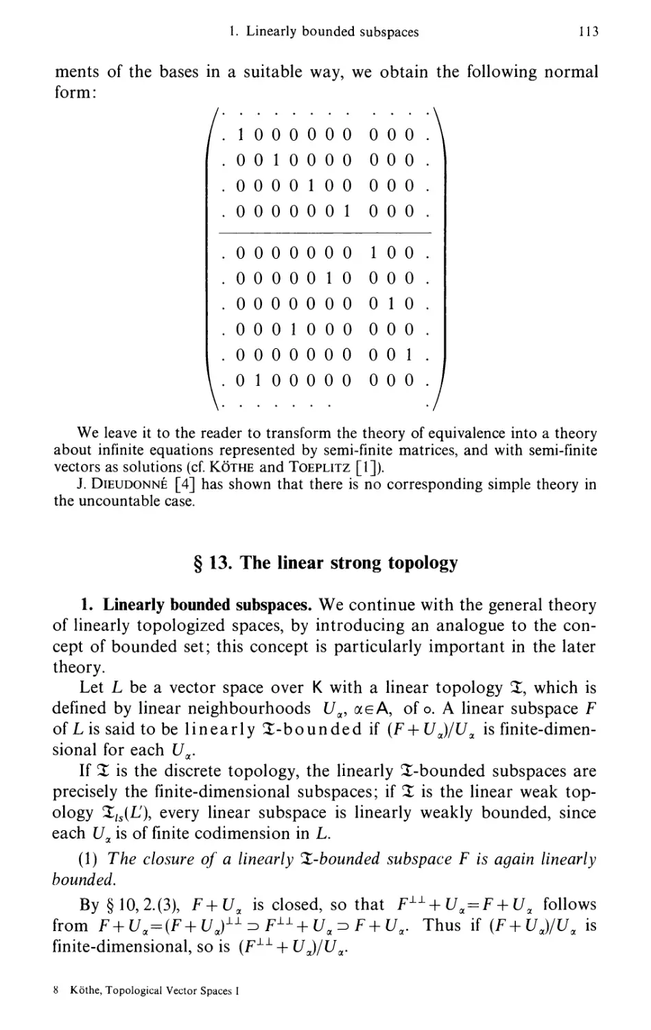


Text
Die Grundlehren der
mathematisdien Wissenschaften in Einzeldarstellungen
Band 159
Gottfried Kothe
Topological Vector Spaces I
Die Grundlehren der
mathematischen Wissenschaften
in Einzeldarstellungen
mit besonderer Beriicksichtigung
der Anwendungsgebiete
Band 159
Herausgegeben von
J. L. Doob • A. Grothendieck • E. Heinz • F. Hirzebruch
E. Hopf • H. Hopf • W. Maak • S. MacLane • W. Magnus
M. M. Postnikov • F. K. Schmidt • D. S. Scott • K. Stein
Geschaftsfuhrende Herausgeber
B. Eckmann und B. L. van der Waerden
Gottfried Kothe
Topological Vector Spaces I
Translated by D. J. H. Garling
i
Springer-Verlag New York Inc. 1969
Prof. Dr. Dr. h.c. Gottfried Kothe
Institut fur angewandte Mathematik
der Johann-Wolfgang-Goethe-Universitat, Frankfurt am Main
Geschaftsfiihrende Herausgeber:
Prof. Dr. B. Eckmann
Eidgenossische Technische Hochschule Zurich
Prof. Dr. B. L. van der Waerden
Mathematisches Institut der Universitat Zurich
Translation of
Topologische Lineare Raume I, 1966
(Grundlehren der mathematischen Wissenschaften,
Vol. 107)
All rights reserved. No part of this book may be translated or reproduced in any form without written permission from
Springer-Verlag. © by Springer-Verlag Berlin • Heidelberg 1969. Library of Congress Catalog Card Number 78-84831
Printed in Germany
Title No. 5142
Preface to the First Edition
It is the author's aim to give a systematic account of the most
important ideas, methods and results of the theory of topological vector
spaces. After a rapid development during the last 15 years, this theory
has now achieved a form which makes such an account seem both
possible and desirable.
This present first volume begins with the fundamental ideas of
general topology. These are of crucial importance for the theory that
follows, and so it seems necessary to give a concise account, giving
complete proofs. This also has the advantage that the only preliminary
knowledge required for reading this book is of classical analysis and
set theory. In the second chapter, infinite dimensional linear algebra is
considered in comparative detail. As a result, the concept of dual pair
and linear topologies on vector spaces over arbitrary fields are
introduced in a natural way. It appears to the author to be of interest to
follow the theory of these linearly topologised spaces quite far, since
this theory can be developed in a way which closely resembles the
theory of locally convex spaces. It should however be stressed that this
part of chapter two is not needed for the comprehension of the later
chapters.
Chapter three is concerned with real and complex topological vector
spaces. The classical results of Banach's theory are given here, as are
fundamental results about convex sets in infinite dimensional spaces.
The subsequent chapters contain a full account of the properties of
locally convex spaces. This account is concerned above all with the
general theory, but some important classes of spaces, such as for example
(F)-spaces, barrelled spaces and bornological spaces, are considered in
greater detail. A large number of examples and counterexamples are
intended to enable both the scope and the limits of the theory to be seen.
The second volume will contain the theory of linear mappings and
the special spaces and classes of spaces which are important in analysis.
The theory of Hilbert space will not be dealt with, since there are plenty
of excellent textbooks on this topic.
Information about the contents of the book is given in the detailed
table of contents at the beginning of the book, and in the short
summaries at the beginning of each chapter. No claim for completeness is made
VI
Preface to the First Edition
for the bibliography at the end of the book, but it should nevertheless
be detailed enough to enable further independent work to be done.
My teacher O. Toeplitz provided the first impulse for work on the
theme of this book. In § 30, I have endeavoured to give an account of
the theory of perfect spaces, which was developed by us together,
I have to thank repeated personal contact with my French colleagues
J. Dieudonne, A. Grothendieck and L. Schwartz since the war, for
detailed knowledge of the theory developed by them; this forms the
main subject-matter of this book. The present account is frequently
based on the two volumes of Bourbaki (Bourbaki [6] in the
bibliography) and on the lectures of Grothendieck [11].
I am particularly indebted to W. Neumer and H. G. Tillmann
who have respectively read through the first half, and the whole of the
manuscript, carefully and critically. M. Landsberg, H. Schaefer and
J. Wloka have made important suggestions and observations.
Finally I thank the publishers for their speedy and excellent printing.
Heidelberg, August 1960
G. Kothe
Preface to the Second Edition
The second edition contains a number of corrections, the need for
which was kindly pointed out to me by various readers, together with
reference to recent articles in which some of the open problems
mentioned in the first edition are solved. Apart from this, the text remains
unaltered.
Frankfurt, October 1965 G. Kothe
Preface to the English Edition
This English edition is a translation of the second German edition.
It differs from the German edition only in several corrections, mainly
due to Dr. D. J. H. Garling.
I wish to express my sincere gratitude to Dr. Garling for the
excellent and careful translation. I am also indebted to Dr. D. Findley for
preparing the index.
Frankfurt, July 1969
G. Kothe
Contents
Chapter One
Fundamentals of General Topology
§ 1. Topological spaces 1
1. The notion of a topological space 1
2. Neighbourhoods 2
3. Bases of neighbourhoods 3
4. Hausdorff spaces 3
5. Some simple topological ideas 4
6. Induced topologies and comparison of topologies. Connectedness . . 4
7. Continuous mappings 6
8. Topological products 7
§2. Nets and filters 9
1. Partially ordered and directed sets 9
2. Zorn's lemma 9
3. Nets in topological spaces 10
4. Filters 11
5. Filters in topological spaces 12
6. Nets and filters in topological products 13
7. Ultrafilters 14
8. Regular spaces 15
§3. Compact spaces and sets 16
1. Definition of compact spaces and sets 16
2. Properties of compact sets 17
3. Tychonoff's theorem 18
4. Other concepts of compactness 18
5. Axioms of countability 19
6. Locally compact spaces 20
7. Normal spaces 22
§ 4. Metric spaces 23
1. Definition 23
2. Metric space as a topological space 23
3. Continuity in metric spaces 24
4. Completion of a metric space 25
5. Separable and compact metric spaces 26
6. Baire's theorem 27
7. The topological product of metric spaces 28
X
Contents
§ 5. Uniform spaces 29
1. Definition 29
2. The topology of a uniform space 30
3. Uniform continuity 31
4. Cauchy filters 32
5. The completion of a Hausdorff uniform space 33
6. Compact uniform spaces 35
7. The product of uniform spaces 37
§ 6. Real functions on topological spaces 38
1. Upper and lower limits 38
2. Semi-continuous functions 40
3. The least upper bound of a collection of functions 41
4. Continuous functions on normal spaces 42
5. The extension of continuous functions on normal spaces 44
6. Completely regular spaces 44
7. Metrizable uniform spaces 45
8. The complete regularity of uniform spaces 47
Chapter Two
Vector Spaces over General Fields
§ 7. Vector spaces 48
1. Definition of a vector space 48
2. Linear subspaces and quotient spaces 50
3. Bases and complements 50
4. The dimension of a linear space 52
5. Isomorphism, canonical form 53
6. Sums and intersections of subspaces 54
7. Dimension and co-dimension of subspaces 55
8. Products and direct sums of vector spaces 56
9. Lattices , 57
10. The lattice of linear subspaces 58
§ 8. Linear mappings and matrices 59
1. Definition and rules of calculation 59
2. The four characteristic spaces of a linear mapping 60
3. Projections 60
4. Inverse mappings 61
5. Representation by matrices 63
6. Rings of matrices 65
7. Change of basis 66
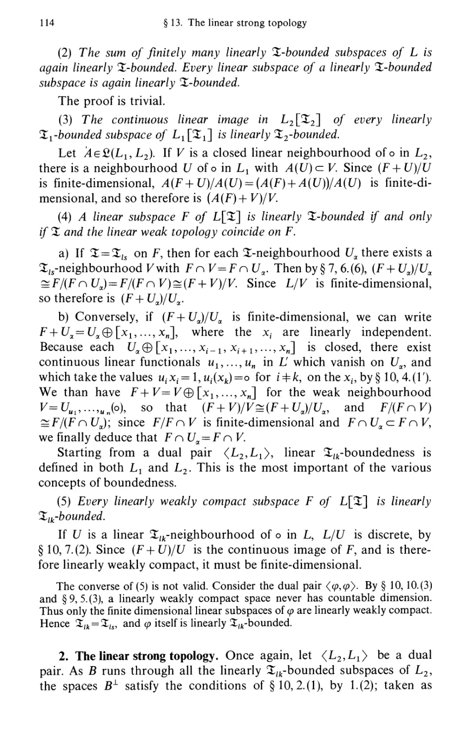
8. Canonical representation of a linear mapping 66
9. Equivalence of mappings and matrices 67
10. The theory of equivalence 68
§ 9. The algebraic dual space. Tensor products 69
1. The dual space 69
2. Orthogonality 70
3. The lattice of orthogonally closed subspaces of E* 72
Contents XI
4. The adjoint mapping 73
5. The dimension of E* 74
6. The tensor product of vector spaces 76
7. Linear mappings of tensor products 78
§10. Linearly topologized spaces 82
1. Preliminary remarks 82
2. Linearly topologized spaces 82
3. Dual pairs, weak topologies 85
4. The dual space 86
5. The dual pairs <£*,£> 88
6. Weak convergence and weak completeness 89
7. Quotient spaces and topological complements 90
8. Dual spaces of subspaces and quotient spaces 93
9. Linearly compact spaces 95
10. E* as a linearly compact space 97
11. The topology 2^ 97
12. ^-continuous linear mappings 98
13. Continuous basis and continuous dimension 100
§11. The theory of equations in E and E* 101
1. The duality of E and E* 101
2. The theory of the solutions of column-and row-finite systems of
equations 103
3. Formulae for solutions 104
4. The countable case 106
5. An example 107
§12. Locally linearly compact spaces 108
1. The structure of locally linearly compact spaces 108
2. The endomorphisms of \jj 109
3. The theory of equivalence in \jt Ill
§13. The linear strong topology 113
1. Linearly bounded subspaces 113
2. The linear strong topology 114
3. The completion 115
4. Topological sums and products 117
5. Spaces of countable degree 119
6. A counterexample 120
7. Further investigations 121
Chapter Three
Topological Vector Spaces
§14. Normed spaces 123
1. Definition of a normed space 123
2. Norm isomorphism, equivalent norms 125
3. Banach spaces 126
4. Quotient spaces and topological products 127
XII
Contents
5. The dual space 128
6. Continuous linear mappings 129
7. The spaces c0, c, ll and /°° 130
8. The spaces /p, 1</?<oo 134
9. (B)-spaces of continuous and holomorphic functions 137
10. The If spaces (p>\) 139
11. The space L00 142
§15. Topological vector spaces 144
1. Definition of a topological vector space 144
2. A second definition 146
3. The completion 148
4. Quotient spaces and topological products 149
5. Finite dimensional topological vector spaces 151
6. Bounded and compact subsets 152
7. Locally compact topological vector spaces 155
8. Topologically complementary spaces 155
9. The dual space, hyperplanes, the spaces LP with 0<p< 1 156
10. Locally bounded spaces, quasi-norms, p-norms 159
11. Metrizable spaces 162
12. The Banach-Schauder theorem and the closed-graph theorem . . 166
13. Equicontinuous mappings, and the theorems of Banach and
Banach-Steinhaus 168
14. Bilinear mappings 171
§16. Convex sets 173
1. The convex and absolutely convex cover of a set 173
2. The algebraic boundary of a convex set 176
3. Half-spaces 179
4. Convex bodies and the Minkowski functionals associated with them 180
5. Convex cones 183
6. Hypercones 184
§17. The separation of convex sets. The Hahn-Banach theorem 186
1. The separation theorem 186
2. The Hahn-Banach theorem 188
3. The analytic proof of the Hahn-Banach theorem 189
4. Two consequences of the Hahn-Banach theorem 192
5. Supporting hyperplanes 193
6. The Hahn-Banach theorem for normed spaces. Adjoint mappings . 196
7. The dual space of C(7) 197
Chapter Four
Locally Convex Spaces. Fundamentals
§18. The definition and simplest properties of locally convex spaces .... 202
1. Definition by neighbourhoods, and by semi-norms 202
2. Metrizable locally convex spaces and (F)-spaces 204
3. Subspaces, quotient spaces and topological products of locally
convex spaces 206
Contents
XIII
4. The completion of a locally convex space 208
5. The locally convex direct sum of locally convex spaces 211
Locally convex hulls and kernels, inductive and projective limits of
locally convex spaces 215
1. The locally convex hull of locally convex spaces 215
2. The inductive limit of vector spaces 217
3. The topological inductive limit of locally convex spaces 220
4. Strict inductive limits 222
5. (LB)-and (LF)-spaces. Completeness 223
6. The locally convex kernel of locally convex spaces 225
7. The projective limit of vector spaces 228
8. The topological projective limit of locally convex spaces 230
9. The representation of a locally convex space as a projective limit . . 231
10. A criterion for completeness 232
Duality 233
1. The existence of continuous linear functional 233
2. Dual pairs and weak topologies 234
3. The duality of closed subspaces 236
4. Duality of mappings 237
5. Duality of complementary spaces 238
6. The convex cover of a compact set 240
7. The separation theorem for compact convex sets 243
8. Polarity 245
9. The polar of a neighbourhood of o 247
10. A representation of locally convex spaces 249
11. Bounded and strongly bounded sets in dual pairs 251
The different topologies on a locally convex space 254
1. The topology 2OT of uniform convergence on 501 254
2. The strong topology 256
3. The original topology of a locally convex space; separability . . . 258
4. The Mackey topology 260
5. The topology of a metrizable space 262
6. The topology 2C of precompact convergence 263
7. Polar topologies 266
8. The topologies Zf and Zlf 267
9. Grothendieck's construction of the completion 269
10. The Banach-Diedonne theorem 272
11. Real and complex locally convex spaces 273
The determination of various dual spaces and their topologies .... 275
1. The dual of subspaces and quotient spaces 275
2. The topologies of subspaces, quotient spaces and their duals . . . . 276
3. Subspaces and quotient spaces of normed spaces 279
4. The quotient spaces of Z1 280
5. The duality of topological products and locally convex direct sums . 283
6. The duality of locally convex hulls and kernels 288
7. Topologies on locally convex hulls and kernels 291
XIV
Contents
Chapter Five
Topological and Geometrical Properties of Locally Convex Spaces
§23. The bidual space. Semi-reflexivity and reflexivity 295
1. Quasi-completeness 295
2. The bidual space 297
3. Semi-reflexivity 298
4. The topologies on the bidual 300
5. Reflexivity 302
6. The relationship between semi-reflexivity and reflexivity 304
7. Distinguished spaces 306
8. The dual of a semi-reflexive space 307
9. Polar reflexivity 308
§24. Some results on compact and on convex sets 310
1. The theorems of Smulian and Kaplansky 310
2. Eberlein's theorem 313
3. Further criteria for weak compactness 315
4. Convex sets in spaces which are not semi-reflexive. The theorems
ofKLEE 319
5. Krein's theorem 323
6. Ptak's theorem 326
§25. Extreme points and extreme rays of convex sets 330
1. The Krein-Milman theorem 330
2. Examples and applications 333
3. Variants of the Krein-Milman theorem 336
4. The extreme rays of a cone 337
5. Locally compact convex sets 339
§ 26. Metric properties of normed spaces 342
1. Strict convexity 342
2. Shortest distance 343
3. Points of smoothness 345
4. Weak differentiability of the norm 347
5. Examples 350
6. Uniform convexity 353
7. The uniform convexity of the lp and LP spaces 355
8. Further examples 359
9. Invariance under topological isomorphisms 360
10. Uniform smoothness and strong differentiability of the norm . . . 363
11. Further ideas 366
Chapter Six
Some Special Classes of Locally Convex Spaces
§ 27. Barrelled spaces and Montel spaces 367
1. Quasi-barrelled spaces and barrelled spaces 367
2. (M)-spaces and (FM)-spaces 369
Contents XV
3. The space//(©) 372
4. (M)-spaces of locally holomorphic functions 375
§ 28. Bornological spaces 379
1. Definition 379
2. The structure of bornological spaces 380
3. Local convergence. Sequentially continuous mappings 382
4. Hereditary properties 383
5. The dual, and the topology <XCo 384
6. Boundedly closed spaces 386
7. Reflexivity and completeness 388
8. The Mackey-Ulam theorem 389
§29. (F)- and (DF)-spaces 392
1. Fundamental sequences of bounded sets. Metrizability 392
2. Thebidual 394
3. (DF)-spaces 396
4. Bornological (DF)-spaces 399
5. Hereditary properties of (DF)-spaces 401
6. Further results, and open questions 403
§ 30. Perfect spaces 405
1. The a-dual. Examples 405
2. The normal topology of a sequence space 407
3. Sums and products of sequence spaces 409
4. Unions and intersections of sequence spaces 410
5. Topological properties of sequence spaces 412
6. Compact subsets of a perfect space 415
7. Barrelled spaces and (M)-spaces 417
8. Echelon and co-echelon spaces 419
9. Co-echelon spaces of type (M) 421
10. Further investigations into sequence spaces 423
§31. Counterexamples 424
1. The dual of/00 424
2. Subspaces of /°° and Z1 with no topological complements 426
3. The problem of complements in lp and LP 428
4. Complements in (F)-spaces 431
5. An (FM)-space 433
6. An (LB)-space which is not complete 434
7. An (F)-space which is not distinguished 435
Bibliography 437
Author and Subject Index 447
CHAPTER ONE
Fundamentals of General Topology
In this preliminary chapter we gather together those ideas and theorems of
general topology which we shall need later. We have also given proofs of the
theorems, since an understanding of the methods of topology is essential for the
study of vector spaces.
For detailied information one must of course refer to texts on general
topology; we mention Bourbaki [5], Kelley [2], Lefschetz [1] and Schubert [1].
The account given here follows Bourbaki closely.
§ 1. Topological spaces
1. The notion of a topological space. A topology % is defined on
a set R when a class O of subsets of R is given, which satisfies the
conditions:
(Ol) K and the empty set are in O;
(O 2) O contains with every finite collection of sets their intersection,
and with every arbitrary collection of sets their union.
The sets of O are called the open sets of R. A set R with a topology
X defined on it is called a topological space. The elements of R
are called the points of the space.
A subclass 33 of O is called a basis of open sets of R if every
open set is a union of sets of 33. A subclass of O is called a sub-basis
when the finite intersections of its sets form a basis.
The topology X is determined by a basis or sub-basis of open sets.
The complement R~0 of an open set 0 is called a closed set of R.
The class 21 of all closed sets of R clearly has the properties:
(A 1) R and the empty set are in 21;
(A 2) 21 contains with every finite collection of sets their union, and
with every arbitrary collection of sets their intersection.
As a result, a topology on a set R can also be defined by giving a
class 21 with the properties (Al) and (A2). In this case the open sets
are the complements of the closed sets. Bases and sub-bases of 21 are
defined as above, exchanging the notions of "union" and "intersection".
When we speak of a basis of R, however, we shall always mean a basis
of open sets of R.
1 Kothe, Topological Vector Spaces 1
2
§ 1. Topological spaces
2. Neighbourhoods. A third way of introducing a topology is by
giving the collection of all neighbourhoods.
A subset of the topological space R which contains an open set
containing the point x is called a neighbourhood of x. Let Sft(x) be
the class of all neighbourhoods of x. It is easy to confirm the following
properties of91(x):
(N 1) $1 (x) is non-empty and x belongs to each set of^l(x);
(N2) If a set belongs to %l(x) then so does every larger subset of R;
(N 3) The intersection of a finite collection of sets ofSH{x) lies in 9l(x);
(N4) For every U in9l(x) there is a V in$l(x) such that Ue9l(y) for
each y in V.
For (N4) we observe that every open neighbourhood V of x
contained in U has the required property.
Conversely, suppose that for each x in a set R a non-empty class
9l(x) of subsets of R is given, and that (N 1) to (N4) are satisfied. If 9l(x)
is to be, for each x, the class of all neighbourhoods of x in some
topology X on R, then the non-empty open sets must be identical with those
subsets 0 of R for which Oe^l(x) whenever xeO.
The class O of all these sets O together with the empty set satisfies
(01) and (02). For the empty set is in O, and by (N2) so is R; by (N3)
the intersection of finitely many sets 0 is again a set of O, and by (N2)
so is an arbitrary union of sets 0. Thus O defines a topology %.
We still have to show that the ^-neighbourhoods of x coincide with
the sets of 9l(x). Every ^-neighbourhood of x contains a set 0 which
belongs to 91(x), so that by (N2) every ^-neighbourhood of x is in 9l(x).
Conversely, suppose that U belongs to 9l(x). We consider the subset
U1 of all y in U for which Ue9l(y). Since x is in U1 it is enough to show
that Ux belongs to O. By (N4) there is for each y in U a V in 9l(y) for
which Ueyi(z) for each z in V. From the definition of Uu z lies in Uu
so that Kcz U1 and so, by (U2), Ux e9i(y). Thus we have shown
(1) Suppose that for each x in a set R a class ^l(x) of subsets is given,
and that (N1) to (N4) are satisfied. Then there is a unique topology on R
for which 91 (x) is the class of all neighbourhoods of x, for each x in R.
Two topologies % and %' on a set R thus give rise to the same
topological space when they give either the same open sets or the same closed
sets or the same neighbourhoods of each point.
Two topological spaces Rx and R2 are homeomorphic when there
is a one-one mapping of the points of Rr onto the points of R2 which
sends every open set of Rx into an open set of R2, and conversely. Such
a mapping is called a homeomorphism. Closed sets or the classes
9l(x) can be used instead of open sets in the definition of homeomorphism.
4. Hausdorff spaces
3
3. Bases of neighbourhoods. If91(x) is the class of all neighbourhoods
of a point x of the topological space R, a subclass 35(x) of 9i(x) is called
a base of neighbourhoods of x (or fundamental system of
neighbourhoods of x) if every neighbourhood in $l(x) contains one in
35(x); to put it another way, $l(x) is obtained from 35(x) by taking
all those subsets of R which contain some set in 35(x). If a base of
neighbourhoods 3S(x) is given for each x, we speak of a base 35 of
neighbourhoods in R.
For a base 35 of neighbourhoods consisting solely of open sets
Hausdorff's three axioms follows easily from (Nl) to (N4), together
with the characterization of open sets given in 2.:
(H 1) Every point x has at least one neighbourhood in 35 (x), and lies
in each of its neighbourhoods;
(H2) The intersection of two neighbourhoods in 3S(x) contains a
neighbourhood in 35 (x);
(H3) If y lies in Ke35(x), there is a WeW(y) with W^V.
Here also the converse holds, that a unique topology is defined
by a base 35 of neighbourhoods in R which satisfies (H 1) to (H3). This
follows, since we obtain a class of neighbourhoods satisfying (Nl) to
(N4) by taking as neighbourhoods all subsets of R larger than the given
neighbourhoods.
Thus we have a fourth method of introducing a topology on a set R.
Starting from a base of neighbourhoods, a set is open if and only if
whenever it contains a point it contains a basic neighbourhood of the
point. The open sets of a topological space other than the empty set
always form a base of neighbourhoods.
Two base of neighbourhoods 35 and 35' on the same set R are called
equivalent when they define the same topology. This is obviously
the case if and only if the classes of all neighbourhoods determined by
them are the same. From this, Hausdorff's criterion, which will
often be used later, follows immediately:
(1) Two bases of neighbourhoods 35 and 35' on the same set R are
equivalent if and only if for each x in R every neighbourhood of x in either
base always contains a neighbourhood of x in the other base.
4. Hausdorff spaces. A topological space R is said to be a
Hausdorff space, or separated, if it satisfies the fourth of Hausdorff's
axioms:
(H4) Any two distinct points of R possess neighbourhoods in 35
without common points.
This can also be expressed in the following way
(T2) Two distinct points of R always lie in disjoint open sets.
T2 is often called the second, or Hausdorff, separation axiom, and
Hausdorff spaces are called T2-spaces (cf. Lefschetz [13]).
i*
4
§ 1. Topological spaces
If R is a general set, and all the subsets of R containing x are taken
as neighbourhoods of x, for each x in R, then R, with the discrete
topology defined in this way, is a Hausdorff space.
5. Some simple topological ideas. A point x is called an interior
point of a subset M of a topological space, if a whole neighbourhood
of x lies in M. The collection of all interior points of M forms an open
set, the interior of M. A point x is called an exterior point of M if
it is an interior point of the complement R~M. A set U => N, where Af
is an open set containing M, is called a neighbourhood ofM.
A point x is called a closure point of the set M if every
neighbourhood of x contains at least one point of M. The set of all closure
points of a set M is called the closure MofM. Since the complement
of M is an open set, M is a closed set, and indeed is the intersection of
all the closed subsets of R which contain M. Thu|a set is closed if and
only if it coincides with its closure. In particular M = M, for any set M.
A point x is called an accumulation point of the set M if every
neighbourhood of x contains at least one point of M distinct from x.
A closure point of M fails to be an accumulation point of M if and
only if it is an isolated point of M—i.e. a point which has a
neighbourhood containing no other point of M. Clearly M is closed if and
only if it contains all its accumulation points.
The boundary of a set M is the intersection of the closures of M
and R~M. A boundary point ofM is thus a closure point of M
and R~M. Every closed set contains its boundary and every open set
is disjoint from its boundary.
The set N is said to be dense in M when M cz N, everywhere
dense when N = R, and nowhere dense when N has no interior
points. The boundary of any open or closed set is nowhere dense.
As an application of these ideas we show
(1) In a Hausdorff space the intersection of the closed neighbourhoods
of a point contains the point alone.
If x0 is the given point and y is a point different from x0 then by
(H4) there exist a neighbourhood U(x0) and a neighbourhood V(y)
with U nV empty. But then y is an interior point of R~U, and so an
exterior point of (/, and thus y does not lie in the closure of U.
From (1) there follows immediately
(2) The only Hausdorff topology on a finite set is the discrete topology.
6. Induced topologies and comparison of topologies. Connectedness. If
S is a subset of the topological space R, the topology % of R induces a
topology on S when the sets SnO, 0 open in R, are taken as open sets
in S. The induced topology is also obtained by considering the inter-
6. Induced topologies and comparison of topologies. Connectedness 5
sections of the closed sets with S or the intersections with S of
neighbourhoods of the points of S. Notice that a set which is open or closed
in S need not be so in R.
If R is Hausdorff, then so is S in the induced topology, which in
general we shall denote by X again.
If two topologies X{ and X2 are defined on a set R, X1 is said to be
finer (or stronger) than X2 if every ^-neighbourhood is also a
Xi-neighbourhood; X2 is said to be coarser (or weaker) than 3^.
That Xx is finer than X2 can also be expressed by saying that the class Oj
of 3^-open sets includes the class C)2 °f ^2 open sets. The same holds
for the classes of closed sets; for this reason we write Xx => X2. If Xl
is finer than X2, every 3^-closure point of a set M is also a 32-closure
point, but not conversely; in general a smaller set is obtained by
forming the Xi-closure than by forming the 32-closure.
If finitely or infinitely many topologies Xa are defined on a set R,
there is a finest topology X among the topologies on R which are coarser
than every Xa: the ^-neighbourhoods of a point x are those sets which
are ^-neighbourhoods of x for each a. If Da are the classes of ^-open-
sets, then the class O of 2-open sets satisfies O = (°)©a, since O ^ Oa
a
for each a. X is called the intersection of the Xa.
X need not be Hausdorff, even if the Xa are Hausdorff. If f] Oa
consists only of the empty set and R, then X is the trivial topology,
in which every point has the single neighbourhood R.
Similarly, given Xa9 there is a coarsest topology X among the
topologies which are finer than every Xa. This is called the union of the Xa.
A base of ^-neighbourhoods of x in R is formed by the
^-neighbourhoods of x, for all a, together with their finite intersections. The discrete
topology (4.) can occur here as an extreme case. The union of
Hausdorff Xa is again Hausdorff.
A topological space R is called connected when it is not the
union of two non-empty disjoint open sets. This is equivalent to saying
that R is not the union of two non-empty disjoint closed sets, or that R
contains no proper non-empty sets which are both open and closed.
A subset S of R is said to be connected, when S is connected as a
topological space with the induced topology.
R is connected whenever every two points of R lie in a connected
subset. If R could be divided into two non-empty open sets Rx and R2,
than any subset S containing two points from Rx and R2 would divide
into two non-empty open subsets RtnS and R2nS of S.
We denote by P the field of real numbers, and by P" real n-dimensional
space in the natural (Euclidean) topology.
6
§ 1. Topological spaces
Since the straight line joining two points of P" is connected, n-di-
mensional space P" is also connected.
A topological space is called totally disconnected when it has
no connected subsets other than the one-point sets. Every discrete
space is totally disconnected, but not conversely; for example the
rational numbers form a totally disconnected space in the topology
induced by the natural topology of P.
7. Continuous mappings. Let A be a mapping from the topological
space #! into the topological space R2—that is, an assignment which
sends each xeR{ to AxeR2. We also speak of a function on Ri with
values in R2, although this term will generally only be used when R2
is a space of numbers.
Every such point-mapping gives rise to a mapping from the class
of subsets of Rt into the class of subsets of R2, which will again be
denoted by A. In detail, if M is a subset of Rl9 the set of all Ax, xeM,
forms a subset A(M) of R2, which is called the image set or image
of M. In particular AiR^ is called the image space of A.
If A is one-one and y = Ax, the correspondence A{~l)y = x defines
a one-one mapping A{~1) from AiR^ onto Rx. We call A{~1) the
inverse of A. This also gives rise to a mapping A{~1) from the class of
subsets of A(R{) onto the class of subsets of ^^
If A is not one-one, the point-mapping has no inverse. To every
subset N of ;4(#i), however, we can make correspond its inverse
image Ai~1)(N), the set of all x in Kt with AxeN. In this way, for
every mapping A the inverse A{~1) is defined as a mapping of the
class of subsets of AiR^ into the class of subsets of Ru
If M is a general subset of R2, by A{~l)(M) we shall always mean
Ai-ViMnAiRJ).
If a mapping A from Rt into R2 maps every open (respectively
closed) subset of #! into a set which is open (respectively closed) in
^(ftj (but not necessarily open or closed in R2\), then A is called an
open (respectively closed) mapping. In the same way the inverse A{~1)
is said to be open (closed) when every open (closed) subset of AiR^ has
an open (closed) inverse image.
A mapping A from #! into R2 is said to be continuous at x0,
when for each neighbourhood V of Ax0 in R2 there exists a
neighbourhood U of x0 in #! whose image lies entirely in V. Clearly we can
restrict attention to neighbourhoods lying in a given base of
neighbourhoods. If A is continuous at every point x of Rl9 A is said to be
continuous (on RJ.
(1) The following properties of A are equivalent: a) A is continuous,
b) A{~1) is open, c) A{~ l) is closed.
8. Topological products
7
Proof. If A{~1} is open, then for a given open neighbourhood V
of Ax0 the set A{~l)(V) is open, and so is a neighbourhood of x0,
whose image under the mapping A is contained in V.
If conversely A is continuous and M is a subset of A(RX) which is
open in AiR^ then if Ax0eM there is a whole neighbourhood
contained in M. The image of this neighbourhood under the mapping
A{~1) contains a neighbourhood of x0, so that A{~l)(M) is open in Rl.
Since A{~1) maps A(Rt)~M into Rl^Ai~l)(M), A{~1) is open
if and only if it is closed.
If the continuous mapping A is one-one, A{~1) need not be
continuous.
(2) A one-one mapping A from Rl onto R2 is a homeomorphism if
and only if A and A{~1) are continuous, and if and only if A and A{~1)
are open (closed).
Under a homeomorphism there is a one-one correspondence
between the neighbourhoods, the open sets and the closed sets of Rt and
those of R2. On the other hand, it follows by (1) from the continuity
of A and A{~1] that A{~1] and A are open—i.e. the open sets of R{ and
R2 are in one-one correspondence, and A is a homeomorphism.
(3) A mapping A is continuous if and only if it sends every closure
point of a set into a closure point of the image set.
Proof. It follows directly from the definition of continuity that a
closure point is sent into a closure point of the image set. We remark
that the image of an accumulation point need not be an accumulation
point.
The other part of (3) does however hold for accumulation points:
if A is not continuous, there exists at least one neighbourhood V of a
point Ax0 for which points xv can be found in every neighbourhood U
of x0, whose images do not belong to V. The set of these xv has x0
as accumulation point, and A x0 is not a accumulation point of the set
of images Axv.
The composition of finitely many continuous mappings is always a
continuous mapping.
8. Topological products. If Ri9...,Rn are given sets, the set R of
n
all w-tuples x = (x1}...,xn), xteRh is denoted by Rl x ••• x Rn = TT Rf.
i = 1
If the Rt are topological spaces, R becomes the topological product
n
of the R( when the class of all sets U = TT L/f(xf) is taken as base of
i= 1
neighbourhoods of x, where L^x,) is a general neighbourhood of x,
n
in R(. We use the expression TT R( for these topological spaces as well.
i=l
8
§ 1. Topological spaces
These definitions can be extended to arbitrarily many factors. If Ra,
aeA, are given, R = TT Ra denotes the set of all functions x(a) = xaeR0i.
aeA
R is called the set-theoretic product or Cartesian product of
the Ra. If the Ra are topological spaces, R becomes the topological
product of the R^ when all subsets U = TT W, are taken as base of
aeA a
neighbpurhoods of the point x, where W^R* for all but finitely
many a, and Wp=Up(xp) for the others, where Up(xp) is a general
neighbourhood of xp in Rp.
If Ra = S for all a, we write SA for the topological product; in
particular we write Sn when there are n equal factors and S03 when there are
countably many. Thus if P is the set of real numbers with its natural
topology, P" is n-dimensional space. Pw is the space of all sequences,
with the topology which has just been defined.
By the parallelotope ^3A we mean the topological product SA,
where S is the closed interval [0,1].
If the Ra are Hausdorff, TT Ra is also Hausdorff.
aeA
The mapping Pa, which sends each xeR to its component xaeKa,
is called the projection of R onto Ra. It is a continuous mapping
from R onto Ka, and the topology of R is the coarsest topology for which
all the projections Pa are continuous. For if Pa is continuous, the inverse
image of Ua{xa) must be a neighbourhood of x in R, by 7.(1). By
taking finite intersections of these inverse images we obtain all the
neighbourhoods in the given base of neighbourhoods.
The projection Pa is open, since an open set contains a
neighbourhood TT W% of each point, the projection contains the neighbourhood W%
of the image, and so the a-components of the points of an open set form
an open set. Pa need not be closed, as is shown for example by
considering the closed set of all (n,\/n), h = 1,2,..., in P2.
(1) If Ma are subsets of Ra, the closure of the set TT Ma is TT Ma,
where Ma is the closure of Ma in Ka.
Proof. It is immediately clear that at least one element of TTMa
lies in each of the neighbourhoods belonging to the given base of
neighbourhoods of xeTTMa, and conversely only elements of TTMa can be
closure points.
// the Ma are all closed, so is TTMa. If the Ma are open, TTMa need
not be open, when A has infinitely many elements.
If A is a mapping from the topological product RtxR2 into the
topological space S which is continuous at the point {x[0\x{2}), the
mapping x1-^A(xl,x{2)), from Rt into S is continuous at the point
x(10) (partial continuity).
2. Zorn's Lemma
9
§ 2. Nets and filters
1. Partially ordered and directed sets. A set H is said to be
partially ordered or semi-ordered if a relation x^y (x less than or
equal to y) is defined for certain pairs of its elements, which is reflexive
(x^x), transitive (x^y and y^z imply x^z) and antisymmetric
(x^y and y^x imply x = y).
For x^y we also write y^x; x<y means xf^y and x + y.
A partially ordered set is called totally ordered or simply
ordered if one of the relations x^y or y^x always holds for any
two of its elements x and y.
A partially ordered set H is called a directed set when for any
two elements x and y there always exists zeH for which x^z and
yrgz. H is said to be inversely directed when for any two elements x
and y there always exists zeH for which z^x and z^y.
Every totally ordered set is both directed and inversely directed.
If x is a point of a topological space, the neighbourhoods of a base
of neighbourhoods of x form a directed set under the set-theoretic
relation =>.
Let M be a subset of the partially ordered set H. It is partially
ordered under ^. M is said to be bounded above (bounded below)
if there exists yeH for which x^y (y^x) for all xeM. y is called an
upper (lower) bound ofM. Every finite subset of a directed set is
bounded above.
If the set of upper (lower) bounds of M has a least (greatest) element y0,
y0 is called the least upper bound (greatest lower bound) of M.
M is called a maximal (minimal) element of M if there exists
no x in M with z<x (x<z). A least element of M is always minimal,
but not conversely.
2. Zorn's Lemma. A totally ordered set is said to be well-
ordered if each of its non-empty sets has a least element.
We shall take the results of classical set theory for granted (cf.
Hausdorff [2] and Kamke [1], for example). In particular, we shall
assume the validity of the axiom of choice. Every set can then be well-
ordered, using the ordinals as index-set. We shall also make occasional
use of transfinite induction and the theory of cardinal numbers.
As an example of transfinite induction, we mention Zorn's lemma
(1) If every totally ordered subset of a partially ordered set H has an
upper bound, H has at least one maximal element.
Proof. Let xa, a = 0,1,..., be a well-ordering of the elements of H.
We determine a totally ordered subset G of H by transfinite induction:
x0 belongs to G; if it has been determined which xp belongs to G, for
10
§ 2. Nets and filters
all P<y, then xy belongs to G if and only if xp<xy for all xpeG. By
hypothesis G has an upper bound z. Since z is an xa, z must lie in G and
so must be the largest element of G and a maximal element of H.
Zorn's lemma is so general that most applications of the well-
ordering principle are special cases of this result, so that we shall not
need to make repeated use of the well-ordering principle.
As a special case, for subsets of a set M partially ordered by <= we
have
(2) // H is a class of subsets of a set M with the property that if a
collection of subsets in H is totally ordered by cz, then its union also
belongs to H, then H has at least one maximal subset.
Let us remark that Zorn's lemma can be deduced diretly from the axiom
of choice, without the aid of the well-ordering principle (cf. Kamke [1], for
example). In fact the axiom of choice, the well-ordering principles and Zorn's lemma
are equivalent assumptions (cf. Birkhoff [3] or Hermes [1] as well).
3. Nets in topological spaces. If x„ is a sequence of points in a
topological space R, xn is said to be convergent to x0eR if for each
neighbourhood U of x0 there exists n0(U) such that xneU for all
n^n0(U). x0 is called limit of the sequence xn, and we write x„->x0.
If R is Hausdorff, a sequence can only have one limit. In this case we
write x0 = \imxn.
n
In a general topological space R an accumulation point of a set M
need not be limit of a sequence of points of M. The parallelotope S$A,
with uncountable A, gives an example of this (cf. § 3, 4.). By using
directed sets, however, the concept of limit is generalized in such a way
that every accumulation point becomes a limit.
Let A be a directed set, and let M be a general set. If for each aeA
an xa e M is given, the xa form a net inM. When A = 1,2,... we obtain
sequences as.special cases of nets.
The net xa, aeA, is said to be convergent to x0eR if for each
neighbourhood U of x0 there exists (S(U)eA such that xyeU for all
y^P(U). xo ls called limit of xa, and we write xa->x0.
Again, the limit of a net in a Hausdorff space must be unique, and
this property characterizes Hausdorff spaces (proof!). In this case we
also write x0 = lim xa.
a
The concept of subsequence can also be generalized: a subset B of a
directed set A is cofinal if for each aeA there exists /7eB with /?g^a.
If a subset of a directed set is not cofinal, then its complement is. If xa,
aeA, is a net, the xp form a cofinal subnet if the f} form a cofinal
subset of A.
If x0 is limit of the net xa, x0 is also limit of every cofinal subnet.
A point y0 is called an adherent point of the net xa if every neigh-
4. Filters
11
bourhood of y0 contains a cofinal subnet. Every adherent point of the
net xa is a closure point of the subset of R consisting of the distinct xa,
but not conversely. Every limit of xa is an adherent point. From this
follows one half of
(1) A subset M of a topological space R is closed if and only if it
contains the limits of all the convergent nets of elements of M.
On the other hand if a is a closure point of M, an xveM can be
picked out of every neighbourhood U of a base of neighbourhoods of a.
The sets U form a directed system under id, by 1. The net xv clearly
has limit a.
(2) A mapping A is continuous at x0 if and only if xa->x0 always
implies Axa-^Ax0.
Necessity follows immediately from the definition of continuity of A
and the definition of convergence of a net.
Conversely, suppose that A is not continuous at x0, and that U={U}
is a base of neighbourhoods of x0. Then there exists a neighbourhood V
of Ax0 and an xv in each UeVL such that Axv does not lie in V. But
then the xv form a net with xv^x0, and the image net Axv does not
converge to Ax0.
We remark that we obtain a proof of continuity at x0 using nets xv,
where U runs through a fixed base of neighbourhoods of x0. An
analogous remark applies to (1).
If Ax„-+Ax0 for all sequences x„->x0, we call A sequentially
continuous at x0. Sequential continuity of A does not in general
imply continuity of A.
4. Filters. Closely related to the concept of net is the concept of
filter.
A non-empty class g = {Fa} of subsets of a set M is called a filter
on M if
(F1) Every subset of M containing an Fa belongs to g ;
(F2) The intersection of finitely many Fa belongs to g;
(F3) The empty set does not belong to g.
The class of all subsets of the natural numbers with finite
complements forms a filter.
More generally a filter on M is obtained from a net xa, aeA, xaeM,
by forming the set Fa of all distinct xp with /?^a, for each a, and
collecting these sets and the subsets of M containing them into a class g.
We call this filter the filter corresponding to the net xa.
Conversely the sets Fa of a filter g form a directed set under =>; moreover
we obtain a net xa if we choose an xa from each Fa, and order the a by
12
§ 2. Nets and filters
the partial order of the Fa which has just been described. Nets formed
in this way are called the nets corresponding to a filter.
An especially important example is given by the filter which consists
of all the neighbourhoods of a point x0 of a topological space, the
neighbourhood filter of x0.
A non-empty subclass 33 of a filter g on M is called a filter-base
of g if it satisfies the conditions
(B 1) The intersection of two sets of 33 contains a set of 33;
(B 2) The empty set does not belong to 33,
and if g consists of all those subsets of M which contain a set of 33.
Conversely, given a collection 33 of subsets of a set M which
satisfies (Bl) and (B2), a filter is obtained by taking all the larger sets.
Because of this, such a collection is called a filter-base.
In this context a base of neighbourhoods of a point is nothing else
than a filter-base of the filter of all neighbourhoods of the point.
Hausdorffs criterion in § 1, 3. generalizes to
(1) Two filter-bases 33 and 33' define the same filter if and only if
every set of either base contains a set of the other base.
Such bases are called equivalent.
A collection 6 of subsets of a set M, for which every finite collection
of sets has a non-empty intersection, gives rise to a filter-base, by taking
all these finite intersections. Such a collection is called a sub-base
of the filter which it determines.
If g and g' are two filters on the same set M, and if g <= g', that is
if g is a subclass of g', then g is said to be coarser than g', and g'
finer than g. If %' is a finer topology on M than % then the
neighbourhood filter of a point x0 relative to 3/ is finer than that relative to X.
If MczAT and g = {Fa} is a filter on M, then the Fa form the base
of a filter on N which we shall in general denote by g again. Conversely
if g = {Fa} is a filter on N, then, provided that all of them are non-empty,
the sets FanM form a filter on M, the restriction of g to M.
5. Filters in topological spaces. Following the pattern of 3. we make
the following definition. A filter g = {Fa} on a topological space R
converges to x0 if there exists an Fpa U for every neighbourhood U
of Xq. Xq is called limit of the filter, and we write Fa-+x0. If R is Haus-
dorff, there is at most one limit, and then we write limg = x0 or
limFa = x0. If g converges to x0, so does every finer filter g'.
a
If the filter is given by a basis {£a}, the condition for convergence
reads: every U(x0) must contain a Ba.
A point x0 which is a closure point of all the Fa is called an
adherent point of the filter. For this it is sufficient for x0 to be a closure
6. Nets and filters in topological products
13
point of all the sets of a base of the filter. If g has limit x0 in a Haus-
dorff space, x0 is the unique adherent point of g. The converse is not
true, as the filter on P with base Fn = {0} u [n, oo), n = 1,2,..., shows.
(1) // x0 is an adherent point of g={Fa} and {Up} is the
neighbourhood filter of x0, then all the Fan Up form a filter convergent to x0,
which is finer than g.
The following relations between these ideas and the corresponding
ones for nets are easily established:
(2) The filter {Fa} has x0 as limit if and only if xa->x0 for every
net corresponding to it. The net xa has limit x0 if and only if the
corresponding filter has limit x0.
(3) // xa is a net corresponding to {Fa}, the filter corresponding to
the net xa is finer than {Fa}, and has exactly the same adherent points as
xa. The adherent points of the nets corresponding to {Fa} are thus
adherent points of {Fa}.
We remark that conversely an adherent point of {Fa} need not
always be an adherent point of every corresponding net.
Theorems (2) and (3) also hold for filter-bases {Bp} and the
corresponding nets xpeBp.
If M is a subset of R and x0 is a closure point of M, consideration
of the filter {Mnl^}, where {Up} is the neighbourhood filter of x0 in
R, shows the following, the direct analogue of 3.(1):
(4) A subset M of a topological space R is closed if and only if it
contains all the limits in R of filters on M.
If A is a mapping of the set Ml into the set M2 and g={Fa} is a
filter on M1? then since A(FJ is non-empty and A(FanFp) cz A(FjnA(Fp)
the image sets A(FJ form the base of a filter on A(MX), and also on
M2, which we call the image-filter i4(g). The images of a base also
form a base of the image-filter. If (& = {Gp} is a filter on A{Ml\ the sets
^(_1)(^/?) generate a filter on M1? which we call the inverse-image
filter A{-1)(($>).
From 3.(2) and (2), or directly, we have
(5) A mapping A from a topological space Rx into a topological space
R2 is continuous at x0 if and only if Fa->x0 always implies that AFa-+Ax0.
6. Nets and filters in topological products. Let R= TT Rp be a
topological product. PeB
(1) A net x{cc)eR has x{0) as limit if and only if x^a)->x^0), for each p.
Necessity follows from the continuity of the projections Pp of R
onto Rp (§ 1, 8.) and 3.(2); sufficiency results from the fact that a neigh-
14
§ 2. Nets and filters
bourhood T7 WB of x{0) has only finitely many WB + RB, so that an in-
dex y exists for which xfeWp{x^\ for all p and all <S^y; i.e. x(<5)eT7H^.
If ^4 is a mapping of the topological space S into the product R,
then PpAx = Apx is a mapping of S into Rp. From (1), we have
(2) The mapping A of a topological space S into R = T\ Rp is
continuous at x0 if and only if all the Ap are continuous at x0.
Let g={Fa} be a filter on R = T\ Rp.The projections of the elements
of Fa on Rp form a set F*p. The filter Pp(%) = %p with sets F*p is called the
projection of the filter g on /^.
(3) T/ze filter g converges to x{0) on R if and only if every projection
g^ converges to xft\
By 5.(2), this is just another wording of (1).
If a filter g^ is given on each Rp, the p r o d u c t - f i 11 e r TT g^ is defined
as the filter g on T\Rp which has as base all sets T\A09 where Ap = Rp
for all but finitely many p, and Ap is an arbitrary set of g^ for finitely
many p.
The product 1733^ of filter-bases of Fp is likewise a base for TTg^. In
this setting, the neighbourhood filter of a point x ofTTi^ is the product
of the neighbourhood filters of its components.
7. Ultrafilters. The filters on M form a partially ordered set under cz.
If a collection ga of filters is given, P)ga is again a filter, since (Ft), (F2)
a
and (F3) are satisfied and M always belongs to it. P)ga is the greatest
a
lower bound of the filters ga. The union (Jga forms a filter (the
a
least upper bound of the ga) if and only if the intersection of finitely
many sets from distinct ga is never empty.
If {ga} is a totally ordered collection of filters on M, the least upper
bound (Jga exists. Using Zorn's lemma [2.(1)] we consequently have
a
(1) For every filter g on M there exists a finer maximal filter, a so-
called ultrafilter.
(2) A filter g is an ultrafilter on M if and only if the following holds
for any two subsets A and B of M: if A u£eg, then g contains at least
one of the two sets A and B.
Proof. If g does not contain A and B, all the subsets N of M with
NkjAe^ form a filter, since (IV1ni\[2)u/l = (]V1u/l)n(]V2u/l) + /l,
so that Nt n N2 is non-empty. This filter is then finer than g, since the
set B has been added to the sets of g. On the other hand, if the condition
is satisfied g contains at least one of every pair of sets A and M ~A.
8. Regular spaces
15
If there were a finer filter, then it would have to contain some A and its
complement M~A, and so would also contain the empty set An(M~A).
(3) The image of an ultrafilter is again an ultrafilter.
Let g = {F^} be an ultrafilter on M, where A maps M into N. If
A(FP) were not the base of an ultrafilter on JV, then by 4.(1) there would
be a finer filter © = {Gy} on N, with at least one Gyo c 4(M) containing
no A(FP). The filter defined by A{~l)(Gyo) and g on M would then be
finer than g, since y4(_1)(GVo) could contain no F/j.
If g is an ultrafilter on M czN, then by (3) 5 defines an ultrafilter
on N. Equally, by (2) the restriction to M of an ultrafilter on N is again
an ultrafilter; the restriction exists if and only if M belongs to the ultra-
filter.
(4) In a topological space an ultrafilter g is either convergent or has
no adherent points.
If g nas an adherent point x0, then by 5.(1) there is a finer filter
convergent to x0. Since g is maximal, this filter coincides with g.
(5) 4 mapping A from a topological space Rx into a topological space
R2 is continuous at x0 if and only if for every ultrafilter g = {Fp}, Fp^x0
always implies that A(Fp)->A{x0).
Proof. By 5.(5) it is enough to show that, given a filter © = {G^}
convergent to x0 but with an image-filter which is not convergent to Ax0,
there exists an ultrafilter with the same property.
Since A(GI}) does not converge to Ax0, there is a neighbourhood V
of A x0 for which all the sets Hp = (R2 ~ V) n A{GP) are non-empty. But
then the sets Mp = A{-l\H[i)nG(i form the base of a filter 9W which is
finer than ©. Any ultrafilter g which is even finer is convergent to x0,
and its image 4(g) is an ultrafilter which does not converge to A(x0),
since the sets A(MP) = HP of the filter are disjoint from V.
8. Regular spaces. A Hausdorff space R is said to be regular if it
satisfies the condition
(R) The closed neighbourhoods of each point form a base for the
neighbourhood filter.
If 95(x) is a base of neighbourhoods of x, and U is an arbitrary closed
neighbourhood of x, then there exists Ve%$(x) with Vcz U, and so
also Kc= U: The closures of the neighbourhoods of a base of
neighbourhoods of a regular space form a base of neighbourhoods for R.
Condition (R) is equivalent to the condition
(R') // M is closed in R and x does not belong to M, then disjoint
neighbourhoods of M and x can always be found.
16
§ 3. Compact spaces and sets
The simple proof is left to the reader.
In regular spaces Fa-»x0 always implies that Fa-»x0.
(1) Every subspace S of a regular space R is regular.
For S is Hausdorff and the intersections with S of the closed
neighbourhoods in R of a point x of S are closed in S, and form a base of
neighbourhoods in S.
(2), The topological product of regular spaces is regular.
In certain circumstances continuous mappings into regular spaces
can be extended.
Let M be dense in the topological space Rx. Let A be a continuous
mapping from M into the regular space R2. If x0 is a point of R{ which
is not in M and (/'a=[/anM, where {Ua} is the neighbourhood filter
of x0 in Rl9 then A can be extended continuously to x0 only if A{U'J
converges to a point of R2, which we define to be the image Ax0.
This requirement is stronger than that of continuity of A on M. It
can also be expressed in terms of nets: if x0eRl9 then for all nets xa->x0,
with xaeM, the image nets Ax^ must all converge to one and the same
element of R2.
We still have to show that the mapping which has now been defined
on the whole of Rx is continuous at each point. Let V be a neighbourhood
of Ax0. Because R2 is assumed to be regular we can suppose that V is
closed. There exists an open neighbourhood U of x0 with A(U n M) c V.
If y is an arbitrary point of U, there is a net ya in UnM with ya-+y,
so that Ay is limit of the net Aya9 which lies in A(U nM)czV. Thus Ay
is in P= K, and A(U)czV. Thus we have established
(3) A continuous mapping A from a dense subset M of a topological
space Rx into a regular space R2 can be continuously extended to the
whole of Rx provided that for each point xgRx with neighbourhood filter
{£/a} A(Uar\M) always converges.
The extension is clearly unique.
§ 3. Compact spaces and sets
1. Definition of compact spaces and sets. A Hausdorff space R is
said to be compact if every filter on R has at least one adherent point.
Since every filter is contained in an ultrafilter, by §2,7.(1), we can also
say
(1) R is compact if and only if every ultrafilter on R is convergent.
(2) A Hausdorff space R is compact if and only if every collection
{Aa} of closed subsets Aa with empty intersection f^A^ contains a
finite collection of subsets with an empty intersection. a
2. Properties of compact sets
17
Proof. Suppose that R is compact, that f]Aa is empty and that the
a
intersection of finitely many Aa is always non-empty. Then the Aa
would form a sub-base of a filter on R which could have no adherent
point, as this would belong to all the Aa, since the A^ are closed.
If R is not compact, there is a filter {Fa} with no adherent points.
The sets Fa form a collection of closed subsets with [\ Fa empty, al-
_ a
though the intersection of finitely many Fa is always non-empty.
Taking complements, we immediately get
(3) A space R is compact if and only if every cover of R by open sets
contains a finite sub-cover.
A subset M of a Hausdorff space R is said to be compact if it is a
compact space in the induced topology. M is thus compact if every
filter on M has at least one adherent point in M. Since the closed
(respectively open) sets of M are intersections of closed (respectively open)
sets of R with M, we also have
(4) A subset M of a Hausdorff space R is compact if and only if
a) every collection {Aa} of closed subsets of R with f](Aar\M) empty
a
contains a finite collection {Aa.} with [}(Aa.nM) empty,
or if and only if a
b) every cover of M by open subsets of R contains a finite sub-cover.
From §2, 5.(3) there follows immediately
(5) M is compact if and only if every net on M has an adherent point
in M.
2. Properties of compact sets. (1) Every compact set is closed.
If x0 is a closure point of the compact set M czR and if {Ua} is the
neighbourhood filter of x0, then {UanM} is a filter on M, which can
only have x0 as adherent point, since R is Hausdorff. By the
compactness condition, x0 must thus lie in M.
A set McK is called relatively compact if its closure M is
compact. Every filter on M then has an adherent point in M cz R.
(2) Every subset of a compact set M is relatively compact, and every
closed subset of M is compact.
(3) Every compact space R is regular.
Were this not the case, there would be a point x0 in R with an open
neighbourhood U, for which Aa n (R — U) would be non-empty, for
every closed neighbourhood Aa of x0. By § 1, 5.(1), [\A(X={x0}, so that,
a
as x0$R~U, the closed sets Aan(R~U) have an empty intersection.
2 Kothe, Topological Vector Spaces 1
18
§ 3. Compact spaces and sets
Since every finite collection of them has a non-empty intersection, we
obtain a contradiction to 1.(2).
(4) The union of finitely many compact sets is compact.
n
This follows directly from the covering property 1.(3); if M = (J M{
i= 1
is covered by open sets, each M,- is covered by finitely many open sets,
and so therefore is M.
(5) The continuous image A(R) of a compact space R in a Hausdorff
space is again compact, so that the mapping A is closed.
Let A be a continuous mapping of a Hausdorff space R] into a
Hausdorff space R2> The image A(M) of a compact (respectively relatively
compact) set M^RX is again compact (respectively relatively compact).
If © = {G/j} is a filter on A(M), the sets A{~l){Gp) generate a filter
A{~1\<&) on M. The compactness condition implies the existence of an
adherent point x0 of ,4(_1)(@>). A{x0) is then an adherent point of 05,
so that A(M) is compact. (1) and (2) establish the other assertions.
As a special case we obtain from § 1, 7.(2)
(6) A continuous one-one mapping of a compact space onto a
Hausdorff space is a homeomorphism.
If R is compact under the topology % every coarser Hausdorff
topology coincides with X.
The second assertion follows from the first by considering the
identity mapping of R onto itself.
3. Tychonoff's Theorem. This says
(1) The topological product R—TIR^ of arbitrarily many compact
spaces is again compact.
Proof. By 1.(1) we must show that every ultrafilter <$={FP} on R
converges. We form the projections ga in each R^ (cf. § 2, 6.). These are
again ultrafilters. By hypothesis, each ga converges to an xae#a. By
§2,6.(3), 5 converges to the element x of R whose components are
the xa.
In particular, by 1.8. every parallelotope S$A is compact.
4. Other concepts of compactness. The concept "compact" can be
weakened in various ways. If Xa is some cardinal number, a subset M
of the Hausdorff space R is called Xa-compact if every filter with a
base of at most Xa sets of M has an adherent point in M. This is the
case if and only if every net x(i of at most Xa elements of M always has
an adherent point in M. The proof of this is given by the generalization
of § 2,5. (3) to filter-bases.
5. Axioms of countability
19
The criteria 1.(2) and 1.(3) are also carried over, if the cardinal of
the collection of closed sets (respectively of the collection of open sets
of the cover) is at most Xa.
For X0-compact, we also say countably compact. If Mis count-
ably compact, every sequence of points of M has at least one adherent
point. On the other hand if this is the case M is countably compact:
indeed if g is a filter on M with countable base Fh i=l,2,..., then a
n
sequence xne f] Ft has an adherent point in M, which is also an ad-
i=l
herent point of all the Ft.
A set M is called sequentially compact if every sequence of
points of M contains a subsequence which is convergent to a point of
M. A sequentially compact set is always countably compact. The
converse is not true, for there even exist compact sets which are not
sequentially compact, and equally there exist sequentially compact sets
which are not compact.
In the parallelotope ^PA, A uncountable, the set M of all x = {£a} with only
countably many coordinates different from zero is sequentially compact, but is
not compact, since M = ^A
If A is the interval [0,1] of the real line, we can consider *PA as the set of all
functions on [0,1] with values in [0,1]. If fn(x) is the function which goes
linearly from 0 to 1 in every sub-interval \_k- \Q~n,(k+ 1)10~") of [0,1], the
sequence fn(x) has no convergent subsequence, so that S$A is compact, but not
sequentially compact.
In P" all these concepts of compactness coincide. The corresponding
"relative" concepts are obtained if the adherent points (respectively
limits) are only required to lie in R.
We shall later be concerned with the question of finding conditions
which ensure that compactness or relative compactness follows from
one of these weaker concepts.
We mention one of the properties resulting from these ideas, which
follows directly from the definitions
(1) // jV1=^N2=>••• is a decreasing sequence of closed non-empty
subsets of a countably compact or sequentially compact set M, then
f]Nt is non-empty.
i
5. Axioms of countability. In the following we shall again suppose
that R is HausdorfT.
First axiom of countability. Every neighbourhood filter of a
point of R has a countable base.
The base can then be chosen as a decreasing sequence Ux => U2 => ••*.
Every subspace also satisfies the first axiom of countability.
20
§ 3. Compact spaces and sets
(1) If R satisfies the first axiom of countability, every closure point
of a subset M of R is limit of a convergent sequence of points of M.
To prove this, form the sets M n Ut from the basic neighbourhoods
Ut of a closure point x0, and choose a point xt from each. A sequence
convergent to x0 is obviously obtained.
In such spaces countably compact sets are sequentially compact.
Furthermore it follows from §1,7.(3) that sequentially continuous
mappings are continuous.
Second axiom ofcountability. R has a countable basis.
For the definition of basis, see §1,1. Every space which satisfies
the second axiom also satisfies the first. Every subspace again has a
countable basis.
(2) Every open cover of a Hausdorff space with a countable basis
contains a countable subcover.
Proof. Let R be covered by the open sets Qa and let Oh i = 1,2,...,
be a basis of the open sets. Let Oin, n= 1,2,..., be the collection of those
Ot from which all the Qa can be formed by taking suitable unions. For
each Oi there is thus at least one Qa with Ot a Qa . But then
a n n
To know whether a set is compact it is therefore only necessary to
examine countable covers by open sets, i.e.
(3) In a Hausdorff' space with a countable basis every countably
compact set is compact.
In such a space the compact, sequentially compact and countably
compact sets thus coincide.
In these spaces, moreover, filters and nets are superfluous, and
everything can be analysed using sequences of points.
We remark that (3) is not always true for Hausdorff spaces satisfying
the first axiom ofcountability (cf. Bourbaki [5], Vol. 4, p. 32, example 21).
(4) // the Hausdorff space R has a countable basis {Ut}, every basis
{Ka} has a countable subsystem which is again a basis.
For every Ut is, by (2), union of countably many Vaik, fc=l,2,...,
and these, taken together, also form a countable basis.
6. Locally compact spaces. A Hausdorff space is called locally
compact if every point has a neighbourhood whose closure is compact.
Every compact space is locally compact.
P" is locally compact but not compact, and every discrete topological
space is locally compact.
Every closed subspace of a locally compact space is, by 2.(2), again
locally compact.
6. Locally compact spaces
21
(1) Every locally compact space is regular, and the compact
neighbourhoods form a base of neighbourhoods.
Every point x has a compact neighbourhood U. If V is any
neighbourhood, Vn U is a neighbourhood of x in the compact space U,
which is regular, by 2.(3). Thus Vn U contains a closed
neighbourhood W of x for the topology of U. W, being the intersection of a
neighbourhood in R with U, is itself a neighbourhood of x in R. W is
compact, by 2.(2), and so is closed in R. Thus the compact neighbourhoods
of x form a base of all the neighbourhoods.
It follows directly from (1) that every open subspace of a locally
compact space is again locally compact.
The topological product of finitely many locally compact and
arbitrarily many compact spaces is again locally compact, by
Tychonoff's theorem. If x0 is a point of a compact space R, R~x0
is clearly locally compact in the topology induced by R. Conversely
(2) Alexandroff's theorem. Every space R which is locally
compact and not compact can be enlarged by the addition of one point to give
a compact space, the one-point compactification of R.
Proof. Let R' be the space consisting of the points of R and one
further point z. We define the closed sets of R' to be all the compact
sets K of R together with the sets Akjz, A closed in R. The axioms
(Al) and (A 2) are clearly satisfied, so that R' is a topological space.
The subspace topology induced on R is the original one, since the
intersections with R of the closed sets of R' which have just been defined
are exactly the closed sets of R.
R' is Hausdorff: it is only necessary to show that there are disjoint
neighbourhoods of xgR and z. If U is a compact neighbourhood of x
in R, U is closed in R', so that R' ~U is an open neighbourhood of z
which has no point in common with U.
R' is compact: given closed sets £a with an empty intersection, they
cannot all be of the form Auz, for otherwise z would lie in their
intersection. If B^o = K0cz R, then P)(K0n#J is also empty. The sets
a
K0nBa are closed sets of the compact set K0, however, so that finitely
many of them have an empty intersection.
(3) The compactijication of (2) is unique up to homeomorphism.
It is enough to show that the closed sets of a compactification
R = Ruz' must coincide with the sets K and Auz', K compact in R
and A closed in R. R, being compact, is Hausdorff, so that z is a closed
set and the sets K and Auz' are closed in R. If conversely B => z is
closed, then B = (B~z')vz'. Thus B~z' has as closure points only
elements of B~ z', and possibly z', and is therefore closed in R.
22
§ 3. Compact spaces and sets
Since every subspace of a regular space is regular, (1) is also a
consequence of (2).
The point z adjoined to R is called the point at infinity.
A space which is locally compact but not compact is said to be
countable at infinity if it is the union of countably many compact
sets.
(4) A space which is locally compact but not compact is countable at
infinity'if and only if the point z at infinity in the compactification R'
has a countable base of neighbourhoods.
Proof. The condition is sufficient, for if Vn is a countable open
base of neighbourhoods of z, the countable collection of compact sets
R' ~ Vn cover the space R.
Conversely, let KlaK2<^'" be a covering of R by countably
many compact sets (by forming finite unions an increasing sequence can
always be obtained). Every point of K1 has a relatively compact open
neighbourhood. The union U1 of finitely many of these neighbourhoods
cover K1. In the same way we find an open relatively compact set U2
which covers U1 uX2, and so on. In this way we obtain a sequence £/_„,
with £/„_! cz Un, which covers R. We now show that the Vn = R' ~ Un
form a base of neighbourhoods of z. From the definition of the closed
sets of R' it follows that the sets R' ~K, K compact in R, form a base
of neighbourhoods of z in R'. It is therefore enough to show that for
every compact subset K there exists a Un with K a Un. X, being a
compact set, is covered by finitely many Uk, and so by one (/„, for
sufficiently large n.
7. Normal spaces. The properties of being a Hausdorff or regular
topological space are not sharp enough for many purposes.
A Hausdorff space is said to be normal if it satisfies the condition
(N) // Ax and A2 are two disjoint closed subsets of R, there always
exist two disjoint open subsets Ul => Ax and U2 => A2.
An equivalent condition to (N) is
(N') // A is a closed subset of R, and if U is open and U => A, then
there is an open neighbourhood V of A with Kc [/.
Proof. Suppose (Nr) holds. If A and B are disjoint and closed,
R~B is an open neighbourhood of A, and so by (N') there exists U1 => A
with U^B empty. U1 and R^Ul are disjoint open neighbourhoods
of A and B.
Conversely suppose that (N) holds. Applying (N) to the closed
sets A and R~U, where U is an open neighbourhood of A, open sets
Ux^ A and U2=> R~U are obtained, with U1 n U2 empty. But then
Ulr\(R~U) is empty, so that U1 a U and (Nr) is satisfied.
2. Metric space as a topological space
23
Taking A to be one point, (N') gives
(1) Every normal space is regular.
Subspaces of normal spaces are not always normal, and there are
locally compact spaces which are not normal. On the other hand
(2) Every compact space is normal.
The closed subsets of a compact space R are again compact. Let A
and B be two disjoint compact subsets of R. Since R is regular, by 2.(3),
for each xeA there exists an open neighbourhood U(x) with U(x)nB
empty. As x runs through the whole of A, the U(x) form an open cover
n n
of A, and, by 1.(4), A a (J U{xt). A' = (J U(xt) is a closed set disjoint
i = i i = i
n
from B. Thus L^ = (J U(xt) and [/2 = #~;4' are disjoint open sets
i= 1
with Ul^ A and £/2 => #•
§ 4. Metric spaces
1. Definition. A set R is called a metric space if a real number
\x,y\, the distance between x and y, is defined for every pair x,y of
elements of R, with the following properties:
(Dl) \x,y\^0,
(D2) |x,j/| = 0 if and only if x = y,
(D3) \x,y\=\y,x\,
(D4) |x,z | ^ |x,}/1 + \y, z| (triangle inequality).
We also say that a metric is defined on R by the function \x,y\.
Every subspace of a metric space is again a metric space, using the
same definition of distance.
A one-one mapping x-»x' of a metric space R onto a metric space R'
is called isometric if \x,y\ = \x\y'\ holds for all pairs x,y.
The simplest example is P" with distance defined by |x,j>|= 1/ X toi~£;l2-
This is called ^-dimensional Euclidean space. ', = 1
00
The set of all real sequences * = (£i,£2>--) with £|£t|2<oo forms a metric
space with distance defined by \x,y\ = / Z to/-£fl2- This space is called Hilbert
space. r , = 1
2. Metric space as a topological space. If x0 is a point of the metric
space R, the set of all yeR with |x0,j/|<r (respectively \x0,y\^r) is
24
§ 4. Metric spaces
called the open (respectively closed) ball of radius r and centre x0.
The set of y with \x0,y\ = r is called the sphere of radius r about x0.
If A, B are two subsets of R the greatest lower bound inf \x,y\ is
xeA,yeB
called the distance between the two sets. The number sup \x,y\ is
x,yeA
called the diameter of the set A. A set A is said to be bounded (with
respect to the metric) if its diameter is finite.
(1) Every metric space becomes a Hausdorjf topological space when
the open balls with centre x are taken as a base of neighbourhoods of the
point x.
Every metric space is a normal space with a countable base of
neighbourhoods at each point.
Proof. Axioms (HI) and (H2) of §1.3 are clearly satisfied. (H3)
results from the following: if y lies in the open ball Kr(x) of radius r
about x, then d=\x,y\<r, so that there exists e>0 with d + e<r.
But then KE(y) lies inside Kr(x), since if zeKE(y), |x,z|:g \x,y\ + \y,z\<d
+ e<r. Further if x=ty, d=\x,y\=£0. The open balls Kd/2(x) and
Kdl2(y) have no common point z, for otherwise |x,j/|:g |x,z| + \z,y\
would be less than d. Thus (H4) is satisfied. Axiom (N) for a normal
space is satisfied: if A and B are disjoint closed sets, the set U of all x
with |x,y4|<-j|x,£| and the set V of all y with |j/,#|<||j;,,4| are
disjoint open neighbourhoods of A and B. Finally the balls about x with
radii 1 /n, n = 1,2,..., form a countable base of neighbourhoods of x.
Two isometric spaces are homeomorphic, but the converse does not
always hold.
3. Continuity in metric spaces. Since a metric space satisfies the first
axiom of countability, the results of § 3, 5 apply. A mapping A from a
metric space R1 into a metric space R2 is therefore continuous if
x(n)->x0, i.e. |x(n),xo|-»0, always implies that Ax{n)^>Ax0. This can
clearly also be expressed in terms of c and 5: A is continuous if for each
£>0 there exists d>0 for which |x,x0|<<5 always implies that
\Ax,Ax0\<8.
Closure points and accumulation points of a set are always limits of
convergent sequences of elements of the set, and so a limit of limits
of a set is again limit of a sequence of elements of the set.
The metric allows what has not been possible in the topological
spaces considered up to now, namely the comparison of the size of
neighbourhoods of different points. This produces a series of further
concepts.
For example, uniform continuity of a mapping A can be defined as
follows: A is uniformly continuous if for every e>0 there exists
(5>0 such that \Ax,Ay\<s whenever |x,j/|<(5.
4. Completion of a metric space 25
The concept of a Cauchy sequence can also be defined: x(n\
rc=l,2,..., is a Cauchy sequence if for each s>0 there exists n0(s)
such that \xim\x(n)\<s whenever m,n = n0.
A metric space is called complete if every Cauchy sequence has a
limit in R.
4. Completion of a metric space. Following the method of
establishing the real numbers of Cantor and Meray, we prove the following
theorem
(1) Every metric space can be embedded in a smallest complete space R,
which is unique up to isometry, and is called the completion ofR.
For every two Cauchy sequences x = (x{n)) and y = (y(n)),lim\x(n\y(n)\
= |x,j/| always exists, for since
\x{m\y{m)\ = \x{m\x(n)\ + \x(n\y(n)\ + \y(n\y(m)\
we have
||x(m))};(m)| _ |x<«>j},<«>|| = |x(«)jX(»)| + \yln\yM\.
If |x,x| = 0 and |y,j>| = 0, then |x,j/| = \x,y\: for from
\xin\y(n)\ = \x(n\x{n)\ + \x{n\y(n)\ + \y(n\y{n)\
lim\xin\yin)\^lim\xin\y(n)\ follows directly, and the interchange of x,
y with x, y establishes the assertion.
The relation |x,}/| = 0 defines an equivalence relation on the set of
all Cauchy sequences. We denote the class to which x belongs by x.
By what we have just shown, a unique real number \x,y\ = lim |x(w),y(w)|
^ n-* oo
is associated with each pair of classes. Under this the set R of all classes
becomes a metric space: (Dl), (D2) and (D3) are trivially satisfied,
and (D4) follows from \x(n\zin)\ = \x{n\y(n)\ + \y(n\zin)l by taking limits.
If we assign the element aeR to the class a determined by the
Cauchy sequence (x{n)) with x(n) = a, an isometry is obtained, and we
can identify R with a subspace of R. R is dense in R, for if x is the Cauchy
sequence (x(n)), 3c = limx("): indeed \x,x(n)\ = lim \x{m\x{n)\^c for
n^no(r,).
R is complete: let (xn) be a Cauchy sequence in R. For each xn there
is an a{n)eR with \xn9ain)\<l/n. Since
|a<->,a<">| ^ |a<™>,xm| + |xm,xj + |x„,a<">|
the a{n) form a Cauchy sequence a in R, and from \a,xn\ g \a,a{n)\ + \a(n\xn\
it follows that a = limx„.
Since R is dense in R and the distances \x,y\ are uniquely defined
as lim|x(n),};(,1)|, they are the same in each extension of R, and R is
uniquely determined up to isometry as the completion of R.
26
§ 4. Metric spaces
5. Separable and compact metric spaces. A topological space is called
separable if there is a countable set of points which is dense in it.
(1) A metric space R is separable if and only if it has a countable
basis.
In one direction the result holds for general topological spaces:
if Oh i= 1,2,..., is a countable basis and xtEOi9 the x{ are clearly dense
in R. If conversely xt is a sequence which is dense in the metric space R,
we shall show that the open balls Kp(xt) with rational p form a basis:
it is enough to show that each xeR has a base of neighbourhoods
formed of suitable K()(xt). But given Kp(x) and |x,xf|<p/2, Kp/2(xt) is
a neighbourhood of x contained in Kp(x).
A compact metric space is called a compactum. Every compactum
is complete, as § 3,1.(3) shows immediately.
(2) Every compactum, and equally every relatively compact subset M
of a metric space, is separable and has a finite diameter.
For every n there are finitely many open balls K1/„(x/")), i= l,...,N(w),
which cover the whole of M. The second part of the proposition follows
from this. Further the countably many xf] taken together clearly form
a dense set in M.
(3) Every sequentially compact metric space is a compactum.
By § 3, 5.(3) it is enough to show that R has a countable basis, and
thus that it is separable. For each n there exist finitely many xj.n) with the
property that each x is at a distance of less than \/n from a suitable x{"\
For otherwise there would be for some n0>0 a sequence x(n) with
\x("\x{m)\ ^ l/nQ for all n, m, and this sequence would have no convergent
subsequence. Again the countable set of all x\n) is dense in R.
Applying § 3, 5.(3) again, we see that
(4) In a metric space the countably compact, sequentially compact and
compact sets coincide.
A metric space R is called precompact if its completion R is
compact. This is the case if and only if every infinite subset of R contains
a Cauchy sequence; it is easy to show that R has this property
whenever R does, and thus is sequentially compact.
A subset M of a metric space is called totally bounded if for
every s>0 there is a finite cover of M by sets of diameter ^s.
(5) A subset of a metric space is precompact if and only if it is totally
bounded.
Proof. Every precompact set is totally bounded, since M, and so
also M, is covered by finitely many sets Nt of diameter <^e.
If conversely M is totally bounded and infinite it is covered by
finitely many sets of diameter ^ 1, and so in one of these sets there
6. Baire's theorem
27
exist infinitely many xj^eM with Ixj^xj^lrgl for all i, /c. From these
in turn we can find infinitely many x\2) with |xj-2),x[2)| ^?, and so
on. The diagonal sequence x[l\x{2\... clearly forms a Cauchy sequence.
(6) // Nx => N2 => • • • is a decreasing sequence of closed sets in a
00
complete metric space, and if their diameters tend to zero, then [\ Nt
consists of one point. i = 1
For every sequence xfeNf is a Cauchy sequence, and all such
sequences converge to one and the same point.
6. Baire's theorem. We give this in several versions.
00
(1) // the complete metric space R is the union [j Mt of countably
i= 1
many subsets, then at least one Mt contains an entire ball
Were this not the case, each Mf would be nowhere dense in R (cf.
§ 1, 5), and there would then be a closed ball Kt of diameter ^1 with
Kx nMx empty, a closed ball K2 in Kt of diameter ^{ with K2c\M2
empty, and so on. The decreasing sequence Kx dK2d- would by
5.(6) have one common point, which could not belong to any Mf and
so could not belong to R.
This theorem of Baire's also holds for locally compact spaces.
00
(2) // the locally compact space R = [J Mh then at least one Mt
contains a non-empty open set. i=l
The proof proceeds analogously: were all the Mt nowhere dense in
R, then there would be a non-empty open set Ox with Ox nMx empty.
By §3,6.(1) R is regular, so that Ox would contain a closed subset Kx
with interior points and Kx nM1 would be empty. We could take K{
to be compact. In Kt there would be a compact subset K2 with K2 n M2
empty, and so on. By § 3,4.(1) the sequence KjD^d- would have
00
a non-empty intersection which again would not lie in R = [j Mf.
i=i
(1) and (2) can be extended to
(3) // an open subset 0 of a complete metric or locally compact
space R is the union of countably many subsets Mh then at least one
Mt n 0 contains a non-empty open subset of R.
If R is locally compact, 0 is also locally compact in the induced
topology, by § 3,6. Hence the assertion follows directly from (2).
Suppose that R is a complete metric space. Since R is regular the
00
open set 0 contains a closed ball K. Then K= [j Nh where Nt = MinK.
Applying (1), we find an Nt which contains a closed ball, and a fortiori
an open ball K0. Consequently K0a MtnK a M. n 0.
28
§ 4. Metric spaces
If the M f are all nowhere dense in R, there is no non-empty open set
00
contained in (J Mh so that
(4) In a complete metric or locally compact space R the complement of
a countable union of nowhere dense sets is dense in R.
A countable union of nowhere dense subsets of R is also called a set
of the first category (Baire) or meagre (Bourbaki). If a set is not
of the first category in R, it is said to be of the second category. In
this case Baire's theorem takes the following form:
(5) Every open subset of a complete metric or locally compact space R
is of the second category in R.
7. The topological product of metric spaces. If Rl^..,Rn are finitely
many metric spaces, we define, for elements x = (xx,...,x„), y = (yi,...,y„)
of RlX"xRn.
n
\x,y\= Z tattl;
i= 1
if Rl9R29... is a sequence of metric spaces, we define in a corresponding
00
way, for x,ye TT Ri9
i=l2l 1+ 1x^1
In either case it is easily confirmed that in this way a metric space
is produced. Instead of 1/21 one could take any cf>0 for which
00
£ ct< oo. To be sure, by doing this, different metrics are given, but we
i= 1
have
00
(1) Every such metric defines the product topology on TT Rt.
Proof. An elementary argument shows that metric convergence
x(")_>x(0) jn y\ ^ js eqUivaient to the metric convergence xi-n)->x[0)
of the components in each Rt. By §2, 6.(1), convergence in the topological
product sense also has this property, so that the two concepts of
convergence are identical. Since the first axiom of countability holds in the
Rh it also holds in the topological product, and thus, by § 3, 5.(1), every
closure point is limit of a convergent sequence. It follows that the closed
sets of R in the metric sense and in the product topology sense coincide,
and so therefore do the topologies.
00
(2) TT Rt is complete if and only if the metric spaces R( are complete.
1. Definition
29
The parallelotope ty™ (cf. §1,8.) is also called the Hilbert par-
00
allelotope, since it is homeomorphic with the product R= T\ Rh
where Rt is the interval [0,1//], for which we have
(3) R is a closed subspace of Hilbert space, and its topology is induced
by the metric on Hilbert space.
Proof. The first part of the assertion is trivial. If
\xjn)\ = \ J|^._^»)|2-*0, ioxx,y{n)eR, then |^-^n)|->0 for each L
00
Conversely, if this holds, then given £>0, £ |^f-^")|2<82/2 for a
i = m
m- 1
sufficiently large m and for each n, and £ \<t{ — rj^l2<s2/2 for suffi-
/= i
ciently large n, so that \x,y{n)\<e. The assertion now follows from the
fact that the two concepts of convergence agree, as in the proof of (1).
R is called the Hilbert cube.
§ 5. Uniform spaces
1. Definition. The topological spaces in which we shall be interested
later are by no means all metric spaces, but ideas can be used for them
which are similar to those used for metric spaces in the preceding
paragraph. These spaces, which, like metric spaces, have an additional
structure defining the topology, were first considered by A. Weil [1].
Let Kbea set, and RxR the set of ordered pairs (x,y) of elements
of R. If N is a subset of RxR, with elements (x,y), we denote the set
of all transposed pairs (y,x) by N'1. The product MN of two such
sets consists of all (x,z) for which there exists a y with (x,y) in M and
(y,z) in N. NN is also written as N2. Using this terminology, we make the
following definition:
R is a uniform space when a filter 91 is given on RxR with the
following properties:
(VI) Every NeW contains the diagonal, that is, the set of all (x,x)
with xeR,
(V2) // NeM, so does AT1,
(V3) For each Ne$l there exists MesJl with M2 a N.
The sets of the filter are called the vicinities of the uniform space;
if (x,y)eN, x and y are called close, of order N. $1 defines a uniform
structure or uniformity on R.
30
§ 5. Uniform spaces
A base of the filter 91 is called a base of the uniform space or of the
uniformity. A filter base © of subsets of R x R forms the base of a
uniformity if (V 1) und (V 3) are satisfied for © instead of % together
with
(V2') // JVgS, there exists iV'e© with N' c AT1.
There is always a base of symmetric vicinities, i.e. those with
N = N~l9 since the symmetric vicinity MnM~l is contained in the
vicinity M.
Every metric space is a uniform space, taking as base the countably
many sets Nl/n of all (x,y) with \x,y\<l/n.
Every subspace S of a uniform space R becomes a uniform space
when the intersections with S x S of the sets of a base for R are taken
as base. This is the uniformity induced on S by R.
Two uniform spaces R and R' are called isomorphic or
equivalent if there is a one-one mapping of R onto R\ and so of R x R onto
R' x /?', under which the filters defining the uniformities are transformed
into each other.
Two metric spaces can be equivalent without being isometric. For
example, one need only multiply all the distances in a metric space by a
fixed positive factor to obtain a new metric equivalent to the original one.
If two uniformities on a set R are given by filters 91 x and$ft2> the
uniformity given by 9^ is called finer (respectively coarser) than that
given by$ft2> if 911 => 9t2 (respectively 9t2 =>5Ri).
2. The topology of a uniform space. If x is a point of the uniform
space R and if N is a vicinity, the set UN(x) of all y with (x,y)eN is
defined to be a neighbourhood of x. The neighbourhoods defined in
this way for all Ne9t and for all xeR satisfy axioms (Nl) to (N4)
of § 1,2: (Nl) follows from (VI), and (N2) and (N3) follow from the
filter properties of 91. To show (V4) we choose an M2 c N9 using
(V3). Then if yeUM(x0)9 every point z of UM(y) is in UN(x0)9 since
from (x0,y)eM and Q/,z)eM it follows that (%z)eM2ciV. Thus
C/N(x0) is also a neighbourhood of y. The topology defined in this
way is called the topology of the uniform space R.
In the case of a metric space we obtain the topology introduced in
§ 4, 2. once again.
A topology is defined on R x R as well, namely the product topology.
(1) Every uniformity has a base of symmetric vicinities which are
closed in the topology of RxR.
If N is a vicinity and M is a symmetric vicinity with M3 <= N9 then
M aN: if (x0,j;0) is a closure point of M there is an (x9y)eM with
(x,x0)eM and (j/,j/0)eM, so that (x0,j/0)eM3 <= Af.
3. Uniform continuity
31
(2) The topology of a uniform space is Hausdorff if and only if the
further axiom
(V4) The intersection of all Ne$1 is the diagonal, is satisfied.
If the intersection is the diagonal, the diagonal is, by (1), also the
intersection of all the closed vicinities, and is itself closed. If x^y, there
is a neighbourhood U x V of (x,y) which has no point in common with
the diagonal, so that the neighbourhood U of x and the neighbourhood
V of y have no common point.
On the other hand if R is Hausdorff and x=Ny, then there is a UN(x)
which does not contain y. This means that (x,y) does not lie in N, and
so the intersection of all vicinities is the diagonal.
If the diagonal is itself a vicinity, the uniformity is called the
discrete uniformity; we obtain the discrete topology on R from it.
If we take the sequence l/«, w=l,2,..., as a subset S of the metric space P,
the induced uniformity on S is not the discrete one, although S is discrete as a
topological space.
If M is a closed vicinity of the Hausdorff uniform space R, the set of
all (x0,y) in M is closed in RxR, being the intersection of the closed
sets {x0} x R and M, so that U^(xQ) is closed in R; (1) gives
(3) Every Hausdorff uniform space is regular.
(4) // A is any subset of Rx R, A = f]N AN, as N runs through all
the symmetric vicinities ofR. N
If Nt and N2 are two symmetric vicinities and if N = N{nN2,
then the neighbourhood UNl(x)x UN2(y) of (x,y) contains the
neighbourhood UN(x)x UN(y); hence these neighbourhoods form a base of
neighbourhoods of (x,y), as N varies. If (x0,y0) is a closure point of A,
there is, for each N, an (x,y)eA with (x,y)eUN(x0) x UN(y0), and by
the symmetry of N we also have that (x0,y0)eUN(x) x UN(y), so that
(xo>yo)ENAN and Aaf)NAN. If conversely (x0,y0)ef)NAN,
N N
there is, for each N, an (x,y)eA with (x0,yQ)eUN(x) x UN(y), so that
(x,y)eUN(x0)x UN{y0), i.e. (x0,y0)eA.
Corresponding to (1) we have
(5) Every uniformity has a base of symmetric vicinities which are
open in the topology of RxR.
It is enough to show that the interior of a vicinity contains a vicinity.
If M is a symmetric vicinity with M3 <= JV, and if (x0j/0)eM, then all the
points (x,y) of the neighbourhood UM(x0) x UM(yQ) lie in N, so that
(xQ,y0) is an interior point of N.
3. Uniform continuity. As can be seen in the proofs which have just
been given, a set whose pairs of points belong to a sufficiently small
32
§ 5. Uniform spaces
symmetric vicinity corresponds to a set of diameter <e in a metric
space; such a set is called small oforder N. A symmetric vicinity M
with M2 <= Af then corresponds to a diameter <a/2.
A mapping Ax — x' of a uniform space R into a uniform space R'
is called uniformly continuous, if to every vicinity N' in R' there
corresponds a vicinity N in R with the property that (x',j/)eAT
whenever x,j/ are two points with (x,y)eN. It is clear that every uniformly
continuous mapping is continuous.
Every isomorphism of two uniform spaces is uniformly continuous
in both directions.
If real functions fp(x),peB are defined on a set R, they can be used
to induce a uniformity on R. For every finitely many fPi, i= l,...,rc, and
£>0, we form the set N of all pairs (x9y)eRxRmth\fPt(x) — fp.{y)\<e
for i—\9...9n. These sets N form the base of a filter of vicinities on RxR.
The fp are clearly uniformly continuous with respect to this uniformity
on R, and it is the coarsest uniformity on R with this property.
The uniformity is Hausdorff if and only if every two points x9y of R
are separated by at least one fp, i.e. fp(x)+fp(y).
This idea can be generalized directly to the case where a collection of
maps Ap from R into uniform spaces Sp is given. The sets of all (x9y)
with (Ap.(x)9Ap.(y))eNPi>y. for i=l,...,n, where NPiyy. is an arbitrary
vicinity in Sp., are then taken as vicinities.
4. Cauchy filters. Cauchy filters and Cauchy nets in uniform spaces
correspond to Cauchy sequences in metric spaces: a filter {FJ on R
is called a Cauchy filter if to each vicinity N there corresponds at
least one Fa which is small of order N9 i.e. (x9y)eN for all x,j/eFa. An
adherent point of a Cauchy filter is a limit of the filter, and in a Hausdorff
uniform space a Cauchy filter has at most one adherent point.
Every convergent filter is a Cauchy filter. If every Cauchy filter on R
is convergent, R is said to be complete.
In an analogous way, a net xa9 aeA is called a Cauchy net if to
each vicinity N there corresponds a j5eA for which (xy,xd)eN whenever
From the connection between nets and filters (§ 2, 4. and § 2, 5.) there
follows directly
(1) R is complete if and only if every Cauchy net has a limit.
For metric spaces we have
(2) A complete metric space is complete as a uniform space.
If {Fa} is a Cauchy filter on R, there is a decreasing sequence Fa„
with \x,y\^\/n for all x,yeFan. A sequence xneFan is then a Cauchy
sequence in R. Its limit x0 is an adherent point of each Fa, since FanFan
is non-empty.
5. The completion of a Hausdorff uniform space
33
In general a uniform space can very well contain limits of all the
Cauchy sequences in it, without being complete, for the limits of certain
Cauchy filters can be missing (cf. the example tyA in § 3, 4.).
(3) Every discrete uniform space is complete.
Every uniformly continuous mapping sends every Cauchy filter
into a Cauchy filter, and equally sends every Cauchy net into a Cauchy
net.
Theorem § 2, 8.(3) on the extension of continuous mappings leads to
(4) A uniformly continuous mapping from a dense subspace S of a
uniform space R into a complete Hausdorff uniform space R' can be
extended in a unique way to a uniformly continuous mapping from the whole of R.
The condition of § 2, 8.(3) is satisfied. For every point xeR, the sets
[/anS form a Cauchy filter g on5; its image A (ft) is a Cauchy filter on
R\ which defines the image Ax. Moreover R' is regular, by 2.(3). Thus
A is continuously defined on the whole of R. A is uniformly continuous
on R: let N' be a closed vicinity in R\ and let N be a vicinity in R with
the property that (Ax,A,y)eN' whenever (x,y)eNn(5 x 5). Let M
be a symmetric vicinity with M3 <= N. If x0,j/0 are points of R with
(x0,j/0)eM, then (x0,j/0) is a closure point in RxR of 5x5, and in
particular of the set of all (x,j/)in5x5 with (x,x0)eM and (j/,j/0)eM.
If (x,j/) belongs to this set, (x,j/)eM3ciV, so that (Ax,Ay)eN'. Since
(Ax0,Ay0) is a closure point of the (Ax,Ay), and since N' is closed,
(Ax0,Ay0) lies in AT. Thus (AxQ,AyQ) belongs to N' for all (x0,j/0)inM.
5. The completion of a Hausdorff uniform space. Let 93 = {Afa}, aeA,
be a base of symmetric vicinities for the uniformity on R [cf. 2.(1)]. If we
put a ^ j8 when Na => Np, A becomes a directed set. 4.(1) can be sharpened
to give
(1) The uniform space R is complete if and only if every net with index
set A has a limit in R.
It is enough to show that every Cauchy filter g = {Fa} has a limit
in R. For every aeA we choose an Fae ft which is small of order Na,
and an xaeFa. If /J^a, y^a and zeFpnFy, then (xp,z) lies in NpczNx
and (xy,z) lies in Ny <= Na, so that (xp,xy) lies in N2a. The net (xj is
thus a Cauchy net and by hypothesis has a limit x0 in R.
Now let Nde%> be given and let Npe93, with N* <=: Ns. There
exists an xff with <r^p and (x0,xJeiVp. If zeFac\Fp, (xa,z)eNp. If
yeFp, then (z,y)eNp. Hence (x0,y)eNp cz A^, for all yeFp. But this
means that $ has x0 as limit.
As analogue of § 4, 4. we now show
(2) Every Hausdorff uniform space R may be embedded in a smallest
complete Hausdorff uniform space R, which is unique up to isomorphism.
R is called the completion of R.
3 Kothe, Topological Vector Spaces I
34
§ 5. Uniform spaces
Proof, a) Definition of R. We consider the Cauchy nets (xj, aeA,
on R, where A is the index set of the base fixed above. Two such nets
(xj and (j/a) are said to be equivalent if for each symmetric vicinity N of
the uniformity on R there exists an index (}(N) for which (xy,yy)eN
for all 7 ^ /}. If (xj is equivalent to (j/a), and (j/J to (zj, then (xJ is also
equivalent to (zj: for if M is a symmetric vicinity with M2 <= JV, it follows
from the fact that (xy,yy)eM and (yy,zy)eM for sufficiently large 7
that (xv,zy)eM2 <= N. We collect equivalent Cauchy nets together into
equivalence classes, which we define to be the points of R. The class in
which the Cauchy net (xj lies will be denoted by x.
b) The uniform structure of R. If M is a symmetric vicinity of R, let
M denote the set of all pairs (x,y) with the property that for each
symmetric vicinity N there exists an index /?(N) such that (xy9yy)eNMN,
for y^.ft(N). This definition is independent of the representatives of the
classes: suppose that (zj is equivalent to (j/J. If Nj <= N, (xy,yy)eNlM Nx
for 7^j8(N1). If, further, 7 is chosen large enough for (yy,zy) to belong
to Nu then (^zJe^MAfJcNMiV. Thus (x,z) belongs to M.
The M form the base of a uniformity on R: (V1) is clearly satisfied,
and so is (V 2), as M~l = M, because of the symmetry of M. M c A/\ n N2
implies that M c NlnN2, so that the M form a filter base on RxR.
Finally, if M3 <= JV, it is easily confirmed that M2 c N, so that (V3)
also holds.
c) RisHausdorff.li (x,y) lies in every M, (xy,yy)eM3 for 7^jS(M),
for all M; (xj and (yj are thus equivalent. The intersection of all the M
is therefore the diagonal.
d) R is a subspace of R. We denote the equivalence class containing
the Cauchy net xa = a, aeR, by a. (a,b) lies in M if and only if
(a9b)ef)NMN. By 2.(4) this means that (a,b)eM. If we identify a and
N
a, then, from what we have just shown, Mn(RxR) = M, so that by
2.(1) the uniformity induced on R by R coincides with the original
structure.
e) R is dense in R. If x is a general element of R and (xj is a net
defining x, there is for each M a j8(M) for which (x7 ,xy)eM for all
y\Y^P- But this means that (x,xy)eM, when xy is considered as an
element of R.
f) R is complete. If 93 = {Afa} is the base defined at the beginning,
then, by b), © = {Na} is a base for the uniformity on R. By (1) it is enough
to show that every Cauchy net (xj, aeA, has a limit in R. By e) we choose
for each xa a point za in R with (xa,za)eiVa. (zj is then a Cauchy net in R:
let peA be specified so that Np3 <= Na. Then (jcy,xy')GNp whenever
7,7'^sup(j5(p), p). Since, moreover, (xy,zy)eNp and (xy>,zy.)eNp, it
follows that (zy,zy,)eNp c Na, i.e. (zj is a Cauchy net z. Since (z,zy)eNp
6. Compact uniform spaces
35
for sufficiently large y, and since (zy,xy)eNp and (xy,xy,)eNp, it follows
that (z,xy,)eN0L for all sufficiently large /, i.e. the Cauchy net (xj has z
as limit.
R is thus a completion of R.
Finally, the fact that R is uniquely determined up to isomorphism is
a direct consequence of
(3) // Rl and R2 are isomorphic uniform spaces which are dense in the
complete Hausdorff uniform spaces Sl and S2 respectively, then any
isomorphism between Rl and R2 can be extended uniquely to an
isomorphism between Sv and S2.
Let A(R1) = R2, B(R2) = Rl be the mappings given by the
isomorphism. Since an isomorphism is uniformly continuous in both
directions, the existence of two uniformly continuous mappings A and
B which map Sl into S2 and S2 into Sj respectively follows, by extension,
from 4.(4). The class of equivalent Cauchy nets in Rt corresponds to
the class of equivalent Cauchy nets in R2 under the isomorphism of
Rt and R2, so that A and B are uniformly continuous mappings of Sj
onto S2 and S2 onto Sl respectively, and are each the inverse of the
other. Consequently the vicinity filters of Sl and S2 are also sent into
each other, and A and B define an isomorphism of St and S2.
(4) // M is a vicinity in RxR, the vicinity M in RxR is the closure
of M in RxR.
The closure in RxR of the vicinities of a base in RxR form a
base in RxR.
If (x(0),y{0)) is a closure point of M, then for each symmetric
vicinity N there exists an (xj)eM for which (x(0),x)eN and (y,yi0))eN,
so that, for sufficiently large y, (x{y°\xy)eN39 (xy,yy)eNMN and
(jvj^gN3; thus (xy°\y^)eN4MN4. But this means that (x(0),y(0))eM,
and that M is closed.
On the other hand if (x,y)eM, then for each symmetric vicinity N
there exists elements xvyy in R such that (x9xy)eN, (y,yy)eN and
(xy9yy)eNMN. Thus there exist zjeR with (z,t)eM, (z,xz)eiV and
(t9y7)eN9 so that (z9t)eUff2(x)x V^(t)9 and M is dense in M.
For the proof of the second assertion we observe that, according
to the definition of the uniform structure on R, the M with symmetric M
form a base in RxR. Every M contains a vicinity N of the given base
in RxR, so that MdN as well, and the N form a base in RxR.
6. Compact uniform spaces. (1) In a compact uniform space every ultra-
filter is a Cauchy filter.
If M is a vicinity of R, R is covered by finitely many open sets M,,
i=\,...,n, which are small of order M. By §2,7.(2) one of the M,-
belongs to the ultrafilter, which thus contains arbitrarily small sets.
3*
36
§ 5. Uniform spaces
(1) also follows directly from §3, 1.(1).
Every compact uniform space is complete, since every Cauchy filter
has an adherent point, and thus has a limit.
As in §4,5. we call a Hausdorff uniform space R precompact if
its completion is compact.
A Hausdorff uniform space is said to be totally bounded if for
every vicinity N of R there exists a covering of R by finitely many sets
which are all small of order N.
Analogous to § 4, 5. we have
(2) a) A Hausdorff uniform space R is precompact if and only if it
is totally bounded.
b) A Hausdorff uniform space is precompact if and only if every
ultrafilter is a Cauchy filter.
Proof, a) If R is precompact, the completion R, and thus also R,
is covered by finitely many sets Mt which are small of order N. R is
covered by the sets MtnR, which are small of order N since N is
obtained from the closed vicinity N in R x R by forming its closure
in RxR.
If conversely R is totally bounded and finitely many Mf of order N
cover the whole of R, then the closures Mt in R cover the whole of R
and are small of order N. By 5.(4) the N form a base for the uniformity
of R. If now 5 is an ultrafilter on R, then, as in (1), by § 2, 7.(2) at least
one Mt is in J$f- 5 tnus contains arbitrarily small sets and is therefore
a Cauchy filter, which converges in R, since R is complete. R is
therefore compact.
b) A precompact space is totally bounded, by a), and it follows
from this, as in (1), that every ultrafilter is a Cauchy filter.
If R is not precompact, R is not compact, and so there is a filter
g={Fa} on R which has no adherent points. For every F* and every
symmetric vicinity N we form the set F| of all zeR with the property
that (x,z)eN for some xeF*. The sets F| form a filter base on R,
and, as F$nR is always non-empty, the sets F%nR form the base
of a filter g' on R. g' has no adherent points in R, since such a point
would also be an adherent point of 5- Any ultrafilter on R which is
finer than 5' is therefore not a Cauchy filter.
(3) A Hausdorff uniform space R is precompact if and only if every
sequence in R has an adherent point in R.
The condition is clearly necessary. If conversely R is not precompact,
there is, by (2) a), a vicinity N for which there is no finite cover of R
by sets of order smaller than N. Let Nl be a symmetric vicinity with
Ni cz N. We choose an xl and form the neighbourhood Uj^^x^. This
is of order Nf. Now suppose that points xu...,xk have already been
7. The product of uniform spaces
37
chosen so that the UNl(xt) are pairwise disjoint. Were there no xk+1
for which UNl(xk + l) was disjoint from the UNl{Xi) already determined,
then all the points of R would be contained in the sets UN2(xt)9 i = l,...,fc,
so that k sets of order smaller than N* cz N would cover the whole
of R. For the sequence xk9 k = 1,2,...,determined in this way, (xk9xm)$Nl
for all fc, m, so that the sequence has no adherent point in R.
(4) A complete Hausdorff uniform space is compact if it is count ably
compact.
For by (3) a countably compact Hausdorff uniform space is pre-
compact, and compactness follows from completeness.
(5) In a compact uniform space, the filter 91 of vicinities consists of
all the neighbourhoods of the diagonal in RxR.
Every vicinity N is a neighbourhood of the diagonal in RxR.
Were there, on the other hand, an open neighbourhood N0 of the
diagonal which did not belong to9l, then, for each Ne9l9(Rx R~N0) n N
would be non-empty, since Nc£N0; the sets (RxR~N0)nN would
thus define a filter 91' => 9t, which, because of the compactness of Rx R,
would have an adherent point belonging to RxR~N09 and so not
belonging to the diagonal. But 9t, and also 91', have only points of the
diagonal as adherent points, since R is Hausdorff and regular.
(6) Every continuous mapping A of a compact uniform space R into
a uniform space R' is uniformly continuous.
If A is continuous, by §2,6.(2) the mapping (x9y)^(Ax9Ay) from
RxR into R' x R' is continuous. If, therefore, AT is an open vicinity
in R' [cf.2.(5)], the set of the inverse images (x9y) of all (Ax9Ay)eNf
is a neighbourhood of the diagonal in RxR, and so, by the preceding
theorem, is a vicinity in R.
7. The product of uniform spaces. If Ra9 aeA, are uniform spaces
with vicinity filters 91a, R = T\Ra becomes the uniform product of
a
the R^ when one takes as basic vicinities N in RxR = T\ (Ra x RJ all
a
sets TTMa, where Ma = RaxRa for all but finitely many a and
M0L = N0Lx Na for the rest, where Na is an arbitrary vicinity in 9ta.
It is easy to see that the topology defined by this uniformity on R
is the product topology (§ 1, 8.). We can add the following easily
established results to those already obtained in §2,6.:
(1) A filter 3 on R is a Cauchy filter if and only if all its projections
5a are Cauchy filters.
(2) The uniform product R = T\ Ra of the uniform spaces R^ is
complete if and only if all the Rx are complete.
The completion of R is the uniform product of the completions of
the Ra.
38
§ 6. Real functions on topological spaces
This follows from (1) and § 2, 6.(3).
A mapping A of a uniform space into the uniform product TT Ka is
uniformly continuous if and only if all the projections A0L = P0LA are.
§ 6. Real functions on topological spaces
1. Upper and lower limits. If we add + oo and — oo to the set P of
real numbers, we obtain a set which we denote by P. The order
relations and algebraic operations in P are defined in the usual way. P
becomes a topological space when we take the intervals [— oo,a], [b9 + oo]
as a sub-basis for the collection $X of closed sets. The original topology
of P is induced by this. The mapping x->tgx maps [ — n/2,n/2] homeo-
morphically onto P, so that P is compact.
The least upper bound supa and the greatest lower bound
aeA _
inf a are defined for any subset A of P. They can of course be + oo
aeA
or—oo.
If M is any set and if an element f(x) in P is ascribed to each xeM,
we speak of a real function on M. If the values lie only in P, f(x) is
called a finite-valued real function. Least upper bounds and greatest
lower bounds of the values of the function on M are denoted by
sup/(x) and inf/(x) respectively.
xeM xeM
Since we allow both + oo and -x as values of functions, the sum
f{x) + g{x) need not be defined for all x (+ oc and — oo cannot be added).
But if f{x) + g(x) is defined for at least one xeM, then the following
hold, provided that the right-hand sides are meaningful:
(1 a) sup (f(x) + g(xj) ^ sup/(x) + sup#(x),
xeM xeM xeM
(lb) inf (f(x) + g(x))Z inf f(x)+ inf g(x).
xeM xeM xeM
The formulation and proof of the corresponding formulae for
multiplication and division are left to the reader.
(2) If f(x)^g(x) for all xeM, then supf(x)^supg(x) and inf/(x)
^infg(x). *eM *eM xeM
xeM
A net £a on P is called monotonic increasing (monotonic
decreasing) if a</? implies that £a^£p {£a^£p).
(3) Every monotonic increasing (decreasing) net £a on P has a limit,
and lim£a = sup£a( = inf£a).
For if sup^ = y, then for each 5<y there exists a ft for which
8<€fi'^ 7 for aU /*'^ ]8, i- e- 7 is tne limit °f tne set ^a-
1. Upper and lower limits 39
If £a is an arbitrary net on P, then the net rja = sup £p derived from
it is monotonic decreasing. By (3), \imrja = mf sup<^ exists; we call it
a P^a
the upper limit or limes superior of £a and denote it by lim £a.
Similarly the lower limit or limes inferior is defined as
lim £a = sup inf £«.
a P^ol
The inequality lim £a ^ lim £a always holds.
If g = {Fa} is a filter on P, whose indices are ordered by the rule
that a:g/? if Fa=> Fp, then we have the analogous definitions
Hmg = limFa = lim sup £ = inf sup £,
limg = limFa = lim inf £ = sup inf i.
a £eF« a $eF„
We observe that in order to form lim 5 it is only necessary to use
the Fy from a base for g, since the net rjy = sup £ is cofinal with the net
of all rja, and so has the same limit. *eFy
(4) T/z^ upper /imit o/ a net or filter on P is the greatest adherent
point of the net or filter.
We shall only show this for nets. Let /7 = lim^a. Since ?7 = inf?7a,
and since rja is monotonic descreasing, given s>0 there is an a0 for
which \rj — rja\<e/2 for a^a0. For each rja there is a <^a, with /5a^a,
for which |?ya—^a|<e/2. The net ^a, a^a0, which is cofinal with £a,
therefore lies in the ^-neighbourhood of rj, and ^ is an adherent point
On the other hand if £ is an adherent point, £^??a for each a, so
that £:ginf?7a = ?7, by (2).
Now let f(x) be a real function on the topological space R. If xa
is a net convergent to a then the values f(xa) of the function form a
net whose upper and lower limits we denote by lim f(x) and lim f(x)
respectively. x""a x""a
On the other hand if U={U0L} is the filter of neighbourhoods of a,
the image filter f(VL) is a filter on P with base /(C/J, and we can form
the upper and lower limits of /(H). They are denoted by
f(a) = lim/(x) = inf sup/(x) = lim sup/(x),
f(a) = lim/(x) = sup inf f(x) = lim inf f(x).
x^a [/eu xeU UeU xeU
f(x) and f{x) are called the upper and lower limits of f(x)
respectively.
40 § 6. Real functions on topological spaces
The two concepts which have just been introduced are generalizations
of the two well known concepts lim f(x) and lim/(x) of analysis.
xn->a x~>a
Since the filter corresponding to a net xa->a is finer than the filter of
neighbourhoods of a, lim f(x) ^ f(x). For a suitable choice of xa,
x<x->a
however, equality holds: let /„ be a sequence of neighbourhoods of
J (a) with intersection f(a). For each neighbourhood U of a we form
the set Un of all xeU for which f(x)el„. The collection of all these Un
defines a filter g whose image /'(g) has /(a) as limit. If xa->a is a
corresponding net, then lim f{x)=f(a)9 by § 2, 5.(2).
(5) The inequalities f(a) ^ f(a) ^ /(a) a/ways /zo/d.
(6) If f(x)^g(x) in some neighbourhood of a, then f(a)^g(a) and
f(a)^g(a).
At every point a for which f(x) + g(x) is defined, we have, by taking
limits in (1 a) and (1 b) respectively,
(V) (f+g) (a)^ f(a) + g(a), (f+g) (a)^ f\a) + g(a)9
provided that the right hand sides are meaningful.
2. Semi-continuous functions. A real function f(x) on a topological
space R is said to be lower semi-continuous at a if f(a)=f(a). It
follows from 1.(5) that it is enough to require that f(a)^f(a).
A function which is lower semi-continuous at each point is called
lower semi-continuous on R. Upper semi-continuity is defined
similarly.
A function which is both upper and lower semi-continuous at a is
continuous at a.
Since f\a) is, by the preceding number, the greatest lower bound of the
lim f(x\ we have
Xot->a
(1) f(x) is lower semi-continuous at a if and only if f(a) ^ lim f(x)9
whenever xa->a. *a"a
A further criterion is
(2) f(x) is lower semi-continuous at a if and only if whenever y <f(a)
there exists a neighbourhood U(a) for which y<f(x) for all xeU(a).
If the condition is satisfied, we have that y^'mf f(x) for some
xeU '
suitable U, so that /(a)^sup inf f(x)=f(a). The converse is also
immediately obvious.
(3) f(x) is lower semi-continuous on R if and only if for each yeP the
set [/> y~\ of those x with f(x) > y is open, or equivalently, if and only if
for each yeP the set [/^y] of those x with f(x)^y is closed.
3. The least upper bound of a collection of functions
41
For (2) implies that if a satisfies the inequality f(x)>y, then so does
a whole neighbourhood of a. The second assertion follows by taking
complements.
(4) The sum of finitely many lower semi-continuous functions is
lower semi-continuous wherever it is defined.
If f(a) + g(a) is defined, then by 1.(7)
(f+9) (a)^ f(a) + g(a) =f(a) + g(a).
(5) The lower limit f(x) of an arbitrary real function on R is always
lower semi-continuous, i.e. f(x)=f(x).
For each 8<f(a) there is, from the definition of /(a), an open
neighbourhood U0(a) for which 8<f(x) for all xeU0(a). If y lies in
U0(a), so does a whole neighbourhood V0(y), so that
/(j/) = lim inf f(x)^3 holds throughout U0, and f (a) = \im inf f(y)^S.
v xev(y) = c; yecz-
Since this holds for every 8<f(a)9 it follows that f(a)^ f(a).
It is easy to give examples of semi-continuous functions on any
topological space. The characteristic function cp(x) of a subset M
of R is defined by cp(x)=\ if xeM, (p(x) = 0 if xeR~M. By (3), M is
open or closed in R if and only if cp is lower or upper semi-continuous
respectively. For the sets [(p>y] (respectively [(p<y]) can only be the
empty set, M (respectively R~M) and R.
For any two distinct points x9 y in a Hausdorff space R there is
therefore always a finite lower semi-continuous function / with f{x)^f(y).
(6) A lower semi-continuous function f(x) on a compact space R
takes a minimum value on R. If it only takes finite values, it is bounded
below.
Since the sets [/^y] are closed, by (3), the non-empty ones among
them form a filter base on R. If a is an adherent point of this filter, a lies
in all the non-empty [/ ^7], so that f(a)^f(x) for all x in R.
A direct consequence is
(7) Every continuous function on a compact space takes a maximum
and a minimum value on R. If it is finite-valued, it is bounded above and
below.
(6) and (7) also hold for sequentially compact spaces. The proof of (6)
is simple: there is a convergent sequence x„->a in R for which f(xn)-+m9
where m is the greatest lower bound of the values of the function. By (1),
f(a) = m.
3. The least upper bound of a collection of functions. If {fp}9 /ie B, is
a collection of real functions on the set M, the function which takes the
value supf'Ax) at each point x is called the least upper bound
sup/^ of the fp. The greatest lower bound inf/^ is defined similarly.
42
§ 6. Real functions on topological spaces
(1) The least upper bound of a collection fp of functions which are
each lower semi-continuous at a point a of a topological space is itself
lower semi-continuous at a. In particular the least upper bound of a
collection of continuous functions on R is lower semi-continuous on R.
We use criterion 2.(2). If y < sup fp(a), y<fp(a) for some /?, so that
y< fn{x)fksup fn{x), throughout some neighbourhood U(a).
p
The next result also follows simply from 2.(2)
(2) The greatest lower bound of finitely many functions which are
lower semi-continuous at a is lower semi-continuous at a.
From Baire's theorem we obtain
(3) // / is a lower semi-continuous finite-valued real function on a
locally compact or complete metric space R, then the set of points which
have a neighbourhood in which f is bounded above is open, and dense in R.
For if Mn is the closed set [/^w], every open set 0 is the union of
the sets MnnO, and by §4,6.(3) at least one MnnOnO = MnnO
contains an interior point. Thus if 0 is some neighbourhood of a point
xeR, there is a point y in it which has a whole neighbourhood on which
/ is bounded above.
From (1) and (3) follows immediately
(4) If the least upper bound of the lower semi-continuous functions fp
on a locally compact or complete metric space R is finite valued, then the
set of points possessing a neighbourhood throughout which the fp are
uniformly bounded above is dense in R.
4. Continuous functions on normal spaces. The question of the
existence of non-constant continuous real functions on topological spaces is
more difficult to answer; fundamental for this is the following lemma of
Urysohn:
(1) A Hausdorff space R is normal if and only if given two disjoint
closed sets A and B there always exists a continuous function on the whole
ofR with values in [0,1], which takes the value 0 on the whole of A and the
value 1 on the whole of B.
If the condition is satisfied, the sets [/<i] and [/>i] are disjoint
and open, since / is continuous, and contain A and B respectively, so
that (N) is satisfied (cf. §3,7.).
Suppose conversely that R is normal. We construct open subsets
B(p) of R for all dyadic fractions p = k/2n9 fc = 0,l,...,2n, with O^p^l.
We set B(0) equal to the empty set and B(l) = R~B.For w = l,
applying § 3, 7. (NT), let B(%) be an open set with B(%) => A and B(%) a B{\).
If the open sets B(k/2") => A have already been constructed for all
fc=l,...,2n, in such a way that B{k/2n) cz B({k+ l)/2") for each k<2\
4. Continuous functions on normal spaces
43
then by § 3, 7.(N') there is always an open set B((2fc+ l)/2" + 1)=>A with
S(fc/2")c:B((2fc+l)/2"+1) and 5((2fc+ l)/2"+1) c B((fc+ l)/2").
It follows that £(p) c B(p') whenever p and p' are dyadic fractions
with p<p'.
We now set /(*)= sup p. Then f(x)= 1 on £, since, if xeB, x lies in
x B(p)
no£(p)with O^p^l. On the other hand, since, B(p)=> A for all p>0,
f(x) = 0 on A The values of f(x) clearly lie in [0,1]. The continuity of
f(x) is shown in the following way: let f(x0) = y. If y = 0, let the interval
[p,p'~\ be equal to [0,p'] with p' >0, and if 0<y<l let [p,pfli be any
interval with dyadic end points p,p' containing y in its interior. Then
B(p) is contained wholly in B(p') and B{p')~B(p) is open and contains
x0 as interior point. But p<^f(x)^pf for each x in B(p')~B(p), i.e.
f(x) is continuous at x0. If, finally, y = l, then x0 lies in R~B(p) for
any p < 1; but/(x) ^ p for xeR~B(p\ so that/(x) is also continuous for
these x0.
If the function f(x) which has just been constructed is replaced by
a + (b — a)f(x)9 a,beP, we obtain
(2) // A and B are disjoint closed subsets of a normal space R, then
there exists a continuous function on R which is equal to a on the whole of
A, equal to b on the whole of B, and whose values lie in [a9b~\.
Remark. For metric spaces, a function with the properties required in (1)
\x9A\
can be given easily. It is enough to put f(x) = -——r^——^t .
A topological space is uniformizable (respectively metrizable)
if a uniformity (respectively a metric) can be defined on R, for which the
corresponding topology is the given one.
A first important consequence of (1) is
(3) Every normal space is uniformizable.
We consider the set C{R) of all finite-valued real continuous functions
on R. By § 5, 3. there is a coarsest uniformity $1 on R, with respect to which
all the feC(R) are uniformly continuous. It is defined by the vicinities
NftC consisting of those (x,y)eRx R for which \f{x)—f(y)\<s. We
have to show that the topology X^ defined by this uniformity coincides
with the original topology X. Since each / is continuous, each UN(x0)9
which is the set of all y with \f(x0)—f(y)\<e9 is an open neighbourhood
with respect to X. If conversely U is an open neighbourhood of x0 with
respect to X9 there is, by (1), a continuous function / with /(x0) = 0
and/(y)=l for all yeR~U. The set [/<1] is then a ^-neighbourhood
of x0 which is contained in U9 so that X and 3^ are identical.
Since every compact space is normal, by § 3, 7. (2), (1) gives information
about the existence of continuous functions on compact spaces. It
follows from (3) and § 5, 6.(5) that
44
§ 6. Real functions on topological spaces
(4) Every compact space is uniformizable in one and only one way.
For locally compact spaces we have
(5) // A is a compact subset of a locally compact space R, and if U
is an open set containing A, then there exists a continuous function on R
which takes the value 1 on the whole of A, and takes the value 0 on the
whole of R~U.
Let R' be the compactification of R, as in § 3, 6.(2). The result follows
by applying (1) to A and R' ~ U.
5. The extension of continuous functions on normal spaces. A
satisfactory account of the existence of continuous real functions on normal
spaces is given by Urysohn's extension theorem.
(1) Any bounded continuous function on a closed subset M of a normal
space R can be extended continuously to the whole of R, preserving the
same bounds.
Proof. Suppose that f(x) is continuous on the closed subset M of K,
and that \f(x)\^c. The subsets Ml = [f^-c/3'] and M2 = [/^c/3]
of M are closed and disjoint, so that by 4.(2) there exists a continuous
function g1(x) defined on the whole of R, with gx(x)= —c/3 on Mu
gl(x) = c/3 onM2and \gl(x)\^c/3 on R. Then if h1(x) is the continuous
function on M defined by h1(x)=f(x) — gl(x), |/z1(x)| ^§c on M. Applying
the same procedure to h^x), with bound fc, a continuous function
g2(x)is obtained on the whole of R, with |#2MI=i'tc> and a continuous
function ^2W = ^W~^2W *s defined on M, with \h2(x)\^(^)2c.
In general, we obtain for each n a continuous function gn{x) on R
with \gn{x)\ ^i(f)"_1-c, and a continuous function hn(x) = hn_l(x)-gn(x)
00
with |/zn(x)| ^(f)"c. The infinite series £ gn(x) converges uniformly
n= 1
on the whole of R, and so defines a continuous function F(x\ with
00
I^MI ^i I (!rc=c.
OnM, F(x)=f(x)-hl(x)+ X (hM-K+l(x))=\im(f(x)-hn+l(x)).
Since \hn+l(x)\^®"+l-c,F(x)=f(x) on M.
The extension theorem only holds for normal spaces: If A and B
are disjoint closed subsets of R, and if the continuous function defined
on AuB by f(x) = 0 on A, f(x)=\ on B may be extended by the
extension theorem to the whole of R, then R is normal, by 4.(1).
6. Completely regular spaces. Looking more closely at the proof
of 4.(3), it can be seen that the result is still valid, with the following
hypothesis about the Hausdorff space R:
7. Metrizable uniform spaces
45
(V) If x0eR and U is a neighbourhood ofx0, there exists a continuous
function f(x) on R with values in [0,1] and with f(x0) = 0 and f(x)=l
on R~U.
A Hausdorff space which satisfies (V) is called completelyregular,
oraTychonoff space. Thus
(1) Every completely regular space is uniformizable.
If x and U(x0) are given, the set [/^i], defined for the function
f(x) whose existence is assured by (V), is a closed neighbourhood W of x
contained in U, so that every completely regular space is regular. Every
subspace of a completely regular space is completely regular, so that
subspaces of normal spaces, and in particular of compact spaces, are
completely regular. From §3,6.(2) it follows that every locally compact
space is completely regular [this also follows from 4.(5)]. Since such
spaces are not always normal, the hypothesis of complete regularity is
weaker than that of normality. On the other hand the following theorem
holds (Tychonoff)
(2) Every completely regular space is homeomorphic to a subspace of
a suitable parallelotope.
Proof. Let {/a}, aeA, be the set of all continuous functions on R
with values in [0,1]. By (V), the set of all [/a< 1] forms a basis of open
sets in R. Let A be the mapping of R into ^A which sends each xeR to
the element yetyA with ya=fa(x). Since R is Hausdorff, for any two
distinct x,x' there is always an fa with fa(x)+fa(x'), so that A is one-one.
A is continuous, by § 2, 6. (2), and further is open, since the image of
each set [/a<l] is open in A(R\ being the complement of the closed
set consisting of those y with ya=\.
As a special case of (2) we obtain Urysohn's embedding theorem.
(3) Every completely regular space with a countable basis, and so for
example every separable metric space, is homeomorphic to a subspace of
the Hilbert cube, and is therefore normal.
For since, by §3,5.(4), there are countably many functions f for
which the sets [/)< 1] form a basis of open sets, a homeomorphism is
obtained with a subspace of s$w, which by §4,7.(3) is homeomorphic
with the Hilbert cube. Normality follows from § 4, 2.(1).
7. Metrizable uniform spaces. Our aim is the converse of 6.(1). In
this number we obtain a partial result:
(1) A uniform space R is metrizable (i.e. its uniform structure can be
determined by a metric) if and only if it is Hausdorff and the vicinity
filter $1 of R has a countable base.
46
§ 6. Real functions on topological spaces
The conditions are necessary, for every metric space is Hausdorff,
and the vicinities Nl/n consisting of those (x,y) with \x,y\<l/n form
a base of the vicinity filter.
The second part is proved in a more general form: a function f(x,y)
which satisfies conditions (Dl), (D3) and (D4) of §4,1., and satisfies a
weaker form of (D2), namely that /(x,x) = 0 for each x, is called a
gauge; we again use the symbol \x,y\. We assert that
(2) The uniformity of a uniform space R whose vicinity filter $1 has
a countable base can be defined by a gauge.
If R is Hausdorff, the gauge is always a metric, and so (2) implies the
second half of (1).
Proof of (2). If Nl, i=l,2,..., is the countable base of 9t ,we form
a sequence of symmetric vicinities Nl9N2,..- for which Nx <= N[ and
k
N3k+ i^N'kn(] Nh for fc^ 1. The Nt again form a base of JR.
t= i
We put f(x,y) = mi(\)k, where k runs through all those indices
k
for which (x,y)eNk; if (x,y)$Nl9 we put f(x,y)=l. Since the Nk
are symmetric, f(x,y)=f(y,x); further f(x,y)^.0 and /(x,x) = 0.
If (x,y)eNk, (y,y')eNk and (y',z)eNk, then (x,z)eNk cz Nk_i; i.e.
from /(x,j;) ^ (i)fc, /(>,,/) ^ (£)* and /(/,z) ^ (i)fc it follows that /(x,z)
^ (£)*" *. We deduce from this that
(3) It follows from f(x,y)^c, f(y,y')^s and f(y\z)^c thatf(x,z)
^2e, /or ei;er j; c> 0.
We now define a function |x,y| by
|x,y| = inf X /(xk-i,xk),
fc = 2
where the greatest lower bound is taken over all sequences
x1=x,x2,...,xw = 3; of finitely many points of R which begin with x
and end with y. \x,y\ is a gauge, for the relations \x,y\ ^ 0, |x,x| =0 and
|x,3;| = |3;,x| result immediately from the corresponding properties of
f(x,y), and the triangle inequality follows from the definition of |x,y|,
since two sequences linking x to z and z to y combine to give a sequence
linking x toy.
The sets of those (x,y) with f(x,y)^\/2k, k= 1,2,..., form a base for
% and so the sets of those (x,y) with \x,y\ ^ l/2fc again form a base for
5R, provided that the relation
(4) $f(x,y)^\x9y\^f(x9y)
holds.
8. The complete regularity of uniform spaces
47
The second inequality of (4) is trivial. The first is established in the
following way: let a sequence x = x1,x2,...,xw = j; be given, and let us
set f(xl9x2) + •*• +f(xn-l9y) = M. We shall then prove by induction onn
that /(xj)^2M. This inequality is implied for n^4 by (3).
Suppose now that the inequality holds for all m<n, n>4.
We divide the sequence x1,x2,...,x„_1,xn by taking out a link
xh,xh+l in such a way that the inequalities
h n
2 /i + 2
hold for the two remaining sequences. By the induction hypothesis we
have that f(x,xh) S M and f(xh+l,y) ^ M, and further f(xh,xh+l) ^ M;
it follows from (3) that /(x,j;) ^ 2M, so that ?f(x9y) ^ M. Since this
holds for all sequences, it also holds for the greatest lower bound of the
values of M, i.e. jf{x,y) ^ |x,y|.
In the case of a discrete uniform space the construction of (2) gives the metric
|x,);| = l for x=\=y.
8. The complete regularity of uniform spaces. Using 7. (2) we now
prove
(1) Every Hausdorff uniform space is completely regular.
If N is a vicinity of R, there is a sequence Nt of symmetric vicinities
with Nx cz N, Nf+l c Nt. These define a uniformity on R, which is in
general no longer Hausdorff. By 7(2), there is a gauge \x,y\N on R whose
vicinities generate the same vicinity filter as the Nt. The vicinity filter N
of R is generated by the sets \x,y\N<£, where N is arbitrary in 91.
\x0,y\N is a continuous function of y on R, for from \x0,y\N^ \x0,z\N
+ |<y,z|Arand \x0,z\N^ Ixq^U + Ij^U it follows immediately that ||x0>.yU
-|x0,z|.v|^b,zU; thus if \y,z\N<e9 then \\x0,y\N-\x0,z\N\<i:.
If U is an arbitrary neighbourhood of x0eR, there exists an N and
an £>0 such that \x0,z\N^e for all zeR~U. Since Ixq^I^ is
continuous, the function /(x) = Min( 1, —|x0,x|N) is continuous on R. But
/(x0) = 0, and f{z)=\ for zeR~U, i.e. (V) is satisfied.
CHAPTER TWO
Vector Spaces over General Fields
The first three paragraphs are concerned with the elementary and purely
algebraic properties of vector spaces E over a general commutative field. In § 7
the lattice V{E) of linear subspaces of E is studied, and § 8 deals with linear
mappings from one vector space into another, and their representation by infinite
matrices. The problem of the equivalence of these mappings is completely solved.
The algebraic dual space £* of all linear functional on E is the theme of § 9. The
lattice K(£*) of algebraically closed subspaces of E* turns out to be dually
isomorphic with V(E). The end of § 9 is concerned with the most important
elementary properties of tensor products of vector spaces.
The attempt to establish a complete symmetry between the properties of E
and those of £* leads in § 10 to the study of linear topologies on vector spaces.
The theory of these linearly topologized spaces is developed in §§ 10—13,
following Dieudonne [4], [6], [10], Lefschetz [1] and Mackey [4]. In § 10 we define
the concept of a dual system, and introduce the weak linear topology Zls and
the topology Xlk defined by the linearly compact subsets of the dual space,
between which the original topology lies. As a first application of this theory, § 11
contains the complete theory of the solution of row- and column-finite systems
of equations. A simpler constructive method is given for the countable case,
which had previously been developed by Toeplitz [1]. § 12 contains the results
of Lefschetz about locally linearly compact spaces, and the theory of equations
in the countable case, which was developed by Toeplitz and the author (cf.
Kothe and Toeplitz [1]), and which is presented in the form given by
Dieudonne [4]. The general theory of linearly topologized spaces is continued in
§ 13, with the introduction of the concepts of linear boundedness and the strong
linear topology, and ends with results about strongly reflexive spaces and spaces
of countable degree.
§ 7. Vector spaces
1. Definition of a vector space. Let K be an arbitrary (commutative)
field with elements a, /?,..., ^ n, with zero element 0 and identity
element 1. A vector space over K (linear space over K, K-module)
is a set E with elements (called points or vectors) a,b,...,x, y,...
which has the following properties:
(LI) For every two elements x,yeE a sum x + y is defined in E;
under this addition, E is an abelian group, i.e. for all x,y,zeE we have
1. Definition of a vector space
49
(a) x + y = y + x,
(b) x + (y + z) = (x + y) + z9
(c) There exists oeE with x+o = x for all xeE,
(d) There exists for each xeE an x'eE with x + x'=o.
(L2) For every £eK and every xeE the product £x = x£ of £ with x
is defined as an element of £, and for all x,j/e£,^eK we have
(e) x(£ + rj) = x£ + xrj,
(f) (x + y)£ = xZ + y^
(g) x(£ri) = (x€)ri9
(h) xl=x.
We shall establish some simple consequences.
(1) For arbitrary a and b in £, the equation a-\-y = b has a unique
solution.
By (d) there is an a' with a + a' =o; application of (b), (a) and (c)
shows that
a + {a' + b) = (a + a') + b=o + b = b+o = b9
so that a' + b is a solution.
On the other hand if yx and y2 are two elements with a + yl=a + y2,
then by adding a! to both sides one obtains first that
a' + (a + yl) = (d -\-a)-\-yl = (a + d) + yi=o + yl=y1+o = yl,
and secondly that d + (a + y2) = y2> so that yx =y2. It follows from this,
by considering (c), that the additive zero element o in E is uniquely
determined, and further, from (d), that x' is uniquely determined, x' is
written as — x, and the solution b + ( — a) of a-\-y = b as b — a (the
difference of b and a).
(2) a-0=o,o-<x=o and a( — a)=—{aa) for all aeE, aeK.
By (e), a-1 =a(\ +0) = a-1 +a-0. But the equation a-\ +y = a-\ has
the unique solution o, so that a-0=o. Likewise it follows from (f) that
o-a = (o+o)-a=o-a+o-a, so that o-a=o. Finally, a'<x + a-( — <x) = a(<x — a)
= a-0=o, so that a( — a)= —(aa).
(3) // x=|=o and a 4=0 then xa4=o.
For if x a were equal to o, then by (2), (g) and (h), (x a) a"i = x(a • a~l)
= x • 1 = x would also be equal to o.
The most important rules of calculation have now been derived;
the rules in which sums of n elements are considered, and the associative
laws (b) and (g) with more than three elements, are deduced from them
in a familiar way, using complete induction.
If K is the field P of real numbers or the field V of complex numbers,
then E is called a real or complex vector space respectively.
4 Kothe, Topological Vector Spaces I
50
§ 7. Vector spaces
2. Linear subspaces and quotient spaces. A subset H of elements of a
vector space £ is a vector space provided that whenever it contains x
and y it also contains xa + yfi, for arbitrary a, /? in K. H is then called
a linear subspace of E. For simplicity we shall usually write o for
the subspace consisting only of the zero element o.
By a linear manifold in E we mean a subset of E consisting of
all elempnts of the form x0 + y, where y belongs to a linear subspace H.
We denote this by x0 + H. We also speak of the manifold x0 + H
through x0 parallel to H. xl+H = x0 + H for each xlex0-\-H.
If xl9...,xn are finitely many elements of £, every element of the
form xi<xi+ ••• + x„a„, a,eK, is called a linear combination of
*!,..., x„. If M is a finite or infinite subset of £, the collection of all
linear combinations of finitely many elements of M forms a linear
subspace, the linear span ofM. This can also be defined as the
intersection of all the linear subspaces containing M. The linear span of the
set {x!,...,*,,} is written as [xx,..., xj.
If H is a linear subspace of E and x0 is an arbitrary element of £,
the linear manifold x0 + H is also called the //-coset of x0, and is
denoted by x0. If we define the sum of two cosets x0 + j)0 to be the
coset x0 + j;0, and the scalar multiple x0a to be x0a, the collection
of cosets becomes a vector space over K, the quotient space E/H
of E by H. The operations which have just been introduced in E/H are
defined using particular representatives from the cosets. But if, instead
of x0, another element x0 + z0 is taken from the coset x0 = x0 + H,
then z0 + H = H, so that the cosets (x0 + y0 + z0) + H and (x0 + y0) + H
contain the same elements. The formation of the sum is therefore
independent of the choice of representatives. The same is true for
multiplication by elements of K, as is immediately verified. Since, further,
both operations in E/H are defined in terms of the corresponding
operations on the representatives, rules (L1) and (L2) carry over directly
to calculations with cosets, and so E/H is a vector space over K. The
zero element in E/H is clearly 6 = H.
3. Bases and complements. A finite collection X!,...,x„ of elements
of E is called linearly dependent if there is a linear combination
xlal + -•• +x„a„, with not all a,- = 0, which is equal to o. In this case at
least one of the xt can be written as a linear combination of the others.
The elements X!,...,x„ are called linearly independent if they are
not linearly dependent; it then follows from a relation x1a1+-- +x„a„=o
that all the af = 0.
An infinite collection xa, aeA, is said to be linearly independent
if each finite collection of them is linearly independent, in the sense
which has just been defined.
3. Bases and complements
51
A set {xa}, aeA, of elements of E is called an algebraic basis
of E if the xa are linearly independent and if each element of E can be
expressed as a linear combination of finitely many xa. It follows directly
from the independence of the xa that this representation is only possible
in one way, i.e. each xeE can be written as £ xa£a, where only fi-
aeA
nitely many £a are different from 0, and the £a are uniquely determined
by x. We shall leave out the prefix "algebraic" for the time being,
provided that there is no possible confusion with other concepts of basis.
(1) Every vector space has a basis.
Proof. The subsets of E which consist of linearly independent
elements clearly satisfy the hypotheses of Zorn's lemma [§2,2.(2)], so
that there is a maximal subset {xa} of linearly independent elements
of E. Thus if x + 0 is an arbitrary element of £, the set consisting of x
and the xa cannot consist of linearly independent elements. There is
therefore a linear combination of x and of finitely many of the xa which
vanishes, without all the coefficients vanishing. Because of the
independence of the xa, the coefficient of x in the linear combination must
be different from zero, and so x can be written as a linear combination
of the xa.
Since, more generally, the subsets of E which consist of independent
elements and which contain a fixed independent set {yp} also satisfy
the hypotheses of Zorn's lemma, we have
(2) Every system of linearly independent elements of E can be extended
to a basis of E.
Two linear subspaces G and H of E are called algebraically
complementary to each other if each xeE can be represented in one
and only one way as a sum x = y + z, with yeG and zeH.
If elements yp form a basis for G and elements zy form a basis for H,
then the set consisting of the yp and the zy is clearly a basis for E.
(3) Every linear subspace G of a vector space E has a complement.
Proof. Let {yp} be a basis for G and let {xy} be a basis for E/G.
If an element zy is picked out of each of the cosets xy, the yp and zy
together form a basis of E: if xe£, then x = £xy£y, so that x = £zy£y + );,
yeG. The expression x = YJzy€7 + Y,yprlp then follows from y = Yjyprjp.
On the other hand the yp and zy are linearly independent, for from
YJypr1p + YJzy£y=0 it follows, by going over to cosets, that ^xy^y=6.
Hence £y = 0 for all 7, and so ^ = 0 for all /?. The linear span H of the
zy is clearly a complement for G.
(3) can also be proved by applying (2) to a basis {yy} of G.
We observe that the complement to G is not in general unique,
since the zy can be chosen arbitrarily in the xy. Further let it be stressed
4+
52 § 7. Vector spaces
that we have only given existence proofs, depending upon the axiom
of choice, for (1) and (2). We return to constructive methods in the case
of a countable basis in § 11.
4. The dimension of a linear space. A basis {xa}, aeA, of E has a
certain magnitude, given by the cardinality of A—the "number" of
elements of the basis. We show that this number is the same for different
bases of E.
n
(1) n+\ linear combinations yt= £ xk<xkh i=l,...,n+l, of n
k= 1
elements xkeE are always linearly dependent.
This is clear for n= 1. Suppose that the result is true for n— 1, and
that further an4=0 (which we can assume without loss of generality).
<xli
Then by the induction hypothesis, the n elements y\ = yi — yx —,
an
i = 2, ...,n+l, are linearly dependent, being linear combinations of
x2,..., x„, and so we can write
n+ 1
(2) Z /,/?,=<>.
1 = 2
But then the yt are also dependent, for (2) implies the relation
n+1 n+ 1
E M-y. E — P<=°
r = 2 i = 2 a 1 1
and not all the /Jf vanish.
If now £ has a basis with finitely many elements, let xl9..., xd be a
basis with smallest possible d. If {y(i} is a second basis with cardinal /
then, by (1), / must be less than or equal to d, since on the one hand the
yp are linear combinations of the xh and on the other they are linearly
independent.
If the bases of £ are all infinite, we finish the proof as follows: Let {xp}
and {ya} be two bases with cardinality d and / respectively. There are
equations
(3a) Xp = Y,ya^afn (3 b) )><r = Z Xp P Po ■>
a p
in which for each p or a there are only finitely many non-zero <xap or fipa
respectively.
In the equations (3 a) each ya has at least one coefficient a(Tp4=0.
Indeed if all the aaoP were zero for some <70, then we would have
>'*„ = E xpPpo0 = E (E x* a° p ) Pp°o = E ^ E a-P /^p^o
/; p \ <t / a p
5. Isomorphism, canonical form
53
which expresses yao as a linear combination of finitely many ya>, o' 4=t70,
contradicting the linear independence of the ya.
Using (3 a), assign to each xp the set Mp of those finitely many ya
for which <xap^0. The set M of all the vectors ya is the union of these d
sets Mp, so that the number / of ya is less than or equal to X0 d, where X0
is the cardinal of the set of natural numbers. By hypothesis, d is an
infinite cardinal; by a well-known theorem of set theory it follows that
tf0d = d. f=d then follows from the inequality f^d and the
corresponding inequality d^f.
We have therefore shown
(4) Two different bases of a vector space E always have the same
number of basic elements.
This cardinal is called the algebraic dimension d(E) of E.
5. Isomorphism, canonical form. Two vector spaces Ex and E2 over
the same field K are called algebraically isomorphic if there is a
one-one correspondence x<-»x' between the elements of Ex and the
elements of £2> under which (x<x + yP)' = x'a + y'P, for all x,yeEi and
all a, /?eK. We shall use the symbol Ex = E2 for this.
The result of the preceding number can now be expressed as follows:
(1) Two vector spaces Ei and E2 over the same field K are isomorphic
if and only if they have the same dimension.
Since an isomorphism sends a basis of Et into a basis of E2, the
dimensions must coincide. On the other hand if they are equal, then
there is a one-one correspondence xa<-»x'a between a basis of £x and
a basis of E2, which defines an isomorphism x = £xa£a<-»£x/a£a = x/.
To each cardinal number d there is, up to isomorphism, at most one
vector space over K of dimension d. On the other hand a vector space of
dimension d over K is obtained in the following way:
Let a run through a set A of magnitude d. If a £aeK is made to
correspond to each aeA, and if only finitely many £a are non-zero,
then we call the function defined in this way a finite vector x={^a},
with d coordinates £a. As usual we define s + n as the vector with
coordinates ^a + na, and further define xp, peK, as the vector with
coordinates £ap; the set E of these vectors is then a vector space over K.
The null-vector o with all coordinates vanishing is the zero element of
E. We denote by ea the a-th unit vector, whose a-coordinate is 1, and
whose other coordinates vanish. Clearly ac = ^ea^a, and the ea are
a
linearly independent and therefore form a basis for E.
We call the space E obtained in this way a d-dimensional finite
coordinate space cpd(K) over K. If d = X0, we write simply cp(K).
54
§ 7. Vector spaces
In this expression the index set A does not appear explicitly, and it
can always be replaced by one with the same cardinality. If a uniquely
determined canonical form is required, it is natural to take the set Qd
of those ordinals with smaller cardinality than d. This corresponds to
the practice, in the finite and countable cases, of taking natural numbers
as indices, and has the advantage that one can fall back upon the order
of Qd in, problems for which an ordering of the coordinates is useful.
Let it be stressed, however, that this order is not essentially connected
with the concept of basis, but is introduced in addition.
By (1), an isomorphism is obtained between a general d-dimensional
vector space E and cpd, when the elements xa of a basis of E are made to
correspond to the unit vectors ea of cpd.
6. Sums and intersections of subspaces. A linear subspace of E is
always obtained when the set theoretic intersection f] Fa of a collection
a
of linear subspaces Fa of E is formed. The intersection of a collection of
linear manifolds is either empty or a linear manifold. If in a
corresponding way the union \J Fa is taken, it need not in general be a linear SUb-
space, although its linear span is. This linear span is called the sum £ Fa
a
of the Fa. For general subsets Ma of F, £ Ma denotes the set of all
finite sums £ xa.(xa.eMJ. For linear subspaces Ma, this is again the
i=\
linear span of the Ma. The plus sign is used as well, when there are
finitely many summands, e.g. Ml+M2.
The sum F = £ Fa is said to be direct, if every xeF can be written
in only one way as £ xa, xaeFa (of course, there are only finitely many
xa=|=o). For direct sums we use the symbols © Fa and Fi®F2 re-
a
spectively. An example of a direct sum is given by two complementary
subspaces G and H of E; E = G®H.
(1) The sum £Fa is direct if and only if Fan £ Fp=o, for each a.
If the condition is satisfied, it follows from £xa=o that x(X= £ ( — xp)9
and so x^eF^n £ Fp; this implies that xa=o for all a, so that the
representation x = £ xa as a sum is unique.
a
On the other hand, if this is the case, and if zeFan £ Fp, then the
representation o = z — z, with zeFa and —ze £ Fp, must coincide
with o=o+o, so that z=o. /J + a
7. Dimension and co-dimension of subspaces
55
(2) If F and G are two linear subspaces of E, and if Fx and Gx are
complementary to F r\G in F and G respectively, so that
(3) F = Fl®(FnG)9 G = Gl®{FnG),
then
(4) F + G = F1®Gl®{FnG).
In this way the sum F + G is reduced to a direct sum.
Proof. Clearly F + G = F1 + G1+(FnG). But this sum is direct, for
it follows from x + y + z=o, xeFl9 yeGl9 zeFnG, that x = —y — zeG
and so that xeF1nG = F1n(FnG)=o, which shows that x=o. But
then y = z=o must hold, by (3).
It follows from (2) that
(5) If F and G are two linear subspaces of £, there is a complement H
of Ffor which G = (GnF)®(GnH) holds.
For if G: is defined by (3) and if L is a complement of F + G in £,
H = G1®L has the required properties.
The next two isomorphism theorems, well-known in group theory,
follow from (2).
(6) If F and G are two linear subspaces of £, then (F + G)/G ^ F/(F n G).
(7) If F and G are two linear subspaces of £, with F cz G, then
E/G^(E/F)/(G/F).
Proof. By (3), F/(FnG)^Fl9 and by (4), (F + G)/G^Fl9 which
establishes (6).
If further F cz G cz £, then we can write E = F®F1®H9 where F1
is a complement of F in G and if is a complement of G in E. E/G^H
and E/F = Fl®H; under this isomorphism G/F is mapped onto Fl9
so that (E/F)/(G/F) is also isomorphic to H.
7. Dimension and co-dimension of subspaces. Let G be a linear sub-
space of £, and let if be a complement of G in E. If each ze H is made
to correspond to its coset z in the quotient space E/G, an isomorphism
is established between H and E/G9 so that
(1) All the complementary subspaces H of a linear subspace G of E
have the same dimension, namely the dimension of E/G.
The dimension of E/G is called the co-dimension, or the defect,
c{G) of G in E. We have
(2) d(G) + c(G) = d(£),
for a basis of G and a basis of one of its complementary spaces together
form a basis of E.
56
§ 7. Vector spaces
More generally, interpreting the sums as sums of cardinal numbers,
we have
(3) If E=® Fa, then d(E) = £d(Fa).
a
a
(4) // F and G are two linear subspaces of F, then
(5) d(F + G) + d(F nG) = d(F) + d(G),
(6) c(F + G) + c(FnG) = c(F) + c(G).
By going over to dimensions, equation (5) can be read off from
equations (3) and (4) of the preceding number.
If, further, H is a complementary subspace of F + G in F, then we
have by 6. (4)
y y) E = H®F1®G1®FnG.
(6) follows by comparing the dimensions of the complements of FnG,
F, G and F + G which appear in this decomposition.
If a linear subspace H has codimension 1 in F, both H and
manifolds x0 + H parallel'to H are called hyperplanes in F.
(7) Every linear manifold is the intersection of the hyperplanes
containing it.
It if sufficient to show this for a linear subspace F. Suppose that z
does not lie in F. The linear span [z] of z consists of all multiples z £,
qe K. The sum G = F + [z] is direct; thus if H is a complement of G,
E = F®\_z~\®H. Clearly F®H has codimension 1 in F, and it is
therefore a hyperplane, which does not contain z. Since z is an arbitrary
element not lying in F, the intersection of all the hyperplanes
containing F is equal to F.
8. Products and direct sums of vector spaces. Given vector spaces Fa,
aeA, the following is a simple method of constructing a new one.
We form the set-theoretic product F = TT Ea (cf. § 1, 8.). F becomes
a
a vector space when we define x + y to be the function x^ + y^ on A,
and define x£, £eK, by (x£)a = xa£. F is called the product oftheFa.
If all the Fa are equal to F, we also write FA for the product, or even
Fd, where d is the cardinality of A, when it does not matter going over
to an isomorphic space.
In particular if F is equal to K, Kd is the vector space of all vectors
x={£a}, with d arbitrary coordinates in K: this is also called the linear
coordinate space cod(K); in the case where d = K0, we simply write co(K).
As with (pd{K\ we may take the ordinals of Qd as coordinate indices, if
necessary. Let us remark straight away that <jod need not have dimension d
(cf.§9,5.).
9. Lattices
57
The collection F of those xeE = TT Ea with only finitely many non-
a
zero xa again forms a vector space. This is clearly equal to the direct
sum © £a, where Ea is the vector space, isomorphic to £a, which
a
consists of those xeE with xp=o for all /}=}=a. We write © Ea for F,
^ a
identifying £a with £a, and again call © £a the direct sum of the £a.
a
If all the £a, aeA, are equal to K, then © Ea is just the space cpd(K)
a
which has already been introduced in 5., where d is the cardinality of A.
© £a is a subspace of TT £a; they coincide if and only if the set A
a a
of indices a is finite. In this case either expression Ex x ••• x En or
E1 © • • • © En can be used.
A further method of forming products, the tensor product of vector
spaces, is dealt with in § 9, 6.
9. Lattices. In 6., we introduced the two operations + and n on
the linear subspaces of E. We can understand their properties most
clearly by using the concept of a lattice. For this we refer to the ideas
of §2.
A partially ordered space Kis called a lattice if every set consisting
of two points a, beV has a least upper bound c and a greatest lower
bound d in V.
c is called the union avb of a and b, d the intersection a/\b
of a and b.
A lattice V is said to be complete if it satisfies the stronger
condition that any arbitrary set {aa} of elements of V has a least upper bound
and a greatest lower bound. These elements are again called the union
\y aa and the intersection /\ aa respectively.
a a
It follows easily from the definition of the operations v and a that
they are commutative and associative (even for infinitely many terms)
and further that they are monotonic with respect to the partial order, i.e.
(1) // a^b, then avc^bvc and aac^ac.
As an example, let us mention the topologies on a set, which, by
§1,6., form a complete lattice with respect to the relation "finer".
Two lattices Vx and V2 are said to be isomorphic if there is a
one-one correspondence a1*-+a2 between the elements of V1 and the
elements of K2, under which al^bl if and only if a2t^b2. Unions and
intersections of corresponding elements also correspond.
Two lattices Vx and V2 are said to be dually isomorphic if there
is a one-one correspondence ax <->a2 under which ax^bx if and only
if b2^a2. The union of a collection of elements then corresponds to
the intersection of the corresponding elements, and conversely.
58
§ 7. Vector spaces
To every lattice there corresponds its dual, obtained by
interchanging rg and ^.
If there are elements 0 and 1 in a lattice V with O^ga and a^ 1, for
all aeV, then they are called the zero element and unit element of V
respectively. Every complete lattice has a zero and a unit element.
A lattice is said to be modular if it satisfies the condition
(2) // a^c, then a v(b Ac) = (a v b) ac,
and is said to be distributive if it satisfies the stronger condition
(3) a v (b a c) = (a v b) a (a v c), a a (b v c) = (a a b) v (a a c)
for all a, b and c.
A lattice V with a zero and a unit element is said to be
complemented if
(4) For each a there is at least one a' with ava' = l,aAa' = 0.
A complemented distributive lattice is called a Boolean algebra.
If the symbols v and a are interchanged in (2), (3) and (4) and if ^
is replaced by ^ in (2), then the statements remain unaltered, and so
these properties are preserved under isomorphisms and dual
isomorphisms.
10. The lattice of linear subspaces. We show
(1) The linear subspaces of a vector space E form a complete
complemented modular lattice V(E) under the relation A<^B. The lattice
operations \J and /\ are just £ and (°), respectively.
a a a a
Proof. It is immediately clear that V(E) is a complete lattice. To
say that it is complemented is to say that each A has a complementary
subspace. It remains to show that V(E) is modular.
Suppose that A <= C. If x is an element of (A + B) n C, then,
considered as an element of A + B, it can be written as x = y + z, ye A, zeB.
Since xeC and yeA^C, it follows that zeC, and so zeBnC.
Thus xeA + (Bc\C). We have therefore shown that (A + B)nC<=A
+ (BnC).
On the other hand the following holds in any lattice, as is easy to see:
(2) // a ^ c, then a v (b a c) ^ (a v b) a c.
From this the proposition follows.
V(E) is not distributive, for although, as in any lattice, one half of
the distributive law holds, namely
(3) C\{F.+Gf)z>(C\Fa)+(C\Gf), £(^G,) = (XF.)nteG,),
<x,P a P a, P a P
1. Definition and rules of calculation
59
equality does not always hold in (3), even for the linear subspaces of a
finite-dimensional E (example!).
We also remark that, using 6.(1), the idea of direct sum can be
defined using + and n, and so can be defined in terms of the lattice.
§ 8. Linear mappings and matrices
1. Definition and rules of calculation. Let E and F be two vector
spaces over K. A correspondence A, which sends each xeE to an
AxeF, is called a linear mapping, a linear transformation or
a homomorphism of E into F if
(1) A(xz + yP) = (Aa)aL + (Ay)P
holds, for all a, /Je K and all x, yeE.
The mapping which sends each xeE to the zero element of F is
denoted by 0.
The sum A + B and the product A a of mappings of E into F are
defined by
(2) (A + B)x = Ax + Bx, {Aot)x = (Ax)(x.
Clearly we have
(3) The set &(E,F) of linear mappings of E into F forms a vector
space over K.
If B maps E into F and A maps F into G, then the formula (AB)x
= A(Bx) defines a linear mapping of E into G, the product AB. This
product is associative, the two distributive laws A(B + C) = AB + AC,
(A + B)C = AC + BC both hold, and by (1) we have (AB)ol = A(B(x)
= (Ax)B.
A linear mapping of E into itself is also called an endomorphism.
We write 8(E) for the set of all endomorphisms of E. The identity
endomorphism is denoted by /.
A vector space jR over K is called an algebra over K if a product ab
is defined for any two elements a and b of jR, which satisfies the rules
(4) (ab)c = a(bc),
(5) a(b + c) = ab + ac, (a + b)c = ac + bc,
(6) (a b) a = a(b a) = (a a) b.
With this terminology we have
(7) The set 8(£) of endomorphisms of a vector space E over K is an
algebra over K, with I as multiplicative identity element.
60
§ 8. Linear mappings and matrices
2. The four characteristic spaces of a linear mapping. Let i be a
linear mapping of E into F. The set A(H) of images of a linear subspace H
of £ forms a linear subspace of F. In particular, A(E) is called the image
space of A
The set of all yeE with Ay=o forms a linear subspace of F, the
null-space or kernel N\_A~\ of the mapping.
If N\_A~]=o, then A is one-one, and A is called a monomorphism
of E into F. In agreement with § 7, 5., A is called an isomorphism of E
onto F if N\_A~\=o and 4(F) = F. An isomorphism of E onto itself is
also called an automorphism. The automorphisms of F form a
group, the linear group A(F) of F.
If H is a linear subspace of F, the monomorphism Je©(//,F) which
sends each yeH to the same element j;, now considered as an element
of F, is called the embedding (injection) of H in F.
If A(E) = F, A is said to be an epimorphism of F onto F. If H
is a linear subspace of F, then the mapping K which sends each xeE
to the coset x in E/H is an epimorphism of F onto F///, which we call
the canonical mapping of F onto E/H. With this terminology we have
(1) Every linear mapping A of E into F is the product JAK of the
canonical mapping K of E onto E/N\_A~\, an isomorphism A of E/N\_A~\
onto A(E), and the embedding J of A(E) into F. The mapping A = J A
is a monomorphism of E/N \_A] into F.
We call E/N\_A~\ the inverse-image space of A. By §7,7.(1)
N\_A~\ has complementary subspaces C/[>4], which, it is true, are not
uniquely determined, but which are all isomorphic to E/N\_A~\. A then
maps each such space U\_A] isomorphically onto A\_E~\. U\_A~\ will
also be called an inverse-image space of A.
The fourth characteristic space for A is F/A{E). The complementary
subspaces of A(E) in F are again isomorphic representatives of F/A(E);
these we call complements C[4] of the image space, as indeed
we call F/A{E).
3. Projections. If E = E1® E2 is a decomposition of F into
complementary subspaces, then each x in F can be expressed uniquely in
the form x = x1+x2, with x1eE1 and x2eE2. If we send each x to
its component xx in F1? then this mapping is linear, it maps Ex
identically onto itself and it sends F2 to zero. This endomorphism is called
the projection PEl of F onto Fl5 with null-space F2, or in the
direction F2.
P£2j = PEl, so that the endomorphism is an idempotent element of the
algebra ©(F).
If conversely P is an idempotent endomorphism of F, so that P2 = P,
then it follows from P(Px) = P2x = Px that the subspace E1=P(E) is
4. Inverse mappings
61
mapped identically onto itself by P. The set of all x — Px forms a linear
subspace E2 of F, which is sent to zero by P. The decomposition
x = Px + (x — Px) = xi+x2 is unique, for from x1+x2=o, x1eEl,
x2eE2, it follows, by multiplying by P, that xl=o. E2 is therefore
complementary to F:. As can be seen immediately, / — P is the projection
of £ onto F2, with null-space El9 and P(I — P) = (I — P) P = 0. Thus we
have established
(1) To every complementary decomposition E = EX® E2 there
correspond two projections PEl and PEl, with El=PEl(E\ E2 = PEl{E\ PElPEl
= PE2PEl = 0 and PEl + PE2 = L
Conversely every idempotent mapping Pe(B(E) determines a
complementary decomposition E = P(E)®(I — P)(E).
As a first application we show
(2) If E= ® Fa, then <S(E,F) is isomorphic, as a vector space over K,
to TT S(Fa,F). "
a
Let Pa be the projection of E onto Fa with null-space © Ea>. Then
a' =t= a
for each xeE we have the representation x = £xa = £Pax. If
/4e8(E,F), then we have «
(3) Ax = YJA{Pax) = YJ{APx){Pax).
<x <x
4Pa, considered as a mapping from Fa in F, is denoted by Aa. Thus,
by (3), to each A there corresponds a vector {/la}eTT ®(Ea,F).
Conversely, given such a vector {yla}, the formula
(4) Ax = YjAa{Pax)
<x
defines a linear mapping in 8(E,F).
4. Inverse mappings. If /1g6(F,F) and 5e®(F,F), and if BA = IE,
where /£ is the identity mapping of F, then £ is called a left inverse
or left reciprocal of A. Similarly Ce<B(F,E) is called a right
inverse of A if >4C = /F, where IF is the identity mapping of F.
If Be&(F,E) is a left inverse of >4, and if Ce<B(F,E) is a right
inverse of A, then B = BIF = B(AC) = (BA)C = IEC = C. In this case we
speak of the (two-sided) inverse of A, and denote it by A'1. A
mapping A which has an inverse A~J is said to be invertible.
(X) A mapping /4gS(F,F) is invertible if and only if it is an
isomorphism of E onto F.
For if A is an isomorphism, the inverse A{~1] is a mapping of F
onto F with Ai~1)A = IE and AA{~l) = IF. On the other hand if A is
62
§ 8. Linear mappings and matrices
invertible, A is one-one, for it follows from Ax=o that A~l(Ax)
= (A~lA)x = x=o. Further, A(E) = F, for given yeF, y = (AA~l)y
= A(A~l y), so that y is the image of A'1 yeE.
If A is not an isomorphism of E onto F, then either A(E) is a proper
subspace of F, or A is not one-one, or both, so that the inverse A{~1]
is either defined only on a proper subspace of F, or is not a
point-mapping of F into E. In neither case, therefore, is it a mapping in <5(F,E).
We now investigate the extent to which it is generally possible to
invert A, using a suitable mapping in 8(F,F). By 2., we can choose
an inverse image space If [4], complementary to the kernel N[>4],
and a space C\_A~\ complementary to A(E). A maps U\_A] isomor-
phically onto A(E). This correspondence can be inverted in a unique
way. If we further stipulate that the elements of C\_A] are mapped
into the zero element of F, then a linear mapping B is defined on the
whole of F, with kernel C\_A], inverse image space A(E) and image
space £/[/4]. If we combine A and B, BA turns out to be the projection
of F onto £/[/4], with null-space N[/4], whereas A B is the projection
of F onto A(E\ with null-space C\_A]. Conversely, by 3.(1), every
projection PN[A] determines a specific £/[,4], and every projection PA(E)
determines a specific C\_A~\, and so we arrive at the following
conclusion:
(2) // Ae<5(E,F), if PN[A] is a projection of E onto the null-space
of A and if PA{E) is a projection of F onto the image space of A, then
there is a mapping Be&(F,E) with
(3) BA = IE-PN[A], AB = PA{E).
Using this, we can answer the question of when A has a left or right
inverse.
(4) Let A^O be a linear mapping of E into F. Then one of the four
following cases holds:
1. N\_A~\=o, A(E) = F. A is invertible.
2. N\_A] #=o, /4(F)#= F. A has neither a left nor a right inverse.
3. Af[y4]4=o, A(E) = F. A has no left inverse, and has at least two
right inverses.
4. N\_A~\=o, A(E)^F. A has at least two left inverses, but has no
right inverse.
Proof. A can only have a left inverse if N(A)=o, and can only
have a right inverse if A(E) = F. The conditions are therefore necessary.
But if they are satisfied, then the existence of left and right inverses
follows from (3). The fact that there is more than one inverse in cases 3.
5. Representation by matrices
63
and 4. follows from the fact that there is more than one projection PN[A]
and PA(E) respectively.
Examples. If E is n-dimensional, then cases 3. und 4. cannot arise for endo-
morphisms of £, as is well-known. If, however, we consider the identity mapping
of <p„(K) into itself as a mapping of (pn(K) into (/>„,(K), with m>n, we obtain an
example of the fourth case.
If K has only finitely many elements, then in this example there are only finitely
many left inverses. If K has infinitely many elements, then there are always infinitely
many inverses in cases 3. and 4.
If x0,*!,... is a basis of cp{K\ then the mapping x,—>xf+1, i = 0,l,..., is an
example of case 4., and the mapping x0->o, xI+1->xf, i = 0,1,..., an example of
case 3.
5. Representation by matrices. It is easy to obtain a general picture
of all the linear mappings of E into F. To this end, we choose bases {xv},
veN, and {yM}, jueM, in E and F respectively. If we specify an
arbitrarily chosen zveF as image, for each xv, then the correspondence
x = Yaxv£>y-*y = Zzv£v defines a linear mapping A, and conversely
V V
every linear mapping is determined by the images Axv = zv, in this way.
Each zv can be expressed in terms of the basis y^ of F
(1) zv = E)VaMv> °eMVeK, veN.
If we combine the elements Axv, veN, to form a vector {Axv},
then A is given by the equation
(2) M*v} = {X3^aMvj-
The mapping is therefore fully determined by the coefficients oeMV.
Following normal practice, we call the collection of terms aMV a matrix
9l = ((oeMV)), jugM, vgN, with elements in K, and defined over M x N.
The terms oeMoV, veN, form the ju0-th row and the terms oeMVo, /*eM,
the v0-th column; the elements of M and N are called row- and
column-indices respectively.
It follows from (1) that every column of our matrix 21 has only
finitely many non-zero elements, and 91 is therefore said to be column-
finite. If d and e are the dimensions of E and F respectively, then 91
has e rows and d columns.
If 9I = ((aMV)), ^gM, vgN, is a matrix, and if x = {^}, /igM, is a
vector over the set of row indices of 91, then the product t) = s9I is
defined as the vector with components ^v = Z^MaMv provided that
each of these sums has only finitely many non-zero summands. In a
corresponding way 913 is defined as the vector with components
XaMvCv> when 3 = {Cv} is a vector defined over N.
V
64
§ 8. Linear mappings and matrices
With this terminology, (2) becomes
(3) {Axy} = {y,}W.
Given x = £xv£ve£, it follows from (2) that
(4) Ax = £04xvKv = X (Ejw) ^v = X3V ZaMv^v,
v v n n v
or, in terms of matrices and vectors,
(5) Ax={Axv}x = ({yJVL)x={yJ(VLx).
If x is replaced by the vector x with respect to the basis xv in £, then
A x is represented by 21 s with respect to the basis y^ in F. Thus we have
shown
(6) // bases {xv}, veN, and {y^}, /ieM, are chosen in E and F
respectively, then using (3), every linear mapping y = Ax from E into F
corresponds to a column-finite matrix 2I = ((aMV)), /zgM, vgN; if x is the
vector corresponding to x with respect to the basis {xv}, and n the vector
corresponding to y with respect to the basis {y^}, then the expression
n = 21 x is the representation of A.
Conversely any column-finite matrix with e rows and d columns can be
interpreted as representing a linear mapping from a d-dimensional vector
space into an e-dimensional vector space.
Let B be a linear mapping of F into G, and suppose that, for a basis
{z;}, AeA, we have
(7) By, = Y,zxPx,-
X
Then for the compound mapping BA we have
(8)
(BA)xv = B(Axv) = £(Bjga„v = X (Y zJXf\ a„v = £ zx £ /^a„v.
H H X ' A. \i
The matrix of BA is therefore the matrix ((X/Ja^v))' AeA, veN,
which is written as the matrix product 9321; the elements of it are
the scalar products of rows of 93 with columns of 21.
The associative law for mappings goes over directly to the
representative column-finite matrices, so that we always have (£(93 21) = ((£ 93)21
The sum A + B of two mappings in <B(E,F) corresponds to the sum
21 + 93 = ((aMV + j8MV)) of the corresponding matrices with respect to the
same bases, and the mapping Ap, peK, corresponds to the matrix
2Ip = ((oeMVp)). The mapping 0 is represented by the zero-matrix D, all
of whose elements are zero, and the identity mapping / by the unit
matrix g = ((eMV)), with eMM=l and eMV = 0 for fi + v.
6. Rings of matrices
65
6. Rings of matrices. A matrix 9I = ((aAiV)), fief\A, veN, is said to be
square if M = N. A matrix with the same number of rows and columns
need not be square, but it can always be changed into a square one by
modifying the indices. The operations 91 p, $1 + 93 and 93 $1, introduced
in 5. for column-finite matrices, may also be defined for general matrices,
although it should be observed that the product 93 91 can only be defined
if the set of column-indices of 93 coincides with the set of row-indices
of 91, and if each sum X/^aMv nas onh finitely many non-zero
summands. ^
A set 9JI of square matrices over the index set N, with elements
in K, is called a linear matrix ring over K if SR forms an algebra
over K with respect to the matrix operations 9lp, 21 + 93 and 9321.
Two algebras R and R' over K are said to be isomorphic if there
is a one-one correspondence a<^>d between the elements of R and R'
for which
(1) (a + b)' = a' + b\ (ab)' = a'b\ {ap)' = a'p
holds, for all a, beR and all peK. They are said to be anti-isomor-
phic if the one-one correspondence satisfies the equation (ab)' = b'a'
instead of the second equation in (1).
We consider the endomorphisms A of a d-dimensional vector space E.
If {xv} is a basis of E, we can take the set Qd of ordinals of magnitude
smaller than d as index set. We take the same basis in F = E, so that
the matrix corresponding to A, as in 5.(3), is square. The results of 5.
then become
(2) The algebra ®(E) of endomorphisms of a d-dimensional space E
over K is isomorphic to the linear matrix ring 2RJ(K) of all dxd square
column-finite matrices over Qd, with elements in K.
A linear matrix ring SR over K, whose square matrices 91 are defined
over the index set N, is said to be maximal, if there is no linear matrix
ring SRj over K, whose matrices are again defined over N, which contains
SR as a proper subset.
(3) 2RJ(K) is maximal.
It can clearly be supposed that d^K0. It is not possible to
extend SRJ(K) by adding a matrix (£ which is not column-finite: if, for
instance, the v-th column of (£ contains infinitely many non-zero
elements, than the dxd matrix 21 which has the v-th column of & as v-th
row, and otherwise has zero rows, belongs to 2RJ(K). The scalar product
of the v-th row of 21 with the v-th column of & cannot be formed, since
the sum must be taken over infinitely many non-zero terms.
5 Kothe, Topological Vector Spaces I
66
§ 8. Linear mappings and matrices
7. Change of basis. If {x'v}, v'eN', is a second basis of E, then it is
related to the basis {xv}, veN, by equations
(la) {xv} = {<,}£, <5, = ({yv.v)), VeN', veN,
(lb) {x'v,} = {xv}X), 3 = ((<5VV0), veN, v'eN'.
(£ and D are column-finite, and by putting (la) in (lb) and conversely
we obtain £D = (£N,, D(£ = (SN, the unit matrices over the sets N' and N
respectively.
A column-finite matrix £ = ((£vv/)), veN, v'eN', is again called a
left inverse of the column-finite matrix 2I = ((av,v)), if £2I = (£N, and
similarly a right inverse ?) = ((f/VV')) is defined by 21*2) = (£N,. As in 4.,
it follows from the existence of both a right and a left inverse of $1 that
they coincide, and are uniquely determined. In this case 91 is again
said to be invertible, and the two-sided inverse is denoted by 9I"1.
Thus in the present case D = (£_1. Conversely, given a column-
finite invertible matrix (£ with two-sided inverse D, it is easy to see
that a change of basis of E is given, using (1 a) and (1 b).
We remark that £ is square only if N = N'.
If x is an element of E, we obtain from (1 a) that
(2) x={xv}x = {x'v,}£x,
so that
(3) Changing the basis {xv} to the basis {x'v>} = {xv}&~1 changes the
representative xto&x.
If we also change the basis {y^}, /ieM, of F to a new basis {y^}
= {<yAi}95~1, /i'eM', then, using (lb) and 5.(3), we get the following for
the matrix corresponding to A:
(4) {xx;.} = Mxv}c-1 = {^}9rc-1={y,.}®sie;-1,
so that
(5) // the bases {xv} and {y^} are changed to the bases {x'v>} = {xv}(£-1
and {y,fl'} = {yfl}^B~1 of E and F respectively, then A is represented by
ESICrJ instead of by VL.
In the case where F = E, if we take the same change of basis both
for the original elements and for the image elements, then from (5) we get
(6) Changing the basis {xv} to the basis {xv,} = {xv}&~1 changes the
representative 21 of an endomorphism Ae&(E) to the representative
CSIGT1.
8. Canonical representation of a linear mapping. We continue with
the ideas of 2. We call the dimension of the image space A(E) the rank
r(A) of A, the dimension of the kernel N[A~\ the nullity s{A) and finally
9. Equivalence of mappings and matrices
67
the dimension of F/A(E)9 and so of a complement C[A] of the image
space, the defect, or co-nullity, s'(A).
The rank r(A) is clearly also equal to the dimension E/N\_A~\. In
order to represent A by a particularly simple matrix, we proceed in the
following way. We choose an inverse image space £/[A], and then
choose a basis zv>, v'eN', of this space. By adding a basis zv», v"eN",
of N\_A~\ to this, we obtain a complete basis of E. The elements wv, = Azv>
then form a basis of A(E), and by adding a basis wM», /i"eM", of some
C[A] to this we obtain a complete basis of F. A is then given by
(1) /lzv, = Hv(v'eN'), 4z,.=o(v"6N").
For the given bases of E and F, X is therefore represented by a
matrix £), for which the elements <5vV, v'eN', are equal to one, and all
the others are zero. Thus we have shown
(2) By choosing bases suitably in E and F, the linear mapping A of
E into F is represented by a matrix £), which reduces to an r(A) x r(A)
square unit matrix when its s'(A) zero rows and s(A) zero columns are
deleted.
T) is called a canonical representation of A, in the wide
sense.
If it is required to use given sets N and M as index sets of the bases
in E and F respectively, then N' and N" can be chosen as complementary
subsets of N, but for the elements Azv> it is only possible to use indices
/i'(v')eM' cz M which are in one-one correspondence with the indices v'.
The canonical representation T) in the narrow sense which is
obtained in this way has <5 ,(v,)>v, = 1, and so the deletion of the zero rows
and zero columns leads to an r(A) x r(A) matrix, which has exactly
one one in each row and column.
In order to obtain a canonical representation of an endomorphism
,4 e 6(F), it is necessary not just to take one basis of F, but to take two
different bases, one for the elements x, and one for the elements A x.
9. Equivalence of mappings and matrices. Two linear mappings A1
and A2 in 6(F,F) are said to be equivalent if there exist an invertible
mapping B in 6(F) and an invertible mapping C in 6(F) for which
A2 = CA1B. The equivalence defined in this way is reflexive, symmetric
and transitive, so that the mappings in 6(F,F) fall into classes of
equivalent mappings.
If we choose bases xv and yM in F and F, then for the corresponding
row-finite matrices we also have $I2 = ^^i®> where 33 and (£ are
invertible and square. In this case we say that $It and $I2 are equivalent
in the narrow sense, and the equivalence of the mappings implies the
equivalence of the matrices in the narrow sense, and conversely.
5*
68
§ 8. Linear mappings and matrices
For this matrix equivalence it is necessary for 2^ and 2I2 to t>e
defined with the same row and column index sets, respectively. More
generally, if $It and $I2 are two column-finite matrices with the same
number of rows and the same number of columns, an equivalence
in the wide sense can be defined by 9l2 = ^^i®> where now the
requirement is that 33 and (£ are invertible. If 2^ and 212 have the same
index sets, this is the same concept of equivalence as before, as 33 and (£
must then be square.
Theorem (5) of 7. can now be expressed in the following terms:
(1) The representative matrix of Ae&(E,F) obtained by changing
the bases in E and F is equivalent to the original one, in the wide sense.
The representatives are equivalent in the narrow sense if the new bases
are defined over the same index sets as the old ones.
From 8. we obtain
(2) Every column-finite matrix is equivalent in the wide sense to a
matrix 35, and in the narrow sense to a matrix T).
10. The theory of equivalence. It is now easy to give a complete
account of the different equivalence classes, both for mappings and for
matrices.
From 9.2 and the connection between the equivalence of matrices
in the narrow sense and the equivalence of mappings there follows
(1) Let A be a linear mapping of E into F, let {xv}, veN, be a basis
of E and let {y^}, fieN\, be a basis of F. Let A have rank r, nullity s and
defect s'. If {xv<}, v'eN', is an arbitrary subset of r elements of the basis,
whose complement {xv»}, v"eN"cN, has s elements, and if {yM'(v')}>
/i'(v')eM'c M, is a subset of {y^} which is mapped in a one-one way,
by fi'(v'), onto N', and whose complement {y^>}, /*"eM" cz M, has s'
elements, then A is equivalent to the mapping given by
(2) 0*v' = >V<v'), Dxv„=o (v'eN',v"eN")
{xv>} is a basis of an inverse-image space of D, {jv(V')} a basis of the
image space, {xv„} a basis of the null-space, and {y^} a basis of a
complement of the image space.
(3) Two linear mappings of E into F are equivalent if and only if they
have equal ranks, equal nullities and equal defects.
The sufficiency of the condition follows from (1). On the other hand,
suppose that A2 = CA1B. If Alx = o, then CA1B(B~lx) = o and
conversely. The kernel and inverse image space of Ax are therefore
transformed into the kernel and inverse image space of A2 respectively,
1. The dual space
69
under the isomorphism B~l. Thus their dimensions remain unaltered.
Finally the image space of A2 is equal to C(A1(E)), and so has the
same dimension and co-dimension as AX(E).
The three invariants of the equivalence classes cannot be chosen
arbitrarily, since they clearly must satisfy the relations
(4) r + s = d, r + s' = e,
where d and e are the dimensions of E and F respectively.
If d and e are finite, then it is clear that an equivalence class is
determined by specifying the rank alone.
For every triple of cardinal numbers r, s, s' satisfying (4), there is a
mapping with these as invariants.
If the rank, nullity and defect of a column-finite matrix 21 are defined
as the rank, nullity and defect of the corresponding linear mapping
(using 5.(3)), then the agreement of r,s and s' is necessary and sufficient
for the equivalence of two matrices, in both the narrow and the wide
senses.
§ 9. The algebraic dual space. Tensor products
1. The dual space. In §7,8. we became acquainted with two methods
of obtaining new vector spaces from given ones. The most important
construction of this sort however is that of the dual space, and we now
turn to the study of this.
Let E be a vector space over the field K. If an element u(x) = ux of
K corresponds to each xeE, and if this correspondence is linear, i.e. if
u^x^oLi + x2a2) = u(x1)al + u(x2)oi2 ^or a^ ^i?^2e^ and all aha2eK,
then ux is called a linear functional or linear form on E.
If we set (ul -\-u2)x = ulx + u2x and (olu)x = ol(ux) for aeK, then
the set of all linear functionals on E clearly forms a vector space over
K, the algebraic dual or algebraic conjugate £* of E.
The prefix "algebraic" will be important later, but we shall leave it
out for the time being.
If £t and E2 are isomorphic, with xx<r+x2, then an isomorphism
u{+-+u2 between Ef and #* ls clearly produced by setting u2x2 = uix1.
(1) Isomorphic vector spaces have isomorphic dual spaces.
It is easy to give an account of all the linear functionals on E. Let E
have dimension d, and let {xv}, veN, be a basis of E. ux is known if all
the values uxv = vv are known, for then we have
(2) ux = u(YjXv^j =£(wxv)£v = £t;v£v.
70
§ 9. The algebraic dual space. Tensor products
On the other hand a linear form (2) is uniquely determined by an
arbitrary choice of the values uxv = vv, for all veN.
If to each ue£* we make correspond the vector u = {vv} then £* is
mapped isomorphically onto the space cod(K) which was introduced in
§7,8., and so onto the product of d copies of K with itself.
If, as in §7,5., we replace x = £xv£v by the co-ordinate vector
V
* = {£v} Which corresponds to it under the isomorphism with cpd(K),
then, by (2), ux is equal to the scalar product ux = ]Ti;v£v of the two
vectors u and x; this is meaningful since only finitely many £v are
nonzero. Combining these ideas together,
(3) // E is a vector space of dimension d over K, then the choice of a
basis xv of E leads to isomorphisms x<-+x and w<->u of E with (pd(K) and
of E* with cod(K) respectively, under which ux = ux.
In particular, (cpd(K))*^cod(K).
It is easily verified that
(4) If E=®Ea, then E*^T\E*.
a a
The dual space of a finite dimensional space E is isomorphic to E.
The unit vectors evecod(K) are the images under the isomorphism (3)
of the linear functionals wve£* defined by
(5) uvxv=l, uvxv> = 0 for v' + v, v,v'eN.
They form the dual system {uv} in £*, dual to the basis {xv} of E.
2. Orthogonality. We have just seen that a linear functional u on
E is determined by its values on a basis of E. Remembering that a basis
of a linear subspace can always be extended to a basis of the whole of
E by adding further elements (§7,3.(2)), we immediately obtain the
extension theorem
(1) //' a linear functional l(y), yeF, is defined on a linear subspace F
of a vector space E, then it can be extended linearly to the whole of E,
and so there exists u0eE* with u0y = l(y) for all yeF.
In a somewhat different version, we have
(1') If x0 is an element of E which does not lie in a linear subspace F
of E, then there is a u0eE* with uoy = 0 for all yeF, and with u0x0 = l.
If ux = 0 for xeE and we£*, we say that u and x are orthogonal.
If M is a subset of E, the set of all we£* which are orthogonal to all
xeM forms a linear subspace of E*9 which we call the orthogonal
space M1 of M in E*. If we start from a subset M of E*, we obtain
the orthogonal space M1 of M in E in the same way. It follows
directly from the definition that
2. Orthogonality
71
(2) // Mx c M2, then M£ <= M|, and so M^ c M^1.
(3) M is always contained in M11.
If M = M11, M is said to be orthogonally closed. An
orthogonally closed subset of E or F* must be a linear subspace. M11 is
called the orthogonal closure ofM.
(4) M1 is always orthogonally closed.
For by (3), M1c= M111; on the other hand, applying (2) to (3), we
obtain M111 <= M1, and so M-l^M111.
(5) Ffery /mear subspace F of E is orthogonally closed.
For if x0 is not in F, then by (T) there is a i^eF1 with w0x0 = 1> so
that x0 does not lie in F11; hence F = F11.
On the other hand we have
(6) //' E is infinite-dimensional, there are always linear subspaces,
and indeed hyperplanes in F*, which are not orthogonally closed.
We can take E = cpd(K), with dg:K0. The dual space cod(K) has
F = <pd(K) as a proper linear subspace, by §7,8. But F1=o, for if
x = {£v}eF1, then evs = £v = 0 for all v. Since F11 = cod(K), F is a proper
subspace of F11.
Every proper subspace lying between F and cod{K) is likewise not
orthogonally closed, and in particular by §7,7.(7) there is a hyperplane
which is not orthogonally closed.
Nevertheless, we have
(7) Every finite-dimensional linear subspace F of F* is orthogonally
closed.
This can also be expressed as follows:
(7a) // u1,...,un are n linearly independent linear forms on E, and
if F1 is the space orthogonal to F=[u1,..., un~], then each linear form
on E which vanishes on F1 is a linear combination of ul9...,u„. F1 has
codimension n in E.
Proof. There is an xx with u1x1 = l. Suppose that it has been
shown for k — \ that there are elements xl,...,xk_l in E such that
UiXi=l and utXj = 0 for ij=l,...,k—l, and /=)=/. Then for each xeE
we have
k-1
(8) x= Yj xf(Mfx) + x;, with w,-x' = 0 for i= 1,..., k— 1.
If ukx' = 0 for all x', then by (8)
fc-1
x = 0, for all
xeF, which is impossible, for the linear functional in the square bracket
would then vanish identically. Thus there exists an xk with ukxk=l,
72
§ 9. The algebraic dual space. Tensor products
utxk = 0 for i=l,..., fc— 1. Putting xf = xf —(wfcxf)xfc, i = 1,..., k — 1, we
have Mfxf=l, mi-xj- = 0 for j + i and ij = 1,..., k — 1; also ukxt = 0. If
we now write xl9...,xfc for x1?..., xfc_l9 xfc, we have established the
assertion for k.
We have thus shown, for k = n, that E = F1@G, where G is the
rc-dimensional subspace of E with basis x1?..., xn. If now u is a linear
functional which vanishes on F1, and if ux( = vh then w — £ ufwf
vanishes on all xeF, and so w = £ ufMf.
i = 1
3. The lattice of orthogonally closed subspaces of £*. The
orthogonally closed subspaces H of F* form a lattice V(E*) under the relation
c=; the greatest lower bound of a set {Ha} exists in K(F*), being the
intersection f] Ha. This is orthogonally closed, for using 2(2) it follows
from H Ha cz ifa that (f) ^a)11 ^ H.1^^ so that (f) ^a)11 <= 0 ^-
and the assertion follows from 2.(3). Similarly \J Ha exists as the
a
intersection of all the orthogonally closed subspaces which contain
all Ha\ \J Ha is the orthogonal closure of the linear span of the Ha.
a
If to each linear subspace F of E we make correspond its orthogonal
space F1, then by 2.(5) we have a one-one correspondence of V(E)
with V(E*); by 2.(2) it transposes the partial order, so that, using § 7, 9.
and 10., we have
(1) The correspondence which sends each linear subspace F of E to
its orthogonal space F1 cz F* is a dual isomorphism of the complete
lattices V(E) and V{E*). V(E*) is thus also a complemented modular
lattice.
The lattice theoretic intersection in V(E) is the same as in V(E*),
namely the set theoretic intersection. The union in V(E) is the linear
span, and in V{E*) is the orthogonal closure. If F is
infinite-dimensional, with basis xv, and if uv is the dual system in F*, the linear span
of the one-dimensional and, by 2.(7), orthogonally closed spaces [wv] is
different from the orthogonal closure F* of the [wv], by 2.(6). Since
V(E*) is modular, however, it follows that
(2) // Bx and B2 are orthogonally closed subspaces of F*, then Bx + B2
is always orthogonally closed, so that Blv B2 = Bl+B2.
Suppose first that Bx is finite-dimensional, that u0eB1vB2 and
that u0$B1+B2. Then the finite dimensional space C = Bi®\u0\ lies
in V{E*). Since Bi cz C and V(E*) is modular,
(3)
(Bl vB2)nC = Bl v(B2nC).
4. The adjoint mapping
73
If veB2nC, then, being an element of C, it has the form v = w + u0ai,
with weB1, aeK. But then u0ol = v — weB1+B29 which is only possible
if a = 0. Thus v = weBx, B2nC cz Bl9 and 51v(52nC) = B1, so that,
by (3), C = (B1v B2)nC = Bl, which contradicts the assumption
about C.
For general Br it follows from this that C lies in K(F*); (2) follows
by repeating the argument.
In particular it follows from (2) that
(4) Two orthogonally closed subspaces of F* which are complements
in the lattice sense are algebraic complements, and conversely.
For, by (2), B1vB2 = E means simply that B1-\-B2 = E; together
with B1nB2 = 0, this establishes the assertion.
From (1), (4), and the fact that every linear subspace has a
complementary space, there follows
(5) If E = F1@F2 then E* = Fi®Fi If E* = Gl®G2 where G,
and G2 are orthogonally closed, then E = G\®G2. Every orthogonally
closed subspace of F* has an orthogonally closed complement.
(6) // F is a linear subspace of F, then F1 ^(F/F)*.
For if ueF1, then u(x + z) = ux, for each zeF. If we therefore
define u' x, for xeE/F, as the common value of ux for all the xex,
then each ueF1 corresponds to a u'e(E/F)*, different u corresponding
to different u'. This correspondence is clearly linear. If, conversely,
u'e{E/F)* is given, the formula ux = u'x defines a linear functional
on E which lies in F1. Since u' is again obtained from this u by the first
part of the argument, the correspondence is an isomorphism.
In particular we have
(7) // F has finite codimension n in E, F1 has dimension n.
The assertion for orthogonally closed subspaces of F* corresponding
to (6) is not in general true; we shall continue the investigation of the
relationship between V(E) and K(F*), using other techniques, in § 10.
4. The adjoint mapping. Suppose that A maps F linearly into F. If v
is a linear functional on F, then v(Ax), considered as a function of
xeE, is a linear functional u on F, since
i)[/l(x1a1 + x2fl(2)] = i;[(/lx1)fl(1 -\-(Ax2)a2]=v(Ax1)x1 +v(Ax2)a2.
The mapping v^>u from F* into F* which is defined in this way is
called the adjoint mapping A' of A. It is therefore defined by
(1) (A'v)x = v(Ax), for all xeE, veF*.
74 § 9. The algebraic dual space. Tensor products
A' is linear, since
[A\(iivl+P2v2)]x = (li1v1+P2v2)(Ax) = pi[vMx)] + [i2[v2(Ax^
= ^[_{A'v1)x\ + ^2\_{A'v2)x\
so that we have
(2) If Ae<5{E,F), then A'e<5(F*,E*).
Let xv, veN, and yM, /ieM, be bases of E and F respectively. A is
represented by a matrix 2l = ((aAiV)) with respect to these bases; with
respect to the dual systems of these bases, v and u = A'v are represented
by coordinate vectors v = {q>ll} and u = {vv} respectively. By 1. and
§ 8, 5., we have
(3) vv = {A' v)xv = v{Axv) = v{S&tv) = YJ(p^^
This implies that u = 2Tt>, where 91' is the transposed matrix of 91;
thus we have
(4) // A is represented by the matrix 91 with respect to certain bases
of E and F, then the adjoint mapping A' is represented by the transposed
matrix 9T, with respect to the dual systems of the same bases.
Since 91 is column-finite, 9F is row-finite.
(5) {olA)' = olA9 {A + By = A+B'.
for general A, B = ®(F,F), aeK. (BA)' = A'B\ for general Ae<Z(E,F\
£e6(F,G).
We shall only establish the last relation: It follows from (1) that, for
xeE, veG*,
({BAyv)x = v({BA)x) = v(B{Ax)) = {B'v){Ax) = (A'{B'v))x = ({A,B')v)x.
The correspondence A^>A' defined by (1) is one-one, by (4), and so
(5) follows from § 8, 6.
(6) The algebra ®'(F) of mappings A' adjoint to the mappings A e ® (F)
forms a sub-algebra of ®(F*) anti-isomorphic to ®(F).
(7) // F is infinite-dimensional, ®'(F) is a proper sub-algebra of ®(F*).
Proof. By (3), a mapping u = 9f o of cod(K) into itself is identically
zero if the individual columns of 9F, which are the images 9F eM of the
vectors eM, are all equal to the zero coordinate vector o. But if d^K0,
there are linear mappings of cod(K) into itself which map all the eM into 0,
but which map the vector e, all of whose coordinates are equal to one,
and which is linearly independent of the eM, into a non-zero vector.
5. The dimension of F*. Because of the equation
(1) (ax ux +ol2u2)x = ol1(u1 x)-\-a2(u2x)
5. The dimension of E*
75
each xeE defines a linear functional x(u) on E*, and so the
correspondence x->x(w) is an isomorphism of E with a subspace of £**,
which we can identify with E. If E is finite-dimensional, then £ = £**;
on the other hand we have
(2) // E is infinite-dimensional, then E is a proper subspace of £**,
and so every term of the sequence E a £** cz £**** c ••• is a proper
subspace of its successor.
Proof. If £ is taken in the form cpd{K), then £* has the form cod(K).
Since the vectors of q>d{K) are finite, they only define linear functionals
which vanish on all but finitely many evecod(K). There exist linear
functionals on cod(K), however, which are different from zero on infinitely
many ev (use a suitable basis of cod(K), and proceed as in 1.(2)).
The following theorem of Erdos and Kaplansky determines the
dimension of £* exactly.
(3) The dimension d* of cod(K) is, for infinite d, equal to the number
kd of elements of cod(K), where k is the number of elements in K.
Proof (W. Neumer). Let {uM} be a basis of cod(K), so that each
uecod(K) is a linear combination of the vectors uM. There are (k— l)d*
elements in cod(K) of the form uMa, aeK, a 4=0, [(/c — l)d*]2 elements of
the form n^ocl +uM2a2, with ol1 and a2 both different from zero, and so
00
on, so that cod(K) contains £ [(/c-l)d*]' elements. Since p2=p for
i = 0 oo oo
every infinite cardinal p, we can write the sum as d* £ (k — 1 )l. £ (k — 1 )l
i = 0 i = 0
is equal to X0, for finite /c^2, and to k, for infinite k; in either case we
00
therefore obtain d* £ (/c— iy = d*/c. This establishes the equation
(4) I = ° /cd = d*/c,
which we use to determine d*. If /crgd*, then d*/c:gd*2 = d*, so that
d*/c = d*; the assertion d* = kd therefore follows from (4).
We now show that /c:gd*, for all d^K0. It is clearly sufficient to
prove this for d = K0. Let us therefore assume that the number d* of
elements uM = (z;^, z;^,...) in the basis of co(K) is less than k. The collection
M of all the coordinates uf of all the vectors uM has cardinal at most
tf0d* = d*. Let K0 be the subfield of K generated by all the uf. Since K0
consists of rational expressions in the vf with coefficients in the prime
field of K, KQ also has not more than K0d* = d* elements. Since d* <fc,
there exists a ^ in K~K0. We set K1 = K0(^1), where K0(^) is the
field obtained by adjoining ^ to K0. Again K{ has at most K0d* = d*
elements. ^2GK~K1 can now be chosen, and the procedure repeated.
76
§ 9. The algebraic dual space. Tensor products
In this way we obtain a sequence
K0c=...c=KMc=..., with K^K^CO, ^eK^K„_,
Now let x = (£i) be the vector in co(K) formed by the £f, and let
m
x= Ysnfiir1i ^e *ts representation in terms of the basis. Because of the
i = l
linear independence of the vectors uM£, there exists an m x m sub-matrix
((i$)) of the matrix ({vf)), i = 1,..., m, j = 1,2,..., which has a non-zero
determinant. The system of equations
m
can therefore be solved to determine the rjh and so the r\{ lie in K„o, for
some sufficiently large n0. But it then follows from the fact that
m
£r= £ ujf^., for r>n0, that all the £r lie in KWo, which is impossible.
i = 1
In particular, since (2Ko)d = 2d for d^K0, we have
(5) // E is a real or complex vector space of dimension d^K0, then
£* has dimension 2d.
A detailed account of the relation between (pd(K{) and <pd(K2), where Kt is
a sub-field of K2, can be found in Bourbaki [4], vol. 2, § 5.
6. The tensor product of vector spaces. Let E and F be two vector
spaces over K. We form the set A(ExF) of all formal finite linear
combinations ]T (x,y)axy of elements of ExF, with coefficients
(x,y)eExF
in K. A(£ x F) becomes a vector space over K, when we put
[Z (*> J>) a*. y] P = Z (x> J>) a*, y /?
and
The zero element is obtained when all the coefficients ax y are put
equal to 0. We write (x,j/) for (x,j;)l.
We now form the linear span A0 in A(ExF) of all elements of the
form
(n m \ n m
Zxt*i> Z ykPk)- Z Z (xf^k)a^fc-
i = 1 fc = 1 / i = 1 k = 1
The quotient space A/A0 is called the tensor product, or direct
product, E®F of £ and F. The coset to which {x,y)a belongs is
denoted by (x(x)j/)a. Again, we write x®y instead of (x®y)l.
6. The tensor product of vector spaces
77
The following rule of calculation in E®F follows from (1):
n m n m
(2) £ x,ai® X yjk= X X (*«$)>*)«,&•
i = 1 k = 1 i = 1 k = 1
Accordingly, o(g)j; = (oO)(g)j/ = (o(g)j;)0=o; likewise x®o=o.
(3) The tensor product is commutative; that is, E®F is isomorphic
to F ® E under the correspondence x ® y<r->y ® x.
Since the mapping (x,y)-+(y,x) of E x F onto FxE defines an
isomorphic mapping of /\(ExF) onto A(F x E) under which the
subspaces A0 correspond, the quotient spaces are also isomorphic.
It follows immediately from the equation (x® y)oc = x®(y<x) that
n
every element of E ® F can be written in the form ]T (xf ® yt).
i= 1
(4) // yi,---,yM are linearly independent elements of F, it follows
n
from Yj (xi®yd =° tnat xi=° for i = 1,• • •,w.
Proof. If u0eF*, a linear mapping A is defined from A(F x F)
into F by putting A^(x,y)aix,y) = Y,y(uox)ax,r Since the elements (1)
are mapped intoo, A induces a linear mapping A of E®F into F. Under
this, £(xf®j/f) is mapped to ^^("o^)- If the j/f are linearly independent,
it follows that £(xf(g)j;f)=o only if WqX—0 for all w0eF*, i.e. only if
Xl.=o, i=l,...,n.
(5) // {xv}, veN, is a basis /or F and {y^}, /ieM, is a basis for F,
t/ierc Kg^h/ijeNxM, is a basis for E®F.
If E has dimension d and F dimension e, then E® F has dimension de.
For if X(xv®yM)aVM=o, then £(£xvaVM)<g) j;m=o, and so, by (4),
V,fi fi V
Yjxvavn=°> tnus avn = ^ f°r eacn (v,//)eNxM. On the other hand,
V
because of (2), every element of F ® F can be written as a finite linear
combination of the xv®yfl.
(6) // F has dimension d then E®F is isomorphic to the direct sum
of d vector spaces isomorphic to F.
For fixed fi, the terms xv®y^ form the basis of a subspace FM, by
(5), and this is isomorphic to F under the correspondence (£xvav)(x));M
->£xvav; on the other hand, E® F = © FM.
It follows easily from (5) that
(7) // A and B are linear subspaces of E and F respectively, then
A®B is isomorphic to the linear subspace of E®F spanned by the
elements a®b, aeA,beB.
78 § 9. The algebraic dual space. Tensor products
r
(8) Every element z=ho of E®F has a representation z =r£x(l)' ®y{l)
for which both the x{l) and the y{l) are linearly independent. i
s t
Proof. By (5), z = £ £ (*Vk® y^&ky ^ we introduce new bases
fc=l 7=1
in £5 = [xvl,...,xvJ and i? = [yM1,...,yMJ, given by xVk = £x;/?,k and
3V,= Z y'm 7mj respectively, then
m
/ m fc j
so that the coefficient matrix SH = ((<xkj)) is replaced by $l = 932I(r,
with 93 = ((/?/fc)), (£rrr((ymj)). Since arbitrary invertible matrices can be
chosen for 93 and (£, if they are chosen suitably, the matrix & has the
equivalent canonical form (cf. §8,9.(2)). If r is the rank of 21, then
r
z = Y^x'i ® y'i is tne required representation.
i
Calling the number r which appears in (8) the rank of z, we have
(9) The rank of an element zeE®F is equal to the rank of the
matrix ((av/J), for any representation z = £X(xv(x) J^)0^ in terms of
bases {xv} and {y^} of E and F. v v
When we introduce new bases by xv = £xv,/?v,v and yM==X jyy^,
v' \i'
only finitely many non-zero av>, appear in the expression
z = £(xV®Jv)(*v>' ^ follows that we can obtain this representation
of z from the first by a change of basis within finite-dimensional sub-
spaces of E and F. For this, as in the proof of (8), the rank of the
coefficient matrix remains unaltered, and in particular it is equal to the
rank of z.
7. Linear mappings of tensor products. A mapping B(x,y) from Ex F
into a vector space H which is linear in both variables is called a
bilinear mapping from ExF into H. Thus, for all xteE, ykeF,
(1) B(Zxiai,Ylykpk) = YlYlB(xt,yl)alpk.
Vi k J i k
If H is the field K of coefficients, we speak of bilinear forms,
or bilinear functionals. The set of all bilinear mappings from
ExF into H forms a vector space %>(ExF,H). We denote the space
of all bilinear functionals on ExF by ^B(ExF).
(2) Every bilinear mapping B of Ex F into H defines a linear mapping
B of E®F into H, and conversely. This correspondence is an
isomorphism between $5(Ex F,H) and <5(E® F,H).
7. Linear mappings of tensor products
79
Putting B[ Yj (x>y)<*x,y\= Z B(x,y)ax y, B ^ extended linearly to
Ux,y) ' J (x,y)
the whole of Aj^FxF). B vanishes on A0, by (1), and so defines a
linear mapping B of E®F into H.
If, conversely, B is a linear mapping of £®F into H, then we
define a mapping £ from ExF into H by the equation B{x,y)
= B(x®y); this is bilinear by 6.(2).
Since B and B are determined by their values at the points (x,j/)
and x®y respectively, the correspondence is an isomorphism between
93(FxF,H) and S(E<g)F,H).
(3) // F, F and H are vector spaces, S(£(g)F,H)^S(£,S(F,H)).
It is sufficient, by (2), to show that 93(F x F,ff)^S(E,S(F,ff)). If
z = #(x,j/) is a bilinear mapping of ExF into H, for fixed x let £x
be the linear mapping which sends each yeF to the element
(4) Bxy = B(x,y) = zeH.
In this way B corresponds to the linear mapping x->2Jx from E into
S(F,H).
Conversely, given a linear mapping x^Bx from F into S(F,H),
a bilinear mapping is defined from F x F into H, using (4) again. This
correspondence is clearly one-one and linear.
If H=K, we obtain as a special case
(5) The vector space (E®F)* is isomorphic to &(E,F*), and to
93(FxF).
How is F* (x) F* related to (F <g) F)*?
(6) F*(x)F* can a/ways be interpreted as a subspace of (F(x)F)*.
The two spaces coincide if and only if E or F is finite-dimensional.
Proof. If, for weF*, ueF*, xeF, yeF, we put
(u,v)(x,y) = (ux){vy),
we obtain bilinear forms on F x F and on E^xF*, which, by (2),
determine linear forms
(7) {u®v)(x®y) = (ux)(vy),
on E® F and F* (x) F* respectively. In this way every element of
£* (g /?* js interpreted as a linear functional on E®F. Different
elements of E* ® F* determine different linear functionals: for this, it
is enough to show that an element ]T u{ ® vt with linearly independent
vt and non-zero ut does not vanish identically. n
The linear functional on E®F determined by £ ut®vt
corresponds, by (4) and (5), to the linear mapping I = 1
n
(8) x-^i^x)^.,
80
§ 9. The algebraic dual space. Tensor products
from F into F*. This does not vanish identically, because the vt are
linearly independent.
The mappings (8) in <S(E,F*) all have finite-dimensional image
spaces in F*. But if E and F are both infinite-dimensional, there are
mappings in S(E,F) with infinite-dimensional image spaces, so that
in this case E* ® F* is a proper subspace of (F(x)F)*.
Finally we show that F* ® F* = (E ® F)* if F is finite-dimensional.
Let {xf} and {j/M} be bases of F and F respectively, so that each
we(E®F)* is determined by its values w(xf(g) 3/^ = 1/^. For each i,
there is a u(0eF*, with v{i)y^ = il/ifi for all /i. If {wj is the basis dual
to {xj, then I ^ w7(x) ^0) J (x^ (x) yM) = (//t> for all i, \i, so that
w= Yj Uj®vU)eE* ® F*.
Similarly, we show that, provided F,F,G,//=ho,
(9) S(F,F)®S(G,i/) can a/ways be interpreted as a subspace of
<Z(E®G,F®H). Equality holds if and only if either E and F, or G
and H, or E and G are finite-dimensional.
((6) is a special case of (9), obtained by replacing F and H by K,
and observing that K® K^K, by 6.(6).)
Proof. As above, a linear mapping
(10) (A®B)(x®z) = (Ax)®(Bz)9
from E®G into F®H is defined by putting (A,B)(x,z) = (Ax)®(Bz)
for Ae<5{E,F), Be<5{G,H), xeE and zeG, and using (2). To the
n
mapping £ At <g) B; there corresponds, by (4), the mapping
(11) x-»XUiX)®B,
I = 1
from F into S(G,F®H). If the Bf are linearly independent, then
(11) is different from zero, and so we obtain the representation of
S(£,F)(g)S(G,H) as a subspace of <Z(E®G,F®H).
As x runs through all of F, we obtain on the right-hand side of (11)
only those mappings from G into F®H which comprise the same Bt.
A mapping ]T A{ ® B{ thus can only correspond to a mapping of F
into S(G,F®H) which sends F into a linear subspace of mappings
contained in the linear span of mappings of the form y®Bh where
yeF, i=l,...,n. If G or H is infinite-dimensional, there are infinitely
many linearly independent Bae&(G,H). If F is also of infinite
dimension, then there is a linear mapping of F into ^(G^F® H) whose image
7. Linear mappings of tensor products
81
space contains infinitely many y0 ® Ba, where y0 is a fixed non-zero
element of F. This mapping cannot be produced by a ]T A(®Bi.
If E and at least one of G and H are infinite-dimensional
S(E,F)® S(G,J/) is therefore a proper subspace of &(E®G,F®H).
Since £ and G are on an equal footing, it also follows that if G is infinite-
dimensional, equality is only possible if E and F are finite-dimensional.
The conditions of (9) are therefore necessary.
It remains to show that the relation
(12) S(£,F)®S(G,H) = S(£®G,F®H)
holds in the specified cases.
a) Let E and G be finite-dimensional, with bases {xn} and {zk}.
If {y^} and {tx} are bases of F and H, a mapping C from E®G into
F®H is determined by C(xw® zJ = £]TywfcM;i(j/M® tA); only finitely
many y are different from zero. If Ajtl is the linear mapping in S(E,F)
which sends .Xj to y^ and x- to o, when j+f, and if, correspondingly,
Bue<Z(G,H) sends z, to tk and zr to o, when /#=/', then
(Z Z Z Z Vjima^jm ® Bii) (x« ® zfc) = Z Z twaOv ® '*)>
so that (12) holds.
b) Let E and F be finite-dimensional, with bases {xn} and {ym},
and let {zK} and {t^} be bases for G and H respectively. A mapping
CeS(£®G,F®#) is determined by C(xn® zK) = YJYjynKmX(ym®tj.
m A
Let X„me6(£,F) be defined by i4IImxII = j;lll, and AMmxM,=o, for n^n';
let Bnme(5(G,H) be defined by £„wzK = £ 7™™a'a, f°r all k. Then
( Z ^'m ® Bn'n) (** <g> zj = £ £ ^mA^m ® **),
n'm ' m A
so that again (12) holds.
c) The case where G and H are finite-dimensional follows from b)
by interchanging E and F with G and H.
If A and £ in (10) have the form
H V A K
with respect to bases {xv}, {j/M}, {zK} and {t;}, then there are
corresponding matrices 9I = ((aMj) and 93 = ((/JAk)). With respect to the bases
xv®zK and yM®rA, the mapping ,4®# is represented by the matrix
((aMV^;J), which is called the Kronecker product 91®95. This
clearly results from replacing the element aMV of the matrix 91 by the
matrix aMV95.
6 Kothe, Topological Vector Spaces I
82
§ 10. Linearly topologized spaces
§ 10. Linearly topologized spaces
1. Preliminary remarks. There is an evident symmetry between a
vector space E over a field K and its dual space £*, as our earlier
considerations have shown. If E is finite-dimensional the symmetry is
complete, as E and £* are isomorphic, and each can be interpreted as the
dual of the other. If E is infinite-dimensional, however, E does not
comprise-all the linear functional on E*. In the same way, the
correspondence which sends each linear subspace of E to its orthogonal
space only produces the orthogonally closed subspaces of £*. Finally
S(£) is anti-isomorphic to the algebra <S'{E) of adjoint mappings,
and S'(E) is a proper subalgebra of S(E*) if E is infinite-dimensional.
It is natural to ask whether this complete duality between E and £*
in the finite-dimensional case can be obtained in the general case as
well, by introducing some concept of continuity, and so some suitable
topology, in E and E*.
This must happen in such a way that the continuous linear
functional on £* must be just those which are determined by the elements
of E. We can use this fact to derive a condition on the topologies on £*
under considerations.
A linear functional l(u) on £* maps £* into the field K. In order
to be able to speak about a continuous linear functional, a topology
must be defined on K. Every Hausdorff topology on a field with finitely
many elements is the discrete one, by §1,5.(2). In order to obtain a
theory valid for general fields, throughout this chapter we shall suppose
that K is discrete.
Now if l(u) is to be continuous at o, there must be a neighbourhood
U(o) for which /(w) = 0 for all ueU{6). Since l(u) is linear, the linear
span of U satisfies this condition, if U does. The continuity of l(u) at
a general point u0e£* is then satisfied if we take U(u0) to be equal
to the linear manifold u0 + U(o).
It will therefore be appropriate for our purpose if we restrict
ourselves to topologies for which there is a base of neighbourhoods of o
consisting of linear subspaces, and for which the neighbourhoods U(u0)
are obtained by taking the translates w0+ U(o) of the neighbourhoods
of zero. Following Lefschetz [1], we call such a topology linear.
2. Linearly topologized spaces. Let L be a vector space over K.
Suppose that a topology X0 is defined on K. A topology X defined on L
is said to be compatible with the vector space operations in L if ax
and x + y are jointly continuous in both variables. For x + y this
means that the mapping (x,j/)->x + j/ from LxL into Lis continuous,
when LxL is given the product topology. Similarly (x,x)->Ax must
be a continuous function on the topological product K x L, with values
2. Linearly topologized spaces
83
in L. If K is discrete, it is sufficient to establish the partial continuity
of ax on L.
If 3: is Hausdorff and compatible with the vector space operations,
then L is called a topological vector space over K. For brevity,
we also write this as L[2T|. A topological vector space over a discrete
field, with a topology which is linear in the sense of 1., is called a
linearly topologized space. We now establish
(1) Let {Ua}, aeA, be a filter base consisting of linear subspaces
of the vector space L, with f] Ua=o. If we introduce the linear topo-
a
logy X on L defined by taking {Ua} as a base of neighbourhoods of o,
then L is a linearly topologized space with respect to X.
In addition, we show
(2) The topology X is produced by a Hausdorff uniformity on L, so
that, in particular, L is regular.
We take for a base of the uniformity on L the sets Na of all
(x,y)eLxL with x — yeUa. The Na form a filter base on LxL, since
the Ua form a filter base on L. Because f] Ua=^)f>\^N>0i is the diagonal,
a a
i. e. the set of all (x,x) in LxL. Thus (V 1) and (V4) of § 5,1. and 2.
are established. (V2') is trivial, and finally (V3) holds, since N* = Na,
for each a.
The uniformity defined in this way is therefore Hausdorff. The
topology corresponding to it is X, and regularity follows from § 5, 2.(3).
Finally X is compatible with the vector space operations: ax is
continuous in x, since ?.xeUa if xeUa. If (x,y)e(x0 + UOL,y0 + UJ, then
x + yex0 + y0+ Ua, and so x + y is also continuous in both variables.
We shall also denote the neighbourhood x0+Ua by Ua(x0).
(3) Every linear neighbourhood U of o is open and closed; more
generally each set M +U, M c L, is open and closed.
Every linearly topologized space is totally disconnected.
M + U is open, since x+U lies in M+U if x does. But L~(M+U)
is also open, since no point of y+ U lies in M + U if y does not belong
to M + U.
If the subset S of L contains two points x and y, and if U(x) is a
linear neighbourhood of x which does not contain y, then SnU(x)
is a proper open and closed subset of S. No subset of L with more than
one point is connected, therefore, and the result follows from §1,6.
The next result is immediately obvious:
(4) A vector space L is a linearly topologized space, when it is given
the discrete topology.
(5) Every finite-dimensional linearly topologized space is discrete.
6-
84
§ 10. Linearly topologized spaces
For it follows from f] Ua=o that finitely many linear U have inter-
a
section o, and so o is a neighbourhood of o.
(6) Let Lx be a linear subspace of L[Z~\.
(a) The closure Lx is again a linear subspace.
(b) Lx is a linearly topologized space under the subspace topology
induced by X.
Proof, (a) Let x0 and y0 be two closure points of L{. For each
linear neighbourhood U of o there are elements x,yeL{ with xex0+U,
yey0 + U; xa + ypex0<x + y0P+U for arbitrary a, /?eK, so that
x0a + y0peLv
(b) As Ua runs through a linear base of ^-neighbourhoods of o, the
sets L{nUa are linear subspaces of L1 with intersection o, and they
form a base of neighbourhoods of o for the induced topology.
(7) The topological product TT Lp of linearly topologized spaces is
again a linearly topologized space.
This follows without difficulty from § 7, 8. and §1,8.
If we define a topology X on the direct sum © LB of linearly topo-
P
logized spaces Lp, with topologies Zfi9 by taking as neighbourhoods
of o the direct sums © UB, where each UB is a linear neighbourhood
P
of o in Lp, we again obtain a linearly topologized space, which we call
the topological direct sum © LB\TB~\ of the Lp. Thus
(8) The topological direct sum L[X] = @Lp[Xp] of linearly
topologized spaces is again a linearly topologized space.
We remark that the topology induced on Lp by % is the original
topology Zp.
Two linearly topologized spaces L^XJ and L2[£2] are said to
be topologically isomorphic, and we write L1[^X1]^L2[^X2]5 if
there is a linear one-one correspondence between L1 and L2, which
is continuous in both directions.
n n
For finitely many Lf, TT Lf[3:f] and © L.-pJ are topologically
isomorphic (§ 7,8.). / = 1 I = 1
(9) // a linear mapping A from Ll\Zl~\ into L2[^X2] is continuous
at o, then it is continuous everywhere, and is also uniformly continuous.
It is enough to establish uniform continuity. By (2), a basic vicinity
N of L2 consists of all {yl,y2) with yl— y2eK, where V is a
neighbourhood of zero in L2. By hypothesis there is a neighbourhood U <=-Lx
with A(U)czV, and so, since Ax{ — Ax2 = A(xl — x2\ the image of
the vicinity consisting of all those (xux2) with xl—x2eU is contained
in V.
3. Dual pairs, weak topologies
85
3. Dual pairs, weak topologies. Dieudonne and Mackey have
introduced an idea which has proved to be particularly fruitful in the
study of topological vector spaces.
Two vector spaces Lx and L2 over K form a dual pair or linear
system (L2,Ll} when an element of K, denoted by ux or <u,x>,
is associated with every pair (u,x)eL2x Lx, in such a way that the
following hold:
(D1) ux is a bilinear form, i. e.
u(xl(xl +x2a2) = (uxl)fxl +(«x2)a2, (ftuj + P2u2)x = j^l(ul x) + fi2(u2x).
(D2') If, for some xeLi9ux = 0 for all ueL2, then x=o.
(D2") If, for some ueL2,ux=o for all xeLx, then u=o.
By (Dl), each ueL2 determines a linear functional in L*l5 and
distinct u determine distinct linear functional, by (D2"); thus L2 can
be interpreted as a subspace of U[, and Z^ as a subspace of L*2. The
conditions (D2) say that Lx and L2 contain "sufficiently many" linear
functional in L*2 and L*u respectively.
We say that two dual pairs {L2,L1} and (L2,L\) are
isomorphic, and write (sL2,Liy = (^L2,Lls), if there are linear one-one
correspondences x<->x and u<^>u between Lt and Lx and between
L2 and L2, for which ux = ux always holds.
In these terms, the results of §9, 1 can be formulated as follows:
(1) A vector space E and its algebraic dual £* form a dual pair
<£*,£>. If E has dimension d over K, <£*,£>^<cod(K),(pd(K)>.
As in §9,2., we call the set M1 of all ueL2 with ux = 0 for all
xeM czLx the space orthogonal to M in L2. M a Ll is said to be
orthogonally closed with respect to L2 if the subspace M11 of L1
orthogonal to M1 is equal to M.
Theorems § 9, 2.(2), (3) and (4), are still valid, and as in § 9. 3. imply
(2) Let (L2,L{y be a dual pair. If we make each orthogonally closed
subspace of Lx (respectively L2) correspond to its orthogonal space, then
the correspondence is a dual isomorphism between the complete lattices
V{LX) and V(L2).
Given a dual pair {L2,L1}, we have the following natural
construction for a linear topology on Lx (with a corresponding one for L2):
we take as base of neighbourhoods of o all sets UUu ^Un, uteL2,
consisting of all those xeL{ for which
(3) u(x = 0, i= l,...,n.
A neighbourhood determined by this base of neighbourhoods is called
a weak neighbourhood of o. The weak neighbourhoods of o in Lx are
just the spaces F1 orthogonal to the finite-dimensional subspaces F
86
§ 10. Linearly topologized spaces
of L2, and the subsets of L1 containing them. The topology defined
on Lx by L2 in this way is called the linear weak topology on Lx
with respect to L2, and is denoted by Zls(L2). In the same way Lx
determines the weak topology %ls(Lx) on L2.
(4) //' {L2,L1} is a dual pair, L1[_<£ls(L2)~] is a linearly topologized
space.
The intersection condition of 2.(1) is satisfied, because of (D2).
4. The dual space. Given a linearly topologized space L[3T|, we
can consider the continuous linear functionals on it. If ux and u2 are
continuous linear functionals on L[3f[, so are oluu aeK, and u{+u2,
and so the collection of continuous linear functionals forms a vector
space, which is called the dual space or conjugate space L[3T|'
(or more simply L) of L[%~] with respect to X. The algebraic dual L*
is nothing but the dual of L with respect to the discrete topology. Thus
we always have L c L*.
As in §9,2., the following extension theorem holds:
(1) If a continuous linear functional /(y), yeF, is defined on a linear
subspace F of the linearly topologized space L, then it can be extended
continuously to the whole of L. Thus there exists ueU with uy = l(y),
for yeF.
(V) If x0 is an element of L not lying in the closed linear subspace F
of L, there exists a u0eL with u0x0 = \ and uoy = 0 for all yeF.
First we establish (V). By hypothesis, there exists a linear
neighbourhood U of o for which (x0 + U) n F is empty. F + U is therefore a linear
subspace which does not contain x0. By §9,2.(1'), there exists w0eL*
with w0x0 = l and uoz = 0, for all zeF+U. Since u0 vanishes on the
whole of U, u0 is continuous, and so belongs to L.
It is sufficient to establish (1) for a linear functional l(y) which does
not vanish identically on F. If l(y0) = 1, F can be written as F = \_y0~\ © Fx,
where l(y0)=\ and l(z) = 0 for all zeFx (put y = ay0-^(y — ay0\ for
arbitrary yeF, where l(y) = a). Since / is continuous on F, there is a
neighbourhood U of o in L, for which the induced neighbourhood
(j/0 +U)nF in F has an empty intersection with Ft. But it follows from
this that y0 does not lie in Ft + U, and this is closed, by 2.(3); applying
(T), we obtain a u0eL which vanishes on Fx + U, and which takes the
value u0y0 = \. Thus u0 coincides with l(y) on F.
(2) Every linearly topologized space L, together with its dual space L',
forms a dual pair (L,L}.
Since L <= L*, conditions (D1) and (D2") are satisfied. (D2') follows
from (1), for if x + 0, there is a non-zero continuous linear functional
on the one-dimensional subspace [x] <= L, by 2.(4), (5) and (6 b); using
(1), this can be extended to ueL\ with wx + 0.
4. The dual space
87
(3) // (L2,Lxy is a dual pair, then LX=L2 and L2 = LU the duals
being taken with respect to the linear weak topologies.
Proof. It is enough to show that L\=L2.
(a) Every ueL2 defines a weakly continuous linear functional on
Lu since ux = 0 for each xeUu, and so u is continuous at o.
(b) If, conversely, u is a weakly continuous linear functional on Lu
there is a weak neighbourhood F1 = [u1,...,un]1 of o, with the ut
independent, on which u vanishes. By § 9, 2. (7 a), u is a linear combination
of the ui9 and so lies in L2.
(L,L} forms a dual pair, by (2), and so, using 3., the weak
topology Zls(L) can be introduced on L. Its relation to the original
topology X is given by
(4) // L[X] is a linearly topologized space, *% is always finer than
the linear weak topology £/s(L').
If u0eL, there is a ^-neighbourhood U of o with uox = 0, for all
xeU. Every hyperplane uox = 0 is thus a ^-neighbourhood of o.
Every basic ^-neighbourhood of o is therefore a ^-neighbourhood of o,
as it is the intersection of finitely many such hyperplanes.
(4) can also be expressed as
(5) Zls(L!) is the coarsest linear topology on L for which L is the
dual space.
(6) // F is a X-closed linear subspace of L[X], F is orthogonally
closed with respect to L; conversely a linear subspace F of L which is
orthogonally closed with respect to L is %ls(L)-closed. In particular the
H-closed and Xls(L)-closed linear subspaces of L[£] coincide.
The closure F of an arbitrary linear subspace F cz L is equal to F11.
Proof. (1') implies that a ^-closed subspace is orthogonally closed.
Suppose conversely that F11 = F, and that x0 is a weak closure point
of F. If u0 is any point of F1, there is at least one yeF in the weak
neighbourhood UUo(x0), and so u0x0 = u0(x0 — j/) = 0. Since this holds
for each u0eFL, x0 lies in F1JL = F. The last assertion now follows
from 2. (6 a).
(7) // F is a closed linear subspace of the linearly topologized space L,
every linear subspace G in which F has finite codimension is also closed.
It is enough, by (6), to show that G = F © [x0] is orthogonally
closed. By (T) there exists u0eFL with w0x0 = l. If u is an arbitrary
element of F1, v = u — (ux0)u0 belongs to G1. If zeG11, we must have
vz = uz — (uxo)uoz = 0, and so u(z — x0(u0z)) = 0, for all ueF1. This
means that z — (u0z)x0eF, that zeG, and that G1L = G.
88
§ 10. Linearly topologized spaces
(8) The linear weak topology of a linearly topologized space L[X]
has as base of neighbourhoods of o the collection of all X-closed linear
subspaces of finite co-dimension.
If F is an n-dimensional linear subspace of L', F1 is of codimension n
in L, by § 9, 2. (7 a). Conversely, a X-closed linear subspace of codimension
n is intersection of n hyperplanes Hh by § 7,7.(7), and these are ^-closed,
by 7. H{ is the space orthogonal to a one-dimensional subspace [w-] c L',
by 4.(1'), and so H = [w1,...,wII]1.
Another proof of (8) will be given in 9.(5).
5. The dual pairs <£*,£>. We now inquire whether we can answer
the problem in 1., using the results which we have established.
We give E and F* the linear weak topologies %ls(E*) and Zls(E)
respectively. Then, by 4.(3), E* = E' and £ = (£*)', so that the linear
functional on F* which lie in E are indeed characterized as the weakly
continuous ones, whereas conversely all the linear functionals on E are
weakly continuous.
By 4.(6), the orthogonally closed subspaces of F* are precisely the
weakly closed ones; on the other hand, by 4.(6) and §9, 2.(5), all the
linear subspaces of E are weakly closed.
Further, we have
(1) // y4eS(£,F), the adjoint mapping A is a weakly continuous
mapping from F* into F*; conversely every weakly continuous linear
mapping from F* into F* is the adjoint of some /le£(F,F).
(a) It is enough to consider continuity at o. Let Ae&(E,F). Given
Uxl9...9Xn(o) in F*, the image A'v of any v in the neighbourhood
U axx*'-">axS°) m ^* lies in Uxl,...,Xn(o\ since (A'v)xi = v(Axi); hence
A is weakly continuous.
(b) Conversely, let B be a weakly continuous linear mapping of F*
into E*. For each x0eE, (Bv)x0 is a weakly continuous linear functional
on F*. Since (F:¥)f = F, there is a uniquely determined y0eF for which
(Bv)x0 = vy0. We put y0 = Ax0. The mapping defined in this way is
clearly linear, and so XeS(F,F). It follows immediately from (Bv)x
= v(Ax) that B = A.
(2) Every Ae&(E,F) is weakly continuous.
For given a neighbourhood UVl,...,Vn(o), v^eF*, in F, Ax lies in this
neighbourhood if xeUA,Vl,...,A,Vn(o).
Using § 9,4. (6) in the case where E = F, (1) and (2) imply that
(3) The algebras L(E) and L(E*) of weakly continuous endomorphisms
are anti-isomorphic.
6. Weak convergence and weak completeness
89
The weak topology therefore satisfies all the requirements made
in 1. The next section shows, however, that it is not satisfactory in every
respect.
6. Weak convergence and weak completeness. If E is
infinite-dimensional, every basic weak neighbourhood of o is a linear subspace of E
of finite co-dimension. The topology Zls(E*) on E is therefore different
from the discrete topology. Nevertheless, the two topologies give the
same criterion for the convergence of sequences, as we shall now show.
A sequence xn cz E is said to be almost constant if all the terms
of the sequence are the same, from a certain n0 onwards. A sequence
is clearly a Cauchy sequence for the discrete topology if and only if it
is almost constant. On the other hand, we also have
(1) Every weak Cauchy sequence in E is almost constant.
Xls induces the discrete topology on every finite dimensional sub-
space of E. It is therefore enough to show that a weak Cauchy sequence
lies in a finite-dimensional subspace of E. If this were not so, it would
be possible to find a subsequence xn of linearly independent terms, and
it would then be possible to define a linear functional u0 on E with
u0xn.=\=u0xn._l9 since K has at least two elements. But there would
then be no n0 beyond which the terms x — x„ , would lie in UUo(o).
An immediate consequence is
(2) E is weakly sequentially complete.
In order to describe weak convergence in £*, we establish
(3) // E has dimension d over K, £*, with the topology %S{E\ is
topologically isomorphic to the topological product Kd, with K discrete.
Let {xv}, veN, be a basis for E, and let {uv} be the dual system. Let
[wv] be the one-dimensional subspace of £*, isomorphic to K, with basic
element uv. By § 9,1., £* is isomorphic, as a vector space, to TT[wv].
Xls induces the discrete topology on [wv], and the sets UXvi f...iJCvn(o)
form a base of neighbourhoods of o in E*. The result therefore follows
from § 1, 8.
From this there follows immediately
(4) If {xv}, veN, is a basis of £, a sequence uneE* is a weak Cauchy
sequence if and only if every sequence unxv, n= 1,2,..., is almost constant.
In particular, a sequence u{n) = {v("}\ in cod(K) is a weak Cauchy
sequence if and only if every sequence v[n\ w = l,2,..., is almost constant
in K.
It follows that £* is weakly sequentially complete. We can say even
more, however.
(5) £* is weakly complete.
90
§ 10. Linearly topologized spaces
For £* is topologically isomorphic to TT[wv], by (3). Each [wv]
V
is a discrete topological space, and is complete, by §5,4.(3). But then
TT [wv] is complete, by § 5, 7.(2), and so, therefore, is £*.
V
In contrast, we have
(6) // E is infinite dimensional, E is not weakly complete. Considering
E as a subspace of £**, E** is the weak closure of E.
Here £** is to be considered as a linearly topologized space under
Xls(E*). £ is a proper subspace of £**, by § 9, 5.(2).
The space E1 orthogonal to E in £* is o, so that the space E11
orthogonal to E1 in £** is £**. Hence £** is the orthogonal closure of E, and
the result follows from 4. (6).
The linear weak topology is therefore not completely satisfactory,
since E and £* are not both weakly complete. It is reasonable to try to
replace Xls by a finer linear topology, which coincides on E with the
discrete topology, but which does not alter the results for E*. The solution
of this problem will be given as we investigate linearly topologized spaces
further; we turn to the study of these once more.
7. Quotient spaces and topological complements. Let L[X~] be a
linearly topologized space, and let X be defined by linear neighbourhoods
Ua of o. Let Ll be a linear subspace of L. By 2.(6), it is again a linearly
topologized space.
A topology can be introduced in a natural way on the quotient
space L/Ll, by taking as open sets in LjLx the images O of the open
sets O in L, under the canonical mapping K of L onto L/Ll (cf. § 8, 2.).
If O is open in L, so is 0-\-Lx, and so K{~ 1}(0) is again open. From this
it follows easily that (01) and (02) of § 1,1. are satisfied; for example,
n
f]6i is again open, since fl^n^'1^^^^"1^,-).
i = 1
The topology defined in this way on LjLx is called the topology
induced by X; it is again denoted by X.
This topology can only be Hausdorff if Lx is closed in L, for if x0 is
a closure point of Lt which does not lie in Ll9 then x^6 belongs to
every neighbourhood of 6. On the other hand, we have
(1) // Lx is a closed linear subspace of L\X\ L/Ll is a linearly
topologized space under the induced topology X.
Proof. The induced topology is linear, since the images \J% of the
Ua are linear subspaces of L/L1, and they form a base of neighbourhoods
ofo.
Further, L/Lx is Hausdorff if there is for each x0=|=6 a neighbourhood
ofo which does not contain x0. For if Ua is a linear neighbourhood
7. Quotient spaces and topological complements
91
contained in this neighbourhood, x0 + Ua and the neighbourhood
Ua of 6 are disjoint. But the set of all x=£x0 is open and contains 6,
since it is the K-image of the complement of the closed set x0 + Ll.
(2) // Lx is a subspace of L which is both open and closed, then L/Lx
is discrete.
For Lx =6 is a neighbourhood of 6.
A continuous linear mapping A from one linearly topologized space
Lx into another L2 is called a topological homomorphism if it
is open - that is, if every open set in Lx is mapped into an open set in
A(LX). MA is also one-one A is called a topological monomorphism
of Lx into L2. A is then a homeomorphism of Lx and A(LX) (cf. § 1, 7.).
If A(Ll) = L2 as well, A is called a topological isomorphism of
Lx and L2.
It follows directly from the definition of the induced topology that
(3) // Lx is closed, the canonical mapping K of L onto L/Lx is a
topological homomorphism.
(4) A continuous linear mapping A from Lx into L2 always has a
closed null-space N[A~\. A is the product of the canonical homomorphism
K of Lj onto Ll/N[A], a continuous one-one linear mapping A of LX/N[A~\
onto A(LX), and the embedding J of A(LX) into L2.
Proof. The null-space N[A~] is closed, since it is the inverse image
of the closed set {o} cz L2. By (3), K is therefore a topological
homomorphism. The inverse image A(~l)(0) of an open set O cz A(LX) is
open, and so therefore is K A(~ 1](0) = A{~ 1](0); thus A is continuous,
and it is clearly one-one.
Further, we have an analogue to §8,2.(1)
(5) Every topological homomorphism A of Lx onto L2 is the product
of the canonical homomorphism K of Lx onto Ll/N[A~\ and a topological
monomorphism A of L1/N[A~\ into L2. The topological monomorphism
A of L{/N\_A~\ into L2 is the product of a topological isomorphism A of
L1/N[A~\ onto A(Lx), and the embedding J of A^L^) into L2, which is a
topological monomorphism.
Conversely, the continuous linear mapping A is a topological
homomorphism if A is a topological isomorphism.
The simple proof, which uses (4), can be omitted.
Let F cz G be two closed linear subspaces of L[£], and let Kx be
the canonical homomorphism of L onto L/F. The image K{(G) is
G/F. If we apply the canonical homomorphism K2 of L/F onto (L/F)/(G/F)
to L/F, K2Kl is a topological homomorphism of L onto (L/F)/(G/F),
92
§ 10. Linearly topologized spaces
with N\_K2Kl~] = G, and so by (5) we have a ^-isomorphism
(L/F)/{G/F) = L/G (cf. §7,6(7)). The other of the two isomorphism
theorems, F/F nG = (F + G)/G, is not generally true in the topological
sense for closed linear subspaces F and G of L[£] (cf. § 13, 6.).
Two complementary closed linear subspaces Lx and L2 of L are
called ^-complementary if L[£] is the topological direct sum (the
topological product) of ^[JX] and L2[3T], in the sense of 2.
(6) A closed linear subspace Lx of L\H\ has a %-complement L2 if
and only if there is a continuous projection P of L onto L1. Pl is then a
topological homomorphism, L2=N\_P1~\, and L/L2 is topologically
isomorphic to L1.
Proof, a) If L[I] = L1[I]xL2[I], the projection Pt of L onto Lx
is continuous, by § 1, 8.
b) On the other hand, if Px is continuous, and if N[P1~] = L2, then
L2 is closed, and by § 8.3 it is an algebraic complement of Lx. Moreover
the projection I — P1=P2 of L onto L2 is continuous. Each x = xx+x2,
xleLu x2eL2 corresponds in a one-one linear way to an element
x = (xl,x2)eLl[X] x L2[X] = L. The mapping x-+x from L onto L
is continuous, for given a neighbourhood U of o in L, it is sufficient to
take xe([/nL1)©([/nL2). Conversely the mapping QiX = (x1,o)
is continuous, as it is the product of the continuous projection Plx = x1
and the continuous mapping x1->(x1,o); the mapping (2i+Q2)x = x
is therefore also continuous.
c) The projection of L{ x L2 onto Lx is a homomorphism since it
is open, by § 1, 8. The last assertion follows from (5).
(7) Every algebraic complement of a linear neighbourhood U of o in
a linearly topologized space L[X] is a discrete %-complement of U.
If H is an algebraic complement of U, H nU=o is an open set in H,
and so H is discrete. The projection of L onto H is continuous, for every
subset M of H has an open inverse image M + U, by 2.(3). The assertion
follows from (6).
(8) Every finite dimensional linear subspace G of a linearly topologized
space L[X] has a %-complement.
By 2.(5), G is discrete. If xl,...,xn is a basis of G, then by 4.(1) there
are elements ul9...9uneU9 with wfxf=l and w,xfc = 0, if i^k. Let F
be the n-dimensional linear subspace of L spanned by the ut. F1 is a
^-neighbourhood of o, and L=FL®G9 by §9, 2. (7 a). F1 and G are
^-complementary, by (7).
(9) Every linearly topologized space L[X] is topologically
isomorphic to a linear subspace H of a topological product of discrete spaces.
8. Dual spaces of subspaces and quotient spaces
93
Let {Ua} be a base of ^-neighbourhoods of o consisting of linear
subspaces. By 2.(3), each Ua is open and closed, and, by (2), L/Ua = La
is discrete. We denote the coset of x with respect to Ua by xa. Let L be
the topological product TTLa. If we make each xeL correspond to the
element x = (xa)eL, L is mapped in a one-one linear way onto a linear
subspace H of L. This mapping is a topological isomorphism, for if Up
denotes the set of all y = (ya) in L for which yp = 0, the neighbourhood
Ux of o in L is mapped onto the neighbourhood UanH of o in H, and
the Ua form a sub-base of neighbourhoods of o for the topology of
ULX.
a
8. Dual spaces of subspaces and quotient spaces. If H is a linear
subspace of L[3T[, every ueL defines a continuous linear functional
u{0) on H, with the induced topology, and conversely the extension
theorem shows that every continuous linear functional u{0) on H can
be extended to a continuous linear functional defined on the whole of
L. The linear mapping w->w(0) is called the natural homomorphism
of L onto H'. The kernel of this mapping is H1, and so
(1) The natural homomorphism of L onto H' defines an algebraic
isomorphism L/H1 = H'.
If u{0)eH' and ueL/H1 correspond to each other, u(0)y = uy for
all yeH, so that
(2) The induced topology £/s(L') and the topology £/s(H') coincide
on H.
The natural question, whether the natural homomorphism is a
topological one, is answered for the linear weak topology as follows:
(3) IfHczL is closed, the natural homomorphism of L onto H'
is a topological homomorphism for the topologies £/s(L) and Hls(H). The
algebraic isomorphism LIHL = H' is therefore a topological isomorphism
for these topologies.
By 7.(5) it is enough to show that the isomorphism L!/H1^H\
established in (1), is a topological isomorphism, when H' is given the
topology %S(H\ and L/H1 the topology %S(L) induced by the canonical
homomorphism K. The X/s(L)-neighbourhood F1 of L, where F is
finite-dimensional in L, is sent by K into F1. The isomorphism (1)
transforms %S(H) into a topology on L/H1, which has the sets G1
as base of neighbourhoods of o, where G runs through the
finite-dimensional linear subspaces of H. F1 has the same image under K as
V=F1 + H1. Since F1 is a neighbourhood of o, V is closed, by 2.(3),
and is therefore orthogonally closed. Since V1 = F11 nH1JL = F nH,
V is of the form G1. Thus we have shown that the image of every £/s(L)-
94
§ 10. Linearly topologized spaces
neighbourhood F1 is a 2/s(//)-neighbourhood G1; the topology Xls(L)
on L/H1 therefore coincides with the topology Xls(H) induced by (1).
If we apply (3) to H1 cz L' instead of to H, and use the fact that HL1 = H,
we obtain
(3 a) IfH is a closed linear subspace ofL, L/H = {HL)\ for the topologies
Zls{L) and 2JH1).
For the dual space {L/H)' of L/H, with the induced topology, we
have
(4) IfH is a closed linear subspace of L[£], {L/H)' is algebraically
isomorphic to H1.
Proof. If ueH1, a linear functional u' on L/H is clearly defined
by u'x = ux. ux = 0 on a linear neighbourhood U of o, and so m'x = 0
on U = KU, where K is the cannonical homomorphism of L onto L/H.
Thus u' is continuous on L/H.
If, conversely, w'x is continuous on L/H, a linear functional is
defined on L by ux = u'x. If u' vanishes on U, u vanishes on
U = K{~1)U =) H, and so u is continuous and lies in H1.
(5) The isomorphism {L/H)' = HL is a topological isomorphism for
the topologies Xls{L/H) on {L/H)' and %S{L) on H1.
For it follows from the fact that u'x = ux for ueH1, u'e{L/H)\
xeL and xeL/H that the £/s(L)-neighbourhood UXl,...,Xn in H1
corresponds to the £/s(L///)-neighbourhood Uxl,...,Xn in (L/H)',
and conversely.
(6) If L[£] is the topological direct sum LX@L2 of two closed
subspaces, then L\ and L2 are Xls{L)-complementary to each other in
L', and L\ = L'2 and L2=L\, for the linear weak topologies.
Each xeL has a decomposition x = xx+x2, with xleLl9 x2eL2.
If weL, a linear functional is defined on L by uxx = uxx. It is
^-continuous, for if ux = 0 for all xeU1@U2, where Ul and U2 are linear
neighbourhoods of o in Lx and L2 respectively, then w1x = wx1=0,
for all these x. Each u1 lies in L2, and clearly v = vt, if ueL^. Thus
P2 = P holds for the linear mapping Pu = u1; it is a projection of L
onto L2, and {I — P)L = L\. Pis 2/s(L)-continuous, forgiven x(1),...,x("}
in L, where x^^x^ + x^0, xil)eLl9 x2i)eL2, it clearly follows from
wxJ^O that w1x(I) = 0, for i=l,...,w. The decomposition L = LX®L2
is therefore a £/s(L)-topological direct sum, by 7.(6). The algebraic
isomorphism L2 = (L/Ll)' follows from the isomorphism L/Lt = L29
for the induced topologies £, which was established in 7.(6). This is also
a topological isomorphism for %S(L2) and Z^L/L^; applying (5),
L2^L\ for the topologies %S(L2) and Xls{L).
9. Linearly compact spaces
95
The following example shows the difficulties associated with the idea of
complementary spaces.
Let Lx be the space <p®<p, consisting of all pairs (x,n) of finite vectors over K.
Let L2 be the space of all vectors (u,o) = (x,n) + a(e,e), where (x,v))eLu c = {l,l,...}
and aeK. (L2,L{) is a dual pair with respect to the bilinear form <(u,d), (x,t))>
= ux + vi), where on the right hand side we take the scalar product of the vectors.
Let H{ a Ll be the subspace consisting of all (x,o), and let H2 be the subspace
consisting of all (o,n).
(7) Ll=Hl®H2
is an algebraic complementary decomposition of L1 into two Zls (L2)-closed sub-
spaces. The spaces orthogonal to H{ and H2 in L2 are H2 and H1 respectively,
and so H\®H2=Lly which is a proper subspace of L2. By (6), the algebraic
decomposition (7) is not %s (L2)-complementary; further the lattice-theoretic
complementary decomposition L2 = H\y H2 in V(L2) dual to (7) is not an
algebraic complementary decomposition.
9. Linearly compact spaces. Following Lefschetz, a linearly topo-
logized space L is said to be linearly compact if every filter g with
a base {Fa} of linear sub-manifolds Fa of L has an adherent point in L.
Every compact linearly topologized space is clearly linearly
compact, and so the concept "linearly compact" is weaker than "compact".
However the most important properties of compact sets carry over to
linearly compact subspaces.
(1) A closed linear subspace F of a linearly compact space is again
linearly compact.
The proof of § 3, 2.(5) can be carried over to give
(2) If A is a continuous linear mapping of a linearly compact space Lx
into a linearly topologized space L2, then A{LX) is linearly compact.
It follows from (1), (2) and 7.(3) that
(3) // Lj is a closed linear subspace of the linearly compact space L,
then L/Ll is linearly compact.
Further, we have
(4) A discrete linearly compact space L is finite-dimensional.
Proof. Let L be infinite-dimensional, and let {xv}, vgN, be a basis
of L. If Lv is the linear subspace spanned by the xv<, v' + v, Lv is closed,
since L is discrete. The sets xv + Lv, vgN, and their finite intersections
form a filter base of linear manifolds in L. An adherent point of this
filter must be equal to Xl^v* which is not possible as there are infinitely
many xv. v
(5) The co-dimension of an open and closed linear subspace U of a
linearly compact space L is always finite. Conversely, every closed linear
subspace of finite co-dimension in a linearly topologized space is open.
96
§ 10. Linearly topologized spaces
If U is open and closed, U = 6 is open in L/U, and so L/U is discrete.
L/U is linearly compact, by (3), and so, by (4), is finite-dimensional.
Conversely, if U is closed and L/U is finite-dimensional, L/U is discrete,
by 2. (5), and so U is open, as it is the inverse image of 6 under the canonical
mapping.
(6) A linearly compact space L is complete. A linearly compact sub-
space of a linearly topologized space is therefore always closed.
Proof. If <$={FP} is a Cauchy filter on L, then for each Ua there
exists an Fm with x-yeUa, for all x, yeFm, and so Fm+Ua is
a linear manifold xa+Ua. All these manifolds are closed, by 2.(3),
and they form a filter base on L. By hypothesis there exists an adherent
point jc0 in L; x0EFm+ Ua9 for each a, and so x0 + Ua = Fm+Ua
=> FPia\ x0 is therefore an adherent point of 5-
The analogue of Tychonoff's theorem is valid:
(7) The topological product of arbitrarily many linearly compact
spaces is linearly compact.
L is a linearly topologized space, by 2.(7). The proof of (7) is a
transcription of the proof of Tychonoff's theorem given in § 3, 3.:
Filters with bases of linear manifolds have a property similar to
that for arbitrary filters:
(8) Every filter with a base of linear manifolds can be refined to a
maximal such filter.
This is proved as in § 2, 7.(1).
In place of §2,7.(3) we have the following result, proved in exactly
the same way.
(9) The image under a linear mapping of a filter maximal among
those with a base of linear manifolds is again a filter maximal among
those with a base of linear manifolds.
(7) now follows from (8) and (9) in the same way as in Tychonoff's
theorem.
(10) Every continuous linear mapping A of a linearly compact space
Lx[}t~\ into a linearly topologized space L2 is a topological homomor-
phism with a closed image space.
By (1), (2) and (6), the image of every closed linear subspace is closed.
In particular A(LX) is closed, and by (3), L1/N\_A~\ is linearly
compact. Under the one-one mapping A of L1/N\_A~\ onto A{LX) (which
is continuous by 7.(4)), every closed linear subspace of finite
co-dimension is sent into one with the same property, by (3). It follows from (5)
that the X-image of every linear neighbourhood is a linear
neighbourhood, so that A is open, and is a topological isomorphism. Thus, by
7.(5), A is a topological homomorphism.
11. The topology Z[k
97
10. £* as a linearly compact space. If the algebraic dual £* of a
linear space E is given the topology Xls(E), £* is topologically
isomorphic to Kd, with K discrete, by 6.(3). Since K, considered as a one-
dimensional vector space, is linearly compact, 9.(7) shows that £* is
linearly compact:
(1) £* is linearly compact with respect to £/s(E).
We shall establish a converse to this theorem, which will
characterise linearly compact spaces.
(2) // L[£] is linearly compact, X is the topology Xls(L).
By 4.(4) it is enough to show that every ^-neighbourhood is a
^-neighbourhood. The linear ^-neighbourhoods of o have finite co-
dimension, by 9.(5), and further are ^-closed subspaces, so that, by
4.(8), they are Xls(L) neighbourhoods.
It follows from (2) and 8.(2) that
(2 a) Every linearly compact subspace of a linearly topologized space L
is linearly Xls(L)-compact.
(3) // L[X~\ is linearly compact, Lis topologically isomorphic to (L')*,
so that linearly compact spaces can be characterised as algebraic duals £*
of linear spaces E, equipped with the topology 3^S(E).
By 4, L can be considered as a subspace of L'*. The space
orthogonal to L in L is [o], and so by 4.(6) the linear ^s(L')-closure of L in
(L')* is equal to (L')*. But since L is complete, by 9.(6), L = (L)*. The
rest of the assertion follows from (1).
11. The topology Hlk. Besides the weak topology, we can introduce
another topology on L[£], and this we shall now investigate.
n
(1) The sum F= £ Ft of finitely many linearly compact subspaces
of L is again linearly compact.
n
For by 9.(7) the topological product TT F{ is linearly compact; if
/ = i
we map this by (x1,...,xn)-+xl +-** + xn onto F c L, we obtain a
continuous linear mapping, and so, by 9.(2), F is linearly compact.
(2) If U is a linear neighbourhood of o in L[£], U1 is linearly weakly
compact in L.
By 7.(7), L=U@LU where L{ is discrete, and so Lx=l*x. By 8.(6),
L = U1@L\ and U1 is weakly isomorphic to L^; by 10.(1) and 8.(2),
U1 is therefore linearly weakly compact.
We now define the topology Zlk(L) in L[3f|, by taking as base
of neighbourhoods of o in L the spaces C1 orthogonal to the linearly
£/s(L)-compact subspaces C of L. By (1), the C1 form a filter base;
7 Kothe, Topological Vector Spaces I
98
§ 10. Linearly topologized spaces
the intersection condition of 2.(1) is satisfied, since Xlk(L) is finer than
Xls{L), by (2). Thus L is a linearly topologized space under Xlk(L').
(3) Let L[X~\ be linearly compact. Then the topology Xlk(L) on L
is equal to Xls(L), and Xlk(L) is the discrete topology on L. L and L
are Uncomplete, and are dual to each other under Xlk.
Proof. Xlk(L) is the discrete topology on L', as, by 10.(2), L is
itself linearly weakly compact, so that L1 = [o] is a I/fc(L)-neighbour-
hood in L. By 10.(3), (L[Xlk(L)])'= L. On the other hand, the method
of proof of 9.(4) shows without difficulty that the linearly weakly
compact subspaces of a discrete space are finite-dimensional; thus the
topology Xlk(L) on L is equal to Xls(L). Completeness follows from
9.(6) and 10.(2), duality from 10.(3).
If £ is a vector space and £* is its algebraic dual, the topologies
Xlk on E and £* are therefore topologies which answer the question
raised at the end of 6., and which maintain a complete symmetry
between E and E*.
The topology Xlk is characterised by
(4) The topology Xlk(L) is the finest linear topology on L[X~\ which
has L as dual space.
Proof, a) Let *X* be a linear topology on L with the property that
L[£*]'' = L[X"]'' = L. We must show that every linear
^-neighbourhood U is a ^-neighbourhood. U is £*-closed, by 2.(3), and so is
orthogonally closed, by 4.(6). U is therefore the space orthogonal to
U1, which is linearly compact, by (2); it follows that U is a
^-neighbourhood.
b) In the opposite direction, we must show that every ^-continuous
linear functional Uq is ^s-continuous on L. By hypothesis, there exists
a linearly weakly compact subspace C of L', with the property that u0
vanishes on C1 c L. If we form the space C11 orthogonal to C1 in
the algebraic dual £*, then u0 lies in C11. By 4.(6), C11 is the Xls(L)-
closure of C in L*. On the other hand C is £/s(L)-complete, by 9.(6),
so that CL1 = C, and u0eL.
The topology Xlk is the analogue of the Mackey topology considered in § 21, 4.,
and (4) corresponds to the Mackey-Arens theorem (cf. §21, 4.).
12. Xlk-continuous linear mappings. We denote the space of
continuous linear mappings from Z^IjXJ into L2[£2] by fi(L1p1],L2[22]).
(1) Every continuous linear mapping A of L^X^ into L2[jX2] *s
also Xls-continuous and Xlk-continuous, and we have
(2) fiCMsa^M «=fi(L,[a;ta(L'1)],L2[a;ta(L'2-)])
= 2(L1[Zlk(Ll)lL2[Xlk(L2T\).
12. £Zfc-continuous linear mappings
99
The adjoint mappings A' form a linear subspace of
£ (L'2 [%s(L2)l^ [Ita(L,)]) = £(L'2 [S^L,)],!/, [SJL,)]).
Proof. As in § 9,4., it follows that a linear mapping is defined from
L'2 into L'j by
(3) (A'v)x = v(Ax) for all xeLl,veL2.
This is the adjoint mapping A' of A, to which A is adjoint in turn. As
in 5.(1), (2) follows from the weak continuity of A and A'. Further A
is £//c-continuous, for given a linearly weakly compact subspace C of
L'2, A'(C) is linearly weakly compact, by 9.(2), and the image Ax of
each xeA'iQ1 lies in C1, by (3). The ^-continuity of each weakly
continuous A' follows by interchanging the spaces and their duals. The
fact, that we have equality instead of inclusion in (2) is proved by taking
the topologies Xls (respectively Xlk) as the original topologies.
It follows from (1) and 7.(6) that
(4) Two closed linear X-complementary subspaces of L[X~\ are
Xls(L)- and Xlk(L)-complementary.
If F is a linearly compact subspace of L[I], F is linearly weakly
compact, by 10.(2a), and F1 is a 2//c(L)-neighbourhood in L\ By 7.(7),
this has a £//c(L)-complement H. By 11.(4) the Xlk(L)-dua\ space of L
is L again, and by 8.(6) H1 is thus a closed space complementary to F
in L. The projection P of Lonto F is ^-continuous: by 10.(2) a
^-neighbourhood in F is of the form U=UU, u nF, where the u, can be
chosen in H. An element xeUUl Un, with decomposition x = xl+x2,
xieF, x2etiL, satisfies the relations uix = uixl=0, so that PxeU.
It therefore follows from 7.(6) that
(5) Every linearly compact subspace F of a linearly topologized space
L[X~\ has a X-complement.
Information about the £/Jk-topology on L/H is given by the
following result, corresponding to 8.(3):
(6) // H is a closed subspace of L, the natural homomorphism of L
onto H' is a topological homomorphism for the topologies Xlk(L) and
Xlk(H), so that L/H1 = H' is a topological isomorphism. Similarly,
L/H^iH1)' for the topologies Xlk{L) and Xlk(HL).
The argument is analogous to the proof of 8.(3): a
^(^-neighbourhood of o in L has the form C1, where C is a linearly ^s(L')-compact
subspace of L. A ^(/^-neighbourhood of o in L/H1 has the form
D1, where D is a linearly £/s(i/')-compact subspace of H. By 8.(2)^D
is a linearly £/s(L')-compact subspace of H, so that each D1 is a C1.
Again, C1 has the same image as V = C1 + H1, and V is £//c-closed,
7*
100
§ 10. Linearly topologized spaces
by 2.(3), since C1 is a £/fc(L)-neighbourhood of o. Thus by 4.(6) V is
orthogonally closed with respect to L. It follows from the fact that
V' = CnH that V has the form D1, where D is linearly weakly
compact in H.
(7) // H is a closed linear subspace of L[3f|, the topology %lk(H')
on H is finer than the topology Xlk(L).
This follows by applying (1) to the inclusion mapping of H into E.
The question whether %k(H') and Zlk(L) coincide on every closed
subspace H of L[3f| depends upon whether every closed linear sub-
space F of L for which L/F is linearly weakly compact has a linearly
weakly compact complement, as does the validity of the result
corresponding to 8.(5).
We shall give a counterexample in § 31, number 4.
13. Continuous basis and continuous dimension. Using the idea of
Cauchy filter, sums with more than countably many terms can be
introduced in a linearly topologized space L[%~\. Let {xv}, veN, be
n
a family of elements of L. We form the partial sums £ xVi, for every
» = i
finite collection of different vh i= l,...,n. Let MV1 Vn denote the set
n m
of all partial sums £ xv.+ £ x^, as the v'k run through collections
£=1 ' fc=l
of pairwise distinct indices, different from the v,-. The sets MV1 Vn
clearly form a filter-base on L. If this filter is a Cauchy filter, with limit x,
x is called the topological sum of the xv, and we write x = £xv.
If N is finite, we obtain the usual sum. v
(1) // A is a continuous linear mapping from Lx into L2, and if
x = Yjxv> tnen Ax = Y,Axv.
V V
Since this holds for finite sums, A(MVl ,...,VJ is the set MVi Vn of all
n m
Y, Axv.+ Y, Axv,k. Because of the uniform continuity of A (2.(9)), the
£ = 1 ' k = 1
continuous linear image of a Cauchy filter-base is again a Cauchy
filter-base, so that Ax is the limit of the filter defined by the MVl Vn.
If follows directly from this that
(2) // x = Yxv> tnen xa = £(xva), for each aeK.
Further, if x = £xv and y = Y,yv> then tne family {(xv,j;v)}, vgN,
is summable in LxL to (x,y); moreover the linear mapping
(zl,z2)-+zl + z2 from LxL into L is continuous. It follows from this,
using (1), that
(3) // x = £xv and j> = ]£.yv in L, then x + y = £(xv + yv).
1. The duality of E and E*
101
A set {xv}, veN, is called a continuous basis of L if every xeL
can be written in one and only one way as a topological sum x = £xv£v,
£veK, and if the component £v is a continuous linear function of x,
for each v. The smallest cardinal of a continuous basis of L is called
the continuous dimension of L. It is invariant under topological
isomorphism, by (1).
If {xM}, //gM, is a basis for the vector space £, and if {u^} is the
system dual to the xM in £*, {u^} clearly forms a continuous basis for
£*, with respect to the weak topology. This is half of
(4) Every weakly continuous basis of £* is the dual system of a basis
of £, and conversely.
If the family {u^} forms a continuous basis of E*, let xM be the
weakly continuous linear functional on £* defined by uxfx = vfx, where
u = Y,uiivn- un,xn = ® *f v'^V* and 1^x^=1. The xM are linearly in-
k
dependent, for given a linear combination £ x^.af (with not all the
af vanishing), it is easy to find a £ u^.p^o, on which the linear com-
i= i
bination does not vanish. The linear span of the xM has o as orthogonal
space in £*, and so it is equal to £ by § 9, 2.(1). The xM therefore form
a basis of £, whose dual system is {u^}.
If d is the dimension of £, every weakly continuous basis of £*
therefore consists of d elements; i.e. the continuous dimension of £*
with respect to Xls(E) is equal to the dimension of E.
Using 8.(6), the continuous dimension of every closed subspace of £*
is determined, as well. If we give the vector space E the discrete
topology, every basis of £ is a continuous basis, and by the same token
the dimension of a subspace of £ can also be considered as the
continuous dimension with respect to the discrete topology.
It is not known whether every linearly topologized space has a
continuous basis.
§11. The theory of equations in E and E*
1. The duality of E and £*. Let us gather together the most important
of the results of the preceding paragraph.
A vector space £ and its algebraic dual £* form a dual pair. If we
give each of them the ^-topology, then this coincides with the discrete
topology on £, and with the weak topology on £*. For these topologies,
each space is the collection of continuous linear functionals on the
other. If we make each closed linear subspace H of one of the two spaces
102
§11. The theory of equations in E and E*
correspond to its orthogonal space H\ we obtain a dual isomorphism
between the lattices V(E) and P(F*) of closed linear subspaces. Under
this correspondence we have topological isomorphisms:
If E = H1@H2,
(1) (E/H.r^Hi^m,
(2) • E/H^(Hiy^H2.
If E* = G1®G2,
(3) (£*/£!)' = G| = G'2,
(4) E*/Gi =(<?!)* = G2.
Proof. The first of the two isomorphisms in (1) and (3) (respectively
in (2) and (4)) follows from § 10, 8.(5) (respectively 8. (3 a)), and the others
follow from § 10, 8.(6). For this it must be borne in mind that if a space F
has the discrete topology, then F' = F*.
Remark. It is not necessary to assume that the direct sum
E* = Gl@G2 of closed linear subspaces Gt and G2 is a topological
sum: it follows from E* = Gl®G2 that E = G\®G\, by §9,3.(5). In
the discrete space E algebraic and topological complements are the
same, and so it follows from § 10, 8.(6) and § 10,12.(4) that the direct
sum G|x © G2L = Gl@G2 is a Xls- and ^-topological direct sum.
These relations, together with § 10,13, imply
(5) If H cz E has dimension d and codimension c, then H1 has
continuous dimension c and continuous codimension d, and conversely.
There is also complete symmetry between the linear mappings
Ae<5(E,F) and their adjoint mappings ^'eS(£*,F*). They form the
collections £(£,F) and £(F*,£*) of all continuous linear mappings, for
either %s or Xlk, from E into F and from F* into £* respectively.
From §10, 9.(10) we have
(6) Every weakly continuous linear mapping X'g£(F*,£*) is a
topological homomorphism with a closed image space.
By §9,2.(5), the same holds for Ae2(E,F). Since A'(F*) and
iV[X'] have closed complements, by §9,3.(5), all the characteristic
subspaces of A and A' are orthogonally closed.
(7) The following relations hold between the characteristic subspaces
of A and A':
(8) Ar[A'] = A(£)1^(FM(£))*^C[>l]*,
(9) A'{F*) = N[Ay^(E/N\_A])*^U[AY,
2. The theory of the solutions of column- and row-finite systems of equations 103
(10) n[a~] = A'(f*)1^(e*/A'(f*))'^C[A'J,
(11) A(E) = N[A'Y^{F*/N\_A'~\)'^U[A'J9
and the isomorphisms are topological.
Proof. It follows from v(Ax) = (A'v)x9 for xeE, veE*, that, for
fixed v, A'v=o ifandonlyif veA(E)1, so that N\_A'~\=A(E)1. Fixings,
we obtain that N\_A~] = A'(F*)1. Going over, in these equations, to the
orthogonal spaces, and using (6), we obtain the first equations of (9)
and (11) immediately. The isomorphisms of (8) to (11) follow by
applying (1) and (3).
If we call the continuous dimensions of A'{F*\ N|\4'] and E*/A'(F*)
the rank r(A'), the nullity s(A') and the defect s'{A'), the next
result follows directly from (9), (10) and (8).
(12) The ranks, nullities and defects of A and A' are related as follows:
(13) r(A) = r(A')9 s(A) = s'(A')9 s'(A) = s(A').
2. The theory of the solutions of column- and row-finite systems of
equations. Let A be a linear mapping from the vector space E of
dimension d over K into the vector space F of dimension e over K. For
given y{0)eF, the relation
(1) Ax = y{0)
is called a linear equation in xeE. Forgiven w(0)e£*, the equation
(2) A'v = u{0)
in veF* is called the transposed equation of (1); conversely, (1) is
called the transposed equation of (2).
(1) and (2) are called homogeneous if y{0) and u{0) are equal to o,
respectively; otherwise they are inhomogeneous.
The ideas which we have considered up to now allow us to describe
the behaviour of the solutions of (1) and (2) in a way modelled on the
determinant-free theory of the solution of finitely many linear equations
in finitely many unknowns.
By the rank, nullity and defect of (1) and (2) we mean the rank,
nullity and defect of A and A' respectively; by considering 1.(8) to (12),
we obtain the following theorem on the solution of equations:
(3) The equations (1) and (2) have the same rank r, and the defect of
either equation is equal to the nullity of its transposed equation.
The solutions of the homogeneous form of equation (1) form a linear
subspace of dimension s(A) = s'(A'\ and the solutions of the homogeneous
104
§11. The theory of equations in E and E*
form of the transposed equation (2) form a closed linear subspace of F*
with continuous dimension s'(A) = s(A').
The inhomogeneous form of equation (1) is solvable for just those
y(0)eF which are orthogonal to all the solutions of the homogeneous
transposed equation (2). The collection of all these y{0) forms a linear
subspace of F of dimension r(A) and codimension s'(A). The inhomogeneous
form of equation (2) is soluble for just those w(0)e£* which are orthogonal
to all the solutions of the homogeneous equation (1). The collection of all
these u{0) forms a closed linear subspace of F* of continuous dimension
r(A) and continuous codimension s'(A').
All the solutions of the inhomogeneous equation can be obtained from
just one solution, by adding all the solutions of the homogeneous equation.
As a special case, if the homogeneous equation and the homogeneous
transposed equation are insoluble, i. e. if they only have the trivial solution o,
then the inhomogeneous equations have a unique solution for each y{0)GF
or w(0)gE* on the right hand side.
If we introduce a basis {xv}, veN, in £ and a basis {y^}, //eM, in F,
then, by § 8, 5., (1) is transformed into e linear equations with d unknowns
(4) Ia,v£v = C> A*eM, respectively 2a = n(0),
V
where 9I = ((a^v)) is a column-finite matrix and x = {£v}ecpd(K) and
x)i0) = {rji^)}G(pe(K) are the vectors representing x and y(0) respectively.
Using § 9, 4., the row-finite system of equations
(5) ZaMv^ = y(v0)» veN> respectively 9Tt> = u(0),
with
o = {<p„}6coe(K), u<°> = {i/¥0>}etod(K),
is obtained from (2) by considering the continuous bases of F* and F*
dual to {xv} and {y^} respectively. (4) and (5) are again called systems
of equations, each the transpose of the other. Conversely, any column-
finite or row-finite system of equations can be interpreted as representing
a linear equation (1) or (2) respectively, by means of a suitable basis,
so that the theorem on the solution of equations can also be construed
as a theorem about the solution of a row- or column-finite system of
equations.
3. Formulae for solutions. The theorem on the solution of equations
gives complete information about the behaviour of the solutions of
column- and row-finite systems of equations over an arbitrary field K.
Nevertheless, it does not enable us to represent the solutions of the
3. Formulae for solutions
105
given system of equations as functions of the matrix of the system of
equations and the right-hand side. The theory of equivalence established
in § 8 helps us to do this.
If 21 is a column-finite matrix, then by § 8, 8. and 9. there exist in-
vertible square column-finite matrices 23 and (£ for which (£2123 = X),
where X) is a matrix for which the elements <V(v),v=l> while all the
other terms vanish. Here v' runs through a index set l\T of r(2l) elements
whose complement N" in the column-index set N contains s(2l) indices,
while \i is a one-one mapping of l\T onto a set M' of indices, whose
complement M" in the row-index set M contains s'i^X) terms.
If we now introduce new variables in 2.(4) by putting x = 23 3, and
multiply the resulting equation on the left by (£, we obtain
(1) G^233 = D3 = ($;n(0) = t(0).
The system (1) of equations is said to be equivalent to 2.(4); the
solutions correspond to each other in a one-one way under the
transformations £ = 233, 3 = 23_1x. Written out, (1) has the simple form
(2) Cv' = tJ?U ° = tf}> v'eN'> A*'(v')eM', A*"eM".
The homogeneous system has for solutions all those 3 which are of
the form £ev»(V"> and which take arbitrary values on the v"eN",
v"
and these therefore comprise N[X)]. The inhomogeneous system only
has a solution if all the 1^ = 0, for /i"eM". If this condition is satisfied,
a solution is given by £<?> = t(m%, Cl—0, v'eN', v"eN". All the
solutions are obtained from this by adding the solutions of the homogeneous
system of equations.
This result can be expressed by formulae. The transposed matrix X)'
provides an inverse of X) in the sense of § 8, 4., for X) X)' is the matrix
which has ones in the (fi'(v\fi'(v')) places of the main diagonal, and has
zero everywhere else; X)X)' is therefore the projection onto the image-
space of X). X)' X) is the projection onto the inverse-image space of X)
consisting of all the 3 with Cv- = 0, for v"eN". (EN-X)'X) is the
projection onto Af [X)], where (EN is the square unit-matrix defined on N.
All the solutions of the homogeneous system (2) therefore have the
form ((EN — X)' X))t), ne<pd(K), and a basis for the solutions is formed by
the columns of (EN — X)' X). The inhomogeneous system is only soluble
for those t(0) for which ((EM — X)X),)t(0) = o. One solution is then given
by 3<°> = D't(0>.
Going back to the equivalent system 2.(4), we obtain
(3) // X) = (£$123 is the canonical form for 91, the non-zero columns
of the matrix 23 ((EN — X)' X)) form a basis of the space of solutions of the
homogeneous system SHx = o. The inhomogeneous system 9lat = t)(0) is
106
§11. The theory of equations in E and E*
only soluble for those t)(0) which satisfy the condition ((£M — X) X)')Ctt)(0) = o.
// this condition is satisfied, 3e(0) = 93 X)'(£t)(()) is a solution.
By going over to transposed matrices, we obtain the following
analogous result:
(4) If I) = (£2123, 1)'= 93'2T (T is the canonical form for the row-
finite matrix 9T. The non-zero columns of the matrix (£'(GM — T)T)r)
form a continuous basis of all the solutions of the homogeneous system
91' o = o. The inhomogeneous system 9l't> = u(0) is only soluble for those
u(0) w/uc/z sari5/> * fce condition (CBN - I)' T)) 93' u(0) = o.
// this condition is satisfied, d(0) = (T X)93'u(0) is a solution.
These formulae for the solutions are generalizations of Cramer's
rule, although to be sure they provide no method for direct calculation,
for it is not possible to determine 93 and (£ by an explicit calculation,
since their existence is only established with the aid of Zorn's lemma.
4. The countable case. If E has countable dimension, the argument can be
simplified considerably, and it is possible to give a constructive method which
produces the canonical form in countably many steps.
00
Let E be equal to cp(K). A vector x= £ e,-^ is said to be of length n if {„
i=l
is the last non-zero coordinate. If H1 is a linear subspace of cp(K), a subspace
complementary to H{ is formed by the space H2 of all those i)e(p(K) for which
rjk = 0 whenever k is the length of some vector xeHl.
This easily established assertion (use a basis of H1 which contains, for each
length appearing in H{, exactly one vector of this length) gives a construction
for a complement in a way which does not depend upon Zorn's lemma.
(1) In co(K) each weak accumulation point is the limit of a convergent sequence.
For if u(0) is an accumulation point of the set M, there is for each n a u(f°eM
which agrees with u(0) in the first n coordinates. Clearly u(n) converges weakly
to u(0) [cf.§10,6.(4)].
Thus the use of filters is not necessary in co(K).
If v„ is the first non-zero term in u = {u,-}eco(K), u is said to have
shortness n. If Hj is a weakly closed linear subspace of co(K), let {Uj} be a set of
vectors in H1 which contains, for each shortness; appearing in H^ just one
vector Uj of this shortness. The {Uj} form a continuous basis of Hl9 and a closed
complement of Hl is obtained by taking the set H2 of all continuous sums
Xefc^fc> £fc£K, where k runs through the set complementary to the set of/s.
k
We now sketch a method of producing the canonical form of a row-finite
matrix 2l = ((aik)), (i,k= 1,2,...,).
A square matrix with an ordered index set is called a triangular matrix
if the terms beneath the main diagonal vanish. The product of two triangular
matrices is again a triangular matrix. If the columns c1,c2,..., of the matrix (£,
considered as vectors in <p, have lengths 1,2,..., then (£ is an invertible triangular
matrix, whose inverse is again a triangular matrix which can be calculated in a
simple way.
Let the first non-zero column of 31 have index s1 and length lu so that
a/lSl=|=0. Let the next non-zero column be the s2-nd. We substract a multiple
5. An example
107
of the srst column from the s2-nd column, choosing the multiple so that the
/rst element of the s2-nd column of the resulting matrix 2I(1) vanishes. If the
s2-nd column of 2I(1) does not vanish, it has a length l2 different from lv For the
second step, we subtract from the next non-zero column of 2I(1) (the s3-rd)
suitable multiples of the srst and s2-nd columns, so that the /rst and /2-nd elements
of the s3-rd column of the corresponding matrix 2I(2) vanish, and so on.
The elementary operation which sends QI("-1) to 2I(n) is obtained by
multiplying on the right by a matrix 93(n). This has ones in the main diagonal, and
zeros every where else with the exception of the s„ + 1-th column, which has certain
elements of K above the one of the main diagonal. The final result of these
infinitely many operations is a matrix $, in which all the non-zero columns a7 have
different lengths /,.
We can adjoin certain cfc to the non-zero d7, to obtain a system of vectors in
which each length appears just once. The matrix obtained in this way can be
turned into an invertible triangular matrix by permuting its columns, and is
therefore itself invertible. We denote its inverse by (L This sends each d7- into an cz., so
that the matrix (£$[ has at most one one in each column and row. By permuting the
rows or columns if necessary (again by multiplication by invertible column-finite
matrices) this can be transformed into a canonical form, which is a unit matrix
when the zero rows and columns are deleted.
To complete the proof of our assertion, it remains to show that 31 = 9193,
where 93 is an invertible triangular matrix. It is natural to take 93 as limit of the
sequence 93(1),93(1)93(2),....
A sequence $R(n) of matrices in 2(<p) is said to converge to the matrix
We£((/>), if to each k there corresponds an n0(k), such that the first k columns
of W — Wn) vanish, for n>n0. To each Cauchy sequence $R(n), defined in a
corresponding way, there clearly exists a column-finite W as limit.
For this concept of limit, S = lim 2I(n), and the sequence of products 93(* ]... 93(n)
converges to an invertible triangular matrix 93. The missing relationship
S = limE(n) = limE©(1\..©(n) = E93.
follows from the easily established rule for column-finite matrices, that if lim SR(n)=W
and limSW^aR, then lim«(n)aR(n) = 9?aR. The multiplication of # by £ can
also be obtained by making infinitely many elementary operations on the rows of
21, and these operations can be made alternately with the column operations. It
finally remains to confirm that this infinite product of elementary operations
converges in the sense described above.
5. An example. Show that the matrix
/ 1 2 2 2
21 =
f 1 1 1 1
0 0 0 1
0 0 0 1
0 0 0 0
i 0 0 0 0
2
2
2
1
0
0
2
2
2
1
0
0
2
2
2
1
1
1
2
2
2
2
2
1
:\
is equivalent to the matrix which is obtained from the unit matrix (E by inserting
zero-columns between the second and third columns, the fourth and fifth, and so
on. The matrices 93 and (£ which make the transformation can be determined
easily, and so formulae can be obtained for solving the system of equations with
matrix 21.
108
§ 12. Locally linearly compact spaces
§ 12. Locally linearly compact spaces
1. The structure of locally linearly compact spaces. We now consider a
further example related to the theory of linearly topologized spaces
developed in § 10.
A linearly topologized space L[X] over K is said to be locally
linearly compact if it has a linearly compact neighbourhood V of o.
By § 10, 7.(7), there is a discrete ^-complement W of V. The topology X
on W is the discrete topology, and so also is the topology induced by
Xlk(V'\ since Xlk{V) is finer than X. By § 10,10.(2) and 11.(3), X is the
same as the topology Xlk(V) on V, and this coincides with the topology
induced by Xlk(L\ since on the one hand this last topology is finer
than that induced by X, and on the other Xlk(V) is finer than Xlk(L)
on V, by § 10,12.(7). By § 10,12.(4), V and W are also
^(^-complementary, and so both Xlk(L) and X are direct sums of the topologies
Xlk{L) onFandPy,sothat X = Xlk(L) on L. Using § 10,10.(3), § 10, 6.(5)
and § 5,7., we obtain
(1) Every locally linearly compact space L[X] is topologically
isomorphic to a topological direct sum (pdl(K)®cod2(K). The topology of L
is the topology Xlk, and it is equal to the product of the discrete topology
on <pdl{K) and the weak topology on cod2(K). Every locally linearly compact
space is complete.
Conversely, we clearly have
(2) The topological direct sum L = Ll®L2 of a linearly compact
space Lx and a discrete space L2 is locally linearly compact. Lx is an
open and closed neighbourhood of 0 in L.
A basis of L2 and a continuous basis of Lx together comprise a
continuous basis of L1®L2.
The dimensions dx and d2 are not in general uniquely determined,
for finite-dimensional subspaces of <pdl can be taken across to codv and
conversely. If dt or d2 is finite, we can therefore always take a decom-
sition in which one of the summands vanishes. Nevertheless, we have
(3) Suppose that L is locally linearly compact, but neither discrete nor
linearly compact. If L = Ll® L2 is a decomposition into a discrete space
L1=cpdl and a linearly compact space L2=a>dl, the infinite dimensions
dt and d2 are uniquely determined.
For if L — Ll®L2 is another such decomposition, with L1=(pd>l
and L2=a>d>2, then (L2 + L2)/L2 is linearly compact in L/L2 = Ll, by
§10,9.(2), and is therefore finite-dimensional by §10,9.(4), It follows
that d'2^d2, and that d'2 = d2. The image of 1^ under the canonical
2. The endomorphisms of \j/
109
mapping of L = Ll®L2 onto L/L2 = Ll contains a complementary
space of (L2©L2)/L2; thus d\^dl, and so d\=dl.
o)dl@cpd2 is the dual of cpdl®a)d2, and so we obtain the following
theorem of Lefschetz:
(4) The dual space L of a locally linearly compact space L is again
locally linearly compact with respect to the topology Xlk9 and (L)' = L.
If dl=d2, L is ^-isomorphic to L.
(5) Every closed linear subspace F of a locally linearly compact space
L[%~\ is locally linearly compact, and has a %-complementary space G.
Proof. Let L = LX®L2, with Lx discrete and L2 linearly compact.
F2 = FnL2 is a linearly compact neighbourhood of o in F in the
induced topology, so that F is locally linearly compact. By §10,7.(7),
F = Fl®F2, with Fj discrete. F2 has a topological complement G2 in
L2, by §10,12.(5), and by §7,6.(2) F + L2 = F1®F2@G2. Hence by
§10,7.(7) the sum FX®L2 is a topological direct sum. Again by
§10,7.(7), F + L2 has a discrete topological complement Gu and
L = Gl®(F1®(F2®G2)). Thus L is the topological product of these
four subspaces. As the order and way in which they are put together
does not matter, L = (Fl® F2)®(G1®G2) = F®G is the required
topological complementary decomposition.
2. The endomorphisms of *//. In the case where both dimensions dl
and d2 are countable, we obtain the semifinite space \j/ = (p®aj. Its
dual space iJ/' = co®(p is topologically isomorphic to ijj.
A full account of the equivalence of the endomorphisms of if/ can
also be established. Using this, the theory of the corresponding
"semi-finite" systems of equations is at our command, in the same way
as for row- and column-finite systems of equations.
First we show that every continuous mapping Ae2(ij/) can be taken
in canonical form, by choosing two continuous bases suitably.
By 1.(5), the kernel N\_A] has a ^-complementary inverse-image
space U\_A] which is again locally linearly compact. By §10,7.(6),
ijj/N\_A] is topologically isomorphic to C/[X], and, by § 10, 7.(4), U\_A]
is mapped continuously by A in a one-one way onto G = A(ip). Let G
be the closure of G. By 1.(5), G has a ^-complement Gx. We decompose
U\_A~\ as Fl®F2, where F\ is discrete and F2 is open and linearly
compact; F2 can be taken either as o or isomorphic to co.
The image space y4(F2) = G2 is again linearly compact, by § 10, 9.(2),
and by §10,9.(10). A establishes a topological isomorphism_between
F2 and G2. By 1.(5), G2 has a topological complement G2 in G. The
inverse images of those elements of A(ijj) which lie in G2 form a linear
110
§ 12. Locally linearly compact spaces
subspace F2 of U\_A]. By §10,7.(7), F2 is topologically
complementary to F2 in l/[4], and is discrete, so that U\_A] = F2®F2. Since
G = A(F2)®A(F2) is dense in G = G2®G2, and since A{F2)^G2 and
A(F2) = G2, A(F2) is dense in G2, by §1,8.(1). We now consider the
continuous one-one mapping from the discrete space F2 into G2. Let
G4 be open and linearly compact in the locally linearly compact space
G2. Once again, we can take G4 either to be o or to be isomorphic to co.
By § 7, 6.(5) and § 10, 7.(7), there is a discrete topological complement G3 to
G4 in G2, and so A(F2) = (A(F2) n G3) © (A(F2) n G4) = H3 0 H4. Let F3
and F4 be the inverse images of H3 and H4, so that F2 = F3®FA,
H3 = A{F3\ HA = A(F4). Since A(F2) is dense in G2, we must again have
A{F3) = G3, A(FA) = GA. G3 is discrete, so that A determines an
isomorphism of F3 onto G3.
It finally remains to investigate the linear mapping A from the
discrete space F4 into the linearly compact space G4, in the case where
G44=o. Equivalently, we may consider a continuous one-one linear
mapping A from <p into co, whose image space is dense in co.
We now refer to the ideas developed in §11,4. Let x1,x2)... be a
basis of cp. Since A(cp) is dense in co, there is, for each /c= 1,2,..., a zecp
whose image y = Az has shortness /c. In particular let zl be chosen so
that yi=Azt has shortness 1. If xt is linearly independent of zy
(otherwise, take x2), there is a zkx=xl-\-zlXll in cp whose image ykl has
shortness fe^l. If fci>2, there exist elements z2,...,zfcl_1 in ^ whose
images j;2, ...,ykl_i have shortness 2,...,kl — 1 respectively. The
elements z j,..., zfc are linearly independent, since their images clearly
are. Let xi2 be the first term in xl5 x2,... which is linearly independent
of z1,...,zkl. Then there exists a ^2 = xi2 + z1>l21 + -" + zfci>l2fci, whose
image ykl has shortness /c2>/c1. If/c2>/c1 + l, elements zfcl + 1,..., zfc2_!
of cp can again be inserted so that all the elements z1?..., zkl are linearly
independent, and so that their images have shortness 1,..., /c2,
respectively. Let xl3 be the first of the terms xi2 + l9... which is linearly
independent of zl5..., zk2. By continuing this process we obtain a basis {zj
of cp for which the images y{ = Az{ have all possible different shortnesses,
so that the {jj form a continuous basis of co.
Combining everything together, corresponding to AeQ(iJ/) we have
constructed two direct topological decompositions of ip
(1) ip = N[A]®F2®F3®F^
(2) il/ = Gt ®G2®G3®G4
with the following properties: the null-space N\_A~\ can be of finite
dimension n or can be topologically isomorphic to cp,co or ij/. The same
holds for the complement Gx of the closure of the image space A(\jj).
3. The theory of equivalence in \J/
111
F2 and G2 are either both o or both isomorphic to co, and A defines a
topological isomorphism of F2 onto G2 which takes the form Ax2l) = y2l\
i=l,2,..., when continuous bases x2l) and y2l) of F2 and G2 are chosen
in a suitable way. F3 and G3 are both discrete, and have the same
dimension, which can be finite or countably infinite. A defines an
isomorphism which takes the form A x^ = y{^\ when bases x(30 and y^ of
F3 and G3 are chosen in a suitable way. Either F4 and G4 both vanish,
or they are isomorphic to cp and co respectively. By choosing a basis
x4° of F4 and a continuous basis y4l) of G4 suitably, X is represented as
the mapping Xx4° = y4° from F4 onto a dense subspace of G4. If U\_A~]
is infinite-dimensional and F3 is finite-dimensional, F3 and G3 can
always be taken to be o.
If A is a mapping of infinite rank, it follows from this account that
the mapping from U\_A\ onto A(ijj) is of one of the seven following
types (we denote by q> the space q> considered as a dense subspace of co,
and provided with the topology induced by the weak topology on co;
this in distinction to q>, with the discrete topology):
(3) U[A~\: cp, <p, <p(B<p, co, 0)®<p, w®cp, w®cp®cp,
A(ip): <p, q>, (p@(f>, co, co©cp, co©<p, w®cp®q).
3. The theory of equivalence in ij/. A continuous basis of \jj is
obtained if \j/ is decomposed in some way as a direct sum \j/l ® \\j2, with
ij/l discrete and \j/2 open and linearly compact, and if an algebraic basis
x_l5 i = l,2,..., is chosen for ^x and a continuous basis xh / = 1,2,...,
is chosen for \j/2.
If a second continuous basis x'_h x\ is chosen, the mapping Bxk = x'k,
(fe= ±1, ±2,...) is a topological isomorphism of ip.
Two mappings Al,A2e2(\J/) are said to be equivalent if there are
topological automorphisms B and C for which A2 = BAlC; the next
two results then follow without difficulty from the results of the
preceding number and the remark made above:
(1) Two mappings of finite rankCi.e. N[X] has finite codimension
in \j/J are equivalent if they are of equal rank.
(2) Two mappings of infinite rank are equivalent if a) their null-spaces
and the complements of the closures of their spaces are respectively either
of the same finite dimension or of the same type <p, co or ij/, and b) the
dimensions of the spaces F2, F3 and F4 are in each case either both 0
or both oo.
This is a complete division into equivalence classes, as the next
result shows:
112
§ 12. Locally linearly compact spaces
(3) Two mappings are equivalent if and only if the conditions given
in{\) and (2) are satisfied.
This is immediately obvious for (1). In case (2), which is clearly not
equivalent to (1), we argue as follows: BAX C has null-space C~ ^(N^A^]),
which is of the same type as Nf/lJ, and in the same way B sends a
complement G[l) of A^ip) into a complement BG[l) of BA^^), so
that these are both of the same type. The inverse-image space contains
an infinite-dimensional linearly compact space if F2 is
infinite-dimensional, and is discrete if F2 is o; these properties are preserved under
equivalence. If F3 is infinite-dimensional, the mapping sends an
infinite-dimensional discrete subspace onto one of the same kind, and if
F3 is zero, this is not the case. If F4 is infinite-dimensional, A(\j/) is not
closed, whereas A(ip) is closed if F4 is o.
By using similar ideas, it is easy to see that of the seven types 2.(3)
of image spaces A(\J/) no two are topologically isomorphic; we can
therefore express this result about equivalence in the following terms:
(4) Two continuous linear mappings of ip into itself are equivalent if
and only if their null-spaces, their image spaces, and the complements of
the closures of their image spaces are topologically isomorphic.
If we have an underlying continuous basis ...,x_2,x_1,x1,x2,...
of ij/, a linear mapping Ae2(ij/) is represented by a matrix 2l = (alfc)),
which is infinite in all directions, and which has the following form:
• a_2_2
• a_!_2
. ax_2
. a2_2
a-2-1
a-i-i
«i-i
a2_i
a-21
a-n
an
a2i
a_22 .
a-12 •
a12 .
a22
«,
«3
<U2
«4
where 2^ is column-finite, 2l2 is finite (and in particular is column- and
row-finite), 2l3 is arbitrary and 2l4 is row-finite. Such a matrix is said
to be semi-finite. The fact that 2l2 is finite follows easily from the
condition that A maps \jj into itself.
In addition to the topological automorphisms of \J/, which are all
equivalent to the identity mapping, there is just one equivalence class
of mappings A for which both Ax = 0, xeip, and Afu = 0,ueiJ/\ are not
soluble. This is the case where N\_A~]=o, Gl=o, and Fl9 F2 and F3 are
all infinite-dimensional, i.e. the last case of 2.(3). By numbering the ele-
1. Linearly bounded subspaces
113
ments of the bases in a suitable way, we obtain the following normal
form:
1000000 000
0010000 000
0000100 000
0000001 000
0000000 100
0000010 000
0000000 010
0001000 000
0000000 001
0100000 000
We leave it to the reader to transform the theory of equivalence into a theory
about infinite equations represented by semi-finite matrices, and with semi-finite
vectors as solutions (cf. Kothe and Toeplitz [1]).
J. Dieudonne [4] has shown that there is no corresponding simple theory in
the uncountable case.
§ 13. The linear strong topology
1. Linearly bounded subspaces. We continue with the general theory
of linearly topologized spaces, by introducing an analogue to the
concept of bounded set; this concept is particularly important in the later
theory.
Let L be a vector space over K with a linear topology X, which is
defined by linear neighbourhoods Ua, aeA, of o. A linear subspace F
of L is said to be linearly ^-bounded if (F + Ua)/Ua is
finite-dimensional for each Ua.
If X is the discrete topology, the linearly ^-bounded subspaces are
precisely the finite-dimensional subspaces; if X is the linear weak
topology Xls(L), every linear subspace is linearly weakly bounded, since
each Ua is of finite codimension in L.
(1) The closure of a linearly X-bounded subspace F is again linearly
bounded.
By §10,2.(3), F+L/a is closed, so that F11-^ t/a = F + Ua follows
from F+U^iF+U,)11 => F^+U^ F+Ua. Thus if (F+ UJ/U, is
finite-dimensional, so is (F±L-{- C/a)/C/a.
8 Kothe, Topological Vector Spaces I
114
§ 13. The linear strong topology
(2) The sum of finitely many linearly X-bounded subspaces of L is
again linearly X-bounded. Every linear subspace of a linearly X-bounded
subspace is again linearly X-bounded.
The proof is trivial.
(3) The continuous linear image in L2[£2] °f every linearly
X-bounded subspace of L^X^ is linearly X2-bounded.
Let Ae£(Ll9 L2). If V is a closed linear neighbourhood of o in L2,
there is a neighbourhood U of o in Lx with A(U)a V. Since (F+U)/U
is finite-dimensional, A(F+U)/A(U) = (A(F) + A(U))/A(U) is
finite-dimensional, and so therefore is (A(F)-{- V)/V.
(4) A linear subspace F of L[3f| is linearly X-bounded if and only
if X and the linear weak topology coincide on F.
a) If X = Xls on F, then for each ^-neighbourhood Ua there exists a
^-neighbourhood Kwith Fn V=Fn Ua. Then by § 7, 6.(6), (F + t/a)/t/a
^F/(FnUJ = F/(FnV)^(F+V)/V. Since L/V is finite-dimensional,
so therefore is (F+t/a)/t/a.
b) Conversely, if (F+Ua)/Ua is finite-dimensional, we can write
F+l/a=l/a©[x1,...,xII], where the x,- are linearly independent.
Because each L/a© [xl5..., x,_i, xf+1, ...,xn] is closed, there exist
continuous linear functionals ul9...,un in L which vanish on C/a, and
which take the values M.xf=l,Mf(xk)=o for i#=fe, on the xh by § 10, 4.(1').
We than have F+ K= V® [xl9..., xn] for the weak neighbourhood
K=l/M1,...,Mn(o), so that (F+K)/K^(F+(7a)/(7a, and F/(FnK)
= F/(FnUJ; since F/FnV is finite-dimensional and Fnt/ac=FnK,
we finally deduce that F nU0L = F nV.
Starting from a dual pair {L2,Ll}, linear £/fe-boundedness is
defined in both Lx and L2. This is the most important of the various
concepts of boundedness.
(5) Every linearly weakly compact subspace F of L[X] is linearly
Xlk-bounded.
If U is a linear ^-neighbourhood of o in L, L/U is discrete, by
§ 10, 7.(2). Since (F+ U)/U is the continuous image of F, and is
therefore linearly weakly compact, it must be finite-dimensional.
The converse of (5) is not valid. Consider the dual pair (q>,q>y. By § 10, 10.(3)
and §9,5.(3), a linearly weakly compact space never has countable dimension.
Thus only the finite dimensional linear subspaces of q> are linearly weakly compact.
Hence Xlk = Xls, and q> itself is linearly £/fc-bounded.
2. The linear strong topology. Once again, let ^2^^ be a dual
pair. As B runs through all the linearly £/fe-bounded subspaces of L2,
the spaces B1 satisfy the conditions of §10,2.(1), by 1.(2); taken as
3. The completion
115
neighbourhoods of o they therefore define a linear topology on Ll5
which 'we call the linear strong topology %lh(L2) on L1.
It follows immediately from 1.(5) that
(1) The strong topology %h(L2) is finer than the topology %k(L2).
Further, it follows from § 10,11.(4) and 1.(1) that
(2) The dual space of Lx [%lh(L2)~] is equal to L2 if and only if %lh(L2)
= %lk(L2\ and so if and only if every weakly closed linearly Unbounded
subspace of L2 is linearly weakly compact.
Let L be a linearly topologized space with topology X. The dual
space L, equipped with the strong topology Zlh(L)9 is called the strong
dual ofL. Lis said to be strongly semi-reflexive ifthedual [L'ljX^])'
of the strong dual is equal to L; Lis said to be strongly reflexive if,
in addition, the strong topology Zlb(L) on L is the same as the original
topology.
(3) L is strongly semi-reflexive if and only if every closed linearly
Unbounded subspace of Lis linearly weakly compact.
(4) L is strongly reflexive if and only if every closed linearly Xlk-
bounded subspace is linearly weakly compact, in both L and L, and the
original topology H is the same as %lk(L).
Proof. (3) is a consequence of (2). If L is strongly reflexive, then
% = %lh(U), and a fortiori <Xlk(L) = <Xlh(L), so that every closed linearly
£,fc-bounded subspace is linearly weakly compact in L as well. The
converse is also clear.
As an application, we give a refinement of the theorem of Lefschetz
(cf. § 12,1.(4)):
(5) Every locally linearly compact space L is strongly reflexive.
By § 12, 1.(1) and § 12, 1.(4), it is enough to show that every linearly
£/fc-bounded subspace B of L is contained in a linearly weakly compact
subspace. We can write L=LX © L2, with L{ discrete and L2 open and
linearly weakly compact. By 1.(3), (B + L2)/L2 is linearly £,fc-bounded in
the discrete space L/L2. Thus (B + L2)/L2 is finite-dimensional, so
that B + L2 is linearly weakly compact.
3. The completion. In § 5, 5, it was shown how a uniquely determined
completion can be constructed for every Hausdorff uniform space.
Later (§ 15, 3.), we shall see that the completion of a topological vector
space constructed in this way is again a topological vector space. In the
present case, however, there is a simple way of constructing this
completion, which corresponds to the method of Grothendieck (cf. § 21, 9.).
This construction is independent of the ideas of § 5.
s^
116
§ 13. The linear strong topology
Let L be a vector space with topology X defined by weakly closed
linear neighbourhoods U ofo. We denote by Lthe collection of all those
linear functionals y on L whose restrictions to each U1 are weakly
continuous. L is clearly a vector space which contains Las a linear
subspace.
We define a linear topology X on L by taking as neighbourhoods in L
the linear subspaces U11 => U orthogonal to the spaces U1. It is easy
to see that X is a linear topology: the intersection of finitely many JJtL
contains the neighbourhood (f]^i) , so that the U11 form a filter
base. That f] U11 = o follows from the fact that a yeL which vanishes
on all of the U1 is identically zero.
Since U11 n L= [/, X is the topology induced on L by X. That L
is the completion of L now follows from
(1) Lis complete with respect to X, and L is dense in L.
If {Fa} is a Cauchy filter on L, then for each U1 there is an Fa such
that all the yeF^ have the same restriction yffl to U1, and this
restriction is a weakly continuous linear functional on U1. The y$
defined on all the sets U^ in this way determine a linear functional
y0)eL, defined on the whole of L. For if U\ and U% are distinct, and
if yi=y{ift for all y^eF*1 and y2=y{Sl for all y2eF*2 respectively,
then we clearly have y^=y = y^) on U\nU% for all yeFyczFainFa2.
The linear functionals yffi and y(^i therefore agree on the intersection
of their domains of definition, and y{0) is the limit of the filter {Fa}.
Since ytfl, being a weakly continuous linear functional on U1, can
also be defined by an veL, j;(0) is a 5^-adherent point of the x^, and
so L is dense in L.
As a first consequence, we obtain a further characterization of the
linearly ^-bounded sets.
A linear subspace F of L is said to be linearly 2-precompact
if the closure of F in L is linearly X-compact.
(2) A linear subspace F is linearly X-precompact if and only if it is
linearly X-bounded.
It is sufficient to show this for L itself, for a linear subspace F of
L[X] is linearly ^-bounded or linearly 2-precompact if and only if it
has the same property with respect to the topology induced on F by X.
If Lis linearly ^-bounded, L/U is finite-dimensional, and so by § 10, 8.(4)
U1 is finite-dimensional; the linear functionals in L therefore consist
of all the linear functionals on L', i.e. L=(U)*. L is therefore linearly
weakly compact, by § 10,10.(1), and X = Xls{L).
4. Topological sums and products
117
If, conversely, L is linearly 2-precompact, L is linearly ^-compact,
and X is the weak topology, by § 10, 10.(2). If therefore follows from the
remark before 1.(1) that L is linearly X-bounded.
If L is :X/fc-complete, every closed linearly :X/fc-bounded subspace
of L is linearly ^-compact, and is therefore linearly weakly compact,
so that by 2.(3) we have
(3) // L is Xlk-complete, then L is strongly semi-reflexive.
Likewise, we have
(4) // L and L are X^-complete, then L[^Xjfc(L')] is strongly reflexive.
Both these theorems are no longer valid if we only require X//rcompleteness,
as the example of the dual pair <</>,</>> shows (cf. the remark at the end of 1.). In
both spaces the strong topology is the discrete topology, under which each is
complete, while the strong dual spaces are isomorphic to co.
Let us mention one closely related problem: is a linearly topologized space
strongly complete if every closed linearly X/k-bounded subspace is linearly weakly
compact?
4. Topological sums and products. We give some examples to
illustrate the theory we have just developed.
Let La, aeA, be linearly topologized spaces with topologies Za.
(1) If L= ® La is the topological direct sum of the spaces La, then L
a
is Xlk-isomorphic to TT L^[2zk(La)].
a
// L = TT La is the topological product of the spaces La, L is Zlk-
isomorphic to © L'a[Zlk(La)].
a
Proof. Let us denote by % the topology defined on L=® La by
the topologies Za, as in § 10, 2. We can consider La as a linear subspace
of L. Each ueL then defines a ^-continuous linear functional uaeL'a
on La, and this we can consider as an element of L', by making it take the
value zero on the spaces Lp with /?=j=a. It is now quite clear that the
correspondence w^{wa}eTTL/a is an algebraic isomorphism between
the spaces L and IT L'a.
a
In a similar way, for the second half of the proposition we establish
the algebraic isomorphism L = © L'a (for a neighbourhood of o in
a
TTLa has the form IT Ua, with Ua = La for all but finitely many a, so
a a
that if ueL there are only finitely many wa=No). We show that the
isomorphisms are ^-isomorphisms in the following way: the
projection Ca of a linearly :X/s(L')-compact set C of © La or of IT La onto La
a a
is linearly :X/s(L^)-compact, by § 10, 8.(2). In the case L = TT La, on the
a
one hand C is contained in the topological product of the linearly
118
§ 13. The linear strong topology
£js(Z4)-compact sets Q, and on the other hand TT Ca is again linearly
:X/s(L')-compact, by §10,9.(7), so that the topology Xlk(L) on L is
equal to the direct sum topology of the spaces La\%lk(L„f\.
In the case where L= © La, the homeomorphism is established in
a
a similar way, using the fact that only finitely many projections Ca are
different from o, so that C is contained in © Ca. For this, it is sufficient
i '
oo
to consider the following case: Let L= © Lk, and suppose there is
oc fc=i
a sequence x{i) = £ xjt°, x[i]eLk, in C, with xj-04=o, and x^ = o for
k= i
/c>i. The linear span H of all the x{l) is infinite-dimensional. We show
that H, considered as a subspace of L, is discrete. There is a
neighbourhood Ul ofo in Lt for which Lx = Ul © [x(1)]. The coset in (Lt © L2)/Ll
= L2 determined by x{2) is non-zero, and so there is a neighbourhood U2
of o in L2 for which {L1 © U2)n [x(2)]=o. Thus Lj ©L2= [/j © U2
00
©[x(1),x(2)], and so on. Then the neighbourhood © Uk of o in L
meets H only in the point o. k=1
H, being a closed linear subspace of C, is linearly compact, and is
therefore finite-dimensional, by § 10, 9.(4); this gives a contradiction.
We know (§ 5, 7.) that IT La is ^-complete if the spaces La are com-
plete with respect to £a. Similarly we have
(2) The topological direct sum L = © La of complete spaces La is
complete.
Proof. If <&={F{P)} is a Cauchy filter on L, the projection
Pag={Pa(F(/J))} is a Cauchy filter on La. Since La is complete, Pag has
a limit xaeLa. We assert that xa = o, except for at most finitely many a,.
Otherwise there would be a sequence xa.4=o, i=l,2,.... Let (7ai be a
closed linear neighbourhood ofo in La., with the property that o does
not lie in x +U . Let U = © [/a be a neighbourhood of o in L for
a
which the Ua. are the neighbourhoods which have just been determined,
and for which the other Ua are chosen arbitrarily. Further, let F{(i) be
small of order U. If now zeF{P\ Poc.z = z0ii lies in xa.+ Ua., and so must
be different from zero for all i, which is impossible. Since Fip) cannot be
empty, we have reached a contradiction.
If xai,..., xan are the finitely many non-zero limits of the filters Pa5,
then clearly xai + ••• + xan is the limit of g.
(3) // the spaces La ar^ all strongly reflexive, then © La and TT La
ar^ strongly reflexive.
Proof. La is strongly reflexive, and so the topology of La is the
2/fc-topology. Applying (1) to L = © L'a[Zlk(Lj] instead of to L= © La,
5. Spaces of countable degree
119
we obtain, for L = (L)\ that 17 La has the topology %k(L!). In the
a
same way we show that the direct sum topology on © La is equal
a
to Xlk. Our assertion therefore follows from 2.(4), provided that we can
show that every closed linearly ^-bounded subspace of 17 La
a
(respectively © La) is linearly weakly compact, when each La has this
property.
Let C be closed and linearly £/fc-bounded in 17 La. (C+U)/U is
finite-dimensional, for each ^-neighbourhood U = TlUa in TTLa. If
Ca is the projection on La, it follows that (Ca+Ua)/Ua is
finite-dimensional, and by 1.(1) the £/fc-closure Ca is also linearly bounded. By
hypothesis, Ca is linearly weakly compact, by § 10, 9.(7) 17 Ca is, as well,
_ a
and finally so is Cc TTCa. If C is closed and linearly ^-bounded in
a
©La, only finitely many Ca can be non-zero, for otherwise a neigh-
bourhood U = © Ua could be constructed, as in the proof of (1), for
a
which (C+ U)/U would be infinite-dimensional. The linear weak
compactness of C then follows as before.
5. Spaces of countable degree. Starting from the spaces cp, co and \jj
we construct further spaces with countable continuous bases, which are
no longer locally linearly compact, but which are strongly reflexive.
By 2.(5), cp and co are strongly reflexive. We denote them by Sx and
Si respectively. Let S2 be the topological direct sum of countably many
copies of Si.
Clearly all the vectors of S2 are obtained when in each vector
{^l9..., f„,0,0,...} of cp the non-zero cjf are replaced by arbitrary
nonzero vectors u, of co, and the zeros are replaced by the zero-vector o of
co. Because of this, we also denote S2 by cp co.
By 4., S2 is the topological product of countably many copies of
S'[ = cp. We also write cocp for S2, since the vectors in S2 can be obtained
as above by replacing the coordinates of vectors in co by vectors in cp.
This procedure can be extended. Let a run through the ordinals of
the first and second classes. We suppose that Sp has already been
defined, for /?<a. If a is not a limit ordinal, we put Sa equal to the
topological direct sum of countably many copies of S'^j, so that Sa = cpS,a_1.
If a is a limit ordinal, we put Sa = © S«.
P<0L
By transfinite induction, we easily obtain
(1) Sa is %lk-complete and strongly reflexive. S^ is equal to coSa_1?
if a is not a limit ordinal, and S'a is equal to TT S«, if a is a limit ordinal.
P<oc
120
§ 13. The linear strong topology
We say that a linearly topologized space over K is of countable
degree if it is obtained from cp(K) and co(K)by a well-ordered collection
(up to ordinals of the second class) of topological sums and products.
It can be shown (cf. Kothe [1]) that every space of countable degree
can be transformed into one of the spaces Sa, S"a or Sa@S'a by a
permutation of countably many coordinates of its vectors, and that these
canonical forms are all different, in the sense that no two are
topological^ isomorphic.
Thus the degree a of such a space can be defined; this is an invariant
of the space. Only the spaces cp, co and \jj of the first degree are locally
linearly compact. In all these spaces, the unit vectors form a continuous
basis.
In (i) co there is no simple theory of equivalence similar to that for
cp, co and ij/9 and no full account has yet been given.
6. A counterexample. Circumstances can be considerably more
complicated for general linearly topologized spaces than they are for cp
and co. This is made particularly clear by the example of the strongly
reflexive ^-complete space cpco©cocp of second degree (cf. Kothe [5]).
We assume in the following that K does not have characteristic 2.
By 5., the vectors in cpco and cocp have the form
We denote the vector with £ik= 1, and ^ = 0 otherwise, by el7c. A vector
lying in both cpco and cocp has only finitely many non-zero £ik, and
conversely any vector with this property lies in both cpco and cocp; for this
reason, we write cp co n co cp = q>, where we consider the coordinates of
the vectors in cp to be indexed by pairs (i,k) of positive integers.
Now let H1 be the linear subspace of cpco ©cocp consisting of all
the (x,x) with atecpconcocp = cp. It is easy to see that H\ consists of all
(at,—at), xecp, in cocp ©cpco. We denote this space by H2. H2=HU so
that Hx and H2 are orthogonally closed both in cpco©cocp and in
co cp© cpco.
(1) H1 and H2 are orthogonally closed in cpco©cocp and HlnH2=o,
but H1@H2 is not orthogonally closed.
HX@H2 consists of all the finite vectors in cpco©cocp and so the
closure of Hl@H2 is equal to cpco©cocp. This is in contrast to the
behaviour of the closed subspaces of co (cf. § 9,3.(2)).
(2) The quotient space ((pco®co(p)/Hl of the Uncomplete space
L = cp co © co cp is not complete in the induced topology %k(L).
Because H{ = H2 a cocp©cpco, it is enough, by §10,12.(6), to take
the topology %k{H2) on ((pcjo + (jocp)/Hl. A linearly weakly compact
7. Further investigations
121
subspace of H2, however, is finite-dimensional. Given a sequence
x{n) = (v){"\ 3(M)) of vectors in (pcoQaxp, the cosets x{n) with respect
to H{ form a Xlk(H 2)-Oduchy sequence if the sequence is almost
constant in each coordinate. In particular if we take the sequence
/ n \
x(n) _ / £ c_^ _ £ e ^ | tjien ^(«) js a cauchy sequence. But this has
\i,k=i i,k=i J
no limit in {cpa> ® a>cp)/Hx, for there is no x = (x)^)ecpoj®(D(p for
which x — x{n) converges to 6; for suitably chosen (/,/), ^ = £^ = 0, and
so if n^jj, we have (cj7, — ej7)(x —x(M))= —2.
(3) Hj feas no closed complement in cpcoQaxp.
For a complement would be ^-isomorphic to ((po)®o)(p)/Hl by
§ 10, 7.(6), and would therefore not be closed.
The theorem on complementary spaces holds in cpco and cacp,
however (cf. Hagemann [1]).
The algebraic isomorphism H2 = H2/(H2nHl) = (H2 + Hl)/Hl is not an
isomorphism for the topologies %lk(L). For H2 is closed, and so complete, whereas
(H2 + Hl)/Hl is not complete, by (2). This is the counterexample mentioned in
§10,7.
7. Further investigations. The theory of linearly topologized spaces
has recently been developed systematically in works of Fischer and
Gross [1], [2], [3], in order to provide a foundation for a theory of
quadratic forms in infinite-dimensional vector spaces.
A large part of the theory of linearly topologized spaces developed
here applies when a skew field K is used as field of coefficients. In the
definition of vector space over K given in § 7.1, it is necessary to restrict
the definition in (L2) to x£; in this way we obtain a right vector-
space or right module L over K. For the sake of simplicity, we have
not developed the theory in full generality; cf. Dieudonne [6].
The circumstances are more complicated when K is supposed to be
a general topological field. We refer to the investigations of Fleischer [1],
Kothe [7], Nachbin [1] and Vilenkin [1]. The case of a non-archi-
medean valued field has had detailed examination; it shows many
similarities to the case of the real number field: cf. for example Bourbaki
[6], Vol. 1, Fleischer [2], Ingleton [1] and Monna [1], [2].
Abelian groups, modules and rings with linear topologies have also
been investigated; we refer to Ballier [1], Leptin [1] and Zelinsky[1].
If L is a linearly topologized space, if Ae2(L) and if C is a
topological automorphism of L, CAC1 is said to be similar to A (cf.
§ 8, 7.). It is well known that, in the case where L is of finite dimension
over the field V of complex numbers, the determination of canonical
forms for A under "similarity-transformations" is achieved using the
122
§ 13. The linear strong topology
theory of elementary divisors. H. Ulm [1] has solved the similarity
problem for a large class of endomorphisms of co(l~), using theorems
about infinite abelian groups.
The problem of the equivalence of quadratic forms can also be
formulated in linearly topologized spaces. Let (L2,Lly be a dual pair.
If A is a weakly continuous linear mapping from Lt into L2, so that
Ae2(LuL2), then A' maps L2 = LX into L1=L2, so that A' is also in
£(L1?L2). We call A symmetric when A — A. If A is symmetric, a
symmetric bilinear form (y,x) -> y(Ax) is defined on LlxL1; the
correspondence (x,x)^>x(Ax) is a quadratic form on Lv The
function y(Ax) is continuous on Lx x Lx for the topologies Xls and Xlk,
and every continuous symmetric bilinear form on L1xLl is
determined by some Ae2(Ll9L2).
If x = Cz is a topological automorphism of L1? an equivalent form
z((CAC)z) is obtained from the quadratic form x(Ax)\ the problem
then arises of classifying quadratic forms with respect to this equivalence.
No general account of this problem has yet been given. For cp(P),
co(P) and ^(P), however, it has been completely solved byK.Rnz-
dorff [1].
CHAPTER THREE
Topological Vector Spaces
§ 14 contains the elementary theory of normed spaces and Banach spaces.
A number of classical examples are discussed, to which we shall refer time and
again in the later parts of the book.
The concept of topological vector space over the real or complex field is
developed in full generality in § 15. In the investigation of these spaces we restrict our
attention essentially to those questions which are of significance for the later
theory of locally convex spaces. One important result is that every locally compact
topological vector space is finite-dimensional, and indeed is topologically
isomorphic to some P" with the usual topology. The spaces LP, with 0<p<l, are
investigated to give an example to show that the dual space can consist of one
element alone. Metrizable spaces are considered in detail. The classical results
of the theory developed by Banach and his colleagues, together with a theorem of
Bourbaki on bilinear mappings from metrizable spaces, bring § 15 to an end.
In the next two paragraphs a detailed account is given of convex sets and the
Hahn-Banach theorem. Provided that necessary care is taken, methods which
go back to Minkowski can also be applied to convex sets in vector spaces of
infinite dimension. We give three proofs of the Hahn-Banach theorem. The first
two are of a geometrical nature, and are consequences of the separation theorem
for convex sets, while the third is the classical analytic proof. The chapter ends
with applications to normed spaces, and the theorem of F. Rmsz on the
representation of the continuous linear functional on the space of continuous functions
in terms of Stieltjes integrals.
§ 14. Normed spaces
1. Definition of a normed space. In this and the following chapters
we shall only deal with real or complex vector spaces. From now on
the coefficient field K means either the field P of real numbers or the
field T of complex numbers. When it is not explicitly mentioned that
we are dealing with a real or a complex vector space, then statements
are always valid in both cases.
A vector space E is called a normed space if a real number ||x||,
the norm of x, is associated with each xeE, with the following
properties:
(Nl) |M|^0 for all xeE,
(N2) if ||x||=0, then x=o,
124 § 14. Normed spaces
(N3) ||Ax|| = |A|||x|| for each xeK,
(N4) ||x + >>||^||x|| + M.
If ||x|| only satisfies (Nl), (N3) and (N4), ||x|| is called a semi-norm
on E.
As well as ||x||, we shall use the notation p(x) or q(x) for a norm or
semi-norm respectively.
The simplest example of a normed space is K itself, with the modulus
as norm. As in this case, we have in general that
(1) |l|x||-|bl||^||x-y||^||x|| + ||y||.
If we introduce a distance in E by putting
(2) l*,J>l = ll*-J'll
then it follows without difficulty that axioms (D1) to (D4) of § 4,1. are
satisfied, so that every normed space is a metric space. The properties of
metric spaces developed in § 4 are therefore also valid for normed spaces.
The distance defined by (2) is translation-invariant, i.e.
|x + z, y + z\ = \x,y\, for each zeE. The open ball Kr(x) of radius r about
x, which consists of all yeE with \\y — x||<r, is obtained from the ball
Kr(o) by a translation; Kr(x) = x + Kr(o).
(3) The topology defined by the norm is compatible with the vector
space operations, i.e. Xx and x + y are continuous in both variables
together.
If ||jc —jc0|| <^\\y-y0\\ <|, then,by(N4),||(x + ^)-(x0 + ^0)||<c
so that x + y is continuous in both variables.
It follows from
\\xx-x0x0\\ = \\(x-x0)(x-x0)+{x-x0)x0+x0{x-x0)\\
^|/-A0|||x-Xol| + |A-A0|||x0|| + |A0|||x-x0||
that we can make ||ax — /0x0||<c if we take \X — X0\ and ||x —x0|| to be
sufficiently small.
m m
In particular it follows from (3) that £ 0$° xj^ converges to ^afcxfc
if a[n)-+ak,x["^xk.
The norm ||x|| is a uniformly continuous function on £, by (1).
A linear subspace H of a normed space E is again a normed space,
when the norm of E is restricted to H.
If a semi-norm ||x|| is given on £, a normed space can be obtained
in the following way: if ||x||=0 and ||y|| = 0, then it follows from (N3)
2. Norm isomorphism, equivalent norms
125
and (N4) respectively that |Ax||=0 and ||x + j/|| = 0. The elements of £
with vanishing semi-norm therefore form a linear subspace N of E. On
the quotient space E/N let us set |x|| = ||x||, if x lies in the coset x. ||x|| is
uniquely defined, since it follows from (N4) that ||x|| = ||x + z||, for zeN.
All the properties of a norm are immediately satisfied by ||x||. Thus we
have shown:
(4) // ||x|| is a semi-norm on E and if N is the null-space of the semi-
norm, then E/N is normed by \\x\\ = ||x||.
2. Norm isomorphism, equivalent norms. Two normed spces E and F
are said to be norm isomorphic if there is a one-one linear mapping
of E onto F, under which corresponding elements have equal norms.
E and F are then isometric, as metric spaces.
Two norms on the same vector space E are said to be equivalent
if they define the same topology on E.
(1) Two norms Pi(x) and p2(x) on E are equivalent if and only if there
exist two positive numbers m and M such that
(2) m ^ ^—^ ^ M
holds for all non-zero x.
Proof. Let K{r1](o) and K[2)(o) denote the open balls of radius r
about o, with respect to the norms px and p2 respectively.
If (2) holds, then it follows from the left hand inequality that K(rl)(o)
is contained in X(r/2w\(o), and it follows from the right hand inequality
that Xj.2)(o) is contained in Xj.^(o). The two systems of balls therefore
form equivalent bases of neighbourhoods ofo. But since the metrics are
translation-invariant it is enough to consider the neighbourhoods ofo,
and so (2) is sufficient.
Conversely, if px and p2 are equivalent the closed ball K{i\o) must
contain a closed ball K{d2)(o). If p2(x) = S, it follows that p1(x)^l. We
therefore have Sp1(x)^p2(x) for all x with p2(x) = 8. But this
inequality must hold for all x, because of (N 3), so that the right hand side
of (2) is established, with M=l/<5. The left hand side is established in
a similar way.
Two normed spaces E and F are said to be topologically
isomorphic if there is an algebraic isomorphism of E onto F, which at
the same time is a homeomorphism. If we have a topological
isomorphism, and if we transfer the norm of E to F by giving corresponding
elements the same norm, then we obtain a norm on F which is
equivalent to the original one. (1) can therefore also be expressed in the
following way:
126
§ 14. Normed spaces
(3) Two normed spaces E and F are topologically isomorphic if and
only if there exist an algebraic isomorphism x1<-+x2 of E onto F and
two positive numbers m and M, for which
(4) m < < M
1 } ~ \\x2\\ ~
holds for,a\\ non-zero xx in E and corresponding x2 in F.
3. Banach spaces. A complete normed space is called a Banach
space or (B)-space.
(1) Every normed space can be embedded in a minimal (B)-space E,
the completion of E, and this is unique up to norm isomorphism.
The closed unit ball in E is the closure in E of either the closed or
the open unit ball of E.
The proof can be established using the corresponding theorem for
metric spaces (§4,4.(1)). As a consequence of this, E is contained in a
complete metric space E. If x and y are two elements of E, and if (x(M))
and (y{n)) are two sequences in E converging to x and y respectively,
then |x,y| = lim|x(,l),j/(,l)|. If we put ||x|| = |o,x|, we obtain an extension
of the norm from E to E, which clearly satisfies (Nl) and (N2). If we
put Xx equal to the equivalence class of Cauchy sequences to which
(Xx{n)) belongs, and likewise put x + y equal to the class to which
(x(M) + y(n)) belongs, it is easy to see that unique elements of E are defined
in this way (e. g. if z(M) -> x as well, then (Az(M)) and (lx(n)) are equivalent
Cauchy sequences, since \\Xz{n)-Xx{n)\\ = \a\ \\z{n)-x{n)\\). Axioms (LI)
and (L2) for a vector space, together with axioms (N3) and (N4) for the
norm, are now established for E by taking limits in the corresponding
axioms for E. Thus £ is a minimal (B)-space containing E.
Two minimal (B)-spaces containing E are always isometric: because
of continuity, sums and scalar products correspond under this isometry,
and so the isometry is a norm isomorphism.
Finally, if x04=o belongs to the closed unit ball of E and if xneE
n—\ ||x0||
and x„^x0, then yn = -—-x„^x0 as well, since ||xj->||x0||^l,
n ||xn||
and yn belongs to the open unit ball of E.
Trivially,
(2) A closed linear subspace of a (B)-space is again a (B)-space.
It is often of interest to know if a (B)-space is separable.
(3) // a normed space E is separable, then every subset, and in
particular every linear subspace, is separable, and so is the completion E.
4. Quotient spaces and topological products 127
Proof. By §4,5.(1), separability is equivalent to the existence of a
countable basis of open sets of E. This property is then satisfied by
every subset. If, further, xt is a countable collection of elements which
is dense in E, then xt is also dense in E.
4. Quotient spaces and topological products. Suppose that E is a
normed space and that H is a closed linear subspace. The induced
topology on the quotient space E/H is defined, as in §10,7., by the
images K(0) of the open subsets O of E, where K is the canonical
mapping of E onto E/H.
(1) If H is a closed linear subspace of a normed space E, and if we
introduce a norm on the quotient space E/H by putting
(2) ||x|| = inf ||x|| (as x runs through all the elements of the coset x),
xex
then E/H becomes a normed space, whose topology is the induced quotient-
space topology.
Proof. If x#=o and x0ex, then inf ||xo + z||>0, for otherwise x0
zeH
would be a closure point of the closed subspace H, and would therefore
lie in H. Thus (Nl) and (N2) are satisfied. (N3) follows immediately
from the corresponding (N3) for E, and (N4) follows from
inf ||x + j/||^ inf ||x + j/||:S inf (||x|| + \\y\\) = inf||x|| + inf||j/||.
x + yex + y xex,yey xex,yey xex yey
Thus (2) defines a norm on E/H.
If ||x||<p, then ||x||<p; conversely if ||x||<p, there is an xex
with ||x||<p, and so the ball ||x||<p is the image of the ball ||x||<p
under the canonical mapping. The topology defined by the norm (2) is
therefore the quotient-space topology.
(3) // E is a (B)-space, so also is E/H.
Proof. We must show that E/H is complete.
Preliminary remark: if x and y are two elements of E/H, and if
xex is given, then, by (2), there exists yey with ||x — y\\ ^2||x — y\\.
00
First let xn be a Cauchy sequence in E/H with £ ||x„ — xn+1 \\ < oo.
n= 1
Choose xx arbitrarily in the coset x1; using the preliminary remark,
there is an x2ex2 with \\x{ — x2\\ ^ 2\\x1 — x2||, and, generally, there is
an xM+1exM+1 with ||xM — xw_ x|| rg 2||xM — xll+1||. But it follows from
00
£ \\x„ — xM+1||<oo that xn is a Cauchy sequence in E. If x0 is its limit,
n= 1
x„^x0 in E/H, since ||x„-x0||^ ||xM-x0||.
128
§ 14. Normed spaces
If xn is an arbitrary Cauchy sequence in E/H, there is a subsequence
00
x„k with Y, \\Xnk — xnk+l\\<co' This subsequence has a limit x0, and
k= 1
this is also limit of the whole sequence.
(4) // E is separable, so is E/H.
We have seen in § 4, 7. that the topological product of countably
many metric spaces can be given a metric which induces the same
topology as the product topology. The topological product of arbitrarily
many normed spaces is again a vector space, on which a topology is
defined. We shall see in § 15,4. that even when there are countably many
factors this topology cannot be defined by a norm. We can only assert:
n
(5) Let El,...,En be finitely many normed spaces, and let E= TT Et
i= 1
be the topological product, with elements x = (x1,..., x„). If we define
norms
(6a) 11*11, = sup||x,||, (6b) IW|2=yil|x,.||2, (6c) ||x||3 = £||x,||,
on E, then under each of these norms E is a normed space whose topology
coincides with the product topology.
The simple proof is left to the reader. There are other norms which
have the same property. £ is a (B)-space if and only if all the Et are
(B)-spaces (cf. § 4, 7.(2)). E is separable if and only if all the Et are.
5. The dual space. We consider the continuous linear functions with
values in K on a normed space E over K. If ux is such a function, there
must be a ball ||x|| <5 such that |wx|rg 1 for all x in the ball. For gen-
d 1
eral non-zero z x = —z lies in the ball, and so \uz\ rg — ||z||. This
gives one half of I'2'' "
(1) A linear functional ux on the normed space E is continuous if
and only if there exists M > 0 for which
(2) M = M||x||
holds for all xeE.
Since it is enough to establish continuity at o, (2) is clearly also
sufficient.
The collection of all the continuous linear functionals on a normed
space E forms a vector space. We again call this the dual or conjugate
space E of E.
It is natural to introduce a norm on E' as well, by putting
(3)
||w|| = sup \ux\.
11*11^1
6. Continuous linear mappings
129
It is trivial to show that this is a norm. The following inequality follows
directly from (3):
(4) liixl^M ||x||.
(5) The dual E' of a normed space E is a (B)-space, when it is given
the norm (3).
Proof. If uin) is a Cauchy sequence, \\u(n) — w(m)||rgc for n,m^n0(e).
By (4), \(u(n) — u{m))x\Ss\\x\l so that the sequence u{n)x converges for
each x. We put vx = hmu{n)x.
v is a linear functional on E. Since \(v — u(m))x\^e\\x\\ for m^n0,
v — uim) is continuous. Since u{m) is also continuous, the sum v is, as well,
i.e. v belongs to E'. Finally it follows from sup \(v — u{m))x\^£ that u{n)
converges to r IMI^1
We are not yet in a position to show that there always exist non-zero
continuous linear functionals on a (B)-space. The Hahn-Banach
theorem (§ 17,6.) is required before we can do this. In this paragraph,
however, we shall determine the duals of some classical examples of
(B)-spaces.
We can also form the dual of the space E'\ in this way we obtain the
bidual space E" of E. The elements x0 of E can be interpreted as linear
functionals x0(u) = ux0, ueE\ on E'. If the (B)-space £, considered in
this way, is identical with the (B)-space E", E is said to be reflexive.
Later in this paragraph we shall meet examples of both reflexive and
non-reflexive (B)-spaces.
If E is separable, E' need not be separable in the norm topology
(cf.7.).
6. Continuous linear mappings. Let E and F be two normed spaces,
and let A be a continuous linear mapping from E into F. Just as for
linear functionals, we can establish
(1) A linear mapping A from a normed space E into a normed space F
is continuous if and only if there is an M > 0 for which
(2) \\Ax\\^M\\x\\
holds, for all xeE.
Let us recall that the continuity of a mapping between metric spaces
can be defined in terms of sequential continuity, i.e. by requiring that
x(«)^x(0) always implies that Ax{n)^Ax{0\
The vector space 2{E,F) of continuous linear mappings from E
into F is turned into a normed space, when we put
(3) 11-411 = sup \\Ax\\.
9 Kothe, Topological Vector Spaces I
130
§ 14. Normed spaces
We observe that
(4) Mxll^MHW.
(5) // F is a (B)-space, then 2(E,F) is a (B)-space.
The proof of 5.(5) carries over directly. The topology defined on
2(E,F) by (3) is called the uniform norm topology.
(6) // A is a continuous linear mapping of E into F, and if B is a
continuous linear mapping of F into G, then the continuous mapping BA of E
into G satisfies
(7) ||B/t||g||B||M||.
For by (4), \\BAx\\ £ \\B\\ \\Ax\\ g ||B|| \\A\\ \\x\\, so that sup \\BAx\\
£\\B\\\\A\\. M = >
If a normed space E is an algebra over K in the sense defined in
§ 8, 1., and if the product xy of two elements of E always satisfies
(8) ||xj;||^||x||||j;||,
then E is called a normed algebra. If, further, E is a (B)-space, then
we call it a Banach algebra.
It follows from (7) that
(9) The set 2(E) of continuous endomorphisms of a normed space
forms a normed algebra with unit element. If E is a Banach space, then
2(E) is a Banach algebra.
It follows from (8) that \\xy-xnyn\\ ^ \\x\\ • \\y-yn\\ + ||j/J • ||x-xj,
so that the product xy is continuous in both variables together;
condition (8) therefore means that the product operation is compatible with
the normed space topology.
This idea also applies to sequences of mappings Ane2(E,F),
Bne2(F,G): if An^A and Bn^B, then BnAn^BA in £(£,G).
The theory of Banach algebras will not be considered in this book; we
refer the reader to Hille and Phillips [1], Loomis [1] and Naimark [1].
7. The spaces c*0, c, I1 and /°°. If we interpret a bounded sequence £fc,
k= 1,2,..., of real or complex numbers as a coordinate vector x = (£k)9
and if we define -e + n to be the vector with coordinates £k-\-rjk, where
r) = (rjk), and define Ax to be (A^), then we obtain a real or complex
vector space /°°.
We introduce a norm on /°° by setting
(1) Na. = IWI = sup|£j.
7. The spaces c0,c,ll and /'
131
The norm properties are satisfied. Moreover,
(2) Z00 is a (B)-space.
For if x{n) = (&n)) is a Cauchy sequence in /°°, then sup l^-^l^e
k
for all n,m^n0. Thus for fixed k each coordinate sequence £{kn)
converges to some £{k°\ so that x{n) is coordinatewise convergent to x{0) = (£[0)).
Further, sup |^M)-^0)|^e, for n^n0, so that x{n)^xi0\ and x(0) is a
k
bounded sequence with \\x{n) —x(0)|| ^ c; i.e. x(M) has x(0) as limit in /°°.
We denote by c and c0 the linear subspace of /°° consisting of all
convergent sequences and all sequences convergent to 0 respectively.
We give both spaces the norm (1). Then we have
(3) c and c0 are (B)-spaces, and so are closed linear subspaces of /°°.
Proof. Let x{n) = (£kn)) be a Cauchy sequence in c. We must show
that its limit x(0) = (^(fc0))= Uim ^"M, which exists by (2), is again a
convergent sequence.
By hypothesis \\m^kn) = ^{n) exists, for each n. Given s>0, there
k-* oo
exists an n0 such that sup \^kn) — ^km)\ < — for n,m^n0, so that
k 3
for sufficiently large/c, and for n,m^n0. Thus lim^(M) = ^(0) exists.
n-* oo
We now show that lim 40) = £(0)- Given £ > 0, let n0 be large enough
k-* oo
for |£<">-£«»| ^ - and sup|^",-4°,| £ - to hold for n^n0. If for a
3 * 3 e
fixed n1^.n0 we choose k0 large enough for l^"1' —^"''l ^ — to hold
for all fc^fc0) then 3
\£0)-?0^\&0,-&Hl)\ + \&Hl)-Pin + \?mi)-?0)\£s
for k^k0, as required.
The proof for c0 is included in this.
00
We denote by Z1 the vector space of all x = (£k) with ]T 1^1 <oo.
This is normed by k=1
J 00
(4) IWI1 = W=EI^|.
k=\
(5) Z1 is a (B)-space.
The simple proof is left to the reader. It is also contained in the
proof of 8. (7).
9*
132
§ 14. Normed spaces
If we only consider the vector space structure, we clearly have
(6) Z1 c=c0c=c(=/ao.
The question of separability is easily answered:
(7) Z1, c0 and c are separable, and /°° is not.
Proof. The vectors with finitely many non-zero rational coordinates
are dense both in Z1 and c0. The vectors with finitely many arbitrary
rational coordinates and with the rest equal to one fixed rational are
dense in c.
In /°° two vectors whose coordinates are equal to +1 or — 1 are
always distance 2 apart. Since there is a continuum of these, the set of
these vectors is not separable, and so by 3.(3) neither is /°°.
We now attempt to determine the dual spaces precisely.
(8) r is the dual of I1.
Proof. More precisely, our assertion says that (Z1)' is norm
isomorphic to /°°, so that each continuous linear functional u(x) can be
represented, in a way yet to be defined, by a vector u in /°°. We shall
come across this problem of the concrete representation of abstract
linear functional more and more often.
We shall formulate the line of thought in a rather more general
setting, as the same idea can be applied in other situations.
A set M of elements of a normed space E is called a fundamental
set if its linear span is dense in E. We also say that M is total in E. A
continuous linear functional is clearly uniquely determined by its values
on a fundamental set.
The unit vectors ep, p= 1,2,..., form a fundamental set in Z1, so that
if we(/1)', u is determined by the vector u = (vp\ where vp = u(ep). If
x = {£p)el\ it follows from the fact that the sections xM = ((^1,...,^„,0,0,...)
converge to x that
n oo
(9) u(x) = lim u{xn) = lim £ vp tp = £ vp £p = u x.
n n l l
If we put x{p) = cplep when v = sp\vp\+09 and put x{p) = ep if vp = 09
then ||*(p)|| = l, so that ux{p)= \vp\ ^ ||u||; i.e. u lies in /°°, and in /°° it
has norm ^ ||w||. On the other hand,
oo) i«(*)i^(suP|0,i) £ ig,
p p= i
7. The spaces c0,c,ll and /'
133
so that ||w|| ^ ||u||. It therefore follows that ||w|| = ||u||, which gives the
required norm isomorphism.
It follows immediately from (10) that conversely every ue/°° defines
a continuous linear functional on Z1. We observe that the dual of the
separable space Z1 is not separable.
(11) I1 is the dual space of c0.
The sections xn converge to x in c0 as well, and we again obtain
n
u(x) = \imYJvp£p = ux,
for a continuous linear functional w, where vp = u(<tp). Again,let vp = t:p\vp\
n
if vp + 0, let sp=l if vp = 0, and let x' = X£p1er Tnen ll^'ll = 1 m co>
» i
so that ux' = £ \vp\ ^ ||w||. Henceu lies in Z1, and ||u||^||w||. Conversely,
\u(x)\^\vp\\\x\\, so that ||u|| ^ ||u||.
1
(8) and (11) show that the bidual of c0 is equal to Z00, and is therefore
larger than c0. Hence c0 is an example of a non-reflexive (B)-space.
We now consider the dual of c. Here we also find that c' = /1,
although the representation is a different one.
The space c contains c0 as a subspace, and c0 has codimension 1.
(12) c = co0[e],
where [e] is the one-dimensional space consisting of the scalar multiples
of the vector e, which has all its coordinates equal to 1. Every convergent
sequence x = {£„) can be represented in the form
(13) x = £0e + x0 with 10 = lim tn and x0ec0.
n-* oc
A fundamental set in c is formed by e and the vectors ep, p= 1,2,....
If u(x) is a continuous linear functional on c/let us put i/0 = w(e)
and vp = u(ep), for p^l. It follows from (13) and (11) that
00
u(x) = u(£0*) + u{x0) = £0Vo + X>p(£p-£o) with (ui,^,--.)^/1.
1
00
If we put u = (i;0,t?1,...), where v0 = v'0-Y,vp9 and put x' = (€0,€i, •••)
then i
(00 \ 00
134 § 14. Normed spaces
Conversely, if uel1, (14) always determines a continuous linear
functional with ||w||<||u||, since
lus'i^ XKI supigniuiisupigHluiuisL.
The inequality ||u||^ ||w||, and hence the norm isomorphism, is
established in jthe following way. Again let vp = ep\vp\ for vp + 0, and sp=l
for vp = 0, and let x{n) be the convergent sequence, the first n of whose
terms are equal to ej"1,..., e~l, and whose subsequent coordinates are
n
all equal to e^1. Then ||x(")||ao = l, and \u(x{n))\ = \ux{n)'\ ^ \v0\ + £ \VP\
i
oo n
- X |wp|. It therefore follows from \u(x{n))\ ^ ||u|| that Kl + X>pl
M + 1 1
00
- Y, KJ^IMI- Letting n^oo, this gives ||u||^||w||.
M+l
We therefore obtain
(15) The dual space of c is norm isomorphic to Z1, when we make the
continuous linear functional u correspond to the vector u = (v0,v1,...),
00
where vp = u(ep) for p=l,2,... and v0 = u(z) — Yvp> an^ wnen we
apply u to x in the way defined by (13) and (14). *
c is therefore not reflexive either. There is no such simple
representation of the dual of Z°°, but we shall see later on that Z1 and /°° are also
not reflexive. We observe that at any rate Z1 is a linear subspace of (/°°)',
when we interpret each ue/1 as the linear functional ui on /°°. A
detailed investigation of (/°°)' is made in § 31, No. 1.
8. The spaces lp91 <p< oo. For the sake of completeness, we prove
the fundamental inequalities upon which the theory of these spaces
depends.
(1) // 0<a<l and a^O, 6^0, then
(2) aaZ?1_a^aa + (l-a)Z?.
Proof. If a = b we have equality. We can clearly suppose that
b > a > 0. By the mean-value theorem,
bl-*-al-* = (l-a)(b-a)Z-* with a<^<b.
Since £~a<a~a, we have
b1~a-al-a<(l-a){b-a)a-a.
Multiplying by aa, we obtain (2).
8. The spaces lp, 1 < p < oo 135
We remark that the proof shows that equality only holds in (2)
when a = b.
Using this result, we prove Holder's inequality
oo /oo \ l/q /oo \ 1/p J ]
(3) 5>*&l^(2>J'J (£^|p) 7 + ^" = 1' 1<p<<x>-
Here yfc and ^ are arbitrary real or complex numbers for which the
sums on the right-hand side converge.
n cc
It is clearly sufficient to establish (3) for £ instead of for £.
1 1
If we put a = —, l-a = —, a = cpk, fc = <#, in (2), we obtain
P 4
(4) Cfcdfcg_cE + _d£.
P 4
Letc* = 7^ yTP>dk = 7~n yTq for fc=1> •••>"• Summing over
(l\Si\p) [Ih\q)
the resulting inequalities, we obtain
n
" v/*/n v/p"p Zl^lp + <? Zkl*
y/q/n \1
which establishes (3), with n in place of oo.
We remark that equality holds in (3) if and only if it holds in all the
inequalities (4), and so if and only if one of the two vectors {\vk\q) and
(\£k\p) is a scalar multiple of the other.
From Holder's inequality we obtain Minkowski's inequality
/oo \l/p /oo \l/p /oo \l/p
(5) (ll^ + ^r) ^(ll&l'J +(Zl^lPj > l<P<oo.
Proof. We have
Zi^+^i^Zi^ii^+^' + ZKii^+^r1-
i i i
Applying (3) to each of the two summands on the right-hand side, and
bearing in mind that (p—\)q = p, we obtain
=[(Zl4lp)1/p+(ZWp),/p](Zl^+^lp)1M-
136 § 14. Normed spaces
If we bring the last factor across to the left-hand side, then because
1 = — the left hand side becomes (Y \£k + rik\p)1,p, so that we ob-
q p
tain (5), with n in place of oo.
Again, equality holds in (5) if and only if one of the vectors (£k) and
(rjk) is a non-negative scalar multiple of the other.
We denote by /p, 1 <p< oo, the collection of real or complex vectors
00
i = (^1,^2j-.-) for which £ \£k\p converges. The expression
k=1 /oo \i/P
(6) 11*11 = 11*11,= £K
is used to define a norm on lp. The norm properties are trivial except for
||s + t)|| ^ ||*|| + ||t)||, and this is Minkowski's inequality.
(7) /p, 1 <p< oo, is a (B)-space.
Proof. For a Cauchy sequence x{n\ Xl^n)-^m)|pgep holds for
i
n,m^n0, and this implies the coordinatewise convergence of x(n) to some
x<0> = (<*°>). It also implies that £ \Zktt)-Zk0)\p^ep for each r, so that
00 1
El&n)-&0)lP^fiP- But this means that x(n)-x(0) lies in /p, and there-
i
fore that xi0) does too, and that x{0) is the limit of the sequence x(n).
(8) Each /p, l<p<oo, is separable, and the dual of lp is lq, where
1 1
- + -= 1.
p q.
Proof. The unit vectors ck, fc=l,2,..., again form a fundamental
set, and their rational linear combinations are dense in /p, so that lp
is separable.
From the fact that the sections xn of x converge to x it follows once
again that a continuous linear functional u can be represented by
n oo
u(x) = lim £ vk£k = X i>fc£fc = uat with ufc = u(efc).
n-oo x x
Let ufc = efc|uk| for |ufc| + 0, let efc=l for ufc = 0, and put
i
The norm of x{n) in /p is equal to
l/p /n \l/p
¥% = (tMq-1)pJP=(t\^
9. (B)-spaces of continuous and holomorphic functions
137
Hence |u(x<">)| = £ \vk\>£ \\u\\ (£ MJ, so that
(zw)1"' = (|:ki,y/^iNu
i. e. u lies in lq and ||u||^||w||.
If, conversely, uelq, then because of Holder's inequality we have
M|^X>^|^||u||j*||p,
1
so that u defines a continuous linear functional u on lp, and ||w|| ^ \\u\\q.
I2 is Hilbert space, which is therefore dual to itself. By (8), all the
spaces lp, 1 <p< oo, are reflexive, in contrast to I1 and /°°.
(9) // l^/?i<P2=°°> JP1 *5 fl proper subspace of lP2. The topology
on lPl defined by lPl is coarser than the norm topology of lPi, and \\x\\P2
^\\*\\Pl, M each xelp\
00
Proof. If at is an element of the unit sphere of lp\ so that £ |£fc|pi = 1,
oo !
then Xl^fclP2=l f°r Pi<P2<co> and sup |<^fc|^ 1 for /?2 = °o. It
i k
follows that ||x||P2^||x||pl for these xelpi. But this inequality also
holds for all Xx, and it therefore holds for all xelpi.
Pi
If p = , and if Pi<p<p2 then clearly the sequence £>k=k p,
1+e
/c=l,2,..., is an element of P2 which is not in lpi.
The spaces lp (l^p^co) can also be defined for general index sets.
If a runs through an index set A with cardinal d, then, for p<co, let
x = (£a) denote a vector with d coordinates, of which at most countably
many are non-zero. Then (6) has a meaning when the sum is taken over
all a; lp is the normed space of all those x for which ||x||p is finite, and
||x||p is again the norm. Once again lp is a (B)-space with dual /jj, for
1 <p< oo. The proof we have given holds in this case as well. The dual
of/] is equal to If, which consists of all the vectors with ||x|| ^ = sup |<? J < oo.
If d is uncountable, the spaces lp are no longer separable. If d is finite,
so that d = n, we obtain finite-dimensional normed spaces. The dual
of If is /*, as can be seen immediately; If is therefore reflexive.
9. (B)-spaces of continuous and holomorphic functions. Let K be a
compact space. We have shown in § 6, 4. that there are "sufficiently many"
continuous functions defined on the whole of K (both real- and complex-
valued), and by § 6,2.(7) sup \f(x)\ is always finite. We have
xeK
138 § 14. Normed spaces
(1) The vector space C(K) of all real-(respectively complex-) valued
continuous functions defined on the compact space K is a (B)-space when
we give it the norm
(2) ||/|| = sup |/(x)|.
xeK
Proof. The linear operations are defined in the usual way:
(fi+f2)(x)=Mx)+f2(x),(Xf)(x) = />(f(x)). If f„ is a Cauchy sequence
in C(K\ there is for each e>0 an n0 with \fn{x)—fm(x)\ ^— for
n,m^n0, and for all xeK. The existence of a limit function f0(x)
follows from this, and \fn(x)—f0(x)\ ^ — for n^n0 and for all xeK;
i.e. the/„ converge to f0(x) uniformly on K. Finally f0(x) is continuous,
for there is a neighbourhood U(x0) in which \fn(x0)—fn{x)\ ^ —, so that
l/oM-/o(*o)l = l/oW-/nWI + l/-M-/n(^o)l + l/n(*o)-/o(*o)l ^
for all xeU(x0).
The dual of C(K) is called the space $ft(K) of measures on K.
We shall study this in detail in the second volume. We shall consider
the classical result of F. Riesz in the case where K = I = \_0,1] as an
example, in §17,7.
C(I) is separable. In the case where the functions are real-valued
this follows directly from the Weierstrass approximation theorem, since
any continuous function can clearly also be approximated uniformly by
polynomials with rational coefficients. The complex-valued case is then
trivial.
Besides these spaces, we shall have to consider spaces of holomorphic
functions.
First let © be a bounded open domain of arbitrary connectedness in
the complex plane. Suppose that the closure © of © consists of ©
together with a system C of finitely or countably many boundary curves Cr
We consider the functions f(z) defined on ©, which are holomorphic
in © and continuous on ©. They clearly form a vector space HJ5(©),
and we have
(3) // we introduce a norm on HB((&) by setting
(4) ||/|| = sup \f(z)\,
ze(5
HB((&) becomes a (B)-space.
For if /„ is a Cauchy sequence with respect to the_ norm (4), fn is
uniformly convergent to a continuous function f0 on ©, which is also
holomorphic throughout ©, by a theorem of Weierstrass.
10. The//-spaces (p^l) 139
We shall also consider the case where © consists of finitely many
open domains ©£ in the complex sphere Q, whose closures ©^ are disjoint.
© must be different from Q itself. A function f(z) defined on © is said
to be locally holomorphic in © if it is differentiable at each point
ze®, and if it vanishes at the point oo, if oo belongs to ©. Now let HJ5(©)
be the space of functions defined on © which are locally holomorphic
in © and are continuous on ©, with the norm (4). (3) also holds for this
space, and it can be seen without difficulty that it is the topological
product of the HJ5(©t), with the norm (6 a) of 4.
10. The L^spaces^^l). If, for a continuous function f{x) on
/ = [a, b] (— oo < a < b < + oo), we take the expression
(1)
\\f(t)\pdt
l^/7<00,
as a norm, then the norm properties are satisfied, as we shall see presently;
it is easily established however that a Cauchy sequence in this normed
space of continuous functions need not have a limit. By 3., this normed
space which we have just defined has a completion. We denote this
completion by LP(I\ or LP for short. Rather than being satisfied with
this abstract definition, however, we give a concrete representation of LP,
using the theory of Lebesgue measure and integration.
Here we assume that this theory is known, although general measure
theory will be developed in the second volume, and this contains the
classical theory as a special case. The elementary LP-spaces considered
here will also appear as special cases of general LP- spaces.
A real- or complex-valued measurable function f(t) defined on
7 = [a,fr] except perhaps on a set of measure zero, is called p-th power
summable (or integrable) (p^l) if
(2) Jl/(0lp<"<oo-
a
For fixed p ^ 1 let Lip) be the set of all measurable p-th power summable
functions on /. For each feL{p\ (1) takes a finite value. ||/||p = 0 if and
only if/ vanishes except on a set of measure zero.
(3) L(p) is a vector space.
Clearly kf is in Lip) iff is, and ||A/||P= W \\f\\p. If a and b are
arbitrary complex numbers,and p^l,
(4) \a + b\p^{2m^x{\a\9\b\)p^2p(\a\p+\b\p).
140
§ 14. Normed spaces
It follows from this that j \f+g\pdt^2p{\ \f\pdt + j \g\pdt)\ i.e. f+g
is in L(p) if/ and g are.
We again prove Holder's inequality:
(5) If f{t)eLip\g(t)eLiq\- + - = l,p>l, then f(t)g(t) belongs to
to L(1), and P 4
(6) fl/Wff(t)|dt^(jV(Olpdt) "• (j\g(t)\qdtjlq= \\f\\p\\g\\q.
Proof. If ||/||p = 0 or ||gf||^ = 0, then the left hand side is also zero, so
that the inequality holds. Otherwise we can put c = ——— and d = ——-
in 8.(4), to obtain HA ^
(7) l/^l 1 \f\P 1 lglg
ll/IUIffll,= P 11/115 9 llffllj"
/gf is measurable, and the absolute value of fg is majorized by an
integrable function, by (7), so that fg is integrable; i.e. fg lies in L(1).
Integration of (7) gives (6).
(8) Minkowski's inequality. If /, geLip\ p^l, then
(9) ii/+ffiip^imi,+yip.
For p=l the assertion is trivial. For p>\ it again follows from
Holder's inequality (which can be applied, since f+g lies in Lip) by (3),
so that If+gl"'1 lies in L{q\ as (p-l)q = p):
l\f+g\Pdt^\f\\f+g\p-'dt + \\g\\f+grUt
^(\\f\\P+\\g\Mf+o\Pdt)1/q-
Again we observe that for p > 1 equality holds in (6) if and only if
one of the functions \f\p and \g\q is a scalar multiple of the other, almost
everywhere, while equality holds in (9) if and only if one the functions /
and g is a non-negative scalar multiple of the other, almost everywhere.
Thus we have shown that in L(p) the expression (1) satisfies all the
properties of a norm with the exception of (N2). Thus (1) only defines
a semi-norm on L(p). The null-space of the semi-norm is the space of
all those functions which vanish almost everywhere.
By 1.(4), Lip)/N is a normed space, under the norm (1).
It is customary to make no distinction between feLip) and the
equivalence class in Lip)/N determined by / It is readily confirmed that
all the results for functions in Lip) contained in this number also hold
10. The //-spaces 141
for the equivalence classes in Lip)/N, since these consist of functions
which are equal almost everywhere.
(10) Lip)/N is a {Byspace.
Proof. Let /„ be a Cauchy sequence in Lip)/N. We say that the
functions fn form a Cauchy sequence in the p-th mean. Then for each v
there is an nv>nv_1 for which \\fm—f„\\p < — holds, for m,n^rcv.
In particular,
1
y'
(ii) ll/„v+1-/„J5<
If now Mv is the set of points for which |/„v + 1(0-/nv(0l>2"v/p,
then the measure m(Mv)<(f)v, for it follows from (11) that
2"vm(Mv)^
\fnv+l-UPdt<jv.
If t does not lie in (J Mv, then |/nv + 1(t)-/nv(t)|^2"v/p for v^JV + 1,
oo N+l oo
so that X l/-v+ M-LM <«d for these t; £ (f^.tf-fjt)) there-
v= 1
00 00
fore converges for all t which do not lie in M = f] \J Mv. The set M
N=\ N+l
has measure zero, and limfn (t) = f(t) throughout I~M. On M we
put/(t) = 0.
We now show that f(t)eLip\ and that /„ converges to / in p-th
b
mean. j\f„v(t) —fn{t)\pdt^s, for sufficiently large nv and n. The func-
a
tions |/f,v(0—/ii(0lp are non-negative, and as wv-»oo they converge
almost everywhere to \f{t)-fn{t)\p. ApplyingFatou's lemma, \f(t)—f„(t)\p
is integrable, and
$\f(t)-fMpdtSiim$\fnv(t)-fn(t)\pdtSc.
a a
Thus f—f„, and consequently /, lie in Lip\ and ||/—/Jp->0. We now
establish
(12) L{p)/N is identical with U.
The space of continuous functions on I = \_a,b~\ can be considered
as a subspace of Lip)/N, for two distinct continuous functions never
differ by a function in N, so that the embedding into Lip)/N is one-one.
142
§ 14. Normed spaces
If we can show that the continuous functions are dense in Lip)/N,
it will follow from (10) and the uniqueness of the completion that Lip)/N
and U are identical.
Since every real valued function in Lip) can be expressed as the
difference of two non-negative functions in Lip\ and since every complex-
valued function can be expressed as fi—f2 + i(f3-/4)*fi = ®> ^ *s
enough to show that a non-negative / can be approximated in p-th
mean by a continuous function.
As is shown in the theory of real functions, given e > 0, 3 > 0 and a
non-negative measurable function f(t) on /, a continuous function cp(t)
can be found for which \f(t) — q>(t)\<6 for all t outside some set of
measure <£. If f(t)^K, cp{t) can also be chosen with cp(t)^K.
b
If now 0^f{t)^K then $\f(t)-<p(t)\pdt^8p(b-a) + Kpe9 so that
a
f can be approximated by continuous functions.
If f(t) is unbounded, we introduce the functions fn{t\ which are
defined by f„(t) = f(t) if f(t)^n, and /„(*) = 0 for f(t)>n. If M„ is the
set on which /„ vanishes, then \\f—fn\\= I J \f{t)\pdt) < — for suf-
M n
ficiently large n. Since a continuous function cp can be chosen for which
8
\\f„ — (p\\ < —, the approximation property also holds for unbounded
feLip)/N. 2
(13) L!\ p^\, is separable.
For it follows directly from the Weierstrass approximation theorem
that C[7] is separable under the norm (1); so therefore is its
completion LP.
We remark without proof that I2 and L2 are norm isomorphic. This
is essentially the Riesz-Fischer theorem.
Analogous to the results about the V spaces, we have
(14) The dual space of LP is Lq, where — + — = 1 and 1 <p, q< 00.
P 4
We shall give the proof later (§ 26, 7.), using more general ideas.
The space L00. A measurable function f(t) defined on I = [a,b\
except perhaps on a set of measure zero, is said to be essentially
bounded if there is an M^O for which \f(t)\^M for all t outside a
set of measure zero. By the essential supremum of such a function,
in symbols ess sup| f(t) |, we mean the greatest lower bound M0 of all
the essential upper bounds M. M0 is itself an essential upper bound,
The space L^ 143
for if \f(t)\^Mh f=l,2,...,M1>M2> •••-^M0, and if Nt are the sets
00
on which |/(r)|>Mf, then N0 = (J iVt- is again of measure zero.
i= 1
We denote by L°°(7) the vector space of all essentially bounded
measurable functions on / where again we identify functions which
are equal almost everywhere.
We introduce a norm on L°°(7) by putting
(1) ll/IL = esssup|/(t)|.
tel
For this we have
(2) La is a (Byspace under the norm (1).
The norm properties are trivially satisfied. Let /„ be a Cauchy
1 1
sequence. The inequality ||/n-/mL^- means that \f„(t)-fm(t)\^-
for all t outside some set N{®m of measure zero. The sequence fn(t) is
00
therefore uniformly convergent for all t outside the set N0= (J N(^m
m,n,k= 1
of measure zero. The limit function f0(t) defined on I ~N0 is measurable
and bounded, and so lies in L00. It is clearly the limit of the sequence fn.
The'(B)-space C(I) with the norm defined in 9.(2) is a proper closed
linear subspace of L00, and so C(I) is not dense in L00.
(3) L° is not separable.
If we divide / = [0,1] into a sequence of intervals /„ = , —
\_n + l n
and consider functions f(t) which take a fixed value +1 or — 1 on
each In, then we obtain uncountably many functions on L00 any two
of which are distance 2 apart.
The inclusion relations between the various LP spaces are the exact
opposite of the relations between the lp spaces.
(4) // 1 ^p1 <p2^ °°> LP2 is a proper subspace of LP1. The topology
induced on LP2 by LP1 is coarser than the norm topology of LP2, and if
fell2 we always have
(5) ll/llP1^ll/Ub-a)1/p,-1/P2, l^p,<p2^oD.
IffeL", ||/IU=lim||/||p.
p->oo
Proof. Let feLP2, p2<oo. For those t for which |/(0I^1 we have
l/Wr^l/WT2, so that |/(t)|pi is majorized by the integrable function
#(x) = max {1,|/(t)|P2}; thus |/(r)|Pl is itself integrable and feLP1. If
p2 = oo, it is trivial that L00 c LP\
144
§ 15. Topological vector spaces
If p2 = oo, (5) is also trivial. Let p2<oo. We apply Holder's
inequality to \f\PleLPllp\ g=l and the exponent p = p2/Pi to obtain
b /b \pi/P2 P2-pi
lurdtz[Wfrdt] (b-a) **
a \a J
from which (5) follows.
Finally let ||/||oo = M>0. Then given e>0, there is a set N of
positive measure \i > 0 on which \f(t) | ^ M — e. Hence \\f\\p ^ \_ii(M — e)p~\1/p
= //1/p(M-e), so that lim ||/||p^M; it follows from (5) that H/L
= lim ll/ll,.
P~* OO
If we take the underlying interval to be / = (—00,00), then the
definition of LP( — 00,00) must be made differently. In this case we start
from the space C00(—00,00) of all continuous functions on / which
vanish outside a finite interval. For these functions
/+00 \i/P
(6) ll/llp = (^ I \f(t)p\dtj
is finite, and we define LP( — 00,00), 1 ^/?< 00, to be the completion of
the space C^ with the norm (6). On the other hand the definition of L(p)
and L00 is again the same as for a finite interval [a,b], and the preceding
results and proofs remain unaltered, up to the following point:
The assertion of 10.(12) still holds, so that Lip)/N is equal to Lp,
but the proof must be changed. We show that C^ is dense in Lip)/N.
Because of the convergence of (6), every feLip) is approximable in /?-th
mean by an feL{p) which vanishes outside some finite interval. Using
the proof of 10.(12), this / is approximable by a continuous function
vanishing outside the same interval, so that C^ is dense in Lip)/N; i.e.
Lip)/N = Lp.
The separability of LP again follows from the separability of Cx.
The space of all bounded continuous functions on ( — 00,00) is a
proper closed linear subspace of L00. Theorem (4) of this number is
false for LP( — 00,00); indeed, L00 is not contained in any of the spaces LP.
(7) The dual space of L1 is L00.
This theorem will also not be proved until later (cf.§ 26,7.).
§ 15. Topological vector spaces
1. Definition of a topological vector space. In this paragraph we
consider vector spaces over the field K of real or complex numbers;
this is given its usual topology by means of the modulus.
1. Definition of a topological vector space
145
The ideas are closely related to those of § 10.2., where of course we
were concerned with an arbitrary field, with the discrete topology.
A vector space E over K is called a topological vector space
or a topological linear space E[X~\ if a Hausdorff topology Z
is defined on E which is compatible with the vector space structure.
Compatibility once more means that the mappings (x,y)^>x + y from
ExE into E and (a,x)->ax from KxE into E are continuous. The
concept goes back to A. Kolmogoroff [1] and J. von Neumann [1].
The topological isomorphism of two topological vector spaces EifXi]
and £2[^2j> m symbols E[^X1]^E2[^2]? *s defined as in § 10,2. as a
vector space isomorphism which at the same time is a homeomorphism.
By § 14,1.(3), a normed space is an example of a topological vector
space. Giving a norm, however, provides a richer structure than that
provided by the topology which it induces; as we saw in § 14,2., two
normed spaces can very well be topologically isomorphic as topological
vector spaces without being norm isomorphic.
If follows directly from the definition of topological vector space
m m
that X!afc,)x*n) converges to Yjockxk with respect to X if each of the
i i
sequences x^\ n=l,2,..., converges to xk with respect to £ and each
sequence o4n)->afc in K.
(1) The mapping x->x + x0 is a homeomorphism of E[X] onto itself.
The mapping x->ax, a4=0, is a topological automorphism of E[%~].
For these mappings are continuous, and linear and continuous,
respectively, and have the whole of E[X] as image space; the inverse
mappings x^x — x0 and x-► — x exist and have the same properties.
a
If U = {U} is a base of neighbourhoods of o, the sets x0 + U
therefore form a base for the neighbourhood filter of x0. Further, if U is a
neighbourhood of o, so is olU, for a 4=0.
(2) // E\%\ is a topological vector space over K and U={U} is a
base of neighbourhoods of o, then we have
(LT1) For each UeU there is a VeU with V+V^U.
(LT2) For each UeU there is a VeU for which olV^U for all oc
with |a|rg 1.
(LT3) For each UeU and each xeE there is a positive integer
n(x,U) for which xenU.
A subset M of E is said to be absorbent if a suitable multiple px,
p > 0, of each element x of E lies in M; (LT 3) says that every
neighbourhood of o is absorbent.
10 Kothe, Topological Vector Spaces I
146
§ 15. Topological vector spaces
Proof of (2). (LT1) is nothing but the continuity of (x,y)->(x + y)
at (o,o). It follows from the continuity of ax at (0,o) that there is an
8>0 and a neighbourhood Wofo such that £xeU for all xeW and
all |^| ^6, so that (LT2) is satisfied with V=s W.
If U were not absorbent, there would be an x0eE which would not
lie in any n U. Thus — x0$ U would hold, which contradicts the conver-
•1 n
gence of — x0 too.
n
A set Mc£ is said to be circled if ax0 belongs to M whenever
|a|:gl and x0eM. The circled cover of a set M consists of all ax,
xeM, |a|^l.
(3) A topological vector space E always has a base of neighbourhoods
of o consisting of circled neighbourhoods.
For the sets [j ocU, UeU, form a base of neighbourhoods of o,
by(LT2). i«|^i
2. A second definition. We now establish the converse of Theorem (2)
of the preceding number.
(1) Let VL = {U} be a filter base on a real or complex vector space E,
with Q U = o, which satisfies conditions (LT 1) to (LT3). // a topology X
is defined on E by taking as neighbourhoods the sets U(x) = x+U, UeVL,
then E[X~\ is a topological vector space, with U as base of
neighbourhoods of o.
By 1.(2), every topological vector space can be defined in this way,
for by the remark after 1.(1) the topology on E is always determined
by a base of neighbourhoods ofo.
The following definition is even simpler:
(2) Suppose that VL = {U} is a filter base of absorbent circled sets U
on a real or complex vector space E; suppose that f]U =o, and that for
each U there exists a VeU with V+ Va U. If we define a topology X
on E by taking as neighbourhoods the set U(x) = x+U, UeU, then E\X~\
is a topological vector space, with H as base of neighbourhoods of o.
Once again, every topological vector space can be defined in this
way, by 1.(2) and 1.(3). It is sufficient to establish (2), for, given a filter
base H which satisfies the hypotheses of (1), we obtain an equivalent
filter base satisfying the hypotheses of (2), just as in the proof of 1.(3).
Proof of (2). We define the open sets of E to be those sets which
contain a neighbourhood U(x) = x+U of each of their points x. It is
easy to confirm that the class O defined in this way satisfies axioms (01)
and (O 2) of § 1,1., so that we have indeed defined a topology X on E.
X is Hausdorff: suppose that x#=y. Since f] U = o there is a U with
2. A second definition
147
x-y$U. If V+VcU, with V circled, then x+V and y+V are
disjoint. For if x + z1=y + z2, with zt,z2eV, then x — y = z2 — zleV
+ Fc[/, contrary to our assumption.
The continuity of the mapping (x,j/)->x + j/ at (x0,y0) follows from
(x0+V) + (y0+V)czx0 + y0+U.
The continuity of the mapping (a,x)-^ax at (a0,x0) is shown as
follows: suppose that we are given a neighbourhood a0x0 + C/, with U
circled, and suppose that |a0|^n. We can then find a circled V such
that V + ••• + V (n + 2 summands) lies in U (this must be distinguished
from (n + 2)V, which only contains the elements (n + 2)x, xeV). A
fortiori, nV+V+Va U. Further, let us choose a positive integer m
such that x0emV. .
If now |a — a0| ^ —, xex0 + V, the relation otxeot0x0 + V+V+nV
m
cza0x0 + U follows from
ax = a0x0 + (a — a0)x0 + (a — a0)(x — x0) + a0(x — x0)
1 1
since — (mV)=V, (a — a0)(x — x0) e— Kc V and oc0(x — x0)enV. Hence
m m
ax is continuous.
(3) Every topological vector space £[JX] is uniformizable, and is
therefore regular (and indeed, by § 6, 8.(1), is completely regular).
The uniformity is uniquely determined, if we require it to have a base
of translation-invariant vicinities.
Proof. We call a vicinity N<^ExE translation-invariant if
(x + z, y + z) lies in N whenever (x,y) does, for arbitrary z in E.
The uniformity on E[X] is defined by the vicinities Nv consisting
of all pairs (x,y)eExE with y — xeU, UeU. We show that the Nv
form the base of a Hausdorff uniformity.
The Nv form a filter base on ExE which clearly satisfies (V1)
of § 5,1., and also satisfies (V4) of § 5, No. 2, since f]U = o. For circled
U, U= — U, so that Nv is symmetric, i.e. Nu = N{j'1, and (V27) is
satisfied. Finally it follows from the existence of a circled V with V+ V^U
that Ny <= Nv, so that (V3) is satisfied. The topology £ is evidently the
topology defined by this uniform structure.
Finally, suppose that some translation-invariant uniformity is given
on E for which £ is the corresponding topology. If U is a
neighbourhood of o which is obtained from a translation-invariant vicinity N, so
that U is the set of all y with (o,y)eN, then x+U is the set of all z
with (x,z)eN, i.e. N is equal to the set Nv defined above, and the
uniformity is uniquely determined.
10*
148
§ 15. Topological vector spaces
Theorem (3) allows us to apply the results of § 5 about uniform
spaces to topological vector spaces.
(4) If a linear mapping A of E[jXi] into £[jX2] f5 continuous at o,
it is continuous everywhere, and indeed is uniformly continuous.
For the proof, cf. §10,2.(9).
(5) The mapping (x,y)^>x + y from £[JI]x£[jX] into £[£] is
uniformly continuous.
Proof. Let V+V<=U, and let Nv be the vicinity of all (x,xr) with
x' — xeV. Then the image of the vicinity NvxNv lies in Nv, since the
differences (x'+/)-(x+j) of the (x,x\y,y')eNv x Nv lies in U.
Trivially,
(6) Every linear subspace H of a topological vector space is again a
topological vector space, under the induced topology.
(7) The closure H of a linear subspace H is again a linear subspace.
Let x0 and y0 be closure points of H and let U be a neighbourhood
of o. There exists V+V<=U, and so if x, yeH and xex0+V, yey0 + V,
then x + yex0 + y0 + U. Hence x0+y0 is a closure point of the x + yeH.
Further if x0 is a closure point of the points xeH, Xx0 is a closure point
of the points Xx.
3. The completion. Every normed space can be completed to give a
(B)-space (§14,3.(1)); in the same way the following result holds for
arbitrary topological vector spaces:
(1) Every topological vector space £[£] over K can be embedded in a
smallest complete topological vector space £[£], the completion of
£[£]. This is unique up to topological isomorphism.
The closures in E[i] of the neighbourhoods of a base of
neighbourhoods of o in E[%~\ form a base of neighbourhoods of o in £[£]. The
closure of a circled neighbourhood is again circled.
Proof. £[£] is a uniform space, by 2. (3). By § 5, 5.(2), there is a
smallest completion EpX], uniquely determined up to uniform space
isomorphism, whose points consist of equivalence classes of Cauchy
nets. E[%~] is again Hausdorff.
By 2.(5), addition x + y is a uniformly continuous mapping from
E\X\ x E[X] into £[£]; it is also uniformly continuous as a mapping
from E[2]xE[a:] into £[2]. By §5,4.(4) and §5,7. it can be
extended uniquely to a uniformly continuous mapping from £[£] x E[pL\.
By 2.(4) ax is also uniformly continuous on £[£], for fixed a; scalar
multiplication can therefore also be^ extended uniquely, in a uniformly
continuous way, to the whole of £[£]. Axioms (LI) and (L2) for a
vector space now follow for £ by taking limits in the axioms for £.
4. Quotient spaces and topological products
149
If {Nv} is the vicinity basis derived from a base {U} of
neighbourhoods of o of EpX], then by §5,5.(4) the closures Nv in ExE
form a base of vicinities in £[£]. We shall show_that Nv = Nv, where U
is the closure of U in E[pL~\. A point (x,y)eNv is a closure point of
pairs (x,y)eNv. But it follows from y — xeU that y — xeU, so that
NvczNv. Conversely if (x,y)eNfj, so that z = y — xeU, then z is a
closure point of points zeU and 3c is a closure point of points xeE;
hence (x,y) = (3c,3c + z)_ is a closure point of elements (x,x + z)eNv,
implying that NfjCiNo. The closures U in £[£] of the
neighbourhoods U therefore form a base of neighbourhoods ofo in £[£].
If the sets U are circled, so also are the sets U9 for from <xU a U(\a\^l)
it follows by continuity that olU a U. From V+ V<=. U and the
continuity of (x,y)^>x + y it follows that V+VaU. Finally every U is
absorbent, as well: given x0eE there exists xeE with x0 — xeV; if
xenV, then x0 = (x0 — x) + xe V+n K<= nU. Applying 2.(2), E[i~\ is
therefore a topological vector space.
Two smallest completions of E[X~\ are isomorphic as uniform
spaces; because of the continuity of the vector space operations, sums
and scalar multiples correspond, so that the uniform space isomorphism
is a topological isomorphism of topological vector spaces. This
completes the proof of (1).
Remark. The completion of a linearly topologized space (cf. § 13,3.) can be
constructed in exactly the same way. In this case U is a linear subspace; we conclude
from this that U is also a linear subspace and, using § 10,2.(1), obtain the result
corresponding to (1).
4. Quotient spaces and topological products. As for normed spaces
and linearly topologized spaces we define the induced topology lona
quotient space E/H of a topological vector space E[X] by taking the
images K(0) of the open sets 0 of E as open sets (where K is the
canonical mapping of E onto E/H).
(1) // H is a closed linear subspace of the topology vector space EpX],
E/H is a topological vector space under the induced topology.
A similar argument to that of § 10, 7. shows that the sets K(0)
determine a Hausdorff topology on E/H. If U c E is absorbent and
circled, K(U) is also absorbent and circled, and it follows from K+Kci U
that K(V) + K(V) a K(U). If, therefore, we start from a base of
neighbourhoods of o in E which satisfies the requirements of 2.(2), we obtain
a base for the induced topology on E/H with the same properties, using
the canonical mapping. The assertion now follows from 2.(2).
We remark that E/H need not be complete if E is. For
counterexamples see § 23, 5. and § 31, 6.
150
§ 15. Topological vector spaces
The concepts of topological homomorphism, topological
monomorphism and topological isomorphism are defined as in
§ 10, 7., and the proofs given there establish the three following results:
(2) The canonical mapping K of £[JX] onto E/H, with H closed, is a
topological homomorphism.
(3) A continuous linear mapping A of £[JXi] into FpX2] always has
a closed null space N\_A~\. A is the product of the canonical
homomorphism K of E onto E/N\_A~\, a continuous one-one linear mapping A of
E/N\_A~] onto A(E) and the embedding J of A(E) into F.
(4) Every topological homomorphism of £[JXi] into F[jX2] *5 the
product of the canonical homomorphism K of E onto E/N\_A\ and a
topological monomorphism A of E/N\_A~\ into F. The topological
monomorphism A is the product of a topological isomorphism A of E/N\_A~\
onto A(E\ and the embedding J of A(E) into F, which is a topological
monomorphism.
Just as in § 10,7. if F a G are two closed linear subspaces of E[X]
we have a topological isomorphism (E/F)/(G/F) ^ E/G. In the converse
direction we have
(5) A linear mapping A of £[^i] into F[U2] with a closed nullspace
is continuous (respectively a topological homomorphism) if A is
continuous (a topological isomorphism).
In § 14,4. we could only show that the topological product of finitely
many normed spaces is again normable. Now we have, more generally,
(6) The topological product E [%] = TT Ea pXJ of arbitrarily many
a.
topological vector spaces £a[jXa] is again a topological vector space.
To prove this, we use §1,8. and § 7, 8. It is not difficult to verify that
the conditions of 2.(2) are satisfied by the base of neighbourhoods
U = TT Wa, where finitely many Wa are circled neighbourhoods Ua of o
in £a, and all the other W« = Ea.
(7) The topological product of infinitely many normed spaces is not
normable.
For a neighbourhood ||x||<l must certainly contain a
neighbourhood TT Wa. Now let x be an element all of whose components xa = o,
a
except for an xp which lies in a Wp which is equal to Ep. But then all
scalar multiples of x must also lie in TT Wa\ since ||/lx|| = \X\ \\x\\ < 1 for
a
all AeK, we obtain ||x|| = 0, which is a contradiction.
We have already shown, in § 5, 7., that the completion of a topological
product is equal to the topological product of the completions, so that
E[X] = TT £a[jXa] is complete if the £a[jXa] are.
5. Finite dimensional topological vector spaces
151
As in § 7, 8., we denote the topological product of d copies of the
field K by cod(K). If d = K0, we simply write co(K). Since we no longer
take the discrete topology on the field of real or complex numbers, but
take the natural topology instead, we obtain a topology on cod which is
different from the linear topology.
By (7), od is only normable if d is finite.
5. Finite dimensional topological vector spaces. The ^-dimensional
real or complex space K" is a topological vector space under its natural
topology. The fact that this is the only topology on K" which is
compatible with the vector space operations was established by Tychonoff [ 1 ].
Thus we have
(1) Every n-dimensional topological vector space E[X] over K is
topologically isomorphic to K" with its natural topology.
Proof, a) We can identity the vector space E with K". Let U be a
circled ^-neighbourhood of o, and let V be a circled ^-neighbourhood
of o for which the n-fold sum V+ ••• +V is contained in U. Since V
is absorbent, there is a k>0 such that all the feef, i=l,...,n, lie in V9
n
where the e, are the unit vectors. But then all the terms k £ a,-ef with
i= 1
Y, M2^ 1 lie in U, i.e. U contains the Euclidean ball of radius k
determined by taking the ef as unit vectors. The topology £ is therefore
coarser than the natural topology on K".
b) In order to show that £ is finer than the natural topology on K"
it is enough to show that there is a ^-neighbourhood of o which is
bounded in K", for then it lies in some Euclidean ball.
Let U0^fE be a circled neighbourhood of o. U0 can contain a
linear subspace of dimension at most n—\. If V is a circled
neighbourhood of o with K+Kci U0, V can only contain one linear subspace
//„_! of dimension n— 1, for otherwise U0 would be equal to E. We
now take a circled neighbourhood W of o which does not contain some
non-zero x in Hn_1. Then U1 = VnW can contain linear subspaces
of dimension at most n — 2. Continuing this process, we obtain a circled
neighbourhood U of o which is bounded along every straight line
through o. Because E[X] is regular, we can suppose that U is closed.
If U were not bounded in K", we could find a sequence x{p) of vectors with
Euclidean lengths ||x(p)|| = l and with x(p) e— U. Some subsequence of
P
this would then converge in K" to a vector x(0)#=o, and by a) it would
also converge in the topology X. Because U is closed, x{0) would lie in
1 ^ 1
each — U, and would therefore lie in \)—U. But this intersection is o,
P p P
152
§ 15. Topological vector spaces
since U is bounded on every straight line through o. This contradicts
the fact that x(0)=ho.
As a immediate consequence of the fact that K" is complete we have
(2) Every finite-dimensional linear subspace of a topological vector
space is closed.
As in § 10,4.(7), we have
(3) // F is a closed linear subspace and G a finite dimensional linear
subspace of a topological vector space E[X], then F + G is closed.
We cannot apply the theory of duality to prove this result, as we did
in § 10. Let K be the canonical mapping of E onto E/F. The image K(G)
is finite-dimensional in E/F, and so is closed, by (2). Because K is
continuous, the inverse image Ki~1)(K(G)) = F + G is closed.
We recall that every linearly topologized space is totally
disconnected. In contrast, we have
(4) Every topological vector space E[X] over K is connected.
By (1), every straight line through o in £[£] is topologically
isomorphic to K.
The straight line joining x0 and y0 results from a parallel
displacement of the line through o and y0 — x0; it is also topologically isomorphic
to K, by 1.(1), and it is therefore connected. The connectedness of E[X~\
follows from this, using §1,6.
6. Bounded and compact subsets. A subset B of a topological vector
space £[£] is said to be bounded (or ^-bounded, if we wish to specify
the topology) if for each neighbourhood U of o there is a p>0 with
BapU.
In a normed space, this clearly means sup||x||<oo, in agreement
with the definition of § 4, No. 2. xeB
If x0 is a non-zero element of E[X~] and if U is a circled
neighbourhood of o which does not contain x0, then the only scalar multiples
ax0 which can lie in U are those with |a| < 1. If B is bounded and£ c pU,
then the only scalar multiples ax0 which can lie in B are those with
|a| <p\ a bounded set therefore cuts a straight line through o in a subset
of a finite interval.
Every subset of a bounded set is bounded. Every finite set is bounded.
The circled cover of a bounded set is bounded.
(1) The sum and the union of finitely many bounded sets are bounded.
We show this for two bounded sets B1 and B2. Let U be circled; if
Bxa p1U,B2<= p2U, and if p = max(p1,p2) then Bxv B2<^ pU.
Further let K+Kc[/, and as before, let B^ pV,B2<=. pV. Then
Bl+B2apV + pVapU.
6. Bounded and compact subsets
153
(2) The closure B of a bounded set B is again bounded.
For BczpU follows from BczpU; but the sets U form a base
of neighbourhoods ofo, since £[£] is regular; hence B is bounded.
(3) A subset B a E[%] is bounded if and only if whenever xn is a
sequence in B and a„-»0 in K then a„x„->o in £[£].
a) Let B be bounded and let U be a circled neighbourhood of o.
There is a p>0 such that xnepU for all n. Then <xnxneocnp U = \ocn\pU.
If n0 is chosen sufficiently large, so that |a„|p^l for n^n0, then ocnxn
lies in U, for n^n0. Since this holds for each U, ocnxn converges to o.
b) If B is unbounded, there is a sequence xneB and a circled neigh-
1
bourhood U of o with xn$nU. The sequence — xn lies outside U and
does not converge to o. n
(4) In a topological vector space, every Cauchy sequence xn is bounded.
Given a circled [/, let V+Va U, with V circled as well. All the
terms xn — xno lie in V, for n^n0, so that xnexno+V. There exists a
pV,p^.l, which contains all the elements xl9...,xno. But then all the
xk9 fc=l,2,..., lie in pV+Vcz pU.
(5) T/ze continuous linear image of a bounded set is bounded.
Suppose that A is a continuous linear mapping of EpJ into
F[jX2]- Given a neighbourhood U of o in F, there is a neighbourhood
F of o in E such that A(V)cU. It then follows from BapV that
X(B)c:pX(K)c:pC/.
We now establish some results concerning precompact and compact
subsets of a topological vector space £[£].
(6) Every precompact subset K of E[X] is bounded; so therefore is
every compact subset.
By §5, 6.(2), K is totally bounded, so that given a neighbourhood V
ofo there are finitely many sets x{+V, xteK, which cover K. If p>\
n
is chosen so that all the xf lie in p V, then we have K c (J (x. + K)
cz pV+VapU, if K and U are circled and V+VaU. i = i
For compact sets, the following result is contained in § 3,2.(5):
(7) T/ze continuous linear image of a precompact set K is precompact.
Let K be precompact in £[3^], and let A be a continuous linear
mapping from £[3^] into F[jX2]- Given a neighbourhood U of o
in FpX2], there is a neighbourhood V of o in E with A(V) c C/. If
X c: (J (x,+ F), then X(K) c (J (^xf + ^(K)). It follows from this that
i = 1 r = 1
,4(K) is covered by n sets which are small of order Nv, so that A(K)
is precompact.
154
§ 15. Topological vector spaces
(8) // Kl,...,Kn are precompact (respectively compact) subsets of
E[X] and if a1?..., a„ are arbitrary constants in K, then the set ai Kx +
••• +otnKn is also precompact (compact).
First we show this for compact Kt. Since a,/^, being the continuous
image of Kh is again compact, it is sufficient to prove the result with
af=l.
By Tychonoff's theorem the topological product Kx x • • • x Kn is
n
compact. The mapping (xt,..., xn) -> £ xt from K1 x • • • x Kn into
i= i
E[X~\ is continuous, and so the image K1 + ••• + Kn is compact.
If theJC, are precompact, we consider the completion E[X~\. The
closures Kt in E[X~\ are compact, and, as we have just shown, so is
alKl + ••• +<xnKn = ((x1K1 + ••• +anKn); i.e. cctKx + ••■ +oinKn is
precompact.
The union of finitely many compact (respectively precompact) sets
is compact (precompact).
(9) // K is compact and disjoint from the closed subset M of EpX],
there is a neighbourhood U of o for which (K+U)n (M + U) is also
empty.
Proof. For each yeK there is an open circled neighbourhood Vy
of o for which {y+Vy+Vy+Vy)nM is empty, (y + Vy + Vy) n (M + Vy)
is also empty. K is covered by finitely many yf+Ky.. Let U = f]Vy..
Then for each yeK we have '
y+Uczy^Vn+Uczyi+Vn+V^
so that (y+ U)n(M + U) is empty, for all yeK.
(10) // K is compact and M is closed in £[£], then K + M is closed.
If x$K + M, (x-M)nK is empty. But x — M is also closed, so
that by (9) there is a U with ((x-M)+U)nK empty. Hence (x + U)
n(K + M) is empty, and so the complement of K + M is open.
(11) If K is closed, precompact and disjoint from the complete subset
M of £[£], then there is a neighbourhood U of o for which (K+U)
n(M + U) is also empty.
The closure K of K in the completion E[i~\ is compact, and is still
disjoint from M. (9) proves the result for the subsets K and M of E;
the result for the subsets K and M of E follows from this.
In the same way, it follows from (10) that
(12) // K is precompact and closed, and if M is complete in £[£],
then K + M is closed.
As an example of the concept of boundedness, we consider
topological products.
8. Topologically complementary spaces
155
(13) The bounded sets of a topological product E[X~\ = T\ Ea[Xa~]
a
are just the subsets of sets of the form T7J3a, with Ba bounded in £a[£J.
a
If B is bounded in £, then by (5) the projections Ba of £ are ^-bounded
in £a[Ia], and so B c T7£a. Conversely a set T\Ba is bounded in £[£];
a a.
this follows directly from the definition of the product topology.
Since every bounded set in the field K is relatively compact, it follows
from Tychonoff's theorem that every bounded set in cod(K) is relatively
compact. A set B of vectors x = (£a) in a>d is bounded if it is "coordinate-
wise" bounded, i.e. if for each a there is an Ma>0 for which \£a\^Ma
for all xeB.
7. Locally compact topological vector spaces. In 5. we showed that
every finite-dimensional topological vector space is topologically
isomorphic to K", and so is locally compact. The following converse holds:
(1) Every locally precompact topological vector space is finite
dimensional.
The hypothesis means that E[X] has an open precompact circled
neighbourhood U of o. Starting with H0=o, we construct a strictly
increasing sequence HQ(^Hlcz ••• of finite-dimensional linear sub-
spaces of E. Suppose that Hk has already been constructed, and that
it is a proper subspace of E. Hk is closed by 5.(2). By 6.(6), U is bounded,
and it is mapped into a bounded subset of E/Hk by the canonical
mapping K of E onto E/Hk9 by 6.(5). K(U), being bounded, is a proper
subset of E/Hk, so that its inverse image K(~l)(K(U)) = Hk+ U is a
proper subset of E. We now show that the closure U of U is not
contained in Hk + U. If C7 c= Hk +JJ9 then we would have Hk+U = Hk + U.
But by (5.(1) and 6.(12), Hk+ U is closed. On the other hand, Hk+ U is
open, so that E would possess a proper open and closed subset,
contradicting 5.(4). There therefore exists a point ykeU which does not lie
in Hk+U. We now put Hk + 1=Hk® \yk~\. If the sequence of spaces Hk
constructed in this way were not to produce E after finitely many steps,
we would obtain a sequence ykeU with y^ — y^U for z=f=/c. There
exists a circled V with F + Kc[/. Since U is totally bounded, it is
covered by finitely many x,+ K But then at least two yh yh and yh
say, would lie in the same Xj+V, and so yh— yi2eV+ V a U, which
is impossible.
8. Topologically complementary spaces. We now link up with the
ideas of §10,7. Two closed algebraically complementary linear sub-
spaces Hx and H2 of the topological vector space E[X~\ are said to
156
§ 15. Topological vector spaces
be topologically complementary if the mapping (xl,x2)->xl +x2
of the topological product HX[X~\ x H2[X~\ onto E[X~\ is a homeo-
morphism.
We repeat a result which was also valid before (§ 10,7.(6)):
(1) A closed linear subspace Hx of E[X~\ has a topological
complement H2 if and only if there is a continuous projection Px of E onto
Hv Px is then a topological homomorphism, H2 = N\_P1], and E/H2 is
topologically isomorphic to Hv
The proof is almost word for word the same as in § 10, 7., and is
left to the reader.
(2) A closed linear subspace H of finite codimension in a topological
vector space £[£] always has a topological complement. Every
algebraic complement of H is also a topological complement.
Proof. Let M be an algebraic complement of//, so that E = H ©M.
By 5.(2), M is closed and is topologically isomorphic to K". The
projection P from E onto M with null-space H is the product of the
canonical homomorphism K of E onto E/H, a one-one linear
mapping P of E/H onto M and the embedding J of M into E.
But since E/H is also topologically isomorphic to K", P is a
topological isomorphism, and so, by 4.(5), P = JPK is continuous,
and the assertion follows from (1).
The obvious conjecture (cf. § 10,7.(8)) that every finite-dimensional
linear subspace of E [X~\ always has a topological complement is false,
as we shall see in the next number.
9. The dual space, hyperplanes, the spaces LP with 0<p<l. We
again denote the vector space of all continuous linear functionals on
E by E', and E is again called the dual of E.
In this number we shall show, by giving an example, that there are
topological vector spaces on which there are no continuous linear
functionals other than the trivial one u(x) = 0, so that the dual space
can consists of the zero element alone.
This pathological possibility prevents us from establishing a really
meaningful and useful theory of general topological vector spaces.
Such a theory is only obtained when we restrict attention to locally
convex spaces, as we shall do in the next chapter.
The following important relation holds between continuous linear
functionals and closed hyperplanes.
(1) // u(x) is a linear functional on E[X~\ which is not identically
zero, its null-space is a hyperplane in E; conversely, for each hyperplane
through o in E there is a linear functional whose null-space is the
hyperplane.
9. The dual space, hyperplanes, the spaces LP with 0<p< 1 157
u(x) is continuous if and only if the corresponding hyper plane is
closed.
A (closed) hyperplane in E[X~\ is given by an equation
(2) u(x) = y, yeK,
where u(x) is a (continuous) linear functional.
A hyperplane which is not closed is dense in E[X~\.
Proof, a) If w=f=o is a linear functional on £, H = u~1(o) is a
vector space, which is closed if u is continuous.
H has codimension 1 in E: there is an x0eE with u(x0)=l; for
arbitrary x in E we have a unique decomposition
(3) x = u(x) x0 + (x - u(x) x0),
where the second summand lies in H\ the scalar multiples of x0
therefore form a one-dimensional complement to H.
b) Let H be a hyperplane through o. Let E = \_x0~\@H. Let us put
w(ax0 + y) = a for yeH. Then u is a linear functional on E with null-
space H. If H is closed u is continuous, for the mapping it from E/H
onto K is the topological isomorphism ax0-»a (cf. 4.(5)).
c) A general hyperplane is of the form x0 + H, where H is a
hyperplane through o; it is closed, if and only if H is. If u is a characteristic
linear functional for H, then u(x0 + y) = u(x0) = y holds for all yeH
and for no other elements of E.
d) If H is not closed, H is a proper subspace of H. Since // has
codimension 1 in E, H must equal £.
The following example was, originally given by M. Day [1]; the simple proof
of (9) was given by W. Robertson [1].
Once again let LP be the space of all measurable functions f(t) on I = [a,b~\ with
J I/WIP^<°° (again, we identify functions which are equal almost everywhere);
a
the case / = (— oo, oo) is also valid in what follows. This time, however, let 0 < p < 1.
A topology is determined on LP by taking as base of neighbourhoods of o the
sets U{c) of all fell with
(4) ll/llP = (fl/(Olp^Y/P^fi.
Clearly ||a/||p=|a| ||/||p.
The sets U(e) are circled and absorbent, and form a filter-base on LP with
f]U(£)=o. LP is a topological vector space, if we can show that for each U there
is a V with V+ Kc= U.
To this end we show that instead of Minkowski's inequality we have the following
inequality:
(5) \\f+g\\P^2~^(\\f\\p+\\g\\p).
158
§ 15. Topological vector spaces
Proof. For q>\ the function has exactly one minimum for x>0,
namely where x=l, so that 1 + xq^2l~q(l+x)q. Putting x = c/d, it follows from
this that if c, d> 0, then
(6) cq + dq^21-q(c + d)q (q>\).
But it follows from (c + d)p^cp + dp, for 0<p<\, and from (6), with q = \/p,
that x x
Thus if U is one of the neighbourhoods (4), it follows from (5) that
(7) 2-llpU + 2-l/pU^U;
hence
(8) LP, 0<p< 1, is a topological vector space.
Now let u(f) be a continuous linear functional on LP which does not vanish
identically. There exists g0eLp with u(g0)=\. For a<s<b we put ^(O equal
to the function which is equal to g0(t) in the interval a^t^s, and which vanishes
s
identically for t>s; let g{s2)(t) = g0(t)-g{s2){t). Now \\g(sl)\\p = i\ao{t)\pdt increases
continuously from 0 to \\g0\\p, so that there is an s0 with H^II^II^H^illfifoli;.
Since \u(g0)\ = l, we must have MfiOl^i for i=\ or 2. Let gl{t) = 2g(s,)0{t), for
this i. Then ^(gfjl^l, but ||gf1||p = 2 p||fif0llp- Repeating this procedure we
obtain a sequence g„ with \u(gn)\^l, but with ||#Jp = 2 p \\g0\\p->09
contradicting the continuity of u. Thus we have shown:
(9) Every continuous linear functional on LP, 0</?<l, vanishes identically.
Using this, we can answer the problem raised in the preceding number.
(10) In LP, 0<p< 1, every hyper plane is dense, and no finite-dimensional linear
subspace H has a topological complement in LP.
Let Hi be a one-dimensional linear subspace of H. By 5.(1), Hi has a topological
complement H2 in H under the topology induced by LP, so that H = Hl@H2.
If G were a topological complement of H, H2®G would be a topological
complement of Hl; H2®G would therefore be a closed hyperplane of LP, which is not
possible, by (1) and (9).
We establish one further general result about dual spaces:
(11) A topological vector space E[X~\ and its completion E\_T~\ have
the same dual space, so that E' = {E)'.
Since E is dense in E, and since every continuous linear functional u
on E is uniformly continuous, by 2.(4), u can be extended in a unique
way to a uniformly continuous functional on E\ conversely the
restriction to E of a continuous linear functional defined on E is also
continuous on E.
10. Locally bounded spaces, quasi-norms, p-norms
159
10. Locally bounded spaces, quasi-norms, p-norms. The expression (4)
of the preceding number does not possess all the properties of a norm.
It is an example of a quasi-norm ||x|| on a topological vector space
£[£], which is characterized by the following properties:
(Qi) IMI^O,
(Q2) x=o if ||x||=o,
(Q3) ||ax|| = |a|||x|| for all aeK,
(Q4) There is a fc^l for which ||x + j;||^/c(||x|| + ||j;||) for all
x,ye£[3;].
If it possible to take k= 1, we obtain a norm.
A base of neighbourhoods of o in Lp, 0<p<l, is given by the sets
||x||p^£. Those spaces whose topology can be given by a quasi-norm
in this way can be characterized quite simply.
A topological vector space is said to be locally bounded if there
is a bounded neighbourhood of o. This can be taken to be circled. We
have (Hyers [1], Bourgin [1]):
(1) The topology of a topological vector space E[X] can be given
by a quasi-norm if E[X~\ is locally bounded. Conversely, a quasi-normed
space is always locally bounded.
Proof, a) Let U be a circled bounded neighbourhood of o in £[3f|.
The sets olU, a>0, form a base of neighbourhoods of o, for U is
bounded, so that for each neighbourhood V of o there exists /?>0 for
which 01/ <= K
We introduce the so-called Minkowski functional q(x) of U:
(2) q(x)= inf a (a^O).
xectU
q(x) is well-defined for each x, for since U is absorbent there always
exists an a>0 with xeolU.
We now show that q(x) has the properties of a quasi-norm. (Q 1) is
trivially satisfied, and (Q2) follows from the fact that a non-zero x
cannot lie in every at/, since f] aU=o. (Q3) follows from the fact
that U is circled. a>0
Since the sets a (7, a>0, form a base of neighbourhoods, there exists
k>0 with U + UczkU, by (LT1). Now let q(x) = p09 q{y) = a0. Then
if p>p0 and o>oQ the elements x/p and yjo lie in U, so that
(3) -J^* + ^y = ?±leU+U.
p + a p p + a o p + G
It follows from this that x + yek(p + (j)U, so that q(x + y)^k(q(x) + q(yj);
we have therefore established (Q4).
160
§ 15. Topological vector spaces
If Kis the set of all xeE with g(x):gl, then we have U cz Fc(l +s)U,
and so the quasi-norm topology coincides with X.
b) If a quasi-norm ||x|| is defined on E, and if we introduce a
topology X' on E by means of the absorbent circled sets a V, a > 0,
consisting of all x with ||x||^a, then we obtain a topological vector space,
since f] aV=o and since — V + — V c K, by (Q4). Finally, V is
a>0 ^ ^
clearly i'-bounded.
In the next paragraph we shall investigate the concept of convex
set in detail. For locally bounded spaces, a generalization of this
concept, introduced by M. Landsberg, has proved to be important.
Let 0<p^ 1. A subset M of a vector space E over K is said to be
p-convex if whenever it contains x and y it contains xx + oy, where
t^O, 0-^0 and xPjrop=\. M is said to be absolutely p-convex
if whenever it contains x and y it contains all xx + oy with |t|p + |o"|p^1,
where t and a are real or complex, depending on whether E is a real
or complex vector space.
If p=l, we speak of convex and absolutely convex sets,
respectively.
The absolutely p-convex cover \~P(M) of a set M is the
intersection of all the absolutely p-convex sets which contain M. \~P(M)
n n
consists of all the terms of the form £ afx,, with ]T |af|p^l. The
i=l i=l
proof for p with 0<p<l is completely similar to the one for p=\
given in § 16,1.(1), using the inequality |a + jft|p^|a|p + |jft|p.
A p-norm |||x|||, 0<p:gl, on a vector space E is characterized by
(Pl) IIMH^O,
(P2) if |||;e||| = 0, then x=o,
(P3) |||ax||| = |aH||x|||, for all aeK,
(P4) |||x + ),|||^|||x||| + ||M||.
If p = 1, we obtain the concept of a norm.
The p-th power of the quasi-norm ||/||p in LP (cf. 9.(4)) is a p-norm
HI/HI on Lp, and the neighbourhood 9.(4) of o is p-convex. The
topology on LP can also be given by the neighbourhoods |||/|||^c; we say
that LP is a p-normable topological vector space.
We now establish
(4) A topological vector space E[X~\ is p-normable, 0<p^l, if and
only if it has a p-convex bounded neighbourhood of o.
In the case p=l, this is the characterization of normed spaces
given by A. Kolmogoroff [1].
10. Locally bounded spaces, quasi-norms, p-norms
161
Proof. It follows directly from (PI) to (P4) that in a p-normed
space the set U of all x with |||x|||^ 1 is absolutely p-convex; further U
is bounded, since WpV^III^P holds for p>0, by (P3), so that pl/pU
lies in the neighbourhood |||x|||^p of o.
Conversely, let V be a bounded p-convex neighbourhood of o in
E[X~\. V contains a circled neighbourhood W of o. Let \~P(W) be the
n
absolutely p-convex cover of W, and let ]T af xf, with x^e W, £|af|p^ 1,
i=l
be an element of \~P{W). We put ]T|af|p = pp. The element ^afx,-
= Y —— fifXf, with ef = —-p, is of the form V— — v,-, j/fe Wc: K, since W
P |af| _ p '
is circled. Now if a p-convex set contains z1,...,zM, it always contains
n n
£ (j.Zi, where /?^0 and £ j8f=l (this is proved analogously to
i = 1 i = 1
" la-l
§ 16,1.(1)). Since the yt lie in K, Y, ~yt a^so ^es m ^ This means that
i = l P
rp(W0 <= K We can therefore assume that V is absolutely p-convex.
We put |||x||| = inf pp, p^O; this is equal to q(x)p, where #(x) is
xepV
the quasi-norm of V. (PI) to (P3) therefore follow from (Q 1) to (Q3).
If x and y are arbitrary points in £, and if p>p0 = q(x), a>a0 = q(y),
then because V is absolutely p-convex the element
p x ay x + y
(pp + <rp)l/p'~p + (pp + ap)l/p ~o = (pp + ap)l/p
lies in V, and (P4) follows easily from this; |||x||| is therefore a p-norm,
and it follows from V a U <= (1 +c)V, where U is the set |||x|||^l,
that X is defined by the p-norm.
Every p-normed space is locally bounded. We shall show that
conversely every locally bounded space E[X~\ is p-normable for a
suitable p with 0<p^l (cf. S. Rolewicz [1]).
For every bounded circled neighbourhood U of o in E[X], there
exists at least one /c^2 with U +U akU. The greatest lower bound
of these k is called the module of concavity of U. The greatest
lower bound of all these modules of concavity is called the module
of concavity k(E) of E[X~\. We now have
(5) // k(E) = 21/P0 is the module of concavity of the locally bounded
space E[_X~], then for each p<p0 there is a p-norm which determines the
topology X.
11 Kothe, Topological Vector Spaces I
162
§ 15. Topological vector spaces
By (4), it is sufficient to show that £[£] has a bounded absolutely
p-convex neighbourhood of o.
By hypothesis there is a bounded circled neighbourhood U of o with
1 _ 1 _ A
U+U<=2PU, i.e. 2 pU + 2 PU<=U. More generally we have
_ *I _ hn n
(6) 2 p£/ + "- + 2 pU^U{ox Y,2~ki^l> where the/c,. are
positive integers. i
It is sufficient to prove this for £2"k,"=l. By the order of such
a decomposition of 1 we mean the maximum of the kt which appear.
The assertion is correct for decompositions of order 1. Every
decomposition of order k +1 results from one of order k by replacing certain
summands 2~k by 2_(fe+1) + 2~(fe+1), since it follows from ^2~fe,= l
that an even number of summands 2~{k+1) appear. Making the inductive
hypothesis that the relation (6) is true for k, we obtain the relation for
_ k
fc+1 when we replace the corresponding summands 2 p U by
_k+1 _k+1 _ 1 _ 1
2 p U + 2 p U; this is permissible since 2 pU + 2 PU<=U.
1 «
We now show that rP(U) <= 2P U, which establishes (5). Let £ |af|p^l,
!= 1
and let kt be chosen so that 2~kl^\(xi\p<2~ki+l holds. But then
n n _1 _ki J_
YJMp<2YJ2-kl^2, so that Juaixie2PYJ2 pUc2pU for arbitrary
i i
xteU, by (6).
It can be shown, by giving examples, that E\_X~\ need not be p0-
normable; Lp, 0<p^l, is /?-normable, however, and k(LP) = 21/p (cf.
Rolewicz [1]).
(7) // E[X~\ is locally bounded, then so is every closed subspace and
every quotient space, and so also is the completion E[X"].
We shall only prove the last assertion. If U is a bounded
neighbourhood of o, the sets p U, p > 0, form a base of neighbourhoods of o in E.
By 3.p) the closures p U in E[Z~\ form a base of neighbourhoods of
o in £[£]; i.e. U is a bounded neighbourhood ofo in E[X~\.
Examples and further results about locally bounded spaces are contained in
the papers of Bourgin [1], Hyers [1], Landsberg [1], [2] and Rolewicz [1].
11. Metrizable spaces. In the classical theory of Banach, not only
were normed spaces considered, but also those spaces on which a metric
is defined which is compatible with the vector space operations. First
we consider the question of when the topology of a topological vector
11. Metrizable spaces
163
space £[£] can be given by a metric. In this case we say that E[X~\ is
metrizable.
(1) A topological vector space is metrizable if and only if it has a
countable base of neighbourhoods of o, 50 that it satisfies the first axiom
of countability. If this is the case, there is always a translation-invariant
metric, and this defines the uniform structure of £[£] as well.
E[X~\ is only metrizable if there exists a countable base of
neighbourhoods of o. If this is the case, then, by §6,7.(1), the translation-
invariant uniform structure of £[£] (and not just the topology) is
metrizable. We now show that the metric constructed in §6,7.(2) is
translation-invariant. A base of vicinities of the uniformity of £[£] is
given by the sets Nv, as U runs through the circled neighbourhoods
of o. Following through the proof of §6, 7.(2) once again, we see that,
since (x,y) and (x — y,o) always belong to the same vicinities, the function
f(x,y) defined there satisfies f(x,y) =/(x —y,o); further, if we make the
sequences x = xl5 x2,..-,x„ = y and x — y, x2 — y,...,y — y correspond
to each other, it follows that |x,y| = |x — y,o|. The metric is therefore
translation-invariant.
In addition let us remark that, as each U is circled, ax belongs to
U for each \a\^1 if x does; hence /(lx,o)^/(x,o), so that |/x,o|
^|x,o|. In particular it follows from this that |tx,o|=|x,o| if |t| = 1.
Once again we write ||x|| = |x,o|, and obtain
(2) The uniform structure of a metrizable topological vector space
can be given by a function ||x|| with the following properties:
(Fl) llxll^O,
(F2) x=o if ||x|| = 0,
(F3) Ux\\£\\x\\ if \A\^h
(F4) Hx + j^llxH + llyll,
(F5) ||/x„H0 if ||xJ-0,
(F6) IkxHO if /B->0.
A function ||x|| with properties (Fl) to (F6) is called an (F)-norm,
and E is said to be (F)-normed. The sets Vr of all x with ||x|| <e form
a base of neighbourhoods of o for the topology determined by the
(F)-norm.
(F5) and (F6) result from the fact that /.xn-*o and a„x->o in the
topology % so that |/x„,o|->0 and |/„x,o|-*0.
The converse of (2) is also valid:
(3) Under the topology defined by the (F)-norm, an (F)-normed space
E is a topological vector space with a countable base of neighbourhoods
of o.
11*
164
§ 15. Topological vector spaces
For by (F3) the sets VE are circled, and by (F6) they are absorbent.
These sets clearly form a filter-base, whose intersection is o, because
of (F2). Further, by (F4), VE/2 + Vrj2 cz VE. The sets V1/n form a countable
base of neighbourhoods ofo.
We remark that the uniform continuity of ||x|| on E can be established
as in § 14.1, and that the (F)-norm of E can be extended continuously
to the completion of E. (Fl) to (F6) still hold, as is shown by taking limits.
If we define an (F)-norm on a quotient space E/H by setting
||x|| = inf ||x||, as in § 14,4., then it is easy to confirm that (Fl) to (F6)
xex
still hold for ||x|| provided that H is closed, and that the topology
defined by this (F)-norm is the quotient-space topology.
(4) The quotient space E/H of a complete metrizable space by a
closed subspace H is again complete.
The proof of § 14,4.(3) also holds for this more general case.
A subset M of an (F)-normed space is bounded (in the sense of 6.) only if
sup ||x|| < oo. As we shall see later, the converse is not true. Sets which are bounded
in the metric sense (cf. § 4, 2.) need not therefore be bounded in the sense of 6.
Banach called a complete (F)-normed space an (F)-space, after
Frechet. Following the terminology of Bourbaki we shall reserve
this name for complete metrizable locally convex spaces (cf. §18,2.).
The p-norms on locally bounded spaces which were introduced in
10. are also (F)-norms, as can be seen immediately.
We have introduced an (F)-norm ||x|| on every metrizable space
£pl], and the corresponding metric defines the uniquely determined
translation-invariant uniformity of E\_X~\ (cf. 2.(3)). Two different
(F)-norms corresponding to the same topology on E\_X~\ are therefore
always equivalent, i.e. the sets NE of all (x,y) with ||x — y\\<e form a
base of vicinities for the uniform structure of £[2], for both (F)-norms.
Conversely, instead of starting from a topology X on £, we can also
start from a metric XR. If this metric is compatible with the vector space
operations on £, i.e. if the mappings {x,y)->x + y and (a,x)->ax are
continuous in the sense of the metric XR, then E[X~\ is called a linear
metric space. XR defines a topology X on £, and E[X] is clearly a
metrizable topological vector space.
If XR is translation-invariant, then the uniform structures on E
determined by SR and by X are the same, by 2.(3). If SR is not translation-
invariant, this need not be the case.
We consider the real line P as an example, first with the metric 5[R defined by
the modulus (and so by an (F)-norm), and secondly with the metric 99^ defined
by \a,fj\l = \<x3 — p3\. The vector space operations are compatible with 99^ as well,
and Wl! defines the same topology on P as does 5[R. The uniform structure correspond-
11. Metrizable spaces
165
ing to 50i! with vicinities |a, /?11 < £, however, is strictly finer than the one
corresponding to 50i, as can easily be seen. P is also complete with respect to 5tR1? since the
5[R-Cauchy and 90^ -Cauchy sequences in P are the same.
A further metric on P is defined by |a,/?|2 = |tan-1a — tan_1/?|; this metric
also gives the same topology, although P is no longer complete; e.g. the sequence
oin = n is a Cauchy sequence which does not converge.
The original metric of a linear metric space therefore need not give
the uniform structure of the topological vector space; indeed the example
given above is a case where E[50i] is not complete with respect to the
metric 501, although it is complete as a topological vector space.
Nevertheless, we have
(5) If a linear metric space £[50^] is yjlrcomplete, then it is also
complete as a topological vector space, and so is complete with respect
to any of its (F)-norms.
This conjecture of Banach was proved by V.L. Klee [3]. First
we establish a lemma due to W. Sierpinski [1]:
(6) Let H be a subset of a metric space £[501]. Let a second metric
50ix be defined on H, which induces the same topology on H as does 50i.
//' H is 50i ^complete, then H is the intersection of countably many open
subsets of £[50i].
Proof. Let xeH. Because 50i and 501 x induce the same topology on//,
1 1
there exists, for each n, a pn(x) < — for which \x,y\l < — holds for
all yeH with \x,y\<pn(x).
If Un(x) is the set of all zeE with |x,z|<p„(x), On= \J Un{x)
xeH
00
is an open subset of £[50t] which contains H. If we put D= f] 0„,
n= 1
then clearly H cz D. (6) is established, if we can show that D a H.
Let z0eD. For each n there is an xneH with z0eUn(xn\ so that
\z0,xn\<pn{xn) <—. Therefore z0 = limx„, in the sense of the metric
n
901. We shall show that xn is a Cauchy sequence with respect to 9Jix. It
follows from |xfc,x„|^|xfc, z0| + |z0,x„| < - + |z0,x„| and |z0,x„|<p„(xII)
k j
that |xk,xII|<pII(xII) for /c^/c0(n), and so |xfc,xw|1 < — for k^k0{n).
2 n
Hence Ix^x^ fg— for k, /^/c0(n), so that xn is an 50irCauchy
n
sequence. Since H is (^Jll-complete, the sequence xn has a limit in H, and
this must coincide with z0, so that z0eH and D cz H.
166
§ 15. Topological vector spaces
Proof of (5). £[501!] and the completion E of E with respect to
the (F)-norm satisfy the hypotheses of (6). Thus £ is a dense linear sub-
00
space of E which is the intersection E = f] On of open subsets of E.
00 ~ n=l
The complement E~E= [j (£~0„), being the union of countably
«= i «, ~
many nowhere dense subsets, is meagre in E. If E~E were non-empty,
it would contain a non-zero x0, and would contain x0 + £, so that E
would also be meagre. This is impossible, since E = Ekj (E~E) is not
meagre in itself (§ 4, 6. (5)). The assertion now follows from E = E.
A detailed account of (F)-norms is to be found in Bessaga, Pelczynski and
ROLEWICZ [1].
12. The Banach-Schauder theorem and the closed-graph theorem.
We now investigate when a continuous linear mapping from one
complete metrizable topological vector space into another is a topological
homomorphism. The fundamental Banach-Schauder theorem states
that
(1) A continuous linear m mapping A from one complete metrizable
topological vector space E into another, F, either is a topological homomorphism
or has an image A(E) which is meagre (of the first category) in A(E).
(2) A is a topological homomorphism if and only if A(E) is closed.
Proof of (1). It is sufficient to consider the case where A(E) = F,
since A(E) is itself complete and metrizable.
We assume that A(E) is not meagre. Let Up be the open ball of
radius p about o in E, i. e. the set of all xeE with ||x|| <p, where ||x||
is an (F)-norm on E. First we show that the closure A(Up) contains
a ball Va about o in F.
00
Since Up/2 is circled and absorbent, (J nUp/2 = E, and so A(E)
= [j A(nUp/2). Since A(E) is not meagre, one of the sets A(nUp/2)
n= 1
= nA(Up/2), and consequently A(Up/2) itself, is not nowhere dense
in F. There therefore exists a yeA(Up/2), together with a
neighbourhood V of o in F, for which y+V a A(Up/2). It follows from this that
V cz -y + A(Up/2) cz A{Up/2) + A{Up/2) cz A{Up). However, V contains a
ball V9.
Next we show that if p'>p then A(UP) contains the ball Va.
Suppose that y0eVa. We put p = pua = au and choose p2>P3>'" such
00
that YJPi<P' For each UPn there is a ball VGn in which A(UPn) is dense.
12. The Banach-Schauder theorem and the closed-graph theorem 167
We can take 0"„->O.
Since A(UPl) is dense in V„l9 there is a xl with ll^iH <px for which
the image A(xl) = yl satisfies \\y0— ^ill<o"2. A(UP2) is dense in Va2,
and so there is an x2 with ||*2||<p2 f°r which the image A(x2) = y2 satis-
II M II
N II
^Pn + "- + Pm
fies ||j;0 — yi— y2\\<^3, and so on. It follows from
00
and the completeness of E that the series ]T xt converges to an element
oo i = 1 N
x0; since £ Pi<p\ *o nes *n ^p'» anc* further /4(x0)= lim £>4(xf-)
oo i= i N -*■ oc ^
= lim^<yI = >y0, so that yoe,4(t/p0.
i
We have therefore shown that the image of every open
neighbourhood of o contains an open neighbourhood of o. This implies that the
image of every open set is open; consequently A is a topological homo-
morphism.
Proof of (2). If A(E) is closed, A(E) is a complete metric space,
and so by Baire's theorem (§4,6.(5)) it is not meagre in itself. A is
therefore a topological homomorphism. If conversely A is a topological
homomorphism, then by 4. (4) A determines a topological isomorphism
A of the quotient space E/N\_A~\ onto A(E). But since E/N\_A~] is
complete (11.(4)), A(E) is also complete, and so it is closed.
By the graph G(A) of a linear mapping A from a topological
vector space £[£i] into a topological vector space £[£2] we mean
the linear subspace of the topological product £[^X1]xF[^I2] which
consists of all pairs (x,Ax)9 xeE. The closed-graph theorem
asserts that
(3) A linear mapping A from a complete metrizable topological vector
space E into a complete metrizable topological vector space F is
continuous if and only if its graph G(A) is closed in Ex F.
Proof, a) Suppose that A is continuous. A sequence (xn,Axn)eG(A)
is a Cauchy sequence only if xn is a Cauchy sequence in E. Let x0 be
the limit of xn. Because A is continuous, Ax0 is also the limit of the
sequence Axn. Thus the Cauchy sequence (xn,Axn) has limit (x0,Ax0)9
and G(A) is closed.
b) If conversely G(A) is closed, the projection (x,Ax)->x is a
continuous one-one linear mapping from the complete metric space G{A)
onto E, so that by (2) it is a topological isomorphism. It therefore
follows from x„->o in £ that (xn9Axn)->o in ExF, and so Axn^o in F.
A is therefore continuous at o, and consequently it is continuous
everywhere.
168
§ 15. Topological vector spaces
The equivalent formulation given by Banach reads:
(3') A linear mapping A from the complete metrizable space E into
the complete metrizable space F is continuous if and only if whenever
x„->x0 and Axn^>y0 then Ax0 = y0.
The following assertion is more elementary:
(4) A linear mapping A from a metrisable space E into a metrisable
space F is continuous if x„->o always implies that Axn is bounded.
Proof. It follows from (F4) that
(5) ||fcx||^fc||x|| for each positive integer k.
If xw->o, then ||xJ->0, and there is a sequence of positive integers
/c„->oo for which fcII||xn||->0 as well. Applying (5), ||/c„xJ->0, and so
the image sequence A(knxn) is bounded. Then — A(knxn) = A(x„)^>o,
by 6.(3), which means that A is continuous at o. n
We establish two corollaries of the Banach-Schauder theorem.
(6) Two closed algebraically complementary linear subspaces Hx and
H2 of a complete metrizable topological vector space E are topologically
complementary.
For the topological product Hx x H2 is again a complete
metrizable space, and the mapping (x1,x2)->x1+x2 from HlxH2 onto E
is one-one and continuous; it is therefore a topological isomorphism,
by the Banach-Schauder theorem.
(7) If a coarser metrizable topology X' is given on a complete
metrizable vector space £[1], and if £[£'] is again complete, then 3/ is
equal to 3.
For the identity mapping of £[3] onto £[£'] is a topological
isomorphism, by (2).
13. Equicontinuous mappings, and the theorems of Banach and
Banach-Steinhaus. Let E be a topological space, F a uniform space,
and 21 a collection of mappings A from E into F. The collection 21 is
said to be equicontinuous at x0 if for each vicinity N in F there is
a neighbourhood U{x0) in E such that (Ax,Ax0) lies in N for all
xe U, Aetyi. 21 is said to be equicontinuous on E if 21 is equicontinuous
at each point of E. If 21 is equicontinuous at x0, then clearly each
AeW is continuous at x0.
If E is also a uniform space, 21 is said to be uniformly
equicontinuous on £ if for each vicinity N in F there is a vicinity M in E
for which (Ax,Ay)eN whenever (x,y)eM and Ae^l.
13. Equicontinuous mappings, and the theorems of Banach and Banach-Steinhaus 169
For linear mappings we have
(1) A set $1 of linear mappings A from the topological vector space E
into the topological vector space F is uniformly equicontinuous if and
only if it is equicontinuous at o, i. e. if and only if for each
neighbourhood V of o in F there is a neighbourhood U of o in E for which A(U) cz V
for all Ae^i.
For given the vicinity Nv of all (yuy2) with yi~y2eV in F, it
follows from (x1,x2)eNu, i.e. xl—x2eU, that A(xl—x2) = Axl—Ax2eV.
In other words (AxuAx2)eNv for all AeW.
The uniform equicontinuity of a collection of linear mappings
therefore follows from equicontinuity at o in just the same way as the
uniform continuity of a single linear mapping follows from continuity ato.
We now prove the theorem of Banach:
(2) Let 21 be a collection of continuous linear mappings A from the
complete metrizahle space E into the topological vector space F. 21 is
equicontinuous if and only if the set ^l(x) of all Ax, Ae$l, is bounded
in F, for each xeE.
a) The condition is necessary: if V is a neighbourhood of o in F,
there is a neighbourhood U of o in E with A(U)a V for all Ae^l.
If xepU then AxepV for all Ae^L, so that 2I(x) is bounded.
b) The condition is sufficient. Let V be a closed circled
neighbourhood of o in F, and let W be another one with W + W a V. We form
the set M= f] A{~l)(W). Because of the continuity of A, each A(~l)(W)
is closed, and so therefore is M. Further M is absorbent, for 21 (x0)
is bounded for each x0eE, and so there is a p>0 with pAx0eW for
00
all Aety', i.e. px0eM. Since M is absorbent and circled, E= (J nM.
By Baire's theorem (§4,6.(1)) one of the sets nM, and therefore M
itself, contains an open set. Consequently the set M — M contains a
neighbourhood U of o, and we have A(U) cz A(M — M) cz W—Wcz V
for all AeM.
For normed spaces the theorem takes the following form:
(2') If tyi is a collection of continuous linear mappings A from the
(B)-space E into the normed space F, and if sup\\Ax\\ = M(x)<oo for
each xeE, then sup||^||<oo. Ae%
The Banach-Steinhaus theorem now follows easily from this
theorem of Banach's.
(3) Let An be a sequence of continuous linear mappings from the
complete metrizahle space E into the topological vector space F. // the
sequence of images Anx is bounded for each xeE, and if it is a Cauchy
170
§ 15. Topological vector spaces
sequence for the points x of a dense subset M of E, then Anx is a Cauchy
sequence for each x.
If all the Cauchy sequences Anx have a limit Ax in F, then the
mapping A defined in this way is linear and continuous.
Proof. Suppose that x0eE. By (2), for each circled
neighbourhood V of o in F there is a neighbourhood U of o in E with An(U) a V
for all n: We choose an xeM with x — x0eU, and write
(4) An x0 — Am x0 = (An x0 — An x) + (An x — Am x) + (Am x — Am x0).
If n0 is chosen large enough for Anx — Amx to belong to V for all
n,m^n0, then each of the three summands on the right-hand side of
(4) lies in V, so that Anx0 — Amx0eV+ V + V; Anx0 is therefore a
Cauchy sequence.
If Ax = \imAnx exists for each xeE, then the mapping A defined
in this way is clearly linear. If V is closed, then since An(U) a V for
all n, A(U) cz V, so that A is continuous.
Banach [3] developed the theory of metrizable vector spaces which
we have described here under apparently weaker hypotheses. He
considered vector spaces E on which a translation-invariant metric
|x,j;| = |x — y, o| = ||x — y\\ is given, which is only required to satisfy
a) a„x-*o if a„->0,
b) ax„->o if x„->o,
c) E is complete with respect to the metric.
We now show:
(5) A vector space E on which a translation invariant metric is defined,
with properties a), b) and c), is a complete metrizable topological vector
space.
We need only show that £ is a topological vector space when the
sets UE9 £>0, are taken as a base of neighbourhoods of o, where UE is
the closed ball given by ||x||^£. We shall prove that the conditions
of 1.(2) are satisfied.
The sets UE clearly form a filter-base with f] UE=o. (LT1) is valid,
£>0 1
since UE/2 + UE/2 <= Us, and (LT3) is satisfied since - xe UE always holds
for a suitable n, by a), so that xenUE.
The main difficulty is to prove (LT2), and so to prove that ax is
continuous in both variables; it is only assumed in a) and b) that ax
is continuous in each variable separately. We prove this using the
method of proof of the theorem of Banach; this itself is not directly
applicable to the present situation.
For each xeE there is an integer k for which XxeUE for all
1
\k\ ^ —. For otherwise there would be a sequence Aw->0 with |a„x|>e
k
14. Bilinear mappings
171
for all n, contradicting a). We denote by M the set of all xeE for which
Axe UE for all |A| ^ 1. Since UE is closed, and because of b), M is closed.
][f x is an arbitrary element of F, and if XxeUE for all |/l| ^ —, then
X oo /C
-eM, so that xekM. Thus E= (J nM, and by Baire's theorem
k n= x
once again one of the sets kM contains a closed ball Ud(x0). But then
M itself contains the ball L^J-yM, for it follows by 12.(5) from
^ - that
k
||x0-fcz|l =
<k
Xq
T
<s.
In other words all the kz belong to Ud(x0)czkM, so that all the z
belong to M.
M — M contains Us/k(6), so that if |A|^1 and xeUd/k(o) then
XxeU2E(o). This establishes (LT2).
We observe that the neighbourhoods used in the proof of (5) need not
be circled, and therefore ||x|| does not necessarily satisfy (F3); using the
results of (5) and 11.(2), however, we can pass over to an equivalent
(F)-norm.
14. Bilinear mappings. We defined bilinear mappings in § 9,7.
Here we consider bilinear mappings B(x,y) from the topological
product Elx E2 of two topological vector spaces into a third topological
vector space F.
For fixed x, B(x,y) defines a linear mapping Bx from E2 into F,
and for fixed y it defines a linear mapping By from El into F.
A bilinear mapping B from Elx E2 into F is said to be continuous
if it is continuous as a mapping from Ex x E2 into F, and so if it is
continuous in both variables together. If this is so, then in particular all the
mappings Bx and all the mappings By are continuous linear mappings
from E2 and El9 respectively, into F.
If it is only assumed that all the mappings Bx and all the mappings
By are continuous, then B(x,y) is said to be separately continuous.
Equicontinuity and separate equicontinuity are defined
in a corresponding way for a collection 95 of bilinear mappings.
(1) A bilinear mapping B fa collection 95 of bilinear mappings) is
continuous (equicontinuous) if it is continuous (equicontinuous) at (o,o).
We prove this for equicontinuity. We write
(2) B{x,y)-B{x0,y0) = B{x0,y-y0) + B{x-x0,y0) + B(x-x0,y-y0).
172
§ 15. Topological vector spaces
Because of the equicontinuity at (o,o), given a neighbourhood W
of o and Wl-\-Wl-\-Wicz Wcz F, there is a neighbourhood U x V
of (o,o) in El xE2 for which £(x-x0, y — y0)e Wl for all Be95 and
all x-x0et/,);-);0eKIf-x0eir, then B(x0,y-y0) = B[—,n(y-y0))eWl
n \n J
for all B and for all y — y0e—V. Likewise it follows from —y0eV
n m
1
that B{x — x0,y0)eWl for all B and all x — x0 e—U. Thus we have
(i \
B(x,y) — B(x0,y0)eW for all B, provided that (x — x0,y — y0)e — U)
We have the following important theorem (Bourbaki) :
(3) Every separately continuous bilinear mapping B(x,y) from the
product of two complete metrizable spaces El,E2 into a topological vector
space F is continuous.
A collection 95 of bilinear mappings B(x,y) is equicontinuous if and
only if the mappings B are separately continuous and the set %5{x,y) of
all values B(x,y) is bounded in F for each fixed (x,y)eEl x E2.
It is enough to show that the conditions of the second assertion are
sufficient.
We establish a preliminary lemma:
(4) A collection 21 of mappings A from a metric space E into a uniform
space F is equicontinuous at x0 if whenever x„->x0 *n E tnen Axn
converges uniformly to Ax0.
Let AT be a vicinity in F. It is enough to show that the set V of all
xeE for which (Ax, Ax0)eN for all Ae$l is a neighbourhood
of x0. If this were not the case, there would be a sequence x„$ K with
x„-»x0, and the sequence Axn would not converge uniformly to Ax0.
By (1) and (4) it is therefore sufficient to show that whenever (x„,y„)
->(o,o) in ElxE2 then the sequence B(xn,yn), Be95, converges
uniformly to o in F.
By hypothesis, for fixed x0 the set 95xo of continuous linear mappings
BX0 = B(x0,y\ Be95, from E2 into F maps each y0 into a bounded set.
By the theorem of Banach 95xo is therefore equicontinuous; since
B(x0,o)=o, for each neighbourhood W ofo in F there is a neighbourhood
V of o in E2 with B{x0,y)eW for all Be95 and all yeV.
We now show that the set C= \J 95(x0,yJ is bounded in F.
«=1,2,...
The yn lie in V from n0 onwards, and so [j 95(x0,y„)c: W; for fixed
1. The convex and absolutely convex cover of a set
173
n=l,...,n0 —1, however, 93(x0,y„) is bounded, so that CczmW for
some suitable m>0; consequently C is bounded.
If we now consider the B(x,y) as mappings By from £x into F, we
have shown that the set of mappings Byn, Be95, n=l,2,..., satisfies the
hypotheses of the theorem of Banach. This set is therefore once again
equicontinuous, and so there is a neighbourhood U of o in £x for which
(J <&{x,yn)cz W. For n^nu therefore B{xn,yn)eW for all £e93;
xel/
n= 1,2,...
this completes the proof.
§ 16. Convex sets
1. The convex and absolutely convex cover of a set. Convex sets in
arbitrary real or complex vector spaces have properties which are
essentially more complicated than in the rc-dimensional case. We shall
give a brief introduction to the theory of these sets, without striving for
completeness. Not everything will be needed later. Reference may be
made to the accounts of Bourbaki [6] and Klee [2].
Convex and absolutely convex sets have already been defined in
§ 15,10. The concept of convex set is the same for both real and complex
spaces, while the concept of absolutely convex set is different in the two
cases. Because of this, we shall from time to time speak of real or
complex absolutely convex sets.
We observe that every complex vector space E can also be interpreted
as a real vector space; if {xa} is a complex algebraic basis of E then the
vectors xa and ixa together form a real algebraic basis of E.
If follows directly from the definitions that the intersection of
arbitrarily many convex (respectively absolutely convex) subsets is again
convex (absolutely convex).
The convex cover C (M) of an arbitrary set M is the intersection
of all the convex subsets of E containing it. C (C (M))= C (M).
If M = (jMa, we shall also write C Ma for C (M).
a
The (real or complex) absolutely convex cover |~~(M) or \~Ma
is defined similarly.
n n
(1) C (M) consists of all elements of the form Y^0iixh af^0, Za»= *>
n
xteM. Likewise \~{M) consists of all elements of the form Y,Pixi> PiEK,
i
174 § 16. Convex sets
Proof. It can be confirmed immediately that the elements of the given
form constitute a convex (respectively absolutely convex) set containing
M.
Conversely, we shall show that these elements belong to every
convex (respectively absolutely convex) set containing M. We shall prove
this for C (M); the proof for |~~(M) is analogous.
n- 1
Suppose that it has been shown for n — 1 that every element £ oct xt
n n- 1 i
of the above form lies in C (M). Given £ a|xf we put £ ai = a- By
the inductive hypothesis y = Y — xf lies in C (M); so therefore does
n ! a
ay + (l—a)x„ = £ aJ-Xf, since 0<a^l.
i= 1
We recall the concept of the circled cover of a set (§ 15,1.). This
concept is also different in the real and complex case.
(2) The absolutely convex cover of a set M is the convex cover of the
circled cover of M. A set is absolutely convex if and only if it is convex
and circled.
The circled cover of the convex cover of a set M need not be convex.
Corollary. If the sets Ma are circled, \~~ Ma= C Ma.
a a
Proof, a) Since every absolutely convex set is circled, it is sufficient
to show that the convex cover of a circled set M is absolutely convex.
n n
By (1), C (M) consists of all £pf xf w*tn P; = 0, Za = *> anc* so ^ f°ll°ws
from (1) that C(M)c=p(M). Conversely given ft + 0 in K with
Zlftl^1* if we put ot—pi^-j- and Pi = -—~, we see that every
element x = £/?IxIeP(M) can be written in the form Y,Piaixi> w*tn
£pj = l, Pi^O, |af|^l a^Xj-eM, so that x belongs to C (M). Hence we
also have T(M) c C (M).
b) Neither the real circled cover in P2 nor the complex circled
cover in l~2 of the convex cover of the three points (0,0), (1,0) and (1,1)
is convex (proof!).
c) The corollary follows from the fact that [JM^ is circled if the
Ma are, and so by (2) we have C Ma= C[\jMa)=r UM* =rM*'
(3) // C1?...,C„ are convex (respectively absolutely convex) and
a!,...,ocn are arbitrary elements of K, then alCl+-- + anCn is convex
(absolutely convex).
1. The convex and absolutely convex cover of a set
175
Since aC is convex or absolutely convex if C is, it is sufficient to
establish the assertion for C^ + C^ For convex C1 and C2 this follows
from the relation
T(x + j;) + (l-T)(x/+y)=[TX+(l-T)x/] + [T^ + (l-T)/]
for x, x'eCl9 y, y'eC2, Ofgr^l, and the absolutely convex case is
proved analogously.
x0 + C is clearly convex if C is. This result, however, does not hold
for absolute convexity, for which the point o plays a special role. If C
is absolutely convex we say that x0 + C is absolutely convex about
x0.
(4) The linear image and the linear inverse image of a convex or
absolutely convex set are again convex or absolutely convex, respectively.
Let A be a linear mapping from the vector space E into the vector
space F. A(C) is convex if C is, since A(tx + (1 — x)y) = xAx + (l — x)Ay.
Further if M is convex in A(E) and if Ax and Ay belong to M, then
A(xx + (l—x)y)eM, so that A(~1](M) is convex. The proof for absolutely
convex sets is similar.
Now suppose that £ is a topological vector space £[£].
(5) The closure C of a convex or absolutely convex set C in E[X]
is again convex or absolutely convex, respectively.
We shall prove this for absolutely convex sets. The proof for convex
sets is similar.
We must show that if x0 and y0 belong to C, then ax0 + /?y0 lies
in C too, if |a| + |/?|5n. Given a neighbourhood U of o, let V be a
circled neighbourhood of o with K+ V a [/.To x0 and y0 there correspond
elements x and y in C with x0 — x e V, y0 — y e V. But then
(<xx0 + Py0)-(<xx + Py) = (x(x0-x) + P(y0-y)eV+VczU,
so that ax0 + Py0eC.
If M is a subset of £[£], the intersection of all the closed convex
sets containing M is called the closed convex cover of M. The
closed absolutely convex cover is defined in a similar way.
(6) The closed convex cover of M is equal to the closure C (M) of the
convex cover of M. C (M) is also equal to C (M).
The closed absolutely convex cover is equal to \~(M)=[~(M).
Once again we shall prove this for absolutely convex sets. By (5),
\~ (M) is closed and absolutely convex, and it is clearly contained in
all the closed absolutely convex sets which contain M, so that it is
the closed absolutely convex cover of M. The last assertion follows
176
§ 16. Convex sets
from the fact that every closed absolutely convex set containing M
must also contain |~"(M).
(7) // M is open, then so are C (M) and |~~(M).
n n
An element of |~~(M) is of the form £afxf, £|af| = a^l, a,=N0.
i i
There is a circled neighbourhood V of o for which all the sets xt+V
n
are contained in M. But then every element £a;X; + az, zeV, lies in
" / |a-l \ *
r(M), since it is of the form £ af I xf + — z I, ze K
If M is closed, C (M) and r(M) need not be closed. An example
of this is given by the real absolutely convex cover of the closed set M
in the plane which consists of the points (—1,0), (1,0) and the y-axis.
2. The algebraic boundary of a convex set. Let C be a convex subset
of the vector space E.
(1) The set C — C is real absolutely convex.
By 1.(3), C — C is certainly convex. If 0<t<1 and z1,z2eC, then
t(z1—z2) = z1—(tz2 + {1—t)z1) lies in C — C, since C is convex. Since
C-C=-(C-C), it follows from this that C-C is real circled. The
assertion now follows from 1.(2).
If C is an arbitrary subset of £, we call the real linear subspace
of E spanned by all the elements of C—C, i.e. by all the differences
of points of C, the real linear space L(C) associated with C.
(2) // C is convex, L(C)= [j n(C — C), and if C is absolutely convex,
oo n= 1
L(C)= (J nC.
n= 1
It follows from (1) that \Jn(C — C) is real absolutely convex. Since
further every ax, aeP, lies in \Jn(C — C) if x does, Un(C-C) is a real
vector space.
The assertion about abcolutely convex sets is proved in a similar way.
(3) Let C be an arbitrary subset of E. The smallest real linear
manifold M(C) containing C is equal to C + L(C) = x0 + L(C), where x0
is any point of C.
If a linear manifold z + H contains the set C, then the linear space H
parallel to it contains all the differences xt — x2 of elements of C, and
so contains C — C. Hence H 3 L(C). On the other hand, if x0eC then
clearly x0 + L(C)^ C. Finally it follows from x = x0 + (x — x0) that
x + L(C) = x0 + L(C), for arbitrary xeC.
A point x0 of a set C c E is called an internal point of C if C is
absorbent about x0 in M(C), i. e. if every straight line through x0
which lies in M(C) contains x0 as an interior point.
2. The algebraic boundary of a convex set
177
When M(C) = E, an internal point of C is called an algebraic
interior point of C. The collection of all algebraic interior points
is called the algebraic kernel C of C.
The algebraic hull Ca of C consists of all those points yeE for
which there exists an xeC for which \_x,y)aC ([x,y) denotes the real
line segment joining x and y, including x and excluding y).
A point of Ca which is not an algebraic interior point of C is called
an algebraic boundary point of C. The collection of all the
algebraic boundary points of C is called the algebraic boundary of C. A
set C is said to be algebraically closed if C = Ca, and to be
algebraically open if C = Cl.
We remark that an algebraic boundary point of a subset of a
topological vector space is always a topological boundary point; Example 2
below shows that the converse is not true, even if the set is convex.
In P", every convex set C contains an internal point; indeed, if
M(C)=Pm, C contains an m-dimensional simplex, and the centroid of
this is an internal point of C. For infinite-dimensional spaces this result
does not always hold.
Example 1. Let {xp}, /JeB, be an algebraic basis of the infinite-dimensional
vector space £, and let C be the convex cover of o and all the xp. M(C) = E. We
shall show that C has no algebraic interior points, so that it consists of algebraic
n
boundary points alone. By 1.(1) every element z of C is of the form z = YJ0LixPi,
tfj^O, £ai=l- If P=¥Pi, i=l,...,w, then the straight line z + a(xp — z) through xp
and z meets C in the segment [x/j,z], so that z is not an interior point of C.
(4) // C is convex, the algebraic hull Ca and algebraic kernel Cl are
again convex (the empty set is taken to be convex).
Proof, a) If y1 and y2 are two points of Cfl, and if xY and x2 are
two points of C with [x^^) cz C and [x2,y2) <= C, then xu x2, y\ and
y2 are the four vertices of a tetrahedron, all of whose interior points
belong to C. But then the boundary points belong to Ca and so
therefore does [yi,y2]-
b) Suppose that xx and x2 lie in C, that x is any point between x1
and x2, and that g is any straight line through x. Then on the straight
line through xl (respectively x2) parallel to g there is an interval [y^Zj]
(respectively [^2)z2]) lying in C. The intersection of g with the
quadrilateral yu zu z2, y2 is contained in C; it is an interval in g which
contains x as an interior point. Thus x belongs to O.
In 4. we shall show that (C^^C1. We now give a counter-example
to show that (Ca)a = Ca does not always hold.
Example 2. Let E be real and infinite-dimensional, and let {xa}, aeA, be an
algebraic basis of E. We denote by C the set of all non-zero x = ^^axa whose
coefficients are non-negative and satisfy Yj%* = ~T~\> where n(x) is the number
12 Kothe, Topological Vector Spaces I
178
§ 16. Convex sets
of a with £a + 0. C is convex, for if z = £(axa = Tx + (l — x)y, y = YJy\ax^ with x
and j> in C, then «(z)^max(«(x),«(y))>0; consequently
"M n(jO w(z)
which shows that zeC.
Let us determine Cfl. We assert that Ca is equal to the set of all x = ££axa
with £a^0 and w(x)>0. If x = ££axa is any non-zero element with £a^0, then
££a>0, so that there is a positive integer m for which ££a^—. Then element
x _|_... _|_x wi
z = _*i am jies -n q jf we choose tjje a t0 ^e different from all those indices
m
oc for which the coefficients £a of x are non-zero, then each tx + (1— t)z with
0^ t < 1 belongs to C. x therefore belongs to C, as it is the end point of the segment
[z,x).
Further if y is any element of C, the whole of the segment \y,6) is not in C, but
only y, , ^— V L so that o does not belong to Ca.
L "W&a J
Finally osCa\ so that Ca*Ca\
As we have just seen, Ca need not be algebraically closed. We can
however repeat the process of forming the algebraic hull transfinitely.
We put Ca = Cl\ for an ordinal y + 1 we put Cy+l=(Cy)a, and for a
limit ordinal p we put Cp = \J Cy. By (4) all the sets Cy + 1 are convex
y<P
if C is, and so are the sets Cp, and we must have CM+1 =CM for a
sufficiently large ordinal \x. Thus C is the smallest algebraically closed
convex set which contains C.
(5) Every convex set C has an algebraically closed hull Ca, which is
again convex.
O. Nikodym [1] has shown that in fact arbitrarily large ordinals \x of cardinality
5^X0 can be needed; cf. Klee [6] as well.
The next result gives a further example of the complicated nature
of convex sets in infinite dimensional spaces.
(6) In every infinite-dimensional vector space E there is a proper
convex subset C with Ca = E.
Again, let {xa}, aeA, be a real algebraic basis of £, and let the index
set be ordered in a way such that there is no final element. Let C be
n
the set of all £ £fxa.=#o, n = l,2,..., whose last non-zero coefficient is
i = l
positive. C is clearly a proper convex subset of E. If z = XCjXa. *s an
arbitrary point of £ and if a>af for i=l,...,n, then z is the end-point
of the segment [xa,z), which lies in C.
3. Half-spaces
179
3. Half-spaces. For the present, let £ be a real vector space. A hyper-
plane in E is either a linear subspace H of codimension 1 or a set x0 + H.
We know (§15,9.(1)) that corresponding to H there is always a real
functional u in the algebraic dual space £* whose null-space is exactly
H. The hyperplane x0 + H is then the set of all the xeE for which
u(x) = u(x0) = y.
The hyperplane x0 + H determines two algebraically open half-
spaces, defined by w(x)<yand u(x)>y respectively; similarly it
determines two algebraically closed half-spaces, defined by u{x)^y and
u(x)^y.
It is a simple consequence of the linearity of u that all these half-
spaces are convex, that they are respectively algebraically open or
closed and that u(x)f^y is the algebraic hull of u(x)<y. The
hyperplane x0 + H is the algebraic boundary of each of the four half-spaces.
A further consequence of § 15,9.(1) is that, in a topological vector
space E[X~\, the half-space u(x)^y is closed if u is continuous. If this
is the case, the half-space u(x)<y is open. If u is not continuous, all
four half-spaces are dense in £[2].
If £ is a complex vector space, £* consists of complex linear
functional on E, and the question arises of how to characterize the half-
spaces of a real hyperplane by means of a complex linear functional.
(1) If a complex vector space E is considered as a real vector space,
and if u is a real linear functional on it, then there is a uniquely determined
complex linear functional v on the complex vector space E for which
ux = y{(vx).
If u is continuous on a complex topological vector space £[3T], then v
is also continuous; conversely, it follows from the continuity of the
complex linear functional v that the real linear functional ux = 9i(vx) is
continuous.
Proof. If ux is to be equal to the real part of ux, then the imaginary
part 3(i;x) must satisfy 3(i;x) = 9?( — ivx)= — <R(v{ix))= — u(ix). The
only possible extension to v is therefore
(2) vx = ux — iu(ix).
This is certainly a complex-valued linear function on E, when E
is considered as a real space, v is however also complex linear, for we
have
v(i x) = u(i x) — iu( — x) = i[ux — iu(i xf\ = ivx.
If |wx|^e for all x belonging to a complex circled neighbourhood U
of o in E[X~\, then by (2) \vx\^2e on U, so that v is continuous if u
is. Conversely it follows from |ux|^£ that |9t(i;x)|^£.
12-*
180
§ 16. Convex sets
The analytic characterization of real hyperplanes x0 + H and half-
spaces in a complex space E follows from (1): corresponding to x0 + H
there is a complex linear functional veE* for which the points of
x0 + H are characterised by the equation 9i(vx) = 9i(vx0) = y. The
algebraically open half-spaces are given by <H(vx):^y. These half-
spaces are topologically open if and only if v is continuous.
Every real hyperplane H through o contains just one complex hyper-
plane, namely HniH. If H is given by ux = 0, HniH is given by
vx = 0, where v is defined by (2).
4. Convex bodies and the Minkowski functionals associated with them.
A particularly important class of convex sets is formed by those which
have at least one algebraic interior point. These are called convex
algebraic bodies, or convex a-bodies. The paradoxical possibilities
of 2. cannot arise for such convex sets, as we shall see.
Every absorbent absolutely convex set is a convex a-body, since o
is an algebraic interior point.
If the underlying space is a topological vector space £[£], we call
a set Ca convex I-body if C has an interior point x0, in the sense
of the topology X, and so if C is a convex ^-neighbourhood of x0. Every
convex £-body is a convex a-body, but not conversely.
If C c E is a convex a-body with o as an algebraic interior point,
we define (cf. § 15,10.) the Minkowski functional q(x) by the
equation
(1) q(x)=infp (p^O)
xepC
(2) The Minkowski functional of a convex a-body C with o as an
algebraic interior point is a non-negative, positive homogeneous,
subadditive function on E; i. e. for all x, yeE it satisfies the conditions
(P) q{ox) = oq{x) for a^O,
Proof. Because C is absorbent, q(x) is defined for all xeE, and
(a) and (/?) are clearly satisfied, (y) is proved as in § 15,10: Let q(x) = p0,
x y
q(y) = G Then if p>p0 and g>g0, the elements - and - he in C,
p g
t . ^ . 1 p x g x x+y
and since C is convex, so does 1 = . Hence
P + G p p + G G p + G
x + ye(p + o-)C, so that q(x + y)^p0 + G0.
4. Convex bodies and the Minkowski functionals associated with them 181
It follows from (/?) and (y) that q(x) is a convex function on £,
i. e.
(3) q(rx + (l -t)jO ^ t^) + (1 -t)^), O^t^ 1,
for all x,yeE.
(4) // g(x) is the Minkowski functional of the convex a-body C
with o as an algebraic interior point, then O consists of all x with
q(x)<\, and Ca consists of all x with q(x)^l, so that the algebraic
boundary of C is given by q(x)=\. Further, O is an algebraically open
convex a-body, and Ca is algebraically closed.
Proof. By (1), q(x)^\ if xeO If q(x)<\, then, conversely, xeC.
We now show that such an x also lies in O. Let q(x) = x<\, and let
0<(7<1— t. The convex a-body x + oC has x as an algebraic interior
point. It follows from
q{x + <jz) ^ q(x) + aq(z) ^ t + (7<1,
for zeC, that x + aCaC, so that every point x with q(x)<l lies
in O.
Indeed, every such point lies in (Of, for it follows from q(x + oz)<\
that x + aCcC1, so that x is an algebraic interior point of O. Hence
O is also a convex a-body.
If q(x) = \, then because of (/?), the interval [o,x) lies in C, so that
all those points with q(x)f^l lie in Ca. Conversely, suppose that xeCa.
There exists an interval [z,x)aC. Then since z + t(x — z)eC for all
0^t<1, it follows from
x = z + x(x — z) + (1 — x)(x — z)
that
^[(x)^^(z + t(x-z)) + (1-t)^(x-z)^ l+(l-T)g(x-z).
Letting t->1, it follows that q(x)^\. Ca is therefore characterized
by^W^l.
If q(x)=\, then x does not belong to O, for otherwise a segment
[o,(jx], g> 1, would lie in C, and this is not possible, by (2) (/?).
Consequently, (Of and C only contain points for which q(x)<\, and so
consist of the collection of all such points; O is therefore algebraically
open. Finally, if the argument which was given in the preceding
paragraph for C is applied to Cfl, we obtain (0)a = 0, so that O is
algebraically closed.
We observe that it also follows from (4) that (O)a = 0. Since
[o,y~\ czC whenever yeO, every algebraic boundary point of C can
be reached from every algebraic interior point by a straight line in C.
We have the following converse:
182
§ 16. Convex sets
(5) // q(x) is a function on E which satisfies conditions (a), (/?) and
(y), then the set q(x)< 1 (respectively q(x)^ 1) that it defines is an
algebraically open (respectively algebraically closed) a-body with o as an
interior point, whose Minkowski functional is q(x).
Proof. The set C of all x with q(x)^l is clearly absorbent, o is an
algebraic interior point of C. It follows directly from (3) that C is convex.
The Minkowski functional of C is q(x) again, and the remaining
assertions follows from (4).
We remark that if q{x) = 0 for some non-zero x, this means that
the whole of the half-line from o through x is contained in C. In
particular E itself is described by the functional q(x) = 0. Starting from a
convex body C, and forming its Minkowski functional, we can certainly
recover O and Ca, but cannot recover C itself, as C can be any
arbitrary convex set satisfying C' cz C cz Ca.
If we make the additional hypothesis on C that it is an absolutely
convex subset of the real (respectively complex) vector space E, then
in place of (/?) we obtain the relation q((xx) = \a\q(x), for arbitrary real
(respectively complex) a. In this case, therefore, q(x) is a real
(respectively complex) semi-norm (cf. § 14,1.). Consequently, we have
(6) The Minkowski functional of an absorbent absolutely convex set
is a semi-norm, and conversely.
The question of when a convex a-body in a topological vector space
E[Z~] is a £-body is answered by
(7) A convex a-body C in E[X~\ with o as an algebraic interior point
is a X-body if and only if its Minkowski functional is continuous. If this
is so, O is the interior of C and Ca is the closure of C; the algebraic and
topological boundaries of C are therefore the same.
Proof, a) Suppose that o is an interior point of C. Then q(x)^e
for all x in the neighbourhood eC of o, i. e. q is continuous at o.
It follows from the continuity of q(x) at o, however, that q(x) is
continuous at an arbitrary point yeE, and indeed that q(x) is uniformly
continuous: If zeeV, then q(y + z)f^q(y) + s; similarly, the inequality
q(y)-zi%q(y + z) follows from q(y) = q((y + z) — z)^q{y + z) + q(-z),
since —zecV. Hence \q(y + z) — q(y)\z%s for zezV.
b) Conversely, if q(x) is continuous, the set of all x with q(x)<\,
i.e. C, is open and contains o, and the set q(x)^\, i.e. Ca, is closed,
so that O is the interior of C and Ca is the closure of C.
The geometric properties of convex bodies with o as an interior
point naturally also hold for convex bodies with a general point x0
as an interior point. If x0 is an algebraic interior point of C and if q(x)
in the Minkowski functional of C — x0, then Ca is given by q{x — x0)^l.
5. Convex cones
183
We now make some comments indicating how these ideas can be
applied to more general convex sets. If C is a convex set for which O
is empty, then (C)1 is also empty, so that we obtain the following general
result from (4):
(8) // C is an arbitrary convex set, then (Cl)l = Cl.
If C is an arbitrary convex set, with corresponding linear manifold
M(C), and if C has at least one internal point, then C is a convex a-body
in M(C), and we obtain from (4) that the set of internal points is
algebraically open in M(C), and that (Ca)a = Ca. In particular, this result
applies to all the convex subsets of an n-dimensional space, since these
have internal points, by (2).
If a convex set has at least one internal point, and if Ca = M(C),
then it follows from (4) that we must have C = M(C), and the
pathological behaviour of example 2.(6) is therefore no longer possible.
5. Convex cones. A subset K(x0) of a vector space E is called a
cone with vertex x0 if K(x0) contains every point x0 + p(x — x0),
p>0, whenever it contains x. A cone with vertex o therefore contains
px,p>0, whenever it contains x. A cone K(x0) can always be obtained
as a translate x0 + K(o) of a cone K(6) with vertex o.
A cone K(o) is convex if K(o) always contains x + y when it contains
x and y. Conversely if a convex cone K(o) contains x and y it always
contains Ax + fiy, for arbitrary positive / and \i.
If K(o) is a cone, so is —K(o). More generally, x0 — K(o) is called
the cone diametrically opposite to K(x0) = x0 + K(o). We denote
it by K*(x0).
The real vector space L(K(x0)) corresponding to a convex cone
K{x0) = x0 + K(o) is equal to K(o)-K(o), by 2.(2).
A cone is said to be proper if it contains no real line through its
vertex. It is said to be truncated if it does not contain its vertex, and
to be pointed, if it does. A truncated cone is always proper. By removing
the vertex of a proper pointed cone, a truncated cone is obtained, which
is convex if the original cone was. Conversely, if the vertex is added to
a truncated convex cone, then a proper pointed convex cone results.
Acone X(o) is proper if and only if either K(o)nK*(o)=o or X(o)niC*(o)
is empty.
Every linear manifold is a convex cone. An algebraically open
half-space is a truncated convex cone, and any point of the boundary
hyperplane can be chosen as vertex.
The convex set C of 2. (6) is a truncated convex cone with vertex o
which has no algebraic interior point.
If K(6) is a cone, so is {K(oj)a. The example which we have just
mentioned shows that if K(o) is a proper cone, {K(o))a need not be proper.
184
§ 16. Convex sets
The linear image and the linear inverse image of a cone with vertex
o are again cones with vertex o.
The intersection of cones all with the same vertex is again a cone
with the same vertex, and the same holds for the union.
(1) Given a collection Ka(o) of convex cones, the smallest convex
cone containing all the Ka(o) is equal to £ Ka(o).
For X^a(°) is a convex cone, since the sum of two elements in
a
Y.K^o) belongs to £Ka(o), and it is clearly the smallest convex cone
a a
containing all the cones Ka(6).
The cone with vertex x0 generated by a set M is the smallest cone
with vertex x0 which contains all the elements of M.
(2) // M is convex, the cone with vertex o generated by M is convex,
and is equal to [j pM. If o $ M the cone generated by M is truncated,
p>0
and is therefore proper.
The set [j pM is a cone, and it contains Ax + jny if A and \i are
p>0
positive and x and y belong to it. The vertexo is not contained in [j pM
if o does not belong to M. p>o
If we construct the set C of example 2 of No. 2 in some hyperplane of a vector
space and use it to generate a cone with vertex outside the hyperplane, then we
obtain a convex cone for which (Ka)a=^Ka. Convex cones therefore exhibit the
same pathological properties as arbitrary convex sets.
The example of the convex set £vj ^ 1, £, r\ > 0, and the cone with vertex o which
it generates shows that the cone generated by a closed set need not be closed.
In topological vector spaces, we have
(3) // K is a convex cone in E[X~\, then so also is its closure K. Kl
is a convex cone as well, and Kl is the interior of K, if Kl contains an
interior point.
Proof. We can take the vertex to be o. By 1.(5), K is convex. If z is
a closure point of the points xeK, then pz, p>0, is closure point of
the points px, which also lie in K, so that K is a cone. If Kl is empty,
then the second assertion is true. If Kl is not empty, then K is respectively
a convex algebraic body or a convex £-body, and the second assertion
follows from 4.(4) and 4.(7), since Kl is again a cone.
6. Hypercones. A maximal convex truncated cone in E with vertex
x0 is called a hypercone at x0.
We have the following important existence theorem:
(1) // M is convex, and if x0 does not belong to M, then there is a
hypercone at x0 which contains M.
6. Hypercones
185
Proof. By 5.(2) there is a truncated convex cone with vertex x0
which contains M. Since the union of a totally ordered collection of
such cones (ordered by inclusion) is again truncated and convex, it
follows from Zorn's lemma that there is a maximal such cone.
The diametrically opposite cone K*(x0) is a hypercone if K(x0)
is, and we have
(2) // K(x0) is a hypercone, then K(x0)uK*(x0) = £^{x0), and
K(x0)nK*(x0) is empty. The complement of a hypercone K(x0) is
therefore the convex cone K*(x0)u {x0}.
The assertion that K(x0)nK*(x0) is empty is obvious, since a
hypercone is convex and truncated, and is therefore proper. The first
assertion follows from maximality: we may clearly suppose that x0=o.
If Kkj(-K) were not equal to E~{o}, there would be a real line ax
not lying inXu(-K). But then the collection of points px with p>0,
together with the points px-\-y with yeK and p^O, would form a
truncated convex cone (since px + y=to), and this would contain K
as a proper subset, which is not possible.
(3) Conversely, if K(x0) is a convex cone with X(x0)uK*(x0)
= E~{x0} and with K(x0)nK*(x0) empty, then K(x0) is a hypercone.
The significance of hypercones in the study of convex sets results from
(4) Every proper convex subset CofE is the intersection of the
hypercones containing it.
For if x0$C, there is a hypercone at x0 containing C and not x0,
by (1).
It follows immediately from (3) that
(5) The intersection of a hypercone K(o) with a linear subspace H
of E is a hypercone in H.
Example 2.(6) is an example of a hypercone whose algebraic hull
is equal to E.
If we apply Theorem 2 of § 17, 1., then in particular we obtain from
(2) that the algebraically closed hull of a hypercone is either E or an
algebraically closed half-space whose bounding hyperplane is the algebraic
boundary of the hypercone.
In the latter case the hypercone is a convex a-body. In the former case
the hypercone has no algebraic interior point (cf. the final remark of 4.).
A hypercone K{o) in P" is a convex a-body, so that it has a hyperplane as
algebraic boundary. The points of K{o) lying in this space again form a hypercone,
and so on. It is an easy consequence of this that a hypercone in P" always has the
following form: there is a basis xl9...,x„ of P" such that K(o) consists of all the
n
points Yj A\x&° f°r which the last non-zero co-ordinate is positive.
i= 1
186 § 17. The separation of convex sets. The Hahn-Banach theorem
§ 17. The separation of convex sets. The Hahn-Banach theorem
1. The separation theorem. Once again, let E be a vector space over
K, where K is the real or complex field.
(1) // A1 and A2 are two disjoint convex proper subsets of E, there
exist two complementary convex subsets C1 and C2 of E with Cx Dib
C2=> A2.
We shall give two proofs of this important theorem (cf. Hammer [1]
and Bourbaki [6], Vol. 1, p. 53).
a) Ax— A2 is a convex subset of E, by § 16,1.(3), and it does not
contain o. By § 16, 6.(1), there is a hypercone K with vertex at o for which
K^Al-A2. We set Cx= f] (x2 + K). Since Ax-x2^K, so that
x2eA2
Ax c= x2 + K, it follows that Al<=Cl. By § 16,6.(2), the complement
of a set x2 + K is equal to x2 + (K*u{o}), so that the complement of
Ct is equal to the union C2 = A2 + (K*u {o}) of these complements.
C2 is convex, by § 16,1.(3), and C2 => A2.
b) The following proof is independent of the theory of hypercones.
We consider the collection of pairs (B1,B2) of disjoint convex sets with
Bx => Al and B2 => A2. The collection of these pairs is partially ordered
if we put {BUB2)^{B'UB'2) when B1czB\ and B2<=B'2. Suppose that
BlvB2 + E. We shall show that another pair (B\,B2) exists with
(B1,B2)<(B'1,B'2).
Suppose that x0^B1kj B2. We assert that either the convex cover of
x0 and Bx has an empty intersection with B2, or the convex cover of x0
and B2 has an empty intersection with Bt. If this were not so, then for
some y1eBl there would be a point z2eB2 in the segment [x0>J>i]>
and for some y2eB2 there would be a point z1eBl in the segment
[x0,j/2]. But then the point of intersection of the segments [j^,zx] and
[^2^2] would lie in both B1 and B2, giving a contradiction. The result
now follows by applying Zorn's lemma to the collection of pairs (Bl,B2).
(2) // Cx and C2 are proper complementary convex subsets of E, then
C\ n C2 is either equal to E or is equal to a real hyper plane. In the latter
case, i. e. if C\ and C2 are not both empty, C\ and C2 each coincide with
one of the two algebraically open half-spaces defined by this hyperplane.
Proof. Weset Ca1nCa2 = H. E-H = C\uC2, for since C1kjC2 = E,
each boundary point of Cx (respectively C2) is also a boundary point of
C2 (respectively CJ, and so lies in H. For the same reason, H is not
empty. CJnC2 is convex, by §16,2.(4). Further, if H contains two
points zx and z2, it contains the whole of the straight line through them.
For suppose that this were not the case, and that z was a point of the line,
lying outside the segment \_zx,z2\ which did not belong to H. Let us
1. The separation theorem
187
suppose that z2 lies between z and zx. z would lie either in C\ or in C2.
Suppose that zeC\. Then it follows from the remark preceding § 16, 4. (5)
that every point of the segment (zl,z~\ would lie in C\, so that z2 would,
and this is impossible. Thus we have shown that H is a linear manifold.
Now suppose that H#=E. We can suppose that oeH, so that H is
a linear subspace. Suppose that x0$H, and that x0eC\, say. Then
— x0 does not belong to H, either, and so — x0 e C\ u C2. But — x0 cannot
belong to C\, for otherwise, o, being a point of the segment [x0, — x0],
would lie in C\, since C\ is convex (§ 16,4.(4)). Thus — x0 belongs to
C2. We assert that H(B\_x0~] = E, where [x0] is the space of all real
scalar multiples of x0. If xeCl9 [x, — x0] contains a point of H, so that
Clcz H©[x0]; if yeC2, [y,x0] contains a point of H, so that
C2 c= H © [x0], as well. Consequently H © [x0] = E.
Since E~H = C\uC2, one of the algebraically open half-spaces
must concide with C\, and the other with C'2.
We say that two sets M and N are separated by a real hyperplane
H if they are contained in different algebraically closed half-spaces
defined by H. We also say that they lie on opposite sides of H. M and N
may have points of H in common. M and N are said to be strictly
separated by H if they are contained in different algebraically open
half-spaces defined by H.
The algebraic form of the separation theorem follows from
(l)and(2):
(3) // Ax is a convex a-body and A2 is a convex set which contains
no algebraic interior point of Al9 then there is a real hyperplane H which
separates Ax and A2, and which contains no algebraic interior point of Ax.
If A1 and A2 are disjoint algebraically open convex a-bodies, then
there exists a strictly separating real hyperplane.
Proof. By hypothesis A\ is non-empty and A\nA2 is empty. By
(1), there exist complementary Cl^>A[, C2^>A2. Since C\ is
nonempty, there exists a hyperplane H, by (2), for which C\, and therefore
A\, lies in one of the algebraically open half-spaces and A2 lies in the
complementary algebraically closed half-space. This establishes the
first part of the theorem.
If Al = A\ and A2 = A2, then, since A2<=Cl2, A\ is contained in
the other open half-space; in this case, therefore, the separation is strict.
In a topological vector space E[X~\ the separation theorem takes
the following geometric form (cf. M. Eidelheit [1], S. Kakutani [1]):
(4) // Ax is a convex %-body in £[£], and if A2 is a convex set
containing no interior point of Al9 then there is a closed real hyperplane
H separating Al and A2, which contains no interior point of Ax.
188 § 17. The separation of convex sets. The Hahn-Banach theorem
// Ai and A2 are disjoint convex open X-bodies, then there exists a
strictly separating closed real hyperplane.
Proof. H is either dense in E or closed, by § 15, 9.(1). Since the set
A\ is open (§ 16,4.(7)) and disjoint from H, H must be closed.
It is not always possible to separate two disjoint algebraically closed convex
a-bodies At and A2 strictly: in the plane, take Ax to be the half-plane £^0, and
take A2 to be the set of all (£,*/) with £rj^l, £,ri>0.
2. The Hahn-Banach theorem. By considering a special case of the
algebraic form of the separation theorem we obtain
(1) If C is a convex <x-body in a vector space E and if M is a linear
manifold which contains no algebraic interior point of C, then there is
a hyperplane H containing M which again contains no algebraic interior
point of C.
For real E, (1) follows as a special case of 1.(3), when we replace the
hyperplane separating C and M by a parallel hyperplane through a
point of M; this must contain the whole of M. If E is complex, there is
a real hyperplane H with the required properties, again by 1.(3). It is
sufficient to consider the case where M goes througho. But then HniH
is a complex hyperplane (cf. § 16, 3.) which again contains M, since
MniM = M, and a fortiori it contains no interior point of C.
From the geometric form of the separation theorem we obtain the
following theorem, originally established by Mazur [2], but called the
geometric form of the Hahn-Banach theorem by Bourbaki :
(2) // C is a convex %-body in a topological vector space £[£], and
if M is a linear manifold which contains no interior point of C, then there
is a closed hyperplane H which contains M, and which again contains no
interior point of C.
If we apply the analytic descriptions of convex bodies and half-
spaces which were established in the preceding section, (1) and (2) can
be expressed in analytic form.
We must now distinguish between the real and the complex case.
(3) Suppose that a non-negative positive-homogeneous sub-additive
function q(x) is given on a real vector space E. If a linear functional
/(z), defined on a linear subspace F, satisfies
(4) Kz)£q(z) for zeF,
then l(z) can be extended to a linear functional u, defined on the whole
of E, which satisfies
(5) ux^q(x) for xeE.
If E is a topological vector space and q(x) is continuous, then ux
is also continuous.
3. The analytic proof of the Hahn-Banach theorem
189
Proof. By § 16,4.(5), the inequality q(x)< 1 defines an algebraically
open convex a-body Cbo. We assume that l(z) does not vanish on the
whole of F (otherwise the linear functional which vanishes identically is a
solution for (5)). There exists a point z0 e F with l(z) = 1, and F = [z0] © Ft,
where / vanishes identically on Flt / is therefore identically one on the
linear manifold z0-\-F1. By (1), there exists a hyperplane z0 + /f, with
Ft a H, which contains no point of C. z0 does not lie in H, so that each
point x of E has the form x = az0 + y, yeH. We define u by ux
= u(az0 + y) = (x. u is an extension of /, and again u takes the value 1 on
the whole of z0 + H. The body C lies in the half-space u x < 1 to which
o belongs.
It is now easy to see that inequality (5) holds: since q is positive-
homogeneous, it is sufficient to prove (5) for one point of each ray through
o. If a ray cuts z0 + H at a point x, then the most x can be is a boundary
point of C, i.e. q(x)^l=ux. A ray which does not cut z0 + H only
contains points for which wx^O, so that (5) is satisfied, since g(x)^0.
Finally, if q(x) is continuous, C is a convex £-body, and so the linear
functional u defining H is continuous, by § 15, 9.(1).
For complex vector spaces we obtain
(6) Suppose that a non-negative positive-homogeneous subadditive
function q(x) is given on a complex vector space E. If a complex linear
functional /(z), defined on a complex linear subspace F, satisfies
(7) 9ll(z)£q(z), for zeF,
then l(z) can be extended to a complex linear functional v defined on the
whole of E, which satisfies
(8) Mvx^q(x), for xeE.
If E is a topological vector space and q(x) is continuous then v is
also continuous.
This follows from (3), since 9t/(z) is a real linear functional on the
space F, considered as a real vector space; it can be extended to a linear
functional which, by § 16, 3.(1), can be written uniquely as the real part
of a complex linear functional vx. The continuity of v follows likewise
from the continuity of 9iv.
3. The analytic proof of the Hahn-Banach theorem. We have given
two essentially geometric proofs of the Hahn-Banach theorem, which
follow from properties of convex sets. The classical proof (cf. Helly [1],
[2], Hahn [2], Banach [2]) is of an analytic nature, and does not use
convexity. It provides a somewhat more general result than 2.(3), as
the hypothesis that g(x)^0 can be omitted.
190 § 17. The separation of convex sets. The Hahn-Banach theorem
(1) (Hahn-Banach theorem). Suppose that q(x) is a positive-
homogenenous subadditive function on a real vector space E. If a linear
functional /(z), defined on a linear subspace F, satisfies
(2) Kz)^q(z), for zeF,
then l(z) can be extended to a linear functional u, defined on the whole
of E, which satisfies
(3) ux^q(x), for xeE.
If E is a topological vector space and q(x) is continuous at o, then u is
also continuous.
Proof. Suppose that l(x) is defined for Fx => F, and that (2) is
satisfied on Fv We shall show that if x0iFl the linear functional l{x) can be
extended to [x0] © Fx in such a way that (2) is still satisfied.
If z and z are arbitrary elements of Ft, then because of (2) and the
properties of q(x) we have
l(z')- l{z) = l{z'-z)Sq[(z' + x0) + (-z-x0)] ^q(z' + x0) + q(-z- x0),
so that -^-z-x0)-/(z)^9(z' + Xo)-/(z').
Since this holds for each z, z'eFl9 we have
sup[-g(-z-x0)-/(z)]^ inf [4(z' + x0)-/(z')].
zeFi z'eFi
Let y be a number lying between these two values, i. e. let
(4) -q(-z-x0)-l(z)^y^q(z + x0)-l(z) for all zeF,.
We now set l(ax0 +z) = ay+ l(z) for all zeF1. In this way / is
extended to [x0] © Fx. We shall show that (2) is satisfied.
First suppose that a > 0. It follows from the right-hand side of (4)
that y^qi—l-x0l—/( — ), and so that ay^aqi hx0|—a/( —
= g(z + ax0) — /(z); i.e. /(z + ax0) = ay + Z(z)^g(z + ax0).
On the other hand suppose that a= — p, p>0. It follows from the
left-hand side of (4) that -q[ x0 I + /( - J ^ y. Multiplying by p,
we get — q(z + otx0) + l(z)^py, and so /(z + ax0) = ay + /(z)!g#(z + ax0).
The existence of u follows either by repeating the process, using
transfinite induction, or by using Zorn's lemma. If q(x) is continuous
at o, then q(x)^s for all x in some circled neighbourhood U of o. It
3. The analytic proof of the Hahn-Banach theorem
191
follows from ux^q(x)^e and — ux = u( — x)^q( — x)^e that |ux|
^e for xelJ, and this implies that u is continuous.
The complex case results from this, as in the preceding number. It
is identical with 2.(6) except that the hypothesis that q(x)^0 is omitted.
Conversely, the geometric form 2. (2) of the Hahn-Banach theorem can also
be derived from the analytic form (1) or 2.(3): let q(x) be the Minkowski functional
of a convex a-body C with o as an algebraic interior point. C is given by q{x) < 1.
M has the form x0 + F, where F is a real vector space. q(x0 + y)^ 1 for all x0 + y
ex0 + F. We set l(<xx0 + y) = <x on [xo]0F. If a>0, /(ax0 + y) = a/( x0 + —)
= <x-\^<xqlx0 H \ = q(<xx0 + y). If a<0, /(axo + y)<0, so that ){txx0 + y)
<g(ax0 + y), since q(x)^0 on E. Hence the hypotheses of (1) are satisfied, and so
there is an extension u of / with uxf^q(x), u(x0)=\ and uy = 0 for yeF.
Consequently C is contained in the half-space wx<l, and x0 + F is contained in the
hyperplane ux = l. This again proves 2.(1) in the real case; the complex case and
2. (2) follow as in 2.
For the most part, the Hahn-Banach theorem is not applied in its
general form (1), but in a more special form, which is the same for real
and complex vector spaces:
(5) Let p(x) be a semi-norm on a vector space E. // l(z) is a linear
functional on a linear subspace F which satisfies
(6) |/(z)|^p(z), for zeF.
then l(z) can be extended to a linear functional u, defined on the whole
of E, which satisfies
(7) \ux\^p(x) for xeE.
If E is a topological vector space and p(x) is continuous, then u is
also continuous.
Proof. In the real case it follows from l(z)^p(z) on F that there
is an extension u with ux^p{x) on the whole of E. But then we also have
— ux = u( — x)^p( — x) = p(x), i.e. (7) holds on the whole of E.
In the complex case, let us put l1(z) = <Rl(z). Then \ll(z)\^p(z) on
F. From what we have just shown, there is a real linear extension ux
of li with lUiXl^pix) on the whole of E. By § 16, 3., ux = u1x — iul(ix)
is a complex linear extension of l(z) to the whole of E. For arbitrary
xeE, let ux = re1^. Then
\ux\ = e~i&ux = u(e~i&x) = ul(e~i*x)Sp{e~i^x) = p(x),
so that (7) is satisfied.
The next result is a special case of (5) which is frequently used:
(8) // p(x) is a continuous semi-norm on £[£] and if x0 is an
arbitrary fixed point of E, then there is a continuous linear functional u on
E with \ux\^p(x) and ux0 = p(x0).
192 § 17. The separation of convex sets. The Hahn-Banach theorem
For l(ax0) = ap(x0) defines a linear functional on the one-dimensional
subspace [x0] of E, and (5) can be applied to this.
Corresponding to (1), we have
(9) // q(x) is a positive-homogeneous subadditive function on a real
(respectively complex) vector space E and if x0eE, then there is a real
(respectively complex J linear functional u on E with ux^q(x) on E and
ux0 = q(x0) (respectively with ^fi(ux)^q(x) and <R(ux0) = q(x0)).
If E is a topological vector space, u is continuous if q(x) is continuous
ato.
Proof. In the real case, a linear functional on [x0] is defined by
l(ax0) = aq(x0). If a^O, l(ocx0) = q(x0) it follows from q(o) = pq{o) for
p>0 that q(o) = 0. Since 0 = q{o)<,q(x0) + q(-x0), -q(x0)^q(-x0),
and so if a <0 we have
l{ctx0) = ccq(x0)<, -aq{-x0) = q((xx0).
The linear functional / defined on [x0] therefore satisfies the
hypotheses of (1).
It is easy to derive the complex case from the real case.
Let us remark that (5) need not hold if a complex-valued linear functional is
only defined on a real linear subspace; cf Bohnenblust and Sobczyk [1].
4. Two consequences of the Hahn-Banach theorem. In §15,9. we
saw that there are topological vector spaces on which the only
continuous linear functional is the one which vanishes identically. We have
the following criterion:
(1) There exist non-trivial continuous linear functional on a
topological vector space E[%~] if and only if there is a convex neighbourhood
ofo in E which is different from the whole space E.
Proof. If u is a non-trivial continuous linear functional on E[%~\,
the set of all x with |ux| ^ 1 is an absolutely convex neighbourhood ofo
in E which is different from E. Conversely, if U is a convex neighbourhood
of o the corresponding Minkowski functional q(x) is continuous, by
§ 16,4.(7). If x0 is a point for which g(x0)4=0, then it follows from 3.(9)
that there exists a continuous linear functional on #[£] which does
not vanish identically.
It follows from (1) and § 15, 9.(9) that the spaces LP, 0<p< 1, have
no convex neighbourhood ofo other than LP itself.
It sometimes happens that we do not have a linear functional defined
on a linear subspace of E, but only a function l(z) defined on a subset
of E. We shall restrict our attention to the case corresponding to 3.(5).
5. Supporting hyperplanes
193
(2) Let p(x) be a continuous semi-norm on £[£]. A function l(z)
defined on a subset M can be extended to a continuous linear functional
u on E\1L\ which satisfies \u(x)\^p(x), provided that the inequality
(3)
E^o?*)
<
p(Zafczfc)
holds for all n, all zkeM and all real (respectively complex) <xk.
Proof. Let F be the linear span of M. If we define a linear functional
on F by setting /I £akzfc )==]Tafc/(zfc), this definition is unambiguous,
since it follows from Xafczk = 0 that £ak/(zk) = 0, by (3). But the linear
functional defined on F in this way satisfies the inequality |/(z)|^p(z);
the assertion follows from 3.(5).
5. Supporting hyperplanes. We continue with the study of convex
sets. If N is a subset of a vector space £, a real hyperplane H is called
a supporting hyperplane of N if H contains at least one point
of N and N lies in one of the two algebraically closed half-spaces defined
by H. A point of N through which a supporting hyperplane passes is
called a point of support of N.
(1) IfCis an algebraically closed convex oc-body in E, every boundary
point is a point of support of C.
If #[£] is a topological vector space, every point of the boundary
of a closed convex X-body C is a point of support of a closed hyperplane,
and every supporting hyperplane of C is closed.
Proof. The first assertion is an immediate consequence of 2.(1),
since every boundary point of C can be taken as M. If C is a £-body,
every supporting hyperplane must be closed, by §15,9.(1), since it
cannot be dense in E.
It follows from (1) that
(2) An algebraically closed convex a-body C is the intersection of the
algebraically closed half-spaces which contain it and which are defined
by its supporting hyperplanes.
If C is a closed convex %-body in £[£], C is the intersection of the
closed half-spaces which contain it and which are defined by its closed
supporting hyperplanes.
For if y$C and x0 is an algebraic interior point of C, there is a
boundary point z0 on the segment between x0 and y. A supporting hyperplane
through z0 cuts the straight line through x0 and y in z0, and y belongs
to the algebraically open half-space which does not contain C.
13 Kothe, Topological Vector Spaces I
194 § 17. The separation of convex sets. The Hahn-Banach theorem
Since a convex set in P" is either a convex body in P" or a convex body in some
manifold of P", every closed convex set is the intersection of the closed half-spaces
containing it.
We now investigate the extent to which (2) can be carried over to
arbitrary algebraically closed convex sets.
(3) // E has a countable real algebraic basis, every algebraically
closed convex subset C of E is the intersection of the closed half-spaces
containing it.
First we show: // o$C, there exists a convex a-body C, with o as an
algebraically interior point, which is disjoint from C.
If xl,x2,... is a basis of E, let En denote the linear subspace spanned
by x!,...,xn, and let Cn be the convex algebraically closed intersection
of C and En. There exists a compact convex subset C\ oiEx which contains
o as interior point and which is disjoint from Cx. Applying § 15, 6.(9) to
the two-dimensional space E2 with its usual topology, there exists a
convex compact neighbourhood U of o in E2 for which (C\ + U)nC2
is empty. But C2 = C\ + U is a convex compact body in E2, by § 15,6.(8)
and § 16,1. (3). Repeating this procedure, we obtain a sequence C\ c C2 <= • • •
00
of convex compact subsets of En, whose union C = [j Cn is a convex
n= 1
a-body in E with o as an interior point. C r\C is empty.
Thus if x$C there is a convex a-body C, with x as an interior
point, which is disjoint from C. The assertion now follows by applying
the algebraic form of the separation theorem.
(3) is false for every vector space with an uncountable basis, as was
shown by Klee [2], III:
(4) If E is any vector space with an uncountable real basis, there
exists an algebraically closed convex set C which does not contain o but
which has a non-empty intersection with every convex a-body which
contains o as an interior point. In particular, every algebraically closed
half-space which contains C also contains o, so that C is not the
intersection of the algebraically closed half-spaces which contain it.
Proof. Let xa, aeA, be a real algebraic basis of E. We denote
1 "
by M the set of all elements —^ £ *ai> n=\,2,..., where the xai are
n i = i
any n basic elements. Let C be the convex cover of M. The elements
of C have non-negative coordinates, and are all different from o. In
every linear subspace F spanned by finitely many xa, the intersection
CnF is the convex cover of finitely many points and is therefore a
closed polyhedron. It follows from this that C is algebraically closed.
5. Supporting hyperplanes
195
Now let C be a convex a-body with o as an interior point. For each
xa there is a positive integer k for which -xaeC. Since A is uncount-
1
able, there exists a k for which -xa.eC for a countably infinite set af.
Ml 1 fc
If we choose k of these xa., then ^ - • - xa.: = -^ X! xai *s ^n C', since
i = 1 »v /v rv i
C is convex; it is also in C, so that Cr\C is non-empty.
If C is a closed convex subset of a topological vector space, C need
not be the intersection of the closed half-spaces containing it: in LP,
0<p<l9 there is no closed hyperplane, by § 15,9.(10). The statement
of (2) has no useful application to LP, since there is no convex I-body
in LP other than LP itself, by 4. There are certainly closed convex sets
in LP though, e. g. sets of the form [o,x], xeLp, and none of these can
be expressed as the intersection of closed half-spaces. On the other
hand, such a representation is always possible in locally convex spaces
(cf.§20,7.(5)).
We now obtain some more results about cones.
(5) Every supporting hyperplane of an algebraically closed cone passes
through the vertex of the cone.
Let o be the vertex of the cone K. If ux = y is a supporting hyperplane
through x0, and if K is contained in the half-space ux^y, then we
must have uo = 0^y. If y were negative u(px0) = py would then be
less than y for p>l, which is impossible. But it follows from y = 0
that the hyperplane is given by ux = 0, and so it contains o.
(6) // an algebraically closed cone lies in one of the half-spaces defined
by a hyperplane H, the hyperplane parallel to H through the vertex of
the cone is a supporting hyperplane.
Again let o be the vertex of K, and let ux^y for all xeK.
It follows that y^O. We show that ux^O for all xeK. If ux0
were negative for some x0eK, u(px0) would be less than y for a
suitably chosen p>0, and this is not possible.
We now give an example of a closed convex cone in the real space //;, p^ 1,
for which not every topological boundary point is a point of support of a closed
hyperplane. Let C be the set of all x = ({J e lp with t„ ^ 0, n = 1,2,.... C is a closed
convex cone with vertex o. Since all the closed hyperplanes of support pass
00 J j
through o, by (5), they must be of the form ux= £ v„£„ = 0t where uelp,- + -= 1,
«=i P Q
or we/00 if p=l. If C lies in wx^O, all the vt must be non-negative.
Consequently only those points x which have at least one zero coordinate can belong
to closed supporting hyperplanes. But it is easy to see that C has no topologically
interior points. It follows that no closed supporting hyperplane passes through
any of the points of C for which all the coordinates are non-zero, and these are
boundary points.
196 § 17. The separation of convex sets. The Hahn-Banach theorem
6. The Hahn-Banach theorem for normed spaces. Adjoint mappings.
We shall now derive certain consequences from the Hahn-Banach
theorem: in the next chapter we shall establish these results in a
somewhat more general form, for arbitrary locally convex spaces; meanwhile
they will serve to complement the theory of normed spaces developed
in § 14.
In § 14 we evaluated some specific dual spaces; the Hahn-Banach
theorem now enables us to show that every general normed space
possesses continuous linear functional which do not vanish identically.
(1) Given a linear functional l(z) on a linear subspace of a normed
space E which satisfies an inequality |/(z)|^M||z||, / can be extended to
a continuous linear funtional u, defined on the whole of £, which satisfies
\ux\^M\\x\\.
If x0 is an element of E, there exists a functional u0eE' with
u0x0 = \\x0\\ <md IK|| = 1.
The first part comes from 3.(5), and the second part follows from
3.(8), and from the definition of the norm in E' given in § 14, 5.(3).
The next statement, which is somewhat sharper, is frequently used:
(2) // H is a linear subspace of the normed space E and if x0 is an
element of E at distance d from H, then there exists u0eE' with u0x0=l,
||w0|| = l/d and uoz = 0 for all zeH.
Proof. By hypothesis ||x0 + y||^d for all y in the closure H of H.
+ // by the formula l(ax0 + y) = a,
^|a|-d, so that |/(ax0 + y)| = |a|
If we define a linear functional on [x0]
y
then we have ||a^c0 + j^|| = |a| bc0 H—
1 " a|1
^- Haxo + yll. Using (1), / can be extended to a continuous linear func-
d i
tional u0 on the whole of E which satisfies |w0x|^-||x||. This shows
i d
that ||w0||^-, and clearly u0x0 = l(x0)=l and uoz = 0 for all zeH.
d
On the other hand, if yn is a sequence in H with ||x0 + .yj->d, then
l=M0(x0 + >;fi)^||M0|| llxo + ^H, by §14,5.(4), and so KH^-, i.e.
1 a
\K\\ = -d-
(3) The bidual E" of a normed space E contains £, and on E the norm
of the bidual space coincides with the norm of £, i. e. we have
(4) ||x||= sup |mx|, for xeE.
Proof. Each x0e£ defines a continuous linear functional x0(u)
= ux0 on £', and we have |x0(m)| = |m(x0)|^||m||||x0||, so that sup |wx0|
7. The dual space of C(I)
197
^||x0||. But on the other hand there exists a u0 with ||w0|| = l and
w0x0 = ||x0||, by the second part of (1), and so (4) is established.
Thus equation (4), which had previously been established for some
of the examples of § 14, is now proved in complete generality.
In § 14, 6. we also introduced a norm on the space of continuous
linear mappings, and in this way made the space 2(E,F) of continuous
linear mappings from a normed space E into a normed space F into
a normed space. To each mapping Ae2(EF) there corresponds the
adjoint mapping A' which maps the algebraic dual space F* into F*
(cf.§9,4.).
(5) // A is a continuous linear mapping from the normed space E
into the normed space F, the adjoint mapping A' maps F' continuously
into E\ and \\A'\\ = \\A\\.
Proof. A' is defined by the relation (A'v)x = v(Ax), where xeE
and veF*. We restrict attention to those v which lie in F'. It follows
from § 14, 5.(4), and §14, 6.(4) that
\(A>v)x\ = \v(Ax)\^\\v\\\\Ax\\^\\v\\\\A\\\\xl
But this means that A'v is bounded by ||j4|| ||i;||, so that A'v is a
continuous linear functional on F, and A' maps F' linearly and continuously
into E'. Further, the relation ||v4'||^||,4|| follows from
\\A'v\\= sup U'v)x\^\\A\\\\v\\.
11*11 ^i
Given e>0, there exists an x0eE with ||x0||^l and ||/lx0||>||y4||—c.
By (1), corresponding to y0 = Ax0 there exists a v0eF' with ||i;0|| = l
and v0y0 = \\y0\\>\\A\\-e. But then \\A'v0\\^:(A'v0)x0 = v0y0>\\A\\-£9
so that \\A'\\>\\A\\-s; i.e. M'|| = ||>1||.
(6) // A is a continuous linear mapping from the normed space E
into the normed space F, A" is an extension of the continuous linear
mapping A to a continuous linear mapping from E" into F". ||j4"|| = ||j4||.
A"e2(E\F") and ||/T|| = ||/1||, by (5). By (3), E" => F and F" ^ F.
We establish the value of A"x, for xeE. The relation A"x = Ax
holds, provided that the two terms represent the same linear functionals
on F', and so provided that v(A"x) = v(Ax) for each veF\ But this
follows from a double application of the definition of the adjoint
maPPmg: v(A"x) = {A'v)x = v(Ax).
7. The dual space of C(/). As a further example of an application of
the Hahn-Banach theorem, we shall prove the theorem of F. Riesz
characterizing the dual of the (B)-space C(I) of all continuous real- or
198 § 17. The separation of convex sets. The Hahn-Banach theorem
complex-valued functions on /= [0,1], i. e. characterizing the space of
measures on /.
Let u(f) be a continuous linear functional on C(I) which does
not vanish identically. If ||w|| = m, then \u(f)\ ^m||/||, where
11/11- sup |/(t)| is the norm of / in C(I).
By §14,11., C(I) is a closed linear subspace of L°°(7), and the
norm of L°°(7) coincides on C(I) with the norm of C(7). By the Hahn-
Banach theorem, u can be extended to a continuous linear functional u
defined on the whole of L°°(7), and with the same bound m.
In particular the value of u is defined on the function (pceU°(I)
which is equal to 0 for t>c and is equal to 1 for t^c, where O^c^l.
We set u((pc) = g(c).
We show that the function g(c) defined in [0,1] in this way is a
function of bounded variation.
Suppose that 0 = co<cl <--<cn=l is a decomposition of [0,1]
into finitely many subintervals, and let £t = lz^— when
0(c,-)-0(Ci_i)
Q(ct) — #(ci-i) + 0> and otherwise let £,- = 0. Then
n n / n \
(l) I \g(Ci)-g(Ci-i)\= I sMci)-g(ci-1)) = u( £ ^{(pCi-(pCl_x))
i = \ i = l \i = l J
for the function Ysei((Pcl-<Pcl-l) nas absolute value ^1 in [0,1]. It
i
follows from this that the total variation \J g of g, which is the least
" 0
upper bound of the values of £ \g{cv) — #(<Vi)| for all decompositions
of [0,1] into finitely many subintervals, is less than or equal to m.
The value of u on an arbitrary feC(I) can be expressed in terms of
g(c) in the following way: if we divide [0,1] into n equal parts and form
the step-function fn(t)= £ f\~)\(Pk(t)~(Pk-i(t))> tnen tne functions
k=1 \ / \ n n '
fn converge uniformly to/ and so converge to j
Consequently u(f) = \imu(fn)= lim L f\ — \
fn converge uniformly to/ and so converge to/in the sense of the norm.
'k\ fk-\\,
.But
g*n rl
this limit is identical with the Stieltjes integral j f{t)dg, which exists
o
since/is continuous and g is of bounded variation (cf. Natanson [1],
for example, for the results used here about functions of bounded
variation and the Stieltjes integral).
7. The dual space of C(/)
199
From the inequality
(2) Hf)\ =
\f(t)dg
^supLAO|V(flr) = ||/||V(0)
0 0
it follows that ||w||^V^; on the other hand, we showed above that
i
V g^m = \\u\\. Consequently ||w||=V(g), where g is the function of
o
bounded variation corresponding to u.
Conversely, it follows from (2) that every real or complex function g
of bounded variation defines a continuous linear functional on C(7),
whose norm is less than or equal to V(g).
Which functions g of bounded variation determine a continuous
linear functional on C(I) which vanishes identically?
(3) \fdg = 0 for all feC(I) if and only if g is equal to some fixed
o
constant K at 0,1 and all its point of continuity.
It is well-known (cf. Natanson [1] p. 219) that the set of points of
discontinuity of g is at most countable, and that for each point of
discontinuity c0 the limits g(co + 0) from the right and g(c0 — 0) from
the left both exist.
If g satisfies the given conditions, g is therefore equal to K at 0,1
and on a dense set. Choosing the points of dissection for the
approximating sums of the Stieltjes integral from this set, we clearly obtain the
value 0 for the integral of any function/
Conversely, suppose that g does not satisfy the conditions. If g(0) =h g(l),
i
then, putting /= 1, the integral § dg = g(l) — g(0)^0. We can therefore
o
suppose that g(0) = g(\) = 0. Let c0 be a point of continuity of g at
which g(co)=f=0. In a sufficiently small intervall [c0, c0 + e] the variation
of g(c) is less than |g(c0)|. This is a consequence of the theorem (cf.
X
Natanson [1], p. 223) which states that the variation V(g) is continuous
b c b
at a point of continuity of g, and the relation V(g) = V(g) + Y(g) for
a a c
1
0^a<c<b^l (Natanson [1], p. 217). If we consider \ fdg for a
o
function/which is equal to 1 from 0 to c0, which decreases linearly from
1 to 0 in the interval [c0,c0 + c], and which is equal to 0 from c0 + etol,
then the integral from 0 to c0 takes the value g(c0), the integral from
200 § 17. The separation of convex sets. The Hahn-Banach theorem
c0to c0 + s takes a value with modulus less than |g(c0)|, and the integral
from c0 + e to 1 is equal to 0. Combining these, jfdg^O. This
completes the proof of (3). °
A function h(c) of bounded variation on [0,1] is said to be
normalized if A(0) = 0 and h(c) = h(c + 0) for 0<c<l.
If g(c) is an arbitrary function of bounded variation, the
corresponding normalized function g*(c) is obtained by setting g*(0) = 09g*(l) = g(l)
i i
-g(0) and g*(c) = g(c + 0)-g(c), for 0<c<l. $fdg=$fdg*, since
o o
g(c) — 0*(c) is equal to 0(0) at 0,1, and all points of continuity of g. Thus
every continuous linear functional on C(I) is determined by a normalized
g. Conversely every normalized g which does not vanish identically
determines a linear functional which does not vanish identically, since
a normalized function only satisfies the condition of (3) if it vanishes
identically: it is equal to 0 at 0,1 and each point of continuity, and at
points of discontinuity it is equal to g(c + 0), which being the limit of
values of g at points of continuity must be equal to 0.
Finally we shall show that if h(c) is a normalized function the norm
i
of the continuous linear functional which it defines is equal to V (h).
o
An arbitrary function g{c) of bounded variation with g(0) = 0 differs
from the corresponding normalized function g*(c) only at points of
n
discontinuity. If we form the sum £l#(c;) — #(c;-i)l onty at points of
i
continuity, then the least upper bound V of these sums is the same for
g and g*. But because of the definition of g* at the points of discontinuity,
i
V is equal to V (g*)\ consequently the normalized function has the
smallest variation of all those functions which define the same normalized
function. As we have already shown, every continuous linear functional
is determined by a function g of bounded variation whose variation is
equal to ||w||, and so the corresponding normalized function g* can only
have a variation ^ ||w||; it then follows from (2) that V(gf*) = ||w||.
We gather these results together to give the theorem of Riesz [1]:
(4) Every continuous linear functional u on the real (respectively
complex) (B)-space C(I) can be represented by a real (respectively
complex) normalized function hu of bounded variation on [0,1]:
(5) u(f)=\fdhu, feC(I).
0
7. The dual space of C{I) 201
The correspondence u-+hu is a norm isomorphism of the space C(I)' of
measures on I onto the space V(I) of normalized functions of bounded
variation, equipped with the norm
(6) \\h\\=V{h).
0
We can now answer the question of whether or not C(I) is reflexive
(cf. Riesz-Sz. Nagy[1]):
(7) C(I) is not reflexive.
It is sufficient to produce a continuous linear functional v0(h) on
i
V(I) which cannot be represented in the form v0(h)=\ f0dh, f0eC(I).
o
Now every h has only countably many points of discontinuity, and the
00
sum of the jumps v0(h)= £ (/Kc;)~~ h(ci — 0)), 0<cf^l, clearly satis-
i i=i
fies \v0(h)\^Y(h). Further v0(h) is linear, so that it is a continuous
o
linear functional on V(I). If v0(h) were representable by a function f0,
then in particular for the function h = \l/c, where ^c = l for x<c and
^c(x) = 0 for x^c, we would have v0(\l/c)= — 1 = — f0{c\ so that f0(c)
would be identically equal to 1. But for continuous functions h,
i
§dh = h(\) — h(0) is in general different from zero whereas v0{h) is
o
always equal to 0.
CHAPTER FOUR
Locally Convex Spaces. Fundamentals
The first two paragraphs are concerned with methods of producing new locally
convex spaces from given ones. Thus subspaces and quotient spaces of locally
convex spaces are again locally convex. The same holds for topological products
and locally convex direct sums. The completion of a locally convex space is obtained
in a simple way by embedding the space in a topological product of Banach spaces.
In § 19, locally convex hulls and locally convex kernels of locally convex spaces
are introduced, together with the related ideas of topological inductive and
projective limits. The precise distinction between hulls and inductive limits, and likewise
between kernels and projective limits, seems to be advisable when giving a
systematic account. Some properties of (LF)-spaces are also dealt with in § 19.
§ 20 begins by examining the dual E of a locally convex space E; the dual pair
<£',£> and the weak topology are introduced. The theory of duality for closed
linear subspaces, complementary decompositions and linear mappings follows in
a simple way. The duality of absolutely convex closed subsets leads to the important
properties of polarity. The paragraph ends with the Alaoglu-Bourbaki theorem
on the weak compactness of the polar of a neighbourhood of o, and the theorems
of Banach-Mackey and of Mackey on the identity of weakly and strongly bounded
sets.
§ 21 deals with the different topologies of a locally convex space, and above all
with the strong topology, the Mackey topology and the topology of precompact
convergence. A detailed knowledge of these is indispensible, since the coincidence
of two of these topologies leads to important structural properties of the space.
In particular the topologies of metrizable locally convex spaces are investigated.
§ 22 applies the theory of duality to the spaces considered in § 18 and § 19. For
example we investigate how far it is possible to express the different topologies
of a topological product in terms of the corresponding topologies on the factors.
We show that these questions do not by any means always have a simple answer
in the completely general case.
§ 18. The definition and simplest properties of locally
convex spaces
1. Definition by neighbourhoods, and by semi-norms. A topological
vector space E[X] over K (which once again is the field of real or
complex numbers) is said to be locally convex if it has base of
neighbourhoods U = {Ua} of o consisting of convex sets Ua.
1. Definition by neighbourhoods, and by semi-norms
203
It follows from § 15,1.(3) and § 16,1.(2) that it then also has a base
of neighbourhoods of o consisting of absolutely convex sets Ua9 since
the convex cover of a circled neighbourhood of o contained in Ua is
absolutely convex.
Corresponding to § 15, 2., we have
(1) Let U = {Ua}, aeA, be a filter-base of absolutely convex
absorbent subsets Ua of a real or complex vector space E, with f] Ua = o. If
aeA
each set pUa, p>0, belongs to U whenever Ua does, then a locally convex
space E[%] is defined by taking U as base of neighbourhoods ofo; every
locally convex space can arise in this way.
This is a simple consequence of § 15, 2.(2), for jUa + jUa = Ua, since
Ua is absolutely convex, and so (LT1) is satisfied.
In applications, the topology on E is often defined in a more
appropriate way by means of a system of semi-norms.
We saw in § 16, 4. that every absolutely convex absorbent set has a
semi-norm as Minkowski functional, and that the algebraic hull Ua is
given by p(x)^\, and the algebraic kernel U{ by p(x)<\. Conversely,
starting from a semi-norm p(x) on £, the sets p(x)^\ and p(x)<\ are
absolutely convex, absorbent, and algebraically closed and open,
respectively.
By §16,4., to the absolutely convex neighbourhoods of a locally
convex space there correspond continuous semi-norms; conversely, if
p(x) is a continuous semi-norm the sets p(x)<£ and p(x)^e are open
(respectively closed) ^-neighbourhoods ofo (§ 16,4.(7)).
(2) Every semi-norm defined on E[%~\ which is continuous at o is
uniformly continuous on the whole of £[£].
This follows directly from the inequality §14,1.(1), which is also
valid for semi-norms.
(3) Let {Px{x)} be a system of semi-norms on a vector space £, with
the property that for each x0 4= o there is at least one pa with pa(x0) 4= 0.
// we denote by Ua the set of all xeE for which pa(x)<l, then the sys-
n
tern of scalar multiples pU, p > 0, of finite intersections U = f] Uai of
i= 1
the U^ forms a base of neighbourhoods VLofo for a locally convex topology X
on E; this base consists of absolutely convex open sets.
Every locally convex space can arise in this way.
n
The set pU = p f] Uai is given by the inequality p(x)<p, where p(x)
i= 1
is the semi-norm sup pa.(x).
i = 1,..., n l
204 § 18. The definition and simplest properties of locally convex spaces
// instead we take the sets defined by pa(x)^ 1, then in a
corresponding way we obtain a base of closed absolutely convex neighbourhoods of o.
Proof. The sets p U are absorbent and absolutely convex in £, by
the preceding remarks, and they form a filter-base on E. Since for each
non-zero x0 there exists a pa with pa(x0) 4= 0, the intersection of all the
sets p U is equal to o, and so by (1), E[X] is locally convex. By the
preceding remarks the sets p U are open.
Conversely, a locally convex space given by (1) can also be given
by a system of semi-norms. If the functions pa(x) are the semi-norms
corresponding to the sets Ua, the open kernels and closed hulls of the
sets p Ua are given by pa(x) < p and pa(x) ^ p respectively, and in
either case these sets form a base of neighbourhoods ofo for X.
n
Finally, the open kernel of the intersection f] Ua.9 which is
again absorbent and absolutely convex, is given by the inequality
p(x) = sup pai(x) < 1; p(x) is therefore a semi-norm as well.
i= l,...,n
Let us remark that if {pa} is a system of semi-norms defining the
topology of £[£], then the neighbourhoods pa{x)<p will in general
only form a sub-base for the filter of neighbourhoods ofo.
(4) Let % and %' be the locally convex topologies defined by two
systems {pa(x)} and {qp(x)} of semi-norms on E. X is finer than X' if
and only if given qp, there exist finitely many pa.y i= 1,..., n, and a p>0
for which the inequality
pqp(x)^ sup pai{x)
i=l,...,n
holds on E.
Proof. If Ur and U2 are two algebraically open absorbent absolutely
convex sets, the relation L^ <= U2 is equivalent to the inequality p2(x)
^pl(x) between the corresponding Minkowski functional px and p2.
% is finer than X' if and only if every ^'-neighbourhood of o of the
form qp(x)<l contains a ^-neighbourhood ofo. By (3), this can be
1
taken in the form sup pa.(x)<p, and it therefore has — sup pai(x)
i = 1,..., n p i = 1,..., n
as Minkowski functional. (4) follows from this.
A criterion for the equality of two topologies, each of which is given
by a system of semi-norms, follows directly from (4); this corresponds
to the Hausdorff criterion for equivalence (§ 2,4.(1)).
2. Metrizable locally convex spaces and (F)-spaces. Every normed
space is locally convex, since its topology is defined as in 1.(3) by a
single semi-norm, which is in fact a norm.
2. Metrizable locally convex spaces and (F)-spaces
205
Earlier we saw that by no means every metrizable topological
vector space is locally convex; indeed the spaces LP, 0<p< 1, which are
metrizable, by §15,11., actually have no convex neighbourhood of o
other than U itself (§17,11.).
A complete metrizable locally convex space is called an (F)-space,
after Frechet (cf. the remark of § 15, 11.). Every (B)-space is an (F)-space.
Since a metrizable locally convex space has a countable base
Un, n= 1,2,..., of neighbourhoods of o, and since each Un contains an
absolutely convex neighbourhood of o, the sets Un can all be assumed
to be absolutely convex. The sets Uu Ulr\U2, U1nU2nU3,... also
form a base of neighbourhoods of o, if Ul9 U2, U3,.'.., do. We therefore
obtain
(1) The topology of a metrizable locally convex space E[X^\ can
always be given by a decreasing sequence U1^> U2^> '" of absolutely
00
convex neighbourhoods of o, with Q Un = o.
n= 1
The semi-norms pn(x) corresponding to the neighbourhoods Un then
form an increasing sequence p1(x)^p2W =
Conversely, starting from a countable system {#;(x)} of semi-
norms on a vector space £, the increasing sequence of semi-norms
Pi(x)= sup qk(x) defines the same topology, by 1.(3). The sets Un
fc=l,...,i
consisting of all those xeE with pn(x) < — then form a decreasing
n
fundamental sequence of neighbourhoods ofo.
We therefore have
(2) A locally convex space E[X] is metrizable if and only if X can be
defined by a countable system of semi-norms. If this is the case X can also
be defined by an increasing sequence p1(x)^p2(x)^ ••• of semi-norms.
The neighbourhoods pn(x) < —, n= 1,2,..., form a base of
neighbourhoods of o for X. n
The construction of an (F)-norm on a metrizable topological vector
space given in §15,11. depends upon the complicated methods of
§6,7.(1). In the locally convex case the following simpler construction
is possible:
(3) Suppose that E[%~\ is locally convex and metrizable, and that
IMIi = IMl2= '" is an increasing sequence of semi-norms which defines X.
X is also defined by the (F)-norm
(4) ||x|| = Y - -!!^- ;
.= 12" l + IML'
206 § 18. The definition and simplest properties of locally convex spaces
X is therefore defined by a translation-invariant metric given by \x,y\
= \\x-y\\.
Proof. First we establish the (F)-norm properties. (Fl) is trivial,
and (F2) is satisfied, since for each non-zero x0 there is a semi-norm
||x|L with HxolL + 0.
a b
If 0<a^b, ^ .
\+a \+b
It follows from ||Ax||ii= \X\ \\x\\n^ \\x\\n9 for |A|^1, that ||Ax||g||x||
for |/|^ 1, so that (F3) is satisfied.
||x + y\\ ^ ||x|| + ||y|| follows directly from
llx+ylL ^ HxlL+llylL ^ IML + ||y|L
1 + \\x + y\\H ~ 1 + ||x|L+ \\y\\n ~ 1 + ||x|L 1 + \\y\\n
so that (F4) is satisfied.
Next we show that the system of ^-neighbourhoods ofo is equivalent
to the metric defined on E by (4).
1
a) The neighbourhood ||x|| < -^, /c^l, contains the I-neighbour-
hood ||x||k+1 <^TT
1+|, <||x||n. If x satisfies ||x||fc+1 <^rrT, then HxH^---
= 1 1 k + i 1 a 1 1
^ W/t+ i < -ttt as well, so that ||x|| < -r— Y h Y — < —.
b) The ^-neighbourhood ||x||m < — contains the neighbourhood
1 2
llxll <
yn+k+l '
If x satisfies llxll < —-ttt, then -^— < —-—r, so that
ii ii 2m+k + 1 2m l + ||x||m 2m+k+1
x|L 1 / 1 \ 1
< -ttt. It follows from this that llxIL 1 - -7—7 <
l + ||x|L ' 2k+1' u"umY 2k + l) 2fc+1'
and so that ||x||m <^.
Since the two neighbourhood systems are equivalent, it also follows
that (F5) and (F6) are satisfied, since the corresponding assertions are
certainly true for I-convergence.
We observe that for this metric the distance between two points is
always less than or equal to one.
3. Subspaces, quotient spaces and topological products of locally
convex spaces. The results obtained in §15,4. can be extended, in the
locally convex case.
3. Subspaces, quotient spaces and topological products of locally convex spaces 207
(1) Every linear subspace H of a locally convex space £[3Q is again
locally convex, in the induced topology.
For U n H is absolutely convex if H is.
(2) Every quotient space E/H of a locally convex space E[Z~] by a
closed linear subspace H is locally convex in the induced topology X.
If the topology X of £[£] is given by a system {p^x)} of semi-
norms which always contains a py^sup(pa,pp) when it contains pa and pfi9
then the induced topology of E/H is given by the system {pa(x)}, where
pa(x) is the semi-norm
(3) pa(x)=infpa(x),
xex
and x is a coset in E/H.
Proof. K(U) is absolutely convex if U is, where K is the canonical
mapping of E onto E/H. The quotient space topology therefore has a
base of absolutely convex neighbourhoods of o.
The assertion about semi-norms is proved in the same way as in
§14,4.(1).
It follows from (2) and § 15,11.(4) that
(4) Every quotient space of an (F)-space by a closed linear subspace
is again an (F)-space.
If £[3T| is an arbitrary complete locally convex space, E/H need
not be complete (cf. § 23, 5. and § 31, 6.).
Similarly for topological products we have
(5) The topological product £[3T| = TT JEa[Xj of locally convex
spaces is again locally convex.
For the neighbourhoods TT Wa, where Wa is an absolutely convex
a
neighbourhood l/a of o for finitely many a, and W0i=E0i otherwise, are
clearly absolutely convex.
If, for fixed a, {ppixj} is a system of semi-norms on Ea which defines
the topology %a, and if we denote by pp(x) the seminorm on E defined
by P°p(x)=P°p(xa)> where x = (xa)eE, then the system of all the semi-
norms p°p(x) defines the product topology on E.
Let us recall that it was shown in § 5, 7. that the completion of a
topological product is equal to the topological product of the
completions. It follows from this and from the ideas which have just been used
that
(6) The topological product of metrizable locally convex spaces is
metrizable if and only if the product has finitely or countably many
factors.
208 § 18. The definition and simplest properties of locally convex spaces
The topological product of countably many (F)-spaces is again an
(F)-space.
The next result gives a certain way of looking at all possible locally
convex spaces (cf. § 10, 7.(9) as well);
(7) Every locally convex space F[3T] is topologically isomorphic to a
linear subspace E of a topological product of (B)-spaces. E is complete
if and only if E is closed.
Proof. Let {pa(x)} be a system of semi-norms on E which defines
the topology X. If Na is the null-space of pa(x), then, by § 14,1. (4), F/Na = Ea
is a normed space under pa(x(?) = pa(x), where xa is the coset of x in Fa.
We form the completion of Fa of Fa (§ 15,3.). Let F be the topological
product TTFa of the (B)-spaces Ea. The extension of the norm pa to Fa
a
is again denoted by pa.
We now map each xeE to the corresponding element x = (xa) ofF.
This mapping is one-one and linear, and it maps E onto a linear sub-
space E of F. We saw above that the topology of F is defined by the
semi-norms p0i(x) = p0i(x(X). Since pa(x) = pa(xa) = pa(x), corresponding
semi-norms pa and pa take the same value on corresponding elements
xeE and xeF, and so the correspondence is a topological isomorphism.
It follows from the completeness of £ that E is closed; conversely, if
E is closed in F, E is complete, since F is, and so therefore is E[X~\.
(8) Every real locally convex space E[X~] can be embedded in a
complex locally convex space F[2/] in such a way that F = E@iE and the
topologies induced on E and i E by X' coincide with X.
Proof. We set F[2/] equal to the topological product ExE, and
define multiplication by i by the equation i(x,y) = ( — y,x). In this way
F becomes a complex vector space. We identify E with the real subspace
of all (x,o). Then (x,y) = x + iy, so that iE is the real subspace consisting
of all points (0,3;), and F = E@iE. By definition, the product topology
X' induces the topology X on E and on iE.
If £ is a real normed space with norm p(x), then by §14,4.(5) the
expressions sup(p(x), p{y)\ p(x) + p(y), |/p2(x) + p2(y\ etc., are norms on
F whose restrictions to E and to iE coincide with the given norm.
4. The completion of a locally convex space. By §15,3.(1), every
topological vector space has a completion.
(1) The completion F[2T| of a locally convex space E[X^ is locally
convex.
For by § 15, 3.(1) we obtain a base of neighbourhoods of o in E by
forming the closures Ua in FpX] of a base of absolutely convex neigh-
4. The completion of a locally convex space
209
bourhoods Ua of o in E. But these are again absolutely convex, by
§16,1.(5).
(2) // the topology of E[X] is defined by a system {pa} of semi-norms,
the topology of £[2] is defined by the system {pa}, where pa is the
uniquely defined continuous extension of pa(x) to E.
Proof. Every semi-norm pa{x) is uniformly continuous on £, by
1.(2), and so it has a uniformly continuous extension pjy) to £, by
§ 5,4.(4). Properties (N1), (N3) and (N4) of § 14,1. are still satisfied, so
that pa(y) is a continuous semi-norm on E.
We denote the neighbourhood pa(x)<c of o in E by l/a£, and its
closure in E by UaE. We denote the neighbourhood pa{y)<& of o in E
by Ka£; it is open, since pa is continuous. Its closure in E we denote by
Pa£; it is given by p^(y)^s, by § 16, 4.
To prove that X is defined by the system {pa} it is sufficient to show
that CaE=VaE. Because pa is continuous, we clearly have pa{z)^& for
each zeUaE, so that UaE a VaE. Since a point z in the open set VaE is a
closure point of UaE= VaenE we have VaE cz (7a£, so that Fa£ cz Uae.
The construction of the completion of a topological vector space
given in § 15, 3. depends upon the construction of the completion of a
uniform space given in § 5, 5., and this is not particularly simple. Using
3.(7), we can give a rather simpler construction which only depends
upon the construction of the completion of a normed space given in
§14,3.
A further construction will be given in § 21,9.
We recapitulate the assertion:
(3) Every locally convex space E[^t] can be embedded in a smallest
complete locally convex space £[2T|, which is unique up to topological
isomorphism. The closures in E of the members of a base of neighbourhoods
of o in E form a base of neighbourhoods of o in E.
Proof. By 3.(7), we can embed E\1L\ in a topological product F of
(B)-spaces. Because F is complete, the closure E of E in F is a complete
locally convex space; this establishes the existence of a completion £[X].
Next we show that the closures Ua in £ of a base of open
neighbourhoods Ua of E form a base of neighbourhoods of o in E. Since H
is the topology induced on E by I, for each Ua there is an open
neighbourhood Ua of o in £, with Ua=U0inE. Since Ua is open and E is
dense in Ua9 Ua is dense in Ua. Hence Ua cz Ua, Ua cz Ua, and so £?a= Ua
is a neighbourhood of o in E. If now V is an arbitrary closed
neighbourhood of o in £, V= Kn £ is a neighbourhood of_o in E. Thus, for
a suitable l/a, Ua cz V, and so C7a cz V cz V. The sets Ua therefore form
a base of neighbourhoods of o in E[X~].
14 Kothe, Topological Vector Spaces I
210 § 18. The definition and simplest properties of locally convex spaces
Two different completions of E can be mapped in a one-one way
onto each other in a way which makes the limits of the same Cauchy
nets correspond to each other. Under this the closures of the sets Ua
correspond, and so the two completions of E are topologically
isomorphic, since the correspondence also preserves the linear operations.
In many situations the locally convex spaces under consideration
are not complete. The two following weaker properties are frequently
useful: a locally convex space E[X~] is said to be sequentially
complete if every X-Cauchy sequence has a limit in E[Z~\, and it is said to
be quasi-complete if every bounded closed set of E[I] is complete.
Clearly every complete space is quasi-complete, and every quasi-
complete space is sequentially complete.
Suppose that a second finer locally convex topology X' is given on
a locally convex space E\X~\. What relation is there between the
completions JEpT] and £[£]?
The identity mapping / from £[3/] into E[X~] is continuous, and
so by § 5,4. (4) there is a uniquely determined continuous extension I
which maps £[£'] into E[%~\. In general this linear mapping need not
still be one-one, so that it is only the quotient of £[27] by /"^o) which
is embedded in E[2T|.
For example, let £[£] be a (B)-space and let X be the topology defined jon E
by a finer norm which is not equivalent to the X-norm. If / were one-one, E[X'~\
and E[X] would be topologically isomorphic, by the Banach-Schauder theorem
[cf. § 15,12.(2)], and this is impossible.
However the following important completeness criterion holds, even
for arbitrary topological vector spaces:
(4) Suppose that a second finer topology X' is given on the topological
vector space E[_X~\. Suppose that X' has a base of neighbourhoods of o
consisting of X-closed sets. Under these hypotheses
a) // a X'-Cauchy filter converges to x0 as a X-Cauchy filter on £,
then it also converges to x0 as a X'-Cauchy filter.
b) Every subset of E which is complete (respectively sequentially
complete) with respect to X is also complete (respectively sequentially
complete) with respect to X'.
c) The identity mapping I from E\%'~\ onto E[%\ can be uniquely
extended to a continuous embedding I of £[£'] into E\Xi\.
Proofofa). A X'-Cauchy filter g is certainly a X-Cauchy filter,
since X is coarser than X'. Suppose that x0 is its X-limit. To each
X-closed circled ^'neighbourhood U of o in E there is an Faeg which
is small of order U. If yeFa, F*ay+U. Since y+U is I-closed, x0
5. The locally convex direct sum of locally convex spaces 211
lies in y+U, as it is a X-closure point of F*. It then follows from
F* <= x0 + U + U that x0 is also I'-limit of ft.
b) follows directly from a) and from the corresponding assertion for
sequences, which is proved in an analogous way.
Proof of c). We must show that / is one-one. Let z be an element
of £[£'] with 7z=o. There exists a 3/-Cauchy filter ft={Fa] in E with
limft = z. The sets Fa form the base of a J'-Cauchy filter ft' in £[2/]
whose limit is again z. Under the continuous mapping 7, ft' is mapped
into a X-Cauchy filter ft = 7(ft') whose limit 7z is o, by hypothesis. The
restriction ftn£ of ft to E is coarser than ft: for if I(M) is an arbitrary
set of the filter ft, where Me ft', and if Fa c M, then Fa = 7(Fa) c 7(M),
so that Fa <= 7(M) n £. Thus ft n E is a filter on £, and as it is the
restriction of ft it is a 2-Cauchy filter with limit o. But then the finer J-Cauchy
filter ft has £-limit o. It now follows from a) that ft, considered as a
£'-Cauchy filter, also has o as limit, so that z=o.
(4) is due to N. Bourbaki [6] and W. Robertson [2]. The latter work contains
a detailed investigation of this and related problems.
5. The locally convex direct sum of locally convex spaces. In §7,8.
we introduced the direct sum E= © Ea of vector spaces Ea. This is the
a
subspace of T\Ea consisting of only those elements x = (xa), xae£a,
a
which have finitely many non-zero xa.
We denote the embedding of Ea into E by 7a. This is the mapping
which sends the element x0LeE0i to the element xeE whose a-th
coordinate is equal to xa, and all of whose other coordinates vanish.
The locally convex direct sum E[Z~] = ©£a[Ja] of the
loot
cally convex spaces £a[Xa] is defined to be the direct sum E of the spaces
Ea equipped with the finest locally convex topology for which each of
the embeddings Ia of Ea into E is continuous.
It is easy to give a base of neighbourhoods of o for E\Z~\.
(1) If for each fixed a, {Up} forms a base of neighbourhoods of 0 in
£a, then the absolutely convex covers \~ IJJJp) form a base of
neighbourhoods of o in ©£a[Ia]. a
a
For if U is an absolutely convex neighbourhood of o for some
topology on E for which la is continuous, then U must contain a set Ia(Up).
This holds for each a; but then \~ Ia(Up) also lies in £/, since U is
abet
solutely convex. The finest of all these locally convex topologies on E
is however clearly the one for which all such sets [~ I^p) f°rm a base
of neighbourhoods ofo.
In what follows we shall write Up instead of Ia{Up), provided that
there is no danger of misunderstanding.
14"
212 § 18. The definition and simplest properties of locally convex spaces
(2) The topology X of © Ea[Xa~] is Hausdorff, so that ©£a|X]
a a
is again a locally convex space.
If /? runs through a subset of the indices a, © Ep [Xp] is a closed
subspace of ©£a[2a], and the topology induced on ©Ep[Xp] by X is
a p
the locally convex direct sum topology.
In particular X induces the topology Xa on each Ea.
n n
For finitely many summands, © £a,.pXaJ and TT £ai[IaJ are
topological^ isomorphic. I_1 I_1
Proof. The topology induced onH = © Ep[Xp] by X is determined
by the neighbourhoods (p Ua)nH = [~ Up of o; these also determine
the locally convex direct sum topology on H.
n n
The neighbourhood [~ Uai of o in © £a.pXa.] lies in the neigh-
i = 1 i = 1
bourhood TT Uai of o in TT EjXal; on the other hand TT \-Uttl
i=l r=l ' ' i=l \n
n
lies in \~ U*\ so that the product topology and the sum topology
i = 1 n n
coincide on © £a. = TT Ea..
i = 1 ' i = 1
n
Since TT £a.[IaJ is Hausdorff, and since each element xe© £a[2J
lies in some © Ea.\Xa^\, there is a ^-neighbourhood of o separating x
i= 1
and o, and so X is Hausdorff.
E = H@H', with H'= ® Ey[%y~], where y runs through the indices
y
a which are different from the /?. By §15,8.(1) this decomposition is
topological, since the projections onto H and H' are continuous. //
and H', being the null spaces of these projections, are closed.
(3) // the spaces £a[2a] are complete locally convex spaces, their
locally convex direct sum is also complete; consequently, we have
©£a[2a]^©£a[2a].
a a
We shall show that E[X~] = ©£a[IJ is complete, when the spaces
£a[Xa] are complete. a
Let $={FP} be a 3>Cauchy filter on E. Since the projection Pa of
£ onto Ea is continuous, Pa(g) is also a Cauchy filter on Ea. Since £a
is complete, Pa(5) has a limit xa.
We assert that only finitely many xa can be different from zero. For
otherwise there would be a sequence xai+o, i=l,2,.... For each xai
there exists a closed absolutely convex ^.-neighbourhood U"1 of o with
5. The locally convex direct sum of locally convex spaces 213
o<Jxai+£/"'. We form a ^-neighbourhood V=Y~V\ with Ka'=C/a\
a
f=l,2,... . Let Fp be small of order V. For an element z = (za)eFp we
have P0Liz = zOLiePOii(Fp). Pa.{Ffi) is small of order Pai(K)=t/ai. Because
Uai is closed and xa. is a closure point of Pai(Fp) we have xa.eza.+ l/ai,
or za.exa. + £/a*, since £/a'' is absolutely convex. Consequently za.=j=o
for £ = 1,2,..., so that z is an element of £ with infinitely many
nonzero components in the spaces £a; this gives a contradiction.
Now let x = xai + ••• +xan be the sum of the non-zero xa. We still
have to show that x = limg. Let U = [~ Ua be a ^-neighbourhood of o.
a
Further let Fp be small of order U and let z be an arbitrary element of Ffi.
m
There is a finite sum H = ® Eai [£a.] in which both x and z lie. If P is
i= 1
the projection of E onto //, then by (2) P(U)cz U and P(U) is a
neighbourhood of o in H. It follows from Fp az+U that P(F*) c Pz + P(t7)
= z + P(l/). Since P(g) has x as limit in tf, xez + 2P(l/), so that
zex + 2P(C/)<=x + 2£/ and Fpcz:x + 2U. Since this holds for each U
and for each Fp which is small of order [/, x = lim g.
(4) Every bounded subset B of £[3T| = ©-EaP^J zs a bounded sub-
n a
s^t o/ a finite sum © £a,.[£a.], and so is contained in a set of the form
n i=l
© Pa. cz E where Ba. is bounded in £a,[£aJ.
i= 1
Proof. The projection P(X(B) = B0i of B in Ea is bounded in Ea[£a],
by (2). We must show that there can be only finitely many at with Bai =j=o.
Let us suppose the contrary. It is sufficient to consider the case
00
© £,[2,], with £f=)=o for each i. We can also suppose that for each /
i= 1
there is an xii) = {xil\xii\...)eB with x|°#o and x{^=o for k>i.
Our assumption will be disproved if we can find a neighbourhood U
1 ,..
of o which contains none of the points — x(0, for then there would be
i
no scalar multiple of U containing all the x(0, so that B would not be
bounded.
For each i we determine an absolutely convex neighbourhood Ut
1
of o in Et which does not contain — x\l\ and we put U = \~ £/,. Then
i i=i
we have Pi(U)=Ui and pi-x(0) = -xj°$t/f. But it follows from this
that -x(0$£/.
i
A vector space E can always be represented as the direct sum of
one-dimensional spaces £a, £=©xaK, where {xa} is a basis for E.
214 § 18. The definition and simplest properties of locally convex spaces
£, considered as the locally convex direct sum of the spaces xa K, has a
topology X, which, by (1), has as base of neighbourhoods of o all
absolutely convex absorbent sets, i.e. all absolutely convex a-bodies. This
topology is clearly the finest of all the locally convex topologies on E.
With the notation introduced in § 7, 5. we therefore have
(5) The topology on the locally convex direct sum (pd{K) of d one-
dimensional spaces topologically isomorphic to K is the finest possible
locally convex topology.
An immediate consequence of (4) is
(6) Every bounded subset ofqyd(K) is finite-dimensional and relatively
compact.
The introduction of the topology X of the direct sum given here provides a
certain contrast with the procedure in the case of linearly topologized spaces
(§ 10, 2.). There we took the sets © Ua as base of neighbourhoods of o. In the
a
present case we can also proceed in this way.
If £a[2J are arbitrary topological vector spaces, we define the topology X' on
E = © Ea by taking as base of neighbourhoods of o sets © C/a, where Ua is an
arbitrary neighbourhood of o in £apXJ. In the locally convex case we clearly
obtain a weaker topology than X, since r~ Ua <= © Ua- We call £[£'] the
topological direct sum of the spaces £a[2J.
The same results hold for the topological direct sum:
(7) £[£'] = (©£a)pX'] is locally convex for locally convex £«[$«], E{X'~\
is complete for complete £apXa], and the bounded sets are contained in the sets
© Bai, so that in the locally convex case they coincide with the X-bounded sets.
The proof, which is almost word for word the same as for the locally convex
direct sum, is left to the reader.
(8) In the locally convex case, if there are countably many summands £,[£,],
00
then X and X coincide on © E(; for more than countably many summands, X can
be different from X. i=l
°°
In the countable case X is equal to X since every ^-neighbourhood \~ Ul
oo 1 '=1
contains the ^'-neighbourhood © —t Ul.
i= 1 2
X and X are different on (pdif d>K0: in each one-dimensional space Ea = xa K
let the neighbourhood Ua of o be given by |£J^1. Then \~ Ua consists of all
a
x = {£a)e(pd with 5Z l^«l = 1- But for every X-neighbourhood of o ©pa[/a there
a a
exists an e0 for which pa^e0 f°r uncountable many a, so that there are always
elements x in ©pa[/a with arbitrarily large £|£J.
The reason for giving preference to the topology X rather than to X will
become apparent when we consider the theory of duality (§ 22, 5.).
1. The locally convex hull of locally convex spaces 215
§ 19. Locally convex hulls and kernels,
inductive and projective limits of locally concex spaces
1. The locally convex hull of locally convex spaces. Locally convex
direct sums and topological products of locally convex spaces are special
cases of more general ideas which we now consider. We begin with the
locally convex hull and the topological inductive limit, which are
particularly important for applications.
If a vector space E is the linear span of certain linear subspaces Ea, we
write E = YJEa. Of particular interest for us is the case where each £a
a
is given as the linear image Aa(Fa) of a vector space Fa. We then write
a
A special case of such a linear span is the direct sum E=®E0L\
conversely we have
(1) Every linear span E = Y^Aa(Fa) is isomorphic to a quotient
E = (®F„)/H.
Proof. A linear mapping A from © Fa onto E = £/la(Fa) is defined
a a
by A\Yx0\=Y^^olx^ x<xeF<x- If H ls tne null-space N[A] of A in
© Fa, then E is isomorphic to E = (® Fa)/H.
Clearly we have the converse:
(2) Every quotient E = (©Fj/H is equal to the linear span
£ = ^Ka(Fa), where Ka is the restriction to Fa of the canonical homo-
a ^
morphism K from © Fa onto E.
a
If the Fa are locally convex spaces Fa[£a], we can try to introduce
as natural a locally convex topology as possible on the linear span
E = YJA0i(F0l). By analogy with the special case of the locally convex
a
direct sum, the finest locally convex topology £ for which all the /la
are continuous mappings from Fa into E suggests itself. An absolutely
convex subset U of E is then a ^-neighbourhood of o if A{~l)(U) is a
^-neighbourhood U* of o in Fa, for each a. All the sets \~ Aa(U% where
each set (7a is taken to be a ^-neighbourhood of o in Fa[IJ, therefore
form a base of ^-neighbourhoods ofo in E.
This topology H need not however always be Hausdorff, as we shall
presently see. But if this is the case, E[X] = ^a(Fa[IJ) is called the
a
locally convex hull of the ,4a(Fa|jXa]), and Z is called the hull
topology on E.
216 §19. Locally convex hulls and kernels
We can say more about the algebraic isomorphism (1):
(3) Every locally convex hull £[3] = X^M^aKx]) *'s topologically
isomorphic to a quotient E = (© FJ/H of the locally convex sum of the
Fa[IJ by a closed linear subspace H.
Proof. Under the mapping A(YJx^j=YJA0ix(X °f ©^Pa] onto
a a
E[X], the neighbourhood \~ U* of o in ©Fa[Ia] is mapped onto the
a a
^-neighbourhood \~~ A^U") of o in £. ,4 is therefore a topological
a
homomorphism. By §15,4.(4), A is a topological isomorphism of
(®F^j/H onto jE[I], where H is the closed null-space of A. The
topology on (®FA/H is therefore the quotient-space topology.
The stronger assertion corresponding to (2) is clearly also true:
(4) Every quotient E = (© FJ/H of a locally convex direct sum of
locally convex spaces F^%^\ by a closed linear subspace H is
topologically isomorphic to the locally convex hull XjKa(^a[3a]), where Ka is the
a
restriction to Fa of the canonical homomorphism K of © Fa onto E.
a
Consequently it is clear that the hull topology on a linear span
^/4a(Fa[IJ) is not Hausdorff if and only if the null-space H of the
a
mapping A which establishes the algebraic isomorphism (1) is not
closed (cf. §10,7.).
Remark. By (4), a quotient space (£/#)[£] of £[£] can be
considered as a locally convex hull; we have (£/H)pI] = K(E\_(X]), where
K is the canonical mapping from E onto E/H.
(5) Suppose on the one hand that E is equal to ^a(Fa[IJ), and on
a
the other that it is equal to X^G^pXJ?]). Let H be the hull topology
P
corresponding to the first representation, and let %' be that corresponding
to the second. If for each a there is a /? for which Aa(Fa) cz Bp(Gp), and if
the topology 3^ defined on Bp(Gp) by Bp induces a coarser topology on
Aa(Fa) than the topology 3a defined on Aa(Fa) by Aa, then X is coarser
then 3 on E.
For if V is an absolutely convex T-neighbourhood of o, VnBp(Gp)
is the 1^-image of a ^-neighbourhood of o in Gp, and by hypothesis
this contains the /la-image of a ^-neighbourhood of o in Fa. V is
therefore also a ^-neighbourhood of o.
If the two representations define the same topology on E, we speak
of equivalent defining systems.
2. The inductive limit of vector spaces 217
(6) The formation of locally convex hulls is transitive.
If E[Z] = YJAJYJBpx(Fp^PA £[!] is also equal to
2^ A;xBp(x(Fp(x[(Xp(x']). This is trivial for the vector space properties, and
the fact that the hull topologies coincide follows from \~ AJ\~BB (l/H
= r AaBfiu{U'-).
X,P<x
(7) A /mear mapping B from a locally convex hull E[i] = X^4a(£a|jXa])
a
(respectively X£a[£a]) *nt0 a locally convex space FpX'] is continuous
a
if and only if all the mappings BAa (respectively all the restrictions of B
to the spaces EJ are continuous mappings from £a[£j into FpX'].
Proof. The condition is clearly necessary. On the other hand, if
each BAa (respectively BIa, where Ia is the embedding of Ea into E) is
continuous, then given an absolutely convex neighbourhood V of o in
F there is always a ^-neighbourhood Ua of o with BA^U^a V. But
then B(r AJJJ*)\czV, so that B is continuous.
An analogous proof shows that a collection M of linear mappings
B is equicontinuous if and only if the mappings BAa are equicontinuous,
for each a.
2. The inductive limit of vector spaces. The ideas which we shall
consider in this number are of a purely algebraic nature, and they are
also valid for vector spaces over arbitrary fields.
Let E = YjAziFJ be a linear span. Suppose that the index set A is
a
a directed set, and that for each pair a</? there is a linear mapping
Apa from Fa into Fp for which
(1) A0L=ApApa for a</?.
Further, we put Aaa equal to the identity mapping from Fa onto itself.
If a^jS, we always have Aa(Fa)cz Ap(Fp).
(2) //' the mappings Aa, aeA, in (1) are one-one, then so are the
mappings Apa, and we have
(3) AyfiAfia = Aya for a^/^y.
To prove this, multiply both sides of (3) by Ay and apply (1).
This situation arises in many cases. For example if E = YJE0L, if the
a
indices a form a directed set A and if Ea cz Ep for a < /?, then we need
only set Aa equal to the embedding 7a of Ea in E and APa equal to the
embedding Ip<x of £a in Ep, and (1) is satisfied. In this case (3) is also
satisfied.
218 §19. Locally convex hulls and kernels
We can even express every linear span £ = £/la(Fa), aeA, in this
a
way: for every finite subset A of A we form the finite direct sum FA = © F5
<5eA
and define the mapping AA from FA into E by setting AL Yjxd = Z^<5X<5-
5 d
The set of A's becomes a directed set when we put A^A2 whenever
Axcz A2. Finally for AX^A2 we define ALlLl to be the embedding of
FAl into FAl. In this way, £ = £/4A(FA), anc* (!) *s satisfied. (3) also
holds for the mappings ALlLr A
If the situation described at the beginning holds, it is transformed by
the isomorphism 1.(1) in the following way:
(4) If E = Yj Aa(Fa\ and if mappings Ap<x from Fa into Fp are given
a ^
which satisfy (1), then the quotient space E = £ Ka(Fa) isomorphic to E
satisfies the following relations: a
(5) K, = KpApoL for a<j3.
Proof. The mapping A of the proof of 1.(1) determines the one-one
mapping A from E = K[@ Fj onto £, and so by 1. (2) £ Aa xa = A K \Y xa)
= AYJK<xx0i' The element Aaxa therefore corresponds in a one-one
a
way to the element Kaxa. It therefore follows from Aaxa = Ap(Ap<xxa)
that Kax(X = Kp{Ap(Xx(X) for all xaeFa, which implies (5).
So far we have started from a space £, together with subspaces Aa(Fa)
and mappings Ap<x from Fa into F^. It is natural to ask how far E is
determined by the Fa and the Ap<x, and whether, given Fa and Ap<x, we can
find a space £ and mappings Aa which satisfy (1).
An answer is given by
(6) Suppose that Fa is a directed system of vector spaces, such that for
each pair a</? there is a linear mapping Ap<x from Fa into Fp, and such
that
(7) AypApa = Ayoi for a<j8<y.
We denote by H0 the linear span in © Fa of all the elements xa— /Laxa,
a
with xaeFa and a</?. // H 3 H0 is a linear subspace of © Fa and if K
is the canonical homomorphism oj © Fa onto [® Fa)/H, then (® Fa)/H
= X Ka(FJ, and (5) holds.
a
This is an easy consequence of 1. (2). For it follows from H 3 H0
that K{xa — Ap(XxJ = o, so that Kax(X = K(XApax(X for all xaefa, and so
(5) is satisfied.
2. The inductive limit of vector spaces 219
Taking H = H0, the uniquely determined space (© Fa)/H0 = £ K[0){Fa)
a
is called the inductive limit of the spaces Fa with respect to
the mappings Ap<l, and it is denoted by lim ApoL(Fa).
Even when all the mappings Ap<x are non-zero it can happen that
lim Ap<x{FJ consists of the element o alone.
So far we have made no use of (7); we now use it to determine H0
exactly.
n
(8) The element Y xa. of ® Fa lies in H0 if and only if there exists
i = i
a ]8^af, i= 1,..., w, with
n
(9) Z 'V*^0'
i= 1
n n
Proof. If (9) holds, then £ xa. = £ (xa.— /I^xJgHq. Conversely
i = 1 i = 1
if y^ft the relation i4yaxa — Ay/j(y4/?axa) = o follows from (7), and so we
obtain an equation of the form (9) for xa — Apaxa. By choosing a
sufficiently large /?, (9) also holds for a linear combination of elements
xai~Api0iixai, and indeed this holds for all /?^/?,-, i= 1,..., w.
From (8) we obtain a certain converse to (2):
(9) // the mappings Ap<x in lim Apa(Fa) = £ K{°\FJ are all one-one,
a
then so also are the mappings X(a0).
For xaeFa, (9) is equivalent to a relation Apax(X = o. The hypothesis
that Apa is one-one means that this is only possible if xa = o. Thus
FanH0 = o.
In particular it follows from this that if the mappings Apa are one-
one, the inductive limit is different from zero, provided that the Fa are
different from zero.
(11) // E = Y, Aa{Fa), and if Ap<x is a system of mappings satisfying (1)
a
and (3), then E is always a homomorphic image of lim Apa(F^. A necessary
and sufficient condition for E to be isomorphic to lim Apa(Fa) is that an
equation A0ix(X = o, xa=}=o, holds in E if and only if there is a /?>a
(depending upon xj for which Apaxa = o.
Proof. If, using (4), we go over from E to the isomorphic space
E = £ Ka{FJ = (0 Fa)/H, then (5) holds, so that Kaxa = KpApaxa. This
a
means that K(xa — Ap<xxJ = o, and consequently x^ — Ap^x^eH. Thus
H 3 H0, and so E is the homomorphic image of (© F^/Hq = lim Ap^FJ.
220 §19. Locally convex hulls and kernels
Further Aaxa = o holds in E if and only if Kaxa = o holds in E.
By (8), X(a0)xa = o, i.e. xaeH0, if and only if APaxa = o for a suitable
/?>a. Thus if it always follows from Kaxa = o that Ap<xx0i = o for a
suitable /?>a, then Xa and X(a0) have the same null-space in Fa. We
still have to show that the equation H = H0 follows from this. Since
H=>H0, it follows from K(£xa.)=o for P^<x-w->*n tnat
K(YJAp(Xix(Xi) = o; from this it follows that
K,(E ^ *«) = *HI ^V- xat) = K<0)(I *..) = °>
i.e. H0=>tf.
(11) gives conditions for a linear span to be representable as an
inductive limit.
A linear span of the special form E = YJE0C, with Ea<^Ep for a</?,
a
is always equal to lim Ipa{Ea)9 where Ip<x is the embedding of Ea into Ep.
We also write lim Ea for this, and speak of the inductive limit of the
directed system of spaces Ea.
As a special case, a direct sum © Ea is the inductive limit of its
finite partial sums.
Likewise, by (11) and (2) a linear span E = £ 4a(Fa) with a system
a
of mappings Ap<x satisfying (1) and (3) can be represented as lim APa(F^
if the mappings Aa are all one-one.
3. The topological inductive limit of locally convex spaces. If the
vector spaces Fa of the preceding number are locally convex, then we
can proceed as in 1.
Let FapXa] be a directed system of locally convex spaces, and let
{Apa} be a system of continuous mappings from Fa[IJ into i^pX^],
for a</?, for which
(1) AyPAPa = Aya for oi<p<y.
If H0 is again the linear span of the xa — Aaaxae © Fa[IJ, and if H0
a
is closed in © Fa[Ia], then the hull topology (respectively quotient
topology) on^m^Fj^X^H^Pa])^^^^)/^ is Haus-
dorff. ""*
The space lim /^(f^pXJ, equipped with this topology % is called
the topological inductive limit of Ap^FJ.
By the final remarks of the preceding number, a locally convex hull
£[^] = Z£a[^al w*tri Ea^Ep for a<]8 is the topological inductive
3. The topological inductive limit of locally convex spaces 221
limit \imIpa(Ea[Zj) = \imEa[Za] of the spaces £a[3j if and only
ifZp induces a weaker topology than 3a on £a, for a</?.
00
In particular, the locally convex hull £ £„[£„] of an increasing
n= 1
sequence ^ip^] cz £2[3;2] cz ••• is the topological inductive limit of
the spaces £„[£„] if and only if the topology 3„ + 1 induces a weaker
topology than 3„ on En, for each n.
Every locally convex hull £[2] = £Ea[Ia] witn an arbitrary
a
index set can be considered as the topological inductive limit of the
locally convex hulls of all the finite collections of £a[3a].
(2) Suppose that we have an inductive limit E[X] = lim /4/3a(Fa[^Xa])
of locally convex spaces Fa|jXa], and that T is a cofinal subset of the
directed index set A. As y and d run through all pairs with y<d in l~, then
E1[X1] = limAdy(Fy[%y]) also exists, and it is topologically isomorphic
to £[£]. "-*
P r o o f. T is also a directed set. We write E as the linear span £ X(a0)(Fa),
and^as £ K(y0)'(Fy). Since it follows from a<y that K[°\Fa) c jK(y0)(Fy),
a
and since, because T is cofinal, there always exists a y^a for each aeA,
E is also equal to the linear span ]T K{y0)(Fy). To each element
J| K^Xy.eE we now make correspond the element £ K^'x^eE^^.
i=l w i=l
By 2.(8) the element £ K^x^ is equal to o if and only if there is a
i= 1
n
jS^^, f=l,...,w, with Y, Aprxr = o in © Fa. But then if deT is such
n
that <5^j3, we also have £ /4dy.xy. = o. Therefore it follows from 2.(8)
that £ K^ xy. e £ is equal to o if and only if the corresponding element
Y K(y®yxyieEl vanishes. The correspondence between E and £x is
i=l
therefore an algebraic isomorphism.
The hull topology X on E is the finest locally convex topology for
which all the mappings X(a0), aeA, are continuous. But it is enough to
require that all the mappings Ky0) are continuous, since it follows from
X(a0) = X(y°Mya for a<y and from the continuity of Aya that X(a0) is
continuous. This implies that E[i] and li^[3^] are topologically
isomorphic.
We now return to the general situation considered at the beginning
of the preceding number. Suppose now that £[3Q = £ Aa(Fa[Ia]) is
222
§ 19. Locally convex hulls and kernels
the locally convex hull of a directed system {Fa[Ia]}, and that to each
pair a</? there corresponds a continuous linear mapping Ap<x of Fa into
Fp, for which again
(3) Aa = AfiAfia for a<j3
and
(4) AypAPa = Aya for a </?<?.
We saw (cf. 2.(11)) that E is the homomorphic image of lim Ap<x(FJ.
It is easy to see that this homomorphism is also a topological homo-
morphism provided that the topological inductive limit of the APa(Fa)
exists, i.e. provided that the hull topology is Hausdorff.
4. Strict inductive limits. A topological inductive limit £[£]
= Yj £<xKJ is said to be strict if Ea cz Ep for a< /? and if the topology
a
induced by Xp on the subspace Ea of Ep is equal to 2a.
In particular, by §18,5.(2) every locally convex direct sum E[i]
= © £a|jXa] is the strict inductive limit of its finite partial sums.
a
By § 18, 5.(2) the sum topology *% induces the topology £a on each Ea.
The question of whether this is also true for the hull topology of every
strict inductive limit has recently been settled by a counterexample given
by Komura [2]. In the countable case, however, we have
(1) Let E be the union of a strictly increasing sequence Ex\%{\
cz E2\Z^\ cz ••• of locally convex spaces £„[£„], and suppose that 2W+1
induces the topology Hn on En. Then the hull topology H is Hausdorff
so that E pX] is the strict inductive limit of the spaces En pX„]; further H
induces the topology Xn on each En.
First we establish two lemmas. We shall only need the first of these
in the proof of (1).
(2) // V is an absolutely convex neighbourhood of o in a linear subspace
H of the locally convex space E[i], there is an absolutely convex
neighbourhood U ofo in E for which U nH=V.
Using the definition of the induced topology, there exists a
neighbourhood Wofo with Wc\H cz V. We can suppose that Wis absolutely
convex. We form U=\~(WuV). Every zeU has the form z = ax + (ly,
xe W, ye V, \a\ + \f}\ g 1. If z lies in H, x also lies in H, so that xeHn W
=> V. Consequently zeV and U nH =V.
(3) If further, H is closed in £|JX] and x0$H, there is an absolutely
convex neighbourhood U of o with Uc\H=V and x0$U.
We can choose an absolutely convex neighbourhood W of o for
which WnHc^V and {x0+W)nH is empty. Then if U=r(W\jV\
5. (LB)- and (LF)-spaces. Completeness
223
UnH=V, by (2), and x0 does not belong to U; for if x0 = ax + Py
with xeW, yeV, |a| + |]8|^l, then x0-ax = Py, which contradicts the
fact that (x0 + W)nH is empty.
Proof of (1). Let Vk be an absolutely convex neighbourhood of o
in Ek. By (2), there is a sequence of absolutely convex neighbourhoods
of o Vk+1 cz Vk + 2 cz •••, where Vk + m is a ^Xfc+m-neighbourhood of o
in Ek+m, for which Vk + mnEk=Vk. For the ^-neighbourhood of o
00 °°
U = \~ Vk+m= [j Vk + m we then have UnEk=Vk. This shows that X
m=1 ro=l
induces the topology Xk on Ek.
Every non-zero x in E lies in some Ek, and so there exists a Vk with
x$Vk; x$U for a neighbourhood Uofo constructed in this way, and so
the hull topology is Hausdorff.
00
(4) Let E[X] = Yj Ek[Xk~] be a strict inductive limit, and suppose
fc=i
that for each k Ek is a proper closed subspace of Ek + l [Xk + l~\. A subset B
of £[£] is bounded if and only if it lies in some Ek[Xk~\ and is bounded
there.
The condition is sufficient, by (1). Conversely let us suppose that
there is a bounded set B in E[X] which is not contained in any En.
There then exists a sequence x{ e B and a sequence n{ with xf e En. ~ En. _ 1.
Because En._ l is closed in Eni, there exists, by (3), a sequence of absolutely
convex neighbourhoods Vn. ofo in En. with Vn.nEn._l = Vn._l and with
1 °°
— xf$ Vn. U = l) Vn. is an absolutely convex ^-neighbourhood ofo in E
i ' i=i ' 1
which contains no — xf. This contradicts the boundedness of the
sequence xf. '
Thus we have proved an analogue of § 18, 5.(4), although § 18, 5.(4)
is by no means a special case of (4).
5. (LB)- and (LF)-spaces. Completeness. A locally convex space E
is called a (strict) (LB)- (respectively (LF)-) space if it can be represented
as the (strict) topological inductive limit of a properly increasing
sequence £i[Ii]c£2[I2]c" of (B)- (respectively (F)-) spaces.
We shall make a deeper investigation of the properties of these
spaces in the second volume; here we investigate the question of their
completeness, which can be tackled in a rather more general setting.
(1) Let E[X~\ be the topological inductive limit of a strictly increasing
sequence £ipi]c£2[I2]c- of locally convex spaces. For each
%-Cauchy filter 5 there is a coarser %-Cauchy filter 5' and a number k
for which 5'n Ek is a %-Cauchy filter on Ek.
224
§ 19. Locally convex hulls and kernels
Proof. As F runs through a base of g and W runs through all the
absolutely convex neighbourhoods of o in E\%\ the sets F+W form
the base of a Cauchy filter g' on FpX], which is coarser than g. For if
F is small of order W, F + W is small of order 3 W, so that the collection
of all the sets F+W contains sets of arbitrarily small order. Further
the set (Fx + Wx) n {F2 + W2) contains the set F3 + (W^ n W2) if
F3czFxnF2.
If there exists a k for which all the sets (F+W)n Ek are non-empty,
then (1) is established. We suppose that this is not the case. Then there
is a sequence W1^W2zd--- of absolutely convex ^-neighbourhoods of
o, together with sets Fk+Wk, where Fk is small of order Wk, for which
the sets (Fk+Wk)nEk are empty, for fc=l,2,....
We put W[n)= WknEn; Wkn) is an absolutely convex
^-neighbourhood of o. Consequently the sets
are ^-neighbourhoods of o, for k= 1, 2,....
Let F'ke% be small of order Vk. We shall show that {F'k+Vk)nEk
is also empty.
Since F'knFk is non-empty, there is an x0eFk in F'k. Elements y of
Fk and elements z of F'k+ Vk therefore take the form
k k k
y=*o+ Z <*ixi> z=*o+ Z a.*.+ Z <x'i>
i = 1 i = 1 i = 1
with xt, xJeW'for i<fc, xk9 x'ke%Wk, £|a£|^l, M^L
Now ttkxk + ttkxkejWk + jWk = Wk. Since x0eFfe and (Fk+Wk)nEk
is empty, the element x0 + (xkxk + ukxkeFk+Wk cannot lie in Ek. On
fc-l /c-l
the other hand Z 0Lixi^- Z a;xi nes m ^fc-i> so tnat z a^so does not
i = i i = i
lie in Ffc; hence (F[+Kk)n£k is empty.
00
We now form the neighbourhood U = [~ \ W[k) of o. U <= Vk for
/c=i
each /c, since W{P^Wk for each /c'^/c. There is a set F0eg
which is small of order U. Let y0 be an element of F0; y0 lies in some Ek.
We assert that F'knF0 is empty, which contradicts the filter properties.
For if yeF'k, y+Vk contains no element of Ek (for (F'k+Vk)nEk
is empty) and so y — y0 does not lie in VkzD JJ\ this means that y does
not belong to y0 + U, and so does not belong to F0, i.e. F'k n F0 is empty.
The following completeness criterion is a simple consequence of (1):
(2) Let FpX] be the topological inductive limit of a strictly increasing
sequence Ft [3^] <=F2|jX2] <= ••• of locally convex spaces. E\fX\ is
6. The locally convex kernel of locally convex spaces
225
complete if and only if, for each n, every X-Cauchy filter on En has a limit
in E, and so has a limit in some En + k.
As a special case we have
(3) Let E[%] be the strict inductive limit of the strictly increasing
sequence F^^] <= F2[£2] ci ••• . E[%~\ is complete if each Ffc[£fc] is
complete.
In particular, every strict (LF)-space is complete.
The following theorem is due to Grothendieck [13]:
(4) Let A be a continuous linear mapping from an (F)-space F into
00
the (LF)-space E[X]= [j E „[_%„]. There exists a k with A(F) c Ek,
n=l
and A is a continuous mapping from F into Ek[_X^].
Proof. Let Hn be the set of all pairs (y,Ay)eFxEn, with AyeEn.
Hn is a closed linear subspace of F x En, and so it is an (F)-space. If Pn
is the continuous mapping Pn(y, A y) = y from Hn into F, Pn(Hn) is the
set of all y with AyeEn. Using Baire's category theorem, it follows
00
from F = (J Pn(Hn) that some Pk(Hk) is not meagre in F. It follows
n= 1
from the Banach-Schauder theorem that F = Pk(Hk), so that A(F)c=Ffc.
The graph Hk of the mapping A of F into Ek is closed, so that A is
continuous, by the closed graph theorem.
(5) Every absolutely convex, bounded, complete subset M of an
00
(LF)-space E[X~\ = (J £„[£„] is a bounded subset of some Ffc[£fc].
n= 1
The linear subspace EM of E generated by M is a (B)-space with unit
ball M (cf. § 20, 11.(2)). If we apply (4) with F = EM and A equal to the
continuous embedding of EM in E, we obtain (5).
Finally we remark that the question of the completeness of a topological
inductive limit of complete spaces £apXa] is identical with the question of
whether the quotient space (0£apXJ)/H, which by 1.(3) is topologically iso-
a
morphic to lim£apXJ, is complete. Since 0 £a[XJ is complete, by §18,5.(3),
a
any example of an incomplete lim£apXJ (with the £apXJ complete) at the
same time gives an example of an incomplete quotient of a complete space. We
shall give such an example in § 31, 6.
6. The locally convex kernel of locally convex spaces. There is a close
parallelism between the ideas of this and the following numbers and the
ideas of numbers 1. to 3. of this paragraph.
Suppose that E is a vector space and that we are given a collection
of vector spaces Ea and a collection of linear mappings Aa from E into
Ea, such that for each non-zero x there is at least one Ea in which the
15 Kothe, Topological Vector Spaces 1
226 § 19. Locally convex hulls and kernels
image Aax is non-zero. We then call E the kernel of the A(a_1)(£a),
and write E=KAi~1\Eay
a
As an example, if the spaces Ea are subspaces of a vector space H,
their intersection E = f]Ea is equal to KJ(a_1)(£a), where Ja is the
a a
embedding of E into £a. The product E = T\Ea can also be represented
a
as the kernel KP(a_1,(£a), where Pa is the projection of E onto £a.
a
Conversely we have
(1) Every kernel E= KA{~1](E^ is isomorphic to a linear subspace
EofT[Ea.
a
The mapping Ax = x = (Aax) of E into TT£a provides the required
a
embedding, because of the hypothesis that for non-zero x at least one
Aax is non-zero.
On the other hand, we have
(2) Every linear subspace E of T\Ea can be represented as the kernel
KP(a_1)(£J, where Pa is the restriction to E of the projection Pa ofT\Ea
a a
onto Ea.
If the spaces Ea are locally convex spaces £a[£a], then, following
the model of the topological product, we introduce as
kernel-topology on E= KA(a~1)(Ea\_Ta]) the coarsest topology for which all the Aa
a
are continuous mappings from E into £a[£a].
We now determine a base of ^-neighbourhoods of o. If Ua is an
absolutely convex ^-neighbourhood ofo in Ea, V(X = Ai(X~1)(Ulx) must be
a ^-neighbourhood ofo. The sets Va are absolutely convex and
absorbent. Their finite intersections clearly form a base of ^-neighbourhoods
ofo.
Since every non-zero x in E has a non-zero image Aax in some Ea,
the kernel topology is always Hausdorff. E[Z]=KA(a~1)(E0i[Xa]) is
a
thus always a locally convex space; it is called the locally convex
kernel of the ^"^(^[IJ).
The algebraic isomorphism (1) can be sharpened to
(3) Every locally convex kernel E[%] = K A{~ ^(i^plj) is topologic-
a.
ally isomorphic to a linear subspace E of the topological product TT £a[£J.
a
Proof. Under the mapping Ax = x = (Aax) of E onto the subspace
E of TT£a, Va = A{-l\Ua) is sent to P(a_1)(^a); the sets P{~l\Ua) form
a sub-base of neighbourhoods of o in E for the topology induced on E
by the product topology on TT£a[£a].
6. The locally convex kernel of locally convex spaces
227
The converse is trivial:
(4) Every linear subspace E[X] of a topological product
E[X] = T\Ea[Xa] is topologically isomorphic to the kernel KJ*~ ^(^aPd)*
^ a ^ a
where Pa is the restriction to E of the projection Pa of E onto Ea.
In particular every linear subspace H of a locally convex space E[X]
can be considered as KJ{~1)(E[X])i where J is the embedding of H
into £[£].
If a locally convex space E[X] is represented as a kernel in two
different ways, £[2] = K^-^pJ) = KB*"1^^]), we again
speak of equivalent defining systems.
(5) The formation of locally convex kernels is transitive.
For the locally convex kernel E[X~] = K A[~ n (K £<" "(F,. [I,.])) can
also be considered as the locally convex kernel K A{~ l)B{p~ ^(^VaP^J)'
in either case a base of neighbourhoods ofo is formed by the finite
intersections of the sets (Bp^A^'^iUpJ, where each UPa is a
^-neighbourhood ofo in FPa.
(6) A linear mapping B from a locally convex space Fp'] into a
locally convex kernel E[X] = KAi(X~1)(E(X[Xlx]) is continuous if and only
a
if AaB is a continuous mapping from F[%'~\ into £apJ, for each a.
Proof. The continuity of AaB follows from the continuity of Aa
and of B. Conversely if all the AaB are continuous, and if ^"^([/J is
a neighbourhood of o in the sub-basis defining the topology X on £,
there is a neighbourhood W of o in F with AaB(W)cz Ua, so that
B{W) cz A{~ ^(l/J, and B is continuous.
(7) A subset M of a locally convex kernel E[X] = KA{a~1)(E(X[Xa])
a
is bounded (respectively precompact) if and only if Aa(M) is bounded
(respectively precompact) in £apJ, for each a.
Proof, a) Aa(M) is bounded if M is (§ 15, 6.(5)). On the other hand
n
if all the sets AJJM) are bounded, and if V = f] A{~ ^(l^.) is a £-neigh-
bourhood ofo, then it follows from Aa.(M)^pi Ua. that Mczp-A^"1^^.),
so that MapV, where p = m3.xpi.
b) By § 15,6.(7), Aa(M) is precompact if M is. On the other hand if
all the sets Aa(M) are precompact, then each set Aa(M) is covered by
finitely many sets B$ which are small of order Ua9 and so M is covered
by finitely many sets A{~l)(B{£) which are small of order ^"^(C/J. If
V=A{-1)(Ua)nA<ji-1)(Ufi) then each MnA{~l){B^) is covered by
finitely many sets which are small of order ^_1)(Ly, and consequently
15*
228 §19. Locally convex hulls and kernels
M is covered by finitely many sets which are small of order K The
corresponding assertion for a V which is intersection of n>2 sets ,4(a-1)(£/a)
follows in exactly the same way. Consequently M is totally bounded,
and so it is precompact.
We mention one more consequence of the definition of the kernel
topology:
(8) The locally convex kernel of at most countably many metrizable
locally convex spaces is metrizable.
7. The projective limit of vector spaces. The ideas of this number
are also valid for vector spaces over arbitrary fields.
Let E= K4(a_1)(£a) be the kernel of /4(a_1)(£a). Suppose that the
set A of indices a is a directed set, and that for each pair a < /? there is a
linear mapping AaP of Ep into Ea for which
(1) Aa = AaPAp for a<jS.
Again we write Aaa for the identity mapping of Ea onto itself.
If af^/J, Aa(E) is therefore isomorphic to a quotient space of Ap(E).
(2) // each Aa maps E onto Ea then Aap also maps the space Ep onto
Ea, and we have
(3) AapApy = Aay for a</?<y.
For an arbitrary kernel E= K,4(a_1)(£a) such mappings AaP are not
a
always given in the first place. A kernel can however always be expressed
in this form. For each finite subset A of the index set A form the product
EA= T\ Edi and define the mapping AL from E into EA as the mapping
<5eA
AAx= T\ Adx. Write AX^A2 if AJCIA2, and put AA A equal to the
<5eA
projection of EAl onto £Al. Then AAl = AAuAlAAl and E= KAA~l)(EA).
Further ALuAlAAljA^ = AAi?A3, so that (3) holds.
(4) Suppose that E=KAia~1)(Ea) and that mappings Aap are given
a.
from Ep into Eai which satisfy (1). Then the relations
(5) P* = AapPp for a<P
hold for the space E=KP{a~1)(Ea), which is isomorphic to E, by 6.(1)
and 6.(2).
This follows directly from
P0ix = A(Xx = A(xpApx = AapPpx for all xeE.
7. The projective limit of vector spaces
229
So far we have started from a vector space £, together with
mappings Aa of E onto spaces Ea and mappings AaP of Ep into Ea. To what
extent is E determined by the spaces Ea and the mappings Aap alone?
(6) Suppose that Ea, cceA, is a directed system of vector spaces, that
a linear mapping Aap from Ep into Ea is given for each cc < /?, and that
(7) AapApy = Aay for cc<p<y.
We denote by E the linear subspace of E = T\Ea= KP(a_1)(£a)
consisting of all x = (xa) with xa = AaftXp for a</J. a a
// E is a linear subspace of £, and if Pa is the restriction of Pa to E,
then E= KP(a_1)(£a) and (5) is satisfied.
a
This follows from 6.(2) and the hypothesis that x(X = AapXp for the
components of the elements of E.
E is the largest possible subspace E of E. The uniquely determined
space E= KP(a_1)(£a) defined in this way is called the projective
a
limit of the space Ea under the mappings A^, and it is also
denoted by lim Aap(Ep).
It can happen that lim Aap(Ep) reduces to the single element o.
In contrast to 2.(10), where it follows from the fact that the mappings
Aap are one-one that the mappings X(a0) have the same property, if E
is a projective limit for which the mappings Aap map Ep onto Ea it
need not follow that the Pa map E onto Ea. This is so, however, in the
following special case:
(8) Suppose that the directed set A is countable. If the Aap, cc < /?, ae A,
each map Ep onto Ea, then in the projective limit E= KP^^EJ the Pa
map E onto Ea. a
In this case we can therefore be sure that £=#o if the Ea are different
from o.
Proof. We must show that given x^eEp there is an element in E
whose component in Ep is x(p0). We arrange the indices a as a sequence
af, i=l,2,..., with <x1=fi. If <Xj<P, we put x^^A^pX^K Let aix be
the first term in the sequence of indices at for which ai<^(x1, and let akl
be the first at with af^afl and ^xx^ By hypothesis there is an x^}
with xf^A^x^. For all a,<afcl we again put x^ = Aaj^ki x[°J:
Because of (7), this is consistent with the terms which have already been
fixed. We now repeat the procedure, letting aI2 be the first af with 0Li^takl
and cck2 the first a, with af^aI2 and af>akl, and so on. In this way we
obtain an element x(0)eE with component x^ in Ep.
230 §19. Locally convex hulls and kernels
(9) If E — K^~ ^(EJ, and if mappings Aa0 are given from E0 into Ea
a
which satisfy (1) and (3), then E is always isomorphic to a linear subspace
of lim AaP(Ep).
We have only to go over from E to the space E= K P{a~ ^(EJ, which
a
is isomorphic to it by 6.(1) and 6.(2), to obtain a linear subspace of
Urn \piEpl using (4) and (6).
8. The topological projective limit of locally convex spaces. If the
spaces Ea are locally convex spaces £a|jXa], and if the mappings Aap
from Ep into Ea are all continuous, then on E = limAap(Ep[_Xp]) we
define as topology X the topology induced on E by the topology of
TIEplZp], i.e. the kernel topology of KP<_1)(Ea[3;a]). E[X] is called
P a
the topological projective limit of the Aap(Ep[Xp]).
(1) // E[X] = KAi~1)(Ea[Xa]) is a locally convex kernel, and if
a
continuous mappings Aap are given from Ep into Ea which satisfy 7.(1)
and 7.(3), then E[X] is topologically isomorphic to a linear subspace E
of the topological projective limit lim Aap(Ep[Xp].
A base of X-neighbourhoods of o is given by all sets of the form
Va = A(a~l)(UlxX where Ua is a Xa-neighbourhood of o in Ea[Xa~].
Proof. The first part of the assertion follows from 7.(9) and the fact
that the topologies on E and lim Aap(Ep) are the kernel topologies
induced by the product topology on TT£a[^J.
a
A ^-neighbourhood of o for the kernel topology can be taken in the
n
form V= f] A{~l\Ua^ where Ua. is a ^.-neighbourhood of o in Ear
i=i
Since the indices form a directed set, there exists a /? with at<jS for
i=l,...,M, and there exists a U^aEp with Aa.p(Up)czUar
It follows from this, and from 7.(1) and 7.(3), that
A}T "(l/,) ci A[~ "A^AJT l)(Up)) = A[~ "A^A,(A!f l\Up))
= ^(«71)^(^)c^"1)(i/J,
i.e. ^~1)(^)c: K and so tne second part of the proposition is proved.
It follows from the remark after 7.(2) and from (1) that every locally
convex kernel is topologically isomorphic to a linear subspace of a
topological projective limit.
In particular the topological product TT£a[£a] can be represented
a
as the topological projective limit limPAl A2(£A2pAJ) of the finite
partial products EL[X^]= Tl Ed[Xd~] under the projections PAl)A2 of
£A2 onto £Al. SeA
9. The representation of a locally convex space as a projective limit 231
(2) Let E be the topological projective limit E[X] = limAap(Ep[%p]) of
locally convex spaces £a[£a], and let V be a cofinal subset of the directed
index set A. As y and 6 run through all pairs y<5ofV, E+ = HmAyd(Ed[Xd~])
is topologically isomorphic to E[X].
Proof. E consists of all x = (xj, aeA, with xa = AapXp for a</}.
If each xeE we make correspond the element x+ = (xy), yef of E + ,
we obtain a homomorphism of E into E+. Conversely suppose that
x+ =(xy) belongs to E+. For each aeA there is a yeT with a<y; we
set xa = Aayxr Because of 7.(3), xa is independent of the choice of y,
and for the same reason we have xa = Aapxp for each pair a</?.
Consequently each x+eE+ corresponds in a one-one way to an xeE, so
that E and E+ are isomorphic.
This is a topological isomorphism: by (1), we can restrict our
attention to neighbourhoods U'a of o, which consist of all x = (xa)eE for
which xae£/a, where Ua is a neighbourhood of o in Ea. If a<(5el~,
U'a also consists of all x with xdeA\^ ^(UJ. To this there corresponds
the neighbourhood of all x+=(xy)e£ + with x5eA^l)(lJ^ and so the
isomorphism between E and E+ is a topological one.
9. The representation of a locally convex space as a projective limit.
We return to the topological isomorphism x->x = (xa) between a locally
convex space E[X] and a subspace £ of a topological product of
(B)-spaces which was established in § 18, 3.(7).
(1) Every locally convex space E[%~\ is topologically isomorphic to a
dense linear subspace of a topological projective limit of (B)-spaces.
Every complete locally convex space is isomorphic to a topological
projective limit of (B)-spaces.
Proof. We take a system {pa(x)} of semi-norms on E corresponding
to a base of ^-neighbourhoods of o. The indices a form a directed set
when we define a^jS if pa(x)^pp(x) for all xeE. If we again denote
the coset of xeE in Ea = E/Na (respectively Ep = E/Np) by xa
(respectively kp\ then a continuous linear mapping Aaf} is defined from the
normed space £/?[£/?] onto the normed space £a[£j by setting
xa = Aa£xp. This mapping can be extended to a continuous linear
mapping Aap from the completion JE^p^] into £a[£a]. The relation
AapApy = Aay is satisfied for a<jS<y, and consequently we have
AapApy = Aay.
As a result, we can form the topological projective limit
E[Z] = \imAap(Ep[Xp])=KP{~1)(Ea[±J), where Pa is the restriction
to E of the projection Pa of T7£a[Ia] onto Ea. Under the mapping
a
x-+x = (xa), E[X~\ is topologically isomorphic to the subspace E of all
such elements x in £, since x(X = A(XpXp if a</J.
232
§ 19. Locally convex hulls and kernels
We now show that E is dense in E. By the second part of 8.(1) this
is so if Pa(E) is dense in Pa(£) for each a. But Pa(E) = Ea, and Pa(E) c Ea.
As a special case, we have
(2) Every (F)-space is topologically isomorphic to a projective limit of
a sequence of (B)-spaces.
10. A criterion for completeness. In contrast to the behaviour of
inductive limits (cf. 5.), the question of the completeness of a projective
limit is easy to answer.
Let E\Z~\ be a locally convex kernel KA{~ l)(Ea\X^.
a
(1) A filter 3 on E\%\ is a Cauchy filter if and only if all the filters
i4a(g) are Cauchy filters in the spaces £a[£a].
Suppose that 3 is a Cauchy filter. The continuous images Aa(g) are
Cauchy filters in the spaces £a[£j. Conversely, suppose that each
n
v4a(5) is a Cauchy filter in £a[£a]. Suppose that V= f] A{-l\Ux) is a
i= 1
^-neighbourhood of o in £[£], where Ua. is a ^.-neighbourhood of o
in £aipXaJ. By hypothesis there is an Ffeg whose image Aai(Ft) is small
n
of order Uar Then Ft is small of order A(a_1)(C/a.) and f]Ft is small
of order V, so that g is a Cauchy filter in E[%~\. i= 1
For arbitrary locally convex kernels the completeness of E[Z~]
certainly does not follow from the completeness of the spaces EapXJ. This
follows from 6.(4), taking the £a[£J to be complete and E[X~\ to be
a non-closed subspace of £[3f).
For projective limits, however, we have
(2) A topological projective limit E[X] =lim Aap(Ep[%p]) is
complete (respectively quasi-complete) (respectively sequentially complete)
if this is so for each space £a[£a].
Proof. In the terminology of 7.(6) we have £[£] = £[£]
= KP(a_1)(£a[Xa]). Suppose that the spaces £apXa] are complete, and
let g be a Cauchy filter on E[Z]. Then each of the Cauchy filters Pa(g)
has a limit xa in £a[£j. If a< jS, it follows from 7.(5) and the continuity
of AaP that
Xx = \imPa(%) = \imA^Pp(%) = A^\imPp(%) = AaPxp.
The element x = (xa) therefore satisfies the compatibility conditions
of 7. (6) and so it belongs to E = E. It follows directly from the fact that
Pa(g)-+xa for each a that %-+x in £, so that £[£] is complete.
If 3 is a Cauchy filter on a bounded set M czE[X], the Pa(%) are
Cauchy filters on the bounded sets Pa(M) in £apXj, and we finish the
argument as before.
1. The existence of continuous linear functional
233
The assertion about sequential completeness is obtained in a similar
way.
(3) A topological projective limit E[%~\ =lim Aap(Ep[Xp]) is a closed
linear subspace of the topological product TTFa[£a].
a
For a closure point of F[£] in TTFa[£a] is the limit of a Cauchy
filter in FpX], and so, as in the proof of (2), it satisfies the compatibility
conditions of 7.(6); consequently it belongs to FpX].
References to additional results on inductive and projective limits: N. Bour-
baki [3], vol. 3., J. Braconnier [1], S. Lefschetz [1], D. A. Raikov [1], J. Se-
BASTIAO E SlLVA [4], O. TAKENOUCHI [1], A. WEIL [2].
§ 20. Duality
1. The existence of continuous linear functional. In § 17,6. we showed,
using the Hahn-Banach theorem, that there are sufficiently many
continuous linear functionals on any normed space F, and derived results
about the dual space E'. It is also possible to do this in the more general
locally convex case.
Once again, the extension theorem holds:
(1) Every continuous linear functional l(z) defined on a linear subspace
F of a locally convex space E[%~\ can be extended to a continuous linear
functional u defined on the whole of E.
In particular if \l(z)\^p(z) on F, where p(x) is a continuous semi-
norm on F[£], there is an extension u with \ux\^p(x) on the whole of F.
Proof. If l(z) is continuous on F, then by § 18,1. there exists a
continuous semi-norm p(x) on E with \l(z)\^p(z) on F. The existence of a
continuous extension u of /, with |wx|^p(x), follows from § 17,3.(5).
(2) // xl5...,x„ are linearly independent elements of E[X] and if
a!,..., a„ are real (respectively complex) numbers, there exists a ueE'
with uxi = oihi=\,...,n.
In particular, for each non-zero x0 in E there exists a u0eE' with
Proof. The ^-dimensional subspace F of E spanned by x^,..., xn
is topologically isomorphic to K", by § 15, 5.(1). The equations l(xt) = ah
i = l,..., w, therefore define a continuous linear functional on F, and
this has a continuous extension u to the whole of F, by (1).
A third theorem on the existence of continuous linear functionals
which is frequently useful is given by
(3) // F is a closed linear subspace of E[X] and if x0$F, then there
is a u0eE' with u0x0=l and uoy = 0 for all yeF.
234
§20. Duality
Proof. E/F is again locally convex under the induced topology X,
by §18,3.(2). By (2) there is a continuous linear functional u0 on E/F
with u0x0 = 1, where x0 is the coset Kx0 of x0 in E/F. A linear functional
u0 is defined on E by setting u0x = u0x, where x is an arbitrary element
of E; clearly w0x0 = l and u0y = u0o = 0 for all yeF. w0, being the
product of the continuous mappings K and w0, is a continuous linear
functional on E.
2. Dual pairs and weak topologies. We now use the concept of dual
pair, defined in § 10, 3., once again.
(1) // E\%\ is a locally convex space, E and its dual space E' form a
dual pair <£',£) over the real (respectively complex) field.
Proof. As in §10,3. we define B(u,x) = ux, i.e. the value of the
linear functional u at x, as the bilinear functional on E' x E. Condition
(D2") is trivially satisfied, and condition (D2') follows from 1.(2).
Thus we have established a result for locally convex spaces which
we obtained for linearly topologized spaces in § 10, 4.
At the same time, the results which we proved in Chapter II for
dual pairs over arbitrary fields are also valid for dual pairs consisting
of a locally convex space and its dual space.
As in Chapter II, it will become apparent that many of the most
important concepts of the duality theory of locally convex spaces do
not depend upon the original topology X of E, but only on the dual
pair <£',£>.
As in §10,3. we shall now start from a dual pair <E2>£i> over K,
where now K can only be the field of real or complex numbers. We
shall denote the bilinear form by ux, or occasionally by <w,x>.
In §10,3. we introduced a linear topology on E1 which we called
the linear weak topology Xls. As we saw in § 10,4.(4), this is the coarsest
linear topology on E1 for which all the ueE2 are continuous linear
functionals on Ex. For this, the topology on K is the discrete topology.
For our study of topological vector spaces in Chapter III, however,
the underlying topology on K is the topology defined in terms of the
modulus. For this reason, we now define the weak topology XS(E2)
on Er to be the coarsest topology on E1 for which each element ueE2
defines a continuous linear functional <u,x>=wx on El9 when K is
given the topology defined in terms of the modulus.
The sets UUl Un.E form a base of neighbourhoods of o for the weak
topology XS(E2), where UUl,...,u„;£ is the set of all xeEx for which
(2) sup |M,-x|<e;
i= 1,..., n
the u( are n arbitrary elements of E2, and n= 1,2,.... For if ueE2, the
set UU;E of all xeEx for which |wx|<a must be a neighbourhood ofo.
2. Dual pairs and weak topologies
235
On the other hand every intersection of neighbourhoods of o of this
form contains a neighbourhood of o of the form (2).
The topology 2s(£i) is defined on E2 in a similar way.
As in § 10, the following result holds for these topologies:
(3) // (E^E^ is a dual pair, El[Zs(E2)~\ and E2[Zs(El)] are locally
convex, and each is the dual of the other.
The proof proceeds in a completely analogous way: the
neighbourhoods (2) are absolutely convex and absorbent and define a filter,
and as a result of 1.(2), the weak topology is Hausdorff; thus El[Zs(E2)]
and E2[2S(E1)] are locally convex, by § 18,1.
Each ueE2 defines a weakly continuous linear functional on El9
since |wx|<£ for each xeUu;E.
Conversely if u is a weakly continuous linear functional on E± there
is a weak neighbourhood l/ = t/Ml,...,Mn;fi of o with |mx|^ sup \utx\.
i=l,...,n
In particular ux = 0 if utx = 0 for i=\,..., n. But then by §9, 2. (7 a) u is
a linear combination of the uh so that ueE2.
If E[Z~] is a locally convex space, then using the dual pair <£',£>
we can introduce the weak topology ZS(E) on E, and we can likewise
introduce the weak topology XS(E) on the dual space E; this makes E
a locally convex space. We call E[ZS(E)~\ the weak dual of E[2].
The relation between the original topology 2 and the weak topology
is given by
(4) The original topology 2 on a locally convex space E[%~] is always
finer than the weak topology 2S(£')-
For every element of E is 2-continuous, while ZS(E) is the coarsest
topology for which this is so.
If E is an infinite-dimensional normed space, the norm topology is
certainly different from the weak topology, since none of the semi-norms
sup \u(x\ is a norm.
We make the following further remark about the relation between
locally convex spaces and their corresponding dual pairs (cf.*§ 10,3.):
(5) // the locally convex spaces £i[2i] and E2[Z2~\ are isomorphic,
then the dual pairs (E^E^ and (E'2,E2} are isomorphic; the converse
need not be true.
The fact that the converse is not true follows from the fact that the
original topology cannot be retrieved from the dual pair. If two dual
pairs are isomorphic, however, it is at least possible to deduce that the
spaces are topologically isomorphic when they are given their weak
topologies. For these topologies depend on the dual pair alone.
236
§20. Duality
3. The duality of closed subspaces. Let <£2,£i> be a dual pair. We
recall the concept of the space M1 orthogonal to a set Mc£1? which
was introduced in §9,2. M1 consists of all ueE2 for which uy = 0 for
all yeM.
Just as for linear topologies, the following theorem also holds for
locally convex topologies:
(1) If F is a Z-closed linear subspace of the locally convex space
£[2], F is orthogonally closed with respect to E; conversely a linear
subspace F of E which is orthogonally closed with respect to E' is 2S(£')-
closed in E.
The proof proceeds in a way analogous to the linear topology case
(§10,4.(6)): it follows from 1.(3) that F is orthogonally closed if it is
^-closed. On the other hand if F1A- = F, if x0 is a weak closure point
of F and if UqeF1, then there is at least one y0 eF in each weak
neighbourhood Uu;£(x0). Consequently \u0x0\ = \u0(x0 — y0)\<s, so that, as e
is arbitrarily small, woxo = 0, and x0eF11 = F.
We have thus shown that although the original topology 2 of a
locally convex space E[Z~\ is certainly not determined by the dual pair
<£',£>, nevertheless the 2-closed linear subspaces are determined by
the dual pair alone.
If we call a locally convex (respectively linear) topology on Et
compatible with the dual pair <£2,£1> when the dual space of Et
is E2, then we can formulate this result as follows:
(2) // <£2, Ety is a dual pair, a linear subspace F of Et is closed with
respect to a compatible locally convex or linear topology if and only if
it is orthogonally closed.
In this sense we can thus speak simply of "closed" linear subspaces.
The question of characterising all the compatible linear topologies was
answered in §10,11.(4), and a characterization of all the compatible
locally convex topologies will be given in §21,4.(3). So far at any rate
we know one compatible topology, namely the weak topology.
If we define /\Fa to be the intersection f]Fa of the closed linear
a a
subspaces Fa of E{ and define \/ Fa to be the smallest closed linear sub-
a
space of Et containing all the Fa, then the closed linear subspaces of Et
form a complete lattice K(£i), and the duality properties of closed linear
subspaces follow from § 10, 3.(2):
(3) Let {E2,E{} be a dual pair. The complete lattices K(Et) and V(E2)
of closed linear subspaces of Ei and E2 respectively are dually isomorphic;
a dual isomorphism is obtained when we make each such subspace
correspond to its orthogonal space.
4. Duality of mappings
237
In particular this duality holds for the ^-closed linear subspaces of
a locally convex space F[2], and the 2s(F)-closed linear subspace of
the dual space E'.
This duality of closed linear subspaces will prove in 8. to be a special
case of a more general duality.
As in § 14, 7. a subset M c F[2] is said to be total in £[2], or a
fundamental subset of F, if the closed linear span of M coincides
with E. We clearly have
(4) A set M is total in E\%~\ if and only if it is total with respect to
any locally convex or linear topology compatible with the dual pair <F', F>,
i.e. if and only if M1=o.
Thus the concept of total set depends only on the dual pair, as well.
4. Duality of mappings. Suppose that two dual pairs <E2,£1> and
<F2,F1> are given. Then by § 10, 3., E2 and F2 are linear subspaces of
the algebraic dual spaces Ff and F? respectively. To every linear mapping
A from E{ into F{ there corresponds the adjoint mapping A' from Ff
into Ff, defined by
v(Ax) = (A'v)x for all xeF1? veF^.
In what follows, A' will always mean the restriction of A' to F2 c F%.
(1) Suppose that (Fjj^i) and ^2^) are two dwa/ pairs ewer K.
y4 /mear mapping A from Ft into Ft is weakly continuous if and only if
the adjoint mapping maps F2 into E2.
Corollary. A is weakly continuous if and only if A' is weakly continuous.
Proof, a) Suppose that A'(F2)czE2. If U=UVly^>Vn.E, vteF2, is a
weak neighbourhood of o in Fl5 then, since vi(Ax) = (A'vi)x and since
A'v{eF2, the image Ax of an xeUA>Vx,...jA>Vnie is contained in U.
Thus A is weakly continuous at o, and consequently it is weakly
continuous on Et.
b) Suppose that A is weakly continuous. Then the linear functional
on Ft defined by l(x) = v0(Ax), v0eF2, is weakly continuous, since v0
is weakly continuous, by 2.(3). l(x) is therefore defined by some u0eE2;
on the other hand, v0(Ax) = (A'v0)x, so that A'v0 = u0eE2, and A'
maps F2 into F2.
c) If A is weakly continuous, then A' maps F2 into F2, by b). The
mapping (A')' adjoint to A' is equal to A, and so maps Ft into Ft. By a),
A' is therefore weakly continuous. Since A" = A, the corollary follows
by interchanging A and A'.
We observe that this method of proof has already been used in
§ 10, 5.(1); accordingly, (1) can also be derived for the linear weak
topologies in exactly the same way. Consequently
238
§20. Duality
(2) The Zs-continuous and Xls-continuous linear mappings from a
locally convex space E[Z~\ into a locally convex space F[%'] are the
same.
If £i[2i] and £2[£2] are two locally convex spaces, we denote
the vector space of all continuous linear mappings from Et into E2 by
2(E1 [21],E2[22])- The following duality theorem now follows from (1):
(3) Let <£2»^i) and (,Fi^F\) be two dual pairs over K. // to each
weakly continuous linear mapping A from El into Fx we make correspond
its adjoint mapping A' from F2 into E2, we obtain a vector space
isomorphism between the spaces 2(El[Zs(E2)~\, Fl[Xs(F2)]) and 2{F2[Xs(Fl)~\,
E2[2s(El)-]).
In the case where the two dual pairs coincide, we obtain
(4) The correspondence which sends each weakly continuous endomor-
phism A of E{ into the weakly continuous adjoint endomorphism A' of E2
maps the algebra Q(El [2S(£2)]) °f weakly continuous endomorphisms
of E{ anti'isomorphically onto the algebra fi(£2ps(E1)]) of weakly
continuous endomorphisms of E2.
In 2. we found that every continuous linear functional on a locally
convex space is weakly continuous, and conversely. In general, for
linear mappings we can only say
(5) Every continuous linear mapping A from El[Zl~\ into E2[Z2~\ is
also weakly continuous, i.e. ^(E^X^, E2[X2~\) is a linear subspace of
fi^p^Ei)], £2[£s(E2)]).
Proof. The linear functional defined by l(x) = v0(Ax), v0eE'2, is
X!-continuous, and so it is defined by some u0eE\. A' therefore maps
E2 into E\, so that A is weakly continuous, by (1).
E be an infinite dimensional normed space. The norm topology X is finer than,
and different from, the weak topology XS(E'). The identity mapping of E onto
itself is certainly an element of £(£[XJ, £[XJ), but does not belong to £(£[XJ,
£[X]).
From (5) and the corollary of (1) we obtain
(6) // A is a continuous linear mapping of E^IJ into £2[£2],
A' is a weakly continuous linear mapping of E2 into E\.
5. Duality of complementary spaces. In §15,9.(10) we saw that in
arbitrary topological vector spaces not every finite-dimensional linear
subspace need have a topological complement. Locally convex spaces
have this property, however, as do linearly topologized spaces (cf.
§ 10, 7.(8)); this we shall now show.
Every weak topological complementary decomposition has a dual
decomposition:
5. Duality of complementary spaces
239
(1) Let <£2»^i) be a dual pair. To every % ^complementary
decomposition
(2) E1=H1®H2
of E{ into two closed linear subspaces there corresponds the
^-complementary decomposition
(3) E2 = H\®Hl
If Px and P2 are the two projections corresponding to the decomposition (2),
with Pl(El) = H\,P2(El) = H2, then their adjoints P/ and P2 are the
projections corresponding to the decomposition (3), with P[{E2) = H2,P2(E2)
=H\.
Proof. A weakly continuous projection of Et is a weakly continuous
endomorphism P of El9 with P2 = P. By 4.(4) the adjoint mapping P'
satisfies the equation (Pf)2 = Pf, so that P' is a weakly continuous
projection of E2.
The projections corresponding to (2) satisfy the equations J = Px + P2,
Pt P2 = P2P1= 0. Again by 4. (4), the adjoint mappings satisfy the equations
/=p;+f2, p'2p[=p[p2=o.
It follows from §15,8.(1) that P[ and P2 determine a
^-complementary decomposition of E2, and E2 = P[(E2)@ P2(E2).
We still have to show that P[{E2) = H2l and P2(E2) = H^
P[{E2) consists of all ueE2 with P[u = u. This is equivalent to
(Plu)x = u(Plx) = ux = u(Plx + P2x) = u(Plx) + u(P2x)
for all xe£l5 i.e. ueH2.
We show that P'2(E2) = H\ in the same way.
Since every ^-continuous projection of a locally convex space E[Z~]
is also weakly continuous, by 4.(5), we have
(4) Every X-continuous complementary decomposition E = Hl@H2
of a locally convex space E[X] is also a <Xs-continuous decomposition,
and it determines a dual <Xs(Ef)-continuous complementary decomposition
E' = H\®Hi
In general, however, it is too much to exspect a weakly continuous
complementary decomposition of E\1L\ to be 2-continuous as well,
for not every weakly continuous projection need be ^-continuous.
(5) Let E\X\ be locally convex. Every finite-dimensional linear
subspace H of E has a %-complement.
Proof. H is a closed subspace of E (cf. §15,5.(2)) and, applying
§ 9, 2. (7 a) to E' instead of to E, its orthogonal complement H1 has co-
dimension n in £', where n is the dimension of H. By § 15, 8.(2), H1 has
a 2s-complement G of dimension n. Since H11 = H, to the complementary
240
§20. Duality
decomposition E' = H1@G there corresponds the ^-complementary
decomposition E = H © G1, by (1). But this decomposition is also
^-complementary, by § 15, 8.(2), since H is a finite-dimensional algebraic
complement of G1.
In § 15,12.(6) we showed that two algebraically complementary closed linear
subspaces of a complete metrizable space, and in particular of an (F)-space, are
always topologically complementary. This is by no means true for arbitrary
locally convex spaces. In § 10.(8) we gave a simple example of a dual pair in which
an algebraically complementary decomposition into X/s-closed subspaces need
not be X/s-continuous. The proof also holds for the weak topologies, because
of 3.(2), and because a Xs-continuous projection is also a X/s-continuous
projection.
By the same token, the example of a closed linear subspace of (paj®a><p
with no topological complement given in §13,6. also provides an example of a
locally convex space with a weakly closed linear subspace with no Xs-complement.
In § 31 we go into the question of the existence of a topological complement in
more detail.
6. The convex cover of a compact set. We now link up with the ideas
of§ 15,6.
From the fact that every locally convex space has a base of
neighbourhoods of o consisting of absolutely convex sets, it follows
immediately that
(1) If M is a bounded subset of a locally convex space, the closed
convex cover C (M) and the closed absolutely convex cover |~~(M) are
again bounded.
We now investigate the corresponding question for compact and
precompact subsets of a locally convex space.
We begin with a counterexample. The space cp of all finite vectors is a
subspace of the Hilbert space/2, and cp is a normed space under the norm
induced by the norm of I2. The set M of vectors x{n) = — e„ is a sequence
n
tending to zero in /2; together with o it forms a compact subset of cp.
oc i k
If a„>0, ]£ a„=l, the sequence n(/c) = -—Xa"*("} is a Cauchy
n= 1 V^ 1
1
sequence in C (M), whose limit is not a finite vector and so does not
belong to cp. Thus C (M) is not compact.
In contrast to this, for precompact sets we have
(2) // M is a precompact subset of the locally convex space E[X],
C (M) and \~(M) are again precompact.
It is sufficient to show that T(M) is totally bounded, for then ]~{M)
and C (M) c F(M) are precompact.
6. The convex cover of a compact set 241
Let V be a closed absolutely convex neighbourhood of o. There are
m
finitely many points x(eM, j=1,...,w, such that M cz (J (xt + jV).
i= 1
Let 5 be chosen so that SM, and consequently \~(SM\ is contained
in \ V, and let A be the subset of the m-dimensional space Km consisting
m
of all a = (a1,...,aWI) with £ |af|^l. There is a finite set of points
jg<J) = (/?</>,..., ptf) in A with the property that for each ae A there is a /?0)
m
with X la,.-^!^.
It is sufficient to show that P(M)<= (J( £ $-/)xf+ K J. An element
N j\i=l /
of r~(M) has the form 3; = ^7^.3;^ with £|yfc|^l, ykeM. For each yk
1 iv iv
there is an xik with yk = xik + zk, zke$V, so that )> = X>fcxik + Xykzfc
m 1 1
1
m m
But then for a suitable /?0), 3; = Y,fiJ)xi + 'L(<*i-PP)**2
m 1 1
= £#j)X; + z' + z with z'er(SM)cz^V, so that ye^^^+K and
sor(Af)<=U(Z/^^+^)
From (2) there follows
(3) // M is a compact subset of the locally convex space E[%~\9
C (M) (respectively |~~(Mj) is compact if and only if C (M) (respectively
|~~ (M)) is complete.
This is always the case if E[X] is quasi-complete.
Proof. If C (M) (respectively P(M)) is complete, then every closure
point of the precompact set C (M) (respectively |~"(M)) lies in this set,
and so it is compact.
The second part of the assertion follows from the fact that every
precompact set is bounded, by § 15, 6.(6).
Later on we shall prove Krein's theorem, which extends the second part
of (3) in a profound way (cf. § 24, 5. and 6.).
(4) The circled cover of a compact subset K of a topological vector
space is again compact.
Proof. The circled cover of K consists of all ax, xeK, |a|^l. If A
is the set of all aeK with |a|^l, then the topological product AxK
is compact, by Tychonoff's theorem. The mapping which sends each
16 Kothe, Topological Vector Spaces 1
242
§20. Duality
(oc,x)eAxK to the element axe£p] is continuous, and maps A x K
onto the circled cover of K; this is therefore compact.
(5) // Kl,..., Kn are convex (respectively absolutely convex) com-
n
pact subsets of the locally convex space E[%~], the convex cover C Kt
(respectively absolutely convex cover |~~ KJ is again compact.
n
Proof. Let A be the set of all a = (a1,...,a„)e K" with £af = l, a^O.
; = i
A is a compact subset of K". The topological product AxK{x -• xKn
is again compact, by Tychonoff's theorem. If we map each
n
(<x,xi,...,xr^eAxKl X"-xKn to the corresponding element £afX;eE[2T|,
n i=l
we obtain a continuous mapping whose image C Kt is compact.
i= 1
For absolutely convex sets the proof is similar; instead of A we
n
consider the set B of all j8 = (]81,..., j8w) with ^IP^l, fteK.
i= 1
In the case of a real locally convex space we have the further result:
(6) The absolutely convex cover \~(K) of a convex compact set K
is compact.
Proof. All elements of the form px — oy with x and y in K, p^o,
o-^o and p + o-^1 lie in \~(K). On the other hand, all the elements
of \~K are of this form: to show this, it is sufficient to show that if two
elements zl=plxl — <rly1 and z2 = p2x2—o2y2 have this form, then
so does a1z1+a2z2, where |a1| + |a2|^l. Since — z = ay — px is again
of the required form, we may suppose that oc1>0 and a2>0. But then
((XiPi &2P2
a1z1+a2z2 = (a1p1+a2p2) *i + *2
(oc1al oc2a2
-(al(J1+a2G2)\-j-x1 +-J~X:
where alpl +oi2p2 = c, alal -\-oc2a2 = d. Since O^c + d^l, and since
the elements in the brackets lie in K, the assertion now follows.
If now C is the set of all (p,a) with p^O, ff^O, p + a^l, C is
compact. The mapping from CxKxK into E which sends the element
(p,a,x,y) to the element px — oy is continuous, and so \~~ K is compact.
For complex locally convex spaces, (6) is not true in general;
however in this case we have
(7) The absolutely convex cover \~ K of a compact convex set M is
relatively compact, so that \~~ K is compact.
7. The separation theorem for compact convex sets
243
Proof. By (6), we can suppose that K is real absolutely convex.
The set K{=K + iK is convex, by §16,1.(3), and is compact, by
§15,6.(8). K{ contains every set of the form ei(pK, and so it contains
the complex circled cover of K. Since Kx is convex, Kt also contains
the convex cover of the circled cover of K, i. e. r~ (K), so that \~~ (K) is
relatively compact.
Consequently (5) can be sharpened to give
(8) // £[£] is real locally convex and if Xj,..., Kn are convex com-
n
pact subsets of E[%~], then |~~Kt is compact.
i= 1
// E[_%~] is complex locally convex and if K{,..., Kn are convex com-
n ~n
pact subsets of £[£], then |~ K{ is relatively compact, so that |~~ Kt
is compact. I_1 I_1
The real case follows from (5), when we replace the Kt by their
absolutely convex covers, which are compact, by (6). In the complex
case we apply (5) to the sets \~(Kt), which are compact, by (7), to obtain
that |~~ (\~K() is compact, so that f~ K( is relatively compact.
i=l i=l
Example. In co, the topological product of countably many one-dimensional
complex spaces, the set K of all x = (xn) with xn real and |xj^ 1 is real absolutely
convex, and is compact. \~~(K) consists of all y = (yn) with yn complex and \yn\^ 1.
We shall show that [~~ K is a proper subset of [~ K, and is therefore not compact.
The elements of \~ K have the form
fc=l
A coordinate
fc=l fc=l
with £l/?fcl = l is of modulus 1 only if all the /?fc vanish except for one /?fc=l.
An element i)0 = (ei<Pn) of r^ with infinitely many different cpn can therefore
never be a 3.
7. The separation theorem for compact convex sets. The existence
theorems obtained in 1. were sufficient to derive the duality properties
that we have obtained so far. We need a further existence theorem,
however, for the duality theory of closed convex sets which we shall
develop in the next number; this we shall first formulate geometrically
as a separation theorem for compact convex sets:
(1) Let A be a closed convex subset of a locally convex space £[£],
and let K be a compact convex set which is disjoint from A. Then there
exists a closed real hyperplane which separates A and K strictly.
244
§20. Duality
Proof. By §15,6.(9) there exists an absolutely convex open
neighbourhood U of o for which A + U and K + U are disjoint. By § 17,1.(4)
these two open convex sets are separated strictly by a closed real hyper-
plane, and consequently so are A and K.
The analytic form follows by characterising the real hyperplane by
an equation $l(ux) = y (cf. § 16, 3.):
(2) Under the same hypotheses as for (1), there exists a continuous
linear functional u0eE' and a real number y for which
(3) sup9{(w0j;)^y< inf9l(w0z).
ysA zeK
The strict inequality in (3) follows from the fact that the infimum is
attained in K.
If instead of §15,6.(9) we apply theorem §15,6.(11), then in place
of (1) we obtain
(1') Let A be a complete convex subset of the locally convex space
E[X~\, and let K be a closed precompact convex subset which is disjoint
from A. Then there exists a real closed hyperplane which separates A
and K strictly.
Every closed convex 2-body C in a topological vector space is the
intersection of the closed half-spaces, containing C, which correspond
to the closed supporting hyperplanes of C (§ 17, 5.). The corresponding
result for compact convex subsets of a locally convex space now follows
from (1):
(4) In a locally convex space, every compact convex set K is the
intersection of the closed real half-spaces containing K which correspond to
the supporting hyperplanes of K.
Proof. If x0$K, then by (1) there exists a hyperplane ^R(u0x) = y
which separates x0 and K strictly. Since K is compact, the infimum p
in (3) is attained for some element z0eK. Then z0 lies in the hyperplane
9l(w0 x) = inf 9l(w0 z) = p, and K is contained in the half-space ^R(u0x) ^ p;
zeK
thus the hyperplane is a supporting hyperplane at z0 and it separates K
from x0. The assertion follows from this.
For arbitrary convex sets we have
(5) Every closed convex subset C of a locally convex space E[X~\ is
the intersection of the closed real half-spaces containing it.
We have only to apply (1) to C and a point x0 which does not lie in
C, since x0 is certainly a compact convex set.
As a result we have shown that forming the closed convex cover of
a set M depends only upon the dual space, and does not depend upon
the original topology:
8. Polarity
245
(6) The closed convex cover C (M) of a set M in a locally convex
space E[%~\ can be obtained using any locally convex topology compatible
with the dual pair <£',£>, e.g. the weak topology.
Any compatible linear topology can be used as well.
As a consequence of (6) we have
(7) Suppose that £[2] is a metrizable locally convex space. If a
sequence xneE has x0 as a weak closure point in E, then there is a
sequence of finite linear combinations of the xn which converges to x0 with
respect to %.
For x0 belongs to the weakly closed convex cover of the set of x„,
and the convex cover of the xn is dense in this set with respect to the
topology % by (6).
In §17,5. we saw that (5) need not hold in arbitrary topological
vector spaces.
We mention one further result about compact sets:
(8) Suppose that M is a compact subset of a locally convex space
£[£], and that H is a real closed hyper plane in E. Then M has a
supporting hyperplane parallel to H.
If H is given by $R(wx) = 0, and if the maximum a of $R(wx) on M is
attained at z0, then $R(wx) = a is a support hyperplane of M, since it
contains z0 and since M lies in the half-space $R(wx)^a.
8. Polarity. Suppose that we are given a dual pair (i^,^). If M
is a subset of El9 we call the set of all ueE2 for which $R(wx)fg 1 for all
xeM the polar M° of M in E2. The polar in Ex of a subset of E2 is
defined similarly.
If M is circled, M° is also equal to the set of all u for which \ux\ ^ 1
for all xeM: for if |a|:g 1, ax is also in M, and it follows from $R(awx)5^1,
for all |a|^l, that |wx|^l; and clearly if |wx|^l then $R(wx)^l.
If we call the set of all ueE2 for which |wx|^l for all xeM the
absolute polar ofM, then the absolute polar of M is the polar of
the circled cover of M. If M is absolutely convex, M° is the absolute
polar of M. The absolute polar is always absolutely convex.
The next result follows easily from the definition:
(1) The following rules hold for forming polars:
1
a) (aM)° = — M° for each non-zero ae K.
a
b)//Mc JV, then N° => M° and M°°c Noc.
c) MczM00.
d) M° = M000.
246
§20. Duality
We shall only prove d): if we apply c) to M° we obtain M° <= M°°°,
and if we apply b) to c) we obtain M° => M°°°; the two together give d).
M°° is also called the bipolar of M. Similarly the absolute polar
of the absolute polar of M is called the absolute bipolar of M. It
is equal to the bipolar of the circled cover of M.
(2) The polar M° of a set M cz Ex is convex, weakly closed and
contains o. // M is circled, M° is absolutely convex.
Indeed M° is the intersection of the weakly closed half-spaces
$R(wx0):g 1 in E2, as x0 runs through all the elements of M, and so M°
is weakly closed and convex; further the element o belongs to all these
half-spaces. If M is circled, M° is the absolute polar of M, and so it is
absolutely convex.
Conversely, we have
(3) M and the weakly closed convex cover C (M,o) of M and o have
the same polar M°.
For <R(wx)^l, for all ueM° and xeM, and also W(uo) = 0<l;
further all the elements x of the real line segment joining xx and x2
satisfy $R(wx)fgl, if xx and x2 do.
If M is a linear subspace, M° = M1, so that forming an orthogonal
space is just a special case of forming a polar set.
If C is a cone with vertex o, the polar set C° is again a cone with
vertex o, which is given by the equation
(4) <R(wx)^0 for all xeC.
For if C contains x it contains px for all p>0, and so if $R(wx);g 1
we also have pR(ux)^l; this is only possible if $R(wx):gO.
We now come to the theorem of bipolars:
(5) The bipolar M°° of a subset M of Ex is the weakly closed convex
cover C (o,M) of o and M. If M is convex and weakly closed, and if M
contains o, then M = M°°.
The absolute bipolar of a subset M of E± is the weakly closed
absolutely convex cover \~{M) of M. If M is circled, M°° = C (M) is equal
to the absolute bipolar of M.
Proof. By (3) we may suppose that oeM, and that M is convex
and weakly closed. By (l)c), Mc=M°°. If on the other hand x0$M,
then by 7.(1) x0 and M are strictly separated by a closed real hyperplane.
Since this does not pass through o, by 7. (2) it can be taken in the form
$R(w0x) = l, where ${(u0y)i^\ for all yeM and 5R(w0x0)>l. But then
x0 does not belong to M°°, and so M => M°°.
The second part of (5) follows directly from the remarks we made
about the relation between polars and absolute polars.
9. The polar of a neighbourhood of o
247
We denote by ^(E^ the collection of all convex weakly closed
subsets of El which contain o. By 7.(6) it is enough to require the sets to be
closed with respect to any topology compatible with the dual pair
(E2,El}, instead of requiring them to be weakly closed.
Under the relation CxaC2, C^) forms a complete lattice; /\Ca
is the intersection p)Ca and \JCa= C Ca.
a a a
(6) Let <£2> £i> be a dual pair. The complete lattices ^(E^ and £(E2)
are dually isomorphic, when each set is made to correspond to its polar.
Proof. By (2), M°e(£(£2) (respectively ^(E,)) if Mett^)
(respectively &(£2)), by (5) the correspondence is one-one, and by (l)b) it
reverses the partial order, so that it is a dual lattice isomorphism
(cf.§7,9.).
In particular, because of the correspondence between /\ and \/
we have
(7) // the sets Ca are weakly closed convex subsets of Ex containing o,
we have
(8) fK =cq.
The dual formula holds for arbitrary subsets Ma of Ex:
(9) ((jMaY=fVVC
Since under the formation of polars absolutely convex sets, cones
and linear subspaces correspond to absolutely convex sets, cones and
linear subspaces, respectively, we obtain dually isomorphic lattices of
weakly closed absolutely convex sets, of weakly closed convex cones
and of weakly closed linear subspaces. This last of these results has
already been obtained in 3.
If the sets Ca are weakly closed absolutely convex sets or weakly
closed linear subspaces Fa, respectively, (8) takes the form
(io) (f]ca) =rc:
or
(ii) ((V.) =5X-
respectively.
9. The polar of a neighbourhood of o. We begin by investigating the
dual pair <£*,£>, where E is a vector space and £* is its algebraic
dual. We have (cf. § 10,6.(3))
(1) // E is a vector space of dimension d over K, then E*[XS(E)] is
topologically isomorphic to cod(K), the topological product of d copies of
the field K.
248
§20. Duality
Proof. If {xa} is an algebraic basis of £, each linear functional u
on E is given by the corresponding coordinate vector u = {ua}, where
va = uxa; conversely, every such coordinate vector u defines a linear
functional on £, so that £* is algebraically isomorphic to a>d(K). In
defining the weak neighbourhoods U of o it is sufficient to take finitely
many elements xa of the basis, sup |wxa.|<6 means however that
i = 1,..., n
finitely many coordinates of the elements u of the neighbourhood U
are bounded in modulus by c. The weak topology XS(E) therefore
coincides with the product topology on cod(K).
(2) // <£2>£i> is a dual pair, the completion of El[Xs(E2j] is
£f [£s(£2)], and it is topologically isomorphic to cod(K), where d is the
algebraic dimension of E2.
Proof. Since £jc£* and E%[XS(E2)] is topologically isomorphic
to cod(K)9 and further since a>d(K), being the topological product of
complete spaces, is again complete, it is sufficient to show that E1 is
dense in E% with respect to the weak topology ZS(E2). If this were not
the case, the weak closure Ex of Ex in E\ would be different from E\\
then by 1.(3) there would be a non-zero weakly continuous linear
functional v on £f which would vanish on Ex. This contradicts the
fact that the weak dual of E\ is equal to £2, by 2.(3), and that there is
no such non-zero v in £2.
Using these results we can characterise the weakly bounded subsets
of a locally convex space:
(3) The weakly bounded subsets of a locally convex space E[%] are
the same as the weakly precompact subsets of E.
Proof. Every weakly precompact set is weakly bounded, by § 15, 6.(6).
On the other hand, if Mis (Xs(Ef) bounded in £, M is also £S(F) bounded
in the weak completion (£')* of £, and this is topologically isomorphic
to some cod(K), by (2). But every bounded subset of cod(K) is relatively
compact, by § 15, 6.
We now prove the Alaoglu-Bourbaki theorem:
(4) // U is a neighbourhood of o in the locally convex space £[£],
U° is a weakly compact subset of E'.
Proof. Suppose first that U is absolutely convex. To begin with we
form the polar of U in E* => F. If the linear functional veE* belongs
to this polar, |i?x|^l for all xeU. But this means that v is continuous,
and is therefore an element of F. U therefore has the same polar in F
as it has in £*.
U° is weakly bounded in F and in E*. For given any xe£, U contains
a suitable scalar multiple px, p>0, and it follows from this that given
finitely many xt in £, sup \vxt\<M for a suitable M>0.
i - 1,..., n
veU°
10. A representation of locally convex spaces
249
By (2), E*[XS(E)] is topologically isomorphic to some cod(K), in
which every bounded set is relatively compact. Thus U°, considered as
a subset of £*, is relatively weakly compact; since it is weakly closed, by
8.(2), it is therefore weakly compact.
Since every neighbourhood U contains an absolutely convex F, and
since U° cz V°, U° is also weakly compact.
We observe that there is a certain analogy between (4) and § 10,11.(2).
In § 14, 5.(3) we introduced a norm on the dual space E of a normed
space E. The closed unit ball in E is simply the polar of the unit ball in E.
We therefore obtain as a special case of (4):
(5) The closed unit ball of the dual of a normed space is weakly compact.
As an application of (5) we prove:
(6) The absolute bipolar of a sequence xn which converges weakly to o
in the sequentially complete locally convex space £[£] is weakly compact,
00 00
and consists of all £ ^nxn with Z l£nl = l-
n=1 n= 1
Proof. The xn form a weakly bounded subset N of £, by § 15,6.(4).
By the theorem of Mackey, which will be proved in the next number
but one (11.(7)), N is also ^-bounded in E. By 6.(1) the absolute bipolar
m
\~{N) is also bounded. All the partial sums £ £nx„ clearly belong to
n= 1
\~{N\ and are ^-convergent, since £[£] is sequentially complete.
00
The collection M of all these £ ^nxn ls therefore a bounded subset of
£[£] which lies in r(N). "=1
The mapping which sends each * = (£„) in Z1 to the element
00
Ax = Yj £>nxneE is a linear mapping from Z1 into E[%~\, underwhichM
n= 1
is the image of the closed unit ball Kofi1.11 is the dual of c0, by § 14, 7. (11).
(00 \ 00
Y,€nxn)= Z ^n(^^n); the sequence vn = (vxn) is con-
n=l / n=l
vergent to zero, and therefore represents an element v = (vn) of c0. It
follows from the relation v(Ax) = vx which we have just established
that A is a weakly continuous mapping for the topologies £s(c0) on Z1
and ZS(E) on E. The set K is weakly compact, by (5), and so therefore
is its continuous image M. Consequently M is absolutely convex and
weakly closed, so that it is equal to the absolute bipolar \~{N) of the
sequence x„.
10. A representation of locally convex spaces. In §14,9. we
introduced the (B)-space C{K) of all continuous real- (respectively complex-)
250
§20. Duality
valued functions on the compact space K. The following representation
of (B)-spaces follows from 9.(5):
(1) Every (B)-space E is norm-isomorphic to a closed linear subspace
of some suitable C(K\ where K is compact.
Proof. We take for K the closed unit ball in the dual space £'ps(£)].
Each x js then a weakly continuous linear functional on K, and so is
an element of C{K). The norm ||x|| is equal to sup|wx|, by § 17,6.(4), and
ueK
so it is equal to the norm of x as an element of C(K). In this way E
becomes a closed linear subspace of C{K).
In order to represent arbitrary locally convex spaces as function
spaces we have to use locally compact spaces.
Let R be a locally compact topological space. We denote by C(R)
the vector space of all continuous real-(respectively complex-)valued
functions on R. As topology X on C(R) we introduce the topology of
uniform convergence on the compact subsets of R, which has
as base of neighbourhoods of o the sets UK;E consisting of all f(x) with
sup|/(x) | <£, where K is a compact subset of R.
xeK
The topology X is also defined by the semi-norms /?*;(/) = sup |/(x)|.
xeK
By §6,4.(5) there are "sufficiently many" continuous functions on
R, i.e. for every two points x=t=y there is always a continuous function
/with /(x) +f(y). C(R) is a locally convex space with respect to X. If
R is compact, we obtain the special case considered at the beginning of
this number.
(2) C(R) is complete. IfR is countable at infinity, C(R) is an (F)-space.
Proof. If 5 is a Cauchy filter of functions in C(R\ then for each
x0eR we can form the corresponding Cauchy filter of values of the
functions at x0. This has a limit /(x0). The function /(x) defined in
this way is the uniform limit on each compact set K of functions in 5, and
so it is continuous on each compact set K; it is therefore continuous on
R, so that C{R) is complete.
If R is countable at infinity, there is a sequence Kx cz K2 <= ••• of
compact sets whose union is the whole of R, and with the property that
every compact subset of R is contained in one of the sets Kn. But then
the topology X is defined by countably many semi-norms pKn(x\ so
that C(R) is metrizable; since it is complete, by the first part of the
proof, C(R) is an (F)-space.
As a generalisation of (1) we now obtain:
(3) Every locally convex space E[X] is topologically isomorphic to
a linear subspace of a suitable C(R\ where R is locally compact.
11. Bounded and strongly bounded sets in dual pairs
251
If, further, £[£] is metrizable, R can be taken to be countable at
infinity.
Proof. By § 18, 3.(7) it is sufficient to establish the result for a
topological product F[X~\ = T\Ea of (B)-spaces Ea. Let Ka be the closed
a
unit ball of E'a equipped with the topology Zs(Ea), under which Ka is
compact. The disjoint union R = [JKa becomes a locally compact
a
space when for each waeKa we take as base of neighbourhoods in R its
neighbourhoods in the compact space Ka. Each compact subset of R
is contained in the union of finitely many Ka. The topology on C{R)
of uniform convergence on the compact sets is therefore given by the
semi-norms pK(f) = sup\f(u)lK = Kaiv--vKan. If we consider each
ueK
element x = (xa) of F as an element of C(R\ by considering each
xae£a as a continuous function on Ka, as in (1), then pK{x) coincides
with the semi-norm p{x)= sup ||xa.|| on F[3f|; the assertion follows
directly from this. i = i,...,n
If £[£] is metrizable, F[X] is the product of countably many
spaces £a, and R is countable at infinity.
We shall obtain a stronger result than (1) for separable (B)-spaces
in §21, 3.
11. Bounded and strongly bounded sets in dual pairs. We saw in 7.
that the formation of the closed absolutely convex cover of a set M a E[X~\
depends only on the dual pair <£',£>, and that every compatible
locally convex topology gives the same result. We shall now show that
the bounded sets of a locally convex space E[Z~] are also the same for
every topology compatible with the dual pair <£',£>, so that the
concept of bounded set depends only on the dual pair.
We shall obtain this result as a special case of a more general result.
Starting from a dual pair <£2,£1>, the following definition of
boundedness for a subset of Ex is particulary natural:
A subset M of E{ is said to be £2-bounded if sup|wx|=/u(w)<oo
for each ueE2.
It can be seen at once that this is not a new concept:
(1) The E2-bounded subsets of E± are the subsets of Ex which are
bounded in the weak topology £s(£2)-
The following definition does however produce a new concept:
a subset M of Ex is said to be strongly £2-bounded if
sup \ux\ = fi(B)<co for each Ex-bounded set B cz E2.
ueB, xeM
Clearly every strongly £2-bounded set is also £2-bounded. We shall
see in §21,2. that strong boundedness also coincides with bound-
252
§20. Duality
edness with respect to a suitable locally convex topology on E1. We
now investigate the question of when a bounded set is strongly bounded.
Let M be an absolutely convex weakly bounded subset of E1. The
00
linear span of M in £x is equal to E1M= \J nM. M is an absolutely
n= 1
convex a-body in the space E1M, and its Minkowski functional defines
a norm |jx||M on E1M. In this way ElM becomes a normed space. We
observe that the norm topology on ElM is finer than the induced topology
<XS{E2\ since each weak neighbourhood of o contains a scalar multiple
ofM.
We say that M is complete in itself if every sequence in M which
is Cauchy with respect to the norm has a limit in M. If M is complete in
itself then E1M is a (B)-space with M as closed unit ball.
(2) Let M be an absolutely convex, bounded, closed, sequentially
complete subset of the locally convex space E[%~\. Then EM is a(B)-space
with closed unit ball M, and X induces a topology on EM which is coarser
than the norm topology.
Proof. X is coarser than the norm topology, since each 2-neigh-
bourhood of o contains a scalar multiple of M. By hypothesis, M is
^-sequentially complete, and applying §18,4.(4) b) to EM, M is also
sequentially complete with respect to the norm, so that EM is a (B)-space.
We now obtain the Banach-Mackey theorem:
(3) Let <£2>£i) be a dual pair. An absolutely convex weakly bounded
subset of Ex which is complete in itself is strongly E2-bounded.
Every absolutely convex, closed, bounded, sequentially complete
subset M of a locally convex space E\%\ is strongly E'-bounded.
We give two proofs of this important theorem.
a) The first proof reduces the theorem to the theorem of Banach
(§15,13.(2')). If B is an arbitrary weakly bounded subset of E2, the
restrictions of the functional ueB to ElM form a set of continuous
linear mappings from ElM into K, and this set is bounded on each
xeElM, i.e. sup|wx|< oo. But then by §15,13.(2') sup |wx|<oo,
ueB ueB,xeM
so that M is strongly £2-bounded. This establishes the first part of (3).
The second part follows from the first, and from (2), since M is
complete in itself, by (2), and is weakly bounded.
b) The second proof uses the "sliding hump" technique of H. Lebes-
gue and O. Toeplitz (cf. F. Hausdorff [1], for example).
We first consider the case where M is complete in itself, and suppose
that M is not strongly £2-bounded.
11. Bounded and strongly bounded sets in dual pairs
253
There then exists a weakly bounded set B cz E2 and a sequence
uneB with v(w„)=:sup|wnx|->oo. On the other hand /i(x) = sup|wx| <oo
for each xeEi.
For each un there exists an xneM with
(4) \unxn\^±v(un).
We now determine a sequence nx <n2<'" of integers for which
(5)
^v(uj^-ii(xj+ -2fi(xn2) + '" + ^Ifi(xnk_l) + k = Rk + k.
Since ||x„J:gl, and since M is absolutely convex and complete in
00 J
itself, the sequence £ -^ x„k is convergent in £1M to an element x0eM.
We decompose x0 into three parts:
(6)
i ... J_ \ 1 (_}_
^ + 7**"* +
4
Then for each wgB we have
and
uyk\ ^ - MxJ +' • • + -^zj v(Xnk-,) = Rk
\uzk\ ^ -^ v(u) + -^-2 v(u) + •■• = — v(w).
Thus \ux0\ ^ ^ |wx„J - Rk - ^ v(w).
In particular, writing u = u„k, we obtain
2?VW"^VW"S
kk*0| ^ ^ V(l/„k) - -~k V(UJ - —r V(uj + k = k,
because of (4) and (5); this contradicts the fact that B is bounded.
The proof also holds if we make the hypothesis on M that M is
absolutely convex and bounded, and that every 2-Cauchy sequence
in M has a limit in M, where X is a locally convex topology on Ex
which induces a coarser topology on ElM than the norm ||x||M. For
CO |
Z ~Akxnu *s tnen a^so ^-convergent to an x0eM.
n = l 4
254 § 21. The different topologies on a locally convex space
The second part of (3) follows from this remark, since on any
bounded subset M of a locally convex space E[X~\ the topology X
is coarser than the norm topology of E1M.
As a first corollary of (3) we derive the theorem of Mackey which
was announced at the beginning of this number:
(7) Suppose that <£2>£i) *s a dual pair. All the compatible locally
convex topologies on E{ define the same collection of bounded sets.
In particular the bounded and weakly bounded subsets of a locally
convex space £[£] are the same.
Proof. It is sufficient to prove the second assertion, and so it is
sufficient to show that a weakly bounded subset M of E[X~\ is bounded
in the topology X. If V is a closed absolutely convex ^-neighbourhood
of o, U=U°°, by the theorem of bipolars, and U° is weakly compact
in F, by 9.(4). The second part of (3), applied to U° a E[XS(E)], shows
that U° is strongly E-bounded, i.e. sup \ux\ = fi<co. This means
ueU ,xeM
that Mc=iuC/°° = /uC/, i. e. that M is ^-bounded.
The next result is a special form of the Banach-Mackey theorem
which is convenient for applications:
(8) // the locally convex space E[X~\ is sequentially complete, every
weakly bounded subset of E (respectively of E') is strongly E'-bounded
(respectively E-bounded).
For by (3) all the absolutely convex bounded closed subsets of
E[X~\ are strongly bounded, and, by (7), so are all the weakly bounded
subsets B of E. But this means that if B' is a weakly bounded subset
of E sup \ux\ < oo holds for each B, i. e. B' is strongly bounded.
ueB',xeB
We end with an example. In the dual pair <<p,<p>, where <p is the space of
00
finite coordinate-vectors 3E = {<J1,...,<J„,0,0,...}, with bilinear form ux= £ Vi€i9
a subset M c: cp is (^-bounded if and only if there are numbers mf > 0 with
\Zi\Smi for £ = 1,2 for all xeM.
In contrast, M is strongly bounded if and only if in addition there exists
an n0 such that £„ = 0 for all seM, n>n0.
§ 21. The different topologies on a locally convex space
1. The topology Xm of uniform convergence on 9W. In §20,2., given
a dual pair <£2>£i>> we introduced the weak topology XS(E2) on
the space El. The definition given there can also be formulated in the
following way:
1. The topology 1^ of uniform convergence on 5R
255
We consider the class g of all finite subsets F of E2\ the absolute
polars (f~ F)° of the sets F form a base of neighbourhoods of o for
XS(E2); alternatively the semi-norms pF(x) = sup\ux\ define the
topology %(E2).
It is natural to try to find other classes $ft of subsets of E2 which
can be used to introduce locally convex topologies on Ex.
If M is a subset of E2, we set pM(x) = sup\ux\. Using this
terminology, we have ueM
(1) If M a E2, pM(x) is a semi-norm on E1 if and only if M is weakly
bounded in E2.
For if M is bounded in E29 Pm(x)<co f°r eacn xeEu so that
pM(x) is a semi-norm. On the other hand if pM(x) is a semi-norm,
sup|wx|<oo for each x, so that M is bounded in E2.
ueM
Right from the beginning, then, the only suitable classes are classes $ft
of bounded sets in E2. We call such a class $ft total in E2 if its union
(J M is total in E2 for the topology ^(i^).
Mean
(2) Suppose that 9M = {M} is a collection of bounded subsets of E2.
The topology XOT defined by the system of semi-norms {pM(x)} on hi
is a locally convex topology on E{ if and only if $ft is total in E2.
Proof. By § 18, 1.(3), %m is a locally convex topology on El if and
only if XOT is Hausdorff; this happens if and only if the linear sub-
space N of all those xeE1 with pM(x) = ® f°r a^ Me9M consists ofo
alone.
But if pM(x) = 0 for all Me9M then xe (] M1 = (|jM)-L, and con-
Mean
versely for such an x pM(x) = 0 for all M. But 9M is total in E2 if and
only if ( (J mY=o.
Vean '
The locally convex topology H^ is also called the topology of
uniform convergence on the sets M of 9M, or on 9M. Here, the
xeEx are considered as functions, namely as linear functional on E2.
A base of XOT-neighbourhoods of o is obtained when we form the
absolute polars {\~ M)° of the sets M of 9M, form their scalar multiples
p([~ M)°, and then form the finite intersections of these.
When do two topologies XOTl and X^2 coincide?
A class 9M={M} is said to be saturated if the following
conditions hold:
1) If M belongs to 9M, so does every subset of M.
2) If M belongs to 9M, so does every scalar multiple pM, peK.
3) If Ml and M2 belong to 9M, so does their weakly closed
absolutely convex cover p(Ml9M2).
256
§21. The different topologies on a locally convex space
If 9M is an arbitrary class of bounded subsets of E2, we can form
the smallest saturated class 9Jt which contains 9M. This saturated
cover of 9M again clearly consists only of bounded subsets of E2.
A little earlier we gave a base of ^-neighbourhoods of o. If SCR
is saturated, we have:
(3) // 9M is total and saturated, the polars M° of the absolutely
convex weakly closed Me9M form a base of ^^-neighbourhoods of o
in E1.
For if M° is the polar of an weakly closed absolutely convex set
in 9W, so is (-M) = pM°, and if M\ and M°2 are, so is r(M1,M2)°
The next result answers the question we raised above:
(4) The topologies %m and %& on Ex are the same; two topologies
3OTl and 3OT2 coincide if and only if 9Jl1=3Jl2- // 90?! cz35l2, %$li is
coarser than 3gft2, and the converse also holds.
Proof, a) In order to show that 3^ = 3^ it is sufficient to prove
that the absolute polars of sets which are obtained from the sets of 9M
by the processes of 1), 2) and 3) are again 3<m-neighbourhoods of o.
If Me9M and JV c M, (r N)° => (rM)°, so that {r N)° is a
3<m-neighbourhood of o. It follows from {\~ pMf = - {\~ M)° that
P
(\~p M)° is also a 3OT-neighbourhood of o. Finally \~(M1,M2)°
= (r Mxf n(r M2)° is a 3OT-neighbourhood of o.
b) Suppose that 91 and 9M are saturated, and that 3^ = 3^. It is
sufficient to show that Wcz9M. If JVeSR, {r N)° is a 3OT-neighbour-
hood of o, and so by (3) there is an Me9M with M°° = M and
M°cz(riV)0. It follows from this that M = M°° => (FN)00 => N. N,
being a subset of M, is therefore also in 9M, so that 91 c 9M.
We remark that the class g of finite subsets of E2 which we introduced at
the beginning is not saturated. The saturated cover § clearly consists of all the
bounded finite-dimensional subsets of E2.
2. The strong topology. Among the locally convex topologies Xm on
El which can be defined in terms of the dual pair <£2,£1> there
is a finest one, by 1.(1), namely the topology of uniform convergence
on all the weakly bounded subsets of E2. For brevity, this is called
the strong topology %h{E2) on E1.
By 1.(3), the collection of all sets B°9 where B is a weakly closed
bounded absolutely convex subset of E2, forms a base of
neighbourhoods of o for the strong topology. It is also given by the system of
semi-norms pB(x) = sup\ux\.
2. The strong topology
257
A subset M of E1 is bounded with respect to the strong topology
if it is strongly bounded in the sense of the definition of § 20, No. 11.
The Banach-Mackey theorem gives a sufficient condition for the
bounded subsets of E1 to coincide with the strongly bounded sets.
This does not always happen, as was shown by an example given in
§20,11. Since, on the other hand, every locally convex topology
compatible with the dual pair defines the same bounded sets as the weak
topology, by Mackey's theorem (§ 20,11.), there are situations in which
the strong topology on £2 is not compatible, and so has a larger dual
space than E2.
We shall consider this question in more detail in § 23.
If E[X] is a locally convex space, we already have an abundance
of possible ways of introducing a locally convex topology on the dual
space E'. If SCR is any total class of bounded subsets of E with respect
to either X or XS(E) (cf. §20, 3.(4)), £'[XOT] is a locally convex space.
In particular we call the space E' with the strong topology Xh(E)
the strong dual of E[X~\.
In the case of a normed space £, the strong dual has already been
introduced in § 14, 5., for the norm introduced there on E clearly defines
the strong topology on E.
We now give two characterisations of the strong topology.
Following the terminology of Bourbaki, we call a closed absorbent
absolutely convex subset of a locally convex space E[X] a barrel.
By §21,7.(6), we can require the sets to be closed in any compatible
topology, e. g. the weak topology.
(1) Suppose that <£2,£1> is a dual pair. The barrels in E1 form a
base of neighbourhoods ofo for the strong topology Xb(E2) on Ex.
Proof. If U is a barrel in El9 U°, being the polar of an absorbent set,
is weakly bounded. By the theorem of bipolars, U = (U°)°, so that U
is a strong neighbourhood of o. Conversely every strong neighbourhood
B° of o, where B is weakly bounded and absolutely convex in £2, is a
barrel in E1.
Following Bourbaki, a locally convex space E[X] is said to be
barrelled if the barrels form a base of X-neighbourhoods of o. From
(1), we get:
(2) The barrelled spaces E [X~\ are those locally convex spaces whose
topology X coincides with the strong topology Xh(E).
The next result gives the second characterisation of the strong
topology:
(3) // E\X] is locally convex, the semi-norms p(x) which are lower
semi-continuous with respect to X coincide with the Xb(E)-continuous
semi-norms.
17 Kothe, Topological Vector Spaces I
258
§21. The different topologies on a locally convex space
X is therefore the strong topology if and only if every lower
semi-continuous semi-norm on E [2] is continuous.
Proof. By §6,2.(3) the lower semi-continuity of a semi-norm p(x)
implies that the subsets of E[%] defined by p{x)^y are closed. These
sets are therefore closed absolutely convex a-bodies, i.e. barrels. Similarly,
by §6,2.(3) the semi-norm corresponding to a barrel is lower semi-
continuous. The assertion therefore follows from (1).
3. The original topology of a locally convex space; separability. We
have just given a condition for the original topology % of a locally
convex space E[X~\ to be the strong topology. We shall now show that
in every case X is one of the topologies Xm defined in 1.
We recall the concept of an equicontinuous set of mappings (§ 15,13.).
The elements u of E\ being continuous linear functionals, are continuous
mappings from E[%] into K. Considering them in this way, we have:
(1) A subset M ofE is %- equicontinuous if and only if M c UG, where
U is a suitable absolutely convex neighbourhood ofo in E[%].
For by § 15,13.(1) the equicontinuity of M is equivalent to the
existence of an absolutely convex X-neighbourhood (/ of o with
sup |wx| = l, i.e. M c U°.
ueM, xeU
(2) Suppose that E[X] is locally convex. Let © denote the class of all
%-equicontinuous subsets ofE'. © is total and saturated in E\ and <X = <£®;
2 is therefore equal to the topology of uniform convergence on the %-equi-
continuous subsets ofE'.
For every locally convex topology %m on E, the saturated cover 9M is
the class of all %m-equicontinuous subsets of E'.
Proof. The closed absolutely convex ^-neighbourhoods ofo form
a base of neighbourhoods ofo. Their polars U° are equicontinuous, and,
since U=U°°, X is the topology of uniform convergence on the sets
U°, so that 2 = 2«>.
© is saturated since pUc=(-Uj and r(U°1,U°2) = (U1nU2)G
again belong to ©. \P J
The second assertion follows from 1.(4) and the definition of
equicontinuity.
In the special case of normed spaces, this result has already been proved
in §17, 6.(3).
If <£2,£1> is a dual pair, every compatible locally convex topology
is therefore a topology Xm. We saw in 2. that the strong topology need
not be compatible, and it is finer than every compatible locally convex
topology.
3. The original topology of a locally convex space; separability 259
Conversely we know (§20,2.(4)) that the weak topology ZS(E2) is
the coarsest compatible locally convex topology on E^ A locally convex
topology on E1 which is strictly coarser than the weak topology will
therefore not be compatible, and will produce a smaller dual than E2.
We now show that this can happen.
Let N be a weakly total subset of E2. We denote by ZS(N) the topology
of uniform convergence on all the finite subsets of N. By 1.(2), ZS(N)
is locally convex on El9 and it is coarser than ZS(E2).
In particular if N is a weakly dense linear subspace H^E2 of E29
then XsiH) is simply the weak topology on E1 defined by the dual pair
<//,#!> (which is a dual pair, since H is dense in E2). By § 20, 2.(3), the
dual of El\%s{H)'\ is H> an<^ so ^ *s smaller than E2. The topology
£s(//) is therefore not compatible with the dual pair <E2>£i>> and it
is coarser than every compatible topology.
This topology can however coincide with the weak topology on
certain subsets of Ex:
(3) Suppose that E[%~\ is locally convex and that M is a %-equicontin-
uous subset ofE'. Then ifN is a weakly total subset of E[%] the topologies
XS(E) and ZS(N) coincide on M.
Proof. We can take M=U°, by (1). By §20,9.(4), U° is weakly
compact. The locally convex, and therefore Hausdorff, topology ZS(N)
on E is coarser than the weak topology; it must therefore coincide with
it, by §3, 2.(6).
From (3) we obtain
(4) If the locally convex space E[%] contains a countable total subset
N, every equicontinuous subset M of E' is metrizable in the weak topology,
and is weakly sequentially separable.
For ZS(N) has a countable base of neighbourhoods of o in E, so
that E' is metrizable under XS(N), and, by (3), M is metrizable under the
weak topology. Since further M is weakly relatively compact, by § 4, 5.(2)
M is weakly separable in the sense that every element of M is limit of a
subsequence of some fixed sequence of elements of M.
(5) // £[X] is a separable metrizable locally convex space, E' is
weakly sequentially separable.
For if the absolutely convex sets Un,n=l,2,..., form a countable
00
base of neighbourhoods of o in E[%~\, E'= \J U°n, and each U° is
weakly sequentially separable, by (4). n=1
Consequently the assertion also holds for E.
As an application of (5) we prove a result of Banach and Mazur relating
to §20,10.(1) (cf. Banach [3]):
17*
260 §21. The different topologies on a locally convex space
(6) Every separable normed space E is norm-isomorphic to a linear subspace
of C(7), the space of continuous functions on the interval / = [0,1].
Proof. The closed unit ball K of E is a compactum under the weak
topology, as in the proof of (5). By a well-known theorem (cf. Hausdorff [2], p. 132
or Bourbaki [5], Vol.4, p. 31, ex.18) K is the continuous image of Cantor's
ternary set JC0 cz/, which is nowhere dense in /. If the point teK0 there
corresponds the continuous linear functional uteK, we set x(t) = ut(x). x(s) is
defined on the disjoint components of the open set /~K0 by linear
interpolation.
This function x(s), defined on the whole of J, is continous on J: it is sufficient
to prove this on K0. But if x is a weakly continuous linear functional on K, then,
because of the continuity of the mapping from K0 onto K, x also defines a
continuous function on K0. The correspondence x->x(s) is clearly linear, and it is
also an isometry, since ||x|| = sup|wfx| = max|x(s)|.
ut se/
4. The Mackey topology. We shall now give a precise
characterization of the topologies XOT which are compatible with a dual pair
<£',£>.
By §20,9.(4) the polar U° of an absolutely convex neighbourhood
U of o of a locally convex space E[%] is absolutely convex and weakly
compact in E'. The class © of all X-equicontinuous subsets of E is
therefore contained in the class ft of all absolutely convex weakly compact
subsets of E'9 together with their subsets. Since all the sets of ft are
bounded in F, the topology Zk(E') of uniform convergence on all the
sets of ft is a locally convex topology on E which is finer than the original
topology.
We call Zk(E') the Mackey topology on E. Like the strong
topology, it depends only on the dual pair <F,£>, and not on the original
topology.
(1) The class ft of all absolutely convex weakly compact subsets of E\
together with their subsets, is total and saturated, and therefore consists
of all the %k(E')-equicontinuous subsets of F.
A base of neighbourhoods of o for the Mackey topology is formed by
the sets K°9 as K runs through the absolutely convex weakly compact
subsets ofE'.
The first part follows from the fact that if the sets Kt are weakly
n
compact and absolutely convex then V Kt is also weakly compact and
i=l
absolutely convex, by §20,6.(5). The second part follows from 1.(3).
Because of the counterexample in § 20, 6., the class ft' of all weakly
relatively compact subsets of E' is in general larger than ft and the
corresponding topology Xfi. is therefore different from the Mackey topology.
We now prove theMACKEY-ARENS theorem (Mackey [5], Arens [1]):
4. The Mackey topology
261
(2) Suppose that <£2»^i) *s a dual pair. The Mackey topology
Zk(E2) is the finest locally convex topology on E1 which has E2 as dual
space, and so it is the finest locally convex topology compatible with the
dual pair <£2^i)«
Proof. We have already shown that every compatible locally
convex topology on E1 is coarser than the Mackey topology.
It remains to show that E2 is the dual space of E1[Xk(E2)]. We
consider the dual pair {E^E^, where E\ is the algebraic dual of E1.
Let u0 be a Xfc-continuous linear functional on E1. It lies in Ef, and
by (1) there is an absolutely convex weakly compact subset K of E2 for
which sup|w0x|gl; u0 therefore belongs to the polar (K°)° of K° in
xeK°
Ef. Since E2 c E\, K is also absolutely convex and weakly compact in
EX, and so it is weakly closed. By the theorem of bipolars, applied to the
dual pair {E^E^, we therefore have K = K°°. Thus it follows from
u0eK°° that u0eKczE2. The dual space of E1[Zk(E2)] is therefore
a subspace of E2. Since conversely every element of E2 defines a Zk-
continuous linear functional on El9 (2) is established.
From (2) and § 20, 2.(4) there follows directly
(3) // E[X] is a locally convex space, the original topology % is finer
than the weak topology ZS(E') and coarser than the Mackey topology
Zk(E'). The Mackey topology in turn is coarser than the strong topology
%{E').
All the locally convex topologies on E1 which are compatible with the
dual pair (E2,Exy are obtained by forming the topologies X^, where $Jl
is a class of subsets of E2 with g cz 9M c ft, where g is the class of finite
subsets oj'E2 and ft is the class defined above.
We remark that analogous results were obtained for linearly topologized
spaces in §10; in particular §10,11.(4) is the analogue of the Mackey-Arens
theorem.
(4) // £[X] is barrelled, % coincides with both the strong and the
Mackey topologies, and every bounded subset of E' is weakly relatively
compact.
For by 2. (2) X is the strong topology, and so it is finer than the Mackey
topology. On the other hand £ is compatible with the dual pair {E',E},
and so X must be coarser than the Mackey topology. The identity of the
topologies implies the identity of the equicontinuous sets, so that every
bounded subset of E' is weakly relatively compact; conversely a weakly
relatively compact set is always bounded.
(5) The completion £[X] of a locally convex space E[%] has the
same dual space E' and the same equicontinuous sets in E'.
262
§21. The different topologies on a locally convex space
The topologies ZS(E) and Xs(£) coincide on the equicontinuous sets
of the dual of a locally convex space E[X].
lf% is the Mackey topology of E\%\ X is the Mackey topology of
£[£].
Proof. The identity of the duals was proved in § 15,9.(11).
If U is a closed absolutely convex neighbourhood of o in E[%], the
closure U~ in E has the same polar U° = U° in £', and so the X-equicontin-
uous and X-equicontinuous subsets coincide.
By §20,9.(4), the polar U° of a neighbourhood U of o in E[%] js
Xs(£)-compact, and from what we have just proved it is also ZS(E)-
compact; since Xs(£) is finer than ZS(E)9 the two topologies coincide
on U°, by §3,2.(6).
Applying this to the Mackey topology X, the classes of absolutely
convex Xs(£)-compact sets and of absolutely convex Xs(£)-compact
sets coincide. But using the first result of (5) this means that % is the
Mackey topology on E.
In analogy to § 10,12.(2), we have:
(6) Suppose that £i[X] and E2\%2\ are locally convex. A linear
mapping from El into E2 is %k-continuous if and only if it is weakly
continuous. Every continuous mapping is %k-continuous.
Proof. By § 20,4.(5) every Xfc-continuous mapping is weakly
continuous. Suppose conversely that A is ^-continuous. The mapping A'
is weakly continuous, by § 20, 4. (6), and it therefore maps every absolutely
convex weakly compact subset K c E'2 into an absolutely convex
weakly compact subset A'(K)czE\. But then it follows from v(Ax)
= (A'v)x thattheimage A(A'(K)°) of the ^-neighbourhood A\K)° c El
lies in the given ^-neighbourhood K° c E2; A is therefore
^-continuous.
Example. It is easy to see that for the dual pair <<p,<p> considered at the
end of §20,11. Xk((p) = Xs((p)>
5. The topology of a metrizable space. Most of the locally convex
spaces met with in applications have a natural original topology X,
which coincides either with the strong or the Mackey topology. Here
we shall establish this fact for metrizable spaces.
(1) Suppose that E[%] is locally convex. Every absolutely convex
weakly compact subset ofE' is strongly bounded.
This is a special case of the Banach-Mackey theorem (§20,11.).
If we call the topology of uniform convergence on the str£ngly bounded
sets of E2 the topology (Xb*(E2)9 we can formulate (1) in the following way:
(2) The topology %b*(E2) is always finer than the Mackey topology
6. The topology Xc of precompact convergence
263
For metrizable spaces we have
(3) If the locally convex space E[%] is metrizable, % is equal to the
Mackey topology %k{E') and to the topology %h*(E').
If, further, E[%] is complete, so that it is an (F)-space, % is equal to
the strong topology Xb(E'); thus all (F)-spaces are barrelled.
Proof, a) Suppose that £[£] is metrizable. By the Mackey-Arens
theorem, X is coarser than Zk(E')9 and Zk(E') is coarser than Zh*(E')9
by (1). The first part of (3) will therefore be established if we can show
that every strongly bounded subset B of E' is £-equicontinuous, and
so if we can show that there is a X-neighbourhood U of o with B c U°.
The topology X is defined by an increasing sequence of semi-norms
\\x\\n on E. We suppose that B is not X-equicontinuous. Then for each n
sup \ux\ = oo.
ueB,\\x\\n£l
There is therefore a sequence uneB, xneE, \\x„\\n^l for which \unxn\>n
for n=\,2,.... It follows from sup ||xjk^max(||x1||k,...,||xjk, l)<oo
w = l,2,...
that the xn form a bounded subset X of E; but then the strong bound-
edness of B implies that sup |wx„|<oo, which contradicts \unxn\>n.
ueB,xneX
b) If E[%] is complete, the strongly bounded and bounded sets
in E' coincide, by §20,11.(8), so that the two topologies Zb(E') and
%b*{E') are the same.
The second part of (3) can also be expressed in the following way:
(4) In the dual E' of an (F)-space E[X] the following classes of sets
coincide: a) the bounded sets, b) the strongly bounded sets, c) the weakly
relatively compact sets and d) the equicontinuous sets.
We now give an example of a normed space E on which the strong and the
Mackey topologies are different. By (3) this is the case if there is a bounded set
in E which is not strongly bounded.
As in §20,6., let E[i] be the space (p equipped with the /2-norm topology.
Then E = l2, and the strongly bounded sets of E are the /2-bounded sets, while
the weakly bounded sets of E are the subsets whose elements x = (£„) satisfy
inequalities \£„\^M„, ft =1,2,..., for arbitrary non-zero M„.
6. The topology Xc of precompact convergence. If E[Z] is locally
convex, the X-precompact subsets of E form a class of bounded sets
which cover E, and so the topology Xc of uniform convergence
on the precompact subsets of E[%~\ is a locally convex topology
on the dual space E'.
In contrast to the topologies Zh(E)9 Zk(E) and £/,*(£), this
topology depends upon the original topology, and not just upon the dual
pair <£',£>.
264
§21. The different topologies on a locally convex space
By § 20, 6., the class (£ of all precompact sets in £[X] is saturated;
by contrast this need not be the case for the class of all relatively
compact subsets of E, since the closed absolutely convex cover of a compact
set need not be compact.
(1) // E[%] is quasi-complete, the topology ZC(E) on E' is coarser
than the Mackey topology Zk(E)9 so that (E'[Xc(Ey\)' is again equal to E.
Proof. If E[X] is quasi-complete, every absolutely convex
precompact subset of E is relatively compact. Every X-compact set C is
also weakly compact, by § 3, 2.(6), so that (£ c ft, where ft is the class
defined in 4. It follows from (£ cz ft that Xk is finer than ZC9 so that,
applying the Mackey-Arens theorem, E is again the dual of F[3J.
The following theorem gives an important property of the
topology Zc:
(2) Suppose that E[%] is locally convex. On every equicontinuous
set M cz E the topologies ZS(E)9 %(E), ZS(E) and ZC(E) coincide,
where E[i~\ is the completion of E[%].
Proof, a) Suppose that M is equicontinuous and that w0eM. In
order to establish the identity of ZC(E) and £s(£) on M it is sufficient
to show that, given a precompact set C cz E, we can find finitely many
x(eE with the property that, if ueM and sup \(u — u0)xi\< 1, then
sup|(w-w0)y|<2. i = i,...,"
yeC
Because of the equicontinuity of M, and therefore of M — u0, there
is a X-neighbourhood U of o with sup \(u — u0)z\<\. C is totally
ueM,zeU n
bounded, so that there are finitely many x{eC with C cz \J (Xi+U).
i= 1
Each yeC therefore takes the form y = xt + z, zeU. For all ueM
with sup|(w — M0)xf|<l we then have
sup|(w — u0)y\ S sup \(u — u0)Xi\ + sup|(w — u0)z\ <2.
yeC i = l,...,n zeU
b) By 4.(5), E[%~\ has the same equicontinuous sets as E[X], and
ZsiE) and ZS(E) coincide on the equicontinuous sets. The assertion
about ZC(E) follows from this.
The following strengthening of the Alaoglu-Bourbaki theorem
follows from (2):
(3) Every equicontinuous set of the dual E' of a locally convex space
£[3f] is relatively compact with respect to the topologies %C{E) and
If U is a X-neighbourhood of o, U° is therefore compact with respect
to these topologies.
Compare 3.(3), as well!
6. The topology Xc of precompact convergence
265
We know that the strong dual of a normed space is complete (§14, 5.
(5)). A more general and stronger result is
(4) // E[X~\ is metrizable and locally convex, E is complete under
both the strong topology and the topology £C(E).
// £[£] is an (F)-space, E is also complete under the Mackey
topology Xk{E).
Before proving this we establish a lemma due to Grothendieck :
(5) A linear mapping A from a locally convex space E[%~\ into a
locally convex space F[jX'] is uniformly continuous on an absolutely
convex subset M cz E if and only if it is continuous at o on M.
Proof. Suppose that A is continuous at o on M; then given an
absolutely convex X'-neighbourhood K of o there is an absolutely
convex ^-neighbourhood U of o with i(Mn[/)c|K If x and y are
two elements of M with x — yeU, then x — yelM, since M is
absolutely convex. From this it follows that x — ye(2M)nU = 2(Mn^U).
Consequently ——-eMnU, so that Al—-—\e-V,A(x — y)eV. This
means that A(x — y)eV if x — yeU, so that A is uniformly continuous
on M.
In particular a linear functional is ^-continuous on M if it is
^-continuous at o on M.
Proof of (4). a) First we show that E[%c(Ej] is complete. A
2C-Cauchy filter g={Fa} on E is certainly a 2S(£)-Cauchy filter, and
so by §20,9.(2) it has a ^-adherent point w0e£*. If r,>0 and C is a
precompact subset of £, then sup|(w' — u)x\ ^ for all u,u' in a
suitable ¥\ and so xeC 2
(6) sup|(w0 — u)x\ ^- for t/eFa.
xeC 2
u0 is therefore also a ^-adherent point of g.
We now show that u0 is ^-continuous on every absolutely convex
precompact set, and so on every precompact set.
Each u is ^-continuous at o in C, and so for any one u in Fa there
£
is a ^-neighbourhood U of o with sup \ux\^-; (6) then shows that
Jcel/nC 2
sup |w0x|^g, so that uQ is ^-continuous at o in C. It then follows
xeUnC
from (5) that u0 is ^-continuous on C.
If u0 were not continuous on E, then since E[%] is metrizable,
there would be a sequence xneE converging to zero with uo{xn)-/>0.
But the subset C0 of E consisting of o and the xn is compact, and u0
would not be continuous on this set C0, contradicting what we have
just proved.
266
§21. The different topologies on a locally convex space
Consequently u0 belongs to £', and F[jXc(£)] is complete.
b) The strong topology Xh(E) is finer than XC(E) on E'. The polars
B° of the bounded subsets B of E form a base of neighbourhoods of o
for the strong topology, and the sets B° are weakly closed, and a fortiori
£c(£)-closed, so that by § 18, 4.(4) b) E' is strongly complete as well.
If E[X~\ is an (F)-space, the topology Xk(E) on E' is finer than
XC(E), by, (1), and so E' is also ^-complete.
7. Polar topologies. We have the following theorem of Grothen-
dieck:
(1) Suppose that <£2>£i> *s a dual pair, that 9JI is a saturated
collection of bounded subsets M of Ex which cover Eu and that 91 is a
similar collection in E2.
The four following statements are equivalent:
a) Each MeWl is X^-precompact.
P) Each Ne9l is Xm-precompact.
y) The topologies X^ and Xs coincide on each MeSR.
S) The topologies Xm and Xs coincide on each Ne9l.
Proof. The sets Ne$l are 3^-equicontinuous subsets in
(Eipgj])' => E2. By 6.(2) the topology Xs coincides with the topology of
^-precompact convergence on N. If a) holds, X^ is coarser than this
last topology, and, since [j M = EU it is finer than X^E^; X^ and
MeSPt
Xs therefore coincide on N. Thus 5) follows from a). We can however
derive /?) from S), for the 3^-equicontinuous subsets N are weakly
bounded in (Ei[£OT])' and are therefore weakly precompact in E2 by
§20, 9.(3); they are therefore also ^-precompact, since Xs and Xm are
the same on the sets N.
Because of the symmetry of the situation, y) now follows from /?),
and a) from y).
As before let 91 be a saturated collection of bounded sets covering
E2, and let X be the topology X^ on Ex. We call the topology ^(^[j!])
on E2 the topology X° polar to X.
From (1) there follows
(2) a) The topology X° polar to X = Xm is the finest locally convex
topology of the form Xm(Ei) on ^2 which coincides with X^E^ on all
the X-equicontinuous subsets N of E2.
b) The topology X°° bipolar to X on Ex is always finer than X, and
it is equal to X if and only if the collection of all the X-equicontinuous
subsets of E2 consists of all the X°-precompact sets.
c) // 3^ is finer than X2 on Eu then X\ is coarser than X°2.
d) X000 = X°.
8. The topologies 27 and Zlf
267
Proof, a) 2° is a topology which coincides with 2S(£1) on the
2-equicontinuous subsets Ne9l. On the other hand if 2' = 2OT is a
second such topology on E2, then S) holds. Theorem (1) then implies
that a) holds; i.e. each Me^R is 2-precompact, and so 2OT is coarser
than 2°.
In particular, putting 2^ = 2°, the class of 2°-equicontinuous
subsets of E1 consists of the collection of all 2-precompact subsets of Ex.
b) The collection 91 of all the 2-equicontinuous subsets of E2
consists of 2°-precompact sets, while the collection 91' of all the
2°°-equicontinuous sets consists of all the 2°-precompact sets. It
therefore follows from 9t <= 9t' that 2°° is finer that 2.
c) This assertion is immediately obvious.
d) On the one hand 2000 = (20)00 is finer than 2°, by b), and on
the other 2°° is finer than 2, again by b), so that 2000 = (200)° is coarser
than 2°, by c).
(3) Suppose that <£2>£i) *s a dual pair. The topology polar to the
weak topology 2S(£2) is the strong topology 2b(£1), and the topology
polar to this is the topology of strongly precompact convergence.
For since the weakly precompact subsets of Ex coincide with the
bounded sets, 2S(£2)° is equal to 2b(£1).
The topology bipolar to the weak topology is therefore different
from the weak topology, in general; in contrast the strong topology,
being the topology 2S(£2)°, is its own bipolar, by (2)d).
8. The topologies %f and 27/. Suppose that (E2,Exy is a dual pair,
and that 2 is a topology <X9l{E2) on Ex lying between 2S(E2) and
Zb{E2). We saw in 1. that 2° = 2C(£1[2]) is the finest topology 2aR(£1)
on E2, defined by a saturated class of bounded subsets of Ex covering
Eu which coincides with the weak topology 2s(Et) on the 2-equi-
continuous subsets of E2.
We now denote by %J (respectively %lf) the finest topology
(respectively the finest locally convex topology) on E2 which coincides with
2S(£1) on the 2-equicontinuous subsets of E2.
As we shall see later, 2/ is generally different from %lf, and so need
not be locally convex. However, we have:
(1) The topology Xf on E2 is Hausdorff and translation-invariant,
and it has a base of circled absorbent neighbourhoods of o.
Proof. The topology 2/ is determined by giving the collection of
2/-closed subsets of E2. Let 51 be the collection of all subsets A of E2
whose intersections AnM with all the 2-equicontinuous subsets M
of E2 are weakly closed in M. It is easy to see that this collection 51
satisfies the axioms for the closed sets of a topology 20 (§1,1.)- ^o
268 §21. The different topologies on a locally convex space
coincides with £s(£i) on the sets M, since it gives the same closed
sets in M as the weak topology does. On the other hand A is the most
extensive class of subsets of E2 for which this is the case, and so X0 is
equal to 3/.
The open ^/-neighbourhoods of o are the sets U whose
intersections UnM with the 3>equicontinuous sets M containing o are
weak open neighbourhoods of o in M. But then the sets x0+U are
the open ^/-neighbourhoods of x0, for x0 + M is 3>equicontinuous
if M is, and so (x0 + U)n(x0-\-M) = x0-\- UnM is a weak open
x0-neighbourhood in x0 + M. The topology 3/ is therefore translation-
invariant.
The open ^/-neighbourhoods U of o form a filter base, and the
intersection of all the sets U reduces to the point o, since this is already
so for the weak neighbourhoods of o. Each U is absorbent, for every
ueE2 belongs to some absolutely convex 3>equicontinuous set M, and
so UnM contains a suitable scalar multiple of w. Finally each U
contains a circled open ^/-neighbourhood of o. To prove this, let V be
the set of all those x for which the set X of all ax, |a| ^ 1, lies in U. If
M is an absolutely convex 3>equicontinuous set, VnM is a weak
neighbourhood of o in M contained in UnM. We show that VnM
is weakly open in M, which implies that V is a circled 3/-open
neighbourhood of o. If xeVnM, X is weakly compact in the open subset
UnM of M. By § 15, 6.(9) there is an absolutely convex weak
neighbourhood W of o in E2 with (X+W)nM <=UnM. But then if
ye{x-\-W)nM, o>y lies in UnM for every |a|^l, so that yeVnM;
VnM is therefore weakly open in M.
Komura [2] has given an example to show that E2 [3/] need not be a
topological vector space.
A base of neighbourhoods of o for the topology %lf is clearly
obtained by taking all the absolutely convex ^/-neighbourhoods of o; a
base is also obtained by taking all the convex ^/-neighbourhoods of o,
for by (1) every ^/-neighbourhood of o contains a circled
^-neighbourhood of o.
We now give an example due to Klee [2] III to show that 3/ and %lf can be
different.
(2) Suppose that El is the space cod, that E2 is cpd and that X is the weak topology
2s(<pd) on cod. 3/ and Xlf coincide on E2 if and only if d^tf0.
Proof. The 3-equicontinuous sets in cpd are the bounded finite-dimensional
subsets of q>d. Thus Xlf is the finest locally convex topology on <pd, and 3/ is the
topology whose open neighbourhoods ofo consist of those sets whose intersections
with the finite-dimensional bounded sets M containing o are open neighbourhoods
ofo in M.
9. Grothendieck's construction of the completion
269
The open ^-neighbourhoods of o can aiso be defined as the sets U whose
intersections with the finite-dimensional linear subspaces H of cpd are open
neighbourhoods ofo in H.
Suppose that d = K0. Once again we denote by cpn the linear subspace of cp
consisting of the vectors x={£l,...,£„,0,0,...}. Every 3/-neigbourhood of o
contains one of the form U=\J U„, where U„ is an open neighbourhood ofo
«=i
in cpn and U„aUn+1. Ul contains a compact absolutely convex neighbourhood
Kx ofo. Since KlczUl, there is a compact absolutely convex neighbourhood K2
ofo with K j + K2 <= U2. Repeating this process we obtain by § 16,1. (3) an
absolutely convex ^-neighbourhood ofo Kx + K2+ •••<= U. Xf and Xlf are therefore the
same on cp.
Now suppose that d>K0. In order to show that the topologies %f and %lf are
different on cpd, it is sufficient to give a convex ^/-closed set C which does not contain
o, but for which o is a 2^-closure point.
We have constructed such a set in § 17,5.(4). We need only set the space E
considered there equal to cpd. The set C constructed there intersects every finite-
dimensional linear subspace in a closed convex polyhedron, and so it is ^/-closed.
Further since the intersection CnC with every convex a-body C containing o
is non-empty, o is a 3^-closure point of C.
Finally, using an example of Collins [1], we show that in general Xlf is different
from X°.
Let £ be a (B)-space, and let E be its dual. We consider the dual pair <£,£'> and
the topology Z = XS(E) on E. Then by 7.(3) X° is equal to Zb(E% and so is the
norm topology on E. The topology Xlf is however the finest locally convex topology
on E, and so in general it is different from £° (cf. § 18, 5.(5)).
We shall determine the topology %lf more precisely in the next
number.
9. Grothendiec k's construction of the completion. So far we have
become acquainted with two methods of constructing the completion
E[%~\ of a locally convex space £[£], one depending upon the
construction of the completion of a uniform space (§ 15, 3.) and the other
using the embedding of E[Z~\ in a topological product of (B)-spaces
(§18,4.).
We now consider a third method, due to Grothendieck [1]; this
method has already been used in the linear topological case (cf. § 13, 3.).
(1) Suppose that <E2,E1) is a dual pair and that X is a locally convex
topology on Ex lying between (XS{E2) and <Xh(E2). Then the dual space
of £2p/], and of E2[%lf~\, consists of all linear functional on E2
whose restrictions to the %-equicontinuous subsets of E2 are %S(EX)-
continuous.
Proof. Suppose that u is a linear functional on E2 whose restrictions
to the £-equicontinuous sets M containing o are weakly continuous.
If U£ is the set of all xeE2 with |wx|<e, UEnM is an open ^(i^)-
neighbourhood ofo in M. By the proof of 8.(1), UE is therefore an open
^/-neighbourhood, and, since Uc is absolutely convex, it is also a
270
§21. The different topologies on a locally convex space
^-neighbourhood of o. u is therefore 3/- and 3^-continuous at o,
and consequently continuous throughout E2. Conversely, the
restriction of a Zf- or 3^-continuous linear functional to any M is clearly
weakly continuous.
We now have the following theorem of Grothendieck:
(2) Suppose that <£2>£i) *s a dual pair, and that 9JI is a saturated
collection'of bounded subsets of E2 which cover E2. Then the completion
of Et [3OT] consists of all the linear functionals on E2 whose restrictions
to the sets Me9Jt are weakly continuous.
Expressed differently, if we form the topology %f or %lf on E2
corresponding to the topology % = %mon E^then (E2[^/]X and {E2[Zif~\y
are equal to £, [3].
Proof. [Pelayo Henriques]. Let Ex be the space of all linear
functionals on E2 with weakly continuous restrictions to the sets Me9Jt,
and let E1 be the completion of £i[3OT]. E1 c Ef, and Et <= E*> by
§20,9.(2) and §18.4.(4). ^
We show that E1(^EX. All the MeWl are equicontinuous
subsets of F1=E1[2SW]' and by 4.(5) the topologies ^(EJ and Zs(Ei)
coincide on M. But then every zeEi <= Ef is a linear functional on
E2 c E\ whose restrictions to all the sets M are weakly continuous,
so that z lies in Ev
Secondly we show that Et is 3^-dense in Ev This implies that
Ex cz El5 and so Ex =EV
<E2,E1> is a dual pair, and from the definition of Ex the topologies
3s(Et) and ZS(E^) coincide on the sets MeW. Thus the sets MeW
are also ^(EJ-bounded, and i^pl^] is locally convex. It is sufficient
so show that every veE\=El[Zm]' that vanishes on Et vanishes on
the whole of Ev
Suppose that v is an arbitrary element of E'v Then there is an
absolutely convex MeW with sup|i;z|^l, i.e. ve(M°)°, where the polar
zeM°
of M°c=E1 is formed in E[. (M°)° is the ^(EJ-closure of M in E'v
There is therefore a ^(E^-Cauchy filter g on M with i; = limg. Since
ZS(E\) anc* ^s(^i) coincide on M, g is also a ^(EJ-Cauchy filter
on M. As such it has a limit v0 in E[, and v0 is the restriction of v to E1?
since if xeEu v0x = lim<$x = vx. If now v0=o, g converges on M to
oeM. But this also holds for g considered as a ^(EJ-Cauchy filter
on M, and so v=o as well.
The following completeness criterion is an immediate consequence
of (2):
(4) The locally convex space E[X~\ is complete if and only if every
linear functional on E' whose restrictions to the equicontinuous sets on
E' are weakly continuous is weakly continuous on the whole of E'.
9. Grothendieck's construction of the completion
271
If we apply 3.(4), we obtain from (2):
(5) // the complete locally convex space E[%~\ contains a countable
total subset, for example if E[%~\ is a separable {¥)-space, then every
weakly sequentially continuous linear functional on E is weakly continuous.
(4) characterises the completeness of a locally convex space in terms
of duality. (4) can be expressed in a somewhat different form which
goes back to V. Ptak [1] and H. S.Collins [1]:
(6) The locally convex space E[%~\ is complete if and only if every
Zf-closed linear subspace H of codimension 1 in E' is also weakly closed,
i. e. if and only if the fact that H nM is weakly closed for every weakly
closed X-equicontinuous subset M of E implies that H is weakly closed.
A hyperplane H in E' is %f-closed if and only if it is Xif-closed.
We shall prove the last assertion first. Suppose that the ^/-closed
hyperplane H is given by z(u) = 0, ze (£')*, ueE, and suppose that
u0$H. By 8.(1) there is a circled ^/-neighbourhood U of o with
(w0+ U)nH empty. z(U) is circled and, as it is a subset of P
(respectively T), it is therefore absolutely convex, so that z(\~ U) = z{U). Since
0$z(w0+L7) it follows that O$z(w0+P U), and so the
^-neighbourhood w0+ r~ U of u0 does not meet H; H is therefore also 3^-closed.
It is therefore sufficient to prove (6) with %lf in place of %f.
By § 15, 9.(1), the 3^-closed hyperplanes through o are precisely the
null -spaces of the ^X'^-continuous linear functionals on E. By (4) the
^-continuous linear functionals are weakly continuous, i. e. their null-
spaces are weakly closed, if and only if E[%~\ is complete.
We can now determine the topology Hlf more precisely:
(7) Suppose that E[X~\ is a locally convex space, and that £[£] is
its completion. The topology %if on E' corresponding to X is the topology
%° of uniform convergence on the compact subsets of E.
For it follows by 3.(2) from {E'[XlJ"])' = E that %lf is the topology
Xw of uniform convergence on some saturated collection 9i of bounded
subsets of E which cover E. Since by 6.(2) the topologies £s(£) and
£S(E) coincide on the £-equicontinuous subsets M of E', %if is also
the finest topology 2OT which coincides with ZS(E) on the sets M. But
by 7. (2) a) this is Z°.
(8) Suppose that £[£] is a locally convex space. The topologies %°
and %if on E are the same if and only if every compact subset of E [%~\
lies in the closure of a precompact subset of E [%~\.
A base of ^-neighbourhoods of o in E is obtained by taking all the
sets C°, where C is absolutely convex and precompact in £[£]; it is
also obtained by taking all the sets (C°°)°, where C°° is the compact
cover of C in E[%~\. On the other hand the sets K°, with K compact in
272
§21. The different topologies on a locally convex space
£[2], form a base of ^-neighbourhoods of o in E'. The two topologies
are therefore equal if and only if each K lies in a C°°.
10. The Banach-Dieudonn£ theorem. Interest in the topologies
3/ and %lf goes back to a classical result of Banach about (B)-spaces.
A new proof was given by Dieudonne, using a method which can be
applied to metrizable spaces.
The Banach-Dieudonne theorem states:
{I) If E[%~\ is locally convex and metrizable, %° and %f coincide on E'.
Expressed in another way, the topology XC{E) of precompact
convergence is the finest topology on E' which coincides with the weak topology
on all the equicontinuous subsets of E'.
Proof. We must show that every open ^/-neighbourhood V of o
is a ^-neighbourhood, and so that there is a precompact subset C in E
with C° c V.
Let Ul => U2 =>... be a sequence of absolutely convex
neighbourhoods of o in E[%~] which form a base of neighbourhoods of o. We set
U0 = E.
We need the following lemma:
(2) For each n>0 there is a finite set F„_l cz JJn_ l with the property
n-l
that if Cn= [j Fp then the set U°n n C° is contained in V.
We prove this using complete induction. Suppose that the sets Fp
have been determined for p < n in such a way that [/° nC°^V for
n- 1
Cn= U FP>
P = o
We set Dn=Un+1n(E'~V). Un+l is weakly compact, and %f
induces the weak topology on U°n+l. Since V is open, E'~V is %f-
closed, so that Dn is weakly closed, and is therefore weakly compact.
We suppose that there is no finite subset Fn of Un with the required
properties. Then for every finite subset F of Un (C„uF)°n Ucn+1 does
not lie in V, so that C„ nF° nDn is not empty. All the sets of the form
C°nF°n Dn are weakly compact, and they form a filter base on D„, since
the intersection of finitely many sets of this form is again of this form.
Since Dn is weakly compact all these sets C°nnF° nDn must have a
common element w0; this must lie in C°nnU°nc\Dn, which contradicts
the relation Ccn n U°n c V. Thus there exists an Fn c U„ with the required
property, and so the lemma is proved.
00
We now prove(l). We form the set C= \J Fp. It is relatively compact
p=i
in E[%], since every subsequence in C converges to o, because of the
11. Real and complex locally convex spaces
273
conditions on the sets Un. Further C° c C°, so that C°nU°n^V for
all n. Since E is the union of the sets l/°, C° c K
(3) £z;ery precompact subset of a metrizable locally convex space
E[X~\ lies in the closed absolutely convex cover of a sequence convergent
too in £[£].
The topology %C{E) therefore coincides with the topology of uniform
convergence on the sequences which converge to o in E[%~\.
This is contained in the proof of (2): %C{E) is coarser than %f, and so,
by this proof, given a ^-neighbourhood K° of o, with K precompact in £,
there is a set C, consisting of a sequence convergent to o, with C° c K°;
by the theorem of bipolars, C°° = T(C) => X.
Using the definition of 3/ and the ideas contained in the proof of
8.(1), we obtain the following direct consequence of (1):
(4) A subset M of the dual E' of a metrizable locally convex space
E[%~\ is %c-closed if and only if Mn5 is weakly closed for every weakly
closed equicontinuous subset B of E'.
The next result is a special case of (4):
(5) A convex subset M of the dual E' of an (F)-space E[%~\ is weakly
closed if and only if the intersection M nB is weakly closed for every
weakly closed bounded subset B of E'.
For, by 6.(1), 3C(£) is coarser than 3fc(£), so that it is compatible
with the dual pair <£',£>; by §20. 7.(6), M is ^-closed if and only if
it is weakly closed, so that (5) follows from (4).
In addition, we record the classical result for (B)-spaces:
(6) // E is a (B)-space and if H is a linear subspace of E, then H is
weakly closed if and only if H c\K is weakly closed, where K is the closed
unit ball in E'.
In the separable case we have
(7) // E[%~\ is a separable (F)-space, a convex subset of E is weakly
closed if and only if it is weakly sequentially closed.
This follows from (5), for by 3.(4) every bounded subset of E is
metrizable in the weak topology.
11. Real and complex locally convex spaces. We have developed the
theory of locally convex spaces in the real and the complex case
simultaneously. It is occasionally desirable to be able to carry a theorem
proved for real locally convex spaces over to the complex case. We shall
prove a theorem which in many cases makes this possible.
Suppose that E[X~\ is a complex locally convex space. We can also
consider it as a real locally convex space (conversely, it is not always
18 Kothe, Topological Vector Spaces I
274
§21. The different topologies on a locally convex space
possible to consider a real locally convex space as a complex one, cf.
Dieudonne [8]). Let E' be the complex dual, E'r the real dual. By § 16,
3.(1), Er = ^R{E), i.e. E'r consists of the real parts ul = (iRv of the complex
linear functional v = u1+iu2 on E. Conversely v is determined by its
real part, for by § 16, 3.(2) u2 is defined by
(1) u2x = — u^ix).
Consequently on the one hand we have the complex dual pair
<£',£>, and on the other the real dual pair (E'r,Er}. Topologies can
now be defined on E in two ways; the question of how far they coincide
is answered as follows for the most important topologies:
(2) // E[%~\ is a complex locally convex space, E' its complex dual
and E'r its real dual, then the topologies %S(E') and Hs{Er) coincide, as do
%b{E') and %h(E'r\ and Xk(E) and Zk(E'r).
Proof. Using the definition of the polar given in §20, 8., it follows
that the polar in E'r of M c E is equal to 9t(M°), where M° is the polar
in E. Therefore by 3.(1) the £-equicontinuous subsets of E'r are the real
parts SR(iV) of the £-equicontinuous subsets N of E'. If 9JI is a total
saturated collection of bounded subsets of £', the topology Xm(E) on
E is therefore equal to the topology IW(aW)(^). We observe that $R($R)
is also saturated.
In particular if M is a weakly bounded subset of E', $R(M) is clearly
a weakly bounded subset of Er\ conversely if N is a weakly bounded
subset of E'r the set of functional v = u1 + iu2 constructed as in (1),
with uxeN, forms a weakly bounded subset of E. It therefore follows
from 28W = 2W(8W) that Zh{E) = Zh{Er).
The £s(£')-equicontinuous sets are tne (complex) finite-dimensional
bounded subsets of E, and their real parts are the (real) finite-dimensional
bounded subsets of Er\ from this it follows that Zs(E) = Zs(E'r).
Finally, if K is complex absolutely convex and weakly compact in E,
${(K) is real absolutely convex and weakly compact in Er. Conversely
suppose that Cx is real absolutely convex and weakly compact in Er.
The same holds for the set C2 of functional u2 which correspond by (1)
to the Mj gCj. By § 20, 6.(5) the closed real absolutely convex cover Kx
of Cl and C2 is weakly compact. If we now again use (1) to form the set
K of all v = ui+iu2 with uleK1, K is real absolutely convex, and is
weakly compact by § 15, 6.(8). Since, further, by the construction of K,
K1 = (iR{K)=^(K), K always contains iv if it contains v; by § 16,1.(1),
\~ (K) is contained in 2K, and so \~{K) is absolutely convex and weakly
compact. Thus Cx lies in the real part of an absolutely convex weakly
compact subset of E. Thus it follows from the definition of the Mackey
topology (cf. 4.) that £fc(£') and %k{Er) are equal.
1. The duals of subspaces and quotient spaces
275
§ 22. The determination of various dual spaces and their topologies
1. The duals of subspaces and quotient spaces. We considered the
corresponding problem for linearly topologized spaces in § 10, 8.
Suppose that H is a linear subspace of the locally convex space
E[X~\. For the sake of clarity, in this and the next number we shall
denote the topology which X induces on H by X (up till now it has been
denoted by X). We denote the embedding of H(X) into E[X] by /. / is
a topological monomorphism of H[X] into E[X~\.
As in §10,8., we also introduce the natural homomorphism
of E onto H\ this is the mapping N which sends each ueE to its
restriction u(0) in H'. It follows from the relation
u{0)y = (Nu)y = u(Iy),
for all yeH and all ueE, that N is the adjoint of I.
(1) Let H[X] be a linear subspace of the locally convex space E[X].
a) The natural homomorphism N of E' onto H' defines an algebraic
isomorphism N of E'/H1 onto H'.
In this sense, H' can be identified with E'/H1.
b) The X-equicontinuous subsets ofH' are the N-images of the X-equi-
continuous subsets ofE, or, considered as subsets of E'/H1, the K-images
of the X-equicontinuous subsets of E\ where K is the canonical
homomorphism ofE onto E'/H1.
Proof, a) is proved as in § 10, 8.(1), and N is the mapping determined
by the decomposition N = N K. If M is a X-equicontinuous subset
of £', so that M <= U° for some absolutely convex neighbourhood U
ofo in £, then clearly \uy\= \u{0)y\^ 1 for ueM and yeUnH, so that
N(M) <= (U nH)°; the image N(M) is therefore X-equicontinuous in H'.
If conversely M' is 4-equicontinuous in H\ then sup |w(0));|:gl
yeUnH
for all ui0)eM\ where U is some suitable absolutely convex
neighbourhood of o in E. By the Hahn-Banach theorem each such u(0) has an
extension u to the whole of £, with sup|wx| ^ 1. The set M of all these
xeU
extensions u of the u{0)eM' is a £-equicontinuous subset of E for which
N(M) = M'.
Now suppose that H is a closed linear subspace of £[£]. We give
the quotient space E/H the quotient space topology corresponding to
X; in this and the next number we shall denote this topology by 2.
If u is a continuous linear functional on {E/H)\X\ then the equation
ux = u x, xeE/H, xex, defines a continuous linear functional u on
E[X~\, for it follows from \u'x\<s for xeU that \ux\<t: for xeK(-1)(L/)
= U, where K is the canonical homomorphism of E onto E/H.
IK*
276 § 22. The determination of various dual spaces and their topologies
We call the mapping u = Iu' which we have just defined the natural
embedding/of (E/H)' into £'. It follows from the relation
u x = u (K x) = (I u) x
for all xeE and all u'e(E/H)' that / is the adjoint of K. We have (cf.
§10,8.(4)):
(2) Suppose that H is a closed linear subspace of the locally convex
space E[X] and that the quotient space E/H is given the quotient
topology %.
a) The natural embedding I of (E/H)' into E' is an algebraic
isomorphism of (E/H)' onto H1.
In this sense, (E/H)' can be identified with H1.
b) Under this isomorphism the X-equicontinuous subsets of (E/H)'
correspond to the H-equicontinuous subsets of E' which lie in H1; i.e. the
X-equicontinuous and %-equicontinuous subsets of H1 are the same.
P r o o f. a) If u' e (E/H)', then, by the definition of /, the linear functional
u = Iu vanishes on H, so that u lies in H1.
Conversely if ueH1 the equation ux = u'x defines a linear functional
u on E/H; this u is continuous on E/H, since it follows from \ux\
<r, for xeU that \u'x\<s for xeK(U).
b) If M' is a X-equicontinuous subset of (E/H)', \u'(x)\^l for
u'eM' and xeK(U), where U is a suitable open absolutely convex
^-neighbourhood of o in E. Then if u = Iu'eI(M'), |wx|^l for all
xeU + H. Thus I{M')^U°nHL. Conversely if M <= (E/H)' satisfies
I(M) <= U°nH1 = (U + H)°, then M is contained in (K(U))°.
2. The topologies of subspaces, quotient spaces and their duals. Again
let H be a subspace of the locally convex space £[£], equipped with
the subspace topology %. We consider a further topology Xm on £,
where SR is a saturated class of bounded subsets of E\ and ask which
class of bounded subsets of H' = E'/HL produces the induced topology
Xm on//.
We denote by $R the collection of all sets M = K{M\ where K is the
canonical mapping of E' onto E'/H1.
(1) Suppose that H is a linear subspace of the locally convex space
E[X~\. IfWl is a saturated class of bounded subsets of E\ the induced
topology Xm(E') on H is the same as the topology (%$l(E'/H1).
In particular 4S(£') is equal to X^E'/H1) on H.
Proof, a) If Me TO is absolutely convex, M defines the
^-neighbourhood M° c\H of o, which consists of all yeH with |wy|^l for
ueM. But since uy = uy, where u is the coset of u in E'/H1, M° c\H is
2. The topologies of subspaces, quotient spaces and their duals 277
also equal to (K(M))°. Conversely every ^-neighbourhood (K(M))°
of o in H, with absolutely convex M, can be written as M° c\H.
b) As M runs through the bounded finite dimensional subsets of £',
M runs through the bounded finite dimensional subsets of E'/H1, so
that XS(E') is equal to X^E'/H1).
This can also be seen directly, as in § 10, 8.(2).
If the topology Xm in (1) is coarser than the Mackey topology Xk(E'),
so that E[Xm~\' = E\ then we can also prove (1) using l.(l)b), by putting
X = X<m there. We then obtain that every 3^-equicontinuous subset in
E'/H1 is the K-image of a 3^-equicontinuous set, so that in this case
9JI is saturated.
If X^ is finer than Xk, then we can only deduce from the proof of (1)
that the saturated cover of M is obtained by taking the weak closures in
E'/H1 of the sets K(M\ MeWl.
Xb(E' /H1) is equal to Xb(E') if and only if every bounded subset
of E'/H1 is contained in the closure of a set K(B), with B bounded in E'.
Thus Xb(E'/HL) can be strictly finer than Xb(E') (for examples cf.
§27.2 and §31, 5.).
In the same way Xk(E'/HL) is equal to Xk(E') on H if and only if
every absolutely convex weakly compact subset of E'/H1 is the K-
image of an absolutely convex weakly compact subset of E'. We shall
give a counterexample in 4.
In general, therefore, we can only say: The topology X^E'/H1)
(respectively X^E'/H1)) on #<=£[£] is finer than Xh(E')
(respectively Xk(E%
If we apply 1.(2) and interchange E and £', we obtain the following
result on the topologies on the dual of a quotient space:
(2) Suppose that H is a closed linear subspace of the locally convex
space E[X]. Ifffll is a saturated collection of bounded subsets of E, the
induced topology X^E) on (E/H)' = H1 coincides with the topology
Z&(E/H).
In particular XS(E) is equal to XS(E/H) on (E/H), = H1.
The remarks following (1) apply in this case, as well.
For the topologies on a quotient space we have:
(3) Suppose that H is a closed linear subspace of the locally convex space
E \X\. Suppose that SR is a saturated collection of subsets of absolutely
convex weakly compact subsets ofE', and that 5ft is the collection of subsets
o/SR lying in H1 <= E'. Then the quotient topology Xm(E') on E/H
coincides with the topology X^H1). $R is also saturated.
In particular XS(E') and X^H1) coincide on E/H, and so do Xk(E')
and Xk(HL).
278 § 22. The determination of various dual spaces and their topologies
Proof, a) By the Mackey-Arens theorem, the dual of £[3^] is
also £', and we can therefore apply Theorem l.(2)b) with X = Xyn; the
^-equicontinuous sets in H1 are therefore the ^-equicontinuous
sets; i.e. 501 is saturated and X^H1) coincides with *im(E') on E/H.
b) The finite-dimensional bounded subsets of H1 are the 4S(£')-
equicontinuous sets in H1, and they clearly define the topology ^(H1)
on E/H; thus ZS(E') and Z^H1) coincide on E/H.
c) By (2), the topologies %S(E/H) and £s(£) coincide on H1, so that
the absolutely convex £s(£)-compact sets which lie in H1 are the same
as the absolutely convex £s(£/H)-compact subsets of HL\ thus %k(E')
and %k(HL) coincide on E/H, by a).
Combining (3) and 1.(1) a) we obtain the following result for the
topologies of the dual of a subspace:
(4) Suppose that H[X] is a linear subspace of the locally convex
space E[%]. Suppose that SR is a saturated collection of subsets of
absolutely convex weakly compact subsets of E, and that SCR is the collection of
all the sets MeSR which lie in H = H11. Then the quotient topology
XyjiiE) on H' = E'/H1 is equal to the topology X^(H). ®? is also saturated.
In particular, is(E) and ^ts(H) coincide on //', and so do ik(E) and
Xk(H).
Theorems (3) and (4) need no longer be true for topologies finer than
the Mackey topology, and in particular they need not be true for the
strong topology. The reason for this is the following: an open absolutely
convex £fe(£')-neighbourhood of o in E/H is of the form K(U), where
U is an open ^-neighbourhood of o in E. Then K(U)° = (U + H)°
U°nHMsa bounded subset B of H'. The polar B° of this in E/H is
then the Is(H1)-closure K(U) of K(U). It follows from this that Z^H1)
is always coarser than %b(E')onE/H. The ^Xs(H1)-closure of K(U\
however, need not be the same as the S^(F)-closure of K(U\ since %(Ef)
need not be compatible with the dual pair {H1,E/H}. Cf. §31,7. for
a counterexample.
We now give two theorems on the topology of precompact
convergence.
(5) Suppose that the locally convex space E[X] is quasicomplete,
and that H is a linear subspace of E. The topologies £c(£) and HC{H)
coincide on H' = E'/H1.
Proof. £c(£) is coarser than %k(E), by §21, 6.(1), so that theorem
(4) can be applied. But the X-compact subsets of H are the sets which
are compact in the induced topology % so that ZC(E) is equal to £C(H).
(6) If E [X~\ is an (F)-space and if H is a closed linear subspace of £,
the topologies 2,.(£) and %C(E/H) coincide on (E/H)' = H1.
3. Subspaces and quotient spaces of normed spaces
279
For E/H is an (F)-space under the quotient topology % (cf. § 18, 3.(4)),
and by the Banach-Dieudonne theorem both ZC(E) and %C(E/H) are
the finest topology which defines the weak topology on the weakly
bounded subsets of H1, and the weak topologies %(E) and XS(E/H)
are the same.
(6) can also be expressed as follows:
(7) If E is an (F)space, every compact subset of E/H is the canonical
image of a compact subset of E.
This follows from (6), (2) and one of the remarks following (1),
according to which (I is saturated, where (£ is the class of relatively compact
subsets of £; (£ therefore contains all the compact subsets of E/H.
(7) can also be proved directly using §21,10.(3). If Ux => U2 => •••
is a fundamental sequence of open neighbourhoods of o in E and if
xk is a sequence convergent to 6 in E/H, then there is an increasing
sequence of integers kn such that xkeK(Un) for /c^/c„, n=l,2,.... There
is then a sequence xk in E, with xfcexfc, such that xkeUn for fc^fcn,
n= 1, 2,.... The sequence xk defined in this way is therefore convergent
to o in E.
3. Subspaces and quotient spaces of normed spaces. In normed spaces
the circumstances are particulary simple; indeed in this case the
topological isomorphisms are norm isomorphisms.
(1) a) If H is a linear subspace of the normed space £, the embedding
IofH into E is a norm isomorphism of H into £, and if yeH
(2) \\y\\H= sup |M<°>y|= sup M = IM|£.
||u(0)||^1>u(0)6/r ||«||^1,mgE'
In particular the topologies £k(F) and Xk(H') on H are the same.
b) If E/H is a quotient of a normed space £, the natural embedding
I of {E/H)' into E' defines a norm isomorphism of (E/H)' onto H1, i.e. if
u e(E/H)' and Iu' =ueH1,
(3) I|m'II= suP |m'x|= sup |wx| = ||w||.
||*|| ^l.JceE/ff ||jc|| ^l.xeE
In particular the topologies Xb(E) and %b(E/H) on (E/H)' = H1 are the
same.
Proof, a) / defines a norm isomorphism, by definition. Considered
as an element of£ an element yeH has norm sup \uy\, by §17,6.(4),
||«||^l,«e£'
and considered as an element of H it has norm sup |w(0)j>|,
and these must be the same. "" )|l = 1'"( )eH
b) In (3) the suprema can be taken over all ||x||<l and all ||x||<l
respectively. If ||x||<l, then ||Xx|| = ||x||< 1; conversely for each x with
280 § 22. The determination of various dual spaces and their topologies
||x||<l there is an x with Kx = x and ||x||<l. It then follows from the
relation u'x = u'(Kx) = (Iu')x = ux proved in 1. that the two suprema
in (3) are equal.
(4) a) IfH is a closed linear subspace of the normed space E, then the
norm on E/H satisfies
(5) ||jc|| = inf||x||= sup \u'x\.
xex Hm'II ^l,u'e(E/f/)'
In particular the topologies Zk(E') and %k((E/H)') on E/H are the same.
b) // H is a linear subspace of the normed space E, the natural homo-
morphism N = N K of E' onto H' defines a norm isomorphism N from
E'/H1 onto H'; i.e. if ueE'/H1 and u{0) = NueH' we have
(6) ||ii|| = inf|M|= sup |u(0)y| = ||u(0)||.
ueu \\y\\£l,yeH
In particular the topologies Xb(E) and %b(H) on H' are the same.
a) follows from § 17, 6.(4) and § 14,4.(1). We shall prove b). Since u
is the coset of all those ueE' whose restriction to H is equal to u{0\
we have ||w|| = sup \u(0)y\ for all ueu, so that ||w|| = inf||w|| = ||w(0)||.
Ilyll^i.yetf
On the other hand, by the Hahn-Banach theorem, for each u{0) with
bound ||w(0)|| on H there is an extension u of equal bound on £, so
that we also have ||m(0)||^||m||.
4. The quotient spaces of/1. In Hilbert space theory it is shown that
every quotient space of I2 is norm isomorphic either to I2 or to K".
Z1 exhibits a completely different behaviour:
(1) Every separable (B)-space E is topologically isomorphic to a
suitable quotient space of ll.
Proof. Let xx,x2,... be a dense sequence of elements in the unit
ball of E. We define a mapping A from Z1 into E by making each vec-
00
tor x = (£i)el1 correspond to the element Ax= £ £txt in E. Since
i=l oo
£ |^| < oo, the series defining Ax in E is convergent and ||>4x|| g £ |^|
= ||x||, so that A is a norm-continuous linear mapping. l = 1
Its image space is the whole of E\ given x with ||x|| = 1, we determine
1
a sequence xni, x„2,...
1 1
for which ||x-xni|| <-,
1 °° 1
<-3,...; then £ -kx„k =
1 z fc=i z
x-x„,
- X.
1
_ 2 X"2
It follows from the Banach-Schauder theorem (§ 15,12.(2)) that A
is a topological homomorphism. Consequently E is topologically
isomorphic to l1/N\_A~\, where N\_A~\ is the kernel of A.
4. The quotient spaces of Z1
281
Conversely by §14,7.(7) every quotient space ll/H, where H is a
closed linear subspace, is a separable (B)-space.
(2) Every weak Cauchy sequence in ll is a strong Cauchy sequence,
and ll is weakly sequentially complete.
The weak convergence is with respect to (/1), = /°°. In order to
prove (2) we use the method of the "sliding hump" (cf. §20,11.). First we
consider a sequence x(n)ell which is weakly convergent to o. If this
were not strongly convergent to o there would be an e>0 and infinitely
00
many np j=\,2,..., for which ||x("-,>|| = £ \^\f,j)\>s. Let JVX be chosen
large enough so that £ \£\ni)\^e and X|#ni)|>fe. Numbers
JVi + l 1
Ni Ni
vl9...,vNl ofmodulus 1 can then be chosen so that ^i;.^ni) = ^|^ni)|>f e;
i i
then, however the vk are chosen with modulus 1, for k>Nu we have
t»it\ni)\>fr>i*.
1 I Ni
For the next step we choose nj2 large enough, so that ^|^"^}|^^e.
00 1
Then we determine an N2>Nl so that £ |^"^)|^^£ and
iV2 N2 + l
Xl£l"j2)l>f£- We can then choose vNl + 1,...,vNl ofmodulus 1 so that
i
iV2 iV2
X vi^TJl)= X l£i""'2)l>fe; then, however the subsequent vk are
JVi + l Ni + l
chosen with modulus 1, we have
I l^1! I °° I
Repeating the process, we obtain a vector u = (vn)elco with
|ux("Jk)|>- for all /c=l,2,...; this contradicts the weak convergence
of x{n) to o.
For a weak Cauchy sequence, we proceed in an analogous way: if it
were not a Cauchy sequence, there would be a sequence of pairs of
indices {npm^ and an e>0 for which ||i("-/) — x{mj)\\>e9nj9mj->oo. Then,
in the proof above, we use the sequence x{nj) — x{mj\ which is weakly
convergent to o, instead of x{nj).
Since I1 is a (B)-space, it follows that Z1 is also weakly sequentially
complete.
(3) In I1 the weakly compact, weakly sequentially compact and strongly
compact sets coincide.
00
Ivifl"'*
1
All
iV2
Z
Ni + 1
-
Ni
z
1
-
00
z
iV2+l
282 § 22. The determination of various dual spaces and their topologies
A bounded subset C of I1 is strongly relatively compact if and only if
00
lim sup £161 = 0.
In particular the closed unit ball of I1 is not weakly compact.
Proof. Suppose that M is a weakly compact subset of/1. Since Z1
is separable, /°° is weakly sequentially separable, by §21,3.(5). There
is therefore a countable weakly dense subset N in /°°. The topology
£s(iV) on I1 is Hausdorff, and it therefore coincides on M with the
topology £s(/°°). Consequently M is metrizable under £s(/°°). Thus
by §4, 5.(4) every weakly compact subset M of I1 is weakly sequentially
compact. By (2), every weakly sequentially compact subset is strongly
sequentially compact, and so it is strongly compact, by § 4, 5. (4). But
every strongly compact set is certainly weakly compact. This proves
the first part of (3).
00
Now suppose that C is the subset of all * = (£,) in ll with £ |£t| f^dn
i = n
and suppose that dn-+0. If x{k) is a sequence in C, we can obtain a
subsequence which converges in each coordinate, by using a diagonal
procedure. Suppose then that x{k) is coordinatewise convergent to x(0).
00 00
Then £ l^l^d,, so that £ IS{0)I^4.> i-e- *<0)eC- Further it fol-
i = n i=n
oo
lows from £ \^ik) — ^[0)\^2dn that x(k) converges weakly to x(0). Every
i = n
such set C is therefore weakly sequentially compact.
00
On the other hand if C is a bounded subset of I1 with sup Y |^|
= d„-f»0, C contains a sequence x{"k) with £ |£["k)|^m>0. It is easy
i = nk
00 m
to obtain a subsequence x{nj) of this with £ |#"-/) —$n/)| ^-r- for all
7,/; C is therefore not strongly compact.
We observe that the assertion about the unit ball of I1 has a simpler proof,
which will be given in § 23, 5.
We now give the counterexample which was announced in 2. By (1) there is
a topological homomorphism A of I1 onto I2. By § 20, 9.(5), the unit ball K2 in I2
is weakly compact but not strongly compact. But, by (3), the image of every weakly
compact subset M of Z1 is strongly compact, so that there is no weakly compact
set which is mapped onto the weakly compact subset K2 of I2. The canonical
homomorphism of I1 onto ll/N[A] therefore has the property that there are
weakly compact sets in the image which are not the image of weakly compact sets.
We now give /°° the topology Zk(lx). Then I1 is the dual of/00. We take H = N[A]L
as linear subspace of /°°. By the remarks in 2. preceding (2), the topology ^tk(H')
= %k(ll/N[A~\) is strictly finer than the topology Zk(ll) on H. Since ll/N[A] is
5. The duality of topological products and locally convex direct sums 283
topologically isomorphic to the Hilbert space /2, the topology Xk(ll/N\_A~\) is the
norm topology on //, which makes H norm isomorphic to l\ It follows from
3.(l)b) that this topology on H is also equal to the topology ^(Z1), and so it is
equal to the topology induced on H by the norm topology on /°°.
The last statement is true in general:
(4) The strong dual of a separable (B)~space is topologically
isomorphic to a weakly closed linear subspace of /°°.
This follows directly from (1) and 3.(l)b).
In § 14, 8. the spaces lld and 1% were defined for arbitrary cardinal d.
If £ is a general (B)-space, and if M = {xa} is a set with cardinal d
which is dense in the unit ball of E, then E is topologically isomorphic
to a quotient space of /j, giving a generalization of (1), and E' is
topologically isomorphic to a weakly closed linear subspace of /^.
(2) is also true for /j, and the proof is the same.
We observe further that every (B)-space can be embedded in a norm-
preserving way in a suitable /*, and in particular every separable
(B)-space can be embedded in /°°. For this it is sufficient to pick out
a weakly dense subset N={u(X} of the unit ball in E\ and to make
each xeE correspond to the vector x = (£J9 with £a = wax, in the
corresponding l^. In the separable case we can manage with countably
many ua, by §21,3.(5).
5. The duality of topological products and locally convex direct sums.
Suppose that a collection of dual pairs <Fa,£a>, aeA, is given. The
direct sum F = © Fa and the product E = TT £a form a dual pair
a a
<F,£> in a natural way, when we define the bilinear form ux for two
elements u = (uJeF and x = (xa)eE by setting ux = ^waxa, where
uaxa is the bilinear form on <Fa,£a>. a
The following rules holds for forming polars in <F,£>:
(1) // each Ma is a closed absolutely convex subset of Ea and if M°a
is its polar in Fa, then the polar (TT Ma)° in F of the subset TT Ma of
E is equal to \~ M°.
a
// each Na is an absolutely convex subset of Fa and if JV° is its polar
in £a, then the polar (\~ Na\° in E of the subset f~ Na °f F is equal to
a
Proof. The first statement follows from §20,8.(10), for TTMa can
a
be considered as the intersection of the sets M{P) = TT M(/}, where
M{P = Mfii and M[p) = Ea for a=#£, and the polar (MiP))° in F is
equal to the polar M°p in Fp.
The second assertion follows in a similar way from §20, 8.(9).
284 § 22. The determination of various dual spaces and their topologies
(2) The dual of a topological product TT£a[jXa] is algebraically iso-
a
morphic to the direct sum © E'a of the duals; the dual of a locally convex
a
direct sum © £a[£a] is algebraically isomorphic to the product TT£'a
of the duals. a
In the dual pairs ( © £a, TT Ea\ and ( TT E'a9 © £a) w/iic/i arise in
this way, the bilinear form is given by MX = ^uaxa,uaG£'a,xa6£a.
Proof, a) If we(T[£a[£a]Y, w is bounded on a neighbourhood py
of o. This can be taken in the form TT Ua9 where Ua. + Ea. for finitely
a.
many a and Up = Ep for the remaining indices, w clearly vanishes on
the subspace TT£«. If P is the projection of TT£a onto TT£a. and Q
P a. i
the projection onto TT EB9 where each projection maps the other space
P
to zero, then the relation u x = u(P x) + u(Q x) = u(P x) holds for each
x = (xa)eT\Ea. Thus u can be considered as a linear functional on
n <*
TT £a.[IaJ. The restriction ua. of u to £a. is an element of (£a.|jXa.])',
i = 1
since the topology induced on Ea. by the product topology of TT £apXa]
is equal to Xar
Since TT JSai[IaJ= © £«,[£«,], we have
e = 1 i = 1
n n
WX = W(PX) = W^ Xa,= X "«^a,» Ma,-e£ar
i=l i = 1
Thus each w is mapped in a one-one way to an element of © £a; con-
a
versely if (wa)e©£a the formula (ua)x = YJuaxa clearly defines a con-
tinuous linear functional on TT£a[Ia].
a
b) By §18,5.(2), the topology % of the locally convex direct sum
© £a[£a] induces the topology Xa on each space Ea9 so that the restric-
tion ua of a continuous linear functional uei® £a[£a]J to £a is an
element of Fa; clearly if x = (xa)e©£a we have wx = £waxa (the sum
a a
containing only finitely many non-zero xa). In this way each
we(©£a|JXa]Y is mapped in a one-one way to a (ua)eT\E'a. Con-
versely if v = {va) is an arbitrary element of TT£^, and if |t;axa|^l
a
for each xa in the ^-neighbourhood Ua of o in £a, then |i;x| ^ 1 for each
x in the neighbourhood \~ Ua of o in © £a[£a], so that v is continuous.
a ay
Consequently TT£^ is algebraically isomorphic to ©£,[0 .
a \ a y
We now determine various topologies on topological products
and locally convex sums.
5. The duality of topological products and locally convex direct sums 285
(3) Suppose that £pX] = TT£a[£a], with dual space E = @E0L.
a a
Suppose that a saturated collection SRa of Ea-bounded subsets is given in
each Fa. We denote by 9JI the saturated collection of bounded subsets ofE'
m
consisting of all the finite direct sums © Ma.,Ma.e9Jla., together with
i= 1
their subsets. The space E\%^\ is then the topological product of the
spaces £a[2anJ-
In particular £[IS(F)] = TT£.[!,(£'«)], E\_Xb{E'j\ = TTEa[Xb(E'j]9
E[I^(F)] = n£a[I^(E'a)] and E[Ik(F)] = n£a[Ik(£^]. "
a a
Proof, a) The fact that %S(E) is equal to the product topology on
TT£a[£s(£a)] can be deduced directly from (2) and the definition of the
product topology.
b) We can take as base of neighbourhoods of o for the topological
product TTE^IgnJ the sets TTl/a, where l/ai = M°., Mafe9Ma. for
a a
finitely many at and Ua = Ea otherwise. By a), TT Ua is weakly closed,
since the sets Ua are, so that TT Ua= (n lO°°. By (1) we have (n C/a
= P M°°. But the saturated collection of subsets of E defined by the
i= 1 '
sets I- M°° is equal to the saturated collection defined by the sets © Ma.
i=l * i= 1
n
Since the sets © Mai are absolutely convex and weakly closed when
i= 1
the Ma. are, the collection of subsets of E which are equicontinuous for
the product topology is precisely 2R.
c) By § 18, 5.(4) an E-bounded subset of E is always contained in a set
n n
© B'ai, where Ba. is £a.-bounded in Fa.. Conversely every set © B'a.
is weakly bounded in E. The product topology on TT£a[^Xb(Fa)] is
therefore equal to Xb(E% by b).
d) The topologie X^ which was introduced in §21,5. is the
topology of uniform convergence on the strongly bounded sets. Since every
strongly bounded subset M' of E is weakly bounded, there are only
finitely many non-zero projections M'a = PaM' in the spaces Ea. Every
set of the form B = TTBa, where Ba is bounded in £apXa], is bounded
a
in TT£apa]. It follows directly from sup |wx|<oo that
a ueM',xeB
sup |uaxJ<oo, i.e. M'a is strongly bounded in Ea. As a result,
n
every strongly bounded subset of E is contained in a finite sum © M'
i= 1
where M'a. is strongly bounded in E'a.. Since conversely every such set
286 § 22. The determination of various dual spaces and their topologies
is strongly bounded in E', it follows that 3ft*(E') is equal to the
product topology of T\ Ea[Xb*(E'j].
a.
e) 3S(£J coincides with the topology induced on E'a by %S(E), so
that every absolutely convex 3s(£a)-compact subset Ca cz E'a is
^(incompact, and conversely. If C is an absolutely convex weakly compact
subset of E, its projections Ca in the spaces E'a are also weakly compact,
and only finitely many of these sets Ca are different from o, since C is
n
weakly bounded. It therefore follows from this that C cz © Ca, where
i= 1
Ca. is weakly compact in E'ai; conversely if the sets Ca. are absolutely
n
convex and weakly compact, then the set © Ca is again absolutely
i= 1
convex (§ 16,1.(3)), and it is weakly compact, by Tychonoff's theorem.
It follows from this, by a), that %k(E') is the product topology on
T\Ex[Zk(E'Jl
a.
The corresponding results on locally convex direct sums run as
follows:
(4) Suppose that E[X] is the locally convex direct sum ©£a[3J,
a
with dual space E'= T\ E'a. Suppose that a saturated collection 9Jla of
a
Ea-bounded subsets is given in each E'^ Let 9JI be the saturated collection
of subsets of E' consisting of all sets of the form TT Ma, M^yR^, together
a
with their subsets. Then £[3^] is the locally convex direct sum of
the spaces £a[3anJ-
In particular we have E[Xb(E')] = © Ea[Xb(E'J], E[Zb*(E')']
= ®Ea [XAE'j] and E [Sk(F)] = © Ea [2fc(E'a)].
a a
For the weak topologies, however, the topology of the locally convex
direct sum © E^X^E'J] is equal to the weak topology of E if and only
a
if there are only finitely many summands Ea\%s(E'0f].
Proof, a) The sum topology %' on © Ea [3^J has a base of neigh-
bourhoods of o of the form U=[~ M°a = C M°, where each Ma is an
a a
absolutely convex weakly closed subset in $Ra. By the second part
of (1), (rM;M° = TTM°° = TTMa. It follows that Wl is the class of
3'-equicontinuous sets, and H'= %m, provided that we can show that
n
[/°°-(nMj° = [/. Clearly (TTMa)" => U. Suppose that x=£xa,
xa.eEa., is an element of (TT MJ . Then at all events sup |wa.xaJ
= pi^l. Since further the u^ can be chosen independently of each
5. The duality of topological products and locally convex direct sums 287
other in such a way that wa.xa.^Pj — s, it follows that ]T pf^l. The
element y. = —xa. lies in M°., and consequently x= £ pty, belongs
Pi ' i = i
to cm:=u.
a
b) If ©£a[^Xs(E^)] has only finitely many summands, the locally
a
convex direct sum is equal to the topological product; in this case,
therefore, it follows from (3) that the weak topology on E is equal to
the locally convex direct sum topology.
If there are infinitely many summands and if each 9Jla is the
collection of bounded finite-dimensional subsets of Ea, then 9JI contains
infinite-dimensional subsets, so that the topology X^ is strictly finer
than the weak topology XS(E) on E.
We observe however that the formula u x = ]T ua xa (u e E', x e E, ua e Ea,
a
xae£a) implies that the topology induced on each Ea by XS(E) is the
same as XS(EJ.
c) If B' is a 3s(£)-bounded subset of E', each of its projections B'a
in ££ is a 3s(£a)-bounded subset of ££, so that B' a T\B'a\ conversely
every such set TT B'a is weakly bounded in E'. It therefore follows from
a
a) that the topology Zb(E) coincides with the topology of the locally
convex direct sum of the spaces Ea\%h(E'a)].
d) Analogously to (3)d), we can apply § 18, 5.(4) and show that the
strongly bounded subsets of E are the subsets of sets of the form TT M'a,
a.
where each M'a is strongly bounded in Ea. It follows from this that
a
e) Using the remark in b), we can establish the proof for the Mackey
topology in a way which corresponds to (3)e).
Theorems (3) and (4) can also be interpreted as statements about
the topologies on the duals of locally convex direct sums and
topological products.
For example it follows from (3) that the weak (respectively strong)
dual of ©£a[3j is the topological product of the weak (respectively
a
strong) duals E^X^EJ] (respectively E'^lX^Ej]).
Likewise it follows from (4) that the strong dual of TT Ea [IJ is the
a
locally convex direct sum of the strong duals Ea[Xb(Ej], and that the
dual of TT£a[3J, equipped with the Mackey topology, is equal to the
a
locally convex direct sum of the spaces E'^X^EJ].
As an example we consider the spaces cod and cpd which were
introduced in §15,4. and §18,5.(5) respectively. These spaces are respec-
288 § 22. The determination of various dual spaces and their topologies
tively the topological product and the locally convex direct sum of d
one-dimensional spaces K.
By (2), cod and cpd are dual to each other. By § 18, 5.(6) all the bounded
subsets of cpd are finite-dimensional, and by Mackey's theorem
(§20,11.(7)) so also are all the weakly bounded sets. Consequently the
strong and the weak topologies on cod coincide, and are both equal to
the topology of the topological product.
The topology on cpd is the topology of the locally convex direct
sum, and by § 18,5.(5) it is the finest possible locally convex topology
on cpd. Consequently it coincides with the strong topology. cpd and a>d
are therefore barrelled (cf. §21,2.).
By (3) and (4), all the spaces formed from cpd and cod by repeatedly
forming topological products and locally convex direct sums are also
barrelled.
The duality between topological products and locally convex direct sums
established here no longer holds when we replace the latter by the topological
direct sums introduced in § 18,5.
(5) The dual of the topological direct sum £[X'] of locally convex spaces £a[XJ
is equal to the subspace of TT E'a consisting of all u = (ua\ uae E'a with at most countably
many non-zero ua.
Proof. The topology X' of the topological direct sum is coarser than the
topology X of the locally convex direct sum, so that by (2) every continuous linear
functional on £[X'] can be represented by a u = (ua)eT\E'a. But such a linear
a
functional u is only X'-continuous if at most countably many ua are different from o.
Let us suppose the contrary. There must be a X'-neighbourhood V= 0 JJa of o,
a
where each Ua is a ^-neighbourhood of o in Ea, on which u is bounded. For each
non-zero ua there is an xaeUa with uaxa = ya>0. It follows that there is a positive
1 k k
integer n0 for which yB ^ — for uncountably many /?. But then u Y x*,- ^ —
k "o i=l n0
for each element £ xph and these lie in K, for each k. This contradicts the fact
[ = i
that u is bounded on V.
On the other hand, if u = (ua) has at most countably many non-zero components
ua, u is X'-continuous on £, by § 18, 5.(8).
6. The duality of locally convex hulls and kernels. We now return to
the concepts and results of §19. Suppose that E[Z]=YjA<x(F0C['Z0J) is
a
the locally convex hull of arbitrary locally convex spaces Fa[Xj. The Aa
are then continuous mappings from Fa[Xj into £[X]. If we form the
locally convex direct sum ©Fa[Xa] and make each x = £xae©Fa[Xa]
a
correspond to the element Ax = YJAaxa, A is the topological homo-
morphism of ©Fa[Xj onto £[X], by § 19,1.(3), and £[X] is topo-
6. The duality of locally convex hulls and kernels 289
logically isomorphic to the quotient (© Fa[£j)///, where H is the
kernel of A.
(1) The dual E' of £[£]=£^a(FapXa]) can be represented as the
a
kernel KA'yl)(F^); in this expression A'a is the adjoint of Aa, mapping
a
E into Fa'.
The mapping A' adjoint to A maps E' isomorphically onto the subspace
E of TTFa' consisting of all the elements (A^u).
a
Proof. A maps ©Fa[£j continuously onto F[£], so that A' maps
E into (©FJ = TTFa'. For each x = £xae©Fa and each ueE we
have a *
(2) M(y4x) = M^y4aXa) = ]T(i4a«) *a = K ") *•
a a
From this it follows that A'u = (A'au)eT\F^ and that ,4' is one-one.
a
But by § 19, 6. this means that E = KA^~ ^(FJ, and that 4' is the map-
a ^
ping of § 19,6.(1), sending E onto the subspace E of T7F'a.
a
A completely analogous result holds for locally convex kernels:
(3) ThedualEofE[X] = KAi-1)(Fa[Xa]) is equal to the span ]£4a(Fa'),
w/zere v4'a 15 f/ze adjoint of Aa, mapping Fa' into E.
If A is the topological monomorphism x->(,4ax) ofE\%] into TTFa[jXa],
a
wi£/z image F, A' is the mapping Yju*^Y*A'aua from ©Fa onto £>4a(Fa).
a
a a
Proof. ,4' clearly maps © Fa' into F'. Since each A'J^FJ is contained
a
in F', X^a(^a) is at aU events a linear subspace of E. On the other hand
a
suppose that v is an arbitrary element of E. Since ^ is a topological
monomorphism, a continuous linear functional is defined on Fez TTFa[jXa]
a
by setting u(A x) = vx. By the Hahn-Banach theorem this can be extended
to give an element of (TTFaY = © Fa', which we shall again denote by u.
Then for this u = Y^u0i and all xeE we have
a
(4) vx = u(Ax) = Y,K(Aax) = Y,(A'0iuJx = (A'u)x.
From this it follows that v = A'u = Y,a'oluv so tnat t;e£/4a(Fa/). Con"
a a
sequently F' = ]T 4a(i£). The assertion about 4' now follows immediately.
a
Theorem (1) can also be carried over to inductive limits.
19 Kothe, Topological Vector Spaces I
290 § 22. The determination of various dual spaces and their topologies
(4) The dual E of a topological inductive limit E[X]=\imAp<x(Flx[Xlx])
can be represented as the projective limit \imA'pa(Fp), where ApcL is the
adjoint of the continuous mapping A pa from Fa[£j into Fp[%p], mapping
Fp into F;.
Proof. By § 19, 3.(1), if a</?<y we have the relation AyjiAji0L = Aya.
This goes over to the relation A'paA'yp = A'ya, and so the relation § 19, 7.(7)
is satisfied by the mappings A'Pa from Fp into Fa'. By § 19, 7.(6) we can
therefore form lim A'Pa(Fp).
By § 19,2, E[2]= (®Fa[Za])/H0, where H0 is the set of all finite
linear combinations of elements of the form xa — Apocxa, xaeFa. We
observe that Apax0i is an element of Fp. By 1.(2), E can be identified with
the subspace Hq of TTFa'. Hq consists of all u = (u0)eT\F^ with
a a
(5) u(xa-ApaxJ = uaxa-up{Apaxa) = (ua-A'paUp)xa = 0
for all a</J and all xaeFa. This means that ua = A'paUp for all a<j8, and
so by §19, 7.(6) H^limyl^').
Theorem (3) cannot be taken over directly to projective limits. We
must first take the projective limit in a normal form.
By definition E[%] = lim Aap(Fp[Zp]) is the subspace E of TTFa[2j
consisting of all (xa) with xa = AapXp for all a</J. We have denoted by
Pa(E) the linear subspace of Fa formed by the projections of the elements
of £ in Fa. We say that lim A ap{Fp[Zp]) is in reduced form if Pa(E)
is dense in Fa[£j, for each a.
Every topological projective limit can be taken in reduced form. For
this it is only necessary to replace the spaces Fa[£a] by the closures of
their subspaces Pa(E), and to replace the mappings AaP by their restrictions
to these closed subspaces. The reduced topological projective limit formed
in this way is clearly topologically isomorphic to the original one.
We now obtain the result corresponding to Theorem (3):
(6) The dual E of a reduced topological projective limit E[X]
= Mm Aap(Fp[%p]) is the inductive limit \imA'ap(F^), where A'ap is the
adjoint of the continuous mapping A ap from Fp[Xp] into Fa[£a], mapping
Fa' into Fp.
Since the relation A'pyA,lxp = A,ay, follows from the relation AapApy
= A%r for a</?<y, the inductive limit limA'ap(F^) = (®F^j/H0 exists,
by §19,2. ~*
7. Topologies on locally convex hulls and kernels 291
E[%] is a subspace of TTFa[IJ. By 1.(1), E is equal to (®F^)/E1;
our theorem is therefore established if we can show that E1 = H0.
n
Suppose that u = ]T ua. is an arbitrary element of © Fa', and that
x = (xa) is an element in E. If /?^af, f=l,...,n, we have x^^.^Xp
for i=l,...,w. Thus we have
(7) UX= XM«iX«i = ZM«i(^«i/JX/j) = ( Z^«f/>M«<W
i=l \i=l /
If ueE1, it therefore follows from (7) and the fact that E is in reduced
n
form that the equation ]T /4'a{/?Ma.=o holds. By §19,2.(8) this means
i = 1
that w belongs to //0. Conversely, it follows in a similar way from (7) and
§19, 2.(8) that HqCzE1.
7. Topologies on locally convex hulls and kernels. We first obtain a
simple lemma about the formation of polars.
(1) Suppose that A is a weakly continuous linear mapping from El [£x]
intoE2\^2\' Then if M is any subset of E±
(2) A(M)0 = A,{-l)(M°).
Proof. A' maps E'2 into E\. By definition A(M)° consists of all the
veE2 with Wi;(i4x)^l for all xeM. This is equivalent to 9l(^'i;)x^l
for all xeM, and so to A'veM% i.e. veA,{-l\M°\
We now consider the locally convex hull E\%] = YaAa(Fa\%0^\)
= a(® ^a[2j). It follows directly from (2) and 5.(1) that
(3) //', for each a, Na is an absolutely convex subset of Fa and N° is
its polar in F'a, then the polar of A (\~~ Na) in E' is equal to A'{~1) (TT N°\
We can obtain information about the hull topology from this:
(4) Suppose that £[!] = Z>la(Fa[IJ) = A (® Fa[xA Let Wla be
the collection of %a-equicontinuous subsets of F'a, and let 9JI be the
saturated collection of subsets of TT F^ consisting of all the sets TT Ma,
a a
Mae^Ra, together with their subsets. Then ,4'(_1)(9Jl) is the collection
of %-equicontinuous subsets of E\ so that Z = ZA.(- 1)(OT).
The neighbourhoods of o of the form A [T~ LfX where each Ua is
a ^-neighbourhood of o in Fa[Xa], form a base of ^-neighbourhoods
292 § 22. The determination of various dual spaces and their topologies
of o in E[%~\. Thus the sets A (f~ l0° and their subsets form the
collection of ^-equicontinuous subsets of E. The assertion now follows
from (3).
We now determine the equicontinuous sets for the kernel topology:
(5) Suppose that E[Z] = KA[-'\Fa[Za]) = A^^(UFa[zA Let ^
be the collection of Ia-equicontinuous subsets of F'a, and let Wl be the
n
collection of subsets M= © Mat, Ma.e9Wa, of © F'a, together with their
i=l ' a „
subsets. We denote by A\W) the collection of the sets A'(M)= £ A'a.(Mai)
in E'. i = i
Then A'($R) is the collection of X-equicontinuous subsets of E, so
inai /-L == ^/I'tyji)'
A base of ^-neighbourhoods of o is given by the finite intersections
of sets ^_1)(M°), where we can suppose that the Mae^Ra are weakly
compact and absolutely convex. The collection of ^-equicontinuous
subsets of E is therefore formed by the weakly closed convex covers
of finitely many A(~l\M°a)0, together with their subsets. The mapping
A'a from F'a into E is weakly continuous, by §20,4.(6); applying (2) to
it, we obtain A{-l)(M°a) = A'a(Ma)0; consequently A{-1)(M°a) = A'a(Ma)00,
and since Ma is absolutely convex and weakly compact, ,4'a(Ma)°°
= A'a(Ma). Since the sets A'^MJ are equicontinuous, so also are the
n
sets ]T A'ai(Ma), which are absolutely convex and weakly compact,
; = i
so that every equicontinuous set lies in such a set.
If each $Ra is the collection of finite-dimensional bounded subsets
of F'a, A'(W) is the collection of finite-dimensional bounded subsets
of E, and so it follows from (5) that
(6) The weak topology %S(E) of a kernel K^-^pIJ) is the
kernel topology of KAi-l\Fa[X8(F'j]).
Interchanging the two spaces, we obtain
(7) The weak dual of a locally convex hull E\%\=Y^Aa(Fa\li^\) is
equal to KA'<-l)(F£t8(F3]).
a
There are no corresponding general results for the topologies Xk,
Xb and Zb* on a kernel. Suppose that we are given a kernel in the form
K^_1)(Fa[^a]), so that we have a subspace of TTFa[IJ. Then
a a
E = © F'J/H, and A' is the canonical mapping K from © F'a onto E.
If y$la is the class of all bounded subsets of F'a, then $R is the class of
all bounded subsets of © F'a. The sets M of $R are mapped by K into
7. Topologies on locally convex hulls and kernels
293
bounded subsets of E, but the sets K(M) need not determine all the
bounded sets of E (cf. 2.). We can draw similar conclusions about Xk
and %b*.
In general, therefore, we can only say that the strong topology of a
kernel is always finer than the kernel topology of KA[~1\Fa[%h(F,J]).
Similar results hold for %k and £b*.
There is no result analogous to (6) for locally convex hulls. We saw
in 5.(4) that even for locally convex direct sums the weak topology can
be strictly coarser than the corresponding sum topology. In general
the hull topology of X^a0Fa[£s]) is finer than the weak topology of
the hull. However, a
(8) Suppose that E[X] = ]£>4a(Fa[Ia]) is a locally convex hull Then
we have £[!*(£')] = I^a(Fa[2fc(Fa)]).
We can take E[2] in the special form (©Fa[£j)//J, where A = K,
the canonical mapping of ©Fa[2a] onto £. Then E is equal to the
a
space H1 orthogonal to H in TTFa. The mapping K' is the embedding
a
of E into TTFa. Now let 9Jla be the class of absolutely convex weakly
a
relatively compact subsets of Fa. The collection 9JI constructed as in (4)
contains all such subsets of TTFa, by 5.(4). The collection K'(_1)(9Jl)
a
consists of all MnH1, with MeWl. H1 is weakly closed in TTFa,
and the topology XS(E) coincides with %S(®F^. K,(-1)(9Jl) therefore
consists of all the absolutely convex relatively £s(£)-compact subsets
of E; the assertion now follows by applying (4) to the compatible
topology Z = Xk.
The corresponding statement about strong topologies does not hold
in general, and indeed it is false in the special case of a quotient space
(cf. 2.).
The result on the Mackey topology of the dual of a locally convex
kernel which corresponds to (8) is true, provided that just one further
condition is imposed. We can suppose that the locally convex kernel
is a subspace £=K^["1)(Fa[IJ) of TTFa[3:J. The hull topology of
a a ,
£Ka(Fa[2j) is then defined by the neighbourhoods f£nTTCj°,
a a
where each Ca is a weakly compact absolutely convex subset of Fa[IJ.
TTCa is certainly weakly compact and absolutely convex in TTFa, but
a a
EnT\Ca need not be weakly compact in E, if E is not closed in TTFa.
a a
If this is the case, however, then Xk(E) is equal to the hull topology of
Y,A'(F^[Zk]); in general this hull topology is finer than Zk(E).
a
294 § 22. The determination of various dual spaces and their topologies
For projective limits, therefore, we have, by § 19,10.(3) and 6.(6):
(9) // £[jX]=limAap(Fp[Zp]) is a topological projective limit in
reduced form, the topology %k(E) of the dual is equal to the hull topology
of \imA'xP(F:[Xk-]).
The fact that the inductive limit is a topological inductive limit
follows' from the fact that the weakly continuous mappings A'aP are
also ^-continuous, by §21, 4.(6).
CHAPTER FIVE
Topological and Geometrical Properties of
Locally Convex Spaces
We continue with the general theory of locally convex spaces. In § 23 the bidual
space is introduced, and the question of the semi-reflexivity or reflexivity of a
locally convex space is raised. A number of criteria are established, and we examine
the connection with other structural properties.
In § 24 we consider the question of finding conditions for a subset of a locally
convex space to be weakly compact. The important theorems of Eberlein and of
Krein are obtained in full generality, as are several related criteria. We give two
proofs of Krein's theorem. The first is due to Grothendieck and uses integration
theory, while the second was given recently by Ptak, who succeeded in proving
the result without the help of integration theory. We also establish three criteria of
Klee's for semireflexivity, which are of a geometric nature.
§ 25 is devoted to a group of problems centred on the Krein-Milman theorem;
it deals with extreme points and extreme rays of compact and locally compact
convex sets.
Closely related to this is the investigation, in § 26, of the various refinements of
the concept of convexity. These have proved to be important above all for the
structure of normed spaces. Thus the reflexivity of a Banach space follows from
the uniform convexity of its unit ball. Strict convexity is of importance for questions
of approximation. The concepts dual to strict and uniform convexity, namely
smoothness and uniform smoothness, are equivalent to differentiability properties
of the norm.
§ 23. The bidual space. Semi-reflexivity and reflexivity
1. Quasi-completeness. The locally convex spaces met with in
applications are frequently not complete. We have already seen that
important results in the general theory can be established under the
weaker hypotheses of sequential completeness or quasi-completeness
(e. g. the Banach-Mackey theorem).
Both these concepts were introduced in § 18, 4. We shall meet examples
of quasi-complete spaces which are not complete later on.
We now given an example of a sequentially complete space which is not quasi-
complete. Suppose that d>N0, and that H is the linear subspace of cod consisting
of all vectors x = (£g) with only countably many non-zero coordinates £a. H is
dense in cod in the topology introduced on cod in § 15,4., and indeed every element
296
§ 23. The bidual space. Semi-reflexivity and reflexivity
of (Dd is a closure point of a bounded subset of H (cf. § 15,6.); H is therefore not
quasi-complete, although it is sequentially complete.
Clearly we have
(1) Every closed linear subspace of a sequentially complete
(respectively quasi-complete) locally convex space is again sequentially complete
(respectively quasi-complete).
The corresponding assertion for quotient spaces is not true; indeed, the example
(pa>(&(jL>(p of § 13,6. shows that the quotient of a complete locally convex space
need not be sequentially complete. We observe that the proof given for linear
topologies in §13,6. also holds for the locally convex topology on (pco®cQ(p
which is obtained from the topologies of co and q> by forming the topological
product and locally convex direct sum.
(2) The topological product and the locally convex direct sum of
sequentially complete (respectively quasi-complete) locally convex spaces
are again sequentially complete (respectively quasi-complete).
Proof. If £[2] = TT£a[2J, a sequence x{n) = (x(an)) in £[2] is a
a
Cauchy sequence if and only if the x{"] form a Cauchy sequence in Ea,
for each a. The sequential completeness of E therefore follows from the
sequential completeness of the spaces Ea.
A set B cz £[£] is bounded if and only if each of its projections
Ba = PaB is bounded m £a[£J. If the spaces £a[£j are all quasi-
complete, the closure Ba of Ba in Ea is complete, for each a, and so also is
TT Ba in E. Since this set contains B, B is also complete, provided that it
a
is assumed to be closed.
Applying §18,5.(4), we easily obtain the assertion about locally
convex direct sums.
A subset M of a locally convex space E[X~\ is said to be quasi-
closed if it contains all the closure points in E of its bounded subsets.
The intersection of arbitrarily many, and the union of finitely many,
quasi-closed subsets are again quasi-closed. If A is a continuous linear
mapping from E[X] into F[T], the inverse image A{~l)(M) of every
quasi-closed subset M of F is quasi-closed.
The quasi-closure M of a set M <=£[£] is the intersection of all
the quasi-closed subsets of E which contain M. Each point of M is
called a strict closure point of M. Such a point is naturally also a
closure point of M, but the converse is not always true. On the other
hand a strict closure point of M need not to be closure point of a
bounded subset of M (cf. the example at the end of this number).
The continuous image A x of a strict closure point x of M is a strict
closure point of A(M\ for if A(M) lies in the quasi-closed set N, M
2. The bidual space
297
lies in A{~l)(N\ and ^(_1)(iV) is quasi-closed and therefore contains x,
so that A x lies in N.
The quasi-completion £ of a locally convex-space E[X] is the
quasi-closure of £ in the completion E[X~\. E is quasi-complete under
under the topology X induced on E by X.
(3) The dual E of a barrelled space E\X\ is weakly quasi-complete.
For the bounded weakly closed subsets of E are weakly compact,
by § 21,4.(4), and so they are weakly complete.
We shall prove the converse in 6.(4).
Hilbert space is weakly quasi-complete, by (3), but is not weakly
complete (cf. §20,9.(2)).
(4) Let Abe a continuous linear mapping from E\_X~] into F\_X'~\. If F
is quasi-complete (respectively complete), A can be extended in a unique
way to a continuous linear mapping from the quasi-completion
(respectively completion) of E[X~\ into F[_X'~\.
Proof. Suppose that F is complete. By §15,2.(4), A is uniformly
continuous, and so by §5,4.(4) it can be extended continuously to E
in a unique way. The extension A is again linear. We have therefore
proved the assertion when F[X'~] is complete.
If F is quasi-complete, A maps the quasi-completion E into F. But
every strict closure point of E in E is mapped by A into a strict closure
point of A(E) in F. Since, by hypothesis, this lies in F, A(E) a F.
Example. Using the terminology of § 13, 5., the locally convex sum of countably
many spaces co is denoted by q>co. The elements of <pco are of the form x = (£ik)
00
= Z £ik cifc» with £ik = 0 for i ^ i0 and all k. Let H be the linear span of the elements
i,k=l
anfc = ein + cnfc» n,fc=l,2,.... None of the elements cln lies in Hy although cln is
the limit of eln + e„fc as /c->oo, and so belongs to the quasi-closure H. Every sum
m oo m
Yj^in also lies in H; x0= ]T cln is limit of the terms £eln, and so x0 is an element
1 ^ n=l 1
of H. x0, however, is not a closure point of a bounded subset of H; for such a set
can only contain linear combinations of the cln + c„fc with nf^n0. x0 is therefore
a strict closure point of H, but not a closure point of a bounded subset of H.
2. The bidual space. If we give the dual E of a locally convex space
E\X~\ a topology Xw, where 9Ji is a total saturated class of bounded
subsets of £[£], then we know from §21,4. that the dual of £'[3^]
coincides with E if and only if X^ is coarser than the Mackey topology
Xk(E) and finer than the weak topology XS(E).
By §21,1.(2), £'[3^] is locally convex, and its dual is a subspace
of the algebraic dual (£')*> which, by §20,9.(2), can also be considered
as the weak completion E[_XS(E')~\ of E.
The dual of Fp-an] can be determined in the following way:
298
§ 23. The bidual space. Semi-reflexivity and reflexivity
(1) If Wl is a total saturated class of bounded subsets of the locally
convex space E[X~\, the dual of £'[3^] is equal [j M, where M is the
weak closure of M in (£')* = E[ZS(E')]. Me9W
Proof. Every continuous linear functional z on £'[3^] is bounded
in modulus by 1 on some suitable 3^-neighbourhood M° of o, where M
is absolutely convex and belongs to 501. In other words, z lies in the polar
M°° of M° in (£')*. Conversely every element of M°° is a continuous
linear functional on E. By the theorem of bipolars, M°° = M, and so
we have {E[Z^])' = \J M.
Mean
(2) // Xm is finer than £s(£), E is a subspace of (£'[3^])'.
For each x0eE is a weakly continuous, and a fortiori 3^-continuous,
linear functional on E.
The finest of the topologies 3^ on E is the strong topology 3^(£),
and this therefore produces the largest dual space. In conformity with
the terminology for normed spaces introduced in § 14, 5., we denote the
dual of E'[Zb{E)] by £", and call it the bidual space of £[3:]. In this
case, (1) becomes:
(3) // £[3Q is a locally convex space, the bidual E" is the union of
the weak closures in (£')* of the boundel subsets of E[Z~].
E" therefore always lies in the £s(£')-quasi-completion of E.
Every bounded subset B of E[X~\ is weakly precompact, by § 20, 9.(3).
Since (£')* is weakly complete, by §20,9.(2), the weak closure B of B
in E" is weakly compact; it therefore follows from (3) that
(4) Every bounded subset of E\fX\ is weakly relatively compact in
the bidual E".
This result can also be expressed as a statement about the
topologies on E:
(5) The Mackey topology 3^(£") on E is always finer than the strong
topology %h{E) on E.
3. Semi-reflexivity. In § 14,5. we said that a (B)-space E was reflexive
if the bidual E" coincided with E as a (B)-space. This means first that
E" is equal to £ as a vector space and secondly that the norm of E"
coincides with the norm of E. Because of § 17, 6.(3), the second statement
is a consequence of the first.
In the case of an arbitrary locally convex space the corresponding
circumstances are more complicated; for this reason we shall begin by
considering the general form of the first statement. Suppose that E\%~\
is locally convex. When we consider E as a space of continuous linear
functionals on £', we have EczE". £[3T] is said to be semi-reflexive
if E is equal to E". We have the following criterion:
3. Semi-reflexivity 299
(1) A locally convex space E[X] is semi-reflexive if and only if every
bounded subset of E[%~] is relatively weakly compact, L e. if and only if
the topologies Zb(E) and %k{E) coincide on E'.
Proof. If E" = E, then the relatively weakly compact subsets are
the same as the bounded subsets, by 2.(4), so that %b(E) is equal to
%k(E) on E'.
On the other hand, if this is the case, it follows from the Mackey-
Arens theorem that E" = (E \Zk(E)~\) = E.
A second criterion is
(2) A locally convex space E[X~\ is semi-reflexive if and only if it is
weakly quasi-complete.
Proof. Suppose that E is weakly quasi-complete. By §20,9.(3),
every bounded set is weakly precompact, and so, since it is contained
in a bounded weakly complete set, it is weakly relatively compact.
£[£] is therefore semi-reflexive, by (1).
Conversely every semi-reflexive space is weakly quasi-complete, by
(1), or 2.(4).
For (B)-spaces, it follows from (1), (2) and the fact that reflexivity
and semi-reflexivity are the same that
(3) A (B)-space E is reflexive if and only if the closed unit ball of E
is weakly compact, or weakly complete.
From (1) and § 21, 2.(2) it follows at once that
(4) The strong dual of a semi-reflexive locally convex space is
barrelled.
The converse of this is not true. For example the (B)-space c0 is not reflexive, by
§ 14, 7., whereas its strong dual Z1 is barrelled, since it is a (B)-space.
(5) Every closed linear subspace H of a semi-reflexive space E[X]
is semi-reflexive.
The topology £s(//') coincides on H with the topology induced by
ZS(E'), by § 22, 2.(1). Since H is weakly closed in E, every weakly closed
bounded subset of H is weakly complete, by (2), so that H is weakly
quasi-complete, and is therefore semi-reflexive, again by (2).
A quotient space of a semi-reflexive space, and likewise the strong dual of a
semi-reflexive space, are in general not semi-reflexive (cf. 5. and 6.).
(6) The locally convex direct sum and the topological product of semi-
rejlexive locally convex spaces are again semi-reflexive.
Proof. Suppose that E\_X~\ = @ Ea[2J. By § 18, 5.(4), each bounded
<x n
subset of E[Z~\ is contained in a set of the form B = © Ba.9 where Bai
300
§ 23. The bidual space. Semi-reflexivity and reflexivity
is bounded in £ai[3^J- By hypothesis we can suppose that the sets Ba.
are £s(£^)-compact. ByTYCHONOFF's theorem, B is compact in the prod-
n
uct topology of © £a.pXs(£a.)], and this coincides with the topology
i= 1
induced by %S(E'), by §22,5.(3). The semi-reflexivity of E[X] now
follows from (1).
b) The semi-reflexivity of a topological product TT£a[£a] follows
a
in an analogous way from the fact that every bounded set lies in a product
TT £a of bounded and weakly compact sets, and this is weakly compact
in TT£a, by §22, 5.(3).
a
(7) The projective limit E[_X~] = lim Aap(Fp[_Xp]) of semi-reflexive
spaces Fp[Xp~\ is semi-reflexive.
By § 19,10.(3), E[Z~] is a closed linear subspace of TTFa[£a], and
so the assertion follows from (5) and (6).
4. The topologies on the bidual. The bidual E" of a locally convex
space E\%~\ forms a dual pair <£",£'> with E\ and so the usual
topologies can be defined on E". Since we must consider the original dual
pair <£',£> as well as <£",£'> in what follows, we shall occasionally
depart from our present usage by mentioning the second space of the
dual pair when we describe a topology; for example, %b(E\E") denotes
the strong topology on E" with respect to the dual pair <£',£">. Its
equicontinuous sets are the £s(£")-bounded subsets of £'.
By the strong bidual of E\Z~\ we mean the bidual E" equipped
with the topology Zb(E\E")\ the strong bidual is therefore the strong
dual of E'[Xb(E)l
E is a subspace of E". We now investigate the topology which Xb(E, E")
induces on E. This need not be the strong topology on £; rather, we have
(1) %b(E\E") induces the topology Zb*(E\E) on E.
Proof. By Mackey's theorem (§20,11.(7)), applied to E'[Zb(E)]
and its dual £", the ^(E'^E^-bounded subsets of E' are the same as the
bounded subsets of E'\Zb(E)\ and these are the strongly bounded
subsets of E' with respect to the dual pair <F,E>. Thus the %b(E\E")-
and ^IM(^^)-ecluicontinuous subsets of E are the same.
Besides the topology Zb(E',E"), there is a second important topology,
the natural topology Xn(E'\ on the bidual of £[£]. This is defined
as the topology of uniform convergence on the ^-equicontinuous
subsets of E'. A base of neighbourhoods ofo for Zn(E') therefore consists
of all the polars U°° in E" of the sets U° cz £', as U runs through the
absolutely convex neighbourhoods ofo of E[_Z~\.
4. The topologies on the bidual
301
Thus if {U} is a base of ^-neighbourhoods of o in £, the XS{E',E")-
closed convex covers in E" of the sets U form a base of
^(^-neighbourhoods of o in E".
Clearly,
(2) The natural topology Xn(E') always induces the original topology X
on E.
Xn(E') is always coarser than the strong topology Xb(E',E"), for
every £-equicontinuous subset of E' is £fo(£)-bounded, by § 21, 5.(1).
When do the natural and the strong topologies coincide on E" ? This
happens if and only if the £-equicontinuous subsets of E' are the same
as the sets which are strongly bounded with respect to £, and thus if
and only if X is equal to Xb*(E').
A locally convex space E[X] is said to be quasi-barrelled if X
coincides with Xb*(E). Since Xb*(Ef) is always finer than X and coarser
than Xh(E'\ a barrelled space is always quasi-barrelled; the converse
is not always true.
Later we shall investigate barrelled and quasi-barrelled spaces in
detail; for the present we shall content ourselves with a simple
characterization of quasi-barrelled spaces.
We say that a subset M of a vector space absorbsasetNifpNczM
for a suitable p>0. Using this terminology, we have
(3) A locally convex space E[X~] is quasi-barrelled if and only if
every barrel in E which absorbs all the bounded sets of E[X] is a X-neigh-
bourhood of o.
For the polar of such a barrel is strongly bounded in E'\ conversely
the polar of an absolutely convex strongly bounded subset of E' is a
barrel with the given property.
It follows from the remarks made above that
(4) The natural and strong topologies of a bidual space E" are the
same if and only if E[X] is quasi-barrelled, and so if and only if the
X-equicontinuous subsets of E are the same as the Xb(E)-bounded sets.
By §21, 5.(3), all metrizable locally convex spaces, and in particular
all (F)-spaces, are quasi-barrelled. Thus the natural and strong topologies
coincide on their biduals.
The strong bidual of a normed space is a (B)-space. We shall prove
in § 29,2. that the strong bidual of a metrizable locally convex space is
an (F)-space. For the present we establish the weaker result:
(5) // E[X] is metrizable, the strong bidual E" is also metrizable.
For if Un, n=l,2,..., is a base of neighbourhoods of o in E[X~\,
the bipolars U°n° in E" form a base of neighbourhoods ofo for the natural,
and so for the strong, topology on E".
302
§ 23. The bidual space. Semi-reflexivity and reflexivity
As a third topology on E" we consider the Mackey topology Zk{E\ E").
It has as equicontinuous sets the absolutely convex £s(£")-relatively
compact subsets of £', together with their subsets. Since E" => £, the
topology %S(E") is finer than %S(E) on £'. Every £s(£")-compact
subset of E' is therefore also £s(£)-compact. Consequently we have
(6) The topology %k(E\E") induces a topology on E which is coarser
than Xk(E',E).
We now show by giving an example that the two topologies can be different.
In the strong dual Z1 of c0 the closed unit ball K is Xs(c0)-compact, by §20,9.(5),
but it is not Xs(/°°)-compact, by § 22,4.(3). As a result, X^/1,/00) induces a weaker
topology on c0 than X^/1,^).
5. Reflexivity. A locally convex space E[X] is said to be reflexive
if the bidual E" is equal to £, and if the topology %b{E\E") coincides
with the original topology; put another way, E\%~] is reflexive if the
strong bidual of E[Z~] coincides with E[X~\.
For (B)-spaces, this agrees with the previous definition.
A first criterion for reflexivity is given by
(1) A locally convex space is reflexive if and only if it is semi-reflexive
and quasi-barrelled.
This follows directly from 4.(2) and 4.(4).
From 3.(2) we obtain
(2) A locally convex space is reflexive if and only if it is weakly quasi-
complete and quasi-barrelled.
The next result contains two further criteria:
(3) A locally convex space E[%~] is reflexive a) if and only if X is the
Mackey topology and every bounded set in E[X~\ and in E'[Xk(E)~\ is
relatively weakly compact, and b) if and only if % is the Mackey topology
and E\1L\ and E'[Xk(E\\ are weakly quasi-complete, or semi-reflexive.
Proof. Suppose that E[X] is reflexive. From the fact that E" = E,
and from the definition of Zb(E',E"), it follows that X coincides with
the topology Xh(E'). Consequently the Mackey topology, which lies
between X and Xh (£'), coincides with them both. It follows from 3^(E')
= Xk(Ef) that every bounded subset of F[£k(£)] is weakly relatively
compact, and also that E' is weakly quasi-complete. It follows from 3.(1)
and 3.(2) that E also has the same properties.
If, conversely, conditions a) or b) are satisfied, then by 3.(1) and 3.(2)
E\%\ is semi-reflexive, and further Xb(E') = Xk(E') = X on E.
Using the fact that every (F)-space is quasi-barrelled, the following
generalization of 3.(3) now follows from (1) and (2):
5. Reflexivity
303
(4) An (F)-space £[£] is reflexive if and only if it is semi-reflexive,
and if and only if it is weakly quasi-complete, and if and only if every
bounded subset of E[X~\ is weakly relatively compact.
The next result follows directly from the definition of reflexivity:
(5) // E[%~\ is reflexive, the strong dual E[Xb(EY\ is also reflexive.
In many cases, the reflexivity of E can be deduced from the reflexivity
ofF:
(6) Suppose that £[£] is quasi-complete, and that % is the Mackey
topology. If the strong dual E[%b(E)~] is semi-reflexive, E[X~\ is reflexive.
Proof. The £6(£)-bounded sets of E' are the £"-bounded sets of £',
where E" is the strong bidual. It follows from the semi-reflexivity of E'
that these sets are relatively £s(£")-compact. Since XS(E) is coarser
than ZS(E") on £', these sets are also relatively £s(£)-compact. But the
fact that the ^(E)-bounded sets of E' are the same as the relatively
£s(£)-compact sets means that E\%~\ is quasi-barrelled.
By (1), our theorem is proved if we can show that E is semi-reflexive.
By 2.(3), E" is obtained from E by taking the £s(£')-closure points in (£')*
of the bounded subsets of E. Since these can be taken to be absolutely
convex, it is sufficient by §20,7.(6) to consider the £k(£',£")-closure
points. But, as the argument of the first part of the proof shows, %k(E,E")
coincides on E with Xk(E, E) = X. It therefore follows from the
assumption that E[X] is quasi-complete that E" = E.
In particular, because of (5) we have
(7) An (F)-space is reflexive if and only if its strong dual is reflexive.
From the fact that c0 is not reflexive (cf. § 14, 7.) it therefore follows
that neither Z1 nor /°° is reflexive. By 3.(3) the closed unit balls of Z1 and
of /°° are not weakly compact.
The strong dual of a (B)-space is again a (B)-space, and so from (7)
we obtain
(8) // the (B)-space E is not reflexive, all the iterated strong duals are
not reflexive, and in the sequences
£c£" c£"" <=••■ and E cz E" <z • • •
each space is a proper closed subspace of the one following it.
In § 29, 2. we shall prove that this holds for (F)-spaces as well.
The following analogue of 3.(6) holds:
(9) The locally convex direct sum and the topological product of
reflexive spaces are again reflexive.
Proof. On each of the reflexive spaces £a[£j, Za is the Mackey
topology, and so the locally convex direct sum topology X on E[X~\
= 0 £a[2a] is the Mackey topology on E, by § 22, 5.(4). By 3.(6), E[%~]
304 § 23. The bidual space. Semi-reflexivity and reflexivity
is semi-reflexive. The spaces E'a[Zb(Ej] are semi-reflexive, and by 3.(6)
so also is (E[Z~])' = Tl E'a. The reflexivity of E[X~\ now follows from
(3)b).
The argument for the topological product is similar.
It follows from 3.(5) and (4) that
(10) Every closed linear sub space of a reflexive (F)-space is reflexive.
For (B)-spaces, we have the further result:
(11) If E is a reflexive (B)~space and if H is a closed linear subspace
of £, then the (B)-space E/H is also reflexive.
For under the canonical mapping K from E onto E/H the image K(B)
of the weakly compact unit ball B of E is ^(H^-compact, by § 22, 2.(3).
On the other hand K(B) is dense in the closed unit ball of E/H, and so
must coincide with it. The assertion now follows from 3.(3).
Later (§31, 5.) we shall give an example of a reflexive (F)-space which
has a non-reflexive quotient space. (10) is not true for arbitary locally
convex spaces, either. We now give an example of this.
By (9), the spaces of countable degree, which are obtained from the ground field
K by repeatedly forming locally convex direct sums and topological products
(cf. § 13, 5.), are all reflexive; in particular the space q>(D®(Dq> and its dual axpt&cpw
are reflexive. In §13,6., closed linear subspaces Hx a (paKQaxp and H2<^u>(p
®(poj where constructed with H2=Hl. The quotient space (q>(D®(Dq>)IHl
contains a sequence which is certainly a Cauchy sequence for the topology XS(H\\
but which does not converge. It follows from this that (qxo^oxpyHx is not
even semi-reflexive.
Further H2 is a closed linear subspace of axpQxpco whose dual space coincides
with ((pcQ®cQ(p)/Hl9 since H2=Hl. Since this is not semi-reflexive, H2 is not
reflexive.
In general a non-reflexive (B)-space E has infinite co-dimension in £", as c0
does in /°°, for example. James [1], [2] has given an example of a real (B)-space E
with one-dimensional E"/E; further E is norm-isomorphic to E". Civin and Yood [ 1 ]
have made a thorough investigation of (B)-spaces with finite dimensional £"/£,
which they call quasi-reflexive, relating their properties to ideas in a paper by
Diximier [1], which contains interesting results about the iterated duals of a
(B)-space.
6. The relationship between semi-reflexivity and reflexivity. The
question of whether a locally convex space E\%\ is semi-reflexive
depends only on the dual pair <£',£>, since the strong topology Zb(E)
on E' is determined by the dual pair alone. Thus % can be replaced by
any topology lying between %S(E') and %k{E') without affecting the
assertion that E is semi-reflexive.
Thus if a dual pair (E2,EX)> is given, Ex can be defined to be semi-
reflexive with respect to E2 if (E2[Xh(El)])' = Ex. Ex is then semi-
reflexive in the earlier sense with respect to any compatible locally
convex topology.
In the same way the concept of reflexivity can be defined for dual
pairs: a dual pair <£2,£1> is said to be reflexive if Ex is semi-reflexive
6. The relationship between semi-reflexivity and reflexivity 305
with respect to E2 and E2 is semi-reflexive with respect to Ex. Thus
<£2,£!> is reflexive if (El[Zh(E2)'])'= E2 and (E2lZb(E1)']), = E1.
(1) A locally convex space E[%~\, where % is the Mackey topology,
is reflexive if and only if <£',£> is a reflexive dual pair.
This is a direct consequence of 5.(3) b).
From 5.(3) a) we obtain
(2) A dual pair <£2, £t > is reflexive if and only if Ex and E2 are weakly
quasi-complete, and if and only if every bounded set in El and in E2 is
weakly relatively compact.
There exist semi-reflexive spaces which are not reflexive. If E[X] is
reflexive, it is only necessary to replace the Mackey topology I by a
strictly coarser one which still gives E' as the dual. This is of course
trivial, since it results from using a topology on E which is clearly
unsuitable. What is the position when £ is the Mackey topology? Put
another way, are there dual pairs <E2,£i> m which only one of the
two spaces is semi-reflexive with respect to the other?
(3) Suppose that <£2,£i> is a dual pair.
a) £i[£fc(£2)] is barrelled if and only if E2[Zk(El)'] is
semi-reflexive.
b) <£2,£i> is reflexive if and only if El[Xk(E2)] and E2\_<Xk(E1j]
are barrelled.
c) El[Zk(E2)~\ is semi-reflexive but not reflexive if and only if
^Pk(^i)] is barrelled but not semi-reflexive.
Proof. To say that Ex \%k{E2)~\ is barrelled is to say that the bounded
sets in E\=E2 are relatively ^(EJ-compact. Since E'2 = El, this is the
same as saying that E2\_<Xk(El)~] is semi-reflexive. This proves a).
b) follows directly from a).
It follows from a) and b) that if Ex [<%k(E2)~] is semi-reflexive and not
reflexive then £2[^Xfc(£1)] is barrelled and not semi-reflexive. Conversely
if E2\_<Xk(El)~\ is barrelled and not semi-reflexive then £i[Sk(£2)] *s
indeed semi-reflexive, by a), but it cannot be reflexive, for it would then
be barrelled, which is not possible, by b). Thus c) is also proved.
The following refinement of 1.(3) follows from (3) a) and 3.(2):
(4) Suppose that £[£] is locally convex and that £ is the Mackey
topology. E[X] is barrelled if and only if E' is %s(E)-quasi-complete.
In another form:
The locally convex space £[£] is weakly quasi-complete if and only
if £'[£fc(£)] is barrelled.
It follows from (3) c) that
20 Kothe, Topological Vector Spaces I
306
§ 23. The bidual space. Semi-reflexivity and reflexivity
(5) We obtain all the locally convex spaces with the Mackey topology
which are semi-reflexive but not reflexive by forming the duals E of all
spaces E\%\ which are barrelled but not semi-reflexive and giving them
the Mackey topology %k(E).
In particular, from § 21,5.(3) we get
(6) // £[£] is a non-reflexive (F)-space, F[£fc(£)] is semi-reflexive,
but not reflexive.
7. Distinguished spaces. We saw in 6. (3) a) that the semi-reflexivity
of £[£] corresponds dually to E'[%k(Ej] being barrelled. On the other
hand we know (3.(4)) that the strong dual E'[Zb(E)~\ of a semi-reflexive
space E[X~\ is always barrelled. We shall now determine a property of
E[X] which corresponds dually to the strong dual being barrelled.
A locally convex space is said to be distinguished if every
^'-bounded subset Bx of the strong bidual E" lies in the %S(E\
^-closure in E" of a bounded set B of E. This is the same as saying that for
every Bx there is a B with Bx cz B°°, where B°° is the polar in E" of
B° cz E'. We now have
(1) A locally convex space E[X] is distinguished if and only if the
strong dual F[£b(£)] is barrelled.
Proof. Suppose that £[£] is distinguished. As B runs through the
bounded sets of E, the sets B° form a base of £b(£)-neighbourhoods of
o in E', and the sets (B00)0 = B° form a base of £b(F')-neighbourhoods
of o, i.e. Zb(E) and Zb(E") are the same topology on E'. E'\%b(E)\ is
therefore barrelled.
Conversely if E'[%b(E)~\ is barrelled, so that Zb(E) and Zb(E") are
the same, then every bounded set Bt off", being a £b(£")-equicontinuous
set, lies in the polar (B°)° in E" of a £b(£)-neighbourhood B° of o, where
B is bounded in E.
Every semi-reflexive space is distinguished. Every (B)-space is
distinguished, since the strong dual, being a (B)-space, is barrelled. A
non-reflexive (B)-space therefore gives an example of a distinguished
space which is not semi-reflexive.
As we shall see in § 31, 7., there are (F)-spaces which are not
distinguished, and whose strong duals are therefore not barrelled.
(2) If E[X] is distinguished, E" is the ZS(E')-quasi-completion of E.
For every bounded set Bx of E" lies in a set B°° which is £s(F)-com-
pact, and so is £s(F)-complete.
(3) // E\jt] is distinguished and E'[%h(Ey\ is semi-reflexive, then E'
is reflexive and E" is the %k(E')-quasi-completion of E.
8. The dual of a semi-reflexive space
307
It follows directly from (1) and 5.(1) that E is reflexive. E" is the
£s(F)-quasi-completion of E, by (2). Since E is the dual of E", the
£s(F)-closure and the Ifc(F)-closure in E" of a bounded absolutely
convex set B cz E coincide. E" is therefore the £fc(£')-quasi-closure of E
(cf.§18,4.(4)).
8. The dual of a semi-reflexive space. As an example at the end of
this number shows, the strong dual of a semi-reflexive space need not
be quasi-complete. However, we have
(1) Suppose that £[£] is semi-reflexive, and let E (respectively E)
be the quasi-completion (respectively completion) of the strong dual
E[Xb(EY\. Then E[%k(Ej] and E[%k(E\\ are also semi-reflexive, and
their strong duals are the quasi-completion and completion, respectively,
of the strong dual of £[£].
Proof. By hypothesis E\Zh{E)~\ has E as dual. By §15,9.(11), the
completion E, and a fortiori the quasi-completion E, of E also have E
as dual. Now the F-bounded subsets of E\%~\ are relatively £s(£')-com-
pact. By § 21,4.(5), they are also relatively £s(£')-compact, and a fortiori
are £s(£')-compact, and so they are also E- and E'-bounded. But by
3.(1) it follows from this that E\%k(E)\ and E\%k(E)\ are semi-reflexive.
Since the subsets of E which are bounded with respect to E, E and E
are the same, the strong topologies on E and on E are the restrictions
of the strong topology on E. The last assertion follows from this.
By making the topology of a semi-reflexive space E finer, it is
therefore always possible to arrange for E to remain semi-reflexive, but for
the strong dual to be quasi-complete, or indeed complete.
If we make the further assumption that E is £s(£)-quasi-complete,
E[Xk(Ey\ is reflexive, for both E[Xk(Ej] and E are semi-reflexive. In
this case we can obtain certain information about the iterated strong
duals.
Thus suppose that E[X] is semi-reflexive, that £ is the Mackey
topology and that F[£b(£)] is not quasi-complete, so that E[X~] is not
reflexive. Further suppose that £'[£b(£)] is semi-reflexive (and so
reflexive, for then £[£fc(£')] is indeed reflexive). Then E" = E, and the
topology £&(£') on E" = E is strictly finer than % so that E" is strictly
larger than E, although contained in E; thus £b(F) is coarser than
Xb(E) = i:k(E) onE
It follows by (1) from E cz E" cz E that the strong dual of E"\Zb{E)\
is again E, equipped with the topology H^E"). In this way we obtain a
sequence E'czE"cz--czE and a sequence £b(F), lLh(E"),... of
topologies on E which get finer and finer, and under each of which E is semi-
reflexive.
20*
308 § 23. The bidual space. Semi-reflexivity and reflexivity
If E is not reached after finitely many steps, we can form
£^ = £'uru-. If E{0)) is also not equal to E, so that E{<0) is^lso not
£b(£)-quasi-complete, then £b(£(£0)) is strictly coarser than %b(E') on E,
and the method can be extended by transfinite induction, until E is
reached.
We give an example in which E" — E — E. It is not known if there
are spaces for which a higher iterated dual is first equal to E.
We consider the space cpdi the direct sum of d spaces Ea= K. Suppose that the
number d is uncountable. In § 18,5., besides the topology of the locally convex
direct sum we also considered the strictly coarser topology X' of the topological
direct sum on cpd. By §22, 5.(5), ((pd[X'~\)' is equal to the linear subspace cod0) of
cod consisting of all u = (vj e wd with only countably many non-zero va. By § 18, 5. (7),
the bounded subsets of cpd [X~] and </>d[jX'] are the same, being the bounded finite-
dimensional subsets. Since these are relatively 2s(cod)-compact, they are also
relatively Xs (coj,0))-compact, so that </>dpX'] is semi-reflexive.
The strong topology %b(cpd) on cod coincides with the weak topology Xs{cpd),
and in particular the strongly bounded and weakly bounded subsets of cod coincide.
The bounded subsets of cod0) are the intersections of the bounded subsets of cod with
cod°\ The set B of all u = (va)ea)d with |t?J^l for all a is bounded and Xs(q>d)-
compact in cod, so that B{0) = Bncod0) is bounded and weakly closed in cod0). But
B{0) is 2s((/>d)-dense in B, so that B(U) is weakly precompact, but not weakly compact,
in o)d°\ But this means that the 2b((/>d)-bounded subsets of cod0) are in general not
relatively weakly compact; cod0) is thus not semi-reflexive.
By 2.(3), (o)d0))" = a)d. If (pd is given the topology Xk((Dd0)\ which lies between X
and X\ cpd is semi-reflexive; the strong dual cod0), whose topology coincides with
the weak topology, is not quasi-complete, but (cpd)'" is equal to the completion
(Dd of (Dd°\ The space q>d9 which is semi-reflexive, but not reflexive, under the topology
Xk(o)d°\ becomes reflexive when we pass to the finer topology Xk((Dd).
Komura [2] has given an example of a reflexive locally convex
space which is not complete.
9. Polar reflexivity. We can raise the questions which lead to the
concepts of semi-reflexivity and reflexivity for topologies other than the
strong topology. By the Mackey-Arens theorem these questions are
only non-trivial for topologies which are finer than the Mackey topology.
We shall investigate these questions for the polar topology £°, that
is, for the topology of precompact convergence. Thus we call a locally
convex space E[Z~\ polar semi-reflexive if (£'p°])' = £, and
polar reflexive if further Z = Z°° (cf. §21, 6. and 7.).
(1) Suppose that E[X] is locally convex. The space {E[%°~\)' is equal
to (J C, where (£ is the class of absolutely convex precompact subsets
of E[X], and C is the completion of C in E[pL~\.
£[£] is polar semi-reflexive if and only if every precompact subset
of E is relatively compact.
9. Polar reflexivity
309
Proof. £[£] c= (£')*. The set C is compact, and therefore weakly
compact, and so it is the weak closure of C in E'*; the first assertion
therefore follows from 2.(1). The second part of the theorem follows
directly from this.
The class of polar semi-reflexive spaces is larger than the class of
semi-reflexive spaces.
(2) Every quasi-complete space E\1L\ is polar semi-reflexive. In
particular, every semi-reflexive space is polar semi-reflexive.
The first assertion follows from (1). If £[£] is semi-reflexive, every
bounded subset of E[X] is relatively weakly compact, and a fortiori
so is every precompact set, and the assertion follows from (1).
Analogously, we have
(3) Every reflexive space is polar reflexive.
For £[£] is polar semi-reflexive and £ is the strong topology, and
it was shown in § 21, 7. that this coincides with £°°.
(4) // £[£] is quasi-complete, if X is the Mackey topology and if
£'[£°] is also quasi-complete, then E[%~\ is polar reflexive.
Proof. By (2), £[£] is polar semi-reflexive. We still have to prove
that <X = <X°°, and so we must show that the absolutely convex weakly
relatively compact subsets K of E' are the same as the £c-precompact
subsets C of E'. Because £'pX°] is quasi-complete, every C is relatively
^-compact, and a fortiori is weakly relatively compact. Since every set
C is contained in an absolutely convex set of the same kind, all the sets
C are also sets K. The converse follows from § 21, 6.(2).
It follows directly from (4) and § 21, 6.(4) that
(5) Every (F)-space is polar reflexive.
These ideas have a simple connection with the duality theory of abelian
topological groups (Freundlich-Smith [1]).
Clearly, with respect to addition alone, every locally convex space E[%~] is
an abelian topological group. A character x on an abelian topological group G is a
continuous group homomorphism from G into the multiplicative group of complex
numbers of modulus 1. The character x(x) = 1 wiU be denoted by 1. The characters
of G form a group G under multiplication, with 1 as unit element.
We now consider the special case of a real locally convex space £[£]. We can
assign a character xu t0 eacn element u of the dual space E\ by setting xu(x) = eiux.
Certainly xu(xl+x2) = xu(x1). Xu{xi\ and Xu ls continuous since u and the
exponential function are both continuous.
We shall now show that all the characters on E[%~] are obtained in this way.
(6) The correspondence u^Xu is an algebraic isomorphism of the additive group
E onto the multiplicative character group Epf E[X~\.
Proof. The linear functional u = 0 corresponds to the character 1. If w#0,
then u does not vanish identically on any neighbourhood U ofo with \u(U)\<2n,
so that eiux + 1 and the correspondence u^>xu is one-one.
310
§ 24. Some results on compact and on convex sets
It remains to show that every character Xo nas tne f°rm Xu- Because x0 is
continuous, there is a neighbourhood U of o with \x0(x)—l\<n for all xeU. A
continuous additive function is defined on U by setting u0x = — log%0(x) = arc%0(x),
where the principal value is taken. It is real linear on U, for linearity with rational
coefficients follows from additivity, and linearity for real coefficients follows from
this by taking limits in the usual way.
Now <if z is an arbitrary element of £, — zeU for suitable n. If we put
/l \ . . n
UqZ = yi'Uq[ — z J, u0 is extended in a continuous linear way to the whole of £, so
that u0eE'. Since XoM = e^Uox holds on U9 Xo^) = eiu°z holds on the whole of E.
If therefore we start from a real dual pair (E2,Exy, by setting {u,x} = eiux we
obtain a dual pairing of the two abelian groups E2 and £x, under which each element
of one group determines a homomorphism of the other group into the group of
complex numbers of modulus 1. If we take the Mackey topology as the topology
on each of the groups, then by the Mackey-Arens theorem each group is the
character group of the other.
The well-known Pontryagin duality theorem says that the character group
G of a locally compact abelian group G is again locally compact under the topology
of uniform convergence on the compact subsets of G, and that conversely G is the
character group of G. Since E[%~] is only locally compact if £ is finite-dimensional,
this theorem only includes the trivial case for locally convex spaces. On the other
hand to every pairing {£',£} corresponding to a polar reflexive £[£], there
corresponds an analogue of the Pontryagin duality theorem; in particular by (5)
a real (F)-space and its X°-dual are each the character group of the other, with
respect to the topology of uniform convergence on compact subsets.
§ 24. Some results on compact and on convex sets
1. The theorems of Smulian and Kaplansky. As in § 3, 4., a subset
M of a topological space R is said to be countably compact or relatively
countably compact, if every sequence in M has an adherent point in M,
or in R, respectively; M is said to be sequentially compact, or relatively
sequentially compact, if every sequence in M has a subsequence
convergent to an element of M, or of R, respectively. Every (relatively)
sequentially compact set is (relatively) countably compact.
We remark that the closure of a relatively countably compact set
need not be countably compact; a similar remark applies to relatively
sequentially compact sets (cf. Grothendieck [6], for example).
(1) If M is a weakly relatively countably compact subset of a locally
convex space E[X], then M is bounded.
For otherwise there would be a sequence xneM and an element
ueE' with |wx|->oo, and xn could then have no weakly adherent point.
1. The theorems of Smulian and Kaplansky
311
We now give an example of a non-reflexive (B)-space in whose dual there is a
weakly relatively countably compact set which is not weakly relatively sequentially
compact. The space Z1 is a subspace of (/°°)'. The set of elements c1,c2,...e/1 is
bounded in (/°°)', and is weakly relatively countably compact, being a subset of
the unit ball of (J00)', which is weakly compact, by the Banach-Alaoglu theorem.
But no subsequence e„ is weakly convergent in (I00)'; to see this, it is enough to
consider the sequence ue„, where u is an element of /°° whose nrth coordinates
are alternately equal to 0 and 1.
We now obtain Smulian's theorem:
(2) Suppose that E[X] is locally convex. If E' is weakly separable,
every weakly relatively countably compact subset of E is weakly relatively
sequentially compact.
Proof. Let xn be a sequence in E each of whose subsequences has
at least one weakly adherent point in E. We must show that xn has at
least one subsequence which is weakly convergent in E. By hypothesis
there is a weakly dense sequence um in E'. Since the sequence xn is
bounded, using a diagonal procedure we can find a subsequence xnu=yk,
for which \im umyk exists, for each m. The sequence yk has a weakly
k->oo
adherent point y in E. If z is any weakly adherent point of the sequence yk,
then it follows from umy = lim umyk = umz that um(y — z) = 0 for each um9
k-* oo
and the um are dense in E'. Thus y = z, and the sequence yk has only one
weakly adherent point. But it follows from this that y is the weak limit
of the yk: for if an infinite subsequence ykj were not to lie in a weak
neighbourhood U(y), ykj would have a weakly adherent point which would
have to be different from y.
It follows directly from §21, 3.(5) that Smulian's theorem holds for
every separable metrizable locally convex space.
The following generalization of (2), due to Dieudonne and
Schwartz [1], is substantially stronger:
(3) Suppose that E[Z~\ is locally convex. If there is a metrizable
locally convex topology %' on E which is coarser than X, then every weakly
relatively countably compact subset of E is weakly relatively sequentially
compact.
In particular this holds for every metrizable locally convex space.
Proof. Since X is metrizable, there is a sequence Ux => U2 => * * * of
00
absolutely convex ^'-neighbourhoods of o in E, with f] Un = o. By
n=i
hypothesis the Un are also ^-neighbourhoods of o. Suppose that xn is a
sequence in E with the property that every subsequence has a weakly
adherent point, and let H be the closed linear span of the xn in E. Then
the set of xn is total in H, and the sets Vn=UnnH form a sequence of
312
§ 24. Some results on compact and on convex sets
^-neighbourhoods of o in H, with f] Vn = o. Thus [j V°n is weakly
m= 1 n— 1
dense in H'. Using exactly the same argument as in the proof of § 21, 3.(5),
it follows that H' is weakly separable. Since all the weakly adherent
points of the subsequence of xn lie in H, xn has a £s(//')-convergent
subsequence x by Smulian's theorem. But by § 22,2.(1), the topologies
£s(/f') and £S(F) coincide on H, so that xn is weakly convergent in E,
and consequently the set {xn} is weakly relatively sequentially compact.
We observe that the hypothesis of (3) is more general than the
hypothesis of (2). For if AT is a countable weakly dense subset of E, then
by §21,1.(2) £S(N) is a metrizable locally convex topology on E, and
it is coarser than % by § 20, 2. (4).
(4) Every weakly relatively countably compact subset of a strict
(LF)-space is also weakly relatively sequentially compact.
For the weak closure of a weakly relatively countably compact set M
00
is bounded, every bounded subset of a strict (LF)-space £ [£] = £ £„[£„]
M=l
always lies in an (F)-space En, by §19,4.(4), and the weak topology
on En coincides with the weak topology of E. The assertion therefore
follows from (3).
(5) Suppose that E[%] is locally convex and that it satisfies the
hypotheses of (2) or (3). // xn is a sequence in E each of whose subsequences
has at least one weakly adherent point in E, then each of these adherent
points is also the weak limit of a suitable subsequence.
Thus the weakly sequentially compact and the weakly countably
compact subsets of E are the same.
Proof. If y is a weakly adherent point of xn then, in the case where
the hypotheses of (2) hold, a diagonal procedure produces a
subsequence xnk with umxnk-+umy, and as before it can be shown that y is
the weak limit of the sequence xnr Case (3) can again be reduced to
case (2).
We now obtain the following theorem of Kaplansky's (cf.
Bourbaki [6], Vol. 2, p. 82)
(6) Suppose that E\%~\ is locally convex and that E is the union of
countably many weakly compact subsets. If M is an arbitrary subset of E,
every weak closure point x0 of M is always a weak closure point of a
countable subset of M.
Proof. Suppose that E is the union of the weakly compact sets
Cj a C2 cz •••. We consider a weak neighbourhood of x0 of the form
2. Eberlein's theorem
313
|wt-(x0 — x)\ < —, i=l,..., k, with/c elements u{eCn. By hypothesis there
m
is a yeM in this neighbourhood. Since x0 and 3; are weakly continuous
on E\ and so also on C„, there are weak neighbourhoods V{ of the uh
1
for which |^-(x0—y)\ < — holds for all i^eVJ. We consider such a
m
system of neighbourhoods for each/c-tuple ul,...,uk and a
corresponding yeM. By Tychonoff's theorem the /c-times topological product C*
is compact, so that C\ is covered by finitely many Vx x ••• x Vk; there is
therefore a finite subset Mnkm of M with the property that at least one
element of Mn k m lies in each neighbourhood of the form |wf(x0 — x)\ < —,
' ' 00 m
i=l,...,k,uieCn. The set (J Mnkm has the required properties.
n,k,m= 1
By §20,7.(6), every convex weakly sequentially closed subset of a
metrizable locally convex space is always weakly closed. The theorems
of Smulian and Kaplansky enable us to make another assertion in
this direction:
(7) Suppose that E[Z~\ is a metrizable locally convex space or a
strict (LF)-space. If x0 is a weak closure point of a weakly relatively
compact subset M of E, x0 is the weak limit of a sequence in M.
A subset of E is therefore weakly compact if and only if it is weakly
relatively compact and weakly sequentially closed.
Proof. If E[X] is metrizable, and if Ul => U2 => • * * is a base of
neighbourhoods of o for E[X~], then E' is the union of the weakly
compact sets U°n. By (6), x0 is therefore an adherent point of a sequence
in M, and the assertion follows from (5).
The case of an (LF)-space can be reduced to this one as in (4).
2. Eberlein's theorem. We have already given an example in § 3,4.
of a sequentially compact (and therefore countably compact) set which
is not compact. We can also describe this example in the following way:
in If, with d>N0, let H be the subspace consisting of all vectors x = (<^a)
with at most countably many non-zero coordinates £a; then the unit
ball of H is £s(/j)-sequentially compact, but is not £s(/j)-compact.
The following theorem of Eberlein's, proved first by Eberlein [2]
for (B)-spaces, and later generalized by Grothendieck [6], gives a
far-reaching condition for the identity of relatively countably compact
and relatively compact sets:
(1) // the locally convex space £[£] is quasi-complete under the
Mackey topology ^k(Ef), every relatively countably %-compact subset M
of E is relatively compact.
314
§ 24. Some results on compact and on convex sets
Indeed, we have
(!') If £pX] is locally convex, if M is relatively countably compact
and if C (M) is ^-complete, then M is relatively compact.
Proof, a) First we show that it is sufficient to prove (1') under the
hypothesis that £[£] is ^-complete.
Suppose therefore that M is a relatively countably compact subset
of £[£]. We form the ^-completion E{Xk~\ of^£. By §21,4.(5), %k is
the Mackey topology on E. The extension of £ to E will again be denoted
by %. M is then also relatively countably compact in E[%~].
We assume that it has been proved that M is relatively compact in E;
we must then show that M is already relatively compact in E. For this
it is enough to show that the closure M of M in E is a subset of E.
But the closed convex cover of M in E is ^-complete, by hypothesis,
and so it is also ^-closed in E. As it is a convex set, it is also ^-closed
in E, and consequently it contains M.
b) By § 5, 6.(3) every relatively countably compact set is precompact.
It is therefore sufficient to show that the closure M of M in E[X~\ is
complete, since a complete precompact set is compact.
We may also assume that £ is the weak topology. For M is also
relatively countably compact with respect to the weak topology, and if
the weak closure of M is weakly complete, then by § 18,4.(4) the ^-closure
of M is also ^-complete. Consequently (V) is reduced to the following
assertion:
(2) Suppose that E\%\ is Uncomplete, and that M is a weakly
relatively countably compact subset of E. Then every weak closure point z
of M in (E')* always belongs to E.
Proof. By Grothendieck's theorem (§21,9.(4)) it is sufficient to
show that z is weakly continuous on every absolutely convex weakly
compact subset K of E'.
We suppose that this is not the case, so that there exists a K on which z
is not weakly continuous. By §21, 6.(5), z is not continuous at o on K,
so that there is an e > 0 with the property that in each weak
neighbourhood of o there is a ueK with |wz|^e.
We now inductively construct two sequences uneK, xkeM for
which the following inequalities hold:
(3) \UiXn-UiZ\^-, l^i^n-l,
n
(4) k*<l^-, l^i^n,
n
(5)
|«„Z| ^ 8.
3. Further criteria for weak compactness
315
For if xl9...9xn_l9 ul9...9un_l have already been constructed, we
determine xneM in such a way that (3) is satisfied. This is possible,
since z is a weak closure point of M. We then determine un in such a
way that (4) and (5) are satisfied. This is possible because z is not
continuous at o.
The sequence xneM now has a weakly adherent point x0 in £, and
likewise the sequence uneK has a weakly adherent point u0eK. As
far as these adherent points are concerned, it follows from (3), by letting n
tend to infinity, that uix0 = uiz9 and likewise it follows from (4) that
0 i
= 0. As x0 is an adherent point of the sequence xn9 it follows that
u0x0 = Q. But x0eE is weakly continuous on K9 so that uoxo = 0 is
adherent to the sequence of values
i 0 — i
z; this contradicts (5).
Thus (2) and (1') are established.
New criteria for reflexivity follow directly from Eberlein's theorem
and theorems § 23, 3.(1), (3) and § 23, 5.(4):
(6) A Xk-quasi-complete locally convex space is semi-reflexive if and
only if every bounded subset is weakly relatively countably compact.
(7) An (F)-space is reflexive if and only if every bounded subset is
weakly relatively countably compact.
(8) A (B)-space is reflexive if and only if its closed unit ball is weakly
relatively countably compact.
Remark. BySMULiAN's theorem, 1.(3), "weakly countably compact"
can be replaced in (7) and (8) by "weakly sequentially compact".
It follows directly from 2.(1) and 1.(7) that
(9) // M is a weakly relatively countably compact subset of an (¥)-
space, the set of all the limits of weakly convergent sequences in M is
weakly compact.
By Eberlein's theorem, the weakly closed weakly countably compact subsets
of a ifc-quasi-complete locally convex space are the same as the weakly compact
sets. A fortiori this also holds for the weakly closed Xa-compact sets (cf. § 3, 4.).
3. Further criteria for weak compactness. A subset M of a Hausdorff
topological space R is said to be pseudo-compact if every continuous
real-valued function f(x) on M is bounded. M is said to be relatively
pseudo-compact if for each unbounded continuous function/ on M
there exists a point x0 in the closure M, in all of whose neighbourhoods
f(x) is unbounded. The closure of a relatively pseudo-compact set is
pseudo-compact.
(1) Every weakly relatively pseudo-compact subset M of a locally
convex space E[%] is bounded.
Every weakly (relatively) countably compact set N is weakly
(relatively) pseudo-compact.
316
§ 24. Some results on compact and on convex sets
Proof. If M is unbounded, there is an element ueE with the
property that \ux\ is unbounded on M. However \ux\ is bounded on
the weak neighbourhood x+Un;E of any xeE.
If f(x) is an unbounded function on N, and if \f(xn)\^n on the
sequence xneN, then / is unbounded on every weak neighbourhood
of a weak accumulation point x0 of the sequence xn.
We now have the following lemma of Ptak [3] :
(2) // M is a weakly (relatively) pseudo-compact subset of a locally
convex space E[X~], if z is a weak closure point of M in Er* and if ut
is a sequence of elements of E\ then there exists a point x0 in M (in M)
with uiz = uix0 for all i=l,2,....
Proof. The functions f(x)=\ui(x — z)\ are weakly continuous on
the weak closure M of M, and they are each bounded, by (1). Suppose
1
that \f(x)\^ki on M. The function f(x) = £ -•—fi(x) is the limit of a
i=\ 2lkt
uniformly convergent series of continuous functions, and it is therefore
continuous on M. Since we can make l/^xJI^e,..., |/w(x)|^e by
choosing x in a suitable way, inf/(x) = 0 on M. If f(x) were strictly
positive on the whole of M, l/f(x) = g(x) would be continuous_and
unbounded on M. But then by hypothesis there would be an x0eM in
all of whose weak neighbourhoods g(x) would be unbounded. Then
f(x) would have infimum 0 in each of these neighbourhoods, so that,
since/is continuous at x0, f(x0) would have to be zero. But this means
that uix0 = uiz for all i.
A subset M of a locally convex space E[%~] is said to be weakly
(relatively) convex-compact if the following holds: suppose that
Kx 3 K2 =3 • • • is a sequence of closed convex subsets of E for which all
the intersections KnnM are non-empty; then the sequence KnnM
has a weakly adherent point in M (in E). This concept is due to
Smulian [1], [3].
(3) Every weakly relatively convex-compact subset M of a locally
convex space E \%~\ is bounded.
Every weakly (relatively) countably compact set N is weakly
(relatively) convex-compact.
If M were unbounded, there would be a point u0eE' and a sequence
xteM with |w0xf|^i. The sequence K1^K2^'" of closed convex
covers Kn of the sets {xn9 xn+1,...} could then have no weakly adherent
point, since \u0y\^n for all yeKn.
If KjD^d- and if KnnN is non-empty for all n, then a
sequence xneKnnN has a weakly adherent point in N (respectively E).
3. Further criteria for weak compactness
317
(4) // M is a weakly (relatively) convex-compact subset of a locally
convex space £[£], if z is a weak closure point of M in £'*, and if uv
is a sequence of elements of £, then there is an x0 in M fin M) with
\imui(z — xo) = 0.
i-*oo _
Here M means the weak closure of M. To prove this, consider the
sequence of closed convex weak neighbourhoods Un(z) defined by the
1
inequalities |Mf(z —x)| ^ —, for i= 1,..., n. A weakly adherent point x0
n
of the sequence Un(z)nM has the required properties.
A bounded subset M of a locally convex space E[%~] is said to be
weakly (relatively) partially compact if the following holds: if a
sequence of elements of M has a weakly adherent point z in £'*, then
for each sequence ut contained in an absolutely convex weakly compact
subset of E there exists an x0 in M (in M) with \imui(z — xo) = 0. This
concept was introduced by Day [8]. I_+0°
(5) Suppose that M is a subset of the locally convex space £[£]• //
M is weakly (relatively) countably compact or weakly (relatively)
pseudo-compact or weakly (relatively) convex-compact, then M is also
weakly (relatively) partially compact.
This follows from (1), (2) and (4).
Eberlein's theorem can be strengthened in the following way:
(6) Suppose that £[£] is a locally convex space and that M is a
subset whose closed convex cover C (M) is Uncomplete. M is weakly
relatively compact if and only if it is weakly relatively partially compact.
The proof proceeds analogously to that of 2.(1):
If M is weakly relatively compact then it follows from (5) that M is
weakly relatively partially compact.
Suppose conversely that M is weakly relatively partially compact,
and that z is a weak closure point of M in (£')*. It is sufficient to show
that z belongs to the ^-completion E of £, for then z, being a weak
closure point of M, lies in C (M), which is weakly closed in £, since it
is ^-complete.
We proceed as in 2.(2) and suppose that z is not weakly continuous
on some absolutely convex weakly compact subset K of E. Then again
there are sequences ukeK and xkeM for which the inequalities (3),
(4) and (5) of No. 2 hold.
Since M is bounded, it is weakly precompact, so that the sequence
xneM has a weakly adherent point 3c0 in (F)*, and likewise uneK has
a weakly adherent point u0eK. As in the proof of 2.(2) we obtain the
relations uix0 = uiz, uoXi = 0 and uoxo = 0. Applying the hypothesis
that M is weakly relatively partially compact to the sequence wl9 w0, w2,
318
§ 24. Some results on compact and on convex sets
u0,... in K and to x0, it follows that there is an x0 e M with lim ut(x0 — x0) = 0
and with uoxo = uoxo = 0. But uoxo = 0 is adherent to the sequence of
values utx0, so that 0 is a closure point of the values uix0 = uiz; this
contradicts 2.(5).
Consequently z is weakly continuous on each K, so that it belongs
to E, by Grothendieck's theorem.
(7) Suppose that M is a subset of a locally convex space E[X], and
that the closed convex cover C (M) is Uncomplete. In particular this
hypothesis is satisfied by any bounded subset of a Xk-quasi-complete space.
Then the following properties of M are equivalent, a) weak relatively
countable compactness, b) weak relative pseudo-compactness, c) weak
relative convex-compactness, d) weak relative partial compactness and
e) weak relative compactness.
By (5) and (6), e) follows from each of the properties a) to d).
Conversely a) and d) follows from e); b) then follows from a), by (1), and c)
follows from a), by (3).
The equivalence of weak relative compactness of M with b) was proved by Ptak
[2], [3], the equivalence with c) byDiEUDONNE[ll] and the equivalence with d) by
Day [8]. Further criteria for weak compactness are given in Day's book [8] and
the work of Grothendieck [6]; we shall consider one of these in No. 6.
Applying 1.(3), we obtain the following special case of (7):
(8) The following properties of a subset M of an (F)-space are
equivalent: a) weak relative countable compactness, b) weak relative pseudo-
compactness, c) weak relative convex-compactness, d) weak relative
partial compactness, e) weak relative compactness and f) weak relative
sequential compactness.
As we saw at the beginning of No. 2, a weakly countably compact
set need not be weakly compact; the assertion of (7) is therefore not
true in general if the word 'relative' is omitted throughout. For (F)-
spaces, however, we have
(9) In an (F)-space E the weakly compact subsets are the same as the
weakly countably compact sets, the weakly sequentially compact sets and
the weakly convex-compact sets.
First we show that a weakly convex-compact subset M of E is weakly
sequentially closed. Suppose that xneM is weakly convergent to x0,
and let H be the closed linear subspace of E defined by the xn. Since H
is separable, there is a weakly dense countable set N in H', by § 21, 3.(5).
The topology %S{N) on H is therefore Hausdorff and metrizable. There
is therefore a sequence Kx^> K2^> •- of closed absolutely convex
4. Convex sets in spaces which are not semi-reflexive. The theorems of Klee 319
00
£s(N)-neighbourhoods of x0 in H with f] Kn={x0}. Since KnnM is
n = 1
non-empty for each n (indeed it contains infinitely many xk) x0 belongs
to M, which is assumed to be weakly convex-compact.
By (8) a set M which satisfies one of the conditions of (9) is weakly
relatively compact. Since it is also weakly sequentially closed, it follows
from 1.(7) that it is weakly compact.
(8) and (9) also hold for strict (LF)-spaces.
The assertion corresponding to (8) follows from (7) and 1.(4), and
the one corresponding to (9) from (9) and § 19, 5.(4).
By § 23, 3.(1), new criteria for reflexivity are given by (7) and (8); let
us state the one produced by the equivalence of weak relative compactness
and property c):
(10) Suppose that £[£] is locally convex and Xk-quasi-complete
(respectively an (F)-space). E is semi-reflexive (respectively reflexive) if
and only if every decreasing sequence of closed bounded non-empty
convex subsets of E has a non-empty intersection.
4. Convex sets in spaces which are not semi-reflexive. The theorems
of Klef:. If a £fc-quasi-complete space E[X] is not semi-reflexive, then
by 2.(6) there is a bounded sequence in E with no weakly adherent point.
This sequence defines a closed separable linear subspace of £[£] which
cannot be semi-reflexive. Thus we obtain the following criterion for
reflexivity from 2.(6):
(1) A ^-quasi-complete locally convex space is semi-reflexive if and
only if every closed separable linear subspace is semi-reflexive.
If E is not semi-reflexive and not separable, E therefore contains a
closed linear subspace of infinite codimension in E which is also not
semi-reflexive. We now show that the same also holds in the separable
case:
(2) // E[%~\ is a ^-quasi-complete locally convex space which is not
semi-reflexive, then there exists a closed linear subspace of infinite co-
dimension which is also not semi-reflexive.
Proof. By 2.(6), E contains a bounded sequence x{n) with no weakly
adherent point. We form the closed linear span H of the x(n) in E. If B
is the closed absolutely convex cover of the x(n) in £, H also contains
oo
the normed space EB= \J nB; the norm topology on EB is finer than
n= 1
the induced topology, by §20,11. Let z1,z2,... be a sequence of linearly
independent elements of EB c H. We set Fk = [zj,..., zfe]. The sequence
320
§ 24. Some results on compact and on convex sets
Fk in H' is decreasing, and each Fk has codimension 1 in Fk_ l.
Corresponding to the spaces Fk we can find an increasing sequence of
algebraic complements Gk in H\ and each Gk has dimension k. By § 15, 8.(2),
the decomposition H' = Fk® Gk is ^-complementary. Then by § 20, 5. (1)
and §15,8. (2) the spaces Hk = Gk form a sequence of topological
complements to the spaces Fx c= F2 <= •••, with Hx => H2 => ••*, #fc of
codimension 1 in Hk_u and Hx of codimension 1 in H.
Each x(n) then has the unique representation
x<»> = <*»>Zl + ••• + ^^x^, Jc^eHfcn^.
Using a diagonal procedure, we now choose a subsequence of the x(n\
again denoted by x(r°, with the property that lim £,kn) = yk exists for all k.
n-* oc
Then for each k we can determine an nk and a .y(k) = yiZi + ••• + ykzk
+ 7/c + i zk + i + £fe+k)i ^ £B with yic + i + 7/c + i in sucn a waY tnat tne ^B-norm
distance between y{k) and x("k) satisfies ||yk) —x(Wk)||^l/fc. It follows
from 7fe+i+7fe+i tnat y{l) — y{k\ ..., y(k~l) — y{k) are linearly
independent, and so therefore are y{1\...,yik~1}, modulo Hk. It follows from this
that the closed linear subspace L spanned by yi2\ y{4\... has infinite
codimension in H, and thus in E as well. Since ||y2fc) —x("2k)||^ 1/2/c, the
yi2k) form a bounded sequence in EB, and a fortiori in L. A point weakly
adherent to the sequence yi2k) must also be weakly adherent to x("2k).
From this it follows that L is not semi-reflexive.
We now give a further criterion for reflexivity:
(3) A %k-quasi-complete locally convex space E[X] is semi-reflexive
if and only if every bounded closed absolutely convex subset K has a
supporting hyperplane parallel to each real closed hyperplane H.
Proof. It is sufficient to prove the theorem for real E (cf. § 21,11.(2)).
a) Suppose that E is semi-reflexive. Then K is weakly compact, and
the existence of the supporting hyperplane follows from § 20, 7. (8).
b) Suppose that E is not semi-reflexive. Given any hyperplane Hbo,
we shall produce a bounded closed absolutely convex set which has no
supporting hyperplane parallel to H. By §23,3.(6), H is not
semi-reflexive.
By 3.(10) there is a decreasing sequence of bounded non-empty
convex ^-closed subsets C„ of H with empty intersection. Suppose
that x0 is an element of E not lying in H. We form the closed absolutely
convex cover K of the sets I 1 )x0 + C„. Then the only possible
support hyperplanes parallel to H are x0 + H and — x0 + H. Because K
is symmetric about o it is sufficient to show that Kn(x0 + #) is empty.
4. Convex sets in spaces which are not semi-reflexive. Th theorems of Klee 321
Let x0 + y be an element of x0 + H. There exists a Cko with y$Cko
and /c0^2. Since Cko is closed, there is an absolutely convex
^-neighbourhood U ofo in H with y$Cko+U. In order to show that x0 + y$K9 it
is sufficient to show that there is a ^-neighbourhood Kofo in E for which
x0 + y+V contains no element of the form K0= P 111 I x0 + C„
The elements of K0 have the form z = (l— p)x0 + z' with 1— p
m / i \ m m
= Ea«(1 and z'= Ea«:Vn' y«eC»i> EW^1- We determine a
(5>0 for which 5Cl a — holds. We can then determine a p(<5)>0 in
such a way that z = (l—p)x0 + z\ with p^p(3), only lies in K0 if in
m
the expression z' = £a„.yn, the sum £ |aw| over ocl,..^<xko-1 and any
i
subsequent negative ocn has magnitude less than (5, and the remaining
sum Yj^n lies between 1 —5 and 1. It is easy to confirm that we can
5
choose a number < for p(d).
K-\
Now let V be the neighbourhood of o in E consisting of all ax0 + x,
U
|a|^p(<5), xe—cz H. Elements (1 — p)x0 + z' of K0 only lie in x0 + y+V
if pf^p(S). But then z has the form z = £ ain> yn> + £ a„» y„» with
I«„'^^Qcy and E <V )V G c*o + y> so that ^eQ0 + fl/.
However all the elements of x0 + y + K have components in H which
1/ U
lie in yH . Therefore z'ey-\ must hold, which contradicts
3 3
y$Cfco + U. Thus K0n(x0 + },+ K) is empty, and so (3) is established.
We now use this example to give some further constructions. Let k
be chosen so that o$Q. If K is our set, constructed as above, and M
is the closed convex set x0 —Cfc, then we assert that C(Ku M) is not
closed.
To show this, we prove that x0$ C (K u M), but that x0 is a closure
point of C (K u M). We have already shown that every element of K
has the form (1— p)x0 + z\ with p>0 and z in H. An element of
C(XuM) therefore has the form
x=[a1(l-p) + (l-a1)]x0 + a1z/-(l-a1)z//,
z'etf, z"eCk, O^a^l.
Because p>0 and x0$H, x could be equal to x0 only if <x1=0; in
this case, though, xeM, and so it is different from x0. On the other
21 Kothe, Topological Vector Spaces I
322
§ 24. Some results on compact and on convex sets
hand, however, if n^k and )/„eC„cCk, (1 )x0 + yneK and
x0 — yneM, so that
i —)x0+yn
n
+ \(*o-y») = (l -^)x0eC(KuM),
hence x0 is in the closure of C {K u M).
In exactly the same way it can be proved that K + M is not closed,
since 2x0 is not in K + M, but belongs to the closure of K + M.
Applying § 20, 6.(5) and § 15, 6.(10), we obtain
(4) The following two conditions are each necessary and sufficient for
a ^-quasi-complete locally convex space to be semi-reflexive:
a) the convex cover of two bounded closed convex sets is always closed.
b) the sum of two bounded closed convex sets is always closed.
(3) and (4) were proved for (B)-spaces by Klee [1]; the following
theorem can also be found, for (B)-spaces, in Klee [2] II.
(5) A Xk-quasi-complete locally convex space E[%~\ is semi-reflexive
if and only if every two disjoint bounded closed convex sets can be
separated by a closed real hyperplane.
Proof, a) It follows from the separation theorem for compact sets
(§20,7.(1)) that in semi-reflexive spaces it is even possible to separate
the sets strictly. We must therefore construct a counterexample in any
non-semi-reflexive Xfc-quasi-complete space E[%~\.
b) Once more we can take £[£] to be real and not semi-reflexive,
and can take X = Xk. Using the ideas of the proof of (2), we can find a
bounded sequence y(k) in E with the following properties: the y{2k) define
a closed linear subspace L of infinite codimension in £, and have no
weakly adherent point in L, while the yi2k+1) are linearly independent
modulo L. Let H be the separable closed linear subspace of E defined
by all the y{k). Let B be the closed absolutely convex cover of the y{k\
00
and let xn be a X-dense sequence in B. The space HB= [j nB<=H
n= 1
with B as unit ball is a (B)-space, since E[X] is quasi-complete, and its
norm topology is finer than X L has infinite codimension in H, and is
not semi-reflexive.
We shall now construct the required counterexample in H.
c) The set formed by o and the sequence xjn is compact in HB
and, by § 20, 6.(3), so also is its closed absolutely convex cover A in HB.
Since A is also ^-compact, the set K0 = A + L is absolutely convex and
^-closed, by § 15, 6.(10), and so also is Kx=K0nB cz HB.
d) We show that o is a boundary point of K'0 = K0nHB in HB.
To do this, we form the closed linear subspace L(n) of H determined by
5. Krein's theorem
323
L and xl,...,xn; L has finite co-dimension in this space, by §15,5.(3).
Thus HB/L(n)nHB is infinite-dimensional. Since the image K'0 of K'0
under the canonical mapping of HB onto HJL(n) n HB lies in B,
n+\
there is an element yneHB~K'0 whose HB-norm satisfies \\yn\\ <—.
n
Thus we have established the existence of a sequence in HB~K'0 which
converges to o.
e) There is no X-closed supporting hyperplane of Kx through o.
Such a hyperplane must take the form ux = 0, with ueH'. But since Kt
contains both xjn and — xjn, we must have uxn = 0 for all n. But the
set of all xn is total in //[I], and so it follows that u = 0.
0 There is an x0eHB for which the ray px0, p>0, is disjoint from
K0. If there were no such ray, K'0 would be absorbent about o; it would
therefore be a barrel in HB, and so by §21,2.(1) it would be a
neighbourhood of o in HB, contradicting d). Since K0 contains L, x0 does
not lie in L.
g) We now construct the second closed convex set K2. Since
Bx=LnB is not weakly compact, by 3. (7) there is a decreasing sequence
Cn of bounded convex ^-closed subsets of ^B{ which have an empty
intersection. We set K2 equal to the closed convex cover of the sets
— + Cn. As in the proof of (3) we see that K2 only contains elements
n
of the form px0 + z, with p>0, zeL. By 0, Kx and K2 are disjoint.
h) Suppose that ux = y is a closed hyperplane in H which separates
Kx and K2; suppose that Kx lies in ux^y. Since ogK15 y^O. Let
y
ux0 = <x. It follows from Cn c= \BX and Bx cz Kx that u(Cn) ^ —. Then
letting rc-» oo in u\ — x0 + Cn) = h u(Cn) ^ y, it follows that y = 0.
\n J n
The hyperplane separating Kx and K2 must therefore pass through o,
contradicting e).
5. Krein's theorem. In what follows we shall need certain results
about the space C(K) of continuous functions on a compact topological
space K. By § 14, 9., C(K) is a (B)-space under the norm ||/|| = sup|/(x)|.
xeK
By the topology £p of pointwise convergence on C(K) we
mean the locally convex topology defined by the neighbourhoods
sup |/(xf) —/"oW^e, x(eK. We can relate this topology in a simple
i=l n
way to the weak topology on C(K). Each x0eK determines a
continuous linear functional dxo{f) = f{x0) on C(K). To each x0eK there
21*
324
§ 24. Some results on compact and on convex sets
therefore corresponds an element of C(K)' = Wl(K), which we call the
point measure 5X0 corresponding to x0.
This embedding K of K in 9Jl(X) is a homeomorphic mapping, when
Wi(K) is given the weak topology: the weak topology on K corresponds
to the coarsest Hausdorff topology on K for which all the feC(K)
are continuous; the weak topology on K is coarser than the one
corresponding to the topology of K\ since K is compact, it must therefore
coincide with it.
If we denote the linear span of K in Wl(K) by H, then Xp is equal
to 2S(H). Since H c 9Jl(X), it is coarser than the weak topology %s(3Jl{K))
on C(K). We observe further that K is weakly total in yJi(K).
(1) Every relatively countably Xp-compact subset of C(K) is relatively
sequentially %p-compact.
Proof. To prove this theorem, we reduce it to an application of
Smulian's theorem. It is sufficient to show that a relatively countably
^-compact sequence fneC(K) has a ^-convergent subsequence. Let
L be the ^-closed linear span of the /„ in C(K). Then {/„} is also
relatively countably compact in L[2p], and L[2p] is separable. By §22,1.(1),
the dual of L[Xp~] is the quotient space H/L1, where H is the linear
span of K. The image K of K under the canonical mapping from H
onto H/L1 is weakly compact, by §22,2.(4). If JV = {/„}, N is total in
L[Xp], so that ZS(N) is a Hausdorff topology on K. K is therefore also
£s(N)-compact. Since N is countable, K is therefore metrizable under
the topology XS(N) = XS(L\ and so it is separable (§4,5.(2));
consequently H/LL = L! is weakly separable. Since Xp = 'Zs(H)i the assertion
follows by applying Smulian's theorem (1.(2)) to fneL[Xp~].
(2) A sequence fneC(K) converges weakly to f0eC(K) if and only
if the fn are uniformly bounded and converge pointwise to f0.
a) Necessity. It follows directly from dX0(f„)-+5X0{f0) that /„
converges pointwise to f0. Since the sequence /„ is a strongly bounded
subset of C(K\ it must also be uniformly bounded on X, so that the
/„ are uniformly bounded.
b) Sufficiency. We use the following theorem of Lebesgue: let \i be
a positive measure on K and let L\ be the space of absolutely integrable
functions with norm ||/|| = \\j \dji. If the sequence hneL\ converges
/i-almost everywhere to h0 and if \hn\^g /^-almost everywhere, for some
g in L*, then h0eL\ and \\hn — ho\dfi-^0. Since C(K) is a subspace of
every L\, the weak convergence of /„ follows for every positive \i, and
so for every measure on K.
For Lebesgue's theorem cf. Bourbaki [7] Vol. 1, p. 140, for example.
The following theorem, proved by Grothendieck [6], follows from
(1) and (2):
5. Krein's theorem
325
(3) A subset M of C(K) is weakly relatively compact if and only if
it is bounded and relatively Up-compact.
Proof. The condition is necessary, for a relatively weakly compact
set is also relatively compact under the coarser topology %p.
On the other hand suppose that M is bounded and relatively 3p-compact.
In order to show that M is relatively weakly compact it is sufficient, by
Eberlein's theorem, to show that every sequence /„ in M contains a
weakly convergent subsequence. By (1) /„ has a 3p-convergent
subsequence, and this converges weakly, by (2).
In §20,6.(3) we showed that the closed convex (respectively ab-
solutely convex) cover C (M) (|~~(M)) of a compact set M is compact
if \~{M) is complete. We now obtain the following sharper result,
Krein's theorem:
(4) The closed convex (respectively absolutely convex) cover C (K)
(\~(Kj) of a compact subset K of the locally convex space £[3f] is
compact if and only if C (K) (rffl) is Uncomplete.
Thus if E\X\ is 3fc-quasi-complete, the closed absolutely convex
cover of a compact set is always compact.
(4) is clearly equivalent to
(4') // K is a weakly compact subset of a locally convex space, C (K)
(respectively \~(Kj) is weakly compact if and only if C(K) (P(K)) is
Uncomplete.
(4') was proved by M. Krein [1] for weakly sequentially compact subsets of
a separable (B)-space; Phillips [2] proved (4') for (B)-spaces, and the general case,
and the proof given here, are due to Grothendieck.
Proof, a) First we show that it is sufficient to prove the theorem
for 3^-complete spaces.
Suppose that K is weakly compact in E[Z], and that C (K)
(respectively r(K)) is ^-complete. We can suppose that Z = Zk. By §21,4.(5),
the topology 3fc of the completion £[£&] is the Mackey topology on E.
Since E and E have the same dual, K is also weakly compact in E.
Because of the assumption that C (K) (respectively \~(K)) is 3^-complete,
C (K) (respectively \~(K)) is also equal to the closed convex (respectively
absolutely convex) cover of K in E. If we assume that (4') has been
proved for £[3^], then it follows that C (K) (respectively \~{K)) is
weakly compact in £, and consequently in E.
b) Now suppose that K is a weakly compact subset of the complete
space £[2fc]. It is sufficient to show that \~(K) is weakly compact. If
Au = u is the restriction of an element ueE' to K, then A is a linear
mapping from E' into C(K). Since all ue(\~(K))° have a restriction u
326
§ 24. Some results on compact and on convex sets
with ||m||^1 in C(K\ A is continuous for the strong topology on E
and the norm topology on C{K). Now %S(E) is finer than %S(K) on E,
so that A is also a continuous mapping from E[XS(E)] into C(l<£) |jlp].
If B is a closed 2fc-equicontinuous subset of £', and thus a strongly
bounded 2s(£)-compact set, it therefore follows that A(B) is a bounded
2p-compact subset of C(K). It follows from (3) that A(B) is weakly
compact in C(K).
The adjoint mapping A' maps C(J£)' = 9W(1C) into E". A
neighbourhood of o for the natural topology %n{E) on E" has the form B°,
where £ is closed and 2fc-equicontinuous in E (cf. §23,4.). By the
preceding argument, (A(B))° is a ^-neighbourhood of o in 9W(K). Since
it follows from ue(A(B))° that A'ueB°, A' is continuous for the
^-topology on yJl(K) and the natural topology on E", and this coincides on
£ with 2 = 2fc, by §23,4.(2).
It follows from (A'Sxo)u = 5xo(Au) = ux0 that A' maps the set K
of point measures onto K c £". K is weakly total in 9W(X), and is
therefore Jfc-total as well. The image A'(yJi(K)) therefore lies in the
Jn-complete linear span of K in E\ and so lies in £, since E is
^-complete. Now K lies in the weakly compact unit ball C of yJi(K); the
mapping A', which is weakly continuous, by §20,4.(6), maps C into an
absolutely convex weakly compact subset of E, which contains \~(K).
\~(K) is therefore weakly compact.
6. Ptak's theorem. We now give a second proof of Krein's theorem.
This does not use the theory of integration; instead it uses Eberlein's
theorem and a combinatorial theorem of Ptak.
We say that a subset M of a locally convex space £[3f] has
interchangeable double limits if for every sequence xteM and every
sequence UjSN, with N absolutely convex and weakly compact in E\
the existence of both the double limits \imlimUjXt and
limlimlicensures that they are equal. J J
We now have the following variant of Eberlein's theorem, due to
Grothendieck [6] :
(1) Suppose that £[2] is Uncomplete. A bounded subset M of E is
weakly relatively compact if and only if it has interchangeable double
limits.
Proof, a) Suppose that M is weakly relatively countably compact,
that xteM and UjeN, with N absolutely convex and weakly compact,
and that a = \im\imujxi and j8 = limlimM-xf both exist. Let x0 be
i j J i
weakly adherent to the sequence xt and let u0 be weakly adherent to
the sequence Uy Then MmUjX^UQXi and UmUjXi = UjX0. It then follows
j i
from lim w0 Xf = w0 x0 and limw-x0 = w0x0 that a = /?.
6. Ptak's theorem
327
b) Suppose that M is bounded and has interchangeable double
limits. If M were not weakly relatively compact there would be a weak
closure point z of M in £'* which does not lie in E. As in the proof of
2.(2), this implies the existence of two sequences xteM and ukeN,
where N is absolutely convex and weakly compact in £', with properties
2.(3), 2.(4) and 2.(5). It follows from 2.(3) that \imujX~UjZ for all;,
i
and it follows from 2.(4) that \imu,oCj = 0, so that limlimi^oc^O.
J i J
The sequence UjZ need have no limit, but since MapN°, p>0,
the moduli remain bounded. We can therefore choose a subsequence,
denoted by u-. again, with the property that \imu:Z = P exists. It then
j
follows from 2.(5) that |j8|^£, so that limlimM:X~j8=t=0 = limlimMjxf.
j i i J
This contradicts the fact that M has interchangeable double limits.
Suppose now that A = {a} is an infinite set, and that cp(A) is the
space of coordinate vectors £ = (£J with only finitely many non-zero £a.
We denote by C(A) the set of all \ = (Aa)e(p(A) with Aa^0, £ Aa=l.
ote A
If B c A, C(B) denotes the set of all I in C(A) with /a = 0 for a$B.
Let © be a collection of finite subsets T of A. We denote by C(B,©,e)
the set of all IeC(B) with £ Xa<e for all Tg®. With these definitions,
<zer
Ptak's theorem [5] reads
(2) The two following conditions on © are equivalent:
a) There exists a strictly increasing sequence A2 czA2c= •• of finite
subsets of A, and a sequence r„e© with An c Vn for all n;
P) There exists an infinite subset B of A and an c>0 for which
C(B,©,e) is empty.
00
Proof, a) Suppose that a) holds. Let B = \J An and IeC(B,©,e),£< 1.
n= 1
Now and in what follows let N(I) denote the set of indices aeA for
which Aa + 0. There exists an n0 with N(I)c=Ano. But then N(l)c=rno,
so that Yj K= Z ^a=l> which contradicts the fact that IeC(B,©,e)
aerV, aeA
and that e<l.
b) If A is a subset of A, let ©(A) denote the collection of all Te©
with non-empty TnA. In particular let ©(a) denote the collection
of all re© which contain a. We prove the following lemma:
(3) Suppose that C(B,©,e) is empty and that B is infinite. If<P is a
finite subset of A and if s1<e9 then there is a non-empty finite subset At
of A which is disjoint from <$> and for which C(B ~ <t>, ©(A j), 82) is empty.
It then follows from the definition of C(B, ©( A),e) that ©(AJ is non-empty.
Proof. Suppose that C(B~<t>, ©(A^ej) is empty for given <t>,
given s1<s and every finite non-empty subset AeA which is disjoint
328
§ 24. Some results on compact and on convex sets
from <P. We choose a finite non-empty subset Mj c B~<t>. Let I(1) be
an element of the set C(B~<fc, ©(Mj), £2), which is non-empty, by
hypothesis. We then form M2 = M1uN(I(1)). Then M2c=B~<t>, and
we can choose an l(2) in C(B~<fc, ®(M2),ej, and so on. In this
way we obtain a sequence \{n) = (?}"))eC(B^<P, ®(Mn), £2) with
Mn = M1uN(I(1))u---uN(I("-1)).
Suppose that re®. We form the sequence a„ = £/l(an):gl, and
aeT
assert that it contains at most one ocn^s1. Suppose that ap^a„ is the
first of these a„. Since N(I(p)) c Mp+1, Mp+1nV is non-empty,
so that re®(Mp+1). Now if q>p, re®(Mp + 1) c ®(Mq). Since
i(^GC(B-0,®(Mq),81), a,<fi! for all q>p.
Consequently if we form the mean — (l(1) + ••• + I(n)) for sufficiently
n
large n, then this lies in C(B~ <£,©,£), which contradicts the hypothesis
of (3).
c) Now suppose that /?) is satisfied. Then by (3) if st < £, C(B, ®(A 2), s^
is also empty. If we apply (3) again, then we obtain for £2<£i a non_
empty subset A2, disjoint from A x, for which C(B ^ A x, ®(A Jn ®(A2),£2)
is empty. Repeating this procedure, we obtain a sequence A1?A2,...
of pairwise disjoint non-empty sets for which the intersections
®(A1)n---n®(An) are non-empty. Now each ®(Afc) is the union of
finitely many ®(afc), afeeAfc; there is therefore an al for which
®(a1)n®(A2)n---n®(AJ is non empty, for all m, and corresponding
to it an a2 for which ®(a1)n®(a2)n®(A3)n---n ®(Am) is non-empty,
for all m, and so on. Then ®(a1)n---n®(an) is non-empty, for all n.
Now let A„= {(*!,..., a„}. The sequence A„ is properly increasing. For
rne®(a1)n-"n®(an), however, A„ c r„, and so a) is established.
The proof of Krein's theorem can be reduced to the case where
E\X\ is ^-complete, as was shown in 5. By §20,6.(4), we can restrict
ourselves to showing that C (M) is relatively weakly compact if M c E
is. Using (1), Krein's theorem therefore follows from
(4) // a bounded subset M of a real locally convex space has
interchangeable double limits, then so does C (M).
Proof. Suppose that the assertion is false. Then there is an absolutely
convex weakly compact subset N of E and sequences xteC(M\ UjeN,
with
(5) lim lim u}xt — lim lim UjxA = c>0.
i* J J i
We denote by ji the finite value of sup \ux\.
ueN, xeM
There is a countable subset T of M with the property that all the x,
lie in C (T). Suppose that u0 is weakly adherent to the sequence uy
6. Ptak's theorem 329
Using a diagonal procedure, we can choose a subsequence of the up
denoted by u} once again, for which HmUjZ = u0z holds for all zeT.
j
We also have lim M7.x~w0xf for all i.
j
Since (5) holds, we can find a= ± 1 and an infinite set B of indices k
for which
(6) cmim ukxt — lim UqX-) ^fe for all /ceB.
^ i i '
For each zeT let l~(z) be the finite set of all indices; with
(V) \(uj-u0)z\^^-.
4
Let © be the collection of all T(z), zeT. We now assert that
c(b,©, — lis non-empty. Let us assume the contrary. Then by (2)
there are index sets An = {/1,...,7n} and sets T(zn) with A„ c T(zn) for
c
"4
let y„ be a subsequence of the sequence z„ with the property that
\im(ujq — u0)yn exists for each q. For the sequence y„eM and the
n
sequence vq = ^(ujq — u0)eN it now follows that \\mvqyn = Q for each rc,
and that lim 1? yn\ ^ — for each q. By choosing a subsequence of the
1 " ' 8 I 1 e
sequence 1; , we now obtain lim lim 1; )>„ ^ — and limlim i^yn==().
This contradicts the assumption that M has interchangeable double
limits.
Thus Cl B,©,— I is non-empty. Let I = (An) be a vector in this set,
so that N(I)c=B. We set u = £ ^k(uk~uo)- By the definitions of
/ fi \ fceN(l)
C B, ©, — and T(z), we then have, for each zeT,
|wz|= Z ^(%-wo)zp Z 1 + 1 Z I
'fceN(I) ker(2) '/ceN (I)~r (z)1
— < —
4 ~ 2*
all rc. By (7) it follows from this that \(ujq — u0)zn\ ^ — for n^iq. Now
^ 14 2/z+ I /J-<
f(z) leN(I)
8
From this it follows that \uxt\ ^ — for all i.
330 § 25. Extreme points and extreme rays of convex sets
Since N(I)c=B, we finally obtain the following contradiction
from (6):
— ^ lim \uxi\ = £ xJlim ukxt — lim w0x,
2 lN(I) \ i i )\
= [Yj Afc)<7(lim ukxt — lim u0xA ^fe.
VN(1) J V »' * J
For the results of this number I am indebted to a written
communication from Professor Ptak, who has recently (cf. Ptak [6]) given a
more extended account of his combinatorial method.
§ 25. Extreme points and extreme rays of convex sets
1. The Krein-Milman theorem. In the following, E may be either a
real or a complex vector space. By (x,y\ however, we always mean the
real open interval tx + (1— x)y, 0<t<1. Suppose that M is a subset
of E. A point z of M is called an extreme point of M if it belongs to
no open interval (x,y) cz M. If M is convex, this means that z never lies
between two points of M.
More generally, we clearly have: if z is an extreme point of the
convex set M, and if z lies in the convex cover of the points xl9..., xn
of M, then z coincides with one of the points xt.
If M is absolutely convex and if z is an extreme point of M, then so
is every point az with |c| = l.
We denote the set of all extreme points of M by Ep(M). The concept
of extreme point is a special case of a more general concept. A real
linear manifold H c E is called a support manifold ofMif HnM
is non-empty and if every open interval (x,j;)<=M which contains a
point of if lies entirely in H, and thus lies in H nM.
The zero-dimensional support manifolds of M are the extreme
points; the support manifolds which are hyperplanes are the supporting
hyperplanes of M (cf. § 17, 5.), provided that M is convex. It should be
pointed out, however, that not every point of support (cf. § 17, 5.) need
be a zero-dimensional support manifold, i. e. an extreme point.
(1) Suppose that H is a support manifold of M in E. A real linear
manifold H1 a H is a support manifold of M if and only if it is a support
manifold of H nM.
Proof. If H1 is a support manifold of M, it is also a support manifold
of HnM, for H1r\(Hr\M) = H1nM is non-empty, and by
hypothesis every open interval in HnM which meets Ht lies in H1nM
= Hln(HnM).
1. The Krein-Milman theorem
331
Conversely, if Hx is a support manifold of HnM, HtnM is
nonempty; further if (x,y) is an interval in M which meets Hx a H, then
(x,y) is contained in H nM, since if is a support manifold of M. But
then by the hypothesis on Hl9 (x,y) lies in H,.
We now investigate the closed support manifolds of a compact
subset of a locally convex space.
(2) Suppose that M is a compact subset of a locally convex space.
Further suppose that {Ha} is a system of closed support manifolds of M,
which contains an Hpa JFfainJFfa2 whenever it contains Hai and Ha2.
Then H = f]Ha is a closed support manifold of M.
a
Proof. The compact sets Ma = MnHa form a filter-base on M
whose intersection H n M = f] Ma is non-empty, if is a closed support
a
manifold of M, for H is closed, and if (x,}/)cM has the point z in
common with H then z belongs to all the Ha, so that (x,y)c=iJa, and
consequently (x,y) czf]Ha = H.
<x
(3) Every closed support manifold H of a compact subset M of a
locally convex space contains at least one extreme point of M.
Proof. By (2), the closed support manifolds of M contained in H
satisfy the hypotheses of Zorn's lemma, so that there is a minimal
closed support manifold H0 of M contained in if.
Suppose that H0 is not a point. We may suppose that oeii0 (this
can always be obtained by a translation). By §20,7.(8) the compact
subset H0nM of H0 has a closed supporting hyperplane H1 in H0.
By (1), Hx is also a closed support manifold of M, which contradicts the
minimality of H0.
The Krein-Milman theorem now reads
(4) Every compact convex subset M of a locally convex space is the
closed convex cover of the set Ep(M) of its extreme points.
We shall prove the rather more general statement
(5) A compact subset M of a locally convex space has the same closed
convex cover as the set Ep(M) of its extreme points.
Proof. We assume that N1 = C{Ep(M)) is a proper subset of
N=C(M). If z0eN~Nl9 then by §20,7.(1) there is a closed real
hyperplane H which separates z0 and Nx strictly. There are points of M
which belong to the same open half-space Rt of H as z0. By § 20, 7.(8),
M has a closed supporting hyperplane H1 cz Rt parallel to H. By (3),
ift contains an extreme point of M, and this cannot lie in Nl9 which is
impossible.
One half of the next theorem follows from (4):
332 § 25. Extreme points and extreme rays of convex sets
(6) Suppose that K is a compact convex subset of a locally convex
space. //McX, then Q(M) = K if and only if M => Ep(K).
The other half results from Milman's theorem [2]:
(7) Suppose that M is a set whose closed convex cover C (M) is
compact. The extreme points of C (M) lie in M, and so they are also
extreme points of M.
Proof (following Bourbaki [6]). It is sufficient to show that every
extreme point z of C (M) lies in each M+U, where U is a closed
absolutely convex neighbourhood of o in the locally convex space. Now
M is covered by finitely many sets xt+U, xteM, i=l,...,w. We set
Mt=C (Mn(xf+[/)). Mi<= Xi+U9 and the Mh being closed subsets
n
of C (M), are compact, so that their convex cover C Mf is also com-
n
pact, by § 20, 6.(5). On the one hand, we now have C M{ c C (M), and
on the other it follows from |J Mt => M that C Mf is a closed convex
i=l i=l
n n
set containing M; consequently C M(- d C (M), so that C(M)= C Mf.
i=l n i=l
The extreme point z therefore has the form ^ afzf, zteMh Yjai=^
i= 1
at-^0. But this is only possible if z coincides with one of the points z{.
Finally it follows from zeM{ and Mf <= xf + If that zeM+U.
On going from M to C (M), extreme points can be lost, as the example of the
set consisting of three collinear points shows. If M is compact and C (M) is not,
then C (M) can have extreme points which do not lie in M. (For an example, cf.
Bourbaki [6], Vol. 1, p. 85, Ex. 3.)
The next result is a corollary of Milman's theorem:
(8) Suppose that M is a set whose closed absolutely convex cover
r~(M) is concept. Then every extreme point of I-(M) has the form az,
|a| = 1, where z is an extreme point of M.
Proof. Let M = [j ocM. M is compact, since it is the continuous
image of the topological product of M and the set of all a with |a| = l.
Since the circled cover of M lies in the convex cover of M, \~ (M) = C (M),
by § 16,1.(2). By (7), every extreme point of \~(M) is therefore an extreme
point of M, and a fortiori of some aM; it is therefore of the form az,
where z is an extreme point of M.
The set Ep(M) of a compact convex M is not in general closed. Suppose that in
P3we are given a circle in the ^,?/-plane through the origin, together with the segment
of the (-axis between (= — 1 and (= + 1, which meets it at o. The closed convex
2. Examples and applications
333
cover of this set has as extreme points the end-points of the segment and all points
of the circle with the exception of o.
Suppose that ^[^i] and £2[3^] are locally convex spaces, and
that A is a continuous linear mapping from Ex into E2. The image Ax0
of an extreme point x0 of a set McEx need not be an extreme point
of A(M). On the other hand, it follows easily from the definition of
support manifold that the inverse image A{~l)(H) of a closed support
manifold H of A(M) in A(El) is a closed support manifold of M.
Applying (3), we obtain
(9) Every extreme point of A(M\ where M is compact in ^[^J,
is the image of an extreme point of M.
2. Examples and applications. The closed unit ball K of c0 has no
extreme points: if x = (£n)ec0 and ||x|| = sup|£J = l, then we may re-
n
place some coordinate £k9 with |£fc|<l, alternately by £k + s and £k — e9
with 8 sufficiently small; x then lies between the two points of K
obtained in this way.
The closed unit ball K of/1 has the set of all <rzh i=l,2,..., |c| = l,
as Ep(K). For if x=t=o-cf, we can divide the set of non-zero coordinates
of x into two non-empty parts, to give two vectors xt and x2. x then
1 1
lies between s, and x9.
11*1 n iMi
The unit ball of /°° has as extreme points all x = (£t) with |£f| = l
for all i.
If l<p<oo, then every boundary point of the unit ball of lp
(respectively LP) is an extreme point. This follows easily from the remarks
on Minkowski's inequality in § 14, 8. (respectively 10.).
On the other hand, the unit ball of L1 has no extreme points: suppose
b c
that /eL1, \\f\dx=\\ we determine c in such a way that \\f\dx = ^.
a a
If we put j\ equal to If on \_a,c) and equal to 0 on [c,fc], and put f2
equal to 0 on [a,c) and equal to If on [c,fc], then / is the mid-point of
the segment [/i,/2]> whose end-points both belong to K.
The extreme points of the unit ball of L00 are the functions f(f) with
1/(01 = 1 almost everywhere.
If R is a compact space and C(R) is the space of continuous real-
(respectively complex-)valued functions on R (cf. § 14, 9.), then the
extreme points of the unit ball K consist of all functions f(t) with \f(t)\ = 1.
If, in addition, R is connected and C(R) is real, then it follows that
/j = 1 and /2 = — 1 are the only two extreme points.
We now investigate $Jl(R), the space of real measures on the compact
space R.
334 § 25. Extreme points and extreme rays of convex sets
By §24,5., the set R of point-measures Sx, xeR, is a subset of the
weakly compact unit ball K of y)l(R) which is homeomorphic to R.
A measure ue^Jl(R) is said to be positive if u(f)^0 whenever /^:0
on the whole of R. Let y)l + (R) be the set of positive measures, and let
K* be the set of positive measures v with ||t;|| = 1.
If veKi, t;(l)=l, so that Kf lies in the closed hyperplane H of
9K(R) given by m(1)=1. It follows from ||u||^l that m(1)^1, so that H
is a supporting hyperplane of K.
If ueKnH, ueKf, so that Kf=HnK. For if u(f)=-k<0 for
ueKnH and for some /^:0, we could choose p>0 so that 1 — pf^O;
we would then obtain u(l—pf)=l+pk>l, contradicting ||w|| = l.
We now show that the points 5X are extreme points of Kf. We
assume that there exist vl9v2eKi with
(i) K=Uvi+v2).
Suppose that g(x)eC(R) and that g(xo) = 0. We assert that v1(g)
= v2(g) = 0. Since every such g is the difference of two non-negative
functions vanishing at x0, it is sufficient to prove this for g^O. In this
case, however, the assertion follows from v^g^O, v2(g)^0 and Sxo(g)
= 0 = i(v1(g) + v2(g)).
Now every feC(R) has the form f=f(x0)'l+g, with g(xo) = 0.
But then
v1(f) = f(x0)vl(l) + vl(g) = f(x0) = Sxo(f)9
so that v1=SX0 and v2 = SX0. The points 8X are therefore extreme points
ofK^.
The absolute polar of R in C(R) is the closed unit ball, and so
K = \~(R), by the theorem of bipolars. By 1.(8), the only possible
extreme points of K are the elements of R and of —R. The points of R
are extreme points of Kf. Since Kf =KnH, they are also extreme
points of X, by 1.(1). A corresponding argument applies to —R. Thus
we have proved
(2) Suppose that ^Jl(R) is the space of real measures on the compact
space R. The extreme points of the unit ball K of 9W(K) are the point-
measures Sx and their mirror-images —5X about o.
The extreme points are shared between the two closed supporting
hyperplanes u(\)=\ and m(1)=—1 of K.
Remark. Similarly, the measures <rSx9 with |c| = l, are found to be
the extreme points of the unit ball of the space of complex measures
on R.
The Banach-Stone theorem is now a simple consequence of (2):
(3) Two compact spaces Rt and R2 are homeomorphic if and only if
the real spaces C(RX) and C(R2) are norm-isomorphic.
2. Examples and applications
335
Proof. The condition is clearly necessary. Conversely, suppose that
C(Rt) and C(R2) are norm-isomorphic. The dual spaces ^(jRJ and
$ft(jR2) are then both weakly isomorphic and norm-isomorphic. In
particular the sets of extreme points of the two unit balls are mapped
onto each other in a weakly isomorphic way. By (2), every SyeR2 has
as image either Sx or —Sx for some xeRl. It follows from this that the
function 1 in QjRJ corresponds to a function cp in C(R2) with values
+ 1 and —1. Because cp is continuous, R2 divides into two compact
open subsets Mx and M2, on which cp is equal to +1 and —1
respectively. The mapping which sends every f(x) in C(R2) to the function
(p(x)f(x) is therefore a norm-isomorphism of C(R2\ under which cp is
sent to the function 1. We may therefore suppose that 1 eC(Rl) is
mapped into \eC(R2). R1 is then mapped in a weakly isomorphic way
onto R2. By § 24, 5., Rt and R2 are therefore homeomorphic.
The properties of the extreme points of the unit ball of 9W(jR) given
in (2) characterise such spaces, as the following theorem of Arens and
Kelley [1] (cf. Kadison [1], as well), which we give without proof,
shows :
(4) A real (B)-space E is norm-isomorphic to some C(R), with
compact jR, if and only if the following hold:
a) the extreme points of the closed unit ball K of the dual space lie
in two supporting hyperplanes of the form u(a)= 1, u(b) = 1, where a and b
are elements of E of norm 1 ;
b) if the weak closure of a set of extreme points contains no two
points symmetric about o, then it is contained in some supporting hyper-
plane of K.
For further characterisations of C(R), cf. Kadison [1] and Day [8].
The next result follows directly from the Krein-Milman theorem
and the weak compactness of every closed equicontinuous set:
(5) Every weakly closed convex equicontinuous subset of the dual E
of a locally convex space E\%\ is the weakly closed convex cover of its
extreme points.
In particular the unit ball of the dual of a (B)-space has this property.
From this it follows that
(6) // E is a reflexive (B)-space, the closed unit ball of E is the closed
convex cover of its extreme points.
It follows immediately from (6) and the examples considered above
that c0, L1 and the real space C(R\ R compact, infinite and connected,
are not reflexive.
Even more can be deduced from (5), however.
(7) The spaces c0, L1 and the real space C(R\ R compact, connected
and infinite, are not norm-isomorphic to a dual (B)-space.
336
§ 25. Extreme points and extreme rays of convex sets
For since their unit balls contain either no extreme points or only
finitely many of them, the closed convex cover of the extreme points
is at most finite-dimensional, for any Hausdorff topology, and so it
cannot be the unit ball.
The papers of Dixmier [1] and Ruston [6] deal with the question of when a
(B)-space is norm-isomorphic to the dual of a (B)-space. Schatten [1] considers
a further example, using the method of extreme points.
3. Variants of the Krein-Milman theorem. We begin with an
example. Let M0 consist of a square with corners A,B,C,D, together with
the coplanar semi-circular disc with diameter AB. A,B,C,D and the
points of the open semi-circular arc R are the extreme points of M0.
We can clearly leave out A and B, and still obtain the whole of M0 as
the closed convex cover of C, D and jR.
Quite generally, as has indeed been made explicit in 1.(6), Ep(K)
can be replaced in the Krein-Milman theorem by any subset M of X,
provided only that M =^ Ep(K). Variants of the Krein-Milman theorem
are therefore obtained when the set Ep(K) is replaced by some such
suitable set M.
Suppose that K is a closed convex subset of a locally convex space
E[Z]. If x0 is a point of support of K, i.e. a point through which at
least one closed supporting hyperplane passes, let D(x0) denote the
intersection of all the closed supporting hyperplanes through x0. D{x0)
is a closed support manifold. We call the intersection S(x0) = D(x0)nK
the supporting facet of K through x0. The supporting facet through
a point is always a closed convex subset of K consisting only of points
of support. If yeS(x0\ then S(y) a S(x0).
A supporting facet of K is said to be minimal if it contains no
proper subset which is also a supporting facet of K.
If K is compact, every decreasing ordered set {^(xj}, with
S(xa)aS(xp) if a>/?, has a non-empty intersection, which contains the
supporting facet through each of its points. Thus by applying Zorn's
lemma we obtain
(1) If K is a compact convex subset of a locally convex space E[%~\,
there is at least one minimal supporting facet in each closed supporting
hyperplane of K.
Two minimal supporting facets of K either coincide or are disjoint.
We now obtain the Milman-Rutman theorem [1]:
(2) Every compact convex subset K of a locally convex space E[%]
is equal to C (M), where M is any subset which contains one arbitrary
point from each minimal supporting facet of K.
4. The extreme rays of a cone
337
The proof proceeds in a completely analogous way to the proof of
1.(5), and will be left to the reader.
Since every supporting facet of K is the intersection of a support
manifold of K with K, by 1.(1) every extreme point of a minimal sup-
porting facet is also an extreme point of K. Thus by (2) K=Q(M\
where M is any subset which contains one extreme point from each
minimal supporting facet of K.
In the example M0 above, the extreme points C, D and the points
of the open semi-circle R are minimal supporting facets, while the
supporting facet through A is the segment AD; it is therefore quite possible
for the supporting facet through an extreme point to fail to be minimal.
A minimal supporting facet need by no means consist of a single
point. If we add another semicircular disc, with diameter CD, to the
set M0, we obtain another compact convex set Mi for which the two
segments AD and BC are minimal supporting facets.
An essentially stronger result has been obtained by Klee [9] for normed spaces.
Following Straszewicz [1], a point x0 of a subset M of a locally convex space
E [%] is called an exposed point of M if x0 is a point of support of a closed
supporting hyperplane H of M, for which HnM = {x0}. Every exposed point of M is
thus an extreme point, but not conversely, as for example the point A of the set M0
shows. In particular, exposed points of a set are zero-dimensional supporting
facets. The following theorem of Klee's [9] is thus an extension both of 1.(4) and
of (2), for normed spaces.
(3) Suppose that K is a compact convex subset of a normed space. The set of
exposed points of'K is dense in Ep(K), so that K is the closed convex cover of the set
of exposed points of K.
Reference must be made to Klee [9] for the proof, and for a collection of further
results about exposed points.
4. The extreme rays of a cone. An analogue of the Krein-Milman
theorem can be proved for cones, once a further concept has been
introduced. Suppose that K is a convex subset of a vector space E. Let
h be a real open half-line contained in K; it is called an extreme ray
of K if every open interval in K which meets h lies wholly in h.
It follows from this that the straight line g which h defines meets K
in a set which consists only of h and possibly the end point a of h. If a
also belongs to X, then a is an extreme point of K.
If C is a convex cone in E with vertex x0, and if x is a point of the
cone other than x0, then x lies on one of the generators of the cone,
namely the open half-line from x0 through x. It follows directly from
this that x0 is the only possible extreme point of C, and that x0 is an
extreme point of C if and only if C is proper and pointed.
The question of which generators of C are extreme rays can be
answered in the following way:
22 Kothe, Topological Vector Spaces I
338
§ 25. Extreme points and extreme rays of convex sets
(1) Suppose that C is a proper convex cone with vertex x0. If a
generator h is an extreme ray, and if a hyperplane H cuts the generator h in
one point y =Nx0, then y is an extreme point of H nC.
Conversely if there is a hyperplane H which cuts the generator h in
an extreme point of H nC, then h is an extreme ray of C.
Corollary. // M is a convex set contained in a hyperplane H, and if
C is the cone generated by M with vertex x0 outside H, then the
generators through the extreme points of M are precisely the extreme rays of C.
Proof. The first part of (1) follows directly from the definition of
extreme point and extreme ray.
Conversely suppose that h meets H in an extreme point y0 of HnC.
Suppose that h is not an extreme ray. Then there is an open interval
(x1,x2) cz C which meets h but which does not lie in h. It is easy to see
that we can suppose that the point of intersection is y0. But then the
open planar surface bounded by the generators x0x1 and x0x2 is
contained in C, contains h9 and meets H in an open interval containing y0;
y0 is therefore not an extreme point of H n C, contrary to hypothesis.
We now consider cones in a locally convex space £[£]•
(2) A proper pointed convex cone C in E[%] is locally compact if
and only if it is the pointed cone generated by a compact convex set M
which does not contain the vertex. M can be chosen to be a subset of a
closed hyperplane.
Such a cone is always closed.
In the proof we can suppose that the vertex is the point o.
a) Suppose that C is proper, pointed, convex and locally compact.
Then there is a closed convex neighbourhood U of o in £[T] for which
U n C is convex and compact. Let M be the intersection of the boundary
of U with C, and let K = Q{M). From M^UnC it follows that
K ci U n C, so that K is convex and compact.
If yeC, j/4=o, then the generator through y contains a boundary
point of V, and so a point of M; C is therefore the cone generated by M,
and a fortiori is the cone generated by K. We still have to show that o
does not belong to K. If o belonged to K, o would be an extreme point
of K, since C is assumed to be proper. By Milman's theorem (1.(7)),
o would then have to be an extreme point of M, and this is not possible.
b) Suppose that C is the pointed cone generated by the convex
compact set K with vertex o$X. By §20,7.(1), there is a real closed
hyperplane H which separates o and K strictly. H intersects every
generator of C in a point which is different from o. Let K = H nC. K is a
subset of the set C1 of all py, pe[0,1], yeK. This set, being the
continuous image of the compact set [0, l]xX, is also compact. Thus
K = H nCl is convex and compact, and C is the cone generated by K.
5. Locally compact convex sets
339
c) Let C be the cone generated by K = HnC, as in b), and let z=f=o
be a closure point of C. The ray from o through z meets H, for otherwise z
would lie in the hyperplane H0 through o parallel to H, and z would
therefore be a closure point of the part C1 (the set of all py, pe[0,1],
yeK) of C which lies on the same side of H; but since Ci is compact,
JL/0nC1=o. Since therefore the ray from o through z meets H, there
is a hyperplane Hi, parallel to H, such that z is an interior point of the
closed half-space Rl defined by H1 and containing o. z must be a closure
point of the part of C lying in jRl5 and this has the form Q (the set of all
ay, <7e[0,/], yeK) and is therefore compact. Hence zeC, and so every
proper pointed convex locally compact cone is closed, by a) and b).
d) Finally suppose that C is the cone generated by a compact convex
set M which does not contain o. By b), we can replace M by a set K
lying in a closed hyperplane H. Every point of C has the form py, p^O,
yeK. If we construct the hyperplane H2 parallel to H through (p + \)y,
py is an interior point of the closed half-space R2 defined by H2 and
containing o, and so R2nC is a compact neighbourhood of py in C.
Thus C is locally compact.
We now have the following analogue of the Krein-Milman theorem.
(3) Every proper pointed convex locally compact cone C in a locally
convex space is the closed convex cover C {Es(C)) of the set Es(C) of
its extreme rays.
Proof. By (2), C can be represented as the pointed cone with vertex o
generated by a compact convex set K lying in a hyperplane H. By the
corollary of (1), the extreme points of K lie on extreme rays of C; by the
Krein-Milman theorem, K is contained in C (Es(C)). Any hyperplane
parallel to H which cuts C other than in o can be used to produce C,
and so every non-zero point of C lies in C (Es(Cj); from this it follows
that C cz Q (Es(C)). C is closed, by (2), and so we also have the converse
inclusion C (Es(Cj) cz C.
The set Wl + (R) of positive measures on the compact space R forms
a proper pointed convex weakly closed cone in Wl(R). Wl + (R) is the
cone generated by Kj", the weakly compact convex subset of positive
measures of norm 1. We have shown that the point-measures Sx are
extreme points of K±. Since K± =KnH, and H is a closed support
hyperplane of the unit ball K, Kf has no further extreme points, by 1.(1)
and 3.(2). The extreme rays of 5R + (jR) are thus the generators defined
by the points dx, and 9Jt + (K) is the weakly closed convex cover of these
extreme rays.
5. Locally compact convex sets. The Krein-Milman theorem and
its analogue for cones, which we have just obtained, are special cases
of a more general theorem of Klee's [8]:
22*
340
§ 25. Extreme points and extreme rays of convex sets
(1) Every closed convex locally compact subset K of a locally convex
space which contains no straight line is the closed convex cover of the set
of its extreme points and extreme rays: K = C {Ep(K)u Es(K)).
Before proving this, we establish two lemmas:
(2) // K is closed, convex and locally compact, K is compact if and
only if it contains no half-line.
We need only show that if K is not compact then it contains a half-
line.
We shall prove rather more, namely that through each point of K
there is a half-line contained in K. We can take this point to be o. There
exists a closed convex neighbourhood U of o for which U n K is
compact. The intersection B^ of the boundary of U with K is also compact,
and it does not contain o. Let Bn be the intersection of n U with K,
multiplied by \/n. Clearly Bl ^ B2 => •••. We shall show that no Bk is empty.
If Bk were empty, we would have K = (kU)nK. It would then follow
from (kJJ)nK <=/c((7r\K) and the compactness of [/nK, and thus
of k(UnK), that K would be relatively compact; since K is closed,
K would therefore be compact, contrary to hypothesis.
The sequence J3X => J32 => — of compact sets Bt therefore has a
nonempty intersection. If z=t=o is an element of this intersection, every nz
belongs to K, and so the ray from o through z lies in K.
(3) If K is closed, convex and locally compact, and if K contains no
straight line, then K has at least one extreme point.
We may assume that K is not compact. By (2) there is at least one
point x0 from which there is a half-line contained in K. The collection
of all half-lines from x0 which are contained in K forms a proper, closed,
convex cone C. This cone is also locally compact, since each point of C
has a compact neighbourhood in K, and therefore also in KnC. By
4.(2) there is a closed hyperplane H^ which has only the point x0 in
common with C. Let jRt be the closed half-space defined by Hi which
does not contain C. Rx has a locally compact intersection K1 with K.
If Kx were not compact, then there would be a half-line through x0
lying in Kl9 by the proof (2). But this contradicts the definition of C.
If the compact convex subset Kx of K lies in Hl9 then every extreme
point of Kx is also an extreme point of K. If K1 <£ H{ then K± has an
extreme point which does not lie in Hu and which is therefore an extreme
point of K.
Proof of (1). We assume that A= C (Ep(K)uEs(K)) is a proper
subset of K. Then by §20,7.(1) (applied to a point of K~A, and A),
there is a closed hyperplane H which meets K, but not A. KnH
satisfies the hypotheses of (3), and so it possesses an extreme point x0, which
5. Locally compact convex sets
341
is not an extreme point of K, since it does not lie in A. There is therefore
a straight line g, cutting H in x0, whose intersection D with K contains x0
as an interior point. D is either a segment or a half-line.
Suppose first that D is a segment [x1?x2]. We assert that xt and x2
are extreme points of K. If xt were not an extreme point, there would
be two points yl9y2eK9 not lying on g, with x1e(yl9y2). If z is a point
of D on the side of H which does not contain xl9 then the triangle z, yl9y2,
which lies in K, would meet H in an interval containing x0 as an interior
point, and this is not possible, since x0 is an extreme point of KnH.
Since x0 lies between the two extreme points x1 and x2 of K9 x0 must
belong to A; this gives a contradiction.
If D is a half-line, then the same argument shows that every open
interval in K which contains a point of D must lie in D. But then D is an
extreme ray of K. Since x0 lies in D9 x0 must again belong to A, which is
impossible. Thus (1) is proved.
Suppose that M is a subset of a locally convex space E\%~\ and that h
is a half-line x0 + py9 p ^0, in E. The half-line H is called an asymptote
of M if for each p>0 and each ^-neighbourhood U of x0 + py there
exists a zeM for which [x0,z] n (7 is non-empty.
Suppose that K is convex, locally compact and closed, and suppose
that K contains no straight line. Suppose further that M is a subset
of K with M =5 Ep(K)9 and suppose that every extreme ray of K is an
asymptote of M. Since the end point of an extreme ray of K is an extreme
point of K9 and so lies in M, it follows easily that C (M) contains every
extreme ray of K as well. Thus C (M) is equal to K9 by (1).
This establishes one half of the following generalization of 1.(6):
(4) Suppose that K is a closed convex locally compact subset of a
locally convex space, which contains no straight line. A subset M of K
satisfies the relation C (M) = K if and only if M => Ep(K) and all the
extreme rays of K are asymptotes of M.
Reference must be made to Klee [8] for the proof of the other half,
which is a not completely straightforward generalisation of Milman's
theorem.
In 3. we introduced the concept of an exposed point. An exposed
ray H of a closed convex subset K of a locally convex space is a closed
half-line which is the intersection with K of a closed supporting hyper-
plane H of K. The corresponding open half-line is an extreme ray of K.
Klee [9] has proved the following stronger form of (1),
corresponding to 3.(3):
(5) Suppose that K is a closed, convex, locally compact subset of a
normed space which contains no straight line. K is the closed convex cover
of the set of exposed points and exposed rays of K.
342
§ 26. Metric properties of normed spaces
§ 26. Metric properties of normed spaces
1. Strict convexity. Although every normed space is a topological
vector space, it has an even richer structure. There is a collection of
properties which are defined in terms of the metric, with the result that
they are preserved under norm-isomorphism, but not under topological
isomorphism. These properties are important above all for various
applications in analysis. In this paragraph we shall investigate some of
the concepts of this kind.
First suppose that £[£] is locally convex and that K is a closed
convex £-body with o as interior point, and with boundary S. K is said
to be strictly convex, or rotund, if every boundary point of K is
an extreme point. A normed space, and its norm, are said to be strictly
convex if the closed unit ball is strictly convex.
(1) // K is a closed convex X-body, the following conditions are
equivalent :
a) K is strictly convex;
b) S contains no line segment ;
c) every supporting hyperplane meets K in at most one point;
d) distinct boundary points have distinct supporting hyperplanes;
e) every boundary point of K is an exposed point.
If K is the closed unit ball of a normed space, we can also add
0 if M = |M| = 1 and x*y, then ||i(x + y)||<l;
g) if \\x + y\\ = \\x\\ + \\y\\ and y+o, then x = oiy for some non-
negative a.
Proof, b) follows from a). Suppose that b) is satisfied, but not a).
Then there is a zeS and a segment [x,y] c K with z as interior point.
If x were an interior point of X, z would be an interior point of the
convex cover of y and a neighbourhood U <=K of x, and this is contained
in K. Thus [x,y]<=S, contradicting b).
c) is necessary; for if a hyperplane of support H met K in more
than one point, HnX c S would contain a line segment,
contradicting b). Conversely if z is a boundary point of K, z is point of support
of a closed hyperplane H (cf. § 17, 5.(1)) and it follows from c) that z is
a minimal support manifold, and so is an extreme point.
d) follows from c). b) follows from d), since there is a supporting
hyperplane through every segment in S (§ 17, 2.(2)).
Since there is a supporting hyperplane through each point of S,
c) and e) are equivalent.
If K is the closed unit ball of a normed space, and if f) holds, then b)
follows. On the other hand, f) follows directly from a).
2. Shortest distance
343
Suppose that g) is satisfied. Ifx, yeE and if ||x|| = \\y\\ = Ili(x + j;)|| = l,
then ||x + j;|| = ||x|| + ||j/||; it follows from g) that x = ay, and we must
then have x = y. f) therefore follows from g).
We now assume that f) holds. If ||x + j/|| = ||x|| + \\y\\ for x, yeE, and
if ||j/||^||x|| and x,y4=o, then
1 x y
\ \\x\\ \\y\\
>
\ x y
\M\ \\x\\
—
y
IMI '
y 1
" IMI1
-w(si-m)=2-
It now follows from f) that x/||x|| = y/\\y\\, i.e. g) is satisfied.
For the examples discussed in § 25, 2. we have the following results:
the spaces lp and LP are strictly convex for 1 <p<oo, while the spaces
c0, l\ /°°, L1, L00, C(K) and Wl(K) are not strictly convex.
2. Shortest distance. Suppose that M is a subset of the normed
space £, and that x0 is a point of E. The quantity |x0,M| = inf ||x0 — y\\
yeM
is the distance of x0 from M. If the infimum is attained for some y0eM,
then we call this point a nearest point to x0 in M.
We shall be concerned with the question of when a nearest point
exists, and when it is unique.
(1) Suppose that E is a normed space, and that M is a closed convex
locally compact subset of E. Then there is always at least one nearest
point to x0 in M.
Proof. The closed unit ball K of E and M are weakly closed. For
sufficiently large p^O (x0 + pK)nM is non-empty. This set is weakly
closed and contained in M, so that it is weakly locally compact. By
§ 25, 5.(2) it is therefore weakly compact. The intersection of all the
nonempty (x0 + pK)nM is thus non-empty, and is equal to (x0 + p0K)nM,
where p0 is the least of these p. All the points of (x0 + p0K)nM (and
no others) are nearest points to x0 in M.
(2) If E is a reflexive (B)-space and if M is a closed convex subset of E,
then there exists at least one nearest point to x0 in M.
This follows in the same way as (1), for the closed bounded sets
(x0 + pK)nM are all weakly compact.
The next result shows the significance of strict convexity for this
problem:
(3) // E is strictly convex, and if M is a convex subset of £, then each x0
has at most one nearest point in M.
344
§ 26. Metric properties of normed spaces
If there were two nearest points yt, y2 at distance p0 from x0, then
\(yl +y2)£M, being the midpoint of two boundary points of the strictly
convex set x0 + p0K, would, by 1.(1)f, have distance less than pQ from x0,
and this is not possible. Clearly strict convexity is also necessary for
(3) to hold.
If E is strictly convex and if M satisfies the hypotheses of (1) we can
define a mapping from E onto M, the nearest-point mapping PM(x),
which sends each xeE to its uniquely determined nearest point in M.
(4) // E is strictly convex and if M is a closed convex locally compact
subset of E, then the nearest-point mapping PM{x) is continuous.
We must show that PmW-^m^o) always follows from x„->x0.
If \\xn-x0\\^s, then dn= inf ||x„-.y|| ^ inf||x0-y|| + ||x0-xj = d0 + e.
yeM
From this it follows that \\x0-PM(xn)\\ ^ \\xn-PM(xn)\\ + ||x0-xj|^
+ e^rf0 + 2e. Thus PM(xn) lies in C(e) = (x0 + (d0 + 2s)K)nM. This set
is compact. The diameters of these sets C(e) must tend to 0 as e-^O,
for otherwise there would be a nearest point to x0 in M different from
Pm(xo)- The PM{xn)eC(e) therefore converge, as e-^O, to PM(x0)
= n cm.
£ >0
In particular, if M is a finite-dimensional linear subspace of a
normed space E there is always at least one best approximation of xeE
by elements of M, by (1). If, further, M is strictly convex, there is only
one such best approximation, and it depends continuously on x.
If M is a closed linear subspace of /2, the nearest-point mapping is the
orthogonal projection on M, and so it is linear. In the general case the
nearest-point mapping need not be linear, even when M is a closed
linear subspace.
We now investigate the behaviour of |x,M|=/(x) with regard to
the weak topology. We first make two general remarks about normed
spaces.
Suppose that £ is a complex normed space, and that Er is the same
space considered as a real normed space. If ueE\ then $iue(Er)\ and
we assert that
(5) IMI = I|5R"I|.
Once again, let K be the closed unit ball of E and of Er. If ux = rei(p,
then \ux\ = ($iu)(e~i(px). It follows from this that
\\u\\ = sup \ux\ ^ sup \(9lu)y\ = ||5Rm||,
xeK yeK
and since ||9tw||^||t/||, (5) follows.
We now prove a generalization of § 17, 6.(2):
3. Points of smoothness
345
(6) Suppose that M is a closed convex subset of the normed space E,
and that x0 has distance \x0,M\ = d from M. Then there is a uQeE'
with ||w0|| = l and 9l(u0{x0 — y))^.d for all yeM.
Because of (5) and § 16, 3.(1), it is sufficient to prove this for a real
normed space. Further, we can take x0=o. We denote the open ball
||x|| <p in E by Klp. By hypothesis the two convex sets Kld and M have no
point in common. By § 17,1.(4) they are separated by a closed hyperplane
given by u0x = p,p>0, with ||w0|| = l. In particular sup u0x = \\u0\\d^p,
so that p^d. But then u0y^d for all yeM. xeK'"
(7) If M is a closed convex subset of a normed space E, f(x)= \x,M\
is a weakly lower semi-continuous function on E.
Proof. Suppose that u0 is an element of E which corresponds to x0,
as in (6). Then
f(x0) = d= inf||x0-.y||^ inf ^(u0(x0-y))^d,
yeM yeM
so that /(x0) = inf5R(M0(x0 —y)). Now if x is in the weak neighbourhood
\u0(x0 — y)\<c, we have
/W=|x,M|^inf^(Wo(x-3;))^inf^(Wo(x0-3;))-|^K(x-x0))|
^/(x0)-c,
so that f(x) is weakly lower semi-continuous at x0.
The distance between two subsets Ml and M2 of E is defined by
inf ||x — j;|| = |M1,M2|. From (7), we obtain
xeMi, yeM2
(8) Suppose that Mr is a weakly compact subset, and M2 a closed,
convex, weakly locally compact subset of the normed space E. Then there
are two points xleMl and x2eM2 with \\xt — x2\\ = \Ml,M2\.
Proof. The function |x,M2|, which is weakly lower
semi-continuous, by (7), takes its minimum value |Ml5M2| at a point xr of Ml9
by §6, 2.(6). By (1) there is an x2eM2 with ||x1-x2|| = |M1,M2|.
Remark. If £ is a reflexive (B)-space, Mx can be taken to be an
arbitrary bounded closed set, and M2 to be an arbitrary closed convex set.
3. Points of smoothness. We obtain a concept which corresponds
dually to the concept of extreme point, by making the following
definition. A boundary point x0 of a convex subset K of a vector space E is
called an algebraic point of smoothness of K if at most one
supporting hyperplane passes through x0.
If £p] is locally convex, and if at most one closed supporting
hyperplane passes through x0, then x0 is called a point ofsmoothness
of K.
346
§ 26. Metric properties of normed spaces
We again consider a closed convex 2-body Kbo in £[2] with
boundary S; let K° be the convex weakly compact subset of E polar
to K. Every supporting hyperplane of x0eS is closed, and has the form
y{{ux)=l, with ueK°. By § 17, 5.(1), there is a closed supporting
hyperplane through each point x0 of S. If x0 is a point of smoothness of K,
there is therefore exactly one supporting hyperplane through x0. In this
case we speak of a tangent hyperplane. The points of smoothness
of S are therefore the points at which a tangent hyperplane exists.
If to each point of S we make correspond all those points ueK°
which define supporting hyperplanes (iR(ux)=\ through the point, we
obtain a many-valued function from S into K°. For this we have
(1) a) To every point of smoothness of S there corresponds just one
point of K°, which is extreme;
b) To every point S which is not a point of smoothness there corresponds
at least one non-extreme point;
cj to every point of S which is not an extreme point there corresponds
at least one point of K° which is not a point of smoothness.
Proof, a) If the point u0 corresponding to the point of smoothness x0
were not an extreme point, then there would be an interval [wl5w2] <= K°
which contains u0 as an interior point. But then $i(u0x0)= 1 would be
a point of \_(iR(ulx0), 9i{u2x0)]. It would then follow from <^R(u1x0)S\
and 9?(w2x0)=l tnat (R(u1x0) = <R(u2xQ)= 1, so that (iR(ulx)=\ and
y{(u2x)=\ would be two further supporting hyperplanes through x0,
and this is not possible.
b) If x0 is not a point of smoothness, let (R(ulx)=\ and ^R(u2x)=\
be two distinct supporting hyperplanes through x0. Then [wl9w2] is
contained in K°, and for each interior point u0 of this line segment we
also have $R(w0x)=l, i.e. u0 defines a supporting hyperplane through x0;
uQ is not an extreme point of K°.
c) Suppose that x0 is an interior point of [xl5x2] <= S. There is a
supporting hyperplane (iR(u0x)=\ containing [xl9x2]. But then all
supporting hyperplanes of K° of the norm (R(ux)=l with xe\_xl,x2]
pass through u0, so that u0 is not an algebraic point of smoothness
of K°; u0 is also not a £s(£)-point of smoothness of K°.
A convex 2-body is said to be smooth if all the points of its
boundary are points of smoothness. In particular a normed space, and
its norm, are said to be smooth, if the closed unit ball is smooth.
From (1) b) and c) we obtain immediately that
(2) // the strong dual E of a normed space is strictly convex
(respectively smooth), then E itself is smooth (respectively strictly convex).
Complete duality clearly holds in the reflexive case:
4. Weak differentiability of the norm
347
(3) A reflexive (B)-space is strictly convex (respectively smooth) if
and only if its strong dual is smooth f respectively strictly convex).
Day [6] has given an example of a non-reflexive strictly convex
(B)-space whose dual is not smooth (cf. 9.).
(4) Linear subspaces of strictly convex (respectively smooth) normed
spaces are again strictly convex (respectively smooth).
This is clear for strict convexity. If H is a subspace of E and if y0 is a
boundary point of the unit ball of H, then it follows from the Hahn-
Banach theorem that if y0 is a point smoothness of the unit ball of E
then y0 is also a point of smoothness of the unit ball of H. The second
part of (4) follows from this.
(5) If E is a reflexive strictly convex ( respectively smooth) (B)-space,
then every quotient space E/H is also strictly convex (respectively
smooth).
By §22, 3.(lb), (E/H)' is norm-isomorphic to a closed linear sub-
space of E\ which is smooth (respectively strictly convex), by (3) and (4).
The assertion now follows from (2).
(5) does not hold for quotients of arbitrary normed spaces:
cf. Klee [10].
It follows directly from (2) and the examples in 1. that none of the
spaces li = (c0)', /00 = (/1)/, L°=(Ll)f, 9W(JC) = C(JQ' is smooth. Further
examples follow in number 5.
4. Weak differentiability of the norm. The question of when a
boundary point of the unit ball of a normed space has a tangent hyperplane is
connected with the differentiability of the norm at this point (cf.
Mazur [2], [3]).
Let q(x) be the Minkowski functional of a convex 3>body Cbo in
the locally convex space £[£]. q(x) is continuous and has properties (a),
0S)and(y)of§16,4.(2).
q(x0 + ty) — q(x0)
Let A(x0,j;,t) = be the difference quotient of q(x)
at x0 in the direction j;.
(1) A(x0,j;,t) is monotonic increasing for t>0.
Proof. If 0<tt <t2, we have
t2q(x0 + tly) = q{t2x0 + t2tly)^tlq(x0 + t2y) + (t2-t1)q(x0),
so that
h(q(x0 + tly)-q(x0))^t1(q{x0 + t2y)-q(x0)).
(2) h(x0,y,t) is bounded below, for t>0, and we have h(x0,y,t)
^-q(-y).
348 §26. Metric properties of normed spaces
This follows directly from
q{x0) = q(x0 + ty-ty)^q(x0 + ty) + tq(-y).
The existence of the right derivative q'+(x0,y) = lim h(x0,y,t) of
q(x0 + ty) at t = 0 now follows from (1) and (2). From (2) we obtain
(3) q'+(x0,y)^-q(-y).
It follows from A(x0,j;, —t) = — A(x0, — y,t) that A(x0,j;,t) is also
monotonic increasing and bounded above for negative t; for the left
derivative q'-(x0,y) = lim A(x0,j;, — t) we have
(4) q'-(xo,y)=-q'+(x0,-y)-
It follows from 2q(x0)^q(x0 + ty) + q(x0 — ty) that A(x0,j/, — t)
^A(x0,j/,£), and, as £->0+, this gives g'-(x0,.y)^tf+(*()>.)>)• From this
we obtain
(5) A(x,j;,£) is monotonic increasing for all t, and we have the
inequality
,,, q(x0-ty)-q(x0) .,q{x0 + ty)-q{x0)
(6) — ^ ^(Xo^tf+Ow) ^ ,
r>0.
The next proposition gives further properties of q'+.
(7) For fixed x0, q'+(x0,y) is a continuous positive homogeneous
subadditive function on E[_%~].
Proof. It follows directly by taking limits in A(x0,<rj;,t)
= (j£L{x0,y,(Tt), for <r>0, that q'+(xQ,(jy) = (jq'+(x0,y).
By subtracting 2q(x0) from the inequality
2qU0 + -(yi+y2)\ ^ q(xQ + tyl) + q(xQ + ty2)
and dividing by t, we obtain
AUo^+j^-j ^ A(xo,3;1,0 + A(xo,3;2,r).
As f->0, this gives q'+(x0,yl+y2)^q'+(x0,yl) + q'+(x0,y2).
Finally the inequality
(8) q'+(xQ9y)^qiy)
follows from A(x0,j;,t)^ql — J + q(y) — q[ — ) = q(y\ and this, to-
4. Weak differentiability of the norm
349
gether with (3), establishes the continuity of q'+{x0,y) at o; the ideas
of the proof of § 16,4.(7) then give continuity for all y.
We observe that at x0 itself we clearly have q'+(xQ,xQ) = q'_(xQ, x0) = l.
If the two derivatives q'-(x0,y) and q'+(x0,y) coincide, the common
value q'(x0,y) = limA(x0,y,t) is called the weak or Gateaux deriv-
ative of q at the point x0 in the direction j;. In particular q(x) is said to
be weakly differentiable at x0 if q'(x0,y) exists for each yeE. For
this it is necessary and sufficient, by (5), for
,m r q(x0 + ty) + q(x0-ty)-2q{x0)
(9 hm = 0
t-o+ t
to hold for all yeE.
(10) // q(x) is weakly differentiable at x0, the function defined by
uy = q'(x0,y) is a real continuous linear functional on £[£].
The linearity and continuity of u follows without difficulty from
q'-(x0,y) = q'+(x09y), (4) and (7).
The next theorem gives the connection with supporting hyperplanes:
(11) Suppose that Cbo is a closed convex %-body in the locally convex
space £p], with Minkowski functional q(x). A boundary point x0 of C
is a point of smoothness if and only if q(x) is weakly differentiable at x0.
The tangent hyperplane through x0 is then given by q'(x0,y)=\.
More generally we have: if ux=\ is a real supporting hyperplane
through x0, u satisfies the inequality
02) -<?'+(*()> -y)S-uy^q'+(x0,y)
for all yeE. Conversely if yQeE and if —q'+(xQ,—yQ)^y^q'+(x0,y0)
then there is a real supporting hyperplane vx=\ through x0 for which
»yo = y-
It is sufficient to prove the second part of the assertion. Suppose
that ux=\ is a supporting hyperplane through x0. Then ux^q(x),
and it follows from
1 +tuy = u(x0 + ty)Sq(x0 + ty), t>0,
*u . ^<l(xo + ty)-q(xQ)
that uy ^ , so that uy^q + (xQ,y). It then follows
from w( — y)^q'+(x0, — y) that —u( — y) = u(y)^—q'+(x09—y). Thus (12)
is established.
350
§ 26. Metric properties of normed spaces
We now define a linear functional on the real linear subspace H of
E spanned by x0 and y0 by setting l(z) = l(oLx0 + Py0) = oL + Py. For
sufficiently small />0 we have
\ 1+OLt J J
from wjiich it follows that q'+(x0,z) = (x + q'+(x0,Py0). From the
definition of y, we have PySq'+(x0,Py0), and we therefore obtain
l(z) = ot + Py^ot + q'+(x0Jy0) = q,+ (x0,z).
It now follows from (8) and the Hahn-Banach theorem that there
exists a real linear functional v with vy^q'+(x0,y)^q(y) for all yeE.
As a special case of (11) we have
(13) A normed space is smooth if and only if its norm is weakly differ-
entiable at every point except the origin.
Since weak differentiation always takes place in a two-dimensional
subspace, we have
(14) A normed space is smooth if and only if every two dimensional
linear subspace is smooth, and if and only if the norm is weakly differen-
tiable (except at the origin) in each of these subspaces.
5. Examples. 1. We now determine all the points of smoothness of
the unit ball of C(R), R compact (cf. Banach [3], p. 169).
In § 25,2. we determined the extreme points of the unit ball of Wl(R).
These are the points adx, with x arbitrary in R and |<r| = l. By 3.(l)a)
the supporting hyperplane through a point of smoothness f0 must have
the form 3i((rdx(f))=l. But there is just one hyperplane of the form
3l(<jSx(f))=l through a point f0, with ||/0II = 1> if anc* only if the
function f0 takes a value of modulus 1 at just one point x0.
The norm p(f) = sup|/(t)| is therefore differentiate only at these
teR
points f0, and we have
(i) p'(fo,g) = m7J^)K(g))-
2. A similar idea can be used for L1. The extreme points of the unit
ball of L00 are the functions h(t) with |/i(t)| = l almost everywhere. If
now J|/(r)|dr=l, f(t) can only lie on the hyperplane 9l^h(t)f(t)dt)= 1
fit)
if f(t) is non-zero almost everywhere and if h(t) = ——- holds almost
\ J wl
everywhere. From this it follows that the points of smoothness of the
unit ball of L1 are those functions f0(t) with ||/0II = 1 an<^ /oW + 0
q(x0 + tz) — q(x0) 1+at
= a H
t t
5. Examples 351
almost everywhere, and that at these points f0 the weak derivative of
the norm has the form
/oW
(2) "^-rm^r
This argument assumes that it has already been shown that {I})' = L?
(cf. 7.).
A proof can be given without making this assumption by using an argument
similar to that of the next example.
3. We now consider IF, 1</?<oo, (cf. Mazur [3]). We calculate
the derivative of the norm directly.
^-[(jl/oW + ^WI^t)1/P]h = o=--(il/olP^r*-^(Il/o + ^lP^=o,
an p ah
whenever the derivative on the right hand side exists. The difference
quotients of the convex function \f0 + hg\p are monotonic increasing
with h; by Lebesgue's theorem, we can therefore take limits under the
integral sign as /i-»—0 and /i->+0; a derivative therefore exists as
/i-»0, provided that \f0 + hg\p is differentiable at h = 0.
If we put \f0 + hg\p = [(f0 + hg)(f0 + hg)y<\ we obtain
dh\f0+hg\%=o=p\for2mo9)=p\for1*WjLlg
Combining these results we see that the weak derivative of \\f\\p = p(f)
= ($\f\pdt)1/p is equal to
(3) p,(/o^) = ll/ollp'
i/»r'*(^K
and it therefore exists at every point except the origin.
Consequently every boundary point of the unit ball is a point of
smoothness, and (3) gives its supporting hyperplane.
This result can be proved much more simply if we use the fact, not
1 1
proved until 7., that (LP)' = I3, where — + — = 1. Since 13 is strictly
P <1
convex, Lp is smooth, by 3.(3). If f0eLp and ||/0llp=1 then tt^I/o
f° IfoK1
f \ \J0\
Jo
is in 13 and has L^-norm 1, so that \fQ\p * 911 g \dt= 1 is the
supporting hyperplane through f0. J ^Jo
4. The points of smoothness of Z1 can again be found using the
extreme points of/00. From the results of § 25, 2. we find that the ^-points
352
§ 26. Metric properties of normed spaces
of smoothness are just those points * = (£„) for which all the coordinates
£n are non-zero. At such a point the derivative of the norm is given by
(4) p'(*,i)) = SRf I enrin), where fi« = 77^-
5. In a similar way it follows that /p, 1 <p< oo, is smooth, and that
the derivative of the norm is given by
oo F
(5) p'(s,D) = K~P £ l&,r'MM,), where c„ = -|l
n= 1 I Cm I
6. We shall show that no boundary point of the unit ball in L00 is
a point of smoothness. We can restrict our attention to L°(I), with
/ = [0,1], as the case / = ( — 00,00) can easily be reduced to it.
If ||/0||=esssup|/0(/)| = 1, there is at least one cr, with |c| = i, for
which \<j — f0(t)\^e holds on a set of positive measure, for each e>0.
There is then a sequence /„ of pairwise disjoint measurable subsets
of /, each of positive measure and with \a— f0(t)\^- for all tel„.
d f ' n
The functions un(f) = f(t)dt are continuous linear functional
Mn) J
In
on La with |1— un(f0)\ ^ — and ||uj = l. Each of the two sequences
n
u2n-i and u2n has a weakly adherent point u{{) (respectively u{2)) in the
weakly compact unit ball of (L00)'. It follows from u{1)(f0) = ui2)(f0)=l
that they define two supporting hyperplanes through f0. These are
distinct: if %n is the characteristic function of In then u2k[ Y, %2n) = ^
so that m(2)(Z^2«) = ^ while w2fc-i(I>2,,) = 0, so that w(1)(I%2m) = 0.
7. The space /°°. Suppose that ate/00 and that ||x|| = l. If there is a
subsequence (£„k) of coordinates which converges to some o with
|cr| = l, then it can be divided into two such subsequences, and we can
define w(1) and u{2) as weakly adherent points of the sequences e„2k_,
and e„2k; as before we obtain two different supporting hyperplanes
through x. If x has two coordinates of modulus 1, then there are clearly
two supporting hyperplanes through x. Finally if at has the form aek + x\
with |<t| = 1 and ||£'||<1, then for sufficiently small t we have p{x + ty)
= \(T-\-trjk\, so that the norm is weakly differentiate at x9 with p'(x,x))
= 5R(er*7k). The points of the form <jtk + x' with ||x'||<l are therefore the
points of smoothness of the unit ball of /°°.
8. Suppose that © is a bounded domain in the complex plane, and
that HB((&) is the (B)-space, defined in §14,9., consisting of functions
6. Uniform convexity
353
which are holomorphic in © and continuous on the boundary S. Since
||/(z)|| = sup|/(z)| = sup|/(z)|, HB((&) is norm-isomorphic to a closed
ze© zeS
linear subspace H of C(S). By 3.(4) and the first example of this number,
all the functions f(z) which attain their maximum modulus 1 at just
one point of S are points of smoothness of the unit ball. We shall assume
that S is a homeomorphic image of the circumference of the unit circle.
Then using results in the theory of conformal mappings, to each point
t of S there is an f(z)eHB((&) which attains its maximum modulus
at t. and at t alone.
By §22,3.(4) the dual HB(&)' is norm-isomorphic to the quotient
space yjl(S)/HL, where H1 is the space of all measures which vanish
on H. By 3.(1)a) the points o8t, where |<r| = l and 8t is the coset in
yjlfiyH1 corresponding to the point measure 8t, teS, are extreme
points of the unit ball K' of SHl(S)IHL. We shall show that these are the
only extreme points of K'. Since the unit ball K' of $R(S) is weakly
compact, its image under the canonical mapping from $R(S) onto
9M(S)//f-1 is also weakly compact, and so it is equal to K'. It then follows
from §25,1.(9) and §25,2. that the points <rdt are the only possible
extreme points of K'. If we now apply 3.(1) a) again, it follows that the
points of smoothness of the unit ball of HB(©) are precisely those f(z)
which attain their maximum modulus 1 at just one point of S.
The extreme points of the unit ball of HB{<&) are more difficult to determine.
For the case where 05 is the unit disc in the complex plane cf. de Leeuw and Rudin
6. Uniform convexity. Following Clarkson [1], a normed space E,
and its closed unit ball, are said to be uniformly convex if for each
c with 0<c^2 there exists a <5(e)>0 for which it always follows from
||x||^l, ||y||^l and ||x-j;||^£ that ||£(x + j0||^l-<5(e). Such a function
8(e) is called a module of convexity for £.
By 1.(1) f) every uniformly convex space is strictly convex.
(1) E is uniformly convex if and only if it always follows from \\xn\\ g 1,
ILyJ^l and lim Hi(^cM + ^JII = 1 that l\m\\xn-yn\\ = 0.
n-* oo n~* oo
Proof. The condition is necessary, for a contradiction of uniform
convexity follows immediately from ||x„k — y„J^;£ and lim^(x^4-^)11 = 1.
n-* oo
On the other hand, if the condition were satisfied, and if for some
8>0 there were no 8(e) with the required properties, then there would
be sequences x„, yn with ||y(x„ + 3;J||^l and ||x„ — yj^e, which would
contradict lim||xn — yj = 0.
23 Kothe, Topological Vector Spaces I
354
§ 26. Metric properties of normed spaces
(2) Every linear subspace and every quotient space of a uniformly
convex normed space is again uniformly convex.
If E is uniformly convex, so is its completion.
We need only prove this for quotient spaces E/H. Suppose e>0 is
given, and suppose that ||x||^l, ||j)||^l and ||ic —j)||^e. Then there
exist xex, yey with ||x||^l+A, \\y\\^ 1 + A, A>0, with A>0 arbitrarily
small. It then follows from ||x —j/|| ^ ||x —j>|| ^ e that
2(* + )>)
<
1
<
\-s
1+A
• (l + A). Consequently lim S
a-o+ Vl+A
c
^ <51 — I is a module of convexity for E/H.
(3) Suppose that E is a uniformly convex normed space, that u0eE'
and that ||w0|| = l. // x' and x" are two elements of E, with ||x'||:gl and
8(e)
||x"||^l, and if they satisfy the inequality \uQx —1|< , then
||x'-x"||<;;.
This follows directly from the inequality
IlKx' + x'Oll^iMx' + x'Ol^lMoxV^M^'-^^l-^)
and the assumption of uniform convexity.
If x0 is a point of the unit sphere ||x|| = l in E, and if w0 is chosen
in such a way that u0x0= 1, then (3) means that the weak neighbourhood
S(c)
of x0 in the unit ball K given by \u0x — 1| < is contained in the
strong neighbourhood of x0 in K given by ||x0 — x||<c. Thus the weak
and the strong topologies coincide on the unit sphere of a uniformly
convex space.
It should be observed that it does not follow from this that the corresponding
uniform structures are the same; the unit sphere, being bounded, is certainly weakly
precompact, but in general it is not strongly precompact, as for example the
uniformly convex space I2 shows (cf. the next number).
We now obtain Milman's [1] important criterion for reflexivity:
(4) Every uniformly convex (B)-space is reflexive.
Proof, (cf. Dieudonne [2]). If is sufficient to show that every element
zeE" with ||z|| = 1 is contained in the closed unit ball K of E. z belongs
to the polar K°° of K° in E", and so, by the theorem of bipolars, it is a
weak closure point of K. As V runs through the weak neighbourhoods
of z in E", the sets Vn K form a weak Cauchy filter g on K with limit z.
If we can show that sets of arbitrary small diameter, in the sense of the
norm on E, are contained in this filter, then g will be a Cauchy filter
7. The uniform convexity of the lp and LP spaces 355
with respect to the strong topology on K; since K is strongly complete,
g will therefore have its limit in K, so that z will belong to K.
Since ||z|| = l, given d>0 there exists a u0 with ||m0|| = 1 and
S S
\u0z —1| < —. The set W3 of all xelC with \u0(z — x)| < — belongs to
S
the filter g, and if xeWd then |m0x —1| < —. If d = (5(e), then it follows
from (3) that ||x' —x"|| <e for x', x"eWd; the diameter of Wd is therefore
at most c.
(4) can be generalized to arbitrary locally convex spaces:
(5) A sequentially complete locally convex space E\%\ is semi-
reflexive if every bounded subset of E is contained in a bounded closed
absolutely convex uniformly convex set B.
Proof. By §20,11.(2), EB is a uniformly convex B-space, and X
defines a weaker topology than the norm topology of EB. By (4), EB is
reflexive, so that B is ^(E^-compact. Since every ueE' defines a
^-continuous linear functional on EB, ZS{E') is coarser than £s(£y
on EB; B is therefore ^Xs(£')-compact. The assertion now follows from
§23,3.(1).
7. The uniform convexity of the lp and IF spaces. The Hilbert space
I2 is easily seen to be uniformly convex. In I2 we have ||i||2=ii, and
from this follows the identity
(1) l|3t + ^l|2 + p-^ll2=2(||3t||2 + ||t)||2).
II 1 P
Thus if ||*||^1, ||i)||^1 and \\x-x)\\^e, then
that I2 is uniformly convex.
The proof of the next result is also comparatively simple.
(2) lp and LP are uniformly convex for p ^ 2.
This depends upon the following inequality, valid for all complex a,
fi and for p^2:
(3) |a + i?|p+|a_i9|p^2^1(|ar+|/ir).
Proof. Using (1) it follows from § 14, 8.(9) that
(|a + ]8r + |a-i8|r^(|a + i8|2 + |a-i8|2)Y = l/2(|a|2 + |i8:
2 p-2
Using Holder's inequality for —| = 1, we get
P P
2 p—2 2 p—2
M2 + |/?|2^(|a|'+ |/W1 + 1)~= (|a|'+ |j8|')^2~.
1
< 1 , so
2 |\2
23*
356
§ 26. Metric properties of normed spaces
Combining these, we have
1 p-1 i
(|a + /?r+|a-/?|')p^2 p (|a|'+|j8|')p,
which gives (3).
By summing over the components of vectors in lp or integrating over
functions of LF, we obtain the relation
(4) l|x + ^||?+||x-^||^2^-1(l|x||^+|b||^), p^2,
from (3), for any two elements of lp or LF, respectively.
Now if ||xjp^l, |bJ|p^l, lim||xB + jJp = 2, then it follows from (4)
that lim||x„ —yjp = 0, and uniform convexity follows from 6.(1).
The case l<p<2 is substantially harder to deal with, as we shall
shortly see. It follows from (2), 6.(4) and § 14,10. that the Lp-spaces are
reflexive for p^2. Using this, we can now derive a result annonced
in §14,10.(14):
(5) If \<p<oo and, - + -= 1, the spaces U and 13 are each the
dual of the other. ^ ^
It is sufficient to show that (U)' = I3 for p^2. For then (I3)' = LF
for l<q^2, since LF is reflexive.
If g(t) is an element of 13, and if we define a linear functional for all
b
fell by setting (g,f} = $f(t)g(t)dt then it follows from Holder's
b a
inequality that j \f(t)g(t)\dt^ \\f\\p \\g\\q, so that <#,/> is continuous
a
on LF. So 13 can be identified with a subspace of (LF)'.
We have
(6) sup |<0,/>|=||0||,.
Il/ll^i
Holder's inequality implies ^ in (6). If we put f(t)=\g(t)\q~1 e,g(t), with
9(t)
c«W = -r7-T for 0(f)#0 and sJt) = 0 for g(t) = 0, then fell, since
\g(t)\
\\f\pdt = \\g\p{q-l)dt = \\g\qdt=\\g\\\. It is immediately verified that
' TmT/ = "^"9' which establishes (6)-
This means that on 13 the norm of (LF)' coincides with the norm
of 13. Since 13 is norm-complete, 13 is therefore a closed linear subspace
of (Lp)'. If 13 were a proper subspace, there would be a continuous linear
functional on (Lp)' which vanished on 13 without vanishing on the
whole of (Lp)'. Because LF is reflexive, this functional must be given by
an feLP. But it follows from §fgdt = 0, for all geI3, that in particular,
putting g=\f\p~1sfeI3, we obtain \\f\pdt = 0. This means that/ is
the zero element in LF, which gives a contradiction.
7. The uniform convexity of the lp and LP spaces
357
The usual proof of (5) uses the theory of differentiation of real functions,
for example the Lebesgue-Nikodym theorem (cf. Banach [3] p. 61 ff or Bourbaki
[7] Vol. 2 p. 55, for example), while the present proof makes do with the results
already used in § 14,10.
It follows from the remarks of § 14,10. and the proof of (5) that (5)
is also valid for LP(— oo, + oo).
The dual of L1 can now be determined, as well.
(7) The dual of L1 is L°°.
The underlying interval of the real line may again be either \a,b\
or (—oo, +oo).
We first investigate the case L1[a9b']. Once again, L00 c= (L1)'.
Suppose that u is a continuous linear functional on L1. By § 14,11.(4),
L1 => L2, and u is also a continuous linear functional on L2. By (5),
there is therefore a function g(t)eL2 with (u,f} = $gfdt for all feL2.
If M is a measurable subset of \_a,b~\, and if cp(t) is its characteristic
function, then cq(t)(p(t) belongs to L2, and we therefore have {u,cgcp}
= J \g\dt^\\u\\fi(M). But it follows directly from this that esssup|#|rg||w||,
M
i.e. gel?. The formula (u,f} = $gfdt therefore holds for all feL\
since L2 is dense in L1.
The case Lx(— oo, + oo) can be reduced to this one: L1 [ — n, n\ can
be considered as a closed subspace of L*(— oo, + oo). On Lx[ — rc, n\
the continuous linear functional u is determined by a function gn(t)
which is essentially bounded by ||w||. These functions gn(t) are the
restrictions to [ — n, n\ of a function g(t) defined on ( — 00,00) and
essentially bounded by ||w||, and this functions satisfies <m,/>
+ 00
= j g(t)f(t)dt. The exact details of the proof are left to the reader.
- 00
We shall now show that lp and LP are uniformly convex for 1 <p<2,
as well. We follow a method due to McShane [1], which works for all p
with 1</?<oo, and which can be applied to more general classes of
(B)-spaces. Theorem (12) was first proved by Clarkson [1].
(8) Suppose that E is a uniformly convex normed space, and that
l<p<oo. Then given e>0, there exists a Sp(c)>0 such that it always
follows from ||x||^ 1, ||y||^ 1 and \\x — y\\^c that
(9)
\(x + y)
^(l-<5p)
MI'+I
For arbitrary x, yeE, we therefore have
(9')
1
(x + y)
S M-5.
Il*-3>ll
PVsup(||x||,
\x\\»+\\y\\^
358
§ 26. Metric properties of normed spaces
Proof. By 15, 9.(6) we have
(10) (i(l+c))p^(l+c') for c^O.
Since
\+tp
attains its minimum at t=\, we have strict inequality
(i+ty
in (10) for 0^c<l.
It is-sufficient to prove (9) for ||x|| = l, \\y\\£ 1 and ||x-.y||^. We
assume that (9) is false. Then there exists e>0 and elements x„, yn with
\\xn\\ = \AynU\Axn-yn\\^ and
(ID
M(xH + yn)\\p
H\M\p+\\yn\\p)
l.
We first show that this is only possible if ||yj->l. If not, there would
be yn with HyJrg^K 1, with (11) holding. But it would follow from this
and the remark following (10) that we would have
1
■(xn + yn)
^ (|(i + lkll)Y^ |(i + lkllp) = f (IKir+lkD
for all n and for some p < 1, which contradicts (11).
yn
If we now put zn = , then ||z„ —y„||->0. Consequently if n^n0,
■^(xn + z„)
= 1. But by
Ik
||x„ — zn\\ ^ —. Further, because of (11), lim
6.(1) this contradicts the uniform convexity of E.
(12) lp and LF are uniformly convex for all 1 </?< oo.
We first prove this for U. Suppose that /, g are in LP, and that
||/||pgl,y|p^l and ||/-0||p^e. /maybeeither [o,b] or (-oo, +oo).
Let M be the set of all tel for which
(13) |/(r)-0(t)l' ^ ^(\f(t)\p+\g(t)\p) ^ ^sup(|/(t)|Mflf(t)|")
Applying (9') to E = K, we obtain the following inequality on the
measurable set M:
(14)
1
■(f(t) + 0(t))
*li-*p[^))(j(\fW+MW)-
On N = I~M we have j \f(t)-g(t)\"dt ^ ^ j (|/|"+ \g\")dt ^ |.
N J
Cp
\f-g\pdt ^-. If fM and gM denote the
It follows from this that
8. Further examples
359
restrictions of/ and g to M, we therefore have ||/m-#mIIp ^ ;^> so
that sup(||/M||p, \\gM\\p) ^
(15)
2-21/p
, i.e.
supf ji/rdt, n^i^tU—T.
It now follows from (14), (15) and the fact that the integrand of the
first integral is non-negative, by (9), that
J{
\{\f\p+\g\p)-(^\f+g\^}dt^
M M
V,
4*/P
\f\p + \g\p)dt
>s,
p\4llpJ 2P + 2 '
Finally it follows from this that
1
<f + 9)
^ IS,
p\4l,pJ 2P+2
Up
for all fg with ||/||p^l, \\g\\p^\ and ||/-flf||p^c.
The proof for lp is similar; it is sufficient to replace the integral
over / by the sum over n=l,2,... .
Let us observe that these results are also valid for the spaces /J,
where d is any cardinal, and that the proofs are the same.
8. Further examples.If En, n = 1,2,..., are (B)-spaces, let lp(En), with
l^/?<oo, denote the space of all sequences x = (xn), xneEn, with
00
X llxJP< °°- Arguing as for the special case lp in § 14, 8., it is not diffi-
«=i / * y/p
cult to see that lp(En) is again a (B)-space, under the norm I £ \\xn\\p I
The norm induced on En is identical with the original norm. If all the
spaces En are equal to the same (B)-space E, we write lp(E).
Similarly l*°(En) is the (B)-space of all sequences x = (xn\ xneEn,
with ||x|| = sup||xJ<oo.
1
(1) The dual of lp{En\ p>l,is lq{E'n)l - + - = 1 1, and the dual of
l\En) is r(E'n). \P « '
We shall prove this for p>\. Every u = (u„)elq{E'n) defines a
continuous linear functional on lp(En\ as is clear from the inequality
\ux\ =
Z UnXn
<
ziMiixj^(Lii«jr,(iwip)i/p
< 00.
360
§ 26. Metric properties of normed spaces
On the other hand every continuous linear functional must be of
00
the form ux= £ unxn, with uneE'n. For each x = (xn) we can find an
n= 1
x = (xB) with ||xJ = |l*JI and unxn = \\un\\ ||xj-fin for arbitrary e„>0. It
then follows from Xw„xn<oo that £||mJ ||xJ<oo. Since this holds
for all xelp(En), we have \\\un\\)el\ so that uelq(En).
Similarly, it is easy to confirm that the norm of lq{E'n) is the same
as the dual norm of lp{En).
It follows directly from (1) that
(2) lp(En),p> 1, is reflexive if and only ij all the spaces En are reflexive.
We now establish
(3) lp(En) is strictly convex if and only if all the spaces En are strictly
convex.
If En is not strictly convex, neither is lp{En), for the boundary of the
unit ball of En is a subset of the boundary of the unit ball of lp(En).
Conversely suppose that all the spaces En are strictly convex, and
suppose that x = (x„) and y = {yn) are two distinct elements on the
boundary of the unit ball of lp{En). Then the vectors x = (||x„||) and
x) = (\\yn\\) in IP also satisfy ||s||p = ||i,||p=l. If x±T), then ||±(s + i))||p<l,
since lp is strictly convex. It follows from this that |li(x + j;)||<l. If
x = x), there is at least one n0 with HxJIHIyJI and x„0*yno. Then
lli(^o + ^o)ll<ll^oll» and aSain {t follows that |li(x + y)||<l.
(4) lp(En\ p>l, is separable if and only if all the spaces En are
separable.
The simple proof is left to the reader.
(5) lp(E) is uniformly convex if and only if E is uniformly convex.
It is easy to see that the condition is necessary. On the other hand
if E is uniformly convex the proof of uniform convexity can be followed
through in exactly the same way as for lp, with the difference that 7.(8)
must be applied to E, and not to K.
Day [3] has shown that, more generally, lp(En\ p>l, is uniformly convex if
and only if the spaces En have a common module of convexity 3(e).
The generalization of the //-spaces to spaces of the form LP{E), which is
essentially more important in applications, will be investigated in greater depth in
the second volume.
9. Invariance under topological isomorphisms. The properties
investigated in this paragraph are of a metric kind. The question arises
of whether concepts can be obtained from them which are invariant
under topological isomorphisms. Now two normed spaces are top-
9. Invariance under topological isomorphisms
361
ologically isomorphic if and only if they are norm-isomorphic under
some suitable equivalent norms (cf. § 14, 2.).
We therefore call a normed space E strictly, smoothly or
uniformly normable if an equivalent norm can be defined under which
E is respectively strictly convex, smooth or uniformly convex; in this
way we define concepts with the required properties.
Theorem 6.(4) can now be expressed in the stronger form: every
uniformly normable (B)-space is reflexive.
Day [2] has shown that the converse is not true; a counterexample
is given by
(1) lp{En), En = l™, p> 1, is reflexive, but not uniformly normable.
Proof. /„*> is the space of all (£l5...,U with ||(£1,...,£II)|| = sup|6|.
That E = lp(En) is reflexive follows from 8.(2). If E were uniformly
normable there would be a second norm 11x11' on E with
(2)
||x||^||x||'^M||x||,
for which E is uniformly convex. It then follows from ||x||'^l, IMI'^l
and \\x-y\\'^s that 5(e) =1-sup ||£(x + y)|r>0.
Suppose that z = (a1,...,a„), |aj = — = a. Then z belongs to
/„°°^E, and, since ||z|| = l/M, it follows from (2) that ||z||'^l. We set
z = (a1,...,an_1,-aj. Then z-z = (0, ..., 0, 2a„) and \{z + z)
= (a1,...,an_1,0). It follows from \\z-z\\'^\\z-z\\ = 2oc that ||£(z + z)|r
^ 1 — 8(2a). This means that
a«-i
K\-S(2a) l-8(2<x)
If we now apply the same idea to
,0
<1.
1
and
1
l-8(2<x)
1 S/-I ;(ai,...,a„_2,an_1,0)
1 — o(2(X)
(a1,...,a„_2, — an_l50), and so on, we finally obtain that
\\yn\\' =
v(l-(5(2a)r-1
1
Since on the other hand \\y„
0,...,0
<1.
— -—, and since (1 -(5(2a))""1
M(l-(5(2a))"-1 v v "
tends to 0 as n->oo, we obtain the contradiction HyJ'^HyJ^l, for
sufficiently large n.
The uniformly normable (B)-spaces therefore form a proper subset
of the collection of reflexive (B)-spaces.
362
§ 26. Metric properties of normed spaces
It is not known if every reflexive (B)-space is strictly normable.
There are however non-reflexive (B)-spaces which are strictly normable,
as we shall see. The situation is the same for smooth normability.
(3) A normed space E is strictly normable if and only if there is a
continuous one-one linear mapping A from E into a strictly convex normed
space F. The norm ||x||'=||x|| + ||;4x|| is then a strictly convex norm on
E, equivalent to \\x\\.
Proof. The equivalence of the two norms follows from ||x||^||x||'
^(M + l)||x||, where ||i4|| = M. Suppose now that IWHIxJ^l and
l|xi + X2ir = ll*iir + ll*2ir- This is only possible if ||x1+X2ll = ||x1|| + ||x2||
and ||y4x1+y4x2|| = ||/lx1|| + ||y4x2||. It tnen follows from the strict
convexity of F and l.(l)g) that Axl=aAx2, with a^O, so that x1=<xx2.
Since ||x1||/ = ||x2ir, this is only possible if xt=x2, so that E is strictly
convex under ||x||\
It is trivial that the condition is necessary.
(4) Suppose that E is smoothly normable. If E has a continuous one-
one linear image in a space F which is simultaneously strictly and smoothly
normable, then E is also simultaneously strictly and smoothly normable.
We can suppose that E is smooth and that F is both smooth and
strictly convex. By (3), the norm ||x||'=||x||+ ||v4x|| is strictly convex.
But it is also smooth, for by 4.(13) both ||x|| and ||^4x|| are weakly
differentiate norms on E, and so also is their sum ||x|| + ||/lx||. Applying
4.(13) again, it follows that ||x||' is smooth as well.
(5) Every separable normed space E is simultaneously smoothly and
strictly normable.
The dual of every separable (B)-space is strictly normable.
Proof. Let {xj be a sequence dense in the sphere ||x|| = l of E.
A continuous one-one linear mapping from the strong dual E into
(U X U X • \
—-^,...,—^,...1. If we again set ||w||t
= ||m|| + ||,4w|| on E, then by (3) \\uWi is a strictly convex norm on E
which is equivalent to ||w||. Thus the second part of the theorem is
proved.
The mapping A sends every weakly convergent sequence in E into
a norm-convergent sequence in I2. It follows directly from this that the
new unit ball Kx of E, given by ||w|| + ||,4w||^l, is weakly sequentially
closed, and so it is weakly closed, by §21,10.(7). By taking K'^ as unit
ball, therefore, we obtain a new norm Hxllj which is equivalent to the
original norm and which gives {{u^ as the dual norm, since K1=K^\
\\x\\r is therefore smooth, by 3.(2).
10. Uniform smoothness and strong differentiability of the norm 363
If we now map E, with norm Hx^, into I2 by setting
fu1 x utx \
Bx = \ ,...—j-,...), where ut is a weakly dense sequence in ||w||i = 1,
then the theorem follows from (4).
In this result of Day's [6], the separability condition cannot be relaxed. None
of the spaces If with d>X0 is smoothly normable (cf. Day [6]).
By (5), Z1 is both strictly and smoothly normable; its dual /°° is strictly normable,
by (5), but is not smoothly normable, as Day [6] has also shown.
10. Uniform smoothness and strong differentiability of the norm.
There is a further concept of convexity, which is dual to uniform
convexity, and which provides a refinement of the concept of smoothness.
A normed space, and its norm, are said to be uniformly smooth
if for each £>0 there is an ^(e)>0 for which ||x||^l, ||y||^l and
\\x-y\\^z always implies \\x + y\\ ^ ||x|| + ||;y||-e||x-j;||.
(1) A normed space E is uniformly smooth if and only if for each
e>0 there is a p(s)>0 for which ||x||=l, |[y||^p always implies that
a) Suppose that E is uniformly smooth, and that there are sequences
x„,y„eE with ||xj = l, |bJ->0 and ||xw + j;J + ||xb-jJ>2 + c0||j;J.
Setting xn+yn = vn,xn-yn = wn, we obtain ||ij + ||wj>2 + —||i>n-wj.
Since ||tf„ + wj = 2, this means that
Ik + wJ^lkll + llwJ-^lk-wJ.
The inequality remains valid when we replace vn and w„ by
vn w„
v'» = -i—r~7 and < = -,—m> resPectlvely- Since IKII^i, KH^i
and ||^ — w'n\\ ^ —, we obtain a contradiction of the uniform
smoothness by letting n^co.
b) Suppose that E satisfies the conditions of (1), and suppose that
there exist c>0 and sequences xn,yn with ||xj|^l, ||j/J^l, ||xn —yJ->0
and ||x„ + )J<||xJ + ||)J-£||x„-)J. Setting xn + yn = sn, xn-yn = tn,
we obtain
\\sn + tn\\ + \\sn-tn\\>2\\sn\\ + 24tn\l
For s'n = -\ and t'n = -\ this gives
K + Q\ + K-Q\>2 + 2e\\Q\9
364
§ 26. Metric properties of normed spaces
and this provides a contradiction to the conditions of (1), since ||sj = l
and IKII-0.
As we saw in 4, smoothness is equivalent to the weak
differentiability of the norm. Uniform smoothness can also be expressed in terms
of differentiability.
Once again let q(x) be the Minkowski functional of a closed convex
£-body Cbo in a locally convex space E\X\. The function q(x) is said
to be strongly differentiable at a point x0 if there is a continuous
real linear functional u on £[£], and a monotonically increasing
function SXo(p), p>0, with \imSxo(p) = 0, for which
(2) \q(*o+y)-<i(xo)-uy\^q(y)$xo{q(y))
holds for all yeE. u is called the strong or Frechet derivative of
q(x) at the point x0.
If q(x) is a norm, (2) can be written more simply as
(3) lim (\\Xo + y\\-\\Xo\\-uy) = 0.
Ibll-o \\y\\
(4) // the strong derivative of q(x) exists at x0, then it is equal to the
weak derivative q'(x0,y). The function q(x) is strongly differentiable at
q(x0 + ty) — q(x0)
x0 if and only if it is weakly differentiable at x0 and
converges uniformly in q(y)^l to q'(x0,y).
Proof. Uniform weak differentiability at x0 means the existence of
a function Sxo(t) with lim Sxo(t) = 0 for which
(5) \q(x0 + ty)-q(x0)-q'(x0,ty)\^\t\SX0{\t\)
holds for all y with q(y)^ 1. But this is equivalent to (2).
q(x) is said to be uniformly strongly differentiable in E[X]
if q(x) is strongly differentiable at every point except the origin, and if
there is a S(p) such that (2) (or (5)) is satisfied, with Sxo(p) = d{p), for
every x0 with ||x0|| = l.
(6) A normed space E is uniformly smooth if and only if its norm is
uniformly strongly differentiable.
a) Suppose that E is uniformly strongly differentiable. The
inequality 4.(6) gives
,., \\x0-ty\\-\\x0\\ l|x0 + ^ll-IM
(7) ^ q {x09y) ^ .
10. Uniform smoothness and strong differentiability of the norm 365
From (7) and (5) we obtain
(8) l|xo + ^|| + ||x0-^||^2 + 2|t|5(|t|)
for all ||x0|| = l and all |[y||^l; but by (1) this means that £ is uniformly
smooth.
b) Conversely if E is uniformly smooth, then (8) holds for some
suitable function 6{p). By 4.(9) the weak derivative q'(x0,y) exists,
and by arguing back from (7) and (8), we obtain uniform strong
differentiability.
In particular, we have also shown that every uniformly smooth normed
space is smooth.
(9) // the (B)-space E is uniformly convex, then E' is uniformly smooth.
We assume that E is not uniformly smooth. Then by (1) there exist
e0>0 and sequences u„, vneE' with ||wj = 1, ||t;J|->0 and
(10) \\un + vn\\ + \\un-vn\\>2 + z0\\vn\\.
Since E is reflexive, by 6.(4), there are elements xn, x'n in E with
II* J = IK|| = 1, \\un + vn\\ = {un + vn)xn and \\un-vn\\ = {un-vn)x'n. Now
|lk + t>J-l|^lkll, so that \(un + vn)xn-\\^\\vn\\; consequently
\unxn-\\S2\\vn\\. Similarly \unx'n- 1| ^ 2||t>J.
8(e)
Now if 2||uJ < it follows from 6.(3) that ||xw — xj<e. It
follows from this that
\K + vJ-\-\\un-vn\\=\(un + vn)xn + (un-vn)x'n\
S\unxn + unx'n\ + \\vn\\\\xn-x'n\\
^2 + eK||,
which contradicts (10), for c<c0.
(11) // the (B)-space E is uniformly smooth, then E is uniformly
convex.
Suppose that E is not uniformly convex. Then by 6.(1) there are
sequences un9 vn with ||wj<; 1, |k||^ 1, lim|k + uj = 2 and \\un-vn\\^c0.
We may assume that \\un + vn\\ >2 .
4n
For each n there exist x„ and x'n in E with ||xj = ||xj = l and
{un + vn)xn^\\un + vn\\ --^-, (un-vn)x'n^\\un-vn\\ --^.
8rc 8n
366
§ 26. Metric properties of normed spaces
Then we have
1 x'«\
\xn + —
1 n 1
+
\xn -
_ x'n\
n \
^un\xn +
+ vn \ xn
= {un + vn)xn + (un-vn):
1 e0
^ \\un + v„\\ +-\\un-vH\\ - —
n 4n
In n
2 +
Since
0, this contradicts (1).
It follows from (11) that every uniformly smooth space is reflexive,
since its dual is. From this fact, (9) and (11) we obtain
(12) A normed space is uniformly smooth (respectively uniformly
convex J if and only if its strong dual is uniformly convex ( respectively
uniformly smooth).
The theorems of this number are due to Day [5], Smulian [3], [4], [6] and
Bourbaki [6], Vol. 2 pp. 144-5.
11. Further ideas. Uniform convexity can be weakened in the following way:
a normed space is said to be locally uniformly convex if to each e>0 and
each xeE with ||x|| = l there corresponds a S(e,x) for which ||j(x + )>)||5n — <5(c,x)
for all Hyll^l with Hy —x0||^c. This concept has been investigated in detail by
Lovaglia [1]. If E is locally uniformly convex, then the norm of E is strongly
differentiable. If E is locally uniformly convex, then E has a strongly differentiable
norm, provided that the additional assumption is made that for each ueE there
is an x in £ with ||x|| = l and mx = ||m||.
Every reflexive space has this property. The question of whether conversely
every (B)-space with the property that each ueE attains its supremum on the unit
ball of £ is reflexive originated with Mazur. James [4] first answered this question
in the affirmative for separable (B)-spaces, and recently (James [5]) gave the same
answer for arbitrary (B)-spaces.
Fan and Glicksberg [1], [2] have introduced and investigated further concepts
of convexity which are weaker than uniform convexity. In this way they have
obtained a stronger form of Eberlein's theorem for normed spaces.
Cudia [2] has recently obtained important results by refining the convexity and
differentiability properties further; these results complement and round off the
results described here. The survey article of Cudia [1] gives a full account of the
present state of the theory.
CHAPTER SIX
Some Special Classes of Locally Convex Spaces
If the topology of a locally convex space is the same as the strong topology, the
space is said to be barrelled. If the topology is the same as the Mackey topology, and
if every linear functional which is bounded on the bounded subsets of the space is
continuous, then the space is said to be bornological. Every (F)-space has these
properties, and each of these properties entails a sequence of important
consequences. The investigation of the properties of barrelled and of bornological
spaces, which generalises the theory of (F)-spaces, and which goes back to Mackey
and to Bourbaki, forms an important part of the general theory of locally convex
spaces. These two classes of spaces are considered in depth in § 27 and § 28.
The theory of (F)- and (DF)-spaces which is given in §29 provides an application
of these results. (DF)-spaces were introduced by Grothendieck to provide a class
of spaces which contains the duals of (F)-spaces as a special case.
In § 30, the theory of perfect spaces, which was originated by Toeplitz and the
author, is developed as a special case of the general theory of locally convex spaces.
The special structure of sequence spaces to some extent allows simplifications to
be made, and to some extent enables further results to be established.
Some of the questions of the general theory which have been left open until
now are answered in §31 by giving counterexamples, which are perfect spaces.
Besides this, § 31 contains a discussion of the problem of the existence of
complements; although a collection of counterexamples is known, there are only a few
general results on this topic.
§ 27. Barrelled spaces and Montel spaces
1. Quasi-barrelled spaces and barrelled spaces. As in § 21,2., a locally
convex space E[%] is said to be barrelled if every barrel in E is a
^-neighbourhood of o. This is equivalent to Z = Xb(E). As a result,
every weakly bounded subset of E' is relatively weakly compact, by
§21,4.(4).
Every (F)-space is barrelled (§21, 5.(3)). By §23,6.(4), a locally
convex space E[Xk(E)] is barrelled if and only if its dual E is ^(^-quasi-
complete. By §23, 3.(4), the strong dual of every semi-reflexive space is
barrelled.
As in § 23,4., E\%\ is said to be quasi-barrelled if every barrel in E
which absorbs all the bounded sets of £ is a ^-neighbourhood of o.
368
§ 27. Barrelled spaces and Montel spaces
This is the same as saying that :X = 2ft*(£'), by §23,4.(3). The 2-equi-
continuous subsets of E' are then the strongly bounded subsets of E'.
Every metrizable locally convex space is quasi-barrelled (§21, 5.(3)).
We now develop some further properties of barrelled and quasi-
barrelled spaces.
Every barrelled space is quasi-barrelled. In the opposite direction,
we have
(1) // a quasi-barrelled space is sequentially complete, then it is
barrelled.
For it then follows from the Banach-Mackey theorem that %b{E')
and %b*{E') coincide on E.
It follows from (1) and §21, 4.(5) that
(2) The quasi-completion and the completion of a quasi-barrelled space
are both barrelled.
aic following results give further hereditary properties.
Every locally convex hull of quasi-barrelled (respectively
barrelled) spaces is again quasi-barrelled (barrelled).
Suppose that E\_(£]=YJAa(Fa\_(£a]), where the Fa[:Xa] are bar-
a
relied. If T is a barrel in £[£], then, because of the continuity of the
maps Aa, each set Ta = A(a~1)(T) is again absolutely convex, absorbent
and closed, and is therefore a barrel in Fa. By hypothesis, Ta is a
^-neighbourhood of o in Fa. But then (cf. § 19,1.) since Tis absolutely
convex and contains all the sets ^4a(TJ, T is a ^-neighbourhood of o
in £, so that £[£] is barrelled.
If Ba is a bounded subset of Fa[£a], Aa(Ba) is bounded in E[3T|. If
T absorbs every bounded subset of £, Ta therefore absorbs every
bounded subset of Fa. Arguing as above, it follows that if the Fa[2a]
are quasi-barrelled, so is £[£].
Since a quotient space (E/H)[%~] can be considered as the locally
convex hull K (£[£]), where K is the canonical map of E onto E/H
(cf. § 19,1.), the next result is a special case of (3):
(4) Every quotient of a quasi-barrelled ( respectively barrelled ) space
is quasi-barrelled ( barrelled).
In particular (3) holds for inductive limits and locally convex direct
sums. Thus all (LB)-spaces and all (LF)-spaces are barrelled.
(5) The topological product of quasi-barrelled ( barrelled ) spaces is
again quasi-barrelled (barrelled).
This is a direct consequence of § 22, 5.(3).
There exist spaces which are complete, but are not quasi-barrelled.
For, applying § 23, 6.(6) to the case where £ is a non-reflexive (F)-space,
E'P^jE)] is certainly semi-reflexive, but is not reflexive, and so it is
not quasi-barrelled (§ 23, 5.(1)). But E'[Xk(E)] is complete, by § 21, 6.(4).
2. (M)-spaces and (FM)-spaces
369
Every complete space which is not quasi-barrelled is a closed linear
subspace of a topological product of (B)-spaces, by § 18. 3.(7), and this
space is barrelled, by (5). A closed subspace of a barrelled space
therefore need not be quasi-barrelled. Every (not necessarily closed) linear
subspace of finite co-dimension is, however, barrelled (for the proof, cf.
Dieudonne [9]).
A topological projective limit of barrelled spaces need not be quasi-
barrelled, for by § 19,9.(1) each of the above spaces E'\_Xk(E)] is the
topological projective limit of (B)-spaces.
A normed space is quasi-barrelled, but need not be barrelled, as the
example of §21,5. shows. On the other hand there are normed spaces
which are barrelled, but not complete: a sequence kn of positive integers
n
is said to have density zero if lim — = 0. Let E be the dense linear
kn
subspace of Z1 which comprises all x = (£i)ell whose coordinates l{
vanish except on a set of density zero. It is easy to verify that the
Xs(£)-bounded subsets of E' ' = /°° coincide with the norm-bounded
subsets of /°°. It follows from this that the norm topology of Ec/1
coincides with the strong topology X&(£').
The strong dual of a barrelled space need not be barrelled, for there
exist (F)-spaces which are not distinguished (cf. §23,7.(1) and §31,7.).
The strong dual and strong bidual of a barrelled space need not be
complete, since Komura [2] has shown that there are (M)-spaces which
are not complete.
2. (M)-spaces and (FM)-spaces Besides (F)-spaces there is a further
class of barrelled spaces which is of particular interest. A barrelled space
Ep] is called aMontelspace, or (M)-space, if every bounded subset
of E is relatively compact.
Every (M)-space is clearly quasi-complete.
A normed space which is also an (M)-space is locally compact, and
so by § 15, 7.(1) it is finite-dimensional; an infinite dimensional (B)-space
is therefore never an (M)-space.
On the other hand there are (F)-spaces which are also (M)-spaces
(the space co is an example of this). We call these spaces (FM)-spaces.
It follows from the definition and § 23, 5.(1) that
(1) Every (M)-space is reflexive.
The topologies %b(E) and %C(E) on the dual of an (M)-space coincide.
(2) The strong dual of an (M)-space E[}£] is again an (M)-space.
Proof. E'[Xb(E)] is barrelled, since it is reflexive. The bounded
subsets of E' are the same as the ^X-equicontinuous subsets. By § 21, 6.(3)
24 Kothe, Topological Vector Spaces I
370
§ 27. Barrelled spaces and Montel spaces
these are relatively Xc(£)-compact, and so, since %b(E) and £c(£) are
the same, they are relatively Xft(£)-compact.
Thus the weak and the strong topologies coincide on the bounded
subsets of an (M)-space. In particular, we have
(3) Every weakly convergent sequence in an (M)-space is also strongly
convergent, to the same limit.
We have the following hereditary properties:
(4) The topological product and the locally convex direct sum of (M)-
spaces are again both (M)-spaces.
The strict inductive limit of a sequence of complete (M)-spaces is again
an (M)-space.
Proof. It follows from 1.(3) and 1.(5) that the spaces are barrelled;
and from the structure of bounded sets in topological products (§15,
6.(13)), locally convex direct sums (§ 18, 5.(4)) and strict inductive limits
(§ 19,4.(1) and (4)), and from Tychonoff's theorem, it follows that every
bounded set is relatively compact.
As we shall see in § 31, 5., there are quotient spaces of (FM)-spaces
and closed linear subspaces of their dual (M)-spaces which are not
(M)-spaces.
For arbitrary (M)-spaces, we can obtain a counterexample as follows: It follows
from (4) that every space of countable degree is an (M)-space. Thus (pat®coy
and its dual wcp^cpw are (M)-spaces. Once again let Hx and H2 be the closed
subspaces of (pco@co(p and axpOxpa), respectively, which were introduced in
§13,6. By §23,5., {cp<x> 0 w cp)/Hx is not semi-reflexive, and so it is not an (M)-
space; further H2 is not reflexive, and so it is not an (M)-space, either.
We further observe that H2 is semi-reflexive, by §23,3.(5), and so it is not
barrelled, by § 23, 5.(1). H2 therefore provides an example of a closed subspace of a
locally convex space E on which the strong topology on E does not induce the
strong topology of H2.
There are (M)-spaces which are not separable, for example cpd9
d>K0. However Dieudonne [13] has proved that
(5) Every (FM)-space E is separable.
Proof. By § 18, 3.(7) we can consider E as subspace of a topological
oo
product TT En of normed spaces £„, where the projection Pn(E) of E
n= 1
in En is equal to £„, for each n.
Suppose that E is not separable. If all the spaces En were separable,
oo
TT En would also be separable, and so would £, by §4, 5.(1). We may
n= 1
therefore assume that Ex is not separable. There is then a bounded
uncountable subset N of Ex, whose elements are all at a distance ^ 3 > 0
from each other. For each x^eN we can determine an xeE whose
projection in E1 is equal to x1. Let M be the collection of these x. We put
2. (M)-spaces and (FM)-spaces
371
M = M1. There is then a proper uncountable subset M2 of Mx whose
projection P2{M2) is bounded in E2 (E2 is the union of countably many
bounded sets). If we continue in this way, we obtain a properly decreasing
sequence M„ of uncountable subsets, with each Pn(Mn) bounded in En.
Suppose that xkeMk+l~Mk. The sequence Pnxk, fc=l,2,..., is
then bounded in £„, since xkePn{Mn) for k^n— 1, so that xk is bounded
in E. Since E is an (FM)-space, x„ has a subsequence which is a Cauchy
sequence in E. The same holds for the projections ^(xj in Ex. But this
is a contradiction, since the Px (xn) are pairwise at a distance ^ (5 apart.
Likewise it follows from (2), (3), (5) and § 21, 3.(5) that
(6) The dual of an (FM)-space is strongly sequentially separable.
We have the following criterion (cf. Dieudonne and Gomes [1]):
(7) A separable (F)-space E[}t] is an (M)-space if and only if weak
and strong sequential convergence coincide in E'.
Proof. Necessity follows from (2) and (3). Conversely suppose that E
is separable, and that every weakly convergent sequence in E' is strongly
convergent. Since E is barrelled, every weakly closed bounded subset
M of E' is weakly compact. Since E is separable, the weak topology on M
is metrizable (cf. §21, 3.(4)); by §4, 5.(4), M is therefore weakly
sequentially compact, and so it is strongly sequentially compact. By §5,6.(3)
every strongly sequentially compact set is strongly precompact, so that
M is strongly precompact. Finally if we apply § 21, 6.(3) to the bounded
closed subsets B of EaE\ it follows that each such B is relatively
strongly compact in E". But B is strongly complete, as it is a closed subset
of the (F)-space E\%\ and so B is strongly compact. E is therefore an
(M)-space.
The strong duals of (FM)-spaces can be characterised more simply.
A locally convex space E\%\ has a countable fundamental system of
absolutely convex compact sets if there is a sequence K1 a K2a •••
of absolutely convex compact sets such that each absolutely convex
compact subset of £ is contained in some Kn.
Following Dieudonne [15], we have
(8) A barrelled space E\%\ is the strong dual of an (FM)-space if and
only if E[X] has a countable fundamental system of absolutely convex
compact subsets.
Proof. If {£/„} is a base of absolutely convex neighbourhoods ofo
in the (FM)-space £[£], the sets U° form a fundamental system of
bounded subsets of E'[Zb(E)~\. By (2), the sets U° are absolutely convex
and compact, and further E \%^\ is barrelled. The conditions are
therefore necessary.
24*
372
§ 27. Barrelled spaces and Montel spaces
Conversely suppose that E[X] is barrelled, and that Kx a K2 <= •••
is a countable fundamental system of absolutely convex compact subsets
of E[X]. If :X0 is the topology of uniform convergence on the absolutely
convex compact subsets of £, £'[jX0] is metrizable, and so it is quasi-
barrelled. Since <£ = Xb(E'\ the bounded subsets of £ coincide with the
:X0-equicontinuous subsets, and so coincide with the subsets of the
absolutely convex compact subsets of £[£]. £(jl]is therefore an (M)-
space, and %b(E) and :X0 coincide on E'. E'\%q\ is therefore an (M)-
space, by (2). Since £'[£0] is then quasi-complete and metrizable,
E'[X0] is an (FM)-space. The assertion now follows from the reflexivity
of E[Z] (cf.(l)).
If E[X] is barrelled and if £[£] has a countable fundamental
system of compact subsets, then £[£] is a dense subspace of the strong
dual of an (FM)-space (Dieudonne [15]). Recently Garling [1] proved
that E[X] is in fact the strong dual of an (FM)-space. This result and (8)
have analogues for reflexive spaces (Garling [1]).
3. The space //(©). Some of the most important spaces of analysis
are (M)-spaces, e.g. the spaces of infinitely differentiable functions, and of
distributions, on a compact interval in P" (cf. Schwartz [1]). A detailed
investigation of these spaces will be made in the second volume. Here
we discuss a class of examples which motivated the name "Montel
space".
Suppose that (5 is a domain, i.e. an open connected proper subset
of the complex sphere Q. The holomorphic functions x(z) defined on ©
which, in the case where © contains oo, vanish at oo form a complex
vector space //(©).
For every compact subset ft of © we define the norm
(1) pa(x) = sup|x(z)|.
This system of norms defines a locally convex topology £ on //(©), the
topology of uniform convergence on the compact subsets of ©.
If ©x c ©2 c ••• is a sequence of open connected subsets of ©, with
00
©„<=©„+i and (J ©„ = ©, then X is also defined by the countable
n= 1
collection of norms
(2) Nl„ = ?*„(*)
so that //(©) is metrizable.
© need not be simply connected, but the ©„ can be chosen in such a
way that each is bounded by finitely many simple closed rectifiable
curves. This system of curves is denoted by Cn.
3. The space //(©)
373
By Weierstrass' theorem, a X-Cauchy sequence in H((5) always has
a holomorphic function as limit (vanishing at oo), so that H((5) is an
(F)-space. In addition, we have
(3) //(©) is an (FM)-space.
Proof. A subset B of //(©) is bounded if and only if px(x)^M($i)
for all xeB. If (5 is a domain which does not contain the point oo, (3)
is just the statement of Montel's theorem.
The case where ooe(5 can be reduced to this by means of a
transformation y(z) = x\ I, a$®.
\z-aj
By 2.(2), the strong dual of //(©) is an (M)-space. This space has a
concrete representation, which we shall now derive.
Suppose that (u,x} is a continuous linear functional on //(©). Then
for a suitable choice of n we have
(4) |<u,x>|^M||x||„.
Now ||x||„ is the norm of the (B)-space HB((&n) of all functions which
are analytic on (5„ and continuous on (5„ (cf. § 15, 9.). By the Hahn-Banach
theorem, u can be extended from //((£>) to H £(©„), with the same bound.
Consequently u is defined for all functions , AeO„ = Q~©„,
A — Z
which, considered as functions of z, are elements of HB((5n).
By defining
(5) U^=\U>JTZ
we obtain a function of a defined in D„ which, following Fantappie, is
called the indicatrix of u. If a=co, \/(a — z) is put equal to 0, so that
w(oo) = 0, if oogO„.
We observe that D„ is open, but that it need not be connected.
(6) The indicatrix u(a) is locally holomorphic in D„ = Q~©„.
If A0=Noo, then for a, A0e£)n we have
U(l)-U(A0) I 1 ( 1 1
A — /iq \ A — /Lq \A — Z
1 -1
Now the difference quotient of converges to with
A — Z (X0 — Z)
respect to the norm of HB((&n). Since u is continuous, we therefore have
u'(a0) = ( u, -z i. Thus the indicatrix is analytic at /0.
\ (A0-z) V
374
§ 27. Barrelled spaces and Montel spaces
If /l0=oo, u(a) is analytic in a neighbourhood of oo, and u(a) con-
1
verges to 0 as /->oo, since converges to 0 with respect to the norm
X — z
of H£(©„) as /l->oo. #(/) is therefore also analytic at oo, and vanishes
there.
Conversely, the linear functional <w,x> on //(©) can be expressed
in terms, of the indicatrix:
(7) // u(X) is the indicatrix ofu in £)„, then
(8) (u,x} = q) u(t)x(t)dt
2ni J
C„+i
/or each xe//(©).
Proof. For each (possibly infinite) ze®„ and each x(z)eH((5)
we have
x(z) = — q) dr.
2 7Cf J t — Z
The system of curves Cn+l is here described in such a way that (5„
1 _x(^>)AtJfc)
always lies to the left. We consider a sequence xk(z) = > —^
27cf j ty — z
of approximating sums for the integral x(z). Since there is a strictly
positive least distance d between the points z of (5„ and the points of
Cn+1, the sequence xfc(z) converges to x(z) uniformly for all ze(&n.
Since u is continuous on HB((&n\ it then follows that
<tt,x>=lim^X^f)\^lfcr—) ^^) = ^ I ^W^)^.
fc-oo27ci \ ty — zf 2ni J
C„+i
We observe that £)„ is an open set containing 2I = Q~(5 and that
On comprises finitely many components, each of which contains at
least one point of 21; a set with these properties will be called an open
neighbourhood H of 21, for short. Now suppose that #(/) is a locally
holomorphic function in U, which vanishes at oo if oo lies in U. There
is then an n for which Q~Uc ©„+i holds. The right hand side of (8)
is defined for all xe#(©), and, as is easy to see, it defines a continuous
linear functional <w,x> on H(G).
The value of (8) is independent of n, provided that Cn+l lies in U;
this follows directly from Cauchy's theorem. For the same reason,
two locally holomorphic functions, defined on neighbourhoods Ul and
H2 respectively, define the same linear functional if they agree on a
neighbourhood of 21 contained in l^ n U2.
4. (M)-spaces of locally holomorphic functions
375
We say that two such functions are equivalent, and call a class of
equivalent functions (vanishing at oo) a locally holomorphic
function on 91; we also use u(a) to denote the class to which u{a) belongs.
The set of all locally holomorphic functions on 91 forms a vector space
We have already seen that every ueH(($))' is given by a usH(9l),
and that conversely every ueH(tyi) defines a ueH((S)\ using (8). This
last correspondence is clearly linear. In order to show that H(($)' and
H(9l) are isomorphic, we must show that only one equivalence class
u corresponds to each u. Now u{a\ considered as a locally holomorphic
function on U zd 91, is determined by the values of its derivatives at one
point in each of the components of U. But by hypothesis each component
of U contains at least one point a0 of 9l = Q~(5.
Thus it is sufficient to show that if the continuous linear functional
defined by (8) vanishes identically on //(©), then u(a), together with
all its derivatives, vanishes on 91. If ag91 and A 4= oo, then all the functions
x(z) = , n=l,2,..., lie in //(($). Substituting these in (8), we get
(z-Xf
u{"\a) = 0 for n = 0,l,....
If /1=oog91, then the functions x(z) = z", n = 0,l,..., lie in H((5),
and (8) shows further that all the coefficients of the Laurent expansion of
u{a) at oo vanish.
We have therefore proved the following theorem:
(9) The dual of H(<&) is isomorphic to the space H(9I) of locally
holomorphic functions u(a) on 91 = Q ~ 05, and the continuous linear
functional u corresponding to a m(a)gH(9I) is given by (8).
The last part of our proof shows that, in spite of the fact that we used the
Hahn-Banach theorem to construct the indicatrix u{l), this is uniquely determined,
up to equivalence, by the linear functional ue//(©)'.
4. (M )-spaces of locally holomorphic functions. It is natural to
consider an arbitrary proper open subset O of Q, instead of a domain 05.
O consists of at most countably many open components §f, and we again
denote the space of all locally holomorphic functions x(z) on O by
H(D). Clearly H(D) is equal to the Cartesian product of the spaces
//(§f), and we define the topology £ on H{D) to be that of the topological
product of the H(§f). It follows directly from this, using 2.(4), that
H{D) is also an (FM)-space.
It is easily confirmed that X coincides with the topology of uniform
convergence on the compact subsets ft of O. In the present case, of
course, the expressions 3.(1) defining X need only be semi-norms. The
sequence (Sj cz (52 c "• can be chosen exactly as in 3., the only difference
376
§ 27. Barrelled spaces and Montel spaces
being that the set (£>„ can no longer be assumed to be connected; instead
it can be taken to consist of just one connected component in each of
§!,...,§„. This has the consequence that the Banach spaces HB(($>„)
of locally holomorphic functions are of the type already introduced in
§14,9.
If 3.(4) holds, then u vanishes on all functions x(z) which vanish on
§!,...,§„. Then //(§! u--u§J cz //£(©„), and we obtain the indicatrix
of u as in 3.
The evaluation of the dual can now be carried through as in 3.: a
functional ueH{£))' satisfies an inequality 3.(4), and so it vanishes
identically on Hi (J §f 1. If we consider u as a linear functional on
V n + 1 /
H\ [j §>il then Hi (J Jr>f I c HB((&n\ and we obtain the
representation 3.(8) on Hi (J §t). This is however valid on the whole of H(O)
= h( (J &)©//( (J &], since (8) vanishes identically on h( (J 9>\
The fact that the correspondence between the functional u and the
locally holomorphic functions u(a) on 9l = Q~€) is one-one is obtained
as in 3.
We therefore have the following general result:
(1) Using 3.(5) and 3.(8), the dual of H(£)) can he represented as the
space H(tyL) of locally holomorphic functions on ^l = Q^O.
If we give H(W) its strong topology lfc(/f(0)), H(ty) becomes a
complete reflexive (M)-space by 2. and § 21,6.(4). Our aim is now to
give a simpler definition of the topology ^(//(O)), which will enable
the structure of the space H(ty) to be seen more clearly.
Let ^l be an arbitrary proper closed subset of Q. Its complement
0 = Q~^l is then an arbitrary proper open subset of Q. Let Ox zdC2^>"-
00
be a sequence of open neighbourhoods of 51 with f] On = $l. We recall
n= 1
that the sets On each have only finitely many components, each of
which contains at least one point of 91. We further suppose that the
boundary of On is a system Cn of finitely many rectifiable closed curves.
00
If ($„ is the sequence determined above for 0= (J §,., we can take
For each €)„ we form the (B)-space HB(DJ of functions which are
locally holomorphic in €)„ and continuous on On. We now identify each
function in H B(D„) with its class of equivalent functions with respect
4. (M)-spaces of locally holomorphic functions
377
to 21, in other words, with a locally holomorphic function on 21. In this
way HB(Dn) becomes a linear subspace of HB(£)n+1)9 and if(21)
becomes the union of the spaces H B{£)n).
It is now natural to try to interpret H(2l) as topological inductive
limit of the spaces HB(On).
Since the norm ||w|ln+i— sup |w(/)| of HB(£)n+ ±) induces a
AeO„ + i _
coarser Hausdorff topology on HB(C„) than the norm ||m||„, we can
00
define the hull topology 2 on H(2I)= (J HB(On). We still have to
show that "=1
(2) The hull topology on H(2l) is Hausdorff.
First we obtain a simple lemma.
(3) Every bounded subset M of HB(£)n) is relatively compact in
H5(6„+1), and its closure M in HB(£)n+1) is compact in each of the
spaces HB(On + m)9 mg; 1.
M consists of functions which are uniformly bounded on On+1; by
Montel's theorem, M is therefore relatively compact in HB(£)n + l). The
rest of (3) follows from § 3, 2.(6).
In order to prove (2) we must show that for each non-zero w0gH(21)
there exists a ^-neighbourhood of o which does not_contain u0. Without
loss of generality we may suppose that ii0eHB(O1). There is then a
closed ball K[ about o in HB(C2) which does not contain u0. If Kx
is the ball of equal radius in HB(Bi)9 u0 does pot belong to the closure
Kx of Kx in HB(62), since K1 cz K\. By (3), Kx is compact in HB(5„)9
n^2. Since u0 does not belong to Kl9 there is a closed ball K'2 about o
in HB(£)3) such that u0 does not belong to \~(K1uK'2). Again, let
K2 be the closure in H B(£)3) of the ball K2 of equal radius in H B(£)2).
u0 does not belong to \~(K1uK2), and this is compact in HB(£)n)9
n^3, by (3) and §20,6.(5). Repeating this procedure, we obtain a Z-
n _
neighbourhood \~ Kt which does not contain u09 since u0 belongs to
oo _ i = 1
no r K(.
i= i
The topological inductive limit lim H B(£)n) therefore exists, and
it defines the hull topology *% on H(2l).
(4) H(O) is the dual of H(2I)[2].
Proof. If <x,m> is a continuous linear functional on //(2(), we
00
have |<x,m>|^M for a suitable ^-neighbourhood (7= P Kn9 where
n= 1
each Kn is a closed ball in H B(£)n). The linear functional x is bounded
on the uneKn9 so that x is continuous on each HB(£)n).
378 § 27. Barrelled spaces and Montel spaces
If, corresponding to 3.(5) (but with the roles of X and z interchanged),
we introduce an indicatrix for x by writing
(5) x(z) = ^x,^-y, zeS,
then x(z) is locally holomorphic in each (&n = Q~£)n and so it is
locally holomorphic in (J (£>„. If ueHB(£)n), we have
n= 1
(6) <x,m> = (D x{t)u(t)dt.
2ni J
The system of curves C„+1 is described in the same sense as in
3.(8), so that the domain ®n+1 is on the left.
Conversely, using (6), every x(z)eH(£)) defines a linear functional
on H(W\ provided that n is suitably chosen for each u. This linear
functional is ^-continuous; for if u belongs to the neighbourhood Kn
In
of all u with ||m||w ^ — —— , where ||x||w+1 = sup \x(z)\ and
IQ+ilNL+i zeC"^
|Cn+1| is the total length of the system of curves C„+l9 then |<x,w>|^l,
00
by (6). Thus |<x,m>|^1 through the whole ^-neighbourhood |~~ Kn.
n= 1
(7) The hull topology % on H{^X) is identical with the strong topology
Zb(H(Z»).
By (4), % is a locally convex topology on H(tyL) for which the dual is
H(O). By the Mackey-Arens theorem (§21,4.(2)), Xb(H(X))) is the
finest topology with this property. (7) will therefore be established when
we have shown that £ is finer than £fc(/f (O)).
Let B be a bounded subset of //(O). There exist numbers M„^0
such that |x(z)|^M„ for all xeB and ze(&n. If now Kn is the set of all
In
ueHB(£)„) with ||m||w ^ , then |<x,m>|^1 for all ueKn
Mn+\ \Cn+ j|
00
and all xeB, by (6); thus the ^-neighbourhood r~ Kn is contained in
the strong neighbourhood B° of o.
In particular if O is the whole complex plane l~, we obtain the space
H(V) of entire functions. Its dual is H(co\ the space of functions
holomorphic at oo.
In the case where O is an open circular disc, this duality, and the results relating
to it, were first obtained by Toeplitz [2] in the setting of the theory of perfect
spaces (cf. § 30). For the general case, and for further generalisations, see Grothen-
dieck [8], [9], Kothe [11], [12], Sebastiao e Silva [1], [3], Silva Dias [1] and
TlLLMANN [1] tO [4],
1. Definition
379
§ 28. Bornological spaces
1. Definition. A linear functional on a normed space is continuous
if it is bounded on the unit ball. This can also be expressed by saying that
every linear functional on a normed space which is bounded on the
bounded sets is continuous.
Expressed in this form, this property need no longer hold for
arbitrary locally convex spaces, as we shall presently see. If we say that a
linear functional we£* is locally bounded when its values remain
bounded on any bounded subset of £, then the problem is to characterise
those locally convex spaces for which every locally bounded linear
functional is continuous. For this we can always suppose that the topology
X is the Mackey topology, since we are concerned with a property which
depends only upon the dual pair <£',£>, and not upon the original
topology X.
Following Bourbaki, a locally convex space £[£] is said to be
bornological if every absolutely convex set M which absorbs all the
bounded sets of £[£] is a ^-neighbourhood of o.
Comparing this definition with the characterisation of quasi-barelled
spaces given in § 23, 4.(3), we see that a definition of quasi-barrelled space
is obtained from the definition of bornological space by adding the
further requirement that M be closed. Thus we have
(1) Every bornological space is quasi-barrelled.
It therefore follows from § 27,1.(1) that
(2) Every sequentially complete bornological space is barrelled.
The topology X of a bornological space always coincides with
Xk{E'\ and indeed with Xh*(E*\ since this is so for quasi-barrelled
spaces (§ 27,1.).
Our original question is answered by
(3) A locally convex space E[X] has the property that every locally
hounded linear functional on E is continuous if and only if E[Xk(E'\\ is
bornological.
a) Sufficiency. If E[X~] is bornological, X = Xk(E'), as we have just
seen. If wg£* is locally bounded, and thus is bounded on every bounded
subset B of E[X~\9 then the absolutely convex set M consisting of all
xeE with |mx|^1 contains a scalar multiple of each set B. It is therefore
a ^-neighbourhood of o, so that u is continuous.
b) Necessity. We consider the locally convex topology Xx on E
which is obtained by taking the absolutely convex sets which absorb
every bounded set as a base of neighbourhoods of o. Xx is clearly finer
than Xk(E'). By hypothesis, every Xx -continuous linear functional is
380
§ 28. Bornological spaces
continuous, and is therefore an element of E'. It now follows from the
Mackey-Arens theorem that %* is coarser than %k{E'). The fact that
<%k(E') = <Xx implies that £[£J is bornological.
This characterisation of bornological spaces was used as a definition
by Mackey [5] (who called them "relatively strong with a boundedly
closed linear system").
Not every locally convex space £[£] with the property that (X = Zk
is bornological, for not every such space is quasi-barrelled (cf. the
example in §27,1.). The class of bornological spaces is however very
extensive, as we shall see. As a first result, we have
(4) Every metrizable locally convex space £[£] is bornological.
Before proving this, we establish the following lemma:
(5) // x„->o in a metrizable locally convex space £[£], there exist
positive numbers p„, with p„->oo, such that pnxn->o as well.
Proof. Let U1 zd U2=>"' be a base of neighbourhoods of o in
£[£]. For each k there exists an nk>nk_1 such that xne—Uk for
k
n^nk. We obtain the required sequence by setting pn = k for nk^n
<Wfc+l-
Proof of (4). Suppose that u is a locally bounded linear functional on
£, and that x„->o. Then pnxn->o as well, so that \u(pnxn)\ = pn\uxn\^M.
But it follows from this that u x„->0, so that u is continuous. The assertion
now follows from (3).
It follows from (4) that not every bornological space is barrelled,
since the example of § 21. 5. gives a normed, and therefore bornological,
space which is not barrelled.
Conversely, not every barrelled space is bornological, as Nachbin [4 ]
and Shirota [1] have shown.
2. The structure of bornological spaces. We are also led to
bornological spaces by asking another question. Suppose that £[£] is
locally convex. Let us consider the finest locally convex topology £x
which has the same bounded sets in E as does X. Its absolutely convex
neighbourhoods of o must absorb all the bounded sets of £[£]. On
the other hand, the collection of all the absolutely convex sets which
absorb all the bounded sets forms a base of neighbourhoods of o for
a locally convex topology on £, and this must be the required topology
£x. £pXx] is clearly bornological, and the dual of £[£x] consists
of all locally bounded linear functional on £[2].
The locally convex space £[£x] which is uniquely defined in this
way is called the bornological space associated with £[£].
Clearly we have
2. The structure of bornological spaces
381
(1) E[X] is bornological if and only if E[X] coincides with its
associated bornological space £[£*].
For each bounded, closed, absolutely convex subset B of a
bornological space E[X] let us form the normed space £Bc£[I],
as in § 20,11. % induces a coarser topology on EB than the norm topology.
If we form the locally convex hull E[(£'~] = Y,Eb °f a'l these spaces EB,
B
then the hull topology X is finer than % by the definition of X. But on
the other hand every T-neighbourhood of o U = \~ pBB, Pb>0, is also
B
a ^-neighbourhood of o, since it is absolutely convex, and absorbs all
the bounded subsets of E[X]. Thus we have shown
(2) Every bornological space is the locally convex hull E[X] = Y,EB
B
of normed spaces EB. If further, E[X] is sequentially complete, E[X]
is the locally convex hull of{B)-spaces.
The last assertion follows from § 20,11. (2).
By § 19, 3., Yj^b can also be interpreted as a topological inductive
limit. B
From (2) there follows an important result, due to Mackey [5],
which generalises 1.(3).
A linear mapping A from a locally convex space E into a locally
convex space F is said to be locally bounded if it maps the bounded
sets of E into bounded sets of F.
(3) A locally convex space E[X] is bornological if and only if every
locally hounded map from E[X] into any locally convex space F[_X~\
is continuous.
Proof, a) Necessity. Suppose that E[X] is bornological, so that
it is equal to £EB. If ^ *s locally bounded, then the restriction of A to EB
B
is a mapping which sends the unit ball B of EB into a bounded set in
FIX]. But then A is continuous, by § 19,1.(7).
b) Sufficiency. Putting F[3/] = K, the condition means that every
locally bounded linear functional is continuous. Since, further, the
identity mapping is a locally bounded mapping from E[X] into
E[_(Xk(E')']9 £ coincides with £k(£'). The assertion follows from 1.(3).
If we now consider the associated bornological space £pXx], we
obtain the following characterisation of locally bounded mappings
from general locally convex spaces from (3):
(4) A linear mapping from a locally convex space E[X] into a
locally convex space F [_X~\ is locally bounded if and only if it is a
continuous mapping from E [Z x ] into F [_X~\.
382
§ 28. Bornological spaces
3. Local convergence. Sequentially continuous mappings. Criterion
2.(3) for the continuity of linear mappings from bornological spaces
can be expressed in another form which is particularly convenient for
applications.
We introduce the concept of local convergence (which is also
called Mackey convergence). A sequence x„ of elements of a locally
convex space E[%~\ is said to be locally convergent to x0 if there is a
bounded, closed absolutely convex subset B of £[£] such that xn and
x0 lie in EB and such that xn converges to x0 with respect to the norm
of EB. A sequence which is locally convergent to o is called a local null-
sequence.
The concept of local convergence clearly depends only upon the dual
pair <£',£>.
A locally convergent sequence in £[£] is always ^-convergent.
(1) a) A sequence xneE[X] is locally convergent to x0 if and only if
xn — x0 is a local null-sequence.
b) xn is a local null-sequence if and only if there exist positive numbers
pn, with p„->oo, such that pnxn is Z-convergent to o.
c) // £[£] is a metrizable locally convex space, every X-convergent
sequence is locally convergent.
Proof, a) If x„ converges to x0 in EB, x„ — x0 converges to o in EB.
Conversely, if xn — x0 converges to o in EB, and if Bx is a bounded,
closed, absolutely convex set containing #, the x„ and x0, then xn
converges to x0 in EBr
b) If xn is a local null-sequence, then xnesnB, for some suitable B
1
and some suitable sequence c„->0. But then xn converges to o in
EB, and so it converges in £[£]. Conversely, if pnxn is ^-convergent
to o, and if B is the closed absolutely convex cover of the pnxn, then xn
converges to o in EB.
c) follows from a), b) and 1.(5).
The problem of giving a precise characterisation of those locally convex spaces
in which every convergent sequence is locally convergent is still unanswered.
(2) A locally convex space E\1L\ is bornological if and only if every
absolutely convex set M which absorbs all the local null-sequences is a
^-neighbourhood ofo.
It is enough to show that such a set M absorbs all the bounded sets.
Suppose that M absorbs all local null-sequences, but not the bounded
x
set B. Then for each n2 there is an xneB with -^ $ M. But then xjn is a
n
4. Hereditary properties
383
local null-sequence, while on the other hand no scalar multiple of the
set of all xjn is contained in M, and this is impossible.
A linear mapping from E into F is said to be locally continuous
if it maps every local null-sequence into a local null-sequence.
(3) If A is a linear mapping from a locally convex space £[£] into
a locally convex space F[X~\9 the following properties are equivalent: a) A
is locally hounded, b) A is locally continuous, c)A maps every local null-
sequence into a sequence which is X'-convergent to o, and d)A maps every
local null-sequence into a bounded sequence.
Clearly a) implies b), b) implies c), and c) implies d). We must therefore
show that d) implies that A is locally bounded. If A were not locally
bounded, there would be a bounded set B in E and an absolutely convex
neighbourhood V of o in F such that A(B) is contained in no n2 V.
Thus there exist points xneB with —y-$V. But then — is a local
(x \ n n
null-sequence and the AI — J are unbounded, contradicting d).
\nj
Since continuity of A implies sequential continuity, and since d)
follows from this, we have the following result for bornological spaces:
(4) A linear mapping A from a bornological space into a locally convex
space is continuous if and only if it is sequentially continuous, and if and
only if it satisfies one of the conditions a), b), c) or d) of (3).
4. Hereditary properties. The class of bornological spaces is stable
under operations similar to those under which the class of barrelled
spaces is stable (cf. § 27, 1.).
(1) Every locally convex hull of bornological spaces is bornological.
Suppose that E[<£~]=YJAa(Fa[%a]\ where each Fa[£a] is bornolo-
a
gical. If the absolutely convex set U absorbs all the bounded subsets of
£[£], then A{a~l)(U) is also absolutely convex, and it absorbs all the
bounded subsets of i^pXJ. Thus by hypothesesis A{~l)(U) is a %a-
neighbourhood Ua of o in Fa[IJ. But then U=>\~Aa(Ua)9 so that,
a
by definition of the hull topology, U is a ^-neighbourhood ofo.
As a special case, as in § 27, 1. we have
(2) Every quotient of a bornological space is bornological.
Further,
(3) The completion £[£] of a bornological space E[X] is bornological
if and only if every locally bounded linear functional on £[£] which
vanishes on E is identically zero.
384
§ 28. Bornological spaces
By § 21,4.(5), 2 is again the Mackey topology, and F=j£jjX])'. The
restriction of any locally bounded linear functional on E[X~\ to E is
certainly locally bounded on £[2]. By hypothesis it lies in £', so that
the assertion follows from 1.(3).
The question of whether the topological product of bornological
spaces is again bornological leads to some special difficulties. For the
time being, we consider the case of countably many factors, and
postpone the investigation of the general case until number 8 of this paragraph.
(4) The topological product of at most countably many bornological
spaces is again bornological.
Suppose that the spaces i^pXj, /=1,2,..., are bornological. The
00
topology £ of £[£]= TT i^plj is again the Mackey topology on £,
i= 1
by §22,5.(3). By 1.(3), we must also show that every locally bounded
linear functional on £[£] is continuous.
Suppose that u is locally bounded on £[£]. We assert that there
exists an n0 such that uy = 0 for all y = (yi)9 yi^Fh whose first n0
components yt all vanish. If this were not the case, there would be a sequence
x(/c) = (x^))g£ with xj-k) = Ofor /=l,...,/c, and ux{k) = k. But the sequence
x{k) is bounded in £[£]; this contradicts the local boundedness of u.
It is therefore sufficient to establish the result for a product £[£]
= ^i[^] x^2p2]- If u is locally bounded on £[£], so are the linear
functionals on E defined by m1x = m1(x1,x2) = m(x1,o) and u2x = u(o,x2).
But by hypothesis the restrictions of ux to ¥x and u2 to F2 are continuous,
so that u1 and u2 are continuous on £, and so also is u = u1+u2.
Since every metrizable locally convex space is bornological (1.(4)),
we obtain a very extensive class of bornological spaces by repeated
application of (1) to (4). For example all (LF)-spaces belong to this class,
and so do all spaces of countable degree.
Not every closed linear subspace H of a bornological space £fX]
is bornological. For example the subspace H2 of the bornological space
co(p®(pco considered in §27.2 is not bornological. For, by §27,2., H2
is complete and not barrelled, and so by 1.(2) it is not bornological.
Dieudonne [9] has shown that every linear subspace of a bornological
space of finite co-dimension is again bornological.
The dual of a bornological space need not be bornological, either;
indeed there exist (F)-spaces whose duals are not bornological, as is
shown by an example in § 31, 7.
Amemiya [1] has given an example of a bornological space whose
strong bidual is not bornological.
5. The dual, and the topology XCo. In § 21, 6.(4) we showed that the
dual E' of every metrizable locally convex space £[£] is £c-complete.
5. The dual, and the topology XCQ
385
By §21,10.(3) the topology Xc on E' coincides with the topology of
uniform convergence on the sequences X-convergent to o. But by 3.(l)c)
these are the same as the local null-sequences in E.
We denote the topology of uniform convergence on all the local
null-sequences of a locally convex space E[X~\ by XCo(E); this topology
depends only upon the dual pair <£',£>, and does not depend on X.
Thus the dual E' of a metrizable locally convex space E is always
^(incomplete. More generally, we now have
(1) The dual E' of a bornological space E[X] is Uncomplete.
In particular E' is always XC(E) and Xb(E)-complete, and, in the case
where E is sequentially complete, E' is also Xk(E)-complete.
Proof, a) Suppose that 5 is a XCo-Cauchy filter on E'. It is also a
Xs(£)-Cauchy filter, and so it has a limit u0e E* = E \_XS~\, and by
§ 18,4.(4) this is also the 2Co-limit of g. By 3.(4) it is enough to show that
u0 remains bounded on every local null-sequence xn.
But there exists a ueE with sup|(w — u0)xn\^e; since u is bounded
n
on the sequence xn, it follows that u0 is also bounded on the sequence xn.
Thus E is XCo-complete; a fortiori it is XC(E)- and Xb(£)-complete, by
§18,4.(4).
b) Suppose that E[X] is sequentially complete. We must show that
Xk(E) is finer than XCo(E), i.e. that the closed absolutely convex covers
r~(C) in E[X] of local null-sequences C={xn} are weakly compact.
But this follows from § 20, 9.(6).
Before proving the converse of (1), we consider some preliminary
ideas.
If K is a compact subset of E[T], every weaker Hausdorff topology
X coincides with X' on K. If K is only precompact with respect to X\
and if X is a weaker Hausdorff on K, then K is still precompact with
respect to X, but X need no longer coincide with X' on K.
We give an example. Suppose that E[Z~\' and E[X~\ are two normed spaces,
and that X is weaker than X'. Suppose that the mapping / from J^pX'] into E[X~]
is not one-one (cf. the example of § 18,4.(4)). Suppose that ze/("^(o), z4=o, and
that x„ is a sequence of elements in E with X'-limit z. This sequence has X-limit o;
the set {o,x1,x2,...} is therefore compact in £[X], but not in £[X'].
However, we have
(2) Suppose that a second, finer, topology X' is given on the topological
vector space £[£]. IfX' has a base ofX-closed neighbourhoods ofo, then
X and X' coincide on everyX'-precompact subset M of E.
Under the given hypotheses, £[X] can be considered as a linear
subspace of E\X\ by §18,4.(4), and so the T-compact closure M of
M in E[X'~\ _is a subset of E[X~\. Consequently X induces the same
topology on M as does X\ and so X and X' coincide on M.
25 Kothe, Topological Vector Spaces I
386
§ 28. Bornological spaces
(3) Suppose that two locally convex topologies Xl and X2 are given
on the vector space E. IfXl and X2 coincide on an absolutely convex subset
M of £, then the uniformities induced on M by Xx and X2 are the same.
Proof. A base for the uniformity induced by Xl on M is given by
the sets Nv of all (x,y),x,yeM,x — yeU, where U is an absolutely
convex ^-neighbourhood of o. Let W be an absolutely convex X2-neigh-
W U
bourhood of o for which M n-— c M n —, and let Nw be the vicinity
corresponding to W. If x\ y'eM, x'— y'eW, then x' — y'elM,
x'—y' W U
—-—eMn—-c Mn —, so \ha\x' —y'eU, and consequently Nw c Nv.
The uniformity induced on M by X2 is therefore finer than the one
induced by Xv
We now establish the following dual characterisation of bornological
spaces :
(4) A locally convex space E[X] is bornological if and only if X is
the Mackey topology and E' is XCo(E)-complete.
One half has been proved in (1). Suppose that E' is XCo-complete.
By 1.(3) it is sufficient to show that every locally bounded linear
functional u0 on E[X~] belongs to E'. According to Grothendieck's theorem
(§21,9.(2)) this is the case if the restrictions of u0 to the sets F(C),
where C = {xn} is a local null-sequence in £[2], are weakly continuous.
Every local null-sequence C = {xn} is a precompact subset of a
suitable EB, where B is a bounded, closed, absolutely convex subset
of E[X~\. EB is a normed space; let the norm topology obtained by
taking B as unit ball be XB. By §20,6.(2), |"~(C) is also XB-precompact
in EB. If we apply (2) to EB and to the two topologies XB and XS(E),
it follows that the topologies XB and XS(E') coincide on \~(C). From
this it follows, using (3), that the XB-closure of \~(C) in EB is the same
as the Xs(F)-closure in EB. Since \~(C)czkB, and since B is weakly
closed in E[X~\, it follows that this is the same as the closure \~(C)
in E. Thus \~(C) is also precompact in EB, and XB and XS(E') coincide
on |~ (C). The restriction of u0 to EB is bounded, and is therefore
XB-continuous, and so the restriction of u0 to \~(C)czEB is XS(E')~
continuous.
6. Boundedly closed spaces. If E[X] is a locally convex space, the
linear subspace of (F)* consisting of all the linear functional on E
which are bounded on the weakly bounded subsets of E is called the
bounded closure E of E. E[X~\ is boundedly closed if E = E.
The bounded closure of E[X] clearly depends only upon the dual
pair <£',£>, and X can be replaced by any other topology compatible
with the dual pair (E\E).
6. Boundedly closed spaces
387
Mackey [4] called a dual pair <£',£> for which E = E a "boundedly closed
linear system".
As a direct consequence of the definition of the associated borno-
logical topology Xx (cf. 2.), we have
(1) The bounded closure E of a locally convex space E[X] is the
dual of the bornological space E[Xkx(E\\.
Xfc(£) can be replaced by the weak topology, or any other topology
which defines the same bounded sets.
There is a simple connection between bornological spaces and
boundedly closed spaces; this is made explicit in the next two results.
(2) E[X~\ is boundedly closed if and only if E[Xk(Ej] is bornological
This follows from the fact that (E'[Zk])' = E, and from the
definition of "boundedly closed" and 1.(3).
Interchanging E and E in (2), we get
(3) £[£] is bornological if and only if X is the Mackey topology
and E \%k(E)~] is boundedly closed.
Here again, Xk(E) can be replaced by any other compatible topology.
00
We denote the linear span [j nC of an absolutely convex subset C
n = 1
of (£')* by L(C). We now have (cf. Dieudonne [9])
(4) The bounded closure E of a locally convex space E[X] is equal to
f]L(T) where T runs through all the barrels of E[%~]9 and T stands for
T
the weak closure of T in (£')*.
Every locally bounded linear functional z on E \_XS(E)] lies in (E)*.
By §21,2.(1), the barrels T are the closed absolutely convex Xb(E)-
neighbourhoods of o in E. Every weakly bounded subset of E
therefore lies in some set T°. Since z is bounded on T°, zenT°° for some
suitable w, where T°° is the polar of T° in (£')*. By the theorem of
bipolars, T°° = f. It follows from this that zef|L(f). Conversely if
zef|L(f), z is bounded on all the sets f° = T°.
T
(5) // £[£] is sequentially complete, E^>E". A boundedly closed
sequentially complete locally convex space is always semi-reflexive.
For in these circumstances the weakly bounded sets of E are
strongly bounded (Mackey's theorem) and every ueE" is bounded on
such a set. It follows that if E = E, then E = E".
E can also be characterised as follows:
(6) The bounded closure E of a locally convex space E\1L\ is equal
to the XC0(E [Xj^-completion of E.
It follows from (1) and 5.(1) that E is 2Co(F[2fcx])-complete. Since
Xk and %£ have the same bounded sets, the local null-sequences in E
are the same for either topology; E is therefore XC()(£'[Xfc])-complete.
25*
388
§ 28. Bornological spaces
We still have to show that E is 2Co-dense in E. By Grothendieck's
theorem it is enough to show that every linear functional which is
bounded on the weakly bounded subsets of E' is weakly continuous
on the sets |"~(C); here C stands for a local null-sequence {un} in
£'[JXfc]. But this can be proved in exactly the same way as the proof
of 5.(4); instead of E[X] and E, one considers £'|JXfc] and its dual E.
(7) A locally convex space E[X] is boundedly closed if and only
if it is XCo(£'[jXfc])-complete.
Necessity follows from (6). Conversely if E is XCo(£')-complete,
E[Xk(E\\ is bornological, by 5.(4), and so E[X] is boundedly closed
by (2).
7. Reflexivity and completeness. We now obtain some further
conclusions from the results proved in 5. and 6.
(1) // the strong dual E[Xb~\ of a locally convex space £[£] is
bornological, the bidual E" is %Co(E'\%b\)-complete, and so it is also
strongly complete.
It follows from 5.(4) that E" is £Co(F[£fc])-complete. The subsets
of E' which are strongly bounded with respect to E are the
equicontinuous subsets of E' for the strong topology Zb(E',E") on E". But the
sets r~(C), where C={un} is a local null-sequence in E[Xb(Ej],
belong to this collection, and these sets form a fundamental collection
of XCo-equicontinuous subsets of E. Hence Xb(E,E") is finer than Xco;
from this it follows that E" is strongly complete.
(2) Suppose that E\X\ is sequentially complete. If the strong dual
E[Xb~\ is bornological, then E" = E = E[XCo(E)].
Suppose that F|jXb] is bornological. By §20,11.(8), the sequential
completeness of E[X~\ ensures that Xb, Xb and Xk coincide on E. It
follows from 6.(1) that E = E", and from 6.(6) that E = E[XCo(E)].
In this case the terminology XCo(E) is unambiguous, since the
weakly and strongly bounded subsets of E with respect to E are the
same, and so the topologies XCo(F[Xfc]) and XCo(F[Xb]) are the same.
If £'[XJ is not bornological, and if <Xb(E) = Zk(E"\ then by 1.(3) there is at
least one locally bounded linear functional on £'[Xb] which does not belong to
E"\ by 6.(1), E" is a proper subspace of E.
If the topology %b(E) on E is strictly coarser than Xk(E"), £'[Xfc(£")] can be
bornological. In this case we have E" = E = E[XCo(£')]. Komura [2] has shown
that, even if E is an (F)-space, we need not always have Xh(E) = Xk(E").
(3) // the strong dual of a quasi-barrelled space E[X] is bornological,
then £[2] c E".
If E[X] is quasi-barrelled, X = Xh*(E). This topology has the same
equicontinuous sets in E as %b{E,E"). The assertion therefore follows
from (1).
8. The Mackey-Ulam theorem
389
A special case of (2) and (3) is given by
(4) // E[X] is reflexive and £'[JXb] bornological, then E[X] is
complete, boundedly closed, and XC0(E)-complete.
We now consider (B)- und (F)-spaces briefly.
(5) The bidual of a (B)-space E is the bounded closure of E, and is
its Xc(E)-completion.
Eff = E = E[ZCo(Ef)] follows directly from (2). But the topology
XC0(E) on the dual of the (B)-space E is the same as the topology XC(E)
of uniform convergence on the compact subsets of E.
The assertion E" = E can also be derived simply from the definition
of the bounded closure.
From (4) and (5) we obtain the following criterion for reflexivity:
(6) A (B)-space E is reflexive if and only if it is Xc(E)-complete.
A corresponding result also holds for (F)-spaces, but in order to prove it we
need the result that the strong dual of a reflexive (F)-space is bornological; this we
obtain in § 29.4.
In the example of the (FM)-space H(0) considered in § 27,4., we showed
directly that (#(£)))' = #(91) is bornological, since we showed (§27,4.(7)) that the
strong topology on H(tyL) is the topology of the locally convex hull of a sequence
of (B)-spaces.
From (2) and 6.(6) there follows directly
(7) The bidual E" of an (F)-space E[X^\ is always contained in
E = E[iC0{E')l
If further, the strong dual of £[£] is bornological, then E" = E
= E[±C0(E')l
The converse of this last statement is false (see the remark before (3)).
8. The Mackey-Ulam theorem. We now return to the question of
when a topological product of bornological spaces is bornological.
First we prove two lemmas.
(1) // the topological product E [X] = TT Ea [XJ of bornological
a.
spaces £a[£a] is not bornological, there exists a discontinuous locally
bounded linear functional u on E which vanishes on the linear subspace
a
Since X is the Mackey topology, by §22,5.(3), there exists a
discontinuous locally bounded linear functional u on E, by 1.(3). There
can only be finitely many £a <= E on which this does not vanish, for
otherwise, as in the proof of 4.(4), there would be a sequence xr-e£a.
which is bounded in E, but on which u is unbounded.
390
§ 28. Bornological spaces
The restriction of u to the product TT £ak of the finitely many £ak
on which u does not vanish is, by hypothesis, a continuous linear
functional on TT£ak. If we extend this linear functional to a linear
functional v on the whole of E which vanishes on the product of the other
spaces £a, then v is continuous on £, and u — v has the desired properties.
(2) Suppose that the spaces £a[£a] are bornological If TT£apa]
a
is bornological, so is every subproduct TT Ep[Xp], where the fi run through
a subset B of the set A of indices a.
For every discontinuous locally bounded linear functional on T\Ep
can be extended to a linear functional with the same properties on
TT£a, by setting it equal to zero on the product of the other spaces £a.
Next we show that the question of whether TT£a is bornological
or not depends only on the cardinal d of the collection of spaces £a.
(3) A product E[X] = T[£a[Xa] of d bornological spaces £a[Xa]
a
is bornological if and only if cod is bornological.
a) Suppose that a>d is bornological. Let us suppose that E is not
bornological. By (1) there is a linear functional u with the properties
described there. Let x be an arbitrary element of E with components
xae£a. The topological product TT^] of the one-dimensional sub-
spaces \_Xp] of Ep defined by the non-zero xp is a subspace of E which,
under the induced topology X, is topologically isomorphic to a space
cod>, d'^d. The restriction u0 of u to TT[^] is locally bounded and
vanishes on © [xj. But a>d> is bornological, by (2), and so u0 is
continuous. But, by §22,5.(2), a continuous linear functional on a>d, is
identically zero if it vanishes on all the elements of a>d. which have at
most finitely many non-zero components. Thus ux = uox = 0 for all
xeE, which gives a contradiction.
b) Suppose that £[£] = TT£a[Xa] is a product of d bornological
a
spaces ^Paj+fo), and that E[X] is bornological. As we have just
seen, a>d is topologically isomorphic to a space TT [xj <= E, where
a
xa=ho for each a. A locally bounded linear functional u0 on TT [xj
a
can be extended to a locally bounded linear functional u on E: for
each Ea can be written as a topological product \_xa~\ x Fa, so that TT[xa]
has a topological complement in TT £a, and it is sufficient to set u equal
a
to zero on this complement. Since E is bornological, u is continuous
on E, and so u0 is continuous on TT [xa]=cod.
We denote the topological product KA by co(A) (cf. § 1, 8.), where K
is either the real or the complex field, and A is an index set. co(A) is
topologically isomorphic to cod, where d is the cardinal of A. If B cz A,
8. The Mackey-Ulam theorem
391
co(B) is identified with the subspace of co(A) consisting of all vectors
(£J with £a = 0 for a$B. We say that a linear functional u defined
on co(A) vanishes on B cz A if its restriction to co(B) vanishes.
We now prove a stronger form of (1) for co(A).
(4) If (o(A) is not bornological, there is a discontinuous locally bounded
linear functional on co(A) with the following properties:
a) u vanishes on all the finite subsets of A, and b) if A is decomposed
into two disjoint sets Ax and A2, then u vanishes on just one of the two sets.
By (1), there is a u which satisfies a). We assert that there is a
decomposition of A into finitely many pairwise disjoint subsets A, such that
the restrictions of u to the corresponding spaces co(Af) also have
property b).
Let us suppose that this is not so. There is then a decomposition
of A into two sets Bx and B2 on which u does not vanish. One of the
two sets must be decomposable into two sets on which u does not
vanish. Repeating this procedure, we obtain a sequence of pairwise
disjoint subsets A, of A on which u does not vanish. But using a sequence
XiEoiAi) for which ux{^0 we can again construct a bounded sequence
in co(A) on which u is not bounded.
One of the sets A, has the same cardinal as A; co(Af) is topologically
isomorphic to co(A), and the restriction of u to co(Af) has properties
a) and b).
(5) // <jod is bornological, so is co2d.
Let us suppose that co(A) is not bornological, where A has cardinal
2d, and let u be a locally bounded linear functional on co(A) with
properties a) and b) of (4).
The elements of A can be written as vectors (x = ((xp), where the
indices j? form a set B with cardinal d, and where <xp takes the values
Oor 1.
Each jS determines a decomposition of A into two sets, one
consisting of those a for which a^ = 0 and the other those a for which
oip=l. By b), u vanishes on exactly one of these two sets, which we
shall denote by A^. Let A'p denote its complement.
We form the set M = yA^. We can also express M as the union
p
of at most d pairwise disjoint subsets Yye Ay, on each of which u vanishes.
We assert that u also vanishes on M. Suppose that x = (xy)e(o(M),
xyEco(ry). The topological product TT[xJ of the one-dimensional
spaces corresponding to the non-zero xd is then bornological, by
hypothesis. Since u vanishes on the vectors xr u therefore vanishes on each x,
and so it vanishes on M.
392
§ 29. (F)- and (DF)-spaces
By b), u does not vanish on the complement f]A'p of M. But, by
p
the construction of the A'p, the set (]A]j consists of just one element,
p
and so we have obtained a contradiction to a).
A cardinal d is said to be strongly inaccessible if a) d>K0,
b) every sum £dy of d'<d cardinals dy<d is a cardinal less than d,
y
and c) if f <d, 2f <d.
It is in fact not known if any strongly inaccessible cardinals exist.
If so, there is a smallest one.
We now come to the Mackey-Ulam theorem:
(6) The topological product of d bornological spaces is bornological,
if d is smaller than the smallest strongly inaccessible cardinal.
By (3) it is sufficient to prove this for a>d. If there is a non-bornological
co^ there is a smallest cardinal d0 for which a>do is non-bornological.
This cardinal has properties a) and c), by 4.(4), and by (5). Since cod-
is bornological for d'<d0, the topological product of d spaces codv,
with dy<d0, is also bornological, by (3), and so d0 satisfies b) as well.
Mackey [3] showed that the question of when TT Ea is bornological is
equivalent to a problem in measure theory which Ulam [1] had considered. Theorem (5)
is due to Ulam.
It is not known if (6) is true for all cardinals d.
§ 29. (F)- and (DF)-spaces
1. Fundamental sequences of bounded sets. Metrizability. An (F)-space
is barrelled and bornological. As a result, theorems about such spaces
hold for (F)-spaces. Besides this, we have considered (F)-spaces in
detail, within the framework of the general theory. Up to now, however,
our knowledge of the properties of the strong dual of an (F)-space has
been very slight. In this paragraph we shall develop some of the recent
results in the theory of (F)-spaces and their duals, which originated with
Grothendieck [2], [10] and with Donoghue and K. T. Smith [1].
We say that a locally convex space E[X] possesses a fundamental
sequence of bounded sets if there exists a sequence ^ cz J52 c • • •
of bounded sets in E[X] such that every bounded set B is contained
in some Bk.
In a (B)-space such a fundamental sequence always exists. We now
investigate whether this is also possible in (F)-spaces which are not
(B)-spaces.
1. Fundamental sequences of bounded sets. Metrizability 393
(1) Suppose that the locally convex space E[X~\ has a fundamental
sequence Bx cz B2 <= • • • of bounded sets. If none of the sets Bk absorbs
all the other sets Bh there is a countable subset M whose closure is
strictly larger than the set obtained by taking all the limits of the Cauchy
sequences in M.
Proof. We can suppose that the sets Bk are absolutely convex, and
that no Bk absorbs the next set Bk+l. Let xn be a sequence of non-zero
terms in Bl which converges to o. For each (n, k) let us choose a znke—Bn
k
with znk((k-\-\)Bn_l. Let M be the set of all xn + znJc, n,k= 1,2,....
For fixed n, xn is obtained as a limit as /c-> oo. xn does not belong to M,
so that o is a limit of limits of Cauchy sequences in M. But o is not itself
limit of a sequence in M. For on the one hand such a sequence would
have to contain elements xn + z„tk with unbounded n; on the other hand
the terms would all have to belong to a fixed set Bm, and this would mean
that znkeB1+Bmcz2Bm, so that n^m.
(2) // £[£] is metrizable and locally convex, and if E[X] has a
fundamental sequence of bounded sets, then E[X] is normable.
For, by (1), E[X~\ is only metrizable if there is a bounded set B
which absorbs all the other bounded sets. But then E \lLh(E)\ is normable
with unit ball B\ so that E[Xb*(E)~] is normable, with unit ball B°°.
But Z = Zh,(E\ by §21, 5.(3).
As a special case, we have
(3) An (F)-space is a (B)-space if and only if it has a fundamental
sequence of bounded sets.
A further consequence of (1) is
(4) A locally convex space E [X] with a fundamental sequence of
bounded sets is metrizable if and only if its strong dual is normable.
The next result deals with the bounded subsets of a metrizable
locally convex space:
(5) // £[£] is locally convex and metrizable, and if Bn is a sequence
of bounded subsets of E, then there always exist positive scalars pn such
OO
that [j pnBn is also bounded.
n= 1
If U1zdU2^>'" is a base of absolutely convex neighbourhoods of
00
o in E[X], and if pnBn c Un, then [j pnBn^ Um for each m, so that
oo n = m
M pnBn is bounded.
n=1
As far as the strongly bounded subsets of the dual of a metrizable
locally convex space are concerned, we have
394
§ 29. (F)- and (DF)-spaces
(6) Suppose that E[Z] is locally convex and metrizable. If
Ul => U2 => •" is a base of neighbourhoods ofo in E[Z], the sets U°nform
a fundamental sequence of strongly bounded subsets ofE'.
For by § 21, 5.(3), every strongly bounded subset M of E is contained
in an equicontinuous set U°, where U is a neighbourhood of o, and,
since U => C/k for some suitable fc, it follows that M cz [/° <= £/£.
(7) // £[£] is locally convex and metrizable, E[_Zb~] is metrizable if
and only if E[Z] is normable.
For if E [Xb~\ is metrizable, the bidual E" is normable in the strong
topology Zb(E',E"), by (4), and so therefore is E[Z], since Z = Zb*(E)
(§21,5.(3)), and since the topology Zb(E,E") induces the topology
Zb*(E) on E, by §23, 4.(4).
(8) Suppose that E[Z] is locally convex and metrizable, but not
normable. Then there is a fundamental sequence Bx cz B2 cz •■• of strongly
bounded absolutely convex weakly closed subsets of E, none of which
absorbs the next, and such that each EBn is a proper subspace of E'Bn+l.
00
Here EBn denotes the linear span of Bn, and E= \J EBn.
n= 1
Proof. It follows from (6) and § 21, 5.(3) that there exists a sequence
(Bn) such that no Bn absorbs the next set Bn+l. By § 21, 6.(4) and § 20,11.
(2), EBn is a (B)-space when Bn is taken as unit ball. If EBn were equal to
EBn + i, EBn would also be a (B)-space under the strictly coarser norm
topology of EBn + x, and this contradicts § 15,12.(7).
(9) An (F)-space E is a (B)-space if and only if E contains a bounded
absorbent set.
The condition is clearly necessary. Conversely if E contains a bounded
absorbent set, E also contains a bounded barrel B. Since E is barrelled,
B is a bounded neighbourhood ofo in E, and E is therefore a (B)-space,
by §15,10.(4).
2. The bidual. Suppose that U1=>U2=>'" is a base of absolutely
convex neighbourhoods of o for the metrizable locally convex space
£[£]. Then the sequence t/?° => U°2° => ••• of polars in E" of the sets
U° forms a base of neighbourhoods ofo for the natural topology Zn(E)
on the bidual E" (cf. §23,4.). Since £[£] is metrizable, Zn{E) is the
same as the strong topology Zb(E,E") onE".
(1) Suppose that E[_Z~\ is locally convex and metrizable, with strong
00
dual E[_Zb(E)~\ and strong bidual E"\Zn(E)~\. If the union M = [j Mn
M= 1
of countably many Zb(E)-equicontinuous subsets Mn of E" is ZS(E)-
bounded in E", then M is also Zb(E)-equicontinuous.
2. The bidual 395
Proof. We can suppose that Mn a Mn+1, and that the sets Mn and
M are absolutely convex. The equicontinuity of Mn means that Mn a J3°°,
where Bn is an absolutely convex bounded subset of £[£], and B°n° is
the polar of B°n c E in E". The set M is weakly bounded, by hypothesis;
since £'[£&] is complete, it is bounded in £"[£„], by the Banach-
Mackey theorem. Thus for each ^-neighbourhood U°k° there is a
ck>0 with M c ck U°k°. Further, for each k and n, there exists an ank>o
with BnaankUk. Let bk = max(ck,ank). Then f| ^^fc^ 0 ^^
/ oo \o / oo \o
so that [ f] bkUk\ cz( f] ankUk) cz B°n. It follows from this that
\n + 1 / \n + 1 /
M^(c)bkuY
\n+l J 1
On the other hand it follows from M„c M a bk U°k° that M„°D-[/fc°,
" f1 \ /A V bfe
so that MJd [-_[/£= (I fct t/t ; this last equation follows
k=i\h J \k=i J / " Y
from §20,6.(5) and §20,8.(10). Consequently 2M°n => I f] bkUk 1
/oo \o / n \ o \fc = 1 /
+ I P) bfe C/k I . But now I f] bk Uk) is the polar of a neighbourhood
of o, and so it is weakly compact in £'. Thus I f) bkUk\ +1 [) bk Uk J
is weakly closed, by §15,6.(10). But it follows from this that
/ oo \o / n \o / oo \o
U\bkUk\ =[C\bkUkJ + f f) h Uk) , and consequently
2M^(f)bkUk)\
\k=1 J / oo \oo Zoo \oo
Thus for each n we have iM„c (l^^) ,andso^Mczl ()bnL/fe) .
00 \fc=i / \fc=i /
But since f] t^ Uk is a bounded subset of £, our assertion is proved.
k= 1
(1) can also be expressed as a property of £'[£,,]:
(2) Suppose that £[£] is locally convex and metrizable, with strong
dual £'[£J. // Vn is a sequence of absolutely convex strongly closed
neighbourhoods ofo in £'[£&] whose intersection V is absorbent, then V
is also a neighbourhood ofo.
Proof. If we put Mn=V°n, Mn is a ^-equicontinuous subset of E".
/ oo \o oo
V° = i f]Vn) id f]V°n = M. Since V is absorbent, V° is weakly
\n=\ J n=l
bounded in £", so that M is weakly bounded. If we now apply (1), we
obtain (2). Similarly it can be shown that (1) follows from (2).
396
§ 29. (F)- and (DF)-spaces
It follows from (1) that every countable bounded subset of £"[!„]
is £b(£)-equicontinuous, and so is relatively £s(£')-compact. In
particular every weak Cauchy sequence and every £„-Cauchy sequence is a
set of this kind; such sequences therefore always have a limit in E".
Since £"[£„] is metrizable, we therefore have
(3) If E\1L\ is locally convex and metrizable, its bidual E"[Xn(E')']
is a weakly sequentially complete (F)-space.
In particular the strong bidual of an (F)-space is again an (F)-space.
Further, we have
(4) If E\X\ is a non-reflexive (F)-space, the strong bidual E"[Xn(E')~\
is again a non-reflexive (F)-space.
Proof. Let us suppose that E" is reflexive. By § 23, 2.(5), the topology
%k(E") on E is finer than Zb(E). But E[Zb(E)] is complete, so that
F[2fe(£")] is also complete. If we apply §23,5.(6) to E[Xk(E% it
follows that E[Xk(E")] is reflexive. Consequently E[%h(Ey\ is semi-
reflexive. Another application of § 23, 5.(6) shows that £[£] is reflexive,
which gives a contradiction.
From (4) and § 23, 5.(7), we obtain the following result, analogous to
the one for (B)-spaces:
(5) If E is a non-reflexive (F)-space, the iterated strong duals are all
non-reflexive, and in each of the sequences
E c E" c E" c ••• and Fc E" c ■•■
each space is a proper subspace of its successor.
3. (DF)-spaces. In 1.(6) and 2.(1) we obtained two special properties
of the strong dual of a metrizable locally convex space; these were used
by Grothendieck to define a new class of locally convex spaces.
A locally convex space E\X\ is said to be a (DF)-space if a) it has
a fundamental sequence of bounded sets, and b) every strongly bounded
subset M of E which is the union of countably many equicontinuous
sets is also equicontinuous.
As in 2.(2), it is easy to see that b) can be replaced by the dual property
b'): if Un is a sequence of closed absolutely convex neighbourhoods ofo
00
in £[£], and if [/=(](/„ absorbs every bounded set, then U is a
n= 1
^-neighbourhood ofo.
A quasi-barrelled locally convex space with a fundamental sequence
of bounded sets is always a (DF)-space. Thus every normed space is a
(DF)-space.
By 2.(1), the strong dual of a metrizable space is a complete (DF)-
space.
3. (DF)-spaces
397
As in 2, it follows from a) and b) that
(1) If E[%] is a (DF)-space, £'[£J is an (F)-space.
The next result, about the neighbourhoods of o in a (DF)-space, is
due to Grothendieck [10]:
(2) Suppose that £[£] isa(DF)-space,andthat (Bn) is a fundamental
sequence of closed, absolutely convex bounded subsets of E. An absolutely
convex subset WofE is a %-neighbourhood ofo if and only if Wn Bn is a
X-neighbourhood ofo in Bn, for each n.
Proof. We have to show that the condition is sufficient. For this,
we construct a sequence ocn of positive numbers and a sequence Un of
closed absolutely convex neighbourhoods ofo, such that
(3) anflnc:£W, (4) anBnczUk, (5) UHnBnczW
for all n and all k. The proof of (2) follows from this construction; for if
00
we put U= (°) Un, then by (4) U absorbs every bounded set, and so
n= 1
by b') U is a ^-neighbourhood ofo; finally it follows from UnBna W
that Un( Q B„J=C/c W.
Suppose that an and Un have been defined for nrgm in such a way
that (3), (4) and (5) are satisfied for n, k^m. By hypothesis, there is a
neighbourhood U of o with U nBm+1 c W. We choose ocm+1 in such a
way that am+1 Bm+1 c ±U and <*m+1Bm+lcz%Bm+l. But then
(xm+lBm+1 <=i(#m+i nU)a^W, so that (3) is satisfied for m+1. Further
am+! can clearly be chosen small enough for (4) to hold for n = m +1 and
/crgm.
m+ 1
We set J5(m+1)= |~~ a,-£f- If we can find an absolutely convex neigh-
i= 1
bourhood Kofo such that Um+1 = J3(m+1) + V satisfies condition (5)
for m+1, then since anBn a B(m+1) c C/m+1, (4) is also satisfied for
n^m + 1 and k = m+l.
Since t/m+1 c 2J3(m+1) + 2 J/ it is sufficient to show that (2B(m+1)
+ 2K)nJ3m+1 c W. If we set M = Bm+ln(E~W), we must show that
(2J3(m + 1) + 2 K)nM is empty for a suitable choice of V, i.e. that
2Fn(M + 2J3(m+1)) is empty. This means that we must show that
N = M + 2Bim+1) cannot haveo as a closure point.
We prove this in the following way. Since B(m+1) c \W, we have
^W+2Bim+1)^W. Since WnM is empty, (±W+2B{m+1))nM is
also empty, and so Nn^W is empty. The set 3N is bounded, and so it
is contained in some Bk; also WnBk is a neighbourhood ofo in Bk.
398
§ 29. (F)- and (DF)-spaces
Since (3N)nW is empty, o is not a closure point of 3 N, and so it is not
a closure point of N.
Let us state the result for the special case of the strong dual of a
metrizable locally convex space explicitly:
(6) Suppose that E[%] is locally convex and metrizable, and that
t/j => l/2 => '" is a base of absolutely convex neighbourhoods of o. An
absolutely convex subset W of E is a strong neighbourhood of o in E if
and only if Wn U°n is a strong neighbourhood ofo in t/°, for each n.
As a simple consequence of (2), we have
(7) A linear mapping A from a (DF)-space E into a locally convex
space F is continuous if and only if its restrictions to the sets Bn of a
fundamental sequence of bounded sets are continuous.
For if A is continuous on the sets Bn, and if Kis an absolutely convex
neighbourhood ofo in F, A{~l)(V)nBn is a neighbourhood ofo in Bn;
by (2), the absolutely convex set A{~X)(V) is thus a neighbourhood of
o in E.
The following result, which is also due to Grothendieck, relates
the topology of a (DF)-space to the topology Zb*(E):
(8) If M is a separable subset of a (DF)-space £[£], the topologies
*% and Zb*(E) coincide on M.
Proof. Xh* is finer than X We must therefore show that given a
closed absolutely convex ^-neighbourhood V of o there is always an
open ^-neighbourhood U of o with Mn[/c V. This is equivalent to
the assertion that (Un(E~V))nM is empty. Since Un(E~V) is
open, it is sufficient to show that if x( is a dense sequence in M, no element
of the sequence lies in U n(£~ V). In other words, we must show that
there is a U which contains none of the x„ which lie in E~V. We denote
the sequence xik by x1,x2,... again. There is clearly nothing to prove,
unless this sequence does not terminate.
For the proof, we construct sequences a„>0 and Un (closed
absolutely convex ^-neighbourhoods ofo) such that
(9) «nBnczUk, (10) anBn^V, (11) xniUn
for all n and k; the sets Bn are a fixed fundamental sequence of bounded
closed absolutely convex subsets of E.
Suppose that these have been found for k,n^m. It is clearly possible
to choose am + 1 in such a way that (10) holds for m + 1 and (9) holds for
n = m + l and /crgm.
tn + l
We set B{m+ ]= [~ anBn. We now have to choose a closed
absolutely convex Um + l => B{m + l) in such a way that xm + l$Um + l. But this
can be done, since J5(m + 1) c V and xw + 1 $K (cf. § 15,6.(9)).
4. Bornological (DF)-spaces
399
If we put U = f] Un9 then because of (9) we obtain an absolutely
convex set which absorbs all the bounded sets, and which is therefore
a ^-neighbourhood, by b'). Because of (11), U contains none of the
xne£~K
Using (8), sufficient conditions can now be given for a (DF)-space
to be quasi-barrelled, i. e. for % and %b*(E') to coincide.
(12) a) Every separable (DF)-space is quasi-barrelled.
b) // the bounded subsets of a (DF)-space E[X] are metrizable under
X, £[£] is quasi-barrelled.
c) An (F)-space is distinguished if the bounded subsets of the strong
dual are metrizable.
Proof, a) follows directly from (8).
By (2), %b*(E') is the same as % if %b*(E') and X coincides on any
bounded set B. If % is metrizable on J5, % is determined by the
collection of sequentially closed subsets of B. But the ^-convergent sequences
are the same as the ^-convergent sequences, by (8). Since every
^-closed set is £b*-closed, the ^-closed and £b*-closed sets of B are
the same, so that X and Xh* are the same on B. Thus b) is proved.
By §23,7.(1), an (F)-space E is distinguished if and only if FpIJ
is barrelled. Since E' is complete, c) follows from b).
4. Bornological (DF)-spaces. Suppose that E\%\ is a metrizable
locally convex space, that E'[Zh(E)] is its strong dual, and that £"[£„]
is its strong bidual. We now investigate the bornological space
associated with F[2J.
(1) Let Bn be a fundamental sequence of absolutely convex bounded
closed subsets of F[3J. The algebraic hull Va of any set V of the form
00
V = r~ otnBn, a„^0, is always Xh-closed.
n= 1
Thus Ef[%b] has a base of ^-closed neighbourhoods of o.
k °°
Proof. Let Vk= [~ anJ5n, so that V= U Vk. Since the sets Bk
n=1 fc=i
are £s(£)-compact (cf. §21,5.(3)), the sets Vk are also £s(£)-compact,
by §20,6.(5), and so they are strongly closed. Suppose that u does not
belong to Va. Then by § 16,4.(4) there exists a /?>1 with u$fiV. Since
u$fiVk, there exists a zkeVk c E" with zku = fi. The sequence zk is
bounded in £"[£„], and so by 2.(1) it is an equicontinuous, and
therefore relatively £s(£')-compact, subset of E". If z0eE" is weakly adher-
00
ent to the sequence zk, z0u = (3, and z0e f] Vk°= V°. Thus u does not
k= 1
400
§ 29. (F)- and (DF)-spaces
belong to V°\ and the ^-closure Voc of V is equal to Va. Finally the
sets Va form a base of neighbourhoods of o for Zbx, by §28,2.
(1) now enables us to determine the topology Zhx on £'.
(2) Suppose that £[£] is metrizable and locally convex. The
bornological topology Xhx associated with the strong topology Zb(E) on E' is
equal to Hb{E").
E'\%b(E")\ is thus always a complete bornological (DF)-space.
Proof. By §21,2.(1), the closed absolutely convex absorbent
subsets of F[£b(£)] form a base of £b(£")-neighbourhoods of o in
£'[2b(£")]. But, by (1) and the definition of bornological space (§28,1.),
these sets also form a base of ^-neighbourhoods of o in E'.
The completeness of E'[Xb(E")'] follows from the
^(^-completeness of £', using (1) and § 18, 4.(4).
We now use (2) to give a criterion for the strong dual of an (F)-space
to be bornological, i. e. for it to be an (LB)-space.
(3) Suppose that E[X] is an (F)-space. The following are
equivalent :
a) E[X] is distinguished;
b) £'[JXb(£)] is bornological;
c) £'[£&] is barrelled, or quasi-barrelled.
Proof. Since F[IJ is complete, a) and c) are equivalent, by
§23,7.(1). Since every bornological space is quasi-barrelled (§28,1.),
c) follows from b). On the other hand, b) follows from c), by (2).
It follows from 3.(12) that if E,[Xh] is separable or if the bounded
sets of £'[£J are metrizable, then £'[£J is bornological.
Further we have (cf. § 28, 7.):
(4) // E is a reflexive (F)-space, its strong dual is bornological.
An (F)-space E is reflexive if and only if it is boundedly closed, and
if and only if it is %Co(E')-complete.
Proof. If E[X~\ is reflexive, £'[£&] is barrelled, and so by (3) it
is bornological. It follows from §28,7.(4) that a reflexive space E is
boundedly closed and £Co-complete. On the other hand if E = E
= E[XC0(E% then E = E\ by §28,7.(7).
In §31,7. we shall give an example of an (F)-space which is not
distinguished. Thus there are (F)-spaces E with the property that not
every bounded set M of E" is contained in the bipolar J5°° of a bounded
subset B of E.
If however M is weakly separable, it follows from the definition of
(DF)-space that there always exists such a B, with M c J5°°.
5. Hereditary properties of (DF)-spaces
401
(5) // £[£] is an (F)-space, and if E is its bounded closure, then
every Xs(E')-bounded subset of E lies in the bipolar Boc in E of a bounded
subset B of E".
By (2), E'\Xh{E")\ is barrelled, and by § 28, 6.(1) its dual is E; thus
the bounded sets of E are the same as the £fo(£")-equicontinuous sets.
These are the subsets of sets B°°, where B° is a £fe(£")-neighbourhood
of o.
(6) Suppose that E[X~\ is locally convex and metrizable. E" = E
= E[XCo(E,j] if and only if Xk(E") = Xb(E"), and if and only if every
Xs(E')-bounded subset of E" is relatively Xs(E')-compact.
This follows from (2), since £ = (£'p;])' and E" = {E'\Xk{E")\)'.
In 3. we gave criteria for the topology X of a (DF)-space to be equal to Xh*(E'),
and in the present number we considered situations in which X is bornological.
The following simple example shows that in general X can be coarser than the
Mackey topology.
Suppose that £ is a reflexive (B)-space which is not separable. We give E the
topology of uniform convergence on the separable bounded subsets of the strong
dual E'. Then E[X~\ is a semi-reflexive (DF)-space, and X is strictly coarser than
the topology Xk(E') = Xb(E').
5. Hereditary properties of (DF )-spaces.
(1) If E[X~\ is a (DF)-space and if H is a closed linear subspace,
then (E/H) [£] is also a (DF)-space, and the two strong topologies Xb(E)
and Xb(E/H) on H1 = (E/H)' are the same.
First we prove the second part of the theorem. The topology Xb(E)
on H1 c E' is coarser than Xh(E/H), so that the identity mapping /
from H1[Xb(E/H)'] to H1[Xb(E)'] is continuous. We must show that
its inverse is also continuous; then / is a topological isomorphism.
H1\Xh(E)~] is metrizable, as it is a subspace of F, and so it is bornological;
by §28, 3.(4) it is sufficient to show that every sequence un in H1 which
is £fo(£)-convergent to o is bounded in H1[Xb(E/H)~]. Since E[X~\ is
a (DF)-space, though, the set {un} is £-equicontinuous in H1. As such,
it is relatively £s(£)-compact, and so it is also relatively Xs(E/H)-com-
pact; consequently it is ^(£/H)-bounded. Thus we have shown that
on H\Xb(E) = Xb(E/H).
From this it now follows that every bounded set in (E/H)[X] is
contained in the closure of the canonical image K(B) of a bounded
set B of £[£]. Thus (E/H)[X] also has a fundamental sequence of
bounded sets. Finally, condition b) of the definition of (DF)-space is
satisfied by E/H, since it holds for £.
A closed linear subspace of a (DF)-space need not be a (DF)-space
(cf. the counterexample in § 31, 5.).
(2) // the linear subspace H[X] of a locally convex space E[X] is
a (DF)-space, the strong dual of H[X~\ is topologically isomorphic to
E'[%(£)]/H\
26 Kothe, Topological Vector Spaces I
402
§ 29. (F)- and (DF)-spaces
We must show that the algebraic isomorphism of H'[Xb(H)] onto
E'\Zb(E)\IHL is a topological isomorphism. Since ^(H) is coarser
than Zb(E) on H\ it is sufficient to show that the isomorphism is
continuous. Since H'[%b{H)~\ is metrizable, and so is bornological, we need
only show that any sequence un which converges to o in H'\%h(H)~\
is bounded in the topology %b(E). Once again, the un form a £-equi-
continuous subset of H', and this set is the image of a £-equicontinuous
subset of E', by §22,1.(1). This set is £b(£)-bounded, and so also is its
image {un}.
(3) a) A (DF)-space £[£] is complete if and only if it is quasi-
complete.
b) The completion of a (DF)-space is again a (DF)-space.
c) Every semi-reflexive (DF)-space is complete.
Proof, a) We apply (2) to E and to its completion E. The two strong
topologies Zb(E) and Zb(E) coincide on E' = E'. Thus every bounded
set in E lies in the closure of a bounded set in E. If E is quasi-complete,
it follows that E = E.
b) If Bn is a fundamental sequence of bounded sets in £, the closures
Bn in E form a fundamental sequence of bounded sets in E. Condition b')
for a (DF)-space is satisfied by £, if it is satisfied by E.
c) Every semi-reflexive space is quasi-complete, so that c) follows
from a).
(4) The locally convex hull E[<X] = YJAn(E„[%„]) of a sequence of
(DF)-spaces £„[£„] is again a (DF)-space.
Every bounded subset of E lies in the closed absolutely convex cover
of finitely many An(Bn), where Bn is bounded in £„[£„].
The strong dual E'[%b(E)] is the locally convex kernel of the spaces
Ai-l\E'n\%b{En)-\).
00
First we show that the locally convex direct sum F = © £„[£„] of
(DF)-spaces is again a (DF)-space.
As J5|n) runs through a fundamental sequence of bounded sets in
N
EnV^n]) tne sets © Bin\ taken in a suitable order, form a fundamental
n= 1
sequence in F, by § 18, 5.(4).
The fact that F satisfies condition b') for a (DF)-space follows from
the fact that the spaces £„[£„] satisfy b'), and from the definition of
the locally convex direct sum topology.
Since ^An(£n[Xn]) is topologically isomorphic to a quotient F/H,
the first assertion of (4) follows from (1).
Likewise it follows from (1) that every bounded subset of F/H lies
in the closure of the canonical image of a bounded set in F, and so
6. Further results, and open questions
403
it lies in a set of the form f~ 4f(jBf). The last part of (4) follows directly
i= 1
from this, when we apply § 22, 7.(5).
In particular (4) says that every topological inductive limit £[£]
of an increasing sequence fjpj] c: £2[^-2] c: ••• of normed spaces is
a (DF)-space. By §28,4.(1), E[X] is then bornological.
We remark that £[£] need not be complete, even when the spaces
En[Zn] are (B)-spaces (cf. § 31, 6.).
(5) A locally convex space E[X] is a bornological (DF)-space if and
only if it is the topological inductive limit of an increasing sequence of
normed spaces.
The simple proof that the condition is also necessary is left to the
reader.
(6) The locally convex hull of a sequence of semi-reflexive (
respectively reflexive) (DF)-spaces En is again a semi-reflexive ( respectively
reflexive) (DF)-space.
If the spaces £„[£„] are semi-reflexive (DF)-spaces, every bounded
set £„(=£„[£„] is relatively Xs(£^)-compact. But then the absolutely
convex cover of finitely many An(Bn) is relatively £s(£')-compact, so
that YjAniEnl^n]) is semi-reflexive, by (4).
If the spaces £„[£„] are reflexive, they are barrelled. By §27,1.(3),
Y^^Jfin[£„]) is also barrelled. The assertion now follows from
§23,5.(1).
6. Further results, and open questions. The properties of linear
mappings between (F)- and (DF)-spaces will be investigated in the second
volume, and important special classes of these spaces will also be
considered there. For the present, we make a few additional remarks.
If E is a normed space with completion £, every bounded subset
of E is contained in the completion of a bounded subset of E. The
question of whether this is also true for metrizable locally convex spaces
was settled quite recently.
(1) // £[^] is separable, metrizable and locally convex, every bounded
subset of the (F)-space E[*X] is contained in the completion of a bounded
subset of E.
As Grothendieck [10] showed, this is a simple consequence of the
theorems of number 2. E a E", by 2.(3). A bounded subset B of E is
thus a separable bounded subset of E". A countable dense subset of B
is £b(£)-equicontinuous, by 2.(1); thus J5, being contained in its closure,
is £b(£)-equicontinuous. Thus B c M°° n£, where M°° is the polar
of M° in E", and M is bounded and absolutely convex in E[%]. But
M°° n E is the completion of M in £, by the theorem of bipolars.
26*
404
§ 29. (F)- and (DF)-spaces
Amemiya [1] has given the following example, which shows that (1)
need no longer be true in the non-separable case.
Let £ip] be a real (F)-space which is not a (B)-space, and let Ba, txe A, be
a fundamental system of absolutely convex bounded subsets of Ex, which must
be uncountable, by 1.(3). By 1.(9), for each a there is a discontinuous linear
functional uaeEf which vanishes on the elements of Ba.
Let p„(x) be a sequence of semi-norms on Ex which define the topology X.
We denote by E = llA(E1) the space of all x = (xjy xaeEu for which all the sums
q„{x) = YJPn(xa) are finite. E is an (F)-space under the topology defined by the
a
seminorms qn(x) on E.
We denote by coA the space of all real vectors i = ({J, ae A. The equation
A(x) = {uaxa) defines a linear mapping from E into coA. Let F = l\ denote the
subspace of all xea)A with £|<!:a|<oo. F is a (B)-space under the norm £|£J.
a a.
Finally let E0 be the subspace of E which is mapped into F by A, E0 is dense
in £, since all the terms x = (xj with only finitely many non-zero xa belong
to E0. For the same reason A(E0) is dense in F, where A denotes the restriction
of A to E0.
Now let B be a bounded subset of E0. We assert that A(B) contains no
neighbourhood of o in F. If qn(x)^Mn for all xeBy then pn(xa)^M„ for each
a; all the components xa of the elements x of 5 thus lie in a fixed bounded set
Bao. But then waoxao = 0, for all xeB; thus the a0-th co-ordinate vanishes for
all elements of A(B). It follows from this that A(B) can contain no scalar
multiple of the unit ball of F.
We now consider the graph G(A) of the mapping A from E0 into^F as a
linear subspace of the (F)-space Ex F. Since E0 is dense in £, since A(E0) is
dense in F, and since, because the functionals ua are discontinuous, /J(-1)(o) is
dense in F0, G(A) is dense in Ex F. We assert that no bounded subset M of
G(A) is dense in a bounded subset of Ex F of the form Mx x K, where K is
the unit ball of F. The set M is contained in a set of the form B x A(B), where
B is bounded in E0. But we have previously shown that A(B) is not dense in X,
so that M is not dense in M1xK; this establishes the counterexample.
Komura [2] has given an example, assuming the continuum
hypothesis to be true, of an (F)-space which is not separable, but all of whose
bounded sets are separable; earlier Dieudonne [14] had given an
example, which again used the continuum hypothesis, of a metrizable
locally convex space with the same properties.
The question, raised by Grothendieck [10], of whether the
topologies £fe(£) and %k(E") on the strong dual E' of an (F)-space are
always the same (cf. § 28,7.) was also answered in the negative by
Komura [2].
The properties "quasi-barrelled" and "bornological" are equivalent
for the strong duals of (F)-spaces, by 4.(3). Komura [1] has shown
however that there exist barrelled (DF)-spaces which are not
bornological.
Amemiya [1] has given an example of a reflexive (F)-space, in which
no bounded set is total: let R be the set of monotonically increasing
1. The a-dual. Examples
405
sequences v) = (rjn), rjn>0. Let us consider the vector space E of all real
functions f(v)) on R which satisfy pt(f)=( £ |/(t))|2^/)T<oo, for
/= 1,2,.... Since each one of these conditions defines a (B)-space which
is norm-isomorphic to a space /J, the space £, equipped with the norms
Pi(f), i= 1,2,..., is a reflexive (F)-space, as it is the intersection of
reflexive (B)-spaces.
It is sufficient to show that the elements / of a bounded set 5c£
all vanish at some fixed t)0. If suppt(f) = Mh and if £ = (£,) is chosen
/eB_
in K in such a way that limMf ^ 1=0, then f(x) must be zero for
i-*oo
each feB, since we have the inequalities \f(x)\2^t^Mf, for /=1,2,....
(2) // E is a reflexive (F)-space in which no bounded set is total, the
strong dual possesses bounded subsets which are not metrizable under the
strong topology.
Let Un, n=l,2,..., be a base of neighbourhoods ofo in E. It is
sufficient to show that not all the sets U° are metrizable. If they were all
metrizable, there would be bounded sets Bnk in E such that the sets
B°nknU° form a strong base of neighbourhoods ofo in U°. By 1.(5),
there is a single bounded set B in E which absorbs all the sets Bnk. If u
is any non-zero element of E\ uel)°n for some n, and there is a Bnk with
u$B°nk. In particular, u does not vanish identically on Bnk, and so it
does not vanish identically on B. Thus B would be total in £, which
contradicts the assumption made about E.
This result of Amemiya's answers a question posed by Grothendieck [10].
§ 30. Perfect spaces
1. The a-dual. Examples. In this paragraph we consider sequence
spaces (which are also called coordinate spaces); these are vector
spaces / whose elements are sequences x = (xi) = (x1,x2,-..) of real or
complex numbers. The vector space operations are given by the usual
operations on the coordinates.
We can always consider such a sequence space / as a linear subspace
of the space at of all sequences, / c at.
A sequence space is said to be n o r m a 1 if whenever it contains x = (xt)
it also contains all vectors r) = (yi) with \yt\S \xt\ for /= 1,2,....
For example the space <p of all sequences with only finitely many
non-zero coordinates is normal.
To each sequence space X we assign another sequence space Xa = kx,
its a-dual. Ax is defined to be the set of all sequences u = (ui) for which the
406 § 30. Perfect spaces
00
scalar products ui= ^ utxt converge absolutely, for all xeX. For
; = i
example cox = <p and <px = co.
It follows directly from the definition that
(1) a) If X a fx, then \ix c Xx.
fej We always have Xx x = (XX)X =) A.
A sequence space / is said to be perfect if Xx x = X. By the remarks
above, <p and co are perfect spaces.
(2) The oc-dual Xx of an arbitrary sequence space is always perfect.
For any sequence space a, we have Xx = a x x x . Xx x is the smallest perfect
space containing X.
Proof. By (1) a) it follows from Xxx => a that (xxx)x c=/l\ On
the other hand, by (1) b), (Xx)x x => Xx, so that Xx = AX x x; X* is perfect.
If jj. is perfect and //da, fx = fix x ^> Xx x. But Ax x is perfect, and so
it is the smallest perfect space containing X.
(3) If X is perfect, X is normal and X => <p.
This is immediately obvious for Xx, and so it also holds for Xx x = (Xx)x.
Thus every perfect space X satisfies <p c X c co.
We now give some simple examples.
(4) I1 and /°° are perfect; we have (/1)x = Z00,!/00)" =/1.
00
Since e = (l,l,...)e/°°, it follows that £|u;|<oo for each ue(n*,
i=l
so that (/°°)x c= I1. On the other hand, clearly I1 c (/oc)x.
Likewise it is trivially true that /°° c (/1)x. On the other hand given
an unbounded sequence t> =(vt) there is an xel1 for which t> x = ^i;lxf
diverges, so that /00=(/1)x.
(5) /2 is perfect, and it is the only self'a-dual sequence space.
a) The inequality |w„x„|^ |wj2+ |x„|2 implies that ux is absolutely
convergent, when both x and u belong to I2. Thus (/2)x => I2. Let us
suppose that (/2)x is bigger than I2. Then there is an element o = (u,-) in
(/2)x for which £|^-|2 = oo. We can therefore find 0 = n1<n2<"'
such that |ull. + 1|2+•••+ |ull. + 1|2 = M?^l. If we put Xj = tt-tVj for
00 ' 1 I All
nt-\-l^j^ni+1, we get £ l*/l2 = Z"^' < °°> so tnat * = (x;)ef2- But
7=1 *
oo 2
on the other hand £|u,-x,-| g: £ — = oo, which contradicts the as-
i = i i
sumption that t>e(/2)x.
b) Suppose that X = XX. X is therefore perfect and normal. If x = (xt)eX,
then x = {Xi)eX = Xx as well, and so we must have xx = £|xf|2<oo.
2. The normal topology of a sequence space 407
From this it follows that X a I2; on the other hand it follows from (1) a)
that X = XX z>(l2)x=l2.
(6) V is perfect, for 1 <p < oo, and (lp)x = lq, 1— = 1.
p q
It follows from Holder's inequality that (lp)x =) lq. For a ve(lp)x with
00
Y, \vt\q=oo we proceed in the same way as in (5): we determine sections
i= 1
of d satisfying |i;B1+1|«+-+ |t;lli + 1|« = Mf^l, put Xj = |^r for
nt + 1 ^j^ni+l, and arrive at a contradiction, as before.
2. The normal topology of a sequence space. It is easy to see how
the ideas which have just been introduced can be fitted into the theory of
locally convex spaces.
If X is a sequence space, and if we further suppose that X contains cp,
then X and its a-dual Xx form a dual pair <AX,A>, with bilinear form
00
(u,x} = ux = Yj uixi- The condition X => cp is necessary in order to
make sure that condition (D2") of § 10, 3. is satisfied.
The construction of Xx therefore enables us to pass from a space
X =d cp to a dual pair <Ax,a>, in a unique way. Consequently if X is a
sequence space, all those concepts which only depend upon the dual pair,
such as the weak topology, the Mackey topology and the strong topology,
are also uniquely defined.
On the other hand, the way that the a-dual was defined makes it
natural to consider the locally convex topology defined by the seminorms
00
(i) ?„(*)= E kl W, uer,
i= l
on the sequence space X. We call this the normal topology % of the
sequence space /.
A coordinate vector x = (xt) is said to be positive, and we write
x>o, if all the xt are greater than or equal to 0, and if x^o. The sets
[/u £ consisting of all xeX with pu(x)^z form a base of ^-neighbourhoods
n
ofo, as u runs through the positive elements of Xx. For f] UUuE contains
the neighbourhood UUiE where u= £ uf.
i = l
If M is a collection of vectors in co, the set of all t) = (>>;)ecu with
|>\.|^|xf|, i=l,2,..., for some x = (xt) in M is called the normal cover
408
§ 30. Perfect spaces
Mn of M. If M = Mn, M is said to be normal. If a normal space
contains M, it contains Mn.
If we denote by 9i the class of normal covers {u}" of sets consisting
of just one positive element u of Xx, together with their subsets, we clearly
have
(2) The normal topology X of a sequence space X is the topology X^
of uniform convergence on the collection 9i of normal covers of the positive
elements of Xx, together with their subsets.
Further,
(3) If X=> q>, 9i is the collection of all %-equicontinuous subsets ofXx.
It is sufficient to show that £/°? t = {u}", for the collection of £-equi-
continuous sets consists of the polars of a base of neighbourhoods of o,
together with their subsets.
If the z'-th coordinate u{ of u is non-zero, every xtt{ with |xf| = —
kl
lies in Uul. From this it follows that if veU°tl, then \vt\^ |wf|. If
ut = 0, then any multiple of cf lies in UUtl, so that vt must be zero, as well.
This proves (3).
If X = a), then Xx =q>, and the normal topology on at is the same
as both the weak and the strong topologies (with respect to cp), and so it
00
is the same as the topology of the product TT £„, En= K.
n= 1
If X = cp, then Xx = co, and the normal topology on cp is the same as
the strong topology, and so it is the same as the locally convex direct
sum topology on cp.
If X = l\ then Xx=l^ by 1.(4), and the normal topology on Z1 is
00
the same as the topology given by the norm ||x||= Y, \xh so tnat ^ ^s
the same as the strong topology. £= x
In the case where X = lco, so that Xx=ll, the collection of sets 91 does
not consist of all the norm-bounded subsets of/1. Indeed, by § 22, 4.(3), 91
is a proper subset of the collection of all £s(/°°)-compact subsets of I1.
Thus the normal topology on /°° is strictly coarser than ^(Z1).
On the lp spaces, \<p<cc, the normal topology X is also strictly
coarser than the Mackey topology, as can easily be seen.
If a is a sequence space and if c = (cf) is a vector with non-zero
coordinates ch i= 1,2,..., the set of all x) = (cixi), where x = (xi)eX again forms
a sequence space /i, which we call adiagonaltransformofl Its a-dual
jux is obtained from Xx by making the diagonal transformation by the
vector b =1 — 1. The mapping s-»t) is clearly a topological isomorphism
of X[X] onto ^[S]. The £-equicontinuous sets {u}" in Xx correspond
3. Sums and products of sequence spaces
409
to the £-equicontinuous sets {o}", where 0 = 1 — 1. We now assert:
(4) The normal topology X of a sequence space X => cp is always
coarser than the Mackey topology %k(Xx).
The topological dual of a sequence space X[X] => cp is therefore always
the same as its a-dual Xx.
It is sufficient to show that every set (u}"c=Ax is £s(A)-compact.
Since such a set is certainly absolutely convex, we shall then have $1 <= ft,
where ft is the collection of £fc(A)-equicontinuous subsets of Xx.
By the remarks made above, we can restrict our attention to the case
where u = e = (l,l,...), provided that all the coordinates of u are
nonzero. But then X is a subspace of I1. Since {u}" is the unit ball of /°°,
and is therefore ^(/^-compact, {u}" is a fortiori £s(A)-compact.
If we delete coordinates on which u vanishes from the vectors of
X and of Ax, we reduce the general case to the one which we have just
considered.
3. Sums and products of sequence spaces. If the coordinates of the
vectors of a sequence space X are permuted, so that x = (x1,x2,...) is
transformed to x' = (xni,x„29...), we obtain a space fi[%] which is
topologically isomorphic to /[£], and whose dual is obtained by
making the same permutation of Xx. For since £w,-xf is absolutely
00
convergent for ug/x, xe/, we have U£ = u'£' = £ un.xnr
i= 1
Sequence spaces which are transformed into themselves by any
permutation are said to be symmetric. Examples are (p,a> and the
/^-spaces, lg/?=oo.
We can also rearrange the coordinates in another way, where,
instead of using the positive integers, we use any countable partially
ordered index set. The vectors can, for example, be written as double
sequences. If we make the same rearrangement of the a-dual, we again
obtain a sequence space which is topologically isomorphic to the original
one.
GO
If XX,X2,... are sequence spaces, then the cartesian product TT Xh
which consists of all double sequences (x(1),x(2),...), x(i)eXh is again a
sequence space, in the sense which we have just described. In the same
00
way the direct sum © Xt consists of the double sequences (x{i\...,x{n\
i=l
o,o,...), where o stands for the zero-vector in X{n+1\ A(" + 2),..., and n is
an arbitrary positive integer. It is not difficult to see that
410 §30. Perfect spaces
(1) If the spaces Xt=> cp are normal (respectively perfect), then the
00 00
spaces © X{ and TT Xt are also normal (perfect).
/ oo \x oo / oo \x oo
For arbitrary X{ =) cp we have I © X{ \ = TT A? and I T\ XA = © A*.
v=1 / i=1 v=1 / i=1
If, further, the spaces X{ are given their normal topologies %, we have
00 00
(2) The normal topologies of © AipX] and TT A£[3f] are respec-
i=l i = 1
£iWy £/ie topologies of the locally convex direct sum, and of the topological
product.
This is easy to prove either directly or by using § 22, 5. (3) and (4).
By starting from cp and co, and repeatedly forming sums and
products, we obtain the spaces of countable degree described in § 13, 5. These
are all perfect spaces, and their normal topology is the same as the
strong topology, since this is the case for cp and co, by 2., and since this
property is carried over to the spaces formed from them, by § 22, 5.
If nl<n2<"m is a sequence of positive integers, and if for each
vector x = (x1,x2,...) of a sequence space X we form the vector
x' = (xni,x„2,...), we obtain another sequence space \i, which we call a
sectional subspace of X. Clearly,
(3) If X^.(p is normal or perfect, this is also the case for any sectional
subspace. The dual of a sectional subspace is obtained by leaving out the
same coordinates of Xx.
\x and the sectional subspace p! defined on the set complementary
to {n1,n2,...} together form a complementary decomposition of X:
X = fi®jj,'.
4. Unions and intersections of sequence spaces. A linear subspace of
a sequence space is again a sequence space, whereas the quotient by
a closed linear subspace need not be a sequence space.
Two important ways of constructing new sequence spaces from
given ones are special cases of forming hulls and kernels.
If {Xa} is a family of sequence spaces, all of which are considered as
subspaces of the same space co, the linear span £xa in a> is again a
a
sequence space. Similarly the intersection f]Xa in at is a sequence space.
a.
(1) a) // all the spaces Xa contain cp and are normal, the same holds
for Y,K and f]K-
a a
b) The intersection Q Xa of perfect spaces Xa is perfect.
4. Unions and intersections of sequence spaces
411
c) // all the spaces Xa contain cp, we have w^K) = 0^« > tf ^e
^ a a.
spaces Xa are perfect, we also have \C\^<x) =\YjK) * *•
a a
Proof, a) and c) follows easily from the definitions, b) follows from
c): if the spaces Xa are perfect, (£Aax)x = f)X* x = f]Xa, and so f]Xa
is perfect, as it is an a-dual.
The following example shows that the equation (PUJ^L^a* nee<^
not always hold, even for perfect spaces Xa (cf. § 13, 5.):
Let Xl = (pa> and 22=coc/>, where both are considered as subspaces of the
same space co, written as a space of double sequences coco. Then Xx nl2 is equal
to <p<p, the space of double sequences with only finitely many non-zero terms.
Thus (Xx r\X2)x =coco. On the other hand, since (<pco)x = co<p, and (axp)x = <pco,
X\ +X$ = coc/> + <pco, and this is a proper subspace of coco, as can be seen directly.
For the finer theory of sequence spaces there is a special
representation in terms of intersections which is particularly important, and
which we shall now develop.
Let a = (at) be an arbitrary coordinate vector. We denote the perfect
00
space consisting of all those xeco which satisfy £ \at\ Ix^oo by Xa.
r= 1
If all but finitely many a{ are non-zero, Xa is a diagonal transform of I1,
as we have already seen in 2. If there are only finitely many non-zero
ai9 Xa is equal to at. If both infinitely many at are non-zero and infinitely
many at are zero, Xa divides into two sectional subspaces, of which one
is a diagonal transform of ll, and the other is equal to co.
It follows from 1. that the a-dual Aax of Xa in general divides into
two sectional subspaces, of which one is a diagonal transform of /°°,
and the other is equal to cp. Aax is the perfect cover of the sequence
space consisting of the vector a and its scalar multiples.
We observe that for positive at we clearly have the relation
k
(2) Xai+...+ak = 2^ Kj-
Every perfect space X consists of all those xeco for which
Yj\ui\ \xi\<co f°r all positive ueXx. From this, and from (2), we get
(3) Suppose that X is perfect. Then X = f] Xu and Xx = [J Aux, where
u u
u runs through all the positive vectors in Xx.
If k=> <p is normal, X = [jX*, where x runs through all the positive
vectors in X. *
Using the terminology of § 19, 6., we can also express the fact that
X = f]Xu by writing X=KIiu~1)(Xu), where Ju is the embedding of X
412
§ 30. Perfect spaces
in Xu. If we equip each space Xu with its normal topology, then we can
give X the kernel topology, as in §19,6. It follows directly from the
definition of this topology and from the definition of the normal
topology on X that these two topologies on X are the same; thus it
follows from (3) that
(4) Every perfect space X[X], where X is the normal topology, is
the locally convex kernel KI{u~l)(Xu[X]) of the spaces XU[X] defined
u
by the positive vectors u in Xx.
If u and o are positive vectors in Xx, we set u<o if o — u>o. In
this way the positive vectors u in Xx form a directed set. If for u < o
we define Iuo to be the embedding of Xv in Xu, then Iuv is a continuous
mapping from XV[Z] into XU[Z]. Using § 19, 7.(6) and § 19, 8.(1), we
obtain the following stronger form of (4):
(5) Every perfect space X[X] is topologically isomorphic to the
projective limit lim/U0(ADpX]), where u and v run through all pairs of
positive vectors in Xx satisfying u<o.
The most important properties of sequence spaces can now be
obtained from the topological properties of the spaces /U[3T|, and
from the general theory of locally convex kernels and projective limits.
5. Topological properties of sequence spaces. As before, let ef denote,
the vector all of whose coordinates vanishes except the z-th, which
is equal to one. The n-th section of a vector x = (xi)eX[(X] is the
vector n
*n= Z ^e. = (Xl,...,x„,0,0,...).
; = i
00
If follows directly from the convergence of ux= £ uixi f°r eacn
ueXx that I = 1
(1) The sequence x„ of n-th sections of a vector x in k"=> cp converges
weakly to x.
The mapping which is obtained by sending each vector xeX to its
z-th coordinate x{ is given by eix = xi; since eieAx, this mapping is
weakly continuous, and a fortiori it is a continuous linear functional
on X for the finer topologies <Zk(Xx) and £.
(2) // a sequence x{n) of vectors in a sequence space X is weakly *£- or
^-convergent to x(0)eX, x{n) is coordinatewise convergent to x{0\
For if x(n)->x(0) with respect to one of these topologies, it follows
that efx(w) = xj-,l)->e,.x(0) = xj-0), by the remarks made above.
A corresponding result holds for filters 5 which are Cauchy with
respect to one of these topologies. If it exists, the limit x{0) of 5 nas>
as z-th coordinate, the limit of the filter e^g-
5. Topological properties of sequence spaces
413
In the case where X = oj, all these modes of convergence coincide with co-
ordinatewise convergence; this is the convergence which corresponds to the
normal topology on co.
We now give the first topological characterisation of perfect spaces.
(3) A sequence space X => cp is perfect if and only if it is weakly
sequentially complete.
Xx x is obtained from X by taking the coordinatewise limits of the
weak Cauchy sequences in X.
Proof, a) Suppose that X is perfect, at is weakly complete, and a
fortiori it is weakly sequentially complete. By § 22,4.(2), ll is also weakly
sequentially complete; so therefore is each au, u>o, ueXx, by 4.
From 4.4 it follows that
(4) A[2j = lim/U0(AU[2J).
This can either be confirmed directly, or we can use §22,7.(6). It then
follows from § 19,10.(2) that X is weakly sequentially complete.
b) Suppose that X => cp. By (1), xeXx x is the £S(AX x x)-limit of its
sections s„, Since Xx x x =/x, and since xneX, x is the £s(Ax)-limit of
the xneX.
It follows directly from (3) and the Banach-Mackey theorem
(§20,11.(8)) that
(5) In every perfect space X the weakly and strongly bounded sets are
the same, and so therefore are the topologies %b(Xx) and cXb*{Xx).
The next result makes it easier to determine the bounded subsets
of a sequence space:
(6) If X^> cp and if X is normal, the normal cover of every bounded
subset M of X is bounded.
Since every bounded subset of X is also bounded in Xx x, and since X
contains Mn if it contains M, we may suppose that X is perfect.
Now in I1 and in at the normal cover of a bounded set is bounded.
This therefore holds in each Xu, and so by 4.(4) and § 19,6.(7) it also
holds in X.
We now give a second topological characterisation of perfect spaces:
(7) A sequence space X => cp is perfect if and only if it is %-complete,
where X is the normal topology.
Xx x is the %-completion of X^> cp.
Proof, a) If X is perfect, /[£] is the projective limit of the spaces
/u[3f|, by 4.(5). Since these are complete, X [X] is also complete, by
§19,10.(2).
b) As in (3)b), the fact that Xx x is the completion of X[Z] follows
from the following result, which strengthens (1):
414 § 30. Perfect spaces
(8) The sequence x„ of n-th sections of a vector x of a sequence space
X => cp is H-convergent to x.
It is sufficient to prove this for perfect X. The assertion is true in co
and in ll, and so it is true in all the spaces ku, ueXx. But it follows
from pu(x — £„)->0 for all ueXx that xn->x with respect to the normal
topology on X.
Since %k(X*) is finer that 2 (cf. 2.(4)), it follows from (7) that
(9) Every perfect space is complete under its Mackey topology.
If we restrict ourselves to normal spaces X containing cp, (8) can
also be improved:
(10) If k^xp and if k is normal, the sections xn of an xek converge
to x with respect to the Mackey topology.
This time we use the representation X = [JXX, xek, of 4.(3).
X
The assertion is true for cp, and it is also true for /°°; this can easily
be seen from the form that the weakly compact subsets of ll take
(§22,4.(3)). As a result, the assertion holds in each X*. But since
Xx^> X, so that £fc(Ax) is coarser than Xk(Xx), the fact that xn->x
with respect to Zk{kx) implies that xn->x with respect to %k(X*).
(11) Every sequence space 2[1] d <p is sequentially separable.
If further, k[X] is normal, k is also sequentially separable under the
Mackey topology.
n
We shall show that the set N of vectors £ pf cf, with p{ rational and
n arbitrary, are sequentially dense in k for the topologies £ and £k.
n
Given xek, we can find, for each n, an element x(n)= £ p|w)cf in N for
which £=1
(12) |Xi_p(»)|^M9 i=i,...,w.
n
Now if B is a 3> or £fc-equicontinuous subset of kx,
(13) SUp|u(3t-3t("))I^SUp|u(3t-3t„)| + SUp|u(3t„-3t("))|.
ueB
The first summand of the right-hand side is less than or equal to —
for n^n0, by (8), and by (10), respectively. But the second summand can
also be made arbitrarily small: B is a bounded set, and by (6) the normal
00
cover of B is bounded. Consequently sup £ \ut\ \xt\ = K< oo. It
therefore follows from (12) that ueB <= *
suplu^-s^suptk-l |x£-pj">| g - £ 4
n 2
for sufficiently large n; the assertion now follows, using (13).
6. Compact subsets of a perfect space
415
6. Compact subsets of a perfect space. Suppose that X is perfect
and that X is a locally convex topology on X; the only assumption we
make about X is that is finer than %S{XX). We have (cf. Kothe [9]):
(1) Suppose that M is a subset of the perfect space X. The following
properties of M are equivalent:
a) M is X'-compact;
b) M is countably X-compact;
c) M is sequentially X-compact;
d) M is bounded, and every sequence x(n)eM which is coordinatewise
convergent to a vector x{0) in cd is X-convergent to xi0\ and x{0) lies in M.
Proof, b) follows trivially from a).
c) follows from b): Suppose that M is countably ^'-compact, and
suppose that x(n) is a sequence in M. Since M is bounded, it is coordinate-
wise bounded, and so using a diagonal procedure we can choose a
coordinatewise convergent subsequence of the x(n). Let this be denoted
by x(n) again, and let x0 be its coordinatewise limit. By hypothesis x(n) has
a ^'-adherent point n0 in M. By the remark preceding 5.(2), however, this
can only be the coordinatewise limit x0. For the same reason, x0 is the
only possible adherent point of any subsequence of x(n\ so that it must
be the S'-limit of x(n). This is essentially the method of proving Smulian's
theorem (cf. §24,1.(2)).
d) follows from c): Suppose that M is T-sequentially compact. M
is then bounded. A sequence x(n) which is coordinatewise convergent to
x0 can only have x0 as T-limit. If x0 were not the T-limit of x{n\ a
subsequence would have to be convergent to some t)0=M0, and this is not
possible.
a) follows from d): Suppose that M satisfies hypothesis d), and that
g={jpa} is a filter on M. If to each x = (xl,x2,...)eM we make correspond
the element (x1,...,xn)eKn, we obtain from g = {Fa} a filter %n={F*}
on K". Let Gn be the bounded set of adherent points of g„ in K". Let
X)(n)eX be chosen in such a way that (y("\..., y^) belongs to G„. We can
pick out a subsequence of the X)(n) which is coordinatewise convergent;
this we again denote by X)(n\ Let its coordinatewise limit be xi0)eco. In
each set Fa there is now an element 3(n) with \z\n) — y^ \ ^ —, for i = 1,..., n.
n
The sequence 3(n) clearly converges coordinatewise to x{0\ By d), x{0)
belongs to M, and it is the T-limit of the sequence 3(n) in Fa. Thus x{0)
is a ^'-closure point of each Fa, so that x(0) is a T-adherent point of the
filter g on M.
The fact that a) and b) are equivalent contains Eberlein's theorem
for perfect spaces; in the present case, therefore, this can be proved in
a much simpler way.
416
§ 30. Perfect spaces
The next result is important for determining weakly compact sets:
(2) The weakly closed normal cover Mn of a weakly compact subset M
of a perfect space X is always weakly compact.
This is true for X = co, since every bounded subset of cd is weakly
relatively compact. It is also true for X = l1, as can be seen from the
structure of the weakly compact subsets of Z1 (cf. §22,4.(3)). Thus (2)
holds for all the spaces Xu, ueXx. Now if M is weakly compact in a,
it is a fortiori weakly compact in each space Xu. If xin)eMn is coordinate-
wise convergent to x0, x{n) converges weakly to x0 in each Au, by (1) d),
so that x0 belongs to X = f)/„u, and x(n) also converges weakly in X to x0.
Mn is therefore weakly compact, by (1) d).
(3) A subset M of the perfect space A[3f] (where 2, is the normal
topology) is weakly compact if and only if it is %-compact. Weakly
convergent and %-convergent sequences are therefore always the same.
Suppose that M is weakly compact in X[X~\ = f]Xu{X']. M is weakly
u
compact in each space Xn. By §22,4.(3) M is strongly sequentially
compact in /u, and a fortiori it is ^-sequentially compact in Xu. If x{n)eM
is coordinatewise convergent to x0, x(n) is ^-convergent to x0 in each space
au, by (1) d), and by 4.(4) x(n) is therefore also ^-convergent to x0 in X.
Consequently M is ^-compact, by (1).
Applying 5.(7), § 21, 7. and § 21, 9.(7), it follows from (3) that
(4) The Mackey topology <Xk(Xx) on the perfect space X is the polar
topology £° of the normal topology £ on Xx.
Zk(X) is the finest locally convex topology which coincides on the
%-equicontinuous sets of Xx with the weak topology.
The polar topology of Zk can also be characterised in a simple way:
(5) The topology 3£, the topology of uniform convergence on the
^-compact subsets of the perfect space X, is the finest locally convex
topology X' on X* which gives the same convergent sequences as the weak
topology.
By §21,9.(7), 3£ is the finest locally convex topology on Xx which
coincides with the weak topology on the weakly compact subsets of Xx.
It follows from this that every weakly convergent sequence is
^-convergent. Conversely if every weakly convergent sequence is ^'-convergent,
the weakly compact and ^'-compact sets are the same, by (1), and so
Z°k is finer than %'.
By (3) and (5), ££ is always finer than Z.
The next result is analogous to (2):
(6) The weakly closed normal hull Mn of every %k-compact subset M
of a perfect space is again Zk-compact.
7. Barrelled spaces and (M)-spaces
417
If Mn were not ^-compact, there would be a weakly convergent
sequence u(n)-> o in Xx for which sup |u(n)x|>m>0, by (5). There
xeiVT' oo
would thus be a sequence x(n)eM with £|t4n)| |xjn)|^m. Since u(n)
i
converges weakly too, every sequence v(n) with |ujn)|= |w|n)| converges
00
weakly to o as well, by (3). If v(n) is chosen in such a way that XlwS"}l lx/n)l
i
= v{n)x{n\ sup |o(n)3e| would not converge to 0, in contradiction to (5).
xeM
The normal cover of a strongly compact subset of a perfect space need not
be strongly compact, as the example of the set consisting of the vector c = (l, 1,...)
in /°° shows.
7. Barrelled spaces and (M )-spaces. We saw in 5.(10) that in every
perfect space X the sections xn of a vector x converge to x in the
topology 3fe(/x). As the example of /°° shows, this need not be so for the
strong topology. The class of perfect spaces for which the sections
converge strongly can be characterised in the following way:
(1) The following properties of a perfect space are equivalent:
a) A[£fc] is barrelled;
b) ^-convergent and strongly convergent sequences are the same;
c) every ^-compact subset of a is strongly compact;
d) the weakly closed normal cover of every strongly compact subset
of a is strongly compact;
e) the sections of every xea converge strongly to x;
f) a [Ift] is sequentially separable.
Proof, b) and c) follow from a), and are equivalent, by 6.(1),
d) follows from c) by 6.(6). If d) holds, the weakly closed normal cover
of the set consisting of a single vector xea is strongly compact. From
this it follows by 6.(1) that the sections of x converge strongly to x,
so that e) holds, f) follows from e) as in 5.(11). In order to be able to
derive a) from f) we must show that every weakly closed bounded
subset M of Xx is weakly sequentially compact. Let u(n) be a sequence
in M, and let xil\ i= 1,2,..., run through a strongly sequentially dense
sequence in a. By using a diagonal procedure, we obtain a subsequence,
which we again denote by u(n\ for which limu(n)x(0 exists, for each i.
We therefore have
(2) Ku^-u^)^0!^! for n,w^«o(fi,0.
Let xe/, and let xU) be a subsequence of x{i) which converges
strongly to x. Since the set of all expressions u(n) — u(m) is bounded in
?.*, there is &j0 for which
27 Kothe, Topological Vector Spaces I
418
§ 30. Perfect spaces
(3) \(u{n)-u{m))(x-xij))\^^ for all n,m and for j^j0{e).
From (2) and (3) it follows that |(u(n)-u(m))x|^e for n9m^n0(ej0).
Thus the u(n) form a weak Cauchy sequence in M, whose limit lies
in M, by hypothesis, and by 5.(3); thus M is weakly sequentially
compact.
Since a perfect space X[X~\ is semi-reflexive if and only if
(Xx [3^(A)])' = A, and so if and only if Xx \%k{X)~] is barrelled, the next
result follows directly from (1):
(4) A perfect space X[X] f w/zere £ is the normal topology J is semi-
reflexive if and only if Xx satisfies one of the conditions a) to f) of (1).
Likewise, we have
(5) A perfect space A[£fe] is reflexive if and only if both X and Xx
satisfy one of the conditions a) to f) of (1).
For the Mackey topology, we have
(6) // X is a perfect space, the following properties are equivalent:
a) weakly convergent and %k-convergent sequences in X are the same;
b) every weakly compact subset of X is Hk-compact;
c) the topologies Zk(X) and 3£(A) on Xx are the same.
A perfect space X has these properties if and only if its a-dual Xx
has them.
Proof, a) and b) are equivalent, by 6.(1) a) and c). Further b) is
equivalent to c). By 6.(5) the weak topology and the topology 3£
coincide on a weakly compact subset of X*. Thus if c) holds, every
weakly compact subset of Xx is ^-compact, i. e. b) is satisfied, for Xx.
Let us remark that in (6) weak convergence and the weak topology
can also be replaced by normal convergence and the normal topology,
using 6.(3). In particular X has the properties described in (6) if the
normal topology X is the same as the Mackey topology.
(7) Weakly and strongly convergent sequences in a perfect space X
are the same if and only if the bounded sets of Xx are relatively %k-compact.
Such a space is always barrelled.
This follows directly from (1) and (6).
We now give a criterion for a perfect space to be an (M)-space.
We observe that, by (1), every perfect (M)-space is sequentially separable.
(8) A perfect space A[£fe] is an (M)-space if and only if the sections
of each vector x in X converge strongly to x and the weakly ( or %-)
convergent sequences in Xx are the same as the strongly convergent ones.
By (1), the first condition means that A[Ifc] is barrelled and that
every ^-compact subset of / is strongly compact. The second
condition means that every bounded closed subset is ^-compact, by (7). The
two together give the result.
8. Echelon and co-echelon spaces
419
T. and Y. Komura [1] have given an example of a barrelled perfect space
which is not bornological.
8. Echelon and co-echelon spaces. In 4. we introduced the special
perfect spaces Xa and their a-duals A*. If we are given countably many
vectors a(fe), fc=l,2,..., in co, which we call steps, we call the linear
00 00
span Y, Kw tne co-echelon space, and the intersection f] AaW
fc=i fe=i
the echelon space, corresponding to them.
We know (cf. 4.(1)) that f] XqW is perfect, and that £xax(k) *s normal.
The steps can all be supposed to be positive. By possibly going over
from the steps a(fe) to the steps a(1) + *-- + a(fc), we can obtain a mono-
tonic increasing system of steps, without altering the spaces. Further
we can suppose that the system of steps is complete, in the sense that
for each index i there is an a(k) for which a^ is non-zero. In what
follows we shall always make these assumptions. Then £Aax(k) is the
union of the spaces Aax(i) c Xx{2) <=•••.
The projective limit topology X' on / = P)Aa(k) is defined by the
oo k
semi-norms qk(x) = £ |a-fe)| |xf|,fc=l,2,..., so that A[2'] is an (F)-space.
; = i
The dual X of A[T] is equal to the co-echelon space \J A^k). X\ being
k
the dual of an (F)-space, is weakly sequentially complete. Since (X)x =x
(cf. 4.(1)), X is perfect, by 5.(3), so that X= (J/.*(*>=/.*, and X' is the
same as the normal topology X on X.
Thus we have shown
(1) The spaces f] Xa(k) and (J/laXk) are perfect and a-dual to each
other. The normal topology X on X=f]Xa(k) is given by the semi-norms
qk(x\and X[X~\ is an (F)-space.
On any (F)-space, the topology is the strong topology. Thus it
follows from X = Xb(Xx) and 6.(3) that weak and strong convergence of
sequences coincide in every echelon space. Further, h[X] is sequentially
separable (7.(1)). In addition it follows from X = Xb(Ax) that every
bounded subset of the co-echelon space Xx =\J/.*ik) lies in the normal
cover of a vector pa{k\ and so it is bounded in some Aax(/c). A weakly
convergent sequence u(n)->u inAx is therefore bounded in some Xx{k),
and is coordinatewise convergent. It is therefore also weakly convergent
in some Ax(k).
The definition of co-echelon space was generalised by Dieudonne
and Gomes [1]. Corresponding to a positive vector a, with at>0 for
00
all i, we form the set Ap of all x with £ \at\ \xt\p< oo, for some p^i 1.
i = 1
AJ, equipped with the norm ^(x) = (^|af| |xt|p)1/p, is a diagonal trans-
27*
420
§ 30. Perfect spaces
form of /p, and so it is perfect. Its dual (and at the same time its a-dual)
is the space (Xp)x of all u with £|af| ^|mi.|«<oo, - + -= 1. {Ap)x is a
diagonal transform of lq, and has norm q(u) = (YJ\ai\ p\ut\q)q. If
infinitely many at are zero, Xp decomposes into a sectional subspace which
is a diagonal transform of lp and one which is isomorphic to o;
corresponding to this there is a sectional subspace cp of (Xp)x.
Once again let a(1)^a(2)^- •• be a complete sequence of positive
00
steps. The intersection f] Xp{k), with the topology Z0 given by the
fe=i
semi-norms qk(x) = (YJ\aiik)\\xi\p)l/p, fc=l,2,..., is called the echelon
space of p-th order corresponding to the a(fe); it is an (F)-space.
00
Similarly, the space (J (Xp{k))x is called the co-echelon space of
n=l
p-th order. When p=l, we obtain the echelon spaces considered
above.
Using the same method of proof as before, we obtain
00 00
(2) The spaces f] Ap(k) and [J (Ap{k))x are perfect and a-dual to
each other. fe=1 fe=1
The topology Z0 = Zb(Xx) is of course in general strictly finer than
the normal topology for p>l. However X = f)Xp(k) is always
sequentially separable. It follows from the fact that Z0 = Zh that every
bounded subset of the co-echelon space ax = (J(^(k>)x *s contained in
a scalar multiple of the unit ball of some (AJ(kj)x, and that weak
sequential convergence in ax means the same as weak sequential
convergence in a suitable (Apik))x (for a bounded coordinatewise
convergent sequence in /p, p > 1, is weakly convergent in lp).
It follows from §23,3.(7) and the fact that the spaces Xp(k) are
reflexive for p > 1 that
(3) Every co-echelon space Ax[Ife(A)] and every echelon space ^[£0]
of order p>\ is reflexive.
Example. If the vectors a{k) = (\,k,k2,...), k=\,2,..., are taken as steps, the
corresponding echelon space X can be considered as the space of entire
transcendental functions: to the vector x = (x0,xl,...)el we assign the function
00
x(z) = Yj xiz*- If. m a corresponding way, we assign to each ue/x the function
u(z) = -1 u0 + wx - + u2 ~2 +' • •), we obtain the space of all functions which are
analytic in a neighbourhood of oo and which vanish at oo. The scalar product
can now be interpreted in the following way:
1 r °°
(4) -—:&>u(z)x(z)dz= Y UjX: = ui.
2nlJ i = o
9. Co-echelon spaces of type (M)
421
For on multiplying the two series together we obtain the Laurent expansion of
u(z)x(z) in an annulus about 0, and ui is the coefficient of 1/z. The integral is
taken along a circular contour about 0 which lies within the annulus.
In the terminology of §27,4., H(T) is the space of entire functions, with the
topology defined there. Using (4), we obtain an isomorphism of the dual pairs
<H(oo),H(0> and </lx,/l>; in particular X[%~] and Xx [Xfc] are topologically
isomorphic to H(V) and H(co) respectively, when these spaces are given the
topologies defined in §27,4. Consequently X[X~\ and /lxpXJ are (M)-spaces, each
being the other's dual. For this, cf. Toeplitz [2].
9. Co-echelon spaces of type (M). A precise criterion can be given
for a co-echelon space to be an (M)-space. We have (cf. Kothe [6],
Dieudonne and Gomes [1]):
(1) Suppose that a(fc) = (ajk)), fc=l,2,..., is a complete monotonic
increasing system of steps, and that A[I0] and ^x[£fc] are the
corresponding echelon and co-echelon spaces of order p^l. These two
spaces are both (M)-spaces if and only if there is no infinite index set
{jn} such that for some suitable fc0, and for suitable Mfe>0, we have
(2) 0<a£>^Mka£o)
for all k^.k0.
Expressed in another way: X and Xx are both (M)-spaces if and only
if there is no sectional subspace of X ( respectively X x) which is a diagonal
transform of lp ( respectively lq) I - + - = 1, q = oo for p = 1 I.
\P Q J
An immediate corollary is: An echelon or co-echelon space of order 1
is reflexive if and only if it is an (M)-space.
Proof of (1). By 7.(8), / is an (M)-space (and so, therefore, is Xx)
if and only if weak and strong sequential convergence coincide in Xx.
This does not happen if Xx has a sectional subspace which is a diagonal
transform of lq, q> 1, or of /°°.
We must therefore show that we can deduce (2) from the fact that
there is a sequence u{n) in Xx which converges weakly but not strongly
to o. By 8., we can suppose that u(n) converges weakly to o in some
(AJ(ko))x. By making a diagonal transformation, and restricting
attention to the sectional subspace defined by the non-zero a\ko\ we may
suppose that a(feo) = e = (l,l,...), so that (AJ(ko))x =lq.
Suppose therefore that \\u{n% = (YJ\u(in)\q)1/q=l, and that u(n)
converges coordinatewise to o. Further suppose that M is a normal bounded
subset in X for which
(3) supf;Mn)lk-|^2c>0
for all n. "M' = 1
For each u(n) there therefore exists an x(n)eM for which
C<ZM")lW",|^l|U<",IU|X(-)||p=||3E(")||p.
422 § 30. Perfect spaces
From this, from the fact that M is normal and from the fact u{n)
converges coordinatewise to o it follows that there exist infinitely many
vectors ^"^(O,...^,^,...,^^^,...) in M, with \\x)(n)\\p>c and
sn<rn + l for n=l,2,....
Since M is bounded, there exists mk<co such that
00
(4)' (&(*))"= EkflW^m*, k=\,2,...,
i = l
for all xeM.
00 | J
Suppose that dk>0 and ^- = -. Let £fcll run through all indices
rn^tkn^sn for which k = °dk 2
mudu
(5) a[k?>^~±.
For the corresponding coordinates of n(n) (with k,n fixed) we have
(6) Ib£ilp<?>
mti c
p
since otherwise we would have Xla!kil l>7SkilP>~V^'T" = mfe' which
would contradict the fact that n(n)eM, and (4).
If we form the sum over fc0,fc0+l,..., it follows from (6) that
00 1 cp
1 Zb£lp<cPZ- = -, for each n.
k=kQtkn ak i
But ||t)(n)||^= £ \yf)\p>cp. Consequently for each n there is at least
one index jn with rn^jn^sn which is different from all the indices tkn,
k = k0, fc0+l,.... Then for this7M (5) is false for all fc^fc0, i.e. we have
afJ^"^ = Mk. Thus (2) is proved, with a(ko) = e.
In §28,3. we defined local convergence. In every (F)-space, and in
particular in every echelon space, local convergence is the same as
topological convergence. We now determine those co-echelon spaces
(of order 1) in which weak convergence is the same as local convergence.
(7) Suppose that a{k) = (a{k)), fc=l,2,..., is a complete monotonic
increasing system of steps, and that Xx is the corresponding co-echelon
space of order 1. Weak convergence and local convergence coincide in X x
if and only if for each k there exists an N(k) such that
a{k)
(8) !™^=0;
here i runs through those indices for which a{fe)4=0.
10. Further investigations into sequence spaces
423
Proof, a) Suppose that (8) is satisfied and let u(n) be a sequence
in Xx which converges weakly to o. There then exists a k and an M
such that |wjn)|^Ma[k), and limw[n) = 0, for all i and n. But then it
H-+00
follows from (8) that supla^l-1 \u\n)\-+0 as rc^oo, i. e. that u(n) con-
i
verges strongly to o in X*iN(k)). But this means that u(n) converges
locally to o.
b) In order to show that (8) is necessary we need only assume that
the sections u„ of each u in lx converge locally to u. The sequence
untn must then converge locally to o. If in particular we take a(fe) as u,
d^tn must converge strongly to o in some suitable /.*<N<k». (8) follows
from this.
By (1), every co-echelon space which satisfies (8) is an (M)-space;
conversely the system of steps of an (M)-space always satisfies (1), but
need not always satisfy (8). If Xx is a co-echelon space which is an
(M)-space but which does not satisfy (8), there must always be vectors u
in Xx whose sections converge strongly to u, but which do not converge
strongly to u in any X*(k).
In § 31, 5., we shall discuss such an example in more detail.
Every co-echelon space Xx [£fe] of order 1 which is an (M)-space
is bornological, by §29,4.(4), and so it is the topological inductive
limit of the spaces ^0Xk)[3^], where Xb is the norm topology. It follows
directly from (8) that every bounded subset of X * [£fe] is relatively
compact in some suitable a0xn)[3^]. The compact subsets of Ax[Ifc]
therefore coincide with the sets which are compact in some A0xn)[IJ.
If (1) is satisfied, but not (8), X* [Xk~] contains closed and bounded,
and therefore compact, sets which are not compact in any X*(N)[Zb~\.
10. Further investigations into sequence spaces. We have considered sequence
spaces with their structure determined by the a-dual Xx. It is also possible to
follow rather different lines. For example, one can introduce the /?-dual Xp of a
sequence space /, which consists of all those veco for which the scalar product
00
oi= Y, vixi converges (not necessarily absolutely) for all xeX. Xfi^X*, and we
i=l
now obtain the dual pair </r,/l>. This extension leads to rather complicated
questions, however, as was pointed out by Kothe and Toeplitz [2]. In recent
times this idea has been taken up again by Chillingworth [1], Matthews [1]
and Garling [2], [3].
The theory of perfect spaces has only been developed here to a level which
enables us to produce some examples which are important for the general theory.
For further results reference may be made to the work of Toeplitz and the
author, mentioned above, to the works of Allen, Cooke and their school (for
this, cf. Cooke [1], [2]), and to the further works of the author. In two works
which have recently appeared (T and Y. Komura [1], Pietsch [1]), further
important developments have been made to the theory, and Pietsch [1] has
generalized it to spaces of sequences whose terms are elements of an arbitrary locally
convex space.
424
§ 31. Counterexamples
Another general class of sequence spaces was introduced by Zeller [1]. A
sequence space I is called an (FK)-space if a locally convex topology X is defined
on a, under which I is an (F)-space; further it is required that each mapping
a = (ak)-*ak is a continuous linear functional on ApX']. Thus if a sequence a{n)
converges to a, it must also converge coordinatewise.
Above all, this class of sequence spaces has found applications to problems
in function theory, and to the theory of summability (cf. Zeller [1], [2]).
The theory of perfect spaces has been carried over to spaces of functions by
Cooper [1] and Dieudonne [7]. Details of this will be given in the second volume.
§ 31. Counterexamples
1. The dual of/00. Our aim is to show that c0 is a closed subspace
of /°° which has no topological complement. We begin by giving a
representation of the dual of /^°, where d is any infinite cardinal.
Let / be the set of indices on which the elements x = (£a), ae/, of /^
are defined. We shall write /°°(7) instead of /". If M is a subset of /,
let /°°(M) be the sectional subspace of /°°(7) defined by M. If u is a
continuous linear functional on /°°(/), let uM denote both the
restriction of u to /°°(M), and the continuous linear functional on /°°(7) which
is obtained from it by assigning the value 0 to the elements of /°°(/~M).
(1) // Mu...,Mn are pairwise disjoint subsets of I,
(2) IKJI^IMI-
i=l
For if elements xt are chosen in /°°(Mf) in such a way that ||xf||^ 1
„ n n
and w^^g: ||wM.||—, £= Yj xi nas norm 11*11 = 1> and ux= £ uMixt
n ;=i i=i
^ZIIwm,II — e> fr°m which (2) follows.
Let 3 be the collection of all subsets M of /. Let eM be the element
of /°°(7) whose coordinates are 1 on M and 0 on the complement of M.
eM is thus the characteristic function of M. For each we(/°°)', we now
define a set function <p(M) on 3 with values in K, by setting
(3) <p(M) = weM, MeZs.
If we define (a^+a2(/>2)(M) to be olx (p1(M) + (x2(p2(M), the
mapping u-^cp is clearly linear.
The set functions cp{M) are finitely additive, i.e. we have
(4) (p ( U Mt J = Yj <P(Mi), for pairwise disjoint Mf.
1. The dual of/00 425
This follows directly from (3). If we define the variation of cp to be
(5) K(<p) = supf>(M;)|,
; = i
where the supremum is taken over all systems of finitely many pairwise
disjoint subsets Mx of/, it follows from (2) that K(<p)^||w||<oo.
We denote by B V(I) the space of all finitely additive set functions
(or measures) cp{M) on /, with the norm given by (5).
(6) The dual of /°°(7) is norm isomorphic to BV(I).
n
Proof. The collection of linear combinations £ aIeM.? with pair-
i=l
wise disjoint Mh forms a dense linear subspace H of /°°. From this it
follows that the mapping u-*cp is a one-one mapping of (/°°)' onto a
linear subspace of BV(I).
Conversely, if cp is an element of BV(I), the equation
(7) ul X a;eMi.j= £ ai<p(Ml
defines a linear functional on H. If £a;eMi. has norm less than or
equal to 1, |af|^l for all f, and so
"( E a«eMi)
^ E WiWviM^Viv).
Thus each cpeBV(I) defines a continuous linear functional on H, and
so it defines an element we(/°°)', with ||w||g K(<p). Since conversely we
have K(<p)^||m||, (6) is proved.
The set-function cp corresponding to u is also written as
(8) ux = §xdcp;
i
the right-hand side is defined for xeH by (7), and is defined for
arbitrary ace/00 by taking limits s(n)-»s, where x(n)eH.
A corresponding result also holds for £° (cf. Hildebrandt [1], Fichtenholz
and Kantorovitch [1],Yosida and Hewitt [1]).
Let c0(I) be the space of all null-sequences in /°°(7). Then c0(I)'
= l1(I). Thus if we(/°°)', the restriction u of u to c0(I) is given by
ux = Yucol£>v where ^|ca|<oo. But this expression also defines a con-
a
tinuous linear functional on the whole of /°°, which we again denote
by u. In this way we obtain the canonical norm-isomorphic embedding
426
§31. Counterexamples
of /*(/) in l1{I)"=lco(I)'. We set u = ii + fi, and in this way obtain an
algebraically complementary decomposition
(9) (/»)' = I1 (/)0 co(l)1
of (J00)'.
In order to show that this is a topological decomposition, we prove
the following result of Dixmier's [1]:
(10) Suppose that E is a (B)-space. There is a continuous projection P
of norm 1 from E" onto F.
Proof. If to each ueE" we assign its restriction u = Pu to E c F,
P is a projection of E" onto E. Since the norm of u in E is less than
or equal to the norm of u in F", P has norm 1, and is therefore
continuous.
(11) The decomposition (9) is continuous with respect to the norm
topology of (J00)'.
In (10) we put E = c0(I). The projection P of (J00)' onto I1 is then
continuous, and has null space Cq. The assertion now follows from
§15,8.(1).
Every ux has the form ws = £ca£a, with £|ca|<oo; the
corresponding measure is given by q>(M)= £ cp. If M, are countably many
(ieM
(00 \ 00
£=1 / i=\
i.e. the measure cp is cr-additive. Conversely if / is countable and if a
cpeB V(I) is cr-additive, it follows easily on applying (2) to the one-point
sets that the corresponding linearly functional lies in I1 (I). Every linear
functional uec^ vanishes on c0, and so the corresponding measure cp
vanishes on all the finite subsets of /, and is not cr-additive.
2. Subspaces of /°° and Z1 with no topological complements. We
continue with the investigation of (/°°)'.
(1) Let M1,M2,... be countably many pairmse disjoint finite subsets
of I. For each we(/0O)/ and each e>0, there exists a subsequence M„k
00
such that the restriction uM of u to /°°(M), where M= [j M„k, satisfies
the inequality \\uM\\^s. k=1
00
For \J Mt can be decomposed into countably many pairwise
i=l
disjoint sets M(l) of the form M, and it follows from 1.(2) that
00
Yj IIwm(«) II = llwll > tne assertion follows from this.
i= 1
2. Subspaces of/00 and Z1 with no topological complements 427
(2) If u{n) is a sequence in /°°(iy, and if the Mt are defined as in (1),
there exists a subsequence Mjk of the M- for whose union N we have
u^ = u{S\foralln.
Proof. By (1), there is a subsequence of the M£ on whose union M(1)
we have Hi^cnll^ 1. Applying (1) again, there is a proper subset M(2) of
M(1), consisting of certain Mh on which ||w$2>||^l and ||w(^|2)||^j.
In the general case, there is a proper subset M{n) of M("_1) for which
||m($(„)||^— , for k^n. Let N be a set which contains exactly one M.
n
from each M{n)~M(n + 1\ We form /°°(JV). If x is an arbitrary element of
/°°(JV) with ||s||^l, and ifx(n) is the section ofx defined by Mjtu* -uMJn,
then luffix — x{n))\ ^— for n^k. Thus for each ace/00, u^\x) is given by
oo n
£ v{£ £ar, v{£ = u{$ ear, where the ar are the countably many indices in N.
r=l
But then the vector (i/afc)) which represents uff lies in ^(N).
(3) // the sequence w(")e(/0O)/ converges weakly to o, the sequence
uin) of restrictions to c0 converges to o with respect to the I1-norm.
Proof. Let us suppose that this is not the case. By choosing a
subsequence of the u(n\ if necessary, we obtain a sequence M1,M2,... of
pairwise disjoint finite subsets of / for which
(4) I l«(n)ej^8,
aeMn
for all rc, and for some £>0. By (2) there is a subsequence Mjn on whose
union N we have u^ = u^\ for all n. By hypothesis the u^ell(N)
converge weakly to o, but by (4) they do not converge strongly to o. But
this contradicts the fact that the weakly and strongly convergent
sequences in I1 are the same.
(5) There is no topological complement of c0(I) in /°°(/).
Let us suppose that there is a norm complementary decomposition
(6) r = c0®H.
Let en be the sequence of unit vectors in Z1 = c'0. We extend each e„ to an
element en of (Z00)', by putting en equal to 0 on H. Because of (6), en is
£s(/°°)-convergent too in (Z00)'. The restrictions en = e„ to c0 are however
not strongly convergent to o in J1, contradicting (3).
(3) and (5) are due to Phillips [1]. For the present account, cf. Bourbaki [6],
II, p. 118. Fichtenholz and Kantorovitch [1] proved the analogous result that
C[0,1] has no topological complement in L°.
428
§31. Counterexamples
It follows from (5) that the ^(/°°)-complementary decomposition
1.(9) is not £s(/°°)-complementary. For if this were so, then by § 20, 5.(1)
there would be a corresponding ^((/^-complementary decomposition
;°° = c0 © H. c0 and H would then be closed subspaces of /°°, and we would
have a contradiction to (5), by § 15,12.(6).
It also follows from this that the projection P of (I00)' onto I1 is
£fo(/°°)-continuous, but is not £s(/°°)-continuous.
It also follows immediately from 1.(10) and (5) that c0 cannot be the
dual of a (B)-space; this we proved in a different way in § 25, 2.(7).
It is very easy to give examples of closed linear subspaces of I1 which
have no topological complement.
Let £ be a separable (B)-space in which there are weakly convergent
sequences which are not strongly convergent. The spaces lp, p>l,
provide examples. By §22,4.(1), E is topologically isomorphic to a
quotient space ll/H. If H had a topological complement in Z1, this
would be topologically isomorphic to E. But then weak and strong
convergence would have to be the same in £, since this is the case in J1.
3. The problem of complements in lp and LP. The question of whether
there are closed linear subspaces without topological complements in
the spaces lp and LP, p> 1, p=l=2, was originally raised by Banach, and
a positive answer was first given by Murray [1]. We shall give a rather
simpler construction, due to Sobczyk [1].
A continuous endomorphism U of a locally convex space E[X] is
called an involution if U2 = I, the identity. The set H of all x with
Ux = x is called the subspace of the involution. H is always linear
and closed.
Projections and involutions are closely related.
(1) If P is a continuous projection of E\jt] onto H, U = 2P — I is an
involution with subspace H. Conversely if U is an involution with subspace
H, P = j(U + I) is a continuous projection of E onto H.
Proof. Clearly (2P-I)2 = I and \}{U+ l)~\2 = k{U+ 1). If Px = x,
(2P — I)x = x, and conversely if Ux = x,j(U + I)x = x.
(2) If P = j(I+U) is a continuous projection of E[%] onto H, then
all the projections onto H are given by the mappings of the form
P = j(I+U + V\ where V is a continuous endomorphism which satisfies
(3) UV=-VU=V
If P is a projection onto H, we must have PP = P and PP = P. The
first condition implies that
i(/+[/)(/+C/+K) = i(/+C/) + i(K+[/K) = i(/ + C/+K),
so that UV=V.
3. The problem of complements in lp and LP
429
Similarly the second condition implies that —VU=V.
Conversely it can be confirmed directly that every P whose V fulfils
the conditions of (3) satisfies the equations PP = P and PP = P, and so,
since PP = PpP = PP = P, it represents a projection onto H.
If H is a closed linear subspace of the (B)-space £, let p{H) denote
the infimum of the norms ||P|| of the projections P of E onto H. Similarly
let u(H) be the infimum of the norms \\U\\ of the involutions U with
subspace H. If there is no projection or involution on H, p(H) and u(H)
are set equal to oo. (1) implies the following inequalities
(4) \{u{H)-\)^p{H)^{u{H)+\).
We now investigate the norms of projections in the rc-dimensional
spaces lp.
(5) Suppose that l^p=co, p=l=2, n = 2v. There is a linear subspace
I1-1! f \--A\ \
Hin) of lp with u{Hin))= n\p 2\and p(Hin))^[n\p 21 - \).
Proof. Because of (4), it is sufficient to prove the first inequality. We
may restrict our attention to the case where p < 2. For if P is the projection
onto H{n) and if U is the corresponding involution, then U' corresponds
to P', and P' is a projection onto H(n)1. Since ||l/'|| = \\U\\, we have
u(Hin)1) = np 2 = n\q 2| for H<n)1czlqn - + -=1
\P Q
Let 2l1=r _|\ and generally let «v = Qv_1 _^v_1 )• Then
the nxn matrix U = 2lv is orthogonal and symmetric, and so
]/n
it defines an involution in lp.
Let H{n) be the subspace of this involution. By (2), every involution
with Hin) as subspace is given by a matrix U + 33, which satisfies the
conditions of (3). If follows from (3) that the trace of 33 is equal to zero.
Thus if VL = (uik) and 33 = (i;l7c), there must be at least one non-
n
negative vkk. Since U'U=(£, we have I = £ u2k. From 33 =11 33 and
the symmetry of U it follows that l=1
l = \+vkk= J]uik{uik + vik]
Since (i\uik\«J =
1 1 _ A
q =n2 p, Holder's inequality gives
A _ A
l^H2^||(U+93)eJ|.
430
§31. Counterexamples
But from this it follows that ||U+S||^n* 2, i.e. u{H{n))^np 2.
The case p= 1 can be dealt with in the same way without any difficulty.
Sobczyk showed that in fact if n = 2\ u(Hin)) = n\p q\ and that
this value is the largest possible value for u(H\ for H <= lp.
00
If we form the space F= © Zfv, FcP. In the same way we can
v= 1
00
construct the space H = © H{n) from the subspaces H{n) a lp2v. Then
_ v= 1
H cz F, and H is a closed linear subspace of lp.
(6) 7/ lrgprg oo, p=|=2, H /zas no topological complement in lp.
By (5) it is sufficient to show that a projection P of lp onto H must, for
each n = 2v, have a greater norm than any projection of lp2, onto H{n).
Let g„ be the projection of lp onto J§v which sends the other spaces
/fv', v' 4= v, to zero. Since Qn maps H onto H^, <2„P is a projection of lp
onto H{n\ Its restriction (6„P)B to lp is a projection of lp onto /f(n). Since
IIQJI^ 1 and since ||(6BP)J g |I2„P|| ^ ||P||, the assertion now follows.
If p= oo, F is contained in c0, and the proof of (6) also holds for c0;
thus there are also closed linear subspaces of c0 which have no topological
complement.
The next simple observation enables us to find further
counterexamples :
(7) If the locally convex space E has a closed linear subspace H with
no topological complement, and if E is topologically isomorphic to a closed
subspace of the locally convex space F, H does not have a topological
complement in F, either.
For the restriction to E of a continuous projection of F onto H would
be a continuous projection of E onto H.
From (6), (7) and §21,3.(6) it follows that C[/], /=[0,1], has a
closed linear subspace with no topological complement.
Following Banach [3], we have
(8) // 1 Spt^ °o, lp is norm-isomorphic to a closed linear subspace of
L'[0,1]. fl j
Proof, a) p<oo. Let us put yi(t) = 2llp in —, -r—^ I, and zero
/i y/p L2' 21 J
elsewhere. Then ||^-|| = ( j Ij^dM =1, so that j^el/. The mapping
\o /
A which sends each x = (£>i)elp to the function x(t)= £ ^y^eU
i=1 i
is a norm isomorphism of V onto a subspace of LP, since \\x(t)\pdt
oo 0
= £|&|", so that Mx|| = ||x||.
i= 1
4. Complements in (F)-spaces
431
b) p=co. We follow the corresponding argument through, putting
Vi(t) = l in —, ^—r , and zero elsewhere.
\_2l 2I~1J
It follows from (6), (7) and (8) that
(9) Every space Z/[0,1], 1 ^ p ^ oo, p #= 2, has a closed linear subspace
with no topological complement.
Kakutani [4] has shown that if a (B)-space of at least three dimensions has
continuous projections of norm 1 onto every closed linear subspace, then if must
be norm isomorphic to a space Ij (cf. Bourbaki [6], II, pp. 142/4, as well). No
infinite-dimensional (B)-space is known, other than the spaces I], and spaces
topologically isomorphic to them, which has continuous projections onto all its
closed linear subspaces.
For further examples cf. James [3] and Komatuzaki [1], [2].
4. Complements in (F)-spaces. Not only does every closed linear
subspace of Ij have a topological complement, but so also does every
closed linear subspace of the spaces cpd, cod, cpdl ©cod2, cpco and cocp, by
§ 12,1.(5) and Hagemann [1]. Let us remark, without proof, that this is
also true for cp@l2 and co®l2; in addition Ornstein [1] has recently
produced an interesting class of spaces with this property. At present
these seem to be the only known examples of complete locally convex
spaces with this property.
We now obtain another negative result, this time for (F)-spaces.
Suppose that E[%~] is an (F)-space. If E has an absolutely convex
neighbourhood U of o which contains no straight line, the corresponding
Minkowski functional is a continuous norm on E. Conversely, to every
continuous norm on E there corresponds a neighbourhood of o with the
given property.
If £[£] possesses no continuous norm, X can be defined by a sequence
of increasing semi-norms, no one of which is a norm.
An (F)-space E[X] possesses a continuous norm if and only if there
is a bounded 2s(£)-total subset of E'.
co is an example of an (F)-space with no continuous norm; every
space H((5), © a domain, is an example of an (F)-space with a continuous
norm (cf. § 27, 3.).
(1) Suppose that E[X~] is an (F)-space which is not a (B)-space, but
which possesses a continuous norm. E has a closed linear subspace H with
E/H = a>, and H has no topological complement.
Proof. Using the terminology of § 29,1.(8), we consider a sequence
vn e E'Bn ~ E'Bn_ 1. The vn are linearly independent; let G be their linear span.
Since the sets Bn form a fundamental sequence of bounded subsets of £',
only finitely many vn lie in each bounded set; the bounded subsets of G
are thus finite-dimensional. By §21,10.(5), G is therefore a weakly
432
§31. Counterexamples
closed subspaceofF. We set G1 = H, and form the space E/H. Z = Zk{E')
and so by § 22, 2. (3) the induced quotient topology X on E/H is equal to
<Xk(H1) = (Xk(G). Now the weakly compact subsets of G are
finite-dimensional, so that X = Zk(G) = Xs(G) = Xs(H'). As a result the space E/H,
which is complete under % is weakly complete, and so it is topologically
isomorphic to cd.
If B had a topological complement H0, this also would have to be
topologically isomorphic to cd. But there would then have to be a
continuous norm on H0, and this is not the case.
We observe that we have established that every (F)-space which is
not a (B)-space has a quotient E/H^co.
Suppose that E is an (F)-space with a linear subspace H which has no
topological complement, and which is such that E/H = co. Using the dual pair <£',£>,
we can also introduce the linear weak topology Xls(E') on E. We now assert
that E[%J provides an example of the circumstances described at the end of
§ 10,12. As was shown in § 20, 3.(2), the lattices of 2s(£')-closed and 2s(F)-closed
linear subspaces of E are the same. Since H does not have a ^-complement in £,
neither can it have a X/s-complement. The ^-isomorphism E/H = a> is also a
^.-isomorphism, so that E/H is linearly weakly compact.
These observations are due to Dieudonne [10]. (1) is a generalisation of the
following example of Toeplitz and the author (cf. Kothe [12]).
Let a(z) be a holomorphic function with infinitely many simple zeros zk in
the simply connected bounded domain (5. The operation A of multiplying the
functions x(z)eH((5) by a(z) is a continuous endomorphism of H((5). Let F
be the image-space. Since the uniform convergence of a(z)x„(z) implies the
uniform convergence of x„(z), F is sequentially closed, and so it is closed; as a result
A is a topological isomorphism of H(©) onto F. Let us determine FL a H(Q~ (5).
We are therefore looking for all those functions w(z), holomorphic in some
neighbourhood of Q~05, and vanishing at oo, which satisfy
-—&>u(t)a(t)x(t)dt = 0
2mJ
c
for all x(z)gH((5). We may restrict our attention to the subset of all x(z) = 7,
z —/
/gQ~(5, since this is total in H((5). We therefore require that
(2) -L(f^df = o for all ,IeQ~<5;
v 2m J t-X
c
u(t)a(t) is holomorphic in some annular domain (Q~(51)n©2, (51c=©2c= (5,
which contains the closed curve C, and so it is the sum of two functions cy(t),
which is holomorphic in (52> and c2(0, which is holomorphic in Q^©! and
which vanishes at oo. Thus we have
(3) liEMdt+l£cMdt = 0t ;.e^(5.
2niJt-X 2niJt-A
c c
The first integrand is holomorphic in (52, and so the integral vanishes.
Considering the second term, it follows that c2(z) = 0 in Q~(5, and so also in
5. An (FM)-space
433
Q~©j. Since a(z)u(z) = cl(z) in (Q~ (51)n@2> we can extend w(z), which is
holomorphic in Q—©^ analytically to all points of C52 which are not zeros of
c (z)
<z(z), by putting w(z) = ~Vt- Since <z(z) has only finitely many zeros zl5...,z„
a(z)
in ©2, u(z) has the form £ . It follows from this that F1 consists of all
k=1 z — zk
finite linear combinations of the functions uk = , and so it has the form given
in the proof of (1). z_Zfc
It follows from (1) that //((5)/F = co, and that F has no topological complement.
5. An (FM)-space. We now resume the discussion of § 30,9. We
start with vectors written as double sequences:
a« = (flft>,ai*i,...;fl?1>,fl?l,...;...)
= (b}k);...,bWi;kte;kt + 1e;...), fe=l,2
where
bjk) = (l,2*,3*,...), c = (l,l,...).
Using these a(k), we form the corresponding echelon space / and its
dual co-echelon space /x.
Since a(1) is the vector with <z-))=l for all i and;, Xx contains the
space /°° = /aX(i), written as a space of double sequences.
By §30,9.(1), A [I] is an (FM)-space, and Axplk] is its strong
dual (M)-space. Xk(l) = Xb(?J on ax.
It can be seen directly that the steps ak (once their coordinates have
been arranged in a sequence) do not satisfy the conditions of § 30, 9.(8).
Thus strong and local convergence in Ax are not the same. It is easy
to see that a(1) is not the strong limit of its sections in any of the spaces
/axk), whereas a(1) is the strong limit of its sections in Ax, by §30,7.(8).
Thus the unit ball of Aaxi) = /00 is compact in >lx, but is not compact
in any of the spaces A^k).
Let A be the linear mapping from / which sends each x = (xij)ek
(00 00 \
Z xfi» Z xi2>---)- Since a(1)e/x, it follows di-
Z xu
= ZZlxo"l<00' so that Axel1.
rectly that Z
j=U
The adjoint mapping A' maps each ue/00 to the element
(u;u; ...)gax ; this can be seen from the equations
n(Ax) = Y,uJYdxij = (n;n;.^)x = {A'n)x.
J i
The linear subspace of all (u;u;...) is weakly closed in Xx; this
follows from the form of the double sequences a{k\ A' is thus a weakly
continuous one-one linear mapping from /°° into Ax with a weakly
28 Kothe, Topological Vector Spaces I
434
§31. Counterexamples
closed image space. Using a theorem about mappings between (F)-spaces
which will be proved in the second volume (cf. Bourbaki [6], Vol. 2,
p. 106, Ex. 5 a), it follows that A is a topological homomorphism of
/[£] onto J1. Thus a/N\_A] is topologically isomorphic to I1 in the
topology induced by Xb(Ax).
The (FM)-space a[£] therefore has a quotient space which is not
an (M)-space.
At the same time this example shows that a quotient of a reflexive
(F)-space need not be reflexive.
Let us now consider the canonical mapping K of a onto ?./N\_A].
Every closed bounded subset B of a is compact, and so its image K(B)
is compact, too. But there exist bounded sets which are not compact
in ?JN\_A]^ll; not every bounded subset of a/N\_A] is contained in
the closure of the image K(B) of a bounded set. This means that the
strong topology Zb(?./N\_A]) on H = N\_A]1 a ax is strictly finer than
H is an example of a closed linear subspace of a barrelled space
which is not barrelled, and is also not quasi-barrelled.
Since a x \_<Xh] is bornological, H is an example of a closed subspace
of a bornological space which is not bornological, by §28, 1.(1).
Finally /x [%b~] is a (DF)-space whose closed linear subspace H is
not a (DF)-space. This follows for example from § 29, 3.(12), since H is
separable, but not quasi-barrelled.
For this example, cf. Kothe [6] and Grothendieck [10].
6. An (LB)-space which is not complete. Our example is constructed
in a similar way to the example of 5.
Let EQ be equal to c0, with the elements written as double sequences,
* = (*11>*12 »••• J X2\^X22^'":> '•')'
Thus x belongs to E0 if and only if lim |xl7c| = 0. E0 is a (B)-space
under the norm ||3c||0=sup|xI-fc|.
i,k
Let d$ = k for i^n and for all /c, and let a{$=\ for i>n and for
|x- I
all k. Let En be the space of all double sequences with lim —^- = 0,
| ''^ a*
with norm ||x||n= sup—~- En is obtained from E0 by making a diag-
i,k a\p
onal transformation, and so it is topologically isomorphic to c0. The
embedding of En_l in En is continuous. The topological inductive
limit E = lim£„ therefore exists, provided that the hull topology H on
E is Hausdorff, and E is then an (LB)-space.
7. An (F)-space which is not distinguished 435
be- I
If we put aik = k for all i and /c, the norm ||*||00 = sup—— is weaker
than ||i||„ on £„, and so it defines a Hausdorff topology on E which is
weaker than X. Thus X is Hausdorff as well.
It is easy to determine the dual space E. The dual E'n of En is a
diagonal transform of Z1, and it consists of all those double sequences u
00
with Y, \uik\aiik <QO- Since the set of unit vectors cfk is total in each
i,k = i
En, and is therefore total in E, E' can be identified with the space of all
00
double sequences u for which £ lu^a^<co for w=l,2,....
i,fc = l
Once again let e denote the vector (1,1,...). Let B be the set of all
n
vectors e(w) = (e,...,e,o,o,...), w=l,2,.... J5 is contained in E, and is
GO
weakly bounded, since |e(w)u|^ £ |wl7c|<oo, for each ue£'. Since e(M)
i,k = l
belongs to En, but not to En_u B is not contained in any one of the
spaces En. If £ were quasi-complete, the closed absolutely convex cover
of B, which would be complete, would have to lie in some £„, by
§ 19, 5.(5); a fortiori the same would be true of B.
We have therefore shown that the (LB)-space E is not quasi-
complete.
Applying the final remark of § 19,5., it follows that we have also
shown that the locally convex direct sum of countable many spaces c0,
which is a complete locally convex space, has a quotient which is not
complete.
7. An (F)-space which is not distinguished. We now take the
sequence of vectors
b^ = (^) = (CTib;e;e;...), fc=l,2,...,
where b = (l,2,3,...) and e = (l,l,l,...), as the system of steps. By
§30,8.(1), the corresponding echelon space a is a separable (F)-space
under the normal topology. Its strong dual is the co-echelon space /x
with the strong topology Xb(X).
In order to show that /l[£] is not distinguished it is sufficient, by
§29,4.(3), to show that /x [£fe] is not bornological.
CO
Let X be the hull topology of Ax = [J /bx(M), when each Abx„) is
n= 1
given its norm topology. If Bn denotes the set of all uelx with
GO
\ui}\^b{V the sets V= \~ cnBn,cn>0, form a base of 2-neighbour-
«= i
hoods of o in Xx. We must show that X is strictly finer than Xb(l) on kx.
28*
436 §31. Counterexamples
oo 1
Let V0= |~" -Bn. Then V0 contains no element u = (uij) with the
n= 1 U
property that, for each i, there is a coordinate u{j with \utj\ ^2. For if
n 1 N |a I *
uer-5„, then |wmfc| ^ V ^—^, with V|aJ^l, for m>N, so that in
in i n i
fact lii^l^l.
We shall show that V0 can contain no ^(A)-neighbourhood of o.
00
Every bounded subset of A[£] is a subset of a set Q (c„J3J°, for
n= 1
suitably chosen c„. Now (] (c„£„)° = r c„B„) = V°, so that we ob-
tain a 3^-base of neighbourhoods of o in /x by taking the bipolars K°°,
as V runs through the ^-neighbourhoods of o. We must therefore show
oo
that V0 can contain no V°°. Suppose that we are given V= \~ cnBn.
«= i
We denote by ttj the vector (utj) with utj=\ and uk = 0 for (fc,/) + (iJ).
The element 2n + 1tnk lies in cnBn for sufficiently large kn.
J\ n
Consequently X™^ e„fcn belongs to P cnBn<^V. Thus the
I 2 ' n= 1
oo
weak limit 2 £ cM>kn belongs to K°°, but does not belong to V0, by the
i
remark made above. Thus we have shown that /x [Xh] is not
bornological, and so /[£] is not distinguished.
Using §19,9.(2), ip] can be considered as a closed linear sub-
00
space H of a topological product £[£] = TT E{ of (B)-spaces. Let us
consider the topologies Xh(H) and %b(E) on E'/H1. We assert that
00
these topologies are different. For E,[_<£b(E)~\9 being © E'h is borno-
i= 1
logical, by §28,4.(1), and so E'/H1, with the topology £*,(£), is also
bornological, by §28,4.(2). On the other hand, as we have just seen,
the space E'/H1 is not born^ogical under the topology Xb(H), as it
is isomorphic to /x.
This example, which is due to Kothe and Grothendieck (cf. Grothendieck
[10]), was used by Amemiya [1] to give an example of a bornological (DF)-space
whose strong bidual is not bornological.
Bibliography
Alaoglu, L.: [1] Weak topologies of normed linear spaces. Ann. Math. 41,
252—267 (1940).
Amemiya, I.: [1] Some examples of (F)- and (DF)-spaces. Proc. Japan Acad. 33,
169—171 (1957).
Arens, R. F: [1] Duality in linear spaces. Duke Math. J. 14, 787—794 (1947).
—, and J. L. Kelley: [1] Characterizations of the space of continuous functions
over a compact Hausdorff space. Trans. Amer. Math. Soc. 62,499—508 (1947).
Ballier, F: [1] Uber lineartopologische Algebren. J. reine angew. Math. 195,
42—75 (1956).
Banach, S.: [1] Sur les operations dans les ensembles abstraits et leur application
aux equations integrates. Fund. Math. 3, 133—181 (1922).
2] Sur les fonctionnelles lineaires, I, II. Studia Math. 1, 211—216, 223—239
1929).
— [3] Theorie des operations lineaires (Monografje Matematyczne Tom I),
Warszawa 1932.
—, u. S. Mazur: [l]Zur Theorie derlinearen Dimension. Studia Math. 4,100—112
(1933).
—, et H. Steinhaus: [1] Sur le principe de la condensation de singularites. Fund.
Math. 9, 50—61 (1927).
Bessaga, C, A. Pe^czynski and S. Rolewicz: [1] Some properties of the norm
in F-spaces. Studia Math. 16, 183—192 (1957).
Birkhoff, G.: [1] A note on topological groups. Compositio Math. 3, 427—430
(1936).
— [2] Moore-Smith convergence in general topology. Ann. Math. 38. 39—56
(1937).
— [3] Lattice theory, 3rd Ed., Amer. Math. Soc. Colloq. Publ. Vol. XXV, New
York 1967.
Bohnenblust, H. F, and A. Sobczyk: [1] Extensions of functionals on complex
linear spaces. Bull. Amer. Math. Soc. 44, 91—93 (1938).
Bourbaki, N.: [1] Sur les espaces de Banach. C. R. Acad. Sci. Paris 206,1701—1704
(1938).
— [2] Sur certains espaces vectoriels topologiques. Ann. Inst. Fourier 2, 5—16
(1950).
— [3] Elements de mathematique, Livre I, Theorie des ensembles, 4 Vols. Paris:
Hermann & Cie. Act. Sci. et Ind. Nos. 1141, 1212, 1243, 1258 (1951—1958).
— [4] Elements de mathematique, Livre II, Algebre, 6 Vols. Act. Sci. et Ind.
Nos. 1144, 1032, 1044, 1102, 1179, 1261 (1947—1958).
— [5] Elements des mathematique, Livre III, Topologie Generate, 6 Vols. Act.
Sci. et Ind. Nos. 1142, 1143, 1029, 1045, 1084, 1196 (1947—1953).
— [6] Elements de mathematique, Livre V, Espaces vectoriels topologiques, 2 Vols.
Act. Sci. et Ind. Vols. 1189, 1229 (1953, 1955).
— [7] Elements de mathematique, Livre VI, Integration, 2 Vols. Act. Sci. et Ind.
Nos. 1175, 1244(1952, 1956).
Bourgin, D. G.: [1] Linear topological spaces. Amer. J. Math. 65,637—659 (1943).
438
Bibliography
Braconnier, J.: [1] Spectres d'espaces et de groupes topologiques. Portugaliae
Math. 7, 93—111 (1948).
Chillingworth, H. R.: [1] Generalised "dual" sequence spaces. Nederl. Akad.
Wet. Proa, Ser. A 61, 307—315 (1958).
Civin, P., and B. Yood: [1] Quasi-reflexive spaces. Proc. Amer. Math. Soc. 8,
906—911 (1957).
Clarkson, J. A.: Uniformly convex spaces. Trans. Amer. Math. Soc. 40, 396—414
(1936).
Collins, 'H. S.: [1] Completeness and compactness in linear topological spaces.
Trans. Amer. Math. Soc. 79, 256—280 (1955).
Cooke, R. G.: [1 ] Infinite matrices and sequence spaces. London: Macmillan & Co.
1950.
— [2] Linear operators. London: Macmillan & Co. 1953.
Cooper, J. L. B.: [1] Coordinated linear spaces. Proc. London Math. Soc, III. ser.
3, 305—327 (1953).
Cudia, D. E: [1] Rotundity. Proc. Symp. Pure Math. VII, 73—97 (1963).
— [2] The geometry of Banach spaces. Smoothness. Trans. Amer. Math. Soc. 110,
284—314(1964).
Day, M. M.: [1] The spaces Lp with 0<p< 1. Bull. Amer. Math. Soc. 46, 816—823
(1940).
— [2] Reflexive Banach spaces not isomorphic to uniformly convex spaces. Bull.
Amer. Math. Soc. 47, 313—317 (1941).
— [3] Some more uniformly convex spaces. Bull. Amer. Math. Soc. 47, 504—507
(1941).
— [4] Uniform convexity III. Bull. Amer. Math. Soc. 49, 745—750 (1943).
— [5] Uniform convexity in factor and conjugate spaces. Ann. Math. (2) 45,
375—385 (1944).
— [6] Strict convexity and smoothness of normed spaces. Trans. Amer. Math.
Soc. 78, 516—528 (1955).
— [7] Every L-space is isomorphic to a strictly convex space. Proc. Amer. Math.
Soc. 8, 415—417 (1957).
— [8] Normed linear spaces. Ergebnisse d. Math., N. E, H. 21. Berlin-Gottingen-
Heidelberg: Springer 1958.
Dieudonne, J.: [1] Sur le theoreme de Hahn-Banach. Rev. Sci. 79, 642—643 (1941).
— [2] La dualite dans les espaces vectoriels topologiques. Ann. Ecole Norm. 59,
107—139(1942).
— [3] Sur la separation des ensembles convexes dans un espace de Banach. Rev.
Sci. 81, 277—278 (1943).
— [4] Matrices semi-finies et espaces localement lineairement compacts. J. reine
angew. Math. 188, 162—166 (1950).
— [5] Natural homomorphisms in Banach spaces. Proc. Amer. Math. Soc. 1,
54—59 (1950).
— [6] Linearly compact spaces and double vector spaces over sfields. Amer. J.
Math. 73, 13—19 (1951).
— [7] Sur les espaces de Kothe. J. Analyse Math. 1, 81—115 (1951).
— [8] Complex structures on real Banach spaces. Proc. Amer. Math. Soc. 3,
162—164 (1952).
— [9] Sur les proprietes de permanence de certains espaces vectoriels topologiques.
Ann. Soc. Polon. Math. 25, 50—55 (1952).
— [10] Sur les sousespaces lineairement compacts. Bol. Soc. Math. Sao Paulo 6,
53—60 (1952).
— [11] Sur un theoreme de Smulian. Arch. d. Math. 3, 436—440 (1953).
Bibliography
439
— [12] Recent developments in the theory of locally convex vector spaces. Bull.
Amer. Math. Soc. 59, 495—512 (1953).
— [13] Sur les espaces de Montel metrisables. C. R. Acad. Sci. Paris 238,194—195
(1954).
— [14] Bounded sets in (F)-spaces. Proc. Amer. Math. Soc. 6, 729—731 (1955).
— [15] Denumerability conditions in locally convex vector spaces. Proc. Amer.
Math. Soc. 8, 367—372 (1957).
—, et A. P. Gomes: [1] Sur certains espaces vectoriels topologiques. C. R. Acad.
Sci. Paris 230, 1129—1130 (1950).
—, et L. Schwartz: [1] La dualite dans les espaces (F) et (LF). Ann. Inst. Fourier
1, 61—101 (1950).
Dixmier, J.: [1] Sur un theoreme de Banach. Duke Math. J. 15, 1057—1071 (1948).
Donoghue, W. F, and K. T. Smith: [1] On the symmetry and bounded closure of
locally convex spaces. Trans. Amer. Math. Soc. 73, 321—344 (1952).
Dunford, N., and J. T. Schwartz: [1] Linear Operators, Part I: General Theory.
New York: Interscience Publishers 1958.
Eberlein, W. F: [1] Closure, convexity and linearity in Banach spaces. Ann. Math.
(2) 47, 688—703 (1946).
— [2] Weak compactness in Banach spaces, I. Proc. Nat. Acad. Sci. USA 33,
51—53 (1947).
Eidelheit, M.: [1] Zur Theorie der konvexen Mengen in linearen normierten
Raumen. Studia Math. 6, 104—111 (1936).
Fan, K., and I. Glicksberg: [1] Fully convex normed linear spaces. Proc. Nat.
Acad. Sci. USA 41, 947—953 (1955).
— [2] Some geometric properties of the spheres in a normed linear space. Duke
Math. J. 25, 553—568 (1958).
Fichtenholz, G., et L. Kantorovitch : [1] Sur les operations dans l'espace des
fonctions bornees. Studia Math. 5, 69—98 (1934).
Fischer, H. R., and H. Gross: [1] Quadratic forms and linear topologies, I. Math.
Ann. 157, 296—325 (1964).
— [2] II. Math. Ann. 159, 285—308 (1965).
— [3] III. Math. Ann. 160, 1—40 (1965).
Fleischer, I.: [1] Locally symmetric spaces. Diss. Univ. of Chicago 1952.
— [2] Sur les espaces normes non-archimediens. Nederl. Akad. Wet. Proc, Ser. A
57, 165—168 (1954).
Freundlich-Smith, A.: [1] The Pontrjagin duality theorem in linear spaces. Ann.
Math. 56,248—253(1952).
Garling, D. J. H.: [1] Locally convex spaces with denumerable systems of weakly
compact subsets. Proc. Cambridge Phil. Soc. 60, 813 -815 (1964).
— [2] On topological sequence spaces. Proc. Cambridge Phil. Soc. 63, 977—1019
(1967).
— [3] The /?- and y-duality of sequence spaces. Proc. Cambridge Phil. Soc. 63,
963—981 (1967).
Goldstine, H. H.: [1] Weakly complete Banach spaces. Duke Math. J. 4, 125—131
(1938).
Graves, L. M.: [1] On the completing of a Hausdorff space. Ann. Math. 38,
61—64 (1937).
Grothendieck, A.: [1] Sur la completion du dual d'un espace vectoriel localement
convexe. C. R. Acad. Sci. Paris 230, 605—606 (1950).
— [2] Quelques resultats relatifs a la dualite dans les espaces (F). C. R. Acad.
Sci. Paris 230, 1561—1563 (1950).
— [3] Criteres generaux de compacite dans les espaces vectoriels localement con-
vexes. Pathologie des espaces (LF). C. R. Acad. Sci. Paris 231, 940—942 (1950).
440
Bibliography
— [4] Quelques resultats sur les espaces vectoriels topologiques. C. R. Acad. Sci.
Paris 233, 839—841 (1951).
— [5] Sur une notion de produit tensoriel topologique d'espaces vectoriels
topologiques, et une classe remarquable d'espaces vectoriels liees a cette notion.
C. R. Acad. Sci. Paris 233, 1556—1558 (1951).
— [6] Criteres de compacite dans les espaces fonctionnels generaux. Amer. J.
Math. 74, 168—186(1952).
— [7] Sur les applications lineaires faiblement compactes d'espaces du type C(K).
Canad. J. Math. 5, 129—173 (1953).
— [8] Sur certains espaces de fonctions holomorphes, I, II. J. reine angew. Math.
192, 35—64, 77—95 (1953).
— [9] Sur les espaces de solutions d'une classe generate d'equations aux derivees
partielles. J. Analyse Math. 2, 243—280 (1953).
— [10] Sur les espaces (F) et (DF). Summa Brasil. Math. 3, 57—123 (1954).
— [11] Espaces vectoriels topologiques, Departamento de Matcmatica da Uni-
versidade de Sao Paulo 1954.
— [12] Resume des resultats essentiels dans la theorie des produits tensoriels
topologiques et des espaces nucleaires. Ann. Inst. Fourier 4, 73—112 (1954).
— [13] Produits tensoriels topologiques et espaces nucleaires. Mem. Amer. Math.
Soc. No. 16 (1955).
— [14] Une caracterisation vectorielle-metrique des espaces L1. Canad. J. Math.
7, 552—561 (1955).
Hagemann, E.: [1] Das Reziprokentheorem in beliebigen linearen Koordinaten-
raumen. Math. Ann. 114, 126—143 (1937).
Hahn, H.: [1 ] Uber Folgen linearer Operationen. Mh. Math. Phys. 32,3—88 (1922).
— [2] Uber lineare Gleichungssysteme in linearen Raumen. J. reine angew. Math.
157, 214—229 (1926).
Halperin, I.: [1] Convex sets in linear topological spaces. Trans. Royal Soc.
Canada 47, Ser. Ill, 1—6 (1953).
— [2] Uniform convexity in function spaces. Duke Math. J. 21, 195—204 (1954).
— [3] Reflexivity in the t-function spaces. Duke Math. J. 21, 205—208 (1954).
Hammer, P. C: [1] Maximal convex sets. Duke Math. J. 22, 103—106 (1955).
Hausdorff, F.: [1] Zur Theorie der linearen metrischen Raume. J. reine angew.
Math. 167, 294—311 (1932).
— [2] Set theory, 2nd Ed. New York: Chelsea Publishing Co. 1962.
Hellinger, E., u. O. Toeplitz: [1] Integralgleichungen und Gleichungen mit un-
endlich vielen Unbekannten. Enz. Math. Wiss. II C 13, 1335—1616 (1928).
Helly, E.: [1] Uber lineare Funktionaloperationen. Sitzgsber. Akad. Wiss. Wien
Math.-Nat. Kl. 121 II a, 265—297 (1912).
— [2] Uber Systeme linearer Gleichungen mit unendlich vielen Unbekannten.
Mh. Math. Phys. 31, 60—91 (1921).
Hermes, H.: [1] Einfiihrungin die Verbandstheorie. Berlin-Gottingen-Heidelberg:
Springer 1955.
Hildebrandt, T. E.: [1] On bounded linear functional operations. Trans. Amer.
Math. Soc. 36, 868—875 (1934).
Hille, E., and R. S. Phillips: [1] Functional analysis and semigroups. Amer.
Math. Soc. Colloq. Publ. Vol. XXXI, New York 1957.
Hyers, D. H.: [1] Locally bounded linear topological spaces. Rev. Ci. Lima 41,
555—574(1939).
— [2] Linear topological spaces. Bull. Amer. Math. Soc. 51, 1—21 (1945).
Ingleton, A. W: [1] The Hahn-Banach theorem for non-Archimedean valued
fields. Proc. Cambridge Phil. Soc. 48, 41—45 (1952).
Bibliography
441
Iyer, G.: [1] On the space of integral functions, I—III. J. Indian Math. Soc. (2)
12,13—30 (1948). — Quart. J. Math. (2) 1, 86—96 (1950). — Proc. Amer. Math.
Soc. 3, 874—883 (1952).
James, R. C: [1] Bases and reflexivity of Banach spaces. Ann. Math. 52, 518—527
(1950).
— [2] A non-reflexive Banach space isometric with its second conjugate space.
Proc. Nat. Acad. Sci. USA 37, 174—177 (1951).
— [3] Projections in the space (m). Proc. Nat. Acad. Sci. USA 41, 899—902 (1955).
— [4] Reflexivity and the supremum of linear functional. Ann. Math. 66,159—169
(1957).
— [5] Characterizations of reflexivity. Studia Math. 23, 205—216 (1964).
Kadison, R. V: [1] A representation theory for commutative topological algebra.
Mem. Amer. Math. Soc. No. 7 (1951).
Kakutani, S.: [1] Ein Beweis des Satzes von M. Eidelheit iiber konvexc Mengen.
Proc. Imp. Acad. Tokyo 13, 93—94 (1937).
— [2] Weak convergence in uniformly convex spaces. Tohoku Math. J. 45,
188—193 (1938).
— [3] Weak topology and regularity of Banach spaces. Proc. Imp. Akad. Tokyo
15, 169—173 (1939).
— [4] Some characterisations of Euclidean spaces. Jap. J. Math. 16,93—97 (1939).
— [5] Weak topology, bicompact set and the principle of duality. Proc. Imp.
Acad. Tokyo 16, 63—67 (1940).
Kamke, E.: [1] Theory of sets. New York: Dover Publications Inc. 1950.
Kaplan, S.: [1] Cartesian products of reals. Amer. J. Math. 74,936—954 (1952).
Kelley, J. L.: [1] Note on a theorem of Krein and Milman. J. Osaka Inst. Sci.
Tech., Parti, 3, 1—2(1951).
— [2] General topology. New York: D. van Nostrand 1955.
Klee, V. L.: [1] Some characterisations of reflexivity. Rev. Ci. Lima 52, 15—23
(1950).
— [2] Convex sets in linaer spaces (I), II, III. Duke Math. J. 18, 443—466,
875—883 (1951); 20, 105—111 (1953).
— [3] Invariant metrics in groups (solution of a problem of Banach). Proc. Amer.
Math. Soc. 3, 484—487 (1952).
— [4] Separation properties of convex cones. Proc. Amer. Math. Soc. 6, 313—318
(1955).
— [5] The structure of semi-spaces. Math. Scand. 4, 54—56 (1956).
— [6] Iteration of the "lin" Operation for convex sets. Math. Scand. 4, 231—238
(1956).
— [7] Strict separation of convex sets. Proc. Amer. Math. Soc. 7, 735—737 (1956).
— [8] Extremal structure of convex sets. Arch. d. Math. 8, 234—240 (1957).
— [9] Extremal structure of convex sets, II. Math. Z. 69, 90—104 (1958).
— [10] Some new results on smoothness and rotundity in normed linear spaces.
Math. Ann. 139, 51—63 (1959).
Kothe, G.: [1] Die konvergenzfreien Raume abzahlbarer Stufe. Math. Ann. Ill,
229—258 (1935).
— [2] Die Teilraume eines linearen Koordinatenraumes. Math. Ann. 114,99—125
(1937).
— [3] Losbarkeitsbedingungen fur Gleichungen mit unendlichvielen Unbekannten.
J. reine angew. Math. 178, 193—213 (1938).
— [4] Erweiterung von Linearfunktionen in linearen Raumen. Math. Ann. 116,
719—732 (1939).
— [5] Die Qoutientenraume eines linearen vollkommenen Raumes. Math. Z. 51,
17—35 (1947).
442
Bibliography
— [6] Die Stufenraume, eine einfache Klasse linearer vollkommener Raume. Math.
Z. 51, 317—345 (1948).
— [7] Eine axiomatische Kennzeichnung der linearen Raume vom Typus co.
Math. Ann. 120, 634—649 (1949).
— [8] Uber die Vollstandigkeit einer Klasse lokalkonvexer Raume. Math. Z. 52,
627—630 (1950).
— [9] Uber zwei Satze von Banach. Math. Z. 53, 203—209 (1950).
— [10] Neubegnindung der Theorie der vollkommenen Raume. Math. Nachr. 4,
70—80(1951).
— [11 ] Die Randverteilungen analytischer Funktionen. Math. Z. 57, 13—33 (1952).
— [12] Dualitat in der Funktionentheorie. J. reine angew. Math. 191, 30—49
(1953).
— [13] Lineare Raume mit linearer Topologie. Proc. Int. Math. Congr.
Amsterdam I, 236—237 (1954).
— [14] Bericht uber neuere Entwicklungen in der Theorie der topologischen
Vektorraume. Jber. DMV 59, 19—36 (1956).
—, u. O. Toeplitz: [1] Theorie der halbfiniten unendlichen Matrizen. J. reine
angew. Math. 165, 116—127 (1931).
— [2] Lineare Raume mit unendlich vielen Koordinaten und Ringe unendlicher
Matrizen. J. reine angew. Math. 171, 193—226 (1934).
Kolmogoroff, A.: [1] Zur Normierbarkeit eines allgemeinen topologischen Rau-
mes. Studia Math. 5, 29—33 (1934).
Komatuzaki, H.: [1] Sur les projections dans certains espaces du type (B). Proc.
Imp. Acad. Tokyo 16, 274—279 (1940).
— [2] Une remarque sur les projections dans certains espaces du type (B). Proc.
Imp. Acad. Tokyo 17, 238—240 (1941).
Komura, Y.: [1] On linear topological spaces. Kumamoto J. Science, Series A, 5,
Nr. 3, 148—157(1962).
— [2] Some examples on linear topological spaces. Math. Ann. 153, 150—162
(1964).
Komura, T, and Y.: [1] Sur les espaces parfaits de suites et leurs generalisations.
J. Math. Soc. Japan 15, 319—338 (1963).
Krein, M.: [1] Sur quelques questions de la geometrie des ensembles convexes
situes dans un espace lineaire norme et complet. Dokl. Akad. Nauk SSSR,
N. S. 14, 5—7 (1937).
—, and D. Milman: [1] On extreme points of regularly convex sets. Studia Math.
9, 133—J38 (1940).
—, and V. Smulian: [1] On regularly convex sets in the space conjugate to a
Banach space. Ann. Math. 41, 556—583 (1940).
Landsberg, M.: [1] Pseudonormen in der Theorie der linearen topologischen
Raume. Math. Nachr. 14, 29—38 (1955).
— [2] Lineare topologische Raume, die nicht lokalkonvex sind. Math. Z. 65,
104—112(1956).
LaSalle, J. P.: [1] Pseudo-normed linear spaces. Duke Math. J. 8, 131—135 (1941).
Leeuw, K. de, and W. Rudin: [1] Extreme points and extremum problems in Hv
Pacific J. 8, 467—485 (1958).
Lefschetz, S.: [1] Algebraic topology. Amer. Math. Soc. Colloq. Publ. Vol.
XXVII, New York 1942.
Leptin, H.: [1] Linearkompakte Moduln, I. Math. Z. 62, 241—267 (1955). —
II. Math. Z. 66, 289—327 (1957).
Lowig, H.: [1] Komplexe Euklidische Raume von beliebiger endlicher oder
unendlicher Dimensionszahl. Acta Sci. Math. Szeged 7, 1—13 (1934).
Bibliography
443
Loomis, L. H.: [1] An introduction to abstract harmonic analysis. New York:
D. van Nostrand 1953.
Lorentz, G. G.: [1] Operations in linear metric spaces. Duke Math. J. 15,755—761
(1948).
Lovaglia, A. R.: [1] Locally uniformly convex Banach spaces. Trans. Amer.
Math. Soc. 78, 225—238 (1955).
Mackey, G. W.: [1] On infinite dimensional linear spaces. Proc. Nat. Acad. Sci.
USA 29, 216—221 (1943).
— [2] On convex topological linear spaces. Proc. Nat. Acad. Sci. USA 29, 315—319
(1943).
— [3] Equivalence of a problem in measure theory to a problem in the theory
of vector lattices. Bull. Amer. Math. Soc. 50, 719—722 (1944).
— [4] On infinite-dimensional linear spaces. Trans. Amer. Math. Soc. 57, 155—207
(1945).
— [5] On convex topological linear spaces. Trans. Amer. Math. Soc. 60, 519—537
(1946).
Matthews, G.: [1] Generalised rings of infinite matrices. Nederl. Akad. Wet.
Proc, Ser. A 61, 298—306 (1958).
Mazur, S.: [1] Uber die kleinste konvexe Menge, die eine gegebene kompakte
Menge enthalt. Studia Math. 2, 7—9 (1930).
— [2] Uber konvexe Mengen in linearen normierten Raumen. Studia Math. 4,
70—84 (1933).
— [3] Uber schwache Konvergenz in den Raumen Lp. Studia Math. 4, 128—133
(1933).
—, u. W. Orlicz: [1] Uber Folgen linearer Operationen. Studia Math. 4, 152—157
(1933).
— [2] Sur les espaces metriques lineaires I, II. Studia Math. 10, 184—208 (1948);
13, 137—179(1953).
McShane, E. J.: [1] Linear functionals on certain Banach spaces. Proc. Amer.
Math. Soc. 1, 402—408 (1950).
Michael, E. A.: [1] Locally multiplicatively-convex topological algebras. Mem.
Amer. Math. Soc. No. 11 (1952).
Milman, D. P.: [1] On some criteria for the regularity of spaces of the type (B).
Dokl. Akad. Nauk SSSR, N. S. 20, 243—246 (1938).
— [2] Characteristics of extremal points of regularly convex spaces. Dokl. Akad.
Nauk SSSR, N. S. 57, 119—122 (1947) [Russian].
—, and M. A. Rutman: [1] On a more precise theorem about the completeness
of the system of extreme points of a regularly convex set. Dokl. Akad. Nauk
SSSR, N. S. 60, 25—27 (1948) [Russian].
Monna, A. F.: [1] Sur les espaces lineaires normes, I—VI. Nederl. Akad. Wet.
Proc. 49,1045—1055,1056—1062,1134—1141,1142— 1152(1946); 51,197—210
(1948); 52, 151—160(1949).
— [2] Espaces lineaires a une infinite denombrable de coordonnees. Nederl. Akad.
Wet. Proc. 53, 1548—1559 (1950).
Murray, F. J.: [1] On complementary manifolds and projections in spaces Lp
and lp. Trans. Amer. Math. Soc. 41, 138—152 (1937).
— [2] Quasi-complements and closed projections in reflexive Banach spaces.
Trans. Amer. Math. Soc. 58, 77—95 (1945).
Nachbin, L.: [1] Espagos vetoriais topologicos. Rio de Janeiro: Livraria Boffoni
1948.
— [2] A characterisation of the normed vector ordered spaces of continuous
functions over a compact space. Amer. J. Math. 71, 701—705 (1949).
444
Bibliography
— [3] A theorem of the Hahn-Banach type for linear transformations. Trans.
Amer. Math. Soc. 68, 28—46 (1950).
— [4] Topological vector spaces of continuous functions. Proc. Nat. Acad. Sci.
USA 40, 471—474(1954).
Naimark, M. A.: [1] Normed rings. Groningen: P. NoordhoffN. V. 1959.
Nakano, H.: [1] Topology and linear topological spaces. Tokyo: Maruzen Co.
1951.
Natanson, I. P.: [1] Theory of functions of a real variable. 2 Vols. New York:
Frederick Ungar Publishing Co. 1955, 1960.
Neumann, J. von: [1] On complete topological linear spaces. Trans. Amer. Math.
Soc. 37, 1—20 (1935).
Nikodym, O. M.: [1] On transfinite iterations of the weak linear closure of convex
sets in linear spaces, A. B. Rend. Circ. Mat. Palermo, II. ser. 2, 85—105 (1953);
3, 5—75 (1954).
Ornstein, D.: [1] Dual vector spaces. Ann. Math. 69, 520—534 (1959).
Pettis, B. J.: [1] A note on regular Banach spaces. Bull. Amer. Math. Soc. 44,
420—428 (1938).
— [2] A proof that every uniformly convex space is reflexive. Duke Math. J. 5,
249—253 (1939).
Phillips, R. S.: [1] On linear transformations. Trans. Amer. Math. Soc. 48,
516—541 (1940).
— [2] On weakly compact subsets of a Banach space. Amer. J. Math. 65,108—136
(1943).
Pietsch, A.: [1] Verallgemeinerte vollkommene Folgenraume. Schriftenreihe d.
Institute d. Math. Deutsche Akad. Wiss. Heft 12, Akademie-Verlag Berlin
(1962).
Ptak, V.: [1] On complete topological linear spaces. Cehosl. Mat. Z. 3 (78),
301—364 (1953) [Russian].
— [2] Weak compactness in convex topological linear space. Cehosl. Mat. Z. 4,
(79), 175—186(1954).
— [3] On a theorem of W. F. Eberlein. Studia Math. 14, 276—284 (1954).
— [4] Completeness and the open mapping theorem. Bull. Soc. math. France 86,
41—74(1958).
— [5] A combinatorial theorem on systems of inequalities and its application to
analysis. Cehosl. Mat. Z. 9 (84), 629—630 (1959).
— [6] A combinatorial lemma on the existence of convex means and its application
to weak compactness. Proc. Symp. Pure Math. VII, 437—450 (1963).
Rai'kow, D. A.: [1] Wpolne neprerywnyje spektry lokalno wypuklych prostranstw.
Trudy Mockowskogo Mat. Obschestwa 7, 413—438 (1958).
Riesz, F.: [1] Sur les operations fonctionnelles lineaires. C. R. Acad. Sci. Paris
149, 974—977 (1909).
— [2] Les systemes d'equations lineaires a une infinite d'inconnues. Paris: Gauthier-
Villars 1913.
— [3] Uber lineare Funktionalgleichungen. Acta Math. 41, 71—98 (1918).
—, and B. Sz. Nagy: Functional Analysis. London and Glasgow: Blackie & Son
1956.
Ritzdorff, F.: [1] Das Tragheitsgesetz der quadratischen Formen mit halbfiniter
Koeffizientenmatrix. Math. Z. 44, 23—54 (1938).
Roberts, G. T.: [1] The bounded-weak topology and completeness in vector
spaces. Proc. Cambridge Phil. Soc. 49, 183—189 (1953).
Robertson, W.: [1] Contributions to the general theory of linear topological
spaces. Thesis, Cambridge 1954.
Bibliography
445
— [2] Completions of topological vector spaces. Proc. London Math. Soc
III. ser. 8, 242—257 (1958).
Rolewicz, S.: [1] On a certain class of linear metric spaces. Bull. Acad. Polon
Sci., CI. Ill 5, 471—473 (1957).
Ruston, F.: [1] A note on convexity in Banach spaces. Proc. Cambridge Phil
Soc. 45, 157—159(1949).
— [2] A short proof of a theorem on reflexive spaces. Proc. Cambridge Phil. Soc
45, 674 (1949).
— [3] Conjugate Banach spaces. Proc. Cambridge Phil. Soc. 53, 576—580 (1957).
Schatten, R.: [1] The space of completely continuous operators on a Hilbert
space. Math. Ann. 134, 47—49 (1957).
Schauder, J.: [1] Zur Theorie stetiger Abbildungen in Funktionalraumen. Math.
Z. 26, 47—65, 417—431 (1927).
— [2] Uber die Umkehrung linearer stetiger Funktionaloperationen. Studia Math.
2,1—6(1930).
Schubert, H.: [1] Topology. London: MacDonald. 1968.
Schwartz, L.: [1] Theorie des distributions. New Ed. Paris: Hermann & Co. 1966.
— [2] Espaces de fonctions differentiates a valeurs vectorielles. J. Analyse Math.
4, 88—148 (1955).
Sebastiao e Silva, J.: [1] As funcoes analiticas e a analise funcional. Port. Math.
9, 1—130(1950).
— [2] Sobre a topologia dos espacos funcionais analiticos. Rev. Fac. Cienc.
Lisboa, II. ser. A 1, 23—102 (1950).
— [3] Sui fundamenti della teoria dei funzionali analitici. Port. Math. 12, 1—46
(1953).
— [4] Su certe classi di spazi localmente convessi importanti per le applicazioni.
Rend. Mat. Roma, V. ser. 14, 388—410 (1955).
Shirota, T.: [1] On locally convex vector spaces of continuous functions. Proc.
Jap. Acad. 30, 294—298 (1954).
Sierpinski, W.: [1] Sur les ensembles complets d'un espace (D). Fund. Math. 11,
203—205 (1928).
Silva Dias, C. L. da : [1 ] Espacos vectoriais topologicos e sua aplicacao nos espacos
funcionais analiticos. Bol. Soc. Mat. Sao Paulo 5, 1—58 (1950).
Smulian, V.: [1] Sur les ensembles regulierement fermes et faiblement compacts
dans 1'espace du type (B). C. R. URSS 18, 405—407 (1938).
— [2] On the principle of inclusion in the space of type (B). Mat. Sbornik, N. S.
5, 327—328 (1939) [Russian].
— [3] On some geometrical properties of the unit sphere in the space of the type
(B). Mat. Sbornik, N. S. 6, 77—94 (1939) [Russian].
— [4] Sur la derivabilite de la norme dans l'espace de Banach. Dokl. Akad. Nauk
SSSR, N. S. 27, 643—648 (1940).
— [5] Uber lineare topologische Raume. Mat. Sbornik, N. S. 7, 425^48 (1940).
— [6] Sur la structure de la sphere unitaire dans l'espace de Banach. Mat. Sbornik,
N. S. 9, 545—561 (1941).
— [7] Sur les espaces lineaires topologiques, II. Mat. Sbornik, N. S. 9, 727—730
(1941).
— [8] Sur les ensembles compacts et faiblement compacts dans l'espace du type
(B). Mat. Sbornik, N. S. 12, 91—95 (1943).
Sobczyk, A.: [1] Projections in Minkowski and Banach spaces. Duke math. J.
8,78—106(1941).
— [2] Projections of the space (m) on its subspace (c0). Bull. Amer. Math. Soc. 47,
938—947 (1941).
29 Kothe, Topological Vector Spaces I
446
Bibliography
— [3] On the extension of linear transformations. Trans. Amer. Math. Soc. 55,
153—169(1944).
Straszewicz, S.: [1] Uber exponierte Punkte abgeschlossener Punktmengen.
Fund. Math. 24, 139—143 (1935).
Suchomlinoff, G. A.: [1] Uber Fortsetzung von linearen Funktionalen in linearen
komplexen Raumen und linearen Quotientenraumen. Mat. Sbornik, N. S. 3,
353—358 (1938) [Russian].
Takenouchi, O.: [1] Sur les espaces lineaires localement convexes. Math. J.
Okayama Univ. 2, 57—84 (1952).
Taylor, A. E.: [1] Banach spaces of functions analytic in the unit circle. Studia
Math. 11, 145—170 (1950); 12, 25—50 (1951).
— [2] Introduction to Functional Analysis. New York. John Wiley & Sons 1958.
Tillmann, H. G.: [1] Randverteilungen analytischer Funktionen und Distribu-
tionen. Math. Z. 59, 61—83 (1953).
— [2] Dualitat in der Potentialtheorie. Port. Math. 13, 55—86 (1954).
— [3] Dualitat in der Funktionentheorie auf Riemannschen Flachen. J. reine
angew. Math. 195, 76—101 (1956).
— [4] Die Fortsetzung analytischer Funktionale. Hamb. Abh. 21, 139—193 (1957).
Toeplitz, O.: [1] Uber die Auflosung unendlich vieler linearer Gleichungen mit
unendlich vielen Unbekannten. Rend. Circ. Mat. Palermo 28, 88—96 (1909).
— [2] Die linearen vollkommenen Raume der Funktionentheorie. Comment.
Math. Helv. 23, 222—242 (1949).
Tukey, J. W.: [1] Some notes on the separation of convex sets. Port. Math. 3,
95—102 (1942).
Tychonoff, A.: [1] Ein Fixpunktsatz. Math. Ann. Ill, 767—776 (1935).
Ulam, S.: [1] Zur MaBtheorie in der allgemeinen Mengenlehre. Fund. Math. 16,
140—150(1930).
Ulm, H.: [1] Elementarteilertheorie unendlicher Matrizen. Math. Ann. 114,
493—505 (1937).
Vilenkin, N. Y.: [1] Vector spaces over topological fields. Mat. Sbornik 74,
195—208 (1953) [Russian].
Warner, S., and A. Blair: [1] On symmetry in convex topological vector spaces.
Proc. Amer. Math. Soc. 6, 301—304 (1955).
Wehausen, J. V.: [1] Transformations in linear topological spaces. Duke math.
J. 4, 157—169(1938).
Weil, A.: [1] Sur les espaces a structure uniforme et sur la topologie generate.
Act. Sci. etInd.No.551(1938).
— [2] L'integration dans les groupes topologiques et ses applications. Act. Sci.
et Ind. No. 869 (1940).
Yosida, K., and E. Hewitt: [1] Finitely additive measures. Trans. Amer. Math.
Soc. 72, 46—66 (1952).
Zaanen, A. C.: [1] Linear Analysis. Groningen: P. Noordhoff 1953.
Zelinsky, D.: [1] Linearly compact modules and rings. Amer. J. Math. 75, 79—90
(1953).
Zeller, K.: [1] FK-Raume in der Funktionentheorie I. Math. Z. 58, 288—305
(1953). — II. Math. Z. 58, 414—435 (1953).
— [2] Theorie der Limitierungsverfahren. Erg. d. Math., N. F., H. 15. Berlin-
Gottingen-Heidelberg: Springer 1958.
Zorn, M.: [1] A remark on method in transfinite algebra. Bull. Amer. Math. Soc.
41, 667—670 (1935).
Author and Subject Index
Ka-compact 18,315
a-dual 405
absolute bipolar 246, 249
— polar 245
absolutely convex 160, 173 ff, 203
about a point 175
cover 173ff., 240 ff., 325
— p-convex 160
cover 160
absorb 301
absorbent 145
accumulation point 4
adherent point of a filter 12
of a net 10
adjoint mapping 73, 197, 237
Alaoglu, L. 248
Alaoglu-Bourbaki theorem 248, 264
AlexandrofT, P. 21
Alexandroff s theorem 21
algebra 59
algebraic basis 51,194
— boundary 177
point 177
— complement 51
— conjugate 69
— dimension 53, 75
— dual 69 ff., 88, 97, 101 ff, 247
— hull 177
— interior point 177
— kernel 177
— point of smoothness 345
algebraically closed 177, 193, 194
convex a-body, cf. convex a-body
half space 179ff.
— isomorphic 53
— open 177
— open half space 179ff
Allen, H. S. 423
almost constant sequence 89
Amemiya, I. 384, 404, 405, 436
anti-isomorphic 65
antisymmetric 9
Arens, R. F. 260, 335
associated bornological space 380
asymptote 341
automorphism 60
BV(I) 425
j5-dual 423
(B)-space 126, 250, 252, 273, 280, 283,
303,304,315,335,336,389,401,
431, cf. also (F)-space
Baire, R. 27
Baire's theorem 27
Ballier, F. 121
Banach, S. 165,168,170,189, 259, 272,
350, 431
Banach algebra 130
— space 126
Banach's theorem 169
Banach-Dieudonne theorem 252, 254,
272
Banach-Mackey theorem 252, 254
Banach-Schauder theorem 166
Banach-Steinhaus theorem 169
Banach-Stone theorem 334
barrel 257
barrelled 257,261,297,305,306,367 ff,
369,371,372,380,434
base of a uniform space 30
— of neighborhoods 3
basis of open sets 1
Bessaga, C. 166
bidual 129, 196, 298, 300 ff,
388
— space, cf. bidual
bilinear form 78
— functional 78
— mapping 78, 171 ff.
bipolar 246
Birkhoff,G. 11
Bohnenblust, H. F. 192
Boolean algebra 58
bornological 379ff, 387, 388, 399 ff,
400,403,419,434,436
29*
448
Author and Subject Index
boundary 4
— point 4
bounded 24, 152, 248 ff., 254, 403 ff.
— above 9
— below 9
— closure 386 ff., 401
boundedly closed 386ff., 400
Bourbaki, N. 1, 12, 20, 76, 121, 172,
173,186, 188, 211, 233, 260, 312, 332,
357,366,427,431,434
Bourbaki's theorem 172
Bourgin, D.G. 159, 162
Braconnier, J. 233
C[/] 138, 197ff.,260,430
C(K), C(R) 138, 250, 323ff., 334, 335,
343, 350
c 131
c0 131,302,333,335,343,425
canonical mapping of E onto E/H 60
— representation in the narrow sense
67
in the wide sense 67
Cantor, G. 25
Cartesian product 8
Cauchy filter 32,210
— net 32
— sequence 25
character 309
characteristic function 41
Chillingworth, H. R. 423
circled 146
— cover 146, 174,241
Civin, P. 304
Clarkson, J. A. 353, 357
close of order N 29
closed 321, 322
— absolutely convex cover 175,
cf. also absolutely convex cover
set, cf. absolutely convex
— ball of radius r 24
— convex cover 175, cf. also convex
cover
set, cf. convex
— graph theorem 167
— linear subspace, cf. linear subspace
— mapping 6
— set 1
closure 4
— point 4, 312
coarser filter 12
— topology 5
coarser uniformity 30
co-dimension 55
co-echelon space 419, 433
p-th order 420
cofinal 10
— subnet 10
Collins, H.S. 269,271
column 63
column-finite matrix 63
compact 16ff., 154, 241 ff., 279, 313ff.,
326,331,336,340,385,415
compactum 26
compatible 82, 145
— locally convex topology 236, 245,
254, 261
— linear topology 236
complement of the image space 60
complementary subspaces 51, 95, cf.
also topological complement
complemented lattice 58
complete 25, 32, 165, 210, 231, 269 ff.,
402, 435, cf. also quasi-complete,
sequentially complete
— in itself 252
— lattice 57, 85
— metric space 25, 42,
— metrizable vector space 166 ff., 172
completely regular 45, 47
completion of a Hausdorff uniform
space 33
— of a linearly topologized space 115,
149
— of a locally convex space 208, 248,
261,269
— of a metric space 25
— of a topological vector space 148,
158
complex hyperplane 180
— linear functional 179
— locally convex space 273 ff.
— vector space 49
cone 183ff, 195, 337 ff.
— generated by a set 184
conjugate space 86, 128
connected 5, 152
continuous 6
— basis 101
— bilinear mapping 171
continuous dimension 101,102
— linear functional 156,158
— linear mapping 98, 129, 148, 166,
167,237,262,291,297,333,381
Author and Subject Index
449
continuous projection, cf. projection
co-nullity 67
converge 10, 12
convergent sequence of matrices 107
convex 160,173 ft, 186 ff, 194,244,273,
322, 336, 337, 343 ff.
— a-body 180—194
— algebraic body, cf. convex a-body
convex-compact (weakly) 316
convex cover 173ff, 240ff., 245, 321,
322,325,331
— function 181
— 2-body 180, 182, 187, 188, 193, 342
Cooke, R. G. 423
Cooper, J. L. B. 424
coordinate space 405
countability axioms 19, 20
countable at infinity 22
— degree 120, 370
countably compact 19, 310ff, 315 316
Cudia, D. 366
Day, M. 157, 317, 318, 360, 361, 363,
366
defect 55, 67, 103
dense 4
density zero 369
(DF)-space 396 ff, 401 ff, 434
diagonal 29
— transform 408
diameter of a set 24
diametrically opposite cone 183
Dieudonne, J. 48,85,113,121,272,274,
311, 318, 354, 369, 370, 371, 372, 384,
387,404,419,421,424,432
dimension, cf. algebraic —,
continuous —
direct product 76
— sum 54, 57
directed set 9
discrete topology 4, 82, 83
— uniformity 31
distance between two points 23
— between two sets 24
distinguished 306 ff, 399, 400, 435
distributive lattice 58
Dixmier, J. 304, 336, 426
Donoghue, W. F. 392
dual 86, 128, 275 ff, 298, cf. also
iterated duals
— pair 85, 234
— space, cf. dual
dual system 70
dually isomorphic lattices 57
£"' 308,426
Eberlein, W. F. 313
Eberlein's theorem 313, 317, 326, 366,
415
Abounded 251,254
echelon space 419, 433
of p-th order 420
Eidelheit, M. 187
embedding 60
endomorphism 59
equicontinuous 168, 172, 258, 259
— bilinear mapping 171 ff.
equivalent base of neighbourhoods 3
— defining system 216, 227
— filter bases 12
— in the narrow sense 67
— in the wide sense 68
— linear mappings 67
— norms 125
— system of equations 105
— uniform spaces 30
Erdos, P. 75
Erdos and Kaplansky's theorem 75
essential supremum 142
essentially bounded 142
Euclidean space 23
everywhere dense 4
exposed point 337
— ray 341
extension of a linear functional 70, 86,
188 ff, 233
— theorem, cf. preceding entry
exterior point 4
extreme point 330, 337, 338, 340, 346
— ray 337
Fan, K. 366
Fantappie, L. 373
Fichtenholz, G. 425, 427
filter 11
filter-base 12
filter corresponding to a net 11
finer filter 12
— topology 5
— uniformity 30
finite coordinate space 53
— dimensional topological vector
spaces 151 ff.
— vector 53
450
Author and Subject Index
finitely additive 424
first axiom of countability 19
— category 28
Fischer, E. 142
Fischer, H. R. 121
Fleischer, I. 121
(F)-norm 163ff.
Frechet, M,. 164
Frechet derivative 364
Freundlich-Smith, A. 309
(F)-space 164, 205, 225, 265, 273, 278,
303, 306, 309, 315, 318, 371, 388, 389,
393, 399, 400 ff, 431
(FK)-space 424
(FM)-space 369, 373, 433
function 6
fundamental sequence of bounded sets
392
— set 132,237
— system of neighbourhoods 3
Garling, D. J. H. 372, 423
Gateaux derivative 349
gauge 46
Glicksberg, I. 366
Gomes, A. P. 371,421
graph 167
greatest lower bound 9
of a collection of functions
41
Gross, H. 121
Grothendieck, A. 115, 225, 265, 266,
269,270, 310, 313, 318, 324, 326, 378,
392, 396, 398, 403, 404, 405, 434,436
Grothendieck's theorem 269
HB{&) 138ff.,352ff.
//(©) 372ff, 432
H(r) 421
H(D) 375
Hagemann, E. 121,431
Hahn, H. 189
Hahn-Banach theorem 188ff, 196
half-space 179
Hammer, P. C. 186
Hausdorff, F. 252, 260
Hausdorff separation axiom 3
Hausdorff space 3
Helly,E. 189
Henriques, P. 270
Hermes, H. 10
Hewitt, E. 425
Hilbert cube 29
Hilbert parallelotope 29
Hilbert space 23
Hille,E. 130
Holder's inequality 135, 140
homeomorphism 2
homogeneous 103
homomorphism 59
hull topology 215
Hyers, D.H. 159,162
hypercone 184
hyperplane 56, 157, 180
image-filter 13
image set 6
— space 6, 60
indicatrix 373
induced topology 4
inductive limit 219
Ingleton, W. A. 121
inhomogeneous 103
injection 60
integrable 139
interchangeable double limits 326
interior 4
— point 4
internal point 176ff.
intersection, a a b 57
— of topologies 5
inverse 6,61
— image 6
inverse-image filter 13
— space 60
inversely directed 9
invertible 61,66
involution 428
isolated point 4
isometric 23
isomorphic algebras 65
— dual pairs 85
— lattices 57
— uniform spaces 30
— vector spaces 53
iterated duals 304, cf. also bidual, E
James, R. C 300,366,431
Kadison, R. V. 335
Kakutani, S. 187,431
Kamke, E. 9, 10
Kantorovitch, L. V. 425, 427
Kaplansky, I. 75
Author and Subject Index
451
Kaplansky's theorem 312
Kelly, J. L. 1,305
kernel 60,226,292
— topology 226, 292
Klee, V. L. 165,173, 178, 194, 268, 322,
337, 339, 341, 347
Klee's theorems 319 ff.
Kolmogroff, A. 145,160
Komatuzaki, H. 431
Komura, T. 419, 423
Komura, Y. 222, 268, 369, 388, 404,
419, 423
Kothe, G. 48, 113, 120, 121, 378, 415,
421,423,432,434,436
Krein, M. 325
Krein's theorem 325, 326, 336
Krein-Milman theorem 331, 336ff.,
339
Kronecker product 81
L1 333, 335, 343, 350, 357, cf. also E
L°° 142, 333, 343, 347, 352, 357, 425
U 139ff., 156, 343, 351, 355 ff., 431
Lp0<p<\, 156, 160, 195
Z1 131,280, 281,282, 311, 333, 343, 347,
351, 363, 406, 426, cf. also lp
\\ 283, 404, 424, cf. also /J
/°° 130,283,333,343, 347,352,363,406,
424, 426, cf. also /"
I? 283, 363, 424, cf. also /J
lp 136, 195, 333, 343, 351, 352, 355, 358,
407, 430
/J 137,359,431
/"(£„) 359,360
lpn 137,429
Landsberg, M. 160, 162
lattice 57
(LB)-space 223 ff., 434
least upper bound 9
of a collection of functions
41
Lebesgue, H. 252
Lebesgue's theorem 324
Leeuw, K. de 353
Lefschetz, S. 1, 3, 48, 82, 95, 109, 115,
233
Lefschetz's theorem 109, 115
left inverse 61,66
— reciprocal 61
length of a vector 106
Leptin, H. 121
(LF)-space 223 ff., 384
limes inferior 39
— superior 39
limit 10, 12
linear combination 50
— equation 103 ff.
— form 69
— functional 69
— group 60
— manifold 50
— mapping 59
— matrix ring 65
— metric space 164ff.
— span 50
— space 48
— strong topology, cf. Xlb
— subspace 50,148,207,275,279, 282, 384,
401, 424 ff.
— system 85
— topology 82
— transformation 59
— weak topology, cf. Xls
linearly bounded 113, 116
— compact 95, 108
— dependent 50
— independent 50
— precompact 116
— topologized space 83
local convergence 382
locally bounded linear functional 379
— bounded linear mapping 381
— bounded topological vector space 159 ff.
— compact 20, 42, 155, 250, 338, 340,
341, 343, 345
— continuous 383
— convex direct sum 211 ff., 283 ff.,
296, 299, 303, 370
hull 215ff., 292ff., 368, 381, 383,
402
kernel 226, 292
topological vector space 202,
208, 232, 250, 258
— holomorphic 139, 375
— linearly compact 108
— uniformly convex 366
Loomis, L. H. 130
Lovaglia, A. R. 366
lower bound 9
— limit 39
— semi-continuous 40, 258
2R(K), <m(R) 138, 324, 333, 339, 343,
347
452
Author and Subject Index
Mackey, G. W. 48, 85, 260, 380, 384,
387, 392
Mackey's theorem 254
Mackey-Arens theorem 98, 260
Mackey convergence 382
— topology, cf. Xk
Mackey-Ulam theorem 392
mapping , 6
matrix 63
— product 64
Matthews, G. 423
maximal 9
— linear matrix ring 65
Mazur,S. 188,259,347,351,366
McShane E. J. 357
meagre 28, 166
measure 138
Meray, C. 25
metric 23
— space 23
metrizable 43,45, 163 ff., 170, 205, 228,
245, 251, 263, 265, 272, 273, 301, 311,
380, 393 ff., 400, 401, 403, cf. also
(F)-space
Milman, D. P. 332, 336, 354
Milman's theorem 332, 341
Milman-Rutman theorem 336, 337
minimal 9
— supporting facet 336 ff.
Minkowski, H. 123
Minkowski functional 159, 180
Minkowski's inequality 135,140
modular lattice 58
module of concavity 161
— of convexity 353
Monna, R. F. 121
monomorphism 60
monotonic decreasing net 38
— increasing net 38
Montel space, cf. (M)-space
Montel's theorem 373
(M)-space 369,421,434
Murray, F. J. 428
Nachbin, L. 121,380
Naimark, M.A. 130
Natanson, I. P. 198, 199
natural embedding 276
— homomorphism 93, 275
— topology 300
nearest point 343
nearest-point mapping 344
neighbourhood 2
— filter 12
— of a set 4
net 10
— corresponding to a filter 12
Neumann, J. von 145
Neumer, W. 75
Nikodym, O. 178
norm 123
— isomorphic 125
normable 150, 160,393
normal 22
— cover 407, 417
— form 113
— sequence space 405
— set 408
— topology of a sequence space 407
normalized 200
normed algebra 130
— space 123,263,279,337,342 ff, 403,
cf. also metrizable space
nowhere dense 4
nullity 66, 103
null-space 60
co, md 56,70,75,119,122,151,155,243,
248,268,287,391,406,431,432
a><p 119, 120,121,431
a)(p@(pa) 304,370
one-point compactification 21
open ball of radius r 24
— mapping 6, cf. also topological
homomorphism
— neighbourhood 374
— set 1
Ornstein, D. 431
orthogonal 70
— space 70
orthogonally closed 71, 85, 120, 236
tyA 8
<p, <pd 53,70,76,122, 214, 268,287,308,
370,406,431
<pa) 119, 120ff,431
<pa)@a)(p 120 ff, 240, 296, 304, 370
\jj 109, 122
parallel 50
parallelotope 8
partial continuity 8
partially compact (weakly) 317
— ordered 9
p-convex 160
Author and Subject Index
453
Pefczynski, A. 166
perfect 406
Phillips, R. S. 130, 325, 427
Pietsch, A. 423
p-norm 160
p-normable 160
point at infinity 22
— measure 324
— of smoothness 345 ff., 349,
350
— of support 193
pointed cone 183
pointwise convergence 323
polar 245
— reflexive 308
— semi-reflexive 308
— topology 266
Pontryagin, L. 310
Pontryagin duality theorem 310
positive measure 334, 339
— vector 407
positive-homogeneous 180, 188
precompact 26, 36, 153, 155, 266, 273,
385
product-filter 14
product of uniform spaces 37
— of vector spaces 56
projection 8, 60, 428, 431, cf. also
topological complement
— of a filter 14
projective limit 229 ff.
proper cone 183
pseudo-compact 315
Ptak,V. 271,316,318,330
Ptak's lemma 316
Ptak's theorem 326
quadratic form 122
quasi-barrelled 301, 367 ff, 379, 388,
396, 399, 400
quasi-closed 296
quasi-closure 296
quasi-complete 210, 278, 295 ff, 299,
305, 309, 313, 318, 319 ff, 325, 402
quasi-completion 297, 306
quasi-norm 159
quasi-reflexive 304
quotient space 50, 90, 99, 120, 127,
149 ff, 207, 275, 279, 296, 304, 368,
383,401,434,435
topology 90, 127, 149
P, P" 5
pco g
Raikow, D. A. 233
rank 66,78,103
real hyperplane 180, 186ff, 243, 320,
322
— locally convex space 208, 243,
273 ff, 328, 344
— vector space 49
reciprocal 61
reduced form 290
reflexive 9, 129, 302 ff, 308, 309, 315,
354, 360, 369, 372, 389, 396, 400, 434
— dual pair 304 ff.
regular 15
relatively compact 17
restriction of a filter 12
Riesz, F. 142,200,201
Riesz's theorem 200
Riesz-Fischer theorem 142
right inverse 61, 66
— module 121
— vector space 121
Ritzdorff,K. 122
Robertson, W. 157,211
Rolewicz, S. 161,162,166
rotund 342
row 63
Rudin, W. 353
Ruston, F 336
Rutman, M. A. 336
a-additive measure 426
saturated 255
— cover 256
Schatten, R. 336
Schauder, J. 166
Schwartz, L. 311,372
Sebastiao e Silva, J. 233, 378
second axiom of countability 20
— category 28
section 412
sectional subspace 410
semi-finite 109, 112
semi-norm 124,203
semi-ordered 9
semi-reflexive 298,304,305,306,307 ff,
315,319,320,322,355
separable 26, 126, 128, 259, 260, 271,
273, 280, 283,362, 370, 371, 398, 400,
401, 403
separated 3, 187
454
Author and Subject Index
separately continuous 171 ff.
— equicontinuous 171 ff.
separation theorem 187ff., 243, 322
for compact convex sets 243
sequence spaces 405
sequentially closed 273, 313
— compact 19, 310ff., 313
— complete 89, 210, 295, 296
— continuous 11,271, 383
set-theoretic product 8
Shirota, T. 380
shortest distance 343 ff.
shortness of a vector 106
Sierpinski, W. 165
Silva Dias, C. L. da 378
similar automorphisms 121 ff
simply ordered 9
"sliding hump" 252, 281
small of order N 32
Smith, K. T. 392
smooth 346 ff.
smoothly normable 361 ff, 363
Smulian, V. 311,366
Smulian's theorem 311
Sobczyk, A. 192,428,430
solution of equations 103
sphere 24
square matrix 65
Steinhaus, H. 169
steps 419
Stone, M. H. 334
Straszewicz, S. 337
strict closure point 296
— inductive limit 222, 370
— (LB)-space 223
— (LF)-space 223, 312, 319
strictly convex 342, 346 ff
— normable 361 ff
— separated 187, 243
strong bidual 300
— derivative 364 ff.
— dual 115,257,306,388
— topology, cf. Zb
stronger topology 5
strongly bounded 251,252,
254
strongly differentiable 364
— inaccessible 392
— reflexive 115, 118
— semi-reflexive 115
sub-additive 180, 188
sub-base 12
sub-basis 1
subspace, cf. linear subspace
— of an involution 428
sum of mappings 59
— of matrices 64
— of subspaces 54, 152, 154, 322
summable 139
support manifold 330
supporting facet 336
— hyperplane 193 ff, 244, 245, 320,
349
symmetric mapping 122
— sequence space 409
— vicinity 30
Sz.-Nagy, B. 201
Zb 256, 257, 263, 277, 285, 286, 300,
370, 385, 400, 436
Zb> 262, 263, 283, 286, 398
Zc 263, 264, 273, 278, 385, 389
Z 385 ff
Zr 267ff,269,271
Zk 98,260, 263, 277, 278,282,285, 286,
293, 302, 325, 385
Zlb 115
Zlf 267ff,269,271
£tt 97
Zls 86ff,238
£TO 255,266
Zn 300
r 266,271
Z 323
ZPS 234,238,248,276,277,285,286, 354
Z* 380
Takenouchi, O. 233
tangent hyperplane 346
tensor product 76
theorem of Alaoglu-Bourbaki 248,
264
— of Alexandroff 21
— ofBaire 27
— of Banach-Dieudonne 252, 254,
272
— of Banach-Mackey 252, 254
— of Banach-Schauder 166
— of Banach-Steinhaus 169
— of Banch-Stone 334
— ofbipolars 246
— ofBourbaki 172
— of Eberlein 313, 317, 326, 366, 415
— of Erdos and Kaplansky 75
— of Grothendieck 269
Author and Subject Index
455
theorem of Hahn-Banach 188ff., 196
— ofKaplansky 312
— ofKlee 319ff.
— of Krein 325, 326, 336
— of Krein-Milman 331, 336 ff, 339
— ofLebesgue 324
— ofLefschetz 109, 115
— ofMackey 254
— of Mackey-Arens 98, 260
— of Mackey-Ulam 392
— of Milman 332, 341
— of Milman-Rutman 336, 337
— of Montel 373
— ofPontryagin 310
— ofPtak 326
— ofRiesz 200
— of Riesz-Fischer 142
— ofSmulian 311
— ofTychonoff 18,96
— of Urysohn 44, 45
Tillmann, H. G. 378
Toeplitz, O. 48,113,252,378,421,423,
432
topological complement 92, 95, 99,
109,121, 156,158, 168, 238, 239, 240,
424ff, 426
— direct sum 84, 117, 214, 288, 308
— group (abelian) 309
— homomorphism 91, 150, 166
— inductive limit 220, 224, 289, 290,
403
— isomorphism 84, 91, 125, 150
— linear space 145
— monomorphism 91, 150
— product 7, 8, 117, 127, 149 ff., 207,
283 ff, 296, 299, 303, 368, 370, 384,
389
— projective limit 230 ff, 290,294,300
— space 1
— sum 100
— vector space 83, 145 ff.
topologically isomorphic 84, 125
topology 1
— of a uniform space 30
— of pointwise convergence, cf. 2p
— of precompact convergence, cf. £c
— of uniform convergence on 90? 255
total 132,237,255
totally bounded 26, 36
— disconnected 6, 83
— ordered 9
transitive 9,227
translation-invariant 124, 147, 164
transposed equation 103
— matrix 74
triangular matrix 106
trivial topology 5
truncated cone 183
T2 -space 3
Tychonoff, A. 45,151
Tychonoff space 45
Tychonoff s theorem 18,96
Ulam, S. 392
Ulm, H. 122
ultrafilter 14
uniform norm topology 130
— space 29, 47
uniformity 29, 386
uniformizable 43, 147
uniformly continuous 24, 32,
265
— convex 353, 360, 365, 366
— equicontinuous 168
— normable 361 ff.
— smooth 363 ff.
— strongly differentiate 364
union, a v b 57
— of topologies 5
upper bound 9
— limit 39
— semi-continuous 40
Urysohn, P. 42
Urysohn's embedding theorem 45
Urysohn's extension theorem 44
Urysohn's lemma 42
variation 425
vector 48
— space 48
vertex 183
vicinities 29
Vilenkin, N. Y. 121
weak derivative 349 ff.
— dual 235
— neighbourhood 85
— topology, cf. Xs
weaker topology 5
weakly complete 89, 248
— continuous 237
456
Author and Subject Index
weakly convex-compact 316 Yood, B. 304
— differentiable 349 Yosida, K. 425
— partially compact 317
— precompact 248 Zelinsky, D. 121
Weil, A. 29,233 Zeller, K. 424
well-ordered 9 Zorn, M. 9
Zorn's Lemma 9, 10
Typesetting and printing: Zechnersche Buchdruckcrei, Speyer
Die Grundlehren der mathematischen Wissenschaften
in Einzeldarstellungen
mit besonderer Beriicksichtigung der Anwendungsgebiete
2. Knopp: Theorie und Anwendung der unendlichen Reihen. DM 48,—; US $ 12.00
3. Hurwitz: Vorlesungen uber allgemeine Funktionentheorie und elliptische Funk-
tionen. DM 49,—; US $ 12.25
4. Madelung: Die mathematischen Hilfsmittel des Physikers. DM 49,70; US $ 12.45
10. Schouten: Ricci-Calculus. DM 58,60; US $ 14.65
14. Klein: Elementarmathematik vom hoheren Standpunkt aus. 1. Band: Arithmetik.
Algebra. Analysis. DM 24,— ; US $ 6.00
15. Klein: Elementarmathematik vom hoheren Standpunkt aus. 2. Band: Geometrie.
DM24,— ; US$6.00
16. Klein: Elementarmathematik vom hoheren Standpunkt aus. 3. Band: Prazisions-
und Approximationsmathematik. DM 19,80; US $ 4.95
19. Polya/Szego: Aufgaben und Lehrsatze aus der Analysis I: Reihen, Integralrechnung,
Funktionentheorie. DM 34,— ; US $ 8.50
20. Polya/Szego: Aufgaben und Lehrsatze aus der Analysis II: Funktionentheorie,
Nullstellen, Polynome, Determinanten, Zahlentheorie. DM 38,—; US $ 9.50
22. Klein: Vorlesungen uber hohere Geometrie. DM 28,— ; US $ 7.00
26. Klein: Vorlesungen uber nicht-euklidische Geometrie. DM 24,—; US $ 6.00
27. Hilbert/Ackermann: Grundzuge der theoretischen Logik. DM 38,—; US $ 9.50
30. Lichtenstein: Grundlagen der Hydromechanik. DM 38,— ; US $ 9.50
31. Kellogg: Foundations of Potential Theory. DM 32,-; US $ 8.00
32. Reidemeister: Vorlesungen uber Grundlagen der Geometrie. DM 18,—; US $ 4.50
38. Neumann: Mathematische Grundlagen der Quantenmechanik. DM 28,—; US $ 7.00
40. Hilbert/Bernays: Grundlagen der Mathematik I. DM 68,— ; US $ 17.00
43. Vorlesungen uber Geschichte der antiken mathematischen Wissenschaften. Band 1:
Neugebauer: Vorgriechische Mathematik. Nachdruck in Vorbereitung.
50. Hilbert/Bernays: Grundlagen der Mathematik II. DM 68, -; US $ 17.00
52. Magnus/Oberhettinger/Soni: Formulas and Theorems for the Special Functions
of Mathematical Physics. DM 66,— ; US $ 16.50
57. Hamel: Theoretische Mechanik. DM 84,— ; US $ 21.00
58. Blaschke/Reichardt: Einfuhrung in die Differentialgeometrie. DM 24,—; US $ 6.00
59. Hasse: Vorlesungen uber Zahlentheorie. DM 69,— ; US $ 17.25
60. Collatz: The Numerical Treatment of Differential Equations. DM 78,— ; US $ 19.50
61. Maak: Fastperiodische Funktionen. DM 38,— ; US $ 9.50
62. Sauer: Anfangswertprobleme bei partiellen Differentialgleichungen. DM 41,—;
US$ 10.25
64. Nevanlinna: Uniformisierung. DM 49,50; US $ 12.40
66. Bieberbach: Theorie der gewohnlichen Differentialgleichungen. DM 58,50;
USS 14.65
68. Aumann: Reelle Funktionen. DM 59,60; US $ 14.90
69. Schmidt: Mathematische Gesetze der Logik I. DM 79,— ; US $ 19.75
71. Meixner/Schafke: Mathieusche Funktionen und Spharoidfunktionen mit Anwen-
dungen auf physikalische und technische Probleme. DM 52,60; US $ 13.15
73. Hermes: Einfuhrung in die Verbandstheorie. DM 46,—; US $ 11.50
74. Boerner: Darstellungen von Gruppen. DM 58,— ; US $ 14.50
75. Rado/Reichelderfer: Continuous Transformations in Analysis, with an
Introduction to Algebraic Topology. DM 59,60; US $ 14.90
76. Tricomi: Vorlesungen uber Orthogonalreihen. DM 37,60; US $ 9.40
77. Behnke/Sommer: Theorie der analytischen Funktionen einer komplexen Verander-
lichen. DM 79,— ; US $ 19.75
78. Lorenzen: Einfuhrung in die operative Logik und Mathematik. DM 54,—;
US,$ 13.50
80. Pickert: Projektive Ebenen. DM 48,60; US $ 12.15
81. Schneider: Einfuhrung in die transzendenten Zahlen. DM 24,80; US $ 6.20
82. Specht: Gruppentheorie. DM 69,60; US $ 17.40
84. Conforto: Abelsche Funktionen und algebraische Geometric DM 41,80; US $ 10.45
86. Richter: Wahrscheinlichkeitstheorie. DM 68,— ; US $ 17.00
87. van der Waerden: Mathematische Statistik. DM 49,60; US $ 12.40
88. Miiller: Grundprobleme der mathematischen Theorie elektromagnetischer Schwin-
gungen. DM 52,80; US $ 13.20
89. Pfluger: Theorie der Riemannschen Flachen. DM 39,20; US $ 9.80
90. Oberhettinger: Tabellen zur Fourier Transformation. DM 39,50; US $ 9.90
91. Prachar: Primzahlverteilung. DM 58,—; US $ 14.50
92. Rehbock: Darstellende Geometric DM 29,— ; US $ 7.25
93. Hadwiger: Vorlesungen uber Inhalt, Oberflache und Isoperimetrie. DM 49,80;
US$ 12.45
94. Funk: Variationsrechnung und ihre Anwendung in Physik und Technik. DM 98,—;
US $ 24.50
95. Maeda: Kontinuierliche Geometrien. DM 39,— ; US $ 9.75
97. Greub: Lineare Algebra. DM 39,20; US $ 9.80
98. Saxer: Versicherungsmathematik. 2. Teil. DM 48,60; US $ 12.15
99. Cassels: An Introduction to the Geometry of Numbers. DM 69,— ; US $ 17.25
100, Koppenfels/Stallmann: Praxis der konformen Abbildung. DM 69,—; US $ 17.25
101. Rund: The Differential Geometry of Finsler Spaces. DM 59,60; US $ 14.90
103. Schutte: Beweistheoric DM 48,— ; US $ 12.00
104. Chung: Markov Chains with Stationary Transition Probabilities. DM 56,—;
US $ 14.00
105. Rinow: Die innere Geometrie der metrischen Raume. DM 83,—; US $ 20.75
106. Scholz/Hasenjaeger: Grundziige der mathematischen Logik. DM 98,—; US $ 24.50
107. Kothe: Topologische Lineare Raume I. DM 78,— ; US $ 19.50
108. Dynkin: Die Grundlagen der Theorie der Markoffschen Prozesse. DM 33,80;
US $ 8.45
109. Hermes: Aufzahlbarkeit, Entscheidbarkeit, Berechenbarkeit. DM 49,80; US $ 12.45
110. Dinghas: Vorlesungen uber Funktionentheorie. DM 69,—; US $ 17.25
111. Lions: Equations differentielles operationnelles et problemes aux limites. DM 64,—;
US$ 16.00
112. Morgenstern/Szabo: Vorlesungen uber theoretische Mechanik. DM 69,—;
US$ 17.25
113. Meschkowski: Hilbertsche Raume mit Kernfunktion. DM 58,— ; US $ 14.50
114. MacLane: Homology. DM 62,— ; US $ 15.50
115. Hewitt/Ross: Abstract Harmonic Analysis. Vol. 1: Structure of Topological Groups.
Integration Theory. Group Representations. DM 76,—; US $ 19.00
116. Hormander: Linear Partial Differential Operators. DM 42,— ; US $ 10.50
117. O'Meara: Introduction to Quadratic Forms. DM 48,—; US $ 12.00
118. Schafke: Einfiihrung in die Theorie der speziellen Funktionen der mathematischen
Physik. DM49,40; US $ 12.35
119. Harris: The Theory of Branching Processes. DM 36,—; US $ 9.00
120. Collatz: Funktionalanalysis und numerische Mathematik. DM 58,—; US $ 14.50
121. Dynkin: Markov Processes. DM 96,— ; US $ 24.00
122.
123. Yosida: Functional Analysis. DM 66,— ; US $ 16.50
124. Morgenstern: Einfiihrung in die Wahrscheinlichkeitsrechnung und mathematische
Statistik. DM 38- ; US $ 9.50
125. Ito/McKean: Diffusion Processes and Their Sample Paths. DM 58,— ; US $ 14.50
126. Letho/Virtanen: Quasikonforme Abbildungen. DM 38,— ; US $ 9.50
127. Hermes: Enumerability, Decidability, Computability. DM 39,— ; US $ 9.75
128. Braun/Koecher: Jordan-Algebren. DM 48,— ; US $ 12.00
129. Nikodym: The Mathematical Apparatus for Quantum-Theories. DM 144,—;
US $ 36.00
130. Morrey: Multiple Integrals in the Calculus of Variations. DM 78,— ; US $ 19.50
131. Hirzebruch: Topological Methods in Algebraic Geometry. DM 38,— ; US $ 9.50
132. Kato: Perturbation Theory for Linear Operators. DM 79,20; US $ 19.80
133. Haupt/Kunneth: Geometrische Ordnungen. DM 68,— ; US $ 17.00
134. Huppert: Endliche Gruppen I. DM 156,— ; US $ 39.00
135. Handbook for Automatic Computation. Vol. 1/Part a: Rutishauser: Description of
Algol 60. DM 58,— ; US $ 14.50
136. Greub: Multilinear Algebra. DM 32,— ; US $ 8.00
137. Handbook for Automatic Computation. Vol. 1/Part b: Grau/Hill/Langmaack:
Translation of Algol 60. DM 64,— ; US $ 16.00
138. Hahn: Stability of Motion. DM 72,— ; US $ 18.00
139. Mathematische Hilfsmittel des Ingenieurs. Herausgeber: Sauer/Szabo. 1. Teil.
DM88,—; US $22.00
140. Mathematische Hilfsmittel des Ingenieurs. Herausgeber: Sauer/Szabo. 2. Teil.
DM 136,— ; US$34.00
141. Mathematische Hilfsmittel des Ingenieurs. Herausgeber: Sauer/Szabo. 3. Teil.
DM98,—; US $24.50
142. Mathematische Hilfsmittel des Ingenieurs. Herausgeber: Sauer/Szabo. 4. Teil.
In Vorbereitung
143. Schur/Grunsky: Vorlesungen iiber Invariantentheorie. DM 32,—; US $ 8.00
144. Weil: Basic Number Theory. DM 48,— ; US $ 12.00
145. Butzer/Berens: Semi-Groups of Operators and Approximation. DM 56,—;
US $ 14.00
146. Treves: Locally Convex Spaces and Linear Partial Differential Equations. DM 36,—;
US $ 9.00
147. Lamotke: Semisimpliziale algebraische Topologie. DM 48,— ; US $ 12.00
148. Chandrasekharan: Introduction to Analytic Number Theory. DM 28,— ; US $ 7.00
149. Sario/Oikawa: Capacity Functions. DM 96,— ; US $ 24.00
150. Iosifescu/Theodorescu: Random Processes and Learning. DM 68,—; US $ 17.00
151. Mandl: Analytical Treatment of One-dimensional Markov Processes. DM 36,—;
US $ 9.00
152. Hewitt/Ross: Abstract Harmonic Analysis. Vol. II. In preparation
153. Federer: Geometric Measure Theory. DM 118,— ; US $ 29.50
154. Singer: Bases in Banach Spaces I. In preparation
155. Miiller: Foundations of the Mathematical Theory of Electromagnetic Waves.
DM 58,— ; US $ 14.50
156. van der Waerden: Mathematical Statistics. DM 68,— ; US $ 17.00
157. Prohorov/Rozanov: Probability Theory. DM 68,— ; US $ 17.00
159. Kothe: Topological Vector Spaces I. DM 78,— ; US $ 19.50
160. Agrest/Maksimov: Theory of Incomplete Cylindrical Functions and their
Applications. In preparation
161. Bhatia/Szego: Stability Theory of Dynamical Systems. In preparation
162. Nevanlinna: Analytic Functions. Approx. DM 68.—; US $ 17.00
163. Stoer/Witzgall: Convexity and Optimization in Finite Dimensions I. In preparation
164. Sario/Nakai: Classification Theory of Riemann Surfaces. In preparation