CLASSICAL DYNAMICS
Recent advances in the study of dynamical systems have revolutionized the
way that classical mechanics is taught and understood. Classical Dynamics:
A Contemporary Approach is a new and comprehensive textbook that provides
a complete description of this fundamental branch of physics.
The authors cover all the material that one would expect to find in a
standard graduate course: Lagrangian and Hamiltonian dynamics, canonical
transformations, the Hamilton-Jacobi equation, perturbation methods, and
rigid bodies. They also deal with more advanced topics such as the relativistic
Kepler problem, Liouville and Darboux theorems, and inverse and chaotic
scattering. Key features of the book are the early gradual introduction of
geometric (differential manifold) ideas, and detailed treatment of topics in
nonlinear dynamics (such as the KAM theorem) and continuum dynamics
(including solitons).
The book contains over 200 homework exercises. A solutions manual is
available exclusively for instructors. Additional unique features of the book
include the many solved exercises (Worked Examples) as well as other
illustrative examples designed to expand on the material of the text.
It will be an ideal textbook for graduate students of physics, applied
mathematics, theoretical chemistry, and engineering, and will also serve as a
useful reference for researchers in these fields.
Jorge Jose studied at the National University of Mexico. He has held
positions at Brown University, University of Chicago, University of Mexico, the
Theoretical Physics Institute of Utrecht University, the Netherlands, and the
Van der Waals Institute at Universiteit van Amsterdam. He is a fellow of
the American Physical Society. Currently he is the Matthews Distinguished
University Professor and the Director of the Center for Interdisciplinary
Research on Complex Systems at Northeastern University.
Eugene Saletan, an emeritus professor of physics at Northeastern
University, earned his Ph.D. in physics from Princeton. He has written two other
books: Theoretical Mechanics with Alan Cromer and Dynamical Systems
with Marmo, Simoni, and Vitale.

CLASSICAL DYNAMICS:
A CONTEMPORARY APPROACH
JORGE V. JOSE
and
EUGENE J. SALETAN
fil CAMBRIDGE
^^ UNIVERSITY PRESS

CAMBRIDGE UNIVERSITY PRESS
Cambridge, New York, Melbourne, Madrid, Cape Town, Singapore, Sao Paulo,
Delhi, Mexico City
Cambridge University Press
32 Avenue of the Americas, New York, NY 10013-2473, USA
www.cambridge.org
Information on this title: www.cambridge.org/9780521631761
© Cambridge University Press 1998
This publication is in copyright. Subject to statutory exception
and to the provisions of relevant collective licensing agreements,
no reproduction of any part may take place without the written
permission of Cambridge University Press.
First published 1998
8th printing 2012
Printed and bound by CPI Group (UK) Ltd, Croydon CRO 4YY
A catalog record for this publication is available from the British Library.
Library of Congress Cataloging in Publication Data
Jose, Jorge V. (Jorge Valenzuela) 1949-
Classical dynamics : a contemporary approach / Jorge V. Jose,
Eugene J. Saletan
p. cm.
1. Mechanics, Analytic. I. Saletan, Eugene J. (Eugene Jerome),
1924- . II. Title.
QA805.J73 1998 97-43733
531'.ll'01515-dc21 CIP
ISBN 978-0-521-63176-1 ardback
ISBN 978-0-521-63636-0 Paperback
Cambridge University Press has no responsibility for the persistence or
accuracy of URLs for external or third-party Internet Web sites referred to in
this publication and does not guarantee that any content on such Web sites is,
or will remain, accurate or appropriate. Information regarding prices, travel
timetables, and other factual information given in this work are correct at
the time of first printing, but Cambridge University Press does not guarantee
the accuracy of such information thereafter.

... Y lo dedico, con profundo cariiio, a todos mis seres
queridos que habitan en ambos lados del rio Bravo.
JVJ
Ellen - Nel mezzo del cammin di nostra vita.
EJS

CONTENTS
List of Worked Examples page xix
Preface xxi
Two Paths Through the Book xxiv
1 FUNDAMENTALS OF MECHANICS 1
1.1 Elementary Kinematics 1
1.1.1 Trajectories of Point Particles 1
1.1.2 Position, Velocity, and Acceleration 3
1.2 Principles of Dynamics 5
1.2.1 Newton's Laws 5
1.2.2 The Two Principles 6
Principle 1 7
Principle 2 7
Discussion 9
1.2.3 Consequences of Newton's Equations 10
Introduction 10
Force is a Vector 11
1.3 One-Particle Dynamical Variables 13
1.3.1 Momentum 14
1.3.2 Angular Momentum 14
1.3.3 Energy and Work 15
In Three Dimensions 15
Application to One-Dimensional Motion 18
1.4 Many-Particle Systems 22
1.4.1 Momentum and Center of Mass 22
Center of Mass 22
Momentum 24
Variable Mass 24
1.4.2 Energy 26
1.4.3 Angular Momentum 27

CONTENTS
1.5 Examples 29
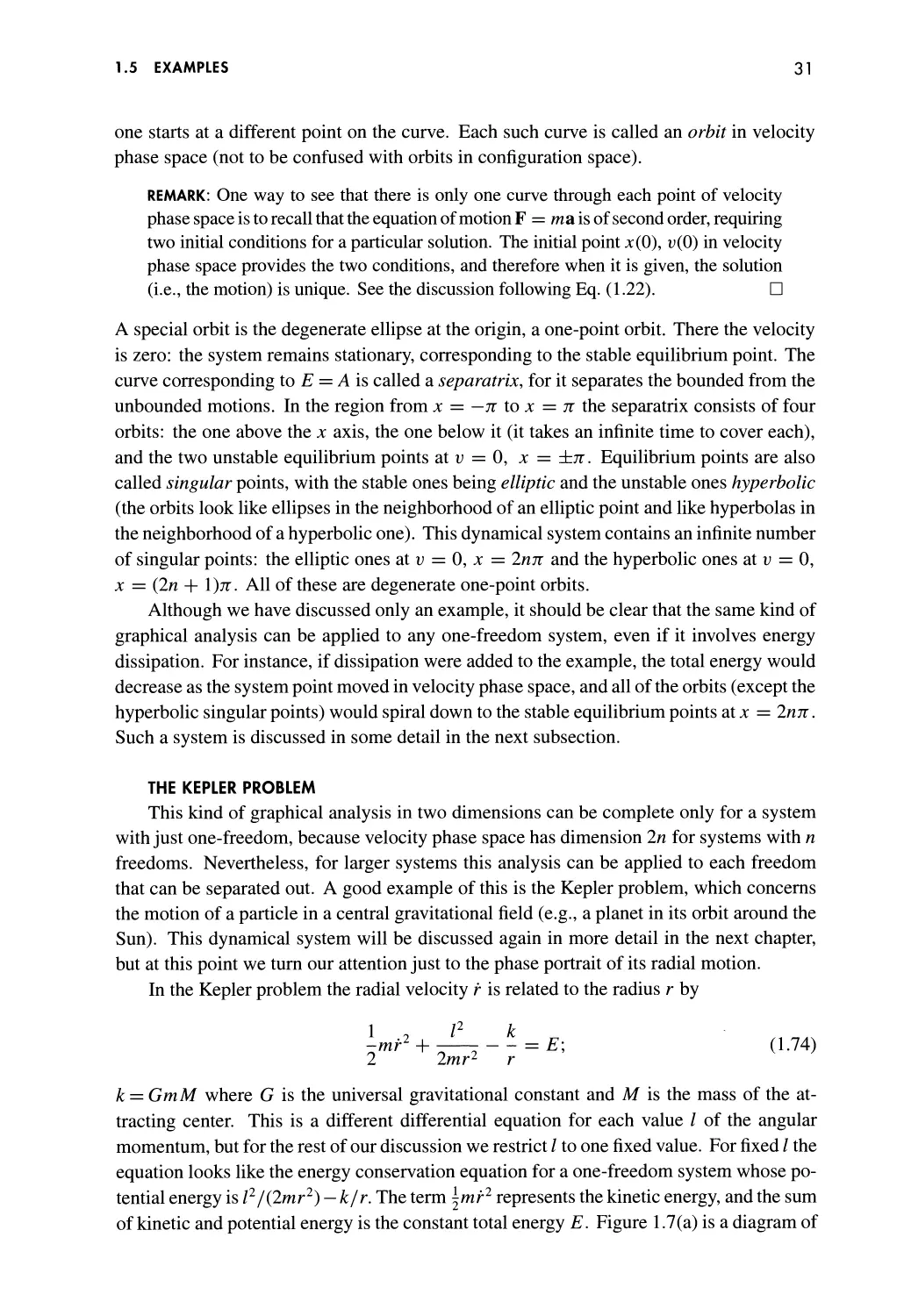
1.5.1 Velocity Phase Space and Phase Portraits 29
The Cosine Potential 29
The Kepler Problem 31
1.5.2 A System with Energy Loss 34
1.5.3 Noninertial Frames and the Equivalence
Principle 38
Equivalence Principle 38
Rotating Frames 41
Problems 42
LAGRANGIAN FORMULATION OF MECHANICS 48
2.1 Constraints and Configuration Manifolds 49
2.1.1 Constraints 49
Constraint Equations 49
Constraints and Work 50
2.1.2 Generalized Coordinates 54
2.1.3 Examples of Configuration Manifolds 57
The Finite Line 57
The Circle 57
The Plane 57
The Two-Sphere §2 57
The Double Pendulum 60
Discussion 60
2.2 Lagrange's Equations 62
2.2.1 Derivation of Lagrange's Equations 62
2.2.2 Transformations of Lagrangians 67
Equivalent Lagrangians 67
Coordinate Independence 68
Hessian Condition 69
2.2.3 Conservation of Energy 70
2.2.4 Charged Particle in an Electromagnetic Field 72
The Lagrangian 72
A Time-Dependent Coordinate Transformation 74
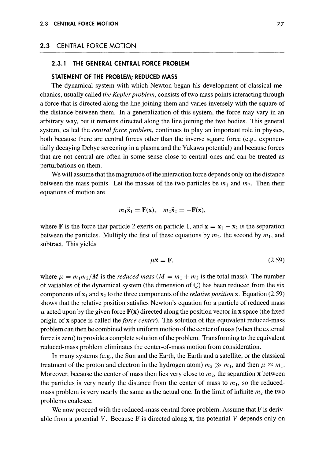
2.3 Central Force Motion 77
2.3.1 The General Central Force Problem 77
Statement of the Problem; Reduced Mass 77
Reduction to Two Freedoms 78
The Equivalent One-Dimensional Problem 79
2.3.2 The Kepler Problem 84
2.3.3 Bertrand's Theorem 88
2.4 The Tangent Bundle TQ 92

CONTENTS
IX
2.4.1 Dynamics on TQ
Velocities Do Not Lie in Q
Tangent Spaces and the Tangent Bundle
Lagrange's Equations and Trajectories on TQ
2.4.2 TQ as a Differential Manifold
Differential Manifolds
Tangent Spaces and Tangent Bundles
Application to Lagrange's Equations
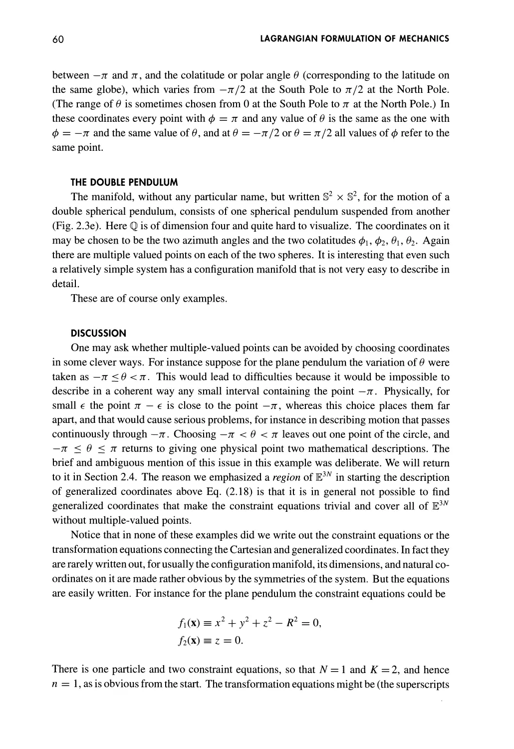
Problems
TOPICS IN LAGRANGIAN DYNAMICS
3.1 The Variational Principle and Lagrange's Equations
3.1.1 Derivation
The Action
Hamilton's Principle
Discussion
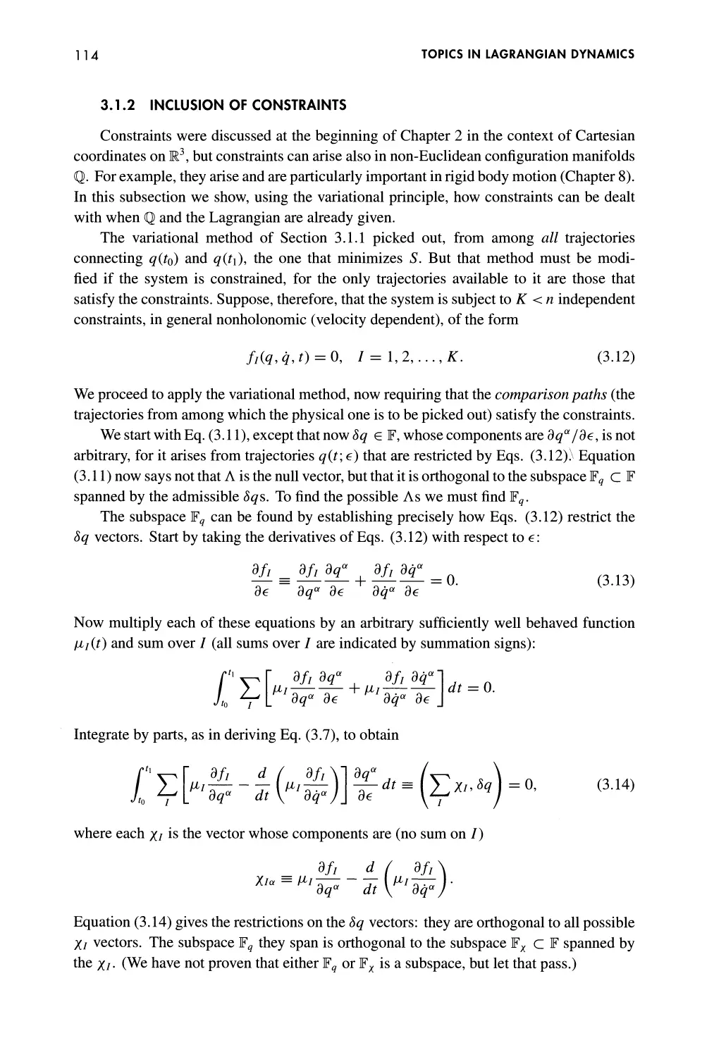
3.1.2 Inclusion of Constraints
3.2 Symmetry and Conservation
3.2.1 Cyclic Coordinates
Invariant Submanifolds and Conservation of
Momentum
Transformations, Passive and Active
Three Examples
3.2.2 Noether's Theorem
Point Transformations
The Theorem
3.3 Nonpotential Forces
3.3.1 Dissipative Forces in the Lagrangian Formalism
Rewriting the EL Equations
The Dissipative and Rayleigh Functions
3.3.2 The Damped Harmonic Oscillator
3.3.3 Comment on Time-Dependent Forces
3.4 A Digression on Geometry
3.4.1 Some Geometry
Vector Fields
One-Forms
The Lie Derivative
3.4.2 The Euler-Lagrange Equations
3.4.3 Noether's Theorem
One-Parameter Groups
The Theorem
Problems
92
92
93
95
97
97
100
102
103
108
108
108
108
110
112
114
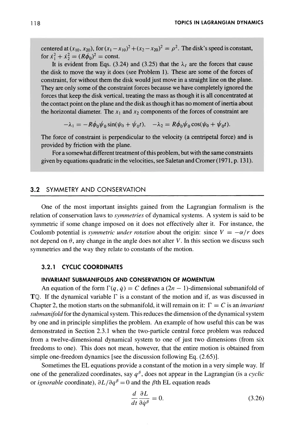
118
118
118
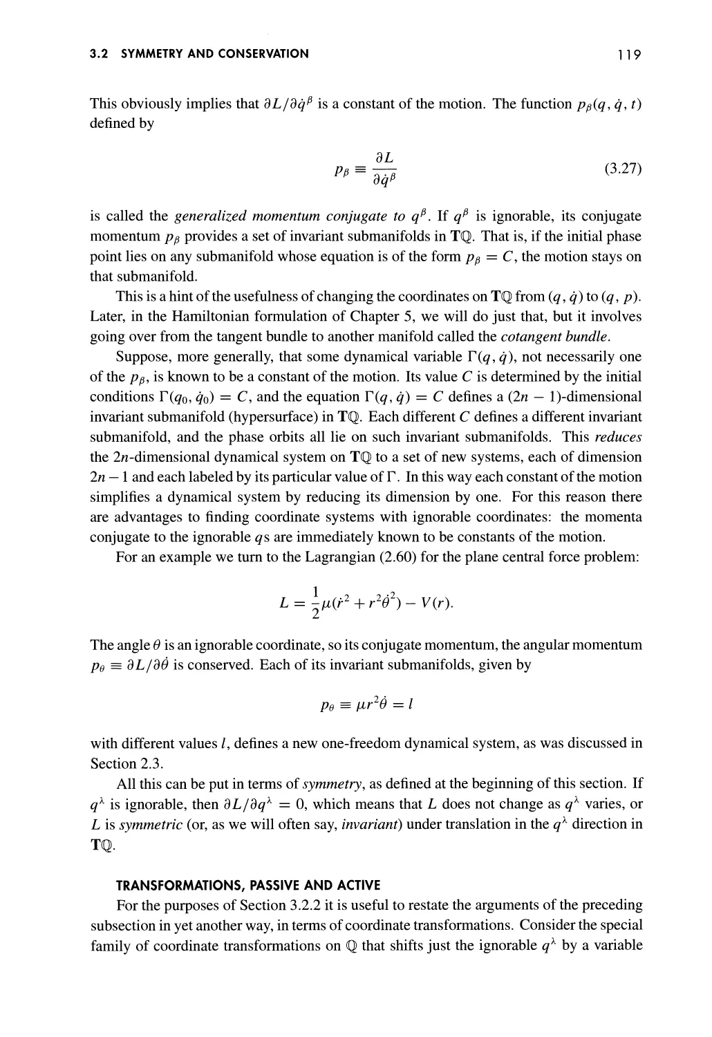
119
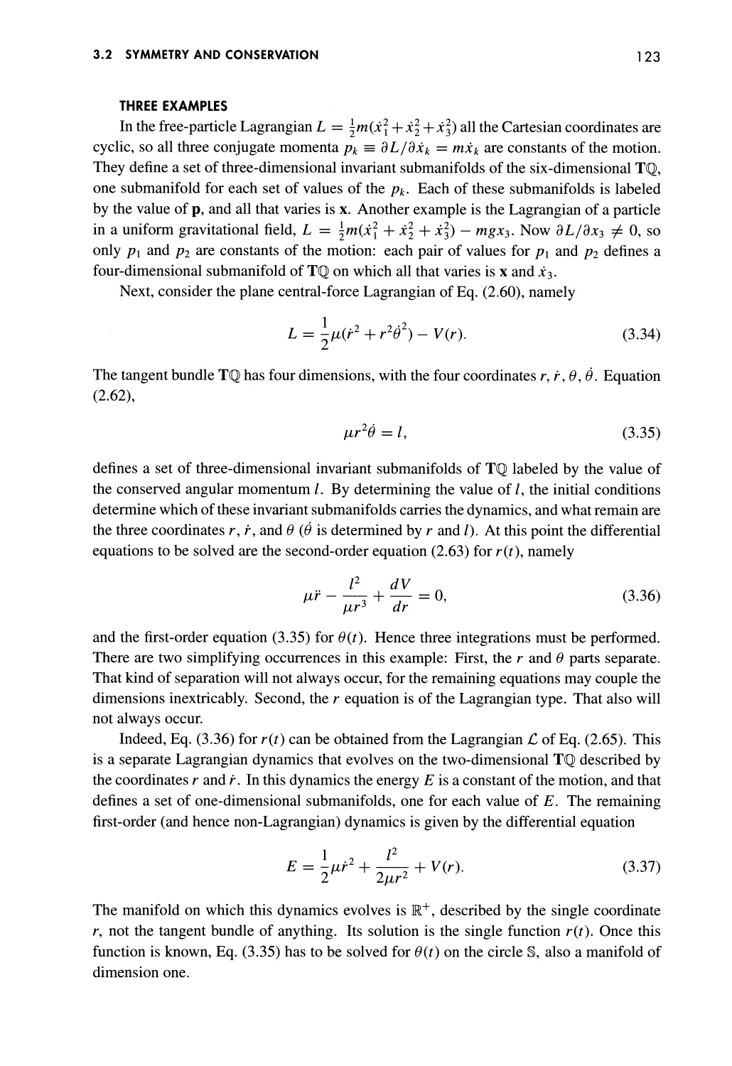
123
124
124
125
128
129
129
129
131
134
134
134
134
135
136
138
139
139
140
143

CONTENTS
SCATTERING AND LINEAR OSCILLATIONS 147
4.1 Scattering 147
4.1.1 Scattering by Central Forces 147
General Considerations 147
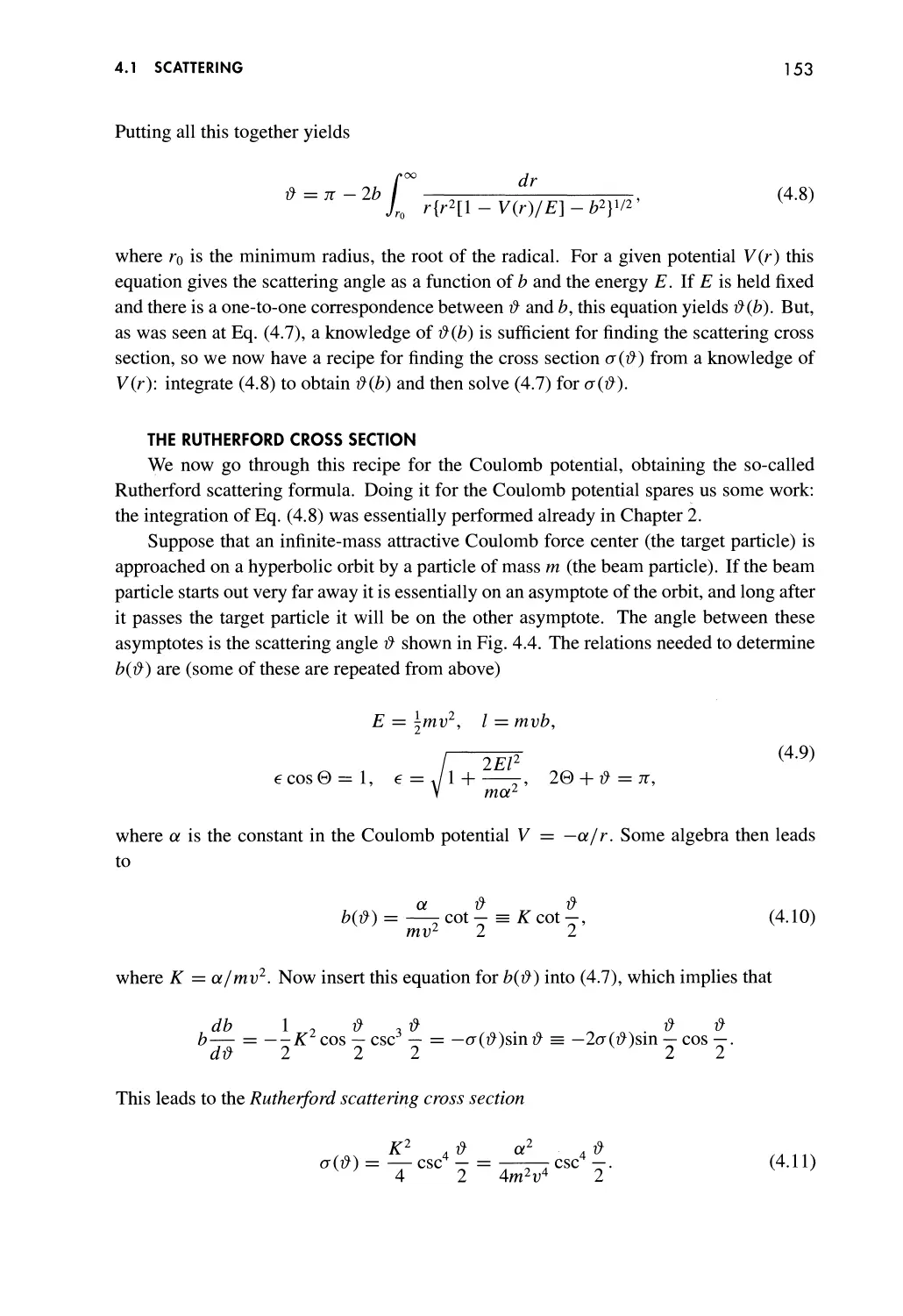
The Rutherford Cross Section 153
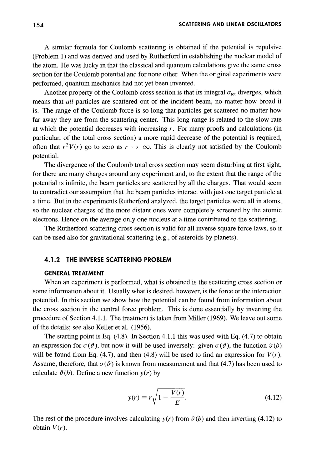
4.1.2 The Inverse Scattering Problem 154
General Treatment 154
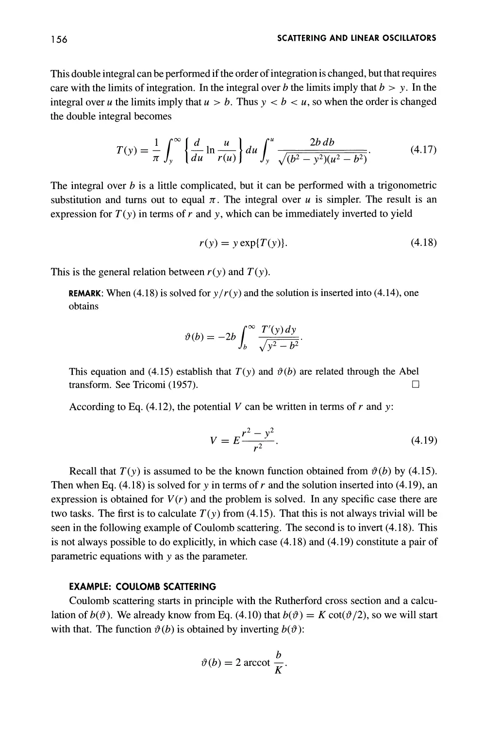
Example: Coulomb Scattering 156
4.1.3 Chaotic Scattering, Cantor Sets, and Fractal
Dimension 157
Two Disks 158
Three Disks, Cantor Sets 162
Fractal Dimension and Lyapunov Exponent 166
Some Further Results 169
4.1.4 Scattering of a Charge by a Magnetic
Dipole 170
The Stormer Problem 170
The Equatorial Limit 171
The General Case 174
4.2 Linear Oscillations 178
4.2.1 Linear Approximation: Small Vibrations 178
Linearization 178
Normal Modes 180
4.2.2 Commensurate and Incommensurate
Frequencies 183
The Invariant Torus T 183
The Poincare Map 185
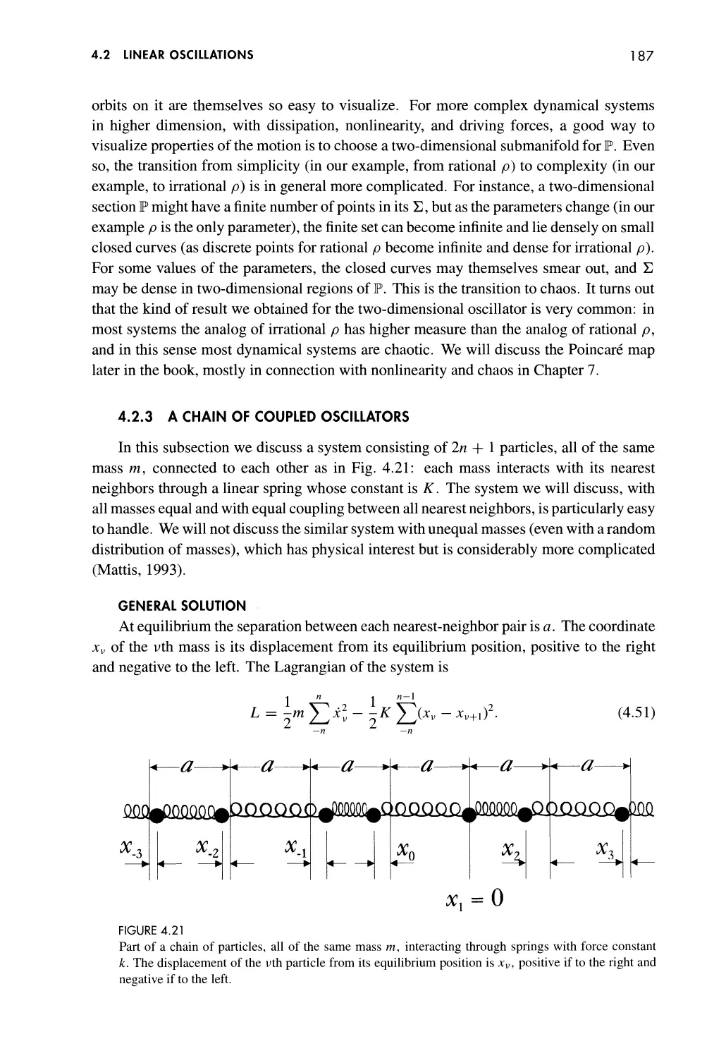
4.2.3 A Chain of Coupled Oscillators 187
General Solution 187
The Finite Chain 189
4.2.4 Forced and Damped Oscillators 192
Forced Undamped Oscillator 192
Forced Damped Oscillator 193
Problems 197
HAMILTONIAN FORMULATION OF MECHANICS 201
5.1 Hamilton's Canonical Equations 202
5.1.1 Local Considerations 202
From the Lagrangian to the Hamiltonian 202
A Brief Review of Special Relativity 207
The Relativistic Kepler Problem 211
5.1.2 The Legendre Transform 212

CONTENTS
XI
5.1.3 Unified Coordinates on T*Q and Poisson
Brackets 215
The | Notation 215
Variational Derivation of Hamilton's Equations 217
Poisson Brackets 218
Poisson Brackets and Hamiltonian Dynamics 222
5.2 Symplectic Geometry 224
5.2.1 The Cotangent Manifold 224
5.2.2 Two-Forms 225
5.2.3 The Symplectic Form co 226
5.3 Canonical Transformations 231
5.3.1 Local Considerations 231
Reduction on T*Q by Constants of the Motion 231
Definition of Canonical Transformations 232
Changes Induced by Canonical Transformations 234
Two Examples 236
5.3.2 Intrinsic Approach 239
5.3.3 Generating Functions of Canonical
Transformations 240
Generating Functions 240
The Generating Functions Gives the New
Hamiltonian 242
Generating Functions of Type 244
5.3.4 One-Parameter Groups of Canonical
Transformations 248
Infinitesimal Generators of One-Parameter Groups;
Hamiltonian Flows 249
The Hamiltonian Noether Theorem 251
Flows and Poisson Brackets 252
5.4 Two Theorems: Liouville and Darboux 253
5.4.1 Liouville's Volume Theorem 253
Volume 253
Integration on T*Q; The Liouville Theorem 257
Poincare Invariants 260
Density of States 261
5.4.2 Darboux's Theorem 268
The Theorem 269
Reduction 270
Problems 275
Canonicity Implies PB Preservation 280

CONTENTS
TOPICS IN HAMILTONIAN DYNAMICS 284
6.1 The Hamilton-Jacobi Method 2 84
6.1.1 The Hamilton-Jacobi Equation 285
Derivation 285
Properties of Solutions 286
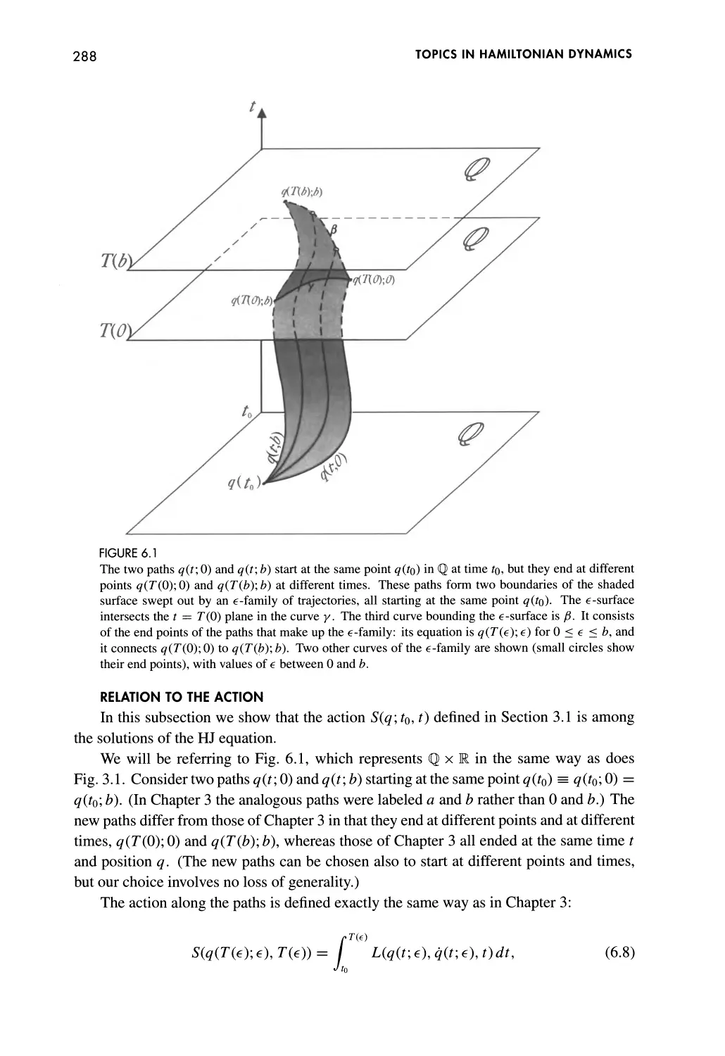
Relation to the Action 288
6.1.2 Separation of Variables 290
The Method of Separation 291
Example: Charged Particle in a Magnetic Field 294
6.1.3 Geometry and the HJ Equation 301
6.1.4 The Analogy Between Optics and the HJ
Method 303
6.2 Completely Integrable Systems 307
6.2.1 Action-Angle Variables 307
Invariant Tori 307
The (pa and Ja 309
The Canonical Transformation to AA Variables 311
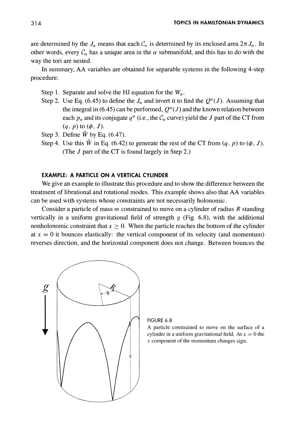
Example: A Particle on a Vertical Cylinder 314
6.2.2 Liouville's Integrability Theorem 320
Complete Integrability 320
The Tori 321
The Ja 323
Example: the Neumann Problem 324
6.2.3 Motion on the Tori 328
Rational and Irrational Winding Lines 328
Fourier Series 331
6.3 Perturbation Theory 332
6.3.1 Example: The Quartic Oscillator; Secular
Perturbation Theory 332
6.3.2 Hamiltonian Perturbation Theory 336
Perturbation via Canonical Transformations 337
Averaging 339
Canonical Perturbation Theory in One Freedom 340
Canonical Perturbation Theory in Many Freedoms 346
The Lie Transformation Method 351
Example: The Quartic Oscillator 357
6.4 Adiabatic Invariance 359
6.4.1 The Adiabatic Theorem 360
Oscillator with Time-Dependent Frequency 360
The Theorem 361
Remarks on N > 1 363
6.4.2 Higher Approximations 364

CONTENTS
XIII
6.4.3 The Hannay Angle 365
6.4.4 Motion of a Charged Particle in a Magnetic
Field 371
The Action Integral 371
Three Magnetic Adiabatic Invariants 374
Problems 377
NONLINEAR DYNAMICS 382
7.1 Nonlinear Oscillators 383
7.1.1 A Model System 383
7.1.2 Driven Quartic Oscillator 386
Damped Driven Quartic Oscillator; Harmonic
Analysis 387
Undamped Driven Quartic Oscillator 390
7.1.3 Example: The van der Pol Oscillator 391
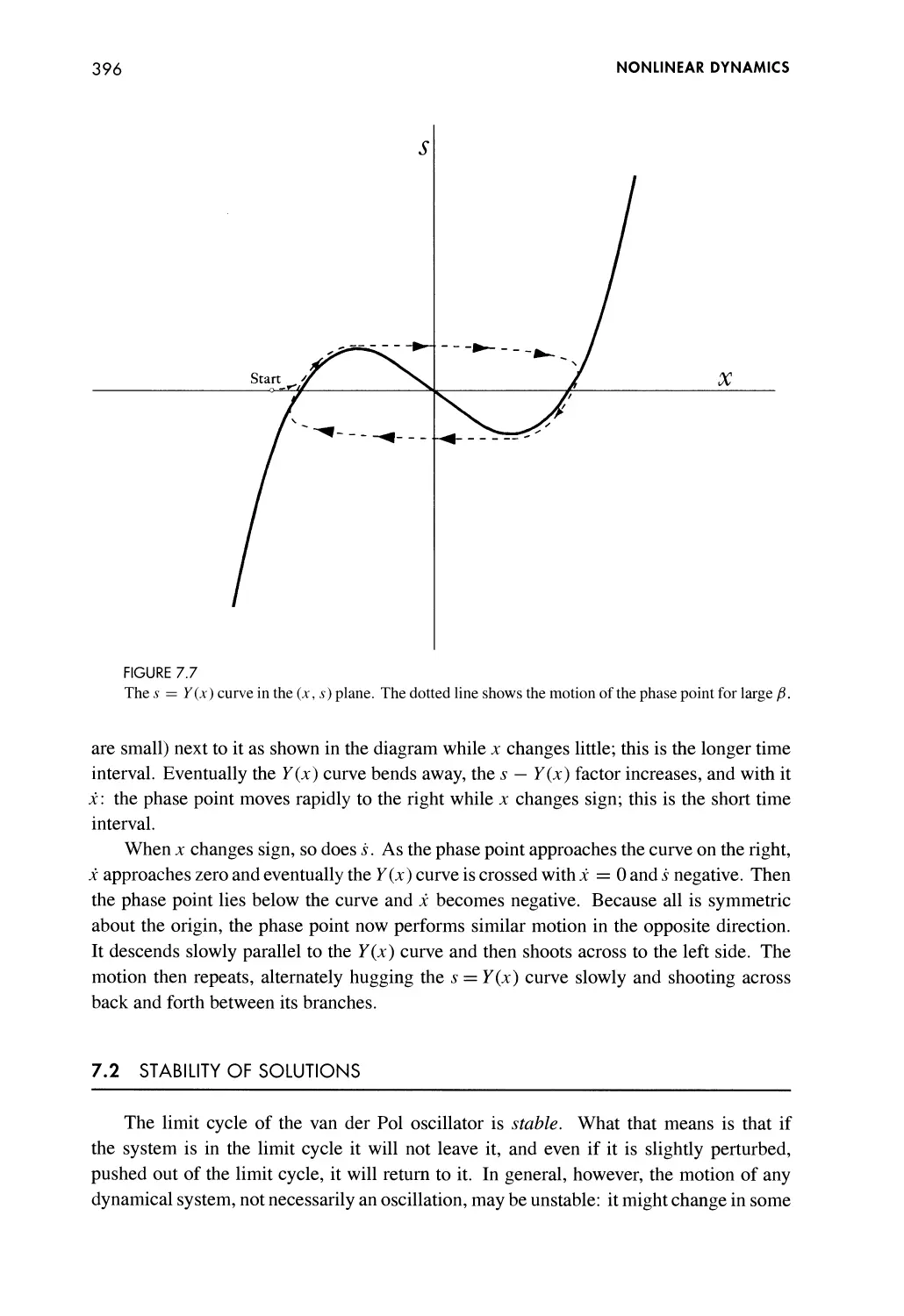
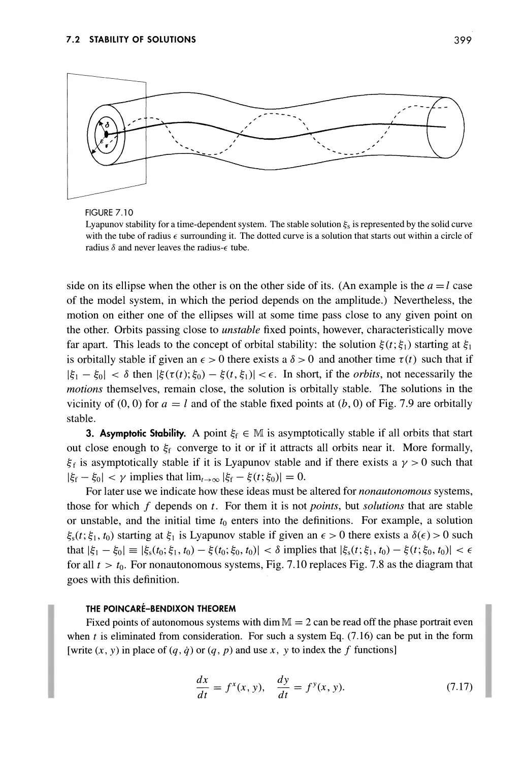
7.2 Stability of Solutions 396
7.2.1 Stability of Autonomous Systems 397
Definitions 397
The Poincare-Bendixon Theorem 399
Linearization 400
7.2.2 Stability of Nonautonomous Systems 410
The Poincare Map 410
Linearization of Discrete Maps 413
Example: The Linearized Henon Map 417
7.3 Parametric Oscillators 418
7.3.1 Floquet Theory 419
The Floquet Operator R 419
Standard Basis 420
Eigenvalues of R and Stability 421
Dependence on G 424
7.3.2 The Vertically Driven Pendulum 424
The Mathieu Equation 424
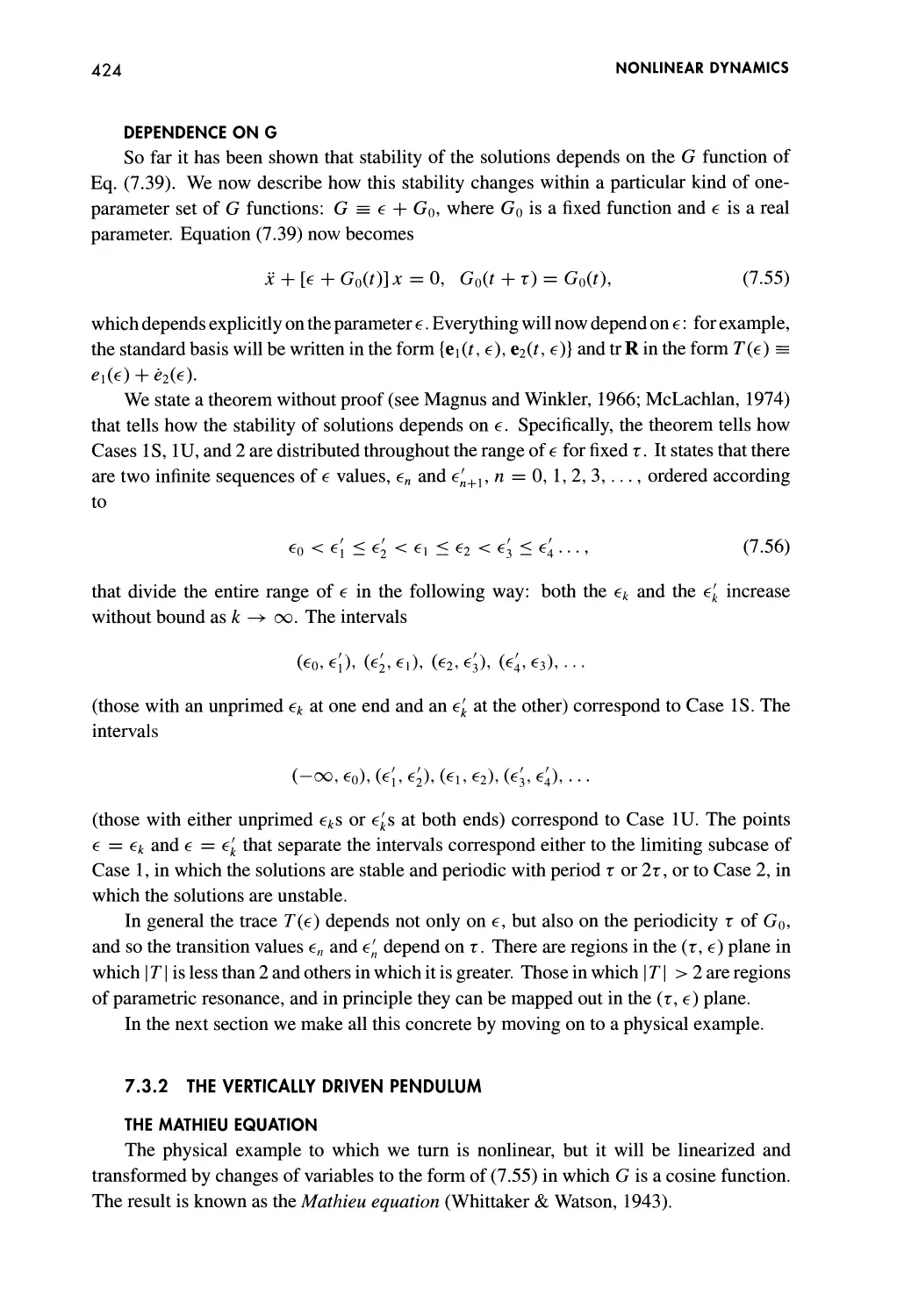
Stability of the Pendulum 42 6
The Inverted Pendulum 427
Damping 429
7.4 Discrete Maps; Chaos 431
7.4.1 The Logistic Map 431
Definition 432
Fixed Points 432
Period Doubling 434
Universality 442
Further Remarks 444

CONTENTS
7.4.2 The Circle Map 445
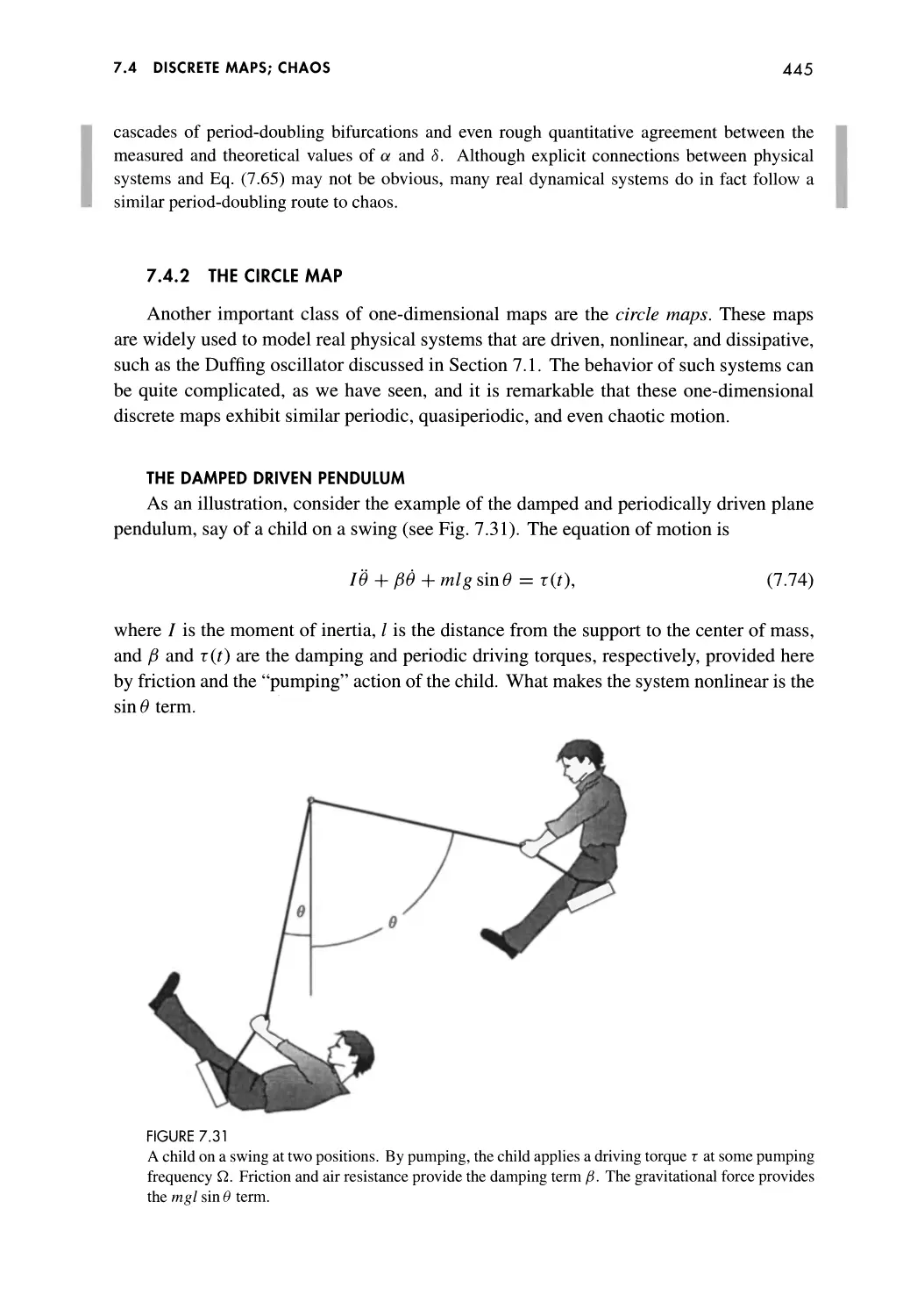
The Damped Driven Pendulum 445
The Standard Sine Circle Map 446
Rotation Number and the Devil's Staircase 447
Fixed Points of the Circle Map 450
7.5 Chaos in Hamiltonian Systems and the KAM
Theorem 452
7.5.1 The Kicked Rotator 453
The Dynamical System 453
The Standard Map 454
Poincare Map of the Perturbed System 455
7.5.2 TheHenonMap 460
7.5.3 Chaos in Hamiltonian Systems 463
Poincare-Birkhoff Theorem 464
The Twist Map 466
Numbers and Properties of the Fixed Points 467
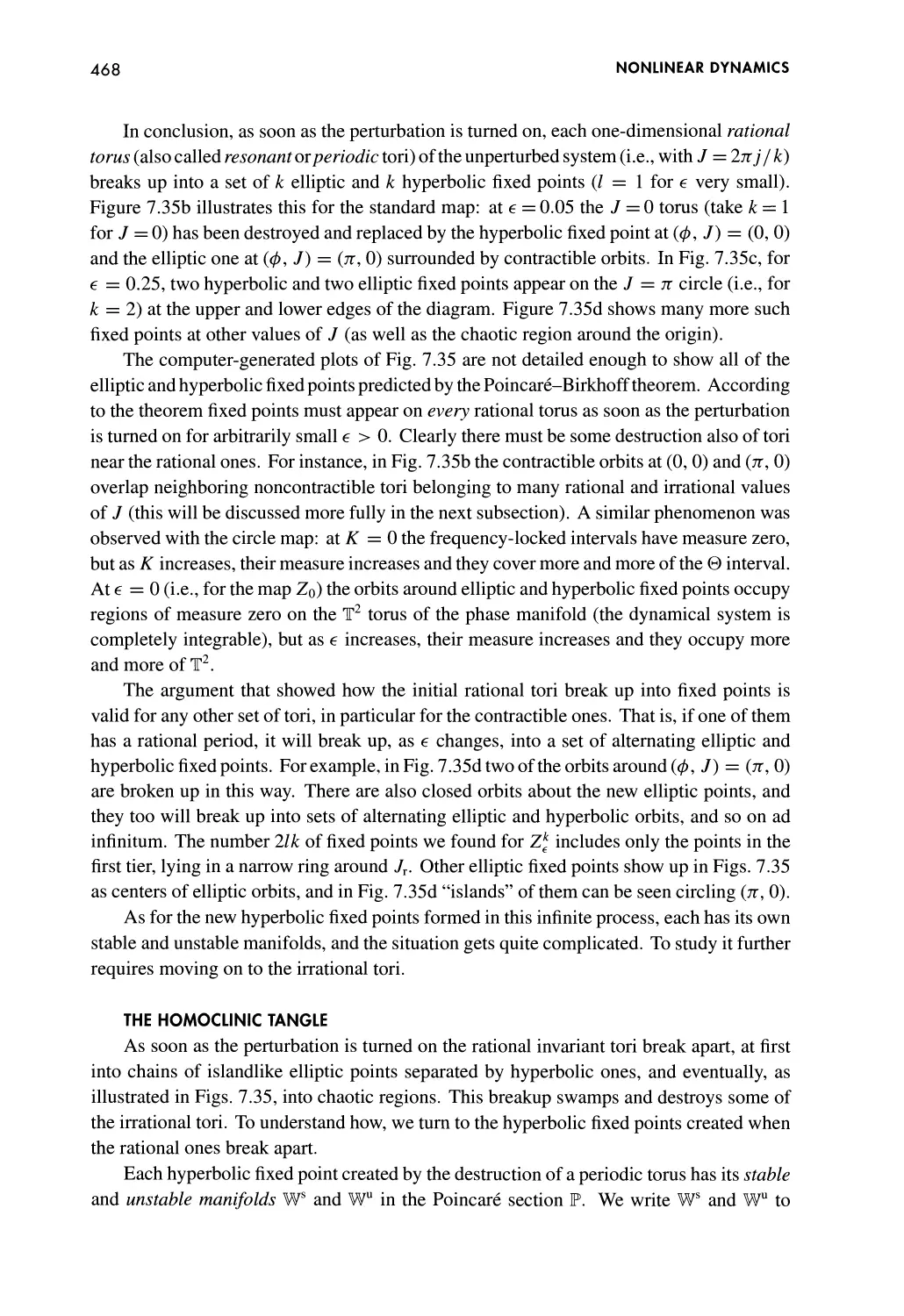
The Homoclinic Tangle 468
The Transition to Chaos 472
7.5.4 The KAM Theorem 474
Background 474
Two Conditions: Hessian and Diophantine 475
The Theorem 477
A Brief Description of the Proof of KAM 480
Problems 483
Number Theory 486
The Unit Interval 486
A Diophantine Condition 487
The Circle and the Plane 488
KAM and Continued Fractions 489
RIGID BODIES 492
8.1 Introduction 492
8.1.1 Rigidity and Kinematics 492
Definition 492
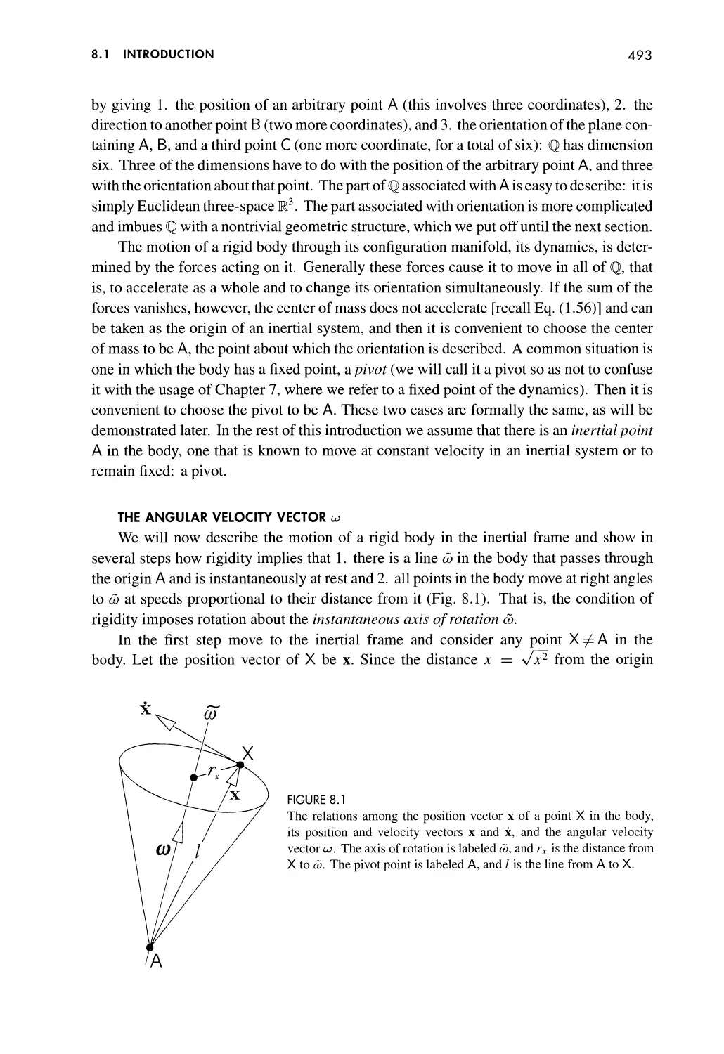
The Angular Velocity Vector uj 493
8.1.2 Kinetic Energy and Angular Momentum 495
Kinetic Energy 495
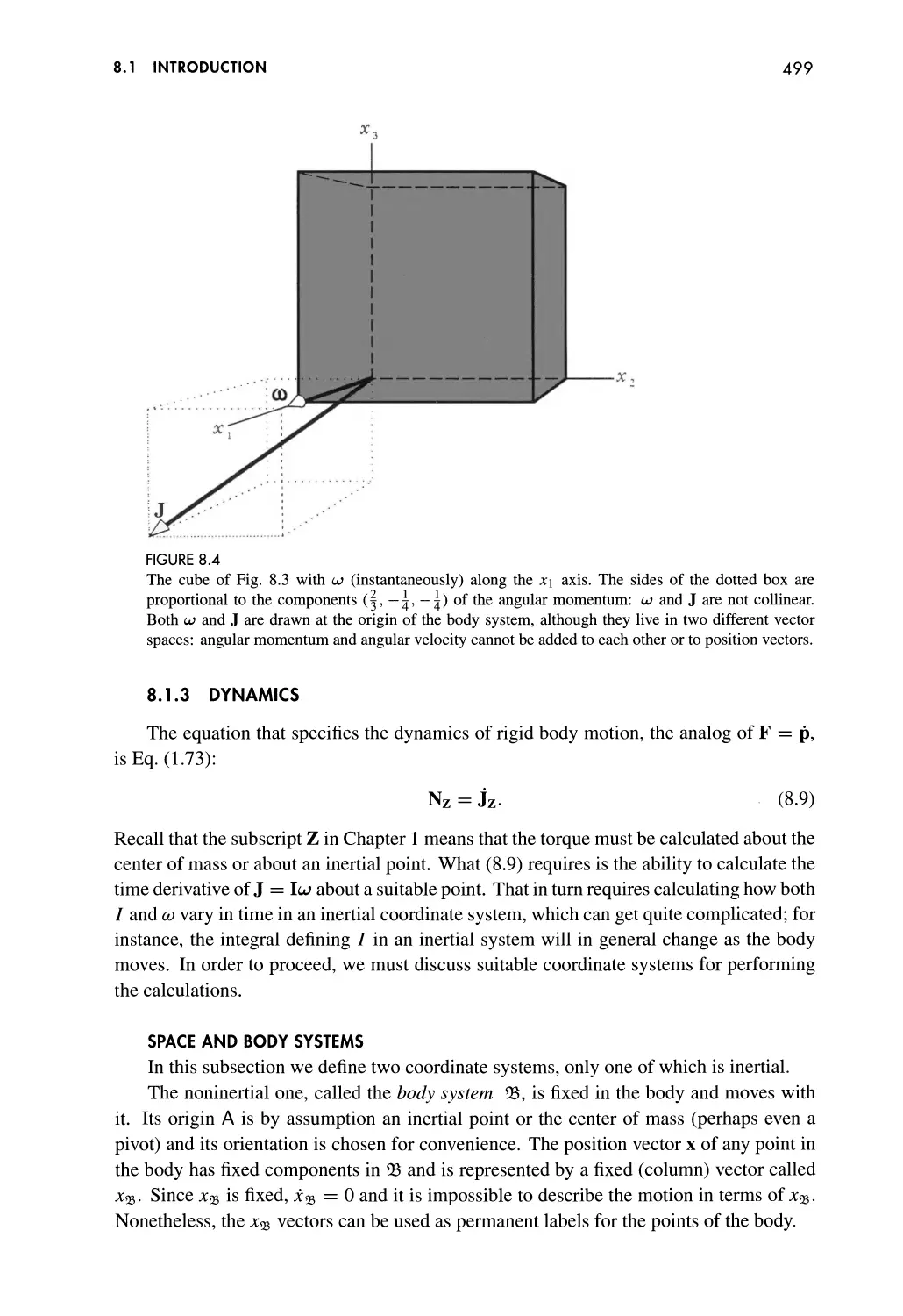
Angular Momentum 498
8.1.3 Dynamics 499
Space and Body Systems 499
Dynamical Equations 500
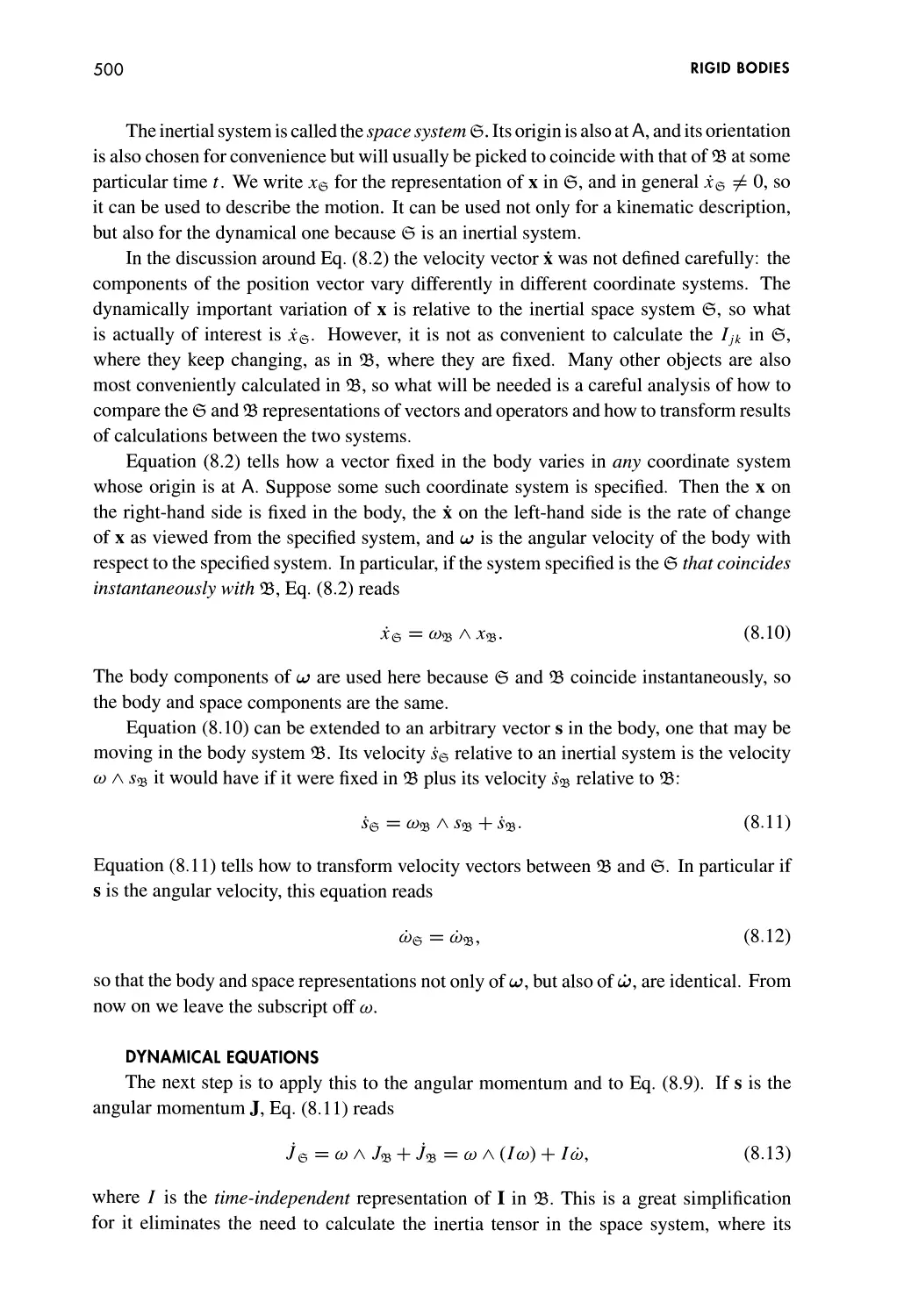
Example: The Gyrocompass 503

CONTENTS
xv
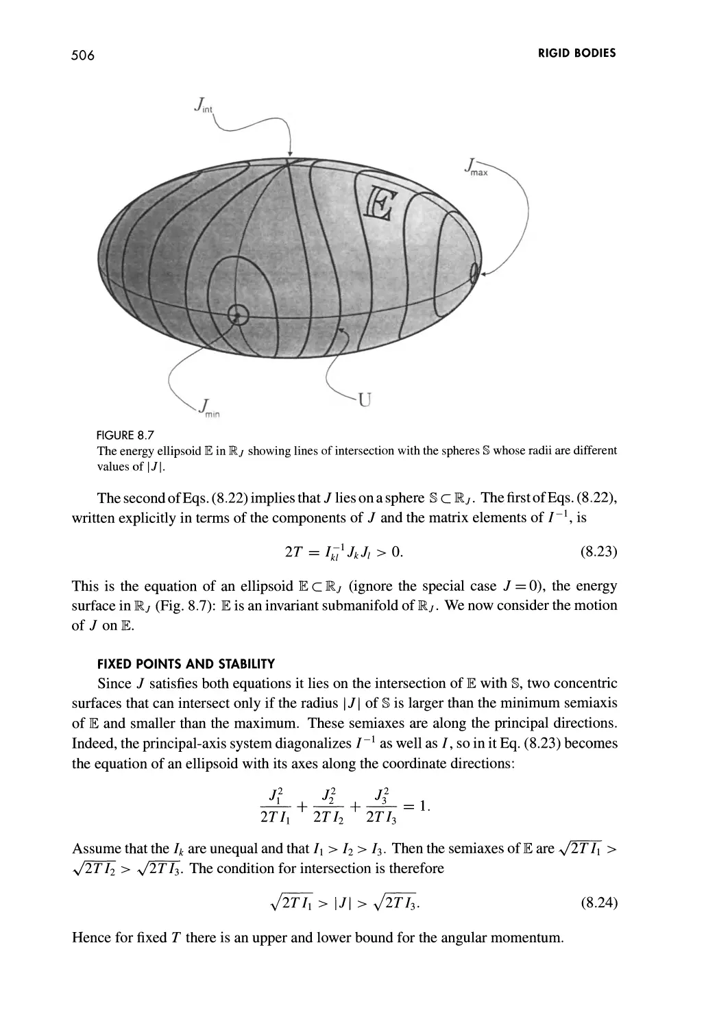
Motion of the Angular Momentum J 505
Fixed Points and Stability 506
The Poinsot Construction 508
8.2 The Lagrangian and Hamiltonian Formulations 510
8.2.1 The Configuration Manifold QR 510
Inertial, Space, and Body Systems 510
The Dimension of Q# 511
The Structure of Q* 512
8.2.2 The Lagrangian 514
Kinetic Energy 514
The Constraints 515
8.2.3 The Euler-Lagrange Equations 516
Derivation 516
The Angular Velocity Matrix Q 518
8.2.4 The Hamiltonian Formalism 519
8.2.5 Equivalence to Euler's Equations 520
Antisymmetric Matrix-Vector Correspondence 520
The Torque 521
The Angular Velocity Pseudovector and
Kinematics 522
Transformations of Velocities 523
Hamilton's Canonical Equations 524
8.2.6 Discussion 525
8.3 Euler Angles and Spinning Tops 526
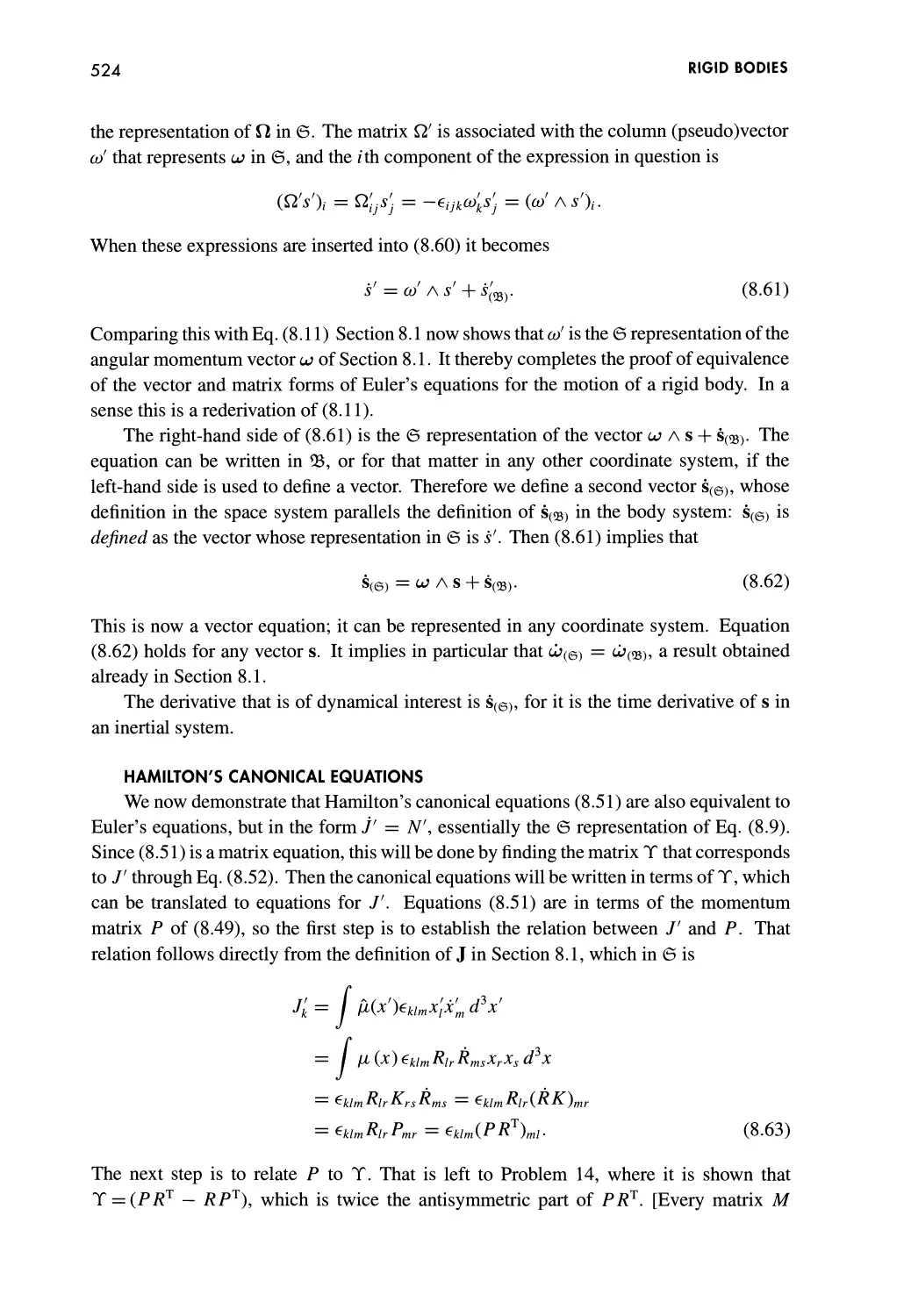
8.3.1 Euler Angles 526
Definition 526
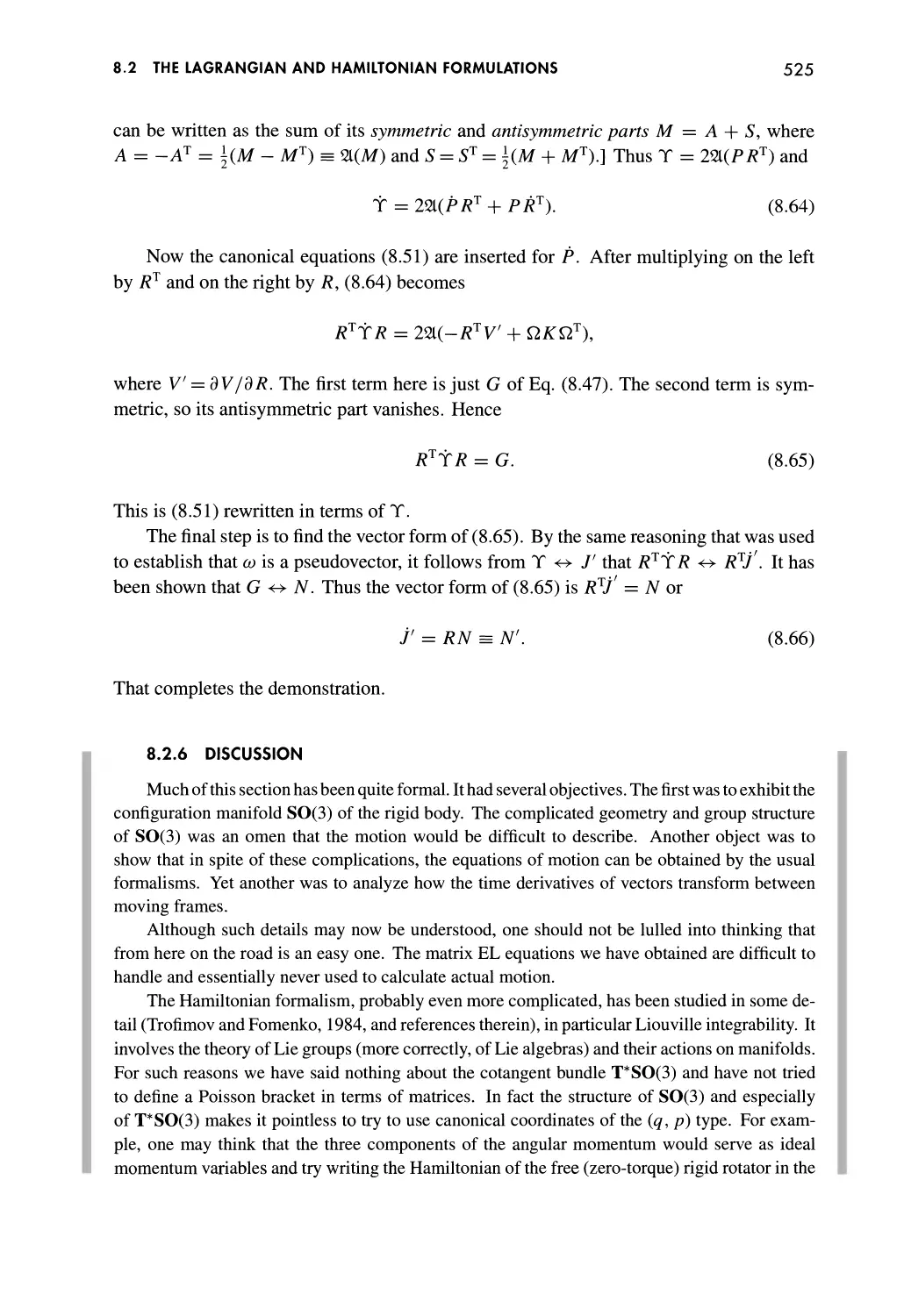
R in Terms of the Euler Angles 527
Angular Velocities 529
Discussion 531
8.3.2 Geometric Phase for a Rigid Body 533
8.3.3 Spinning Tops 535
The Lagrangian and Hamiltonian 536
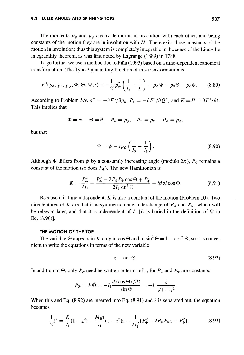
The Motion of the Top 537
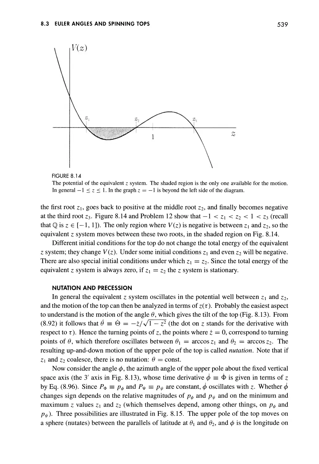
Nutation and Precession 539
Quadratic Potential; the Neumann Problem 542
8.4 Cayley-Klein Parameters 543
8.4.1 2x2 Matrix Representation of 3-Vectors and
Rotations 543
3-Vectors 543
Rotations 544
8.4.2 The Pauli Matrices and CK Parameters 544
Definitions 544

XVI
CONTENTS
Finding Rv 545
Axis and Angle in terms of the CK Parameters 546
8.4.3 Relation Between SU(2) and SO(3) 547
Problems 549
CONTINUUM DYNAMICS 553
9.1 Lagrangian Formulation of Continuum
Dynamics 553
9.1.1 Passing to the Continuum Limit 553
The Sine-Gordon Equation 553
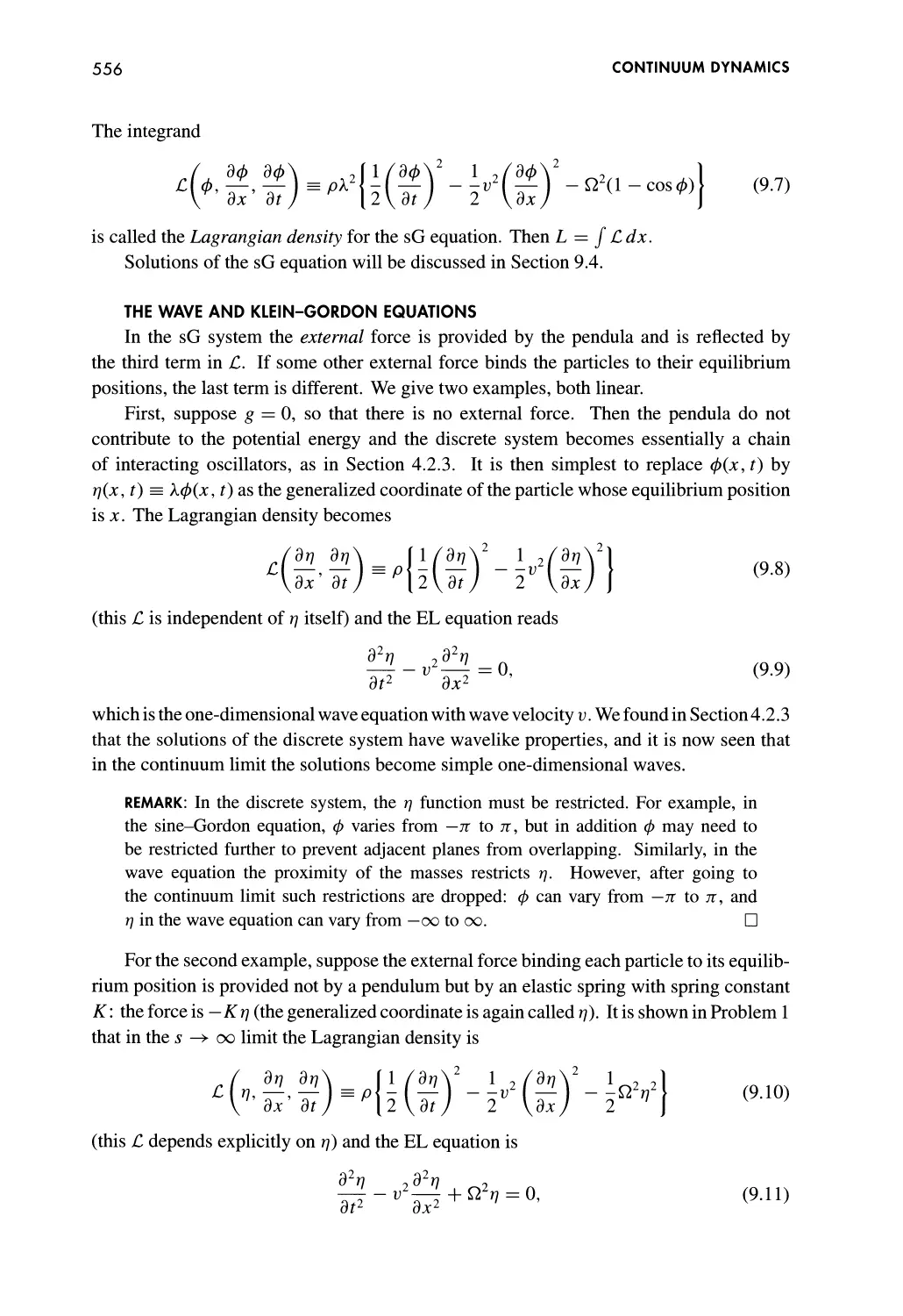
The Wave and Klein-Gordon Equations 556
9.1.2 The Variational Principle 557
Introduction 557
Variational Derivation of the EL Equations 557
The Functional Derivative 560
Discussion 560
9.1.3 Maxwell's Equations 561
Some Special Relativity 561
Electromagnetic Fields 562
The Lagrangian and the EL Equations 564
9.2 Noether's Theorem and Relativistic Fields 565
9.2.1 Noether's Theorem 565
The Theorem 565
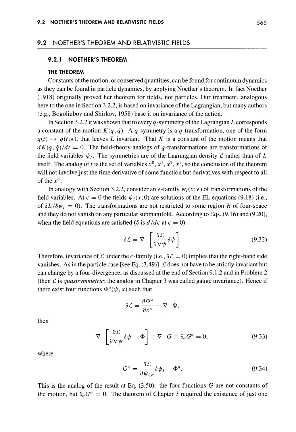
Conserved Currents 566
Energy and Momentum in the Field 567
Example: The Electromagnetic
Energy-Momentum Tensor 569
9.2.2 Relativistic Fields 571
Lorentz Transformations 571
Lorentz Invariant C and Conservation 572
Free Klein-Gordon Fields 576
Complex K-G Field and Interaction with the
Maxwell Field 577
Discussion of the Coupled Field Equations 579
9.2.3 Spinors 580
Spinor Fields 580
A Spinor Field Equation 582
9.3 The Hamiltonian Formalism 583
9.3.1 The Hamiltonian Formalism for Fields 583
Definitions 583
The Canonical Equations 584
Poisson Brackets 586

CONTENTS
XVII
9.3.2 Expansion in Orthonormal Functions 588
Orthonormal Functions 589
Particle-like Equations 590
Example: Klein-Gordon 591
9.4 Nonlinear Field Theory 594
9.4.1 The Sine-Gordon Equation 594
Soliton Solutions 595
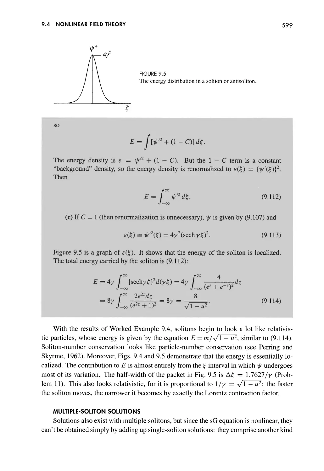
Properties of sG Solitons 597
Multiple-Soliton Solutions 599
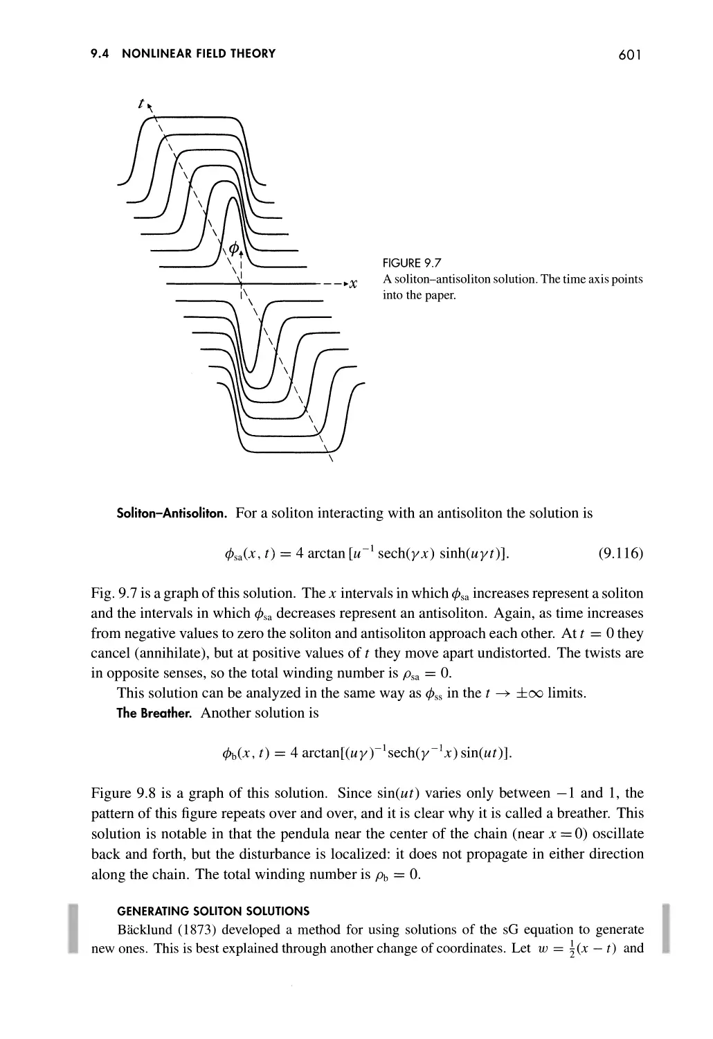
Generating Soliton Solutions 601
Nonsoliton Solutions 605
Josephson Junctions 60 8
9.4.2 The Nonlinear K-G Equation 608
The Lagrangian and the EL Equation 608
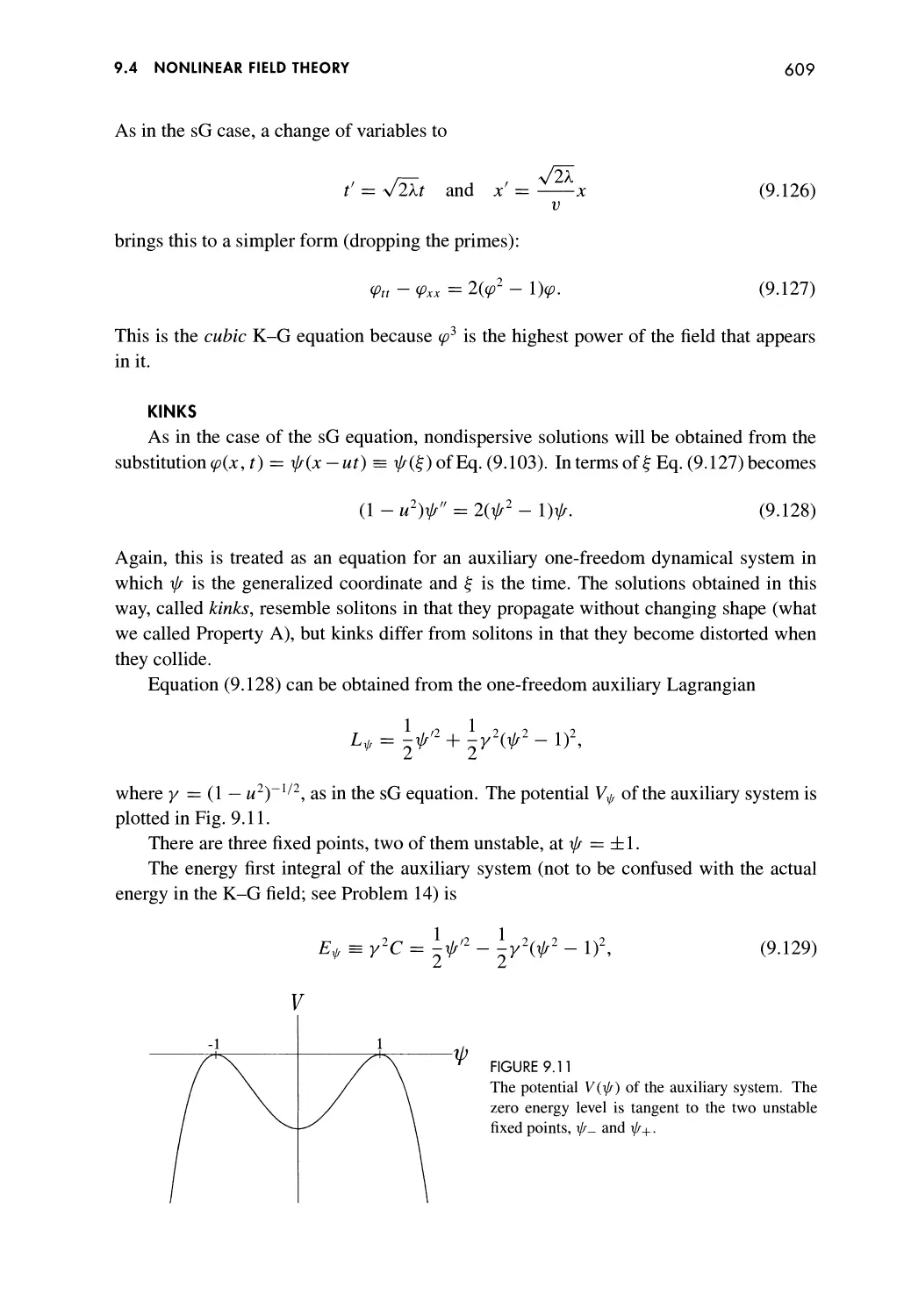
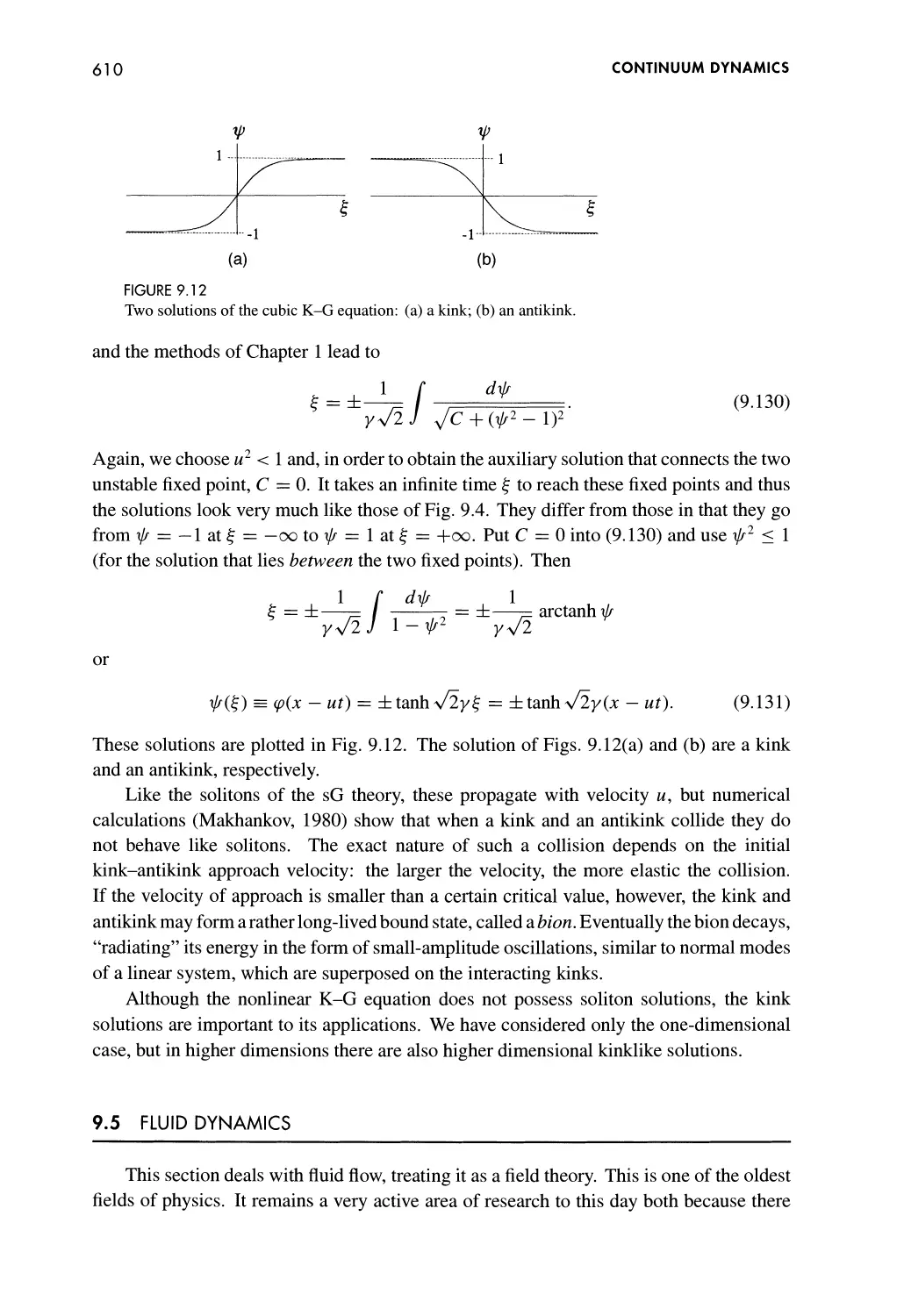
Kinks 609
9.5 Fluid Dynamics 610
9.5.1 The Euler and Navier-Stokes Equations 611
Substantial Derivative and Mass Conservation 611
Euler's Equation 612
Viscosity and Incompressibility 614
The Navier-Stokes Equations 615
Turbulence 616
9.5.2 The Burgers Equation 618
The Equation 618
Asymptotic Solution 620
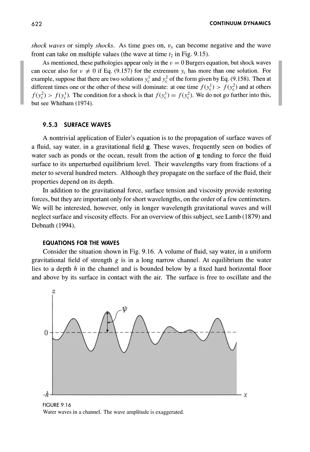
9.5.3 Surface Waves 622
Equations for the Waves 622
Linear Gravity Waves 624
Nonlinear Shallow Water Waves: the KdV Equation 626
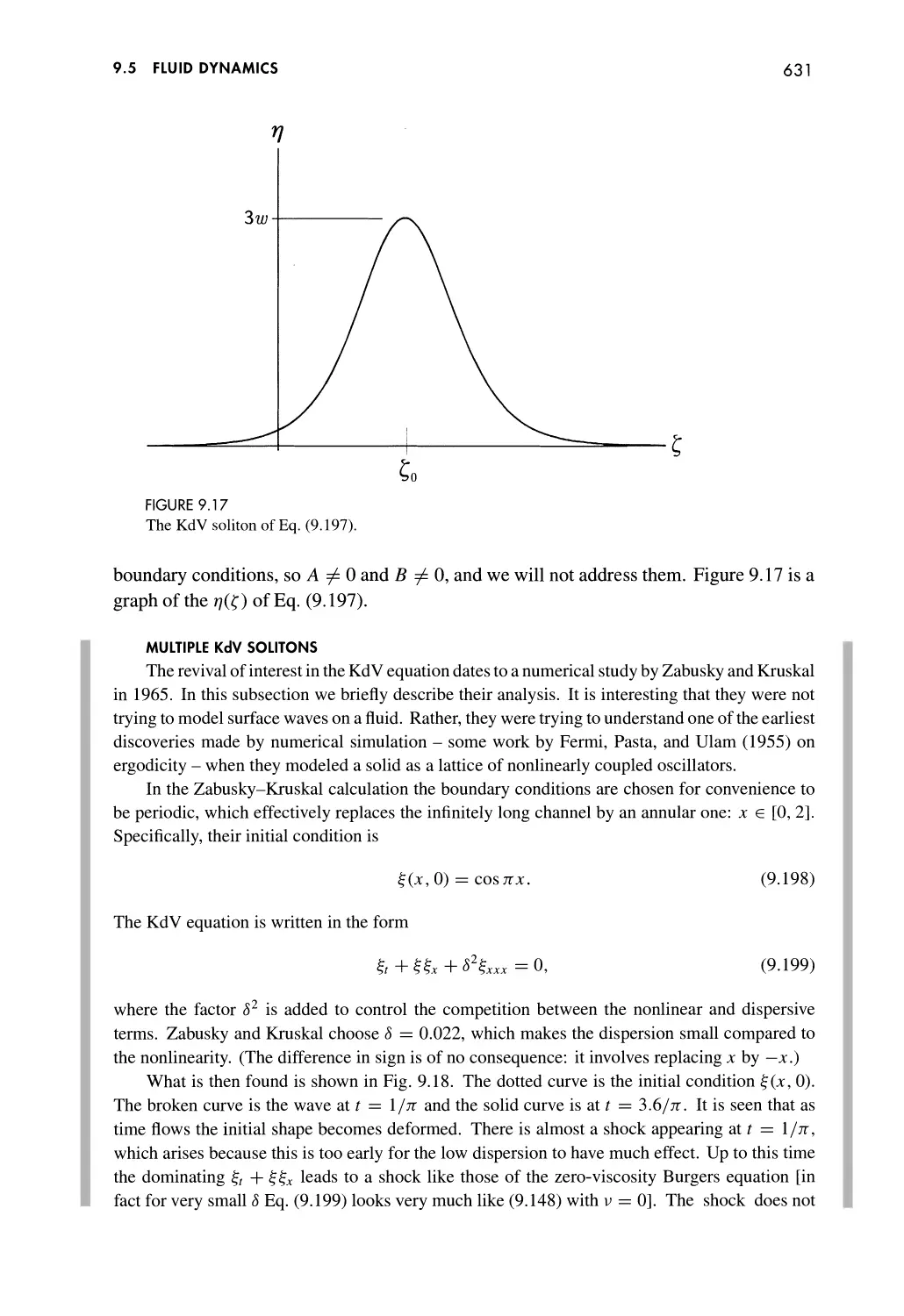
Single KdV Solitons 629
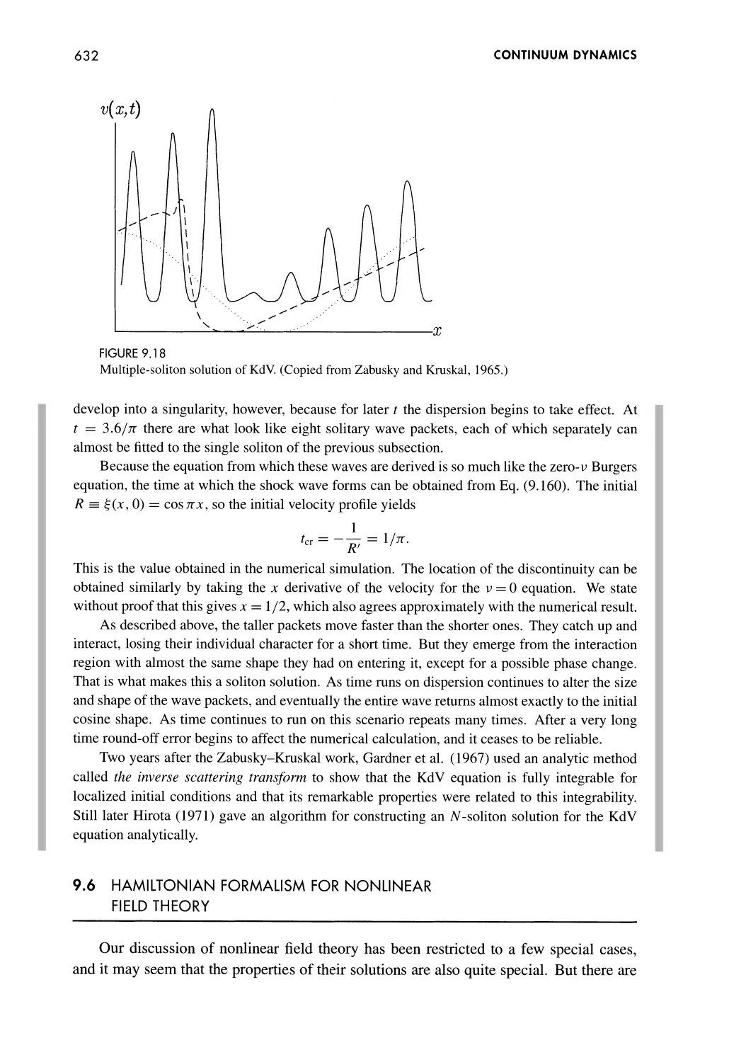
Multiple KdV Solitons 631
9.6 Hamiltonian Formalism for Nonlinear Field Theory 632
9.6.1 The Field Theory Analog of Particle Dynamics 633
From Particles to Fields 633
Dynamical Variables and Equations of Motion 63 4
9.6.2 The Hamiltonian Formalism 634
The Gradient 634
The Symplectic Form 636
The Condition for Canonicity 63 6
Poisson Brackets 63 6
9.6.3 The kdV Equation 637
KdV as a Hamiltonian Field 637

XVIII
CONTENTS
Constants of the Motion 638
Generating the Constants of the Motion 639
More on Constants of the Motion 640
9.6.4 The Sine-Gordon Equation 642
Two-Component Field Variables 642
sG as a Hamiltonian Field 643
Problems 646
EPILOGUE 648
APPENDIX: VECTOR SPACES 649
General Vector Spaces 649
Linear Operators 651
Inverses and Eigenvalues 652
Inner Products and Hermitian Operators 653
BIBLIOGRAPHY 656
INDEX
663

LIST OF WORKED EXAMPLES
1.1 Phase portrait of inverse harmonic oscillator 33
1.2 Accelerating pendulum 40
2.1 Neumann problem in three dimensions 61
2.2.1 Bead on a rotating hoop 65
2.2.2 Bead on a rotating hoop, energy 71
2.3 Morse potential 80
2.4 Moon-Earth system approximation 86
2.5 Atlas for the torus 99
2.6 Curves and tangents in two charts 102
3.1 Rolling disk 116
3.2 Noether in a gravitational field 128
3.3 Inverted harmonic oscillator 141
3.4 Energy in the underdamped harmonic oscillator 142
4.1 Stormer problem equatorial limit 176
4.2 Linear classical water molecule 181
5.1 Hamilton's equations for a particle in an
electromagnetic field 204
5.2 Hamilton's equations for a central force field 206
5.3 Poisson brackets of the angular momentum 219
5.4 Hamiltonian vector field 230
5.5 Two complex canonical transformations 246
5.6 Gaussian phase-space density distribution 264
5.7 Angular-momentum reduction of central force
system 273
6.1 HJ treatment of central force problem 293
6.2 HJ treatment of relativistic Kepler problem 296

XX
LIST OF WORKED EXAMPLES
6.3 Separability of two-center problem in confocal
coordinates 298
6.4 AA variables for the perturbed Kepler problem 318
6.5 Canonical perturbation theory for the quartic
oscillator 344
6.6 Nonlinearly coupled harmonic oscillators 348
6.7 Foucault pendulum 367
7.1 Linearized spring-mounted bead on a rod 407
7.2 Particle in time-dependent magnetic field 429
7.3 Period-two points of the logistic map 436
7.4 Closed form expression for the end of the logistic
map 444
7.5 Hessian condition in the KAM theorem 476
8.1.1 Inertia tensor of a uniform cube 496
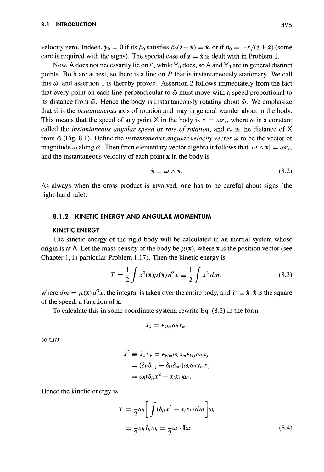
8.1.2 Angular momentum of a uniform cube 498
8.2 Rolling sphere, informal treatment 502
8.3 Rolling sphere, formal treatment 532
8.4 Cay ley-Klein parameters and Euler angles 548
9.1 Schrodinger field 568
9.2 Poynting vector from symmetrized
energy-momentum tensor 570
9.3 Hamiltonian density from Lagrangian density 585
9.4 Sine-Gordon soliton 597
9.5 Generating soliton-soliton solutions 604
9.6 Gradient of the KdV Hamiltonian 635
9.7 A KdV constant of the motion 638
9.8 Symmetric operator 642
9.9 Gradient of the sine-Gordon Hamiltonian 644

PREFACE
Among the first courses taken by graduate students in physics in North America is
Classical Mechanics. This book is a contemporary text for such a course, containing material
traditionally found in the classical textbooks written through the early 1970s as well as
recent developments that have transformed classical mechanics to a subject of significant
contemporary research. It is an attempt to merge the traditional and the modern in one
coherent presentation.
When we started writing the book we planned merely to update the classical book by
Saletan and Cromer (1971) (SC) by adding more modern topics, mostly by emphasizing
differential geometric and nonlinear dynamical methods. But that book was written when
the frontier was largely quantum field theory, and the frontier has changed and is now
moving in many different directions. Moreover, classical mechanics occupies a different
position in contemporary physics than it did when SC was written. Thus this book is not
merely an update of SC. Every page has been written anew and the book now includes
many new topics that were not even in existence when SC was written. (Nevertheless,
traces of SC remain and are evident in the frequent references to it.)
From the late seventeenth century well into the nineteenth, classical mechanics was
one of the main driving forces in the development of physics, interacting strongly with
developments in mathematics, both by borrowing and lending. The topics developed by
its main protagonists, Newton, Lagrange, Euler, Hamilton, and Jacobi among others, form
the basis of the traditional material.
In the first few decades following World War II, the graduate Classical Mechanics
course, although still recognized as fundamental, was barely considered important in its
own right to the education of a physicist: it was thought of mostly as a peg on which to hang
quantum physics, field theory, and many-body theory, areas in which the budding physicist
was expected to be working. Textbooks, including SC, concentrated on problems, mostly
linear, both old and new, whose solutions could be obtained by reduction to quadrature,
even though, as is now apparent, such systems form an exceptional subset of all classical
dynamical systems.
In those same decades the subject itself was undergoing a rebirth and expanding, again
in strong interaction with developments in mathematics. There has been an explosion in

XXII
PREFACE
the study of nonlinear classical dynamical systems, centering in part around the discovery
of novel phenomena such as chaos. (In its new incarnation the subject is often also called
Dynamical Systems, particularly in its mathematical manifestations.)
What made substantive new advances possible in a subject as old as classical
mechanics are two complementary developments. The first consists of qualitative but powerful
geometric ideas through which the general nature of nonlinear systems can be studied
(including global, rather than local analysis). The second, building upon the first, is the
modern computer, which allows quantitative analysis of nonlinear systems that had not
been amenable to full study by traditional analytic methods.
Unfortunately the new developments seldom found their way into Classical Mechanics
courses and textbooks. There was one set of books for the traditional topics and another
for the modern ones, and when we tried to teach a course that includes both the old and
the new, we had to jump from one set to the other (and often to use original papers and
reviews). In this book we attempt to bridge the gap: our main purpose is not only to bring
the new developments to the fore, but to interweave them with more traditional topics, all
under one umbrella.
That is the reason it became necessary to do more than simply update SC. In
trying to mesh the modern developments with traditional subjects like the Lagrangian and
Hamiltonian formulations and Hamilton-Jacobi theory we found that we needed to write
an entirely new book and to add strong emphasis on nonlinear dynamics. As a result the
book differs significantly not only from SC, but also from other classical textbooks such
as Goldstein's.
The language of modern differential geometry is now used extensively in the literature,
both physical and mathematical, in the same way that vector and matrix notation is used
in place of writing out equations for each component and even of indicial notation. We
therefore introduce geometric ideas early in the book and use them throughout, principally
in the chapters on Hamiltonian dynamics, chaos, and Hamiltonian field theory.
Although we often present the results of computer calculations, we do not actually deal
with programming as such. Nowadays that is usually treated in separate Computational
Physics courses.
Because of the strong interaction between classical mechanics and mathematics, any
modern book on classical mechanics must emphasize mathematics. In this book we do
not shy away from that necessity. We try not to get too formal, however, in explaining the
mathematics. For a rigorous treatment the reader will have to consult the mathematical
literature, much of which we cite.
We have tried to start most chapters with the traditional subjects presented in a
conventional way. The material then becomes more mathematically sophisticated and quantitative.
Detailed applications are included both in the body of the text and as Worked Examples,
whose purpose is to demonstrate to the student how the core material can be used in
attacking problems.
The problems at the end of each chapter are meant to be an integral part of the
course. They vary from simple extensions and mathematical exercises to more
elaborate applications and include some material deliberately left for the student to discover.

PREFACE
XXIII
An extensive bibliography is provided to further avenues of inquiry for the motivated
student as well as to give credit to the proper authors of most of the ideas and developments
in the book. (We have tried to be inclusive but cannot claim to be exhaustive; we apologize
for works that we have failed to include and would be happy to add others that may be
suggested for a possible later edition.)
Topics that are out of the mainstream of the presentation or that seem to us overly
technical or represent descriptions of further developments (many with references to the
literature) are set in smaller type and are bounded by vertical rules. Worked Examples are
also set in smaller type and have a shaded background.
The book is undoubtedly too inclusive to be covered in a one-semester course, but it can
be covered in a full year. It does not have to be studied from start to finish, and an instructor
should be able to find several different fully coherent syllabus paths that include the basics
of various aspects of the subject with choices from the large number of applications and
extensions. We present two suggested paths at the end of this preface.
Chapter 1 is a brief review and some expansion of Newton's laws that the student
is expected to bring from the undergraduate mechanics courses. It is in this chapter that
velocity phase space is first introduced.
Chapter 2 and 3 are devoted to the Lagrangian formulation. In them geometric ideas
are first introduced and the tangent manifold is described.
Chapter 4 covers scattering and linear oscillators. Chaos is first encountered in the
context of scattering. Wave motion is introduced in the context of chains of coupled
oscillators, to be used again later in connection with classical field theory.
Chapter 5 and 6 are devoted to the Hamiltonian formulation. They discuss symplec-
tic geometry, completely integrable systems, the Hamilton-Jacobi method, perturbation
theory, adiabatic invariance, and the theory of canonical transformations.
Chapter 7 is devoted to the important topic of nonlinearity. It treats nonlinear dynamical
systems and maps, both continuous and discrete, as well as chaos in Hamiltonian systems
and the essence of the KAM theorem.
Rigid-body motion is discussed in Chapter 8.
Chapter 9 is devoted to continuum dynamics (i.e., to classical field theory). It deals
with wave equations, both linear and nonlinear, relativistic fields, and fluid dynamics. The
nonlinear fields include sine-Gordon, nonlinear Klein-Gordon, as well as the Burgers and
Korteweg-de Vries equations.
In the years that we have been writing this book, we have been aided by the direct
help and comments of many people. In particular we want to thank Graham Farmelo
for the many detailed suggestions he made concerning both substance and style. Jean
Bellisard was very kind in explaining to us his version and understanding of the famous
KAM theorem, which forms the basis of Section 7.5.4. Robert Dorfman made many useful
suggestions after he and John Maddocks had used a preliminary version of the book in
their Classical Mechanics course at the University of Maryland in 1994-5. Alan Cromer,
Theo Ruijgrok, and Jeff Sokoloff also helped by reading and commenting on parts of the
book. Colleagues from the Theoretical Physics Institute of Naples helped us understand
the geometry that lies at the basis of much of this book. Special thanks should also go

XXIV
PREFACE
to Martin Schwarz for clarifying many subtle mathematical points to Eduardo Pina, and to
Alain Chenciner. We are particularly grateful to Professor D. Schliiter for the very many
corrections that he offered. We also want to thank the many anonymous referees for their
constructive criticisms and suggestions, many of which we have tried to incorporate. We
should also thank the many students who have used early versions of the book. The
questions they raised and their suggestions have been particularly helpful. In addition,
innumerable discussions with our colleagues, both present and past, have contributed to the project.
Last, but not least, JVJ wants to thank the Physics Institute of the National University
of Mexico and the Theoretical Physics Institute of the University of Utrecht for their
kind hospitality while part of the book was being written. The continuous support by the
National Science Foundation and the Office of Naval Research has also been important in
the completion of this project.
The software used in writing this book was Scientific Workplace. Most of the figures
were produced using Corel Draw.
TWO PATHS THROUGH THE BOOK
In conclusion we present two suggested paths through the book for students with
different undergraduate backgrounds. Both of these paths are for one-semester courses.
We leave to the individual instructors the choice of material for students with really strong
undergraduate backgrounds, for a second-semester graduate course, and for a one-year
graduate course, all of which would treat in more detail the more advanced topics.
Path 1. For the "traditional" graduate course.
Comment: This is a suggested path through the book that comes as close as possible
to the traditional course. On this path the geometry and nonlinear dynamics are
minimized, though not excluded. The instructor might need to add material to this
path. Other suggestions can be culled from path two.
Chapter 1. Quick review.
Chapter 2. Sections 2.1, 2.2, 2.3.1, 2.3.2, and 2.4.1.
Chapter 3. Sections 3.1.1, 3.2.1 (first and third subsections), and 3.3.1.
Chapter 4. Sections 4.1.1, 4.1.2, 4.2.1, 4.2.3, and 4.2.4.
Chapter 5. Sections 5.1.1, 5.1.3, 5.3.1, and 5.3.3.
Chapter 6. Sections 6.1.1, 6.1.2, 6.2.1, 6.2.2 (first subsection), 6.3.1, 6.3.2 (first
three subsections), and 6.4.1.
Chapter 7. Sections 7.1.1, 7.1.2, 7.4.2, and 7.5.1.
Chapter 8. Sections 8.1, 8.2.1 (first two subsections), 8.3.1., and 8.3.3 (first
three subsections).
Path 2. For students who have had a good undergraduate course, but one without
Hamiltonian dynamics.
Comment: A lot depends on the students's background. Therefore some sections
are labeled IN, for "If New." If, in addition, the students' background includes
Hamiltonian dynamics, much of the first few chapters can be skimmed and the

TWO PATHS THROUGH THE BOOK
XXV
emphasis placed on later material. At the end of this path we indicate some sections
that might be added for optional enrichment or substituted for skipped material.
Chapter 1. Quick review.
Chapter 2. Sections 2.1.3, 2.2.2-2.2.4, and 2.4.
Chapter 3. Sections 3.1.1 (IN), 3.2, 3.3.1, 3.3.2 (IN), and 3.4.1.
Chapter 4. Sections 4.1.1 (IN), 4.1.2, 4.1.3, 4.2.1 (IN), 4.2.2, 4.2.3, and 4.2.4
(IN).
Chapter 5. Sections 5.1.1, 5.1.3, 5.2, 5.3.1, 5.3.3, 5.3.4 (first two subsections),
and 5.4.1 (first two subsections).
Chapter 6. Sections 6.1.1,6.1.2,6.2.1,6.2.2 (first and fourth subsections), 6.3.1,
6.3.2 (first four subsections), 6.4.1, and 6.4.4.
Chapter 7. Sections 7.1.1, 7.1.2, 7.2, 7.4, and 7.5.1-7.5.3.
Chapter 8. Sections 8.1, 8.2.1, 8.3.1, and 8.3.3.
Chapter 9. Section 9.1.
Suggested material for optional enrichment:
Chapter 2. Section 2.3.3.
Chapter 3. Section 3.1.2.
Chapter 4. Section 4.1.4.
Chapter 5. Sections 5.1.2, 5.3.4 (third subsection), and 5.4.1 (third and fourth
subsections).
Chapter 6. Sections 6.2.3, 6.3.2 (fifth and sixth subsections), 6.4.2, and 6.4.3.
Chapter 7. Sections 7.1.3, 7.3, 7.5.4, and the appendix.
Chapter 8. Sections 8.2.2 and 8.2.3.
Chapter 9. Section 9.2.1.

CHAPTER 1
FUNDAMENTALS OF MECHANICS
CHAPTER OVERVIEW
This chapter discusses some aspects of elementary mechanics. It is assumed that
the reader has worked out many problems using the basic techniques of Newtonian
mechanics. The brief review presented here thus emphasizes the underlying ideas and
introduces the notation and the geometrical approach to mechanics that will be used
throughout the book.
1.1 ELEMENTARY KINEMATICS
1.1.1 TRAJECTORIES OF POINT PARTICLES
The main goal of classical mechanics is to describe and explain the motion of
macroscopic objects acted upon by external forces. Because the position of a moving object is
specified by the location of every point composing it, we must start by considering how
to specify the location of an arbitrary point. This is done by giving the coordinates of the
point in a coordinate system, called the reference system or reference frame. Each point
in space is associated with a set of three real numbers, the coordinates of the point, and
this association is unique, which means that any given set of coordinates is associated with
only one point or that two different points have different sets of coordinates. Probably the
most familiar example of this geometric construction is a Cartesian coordinate system;
other examples are spherical polar and cylindrical polar coordinates.
Given a reference frame, the position of a point can be specified by giving the radius
vector x which goes from the origin of the frame to the point. In a Cartesian frame, the
components of x with respect to the three axes X\, X2, X3 of the frame, are the coordinates
jci, JC2, *3 of the point. One writes
3
x = ^Px/e; =*iei +x2e2 + x3e3, (1.1)
/=i

2
FUNDAMENTALS OF MECHANICS
where et is the unit vector in the /th direction. We are assuming here that space is three
dimensional and Euclidean and that it has the usual properties one associates with such a
space (Shilov, 1974; Doubrovine et al., 1982). This assumption is necessary for much of
what we will say, becoming more explicit in the next section, on dynamics.
To simplify many of the equations, we will now start using the summation convention,
according to which the summation sign £ is omitted together with its limits in equations
such as (1.1). An index that appears twice in a mathematical term is summed over the
entire range of that index, which should be specified the first time it appears. The occasional
exceptions to this convention will always be explained. If an index appears singly, the
equation applies to its entire range, even in isolated mathematical expressions. Thus, "The
otij^j are real" means that the expression a^j, summed over the range of j, is real for each
value of / in the range of /. If an index appears more than twice, its use will be explained.
Accordingly, Eq. (1.1) can be written in the form
x = jCje/. (1.2)
The points one deals with in mechanics are generally the locations of material particles:
what are being discussed here are not simply geometric, mathematical points, but point
particles, and x then labels the position of a particle. When such a particle moves, its
position vector changes, and thus a parameter t is needed to label the different space points
that the particle occupies. Hence x becomes a function of t, or
x = x(0. (1.3)
We require the parameter t to have the property of increasing monotonically as x(0 runs
through successively later positions. This concept of successively later positions is an
intuitive one depending on the ability to distinguish the order in which events take place,
that is, between before and after. For any two positions of the particle we assume that there
is no question as to which is the earlier one: given two values t\ and t2 of t such that t\ < t2,
the point occupies the position x(t2) after it occupies x(t\). Clearly t is a quantification of
the intuitive idea of time and we will call it "tifrie" without discussing the details at this
point. Later, in the section on dynamics, the elusive concept of time will be quantified
somewhat more precisely. For the kinematic statements of this section, t need have only
two properties: (a) it must increase monotonically with successive positions and (b) the
first and second derivatives of x with respect to t must exist and be continuous.
For a given coordinate system, Eq. (1.3) can be represented by the set of three equations
*,-=*,■(*), (i = l,2,3). (1.4)
It should be borne in mind that the three functions x((t) appearing in (1.4) depend on the
particular coordinate system chosen. Once the frame is chosen, however, and the jc,-(f)
are given, Eqs. (1.4) becomes a set of three parametric equations for the trajectory of the
particle (the curve it sweeps out in its motion) in which t appears as the parameter. In these
terms, the main goal of classical mechanics as applied to point particles (i.e., to describe
and explain their motion) reduces to finding the three functions xt(t) or to finding the vector
function x(t).

1.1 ELEMENTARY KINEMATICS
3
1.1.2 POSITION, VELOCITY, AND ACCELERATION
The reason physicists are interested in making quantitative statements about the
properties of a system is to compare theoretical predictions with experimental measurements.
Among the most commonly measured quantities, particularly relevant to geometry and to
the kinematic discussion of classical mechanics, is distance. The definition of distance is
known as the metric of the space for which it is being defined. The Euclidean metric (i.e.,
in Euclidean space) defines the distance D between two points x and y, with coordinates
X( and yi9 as
D = /£>< - yd2. (1.5)
We will use this definition of distance also to discuss velocity.
The reason for bringing in the velocity at this point is that trajectories are usually found
from other properties of the motion, of which velocity is an example. Another reason is
that one is often interested not only in the trajectory itself, but also in other properties of
the motion such as velocity.
If t is the time, the velocity v is defined as
V(,) = i(,) = ^. (1.6)
at
(Here and in what follows, the dot (•) over a symbol denotes differentiation with respect
to t.) It is convenient to write v in terms of distance / along the trajectory. Let s be any
parameter that increases smoothly and monotonically along the trajectory, and let x(so) and
x(s\) be any two points on the trajectory. Then the definition of Eq. (1.5) is used to define
the distance along the trajectory between the two points as
/(*,*)= r {d^d-rY a*. (I.?)
JSo \ds ds )
Note the use of the summation convention here: there is a sum over /. Although this
definition of / seems to depend on the parameter s, it actually does not (see Problem 10).
The trajectory can be parameterized by the time t or even by / itself, and the result would
be the same.
If / is taken as the parameter, v can be written in terms of /:
v=^. (1.8)
dldt
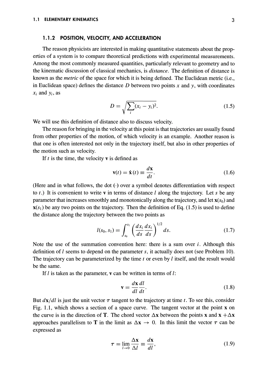
But dx/dl is just the unit vector r tangent to the trajectory at time t. To see this, consider
Fig. 1.1, which shows a section of a space curve. The tangent vector at the point x on
the curve is in the direction of T. The chord vector Ax between the points x and x + Ax
approaches parallelism to T in the limit as Ax —> 0. In this limit the vector r can be
expressed as
Ax dx
T = lim— = —, (1.9)
/-►o A/ dl

4
FUNDAMENTALS OF MECHANICS
^Ax
x+Ax
FIGURE 1.1
A vector T tangent to a space curve.
which is of unit length and parallel to T. Then (1.8) becomes
dl
V = T— = TV,
dt
(1.10)
which says that v is everywhere tangent to the trajectory and equal in magnitude to the
speed v = / along the trajectory.
Another important property of the motion is the acceleration, which is defined as the
time derivative of the velocity, or
a = v = x =
d\
dt'
(l.H)
Then Eq. (1.10) implies that
dr dv
a = —v + r —.
dt dt
(1.12)
The acceleration is related to the bending or curvature of the trajectory. To see this note
first that r is perpendicular to the trajectory. Indeed, r is a unit vector, so that r • r — 1,
and therefore
d dr
-«r.T)-0-2r.-:
dr/dt is perpendicular to r and hence to the curve. Let n be the unit vector in this
perpendicular direction, called the principal normal vector: n = r/|r|. The curvature k
of the trajectory, the inverse of the radius of curvature p (see Problem 11) is defined by
,. \r{h) - r(t2)\
hm
dr
dl
= K.
(1.13)
Thus kv = |r|, or f — Kvn. When these expressions for / and r are inserted into
(1.12), one obtains
kv n + /r.
(1.14)
In this expression the second term is the tangential acceleration and the first is the centripetal
acceleration (recall that k — 1/p).

1.2 PRINCIPLES OF DYNAMICS
5
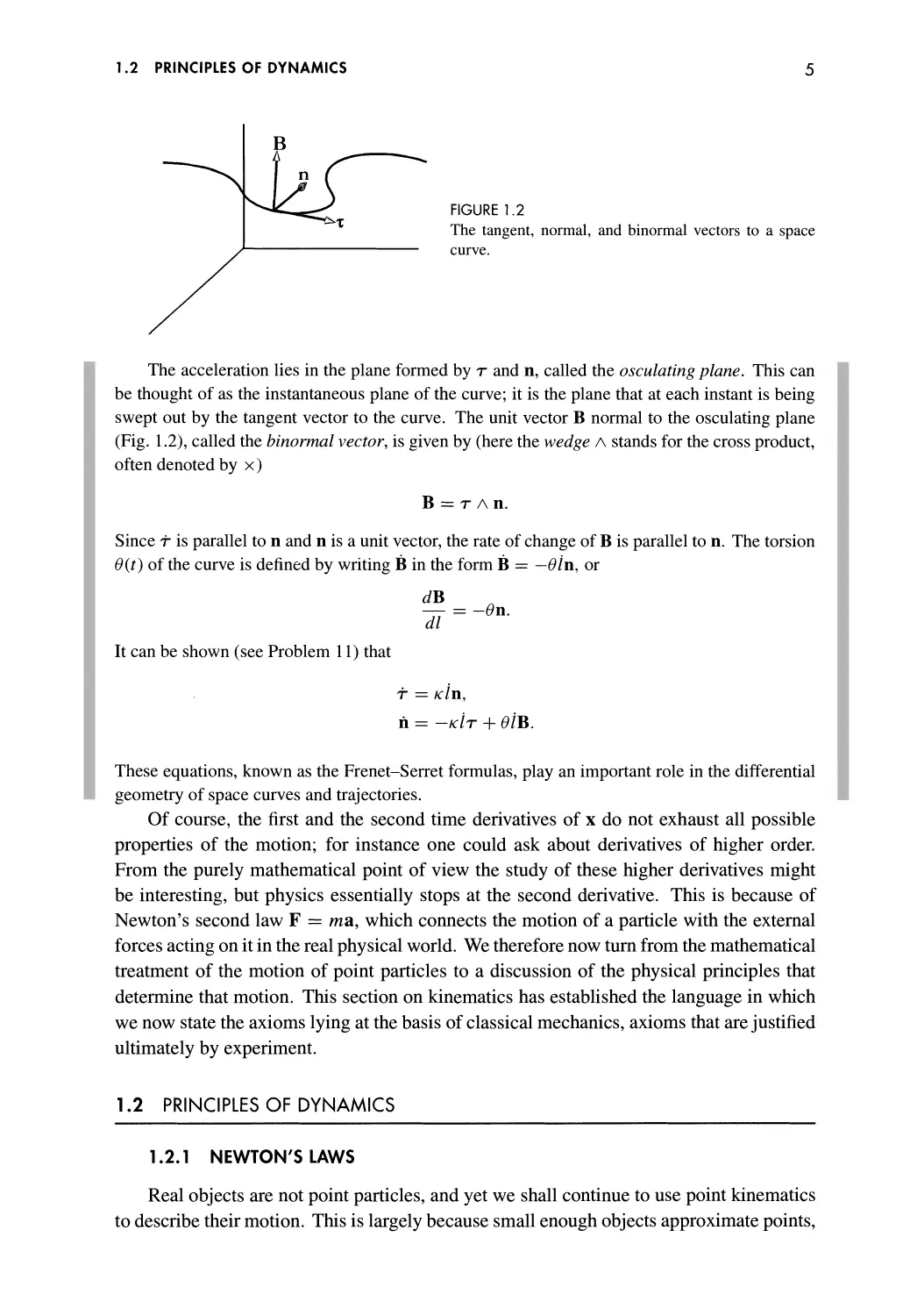
FIGURE 1.2
The tangent, normal, and binormal vectors to a space
curve.
The acceleration lies in the plane formed by r and n, called the osculating plane. This can
be thought of as the instantaneous plane of the curve; it is the plane that at each instant is being
swept out by the tangent vector to the curve. The unit vector B normal to the osculating plane
(Fig. 1.2), called the binormal vector, is given by (here the wedge A stands for the cross product,
often denoted by x)
B = r a n.
Since t is parallel to n and n is a unit vector, the rate of change of B is parallel to n. The torsion
0(t) of the curve is defined by writing B in the form B = — 6 in, or
dB
— = -On.
dl
It can be shown (see Problem 11) that
r = Kin,
h = -kIt + 0/B.
These equations, known as the Frenet-Serret formulas, play an important role in the differential
geometry of space curves and trajectories.
Of course, the first and the second time derivatives of x do not exhaust all possible
properties of the motion; for instance one could ask about derivatives of higher order.
From the purely mathematical point of view the study of these higher derivatives might
be interesting, but physics essentially stops at the second derivative. This is because of
Newton's second law F = ma, which connects the motion of a particle with the external
forces acting on it in the real physical world. We therefore now turn from the mathematical
treatment of the motion of point particles to a discussion of the physical principles that
determine that motion. This section on kinematics has established the language in which
we now state the axioms lying at the basis of classical mechanics, axioms that are justified
ultimately by experiment.
1.2 PRINCIPLES OF DYNAMICS
1.2.1 NEWTON'S LAWS
Real objects are not point particles, and yet we shall continue to use point kinematics
to describe their motion. This is largely because small enough objects approximate points,

6
FUNDAMENTALS OF MECHANICS
and their motion can be described with some accuracy in this way. Moreover, as we
will show later, results about the motion of extended objects can be derived from axioms
about idealized point particles. These axioms, as we have said, are ultimately justified by
experiment, so we will try to state them in terms of idealized "thought experiments."
In general the objects and the motions we treat are restricted in two ways. The first is
that the small objects we speak of, even though they are to approximate points, may not
get too small. As is well known, at atomic dimensions classical mechanics breaks down
and quantum mechanics takes over. That breakdown prescribes a lower limit on the size of
the objects admitted in our discussions. The other restriction is on the magnitudes of the
velocities involved: we exclude speeds so high that relativistic effects become important.
Unless otherwise stated, these restrictions apply to all the following discussion.
Our treatment starts with the notion of an isolated particle. An isolated particle is a
sufficiently small physical object removed sufficiently far from all other matter. What is
meant here by "sufficiently" depends on the precision of measurements, and the statements
we are about to make are statements about limits determined by such precision. They are
true for measurements of distance whose uncertainties are large compared to characteristic
dimensions of the object ("in the limit" of large distances or of small objects) and for
measurements of time whose uncertainties are large compared to characteristic times of
changes within the object ("in the limit" of long times). These distances and times, though
long compared with the characteristics of the object, should nevertheless be short compared
to the distance from the nearest object and the time to reach it. When isolation is understood
in this way, the accuracy of the principles stated below will increase with the degree of
isolation of the object.
It follows that there are two ways to test the axioms: the first is by choosing smaller
objects and removing them further from other matter, and the second is by making cruder
measurements. We say this not to advocate cruder measurements, but to indicate that the
relation between theory and experiment has many facets. Not only are the axioms actually
statements about the result of experiment, but the very terms in which the axioms are
stated must involve detailed experimental considerations, even in an "axiomatized" field
like classical mechanics. Similar considerations apply to the two restrictions described
above. The detection of quantum or relativistic effects depends also on the accuracy of
measurement.
1.2.2 THE TWO PRINCIPLES
The laws of mechanics can be formulated in two principles. The first of these quantifies
the notion of time [see the discussion after Eq. (1.3)] for the purposes of classical mechanics
and states Newton's first law in terms of this quantification. The second states conservation
of momentum for two-particle interactions, which is equivalent to Newton's third law.
Together they pave the way for a statement of Newton's second law. Both principles must
be understood as statements about idealized experiments. They are based on years, even
centuries, of constantly refined experiments. We continue to assume that physical space is
three dimensional, Euclidean, and endowed with the usual Euclidean metric of Eq. (1.5).

1.2 PRINCIPLES OF DYNAMICS
7
PRINCIPLE 1
There exist certain frames of reference, called inertial, with the following two
properties.
Property A) Every isolated particle moves in a straight line in such a frame.
Property B) If the notion of time is quantified by defining the unit of time so that one
particular isolated particle moves at constant velocity in this frame, then
every other isolated particle moves at constant velocity in this frame.
This defines the parameter t to be linear with respect to length along the trajectory of
the chosen isolated particle, and then Property B states that any other parameter t, defined
in the same way by using some other isolated particle, will be linearly related to the first
one. (Buried in this statement is the nonrelativistic idea of simultaneity.) Although it is not
practical to measure time in terms of an isolated (free) particle, it will be seen eventually
that the laws of motion derived from the two principles imply that the rotation of an isolated
rigid body about a symmetry axis also takes place at a constant rate and can thus be used
as a measure of time. In practice the Earth is usually used for this purpose, but corrections
have to be introduced to take account of the fact that the Earth is not really isolated (in
terms of the measuring instruments being used) or completely rigid. The most accurate
modern timing devices are atomic and are based on a long chain of reasoning stretching
from the two principles and involving quantum as well as classical concepts.
The existence of one inertial frame, as postulated in Principle 1, implies the existence
of many more, all moving at constant velocity with respect to each other. Two such inertial
frames cannot rotate with respect to each other, for then a particle moving in a straight line
in one of the frames would not move in a straight line in the other. The transformations
that connect such inertial frames are called Galileian; more about this is discussed in later
chapters.
REMARK: Since inertial frames are defined in terms of isolated bodies, they cannot
in general be extended indefinitely. In other words, they have a local character, for
extending them would change the degree of isolation. Suppose, for instance, that
there exist two inertial frames very far apart. If they are extended until they intersect,
it may turn out that a particle that is free in the first frame is not free in the second.
Considerations such as these play a role in physics, but are not important for the
purposes of this book (Taylor, 1964). □
PRINCIPLE 2
Conservation of Momentum. Consider two particles 1 and 2 isolated from all other
matter, but not from each other, and observed from an inertial frame. In general they will
not move at constant velocities: their proximity leads to accelerations (the particles are
said to interact). Let \j(t) be the velocity of particle j at time t, where j = 1,2. Then
there exists a constant /xi2 > 0 and a constant vector K independent of the time such that
Vi(0 + Ml2V2(0 = K
(1.15)

8
FUNDAMENTALS OF MECHANICS
for all time t. Moreover, although K depends both on the inertial frame in which the motion
is being observed and on the particular motion, /z!2 does not: /zi2 is always the same number
for particles 1 and 2. Even if the motion is interrupted and a new experiment is performed,
even if the interaction between the particles is somehow changed (say from gravitational
to magnetic, or from rods of negligible weight to rubber bands), the same number /z12 will
be found provided the experiment involves the same two particles 1 and 2. If a similar set
of experiments is performed with particle 1 and a third particle 3, a similar result will be
obtained, and the same is true for experiments involving particles 2 and 3. In this way, one
arrives at
V2(0 +/*23V3(0 = L,
(l.lo)
V3(0 + /*3lVi(f) = M.
As before, L and M depend on the particular experiment, but the /xr; > 0 do not.
Existence of Mass. The /xr; are related according to
^12^23^31 = I- (1-17)
That completes the statement of Principle 2.
It follows from (1.17) (see Problem 13) that there exist positive constants mt, / =
1, 2, 3, such that Eqs. (1.15) and (1.16) can be put in the form
raiVi + ra2v2 = P12,
m2v2 + m3v3 = P23, (1.18)
ra3v3 +miVi =P3i,
where the P,7, called momenta, are constant vectors that depend on the experiment. The
rrti are, of course, the masses of the particles. It should now be clear that Principle 2 states
the law of conservation of momentum in two-particle interactions.
The masses of the particles are not unique: it is the /x,7 that are determined by
experiment, and the /xr; are only the ratios of the masses. But given any set of ra7, any other
set is obtained from the first by multiplying all of the ra7 by the same constant. What is
done in practice is that some body is chosen as a standard (say, 1 cm3 of water at 4°C and
atmospheric pressure) and the masses of all other bodies are related to it. The important
thing is that once such a standard has been chosen, there is just one number rar associated
with each body, independent of any object with which it is interacting.
The vectors on the right-hand sides of Eqs. (1.18) are constant, so the time derivatives
of these equations yield
m\2i\ +ra2a2 = 0,
ra2a2 + ra3a3 = 0, (1.19)
ra3a3 +m\SL\ = 0.
These equations are equivalent to (1.18): their integrals with respect to time yield (1.18).
They [or rather their analogs obtained by differentiating (1.15) and (1.16)] could have been

1.2 PRINCIPLES OF DYNAMICS
9
used in place of (1.15) and (1.16) to state Principle 2. In fact Eqs. (1.19) are perhaps a
more familiar starting point for stating the principles of classical mechanics, for what they
assert is Newton's third law. Indeed, let the force F acting on a particle be defined by the
equation
d2x
F = ma = m —-. (1.20)
at2
This is Newton's second law (but see Discussion below). Now turn to the first of Eqs.
(1.19). The experiment it describes involves the interaction of particles 1 and 2: the
acceleration ai of particle 1 arises as a result of that interaction. One says there is a force
F12 = m\2i\ on particle 1 due to the presence of particle 2 (or by particle 2). Similarly, there
is a force F2i = m2a2 on particle 2 by particle 1. Then the first of Eqs. (1.19) becomes
F12+F21=0, (1.21)
which is Newton's third law.
DISCUSSION
The two principles are equivalent to Newton's three laws of motion, which in their
usual formulation involve a number of logical difficulties that the present treatment tries
to avoid. For instance, Newton's first law, which states that a particle moves with constant
velocity in the absence of an applied force, is incomplete without a definition of force and
might at first seem to be but a special case of the second law. Actually it is an implicit
statement of Principle 1 and was logically necessary for Newton's complete formulation of
mechanics. Although such questions would seem to arise in understanding Newton's laws,
we should remember that it is his formulation that lies at the basis of classical mechanics as
we know it today. The two principles as we have given them are, in fact, an interpretation
of Newton's laws. This interpretation is due originally to Mach (1942). Our development
is closely related to work by Eisenbud (1958).
It is interesting that Eq. (1.20), Newton's second law, is now a definition of force,
rather than a fundamental law. Why, one may ask, has this definition been so important in
classical mechanics? As may have been expected, the answer lies in its physical content.
It is found empirically that in many physical situations it is ma that is known a priori rather
than some other dynamical property. That is, the force is what is specified independent
of the mass, acceleration, or many other properties of the particle whose motion is being
studied. Moreover, forces satisfy a superposition principle: the total force on a particle can
be found by adding contributions from different agents. It is such properties that elevate
Eq. (1.20) from a rather empty definition to a dynamical relationship. For an interesting
discussion of this point see Feynman et al. (1963).
REMARK: Strangely enough, in one of the most familiar cases of motion, that of a
particle in a gravitational field, it is not the force ma that is known a priori, but the
acceleration a. □

10
FUNDAMENTALS OF MECHANICS
1.2.3 CONSEQUENCES OF NEWTON'S EQUATIONS
INTRODUCTION
The general problem in the mechanics of a single particle is to solve Eq. (1.20) for the
function x(0 when the force F is a given function of x, x, and t. Then (1.20) becomes the
differential equation
F(x,x,0 = m^. (1.22)
A mathematical solution of this second-order differential equation [i.e., a vector function
x(t) that satisfies (1.22)] requires a set of initial conditions [e.g., the values x(t0) and x(t0)
of x and x at some initial time t0]. There are theorems stating that, with certain unusual
exceptions (see, e.g., Arnol'd, 1990, p. 31; Dhar, 1993), once such initial conditions are
given, the solution exists and is unique. In this book we will deal only in situations for
which solutions exist and are unique.
For many years physicists took comfort in such theorems and concentrated on trying to
find solutions for a given force with various different initial conditions. Recently, however,
it has become increasingly clear that there remain many subtle and fundamental questions,
largely having to do with the stability of solutions. To see what this means, consider
the behavior of two solutions of Eq. (1.22) whose initial positions x^o) and x2(to) =
Xi (to) + Sx(t0) are infinitesimally close [assume for the purposes of this example that Xi (t0)
= x2(£o)]. One then asks how the separation 8x(t) between the solutions behaves as t
increases: will the trajectories remain infinitesimally close, will their separation approach
some nonzero limit, will it oscillate, or will it grow without bound? Let Dx(t) = \Sx(t)\
be the distance between the two trajectories at time t. Then the solutions of the differential
equation are called stable if Dx(t) approaches either zero or a constant of the order of
8x(t0) and unstable if it grows without bound as t increases.
Stability in this sense is highly significant because initial conditions cannot be
established with absolute precision in any experiment on a classical mechanical system, and
thus there will always be some uncertainty in their values. Suppose, for example, that a
certain dynamical system has the property that it invariably tends to one of two regions A
and B that are separated by a finite distance. In general the final state of such a system can
in principle be calculated from a knowledge of the initial conditions, and therefore each
initial condition can be labeled a or b, belonging to final state A or B. If there exist small
regions that contain initial conditions with both labels, then in those regions the system is
unstable in the above sense. In fact there exist dynamical systems in which the two types
of initial conditions are mixed together so tightly that it is impossible to separate them: in
every neighborhood, no matter how small, there are conditions labeled both a and b. Then
even though such a system is entirely deterministic, predicting its end state would require
knowing its initial conditions with infinite precision. Such a system is called chaotic or said
to exhibit chaos. An everyday example of chaos, somewhat outside the realm of classical
mechanics, is the weather: very similar weather conditions one day can be followed by
drastically different ones the next.

1.2 PRINCIPLES OF DYNAMICS
11
This kind of instability was not of major concern to the founders of classical mechanics,
so one might guess that it is a rare phenomenon in classical dynamical systems. It turns
out that exactly the opposite is true: most classical mechanical systems are unstable in the
sense defined above. The most common exceptions are systems that can be reduced to a
collection of one-dimensional ones. (One-dimensional systems are discussed in Section
1.5.1, but reduction to one-dimensional systems will come much later, in the discussion
of Hamiltonian systems.) For many reasons, the leading early contributors to classical
mechanics were concerned mainly with stable systems, and for a long time their concerns
continued to dominate the study of dynamics. In recent years, however, significant progress
has been made in understanding instability, and later in this book, especially in Chapter 7,
we will discuss specific systems that possess instabilities and in particular those solutions
that manifest the instabilities.
FORCE IS A VECTOR
Equation (1.22) has an important property related to the acceleration of a particle as
measured by observers in different inertial frames. Suppose that according to one observer
a particle has position vector x, with components xt,i = 1,2,3 in her Cartesian coordinate
system. Now consider another observer looking at the same particle at the same time, and
suppose that in the second observer's frame the position vector of the particle is y, with
coordinates yt. It is clear that there must be some transformation law, a sort of dictionary,
that translates one observer's coordinates into the other's, or they could not communicate
with each other and could not tell whether they are looking at the same particle. This
dictionary must give the xt in terms of the y{ and vice versa: it should consist of equations
of the form
yt = Mx9t)9 Xi=gi(y9t), (1.23)
where the x in the argument of the three functions ft denotes the collection of the three
components of x and similarly for y in the arguments of the gt. Note that the transformation
law in general depends on the time t.
If the f functions are known, Eq. (1.23) can be used to calculate the velocities and
accelerations as seen by the second observer in terms of the observations of the first. Indeed,
one obtains (don't forget the summation convention)
yi = d7jXj + -d7 (L24)
and
.. b/,„ , d2ft . . d2ft . a2/;-
yi dxj J dxjdxk J dxjdt J dt2
So far we have not assumed any particular properties of the two coordinate systems, but
if they are both Cartesian, the transformation between them must be linear, that is, the ft

12
FUNDAMENTALS OF MECHANICS
functions, which give the yj in terms of the xt, must be of the form
Ji = Mx91) = fik(t)xk + bt(t). (1.26)
If, in addition, both frames of reference are inertial, they are moving at constant velocity
and are not rotating with respect to each other, and then the bt(t) = fat must be linear
in t and the ftk(t) = (ptk must be time independent (i.e., constants). Indeed, if x = 0,
then yt = b(, so the bt term alone gives the y coordinates of the x origin, and the ftk(t)
determine the linear combinations of the xk that go into making up the yt. In that case the
last three terms of (1.25) vanish, and thus
yt = (pikXk- (1-27)
This shows that the acceleration as measured by the second observer is a linear
homogeneous function of the acceleration as measured by the first.
It is important that the same 0,7 coefficients appear in the expressions for the
acceleration and for the position [in Eq. (1.26) the ftk(t) are now the constants (j)ik\. This is
interpreted (see the Remark later in this section) to mean that the acceleration is a vector,
that the transformation law for its components is the same as that for the components of
the position vector. That, together with the F = ma equation, guarantees that force is also
a vector. What is more, as we shall now show, the converse of this is also true: if force is to
be a vector, then acceleration must be a vector, and then ft(x, t) = fik{t)xk+bt{t). (This is
also true if one demands that the acceleration seen by one observer should be determined
entirely by the acceleration (i.e., be independent of the velocity) seen by the other.)
Before we prove the converse, we make a comment. It is actually relative position
vectors that transform like accelerations and forces. A relative position is the difference
of two position vectors, the vector that goes from one particle to another. Let there be two
particles, with position vectors x and x' in one frame and y and y' in the other. Then if
x — x' = Ax and y — y' = Ay, Eq. (1.26) yields
Ayt = flk(t)Axk. (1.28)
It is seen that in the transformation law for relative positions the bt of (1.26) drop out
and thus that the equations are homogeneous, even before restrictions are placed on the
transformation properties of the components and before the frames are assumed to be
inertial. But it is also seen that when the frames are inertial, so that the fy are constants,
the transformation law for the relative positions is of exactly the same form as for the
acceleration. Incidentally, this is true also for relative velocities, which can be defined
either as the time derivatives of relative positions or, equivalently, as the difference of the
velocities of two particles.
REMARK: In elementary mechanics, vectors (e.g., displacement, velocity, acceleration,
force) are required to have three (Cartesian) components that combine properly under
the vector addition law when the vectors are added. Furthermore, there is a
transformation law by which the components of a vector in one frame can be found from

1.3 ONE-PARTICLE DYNAMICAL VARIABLES
13
its components in another. Moreover, for vector equations to be frame independent
(i.e., to be true in all frames if they are true in one) the components of all vectors must
transform according to the same law. This means that the 0,7 appearing in the
transformation law for the (relative) position vectors must be the same as those appearing
in the law for other vectors, a principle that we have used in the above discussion. □
We now return to the proof of the converse. If the acceleration is a vector, its
transformation law must be linear and homogeneous, which means that each of the last three
terms of (1.25) must vanish. But that implies that all the second derivatives of the f(x, t)
must vanish and hence that the f(x, t) must be linear in the xk and in t, that is, of the form
fi(x,t) = <j)ikxk + pit, (1.29)
where the 0/7 and fa are constants, and then the two frames are relatively inertial and
Eq. (1.27) follows. This proves the converse: it establishes the transformation law of
the position if acceleration is a vector. This also exhibits the intimate connection between
Newton's laws and inertial frames, a connection manifested here in terms of transformation
properties. The result may be summarized as follows:
If the acceleration is a vector in one frame, then it is a vector in and only in relatively
inertial frames. If force is a vector and Newton's laws are valid in one inertial frame, then
all of the frames in which they are valid are inertial.
Stated in terms of the observers (for after all, it is the observers who determine the
frames, not the other way around), if Newton's laws are to be valid for different observers,
those observers can be moving with respect to each other only at constant velocity. The
transformation defined by the f functions of (1.29) is called a Galileian transformation.
1.3 ONE-PARTICLE DYNAMICAL VARIABLES
We have said that the general problem of single-particle mechanics is to solve Eq. (1.22),
F = ma, for x(0 when the force F is given. We now extend this statement of the general
problem: to find not only x(0 but also x(t). Once x(t) is known, of course, x(t) is easily
found by simple differentiation; so this extension of the problem may seem redundant. Let
it be so; in due course the reason for it will become clear.
Solving (1.22) is often easier said than done, for in many specific cases it is hard to
find practical ways to solve the equation. Often, however, one is not interested in all of
the details of the motion, but in some properties of it, like the energy, or the stable points,
or, for periodic motion, the frequency. Then it becomes superfluous actually to find x(0
and x(0- For this reason other useful objects are defined, which are generally easier to
solve for and sufficient for most purposes. These objects, functions of x and x, are called
dynamical variables. Many dynamical variables are quite important. Their study leads to
a deeper understanding of dynamics, they are the terms in which properties of dynamical
systems are usually stated, and they are of considerable help in obtaining detailed solutions
of Eq. (1.22).

14
FUNDAMENTALS OF MECHANICS
In this section we briefly discuss momentum, angular momentum, and energy in single-
particle motion. In Section 1.4 we extend the discussion to systems of several particles.
1.3.1 MOMENTUM
We have already mentioned the first of these dynamical variables in Eq. (1.18). The
momentum p of a particle of mass m moving at velocity v is defined by
p = rav. (1.30)
With this definition, (1.22) becomes
F = ^. (1.31)
at
A glance at Eq. (1.18) shows that the total momentum of two particles is just the sum
of the individual momenta of both particles. This will be discussed more fully in the next
section, where the definition of momentum will be extended to systems of particles (even
if the mass is not constant; see the discussion of variable mass in Section 1.4.1), and it
will be seen that Eq. (1.31) is in a form more suitable to generalization than is (1.22). An
important property of the extended definition of momentum is evident from Eq. (1.18):
the total momentum of two particles is constant if the particles are interacting with each
other and with nothing else. In terms of forces, this means that the total momentum of
the two-particle system is constant if the sum of the external forces acting on it is zero.
Similarly, if the total force on one particle is zero, then according to (1.31) dp/dt = 0
and p is constant. In fact it is the constancy of momentum, its conservation in this kind of
situation, that singles it out for definition. All this assumes, as usual, that all measurements
are performed in inertial systems. Otherwise, Eq. (1.31) is no longer true and momentum
is no longer conserved even in the absence of external forces.
1.3.2 ANGULAR MOMENTUM
The angular momentum hofa particle about some point S is defined in terms of its
(linear) momentum p as
L = xAp, (1.32)
where x is the position vector of the particle measured from the point S. In general S may
be any moving point, but we shall restrict it to be an inertial point, that is, a point moving at
constant velocity in any inertial frame (more about this in Section 1.4). The time derivative
of (1.32) is
d
L = — (xAp) = VAp + XAp.
dt

1.3 ONE-PARTICLE DYNAMICAL VARIABLES
15
But v A p = m(v a v) = 0, and then with (1.31) one arrives at
L = xap = xaF = N, (1.33)
which defines the torque N about the point S. This equation shows that the relation between
torque and angular momentum is similar to that between force and momentum: torque
is the analog of force and angular momentum is the analog of momentum in problems
involving only rotation (about inertial points). In particular, if the torque is zero, the angular
momentum is conserved.
1.3.3 ENERGY AND WORK
IN THREE DIMENSIONS
If the force F of Eq. (1.22) is a function of t alone, it is easy to find x(0 by integrating
twice with respect to time:
x(t) = x(f0) + (t - fo)v(fo) + - I dt' I W)dt\ (1.34)
m J to J to
where x(t0) and \(t0) are position and velocity at the initial time t0. Unfortunately, however,
F is almost never a function of t alone but a function of x, v, and t. It is only when x and
v are known as functions of t that F can be written as a function of t alone and Eq. (1.34)
prove useful. But x and v are not known as functions of the time until the problem is
solved, and when the problem is solved there is nothing to be gained from (1.34). Thus
Eq. (1.34) is almost never of any help.
Often, however, F is a function of x alone, with no v or t dependence. Then one can
take the line integral with respect to x along the trajectory, obtaining
rx(t) r* r* d2x dx
/ F(x) dx = / F(x) -xdt = m —- dt
Jx(to) Jto Jto dt dt
1 V d 9
= om / ~rM)dt a-35)
2 Jt0 dt
= -mv2(t)--mv2(t0l (1.36)
where v2 = v • v. This equation doesn't give x(t) in terms of the initial conditions, but it
does give the magnitude v(t) of the velocity, provided the integral on the left-hand side can
be performed. But there are two problems with performing the integral. The first involves
the upper limit x(0- Recall that the problem is to find x(t), so x(t) is hardly useful as an
upper limit. What Eq. (1.35) actually describes is how v(t) depends on the upper limit: it
gives v as a function of x rather than of t. To find v as a function of t requires finding x as
a function of t some other way. Since the time / actually plays no role in Eq. (1.35), t and
t0 can be dropped from the limits of the integral and the argument of v can be changed to
x. What the equation really says is that no matter how long it takes for the trajectory to be
covered, the line integral on the left-hand side is equal to ^mv2(x) — ^mv2(x0).

16
FUNDAMENTALS OF MECHANICS
The second problem with the integral on the left-hand side of (1.35) is that, being a
line integral, it depends on the path of integration, in this case on the entire trajectory: in
general, even if its end point x is known, v(x) is not. But in spite of these difficulties,
Eq. (1.35) is quite useful.
The usefulness of Eq. (1.35) involves the dynamical variable \mv2 appearing in it,
which is the kinetic energy T:
T = -mv2. (1.37)
2
Let the trajectory (more generally, the path) of the integral on the left-hand side of (1.35)
be called C; then the integral itself is defined as the work Wc done by the force F along C:
=//
Wc= / F-dx. (1.38)
Equation (1.35) can now be written in the form Wc = [T(t) — T(t0)]c, or, in view of the
fact that x, not t, is the argument of v,
Wc = [T(x)-T(xo)]c. (1.39)
In words, the work done by the force F along the trajectory is equal to the change in kinetic
energy between the initial point x0 and the final point x of the trajectory.
Equation (1.39) is known as the work-energy theorem. Both sides of it, the work W
and the change AT of the kinetic energy, depend on the entire path of integration, not just
on its end points. This path dependence reduces the practical value of the theorem, because
often only some of the points of a trajectory are known without the trajectory being known
in its entirety. Fortunately, however, it turns out that for many forces that occur in nature
the integral that gives W is not path dependent; it depends on nothing but the end points.
Forces for which this is true are called conservative.
Conservative forces are common in physical systems, so we now study some of their
properties. Let F be a conservative force (it should be borne in mind that in all of these
equations F is a function of x), and let C\ and C2 be any two paths connecting two points
X! and x2, as shown in Fig. 1.3. Then, by the definition of a conservative force,
f F • dx = f F • dx,
>c2
or
/ F dx - J F • dx = <b F • dx = 0,
'c, Jc2
where the third integration is around the closed path from Xi to x2 and back again. Thus if
F is conservative, § F • dx — 0 around any closed path, for Xi and x2 are arbitrary. Stokes's
theorem can now be used to transform the closed line integral to a surface integral, giving
d>F-dx= |(V A F) • dS9 (1.40)

1.3 ONE-PARTICLE DYNAMICAL VARIABLES
17
FIGURE 1.3
Two paths connecting the points xi and X2.
where X is any smooth surface bounded by the closed path C of the line integral, and dS is
the vector element of area on X. Since the left-hand side of (1.40) is zero for every closed
contour C, the right-hand side is zero for every surface X, and hence
V aF = 0 (1.41)
is a necessary condition for F to be conservative. The argument can be reversed to show
that Eq. (1.41) is also a sufficient condition. Thus Eq. (1.41) characterizes conservative
forces.
Equation (1.41) may be recognized as the integrability condition for the existence of
a single function that is a solution V(x) of the three partial differential equations (one for
each component)
F(x) = -VV(x) (1.42)
(the negative sign is chosen for later convenience). In other words, if F is conservative,
there exists a function V satisfying Eq. (1.42) and defined by it up to an additive constant.
This important function V is called the potential energy of the dynamical system whose
force is F.
Up to now, a one-particle dynamical system has been characterized by its vector force
function F. That is, given F, the dynamical problem is defined: solve (1.22) with that
given F. From now on, if the force is conservative, the characterization can be simplified:
all that need be given is the single scalar function V, and F is easily obtained from V via
(1.42). This reduction from the three components of a vector function to a single function
simplifies the problem considerably. Later, when we deal with systems more complicated
than one-particle systems, it will be seen that the simplification obtained from a potential
energy function can be even greater.
Let us return to Eq. (1.38), defining the work along a path C, and now let C be a
contour going from some point x0 to some arbitrary point x. Then (1.38) may be written

18
FUNDAMENTALS OF MECHANICS
in the form
Wc = W(x, x0) = I F(x') -dxf = - t VV(x') • dxf
Jx0 Jx0
= V(x0) - V(x) =V0-V.
Equation (1.39) can now be written in the form (here is where that negative sign helps)
V + T = V0 + T0 = E = const. (1.43)
The last equality, namely the assertion that the total (mechanical) energy E is constant,
comes from the first one, which asserts that the sum V + T at any point x whatsoever is
the same as it is atx0.
We have derived conservation of energy for any dynamical system consisting of a
single particle acted upon by a conservative force. Because the total energy E is a sum of
T and V, and because V is defined only up to an additive constant, E is also defined only
up to an additive constant. This constant is usually chosen by specifying V to be zero at
some arbitrarily designated point. It is clear that conservation of energy does not solve the
problem of finding x(t) in conservative systems, but it is a significant step. We will see in
what follows that in one-dimensional systems it leads directly to a solution.
It is important to note that the three dynamical variables p, L, and E that have been
defined are associated with conservation laws. Historically, it is their conservation in
many physical systems that has led these functions of x and x to be singled out for special
consideration and definition.
APPLICATION TO ONE-DIMENSIONAL MOTION
The properties of dynamical systems depend crucially on the "arena" in which the
motion takes place, and one important aspect of this arena is its dimension. For example,
the arena for the single-particle dynamical systems we have been discussing is three-
dimensional Euclidean space. Later we will be discussing systems with N > 1 particles,
and then the arena consists of N copies of three-space (one copy for the position of
each particle), or a 3//-dimensional space. In another way, the arena for a single particle
constrained to remain on the surface of a sphere is the two-dimensional spherical surface.
The dimension of the arena is called the number of degrees of freedom of the system or
simply the number of its freedoms. It is the number of functions of the time needed to
describe fully the motion of the system.
The simplest of all arenas is that for a particle constrained to move along a straight
line. This is clearly a one-freedom system (there are other one-freedom systems; e.g., a
particle constrained to a circle). One-freedom systems are of particular interest not only
because they are the simplest, but also because often a higher-freedom problem is solved
by breaking it up into a set of independent one-freedom problems and then solving each
of those by the technique we will now describe. This technique reduces the problem to
performing a one-dimensional integration or, as is said, to quadrature.

1.3 ONE-PARTICLE DYNAMICAL VARIABLES
19
Let distance along the line be x and let the force F (also along the line) acting on the
particle be a function only of x. The equation of motion is then
mx = F(x). (1.44)
In one dimension all forces that depend only on x are conservative. Thus F is the negative
derivative of a potential energy function V(x) defined up to an arbitrary additive constant,
and Eq. (1.43) can be written in the form
-mx2 + V(x) = E, (1.45)
where E is the total energy of the system and is constant. This equation is obtained by
integrating (1.44) once (E is the constant of integration): the dynamical variable on the
left-hand side of (1.45) is called the energy first-integral.
Equation (1.45) can be solved for l/x = dt/dx and integrated to yield
[m fx dx
where x0 is the position of the particle at time to, and x is its position at time t. If this
equation is inverted, it yields the solution of the problem in the form
x =x(t -t0,E). (1.47)
Thus if E and x0 = x(t0) are known, the problem is solved in principle. In practice t0 is
usually taken to be zero without loss of generality, so that the only constants that appear
in the final expression are x0 and E.
Most of the time the integral on the right-hand side of (1.46) cannot be performed in
terms of elementary functions. Essentially Eq. (1.46) is just (1.45) rewritten. Thus we turn
to (1.45) to see what information it provides before integration. It turns out that it contains
much information about the various kinds of motion that belong to different values of E.
For example, since the kinetic energy \mx2 is always positive, the particle cannot enter a
region where E — V(x) is negative. Starting in a region where E — V(x) is positive, the
particle can move toward higher values of the potential V until it gets to a point where
V(x) = E and then can go no further. This is a turning point for the motion, and in this
way E determines the turning points.
In analyzing the possible motions, it helps to plot a graph of V as a function of x with
horizontal lines representing the various constant values of E. Figure 1.4 is an example
of such a graph. If the particle starts out to the left of x\ moving to the right with total
energy E = E0, it cannot pass x\\ as it approaches x\ it slows down (its kinetic energy
^mx2 = E — V decreases) and comes to rest at x\. Then because F = —d V/dx is negative,
it accelerates to the left. It makes no physical sense to say that the particle with energy

20
FUNDAMENTALS OF MECHANICS
Xj X9
*6 *7
FIGURE 1.4
A one-dimensional potential energy diagram. The curve indicates the potential energy V(x).
E0 starts at some point like x3. However, with that energy it could start somewhere to the
right of x%. For energies between E0 and E2 the region from x3 to x7 becomes physically
accessible to the particle. For example, if the energy is Eu the particle can be trapped
between x4 and x6. For energies between E2 and £3, motion starting from the left of x7 will
be bounded on the right but not on the left. Finally, if E > E3, the motion is unbounded
in both directions.
Consider the bounded motion at energy E\. The time to complete one round trip from
x4 to x6 and back again is called the period P. According to Eq. (1.46) the period is given
by
P = V2m
dx
JE- V(x)'
(1.48)
where we have used the fact that the time to go from x4 to x6 is the same as the time to go
back. This is a general formula for the period of bounded motion between any two turning
points, with the limits of the integral being the two roots of the radical in the denominator.
We turn to an explicit example, related to the simple pendulum. Let
V(x) — —A cosx, —oo < x < oo, A > 0.
(1.49)
This potential is plotted in Fig. 1.5(a); it consists of a series of identical potential wells

1.3 ONE-PARTICLE DYNAMICAL VARIABLES
21
FIGURE 1.5
(a) The potential energy function V(x) = —Acosx. (b) The phase portrait for the system whose
potential is V(x) = —A cosx (see Section 1.5.1 for further explanation).
separated by identical potential barriers. The total energy is given by
1 ? * 2
E = -rnx — A cosx = -mv
2 2
— A cosx.
(1.50)
We start by considering motion with E < A, which lies entirely within one of the wells.
The initial value of x determines which of the wells traps the particle, but since the motion
within the well is the same no matter which well is the trap, there is no loss of generality
in considering bounded motion restricted to the well at — ix < x < n. Since the kinetic
energy ^mx2 is nonnegative, the lowest possible value for E is —A. The period of bounded
motion is given in general by Eq. (1.48), in this case by
dx
P = V2m
/
(1.51)
y/E + ACOSJC
where x\ < 0 and xi > 0 (as follows also from the condition that E < A) are the roots of
the radical in the denominator of the integrand, or
jcu =±cos_1(£/A).
The integral cannot be evaluated in general in terms of elementary functions, but it is related
to the complete elliptic integral K (Abramowitz and Stegun, 1976); this is a tabulated

22
FUNDAMENTALS OF MECHANICS
function, and hence the period can be calculated numerically. (Figure 1.5(b) is discussed
in Section 1.5.1.) A special value of E is its minimum E = — A. At this energy, the two
turning points merge at x = 0, and the particle is forced to remain stationary there, and
therefore the point x = 0 is an equilibrium point. This is a point of stable equilibrium: if
the mass is located near it, the force on the mass is directed toward the equilibrium point,
causing the particle to accelerate toward it. For greater values of E, approaching A, the
period of oscillation is longer. At E = A the integral diverges and the period becomes
infinite. For this value of E the turning points are at x = ±n, but only nominally, for they
are not reached in any finite time. However, with this value of E the particle could actually
start out at x = ±n, but then its velocity would have to be zero and it would remain at
that value of x. Thus x = ±tt are also equilibrium points, but these are unstable. That is,
if the mass is located near one of them, the force on the mass is directed away from the
equilibrium point, causing the particle to accelerate away from it.
If E is allowed to increase further, so that E > A, the motion is no longer bounded.
For each such value of E there is no value of x where the kinetic energy vanishes, and the
particle moves either to the right or the left, never turning back.
We will return to this system in Section 1.5.1.
1.4 MANY-PARTICLE SYSTEMS
1.4.1 MOMENTUM AND CENTER OF MASS
CENTER OF MASS
We now turn to dynamical systems composed of TV > 1 particles interacting with each
other and acted on also by external forces. Such a many-particle problem can in general
be very complicated, and even the solution of the three-body gravitational-interaction
problem cannot be reduced to simple integrations. Fortunately, important general results
can be obtained that allow significant simplification in the formulation of such problems
and lead to at least partial solutions. In a way these results beg the question: they avoid
solving the general problem (to find the motion of all N particles), replacing it by other, less
detailed questions. Although these other questions have important and useful answers that
provide considerable insight, their chief virtue may be that they have any answers at all.
Suppose that in a system consisting of N particles a known external force is applied
to each particle, but that the details of their mutual interactions are unknown. What can
be said about their motion? To begin to answer this question, Principles 1 and 2 must
be extended to interactions of several particles. As was mentioned in the discussion of
Eq. (1.20), forces satisfy a superposition principle: the total force on a particle can be found
by adding the contributions from different agents. It follows that the total force acting on
a particle is the vector sum of all the forces exerted on it by each of the other particles in
the system (the internal forces) plus all of the external forces.
The superposition principle implies that all forces can be analyzed in terms of two-
particle interactions. Consider, for example, a system of three particles, A, B, and C.

1.4 MANY-PARTICLE SYSTEMS
23
Particle A, in interacting with B and C, feels no additional force having to do with the
interaction of B with C: the force on A is exactly the sum of the force it would feel if only B
were present and the force it would feel if only C were present. The superposition principle
is an assumption additional to Newton's laws (or to the two Principles of Mechanics), a
result of delicate experimental observation. One could imagine a different universe, in
which the force on A depended on B, on C, and also on the interaction between B and
C. (In fact something of this sort often happens when the objects that are acted on are not
exactly particles, say small charged conducting spheres. Then the charge on each sphere
redistributes in a way that depends on the other charged spheres in the vicinity, and that
alters the forces. This shows why the experiments must be delicate.) The present treatment
is valid only if all interactions between particles arise from such two-particle interactions.
REMARK: We could have started with a more general statement, similar to (1.15), but
involving N >2 particles and leading directly to the conservation of momentum for
Af-particle systems, just as (1.15) led directly to (1.18). □
Let Ftj be the force exerted on the /th particle by the y th. Then Fa = 0, and Eq. (1.21)
implies that
Fy = -¥„. (1.52)
The equation of motion of the /th particle is then (we abandon the summation convention
here - all sums are indicated by summation signs)
,x,=F,+^Fi7, (1.53)
j =
where F( is the total external force on the /th particle, ra, is its mass, and x, is its position.
Clearly this equation cannot be solved unless all of the Ftj are known, and they will be
changing as the particle moves. But a certain amount of information is obtained if this
equation is summed over /. This sum yields
]£mI-xI- = ][]FI-=F, (1.54)
where the total external force F is the sum of only the external forces, since according to
Eq. (1.52)
EFy = EF* = -EFy = °- (L55)
ij i,j i,j
The first equality here is obtained by interchanging the roles of / and j in the sum. It is
convenient in Eq. (1.54) to factor out the total mass M = J2i m^ so that
= MX, (1.56)

24
FUNDAMENTALS OF MECHANICS
where
M *-^
is defined as the center of mass of the system of particles. Equation (1.56) is a useful
result, for what it tells us is that the center of mass moves as though the total mass were
concentrated there and were acted upon by the total external force. This result is known
as the center-of-mass theorem.
MOMENTUM
The center of mass is a useful concept for many reasons. For instance, the total
momentum of the system of particles, the sum of the individual momenta, is seen to be
P = ]TmI-xI- = MX, (1.58)
i
as if the total mass of the system of particles were concentrated at X. In terms of P, Eq. (1.56)
can be rewritten
F = P,
and therefore if the total external force F = 0 the total momentum of the system of particles
is constant and hence conserved.
Equation (1.56) is an important result. For example, it can be used to show (see
Problem 16) that a large system can be made up of smaller ones in almost exactly the same
way that any system is made up of its particles: the center of mass of the large system and
its motion can be found from the centers of mass of its subsystems and their motion. Just
as small systems can be combined in this way to make up larger ones, any system can be
broken up into smaller parts: from the motion of the center of mass of a system of particles
inferences can be derived about the motion of its parts. Equation (1.56) tells us in what
sense the laws of motion apply to systems and subsystems and the extent to which we can
disregard their internal structure.
VARIABLE MASS
In this subsection we show the usefulness of restating Newton's second law in the form
F = P. This will be done on a many-particle system in the limit as the number of particles
N -> oo and the masses of the point particles become infinitesimal, which means that the
sums over particles will become integrals over a continuous mass distribution. Not all of
the mass of the system will be acted upon by the external forces, and the part that is acted
upon will be allowed to vary. That will model a system of varying mass. An example is
a rocket, from which mass is ejected as it moves. There are other systems to which mass
is added (see Problem 25). Thus dynamical systems whose mass varies in this way arise
strictly within the bounds of classical mechanics.

1.4 MANY-PARTICLE SYSTEMS
25
REMARK: The restriction to low velocities made in Section 1.2 allows us to avoid the
question of relativistically varying mass. □
We will discuss only a simple system of this type, a continuous mass distribution that can be
described by a single parameter X. Each infinitesimal particle of the system is labeled by a value
of X, and that value stays with the particle as it moves. Suppose, for instance, that the distribution
is one dimensional along some curve (see Problem 25); then X could be the original length along
the curve. Let the mass density p within the distribution be written as a function of this single
parameter: p = p(X). The parametrization is chosen so that X varies from 0 to some maximum
value A, and then the total mass of the system is
JO
-A
M= I p(X)dX. (1.59)
Let the system be acted on by a total external force F. It then follows from the center-of-mass
theorem that
d2 fA
F=T7 / x(t,X)p(X)dX, (1.60)
dt2 Jo
where x(t, X) is the position at time t of the particle whose parameter is X.
Assume now that the force acts only on a constantly changing part of the total mass, in
particular that part of it for which X < fi(t) , where /x(0 is some differentiable monotonically
increasing function. This means that as time increases, more and more of the mass is acted upon
by the force. For simplicity, we assume further that for X > /x(f) the velocity dx(t, X)/dt = 0,
which means that before the force acts on any part of the mass, that part is stationary. Then the
integrals in (1.59) and (1.60) can each be broken up into two separate integrals, one from X = 0
to X = /ui(t), and the other from X = ii(t) to A = A. Thus Eq. (1.59) may be written in the
form
p/jL(t) pA pA
= / p(X)dX + / p(k)dX. = m(ti)+ / p(X)dX, (1.61)
JO J a(t) Ju.it)
defining m(/x), which is the part of the mass acted on by the force. We will use the name small
system for that part of the total system whose mass is m(/x). Now take one of the derivatives
with respect to t in Eq. (1.60) into the integral sign, so that the integral will contain dx/dt,
whose vanishing for X > \i will cause the second integral from /jl to A to vanish. Thus (1.60)
becomes
„ d fA dx d f^ dx
where we have used Leibnitz's theorem for taking the derivative of an integral with variable limits.
The value of dx/dt in the first term in (1.62) is taken in the limit as X approaches n from below:

26
FUNDAMENTALS OF MECHANICS
it is the velocity v at which mass is moving as it joins the small system at X = fi. Moreover,
pW\x=/jl - d/x/dt is the rate dm/dt at which mass is entering the small system, or the rate
at which the mass of the small system is growing. Indeed, it is evident from Eq. (1.61) that
P(X)\x=/jl = dm(ii)/dii. Thus the first term on the last line of (1.62) is just vdm/dt. The next
term is by definition equal to m(/x)X(/x), where X is the center of mass of the small system [see
Eq. (1.57)]. Then if the argument /jl is dropped from the variables, Eq. (1.62) becomes
^ dm d\ „ ^x
F = v—-+m —, (1.63)
dt dt
where V = X. In general v / V, but if the small system is moving as a whole (i.e., if all of its
parts are moving at the same velocity) then v = V. In that case, it turns out that
dF
F=—, (1.64)
dt
where P = m(/x)V is the momentum of the small system. With this understanding, Eq. (1.64)
can be understood as a generalization of Eq. (1.22).
How does one deal with Eq. (1.63)? That is, how and for what does one solve it? An example
of a system to which it can be applied is a rocket. In a rocket, F = 0 and v is the velocity at
which the rocket fuel is ejected. The rate at which mass is ejected is dm/dt, and (1.63) can then
be solved for V, the velocity of the rocket (whose mass m is constantly decreasing). Both dm/dt
and v are also given by some equations, differential equations that govern the chemical or other
reactions that control the rate at which fuel is burned. Problem 25 presents another example. It
involves a chain piled up next to a hole in a table, with some initial length hanging down. The
problem is to find how much hangs down at time t later. This problem can be handled by applying
the above discussion, with the role of the small system being played by the hanging part of the
chain. In this case v = V. In general there must be additional relations between the variables m,
V, and v in Eq. (1.63) if the equation is to be solvable, or there must be other equations for some
of these variables.
1.4.2 ENERGY
Unlike the momentum, the kinetic energy of a system of particles, defined as the sum
of the individual kinetic energies, is not the kinetic energy of a particle of mass M located
at the center of mass. It is found (see Problem 17) that
T =l-MX2+l~Yjrniyl (1.65)
i
where
yi=xi-X (1.66)
is the position of the /th particle relative to the center of mass. Therefore the kinetic energy
of a system of particles is equal to the kinetic energy of the center of mass plus the sum of
kinetic energies of the particles with respect to the center of mass.

1.4 MANY-PARTICLE SYSTEMS
27
In analogy with the one-particle problem, conservation of energy can be derived by
calculating the total work that must be done on all the particles in carrying the system from
an initial configuration 0 to a final configuration f:
H f f (F<+J2FiJ) -dXi = J2 f fm^ •dXi- (L67>
i JxiO \ j / i Jtio
It is clear that the right-hand side of this equation is just the difference 7} — T0 between the
initial and final total kinetic energies. As for the left-hand side, if each external force F; is
derivable from a potential Vt, the first term becomes
^rfFi..jx,=2:(^-v/)=^t-v/xt.
i JxiQ i
(1.68)
If the order of summation and integration over / is changed, the second term on the left-hand
side of Eq. (1.67) becomes [use Eq. (1.55)]
= ~ / EF'V •d^ -x;> = 9 / EF'V • dx'J-
Assume now that F/7 is a function only of the relative position xtj = x, — x7 and that it is
derivable from a potential function Vij9 also a function only of x/;. Then by changing back
the order of summation and integration, one obtains
f
£ Fy • d* =l-J2 (Vij ~ K) = V* ~ VL- d-69)
2
i,j i,i
As shown in elementary texts (Reitz & Milford, 1964, p. 106), the expression in the center
of this equation is in fact the amount of work it takes to move all of the particles of the
system from their initial configuration to the final one.
The results of Eqs. (1.67), (1.41), and (1.69) are summarized by the equation
(Vext + Viet + r)° = (Vext + Vint + T)f, (1.70)
which is the statement of conservation of energy that includes the internal as well as external
potential energies.
REMARK: It is interesting that F/7 = — F7;, and yet Vtj=Vp. Verify this; it's instructive.
□
1.4.3 ANGULAR MOMENTUM
Like the total kinetic energy, the total angular momentum of a system of Af particles
is not just the angular momentum of a particle of mass M located at the center of mass.

28
FUNDAMENTALS OF MECHANICS
We calculate the total angular momentum of such a system about the origin of an inertial
reference system. The total, obtained by summing the angular momenta of all the particles,
is
L = y^m^X/ ax,-.
i
The total angular momentum about the center of mass is
Lc = ^m*y* Ay/,
i
where yt is defined in Eq. (1.66). With that definition the expression for L becomes
L = 2".-(X + y.-)A(X + yI.)
i
= ^m^XAX + ^m^ Ay,- +]£^ml-yl- AX + ^m^A^.
i i i i
The last two terms vanish because ^ m^ji is the position of the center of mass relative to
the center of mass and is hence zero. Thus the total angular momentum is
L = Lc + MXaX. (1.71)
This result states that the total angular momentum about the origin of an inertial system
(and hence about any point moving at constant speed in an inertial frame) is the sum of the
angular momentum of the total mass as though all the mass were concentrated at the center
of mass plus the internal angular momentum - the angular momentum of the particles
about the center of mass.
In the previous section it was seen that for a single particle the applied torque about
the origin is equal to the rate of change of the angular momentum about the origin. Is this
true also for a system of particles? If it is assumed that the internal torques do not
contribute to the change in the total angular momentum, just as the internal forces do not contribute
to the change in the total linear momentum (see Problem 18), one may consider only the
externally applied torque. The external forces apply a total torque about an arbitrary
(moving) point Z equal to
Nz = ^2 Zi A F' = XImiZi A **'
i i
where x, is the position of the /th particle in an inertial frame and zt = xt — Z is its position
relative to Z, as shown in Fig. 1.6. It then follows that
NZ = ^ miZi A (Zi + Z) = — ^ miZi A Zi + MC A Z, (1.72)
i i
where £ = X — Z is the position of the center of mass relative to Z. The first term on the
right-hand side of this equation is just Lz, and therefore Nz = Lz if and only if £ A Z = 0.

1.5 EXAMPLES
29
FIGURE 1.6
The relations among Z, zz-, and x/.
Therefore Z must be parallel to the line connecting Z and the center of mass or, as special
cases, Z = 0 or £ = 0. When Z = 0, the point Z is moving at constant velocity relative
to the origin of the inertial frame. When £ = 0, the point Z is the center of mass of the
system. Thus
NZ = LZ (1.73)
if (but not only if) Z is an inertial (nonaccelerating) point or the center of mass, even if
the center of mass is accelerating. In the one-particle case, torques only about fixed (or
inertial) points were considered, so this problem did not occur.
1.5 EXAMPLES
1.5.1 VELOCITY PHASE SPACE AND PHASE PORTRAITS
The state of a dynamical system can be characterized by its velocity and position. For a
particle in ordinary three-dimensional configuration space, the velocity and the position are
both vectors, with three components each, so even in this simple case a complete description
of the state of the system requires six variables. As the system evolves, these six variables
all change, and a calculation of the system's time development requires calculating six
functions of the time. Fortunately, one is often interested in less than such complete
solutions, for instance in just the energy or, for the case of bounded motion, in just the
minimum and maximum magnitudes of the position vector. For many such purposes it is
enough to know the relation between the velocity and position without knowing in detail
how these dynamical variables develop in time.
THE COSINE POTENTIAL
Of great help in understanding, even in analyzing, this relation is to study graphs of
velocity as a function of position. In this subsection we discuss this procedure, starting
with the example of the system whose potential is given in Eq. (1.49).
The velocity and position of this system are related through Eq. (1.50), which is
illustrated in Fig. 1.5(b). Each value of E yields a different set of curves in the v-x plane. To
see the relation between these curves and the values of E, consider first the bounded motions

30
FUNDAMENTALS OF MECHANICS
(i.e., those values of E in the range —A < E < A). The curves, whose equations are
v = ± J —(E + Acosjc),
V m
are closed curves crossing the x axis at the turning points (remember, the radical vanishes
at these points). The graph shows the v-x curves for motion trapped in the potential well
at x = 0 and partially also at x = ±2n. For the lower values of E, very close to —A, the
turning points are very close to the bottom of each well at x = 2nn, and the particle never
gets far from these equilibrium points. The potential can be approximated there by just the
first two terms of Taylor's series (we consider only the well at x = 0),
V(x) = V(0) + *V'(0) + -x2V"(0) + • • • « a(-\ + -x2 J,
and then the v-x relation is given by
mv2 Ax2
2(E + A) + 2(E + A) =
This is the equation of an ellipse centered at x = 0, with major and minor axes depending
on m, A, and the energy E and lying along the x and y axes. For the lowest possible
energy E = —A the ellipse degenerates to the point at the origin (more generally, at v = 0,
x = Inn). Recall from Section 1.3.3 that this is a stable equilibrium point. As the energy
increases toward A, the two-term Taylor expansion becomes less valid, and the graphs
are less accurately described as ellipses. They remain closed curves (at least for E < A),
getting larger as E increases, and hence are nested one within the other.
The case of E = A corresponds to the transition from bounded to unbounded motion
and is represented in the v-x graph by the curves that cross at v = 0, x = (2n + \)n. As
was mentioned in Section 1.3.1, the period of this motion becomes infinite. When E > A,
the motion is unbounded; the curves representing it are the continuous ones running from
left to right at the top and from right to left at the bottom of Fig. 1.5(b).
Such a graph, containing such a set of curves, is called a phase portrait of the
dynamical system, and the v-x plane is called velocity phase space (the term "phase space" is
reserved for something else: see Chapter 5). Each point in velocity phase space defines
a state of the system, that is, gives its position and velocity. As the system evolves in
time, the system point moves in velocity phase space. Suppose that in the example we
have been describing certain initial values x(0) and v (0) are given, determining the initial
system point. Through that point passes only one curve of the phase portrait, the one
corresponding to the energy determined by x(0) and v(0) (see the next remark). The rest of
the motion satisfies Eq. (1.50), so that as time progresses the system point remains on the
initial curve, moving to the right (positive v) if it is above the x axis and to the left (negative
v) if below. If the curve in question is one of the closed curves (E < A), the system point
crosses the x axis at the turning point and begins to move in the opposite direction. If
E > A, the point continues to the right or left in unbounded motion without ever turning
back. Different initial points on the same curve lead to similar motions in velocity phase
space: a curve of the phase portrait contains a set of motions that differ only in that each

1.5 EXAMPLES 31
one starts at a different point on the curve. Each such curve is called an orbit in velocity
phase space (not to be confused with orbits in configuration space).
REMARK: One way to see that there is only one curve through each point of velocity
phase space is to recall that the equation of motion F = ma is of second order, requiring
two initial conditions for a particular solution. The initial point x(0), v(0) in velocity
phase space provides the two conditions, and therefore when it is given, the solution
(i.e., the motion) is unique. See the discussion following Eq. (1.22). □
A special orbit is the degenerate ellipse at the origin, a one-point orbit. There the velocity
is zero: the system remains stationary, corresponding to the stable equilibrium point. The
curve corresponding to E = A is called a separatrix, for it separates the bounded from the
unbounded motions. In the region from x = — tt to x = tt the separatrix consists of four
orbits: the one above the x axis, the one below it (it takes an infinite time to cover each),
and the two unstable equilibrium points at v = 0, x = ±n. Equilibrium points are also
called singular points, with the stable ones being elliptic and the unstable ones hyperbolic
(the orbits look like ellipses in the neighborhood of an elliptic point and like hyperbolas in
the neighborhood of a hyperbolic one). This dynamical system contains an infinite number
of singular points: the elliptic ones at v = 0, x = 2utt and the hyperbolic ones at v = 0,
x = (2n + \)tt. All of these are degenerate one-point orbits.
Although we have discussed only an example, it should be clear that the same kind of
graphical analysis can be applied to any one-freedom system, even if it involves energy
dissipation. For instance, if dissipation were added to the example, the total energy would
decrease as the system point moved in velocity phase space, and all of the orbits (except the
hyperbolic singular points) would spiral down to the stable equilibrium points at x = Inn.
Such a system is discussed in some detail in the next subsection.
THE KEPLER PROBLEM
This kind of graphical analysis in two dimensions can be complete only for a system
with just one-freedom, because velocity phase space has dimension 2n for systems with n
freedoms. Nevertheless, for larger systems this analysis can be applied to each freedom
that can be separated out. A good example of this is the Kepler problem, which concerns
the motion of a particle in a central gravitational field (e.g., a planet in its orbit around the
Sun). This dynamical system will be discussed again in more detail in the next chapter,
but at this point we turn our attention just to the phase portrait of its radial motion.
In the Kepler problem the radial velocity r is related to the radius r by
1 I2 k
-mr2 + __-- = £; (1.74)
2 2mrz r
k = GmM where G is the universal gravitational constant and M is the mass of the
attracting center. This is a different differential equation for each value / of the angular
momentum, but for the rest of our discussion we restrict / to one fixed value. For fixed / the
equation looks like the energy conservation equation for a one-freedom system whose
potential energy is l2/(2mr2) — k/r. The term \mr2 represents the kinetic energy, and the sum
of kinetic and potential energy is the constant total energy E. Figure 1.7(a) is a diagram of

32
FUNDAMENTALS OF MECHANICS
(a) vwtl
FIGURE 1.7
(a) The equivalent potential for the radial motion in the Kepler problem, (b) The phase portrait for the
radial motion in the Kepler problem.
the potential, and below it, just as in the previous example, Fig. 1.7(b) is the phase portrait
of this system. The closed curves of this phase portrait, as in the previous example,
correspond to bound states, in which the particle has a minimum and maximum distance from
the force center; but recall that these diagrams describe only the radial motion, so that while
r is moving between its minimum and maximum values, in configuration space the particle
is rotating about the force center. Thus these bound states represent orbits in configuration
space like those of a planet orbiting the sun. These states all have negative energies E and
the velocity phase space orbits cross the r axis at points that depend on E. The higher E
(the closer it is to zero), the closer the inner crossing point (minimum r) is to the origin and
the farther the outer one (maximum r) is from it. The negative energies end at E = 0, when
the outer crossing point moves out to r = oo. This is the separatrix for this problem, and
it corresponds to the parabolic configuration-space orbit. The lower E (the more negative
it gets), the further out the inner crossing point and the closer in the outer one, until they
meet at a common point. This gives the lower bound of the energy; the velocity phase-space
orbit degenerates to a single point, corresponding to fixed r or to the circular configuration-
space orbit with the given value of/. This is the unique elliptic singular point of this system.
The negative-is velocity phase-space orbits between E = 0 and this lower bound
correspond to elliptical orbits in configuration space. The velocity phase-space orbits for E > 0

1.5 EXAMPLES
33
cross the r axis only once: each such orbit has an asymptote, for large r, that is parallel
to the r axis in velocity phase space. The distance of this orbit from the r axis is the
minimum speed \f | at that energy. These positive-E configuration-space orbits correspond
to hyperbolic orbits in configuration space. Remember that / has been taken as fixed.
This analysis is possible for the radial motion, but it is much more complicated for
the angular motion about the force center, because the equation for the angular motion
involves not only the angle 0 itself but also the radius r. We point out again that in systems
with several freedoms this graphical analysis, essentially for one-dimensional motion, can
be applied only to those freedoms that can be separated out.
This kind of treatment in velocity phase space will become more meaningful in the
next chapter, which treats the Lagrangian formulation of dynamics. One of the results of
the Lagrangian formulation is that the arena in which the motion takes place, the "carrier
space" of the motion, is seen not as configuration space, but as velocity phase space, which
will there be called the tangent bundle.
WORKED EXAMPLE 1.1
(a) Consider a particle of mass m in the inverse harmonic oscillator potential V =
— ~kx2 (with one freedom). Write down the F = ma equation and solve for the
motion in terms of initial conditions x0 and x{) at t = 0. (b) Draw the phase portrait
in velocity phase space.
Solution, (a) The force is given by F = —d{—\kx2)/dx = kx, so the equation of
motion is
x = o)2jc,
where to — y/k/m . This equation differs from the harmonic oscillator equation only
in sign. The usual procedure for solving that equation (or, equivalently, replacing the
harmonic oscillator co by ia>) yields
.v(/) = Aewl + Be'™' = a cosh(wf) + * sinh(tyf),
where A = \(a + b) and B = \(a — b). By setting t = 0 one finds that A = \(xo +
X()/co) and B = \(x{) — xq/co) or that a = xq and b = Xq/o). Thus
x(t) = -(a-o + x{)/co)e(0t + -(a-o - x0/co)e-°Jt
= A-()COsh(&>/) + (xq/co) sinh(w/).
(b) The easiest way to draw the phase portrait is from the equation for the energy.
The total energy is E = T + V is given by
or- • "> 2 2
Lb. = mx — ma) x .

34
FUNDAMENTALS OF MECHANICS
FIGURE 1.8
The phase portrait of the dynamical system of Worked Example 1.1.
For each value of E this is the equation of a hyperbola; if E is positive, the
hyperbola opens vertically, and if E is negative, horizontally (Fig. 1.8). When E is
zero, the hyperbolas degenerate to the two straight lines i = ±cox, which are also
asymptotes of all of the hyperbolas. There is an unstable equilibrium point at the
origin.
1.5.2 A SYSTEM WITH ENERGY LOSS
Energy is not conserved in all dynamical systems: in general it is given up in many
possible ways, for example, directly to other dynamical systems, as heat, or as radiation.
Systems whose energy is conserved are called conservative, and those that give up energy
are called dissipative. Typical dissipative systems the reader may have come across
previously are those with frictional forces. So far in this chapter we have discussed only
conservative systems, though some of the problems refer to dissipative ones.
In this section we present an example of a system with one degree of freedom in which
energy is dissipated by friction. The object will be to map out its phase portrait. The phase
portraits of the conservative systems that have been presented so far have orbits that are
closed or extend to infinity. It will be seen that the phase portrait of this system is different
in an essential way.
The system consists of a mass m sliding down an inclined plane, over a hump, and up
a plane on the other side, as shown in Fig. 1.9. Friction on the two planes, to the left of A
and to the right of B, causes the mass to lose energy in proportion to the distance traversed,
but no energy is lost on the (symmetric) hump between A and B. Eventually the mass will

1.5 EXAMPLES
35
FIGURE 1.9
A simple system with energy dissipation.
lose enough energy to be trapped either to the left or right of the hump, near A or near
B, depending on the initial conditions. Let the plane be tilted at an angle 0 and choose a
horizontal coordinate x in which A is at x = —/ and B at x = +/, so that the origin is right
under the highest point of the hump.
Because each initial condition is represented by a point in velocity phase space, to
understand the phase portrait, we will first try to find those regions where the initial
conditions lead to entrapment at A or at B. We choose coordinates in velocity phase
space to be the vertical height h and the velocity v along the plane.
Let Ek be the energy of the mass the A:th time it arrives at the hump; it will have the
same energy Ek at A, at B, and on the hump. Let e be the threshold energy required to get
over the hump (then e = mgH, where H is the height of the hump at x = 0). If the mass
is moving to the left and has energy Ek when it reaches the hump, it first must have passed
B; it then passes the hump without losing any energy, arrives at A still with energy Ek, and
rises to a height hk on the left-hand side, where its energy drops to a lower value ETOv,k
given by
£top,£ = rnghk = Ek - hka;
here a = dE/dh is the rate of energy loss on the plane. If the mass is moving to the right
when it reaches the hump with energy Ek, it arrives at B with energy Ek and rises the same
height hk on the right-hand side. In both cases,
Ek
hk =
mg + a
so that
-TOP,/:
= Ek
1-
a
mg -\-a
= Ek
mg
mg + a
The mass then slides down on the left-hand side to A (or on the right-hand side to B),
losing an amount of energy equal to hkot = Eka/(mg + a). If we write a = mg/3, we find
that the mass will come back to B in both cases (remember that it loses no energy in going
from A to B) with energy
Ek+i = Eky,
(1.75)

36
FUNDAMENTALS OF MECHANICS
where
y = —- . (1.76)
Y 1+P
Note that y > 0 as long as long as a / 0. The mass now rises to a new height hk+x and
returns to B with its energy reduced again by the same factor.
Equation (1.75) is a recursion relation or a recursion map: it gives the value of the
(k + l)st energy in terms of the fcth, the (k + 2)nd in terms of the (k + l)st, etc. Recursion
maps are very useful in the analysis of certain complicated dynamical systems and will
play a role later in the book. The recursion map of Eq. (1.75) is particularly easy to solve
(a solution gives all of the energies in terms of the initial one). The solution is
Ek+\ = E\y .
REMARK: If the energy loss is due to friction on the plane, a depends on both the
coefficient of friction /x and the angle </>. Since /3 and y are defined in terms of a,
they also depend on /x and </>. In the limit a = 0 the definitions imply that f$ = 0 and
y = 1. □
Assume for the time being that the mass starts at some height h0 on the plane on the
right-hand side with a velocity u0 to the left. It has an initial energy 2s 0, arrives at B with
lower energy Ex, comes back to B with energy E2 , and so on, until it gets trapped near
A or near B. When Ek+X becomes less than e, that is, when Exyk < e, the mass will no
longer cross the hump. Let K be the lowest integer k for which this happens; clearly K
depends on E\. Indeed, if E\ < e, then the first time the mass arrives at B it fails to cross
the hump and becomes trapped near B; in this case K = 0. If E\ is a little larger, the mass
will cross the hump the first time, rise on the plane on the left of the hump, and arrive back
down at the hump with energy E2 insufficient to cross it, becoming trapped near A; then
K = 1. If Ex is a little larger than that, so that E2 is sufficient for the mass to cross the
hump, but 2s 3 is not, it is trapped near B and K = 2; etc. The boundaries of the regions
we are looking for in phase space correspond to those values of Ex for which ExyK = e
for some integer K. Those boundaries are given by
Ex = ey~K = E0- ah0 = mgh0 - ah0 + -mv\\ (1-77)
so far we are assuming that u0 is to the left: vo < 0. This yields
€{\/Y)K 1 2
ho = i>n.
mg(l - p) 2g{\ - p) °
We now change coordinates in velocity phase space from h, v to x, v. This is useful
because h is not a unique coordinate for the position: for h < H four values of h
correspond to one position, and for h > H two values. The change is a simple one because
h = (x — I) tan 0. Let us drop the subscripts 0 and subsume some of the constants in two
new ones, P and Q. Then the boundaries between the regions of velocity phase space are

1.5 EXAMPLES
37
given by
AVy)k - v
2
x = / + P-^-^ Q forx > I, v < 0. (1.78)
1-/3 1-/3
If u0 is to the right, that is, if v0 > 0 (still for x0 > I ), Eq. (1.77) no longer describes
the situation. The mass rises from h0 to a new height h'0 and arrives back at h0 again with
a new energy E'0 = E0 — 2a(hf0 — h0). This new energy can then be used in the same way
that E0 was for i>0 < 0. A similar calculation to the one above leads to
(\/y)K v2
x = l + p\^--Q—— forx>l9v>0. (1.79)
1 - P 1+P
The only difference is in the factor multiplying v2.
The calculation for x < — I is quite similar to the one for x > I. Its result is
(l/y)K v2
-I - PK IY) + Q forx < /, v > 0, (1.80)
1-/3 1-/3
x =
AVy)k - v
2
-/ - P " + Q for x < /, v < 0. (1.81)
1-/3 1 +/3
So far we have calculated the boundaries of the regions to the left of A and to the right
of B. In between, on the hump between A and B, the phase portrait resembles that of the
cosine potential of Section 1.5.1, or at least a part of it between two neighboring elliptic
equilibrium points. For the purposes of this discussion, however, the details of this part of
the phase portrait are immaterial. The important question is how this part connects with
the part of the phase portrait representing the motion on the two planes.
Figure 1.10 is a map of velocity phase space showing the boundaries we have just
calculated. These boundaries are parabolic to the right of the line x = I and to the left of
the line x = — I , but the parabolas are different above and below the x axis, reflecting
the different coefficients of v2. On the right, the parabolas below the x axis approach the
v axis more rapidly, and on the left, those above approach it more rapidly. The intercepts
on the x axis are at x = I + py~K on the right and x = —I — py~K on the left, where
p = p/(\ — ft). The intercepts on the lines x = ±1 are at
v = ± / —y~K/2 for v and / both positive or both negative
and at
/ D
-{k+\)/2 for v negatjve ancj / positive and vice versa.
Here we have used the definition (1.76) of y. These equations show that the #th intercept
on one side lines up horizontally with the (K + l)st on the other, so that the symmetric
phase portrait between x — —I and x = +/ has orbits that connect the boundaries we have
calculated in the rest of velocity phase space.

FUNDAMENTALS OF MECHANICS
x~-- - --"®
FIGURE 1.10
The phase portrait for the system with energy dissipation.
Because they separate the orbits into two classes, those that converge to A and those
that converge to B, the calculated boundaries must lie on separatrices. In this system there
is just one separatrix, which is made up of the calculated boundaries and of the curves
connecting them between the lines x = ± /: it is the long winding line that spirals in,
crosses the origin, and spirals out again, separating the two snakelike regions we have
labeled A and B. No phase orbit can cross the separatrix; each orbit is forced to remain in
one or the other of the regions, spiraling in closer and closer to one of the two foci (A and
B) at v = 0, x = ±1 (this explains why the regions are labeled A and B). A pair of orbits
is drawn in on Fig. 1.10. An interesting feature of this dynamical system is that two initial
conditions on opposite sides of the separatrix, even if they are infinitesimally close to each
other, give rise to motions that end up in finitely separated regions of velocity phase space.
We leave to Problem 23 the question of what happens if the initial condition lies
precisely on the separatrix or on the strange short line passing through the origin (which
would have been part of a separatrix if there had been no energy dissipation).
1.5.3 NONINERTIAL FRAMES AND THE EQUIVALENCE PRINCIPLE
EQUIVALENCE PRINCIPLE
Although our discussion so far has been restricted to dynamics in inertial systems, most
physical experiments are actually performed in frames that are not inertial. A frame attached
to the surface of the Earth, for example, is obviously not inertial, because it rotates about the
Earth's axis and moves with the Earth around the Sun. It is therefore important to state the laws
of mechanics in a way that can be of use also when observations are made in noninertial systems.

1.5 EXAMPLES
39
Suppose first that an observer moving with constant acceleration A relative to an inertial
frame is making measurements on a particle that has no forces acting on it. Since the particle is
not accelerating with respect to the inertial frame, the observer has an acceleration A with respect
to the particle, and the particle therefore has acceleration —A with respect to the observer.
A stubborn observer, one who insists that the equation F = ma applies in every frame (e.g.,
relative to himself) as surely as in an inertial one, would then be forced by consistency to interpret
the cause of the acceleration —A to be an additional force ¥A = —mA. A similar force, sometimes
called fictitious or inertial, would seem to be applied to every other particle in the noninertial
frame of reference, no matter what other "real" forces were applied to it. Here real forces are
understood to be forces that can be assigned to external agents,to interactions with other particles.
If such a real force F were applied to a particle, the observer would interpret the total force on it
as Ftot = F — mA. Indeed, in order to keep a noninteracting particle stationary in the noninertial
frame, the observer would have to arrange to have a real force F = m A applied to it.
The resulting situation looks almost exactly like a gravitational field —A in an inertial frame;
that is, in addition to anything else, there is a gravitational force equal to —mA acting on each
particle of mass m. This is sometimes called the Equivalence Principle, establishing the
equivalence of acceleration and gravitation. This view depends on the equality between the inertial
mass, the m that appears in Newton's second law F = ma, and the gravitational mass, the m
that appears in the universal gravitational law F = mr (here V is the gravitational field, which
in the case of an attractive center of mass M has magnitude GM/r2, where G is the universal
gravitational constant). It is ordinarily assumed that these two masses are in fact equal, and for
the moment let us assume it without question.
The Equivalence Principle sometimes provides a shortcut for solving problems, but it should
be used with caution, for not every point in a noninertial frame accelerates at the same rate -
the fictitious gravitational force may be different at different points. For instance, in a rotating
frame the acceleration depends on the distance from the center of rotation. Detailed analysis
(see Problem 14) shows also that in general the fictitious force can depend on the velocity of the
particle.
The following simple example illustrates this shortcut. Consider a rectangular box of uniform
density resting on an accelerating platform in a gravitational field, say a crate in an accelerating
truck. Assuming that there is enough friction to keep the crate from slipping, at what acceleration
A will it begin to tip over? The pedestrian way to solve this problem is to take moments about
the center of mass (or about any point accelerating directly toward or away from the center of
mass; see Section 1.4.3). The factional force / = mA, which causes the acceleration, has
torque of magnitude \fh [Fig. 1.11(a)], and the supporting normal force that the truck applies
to the crate has torque of magnitude mgd in the opposite sense, where d is the distance between
the vertical through the center of mass and the point at which the normal force mg is applied.
From the condition that the crate does not tilt (i.e., that the total torque is zero) one arrives at
d = ^hA/g. The maximum value of d is | w, and therefore the maximum acceleration is given by
A/g = w/h. The shortcut involves recognizing that the truck bed is a noninertial frame and using
the Equivalence Principle. The problem is then to find the total equivalent gravitational field G,
composed of the real field and the fictitious one: G = g — A. The crate will begin to tilt when
the gravitational field vector passing through the crate's center of mass fails to intersect its base
[see Fig. 1.11(b), which is drawn rotated so that G points downward], that is, when A/g > w/h.
A comparison of gravitational and electrostatic forces is of some help in understanding
the significance of the Equivalence Principle. In the electrostatic case, the force F = qE on a

40
FUNDAMENTALS OF MECHANICS
o . o
( )
FIGURE 1.11
(a) A crate on an accelerating truck, (b) The same crate, drawn tilted so that the fictitious gravitational
field G points straight down.
particle is obtained by multiplying its electric charge q by the electric field E, and the acceleration
is then given by a = F/ra = (q/m)E. The response (acceleration) of a particle to a given field E
can thus be modified by changing either its electric charge or its mass; two particles with the same
electric charge but different masses (or different electric charges, but the same mass) will respond
differently. In the gravitational case q must be replaced by the gravitational mass mg, also known
as the gravitational charge, and E by I\ so the acceleration is a = (mg/m)T. If the gravitational
mass is the same as the inertial mass m, this equation becomes a = I\ and all particles respond
in the same way. If the two masses are different, two particles with the same inertial mass but
different gravitational masses will respond differently.
The Equivalence Principle is an important part of Einstein's formulation of the general theory
of relativity. It is therefore not surprising, for instance, that in the general theory gravitational
forces depend in general on velocities, as do inertial forces (e.g., Coriolis forces). On the other
hand, if inertial and gravitational masses are not equal, much of not only Einstein's gravitational
theory, but also of Newton's, is called into doubt. Recently some researchers (Goldman et al.,
1988) have investigated the possible violation of this principle.

1.5 EXAMPLES
41
WORKED EXAMPLE 1.2
A simple pendulum (a string of length / and negligible mass, with a small mass m
attached at the end) hangs in equilibrium in a uniform gravitational field g. Its point
of suspension is suddenly given a sustained acceleration a at an angle a with respect
to the upward vertical. Describe the resulting motion of the pendulum for small
a.
Solution. Use the Equivalence Principle. The acceleration a of the point of suspension
is equivalent to a gravitational field —a in a frame moving with acceleration a. The
total gravitational field G in that frame is the sum of —a and the uniform field g (of
magnitude g and pointing downward). Thus G = g — a. A simple vector diagram
shows that the magnitude of G is
G2 = g2 + a2 + 2agcosa
and that the angle 0 that G makes with the vertical is
g + acosa
cos0 = .
Since the pendulum is initially hanging vertically, 0 is also the angle between the
initial position of the pendulum and the total gravitational field G. Note that 0 is less
than a. The initial velocity of the pendulum is zero, even in the accelerating frame.
The rest of the problem is solved in the standard way for a pendulum suspended in a
gravitational field with given initial conditions.
ROTATING FRAMES
Another familiar type of noninertial frame is one that is rotating at a constant rate, such as
the surface of the Earth. We will not treat the case in which the rate and/or axis of rotation varies.
Consider two coordinate systems, one inertial and the other rotating at a constant rate about the
inertial 3 axis. Let the Cartesian coordinates in the inertial system be Xj and those of the rotating
one be yj. Then the transformation equations corresponding to (1.23) are
yx = x\ cos cot — X2 sin cot,
y2 = x\ sin cot + x2 cos cot, (1.82)
?3 =*3;
xi = yi cos cot + y2 sin cot,
X2 =—y\ sin cot-\-y2 cos cot, (1.83)
*3 = ?3.

42
FUNDAMENTALS OF MECHANICS
A free particle moves with x = 0 in the inertial frame. By taking derivatives with respect to
t, we get
y{ = x\ cos cot — X2 sin cot — coy2,
y2 = x i sin cot + X2 cos cot + coyi,
The second derivative with respect to t then yields (use Xk = 0)
yx = co{—x\ sin cot — X2 cos cot) — coy2
= -co(y2 - coyi) - coy2 = co2yi - 2coy2,
y2 = co{x\ cos cot — X2 sin cot) + coyi (1-84)
= w(yi + coy2) + coyi = o?yi + 2wy\.
3>3 =0;
a free particle in a rotating frame looks as though it is accelerating. These equations arise because
of choosing the 3 axis along the axis of rotation. It is left to the reader to show that in general
y = lj A (uj A y) + 2uj A y, (1.85)
where u> is the angular velocity vector, of magnitude co and pointing along the axis of rotation (in
accordance with the right-hand-rule; see Chapter 8).
An observer in a rotating frame, seeing the particle accelerating, tends to assign a force to this
acceleration. That is, in order to keep the particle from accelerating in that frame, the observer
must apply a force equal to —ray. This is essentially the same phenomenon as the fictitious force
of the previous subsection, except that now it depends on the position y and the velocity y.
The first term of (1.85), namely u A(u; Ay), is the familiar centrifugal acceleration. The
second term, namely 2u; Ay, is the Coriolis acceleration (also called the Buys Ballot acceleration).
The Coriolis force is felt only by objects that are moving in the rotating frame, and then only if
they are not moving parallel to the axis of rotation.
PROBLEMS
1. A gun is mounted on a hill of height h above a level plane. Neglecting air resistance, find
the angle of elevation a for the greatest horizontal range at a given muzzle speed v. Find
this range.
2. A mass m slides without friction on a plane tilted at an angle 9 in a vertical uniform
gravitational field g. The plane itself is on rollers and is free to move horizontally, also
without friction; it has mass M. Find the acceleration A of the plane and the acceleration
a of the mass ra.
3. Figures 1.12(a)-(e) show a hand pulling a circular cylindrical object (whose mass is
distributed with cylindrical symmetry). The cylinder has radius R, mass M, and moment of
inertia / about its symmetry axis. The hand applies a force F by means of a weightless,
flexible string. In all five cases find the acceleration A of the center of mass and the angular

CHAPTER 1 PROBLEMS
43
-> F
(a)
-+ F
-> F
-► F
-► F
FIGURE 1.12
acceleration a of the cylindrical object; show explicitly that the work-energy theorem is
satisfied.
(a) Empty space, no gravity, the string passes through the center of mass of the
cylinder.
(b) Empty space, no gravity, the string is wrapped around the cylinder. [Question: How
can the hand, applying the same force as in Part (a), supply the (hint) same translational
kinetic energy as in Part (a) plus the extra rotational kinetic energy?]
(c) Uniform vertical gravitation sufficient, together with friction, to constrain the cylinder

44
FUNDAMENTALS OF MECHANICS
to roll without slipping on the surface shown. The string passes through the center of
mass of the cylinder.
(d) Same as Part (c), but with the string wrapped around the cylinder. [Questions: In
which direction is the frictional force? How does the hand manage to supply the
necessary translational and kinetic energies different from Part (c)?]
(e) Same as Part (c), but with the string now wrapped around a shaft of radius r < R within
the cylinder (it's a kind of yo-yo). [Question: In which direction is the frictional force?]
4. A particle of mass m \ makes an elastic (kinetic-energy conserving) collision with another
particle of mass m2. Before the collision m\ has velocity Vi and m2 is at rest relative to
a certain inertial frame which we shall call the laboratory system. After the collision m\
has velocity Ui making an angle 0 with Vi.
(a) Find the magnitude of Ui.
(b) Relative to another inertial frame, called the center-of-mass system, the total linear
momentum of the two-body system is zero. Find the velocity of the center-of-mass
system relative to the laboratory system.
(c) Find the velocities \[, \f2, u\, uf2 of the two bodies before and after the collision in
the center-of-mass system. Find the scattering angle 0' (the angle between \\ and
Uj) in terms of 0.
5. Two masses m\ and m2 in a uniform gravitational field are connected by a spring of
unstretched length h and spring constant k. The system is held by mx so that m2 hangs
down vertically, stretching the spring. At t = 0 both m\ and m2 are at rest, and m\ is
released, so that the system starts to fall. Set up a suitable coordinate system and describe
the subsequent motion of mi and m2.
6. The Earth and the Moon form a two-body system interacting through their mutual
gravitational attraction. In addition, each body is attracted by the gravitational field of the Sun,
which in the sense of Section 1.3 is an external force. Take the Sun as the origin and write
down the equations of motion for the center of mass X and the relative position x of the
Earth-Moon system. Expand the resulting expressions in powers of x/X, the ratio of the
magnitudes. Show that to lowest order in x/X the center of mass and relative position
are uncoupled, but that in higher orders they are coupled because the Sun's gravitational
force is not constant.
7. Show that a one-dimensional particle subject to the force F = — kx2n+l, where n is an
integer, will oscillate with a period proportional to A~n, where A is the amplitude. Pay
special attention to the case of n < 0.
8. A yo-yo consists of two disks of mass M and radius R connected by a shaft of mass m
and radius r; a weightless string is wrapped around the shaft.
(a) The free end of the string is held stationary in the Earth's gravitational field. Assuming
that the string starts out vertical, find the motion of the yo-yo's center of mass.
(b) The free end is moved so as to keep the yo-yo's center of mass stationary. Describe
the motion of the free end of the string and the rotation of the yo-yo.
(c) The yo-yo is transported to empty space, where there is no gravitational field, and
a force F is applied to the free end of the string. Describe the motion of the center
of mass of the yo-yo, the yo-yo's rotation, and the motion of the free end of the
string.

CHAPTER 1 PROBLEMS
45
9. A particle in a uniform gravitational field experiences an additional retarding force F =
—a\, where v is its velocity. Find the general solution to the equations of motion and
show that the velocity has an asymptotic value (called the terminal velocity). Find the
terminal velocity.
10. Change the variable of integration in Eq. (1.7) from s to any other parameter in order to
show that the distance between two points on the trajectory, as defined by (1.7), is indeed
independent of the parameter.
11. (a) The concept of curvature and radius of curvature are defined by extending those
concepts from circles to curves in general. The curvature k is defined, as in Eq. (1.13),
as the rate (with respect to length along the curve) of rotation of the tangent vector.
Show that what Eq. (1.13) defines is in fact the rate of rotation of r (i.e., that it gives
the rate of change of the angle r makes with a fixed direction). Show also that for a
circle in the plane k = l/R, where R is the radius of the circle.
(b) Derive the second of the Frenet formulas from the fact that r, n, and B are a set of
orthogonal unit vectors and from the definition of 0.
12. A particle is constrained to move at constant speed on the ellipse atjXlxj = 1(/, j = 1,2).
Find the Cartesian components of its acceleration as a function of position on the ellipse.
13. Show that if Eq. (1.17) is satisfied, there exist constants m\, m^, and W3 such that Eqs.
(1.15) and (1.16) can be put in the form of (1.18).
14. Consider Eq. (1.23) in two rather than three dimensions, and assume that the x and y
coordinates are not both inertial, but rotating with respect to each other: y\ = x\ cos cot —
x2 sin cot, J2 = x\ sin cot + x2 cos cot. Show that in general even if the x acceleration
vanishes, the y acceleration does not. Find y for x = 0, but x^O and x^O. Give the
physical significance of the terms you obtain.
15. A particle of mass m moves in one dimension under the influence of the force
a
F = -kx + —.
x5
Find the equilibrium points, show that they are stable, and calculate the frequencies of
oscillation about them. Show that the frequencies are independent of the energy.
16. Consider a system of particles made up of K subsystems, each itself a system of particles.
Let Mj be the mass and X/ the center of mass of the 7th subsystem. Show that the center
of mass of the entire system is given by an equation similar to (1.57), but with ra, and x,
replaced by M7 and X7 and the sum taken from I = 1 to I = K.
17. Express the total kinetic energy of a system of N particles in terms of their center of mass
and the relative positions of the particles [i.e., derive Eq. (1.65)]. Extend the result to a
continuous distribution of particles with mass density p(x). (Hint: Replace the sum by an
integral.)
18. In deriving Eq. (1.73) we assumed that the internal forces do not contribute to the total
torque on a system of particles. Show explicitly that if for each / and j the internal force
Fij lies along the line connecting the ith and y'th particles, then the internal forces indeed
do not contribute to the total torque.
19. Draw the phase portrait for a particle in a uniform gravitational field. Make this a system
of one-freedom by considering motion only in the vertical direction.
20. A particle of mass m moves along the x axis under the influence of the potential
V(x) = V0x2e~ax\

46
FUNDAMENTALS OF MECHANICS
where Vb and a > 0 are constants. Find the equilibrium points of the motion, draw a rough
graph of the potential, and draw the phase portrait of the system. On these graphs indicate
the relation between the energy and geometry of the orbits in velocity phase space.
21. Draw the phase portrait for the system of Problem 15.
22. Draw the phase portrait for a particle in a uniform gravitational field with a velocity-
dependent retarding force the same as the one in Problem 9. Consider motion only in the
vertical direction.
23. Consider the dynamical system of Section 1.5.2. Let tk be the time it takes the mass to
rise from B to the turning point at hk and to descend again (assume it was moving to the
right at B).
(a) Find tk in terms of t\.
(b) Suppose there is no hump, but that the left- and right-hand planes are connected, so
that A and B are the same point (assume that the mass loses no energy in passing
through this point). Show that the mass will come to rest at the bottom in a finite
time, and calculate that time in terms of t\.
(c) Now suppose that the hump is there, and consider motion already trapped in the well
at B. Show that the mass may never come to rest and that whether it does or not
depends on the shape of the hump. Give one example for which it comes to rest in a
finite time and one for which it does not.
(d) Describe the motion if the initial condition lies on the short line of the phase portrait
that passes through the origin and lies entirely in the region containing B. (Suppose
it lies on a more general point of the separatrix. To what extent is the situation
different?)
24. (a) Draw the phase portrait of a dynamical system just like that of Section 1.5.2, but with
no energy dissipation on the two planes. Calculate the shapes of the phase orbits
exactly to the right of B and to the left of A. (The exact shapes of the phase orbits
cannot be calculated between A and B unless the exact shape of the hump is known.)
(b) Show that in the limit as a -> 0, the phase portrait of Section 1.5.2 approaches the
one you have drawn. (Remark: This may help in understanding the phase portrait of
Fig. 1.10.)
25. (a) Consider an idealized chain piled up next to a hole on a table. (By "idealized" we
mean that the chain has infinitesimal links and is capable of being piled up exactly
at the very edge of the hole in the table, so that no part of the chain must move to
reach the hole.) Let the chain have linear mass density p, and assume that a finite
length / of the chain is initially hanging through the hole at rest. As this length starts
to fall, it pulls the rest of the chain through. Let x(t) be the length of chain hanging
through the hole at time t. Reduce the problem of finding x{t) to quadrature [i.e.,
write down an integral whose solution would give the desired function, something
like Eq. (1.46)]. Find x{t) itself in the limit / = 0.
(b) Now consider a chain of finite individual links, each of length e and mass m = fi€.
Although the links are not infinitesimal, assume that the chain can be piled up ideally
at the edge of the hole. This chain is piled up next to the hole with n of its links
hanging through and initially at rest. These start to fall and pull the rest of the chain
through, each link starting the next one in a completely inelastic collision (i.e., after
each collision the entire falling part of the chain, including the newly added link, is

CHAPTER 1 PROBLEMS
47
falling at the same speed). Find the velocity of the chain after k links have fallen
through the hole.
(c) Compare the result of part (a) with that of (b) in the limit as e -> 0.
(d) In both cases, check and comment upon conservation of energy.
26. Derive Eq. (1.85).
27. In the film "2001: A Space Odyssey" there is a toroidal space station rotating about a fixed
axis that provides a centrifugal acceleration equal to the Earth's gravitational acceleration
g = 10 m/s2 on a stationary object.
(a) Find the needed co, assuming that the radius of the space station is 150 m.
(b) Find the (fictitious) gravitational acceleration that would be felt by a person walking
at 1.3 m/s in two directions along the inner tube of the torus and across it.
(c) Find the (fictitious) acceleration that would be felt by a person sitting down or rising
from a chair at 1.3 m/s.

CHAPTER 2
LAGRANGIAN FORMULATION
OF MECHANICS
CHAPTER OVERVIEW
Chapter 1 set the stage for the rest of the book: it reviewed Newton's equations and the
basic concepts of Newton's formulation of mechanics. The discussion in that chapter
was applied mostly to dynamical systems whose arena of motion is Euclidean three-
dimensional space, in which it is natural to use Cartesian coordinates. However, we
referred on occasion to other situations, such as one-dimensional systems in which a
particle is not free to move in Euclidean 3-space but only in a restricted region of it.
Such a system is said to be constrained: its arena of motion, or, as we shall define
below, its configuration manifold, turns out in general to be neither Euclidean nor
three dimensional (nor 3N-dimensional, if there are N particles involved). In such
cases the equations of motion must include information about the forces that give rise
to the constraints.
In this chapter we show how the equations of motion can be rewritten in the
appropriate configuration manifold in such a way that the constraints are taken into
account from the outset. The result is the Lagrangian formulation of dynamics (the
equations of motion are then called Lagrange's equations). We should emphasize that
the physical content of Lagrange's equations is the same as that of Newton's. But
in addition to being logically more appealing, Lagrange's formulation has several
important advantages.
Perhaps the first evident advantage is that the Lagrangian formulation is
easier to apply to dynamical systems other than the simplest. Moreover, it brings out
the connection between conservation laws and important symmetry properties of
dynamical systems. Of great significance is that Lagrange's equations can be
derived from a variational principle, a method that turns out to be extremely
general and applicable in many branches of physics. One of the reasons for studying
classical mechanics is to understand the Lagrangian formulation, for many
equations of physics are conventionally formulated in Lagrangian terms and many
conservation laws are understood also in Lagrangian terms, through their
connection with symmetries. Some of the topics we mention here will be put off until
Chapter 3.

2.1 CONSTRAINTS AND CONFIGURATION MANIFOLDS 49
2.1 CONSTRAINTS AND CONFIGURATION MANIFOLDS
In this section we change from Cartesian coordinates to others, which are more useful
for dealing with dynamical systems. The new coordinates are chosen in a way that depends
on the particular dynamical system for which they will be used (but they are nevertheless
called generalized coordinates)', they are adapted to that system and are more or less natural
coordinates for it. The properties of the system that determine the choice are geometric:
they are the number of freedoms and the shape, or topology, of the region in which the
system is free to move (e.g., whether it is a sphere or an inclined plane). This region
is determined by the constraints placed upon the system; it is called the configuration
manifold Q. The new coordinates, called the qa, will lie on Q, and their number will be the
number of freedoms, which is also the dimension of Q. In this section we do two things:
1. explain the idea of the configuration manifold and 2. describe the change from the
Cartesian coordinates to the qa.
2.1.1 CONSTRAINTS
We start with an example. Think of a sphere rolling on a curved surface under the
action of gravity. The sphere consists of many particles whose motion is correlated so
that they always form a rigid sphere and so that there is always one of them in contact
with the surface and, as the body is rolling, instantaneously at rest. The forces on the
sphere are far from simple. They are composed of the forces internal to the sphere (which
keep it rigid), the forces applied to it by the surface on which it is rolling (which keep
it in contact with that surface and prevent it from sliding), and the force of gravity. The
force of gravity is known a priori, but the others, the constraining forces, are not. What
is known is that under the action of gravity and the forces of constraint the body remains
on the surface and continues to roll. It might seem that to describe the motion completely
one would have to find the constraining forces, but it will be shown that the opposite
is true, that the motion can be obtained from the gravitational force and from knowing
the geometric constraints (i.e., of the shape of the surface and of the fact of rigidity);
the forces of constraint, if needed, are easier to find later. This seemingly simple example
of a sphere rolling on a curved surface is actually quite complicated. Most of the time we
will be dealing with much simpler constraints. We now proceed to generalize this example.
CONSTRAINT EQUATIONS
The motion of a dynamical system is often constrained by external agents applying
forces that are initially unknown. What is known is the geometric effect of such agents,
or rather their effect combined with those applied forces that are known. Suppose one
is dealing with a system of N particles and that the constraints are given by a set of K
constraint equations of the form
f,(xu ..., xN, t) = 0, I = 1,...,K<3N, (2.1)

50
LAGRANGIAN FORMULATION OF MECHANICS
where the x, are the position vectors of the N particles. The // are assumed to be differen-
tiable functions of their arguments, and the t dependence describes the known way in which
the constraints vary with time, independent of the motion of the particles (for instance, in
the example of the rolling sphere with which we started this chapter, the surface on which
it is rolling could be waving).
Constraints given by equations like (2.1) are called holonomic (meaning essentially
integrable, from the Greek). More general constraints depend also on the velocities (rolling
constraints are among them); they are given by equations of the form
fj(xu ...,xN:9±l9...,±N,t) = 0, I = l,...,K<3N. (2.2)
There exist constraints that appear to be velocity dependent but are actually differential
equations that can be integrated to give simply holonomic constraints. When this is not
the case, velocity-dependent constraints are nonholonomic. In any case, it should be clear
that holonomic constraints are a special case of this more general type. Finally, there are
other types of constraints entirely that are not even given by equations, for example, those
given by expressions of the form
/7(xi, ...,xN,t)<0, I = l,...,K<3N, (2.3)
as in the case of particles restricted to a certain region of space. An example is a particle
constrained to remain within a container of some given shape. Although this kind of
constraint will be mentioned on occasion in the book, it will not be treated in any generality.
In this chapter we will deal only with holonomic constraints.
CONSTRAINTS AND WORK
How one deals with constraints can be illustrated (Fig. 2.1) by the relatively simple
example of a point particle in 3-space restricted to a surface whose equation is
/(x, 0 - 0. (2.4)
In this example N = 1 (a. single particle) and K = 1 (a single constraint equation). The
Newtonian equation of motion of the particle is
mx = F + C, (2.5)
where F(x, x, t) is the known external force and C is the unknown force of constraint
that the surface exerts on the particle. We now have four equations, namely (2.4) and the
three components of (2.5), for six unknown functions of the time, the three components
of x and the three components of C. Clearly this is not enough to determine the motion.
The problem arises from the physical fact that there are many possible constraint forces C
that will keep the particle on the surface [i.e., will lead to motions that satisfy (2.4)]. For
example, suppose that the surface is a stationary plane and that a constraint force C has

2.1 CONSTRAINTS AND CONFIGURATION MANIFOLDS
FIGURE 2.1
A particle in 3-space constrained to a two-dimensional surface given by an equation of the form
fix, t) = 0.
been found that will keep the particle on the plane. Now add to C another force that is
parallel to the plane (friction is an example of such a force) and call the sum C. It is clear
then that C will also keep the particle on the plane but accelerating at some different rate,
for the only difference between the two is a force along the plane. For a curved surface the
argument is similar: to a constraining force C can be added a force that at each point is
parallel to the surface, and the resulting force will still constrain the particle to the surface.
What is needed here is some physical input that will allow us to choose among the different
possibilities for C.
This input will be obtained by what seems at first an arbitrary choice (as will be
seen later, what this does physically is to place restrictions on the work done by the
constraint forces): the forces parallel to the surface will be eliminated by choosing C to
be perpendicular (normal) to the surface. The way to obtain a vector perpendicular to a
surface is the following:
Let /(x, t) = const, be the equation of any surface; then V/(x, t) is a vector
perpendicular to the surface at position x and time t, provided that V/ ^ 0 on the surface.
If V/ = 0 on the surface, of course, the procedure we are outlining here will not work.
To avoid this difficulty, we shall require that the constraint has been written in such a

52
LAGRANGIAN FORMULATION OF MECHANICS
way that
V/ ^ 0 on the / = 0 surface. (2.6)
For example, the two equations fa(x) = s • x = 0 and fb(x) = (s • x)2 = 0 constrain a
particle to the same plane, but on that plane V/fl = s, while V/& = 0, so only /fl = 0
is acceptable. (If ^T > 1 and Af > 1, the requirement is that the matrix of the df[/dxa be
at least of rank K\ see the book's appendix for the definition of rank. The xa are the 3N
components of N position vectors of the particles.)
The constraint force perpendicular or normal to the surface (often called a normal
force and written N in place of C, but we will stick with C) can therefore be written
C = A.V/(x,0, (2-7)
where X can be any number, in particular a function of t. This removes the mathematical
difficulty, because now the four equations involve only four unknown functions, namely
k(t) and the three components of x(t). But the physical implications of this assumption
have yet to be understood, so we now turn aside in order to understand them.
Assume that the external force depends on a potential: F = — VV(x, t). Then
expressing C through (2.7) and taking the dot product with x on both sides of (2.5) leads
to
rax • x = — ( -rai2 I = -VV • x + A.V/ • x. (2.8)
ix • x = — ( -rai2 J = -VV • x + A.V/
dt \2 )
Now suppose that x(i) is a solution of the equations of motion. Then since the particle
remains on the surface, f(x(t), t) = 0, and therefore df/dt = 0. But
and similarly
df df
dV dV
— = VV-X+—.
dt dt
dE
dt
d
= —
dt
1 7
-rai2 + V
2
From these equations and (2.8) it follows that
dv df
= A.—. (2.9)
dt dt y J
This means that the total energy E of the particle changes if V or / are explicit functions
of the time (i.e., if the potential depends on the time or if the constraint surface is moving).
We will not deal at this point with time-dependent potential energy functions, and therefore
if (but not only if) the surface moves, the total energy changes.

2.1 CONSTRAINTS AND CONFIGURATION MANIFOLDS
53
The relation between movement of the surface and energy change can be understood
physically. If the energy is changing, that is, if dE/dt ^ 0, the work-energy theorem
[Eq. (1.39)] implies that there is work being done on the system; as we are assuming
that dV/dt = 0, Eq. (2.9) implies that the work is performed by the surface. To see
how the surface does this work, suppose first that it is not moving. Since C is normal to
the surface, it is always perpendicular to the velocity x, and thus C • x = 0: the rate at
which work is done by the constraint force is zero. If the surface moves, however, the
particle velocity need not be tangent to the surface, as shown in Fig. 2.2, and even if C
is perpendicular to the surface C • x ^ 0: the surface through C can do work at a
nonzero rate.
FIGURE 2.2
A two-dimensional constraint surface that depends on time. Although the constraint force C is always
normal to the surface, the angle between C and the particle's velocity vector x is not a right angle.
Therefore the constraint force can do work on the particle.

54
LAGRANGIAN FORMULATION OF MECHANICS
The physical content of Eq. (2.7), i.e., the assumption that C is normal to the surface,
should now be clear: it is that the forces of constraint do no work. On the other hand, in
reality, most surfaces exert forces which have tangential components such as friction and
therefore do work. Thus for the time being we are excluding frictional forces. But there
can be other constraint forces, nondissipative ones, that have components parallel to the
surface of constraint yet do no work (they need only be perpendicular to the velocity, like
magnetic forces on charged particles). We are excluding those also. When those conditions
are satisfied, the surface is called smooth.
2.1.2 GENERALIZED COORDINATES
We now return to the equations of motion for a single particle constrained to a surface:
rax = F + A.V/, (2.10)
/(x,0 = 0. (2.11)
These are solved by first eliminating X(t). Since XV f is perpendicular to the surface, one
can eliminate X by taking only those components of (2.10) that are tangent to it. For this
purpose let r be an arbitrary vector tangent to the surface at x at time t, that is, a vector
restricted only by the condition that r • V/ = 0 (recall that V/ ^ 0 on the constraint
surface). Then the dot product of (2.10) with r yields
(mx-F)-r = 0. (2.12)
This equation says only that rax — F is perpendicular to the surface at x at time t. Such a
tangent vector r is now found at each point x of the surface and at all times t (that is, r is
a vector function of x and of t); thus we obtain a r-dependent equation for rax — F. Since
r is an arbitrary vector tangent to the surface, there are two linearly independent vectors at
each point x and hence two linearly independent vector functions of x and t. Therefore this
procedure yields not one but two equations for rax — F. But three equations are needed if
one wants to find the vector function x(t). The third equation that is available is Eq. (2.11).
The result is essentially a set of second-order differential equations for the components
of x(t). If one wants to know the force C of constraint, one can solve for x(t) and return
to (2.5).
So far we have found how to write the equations of motion for a single particle with
a single holonomic constraint. We now generalize to a system of N particles with K
independent holonomic constraints. Because we will often be using double indices
without summing and because triple indices will sometimes occur, we drop the summation
convention for a while. The analog of Eq. (2.5), the equation of motion of the /th particle,
is (no sum on /)
ntiXi = FI- + Q, (2.13)
and the constraints are given by (2.1). As before, the constraints fail to determine the
Q completely, and we add the assumption of smoothness by writing the analog

2.1 CONSTRAINTS AND CONFIGURATION MANIFOLDS
55
of (2.7), namely
K
Ci = J2kIVifl9 (2.14)
/=i
where V; is the gradient with respect to the position vector xt of the /th particle and the
k[(t) are ^ functions, which are as yet unknown. Like X in the one-particle case, the Xt
will be eliminated in solving the problem. We leave to the reader (see Problem 1) the task
of proving that, in analogy with the one-particle case, if the potential V satisfies 3 V/dt = 0
the total change in energy is given by
dt V dt
--!>£. »'»
so that the forces of constraint do work only if the constraint functions depend on t.
Now let the r( be N arbitrary vectors "tangent to the surface," that is, vectors restricted
only by the condition that
n
XV'--V'-//=0' / = !,...,*. (2.16)
=i
If, as required in the discussion around Eq. (2.6), the matrix of the dfr/dxa is of rank K,
this equation gives K independent relations among the 3N components of the N vectors
T/, so that only 3N — K of the components are independent. Then the dot product of (2.13)
with T/, summed over /, yields [use (2.14) and (2.16)]
J2(mixi-Fi)-ri=0. (2.17)
i
This equation, the analog of (2.12), is sometimes called D'Alembert's principle. Through
it, the 3N — K independent components of the rt lead to 3N — K independent relations.
Equations (2.1) provide K other relations, so that there are 3Af in all from which the 3Af
components of the x( can be obtained.
The problem now is to find a suitable algorithm for picking vectors rt that satisfy (2.16).
We will do this by sharpening the analogy to the one-particle case. In the one-particle case
r was an arbitrary vector tangent to the surface of constraint. In the Af-particle case there
is no surface of constraint, so the rt are not readily visualized. But Eq. (2.1) defines a
(3N — /T)-dimensional hypersurface in the 3Af-dimensional Euclidean space E3N of the
components of the x,, and the dynamical system is constrained to this hypersurface. That
is, as the system moves and the xt keep changing, the point in 3Af-space described by the
collection of all the components of the x, remains always on this hypersurface. We could
therefore call it the configuration hypersurface of the dynamical system, but for reasons
that will be explained in Section 2.4* we will call it its configuration manifold Q. Start with
Af tangent vectors rt that satisfy (2.16). Their 3Af components define a (3Af-component)

56
LAGRANGIAN FORMULATION OF MECHANICS
vector in E3N that is a kind of generalized tangent vector to the configuration manifold, for
in Eq. (2.16) the sum is not only over /, as indicated by the summation sign, but also over
the three components of each t,, as indicated by the dot product. Thus just as r • V/ = 0
defines a 3-vector tangent to the / = 0 surface, Eq. (2.16) defines a 3Af-vector tangent to
the // = 0 hypersurface Q (see Problem 2).
In these terms picking the rt to satisfy (2.16) means picking the generalized tangent
vector in 3N dimensions. This vector will be found in several steps. The first will be to
define what are called generalized coordinates qa in the 3Af-space (superscripts rather
than subscripts are generally used for these coordinates) for which Q is a coordinate
hypersurface. Consider a region of E3N that contains a point x{ of Q, and let q01, a =
1,..., 3N, be new coordinates in that region, a set of invertible functions of the xt:
qa = q0C(xu...,xN,t),
h h n, (2 18)
xi=xi(q\...,q3N,t)
for X( in that region. Equations (2.18) define a transformation between the X; and the qa.
Invertibility means that the Jacobian of the transformation is nonsingular. (The Jacobian
of the transformation is the matrix whose elements are the dqa/dx^, where the x& are the
3N components of the N vectors xt.)
Assume further that the qa are continuous and, because accelerations will lead to
second derivatives, twice continuously differentiable functions. The first object will be to
pick the qa so that the equations of constraint become trivial (i.e., reduce to the statement
that some of the qa are constant). Then if the equations of motion are written in terms
of the qa (invertibility guarantees that they can be), those qa that are constant will drop
out. This is done by choosing the qa so that K of them (we choose the last K) depend
on the X; through the functions appearing in the constraint equations. Suppressing any t
dependence, we write
qn+I(x) = R,(Mx), ..., fK(x))9 7 = 1,...,*, (2.19)
where x stands for the collection of the xt and n = 3N — K is the dimension of the
configuration manifold Q; n is also the number of freedoms. Equations (2.19) are the last K
of the 3 N equations that give the qa in terms of the xt, and as such they too must be invertible,
which means that it must be possible to solve them for the// = fi(qn+I,..., qn+K). When
the constraint conditions are imposed, they force the last K of the qa to be constants
independent of the time:
qn+I = R(p9 ..., 0). (2.20)
This is what we mean by the constraint equations becoming trivial in these coordinates.
Since the last K of the qa remain fixed as the motion proceeds, the problem reduces to
finding how the rest of the qa, the first n, depend on the time.
The full set of qa can be used as well as the x, to define a point in E3N. That is what
is meant by invertibility. Equation (2.20) restricts the point to lie in Q: it makes the same

2.1 CONSTRAINTS AND CONFIGURATION MANIFOLDS 57
statement as does (2.18) but in terms of different coordinates. As the first n of the qa
vary in time, the point described by the full set moves about in E3N, but it remains on the
configuration manifold, and therefore the first n of the qa form a coordinate system on Q.
The first n of the qa are called generalized coordinates of the dynamical system. Hence
when the equations of motion are written in terms of the generalized coordinates, they will
describe the way the system moves within the configuration manifold.
From now on, Greek indices run from I io n = ?>N — K, rather than from 1 to 3N.
2.1.3 EXAMPLES OF CONFIGURATION MANIFOLDS
In this subsection we give examples of configuration manifolds and generalized
coordinates for some particular dynamical systems. In these examples and in most of what
follows, Greek indices will run from 1 to n.
THE FINITE LINE
The finite line, which may be curved, applies to the motion of a bead along a wire of
length / (Fig. 2.3a). In this case N = 1 and K = 2 (see Problem 2), so that n = 1 and a
takes on only the single value 1 and may be dropped altogether. Here Q is of dimension 1
(the dimension being essentially the number of coordinates, the number of values that a
takes on), and the coordinate system on it may be chosen so that the values of q range from
-1/2 to 1/2.
THE CIRCLE
The circle applies to the motion of a plane pendulum (Fig. 2.3b). Denote the circle
by S1. Again Q is one dimensional, and the single generalized coordinate is usually taken
to be the angle and is called 0 rather than q. Typically the coordinates on the circle are
chosen so that 6 varies from — tt to n, or from 0 to 2n. But note that both of these choices
have a problem: in each of them there is one point with two coordinate values. In the
first choice the point with coordinate n is the same as the one with coordinate — n, and
in the second, this is true for the coordinates 0 and 2n. This lack of a unique relationship
between the points of Q and a coordinate system is an important property of manifolds and
will be treated in some detail later (see Section 2.4).
THE PLANE
The plane applies to the motion of a particle on a table (Fig. 2.3c). As before, N = 1,
but now K = 1, so that n — 2. The coordinates are conveniently chosen to be the usual
plane Cartesian, plane polar, or other familiar coordinates.
THE TWO-SPHERE §2
The surface of the sphere applies to the motion of a spherical pendulum, which consists
of a point mass attached to a weightless rigid rod that is free to rotate about a fixed point
in a uniform gravitational field (Fig. 2.3d). The coordinates usually chosen on §2 are the
azimuth angle 0 (corresponding to the longitude on the globe of the Earth), which varies

LAGRANGIAN FORMULATION OF MECHANICS
(a)
e = -7t;6 = 7t
6 = -jr/2
o = 7i a
0 = 0
(b)
Particle
-V
^r
(c)
FIGURE 2.3
Examples of configuration manifolds, (a) A bead on a finite wire, (b) The configuration manifold S1
of the plane pendulum. The point at the top has coordinate 6 = tt as well as 0 = —tt. (c) A particle
on a table. The X and Y axes are shown, as well as the coordinates (x, y) of the particle, (d) The
configuration manifold §2 of the spherical pendulum. The pendulum itself is not shown; its point of
suspension is at the center of the sphere. The coordinates of the North Pole are 0 = n/2 and arbitrary
(p. The South Pole (0 = — it/2) can not be seen, (e) A schematic diagram of the double spherical
pendulum. No attempt is made to show the 4-dimensional configuration manifold.

2.1 CONSTRAINTS AND CONFIGURATION MANIFOLDS 59
FIGURE 2.3
(Continued)

60
LAGRANGIAN FORMULATION OF MECHANICS
between — n and n, and the colatitude or polar angle 9 (corresponding to the latitude on
the same globe), which varies from — n/2 at the South Pole to n/2 at the North Pole.
(The range of 9 is sometimes chosen from 0 at the South Pole to n at the North Pole.) In
these coordinates every point with </> = n and any value of 9 is the same as the one with
cj) = —7i and the same value of 9, and at 9 = —n/2 or9 = n/2 all values of </> refer to the
same point.
THE DOUBLE PENDULUM
The manifold, without any particular name, but written S2 x S2, for the motion of a
double spherical pendulum, consists of one spherical pendulum suspended from another
(Fig. 2.3e). Here Q is of dimension four and quite hard to visualize. The coordinates on it
may be chosen to be the two azimuth angles and the two colatitudes 01? <p2,9\, 92. Again
there are multiple valued points on each of the two spheres. It is interesting that even such
a relatively simple system has a configuration manifold that is not very easy to describe in
detail.
These are of course only examples.
DISCUSSION
One may ask whether multiple-valued points can be avoided by choosing coordinates
in some clever ways. For instance suppose for the plane pendulum the variation of 9 were
taken as — n < 9 < n. This would lead to difficulties because it would be impossible to
describe in a coherent way any small interval containing the point — n. Physically, for
small € the point n — € is close to the point — n, whereas this choice places them far
apart, and that would cause serious problems, for instance in describing motion that passes
continuously through — n. Choosing — n < 9 < n leaves out one point of the circle, and
—n<9<n returns to giving one physical point two mathematical descriptions. The
brief and ambiguous mention of this issue in this example was deliberate. We will return
to it in Section 2.4. The reason we emphasized a region of E3N in starting the description
of generalized coordinates above Eq. (2.18) is that it is in general not possible to find
generalized coordinates that make the constraint equations trivial and cover all of E3N
without multiple-valued points.
Notice that in none of these examples did we write out the constraint equations or the
transformation equations connecting the Cartesian and generalized coordinates. In fact they
are rarely written out, for usually the configuration manifold, its dimensions, and natural
coordinates on it are made rather obvious by the symmetries of the system. But the equations
are easily written. For instance for the plane pendulum the constraint equations could be
/i(x) = jt2 + y2 + z2-tf2 = 0,
/2(x) = z = 0.
There is one particle and two constraint equations, so that N = 1 and K = 2, and hence
n = 1, as is obvious from the start. The transformation equations might be (the superscripts

2.1 CONSTRAINTS AND CONFIGURATION MANIFOLDS
61
on the qs are indices, not powers)
qx = 6 — arctan(y/x),
q2 = r = ^x2 + y2,
The last two can be written in terms of the constraint functions: q2 = yf f\ — f% + R2,
q3 = f2. In terms of the full set of qa (i.e., with a running from 1 to 3N) the constraint
equations become q2 = R,q3 = 0.
In the next section we use generalized coordinates to rewrite Newton's equations.
WORKED EXAMPLE 2.1
This example, an anisotropic harmonic oscillator constrained to the surface of a
sphere, was first treated by Neumann (1859). We will return to it in Section 6.2.2
and again in Section 8.3.3. [Here we use only lower indices and indicate all sums
by summation signs.] Consider the equations (no sum on a)
xa + u>l*a = 0, a = 1, ..., n,
where a>l = ka/m, ka -^ kp for a ^ /*. In the absence of constraints this system
can be thought of either as n uncoupled one-freedom oscillators or as an anisotropic
oscillator in n freedoms with n unequal frequencies coa. Take the second view.
(a) Find the constraint force C(x) that will keep this oscillator on the sphere
S""1 of radius 1 in E\ whose equation is |x|2 = £ x\ = 1. Here x is the vector with
components xa in E\ Assume that C is normal to S""1 (i.e., parallel to x). Write
down the equations of motion for the constrained oscillator.
(b) Show that the n functions
rct — xa "t" 7 - j
are constants of the motion (their importance will become evident in Section 6.2.2).
Solution, (a) Since C is parallel to x, we may write C(jc, x) = v(x, i)x, where v is a
scalar function. Then the equations of motion are
xa + a>\xa = v(xyx)xa-
Multiply by xa and sum over a:
]T (xaxa + 0)1x1) = v(x, x)Y^x% = v(x, x).
But
0=zdi2 ^*° = 2!2X°X° + 2X^«' or J2X°*° = ~J2X^

62
LAGRANGIAN FORMULATION OF MECHANICS
so that the scalar function is v(x, x) = XX^^'a ~xl^ anci the constraint force itself is
C(x,x) = xJ2(co2axl-x2a).
The equations of motion become (note that some indices must be changed)
xa + (D2axa = xa Y2 (°>lxl ~ *D-
P
It is seen that the equations of motion are nonlinear, which makes the problem
nontrivial.
(b) Take the time derivative of Fa:
dFa
dt
2(XpXa — XpXa)(XpXa + XpXa — XaXp — XpXa)
^l-^l
— ZXaXa -+" / j
/¥<*
= £XaXa T ^ / : 9 yXpXa ~ XpXa)
= 2xaXa - l^XaXfliXfiXa - X pXa)
P&*
= 2xaxa + 2x~ y Xpxp — 2xaxa y x^
P^a P^a
= 2xaxa + 2x*(-*aia) - 2xaxa(\ - xl) = 0.
To get the second line, use the equations of motion. To get the last line, use the
constraint equation.
2.2 LAGRANGE'S EQUATIONS
2.2.1 DERIVATION OF LAGRANGE'S EQUATIONS
We now turn to writing the equations of motion [i.e., Eq. (2.17)] in terms of the
generalized coordinates qa on the configuration manifold Q. That means that X/, F/, and
Tt of Eq. (2.17) have to be written in terms of the qa.
We start with the t, . These vectors are to be tangent to the configuration manifold
Q, which we may now think of as criss-crossed by a network of coordinate curves, as
in Fig. 2.4. Any vector that is tangent to one of these curves is tangent to the manifold,
FIGURE 2.4
A surface criss-crossed by coordinate curves,
with tangents to them.

2.2 LAGRANGE'S EQUATIONS
63
and since n curves meet at each point of the manifold, n tangents to the manifold can be
obtained from the n coordinate curves. Each curve is parametrized by one of the first n of
the qa (i.e., in its expression x{(q) only one of the qs varies, say the yth) and, as was seen
in Chapter 1, this means that the tangent to this curve is given by the derivative of x( with
respect to qy. Any linear combination of such tangent vectors is also a tangent vector.
We now make this statement more rigorous and quantitative. We prove below that the
tangent vectors can be put in the form
adXi
where the ea are a set of n arbitrary constants. Here and in what follows we use the
summation convention for the Greek indices, which run from 1 to n, but we continue to
use summation signs for /. Because the x{ are functions of the qa, the expressions on the
right-hand side of this equation are also functions of the qa, so the tangency point of the
manifold for each rt is specified not in terms of the x/9 but in terms of the qa. The proof
of tangency is obtained by inserting this expression for rt into Eq. (2.16) (again, there is
a sum on a):
Er.-.V,/, =^2^/,. |^=^=0. (2.21)
The last equality follows from the fact that the // depend only on the last K of the qs,
whereas a runs only from 1 to n. Equation (2.21) proves generalized tangency in E3N, in
the sense described between Eqs. (2.17) and (2.18).
Now these tangent vectors can be inserted into (2.17). Since the ea are arbitrary (take
n independent sets of ea, the first with only e1 nonzero, the second with only e2 nonzero,
etc.), Eq. (2.17) now becomes n independent equations of the form
N 3x
y^iniiXi - V() • —- = 0, a = 1, ..., n. (2.22)
j^f dqa
This takes care of the rt of Eq. (2.17): they are now written as functions of the qa.
Next, we turn to the F/. Assume that the forces are conservative, so that Ft =
-V/V(x1,...,xiV). Then
A dxt A dxt dV
VFr — = _y^vfV- — = . (2.23)
f^ dqa f^ dqa dq"
This expresses another part of the equations of motion in generalized coordinates if V is
written as a function of the qa.
Finally, we deal with the %:

64
LAGRANGIAN FORMULATION OF MECHANICS
But
dxt dxt dxt
\t = xt = = q H ,
dt 9<r dt
so that
^ ^ °* = ^ (2.25)
dqa dqa dqa
(a sort of "law of cancellation of dots"). In the last term on the right-hand side of Eq. (2.24)
d dxt 32X/ . ^ 3 / 3x/
~dtlkf ~~ dqadqPq + fa \dq°
" dqa \dqPq dt ) ~ 8qa'
Inserting the last two equations into (2.24), multiplying by m,, and summing over /, yields
A .. 3x, Afrf / 3vA dvtl
_ d 8T 8T
~ dt dqa dqa '
where r = \ ^ w/i;? is the total kinetic energy of the system of particles. Then Eq. (2.17)
becomes
d 8T 8T 8V „ _x
+ =0. (2.26)
dt 8qa dq01 8qa
If T is written out in terms of the generalized coordinates qa, these equations are the
equations of motion in terms of the qa. Since dV/dqa = 0 (for V is a function only of the
qa, not the qa), one can define a new function
L = T -V (2.27)
called the Lagrangian function or simply the Lagrangian.
In terms of the Lagrangian function, the equations of motion become
d 8L 8L
-0. (2.28)
dtdq" dqa
These are called Lagrange's equations. They are the equations we have been looking
for.
In obtaining Lagrange's equations, T and V, and consequently L, were written entirely
in terms of the qa, which were defined to accommodate the constraints. But Lagrange's
equations can also be used without constraints (i.e., if K = 0), and then the qa can be
Cartesian or any other coordinates.

2.2 LAGRANGE'S EQUATIONS
65
Lagrange's equations have been derived from Newton's laws. They are in fact a
restatement of Newton's laws written out in terms of appropriate variables that allow constraint
forces to be eliminated from consideration. In Section 1.3 it was pointed out that when the
force on a single particle is conservative, a dynamical system need not be defined by three
functions, the components of the force, but by just the single potential energy function. Now
it is seen that if in a many-particle system the forces are conservative and the constraints are
smooth, the dynamical system can be defined by the single Lagrangian function. Equations
(2.28) are simpler than the F = ma equations for all of the particles plus the constraints,
so Lagrange's equations are a simplification of Newton's. A full description of a system's
motion now is obtained by finding its Lagrangian, specifying the initial conditions, writing
out Lagrange's equations, and solving them for the qa(t). The simplest way to find the
Lagrangian function L(q, q, t) is to write out the kinetic and potential energies in terms of
the qa and insert them into (2.27) (we write q and q for the collection of the qa and qa).
In Section 2.2.4 we will show, in contrast, that one of the most important of Lagrangians -
for a charged particle in an electromagnetic field - is not just the difference of kinetic and
potential energies. Indeed, the force in that case depends on the velocity and is therefore
not simply the gradient of a potential. Like Newton's equations, Lagrange's are a set of
second-order differential equations, but now for the qa(t) rather than the Xt(t). To exhibit
their second-order nature, write them out explicitly by expanding the time derivatives:
d2L R d2L R d2L dL
« + , «,. 4 + ^7— -^— = °- (2-29)
dqPdqa dqPdqa dtdqa dqa
The qa that appear here come from the second time derivatives a of x in Newton's equations.
WORKED EXAMPLE 2.2.1
A bead of mass m slides without friction in a uniform gravitational field on a vertical
circular hoop of radius R. The hoop is constrained to rotate at a fixed angular
velocity Q about its vertical diameter. Let 0 be the position of the bead on the hoop
measured from the lowest point (Fig. 2.5). (a) Write down the Lagrangian L(0, 0).
(b) Find how the equilibrium values of 0 depend on Q. Which are stable, which
unstable? (c) Find the frequencies of small vibrations about the stable equilibrium
positions. Say something concerning the motion about the only stable equilibrium
point when Q = y/g/R.
Solution, (a) The constraint equations in spherical polar coordinates are r = R and
<p — Qt, where ip is the azimuth angle, but we do not use them explicitly. The
Lagrangian is
1 ->
L = -m(R26~ + R2Q2 sin2 0) + mgRcosO.
The first term is the kinetic energy T and the second is the negative potential — V
relative to 0 = tt/2. In T the first term comes from the velocity along the hoop, and

66
LAGRANGIAN FORMULATION OF MECHANICS
FIGURE 2.5
A bead on a rotating wire, for Worked Example 2.2.
the second from the rotation of the hoop. The constraints are built into 7\ for the
r is constrained to be R, r is constrained to be zero (it doesn't appear), and <p is
constrained to be ft. This is a one-freedom system,
(b) Lagrange's equation (divided by mR2) is
0 = ft2sin0cos0 - -sin0 = F(0).
R
Equilibrium occurs where 0 = 0 (i.e., at 0 = 0, n) and at 0O given by
g
COS 0Q =
RSI2'
This last equation can hold only if ft > y/g/R. As ft approaches y/g/R from
above, 0O approaches zero, and it merges with the equilibrium point at 0 = 0 when
ft = y/g/R, As ft increases, 0O approaches n/2. To check on the stability, think of
F(0) as a force, the negative derivative of a potential. To see whether that potential
is at a minimum or a maximum at equilibrium, take the second derivative of the
potential, namely —dF/dO. It is found that 0O is stable for 0 < 0O < tt/2 (i.e.,
for all possible 0O). The equilibrium point at 0 = 0 is stable for ft < y/g/R and
unstable otherwise. (We ignore the obviously unstable equilibrium point at 0 = 7T.)
Thus, 0 = 0 is the only stable point at ft = 0. As ft increases from zero, 0 = 0
remains at first the only (stable) equilibrium point, until ft gets to y/g/R. At
that point the equilibrium point at 0 = 0 bifurcates into two new stable points at
0O = ±arccos(g//?ft2) (and 0 = 0 becomes unstable). As ft increases, the two
points at 0o move apart, approaching ±n/2 in the limit of large ft.
(c) For ft > y/g/R, the first term in a Taylor series expansion about 0o yields
A0 = [ft2(cos2 0O - sin2 0O) - — cos0ol A0 = - A0ft2 sin2 0o
so the (circular) frequency of small vibrations is ft sin 0O. For ft < y/g/R, a Taylor
expansion about 0 = 0 yields
0 = -(g/R - ft2)0,
so the (circular) frequency is y/g/R — ft2. For ft = y/g/R, the linear term in the
Taylor series vanishes, so in this special case the vibration isn't harmonic.

2.2 LAGRANGE'S EQUATIONS
67
2.2.2 TRANSFORMATIONS OF LAGRANGIANS
EQUIVALENT LAGRANGIANS
Although the Lagrangian function determines the equations of motion uniquely, the
equations of motion do not determine the Lagrangian uniquely. That is, two Lagrangians
that are different can lead to equations of motion that are the same. For example, let L\
and L2 be two Lagrangian functions such that the equations of motion obtained from them
are exactly the same. Then it can be shown that there exists a function O on Q such that
Li - L2 = d^/dt.
To prove this assertion, we must explain what is meant by "exactly the same." For this
purpose, consider the In functions Aja, where j = 1,2, and a = 1,..., n, defined by
d dLj dLj
so that Lagrange's equations can be written
Aja(q,q,q,t) = 0.
Then to say that the equations of motion are exactly the same is to say that the two functions
are equal. In other words
Aia = A2a (2.30)
identically, for each a. We now go on to prove the assertion, but only for one-freedom
(i.e., for n = 1), leaving the general case for Problem 4. For n = 1 the index a may be
dropped from the equations. Write \j/ = L\ — L2. Then Eq. (2.29) can be used to write
(2.30) in the form
d2rlr d2\ls d2\ls dti
AY - A2 = —V4 + ——q + —- - — = 0. (2.31)
dq2 dqdq dqdt dq
Because L\ and L2 are functions only of q, q, and t, so is i/r, and hence the only place q
appears in (2.31) is where it is seen multiplying the first term. But (2.31) must be true for
all values of q, q, q, t. Hence the coefficient of q must therefore vanish: d2x///dq2 = 0.
This means that \j/ is linear in q:
1r = qF(q,t) + G(q,t). (2.32)
This and some algebra can be used to transform (2.31) to
dF dG
— - — =0. (2.33)
dt dq
This is just the integrability condition for the pair of equations
F = d<$>/dq and G = d$>/dt. (2.34)

68
LAGRANGIAN FORMULATION OF MECHANICS
That is, (2.33) is the condition that there exist a local function <&(q, t) that makes it possible
to write F and G locally in the form of (2.34). When they are written that way, (2.32)
becomes
dq dt dt
as asserted. The emphasis on locality here is to warn the reader that it may not be possible
to find a single-valued function 0(g, t) on all of Q. Such matters will be discussed more
fully later.
What we have just proven (or rather what is proven in Problem 4) means that if a Lagrangian is
changed by adding the time derivative of a function, the equations of motion will not be changed. It
does not mean, however, that Lagrangians that yield the same dynamics must necessarily differ by
a total time derivative. For example La = qlq2—qlq2 and Lb = \[(q1)2 + (q2)2 — (q1)2 — (q2)2]
yield the same dynamics, but they do not differ by a total time derivative (we return to this example
in Problem 3.12). See Morandi et al. (1990) and references therein.
COORDINATE INDEPENDENCE
Lagrange's equations were derived without specifying in any way the particular
generalized coordinates used on Q, and thus they are as valid in one coordinate system as
in another. This is an important and useful property of the Lagrangian formulation (see
Section 2.2.4 for an example of its usefulness). To observe it in detail, let qfce(q, t) be a
new set of generalized coordinates, in which case the functions must be invertible: the
qa(q'', t) exist. What this means physically is that it is possible to write down the particle
trajectories in terms of the q'a as well as in terms of the qa, and when they are known in
terms of one set they can be calculated in terms of the other. When the qa(q\ t) are known,
so are the qa(q\ q\ t):
r(,^0=^V + ^. (2.35)
The Lagrangian is a function of 2n + 1 variables: the n generalized coordinates, their n
time derivatives, and the time. This means that L assigns a real number (the value of the
function) to each set of 2n + 1 numbers (the values of the variables). But the set of 2n + 1
numbers describes the physical state of the dynamical system. Therefore the Lagrangian
function assigns a real number not actually to each set of 2n +1 numbers but to the physical
state itself. When a coordinate transformation is performed, the same physical state of the
system is described by a different set of 2n + 1 numbers. Since the state doesn't change,
the Lagrangian function must assign the same real value to this transformed set of 2n + 1
numbers.
We now make this explicit mathematically. Suppose that a Lagrangian function L(q, q, t) is
given in the original, unprimed coordinates. It can be written in terms of the primed ones simply
by substituting the known expressions for the qa and qa in terms of the q'& and the q'P. The

2.2 LAGRANGE'S EQUATIONS
69
result will be a new (transformed) Lagrangian function V of the primed coordinates, different
from L. That is, L'(q'', qr, t) is defined by
L'(q\ q\ t) = L(q(q\ t), q(q\ q\ t\ t) = L(q, q, t), (2.36)
the equality arising from what has just been said: the primed and unprimed variables describe
the same physical state of the system. Then, as shown in Problem 3, Lagrange's equations (2.28)
imply
d dV dV
-— =0. (2.37)
dtdq'a dq,cl
Because this equation and (2.28) are equally valid, Lagrange's equations are said to be
coordinate independent (or covariant under coordinate transformations). But then these equations are
somehow making a statement that does not depend on the coordinates, and the specific qa or
qfa that appear in them play a nonessential, entirely auxiliary role. There should then be a way
to write down these differential equations on the configuration manifold in such a way that the
coordinates do not appear. We will do so in Chapter 3.
HESSIAN CONDITION
The equations of motion, Lagrange's and Newton's, are of second order. They are a
prescription for calculating the acceleration from the state of the system (from the initial
position and velocity). The initial state yields the initial acceleration, and then integration
leads from the initial acceleration to later states. Lagrange's equations in the form of (2.29)
may be rewritten as
d2L R
—qp = Ga(q,q,t),
dqPdq01
where the Ga and the second partial derivatives on the left-hand side are functions of
(q, q, t) that can be calculated once the Lagrangian is known. The q^(t0) can be found
by inserting the initial q(t0) and q(t0) into the expressions for the Ga and d2L/dqadqP,
which then form a numerical column vector and a numerical matrix, and by then applying
the inverse of the matrix to the vector. For that to work, the Hessian matrix d2L/dqadqP
must be nonsingular. Hence we will always assume (unless explicitly stated otherwise)
that
det(32 L/dqadq?) + 0.
This is called the Hessian condition.
REMARK: See Dirac (1966) for ways of dealing with systems for which this condition
does not hold (in the Hamiltonian formalism). □
The rest of the procedure in solving the equations of motion involves integration.
Integration can be thought of as proceeding in small time increments At (infinitesimal, in

70
LAGRANGIAN FORMULATION OF MECHANICS
the limit) with the new q and q calculated from the q obtained as described above. The
later time is then treated as a new initial time, and as the procedure is iterated the orbit of
the phase portrait is "unrolled" on Q.
2.2.3 CONSERVATION OF ENERGY
The difference between the usual Lagrangian function L = T — V and the energy
E = T + V is just in the sign of V. Is there some general way to calculate E from a
knowledge of L? For a single particle in Cartesian coordinates, so long as V is independent
of the velocity x (i.e., so long as dV/dxa = 0), this can be done easily. Write T = \mx2\
then
xa L= xa T + V = T + V = E. (2.38)
dxa dxa y }
We now take this approach to generalize from one particle to several generalized
coordinates.
The analog of E as defined by (2.38) is the dynamical variable
E{q,q)^qa^--L. (2.39)
This generalized £ is a candidate for the total energy in general. We first check on its
conservation:
E = — q L \ = qa \- qa qa qa
dt L dqa J H dq<* H dt dqa H dqa H
dL 8L
~dq"~lh'
The first and third terms on the right-hand side cancel, and Lagrange's equations imply
that so do the second and fourth terms; thus
dE dL
— = . (2.40)
dt dt
This means that if L is time independent E is conserved, that is,
dL dE
— = 0 =» — =0. (2.41)
dt dt V '
In other words, if dL/dt = 0, then £ is a constant of the motion, like the energy.
But we have not yet established whether E is in fact the energy T + V. To do so we
now calculate T explicitly in generalized coordinates:
T = - > rriivr = - > m, qa -\ • qy -\
2^ ' 2^ IH" 3r J \_dqyH dt J
= a(q, t) + ba(q, t)qa + gafi{q, t)qaq0,

2.2 LAGRANGE'S EQUATIONS
71
where the coefficients
1 ^-^ dxt dxt
2 4^ dt dt
i
E3X; 3X/
, ""sTa^ ,242)
1 ^ 3x/ 3x/
are functions of q and t, but not of g. Thus T is a quadratic function of the qa, but it is not
in general a homogeneous quadratic function.
We turn aside to explain homogeneity. A function fofk variables z\,..., Zk is
homogeneous of degree X iff (if and only if) for all a > 0
f(azu • • •, «*) = akf(z\, .. •, z*).
For instance z\ + lz\Zi + 3(z2)2 is quadratic, and 7ziz2 + 3(z2)2 is homogeneous quadratic.
We will frequently use Euler's theorem on homogeneous functions: if / is homogeneous
of degree A., then
Zi-r- =W-
dZi
The reason that the homogeneity of T is important is that (we assume that 3 V/dqa = 0
and dV/dt = 0) then Euler's theorem implies that
E = qa L = 2T-T + V = T + V.
dqa
Thus homogeneity guarantees that E is the energy. So under what conditions is T
homogeneous quadratic in ql According to Eq. (2.42) if the xt are time independent functions
of q, then a = 0 and ba = 0, and T is homogeneous quadratic in the qa (it may still be a
function of the qa but not of t).
Hence if L = T — V is time independent, the potential V is q independent, and the
transformation from Cartesian to generalized coordinates is time independent, then E is
the energy. Although this sounds like a lot of arbitrary assumptions, it is one of the most
common situations. Thus Eq. (2.41) states that under these conditions energy is conserved.
Note that the dynamical variable E is conserved under the single condition that L is time
independent, but this one condition will not guarantee E to be the energy. To see an instance
of this, we return to Worked Example 2.2.1.
WORKED EXAMPLE 2.2.2
In Worked Example 2.2.1, is £ = 9dL/d6 — L conserved? Compare E to the energy.
Solution. Recall that the Lagrangian
L = -m(R2G2 + R2Q2 sin2 6) + mgR cos 0

72
LAGRANGIAN FORMULATION OF MECHANICS
is time independent. Hence E is conserved. Direct calculation yields
1 7
E(0,6) = -m(R26 - R2Q2 sin2 0) - mgR cos 0.
This is not the energy. The energy H is
H = T + V = -m(/?202 + /?2^2sin260-mg/?cos<9 = £ -\-mR2Q2 sm20.
Since £ is constant in time but 0 may vary, H is not constant in time. Energy must
enter and leave the system to keep the hoop rotating at constant speed, and the term
mR2£22 sin2 0 represents this varying amount of energy.
2.2.4 CHARGED PARTICLE IN AN ELECTROMAGNETIC FIELD
THE LAGRANGIAN
Not all Lagrangians are of the form L = T — V, and because not all forces are
conservative a potential function V may not even exist. Nevertheless, many systems whose
forces do not arise from potentials that are functions of the form V(q) on Q can be handled
by the Lagrangian formalism, but with more general Lagrangian functions. A
particularly important example is that of a charged particle in an electromagnetic field, which we
discuss in this subsection.
The Lorentz force on such a particle is a function of v as well as x (it is defined on
what will soon be called TQ). It is given by
F = Je + -vaB|, (2.43)
where e is the charge on the particle (not necessarily the electron charge), E(x, t) and
B(x, t) are the electric and magnetic fields (in this subsection we will use W for the energy
to distinguish it from the electric field), and c is the speed of light in a vacuum. For the
purposes of this discussion we choose the scales of space and time to be such that c = 1.
In indicial (tensor) notation the ath component of the Lorentz force is
Fa = e(Ea+€apYvf*BY). (2.44)
Here eapY is the Levi-Civita antisymmetric tensor density defined as equal to 1 if afty is
an even permutation of 123, equal to —1 if it is an odd permutation, and equal to zero if
any index is repeated. (The even permutations, 123, 231, and 312, are also called cyclic
permutations. The odd ones are 132, 321, and 213.) This is a common way of writing
the cross product, and we will constantly make use of it, for the properties of eapY are
helpful in making calculations. (In this subsection we do not distinguish carefully between
superscript and subscript indices.)
The electric and magnetic fields can be written in the form
Ea = —da(p — dtAa,

2.2 LAGRANGE'S EQUATIONS
73
where cp(x, t) is the scalar potential, A(x, t) is the vector potential, da = d/dxa, and
dt = 3/3/. These equations are usually written in the form E = —Vcp — dA/dt and B =
V a A. With these expressions for the fields, Newton's equations for the acceleration
become
mxa = -edacp - edtAa + eea^Yx^ey^vd^Av.
Notice that the xa themselves do not appear in this equation, only their first and second
time derivatives, so it is convenient to write these as equations for va = xa:
mi)01 = -eda(p - edtAa + eea^Yv^ey^vd^Av. (2.46)
We now use one of the calculational advantages of the eapY. It can be shown from their
definition (this is an exercise on manipulating indices, left for the reader) that
CaPyZyiiv = <W<^v — <5<xv<W- (2.47)
The order of the indices is crucial here: it determines the sign. When (2.47) is inserted
into (2.46) and sums are taken over [x and v, that equation becomes
mva = -eda(p - edtAa + e(vvdaAv - u%AJ. (2.48)
The second and last terms on the right-hand side add up to —dAa/dt, so that (2.48) can
be written in the form
d
— (mva + eAa) + da(e(p - evvAv) = 0.
dt
This can be made to look like Lagrange's equations if L can be found such that the
expression in the first parentheses is dL/dva and the second term is daL. Since neither
cp nor the Aa depend on the va, the Lagrangian can be chosen as (we return to writing x
for v)
L = -mx2 — ecp(x, t) + ex^A^(x, t)
= -mx1 - ecp(x, t) + ex- A(x, t). (2.49)
For this system the dynamical variable W (previously E) defined in Eq. ( 2.39) is
W = -mx2 + e<p, (2.50)
which is the sum of the kinetic energy and the charge times the scalar potential. In other
words, the vector potential does not enter into the expression for W. Equation (2.41) then
implies that if both cp and A are t independent, W is conserved. This is understood to
mean that the sum of the particle's kinetic plus electrostatic (for cp is now time
independent) potential energy remains constant, and it is explained by the fact that the magnetic

74
LAGRANGIAN FORMULATION OF MECHANICS
force x A B does no work on the particle because it is always perpendicular to the velocity.
Nevertheless, the A-dependent term from which the magnetic field is obtained is part of
the energy of interaction between the charged particle and the electromagnetic field.
The quantity f/(x, x, t) = ecp(x, t) — ex- A, called the total interaction energy, allows
the Lagrangian to be written in the form L = T — U. Nevertheless the conserved quantity
W is not equal to T + U, for U depends on the velocity.
In electrodynamics, a gauge transformation is a change in cp and A that does not change
the electric and magnetic fields obtained through Eq. (2.45). It is seen from (2.45) that the
fields are not changed when Aa is replaced by A'a and cp by cp' in accordance with
Aa -> Aa = Aa + 3«A,
cp -> <p' = cp — dtA.
Since the force on a charged particle depends on E and B, not on <p and A, it should not
change under a gauge transformation. Yet the Lagrangian depends on cp and A, so one may
ask how it happens that although the Lagrangian changes under a gauge transformation,
the force does not.
The change in the Lagrangian under a gauge transformation can be calculated. It is
given by
L -> U = L + edtA + exadaA = L + e — .
at
We have seen that if L and L' differ by a total time derivative, they yield exactly the
same equations of motion. Thus in spite of the change in the Lagrangian, the equations of
motion, and hence the force, remain the same. The Lagrangian of Eq. (2.49) is then said
to be gauge invariant.
In classical mechanics E and B are the physically relevant aspects of the
electromagnetic field; it is E and B that are "physically real." In other words, not the vector potential
A and cp, but only their derivatives are physically relevant. In quantum mechanics, as was
shown by Aharonov and Bohm (1965), physical effects depend not only on the derivatives,
but also on A and cp themselves, through certain path integrals. For this reason gauge in-
variance does not play a large role in classical mechanics, whereas it becomes of paramount
importance in quantum mechanics.
A TIME-DEPENDENT COORDINATE TRANSFORMATION
As is well known, a charged particle in a uniform magnetic field tends to move in a
circular orbit. In this subsection we show how that is related to viewing a free particle
from a rotating frame.
The Lagrangian of a free particle (V = 0) is simply the kinetic energy. In an inertial
Cartesian frame
L(x, x) = T(x) = -mxaxa. (2.52)
Moreover, the total energy Wx = xadL/dxa -Lis conserved and equal to T.

2.2 LAGRANGE'S EQUATIONS
75
Now consider an observer viewing a free particle from a noninertial coordinate system
attached to and rotating with the Earth. Choose the coordinate axes in both the inertial and
noninertial system so that the two 3 axes (the z axes) lie along the axis of rotation. Then
the transformation equations from the noninertial to the inertial coordinates are
xl = yl cos cot — y2 sin cot,
x1 = yl sin cot + y2 cos cot, (2.53)
x3 = y\
where co is the angular rate of rotation and the ya are the rotating coordinates. A
straightforward calculation shows that in the rotating frame the Lagrangian (and the kinetic
energy) is given by
L(y, y) = T = l-m{fya + co2({y1}2 + {y2}2) + 2a>{fyl - yly2)]. (2.54)
The second term here looks like a repulsive potential and provides what the observer in
the rotating system sees as a centrifugal force acting on the particle. The third term is
essentially the Coriolis force (see Section 1.5.3). Equation (2.54) is the kinetic energy
written out in the noninertial system; it is nonzero even if the y velocity is zero, for the x
velocity is nonzero if the particle is off the 3 axis.
It is clear that in the y system T is not homogeneous quadratic in the ya. In these
coordinates the conserved dynamical variable Wy is
Wy = r^-L = \m\yar + «>\{yl? + {y2}2)].
In the rotating coordinate system the kinetic energy is not conserved. The quantity
conserved does not even look like the kinetic energy (i.e., it is not just \myaya). This
exemplifies the kind of thing that can happen if the transformation from Cartesian to generalized
coordinates depends on time.
Note, incidentally, that in the Lagrangian of Eq. (2.54) the third coordinate y3 plays
almost no role: the particle is free to move at constant velocity in the 3 direction. The
3 direction is special because it is the axis of the rotation (2.53). In other words, for any
other rotation transformation the result would be essentially the same: the motion along
the axis of the rotation would be free, and in the plane perpendicular to the axis it would
be given by terms similar to the yl and y2 terms in (2.54).
The transformation of (2.53) is usefully applied to the dynamical system consisting of
a charged particle in a uniform magnetic field B. The vector potential A(x) for a uniform
B is A(x) = — \x A B (this is not a gauge invariant statement: we are choosing what is
called the Landau gauge). In tensor notation
Aa = -^€aPyxpB*. (2.55)

76
LAGRANGIAN FORMULATION OF MECHANICS
As is customary, we choose a coordinate system in which B points along the 3 axis. The
3 axis is now special in that it is parallel to B. Then A is everywhere parallel to the (1,2)
plane, with components A\ = — \x2B and A2 = \xxB. With this vector potential and no
electrostatic potential, Eq. (2.49) gives
L = -m(xaxa) + -eB(xlx2 - x2xx). (2.56)
Note the similarity of the last terms of (2.56) and (2.54). Is it possible to go to a system
rotating about the 3 axis (i.e., about B), as in (2.53), choosing co so as to eliminate the term
involving B?
We have already seen how the kinetic energy term, that is, the Lagrangian of (2.52),
transforms under (2.53). A brief calculation shows that in the y coordinates the term
involving B in (2.56) is
^eB(co[(yx)2 + (y2)2] + yxy2-y2yx).
When this is combined with Eq. (2.54), the charged-particle Lagrangian takes on the form
L = l-rn(yaya) + \a>{m(o + eB)({yx}2 + {y2}2) + (mco + ^e5Wy1 - yly2).
We are looking for an co that will make the last term vanish. Clearly, co must then be chosen
to be
eB
^l = - — , (2.57)
2m
which is known as the Larmor frequency (the negative sign determines the direction of
rotation; see Problem 8). With this choice, the Lagrangian becomes
L = l-m(yaya) ~ \mco2L({y1}2 + {y2}2). (2.58)
This equation tells us that in a coordinate system rotating at the Larmor frequency, the
particle in the magnetic field looks as though it is in a two-dimensional harmonic-oscillator
potential whose frequency is precisely the Larmor frequency. This is a remarkable fact.
Recall that the orbits of a charged particle in a magnetic field (ignoring the motion in the
3 direction) are circles of all possible radii centered everywhere in the plane. The result we
have just obtained states that when viewed from a frame rotating about any arbitrary point
P in the plane, every one of these circles will look like an ellipse centered at P, provided
the rate of rotation is at the Larmor frequency and in the correct direction.
This procedure is a well-known and useful technique. It is particularly important in
quantum mechanics, for it can be used to predict the energy spectrum of a particle in a
magnetic field.

2.3 CENTRAL FORCE MOTION 77
2.3 CENTRAL FORCE MOTION
2.3.1 THE GENERAL CENTRAL FORCE PROBLEM
STATEMENT OF THE PROBLEM; REDUCED MASS
The dynamical system with which Newton began his development of classical
mechanics, usually called the Kepler problem, consists of two mass points interacting through
a force that is directed along the line joining them and varies inversely with the square of
the distance between them. In a generalization of this system, the force may vary in an
arbitrary way, but it remains directed along the line joining the two bodies. This general
system, called the central force problem, continues to play an important role in physics,
both because there are central forces other than the inverse square force (e.g.,
exponentially decaying Debye screening in a plasma and the Yukawa potential) and because forces
that are not central are often in some sense close to central ones and can be treated as
perturbations on them.
We will assume that the magnitude of the interaction force depends only on the distance
between the mass points. Let the masses of the two particles be mx and m2. Then their
equations of motion are
miXi = F(x), m2x2 = — F(x),
where F is the force that particle 2 exerts on particle 1, and x = Xi — x2 is the separation
between the particles. Multiply the first of these equations by m2, the second by mi, and
subtract. This yields
fix = F, (2.59)
where /x = mim2/M is the reduced mass (M = mx + m2 is the total mass). The number
of variables of the dynamical system (the dimension of Q) has been reduced from the six
components of Xi and x2 to the three components of the relative position x. Equation (2.59)
shows that the relative position satisfies Newton's equation for a particle of reduced mass
/x acted upon by the given force F(x) directed along the position vector in x space (the fixed
origin of x space is called the force center). The solution of this equivalent reduced-mass
problem can then be combined with uniform motion of the center of mass (when the external
force is zero) to provide a complete solution of the problem. Transforming to the equivalent
reduced-mass problem eliminates the center-of-mass motion from consideration.
In many systems (e.g., the Sun and the Earth, the Earth and a satellite, or the classical
treatment of the proton and electron in the hydrogen atom) m2 ^> ml5 and then /x ^ mx.
Moreover, because the center of mass then lies very close to m2, the separation x between
the particles is very nearly the distance from the center of mass to mx, so the reduced-
mass problem is very nearly the same as the actual one. In the limit of infinite m2 the two
problems coalesce.
We now proceed with the reduced-mass central force problem. Assume that F is
derivable from a potential V. Because F is directed along x, the potential V depends only on

78
LAGRANGIAN FORMULATION OF MECHANICS
Z
Particle
r
Force center
x
FIGURE 2.6
Spherical polar coordinates for the central force problem. (We choose the unusual notation of \j/ and 6
for the polar and azimuth angles in order to use r and 6 when we finally get down to calculation.)
the magnitude r of x. Two ways to see this are: 1. by calculating the gradient operator
in polar coordinates or 2. by recalling that the force is everywhere perpendicular to the
equipotentials; since the force is radial, the equipotential surfaces are spheres about the
force center, so that V = V(r). It is then natural to write the equations of motion, and
therefore the Lagrangian, in spherical coordinates (Fig. 2.6). Although the angles do not
appear in the potential energy, they do appear in the kinetic energy, for
i2 = f2 + r2x[r2 + (r2 sin2 xl/)9\
where \j/ is the polar angle (colatitude) and 9 is the azimuth. The Lagrangian is therefore
REDUCTION TO TWO FREEDOMS
The number of variables can now be lowered further by reducing their number in the
kinetic energy term. Since the force is central, the angular momentum vector J = fix A x
is constant (we write J rather than L to avoid confusion with the Lagrangian). Since J

2.3 CENTRAL FORCE MOTION
79
is always perpendicular to both x and x, the fixed direction of J alone implies that x lies
always in the fixed plane perpendicular to this direction. The initial conditions determine
the initial direction of J and hence also the fixed plane in which the motion will evolve.
Choose the z axis perpendicular to this plane, that is, parallel to the angular momentum
vector. Then \j/ = n/2 and ifr = 0, so that x2 = r2 + r29 .
In these coordinates, chosen after the direction of the angular momentum has been set,
the Lagrangian becomes simply
L = -fi(r2 + r202) - V(r). (2.60)
The dynamical system described by this Lagrangian has two freedoms, represented here
by the variables r and 9.
The initial configuration manifold Q of this system has dimension six, and hence the
velocity phase space, which we will call TQ , has dimension twelve (TQ will be discussed
more fully in Sections 2.4 and 2.5). This has been reduced to four by (i) eliminating the
center-of-mass motion, which reduces Q to three dimensions and TQ to six, and (ii) using
the fixed direction of J to reduce the number of freedoms by one more, leaving Q with two
dimensions and TQ four. Each one of these two steps seems to simplify the problem, but
in actual fact part of it is swept under the rug. In step (i) the center-of-mass motion is not
eliminated, but set aside. In step (ii) the final solution still requires knowing the direction
of the angular momentum. There is yet a third step to come.
There are now two Lagrange equations, one for 6 and one for r. They are
d-(fir26) = 0,
dt
• 2 dV
fir — firO H = 0.
dr
(2.61)
The first of these is immediately integrated (it will be seen in Chapter 3 that 9 is what
is called an ignorable or cyclic coordinate):
lir20 = const. = /. (2.62)
The constant / turns out to be the magnitude of the angular momentum. Indeed, the
magnitude of the angular momentum is just firv±, where v± is the component of v perpendicular
to the radius vector, and this component is just r9. Now solve (2.62) for 9 and insert the
result into the second of (2.61), obtaining
^ - —^ + d-y~ = °- <2-63)
[ir6 dr
THE EQUIVALENT ONE-DIMENSIONAL PROBLEM
Equation (2.63) looks just like an equation for the one-dimensional motion of a single
particle of mass /x under the influence of the force /2/(/xr3) — dV/dr, a force that can be
obtained in the usual way from the effective potential
V(r) - -1— + V(r). (2.64)
L\irl

80
LAGRANGIAN FORMULATION OF MECHANICS
In other words, the equation of motion for r can be obtained from the Lagrangian C for
what may be called the equivalent one-dimensional problem (actually a set of problems,
one for each /)
C{r) = l-iif2 - V(r). (2.65)
We have now taken the third step, reducing the original six dimensions of Q to one
(parametrized by r) and the original twelve dimensions of TQ to two. The new Q is not
simply R, however, for r takes on only positive values; it is sometimes denoted as M+.
The way to solve the initial problem is first to solve (2.65) for r(t) and then to go
backward through the three reduction steps. (hi') Insert r(t) into (2.62) and solve for 6(t).
This yields the solution of the reduced-mass problem in the plane of the motion. (hv) Orient
the plane (actually J) in space in accordance with the initial conditions, (i') Fold in the
center-of-mass motion, also obtained from the initial conditions, to complete the solution.
Because C is of the form C = T — V, where T is the kinetic energy of the
equivalent one-dimensional problem, the total energy of the equivalent one-dimensional system,
namely
E = T + V = \ixr2 + -L^ + V(r),
2 2/xr2
is conserved. Using (2.62) to eliminate / from V leads to
E = -/xr2 + -fir202 + V(r), (2.66)
which is also the total energy of the reduced-mass problem. It can be shown (see Problem 7)
that the total energy of the original two-particle system is (2.66) plus the energy of the
center-of-mass motion.
The equivalent one-dimensional system can be handled by the methods discussed in
Section 1.3.1. For instance, whether the motion in r is bounded can be studied by looking
at a graph of V.
WORKED EXAMPLE 2.3
It has been found that the experimentally determined interaction between the atoms
of diatomic molecules can be described quite well by the Morse potential (Karplus
and Porter, 1970)
V(r) = D(e~2ar - 2e~ar), (2.67)
with D,a > 0. By expanding the exponentials in a Taylor's series one can see
that for otr <& 1 the potential is approximately harmonic (see Fig. 2.7); in general,
however, the oscillation is nonlinear and the period depends on the energy. Although

2.3 CENTRAL FORCE MOTION
81
(a)
ax). xt\ is the turning point for E > 0. xt2 and xt3
0. The minimum of the potential is Vmin = — D,
FIGURE 2.7
(a) The Morse potential V(x) = D(e~2ax - 2e
are the turning points of a bound orbit with E <
located at x = 0. (b) The phase portrait for the Morse potential. The closed curves represent
bound orbits, with E < 0. The rest are unbounded orbits. The heavy curve is the E = 0 orbit,
the separatrix between the unbounded and bound ones. There is an elliptic stable fixed point at
(jc, i) = (0, 0), represented by the heavy dot.

LAGRANGIAN FORMULATION OF MECHANICS
this is an example of a central force, we will treat it here in the simplified form of a
one-freedom problem.
(a) Consider a particle of mass m in the one-dimensional version of the Morse
potential [that is, set r = x in Eq. (2.67)]. Solve for x(t), the motion of the particle,
obtaining expressions for x(t) in the three energy regions E < 0, E > 0, and E = 0,
where E is the energy. In particular, show that the motion is unbounded for E > 0
but bounded for E < 0. Find the minimum possible value for E and the turning
points for the motion, (b) Draw a graph of V(x) and a phase portrait.
Solution, (a) The Lagrangian is
1
and the energy is
L = -mx2 - D(e~
E = -mx' + D(e
2
-lux
2e~axl
2e~QX).
The turning points occur where V = £\ that is, at values of x that are solutions of the
equation
By writings"
are
e -ax -2e~ax = -.
D
3, this condition becomes a quadratic equation in z, whose solutions
x, = — In
1±%/1 +
§]•
For E > 0 there is only one real value of xn and for E < 0 there are two. The
corresponding turning points are (see Fig. 2.7)
E > 0, xt = — In
or
£ = 0, xt = In 2
a
E < 0, jcp = — In
a
i + j i +
D
1+Jl + f
, x^ = — In
a
.-,/.+§
The turning point for E > 0 is the lower limit for .t, and the motion is unbounded
for x > 0. For E < 0, xt2 is negative and jc,3 is positive, so the motion is bounded
between these two points (see Fig. 2.7). The potential has a minimum at x = 0, where
V(0) = -D, so the minimum value of E is -D.
We use Eq. (1.46) to obtain the motion:

CENTRAL FORCE MOTION
where x0 is the value of x at time / = t0. To perform the integration, multiply the
numerator and denominator in the integrand by eax and change variables to eax = «.
Then / becomes
/
_x r
du
JEu2 + 2Du - D'
This is a tabulated integral. For E < 0 the indefinite integral is given as
/ = -
1
f 2Eu + 2D
~aJ\E\ LV4D(D-|£|).
When this is substituted into Eq. (2.68), the solution for x(t) becomes
1 f D - JD(D - \E\)sm(atj2\E\7JR+C)}
£<0, ^(/)=-ln ——
a \E\
where C is a constant of integration, which can be given in terms of E and jc0- In
this E < 0 case it is
sin
r p~i
- |£|^
|£|).
Observe that the motion is periodic. As we mentioned above, however, unlike the
case of the harmonic oscillator, the period P in the Morse potential depends on the
energy:
7i 2m
P = a Vlfil"
The solutions for E > 0 are obtained similarly. They are
and
1 f y/D(D + E)cosh(atj2EjJii + C) - D
E > 0, *(/)=-lnj
1 f 1 Da2
E = 0, x(t) = - In - + —(r + C)2
a \2 m
In both solutions C is again a constant of integration, but its expression in terms of
E and x0 is different in the three energy regions.
It is interesting to note that for large times x(t) grows exponentially in / if E > 0
but only logarithmically (i.e., more slowly) if E = 0.
For Part (b) see Fig. 2.7.

84
LAGRANGIAN FORMULATION OF MECHANICS
2.3.2 THE KEPLER PROBLEM
We now return to the Kepler problem, already mentioned in Section 1.5.1, for which
V(r) = —a/r, with a = GfiM. The problem is named for the three laws of planetary
motion formulated by Johannes Kepler early in the seventeenth century on the basis of
careful observations by Tycho Brahe. These laws are: (Kl) the orbit of each planet is an
ellipse with the Sun at one of its foci, (K2) the position vector from the Sun to the planet
sweeps out equal areas in equal times, and (K3) the period T of each planet's orbit is related
to its semimajor axis R so that T2/R3 is the same for all of the planets. In reality these three
laws are only approximately true, for each planet's orbit is perturbed by the presence of the
other planets. The same potential, now with a = e\e2, is called the Coulomb potential, for
it is the potential energy of two opposite charges ex and e2 attracting through the Coulomb
force.
Although we described the orbits of this dynamical system in Chapter 1, we did not
actually derive them. Here we show how to derive them, that is, how to find the function
r(6). Let the potential be V(r) = —a/r with arbitrary a > 0. The needed equation for
r{9) can be obtained by rewriting (2.63) in terms of 0 rather than t. To do this, (2.62) is
used to replace the derivatives with respect to t by derivatives with respect to 6:
d . d Id
— = 9 — = —— (2.69)
dt dO iir2d6
and
d2 I2 d ( 1 d
dt2 ii2r2d6\r2d6
Things become simpler if u = \/r is taken as the dependent variable instead of r itself.
Then dV/dr = a/r2 becomes otu2 and Eq. (2.63) is
d2u . °^ /07m
^ + W = 7^' (2'70)
which has the well-known form of the harmonic oscillator equation and can be solved at
once. The solution is
u = - = °^[e cos(0 - 0O) + 1], (2.71)
r I2
where e (called the eccentricity) and 00 are constants of integration.
We consider only e > 0. This involves no loss of generality, since the sign of 6 can be
changed by replacing 6 by 6 + n (i.e., by reorienting the coordinate system).
First consider 6 = 0. Then r is fixed as 6 varies, so the orbit is a circle.
Next, consider 0 < e < 1. Then the expression in square brackets in (2.71) is always
positive, maximal when 9 — 00, and minimal when 6 — 60 = n. That means that rmin
(perihelion) is
I2
r(0o) = >*min = .. , . (2.72)

2.3 CENTRAL FORCE MOTION
85
and rmax (aphelion) is
I2
r(n + 0O) = rmax = -.
a\x(\ — e)
It is seen that 90 is the angle at perihelion. Reorient the coordinate system so that 9q = n,
and then rmin = r(n) and rmax = r (0). The orbit is an ellipse. Note that we have not yet found
how 6 is related to physical properties that determine the orbit (e.g., the initial conditions).
Suppose now that e > 1. Then there are two values of 9 for which e cos(9 — 9q) = —\
and therefore for which 1/r = 0. The orbit is defined only if r is finite and nonnegative,
that is, for those values of 9 for which e cos(# — 0O) > — 1- Again, choose 90 — n, and
then 6 cos 9 < 1. Let 0 be one limiting angle of the orbit: e cos 0 = 1,0 < n. Then the
orbit is restricted to 0 < 9 < 2n — 0. This orbit is one branch of a hyperbola. As in the
case of the elliptic orbit, perihelion occurs at 9 = n and is again given by (2.72). Now,
however, there is no aphelion: the orbit fails to close (Fig. 2.8).
FIGURE 2.8
A hyperbolic Kepler orbit (e > 1). Any line through the force center at an angle greater than @ (see the
text) will intersect the orbit at some finite distance r. The half-angle between the asymptotes is also 0.

86
LAGRANGIAN FORMULATION OF MECHANICS
Finally, suppose that e = 1. Then r is finite for all 0 ^ n, growing without bound as 0
approaches tt. The orbit in this case is a parabola. Again, choose 00 = n, and then
perihelion is as usual at 0 = it and given by (2.72); the parabola opens in the direction of 0 = 0.
All of the orbits are conic sections. If one ignores perturbations, the orbits of the
planets all close: they are ellipses. It is left to the problems to show that in all cases, even
for parabolic and hyperbolic orbits, the Sun is at a focus of the conic section.
What remains is to relate the eccentricity e to physical properties of the orbit. For this
purpose consider the orbit at perihelion. When r = rmin the planet is moving with some
velocity v perpendicular to its position vector relative to the Sun. Its angular momentum
is therefore / = rmin fiv, and with the aid of (2.72) its kinetic energy T = \\xv2 is found to
be
/za2(e + l)2
2/2
Since V = —a/rmin, the total energy E = T + V can be written
F _ /xcx V - 1)
2/2 '
which relates e to E. Note, incidentally, that E is negative if e < 1 (for closed orbits), is
zero if 6 = 1 (for parabolic orbits), and is positive if e > 1 (for hyperbolic orbits). Solving
this equation for e reveals its physical meaning:
2E12
6= /l + ^-. (2.73)
It is seen that for fixed \x and a, the eccentricity is determined by the energy E and the
angular momentum /.
Additional discussion of the Coulomb potential appears with the problems.
WORKED EXAMPLE 2.4
Show that the effective potential for the Moon-Earth system treated as a body in the
gravitational field of the Sun can be approximated by V = — a/r — e/r3, where r
is the distance from the Sun to the center of mass of the Moon-Earth system.
Solution. The Lagrangian for the system is
tf*e 9 mm i Mmt Mmm memm
L = -±rl + -£-ri + G -+G - + G-
2 e 2 m re rm |re - rm|'
where the subscripts e and m stand for Earth and Moon, respectively, i*j, j = e, m,
are the radius vectors from the Sun, m^ are the masses, M is the mass of the Sun, and
G = 6.67 x 10~u N • m2/kg2 is the universal gravitational constant. The desired result
will be obtained by writing an approximate form of this Lagrangian.

CENTRAL FORCE MOTION
87
The center of mass of the Moon-Earth system and the separation between the
Earth and the Moon are
mere + mmrm _
r _ 1 k — re — rm,
me + mm
so that Tj = r + Rj, where R} = jxR/m^ is the distance from the Moon-Earth center
of mass to m} (here \x = memm/(me + mm) & mm, is the reduced mass). Then the
kinetic energy can be put in the form (this is largely the point of introducing the
reduced mass)
2
e .2 , mm .2 __ A -2 , x p2
where m = me + ram.
The Lagrangian is now
L = -rarz + -At/? + (7 h G h G——-,
2 2 >"e rra #
and what remains is to write it entirely in terms of r and R, that is to alter the first
two terms of the potential energy
G - + G -.
This is done by approximating the \/ry From the definition i-j = r + Rj we have
rj = v/r2 + 2r.Rj + tfJ2.
Now expand \/r} in powers of RJr (note that r ^> R}). Keeping terms only up to
the quadratic (this involves the first three terms in the binomial expansion) yields
1 _ 1 1
/j ~~ r 2r3
2r.Rj + ^-i(r-Rj)2] +
Then
^ + ^ « ™ _ [2r • (meRe + mmRm) + mm^ + me*2]
re rm r 2r3 L
+ ^5[me(r.Re)2+mm(r.Rm)2].
Now use meRe + mmRm = 0 and m}R2 = /z2/?2/mj, and me/?2 <£: mm/?^
wmfl2 ^ M#2 to obtain
we mm m /x
re rm r 2r3
3(r • R)2
-4

88
LAGRANGIAN FORMULATION OF MECHANICS
Finally, the approximate Lagrangian becomes (we write /x in place of mm)
L = -mr2 + G + -fiR2 + G-^f- + 8L,
2 r 2 R
where
2r3 [ r
If 8L were zero, the r and R parts of the system would be independent, and the r part
would simply be the Kepler problem for the Moon-Earth system in the field of the
Sun; 8L is a perturbation. To see how small it is, estimate it as 8L % —GMfjiR2/r3
and compare it with GMm/r. The relevant numbers are m « 5.98 x 1024 kg
(the mass of the Earth, approximately that of Earth plus Moon), [i « 7.35 x 1022
kg (the reduced mass approximately the mass of the Moon), r « 150 x 106 km,
R « 3.84 x 105 km. Then
8 x 10"8,
GMm
so that 8L is indeed a small perturbation. If it is assumed that the Moon's orbit is
circular of radius R and in the plane of the Earth's orbit, then 8L can be expressed
as
<5L = -^-(3cos2#- 1),
r5
where € = \MiaR2 and & is the angle between r and R (# runs through 2n in 29.5
days). The average value of cos2 # over one period is 1/2, and this can be used to
obtain an average 8L = — e/r3, which is the desired result.
2.3.3 BERTRAND'S THEOREM
We now return to the general central potential problem. There are several ways in which
the general case differs from the Coulomb (or Kepler) problem. One difference is that in the
Coulomb problem every bounded orbit is closed, that is, it is retraced after some integer number
n of revolutions (in Coulomb motion, in particular, n = 1). In terms of the velocity phase space,
a closed orbit is one that returns to its initial point in TQ in some finite time. For the central
potential this means that after some integer number n of complete rotations (i.e., when 0 changes
by Inn) both r and r return to their initial values. Figure 2.9(a) shows an example (in Q) of an
orbit that is closed, and Fig. 2.9(b) shows one that is not.
Are there other central potentials all of whose orbits are closed (or at least all of whose
bounded orbits are closed), or is the Coulomb potential unique? The question was answered in
1873 by Bertrand in a theorem that asserts that the only central power-law potentials all of

2.3 CENTRAL FORCE MOTION 89
FIGURE 2.9
(a) An orbit that closes after seven periods of the r motion.
In this example 0 = \tz. The radii of the inner and outer
circles are rmin and rmax. The orbit lies entirely within the
annular region between them, (b) An orbit that fails to close.
We do not try to show a complete orbit that fails to close, for
it is dense in the annular region.
(b)
whose bounded orbits are closed are V(r) = —a/r, a > 0 (the Coulomb potential) and V(r) =
/3r2, fi > 0 (the isotropic harmonic oscillator). The Coulomb potential is, therefore, somewhat
special in this sense. Bertrand's theorem does not state that no other potentials have closed orbits
(see, for example, Problem 14), only that these are the only ones all of whose bounded orbits are
closed. We sketch a proof below, but first we need some preliminaries.
The proof will be based on comparing the period in r (since we are interested only in
bounded orbits, r must vary periodically) with the time it takes 0 to change by 2n. If the orbit
is closed, there must be some integer number of revolutions after which both r and r return
to their initial values. It follows from conservation of angular momentum that 6 does as well,
so the system returns to the initial point in TQ. At a maximum or minimum value of r (at
aphelion or perihelion) r vanishes, so if counting starts there, all that need be verified for closure
is that r returns to its initial maximum or minimum value after 0 has changed by an integer
multiple of 2tt: there must be some integer number m of periods of r in which 0 changes
by Inn.
Now, in analogy with Eq. (1.48) for one-dimensional motion, the time to go from some r$ to
r is given by

90
LAGRANGIAN FORMULATION OF MECHANICS
From this, one could calculate the period and use it in the scheme just described, thereby
determining whether the orbit is closed.
An easier way, however, is to eliminate the time and write an equation for 0(r), the
configuration-space orbit itself. This can be done by composing the two functions 0(t) and t(r). Another,
simpler approach, is to replace t by 0 in the equation for the energy, thus arriving at a first-order
differential equation for r(0) or, equivalently, for 0{r). To do this, insert the transformation of
Eq. (2.69) into (2.66), which becomes
2
• /dry I2
and solve for 0:
dr
V(r) - /2/(2/xr2)
(2.75)
This integral can now be used to find the change AG in 0 when r changes from its minimum
value rmin to its maximum rmax and then back to rmjn again. If this is commensurate with 2n
(i.e., if there exist positive integers n and m such that mAO = Inn) the orbit closes. Since the
orbit is symmetric about rm\n (or, for that matter, about rmax), it suffices to integrate once from the
minimum to the maximum. The apsidal angle so obtained is 0 = \A0, and hence the orbit is
closed if 0 = nn/m for some integers n and ra. If 0 / nn/m, the orbit fills the annular region
of Fig. 2.9 densely.
We now turn to Bertrand's theorem. The proof will go as follows: first it treats circular orbits,
of fixed radius rc. These are easily shown to exist for all attractive power-law potentials of the form
V = ark (Problem 14). Next, it turns to small deviations Ar from rc and expands to first order
in Ar. That will show that the perturbed orbits close only for k > —2. (The condition k > — 2 is
also the condition for stability of the circular orbit, treated in Problem 14.) Finally, calculations
for other limiting orbits will show that only for k = — 1 and k = 2 are all of the orbits closed. The
detailed proof, though algebraically straightforward, is lengthy, so we will just give an outline,
based on Arnol'd's treatment (Arnol'd, 1988, Section 2.8D; see also Goldstein, 1981, p. 601).
In the first step the integral of (2.75) is taken from rmjn to rmax with V = ark; the variable of
integration is changed from r to u = l/r. Note that the potential is attractive only ifak > 0, so
we treat only a and k of the same sign. The integral now becomes (um[n is associated with rn
and vice versa):
' max
i^L
^-^r7sm-
where
i
/2
U(u) = V{\/u) = —u2 + au~k
111
is V written as a function of u. It follows from Problem 14 that uc = \/rc is
l/(*+2)
(ak/ji\

2.3 CENTRAL FORCE MOTION
91
and that U\uc) = 0. Now expand U(u) in a Taylor's series about U(uc) keeping only the
(quadratic) term of lowest order in Aw = u — uc. The roots of the radical in (2.76), and hence
the limits of the integral, can then be found and the integral in Aw performed by a trigonometric
substitution. The result is
0 = —^=. (2.77)
It was seen above that if the orbit closes, 0 is a rational multiple of tt, and hence so is the
expression on the right-hand side of (2.77). Now, as the energy and/or momentum change, 0
changes, if at all, continuously with respect to both E and /. But if 0 changes continuously, it
must pass through values that are irrational multiples of n, corresponding to orbits that do not
close. We are looking for values of k all of whose orbits are closed, that is, for all values of E
and /, so 0 cannot change with changes in E and /. Because all orbits can be reached from any
given one by changing the values of E and /, it follows that if for a given value of k all orbits
close, they all have the same value of®, satisfying Eq. (2.77). (We thank Alain Chenciner for
explaining this to us in a private communication.) Finally, 0 = nn/m and Eq. (2.77) together
imply that k is of the form k = — 2 + m2/n2 for integer n and m, so k > —2.
REMARK: When k = -1, that is, for the Coulomb potential, 0 = it. When k = 2, that is, for
the harmonic oscillator, 0 = \n. Their orbits close also when they are far from the circular
ones. Interestingly enough, in both cases the general closed orbits are elliptical. □
The situation is more complicated for orbits that are not nearly circular. Positive and
negative k must be treated separately. For positive k consider the limit of high energy E. In that
limit 0 = 7r/2 for the general orbit. Indeed, if one writes u = vwmax, the integral in (2.76)
becomes
v2^l
© = ,/— / , dy (2.78)
w"-- ' vow - yoo
where
y(y) = y2 {T~+ a(yu™*r(k+2) 1 •
In the limit of high E the second term can be ignored, and then the integral reduces to n/2. But
according to Eq. (2.77) this must be equal to n/y/2 + k. Thus k = 2.
For negative k consider the limit as E approaches zero from below. Again, set u = vwmax,
where now
\umax) — j2 •
The integral now becomes

92
LAGRANGIAN FORMULATION OF MECHANICS
The substitution z = y^2+k)/2 makes it easy to obtain
n
@ =
2 + k
But according to Eq. (2.77) this must be n/^/2 + k. Thus k = — 1.
This completes the outline of the proof of Bertrand's theorem.
2.4 THE TANGENT BUNDLE TQ
2.4.1 DYNAMICS ON TQ
VELOCITIES DO NOT LIE IN Q
We now return to a discussion of Lagrange's equations in the form of Eqs. (2.28) or
(2.29), namely
d dL 8L „ __
=0 (2.28)
dt dqa dqa
or
—i qP + —i qfi + =0. (2.29)
So far, although we have paid lip service to velocity phase space, we have treated these
equations as a set of second-order differential equations on the configuration manifold Q.
In this section we extend the idea of velocity phase space to the velocity phase manifold TQ.
In the process, we will exhibit the importance of manifolds by showing how the properties
of general dynamical systems are reflected in the manifold structure of TQ.
Some of these properties are illustrated by comparing two different systems, each
consisting of two material particles. In the first system the two particles move in ordinary
Euclidean 3-space E3. The difference Vi — v2 between their velocities is a vector in E3
(which can be moved to any point in E3), and it has a clear physical meaning: it is the
relative velocity of the two points. In the second system the two particles move on the
two-dimensional surface of a sphere §2. The velocity vector of each particle is tangent to
the sphere: it leaves the sphere and reaches out into the E3 in which the sphere is imbedded.
All possible velocity vectors at any point of the sphere lie in the plane tangent to the sphere
at that point: they span that plane (the plane is a two-dimensional vector space). Much
as we might like to discuss motion on S2 entirely in terms of objects on S2 itself, we are
forced off S2 onto the tangent plane, in fact onto the set of all tangent planes at all points
of the sphere. And even that is not enough, for the difference between the velocity vectors
at two different points does not lie in either tangent plane, and although this difference
is the relative velocity of the two points in E3, it represents nothing physical that can be
described simply in terms of S2 itself. This is certainly different from the first two-particle
system on E3.
In this example it is not very important to treat the motion entirely in terms of S2; it can
be treated in the E3 in which §2 is imbedded. In many other dynamical systems, however,

2.4 THE TANGENT BUNDLE TQ
93
no such higher-dimensional space is readily available. For instance the double pendulum of
Fig. 2.3(e) has no obvious physical space in which to imbed the four-dimensional
configuration manifold. Even though it can be shown that S2 x S2, like all the manifolds we deal
with in this book, can be imbedded in some En, this En is not obvious and has no particular
physical meaning. Even its dimension n is not obvious.
For reasons like this it is important to keep the general discussion intrinsic to the
configuration manifold itself, without bringing in spaces of higher dimension except in
ways that grow out of Q itself. It will be seen that TQ is constructed in this way, from Q
itself.
On a vector space, dynamics is relatively easy to deal with, mainly because velocity
vectors are similar to position vectors. On manifolds, however, problems are encountered of
the kind that arise in the example of S2, and vectors have to be discussed in terms of tangent
spaces, the analogs of the tangent planes of S2. As on S2, there is no immediately evident
way to compare vectors at different points, so relative velocities present problems. One
of the first hurdles in dealing with dynamics on manifolds is therefore finding a consistent
way to treat tangent vectors. Another difficulty will be finding a consistent way to deal
with a question we already encountered in some of the configuration manifold examples
of Section 2.1: it is in general impossible to find a coordinate system that will cover a
manifold, unlike a vector space, without multiple-valued points.
We now proceed to discuss such topics.
TANGENT SPACES AND THE TANGENT BUNDLE
Even while we were thinking of Lagrange's equations as second-order differential
equations on Q, the principal function we were using is a function not on Q. The Lagrangian
L(q, q, t) depends not only on the qa, but also on the qa. It is a function on a larger manifold
that is called TQ. If t is thought of as a parameter rather than another variable, the number of
coordinates on TQ is 2n, the qa and qa. Because it involves both the generalized velocities
and the generalized coordinates, TQ is the analog of velocity phase space. It is not a vector
space, and we will call it the velocity phase manifold. It is generally called the tangent
bundle or tangent manifold of Q, and thus the Lagrangian is a function on the tangent
bundle TQ.
The reason TQ is called the tangent bundle is that the generalized velocities qa lie
along the tangents (recall the discussion of space curves at the end of Section 1.1) to all
possible trajectories, as in the S2 example. The tangent bundle TQ is obtained from Q
by adjoining to each point q e Q the vector space, called the tangent space T^Q, of all
possible velocities at q, all tangent to Q at that point. The components of the vectors in
T^Q are all possible values of the qa. Then TQ is made up of Q plus all the T^Q. This
will be discussed in more detail later, and it will be shown how this can be done without
introducing a higher-dimensional space in which to imbed Q, in a way that is intrinsic to
Q itself.
Since TQ is the manifold analog of velocity phase space, it has many of its
properties. Indeed, the two-dimensional velocity phase space in the examples of Chapter 1 is
actually the tangent bundle of the line. In TQ each point is specified by the set (q, q),

94
LAGRANGIAN FORMULATION OF MECHANICS
FIGURE 2.10
The tangent bundle TS1 of the circle S1, constructed by attaching
an infinite line to each point of S1. The coordinate measured
along the circle is 6; the coordinate measured along the line (the
fiber) is 6.
just as each point in those examples was specified by the set (x, v). (We will use (q, q)
some of the time to designate the collection of coordinates {qa, q01} and some of the time
abstractly to designate the point in TQ regardless of coordinates.) Through each point
(q, q) of TQ passes just one solution of the equations of motion, one phase trajectory, and
therefore phase portraits can be constructed on TQ in exact analogy with velocity phase
space.
Just about the only easily visualized nontrivial TQ is the tangent bundle of the circle
S1, the Q of Fig. 2.3(b). To each point 0 of S1 adjoin all possible values of 0, which runs
from — oo to +oo. This attaches an infinite line running in both directions to each point
of S1, generating a cylinder (Fig. 2.10). This cylinder, with coordinates 0, 0, is TS1, the
TQ manifold of the plane pendulum. The line attached to 0 is T08>1 and is called the fiber
above 0.
This example is not as simple as it looks. We have overlooked the question of how the
fibers over points 0 on S1 are related to each other away from the initial S1 circle. Even
if two values of 0 are very close, it is not immediately evident that their T#Q lines must
remain close throughout their lengths. We return to this question later.
The Lagrangian can now be understood as a function on TQ: it assigns to each point
(q, q) of TQ a certain value. That value is independent of coordinates on TQ. Two La-
grangians L and V that are related through a change of coordinates as in Eq. (2.35) merely
express that value in different ways. In this sense the Lagrangian is itself coordinate
independent (i.e., it is a scalar function). In an intrinsic description that does not involve
coordinates, there is only the Lagrangian function L itself, not its various forms in different
coordinate systems.
This can be made clearer by defining what we mean by a function. A function is a map
from its domain onto its range or codomain. For a Lagrangian that is time independent
the domain is TQ and the range is the real numbers HL One writes L : TQ -> R. When

2.4 THE TANGENT BUNDLE TQ
95
the Lagrangian depends on time its domain is TQ x R, where R is the infinite time line
parametrized by the time t. The range is still R, this R consisting of the real-number values
taken on by L, as in the time-independent case.
The tangent bundle TS2 of the spherical pendulum, the sphere S2 with its tangent planes
at all points, is a four-dimensional object which is not easily visualized.
LAGRANGE'S EQUATIONS AND TRAJECTORIES ON TQ
On TQ (as opposed to Q) Lagrange's equations are a set of first-order (as opposed to
second-order) differential equations: their solution in generalized coordinates are the 2n
functions qa(t), qa(t), with the q& that appear in (2.29) interpreted as the derivatives of
qP with respect to the time t. It may seem that there are 2n functions to be found from
Lagrange's n equations, but there are actually n other equations, also of first order:
*" = ^- (2-79)
Hence there are 2n equations for the 2n functions. The advantages of viewing the dynamical
system as a set of first-order equations on TQ are the ones discussed in connection with
velocity phase space in Chapter 1.
As a demonstration we construct the phase portrait of the plane pendulum of Fig. 2.3(b)
on its tangent bundle. The phase portrait is similar to Fig. 1.5(b) except that the phase
manifold is now a cylinder instead of a plane: the lines 0 — ix and 0 — —n are identified
(recall that q is called 9 in this example). The potential energy is a multiple of cos 9, as it
was in the example of Eq. (1.49), and the kinetic energy is a multiple of 9 :
1 o -2
E = -ml 9 — mgl cos 9.
2
This is the same as Eq. (1.50) but in different notation. Thus wherever this expression
for E is valid (i.e., for the range of 9 from —re to tc) the phase portrait will be the same
as the one obtained from Eq. (1.50). Figure 2.11 shows this phase portrait drawn on two
views of the cylinder. Elliptic and hyperbolic points of equilibrium and a separatrix are
recognized by comparing this figure with that of Chapter 1. The elliptic point corresponds
to the pendulum hanging straight down, and the hyperbolic one to it balancing vertically.
The separatrix consists of three distinct orbits.
Consider a fixed value of 9. As would be true if Q were an infinite line, on the circular
configuration manifold Q = S1 there are many trajectories passing through 9, namely all
those that have different velocities 9 at that 9. Some of these trajectories oscillate back
and forth on S1 (if the 9 is small enough), and others, for large enough 0, go completely
around S1. But when 0 is also given, the trajectory is unique and the rest of the motion is
determined. Each pair (0, 0) on TQ lies on and determines a unique trajectory, and no two
different trajectories pass through the same point of TQ.
This general geometric property of TQ is what makes it so useful: it separates the
trajectories from each other and is a reflection of the first-order nature of the differential

96
LAGRANGIAN FORMULATION OF MECHANICS
(a) (b)
FIGURE 2.11
The phase portrait of the pendulum drawn on its tangent manifold TQ. The point at the origin in (a) is
the stable equilibrium, or elliptic point, representing the pendulum hanging motionless straight down,
i.e., (6,6) = (0, 0). The two separatrices cross in (b) at the unstable equilibrium, or hyperbolic point,
representing the pendulum pointing straight up, i.e., (0,0) = (n, 0) or, equivalently, (0,0) = (—n, 0)
(they are the same point).
equations on TQ. The initial conditions for a solution of In first-order differential equations
are the In initial values (q0, q0) = {qa(0), qa(0)}. Thus, given the initial point in TQ, the
rest of the trajectory is uniquely determined analytically by the equations of motion or
graphically by the phase portrait. The solutions can therefore be written qa = qa(t',q0, q0),
qa = qa(t\ q0, q0), where (q0, go) is the set of initial values of the generalized coordinates
and velocities.
In practice a trajectory is not always specified by naming its initial conditions but by
other properties, such as a function V(q, q, t) (e.g., the energy). Giving the initial value of
r determines a relation among the q% and q%, and then In — 1 of the initial coordinates
on TQ determine the 2?zth, so not all In of the initial conditions need be given. A function
on TQ is called a dynamical variable (this generalizes the definition of Chapter 1). The
initial value of any dynamical variable, each equation of the form r(q0,q0,0) = C with
C a constant, obviates the need to know one of the initial coordinates. A trajectory can
be specified also by other means, such as the position in Q at two different times (see
Section 3.1). In any way it is done, what must be given are In independent pieces of
information.
There is a geometric way to understand how specifying a dynamical variable reduces
by one the number of needed initial conditions. Suppose that T(q, q) is a time-independent
dynamical variable. Then the equation V(q, q) = C defines a submanifold M2w_i of
dimension In — 1 in TQ, and if C is the initial value of T, the motion starts on M2w_i. The
only additional needed information is where the initial point lies on this manifold, and
that can be specified by giving its coordinates in some (In — l)-dimensional coordinate
system on M2n-i. If T is time dependent the only difference is that M2n_i changes with
time.

2.4 THE TANGENT BUNDLE TQ
97
In conclusion, Lagrange's equations can be transformed to a set of first-order
differential equations on TQ of the form (recall that d2L/dqadqP ^ 0 by assumption)
dqa dqa
di=r' di = Wa(q'^t) (2*80)
or, by combining the qa and qa into a single set of In variables £J, in the form
^ = /;'(£,?), j = \,...2n. (2.81)
at
This last form will be discussed more fully in the next section. The motion is found by
solving the equations for §(/) with initial conditions §(/o).
Much of the discussion in this book will be in terms that have been defined so far in this
section. In the next subsection we introduce some of the formal properties of manifolds.
2.4.2 TQ AS A DIFFERENTIAL MANIFOLD
DIFFERENTIAL MANIFOLDS
Both Q and TQ have been called manifolds without the concept of manifolds ever
being defined. In this subsection we define the concept and discuss some of the geometric
properties of manifolds. We aim here to make things clearer, but without introducing the
rigor that would please a mathematician. For that the interested reader is referred to
books about calculus on manifolds. A good place for a physicist to start is Spivak (1968),
Crampin and Pirani (1985), or Schutz (1980). For a formal and more demanding treatment
of classical mechanics from the geometric point of view, see Abraham & Marsden (1985).
Arnol'd (1965) is highly recommended.
We introduce manifolds by analogy with mapmaking. The mapmaker represents the
surface of a sphere, part or all of the Earth's surface, on the flat surface of a map or chart. He
uses many techniques: there are conical, Mercator, polar, and many other projections, each
in its own way distorting some aspect of the true surface. No one of these projections covers
the entire Earth without missing some points, making cuts, representing some points twice,
therefore deviating from faithful representation (e.g., the exaggeration of Greenland's size
in the Mercator projection). Yet maps are understood for what they are: locally reasonably
faithful representations. An atlas is a collection of overlapping maps or charts that covers
the entire Earth. In an atlas each point on the Earth's surface can be specified by the chart
(or charts) on which it appears and Cartesian coordinates that are usually drawn on that
chart. Each point is thereby assigned coordinates that are valid locally in one of the charts.
A manifold is a similar construct. An n-dimensional manifold M can be modeled by an
?z-dimensional hypersurface (e.g., the Earth's surface S2) in a real Euclidean vector space
Em (e.g., E3) whose dimension m is greater than n. In general such a hypersurface can
not be parametrized with a single nice Cartesian-like coordinate system, so it is covered
with a patchwork of overlapping ^-dimensional Cartesian coordinate systems, called local
charts. (For example, longitude and latitude can be used for local charts, but they can not
be used around the poles. They must be supplemented by other charts.) This eliminates

98
LAGRANGIAN FORMULATION OF MECHANICS
the need to know m. The collection of local charts is an atlas. In the regions that overlap,
coordinate transformations, which are generally nonlinear, carry the coordinates of one
chart into those of the other. A special case of M is TQ, a manifold of dimension In whose
Em is not specified.
To put it differently, each local chart is a map 0 of a connected neighborhood U in M (written
UcM) into Rn. In the mapmaking analogy, for which n = 2, the neighborhood U could be the
United States and 0 could map it onto a flat page containing a Cartesian coordinate grid, which
is then the chart 0(U). If u is a point in U (written u e U), then <p(u) e Mn and has coordinates
<j>j(u), j = 1,..., n. Every such chart must be one-to-one, mapping each u eU to just one point
of W1. That means that each point in 0(U) is the image of a single point in U and therefore there
exists an inverse map 0-1 that carries 0(U) back to U. The inverse 0-1 can be used to transfer
the coordinate grid to U.
In the analogy, each point u in the United States is mapped to one point 0(w) on the chart,
and its coordinates </>J\u) can be read off the Cartesian grid on the page. The inverse 0-1 maps
the chart and its Cartesian grid back to the United States on the surface of the Earth.
REMARK: A neighborhood is an open set, which is most easily defined in terms of a closed
one. For our purposes, a closed set is one that contains its boundaries, and an open set is
one that does not. For instance the interval 0 < x < 1 is open, for it does not contain its
boundaries 0 and 1. The interval 0 < x < 1 is closed. □
In a sense the manifold itself can be identified with the atlas, yielding an alternate model for
a manifold M: a manifold is then a collection of points that is the union of a set of denumerable
sets Vp in Rn, each with its own local coordinate system </>p. This can be written M = UPVP. In
both this atlas model and the hypersurface model we write (U, 0) for a chart i.e., for the set or the
neighborhood with its local Cartesian coordinate system. We think of (U, 0) as the coordinate
patch itself, a small piece of Rn.
The global structure of the manifold is determined by the relations between the charts in the
regions where they overlap. Suppose that (U, 0) and (V, \[r) are two charts whose neighborhoods
intersect: U Pi V = W is not empty. In general the coordinate grids of the two charts will not be
identical in W. That is if u is in W and 0(w) = £, t/t(w) = 77, then in general £ / r\. But there is a
transformation O (remember that £ and r\ are n -component vectors) that carries one to the other:
£= 0(M) = 0(Vr-^)) = 0(77),
where O = 0 o ty~l (0 composed with Vr~1)- Hence O maps (V, \j/) onto (U, 0), one piece of
Rn into another. In coordinates this can be written £J = <3>J(r]).
To visualize this, think of the United States and Mexico together making up U, and the United
States and Canada together making up V. Then W is the United States. For points in the United
States, <& maps their coordinates in the US-Canada map onto its coordinates on the US-Mexico
map. We do not go further into the analogy.
Essentially all the manifolds we will deal with in this book are finite dimensional and
differential. A manifold M is differential if there exists an atlas all of whose O* functions (and their
inverses) for all overlapping charts are differentiable.
REMARK: Except when otherwise stated, by "differentiable function" we mean one possessing
derivatives to all orders, what mathematicians call C°°. □

2.4 THE TANGENT BUNDLE TQ
99
(a)
-nil
nil
7t/2
ji
37t/2
In
e
e'
(b)
FIGURE 2.12
An atlas for the circle S1. (a) The circle with coordinates 6 and 6' indicated. The overlap regions,
namely the second and fourth quadrants, are covered by both coordinates, (b) The atlas itself: two
charts on E1 (the line), one for 6 and one for 6'.
WORKED EXAMPLE 2.5
Find an atlas for the torus T2 = S1 x S1. Find transformation equations in the overlap
regions.
Solution. Since T2 = Sl x S1, the charts can be constructed by choosing coordinates
on the two circles (0 and 0). At least two charts are needed for a circle. Start with
the 6 circle and call the coordinates in the two charts 0 and 9'. An example (there
are many possible atlases) is shown in Fig. 2.12, with —7r/2 < 0 < it and 7r/2 <
0' < 2it and two overlap regions. In one overlap region (the fourth quadrant) 6 €
[-it/2, 0] and 0' 6 [37r/2, 27r]; the transformation equations there are 9f = 0 + lit.
In the other overlap region (the second quadrant) 6 e [ir/2, it] and 0' e [it/2, it]\
the transformation equations there are 0f = 0. In this example the transformation
equations are all linear. Charts for the torus can be obtained by using these and

100
LAGRANGIAN FORMULATION OF MECHANICS
similar charts for the 0 circle. Then the four charts may be labeled {#, 0}, [9f, 0},
{#, 0'}, [9\ 0'}. We label the overlap regions by the ranges of 9y and 0 (the ranges
of 9' and 0' and the transformation equations follow from the equations already
obtained for the circle).
Overlap region I: 0 € [-tt/2, 0], 0 € [-tt/2, 0J.
Overlap region II. 9 e [-n/2, 0], 0 e [n/2, n].
Overlap region III. 9 € [tt/2, tx], 0 € [-;r/2, 0].
Overlap region IV. 9 e [n/2, it], 0 € [jt/2, tt].
As an example of the transformation equations, in region II9' = 9+2n, 0' = 0.
TANGENT SPACES AND TANGENT BUNDLES
Both the configuration manifold Q and the velocity phase manifold TQ are differential
manifolds, but TQ is constructed from Q by adjoining tangent spaces. We now describe
how tangent vectors and tangent spaces are defined intrinsically, without invoking spaces
Em of higher dimension.
Tangent vectors of a manifold M are defined in terms of curves on M. A curve is a
function c(t) that gives a point of the manifold M for each value of a parameter t, where t
varies through a certain interval / of the real numbers, or c : / -» M. In a local chart 0,
a curve c in M induces a curve C = 0 o c on a chart of the atlas (think of this as a page
in the mapmaking analogy). For each t e I this gives the local coordinates f7 of a point
on c, that is, f' = 0(0 = (j)l{c(t)). In the mapmaking analog, c could be a road and
then the $l(t) are the coordinates of its image on the page. We will restrict our attention
to smooth curves for which all of the Cl(t) are differentiate. In neighborhoods where
charts overlap, the coordinates of a given curve will depend on the chart, but because
our manifolds are all differentiable, smoothness is chart independent. Indeed, if Cj(t) and
Dj(t) are the coordinates of a curve in two different charts, then
Cj(t) = <S>J(D(t)\
and the differentiability of O (and its inverse) guarantees that if D is smooth, so is C (and
vice versa).
The tangent vectors to a curve C in a chart are defined in the usual way: they have
components
, dCj
xJ = .
dt
Note that we previously spoke of unit tangent vectors. Now the rj will not generally form
a unit vector. Like the coordinates of curves, the r7 depend on the chart, but the O maps can be
used to transform among the components in overlapping regions:
d& dDk _ d&
(2.82)

2.4 THE TANGENT BUNDLE TQ
101
where the ak are the tangent vectors of the same curve in the other chart. At each m e M the
d<Pj/dDk form a constant matrix, so (2.82) is simply a coordinate transformation.
A tangent vector r to a curve c at some point m e M can be defined in terms of its components
W in a local chart </> in three steps. First, the curve c is used to construct its image C = </>(c)
in the local chart. Second, the components of the tangent vector to the image curve at </>(ra), the
rJ = dCj/dt, are found. Third, the vector r is identified with the numbers W and the chart </>.
If another chart \j/ is used, whose image curve is D = xl/(c), the components of the tangent curve
will be a7 = dDj /dt. Then r is identified with the numbers a-7 and the chart i//. The r7 and
aj are called the components, in the two charts, of the abstract vector r on M, and Eq. (2.82)
shows how these components are related. Any local chart can be used to define r: the components
obtained in all other local charts will be independent of the defining chart.
Given a point m e M, a chart at m, and a set of n numbers rj, there is just one tangent vector
t at m whose components in that chart are the rj. Given two tangent vectors whose components
in that chart are r7 and oJ', there is another whose components in that chart are pj = arJ + fio]',
where a and ft are real numbers, and it defines a vector p at m. In this way the tangent vectors at
a point form the vector space called the tangent space at m (Fig. 2.13). Since the tangent vectors
are chart-independent objects, so is the tangent plane. Each m e M has its own tangent space,
denoted TmM, the fiber above m. All the TmM are of the same dimension.
The tangent bundle (or tangent manifold) TM consists of M together with the collection of
all of its tangent spaces. But this is not a complete definition, for it does not yet make TM a
differential manifold. This is because of the problem mentioned in connection with Fig. 2.10:
simply adjoining a line to each point of S1 does not create a differential manifold unless the lines
are joined to each other, glued together, so as to make the resulting TS1 a cylinder in the usual
sense. More generally this requires gluing together tangent spaces, which is done by defining
charts on TM in order to distinguish local neighborhoods that tell which points in one TmM are
close to others on a neighboring TmM.
FIGURE 2.13
The manifold here is a sphere. The figure shows the manifold with three of its tangent planes. Some
curves are indicated, with their tangent vectors on the planes. The heavy dot on each plane is the point
of tangency, or the point on the manifold above which the plane lies.

102
LAGRANGIAN FORMULATION OF MECHANICS
This is done by using a local chart (U, </>) on M to construct a local chart (TU, T</>) on TM.
First TU is taken to be the set of points in U and all of the tangent planes to them: a point (w, r)
in TU consists of a point u e U and one vector r (we drop the boldface notation) in TUU, the
tangent plane at u. The In components of (u, r) in the chart (TU, T</>) are the n coordinates
of u plus the n components rj of r, all obtained from the chart (U, </>); that is, T</> maps TU to
Rn x Rn = R2n, mapping (u, r) to the point with coordinates ((/)j(u), rk). If the (U, </>) charts
from which one starts form an atlas for M, the (TU, T</>) charts defined in this way form an atlas
for TM, which then becomes a 2n-dimensional differentiable manifold.
WORKED EXAMPLE 2.6
Let U and V be neighborhoods of a manifold M such that U D V is not empty, and
let c be a curve passing through a point m e U Pi V with tangent vector r. Let 4> be
the transformation in U D V from the chart (U, (p) to the chart (V, \j/).
(a) Find the components of r in the (V, yfr) chart in terms of O and of its
components in the (U, 0) chart, (b) Let b be a curve tangent to c at m in terms of
the (U, 4>) chart. Show that the two curves are tangent also in terms of the (V, \j/)
chart, so that tangency is indeed a chart-independent concept.
Solution, (a) Write £' for the coordinates in V, and rjl for the coordinates in U. Then
£ = VK0-1 (??))> or £' = 3>'(?7), where <J> = V ° 0_1- Now let the equation of the
curve be £'(0 in (V, x/r) and r)l(t) in (U, 0). In the two charts the components of the
tangent vector are xl = d%1 /dt and a1 = drj1 /dt, respectively:
,. _ d? _ 90' drjj _ 80' j
~ dt ~ dr)J dt ~ drjj
When the functions and derivatives are all evaluated at m e M, this gives the relation
between the components in one chart and those in the other. Note that the relation is
a linear transformation, (b) Two curves are tangent at a point they both pass through
if they have the same tangent vector at that point. Now consider two curves, with two
tangent vectors, whose components are rj and r^ m one cnart and crj and o[ in the
other. Then the result just obtained shows that if a[ = ol2, then r[ = xl2. The converse
is also true, as the transformation matrix d$>1 /dr)j is nonsingular in U 0 V.
APPLICATION TO LAGRANGE'S EQUATIONS
We now return to the differential equations of a dynamical system, Lagrange's
equations. The manifold on which they appear is the tangent bundle TQ and although it is natural
to separate coordinates into the qa and the qa this is not a natural procedure on manifolds
in general. We shall therefore often proceed as at Eq. (2.81), writing §•>\ j = 1, ..., 2n for
the coordinates on TQ. The first n of the £7 are the qa and the last n are the qa, and the
general point on TQ is called £ (like m in the previous subsection).

CHAPTER 2 PROBLEMS
103
The equations of motion on TQ are first-order differential equations (for the present
we exclude equations in which the time appears explicitly) of the form
-7- = fJ(^ (2.83)
at
The first n of Eqs. (2.83) read dqa/dt = qa, and the last are Lagrange's equations (2.29).
The left-hand side of (2.83) is the jth component, in this chart, of the vector tangent to
the orbit of the phase portrait that passes through £ e TQ; the right-hand side specifies the
components of that vector. Because it does so for every point § e TQ, Eq. (2.83) defines
the vector field fj(%) on TQ. The problem of solving the equations of motion is the
problem of constructing the phase portrait from the vector field. Because the vector field
is defined by and defines the dynamics, we will regularly refer to it as the dynamics. The
curves of the phase portrait are called the integral curves of the vector field. Integrating
the dynamics means finding the integral curves. Tangent vectors were defined in terms of
curves: a curve determines its tangent vectors. The problem of dynamics, as we now see,
is the exact opposite: to find the curves from the tangents.
We finish with two remarks about Eqs. (2.83). First, the f' and the /' in Eqs. (2.83)
are defined only in a chart, so these equations have only local meaning. However, if they
are given for each chart in an atlas, they define a global dynamical system on the entire
manifold. Second, the equations define a vector in the tangent space at each § e TQ. But
TQ is itself a tangent bundle, so Eqs. (2.83) involve the tangent bundle of a tangent bundle:
T(TQ), or T2Q.
These topics will be discussed more fully in later chapters. In this section we have
only introduced the geometric, differentiable-manifold approach to the study of dynamical
systems. This introduction is meant to give a perspective, to aid in visualizing many
qualitative properties of the dynamical systems we shall be discussing as we go on. More direct
use of this material requires the tools of calculus on manifolds (or differential geometry),
but we are putting that off until Chapter 3, when Lagrange's equations will be written out
intrinsically, without reference to coordinates on TQ.
PROBLEMS
1. Show that if all the external forces are given by a time-independent potential (i.e., if
F; = — V; V(xi,..., x#)), then the rate of change of total energy is given by Eq. (2.15).
2. Let a curve in 3-space be defined by the two equations //(x) = 0, / = 1, 2. Show that
the two equations r • V/j =0 define a tangent vector to the curve. (We write "a tangent
vector" rather than "the tangent vector" because r is not necessarily of unit magnitude
like the tangent vector defined in Eq. (1.9).)
3. Prove that if V is defined by (2.36), then Eq. (2.28) implies Eq. (2.37).
4. Show that if two Lagrangians L1 and L2 in n > 1 freedoms give exactly the same equations
of motion, then L\ — L2 = d®/dt, where O is a function on Q. See the proof for the case
n = 1 in Section 2.2.2. [Hint: Just as in 3-space V A E = 0 implies that there exists a

104
LAGRANGIAN FORMULATION OF MECHANICS
function V such that E = V V; so in n dimensions dEJdxk = dEk/dx} implies that there
exists a function V such that Ek = dV/dxk.]
5. Describe a possible atlas for each of the following manifolds. In each case write the
transformation equations in the regions where the charts overlap. How many charts x are
there in each atlas?
(a) The circles1.
(b) The cylinder R x S1.
(c) The sphere S2. For this case, skip the transformation equations. [Partial answer: The
lower limits for x are 2 in all three cases.]
6. Suppose that the dynamical system represented by Eq. (2.60) has been determined; that
is, that 6(t) and r{t) have been found. In a Cartesian coordinate system which is not
necessarily lined up either with the angular momentum J or with the direction of motion
of the center of mass, write down the complete solution of the two-body problem in terms
of the initial conditions Xi(0), Xi(0), x2(0), x2(0) and 6(t) and r(t).
7. Show that the total energy of the two particles in the central force problem is the sum of
\[ir2 + V(r) and the center-of-mass energy, where /x is the reduced mass and V is the
effective potential of the equivalent one-dimensional problem.
8. (a) It has been seen that transforming to a coordinate system rotating at the Larmor
frequency changes the dynamical system of a charged particle in a uniform magnetic
field to the two-dimensional isotropic harmonic oscillator. Given the sign of the
charge and the direction of the magnetic field, find the direction of the rotation.
(b) As has been pointed out, this transformation changes circular orbits centered at any
point in the plane to ellipses centered at the center of rotational transformation.
What is the relation among center and radius of the circular orbit, the center of the
transformation, and the axes of the ellipse?
(c) Examine and compare the two conserved quantities L —xadL/dxa and L —
yadL/dya.
9. A double plane pendulum consists of a simple pendulum (mass m \, length l\) with another
simple pendulum (mass ra2, length /2) suspended from mi, both constrained to move in
the same vertical plane.
(a) Describe the configuration manifold Q of this dynamical system. Say what you can
about TQ.
(b) Write down the Lagrangian of this system in suitable coordinates.
(c) Derive Lagrange's equations.
10. Consider a stretchable plane pendulum, that is, a mass m suspended from a spring of
spring constant k and unstretched length /, constrained to move in a vertical plane. Write
down the Lagrangian and obtain the Euler-Lagrange equations.
11. A wire is bent into the shape given by y = A\xn |, n > 2 and oriented vertically, opening
upward, in a uniform gravitational field g. The wire rotates at a constant angular velocity
co about the y axis, and a bead of mass m is free to slide on it without friction.
(a) Find the equilibrium height of the bead on the wire. Consider especially the case
/i =2.
(b) Find the frequency of small vibrations about the equilibrium position.

CHAPTER 2 PROBLEMS
105
12. A particle starts at rest and moves along a cycloid whose equation is
x = ± \a cos"1 ( -—- j + y/2ay - y2
There is a gravitational field of strength g in the negative y direction. Obtain and solve
the equations of motion. Show that no matter where on the cycloid the particle starts out
at time t = 0, it will reach the bottom at the same time. [Suggestion: Choose arclength
along the cycloid as the generalized coordinate.]
13. Two masses m\ and ra2 are connected by a massless spring of spring constant k. The
spring is at its equilibrium length and the masses are both at rest; there is no gravitational
field. Suddenly m^ is given a velocity v. Assume that v is so small that the two masses
never collide in their subsequent motion. Describe the motion of both masses. What are
their maximum and minimum separations?
14. (a) Show that circular orbits exist for all attractive power-law central potentials. Find
the radius and total energy of the circular orbit as functions of the power of r and the
angular momentum.
(b) Show that the orbits are stable only if k > — 2 for all k in V = ark. [Hint: It may be
easier to show it separately for V = —a/rk and for V = ark, both with positive k.]
(c) We mentioned, in preparation for the proof of Bertrand's theorem, that at aphelion
(or perihelion) r = 0. But closure of the orbit requires also that 0 at aphelion (or
perihelion) be the same at all aphelion (or perihelion) points. Prove that it is.
(d) Show that in central force motion the orbit is symmetric about rmin or about rmax.
15. Check the validity of Kepler's third law of planetary motion. Find the value of T2/R3.
16. Show that for all three types of Kepler orbits (ellipses, hyperbolas, parabolas) the Sun is
at one of the foci.
17. Let x be the position vector, J the angular momentum vector, and p the momentum vector
of a mass /x in a Coulomb potential V = —a/r, where r is the magnitude of x.
(a) Show that the Runge-Lenz vector A = p A J — a/jix/r is (actually each of its
components is) a constant of the motion.
(b) Show that A lies in the plane of the orbit. From the dot product of A with x obtain the
equation of the orbit and show thereby that the eccentricity is given by e = A/fia
and that A points along the major axis of an elliptical orbit.
18. This problem involves placing a satellite of mass m into orbit about a spherical planet (with
no atmosphere) of mass M ^> m and radius p. The mass is raised to altitude h = R — p
(i.e., to radius R) and given an initial velocity V perpendicular to the radius.
(a) Find the eccentricity e of the resulting orbit as a function of V. For what values of
V is the orbit an ellipse, a circle, a parabola, or a hyperbola?
(b) Find the distance of closest and, where appropriate, farthest approach to the planet.
For this part ignore the possibility of collision with the planet.
(c) Find the energy needed to raise the satellite into the lowest orbit that fails to collide
with the planet (a surface-skimming orbit).
(d) Now suppose V is not necessarily perpendicular to the radius. Find the escape
velocity VE as a function of the angle a between V and the radius. Be careful
to avoid collisions with the planet! [Answer to part (d): Let R/p = r;sinc*i =

106
LAGRANGIAN FORMULATION OF MECHANICS
sina2 = Vl/r> 0 < ot\ < \tz < a2 < n\ sina3 = 1/r. Then VE = ^IGM/R for
0 < a < ct2\ VE = y/(2GM/R)(r - l)/(r2sin2<9 - 1) for c*2 < ot < oti; there is no
escape velocity for a3 < a < n.]
19. Find the general orbit (r as a function of 0) in a repulsive Coulomb potential, V = a/r
for a positive.
20. Find the general orbit (r as a function of 0) for a particle moving in a perturbed gravitational
potential
k p
V = — + 4-
Show that if k > 0 and £ < £(1 — e2), the orbit may be thought of as an ellipse of
eccentricity e precessing slowly with angular velocity
2ttP
Tka(l-€2Y
where a is the semimajor axis and r is the orbital period.
21. A particle of mass m and electric charge e moves in a uniform electrostatic field whose
potential is (p = Ex\ and a uniform magnetic field whose vector potential is A = fyBxi,
where E and B are constants. (We use x instead of q for Cartesian coordinates and
subscripts rather than superscripts for the indices; e& is the unit vector in the k direction.)
(a) Write down the Lagrangian and describe the general motion: show that it is along
cycloids, more specifically that it is uniform circular motion in the (1,2) plane
superposed on a constant velocity V in the (2, 3) plane. Write down the angular
speed co of the circular motion and the 2-component V2 of the linear motion, both in
terms of the initial conditions.
(b) Take the 3-component of the linear motion to be zero. Find initial conditions for the
following three cases: (/) the particle sometimes moves in the direction opposite to
V, (//) the particle occasionally comes to rest, and (Hi) the particle never moves in
the direction opposite to V. Draw all three types of trajectories.
(c) Find initial conditions under which the circular part of the motion is eliminated, so
the particle moves at constant velocity in the (2, 3) plane.
22. As was shown in Worked Example 2.4, an effective central potential for the Moon-Earth
system in the gravitational field of the Sun is V(r) = —a/r — y/r3 (both a and y
are positive). Although this potential is clearly unrealistic close to the force center, for
purposes of this discussion assume that it is valid for all r.
(a) Discuss qualitatively how the possible trajectories depend on the energy and angular
momentum.
(b) If y =0, the potential is, of course, the Kepler (Coulomb) potential. For small y the
motion should look like a perturbed Kepler orbit. Show that for sufficiently small y
the orbit behaves like a Kepler ellipse precessing through an angle A# ^ 6nayiJL2/14
per orbit (/x is the reduced mass and / is the angular momentum).
23. The Yukawa potential is given by V = —(k/r) exp(—r/k).
(a) Find the trajectory of a bound orbit in this potential to the first order in r/k.

CHAPTER 2 PROBLEMS
107
(b) For the lowest order in which a bound orbit of energy E and angular momentum /
differs from a Kepler ellipse, calculate the angle A0 between successive maxima of
r. [Hint: To first order it looks like a Kepler orbit with a different energy. Part (b)
requires going to the second order.]
24. For a particle of mass m in a Yukawa potential with given k and X find the conditions on the
angular momentum for there to be bound orbits. For each angular momentum satisfying
the bound-orbit condition, show how to find the maximum energy for which the orbit will
be bound. (The angular momentum of an orbit does not uniquely determine its energy.)
25. A particle of mass m moves in one-freedom in the potential
TO- ""
cosh ax
(a) Solve for x(t), the motion of the particle, obtaining expressions for x(t) in the three
energy regions E < 0, E > 0, and E = 0, where E is the energy. In particular, show
that the motion is unbounded for E > 0 but bounded for E < 0. Find the minimum
possible value for E and the turning points for the motion.
(b) For the bound orbits, find the period as a function of E.
(c) Draw a graph of V(x) and a phase diagram.

CHAPTER 3
TOPICS IN LAGRANGIAN DYNAMICS
CHAPTER OVERVIEW
One might have guessed that the Lagrangian formulation, derived simply by rewriting
Newton's equations in generalized coordinates, has little new to offer, but it turns out
that it provides insights that are difficult to obtain from the Newtonian point of view.
This chapter starts with two topics that are intimately related to the Lagrangian point of
view, the variational principle and the connection between symmetry and conservation
laws (the Noether theorem). We also treat forces that do not arise from potentials and
expand the application of geometric methods to Lagrangian systems.
3.1 THE VARIATIONAL PRINCIPLE AND LAGRANGE'S EQUATIONS
3.1.1 DERIVATION
THE ACTION
It is noteworthy that Lagrange's equations resemble the equations one obtains from a
variational problem. Variational problems are classical in mathematics. An example is the
isoperimetric problem: given a fence of a fixed length, what shape provides the largest area
it can surround? The well-known answer (a circle) is obtained from equations that look very
much like Lagrange's. Other variational problems arise often in physics and engineering.
An example is optimization, when certain parameters have to be chosen so as to make some
property, say a value or a function, an extremum (i.e., a maximum or minimum). Other
examples are found in various branches of physics, for example, quantum mechanics,
classical and quantum field theory, solid state physics, and fluid dynamics.
That Lagrange's equations look like variational equations is intriguing, for it means
that a dynamical system moves in such a way as to minimize or maximize something. We
will show that the dynamical system moves so as to minimize the action
S = I L(q, q, t)dt,

3.1 THE VARIATIONAL PRINCIPLE AND LAGRANGE'S EQUATIONS 1 09
a quantity that will play a larger role as we move on (e.g., in Chapter 6). Of all the possible
motions the dynamical system could choose, of all the possible functions q(t) that one
could imagine, the actual physical motion is that for which S is minimal.
More accurately, suppose that an initial time to, a final time t\, and a function q(t) are
given. Then the action associated with them is
S(q\t0,ti)= I L(q,q,t)dt. (3.1)
J t0
When the given q(t) is inserted into the expression for L(q, q, t), the integrand becomes a
function oft alone, so it can be integrated with respect to t. Clearly the value of S depends
on the trajectory q(t): S is afunctional of q(t), for it depends not on one value of t, but on
the function q and all of t in the interval t0 < t < t{.
In this chapter we will deal only with trajectories that start and end at the same two
points in Q (see Fig. 3.1). Two such trajectories, given by functions q(t\d) and q(t',b),
coincide at the limits of the integral but may not in between: q(t0\a) = q(h',b) = q(t0)
and q(t\\a) = q(t\\b) = q(t\). If q(t',a) ^ q(t;b), the corresponding actions will not be
equal. There are, in fact, many possible trajectories with the same end points, and each
FIGURE 3.1
Two possible trajectories q{t\ a) and q(t; b) from q(to) to q(t\). The horizontal planes represent Q at the
two times. A continuous family of possible trajectories would form a surface in this diagram, whose
boundaries could be q(t; a) and q(t\ b).

no
TOPICS IN LAGRANGIAN DYNAMICS
one yields a characteristic value of S. The physical problem is to choose among all these
possibilities, to find the particular q(t) that the dynamical system takes in making the trip
from q(t0) to q(h). What we are looking for is the physical trajectory that passes through
the two given positions at the two distinct times tQ and tx. That such data determine the
physical trajectory was established near the end of Section 2.4.1: the positions at two
different times specifies the trajectory by giving In independent conditions.
HAMILTON'S PRINCIPLE
We now proceed to show that the physical trajectory is the one that yields the minimum
value of S: minimizing S leads to Lagrange's equations. Consider a family of many
trajectories q(t; 6), all starting and ending at q(t0) and q(tx), where e is an index labeling
each particular trajectory of the family. Just as q(t\a) and q(t\ b) lead to different actions,
each q(t;e) leads to its corresponding action S(e). Then the variational principle states
that the physical trajectory is the one for which the action is a minimum and that this is
independent of the way in which the e-family of trajectories is chosen, provided it contains
the physical one. This is known as Hamilton's variational principle.
More specifically, we require that e takes its values from the real numbers and
parametrizes the family of trajectories continuously and differentiably. This means that the
family forms a connected surface in the diagram of Fig. 3.1 and that the partial derivative
dq(t\ e)/de exists for all values of t in the interval [t0, tx]. All the calculations will depend
on e only through derivatives, so e can be changed without loss of generality by adding
an arbitrary constant, and we choose it so that e = 0 labels the trajectory that gives the
minimum S in that family. (Incidentally, the requirement of differentiability will be used,
and is therefore needed, only at e = 0.)
The e-families of trajectories are otherwise chosen quite arbitrarily, and it is only
by chance that any one of them contains the physical trajectory. Yet in any such family,
whether it includes the physical trajectory or not, there will be one trajectory for which S
is a minimum. That trajectory can be included also in many other e-families, but it will not
in general yield the minimum S in every other family. What Hamilton's principle states is
that the physical trajectory yields the minimal S of every family in which it can be included.
Put mathematically, this means that for any such e -family the physical trajectory satisfies
the equation
dS
~d~t
d Ch
— I L(q,q,t)dt
€=0 L"€ Jt0 Je=o
= 0. (3.2)
Henceforth we abbreviate d/de\€=o as 8, so (3.2) becomes
-'/
Jt0
It should be remembered that in all such expressions everything is evaluated at e = 0.
8S = 8 I L(q,q,t)dt = 0. (3.3)

3.1 THE VARIATIONAL PRINCIPLE AND LAGRANGE'S EQUATIONS
111
The next step is to take the derivative of the integral with respect to e. The e dependence
arises because q and q in the Lagrangian depend on 6, so
8S
-f
hLdt.
(3.4)
Since 8 = d/de\e=0,
dL dL
8L = 8qa + 8qa.
3qa H dqa H
(3.5)
Now, qa = dqa/dt is the generalized velocity along a trajectory specified by a certain value
of e; that is, the time derivative is taken for fixed €. This should be written dqa /dt, rather
than dqa/dt, but in keeping with tradition and with the final resolution of the problem, we
continue to use dqa/dt. Since it is a partial derivative there is no problem about changing
the order of d/dt and 3/36, and hence the order of d/dt and 8. Thus
dqa dqa dt H
d
dt
dL
8qa
8qa H
d dL
dt dqa
8qa.
Inserting this into the expression for 8L yields
d dL
<5L =
8L
\Jq"
dt dqa
s«- + 7,
.34"
(3.6)
For later use we remark that this result was arrived at without any restrictions on the
variation of the q(t\ e) at the end points.
Now insert (3.6) into (3.4). Then
0 = 8S=r\^-^]8q°dt+r^\^8q°
Jt0 [dq" dtdq«\ Jta dtldq" .
dt.
(3.7)
[This result could also have been obtained by inserting Eq. (3.5) into Eq. (3.4) and
integrating the second term by parts.] The second integral here is easily obtained: it is
dL
= 0,
which vanishes because at the end points all the trajectories come together, so that there
8qa = 0. The remaining term can be written (see Section 2.2.2 for the definition of the
A«)
/'
Jin
Aa8qa dt = 0.
(3.8)

112
TOPICS IN LAGRANGIAN DYNAMICS
Now make use of the following theorem (Gel'fand and Fomin, 1963). Let fa, a =
1, 2,..., n, be a set of n integrable functions of a real variable t on an interval /. Suppose
that
/
fahadt = 0 (3.9)
for every arbitrary set of integrable functions ha on the same interval, all of which vanish
at its end points; then fa = 0 for all a. Since Hamilton's principle applies to any e-family
of trajectories, the 8qa are a set of arbitrary functions of t, like the ha, that vanish at the
end points (recall that everything is evaluated at e = 0). Therefore Aa = 0, or
=0. (3.10)
dqa dtdq01
These are, of course, Lagrange's equations. What they tell us is that the qa(t) functions
that minimize the action, when inserted together with their derivatives into the Lagrangian
function and its derivatives, are the very ones that satisfy Lagrange's equation.
In Section 3.2.2 it will be useful to view Eq. (3.9) as an inner product in a vector space
F. Think of the fa as the components of a vector / e F (and similarly h), and write
/
faha dt = (/, h).
Then the theorem quoted above states that if / is orthogonal to all vectors (arbitrary ha)
in F, then / = 0. There are some fine points that could be made more rigorous, but this
will do for our purposes. The derivation of Lagrange's equations can then be put into these
terms: Eq. (3.8) states that
(A,8q) = 0, (3.11)
and since the 8q are arbitrary vectors and span F, the vector A is orthogonal to all vectors
in the space and therefore vanishes, which is the content of (3.10).
DISCUSSION
Similar equations were first obtained by Euler for the general mathematical variational
problem, and we will henceforth refer to Eqs. (3.10) as the Euler-Lagrange (or EL) equations. An
interesting discussion of the variational principle in mechanics is found in Feynman et al. (1963),
Volume 2, Chapter 19. Feynman had a deep understanding of variational methods in physics and
applied them, in particular, in the so-called Dirac-Feynman path integral approach to quantum
mechanics (Feynman and Hibbs, 1965).
The variational principle yields the Euler-Lagrange equations not simply when S is a
minimum, but more generally when its derivative vanishes. Recall from elementary calculus that a
function f(x) has a critical point xc when f'(xc) = 0, which can be a minimum, a maximum, or
a point of inflection. The same is true of the functional S, and to determine whether the solution

3.1 THE VARIATIONAL PRINCIPLE AND LAGRANGE'S EQUATIONS
113
of the EL equations yield a maximum, a minimum, or (in this case) a saddle point requires
examining the second derivative
For this to be a minimum requires that 82S > 0, and it can be shown (Gel'fand and Fomin, 1963)
that a necessary, but not sufficient condition for this is that
>0.
dqadqa ~
This condition on the trace of the Hessian d2L/dqadqP (defined at the end of Section 2.2.2) is
called the Legendre condition. It is always satisfied by the standard Lagrangian functions of the
form T — V with T = ^Y,mjX2 and a velocity-independent potential (or if V depends linearly on
the velocity, as for a charged particle in an electromagnetic field): for such systems the variational
principle always yields a minimum for S. More generally, when L may depend on higher powers
of the qa, it may not yield a minimum. But in mechanics S is essentially always a minimum, and
one is hardly ever concerned about this question.
Hamilton's variational principle is a global statement about the entire trajectory between
q(to) and q(t\). This is to be contrasted with the EL equations, which are local statements on
TQ (as is the Legendre condition): they are differential equations that describe behavior in small
neighborhoods. The global principle leads to local differential equations. On the other hand there
is a different kind of locality in the variational principle, locality in e. Even if a trajectory q(t)
yields a minimum S, it may be only a local minimum in e. There may be other trajectories, not
close to q(t) in any e-family, that also yield e-local minima of S, perhaps even lower than that
obtained from q{t). In that case both trajectories satisfy the EL equations, and therefore both are
physically possible (see Problem 2 for a simple example).
We finish this subsection with some physical remarks about the variational method.
The fact that the physical trajectory minimizes S gives physical significance to the action and
adds it to the Lagrangian. As Feynman points out, it is as though the system feels out the action
on many possible paths and chooses the one for which S is minimal. The Lagrangian, previously
simply a function that emerged in rewriting Newton's equations, is now seen as the stuff of which
the action is made. And in that large class of systems for which L = T — V, the system moves
so that the integrated difference between kinetic and potential energies is as small as possible.
Variational principles have been extremely important in physics: in almost every branch
the ultimate theory has been cast in this form. Usually, however, Lagrangians are not obtained
from the equations of motion (the analogs of Newton's equations) but from other considerations,
typically from symmetry considerations. The usual situation is the opposite of the one we have
presented: before the differential equations of motion are known, the Lagrangian is obtained from
other conditions. Then the Lagrangian is inserted into the variational principle, and that yields
the equations of motion. In that procedure the variational principle is crucial.
There are other variational principles that are used in dynamics, but we shall not discuss them
here in any detail. Later (Chapter 6) we will take up a variant in which the end points q(to) and
q{t\) are not fixed.

114
TOPICS IN LAGRANGIAN DYNAMICS
3.1.2 INCLUSION OF CONSTRAINTS
Constraints were discussed at the beginning of Chapter 2 in the context of Cartesian
coordinates on R3, but constraints can arise also in non-Euclidean configuration manifolds
Q. For example, they arise and are particularly important in rigid body motion (Chapter 8).
In this subsection we show, using the variational principle, how constraints can be dealt
with when Q and the Lagrangian are already given.
The variational method of Section 3.1.1 picked out, from among all trajectories
connecting q(t0) and q(t\), the one that minimizes S. But that method must be
modified if the system is constrained, for the only trajectories available to it are those that
satisfy the constraints. Suppose, therefore, that the system is subject to K < n independent
constraints, in general nonholonomic (velocity dependent), of the form
//(?,$, 0 = 0, 7 = 1,2,...,*. (3.12)
We proceed to apply the variational method, now requiring that the comparison paths (the
trajectories from among which the physical one is to be picked out) satisfy the constraints.
We start with Eq. (3.11), except that now 8q e F, whose components are dqa/9e, is not
arbitrary, for it arises from trajectories q(t\ e) that are restricted by Eqs. (3.12).\ Equation
(3.11) now says not that A is the null vector, but that it is orthogonal to the subspace F^cF
spanned by the admissible 8qs. To find the possible As we must find F^.
The subspace F^ can be found by establishing precisely how Eqs. (3.12) restrict the
8q vectors. Start by taking the derivatives of Eqs. (3.12) with respect to e:
dfi 3// dqa dfi dqa „ „^x
— = -^-±- + -^—=0. (3.13)
d€ dqa d€ dq01 d€
Now multiply each of these equations by an arbitrary sufficiently well behaved function
lilit) and sum over I (all sums over I are indicated by summation signs):
JtQ J
^'dq* d€ ^'dq" de
Integrate by parts, as in deriving Eq. (3.7), to obtain
dt = 0.
fX[^-u»m^H^)--°- ™
where each Xi is the vector whose components are (no sum on /)
dfi d ( dfj\
Equation (3.14) gives the restrictions on the 8q vectors: they are orthogonal to all possible
Xi vectors. The subspace F^ they span is orthogonal to the subspace Fx c F spanned by
the //. (We have not proven that either F^ or Fx is a subspace, but let that pass.)

3.1 THE VARIATIONAL PRINCIPLE AND LAGRANGE'S EQUATIONS
115
Since A is orthogonal to F^, which is itself orthogonal to Fx, it must lie in Fx. That
is, there exist constants a7 such that A = J2 aiXi- These a7 may be absorbed into the /z7,
writing A7(0 = a7/z7(0, and then the definition of the Aa and Eq. (3.14) allow the result
to be put in the form
^(' + EW,)-^(UEM) = » (3-15)
(the A/ are called Lagrange multipliers). This is the result of applying the variational
principle with constraints: it yields a set of equations that look like the EL equations for
the Lagrangian
C = L + J2Xjfj. (3.16)
We now have the n EL equations (3.15) and the K constraint equations (3.12) from
which we are to find the n + K functions qa(t) and A7(0- But there is a serious problem:
Eqs. (3.15) are first-order differential equations for the A7, and a solution requires having
initial values A7(£0). This requirement is unphysical, for it means that the initial forces of
constraint (see Problem 1) or, equivalently, the initial qa must be known. For this reason
the straightforward variational approach must be rejected (for more details, see Saletan &
Cromer, 1971, p. 125 ff).
If, however, the constraints are holonomic (if the // do not depend on the qa),
Eqs. (3.15) become
d dL
-(l + J>//)=0 (3.17)
dt dqa dq
or
^-^-V y.VL.0, (3.18)
dtdqa dq01 ^ dq01
which involve no time derivatives of the A7. The difficulty is then avoided. For holonomic
constraints (3.17) are the accepted equations, and because the // are qa independent, the
equations can be written as
!ȣ-M_o (3.19)
dt dqa dqa
with the £ of (3.16).
What is to be done in the general case, when the // depend on the qal A hint is
obtained by returning to holonomic constraints, taking their time derivatives, and calling
these the new constraints:
fj = — = —qa = 0. (3.20)
JI dt dq"H

116
TOPICS IN LAGRANGIAN DYNAMICS
The fj(q,q,t) are now velocity-dependent constraints, and in terms of them Eq. (3.18)
becomes
d dL
dt dqa
dqa ^ dqa
(3.21)
This result is generally accepted for velocity-dependent constraints even if the fj(q,q, t),
unlike those of (3.20), are nonlinear in the qa. This result can also be obtained from quasi-
physical reasoning by requiring that the comparison paths have the property that virtual
displacements (displacements between adjacent paths at a given time) do no work. We
will not go into a detailed explanation here; it is discussed by Saletan & Cromer (1971).
WORKED EXAMPLE 3.1
A disk of radius R rolls along a perfectly rough horizontal plane. (This is a velocity-
dependent constraint.) The disk is constrained to remain vertical (Fig. 3.2). Write
down the constraint equations and solve for the motion in general.
Solution. Figure 3.2 shows generalized coordinates for this problem (the coordinates
of the center of mass of the disk are x\ and ^2). The constraint equations, stating that
the disk rolls, may be written
f[ = R(j> cos xf/ — x 1 =0,
f2 = R(j> sin t/r — X2 = 0.
FIGURE 3.2
Generalized coordinates.

3.1 THE VARIATIONAL PRINCIPLE AND LAGRANGE'S EQUATIONS
117
The Lagrangian is
L = 2/o^2 + 2Zl^2 + 2m(*2{ + ^)»
where /<> is the moment of inertia of the disk about its symmetry axis and I\ is its
moment of inertia about a diameter. The equations of motion are
A 1 V'
dqa
which, when written out, become
/o0 = k i R cos tfr + X2 # sin ^, (3.22)
/i^=0, (3.23)
mJci = -A.i, (3.24)
mJc2 = -X2. (3.25)
The constraint equations imply that R cos t/r = xx/<p and /? sin ^ = *2/0, so (3.22)
becomes
Jo00 = Xiii -h A2i2 = —m(^iici -hi2x2),
where (3.24) and (3.25) have been used. This is immediately integrated to yield
I0(j> + m{x\ + i2) = const.
But the constraint equations imply that x\-\-x\ — R2<j> , so (/0 + mR2)<j> = const.,
or 0 = const. Thus
0 = 0o + 0o* •
From (3.23) it follows immediately that
f = ^0 + iM-
Inserting these results into the constraint equations and integrating gives
i\ = /?0ocos(^o + ^O0; *i = *io + fl-/ sin(^r0 + VV);
V^o
00
i2 = i?0o sin(^o + ^oO; x2 = *20 - *-r- cos(^o + VoO-
^0
The disk rolls at a constant rate (0 = const.), changing direction also at a
constant rate (^ = const.). Its center of mass moves in a circle of radius p = |#0o/^ol

118
TOPICS IN LAGRANGIAN DYNAMICS
centered at (jc10,jc2o), for(xi -xio)2 + U*2--*2o)2 = P2- The disk's speed is constant,
forjq + x\ = {R<f>0)2 = const.
It is evident from Eqs. (3.24) and (3.25) that the Xj are the forces that cause
the disk to move the way it does (see Problem 1). These are some of the forces of
constraint, for without them the disk would just move in a straight line on the plane.
They are only some of the constraint forces because we have completely ignored the
forces that keep the disk vertical, treating the mass as though it is all concentrated at
the contact point on the plane and the disk as though it has no moment of inertia about
the horizontal diameter. The jci and x2 components of the forces of constraint are
-k{ = -/?0o^osin(^o + ir0t), -k2 = R<f>0if0cos(\l/0 + rjr0t).
The force of constraint is perpendicular to the velocity (a centripetal force) and is
provided by friction with the plane.
For a somewhat di fferent treatment of thi s problem, but with the same constraints
given by equations quadratic in the velocities, see Saletan and Cromer (1971, p. 131).
3.2 SYMMETRY AND CONSERVATION
One of the most important insights gained from the Lagrangian formalism is the
relation of conservation laws to symmetries of dynamical systems. A system is said to be
symmetric if some change imposed on it does not effectively alter it. For instance, the
Coulomb potential is symmetric under rotation about the origin: since V = —a/r does
not depend on 0, any change in the angle does not alter V. In this section we discuss such
symmetries and the way they relate to constants of the motion.
3.2.1 CYCLIC COORDINATES
INVARIANT SUBMANIFOLDS AND CONSERVATION OF MOMENTUM
An equation of the form T(q, q) = C defines a (2n — l)-dimensional submanifold of
T(Q). If the dynamical variable T is a constant of the motion and if, as was discussed in
Chapter 2, the motion starts on the submanifold, it will remain on it: V = C is an invariant
submanifold for the dynamical system. This reduces the dimension of the dynamical system
by one and in principle simplifies the problem. An example of how useful this can be was
demonstrated in Section 2.3.1 when the two-particle central force problem was reduced
from a twelve-dimensional dynamical system to one of just two dimensions (from six
freedoms to one). This does not mean, however, that the entire motion is obtained from
simple one-freedom dynamics [see the discussion following Eq. (2.65)].
Sometimes the EL equations provide a constant of the motion in a very simple way. If
one of the generalized coordinates, say q&, does not appear in the Lagrangian (is a cyclic
or ignorable coordinate), dL/dq? = 0 and the /?th EL equation reads
d 8L
*5F-a (326)

3.2 SYMMETRY AND CONSERVATION
119
This obviously implies that dL/dq? is a constant of the motion. The function pp(q, q, t)
defined by
dL
P, = W (327)
is called the generalized momentum conjugate to q&'. If q& is ignorable, its conjugate
momentum pp provides a set of invariant submanifolds in TQ. That is, if the initial phase
point lies on any submanifold whose equation is of the form pp = C, the motion stays on
that submanifold.
This is a hint of the usefulness of changing the coordinates on TQ from (q, q) to (q, p).
Later, in the Hamiltonian formulation of Chapter 5, we will do just that, but it involves
going over from the tangent bundle to another manifold called the cotangent bundle.
Suppose, more generally, that some dynamical variable F(q, q), not necessarily one
of the pp, is known to be a constant of the motion. Its value C is determined by the initial
conditions V(q0, q0) = C, and the equation F(q, q) = C defines a (2n — l)-dimensional
invariant submanifold (hypersurface) in TQ. Each different C defines a different invariant
submanifold, and the phase orbits all lie on such invariant submanifolds. This reduces
the In -dimensional dynamical system on TQ to a set of new systems, each of dimension
2n — l and each labeled by its particular value of T. In this way each constant of the motion
simplifies a dynamical system by reducing its dimension by one. For this reason there
are advantages to finding coordinate systems with ignorable coordinates: the momenta
conjugate to the ignorable qs are immediately known to be constants of the motion.
For an example we turn to the Lagrangian (2.60) for the plane central force problem:
L = -/z(r2 + r2#2)-V(r).
The angle 9 is an ignorable coordinate, so its conjugate momentum, the angular momentum
p0 = dL/dO is conserved. Each of its invariant submanifolds, given by
po = jir2e = I
with different values /, defines a new one-freedom dynamical system, as was discussed in
Section 2.3.
All this can be put in terms of symmetry, as defined at the beginning of this section. If
qx is ignorable, then dL/dqx = 0, which means that L does not change as qx varies, or
L is symmetric (or, as we will often say, invariant) under translation in the qx direction in
TRANSFORMATIONS, PASSIVE AND ACTIVE
For the purposes of Section 3.2.2 it is useful to restate the arguments of the preceding
subsection in yet another way, in terms of coordinate transformations. Consider the special
family of coordinate transformations on Q that shifts just the ignorable qx by a variable

120
TOPICS IN LAGRANGIAN DYNAMICS
amount e. These transformations on Q induce others on TQ; if the new coordinates are
called (Q, Q), the transformation to these new ones from the old ones is given by
Qa=qa + €8°\ Qa =q°. (3.28)
Only Qx actually changes; every other Qa is equal to its qa. Under this e-family of
transformation the Lagrangian becomes [L6 corresponds to the V of Eq. (2.36)]
L€(Q, Q, t) = L(q(Q, t), q(Q, G> 0, 0, (3.29)
or, briefly, Le(Q, Q, t) = L(q, q, t). Notice that what enters on the right-hand side is the
inverse transformation of (3.28), the one-from( Q, Q)to(q, q). Although the 6 that appears
here plays a somewhat different role than the e of the variational principle, some equations
involving e are the same in both situations. In particular, derivatives of L with respect to
6 can be calculated the same way. That is,
8L€ dL dqa dL dqa dL . dL
H +— — = Sak = -. (3.30)
x
9e 8qa 9e 8qa 9e dqa dq
So far we have not used the invariance of L under this family of transformations:
Eqs. (3.29) and (3.30) tell how a function L changes in general. But if L is invariant; it
is the same function of the new coordinates as it was of the old ones (e.g., if it had been
q2 + q2, it would now be Q + Q2). In other words,
Le(q,q,t) = L(q,q,t) (3.31)
[or, equivalently, L€(Q, Q, t) = L(Q, Q, t)], and then from (3.30)
8L€ dL
—^^-—=0. (3.32)
d6 aqx
Thus to say that L is invariant under translation in qx is the same as to say that it is invariant
under this 6-family of transformations. [Notice the minus sign in the last part of (3.32),
which arises from the fact that the inverse of (3.28) is being used.]
There are two ways to view a set of transformation equations like Eq. (3.28) and two
ways to interpret Eqs. (3.29), called the passive and active views. We will use Fig. 3.3 as
an example in terms of which to explain these two views. We take the transformation to
be a rotation of the two-plane TQ by n/4 and the Lagrangian to be L(q, q) = exp[—(q —
-y/la)2 — q2] on the plane. This is graphed in Fig. 3.3(a). The maximum of L occurs at
(q,q) = (ojla, 0) and it is circularly symmetric about that point. Incidentally, this is in
no sense a realistic Lagrangian.
We start with the passive view. Figures 3.3(a) and (b) show two coordinate systems
on TQ obtained from each other by a rotation of n/4. In both figures the hill illustrates
a certain map L from TQ to E, and L represents this map in the (q, q) coordinates.
In the (g, Q) coordinates the same L is represented by the different functional form

3.2 SYMMETRY AND CONSERVATION
121
FIGURE 3.3
Active and passive views of the same transformation, (a) A graph of the (quite unrealistic) Lagrangian
L(q, q) = exp[-(4 - <Jla)2 - q2]. (b) Under a passive coordinate rotation by the angle e = tt/4
in TQ the expression for L in the new coordinates is L€(Q, Q) = exp[—(Q — a)2 — (Q — a)2].
(c) Under an active transformation L changes to a new function whose expression in terms of the
original coordinates is L€(q, q) = exp[—(q — a)2 — (q — a)2].
L€ = exp[—(q — a)2 — (q — a)2]. In this passive view the plane and all geometric objects
on it (points, vectors, maps such as L) remain fixed, but their functional forms change as
the coordinates change under them. A given point £ e TQ, with coordinates (q, q) in one
system and (Q, Q) in the other, is sent by L, L, and L€ to the same value in R:
LG) = L(q,q) = L€(Q,Q).
That is the content of Eq. (3.29) in the passive view.

122
TOPICS IN LAGRANGIAN DYNAMICS
The active view is illustrated in Figs. 3.3(a) and (c). The space itself is rotated, together
with all geometric objects on it, but the coordinates remain fixed. A rotation of 7r/4 (in the
opposite sense) moves the map L(§) from its original position to the new one in Fig. 3.3(c);
the new map is called L6(§). The two maps are different and have different representations
L and L€ in the fixed (q, q) coordinate system. If § e TQ is held fixed, not allowed to move
under the rotation, L and L€ map § to different values in R. But if the rotation maps § with
coordinates (q, q) to the new point §6 with coordinates (Q, Q), then
L(£) = L6fe) = L(q,q) = L€(Q, Q).
That is the content of Eq. (3.29) in the active view.
So far L has not been invariant under the transformation. Now suppose that it is. In
Fig. 3.3 that means that a = 0. In the passive view invariance means that L and L€ have
the same form - that the expressions are the same in both coordinate systems, as is obvious
in the figure if a = 0 and the maximum is at the origin. That is the content of Eq. (3.31)
in the passive view. In the active view invariance means that L and L€ are in fact the same
function, as is also obvious in the figure if the maximum is at the origin. That is the content
of Eq. (3.31) in the active view. In both the active and the passive views, Eq. (3.32) is the
differential form of (3.31).
The distinction will become important when we dispense with coordinates in the
geometrical description of dynamical systems. It will then be impossible to adopt the passive
view, for it requires coordinates. On the other hand, the passive view is extremely
convenient, even necessary, when quantitative calculations are performed in terms of coordinate
systems.
When we discussed the relation between transformations (rotations) and conservation
we took the passive view. Yet physical properties of a dynamical system are independent
of coordinate systems. For instance, a constant of the motion is constant no matter what
coordinates are used to describe the dynamics. Moreover, transformations can be described
in any coordinate system. For instance, a rotation of the plane through an angle e can be
described either in polar or in Cartesian coordinates, that is, either by
r' = r, 9' = 9 + <e (3.33a)
or by
*; = *cose-ysin€,j
y — x sine + y cos6. J
The invariance of a Lagrangian can be expressed in either of these systems. In polar
coordinates that means that 0 is cyclic: dLJde = —dL/d6 = 0, as in Eq. (3.32), and
this leads immediately to conservation of angular momentum. In Cartesian coordinates,
invariance under rotation, and therefore also conservation of angular momentum, is less
transparent, for there is no cyclic coordinate. The general way to connect invariance to
conservation will be discussed in the next subsection, on the Noether theorem.
In conclusion, each cyclic coordinate reduces the dimension by one and yields a
conserved quantity.

3.2 SYMMETRY AND CONSERVATION
123
THREE EXAMPLES
In the free-particle Lagrangian L = \m(x\ + x\ + x\) all the Cartesian coordinates are
cyclic, so all three conjugate momenta pk = 8L/dxk = mxk are constants of the motion.
They define a set of three-dimensional invariant submanifolds of the six-dimensional TQ,
one submanifold for each set of values of the pk. Each of these submanifolds is labeled
by the value of p, and all that varies is x. Another example is the Lagrangian of a particle
in a uniform gravitational field, L = \m{x\ + x\ + x\) — mgx3. Now 8L/dx3 ^ 0, so
only pi and p2 are constants of the motion: each pair of values for px and p2 defines a
four-dimensional submanifold of TQ on which all that varies is x and i3.
Next, consider the plane central-force Lagrangian of Eq. (2.60), namely
L = -/x(r2 + r202) - V(r). (3.34)
The tangent bundle TQ has four dimensions, with the four coordinates r,f,6,6. Equation
(2.62),
[ir2e = /, (3.35)
defines a set of three-dimensional invariant submanifolds of TQ labeled by the value of
the conserved angular momentum /. By determining the value of /, the initial conditions
determine which of these invariant submanifolds carries the dynamics, and what remain are
the three coordinates r,r, and 0 (0 is determined by r and /). At this point the differential
equations to be solved are the second-order equation (2.63) for r(t), namely
fir + — = 0, (3.36)
fir5 dr
and the first-order equation (3.35) for 6(t). Hence three integrations must be performed.
There are two simplifying occurrences in this example: First, the r and 0 parts separate.
That kind of separation will not always occur, for the remaining equations may couple the
dimensions inextricably. Second, the r equation is of the Lagrangian type. That also will
not always occur.
Indeed, Eq. (3.36) for r(t) can be obtained from the Lagrangian C of Eq. (2.65). This
is a separate Lagrangian dynamics that evolves on the two-dimensional TQ described by
the coordinates r and r. In this dynamics the energy E is a constant of the motion, and that
defines a set of one-dimensional submanifolds, one for each value of E. The remaining
first-order (and hence non-Lagrangian) dynamics is given by the differential equation
E = l^2 + ^—2 + V^' (3-3?)
2 2/xr2
The manifold on which this dynamics evolves is R+, described by the single coordinate
r, not the tangent bundle of anything. Its solution is the single function r(t). Once this
function is known, Eq. (3.35) has to be solved for 6(t) on the circle S, also a manifold of
dimension one.

124
TOPICS IN LAGRANGIAN DYNAMICS
This shows how the two constants of the motion / and E have reduced the dimension
from four to two, for there are two equations left: (3.37) and (3.35). Neither of these
equations is itself of the Lagrangian type. Lagrangian dynamics always evolves on a tangent
bundle, a manifold whose dimension is even. The remaining equations are of first order
and evolve on one-dimensional manifolds.
A final example is that of the two-dimensional harmonic oscillator. The equations of
motion are (no sum on j in this example)
Xj+co2jXj=0, j = 1,2. (3.38)
Two immediate constants of the motion are
Ej=l-x)+l-a>)x2j, / = 1,2. (3.39)
Given a pair of values for the Ej9 each defining an ellipse in the (Xj, iy) plane, the system
is reduced by two dimensions. The pair of ellipses defines a two-dimensional torus T in
the initial four-dimensional TQ, so the reduced system lies on this torus. (The torus is
generated by attaching a circle to each point of another circle, more or less the way the
cylinder was generated in Section 2.4.1 by attaching a line to each point of a circle. For
this construction ellipses can be used in place of circles. More about tori is presented
in Chapter 6.) The reduced dynamical system on T is separated into two independent
equations, one for x\ and the other for x2. As in the previous case, we are left with two
separated one-dimensional systems.
3.2.2 NOETHER'S THEOREM
POINT TRANSFORMATIONS
In this subsection we show how the connection between invariance and conservation
can be understood in coordinate systems in which there are no ignorable coordinates.
(Later, in Section 3.4.3 we will show how it can be understood in a completely coordinate-
free way.) The connection is made through Noether's theorem: if a Lagrangian is invariant
under a family of transformations, its dynamical system possesses a constant of the motion,
and that constant can be found from a knowledge of the Lagrangian and the transformation.
The theorem involves not single discrete transformations cp, but continuous families
<p(e) of them, as in Eqs. (3.28) and (3.33). The transformations we have dealt with in the
preceding subsection were transformations on Q (called point transformations), whereas
the Lagrangians, whose transformation properties we will be studying, are functions on
TQ. This is possible because transformations on Q induce transformations on TQ. We
will first explain how this comes about before going on to the theorem itself.
Equations (3.28), (3.33a), and (3.33b) are examples of e-families <p(e) of
transformations on Q. Viewed passively, each q (i.e., each set of coordinates qa) is in general changed,
for each value of 6, to some other q(<e). We assume that <p(0) is the identity transformation,
so q(0) = q. In this way each trajectory q(t) has its coordinates changed to new coordinates

3.2 SYMMETRY AND CONSERVATION
125
q(t,€). The new coordinates satisfy
q(t,€) = —q(t,€) (3.40)
(the partial derivative is taken with e held fixed; recall the similar considerations around
Eq. (3.5), where the partial with respect to t was written d/dt). This equation shows how
the components of q vary with e and, since q represents the local coordinate on the fiber
(tangent space) in TQ, it shows how the coordinate transformation on Q induces one on
TQ. That is, q(t) = q(t, 0) is changed to q(t, e). This transformation on TQ is called
T#?(e). To describe it geometrically, we take the active view: q(t, 0) is a vector in the
tangent space at T^(0)Q, and q(t, e) is a vector in the tangent space at T^(6)Q. Then T<p(e)
maps each q = q(0) e Q to a new point q(e) e Q, each trajectory q(t, 0) = q(t) to a new
trajectory q(t, e), and each vector q e T^Q to a vector q(t) e T^(6)Q.
From now on we will write cpe instead of <p(e) because it is convenient to use the
functional notation to describe where the map sends points: q(z) = (pe(q), and we will often
suppress the 6 dependence, as in Eq. (3.42) below, writing q(e) = cp(q). The dependence
of cp will always be restricted by requiring that the family of transformations start with the
identity transformation at 6 = 0:
<Po(q) = q. (3.41)
Under transformations of the kind being discussed, the Lagrangian changes in accordance
with Eq. (3.29), which can now be written [here § = (q, q) is a point in TQ]
L€<J<pG),t) = LG,t). (3.42)
This can also be written in the form
/ 9
L€ l<p(q), —<p(q), tj = L(g, q, t), (3.43)
where d(p(q)/dt is dq(t, e)/dt [see Eq. (3.40)]. It is convenient to put these equations in
terms of the inverses of cp and Tcp. Let V = cp~l be the inverse of cp and Ti^ = (Tcp)~l
be the inverse of Tcp (see Problem 7). Then the above two equations are (\j/ also depends
on 6)
Le{^t) = L(J^\t) (3.44)
and
L€(q, q,t) = L U(q), ^(?), t). (3.45)
THE THEOREM
So far we have said nothing about Lagrangians that are invariant under the
transformations. Assume now that L is invariant under the family of transformations, so that the

126
TOPICS IN LAGRANGIAN DYNAMICS
derivative of L€ with respect to 6 vanishes. The derivative can be calculated from Eq. (3.45)
by using Eq. (3.6) (that was our reason for using the same parameter 6 in both contexts).
Recall that Eq. (3.6) was obtained without any restrictions on the variation with respect
to 6, so it can be used here. What was called there the total time derivative has been here
called the partial time derivative, but we now return to calling it the total time derivative. In
addition, to emphasize that the derivative with respect to 6 is also being taken, we replace
the 8 of Eq. (3.6) by 3/36. Then Eq. (3.6) becomes
3L6
~d7
dL d dL
dqa dtdq01]
36 dt
dL d\j/(qa)
3^ 36
(3.46)
where r/r(qa) is what was previously called qa(<e) (recall again that \j/ is 6 dependent).
As before, ^o(q(t)) = q(t). Assume that q(t) is a solution of the equations of motion.
Then the EL equations imply that the first term on the right-hand side of (3.46) vanishes,
so that (the derivative at 6 = 0 is written 8)
d
dL
8qa
(3.47)
We now insert the condition that L is invariant under the transformation, thatis, 3Le/3e = 0
(actually, it is enough to suppose that L is invariant at e = 0, i.e., that 8L€ = 0). Then
d
dt
dL
8qa
= 0,
or
dL
r ■ wSq
(3.48)
is a constant of the motion.
This is Noether's theorem: if L is invariant under an 6 family of point transformations
\j/e (i.e., transformations on Q), then T of Eq. (3.48) is a constant of the motion. Briefly,
to every q-symmetry of the Lagrangian corresponds a constant of the motion. This is
essentially the ignorable-coordinate result, but now stated without recourse to ignorable
coordinates.
We now return to a previous example. Rewrite the plane central force problem in
Cartesian coordinates:
L = ^m(x2 + y2)+V(r),
where r2 = x2 + y2 as usual. This Lagrangian is invariant under the rotations (3.33b). To
make use of the theorem, calculate the 8qs. They are
Sx = -y, 8y = x,

3.2 SYMMETRY AND CONSERVATION
127
and then
r = m(x y — yx).
This is the angular momentum. Invariance of L under rotation leads to conservation of
angular momentum. It has been demonstrated here for only two freedoms and rotations in
the plane, but it is true also in 3-space: if L is invariant under rotations in R3, then all three
components of the angular momentum vector are conserved (see Problem 8; consider also
Problem 12).
Noether's theorem can be generalized: the Lagrangian need not be strictly invariant
under the transformation but can change by the addition of a total time derivative according
to
L€ = L + Q(q,t,€). (3.49)
Recall from Chapter 2 that if two Lagrangians differ by a total time derivative of a function
of q and t, they give the same equations of motion. Thus Noether's theorem says that if
the Lagrangian changes by the same kind of total time derivative, it will yield a constant
of the motion. Indeed, in that case
8L€ = —&&,
at
and when this is combined with (3.47) it leads to
^ dL
-8qa-8<S>
dt ldqa
= 0.
This means that the new function
dL
r = 8qa-8Q (3.50)
dqa
is a constant of the motion.
This is a more general and hence more important result. Recall that the Lagrangian
of a charge in an electromagnetic field changes by a total time derivative when A and 0
undergo a gauge transformation. We extend this terminology: a Lagrangian undergoes a
gauge transformation whenever a total time derivative is added to it and is gauge invariant
under a family of transformations if it satisfies (3.49). Hence Noether's theorem says that
a constant of the motion is associated with every gauge invariance of a Lagrangian under
an e family of transformations.
Noether's theorem is interesting but not of great importance in particle dynamics. It
becomes extremely important in field theory (Chapter 9) and in quantum mechanics. We
mentioned near the end of Section 3.2.1 that Lagrangians are often chosen partly on the
basis of symmetry considerations. Such physical requirements as conservation of certain
dynamical variables imply, through Noether's theorem, restrictions on the possible choice
of Lagrangian.

128
TOPICS IN LAGRANGIAN DYNAMICS
WORKED EXAMPLE 3.2
Consider the one-freedom Lagrangian
1 2
L = -mx — mgx
(a) Show that L is gauge invariant under the point transformation
Vr€(x) = or+€.
(b) Find the associated constant of the motion.
(c) Use (b) to solve for the motion.
Solution, (a) Under this transformation Sx = \,so&L = —mg = -d(mgt)/dt. Thus
with 8<t> = —mgt
d
SL = —8<t>,
dt
and L is gauge invariant.
(b) According to (3.50)
mx+mgt = r (3.51)
is the associated constant of the motion.
(c) Integration of (3.51) yields
r
*(*) = —gt.
m
and from this
r i 7
*(0 = *o + -i - r*r.
m 2
Not very surprisingly, this represents the trajectory of a mass in a uniform gravitational
field.
3.3 NONPOTENTIAL FORCES
Not all forces can be derived from potentials. In this section we discuss forces that
depend on the velocity, particularly what are called dissipative forces. It should be
mentioned that although dissipative forces must derive ultimately from microscopic forces, the
connecting chain is usually complicated and their properties are often obtained directly
from experiment.

3.3 NONPOTENTIAL FORCES 1 29
3.3.1 DISSIPATIVE FORCES IN THE LAGRANGIAN FORMALISM
REWRITING THE EL EQUATIONS
In deriving the EL equations of motion for a system of particles we passed through
Eq. (2.23), namely
-A 9X; 8V
) F, • —- = . (3.52)
j~( dqa dqa
Now, however, we no longer assume that there exists a potential energy function V that
satisfies this equation. Instead we write the external forces on the system in the form
Fi=FPi+FDi, (3.53)
where FP, is derivable from a potential V(xi, x2, ..., Xn) and FD, is not. Then if Da is
defined by
A ax,-
Eq. (3.52) becomes
dqa
A dxj _ dv
j^ i'd^"dqa+Da
and the EL equations are modified to read
d 8L
dt dq01 dq01
d 8L dL
^^T--^r- = Da, (3.55)
where L = T — V, as before.
Since the ¥Di (and hence also the Da) do not arise from a potential energy function,
they do not in general lead to conservation of energy. When the energy decreases they are
dissipative forces, and when it increases they are driving forces. The Da will be called
generalized dissipative or driving forces because they refer to generalized coordinates.
Usually driving forces are time dependent, so here we concentrate mostly on dissipative
ones.
THE DISSIPATIVE AND RAYLEIGH FUNCTIONS
Suppose that the nonpotential forces are functions of the velocities and that the force
on each particle is directed opposite to its velocity. In particular, assume that (no sum on
/ in what follows unless indicated by a summation sign)
FDi = -gi(\i)\i, (3.56)

130
TOPICS IN LAGRANGIAN DYNAMICS
where g( is a function only of \t. Then the dissipative force on the /th particle depends
only on its own velocity, and if gt is positive, the force is directed opposite to the direction
of motion. The force then does negative work on the particle as it moves and therefore
leads to energy loss. That is, if the gt are positive, the forces are dissipative.
From Eqs. (3.54), (3.56), and (2.25) it follows that
A 3v-
But v,- • V| = vf implies that (remember: no sum on /)
d\t dvt
so that
N dv
D« = ~lL8i^vi^- (3.57)
Assume further that the gt depend only on the magnitudes of the velocities. This is
physically quite reasonable. It implies that there is no preferred direction for the dissipative
forces; the magnitude of a friction-like force on a particle, for example, depends on the
speed but not on the direction in which the particle is moving. Then (3.57) becomes
^ = -f><»^ = -^. C3J8)
where the last equality (the identity) defines the dissipative function T. The solution of
the defining differential equation for T is
N
F=Y.I 8iiz)zdz. (3.59)
Here z is a variable of integration. That (3.59) is a solution of (3.58) can be verified by
taking its derivative with respect to qa with the vt treated as functions of q. Although
in Cartesian coordinates T is a function only of the velocities v,-, when written out in
terms of generalized coordinates it is not a function only of q, for each Cartesian velocity
V; = qadxi/dqa + dx(/dt is a function of q as well as of q. If the gt are positive, so is T\
when the force is dissipative, T is a positive function.
The modified EL equations now read
d dLa dL dT
(3.60)
The rate of
energy
dE _
dt
dtdqa
loss (actually
■£(«■
■«■(*
dL
dqa '
dL
~dq~"~
dqa
dq<
- =V
).
the rate of change of E)
-')"
8L\
dL
qa
H dqa
= -qa
+ qa
9^'
d_
dt
is given by
dL
9^
dL
dt
(3.61)

3.3 NONPOTENTIAL FORCES
131
In Cartesian coordinates this is — Y^i ' Fdi» which is the usual expression for the rate of
energy loss (power loss).
When the gt = bt are positive constants, Eq. (3.56) implies that the dissipative forces
are proportional to the speed. They are then sometimes called frictional forces, although
experiments usually give a different velocity dependence for real frictional forces (Krim,
1996). The function T is then called the Rayleigh function and is given by
N l
1=1i
3.3.2 THE DAMPED HARMONIC OSCILLATOR
In anticipation of later chapters, we turn to the best-known and simplest example of a
force proportional to the velocity, namely the damped harmonic oscillator. We start with a
slightly more general problem in order to demonstrate why the harmonic oscillator arises
so often. Consider a system in one-freedom whose Lagrangian is
L = \T(q)q2 ~ V{q\ (3.63)
where r is a positive definite function (i.e., greater than zero for all q) and V has a minimum
at some value q0ofq. For a small displacement x from q0, the potential V can be expanded
in a Taylor series of the form
V(q) = V(qo) + V'(q0)x + \v"(qo)x2 + \v'"{qo)x* + • • •.
2 6
Because q0 is a minimum for V, the first derivative vanishes. Every potential energy
function is defined only up to an additive constant, which can always be chosen so that
V(qo) = 0; then the series becomes (we change the argument of V from q to x)
V(x) = -kx2 + -sx3 + • • •, (3.64)
2 6
where k = V"(qo) and s = V"\q0).
Now expand also the kinetic energy term, again writing everything in terms of x (note
that x = q), to obtain
-r(q)q2 = -mx2 + -rxx2 H ,
where m = r(qo) is positive (by the assumption that r is a positive definite function) and
r = r'iqo)- Then if k ^ 0, for small enough displacements from equilibrium the Lagrangian
can be approximated by
1 9 1 9
L = -mx2 kx2, (3.65)

132
TOPICS IN LAGRANGIAN DYNAMICS
which is the Lagrangian of the harmonic oscillator. In other words, for sufficiently small
vibrations about an equilibrium point, every time-independent one-freedom dynamical
system looks like a harmonic oscillator as long as V" ^ 0 at the point of equilibrium.
If V"(q0) = 0 but Vf"(q0) ^ 0, the force is quadratic in x and hence always of the
same sign, always causing accelerations in the same direction. Then it is not a restoring
force, and the equilibrium is not stable. More generally, for oscillations to occur, the lowest
power in the Taylor expansion of the potential must be even. If V"'{qo) also vanishes, the
first term in the expansion is quartic and although oscillations will occur, the system is
nonlinear.
The Lagrangian of Eq. (3.65) is the undamped harmonic oscillator. We now add a
damping force by introducing the Rayleigh function T = bx2. Then according to (3.60)
the equation of motion is
mx + 2bx + kx = 0. (3.66)
This is now the damped harmonic oscillator. Two forms of its solution are
x(t) = e-^(AeiMt + A*e-ioa), J
x(t) = e~Pt(a cos cot + b sin cot), J
where /3 = b/m is the damping factor and co = y' co\ — /32, with co0 = ojk/m. The initial
conditions determine the two real constants of integration (both contained in the complex
constant A in the first form and in a and b in the second).
This system is still linear, because x and its derivatives appear linearly in Eq. (3.66).
If V"(qo) = 0 (as mentioned above) or if the dissipation is not proportional to i, that is,
if T is not quadratic in i, some higher powers of x and x will appear, causing the system
to become nonlinear. Nonlinear systems are considerably more complicated than linear
ones. They will be discussed in some detail in Chapter 7.
The phase portrait of the undamped oscillator (i.e., with ft = 0) is shown in Fig. 3.4.
The phase portrait consists of nested ellipses whose semi-axes are c = *Ja2 + b2 = \A\2
along the x axis and coc along the x axis (for the undamped case co = co0). Each ellipse
corresponds to a given pair of values for a and b, and the energy of the motion is directly
related to the area of the ellipse (Problem 15).
When/3 ^ 0, the phase portrait consists of curves converging on the origin of TQ = R2,
as shown in Fig. 3.5.
If p < co0, so that co is real, the curves are spirals, like the one shown in Fig. 3.5(a), and
the origin of TQ is called the focal point of the dynamics. The system oscillates about
x = 0, with the amplitude decreasing in each oscillation. This is called the underdamped
case.
If /3 > co0, then co = / v is imaginary and the system makes at most one oscillation
(depending on the initial conditions) before converging to x = 0. This is called the overdamped
case. Choose v > 0 and note that f5 > v. In terms of the real constant v,
x(t) = e-^{ae~vt +bevt]

3.3 NONPOTENTIAL FORCES
133
FIGURE 3.4
The phase portrait of the undamped harmonic oscillator. There
is an elliptic singular point at (x, x) = (0, 0).
and
For large t
v(t) = -px(t) + ve-^{-ae~vt + be
lim - = -0 + v,
(3.68)
which means that as the system approaches the origin of TQ it also approaches the line
that passes through the origin with (negative) slope v — /3, as in Fig. 3.5(b). In this case
the origin is called a nodal point.
FIGURE 3.5
(a) One trajectory of the phase portrait of the underdamped harmonic oscillator. There is a focal point
at (x, x) = (0, 0). The faint dotted ellipses are constant-energy curves, (b) The phase portrait of the
overdamped harmonic oscillator. There is a nodal point at (x, x) = (0, 0). The faint dotted ellipses are
constant-energy curves.

134
TOPICS IN LAGRANGIAN DYNAMICS
The case in which /3 = co0 is called critically damped. The solution is then
x = (a + bt)e-fit, (3.69)
as is easily verified (Problem 16).
Incidentally, b in Eq. (3.66) can in principle (although unphysically) be taken as
negative. Then fi is also negative and the origin of TQ becomes an unstable focal point.
3.3.3 COMMENT ON TIME-DEPENDENT FORCES
We add some words on time-dependent forces. If the potential is time independent, the
equations of motion derived from the usual Lagrangian L = T — V are also time independent. If
a system is subjected, in addition to such a generalized force —dV/dq01, to time-dependent but
^-independent forces Fa(t), it will still fit into the Lagrangian formalism. The time-dependent
Lagrangian is then
L'(0, q, t) = L(q, q) + qa Fa(t). (3.70)
Indeed, the equations of motion obtained from U are
a dV
We will not go more deeply into the question of time-dependent forces, but in Chapter 4 we will
apply this approach to a driven harmonic oscillator.
3.4 A DIGRESSION ON GEOMETRY
In this section we describe the geometric, or intrinsic approach to dynamical systems
and will show how it can be applied to the Lagrangian formalism, in particular to the
Euler-Lagrange equations in Section 3.4.2 and the Noether theorem in Section 3.4.3.
Section 3.4.1 is essentially mathematical.
3.4.1 SOME GEOMETRY
VECTOR FIELDS
It was shown in Chapter 2 that the equations of motion are equivalent to a vector field
and that solving them means finding the integral curves of the dynamical vector field (or
simply of the dynamics), which will be called A. We will now make A explicit and show
how it is used to calculate the time dependence of any dynamical variable. If F(q, q) is a
dynamical variable (explicitly t independent), its variation along the dynamics is obtained
by substituting solutions of the equations of motion for q and q in the argument of F. Then
dF 8F dF
F^'i; = ^" + Wr- <3'71)

3.4 A DIGRESSION ON GEOMETRY
135
If the solutions are inserted, F becomes a function of t. This equation and many of those
that follow are valid locally (i.e., in each local coordinate chart).
But Eq. (3.71) is useful even before the solutions are obtained. The equations of motion
give the accelerations as functions on TQ, and when those are inserted into the right-hand
side, (3.71) tells how F varies also as a function on TQ. Since (q, q) are the components
of A, the time variation of F is obtained in this way from the vector field itself.
One says that F is obtained by applying A to F. This is often written in the form
F = A(F), (3.72)
where
Then when A, treated as an operator, is applied to F, the result is Eq. (3.71): the operator
A maps functions on TQ to other functions on TQ (the qa must themselves be written out
as functions on TQ). An arbitrary vector field X on TQ, not just A, can be written locally
in the form
3 3
X = X°— + X?—, (3.74)
ldqa 2dqa
where the X" and X£ are functions on TQ. Then every vector field, like A, maps functions
to functions. This is written X : J'(TQ) -> J'(TQ), where J'(TQ) is the space of functions
onTQ.
ONE-FORMS
There is another common way to write (3.71), which requires defining a new geometric
object on TQ called a one-form. One-forms are linear functionals that map vector fields
into functions: if a is a one-form on TQ and X is a vector field on TQ, then a(X) is a
function on TQ. That one-forms are linear means that if X and Y are vector fields and /
and g are functions, then
a(fX + gY) = fa(X) + ga(Y).
The vector fields on TQ make up a vector space Af(TQ), more or less as defined in
the appendix (the difference is that unlike the vectors of the appendix, vector fields can be
multiplied by functions, not just constants). The one-forms on TQ also make up a vector
space, which we will call ZY(TQ), so that if a and fi are one-forms, so is y = fa + gfi,
defined by its action on an arbitrary vector field X:
y(X) = (fa + g/3)(X) = fa(X) + gp(X).
The spaces X and U are said to be dual to each other. The operation of one-forms on
vector fields is a generalization of the inner product on vector spaces, and for that reason

136
TOPICS IN LAGRANGIAN DYNAMICS
we will often write the operation in Dirac notation as
a(X)= (a,X).
In the classical literature one-forms are called covariant vectors and vector fields are called
contravariant vectors.
According to Eq. (3.74) the partial derivatives d/dqa and d/dqa are themselves vector
fields, each with just one component equal to 1 and the rest all zero. In fact (3.74) implies
that the d/dq01 and d/dq01 form a (local) basis in X, for the general vector field is a linear
combination of them. Similarly, U also has a local basis, whose elements are called dqa
and dqa. They are one-forms defined by their action on vector fields in X by
dqfi(X) = Xfix,
dqp(X) = X%.
In particular, acting on the d/dqa and d/dqa they yield local equations that look like the
inner products of basis vectors in an orthogonal vector space:
dq°(d/dqP) = 8$, dq«(dldqt) = ««, 1
dqa(d/dqP) = dqa(d/dqP) = 0. J
The general one-form can be written locally as
co = rjadqa + t;adqa,
where the t]a and fa are functions of (q, q). As an example, if co is a one-form, / a function,
and X a vector field, then
co(fX) = fco(X) = (fco)(X), (3.76)
where fco is a one-form.
The differential of a function F e .F(TQ) is the one-form
3F 3F
From (3.71), (3.73), (3.75), and (3.76) it follows that
F = dF(A) = {dF, A). (3.78)
The definitions and notation for one-forms and vector fields are easily extended to any
differentiable manifold M, not only TQ, by merely replacing the variables (q, q) e TQ by
general variables § e M.
THE LIE DERIVATIVE
Of course F is the time derivative of F along the motion or, as we can now say, along
the vector field A. This is often called the Lie derivative with respect to or along A and is

3.4 A DIGRESSION ON GEOMETRY
137
written, in a notation we will often employ,
A(F) = F = LAF. (3.79)
More generally, if / e T and X e X, then
X(f) = Lx(f).
This is a particularly useful notation, as the Lie derivative can be generalized and
applied not only to functions, but to vector fields and one-forms. We start with the one-
form df. The Lie derivative of the one-form df along X is defined as
Lxdf = d(Lxf); (3.80)
that is, d and Tux commute when acting on functions. The rest is done by the Leibnitz rule
for derivatives of products. For instance, on a general manifold M, if co is a one-form, it
can be written locally (in a chart where the coordinates t=a are defined) as co = coa dt=a,
with coa g J*(M), and then locally
Lxco = Lx(coadn = (]LXQ>a)d$a+coa(]Lxdn. (3-81)
This defines the Lie derivative of a general one-form in each chart and hence everywhere.
The Lie derivative of a function is another function, and the Lie derivative of a one-form is
another one-form. In general the Lie derivative of any geometric object is another geometric
object of the same kind.
The Lie derivative of a vector field is obtained by extending the Leibnitz rule to the
"inner product." If Y is a vector field, then
Lx(eo, Y) = (Lxeo, Y) + (co, LXY). (3.82)
We state without proof (but see Problem 5) that the Lie derivative of a vector field is the
vector field defined by
U = LXY = LXLF - LYLX. (3.83)
On the right-hand side LXLY is defined by its application to functions: it is applied to a
function / e T by first applying LY and then applying Lx to the function Ly/. We do
not prove that the right-hand side of (3.83) is in fact a vector field, but to make it plausible
we point out that it has two properties of vector fields: it maps functions to functions and
it satisfies the Leibnitz rule when applied to products of functions. The vector field U is
called the Lie bracket of X and Y and is written as
U = [X, Y].
(3.84)

138
TOPICS IN LAGRANGIAN DYNAMICS
The same bracket notation [, ] is used in several other contexts. The Lie bracket, like all
other brackets, is bilinear, antisymmetric,
[X,Y] = -[Y,X],
and satisfies the important Jacobi identity
[X, [Y, Z]] + [Y, [Z, X]] + [Z, [X, Y]] = 0. (3.85)
3.4.2 THE EULER-LAGRANGE EQUATIONS
We have now covered the mathematics and now use this to write the EL equations in a
coordinate-free geometric way. To do so, take 0L to be the one-form defined locally by
0L = ^-dq\ (3.86)
dqa
It follows that
The LA in both terms of this equation acts on functions in ^(TQ), so according to Eq. (3.79) it
can be replaced by d/dt, and then the equation becomes
Now the EL equations can be inserted by rewriting the first term on the right-hand side of this
equation. This yields
What appears on the right-hand side here is just JL, so the EL equations can be put in the
form
LA0L -dL = 0. (3.87)
This is the desired coordinate-free form of writing the equations of motion. The three objects, A,
0i, and L that which appear in this equation are intrinsically geometric, a vector field, a one-form,
and a function. They belong to the manifold TQ itself, rather than to any coordinate system on
it. In our formulation they were all defined locally, but the definitions hold in every chart, and
hence they hold globally, so that Eq. (3.87) is chart independent. In Chapter 2 we pointed out
that the EL equations are coordinate independent. Now we have shown that (and how) they can
be written in a consistent coordinate-independent manner.

3.4 A DIGRESSION ON GEOMETRY
139
Equation (3.87) is useful for proving theorems, for obtaining general results, and sometimes
for reducing expressions in the early stages of calculations. Explicit quantitative results,
however, are almost always obtained in local coordinates. The intrinsic, geometric way of writing
classical equations of motion is in this sense similar to Dirac notation in quantum
mechanics or to general vector-space notation (as opposed to indicial notation) in performing vector
calculations.
3.4.3 NOETHER'S THEOREM
Geometric methods can be used also to prove Noether's theorem in a coordinate-free
way. We will sketch the proof without presenting its details.
ONE-PARAMETER GROUPS
A construct used in the proof of the theorem, one that will be important later in the
book, is the one-parameter group of maps. Before describing the proof itself, we explain
what this means; we start with an important example. The dynamics A provides a family
of maps of TQ into itself by mapping each arbitrary initial condition §(0) = (g(0), q(0)) at
time t into §(0 = (q(t), q(t)). As time flows, each § is mapped further and further along the
integral curve (trajectory) passing through it, and in this way the entire manifold is mapped
continuously into itself by being pulled along the integral curves of A. We designate this
continuous family of mappings by cpf and write t=(t) = cp^(0). The superscript reminds
us that the family comes from the vector field A, and the subscript names the parameter
along the integral curves. The mappings satisfy the equation
*>,A°P,A = «C (3.88)
(o is defined above Worked Example 2.5), which makes the family by definition a one-
parameter group of transformations. Although we will not go into the technical details of
what that means (see Saletan & Cromer, p. 315), we will refer to cpf as the dynamical group.
To prove that the dynamical group satisfies (3.88) observe where (pfcp^ sends the point
§(0): first <pf maps §(0) into ^A£(0) = £(s), and then <pf maps £(s) into <p*$(s) = l=(t+s),
which is just ^^§(0). This is the active view.
Under the action of the dynamical group a function F e ^(TQ) is mapped from F(§)
to F(i-(t)) = F((pf%)\ since cp^ moves along the integral curve from the initial §, the
change of F is its change along the motion. As was shown in Section 3.4.1, its rate of
change is given by the Lie derivative LA F. If LA F = 0, then F is a constant of the motion,
invariant under cpf, or F(cp^) = F(£).
That is an example of a one-parameter group of maps generated by a vector field. Later
we will be using other transformations on TQ, not the one generated by the dynamics, so
now we generalize the example. Consider an arbitrary differentiable manifold M and
a vector field X e X(M). Just as A e Af(TQ) generates the dynamical group <pf, so X
generates its own one-parameter group. Although X is not the dynamical vector field, it

140
TOPICS IN LAGRANGIAN DYNAMICS
has integral curves: in local coordinates §7 on M the integral curves are, in analogy with
those of A, solutions of the differential equations
— =XJ. (3.89)
de
Here 6 is the analog of t, measured along the integral curves as though X defined a motion
on M and e were the time. The one-parameter group that X generates is <pf, which acts
onM.
Underthe action of <pf afunction/ e JF(M)ismappedfrom/(£)to/(£(e)) = /(<pf§);
the change of / is its change along the integral curve. By analogy with the action of <pf
on F, the rate of change of / is given by the Lie derivative L*/. If Lxf = 0, then / is
invariant under the action of (pf, or f((pf%) = /(£).
THE THEOREM
Suppose L e .F(TQ) is the Lagrangian function of a dynamical system and that X e /f(TQ)
is some vector field other than A. What the theorem shows is that if L is invariant under cp*, that
is, if 8L = L^L = 0,/or certain kinds of vector fields, then
La(0l,X) = 0, (3.90)
or the function F = (0l, X) is a constant of the motion, where QL is the one-form defined in
Eq. (3.86). This is an intrinsic, coordinate-free statement of the theorem, and as such it is valid
globally.
The vector fields for which the theorem holds are those whose <p* groups consist of point
transformations (Section 3.2.2) - those that are obtained from transformations on Q. Such vector
fields are of the form
^A + ^i (3-91)
q
dqa dq^ dqa
where the X" do not depend on the qa. It can be shown, by writing out 8qa = \^xqa = X(qa)
and using the local-coordinate definition of 0l, that locally (3.90) gives the same result as the one
obtained at Eq. (3.48).
A brief sketch of the theorem's proof is the following: it is first shown that
*L = <0L,Z)+LA<0L,X), (3.92)
where Z = [X, A]. It is then established that (0L, Z) = 0 if X is of the form of (3.91). See
Marmo et al. (1985) for details.
This form of Noether's theorem can be useful in that it shows that the theorem can have no
simple converse. That is, given a constant of the motion T, there is no well-defined vector field
X such that (#/,, X) = V. For even if one could find such an X, one could add to it any vector
field V such that (0L, V) = 0: the sum X + V would do just as well as X. That there are many
such Vs can be understood if one thinks of the action of a one-form as analogous to an inner

3.4 A DIGRESSION ON GEOMETRY 141
product. Then the V vector fields span the analog of the orthogonal complement of a vector,
which is of dimension 2n — 1.
WORKED EXAMPLE 3.3
Return to the inverted harmonic oscillator of Worked Example 1.1, with potential
V = -\kx2 in one-freedom, (a) Its phase portrait on TQ is shown in Fig. 1.8. Write
down the dynamical vector field A and discuss the relation between A and the phase
portrait, (b) Obtain the equations for the integral curves, that is, solve completely for
the motion on TQ (this is a small extension of the solution obtained in Chapter 1).
(c) Take the Lie derivatives with respect to A of the energy E and the momentum mi,
and compare them with their time derivatives, (d) Show, by taking its Lie derivative
with respect to A, that x — cox goes to zero (i.e., that the integral curves approach
the positive-slope asymptote) exponentially in time.
Solution, (a) From Eq. (3.73) and the fact that x = co2x (in this example x takes the
place of q) with co = y/k/my the vector field is
a • a 2 d
A =*— +«> x —.
ax ox
This can be used to draw the vector field: the vector at each point of the TQ plane
has horizontal (or x) component x (equal to the vertical coordinate) and vertical (or
i) component co2x (proportional to the horizontal coordinate). In Chapter 1 the phase
portrait, consisting of the integral curves of A, was obtained from the expression for
the energy E. The integral curves are everywhere tangent to the vector field, the way
"lines of force" are everywhere tangent to the magnetic field B. If you write y fori and
use standard notation for vectors in the plane, then A = yt 4- co2xj, whose divergence
vanishes and whose curl has only a z component, like a magnetic field parallel to the
(x, y) plane. Compare to Fig. 1.8.
(b) The equations of motion on TQ are of first order: dx/dt = x and dx/dt =
co2x. The solution on TQ is
x(t) = a cosha>(f — *o) + b sinh co(t — to),
x(t) = acosinhco(t — to) + bco cosh co{t — to).
This is similar to the general solution of the harmonic oscillator, except that the
trigonometric functions are replaced by hyperbolic ones and some signs are different. As was
found in Chapter 1, and in agreement with these solutions, the initial point in TQ is
given by xo = a,xo = bco. Then in terms of these initial conditions, the solution can
be written in the form
where r
= / - to.
x(r)
m
cosh cor
co sinh cor
co * sinh cor
cosh cor

142
TOPICS IN LAGRANGIAN DYNAMICS
(c) The Lie derivative of a function with respect to a vector field is obtained by
just applying the field as a derivative operator to the function. Hence
_ _ dE ? dE j 7
LAE — x — -f to x— = —mco xx -f moo xx = 0;
3x dx
LA(mi) = mco2x = kx.
In both cases this gives the time derivative: the energy is a conserved quantity and
the time derivative of the momentum is the force.
(d) The Lie derivative of § = x — cox is
LA£ = LA(i — cox) = — xco + co2x = —co(x — cox) = —cot; = |.
Thus %(t) = %<ye~l0t, as required. This shows that for large / the velocity x can be
approximated by cox.
WORKED EXAMPLE 3.4
Find the rate of energy dissipation for an underdamped harmonic oscillator.
Solution. The equation of motion (3.66) is
x + 2px + colx — 0,
where fi — b/m and co0 = y/k/m. Write the solution in the first form of (3.67):
x =e-pt(Aeio)t + A*e-ia"),
x = e-fit[(-p -f ico)AeUot + (-0 - ico)A*e~ia)tl
The equation of motion gives the dynamical vector field
The energy is E — ~mx2 + ^kx2. Consider instead
s = —E = x2 + colx2.
m
The Lie derivative of e along A is
LA£ = s = ~(2px + colx)2x + xlco^x = —4f$x2.
Now insert the expression for x into this equation. For simplicity take A to be real,
which just fixes the phase of the trigonometric part: (Aeio)f + A*e~ia)t) = 2A cos cot.

CHAPTER 3 PROBLEMS
143
The expression for e then becomes (we write v = —f$ -f ico)
s = -4pA2e-2Pt(v2e2J<ot + v'V2'"' + 2|v|2)
= 8pA2e~2fit{(ct)2 - p2)cos(2wt) + 2pa)sin(2cot) - (p2 + co2)}
2 .
= -£;
that is, the rate of energy dissipation oscillates with frequency Ico about a steady
exponential decay with a lifetime 2p.
PROBLEMS
1. Equation (3.18) together with the equations of constraint yield the equations of motion of a
constrained system within the Lagrangian formalism. Take the generalized coordinates to
be Cartesian; then the Euler-Lagrange equations equate ma to the forces derived from the
potential plus other forces, which we shall call N. Show that the N forces are perpendicular
to the surfaces of constraint and linear in the Lagrange multipliers A/. Argue from the
definition of the constraint forces that the N forces are in fact the forces of constraint.
This shows the relation between the constraint forces and the A./.
2. A particle is free to move on the surface of a sphere S2 under the influence of no forces
other than those that constrain it to the sphere. It starts at a point q\ and ends at another
q2 (without loss of generality, both points may be taken to lie on a meridian of longitude).
(a) Show that there are many physical paths (i.e., q(t) functions) the particle can take in
going from q\ to q2 in a given time r. How many? Under what conditions are there
uncountably many?
(b) Calculate the action for each of two possible paths the particle can take and show
that they are not in general equal. Now construct two new, nonphysical paths close
to the original ones, going from q\ to q2 in the same time r. This can be done by
adding to each physical path a small distortion in the form of a function f(t) such that
/(0) = f{x) = 0. Show that for each of the nonphysical paths the action is greater
than it is on the neighboring physical one, thus demonstrating that each physical path
minimizes the action locally in e, as described in the text.
3. Show explicitly that the Lagrangian L = ^m(x2 + y2)— V(r) is invariant under the rotation
transformation of Eq. (3.33b).
4. (An exercise in geometry.) Let X be a vector field and / and g functions on a differentiable
manifold M. Show that the Lie derivative satisfies the Leibnitz rule hxfg = fLxg +
gLxf. [It can be shown inversely (Marmo et al., 1985, p. 43) that if a map <p from functions
to functions satisfies the Leibnitz rule (p(fg) = f((/)g) + g{4>f), then 0 defines a vector
field X in accordance with </> = L,x.]
5. (Some exercises in geometry.) Let {^} be a local coordinate system in some
neighborhood U of a differential manifold M. Let / be a function and X = Xjd/d^j and
Y = Yjd/d%j be vector fields on U.
(a) Obtain an explicit expression in terms of local coordinates for hx df.
(b) Do the same for L,xgdf.

144
TOPICS IN LAGRANGIAN DYNAMICS
6.
7.
8.
10.
(c) Do the same for LxLYf = Lx(JLYf) = Lx(df, Y).
Those were local results. Now we find a global one.
(d) Use the Leibnitz rule (Problem 4), treating Ly / or (df, Y) as a product, to show that
(LxY)f = (df, LXY) = [LXLY - LYLx]f,
with the product L^Ly defined in part (c). [Hint: Start with hx(LYf).]
(e) Globally or locally, show that
(LxLY)fg = f(LxLY)g + gQLxLY)f,
and then show that, in accordance with the note at the end of Problem 4, hxhY — Ly hx
defines a vector field Z such that (L^Ly — hYhx)f = Lz/- See Eq. (3.83).
(f) Returning to local calculations, find the jth component ZJ of the vector field Z of
Part (e) in terms of the XJ and the YJ.
Answers:
(a)
(b)
Udf
dXJ df . d2f
J +XJ J
T At fvk d8 df ,
Lxgdf = {xWW + 8
dYk df
d$kdi;J
dXk df
d$k
(c) LxLYf = XJ
di;J d?
+ XJY
d$j d$k
d2f
-{-Xk
d2f
d$j
d$Jd$
k'
(I)
,dYJ
ZJ =Xk—r
:dXJ
~d^'
(An exercise in geometry.) Prove that the Lie bracket satisfies the Jacobi identity,
Eq. (3.85).
Prove that if i/r is the inverse of <p, then Tx/r is the inverse of Tcp [see the discussion above
Eq. (3.44)]. This is probably easiest to do in local coordinates.
(a) Show that the free-particle Lagrangian is invariant under all rotations in E3 and derive
from that the conservation of angular momentum J by the use of the Noether theorem.
(b) Let L = T — V be a single-particle Lagrangian invariant under rotations in E3. Show
that J is conserved.
(a) Find the transformation laws for the energy function E and the generalized
momentum pa = dL/dqa under a general point transformation Q01 = Qa(q, t). Apply the
result to find the transformed energy function and generalized momenta under the
/u. following two transformations:
(b) fc
cos cot
sin cot
—sin cot
cos cot
(c)
& = e + cot, r
Given the Lagrangian L = m/yJ\ — x2, find the transformed Lagrangian function Lx
under the transformation (X is a parameter)
cosh k sinh k
sinh k cosh k

CHAPTER 3 PROBLEMS
145
11. Consider a three-dimensional one-particle system whose potential energy in cylindrical
polar coordinates p, 0, z is of the form V(p, kO + z), where k is a constant.
(a) Find a symmetry of the Lagrangian and use Noether's theorem to obtain the constant
of the motion associated with it.
(b) Write down at least one other constant of the motion.
(c) Obtain an explicit expression for the dynamical vector field A and use it to verify
that the functions found in (a) and (b) are indeed constants of the motion.
[Note: Cylindrical polar coordinates are related to Cartesian by the
transformation x = pcos6, y = psinO, z = z.] [Partial answer: mz — mp20/k is the Noether
constant.]
12. (a) Describe the motion for the Lagrangian L = q\q2 — (o2q\q2. Comment on the
relevance of this result to Problem 2.4.
(b) Show that L is invariant under the family of point transformation Q\=e€q\,
Q2 = e~€q2. Find the Noether constant associated with this group of
transformations. See Marmo et al. (1985), p. 128 ff.
13. Consider the continuous family of coordinate and time transformations
Qa=qa+€fa(q,t), T = t + €T(q,t)
(for small e). Show that if this transformation preserves the action
= V L(q,q,t)dt= f 2 L(Q,Q,T)dT,
Jti JTi
then
is a constant of the motion. [Note: It is invariance of S that plays a role here, not the
usual invariance of L. But this should not be confused with the variational derivation of
the equations of motion. It is assumed here that the qa(t) satisfy Lagrange's equations.]
14. Find the general orbit for a particle of mass m (in two dimensions) in a uniform gravitational
field and acted on by a dissipative force according to the Rayleigh function, assuming
that kx = ky. Obtain the solution in terms of the initial conditions (initial velocity and
position). Find the rate of energy loss.
15. The phase portrait of the undamped harmonic oscillator consists of ellipses, with each
ellipse determined by the initial conditions. It follows that the area of the ellipse is a
constant of the motion. Express the area in terms of the other known constants, namely
the energy E and the phase angle cp [the phase angle is defined by writing the general
solution in the form x = a cos(a)t + <p)].
16. Verify the solution of Eq. (3.69) for the critically damped harmonic oscillator. Draw the
phase portrait in TQ.
17. Compare the time it takes the overdamped and critically damped oscillators with the same
)8 and the same initial conditions to achieve |jc| < e, where e is some small positive
constant. Show that in the limit of long times the critically damped oscillator is much closer
to the x axis than the overdamped one. How much closer?
18. Find the rate of energy dissipation for the overdamped and critically damped harmonic
oscillators.

146
TOPICS IN LAGRANGIAN DYNAMICS
19. A mass m is attached to a spring of force constant k and is free to move horizontally along
a fixed line on a horizontal surface. The other end of the spring is attached to a fixed point
on the line along which the mass moves. The surface on which the mass rests is a moving
belt, which moves with velocity v0 along the line of motion. The friction between the
belt and the mass provides a damping factor /3. Describe the motion of the mass. [Hint:
It's the relative velocity that matters.] Consider all three degrees of damping (critical,
overdamped, and underdamped) and treat in particular the initial condition x = 0, x = 0,
where distance is measured from the equilibrium length of the spring. Discuss energy
conservation. [Note: In the usual undergraduate treatment, the frictional force is not
proportional to the velocity as it is in the damped oscillator of this problem. It has two
values, one given by the static coefficient, and the other by the lower kinetic one. Think
about the subsequent motion.]
20. Consider a two-dimensional inverted oscillator with potentialV = — \(k\x\ + k2x\) and
mass m. Show that unless k\ = k^ (i.e., unless the potential is circularly symmetric),
asymptotically the mass moves in either the x\ or x^ direction.
21. (Damped simple pendulum.) Consider a simple pendulum of length R and mass m with
a Rayleigh function T = \kQ , where k is a positive constant and 0 is the angle the
pendulum makes with the vertical.
(a) Write down the equation of motion.
(b) Show that the rate at which energy is dissipated is proportional to the kinetic energy.
Find the proportionality factor.
(c) For the undamped pendulum (i.e., k = 0) show that the average kinetic energy (T)
satisfies the equation
= <T)_= ioVsfl- cos©)1/2dO
~ Tmax (i _ Cos 0) /o0(cos 0 - cos 0)-1/2 dO'
where rmax is the maximum kinetic energy in a period and 0 is the amplitude of the
period. Numerical calculation shows that r(0) deviates by no more than 10% from
0.5 for 0 between 0 and \n.
(d) Assume that the numbers of Part (c) apply for small enough k. For a clock with a
damping constant k and a simple pendulum of length R, whose period is 1 sec at an
amplitude of 10°, estimate the energy that must be supplied per period to keep the
clock running.
22. Use the Lagrange multiplier method to solve the following problem: A particle in a
uniform gravitational field is free to move without friction on a paraboloid of revolution whose
symmetry axis is vertical (opening upward). Obtain the force of constraint. Prove that
for given energy and angular momentum about the symmetry axis there are a minimum
and a maximum height to which the particle will go.
23. A bead is constrained to move without friction on a helix whose equation in cylindrical
polar coordinates is p = b, z = cm)), with the potential V = ^k(p2 + z2). Use the Lagrange
multiplier method to find the constraint forces.
24. Derive the equations of motion for the Lagrangian L = eYt\\mq2 — \kq2], y > 0.
Compare with known systems. Rewrite the Lagrangian in the new variable Q = eyt/2q.
From this obtain a constant of the motion. (It is seen that there is more than one way to
deal with a dissipative system.)

CHAPTER 4
SCATTERING AND LINEAR
OSCILLATORS
CHAPTER OVERVIEW
This chapter contains material that grows out of and sometimes away from Lagrangian
mechanics. Some of it makes use of the Lagrangian formulation (e.g., scattering by a
magnetic dipole, linear oscillations), and some does not (e.g., scattering by a central
potential, chaotic scattering). Much of this material is intended to prepare the reader
for topics to be discussed later: chaotic scattering off hard disks is a particularly
understandable example of chaos, and linear oscillators are the starting point for the
discussion of nonlinear ones, of perturbation theory, and field theory.
4.1 SCATTERING
4.1.1 SCATTERING BY CENTRAL FORCES
So far we have mostly concentrated on bounded orbits of central-force systems. Yet
unbounded orbits are very common for both attractive and repulsive central forces. Indeed,
for repulsive ones all orbits are unbounded. For attractive ones, the outer turning point of
bounded orbits - the maximum distance of the particle from the attracting center - increases
with increasing energy. If the force is weak enough at large distances, the particle may
escape from the force center even at finite energies: the orbit may break open and the
outer turning point may move off to infinity. Then the orbit becomes unbounded, as in the
hyperbolic orbits in the Coulomb potential. The result is what is called scattering.
GENERAL CONSIDERATIONS
Consider a central-force dynamical system that possesses unbounded orbits. Let the
initial conditions be that a particle is approaching the force center from far away, so far
away that it may be thought of as coming from infinity, which means that it is moving
on one of the unbounded orbits. When it comes close to the force center it gets deflected
and goes off in a new direction. It is then said to be scattered, and the angle between the
distant incoming velocity vector and the distant outgoing one is called the scattering angle

148
SCATTERING AND LINEAR OSCILLATORS
(the angle # in Figs. 4.1 to 4.4). Is there some information that can be obtained about the
force by measuring the scattering angle?
If one particle is scattered only once by a single force center, little can be learned,
because almost any angle of scattering is possible; it will depend on the details of the
initial conditions. But if many particles are scattered, if many scattering experiments are
performed, much can be learned by studying the distribution of scattering angles. In fact
this is one of the main experimental techniques used to study interactions in physics. This
section discusses some results of the classical theory of scattering.
Consider a beam of mutually noninteracting particles incident on a stationary target
that consists of a collection of other particles. The target particles are the force centers
that scatter the beam particles. Take J to be the flux density, or intensity, of the beam (the
number of particles crossing a unit area perpendicular to the beam per unit time) and A
to be its cross-sectional area. Let the target have a density of n particles per unit area.
Assume for the time being that the beam particles interact with the target particles through
a hard-sphere (or hard-core) interaction: both are small spheres that interact only when
they collide, as in Fig. 4.1. Let the cross-sectional area of this interaction be a: a beam
particle interacts with a target particle only if its center intersects a circle of area a around
the center of the target particle. In the hard-sphere example a = ix(r + R)2, where r and
R are the radii of the target and beam particles, respectively. The total interaction cross
section that the target particles present to the beam is
D = nAo = Na,
>
>
r
>
a
FIGURE 4.1
Hard-core scattering of spheres. The cross section is a disk of radius R + r.
+ r
>
>

4.1 SCATTERING
149
where N is the number of target particles within the cross-sectional area of the beam. On
the average the number of collisions per unit time will then be J £. Each collision scatters
a particle, so the number of particles scattered out of the beam per unit time is, on the
average, the scattering rate
S = /£ = JNcr. (4.1)
If a scattering experiment lasts a long enough time t, any fluctuations from the average get
smoothed out, and St = tJNo is the total number of particles scattered.
Initially we make three assumptions. First, the force and the potential both go to zero at
large distances: F(r —► oo) = 0 and V(r —► oo) = 0. Second, each beam particle interacts
with only one target particle at a time. This may be because the target particles are separated
by distances that are large compared with the range of the interaction. If the interaction
is through a potential, its range may be reduced by shielding, as when atomic electrons
shield the nuclei in Coulomb scattering of heavy particles by nuclei. A beam particle has
to penetrate the electron cloud before it sees a nucleus, and the electrons hardly affect
the scattering because their masses are so low. Third, the target is so thin that successive
interactions (multiple scattering) can be neglected.
Later, in Section 4.1.3, we will remove the last two assumptions, and it will be seen that
the situation can then change radically when each beam particle interacts simultaneously
with more than one target particle.
That the scattering rate of Eq. (4.1) is proportional to the flux J and to the number TV
of target particles is intuitively reasonable. The only factor in the equation that is intrinsic
to the particular interaction is the cross section (in the hard-sphere example, this means the
sizes of the spheres). For arbitrary interactions, other than hard core, Eq. (4.1) is taken as
the definition of the total cross section a (per particle) for the interaction.
In an actual experiment a detector is placed at a location some distance from the target
and records particles coming out in a fixed direction (Fig. 4.2). Let that direction be
characterized by its colatitude and azimuth angles ft and cp. The detector itself subtends a
small solid angle d Q, and then the number dS of particles detected is some fraction of S
which is proportional to d Q and depends on # and cp. The differential cross section a (ft, cp)
is then defined by the equation
dS = JNcr($,(p)dQ. (4.2)
In general a depends also on the energy, but we do not include that dependence in the
notation.
Because the total cross section atot (we shall write atot for a from now on) measures
the total number of particles scattered, it is related to the differential cross section by
<*«*= f cr(#,<p)dSl. (4.3)
In this integration dQ = sin # dip dft is the element of solid angle (the element of area on
the unit sphere). The integral is taken over all directions.

150
SCATTERING AND LINEAR OSCILLATORS
Beam
Target
FIGURE 4.2
Experimental setup for measuring differential scattering cross sections.
Since a real detector subtends a finite solid angle, a (ft, <p) is more accurately defined
by a generalization of Eq. (4.3): for any finite solid angle Q call the number of particles
scattered into Q per unit time JNaQ. Then for arbitrary Q
(?n
(ft,cp)dQ.
Consider scattering by a single target particle (so that N = 1) with a central-force
interaction. Let this target particle be in the center of the beam, so that the scattering is
symmetric about the axis of the beam. For N = 1 Eq. (4.2) implies that
dS
a(ft,cp)dQ = —.
(4.4)
Because the scattering is symmetric about the axis of the beam, a (ft, cp) is independent of
cp, a function of ft alone. We write a(ft) instead of a (ft, cp), and then Eq. (4.3) becomes
<jtot — 2tx\o
(ft^mftdft,
(4.5)

4.1 SCATTERING
151
and Eq. (4.4) can be written as
2na(ft)smftdft =
dS
(4.6)
where d S now represents the number of particles scattered into the solid angle between
ft and dft for all 0 < cp < 2n, that is, between the two cones at the origin with vertex
semi-angles ft and ft + dft.
This equation, like (4.4), can be used by the experimentalist to determine a because both
the number of particles d S entering the (idealized) detector per unit time and the beam
intensity J are measured quantities. From one point of view, the theorist predicts a and the
experimentalist checks the prediction. From another, the experimentalist determines a, from
which the theorist tries to derive the potential. The second view is an application of inverse
scattering theory: can V(r) be determined uniquely from a knowledge of a(ft)l Inverse
scattering theory will be discussed in Section 4.1.2. Here we discuss the first point of view.
Consider an incident particle aimed some distance b (called the impact parameter)
from the target particle (Fig. 4.3). If there were no interaction, the beam particle would
simply pass the target without deflection. When there is an interaction, the scattering angle
ft depends on b, so that ft is a function of b or vice versa (i.e., either ft(b) or b(ft)). The
part of the beam that is scattered through angles between ft and ft + dft lies in a circular
ring of radius b(ft) and of width db, as shown in Fig. 4.3. This ring has area Inbdb, and
its area times the beam intensity J is the number of particles scattered into the dft interval.
Then according to Eq. (4.6)
2nb(ft)db = -2ncr(ft)smft dft.
(4.7)
If the force is a monotonic function of r, which gets stronger as r decreases, a beam particle
aimed close to the target particle will encounter a stronger force and be deflected through
a larger angle. Thus ft increases as b decreases; this is the source of the negative sign in
y+di>)
FIGURE 4.3
Illustrating the differentials dft and db. dft = ft(b+db) — ft(b). Notice that ft decreases as b increases.
<p is not shown in the figure.

152
SCATTERING AND LINEAR OSCILLATORS
Eq. (4.7). Equation (4.7) is a differential equation for either b($) or #(/?). If o($) is known
from measurement, (4.7) can be used to find b($), and if b($) is known, (4.7) can be used
tofinda(#).
Consider the (unbounded) trajectory of one beam particle. Clearly b is related to the
initial conditions, for it depends on how the particle starts its trip to the scattering center,
essentially at r = oo. There the total energy is just the kinetic energy E — ^mv1 and the
magnitude of the angular momentum is simply l — mvb, where v is the initial speed.
Suppose that the potential is known. We will now rewrite Eq. (2.75) for the particular case
of scattering. When r = oo the angle 9 in (2.75) becomes what is called 0 in Section 2.3.2,
and then according to Fig. 4.4 the scattering angle is ft = n — 20. The equations for E
and / are now used to eliminate / in (2.75) in favor of b:
I = W2ra£.
Scattered
particle
Target
particle
Incident
particle
FIGURE 4.4
Asymptotes for scattering. The diagram shows that 20 + ft = n.

4.1 SCATTERING
153
Putting all this together yields
dr
= n-2b f
r{r2[l- V(r)/E]-b2}1/2'
(4.8)
where r0 is the minimum radius, the root of the radical. For a given potential V(r) this
equation gives the scattering angle as a function of b and the energy E. If E is held fixed
and there is a one-to-one correspondence between # and b, this equation yields #(/?). But,
as was seen at Eq. (4.7), a knowledge of $(b) is sufficient for finding the scattering cross
section, so we now have a recipe for finding the cross section a(#) from a knowledge of
V(r): integrate (4.8) to obtain &(b) and then solve (4.7) for a(#).
THE RUTHERFORD CROSS SECTION
We now go through this recipe for the Coulomb potential, obtaining the so-called
Rutherford scattering formula. Doing it for the Coulomb potential spares us some work:
the integration of Eq. (4.8) was essentially performed already in Chapter 2.
Suppose that an infinite-mass attractive Coulomb force center (the target particle) is
approached on a hyperbolic orbit by a particle of mass m (the beam particle). If the beam
particle starts out very far away it is essentially on an asymptote of the orbit, and long after
it passes the target particle it will be on the other asymptote. The angle between these
asymptotes is the scattering angle # shown in Fig. 4.4. The relations needed to determine
b($) are (some of these are repeated from above)
E = \mv , / = mvb,
2 (4.9)
2El
€COS0=1, 6=JH -, 20 + #=7T,
where a is the constant in the Coulomb potential V = —a/r. Some algebra then leads
to
a # &
b($) = —- cot- = Kcot-, (4.10)
mxr 2 2
where K = a/mv2. Now insert this equation for b(p) into (4.7), which implies that
db 1 9 # , ft . „ . # #
b— = —K cos — esc — = — a(#)sin# = — 2a(#)sin — cos —.
d$ 2 2 2 2 2
This leads to the Rutherford scattering cross section
K2 & a2 #
a($) = —esc4- = —-—esc4-. (4.11)
v } 4 2 Am2vA 2

154
SCATTERING AND LINEAR OSCILLATORS
A similar formula for Coulomb scattering is obtained if the potential is repulsive
(Problem 1) and was derived and used by Rutherford in establishing the nuclear model of
the atom. He was lucky in that the classical and quantum calculations give the same cross
section for the Coulomb potential and for none other. When the original experiments were
performed, quantum mechanics had not yet been invented.
Another property of the Coulomb cross section is that its integral atot diverges, which
means that all particles are scattered out of the incident beam, no matter how broad it
is. The range of the Coulomb force is so long that particles get scattered no matter how
far away they are from the scattering center. This long range is related to the slow rate
at which the potential decreases with increasing r. For many proofs and calculations (in
particular, of the total cross section) a more rapid decrease of the potential is required,
often that r2V(r) go to zero as r -> oo. This is clearly not satisfied by the Coulomb
potential.
The divergence of the Coulomb total cross section may seem disturbing at first sight,
for there are many charges around any experiment and, to the extent that the range of the
potential is infinite, the beam particles are scattered by all the charges. That would seem
to contradict our assumption that the beam particles interact with just one target particle at
a time. But in the experiments Rutherford analyzed, the target particles were all in atoms,
so the nuclear charges of the more distant ones were completely screened by the atomic
electrons. Hence on the average only one nucleus at a time contributed to the scattering.
The Rutherford scattering cross section is valid for all inverse square force laws, so it
can be used also for gravitational scattering (e.g., of asteroids by planets).
4.1.2 THE INVERSE SCATTERING PROBLEM
GENERAL TREATMENT
When an experiment is performed, what is obtained is the scattering cross section or
some information about it. Usually what is desired, however, is the force or the interaction
potential. In this section we show how the potential can be found from information about
the cross section in the central force problem. This is done essentially by inverting the
procedure of Section 4.1.1. The treatment is taken from Miller (1969). We leave out some
of the details; see also Keller et al. (1956).
The starting point is Eq. (4.8). In Section 4.1.1 this was used with Eq. (4.7) to obtain
an expression for a(#), but now it will be used inversely: given a(#), the function ft(b)
will be found from Eq. (4.7), and then (4.8) will be used to find an expression for V(r).
Assume, therefore, that <t(#) is known from measurement and that (4.7) has been used to
calculate ft(b). Define a new function y(r) by
/ V{r)
y(r) = iyi--^. (4.12)
The rest of the procedure involves calculating y(r) from ft(b) and then inverting (4.12) to
obtain V(r).

4.1 SCATTERING
155
Let the integral on the right-hand side of (4.8) be called /. It can be written in terms
of y(r) as
/•OO
= 2b / -
dr
Assume that y(r) is invertible, so that r(y) exists, and change the variable of integration
from r to y (this change of variables is implicit, for it depends on the potential V(r), which
is still to be found). Then
I=2b = 2b / — In r(y). (4.13)
The lower limit in the y integral is b because the lower limit in the r integral is the root r0
of the radical in the denominator, which is given by y(r0) = b. Now, according to (4.8),
$(b) = n — I. But n can be written as an integral that can be combined with /, namely
„,, r dy ,u f°° dy d,
n = 2b I —. = 2b I , — In y,
Jb yjy2 - b2 Jb Jy2 - b2 dy
so that
f°° dy d y
#(b) = n-I = 2b / . y — ln-f-. (4.14)
Rather than calculate this integral directly, define a new function from which y(r) will
be found. This new function T(y) is defined in terms of ft(b) by
1 f°° db
T(y)=- Mb)- (4.15)
7T Jy ^b2 - y2
It will be shown later that y(r) can be found from T(y), so the next thing to do is to
perform the integration in (4.15). In principle this integration can be performed if ft(b) is
known, but the integral is not always a simple one and may sometimes have to be calculated
numerically. We assume for the sake of argument, however, that it can be performed (as is
indeed the case in the example we give and in Problem 2).
Note that the integral in (4.15) diverges if &(b) is a nonzero constant. But that means
that the scattering angle # is independent of b, which happens only if there is no scattering
at all. So ft(b) = constant implies ft(b) = 0, which in turn implies that T(y) = 0.
Moreover, when scattering actually occurs, lim^oo ft(b) = 0, and if ft(b) approaches zero as
b~x, X > 0, the integral converges. That means that under reasonable assumptions it will
always converge.
We now show the relation between T(y) and y(r). Eliminate $(b) from (4.15) by
inserting the integral expression (4.14); then (4.15) becomes

156
SCATTERING AND LINEAR OSCILLATORS
This double integral can be performed if the order of integration is changed, but that requires
care with the limits of integration. In the integral over b the limits imply that b > y. In the
integral over u the limits imply that u > b. Thus y < b < u, so when the order is changed
the double integral becomes
I f°° [ d u 1 Cu 2bdb
T(y) = - | — In \du \ . (4.17)
n Jy \du r(u)\ ]y J(b2 - y2)(u2 - b2)
The integral over b is a little complicated, but it can be performed with a trigonometric
substitution and turns out to equal n. The integral over u is simpler. The result is an
expression for T(y) in terms of r and y, which can be immediately inverted to yield
r(y) = yexp{T(y)}. (4.18)
This is the general relation between r(y) and T(y).
REMARK: When (4.18) is solved for y/r(y) and the solution is inserted into (4.14), one
obtains
#(6) = -2b
[
T'(y)dy
This equation and (4.15) establish that T(y) and ft(b) are related through the Abel
transform. See Tricomi (1957). □
According to Eq. (4.12), the potential V can be written in terms of r and y:
2 2
V = E -^-. (4.19)
Recall that T(y) is assumed to be the known function obtained from #(fc) by (4.15).
Then when Eq. (4.18) is solved for y in terms of r and the solution inserted into (4.19), an
expression is obtained for V(r) and the problem is solved. In any specific case there are
two tasks. The first is to calculate T(y) from (4.15). That this is not always trivial will be
seen in the following example of Coulomb scattering. The second is to invert (4.18). This
is not always possible to do explicitly, in which case (4.18) and (4.19) constitute a pair of
parametric equations with y as the parameter.
EXAMPLE: COULOMB SCATTERING
Coulomb scattering starts in principle with the Rutherford cross section and a
calculation of &(#). We already know from Eq. (4.10) that b(&) = K cot(#/2), so we will start
with that. The function ft(b) is obtained by inverting &(#):
b
$(b) = 2arccot —.
K

4.1 SCATTERING
157
In this case Eq. (4.15) is therefore
2 r
r,K)=- /
7T Jy
_ f arccot(Z?IK)db
Since T depends on K, we have added K to its argument. This is an example of the kind
of nontrivial integral to which (4.15) can give rise, and we use a clever little trick. We first
take the derivative with respect to K, obtaining
8T _ 2 fc
~dK~njy
bdb
{b2 + K2}Jb2 - y2'
To integrate this, make the substitution f = ^/b2 — y2. The result is
8T 1
Finally, T is obtained by integrating this with respect to K (say, by the substitution K =
y tan#) with the condition that T(y; 0) = 0; this yields
r=h,£+,/(*Y+i
Equation (4.18) then becomes
r = K + JK2 + y\
whose solution for y2 is
y2 = r2 - 2rK.
Inserting this into (4.19) finally yields
V = E™ = a-, (4.21)
r r
where we have used K = a/mv2 = a/2E. Thus the Coulomb potential has been recovered
from the Rutherford scattering formula [actually from Eq. (4.10) for the impact parameter,
which can in turn be derived from the cross section].
4.1.3 CHAOTIC SCATTERING, CANTOR SETS, AND
FRACTAL DIMENSION
So far we have been assuming that the particles in the target are so far apart that the
scattered particle interacts with only one target particle at a time, a process called one-on-
one scattering. We will now drop this assumption. For the usual kind of scattering by a

158
SCATTERING AND LINEAR OSCILLATORS
continuous potential this can get quite complicated, so we start with the simplified example
of a hard-core interaction. Later we will add only a few words about continuous potentials.
This should not be confused with multiple scattering, the result of a large number of
successive one-on-one scattering events in a many-particle target, which will not be treated
in this book.
We will concentrate on two-dimensional scattering (i.e., in a plane) with a hard-core
elastic interaction. The incoming beam is composed of noninteracting point particles
(projectiles of radius zero), and the target is composed of infinite-mass hard disks of radius
a. In the hard-core interaction the projectile interacts with only one disk at a time, so this
example seems not to get away from one-on-one scattering. But the projectile can bounce
back and forth between the disks, which turns out to mimic one-on-several scattering in
significant ways. In particular, it leads to scattering angles that can be very irregular functions
of initial data and even to orbits that are trapped and never leave the scattering region.
Because the collisions are elastic and the angle of incidence equals the angle of
reflection, neither the energy nor the disk radius play any role in the scattering from each
individual disk. We will therefore take a = 1 and will not refer to the (constant) projectile
energy. The configuration manifold Q of the system is a plane with circular holes at the disk
positions, regions that the projectile cannot enter. The four-dimensional TQ is obtained
by attaching the two-dimensional tangent plane of the velocities above each point of Q. In
general there would be four initial conditions, but as the energy plays no role and all that
matters in scattering is the incident line of the projectile (not its initial point on that line),
the needed part of TQ is just a two-dimensional submanifold. Different numbers of target
particles lead to different geometries for TQ and the needed submanifold.
We start the discussion with scattering by two stationary target disks. Later we will
discuss three or more disks.
TWO DISKS
Assume that the centers of the two target disks are separated by a distance D > 2
(or D/a > 2 if a ^ 1; then what we call D is the ratio of the separation to the disk
radius). Consider a projectile that collides with one of the disks at a point defined by
the angle 9 while moving at an angle 0 with respect to the radial normal at that point
(Fig. 4.5). Without loss of generality, consider a hit on Disk L, the disk on the left; hits
on Disk R can be treated by reflection in the vertical line of symmetry between the two
disks. The projectile bounces off at the same angle 0 on the other side of the normal.
Since 0 ranges from — n to n and 0 from — n/2 to 7r/2, it looks like the initial conditions
(#o, 0o) can lie on half of a torus, but actually that is too big: if 0 is small, part of Disk
L is masked by Disk R (for example if 0O = 0, a neighborhood of #0 = 0 on Disk L
cannot be reached by an incident particle). After several bounces, however, the projectile
can enter some part of the (#, 0) region forbidden to the initial conditions. Because in this
discussion we are interested only in multiple hits, we may also restrict to the range of 0
from — n/2 to n/2.
After a first collision with Disk L the projectile may hit Disk R, then Disk L again,
etc. In this way, it may collide several times with the two disks before finally leaving the

4.1 SCATTERING
159
FIGURE 4.5
Illustrating the parameters in hard-core scattering from two disks. (0o, 0o)- angles for the first collision
with Disk L; (cp\,0\): angles for the second collision with Disk L.
target area. The time the projectile spends in the target area is called the dwell time. If it
were possible for the projectile to travel exactly along the symmetry axis, it would remain
trapped forever, and its dwell time would be infinite. But this exceptional periodic orbit can
never occur, because it requires that (0,0) = (0, 0), and that is forbidden by time-reversal
invariance not only to the first hit (0O, 0o). What this means is that given any possible orbit,
another possible orbit can be constructed by replacing t by — t. In the scattering example,
that involves simply reversing the arrows in a diagram such as Fig. 4.5, and reversing the
arrows on the exceptional periodic orbit leaves it invariant. If it were reachable from any
initial conditions, its time reversal, which is the orbit itself, would leave the region in a
finite time. That is a contradiction, for the dwell time is infinite, so the periodic orbit is not
reachable from any initial conditions.
The exceptional periodic orbit can be approached but never reached. On some orbits
the (0, 0) point of successive hits comes close to (0, 0), but the exceptional periodic orbit is
a repeller of almost all orbits that approach it: (0,0) eventually moves further and further
from (0, 0) (for this reason it is also called an unstable orbit). However, there exist a few
nonperiodic exceptional orbits that approach the periodic one asymptotically. These are
also infinite dwell-time orbits: on them the projectile is incident from outside the target
area and, although never quite reaching the periodic orbit, it remains trapped. It never
leaves.
Before discussing the analytic solution of this problem we present a brief
qualitative argument for the existence of nonperiodic trapped orbits. Suppose a projectile hits
Disk L at 0 = — 7r/4 with 0i = n/4 (straight up, as in Trajectory 1 of Fig. 4.6). It will
bounce off horizontally, hit Disk R, and then bounce straight down and leave the target
area. Now consider Trajectory 2 of Fig. 4.6, which hits Disk L at the same 0, but at

160
SCATTERING AND LINEAR OSCILLATORS
FIGURE 4.6
Two symmetric trajectories in hard-core scattering from two disks. See text for explanation.
a 0 = 02 such that after bouncing off Disk L it hits Disk R at the point of intersection with
the line joining the centers of the disks (this is possible only if D > \/2 + 1; assume it
so). Symmetry then shows that the projectile will bounce off Disk R, hit Disk L directly
above the first hit, and leave in the direction given by the mirror image of 02, as shown in
Fig. 4.6.
Now let the incident angle vary between 4>x and 02. There will be a range of 0 values
for which the projectile will leave the scattering region below the disks, as on Trajectory
1, and another range of 0 values for which it will leave above, as on Trajectory 2. These
are two open sets of trajectories, and between them is an incident 0 whose trajectory ends
up neither above nor below. That is a trapped orbit. The argument is easily extended to
more general 9.
This two-disk system can be solved exactly analytically (Jose et al., 1992), and we
now present some of the results. Assume the projectile hits Disk L initially at (0, 0) =
(0O, 0o), then Disk R, and then Disk L at (0, 0) = (9U 00 (Fig. 4.5). There is a map M of
the (9, 0) plane that carries every possible (0O, 0o) to its corresponding (01? 00. That is,
M(90, 0o) = (0i, 0i). The same map carries (01? 00 to the subsequent hit (02, 4>i) on Disk
L (if there is one), etc., and the nth hit (if there is one) is given by (0„, </>n) = M"(0O, 0O).
It is found that M is given by
6n+x = M0(9n, 0„) = sin"1 [sin9n - k(0n, 0„) sin(0„ - 0n)],
0„+i = M0(#„, 0„) = sin_1[D sin(0„ - 9n) - sin0„],

4.1 SCATTERING
161
/
FIGURE 4.7
The region for which — jt/2 < 6 < jt/2
1 and — 7t/2<(p <tt/2. The central shaded
belt is the two-hit zone in which the
projectile must hit Disk L if it is subsequently
to hit Disk R. The point at (0, 0) is the
hyperbolic singular point, representing the
-1 1 exceptional periodic orbit. The curves
I ?. «_J are of the orbits under the action of the
T map M. The curve labeled s is the
stable manifold; the curve labeled u is the
unstable manifold. If the projectile is on
any M-orbit other than the stable mani-
_1 fold, it eventually leaves the two-hit zone
and escapes.
where X(9, 0) is the solution to the equation
X2 + 2[cos 0 - D cos(0 - 9)]X + D2 - 2D cos 9 = 0.
Successive applications of M to any initial point of the (0, 0) plane carries it to a
discrete set of points, called an orbit under the action of M. These points lie on curves
that are invariant under such successive applications of M, some of which are shown in
Fig. 4.7. The periodic exceptional orbit is at (0,0) = (0, 0); the arrows show the direction
in which M moves the points. It is seen that under the action of M almost all points of the
plane are repelled by (0, 0) (which is why it is called unstable, or a repeller); a finite number
of applications will carry almost any point far from the neighborhood of (0, 0) and away,
for almost all orbits leave the scattering region after a finite number of hits. However, as
seen from Fig. 4.7, there also exists a curve of points that approaches (0, 0). This curve
is called the stable manifold of the periodic exceptional orbit. On it lie the nonperiodic
exceptional orbits, those that are trapped. There is also another curve of points, the unstable
manifold of the periodic exceptional orbit, which is the stable manifold under the action
of M~x (found by reversing the direction of the arrows).
Notice how similar the structure in Fig. 4.7 is to an unstable equilibrium point in the
phase portrait of a physical dynamical system (e.g., to the hyperbolic point of Fig. 2.11 in
the discussion of the plane pendulum). In the present case, the (9, 0) region is not the TQ
of a dynamical system, and the flow lines of Fig. 4.7 do not map out the motion of a physical
system on its velocity phase space. Nevertheless, the action of M does reproduce the state
of the system every time the projectile hits Disk L, and repeated application of M forms
a kind of discrete dynamical system in the (9, 0) plane. In that discrete dynamics (0, 0)
is an equilibrium point. Its stable manifold corresponds to the line of initial conditions of
the plane pendulum for which the pendulum approaches the state in which it is standing
upright. The pendulum never actually reaches that state (it takes an infinite time to get

162
SCATTERING AND LINEAR OSCILLATORS
there), just as the projectile, bouncing back and forth between the two disks, never reaches
the periodic exceptional orbit: the periodic exceptional orbit is a hyperbolic equilibrium
point of the discrete dynamics.
THREE DISKS, CANTOR SETS
In three-disk scattering there is an infinite number of unstable periodic orbits (it hardly
makes sense to call them exceptional when there are so many), each with its own stable
and unstable manifold. Thus the situation is remarkably more complicated. What makes
the situation even more complicated than that is the way in which the periodic orbits are
distributed in the parameter space that is the equivalent of the (0, 0) region in two-disk
scattering. They are distributed in what is called a Cantor set.
In what follows we explain what is meant by a Cantor set, describe the scattering
parameters for the three-disk problem, and show how the periodic orbits form a Cantor set
in these parameters. Even for the relatively simple problem of elastic scattering from three
disks, the detailed results are not amenable to analytic methods and require extensive use
of computers. Although we will not describe the computer techniques, we will present
some of the results of calculations.
To explain Cantor sets we turn to the standard example of the middle third Cantor
set (Cantor, 1915). It is constructed in the following way. From the unit closed
interval I0 = [0, 1] remove the open set of its center third, leaving the closed sets / = [0, |]
(/ for /eft) and r = [|, 1] (r for right). Define I\ = / U r. Now remove the center thirds of
/ and r, leaving the sets // = [0, \\ Ir = [§, |], rl = [§, |], and rr = [§, 1] (/eft /eft, /eft
right, etc.). Define I2 = 11 U Ir U rl U rr. Next, remove the center thirds of //, /r, r/, and
rr to obtain ///, //r, /r/,..., rrl, rrr, and define I3 = III U llr U • • • U rrr. Go on in this
way, always removing the center thirds of the remaining intervals. The nth step yields the
set /„, a union of 2n intervals designated by all possible permutations of n letters / and r,
which we will call n-strings. The /„ designated by the n-strings satisfy I0 D h D • • • D /„.
Figure 4.8 shows the result of the first three steps in this procedure. The middle third
Cantor set C is then defined as what is left after an infinite number of steps, or more
accurately,
00
C = f|/„. (4.22)
Since all that is removed in any step is an open set, some points remain, and C is not
empty. Indeed, it is obvious that 1, |, |, |, and many other such points are in it; C contains
an infinite number of points. It is, moreover, a pretty exotic point set, some of whose
properties may at first seem contradictory. Every point in it is separated from every other.
Its measure is zero, which means that, like the rationals, it occupies none of the length of
the line. (Measure is discussed in more detail in the number-theory appendix to Chapter 7.
See Halmos (1950).) Indeed, the length of I0 is 1, that of Ix is f, that of I2 is |,..., that
of /„ is (|)n, and that of C is lim^^l)" = 0. Yet C has the power of the continuum,
which means that there are as many points in C as there are points on the line, rational and

4.1 SCATTERING
163
/,
0
/ r
11 Ir rl rr
A
h
III llr Irl Irr
rll rlr rrl rrr T
i3
FIGURE 4.8
The first three steps in the construction of the middle third Cantor set.
irrational. This can be demonstrated by assigning to every point in C a number in the unit
interval and vice versa to every number in the unit interval a point in C. An easy way to
do this is in binary notation. Every point in C can be specified by its oo-string of Is and
rs. For example the string for 0 is /////..., the one for | is Will Now replace the Is by
Os and the rs by Is and place a decimal point before it all. Then the string for 0 becomes
.00000..., and that for | becomes .01000 Every point in C is associated in this way
with a unique binary fraction and hence with a number on the unit interval. Conversely,
every number on the unit interval is associated in this way with a unique point in C. Thus
C has indeed the power of the continuum.
The middle third Cantor set has another important property: it is self-similar or scale
invariant. That is, after an infinite number of steps, each subinterval designated by a finite
n-string looks like /1? except that it is shorter by a factor of 3n. For example, if Irl (from
| to ^), with the center thirds taken out to all orders, is scaled up by a factor of 27 = 33,
it looks exactly like I\. As will soon be seen, self-similarity is one of the features that are
found in scattering from three disks arranged in an equilateral triangle.
Scattering from three or more disks with forces more general than the hard core has
been treated in several papers (see Bleher et al., 1990, and references they cite). We go into
some detail only for three disks with the hard-core interaction. Consider a system of three
disks, labeled K, L, and M and arranged in an equilateral triangle, as illustrated in Fig. 4.9.
Each disk has radius 1, and the triangle connecting their centers has sides of length D > 2
(or, as in the two-disk case, D is the ratio of the side of the triangle to the disk radius a).
There are many periodic orbits. For example there are three that have been seen already in
the two-disk case, but now between Disks K and L, between Disks L and M, and between
Disks M and K. Another, going round and round from Disk K to L to M to K, etc., is

164
SCATTERING AND LINEAR OSCILLATORS
FIGURE 4.9
Hard-core scattering from three disks arranged equilaterally. Two periodic orbits are shown.
labeled a{ in Fig. 4.9. Yet another, labeled a2, goes from Disk K to L to M to L to K and
repeats (see Problem 6). There are many others.
We will deal only with projectiles incident from below and perpendicular to the base
line connecting Disks K and M. Let b (we will call it the impact parameter) be the distance
from the incident trajectory to the center of the triangle. Unlike central-force scattering, this
system is not rotationally invariant, so the incident angle is needed to describe the trajectory
completely: the full submanifold of initial conditions is two dimensional, as expected. But
for simplicity we restrict our discussion to the one-dimensional submanifold which consists
only of the perpendicular trajectories. Moreover, we are interested only in collisions with
\b\ < \D, as collisions at larger values of \b\ will certainly leave the target area without a
second hit.
Let I0 be the b interval from — \D to \D. If D < 4, every value of b e 70 leads to a
hit on one of the disks, but if D > 4, there are gaps between b = 1 and b = \D — 1 and
between b = \D + 1 and b — D — 1, where the projectile misses all three disks. Remove
these gaps, if any, from 70, and let Ix be what is left (if D < 4, then Ix = I0). Figure 4.10
illustrates this procedure.

4.1 SCATTERING
165
FIGURE 4.10
The first two steps in constructing the Cantor set for three-disk scattering. See text for an explanation.
Within Ix there are subintervals for which the projectile, after colliding with whichever
disk it hits first, goes on to hit a second disk, and there are other subintervals for which it
leaves the target area after just one collision. Remove the one-hit subintervals, from I\,
and let I2 be what is left, as shown in Fig. 4.10. Then I2 represents all the trajectories
that make at least two hits before leaving the target area. Now remove from I2 those
subintervals whose projectiles leave after just two hits, and let I3 be what is left. Next,
remove from I3 those subintervals whose projectiles leave after just three hits. Go on in
this way, always removing more subintervals. What is left at the nth stage is In, which
represents all the trajectories that make at least n hits before leaving the target area, with
IoDhD'-Dln.
In the limit this process yields a set of points /oo, which will be shown in the next
paragraph not to be empty. The procedure is in obvious ways similar to the one that
yields the middle third Cantor set. Labeling the trajectories belonging to ln exhibits further
similarities. Each trajectory starts with a hit on one of the disks, and every subsequent hit

166
SCATTERING AND LINEAR OSCILLATORS
can be denoted by / or r depending on whether, in coming off the previously hit disk, the
projectile hits the one to its left or to its right. Thus each In trajectory can be labeled by an
n-string whose first letter is K, L, or M, corresponding to the first disk hit, and whose other
n — 1 letters form a string of /s and rs. For example, an 74 trajectory that first hits L then
M then L then K (and then must leave the target area, for it belongs to 74) is labeled by the
4-string Llrr and its b lies in the subinterval of I4 that contains all trajectories belonging
to this 4-string. The 1^ trajectories belong to strings that are infinitely long and, by the
same argument as for the middle third Cantor set, the set of these oo-strings has the power
of the continuum. (The extra K, L, and M don't alter the argument, for there are as many
points on the interval of length 3 as there are on the unit interval, as was first shown by the
same Cantor who discovered the Cantor set.)
To show that 1^ is not empty, we show that it contains at least one orbit. The arguments
of the first part of this section can be applied to disks K and M alone: there are exceptional
orbits that approach the periodic one between K and M. One of these is incident straight up
and is therefore in 1^. Similarly, a two-disk stable periodic orbit exists between L and M,
and its stable manifold is available to orbits whose first hit is on Disk K (Kllrlrlr ...). The
same is true of three-disk periodic orbits, like those of Fig. 4.9. That 1^ is not empty can
be seen more formally. Given any oo-string, it can be reproduced to any order, no matter
how large, by an n-string in In: there is an orbit that approximates it to any finite order, no
matter how high. That is enough to establish that 1^ is not empty, for it is defined, like C,
by Eq. (4.22):
OQ
The system of three disks with the hard-core interaction has been the subject of several
computer and analytic investigations (see Gaspard and Rice, 1989, who also give many
other references). What is often studied is the dependence of dwell time on initial data.
Figure 4.11 shows a pair of graphs that Gaspard and Rice computed for the time delay
function T(y0) (essentially the dwell time) as a function of 0 < b < 0.5 (their y0 is our b)
for D — 2.5. We see that T is a highly discontinuous function. There are intervals in which
the dwell time is a smooth function of Z?, but in others its b dependence is highly singular.
The b values for which T is infinite belong to trajectories in 1^. The self-similarity of this
set of b values is made evident by the enlargement in Fig. 4.11(b). Other investigators have
studied the dependence of scattering angle on initial data and have found discontinuities in
it (Ott and Tel, 1993). This means that the scattering angle cannot in general be predicted
with complete accuracy, as extremely small variations in the initial data may cause wild
changes in the scattering angle for orbits that lie close to points in 1^.
FRACTAL DIMENSION AND LYAPUNOV EXPONENT
So far our considerations have been almost entirely qualitative. As stated at the beginning of
this subsection, quantitative analysis requires computers. It focuses on several parameters, some
of which we now discuss.

4.1 SCATTERING
167
1.49
^,1.47
S
* 1.45
1.43
i §
0.306
3'
! i
i i
/
1 (b) L
I 1
0.308
i i |
1
1
!
i
A
/
I l
0.310
i ii
i 1
'
i
•m
1
FIGURE4.il
The logarithm of the time-delay function T(yo) in
three-disk scattering with D = 2.5 (from Gaspard and
Rice, 1989). yo is what we call the impact parameter
b, and T(yo) is essentially what we call the dwell time
(the authors define it more carefully, as the time the
projectile spends inside a certain region that encloses
the three disks). In Fig. (a) yo varies from 0 to 0.5.
Figure (b) is a blow up of the yo interval from 0.305
to 0.311. The similarity of the two graphs reflects the
self-similarity of the Cantor-like structure of the set of
trapped orbits.
The first parameter is what is called the fractal dimension (Mandelbrot, 1982; Barnsley, 1990) of
the Cantor set. There are various ways to define the dimension of an object; for the purpose of a
Cantor set it is done as follows. Start with a line. To cover a line of length L with nonoverlapping
intervals of length e requires N(€) — L/e intervals. In the limit of small e the approximate
equality becomes exact. In an abuse of notation we write v(e) = lim6_>o N(e) = L/e. Next,
consider a regular area A, and cover it {tile it) with patches of linear dimension e. In the limit of
small 6 the number of patches needed is v(e) = lim6^o N(e) = A/e2. For a three-dimensional
regular volume V, the equivalent formula is v(e) = V/e3. The dimension, called the Euclidean
dimension, is the exponent of e in each of these expressions. The fractal dimension df is defined
similarly by the exponent of 6, but it will be seen that for a Cantor set df need not be an integer.
In general we have found that v(e) = vo€~d for some vq, so df is defined similarly, as
df = -
ln[v(6)/vQ]
(4.23)
We now show how this idea yields a noninteger fractal dimension for the middle third Cantor
set C. Pick an rc-string for some integer n and cover C by copies of the subinterval in belonging
to that rc-string; in is of length e = 3~n. The set C consists of 2n such subintervals, all of the same
length, with gaps between them, so it can be covered by 2" copies of in. Hence v/vq = 2n, and

168
SCATTERING AND LINEAR OSCILLATORS
according to (4.23) the fractal dimension of the middle third Cantor set C is
n\n2
df= ** 0.631.
ft In 3
Sets of noninteger dimension are called fractals: C is a fractal.
A Cantor set can be formed also by removing some fraction 1 // other than 1 /3 of the intervals
in each step. The fractal dimension df of such a Cantor set depends on /, and in general df is
In 2/ ln{2//(/ — 1)} (the number of intervals in each stage is still 2n). This result is often stated
in terms of the ratio g of the length of In+\ to that of In, which is g = (f — \)/f < 1. In these
terms, the fractal dimension of such a Cantor set is
In 2
<k=. 0JL„ ,. (4.24)
ln2+|lng|
These considerations can be used for the further analysis of three-disk scattering. For the
Cantor set obtained in three-disk scattering it is not easy to find the ratio In+\/In (we use ln for
both the set and its length). It is clear that it varies with n, and one may assume that as n —>> oo
it approaches some limit g that depends only on D. This is because the longer the projectile
bounces around among the disks, the more it loses any memory of how it got there in the first
place, and g is essentially the probability that the projectile, coming off in some random direction
from one of the disks, will hit one of the others (the probability enters because the length of In
is a measure of the number of nth hits). This obviously depends on D. Thus physically g is
understood as the probability that after the nth collision the particle will make an (n + l)st. It
follows that the probability that it will make m in a row is gm = e~ym, where y = \\ng\. As just
mentioned, the length of ln is a measure of the number of trajectories in it. Each collision reduces
the number of remaining trajectories by a factor of g, and the number in /n+m is lower by a factor
of e~ym than the number in ln. In analogy with radioactive decay, y is a sort of lifetime for the
set of trajectories. In computer simulations one can determine how the lengths of the ln depend
on n and thereby establish the lifetime and the fractal dimension of Ioq.
Let us call two trajectories equivalent of order n if they both belong to the same n-string.
Two trajectories that are equivalent of order n will eventually belong to different /c-strings, where
k > n, and may therefore end up far apart, especially if one of them leaves the scattering region
and the other goes on colliding with the disks. For this reason among others, three-disk scattering
is called chaotic or irregular. What is the probability that two trajectories that are equivalent of
order n are also equivalent of order n + 1? This depends on the length ratio of an n-string to
an (n + l)-string; the ratio is g/2 (for In/In+\ = g and there are twice as many strings in In+\
as in In). Thus the probability that two orbits will be separated in one collision is g/2, and the
probability that they will be separated in m collisions is (g/2)m = e~Xm, where X = y + ln2.
The number A, called the Lyapunov exponent (Liapounoff, 1949), is a measure of the instability
of the scattering system, as it shows how fast two trajectories that are initially close together will
separate.
It follows from (4.24) and the defining equations for y and A that
y = (l-df)X. (4.25)

4.1 SCATTERING
169
Bercovich et al. (1991) have studied the three-disk problem experimentally on an equivalent
system of optically reflecting cylinders with a laser beam. They have successfully compared their
results with computer calculations. Their paper also treats the theory, and some of our discussion
is based on their work.
We emphasize that we have discussed only a one-dimensional submanifold of initial
conditions. A full treatment would require dealing not only with variations in the impact parameter, but
also in the incident angle. The full treatment shows that at all angles the scattering singularities
(e.g., infinite dwell times) lie in a Cantor set (Eckhardt, 1988).
SOME FURTHER RESULTS
The 1990 paper of Bleher et al. treats scattering by forces other than the hard-core potential.
It deals with four force centers in some detail and also discusses three-center scattering. We will
not go into these matters in detail, but the results are similar to the ones we have described here.
There are periodic orbits very similar to the ones in the hard-core case, also distributed in Cantor
sets. The fractal dimension Jf, the "lifetime" y, the Lyapunov exponent A, and the relation among
them play roles in many of the treatments that are similar to the ones we have discussed. A
crucial difference, however, is the energy dependence: there is a critical energy above which the
scattering is not chaotic. The potentials dealt with are usually in the form of several circularly
symmetric hills (as in Fig. 4.12), and the critical energy for chaotic scattering is related to the
maximum height of the lowest of the hills.
The treatment for three hills is similar to that for three disks. The projectile must be scattered
from each of the hills at an angle large enough to interact significantly with one of the others, and
if the energy of the projectile is above the maximum Vmax of the lowest hill, the scattering angle
from that hill may not be large enough.
Consider a projectile with E > Vmax incident on a single circularly symmetric potential hill
with a finite maximum and of finite range, that is, one that vanishes outside some finite distance.
(Strictly finite range is not necessary, but the potential must go to zero rapidly or an impact
parameter cannot be defined; see Problem 3 for an example.) If the projectile is incident at a
very large impact parameter b, the particle feels almost no force and the scattering angle ft is
close to zero. If b is zero, however, the particle slows down as it passes over the force center, but
•& is zero. If ft(b) is a continuous function, it follows that •& reaches at least one maximum for
finite b as long as E > Vmax- This is a generic property of potentials with finite maxima and finite
FIGURE 4.12
Four circularly symmetric potential hills in the plane.

170
SCATTERING AND LINEAR OSCILLATORS
range. It can be shown that the maximum value of # is less than ^n if E is strictly greater than
the maximum of the potential.
Hence if the energy of the projectile is greater than the maximum of the lowest hill, the
scattering angle from that hill may not be large enough to scatter the projectile back to one of the
others. It is thus seen that the maximum of the lowest hill plays a special role in scattering from
several potential hills: chaos does not occur for projectile energies greater than a maximum that
depends on the height of the lowest hill.
In the next section we discuss another type of scattering that exhibits similar chaos. Although
there is only one scattering center, the scattering angle and the dwell time depend discontinuously
on the initial data, leading to chaos and making accurate prediction impossible.
4.1.4 SCATTERING OF A CHARGE BY A MAGNETIC DIPOLE
Irregular (chaotic) scattering occurs in most scattering systems, even for some systems
with a single scattering center. An example, physically more meaningful than hard-core
scattering from disks, consists of an electrically charged particle in the field of a magnetic
dipole. In this section we discuss this system briefly in order to demonstrate that in spite
of its apparent simplicity it also exhibits irregular scattering.
THE STORMER PROBLEM
Scattering by a magnetic dipole has been of interest ever since the discovery of cosmic
rays - charged particles impinging on the Earth from outer space. The Earth's magnetic
field is taken in the first approximation to be dipolar, the field of a bar magnet. Yet
although the problem has been studied since the beginning of the twentieth century, a
complete analytic solution has not and cannot be found: it is what is called a nonintegrable
system (Chapter 6), one whose integral curves cannot be calculated analytically. It was
studied extensively by Stormer (1955) for over thirty years and is now called Stormer's
problem (for a relatively early review see Sandoval-Vallarta, 1961).
As for hard-core scattering by disks (first two, then three disks), we first discuss a limit
for which this system has an explicit analytic solution and will later indicate the ways in
which the general problem leads to chaotic scattering.
The Lagrangian for a charge in a static magnetic field is
1 2
L = -mv + e\ • A,
2
where m is the mass of the charged particle, e is its charge, v is its velocity, and A is the
vector potential [see Eq. (2.49); we take c = 1]. For a magnetic dipole at the origin, the
vector potential is given by
Mat
A- ——,
where r is the radius vector measured from the origin and M is the magnetic moment of
the dipole, a constant vector. Without loss of generality the z axis can be taken aligned

4.1 SCATTERING
171
along the dipole, so that M has only one component: M = Afk, where k is the unit vector
in the z direction. Because the dipole field has cylindrical symmetry, it is natural to write
the Lagrangian in cylindrical polar coordinates (p, 0, z):
L = W + P^ + z2) + -4^. (4.26)
2 (p2 + z2)3/2
The Lorentz force evABon the charge does no work, so the kinetic energy T = E is
conserved. Because <j> is an ignorable coordinate, its conjugate generalized momentum p^
is also conserved:
dL 7 . eMp2
Pt = -=m^+-r-^m. (4.27)
In the limit of large r, when the magnetic field becomes negligibly small, this expression
reverts to the usual expression for the angular momentum about the axis.
The two remaining equations of motion for p and z are
• 2 leMpcp 3eMp3(j)
mp = mp</) +
mz =
(p2 + z2)3/2 (p2 + z2)5/2'
3eMp2z(p
(p2 + z2)5/2-
(4.28)
In analogy with central force motion, one can eliminate <j> from these equations by using
(4.27), attempt to solve the resulting equations for p(t) and z(t), and then use (4.27) to find
4>(t). Because z = Oifz = 0, any motion whose initial conditions are z(0) = z(0) = 0(i.e.,
motion that starts in the equatorial plane with the velocity vector lying in that plane) will
remain forever in the equatorial plane. We first consider this special case, the equatorial
limit.
THE EQUATORIAL LIMIT
In the equatorial limit only the p equation of motion remains to be solved; it becomes
A2 eM^ (A ^
mp = mpcp —, (4.29)
P2
and p^ is given by
p^=mp2<j) + eM/p. (4.30)
Inserting (4.30) into (4.29) yields
1 / eM\ ( 2eM
mp = —J IP* )\P<t>
mp3 V P J V P
which is the equation of motion of an equivalent one-dimensional problem whose
Lagrangian is
1 2
Left = -mp - Veff,

172
SCATTERING AND LINEAR OSCILLATORS
with
1 / pM\2
(4.31)
The conserved
energy
£forl
E =
veS =
'eff IS
: -m(p
2 y
J_,
Imp1
\P*~
2 + P24>2) =
eM\2
~t)
1 2
2mP H
if. (4.32)
In fact E is the actual energy (compare to the situation in the equivalent one-dimensional
problem for central force motion). We have arrived in Eq. (4.32) at a family of equivalent
one-dimensional problems, one for each value of p^.
The sign of p^ is important. If p^ < 0 the effective force is always positive (i.e., the
effective potential is always repulsive). If p$ > 0, however, the potential is repulsive for
large and small p but attractive for \x^ < p < 2/x^,, where
jL60 = eM/pf (4.33)
(see Fig. 4.13): Veff has a minimum Vmin = VeffO^) = 0 and a maximum
Vm„ = «2w,)=J-(J?). (4.34)
For p^ < 0 the incoming charged particle is repelled and scattered from the dipole. For
each value of E there is a minimum p, which means that in the equatorial plane there is a
forbidden circle about the origin that the particle cannot enter.
For P(f)>0 there are several possibilities. If the energy E < Vmax, let pi, p2, and p3
be the three positive roots of the equation E = Ve& (Fig. 4.13). There are two forbidden
regions: a circle about the origin of radius px and a ring about the origin between the
radii p2 and p3. The particle in the equivalent one-dimensional region is either trapped and
oscillating between px and p2 or it is outside p3. If it is trapped, the charge is in a bound
orbit about the dipole. If it is in the outer region, the charge comes in from afar, bounces
off the dipole field, and is scattered. If E > Vmax, there is only one forbidden circle about
the origin; the value of p eventually increases without bound and the charge is scattered.
From the point of view of scattering, the most interesting cases for E both greater
and less than Vmax are those in which E is close to Vmax. As was mentioned in the second
subsection of Section 1.3.3, in discussing Fig. 1.5, if E = Vmax it takes an infinite time for
p to reach the unstable equilibrium point p = 2/x^ where V(p) = Vmax. In the velocity
phase space of the equivalent one-dimensional problem, (p, p) = (2/x^, 0) is a hyperbolic
singular point (Fig. 4.14). The positive-p stable submanifold of this hyperbolic point
holds the initial conditions for trapped scattering orbits (compare the two-disk hard-core
problem). The incident particle, with energy E = Vmax, comes in on this stable submanifold

Pi P2
FIGURE 4.13
The potential Veff(p) of the equivalent one-dimensional system in the equatorial limit of the Stormer
problem. [l$ and 2/x^ are the equilibrium values of p (/x^ is the radius of the stable circular orbit,
and Ifjicf) of the unstable one). p\, P2, and P3 are the turning points in the equivalent one-dimensional
system at energy E < Vmax.
FIGURE 4.14
The phase portrait of the equivalent one-dimensional system, h is a hyperbolic singular point, e is an
elliptic singular point. The stable manifold of h is the curve labeled "trapped orbits." Its mirror image
in the p axis is the unstable manifold.

174
SCATTERING AND LINEAR OSCILLATORS
from large p, taking an infinite time to reach p = 2/x^. While this is happening the angle
4> keeps changing and the particle circles the origin forever. If E is just slightly less than
Vmax> ^ takes a very long time before p comes close to 2/x^, and in this long time 0 changes
by a large amount, many circuits, before the particle is scattered. If E is just slightly
more than V^, it takes a very long time for p to pass 2/x^, and the result is similar. As E
approaches V^, either from above or below, the time spent in the scattering region grows
without bound and so does the change in 0: the scattering angle diverges. This is similar
to two-disk scattering since the hyperbolic singular point in velocity phase space leads to
trapped orbits and a scattering angle that varies very rapidly as a function of initial data.
The difference is that there the scattering angle is restricted by the geometry but here it
isn't.
This discussion ignores the way different values of p^ affect the scattering by altering
Vgff- Worked Example 4.1 presents some explicit calculations of trajectories for various
values of p^ in both the bound and unbound cases.
THE GENERAL CASE
We now pass from the equatorial limit to the general case. There are only two freedoms
to be considered, and the effective potential V(p, z) is
As in the equatorial limit, the potential depends on p^. Unlike the equatorial limit, this
problem cannot be analyzed exactly, but some analogies will help. First, the potential has
a minimum, which occurs not at a point, but along the curve in the (p, z) plane whose
equation is
p2^ = (p2 + z2)V2.
Stormer called this curve the talweg, which is German for "the road through the dale," the
path connecting the lowest points. The maximum is also a curve in the (p, z) plane, but it
is harder to find than the talweg and is generally obtained by numerical calculation, as are
the details of the motion.
As in the equatorial limit, if p^ < 0 there are no trapped orbits, but trapped orbits can
occur if /?0 > 0. There are allowed and forbidden regions in the (p, z) plane, just as there
were on the p axis in the equatorial limit (Fig. 4.15), and there exist unstable periodic orbits
analogous to those found in the three-disk system. Jung and Scholz (1988) have shown
that trapped orbits occur whenever there is a hyperbolic point and that there is an infinite
number of such points. There is therefore an infinite number of initial conditions for which
the particle can be trapped, and these initial conditions have Cantor-set properties. The step
from the equatorial limit to the general system is reminiscent of the step from two disks
to three in hard-core scattering. As in the three-disk problem, the general solutions cannot

4.1 SCATTERING
175
(a)
(b)
FIGURE 4.15
Allowed and forbidden regions in the meridian plane for the general Stormer problem for several values
of y\ = p^/imv/ji^), where v is the speed. X is the latitude angle, and x is defined in Worked Example
4.1. The meridian plane is perpendicular to the equatorial plane and contains the cylindrical axis.
Shaded areas are the forbidden regions. The allowed and forbidden regions in three dimensions are
obtained by rotating these diagrams about the X axis, (a) yi > 1. There is an internal allowed region
disconnected from the external allowed region. Particles coming from infinity cannot enter the internal
allowed region, and particles in the internal one are in bounded orbits (see the next figure), (b) For
Y\ < 1 the barrier dividing the two regions breaks open into a small neck (at yi = 1 the point x = 1
becomes a hyperbolic point), (c), (d) For smaller values of y\ the neck widens out and the difference
between the two regions disappears, while the forbidden region near the origin gradually increases.
(From Sandoval-Vallarta, 1961.)
be obtained analytically and numerical methods must be used to find the trajectories. The
results are qualitatively similar to those of the three-disk problem. A more detailed and
quantitative discussion will be found in the cited references. We will return to this problem
in discussing adiabatic invariance in Chapter 6.
We have demonstrated that scattering, even for relatively simple systems, can be quite
complex. Very small changes in the initial conditions can lead to very different scattering
results. At the present writing chaotic scattering is a subject of intense research.

176
SCATTERING AND LINEAR OSCILLATORS
WORKED EXAMPLE 4.1
Obtain integral expressions for the orbit (eliminating the time) in the equatorial limit
of the Stormer problem.
Solution. We follow Stormer in presenting the solution. In the equatorial limit there
are three equations: apart from the equation of motion (4.29) there are conservation of
generalized momentum (4.30) and conservation of kinetic energy. We write the latter as
v2 = p2 + p2<j>\
where v is the constant speed. Stormer writes the three equations in a dimensionless
form by changing variables according to
v dt = ^ dx, /x0/o=jc,
where /i^, defined in Eq. (4.33), is the value of p at the minimum of V^ and is hence the
radius of the stable circular orbit. With this change of variables, the equations become
*-j02= * (4.36a)
xl
jc2+;c202 = 1, (4.36b)
x2<f> + - =2yi, (4.36c)
x
where the dot now denotes differentiation with respect to r, and the constant y\, also
introduced by Stormer, is given by
P<t> *P\
mvfMf eMy 2Em'
Y\ takes on values in the range — oo < yx < oo. Recall that in the equatorial limit we
are dealing with a family of equivalent one-dimensional systems, one for each value
of p0. Since y\ depends on both E and p^, in each equivalent one-dimensional system
Y\ depends only on E. Similarly, for a given E, it depends only on p^. In terms of
the dimensionless variables, VCff simplifies to
V«?(x) = 2Ey\
*(-;)'■
As usual, to find the equation for the orbit we eliminate dx in favor of d<j>. From
Eq. (4.36c) we obtain
-(*-:)■
x2d(/>= [2yi--)dr

4.1 SCATTERING
177
Now dx/dcf) can be found by substituting this into Eq. (4.36a), and finally we obtain
the desired integral expression:
f«.±f
dx
\/x
Jx*
4y?x2 +4yijc — 1
Note that this is an elliptic integral whose behavior depends on whether yi < 1,
Yx — l,oryi > 1. The integral cannot be evaluated exactly for general y\. Curiously,
it can be evaluated for -/] = ^, yielding
1 /2x- V5+l\ 1 / , \
4>(x) = —Flog F + ~Flog x~ - x + 1 + log*
This analytic expression is not very transparent. When an expression suffers from
such lack of transparency, as often happens, graphs can be very helpful. Some
possible orbits are shown in Fig. 4.16. Figure 4.16(a) was obtained on a computer
by inserting numbers into the analytic expression for Y\ = \- The orbit is very tightly
wound at the center, and numerical calculation may miss its details. This is related
to the irrational number \{\/5 + 1), called the golden mean, which is in some sense
as irrational as a number can get (see the number-theory appendix to Chapter 7) and
is therefore difficult to handle accurately on a computer. For more general values
(a)
(b)
FIGURE 4.16
(a) The orbit for the exact solution at y\ = \. The charged particle spirals in toward the dipole and then
spirals out again in the equatorial plane (see Fig. 4.15c or 4.15d). The horizontal and vertical axes are
the Cartesian coordinates x cos </> and x sin</>, respectively. In this diagram x varies from zero to 400.
(b) A possible orbit for yi > 1. The charged particle is trapped in the internal allowed region (see Fig.
4.15a).

178
SCATTERING AND LINEAR OSCILLATORS
of Y\, computers are needed even earlier for the numerical evaluation of the integral.
The orbit of Fig. 4.16(b) is an example.
4.2 LINEAR OSCILLATIONS
This section is devoted to free, driven, and damped linear oscillations in one and several
freedoms. The material discussed here has important applications in mechanics as well as
in molecular and solid state physics and field theory. It also serves as the starting point for
perturbation theory of nonlinear oscillators.
An oscillating dynamical system is one whose motion is recurrent and bounded on
Q. The simplest ones are linear or harmonic oscillators. More general, nonlinear systems
are often treated by starting with a linear approximation and trying to take account of
nonlinearities by perturbative methods. Nonlinear systems will be discussed in Chapter 7.
4.2.1 LINEAR APPROXIMATION: SMALL VIBRATIONS
LINEARIZATION
If a dynamical system oscillates, it does so about one of perhaps several stable
equilibrium positions. Suppose that q0 is a stable equilibrium point of a Lagrangian
dynamical system in one freedom. Section 3.3 shows that most such systems behave like
harmonic oscillators for small displacements from q0. We briefly review the argument. In the
Lagrangian L = T — V, with T = \mq2, the potential is expanded in a Taylor series about
q0, and as long as V"(q0) ^ 0 the approximate Lagrangian becomes
1 9 1 9
L(x,x) % -mx — -kx — V(q0),
where k = V"(qo) and q = q0 + x. The constant V(qo) does not contribute to the motion,
so the (approximate) system is the one-dimensional oscillator with (circular) frequency
co = yjk/m. The second-order equation of motion is x + co2x = 0, and three ways of
writing the solutions are
x(t) = a cos cot + b sin cot,
x(t) = C cos(cot + 8),
x(t) = a exp(icot) + a* exp(—icot),
(4.37)
where the constants a,b,C, and 8 are real and a is complex, all determined by the
initial conditions; a* must be the complex conjugate of a if x(t) is to be real. The energy
equation
E = -mx2 + -kx2 = -kC2 = 2k\a\2
2 2 2

4.2 LINEAR OSCILLATIONS
179
can be used to draw the phase portrait (Fig. 3.4) on TQ, which consists of ellipses whose
equations are
•2 2-2 2
X X X X
+ ^7TT^^^ + ^ = 1
2E/m 2E/k co2C2 C2
with all possible E > 0. The origin x = x = 0 is a stable (elliptic) equilibrium point of
the dynamical system on TQ.
We now move on to n freedoms. The Lagrangian is
L = l-ma^q)qaq^ - V(q). (4.38)
The first term is the kinetic energy, which in general may depend on q. The configuration
manifold Q need not be R\
Assume that the potential energy V(q) has a minimum at some point q0, so that
dV/dqP\qo = 0V/3. Then q0 is a stable equilibrium position. This is clear physically
for n < 3, for if the particle is close to q0, the force F = — \/V(q) tends to return it to
golf the second derivatives of V do not vanish, the Taylor series expansion about q0 starts
with a quadratic term:
v"»=VM+r'x'^h
+ /M-), (4.39)
x=0
where xa = qa — q%. The constant V(q0) can be set equal to zero. Call the (symmetric)
matrix of the second derivatives K:
a2v
A,y/i —
dxadxP
Then to the lowest nonzero order the potential is
(4.40)
x=0
V(x) « -KafixaxP. (4.41)
Because x = 0 is a minimum of V, the Kap form a positive matrix: V(x) = Ka^xax^ > 0,
for any nonzero x (> is used rather than > because some displacements may leave the
potential unchanged).
The Taylor series for the kinetic energy is
maP{q) = Map + Rapyxy -\ .
The map and Map matrices may be assumed without loss of generality to be symmetric.
Since the kinetic energy is always positive, the Map form a positive definite matrix:
MapxaxP > 0 for any nonzero x. Then to lowest order in x the Lagrangian is
L = -MapxaxP - -KapXaxP. (4.42)

180
SCATTERING AND LINEAR OSCILLATORS
The resulting equations of motion are
x" + A°xfi = 0, (4.43)
where A^ = (M~x)ayKYp. The transition from q to x linearizes the problem by moving
from Q to its (Euclidean) tangent space T^0Q at q0. The q coordinates on Q induce
coordinates on T^0Q: the xa are the components, in those coordinates, of a vector x in T^0Q, and
the Map and Kap are the matrix elements, in those coordinates, of operators M and K on
NORMAL MODES
In general (unless the A^ happen to form a diagonal matrix) Eqs. (4.43) are the
equations of n coupled oscillators. The rest of the treatment involves uncoupling them, that
is, finding directions in T^0Q (linear combinations of the xa, called normal modes) along
which the oscillations are independent of each other.
In vector notation the Lagrangian on T^0Q is
L = i(x, Mx) - i(x, Kx), (4.44)
and the equations of motion are
x + Ax = 0, (4.45)
where A = M_1K (since M is positive definite, M"1 exists). Finding the normal modes
requires finding the eigenvectors of (diagonalizing) A: if x is an eigenvector belonging to
eigenvalue k, that is, if
Ax = kx, (4.46)
Eq. (4.45) becomes
x = -A.x = -co\ (4.47)
defining normal frequencies co. The eigenvectors oscillate like independent one-freedom
harmonic oscillators and thus point along the normal modes. The normal frequencies are
the square roots of the eigenvalues.
Each co must be real, so A, must be nonnegative: the eigenvalues of A must all be real and
nonnegative. This can be proven by using the properties (symmetry and positiveness) of
M and K. The details are left to Problem 9, which shows that A has n linearly independent
eigenvectors with real components belonging to nonnegative eigenvalues k. The system
can oscillate in each of the normal modes at its normal frequency co = y/k.
Let a be an eigenvector: Aa = &>2a. Then
x(0 = n(aeia)t + a*e~ia)t) = 2a{3t(a) cos cot + 3(a) sin cot]

4.2 LINEAR OSCILLATIONS
181
is the general solution of Eq. (4.47), where a is a complex number and 9}(a?) and 3(0?) are
its real and imaginary parts. The initial conditions determine a.
The general solution is a linear combination of normal modes:
n n
x(0 = ^xK(0 = ^aK[aK exp(i(oyt) + a* exp(-icoyt)]. (4.48)
Y = \ y = l
Here the aK, y = {1, ..., n}, are the n normal modes, which are linearly independent and
hence form a basis for T^Q. Diagonalizing A is equivalent to transforming to the aK
basis (see the appendix). The ay are constants determined by the initial conditions. The
normal modes thus yield 2n linearly independent solutions of the n second-order linear
differential equations of motion, and their linear combinations are the general solutions.
See Problem 9.
A general solution oscillates in several different normal modes simultaneously, each
at its own frequency and with its own phase. This may make the motion appear quite
complicated. Sometimes the initial conditions (amplitudes and phases) happen to be such
that the system moves periodically into one of the xY directions and stays close to it for
a while, then to another, etc. To an observer it may look as though it is oscillating along
each of these xy for a while.
Because K is positive, but not necessarily positive definite, A may have zero
eigenvalues. In that case Eq. (4.45) becomes x = 0. Thus there is no force and the potential does
not change in this direction. The solution is then
x = a + vf, (4.49)
where a and v are constant vectors. These are zero modes in T^0Q, and the corresponding
solution is the one-dimensional free particle. The displacement does not stay small and
the approximation breaks down unless the force continues to vanish: the treatment works
only for those zero directions in which all of the terms vanish in the Taylor expansion of
V. The last sum of Eq. (4.48) changes correspondingly. This is illustrated in the following
example.
WORKED EXAMPLE 4.2
An idealized linear classical water molecule consists of three particles in a line
connected by equal springs and constrained to move along the line joining them
(Fig. 4.17). The outer two particles 1 and 3 have equal masses /x and the central
one has mass vy and the spring constant is k. (a) Find the normal modes (describe
them) and normal frequencies, (b) Write down the general solution, (c) Write down
the solution with initial conditions X\(0) = —A, x2(0) = Afi/v, x^(0) = 0 , and
iK(0) = 0Vy.
Solution, (a) This is a linear problem ab initio. Choose the coordinate x2 of mass v
to be zero at some arbitrary point along the line. The coordinates jcj and ^3 of the

182
SCATTERING AND LINEAR OSCILLATORS
Equilibrium » • • i i i
P k v k f
• • I I I
First mode
Second mode
Third mode
Part (c)
Mill - I I I I I
• • I I I
• • • ♦ •
• ••II
I I I I I
FIGURE 4.17
The linear classical water molecule. The top line shows all three particles in equilibrium. The next
three lines show the three normal modes described in the text. In each mode the phases are indicated by
the shade of the arrows. That is, in the first mode the phase difference between the two outer particles
is 7r, and the central particle remains at rest. In the second mode the two outer particles are in phase,
while the central particle is out of phase with them. In the third mode the molecule moves as a rigid
body. The last line of the diagram illustrates the example that ends the discussion of this system.
other two masses will be their deviations from equilibrium when x2 = 0: If -/ and
/ are their equilibrium positions when v is at x2 = 0, then x\ and *3 are the distances
of the other two masses from —/ and /, respectively. (We use lower indices so as not
to confuse squaring with the index 2.) The Lagrangian is
L = oMv*l + *3) + ^VX
1
Mxi-x2r + (x2-x3yi
2r-X . ■ 3/ ■ 2 Z 2
In the x coordinates, M and K are represented by the matrices
M =
ti 0 0
0 v 0
0 0m
and
K = k
1
-1
0
-1
2
-1
0
-1
1
and A by the matrix
A = *
1/M -\/n 0
-\/v 2/v -l/v
0 -1/M 1/M
The solution to the eigenvector problem gives the following normal frequencies

4.2 LINEAR OSCILLATIONS
183
coy and column vectors aY of the normal modes ay, y = 1, 2, 3:
1
0
-1
; o>2 = y/k(l/ii + 2/v), a2 =
1
1
; &>3 = 0, a3 =
In the first normal mode, X\ = — x3, so the two outer masses vibrate out of phase
by 180° at frequency a>\ and with equal amplitudes. The central mass remains fixed
(its amplitude is zero).
In the second normal mode, x\ = x3, so the two outer masses vibrate in phase
at frequency ooi and with equal amplitudes. Because x2 = —2x\fi/v, the central
mass vibrates out of phase by 180° at the same frequency and with 2/x/v times the
amplitude. In the first and second modes the center of mass remains stationary.
In the third normal mode, X\ = x2 = x3, so the system moves as a whole. The
center of mass moves at some fixed velocity v. Clearly there is no force. This is the
zero mode. See Fig. 4.17.
(b) The general solution is
Xl(t)
x2(t)
x3(t)
=
1
0
-1
{aieia"'+a*le-i0»'} +
1
-2jx/v
1
{a2eim'+a*2e-'uai,) +
[a + vt).
The ay, a, and v are determined by the initial conditions, and in general die
motion will not be in one of the normal modes,
(c) Some algebra leads to
*i(0
x2(t)
x3(t)
= -l-A
COSCO\t + COSO>2^
—2(ix/v)cosa)2t
— COS (i)\t + COS COtf
The center of mass remains fixed. The central mass performs simple harmonic
motion at frequency o)2, while the two outer masses perform more complicated
motion at a combination of frequencies co\ and co2. If (i.e., if v ^> fA), the
phenomenon of beats occurs (Halliday et al., 1993), but the two outer masses beat
out of phase. That is, when the amplitude of one is large, the amplitude of the other
is small, and it appears that only one of the outer masses is oscillating, and at other
times only the other one. Roughly speaking, energy flows back and forth between
the two of them at the beat frequency Ua)\ — co2).
4.2.2 COMMENSURATE AND INCOMMENSURATE FREQUENCIES
THE INVARIANT TORUS T
We return in this subsection to the two-freedom harmonic oscillator of Eq. (3.38), whose
vector field A lies on the toroidal invariant submanifold T described after Eq. (3.39). It

184
SCATTERING AND LINEAR OSCILLATORS
will be shown that the properties of A, and hence of the motion on T, depend on the ratio
of the two frequencies. In the process we will introduce the idea of the Poincare map.
The equations of motion are 'ij + cojxj = 0, j = 1, 2; their solutions are
xj(t) = Aj cos(o)jt + 07), (4.50)
where Aj = ^JlEj/cOj is the jth amplitude and Ej the jth energy. The torus T is the
product of the two ellipses that make up the phase portraits of each of the oscillators
(there is a different torus for each pair of Ej). At time t = Pj = 2tc/q)j both Xj and Xj
return to their original values at t0 — 0, so the system point on the 7th ellipse returns to
its original position. The system point will return again to the same position on the 7th
ellipse at every time nPj, where n is any integer. If there exist integers n\ and n2 such
that co\/o)2 = n\/n2, then after a time n\P\ = n2P2 the system will return to its original
position on both ellipses and hence to its original position on T. But if p = cox/o)2 is
an irrational number, such integers do not exist. The system will then never return to its
original position on T. It will cover T densely, coming arbitrarily close to every point
on T. Each phase orbit (each integral curve of A) winds around and around the torus,
never returning exactly to any point through which it had previously passed (it is called
an irrational winding line on the torus). If p is rational, the frequencies coj are said to
be commensurate. If p is irrational, they are said to be incommensurate. There is a sharp
qualitative difference between two-dimensional harmonic oscillators with commensurate
frequencies and those with incommensurate ones. Given any bounded region U on T, the
phase portrait will pass through U a finite number of times (if at all) if the frequencies are
commensurate and an infinite number of times if they are incommensurate (Fig. 4.18).
Another way to do this is to define angle variables 0j such that Q}■= C0j/2n (then 9j
counts revolutions on the yth ellipse). If an incommensurate system starts at (0\, 02) =
FIGURE 4.18
An attempt to illustrate the difference between the
oscillator with commensurate and incommensurate frequencies,
(a) The frequencies are commensurate: each trajectory
passes through U only a finite number of times, (b) The
frequencies are incommensurate: each trajectory passes
through U an infinite number of times (of course this is
impossible to illustrate accurately).

4.2 LINEAR OSCILLATIONS
185
(0, 0), it will never again pass through a point whose 0j simultaneously take on rational
values.
Recall that at the beginning of Section 3.2.1 invariant submanifolds were related to
constants of the motion. A particular example of an invariant submanifold is any trajectory
of a dynamical system, since by definition the motion remains always on its trajectory. Can
each trajectory be associated to a set of constants of the motion, In — 1 dynamical variables?
It is tempting to say that it can be: if you know the energy, the angular momentum, etc., you
should know the trajectory. But because every neighborhood U on the torus, no matter how
small, is traversed by every trajectory, this cannot be done on T for the incommensurate
double harmonic oscillator. Indeed, suppose there were a function T on T that takes on
different values on different trajectories but remains constant along each trajectory. Since
every trajectory traverses every neighborhood U C T, no matter how small, an infinite
number of times, Y would have to take on all of its values in every arbitrarily small U;
it would have to be pathologically discontinuous. Any function used to label trajectories
on T (and hence on TQ) would be everywhere discontinuous! Because we deal only with
differentiable functions and because constants of the motion are functions on TQ, we must
exclude such pathological functions. This means that apart from Ex and E2 there are no
constants of the motion for this dynamical system.
However, there is a sense in which each trajectory can be labeled by 2n constants of the
motion but only locally. Given a local neighborhood like the small rectangle in Fig. 4.18,
each trajectory segment crossing it can be labeled uniquely, for instance by the point at
which it enters the neighborhood. But segments of trajectories within the neighborhood are
often parts of the same global trajectory. Thus it is possible to label each local trajectory
segment by three constants of the motion (E\, E2, and one other); that is the sense in which
there exist local constants of the motion that correspond to no global ones. In the same
sense, in n freedoms there exist 2n — l local constants of the motion, even though in general
they do not exist globally.
THE POINCARE MAP
A way to describe the difference between the commensurate and incommensurate
cases is by means of the Poincare map, as illustrated in Fig. 4.19. To do this, one chooses
a submanifold of TQ that is crossed by the integral curves, and one studies the trace left
on it by an integral curve. In the figure P represents such a submanifold, and a trajectory is
shown intersecting P in two points. Write X for the set of intersection points (in Fig. 4.19
X consists of only two points). For the two-freedom oscillator P could be a circular cut
of T, and X would be the set of points where a trajectory crosses P. Figure 4.20 shows
two such possibilities for P, the circles Si and S2 (although both are closed curves, neither
divides T into two separate pieces). If the frequencies are commensurate, X contains a
finite number of points (Fig. 4.20a). If they are incommensurate, X contains an infinite
number of points densely packed on the whole circle (Fig. 4.20b).
It is often difficult to visualize properties of complicated dynamical systems whose
tangent bundles have more than two dimensions, and for such systems the Poincare map
can be quite helpful. In general P (a section of TQ with respect to the dynamical vector

1 86 SCATTERING AND LINEAR OSCILLATORS
FIGURE 4.19
An illustration of the Poincare map. P is a Poincare section, intersected at two points by an integral
curve. The two points form the set £. The integral curve is mapped to £ by the Poincare map.
field) is intersected by an integral curve (or by some set of integral curves) of the dynamics
in a set of points H. The integral curve on TQ is thereby mapped onto £ on P (this defines
the Poincare map), the way the trajectory in Fig. 4.19 is mapped onto the two points of
intersection. Properties of the dynamical system are then deduced from the structure of D.
In the two-freedom oscillator the nature of X! changes an infinite number of times as p is
allowed to vary in the interval / =]0, 1] (that is, open at 0 and closed at 1, hence excluding
the value zero). For rational p it contains a finite number of points, and for irrational p it
contains a densely packed infinite number. It is known that the measure of the rationals on
the unit interval is zero (see the number theory appendix to Chapter 7), which implies that
if p is chosen at random in /, it is hardly likely that a rational number will be hit. In this
sense almost all two-dimensional harmonic oscillators are of the irrational type.
In the harmonic-oscillator example the Poincare map is simple and probably adds little
to our understanding of the motion. At least in part this is because the torus T and the
*"" _^
1 r
/
* FIGURE 4.20
Another attempt to illustrate the difference between the
2 oscillator with commensurate and incommensurate
frequencies, this time with the Poincare map. Two possible
,„ Poincare sections are illustrated, §i and §2- (a) Com-
"*"-- mensurate frequencies, (b) Incommensurate frequencies
. , ^ (again, impossible to illustrate accurately).
^ '' /// /Jlift A

4.2 LINEAR OSCILLATIONS
187
orbits on it are themselves so easy to visualize. For more complex dynamical systems
in higher dimension, with dissipation, nonlinearity, and driving forces, a good way to
visualize properties of the motion is to choose a two-dimensional submanifold for P. Even
so, the transition from simplicity (in our example, from rational p) to complexity (in our
example, to irrational p) is in general more complicated. For instance, a two-dimensional
section P might have a finite number of points in its X, but as the parameters change (in our
example p is the only parameter), the finite set can become infinite and lie densely on small
closed curves (as discrete points for rational p become infinite and dense for irrational p).
For some values of the parameters, the closed curves may themselves smear out, and X
may be dense in two-dimensional regions of P. This is the transition to chaos. It turns out
that the kind of result we obtained for the two-dimensional oscillator is very common: in
most systems the analog of irrational p has higher measure than the analog of rational p,
and in this sense most dynamical systems are chaotic. We will discuss the Poincare map
later in the book, mostly in connection with nonlinearity and chaos in Chapter 7.
4.2.3 A CHAIN OF COUPLED OSCILLATORS
In this subsection we discuss a system consisting of In + 1 particles, all of the same
mass m, connected to each other as in Fig. 4.21: each mass interacts with its nearest
neighbors through a linear spring whose constant is K. The system we will discuss, with
all masses equal and with equal coupling between all nearest neighbors, is particularly easy
to handle. We will not discuss the similar system with unequal masses (even with a random
distribution of masses), which has physical interest but is considerably more complicated
(Mattis, 1993).
GENERAL SOLUTION
At equilibrium the separation between each nearest-neighbor pair is a. The coordinate
xv of the vth mass is its displacement from its equilibrium position, positive to the right
and negative to the left. The Lagrangian of the system is
1
L = -m Y^*2v ~ ^K ]D^ ~ ^+l)
(4.51)
fmQQQD^m
xx = 0
FIGURE 4.21
Part of a chain of particles, all of the same mass m, interacting through springs with force constant
k. The displacement of the vth particle from its equilibrium position is xv, positive if to the right and
negative if to the left.

188
SCATTERING AND LINEAR OSCILLATORS
The second sum, the negative of the potential energy V, goes only to n — 1 because it is
over the springs, not the particles. Each xK with
k e {—n + 1, — n + 2, ..., n — 2, n — 1}
appears twice in V, both in (xK — xK+\) and in (j^-i — xK). However, the positions x_„ and
xn of the end masses appear only once. The EL equations of motion (divided through by
m) are
X-n + &>0(X-n — X-n+\) = 0,
xv - &>oUy_i - 2xv + xv+i) = 0, -n + l <v <n- 1 (4.52)
x„ +a)l(xn -xn-i) = 0,
where &>q = K/m, as usual. For the time being we ignore the end masses and concentrate
only on those whose indices are in the interval (—n + 1, n — 1).
This system is of the type dealt with in Section 4.2.1, for Eqs. (4.51) and (4.52) are of
the form of (4.44) and (4.45). The A matrix in the present case is — col<&, where * is the
(2/i + l)-dimensional matrix (rows and columns run from —n to ri)
0
0
1
2
1
0
0
0
0
1
-2
0
0
0
0
The only nonzero elements of * are on the main diagonal and the two adjacent ones (* is
a tridiagonal matrix).
Instead of trying to diagonalize A analytically, we look directly for solutions of the
normal mode type, but with a wavelike structure (the v in the exponent, like those above,
is an integer, not a frequency!):
xv{t) = Cei(kva-Mt\ (4.53)
Such a solution (if it exists) looks like a wave of amplitude C propagating down the
chain of masses: at time t + At there is an index y + Av whose mass is doing what the
mass with index v was doing at time t. To find Av simply solve the equation k(y +
Av)a = kva + coAt. In such solutions the vibration, or disturbance, is moving to the
right (i.e., toward increasing v) with v changing at the rate Av/At = co/ka. Since av
measures the distance along the chain, the disturbance of Eq. (4.53) propagates at speed
c = aAv/At = co/k. The frequency of the disturbance is / = co/ln and the wavelength
is X = 2it/k. Similar disturbances propagating to the left are described by (4.53) with
0
0
0
0
-2
1
0
0
0
0
1
-2
1
0
0

4.2 LINEAR OSCILLATIONS
189
kva + cot in the exponent. As always, it is the real parts of such solutions (or the solutions
plus their complex conjugates) that represent the physical motion.
To find such solutions, insert (4.53) into Eq. (4.52), obtaining
-co2xv = o)20[e-ika -2 + eika]xv.
This equation gives a dispersion relation between co and k:
co2 = Acol sin2 y (4.54)
These results are interpreted in the following way: a wavelike solution
xv(t, k) = C(k) exp i{kva - co(k)t} (4.55)
exists at every wave vector k whose frequency co satisfies (4.54). The wave of (4.55) travels
along the chain at a speed that depends on k (or equivalently on co):
C(k) =y =
k
2co0 .
—— sin
k
(f)
(4.56)
Thus far (we have not yet included the boundary conditions) this is a continuous (not
countable) set of solutions, since k can take on all positive values from 0 to oo. In the limit
of long wavelength, as k —► 0, the speed approaches c0 = co0a. For all finite values of k
the wave speed is less than c0.
The general solution xv(t) is a linear combination of waves with different wave vectors
k, that is, an integral of the form
cv(0 = I
J — c
C(k)expi{-co(k)t + kva}dk. (4.57)
The C here is not exactly the same as the one of Eq. (4.55): that one is more like the
present C(k) dk. It is seen that the linear combination of solutions is a Fourier transform in
which va and k are the Fourier conjugate variables. As usual, the coefficients of the linear
combination, in this case the C(k), are found from the initial conditions. Setting t = 0 in
(4.57) yields
oo
kva
jcv(0)= / C(k)elkvadk. (4.58)
THE FINITE CHAIN
In any finite chain the solutions depend on the boundary conditions imposed on the
end-point masses. The most common boundary conditions are of four types: (A) fixed
ends, (B) free ends, (C) absorbing ends, or (D) periodic boundary conditions. Condition

190
SCATTERING AND LINEAR OSCILLATORS
(A) is x_n = xn = 0: the chain is treated as though attached to walls at its ends. Under
condition (B) the only force on the end masses comes from the springs attaching them
to masses — n + 1 and n — 1. Under both (A) and (B) waves are reflected at the ends.
Under condition (C) the end points are attached to devices that mimic the behavior of an
infinite chain and absorb all the energy in a wave running up or down the chain: there is
no reflection. Condition (D) is x_n = xn. This is equivalent to identifying the nth mass
with the —nth or to looping the chain into a circle.
As an example, we treat condition (A). The equations become simpler if the masses
are renumbered according to v' = v + n, so that v' runs from 0 to n' = 2n. In this example
we will use only this new indexing scheme, so we drop the prime and rewrite the fixed
end-point condition as
x0 = xn= 0. (4.59)
To be completely general, we no longer restrict the new n to odd numbers. Since the masses
at x0 and xn do not move, the dynamical system now consists of the n — 1 particles with
indices running from v = ltov=n — 1.
The end-point condition can be satisfied by combining pairs of the running-waves of
(4.55) so as to interfere destructively and cancel out at the end points, forming standing
waves. The equation of a standing wave is
xv(t) = C(k)eiwt sin(vka). (4.60)
Such a wave vanishes at v = 0 and will vanish also at the other end point if sin(nka) = 0,
or
k= —y=ky, (4.61)
na
where y can be any integer, which means that only a discrete set of wave vectors k is
allowed. Then Eq. (4.61) and the dispersion relation (4.54) show that there is also only a
discrete set of allowed frequencies, namely
col = *4 si"2 (Y) = M sin2 {?£}. (4.62)
Standing waves can be formed of two waves running in opposite directions. Indeed,
the standing wave of Eq. (4.60) can be written in the form
r*s,i{kva—cot) r*^-i{kva+cot)
xv(t)= .
2i
This consists of two waves, (kva — cot) running to the right and (kva + cot) to the left. It is
as though the wave running to the right is reflected at the right end, giving rise to the wave
running to the left, which in turn is reflected at the left end.

4.2 LINEAR OSCILLATIONS
191
When (4.61) is inserted into (4.60), the standing-wave solution is (we drop the tilde
and index the wave by the value of y to which it belongs)
^y(t) = Cyeic°ytsm(-y7t\
(4.63)
It will now be shown that these solutions correspond to the normal modes of Section
4.2.1.
First we show that there is a finite number of them. According to (4.63), when the
integer y runs from 0 to n, the argument of the sine runs from 0 to vtt. As y continues
beyond the interval (0, n), both the expressions for coy and xViY(t) repeat themselves [any
sign change ofxvy(t) can be taken up in the amplitude Cy\ In fact y = 0 and y = n give
zero solutions, so distinct solutions belong only to ys in the interval (1, n — 1) and y takes
on only n — 1 values: y and v have the same range. This is in keeping with the idea that
these are normal modes, for the (n — l)-particle system should have n — 1 normal modes.
To show that our solutions are the normal modes, we put them in standard form by
writing the general solution in the form of Eq. (4.48). The general solution is a sum of
solutions of the form of (4.63):
n-\ n-\ / \
Xv(t) = 5^*y,K(o = J2 cYei0)yt sin (-y* )• <4-64)
v = l v = l \n /
Y = \
y = l
This is already essentially in the desired standard form: xv(t) is the vth component of the
vector x(t) on the left-hand side of (4.48). The xv, remember, are the displacements of the
masses from their equilibrium positions; they define the initial basis. The right-hand side
of (4.64) corresponds to the right-hand side of (4.48), namely
x(t) = ^aK[aK exp(io)Yt) + a* exp(—icQyt)\,
y = \
(4.65)
which is (4.48), except that the upper limit v is here replaced by n. We are writing the
solutions in complex form, so we needn't worry about the complex conjugate term in
(4.65). In Eq. (4.64) the aK are also expressed in terms of their components in the initial
basis. The vth component of aK is aYtV = sm(vy7t/n). All the aYtV belonging to one value
of y are multiplied by the same factor eiQ)yt and hence so is the entire vector aK. Thus (4.64)
and (4.65) are of the same form.
The column vector representing aK in the initial basis, called ay in Section 4.2.1, is
sin
ay = Fy
sin(jf)/7r)
sin^KTr)
sin(^H
Lsin(^y*)J
(4.66)

192
SCATTERING AND LINEAR OSCILLATORS
where Fy is a normalizing factor. Although the ay do not have to be normalized (see,
e.g., Worked Example 4.2), we choose to do so here. The ay are orthogonal even before
normalization, but the normalized ones satisfy
ay - ap = y^ay,vap,v — $yp-
It is shown in Problem 17 that Fy = F = y/2/(n — 1), the same for all y. The ay are
the normal modes, a different one for each y9 each with its own normal frequency coy. If
the system is in a normal mode, all of the masses vibrate at the same frequency and in
phase, but their amplitudes, in the ratio of the components of ay, are different. The general
solution is made up of a linear combination of these, each with its own complex amplitude
Cy. Written out in real, as opposed to complex, notation, the general solution is
n-\ n-\
x(t) = ^xK0) = ^aKAK cos(coyt + 0y), (4.67)
y=l y = \
where Ay is the amplitude and 0K the phase of xy(t).
The Lagrangian can be written in terms of the normal modes. Let§K, y e{l,... ,n — 1}
label the components of vectors in the aK basis. Since each normal mode behaves like an
oscillator uncoupled from all the others, the Lagrangian must be a sum of independent
Lagrangians, of the form
L = £Ly(U) = !:T(i2-^2)- (4.68)
y r
This can be verified formally by transforming the Lagrangian of (4.51) from the xv
components to the §K components (Problem 18); Eq. (4.66) can be used to obtain the transformation
matrix. The EL equations derived from (4.68) are (no sum on y)
These are the equations of n — 1 uncoupled oscillators with frequencies ooy, as is to be
expected if they are the normal modes.
4.2.4 FORCED AND DAMPED OSCILLATORS
FORCED UNDAMPED OSCILLATOR
We return now to the one-freedom case and consider an undamped harmonic oscillator
driven by an additional, external, time-dependent force Fit). As pointed out at Eq. (3.70),
the Lagrangian is
L=l-mq2-\kq2+qF(t), (4.69)

4.2 LINEAR OSCILLATIONS
193
and the equation of motion is
q+o>20q = f(t), (4.70)
where / = F/m and co0 = »Jk/m.
This is the equation of the forced or driven oscillator. If qv(t) is any particular solution
of (4.70), every other solution is of the form q(t) = qp(t) + qh(t), where qh(t) is an arbitrary
solution of the free oscillator, without a driving force (of the homogeneous equation). The
solutions of the homogeneous equation have been discussed in the first part of Section 4.2.1.
Suppose that the driving force is harmonic at some frequency £2:
F(t) = F0cosQt. (4.71)
Physical intuition leads to the expectation that a linear oscillator driven at a frequency £2 will
respond at that frequency; hence we look for a solution of the form qv(t) = C cos(£2J + y).
When this is inserted into (4.70) it is found that y = 0 and
c= /o
(Oq — Q2'
where /0 = F0/m. Unless £2 = a>0, the general solution of (4.70) is therefore
fo cos Qt
q(t) = A sm((D0t + S) + J—2——, (4.72)
coq — Q2
where A and 8 are constants of integration that depend on the initial conditions. The general
solution oscillates at two frequencies, &>0 and £2.
The amplitude and phase of the &>0 oscillation depend on the initial conditions, whereas
those of the £2 oscillation depend on the driving frequency (and /0). The numerator is in
phase with the driving force (y = 0), but the denominator can be positive or negative, so
the Q term is in phase with the driving force if Q < co0 and is tt out of phase if Q > co0. Its
amplitude also depends on £2 through the denominator. As £2 approaches coq, the amplitude
of the £2 term increases without bound, and in the limit the solution is no longer valid.
When Q = coo the correct solution is (see Problem 14)
q(t) = Asm(co0t + 8)+fot™COot: (4.73)
2o)0
the inhomogeneous part grows linearly with time and eventually overwhelms the
homogeneous part. This is unrealistic because every real system has some damping. Without
damping, the system has no way to dissipate the energy that the driving force constantly
pumps into it (see Problem 11).
FORCED DAMPED OSCILLATOR
With damping, the equation of motion of the oscillator becomes
q + 2Pq+o>lq = f(t), (4.74)

194
SCATTERING AND LINEAR OSCILLATORS
obtained by adding the driving term to the right-hand side of a modification of Eq. (3.66).
Again, we take / to be of the form / = /0 cos Qt.
The easiest way to deal with this equation is to shift to the complex domain (this does
not always work for nonlinear oscillators). A homogeneous solution is qh(t) = ae(~^l0))\
where co = -y/col — P2 is the natural frequency of the damped oscillator and or is a complex
constant. The physical solution is obtained from this complex-valued function by taking
its real part e~^ [91(a) cos cot — S(a) sin cot]. Because this is the general form of the real
solution, the complex form can be used if at the end the real part is taken ("real" often
means both real as opposed to complex and physically real). If the complex number a is
written in its polar form a = ael8, where a > 0 and 8 are both real, the real part of qh is
ae~Pf cos(cot + <$), so that the complex phase 8 of a is the physical phase of the oscillation.
In complex form, the driving term is
/ = foeiQ\ (4.75)
where /0 is now a complex constant. The physical driving force is the real part of /. If /o
happens to be real, the driving force is /0 cos Qt. If f0 is not real, its complex phase is its
physical phase.
With the same physical insight as in the undamped case, we look for a solution the
form
q(t) = ae{-P+i0))t + YeiQt. (4.76)
The first term is a homogeneous solution qh and the second is a particular solution qr
When this q(t) is inserted into (4.74) it is found that
r = — (4 id
u20-n2 + 2ii3n' K ' }
Again the solution is a sum of qh, an oscillation at the natural frequency co (not co0), and gp,
an oscillation at the driving frequency £2. The natural oscillation, damped with time constant
P, eventually becomes negligible; it is called the transient response. The amplitude of the
£2 component is finite even if £2 = co0, for g^ — £22 + 2i/3Q never vanishes provided /3 ^ 0.
The Q component is called the steady state response.
The driving force foe1®' and the response Ye1*1* are not necessarily in phase (or n out of
phase) as in the undamped case. The phase difference between the two complex numbers
/o and T is the phase of their quotient, namely of
— =col-n2 + 2ipn.
Thus the phase difference y between them is given by
3(/o/r) 2pQ
tany =
3t(/0/r) co2-a2'

4.2 LINEAR OSCILLATIONS
195
The steady-state amplitude is
l/ol
in = c =
y/(a$-n2)2 + 4p2n2
For a given driving amplitude |/0|, the response amplitude |T| is a maximum when Q =
co' = V'col ~ 2j82.
Much of this behavior is analogous to that of AC circuits (Feynman et al., 1963, Vol. 1,
Chapter 23). In circuits the driving term is the applied voltage and the response of interest
is not the charge q, but the current, whose analog is q. According to Eq. (4.76), the steady-
state q is iQF, so \q\ = \QT\, which is a maximum at resonance (i.e., when £2 = coq).
In mechanics also q is of more interest than q, because the kinetic energy and the rate of
energy dissipation are both proportional to q2.
In the steady state, energy is dissipated at the rate it is fed in by the driving force:
fq = (q + 2pq + co20q)q.
Over a period qq and qq integrate out to zero, for q and q (as well as q and q) are n/2
out of phase and hence are negative as much as they are positive. All that survives is the
contribution from the term 2pq2. The average rate at which energy is dissipated is the
intensity /, defined by
dF\ £2 p2jT/^
— ) = / = _/ 2p[QT cos(«0]2 dt = p(£2T)2. (4.78)
at / In In
Thus (^2r)2 or, in complex notation, \QT\2 is a measure of the intensity. The intensity is
given by
I f I2
I = P ^ . (4.79)
(col/Sl2-!) Q2+4p2
This is known as a Lorentzian function of £2. The intensity / is maximal at resonance.
At resonance tan y becomes infinite, so q is n/2 out of phase with the driving term; q
is in phase with the driving term (which in circuit theory means that the current is in phase
with the voltage). Figure 4.22 shows |T|2, /, and y as functions of £2.
The maximum value of / is
T _ l/ol2
-'max —
40
A measure of the sharpness of the resonance is its half-width at half maximum A £2, half
the width of the / curve at half its total height. For ft < co0 it is found that A £2 « f5
to first order in p. (The half-width of the |T|2 curve is also /$ to first order in p.) We
leave the calculation to Problem 13. Another measure of the sharpness is the quality factor
Q = cof/2p. To first order in p it can be shown that Q = co0/(AQ). For p very small, the
/ curve is narrow and has a sharp maximum. Some of this is illustrated in Fig. 4.22. Many
real physical systems have Q values of the order of 104 and higher.

0 = O.lu;o
Q = 4.95
f3 = 0.15uj0
2 = 3.26
(b)
FIGURE 4.22
The response of a damped harmonic oscillator driven at different frequencies Q. (a) The square
amplitude |T21 of the response as a function of Q for three different values of /?. (b) The intensity / as
a function of Q for the same three values of p. The quality factor Q is given for each value of Q. (c)
The phase difference y as a function of Q for one value of /?. The smaller /?, the sharper the rise of y
from 0 to 7r, and in the undamped limit (/? = 0), y = 0 for Q < ooq and y = tt for £2 > co§.

CHAPTER 4 PROBLEMS
4Y
% i
ZnlAA
%I2A
n/A-\
0
FIGURE 4.22
(Continued)
PROBLEMS
1. Obtain the Rutherford scattering formula for a repulsive Coulomb potential (see Problem
2.19).
2. Find the central potential whose scattering cross section is given by
or(#) = an2 — .
(In - #)2#2 sin #
[Answer: V = K/r2, where the dependence of K on E and a will be found when the
problem is solved.]
3. This problem involves scattering off the circularly symmetric inverted oscillator (i.e., the
potential of Problem 3.20, but with k\ = k2 = k).
(a) Show that all orbits are asymptotic in the t -^ oo and t -+ — oo limits to straight
lines passing through the origin.
(b) It follows from Part (a) that it is impossible to define an impact parameter b in the
usual sense, since b depends on the orbit's being asymptotic, in the t —> — oo limit,
to a line that misses the origin by a distance b. (This has to do with the force getting
stronger and stronger as the distance from the force center increases.) Nevertheless
197

198
SCATTERING AND LINEAR OSCILLATORS
a scattering angle can be found. Let B be the distance of closest approach to the force
center and find the scattering angle as a function of B and the total energy E. [Partial
answer: The scattering angle varies continuously from n (back-scattering at the
lowest possible value of E for a given B), passing through \n at E = 0 (independent
of B, except for the singular case B = 0), to zero as E grows without bound.]
(c) Show that the same is true of the three-dimensional inverted symmetric oscillator,
for which V = — \(k\x\ + k2x\ + k^xj).
4. On Fig. 4.7 identify the points that correspond to trajectories that leave the scattering
region above and those that leave it below the two disks. Argue that the curve of trapped
orbits is the separatrix between these two sets. Find a way to determine which region of
the figure is forbidden to first hits.
5. In the two-disk system an orbit can be its own time reversal in two different ways. Each
of Trajectories 1 and 2 of Fig. 4.6 is its own time reversal only if one ignores the arrows
showing the direction of motion. We call such a trajectory weakly time-reversal invariant.
In contrast, the periodic exceptional orbit is its own time reversal even if one keeps track
of the direction of motion. We call such a trajectory strongly time-reversal invariant.
Consider a trajectory with the property that for one of the bounces on one of the two disks,
0 = 0. Show that this trajectory is strongly time-reversal invariant. Is the condition 0 = 0
a necessary condition for a trajectory to be strongly time-reversal invariant? Either prove
that it is or find a counterexample.
6. The trajectory labeled a2 in Fig. 4.9 is normal to the edge of Disk K. Find the angle 0
between the horizontal and the trajectory at the edge of Disk K and show such that a periodic
trajectory exists even if the three disks touch each other. [Answer: 0 = arctan(>/3—2/D).]
7. A certain Cantor set S is constructed in the following way: starting from the interval
[0, 1], the middle third is removed. From the two remaining intervals the middle fourth
is removed; from the four remaining intervals the middle fifth is removed; from the eight
remaining intervals the middle sixth is removed; etc. Calculate the measure /x and the
fractal dimension df of S. [Answer: /x = 0, df = 1.]
8. Find the relation between the three sets of constants of Eqs. (4.37): (A, B), (C, <$),
and a.
9. Let § and rj be complex vectors in T^Q, and define (£, rj) = (£, Mrj) = %a*Mapr]P,
where the §a and rf may be complex.
(a) Use the properties of the Map matrix to show that (£, rj) is an inner product on T^Q
by showing that it is linear, Hermitian, and positive definite.
(b) Show that A is Hermitian with respect to this inner product and hence that A has
n linearly independent eigenvectors (orthogonal in the inner product ( )) spanning
(c) Use the properties of the Kap matrix to show that (£, A£) > 0 and hence that all
of the eigenvalues of A are nonnegative. [Hint: Map and Kap are real and
symmetric. What about A? For help, see Saletan & Cromer (1971, p. 112). Comment:
Although vectors with complex components are used to obtain the above result,
the actual eigenvectors of A can be chosen to be real, for the Map and Kap are all
real.]
10. Let x(t) = J2y xy(0 — J2y &y[ay exp(/6Dy0 + a* exp(—icoyt)] be a solution of the free
n -dimensional harmonic oscillator problem. Show that the energy Ey = ^(xK, MxK) +

CHAPTER 4 PROBLEMS
199
\(xy, Kxy) in each normal mode is a constant of the motion. Find an expression for EY
in terms of ay, ay, and K. [Hint: Show that w^May = KaK.]
11. (a) For the undamped, one-freedom, linear oscillator with natural frequency &>0, driven
at frequency Q / &>0, find the rate at which energy is pumped into the oscillator.
Find the maximum energy of an oscillator starting from rest at q = 0.
(b) Do the same when the driving frequency is &>o-
12. Consider a two-freedom linear oscillating system whose A matrix is given by
Find its normal modes and normal frequencies. Obtain the particular motion whose initial
conditions are x\ = 1, x2 = x\ = x2 = 0.
13. (a) Find the half-width at half maximum AQr of the |T|2 curve in terms of /3 and coq.
Show that to first order in ft, AQr ^ p.
(b) Find the half-width A £2/ of the / curve in terms of /3 and &>0- Show that to first order
in ft, A£27 & p. [Comment: a)0 ^ co ^ cof to zeroth order in ft for ft <^ co0, so
Q ^ &>0/(2A£2) to first order in /3, whether AQr or A£27 is used for AQ.]
14. For the undamped linear oscillator driven at its natural frequency, whose equation is
q + CD20q = f0eia)°\
set q = a(t)el0)Qt and find a(t). In this way obtain the real solution when the driving term
is focoscoot.
15. For the two-dimensional harmonic oscillator, suppose p = co\ /002 is rational.
(a) How many points are marked on the circular section of the Poincare map (Fig. 4.19)?
(b) How is the Poincare map related to Lissajous figures? Try to give a mathematical
description. What happens to the Lissajous figure when p is irrational?
16. (This Problem also depends on real numbers that may be commensurate or
incommensurate.) Consider the dynamical system consisting of a free particle in a two-dimensional
square box. When it collides with the walls, the particle loses no energy (the collisions
are elastic), the component of its momentum parallel to the wall is conserved, and the
component of its momentum perpendicular to the wall is reversed (the angle of reflection
is equal to the angle of incidence). Assume, without loss of generality, that the particle
starts somewhere at the left-hand wall.
(a) Assume that the slope of its initial trajectory is a rational number p/q, where p and
q are integers. Show that the particle will return to its initial position after a finite
number n of collisions. Find n. Show that the number of points at which it hits any
wall is finite. Find this number for each of the four walls.
(b) Assume that the slope is irrational. Show that the particle will never return to its
initial position and that it will hit any finite interval of any of the four walls an infinite
number of times.
(c) Extend these results to a rectangular box that is not square. [Hint: Think of the walls
as mirrors and consider all of the images of the box.]
17. For the chain of Af masses with fixed ends show that the normal modes ay are orthogonal
and derive the normalizing factor F = <s/2/(N — 1) given in the text. [Hint: Write cos 0 =
\{ew+e-w}.]

200
SCATTERING AND LINEAR OSCILLATORS
18. Show that the Lagrangian for the chain of n masses with fixed ends, treated in Section
4.2.3, transforms to the form given in Eq. (4.68).
19. A chain of N + 1 particles interacting through springs as in Section 4.2.3 is subject to the
condition that x0 = xN; that is, we impose periodic boundary conditions, or the chain is
looped on itself. This means that there are just N independent particles.
(a) Find the normal modes. (The normal modes are running waves.)
(b) Find the velocities of the normal-mode waves.
20. For the fixed-end chain of N particles as in Section 4.2.3, consider the initial conditions
jci(0) = 1, all other jcy(0) = 0, and all xv(0) = 0. Find the xv(t). [See the hint to
Problem 17.]

CHAPTER 5
HAMILTONIAN FORMULATION
OF MECHANICS
CHAPTER OVERVIEW
The reason it is preferable to describe the motion of a dynamical system on TQ rather
than on Q is that on TQ the equations of motion are of first order, and hence there is
just one trajectory passing through each point (q, q) of the manifold: the trajectories
are separated. Then TQ is called a carrier manifold for the dynamics. But TQ is not
the only carrier manifold that separates the trajectories. There are others on which the
equations of motion have a simpler form. Indeed, although the equations on TQ give
explicit expressions for half of the variables (q, q) they do not give explicit expressions
for the other half. The first derivatives of the qs are simple: dqa/dt = qa. But the first
derivatives of the q s are buried in the EL equations. It would be simpler if the equations
for them were in the similarly explicit form dqa/dt = fa(q,q), where the fa would be
functions that depend on the properties of the particular dynamical system. However,
there is no obvious way to do this for (q,q) on the tangent bundle, for there is no
general way to dig the qa out of the EL equations.
This can be done, however, for the variables (q, /?), which involve the ps (the
generalized momenta) rather than the qs. That is, if the dynamical variables and all
else are written in terms of the variables (q, p) instead of (q,q), the equations of
motion become explicit expressions for the time derivatives of both the qa and the
Pp as functions of (q, p). This chapter is devoted to developing this idea in what is
called the Hamiltonian formalism. The Hamiltonian formalism has other advantages
as well. It yields a different perspective and leads to a deeper understanding of
mechanics, allows for extensions to other fields of physics, and provides, in particular,
a route to quantization (Dirac, 1958). It also allows a broader class of (canonical)
transformations than does the Lagrangian formalism.
Since the most general goal of a mechanics problem is to find the qa(t), it may
be said that physics actually takes place on Q. To the extent that this is so, TQ
is just a mathematical construct used to simplify the description and to perform the
calculations (through the Lagrangian formalism). When the calculations are complete,
the physical motion is obtained by projecting the trajectories (q (t), q(t)) from TQ down
to the trajectories q(t) on Q, essentially by ignoring the q(t) part. Recall how TQ is
constructed by appending its tangent plane (fiber) T^Q to each point q e Q. One

202
HAMILTONIAN FORMULATION OF MECHANICS
could imagine, more generally, constructing a different manifold F by appending a
different kind of fiber to each point of Q (the result would be a. fiber bundle over Q). If
F could somehow be made to carry the dynamics (to separate the trajectories), and if
the trajectories on F could be projected down to the physical trajectories on Q, then F
would serve our purposes as well as TQ. In the Hamiltonian formalism this is precisely
what is done: F is the bundle whose fibers consist of possible values of the momentum
/?, a manifold whose points are of the form (q, p). It is called the cotangent bundle or
the phase manifold (or phase space) T*Q; its fibers are not the tangent spaces to the
points of Q, but their dual spaces (defined in Section 3.4.1), called cotangent spaces.
These statements will be clarified as we proceed.
5.1 HAMILTON'S CANONICAL EQUATIONS
We will discuss the transition to the Hamiltonian formalism from three different
complementary points of view.
5.1.1 LOCAL CONSIDERATIONS
FROM THE LAGRANGIAN TO THE HAMILTONIAN
The generalized momentum pa conjugate to qa has been defined (Section 3.2.1) as
dL
P. = w, (5.1)
where L : TQ x R -> R is, as always, the Lagrangian function. (The domain of L is formed
by TQ and the time t e R.) The EL equations and the differential equations for the qa can
therefore be written in the form
//n XT
(5.2a)
(5.2b)
Except for the fact that L and the qa are all functions of (q, q, t) (the qa trivially so) rather
than of (g, /?, t), these equations are in the desired simple form. To obtain precisely the
desired form requires only that the right-hand sides be written in terms of (q, p, t).
In principle this is easy to do for Eq. (5.2b): write the qa on the right-hand side
as functions of (q, p, t) by inverting (5.1). Assume that this can be done (we will find
necessary conditions for this later), and call the resulting functions qa(q, p, t). The right-
hand side of Eq. (5.2a) can be similarly transformed: in all the dL/dqP replace the qa
wherever they appear by qa(q, p, t). It would be easier to do the replacement in L first,
turning L into a function of (q, p, t), and then to take the derivatives. This requires care,
however, because the partial derivative of L(q, q, t) with respect to qa is not the same as
that of L(g, /?, t) = L(q, q(q, p, t), t), for L is a function of (g, g, t), and L is a function
of (g, /?, t). In taking derivatives of L, the ^s are held fixed, whereas in L the ps are held
dpa
dt
dqa
dt
dL
= qa.

5.1 HAMILTON'S CANONICAL EQUATIONS
203
fixed. We compare these two sets of derivatives:
dL_ _ dL_ MLdq^__ 8L dqP
~dq" ~ ~dq" ~d^ ~dq« ~ ~dq« P^Jq^'
where we used (5.1). The last term on the right-hand side is the derivative of the function
qP(q, p, t). Now put all the functions of (g, /?, t) on one side of the equation to obtain
dL 3 n
^ = ^(*./>.»-M'(*.p.')].
The derivative of L with respect to pa will also be needed. It is
dL _ dL dqP _ 3qP
dpa dqP dpa ^ dpa
or (again put all of the functions of (q, p, t) on one side)
— [L(4, p, t) - ppq^q, p, t)] = -q\ (5.3)
dpa
This equation looks like the solution one would obtain for qa by inverting (5.1), but actually
it is not, for the left-hand side itself depends on the q&. It is instead a differential equation
for qa as a function of (g, /?, t).
The function
H(q, p, t) = ppqp(q, p, t) - L(q, p, t) (5.4)
appears in Eqs. (5.3) and (5.4). This very important function is called the Hamiltonian
function, or simply the Hamiltonian.
It is noteworthy that the Hamiltonian is the dynamical variable we have called E,
written now in terms of (q, p) rather than (q,q). Recall that for many dynamical systems
E is the energy, and hence when L = T — V the Hamiltonian is H = T + V expressed in
terms of (g, p). In those common cases when V is independent of the q^ only the kinetic
energy T need be written out in terms of (q, p). It is not always that simple, however, as
will be evident from Worked Example 5.1 of the Hamiltonian for a charged particle in an
electromagnetic field.
With the aid of the Hamiltonian, Eqs. (5.2a, b) can now be written down entirely in
terms of (g, /?, t):
(5.5)
These are called Hamilton's canonical equations. They are the equations of motion in
the Hamiltonian formalism. Their solution yields local expressions for the trajectories
. R
qf> =
Pfi =
dH
dPfi'
dH
= _v

204
HAMILTONIAN FORMULATION OF MECHANICS
(q(t), p(t)) in T*Q, the (g, p) manifold. This manifold is called the cotangent bundle
(which will be discussed in Section 5.2). The projections of these trajectories down to Q
(essentially by ignoring the p(t) part) are the configuration-manifold trajectories q(t). We
leave to Section 5.2 a more detailed discussion of T*Q and an explanation of the difference
between it and TQ.
REMARK: The term "canonical" means standard or conventional (according to the
canons). It is used technically for dynamical systems, in particular in the Hamiltonian
formalism. □
The recipe for writing down Hamilton's equations for a system whose Lagrangian is
known is then the following:
/. Use (5.1) to calculate the pa in terms of (q, q, t).
ii. Invert these equations to obtain the qa in terms of (g, /?, 0-
Hi. Insert the qa(q, p, t) into the expression for L to obtain L.
iv. Use (5.4) to obtain an explicit expression for H(q, /?, t).
v. By taking the derivatives of //, write down (5.5).
The recipe works only if step ii is possible, that is, only if Eqs. (5.1) can be solved
uniquely for the qa. According to the implicit function theorem a necessary and sufficient
condition for invertibility locally is that the Hessian d2L/dqadqP be nonsingular (see
Abraham and Marsden, 1985). We came across the same requirement in Section 2.2.2. As
a general rule we will assume it to be fulfilled, although there will be occasions when it
fails on small subsets.
Hamilton's canonical equations have been derived from the Euler-Lagrange equations,
which have in turn been derived from Newton's equations of motion. Thus far the only
method we have of finding the Hamiltonian function is by passing through the Lagrangian,
but often it is as simple from scratch to write down one as the other. More about this will
be discussed later.
WORKED EXAMPLE 5 J
(a) Obtain the Hamiltonian and (b) write down Hamilton's canonical equations for
a charged particle in an electromagnetic field. Project them down to Q and show
that they are the usual equations for a particle in an electromagnetic field.
Solution* (a) The Lagrangian (Section 2.2.4) is
Uq> q, t) = -mqPqP - e<p(q, t) + eqfiAfi(q, 0,

5.1 HAMILTON'S CANONICAL EQUATIONS
205
where the index, 0 in this case, runs from 1 to n = 3. [Note the slight abuse of
notation: some sums are on two superscripts and some on a superscript and a
subscript. This is inevitable in the transition from (q. q)lo(q% /?), for the qQ carry
superscripts and the pa carry subscripts. Eventually all sums will be on superscript-
subscript pairs.] According to Eq. (5.1)
pY = mqY + eAy% (5.6)
which is the generalized momentum canonically conjugate to qy. The generalized
momentum is not the dynamical momentum mqY but has a contribution that comes
from the electromagnetic field.
To obtain the Hamiltonian, solve this equation for qY and insert it into Eq. (5.4).
The result is (we use 8at* to force the sums to be on superscript-subscript pairs)
H(q> p.t)= —8aYiPa - eAa(q. t)\\pY - eAy(q.t)\ + e<piq% /). (5.7)
Lm
(b) The canonical equations obtained from this Hamiltonian are
q* = satl{pa-eAa(q%t)l (5.8a)
m
>' = ^1£<*-^-'>'-0- (58b)
The equations of motion on Q are obtained by eliminating the pp from Eqs. (5.8a,
b). This is done by taking the time derivatives of the qa in (5.8a) and replacing the
pa that appear by their expressions in (5.8b). Equation (5.8a) yields
q» = -8ufi(pa - e'dyAQqY - ed,Aa).
m
where dy = d/dqy and 3, = d/dt. Now Eq. (5.8b) is used to eliminate pa, but
the pY on the right-hand side must be replaced by its expression in terms of (q, q)y
namely by Eq. (5.6). Then the equation for q* becomes (here we no longer worry
about whether the indices are superscripts or subscripts)
mq0 = e{(dpAy - dYAfi)qy - d.Ap - dfitp). (5.9)
It follows from Section 2.2.4 that dpAy - dYAp = €0yaBa and -d,AQ - da(f = Ea%
where B = (B\, B2% £3) is the magnetic field and E = (E\. E2. £.0 is the electric
field (not to be confused with the energy). Thus
mq0 = e{cYa0qyBa + £^),
which is the component form of the Lorentz force F = ma = ^(v a B + E), which
is the required result.

206
HAMILTONIAN FORMULATION OF MECHANICS
WORKED EXAMPLE 5.2
(a) Obtain the Hamiltonian and the canonical equations for a particle in a central
force field, (b) Take two of the initial conditions to be /?#(0) = 0 and <£(0) = 0 (this
is essentially the choice of a particular spherical coordinate system). Discuss the
resulting simplification of the canonical equations.
Solution, (a) The Lagrangian is (Section 2.3)
1
L = -m[r + r202 + (r2 sin2 0)<j>1]
V(rl
(5J0)
where 0 is the azimuth angle and 4> is the colatitude. Denote the conjugate momenta
by pr% po, and p^. The defining equations for them are
dL
Pr = — = mr,
dr
3L
Jih
Pe = —r = mrz6<
d0
3L ^ . ">
= —r = m(r sin" 6)</>.
d<p
(5.11)
Inverting these equations yields
r =
m
Pe_
mr
4> =
2y
P<t>
mr2 sin 0
(5.12)
The Hamiltonian is
ti - pQq - L - h + . 2
2w 2mr2 2mr2 sm 0
+ V(r) s r + V,
(5.13)
where the kinetic energy T is the sum of the first three terms. Hamilton's canonical
equations in these variables are
0 =
dH
dpr
dH
dpe
dH
dp<p mr2 sin20'
El
m '
Pb_
mr
2'
P<P
dH
^s-17 = I3[ft2 + ^]-m
dr
= _d_H_ _
mr
sin2 0'
d0 mr2sin30*
(5.14)
Comment: Notice that the three equations on the left follow immediately from the
definitions of the generalized momenta. This is always the case with Hamilton's canonical
equations: by studying their derivation it becomes clear that half of them are simply
inversions of those definitions.

5.1 HAMILTON'S CANONICAL EQUATIONS
207
r - —
m '
6 = Pe ,
mr2'
0 = 0,
Pr = 3
^ =0;
P, = 0.
- V'(r);
(b) If /^(0) = 0, the last of Eqs. (5.14) implies that p^t) = 0 for all r. Then
the canonical equations become
(5.15)
From 0(0) = 0 and these equations it follows that 0(f) = 0 for all t: the motion
stays in the 0 = 0 plane. The result is the two-freedom system consisting of the first
two lines of (5.15). The fourth equation implies that pe is a constant of the motion.
This is the angular momentum in the 0 = 0 plane, called / in Section 2.3.
These examples demonstrate some properties of the Hamiltonian formulation. Like
the EL equations on TQ, Hamilton's canonical equations are a set of first-order differential
equations, but in a new set of 2n variables, the (q, p) on T*Q. Because they are constructed
from Lagrange's, Hamilton's equations contain the same information. Indeed, we see that
they give the correct second-order differential equations on Q. They can also be solved for
the qa(t) and the pa(t), and then the qa(t) are the physical trajectories on Q. This also yields
the trajectories on TQ, since the qa(t) can be obtained by differentiation. The Hamiltonian
formalism can also yield the EL equations directly (Problem 5). However going from T*Q
to TQ gains us nothing: the Hamiltonian formalism is sufficient and autonomous.
Worked Example 5.2 dealt with the general central-force problem. We now specify to
the Kepler problem, but we treat it within the special theory of relativity to show how a
relativistic system can be handled within the Hamiltonian formalism. To do so requires
a brief review of some aspects of special relativity. (For more details see Landau and
Lifshitz, 1975, or Bergmann, 1976.)
A BRIEF REVIEW OF SPECIAL RELATIVITY
In the early part of the 20th century physics was radically altered by the special theory of
relativity and by quantum mechanics. Each of these contains classical mechanics as a limit;
quantum mechanics in the limit of small h (Planck's constant), and relativity in the limit
of large c (the speed of light). Relativity is in some sense "more classical" than quantum
mechanics, for unlike quantum mechanics it refers to particles moving along trajectories.
Einstein's special theory of relativity compares the way a physical system is described
by different observers moving at constant velocity with respect to each other. Before
relativity, the way to transform from one such observer's description to the other's would
be to use Galilean transformations. If one observer sees a certain event taking place at
position x and at time t, a second observer moving with velocity V relative to the first sees
the same event taking place at position x' and time t' given by
x' = x-V/, t' = t. (5.16)
It is assumed here that at time t = 0 the two observers are at the same point and that they

208
HAMILTONIAN FORMULATION OF MECHANICS
have synchronized their clocks. It is also assumed that the two observers have lined up their
axes, so that no rotation is involved. The most general Galilean transformation relinquishes
all of these assumptions; in particular it involves rotations.
Experimentally it is found that the Galilean transformation is only approximately
accurate: the lower the magnitude of V, the better. The accurate relation is given by the
Lorentz transformation (with the above assumptions)
x' = y(x-V0 + (l-y)
x —
V
x V
),,.,(,--). <,
17)
where
Y
yJ\-V2/C2'
(5.18)
Equation (5.17) shows that in the limit as c —> oo, or equivalently as y —> 1, the Lorentz
transformation reduces to the Galilean transformation. This is the sense in which relativity
contains classical mechanics in the limit of high c.
Equation (5.17) hides some of the simplicity of the Lorentz transformation, so we write
it out for the special case in which V is directed along the 1-axis. In that case x2 and x3
are unaffected, and the rest of the transformation can be written in the form
xl, = y
Vxc
x°' = y
Vxl
+ xu
(5.19)
where x° = ct. Because of the similarity between the way x1 and x° transform, it is
convenient to deal with four-vectors x = (x°, xl, x2, x3). Henceforth we will choose coordinates
in space and time such that c = 1 (e.g., light years for distance).
The geometry of the four-dimensional space-time manifold so obtained is called
Minkowskian. In Euclidean geometry, the square magnitude of a three-vector (or the
Euclidean distance between two points) remains invariant under Galilean transformations
(including rotations). The invariant may be written in the form
As2 = (Ax1)2 + (Ax2)2 + (Ax3)2,
where Ax is the separation between two points. In Minkowskian geometry a different
quadratic expression remains invariant under Lorentz transformation:
Aor2 = gflv Ax^Axy = -(Ax0)2 + (Ax1)2 + (Ax2)2 + (Ax3)2, (5.20)
where Ax = (Ax°, Ax1, Ax2, Ax3) is the space-time separation between two events. The
indices run from 0 to 3, and the Minkowskian metric g^v has elements g^v = 0 if ijl ^ v
and gn = g22 = g33 = -goo = 1-
The equations of Newtonian physics reflect Euclidean geometry by involving only
scalars and three-vectors. For instance, Newton's second law mx = F contains only the

5.1 HAMILTON'S CANONICAL EQUATIONS
209
(5.23)
scalar m and the three-vectors x and F. That m is a (Euclidean) scalar means that it is
invariant under rotation, and that F is a three-vector means that it transforms in the same
way as x. This ensures the invariance of the equation under Galilean transformations.
Similarly, the equations of relativistic physics reflect Minkowskian geometry by involving
only scalars and four-vectors. Therefore Newton's equations of motion must be modified.
The special relativistic generalization of Newton's equations is
d2x» u J dx \
m-— = ma^ = F'lx, —, r . (5.21)
dz2 \ dx )
Like x, both a and F are four-vectors, generalizations of the three-vector acceleration and
force. The mass m in this equation is sometimes called the rest mass, but it is the only
mass we will use here, so we call it simply the mass. The scalar r is called the proper time;
it is measured along the motion and defined by the analog of Eq. (5.20)
(dr)2 = -gflvdxlldx\ (5.22)
The four-vector generalization of the three-vector velocity has components
m ***
dz
and it follows from Eq. (5.22) that
g^uV = -1. (5.24)
We state without proof that u° = y and that uk = yvk for k = l,2,3, where vk is the
nonrelativistic velocity dxk/dt.
We now want to find the Hamiltonian form of this relativistic dynamics. The first step
is to find a Lagrangian that leads to Eq. (5.21). We take as a principle that in the Newtonian
(i.e., high-c) limit all results should approach the nonrelativistic ones, and therefore we
write a time-independent Lagrangian modeled on a standard nonrelativistic one:
LR = r(v) - f/(x), (5.25)
where T and U are the relativistic generalizations of the kinetic and potential energies, but
v and x are the nonrelativistic velocity and position three-vectors of the particle. Since c
will not appear in any of the equations, the Newtonian limit is obtained by going to speeds
low with respect to the speed of light, that is, speeds much less than 1.
The three-velocity should satisfy the equation dLR/dvk = pk (Latin indices will be
used from 1 to 3, Greek indices from 0 to 3), but the relativistic generalization of the
momentum must now be used. It follows from arguments concerning conservation of both
momentum and energy (Landau and Lifshitz, 1975) that the generalization involves the
four-vector p^ = mu^, called the relativistic momentum. The space components of p^ are
k
mv
pk = muk = myvk = , (5.26)
VI - v2

210
HAMILTONIAN FORMULATION OF MECHANICS
where v2 = v • \ = (v1)2 + (v2)2 + (v3)2 and y is redefined by generalizing Eq. (5.18).
(Recall that the previous definition of y contained the relative velocity V of two observers.
This one contains the velocity v of the particle.) For |v| <g 1, the space components of the
relativistic momentum hardly differ from the nonrelativistic ones, and the time component
(i.e., p° = my) is m + jmv2 to lowest order in the velocity, or p° hardly differs from the
nonrelativistic kinetic energy plus a constant.
The requirement that dLR/dvk = pk can now be put in the form
dT mv
k
dvk yr^2
whose solution is
T = -my/l - v2 + C.
Again, in the Newtonian limit this yields T ^ \mv2 + /c, the kinetic energy plus a constant,
as it should.
Equation (5.25) can now be written out more explicitly: the relativistic Lagrangian of
a conservative one-particle system is
Lr = _m/y _ [/(x). (5.27)
Accordingly, the relativistic expression for the energy is
C\ J
ER = —V -LR = my + f/(x), (5.28)
which, in the Newtonian limit, is the usual energy (plus a constant).
This treatment of the relativistic particle exhibits some of the imperfections of the
relativistic Lagrangian (and Hamiltonian) formulation of classical dynamical systems.
For one thing, it uses the nonrelativistic three-vector velocity and position but uses the
relativistic momentum. For another, all of the equations are written in the special coordinate
system in which the potential is time independent, and this violates the relativistic principle
according to which space and time are to be treated on an equal footing. Nevertheless, in
the system we will treat, this approach leads to results that agree with experiment.
The Hamiltonian is then
3LR , pkpk m
HR = —| vk -LR = ^- + - + £/(x).
3vK my y
Some algebra shows that my = y/p2 + m2 (where p2 = pkpk), and then
HR = Vp2 + m2 + f/(x). (5.29)
Since this HR is time independent, dHR/dt = 0, and comparison with (5.28) shows that
#r = ER.

5.1 HAMILTON'S CANONICAL EQUATIONS
211
THE RELATIVISTIC KEPLER PROBLEM
Now that we have established the basics of the formalism, we apply it to the rela-
tivistic Kepler problem or relativistic classical hydrogen atom (Sommerfeld, 1916). In an
important step in the history of quantum mechanics, Sommerfeld used this approach in
the "old quantum theory" (Born, 1960) to obtain the correct first-order expressions for the
fine structure of the hydrogen spectrum. To get the Hamiltonian of the relativistic
hydrogen atom, write U = —e2/r in (5.29), where r2 = x • x and e is the electron charge in
appropriate units (drop the subscript R from H):
H = Vp2 + m2 . (5.30)
r
As in the nonrelativistic case, the motion is confined to a plane and the number of freedoms
reduce immediately to two. In plane polar coordinates the Hamiltonian becomes
where (drop the subscript R also from L)
dL dL
Po = —- and pr = —.
F 89 F df
As in the nonrelativistic case, 9 is an ignorable coordinate so pe is conserved.
We proceed to find the equation of the orbit, that is, r(9). The fact (see Problem 26)
that
r1 d9
can be used to find r' = dr/d9 from Eq. (5.31). The result (recall that H = E) is
'-£/R)W
Changing the dependent variable from r to u = \/r [see Eq. (2.70)] yields
u' = -y/(a + bu)2 -u2-D, (5.33)
where a = E/p9, b = e2/pe, and D = m21p2Q. One way to handle this equation is to
square both sides and take the derivative with respect to 9. The result is
u" = (b2 - \)u + ab.
Like Eq. (2.70), this a harmonic-oscillator equation (if b2 < 1; see Problem 27), whose
solution is obtained immediately:
ab
u = A cos{V 1 - b\9 - 90)} + ■ _ 2,
1 — b1

212
HAMILTONIAN FORMULATION OF MECHANICS
where A and #o are constants of integration (0O determines the initial point on the orbit).
To determine A, the solution has to be inserted back into Eq. (5.33). After some algebra,
the solution for r is found to be
l+ecos[r(0-0o)]'
where
I ~7~ c2Y2p2 I r2(l - m2c*/E2)
r = Jl-T1, q = 0 , € = Jl + — ^ -. (5.35)
y c2P2 H e2E y l - r2
In order to estimate the size of various terms we have reintroduced the speed of light c,
which can be done entirely from dimensional considerations (e.g., m must be multiplied
by the square of a velocity to have the dimensions of energy).
In spite of the similarity to the result of Section 2.3.2, the relativistic orbit as given by
Eq. (5.34) is not a conic section with eccentricity €. The difference lies in the factor T of
the argument of the cosine, which almost always causes the orbits to fail to close if T ^ 1.
From Eq. (5.35) it is seen that as c —> oo (i.e., in the nonrelativistic limit) r —> 1 and the
orbit approaches a conic section. (It is not clear from our equations what happens to 6 in the
nonrelativistic limit, but that is treated in the Sommerfeld paper.) Before reaching this limit
and under some conditions, the orbit looks like a precessing ellipse, and this precession is
what gives rise to the fine structure in the hydrogen spectrum. The change A9 between
successive minima is calculated in Problem 11.
5.1.2 THE LEGENDRE TRANSFORM
The transition from the Lagrangian and TQ to the Hamiltonian and T*Q is an example of
what is called the Legendre transform. We explain this in one dimension and then indicate how
to extend the explanation to more than one.
Consider a differentiable function L(v) of the single variable v. For each value of v in its
domain, the function gives the number L(v) in its range, and its graph is the continuous curve
of all the points (v, L(v)) (Fig. 5.1). At each point the function has a derivative (the curve has a
tangent), which we write
p(v) = dL(v)/dv. (5.36)
The Legendre transform is a way of describing the function or reproducing the graph entirely in
terms of p, with no reference to v: that is, p will become the independent variable whose values
are used to construct the curve. But just as the values of v alone without the values of L(v) are
not enough to define the curve, the values of p alone are not enough. What is needed is a function
H(p) of the new variable p.
The function H(p) is obtained in the following way. Start from Fig. 5.1, which shows the
tangent to the curve L(y) at the point v = vq. The slope of this tangent is p(vo) = po, and its

5.1 HAMILTON'S CANONICAL EQUATIONS 21 3
FIGURE 5.1
A function L(v), which has a point of inflection at the origin. The tangent to the curve at v = vq has
slope p = dL/dv calculated at vq. The intercept on the L axis is labeled /.
intercept / on the L axis is given by
/ = L(v0) - Povo.
There is a different intercept for each v on the curve (we then drop the subscript 0), so the intercept
becomes a function of the point v and of the derivative p at that point:
I(v, p) = L(v) - pv. (5.37)
Suppose now that Eq. (5.36) is invertible, so that v can be obtained as a function of p. In
that case each value of p uniquely determines a value of v: a given slope occurs only at one point
on the curve. (The function of Fig. 5.1 does not satisfy this requirement: the same slope occurs
at more than one point. We will return to this later.) When v(p) is found, it can substituted for v
in (5.37), which then becomes a function of p alone. Then H(p) is defined by
H(p) = -I(v(p), p) = Pv(p) - L(v(p)). (5.38)
So far H(p) has been obtained from L(v). We now show that L(v) can be obtained from
H(p), and thus that the two functions are equivalent. We will first demonstrate this graphically
and then prove it analytically.
Suppose H(p) is known. Each combination (/?, H(p)) corresponds to a line of slope p
and intercept —H(p) on the L axis in the (L, i;) plane. The set of such lines for u>0 (where the

214
HAMILTONIAN FORMULATION OF MECHANICS
L
i i
i i
i i
i #
i *
i * /
i » /
I * / /
I * / /
I */ /
I */ /
I V /
FIGURE 5.2
Tangents to the L(v) curve of Fig. 5.1 for values of v above the point of inflection, obtained by
calculating (p, H(p)) for several values of p. The dotted curve is L(i>), seen to be the envelope of the
tangents.
relationship between v and p is unique) on Fig. 5.1 is shown in Fig. 5.2. The curve L(v) is the
envelope of these lines, the continuous curve that is tangent to them all. Thus the L(y) curve (or
part of it) has been constructed from H(p).
The analytic proof requires showing that the function L(v) can be obtained from H(p).
Assume that H(p) is known, and take the derivative of (5.38) with respect to p:
dH dv dL dv
— = v(p) + p— - —— = v(p)
dp dp dv dp
(5.39)
(use dL/dv = p). The left-hand side is a function of p, so (5.39) gives v as a function of p. Now
assume that this equation can be inverted to yield the function p(v), which can then be used to
rewrite Eq. (5.38) as a function of u:
L(v) = H(p(v)) - p(v)v.
(5.40)

5.1 HAMILTON'S CANONICAL EQUATIONS
215
The similarity of this equation and (5.38) is suggestive: just as H gives the slope-intercept
representation of L(v) in the (v, L) plane, so L gives the slope-intercept representation of H(p)
in the (p, H) plane.
We now turn to the conditions for invertibility. By definition any function p(y) gives a unique
p for each value of v\ invertibility means that p(y) is a one-to-one function. This means that
p{v) does not pass through a maximum or minimum, so dp/dv ^ 0. But dp/dv = d2L/dv2,
so a necessary condition for invertibility is that the second derivative of L fail to vanish: L must
have no point of inflection. (Similarly, a necessary condition for invertibility of v(p) is that
d2H/dp2 7^ 0.) This can be seen also on Figs. 5.1 and 5.2. There is a point of inflection at the
origin: d2L/dv2 = 0 at v = 0. If tangents are drawn in Fig. 5.2 on both sides of v = 0, there
will be more than one point v with the same slope p, the lines overlap, and the diagram becomes
hopelessly confusing. Either to the right or to the left of v = 0, however, where v(p) is single
valued, the diagram is clear.
To go on to higher dimension, suppose that L(v) depends on a collection of n variables
v = {vl, v2,..., vn}. The diagrammatic demonstration is much more difficult, for the partial
derivatives dL(v)/dva = pa(v) give the inclination of the tangent hyperplane at v, rather than
the slope of the tangent line. The L(v) hypersurface in n + 1 dimensions is the envelope of the
tangent hyperplanes. Analytically, however, the treatment proceeds in complete analogy with
the single-variable case, except that the necessary conditions for invertibility now become that
the Hessians d2L/dvadv^ and d2H/dpadpp be nonsingular (this is again a manifestation of the
implicit function theorem).
The similarity between the Legendre transform and the treatment of Section 5.1.1 should now
be clear: in the transition from the Lagrangian to the Hamiltonian formalism, the generalized
velocities qa are the va in the Legendre transform, and the generalized momenta are the pa.
The main difference is that the Lagrangian and Hamiltonian are functions also of the generalized
coordinates ^a, so a Legendre transform is performed for each point of Q. The Legendre
transform occurs also in other branches of physics, notably in thermodynamics and field theory; its
geometric content for dynamical systems is discussed in Section 5.2.
5.1.3 UNIFIED COORDINATES ON T*Q AND POISSON BRACKETS
THE £ NOTATION
One of the main advantages of the Hamiltonian formalism is that the q and p variables
are treated on an equal footing. In order to do this consistently we unify them into a set of
In variables that will be called the £7 with the index j running from 1 to In (Latin indices
run from 1 to 2n and Greek indices continue to run from 1 to n). The first n of the £7 are
the qP, and the second n are the pp. More explicitly,
£'"= qj, ./ €{1,...,/!},
£7 = pj_n, j e {n + l,...,2w},
If we now want to write Hamilton's canonical equations in the unified form £7 = fj (£),
the fj functions must be found from the right-hand side of (5.5): the first n of the fj are
the dH/dpj = dH/d%j+n, and the last n are -8H/dqj = -8H/d^j, so the canonical

216
HAMILTONIAN FORMULATION OF MECHANICS
equations are
kk =
dH
k-n
k = 1,..., n,
kk = — nut_„, k = n + \,...,2n.
3§
This can be written in one of the two equivalent forms
!■>' = cojkdkH
(5.41)
(5.42a)
or
<o,jlJ = 3,H.
(5.42b)
Here dk = d/d$k.
Equation (5.42a) introduces the In x 2n symplectic matrix Q, with matrix elements
coJk given by
Q =
0„ In
-In 0„
(5.43)
where I„ and 0„ are the n x n unit and null matrices, respectively. Two important properties
of Q are that £2-1 = — £2 (we use lower indices for the matrix elements of ft-1, writing
(Oji) and that it is antisymmetric. In other words,
Q.2 = -I, ST = -tt,
(5.44)
or, in terms of the matrix elements,
CO
Jkcokl=8J,
CDkiCOij8il = —8kj, CDkiCDlj8u = Skj,
(5.45)
-(Of
colJ =
-coJ
The points of T*Q are labeled £, or equivalently (q, p), the way the points of TQ are
labeled (q, q).
We now argue that T*Q is a new and different carrier manifold from TQ. It is clearly
a carrier manifold, for Eqs. (5.42a, b), Hamilton's canonical equations in the § notation,
are first-order differential equations, so the trajectories are separated on T*Q, and, as was
illustrated in Worked Example 5.1, the T*Q trajectories project down properly to Q. But
is T*Q really different, not just TQ dressed up in new coordinates? All that has been
done, after all, is to replace the q01 by pa, and since either one of these two sets can be
written unambiguously in terms of the other, this looks simply like a coordinate change; it
doesn't seem very profound. We will discuss this in more detail in Section 5.2, but in the
meantime we will treat T*Q as a manifold in its own right, different from TQ. Indeed, the

5.1 HAMILTON'S CANONICAL EQUATIONS
217
Legendre transform of Section 5.1.2 leads one to suspect that there actually is a nontrivial
difference between L and q on the one hand and H and p on the other. They may contain
the same information, but they do so in very different ways: to reconstruct a function from
its derivatives is not the same as to have an explicit expression for it.
Equations (5.42a) are of the form of (2.83) and (3.89). They define a vector field on
T*Q whose components are the 2n functions cojkdkH. The solutions t-J(t) are the integral
curves of the vector field. We will call this the dynamical vector field or the dynamics A,
just as we did on TQ. As Lagrange's equations establish a vector field on TQ, the canonical
equations establish a vector field on T*Q.
Recall that in Chapter 2 dynamical variables were defined as functions of the form
f(q, q, t) eJ^TQ). They can also be defined as functions of the form f(q, p, t) e ^(T*Q).
If / e JRTQ) and / e .F(T*Q) are related by f(q, p, t) = f(q, q(q, p, t), t), then / and
/ represent the same physical object.
Consider a dynamical variable f(q,p,t) (we omit the circumflex). Just as it was
possible, without solving the equations of motion, to find how a dynamical variable on
TQ varies along the motion, so it is possible to do so on T*Q. Indeed (recall that the time
derivative is also the Lie derivative along the dynamical vector field),
Uf = Yt = (9;/}^ + dtf = (3y/V*3^ + dJ, (5.46)
where dt = 3/3/.
VARIATIONAL DERIVATION OF HAMILTON'S EQUATIONS
As a demonstration of the usefulness of the £ notation, we show that Hamilton's
canonical equations can be derived from a variational principle on T*Q. It is shown in
Problem 7 that Hamilton's canonical equations are the Euler-Lagrange equations for the
Lagrangian L(q, q, p, p,t) = L(£, f, t), a function on the tangent bundle of T*Q defined
in an inversion of the Legendre map by
L(q9 q, p, p, t) = qapa - H(q, p, t);
L is in fact L(q, q, t) rewritten in terms of the i-k and |*. Since they are EL equations, the
canonical equations should be derivable by a variational procedure on T*Q very similar to
that used for the EL equations on Q. We describe it only briefly.
The action is again defined by integrating the Lagrangian:
S= I LG,l,t)dt,
and S is calculated now for various paths in T*Q, rather than in Q. That is, the two Q
planes of Fig. 3.1 are replaced by T*Q, and the beginning and end points q(t0) and q(t\)
are replaced by £(f0) and %{t\). All this can be treated as merely a notational change, and
the result will be the same EL equations, but with L replaced by L and qa and qa replaced

218
HAMILTONIAN FORMULATION OF MECHANICS
by £* and|*:
d dl dl _
It is shown in Problem 7 that these are Hamilton's canonical equations.
The variation on T*Q differs, however, from that on Q: what are held fixed at t0 and t\
are points in T*Q, not in Q. In Q, when points qa are held fixed, the qa are allowed to vary.
In T*Q, when points i=k (i.e., both the qa and the pa) are held fixed, the |* (i.e., both the qa
and pa) are allowed to vary. There seems to be a contradiction. The qa are related to the
pa by the Legendre transform, so if the pa are fixed, the qa must also be fixed; how then
can they be allowed to vary? The answer is that the variational procedure is performed in
T*Q without regard to its cotangent-bundle structure and its relation to TQ.
POISSON BRACKETS
The term involving cojk on the right-hand side of (5.46) is important; it is called the
Poisson bracket of / with H. In general if /, g e .F(T*(Q>), the Poisson bracket of / with
g is defined as
(/,#) = (WW) =|^«>"^
m»L»L-»L»L. (5.47)
dqa dpa dpa dqa
The Poisson bracket (PB) has the properties of brackets that were mentioned in Section
3.4.1 in connection with the Lie bracket: it is bilinear and antisymmetric and satisfies the
Jacobi identity (see Problem 20). In addition it satisfies a Leibnitz type of product rule:
{f,gh} = g{f,h} + {f,g}h (5.48)
(the way to remember this is to think of {/, •} as a kind of derivative operator, where •
marks the place for the function on which the operator is acting).
REMARK: Bilinearity, antisymmetry, and the Jacobi identity are the defining properties
of an important kind of algebraic structure called a Lie algebra. The function space
^r(T*Q) is therefore a Lie algebra under the PB, and Hamiltonian dynamics can be
fruitfully studied from the point of view of Lie algebras. There is a lot of literature
on this, too much to enumerate in detail (e.g., Arnol'd, 1988; Sudarshan & Mukunda,
1974; Marmo et al., 1987; Saletan & Cromer, 1971). The Lie algebraic point of view
plays an important role also in the transition to quantum mechanics. O
In terms of the PB Eq. (5.46) becomes
LA/^^ = {/,//}+ 3r/. (5.49)
Equation (5.49) is satisfied by every dynamical variable, including the coordinates

5.1 HAMILTON'S CANONICAL EQUATIONS
219
themselves. Applied to the local coordinates, it becomes
lj = ti\H}, (5.50)
which is just another way of writing Hamilton's canonical equations. Another application
of Eq. (5.49) is to the Hamiltonian. Antisymmetry of the PBs implies that {//, H} = 0,
and then
H = {H, H} + dtH = dtH, (5.51)
that is, the total time derivative of the Hamiltonian is equal to its partial time derivative.
This reflects the conservation of energy for time-independent Lagrangians, for it can be
shown from the original definition of the Hamiltonian that dtH = —dtL.
The PBs of functions taken with the coordinates will play a special role in much of
what follows, so we present them here. If / e ^r(T*Q), then
{£'",/} = o>'"*3*/, or
{q\f} = df/dpa, {Pa,f} = -df/dqa; .
feJ,Sk} = coJk, or '
{q\ p?} = -{pp, qa) = si, {qa, qp) = {/>«, p?} = o.
WORKED EXAMPLE 5.3
(a) Find the Poisson brackets of the components ja of the angular momentum j with
dynamical variables (we use j rather than L to avoid confusion with the Lagrangian
and the Lie derivative), (b) Find the PBs of the ja with the position and momentum
in Euclidean 3-space. (c) The only way to form scalars from the momentum and
position is by dot products. Find the PBs of the ja with scalars. (d) The only way to
form vectors is by multiplying x and p by scalars and by taking cross products. Find
the PBs of the ja with vectors. Specialize to the PBs of the ja among themselves.
Solution. The configuration space Q is the vector space E3 with coordinates
(jc1 , x2, x3) = x. The angular momentum j of a single particle is defined as j = x A p.
Here p is the momentum, which lies in another E3. The angular momentum j, in a
third E3, has components
ja =€afiyXPPy. (5.53)
(As we do often when using Cartesian coordinates, we violate conventions about upper
and lower indices.)
(a) From the second line of Eq. (5.52) we have
{Ja, /} = €afiy{XfiPy, /} = €afiyXfi{Py, /} 4* €Qfiy {X^ , f)Py
= €afiy[-xtdf/dxy + Pydf/dPfi].

220
HAMILTONIAN FORMULATION OF MECHANICS
(b) Use the above result with f = xk and / = pK to get
{ja, Pk\ = taPvPY^k = €ctkyPy
(c) Use the Leibnitz rule, Eq. (5.48), to obtain
{;«,* V} = 2xxeakpx^ = 0;
[ja, PkPk] = 2px€akyPy = 0;
Ua, *APk} = *akyXkPy + €akp^Pk = 0.
(d) The only vectors are products of scalar functions with x, p, and j = x a p,
that is, they are of the form
where /, g, and h are scalars. By the Leibnitz rule and Part (a)
Ua>fxk} = f€akpx0','
Ua,gPk} = gtakyPy
All that need be calculated are the PBs of the components of j with each other:
Ua, jfi] = ecwv^Pvi jfi] = CanvX^iPv, jp] + €aMy{*M, jp}pv
=z ^a^xv^vpyX Py ~r €a(j.\>€fiftyX P\>
= \^afxv^vf3y H" ^avy^vf3fi)X Py
= l(8a0&ny - &ay&np) + (&yP&nct - Sy/jL&ap)]**1 Py
= (&yP$av. — Say&n^X^Py — €apv€VfiyXfIpy,
or
UaJfi] =€afivjv (5.54)
Because h is a scalar, the Leibnitz rule implies that {jai hjp] = heapvjv. Hence for
any vector w,
Ua> ™p) = €apvWv.
Summarizing, we have
{ji»^i} = {72.^2} = {73.^3} = 0,
{;'i, 1^2} = w$, [J2, W3} = W\, and cyclic permutations.

5.1 HAMILTON'S CANONICAL EQUATIONS
221
In particular,
lj\ 1 ji\ = h anc* cyclic permutations,
The Cartesian components of the angular momentum do not commute with each
other (the term is taken from matrix algebra). We will see later that this has important
consequences.
An example will illustrate how the Poisson brackets can be used. Consider the isotropic
harmonic oscillator in n degrees of freedom (for simplicity let both the mass m = 1 and the
spring constant k = 1). The Lagrangian isL = \8ap(qaqP — qaqP), which leads to
1
~2
H = ^8j£JSk.
Then from (5.50) with bilinearity and Leibnitz it follows that
Sl = UjkW,^^k} = l-Sk&<Jk + a>'^k) = 8Jka>V$k. (5.55)
One way to solve these equations is to take their time derivatives and use the property that
Q2 = —I, obtaining |* = —i-k. These In second-order equations give rise to An constants
of the motion that are connected by the first-order equations (5.55), so only In of them
are independent. A different, perhaps more interesting, way to solve these equations is to
write them in the form
i = A£, (5.56)
where £ is the In -dimensional vector with components i-k and A is the matrix with elements
X[ = 8jkcolj. The solution of Eq. (5.56) is
t(t) = eA'^, (5.57)
where £0 is a constant vector whose components are the initial conditions, and
"" (AO"
eA
o
Calculating eAt is simplified by the fact that A2 = —I; indeed,
(A2)j = )JkXk = o)ij8jka)kr8rl = -8ir8rl = -S\.
This can be used to write down all powers of A:
A3 = -A, A4 = E, A5 = A, A6 =-I, ....

222
HAMILTONIAN FORMULATION OF MECHANICS
Then expanding the sum in (5.58) leads to
--0-*+£+~)+aH+s+-)
= I cos t + A sin t
(compare the similar expansion for elt). The solution of the equations of motion is then
£(t) = £0 cos t + A£0 sin t (5.59a)
or
£*(*) = £* cos t + k) ^ sin t. (5.59b)
Equations (5.59a, b) are just a different way of writing (5.57). Because only first-order
equations were used, only the In constants of the motion ^ appear in these solutions.
Finally, to complete the example, we write the (q, p) form of the solution:
tf "(0 = <7o cos t + Poa sin t,
Pa(0 = -ql sin t + p0a cos t.
POISSON BRACKETS AND HAMILTONIAN DYNAMICS
The Poisson brackets play a special role when the motion derives from Hamilton's
canonical equations. Not every conceivable motion on T*Q is a Hamiltonian dynamical
system, defined in the canonical way by (5.42a) or (5.50). Any equations of the form
lj = X'(£), (5.60)
with the XJ e Jr(T*Q), define a dynamical system on T*Q (the XJ are the components of
a dynamical vector field). If there is no H e Jr(T*Q) such that Xj = a)jkdkH it may be
impossible to put the equations of motion in the canonical form of (5.42a). Consider, for
example, the system in two freedoms given by
q =qp, p = -qp. (5.61)
If this were a Hamiltonian system, q — qp would equal dH/dp, and p = — qp would equal
—dH/dq. But then d2H/dq dp would not equal d2H/dp dq\ thus there is no function H
that is the Hamiltonian for this system. Nevertheless, this is a legitimate dynamical system
whose integral curves are easily found:
CeCt C
9(0 = 40 ; tt , Pit) = po ; pr-,
Po + qoeCt Po + qoeCt
where C = q0 + p0 = q + p is a constant of the motion.

5.1 HAMILTON'S CANONICAL EQUATIONS
223
One special role of the Poisson bracket is that it provides a test of whether or not a
dynamical system is Hamiltonian. We now show that a dynamical system is Hamiltonian
(or that the Xj are the components of a Hamiltonian vector field) if and only if the time
derivative acts on PBs as though they were products (i.e., by the Leibnitz rule). That is,
the system is Hamiltonian iff
^{/, *} = {/, *} + {/,*}■ (5.62)
For the proof, assume that the dynamical system is Hamiltonian, and let //(£, 0 be the
Hamiltonian function. Then
£{f,g} = {{f,g},H} + dt[f,g}.
at
According to the Jacobi identity (and antisymmetry) the first term can be written
{{f,g),H} = {{f, H], g} + {f,{g,H}}.
The second term is
dt{f,g} = dt[(djf)cojkdkg]
= (djdtf)coJkdkg + (djf)(ojkdkdtg
= {d,f,g} + {f,dtg}.
Combining the two results yields
jtV, g) = {{/, h} + d,f, g} + {/, [g, H} + dtg}
= {f,g}+{f,g}-
This proves that if a Hamiltonian function exists, the Leibnitz rule works for the Poisson
bracket.
We now prove the converse by the following logic. If the Leibnitz rule Eq. (5.62) is
satisfied for all f,ge ^r(T*Q) it is satisfied in particular by the pair £z, £'. The proof then
shows that if (5.62) is satisfied for this pair, there exists a Hamiltonian function H such
that (Ojkkk = dj H » or the existence of the Hamiltonian function follows from the Leibnitz
rule.
Since {£z, £'} = ooli, its time derivative is zero. Hence
jt{}=1, r} = o = {il, r} + {?z, I1'} = {xl, r} + {^ x*}
= (djxlwkdk$i + (dj$l)cDjkdkxi
= dj(xlcDji) + dk(cDlkxi),
where we have used Eq. (5.60). Now multiply by coipcoir and sum over repeated indices to
obtain
dpZr — drZp = 0,

224
HAMILTONIAN FORMULATION OF MECHANICS
where Z7 = cojkXk. This is the local integrability condition (see Problem 2.4) for the
existence of a function H satisfying the set of partial differential equations
djH = Zj=(ojkXk = (Ojkkk.
This completes the proof. We have proven the result only locally, but that is the best that
can be done. If the Poisson bracket behaves as a product with respect to time
differentiation, there exists a local Hamiltonian function //, that is, the dynamical system is locally
Hamiltonian. There may not exist a single H that holds for all of T*Q.
We illustrate the theorem on the example of Eq. (5.61). The time derivative of {q, p} =
1 is of course zero, yet
{q, p) + {<?> P) = {qp> p) - te> qp) = te> p)p - te> p)q
= p-q^0.
This section has introduced the Hamiltonian formalism and the Poisson brackets on
T*Q, as well as the unified treatment of coordinates and momenta. The next section
concentrates on the structure of T*Q and sets the stage for transformation theory, which takes
advantage of the unified treatment.
5.2 SYMPLECTIC GEOMETRY
In this section we discuss the geometry of T*Q and the way in which this geometry
contributes to its properties as a carrier manifold for the dynamics.
5.2.1 THE COTANGENT MANIFOLD
We first demonstrate the difference between TQ and T*Q. The tangent bundle TQ
consists of the configuration manifold Q and the set of tangent spaces T^Q, each attached
to a point q e Q. The points of TQ are of the form (q, q), where q e Q and q is a vector
in T^Q. But the points (q, p) of T*Q are not of this form, for p is not a vector in T^Q.
We show this by turning to the one-form 6L = (dL/dqa) dqa = pa dqa of Eq. (3.86) and
comparing it to the vector field qa(d/dqa).
The qa are the local components of the vector field qa(d/dqa) on Q: for given functions
qa e TiQ) they specify the vector with components qa(q) in the tangent space T^Q at each
q e TQ. The pa, however, are the local components of the one-form 0L = padqa. Although
0L was introduced as a one-form on TQ, it can be viewed also as a one-form on Q, for it
has no dq part (when viewed this way, its components nevertheless depend on the qa as
parameters). A one-form is not a vector field, and hence the pa = dL/dqa, components
of a one-form, are not the components of a vector field. In Section 3.4.1 we said that one-
forms are dual to vectors fields, so 0L lies in a space that is dual to T^Q. This new space
is denoted T*Q and called the cotangent space atq e Q. Its elements, the one-forms, map

5.2 SYMPLECTIC GEOMETRY
225
the vectors (i.e., combine with them in a kind of inner product) to functions. For example,
according to Eq. (3.75) the one-form 0L = pa dqa combines with the vector q^d/dq? to
form (we use Dirac notation)
(0L, qPd/dq?) = paqP{dq\ d/dq?) = paqf*8afi = paqa.
As the tangent bundle TQ is formed of Q and its tangent spaces T^Q, so the cotangent
bundle, or cotangent manifold, is formed of Q and its cotangent spaces T*Q. As a vector
field consists of a set of vectors, one in each fiber T^Q of TQ, so a one-form consists of a
set of covectors (i.e., one-forms), one in each fiber T*Q of T*Q. Therefore the Hamiltonian
formalism, whose dynamical points are labeled (q, /?), takes place not on the tangent bundle
TQ, but on the cotangent bundle T*Q. Often T*Q is also called phase space or the phase
manifold.
Hamilton's canonical equations (5.42a or b) are thus a set of differential equations on
T*Q. They set the |7 equal to the components of the dynamical vector field on T*Q (not
on Q!): locally
AH = ljdj, (5.63)
or, in terms of(q,p),
AH = q^+pa^- (5.64)
oqa dpa
(where we use H for Hamiltonian to distinguish AH from the AL, Lagrangian). Explicit
expressions for the |7 are provided by the canonical equations (5.42a or b). The Legendre
transform carries the Lagrangian to the Hamiltonian formalism: it maps TQ to T*Q, sending
T^Q at each point q e Q into T*Q by mapping the vector with components qa in T^Q to
the covector with components pa = dL/dqa in T*Q. Because this covector depends on L,
the Legendre transform depends on L. It sends every geometric object on TQ to a similar
geometric object on T*Q, in particular AL to AH.
Most importantly, it sends 6L = (dL/dqa) dqa (now viewed as a one-form on TQ) to
the one-form
00 = padqa (5.65a)
on T*Q. The components dL/dq01 of 6L are functions of (q, q) and, like the Legendre
transform, they depend on the Lagrangian L. But the components of 00 are always the
same functions of (q, p) (indeed, trivially, they are the pa themselves). The Legendre
transform and 6L depend on L in such a way that 6L is always sent to the same canonical
one-form 90 on T*Q.
5.2.2 TWO-FORMS
We return to the equations of motion (5.42b). The %j on the left-hand side are the
components of a vector field in ^(T*Q) and the 37 H on the other side are the components

226
HAMILTONIAN FORMULATION OF MECHANICS
of the one-form dH in W(T*Q) (X and U are spaces of vector fields and one-forms,
respectively). Before going on, we should explain how one-forms can be associated to
vectors. The cojk, which associate the vector with the one-form, are the elements of a
geometric object co called a two-form. We now describe two-forms and show explicitly
what it means to say that the 00jk are the elements of a two-form.
Recall that in Chapter 3 a one-form a on TQ was defined as a linear map from
vector fields X to functions, that is, a : X —>• T \ X \-^ {a, X). (This definition is valid
for any differential manifold, for T*Q as well as TQ.) Two-forms are defined as bilinear,
antisymmetric maps of pairs of vector fields to functions. That is, if co is a two-form on
T*Q and X and Y are vector fields on T*Q, then
co(X, Y) = -co(Y, X) e JRT*Q); (5.66)
mathematically, co : X x X —>• T. Since the map is bilinear, it can be represented locally
by a matrix whose elements are (recall that dj = d/d%j is a vector field)
C0jk = co(dj, dk) = -cokj = -co(dk, dj), (5.67)
so that by linearity if (locally) X = Xjdj and Y = Yjdj, then
(o(X, Y) = (ojkXjYk. (5.68)
What happens if a two-form is applied to only one vector field Ykdk, that is, what
kind of object is cojkYkl It is not a function, for its dangling subscript j implies that it
has n components. A function can, however, be constructed from it and from a second
vector field Xjdj by multiplying the components and summing over j, thus obtaining
(cojkYk)Xj, which is the right-hand side of Eq. (5.68). That means that cojkYk is the jth
component of a one-form, for it can be used to map any vector field XJ dj to a function. In
an obvious notation, this one-form can be called &>(#, Y) = — co(Y, •) (the • shows where to
put the other vector field): when the one-form &>(#, Y) is applied to a vector field X = Xj dj
the result is co(X, Y). It is convenient to introduce uniform terminology and notation for
the action of both one-forms and two-forms on vector fields. Vector fields are said to be
contracted with or inserted into the forms, denoted by ix'.
ixa = a(X) = {a, X) and ixco = co(; X), (5.69)
where X is a vector field, a is a one-form, and co is a two-form. Then ixa and iYix&> =
co(X, Y) = —ixiYco are functions, and ixco is a one-form.
5.2.3 THE SYMPLECTIC FORM u>
We now proceed to see how this relates to the canonical equations. Since the a>jk of
Eq. (5.42b) are antisymmetric in j and k, they are the components of a two-form (which

5.2 SYMPLECTIC GEOMETRY
227
we will call co). The left-hand side of (5.42b) is the local coordinate expression for the /th
component of the one-form iAco (we drop the subscript H on A, for we'll be discussing
only T*Q), and the right-hand side is the /th component of the one-form dH. The canonical
equations equate these two one-forms:
iAco = dH. (5.70)
This is the geometric form of Hamilton's canonical equations, no longer in local
coordinates.
Writing this in the (q, p) notation requires an explicit expression for co. That requires
an explanation of the two ways that two-forms can be created from one-forms. The first is
by combining two one-forms in the exterior or wedge product. If a and p are one-forms,
their exterior product o(Aj8 ("a wedge /3") is defined by its action on an arbitrary vector
field:
ix(a A p) = (ixa)p - (ixp)a = (a, X)p - (/}, X)a. (5.71)
Because ixa and ixji are functions, ix(a A P) is a one-form. Then
iYix(a Ap) = iY[ix(a A p)] = -ixiY(ct A p)
= (a,X)(P,Y)-(P,X)(a,Y). (5.72)
This shows that a Ap = ~PAa maps pairs of vector fields bilinearly and
antisymmetrically to functions and hence it is a two-form.
The second way to create two-forms from one-forms uses the wedge product and
extends the definition of the exterior derivative d, which was used to construct one-forms
from functions (e.g., df from /). Let a = fdg be a one-form, where f,ge ^r(T*Q); then
the two-form da is defined as
da= df Adg. (5.73)
In particular, if a = dg (that is, if / = 1), then da = 0, or d2 = 0 (this reflects the fact that
djdkg = dkdjg). More generally (in local coordinates) if a = akd^k with ak e ^r(T*Q),
then
da = dak A d$k = (djak) d& A d$k. (5.74)
Just as the d%j make up a local basis for one-forms, the d%j A d%k make up a local basis for
two-forms, so that locally every two-form can be written as cojkd^j A d%k with cojk = —cokj
[only the antisymmetric part of djak enters in Eq. (5.74)]. Globally da is defined by its
contraction with pairs of vector fields:
ixiYda = ixd(iYa) — iYd(ixa) — i[x,Y]&-

228
HAMILTONIAN FORMULATION OF MECHANICS
Further application of the exterior product and derivative can be used to obtain /?-forms
with p > 2. They will be defined when needed.
The properties of two-forms can be used to obtain an explicit expression for the co of
Eq. (5.70) in the (q, p) notation. In that notation, the general tworform co may be written
(the factor ^ is added for convenience; recall that Greek indices run from 1 to n)
co = co^dq01 A dpp + -(a^dq01 A dq? + bafidpa A dp,),
with aap = —a,a and b01? = —b^a. When this co is contracted with the A of Eq. (5.64), the
result must be dH. Contraction yields
iAco = q*1
^;^ + J(^KV-<^})
+,
p^ [-a£8$ dq« + \ (b<# {*£ dp, - 8; dpa})^
= r K dpp+a*AV] - p» K d«a -b^ dp^\
= dH = -plldq'*+q'>dpll
[the last equality comes from Eq. (5.5)]. Equating coefficients of p^ and q*1 shows that
a^ = b^ = 0 and < = <$£ or that
co = dqa A dpa. (5.75)
An important consequence of (5.75) is that dco = 0 (we state this without explicit
proof, for dco is a three-form); co is then called closed. Note also that
co = —d00,
so that dco = —d200 = 0 (again, d2 = 0). Another important property of co is that it is
nondegenerate (the matrix of the of, is nonsingular): ixco = 0 iff X is the null vector
field. This has physical consequences, because it implies that each Hamiltonian uniquely
determines its dynamical vector field A, for if there were two fields Ai and A2 such that
iAico = iAlco = dH for one //, then it would follow that
iAlco - iA2co = /(Ai-a2)&> = 0.
Then nondegeneracy implies that Ai = A2. The converse is not quite true: A determines
H only up to an additive constant: if iAco = dHx and iAco = dH2, then iAco — iAco = 0 =
dHx — dH2 = d(Hi — H2) or Hx — H2 = const. The physical consequence of this is that
the dynamics on T*Q determines the Hamiltonian function only up to an additive constant,
reflecting the indeterminacy of the potential energy.
A two-form which, like co, is closed and nondegenerate is called a symplectic form.
Recall that the canonical one-form 90 appears naturally in T*Q as a result of the Legendre

5.2 SYMPLECTIC GEOMETRY
229
transform, and hence so does co = —d00. For this reason it is said that the cotangent bundle
is endowed with a natural symplectic form (or structure), and T*Q is called a symplectic
manifold. As will be seen, the symplectic form furnishes the cotangent bundle with a rich
geometric structure.
A geometric property of the symplectic form has to do with areas in T*Q. To see this,
consider two vector fields X = Xa(d/dqa) +Xa(d/dpa)andY = Ya(d/dqa) + Ya(d/dpa).
Then
co(X, Y) = iYix dqa A dpa = (ix dqa)(iY dpa) - (iY dqa)(ix dpa)
= XaYa - YaXa.
(5.76)
At a fixed point i= = (q, p) e T*Q these vector fields define vectors in the tangent space
T| (T*Q) = T|M (in order to avoid too many Ts, we will write T*Q = M for a while). If
the number of freedoms n = 1, so that T^M is a two-dimensional plane, Eq. (5.76) looks like
the area of the parallelogram formed by the two vectors X and Y in that plane. See Fig. 5.3.
In more than one freedom, (5.76) is the sum of such areas in each of the (q, p) planes of
T|M, sort of a generalized area subtended by the two vector fields at that point. Thus co
provides a means of measuring areas. This will be discussed more fully in Section 5.4 in
connection with the Liouville volume theorem.
ff„
X
y
x°
y
ya
qa
FIGURE 5.3
The (qa, pa) tangent plane at a point £ e M. Two vector fields X and Y project to the vectors x and
y in the (qa, pa) plane. The components of the projected vectors are xa and ya on the pa axis, and
xa and ya on the qa axis. The shaded parallelogram is the area subtended by x and y. The value that
the function co(X, Y) e .F(M) takes on at any point £ e M is the sum of such areas formed by the
projections of X and Y into all (q, p) planes of the tangent space at £.

230
HAMILTONIAN FORMULATION OF MECHANICS
The elements cojk of the symplectic form and the cojk of the Poisson bracket, both
obtained from Hamilton's canonical equations, are the matrix elements of Q and Q~l,
respectively. The symplectic form co is therefore directly related to the Poisson bracket,
and it is possible to write the relation in a coordinate-free way by using the fact that two-
forms map vector fields to one-forms. Recall that H uniquely determines A through the
one-form dH and the equation iAco = dH. In the same way any other dynamical variable
/ uniquely determines a vector field Xf through the one-form df and the equation
ixf<o = df. (5.77)
(Note, incidentally, that although A does not uniquely determine H, it does uniquely
determine dH: because it is nondegenerate, co provides a one-to-one association of vector
fields to one-forms.) A vector field Xf e Af(T*Q) that is associated through Eq. (5.77)
with some function in «F(T*Q) is called a Hamiltonian vector field (Xf is Hamiltonian with
respect to f). Not all vector fields are Hamiltonian; for example, the dynamical vector
field of Eq. (5.61) is not.
WORKED EXAMPLE 5.4
Half of the components of a certain Hamiltonian vector field X = Xa(d/dqa) +
Xa(d/dpa) are Xa = S^Pp- Find the function / with respect to which X is
Hamiltonian and the most general expression for X. Write out the differential
equations for the integral curves of X. Comment on the result.
Solution. From co = dqa a dpa it follows that
ixco = Xa dpa - Xa dqa = SaPpfi dpa - Xa dqa = rf/f
and then df = (df/dqa)dqa + {dfldpa)dpa implies that
or that
8 pe = *n
f(q,p)=~8af,paPl) + F(q),
with F(q) arbitrary. Then Xa = -3f/3q" = -dF/dqa, and
yp dqa dqa dpa

5.3 CANONICAL TRANSFORMATIONS
231
The integral curves (use t for the parameter) are given by
IT =s P)»
dpa _ dF
~dt ~ ~"dq«'
These are the equations for a particle (of mass m = 1) in the potential F. The
Hamiltonian / is the sum of the kinetic and potential energies.
We now use these considerations to establish the relation between co and the Poisson
bracket. Consider two dynamical variables f,ge ^r(T*Q) and their Hamiltonian vector
fields Xf and Xg. If one thinks of g as the Hamiltonian function, then Xg is its dynamical
vector field, and according to (5.46) the time derivative of / along the motion is
l^xj = {/, g} = ixg df = iXgiXfco = co(Xf, Xg). (5.78)
This is the general result: the connection between the Poisson bracket and the symplectic
form is given by
{/, g} = co(Xf, Xg) = -co(Xg, Xf). (5.79)
Equation (5.79) is the intrinsic, coordinate-free definition of the Poisson bracket. It can
then be shown that the Jacobi identity is a consequence of the closure of co (i.e., of dco = 0).
Equations (5.78) and (5.79) are quite important. It will be seen in the next section that
(5.78) is the basis for the Hamiltonian version of the Noether theorem.
5.3 CANONICAL TRANSFORMATIONS
In the Lagrangian formalism we considered transformations only on Q. One of the
advantages of the Hamiltonian formalism is that it allows transformations on T*Q, which
mix the qs and ps yet preserve the Hamiltonian nature of the equations of motion. Such
canonical transformations are the subject of this section.
5.3.1 LOCAL CONSIDERATIONS
REDUCTION ON T*Q BY CONSTANTS OF THE MOTION
If one of the generalized coordinates qa of a dynamical system is ignorable (or cyclic),
it is absent not only from the Lagrangian L, but also from the Hamiltonian H. The equation
for pa is then pa = 0, so pa is a constant of the motion. We've seen this before: if qa
does not appear in L, the conjugate momentum is conserved. In Chapter 2 it was seen that
this reduces the dimension of TQ by one, somewhat simplifying the problem. A similar
reduction takes place in the Hamiltonian formalism, but with a difference.

232
HAMILTONIAN FORMULATION OF MECHANICS
We demonstrate this difference on the central-force Hamiltonian of (5.13), which we
repeat here:
2 2 2
H = Paqa -L = ^ + -^-2+ P\ 2 + V(r). (5.80)
2m 2mrl 2mr2 sin 0
Because
p^ is a constant of the motion (it will be seen shortly that p^ is the z component of the angular
momentum r A p). Because p^ is conserved, the motion takes place on five-dimensional
invariant submanifolds of the six-dimensional T*Q whose equations are p^ = /x, where /x
is any constant. On each invariant submanifold the Hamiltonian becomes
H = f + A + o f- ^ + V(r)' (5-81)
2ra 2mrl 2mr2 sin 0
which is a perfectly good Hamiltonian in only two freedoms, namely r and 9. This means
that the motion now takes place on a T*Q of four dimensions, not five: one constant of the
motion has reduced the dimension by two! (This does not mean, incidentally, that 0 is also
a constant of the motion; its time variation is obtained from one of Eqs. (5.14) after r(t) and
9(t) are found.) This is a general phenomenon, one further advantage of the Hamiltonian
formalism. A constant of the motion reduces the dimension of T*Q by two. We will return
to this later, in Section 5.4.2, on the Darboux theorem.
Every ignorable coordinate simplifies the problem. The best imaginable situation, in
which the problem would all but solve itself, would be if all of the generalized coordinates
were ignorable and the Hamiltonian were a function of the p$ alone. But that seems too
much to wish for. If it were to happen, all of the momenta would be constant and the
equations for the qa would be of the extremely simple form qa = const. It actually turns
out, however, that in a certain sense this can often be arranged through a coordinate change
on T*Q, and the next chapter will show how.
DEFINITION OF CANONICAL TRANSFORMATIONS
The kind of coordinate change now to be considered, of which the one just mentioned
is a special case, mixes the qa and p$ in a way that preserves the Hamiltonian structure of
the dynamical system. That is, the transformation
Qa(q,p,t), Pa(q,p,t) (5.82)
to new variables (Qa, Pa) has the property that if the equations of motion for (q, p) are
Hamilton's canonical equations with some Hamiltonian H(q, p, t), then there exists a new
Hamiltonian K(Q, P, t) e J^(T*Q) such that
dK . dK
Q = — , Pa = ; (5.83)
8Pa dQa

5.3 CANONICAL TRANSFORMATIONS
233
in other words, K serves as a Hamiltonian function for the new variables. If such
transformations exist and if a particular one can be found for which K depends only on the Pa, it
will yield what we called the best imaginable situation.
Transformations (5.82) on T*Q that preserve the Hamiltonian formalism are called
canonical transformations. They are very different from the point transformations of the
Lagrangian formalism, because (5.82) loses track of the cotangent-bundle nature of T*Q:
the new generalized coordinates Qa are no longer functions only of the old generalized
coordinates q01, so they are not coordinates on Q. Canonical transformations are general
in that they mix the qa and pp, but they are special in that they preserve the Hamiltonian
formalism.
We start by redefining canonical transformations more carefully and in the £ notation.
For a while we will be working in local coordinates, so we'll restrict our considerations
only to local transformations; later the definitions will be extended to global ones. Consider
a dynamical system on T*Q with a local Hamiltonian function H(i=, t), so that Hamilton's
canonical equations read cojk^k = dH/d%j. Let
*?*(£,*) (5.84)
be an invertible local-coordinate transformation on T*Q. If there exists a function K(rj, t)
such that
"J* = F7' (5'85)
the transformation Eq. (5.84) will be called locally canonoid with respect to H. It
transforms the Hamiltonian dynamical system generated by H in the £ variables into a
Hamiltonian system generated by K in the rj variables.
Here is an example in one freedom. If H = ^p2 (the free particle), the transformation
Q = q, P = ^P~^q (5.86)
is canonoid with respect to H on that part of T*Q = R2 where it is invertible (the new
Hamiltonian is K = | [P + >/<2]3). The transformation of (5.86) is not canonoid, however,
with respect to H = \{p2 + q1) (the harmonic oscillator) or many other Hamiltonians (see
Problem 12).
Some transformations are locally canonoid with respect to all Hamiltonians: they
comprise the important class of locally canonical transformations (CTs).
To demonstrate that canonical transformations exist, we give an example. The
transformation rjk = 8kja)ji^1 [in (q, p) notation, Q = —p, P = q] is canonical. To prove its
canonicity (i.e., that it is canonical), we calculate:
O IT
corkr]k = a)rk8kicOj,l' = (ork8kj —
. dH dH
= 8rsS,s — = (5.87)
dt]' dr)r

234
HAMILTONIAN FORMULATION OF MECHANICS
[using the defining properties of the cojk at Eq. (5.45).] Thus H is a Hamiltonian for both
the old £ and new r] variables; the expression dH/dr]r shows that H must be written in
terms of the rjk or that K(r]) = H(%(r])). What makes this transformation canonical is that
it works for any Hamiltonian function H.
CHANGES INDUCED BY CANONICAL TRANSFORMATIONS
An important property of CTs (and a useful one, for it can be used to check canonicity)
is that they preserve the Poisson brackets (PBs). Proving this result requires taking PBs
with respect to both the new and the old variables, which will be indicated by superscripts:
The claim is that a transformation 77" (f, t) is canonical iff for every pair /, g € .F(T*Q)
there exists a nonzero constant a such that
{f,gY=a{f,gf. (5.88)
Here we prove only that if (5.88) is satisfied, the existence of a Hamiltonian H for the £
variables implies the existence of a Hamiltonian K for the r\ variables. The converse is
proven in the appendix to this chapter.
According to (5.88),
It {/' gY = aJtU' g)H = a{^ g}^ + a{/' *}*' (5<89)
The second equality comes from Eq. (5.62) and the fact that the £ system is Hamiltonian.
Now apply Eq. (5.88) to the right-hand side of (5.89) to obtain
at
According to the argument at (5.62) this means that the rj system is Hamiltonian, or there
exists a function K(rj91) such that C0jkf]k = dK/drjj.
As explained in the appendix, we always take a = 1, so for us a CT is a transformation
that preserves the PBs with a = 1. It follows from the appendix that preservation of the
fundamental PBs is sufficient:
{£', $ky = {£', £*}*, or equivalent^, {rjj, r)kf = fa'", r)k}\ (5.90)
Hence a fast way to check canonicity of a transformation is to calculate the PBs of the new
variables. For instance in the example of Eq. (5.86) [take PBs with respect to the (q, p)
variables],
{Q, P) = {q,Vp-Jq} = {q,y/p) = 2J=¥:U

5.3 CANONICAL TRANSFORMATIONS
235
{g, Q} = {P, P} = 0 by antisymmetry. Because {Q, P} is not equal to 1, the
transformation is not canonical. In contrast, the example of Eq. (5.87) (in one freedom) yields
{Q,P} = {-p,q} = {q,p} = U
which proves its canonicity.
Preservation of the Poisson brackets shows that the inverse of a CT is also a CT and
that the result of following one CT by another is also a CT. This is enough to establish that
the CTs form a group. More about this is discussed in Section 5.3.4.
If the CT is time independent (i.e., if the r]k(%) do not depend explicitly on t), invariance
of the PBs can be used to find the new Hamiltonian K. Indeed,
^ = {|,*,H}* ={!,*,//}' =6)*^.
ar]J
The partial derivative with respect to rjj means that H must be written as a function of the
rj variables. Then f\k — cokjdK/dr)j implies that (up to a constant)
K(r1,t) = H($(r1),t): (5.91)
the new Hamiltonian is the old one written in terms of the new coordinates. If the rjk(t=, t)
depend explicitly on t, the situation is more complicated; we turn to that in Section 5.3.3.
Note, incidentally, that the result depends not on the transformation rjk(^), but on its inverse
Under any (invertible) transformation rjk(^) on the manifold T*Q, whether canonical
or not, the expressions for vector fields and differential forms also change. For example,
if V is a vector field, its components Xk and Yj in the two coordinate systems are defined
by the equations
V = Xk—- = YJ :.
d%k dr]J
The Yj can be found in terms of the Xk by using the relation between the derivatives:
d%k d%k drjj dr)J'
so
Usually the Yj are needed as functions of the rj variables, so the inverse transformation
must be used to write the Xk and the drjj/dt;k in terms of the rj'.
Similarly, the formula d%k = (dt=k/dr]j)dr]j can be used to find the elements of a
differential form in the rj coordinates in terms of its elements in the § coordinates. For
example if a two-form a = pjk d^j A dt-k = an drf A drj1, then
drj1 drj1
Gn = Pik——r (5.93)

236
HAMILTONIAN FORMULATION OF MECHANICS
Equation (5.93) can be used to find the elements of the symplectic form co in one
coordinate system from its elements in the other. It turns out that the new elements are the
same as the old ones. This invariance of co under CTs can be proven by using the invariance
of the PBs, for these two are intimately connected. To do so, consider the expression
dr]1 dr]1
a,, ' ^ssLf/WJS (5.94)
which is called the Lagrange bracket of the 77 s with respect to the £ s (in general the Lagrange
brackets are defined for 2n independent functions rjj of the £*). In the (q, p) notation they
are given by
1,',,'^ = ^%-^^. (5.95)
dr]1 dr]1 dr]1 dr]1
It is implied by cOjkcokl = Slj and (d^1/dr]k)(dr]k/d^J) = Slj that the Lagrange and Poisson
brackets form inverse matrices:
{^*}H^'J* = «J-. (5.96)
Since the PBs are invariant under CTs, [r]1, rf}* = colk, and since \r]1, r]l\^ is the inverse,
\rf , ^J* = a>n. Inserting this into Eq. (5.94) and comparing with Eq. (5.93) shows that the
symplectic form is invariant under canonical transformations:
d$J d%k
dr]1 dr]1
**' = ^*iizriw- (5'97)
In the (q, p) notation the expression for co is therefore the same in the new and old
coordinates, or
(o = dQa AdPa. (5.98)
The generalized area defined by the symplectic form [see Section 5.2] is also invariant under
CTs. This is related to the important Liouville volume theorem, which will be discussed in
Section 5.4.1.
TWO EXAMPLES
An example of a canonical transformation that is somewhat less simple than the one of
Eq. (5.87) is the following one in two freedoms:
Q1 = q1 cos a sin a, Pi = Pq2sina + p\ cos a,
p, (5-99)
Q2 = q2cosa sin a, P2 = fiq1 sin a + p2cosa.
P

5.3 CANONICAL TRANSFORMATIONS
237
Canonicity can be checked by taking PBs. Straightforward calculation yields
{Q\ P\}(q,p) = cos2a + sin2a = 1,
{Q\Q1}
i\(q,p) - _
cos a sin a
+
sin a cos a
0,
P P
{Q\p2}to>P>=0,
{Pi, P2}<<q,p) = —ft cos a sin a + /? sin a cos a = 0.
All the other basic PBs vanish by antisymmetry or can be obtained from these by interchanging
the indices 1 and 2. Since the PBs of the new variables are the same as those of the old, the
transformation is canonical. This transformation is useful in solving dynamical systems that
involve a charged particle in a constant magnetic field (Problem 16).
Another example is provided by the transition from Cartesian to polar coordinates.
The transformation on Q (and its inverse) is given by
r = y/x2 + y2 + x2, 9 = arccos
, , 0 = arctan —;
jx2 + y2 + z2 x
(5.100)
x = r sin0 cos0, y = r sinO sin0, z = rcosO,
where 9 is the colatitude and 0 is the azimuth angle. Since (5.100) is not a transformation
on T*Q it cannot be canonical, but it can be the first half of a canonical transformation if
appropriate equations for the momenta are added. We could find general equations for the
momenta by requiring that the PBs remain invariant, but instead we will find them from
the equations of Worked Example 5.2. When we have found a full set of transformation
equations on T*Q we will discuss the canonicity of the transformation.
From px = mx it follows that
px = mr sin6 cos0 + mrO cos0 cos0 — mr(j)sm6 sin0.
Now insert f,d9<j> from Eqs. (5.12) into (5.101), from which we get
Po cos 0 cos 0 P(j) sin 0
px = pr sin 0 cos 0 +
It can be shown similarly that
r sin#
(5.101)
(5.102)
py = pr sin 6 sin 0 +
Po cos 9 sin 0 ( p^ cos 0
r sin 0
+
pz = pr cos 6
Po sin 9
(5.103)
The momenta transform linearly, so to obtain the inverse we need only invert the matrix
cos 0 cos 0 sin 0
T =
sin 0 cos 0
sin 9 sin 0
cos#
r r sin 9
cos 9 sin 0 cos 0
r
sin#
r sin#
0

238
HAMILTONIAN FORMULATION OF MECHANICS
Calculation yields
T-1 =
sin 9 cos 0 sin 9 sin 0 cos 9
rcos(/)Cos9 r sin </> cos 0 — rsin#
—rsin#sin</> rsin#cos0 0
x/r y/r z/r
xz/p yz/p -p
-y x 0
where p — sjx1 + y1. Thus the inverse is
Pr
Po
LP* J
xPx+yPy+Zpz
r
xzpx+yzpy-p2pz
p
-ypx +xpy
(5.104)
The full set of transformations on T*Q (and their inverses) is given by Eqs. (5.100), (5.102),
(5.103), and (5.104). The last entry in (5.104) shows that p^ is the angular momentum
about the z axis.
The canonicity of the transformation can be demonstrated by calculating the PBs of
the Cartesian coordinates with respect to the polar ones, or vice versa. We will exhibit only
three of the PBs, leaving the rest to the reader. Equations (5.100) give the coordinates
(as opposed to the momenta) only in terms of other coordinates, so it is relatively easy to
calculate brackets like {x, W}polaT or {r, \y}Cartesian where W is any dynamical variable (in
particular, the brackets of the coordinates among themselves vanish trivially). For example,
dr dpr d9 dpe 90 dp^
= sin2 0 cos2 0 + cos2 0 cos2 0 + sin2 0=1.
The PBs of the polar variables with respect to the Cartesian ones do not involve
trigonometric functions and are on the whole easier to verify. For example,
{r Prf^™ - dr dPr | dr dPr | dr dpr
dx dpx dy dpy dz dpx
2 2 2
xl yl r
The PBs of the momenta are nevertheless complicated because they involve both
coordinates and momenta. But p^ does not involve z or pz, so its PBs have four instead of six
terms. For example,
r .Cartesian dPr 9P* dPr dP<P ■ for ty* for fo*
ax opx opx ox ay apy dpy dy
Direct calculation shows that this vanishes. Thus only {pr, p0}Canesian remains. We leave
the rest to the reader.

5.3 CANONICAL TRANSFORMATIONS
239
5.3.2 INTRINSIC APPROACH
We now restate these matters briefly in the language of the intrinsic, geometric point of
view. In that point of view a passive coordinate transformation is replaced by an active invertible
mapping O of T*Q onto itself, carrying each point § e T*Q to another point 0§ = rj e T*Q.
This is written O : T*Q -> T*Q : % b+ rj.
Under such a mapping each function / e ^(T*Q) is changed as described in Chapter 3 into
a new function that we will call /' = 4>fn/ (the notation Ofn is used to distinguish the way the
transformation acts on the function from the way it acts on the points of T*Q). The function f
takes on the same value at the new point rj as / takes at the old point §:
f(n) = (Dfa/fo) = <Dfa/(<D£) = /(£),
or, equivalently,
/'(£) = *>&/($) = /(O-^), (5.105)
which is an explicit definition of Ofn/ e ^(T*Q).
Vector fields and differential forms are also changed, and the criteria used to find how they
change are similar to the criterion used for functions. For instance, let X e A'(T*Q) be a vector
field. What is required is a new vector field X' that has the same action on the transformed
function Ofn/ at the new point r\ as X has on / at §. That is, if / e Jr(T*Q) and g = X(f), then
Wfh/)(f7) = *(£) = *(/)(£) = X(/)(0-S) = *fa[X(fm).
Now write 4>fn/ = h, or / = ®^h (O^1 is obtained from O-1 the same way that Ofn is obtained
from <D). Then X'{h){rj) = OfJX^1/*)]^), or
X' = <S>{nX<S>gl. (5.106)
Linear operators on vector spaces transform in a similar way under linear transformations.
In local coordinates this leads to the same formula as (5.92): by definition,
X'(f)(rj) = X'k-^-k,
where the X'h and / are all written as functions of the rji. Moreover,
OfnX(Ofr1/)(^) = <DfaX/(£) = Ofn
The Ofn in front of the bracket in the last term means that everything must be written as functions
of the rjj, so
OfaXfOZ1/)^) = XJ—--+T.
tn V fn J )\l> ^j g k

240
HAMILTONIAN FORMULATION OF MECHANICS
Equation (5.106) therefore implies that
X'k
■ drjk
which agrees with Eq. (5.92).
The change induced by <£ in a one-form a is found similarly: contract a with a vector field
to yield a function and use the known ways in which the function and vector field change. It is
convenient to denote the change of the vector field by an operator we will call Ovf:
X'= <byfX = ^X^K (5.107)
Then by a calculation similar to the one that led to Eq. (5.106), the new one-form a' is found to
be
a^cDfaC*^1. (5.108)
This means that contracting a' with a vector field X is the same as first applying 0~f* to X, then
contracting the resulting vector field with a, and then applying <£fn to the resulting function. A
similar result can be obtained for two-forms, but we do not describe it in detail. The main point is
that the changes induced on functions, vector fields, and differential forms of any degree can all
be calculated in the intrinsic formulation. We will write a' = Oform^5 whether a be a one-form,
a two-form, or even one of higher degree.
The intrinsic (active) interpretation of Eq. (5.97) is that the symplectic form oo is not changed
under the mapping O: the new one is the same as the original one. Thus in the intrinsic formulation,
a mapping 3> : T*Q -> T*Q is canonical iff
d>form^ = ^. (5.109)
This will prove important in later sections, when we'll be dealing not with single canonical
transformations, but continuous families of them.
5.3.3 GENERATING FUNCTIONS OF CANONICAL TRANSFORMATIONS
GENERATING FUNCTIONS
We now discuss how canonical transformations can be generated and in part how they
can be classified. So far specifying a canonical transformation requires giving the 2n
functions r]k(t;, t). But the fact that the transformation is canonical means that these In
functions are restricted in some way, that there must be a connection between them. What
we will show is that to each local CT corresponds a single local function F on T*Q, called
the generating function. However, F does not specify the CT uniquely, for many different
sets of the r]k functions correspond to the same F. Nevertheless, with more information
about the transformation (what will be called its type), the F functions lead to a complete
classification of the CTs, and that gives a way of specifying a local CT by naming its type
and its generating function.

5.3 CANONICAL TRANSFORMATIONS
241
We first show how to obtain the generating function F in local (q, p) notation. Recall
the canonical one-form 00 = pa dqa of Eq. (5.65a) whose exterior derivative satisfies d00 =
-co = dpa A dqa. Consider also the similar one-form constructed from new coordinates
obtained from a canonical transformation: 6\ = PadQa. The exterior derivative of 9\ is
also co, for according to Eq. (5.98) dPa A dQa = —co, so
d(00 - 6x) = d{padqa - PadQa) = 0.
This is, incidentally, another test for canonicity.
There is a theorem (called the Poincare lemma; Schutz, 1980, pp. 140-141) that states
that if a one-form a is closed (i.e., if da = 0) there exists a local function / such that
a = df. Indeed, dot = 0 is just the integrability condition for the existence of such an /, a
condition we have invoked several times already [e.g., at Eq. (1.42), Problem 2.4, and the
discussion of invertibility of Eq. (5.1) above Worked Example 5.1]. This implies that, given
a CT, in each neighborhood U C T*Q there exists a local function F e ^"(U) such that
padqa - PadQa =dF. (5.110)
Now, F can be written as a function of any set of local coordinates on U, for instance (q, p)
ov{Q, P), but not in general of combinations of the new and old variables. For example,
(q, P) will not do in general, because the qa may not be independent of the Pp (although
later we will consider cases in which they are). When all terms in Eq. (5.110) are written
in terms of (q, p) and coefficients of the dqa and dpa are equated, it is found that
dF _ dQp
Jq" ~ Pa~ Ihf
dF dQP
(5.111)
dpa dpa
If a CT is given, Eq. (5.111) is a set of partial differential equations for F(q, p,t). The
integrability conditions for these equations are satisfied, for they are just d(00 — 0\) = 0.
We now restate all this in the § notation. To write the equations concisely, we define
a new matrix V by
0 -In
0 0
= {y/*} (5.H2)
so that £2T = T — TT or cojk = yjk — ykj. Then pa dqa = —yki^1 d%k, and the
generating function F(£, t) of a canonical transformation r]k(^, t) is defined by the analog of
Eq. (5.110):
dF = ykl(r1ldr1k-^ld^). (5.113)
In general the transformation r\k{%, t) is time dependent: the independent variables are now
the £* and t (and hence the £* are t independent). Equations (5.111) now become
W = YaWlf~YaHl' (5'114)

242
HAMILTONIAN FORMULATION OF MECHANICS
Again, these are differential equations for F(£, t). They give all the §-derivatives of F in
terms of the canonical transformation r]k(^, t), so the CT determines F up to an additive
function of t. The integrability conditions are satisfied locally if and only if the
transformation from the %k to the rjk is locally canonical. It will be seen later, however, that F does
not determine the CT uniquely.
THE GENERATING FUNCTION GIVES THE NEW HAMILTONIAN
Suppose that a certain dynamical system is specified by giving //(£, 0 and that a
particular CT is used to transform to new variables rjk. How does one find the new Hamiltonian
K7 This is where the generating function comes in: F and the CT can be used to find K.
To show how, we start by writing the rf in two ways:
rf = coJ —:
drii
Bnl , drf drf ,.,9/f
= — + {rf, H] = —- + —-co,J—:
dt ' dt dp d$J
(the first way comes from canonicity); therefore
toL^^-'jLp'-l. (5.115,
dt drj1 dp 8%J
In order to use these equations to find K, we now obtain another equation involving dr]1 /dt.
Since t appears on the right-hand side of (5.114) only in the rjk functions (the %k and t are
independent variables), we can write
d2F ( d2rf ; drf dr]1
= Yu[^:ti' + ^^T
d%kdt ' \d%kdt' d$k dt
_ 9 ( drll i\ (dr)' dr)' dr]' dr}1
dty . dr]' drj1
= dfk+iyn~Yli)Wk~di
d\lr dri drf
= — -ft)H—r, (5.116)
3§* dt d%k
where
Now insert (5.115) into the last term on the last line of (5.116) to get
drj dt]1 drj1 drf dH , dr]1 dK
lFaH,Wk = Wk<0uWr<0 W + co ^WW
LS s J d& l d%k d%j

5.3 CANONICAL TRANSFORMATIONS
243
Hence (5.116) becomes
3 Yc)F 1
= 0,
9 \dF
which means that the sum in square brackets is a function of t alone. But F is defined
only up to an additive f(t), so it can always be chosen to make the sum in square brackets
vanish. With such a choice,
dF drf j
^_H+K^ y.'i -h + K. (5.117)
ot at
In (q, p) notation this becomes
dF dQa
Equation (5.117) [or (5.118)] gives K as a function of £* in terms of the CT and F
(the latter is itself determined by the CT). The inverse transformation must be used to
write K(rj, t). Note that, in agreement with (5.91), K = H if the transformation is time
independent.
-k
If Eq. (5.114) is multiplied by £ , summed over k, and added to dF/dt from (5.117),
the result is
dF dn1 , .k i -k drf i
= -Ykif^1 -H- (-yufi'n1 ~ K)
= qapa-H-(QaPa-K). (5.119)
This equation is another useful relation between F, the CT, and the two Hamiltonians.
At the beginning of this section we mentioned the classification of canonical
transformations. To some extent the generating functions provide such a classification, since each
local CT gives rise to a generating function F unique up to an additive function of t. We
have already mentioned, however, that each F does not determine a local CT. Indeed, for a
given F(£, t), Eq. (5.114) is a set of differential equations for the ^(£, t), and its solutions
are not unique. For example, consider the two CTs on T*Q = R2 given by
Q = p, P = -q (5.120a)
and
Q = \p\ P = ~q/P- (5.120b)
It is easily verified by checking the only nonvanishing PB in each case that these are both
CTs. If either one of these is inserted into Eq. (5.111), the result is
dF dF

244
HAMILTONIAN FORMULATION OF MECHANICS
whose solution is F = qp. Thus F = qp is the generating function for at least two CTs.
The same situation is found in more than one freedom: the set of CTs belonging to each
generating function is quite large. Although up to this point our treatment does not classify
the CTs, it does group them into categories, each of which belongs to a particular generating
function.
GENERATING FUNCTIONS OF TYPE
There is another way, however, that generating functions can be used to classify
canonical transformations. Suppose that a CT has the property that in a neighborhood U c T*Q
the qa and Qa variables are independent and can thus be used to specify points in U. In
Eq. (5.120a), for example, a property of the CT is that Q = p, so q and Q can be used
instead of q and p to specify a point anywhere in T*Q. A CT for which this is true will be
called a transformation of Type 1. With such a transformation all functions can be written
as a function of (q, Q), and then Eq. (5.110) can be put in the form
dF = ^dq<* + ^~dQa = Pa dqa - Pa dQ\
dqa dQa
where Fl(q, Q, t) = F(q, p(q, Q, t), t). This gives the pa and Pa immediately as
functions of (q, Q, t):
dF1 dF1
»-w p-='w-- <5121)
To find the new Hamiltonian, invert to write F(q, p, t) = Fl(q, Q(q, p, t), t), and then
from Eq. (5.118)
dF dQa dF1 dF1 dQa
— = K - H —Pa = + —
dt dt dt dQa dt
dF1 dQa
= p
dt a dt '
or
dF1
K = H + . (5.122)
dt
Note the difference between dF/dt and dFl/dt: the former is calculated with
(q, p) fixed, whereas the latter is calculated with (q, Q) fixed, which explains the term
(dFl/dQa)(dQa/dt) in the first line.
This yields a classification of the canonical transformations of Type 1. For each
generating function of Type 1, Eqs. (5.121) give unique expressions for the pa and Pa. To
obtain explicit equations for the CT itself, the first set of Eqs. (5.121) is inverted to obtain
the Q^iq, p, t), and this is inserted into the second set to obtain the Pp(q, p, t). But, as
usual, invertibility imposes a Hessian condition:
I d2Fl I
det ^0.
\dqadQfi\

5.3 CANONICAL TRANSFORMATIONS
245
The procedure works only if the Hessian condition is satisfied, so such invertible functions
of In +1 variables classify the CTs of Type 1. Moreover, Eq. (5.122) gives the new
Hamiltonian K in terms of H and F1.
Not all transformations are of Type 1. We define four types of transformations as
follows:
Type 1. (q, Q) are independent.
Type 2. (q, P) are independent.
Type 3. (p, Q) are independent.
Type 4. (p, P) are independent.
For example, the transformation Q = q, P = q + p in two freedoms is canonical and of
Types 2, 3, and 4 simultaneously, but not of Type 1. The CTs of other types can also be
classified by functions of In + 1 variables.
As an example, consider Type 2. Write f2(q, P, t) = F(q, p(q, P, t), t). Then if
everything in Eq. (5.110) is written in terms of (q, P, t) and dF is set equal to df2,
that equation becomes
{dQP dQP \
Equating
or
coefficients of dqc
dqa
" and dPa then yields
Pa "
Pa
dF2
and
and Q
9/2
dPa
a
= -
dF2
90"
")
dqa dPa
(5.123)
where
F2(q, P, 0 = f2(q, P, t) + PaQa(q, P, t)
^F(q,Q(q,P,t),t) + PaQa(q,P,t).
To obtain explicit equations for the CT itself, the first set of Eqs. (5.123) is inverted (again,
there is an invertibility condition) to obtain the Pp(q, p, t), and this is inserted into the
second half to obtain an explicit expression for the Q^(q, p, t). Thus the Type 2 CTs, like
those of Type 1, can also be classified by functions of 2n +1 variables. [Note that F2 is not
simply the generating function F written in the variables (q, P, t).] It is a simple matter
to show that, in analogy with Type 1,
dF2
K = H + . (5.124)
dt

246
HAMILTONIAN FORMULATION OF MECHANICS
We leave Types 3 and 4 to the problems. Of the four types, we will have most use
for Type 1, in Hamilton-Jacobi theory (Section 6.1), and Type 2, in canonical perturbation
theory (Section 6.3), although other types can also be used for both of these purposes.
Having achieved a partial classification of the CTs in terms of generating functions of type,
we now leave the question of classifying the CTs.
WORKED EXAMPLE 5.5
(a) In one freedom, consider the complex transformation
6 = "^, P = imalZiP=iQ: (5.125)
\j2ma> y/lmci)
where the asterisk denotes the complex conjugate. Show that this transformation
is a CT of Type 1, and find its generating function of Type 1. Apply this CT to the
harmonic oscillator whose Hamiltonian is
1 -j 0 p2
H = -mco2q2 + —.
2 H 2m
That is, find the new Hamiltonian, solve for the motion in terms of (Q, P), and
transform back to (q, p).
(b) Do the same for the complex transformation
Q, = ""*+}?,>-. Pl = inuulZlPe-"'SiQ; (5.126)
y/2mco \l2mco
[the subscript I is used to avoid confusion with Eq. (5.125) and to emphasize the
time dependence].
Solution, (a) Canonicity can be checked by calculating that [Q, P}= 1. (It is of some
importance in quantum mechanics that (Q*, Q] = i.) From the dependence of Q
on both q and p it follows that Q and q are independent, so the CT is of Type 1 (by
the same argument it is also of Types 2, 3, and 4). Equations (5.121) can be used to
find the Type 1 generating function F}(q. Q): the equations are
a df]
p = i(mcoq — w2mcoQ) = ,
dq
P^i(j2m~^>q-Q)-.
The solution (up to an additive constant) is
F\q, Q) = i (y ~ ^^qQ + ^-Y (5.127)

5.3 CANONICAL TRANSFORMATIONS
247
Now consider the harmonic oscillator Hamiltonian. Because the CT of Eq.
(5.125) is time independent, the new Hamiltonian K is just H written out in the new
coordinates:
K = H = -ia)QP. (5.128)
Hamilton's canonical equations are
Q = -iaiQ, P = icoP.
The equations for Q(t) and P(t) seem to be uncoupled, but since P = / Q*, the P
motion can be found from the Q motion. The solutions are immediate:
(2(0 = Go*"'"". PO) = V. (5.129)
where Qq and Pq are complex constants determined by the initial conditions (each
first-order equation needs only one initial condition). These are two complex
constants, so the initial conditions seem to depend on four real constants. But P = iQm,
so P0 = iQl\ that is, the initial conditions depend only on the two real constants of
(?o- if Qo = (mo>q0 + ip0)/y/2ma), then P0 = i(ma)qo - ipo)/y/2mco. The (<?, p)
motion can be obtained by inverting Eq. (5.125) or by taking real and imaginary parts:
(5.130)
9(0 = J—mQO)) = J^-[Q(o + e*(oi
V ma) V 2ma)
= xhr—{Qoe-iwt + Qle>°») s qQcosa>t + -^- sin a;/.
V Zmco mo)
p(t) = V2^>S{Q(t)} = -iJ^lQU) - Q'{t)]
Imco. . . .
= -i<J^r\Qoe~ - Qoe ) — -mcoqosmcot + pocoscot,
where 9ft means "the real part of and 3 means "the imaginary part of."
Note: It is impossible to obtain a Lagrangian from the Hamiltonian of Eq.
(5.128), because it does not satisfy the Hessian condition (see Problem 5; in this
one-freedom case the condition is d2H/d2P2 ^ 0). Hence the complex CT of this
example makes it impossible to obtain the Lagrangian formalism for the generalized
coordinate Q. Nevertheless this transformation is often used in quantum mechanics.
(b) We now turn to the transformation of Eq. (5.126). Again canonicity is
guaranteed by the fact that {Qu Pt] = 1, and the CT is of Type 1 by the same
argument as in part (a). Equations (5.121) now read
p = i(mcoq — \/2mcoQte~t(ot) = —-,
dq
Px = H</2^qe-h» - Qte-2i»l) = -|£.

248
HAMILTONIAN FORMULATION OF MECHANICS
whose solution (up to an additive function of t) is
Ft(q, QuO = i^e-*** - V^qQ^"' + ^-\ (5.131)
[the subscript t is again used to distinguish between this and Eq. (5.127)]. The
similarity to Eq. (5.127) is obvious: the differences are the factors e~2lwt on the first
term and e~lwt on the second.
This CT can also be inverted by calculating real and imaginary parts. The results
are
Imco
P(') = ^\/^{Gt(Oe-/a>/ +1^(0^}.
(5.132)
Although the old Hamiltonian is given in the new coordinates by the analog of
Eq. (5.128), namely H = —icoQtPti the generating function is now t dependent, so
the new Hamiltonian is
KK = H + —- = H + coQ;e-2ia)l - a)^2mcoqQ,e-i(t)t
dt
= H + coQ2{e-2ia,t - a)Q2e-2ia,f + icoPtQt
= 0.
The new Hamiltonian vanishes identically! The motion is now trivial: Q{ =
const. = Qo, P{ = const. = Pq. A glance at Eq. (5.132) and comparison with
(5.130) shows that this yields the correct (q, p) solution.
Note: If the Hamiltonian of Eq. (5.128) was pathological because no Lagrangian
could be obtained from it, this one is even more so. But this pathology is useful:
because Q{ = Pt = 0, both of these new variables are constants of the motion, and
we are in the happy position of having no equations of motion to solve. This seems
like a good way to solve dynamical systems: find a CT in which the new variables
are constants of the motion. It would be useful to have a general recipe for doing
this, and in the next chapter we describe such a procedure, the Hamilton-Jacobi
method.
5.3.4 ONE-PARAMETER GROUPS OF CANONICAL TRANSFORMATIONS
We now extend the discussion of canonical transformations to families of CTs that
depend continuously on a parameter. It will be seen that every dynamical variable on T*Q
generates a continuous one-parameter family (in fact a group) of CTs, and this will lead to
the Hamiltonian version of the Noether theorem.

5.3 CANONICAL TRANSFORMATIONS
249
INFINITESIMAL GENERATORS OF ONE-PARAMETER GROUPS;
HAMILTONIAN FLOWS
An example of a one-parameter group of CTs is the physical motion itself, generated
by the Hamiltonian H e ^r(T*Q) with parameter t. We start from this case. The group is
the dynamical group cpA of Section 3.4.3 (we drop the subscript t for the group) generated
by the dynamical vector field A. This is done on T*Q the same way as on TQ: each point
£ e T*Q is carried along by the dynamics A, arriving at time t at the point £(7) e T*Q. As
in Chapter 3, we write %(t) = <pA£, where <pA e <pA is now an element of the group: the
collection of the <pA for all t is the group (pA. As t varies, (pA wanders through <pA, and each
%(t) = <pA£ sweeps out an integral curve of A, as though the points of T*Q were flowing
along the trajectories.
A similar flow or one-parameter group <px can be generated in this way by any vector
field X on a manifold. Now, it was shown at Eq. (5.77) that the symplectic structure of
T*Q associates a unique Hamiltonian vector field Xg = G with each dynamical variable
g e ^r(T*Q). Hence each dynamical variable g on T*Q leads to the one-parameter group
cpG through a chain of associations: g leads to G, and G leads to cpG = cp8. Since we will
usually concentrate on the function g rather than its Hamiltonian vector field G we will
usually write cp8 f or cp G. The function g is called the infinitesimal generator of the group cp8,
and the flow a Hamiltonian flow. Note that cpl is the identity map, sending each £ e T*Q
into itself.
To understand precisely how a transformation group cp8 is related to its infinitesimal
generator g consider how a function / e ^(T*Q) varies under the action of cp8. Actually,
we have already discussed the variation of functions. Equation (5.78) shows that if /, g e
^(T*Q), then the Lie derivative of / with respect to G gives the variation of / along the
integral curves (along the flow) of G and hence under the action of cp8 [this is a repeat of (5.78)]:
Lg/ = {/» g) = h df = iGixfco = co(G, Xf) = co(Xg, Xf). (5.133)
As a general example, let the / of Eq. (5.133) be one of the local coordinates %j and write
e instead of t for the parameter of <p8. Then (5.133) becomes
LG£'" = ^r = {£'". 8) = d^ig. (5-134)
de
This is a set of differential equations for the integral curves i=j(e) of G. For each e the
solutions give an explicit expression for the transformation <pf, specifying that each point
with coordinates %j is mapped to the point t-j(e) = (p8%J:.
This formulation makes it possible, as long as g is independent of 6, to write down an
expression for (pi as a formal power series in e, one that is more than formal in those cases for
which the series converges. To see how this works, start by writing §(e) = <pf §o (we suppress the
superscript j on §) and insert this into Eq. (5.134):

250
HAMILTONIAN FORMULATION OF MECHANICS
This may be abbreviated by the operator equation
M=LGo^ = {#,g}o^. (5.135)
The circle (o) as usual indicates successive application or composition, and the bullet (•) shows
where to put § (or more generally where to put the dynamical variable on which the operator
acts).
Equation (5.135) is now used to obtain the power series. At e = 0 the CT is the identity
(<Pq = I), so if (pi is to be expanded in a power series in e, the zeroth-order term is just I.
Then proceed to first order. In first order one writes (pi « I + e4>i, and then to lowest order
in e
dwi
-j- « <&! « LG o (I + e<Di) « LG = {•, g},
de
where we have kept only terms of order zero and used (5.135). Thus, to first order in e
(pi^l + e{.,g}.
In second order write (pi ^I + eOi + \^2(^2 and take the derivative again:
d(p\
— ~*i
de
+ <r<I>2 «LG(l + e4>! + -e202) ^LG + 6LGOi.
Thus <I>2 = LG4>i = {{•, g}, g}, so that (pi & I + <?{•, g} + ^e2{{«, g}, g} to second order
in 6. Since Oi = LG, the expression for <I>2 may be written as \?G (and similarly for higher
orders). Proceeding in this way, one obtains a power series for (pi that can be put in the form
q>l=I + eLG + y^g? + ^(^g)3 + • • •
OO j
= J] -A^gT = exp(eLG) = exp(e{., g}). (5.136)
We emphasize that this expression for (pi is valid (when it converges) only if g is not a function
of e.
When applied to the Hamiltonian dynamics A with a t-independent Hamiltonian H,
Eq. (5.136) yields a formal solution of Hamilton's canonical equations:
§(0 = exp(fLA)§o = exp(f{•, #})£(>,
where H must be written as a function of §o and the PB is taken with respect to §o- This is
sometimes called exponentiating the Poisson bracket. For more on this group theoretical approach
to Hamiltonian dynamics, see Marmo et al. (1985), Sudarshan & Mukunda (1974), and Saletan
& Cromer (1971). See also Problem 32.

5.3 CANONICAL TRANSFORMATIONS
251
THE HAMILTONIAN NOETHER THEOREM
An immediate consequence of (5.133) is the Hamiltonian Noether theorem. Suppose
that the Hamiltonian function H is invariant under the group infinitesimally generated by
g. Since H is invariant, (5.133) implies that
{H,g} = 0. (5.137)
The Poisson bracket here is just (the negative of) dg/dt, since {//, g} = —{g, //}, so g
must be a constant of the motion. The converse is also true: if dg/dt = {g, H) = 0, then
Eq. (5.133) shows that H is invariant under cp8. Thus we have the Hamiltonian Noether
theorem and its converse: g is a constant of the motion iffH is invariant under the group of
transformations infinitesimally generated by g. The Hamiltonian Noether theorem, unlike
its Lagrangian counterpart, has a converse.
For example, let the function g be one of the local generalized coordinates qa, say
qk with fixed index X. Its Hamiltonian vector field Xx = Xqx is obtained from Hamilton's
canonical equations for H = qx (with the time t replaced by the parameter e). Let the
components of Xk in the (q, p) notation be given by Xk = X"(d/dqa) + Xxa(d/dpa). Then
^£ ee XI = {q\ qx} = 0, ^- = XXa = {q\ px} = -Sax,
so the vector field is Xk = — 3/3/7^. The integral curves of Xx, obtained by solving the
differential equations dqa/de = 0, dpa/de = —S"9 are
qa(€) = qa(0), Pa(e) = pa(0)-e8(Xk. (5.138)
Thus cpf moves each point (q, p) e T*Q a distance e in the negative pk direction from its
initial position: the flow generated by qk is simply translation in the negative pk direction.
The transformation cpf of Eq. (5.138), from (#(0), p(0)) to (q(e), p(e))> is obviously
canonical, and soon it will be shown that all the transformations of a Hamiltonian flow are
canonical.
A similar calculation shows that the vector field Yk = YPx, which is Hamiltonian with
respect to pk, is Yx = d/dqx: the flow generated by pk is translation in the positive qx
direction.
Consider a dynamical system whose Hamiltonian is H. Along the flow generated by
px the variation of H is given by
U^H = {H,pk} = ^ = -px.
The Noether theorem in this case states that if H is invariant under translation in the qk
direction (i.e., if Lyx// = 0), then px = 0 - the conjugate momentum pk is conserved.
(This reflects a familiar Lagrangian result: the momentum px is conserved iff H is
independent of qk, i.e., iff qx is an ignorable coordinate.)

252
HAMILTONIAN FORMULATION OF MECHANICS
FLOWS AND POISSON BRACKETS
Invariance of a function under a flow can be stated in terms of Lie derivatives:
/ e JRT*Q) is invariant under the flow generated by g e JRT*Q) if <p8€fnf = f [see the
beginning of Section 5.3.2. for the notation] or if {/, g} = hXg f = 0. Similarly any other
geometric object is invariant under the flow if its Lie derivative with respect to Xg vanishes.
For example, a two-form y is invariant if <#fformy ~ y or if LxgY = 0. If this is true for
y = co, it means that every element <p8 e <p8 is a canonical transformation.
To prove this, it is sufficient, according to Eq. (5.109), to show that the symplectic
form co is invariant under each of the <p8. Since cpl is the identity, which of course leaves
co invariant, all that need be shown is that co does not vary as e changes, and thus that
L,Xgco = 0. To do so we use the Cartan identity,
LXg=iXgd + diXg, (5.139)
which is discussed in Problem 21. Indeed, the Cartan identity implies that
LZg&> = iXg dco + diXgco = 0; (5.140)
here the first term vanishes because co is closed (i.e., dco = 0) and the second because it
equals — d2g = 0. (The same result can also be obtained in local coordinates by using
Problem 23 and setting the components of Xg equal to cokldig. The vanishing of the Lie
derivative of co follows from dtdjg = djdig, which is the same as d2g = 0.) Thus each
transformation <p\ e <p8 leaves co invariant and hence is canonical.
For example, in two freedoms consider the infinitesimal generator
g(q\q\ Pu Pi) = ~Uqlq2 + ^j1) . (5.141)
Calculation using the equation above (5.138) yields
= Pq\
p at
The solution of these equations is
dql
de
dq2
~dl~ ~
P2
P*
Pi
P'
dp\
de
dp2
de
1 1 Pl(fy ?
q\e) = ql(0)cose sine, px(e) = fiq (0)sine + px(0)cose,
P
q2(e) = q2(0)cose sine, Piie) = Pql(0)sine + /?2(0)cose.
P
(5.142)
Compare this to Eq. (5.99).
The fact that pa generates translation in the q01 direction depends only on the fact that
{qa, Pa) = 1. In fact let f,ge JF(T*Q) be any two dynamical variables such that {/, g} = 1.

5.4 TWO THEOREMS: UOUVILLE AND DARBOUX
253
Then under the action of cp8, the variation of / is given by
It follows that for finite e the change in / is given by
tfbf = f + e.
In other words, / varies along the Hamiltonian flow generated by g in the same way that qa varies
along the Hamiltonian flow generated by pa. This hints that the PB relation {f,g} = 1 implies
that the dynamical variables / and g can be taken as a pair of conjugate local q and p coordinates
of a canonical coordinate system in a neighborhood of T*Q. More about this is discussed when
we turn to the Darboux theorem in Section 5.4.2.
5.4 TWO THEOREMS: UOUVILLE AND DARBOUX
In this section we discuss two important theorems relating to Hamiltonian dynamics.
5.4.1 LIOUVILLE'S VOLUME THEOREM
There is more than one theorem associated with Liouville. The one we treat in this
subsection discusses how regions of the phase manifold T*Q change under the flow of
a Hamiltonian dynamical system (Liouville, 1838). We will call it Liouville's Volume
theorem, or the LV theorem.
Suppose a dense set of initial points occupy a region R c T*Q whose dimension is 2n;
that is, dim R = dim T*Q. Then as the dynamics develops in time the points in R will move
and at some later time will occupy another region R(t) (Fig. 5.4). What the LV theorem
says is that the volume of R(t) is the same as the volume of R = R(0). With the LV theorem
is associated a whole set of other assertions, which make the same sort of statement for
regions whose dimensions are less than In. The constants of the motion associated with
those other assertions are called Poincare invariants. We will also describe them in this
subsection.
VOLUME
To explain and prove the LV theorem we first explain what is meant by a volume on
a manifold. In a two-dimensional vector space two vectors Vi, v2 define a parallelogram
(Fig. 5.5) whose area (up to sign) is
^(vi, v2) = Vi A v2 = det
~ijui
A,

254
HAMILTONIAN FORMULATION OF MECHANICS
FIGURE 5.4
A three-dimensional representation of W = T*Q x {t}, where t is the time. The horizontal plane
represents T*Q (the projection of W along the t direction). The shaded area on the t = 0 plane
represents a region R(0) at time t = 0. At a later time the region becomes R(t). According to the LV
theorem, the volumes of R(0) and R(t) are equal.
where v\ is the kth component of \t. Here etj is the two-dimensional Levi-Civita symbol
defined by eu = — e2i = 1, €\\ = 622 = 0, and the epsilon-product in the last term is one
of the ways to define the determinant. In a three-dimensional space, three vectors Vi, v2, v3
define a parallelepiped (Fig. 5.6) whose volume (up to sign) is
V(vi, v2, v3) = V! • (v2 a v3) = det
= €ijkv\vJ2V*.
,c\t#
V,
FIGURE 5.5
The area of the parallelogram subtended by the
two vectors vi and V2 is v\ V2 sin 0 = |vi A v21.

5.4 TWO THEOREMS: LIOUVILLE AND DARBOUX
255
FIGURE 5.6
The volume of the parallelepiped subtended by the three vectors vi, V2, and V3 is vi • (V2 A V3) =
€ijkv\vJ2V%.
In a vector space of dimension n = 2 or n = 3, therefore, the determinant or epsilon-product
can be thought of as a volume function on the space: it maps n vectors into the volume they
subtend. This definition is in accord with several well-known properties of the volume.
If the vectors are linearly dependent, the volume is zero; if a multiple of one of the v,- is
added to one of the others, the volume remains the same (Fig. 5.7); the volume depends
linearly on each of the vectors.
Volume defined in this way may be positive or negative, depending on the order in
which the vectors are written down, but this is not a serious problem. The real problem with
this definition is that it is not invariant under coordinate transformations. There are many
volume functions, each defined in a different coordinate system. A more general definition
(see Schutz, 1980; Crampin and Pirani, 1986; or Bishop and Goldberg, 1980) puts it more
FIGURE 5.7
When any multiple of vi is added to V2 the volume of the parallelepiped remains the same: The volume
subtended by vi, V2, and V3 is the same as that subtended by vi, V2, and V3, where V2 — v2 + ^vi f°r
some constant k.

256
HAMILTONIAN FORMULATION OF MECHANICS
directly: a volume in a three-dimensional vector space V3 is any antisymmetric linear
function V : V3 x V3 x V3 -> R that is nondegenerate (i.e., that takes on a nonzero value
for three linearly independent vectors). This implies that there are many different volume
functions, which reflects the coordinate-system dependence of the determinant definition.
It is shown in Problem 29 that volume functions defined in this way are constant multiples
of each other. That is, if V\ and V2 are two volume functions, then there is a constant c
such that V2 = cV\.
REMARK: The coordinate dependence of the determinant definition does not arise in the
usual vector algebra on three-space because volume is defined in a fixed orthonormal
coordinate system that is taken as fundamental. Moreover, it is shown in Problem 29
that volume functions defined in two different orthonormal coordinate systems are the
same, i.e., that c = 1. □
In the generalization to an ^-dimensional vector space V" a volume function is defined
as a linear, antisymmetric, nondegenerate function
V:(Yn)xn ->R, (5.143)
where (Yn)xn = Yn x V" x • • • x V" (n factors). As for n = 3, this is equivalent to a
determinant definition: given n vectors v7 e Vn, the volume they subtend is
Vr(vi,...,vn) = det
'v\ ••• vl
L"l
*hir~inv>2 ''' <\ (5.144)
where €iii2...in is the ^-dimensional Levi-Civita symbol: it is equal to 1 if {iu ii, ..., in}
is obtained by an even number of interchanges in {1, 2,..., n}, is equal to —1 if by an
odd number of interchanges, and is equal to 0 if any index is repeated. One may think of
V(vi,..., vn) as the volume of an ^-dimensional parallelepiped, but in more than three
dimensions it is difficult to draw.
These considerations are carried to a differential manifold M by gluing together
volume functions defined in each of its tangent spaces: at each point £ e M there is a volume
function V%: (T|M)X/I -> R on T^M, that maps n vectors in T^M into R. The
collection v of these V% for all points § e M maps n vector fields to a value in R at each
§ G M (i.e., to a function on M), and if it does so differentiably, it maps n vector
fields linearly and antisymmetrically to JF(M). That means that v is an n-form on M,
which we will call a volume element. A familiar example of a volume element is d3x in
three-space.
In sum, a volume element v on an ^-dimensional manifold M is a nondegenerate n-
form. There are many possible volume elements, but at each point § e M (i.e., in each
tangent plane T^M) they are all multiples of each other (Problem 29). Because they may
be different multiples at different points £, the ratio of any two volume elements v\ and v2
is a function on M: there is an / e JF(M) such that v2 = fv\. A volume element is not

5.4 TWO THEOREMS: LIOUVILLE AND DARBOUX
257
quite a volume: it is a volume function in each of the tangent spaces, which are very local
objects. That makes it a sort of infinitesimal volume function, and a volume is therefore
obtained from it only by integration, as will soon be explained.
But first we turn from a general manifold M to T*Q. Recall (Section 5.2.3) that the
symplectic form co is related to areas in the various (q, p) planes. It also provides a natural
canonical volume element on T*Q: since co is a two-form,
v = —coAn = —co A co A • • • A co (n factors) (5.145)
n\ n\
is a 2?z-form and hence a volume element (it is nondegenerate because co is nondegenerate).
Equation (5.145) can be used to express v directly in the (q, p) notation. Most of the terms
in the rath wedge power contain two factors of at least one of the d%k, and antisymmetry
causes them to vanish. There are n! terms that fail to vanish, and these turn out to be all
equal (which explains the factor \/n\). For example if n = 2,
v = -[dq1 A dp\ Adq1 A dpx + dql A dpx A dq2 A dp2
+ dq2 A dp2 Adq1 A dpx + dq2 A dp2 A dq2 A dp2]
= dq1 A dp\ A dq2 A dp2
(the first and last terms vanish by antisymmetry, and the two other terms are equal, also by
antisymmetry). A similar calculation gives the general expression for higher n\
n 2n
v = dq1 A dpx A • • • Adqn A dpn = f\dqa A dpa = ±/\di-k. (5.146)
a=\ k=\
The invariance of co under canonical transformations leads immediately to one form
of the LV theorem:
v = —coAn is invariant under CTs.
n\
This is the differential LV theorem: the canonical volume element is invariant under CTs
and hence under Hamiltonian flows.
INTEGRATION ON T*Q; THE LIOUVILLE THEOREM
The integral LV theorem states that the (canonical) volume V of a region in T*Q is
invariant under Hamiltonian flows. To prove the theorem, we will first show how to use v
to calculate the volume V of a region through integration and then show that the volume
so calculated is invariant.
We will define integration in analogy with the usual textbook definition of the Riemann
integral as a limiting process applied to summation. The definition differs from the textbook
definition, however, in that the volume in T*Q is obtained by summing small volumes which
themselves are in the tangent spaces to T*Q rather than on T*Q itself.

258
HAMILTONIAN FORMULATION OF MECHANICS
FIGURE 5.8
The cell bounded by A£i and A§2 at a point §o on a two-dimensional T*Q, and the parallelogram
bounded by Af i and A§2 on the tangent plane at §o- The tangent plane is drawn some distance from
T*Q in order to make the figure clearer.
REMARK: We use the Riemann definition of integration because it is more familiar
to most physics students than the alternative Lebesgue definition. The latter is more
general and elegant, but it requires some discussion of measure, which we are avoiding
at this point. □
Start by approximating the volume AV of a small cell in T*Q, a sort of parallelepiped
defined by small displacements Atjk in the coordinate directions from some point £0 € T*Q
as in Fig. 5.8. It is only a "sort of" parallelepiped because the A£* are not straight-line
segments, because T*Q is not a linear space. But for sufficiently small A£*, the region
around £0 is nearly linear, so AV is approximately A£! A£2 • • • A£2", and the smaller
the A£*, the better the approximation. What we want to show is how to obtain AV by
using the canonical volume function defined in the previous subsection. Thus we turn to the
tangent space T|0(T*Q) at £0- There a volume 8 V can be obtained by applying the canonical
volume element v with In vectors A£* at T|0(T*Q) (Fig. 5.8), and it turns out that 8 V « A V.
Indeed, construct 2n vector fields Xk defined by (no sum on k) Xk = A^k(d/d^k). Then
contracting these with the canonical volume element at £0 yields
In
8V = i*ii*2 • -ix*v = ix^ix* • • • ix* /\d$k = A£!A£2 • • • A%2n « AV. (5.147)
k=\
The volume V of a larger region R C T*Q is approximated by breaking R up into
small cells, calculating 8V according to (5.147) for each cell, and summing over all the

5.4 TWO THEOREMS: LIOUVILLE AND DARBOUX
259
cells in R. The smaller the A£*, the more cells there will be and the more closely each 8 V
approximates its AV and hence the more accurately their sum approximates V.
The exact value of V is obtained in the limit Ai=k -> 0. In that limit the components
of the Xk become infinitesimal. The limit expression is called the integral of v over R and
is written in the following way:
lim 7 ixlh2'' -ix2»v = V = I v= I dql A dpx A • • • A dqn A dpn. (5.148)
A^° ^ Jr Jr
The expression / v may look a little strange, as we are accustomed to seeing differentials in
integrands, but remember that v contains In differentials. The volume integral that appears
here is a 2w-fold integral.
Having defined volume, we are prepared to state the integral LV theorem. Suppose
that rjk(t-) is a canonical transformation, viewed as a passive coordinate change. Since
v is invariant under CTs, (5.146) can be used to write it in terms of the transformed
variables:
v In
v = /\dQa A dPa = dQ} A dPx A . •. A dQn AdPn = ±/\dr)\ (5.149)
a=l k=\
where (Q, P) are the new coordinates. Under a passive transformation, R does not change,
but it has a different expression in the new coordinates. We emphasize this by writing R'
instead of R. Since the volume does not change, Eq. (5.148) can also be written in the new
coordinates:
-/,
dQ1 A dPx A • • • A dQn A dPn. (5.150)
Now think of rjk(i=) as an active transformation. In the active interpretation, (Q, P)
is the transformed point, and Rr is a new region, obtained by applying the CT to R. The
active interpretation of Eq. (5.150) is that the volume of the new region R' is the same as
the volume of R', although the region has changed, its volume has not.
It was pointed out in Section 5.3.4 that a Hamiltonian dynamical system yields a
Hamiltonian flow - a continuous family of CTs (i.e., the transformation from an initial
point §(0) g T*Q to the point %(t) e T*Q is a CT). Thus (£>, P) in Eq. (5.150) can
be replaced by (q(t), p(t)) and R' by R(t) [see Fig. 5.4; we also replace R by R(0)] to
obtain
/ v = V = / dq\t) A dpi(t) A • • • A dqn(t) A dpn(t) = / v(t) = V(t).
JR(0) JR(t) JR(t)
(5.151)
This is the integral LV theorem. It tells us that as a region is carried along and distorted by
a Hamiltonian flow, its volume nevertheless remains fixed, that is, dV/dt = 0.

260
HAMILTONIAN FORMULATION OF MECHANICS
POINCARE INVARIANTS
Just as the volume element v = coAn/n\ is invariant under CTs, and hence under any Hamil-
tonian dynamics, so is any other wedge power of co. That is, coAp is an invariant of the motion for
all nonnegative p < n (for p > n antisymmetry implies that coAp = 0). Indeed, by the Leibnitz
rule
LAcoAp = pcoA(p-l)lLAco = 0.
In particular, L,Av = 0, which is again the differential Liouville theorem. Each coAp is a 2/7-form,
called the pth differential Poincare invariant.
Integral Poincare invariants are obtained by integrating the differential ones. For example,
take the first differential Poincare invariant, co itself. Its integral over any simply connected
two-dimensional surface S in T*Q, the first integral Poincare invariant, is
Ii = J co = J dq01 A dpa.
Js Js
Without the details, the surface integral here is defined roughly the same way as the volume integral
of Eq. (5.148): small areas AS on S are approximated by areas 8S of small parallelograms in
tangent planes to S, and these are summed. The limit of the sum for small 8S is the integral.
(This generalization is not immediate, for it requires finding a coordinate system tangent to S at
each £ g S.) By the same argument as was used for the volume integral (invariance of co under
CTs, taking first the passive view and then the active one) one concludes that dl\/dt = 0 or that
/ dqa(t)Adpa(t)
JS(t)
is a constant of the motion. Other integral Poincare invariants Ik,k > 1, are defined similarly.
Integral Poincare invariants can also be written as integrals over closed submanifolds
(boundaries of regions) in T*Q. We start with the case of one freedom (n = 1). Then dim(T*Q) = 2,
and 11 is the volume integral of Eq. (5.151). For n = 1 any one-form a can be written locally as
a = a(q, p)dq + b(q, p)dp, (5.152)
where a(q, p) and b(q, p) are local functions. The exterior derivative of a is the two-form
da = da A dq + db A dp =
da db
dp dq
dp Adq
(use dq Adq = dp A dp = 0). Now let S be a connected finite area on T*Q; the boundary dS
of S is a closed contour, and according to Stokes's theorem (think of a and b as the components
of a vector in two dimensions, and then da is essentially the curl of that vector; see also Schutz,
1980),
<p a = <p (adq +bdp) = I I
Jds Jds J Js
da db
dp dq
dpdq.

5.4 TWO THEOREMS: LIOUVILLE AND DARBOUX
261
Now write the double integral with a single integral sign, drop the circle from the contour integral
(the integration is once over dS), and, as in the integrals discussed above, replace dp dq by
dp Adq. Then Stokes's theorem becomes
Jds Js
da. (5.153)
To apply this to I\, set a = p and b = 0, so that a = pdq and da = dp Adq. Then Eq. (5.153)
becomes (for n = 1)
/ pdq = /
Jds Js
dpAdq = -h. (5.154)
Hence I\ can be written as a contour integral as well as a surface integral.
We have used Stokes's theorem by integrating over a two-dimensional region S in a two-
dimensional T*Q, yet it is equally valid for integrals over two-dimensional S regions in manifolds
M of higher dimension:
/ padqa= f
Jds Js
dpaAdqa = -Ix. (5.155)
If dimM = m > 2, moreover, Stokes's theorem can be generalized to integrals over regions of
dimension higher than two. Let /?(r) be an r-form 1 <r<m — 1, on M and let £, of dimension
2 < s < m, be a bounded region in M with boundary 3 S. Then the generalized Stokes's theorem
reads
/ ^r) = f
JdH t/E
(r)
dp
This makes it possible to write all of the integral Poincare invariants 4 as integrals over closed
submanifolds, but we do not go into that here.
We end with a remark about the sign in Eq. (5.155). It depends on the sense of the integral
around dS, that is, the order in which the dpa and dqa are written. There are caveats about what
is known technically as orientability of manifolds. The interested reader is referred to Schutz
(1980).
DENSITY OF STATES
The LV theorem has important applications in statistical physics, having to do with the
density of states in the phase manifold. We discuss this at first without any reference to
statistics and at the end of this subsection we mention the application to statistical mechanics.
Suppose a finite (but large) number N of points is distributed in an arbitrary way over
the phase manifold, as though someone had peppered T*Q (Fig. 5.9). Label the points of
the distribution %K, K e {1, 2,..., N}. Now break up T*Q into N cells, each of volume
VK and each containing just one of the points, and define a discrete density function D'{%K)
on the distribution by
D\I;K) = -J-. (5.156)
NVK

262 HAMILTONIAN FORMULATION OF MECHANICS
FIGURE 5.9
The same W as in Fig. 5.4, with the same region R. The dots on the t = 0 plane represent a discrete
set %k(0) of initial conditions within ^(0). These become ^k(0 at time t. Some of the integral curves
that start on the boundary of R(0) are drawn in; they all reach the boundary of R(t). An integral curve
starting at one of the interior §/K0) is drawn in; it reaches one of the §/K0- If an integral curve starting
at one of the interior £# (0) were to leave R(t) at some t, it would have to pierce the boundary and hence
intersect one of the boundary's integral curves, which can not happen. Thus the number of points in
R(t) does not change as t increases, and hence the LV theorem implies that their density also does not
change.
The explicit form of D'(£K) depends on the way the N points are distributed over T*Q. For
instance, in regions where the points are tightly packed, the VK are smaller than in regions where
the packing is looser, and hence Df(£K) takes on relatively large values in such regions. Assume
for the time being that the total volume of T*Q is finite (that T*Q is compact). Then the discrete
density function defined in this way can be normalized in the sense that
N
J^D,(^K)VK = L (5.157)
K = \
Now increase N, so the packing gets tighter and the VK get smaller, but do this so that the
products NVK all have finite limits as N grows without bound and the separations between the
%K (and the VK) shrink to zero. In the limit D' approaches a function D(£) defined on the entire
manifold, called a normalized density distribution function, which is assumed to be continuous
and finite. The sum in Eq. (5.157) becomes an integral:
[ D($)v = 1. (5.158)

5.4 TWO THEOREMS: LIOUVILLE AND DARBOUX
263
The v here is the same as in Eq. (5.148), and the integral is understood in the same way (sum small
volumes in the tangent spaces, each volume weighted now by a value of D, and then go to the
limit of small volumes). The integral in Eq. (5.158), over the entire manifold, converges because
T*Q is assumed compact (if T*Q is not compact assume that Z)(£) vanishes outside some finite
region).
Now consider an integral like (5.158), but over a finite region R C T*Q:
vR = f D($)v. (5.159)
Jr
This integral can be obtained in much the same way as that of Eq. (5.158), by going to the limit
of a finite sum like that of (5.157), but taken only over the £# in R. Before reaching the limit, the
finite sum is equal to
K=\ iy
where hr is the number of points in R. Thus vr is a measure of the number of points in R.
As the system develops in time, the density distribution will change and hence is a function
of both £ and t. We write D(£, t). A given region R in T*Q will also develop in time, and so will
the volume element v. Then vR becomes time dependent:
vR(t)= f D($9t)v(t)9 (5.160)
jR(t)
where we have written v(t) and R(t) as in (5.151). If the dynamics A is Hamiltonian, the volume
of R(t) does not change, and we now argue that neither does v>/?(0, that it is in fact independent
of the time. This is because vR is a measure of the number of states in R(t\ and states cannot
enter or leave the changing region. Indeed, in order for a state to enter or leave R(t) at some
time t, an integral curve of A from the interior of R(t) must cross the boundary at time t. But
as is seen in Fig. 5.9, the boundary is itself made up of integral curves, those that start on the
boundary of R(0). For an internal integral curve of A to leave (or an external one to enter) R(t)
it must intersect an integral curve of the boundary, and that is impossible because there is only
one integral curve passing through each point of T*Q. Hence the number of states in R(t) does
not change: dvR/dt = 0.
Because this is true for any time t and for any region R(0) and because according to the LV
theorem the volume of R(t) remains constant, the density Z)(£, t) must also be invariant under
the Hamiltonian flow. In terms of Poisson brackets, if H is the Hamiltonian of A,
dD
LAD = {D,H} + = 0. (5.161)
dt
In three dimensions this looks like a continuity equation, a conservation law for the normalized
number of points vr , which is generally written in the form
dD

264
HAMILTONIAN FORMULATION OF MECHANICS
where J, the number current, measures the rate at which points leave or enter the boundary of
a fixed region R. This equation can be understood also in higher dimensions as a continuity
equation with V J replaced by dkJk, where Jk is the rate of flow in the i-k direction. From
Eq. (5.161) it is seen that dkJk = {D, H} = dkDcokJdjH, or
Jk = DcokjdjH. (5.162)
The LV theorem plays an important role in the formulation of classical statistical mechanics,
which deals with systems containing on the order of N = 1023 particles. It is hopeless to try to
solve each and every equation of motion for such a large set of interacting particles, and there are
essentially two approaches to this problem. Both use the LV theorem, but in different ways. They
are the Gibbs "ensemble" approach and the Boltzman "kinetic" approach. This is not the place
to go into a discussion of statistical mechanics, but we indicate where the LV theorem is used.
The Gibbs approach assumes an ensemble, or set of systems, all described by the same
Hamiltonian, each with its own set of positions and momenta in its own 67V-dimensional T*Q,
yet all with identical macroscopic properties (temperature, pressure, volume). The time evolution
of T*Q satisfies the LV theorem and the properties of the macroscopic system are then obtained
by averaging the density D(£) over the ensemble. The hypothesis that the macroscopic properties
can be obtained in this way is known as the ergodic hypothesis. Although no general proof has
yet been found for this hypothesis, the theoretical results it yields agree with experiment to a
remarkable extent.
The Boltzmann approach deals instead with only one system, whose phase manifold is of
dimension six. The LV theorem is used extensively in this formulation.
WORKED EXAMPLE 5.6
In one freedom consider a density distribution which at time t — 0 is Gaussian (we
use x, rather than q)
DQ(x9 p) = D(x, /?, 0) = exp{ - — \ (5.163)
nOx<rP I °x or; J
(ax > 0 and ap > 0) for a standard Hamiltonian of the form
2
H = ^- + V(x) (5.164)
2m
on T*Q = E2. The maximum of this distribution is at (x, p) = (a, b).
(a) Show that D0(x, p) has elliptical symmetry about its maximum. That is,
show that the curves of equal values of D0 are ellipses in (x, p). Under what condition
is the symmetry circular?
(b) Show that
/» /»oo /»oo
DQv= dx dpD0 = 1. (5.165)
./R2 ./-oo J-oo

5.4 TWO THEOREMS: LIOUVILLE AND DARBOUX 265
FIGURE 5.10
Phase diagram on T*Q for the harmonic oscillator of Worked Example 5.6(c). P = pi moo. R is an
arbitrarily chosen region of T*Q at time t = 0, which moves to R(t) at some time t later, (p, 6) are
polar coordinates on T*Q.
(c) For V = \m(o2x2, find the density distribution D (jc, p, t) at some later time.
(d) Choose a convenient area R and study the way it moves and changes shape
under the motion.
(e) Repeat Part (d), but for the free-particle (i.e., for V = 0).
Solution, (a) D0 is constant where the argument of the exponential is a constant, that

266
HAMILTONIAN FORMULATION OF MECHANICS
FIGURE5.il
Phase diagram on T*Q for the free particle of Worked Example 5.6(e). R is an arbitrarily chosen region
of T*Q at time t = 0, which moves to R(t) at some time t later.
is, along the curve on which x and p satisfy the equation
(x-a)2 , (p-b)2 2
1 — = A ^
where K > 0 is a constant. This is the equation of an ellipse centered at {x, p) =
(a, b) and with semiaxes axK and opK. The ellipse is a circle if a* = ap.

5.4 TWO THEOREMS: LIOUVILLE AND DARBOUX
267
(b) We now use the fact that
The integral in Part (b) is therefore
/ exP( 2ldS I exP(-^)^
TtVxVp J-oo \ <*?/ J-oo \ ap}
where £ = x — a and r\ = y — b. The result follows immediately.
(c) To say, as in Eq. (5.161), that LAD = 0 is to say that the value of D remains
fixed along an integral curve. In other words, if (jc(/), p(t)) is an integral curve that
starts at (x0, po)> then D (*(/), p(/), t) = D(xq, Po, 0), or more generally,
D(*,p,r) = D (*(-/), p(-r),0).
Thus we need to find the solutions of the equations of motion. As this is the harmonic
oscillator, the solutions are
Pq
x(() == jc0cosa>/ H sin cot, p(t) = —mcoxosmcot -f p0 cos cot,
mco
where (jc0, po) is the initial point. Therefore, given a point (*, p),
P
x(—t) = x coscot smcot, p(—t) = mcox smcot + p coscot,
mco
and
(x(-t)-a)2 (p(-t)-b)2)
D(x, p,t) = exp{
ixaxoD ai a
2
*"P [ "x "p
At each time t the density function retains its elliptical symmetry, except that the
ellipses are centered at the point whose coordinates are given by x(—t) = a and
p(-t) — b and are rotated through an angle cot. The new center is at
b • u
x = a cos cot H sin cot, p = —mcoa sin cot -f b cos o>r,
mco
which is just the point to which the original center has moved under the motion. In
one period the center of the distribution returns to its original point in T*Q.
(d) We could choose R to be an ellipse, but we choose a truncated circular
segment (Fig. 5.10). The p axis in Fig. 5.10 is divided by mco to convert the elliptical
integral curves into circles: we write P = p/mco. The vertices of R are labeled in
polar coordinates (p, 0): they are at (p{, 0\), (pi, 92), (P2, #2)* and (p2,#i). After a
time / each point (x, P) moves to the point (*(/), P(t)) given by
x(t) — x cos cot -f- P sincot, P(t) = -x sincot + P coscot.

268
HAMILTONIAN FORMULATION OF MECHANICS
This is a rotation in the (a\ P) plane: each point (p, 0) moves to (p, 6 + cd/). Thus
the segment R is simply rotated through the angle cot about the origin into the new
segment R(t). A similar result is obtained for an area of any shape: it is simply rotated
in the (x, P) plane. In the (x, p) coordinates there is some distortion as the p axis
is multiplied by moo, but at the end of each period the area returns to its original
position and original shape.
(e) The harmonic oscillator is peculiar in that every area R maintains its shape
as the system moves. For the free particle, the motion starting at (jc, p) is given by
x(t) = x + pt/m, p(t) = p.
Let R be an arbitrary shape, as in Fig. 5.11. Each point (jc, p) in R moves in a time
t through a distance in the x direction equal to pt/m, so points with large values of
p move further than points with small values of p. As a result R gets distorted, as
shown in the figure.
One of the things that makes the harmonic oscillator special is that the period
is independent of the energy, which makes the (angular) rate of motion the same
along all of the integral curves. This means that at the end of each period, the area
R returns to its original position and shape. The area keeps its shape on the way
because we are using P instead of p and because the motion is uniform around the
circle (x depends sinusoidally on /). If the period were different on different integral
curves, as in the case of the Morse potential (Worked Example 2.3), R would become
distorted and wind around the origin in a spiral whose exact shape would depend on
the details of the motion. See Problem 31.
5.4.2 DARBOUX'S THEOREM
The elements of a two-form make up a matrix, and under any coordinate transformation
this matrix changes (see the book's appendix), and under a general coordinate-dependent
transformation the matrix changes in a coordinate-dependent way. This is true of any two-
form, including the symplectic form co, so under a general coordinate transformation on
T*Q its elements will not necessarily be constants. Darboux's theorem says, however, that
local coordinates can always be chosen so as to make the matrix elements of co not only
constants, but the very same constants as the matrix elements of Q of Eq. (5.43). That is, in
any 2n-dimensional symplectic manifold M, there exist local canonical coordinates qa, pa
in terms of which the symplectic form takes on the canonical form co = dqa A dpa. This
means that the PBs of these coordinates satisfy Eq. (5.52). Thus locally every symplectic
manifold of a given dimension looks essentially the same: they are all locally isomorphic.
Recall the definition of a manifold in terms of local coordinate patches (Section 2.4.2),
in each of which the manifold looks like a Euclidean space. Darboux's theorem tells
us that in these local quasi-Euclidean patches coordinates can always be chosen to be
canonical.

5.4 TWO THEOREMS: LIOUVILLE AND DARBOUX
269
The theorem also makes a second statement: any function S e JF(M) (with some simple
restrictions) can be chosen as one of the qa or pa, or any dynamical variable you choose
can be one of the canonical coordinates. Once that coordinate is chosen, the others are
somewhat restricted, but, as will be seen, there is still considerable latitude. An example
of this is the central force problem of Section 5.3.1.
THE THEOREM
We won't actually prove the theorem, but we will describe briefly a proof that is essentially
that of Arnol'd (1988). The brief description is all that is needed for applying the theorem (the
reader wanting the details is referred to Arnol'd's book).
We concentrate on a neighborhood UcM. Proving the theorem requires finding 2n
functions qa, pae JF(U) that satisfy the PB relations of Eq. (5.52), for when these 2n functions are
chosen as the coordinates, co is in the canonical form of Eq. (5.43). There are two steps to the
proof.
We start with the second statement. First we show that given any function S e .F(M) (with
the condition that dS ^ 0 in U), there exists another function R e ,F(U) whose PB with S is
{R, S} = 1. The function S, through its vector field Xs or its one-parameter group cps, generates
motion in U the same way that px generates translations in the direction of increasing qx. Then
in U a function R is constructed to increase along the motion so that {R, S} = 1: S generates
translation in the direction of increasing R.
Rather than prove this analytically we illustrate it in Fig. 5.12. The directed curves of Fig.
5.12 represent the integral curves of Xs (or the flow of cps). At some point §o in U set S = 0 (by
adding a constant to S) and pass a submanifold N through §o that crosses all the integral curves of
Xs in U. Pick a point § e U not on N; it necessarily lies on an integral curve of Xs and belongs to
some value of the parameter X of the one-parameter group cps. If we set X = 0 on N, then cp^ e cps
carries a point on N to §, and we will call X the distance from N to §. This is illustrated in the
figure. Varying X then maps out the integral curve passing through the chosen §, just as varying t
for a fixed initial point in a dynamical system maps out a dynamical integral curve. Now define
the function R(i=) for each § e U as the distance X of § from N, so that by definition the rate of
change of R along the integral curves is dR/dX = 1. But as is true for all dynamical variables,
the rate of change of R along the integral curves of Xs is {R, S}. Hence {R, S} = 1. Thus the
desired function R has been constructed.
If n = 1, this completes the proof of the theorem, for R can be taken to be q1, and S to be
px. The proof for higher n is by induction: the theorem is assumed proven for manifolds of lower
dimension In — 2 and then the n = 1 proof extends it to dimension 2n. Unfortunately N cannot
serve as the manifold of lower dimension, for its dimension is 2n — 1, not 2n — 2, and being of
odd dimension it cannot have canonical coordinates. Instead, the lower-dimensional manifold to
which the assumption hypothesis is applied is the (2n — 2)-dimensional submanifold L of N given
by ql = pi = 0 (the coordinates of §0 are ql = S = 0 and p\ = R = 0, so L passes through §0;
see Fig. 5.13). The rest of the proof, which we do not describe, shows that the symplectic form
co on M can be broken into two parts:
co = dR A dS + &>|l>
(5.166)

270
HAMILTONIAN FORMULATION OF MECHANICS
FIGURE 5.12
A neighborhood U of M (both of dimension 2n) containing the submanifold N. In the diagram U
is represented by a region in IR3, which masks the fact that its dimension In is even. (The lowest
nontrivial value of n is 2, so that U has dimension 4, which makes it impossible to draw.) Similarly,
N is represented by a 2-dimensional surface, which masks its odd dimension In — 1. The point §o lies
in N. The integral curves of Xs (the flow lines of cps) are shown, passing through N. For the point §
shown, R(^) = X. For any point in N (including £o)> ^(£) = 0-
where &>|l is a symplectic form on L. Then the inductive assumption implies that &>|l can be
written in the canonical form
n
where qa, pa, a e (2, ..., n), are canonical coordinates on L. When R is taken as ql and S as
pi, the symplectic form co is in canonical form. An important aspect of this is that the qa and
pa, a e (2,..., n), in addition to having the correct PB commutation properties with each other,
commute with ql and p\. For more details, see Arnol'd (1988).
REDUCTION
Darboux's theorem is important in reducing the dimension of a dynamical system: it is what
lends each constant of the motion its "double value," as mentioned at Eq. (5.81). The central

5.4 TWO THEOREMS: LIOUVILLE AND DARBOUX
271
FIGURE 5.13
The neighborhood U of Fig. 5.12, showing three constant-R (equivalently, constant-^1) submanifolds.
The submanifold N, on which ql = 0, contains a further submanifold on which p\ = 0: this is L,
of dimension 2n — 2, represented in the diagram by the heavy curve. (Because N, whose dimension
is In — 1, is represented by a two-dimensional surface, L must be represented by a one-dimensional
curve. This masks the fact that even if n = 2, the dimension of L is greater than 1.) The constant-pi
submanifolds in U are not shown, but they intersect the constant-^1 submanifolds in the broken curves
(actually in manifolds of dimension In — 2). The solid curves (these are in fact one-dimensional curves)
on the constant-^l submanifolds are the integral curves of Xr, along which only p\ varies. These form
part of the coordinate grid.
force problem can be used to illustrate this and to point out some of the subtleties involved in
reduction. Recall how the constancy of p^ was used to reduce the central force problem and obtain
Eq. (5.81) from (5.80). We will use that as an example from which to generalize the reduction
procedure.
Suppose a constant of the motion 5 is known (p^ in the example) so the dynamical system is
known to flow on the {In — l)-dimensional invariant submanifolds whose equations are 5 = const.
(/70 = /jl in the example). By Darboux's theorem, 5 can be taken as the first of the momentum
coordinates in a canonical coordinate system on T*Q, and its canonically conjugate generalized
coordinate R can be found (in the example 5 is p^ and R is 0). When the Hamiltonian H is
written in this canonical coordinate system (in the example H is already written that way), it does
not depend on R (in the example 0 is ignorable) because 5 is a constant of the motion. That is,
5 = 0, and since 5 = —dH/dR, this means that dH/dR = 0. Thus on each (2n — l)-dimensional
submanifold the dynamics does not depend on R and involves only 2n — 2 other variables (in the

272
HAMILTONIAN FORMULATION OF MECHANICS
example, 0 fails to appear not only in the Hamiltonian, but also in Hamilton's canonical equations
obtained from it). This results in a set of reduced (2n — 2)-dimensional Hamiltonian dynamical
systems, one for each constant value of S. Notice that the dimension has been reduced by two:
that is the "double value" of the constant of the motion S.
Each of the reduced systems flows on a (2n — 2)-dimensional submanifold L C T*Q on
which neither S nor R appear as variables. That is, a fixed value of S labels the
submanifold L, and R is ignorable (in the example, /x labels L, and 0 is ignorable; the remaining
variables on L are r, pr,0, pe). To deal with the reduced dynamics and show that it is
Hamiltonian, one breaks up the symplectic form co on T*Q into two parts in accordance with Eq.
(5.166) by identifying <w|l (co restricted to L) as what is left when dR A dS is subtracted from
co (in the example dR A dS is dcj) A dp^, and <w|l is dr A dpr + dO A dpe). It is important
to understand how it comes about that the reduced dynamics is Hamiltonian. This is seen by
analyzing co\i,.
Here is where Darboux's theorem comes in. It says that a local canonical coordinate system
can be chosen of the form {R, S, §3,... ,i;2n] with the i=k being coordinates on L (in the example
they are r, pr, 0, pe) such that co\i, contains only wedge products of the form d^ A dt=k, j, k e
{3,..., 2n}, none involving dR or dS (as in the example). Then the action of a; on a vector field
X can also be broken up into two parts. Write
d d A . d d d
x = xR — + xs — +>xk — =xR — + xs — + x L,
dR dS (^ d$k dR ds
so that
ixco = ix(dR A dS) -\- ixco\i^, (5.167)
The Xk, and hence X|l, may depend on R and S, but S is a constant on L, so even if it appears
in X|l it won't affect the reduced dynamics. Moreover, if X = A is the dynamics, it does not
depend on the ignorable coordinate R (in the example, the dynamical vector field is independent
of 0; see Eq. (5.14), whose right-hand sides are the components of A). Then both <w|l and
X\l = A|l (ignoring its possible S dependence) depend only on the %k, and i^co can be rewritten
as
ixco = iA(dR A dS) + i"a|l<w|l. (5.168)
But since dH/dR = 0,
dH A dH . dH
dH = —dS + V —7^ = ds + dH\h. (5.169)
When this is inserted into Eq. (5.168), it implies that i&dS = 0 (we already knew this, for
S is a constant of the motion) and that iAdR = dH/dS = R (in the example, there is no d/dp^

5.4 TWO THEOREMS: LIOUVILLE AND DARBOUX
273
part in A, and the 3/30 part is dH/dp^ = 0). More to the point, it also implies that
'a|l<^Il = dH\h (5.170)
[in the example these are the canonical equations obtained from the Hamiltonian of Eq. (5.81),
namely the upper four of Eqs. (5.14) with p^ replaced by //]. This shows that the reduced
dynamics A|l on L is Hamiltonian, as asserted. Moreover, the Hamiltonian of the
reduced system is just H restricted to L and the symplectic form is just co restricted to L.
So far we have dealt with only one constant of the motion. If more than one is used, the
situation gets more complicated. Suppose that S\ and S2 are two constants of the motion and that
S\ has already been used to reduce the system by two dimensions. If S2 is to reduce it further, it
must be a coordinate on L, a function only of the t=k. This is possible iff {S\, £2} = 0. Thus the
double reduction will work for each of the two constants only if they are in involution (i.e., if they
commute). Only then can S\ and S2 be generalized momenta in a canonical coordinate system
and thus both appear in the argument of H. If both do appear, their two canonically conjugate
variables R\ and R2 will be ignorable and the reduction will be by two additional dimensions, for
a total of four. But if S\ and S2 are not in involution, they cannot both appear as momenta in the
argument of //, and the second reduction is just by one dimension (only R\or R2 is ignorable), to a
manifold of dimension 2n — 3. Because its dimension is odd, the manifold cannot be symplectic,
and the Hamiltonian formalism can no longer be used.
This happens if one tries to use more than one component of the angular momentum vector
for the canonical reduction of a rotationally invariant Hamiltonian system, for the components of
the angular momentum do not commute, as was seen in Worked Example 5.3. This implies also
that the three components of the angular momentum cannot be used as canonical momenta in the
Hamiltonian description of a dynamical system (but see Marsden et al., 1991, and Saletan and
Cromer, 1971, p. 207). We do not deal with the general case of noncommuting constants of the
motion (Marmo et al., 1985).
It is therefore always helpful to find the maximum number of commuting constants of the
motion (i.e., in involution). In the best of all possible cases, n of them can be found: S\, S2, ..., Sn.
Then all of their canonically conjugate coordinates R\, R2, ..., Rn are ignorable, and H can
be written as a function of the S* alone. The equations of motion are then trivial: 5* = 0
and Rk = const. This possibility will be discussed in some detail in Chapter 6. (Full sets of
n commuting constants of the motion are reminiscent of, in fact related to, complete sets of
commuting observables in quantum mechanics.)
WORKED EXAMPLE 5.7
Reduce the central force problem of Eq. (5.13) by using the constant of the motion
Solution. Use Eqs. (5.102) and (5.103) to write the Cartesian components of j in terms

274
HAMILTONIAN FORMULATION OF MECHANICS
of the polar coordinates and momenta (e.g., jx = ypz — zpy):
cos 0 cos (j>
jx = ~Po sin 0-/70 -
sinfl
cos<9sin0 /C1-71X
7V = p0cos(p - pf —-—, (5.171)
sin#
Jz = P<t>-
Squaring each of these and adding them up yields
^2
J2 = PS + -fh- (5-172)
sin 0
With this, the Hamiltonian of Eq. (5.13) becomes
1
V2 + ^l + y(r), (5.173)
in which j2 is a constant, reducing the problem to one freedom. The equations of
2m
(5.174)
motion on each j2 = const, submanifold are
dpr m '
or mr5
Comments:
1. These would be the same as the first two equations of (5.15) if j2 were equal to
pj, but that is true only if p^ = 0. In the present reduction we did not need to
make that assumption.
2. The reduction is immediately by four dimensions, from six to two.
3. In principle, because it commutes with both r and pr (this follows from Worked
Example 5.3) the dynamical variable j2 can be taken as a generalized momentum
in a canonical coordinate system on T*Q. In accordance with Darboux's theorem
the symplectic form can then be written
oo = dr a dpr -f df a dj2 + another term, (5.175)
where \// is a dynamical variable that serves as the coordinate conjugate to j2.
The "other term" is necessary because T*Q is of dimension six; it and the last
term, still to be found, contains a third pair of conjugate variables. That is,
(d\jj A dj2 + another term) is the o>|l of the theorem. But neither \jr nor the third
pair of variables is easy to find, and therefore it is difficult to write co in this way.
That is, completing the coordinate system is not trivial, and we avoid it by not
trying to write out co in these terms.

CHAPTER 5 PROBLEMS
PROBLEMS
1. A particle in a uniform gravitational field is constrained to the surface of a sphere, centered
at the origin, with a radius r(t) which is a given function of the time. Obtain the Hamil-
tonian and the canonical equations. Discuss energy conservation. Is the Hamiltonian the
total energy?
2. Consider the one-freedom Hamiltonian
H(q,p) = ^-e-^a
2m
for a particle of mass m.
(a) Solve for q(t) and p(t). Show that if T*Q is taken to be the half-plane with p > 0,
the system looks like a particle with a retarding force proportional to q2. Find the
particular motion with the initial conditions q(0) = 0, p(0) = mv, where v > 0.
Find the limits of q, p, and q as t -> oo. What is the relation of H to the kinetic
energy T = \mq2c] At what rate is T dissipated?
(b) What term has to be added to the Hamiltonian to provide an additional positive
constant force?
3. Given the Hamiltonian
H = qlPl - q2p2 - a(q1)2 + b(q2)\
where a and b are constants, show that the three functions
fi=(P2~bq2)/q\ fi = qlq\ h = qXe~f
are constants of the motion. Are they functionally independent? Do there exist other
independent constants of the motion? If they do exist, find them until you obtain the
maximum number of functionally independent ones. Show explicitly that Poisson's theorem
(see Problem 19) is valid. [Note: This Hamiltonian is unusual in that it does not come from
any Lagrangian (see Problem 5). Indeed, one of the equations of motion on Q is of first
order. Hint: If / and g are functionally dependent (i.e., if one can be written as a function
of the other or both can be written as functions of a third function) then df A dg = 0.
Can you see why?]
4. Consider a particle moving in the plane under the influence of the generalized potential
(generalized because it is velocity dependent) V = (1 + r2)/r, where r is the distance from
the origin. Write down the Hamiltonian in polar coordinates. Discuss the conservation
of angular momentum (is H invariant under rotation?). Reduce the problem on Q to a
first-order differential equation in r.
5. Given a Hamiltonian function H(q,p,t), how does one obtain the corresponding
Lagrangian? That is,
(a) describe the inverse of the procedure that leads to Eq. (5.4).
(b) Establish necessary conditions for this procedure.

276
HAMILTONIAN FORMULATION OF MECHANICS
(c) Show that the EL equations are derivable from Hamilton's canonical equations and
the procedure of Part (a).
[Partial answers: (a) L(q, q, t) = q^ppiq, q, t) - H(q, p(q, q, t), t). (b) 32H/dpadpP
is nonsingular.]
6. We say that a Lagrangian L undergoes a gauge transformation when any function of the
form di/r(q, t)/dt is added to it (see Section 2.2.4.) How does the Hamiltonian change
under such a gauge transformation? [Remark: The pa change to new momenta p'a, and
the transformation from (q, p) to (q, p') is a particular kind of CT called a gauge CT. See
Problem 8.]
7. Define a Lagrangian function L(q, q\ p, p, t) = L(§, |, t) on T*Q by
L(q, q, p, p, t) = qapa - H(q, p, t).
Show that Hamilton's canonical equations are the EL equations for the Lagrangian L, that
is, show that
d 8L dl
[Hint: This is easier to do in the (q,p) notation. Incidentally, this result implies
that Hamilton's canonical equations can be derived from a variational principle.]
8. A gauge transformation of the electromagnetic field [Eq. (2.51)] changes both the
Hamiltonian of Eq. (5.7) and the momentum of Eq. (5.6).
(a) Show that the change is a CT of Type 2, find its generating function, and show that
the new Hamiltonian is given by Eq. (5.124).
(b) Call a CT like that of Part (a) a gauge CT. Show in n freedoms that any CT that leaves
all of the qa invariant is a gauge CT.
9. Obtain the following equations for transformations of Types 3 and 4.
Type 3:
qa = -dF3/dpa, Pa = -dF3/dQa, K = H + 8F3/dt.
Type 4:
qa = -dF4/dpa, Qa = dF4/dPa, K = H + dF4/dt.
Express F3(p, Q, t) and F4(p, P, t) in terms of F(q, p, t).
10. Of what Type or Types j is the identity transformation Qa =qa, Pa =/?«? Find the
generating functions Fj of all possible Types for this transformation.
11. From the solution to the relativistic Kepler problem find the change A# between
successive minima of the precessing elliptic orbit when T of Eq. (5.35) is close to 1. [Partial
answer: A# is proportional to p^2-] [Note: This result is not the same as one of Einstein's
original three tests of the general theory. Einstein showed in 1915 that general relativistic
effects perturb the Kepler potential by an additive term proportional to 1/r2 and used that

CHAPTER 5 PROBLEMS
277
to calculate the degree to which the orbit of Mercury fails to close. That AO is also
proportional to pg2, but by a larger factor. See Worked Example 6.4 and Goldstein, 1981, p. 338,
Problem 26.]
12. (a) Prove that the transformation of Eq. (5.86) is canonoid with respect to H = ^p2 and
that the new Hamiltonian K is the one given.
(b) Show that this transformation is not canonoid with respect to H = j(p2 + q2). [Hint:
Find the equations for Q and P and show that no new Hamiltonian exists.]
(c) Find a region of T*Q = M2, as large as possible, on which the transformation is
invertible.
13. Consider the function F(£, t) = pq - \p2t/m on T*Q = R2.
(a) Find all CTs for which F is the generating function.
(b) Consider a system whose Hamiltonian is H = T + V(q), where T = \p2/m. From
among the CTs found in Part (a) find those for which the new Hamiltonian is
K = V (q(Q, P)). [This is reminiscent of the interaction representation in quantum
mechanics.]
14. Let
Ql=(ql)\ Q2 = qX+q\ Pa = Pa(q,p), a = 1,2
be a CT in two freedoms.
(a) Complete the transformation by finding the most general expressions for the Pa.
(b) Find a particular choice for the Pa that will reduce the Hamiltonian
H=(EL^r)2+P2+iql+q2)2
to
K = P? + P2.
Use this to solve for the qa(t).
15. Let Qa = AapqP be part of a time-independent CT from (q, p) to (Q, P), where the Aap
are the elements of a nonsingular constant matrix A. Write Pa = fa(q, p).
(a) Show that then Pa = Bjpp + ga(q), where the Bj Ayp = 8%. That is, show that the
Bj> are the elements of a matrix B, the inverse transpose of A. Show that the ga
satisfy a condition that causes the Pa to be defined only up to a gauge transformation
(see Problem 8). [Note that ga = 0 V a satisfies these conditions.]
(b) Apply this to the case in which A is a rotation in M3. [Rotations are discussed in
some detail in Chapter 8.]
16. A particle of mass m and charge e moves in the (1, 2) plane under the combined influence
of the harmonic oscillator potential ^mcol[(q1)2 + (q2)2] and a magnetic field whose
vector potential is A = (0, hql, 0), where h is a constant. Use the CT of Eq. (5.99) with
tan 2a = 2mco(eh)~l and ft chosen for convenience to find the motion in general and in
the two limits h = 0 and h -> oo.

278
HAMILTONIAN FORMULATION OF MECHANICS
17. The Q part of a CT in one freedom (T*Q = R2) is Q = arcton(kq/p), X ^ 0. Complete it
by finding P(q, p, t). [Answer: P = \(p2 /"k + kq2) + R(q, p, t), where R is an arbitrary
function that is homogeneous of degree zero in the pair of variables (q, p).]
18. A particle of mass m is subjected to the force F = —kq — a/q3.
(a) Show that a possible Hamiltonian for this system is H = p2/(2m) + \kq2 + Ap/q,
where A is a properly chosen constant.
(b) Use the CT of Problem 17 to solve for the motion.
(c) Discuss the relation of H to the Hamiltonian Hr that would be found by simply
finding a potential V(q) from the given F, constructing the Lagrangian V = T — V,
and then obtaining the Hamiltonian by the usual procedure.
19. Prove Poisson's theorem: if F, G e ^r(T*Q) are constants of the motion of a Hamiltonian
dynamical system, so is their PB {F, G}.
20. Let f,g,he Jr(T*Q).
(a) Prove that the Poisson bracket satisfies the Jacobi identity, i.e., that {/, {g, h}} +
{g, {h, /}} + {K {f,g}} = 0.
(b) Prove thatthe Poisson bracket satisfies the Leibnitz rule, i.e., that{/, gh} = g{f, h} +
{f*g}h. [Both of these proofs are easier in the § notation than in the (q, p)
notation.]
21. Demonstrate that the Cartan identity L* = ixd + dix holds when applied (a) to gdf and
(b) to dg Adf. (This identity is true in general, but its full proof requires dealing with
forms of higher degree.) [Answer to Part (b): (Note: To avoid confusion, always write
expressions like fdg, never (dg)f, because d(fdg) = df Adg ^ dg A df.) The second
equality of the first of the two calculations below comes from Part (a). The solution would
be complete without the last two lines of the first calculation, but we carry it further to
exhibit some manipulations in the exterior calculus.
Lx(dg A df) = Lxd(g df) = d[(ixd + dix)(g df)]
= dixd(g df) = dix{dg A df)
= d[(ix dg) df - (ix df) dg
= (d • ix dg) A df - (d • ix df) A dg.
We have used d2 = 0 and we use it again below.
(ixd + dixXdg A df) = dix(dg A df) = Lx(dg A df),
which completes Part (b).]
22. Let f,ge JRT*Q), and let F,Ge A,(T*Q) be the associated Hamiltonian vector fields,
that is, iFo) = —df and iGco = —dg. Show that the vector field [G, F] is Hamiltonian
with respect to the Poisson bracket {/, g}. [Hint: Use Problem 3.5(d) and (e), the Leibnitz
product rule, and the Cartan identity of Problem 21.]
23. Given a one-form a = akd^k, a two-form co = (t>jkd^j Ad%k, and a vector field
X = Xkdk, calculate the components of the one-form L,xa and of the two-form L,xcd.

CHAPTER 5 PROBLEMS
279
[Hint: Remember that Lxd%k = dLx%k.] [Answer: (Lxa)k = (djak)Xj + <Xj(dkXj)and
(Lxco)ij = (dkcou)Xk + (cokjdi - o)kidj)Xk.]
24. Show that idj(d$k) = (dl=k, dj) = 8k.
25. Let rjk(i-, t) be a CT from the £s, or from (q, p), to the rjk, or to (Q, P), and define
L(§, |, t) as in Problem 7. Define L\rj, r), t) similarly by
£'(G, G, *>, A 0 = QaPa - K(Q, P, t).
Assume that
d dl dl _
~dt^ ~ W ~ '
that is, that the £* satisfy Hamilton's canonical equations. Show that then
d dV dl' _
dt~a^ ~ W ~
[Note: Because the transformation is canonical, a result similar to that of Problem 7 holds:
Hamilton's canonical equations in the rf for the Hamiltonian K are the EL equations in
the rjk for the Lagrangian L'. Thus if the EL equations hold in the i=k, they hold in the rjk.
But beware! You are asked to prove something different, for the equations that appear
here are neither the § nor the rj EL equations; not the § equations because L and V are
different functions on T*Q, and not the r\ equations because those are
d dV dV _
~dt^ ~ ~drf ~ '
and the i-k and rjk are different variables. This is discussed further in Chapter 6.]
26. Use the Hamiltonian of Eq. (5.31) to verify that r2pr = r'pe, where r' = dr/dO; that is,
derive Eq. (5.32).
27. For the relativistic Kepler problem show (a) that if po > e2/c, the orbit never passes
through the center of force (as in the nonrelativistic problem), but (b) that if p0 < e2/c,
the orbit is a spiral, and argue that the radius r from the center of force reaches zero in a
finite time.
28. (a) Prove that Aa2 of Eq. (5.20) is invariant under Lorentz transformations.
(b) (This is harder!) Prove that the only linear transformation under which Aa2 is
invariant is the Lorentz transformation. [Hints: Do this in two dimensions (one
space dimension and the time t). Take one of the two events to be the origin, with
coordinates (0, 0). What you should find is that there is a parameter ft that can be
interpreted as V/c]
29. Let V be an n -dimensional vector space, and consider a set of n vectors v^ e V, with
components vJk in one coordinate system and wJk in another, k, j e {1,2, ..., n}. Consider
the two volumes
Vi(vi,...,v„) = det
L"l

280 APPENDIX
and
V2(vi,...,v„) = det : -.. : .
L^i ••• <J
Show that V2 = cV\, where c is the determinant of the transformation matrix between
the two coordinate systems. Show that if the coordinate systems are both orthonormal,
c = ±l.
30. Consider a free particle in one freedom confined to a box of length 2/, with perfectly
reflecting walls at / and —/. Study the evolution of the density distribution function which
at t = 0 is given by D(q, p, 0) = (ab)~l for 0 < q < a, 0 < p < b, and D(q, p, 0) = 0
elsewhere in T*Q, where a < 1/2. That is, check whether D is normalized and see what
happens to the region in which D ^ 0 as time progresses.
31. A one-freedom system consists of a bead of mass m sliding on a frictionless V-shaped
wire which is standing upright in a uniform gravitational field. Assume (unrealistically)
no energy loss as the bead passes the low point of the V, where the two straight portions
of the wire meet. Solve for the motion and find how the period depends on the amplitude.
Choose q to be the horizontal component of the bead's position vector, and draw the
phase diagram for this system. Discuss the motion of a region i? cT*Q and make a
rough diagram (as in Worked Example 5.6). [Suggestion: Choose a narrow wedge-shaped
region for R.]
32. Apply the method of Eq. (5.136) to the simple case of a harmonic oscillator in one freedom.
Show explicitly that the power series in t converges to the usual result.
33. Show that if a function f(q) is a constant of the motion of a Hamiltonian dynamical
system, the Hamiltonian H is degenerate in the sense that det(d2H/dpadpp) vanishes.
[Hint: Take the PB of / with H.]
34. Half of the components of a certain Hamiltonian vector field X = Xa(d/dqa) +Xa{d/dpa)
are Xa = qa. Find the function / with respect to which X is Hamiltonian and the most
general expression for X. Write out the differential equations for the integral curves of
X. Solve the q part of the equations. Find a simple special case and solve the p part.
Comment on the solutions.
35. (a) Half of the components of a certain Hamiltonian vector field in two freedoms (T* Q is
of dimension four) X = Xa(d/dqa) + Xa(d/dpa) are X1 = q2, X2 = -ql. Find the
function / with respect to which X is Hamiltonian and the most general expression
for X. Write out the differential equations for the integral curves of X. Solve the q
part of the equations. Find a simple special case and solve the p part. Comment on
the solutions.
(b) Solve the same problem as Part (a) except for X1 = q2, X2 = ql.
CANONICITY IMPLIES PB PRESERVATION
In this appendix we prove that canonicity implies preservation of the Poisson brackets (Currie
and Saletan, 1972).

CANONICITY IMPLIES PB PRESERVATION
281
Let //(§, t) be any function in ^r(T*Q) and write § = cokJdjH. Then a transformation
?7(§, t) is canonical if for every H there exists a K(r], t) such that
.,^,.9^0 (51?6)
dr]j
What we will prove is that canonicity of r\ implies that there exists a nonzero constant a such that
{f,g}r,=a{f,g}* (5.177)
for any two functions /, g e ^r(T*Q).
The proof will be obtained by calculating the PB {§7, §*}^ = /x;/c(§, 0- (Note that the ixjk are
defined as functions of the i-k.) The logic of the proof is that if K exists for every Hamiltonian H,
it exists for specific choices of H, in particular for simple ones. By choosing certain Hamiltonians
it is first shown that the ixjk are constants. Then by choosing others the constants are calculated.
It should be clear from the start that the ixjk are defined only by the transformation rjk(i-, t) and
do not depend on the Hamiltonians that are used to calculate them.
If for every H there exists a K, surely K exists if H = c is a constant. In that case £ = 0. Like
the time variation of any function, that of § can be described in the r) coordinates, and because K
exists, the Leibnitz rule of Eq. (5.62) for the PB yields
at at
= {o,^r + {^',or = o.
Thus the \x^k are constant for the motion generated by H = c, or (now in the § coordinates)
dt lM ' } + dt '
and since the PB here vanishes identically,
d^k
dt
= 0: (5.178)
the ixjk are independent of t. We emphasize the fact that the /j,jk do not depend on the choice of
H even though a particular H was used to discover that they are time independent.
Next, if for every H there exists a K, surely K exists if H = c&1 where the q are arbitrary
•k i •
constants. In that case § = ar] Cj, and again describing the motion in the r) coordinates yields
^- = {|7', $kr + &, lkY = {cojlch $ky + {$', (okldY = o,
at
so that [using (5.178)]
dt d$m

282
APPENDIX
This must be true or arbitrary q. Since the of11 form a nonsingular matrix,
d$n
0: (5.179)
the \x^k are independent of the §m or are identically constants: d/j,jk/dt = 0. It remains to find
what constants they are.
Finally, if for every H there exists a K, surely K exists if H = jcim^l^m, where the c/m = cm\
are otherwise arbitrary constants. Then £ = cokjCji^1, and
0 EE ^ = {^, £*}' + {£'-, ^ = ^Cm/{^, §*} + {£'", ^}c/m^,
or
ftCM - MC^ = 0,
where Q and M are the antisymmetric matrices of the cojk and ixjk, respectively, and C is the
symmetric matrix of the c/*. Multiply this on the left by — Q and on the right by Q, and use the
fact that Q2 = -I, to obtain
CMQ = QMC. (5.180)
This must be true for all possible symmetric C matrices, in particular for C = I, so MQ = QM,
and (5.180) becomes
C(MQ) = (MQ)C.
Thus MQ commutes with all symmetric matrices. The only matrices that commute with all
symmetric matrices are multiples of the unit matrix (proven in the last paragraph of this appendix),
so MQ = kl, or M = —kQ. If —k is replaced by a, the result is
lijk = {$s,$k}r,=aa)jk,
and
{fgv = ^dJLaf.WL*L=*L&?y,*L
= a—c°J -zzi=a{f,gY,
which completes the proof.
It is convenient always to take a = 1. A more general canonical transformation, one for which
a ^ 1, can be obtained, for instance, by following one with a = 1 by the trivial transformation
rf- = *fa%k. (Questions: How would you obtain one for which a = — 1? What can you say about
a = 0?)

CANONICITY IMPLIES PB PRESERVATION
283
It is interesting that not all Hamiltonians are used in this proof, but only those that are quadratic
in the variables. This shows that such quadratic Hamiltonians play a special role in symplectic
dynamics.
We indicate how to prove that the only matrices that commute with all symmetric ones are
multiples of the unit matrix. Suppose C is a symmetric matrix and that N commutes with it. Let
xk be a column eigenvector of C belonging to eigenvalue A, so that Cxk = Xxk. Then
CNxk = NCxk = XNxk,
and Nxk is also an eigenvector of C belonging to the same eigenvalue. If the eigenspace is of
dimension one (i.e., if X has multiplicity one), Nxk must be a multiple of xk, and hence xk is an
eigenvector also of N. Now, every column vector is an eigenvector of multiplicity one of some
symmetric matrix, so if N commutes with all symmetric matrices, every column vector is an
eigenvector of N. That is possible only if N is a multiple of the unit matrix.

CHAPTER 6
TOPICS IN HAMILTONIAN DYNAMICS
CHAPTER OVERVIEW
Most dynamical systems cannot be integrated in closed form: the equations of motion
do not lend themselves to explicit analytic solution. There exist strategies, however, for
approximating solutions analytically and for obtaining qualitative information about
even extremely complex and difficult dynamical systems. Part of this chapter is devoted
to such strategies for Hamiltonian dynamics.
The first two sections describe Hamilton-Jacobi (HJ) theory and introduce action-
angle (AA) variables on T*Q. HJ theory presents a new and powerful way for
integrating Hamilton's canonical equations, and motion on T*Q is particularly elegant and
easy to visualize when it can be viewed in terms of AA variables. Both schemes are
important in their own right, but they also set the stage for Section 6.3.
6.1 THE HAMILTON-JACOBI METHOD
It was mentioned at the end of Worked Example 5.5 that there would be some advantage
to finding local canonical coordinates on T*Q in which the new Hamiltonian function
vanishes identically, or more generally is identically equal to a constant. In this section we
show how to do this by obtaining a Type 1 generating function for a CT from the initial
local coordinates on T*Q to new ones, all of which are constants of the motion. The desired
generating function is the solution of a nonlinear partial differential equation known as the
Hamilton-Jacobi (or HJ) equation. Unfortunately, the HJ equation is in general not easy to
solve. In fact it is often impossible to solve it analytically in closed form even in physically
important situations. Nevertheless, the HJ equation and the procedure that evolves from
it for integrating the equations of motion proves to be an extremely useful tool, in general
more so than Hamilton's canonical equations (which can be just as intractable). This is
because the HJ method can be used to deal with many difficult dynamical systems as
distortions of other systems that are easier to solve. We will discuss this in Section 6.3.2
on Hamiltonian perturbation theory.

6.1 THE HAMILTON-JACOBI METHOD
285
Because it lends itself to perturbative calculations, the HJ method is extremely
important in celestial mechanics. In addition, it played a crucial role in the old quantum theory
and thereby in the early development of quantum mechanics (see Born, 1960).
6.1.1 THE HAMILTON-JACOBI EQUATION
DERIVATION
We start by using the ideas of Section 5.3.3 to obtain a differential equation for the
Type 1 generator of a local CT from the point %(t) e T*Q to a set of 2n local constants of
the motion r]J. (As explained in Section 4.2.2, there do not always exist In global constants
of the motion, so in general the method will work only locally.) Then the new Hamiltonian
K must be independent of the new variables rjJ. Indeed, the rjj are all constants of the
motion, so Hamilton's canonical equations read
K depends on none of the r]k, or K is identically a constant. Conversely, if the CT give a
new Hamiltonian K = const., the new variables are constants of the motion. The CT from
the §7 to the r\j will have to depend on t, and therefore the generating function will also
depend on t. When the generating function is found, Eqs. (5.121) can be used to find q(t)
and p(t). Because in general the procedure works only locally, the CT obtained is a local
one, which implies that it is valid only for a finite time, the time during which the system
remains in the local region in which the In constants of the motion are valid. Such a region
always exists, for the initial point in T*Q defines the motion at least locally.
If it is possible to make K identically equal to a constant, that constant can be set equal
to zero without losing generality, because an arbitrary constant can always be added to
the Hamiltonian without changing the motion. We proceed, therefore, to look for a local
CT whose new Hamiltonian K is identically equal to zero. As usual, we write ?/(§, t) or
Q(q, p, t), P(q, p, t) for the transformation. Which of the new variables are called P sand
which Qs is unimportant, but it is determined by the type of the CT. We choose the CT to
be of Type 1 (though it is often chosen also to be of Type 2). It is usual to write S(q, Q, t)
for the generating function that we have called Fl(q, Q, t) in Section 5.3.3, for it turns out
to be almost the same as the action defined in the Lagrangian context of Section 3.1 (more
about this in the last part of this section). With this in mind, Eq. (5.122) becomes
dt
In this equation everything, including the momenta pa in the argument of H(q, p, t),
must be written as functions of (q, Q, t). This can be done through Eq. (5.121): pa =
dS/dqa. Then
= -"(«• If •')■
^ = -H|«.^,<|- («••)

286
TOPICS IN HAMILTONIAN DYNAMICS
This is the celebrated Hamilton-Jacobi (HJ) equation, a partial differential equation for
the Type 1 generating function from (q, p) to a set of In local constants of the motion
(<2, P). For actual physical systems, the equation is always nonlinear, since the momenta,
and hence also the dS/dqa, appear quadratically in the Hamiltonian.
We will discuss solving the HJ equation in Section 6.1.2. In the meantime, assume
that a solution for S(q, Q, t) has been found. Because K = 0 by construction, the motion
in the (Q, P) coordinates is trivial:
Qa(t) = const., Pp(t) = const.
To find the motion in the (q, p) coordinates, use Eqs. (5.121):
Invert the second of these to find the q& in terms of (<2, P, t) and insert that into the first
to find the p$ in terms of (Q, P, t). This can be done only if the Hessian satisfies the
condition \d2S/dqadQ^\ ^ 0, but recall that this is a condition already imposed on a
Type 1 generator. The problem is thereby solved, since q(t) and pit) have been obtained
in terms of the In constants of the motion (Q, P).
In summary, the HJ method for integrating a dynamical system consists of solving
Eq. (6.1) for S(q, Q, t) with the Hessian condition \d2S/dqadQp\ ^ 0, and then of using
Eq. (6.2) to obtain the motion.
PROPERTIES OF SOLUTIONS
Equation (6.1) is a partial differential equation for S involving only the variables qa
and t. Although the solutions of ordinary differential equations depend on constants of
integration, the solution of a partial differential equation depends on functions (e.g., Cauchy
data). It is therefore not clear how to obtain a solution S of the HJ equation that will depend
on the n constants Qa.
Nevertheless, there are many such solutions, called complete solutions, and Eq. (6.2)
requires that we find not general solutions, but complete solutions. Therefore we will
concentrate on complete solutions of Eq. (6.1). For each dynamical system there exist
many very different complete solutions, in which the Qa are very different constants. We
exhibit two such different solutions for the simplest of systems, the free particle in one
freedom, whose Hamiltonian is H = \p2 (we set m = 1). Each of the two functions
Sa(q,QaJ)=(q~2fa) , (6.3a)
Sb(q, Qb, t) = qJlQb ~ Qbt (6.3b)
is a complete solution of the HJ equation (see Problem 1). Indeed,

6.1 THE HAMILTON-JACOB! METHOD
287
and
Also, each satisfies the Hessian condition. Yet these are very different functions. It is found
in Problem 1 that Qa is the initial position and Qb is the energy: Sa generates a CT to
constants of the motion (Qa, Pa) of which Qa is the initial position, and Sb generates a
CT to (Qb, Pb) of which Qb is the energy. This reflects the fact that the generator of
the transformation from (q, p) to the set of constants of the motion (Q, P) differs for
different (Q, P) sets: each (g, P) set gives rise to its own complete solution. Our example
is particularly simple because it is for one freedom.
Notice that Eq. (6.1) contains only derivatives of 5, so if an arbitrary constant C is
added to any solution of the HJ equation, it remains a solution. But this constant cannot
be one of the Qa, since for an additive constant dS/dC = 1, and thus d2S/dCdqa = 0 for
all a and the Hessian condition would not be satisfied.
For time-independent Hamiltonians there is a standard technique for determining one
of the Qa by separating out the time dependence of S. One looks for a solution in the
special form
S(q,Q,t) = W(q,Q) + T(t). (6.4)
Then Eq. (6.1) becomes
The left-hand side of (6.5) is independent of the qa and the right-hand side is independent
of t. The two sides must therefore be equal to the same constant, which we call — Ql, and
that leads immediately to the first step of the solution:
T = -Qlt or S(q,Q,t) = W(q,Q)-Qlt. (6.6)
The HJ equation now becomes
which is a partial differential equation for Hamilton's characteristic function W(q, Q). In
this way the problem is reduced to solving a differential equation in one less variable. We
will call (6.7) the time-independent HJ equation. We emphasize that Eq. (6.4) is an ansatz:
it restricts the form of S. But if it leads to a complete solution, this form will do as well
as any other. We have seen before that when H is time independent, it is conserved and is
usually the energy. Thus we will often write E for Ql. An arbitrary constant can still be
added to 5, say by replacing t by t — to; then C = Qlt0.
Before going on to discuss a broadly used method for finding solutions of (6.7) and
giving some examples, we show the relation between the HJ equation and the action defined
in Chapter 3.

288
TOPICS IN HAMILTONIAN DYNAMICS
T(0
&
FIGURE 6.1
The two paths q{t\ 0) and q(t;b) start at the same point q(to) in Q at time to, but they end at different
points q(T(0); 0) and q(T(b); b) at different times. These paths form two boundaries of the shaded
surface swept out by an €-family of trajectories, all starting at the same point q(to). The €-surface
intersects the t = T(0) plane in the curve y. The third curve bounding the ^-surface is p. It consists
of the end points of the paths that make up the ^-family: its equation is q(T(e); e) for 0 < € < b, and
it connects q(T(0); 0) to q(T(b);b). Two other curves of the e-family are shown (small circles show
their end points), with values of e between 0 and b.
RELATION TO THE ACTION
In this subsection we show that the action S(q; t0, t) defined in Section 3.1 is among
the solutions of the HJ equation.
We will be referring to Fig. 6.1, which represents QxRin the same way as does
Fig. 3.1. Consider two paths q(t;0) and q(t\b) starting at the same point q(t0) = q(t0', 0) =
q(t0; b). (In Chapter 3 the analogous paths were labeled a and b rather than 0 and b.) The
new paths differ from those of Chapter 3 in that they end at different points and at different
times, q(T(0); 0) and q(T(b)\ b), whereas those of Chapter 3 all ended at the same time t
and position q. (The new paths can be chosen also to start at different points and times,
but our choice involves no loss of generality.)
The action along the paths is defined exactly the same way as in Chapter 3:
S(q(T(e); 6), T(€)) = / L(q(t; 6), q(t; 6), t)dt, (6.8)
J t0
T{b
9i1\0)\d)
to

6.1 THE HAMILTON-JACOB! METHOD
289
where e is either 0 or b for the two paths illustrated in the figure (we suppress the t0
dependence of S). As in Chapter 3, 6 is then made a differentiable parameter which varies
from 0 to b. By taking the e derivative of S, we will obtain a differential equation for
S(q, T), and this equation will turn out to be the HJ equation (T ends up as the time
variable in S because t is used for the variable of integration).
We are now dealing with an 6-family of paths that sweeps out the shaded surface in
the space Qxlof Fig. 6.1. The surface has three boundaries. Two of them are q(t;0)
and q(t;b), which intersect the T(0) hyperplane at q(T(0); 0) and q(T(0);b). In addition,
q(t\b) reaches the T(b) hyperplane atq(T(b)',b). The third boundary of the shaded surface
is the curve /? of the end points of the q(t;e) paths. The points of /? are given by q (T(e); e)
with 0 < 6 < b. Finally, the shaded surface intersects the T(0) plane in the curve y, whose
points are given by q(T(0); e).
For each path the action S is calculated by integrating from the initial point to the final
point, from q(t0) to q(T(e); e) (i.e., up to f5). To see how S varies with e we must calculate
its derivative along /3. Let / be any function onQxl that is differentiable with respect to
6. We will write Af = df/de\€=0 for its derivative along p. This should not be confused
with Sf = df/de\€=o of Chapter 3, which is its derivative along y, that is, holding T fixed.
Then since S depends on both T and the qa,
Here Aqa is given by
dS dS
AS= —A7 + Aq01.
8T dqa H
Aqa =qaAT + SqQ
qa is the time derivative holding e fixed, and Sqa is the e derivative along y holding T
fixed. Hence
A5=(h+!V)a7-+!^4'. (6-9)
According to Eq. (6.8), however,
d fT(€)
AS = — / L(q,q,t)dt,
d€ J to
or, according to the Leibnitz rule for taking the derivative of an integral (remember that
everything is evaluated at e = 0; we suppress the \e=0 notation),
fTm 3 dT
AS= —L(q,q,t)dt + L(q0,q0,T(0))—, (6.10)
J U, d€ de
where the subscript 0 on q and q indicates that the argument of the function is (7\0); 0).
The upper limit in the integral in Eq. (6.10) is the fixed value 7\0) of t independent of e,

290
TOPICS IN HAMILTONIAN DYNAMICS
so the integral is the same as that of Eq. (3.4), except that the t\ there is replaced by T(0)
here. The integral may therefore be called SS and expanded in accordance with Eq. (3.7):
SS= Sqadt + / —
**.
dt,
where the derivatives of L are evaluated along the e = 0 path q(t\ 0). Because the upper
limit is the fixed time T(Q), the Sqa are calculated for fixed time and hence are what we
have called Sqa above: they are the derivatives of the qa along the curve y, which lies
entirely in the T(0) plane.
Assume now that q(t',0) is the physical path satisfying the EL equations. Then the first
integral of the last equation vanishes, independent of the Sqa. The second term, however,
does not vanish because the derivatives of the qa along y do not vanish (in Chapter 3 all
the paths ended at the same point, so the 8qa vanished). The integration can be performed
to give
•m d
r(0) d r 3L 1 dL „
where everything is evaluated at t = 7X0). Insertion of this into Eq. (6.10) yields
AS = LAT + Sqa. (6.11)
dqa
Comparison with Eq. (6.9) shows that
35 3L 35
8f = WBPa' dT=L~Pa* =~H-
Thus S satisfies the HJ equation.
If we had allowed the paths to vary also at the starting point q(t0), we would have
obtained a similar equation showing that dS/dqa(to) = —pa(to)- Then S becomes just
the kind of Type 1 generator of a canonical transformation from (q, t) to constants of the
motion that are the initial positions and moments (q(t0), p(to)). Thus the action is found
to be a complete solution of the HJ equation.
The calculation we have just performed is sometimes called a variational derivation
of the HJ equation. A variational derivation, however, would imply that some derivative
vanishes and hence that something is minimized by the variation, yet here nothing has been
minimized. Certainly AS does not vanish, as it does if the paths all arrive at the same point
at the same time. This calculation shows only that the action satisfies the HJ equation.
6.1.2 SEPARATION OF VARIABLES
Solving the Hamilton-Jacobi equation can be difficult. As far as we know there is no
general method for solving it in all situations. In this section we describe the method of

6.1 THE HAMILTON-JACOB! METHOD
291
separation of variables, a commonly used technique that works only for certain particular
Hamiltonians in certain special local charts. This technique is important for two reasons.
The first is that it often meets with success. But the major reason is that the dynamical
systems for which it works are often the starting points for perturbative calculations, and
that makes it possible to obtain accurate approximations for other systems, which would
otherwise be intractable.
There also exist dynamical systems whose HJ equations cannot be separated, but which
can nevertheless be integrated in other ways (see Perelomov, 1990). In this book we do
not discuss those other ways.
In the following subsections sums will be indicated by summation signs.
THE METHOD OF SEPARATION
The separation method was already used in Section 6.1.1 to separate out the time
for time-independent H. In a similar way, if the Hamiltonian is independent of qa (i.e.,
if qa is ignorable), qa can be separated out by an ansatz similar to Eq. (6.4). Write
W = W + Wa(qa), where W depends on all the other ^^, and solve Eq. (6.7) for 3 W/3^a =
dWa/dqa = W'a. This leads to an equation, one of whose sides depends on only qa and the
other on all the other q&. Hence the two sides are equal to the same constant, as at Eq. (6.7).
More generally, a similar procedure can be used to separate out m < n of the qa in W
if a solution of (6.7) exists that can be written in the form
m
W = J2wa(qa,Q)+Wm, (6.12)
where each Wa depends only on one of the qa (though it may depend on all of the Q&)
and Wm depends on the q? with fi > m. If such a solution exists, the first m of the qa are
said to be separated out and the HJ equation is said to be partially separable; if this can be
done with m = n, the equation is (completely) separable, in which case the Wm term drops
out of Eq. (6.12), and
n
W = £ Wa(qa, Q). (6.13)
Each Wa is a function only of its qa, so the partial differential equation becomes an
ordinary differential equation in n variables (in m if the equation is only partially separable,
remaining a partial differential equation in the other n —m).
In the completely separable case of Eq. (6.13) the ordinary differential equation in n
variables is converted to a set of n equations in one variable by a procedure similar to the
one described for an ignorable coordinate. Equation (6.13) is inserted into (6.7), which
can sometimes simply be solved for one of the W'a = d Wa/dqa (d/dqa rather than d/dqa
because each Wa depends in general on several of the Q&) isolating the terms involving qa
from all others (see the example below):
W^+ga(qa) = Fa(q).

292
TOPICS IN HAMILTONIAN DYNAMICS
where Fa contains no qa dependence. Again, each side must be a constant:
K + 8a(qa) = const.
This first-order ordinary differential for Wa involves only the single variable qa and can
always be reduced to quadrature. Then the equation Fa = const, is separated further in the
same way, and so on.
Sometimes the situation is not so simple and more complicated procedures are needed.
For example, after inserting Eq. (6.12) into (6.7), one looks for a function f(ql,..., qn~l)
(only the first n — 1 of the qa appear) such that the g"-dependence in fH will be
isolated:
fH(q, Wf) = H^iq, Wf) + Hn (q\ W'n) = f Q\ (6.14)
where Hn-\ does not depend on qn or on Wn. Then
Hn = fQ — Hn-U
and by the same reasoning again, one arrives at
Hn(q\W,n)= const.,
which is a first-order ordinary differential equation for W'n, again involving only the single
variable qn. What remains then is the equation
fQl-Hn-i= const.,
which involves only the n — 1 variables ql, ..., qn~l. This procedure is illustrated in
Worked Example 6.1 below.
If either procedure we have described (or any other) is successful, it results in n
equations of the form
Ha(q\Wra) = Q\ a = h...,n. (6.15)
When these equations are all solved for the Wa, the solution S of the HJ equation can be
written
n
S(q, Q;t) = £lW, Q)-Qlt, (6.16)
and the equations of motion can be obtained from
dWa v^ 3W/J

6.1 THE HAMILTON-JACOB! METHOD
293
WORKED EXAMPLE 6.1
Write down the HJ equation for the two-dimensional central force problem in polar
coordinates. Show that the equation is separable in these coordinates, and solve
for Hamilton's principal function (reduce it at least to quadrature). From the result,
prove that angular momentum is conserved.
Solution. The Hamiltonian for the plane central-force problem is
2 2
H = T~ + 7^4 + V^-
2m 2mrl
Write W = Wr + We\ then the time-independent HJ equation is
2 1 /nTI/ \ 2-1
(6.18)
1
2^
fdWrV 1 (dWeV
\ dr J r2\ dO J
+ V(r)=Qi = £
(we use subscripts on the Qs so as not to confuse the indices with powers). This is
where the procedure of (6.14) comes in. If both sides are multiplied by /(r) = 2mr2,
this equation becomes
+ 2mr2V(r)-2mr2Q{
which separates the r and 9 parts. Thus
W'r = j2mQi-2mV{r)-r-2(%,
% = Q2.
Integration then yields
Wr(r) = V2m~fy/<2i - V(r)-(2mri)-iQldr,
w$(e) = Q2e.
It follows immediately that pe = Q2 is a constant.
(6.19)
Separable systems have interesting properties. One property follows from the first set
of Eqs. (6.17), in which each pa is written as a function of the constants Q& and of only
its conjugate qa. Since in any particular motion all of the Q? are fixed, there is a direct
relation between each pa and its qa as the motion proceeds, independent of how the other
generalized coordinates move. That is, for fixed values of the Q?, if at any time during the
motion qa is known, Eqs. (6.17) give pa at that time, independent of the Pp. This means
that all particular motions with a given set of Q?, even if their sets of Pp are different,
yield the same relation between each of the pa and its conjugate qa, though the function

294
TOPICS IN HAMILTONIAN DYNAMICS
qa(t) depends in general on all of the Pp. The Pp also tell how the motions in the different
(qa, Pa) planes of T*Q are related to each other. The time plays a role also in another
property of separable systems, namely the special nature of Pi. Every constant of the
motion is a dynamical variable and can hence be written as a function of (q, p, t). For the
constants (Q, P) in particular this is done by inverting the first set of Eqs. (6.17) to obtain
expressions for Qa(q, p, t) that are then inserted into the second set to obtain Pa{q, p, t).
All of the (<2, P) functions obtained in this way are independent of t with the exception
of Pi, for which dP\/dt = 1. This means that Pi is the initial time, usually written to.
Although the HJ equation for a given dynamical system may be separable in one set
of coordinates, it is not in general separable in another: finding separable HJ equations
involves not only studying the dynamical systems themselves, but also the coordinates in
which they are written. The conditions for separability are not simple, and much has been
written about them (e.g., see Perelomov, 1990). Symmetry considerations often help. For
instance, a problem with spherical symmetry (e.g., a central force problem) is likely to be
separable in spherical polar coordinates.
EXAMPLE: CHARGED PARTICLE IN A MAGNETIC FIELD
As an example consider the two-freedom system of a charged particle in the (x, y)
plane subjected to a constant uniform magnetic field B perpendicular to the plane. Let the
charge on the particle be e and choose the vector potential A to have only a y component
(this is known as the Landau gauge). Then Ay = Bx, and the Hamiltonian of the system
is
1,1 o
H(x, y, px, py) = —px + — (py + bx) ,
where b — —eB (we take c = 1). Assume that the HJ equation is separable, writing S =
X(x) + Y(y) — Q}t. The time-independent equation (multiplied by 2m) is
2mQl =X'2 + (Y' + bx)2.
Solving for Y' separates the equation:
Y' = -bx + y/2mQl-Xa = Q2
(the superscript 2 on Q is an index, not the square of Q). The y part can be integrated
immediately:
Y(y) = Q2y,
and for the time being the x part may be left in the form of an indefinite integral, as in
Worked Example 6.1:
X(x)= I y/lmQi -(Q2 + bx)2dx.

6.1 THE HAMILTON-JACOBI METHOD
295
Thus S is
S = f y/2mQi-(Q2 + bx)2dx + Q2y - Qlt.
(6.20)
The important things about S are its derivatives, so it is convenient to leave parts of S
as indefinite integrals: the derivative is obtained simply by undoing the integration. For
instance, the equations for the pj are
dS
dS
px = — =y/lmQ'-{Q2 + bxY- py = — = Q2.
dx dy
(6.21)
The equations for the Pa require integration, however:
Pi =
ds
ds
Hq1
= t
-I
m
/
dx
jlmQi-iQi+bx)2
(Q2 + bx)dx
= t — ml\
-y = I2-y.
j2mQl-(Q2 + bx)2
To calculate h make the substitution Q2 + bx = ^/2mQl sinO. The integral evaluates to
h = - sin
b
Q2 + bx
To evaluate I2 without actually performing the integration, write z = Q2 + bx. Then px =
dX/dx = bdX/dz, and 72 = -dX/dQ2 = -dX/dz. Hence
I2 = ~ = -\j2rnQ'-{Q2 + bx)2.
b b
Collecting the results, yields
m . _AQ2 + bx\
b [j2mQl J \ (6.22)
P2 + y = -\j2mQ'-(Q2 + bx)2.
b
Equations (6.21) and (6.22) can now be used to give the motion in T*Q.
We will, however, write down the motion in Q and make only some remarks about T*Q.
The first of Eqs. (6.22) shows that Pi is equal to to (it always is, in the time-independent
case). Inverting the equation yields
x(t) = x0 + r sin
b
-it - t0)
m
where x0 — —Q2/b and r = ^/2mQl/b. Thus x(t) oscillates about x = x0 with
amplitude r and frequency a)C = b/m = eB/m, called the cyclotron frequency. After some
manipulation, the second of Eqs. (6.22) yields
(y-yo)2 + (x-*o)2 = r2,

296
TOPICS IN HAMILTONIAN DYNAMICS
where y0 — — Pi- This shows that the trajectory is a circle centered at (x0, yo) with radius
r. Since x0, r, and y0 depend on the arbitrary constants of integration Q\ Q2, and P2, they
are also arbitrary: the dynamical system consists of all possible circles in the plane. The
only fixed quantity that has emerged is the frequency a)C, twice the Larmor frequency coL
of Section 2.2.4.
As for T*Q, we look first at the (x, px) plane. From the first of Eqs. (6.21) it follows
that
E± + (x-x0)2 = r2. (6.23)
bz
This is the equation of an ellipse centered at (jc0, 0) with semiaxes in the ratio \/b (see
Fig. 6.5). Every trajectory in the (x, px) plane of T*Q is an ellipse on the x axis, all of the
same eccentricity, but of different sizes. In the (y, py) plane, the trajectory is an oscillation
in y for a fixed value of py. It may seem strange that py is constant even though y is not.
This has to do with the choice of gauge: py is not my, for one of the canonical equations
is y = (py + bx)/m. In summary, the constants of integration play the following roles:
Ql determines r; Q2 determines the x coordinate of the center of the circle in Q and the
center of the ellipse in T*Q; P\ = t0 determines where on the circle in Q (or where on the
ellipse in T*Q) the motion starts; and P2 determines the y coordinate of the center of the
circle in Q.
The same dynamical system can be written out in other gauges as well, because a
gauge transformation will not alter the motion in Q even though it changes the Hamiltonian.
Consider in particular the gauge transformation A -> A' = A + VA, where A = —Bxy/2.
The new Hamiltonian is then
H(x, y, px, Pv) = —{Px - by/If + ^-(py + bx/2)2. (6.24)
2m 2m
The HJ equation for this Hamiltonian is harder to separate (see Problem 2). Separability of
the HJ equation depends on many factors. Earlier we mentioned that it can depend on the
coordinate system. We see here that it can depend also on the gauge in which it is written.
WORKED EXAMPLE 6.2
Treat the relativistic two-freedom Kepler problem of Section 5.1.1 by the HJ method,
separating the HJ equation in polar coordinates. That is: (a) Find an expression for
S (it may involve an integral), (b) Obtain an explicit expression for the orbit (no
integrals) and show that for small enough angular momentum the particle will spiral
down into the force center.
Solution, (a) The Hamiltonian of Eq. (5.31) is

6.1 THE HAMILTON-JACOBI METHOD
297
Since H is time independent, write S = W - Et and then the time-independent HJ
equation becomes
E = J(W^- + ^ + m2 - j. (6.25)
Equation (6.25) is easily separated to yield
V'0=rjU + ~\ -{W'rf-m2^
where pe = Q$ is the (constant) angular momentum, and We = PoO. The equation
for W, is
/ 2 2
E = J(Wr')2 + ^ + m2 - j, (6.26)
whose solution leads to
S(r,e,E,pe) = -Et + Wf) + Wr
= -Et + p90+ I J(e+—J -^-m2dr. (6.27)
2 2
r2
(b) Recall that dS/d Qa = Pa = const. Now the Qa are £ and p0. The derivative
with respect to E yields the equation for r(t), but we do not calculate that. The
derivative with respect to pe yields the equation for the orbit r{6):
*-*> = ">/{(* +7)
= - f{A + Bu
yw2} 2rfM, (6.28)
where 00 ~ Pe, u = 1/r, and [compare with Eq. (5.35); factors of c are made
explicit there]
E2-m2 2e2E e4
A = —, fi = ——, j/=l- —.
W W W
We had already obtained an expression for the orbit at Eq. (5.35), where y was
called T2. It was assumed in Chapter 5 that y = T2 is positive, but it is seen from
the definition that for small enough p0 it will become negative. To perform the
integration of Eq. (6.28), therefore, we distinguish three cases: y positive, negative, and
zero.

298
TOPICS IN HAMILTONIAN DYNAMICS
7 > 0. The integral can be performed by completing the square and by setting
u = y/(B2 + 4 Ay) /Ay2 cos 0.
The result obtained is that of Eq. (5.34).
7 < 0. The integral can be performed by completing the square and by setting
u = y/(4A\y\ - £2)/4)/2tan0.
The result obtained for 9 — 00 is
0-e0 = -T=[ln{2v/|y|(A + Bu - yu2) + B- 2yu) - In K].
V\r\
We have included an arbitrary constant of integration here (which effectively sets
#o) because by a judicious choice of K the solution for r = \/u becomes
= Y
A cosh{Vf7l(0-«>)} + */>''
where A = y/B2 + 4Ay. The particle spirals down to the force center. In the non-
relativistic case, the particle hits the force center only if the angular momentum
pe = 0, but in the relativistic case also if \pe\ < e2.
7 = 0. This is the nonrelativistic case, which was treated in Section 2.3.2.
WORKED EXAMPLE 6.3
Show that the HJ equation for a particle attracted to two fixed (nonrelativistic)
gravitational centers in the plane is separable in confocal elliptical coordinates.
Obtain integral expressions for Hamilton's characteristic function W.
(This problem was first shown to be integrable by Euler in 1760 and then by
Lagrange in 1766. It has been treated since then by several authors, and the most
recent complete analysis known to us was by Strand and Reinhardt in 1979 in
connection with the ionized hydrogen molecule. It is of general interest in M3, but
this example refers only to E2.)
Solution. Confocal elliptic coordinates £ and r\ are related to Cartesian (x,y)
coordinates by
x = ccosh§ cost],
y = csinh£ sin^.
The ranges of £ and ?7are-oo<£<oo and 0 < rj < 2n. To find the coordinate

6.1 THE HAMILTON-JACOBI METHOD
299
FIGURE 6.2
Confocal elliptic coordinates (^,rj) in the plane, related to Cartesian coordinates (x, y) by x =
a cosh§ cos rj, y = a sinh§ sin rj. The curves of constant § are ellipses and those of constant r\ are
hyperbolas. The two dots are the common foci of all of the ellipses and hyperbolas at x = ±a.
curves (Fig. 6.2) first let § = const., and write cosh£ = A and sinh£ = B. Then
x2 v2
— + ^ = c2, f fixed:
A2 B2 s
each constant-^ curve is an ellipse. Next, let r) = const., and write cos r] = a and
sin t) — b. Then
2 2
x y
b2
= c
t] fixed:
each constant-rj curve is a hyperbola opening in the ±jc directions. We state without
proof that all of these curves have the same foci at y = 0, x = ±c and that the
ellipses intersect the hyperbolas at right angles.
For this problem, set the foci of the elliptic coordinate system at the fixed
gravitational centers (*, y) = (±c, 0). The Hamiltonian is
2m
where the potential energy V depends on the distances n and r2 from the two force

300
TOPICS IN HAMILTONIAN DYNAMICS
centers and is given by
(a i and a2 are the strengths of the force centers).
Now rewrite H in the (£, r\) variables. Some algebra leads to the expression
1 a. cosh £ + a' cos rj
v(t-,n) = r^ r1
c cosrr £ — cos^ r)
for the potential energy, where a =ct\ +a2andaf' = ct\ — a2. Rewriting the kinetic
energy requires calculating the conjugate momenta p$ = 3L/d% = dT/dt; and
pn = dL/df] = dT/df] (V is independent off and f]). The kinetic energy is
T = £- s l-m(x2 + y2) = ^r2/n(cosh2 £ - cos2 r?)(£2 + i)2),
2m 2 2
so that
p$ = c2m(cosh2 £ — cos2 ?;)£ and /?,, = c2w(cosh~ £ — cos2 r/)^.
Finally, T must be rewritten by replacing £ and r/ by their expressions in terms of
Pi and pn.
When all this is done, the Hamiltonian in the new coordinates becomes
p\ + p\ ~ a cos^ £ + a'cos'?
H = _- .
2c2/n(cosh £ — cos- r})
The time-independent HJ equation then reads
/dW\2 /dW\2 9 7 9
I I + ( ) = 2Ec /n(cosh £ - cos r)) + a cosh % — a cos r?.
\dl= J \dn /
The £ and 77 terms are easily separated: writing W = W$ + Wn leads to
I —- 1 = Q + 2Ec-w cosh" £ + a cosh £,
(dWA2 n ^ " 2
) — —Q — 2Ec m cos // - a cos rj.
\ 8*1 J
The desired integral expressions are
= Ac + 2£c2m cosh2 £ + a cosh$]]/2 </£,
— I [-Q — 2Ec2m cos2 i) — a' cos r}]]/2 ch].
These are elliptic integrals.

6.1 THE HAMILTON-JACOBI METHOD
301
The problem in three freedoms, also separable and integrable, is discussed in
detail by Strand and Reinhardt (1979). There are certain limits of this problem which
are also of physical interest. See Problems 14 and 16.
6.1.3 GEOMETRY AND THE HJ EQUATION
In this section we describe the geometric content of the HJ equation and show how its solutions
yield the phase portrait of a dynamical system A, that is, how it constructs the integral curves
(Crampin and Pirani, 1986, pp. 160-2). In the process we clarify the nature of complete solutions
and exhibit the role of the n constants Qa. The discussion is local, restricted to a neighborhood
U C T*Q that has a nonempty intersection with Q, but we will treat U as though it were T*Q
itself. We will discuss only the time-independent HJ equation.
We deal first with energy E = 0 (recall that Ql = E). Let Wo e J^(Q) be any solution, not
necessarily a complete solution, of the zero-energy HJ equation
/ dW0\
H[q, - =0, (6.29)
dq
and form the functions
fa = Pa- dW0/dqa e ^(T*Q). (6.30)
The n equations
fa=0 (6.31)
define an ^-dimensional submanifold Wo of the 2n-dimensional T*Q, and we now show that the
zero-energy curves of the phase portrait lie within Wo, that is, that Wo is an invariant manifold.
Since Wo is defined by (6.31), we must show that the fa do not change along the motion, that is,
that LA fa = 0 V/a, where
_ dH d dH d
dpp dq? dq? dpp
and the fa are given by (6.30). The Lie derivatives are indeed zero:
\oH d dH d W
dq«
dH d2W0 dH d ( dW0\ n „_
= -tt^7# q> ^— = °- (6-32)
dppdq^dq01 dqa dqa \ dq
Of course the zero-energy integral curves also lie in the (2n — l)-dimensional submanifold
2o C T*Q defined by H = 0. In fact the entire ^-dimensional submanifold W0 lies in M0, for
¥0 is defined by (6.31), so on W0

302
TOPICS IN HAMILTONIAN DYNAMICS
FIGURE 6.3
Diagram illustrating the interior of one of the ME for n = 2
with dim(IHlE) = 2n — 1 = 3. The eight surfaces in the
diagram are all (pieces of) WE submanifolds. The four
surfaces labeled a are in one set of nonintersecting WE
submanifolds, and the three surfaces labeled b are in another such set.
The eighth lies in another such set and is drawn to illustrate
the abundance of WE submanifolds: there are many others,
and they can intersect in complicated ways. But the integral
curves of the phase portrait lie in all of the WE
submanifolds, so they must lie in their intersections. In this n = 2
case the intersections are curves, so the integral curves are
the intersections themselves.
[where the last equality comes from (6.29)]. This means that all points (q, p) e Wo lie in Mo,
and therefore W0 C H0.
To generalize to nonzero energy E, replace H in the preceding discussion by HE = H — E
and consider the zero-energy solutions of the HJ equation for HE, which are energy-^ solutions
for H. Write WE and ME for the analogs of Wo and M0, and then the conclusion is that the
energy-E integral curves lie in WE and that WE c ME.
Each ME contains all points in T*Q that belong to energy E, and since no point (q, p) e T*Q
can have two energies, the ME manifolds do not intersect. Moreover, since every (q, p) e T*Q
has some energy E, the ME manifolds fill up T*Q. But since there are many solutions of the HJ
equation for each E, there are many WE submanifolds within each ME, and these can intersect
in complicated ways.
From all of the WE in ME choose a nonintersecting subset, one through each point of each
ME. Because dimlHI^ = In — 1 and dimW^ = n, this yields an (n — l)-dimensional set of
nonintersecting W#, parametrized by n — 1 numbers: each W# is labeled by a different set of
n — 1 numbers. Figure 6.3 illustrates this for n = 2 (then dimM£ = 3). It shows a portion of
one of the ME, in which a set of nonintersecting W# form a continuous stack of two-dimensional
surfaces. A finite subset of one such stack are labeled a in the figure, and another is labeled b.
Each stack is parametrized by one number, which we will call Q2: each W# in the stack is labeled
by a different value of Q2. For n > 2 the n — 1 numbers are called Qa,a = 2,3,...,«.
Now repeat the procedure for all values of E. The result is a set of nonintersecting W#
submanifolds, one passing through each point of T*Q, parametrized now by E = Ql and the Qa
with a > 1, in all by n numbers: each WE is labeled by a different set of n numbers.
The WE are not unique, for there are many sets of nonintersecting W# submanifolds that can
be chosen. All are equally valid. For example, Fig. 6.3 shows W# surfaces from three different
stacks.
Because the WE are labeled not by E = Ql alone, but by Q = {Ql, Q2,..., Qn} =Q,
we will now call them Wg. Each Wg is defined through Eq. (6.31), or rather through its
generalization to arbitrary E, by a different solution W of the HJ equation, which can be labeled by
Q and written W(q, Q). Because it depends on the n constants Q, each one of the W(q, Q) is a
complete solution of the (time independent) HJ equation. Different sets of Wg manifolds are
>»v

6.1 THE HAMILTON-JACOBI METHOD
303
defined by different Wq functions. Equations (6.3a, b) show two such different complete solutions
(for the time-dependent HJ equation).
What we set out to show is how this maps out the integral curves. But it was already seen at
Eqs. (6.2) that the integral curves are given by
dw
F« = P« + ^7^=0' « = 2,3,...,*, (6.33)
where the Pa are constants. Indeed, these are n — 1 equations, so they define a curve within each
n-dimensional Wq , and to verify that it is an integral curve (a one-dimensional invariant manifold)
requires only showing that the Fa are invariant under the motion:
L F -\dJL±._dJLA\(p + ™\
_ dH d2w d / dw\ _
~ JfpdqPdQ" ~ JQ«H V' ~dq) ~ °'
vanishing because H — E — const, provided the only Qa that vary are those with a ^ 1.
Because time dependence is left out, Eq. (6.33) yields only the orbits in T*Q. However, time
dependence can be included by using the Ql equation P\ + 3 W/d Ql = 0, but we do not go into
that.
6.1.4 THE ANALOGY BETWEEN OPTICS AND THE HJ METHOD
Hamilton came upon the HJ equation while studying optics, and it was only later that Jacobi
established its relevance also to dynamics. This reflects a certain analogy between optics and
mechanics, one that is connected with HJ theory. In this section we describe that analogy.
We start from Snell's law for the refraction of a light ray at a smooth surface between two
media M\ and M2 with indices of refraction n\ and ni\
n\ sin#i = ft2sin#2-
Here Ok is the angle between the light ray and the normal to the surface. Compare this to the path
of a particle in two dimensions that moves from a region R\ of constant potential energy V\ to
another R2 of a different constant potential V2 > V\. Suppose that the two regions are separated
by a line parallel to the y axis (Fig. 6.4), that the particle is incident on the separating line at an
angle 0\ with respect to its normal, and that it has enough momentum to pass from R\ to R2. Let
#2 be the angle at which the particle leaves the normal. Since the only force the particle feels
in crossing the line is in the x direction, the y component py of the momentum is the same in
both regions, but because px changes in going from one region to the other, the magnitude of the
momentum p\ in R\ is different from /?2 in Ri- The Ok are related to the pk by pk sin Ok = py, or
px sin#i = /?2sin#2-
This is clearly similar to Snell's law: all particles incident on the separating line with a given
momentum of magnitude p\ behave like light rays passing from one medium to another. (The
index of refraction n always satisfies the condition n > 1, which is not true for the momentum

304
TOPICS IN HAMILTONIAN DYNAMICS
(a)
Ri
> R2
Py
X
(b)
FIGURE 6.4
Two views of the dynamical system consisting of a particle of given momentum p\ passing from a
region with constant potential energy V\ to another with potential energy V2. (a) Path in configuration
space, (b) Energy diagram.
of a particle, but if the optical and dynamical equations are divided by n \ and p\ respectively, the
analogy is perfect.)
One way to explain Snell's law is by Huygens's principle (see, e.g., Ohanian, 1989, p. 905).
It can also be derived from Fermat's variational principle of least time (for the derivation, see
Hecht and Zajac, 1974), according to which a light ray, in moving from a point xi to another
point x2, travels so as to minimize the time. The mechanical analog of this is also a variational
principle, but not one of those we have already discussed. The present one states that the integral
= jpaqa
dt
(6.34)
is an extremum for the physical path if the comparison paths all have the same total energy. As
in Section 3.1, the integral is taken between fixed end points in Q. We do not prove this result:
a proof can be found in Whittaker (1944, p. 247), We want only to exhibit the analogy between

6.1 THE HAMILTON-JACOBI METHOD
305
Eq. (6.34) and Fermat's principle, which we will do by rewriting (6.34) and putting Fermat's
principle in the form of an integral. Rather than treat this subject in all of its generality, we restrict
the discussion to motion in M3.
Start with Fermat's principle. Geometrical optics deals with the trajectories of light rays as
they traverse media of different indices of refraction n. The index of refraction of a medium is
defined as
n(x,x) = - > 1,
v
where c is the velocity of light in vacuum and v is the velocity in the medium. In general n can
depend on the point x in the medium and on the direction x' of the ray, but we assume the medium
to be isotropic, so n = n(x) is a function only of position. The optical path length I of a light ray
traveling from xi to X2 is defined by
= I nds,
Jxi
where ds is the element of distance along the ray. Since v = ds/dt,
nX2 J f>l
I — c \ - ds = c I dt,
Jx{ V JO
where T is the time it takes the ray to go from xi to X2. Minimizing T is the same as minimizing
/, and Fermat's principle may be written as
d T2 , , dl „
— / n(x)ds = — = 0.
dt Jx dt
(Actually this implies that / is an extremum, not necessarily a minimum.)
Now rewrite Eq. (6.34) for a particle of mass m in a potential V(x). Then paqa = mv2, and
the integral from xi to X2 becomes
nX2 PX2 PX2
I mv2dt = I mv ds = I pds.
Jx\ Jx\ Jx\
If the physical trajectory can be found from the extremum of this integral, p is the analog of n in
Fermat's principle, which is in agreement with the example of Snell's law. We write n oc p.
The analogy can be carried further, and the wave properties of optical phenomena can be
related to the HJ equation. The propagation of a wave can be described in terms of wave fronts,
moving surfaces on which the phase of the wave is constant, usually chosen to be the maximum
or minimum of the phase. If the medium is isotropic, as we are assuming, the rays are everywhere
perpendicular to the wave fronts. Although a light wave is electromagnetic and is therefore a
vector wave (e.g., it is described by the electric field E), we will consider only scalar waves (which
means essentially that we consider just one component of E). Such a scalar wave is described by
a wave function of the form
1r(x,t)= \x/f(x,t)\e
-z'</>(x,0

306
TOPICS IN HAMILTONIAN DYNAMICS
The amplitude \x[r(x, t)\ gives the strength of the wave and 0(x, t) gives its phase at all positions
and times (x, t).
For dealing with the wave front it is the phase that is important, for the wave fronts are defined
by 0(x, t) = C, where C is a constant. It will be seen that 0 is the analog of the solution S of the
HJ equation. Because 0 is constant on the wave front,
^V0.x+^=O
dt * dt
there, or
30
V0-x = -^. (6.35)
at
But V0 • x is just | V0| times the speed of the wave along the ray, for V0 is perpendicular to the
wave front, so the speed of the wave is — (30/31)/\ V0|.
A plane wave is one whose fronts are planes and whose rays are parallel straight lines
perpendicular to the fronts. In an ideal situation without dissipation, \^r\ of a plane wave is
constant and its phase is given by the equation
0(x, t) = k • x — cot + «, (6.36)
in which k is the constant wave vector pointing in the direction of propagation (its magnitude is
k = 2n/k9 where X is the wavelength), co = In/x is the (circular) frequency (t is the period), and
a is a phase angle. Equation (6.35) implies that k • x = co: a plane wave moves at a speed equal
toi = co/k.
In small enough regions even a curved wave front is approximately plane with an
approximate k and an approximate co. Assume that | x//1 changes very little over a wavelength: more
specifically, assume that |V^| <^C |k^|. This is called the short-wavelength (or high-frequency)
approximation. In order to make sense of this assumption, we find the approximate k and co by
expanding 0 in a Taylor series in a small region of space and for short times. The first few terms,
the only ones we will keep, are
30
0 = 0o + x • V0 + t-J- + • • •.
at
Comparison with (6.36) shows that in this approximation
30
k ^ V0 and co ^ .
^ dt
The short-wavelength approximation can now be written | V \//1 <£ | ty V01. Assume for the purposes
of this discussion that the frequency remains fixed. Then in this approximation the speed of the
curved wave front is x = cd/\V</>\. But according to the definition of the index of refraction,
x = c/n, so | V0| = nco/c, or
o CO2 0
(V0)2 = — n2.
cl

6.2 COMPLETELY INTEGRABLE SYSTEMS
307
This result is known as the eikonal equation of geometric optics. It implies that | V0| is inversely
proportional to the speed of the wave.
We have seen that the momentum p is the particle analog of the n in optics. Thus | V0| is the
analog of cop/c. We extend the analogy from the magnitudes to the vectors themselves, writing
cV(j)/co oc p. Recall that if S is a solution of the HJ equation, pa = dS/dqa, or p = VS.
Therefore cV0/&> oc VS, or
c
-0(x, t) oc S(x, t).
CO
The momentum is always tangent to the trajectories of the dynamical system in R3, and the
equation p = VS implies that the trajectories are everywhere perpendicular to the S = const,
surfaces (we will call these surfaces £). In just the same way, the light rays are everywhere
perpendicular to the 0 = const, surfaces, the wave fronts. Thus the dynamical system looks just
like the optical system: the dynamical trajectories correspond to the light rays and the X] surfaces
correspond to the wave fronts.
In quantum mechanics dynamical systems are described by complex waves; in fact quantum
mechanics is also called wave mechanics. The wave function *I> of quantum mechanics satisfies
the Schrodinger equation, and if *I> is written in the form
[ S(x9t)
vl>(x, 0 = A(x, Oexpji——
the function S satisfies the HJ equation in the limit as h -> 0 (Maslov and Fedoriuk, 1981).
Here h = h/2jr, where h is Planck's constant. In other words, the wave analogy is deeper than
simply between optics and dynamics: it actually describes the semiclassical limit of quantum
mechanics.
Our discussion is restricted to M3 == Q. Unlike trajectories on TQ, the trajectories in Q are
not separated: they intersect in complicated ways. It is possible, however, to form a particular
subset whose trajectories are initially separated. This can be done by giving conditions to specify
an initial £ surface in R3 and initial momenta p as a function of position on S. Even though
they start off separated and perpendicular to X], these trajectories will in general intersect at some
later time. In the optical analogy this means that the rays will intersect and therefore that the
wave front will have singular points. It then follows that the dynamical S function will also have
singular points. Such singular points, called caustics, play an important role in the semiclassical
limit.
6.2 COMPLETELY INTEGRABLE SYSTEMS
6.2.1 ACTION-ANGLE VARIABLES
INVARIANT TORI
It was pointed out in the first part of Section 6.1.2 that in a separable system each pa
can be written as a function of its own conjugate q01. This means that a graph connecting

308
TOPICS IN HAMILTONIAN DYNAMICS
FIGURE 6.5
The relation between px and x as given by Eq. (6.23) for fixed xq and several values of r. The ratio
of the minor axes to the major axes is \/b. The ellipses are all centered at xo — —py/b. In a given
motion r and xo (and hence py) are fixed, and therefore as time proceeds x and px vary so as to remain
on one of these ellipses. In a different (x, px) plane, in particular for a different value of py, the center
of the ellipses is at a different point on the x axis.
pa and qa can be drawn in the a submanifold of T*Q, defined by the 2n — 2 equations
Pp = const., qP = const., /3 ^ a. An example was given for a charge in a magnetic field:
see Eq. (6.23) and Fig. 6.5.
For most physical systems the momenta appear quadratically in the Hamiltonian, and
the resulting square root causes the dependence of each pa on qa to be double-valued.
This reflects the physics: for a given position, the velocity, and hence also the momentum,
can be positive or negative, even when many other constants are fixed, such as the energy.
That is illustrated by the ellipses of Fig. 6.5.
Figure 6.5 and similar graphs of pa as a function of qa are restricted to fixed a
submanifolds of T*Q. They are not phase portraits, which consist of integral curves that
move from one a submanifold to another as the motion proceeds, for in a motion all of
the qP and pp change, even for fi =^ a. The curve in the a submanifold is the projection
of the motion onto that submanifold. (In one freedom the a submanifold is T*Q itself,
so the a projection is the full phase portrait.) We will write Ca for each curve of the a
projection.
Figure 6.5 shows a typical a projection for one kind of separable system with
bounded orbits (unless explicitly stated otherwise, we will deal only with time-independent
Hamiltonians): the Ca are closed curves, though not in general ellipses. A different kind of
separable system with bounded orbits is represented by the plane pendulum of Section 2.4.1.
This is a one-freedom system, whose T*Q is the two-dimensional surface of a cylinder, so
the a projection is the phase portrait of Fig. 2.11 (Fig. 2.11 is the TQ phase portrait; the one

6.2 COMPLETELY INTEGRABLE SYSTEMS
309
in T*Q is essentially the same because pe = ml26). Because T*Q is a cylinder, two types of
closed orbits are possible. One type consists of Ca curves like those of the charged particle
in a magnetic field, curves that enclose the elliptic point at (0, 0) and can be contracted to
points. These are called librational orbits and correspond to oscillations of the pendulum
about its equilibrium position. The other type consists of Ca curves that run completely
around the cylindrical T*Q and cannot be contracted to points. These are called rotational
orbits and correspond to rotations of the pendulum completely around its support.
What the pendulum and charged particle have in common is the boundedness of the
orbits. Boundedness leads to periodicity in the a submanifold. That is, the system point
remains on a fixed Ca, and after a certain time it returns to its original position, repeating
over and over.
In a completely separable system with bounded orbits, all of the Ca look like those of
Fig. 6.5 or Fig. 2.11: each trajectory in T*Q traces out a closed Ca in every one of the a
submanifolds, and each Ca is homotopic to (can be continuously distorted into) a circle S1.
Each trajectory of the phase portrait therefore lies on all of these "circles" simultaneously.
In two freedoms there are two circles, and for each given point (q\ px) on the first S1
circle there is a second complete S1 circle of (q2, p2) values: to each point of S1 is attached
another S1. This describes a 2-torus T2 = S1 x S1, so the motion takes place on such a
T2. Although this is easy to visualize in two freedoms, it is much harder in n9 when the
motion takes place simultaneously on n circles, or on an rc-torus Tn = S1 x • • • x S1 in
T*Q. The dynamics flows entirely on such tori: each Tn is an invariant manifold. Each TT
intersects the a submanifold in one of the Ca curves and each carries many motions. The
initial conditions for each particular motion are given by naming all the Ca on which it lies
(and thereby its torus) and by naming the initial point on each of its Ca.
There are many such tori, corresponding to the many Ca curves in each of the a
submanifolds. Because integral curves can not intersect, neither can the tori, and hence the
dynamics flows on a set of nonintersecting tori, as illustrated in Fig. 6.6. A system whose
integral curves are organized in this way is called completely integrable.
Although it is often helpful to visualize tori, the visualization should not be taken too literally,
especially in higher dimensions. Even the 2-torus T2 imbedded in R3, for example, can often be
visualized in two ways. In Fig. 6.7, torus A can be thought of as one circle S with another s attached
at each point, or as s with S attached at each point. Torus B is nested in A in one visualization
and linked with A in the other. For our purposes, both pictures represent the same system of tori.
When the coordinates in R3 are well specified, however, only one visualization of the two tori is
possible.
THE 0" AND Ja
In this subsection we will show that for a completely integrable system it is possible
to transform canonically from (q, p) to new coordinates (0, /) that directly specify both
the torus Tn C T*Q on which a particular motion lies and the rate at which each Ca curve
(each circle S1) of that torus is traversed.
The new momenta Ja are used to specify the torus, and since the tori are invariant
manifolds, the Ja must be constants of the motion. That implies that the new generalized

310
TOPICS IN HAMILTONIAN DYNAMICS
FIGURE 6.6
Illustration of flow on two-dimensional tori in IR3 (since T*Q is necessarily of even dimension, the
diagram may be misleading). Four nested tori of a one-dimensional set are shown, with integral
curves indicated. A typical Ca curve runs around a torus either vertically or horizontally (see
Fig. 6.10). Integral curves, however, move simultaneously along both kinds of Ca (a = 1, 2 in this
diagram), and so they wind around the torus. Both the frequencies va and their ratio v] /v2 are
different on different tori. [Another misleading aspect of this kind of diagram: when a 2-torus is
imbedded in a space of dimension higher than three, the separation of its interior from its exterior
is unclear and it is possible to pass from the interior to the exterior without intersecting the torus
(think about the difference between a circle - a 1-torus - in IR2 and the same circle in IR3).]
position coordinates cf)01 cannot appear in the Hamiltonian, for
ja = -dH/d(f)a =0. (6.37)
In other words, H = H(J). The Ja are called action variables.
The coordinate (f)a will describe the motion on Ca, and all of the (f)a will be normalized
to increase by 2n each time a Ca is traversed, that is,
<b d(/)a = 2tt, (6.38)
where the integral is taken once around one of the Ca in the a projection. This means that
FIGURE 6.7
Two visualizations of a pair of 2-tori imbedded in R3.
Torus A is S x s. The circle s links torus B. If torus A
is developed by attaching S at each point of s, the two
tori are linked. If S is drawn next to torus B and torus
A is developed by attaching s at each point of S, torus
B lies inside of torus A.

6.2 COMPLETELY INTEGRABLE SYSTEMS
311
the c/)a are local coordinates only: they increase by 2n in one trip around Ca and it takes
two charts to cover the closed curve, like the angle around a circle. The </>" are thus called
angle variables. Because H is a function only of the Ja, the (j)a(t) are linear in the time.
That is,
f = ^L = v«(/)j (6.39)
and since the Ja, and therefore also the v01, are constants of the motion, this integrates
immediately to
cj)a{t) = vat + ®\ (6.40)
where the ©a are constants. Thus the v01 arc frequencies that describe the rate at which the
Ca curves are traversed: on each Ca the motion is periodic with period Ta = Itt/v01 . The
(0, /) variables are called action-angle (AA) variables. By construction, from Eqs. (6.37)
and (6.39), they form a canonical set [there is a CT, yet to be found, from (q, p) to (<j>, /)]:
U,^} = {</>*, <^} = 0, {</>*, Jfi} = 8$, ]
(6.41)
Because ja = 0, the dynamical vector field is
The periodicity in the (f)a will allow us eventually to write the motion itself as a Fourier
series.
THE CANONICAL TRANSFORMATION TO AA VARIABLES
We now establish more accurately the existence of the new variables and show how
to obtain the CT from (q, p) to (0, /). Because Ja determines the Ca in the a projection,
and because qa determines the point on Ca (up to the sign of pa), the set (q, J) determines
the point in T*Q. It is therefore reasonable to assume that the transformation is of Type 2.
Instead of F2(q, J) we will write W(q, J) for the Type 2 generating function (we will see
later that it is related to Hamilton's characteristic function W), so that
dw dw
pa = —, 4>a = —, (6.42)
oqa oJa
and when we have found W we will have found the CT. Now rewrite Eq. (6.38) in the form
(remember, we are not using the summation convention)
/ d2w 9 / dw d r
JCa dqadJa 8Ja JCa dqa 3Ja JCa

312
TOPICS IN HAMILTONIAN DYNAMICS
This suggests that Ja is
Ja = — <f> padqa9 (6.44)
which is (2n)~l times the area enclosed by Ca in the a projection [it is also the Poincare
invariant of Eq. (5.155)]. This, too, is reasonable, since the motion projects onto Ca, so the
area it encloses is a constant of the motion. Equation (6.44) is therefore taken to be the
defining equation for the action variables.
Since AA variables refer to systems whose HJ equation is separable, there is an intimate
relation between AA variables and H J theory. Recall that (Q, P) of HJ theory is a set of
constants of the motion, and because there are 2n of them, any other constant of the motion can
be expressed as a function of (Q, P). Moreover, the Ja are special: they are functions only
of the QP, independent of the Pp. This is because the Ca are defined by the equations pa =
dWa/dqa, and these are independent of the Pp. Indeed, writing out the equations yields
2nJa = j> 8W«fr; Q) dq" = j> ^dq» ee 2xUQ) (6.45)
(where we have used 3W/dqa = dWa/dqa). In principle this gives the Ja as functions of
the QP\ however, for the CT to (0, /) from (q, p) we need the Ja as functions of (q, p).
These can be obtained by inserting the Qa(q, p) into the Ja(Q)'
Ja(q,p) = Ja(Q(q,p)). (6.46)
Equation (6.46) is the first half of the CT from (q, p) to (0, /).
To find the second half, invert Eq. (6.45) to obtain Qa(J) (invertibility will be discussed
later), and then the first of Eqs. (6.42) is satisfied if W(q, Q(J)) is taken to be W(q, J).
Indeed,
dw _dw _
We will write
Wa(q\ Q(J)) = Wa(q\ J) and W = ]£wa, (6.47)
a
so that (note the subscript a)
dwa
P« = ^ri- (6.48)
dqa
Thus we take W to be the Type 2 generating W from (q, p) to (0, /); it is
a a
Then the CT is completed by the second of Eqs. (6.42).

6.2 COMPLETELY INTEGRABLE SYSTEMS
313
To check, we show that the (f)a obtained from this CT satisfy (6.38). The d(j)a on Ca
appearing in (6.38) can be calculated from (6.42). On Ca the q? for $ / a are constant,
and all of the Ja are constant, so that on Ca (no sum on a),
dJa dJadqa
Therefore
idr -u{ w* -kL»«=*yr.=7"- (6A9>
which satisfies Eq. (6.38).
We have now arrived at an elegant view of a completely integrable dynamical system
with bounded orbits. The cotangent bundle is decomposed into an ^-dimensional set of
^-dimensional tori Tn, and the integral curves lie on these tori, as illustrated in Fig. 6.6. The
new canonical coordinates (</>, /) on T*Q are perfectly adapted for describing the motion:
the values of the Ja label the torus on which a particular motion is taking place, and the (j)a
are coordinates on the torus that vary linearly with the time, as in Eq. (6.40). The equations
of motion are
9Q1 .a dQl
0 = — = v\ J = — =0, (6.50)
where Ql is the Hamiltonian expressed as a function of (0, /). The values of the frequencies
v01 are completely determined by the torus. We have seen (Section 4.2.2) that motion on
tori can have nontrivial properties, and we shall expand on this shortly.
REMARK: If the original (q, p) coordinates are Cartesian, the Ja have the dimensions
of angular momentum or action, which is one reason why they are taken to be the new
momenta. Then if H has the dimensions of energy, the (j)a will be dimensionless (pure
numbers). □
We return to the invertibility of Eq. (6.45), which requires that
Write D in the form
D=h'(^)dq'■■"">"
and then use the fact that W is a solution of the HJ equation. The determinant in the
integrand is nonzero by assumption, and it follows that the integral itself is nonzero. That
Eq. (6.45) is invertible is interesting. Each Ca is determined by the Qp, and that the Q?

314
TOPICS IN HAMILTONIAN DYNAMICS
are determined by the Ja means that each Ca is determined by its enclosed area 2iz Ja. In
other words, every Ca has a unique area in the a submanifold, and this has to do with the
way the tori are nested.
In summary, AA variables are obtained for separable systems in the following 4-step
procedure:
Step 1. Separate and solve the HJ equation for the Wa.
Step 2. Use Eq. (6.45) to define the Ja and invert it to find the Qa(J). Assuming that
the integral in (6.45) can be performed, Qa(J) and the known relation between
each pa and its conjugate qa (i.e., the Ca curve) yield the J part of the CT from
(?,/>) to (0,7).
Step 3. Define W by Eq. (6.47).
Step 4. Use this W in Eq. (6.42) to generate the rest of the CT from (q, p) to (0, J).
(The J part of the CT is found largely in Step 2.)
EXAMPLE: A PARTICLE ON A VERTICAL CYLINDER
We give an example to illustrate this procedure and to show the difference between the
treatment of librational and rotational modes. This example shows also that AA variables
can be used with systems whose constraints are not necessarily holonomic.
Consider a particle of mass m constrained to move on a cylinder of radius R standing
vertically in a uniform gravitational field of strength g (Fig. 6.8), with the additional
nonholonomic constraint that x > 0. When the particle reaches the bottom of the cylinder
at x = 0 it bounces elastically: the vertical component of its velocity (and momentum)
reverses direction, and the horizontal component does not change. Between bounces the
g
FIGURE 6.8
A particle constrained to move on the surface of a
cylinder in a uniform gravitational field. At x = 0 the
x component of the momentum changes sign.

6.2 COMPLETELY INTEGRABLE SYSTEMS
315
Hamiltonian is
2m R2 2m
The angle 9 varies from — n to n.
Step 1. The time-independent HJ equation for W(9, x) = We(9) + Wx(x) is
l (dwe\2 l fdwx\2
where E = Ql. The variables are separated by setting (Wx)2 + 2m2gx = Qx, and it is
found that
W = Wx + Wd = --\- (Qx - 2m2gx)V2 + R6y/2mE-Q*.
Step 2. According to (6.45) 2nJx is given by fc(dWx/dx)dx. But
3W3
dx
so
i = Px = JQ* - 2m2gx, (6.51)
Jx = — <b pxdx = — <b JQX -2m2gxdx,
where the Cx are shown in Fig. 6.9: they are parabolas truncated and closed at x = 0. The
closure of the parabolas comes from the nonholonomic constraint: the momentum jumps
discontinuously from its negative value —px to +px. The integral is just the area enclosed
by Cx and can be calculated in terms of the xmax of each curve, which is the root of the
radical: xmax = Qx/(2m2g). Taking the square root to be positive, Jx is given by
1 /* -*max
= - / y/Q*-2m2gxdx = ;r-V(0*)3/2. (6-52)
n Jo ~>--i~
1
3nm2g
Notice that in this librational mode the x integration is from 0 to xmax for the positive root
(positive px) and back from xmax to 0 for the negative root.
Inversion yields QX(JX) = (3nm2gJx)2/3.
To find Je, use We = 9R^/2mE — Qx, so that pe = R^/2mE — Qx, which is constant
(angular momentum is conserved). Hence
Jo = — Spod9 = p0 = R^2mE-Q*.
27T J Co
The 9 submanifold is a cylinder, like the T*Q of the plane pendulum. But in this case all of
the C0 curves are rotational, in opposite senses for opposite signs of pe. The curves for the
positive and negative roots (the two signs of pe) are disconnected. The integration is now
once around one of these curves (e.g., for positive p0 from 9 = 0 to 2n). This is different
from the librational mode, where the integral was up and back.

316
TOPICS IN HAMILTONIAN DYNAMICS
FIGURE 6.9
The x projection of the phase portrait. Each Cx is a closed curve consisting of a piece of a parabola
pi — Qx — 2m2gx and the line closing it along the px axis. The arrows on the graph show the direction
of motion and of integration for § px dx. When the system point reaches x = 0 at a negative value of
px, it jumps discontinuously to the positive value of px at x = 0 on the same parabola.
Inversion now requires finding E as a function of the Js.
Step 3. To find Wx we use the following trick. Since px(x, J) = dWx(x, J)/dx,
Wx(x,J)= Pxdx= JQX -2m2gx'dx\
Jxq Jxq
(where xQ can be chosen for convenience). This is the same as the integral from which
Jx was found, except for the limits of integration. In fact it would have been convenient
to find Wx first and then change the limits to find Jx. This trick can always be used in a
one-freedom problem (the integrand in the expression for W is then ^/2m{E — V(x)}) and
generally for the first of several separable freedoms. In any case, setting x0 so as to give

6.2 COMPLETELY INTEGRABLE SYSTEMS
317
no contribution from the lower limit, one obtains
Wx
rx r / 1 \2/3 i3/2
= J ^Q^-2m2gx'dx' = -UnJx)2/3 - I — ) 2m2gx\ ,
where Qx has been written in terms of Jx.
The 9 part is simpler:
W6
./*/
2mE- Qxd8 = 0Je,
so that
W
r / i \2/3 i3/2
= 0Je-UnJx)2/3-l — \ 2m2gx\ .
Step 4. The full CT from (x, 9, px, pe) to (4>x, <pe, Jx, Je) is obtained as follows: for
Jx, solve Eq. (6.51) for Qx and insert into (6.52). Je has already been found. <px and <f>e
are found by taking derivatives of W and inserting Jx(x, px). The result is
Jx =
1
3nm2g
Je = Pe,
{p2x + 2m2gxy/l, 4>x = ~
JtPx
Jp2x + 2m2gx'
4>» = e.
To obtain the motion in AA variables, first rewrite the Hamiltonian as
H = ^r + ^- (3nm2gJx)
2/3
2m R2 2m
Then each <j>a{t) is linear in t with frequency va = <pa = dH/dJ^, or
v* = J_(3^m2^)2/3y-1/3) ve = Je
3m mR1
The motion is qualitatively different depending on whether vx and v° are commensurate
(see Section 4.2.2 and Problem 3).
We check that (j)x is normalized:
& d(j)x = & —dx = 2 I ^ — dx = [20X]J*
J J dx Jo dx
= -2
VN
Jx,
7T2-
>"7<
7T2X
•^max
nJx?" ~ |
•^max
= 2n
0
{ l ^
\K3m2g/
2/3
J 2m2gx
(this requires calculating xmax in terms of Jx). Since (j)e = 0 its normalization is trivially
verified.

318
TOPICS IN HAMILTONIAN DYNAMICS
When the AA solution is transformed back to cylindrical coordinates, it is found, not
surprisingly, that x = x0 + x0t — \gt2 and 0 = 0o-\-0ot.
WORKED EXAMPLE 6.4
This problem returns to the Kepler problem in two dimensions (see Worked Example
6.1). (a) For V = —a/r, find the CT from the polar variables (r, 0, /?r, pe) to the
AA variables. Obtain explicit expressions for Jr and Je and integral expressions for
0r and <t>e. Find the Hamiltonian H(J) and show that the orbits close, (b) Add the
term e/r2 to the potential, and find the Jk and H, this time showing that the orbits do
not close in general. Calculate the angular separation between successive minima
in r exactly, and from that to first order in e for small e.
Solution, (a) Step 1 is taken care of by Worked Example 6.1. According to Eq. (6.19)
Wr(r) = Jhn f y/Qy -V(r)-{2mr2)-lQl<lr,
w0(0) = q2o,
(6.53)
from which p$ = Q2 = const, (remember that we are using subscripts on the Qs and
that fi,s£).
Step 2 defines the 7s by
Jr =^$Prdr= -^ <£ jE-V(r)-(2mr2)-U2dr,
(6.54)
ped6 = p0 = Q2-
The 0 equation is inverted automatically: Q2 = Jo- Note that the 0 projection is
rotational, as opposed to librational.
If the first of Eqs. (6.54) can be integrated, the equation can be inverted and the /
part of the CT obtained. We are dealing now only with closed Cr curves, which means
bounded (elliptical) orbits in Q. This is a librational mode, so the integral around Cr
is twice the integral between the turning points of the motion, which are the roots r\
and r2 of the radical. Now insert V(r) = —ot/r. The integral for Jr becomes
V2m r / « Jo
The integration is usually performed in the complex plane. We do not go into that here
but merely state the result:
Jr = -\Je\+*J-^. (6.56)

6.2 COMPLETELY INTEGRABLE SYSTEMS
319
In order to obtain one of the CT equations from this, Je and E must be written in
polar coordinates:
2mar — prr — Pe\ • (6.57)
Solving (6.56) for E = <2i both inverts the equation and gives the Hamiltonian
in terms of the action variables:
Qx s E = -9r/*lT/n2 = ^W- (6'58>
2(/r + l^lr
In Step 3 W = WKr + We is obtained, in accordance with (6.47), by substituting
Je for Q2 and Eq. (6.58) for Q{ in Eq. (6.53):
^/f + 7-2^
We=0J*,
where we have not written out £ in full.
For Step 4, the 0s are obtained from the derivatives of W(q, J):
dWr dWe HR H. * 4? Yy\
dwr dw9 faf {„_,_* Jo \~l/2l h 1. ^ I
(6.59)
where v^ = dH/dJ^ for £ either r or 0. Both of the integrals that appear here can be
performed, but the results are not particularly informative and are difficult to invert.
The full CT is then given by (6.57), the second of (6.54), and (6.59).
It follows from (6.58) that up to sign vr = vg, since dH/dJr — ±dH/dJe. This
means that Cr is traversed at the same rate as C^, or that Tr = Te (the sign ambiguity
accounts for the two senses in which Cr can be traversed). Since the periods are the
same, r and 0 return to their starting points at the same time, and the Q orbit closes:
the orbits of the Kepler problem are closed [see the discussion following Eq. (2.75)].
(b) Adding e/r1 to the potential replaces Jg in the first of Eqs. (6.54) and in some
other equations by J% + 2me. In particular, Eq. (6.55) is changed, and Eq. (6.56)
then becomes
Jr = —Jjj + line + a
(positive square root). This means that H is now
m
2E
a2m
H = . (6.60)
2(^r + y%2 + 2m6)2

320
TOPICS IN HAMILTONIAN DYNAMICS
The two frequencies are no longer equal. If we write D for the denominator in
Eq. (6.60), we get
vr _ dD/dJr _ yjll + 2me
ve dD/dJe Je
The r circuit and the 6 circuit are traversed at rates given by vr and vg9 respectively.
This means that when one r circuit is completed, the fraction v0/vr of the 6 circuit is
covered. In one circuit 0 changes by 27r, so in each r circuit the 0 orbit fails to close by
\Vr / \ J]} + 2m€ J
The sign of A0 depends on the sign of €. By expanding this result for A0 in a Taylor
series, one finds that to first order in € (see the note on Problem 5.11)
me
|A0| * -y.
pi
6.2.2 LIOUVILLE'S INTEGRABILITY THEOREM
COMPLETE INTEGRABILITY
This section is devoted to another important theorem due to Liouville, one that leads
to a different definition of a completely integrable system on T*Q. The new definition is
something like the inverse of the previous section's, for rather than arriving at the Ja, it
starts from constants of the motion that resemble them. Loosely speaking, the theorem
states that if a system has n independent constants of the motion that commute with each
other, then it admits AA variables. We now present the theorem in more detail.
Suppose that a Hamiltonian dynamical system A in n freedoms possesses n
independent constants of the motion Ia that are in involution (i.e., commute with each other; see
Section 5.4.2):
{/«,//>} = <>, (6.61)
a, P e [1,2, .. .,n}. One of the Ia may be the Hamiltonian H itself, provided the
Hamiltonian is a constant of the motion (i.e., the system is conservative).
Independence of the Ia means that (this is an extension of the hint in Problem 5.3; see
also Problem 4 in this chapter)
dhAdhA'.-A dln / 0. (6.62)
The following different aspect of independence is used in the theorem: Let Eabe the (2n—1 )-
dimensional submanifold defined by equation Ia = aa= const. Write I = {ox, <r2, • • •, crn]

6.2 COMPLETELY INTEGRABLE SYSTEMS
321
for a set of constant values of the Ia and define the intersection of the Sa as Si:
Si = S! n s2n-.-n s„.
Then the Ia are independent functions iff dim Si = n. [For example, in 3-space two
functions f(x, y, z) and g(x, y, z) are independent iff the intersection of the 2-dimensional
surfaces / = const, and g = const, is a 1-dimensional curve.] We make one further
assumption: each Si is compact, which means essentially that it is contained in a finite region
of T*Q (for our purposes a more technical definition is not needed).
Before proceeding, we point out that the Si are invariant manifolds. This is because
the Ia are constants of the motion, so each Sa is an invariant submanifold and hence so is
Si for each set I of aa constants. That means that A is tangent to all of the Si; thus its
integral curves (the Hamiltonian flow) lie on the Si submanifolds.
A Hamiltonian dynamical system satisfying these two properties (i.e., n independent
constants of the motion in involution and compact Si submanifolds) is now defined as
a dynamical system completely integrable in the sense of the Liouville integrability (LI)
theorem.
The Liouville integrability theorem for such systems states that (a) each Si is homotopic
to an ^-dimensional torus T" and (b) there exist canonical coordinates (0, J) such that the
values of the Ja label the torus (the Si) and are therefore constants of the motion and the
d(j)a/dt are constant on each torus: (0, J) are a set of AA variables.
Although it starts from a different premise, the LI theorem leads to the same elegant
view of integrable dynamical systems as does Section 6.2.1. The new approach is more
general, however, in that it does not presuppose separability in some coordinate system on
Q. This is an important difference, for there exist dynamical systems that are not separable
on Q but are completely integrable in the sense of the LI theorem (see Toda, 1987).
For a detailed proof of the LI theorem, see Arnol'd (1988), Section 49 (in fact the LI
theorem is also known as the Liouville-Arnol'd theorem). Here we will only outline the
proof and comment on some of the aspects of the theorem.
THE TORI
The theorem establishes that each Sx is a torus by showing that there are certain
principal directions on it in which finite translations map every point back to where it
started: a translation far enough in a principal direction is the identity transformation.
The principal directions are found by combining the CTs generated by the Ia. The Ia
generate CTs in the same way that any other dynamical variable does (Section 5.3.4): each of
the Ia generates its Hamiltonian vector field Xa and its own one-parameter group cpa of CTs (do
not confuse cp with 0). Involution, Eq. (6.61), implies that each of the Ip is invariant (Si is an
invariant manifold) under any (pa group, so all of the Xp are tangent to the Si; hence each (pa
maps each Si into itself. (In this context the Hamiltonian of a conservative system is no different
from any other Ia.) Recall the translations in the qa directions of T*Q generated by the pa. The
(pa are analogously generated by the Ia. Just as involution of the pa implies that translations in the
qa directions commute, so involution of the Ia implies that the cpa commute: involution implies
commutation.

322
TOPICS IN HAMILTONIAN DYNAMICS
FIGURE 6.10
The torus T2 with two coordinates xl and x2 shown.
The coordinate directions also form a basis of
principal directions (see the text). The two circles
representing the xl and x2 axes cannot be continuously
deformed to points or to each other.
Commutation is important, for it makes the (pa behave like translations in independent
directions, and that will make Si look like a torus. If cp" e (pa (e is the parameter) is applied to some
§o e Si for fixed I and e is allowed to increase, §o remains on Si while it gets translated farther
and farther from its initial position. The compactness of Si implies, however, that §o can't be
translated arbitrarily far. In the proof of the LI theorem it is shown that as e grows, §o is eventually
brought close to its initial position again. By combining several cp® with different a and e, it can
be brought even closer, and there are combinations of the cp® that map every § e Si right back to
its initial position: these are the identity transformations that lie in the principal directions. The
commutation makes Si look like a torus rather than a sphere. On the 2-sphere S2, for example,
rotation by 2n about any axis brings every point back to where it started, but rotations by arbitrary
angles about different axes do not commute. On T2, however, there are such transformations that
do commute. This is illustrated in Fig. 6.10. The maps xl -> xl + a and x2 -> x2 + b commute
for all a, b, and if a and b are both chosen to be 2n, each map sends every point back to where it
started.
The identity transformations in the principal directions are thus combinations of the cp".
Every combination of the (p® is necessarily of the form
where
e= {€U€2, ...,€„} (6.63)
is an n -dimensional vector labeling each such combination. Transformations in the principal
directions are labeled by particular e vectors. In the proof of the LI theorem it is shown that there
are n linearly independent e vectors ea whose linear combinations with any integer coefficients
label all possible identity transformations (there is an infinite number of them). The proof is then
concluded by showing that this is possible only on Tn. We will call the n linearly independent ea
vectors a basis of principal vectors and the directions they define a basis of principal directions.
On T2, for instance (refer again to Fig. 6.10), a basis of principal vectors is (2tt, 0) and (0, 2n),
corresponding to the translations xx -> xl + 2n and x2 -> x2 + 2n. On T" there are n similar
closed loops (circuits) along the basis of principal directions, on which the coordinates can be
chosen also to vary from 0 to 2it .

6.2 COMPLETELY INTEGRABLE SYSTEMS
323
THE Ja
It is not hard to find canonical coordinates (0, /) on T*Q such that (a) the Ja label the Si
tori and (b) the dynamics is then given by (pa = const. For instance, the Ia themselves can be
chosen as the Ja, for they satisfy condition (a). But so does any independent invertible set of
functions Ja formed from them (invertible in order that they label the tori). Moreover, any such
set of Ja is involutive, and since they label invariant tori the Ja do not vary in time. If c/)01 are their
canonical conjugates, ja = dH/dcj)01 = 0, so H is a function only of the Ja, and it follows that
(j)a is a constant, just as for the AA variables of Section 6.2.1. Since there are many independent
invertible Ja sets that can be formed from the Ia, one may ask whether one set is better than
another. Is there some way to choose among the possibilities?
There is indeed a way to choose - some sets are better than others. It may turn out that with
one choice the line traced out on the torus by the (pa coordinate, the (pa "axis," winds irrationally
around Si, covering it completely (more accurately, coming arbitrarily close to every point on
it; see Fig. 4.18). Every neighborhood of Si, no matter how small, would then contain points
whose 0a coordinates were arbitrarily far apart. Such a pathological 0a coordinate can be avoided,
however, if the 0a "axis" lies in one of the principal directions. Since the Ja generate translations in
the (pa directions, they must hence be chosen to generate translations along independent principal
directions. Thus n acceptable Ja must satisfy two criteria: they must be independent functions of
the Ia and they must generate translations along a basis of principal directions. The coordinates
along the principal directions can be chosen to range from 0 to 2n.
We assert that certain linear combinations of the Ia formed with the ea are such acceptable Ja,
where the ea are principal basis vectors. Choose any fixed e vector, not necessarily in the principal
basis. Then the one-parameter group generated by J = ^2a €<* ?<* *s ^U ^L2 *'' ^L„' wnere tne €a
are the components of e, as in Eq. (6.63) (the ea are fixed and X is the group parameter). Indeed,
take the derivative at A = 0:
dk "' ' *— ""' "' ^ " dk
E
dX dX
The last equality uses the fact that at X = 0 each of the cp%€ is the identity. It follows that if e is
one of the principal basis vectors ea, then / generates a transformation in a principal direction.
If ea = {ea;i, ea;2,. • •, £<*;«}, the n dynamical variables
generate translations along the corresponding basis of principal directions. These Ja are
independent (because the ea are a basis) and hence satisfy the requirements for an acceptable set, and the
cj)01 canonically conjugate to them are nonpathological coordinates on Tn. To make the c/)a vary
from 0 to 2tt, the ea vectors must be properly normalized, but even without normalization the
construction would yield an acceptable set of canonical coordinates.
The principal directions are illustrated by the circles we have called the xl and x2
"axes" of Fig. 6.10. Each of these circles has the property that it cannot be continuously
shrunk to a point. To explain what this means, we first turn to R2. The R2 plane has the

324
TOPICS IN HAMILTONIAN DYNAMICS
topological property that any circle on it can be shrunk to a point by letting the radius
go continuously to zero. Every Rn has the same topological property, and so does the
sphere Sn. The torus T, however, does not: the xl and x2 circles are obvious
counterexamples. Moreover, these two circles cannot be continuously deformed into each
other: they are inequivalent circuits. In general Tn has sets of n inequivalent circuits that
cannot be shrunk to points, and the principal directions are along such circuits. This
is another way to understand the LI theorem: it shows that under the conditions of the
theorem there exist canonical coordinates (0, J) on T*Q such that the Ja label the tori
and the (j)a are coordinates along n inequivalent circuits (see Ozorio de Almeida, 1990,
Section 6.1).
This completes our description of the LI theorem.
EXAMPLE: THE NEUMANN PROBLEM
This example represents an anisotropic n-freedom harmonic oscillator constrained to
a sphere $n~l in Rn. It was first treated by Neumann (1859) for n = 3; later Uhlenbeck
(1982) showed it to be completely integrable in the sense of the LI theorem for arbitrary
finite n. The same system was discussed briefly in Worked Example 2.1, but now it will be
treated more fully by the Hamiltonian formalism. (As in Worked Example 2.1, we do not
use the summation convention and write x, rather than q, for the coordinates, using only
lower indices.)
We first present the system in three, and then describe its extension to n freedoms. The
Hamiltonian H on T*R3 is given by
1 1 3
H =-\\\2 +-^Kxl (6.64)
01 —\
where the xa, a = 1, 2, 3, are Cartesian coordinates of a particle, and j = x A p is its angular
momentum. Although the second term of the Hamiltonian resembles the potential energy
of the anisotropic oscillator, the first term does not look like its kinetic energy.
The dynamical system of this H is an anisotropic harmonic oscillator constrained to
S2. To prove it, we show that H is the sum of the kinetic and potential energies of such an
oscillator. The second term is obviously the potential energy. To see that the first term is
the kinetic energy, notice first that {|x|2, H} = 0, for the xa commute among themselves
and |j|2 commutes with |x|2 (it was shown in worked Example 5.3 that |j|2 commutes with
all scalars). Thus |x|2 is a constant of the motion, which implies that the motion lies on
the two-dimensional surface of the sphere defined by the initial position. (This is different
from Worked Example 2.1, where the sphere was of radius 1.) The kinetic energy of a
particle on a sphere is |j|2 up to a constant multiple involving its mass, so the first term of
H is the kinetic energy of the constrained particle. Thus the system is as asserted.
Because it is constrained to S2, the system does not have three freedoms, but two, even
though it is written in terms of Cartesian coordinates on R3. This is a reflection of the result
of Problem 5.33: H is a degenerate Hamiltonian and the constraint is a consequence of
H itself (no additional constraint equation is required). It is evident from the physics that

6.2 COMPLETELY INTEGRABLE SYSTEMS
325
if the oscillator is isotropic (i.e., if the three ka are equal), the constraint force cancels the
spring force and there is no total force on the particle. Therefore the system is nontrivial
only if the ka are unequal.
We now generalize to n freedoms. In going from T*R3 to T*R" the Hamiltonian will
be written in terms of Cartesian coordinates on R", although it will be seen that there are
actually only n — 1 freedoms. To generalize from 3 to n, the ja are replaced by
Jafi =XaPp~ XfiPa (6.65)
(we use only lower indices) and the Hamiltonian is written
<x,P
The extra factor of | on the first term of H is necessary because of the antisymmetry
of the Jap. As in the case of n = 3, it turns out that |x|2 = J2 xlls a constant of the motion,
so that the motion takes place on the sphere S""1 in R". We first show that |x|2 is a constant
of the motion by calculating {|x|2, H). Because the xa all commute among themselves,
we need only calculate the PB of |x|2 with the J^ term of H. This will be done in several
steps, because some of the intermediate results will be needed later (remember, there are
no sums without summation signs):
{xy, Jap] = {xy, (xapp - paxp)} = xa8y/3 - Xp8ya, (6.67a)
\xy* Jap] = 2Jap{xy, Jap] = 2Jap(xa8yp — Xp8ya), (6.67b)
[Xy* Jlp\ = 4XyJa/3{Xy, Ja/3} = 4XyJap(Xa8yp ~ XfiSya), (6.67c)
X) ixY> J«p) =4xy\ X) J°yXa ~^2xpjyp\= %xy X) J"yx*> (6.67d)
a,p L a p J a
J2 K' J«a) = %J2xyXaJay = a (6.67e)
y,a,p y,a
Antisymmetry of the Jap is used in obtaining both the last equality of Eq. (6.67d) and
Eq. (6.67e). From Eq. (6.67e) it follows that {|x|2, H} = 0 and hence that |x|2 is a constant
of the motion.
To show that this is a completely integrable system we use the LI theorem and exhibit
n constants of the motion Ia in involution, which were first found by Uhlenbeck:
/«=** + *«, (6.68)
where (again, see Worked Example 2.1)

326
TOPICS IN HAMILTONIAN DYNAMICS
In the case of n = 3 the Oa are
•2 -2 -2 -2 -2 -2
<Dt = ;3 + h <t>2 = h + ^ Q3= ^ + -71
k\ — k,2 k\ ■ - k?,' £2 — £3 fe — &i' ^3 -~ &i ^3 — ^2
We first show that the /a are constants of the motion, that is, that {Ia, H] = {x%, H] +
{<&a, H} = 0. In the first term, x% commutes with the potential energy term of //, and
according to Eq. (6.67d)
ixr' H\ = \ E K' 41 = 2xr E 7^x- <669)
The term {Oa, //} is more complicated; it involves the PBs of powers of the Jap. Equation
(6.65) implies that {Jap, JXfl} = 0 unless exactly one of a or /3 equals exactly one of X
or /z. If more than one are equal (e.g., if a = X and /3 = /x) the PB also vanishes. Thus it
is enough to calculate this PB for a ^ j3 ^ fi ^ a, or
{Jap, Jail] = {XaPp, xaPfi} + {xpPa> XfiPa} — {xaPp> x^Pa] — {XpPai xaPfi}
— ~Ppxix +xpPfi — Jpix-
We write down the general formula without an explicit derivation and two other formulas
that follow:
{Jafi, Jkti] = Jkp&aii + JfiaSpx + Jak&fiii + Jp^ak, (6.70a)
\JaP> Jkfi] = 2Jap{Jap, Jkfi] = 2Jap(Jxp8afl + J^a^pk + Jak^Pfi + Jpii&ak), (6.70b)
/ , {Jap> Jkfi] =2 2^ Jap(Jkp8afi + ^<x<V + ^aA.^ + Jp^ak) = 0. (6.70c)
Equation (6.70c) implies that the Jap term of Oa commutes with the Jap term of //. We
are left with
A way to eliminate the /3 = a term in the sum is to add a small quantity e to the denominator
and take the sum over all values of ft. The antisymmetry of the Jap eliminates the /3 = a
term, and after the sum is taken e can be set equal to zero. We will proceed as if we were
doing this, though not explicitly, by simply ignoring the condition f5 =£ a on the sum.
Then, according to Eq. (6.67c), the PB is
d__ oV^r Jap(xa8yP ~ xP^ya)
P,y K<* KP
- -2 V k x XaJay 4-?VH Xf*JaP
y H>a H>y o /va iKp
_?v^ (kg ~ kp)Jap __ r.
— Z ^ XOLXP 7 7 — ^XOL 2_j XP JOLP '
a Ka — Kp o

6.2 COMPLETELY INTEGRABLE SYSTEMS
327
This cancels (6.69) because of the antisymmetry of the Jap, so that {Ia, H} = 0: the Ia are
constants of the motion.
We now show that the Ia are in involution: {Ia, Ip} = 0. The calculations are similar
to those for {Ia, //}, and we present them only in outline. What needs to be calculated is
{4,^} = {^2 + Oa,^ + 0^. (6.71)
There are three kinds of terms here:
The first kind vanishes. The second kind can be calculated with the aid of Eq. (6.67c) and
turns out to be symmetric in a and p, which means that the two terms of the second kind
cancel each other. The third kind can be calculated with the aid of Eq. (6.70a). We have
(again, we ignore the condition on the sums)
=%».-t')(h-kJJ"-A"]
= 4 /_. Ti T^n r~:(A^5aAt + J^Spk + Jak&pn + Jpn&ak)-
y^ {Ka — Kp)(Kk — Kp)
Consider the first two terms:
„ _ V-^ JaPJkaJkp V-^
12 ~~ 2s (h _ 1rn\(h _ Lr_\ + 2s
*y (K - kp)(kk - ka) *-£ (ka - kk)(kk - k^)
Jka ^~y JafiJkp Jak ^v JkpJpa
2s h _ h0 + r~ZT" 2sT~l~
Kk Ka
_ Jka ^-^ j j J 1 l|_r V^ ^kP J fig
kk-ka ^ ^ fict \_kk -kp ka-kp\ ak ^ (kk - kp)(ka -
kfiY
Now consider the third term:
~ _ V-^ JakJkiiJakOpii _ j Y^ Jk^Jak _ „
Hence
{<&«,<&,} = 4SaXJ2
Jap Jkfi Jpi±
J^ (ka ~ kp)(kk - kfj)
But since the calculation is performed only for a ^ A, this vanishes, so {Oa, <&k} = 0 and
the Ia are in involution.

328
TOPICS IN HAMILTONIAN DYNAMICS
Since the Ia are in involution, (x, p) can be replaced by a new set of canonical
coordinates (z, /), where the za, yet to be found, are canonically conjugate to the Ia. Moreover,
because the Ia are constants of the motion, the Hamiltonian will be independent of the za,
or H = H(I). In fact it turns out that
H = ^J2k°1*' (672)
a
Indeed, since the \ J2 ^otxlterm °f H can t>e obtained from Eq. (6.72) and the definition of
the 4, proof of (6.72) requires only showing that J] fcaOa = \ J2 ^ap- This can be shown
by ignoring the condition on the sums in the definition of the Oa and using the symmetry
V^, - _ v~^ k<xJ<xp _ v^ kpJcip _ j_ v^ \ka — kp)Jap ^ ^ „
a <x,p koc — kp ^a kp — ka 2 a p ka — kp 2 a ^
6.2.3 MOTION ON THE TORI
RATIONAL AND IRRATIONAL WINDING LINES
The LI theorem would appear to imply that completely integrable Hamiltonian
dynamical systems are quite common; after all, they require only the existence of n independent
constants of the motion in involution. The fact is, however, that such systems are far from
common and hence it may seem strange that we spend so much time on them. Nevertheless
integrable systems are important because they are simpler to deal with and because there
are many other systems that can be approximated as small enough perturbations of them.
Later we will discuss what is meant by "small enough" and how to perform the
approximations. It is important, in the meantime, to understand details of motion of integrable
systems.
Equation (6.40) gives the motion of an ji-dimensional completely integrable system
on each of its n -tori Tn as
(/)oe(t) = va(J)t + ®oe, (6.73)
where the 0a, running from 0 to 2n, are coordinates in a basis of principal directions. For
each a there is a time ta = 2n lva in which (j)a returns to its original value modulo 2n; that
is, each a projection of the motion is periodic.
But the full motion on T2 is not always periodic. It is periodic iff there is a time T
when all of the (j)01 return simultaneously to their original values, that is, a time T such that
(/)<*(t + T) = c/)a(t)mod(27T) Vex. (6.74)
According to Eq. (6.73) this means that
vaT = 2nka Vex,

6.2 COMPLETELY INTEGRABLE SYSTEMS
329
where the ka are integers, and this, in turn, implies that all the ratios
va _ ka
(6.75)
are rational: there must exist nonzero integers la such that Yl y0^a — 0- In other words,
the orbit of the dynamical system is periodic iff the frequencies are commensurate
(Section 4.2.2). Otherwise it is not. The frequencies are functions of the Ja, so whether
or not they are commensurate depends in general on the particular torus: on a given torus
either all orbits are periodic or none are. A system can be periodic on some of its tori (i.e.,
for certain initial conditions), but not on others. Since the rational numbers have measure
zero over the reals, completely integrable systems are almost never periodic.
As was described in Section 4.2.2, this is related to rationality and irrationality of
winding lines on the torus. We will first discuss these questions on the 2-torus T2, which
is much easier to visualize than Tn for n > 2.
Suppose that T2 is slit open along the xl and x2 axes of Fig. 6.10 and laid flat on
the plane R2. Assuming that xa varies from 0 to 2n, the torus then occupies a square of
side 27r, whose opposite edges represent the same line on the torus, as in Fig. 6.11. To
reconstitute the torus, just glue the right edge of the square to the left, and the top to the
bottom. Hence a square on R2 with opposite edges identified (potentially glued together)
represents T2.
Now draw a line of positive slope through the origin of the square. This line hits one of
the edges of the square that do not pass through the origin at the point A of Fig. 6.11. The
point A! on the opposite edge is actually the same point as A on T2, so the line also arrives
at A! and continues with the same slope until it hits some edge at another point B. The two
lines in the square represent just one line on T2, starting at the origin and winding around
to B. This line can be extended further by finding the other representation B' of B, etc.
As the process is repeated, a set of lines appears on the square, representing a single line
that winds around T2. If one line of the set passes through (2n, 2tz), the winding line on
T2 comes back to its starting point, for (0, 0) and (2n, 2n) represent the same point on the
torus. If the processes is repeated ad infinitum and no line ever passes through (2n, 2n),
(0&t) G D A
E B (2ji,2jz)
FIGURE 6.11
The torus T2 represented by a square in R2
with opposite sides identified. A winding line
starts at the origin, goes to A, continues at A'
(which represents the same point as A on T2),
goes to B, continues at B\ etc., to G. The line
continues past G, but that is not shown. If the
slope is rational, the line will eventually hit
one of the corners of the square, all of which
represent the same point on T2.
E B (2;r,0)

330
TOPICS IN HAMILTONIAN DYNAMICS
FIGURE 6.12
The torus T2 represented by covering IR2 with squares
of side In , so the coordinates of the lattice points
(not labeled in the figure) are all (2kn, 2ln) for k, I
integers. The winding line of Fig. 6.11 is shown,
together with the points A to G. If the slope is rational,
the line will eventually hit one of the lattice points.
the winding line is irrational: it never returns to its starting point and covers the torus
densely, as described in Section 4.2.2.
To see explicitly what this has to do with rational and irrational numbers, represent T2
on R2 by periodic boundary conditions: cover the plane by adjacent squares, each of which
separately represents the torus (Fig. 6.12). Then all the lattice points, whose coordinates
are (2nk, 2nl) with integer k and /, represent the origin on T2. The winding line on T2 is
then represented by a single line on R2, and it returns to the origin on T2 iff its representation
on R2 passes through a lattice point. But that happens iff its slope is a rational number
l/k. Since the rational numbers have measure zero (discussed in more detail in Chapter 7),
almost all winding lines on T2 are irrational! It should now be clear that it is not frivolous
to discuss irrational flow on a torus.
This procedure is easily generalized to the n-torus Tn,n > 2: simply replace the squares
on R2 by right parallelepipeds of dimension n on Rn and represent Tn either by one such
parallelepiped with opposite (n — l)-dimensional faces identified (generalizing Fig. 6.11)
or by periodic boundary conditions (generalizing Fig. 6.12). A rational winding line passes
through a lattice point (coordinates 27tka with integer ka)\ an irrational one misses them
all.
In parametric form the equation of a line passing through the origin of R" is
xa(T) = fiaz Vex,
(6.76)
and the line will pass through a lattice point iff there is a value of r such that /xar =
Ink01 Va. This, in turn, can happen iff /xa//x^ = ka/k^ is rational for all a, ft (or, equiv-
alently, if there exist nonzero integers la such that ]T /z°7a = 0). This clearly reproduces
the argument of Eq. (6.75).
The point of this discussion is to make clear that for almost all initial conditions the orbit
of an integrable dynamical system is an irrational winding line on a torus: given a point on

6.2 COMPLETELY INTEGRABLE SYSTEMS
331
the orbit [e.g., the initial point £(0)] and a neighborhood of that point no matter how small,
there is a time r when the orbit will again enter that neighborhood. In the unlikely case
£(0) = £(r) for some r, the orbit would be periodic with period r. Otherwise the orbit is
called quasiperiodic. the generic orbit of a completely integrable system is quasiperiodic.
FOURIER SERIES
We now discuss how the motion on the tori is translated to (q, p) coordinates. In
general, that requires the CT from (0, /) to (q, p), but even before it is known, the nature
of AA variables can be used to establish some of the properties of the CT and thereby some
general properties of the motion on T*Q.
First consider the CT itself, without reference to the dynamics. Pick a point £ e T*Q.
If all of the Ja coordinates of £ are held fixed (by remaining on the torus passing through £)
and all of its 4>a coordinates are simultaneously changed by 2n (which does not in general
happen in a motion), £ is not changed. That means that none of the (q, p) coordinates are
changed; hence the CT (we emphasize: the CT, not the dynamics) has the property that
9*(0, /) = qa{(j) + Ink, J) and p"(0, /) = pa(<j) + Ink, J),
where 0 + 2jtk is the set {(pa + 27tka} with integer ka and a = 1, 2,..., n. Thus for fixed
Ja (as usual writing £ for the q and p coordinates) the CT can be written as a multiple
Fourier series of the form
$j(4>, J) = J2 AL-* «PP(*V + * * * + F</>»)]. (6.77)
The sum is over all positive and negative integer values of the ka. For the full CT, the
Ajkl_kn are (as yet unknown) functions of the Ja. If the CT is known, the AJkl kn can be
obtained by the inverse Fourier transform:
i p2rt p2rt p2jr
4...*« = TT^n / d(t>1 / d<p2-- \ d<f>"^((t>, /)exp[-i(fcV + • • ■ + *>")].
\l7l) Jo JO JO
Any dynamical variable F e ^*(T*Q) can be written in a similar multiple Fourier series,
for when the system returns to its initial point in T*Q, so does the value of F:
F(£) = J2 F^n exp[i(*V + • • • + k?4>n)l
That has to do with the CT but not with the dynamics.
Now fold in the dynamics by using Eqs. (6.73) and (6.77). This gives a multiple Fourier
series for the time development of the £7:
£'■(/, @;t) = J2 BL.kn expt/^V + • • • + knvn)l (6.78)
where
BJkl„„ = J2 ALk* expt/^1©1 + • • • + kn@n)].

332
TOPICS IN HAMILTONIAN DYNAMICS
The same is true of a dynamical variable F:
F(m) = J2 GjkK..kn exp[it(klvl + • • • + knvn)].
Although these equations exhibit some general properties of the motion they are
incomplete in that the Fourier coefficients are unknown functions that depend on the actual
canonical transformation between (q, p) and (0, /).
6.3 PERTURBATION THEORY
The equations of most dynamical systems cannot be solved exactly, so for the vast
majority it is important to develop methods for finding approximate solutions. One of the
most useful approaches, often the only analytic one, is through perturbation theory, which
is widespread also in many other branches of physics. In this approach a solvable system
is found that differs in small ways from the insoluble one, and then the solvable one is
perturbed to approximate the other.
By their very nature, perturbative calculations always involve small parameters.
Modern computers, on the other hand, can in principle be used to solve problems whose
parameters are far from the perturbation range, which seems to eliminate the need for
perturbation theory. Nevertheless, analytic perturbation theory remains necessary: it is
used for checking the results of numerical calculations, at least for small values of the
parameters, and a complete understanding of the solutions often requires a combination of
analytical and numerical analyses.
6.3.1 EXAMPLE: THE QUARTIC OSCILLATOR; SECULAR
PERTURBATION THEORY
In this section the quartic oscillator is used to exhibit some properties and difficulties
of perturbative calculation. The Hamiltonian of the one-dimensional quartic oscillator is
P2 1 2 2 1
2m 2 ° 4
H = ^— + -ma)z0xz + -emx* = H0 + eU, (6.79)
where H0 is the ordinary harmonic-oscillator Hamiltonian, and U(x) = \mxA contains the
quartic term; e U is the perturbation of the harmonic oscillator. As long as 6 > 0 the motion
is bounded, as is clear from the potential-energy diagram (Fig. 6.13). Solutions exist and
are periodic, but their frequencies will not all be the same. As is well known, only for the
harmonic oscillator is the frequency independent of amplitude.
Solution by perturbation theory is based on the hope that for small enough e > 0 the
motion x(t) on Q can be written as a convergent series in the perturbation parameter, of
the form
x(t) = x0(t) + €xx(t) + 62x2(0 + • • •, (6.80)

6.3 PERTURBATION THEORY
333
FIGURE 6.13
The potential V(x) = ^moy^x1 + emx4 of the quartic oscillator (heavy curve). The dashed curve
represents the potential jmco^x2 of the unperturbed harmonic oscillator. For motion with amplitude a
the total energy for the harmonic oscillator is E\, and for the quartic oscillator it is E^.
where x0(t) is a solution on Q of the unperturbed dynamical system whose Hamiltonian
is H0. Equations for the xk(t) are obtained by inserting (6.80) into the second-order
differential equation of motion
x + co0x + ex = 0
(6.81)
obtained from Eq. (6.79) and assuming that this equation is satisfied for each power of e
separately. The resulting equations are
x0 + colxo = 0,
X\ + COqX\ = ~Xq,
X2 ~\~ COqX2 — —jXqX\,
(6.82)
This is an infinite set of coupled second-order ordinary differential equations whose solution
requires an infinite set of initial conditions. In order to set x(0) = a and i(0) = 0 for all
values of 6, we take the conditions to be
jc0(0) = a, jcjfe(O) = 0, k > 0, and xk(0) = 0 Wk.
(6.83)
Incidentally, note that (6.81) implies that 6 is not dimensionless, so for k ^ 0 the xk do not
have the dimensions of length and the cok (defined below) do not have the dimensions of
frequency.

334
TOPICS IN HAMILTONIAN DYNAMICS
Equations (6.82) are solved consecutively. The solution to zeroth order, (i.e., of the
first of (6.82)) is
jco(0 = a cos a>ot.
The first-order equation (i.e., the second of (6.82)) now reads
3 1
Jci + <j)^x\ = — a3 cos3 coot = —-a3 coscoot — -tf3cos3&>o^
and its solution is
x\ (t) = — -f-r \ 3co0t sin co0t + - [cos a)0t — cos 3a)0t] }. (6.84)
HI
4
Then to first order in e the solution of the quartic oscillator becomes
X(t) & X0(t) + €Xi(t)
«M~ . 1.
= a cos co0t — 6 —r \ 3co0t sin co0t H— [cos co0t — cos 3a>ot] \. (6.85)
Scot 4
This satisfies the initial condition x\(t) = 0, xx{t) = 0 (Problem 5).
A serious problem with this approximation is the linear dependence on t in the first
term in the braces. It implies that the amplitude of oscillation grows without bound for any
6 > 0, no matter how small, diverging wildly from the unperturbed oscillator. Moreover,
it was established right after (6.79) that the motion is bounded, so the solution of (6.85)
makes no sense at all. That this would happen is evident even from the differential equation
for x\: it is the equation of an undamped oscillator driven at its resonant frequency, whose
solution is known to diverge [see Eq. (4.73)]. Higher-order approximations get even worse;
they involve terms of the form (et)n (called secular terms).
The cause of the secular terms is that to all orders the right-hand sides of Eqs. (6.82)
contain driving terms of the same frequency co0 as the unperturbed motion. Yet that the
frequency will change if 6 is nonzero is almost obvious. Figure 6.13 shows that for a
given amplitude a the total energy of the harmonic oscillator is E\ and that for the quartic
oscillator is 2?2- The vertical distance between the potential energy curve and the total
energy represents the kinetic energy, and since this is greater for the quartic potential at
every value of x between —a and a, the particle in the quartic potential moves faster than
the one in the harmonic potential. Therefore it covers the distance 2a more rapidly, so its
period is lower and its frequency a> is greater than coq.
An attempt to get around this problem is to impose an 6-dependent frequency co(e) ^ &>0
on the solution. As 6 approaches zero co should approach co0, so one possibility might be
to write co(e) = co0 + e&>i, that is, to set
x(t) = a(e){cos(co0 + ea)i)t} ~ a(e){cosa)0t — £oo\t sino^}-
But this clearly again gives rise to secular terms.

6.3 PERTURBATION THEORY
335
A more successful approach (Poincare, 1992; see also Tabor, 1989) generalizes the
6 dependence of the frequency to a power series. There are then two expansions, namely
Eq. (6.80) and
co = q)0 + eco\ + e2co2 + • • •. (6.86)
In this approach the solution is explicitly forced to be periodic with frequency co by assuming
that it is of the form x (cot) and by replacing the derivatives with respect to time by derivatives
with respect to r = cot, producing additional e dependence in the second derivative:
d2 d2
x = —-x = to2—,-x = co2x" = (co0 + ecox + e2co2 H )V. (6.87)
dt1 dx1
The set of equations obtained by equating powers of e on both sides of Eq. (6.87) becomes
to\(xl + x0) = 0,
(O^ix'l + X\) = —Xq — 2cOqCO\Xq,
The initial conditions are again given by Eq. (6.83) and the solution to the zeroth-order
equation is the same as before, but the first-order equation is now
col(x" + x\) = I 2co\coo a2 \a cos r a3 cos 3r. (6.88)
Here we have written r = to<)t rather than r = cot, to make the equation e independent.
Anyway, xx will eventually be multiplied by 6 and added to x0 to give the first-order
solution, and the difference between co and coq in the arguments of these cosines is of
higher order.
The independent variable is now r and the resonant frequency is 1, so Eq. (6.88) is an
undamped harmonic oscillator driven in part at its resonant frequency. This again gives
rise to secular terms, but now the resonant term in the driver can be annihilated by choosing
co\ to satisfy
3a2
CO\ = .
8&>0
That leaves only the 3r = 3co0t term in the driver. The solution that satisfies the boundary
conditions is
a3
x\(t) = t(cos co0t — cos3co0t).
32coq
Then to first order in 6 the solution for the quartic oscillator is
f 3a2 1 a2
x(t) ~ a cos \co0 + 6 } t — 6 ^(coscoot — cos3co0t). (6.89)
I 8&>0 J 32&>5

336
TOPICS IN HAMILTONIAN DYNAMICS
In the first term co0 has been replaced by co = co0 + eco\. Since the second term is of first
order in 6, it does not matter whether co or co0 is used.
We verify that (6.89) satisfies (6.81) to first order in e. The second time derivative of
x(t) is
acocoi 3acoco\
cos cot cos 3cot
12 4
x = — a{co0 + eco\} cos{co0 + eco\}t + e
= — acolcos{coo + eco\}t + 0(e2)
2 aco\ * -
+ eco0 (cos corf — cos 3&>00 — ^laco^cox I - cos 3co0t + cos co0t
G
12ooq \3
2 3 3/1
= — co0x — 6 -a I - cos 3o;0^ + cos ^0^
If (6.89) is a first-order solution, the second term here should equal ex3 to first order in 6.
All that is needed to verify this is the zeroth-order term Z in x3, namely
Z = a [cos {coq + ecoi}t]€=0 = a cos co0t = a
1 o 3
- cos 3aW H— cos corf
4 4
This shows that x(t) of Eq. (6.89) fulfills all the requirements: it satisfies the initial
conditions, is bounded, and approaches the unperturbed solution in the limit 6 -> 0. It
differs from the harmonic oscillator in two ways. First, it oscillates at a combination of the
frequencies co and (to first order in 6) 3co. Second, co depends through co\ on the amplitude
a and on e. Both the amplitude dependence of co and the appearance of harmonics (the 3co
term in this case) are characteristic of nonlinear oscillators.
The procedure we used here is called secular perturbation theory. We do not go on to
higher approximations.
The moral of this example is: beware of perturbative calculations. They require
alertness and testing, for they often lead to nonphysical results. In our example the testing
was relatively easy, for this is a one-freedom system. In higher freedoms the situation is
often much cloudier, and keeping strict control of the perturbative analysis becomes more
difficult and more important. As in the one-freedom case, perturbative calculations lead to
divergent results brought about by resonances, but in general the resonances are between
frequencies in different freedoms. They lead to breakdowns in perturbation theory and to
chaotic solutions.
The next section is devoted to two perturbation methods adapted specifically to
Hamiltonian dynamical systems, in which such problems are at least partially understood
in a general way.
6.3.2 HAMILTONIAN PERTURBATION THEORY
The secular perturbation theory of Section 6.3.1 makes no use of the properties of the
carrier manifold TQ or T*Q. In this section we discuss the perturbation of Hamiltonian
dynamical systems on T*Q. Usually this will involve perturbations of completely integrable

6.3 PERTURBATION THEORY
337
systems, but we begin from a more general point of view, without starting from completely
integrable ones.
PERTURBATION VIA CANONICAL TRANSFORMATIONS
Suppose that the Hamiltonian H of a dynamical system A deviates only slightly from
the Hamiltonian //0 of a dynamical system A0 whose solution is known. That is,
//(§, t, 6) = flb(f, t) + €HXG, t), (6.90)
where 6 is a small parameter. H0 is called the unperturbed Hamiltonian and H the perturbed
one. A perturbative calculation is based on the assumption that the difference between
A and A0 is slight: A0 is taken as the zeroth approximation to A and then successive
approximations improve the accuracy in stages.
This is accomplished by an 6-dependent canonical transformation from the initial set
of variables § to a new set rj(^, e) in which the dynamics becomes in some sense more
tractable. At e = 0 the CT is the identity transformation, and for e ^ 0 the CT is chosen
in an attempt to make the new Hamiltonian, the one for the rj variables, easier to handle
than //(§) (we will suppress the e dependence of H).
We will first study how dynamical variables, in particular the Hamiltonian, are changed
by such a CT. Only later will we apply the results to the motion. The changed, or perturbed,
dynamical variables will be written as power series in e whose leading terms are their
unperturbed forms. As in all perturbative calculations, it is assumed that the first few terms
of such a series give reasonably good approximations.
The CT is treated by means of either its global generating function (Section 5.3.3) or
its infinitesimal one (Section 5.3.4). In the global treatment, e is taken as fixed, though
small. This is the method called canonical perturbation theory, and it is useful to about
second order in 6. In the infinitesimal treatment, e is taken to vary from 0 to some finite
value, also small. This is called the Lie transformation method, and in principle it is easier
to take to higher orders.
At this point we consider only the global method [the Lie method is discussed later
in this section]. The CT is taken to be, like the identity transformation, of Type 2. Call
the Type 2 generator S(q, P, t\ e) or simply S(q, P, t). The § variables are represented by
(q, /?), and the rj variables by (Q, P). According to Section 5.3.3 the new Hamiltonian for
the rj variables is then
H(Q, P, t) = H(q, p, t) + —{q, P, t), (6.91)
ot
where q and p must be written as functions of (Q, P) on the right-hand side. Now expand
in powers of 6:
H = H0 + eHx+e2H2 + ..
q = Q + eq\+ £2qi H ,
p = P + €pi + e2p2 H ;
(6.92)

338
TOPICS IN HAMILTONIAN DYNAMICS
everything here is a function of (Q, P). Now expand 5 in powers of e, starting with qP,
the Type 2 generator of the identity transformation:
S = qP+eS1+e2S2 +
(6.93)
where all the 5* are functions of (q, P). At present all we assume is that e is small and that
the power-series expansions are valid. No particular properties are assigned to S. Later,
when this is used for canonical perturbation theory, S will be chosen to yield an H that
makes the dynamics relatively easy to handle.
The expansions for q, p, and S are now inserted into the CT equations
Q =
ds_
p =
35
to yield (up to first order in e)
Q = Q + eqx +
3 Si
+ €JP- +
35,
(6.94)
P + epi + --- = P + e— + •■•
dq
Equating the coefficients of equal powers of e leads to the first-order equations
P\ =
3 Si
Q\=-
3 Si
JP
Equations of higher order are more complicated.
Now use this to obtain a first-order expression for H(q, p, t) from (6.90) (remember
that everything is a function now of (Q, P)):
H(q, p, t) « H0(q, p, /) + eHi(q, p, t)
dHodq dH0dp
H0 + €
H0 + e
dq de dp de
+ HX
dHpdS, 3//03Si h
' dq 8P dP dq \
where H0 in the second and third lines is taken at e = 0, when (Q, P) = (q, p). This can
be inserted into the right-hand side of (6.91), which then becomes, to first order in e,
\_ dq dP dP dq
d Si
~~dt~
This is a first-order equation. In the partial derivatives of Si, already multiplied by e, to
zeroth order (Q, P) can be replaced by (q, p). Hence
Ho — Ho,
H1-H1 = {SUH0} +
3 Si
~dt'
(6.95)

6.3 PERTURBATION THEORY
339
This shows how Si determines H \. We state without proof that the Sk with k > 1 affect
only Hk with k > 1: although a complete theory must go on to higher k, the first-order
results are not altered thereby.
AVERAGING
Equation (6.95) gives H\ if Si is known, but in the application of all this to dynamics,
both H and S need to be found, so none of the Sk are known a priori. This means that even
in first order there are more unknown functions than equations: the single Eq. (6.95) and
the two unknown functions H\ and Si. The way to get around this problem is to replace
some of the dynamical variables by their averages over invariant tori, which averages
out fluctuations about periodic motion of the unperturbed system. We will illustrate this
procedure in first order on a system in one freedom (a T*Q of two dimensions).
Suppose that (0, /) are the AA variables of a one-freedom system A0 whose Hamil-
tonian is H0(J). Suppose we want to integrate another system A, whose Hamiltonian is
given, in analogy with Eq. (6.90), by
H(4>, J) = H0(J) + 6#i(0, /). (6.96)
This equation is simpler than Eq. (6.90) because there is no t dependence. We assume
explicitly that H\ is a single-valued function and is therefore periodic in 0.
The equations of motion for A are
0 = Vb(/) + €_J., / = _6_^ = _6F(0,/), (6.97)
where v0 =dH0/dJ is the frequency of A0. Since / is a generalized momentum, eF can
be thought of as generalized force. Suppose for a moment that this force is turned off (e is
set equal to zero), so that the dynamics returns to A0. Under the flow of A0 the dynamical
variable F is periodic because //0 is periodic, and its average over one circuit on an invariant
torus T (in this case T is just a closed Ca curve like those of Fig. 6.5) is
(F(/)) = J-/" F(<p,J)d<t>.
If 6 is small, eF does not change much from its average in each period, and then as a
first approximation (6.97) can be replaced by the new equations
0 = yo(/) + 6^, J = -€(F(J)).
These are the equations of motion of a new dynamical system (A) which serves as an
approximation to A (at this time we do not discuss how good an approximation it is). Not
too surprisingly, the action variable / of A0 is not a constant of the motion for (A), which
flows therefore from torus to torus (from one Ca to others) of A0. Because / is not constant,
0 is not linear in the time. Although (A) does not flow on the Ca curves of A0, it may turn

340
TOPICS IN HAMILTONIAN DYNAMICS
out that (A) has its own invariant tori (its own (C)a curves crossing those of A0) and hence
that (A) is also completely integrable.
When this sort of averaging is applied to canonical perturbation theory, it is assumed
that the perturbed motion is in fact completely integrable.
CANONICAL PERTURBATION THEORY IN ONE FREEDOM
Canonical perturbation theory is sometimes also called classical perturbation theory,
both because it refers to classical mechanics and because it is a time-honored procedure that
has led to many important results. It was developed by Poincare and further extended by von
Zeipel (1916). Among its triumphs has been the calculation of deviations from ellipticity
of the orbits of planets around the Sun caused by nonsphericity of the Sun, the presence
of other planets, and relativistic effects. In particular Delaunay (1867) used this method
to study the detailed motion of the Moon. His extremely meticulous work, performed in
the nineteenth century, took several decades. In this computer age it is impressive that all
of his very accurate calculations were performed by hand! For a recent computer-based
numerical calculation of the entire solar system, see Sussman and Wisdom (1992).
In general the technique is the following: As in the preceding subsections, the zeroth
approximation to the dynamical system A is a completely integrable system A0. Then AA
theory and canonical transformations are used to improve the approximation in stages.
Estimates are made for the accuracy at each stage, and the procedure is continued until the
desired accuracy is reached. We will first explain this in detail for a A in one freedom.
Later we will show how to extend the procedure to more freedoms.
Assume that //0(§), the Hamiltonian of A0, is time independent, and write Eq. (6.90)
in the form
Although H0 is completely integrable, it may not be given initially in terms of its AA
variables. Let (<f>o, Jo) be its A A variables and K0 be its Hamiltonian in terms of these
variables, a function only of /0-
Ko(Jo) = HoG(<l>o,Jo)),
where §(0o> Jo) is the CT from (0O, Jo)to § = (#,/?)• The subscript 0 is a reminder that
all this refers to the unperturbed system. The perturbed Hamiltonian, like any dynamical
variable, can also be written in terms of the unperturbed A A variables:
Kith, Jo) = #(f(0o, Jo)) = KoUo) + **i(0o, Jo), (6-98)
where Kx (0O, Jo) = i/i(?(0o> Jo)) This is the analog of Eq. (6.90): (0O, Jo) replaces (g, p),
and K replaces H. It is important to bear in mind that K((p0, Jo) is in principle a known
function, and so are K0(Jo) and Kx (0O, Jo), f°r H(%) is given in the statement of the problem
and the CT from (q, p) to (0O, Jo) is obtained by applying to A0 the general procedure for
finding A A variables.

6.3 PERTURBATION THEORY 341
Assume now that A is also completely integrable. Then it has its own AA variables
(0, /), and since there must exist CTs from (q, p) to both (0, /) and (0O, Jo)> there must
exist another CT, call it O, from (0, /) to (0O, Jo)- If * were known, the perturbed Hamil-
tonian (call it E) could be written as a function of / alone:
E(J) = K(fo, Jo) = #(?). (6.99)
This equation (or rather its first equality) is the analog of Eq. (6.91): E replaces H and
(0,/) replaces (Q, P).
The CT that must be found is O, and the condition on the CT is that the new Hamilto-
nian E(J) be a function of / alone. We will soon see the extent to which this determines
O. In any case, O determines E(J), and once E(J) is known the system can be
integrated. Moreover, the CT from (0, /) to (q, p) will then be obtained by composing <J> with
§(0o> Jo), and that will yield the motion in terms of the original variables. The sequence
of CTs may be illustrated as
(0, /) -> (0o, Jo) -> (q,p).
Many of the functions (as well as O) depend on e, but this dependence is suppressed.
Successive approximations of O are obtained from successive approximations of its
e-dependent Type 2 generator 5(0o, /). As in Eq. (6.93), S is expanded in a power series
in 6,
5(0o, /) = 0O/ + 6^(00, /) + 6252(0O, /) + •••,
and the problem is to find expressions for the Sk. Note, incidentally, that if a and b are
constants, S and S = S + a0o + bJ yield 0 and / that differ only by additive constants,
so terms in S that are linear in either 0O or / can be dropped.
We skip some of the steps analogous to those of the first subsection in obtaining the
second-order approximations
35 3 5i o 3 52
Jo = = J + 6—- + e2—- + • • •,
30o 30o 30o
35 3 5i o 3 52
0 = — = 0o + 6 h <r 1 .
^ dJ w dJ dj
Equation (6.99) can also be expanded in a power series to obtain successive approximations
for E(J):
E(J) = E0(J) + €EX(J) + e2E2(J) + • • •
= K(0O, Jo) = K0(J0) + 6^(0o, Jo). (6.101)
The reason there are higher orders of 6 on the first line of (6.101) than on the second is
that the 6 dependence in the relation between / and J0 has not been made explicit. This is
(6.100a)
(6.100b)

342
TOPICS IN HAMILTONIAN DYNAMICS
overcome, as in the first subsection, by expanding K in a Taylor series (in /0) about / and
inserting the expansion of /0 from Eq. (6.100a):
K(4>o, Jo) = K(4h>, J) + ^-(/o - /) + l^(Jo -Jf + "-
oJ 2 aJz
dK / dS^ 2dS1 \
dJ \ d(f>0 90o /
ld2K /
dKdSx 2\8KdS2 ld2K (8SA
= K(4>0,J) + e — — + e [ — — + -—{—)
In the K that appears on the right-hand side Jo is replaced everywhere by J. The djK/dJj
are y'th derivatives of K with respect to its second variable, again with J0 replaced by J.
All of the derivatives of K, as well as K itself, are known functions linear in e, so one
more step is needed. That step yields
K(cp0, J0) = K0(J) + €Kx(4>v, J) + €-±[—^- + €
dS\ 2dS2 \
+ iJp \€~dfo+€ Wo+") + "
\8K 8S, ld2K /35A21
+
2.3^o352 l^o/^2
^ ay 300 2 dp \d<t>o "'
30o \ 3/ dJ
This is the full development up to second order in e: all of the e dependence has been made
explicit in this expression.
The terms in the expansion of E(J) can now be obtained by equating the coefficients
of the powers of e in this equation to those in the top line of Eq. (6.101):
E0(J) = K0(J), (6.102a)
E,(J) = K,{fh, J) + -^T^T = ^i(0o, /) + MJ)tt~, (6.102b)
OJ O<po O<po
19v0 (dSjV
iJJ \Mo)
£2(^) = T7iTTi + vo(/)^ + -^hrTi • (6-102c)
a J d(po d(po
Equation (6.102a) has been used to write 8K0/dJ = dE0/dJ = v0(J) in Eqs. (6.102b,c)
[v0(J0) is the unperturbed frequency, and v0(J) is obtained by replacing J0 by /].
Equations (6.102a,b) are the analogs of Eqs. (6.95). The analogy is not obvious because now
everything is independent of t and because K0 is a function only of J0, not also of 0O-
These equations give approximations to E(J) up to second order in e, and in principle
the procedure can be extended to give approximations to higher orders. According to
Eqs. (6.102a,b,c) what are needed are not the Sk, but only their derivatives.
As in the first subsection, some of these equations can be written in terms of PBs:
dKo/dJ is actually dKo/dJ0 with /0 replaced by J, soEq. (6.102b) can be put in the form
£i = *i-{Si,tf0}. (6.103)

6.3 PERTURBATION THEORY
343
As before there is the problem of more unknown functions than equations, so this
is where averaging comes in. In the previous subsection the average was taken over the
unperturbed torus, but it will now be taken over the perturbed one. This is unavoidable,
because the Sk are functions not of (0O, Jo), but of (0O, J)- The averaging is simplified
when the functional form of the Sk((l)o, J) is understood. When 0O changes by 2tt while the
unperturbed action variable J0 is fixed, a closed path C0 is traversed, ending at the starting
point. Since (<f>0, J) is a set of independent coordinates on T*Q (the CT is of Type 2), / is
the same at the start as at the end of a trip around C0. Hence holding J fixed and changing
0o by In also returns to the same starting point: it yields another closed path C. In one
circuit around C the generating function 5, whose leading term is </}0J, changes by 2ttJ9
but Eqs. (6.100a,b) show that 3S/30O and 35/3/ do not change. Thus for fixed / both
derivatives of S are periodic in </>0. If this is true independent of 6, it must be true for each
of the St: both derivatives of each Sk are periodic in 0O. For fixed /, therefore, each Sk
is the sum of a function periodic in 0O and another, which is at most linear in 0O and can
therefore be discarded. That is what will simplify the averaging.
Because of their periodicity, the Sk can be expanded in Fourier series of the form
oo
Sk(4>o, J)= J2 Sk(J;m)exp(im<p0), k ^ 0, (6.104)
m=—oo
and the dSk/d(po can be expanded similarly, except that their expansions will contain no
constant (i.e., m = 0) terms. That means, in particular, that the averages of the dSk/d(j)o
vanish:
\30o/ 27T Jo 90O
Now we are ready to take the average of Eq. (6.102b). Since E\ and v0 are functions
of / alone, and since (/(/)) = /(/), averaging yields
Ei(J)= {Ki). (6.105)
The average of Kx can be calculated because Kx((po, J) is a known function, so (6.105)
gives E\, a first approximation for E(J). With this expression for E\, Eq. (6.102b) becomes
a simple differential equation for 5i:
— = ^ -. (6.106)
30o ^o
Its solution may be written in the form Si((po, J) + a(J), where a is an arbitrary function.
But Eq. (6.100a) shows that a does not affect the relation between / and J0, and (6.100b)
shows that it adds ea\J) to 0 — 0O- Since / is a constant of the motion labeling the invariant
torus, this a merely resets the zero point for 0 (the phase angle) on each torus. We will set
a = 0 to obtain a first approximation for S((p0, J).

344
TOPICS IN HAMILTONIAN DYNAMICS
A similar procedure applied to Eq. (6.102c) leads to
E (J) = l^l^l] + 1^/ f^iV\
2K ' \dj d<Poj 2dJ\\d(i>0) I
and (using this expression for E2)
vl\\dj)'
AKi)-{ -Kt) -(Ki} + -Ki
d(j)0 v02 [\dJ T ' \ dJ I dJ 8J
+T1T7 {(*?) - 2^>2 + 2{K^K> - K^-
2vq a J
The requirement that E be a function of / has led to differential equations for the first
and second approximations to S, and in principle the procedure can be carried to higher
orders. It is interesting, however, that E can be written as a function of / without first
calculating S. Indeed, in the second approximation the Hamiltonian is
E(J) = K0(J) + e(Kl)
Once E(J) has been found in this way to £th order, the perturbed frequency is given
to the same order by v — dE/dJ. This is useful information, and sometimes it is all that
is desired. Nevertheless, it is possible in principle to go further and to obtain the motion in
terms of the initial § variables, also to order k. First the £th approximation for S((po, J) is
used to find O and then O is composed with f (0O> ^o) to yield the CT from (0, /) to f, all to
order k. Since (j)(t) = vt + 0(0) and / is a constant of the motion, this gives the § motion.
This describes canonical perturbation theory to second order for systems in one
freedom. We do not go on to higher orders; in principle the procedure is the same, but it involves
more terms, making it much more complicated. We go on to more than one freedom in the
next subsection.
WORKED EXAMPLE 6.5
Solve the quartic oscillator of Eq. (6.79) by canonical perturbation theory to first
order in e. (a) Find the perturbed frequency v for the same initial conditions as in
those used at Eq. (6.79). (b) Find the CT connecting (0O> Jo) and (0> J)-
Solution. The Hamiltonian is (Hi and v0 were previously called U and a)0)
H = £- + \mv\q1 + \ernq4 = H0 + eHv (6.107)
2m 2 4

6.3 PERTURBATION THEORY
345
(a) The AA variables for the harmonic oscillator are (see Problem 7)
0O = tan_,|mv0- | , ^o = -( + mv0q2 ),
( p\ 2\mv0 )
and in terms of the A A variables H0 = v() J0 = K0(Jq). The perturbed Hamiltonian
is
K(0o, Jo) s ^o(Jb) + ^i(0o, Jo) = voJo + 6/x/02sin40O, (6.108)
where j^ = \jmv\. In first order the new Hamiltonian E is (remember to replace
Jo by J)
uJ2 C2jT 3u
E](J)=(Kl) = ?— / sin*4>od4>o = -£j2.
2n Jo 8
Use / sin4x dx = |[3jc — cosx{2 sin3 x + 3 sin*}], so that to first order
and the frequency is
E(J)*v0J + e?^J2
v = —^vo + ^y. (6.109)
To first order in e the J in this equation can be replaced by J0. As in Section 6.3.1,
consider motion whose initial conditions are #(0) = a, p(0) = 0. Then Jo = \m voa2,
and to first order the perturbed frequency is
3a2
v « vo + e-—.
This is the same correction to the frequency as was found in Section 6.3.1. For more
general initial conditions the perturbed frequency depends on the energy.
(b) The CT from (0O, Jo) to (0, J) is obtained by first finding the generator
5(0o, J)- To first order this requires Eq. (6.106), according to which
e ^J'
and then
/ ( - - sin4 0O j J0O,
fjiJ2 j
S & (p0J + € (2 sin 0o + 3) sin 0O cos 0O,
8v0

346
TOPICS IN HAMILTONIAN DYNAMICS
from which
ds jij ...
Jb = Tr-^ J + €_5—(4cos20o-cos40o),
000 oVq
dS aJ 0
0 = tt ^0o + ^i— (2sinz0o + 3)sin0ocos0o.
dJ 4v0
The first of these is a quadratic equation for 7, but to first order in e its solution
can also be obtained simply by replacing J2 by Jq (see also Problem 9). The same
replacement can be made in the equation for 0, so to first order
uJ2
J?vJ0-€—~(4cos20o - cos40o),
8v0
0 ^0o + e —-(2sin20o + 3)sin0ocos0o.
4v0
This gives <!>, the CT connecting (0, J) and (0O, Jo). The expressions for (0O, Jo) in
terms of (#, p) can be inserted into these, but the resulting transcendental equations
cannot be inverted analytically to obtain (q, p) in terms of (0, 7). To go further
requires numerical calculation.
CANONICAL PERTURBATION THEORY IN MANY FREEDOMS
We now move on to several freedoms. As before, //(§) = //0(§) + e#i(£) where
H0 is a completely integrable Hamiltonian for the dynamical system A0, but now § =
{§\ §2, ..., §2n}. Also, 0o = {0^,..., 0^} and J0 = {Jou ..., J0n}. As before, in terms of
the AA variables of the unperturbed problem the Hamiltonian is given by Eq. (6.98), and it is
assumed that the perturbed system is also completely integrable, with its own AA variables
(0, J). The Hamiltonian of the perturbed system is written in the form of Eq. (6.101), and
calculations similar to those for one freedom lead to analogs of Eqs. (6.102a,b,c) (the sums
go from 1 to n)\
E0U) = KoU), (6.110a)
Et(J) = Kt((po, J)+ J2vo(-J^i' (6110b>
E^ = E irrid + vo(7)^ + 9 E jt^-^j- (6-110c)
Averages are now taken over the n variables $%: for a function /(<&>> J),
As in the one-freedom case, E^J) — (K\), and the analog of Eq. (6.106) becomes
X>»H = ™-*'- <61U)

6.3 PERTURBATION THEORY
347
As before, K, Kx, and their averages are known functions, and the right-hand side can be
written in a Fourier series of the form
(Kx) - Kx= ^/Cm(/)exp{/m • 0O},
m
where the sum is over all sets of positive and negative integers m = {m1, m2,..., ra"}, and
m • 0o = J2a m"0o • The /Cm are given by
^m = (2^yJ ^"J d^'"J ^on{(^i)-^i}exp{-/m.0o},
which can therefore all be calculated in principle. That means that the Fourier coefficients
of S\ can also be calculated. The Fourier series for 5i is
S\ = y^5i(/;m)exp{/m • 0O}>
so that
Now use Eq. (6.111) and equate these Fourier coefficients with those of {Kx} — Kx; then
Sl(J;m) = -^l- (6.112)
i(v0 -m)
Equation (6.112) is an explicit expression for the Fourier coefficients of S\ and
provides a solution to the problem in first order as long as none of the denominators vanishl
If a denominator vanishes, the corresponding Fourier coefficient blows up and the entire
perturbation procedure fails. Then the perturbed system cannot be described by A A
variables that are related through a CT to the AA variables of the unperturbed system. This
problem is very serious, for the Fourier series involve sums over all integer sets m, and if the
unperturbed frequencies are commensurate there is definitely an m for which v0 • m = 0.
Thus canonical perturbation theory does not work for commensurate frequencies unless
the corresponding /Cm happen to vanish. But even if the frequencies are not commensurate,
there are bound to be integer sets m for which v0 • m is very small, and then the
corresponding S\ can be very large and the corrections become large, so that the perturbation
calculation may work only for an extremely small, restricted range of e.
Systems with commensurate frequencies, or resonances, are sometimes called
degenerate. Canonical perturbation theory does not work in general for degenerate systems, and
it must be applied with caution to nearly degenerate systems (those for which v0 • m gets
very small compared to JCm). When the method works, the perturbed system is completely
integrable and its invariant tori are slight distortions of the tori of the unperturbed system.

348
TOPICS IN HAMILTONIAN DYNAMICS
When it does not, the original invariant tori not only distort, they may actually break apart.
This will be discussed in more detail in connection with the KAM theorem in Chapter 7.
There are other problems associated with canonical perturbation theory. The method
assumes that the perturbed system, like the unperturbed one, is completely integrable.
Without this assumption, the strategy of averaging could not work, for it depends on
E being a function only of J. But averaging is a self-fulfilling strategy, for it forces
the approximations to the perturbed system to be completely integrable in every order.
The exact perturbed dynamics A, even if it can't be integrated, exists on its own: it is
the dynamical system belonging to the Hamiltonian H = H0-\-eHx, and it may simply
not be completely integrable. The theory, however, constructs a sequence of completely
integrable dynamical systems with which to approximate A. It is far from clear that such
a sequence will converge even to a completely integrable A (or for that matter that it
converges to anything!), and it is clear that it can not if A is not completely integrable.
Thus canonical perturbation theory, through averaging, generally masks many details of
A: it never shows how it deviates from complete integrability, nor in particular how it
may become chaotic. Nevertheless, when used judiciously, it is often a useful technique
for studying many properties of perturbed dynamical systems. The KAM theorem will
show how useful. (For systems in one freedom the situation is not so stark, for all time-
independent Hamiltonian one-freedom systems are completely integrable in the sense of
the LI theorem: the Hamiltonian is a constant of the motion.)
WORKED EXAMPLE 6.6
Consider two one-freedom harmonic oscillators coupled by a nonlinear interaction,
with Hamiltonian given by
H = M + Pi) + ;HW) V)2 + (v02) V)2] + e(vMf(lVf
In first-order canonical perturbation theory: (a) Find the two frequencies v\ v2, the
Hamiltonian E(J), and the generating function S(<£, /0). (b) Obtain the CT from
(4>o, Jo) to (<f), J), (c) Discuss the CT from (q, p) to (<£, /).
Solution, (a) We will not use the summation convention: all sums will be indicated
by summation signs. The unperturbed Hamiltonian for the two uncoupled oscillators
is
H0 = i(p? + pi) + ^[{vlYtfi + (v%) V)2],
and the coupling perturbation is
etf, = e{Vlvl)\qlq2)\
which is of fourth order in the qa, not quadratic as in small-vibration theory.

6.3 PERTURBATION THEORY
349
The CT from (q, p) to (<po, Jo) for the one-freedom harmonic oscillator was
found in Worked Example 6.5 and in Problem 7 (here the mass is set equal to 1):
^tan-'lvS^l, Ja0 = \
r M2
^ + "o(*°r
L^O
, ot = 1,2. (6.113)
The inverse CT is
\2Ja0
^-sin0£, pa = ^2v$Ja0cos<p%.
(6.114)
In terms of the unperturbed AA variables, the Hamiltonian is
2
K(<f>0, Jo) = ^o + eK\ = ^2 vo Ja0 + 4^^oyio^oy2o(sin20d)(sin2^).
Gf=l
The unperturbed frequencies are the Vq . In first order the perturbed Hamiltonian E
is (remember to replace each JaQ by /„)
4u J v 1 f C
EX{J) = (Kx) = ° ' ° 2 / sin2 <j>l d<j>l / sin2 02 dcf>20 = v^/i v2/2,
(27T)Z J0 J0
so in first order the new Hamiltonian E(J) is
E(J) « tf0(/) + e£i(J) = J] v0Va + ev^iv2/2.
The first-order perturbed frequencies obtained from this are
1 O Et I 19 0 O E* 9 19 '
v % TT = vo + €v>5/2, v2 w —- = v2 + evX-A-
(b) The first-order CT between (<£o, Jo) and (<t>, J) requires finding
Of
The function 5j is obtained from its Fourier series, whose components S\(m) (we
suppress the J dependence) are given in terms of the Fourier components /Cm of
{K\) — K\ by Eq. (6.112). Thus what must first be found are the /Cm, where m ==
(m \, m-i) is a vector with two integer components, corresponding to the two freedoms.
The Km are given by
1 /»2n p 2tt
*-* = T^T / J^d / <*0o {(^1) - ^i)exp{ - imx<pl - im2<t>l)
{in)- Jo Jo
= 7T^ f*d<t>o f* WK ^ "o-fc {1 - 4( sin2 ^) ( sin2 02)}
x exp{ — im\(pQ — im2<f>l}.

350
TOPICS IN HAMILTONIAN DYNAMICS
The integrations are straightforward; the only nonzero coefficients are those with
(ffli,m2) = (±2, 0), (0, ±2), or (±2, ±2). Write A = \v^JlV^J2, and then
£±2.±2 = —A, /Co,±2 = £±2.0 = 2/4.
According to Eq. (6.112), 5|(m) = -HCm/(vQtn] + UqWi), so that the only
nonzero S\(m) are
5,(2,2) = -S,(-2,-2)
5,(2,-2) = -5,(-2,2) =
5,(2,0)--5,(-2,0) =
2K + v02)'
iA
"o
5,(0, 2) = -5,(0,-2) = -4
Avo " vl)'
iA
With these, the first-order expression for 5 becomes
5 % ^0o^« + e]P<S1(J;w)exp{/mi0o- + m20o}
a m
a '
-^^sin2(^ + ^)--^^sin2(K-0o2)i
2{vo + vo) 2(l'o - vo) I
The first-order CT between (<£, 7)and(«^o- -A)) can now be found. Write S ~ £^0 <PqJ„
+ €j\J2F((j)0). Then
0» -ds
9 37,
7 - dS
30o
^0O+6J2F(0o),
3F
30o
d J 2
35 3F
30o 30o
These equations are good only to first order in e, so wherever Ja appears multiplied
by 6, it can be replaced by Ja0. That leads to the following solution of these equations
for the first-order CT:
01 % 0O + eJ20F(<t>0l <t>2-4>l+ €JxoF(4>o).
(6.115)
3F 3F
J\ ~ ^10 — *^10^20TTTT' ^2 % ^20 — tJwJlOTTTi'
30o 30^
(c) Finding the CT between (q, p) and (0, J) requires using Eqs. (6.113) to
replace (0o, Jo)inEqs- (6.115) by their expressions in terms of (q, p). The 7ao appear
explicitly in Eqs. (6.115), whereas the 0J are buried in F and its partial derivatives.
The calculation requires writing sines and cosines of multiples and sums of the 0q

6.3 PERTURBATION THEORY
351
as functions of (q, p). We show two examples of how to do this:
S1n2^,0 =2sm0o cos200 = — = ^-^,
1 \)a n2 — \)a2na2
cos 2<ba - cos2 d>a - sin2 <ha - n2 - -~$-~nal - Pa ° q
cosz<p0 -cos <p0 sin <p0 - /?a q _ 2 a2 ~2-
These and similar expressions can be inserted into Eqs. (6.115) to yield the CT from
(q, p) to (<f>, J). Inverting the resulting transcendental equations analytically to find
the CT from (0, J) to (q, p) is all but impossible. This is as far as we go with this
problem.
We add the following remarks. If v^ = Vq, the resonance condition, the equation
for S shows that canonical perturbation theory blows up for this dynamical system
even in first order. But as long as v$ ^ v^, the calculation makes sense. Even if
there is some integer n such that v^ = «Vq, there is no problem, for there are no
nonzero /Cm for m = {m {, m2) = 1(1, —n), where / is some integer. In higher orders,
however, this problem might arise.
We have proceeded on the assumption that this system is integrable and that
perturbation theory works. In fact the system has been shown to be chaotic for
certain parameter values in a sense that will be described more fully in the next
chapter. Specifically, if we set Vq = Vq = 1 and € = 0.05, and then vary the energy
(in our case H) from say H — 10 to H = 20 and then to H = 50, the solutions
become completely chaotic (see Pullen and Edmonds, 1981).
THE LIE TRANSFORMATION METHOD
Because canonical perturbation theory uses the global generating function S, it mixes
the old and new variables and thereby makes higher order corrections extremely
cumbersome. There is no simple and systematic way to disentangle the mixed dependence within
S, and in each order this mixing gets more convoluted. The technique then becomes too
complicated to be of practical use, and we have stopped at the second order.
If the CT is handled through its infinitesimal generating function, however, the new
AA variables are given directly in terms of the old ones, and it should be easier in principle
to carry the calculations to higher orders. This is what is done in the Lie transformation
method (Hori, 1966; Deprit, 1969; Giacaglia, 1972; Cary, 1981). In this book we do not
actually carry perturbative calculations past the second order, but we will show in this
subsection that the Lie method moves systematically even to the fourth order. The Lie
method will be used in Chapter 7 to discuss the KAM theorem.
In the Lie transformation method, as before, the unperturbed system A0 and the
perturbed one A are both assumed to be completely integrable. The Hamiltonian for A is
//(£, t, ^), and at € = 0 it becomes the unperturbed Hamiltonian for A0. We will now start
with H already written in terms of its AA variables, not in terms of (q, p). (Since the §
are AA variables, H is what was called K in the canonical perturbation method.) Then
£ = (0o, ^o) denotes the AA variables of A0 and r\ = (</>, J) denotes the AA variables of

352
TOPICS IN HAMILTONIAN DYNAMICS
A. The new Hamiltonian will be called E{J) because it is written in terms of the new A A
variables for the r\ flow [this is the notation of the previous two subsections]. For each
value of € there is a canonical transformation r/(§, t, e), in general time-dependent, from
the £s to the 77s, and since both sets are canonical variables on T*Q these transformations
form an e family of CTs. They therefore satisfy PB equations of the form
dnk
-j- = {rik,G}, (6.116)
de
where G(i-,t,e) is the infinitesimal generator of the one-parameter group <pG of CTs
(Section 5.3.4). In canonical perturbation theory the problem was to find S, and in the Lie
method the problem is to find G.
The dynamical system itself forms a one-parameter group <pH of CTs, this one generated
by the Hamiltonian H. If we write £ (rather than £0) for the initial point in T*Q and f (£, t)
for the moving point, the action of the dynamical group cpH (the motion) is given by the
similar PB equations
^ = {?*,#}. (6.H7)
at
From the point of view of perturbation theory, the essential difference between (6.116) and
(6.117) is that H is known, but G is to be found. However, we start the discussion by
treating them both as known functions. Both G and H are assumed to depend explicitly
on t and e.
Figure 6.14 illustrates the relation between the flows of <pG and <pH. Start with some
initial point £ e T*Q. For fixed t = 0 the flow cpG generated by G(rj, 0, e), starting at € = 0,
carries § along the curve labeled e on the left in the figure. At some e > 0 the flow brings
£ to 770(£, e) (the subscript Oonr/ indicates that t = 0 on this trajectory). For fixed 6 the
flow of <pH can then carry rj0 along the upper t curve to the point f€(r/o, 0 (the subscript
6 on f indicates that € > 0 is fixed on this trajectory). Now consider the two flows in the
opposite order. For fixed € = 0 the flow of H(£, t, 0) carries § along the lower t curve to
fo(£, t), and then the flow of <pG carries f0 along the right-hand € curve to rjt(^o, e). Notice
that even though the two paths end up at the same values of t and 6, in general they will
end up at different points. The exact shape of the trajectories in the figure depend on the
starting time t, here taken to be t = 0.
Along a t curve the rjk vary according to (we omit the index k)
dri dri
The partial derivative here is taken holding 6 fixed, and because the transformations are
canonical the PB can be taken with respect to either the £, f, or rj variables on T*Q. Since
the Hamiltonian for the rj is E,
dr] r J7\

6.3 PERTURBATION THEORY
353
generator
GfoAe)
/=0 fixed
mue)
fixed
7o(£,e)
FIGURE 6.14
The relation between the flows generated by H and by G. Explanation in the text.
Hence
dt]
= {r1,E-H} = {r1,R},
(6.118)
defining the function R = E — H. So far this definition ignores the fact that E is a function
ofthe?7*andffofthe?*.
The next step is to obtain a differential equation for R, and from that another for E.
For the R equation, take the derivative of Eq. (6.116) with respect to t and the derivative of
Eq. (6.118) with respect to e (holding t fixed). The d/de of Eq. (6.116) is taken holding t
fixed, so for the purposes of this argument it should be written 3/36. This gives
d2r] 3 3
—f- = 7riri,G} = —{ij, R}.
dt de dt de
Both partial derivatives can be taken inside the PBs [see Eq. (5.62)], and then with the aid
of Eqs. (6.116) and (6.118) this can be put in the form
{{ri,R},G} + \ri
dG_
= {{ri,GhR} +
dR

354
TOPICS IN HAMILTONIAN DYNAMICS
The Jacobi identity and antisymmetry of the PB then yield
= 0,
lf _ dR dG\]
which implies that
dR dG
{R,G} = —. (6.119)
d€ dt
In principle a constant C should be added to the right-hand side of this equation, but we
have set it equal to zero.
If the PB in Eq. (6.119) had the opposite sign, the left-hand side could be interpreted
as dR/de along the e flow: if G were in general e independent, it could be interpreted as
dR/de for the flow generated by — G. But as it stands (6.119) is not very transparent. It
does, however, lead to a differential equation for the new Hamiltonian E, whose derivation
is simplified by the introduction of two operators, U and VG operating on functions in
.F(T*Q) (in this subsection operators will be designated by cursive letters).
The operator U is cpfn as defined at Eq. (5.105): it shows the change (pG induces on
functions on T*Q. It is defined explicitly by UF(%) = F((^G)"^), where F e JRT*Q).
In our present application, the functions will be on T*Q x R(e) (they depend on e as well
as on the point of the phase manifold), and because G is e dependent, so is <pG. This
€ dependence complicates the description of U considerably, even more so because cpG
depends not only on e, but also on its starting value e0. However, our notation will suppress
this extra dependence, and we will write simply (pG: instead of writing U(e, e0)F(r], e) =
F(((pG)~lrj, e), we write simply
U(€)F(rj) = F«spGTlri) = F(£), (6.120)
where r\ = § at e = e0. From this equation it follows that
F(r])=U-lF(t;), (6.121)
which describes how such a function changes under the Hamiltonian € -flow generated by
G. In these equations § is independent of 6, but r\ = (pGtj depends on 6.
Here is a useful way to understand U~l and U. View cpG as a passive transformation,
and then U~l is the operator that rewrites functions of the § variables as functions of the r)
variables and U rewrites functions of r\ as functions of £.
Under the flow generated by G the total € derivative of any function F(rj, e) satisfies
—— = {F{y\\ G} + ——, (6.122)
d€ de
where 3F/3e is the derivative of the explicit € dependence. According to Eq. (6.121) this
derivative can also be written as
de d€ de

6.3 PERTURBATION THEORY
355
ButU-ldF(%)/d€ = 8F(ri)/d€ and F(£) = WFfa), so
—,— = —r—UF(ri) + ——,
and hence it follows from (6.122) that
{Ffo), G} = d^—UF{ri). (6.123)
Since this equation is true for any function F e .F(T*Q), it gives a relation between U and
the PB with respect to G. That leads to the definition of what we will call the Poisson
operator VG •
VG = {;GY9 (6.124)
that is, VGF = {F, G}.
In terms of VG, the relation (6.123) between U and the PB is
dU~x dU~l
VG = —-U or ——=vGu-1. (6.125)
d€ d€
These are operator equations; for instance, the first one says that applying VG gives the
same result as applying first U and then dU~l/de. We have seen that U can be understood
as changing variables from rj to £, and Vq is essentially the Poisson bracket, so in a way
this relation gives meaning to dU/d€. That meaning can be made clearer by using the fact
that d(U~xU)/d€ = dl/d€ = 0, or
Then Eq. (6.125) can be put in the form
VG = -U~1^ or d^- = -UVG. (6.126)
The second of Eqs. (6.126) clarifies the meaning of dU/de: applying dU/d€ to a function
F(rjj) is the same as taking the PB of F with G, rewriting the result as a function of £, and
changing its sign.
Recall that we intend to find a differential equation for E. The first step is to rewrite
Eq. (6.119) in terms of U and VG. The PB in Eq. (6.119) is {/?, G} = VGR, so (6.119)
becomes
--7V? = —. (6.127)
dt G dt )
According to its definition, Ris E — H. But E is usually written as a function of the new
r] variables, and H as a function of the old § variables. To rewrite H as a function of r]
apply U~l(e), so i? as a function of rj is given by R = E — U~lH. Then (6.127) becomes
3e 3e 3e
azr1 '
7>G£ - —-H
3e
3G
"37'

356
TOPICS IN HAMILTONIAN DYNAMICS
where the expression in brackets is VGR with (6.125) used for the second term. Two of
the terms cancel out and the result may be put in the form
8G dE ,dH
— = VgE-U-1 — . (6.128)
dt 0€ d€
This is the desired differential equation for E (recall that G is still being treated as a known
function).
A formal solution for E can be obtained (and is stated at Problem 10) if G and H are
known and if U~l can be found. However, in perturbation theory G is not a known function,
and therefore U, defined in terms of <pG, is not a known operator. In fact the essence of the
problem is to find <pG and its generator G. One proceeds as usual in perturbation theory,
by expanding all functions and operators in power series in e. Assume as before that H
is of the form //(£, t, e) = if0(?> 0 + e#i(?> 0- The time t is included in H0 only for
generality, for if, as assumed, the unperturbed system is completely integrable and written
in AA variables, H0 is a function of the 7s alone, independent of t. As for the rest, write
(note the indices on the Gk and Vk)
£(£, *,*) = £ €nEn(S, t), G = J2 enGn+i(£, 0,
0 0
oo oo
u-\€) = JVv,,, vG = J2*nv^-
(6.129)
0 0
The reason U~l and not U is expanded is that U~l is what appears in Eq. (6.128). At 6 = 0
the CT is assumed to be the identity, so Vo = I and E0 = H0.
The four power series of Eq. (6.129) are now inserted into Eq. (6.128), which becomes
Ee"^f = E»e""I^-E^-+>E€"£--(Ee"v-)»-
n n n m \ n /
Now coefficients of equal powers of € are equated, and some manipulation of indices yields
the general result
9G- = nEn - YVn-mEm - Vn-iHx. (6.130)
dt -"~B ^
m=0
The Vk can be eliminated from these equations in favor of the Vm by using the second of
Eqs. (6.125) to obtain the relation
n-\
v„ = - y>B-»vm.
m=0
This is a set of recursion relations, whose first four solutions are (Vo = I is added; see
Problem 11)
v0 = i, v,=-p,, v2 = Uvf + v2),
! ! j 2 j (6-131)
o o J 5

6.3 PERTURBATION THEORY
357
The reason the Vk were indexed with n + 1 in Eq. (6.129) is so that the indices on the Vk
operators in each term sum up to the order (index) of the V operator in these equations.
This procedure can be extended to give a general expression for Vn in terms of Vm operators
with m < n, but we omit that.
Equation (6.124) can be used to show that
Vn = {#, Gn},
and this, together with the recursion relations for the V„ and Eq. (6.130), leads to an infinite
set of coupled equations. Up to n = 4 these are (E0 = H0 is included as the equation of
zeroth order and is used in all the others)
dG
dt
dG2
~df
dG3
dt
8G4
E0 = H0, (6.132a)
~{GuH0} = El-Hu (6.132b)
- {G2, H0] = 2E2 - VX{EX + Hx), (6.132c)
{G3, H0} = 3E3 - VlE2 - V2(e1 + 1~h\ - \v\Hu (6.132d)
dt {G4, H0} = 4E4 - VXE, - V,(ex + 1~h\
-\{^PxV2 + V2v\ - \v\Hi. (6.132e)
The indices are grouped as in Eq. (6.131). Because the unperturbed system is completely
integrable, H0 is time independent. That makes it possible to interpret the left-hand sides
of all of Eqs. (6.132) as the rate of change of the Gk backward in time, as Eq. (6.119) could
have been interpreted in terms of a flow in the —€ direction.
As in canonical perturbation theory, there are too many unknown functions and not
enough equations. In Eqs. (6.132) only H0 and Hi (and therefore E0) are known functions.
For each order k > 0 there is one equation for two functions, Gk and Ek (the Vk are simply
PBs with respect to the Gk). Thus some additional strategy is needed. We do not describe
it in general, but illustrate it in the example of the next subsection.
EXAMPLE: THE QUARTIC OSCILLATOR
We return to the quartic oscillator of Worked Example 6.5 and show how to treat it
by the Lie method. Equation (6.108) gives the perturbed Hamiltonian in terms of the
initial (unperturbed) AA variables (remember that K is now called H and recall that
fi = l/mv02):
#(0O, Jo) = Ho(Jo) + e#!(0o, Jo) = v0Jo + e/z702 sin4 0O- (6.133)
This Ho is the starting point for Eqs. (6.132).

358
TOPICS IN HAMILTONIAN DYNAMICS
It is shown in Problem 10 that if V(e) is an operator such that 3 V/3e = Vq V, then the
function F defined by
F = V(€) f V-\€')g(€')d€' (6.134)
satisfies the equation 3 F/3e — VGF = g. This fact is used to deal with Eqs. (6.132) (observe
that the PB with respect to H0 is just VHo) by finding an operator Vo that satisfies 3 Vo/dt =
VHoVo so that the relation between V0 and H0 will be analogous to the relation between
U~x(€) and G in Eq. (6.125). What will actually be found is not Vo, but V0-1, the analog of
U(e), and then that can be inverted to yield Vo-
Just as U(€) is the ^-translation operator belonging to G, so V0-1(0 is the time-
translation operator belonging to H0. The initial time t0 can be omitted from the argument
of V0-1(0> f°r #o is t independent. Since A0 is completely integrable, the time translation
of its AA variables (0O, Jo) is known and from that Vo can be found. The motion of the
AA variables is 0O(O = 0o(O) + v0t and J0(t) = J0 = const., so according to Eq. (6.120),
Vo(O^(0o, Jo, 0 = F (0O(O, Jo, t) (6.135)
for any function F e JRT*Q) x R(t).
Each of Eqs. (6.132) is of the form
^T - {Gk, Ho) = gk, (6.136)
ot
and in accordance with the preceding discussion this is equivalent to
G* = V0(0 f V^(t')gk(t')dt',
Jo
where Vo(0> an(l hence also V0-1(0> is defined in Eq. (6.135). To proceed, use the fact
that since V0_1(0 translates forward in time and Vo(0 translates backward in time by t, it
follows that Vo(OV0_1(0 = Vq"1^ - 0 = V0(t - t').
For k = 1 the result is (we put only the upper limit on the integral)
Gi= J Voit-t'KEi-HAdt'
= J [E^oit - t\ J0, t') - /x702 sin4{0o(^ - ?)}] dt'. (6.137)
This equation, like (6.132b), still contains the two unknown functions G\ and E\. Some
simplification results when it is assumed that the perturbed system is also completely
integrable so that E\ is independent of both <p and t, but even that is not enough. Again,
the strategy is to use averaging.
Because H\ is a positive function, its integral in (6.137) grows as t increases, which
leads to a secular term in G\, one that grows without bound. If E\ could be made to cancel

6.4 ADIABATIC INVARIANCE
359
out this growth in each period, the secular term would be eliminated. Therefore E\ is chosen
equal to the average of H\ over each period. Now, t varies from some initial value t0 to
t0 + 2tz/vq in one period, so (as before, use / sin4 x dx = | [3x — cos x(2 sin3 x + 3 sin x)])
ExiJo) = ^ I dt'HiUo, 0o(O) + v0t') = -j-Jl
To obtain EX{J), replace J0 by J. This result (and hence also the first-order perturbed
frequency) is the same as in canonical perturbation theory: the two procedures yield the
same result in first order. Integration of sin4 x again leads to an expression for G\:
G\ = — -—702/z cos 0o (2 sin3 0o + 3sin0o).
8v0
This can be used to find the first-order transformation between (0, 7)and(0o, Jo). However,
we do not go into that.
The next step is to proceed to second order, but except for the following comment, we
leave that to Problem 13. The second term on the right-hand side of Eq. (6.132c) is
<n ,* i z/ ^ - 9Gl 9(£l + Hl) 9Gl 9(£l + Hl)
r\\£j\ + tl\) = .
dJ0 30o 30o 3^o
The expressions already obtained for E\ and H\ can be inserted into this equation and
then into Eq. (6.132c) to obtain g2, the right-hand side of Eq. (6.136) with k = 2. The g2
so obtained depends on (0O, Jo) and on the unknown function E2, which is similar to the
dependence of g\ in first order. As E\ was chosen in that case, E2 is chosen to cancel the
one-period average of the potentially secular term.
The example of the quartic oscillator shows how averaging can be used to eliminate
the secular terms in the Lie method. We will not discuss averaging more generally.
This completes our general treatment of Hamiltonian perturbation theory, but in the
next chapter we will return to some of these topics. It will be seen then that the same
problems arise in the Lie method as in canonical perturbation theory: secular terms, small
denominators, and all that entails. But the Lie method has some advantages. One is
that the equations to any order can be written out explicitly. We wrote them out to fourth
order without too much difficulty, which would have been much more complicated in the
canonical method. Another advantage is that the general results we obtained are valid for
any number of freedoms. In the canonical method, freedoms higher than one become
very cumbersome. The Lie method is also more adapted to proving general results and
theorems, like the KAM theorem of Chapter 7.
6.4 ADIABATIC INVARIANCE
When the Hamiltonian depends on the time, even in one freedom, it can be quite
difficult to solve for the motion. This results in part because in time-dependent systems

360
TOPICS IN HAMILTONIAN DYNAMICS
constants of the motion are hard to find. But when the time dependence is sufficiently slow
(what this means will be explained later) there often exist dynamical variables that are
almost constant, and these can be used almost like exact constants to analyze properties of
the motion. In particular, such approximate constants are the familiar action variables of
completely integrable systems.
6.4.1 THE ADIABATIC THEOREM
We start with one-freedom systems. Suppose that a completely integrable one-freedom
Hamiltonian
H(q,p,k) (6.138)
contains a constant parameter X. The A A variables will depend on the value of A: they
become J(q, p, X), (p(q, p, X). If A is replaced by a time-dependent function X(t), the system
will in general no longer be completely integrable, but if the usual prescription for finding
AA variables is followed (treating X as if it were time independent), J(q, p, X), c/)(q, p, X)
become functions of the time through X(t). Then J will no longer be a constant of the
motion. It will be shown in what follows, however, that if X varies very slowly J is very
nearly constant. More specifically, if A changes by an amount AX in a time AT, the change
A J in J is (roughly) proportional to AX/AT, so that for any AX no matter how large,
A J can be made as small as desired by forcing the change in X to take place over a long
enough time AT. Such a J is called an adiabatic invariant.
OSCILLATOR WITH TIME-DEPENDENT FREQUENCY
For an example of this kind of adiabatic invariant consider a particle on a spring (a
harmonic oscillator) whose force constant k (or natural frequency co = y/k/m) is made
to change with time. For instance, the spring could be heated, which changes k. The
Hamiltonian is H = \p2 + \ao(t)2q2, so for a given energy and constant co the trajectory
in T*Q is an ellipse whose equation is
p2 + a)2q2 = 2E.
The action,
is the area of that ellipse. As t increases, changing co, both J and E vary, but it is not clear
a priori how they vary or even how their variations are related.
As we will show in the next subsection, however, J is an adiabatic invariant, so if
co(t) changes slowly enough, the area J of the ellipse in T*Q remains approximately
constant. Suppose that at t = 0 the frequency co(0) is high (the force constant is large).
Then the major axis of the ellipse starts out in the p direction. If the spring is heated,

6.4 ADIABATIC INVARIANCE
361
then at t = AT the frequency co(AT) is lower; suppose that it is so low at t = AT
that the major axis is in the q direction. Then although the area of the ellipse remains
approximately constant in the time interval AT, the ellipse itself gets distorted. The
trajectory in T*Q is strictly an ellipse only if co is constant, but if co(t) varies slowly
enough, the trajectory looks like a slowly distorting ellipse throughout the time interval
AT. More to the point, however, is that the energy change can be calculated from the
constancy of J = E(t)/co(t): the energy must increase to compensate for the change in co,
or E(AT) = E(0)q)(AT)/cd(0).
THE THEOREM
We now show that J is indeed an adiabatic invariant in any one-freedom completely
integrable system (Lichtenberg, 1969). Insert the time dependence into the X of (6.138),
and calculate
dH dH dH .
H = —q + —p + —X. (6.139)
aq dp dX
For a physical trajectory, the first two terms cancel by Hamilton's canonical equations;
therefore along the motion the change in H in a time interval AT is
AH = I —kdt,
r1 dH .
~ Jo "9AT'
where we have set the initial time to zero. We now make the crucial adiabatic assumption,
namely that X(t) varies so slowly that X ^ AX/AT is constant and small during the time
of integration (how small has yet to be established). Then the change in H is
AX fAT dH
4H = at| «:*• (6140)
The argument now proceeds in two steps. Step 1 shows that for a given AX and for large
enough A T the right-hand side of (6.140) is independent of the initial conditions, as long as
they all belong to the same energy. Step 2 shows that this independence implies the adiabatic
invariance of J. Both steps make use of some of the reasoning of the Liouville volume
theorem [Section 5.4.1], in particular some aspects of Fig. 5.9. That figure is redrawn and
somewhat altered in Fig. 6.15.
Step 1. In Fig. 5.9, R(0) at time t = 0 is bordered by an arbitrary closed curve in T*Q,
but in Fig. 6.15 we take it to be a curve C(0) of constant energy
E(0) = H(q,p,MP)). (6.141)
This is an implicit equation for C(0); it can be made explicit only if it can be solved for
p(q, E(0), X(0)). The "tube" in the figure, rising from the T*Q plane at t = 0 to the T*Q
plane at t = At, is mapped out by C(t) as time progresses [C(0) is partially seen at t = 0,
but R(0) is obscured by the tube]: as time develops, each initial point on C(0) moves, and

362
TOPICS IN HAMILTONIAN DYNAMICS
/
FIGURE 6.15
The tube formed by the development
in time of a constant-energy curve C(0)
/ = 'I bounding a region R(0) in T*Q at t = 0
[R(0) is obscured by the tube.] Att = AT
the curve and the region it bounds become
C(AT) and R(AT). The trajectory whose
initial conditions belong to the dot on C(0)
is the spiral winding up the tube. The
distortion of the tube in each circuit of C is
very slight if the adiabatic condition is
satisfied; it is exaggerated in the figure, r is
t— the time it takes the system to go once
( ) around C. Because C changes in time, r
can be defined only approximately, but the
better the adiabatic condition is satisfied,
the more accurately r can be defined.
the collection of such initial points map out the tube. Although all the points start out
at the same energy, there is no guarantee that at a later time they will also all have the
same energy, so C(AT) is not necessarily a curve of constant energy. What Step 1 will
show is that C(AT) is approximately a curve of constant energy if the t dependence of X is
slow enough. In fact if X were entirely time independent, there would be no problem, for
the energy would not change and all points that start on C(0) would continue to have
the same energy. As time went on C(t) would remain the same and the tube would rise
vertically undistorted: R(AT) and C(AT) would look exactly the same as R(0) and C(0).
The time dependence of X is what causes the tube of Fig. 6.15 to distort and raises the
question of the energy on C(AT).
Consider an initial condition on C(0), indicated by the dot in the t = 0 plane. If X were
constant, the system would run around C(0), and as time proceeded from t = 0 to £ = AT,
it would spiral simply up the surface of the tube to some point on C(AT). Different initial
conditions would start at different points on C(0) and yield different noninter sec ting spirals.
If the AT in the figure represented a long time in which the system ran many times around
C(0), the spirals would pack tightly on the undistorted tube. Almost the same is true on the
distorted tube when X = X(t)\ the system still spirals up the surface of the tube to C(AT).
To study the energy on C(AT) we return to the integral of Eq. (6.140), which is taken
along the motion, or along one of the spirals. Since different spirals lie on different parts
of the distorted tube, the integral is different along different spirals (i.e., for different initial
condition). The point of Step 1 is that if the tube distorts slowly enough AH is almost
the same for all initial conditions. Indeed, if the tube hardly distorts in the time r that it
takes the system to cycle once around, the spirals pack together so closely that the integral
is almost the same on all of them. Now, the distortion of the tube depends on how the
expression for H changes with time, and that depends on how X changes with time. The
distortion can be made small in one period r by forcing the one-period change in A, namely

6.4 ADIABATIC INVARIANCE
363
Xx = x AX/AT, to be much smaller than X:
AX AT AX
t— « X, or » —. (6.142)
AT x X
This is the adiabatic condition: the rate of change of X should be slow, or the time AT it
takes to achieve a given change AX should be long, in accordance with this equation.
If the adiabatic condition (6.142) is satisfied, the integral AH is almost the same for
all initial conditions on C(0), making the energy almost the same for all points on C(AT).
Call the new energy E(AT) = H(q9 p, X(AT)). In general, of course, E(AT) ^ £(0).
In particular, the integral and the denominator of AX/AT both grow with AT. A useful
mnemonic for remembering the energy change according to (6.140) is that AH is AX times
the average of dH/dX in the time AT.
Step 2. The remainder of the theorem is quite short. Adiabatic invariance of J is
proven almost immediately by invoking the Liouville volume theorem, according to which
R(0) and R(AT) have equal areas. Because both C(AT) and C(0) are equal-energy curves,
the areas at both times can be calculated by solving E = H(q, p, X) for p(q, E, X) and
integrating to obtain J = (2n)~l § pdq. Hence the LV theorem implies that
J (AT) = 7(0). (6.143)
To the extent that the adiabatic assumption is valid, J is therefore constant under the motion:
J is an adiabatic invariant, as was asserted. This result is the adiabatic theorem.
REMARKS ON N> 1
There is a way to apply our one-freedom results to certain systems with many freedoms.
Suppose some of the freedoms of a multiple-freedom system are known a priori to change
significantly more slowly than the others. Then it is often possible to treat the slow ones as
adiabatically varying parameters on a reduced system consisting only of the rapid freedoms.
Two considerations are important in this connection. The first is that the slow freedoms
must vary adiabatically, that is, that significant changes in them take place over times that
are long with respect to any period AT of the reduced system.
The second consideration is connected to complete integrability. One of the explicit
assumptions of the adiabatic theorem is that the system is completely integrable if A is time
independent (this is necessary for the action variable J to be defined at each value of X).
But complete integrability is the exception rather than the rule for systems with more than
one freedom, and therefore adiabatic considerations cannot usually be applied to systems
with many freedoms. Nevertheless, systems exist such that if some variables are artificially
held fixed, the reduced system formed by the remaining variables is completely integrable.
If it is known a priori that the reduced system oscillates many times in the time it takes the
slowly varying variables to undergo significant changes, then the adiabatic theorem can be
applied to the reduced system. This is a particularly fruitful technique if the reduced system
has just one freedom, for essentially all one-freedom (oscillating) systems are completely
integrable. This will be made clearer in some of the examples to be discussed later.

364
TOPICS IN HAMILTONIAN DYNAMICS
6.4.2 HIGHER APPROXIMATIONS
Even for one-freedom systems such as harmonic oscillators with slowly varying oo,
adiabatic invariance is only approximate.
In order to show how approximate, we use general canonical perturbation theory to start
to calculate the perturbation series for J in the case of an oscillator with a time-dependent
frequency. The Hamiltonian may be written in the form
H = -p2 + p(tt)q\
where p = co2 and the small parameter e is inserted to ensure the slow time dependence
of p and to have a perturbation parameter. In the e -^ 0 limit the Hamiltonian is time
independent.
Transform to unperturbed AA variables by using a generating function similar to the
one of Problem 7:
1 2
S = -pq cot0o-
Straightforward calculation yields the results of Problem 7, slightly modified because of
the different parameters and the different way the Hamiltonian is written:
0o = tan
Because p is time dependent, however, the new Hamiltonian is not simply H written in
the new coordinates, but
ds l p'
K = v0J0 + — = v0J0 + ^Jo— sin 20o, (6.144)
dt 2 p
where p' is the derivative of p with respect to zt (this makes the e dependence explicit).
The first term v0Jo of (6.144) is the unperturbed, completely integrable Hamiltonian
in AA variables. The ^-dependent term is the perturbation, called K\ in canonical
perturbation theory. The next step requires using (6.106) to find the first-order correction to
the generating function and then (6.100a and b) to calculate the new A A variables to first
order. We write 5(0O, J) for the generating function of the transformation from (0O, Jo) to
the new variables (0, J). The calculation is simplified by the fact that the average of K\
over 0 vanishes, and then to first order
S « </>0J + 6 -— J0 cos 20o,
4vp
where, as in the general discussion, J is replaced by 70 in the second term. Then
ds p'
Jo = —- = J -€-—7sin20o,
d0o 2vp
4
p\
Jo = ~[pq2 +
-
p)

6.4 ADIABATIC INVARIANCE
365
or
J = J0[ 1+e^— sin2(/>0|. (6.145)
^sin2*>).
This equation gives the first-order correction to the action. It shows the first-order
departure of the adiabatically invariant J from strict invariance. The time dependence of
J can be calculated if p(zt) is a known function. Because the time derivative of p adds
a factor of e, the lowest order in dJ/dt is the second, so that to first order J is actually
invariant. In other words, adiabatic invariance, at least for this problem, gives a pretty good
approximation.
6.4.3 THE HANNAY ANGLE
For many years only the adiabatic behavior of the action J had been studied, but recently
(Hannay, 1985), motivated by the quantum analog of the adiabatic theorem (Aharonov &
Bohm, 1959; Berry, 1984 and 1985), interest has also turned to the angle 0, and we
now discuss that. For the purposes of this discussion it is assumed that there are N > 1
time-dependent parameters, so the Hamiltonian is of the form H(q, p, A), where \(et) =
{Xi(et), X2(£t),..., \N(€t)}. As in Section 6.4.1, 6 is a small parameter and the system is
completely integrable for constant A. Suppose further that the kk are all periodic in t (and
hence in €t) with commensurate periods. Then there is a Hamiltonian period T such that
Xk(eT) = Afc(O) for all k and the Hamiltonian returns to its original form. If N = 1, we
will assume the A manifold L to be a circle, not a line, so that the path from A(0) to A(eT)
is a noncontractible closed loop.
The transformation to AA variables for constant A yields a time-dependent Hamiltonian
K(J, 0, A) = v(\)J + 9tS(^7,A) = v(\)J + KX(J, 0, A). (6.146)
dt
Although we do not prove it, the argument that led to Eq. (6.143) can be generalized to X
replaced by A, so that for the present case J is also an adiabatic invariant. We now show
how to calculate the change A0 of 0 in the Hamiltonian period T.
The total change A0 in one period can be found by calculating 0 in two ways. First,
use
ot
The PB here is the rate of change of 0 when it is not an explicit function of t (i.e., for a
fixed value of A). But that is known: it is the 0 obtained from the transformation to AA
variables of the system in which H is time independent; therefore
. d(/)(q,p,X)
Second, use Eq. (6.146) to get
4> = ^ = v + ^- = v + S<l>. (6.147)

366
TOPICS IN HAMILTONIAN DYNAMICS
From these two expressions, we obtain
* at dxk y J
In a motion, A varies, so v changes in time, and hence the total change of 0 in one period
contains two parts:
A0 = / v(X)dt+ J S4>dt = Sv + S4>. (6.149)
Jo Jo
The part due to v is called the dynamical change, and the part due to 50 the geometric
change. The dynamical change can be calculated when \(et) is known. The geometric
change 50, called the Hannay angle, is more interesting, as we will explain shortly. The
geometric change can also be calculated by simply integrating over T: find 50 from (6.147)
and calculate
Jo
50 = / 84> dt.
This is how it will be calculated in treating the Foucault pendulum in the next worked
example.
Equation (6.147) cannot be used to calculate 50 if K\ is not known. One can, however,
calculate 50 from (6.148) and write out the ak as functions of (0, J). But to use that to
calculate 50 requires knowing how 0 varies in time, or knowing the answer to the problem
before solving it. As is often the case in perturbative calculations, the difficulty is avoided
by averaging. Let
1 r
Ak(J, A) = (ak) = — / ak(4>, J, X)d(p.
2n J0
Then the average of 50 is
(50) = / AkXkdt = / AkdXk.
Jo J\(0)
By assumption \(eT) = A(0), so this is an integral over a closed path C in the A
manifold L:
(50) = d> Akd\k. (6.150)
-i
The result is that (50) does not depend on T but only on the path C in L, as long as
A changes adiabatically (slowly). That is why it is called geometric. An expression such
as Ak dkk is a one-form, this one on L, and the integration in Eq. (6.150) is an integral

6.4 ADIABATIC INVARIANCE
367
over a one-form, like the integral Poincare invariants of the Liouville volume theorem.
Although A returns to its original value in time 7\ in general (Sep) does not (it is then called
nonholonomic). An n-form a is exact if there is an (n — l)-form /? such that a = dp. In
particular, a one-form a is exact if a = df for some function /. If a is exact, j> a = 0;
therefore (50) is nonholonomic iff Ak dXk is not exact. Berry (1988) points out that the
Hannay angle is related to the concept of parallel transport on manifolds.
If N = 3, in particular if L = M3, Eq. (6.150) can be written
(50) = & A • d\,
and Stokes's theorem can be used to convert this to
(50) = J V A A- da,
where E is a surface bounded by C and da is the vector surface element on £. Writing
V A A = B makes this reminiscent of electrodynamics: (50) looks like the magnetic flux
through £. The integrand B • da = V A A • da is a two-form.
WORKED EXAMPLE 6.7
The point of suspension of a Foucault pendulum is attached to the rotating Earth, so
its motion depends on, and has been used to measure, the Earth's rate of rotation.
Although the Hamiltonian will be seen not to depend explicitly on t, the motion in
the rotating noninertial frame yields a Hannay angle, and the Foucault pendulum
is often used to illustrate it (Berry, 1985); the Earth's rotation provides a natural
period. Treat the pendulum in the small-angle limit, i.e., as a harmonic oscillator in
two freedoms (in the horizontal plane). See Fig. 6.16. If the Earth's angular speed
is constant and equal to £2E, the horizontal plane is rotating at Q = QE sin a, where
a is the latitude. It is this Q, zero at the equator and equal to ±2n day-1 at the
poles, that enters the equations. (This is actually the z component, perpendicular to
the plane, of the angular velocity of the plane. There is also a component parallel
to the plane, but this plays no role in the motion we are describing.) (a) Find the
Lagrangian and Hamiltonian of the system in polar coordinates in the rotating frame,
(b) Transform to action-angle variables and write down the Hamiltonian in terms
of AA variables, (c) Use Eqs. (6.147) and (6.149) to find the Hannay angles for the
radial and angular motion of the small-angle Foucault pendulum. (Take the Earth's
gravitational field to be uniform.)
Solution, (a) In polar coordinates (r, 0) in an inertial frame the Lagrangian is
L = -(r2 + r202)--4-r2,
2 2
where coq is the natural frequency of the oscillator. The transformation between (r, 6)

368
TOPICS IN HAMILTONIAN DYNAMICS
FIGURE 6.16
The Foucault pendulum and the equivalent harmonic oscillator, both in the same plane, which makes
an angle & with respect to the North-South line.
and the rotating coordinates (r, $) is
The Lagrangian is then
L = -
>'
'>'
+
+
r =
& =
r20 -
r2r-\
t\
o + nt.
-Q)2]-
- mQr2
2 1
* -
arm -,
—r 1
(6.151)
where to2 = co^ - Q2.
The period of the Earth's rotation is much longer than that of a typical pendulum,
so Q <<C coq% and hence co and co() are equal for all practical purposes. Recall from
the discussion at Eq. (2.54) that in a rotating system the free-particle Lagrangian
picks up two terms: one, 2Q(xy - x v), mimics an equivalent uniform magnetic
field perpendicular to the plane of rotation, and another, ft2U2 + v2), mimics an
inverted harmonic oscillator potential and provides the so-called centrifugal force.
In the second line of Eq. (6.151) the mQr2& term is the equivalent magnetic field,
and the weak centrifugal force is buried in the third term (that Q«wo means that
the inverted harmonic oscillator weakens the harmonic oscillator only slightly). In
the rotating coordinates the system looks like a slightly weaker harmonic oscillator
for a charged particle in a uniform magnetic field.

6.4 ADIABATIC INVARIANCE
369
To obtain the Hamiltonian, first calculate the momenta:
dL
Pr = — = mr,
or
dL , .
p& = —^ = mr-{$ — Q).
In the rotating frame the angular momentum is not simply mr2$, as it usually is in
inertial polar coordinates. The canonical procedure then gives the Hamiltonian
H = f + A1 + Qp, + '^. (6,52)
2m 2mrz 2
Note that col reappears in this equation: the rotation of the frame is entirely contained
in the Qp# term. Since # is an ignorable coordinate, p# = j is a constant of the
motion.
For completeness we include the expression for the Hamiltonian in rotating
Cartesian coordinates (we leave out the definitions of the momenta px and py):
1 ^ o co2m o o
H = ^-{(P* ~ mtoyY + (Pv + mQx)2} + —-(x2 + y2).
2m 2
Compare this with Eq. (6.24).
(b) To find the AA variables, first calculate J& and Jr:
2nf
J& = -z-<pPi>d# = pi>= j.
To find Jr, first solve (6.152) for pr:
1
pr = -yj-m2a)lr4 + 2mr2(E - Qj) - j2,
where we have written E = H. Keep in mind that there are two solutions here, the
positive and negative square roots. Then
Jr = i- j pr dr = i- i y/-m2a)2r4 + 2mr2(E - Qj) - j2
dr
r
where the integral is taken around the roots of the radical. It is convenient to
perform this integration in the complex plane. We outline the calculation. Write
a = m2(o\, b = 2m(E — Qj), c = j2 (all positive). Then the integral becomes
U
—ar2 + b dr

TOPICS IN HAMILTONIAN DYNAMICS
FIGURE 6.17
The complex r plane for calculating Jr for the Foucault pendulum.
between the roots of the radical. The squares of the roots are
rl = —{b±y/b2-4ac}9
2a
(6.153)
which are both real and positive (prove this!). Thus there are four real roots, two
positive and two negative. Figure 6.17 shows the complex r plane with two cuts (dark
lines) on the real axis, one between the positive roots and one between the negative
ones. The integration takes place around the positive roots, along the contour labeled
C.. For the integration, C. is distorted to the combination of Co around the origin,
Coo at infinity, and C\ around the other cut. The integral around C\ is the negative
of that around C., so
4 = * +<* + A = - <b + <b + <b =-<*+*
Jcm JCx JCq Jc^ Jc. Jc0 Jc^ 2 Uc0 Jc
To perform the integrations around C0 and C^, use the Cauchy integral theorem.
The residue around Co is yf^c. For the integral around C^ write u = 1/r. The
integral then takes place around the origin in the u plane and is

6.4 ADIABATIC INVARIANCE
371
which leaves a residue of — \b{—a)xf2. From the definitions of a, b, and c, the result
is then
j =E_-_Qj_
2coQ
To write down the Hamiltonian in terms of the AA variables, one need only
solve this equation for E = H:
H =a>0(2Jr + \j\)-S2j.
(c) To find the Hannay angles using Eqs. (6.147) and (6.149), first find the
frequency for the r motion:
OJr
which is the same as in the nonrotating frame (remember that r = y/x2 + y2 is
always positive, so its frequency is twice that of x or y\ see Problem 29). Therefore,
according to (6.147) 8<j)r = 0, and then (6.149) implies that the Hannay angle for
the r motion is zero. Next, find the frequency for the # motion:
dH
4>& = — = ±(»o + £2
(the sign of the first term depends on whether j is positive or negative). Therefore,
according to (6.147) 8(j># = +Q. To use (6.149), note that T is one day. Thus
8(p# —\ Qdt = QT = £2ET sin a.
Since £2E = 27T day"l, this means that 8</># = 2n sin a. Hence after one day the angle
at which the pendulum is swinging will have changed by an amount that depends
on the latitude. This is the Hannay angle for the # motion.
6.4.4 MOTION OF A CHARGED PARTICLE IN A MAGNETIC FIELD
THE ACTION INTEGRAL
The motion of a charged particle in a variable magnetic field can be very complicated,
even chaotic, and more often than not can be studied only by numerical methods. This
is true, for instance, of the general Stormer problem (Section 4.1.4) (De Almeida et al.,
1992). However, if the magnetic field changes slowly in space or time, useful results can
be obtained by adiabatic approximation. It has been fruitful in explaining the long-term
trapping of charged particles in the Earth's magnetosphere (Alfven, 1950) and has been

372
TOPICS IN HAMILTONIAN DYNAMICS
applied to magnetic confinement of hot plasmas to bounded space regions, especially in
attempts to control thermonuclear reactions.
Before getting to varying fields, a reminder about the motion of a charged particle in
a constant and uniform magnetic field B (Section 2.2.4). The particle's velocity can be
decomposed into components parallel and perpendicular to the field lines: v = Vy + Vj_.
Then Vy is constant, and the orbit projects as a circle onto the plane perpendicular to B
[taken along the 3 direction in Chapter 2]. The radius of gyration p of the circle is given by
where m is the mass of the particle and e its charge. As was shown in Section 6.1.2, the
particle traverses its circular orbit at the cyclotron frequency coc — eB/m. The circle is
called a cyclotron orbit.
Now consider a varying field, but with the adiabatic assumption: the magnetic field B
felt by the particle changes slowly compared to one cyclotron period rc = 27t/a)C. This is in
keeping with the criterion established around Fig. 6.15: the C curve in T*Q distorts slowly
compared with the rate at which the system goes around it. If the change of B is small in
rc, it is also small in one radius of gyration p. What this means is that the particle sees
an approximately constant magnetic field in each gyration and moves in an approximate
cyclotron orbit.
The nonuniformity of B causes the orbit to accelerate, however, along the magnetic
field lines. This can be explained by considering the Lorentz force
F = £VAB
If B is uniform and in the 3 direction, the Lorentz force is in the (1, 2) plane and hence
causes no acceleration along the field. But suppose that B is not uniform. Maxwell's
equations imply that a nonuniform static B cannot be unidirectional. Figure 6.18 illustrates
the static situation when B differs slightly from uniformity and B is approximately constant
on surfaces perpendicular to B. The Lorentz force then has a component along the average
field, and the particle accelerates in that direction. More generally, when B is not constant
FIGURE 6.18
The approximately circular orbit of a particle in a nonuniform
magnetic field B. The Lorentz force F, shown at two positions
on the orbit, has a component along the average field. This
orbit is associated with J\.

6.4 ADIABATIC INVARIANCE
373
on surfaces perpendicular to B or when there are other external forces acting on the particle,
the orbit will also drift across field lines. We do not discuss external forces at this point.
The way nonuniform B causes drift across field lines (this has already been seen in the
Stormer problem) is as follows: Even though the speed of the particle remains constant
(the magnetic force is always perpendicular to the velocity), at points of stronger B the
Lorentz force is stronger than at others. Then the net force on the approximate cyclotron
orbit becomes nonzero in the plane of the orbit, causing the entire orbit to drift across lines
of force. Another way to say this is that the radius of curvature is different at different
points of the orbit.
Now, Vj_ has contributions from both the gyration and the drift. We make the
assumption (this will be justified later) that the contribution from the drift is much smaller than
that from gyration, and then Eq. (6.154) still applies, as do the definitions of coc and rc.
Then the particle moves on an approximate cyclotron orbit, and its position is described
by the location of the center of the orbit plus the angular location of the charge on it. The
condition for applicability of the adiabatic theorem is that changes in the relevant physical
quantities be small in the time rc or within one radius of gyration. When this condition
is satisfied, the motion on the cyclotron orbit can be thought of as the reduced system of
Section 6.4.2 (such a treatment is sometimes called the guiding center approximation).
The rest of the motion is of two types: motion of the orbit along the magnetic field lines
and drift across them. Each of the resulting three types of motion (on the orbit, along the
field lines, and across them) is associated with its own action integral, and under certain
conditions these can become adiabatic invariants. Thus we will discuss three adiabatic
invariants.
For cyclic motion in general the action integral / is
J =2jx ? Pdq'
where C is a closed curve in T*Q. For the purposes of this section we write this as
J = — (f>Vdl (6.155)
2n Jc
where C is the orbit in M3 and d\ is the element of length around the orbit. For example,
if the particle moves in a circle about a fixed center, as in cyclotron motion, dq is d(p and
p is the angular momentum mvp, so
/ = — (p pdq = — (p mvp d(p = — (p mvdl = — <p p • dl,
2ix Jc 2n Jc 2ix Jc 2jz Jc
for p d(p is the element of arc length along the circle. The momentum p must be written
as a function of position on the orbit.
In application to a particle of charge e in a magnetic field (6.155) becomes
J — — <p [mv + eA] • d\ = — <t> mv • d\-\ (p eA-dl,
2ix Jc 2ix Jc 2jz Jc

374
TOPICS IN HAMILTONIAN DYNAMICS
where A is the vector potential: B = V A A [use the canonical momentum of Eq. (5.6)].
According to Stokes's theorem, this can be written
J = — (h m\ • d\ + — 7 eB . da, (6.156)
2n Jc 2tt J^
where S is a surface of which C is the boundary and da is the vector element of area on
that surface. We will apply Eq. (6.156) to all three types of motion mentioned above.
THREE MAGNETIC ADIABATIC INVARIANTS
First consider the action integral J\ for gyration about the magnetic field lines,
illustrated in Fig. 6.18. The first integral on the right-hand side of Eq. (6.156) is just mv± times
the circumference 2jtp of the orbit, or (mv±)2/eB. The second integral is eB times the
area, \p2eB = (mv_L)2/2eB. According to the right-hand rule these contributions have
opposite signs: if B is out of the paper, vj_ must rotate counterclockwise for a centripetal
force, while A goes clockwise. Thus
_ (mv±)2 = p^_
1 2eB 2eB'
where we write pd for the dynamical momentum mv. If B changes slowly enough, J\ is an
adiabatic invariant and pj± is proportional to B. If in addition pA\\ = mv\\ is much smaller
than /7d_L, essentially the entire kinetic energy is p\j2m and hence the kinetic energy is
proportional to B. The increase in energy (actually the increase in speed) with increasing
B is known as betatron acceleration. The quantity
M=e-± = ^-, (6.157)
m 2mB
called the first adiabatic invariant (Alfven, 1950), is the magnetic moment of the cyclotron
orbit. Because J\ is an adiabatic invariant, so is M. This is important in plasma physics,
in attempting to confine charged particles to bounded regions.
REMARK: Strictly speaking, this M is an adiabatic invariant only in the nonrelativistic
limit, when m can be treated as a constant. □
Next, consider a nonuniform field in which the cyclotron orbit can accelerate along the
magnetic lines of force. This type of motion occurs, for example, in the Stormer problem,
and more generally, as pointed out above, whenever the magnetic field is nonuniform. If
the motion along lines of force also oscillates (and we show below that it does), there is
a second action integral, called J2. Since the contour of integration in this case is along
the magnetic field lines, §^ B • da = 0 and the second term of (6.156) vanishes. The
component of the velocity v along d\ is parallel to B {d\ is along the field lines), so that
J2 = — (p mv\\ dl = — (p pd\\ dl. (6.158)

6.4 ADIABATIC INVARIANCE
375
The /?d|| in the integrand can be written in terms of the energy E of the particle and the field
strength B. The energy is
E = ^{p$±+p%)>
and then from (6.157),
PdH = JlmE - p2d± = y/2m[E-MB]. (6.159)
Assume that the magnetic field changes adiabatically as the orbit moves, so that M is
an adiabatic invariant. Then p^ goes to zero when B = #max = E/M, and that gives
rise to a turning point: the cyclotron orbit will start moving in the opposite direction.
At first B will decrease, but eventually the field lines must converge again and B will
increase. The motion will continue until pd\\ = 0 again, when B reaches BmSiX. (Such
turning points are called magnetic field mirrors in plasma physics.) Thus, as asserted,
the orbit oscillates back along the lines of force, and the particle completes closed orbits
in T*Q, analogous to motion in an oscillator potential. If B changes slowly enough (in
the analogous oscillator, if the potential changes slowly enough), J2 is also an adiabatic
invariant. The particle experiences changes in B because the field is time dependent and/or
because it is nonuniform. Nonuniformity will also cause drift across field lines.
To see this in more detail, consider for example a dipole field (i.e., the Stormer problem).
A complete treatment requires numerical calculations (Dragt, 1965; see also the account
in Lichtenberg, 1969), but a qualitative description of the physics is not too involved. A
magnetic dipole field is illustrated in Fig. 6.19. If B did not vary transversely (i.e., in the
plane perpendicular to the field lines), the guiding center about which the particle performs
cyclotron motion would move down one field line, say So, to the point where B = BmSiX
on that line. Transversal nonuniformity causes the guiding center to drift to another line
So
\ B
' i
£m« surface-
FIGURE 6.19
Some field lines of a magnetic dipole field. Only field lines in the plane of the paper are shown. The
dotted curve indicates the intersection of the B = BmsiX surface with the plane of the paper. The sphere
represents the Earth, which is the source of the dipole field in the Stormer problem.

376
TOPICS IN HAMILTONIAN DYNAMICS
FIGURE 6.20
A particle spiraling along a magnetic field line to B = £max and
starting back along a neighboring line (magnetic field mirror). This
orbit is associated with J2.
such as Si. But £max depends only on E, which remains constant, and on M, which is an
adiabatic invariant, so for adiabatic motion £max is a constant. While drifting across the
field lines, the cyclotron orbit also oscillates along them, bouncing off the field mirrors,
more or less as illustrated in Fig. 6.20. If B changes slowly compared to the rate of cycling
around lines of force, J2 is an adiabatic invariant for this motion. For this to be true,
the orbit must move across field lines in such a way as to keep the integral constant in
Eq. (6.158). Because B(SX) > B(S0) Eq. (6.159) implies that v(Sx) >v(S0). This is what
compensates for the extra length of Si in the integral and allows the integrals along Si and
So to be equal between the two turning points.
While drifting in latitude between field lines such as S0 and Si, the orbit can also drift
in longitude (azimuthally) around the dipole, as in the Stormer problem. For one such
cycle around the dipole Eq. (6.156) yields a third action integral 73, in which C is a circuit
around the dipole and S is a surface for which that circuit is the border. If, for example, C
is a circle in the equatorial plane of the dipole, as in Fig. 6.21, the second term of (6.156)
is the flux of B through a hemisphere capping C. Suppose the radius of C is R, and write
ooD = 271 v±/R for the (circular) frequency with which the orbit goes around C. In general
coD <^ coc, and this can be used (Problem 30) to estimate the relative sizes of the two terms
of (6.156). It turns out that the second integral is much greater than the first, so that to a
good approximation J3 is the total flux enclosed by C. When the field changes so slowly
that J3 is an adiabatic invariant, the total flux of B through the drift orbit therefore remains
constant.

CHAPTER 6 PROBLEMS
377
c* > B
FIGURE 6.21
A circular orbit C in the equatorial plane of the dipole. This orbit is associated with J3.
We conclude by outlining the picture that emerges from this section. In a magnetic field
(with the proper symmetry) that varies slowly enough, there are three adiabatic invariants
associated with three distinct periodic motions of the charge. The fastest of these is cyclotron
motion about the magnetic field lines. Next is periodic longitudinal motion along the field
lines. The slowest is drift around a trajectory that encloses part of the magnetic field.
The actual calculation of the integrals can be quite difficult, usually requiring numerical
methods. We do not go into that, but see Dragt (1965). In addition, we do not discuss
the motion that arises when the magnetic field varies in time so rapidly that the induced
electric field is large enough to have to be taken into account.
PROBLEMS
1. (a) Show that both Sa and Sb of Eqs. (6.3a) and (6.3b) satisfy the HJ equation for the
Hamiltonian H = \p2. For each of the Sk functions, solve the problem completely.
That is, find q(t) and pit) and identify the constants Pk, k = a,b. (You should
convince yourself that the two solutions are really different, that there is no way to
choose Qa in Sa so as to turn Sa into Sb.)
(b) Obtain Sa by reversing this procedure. That is, take Qa to be the initial position
and Pa to be the constant of the motion found in Part (a), write the CT from (q, p)
to {Qa, Pa), and solve Eqs. (6.2) for Sa. {Sb is the standard solution obtained by
separation of variables.)
2. The HJ equation for the Hamiltonian of Eq. (6.24) does not separate in the usual way. Try
writing W = \bxy + X{x) + Y{y) to separate it and then solve the HJ equation. How

378
TOPICS IN HAMILTONIAN DYNAMICS
are the (P, Q) constants of this solution related to those of Section 6.1.2? How are the
pa of this solution related to those of Section 6.1.2? Find the CT that takes you from one
set to the other.
3. For the example of Section 6.2.1 (particle on a vertical cylinder):
(a) Find the inverse CT from (0, J) to (q, p).
(b) Find the initial conditions under which the motion is periodic. State these conditions
in terms of both the (q, p) and (0,7) variables. Find the period for each initial
condition. How many times does the particle go around the cylinder in one period?
4. A set of functions fa on a manifold M, a = 1,..., N, are (functionally) independent if
none of them can be written as a function of any of the others. Prove the necessity of the
assertion at Eq. (6.62): if the fa are dependent, then /\a dfa = 0. (The converse is harder
to prove.) Show that independence requires that N < dimM.
5. Solve the equation above Eq. (6.84) to obtain Eq. (6.84) for the quartic oscillator.
6. Use the results of the secular perturbation theory treatment of the quartic oscillator to
obtain the first-order correction for the frequency of a simple pendulum whose amplitude
is0.
7. (a) Find the AA variables for the harmonic oscillator in one freedom, whose Hamil-
tonian is H = \p2/m + \kq2. That is, obtain the explicit expressions for the CT
c/)(q, /?), J(q, /?), and for its inverse,
(b) Show that the Type 1 generator for the CT is Fl = \mcDq1 cot0.
8. Obtain expressions in terms of elliptic integrals for the action variable of a simple
pendulum. [For the angle variable see Lichtenberg and Lieberman (1992, Section 1.3).]
9. In Worked Example 6.5 solve the quadratic equation for J in terms of (0O, Jo) and show
that to first order in e it is equivalent simply to replacing J2 in the quadratic equation
by Jl
10. Prove the assertion at Eq. (6.134): suppose that V(e) is an operator that, like U *(e),
satisfies the equation dV/de = VgV, where Vq is defined in Eq. (6.124). Show that the
function
F(€) = V(€) fv-\e')g{e')de\
satisfies the equation dF/de — PGF = g. [Hint: Use the Leibnitz rule for derivatives of
integrals and remember that V is an operator; thus V(e)g(e) is a function of e.]
11. Obtain the results of Eq. (6.131) as well as an expression for V4 in terms of the Pk.
12. For the quartic oscillator in the Lie transform method, use the expression for G\ to find
the first-order transformation between (0, J) and (0O, Jo). [Hint: recall that G is the
infinitesimal generator of the e transformation.]
13. For the quartic oscillator in the Lie transform method, find E2 and the second-order
approximation to the perturbed frequency v. Obtain an explicit expression for v for motion
starting at q = a and p = 0.
14. In Worked Example 6.3 go to the limit c -> 0 and a2 -> —ct\ = a so that otc = /x/2 < 00.
In this limit the system becomes that of a charged particle in the field of a point dipole in
two freedoms. Obtain an equation for S.
15. Consider the r/zree-freedom problem of a charged particle in the field of a dipole (see
Problem 14) by using polar coordinates to separate the HJ equation. Obtain an expression
for S in terms of integrals. (Have the dipole point along one of the axes.)

CHAPTER 6 PROBLEMS
379
16. In Worked Example 6.3 go to the limit c —> oo and oti —> oo so that ot^l^c1 = I < oo.
In this limit the system becomes that of a particle in a Coulomb field subjected to an
additional constant electric field (the two-freedom Stark problem). Obtain an equation
for S.
17. Solve the three-freedom Stark problem (see Problem 16) directly by using parabolic polar
coordinates to separate the HJ equation. Obtain an integral expression for S. [Parabolic
polar coordinates (§, rj, 0) are related to Cartesian coordinates (x, y, z) by x = t-rj cos 0,
y = §77 sin 0, and z = |(§2 — rj1). Take the constant electric field pointing in the z
direction.]
18. Show that H, jz, and |j|2are independent constants of the motion for the three-freedom
Kepler problem.
19. In the geometric explanation (Section 6.1.3) of the origin of the Qa no account was
taken of the necessity for the PB relation {<2M, Qv} = 0. Prove that if the Hessian
condition \d2WQ/dqadQP\ ^ 0 is satisfied, this PB relation follows fromEq. (6.31). [Answer:
VJxitz dWQ/dqa = Fa(q, Q). Equation (6.31) states that pa = Fa(q, Q) .The Hessian
condition \dFa/d QP\^0 implies invertibility: Q^ = G»(q, p). Note that G^iq, F(q, Q)) =
Q<* and Fa(q, G(q, p)) = pa. Then
dFa dGv _ p dFa dGv _ dFa dG» dFa _ dG»
JqvJp^ ~ a' aG^a^~~a^' ~dp^Jq^ ~~~dq^'
Calculating, we get
^|0, ^ldG^dG^_dG^dG^)
dQvM >U dQv \dqa dpa dpa dqa\
1 dqP dpa dq" J
We used dFp/dqa = dFa/dqp. The required result follows from the Hessian condition.]
20. A particle of mass m is constrained to move on the x axis subject to the potential
V = cisqc2(x/1).
(a) Solve the HJ equation, obtaining an integral expression for S. Find x(t) from the
solution of the HJ equation.
(b) Find the A A variables (0,7) and the frequency v. Obtain the amplitude dependence
of v. Check that the small-amplitude limit of v is the same as that given by the theory
of small vibrations (Section 4.2.1).
21. Find the AA variables for a free particle in two freedoms constrained to move
inside a circular region of radius a (i.e., subjected to the potential V(r) = 0, r <a, and
V(r) = 00, r > a). The particle makes elastic collisions (the angle of incidence equals
the angle of reflection) with the circular boundary.
22. An otherwise free particle is constrained inside an ellipsoid of revolution.
(a) Show that the (nonholonomic) constraint conditions can be stated very simply in
terms of suitably chosen prolate spheroidal coordinates. [Prolate spheroidal
coordinates (§, rj, (j>) are an extension to three dimensions of confocal elliptical
coordinates of Worked Example 6.3. They are related to Cartesian (x, y, z) coordinates by
x = c sinh § sin rj cos 0, y = c sinh § sin rj sin 0, and z = c cosh § cos rj.]

380
TOPICS IN HAMILTONIAN DYNAMICS
FIGURE 6.22
The solid line is an orbit starting on the axis. The dashed lines are orbits starting from a point off the
axis; they show how an image is formed.
(b) Show that the HJ equation for the free particle is separable in prolate spheroidal
coordinates. Obtain integral expressions for Hamilton's characteristic function.
(c) The particle makes elastic collisions (energy is conserved and angle of incidence
equals angle of reflection) with the walls of the ellipsoid. Write down the boundary
conditions on the momenta canonical to the ellipsoidal coordinates.
23. Solve the HJ equation for the Hamiltonian
2 ka2
H(q,p,t) = f(t)[^ + -±-
where m and k are constants and f(t) is an integrable function. Find q(t) and p(t) and
the phase-space trajectory. Find the kinetic energy as a function of the time for the three
special cases (a) f(t) = eat, (b) f(t) = e~at, and (c) f(t) = cos £2r, where a > 0 and Q
are constants. Describe the motion for these three cases.
24. A magnetic lens for a beam of charged particles is formed by an appropriately designed
magnetic field B = V x A restricted to a finite region. The vector potential A is given in
cylindrical polar coordinates by A = (Ar, A0, Az) = (0, ^rh(z), 0), where h(z) is nonzero
in a region r < R and — a < z < a (Fig. 6.22). Consider an electron that starts out from an
object point near the axis with z coordinate zo <C —a (see Fig. 6.22), passes through the
magnetic lens, and issues from the other side, as shown in the figure.
(a) Show that t and 6 can be separated in this equation but that r and z cannot, that is,
that Hamilton's principal function can be written in the form W(r, 0, z,t) = —Et
+pe0 + s(r, z).
(b) If an electron is to pass through the lens, it must start out moving close to the z
direction and cross the z axis. Obtain an approximate expression for s(r, z) for such
an electron by expanding s in powers of r up to second order. Show that in this
approximation the setup behaves like a lens for monoenergetic electrons, that is,
that there exists an image point whose z coordinate z\ satisfies the lens equation
1/zo + l/^i = !//> where / is proportional to f°_ h(z)2dz. Find the constant of
proportionality. [Hints: Do this for the solid-line orbit in Fig. 6.22. The function s
must be continuous at r = 0 (so it has no linear term in r) and at z = ±a. Assume
that s does not depend strongly on z in the region |z| < a.]
25. An object is bouncing vertically and perfectly elastically in an accelerating elevator. If the
time dependence of the acceleration a(t) is slow enough to satisfy the adiabatic assump-

CHAPTER 6 PROBLEMS
381
tion, find the maximum heights hmSiX(t) that the object reaches on its bounces [hmSiX(t) is
measured relative to the floor of the elevator].
26. (a) In kinetic theory the model of a gas is sometimes taken as a collection of hard spheres
confined in a box. Consider a single free particle of mass m confined to a finite
interval of the x axis (a one-dimensional box), moving rapidly and bouncing back and
forth between the ends of the interval (the walls). Suppose the walls are now slowly
brought together. Use the adiabatic theorem to find out how the pressure varies as
a function of the length of the box. How does the temperature (energy) vary? In
an adiabatic process PVy is constant. From your results, calculate y for such a
one-dimensional gas. Compare the result from the usual kinetic theory.
(b) Now suppose the length changes suddenly. Which thermodynamic variables (P, V, T)
remain constant? Explain.
27. Return to Problem 21.
(a) Show that if the radius a of the circle changes adiabatically, the energy goes as I/a2.
(b) Find the angle <$> that the particle's velocity makes with the wall (as a function of E
and the 7 s). Show that <$> is an adiabatic invariant.
(c) Find the average force the particle applies to the wall.
(d) Assume that the circle is filled with a gas of particles all at the same energy moving
with equal probability at all angles with respect to the wall. Find how the pressure
the gas exerts on the wall depends on a when a changes adiabatically. Find y for
this system.
28. Consider the one-freedom Hamiltonian
P2 i
H = ^— + G tan2/zx,
2m
where /x is a function of the time t. Assuming that /x(r) is given and varies slowly enough
to satisfy the adiabatic hypothesis, find how the energy and frequency of oscillation vary
with time. [Hint: The integral / = f^ ^a2 — tan2 § d§, where p is the root of the
radical, can be performed in the complex plane. Show that §c y/a2 — z2[l + z2]~ldz =
—2n(\ + \/a2 + 1), where C is a contour that goes once around a cut on the real axis
from z = —a to z = a.]
29. Write the general solution of the two-dimensional isotropic oscillator in polar coordinates
(to observe that r oscillates at twice the frequency of x or y).
30. Estimate the sizes of the two integrals of Eq. (6.156) and show that &>D <C coc implies that
the second integral dominates.

CHAPTER 7
NONLINEAR DYNAMICS
CHAPTER OVERVIEW
This chapter is devoted almost entirely to nonlinear dynamical systems, whose
equations of motion involve nonlinear functions of positions and velocities. We concentrate
on some general topics, like stability of solutions, behavior near fixed points, and the
extent to which perturbative methods converge. Because nonlinear systems involve
complicated calculations, the chapter stresses mathematical detail. It also presents
results of some numerical calculations. The importance of numerical methods can
not be overemphasized: because nonlinear systems are inherently more complicated
than linear ones, it is often impossible to handle them by purely analytic methods.
Some results depend also on topics from number theory, and these are discussed in an
appendix at the end of the chapter.
We have already dealt with nonlinear systems perturbatively (e.g., the quartic
oscillator of Section 6.3.1), but now we will go into more detail. It will be shown,
among other things, that in the nonperturbative regime nonlinear systems often exhibit
the kind of complicated behavior that is called chaos.
The first four sections of the chapter do not use the Lagrangian or Hamiltonian
description to deal with dynamical systems. In them we discuss various kinds of
systems, largely oscillators, which are often dissipative and/or driven. We go into
detail concerning some matters that have been touched on earlier (e.g., stability, the
Poincare map), introducing ideas and terminology that are important in understanding
the behavior of nonlinear systems of all kinds. In particular, considerable space is
devoted to discrete maps. (Section 7.3 differs from the rest of the chapter in that it
concerns parametric oscillators, which are not, strictly speaking, nonlinear.)
Section 7.5 deals with Hamiltonian dynamics. In it we use some of the material
from the first four sections and, of course, from previous chapters, to discuss
Hamiltonian chaos. In Section 7.5.4, one of the most important parts of the book, we take a
second look at perturbation theory through the KAM theorem. A reader interested
primarily in the behavior of Hamiltonian systems, or one familiar with nonlinear
oscillators, may want to start with Section 7.5, referring to the earlier sections only
when necessary.

7.1 NONLINEAR OSCILLATORS 383
7.1 NONLINEAR OSCILLATORS
This section is devoted to nonlinear oscillating systems. Nonlinear oscillators are
often treated by approximations that start with linear ones, but when the nonlinearities
are large the motion often differs drastically from any conceivable linear approximation.
Analytic approximation techniques then fail entirely and different methods are needed. The
computer then becomes essential, and computer results often provide important insights.
In any case, the physics of nonlinear oscillators is still far from being completely
understood. Nevertheless, it has been studied analytically with fruitful results, and we
start our discussion with some analytic approximation methods for nonlinear oscillators.
We will be interested largely in the periodic motion of such oscillators, that is, in periodic
solutions of their equations, assuming that they exist.
The typical equation of the kind we concentrate on is
x = g(x,x,t),
where g is a function with some period T: that is, g(x, i, t + T) = g(x, i, t). There
are no general theorems that guarantee that such equations have periodic solutions, and
the methods for finding them tend to be somewhat ad hoc. One important difference
from the linear case is that the response and driver may have different frequencies, even
incommensurate ones. A simple example (Forbat, 1966) is
x = -x + (x2 + x2 - 1) sinCv^O- (7.1)
The driving frequency here is Q — \fl. A particular periodic solution is x(t) = sin t, with
response frequency co=l, as is easily verified by inserting x(t) into Eq. (7.1). Another
is cost. Because the equation is not linear, solutions cannot be constructed from linear
combinations, even simple multiples, of sint and cost. These two solutions belong to
particular initial conditions (x(0) = 0, i(0) = 1 and x(0) = 1, i(0) = 0, respectively), and
according to the theory of ordinary differential equations they are the unique solutions for
those initial conditions. If the equation had been linear, these solutions could have been
used easily to construct solutions for other initial conditions, but in this nonlinear example
they cannot. The response and driving frequencies for these solutions are incommensurate:
co = Q/V2.
7.1.1 A MODEL SYSTEM
The one-freedom system of Fig. 7.1 will be used to illustrate some properties of
nonlinear oscillations. A bead of mass m slides on a horizontal bar and is acted on by a
spring attached to a fixed point a distance a from the bar. The force constant of the spring
is k.
The Lagrangian of the system is
L = T -V = -mx2 - -k(Ja2 + x2 - I)2, (7.2)

384
NONLINEAR DYNAMICS
a
FIGURE 7.1
A spring-loaded bead free to slide on a horizontal bar. The distance a from the bar to the fixed end of
the spring may be less than, more than, or equal to the unstretched length / of the spring.
where / is the natural length of the spring: \/a2 + x2 — I is its stretch. The equation of
motion is
mx + kx[\ - l(a2 + x2)~l/2] = 0. (7.3)
Later, damping and a driving force will be added, but first we make some remarks
about the system in the simple form of Eq. (7.3). It is clear from the physics that at x = 0
there is no force on the bead: x — 0 is an equilibrium position. If a > /, the spring is
stretched or at its natural length at x — 0 and the equilibrium is stable, for if the bead is
displaced the spring pulls it back to x = 0. If a < /, the spring is compressed at x = 0
and the equilibrium is unstable, for if the bead is displaced the spring pushes it farther. In
addition, if a < I there are two values of x, at x = ±V/2 — a2, at which the spring reaches
its natural length. These are both stable equilibrium points. All the equilibrium points and
their stability can also be understood by studying the potential (see Fig. 7.2).
Exact analytic solutions for the motion of this system are essentially impossible to
obtain. When x — 0 is a stable point, the motion for small displacements from equilibrium
can be approximated by expanding the force term of Eq. (7.3) in a Taylor series. Then the
equation of motion becomes
/ /\ kl , 3kl ,
mx + k 1 - - )x + —x3 - —x5 « 0. (7.4)
\ a J 2a5 8a5
We will keep only terms up to the cubic one, with several relations between a and /. If only
the first term is kept, the system becomes the harmonic oscillator, the linear approximation
to the problem.

7.1 NONLINEAR OSCILLATORS
385
a = 112
a =
FIGURE 7.2
The potential V(x) = \k{<s/a2 + x2 - I)1 - Z(a) for 0 < a < 2/ in the system of Fig. 7.1. V(*)
graphs for a = 1/2 and a = 2/ are emphasized in the diagram. The minima of Vare the stable
equilibrium positions xq in the one-dimensional configuration space, and the function Z(a) is chosen to
make V(xo) = 0 for every value of a. As a result, the stable equilibrium positions lie on the heavy curve
(in the valley of the graph). The curve bifurcates at x = 0, a = /, showing that for each a > / there
is one stable equilibrium position and for each a < I there are two (compare with the &>-dependent
bifurcation of the stable equilibrium position in Worked Example 2.2.1). There is also an unstable
equilibrium position for each a < / on the ridge that runs from the bifurcation point to the V axis. (The
origin, where the x, a, and V axes meet, is hidden by the surface.)
First consider the case in which a — I. Then the linear term vanishes, and the
approximate equation of motion becomes
m* + 2PX
= 0.
This equation describes an oscillator so radically anharmonic that even its zeroth
approximation is not harmonic: there is no linear approximation of which this is a
perturbation. Choose the initial conditions to be i(0) = 0, x(0) = —A, so the amplitude of
the motion is A and the total energy is E = kA4/8l2. According to Eq. (1.46) (we set
-vf/I
d%
Ta^F
The variable of integration here is called § rather than xorx'. The integral can be converted
to a standard form by the substitution
£ = — Acos#,

386
NONLINEAR DYNAMICS
and then after some algebra, the equation for t becomes
where © = arccos (—£/A). This integral is known as the elliptic integral of the first kind
F(©, |). Like the trigonometric functions, it is tabulated (see, e.g., Abramowitz and
Stegun, 1972), and in principle the problem is solved:
The solution in terms of the elliptic integral is not different in kind from the solution of
the harmonic oscillator in terms of trigonometric functions. The functions in both cases
are transcendental, and any numerical solution requires tables (or their equivalent through
computers).
Setting the upper limit © to tt/2 yields t — P/4, where P is the period. It is found in
this way that
The period is inversely proportional to the amplitude; compare with Problem 1.7. One of
the hallmarks of nonlinear oscillators as opposed to linear ones is that their periods vary
with amplitude.
7.1.2 DRIVEN QUARTIC OSCILLATOR
In this section we study what happens when damping and a driving force are added to
the system described by Eq. (7.4), again restricted to third order in x. The dynamics of the
systems for a < I and a > I are quite different, so they will be treated separately.
For a < I the linear term is negative and the force in the vicinity of the origin is repulsive
(this is clear in Fig. 7.2). At large values of x, however, the positive cubic term in the force
(quartic in the potential) begins to dominate and the motion changes character. In the same
approximation as was made above for a = I (i.e., up to terms of order x3) this system can
also be solved exactly in terms of elliptic integrals, and we discuss some of its aspects in
Section 7.2.
For a > /, which is all we will deal with here, the linear term is positive, so the force in
the vicinity of the origin is attractive (see Crutchfield and Huberman, 1979). The smaller
the displacements, the more nearly the system approaches the harmonic oscillator, but as
in the case of a < I the cubic term dominates when x becomes large. In the absence of
damping and a driving force this is the problem of the quartic oscillator, treated several
times in Chapter 6. This is the case, with damping and without, that will be discussed in
this section.

7.1 NONLINEAR OSCILLATORS
387
There exist other systems related to these, but with a negative cubic term. At large
displacements the force in those systems becomes repulsive, so oscillations take place only
for relatively small displacements and only if the linear term is positive (otherwise the
force is repulsive at all values of x). We do not discuss those systems.
DAMPED DRIVEN QUARTIC OSCILLATOR; HARMONIC ANALYSIS
We now add damping (a term linear in x) and a sinusoidal driving term to Eq. (7.4).
Then the third-degree equation, divided by m, becomes
x + 2fix + cofix + ex3 = fx sin Qt + f2 cos Qt, (7.5)
where Q is the driving frequency. The driver is written as the sum of two terms to allow
the response to contain a term of the simple form F sin Qt, which may be out of phase with
the driver. The driver can also be written as /0 sin(£2f + y), where y is the phase difference
between the driver and the response:
tmy = f2/fl. (7.6)
The amplitude /0 = yjfl + f2 and frequency Q of the driving term are given in the
statement of the problem, but y (or equivalently fx and f2 separately) have to be found.
No closed-form solution of Eq. (7.5) is known. The method of successive
approximations that we now describe, sometimes called the method of harmonic analysis, is due to
Duffing (1918). In fact the problem is known also as the Duffing oscillator. We will go
only to the second approximation in e.
The equation is written in the form
x = -2fix - a%x - ex3 + fx sin Qt + f2 cos Qt, (7.7)
and the first approximation x\(t) is taken to be a response at the driving frequency, almost
as though this were simply a forced harmonic oscillator:
jci(0 = rsinn*.
The second approximation x2{t) is obtained by inserting x\{t) into the right-hand side
of (7.7). The equation then becomes
x2{t) = (f2-2pFQ)cosQt+ (fx -cofr - -6r3)sin£^ + -eV3 sin 3Qt,
which is an explicit equation for the second derivative of x2(t) and can therefore be
integrated (twice) directly. The constants of integration lead to an additive expression of the
form x0 + v0t, which does not lend itself to successive approximation unless x0 = v0 = 0
(moreover, the solution is not even periodic unless v0 = 0). This corresponds to the zeroth
mode, and we leave it out, so the second approximation becomes
(26r-f2/Q) (colF + leF3-fx) eF3
x2(t) = ^ J-^—- cos Qt + -^ A- -11 sin Qt - —- sin 3Qt. (7.8)
Q Q2 36£22

388
NONLINEAR DYNAMICS
This second approximation has two parts. The first, an oscillation at the driving
frequency Q, itself has two terms; this is called the isochronous part. The other part is a
harmonic at a frequency of 3 £2. Although we go only to the second approximation, the
third can be obtained similarly by inserting the second into Eq. (7.7), and so on. The
convergence properties of this procedure are not known, but the second approximation
already gives reasonably good results.
To proceed, assume that the second approximation differs from the first only in the
harmonic term. That is, set the isochronous part of the second approximation equal to
xi(t). This leads to two equations:
/l
= (col - "2)r + jc r3,
f2 = 2prn.
Squaring and adding yields
/o2 = r2{
r 3 i2 l
col-Q2 + -er2\ +4p2Q21,
which establishes a relation, to first order in e, between the amplitude T of the steady state
and the parameters f0 and Q of the driver.
To understand this result it helps to graph this equation. This can be done by first
solving for Q2:
Q2 = col ~ 2£2 + ^r2 ± [4)82(j82 - co20) - 3e/32V2 + (/0/ T)2]
1/2
This can be written in the form
\*>o)
_2( £)' + *£( LY
\cooj 4co60 \r0)
£
co0
¥ms+mr- *»
where r0 = fo/o%. According to Eq. (7.6), the phase difference y satisfies
tany =
2)8 n
co2 - Q2 + f er
(7.10)
Before studying the graph, we make two digressions. First we check the result by
going to the e = 0 limit, in which the amplitude and phase difference should agree with
the results of Section 4.2.4 for the damped harmonic oscillator. This is easily verified: the
phase difference reduces immediately to the result of Section 4.2.4, whereas the amplitude
takes a bit of algebra. (Later we will go to the ft — 0 limit to study the undamped case.)
The second digression involves initial conditions. Equation (7.9) can be treated as a
cubic equation, solvable in principle, for (V/ V0)2 as a function of the parameters of the
driver. Suppose it has been solved. Then Eq. (7.8) can be written in the form
x2(t) = r sin Qt
eF3
36£22
sin 3Qt,
(7.11)

7.1 NONLINEAR OSCILLATORS
389
which gives the steady-state behavior of the Duffing oscillator to second order in e. This
particular solution belongs to particular initial conditions, found by setting t = 0:
jc2(0) = 0, jc2(0) = ftf
2 n
1
Both r and y are determined by /0 and ft, so these initial conditions are determined
entirely by the driver. Since the system is nonlinear there is no way to use this solution
to obtain other solutions with the same driver but with different initial conditions. In this
book we do not discuss other initial conditions for the Duffing oscillator (but see Nayfeh
andMook, 1979).
We now turn to the graph. Rather than solve for T as a function of ft, we use Eq. (7.9)
to plot (Q/coq)2 as a function of |T/ T0| by adding together the terms on the right-hand
side. Then the graph can be turned on its side and read as a graph for |T/ r0| as a function
of (Q/cD0)2. Figure 7.3 is the result for fixed f0 and three values of 0. This graph looks
like a distortion of Fig. 4.22a for the driven damped linear oscillator, with the distortion
giving rise to regions of ft in which T takes on multiple values, at least for small values
of£.
A ir/r0
P = 0.2(00
1 h-
£>
0
P = 0.05co0
p=0.1co0
>y
1
R,
1
1
H
1
(e
1 1 V
.B
—i
1
(Q/o>o)2
FIGURE 7.3
The response |T/ Tol of the driven, damped, quartic oscillator as a function of (Q/coq)2 for e > 0 and
for fixed /o and three values of ft. It is as though the nonlinearity causes the curves of Fig. 4.22a to
bend over. Hysteresis can occur for sufficiently small ft, as described in the text.

390
NONLINEAR DYNAMICS
Multiple-valued regions lead to discontinuities in the steady-state behavior of the
system. We demonstrate this on the /3 = 0.05 co0 curve of Fig. 7.3. Suppose the oscillator
is first driven at a value of Q that lies below the triple-valued region, say at the frequency
of the point A on Fig. 7.3. If Q is then raised very slowly, so slowly that at each driving
frequency the system remains in its steady state or very close to it, T will climb along the
curve as far as point B. If Q continues to increase, T must jump discontinuously to the low
value at D. Then as Q continues to rise slowly, V will decrease slowly along the rest of the
curve. Suppose now that the system starts at an Q that lies above the triple-valued region
(an Q higher than at D). If Q is then lowered very slowly, V will follow the curve to E,
where it must jump discontinuously to the high value at F. This type of behavior is called
hysteresis. By changing the driving frequency appropriately, the system can be forced to
move from D to E to F to B and back to D again, sweeping out a finite area in the plane of
the graph. The region EFBD swept out in this way is called a hysteresis loop. At larger
values of /3 the loop gets quite small, as is evident from Fig. 7.3, and for sufficiently large
/3 there is no hysteresis. The smaller the hysteresis loop, the easier it is to make the system
jump from one branch of the curve to another, and its area is a measure of the stability of
a state that lies on the loop.
The system can also be forced initially into a state on the underside of the curve (on
the branch between E and B), but such states are unstable. This behavior, both hysteresis
and instability, occurs in many nonlinear physical systems. An experimental example for
the Duffing oscillator is given by Arnold and Case (1982).
UNDAMPED DRIVEN QUARTIC OSCILLATOR
Now remove damping by going to the /3 = 0 limit. Then it turns out that f2 = 0, so
/o = /i, and Eq. (7.8) becomes
(air + ^r3 - /x) 6r3
x2(t) = ^ 4—2 '-1 sinta - — sin3ta. (7.12)
Setting the first term equal to the first approximation x\{t) = V sin Qt, as was done
for f5 ^ 0, leads to
(q\2 36/02/r\2 r0
\cooj Acol \T0) T
which replaces (7.9). [This could also have been done simply by setting fi = 0 in (7.9).]
There is no phase difference between the driver and response in this case, though T changes
sign as Q passes through co0. This causes the response and driver to be in phase when £2 < &>0
and n out of phase when Q > co0, exactly as in the linear case. Figure 7.4 is a graph of
IT/ r0| as a function of (Q/a>o)2. [On this graph the dashed curves exhibit the technique
of plotting by adding two functions, one of which is the second term of Eq. (7.13) and
the other of which consists of the first and third terms.] The resulting graph resembles its
linear analog (not drawn) in the same way that Fig. 7.3 resembles Fig. 4.22a. Again there
is a range of £2 for which V is multiple valued, but because it extends to unboundedly large
£2, hysteresis does not occur. If V starts at large Q on the out-of-phase branch of the graph

7.1 NONLINEAR OSCILLATORS
391
ir/rd
A 1
I
i £>0
FIGURE 7.4
The response |T/ Tol of a driven undamped quartic oscillator as a function of (Q/coq)2. The dotted
curves correspond to the functions (Q/coq)2 = I To/ T| and (Q/coq)2 = A(T/ To)2, where A is found
in Eq. (7.13). The response is in phase with the driving frequency for £2 < coo and out of phase for
Q > coq.
and slowly decreases, it will eventually jump discontinuously to the in-phase branch. But
then if T increases, it will not jump back to the out-of-phase branch.
We have dealt only with the case of positive e. In our model system of Section 7.1.1,
that corresponds to a > I with damping and a driving force added.
As is seen in the hysteresis of the driven damped Duffing oscillator, nonlinear systems
can jump from one state of motion to another. Before discussing stability more generally
in Section 7.2, we present an example of a nonlinear oscillator.
7.1.3 EXAMPLE: THE VAN DER POL OSCILLATOR
An important class of nonlinear oscillators comprises those that exhibit limit cycles
(the term is Poincare's). A stable limit cycle is an isolated periodic trajectory that will be
approached by any other nearby trajectory as t -> oo, something like the periodic trapped

392
NONLINEAR DYNAMICS
orbits of Section 4.1.3, except that those were unstable. An unstable limit cycle is one
that becomes stable under time reversal or that will be approached by any other nearby
trajectory as t -> — oo, but unless specified otherwise, the limit cycles we discuss will
always be stable. The limit cycle is itself a true trajectory, an integral curve in the phase
manifold. According to the definition, a system moves toward its limit cycle regardless
of its initial conditions. This is similar to the damped driven linear oscillator, but now the
discussion is of undriven and undamped nonlinear ones. Because they reach their steady
state without a driving force, such systems are also called self-sustaining oscillators.
In general it is hard to tell in advance whether a given differential equation has a limit
cycle among its solutions, but such cycles are known to exist only in nonlinear dissipative
systems. There is a relevant theorem due to Lienard (see for instance Strogatz, 1994),
applying to dynamical systems on TQ = R2 governed by equations of the form
jc + j8r(jc)* + /(jc) = 0, (7.14)
where T is a nonlinear odd function and / is an even function, both continuous and differ-
entiable. The theorem shows that such systems have a unique limit cycle that surrounds
the origin in the phase plane. This book, however, will not treat the general questions of
the existence of limit cycles.
Instead, we turn to a particular case of (7.14) known as the van der Pol oscillator,
one of the best understood self-sustained oscillators and one that exhibits many properties
generic to such systems. It was first introduced by van der Pol in 1926 in a study of the
nonlinear vacuum tube circuits of early radios.
The van der Pol equation is
x + fi(x2 -l)x+x=0, (7.15)
where fi > 0. We will deal with this equation mostly numerically, but first we argue heuris-
tically that a limit cycle exists. The term involving x looks like an x-dependent frictional
term, positive when |jc| > 1 and negative when |jc| < 1. That implies that the motion is
damped for large values of x and gains energy when x is small. At |jc| =1 these effects
cancel out - the system looks like a simple harmonic oscillator. It is therefore reasonable
to suppose that a steady state can set in around |jc| = 1, leading to a limit cycle. Another
way to see this is to study the energy E = ^(x2 + v2), which is the distance from the origin
in the phase plane (we write v = x and i) = x). The time rate of change of E is given by
dE
— = xx + vi) = xv + j8(l - x2)v2 - vx = f}(l - x2)v2.
dt
When |jc| > 1 this is negative, meaning that E decreases, and when |jc| > 1 it is positive,
meaning that E increases. When |jc| = 1 the energy is constant, so a limit cycle seems
plausible.
In the fi = 0 limit Eq. (7.15) becomes the equation of a harmonic oscillator with
frequency co = 1. Apparently, then, the phase portrait for small /} should look something
like the harmonic oscillator, consisting of circles about the origin in the phase plane. The
extent to which this is true will be seen as we proceed.

7.1 NONLINEAR OSCILLATORS
393
P = -1 p = .5
u u
(a) (b)
(c) (d)
FIGURE 7.5
Phase portraits of the van der Pol oscillator. Initial points, indicated by small circles, are at v =
±4.5, x = —5, —3, —1, 1, 3, 5. (a) ft = 0.1. Integral curves pack tightly about the almost circular
limit cycle, (b) ft — 0.5. The limit cycle is no longer circular, and all external initial points converge
to the feeding curve before entering the limit cycle, (c) ft — 1.5. The limit cycle is more distorted,
(d) fi — 3. The limit cycle is highly distorted and the approach to it is more rapid from inside. From
outside, the approach to the feeding curve is more rapid.
We now turn to numerical computations. Figures 7.5(a)-(d) are phase portraits of (7.15)
with several initial conditions and for various values of fi, all obtained on a computer. At
each value of ft all the solutions converge to a final trajectory, the limit cycle. In Fig. 7.5(a)
fi = 0.1 is small, and the limit cycle is almost a circle around the origin. As was predicted
above, this resembles an integral curve, but not the phase portrait, of the harmonic oscillator.

394
NONLINEAR DYNAMICS
Here there is only one such curve, whereas the harmonic oscillator phase portrait consists of
an infinity of them. At this low value of P the approach to the limit cycle from both outside
and inside is very slow, so that other integral curves pack in very tightly in its vicinity.
In Figs. 7.5(b) and (c) P is larger: the limit cycle is less circular and is approached more
rapidly. Starting from any initial condition outside the limit cycle, the system moves first
to a single integral curve that lies almost along the x axis. It is then fed relatively slowly
(v ~ 0) along this feeding curve into the limit cycle. Starting from any initial condition
inside, the system spirals out to the limit cycle. As P increases, the convergence to the
feeding curve from outside and the spiral to the limit cycle from inside become ever more
rapid. In Fig. 7.5(d) ft = 3: the limit cycle is highly distorted and the convergence to the
feeding curve from outside is almost immediate. Similarly, the spiral to the limit cycle
from inside is very rapid.
What all of this shows is that no matter where the system starts, it ends up oscillating
in the limit cycle. This is reflected in Figs. 7.6(a)-(c), graphs of x(t) for a few values of
p. After some initial transients, the graph of Fig. 7.6(a) for p = 0.1 settles down to what
looks like a harmonic vibration. This agrees with the prediction for small p. In Fig. 7.6(b),
for /3 = 3, the transients reflects the slow approach to the limit cycle along the feeding.
Then, after the system has entered the limit cycle, x rises rapidly to a maximum, decreases
for a while relatively slowly, drops rapidly to a minimum, increases for a while relatively
slowly, and repeats this pattern. This kind of behavior becomes more pronounced as f5
increases, as is seen in Fig. 7.6(c), for P = 10. On this graph the van der Pol oscillator
generates practically a square wave.
Two types of time intervals can be seen on the "square-wave" graph: 1. a rapid rise
time when x jumps from negative to positive or vice versa and 2. the relatively longer time
interval between these jumps when x is almost constant. Another way to understand these
two intervals is through a change of variables (due to Lienard). He introduces the function
Y(x) = -x3 - x
3
and the new variable
s = P(v + PY).
Note that (x, s) form coordinates on the phase plane, and in their terms Eq. (7.15) is
x = fi[s- Y(x)l
s = -P~lx.
Now consider the curve s = Y(x) in the (x, s) plane (Fig. 7.7). If the phase point is above
the curve, s — Y(x) is positive and hence so is i, and conversely if the phase point is below
the curve, x is negative. Suppose that initially the phase point is at s = 0, x < — >/3 (i.e., on
the x axis to the left of the curve). To understand the square wave, consider only relatively
large values of p. Then s is small (because P is large) and positive, and x is positive: the
phase point approaches the curve. As it comes closer to the curve s — Y(x) decreases, and
so does x. The phase point doesn't quite get to the curve but climbs slowly (for s and x

7.1 NONLINEAR OSCILLATORS
P= -1
P= 3
(b)
p = 10
FIGURE 7.6
x(t) curves for the van der Pol oscillator. jc(0) = -4, v(0) = -4. (a) p = 0.1. (b) 0 = 3. The first
part of the graph shows the motion along the feeding curve in the phase plane, (c) fi = 10 (extremely
high ft). In the limit cycle (after the feeding curve) the graph is almost a square wave.

396
NONLINEAR DYNAMICS
FIGURE 7.7
The s = Y(x) curve in the (x, s) plane. The dotted line shows the motion of the phase point for large /3.
are small) next to it as shown in the diagram while x changes little; this is the longer time
interval. Eventually the Y(x) curve bends away, the s — Y(x) factor increases, and with it
x: the phase point moves rapidly to the right while x changes sign; this is the short time
interval.
When x changes sign, so does s. As the phase point approaches the curve on the right,
x approaches zero and eventually the Y(x) curve is crossed with x = 0 and s negative. Then
the phase point lies below the curve and x becomes negative. Because all is symmetric
about the origin, the phase point now performs similar motion in the opposite direction.
It descends slowly parallel to the Y(x) curve and then shoots across to the left side. The
motion then repeats, alternately hugging the s = Y(x) curve slowly and shooting across
back and forth between its branches.
7.2 STABILITY OF SOLUTIONS
The limit cycle of the van der Pol oscillator is stable. What that means is that if
the system is in the limit cycle it will not leave it, and even if it is slightly perturbed,
pushed out of the limit cycle, it will return to it. In general, however, the motion of any
dynamical system, not necessarily an oscillation, may be unstable: it might change in some

7,2 STABILITY OF SOLUTIONS
397
fundamental way, especially if perturbed. In this section we discuss stability and instability
and define them more completely.
The model system of Fig. 7.1 with a < I provides some simple examples of
stability. The equilibrium positions at x = ±fe, where b = V/2 — a2, are stable, and in TQ the
points with coordinates (x, x) = (±fc, 0) are stable equilibrium points. If the system is in
the neighborhood of (b, 0), for instance, it will remain in that neighborhood; in
configuration space it will oscillate about b, never moving very far away. In contrast, x = 0 [or
(jc, x) = (0, 0)] is unstable. If the system is at rest at x = 0, the slightest perturbation will
cause it to move away. Such examples have arisen earlier in the book, but we now go
into more detail. Another kind of instability occurs at the bifurcation in Fig. 7.2. If the
parameter a is allowed to decrease, when it passes through the value a = I the motion
changes character. The stable equilibrium point becomes unstable and two new stable ones
appear.
7.2.1 STABILITY OF AUTONOMOUS SYSTEMS
Every equation of motion is of the form
I = /($,*), (7.16)
where / = {/*, f2, ..., f2n] is made up of the components of the dynamical vector field
A. We start the discussion with autonomous systems, those for which / does not depend
on the time.
DEFINITIONS
A fixed point (a stationary point, equilibrium point, or critical point) of the dynamical
system of the time-independent version of Eq. (7.16) is £f such that A(£f) = 0, in other
words such that /*(&) = 0 Vfc. Then the solution with the initial condition £f satisfies the
equation |(f; £f) = 0, or £(f; £f) = const, (we take t0 = 0 for autonomous systems). Such
a fixed point can be stable or unstable, as was described in Chapters 1 and 2 (elliptic and
hyperbolic points). We will define three different kinds of stability.
1. Lyapunov Stability. Roughly speaking, a fixed point is stable in the sense of Lyapunov
if solutions that start out near the fixed point stay near it for long times. More formally, £f
is a stable fixed point if given any € > 0, no matter how small, there exists a 8(e) > 0 such
that if |£f - &I = l£(0; £f) - £(0; £0)l < & then |£(r; &) - £(r; £0)l < * for all t > 0. Real
rigor requires a definition of distance, denoted by the magnitude symbol as in |£f — £0|>
but we will simply assume that this is Euclidean distance unless specified otherwise. This
definition of stability resembles the usual definition of continuity for functions. It means
that if you want a solution that will get no further than e from the fixed point, all you need
do is find one that starts at a £0 no further from £f than S (clearly S < e, or the condition
would be violated at t = 0). See Fig. 7.8.
Figure 7.9 shows the phase diagram of the model system for a < I (the diagram in TQ
is almost the same as in T*Q because p = mx for this system; we will write M in general).
The fixed points at £f = (±fc, 0) are stable (or elliptic): close to the equilibrium point the

398
NONLINEAR DYNAMICS
FIGURE 7.8
Illustration of Lyapunov stability. All motions that start within the 8 circle remain within the € circle.
orbits are almost ellipses (in the small-vibrations approximation they are ellipses) and the
situation is similar to that of Fig. 7.8. In contrast, £f = (0, 0) is unstable (hyperbolic):
given a small e, almost every orbit that starts out within a circle of radius e about this £f
moves out of the circle.
2. Orbital Stability. Although any motion that starts out near £f = (£>, 0) remains near
If, it does not follow that two motions that start out near £f remain near each other, even
if the distance between their integral curves never gets very large. Two motions that
start close together, but on different ellipses, will stay close together only if their periods
are the same. If they cover their ellipses at different rates, one motion may be on one
FIGURE 7.9
The phase diagram of the model system of Fig. l.l for a < I. The three stationary points are indicated
by dots. (0, ±b) are both Lyapunov stable. (0, 0) is unstable.

7.2 STABILITY OF SOLUTIONS
399
FIGURE 7.10
Lyapunov stability for a time-dependent system. The stable solution £s is represented by the solid curve
with the tube of radius € surrounding it. The dotted curve is a solution that starts out within a circle of
radius 8 and never leaves the radius-e tube.
side on its ellipse when the other is on the other side of its. (An example is the a = I case
of the model system, in which the period depends on the amplitude.) Nevertheless, the
motion on either one of the ellipses will at some time pass close to any given point on
the other. Orbits passing close to unstable fixed points, however, characteristically move
far apart. This leads to the concept of orbital stability: the solution f (f ;£i) starting at ^
is orbitally stable if given an e > 0 there exists a 8 > 0 and another time x(t) such that if
Hi — £ol < & then |£(t(0;£o) — £('> £i)l < e- *n short, if the orbits, not necessarily the
motions themselves, remain close, the solution is orbitally stable. The solutions in the
vicinity of (0, 0) for a = I and of the stable fixed points at (b, 0) of Fig. 7.9 are orbitally
stable.
3. Asymptotic Stability. A point £f e M is asymptotically stable if all orbits that start
out close enough to £f converge to it or if it attracts all orbits near it. More formally,
£f is asymptotically stable if it is Lyapunov stable and if there exists a y > 0 such that
Iff ~ fol < Y implies that lim,^*, |ff - f (f; f0)| = 0.
For later use we indicate how these ideas must be altered for nonautonomous systems,
those for which / depends on t. For them it is not points, but solutions that are stable
or unstable, and the initial time t0 enters into the definitions. For example, a solution
£s(*> £i> to) starting at £i is Lyapunov stable if given an e > 0 there exists a 8(e) > 0 such
that |& - £0| = l£s(*o;£i, *o) - £fo>;£o, *o)l < $ implies that |£s(f;£i, f0) - £(*;&, *o)l < €
for all £ > t0. For nonautonomous systems, Fig. 7.10 replaces Fig. 7.8 as the diagram that
goes with this definition.
THE POINCARE-BENDIXON THEOREM
Fixed points of autonomous systems with dim M = 2 can be read off the phase portrait even
when t is eliminated from consideration. For such a system Eq. (7.16) can be put in the form
[write (jc, y) in place of (q, q) or (q, p) and use x, y to index the / functions]
^ = f*(x,y), Q = f>(x,y). (7.17)
at at

400
NONLINEAR DYNAMICS
The time can be eliminated by writing
dy fy(x,y)
(7.18)
dx fx(x,y)
This is a differential equation whose integration yields the curves of the phase portrait (without
indicating the time). A solution is a function y(x\ E) depending on a constant of integration E.
We have seen such solutions, in which E has usually been the energy, and from them we have
constructed many phase portraits (Figs. 1.5, 1.7, 2.7, 2.11, 3.4, 4.14, to name just some).
It is not always easy to go from the differential equation to the equations for the integral
curves. For example, Eq. (7.3) can be put in the form
p = mx = y = mfx(x, y), y = -kx[l - l(a2 + x2)~l/2] = fy(x, y). (7.19)
The resulting differential equation for y(x), namely
dy _ mkx[l-l(a2+x2)-1/2]
dx y
is not easily integrated [anyway, we already have its phase portrait for a < I (Fig. 7.9)]. Points
where fx = 0 or fy = 0 are not in general fixed points of the phase portrait; they are points
where the integral curves are vertical (parallel to the 3; axis) or horizontal (parallel to the x axis).
Fixed points occur where both fx = 0 and fy = 0. Stable fixed points occur within closed orbits,
and the functions fx and fy of Eq. (7.17) can be used to tell whether there are closed orbits in a
finite region D of the (jc, y) plane. Write dD for the closed curve that bounds D. Then it follows
from (7.18) that
JdD
(fxdy - fydx) = 0.
But then Stokes's theorem implies that
JD\dx dy J
where a is the element of area on the (x, y) plane. This means that a necessary, but not sufficient,
condition for there to be closed orbits in D is that (dfx/dx + dfy/dy) either change sign or be
identically zero in D. This is known as the Poincare-Bendixson theorem and can prove useful in
looking for closed orbits in regions of the phase manifold for one-freedom systems. In particular,
periodic orbits are closed, so this is also a necessary condition for the existence of periodic orbits
and could have been used in the analysis of the van der Pol oscillator.
LINEARIZATION
Detailed information about the motion of an autonomous system close to a fixed point
£f can be obtained by linearizing the equations of motion. This is done as follows: First
the origin is moved to the fixed point by writing
?(0 = ^;£o)-£f. (7.20)

7.2 STABILITY OF SOLUTIONS 401
Second, Eq. (7.16) is written for £ rather than for §:
? = /(?+&) = *(?) (7.21)
(g is independent of t in the autonomous case). Third, g is expanded in a Taylor series
about f = 0. Written out in local coordinates, the result is
f* + *(f2)sAi(?*+0(?2),
where <?(f2) contains higher order terms in f. We assume that the A^ do not all vanish.
Finally, the linearization of Eq. (7.21) is obtained by dropping <?(f2). The result is written
in the form
z = Az, (7.22)
where z is the vector whose components are the f * and A is the constant matrix whose
elements are the AJk.
Linearization is equivalent to going to infinitesimal values of the f * or to moving to
the tangent space T0M at f = 0. Equation (7.22) is similar in structure to (5.56) and can
be handled the same way. Its general solution is
z(0 = eAtz0, (7.23)
where z0 represents the 2n initial conditions and
oo
eAt = exp{Ar} = ]T Kntn/n\.
n=0
Clearly, if z0 = 0 then z(t) = 0 - that is the nature of the fixed point. What is of interest
is the behavior of the system for z0 ^ 0, although z0 must be small and z(t) remain small
for (7.22) to approximate (7.21) and for (7.23) to approximate the actual motion.
The linearized dynamics in T0M depends on the properties of A, in particular on its
eigenvalue structure. For instance, suppose that A is diagonalizable over the real numbers;
let A.i,..., X2n be its eigenvalues and zx z2n be the corresponding eigenvectors. If z0
happens to be one of the zk, Eq. (7.23) reads z(t) = eXktzk (no sum on k): z(t) is just a
time-dependent multiple of zk. If Xk > 0, then z(t) grows exponentially and this points
to instability. If Xk < 0, then z(t) approaches the origin exponentially and this points to
stability. If Xk = 0, then z(t) is a constant vector (does not vary in time). This is a special
marginal case, and stability can be determined only by moving on to higher order terms in
the Taylor series. More generally, A may not be diagonalizable over the reals, so Eq. (7.23)
requires a more thorough examination.
If A is not diagonalizable over the reals, any complex eigenvalues it may have must
occur in complex conjugate pairs. Then it is clearly reasonable to study the two-dimensional
£J=*L
* dt;k

402
NONLINEAR DYNAMICS
eigenspace of T0M that is spanned by the two eigenvectors belonging to such a pair of
eigenvalues. It turns out that also for real eigenvalues it is helpful to study two-dimensional
subspaces spanned by eigenvectors [remember that dim(T0M) = In is even, so T0M can be
decomposed into n two-dimensional subspaces]. It is much easier to visualize the motion
projected onto a plane than to try to absorb it in all the complications of its In dimensions.
In fact it is partly for this reason that we discussed the n = 2 case even before linearization.
Let us therefore concentrate on two eigenvalues, which we denote by A.i, X2, and for
the time being we take T0M to be of dimension 2. When the two Xk are complex, they
have no eigenvectors in the real vector space T0M. When they are real, they almost always
have two linearly independent eigenvectors z\, z2, although if the Xk are equal there may
be only one eigenvector (that is, A may not be diagonalizable; see the book's appendix).
We start with three cases of real eigenvalues.
Case 1. X2 > A.i > 0, linearly independent eigenvectors. Figure 7.11(a) shows the
resulting phase portrait of the dynamics on T0M. The fixed point at the origin is an
unstable node. (The eigenvectors z\ and z2 are not in general along the initial f coordinate
directions, but we have drawn them as though they were, at right angles. Equivalently,
we have performed a f coordinate change to place the coordinate directions along the
eigenvectors.) All of the integral curves of Fig. 7.11(a) pass through the origin, and the
only curve that is not tangent to zi at the origin is the one along z2. This is because A.i > X2,
so the growth in the Z\ direction is faster than in the z2 direction. Figure 7.11(b) shows the
phase portrait when A.i = X2.
Case 2. A.i = X2 = X > 0, but A is not diagonalizable. In that case A is of the form
and calculation yields
A =
expAr = eXt
X
0
fx X
?xt
1
[It
1
0
1
If the initial vector z0 has coordinates (f i, f2) in the (zi, z2) basis, that is, if z0 = ? \Z\ + f2z2,
then z(t) — eXt{$\Zx + (/x£fi + f2)z2}. Figure 7.12 is a phase portrait of such a system on
T0M for positive /x. The fixed point at the origin is again an unstable node.
Case 3. A.i < 0, X2 > 0. In this case the fixed point at the origin is stable along the Z\
direction and unstable along the z2 direction. Figure 7.13 is the phase portrait on T0M for
this kind of system. The origin is a hyperbolic point (Section 1.5.1), also called a saddle
point. The zx axis is its stable manifold (Section 4.1.3): all points on the Z\ axis converge
to the origin as t —>► oc. The z2 axis is its unstable manifold: all points on the z2 axis
converge to the origin as t —>► — oc.
If the signs of the eigenvalues are changed, the arrows on the phase portraits reverse.
The unstable nodes of Cases 1 and 2 then become stable nodes. We do not draw the
corresponding phase portraits.
We now move on to complex eigenvalues. They always occur in complex conjugates
pairs, and we will write A.i = X\ = X. In this case there are no eigenvectors in the real

7.2 STABILITY OF SOLUTIONS
403
FIGURE7.il
(a) Unstable fixed point for real A, 2 > A4 > 0. In this and the subsequent four figures, the z\ and Z2
directions are indicated, but not the vectors themselves, (b) Unstable fixed point for real X2 = X\ > 0.

404 NONLINEAR DYNAMICS
FIGURE 7.12
Unstable fixed point for nondiagonalizable A matrix. All of the integral curves are tangent to Z2 at the
fixed point.
FIGURE 7.13
Hyperbolic fixed point for real X\ < 0, A, 2 > 0.

7.2 STABILITY OF SOLUTIONS
405
vector space T0M, but there are eigenvectors in its complexification. Let z = u + i\ be an
eigenvector of A belonging to eigenvalue X = a + //?, where u and v are real vectors in
T0M and a and fi are real numbers. Then
Az = Xz = A(u + i\) = cm—/?v + /(/hi + av).
The real and imaginary parts of all expressions here are separated, so
Au = cm - )8v, Av = £u + av. (7.24)
From this it follows that Az* = A*z*, so that z* is an eigenvector belonging to A* and
is therefore linearly independent of z. In terms of z and z* the vectors u and v are given by
z + z* z — z*
u= —-—, v =
2/ '
which shows that u and v are linearly independent and therefore that (7.24) completely
defines the action of A on T0M. That X is complex implies that ft / 0.
Now apply Eq. (7.23) to the initial condition z0 = z, where z is an eigenvector belonging
to X:
z(t) = exp(Ar)z = eXtz = eat(cosfit + i sinj8f)(u + iv)
= eat[ucospt — \sinfit + /(u sin/Jf + v cos/}*)]
= eAtu + ieAt\.
Equating real and imaginary parts we obtain
eAtu = eat(u cos fit — v sin fit),
eAt\ = eat(u sin fit + v cos fit).
(7.25)
Since u and v are linearly independent, this equation describes the action of exp(Ar) on all
of T0M. We discuss two cases.
Case 4. a > 0. For the purposes of visualizing the results, let u and v be at right
angles (see the parenthetical remarks under Case 1). The trigonometric parts of Eq. (7.25)
describe a rotation of T0M through the angle fit, which increases with time. The eat factor
turns the rotation into a growing spiral. Figure 7.14 is the phase portrait of the resulting
dynamics on T0M. The fixed point at the origin is an unstable focus. It is assumed in
Fig. 7.14 that u and v have equal magnitudes. If the magnitudes were not equal, the spirals
would be built on ellipses rather than on circles.
Case 5. Here a = 0. In this case only the trigonometric terms of Eq. (7.25) survive,
and the phase portrait, Fig. 7.15, consists of ellipses (circles if the magnitudes of u and v
are equal). The origin is an elliptic point, also called a center.
Changing the signs of the eigenvalues leads to altered phase portraits. If a < 0 the
origin in Case 4 becomes a stable focus. Changing the sign of fi changes the rotations in
both Cases 4 and 5 from counterclockwise to clockwise. This demonstrates that stability

406
NONLINEAR DYNAMICS
FIGURE 7.14
Unstable fixed point for complex k with dl(k) = a > 0. The magnitudes of u and v are assumed
equal. The u and v directions are indicated, but not the vectors themselves. The sense of rotation is
determined by the sign of £s(A.) =^. (Is f5 positive or negative here and in the subsequent two figures?)
FIGURE 7.15
Stable fixed point for k pure imaginary. Here the magnitudes of
u and v are unequal. (Which is larger, u or v?)
and instability at a fixed point can be classified by the real part of the eigenvalues of A.
The subspace spanned by eigenvectors belonging to eigenvalues for which $i(Xk) < 0 is the
stable manifold Es (actually stable space in the linearization) of T0M, and the one spanned
by those for which %i(Xk) > 0 is the unstable manifold Eu. The subspace spanned by those
for which $i(kk) = 0 is called the center manifold Ec.

7.2 STABILITY OF SOLUTIONS
407
WORKED EXAMPLE 7.1
Find the A matrix for the model of Fig. 7.1 with a < I and find its linearized forms
at the three fixed points. Find the eigenvalues and eigenvectors of A and the stable,
unstable, and center manifolds in all three cases. Draw phase portraits in T0M for
all three cases. Discuss the direction of motion in the case of the two elliptic points.
Solution. The only matrix elements of A that are nonzero are (we continue to write
y = x)
dfx
*;-^=i
(7.26)
and
dP
la2
-1
Sa2 + x2f'2
There is a fixed point at the origin of Fig. 7.9, and at x = y = 0 the A matrix is
(7.27)
Ax Ay
0 1
k2 0
(7.28)
where k2 = k(l — a)/a > 0. The eigenvalues are ±k, so this is Case 3. The (unnor-
malized) eigenvectors are
*-[l]- -W-
belonging to +X and —A, respectively; z+ spans Eu, z_ spans Es, and Ec is empty. In
the initial jc, y coordinates the eigenvectors are not orthogonal: the directions in which
they point depend on A, for the y component is X times as large as the x component.
Figure 7.16 is the phase portrait in T0M for A. % 0.75.
At the other two fixed points (i.e., at x = ±b = ±V/2 — a2) the A matrix is
J-[42 .JJ"
(7.29)
where f$2 = kb2/l2 > 0. The eigenvalues are ±//J, so this is Case 5: Ec is two
dimensional and is hence the entire space TqM . The (unnormalized) eigenvectors are
z =
1
'-W-
belonging to ifi and — if}, respectively. If z = u + /v, as above, then
■-[*]•»
'0'

NONLINEAR DYNAMICS
FIGURE 7.16
The linearization of the unstable, hyperbolic fixed point at the origin of the model system with a < I.
Here X ^ 0.75. The eigenvectors z+ and z_ are shown. The arrows on the eigenvectors do not
necessarily point in the direction of the motion, for any multiples of them are equally valid eigenvectors.
For instance, z_ could have been drawn pointing in the opposite direction.
Figure 7.15 can be used for the phase portrait in both cases. Which of the elliptical
axes is minor and which major depends on |/J|. In Fig. 7.15, |/?| > 1. If /J is
positive, v points in the y = x direction and the motion is clockwise, opposite to
that in Fig. 7.15. Therefore Fig. 7.15 is for negative ft. If P = 1, the ellipse is a
circle.
To what extent does the linearized dynamics approximate the true nonlinear dynamics
in the vicinity of a fixed point? The answer is given by the Hartman-Grobman theorem
(see Hartman, 1982; also Wiggins, 1990, around p. 234). This theorem shows that there is a
continuous and invertible (but not necessarily differentiable) map that carries the linearized
dynamics into the actual dynamics in a finite neighborhood of the fixed point. This means
that close to the fixed point they look similar. We do not go further into this question.
Worked Example 7.1 involved only elliptic and hyperbolic points, but when damping
is added, the two stable fixed points become foci. With damping the second of Eqs. (7.19)
becomes
y = —kx[l — I (a2 + x2) ] — 2yy,
where y > 0 is the damping factor. The A matrix now has a third nonzero term: Ay = —2y,
so that for the fixed point at the origin
=
"0 1
X2 -2y_
where A. is the same as without damping. The two eigenvalues are now
kd± = -y± Jy2 + X2

7.2 STABILITY OF SOLUTIONS
409
(subscript d for "damping"), which are both real. The radical is larger than y, so kd+ > 0 and
Ad_ < 0. The eigenvalues lie on either side of zero, so this fixed point remains hyperbolic.
The eigenvectors are
z+ =
1
1
and since |A.d+| ^ |A.d_| the eigenvectors are not symmetric about the x axis.
At the other two fixed points the matrix becomes
Ay.
0
1
-2y.
where P is the same as without damping. The eigenvalues are now
= -Y +iy/P2~Y2
rd =-Y
ijp - y2,
a complex conjugate pair (we consider only the case of weak damping: y < |/J|). This is
Case 4 with negative real part, so the two points are stable foci. The eigenvectors are
z =
1
—y + ifi
r =
1
-y ~i^
where /x = jf}2 — y2 > 0. The real and imaginary parts of z = u + iv are
u =
r i
L-Kj
, v =
"0"
LMJ
Now u does not point along the x axis, as it did in the absence of damping.
The linearizations with damping and without differ, and their difference reflects changes
in the global phase portrait. Figure 7.17 is the phase portrait (without arrows) obtained
.^^b
FIGURE 7.17
The phase portrait of the model system with
damping. All the initial points whose motions
converge to (b, 0) are shaded dark [this is the
basin of (b, 0)]. The basin of (—b, 0) is not
shaded. The stable and unstable invariant
manifolds of the hyperbolic point at the origin form
the separatrix between the two basins.

410
NONLINEAR DYNAMICS
from a numerical solution of the full nonlinear differential equation. The origin is a saddle
point and almost every integral curve converges to one or the other two fixed points at
(jc, y) = (±b, 0). There are three exceptional solutions: the saddle point itself and the
two integral curves that form its stable manifolds. These two integral curves also form the
separatrix between the motions that converge to (b, 0) and to (—b, 0). Although the phase
portrait of Fig. 7.17 has been obtained by computer calculation, it could have been sketched
roughly without it. The linearizations at the fixed points, together with the phase portrait
of the undamped system, would have been enough for a rough sketch. In other words,
even for the damped system, linearization at the fixed points gives enough information to
yield the general properties of the global phase portrait. This is essentially the content of
the Hartman-Grobman theorem: the linearization really looks like the real thing in the
vicinity of a fixed point.
On the other hand, numerical calculation provides about the only way to obtain an
accurate phase portrait of this system, as analytic results shed little light on it. For truly
nonlinear systems, except in some special cases, analytic closed-form solutions can almost
never be obtained. The situation is even more complicated if a driving force is added.
7.2.2 STABILITY OF NONAUTONOMOUS SYSTEMS
When a time-dependent driving force is added, the system is no longer autonomous.
Stationary states of nonautonomous systems are not necessarily fixed points of M but are
orbits. In the case of oscillators, when such orbits are periodic and isolated from each other
they are limit cycles, as in the van der Pol oscillator of Section 7.1.3. Like fixed points,
limit cycles can be stable or unstable. We do not present phase portraits of systems with
limit cycles, as Figs. 7.5 show their general characteristics.
In general, moreover, phase portraits are not as useful for nonautonomous systems as
for autonomous ones. On TQ, for instance, a driven oscillator may have the same values
of x and x at two different times, but since the driving force may be different at the two
times, so may the values of x. That means that the direction of the integral curve passing
through (x,x) will be different at the two times, so the phase portrait will fail to satisfy the
condition that there is only one integral curve passing through each point of the manifold.
That can become quite confusing. For example, for the Duffing oscillator, because the
x2(t) of Eq. (7.11) depends on both sin Qt and sin 3^2/, one of its integral curves can look
like Fig. 7.18(a) for certain values of the parameters.
There are several ways to deal with a confusing phase portrait of this kind. One way
is to develop it in time. This is essentially what was done to obtain Fig. 7.10, and when it
is done for the Duffing oscillator of Fig. 7.18(a) it becomes Fig. 7.18(b).
THE POINCARE MAP
Another way to deal with nonautonomous systems is through the Poincare map
(mentioned in Section 4.2.2). In this subsection we discuss it in more detail. The Poincare map
is particularly useful in systems that are periodic or almost periodic and in systems with a
periodic driving force.

7.2 STABILITY OF SOLUTIONS 411
FIGURE 7.18
A single integral curve of the Duffing oscillator, obtained from the X2(t) of Eq. (7.11). (a) The integral
curve intersects itself at several points, (b) If the integral curve is developed in time, there are no
intersections.
Consider a periodic orbit of a dynamical system A on a carrier manifold M of dimension
n. If £(7, £o) is a solution of period r, then
£(f + T,to) = t(',?o).
Let P be an (n — l)-dimensional submanifold of M, called a Poincare section, that is
transverse to this orbit at time f0, that is, that intersects the orbit at the point t=(t0, £0) = P € P,
as shown in Fig. 7.19.
Now suppose that A is subjected to some perturbation, which forces t=(t, £o) to change
to some nearby orbit t=(t). Or suppose that A is not perturbed, but that the initial conditions
are slightly changed, again causing i-(t, £o) to change to a different orbit that we will also
call £(f). Then %(t + r) will not in general be the same point in M as t=(t). Pick t0 so that

412
NONLINEAR DYNAMICS
FIGURE 7.19
A Poincare section P intersected at a point
p by a periodic orbit £(f, £o)«
£(f0) = p0 lies on P and assume that for small enough perturbation £(7) crosses P at a time
close to to + x at some point p\. This is illustrated in Fig. 7.20, which is essentially the
same as Fig. 4.19.
The system of Fig. 7.20 has the special property that it alternates between p0 and p\
every time it arrives at P, but in general this needn't happen. After px the system might
arrive at a third point p2 € P, and so on, mapping out a sequence of points on the Poincare
section. In this way the dynamical system defines the map O ; p -> p that sends p0 to px
and p\ to p2, and more generally pk to pk+\:
Pk+x = *(/>*)• (7.30)
In the special example of Fig. 7.20, O o <£>(pk) = ®2{pk) = Pk and k takes on only the
values 0 and 1. More generally, however,
Pt+i = <S>k(Pi). (7.31)
Unlike the flow or one-parameter group cpt associated with a continuous dynamical
system, O is a single discrete map. Yet Eq. (7.31) shows that its successive application
maps out what might be called a discrete dynamical system on P. The image of a point
p e P under successive applications of O (i.e., the set of points obtained in this way), called
E in Section 4.2.2, is analogous to an integral curve of a continuous dynamical system.
The set of such images on P is called a Poincare map. Although it restricts the continuous
P
.A
A
FIGURE 7.20
A Poincare section P intersected at two points by an orbit £(f). The Poincare map O satisfies 0(/?o) = p\
and<D(pi) = p0.

7.2 STABILITY OF SOLUTIONS
413
dynamical system A from which it is formed to the Poincare section P c M, it can give
useful and often important information about A. For example, the simplest situation is one
in which p = pf is a fixed point of the Poincare map: 0(/?f) = pf. Then the orbit of A
that passes through pf is periodic, as in Fig. 7.19. A limit cycle of A is a periodic orbit,
and whether it is stable or unstable can also be answered entirely within the context of the
Poincare map. Indeed, suppose that pf e P corresponds to a limit cycle of A, and suppose
that p0 e P is close to pf. Then if the Poincare map of p0 approaches pf, the limit cycle is
stable, and if it diverges from pf, it is unstable. In other words, the stability or instability
of the limit cycle of A is reflected in the stability or instability of p0 under the Poincare
map.
REMARK: We came across a discrete dynamical system in connection with scattering
by two hard disks in Section 4.1.3. There the role of O was played by M. □
In Fig. 7.20 neither p0 nor px is a fixed point of <t>: the map alternates between the
two of them. As has been pointed out, however, both p0 and px separately are fixed points
of O2. Similar situations often arise. Discrete maps, like autonomous systems, can have
stable orbits, and in the example of Fig. 7.20 the two points {po, p\} form such a stable
orbit. In general, a stable orbit of a discrete map can consist of more than two points, even
an infinite number, and they even can form a dense set or a fractal set (Section 4.1.3). Often
a stable isolated orbit is a limit cycle of the discrete map; an example of this is the logistic
map, to be discussed in Section 7.4.
LINEARIZATION OF DISCRETE MAPS
The preceding discussion shows the importance of the stability of the Poincare map
(and of other discrete maps that are useful in describing dynamical systems). Analyzing
stability of such maps is analogous to analyzing stability of continuous dynamical systems,
and we will proceed in a similar way.
The general discrete map that we treat is of the form
pk+i = <&(pk,a), (7.32)
where a represents a set of what are called tuning parameters (e.g., the frequency and
strength of the driving force, the damping factor, etc.). Let pf be a fixed point of O. The
first step is to move the origin to the fixed point, much as was done at Eq. (7.20): write
Pk = Pk~ Pf- Then
K+i = Pk+i ~ Pf = ®(Pk, a) - pf = <$>(p'k + pf9 a) = &(p'k, a).
Drop the primes and simply use Eq. (7.32), remembering that the fixed point is now at the
origin.
The next step is to linearize about the fixed point by expanding the right-hand side of
(7.32) in a Taylor series. Let m = n — 1 be the dimension of P. Then pk and <i> have m

414
NONLINEAR DYNAMICS
components each, and the /th component of O expands to
<S>l(p, a) = --pJ + o(p2) ^ Alj(a)pJ,
dpJ J
defining the matrix A(a), called the tangent map, whose components are the Alj(a). In
fact, as in the continuous case, linearization shifts from P to its tangent space TPfP at the
fixed point. But since P is itself often a vector space, the distinction between P and T^fP
can usually be neglected. We suppress the dependence on a (although it will become
important when we come to bifurcations) and write p as an m-component vector p to write
the linearized form of Eq. (7.32) as the vector equation
Pik+i =Apk.
Note the differences between this equation and (7.22). What appears on the left-hand
side here is not the time derivative, but the new point itself, which means that the solution
depends not on the exponential of A, as in (7.23), but on a power of it:
P* = A*p0, (7.33)
where p0 is the initial point (necessarily close to the fixed point pf = 0). Another difference,
even more evident, is that (7.33) yields not a continuous curve, but a discrete set of points.
Assume that A can be diagonalized. Then if p0 is an eigenvector of A belonging to
eigenvalue A,
P. = X*Po (7.34)
and the modulus of p^, its magnitude, is given by | p^ | = | X \h | p01. The modulus of pf is zero
(the origin), so whether or not p^ approaches pf (i.e., whether or not pf is stable) depends
on | A. |. The stable submanifold Es is spanned by the eigenvectors belonging to eigenvalues
for which |A.| < 1, the center manifold Ec is spanned by those for which |A.| = 1, and
the unstable manifold Eu is spanned by those for which |A.| > 1. For continuous systems
stability depends on the real part of the eigenvalues, but for discrete maps it depends on the
modulus of the eigenvalues. This is an important difference. Nevertheless, linearization of
discrete maps gives some results that are similar to the ones for linearization of autonomous
systems. To see how similar, write X = ea, so that Eq. (7.34) becomes
This looks like the diagonalized version of Eq. (7.23), except that here A: is a discrete
variable taking on integer values, whereas in (7.23) £ is a continuous variable. As a result,
all of the different cases of the autonomous system occur also here, with similar diagrams,
but only for discrete sets of points and in the Poincare section P (for the Poincare map, a
plays the role that X plays for autonomous systems). In addition, as we shall see, there is
a new type of diagram.

7.2 STABILITY OF SOLUTIONS
415
D = (TIZ)2
X—U-D £)| /
*
♦•
...
♦ •
Z)= 1—:
...
D = -1 — a
♦
♦
■
♦
.....
.....
♦
.....
...
*
~r
■-••
••♦••
....
*;.
♦
...
• ♦
...
—
♦•
....
...
....
♦ •
....
T
...:.:
.....
.i..
.....
..;
...
T
....
. *.
..♦.
....
♦ •
.....
•♦
• ♦
..:..
.....
• ♦
.....
...
„...
....
•♦
.....
T
....
..
...N
•♦
♦•
.....
...
....
....
/) =
.....
•♦
♦ •
.;.
..,..
= i
t
•r
....
.....
♦.
...
....
....
....
.....
■*■
^\
"/
r-l
m..
~xf-
....
♦
...
....
...
♦
A-
....
-
4.
♦•
...
....
♦
..;.
...
....
..
D =
♦
.....
.;.
,...,
t ....
...
...
.....
"Z
tr:
....
.;.
>
♦ •
.....
....
...
....
...
.....
...
T-
.....
...
...
....
►...
...
.i.
...
...
•♦
t
ID
♦ •
...
♦ •
.;.
...
♦ •
•♦
...
....
...
....
...
...
• *
...
• ♦
...
♦
♦
...
.;.
-4-
♦•
.....
♦•
...
....
...
♦ •
»
*
...
»
...
...
->
♦
*
rr
-*—
* w.
1 ' W
*
FIGURE 7.21
The (T, D) plane for a two-dimensional discrete map. The horizontal hatching indicates the region in
which both eigenvalues are real and at least one of the |A.| > 1. The vertical hatching indicates the
region in which both eigenvalues are real and at least one of the |A.| < 1. In the cross-hatched region,
| A-11 < 1 < |A.21. Inside the parabola D — (T/2)2, the two eigenvalues are a complex conjugate pair.
The only region in which |A.| < 1 for both eigenvalues is inside the stability triangle with vertices
(—2, 1), (2, 1), (0, —1) indicated by black dots. The only place where |A.| can be 1 is on the two lines
D = ±T - 1.
In two dimensions the eigenvalues of A can be written entirely in terms of the
determinant D = det A and the trace T = tr A, which are both real. The eigenvalues satisfy the
equations T = X{ + X2 and D = X\X2, and thus they are the roots of the quadratic equation
T
i=2±
m7*
(7.35)
The eigenvalues determine the nature of the fixed point; D and T determine the eigenvalues;
hence D and T determine the nature of the fixed point. Figure 7.21 maps out the (7\ D)
plane and shows the various possibilities.
If D > (T/2)2, in the (blank) interior of the parabola in Fig. 7.21, the eigenvalues are
a complex conjugate pair and, as in autonomous continuous systems, the Poincare map
involves rotation about the fixed point. The product of the eigenvalues is XX* = D, so
there is a real number 9 such that X = <J\D\eld. If \D\ < 1, the fixed point is stable
(dimEs = 2), and if | D \ > 1, it is unstable (dimEu = 2).
If D < (T/2)2, the eigenvalues are both real. The stability of the fixed point (i.e.,
whether |A,| is greater or less than 1) depends on the particular values of T and D. Because
X2 = D/Xu the moduli of the eigenvalues can both be greater than 1 (unstable, dim Eu = 2,
\D\ > IA.il, | X21), both less than 1 (stable, dim Es = 2,\D\ < \XX\, \X2\\ and on both sides of
1 (unstable, dimEs = dimEu = 1, 1^1 < \D\ < \X2\). In Fig. 7.21 the horizontal hatching
indicates the region in which |A,| > 1 for at least one of the eigenvalues, and the vertical
hatching indicates the region in which |A,| < 1 for one of them. The cross-hatched region,

416
NONLINEAR DYNAMICS
in which both possibilities occur, corresponds to saddle points, where the moduli of the
eigenvalues lie on both sides of 1.
The only region where both moduli are less than 1, so the fixed point is stable, is
the small stability triangle with vertices at (7\ D) = (—2, 1), (2, 1), and (0, -1). This
includes both the part inside the parabola and the small part hatched vertically. There
dimEs = 2. The rest of the plane, inside the rest of the parabola and where the hatching
is only horizontal, is the region in which both eigenvalues have moduli 1 or greater. There
dimEu = 2.
If D = (r/2)2, on the parabola in Fig. 7.21, the eigenvalues are equal: Xx = X2 =
X = T/2 = \/Z). This is of particular interest if D = 1, because it applies to Hamiltonian
systems. If A is a Hamiltonian dynamical system on M = T*Q, then for each time t
the dynamics yields a canonical transformation on M. More to the point, the map <$>
of P into itself is also canonical. This statement can be meaningful only if P possesses
a (local) canonical structure, but Darboux's theorem (Section 5.4.2) assures us that an
even-dimensional Poincare section can always be constructed with a canonical structure
inherited from T*Q. Then <i> is canonical because it represents the development of A over
a finite time. The Liouville volume theorem (Section 5.4.1) then tells us, moreover, that
O preserves areas, and so does the tangent map A, for it is the infinitesimal form of O. If
Pi, p2 € P are two vectors, the area they subtend is, up to sign,
detP = det
p\ p\
2 2
Pi Pi
where p\ is the yth component of p,. The transformed area is det AP = det A det P, and
since A is area preserving, it follows that D = det A = =b 1 (the sign ambiguity enters here).
This is why |D| = 1 is of particular interest for Hamiltonian systems. Area-preserving
maps, because they correspond to Hamiltonian systems, are called conservative. Maps for
which |D| < 1 are called dissipative.
Hence for a two-dimensional area-preserving tangent map, D = 1 (for the purposes
of this discussion we choose the positive sign) and Eq. (7.35) becomes
Then k2 = 1/A.i, and the eigenvalues can be calculated entirely in terms of T.
The various possibilities can now be classified as follows:
Case 1: |7| > 2. Then A.i, X2 are real, and |A.i| > 1 =>► \X2\ < 1 (this case lies in the
cross-hatched area of Fig. 7.21). The fixed point is hyperbolic: Eu and Es are each one
dimensional. There are two possibilities. If Ai is positive (and hence so is X2), the Poincare
map develops very much like the phase portrait in Case 3 of the continuous autonomous
system (Fig. 7.13). If A.i is negative (and hence so is X2), the Poincare map jumps from
one branch of its hyperbola to the other each time k increases by 1 in (7.33).
Case 2: |7| < 2. The map lies inside the parabola of Fig. 7.21: the eigenvalues occur
in complex conjugate pairs and their product is 1, so k\ = ew, X2 = e~w, where 6 is real.

7.2 STABILITY OF SOLUTIONS
417
This is a pure rotation by the angle 0 each time k increases by 1 in (7.33). The fixed point
is elliptic: Ec is two dimensional. If 9/tv is irrational, the points of the Poincare map are
dense on circles.
Case 3: | T \ = 2. The map lies on one of the two upper vertices of the stability triangle
in Fig. 7.21. Then A.i = X2 = X = ±1. (This is the new type of diagram that does not
occur in autonomous systems.) There are two possibilities: A is diagonalizable or it isn't.
If A is diagonalizable, the Poincare map depends on the sign of X. If X = 1 all points
of the Poincare map are fixed. If X = —1, each point of the Poincare map jumps to its
reflection through the origin each time k increases by 1 in (7.33). Ec is two dimensional.
If A is not diagonalizable, then it is similar to the A of Case 2 for autonomous systems,
namely
[±1 0 1
The Poincare map traces out points on lines parallel to the 1 axis (or the 2 axis if /x is in
the upper right-hand corner of A). The fixed point is said to be parabolic. We leave the
details of the motion to Problem 3. See also Problem 4.
EXAMPLE: THE LINEARIZED HENON MAP
We end this section with a brief introduction to a particular discrete map, the Henon map
(Henon, 1976, Devaney, 1986), which exhibits many properties common to two-dimensional
discrete maps. Later, in Section 7.5.2, it will be related to a physical system, but at this point
we neglect that and study it as a typical example. Although this section will deal only with its
linearization, we start with the general expression.
The Henon map H : M2 -» R2 is defined by the equations
xn+i = 1 -ax2 + yn,
yn+x = bxn,
where a and b make up the tuning parameters [defined at Eq. (7.32)]. Here we have written
p = (jc, y) rather than p = (pl, p2) in order to avoid a profusion of indices. This nonlinear map
will be discussed in Section 7.5.2; at this point we linearize about its fixed points.
The fixed points are obtained by setting xn+\ = xn = X and yn+\ = yn = Y. This results in
a quadratic equation for X, namely
aX2 + (1 - b)X - 1 = 0,
whose solutions are
b-l±y/(b-l)2+4a
X±~ 2a "•
The corresponding values for Y are
Y± = bX±.
There are two fixed points, p+ = (X+, Y+) and p_ = (X_, F_).
(7.36)

418
NONLINEAR DYNAMICS
The prescription for analyzing the stability about any fixed point pf = (X, Y) starts by
moving the origin to pf. For (X, Y) either fixed point, (X+, Y+) or (X_, F_), write x = X + x'
and y = Y + y\ which yields the following equations for (V, /), the deviation from (X, Y)\
xfn+x = -2aXx'n-a(xfnf + yfn,
y'n+l =bx'n-
To linearize, drop the quadratic term in the first of these equations:
x',} = —2aXx' + y'
n+l n 1m (73?)
y'n+l =bx'n'
The tangent map is thus
_ (-2aX 1\
-{ b o)
(7.38)
The trace and determinant of the tangent map are tr A = T = —2aX and det A = D = —b.
The nature of the fixed points depends on a and b (recall that X± depend on a and b). Whether
the fixed point is stable or not is answered by referring to Fig. 7.21: stability occurs only inside
a region that corresponds to the stability triangle of that figure (see Problem 5). All other points
on the (a, b) plane lead to fixed points that are unstable or have center manifolds.
7.3 PARAMETRIC OSCILLATORS
This chapter is devoted to nonlinear dynamics, but most of it concerns oscillating
systems. In this section we discuss another type of oscillating system even though we will
consider only its linear approximation.
Harmonic oscillators can be generalized not only by explicitly nonlinear terms in their
equations of motion, but also by frequencies that depend on time. We have already treated
time-dependent frequencies in Section 6.4.1 on adiabatic invariance, but the systems we
will now discuss have frequencies that depend periodically on the time. Because such
systems occur in several physical contexts (e.g., astronomy, solid state physics, plasma
physics, stability theory) the general properties of their solutions are of some interest.
The general equation of this type, called Hill's equation (Hill, 1886), is
x + G(t)x = 0, G(t + t) = G(t). (7.39)
Systems satisfying (7.39) are called parametric oscillators. Although these are linear
equations, what they have in common with nonlinear ones is that they have no known general
solutions in closed form, and actual solutions are found by approximation and perturbative
techniques. Nevertheless, some general results can be obtained analytically. Our approach
will be through Floquet theory (Floquet, 1883; see also Magnus and Winkler, 1966, or
McLachlan, 1947).

7.3 PARAMETRIC OSCILLATORS
419
7.3.1 FLOQUET THEORY
THE FLOQUET OPERATOR R
Equation (7.39) is actually more general than it may seem at first. Indeed, a damped
parametric oscillator equation
y + m(t)y + m(t)y = 0,
where rji(t + r) = r]((t), i = 1,2, can be brought into the form of (7.39). To do this,
make the substitution y = x exp{—\ f rj\{t) dt). It is then found that x satisfies (7.39) with
G(t) = [rj2(t) — \f]i — \tf], which is also periodic with period r. Thus the undamped-
oscillator Eq. (7.39) can be used also to analyze the damped parametric oscillator.
Equation (7.39) is general also because it represents many possible systems, one for
each function G, and each G will lend the system different properties. For example, the
stability of oscillatory solutions of these equations depends on G. We will describe
oscillatory solutions and will then describe a way of parametrizing G in order to find the
conditions for stability and instability. We consider only real functions G.
For any G Eq. (7.39) is a linear ordinary differential equation of second order with
real periodic coefficients, whose solutions x(t) form a two-dimensional vector space VG
(boldface to emphasize the vector-space nature of the solutions). Although G(t), and hence
also Eq. (7.39), are periodic with period r, the general solution x(t) need not be periodic.
Nevertheless, the periodicity of (7.39) implies that if x(t) is a solution, so is x(t + r). Thus
x(t + r) is also in VG, and hence there is an operator R : VG -> VG, called the Floquet
operator, that maps x(0 onto x(t + r). Moreover, R is linear. Indeed, suppose X\(t) and
x2(0 are solutions; then because (7.39) is linear, axi(t) + /3x2(/) = y(0 is also a solution.
Hence
y(t + r) = Ry(0 = R[axx(t) + 0x2(t)].
But
y(f + r) = axi(t + r) + 0x2(t + r) = aRxi(f) + j8Rx(f).
Hence
R[axi(0 + j8x2(01 = <*Rxi(0 + /?Rx(0,
or R is linear.
If the Floquet operator R is known, the solution at any time t is determined by the
solution during one r period, for instance 0 < t < r. Hence one-period solutions can be
extended to longer times by applying R, so the stability of a solution can be understood
in terms of R. As in Section 7.2.2, this involves the eigenvalues of R and its stable and
unstable manifolds. Different instances of Eq. (7.39) (i.e., different G functions) have

420
NONLINEAR DYNAMICS
different solution spaces VG in which the solutions have different long-term behavior, so R
depends on G (we write R rather then RG only to avoid too many indices in the equations).
Since stability depends on R, it depends through R on G. We will turn to this dependence
later.
STANDARD BASIS
First we present a standard representation of R in a standard basis in VG. In general,
solutions are determined by their initial conditions, and we choose the standard basis
{ei(0, e2(01 to satisfy the conditions (we use boldface for the functions, but not for the
values they take on at specific values of t)
-A
«l(0)=l, *<(» = ,
*2(0) = 0, e2(0) W
The standard basis is the analog of the sine and cosine basis for the harmonic oscillator.
Incidentally, there is no implication that the ek(t) are in any sense normalized or orthogonal.
The functions {e\(t), e2(t)} form a basis iff they are linearly independent. Their linear
independence follows from Eqs. (7.40). Indeed, consider the equations
ctiei(t) + a2e2(t) = 0
ctiei(t) + a2e2(t) = 0;
ei and e2 are linearly dependent iff these equations yield nonzero solutions for a\ and a2.
But that can happen iff the Wronskian determinant
W(eue2) =
f"ei e2~| =
Lei e2J ~
eie2 - e2ei
of the two functions, vanishes. Equations (7.40) show that W(e\, e2) = 1 at time t = 0, and
Eq. (7.39) can be used to show that d W(e\, e2)/dt = 0. Hence W(e\, e2) = 1 for all time t.
Thus W(e\, e2) ^ 0, so ei and e2 are linearly independent as asserted, and they therefore
form a basis for VG. It is interesting, moreover, that W(ei, e2) = 1: since ei and e2 are
solutions of (7.39) with a particular G function, they depend on G, and yet W(ei, e2) = 1
is independent of G.
Because {ei(0, e2(0} form a basis, every solution x(t) e VG can be written in the form
x(0 = axei(t) + a2e2(t). (7.41)
In particular, the ek(t + r) = Re^(0 are solutions. The right-hand side here is merely the
result of R acting on the basis vectors, so
ek(! + t) = rjkej(t), (7.42)
where the rjk are the matrix elements of R, the representation of R in the standard basis
(see the book's appendix). Equation (7.42) is the expansion of ek(t + r) in the standard

7.3 PARAMETRIC OSCILLATORS
421
basis according to (7.41). The rjk can be calculated from the initial values (7.40) of ei and
e2. For instance (as above, we do not use boldface for values that the functions take on at
specific values of t)
ex(x) = rnei(0) + r2le2(0) = ru.
In this way it is found that
Cl(f + r) = ei(r)e!(0 + <?i(r)e2(0,
e2(t + t) = e2(r)el(t) + e2(r)e2(t),
or that
R =
ex(x) e2(r)
e\(r) e2(r)
(7.43)
(See the book's appendix to understand the order in which the matrix elements are written.)
EIGENVALUES OF R AND STABILITY
Stability of the solutions depends on the eigenvalues of R. Because dim VG = 2, the
eigenvalue condition Rx = px yields a quadratic equation for p. This equation can be
obtained in the standard basis from Eq. (7.43); it is (we will often write simply ek and ek
for ek(z) and ek(z))
p2-(e1+e2)p + l=0, (7.44)
whose solutions are [using the fact that W(ei, e2) = 1]
(ei + e2) ± y/(ex + e2f ~ 4
P± = j ' ( 5)
Notice that p± can be complex and that
trR = p+ + p_= ex(x) + e2(r) = T (7.46)
[T is sometimes also called the discriminant A of (7.39)]; also,
detR = p+p_ = 1. (7.47)
The determinant condition is essentially a consequence of the Wronskian condition. The
trace condition will allow the calculation of certain special solutions, as will be seen in
what follows.
Since R depends on G, so do p±. Some G functions yield eigenvalues that are distinct,
and some yield eigenvalues that are equal. We take up these two cases separately.

422
NONLINEAR DYNAMICS
Case 1. R has distinct eigenvalues. Then R is diagonalizable, or its eigenfunctions,
which we will call e±(t), form a basis in VG. (This is the analog of the exponential form
of the solutions of the harmonic oscillator.) If G is such that the eigenvalues do not lie on
the unit circle, one of them has magnitude greater than one and the other less than one. As
in Section 7.2.2, R then has a stable and unstable manifold Es and Eu, each of dimension
one. If G is such that the eigenvalues lie on the unit circle, they are complex conjugates
and R has only a center manifold Ec, of dimension two. It is usual to write this in terms of
the Floquet characteristic exponent X (also known as the quasi-energy eigenvalue) given
by
p± = exp{±/A.r}; (7.48)
A. is defined up to addition of 2nn/x, where n is a nonzero integer. The eigenfunctions e±
can be written at any time in terms of k (or p±) and of e±(t) for 0 < t < x:
e±(t + nx) = p±e±(f) = exp{±inkx} e±(t). (7.49)
In other words, if e±(t) is known for 0 < t < x it is known for any other time. If e±(t) for
all t is written in the form
e±(0 = exp{±/Ai} u±(t), (7.50)
then the u±(t), not themselves solutions of (7.39), are both periodic with period r. Indeed,
from (7.49) and (7.50) it follows that
e+(t + r) = exp{/A.(f + r)} u+(t + r) = exp{zA.r}[exp{/Ai} u+(t)],
so that u+(t + r) = u+(t). Similarly, w_(r + r) = u-(t).
Stability can be stated in terms of A.. The Floquet exponent A is real iff p± are a
complex-conjugate pair on the unit circle. A necessary and sufficient condition for this
(Problem 16) is that \T\ = \e\{x) + e2(x)\ < 2. This is the situation in which dimEc = 2,
when the solutions oscillate and are bounded and hence stable. The operator R cannot be
diagonalized over the reals: it is a rotation in the real space VG. Although the solutions
oscillate, Eq. (7.50) shows that they are not strictly periodic unless Xx/2n is rational. We
call this Case IS (for "Stable"). A limiting subcase is kx = nn (or p± = ± 1), in which
R = ±I.
If G is such that X is complex or imaginary, (7.49) shows that one of e± diverges
exponentially (is unstable), while the other converges to zero (is stable) in the solution
space: Es and Eu are each one dimensional. In terms of the standard basis, this occurs iff
\T\ > 2. The divergent solution is calledparametrically resonant. We call this Case 1U
(for "Unstable"). It also has the limiting subcase in which R = ±1. In fact Cases IS and
1U are separated by this limiting subcase, for which \T\ =2.
Case 2. R has equal eigenvalues Then the determinant condition implies that p+ =
P- = p = ±1 and the trace condition implies that 2p = ex + e2, or \T\ = 2. We exclude

7.3 PARAMETRIC OSCILLATORS
423
R = ±1, which is the subcase separating Case IS from Case 1U. The only other possibility
is that G is such that R is not diagonalizable and therefore can be represented by
(7.51)
with \jl ^ 0. For this situation consider the pair of vectors whose representation in the
basis of (7.51) is
Si = [q] and e2 = [^j. (7.52)
Because these are linearly independent and hence also form a basis for VG, they can be
used to study the stability of solutions. From their definition, Rei(0 = e\(t + r) = pe\(t)
and Re2(0 = e2(t + r) = ei(t) + pe2(t). Iterating this operation leads to
6i(f + nx) = Rnex(t) = pnex(t), 1
e2(t + nx) = Rne2(t) = npn~lex(t) + pne2(t).\ '
This shows that §i(0 oscillates with period x if p = 1 and with period 2x if p = — 1 and that
e2(0 diverges for both values of p. The divergence of e2(t) is not exponential as in Case 1U,
but linear (or algebraic). As in Case 1U, nevertheless, dimEu = 1, but now dimEc = 1.
We show briefly how the {ei, e2} basis can be expressed in terms of the {ei, e2} basis.
Write 6i = a^i + a2e2. Remember that 6i is an eigenvector of R; when that is written in
the {ei, e2} basis it leads to the equation
(rn - p)ax + ri2a2 = (ex - p)otx + e2a2 = 0,
where Eq. (7.43) has been used [recall that ek = ek(x)]. It follows that (up to a constant
multiple)
ei(0 = e2e\(t) - \ex - p] e2(t).
If e2 ^ 0, this has nonzero component along ei, so e2(t) can be chosen as e2(t) = e2(t).
Then after some algebra it is found that
e2(t + x) = Re2(0 = 6i(0 + pe2(t). (7.54)
If e2 = 0, the situation is slightly different. We leave that to Problem 17.
In sum, stability is determined largely by |T|. If |T| < 2, all solutions oscillate and
are stable (Case IS). If \T\ > 2, there is one stable solution converging to zero, but the
general solution is exponentially unstable (Case 1U). These two possibilities are separated
by \T\ =2, for which there is one stable oscillating solution and the general solution is
either also stable and oscillating (limit of Cases IS and 1U) or is algebraically unstable
(Case 2). Further, when \T\ =2, the oscillating solutions have period x if T = 2 and period
2xifT = -2.

424
NONLINEAR DYNAMICS
DEPENDENCE ON G
So far it has been shown that stability of the solutions depends on the G function of
Eq. (7.39). We now describe how this stability changes within a particular kind of one-
parameter set of G functions: G = e + G0, where G0 is a fixed function and 6 is a real
parameter. Equation (7.39) now becomes
x + [6 + G0(0] x = 0, G0(t + r) = G0(t), (7.55)
which depends explicitly on the parameter e. Everything will now depend on e: for example,
the standard basis will be written in the form {e\(t, e), e2(t, e)} and tr R in the form T(e) =
We state a theorem without proof (see Magnus and Winkler, 1966; McLachlan, 1974)
that tells how the stability of solutions depends on e. Specifically, the theorem tells how
Cases IS, 1U, and 2 are distributed throughout the range of e for fixed r. It states that there
are two infinite sequences of e values, en and e'n+l, n = 0, 1,2,3, ..., ordered according
to
60 < €[ < t'2 < 6, < 62 < 63 < < . . . , (7.56)
that divide the entire range of e in the following way: both the ek and the e'k increase
without bound as k -> 00. The intervals
(60, e[), (e'2, 60, (62, 63), (64, 63), • • •
(those with an unprimed ek at one end and an e'k at the other) correspond to Case IS. The
intervals
(-OO, 60), (6p 62), (61, 62), (63, 64), . . .
(those with either unprimed qs or e^s at both ends) correspond to Case 1U. The points
6 = q and e = e^ that separate the intervals correspond either to the limiting subcase of
Case 1, in which the solutions are stable and periodic with period r or 2r, or to Case 2, in
which the solutions are unstable.
In general the trace T(e) depends not only on 6, but also on the periodicity r of G0,
and so the transition values en and e'n depend on r. There are regions in the (r, e) plane in
which ITI is less than 2 and others in which it is greater. Those in which \T\ > 2 are regions
of parametric resonance, and in principle they can be mapped out in the (r, e) plane.
In the next section we make all this concrete by moving on to a physical example.
7.3.2 THE VERTICALLY DRIVEN PENDULUM
THE MATHIEU EQUATION
The physical example to which we turn is nonlinear, but it will be linearized and
transformed by changes of variables to the form of (7.55) in which G is a cosine function.
The result is known as the Mathieu equation (Whittaker & Watson, 1943).

7.3 PARAMETRIC OSCILLATORS
425
V
<§> A
FIGURE 7.22
A pendulum whose support vibrates with amplitude A and frequency v.
0
Consider a frictionless plane pendulum consisting of a light stiff rod of a fixed length
/ with a mass m attached to its end and whose pivot oscillates vertically with frequency
v (see Fig. 7.22). The vertical position of the pivot is given by y = A cos(vO- Although
the equation of the pendulum can be obtained from the appropriate Lagrangian (Problem
18), we use the equivalence principle (Section 1.5.3). Since the acceleration of the pivot
is —Av2 cos vt, the acceleration of gravity g in the usual equation for a pendulum should
be replaced by g ± Av2 cos vt (the sign, which can be chosen for convenience, depends
on when / is taken to be zero and which direction is counted as positive). The equation of
motion of this driven pendulum is therefore
0 + [co2 -av2 cos vt] sin 6 = 0, (7.57)
where a — A/1 and co = ^/g/l is the natural (circular) frequency of the pendulum.
We want to study how the behavior of the pendulum depends on the amplitude A
and (circular) frequency v = 2tt/t of the pivot's vibration and will treat the system in
two regimes: one in which the pendulum hangs downward the way a pendulum normally
does and the other in which it is inverted (i.e., for angles 6 close to n). It will be seen
that contrary to intuition there are certain conditions under which the inverted vibrating
pendulum is stable. When 6 is replaced by 0 = n — 6, so that 6 close to it means that 0
is small, Eq. (7.57) becomes
0 — [co2 — av2 cos vt] sin 0 = 0, (7.58)
which differs from (7.57) only in sign. Both equations are nonlinear. They can be fully
solved only numerically, and the solutions can exhibit chaotic behavior. We will treat them,
however, in the small-angle approximation by linearizing them.
The two equations are first written in a unified way. Start by changing the independent
variable to t' — vt/2 and dropping the prime. The driving frequency v is then partially
hidden in the new time variable and both equations become
Y] + [6 - 2h cos It] sin r\ = 0, (7.59)
where r\ can be either 6 or 0, and h = ±2A/Z (the sign of the cosine term is irrelevant).
In (7.57) 6 = (2co/v)2, and in (7.58) e = — (2co/v)2, so positive 6 describes the normal

426
NONLINEAR DYNAMICS
pendulum and negative e the inverted one. In the small-angle approximation Eq. (7.59)
takes on the linearized form
rj + [€-2h cos 2t] 1/ = 0. (7.60)
This is the Mathieu equation (Abramowitz and Stegun, 1972), an instance of Eq. (7.55),
with Go(t) = 2h cos 2t, a function of period it.
STABILITY OF THE PENDULUM
According to (7.56), the stability of solutions of Eq. (7.60) is determined by a sequence
of ek and e'k, which are now functions depending on h; we write ek (h) and e'k (h). Hence
the (ek, ek+i) etc. intervals depend on h, so the stability of the pendulum can be mapped
out in the (e, h) plane. Since / and co are fixed, h oc A and e a v-2, so a stability map in
the (e,h) plane is equivalent to one in the (v, A) plane.
Mapping out the regions of stability and instability requires only finding their
boundaries, where \T\ =2. Case 2 does not occur in the Mathieu equation (7.60), so its solutions
at the boundaries are periodic with period r = n or 2r = 2it. This leads to an eigenvalue
problem: to find the values of e(h) that correspond to solutions of (7.60) with period n
or 2n.
Solutions of the Mathieu equation have been found by many authors. A convenient
place to find the needed results is in Section 20 of the Abramowitz and Stegun book cited
above (Fig. 7.23). The \T\ > 2 regions of parametric resonance or instability are shaded,
and the | T | < 2 regions of stability are unshaded. The curves separating them are the
en(h) (T = 2; solid curves) and t'n(h) (T = — 2; dashed curves). Only positive h is shown
because the graph is symmetric about the e axis.
First consider positive 6. The figure shows that the regions of parametric resonance
(we will call them tongues) touch the e axis wherever e is the square of an integer n. At
i/z
15.0 r-
-24 -20 -16 -12 -8-4 0 4 8 12 16 20 24 28 32 e
FIGURE 7.23
The stability and instability regions for the inverted pendulum (from Magnus and Winkler, 1966).

7.3 PARAMETRIC OSCILLATORS
427
these points v = 2co/n (compare Problem 19). The tongues get broader in the direction
of increasing A (increasing h), but the lower the driving frequency v (the larger 6) the
narrower the tongue. At high v and high A (low 6 and high h) the tongues coalesce into a
large region of instability. In between the tongues at relatively low A are stable (unshaded)
regions. The unstable regions become narrower as 6 increases (as v decreases), eventually
becoming indistinguishable from curves at the scale of this graph. Physical considerations
alone predict that the positive e axis itself is a region of stability, since it represents the
pendulum hanging down undisturbed.
REMARK: The linearized theory predicts that the angle rj will grow without bound in
unstable motion. Of course this ignores dissipation and nonlinear effects in a real
pendulum. □
THE INVERTED PENDULUM
Now consider negative 6. Physical considerations predict that the entire negative-6
axis is a region of instability, since it represents the inverted pendulum at rest: the slightest
disturbance causes the pendulum to swing. In fact it might be expected on such
considerations that the entire negative-6 half plane is unstable. Yet it turns out that a small
part of the stable region that intersects the 6 axis between 6=0 and 6 = +1 extends
across the h axis into the negative-6 half plane. That may be surprising, for it represents
a small region of stability for the inverted pendulum at low values of \e\ (high v) and
amplitudes that are not too high. The boundaries of this region, namely €0(h) and 6/1(/z),
have been calculated numerically and are reported in Abramowitz and Stegun to eighth
order in h:
h2 lhA 29h6 68687/z8
6o( " ~Y + 128 ~ 2304 + 18874368 + ' " '
h2 h3 h4 Uh5 49h6 55h7 83/z8
€X(h) - 1 - - y + ^ ~ J1^6 " 36864 + 589824 " 9437184 " 35389440 + ' "'
These formulas are good only for relatively small values of h\ we give some numerical
results where the approximations are valid.
The €[{h) curve crosses the h axis at h « 0.90805, or at A « 0.45403/, at which
value 60 (0.90805) « -0.38047 or v « 5.2567 co. That means that if the pivot amplitude is
0.45403 /, the inverted pendulum is stable at all frequencies higher than v^ = 5.2567 co.
At lower amplitudes the minimum frequency vmin for stability increases [60(ft) decreases]
as h approaches zero. It is shown in Problem 21 that vmin grows as \/A in the limit as
A-*0.
At higher amplitudes there is also a maximum v for stability. For instance, at h = 1
(or A = 1/2) the two curves take on the values 60(1) « -0.45426 (where v « 4.4O28&0
and e[(l) « -0.11025 (where v « 18.141&>). That means that if the pivot amplitude
is 1/2, the inverted pendulum is stable at all frequencies between vmin = 4.4028&* and
vmax = 18.141&*. The graph shows that the stability region gets narrower as h increases,
essentially vanishing by the time h = 3.

428
NONLINEAR DYNAMICS
A reasonable estimate of the small-/* shape of the first tongue can be obtained in
the following way. It is shown in Problem 19 that the first tongue reaches the e axis at
(h, e) = (0, 1). With those values of the parameters the solution of Eq. (7.60) is r\ (t) =
r)o cos(t + 8). Assume from considerations of continuity that for values of (/z, e) close to
(0, 1) the solution is similar:
r\{t) — rjo exp(//x0 cos(t + 8), (7.61)
where /x is a constant yet to be determined. There will be two values of /x, for it is
given by a quadratic equation. If they are real, the solutions are stable, whereas if they are
complex, the general solution is unstable. This is similar to the Floquet-theory expression
exp(±iXt)u±(t) in Eq. (7.50), but there is a difference: /x is not k and cos(t + 8) does not
have the same period as u±(t).
The r)(t) of (7.61) is now inserted into (7.60), which leads to
(/x2 + 1 - 6) cos(f + 8) + 2//x sin(J + 8) + 2h cos It cos(t + 8) = 0.
The three terms of this equation can be transformed by using trigonometric identities. In
the last term, cos It cos(£+<5) = \ [cos(3^ + <5)+cos(£ — <5)], the third harmonic is neglected
to this order of approximation (recall the quartic oscillator of Section 6.3.1). The result is
cos£[(/x2 + 1 — 6 + h)cos8 + 2//zsin<5]
+ sint[2i/jicos8 — (/jL2 + 1 — e — h)sin8] = 0.
If this equation is to hold at all times t, the coefficients of cos£ and sin£ must vanish
separately. Therefore
(/x2 + 1 — 6 + h) cos 8 + 2//x sin 8 = 0,
2i\x cos 8 — (ijl2 + 1 — 6 — h) sin 8 = 0.
There can be no trivial solution of these equations, for it is impossible that cos 8 =
sin 8 = 0. A nontrivial solution requires that the determinant of the coefficients vanish,
which yields the equation
-(/x2 + 1 - 6)2 + h2 + 4/x2 = 0. (7.62)
If /x2 is positive, /x is real and the solutions of (7.61) are stable. If /x2 is negative, /x is
complex and the solutions are in general unstable. Therefore the curve in the (h, 6) plane
that separates the stable from the unstable solutions is determined by the condition that
IX2 = 0. This is the boundary of the tongue and is given by
ft = ±(1-0, (7-63)
which represents two straight lines in the plane. This calculation holds only for small
values of h and thus gives essentially only the tangents to the tongue where it reaches the
6 axis.

7.3 PARAMETRIC OSCILLATORS
429
DAMPING
If the pendulum is damped, that adds a term of the form /3r/ to Eq. (7.60). We continue
to assume a solution of the form of (7.61). Then after some algebra (Problem 20) Eq. (7.62)
is replaced by
-(/x2 + 1 - 6 - i^f + h2- (2//x + P)2 = 0,
and the condition for \x2 = 0 becomes
h2 - (1 - 6)2 = p2. (7.64)
This can be recognized as the equation of a hyperbola opening in the h direction, whose
asymptotes are the two lines of Eq. (7.63): the region of instability does not reach the e
axis. This result is reminiscent of the driven oscillator. In the driven oscillator, damping
completely removes the instability of the undamped system. In the present case even
the damped system has unstable solutions, but they require larger values of h (i.e., larger
amplitudes). Indeed, the minimum value of h for instability is h = ft (at e = 1).
We conclude with some indications to the literature. Landau and Lifshitz (1976) discuss
the inverted pendulum twice, both in the linear limit and in a weakly nonlinear form (their
Section 6.30). They calculate some of its parameters by using a different approach from the
one we present here. When the general case in which t}ie oscillations are not small is studied
by numerical methods, it is found that the forced pendulum can become completely chaotic. If
dissipation is included, a strange attractor appears (Blackburn, Smith, and Jensen, 1992). Acheson
(1993) and Acheson and Mollin (1993) have shown both experimentally and theoretically that a
multiple pendulum also has regions of stability. The latter paper has a graph that successfully
compares theoretical and experimental results for the single inverted pendulum.
WORKED EXAMPLE 7.2
A uniform, but time-dependent magnetic field B(t) = kB(t) in the z direction acts
on a particle of mass m and charge e. (a) Find the induced electric field and show
that the total Lorentz force on the particle lies in the (x, y) plane. Write the Lorentz
force in terms of the cyclotron frequency (Section 6.4.4) coq- (b) By transforming
to an appropriately rotating coordinate system (see Section 2.2.4 and Problem 2.8)
show that the equation obtained is that of a parametric oscillator. [Hint: In Chapter
2 the magnetic field was constant in time. Here it isn't. That means that cot of the
old treatment must be replaced by an integral here.] (c) Show that the magnetic
moment of Eq. (6.157) is an adiabatic invariant.
Solution, (a) Start by writing a vector potential A that yields a uniform magnetic field
B (see Section 2.2.4): A = -|rAB. Since B, although uniform (the same at all points
in space), depends on t, so does A, and in accordance with Eq. (2.45), E is given by
3A 1 . 1 . *
E = = -rAB = —Mat,
dt 2 2

430
NONLINEAR DYNAMICS
where r is the position vector relative to an arbitrarily chosen origin. We write r,
rather than x as in Section 2.2 in order to call the components x, y without confusing
x with the magnitude of the position vector.
Now write the Lorentz force equation, using coc = co = eB/m (we drop the
subscript C on co, for this is the only frequency that enters here) and v = r:
r + cok a r -f -cbk A r = 0.
2
Because B depends on time, co also depends on time. The total force is perpendicular
to k; hence it is in the (x, y) plane. Ignore the motion in the z direction. In Cartesian
coordinates this equation becomes
d2jc dy , x l., * a
---.(0-^(0^0,
d2y dx 1
—j + —(o(t) + -co(t)x = 0.
at1 at 2
(b) It was seen in Section 2.2.4 that one way to deal with charged particles in
constant magnetic fields is to transform to systems rotating at the Larmor frequency
u)/2. As suggested in the statement of the problem, ^cot should be replaced in the
trigonometric functions by an integral over time. Write
-i/
fi(f) = - / a>(t')dt'
[note that Q(t) = \co(t)] and transform to a new coordinate system rotating at the
rate Q (t) with respect to (x, y).
The easiest way to proceed is probably to transform to a complex variable. Write
Z = x + ry, and then the equation of motion becomes
ico
Z + itoZ+ —Z =0.
2
The rotated system is obtained by defining f in accordance with
Z = ?exp\-1- j (o(t')dn
s t;e-iQU\
(The sign of the exponential here is important: it determines the direction of rotation.
See Section 2.2.4 and Problem 2.8). The equation for £ is then
? + ^>2(*K=0.
This is the harmonic oscillator with a time-dependent frequency. If co2 is periodic
it is the equation of a parametric oscillator. Now, however, the variable is complex.
Nevertheless, there will be regions of stability and instability, as described for the
inverted pendulum.

7.4 DISCRETE MAPS; CHAOS
431
(c) Since co2 is a real function, the real and imaginary parts of f = £ -f ir\
separately satisfy the same equation:
I + io>2(0£ = 0,
4
fl + -co2(t)rj = 0.
If 2? and hence also &> vary slowly enough, each of the action variables of these two
equations are adiabatic invariants. It has already been seen (e.g., in Section 6.4.1)
that the action is
_ Ea _ p2a + o)2ot2 _ ri2 + co2a2
a) 2co 2co
where a is either £ or rj [the Hamiltonian is of the form H = ~(p2 + co2a2), so that
a — p]. Write J = J$ + J^. Then J is also an adiabatic invariant, and it can be
written as
j = k2 + n2 + co\e + n2) Jt? + cq2\K\2 = \z\2 + co2\z\2
2co 2co 2co
The last equality follows from the definition of f in terms of Z and from the fact
that Q (/) is a real function.
Now, \Z\2 = x2-h y2 = v2and|Z|2 = r2. Asaresult, J looks just like the action
for a harmonic oscillator (or rather the sum of two harmonic oscillators), namely
E/co: the first term in the numerator is twice the kinetic energy and the second is
twice the potential energy. Since B varies slowly in time, the motion is roughly
circular motion in the plane perpendicular to B, and imax = y^^ — v±. The energy
E is the sum of the maximum kinetic energies in the two coordinates, or E = v\.
Hence (putting back the time dependence)
J a*0 eB{t) ZM/£'
where M is the magnetic moment, as defined in Eq. (6.157). Since J is an adiabatic
invariant, so is M.
7.4 DISCRETE MAPS; CHAOS
In this section we return to a discussion of discrete maps.
7.4.1 THE LOGISTIC MAP
Even seemingly simple discrete maps can give rise to really complicated and interesting
behavior. In this section we present an example of this in one dimension, the logistic map.
This example has particular interest because it will lead to our second encounter with chaos

432
NONLINEAR DYNAMICS
in dynamical systems (the first was chaotic scattering in the Chapter 4). It can also lead to
some intuitive feel for behavior that can be expected in other dynamical systems of higher
dimensions. In fact some one-dimensional results can even be quantitatively correct in
higher dimensions.
DEFINITION
We start by reducing the Henon map to one dimension by setting yn = axn — 1 and
b = 0 in Eq. (7.36), which then becomes
xn+l = axn{\ - xn) = Fa(xn). (7.65)
This is the logistic equation (May, 1976; Feigenbaum, 1978; Devaney, 1986; Ott, 1993;
also the book by Hao, 1984). It arises in many disciplines as well as in physics, for example,
biology, engineering, and economics. The discrete dynamical system it describes is in a
sense universal: its behavior, which changes dramatically depending on the tuning
parameter a, is characteristic of many such one-dimensional systems. Not only the qualitative
aspects of the behavior, but also many of the quantitative results depend very little on the
details. That is, if Fa were replaced by some other function with a quadratic maximum,
the behavior we are about to describe would be very similar. In his 1976 paper May names
several functions other than Fa that give similar qualitative and quantitative results. The
functions he names are
xexp{a(l — x)}\
1 1
ax if x < -, a(\ — x) if x > -;
2 2
Xx if jc < 1, Xxl~a if x > 1.
We will not discuss these functions further, except to mention that the range of the tuning
parameter a is not the same in all of them. The equality of quantitative results for such
different functions is called universality.
FIXED POINTS
The logistic map is generally applied only to x in the interval / = [0, 1]. Figure 7.24
shows graphs of Fa(x) on this interval for four values of a. The graphs show that Fa(0) =
Fa{\) = 0 for all a and that the maximum is always at x = \, where Fa(^) = a/4. Thus
Fa maps / into itself for a < 4, so that at these values of a, iterations of Fa according
to Eq. (7.65) remain within /. For a > 4, F maps / out of the interval and its iterations
diverge; we will not deal with a > 4.
To study Fa9 we first find its fixed points for various values of a by setting xn+\ = xn =
Xf or simply xf = Fa(xf). The solutions are
Xf = 0, Xf = 1 .
a
We will generally ignore the trivial xf = 0 solution. The other xf is in / only if a > 1, so
we will consider only values of a in the interval 1 < a < 4. On Fig. 7.24 xf for each value

7.4 DISCRETE MAPS; CHAOS 433
0 0.2 0.4 0.6 0.8 1
FIGURE 7.24
Graphs of Fa(x) = ax{\ — x) in the interval 0 < x < 1 for four values of a in the interval 1 < a < 4.
For each a the fixed point is at the intersection of Fa(x) and the line y = x.
of a is at the intersection of Fa{x) and the line y = x. The only intersection with Fx(x) is
at x = 0.
Next, we investigate the stability of fixed points by linearizing about jCf. The map is
one dimensional, so A is a 1 x 1 matrix and its only element is its eigenvalue X. The
derivative of Fa at the fixed point is A, so the stability condition \X\ < 1 can be restated in
the form \dFa/dx\X{ < 1. At the origin dFa/dx = a > 1, so the fixed point at the origin is
unstable. At the other fixed point
^ = a(l-2x)\Xf = 2-a. (7.66)
"X \xf
This implies that the nontrivial fixed point is stable for a < 3 and unstable for a > 3. In
Fig. 7.24 the slope at the fixed point is steepest (\dFa/dx\ is greatest) for a = 4, where
dF4/dx = —2.
The fixed point is not only stable but is an attractor for 1 < a < 3. This can be seen very
neatly graphically. Figure 7.25 is a graph of F2A*) (the slope at the fixed point xf ^ 0.6154
is dF2.6/dx = —0.6, so x{ is stable). Pick an arbitrary value of x0 e I (x0 = 0.15 in the
figure) and draw a vertical line from (x0, 0) to the F2.(>(x) curve (the arrow in the diagram).
The ordinate at the intersection (at the arrow point) is xx = F2.6(*o)- To find x{ on the x
axis, draw a horizontal line from that intersection. Where it reaches the y = x line (the next
arrow in the diagram), both the ordinate and abscissa equal x\. To find x2, draw a vertical
line at x = x\ from the y = x line to the curve (the third arrow). Repeat this procedure by
following the arrows in Fig. 7.25: the sequence of intersections with the F2A*) curve is
the sequence of xn values; and it is seen that it converges rapidly to Xf at the intersection

434
NONLINEAR DYNAMICS
FIGURE 7.25
Fa(x) for a — 2.6. Starting with an arbitrarily chosen xo = 0.15, the logistic map leads to the xn
sequence indicated in the curve. The xn values for n = 1, 2, 3,... are the ordinates of the intersections
on the y = x line. The sequence closes in on the fixed point Xf = 0.6154 at the intersection of F2.6M
and y = x.
of the y = x line and the F2.6(*) curve. This is typical of the behavior of the logistic map
for a < 3.
The same kind of construction will show that for all a the trivial fixed point at x = 0
is a repeller (Problem 6).
PERIOD DOUBLING
To see what happens if a > 3, for which the fixed point at Xf = 1 — I/a is unstable
according to Eq. (7.66), consider a = 3.5, for which the fixed point is at jcf ~ 0.7143 (the
slope at Xf is dF35/dx = —1.5). This case is shown in Fig. 7.26. Starting at the same
value xo = 0.15 and proceeding in the same way as for Fig. 7.25, the xn sequence fails
to converge to jcf. It settles down to a sort of limit cycle: from point A, it goes to B, then
to C, D, E, F, G, H, and finally back to A again (or very close to it). In the limit it keeps
repeating this cycle from A to H and back to A again, corresponding to four values of the
xn\ one at the AB level, one at the CD level, one at the EF level, and one at the GH level.
Thus when n is large, xn is one of the four values in the limit cycle, so if F3.5 is applied
four times to xn, the sequence returns to xn. For large n each xn is a fixed point of F345,
defined by
Fl5{xn) = F3.5(F3.5(F3.5(F3.5(xn))))
= F3.5 o F3.5 o F3.5 o F3.5(xn) = xn.

7.4 DISCRETE MAPS; CHAOS
435
F*A
1 /
0
{
I
0.2
G
C^X
J
r ]
V
I "^
y
^ /||H
Dll
w
~7et -■
0
A
i
0.6
%
\
0.8
1
^0
FIGURE 7.26
Fa(x) for a = 3.5. Starting from the same xo = 0.15 as in Fig. 7.25, limn_>oo *n fails to converge to a
single value. Instead it converges to a cycle of four values obtained from the limit cycle ABCDEFGH.
Only some of the arrows are drawn.
Moreover, each xn is a stable fixed point of F345, as can be seen from the way the limit
cycle is approached in Fig. 7.26 (see also Problem 6). Because x{ = 0.7143 is an unstable
fixed point of F3<5, it is also an unstable fixed point of F45 (we continue to ignore the trivial
unstable fixed point at x = 0). We have not written out the sixteenth degree polynomial
F45. To deal with it analytically is extremely difficult.
The fixed points of F" = Fa o Fa o • • • o Fa for general values of n and a are important in
analyzing the logistic map. We start with n = 2. According to Eq. (7.66), up to a = 3 = a0
the fixed point at Xf = 1 — \/a is stable, but if a > 3, even if a — 3 = e is very small, it
is unstable. For small enough e, however, there is a stable limit cycle consisting of two
values of x. This is proven by showing that F^ has three fixed points, two of which are
new and stable for small e. The fixed point at Xf = 1 — \/a is unstable for Fj because it
is unstable for Fa. If any others exist, they are solutions of the equation
x = Fa o Fa(x) = aFa(x)[l — Fa(x)] = a2x(l — x)[l — ax{\ — x)].
After some algebra (still ignoring the trivial x = 0 solution), this equation can be expressed
as
a3x3 - 2a3x2 + a2{\ + a)x - a1 + 1 = 0.
Now, x = Xf = 1 — \/a is known to be a solution, so the factor x — \ + \/a can be divided

436
NONLINEAR DYNAMICS
out. The resulting equation is
a3x2 — a2(l + a)x + a(l + a) = 0,
a quadratic equation whose solutions are
*± = — 0 + l±V(fl + l)(0-3) = _,_ , . . (7.67)
2a L J 2(3 + e)
For the purposes of this calculation, 3 < a < 4, or 0 < e < 1, so the solutions are real.
Thus two new fixed points are found for F2. (As a check, at a = a0 = 3, the two solutions
coalesce to x = | = 1 — l/a0, as they should.)
WORKED EXAMPLE 7.3
(a) Show that Fa(x±) = xT. (b) Show that x+ and Jt_ are stable fixed points of Fa2
for small enough 6. (c) Find the largest value of € for which they are stable.
Solution, (a) Write Ffl(jc+) = x. Then x ^ x+ because x+ is not a fixed point for
Fa. But Fa(x) = x+ because x+ is a fixed point for F2, as has been shown above.
Then x ^ Xf == 1 — 1/a because *f is a fixed point for Fa. But Fa2(Jc) = Ffl0t+) = x,
so x is a fixed point for F%. Since x is not x+ or xf, it must be *_. Moreover,
Fa(x.) = Fa(x) = x+.
(b) Stability is determined by the derivatives of Ffl2 at x±. The chain rule gives
i j-»2 j
—5- = — Fa(Fa(x)) = Ffl'(Ffl(*)) • F». (7.68)
dx dx
Now use Eqs. (7.66) and (7.68) to obtain
dFl
X= dx
= a{\-2Fa(x±)}-a{\-2x±}
= a2[l-2(x++x-) + 4x+x-].
= a\\ - 2xT)(l - 2x±)
This can be expressed entirely in terms of a or e by using Eq. (7.67):
k = 4 + 2a-a2 = l-4e-e2. (7.69)
The derivative is the same at both fixed points. Since e is positive, as long as e is small
|A| < 1, so x± are stable, which is what we set out to prove.
(c) The condition — 1 < A. < 1 is found by solving the equations
1 - 4e - e2 = 1

7.4 DISCRETE MAPS; CHAOS
437
and
1 _46-e2 = -l.
The allowed range of e is 0 < € < 1. The solutions of the quadratic equations are
—4 and 0 for the first one and —2 — y/6 and —2 -f- y/f> for the second. There are two
resulting regions where — 1 < X < 1. The first, namely —2 — V6 < 6 < —4, is
outside the allowed range of 6. The second, namely 0 < e < — 2 + V6 % 0.4495,
is allowed. Thus the maximum value of e is — 2 + \/6.
As long as a < a0 = 3, the fixed point at xf = 1 — \/a remains stable, but at a0 it
becomes unstable and the two-point limit cycle appears. This is called a period-doubling
bifurcation (recall the similar phenomenon in Worked Example 2.2.1), and the map is
said to undergo a pitchfork bifurcation from period one to period two. As a increases
further, each of the two points of the bifurcation, fixed points of Ffl2, bifurcates to two fixed
points of F4, and each of these eventually also bifurcates. We now describe how, as a
continues to increase, more and more such bifurcations take place at fixed points of F" for
higher ?z.
First we show how the next bifurcation arises. As e (or a) increases in Eq. (7.69),
X decreases from X = 1 at 6 =0, passes through zero, and eventually reaches —1, after
which x+ and *_ also become unstable. Each of the two points then undergoes its own
period-doubling bifurcation, and Fa undergoes a transition from period two to period four.
The a value at this bifurcation, called a\9 was found analytically in the Worked Example 7.3
(see also Problem 7), but other bifurcations require numerical calculation (even F4(*) is
already a polynomial of degree 16). Graphical analysis helps, and we now turn to some
graphs.
Figure 7.27 shows graphs of Ffl2 for three different values of a. In Fig. 7.27(a) a = 2.6,
corresponding to Fig. 7.25. The intersection of the curve with the y =x line shows the
fixed point, and the slope dF^/dx at the intersection is clearly less than 1 (it is less than
the slope of the line). That means that the fixed point is stable. As a increases, the curve
changes shape, and Fig. 7.27(b) shows what happens at a = 3.3. There are now three fixed
points, that is, three intersections. At the middle one dF^/dx is greater than the slope of
the line, hence greater than 1, and this point is unstable. At the other two fixed points the
slope (negative in both cases) is of modulus less than one, so these are stable; they are the
x+ and *_ of Eq. (7.67). There must be a value of a between 2.6 and 3.3 where dF^/dx
at the period-one fixed point is equal to 1 and therefore the curve and the line are tangent.
That value is a = 3, when the curve crosses the y = x line in the opposite sense and the
fixed point changes from stable to unstable. We have not drawn that graph.
As a increases, dF^/dx at x± changes. Figure 7.27(c) shows the situation at a = 3.5,
corresponding to Fig. 7.26. The slope at x± is found from (7.69) to be —1.25, so that x+
and jc_ are now unstable. In fact at a ^ 3.4495 = a\ they both bifurcated to yield a
cycle of period 4. This is illustrated in Fig. 7.28, which is a graph of F345,
corresponding to Figs. 7.26 and 7.27(c). It is seen that F345 has seven fixed points, of which three are

438
NONLINEAR DYNAMICS
1T
0.8
0.6
0.4
0.2
0 0.2 0.4 0.6 0.8 1
(a)
x
0 0 0.2 0.4 0.6 0.8
(b)
FIGURE 7.27
F^(x) for (a) a = 2.6, (b) a = 3.3, (c) a = 3.5.

7.4 DISCRETE MAPS; CHAOS
439
In
0.8
0.6
0.4
0.2
FL
£. 1 1
y
1 1 —
0 0 0.2
FIGURE 7.27
{Continued)
0.4 0.6
(c)
0.8 1
x
0 0.2
FIGURE 7.28
F*(x) fora = 3.5.

440
NONLINEAR DYNAMICS
unstable (the three unstable fixed points of Fig. 7.27(c)) and four are stable (the two period-
doubling bifurcations of jc±, intersections No. 1,3,5, and 7, counting from the left). These
are the four x values of the limit cycle in Fig. 7.26.
If a continues to increase, there is a value a2 at which the period-four points bifurcate
to period eight, and so on to a cascade of bifurcations to periods 16, 32, ..., 2n, For
every positive integer n there is an an at which a bifurcation takes place from period 2n to
period 2n+1. Analytic calculations and graphical analysis get progressively more difficult
as n increases, so numerical methods must be used. There are nevertheless some things
that can be learned analytically in a treatment similar to the one around Eq. (7.68).
Consider F™ = Fa o Fa o • • • o Fa (m terms, not necessarily 2n), and write Fa(xn) = xn+\,
as before. Then multiple application of the chain rule shows that
= F'a{x,)Ffa{xx)Ffa{x2) • • • F>m_0 (7.70)
for arbitrary x0. If *o is any one of the m points in the ra-cycle of F™, then x\, ..., xm_i
are the rest, as can be shown in the same way that it was shown for m = 2 that Fa(x±) =
Fa(xT). It follows that the slope is the same at all the points of the m-cycle, which implies
that they all become unstable at the same value of a. At x0 = \ the derivative dF™/dx = 0
because F^(x0) = 0. This means that x = \ is an extremum for all F™. This is true even
ifm + 2n.
Numerical calculation shows (see Feigenbaum) that as n increases, the period-doubling
an converge to a limit given by
aoo = lim an « 3.5699456
n->oo
As a increases still further in the range a^ < a < 4, the behavior is largely irregular
and will be described more fully later. Figure 7.29 shows bifurcation diagrams exhibiting
the structure of the large-rc solutions of the logistic map for 1 < a < 4. The graphs are
obtained by writing a computer program that does the following: For each value of a
an arbitrary value is chosen for jc0. The map is iterated, calculating xn+\ = Fa(xn) from
n = 0 as long as necessary to reach a steady state. The iteration then continues, but now
successive values of xn+i are plotted for enough values of n to exhibit the steady state. The
number of iterations in both the transient part of the calculation and in the steady-state part
depend on the value of a (in our graph they vary from 1 to about 1000). After finishing with
one value of a, the computer moves to a slightly higher value and repeats the calculation,
running through 2,000 values of a.
Figure 7.29(a) is the bifurcation diagram for the entire interval 1 < a < 4. It shows that
up to a = 3 there is just one stable fixed point. At a = a0 = 3 the first pitchfork bifurcation
takes place, resulting in a two-cycle, which continues up to a\. At ax the second bifurcation
takes place, and so on. Figure 7.29(b) stretches out the interval 3.4 < a < 4, showing more
bifurcations and some details of the structure between a^ and a = 4. A large period-
three window is clearly visible in this figure, as well as smaller period-five and period-six
windows. The small box in the period-three window is blown up in Fig. 7.29(c). The
self-similarity of the graph is evident.
dji
dx

(b)
3.84
(C)
3.855
FIGURE 7.29
Bifurcation diagrams for the logistic map. (a) From a = 1 to a = 4. (b) From a = 3.4 to a = 4. (c) An
enlargement of the small box in the period-3 window of (b): 3.84 < a < 3.855 and 0.445 < x < 0.55.

442 NONLINEAR DYNAMICS
UNIVERSALITY
The structure of the bifurcation diagram between a^ and a = 4 has been studied in
detail (for a review, see Ott, 1993, p. 42). A value of a in this range will be called periodic
if iteration of Fa yields an m-period (m ^ 2n) and chaotic if it yields irregular behavior
(although the behavior is not, strictly speaking, chaotic). The periodic a values are dense
between a^ and a = 4, and the chaotic ones form a Cantor set of nonzero measure (see
Jacobson, 1981; measure is mentioned in Section 4.1.3 and discussed somewhat more fully
in the number theory appendix to this chapter). All positive integer values ofm^2n occur
(e.g., the period-3 window), and if m is large enough an m-period can look chaotic even
though it is not.
We list some universal results, starting with some qualitative ones. Characteristic of
one-dimensional maps on the unit interval with a quadratic maximum are period-doubling
bifurcations up to a limit value of the tuning parameter, corresponding to a^, though the
limit depends on the map. The bifurcation zone is followed by a quasi-chaotic zone. Such
maps all have bifurcation diagrams that look very much like Fig. 7.29(a). As the tuning
parameter increases through the quasi-chaotic range, cycles of all periods appear in the
same order, independent of the particular map.
Next, we present two quantitative results (Feigenbaum, 1978): 1. In the range below
<2oo, the numbers
#n+l — &n
On =
converge to
8 = lim 8n « 4.6692016091....
Another way of putting this, perhaps easier to visualize, is that for large n the separation
ctoQ—an ~ 8~n. 2. A scaling factor sn can be defined within each 2n -cycle in the following
way: as a increases from an to an+\ (i.e., within the 2/i-cycle), the derivative dFf /dx
on the limit cycle changes continuously from +1 to —1 (this was seen explicitly for the
case n = 1). Continuity means that there is a value of a for which dFf /dx = 0. Let
a = anbt that value. Because F'jjj) = 0, Eq. (7.70) implies that the point x = \ lies on the
2n-cycle at a = an\ that is, the line x — \ intersects one of the pitchforks at a = an. Then
sn is defined as the (absolute value of the) width of that particular pitchfork at a = an or
at x = \. This scaling factor is a measure of how the points are spaced within each limit
cycle. The universal result is that the numbers
an =
converge to
a = lim an « 2.5029078750....
We emphasize that the universality of both 8 and a means that they are independent
of the exact form of Fa, as long as it has a quadratic maximum and is linear in a.

7.4 DISCRETE MAPS; CHAOS
443
Lyapunov exponents were introduced in Section 4.1.3. They measure the rate at which
two points, initially close together, are separated by the action of a given dynamical system
and in general depend on the location of the two initial points. For the logistic map, the
Lyapunov exponent X(x0) is defined by
\FaN(x0 + e)-FaN(x0)\
lim
€^0
9Nk(x0)
Therefore
X(x0) = lim — log
Af-»oo TV
dFaN(x0)
dx0
According to Eq. (7.70), then,
1
X(x0) = lim — log
N-l
n Kb*)
k=0
= lim
i-^logl^fc)!, (7.71)
iV k=0
where xk = F^(x0). If X is negative, two adjacent points come closer together and the
system is stable. If X is positive, the system is unstable.
Suppose that x0 approaches a limit cycle. Then the | F'a(xk)\ with large k all lie between
0 and 1, and their logarithms are negative. In the limit of large N these negative values
dominate in (7.71), and thus X(x0) is negative for all x0 for a values of limit cycles, in
particular between the pitchfork bifurcation points. This reflects the stability of the map.
Now suppose that x0 approaches a pitchfork bifurcation point. Then | F'a (xk) | -> 1 for large
k, and the logarithms go to zero. In the limit of large N the sum in (7.71) approaches zero
and thus X(x0) = 0 at pitchfork bifurcation points. This is the border between stability and
instability. Figure 7.30 shows A(0) as a function of a between a = 3.4 and a = 4. It is
i A(0)
FIGURE 7.30
The Lyapunov exponent for the logistic map Fa as a function of a (from Shaw, 1981).

444
NONLINEAR DYNAMICS
seen that although k < 0 for a < a^, it has positive values for a > a^, where the map
becomes chaotic. For values of a in the chaotic region the map is unstable: two initial x
values that are close together are sent far apart by iterations of the map.
WORKED EXAMPLE 7.4
Consider F4, and write xn+\ = F4(jt„). Make the transformation
cos0n = 1-2jtn Vn. (7.72)
Since 0 < x < 1,6 can be restricted to the range -n < 0 < tt. Show that
0/l = 2n(9o(mod27r). (7.73)
Solution. Use F4 to calculate jc„+i and insert that into (7.72):
cos0„+i = 1 - 2xn+i = 1 - 8*„(1 - xn)
= 2[1 - 4xn +4x2n] - 1 = 2(1 - 2xn)2 - 1
= 2cos20„ - 1 =cos20n.
The restriction on the range of 6 leads to
Qn+i = cos-1 cos2#n = 20„(mod2jr),
from which (7.73) follows immediately.
Comments: 1. Equation (7.73) can be used to obtain a closed-form expression
for xn in terms of xq at a = 4 (Problem 8). 2. As n increases, the values of 0n obtained
from Eq. (7.73) cover the interval [0, 2n] ergodically. We do not define ergodicity
exactly (see Rivlin, 1974), but for our purposes this means the following: as n varies,
0n covers [0, 27r] densely, eventually coming arbitrarily close to every point in [0, 27r],
independent of 0q-
FURTHER REMARKS
So far we have discussed the logistic map from a purely mathematical point of view.
Nevertheless, it has relevance in the real world. An early application of Eq. (7.65) was as a model
for successive generations of biological populations under certain ecological conditions (May,
1976). Although probably oversimplified, the model shows that under some circumstances (for
#oc < a < 4) populations are almost unpredictable. Starting with an arbitrary initial population
xo, the populations xn of subsequent generations can vary wildly.
Several numerical calculations and experiments have also established the relevance of the
logistic map to physics. We mention only three. Careful numerical calculations (Crutchfield and
Huberman, 1979) for the Duffing oscillator (Section 7.1.2) have uncovered a cascade of period-
doubling bifurcations with increasing driving frequency. Our analytic treatment missed this. Two
experiments on nonlinear driven LRC circuits (Testa et al., 1982, Linsay, 1981) have also found

7.4 DISCRETE MAPS; CHAOS
445
cascades of period-doubling bifurcations and even rough quantitative agreement between the
measured and theoretical values of a and 8. Although explicit connections between physical
systems and Eq. (7.65) may not be obvious, many real dynamical systems do in fact follow a
similar period-doubling route to chaos.
7.4.2 THE CIRCLE MAP
Another important class of one-dimensional maps are the circle maps. These maps
are widely used to model real physical systems that are driven, nonlinear, and dissipative,
such as the Duffing oscillator discussed in Section 7.1. The behavior of such systems can
be quite complicated, as we have seen, and it is remarkable that these one-dimensional
discrete maps exhibit similar periodic, quasiperiodic, and even chaotic motion.
THE DAMPED DRIVEN PENDULUM
As an illustration, consider the example of the damped and periodically driven plane
pendulum, say of a child on a swing (see Fig. 7.31). The equation of motion is
10 + P6 + mlg sin 9 = x (t), (1.14)
where / is the moment of inertia, / is the distance from the support to the center of mass,
and f5 and x(t) are the damping and periodic driving torques, respectively, provided here
by friction and the "pumping" action of the child. What makes the system nonlinear is the
sin 0 term.
*
FIGURE 7.31
A child on a swing at two positions. By pumping, the child applies a driving torque r at some pumping
frequency Q. Friction and air resistance provide the damping term p. The gravitational force provides
the mgl sin 0 term.

446
NONLINEAR DYNAMICS
The explicit form of the driving term in Eq. (7.74) is not very important as long as it
is periodic, for most of the results we will obtain are universal in the same sense that the
results of Section 7.4.1 are universal, independent of the explicit form of Fa. Therefore
the driving torque may be taken to be of the simple form
x(t) = t0 + Ti sin£^.
When there is no friction and the child is not pumping, the swing oscillates like a
simple undamped pendulum. With friction, but without pumping, the oscillations eventually
damp out and the swing stops, independent of the initial conditions 9(t0) and 9(t0). If the
child pumps periodically, however, several different kinds of stationary states can arise,
depending on the parameters. In this section we will show that the swing oscillates in a
periodic stationary state if coo/ Q is rational, that is, if there exist integers j and k such that
coq/ Q = j/k, where &>0 is the natural frequency of the undamped pendulum. Moreover,
periodicity prevails even if the frequency or strength of the driving torque are changed
slightly. This is called frequency locking (sometimes also phase locking) and often also
occurs when several nonlinear oscillators are coupled, even weakly. We will show also that
there are quasi-periodic frequency-locking regimes, in which coq/ Q is irrational and that
both the periodic and quasiperiodic regions broaden as the nonlinearity becomes stronger.
When such regions overlap, the system can become chaotic.
THE STANDARD SINE CIRCLE MAP
Two possible approaches to trying to solve Eq. (7.74) are analytic approximation
and numerical methods. Both these approaches have practical problems. The analytic
approach, as was seen in Section 7.1, is very complicated for studying even relatively
simple questions about a system as behaviorally rich as this one. The numerical approach
suffers from the fact that all numbers on a computer are rational, whereas the behavior of
this system is different for rationals and irrationals. It is more fruitful to deal with Eq. (7.74)
by means of a Poincare map.
Suppose that 0 and 0 are observed periodically at the driving period, and let (0„, 0„)
be the nth observation at time Tn = 2jtn/Q . Clearly (0n+i, 0„+i) is uniquely determined
by the initial values (0n, 9n) at the start of the period: there is some function / such that
(0n+l,0n+l) = /(0n,0J. (7.75)
The function / can be calculated numerically, but we do not go into that. Periodic
observation is a variation on the Poincare map of Section 7.2.2. The difference is that now
P = TQ is the entire (cylindrical) velocity phase manifold, and the period of observation
is determined not by the motion, but by the driving term. This Poincare map establishes
the basic properties of the motion. For instance, if the motion is periodic with a frequency
that is a multiple of Q (i.e., for periodic frequency locking), the map consists of a series of
discrete points in TQ.
To the extent that the Poincare map describes the dynamical system of Eq. (7.74), the
entire motion is determined by the two-dimensional discrete map of Eq. (7.75). Assume

7.4 DISCRETE MAPS; CHAOS
447
now (and it is found in many cases to be true) that after some initial transient time the
system reaches a steady state on an invariant curve in the phase manifold. Then the state
of the system is completely determined by 9(t) alone, and the two-dimensional map of
Eq. (7.75) collapses to a one-dimensional map of the form (Arnol'd & Avez, 1968, Herman,
1977, Jensen et al., 1984)
9n+l = (9n + & + g(9n))mod2n.
The mod 2n on the right-hand side emphasizes that 9 lies on a circle. For the same reason,
g{9) = g(0 -f 2n) is a periodic function with period 2n, and © can be taken to lie between
0 and 2n. The general features of this map do not depend strongly on the form of g(9)
(recall the similar fact for the logistic map), so we make the further simplifying assumption
that
g(9) = K sin (9. (7.76)
Thus we have a somewhat simplified version of the damped driven pendulum.
The resulting map, known as the one-dimensional standard sine-circle map (we will
call it simply the circle map) is
9n+l = (0n + @ + K sin0n)mod27r = CQK(0n). (7.77)
In words, in each iteration C@K(9n) changes 9n by adding the constant 0 plus a sinusoidal
term that depends on 9n itself. The circle map is a model for the damped driven pendulum
and for many similar systems. For the child on the swing, for instance, it gives the position
at integer multiples of the pumping period 2n/Q. Equation (7.77) has been obtained
heuristically: it is important to emphasize that there is no rigorous result that establishes a
connection between this equation, Eq. (7.74), and Eq. (7.75). Nevertheless, no cases have
been found as of this writing without at least a qualitative connection.
ROTATION NUMBER AND THE DEVIL'S STAIRCASE
We now turn to the properties of C@K. Although Eq. (7.77), like the equation for the
logistic map, looks quite simple, the discrete dynamics it describes has many complex
features.
Consider first the case K = 0, for which g(9) = 0 and C0O is linear. If @/2tt = j/k,
where j and k are incommensurate integers (i.e., if 0 is a rational multiple of 2n), iterating
the map k times adds 2nj to 9, rotating the circle j times and returning every point to
its initial position. A given 0O is carried by these k iterations to k equally spaced points
on the circle. All that j determines is the order in which these k points are visited: in
each application of C0O the circle undergoes the fraction p = j/k of a complete rotation.
The fraction p is called the winding or rotation number of the map. The definition of p
is then extended to irrational values of &/2n (i.e., p = ®/2n). In the irrational case the
iterations carry an initial 90 to an infinite set of points, bringing it arbitrarily close to every
point on the circle.

448
NONLINEAR DYNAMICS
For K ^ 0 the definition of p is extended further, to a function p(0, K): it is taken to
be the average amount by which the circle is rotated in each application of the map C@K.
Suppose 9 changes by A9n in the nth iteration. Then the average change of 0 during the
first m iterations is
I m
A0av = -J^A0n.
The rotation number is defined as the average rotation A9av/2n over all iterations:
1 1 m
p(0, K) = — lim - V A0n. (US)
2n m^oo m *—*
n=0
From the fact that AO = C@K(0) - 0 it follows (Problem 11) that
1 C™(9)-6
p(0, K) = — lim @KK } ,
2n m^°° m
where C@K is C@K without the mod 2n restriction, and C®K = C@K ° C@K o • • • o C&K (m
terms). Note that p e [0, 1].
The rotation number p(0, K) has exotic properties. For the time being consider only
nonnegative K < 1. As we have seen, p(0, 0) = ®/2n is a smooth continuous function.
As soon as K is greater than 0, however, p(0, K) changes character. It remains everywhere
continuous but is constant on finite 0 intervals about all points where p(0, K) = r is
rational. Let A@rK be the width of the 0 interval for p = r at a particular value of K.
The A0rO all equal zero, but as K increases from 0 to 1, the A®rK intervals become finite
and begin to grow, as shown in Fig. 7.32.
For each value of K there is some overlapping of the A@rK, and their union |Jr A&rK
(taken over all rational values of p(0, K)) occupies some part of the entire 0 range from 0
to 2n. The rest of the 0 range consists entirely of 0 values at irrational values of p(0, K).
As the A@rK increase with increasing K their union leaves less and less room for irrational
values, until at K = 1 there is no room left at all. Let IK c [0, 1] be the set of values of
0/27T for which p(0, K) takes on irrational values: 0/27T e IK implies that p(0, K) is
irrational (/ for "irrational"). Then the measure ih(Ik) of IK on the interval 0 < 0/27T < 1
is
li(IK)=l-^{jA@rK. (7.79)
r
Then /x(/o) = 1 because 70 consists of all the irrational numbers. For K > 0, however,
Ih(Ik) is less than 1 and decreases as K grows, reaching zero at K = 1; as each A@rK
increases with K, the union on the right-hand side of Eq. (7.79) approaches 1, eventually
reducing jjl(I\) to zero.
The graph of p(0, 1) is the near edge of the surface in Fig. 7.32, shown separately in
Fig. 7.33. The function p(0, 1), the Devil's Staircase, is scale-invariant (self-similar) with

7.4 DISCRETE MAPS; CHAOS
K
FIGURE 7.32
The rotation number p(S, K) for the circle map C@k as a function of both K and 0. The plateaus
occur where p(@, K) takes on rational values, and they project down to the Arnol'd tongues, indicated
by dark hatching on the (K, S/2n) plane. This graph was obtained numerically by iterating C@k
at each point between 100 and 600 times, depending on K. Numerical calculation obtains Arnol'd
tongues even for some plateaus that are not visible to the eye. The K, ®/2tt, p origin is at the far left
lower corner.
P(e,i)
1.0
0.9
0.8
0.7
0.6
0.5
0.4
0.3
0.2
0.1
0
0
0.325
j I | l
0.1
0.2
0.3
0.4
-I 0/271
0.5
0.6
0.7
0.8
0.9
1
FIGURE 7.33
The Devil's Staircase: the rotation number p(0, 1) for the circle map C®\ at K = 1. This is the near
edge of Fig. 7.32. (The x axis is 0/27T running from 0 to 1; the y axis is p, also running from 0 to 1.)
The inset illustrates the self-similarity by enlarging the small window for 0/27T between 0.300 and
0.325.

450
NONLINEAR DYNAMICS
fractal structure: stretching and rescaling any part of the graph will reproduce the structure
of the whole. Although /jl(I\) = 0, the set Ix is not empty; it turns out to be a Cantor set
(Section 4.1.3). The situation is reversed at K = 0. There /x(70) = 1, and the set on which
p(0, 0) is rational has measure zero (like the rationals themselves).
For more details about the Devil's Staircase see Herman (1977) and Jensen et al.
(1984). They calculate the fractal dimension (Section 4.1.3) of the Devil's Staircase to be
0.87. They also show that the pendulum equation has applications to other problems, for
example, to the description of a Josephson junction. In that case the steps in the Devil's
Staircase are called Shapiro steps and their measurement has led to one of the most precise
measurements of h/e, where h is Planck's constant and e is the electron charge. See also
Bak(1986).
The A@rK are the regions of frequency locking mentioned at the beginning of this
section. This can be seen in the following way: if p(0, K) = r = j/k, then on the average
after k iterations C®K(0n) rotates the circle exactly j times. To the extent that CQK(0n) is a
model for the pumped swing, this means that after an integer number of pumping periods
the swing is back in its initial position, so the swing's frequency is a rational multiple of
the pumping frequency Q. The plateaus in Fig. 7.32 are the A&rK, and it is clear from the
figure that if the system is on one of the plateaus, small variations of 0 or K leave it on the
plateau. That is, small variations of 0 or K will not change p and hence will not change
the average frequency: the frequency is "locked."
If p(0, K) is irrational, then on the average C@K rotates the circle through an irrational
multiple of In. Given any two points 0U 02 on the circle, there is an m high enough for
C®k(0\) to be arbitrarily close to 02: the map is ergodic. This means that the swing
does not return to its original position in any integer number of driving periods, but the
motion is still periodic on the average, though at a frequency that is not rationally related
to (is incommensurate with) the pumping frequency. This is called quasiperiodic motion.
Since the system is not on a plateau, variations of 0 or K will cause changes in the
frequency.
Only the widest of the plateaus are actually visible in Fig. 7.32. The projections of the
plateaus onto the (0, K) plane are called Arnol 'd tongues (because the system is nonlinear,
these are different from the tongues of the parametric oscillator) and the figure shows these
projections even for some plateaus that are barely visible on the p(0, K) surface itself.
(We will sometimes call the plateaus themselves Arnol'd tongues.)
FIXED POINTS OF THE CIRCLE MAP
In this subsection we show the relation between the fixed points of C@K and the Arnol'd
tongues.
If Of is a fixed point, then A0n = 0 and Eq. (7.78) implies that p(0, K) = 0. According
to Eq. (7.77), the fixed point condition is
® + Ksm0f = 2mn, (7.80)
where m is an integer (just another way to restate the mod 2n condition) and 0f is the fixed

7.4 DISCRETE MAPS; CHAOS
451
point. This is a transcendental equation that can have more than one solution for given 0,
K, andm.
Typically m is either 0 or 1, for 0 < 2n and K < 1. Consider the case in which m = 0
(the m = 1 case can be treated similarly). Its solution is
ef=-sm-l(^Y (7.81)
Suppose that 0 and K are both positive. Then since K < 1 Eq. (7.81) has solutions only if
0 < K. Consider a fixed 0 and K increasing from K = 0. There is no fixed point while
K < 0, but when K reaches 0 a fixed point appears at 0f = 3tt/2. As K continues
to grow, this point bifurcates [there are two solutions of (7.81) close to Of = 3tt/2] and
moves. Now consider fixed K and © decreasing from n. There is no fixed point while
0 > K, but when 0 reaches K a fixed point appears. The border between the existence
and nonexistence of fixed points is the line K = 0, the edge of the Arnol'd tongue whose
apex is at the origin in Fig. 7.32, the lowest plateau in the figure. Thus the region in which
m = 0 fixed points exist is the triangle on the (0, K) plane for which © < K (i.e., the
Arnol'd tongue itself).
This relation between fixed points and Arnol'd tongues applies also to periodic points
with periods greater than 1. For instance, if there is a fixed point for C%K = C®K o C®K (i.e.,
a point of period 2), on the average the circle undergoes a half rotation in each application
of C@K- In that case p(0, K) = \, and this corresponds to the Arnol'd tongue formed by
the large plateau in the middle of Fig. 7.32. The other plateaus of Fig. 7.32 correspond to
fixed points of other powers of C®K, and hence the figure may be viewed as an analog of
a bifurcation diagram, now depending on the two variables K and ©.
The stability of the fixed points is found by taking the derivative of CeK(0) with respect
to 0 at 9 = Of. The derivative is
CQK(0)= 1 + KcosO. (7.82)
If Of is an m = 0 fixed point, this becomes
C@K(0f) = 1 + K cos Of = 1 + Kxj\ - —, (7.83)
©2
K2'
and the condition for stability is that this have absolute value less than one. Consider
Eq. (7.83) for fixed © and for K increasing from K = © (the value at which a fixed
point appears) to K = 1. At K = © the derivative is 1, and cos#f = 0. As K grows, the
fixed point bifurcates and the cosine takes on two values, one positive (for Of > 37r/2) and
the other negative (for Of < 3tt/2), corresponding to the two signs of the radical on the
right-hand side of (7.83). Suppose that K is just slightly larger than ©; for convenience
we write K2 = @2/(l — a2), where 0<Qf<l. Then the derivatives at the two new fixed
points are
ceKm = i t -7=^=f ©;
VI — OL2

452
NONLINEAR DYNAMICS
one fixed point is stable (if 0f > 3n/2), and the other is unstable (if 0f < 37r/2). The
stable one (the only one really of interest, corresponding to the positive square root) moves
to higher values of 0 as K —► 1. Similar results are obtained for fixed K and
varying 0.
We add some remarks, mostly without proof, for K > 1. First we cite a theorem (see Arnol'd,
1965) that guarantees that a smooth and invertible one-dimensional map cannot lead to chaos.
According to Eq. (7.82) the derivative of the circle map is nonnegative for K < 1, so C®K(0) is
a monotonically increasing function of 0 and hence is invertible. When K — 1 the derivative
C'&1 (it) = 0, but C^ (n) = 0 as well, so this is a point of inflection (a cubic singular point), not a
maximum: the function is still monotonically increasing, and hence invertible, and the theorem
continues to apply. When K > 1, however, C'QK(0) becomes negative for some values of 0, so
the map has a maximum; hence it is no longer invertible, and the theorem no longer applies.
Lichtenberg & Lieberman (1992, p. 526) show that for K > 1 the circle map satisfies the
conditions for chaos that are obtained for the logistic map at a = 4 (Worked Example 7.4). Chaos
occurs, however, only for certain initial conditions. For instance, suppose that K = 1 + e at a
fixed point Of. From Eq. (7.83) it follows that
CeK(0f)*\[®2-e(2 + e2)l
whose magnitude is less than 1 if 0 and e are sufficiently small. This implies that Of can be
stable; thus stable fixed points exist even for K > 1. In other words, K > 1 is a necessary, but not
a sufficient condition for chaos. It turns out that when K < 1 the Lyapunov exponent is negative
for rational values of p(0, K) (reflecting periodicity) and zero for irrational values (i.e., for
quasiperiodicity). When K > 1, however, the Lyapunov exponent becomes positive for irrational
rotation numbers. This is a signature of chaos.
7.5 CHAOS IN HAMILTONIAN SYSTEMS AND THE
KAM THEOREM
It was pointed out in Section 6.3.2 that there are serious questions about applying
perturbation techniques to completely integrable Hamiltonian systems: in both canonical
perturbation theory and the Lie method it is assumed that the perturbed system is also
completely integrable. In this section we want to scrutinize this assumption and study the
extent to which it holds true. That will carry us back to the question of small denominators
and the convergence of the Fourier expansions for the perturbed system. We will deal mostly
with time-independent conservative Hamiltonian systems. However, time-independent
Hamiltonian systems in n freedoms can be reduced to periodically time-dependent ones in
n — 1 freedoms, so we will actually deal also with the latter kind (in fact the first system we
consider is of this type). The first parts of this section discuss systems in two dimensions
(one freedom), partly because it is easier to visualize what is going on in them, but also
because more is known about them and because they are interesting in their own right. The
last part, on the KAM theorem, is more general, but our presentation will be helped by the
insights gained in the two-dimensional discussion. The appendix to this chapter discusses

7.5 CHAOS IN HAMILTONIAN SYSTEMS AND THE KAM THEOREM
453
the number theory that is important to understanding much of the material, in particular to
the KAM theorem.
7.5.1 THE KICKED ROTATOR
THE DYNAMICAL SYSTEM
The discussion of this section will focus on the important example of the kicked rotator.
The unperturbed system is a plane rigid body of moment of inertia / free to rotate about
one point; "free" means that the only force is applied at the pivot: no friction or gravity.
The Hamiltonian of this system is
H0 =
27'
(7.84)
where / is the angular momentum. This is clearly an integrable dynamical system. An
obvious constant of the motion is J, and the tori on which the motion takes place are
particularly simple: they are of one dimension only, circles of constant / running around
the cylindrical T*Q.
Now suppose the system is perturbed by an external, periodically applied impulsive
force F, a "kick" of fixed magnitude and direction. The force is always applied to the
same point on the body at a distance / from the pivot, as shown in Fig. 7.34, and its period
is T. This means that between kicks the angular momentum is constant, and at each
kick it increases by the amount of the impulsive torque applied. The impulsive torque r
provided by the force is given by r = Fl sin 0 = e sin 0. Assume that it is applied at times
t = 0, 7\ 27\ ....
Pivot,
FIGURE 7.34
The kicked rotator.

454
NONLINEAR DYNAMICS
The perturbed, explicitly time-dependent Hamiltonian that yields the correct equations
of motion is
J2 x-.
H = — + € cos 0 22 8(t - nT). (7.85)
We check that the equations obtained from this Hamiltonian are the correct ones.
Hamilton's canonical equations are
J
1
J = € sin0 ^S(t — nT).\
4>~ I' } (7.86)
They imply, correctly, that J (and hence 0) is constant between kicks. They also give the
correct change of J in each kick. Indeed, suppose that at time t = nT the rotator arrives
at 0 = (j)n with momentum Jn. Then the nth kick, at time t = nT, changes the momentum
to Jn+X given by
pnT+a
Jn+X — Jn = lim / J dt = € sin0„. (7.87)
Thus H yields the motion correctly. Note that H is not the energy J2/2I of the rotator.
Neither the energy nor the Hamiltonian are conserved: the energy is changed by the kicks,
and dH/dt = dH/dt ^ 0. This dynamical system is called the kicked rotator.
REMARK: Some authors call dynamical systems Hamiltonian only if they are time
independent. According to those, this system is not Hamiltonian, but according to the
terminology of this book, it is. □
The kicked rotator is not, of course, a very realistic physical system, for ideally
impulsive 8-function forces do not exist. The Fourier series for the infinite sum of 8 functions in
Eq. (7.85) contains all integer multiples of the fundamental frequency 2tt/T', all with the
same amplitude. Such a Fourier series does not converge, although it does in the sense of
distributions or generalized functions (Gel'fand & Shilov, 1964; Schwartz, 1966). A
realistic periodic driving force would have to be described by a Fourier series that converges
in the ordinary sense. Nevertheless this dynamical system lends itself to detailed analysis,
and many of the results obtained from it turn out to be characteristic of a large class of
two-dimensional systems.
THE STANDARD MAP
During the interval between the rcth and in + l)st kicks, (p(t) = (pn + Jn+\t/I so that
at t = in + 1)7\
0«+i = Un + ^T jmod27r. (7.88)

7.5 CHAOS IN HAMILTONIAN SYSTEMS AND THE KAM THEOREM
455
The mod27r is needed for the same reason as in the circle map: because it is an angle
variable, 0 ranges only through In, and the mod27r guarantees that. Equations (7.87) and
(7.88) can be simplified if the units are chosen so that T/I = 1. They then become
0n+i = (0n + ^+i)mod27r,
Jn+1 =esin0„ + Jn.
These equations define what is known as the standard map (also the Chirikov-Taylor map;
Chirikov, 1979). It is an important tool for understanding chaos in Hamiltonian systems,
particularly in two freedoms. In particular, we will use it as a bridge to the KAM theorem,
which concerns the onset of chaos in Hamiltonian systems. (For other examples of physical
systems that lead to the standard map, see Jackson, 1990, vol. 2, pp. 33 ff.)
We denote the standard map of Eqs. (7.89) by Ze:
Ze : (0„, Jn) i—> Ze(0„, Jn) = (0„+i, Jn+i).
Not only 0, but also J is periodic with period In under Ze, a fact that will prove significant
later. The map Ze provides the same kind of Poincare map for the kicked rotator as C®K
provided for the pendulum in Section 7.4.2: the system is observed once in each period
of the applied force, and the Poincare section P is the full phase manifold T*Q. We list
some properties of Ze (Problem 13). In spite of the fact that the Hamiltonian of Eq. (7.85)
is not conserved, Ze yields a conservative discrete dynamical system. That is, it is area-
preserving (has Jacobian determinant equal to 1; see the discussion in Section 7.2.2). Both
(0, 0) and (n, 0) are fixed points of Ze for all values of e. The origin is hyperbolic for 6 > 0
and the other point is elliptic, at least for small e.
POINCARE MAP OF THE PERTURBED SYSTEM
If the rotator is not kicked (i.e., in the unperturbed system with 6 = 0) each constant-/
circular orbit of the rotator, on which only 0 varies, is replaced in the Poincare map by a
sequence of discrete values of 0 on that orbit (remember that P is all of T*Q). If J = 2nr,
where r is a rational number (we will say J "is rational"), a finite number of 0 values
exist; if J is not rational, the Poincare map is ergodic on the circle. Figure 7.35a shows the
results of iterating Z0 300 times numerically at each of 62 initial points of P. The orbits,
circles that go around P at constant J, are horizontal lines in the figure. The figure is drawn
for — n < 0 < 7T. According to Eq. (7.89) the map will be the same for initial values J0
and J0 + 2n even for nonzero e, so the Poincare map will be identical at values of J that
differ by 2n. Therefore the map for a J interval of In shows the behavior of the system
for all J and it need be drawn only in the range —n<J<n. (This periodicity of the map
means that the cylindrical P can be thought of as the torus T2, but this T2 should not be
confused with the one-dimensional invariant tori (Section 6.2.1) that are the orbits of the
unperturbed system.) In this numerical calculation no more than 300 points can be drawn
on an orbit of the Poincare map, so they all look as though J is rational. Moreover, in a
computer all numbers are rational.
(7.89)

456
NONLINEAR DYNAMICS
Under the perturbation, as 6 increases, the picture changes (Fig. 7.35b, 6=0.05).
Most of the orbits of the Poincare map remain slightly distorted versions of the 6=0 orbits
and go completely around the cylinder, or around T2 in the 0 direction. But now a new
kind of orbit appears: closed curves centered on the fixed point (0, /) = (jt, 0) (they are
clearly elliptic in the figure, verifying one of the results of Problem 13). Although they
are closed orbits, they fail to go around the cylinder. They are contractible: each can be
shrunk to a point (see the third subsection of Section 6.2.2). Contractible orbits
represent motion in which the rotator oscillates about the angle 0 = 7r, whereas noncontractible
(-71,71)
6=0.000
(7t,7t)
(-71,-71)
(a)
(7C-71)
(-7C,7C)
6 = 0.050
(7C,7C)
,::>>.:^:^s^
-^M.c; cc
C17..1
(-7C-7C)
(7C,-7C)
(b)
FIGURE 7.35
The standard map for several values of e. In (a)-(c) the map is iterated 300 times; in the rest of the
figures, 500 times. The initial points for the iterations are obtained by choosing 0 randomly for each
of 62 equally spaced values of J. In (e) e is about 3% above the critical value ec ^ 0.9716.

(-n,K)
6=0.250
(7t,7t)
"■**«• v '• -V >• „ - "-^--a
XZ-
^mSXC. ;C
(-7C-7C)
Hc,n)
(7C,-7t)
(71,71)
(-K-K)
(-K, 7C)
.000
(7C,-7l)
(7t.7C)
>*&?$?:
: ■■ --fi-.-fc* J^.-.Ov. ^*«i^*W ~7-^,*U-"-v' .*■
(-71,-71)
(7l,-7C)
(e)
FIGURE 7.35
{Continued)

(-71,71)
e=1.5KX)
(71, 71)
(-7C-7C)
(-71,71)
(7t,-7t)
(71,71)
(-71,-71)
(-71,71)
(7C,—7C]
(7C,7t)
,'Vi;i,--p«.
?-$£#.
(-7C-7C)
(7C-7C)
(h)
FIGURE 7.35
(Continued)

7.S CHAOS IN HAMILTONIAN SYSTEMS AND THE KAM THEOREM
459
ones represent complete rotations about the pivot. Between these two kinds of orbits lies
a separatrix passing through the origin, which is seen to be hyperbolic, in agreement with
another result of Problem 13. Separatrices are important, as will be seen as we proceed.
All of the orbits in Fig. 7.35b are still (one-dimensional) tori. Thus to the extent the
picture describes the perturbed dynamics with e = 0.05, the dynamical system is integrable,
for the motion lies entirely on tori. According to the remarks at the end of the canonical
perturbation theory section, that means that perturbation theory will work.
At higher values of e (Fig. 7.35c, e = 0.25) other smaller contractible periodic orbits
of the Poincare map become visible, centered on the period-two points at (0, n) and
(jt, tc). They too are separated from adjacent noncontractible orbits by separatrices, these
passing through a pair of period-two points that are located near (—n/2, n) and (n/2, jt)
(a conjugate pair of period-two points of Z0.) These are still one-dimensional tori, and
the system still looks integrable. As e increases, more and more such contractible orbits
appear, associated in the same way with other periodic points of higher orders.
Eventually (Fig. 7.35d, e = 0.75) disordered scattered points appear, not on a curve
at all, but in two-dimensional regions of P. The region near the origin of the figure is an
example. It is located, characteristically, in the vicinity of a separatrix, this one between
the largest contractible orbits and the noncontractible ones. This is the visible onset of
chaos. At lower e the Poincare map has periodic orbits in this chaotic region, but as e
increases, the chaos destroys those periodic orbits. With higher e (Fig. 7.35e, e = 1.0)
more and more chaotic regions appear in the vicinity of separatrices, destroying more and
more periodic orbits, both the contractible and noncontractible varieties.
At first (that is, for relatively low values of e), the chaotic regions are bounded by
noncontractible periodic Poincare orbits. That means that /, although it jumps around
chaotically within a two-dimensional region, cannot wander very far and thus cannot cross
one of the periodic orbits that bound the region. In that case / will never change by more
than 2n. But there is a critical value ec after which all of the noncontractible orbits are
destroyed. Then / can change by more than 2jt. If 6 > ec, the momentum |/|, and hence
also the energy J2/2I, can increase without bound. It has been found (Lichtenberg and
Lieberman, 1992, Section 4.1b) that ec & 0.9716, so that the e of Fig. 7.35e is just above
the critical value.
As 6 increases further (Figs. 7.35f,g) the standard map becomes progressively more
chaotic, reflecting the chaotic nature of the kicked rotator. When the kicks get strong
enough, the dynamics becomes completely chaotic, as is evident in Fig. 7.35h, where the
last of the periodic orbits has been destroyed.
Because Figs. 7.35(a)-(h) are generated by a computer, which can deal only with
rational numbers and only with finite precision, they do not show all the details. In reality
even very small values of e destroy some of the tori passing through the origin in the
standard map. Hence it can be misleading to visualize the transition to chaos entirely in
terms of pictures like those of Figs. 7.35. The next few sections discuss in some detail the
mechanisms that lead to the destruction of periodic orbits, and then it will be seen that the
difference between rational and irrational numbers is crucial and that Figs. 7.35 tell only
part of the story.

460
NONLINEAR DYNAMICS
7.5.2 THEHENONMAP
We return to the Henon map, whose linearized version was discussed in Section 7.2.2. We
will not go into great detail, relying on references to the literature, both original papers and
books.
The Henon map is generated by another kicked Hamiltonian system, the harmonic oscillator
kicked with period r by a force proportional to the cube of the displacement (Heagy, 1992). The
Hamiltonian is
1 1 °°
We do not describe the technique for obtaining the map from this Hamiltonian, but it is similar
to the technique used for the kicked rotator. The Henon map is of interest not only because it is
related to a Hamiltonian system, but also because it has a strange attractor. More about this is
presented at the end of this section.
Henon's (1976) original definition of his area-preserving map is
Xn+i = Xn cos r + (Pn - Xl) sin r,
(7.90)
Pn+X = -Xn sin r + (Pn - Xl) cos r,
where r is a constant. To show how this map is related to the Henon map of Section 7.2.2,
eliminate the Pk from this map. Then it is found that
Xn+l + Xn_x = 2Xn cos r - Xl sin r. (7.91)
Now write
Then some algebra leads to
X = Xx + cot r,
a = cosr(cosr — 2),
X = a/sinr.
Xn+i + xn-\ — 1 — axn.
(7.92)
which is the first line of Eq. (7.36) with b = — 1. It follows from the discussion in Section 7.2
that the map is area-preserving (conservative) when \b\ = 1. The second line of Eq. (7.36) can
be obtained by setting
cotr
1 H h x cos x + y
sinr
The more general case, with \b\ ^ 1, can be identified with essentially the same physical system,
but with damping. See Heagy (1992) for details.

7.5 CHAOS IN HAMILTONIAN SYSTEMS AND THE KAM THEOREM
461
Before proceeding we point out an interesting interpretation of the map in terms of folding
and reflections in the plane (Henon, 1976). Consider the following three maps:
Mi
M2
M3
:(x
:(x
: (x
y)
y)
y)
h>
h>
\-+
(x,
(bx
(y,
y + i
;y),
x),
ax2),
with a > 0,0 < b < I. The first map M\ is quadratic and bends the plane by raising all points
on the y axis by one unit, raising them by less at values of x where ax1 < 1, not moving them
at ax2 = 1, and lowering them by progressively greater amounts at each value of x for which
ax2 > 1. The second map Mi squeezes the plane in toward the y axis. The third map M3 reflects
the plane in the line y = x. The Henon map is obtained by combining these [compare Eq. (7.36)]:
H = M3M2Mi : (jc, y) h> (1 - ax2 + y, bx).
(7.93)
The reason we mention this here is that this kind of squeezing, folding, and reflection is a common
feature of maps that lead to chaos.
For numerical calculation it is convenient to change coordinates by making the replacements
x -> ax and y —» ay/b. Then (7.36) becomes
*n+\ =a -x2 + byn,
yn+l — Xn.
(7.94)
In what follows we use this form for the Henon map H.
As we know, the Henon map is not area-preserving when b ^ 1. Indeed, its Jacobian matrix
/ =
-2x b
1 0
has absolute determinant b ^ 1 (for 0 < b < 1). In Section 7.2.2 such a map was called
dissipative. Repeated application of a dissipative map to a volume of initial conditions will
shrink the area asymptotically to an attractor of lower dimension. Different initial conditions may
converge to different attractors: those points that converge to a given attractor form its basin of
attraction. For example, Fig. 7.17 illustrates two one-point attractors and their basins. Although
many dissipative maps are not invertible, the Henon map is. Its inverse is simply
Xn = yn + U
yn = ^ [xn+i -a + y2n+l].
The details of H, in particular the properties of its attractor, depend sensitively on the tuning
parameters a and b. For example, if 1.42 < a < 2.65 and b = 0.3, orbits for most initial conditions
go off to infinity (Feit, 1978; see also Jackson, 1990). However, for a = 1.4 and b = 0.3, there
is a finite attractor, namely the curve shown in Fig. 7.36, which has been obtained by numerical
calculation. The point at infinity is another attractor.

FIGURE 7.36
(a) The attractor for the Henon map with a = 1.4 and b = 0.3. In this view x and y both run from —2
to 2. The small outlined box is enlarged in the next view, (b) Part of the same attractor. In this view x
runs from 1.0 to 1.2, and y runs from 0.6 to 0.8. The small outlined box is enlarged in the next view,
(c) Part of the same attractor. In this view x runs from 1.15 to 1.16, and y runs from 0.72 to 0.73. There
are fewer points in this view because the computer plots only one in every 16,000 points it calculates.

7.5 CHAOS IN HAMILTONIAN SYSTEMS AND THE KAM THEOREM
463
The fixed points of H were discussed in Section 7.2. In the present coordinates the two fixed
points, both hyperbolic, are at x = y « 0.883896 and -1.583896. The first of these lies on the
finite attractor, and hence its neighborhood is in the basin of the attractor. The neighborhood of
the second fixed point is in the basin of the attractor at infinity.
The Henon map is of particular interest because of the nature of its finite attractor. In
Fig. 7.36(a) it looks as though the attractor consists of three or four well-defined curves. In fact it
is more complicated than that. On the figure there is a 20 x 20 grid, therefore consisting of 400
small rectangles. Figure 7.36(b) shows the result of enlarging one of the rectangles through which
the attractor passes, the one defined by 1 < x < 1.2, 0.6 < y < 0.8. It is seen that what looked like
three or four lines actually consists of sets of points distributed along about seven. This figure is
also divided into 400 boxes, and Fig. 7.36(c) shows the result of enlarging one of them. Again,
several lines of points can be seen. As smaller and smaller portions of the attractor are enlarged,
showing more and more detail, the structure repeats itself, exhibiting self-similarity. The local
structure of the attractor has been recognized (see Henon and other references in Jackson) as a
Cantor set of lines: it is as though transverse lines have been drawn through the points of a Cantor
set, and the points of the attractor are distributed along those lines.
The finite attractor of the Henon map is fractal (Section 4.1.3) and chaotic. Its fractal
dimension has been found to be d & 1.26 (Russell et al., 1980). It is chaotic in the sense that its
orbits are sensitive to initial conditions, that is, initial conditions that are very close to each other
move very far apart under iteration of the map (see Ott, Fig. 1.15 for a clear illustration of this for
H). This can be stated more precisely in terms of nonzero Lyapunov exponents, but we do not
go into that.
Attractors that are fractal, localized, and chaotic are sometimes called strange (Feit uses that
terminology), although there is some disagreement about the definition of strangeness. At any
rate, many maps have such attractors, and we have presented the Henon map as an important
example.
7.5.3 CHAOS IN HAMILTONIAN SYSTEMS
The example of the kicked rotator illustrates the way chaos can arise in Hamiltonian
dynamics. The assumption of canonical perturbation theory (i.e., when a completely in-
tegrable system is perturbed it remains completely integrable) implies that the perturbed
system must have n — \ constants of the motion in addition to the Hamiltonian. If this were
true, the system would move on the tori that are the level sets of these other constants. But
we have just seen on the example of the standard map that the perturbation destroys some
of those tori, and the stronger the perturbation, the more tori it destroys.
According to Eq. (6.112), namely
Sl(J,m) = ^\, (7.95)
i(v0 -m)
and the discussion following it, perturbation theory breaks down for small denominators
(i.e., when the frequencies are commensurate or nearly so). Recall that the v0 are functions
of /, and that / determines the invariant torus of the unperturbed dynamics. That means
that perturbation theory breaks down for some tori before it does for others. This is just

464
NONLINEAR DYNAMICS
what we saw happening in the standard map: some tori were destroyed before others.
These two phenomena are in fact the same, described first in terms of small denominators
and then in terms of breakup of tori. Perturbation theory breaks down even in lowest
order for commensurate frequencies, for which some of the denominators surely vanish.
Commensurate frequencies correspond to what we have called rational J in the standard
map, and we start our considerations from them.
POINCARE-BIRKHOFF THEOREM
Consider the unperturbed standard map Z0 of Eq. (7.89) with € — 0. Choose J = Jr =
2nj/k, a rational multiple of 2iz (the subscript r stands for "rational"). Then
Z*(0,7r) = (0,Jr),
or the kth iteration of the unperturbed standard map sends every point of the Jr circle
back to its original position: Zq is the identity on the Jr circle. Since Z0 is a continuous
function, Zq maps the J circle in one sense for J = J+> Jr and in the other for J = J_ < JT.
To visualize this, distort the cylinder to a truncated cone and flatten it out, as shown in
Fig. 7.37. The noncontractible circles become concentric, the J direction becomes radial,
and then the /_, 7r, and J+ circles are arranged as illustrated in Fig. 7.38a.
Now move on to 6 slightly larger than 0 (Fig. 7.38b). By continuity in €, for small
enough e there must exist in the ring between J+ and 7_ a closed curve C consisting of
points whose 0 values, like those of the points on JT, are not changed by Z*. In other words,
this curve C is mapped purely along the J direction by Z*, or purely radially as seen in
Fig. 7.39. Inside and outside C the value of 0 is changed: inside points are mapped in
the sense of /_ (counterclockwise in our example); outside, ones in the 7+ direction. We
write D for the curve into which C is mapped: Z£(0, Jc) = (0, Jd)> where (0, Jc) € C
and (0, JD) e D.
FIGURE 7.37
Distorting the cylindrical phase manifold of the standard map into a circular disk with a hole in it. In
Step 1 the cylinder is distorted to a cone. In Step 2 the cone starts to be flattened. Step 3 finishes the
flattening. The dotted line represents the J axis, which becomes the radial direction on the final disk.

7.5 CHAOS IN HAMILTONIAN SYSTEMS AND THE KAM THEOREM
465
(a)
(b)
FIGURE 7.38
(a) Three orbits of the unperturbed standard map Zq. The Jr
orbit is left stationary by Zq, and each other orbit is mapped
by Zq in the sense of its arrow, (b) The 4> coordinate is left
invariant on C by the perturbed map Z*. The <j> coordinates
of points inside and outside C are changed in the sense of
J- and 7_|_, respectively. In this and the next two figures the
distances between curves are exaggerated in the interest of
clarity.
In general, C and D will intersect, for the map is area-preserving, so D cannot lie
entirely inside or outside C. Because they are both closed curves, they must intersect an
even number of times, as in Fig. 7.39. At each intersection (and only at the intersections)
Jc = JD and since 0 is left unaltered, every intersection is a fixed point for Z*. Thus Z\
has an even number of fixed points on C.
Whether these fixed points are hyperbolic or elliptic can be discovered by studying the
motion in their neighborhoods. Consider the intersections marked a and b in Fig. 7.39 and
enlarged in Fig. 7.40. The directions of the mappings in their neighborhoods are indicated
in the upper half of the figure, and they imply that a is hyperbolic and b is elliptic, as
indicated in the lower half. This is the general situation. There is an even number of
fixed points, alternately elliptic and hyperbolic. In short, when J = JY — 2nj/k labels an
FIGURE 7.39
Z\ maps C onto D in the J direction, along the arrows.
The areas enclosed by C and D are equal, a and b are
fixed points for Zk€.

466 NONLINEAR DYNAMICS
FIGURE 7.40
A closer look at the fixed points a and b in order to exhibit their nature.
invariant torus of the unperturbed standard map Z0, the perturbation breaks up the torus
into an even number of alternating elliptic and hyperbolic fixed points of Z*. Their number
will be counted later in this section.
This is a general result that applies to many one-freedom (i.e., two-dimensional) Hamil-
tonian dynamical system other than the standard map. In its full generality it is known as
the Poincare-Birkhoff theorem (Poincare, 1909-1912; Birkhoff, 1927). We digress now
with another important example to outline this generality.
THE TWIST MAP
Every completely integrable Hamiltonian system in one freedom flows on a set of tori. In
the Poincare-map description of such a system the canonical coordinates (0, J) can be replaced
by other coordinates (0, r), where r is the radius of the torus (actually only J is replaced). The
Poincare manifold P is chosen to intersect the tori in a set of concentric circles (the Poincare map
will be denoted by M). For the unperturbed system Mq is defined by
</>n+i = {0n + 0(rn)}mod27T,
rn+\ =rn.
(7.96)

7.5 CHAOS IN HAMILTONIAN SYSTEMS AND THE KAM THEOREM
467
This is the Poincare map for the most general completely integrable two-dimensional (one-
freedom) system, in which each circle (torus) is rotated rigidly, even though the angle <& through
which it is rotated depends on the torus. This is called the (unperturbed) twist map. The
unperturbed standard map Z0 is seen to be a special case of M0.
The perturbation adds e -dependent terms to both lines of Mo: the general form of the perturbed
map M€ is
0«+l = {<t>n + ®(rn) + (=0(rn, 0n)}mod27T,
rn+x = rn + €p(rn,(f>n).
This is the complete twist map. The standard map Ze is also seen to be a special case of M€.
Now choose a value of r for which <J> is rational; let <E>(rr) = 2jtj/k. Then essentially the same
argument that led to the Poincare-Birkhoff theorem for the standard map can be modified to
obtain the same result for the twist map. We do not go into that here, however, but see Moser
(1973) and also Ott (1993, pp. 230 ff).
Moreover, the relevant properties of the standard map are possessed not only by the twist
maps, but by more general area-preserving maps in two dimensions. They are Poincare maps for
Hamiltonian systems, including time-independent ones (even though we have used the example
of the time-periodic driven pendulum). The Poincare section is generally a submanifold whose
dimension is less than that of the entire phase manifold, so even though the maps are of dimension
two, the dimension of the phase manifold may be greater than two. In what follows we continue
to denote the map by Z, even though it need not be the standard map, and we will continue to use
the standard map as an example.
If the Poincare section has more than two dimensions the situation is more complicated, for
the elliptic-hyperbolic classification of fixed points breaks down. For example, in four freedoms a
fixed point could be stable along two of its principal directions but hyperbolic along two others: Es
could be of dimension three and Eu of dimension one, or three of the eigenvalues of the linearized
matrix could be smaller than 1 and the other larger. The extension of the Poincare-Birkhoff
theorem to higher dimensions is at present an active area of research.
NUMBERS AND PROPERTIES OF THE FIXED POINTS
We now proceed to count the number of elliptic and hyperbolic fixed points on the
curve C of Figs. 7.39 and 7.40. If(0o> /o) is a fixed point of Z\, soared, Js) = Zs€((f>0, Jo),
s = 0, 1, 2, ... ,k — 1, all of which are mapped into each other by Z€. This means that each
of the ((f>s, Js) is a periodic point of Z€ with period k. Some could conceivably have period
less than k, but in fact none do (except for the trivial period zero: Z° is the identity). Indeed,
suppose that k > 0 is the smallest positive integer for which Z^(0O> Jo) = (0o> Jo) and that
Z™((f>s, Js) = ((f)s, Js), 0 < m < k. Apply Z~s to both sides of the last equation, we obtain
Z™((f)0, J0) = (0o> Jo)- But by assumption there is no positive integer smaller than k for
which this is true, so m = 0, as asserted. This does not mean that the Zs€((p0, Jo) exhaust
the fixed points of Z\, but the same argument shows that if there are any others, they must
also lie in sets of A: distinct points mapped into each other by Z6. If there are I such sets, Z\
has Ik fixed points. Moreover, continuity in 0 and / implies that the fixed point (0O> Jo) of
Z\ is of the same type (elliptic or hyperbolic) as Z6(0O, Jo)> so eacn °ftne I se*s contains
only points of a given type. Since the type alternates around C, there must be an even
number of sets (replace I by 21) or an even number 2lk, of fixed points, Ik, of each type.
(7.97)

468
NONLINEAR DYNAMICS
In conclusion, as soon as the perturbation is turned on, each one-dimensional rational
torus (also called resonant or periodic tori) of the unperturbed system (i.e., with / = 2nj/k)
breaks up into a set of k elliptic and k hyperbolic fixed points (1 = 1 for e very small).
Figure 7.35b illustrates this for the standard map: at e = 0.05 the / = 0 torus (take k = 1
for 7 = 0) has been destroyed and replaced by the hyperbolic fixed point at (</>, /) = (0, 0)
and the elliptic one at (</>, /) = (n, 0) surrounded by contractible orbits. In Fig. 7.35c, for
e = 0.25, two hyperbolic and two elliptic fixed points appear on the J = n circle (i.e., for
k = 2) at the upper and lower edges of the diagram. Figure 7.35d shows many more such
fixed points at other values of / (as well as the chaotic region around the origin).
The computer-generated plots of Fig. 7.35 are not detailed enough to show all of the
elliptic and hyperbolic fixed points predicted by the Poincare-Birkhoff theorem. According
to the theorem fixed points must appear on every rational torus as soon as the perturbation
is turned on for arbitrarily small e > 0. Clearly there must be some destruction also of tori
near the rational ones. For instance, in Fig. 7.35b the contractible orbits at (0, 0) and (n, 0)
overlap neighboring noncontractible tori belonging to many rational and irrational values
of / (this will be discussed more fully in the next subsection). A similar phenomenon was
observed with the circle map: at K = 0 the frequency-locked intervals have measure zero,
but as K increases, their measure increases and they cover more and more of the 0 interval.
At e = 0 (i.e., for the map Z0) the orbits around elliptic and hyperbolic fixed points occupy
regions of measure zero on the T2 torus of the phase manifold (the dynamical system is
completely integrable), but as e increases, their measure increases and they occupy more
and more of T2.
The argument that showed how the initial rational tori break up into fixed points is
valid for any other set of tori, in particular for the contractible ones. That is, if one of them
has a rational period, it will break up, as e changes, into a set of alternating elliptic and
hyperbolic fixed points. For example, in Fig. 7.35d two of the orbits around (</>, /) = (jx, 0)
are broken up in this way. There are also closed orbits about the new elliptic points, and
they too will break up into sets of alternating elliptic and hyperbolic orbits, and so on ad
infinitum. The number Ilk of fixed points we found for Z\ includes only the points in the
first tier, lying in a narrow ring around JT. Other elliptic fixed points show up in Figs. 7.35
as centers of elliptic orbits, and in Fig. 7.35d "islands" of them can be seen circling (ix, 0).
As for the new hyperbolic fixed points formed in this infinite process, each has its own
stable and unstable manifolds, and the situation gets quite complicated. To study it further
requires moving on to the irrational tori.
THE HOMOCLINIC TANGLE
As soon as the perturbation is turned on the rational invariant tori break apart, at first
into chains of islandlike elliptic points separated by hyperbolic ones, and eventually, as
illustrated in Figs. 7.35, into chaotic regions. This breakup swamps and destroys some of
the irrational tori. To understand how, we turn to the hyperbolic fixed points created when
the rational ones break apart.
Each hyperbolic fixed point created by the destruction of a periodic torus has its stable
and unstable manifolds Ws and Wu in the Poincare section P. We write Ws and Wu to

7.5 CHAOS IN HAMILTONIAN SYSTEMS AND THE KAM THEOREM
469
emphasize that unlike Es and Eu of Section 7.2.1 they are nonlinear sets. They need not
in general have manifold structure, but we assume that they do (recall the nonlinear stable
and unstable manifolds of chaotic scattering in Section 4.1, as well as in Fig. 7.17). By
definition the stable manifold Ws of a hyperbolic fixed point pi consists of the set of points
x e P for which Zkx -> pf in the limit as k --> +oo. Similarly, the unstable manifold Wu
consists of the set of points for which Z~kx —> pf in the same limit. In the two-dimensional
case, which is all we are considering now, these are one-dimensional curves, but in general
they can be manifolds of higher dimension. If x is a point on Ws, the Zkx are a discrete set
of points, all on Ws. At the fixed point, Ws and Wu are tangent to the stable and unstable
spaces (straight lines) Es and Eu of the linear approximation. We now show that Ws and
Wu can not intersect themselves, but that they can and do intersect each other, and that this
leads to what is called the homoclinic tangle and to chaos.
First we show that they can not intersect themselves. This follows from the invertibility
of Ze (recall that Z€ now stands for the general map in two dimensions obtained from the
Poincare section of a perturbed Hamiltonian system). Indeed, suppose that the unstable
manifold Wu of a fixed point pi intersected itself at a point p\ then Wu would contain a
loop L from p back around to p again. Applying Z_1 (we suppress the e dependence) to
all the points of L yields a set of points Z_1L, and the continuity of Z~x implies that Z~lh
is some interval AWU of Wu. Then AWU is mapped by Z onto L in such a way that both
of its end points are mapped into p. But if Z is invertible it cannot map two distinct points
into one, so there can be no such loop and hence no intersection. The same proof works
for stable manifolds if Z is replaced by Z_1.
Moreover, stable manifolds of different fixed points cannot intersect each other. Indeed,
suppose the stable manifolds of pn and pf2 intersected at p. Then Zk(p) would approach
the distinct points pn and pf2 as k -> oo, which is impossible if Z is invertible. Thus they
can't intersect. This same proof, but with Z replaced by Z_1, can be used to show that
unstable manifolds of different fixed points also cannot intersect.
There is nothing, however, to prevent stable manifolds from intersecting with unstable
ones. The stable and unstable manifolds of a single fixed point intersect in what are called
homoclinic points, and those of two different fixed points, in heteroclinic points.
In Fig. 7.41, x0 is a heteroclinic point that lies on the Wu of pn and the Ws of pf2
[Fig. 7.41(a)]. Since both Wu and Ws are invariant under Z, the ZkXo are a set of discrete
points that lie on both manifolds, so Wu and Ws must therefore intersect again. For instance,
because X\ = Zx0 is on both manifolds, Wu must loop around to meet Ws. Similarly, the
xk = Zkx0 for all positive integers k lie on both manifolds, so Wu must loop around over and
over again, as illustrated in Fig. 7.41(b). The inverse map also leaves Wu and Ws invariant,
and hence the x^k = Z~kx0 are intersections that force Ws to loop around similarly to
meet Wu; some of these loops of Ws are illustrated in Fig. 7.41(c). As \k\ increases and
xk approaches one of the fixed points, the spacing between the intersections gets smaller,
so the loops they create get narrower. But because Z is area-preserving, the loop areas
are the same, so the loops get longer, which leads to many intersections among them, as
illustrated in the figure.

470
NONLINEAR DYNAMICS
(a) (b)
(c) (d)
FIGURE 7.41
A heteroclinic intersection, (a) Two hyperbolic fixed points pn and pf2, and an intersection xo of the
unstable manifold of pn with the stable manifold of pf2- (b) Adding the forward maps Zkxo of the
intersection, (c) Adding the backward maps Z~kxo of the intersection, (d) Adding another intersection
x1 and some of its backward maps. U - unstable manifold; S - stable manifold.
This may seem confusing, for how does x0 know whether to move along Wu or Ws? But
remember that these are not integral curves of a dynamical system: they show how integral
curves of the underlying Hamiltonian system intersect the Poincare manifold. A point x0
does not "move along" Ws or Wu under the action of Z, but rather it jumps discontinuously
to a new position. The stable (or unstable) manifolds of Fig. 7.41 are continuous because
they show all the points that are asymptotic to the fixed point under the action of Z (or of

7.5 CHAOS IN HAMILTONIAN SYSTEMS AND THE KAM THEOREM
471
Z_1). The action of Z (or of Z_1) moves any particular point on the manifold in discrete
jumps.
The result is that infinitely many intersection points pack into the region bounded by
the stable and unstable manifolds of pn and pf2. Figure 7.41(d) shows why the loops, and
hence the intersections, must lie in those bounds. In that figure x' is another intersection
of Wu and Ws; some of the Zkx' intersections and their loops are shown for negative k and
none for positive k. The Wu curves are labeled U, and the Ws curves are labeled S. Since
stable manifolds cannot intersect each other, the Ws curve emanating from pn forms a
barrier to the one emanating from pn, and vice versa. Similarly, unstable manifolds form
barriers for each other (this is not illustrated in the figure). Thus intersections between the
loops are all confined to a region bounded by the stable and unstable manifolds.
As the loops get longer and longer they are therefore forced to bend around, and this
leads to even further complications, which we do not attempt to illustrate. For a more
detailed discussion of the complex tangle of loops that results, see, for instance, Jackson
(1990), Lichtenberg and Lieberman (1992) or Ott (1993). For our purposes it is enough
to point out in conclusion that there is an infinite number of convolutions in a region close
to hyperbolic fixed points. Although we have not discussed homoclinic intersections, the
situation is quite similar. [Actually, there are homoclinic intersections even in Fig. 7.41(d)
where a loop of the pn stable manifold can be seen to intersect a loop of the pn unstable
manifold. Many more would be seen if the diagram were more detailed.]
Invertibility of Z implies that stable and unstable manifolds of hyperbolic points cannot
cross elliptic orbits. Therefore elliptic orbits form barriers to both the Wu and Ws. So
far we have been discussing only the rational (periodic) orbits, ignoring the irrational
(quasiperiodic) ones. Any irrational ones that have not been destroyed (and in the next
subsection it will be shown that there are many of them, at least for small e) consist of
elliptic orbits. In two dimensions these elliptic orbits also form boundaries that cannot be
crossed by the complicated network of loops: the tangles therefore lie in rings between
such boundaries.
REMARK: In more than two dimensions quasiperiodic invariant tori do not form such
barriers because the interior and exterior of a torus are not well defined (see Fig. 6.7).
Hence iteration of the map can send points far from their initial positions, even when
few of the invariant tori are destroyed. Motion on such trajectories is very slow. The
phenomenon is called Arnol'd diffusion (Arnol'd, 1964; see also Saslavsky et al.,
1991). □
We have seen that for small e hyperbolic fixed points on periodic tori alternate with
elliptic ones. The closed orbits around the elliptic points, like the quasiperiodic tori,
form barriers to the Wu and Ws manifolds of the hyperbolic points. The resulting picture
is roughly illustrated in Fig. 7.42, which shows two hyperbolic points and the elliptic
point between them. Stable manifolds are shown intersecting with unstable ones. Actually
the pattern is far more complex, as the loops get tighter and bend around. The picture
of Fig. 7.42 repeats throughout each chain of islands that gets formed between pairs of
remaining irrational tori, yielding the pattern indicated in Fig. 7.43.

472
NONLINEAR DYNAMICS
FIGURE 7.42
Two hyperbolic fixed points separated by an elliptic one, all sandwiched between two invariant tori.
Arrows indicate directions of motion. U - unstable manifold; S - stable manifold.
Figure 7.43 is a schematic diagram of some of the island chains of elliptic points
separated by hyperbolic points and the webs formed by their stable and unstable
manifolds. Only one island chain is shown in any detail; three other smaller ones are shown
in decreasing detail. Each chain is bounded by irrational invariant tori that have not yet
been destroyed. This figure does not apply directly to the standard map but to perturbed
integrable systems in two dimensions in general. Nevertheless it reflects the patterns that
were obtained by numerical calculation in Fig. 7.35.
The picture obtained is self-similar in that each elliptic point in an island chain repeats
the pattern of the whole. Indeed, it was pointed out near the end of the previous subsection
that the argument for the breakup of the periodic tori can be applied also to the closed
orbits about each of the small elliptic points. Therefore if the neighborhood of any one of
the small elliptic points were enlarged, it would have the same general appearance as the
whole diagram.
THE TRANSITION TO CHAOS
Consider an initial point of the Poincare section lying somewhere in the tangle formed
by the infinite intersections of Wu and Ws. As time progresses, Z will carry this point
throughout the tangle, and because Wu and Ws loop and bend in complicated ways, the
time development is hard to follow. Two points that start out close together can end up far
apart after a few applications of Z. This is the onset of chaos.
In the two-dimensional case, the separation of two such points cannot grow arbitrarily,
because their motion is bounded by those of the irrational invariant tori that remain whole.
In more than two dimensions, however, they can end up far apart. Even in two dimensions,
as 6 increases and more irrational tori are destroyed, such points can wander further and
further apart. In contrast, chaos does not affect points that lie on remaining irrational tori:
on them the motion develops in an orderly way.

7.5 CHAOS IN HAMILTONIAN SYSTEMS AND THE KAM THEOREM
473
FIGURE 7.43
The Poincare map of a perturbed Hamiltonian system in two dimensions. The figure shows four island
chains of stable fixed points separated by unstable fixed points. The largest island chain also shows
some detail of the webs formed by intersecting loops of stable and unstable manifolds. Each island
chain lies in a ring bounded by invariant tori that are still undestroyed. The greater the perturbation
(i.e., the larger e), the fewer the invariant tori that remain undestroyed (Arnol'd and Avez, 1968).
The map Z on the Poincare section reflects the underlying Hamiltonian dynamics. That
means that under some initial conditions, chaos sets in for the Hamiltonian dynamics as
soon as e becomes greater than zero; hence canonical perturbation theory is not applicable to
those initial conditions. In Section 6.3.2 we described some problems inherent in canonical
perturbation theory. The results of the Poincare analysis show that those problems are of
crucial importance: even for very small e canonical perturbation theory must be used with
caution. Perturbation theory is valid for points that lie on those irrational tori that remain,
if there are any (even for the smallest perturbations some of the irrational tori break up),
but not for points that do not. If we want to apply perturbation theory, we need to know
which of the irrational tori remain. At the very least, as a gauge of the applicability of
perturbation theory, we need to know what fraction of them remains. Since this fraction
depends on e, the degree of caution required in using perturbation theory depends on e.
These matters are addressed by the KAM theorem.

474
NONLINEAR DYNAMICS
7.5.4 THE KAM THEOREM
BACKGROUND
The Poincare-Birkhoff theorem applies to the rational (resonant or periodic) tori. In
this section we turn to the irrational (quasiperiodic) ones. The method for dealing with them,
known as the KAM theorem (or simply KAM), was first enunciated by Kolmogorov (1957)
in 1954 and later proven and extended under more general conditions by Arnold in 1963
and Moser in 1962 (see also Moser, 1973). It asserts that for sufficiently small perturbations
of the Hamiltonian, most quasiperiodic orbits are only slightly changed, or to put it another
way, that most of the irrational tori are stable under a sufficiently small perturbation of an
integrable Hamiltonian system. We will state this more precisely in what follows. The
Poincare-Birkhoff theorem is strictly valid only for two-dimensional Poincare sections,
but KAM applies more generally to perturbations of Hamiltonian dynamical systems.
The question answered by KAM was originally posed in the nineteenth century in the
context of celestial mechanics: is the solar system stable? Do the perturbations the planets
impose on each other's orbits cause the orbits to break up (in the sense, for example, of
Poincare-Birkhoff), or do the perturbed orbits remain close to the unperturbed elliptical
ones of Kepler theory? The first relevant nontrivial problem studied in this connection was
the so-called three-body problem in which three bodies attract each other gravitationally.
This problem can be treated by canonical perturbation theory by taking the integrable
Hamiltonian of just two of the bodies as the unperturbed Hamiltonian and adding the effect
of the third body, if its mass is sufficiently small, as a perturbation. Poincare found that small
denominators cause the Fourier series (Section 6.3.2) to diverge even in the lowest orders of
6. Is the gravitational two-body system consequently unstable against small perturbations,
or is it the mathematical treatment that is at fault? The Poincare-Birkhoff theorem would
make it seem that such problems are inherently unstable, for it shows that, at least in two
dimensions, the rational tori all break up under even the smallest perturbation, and the
rational tori are in some sense dense in the space of all tori. But since there are many
more irrational tori than rational ones in the phase manifold, just as (in fact because) there
are many more irrational numbers than rational ones, the Poincare-Birkhoff treatment just
scratches the surface of the problem. The larger question is answered, reassuringly, by
the KAM theorem, which proves that most irrational tori are preserved if the perturbation
is sufficiently small. That means that for most initial conditions the three-body system is
stable, and this has given some hope for the stability of the solar system as long as the
perturbations are quite small (see Hut, 1983). It has been found recently, however, that the
solar system actually does exhibit chaotic behavior (see Lasker, 1989, and Sussman and
Wisdom, 1992).
Before going on to describe the KAM theorem and its proof, we make some definitions.
We emphasize that the systems now under discussion have in general n > 2 freedoms. The
Hamiltonian
//(0o, Jo, £) = Ho(Jo) + c/Jito), Jo) (7.98)
is written from the start in the AA variables 0O = {0q, 0q, • • •' ^o) and Jo = {Joi, J02, • • •,

7.5 CHAOS IN HAMILTONIAN SYSTEMS AND THE KAM THEOREM
475
J0n} of the completely integrable unperturbed Hamiltonian H0. The perturbation is
e//i(0o, Jo)- The unperturbed flow is on n-toh Tq defined by values of J0. Recall that
the unperturbed frequencies are functions of J0:
vi,v^...,v» = « ° ... ° SVbS—2. (7.99)
IdJoi o7o2 o J0w J a J0
The KAM theorem is quite intricate and is difficult to understand. Even pure
mathematicians find it difficult to follow the proof, so we will describe it only in outline, together
with an explanation of its assumptions and restrictions. We will first give a statement of the
theorem, then proceed with a more discursive description of what it establishes, and finally
give a brief outline of one method of proof (J. Bellissard, 1985 and private communication).
[For the interested reader who wants more than we present, we recommend, in addition
to Bellissard, the reviews by Arnold (1963), Moser (1973), and Bost (1986), as well as
the original statement of the theorem given by Kolmogorov (1957).] Although the
original approach to KAM used canonical perturbation theory, the Lie transformation method
(Section 6.3.2) is probably better suited to it, for explicit expressions can be written to
arbitrary orders in the perturbation and it does not give rise to complications having to do with
inversion of functions. [The Lie method of proof is described also by Bennetin et al. (1984).]
Recall that both of these methods are based on finding a canonical transformation Oe to new
AA variables (0, J) = O,(0O, J0) such that #(0O, Jo, <0 = H(<S>;l((f), J), e) = H'(J, e),
that is, such that the new Hamiltonian is a function only of the new action variables. Both
perturbation-theory methods try to construct Oe as a power series in e. The problem with
such an approach is that the actual perturbed system is not completely integrable and hence
does not even have AA variables. Thus if the perturbative treatment leads to a solution,
the power series for <i>e cannot converge to a canonical transformation. Moreover, because
of small denominators the procedure can break down even at the lowest orders in e. The
achievement of KAM is to show that for sufficiently small e and under certain conditions,
there are regions of the phase manifold in which the perturbative program converges to all
orders in 6.
TWO CONDITIONS: HESSIAN AND DIOPHANTINE
The regions of convergence in T*Q are specified by two conditions. The first is a
Hessian condition:
d2H0
det
9v0a
dJ(
op
= det
dJoadJ0p
^0. (7.100)
This condition guarantees that the function v0( Jo) is invertible, or that there exists a function
JoC^oX and allows the treatment to proceed equivalently in terms of the action variables
or the frequencies (such frequencies are called nondegenerate). Recall that the
unperturbed tori are defined by their J0 values; this condition thus implies that each unperturbed
frequency also uniquely defines a torus Tg(vo). Wherever the Hessian condition is not
satisfied, H0 is a linear function of at least some of the action variables. The corresponding
frequencies do not vary from torus to torus (dH0/dJ0a = Vq is a constant for some a),

476
NONLINEAR DYNAMICS
and the frequencies cannot be used as unique labels for the tori. This restricts the J0a to
some subset QH C M" (where the subscript H stands for Hessian), and that in turn means
that the treatment is restricted to a subset £2H x Tn c T*Q. Often such good regions are
traversed by bad ones, in which (7.100) is not satisfied, so the good region may not be
connected. The treatment is then further restricted to a connected component of the good
region (see Problems 14 and 15). There are some degenerate systems, however, for which
(7.100) is nowhere satisfied. We do not discuss such systems, even though they include,
for example, the harmonic oscillator. From now on we restrict QH to sets such that Qu x Tn
are connected regions of T*Q and write £2^ for the image of £2H under the function v0(J0).
WORKED EXAMPLE 7.5
(Finding £2H in one freedom.) Consider the one-freedom Hamiltonian H = aJ3/3
in which J takes on values in the open interval — 1 < J < 1, where a > 0 is constant.
Find all possible QH and Q^.
Comment: Although this is an artificial example, it helps to clarify the Hessian
condition. See also Problems 14 and 15.
Solution. The Hessian condition is
d2H
2aJ =s*0.
dJ2
This is satisfied everywhere except at 7=0, which cuts the interval into two parts:
J > 0 and J <0. Thus Qn is either £2H+ = [0, 1] or QH- s= [—1, 0]. Either will do;
choose £2H+ (&h~ is treated similarly). This is illustrated in Fig. 7.44. In £2H+ the
FIGURE 7.44
The transition from [— 1, 1 ] to £2oo. The
Hessian splits the / manifold into two parts, of
which we consider only one, which we call
£2h+- Then v(J) maps this to ^^+. The DC
eliminates many frequencies, leaving only
£2^, indicated here by dots. Then J(v) maps
that to £2oo •

7.5 CHAOS IN HAMILTONIAN SYSTEMS AND THE KAM THEOREM
477
one-to-one relation between J and v is v(J) == dH/dJ = a J2 and J(v) = y/v/a
[on £2H- this becomes J(v) = —y/v/a]. There is no equivalent one-to-one map on
the entire J manifold. Then £2^+ consists of all v values that satisfy v(J) = a J2
with J e QH+, that is, £2Ji+ == [0, a].
There is, in addition, a second condition restricting the frequencies. Recall that we
are dealing now only with nonresonant (incommensurate, irrational) frequencies, those for
which (v0 • m) = J2 vomu = 0 witn integer m = {m\, m2, ..., mw} implies that ma = 0
for all a. In other words, if the frequencies are incommensurate, then |v0 • m\ > 0 for
any nonzero integer m; but \v0 • m\ may get arbitrarily small. KAM does not treat all
incommensurate frequencies, only those for which the | v0 • w I are bounded from below by
the weak diophantine condition
\v0 - m\ > y \m\~K for all integer m, (7.101)
where \m\ = ^/(m • m) and y and k > n are positive constants. This condition is a way
of dealing with the problem of small denominators. We will have much more to say about
this condition later.
THE THEOREM
Let H0 be the Hamiltonian of a completely integrable system in the sense of the
Liouville integrability theorem (Section 6.2.2) and assume that H((p0, J0i e) is a well-
behaved (specifically, analytic) function of all of its arguments. The theorem then makes
two statements: 1. For sufficiently small 6, frequencies in Q^ can be found that (a) satisfy
(7.101) with an appropriately chosen y and (b) define tori on which the perturbed flow
is quasiperiodic at those frequencies. 2. The measure of such quasiperiodic frequencies
(essentially the fraction they make up of all the frequencies in £2^) increases as € decreases.
There are other, aperiodic frequencies, that do not define tori with quasiperiodic flows: their
tori break up when 6 > 0. Let the measure of the aperiodic frequencies be jjl. Then jjl
depends on 6, and in the unperturbed limit /jl vanishes: /x|6=0 = 0.
The diophantine condition (DC) (7.101) is a way to deal with the problem of small
denominators, and the proof we describe of the KAM theorem is based on the Lie
transformation method. Yet we discussed the small-denominator problem only in connection
with canonical perturbation theory. We must first show, therefore, that the problem exists
also in the Lie method. To do so we rewrite the Lie method's first-order equation (6.132b):
E\ = H\ — {Gi, H0);
dGi/dt = 0 because the CT from the initial variables £ = (0o> /o) to the new ones 77 = (0, J)
is time independent (see the subsection on the Lie transformation method in Section 6.3.2).
For convenience, we drop the subscript 1 from Gi, as it is the only generator we'll be using
for a while. The first-order Hamiltonian Ex leads to quasiperiodic motion on a torus if
dEx/d(j) = 0, where 0 will become the first-order angle variable (we will consider higher

478
NONLINEAR DYNAMICS
orders later). Thus
{G,//0} = //i+/*, (7.102)
where h is some function, yet to be determined, independent of 0. Now assume that G and
Hi, the only functions in Eq. (7.102) that depend on 0, can be expanded in Fourier series:
G(0O, Jo) = J2 Gm(Jo)ei(^m\ (7.103)
m
tfiWo, Jo) = J2 HiAJo)ei(<k'm)- (7-104)
The PB is
[G, H0] = J2
a=\
dG dH0 dH0 dG
The second term vanishes, and 8H0/dJa = va(J) (we drop the subscript 0 on v, 0, and J),
so that when expanded in a Fourier series Eq. (7.102) becomes
J2 HP ' m)Gmei^m) = h + J2 H^
(0-m)
where v, Gm, and H\m are all functions of J. There is no m = {0, 0,..., 0} term on the
left-hand side of this equation, so h is chosen to cancel out the corresponding term in the
sum on the right-hand side (this is essentially the averaging procedure of Section 6.3.2).
Hence the Fourier coefficients of G are given by
Gm(J) = "l/:y\- (7-105)
i(v(J) • m)
Compare this to Eq. (6.112): small denominators arise in the Lie transformation method
in almost the same way as they do in canonical perturbation theory.
The diophantine condition (7.101) bypasses the problem caused by small denominators
by affecting the convergence of the Fourier series (7.103). Of course (7.103) will fail to
converge if v • m =0 for any integer m whose HXm ^0, which means that it will not
work for the rational tori. But convergence requires more: the \Gm \ must decrease rapidly
enough with increasing \m\. According to Eq. (7.105), the rate of decrease of the \Gm\
depends both on the | HXm \ and on the denominators | v • m \, so even if the | HXm | decrease
fast enough for (7.104) to converge, (7.103) will not converge if the \v • m\ decrease too
rapidly. The DC, by placing a lower bound on the | v • m \, controls their rate of decrease.
To see more clearly the mechanism by which the DC excludes certain frequencies, turn
to the space of the va (remember that the subscript 0 has been dropped). Replace the > in
the DC initially by >. Then if y is set equal to zero, the DC allows all incommensurate
frequencies, excluding only the commensurate ones, for which \v • m\ = 0 for some m.
The way this happens in two dimensions is illustrated in Fig. 7.45. The lattice in the
figure consists of all points with integer coordinates. Suppose mx is an integer vector.
Then the DC with y = 0 eliminates all frequencies on the line passing through the origin

7.5 CHAOS IN HAMILTONIAN SYSTEMS AND THE KAM THEOREM 479
FIGURE 7.45
The v plane for two degrees of freedom. The dots are at points with integer coordinates. See the text
for an explanation.
perpendicular to mi, the single thick line labeled V\ in the figure. Thus it eliminates all
the periodic frequencies that lie on what we will call periodic lines, that is, those passing
through the origin perpendicular to any integer vector. The line labeled v2 is another
example. The periodic lines are all those that pass through the origin and any lattice point
of the figure; they form a set of measure zero in the space of lines through the origin,
but they are dense in the sense that between any two periodic lines there is an infinite
number of others. (In exactly the same way, the rational numbers on the unit interval
form a dense set of measure zero. See the number-theory appendix to this chapter.) By
eliminating the periodic frequencies, the DC with y = 0 eliminates all rational tori. By
leaving all the quasiperiodic frequencies, it leaves the irrational tori. We have illustrated
this in two dimensions, but a similar result is obtained in more than two: the degenerate DC
eliminates a measure-zero dense set of periodic hyperplanes orthogonal to integer vectors,
again leaving all the quasiperiodic frequencies and their tori.
Now replace the > in the DC and consider y > 0. This broadens each periodic line to
a strip of width w = y \m\~K and eliminates the union of all such strips. In Fig. 7.45 this

480
NONLINEAR DYNAMICS
is illustrated for m equal to m\ and ra2: both strips are eliminated. If more integer vectors
m are drawn, more of the v plane will be eliminated. It may appear that this broadening
will eliminate the entire plane, swamping all of the quasiperiodic frequencies. In fact if
y is small enough, it can fail to eliminate a set of nonzero measure. That is discussed in
the number-theory appendix. We write £2^ c ^ for the set of remaining frequencies
(the subscript oo will be explained later). In more than two dimensions the situation is
similar: the nondegenerate DC eliminates a hyperslab about each periodic hyperplane, but
for small enough y it leaves a nonzero-measure set £2^ c £2h of quasiperiodic frequencies
and their tori. All the rational frequencies are eliminated from £2^, leaving something that
looks very much like a Cantor set. What the KAM theorem proves is that on this set of
initial conditions (or rather on £2^) the system behaves like a completely integrable one.
In one freedom, for which m is simply an integer and there is only one frequency v,
the analog of commensurate frequencies is rationality of v, that is, v = p/q, where p and
q are integers with no common divisor. The diophantine condition then becomes
\v - p/q\ > yq~K
(see the number-theory appendix). In Worked Example 7.5 this eliminates many values of
v that lie in Q^+ = [0> a\- The values of v that are not eliminated form £2^ c £2{^+. Then
£2oo is the image of £2^ under the map J(v) = *Jv/a (see Fig. 7.44). From £2^ c £2J^+ it
follows that Qoq c £2H+. KAM is proven for v e £2^ or, equivalently, for J e £2^.
That is the way the DC restricts the frequencies for the KAM theorem, but how e
enters these considerations has not yet been indicated. That will be pointed out in the next
subsection. In the meantime, we state only that the "appropriate" choice of y depends on
6. As 6 increases, so does the minimum y, and that eliminates ever increasing regions of
Qn. Eventually, when e gets large enough, the minimum y becomes so large that all of the
frequencies are swamped by the hyperslabs surrounding the periodic frequencies, and the
6 series fails to converge anywhere on T*Q. But as e gets smaller, so does the minimum
Y and the measure of the admitted frequencies increases. In the limit y|6=o = 0, only the
periodic frequencies (a set of measure zero) are eliminated. Moreover, KAM shows that
on the tori belonging to the admitted frequencies (i.e., to frequencies in £2^) the motion
of the perturbed dynamics is quasiperiodic and that if J(v) e £2^, the perturbation series
converges to infinite orders in e.
A BRIEF DESCRIPTION OF THE PROOF OF KAM
KAM is a theorem about the convergence of a perturbative procedure. But the KAM
procedure differs in two important ways from other perturbative procedures we have discussed. One
difference is that in KAM the frequencies remain fixed as the order of perturbation increases.
The other is that the convergence is much more rapid in KAM: the perturbation parameter goes
in successive steps as e, e2, e4, e8,..., e2'-1,... , rather than as 6, e2, e3, e4,... , ez,... , as in
other perturbative routines. The proof we outline is based on the Lie method, which allows the
calculation of G/ at each order by solving equations that do not involve Gj with j < I.
For reasons that will eventually become clear, we write eo for £• Both Fourier series (7.103)
and (7.104) must converge, and that places conditions not only on the Gm, but also on the Him.

7.5 CHAOS IN HAMILTONIAN SYSTEMS AND THE KAM THEOREM
481
The condition that a Fourier series converge (an analyticity condition), as applied to the H\m,
is
\Hhm(J)\ < (const.)e~lmls (7.106)
for some real s > 0. As applied to the Gm it is
\Gm\ < (const.)*r|m|r. (7.107)
But the Gm and H\m are related through (7.105), in which the frequencies appear in the
denominator. It is the DC that keeps the denominators from getting too small and allows (7.103) to
converge, and the DC involves y. This results in a relation among s, r, and y, which is used in
the proof in such a way as to avoid divergences at each step of the perturbative procedure.
In the first step the Fourier series is truncated (this is a method introduced by Arnol'd) to a
finite sum. The point of truncation is chosen so that the remaining infinite sum is small compared
with the finite one. Specifically, the Fourier series of Eq. (7.104) is broken into two parts
HfL(4>, J)=Y1 Hhm(J)emm) (7.108)
\m\<L
and
H>L(4>, J)=J2 HhM)em'm\ (7.109)
\m\>L
with L chosen to make H^L ~ 0(6q); then L depends on €o (this is where the dependence on
6o enters). The sizes of the sums depend on the rates of convergence of the Fourier series, so L
depends on s and r. Now H^L is of second order in eo, which means that it can be neglected
in first order, and H<L is a finite sum of trigonometric functions, which means that there is no
question of its convergence.
Continuing with the first step, a kind of truncated theorem is proven, one that applies only to
the ras for which \m\ < L. Only the lower ras are involved in the truncated series, and the DC can
be weakened by replacing all integer m in Eq. (7.101) by just the lower ras. This defines a region
Q\ of y-space that is larger than Q^ (more frequencies are allowed) and consequently a region
^i C £2h of /-space. Thus £2H 3 ^i D ^oo- This achieves a solution of Eq. (7.102) to first order
in 60 on Qi xT": a new Hamiltonian, independent of the new, first-order angle variables </>i, is
obtained. This new first-order Hamiltonian //oi is a function defined on £2i x T\ that is, defined
only for the frequencies admitted by the weakened DC. It can be written in the form
Hoi = H0 + €0fto, (7-n°)
where eo^o is the first-order addition to H0. Moreover, on Q\ x Tn this defines a completely
integrable system.
We are now ready for the second step. In this step H0\ is treated as the unperturbed
Hamiltonian and the cut-off part H^L is introduced as a perturbation. But H^L is of order

482
NONLINEAR DYNAMICS
6q, so it can be written as £q//2, and the perturbation parameter becomes e\ = 6q, not e0. The
Hamiltonian is then
H = Hoi + £\H2,
analogous to (7.98), and this is treated in the same way that H$ + 60H\ was in the first step: the
Fourier series is truncated, now at a larger L, cutting off a part that is of order e\ = 6q, and a
procedure similar to the one that led to (7.110) now leads to
H02 = Hoi +£ihu
where e\h\ is the first-order (in 61) addition to H$\. The "unperturbed" Hamiltonian H$\ is
defined on Q\, but the truncation leads to a weaker DC, which cuts down the region further to a
subset ^2 of ^1 that is also larger than ftoo (again, because more frequencies are allowed). Thus
^h D &i D ^2 D ^oo- What is obtained in this way is a solution of Eq. (7.102) to first order in
61 =el on Q2 xTn.
The third step is similar. It yields a solution of order e\ = 6q , and so on. As the proof goes
on, it constructs a sequence of Hamiltonians H0i that converge to some final Hamiltonian //Ooo-
Each Hoi is defined on Qi xTn, where Qu D ^1 D ^2 3 • • * 3 &i 3 • • * D ^00•
An important tool for proving KAM is Newton's method for finding the roots of functions
(Press, 1992). In Newton's method an educated guess is taken for the root and then successive
approximations are made that converge exponentially fast (superconverge) to the true root. In the
KAM proof the successive approximations also superconverge: in the (/ + l)st step a solution is
obtained to order ef_x = 6q . Originally, when the perturbative approach was first attempted, it
was suspected that if perturbative expansion converges at all, it does so very slowly. Kolmogorov
suggested the approach that uses a generalization of Newton's method. In fact the proof of KAM
actually involves finding roots of functional equations, and it is precisely there that Newton's
method enters.
What KAM shows is that for small enough 60 and for frequencies v that satisfy the DC this
process converges in the limit / —► 00 to a Hamiltonian //ooo(«/oo) that is independent of the final
angle variables 0^. This Hamiltonian is a function on ftoo x Tn, where ftoo is the final subset
to which the Qi converge. That is, ftoo = H/>o ^1 (m^s explams the subscript 00). If the initial
conditions for the motion lie in ftoo xfc T*Q, the motion remains on a certain torus T^(v)
defined by the initial value of /oo, or equivalently, according to (7.100), by v. In this way KAM
tells us not only that the motion stays on T^(y), but that its frequency is v.
This brief description leaves out several important aspects of the proof and of the theorem
itself. Among them is a description of how Newton's method is actually used. Another is that
6/+i is not strictly proportional to ef. There is an /-dependent factor T/ that complicates matters,
so that in successive orders
*z+i < iW.
This factor is important because it involves y (as well as r and s), and at each successive step a
new yi is defined. There is a relation between y\ and 6/, and what the theorem proves is that in
the limit a y^ exists if 60 is small enough. Another aspect of KAM that we did not cover is that
T^(y) is close to the unperturbed torus Tq(v) belonging to the same frequency (closeness has
to be defined in terms of some topology on T*Q). Hence the perturbed and unperturbed motions

CHAPTER 7 PROBLEMS
483
are not only at the same frequency but also close. This is seen in the example of Figs. 7.35. For
instance, the preserved tori of Fig. 7.35(b), those with the higher values of |/|, are close to the
unperturbed ones of Fig. 7.35(a) and may even be called distorted versions of them. Yet another
uncovered aspect is that Q^ and £2^ are Cantor sets.
In sum, the proof of the KAM theorem reduces the admitted (or good) frequencies in each
step. Before the perturbation is turned on, when e = 0 the system is completely integrable and all
frequencies are good. But all frequencies satisfy the equation | v • m | > 0, so for the unperturbed
system, an admissible DC has y = 0. When e > 0, however, fewer frequencies are still good,
only those that satisfy the DC with some y > 0. As 6 grows, so does the y in the DC, and the
measure a of good frequencies gets smaller. Normalize a so that amax = 1. Eventually y gets so
large that the DC eliminates all frequencies (a goes to zero). In the limit as e -► 0, all frequencies
are allowed, soa^ 1. This is the main import of KAM: for sufficiently small e almost all tori
are preserved. Is the solar system stable against small perturbations? Well, for almost all initial
conditions it is!
We end the discussion of KAM by remarking that what the theorem provides is
essentially an algorithm and a qualitative statement. It gives no method for calculating either
the maximum value of e for which the theorem holds or of y as a function of 6. On the
one hand some estimates for the maximum, or critical, value of e are ridiculously small
(e ~ 10~50). On the other hand, we have seen that for the example of the standard map the
critical value, found numerically by careful analysis, is ec & 0.9716: up to this value some
tori are preserved. To our knowledge a rigorous formal estimate of a realistic critical value
for 6 remains an open question.
PROBLEMS
1. For the model system of Section 7.1.1, draw the velocity-phase diagram for the two cases
a < I and a > /.
2. (a) Verify the eigenvalues and eigenvectors z\ and z2 of the A matrix of Eq. (7.28).
(b) Do the same for Eq. (1.29). Show how the A matrix operates on u and v. Which is
the major and which the minor axis of the ellipse?
(c) Give a physical interpretation of the ellipses found at Eq. (7.29): show that this is the
small-vibration approximation and find the frequency of small vibrations.
3. Draw Poincare maps for the three cases near the end of the second subsection of Section
7.2.2, indicating the order in which the successive points are plotted on P. [Partial answer:
Consider Case 3 with the tangent matrix given by
A =
-1 0
li -1
= -I + M.
Show that An = (— l)n(I — nM). The fixed point is the origin: pf = 0. We choose /x = 1
and plot the Poincare map in Fig. 7.46 for several different initial points, called ao, bo,... ,fo,
all chosen on the 1 axis. Since the origin a0 is a fixed point, all the an = Ana0 are also at
the origin. The bn,... , fn are shown in the figure for those n that fit on the diagram.]
Complete the discussion of the (T, D) plane:

484
NONLINEAR DYNAMICS
d.
♦b7
4b
*+»
At
h
♦ 4
A
FIGURE 7.46
(a) Where are the two eigenvalues equal? If they are equal, the map may not be diago-
nalizable. For that case, plot the map in the same detail as in the previous problem.
(b) Discuss the various possibilities for D = — 1 (see the discussion for D = 1).
5. For the linearized Henon map, find the equations of the curves corresponding to the three
curves of Fig. 7.21 whose equations are D = T — I, D = — T — 1, and D = (T/2)2.
Find the stability region of the Henon map, that is, the region corresponding to the stability
triangle of Fig. 7.21. [Partial answer: None of the three curves are straight lines. The
parabola corresponds to a2 + lab — b2 + b(\ + b2) = 0. This curve, with two branches,
is tangent to both other curves, just as the parabola is tangent to the lines in Fig. 7.21.]
6. (a) Show graphically that for the logistic map the trivial fixed point at x = 0 is a repellor.
(b) InFig. 7.26pickx0 to lie within the interval defined by the limit cycle, somewhere in the
interval [0.49, 0.83]. Graphically construct the xn sequence to see how it approaches
the limit cycle.
7. For the logistic map, find the a value a\ at which the fixed points x+ and x_ of F2 in
Eq. (7.67) become unstable. Do this without referring to 6 of Worked Example 7.3.

CHAPTER 7 PROBLEMS
485
8. Obtain a closed-form expression for xn = F%(xo) (see Worked Example 7.4).
9. Write out the 16th-degree polynomial F*(x).
10. The Ulam-von Neumann map is defined by (Ulam & von Neumann, 1947)
where £ e [—1,1] and the tuning parameter r e [0, 2]. Write a computer program
that will generate the bifurcation diagram for the Ulam-von Neumann map. [Note: The
substitution £ = cos# relates G2 to the map of Worked Example 7.4. Gr can also be
related directly to the logistic map Fa by writing £ = (Ax — 2)/(a — 2) and r = \a(a — 2).]
11. Show that the two definitions of p(0, K) for the circle map are equivalent. Show that the
general definition gives the correct result for K = 0, ®/2tc rational.
12. Find the value of K > 0 at which the fixed point of the circle map becomes unstable for
0 > 0. Find the corresponding fixed point Of.
13. For the standard map Z6:
(a) Show that the map is conservative (area preserving).
(b) Show that (0, 0) and (it, 0) are fixed points. By linearizing the map about these fixed
points, find their nature (i.e., whether they are elliptic, hyperbolic, etc.). Find Eu and
Es if either is hyperbolic. Discuss the axes of the ellipse if either is elliptic. Compare
with Figs. 7.35.
(c) Show that (0, n) and (n, n) are a conjugate pair of period-two points (i.e., are mapped
into each other by Z6). Find their nature as fixed points of Z2. [Partial answer: The
Jacobian matrix is
A =
1 + E 1
E 1
where E = e cos 0. det A = 1. Eigenvalues are: p± = 1 + E/2 ± y/E + E2/A.
Eigenvectors: ([p — 1] /E, 1). The eigenvectors give Eus.]
14. Consider the one-freedom Hamiltonian H = E[\— exp(—72/2)], where E is a positive
constant and J varies from —00 to +00. Show that the Hessian condition allows three
possible £2H manifolds, find the map v(J) on each, and obtain Q^ for each.
15. Consider the two-freedom Hamiltonian H = ^aJfj^, where a is a positive constant
and the J manifold is R2. Show that the Hessian condition allows four possible £2H
manifolds, find the maps v(J) and J(v) on each, and obtain Q^ for each. Write the DC
I v • m\ > y \m\~K explicitly in terms of the Ja (these are the equations that define the four
possible £2oo sets).
16. Show that a necessary and sufficient condition that the Floquet exponent be real is that
\ei(r) + e2(x)\ <2.
17. Find the vectors tk(t) when the eigenvalues of R are equal, but R is not diagonalizable.
That is, calculate their components in the standard basis {e\(t), e2(t)}. (This is done in the
text for the case e2(r) ^ 0. Do it for the case e2 = 0.)
18. (a) Without using the equivalence principle (i.e., by imposing the appropriate constraint
in Cartesian coordinates), write down the Lagrangian L = T — V for the pendulum
whose point of support oscillates in the y direction according to y = f(t), where
/ is a given function. Obtain the equation of motion and show that it is (7.57) if
f(t) = A cos vt.

486
APPENDIX
(b) Show that a gauge transformation (adding a function of the form dF(6,t) /dt to
the Lagrangian; Section 4.2.2) yields a new Lagrangian V = T — V, where T
is the usual kinetic energy of a pendulum and V is the potential of a time-varying
gravitational field. Compare the two Hamiltonians.
19. A degenerate case of Hill's equation is the harmonic oscillator, in which G = const.
= co2. Calculate the standard basis and, taking the periodicity r to be undetermined, the
representation of R in the standard basis.
(a) Show that T = tr R = 2 cos cor, and discuss the case in which r = In/to.
(b) Calculate the values of r that yield Cases 1 and 2.
(c) Argue that this degenerate case of Hill's equation, when applied to the inverted
pendulum, is the limit as h -> 0. From the definition of e for the inverted pendulum,
calculate the values of e at the points where the tongues reach the h axis.
20. Obtain Eq. (7.64) for the damped pendulum with the vibrating pivot.
21. For the inverted pendulum show that the minimum frequency vmin for stability increases
as \/A in the limit as A -> 0.
22. The equation
my + (By2 - A) y + ky = 0
describes a self-sustained oscillator known as the Rayleigh model (Rayleigh, 1883). Show
that by an appropriate change of variables this can be reduced to the van der Pol oscillator
and analyze the properties of the motion on the basis of Section 7.1.3.
NUMBER THEORY
In this appendix we first discuss some properties of rational and irrational numbers as they
apply to the nonlinear dynamical systems. In particular, we explain how in the case of the circle
map it is possible that the union of finite A@r intervals at all rationals does not completely cover
[0,1]. We also explain how the diophantine condition of the KAM theorem, which seems at first
glance to eliminate all frequencies, actually fails to eliminate a substantial fraction of them. We
do both of these by first establishing a relevant result on the unit interval, which can be applied
directly to the circle map. We then extend that result from the unit interval to the circle and
eventually to the DC on the plane. Then we turn to the cases of one and, briefly, two freedoms and
show how representing real numbers by continued fractions helps us understand the transition to
chaos (Khinchin, 1964).
THE UNIT INTERVAL
As is known (Cantor, 1915; James, 1966, pp. 35-36), the rational numbers (the rationals) on
the unit interval [0, 1] form an everywhere dense set of measure zero. That they are everywhere
dense means that the neighborhood of any point, no matter how small, contains rationals. That
their measure is zero means roughly that in spite of being everywhere dense, they occupy no
space on [0, 1]. This is because they are countable: unlike the irrationals, they can be put into
one-to-one correspondence with the positive integers. Their countability is used in the following
way to show that their measure is zero. Having ordered them (i.e., put them into one-to-one

NUMBER THEORY
487
correspondence with the integers), construct a small open interval of length e < 1 about the first
rational, and one of length e2 about the second, ..., and one of length en about the nth. The
sum of all these little intervals (this is a geometric series) is a = 6/(1 — e), which can be made
arbitrarily small by choosing e small enough. Thus the space occupied by the rationals is less
than any positive number; hence it is zero.
Countability can also be used to show that it is possible to remove a finite open interval about
each rational without removing all of [0,1]. To generalize the argument we just used to show
that their measure is zero, replace each en, n = 1, 2,..., by Fen, where F may be any positive
number. The sum of all the little finite intervals is a = Te/(\ — e), which can also be made
arbitrarily small by choosing e small enough. In fact a < 1 if e < \/(T + 1). That means that it is
possible to remove & finite interval about every rational and still leave some of [0,1], in spite of
the fact that the rationals are dense! Moreover, the total length A removed, necessarily positive,
is even less than a, since there is bound to be some overlap among the small intervals. The
actual size of A depends on how the rationals are ordered (there are many ways to order them),
but ife<l/(r + l), then 0 < A < 1. That means that there must be points that have not been
removed, and these must be irrational. The remaining irrationals are totally disconnected (there
are no intervals remaining), for between any two of them are rational points about which small
intervals have been removed. Nevertheless, the measure of the remaining irrationals, the length
they occupy, is /x = 1 — A > 0. We will call this the e-procedure for removing intervals about the
rationals.
Recall that the rotation number in the circle map is constant on finite widths A0r# about
all of the rationals, yet is not constant everywhere. Now we can see how that is possible: just as
the total length occupied by the Fen intervals is less than 1, so the total length occupied by the
A0rk widths is less than the full variation In of 0. Moreover, just as the length occupied by the
Ten intervals is less than their sum a, so the length occupied by the A0r# is less than ]T ASrK,
also as a result of overlaps. That is why we wrote U A0r# in Section 7.4.2 rather than ]T A0r#.
There are many ways to construct finite intervals about all rationals without covering all of [0,1],
so the ASrK need not be in any way equal to or proportional to the Ten. Indeed, the e-procedure
is just a particularly simple example of how such intervals can be chosen.
A DIOPHANTINE CONDITION
We illustrate the existence of other possibilities with a different example, one that is relevant
to the diophantine condition of the KAM theorem. Write each rational in [0, 1] in its lowest form
p/q, and about each one construct an interval of length l/q3. For each q there are at most q — \
rationals. For instance if q = 5, there are four: ^, |, |, and |. But if q = 6 there are only two:
| and |; for \ — \ and \ = | belong to q = 3 and | = \ belongs to q = 2. Thus, for a given q,
no more than (q — l)/q3 is covered by the intervals, and the total length Q that is covered is less
(because of overlaps) than the sum of these intervals over all q:
q=2 * q=2 q
Now, it is known [this is f (2), where £ is the Riemann zeta function] that
00 1 1
V— = -tt2^ 1.64493407,
^—' ql 6

488
APPENDIX
so that
Q < 0.64493407.
That means that the total length kq covered in this procedure satisfies kq < 0.65. In fact Xq can
be decreased if l/q3 is replaced by T/q3, where T < 1. In any case, as in the e-procedure, the
irrationals that remain uncovered occupy a length /x = 1 - kq > 0. We will call this example, in
general with T < 1, the q3-procedure for covering finite intervals about the rationals. We stress
again that the e- and q3-procedures are just two among many.
The advantage of the q3-procedure over the e-procedure is that the covered and uncovered
irrationals are easily characterized. Every irrational v that satisfies
P
v
q
r
< —- for some q (7.111)
v -
p
q
r
> —
~ q3
lies in one of the covered intervals. Hence the only (disconnected) irrationals left uncovered are
those that satisfy a diophantine condition, namely those for which
Vq. (7.112)
That plenty of irrationals satisfy (7.112) follows from the fact that their measure is /z > 0. The
same thing can be done with q3 replaced by qn, n > 2, leading to a different diophantine condition
(Khinchin, 1964, p. 45).
This procedure also offers a way to characterize the degree of irrationality of a number: the
irrationals that satisfy (7.112) are further away from all rationals than those that satisfy (7.111) and
they can therefore be considered more irrational. We will return to this idea again, in discussing
approximation of irrationals by rationals as applied to the DC in two dimensions (one freedom).
THE CIRCLE AND THE PLANE
We now want to demonstrate that finite strips can be removed about all periodic lines in the
plane without removing all the points of the plane [see the discussion in the paragraphs following
Eq. (7.105)]. At issue in this demonstration is the rationality not of points on the unit interval,
but of slopes of lines, that is, tangents of certain angles: analogs of the e- or q3-procedures must
be applied to tangents of angles (think of the angles as coordinates on a circle). We describe only
the g3-procedure. First consider only angles 0 that are on the arc [0,7r/4]; the g3-procedures can
be applied directly to their tangents, for they are all on the unit interval. Do this in the following
way: for every rational value p/q of tan 0 construct a small finite arc of length a(0) = \n/q3 on
the circle about 0. The total arc length covered in this way is A = \nXq, which is less than all
of [0,7r/4], and all the points that remain uncovered have irrational values of tan#. This takes
care of one eighth of the circle. Now extend this process to the arcs [7r/4,7r/2], [0, — 7r/4], and
[—7r/4, — 7r/2] by changing signs and/or using cotangents instead of tangents. This now takes
care of half the circle, which proves to be sufficient for our purposes. Call 0 a rational angle if
|tan#| < 1 or |cot#| < 1 is rational.
Now place the circle, of some fixed radius R0, at the origin on the plane and call 1(0) the
line drawn through the origin at the angle 0. Draw all lines 1(0) for rational angles 0 on the half

NUMBER THEORY
489
circle. Each such 1(0) passes through a lattice point of Fig. 7.42 and hence is what we have called
a periodic line. Moreover, all periodic lines are obtained in this way. Finally, remove a finite
strip about each 1(0) so as to remove precisely the arc length a(0) on the circle. This leaves a
nonzero measure of irrational points on the circle, as well as all points on the plane that radiate
outward from them. That is, if there are points left on the circle of radius Ro, there will also be
points left on circles of radius R> Ro. (The different radii correspond to different values of V in
the analogs on the line.) This demonstrates what we set out to show: it is possible to remove a
finite strip about every periodic line without removing all the points of the plane. We do not try
to prove the analogous result for higher dimensions.
KAM AND CONTINUED FRACTIONS
The origin of the DC in the KAM theorem lies in the fact that even if the va are an
incommensurate set, (v • m) can get very small [if the va are a commensurate set, there is some
integer m vector for which (v • m) = 0]. The DC is designed to eliminate sets of frequencies
that, though incommensurate, are in some sense closer than others to commensurate ones. In
two dimensions (one freedom, when there is only one v variable) these equations cease to be
meaningful. From now on we consider only systems with one freedom (it may help to refer to
Figs. 7.35). This case is illustrated by the (discrete) standard map of Section 7.5.1. The one-
freedom analog of a commensurate set of frequencies is a rational rotation number v = p/q in the
equation
0n+i = [0n + v(7)]mod(2jr)
[compare the first of Eqs. (7.89)]. The one-freedom analog of a rational torus is a value of J
for which v is rational (we will call the closed-curve orbits tori, as we did for the standard map,
and write J(v) for such a torus). The danger of rational frequencies lies not in vanishing or
small denominators, but in the breakup of the rational tori, as described by the Poincare-Birkhoff
theorem for one freedom: as soon as the perturbation e is greater than zero, the rational tori break
up and begin to swamp the irrational tori closest to them. The one-freedom analog of the DC is
designed to eliminate rotation numbers that, though irrational, are close enough to rational ones
to get swamped. It is consequently of the form
L_Z >Z. yq (7.H3)
I q\ qK
for some k. The one-freedom analog of the Hessian condition is the condition that there be a
one-to-one relation between J and the rotation number v.
When the rational tori break up, they all spread out into rings of finite thickness, swamping
the irrational tori that lie in those rings. Yet, as we have learned from the previous discussion,
in spite of the finite thickness of the rings there can still be irrational tori that survive, and the
"farther" an irrational torus is from all of the rational ones, the more likely it is to be among
the survivors. Equation (7.113) provides a way to describe how different an irrational rotation
number is from any rational one, hence (by the analog of the DC) how different an irrational torus
is from its rational neighbors. This idea can be made more precise in the context of continued
fractions (Richards, 1981, is an informal complement to Khinchin).

490
APPENDIX
Every real positive number a can be written as a continued fraction in the form
a = tfoH j = [a0;aua2,...], (7.114)
«i +
a2 H
where the a7 are all positive integers (except that a0 may be zero). A continued fraction terminates
(i.e., there is an integer N such that aj = 0 for all 7 > N) if and only if it represents a rational
number. Indeed, if it terminates it can of course be written in the form a = p/q. Hence if a is irrational,
its continued-faction representation [ao\ a\, a2,...] does not terminate. Rational approximations
for an irrational a are called its convergents, obtained by terminating its representation. That is,
the &th convergent is the rational a* = pu/qk represented by [clq\ a\, a2, •.. 0*]:
1
ak=a0-\ z .
ax +
a2 +
1
ak
Then a = lim^oo a^. The &th convergent can be calculated from the recursion relation (Khinchin,
1964, p. 4)
Pk =akpk-x + pk-2,
qk =akqk-i +qk-2,
with initial conditions po = ao, qo = 1, p\ = a\do + 1, q\ = a\.
We list some examples:
e = [2; 1,2, 1,1,4, 1,1,6,1, 1,8, 1,...],
7r = [3;7, 15, 1, 292, 1, 1, 1, 2, 1, 3, 1, 14, 2, 1, 1, 2, 2, 2, 2, 1, 84, 2,...],
V2 = [l;2,2,2,...], (1.U6)
,-i±^-[l;l.l.l....l.
There are several number-theoretic theorems about continued-fractions. One is that the
continued-fraction representation of a number a is periodic iff a is a quadratic irrational, one
that is a solution of a quadratic equation with integer coefficients (\/2 and cp are particularly
simple examples, both of period one). Another is that transcendental numbers, like e and n,
which are the solutions of no algebraic equations, have aperiodic continued fractions. Of use in
approximating irrationals by rationals are the following two theorems: 1. The &th convergent ak
is the best approximation to an irrational a by a rational number p/q whose denominator q < q^.
2. If a is an irrational number whose &th convergent is pk/qic, then
Pk
a
<lk
1
(7.117)
qkqk+\
Notice the resemblance of this inequality to (7. 111).

NUMBER THEORY
491
For reasons that date back to ancient Greece, the number <p & 1.61803399 of Eq. (7.116) is
called the golden mean. The series of its convergents approach the golden mean more slowly
than does the series of convergents for any other irrational. Indeed, for cp all of the tf& = 1,
and then the second of Eqs. (7.115) implies that the qu grow as slowly as possible (specifically,
qk = qk_l + qk-2\ these turn out to be the Fibonacci numbers qu = F^). Thus (7.116) imposes
the largest possible upper bound on the rate at which the convergents approach their limit. In
these terms, the golden mean is as far as an irrational can get from the rationals; it is as irrational
as a number can be.
Now we relate some of these number-theoretic results to KAM.
Suppose a torus J(v) has an irrational rotation number v whose &th convergent is Vk = Pk/qic-
Since v# is the closest rational number to v with denominator q < q^, it follows that J(vk) is the
closest rational torus to J(v) with points of period q < q^. Such considerations tell us something
about which rational tori are close to irrational ones and are therefore likely to swamp them.
For instance, if y/q% > l/gM*+i, then according to (7.117) \v — vk\ < y/ql and hence J(v)
is swamped by the breakup of J(Vk) and is therefore not a torus for which the KAM theorem
holds. Notice that this depends on how large y is, and hence on e, as was explained at the end
of Section 7.5.3. This is illustrated by the numerical calculations that yielded Figs. 7.35: as e
increases, fewer and fewer irrational tori are preserved. The torus that is farthest from the rational
ones is the one whose rotation number v is most difficult to approximate by rational numbers.
For the standard map (this is not true more generally), as e increases, the last torus to succumb is
the one whose rotation number is the golden mean.
It is indeed remarkable that such subtle properties of numbers play such a significant role in
the analysis of dynamical systems.
Although we have related continued fractions only to systems with one freedom, they are
relevant also to systems with two (but not more; see the last Remark in Section 7.5.3). We will
only hint at this. Recall Fig. 7.45. Commensurate frequencies are represented in that figure
by rational lines, those with rational slope, so that for them vl/v2 = p/q is a rational number.
Incommensurate frequencies are represented by lines that pass through no lattice points and whose
(irrational) slopes can be written as nonterminating continued fractions. The general DC can be
replaced in this two-freedom case by
K _ p\ > y_
I v2 q\~ qK
and can be treated, as was the one-freedom case, in terms of continued fractions. The geometry
of the integer lattice of the plane can, in fact, be used to prove many of the theorems concerning
continued fractions, so the two-freedom case lends itself naturally to such a treatment. We will
not go into that, but we refer the interested reader to Stark (1970).

CHAPTER 8
RIGID BODIES
CHAPTER OVERVIEW
The motion of rigid bodies, also called rotational dynamics, is one of the oldest
branches of classical mechanics. Interest in this field has grown recently, motivated
largely by problems of stability and control of rigid body motions, for example in
robotics (for manufacturing in particular) and in satellite physics. Our discussion
of rigid-body dynamics will first be through Euler's equations of motion and then
through the Lagrangian and Hamiltonian formalisms. The configuration manifold of
rotational dynamics has properties that are different from those of the manifolds we
have so far been discussing, so the analysis presents special problems, in particular in
the Lagrangian and Hamiltonian formalisms.
8.1 INTRODUCTION
8.1.1 RIGIDITY AND KINEMATICS
Discussions of rigid bodies often rely on intuitive notions of rigidity. We want to define
rigidity carefully, to show how the definition leads to the intuitive concept, and then to draw
further inferences from it.
DEFINITION
A rigid body is an extended collection of point particles constrained so that the distance
between any two of them remains constant.
To see how this leads to the intuitive idea of rigidity, consider any three points A, B,
and C in the body. The definition implies that the lengths of the three lines connecting them
remain constant, and then Euclidean geometry implies that so do the angles: triangle ABC
moves rigidly. Since this is true for every set of three points, it holds also by triangulation
for sets of more than three, so the entire set of points moves rigidly. In other words, fix the
lengths and the angles will take care of themselves.
What is the configuration manifold Q of a rigid body? Suppose the distances between
all the points of a rigid body are known. The configuration of the body can then be specified

8.1 INTRODUCTION
493
by giving 1. the position of an arbitrary point A (this involves three coordinates), 2. the
direction to another point B (two more coordinates), and 3. the orientation of the plane
containing A, B, and a third point C (one more coordinate, for a total of six): Q has dimension
six. Three of the dimensions have to do with the position of the arbitrary point A, and three
with the orientation about that point. The part of Q associated with A is easy to describe: it is
simply Euclidean three-space R3. The part associated with orientation is more complicated
and imbues Q with a nontrivial geometric structure, which we put off until the next section.
The motion of a rigid body through its configuration manifold, its dynamics, is
determined by the forces acting on it. Generally these forces cause it to move in all of Q, that
is, to accelerate as a whole and to change its orientation simultaneously. If the sum of the
forces vanishes, however, the center of mass does not accelerate [recall Eq. (1.56)] and can
be taken as the origin of an inertial system, and then it is convenient to choose the center
of mass to be A, the point about which the orientation is described. A common situation is
one in which the body has a fixed point, a pivot (we will call it a pivot so as not to confuse
it with the usage of Chapter 7, where we refer to a fixed point of the dynamics). Then it is
convenient to choose the pivot to be A. These two cases are formally the same, as will be
demonstrated later. In the rest of this introduction we assume that there is an inertial point
A in the body, one that is known to move at constant velocity in an inertial system or to
remain fixed: a pivot.
THE ANGULAR VELOCITY VECTOR u>
We will now describe the motion of a rigid body in the inertial frame and show in
several steps how rigidity implies that 1. there is a line co in the body that passes through
the origin A and is instantaneously at rest and 2. all points in the body move at right angles
to co at speeds proportional to their distance from it (Fig. 8.1). That is, the condition of
rigidity imposes rotation about the instantaneous axis of rotation co.
In the first step move to the inertial frame and consider any point X/A in the
body. Let the position vector of X be x. Since the distance x = \fx^ from the origin
FIGURE 8.1
The relations among the position vector x of a point X in the body,
its position and velocity vectors x and x, and the angular velocity
vector u. The axis of rotation is labeled co, and rx is the distance from
X to co. The pivot point is labeled A, and / is the line from A to X.

494
RIGID BODIES
A to X is fixed,
—x2 = 2x • x = 0,
dt
so the velocity of every point in the body is either perpendicular to its position vector or is
zero. The line / from A to X remains straight, so / pivots about A. Therefore the velocities
of all points on / are parallel (hence parallel to x) and proportional to their distances from A.
Second, consider the plane P containing / that is perpendicular to x (Fig. 8.1). Rigidity
constrains every point on P to have a velocity parallel to x. Indeed, let Y be any point on
P with arbitrary position vector y in P. Because |x — y|2 is fixed,
1 d 7
-—|x-y| =(x-y)-(x-y) = -x-y = 0,
2dt
for x is perpendicular to every vector in P and y • y = 0. Hence y, which is perpendicular
to both x and y, is perpendicular to P.
Third, consider three points X, Y, Z on a line /' on P, with position vectors x, y, z
(Fig. 8.2; in the figure P is viewed on edge). Because they are on a line, there is some
number fi such that
y - x = fi(z - x).
Each point Yon/' belongs to a unique value of /3 and each value of /3 specifies a unique
point on /'. The time derivative yields
y = j8z + (l-j8)x. (8.1)
This means that if x and z are known, the velocity y of every other point Y between X
and Z on /' is also known. Moreover, as long as z / x there is one point Y0 on /' that has
^'t
^^i
V""" X
X
Y
r.'i
y
z
z
Plz-xl—J
FIGURE 8.2
Two points X and Z that define a line I' on the plane P. Y is a point between X and Z. The plane is
viewed edge on, so is represented by the horizontal line. The three velocities x, y, z are perpendicular
to the plane. There is a stationary point Yo where the dotted line passing through the velocity vectors
meets P.

8.1 INTRODUCTION
495
velocity zero. Indeed, y0 = 0 if its /30 satisfies /30(z — x) = x, or if /30 = ±x/(z ± x) (some
care is required with the signs). The special case of z = x is dealt with in Problem 1.
Now, A does not necessarily lie on /', while Y0 does, so A and Y0 are in general distinct
points. Both are at rest, so there is a line on P that is instantaneously stationary. We call
this co, and assertion 1 is thereby proved. Assertion 2 follows immediately from the fact
that every point on each line perpendicular to & must move with a speed proportional to
its distance from co. Hence the body is instantaneously rotating about co. We emphasize
that co is the instantaneous axis of rotation and may in general wander about in the body.
This means that the speed of any point X in the body is x = corx, where co is a constant
called the instantaneous angular speed or rate of rotation, and rx is the distance of X
from co (Fig. 8.1). Define the instantaneous angular velocity vector uj to be the vector of
magnitude co along co. Then from elementary vector algebra it follows that \lj a x| = corx,
and the instantaneous velocity of each point x in the body is
x = uj A x. (8.2)
As always when the cross product is involved, one has to be careful about signs (the
right-hand rule).
8.1.2 KINETIC ENERGY AND ANGULAR MOMENTUM
KINETIC ENERGY
The kinetic energy of the rigid body will be calculated in an inertial system whose
origin is at A. Let the mass density of the body be /x(x), where x is the position vector (see
Chapter 1, in particular Problem 1.17). Then the kinetic energy is
T = - J x2(x)fjL(x)d3x = - J x2dm, (8.3)
where dm = /x(x) d3x, the integral is taken over the entire body, and x2 = x • x is the square
of the speed, a function of x.
To calculate this in some coordinate system, rewrite Eq. (8.2) in the form
so that
xk — €klmU>iXm,
•2 • •
X = XkXk — ^klm^l^m^kij^i^j
= (&li&mj — SijSmi)C0iC0iXmXj
= COi(8nX2 —XiXi)(0i.
Hence the kinetic energy is
1
T = -cot
f(8Hx2 -
XiXi)dm
cot
= -coJuCOi = -w • Iu;, (8.4)

496
RIGID BODIES
where the
(8ux2 — xiXi)dm (8.5)
■-/<
are elements of the inertia tensor or inertia matrix, which depends only on the geometry
of the rigid body and its mass distribution; I is the operator whose representation in that
particular coordinate system is /; and Iu; is the vector obtained when I is applied to a;.
The inertia tensor is an important property of a rigid body. It is the analog in rotational
motion of the mass in translational motion: if lj is the analog of velocity, then T = uj • Ilj/2
can be thought of as the analog of T = v • my/2. The Itj depend on the orientation of the
body in the inertial system and change with time as the body changes its orientation. We
will see later how time-independent matrix elements Ijk calculated for the rigid body at
rest can be used to find the time-dependent matrix elements Ijk(t).
It is important that I has an inverse I-1. This can be proven from physical considerations
alone. If the body is rotating, the coj are not all zero, and the kinetic energy is also nonzero
(in fact positive). Thus
Ijk(Oj(ok>0 Vo)^0, (8.6)
where co is the column vector whose components are the coj . That means that the I matrix
annihilates no nonzero vector and hence has an inverse (see the book's appendix). [A matrix
such as I that satisfies (8.6) is called positive definite.]
Equation (8.5) implies that I is a symmetric matrix. Therefore (see the appendix) it can
be diagonalized by an orthogonal transformation, which means that there is an orthogonal
coordinate system whose basis vectors are eigenvectors of I. A coordinate system in which I
is diagonal is called & principal-axis system, and the eigenvalues of I are called the principal
moments or the moments of inertia of the body, usually labeled Iu I2, h- Equation (8.6)
implies that the h are all positive. In the principal-axis system, Eq. (8.4) becomes
T = - {ll(o\ + W2 + hco\), (8.7)
where the cok are the components of lj in the principal-axis system.
WORKED EXAMPLE 8.1.1
(a) Find the /,-* of a uniform cube of side s whose pivot A is at a corner (Fig. 8.3)
and whose sides are lined up along the axes of an orthonormal coordinate system.
(b) Find the principal-axis system and the moments of inertia.
Solution, (a) In this example /x is constant. According to Eq. (8.5)
h\ = hi = fe = M / dx\ I dx2 / ^3(^2+^2) = ^^^
Jo Jo Jo 3
hi = fe = /31 = ~M / dx\ I dx2 I dxi(xix2) = -tM*5.
Jo Jo Jo 4

8.1 INTRODUCTION
497
/
/
/
/
/
/
A\
FIGURE 8.3
A uniform cube in an orthonormal system of coordinates, with its origin is at one of the corners. One
of the principal axes of the inertia tensor about the origin lies along the diagonal of the cube and is
labeled l\ I\ in the figure. The other two are perpendicular to it and are not shown.
Hence in this coordinate system the / matrix is
1 a a~]
a 1 a ,
a a 1 J
where M = fis* is the mass of the cube, a = —3/8, and A is the 3 x 3 matrix.
(b) To find the principal axes, diagonalize A. The eigenvalue equation is
(1 - kf - 3a2(l - k) + 2a3 == (1 - k - a)2(\ - k + 2a) = 0,
whose solutions are A i = 2a + 1. = 1/4, k2 = A.3 = 1 — a = 11/8. The eigenvector
belonging to k\ (not normalized) is (1, 1, 1), and thus it lies along the diagonal of
the cube: one of the principal axes of the cube pivoted at a corner is along its
diagonal. The other two belong to equal eigenvalues, so they form a two-dimensional
eigenspace. Any two mutually perpendicular directions perpendicular to the
diagonal of the cube can serve as the other two principal axes. The moments of inertia
are Ix = {Ms2, I2 = h = y2Ms2.
2 2
/ = -Ms2 A = -Ms2
3 3

498
RIGID BODIES
ANGULAR MOMENTUM
According to Section 1.4 (sums must be replaced by integrals), the angular momentum
of the rigid body is
J = / //(x)x A xd3x = / x A xdm = / x A (u? A x)dm,
(where we use J rather than L so as to avoid confusion with the Lagrangian). The /th
component of x A (a; A x) is
[X A (U? A X)]/ = €ijkXj€kimQ)iXm
= (8il$jm - SimSji)XjCOiXm
= (SuX2 - XiXi)cOh
Hence the /th component of J is
Jt =
/
(8ux2 — XiX[)dm
coi = Iucoi = [la;],-,
or
ICc?
(8.8)
Note that the analogy extends to momentum and angular momentum: Iu? is the analog of
my. Equation (8.8) implies that J is parallel to u? iff u? is an eigenvector of I.
In the principal-axis system, in which / is diagonal, the £th component of the angular
momentum is Jk = Ikcok (no sum), where the cok are the components of uj in the principal-
axis system.
WORKED EXAMPLE 8.1.2
The cube in Worked Example 8.1.1, oriented as in Fig. 8.3, rotates instantaneously
about the edge that is lined up along the x\ axis. Find J and the angle between J
and a;.
Solution. If a; is along the jci axis, co = (Q, 0,0), where £2 = |u>|. In that coordinate
system
J = -Ms2
1
a
a
a
1
a
a"
a
1_
~Q~
0 i
0J
= -Ms2Q
3
= Ms2Q
2"
3
I
~4
_1
L 4,
Clearly cj is not an eigenvector of I, and J is not parallel to a? (see Fig. 8.4). The angle
0 between J and u; is given by
„ J • cj Ms2& 2/3
cos(9 = —— = %M t^—f= = 0.8835,
JQ Ms2Q2 V4/9 +2/16
or 0 = arccos 0.8835 = 0.4876 rad = 27.9°.

8.1 INTRODUCTION
499
>;.;.;
FIGURE 8.4
The cube of Fig. 8.3 with uj (instantaneously) along the x\ axis. The sides of the dotted box are
proportional to the components (^, — ^, — \) of the angular momentum: u> and J are not collinear.
Both uj and J are drawn at the origin of the body system, although they live in two different vector
spaces: angular momentum and angular velocity cannot be added to each other or to position vectors.
8.1.3 DYNAMICS
The equation that specifies the dynamics of rigid body motion, the analog of F = p,
is Eq. (1.73):
Nz = Jz
(8.9)
Recall that the subscript Z in Chapter 1 means that the torque must be calculated about the
center of mass or about an inertial point. What (8.9) requires is the ability to calculate the
time derivative of J = Iu? about a suitable point. That in turn requires calculating how both
/ and co vary in time in an inertial coordinate system, which can get quite complicated; for
instance, the integral defining / in an inertial system will in general change as the body
moves. In order to proceed, we must discuss suitable coordinate systems for performing
the calculations.
SPACE AND BODY SYSTEMS
In this subsection we define two coordinate systems, only one of which is inertial.
The noninertial one, called the body system *B, is fixed in the body and moves with
it. Its origin A is by assumption an inertial point or the center of mass (perhaps even a
pivot) and its orientation is chosen for convenience. The position vector x of any point in
the body has fixed components in *B and is represented by a fixed (column) vector called
x%. Since x% is fixed, x% = 0 and it is impossible to describe the motion in terms of x%.
Nonetheless, the x% vectors can be used as permanent labels for the points of the body.

500
RIGID BODIES
The inertial system is called the space system 6. Its origin is also at A, and its orientation
is also chosen for convenience but will usually be picked to coincide with that of 05 at some
particular time t. We write x& for the representation of x in 6, and in general x& / 0, so
it can be used to describe the motion. It can be used not only for a kinematic description,
but also for the dynamical one because 6 is an inertial system.
In the discussion around Eq. (8.2) the velocity vector x was not defined carefully: the
components of the position vector vary differently in different coordinate systems. The
dynamically important variation of x is relative to the inertial space system 6, so what
is actually of interest is x&. However, it is not as convenient to calculate the Ijk in 6,
where they keep changing, as in 05, where they are fixed. Many other objects are also
most conveniently calculated in 05, so what will be needed is a careful analysis of how to
compare the 6 and 05 representations of vectors and operators and how to transform results
of calculations between the two systems.
Equation (8.2) tells how a vector fixed in the body varies in any coordinate system
whose origin is at A. Suppose some such coordinate system is specified. Then the x on
the right-hand side is fixed in the body, the x on the left-hand side is the rate of change
of x as viewed from the specified system, and u? is the angular velocity of the body with
respect to the specified system. In particular, if the system specified is the 6 that coincides
instantaneously with 05, Eq. (8.2) reads
Xq = CO<£ A X<£. (8.10)
The body components of uj are used here because 6 and 05 coincide instantaneously, so
the body and space components are the same.
Equation (8.10) can be extended to an arbitrary vector s in the body, one that may be
moving in the body system 05. Its velocity s<$ relative to an inertial system is the velocity
co A s<s it would have if it were fixed in 05 plus its velocity s% relative to 05:
se = co® A s& +i©. (8.11)
Equation (8.11) tells how to transform velocity vectors between 05 and 6. In particular if
s is the angular velocity, this equation reads
d)& = tbrg, (8.12)
so that the body and space representations not only of u?, but also of u?, are identical. From
now on we leave the subscript off co.
DYNAMICAL EQUATIONS
The next step is to apply this to the angular momentum and to Eq. (8.9). If s is the
angular momentum J, Eq. (8.11) reads
J&=COAj<B + j<B=COA {1(D) + Id), (8.13)
where / is the time-independent representation of I in 05. This is a great simplification
for it eliminates the need to calculate the inertia tensor in the space system, where its

8.1 INTRODUCTION
501
elements keep changing. According to Eq. (8.9), J& has to be equated to the space-system
representation N& of the torque N:
Ne =a)A(Ico) + I(b. (8.14)
The analogy with particle mechanics goes one step further. If Eq. (8.14) is written in
terms of vectors and operators rather than their representations, it is
j = N = Cc? A (lie?) + Iu?,
which means that u? • N = u? • Iu?. The kinetic energy changes according to t = \{u • Iu? +
uj • Iu?) = uj • Iu?, where we have used the symmetry of I, so uj • N = 7\ which is the
analog of v • F = f.
Before proceeding, we write out (8.14) in the principal-axis system:
N2 = (I\ — 13)0)10)3 + h^i, \
N3 = (I2 — I\)0)20)\ + h&l- J
(8.15)
These are known as the Euler equations for the motion of a rigid body. In these equations
everything is calculated in *B.
As a special case consider torque-free motion of a rigid body with a pivot A, the
common origin of 6 and *B. (This applies equally to a body falling freely in a uniform
gravitational field: in the falling frame the equivalent gravitational field vanishes and the
center of mass can be taken as A.) Then all of the left-hand sides of (8.15) vanish. If the body
is instantaneously rotating about one of its principal axes, two of the cok also vanish, and
all of the first terms on the right-hand sides vanish. The solution of the resulting equations
is d>k = 0, k = 1, 2, 3, so the angular velocity vector is stationary. Thus if the body starts
rotating about a principal axis, uj remains fixed, and the body continues to rotate about
the same axis. If, however, the rotation is not about a principal axis, u? varies in time
and wanders through the body, which is then observed to wobble, flip, and in general to
move in complicated ways. This happens in spite of the fact that the angular momentum
is constant, for there is no torque on the body.
Consider &>-space, the vector space in which u? moves as the motion proceeds. We
have found three fixed points in &>-space for the torque-free motion of a rigid body: the
three vectors (Q, 0, 0), (0, Q, 0), and (0, 0, Q) in the principal-axis system, where Q is
a constant. Actually, these arc fixed rays rather than fixed points, because Q may be any
constant. We will turn to their stability later. It should be borne in mind, however, that
co-space is not the carrier manifold for the dynamics, so these fixed points are not the kind
we have discussed before. More about all this is discussed in later sections.
In spite of the analogs we have been pointing out, the dynamical equations themselves
(i.e., Euler's equations for rotational motion) are not analogs of Newton's equations for
particle motion. Newton's are second-order equations for the position vector x(t), whereas
Euler's are first-order equations for the angular velocity vector iv(t). The solution of Euler's
equations does not describe the orientation of the body, only its instantaneous axis and

502
RIGID BODIES
rate of rotation. The best analog in particle motion would be a set of equations for the
velocity vector \(t). This will become clearer later, when we derive Euler's equations by
the Lagrangian formalism, in the process taking a careful look at the configuration and
tangent manifolds Q and TQ for rigid-body motion.
WORKED EXAMPLE 8.2
A sphere of mass M, radius a, and moment of inertia / about its center (the inertia
matrix is /E, a multiple of the unit matrix) rolls without slipping on a horizontal
plane. Obtain the general motion.
Solution. There may be a constraint force F parallel to the plane, forcing the sphere to
roll. Call Cartesian coordinates in the plane x\ and jc2. Newton's equations of motion
in the plane are
F, = Afjci, F2 = Mx2. (8.16)
The torque equations about the center of mass (all the /* are equal) are
N\ = F2a = Id>\,
N2 = — F\a = Icb2,
N3 = 0 = Icb3.
The rolling constraint equations are
x\~aco2, x2 = —aco\. (8.18)
Equations (8.16), (8.17b), and the first of (8.18) yield
F\ = —Icb2/a = Mx\ — Macb2,
which implies that co2 = -Ma2cb2/I. But since Ma2/1 is positive, this equality is
impossible unless d>2 = 0. Thus F\ = 0. Similarly, F2 = 0, so x = 0 and the motion
is simply in a straight line. We conclude that the sphere rolls at constant speed in a
straight line and that its angular velocity u is constant.
Several aspects of this system are interesting. First, it turns out that F = 0: once
the sphere is rolling, no frictional force is necessary to keep it rolling. Second, co3 is
not necessarily zero, so uj is not necessarily horizontal, as one might have guessed.
That it would have been a bad guess is clear from the fact that a ball can spin about
the vertical axis (the special case x = 0, u vertical). Also, anyone who has watched
soccer matches has noticed that the rolling axis is only rarely horizontal.
Comment: This example demonstrates that some rigid body problems can be
solved very simply, but even then the properties of their solutions can be surprising.
We will turn to a more formal solution of this problem at the end of Section 8.3.1.
(8.17a)
(8.17b)
(8.17c)

8.1 INTRODUCTION
503
FIGURE 8.5
The gyrocompass.
EXAMPLE: THE GYROCOMPASS
A gyrocompass is a device used to find true North without reference to the Earth's magnetic
field. It consists of a circular disk spinning about its symmetry axis, with the axis constrained
to remain horizontal but free to turn in the horizontal plane (Fig. 8.5). The rate of spin a>s is
maintained constant by an external driving mechanism. Actually, gyrocompasses that are used
on ships and planes are more complicated than this, but we will treat just this idealized system.
Our treatment follows essentially that of Moore (1983).
Suppose the compass is set in motion at a point P on the Earth whose latitude is a and with
its axis initially at some angle 0o with respect to true North. We will show that if a>s ^> &e (^e
is the rate of rotation of the Earth), the axis of the gyrocompass oscillates about true North.
To analyze this system, we choose two local Cartesian coordinate systems at P. The first
(primed) system is attached to the Earth. The 3' axis always points north, the Y axis always points
west, and the 2' axis is always vertical. This system rotates with an angular velocity fl whose
components are (Fig. 8.6)
Q\> = 0, Q? = ^e sin of, £2y = ^ecoso?.
The second (unprimed) system is lined up with the gyrocompass frame. The 2 axis coincides with
2', the 3 axis is along the gyrocompass symmetry axis, and the 1 axis is as shown in Fig. 8.6(b).
The unprimed system rotates with respect to the primed one, and its total angular velocity has
components
co\ = — £2Ecosasin0, co2 = &e sina + 0, C03 = QE cos a cos 6. (8.19)
In the unprimed system the angular momentum of the gyrocompass is given by Jk = hj&j,
where the cbj are obtained by adding a>s along the 3 direction to the cof. then cb\^ = &>i,2 and
a>3 = a)?, + &>s. In this idealized version we assume that the mounting frame itself has negligible
inertia. Then symmetry implies that Ii = I2, so that
J\ = —IiQEcosasinO,
J2 = h (^e sin of + 0),
^3 = 73 (£2e cos a cos 0 + a>s).

504 RIGID BODIES
(a) (b)
FIGURE 8.6
Coordinates in the calculations for the gyrocompass, (a) Coordinates on the Earth; a is the latitude, (b)
Looking down vertically (down the 2 axis) at latitude a. North is in the 3' direction, and the gyrocompass
axis is in the 3 direction.
This gives the Jk in the unprimed system. Although the unprimed system is not the body
system (for the gyrocompass is spinning in it), what is of interest is 0, the angle between the 3 and
y directions. Equation (8.11) is valid for relating the components of vectors in any two relatively
rotating frames, so for the purposes of this discussion, the primed frame can be labeled (5 and the
unprimed one 03. Then the rate of change of J in the primed system is
where co^ is given by (8.19). The primed system is almost inertial, so J' is essentially the torque
N on the gyrocompass. But the 2' component of the torque is clearly zero, for the gyrocompass
is free to rotate about its vertical spindle. Hence (this is calculated for a fixed latitude a)
Nt = Ji> =Ji -\- co^J\ — o)\J^
— I\0 + ^e cos a sin 6 [^e (^3 — /i)cosa? cos# + h<^s\ — 0.
A gyrocompass runs in a regime such that
I^e(^3 — /i)cosafcos0| < /3&>s,
so
h0 + /3^s^ecosq? sin<9 ^ 0. (8.20)
This looks like the pendulum equation, since h, h, &>s, £2e> and a are all constants. In the

8.1 INTRODUCTION
505
small-angle approximation, therefore, 0 oscillates about zero with (circular) frequency
&>osc = J — &>S^E COS Of. (8.21)
This result shows that the gyrocompass will seek north in the same sense as a pendulum seeks
the vertical. The frequency &>osc with which it oscillates about north depends on the latitude a:
it is a maximum at the equator, where cos a = 1. At the north pole, where cos a? = 0, Eq. (8.20)
reads 0 = 0, so 0 changes at a constant rate. This is what would be expected. For instance, if 0 is
initially set equal to — QE, the gyrocompass will remain stationary while the Earth rotates under
it. From the rotating Earth it will look as though the gyrocompass rotates once a day - at the pole
the gyrocompass is useless.
MOTION OF THE ANGULAR MOMENTUM J
We now want to discuss questions of stability for a freely rotating body (with no
applied torques). We will do this by studying the motion of the angular momentum vector
J through the body.
A freely rotating body may be falling (so that the gravitational force applies no torques)
and rotating about its center of mass, or it may be pivoted at an arbitrary point with no other
forces. Since N = 0, the angular momentum vector J (in the space system) is invariant, a
vector-valued constant of the motion. But its body-system representation J = J^ will in
general not be invariant. Indeed, according to Eq. (8.13) J = coaJ, which is equal to zero
only if co and / are parallel.
Much can be learned about the motion by studying the way / moves in the three-
dimensional space Ry of all / values. But just as finding u>(t) does not solve for the
motion, neither does finding J(t). Indeed, although Ry is three dimensional, it is not the
rotational part of the configuration manifold of the rigid body, for it does not specify its
orientation. And of course it cannot be TQ, for its dimension is wrong. Nevertheless Ry
provides insight into the motion.
In general/ = Ico (these are representations in the body system). If co is an eigenvector
of /, the angular velocity co is parallel to /, and since that means that / = 0, if the body
is spinning about one of its principal axes / is fixed: in Ry the principal directions define
fixed rays for the motion of /. Since then co is parallel to /, the angular velocity co also
remains fixed in these directions, so if the body is spinning along a principal axis, it will
continue to do so.
A neat way see this in more detail is to make use of two important scalar constants
of the motion, J2 and the kinetic energy T = ^co • Ico. Because these are scalars, they are
the same in all coordinate systems, constant in all. In particular they are constants in the
body system. To see this in Ry, rewrite T in terms of / by using co = I~lJ (recall that /
is nonsingular): the two scalar invariants are
IT = /• I~lJ = const., J2 = const. (8.22)
The angular momentum vector / (in the body system) satisfies these two equations
simultaneously.

506
RIGID BODIES
4%
FIGURE 8.7
The energy ellipsoid E in Rj showing lines of intersection with the spheres § whose radii are different
values of |/|.
The second of Eqs. (8.22) implies that / lies on a sphere § C Rj. The first of Eqs. (8.22),
written explicitly in terms of the components of / and the matrix elements of 7_1, is
TT = I~l JkJt >0. (8.23)
This is the equation of an ellipsoid Eel; (ignore the special case J = 0), the energy
surface in Rj (Fig. 8.7): E is an invariant submanifold of Rj. We now consider the motion
of / on E.
FIXED POINTS AND STABILITY
Since / satisfies both equations it lies on the intersection of E with S, two concentric
surfaces that can intersect only if the radius |/| of S is larger than the minimum semiaxis
of E and smaller than the maximum. These semiaxes are along the principal directions.
Indeed, the principal-axis system diagonalizes 7_1 as well as 7, so in it Eq. (8.23) becomes
the equation of an ellipsoid with its axes along the coordinate directions:
^ 4- 2 _l 3 _ i
2TL 2TI2 277,
Assume that the Ik are unequal and that I\ > I2 > h. Then the semiaxes of E are ^/2TI\ >
x/2772 > \f2J%. The condition for intersection is therefore
^2Th> \J\ > 72773. (8.24)
Hence for fixed T there is an upper and lower bound for the angular momentum.

8.1 INTRODUCTION
507
In general a sphere intersects a concentric ellipsoid in two curves (if they intersect at
all). There are two special cases. If the radius |/| of § is minimal, 7min = \/2TI3 and S
and E make contact only at two points, the ends of the smallest semiaxis of E. Similarly,
if | J\ is maximal, /max = *J2TI\ and § and E make contact only at the ends of the largest
semiaxis. Since / lies on an intersection throughout its motion, it cannot move from one of
these points if / = /min or / = /max. In other words, these are fixed points on E, confirming
what was said above about fixed rays lying along the principal axes. There is also a third
fixed point at the intermediate axis; this will be discussed later.
Figure 8.7 shows the energy ellipsoid E with some of the curves along which it
intersects S. The three fixed points are at /min, /max, and /int = <s/2TI2. In general, as the
body changes its orientation and / moves on the ellipsoid, it continues to satisfy both of
Eqs. (8.22), so / moves on one of the intersection curves. Precisely how / moves on such
a curve has yet to be established, but it is clear that 7^ and /max are stable (elliptic) points.
Indeed, if / starts out close to one of these points, say one of the small circles in Fig. 8.7, it
remains close to it. In contrast, /int looks like an unstable (hyperbolic) fixed point, but that
has yet to be established. Suppose, for example, that / starts out close to /int on the curve
marked U in Fig. 8.7. It may continue to remain close to /int or it may move far away on
U. To establish just how / moves on U we return to Euler's equations (8.15).
Since this is the torque-free case, the Nj are all zero. To deal with questions of stability
consider motion close to the fixed points. If / is close to one of the principal axes, so is
co = I~lJ, which means that the body is rotating about a line close to one of the principal
axes. Although it has already been seen that Jmin and /max are stable, it is worth seeing how
this is implied by (8.15). Suppose that the rigid body is rotating about a line very close to
h. Then in the first approximation co2 and (o3 can be neglected in the first of Eqs. (8.15),
so Q)\ is constant. The second and third of Eqs. (8.15) read d>2 = (0\(o3 (h — h) Ih and
co3 = q)\(jc>2 (h — h) lh, and if co\ is constant, these are a pair of coupled equations for co2
and &>3. Taking their time derivatives uncouples them, yielding
(Ok = (Ok, k = 2, 3. (5.25)
hh
The factor multiplying (ok on the right-hand side is negative, so this is the equation of
a harmonic oscillator: to the extent that this approximation is valid, (o2 and &>3 oscillate
harmonically about zero with frequency
Uix-I3)(Ix-I2)
°>u —
hi
2^3
remaining small. Therefore they can continue to be neglected in the first of Eqs. (8.15),
and the approximation remains valid. A similar result is obtained if the body is rotating
about a line very close to 73. Then it is found that &>3 is approximately constant and co\ and
(o2 oscillate about zero with frequency
h)(h~h)
hh

508
RIGID BODIES
This verifies that the fixed points at 7max and /min are stable: the body continues to rotate
about a line close to either of them and J stays close to its initial value.
The situation close to /int is quite different. There the equation corresponding to (8.25)
is
(ok = — cok, k = 1, 3, (8.26)
which is similar, except that now the factor multiplying cok on the right-hand side is positive.
Hence co\ and co3 start out to grow exponentially, and the approximation breaks down: co2
does not remain approximately constant. All three components of co change significantly,
so the angular velocity vector moves far away from the intermediate principal axis, and
therefore so does the angular momentum.
This confirms what seemed likely from Fig. 8.7. If / starts out close to /int on the orbit
labeled U it moves far away; therefore /int is an unstable fixed point.
A simple experiment illustrates these stability properties. Take a body with three
different moments of inertia, say, a chalk eraser. Toss it lightly into the air, at the same time
spinning it about its maximal principal axis, the shortest dimension. Then do the same,
spinning it about its minimal principal axis, the longest dimension. In both cases the body
continues to spin about that axis, perhaps wobbling slightly. This shows that these two axes
are stable fixed points. Finally, do the same, spinning it about the intermediate principal
axis. The object almost always (i.e., unless you happen to hit the axis exactly) flips around
in a complicated way, demonstrating that this axis is unstable.
THE POINSOT CONSTRUCTION
Thus far we have been studying the motion of 7 in My, but a similar approach, called
the Poinsot construction, can be used to visualize the motion of the body itself in the space
system 6.
Consider the kinetic energy T = |u> • Iu? of a body whose inertial tensor is I. The
equation for T can be put in the form
where s = u>/y/2T. This is also an equation for an ellipsoid, this one called the inertial
ellipsoid. (The inertial ellipsoid and E are different: the lengths of their semiaxes are
inversely proportional.) Because its semiaxes are always parallel to the principal axes
of the rigid body, the motion of the inertial ellipsoid mimics that of the body in 6. The
Poinsot construction studies the motion of the body by means of the equivalent motion of
the inertial ellipsoid.
As the body rotates about its pivot or its center of mass, the angular velocity u> moves
both in 6 and in the body, and hence s moves both in 6 and on (i.e., on the surface of) the
inertial ellipsoid. In 6 it moves so that its projection on the (constant) angular momentum
vector remains constant. Indeed,
s J = s Iu? = s IsV2r = V2r

8.1 INTRODUCTION
509
FIGURE 8.8
The inertial ellipsoid rolling on the invariable plane. The angular momentum vector J is perpendicular
to the plane. The two curves trace out the paths of the contact point on the plane and the ellipsoid.
On the surface of the ellipsoid s moves so that its contact point with the surface always has
a normal n that is parallel to J. This normal n is given by
Iu? [2
n = V, (s • Is) = 21s = 2—= = J -J.
V2T V T
These two facts can be used to construct the following picture (Fig. 8.8): at the contact
point of s and the surface of the ellipsoid, draw the plane tangent to the ellipsoid. This
plane is perpendicular to n (not drawn in the figure, but n is parallel to J) and therefore
also to the constant J, so it does not change its orientation as the body rotates. The rest
of the picture is drawn with the plane's position, as well as its orientation, held fixed (it is
then called the invariable plane). Because the projection of s perpendicular to the plane is
constant, the distance from the s vector's tail to the plane is constant. The tail of s is then
placed at a stationary point 0, and s moves (i.e., its arrow moves) always on the invariable
plane. But s also lies on the ellipsoid, which must therefore contact the invariable plane
where s does. The inertial ellipsoid is tangent to the invariable plane at the contact point
because its normal n is parallel to J, and it is rotating about s (the rigid body is rotating
about u>). Hence the contact point is instantaneously stationary: the ellipsoid is rolling on
the invariable plane while its center remains stationary at O. As it rolls, the rate at which
it rotates is proportional to s = |s| (the projection of s on J is constant, but s is not). This
constitutes a complete description of the motion of the inertial ellipsoid and hence also of
the rigid body in 6.
The stability of the fixed points can also be understood in terms of the Poinsot
construction. When the inertial ellipsoid contacts the plane at a point near the largest semiaxis
(corresponding to the largest moment of inertia), the distance from O to the plane is close

510
RIGID BODIES
to the length of the semiaxis. If contact is to be maintained between the plane and the
ellipsoid, the angle between the semiaxis and the normal to the plane cannot get too big.
When the ellipsoid contacts the plane near the smallest semiaxis, the distance from O to
the plane is close to the length of the semiaxis. If the ellipse is not to penetrate the plane,
the angle between the semiaxis and the normal to the plane cannot get too big. In both
cases that implies that the motion remains close to rotation about the semiaxis. When the
ellipsoid contacts the plane near the intermediate semiaxis, these constraints on the angle
disappear and the motion need not remain close to rotation about that semiaxis. In fact it
can be seen that the angle must increase by a large amount.
8.2 THE LAGRANGIAN AND HAMILTONIAN FORMULATIONS
Euler's equations for the motion of a rigid body were derived by using the approach
of Chapter 1 and thus involve neither the Lagrangian nor the Hamiltonian formalism on
which much of this book is based. We now return to one of the principal themes of this
book and derive the Euler-Lagrange equations by a systematic application of the procedure
of Chapters 2 and 3 and then move on to the Hamiltonian formalism through the Legendre
transform of Chapter 5. It will be seen that the Euler-Lagrange and Hamilton's canonical
equations are entirely equivalent to Euler's equations of Section 8.1.
To do this requires understanding the configuration manifold of a rigid body, to which
we devote Section 8.2.1.
8.2.1 THE CONFIGURATION MANIFOLD Q^
It was stated in Section 8.1 that the configuration manifold Q of a rigid body consists
of two parts: M3, which describes the position of a point A in the body, and another part
that we will call QR for the time being, which describes the orientation of the body about
A. Hence Q = E3 x Q^. We relax the requirement that A be an inertial point: A is now
either a fixed pivot or the center of mass of the body. This choice guarantees that Eq. (8.9)
is still valid even if the center of mass is not itself an inertial point (torques can be taken
about an inertial point or the center of mass). It was established that it takes three variables
to fix the orientation of the body, so dimQ^ = 3.
INERTIAL, SPACE, AND BODY SYSTEMS
Since a coordinate system centered at A will not in general be inertial, the definitions
of 6 and 93 must be generalized. Let 3 be a truly inertial system in which the center of
mass A has position vector r(t). If x is the position vector, relative to A, of some point X
in the body, the position vector relative to 3 is
y = r + x. (8.27)
See Fig. 8.9. This vector equation can be written in any coordinate system. For instance,

8.2 THE LAGRANGIAN AND HAMILTONIAN FORMULATIONS
511
FIGURE 8.9
The inertial, space, and body systems 3, 6, and 05 and the vectors r, y, and x. The origins of both 6
(solid lines) and 05 (dotted lines) are within the rigid body, and 05 is fixed in the body and rotates with
it. The heavy dots represent the points A and X of the text.
in 3 it becomes
y' = r' +x'\ (8.28)
primes will be used to indicate representations of vectors in 3. Now we define a new space
system 6 whose origin is at the center of mass and whose axes remain always parallel to
those of 3. This system need not be inertial, but the components of any vector (e.g., of x)
are the same in 3 as in 6, so the prime in Eq. (8.28) indicates representations in 6 as well
as in 3. The body system 05 is the same as defined in Section 8.1.
The representations x' and jc<b in 6 and 05 of any vector x are related through the
coordinate transformation connecting the two systems. Let R be the transformation matrix
from 05 to 6, i.e., let x' = Rx. The R matrix preserves lengths (in fact inner products), so
it is the real analog of a unitary matrix, called orthogonal, which means that RRT = I, as
will be shown below (see also the appendix). From now on we drop the subscript 05 for
representations in the body system, and then (8.28) becomes
/ = r' + Rx. (8.29)
As the body moves, 05 rotates with it, while 6 remains always lined up with 3. Hence
R changes in time (jc is the fixed body label of the point), and the time dependence on the
right-hand side of (8.29) is all in r' and R. The dynamically relevant coordinates of a point
X in the body, the coordinates in the inertial system 3, are therefore contained in its label
x and in r' and R.
THE DIMENSION OF QR
The same r' and R work for any point in the rigid body; all that varies from point
to point is jc. Since, therefore, r' and R can be taken as generalized coordinates for the

512
RIGID BODIES
entire rigid body, they must range over the whole configuration manifold Q = R3 xQ^.
Clearly r' runs through the R3 part of Q, so the R matrices are coordinates for QR. Now,
R has nine matrix elements, which seems to imply that dim Q^ = 9, but it was shown in
Section 8.1 that dimQ^ = 3. The reduction comes from six equations that constrain the
matrix elements of R, leaving only three independent.
The six relations arise from the fact that the R matrices are rotations: they preserve
lengths and dot products (inner or scalar products). That is, the scalar product of two
arbitrary vectors x and z is the same whether calculated in 33 or in 6:
(x, z) = O, z) = (*', z) = xkzk = x'kz'k.
Since x' = Rx,
(jc, z) = (Rx, Rz) = (R^Rx, z),
where we use the notation of the appendix. This shows that R must be a unitary matrix,
and since it is real, it is orthogonal (that is, the Hermitian conjugate /?* should be replaced
by the transpose RT):
RTR = RRT = L (8.30)
In terms of the matrix elements pjk of R,
PjkPik = PkjPu = Sji. (8.31)
These are the equations that constrain the matrix elements. There are six of them, not
nine (/ and j run from 1 to 3), because Sji is symmetric. Thus only three of the pjk are
independent and each rotation matrix R can be specified by giving just three numbers:
dimQfl = 3.
THE STRUCTURE OF QR
Of course the dimension of a manifold does not characterize it completely. For
example, the plane M2, the two-sphere S2, and the two-torus T2, all of dimension two, are very
different manifolds. The next step is to exhibit the geometry (or topology) of QR. Just as
the geometry of S2 can be derived from the equation xkxk = 1 connecting its coordinates in
three-space, so the geometry of QR can be derived from Eq. (8.30) or (8.31). We proceed
in three steps to unfold the properties of QR.
Step 1. We show that det R = 1; that is, every rotation is an orthogonal matrix of
determinant one. The determinant of J? is a polynomial of degree three in its matrix
elements. According to the theory of determinants, det R = det RT and det I = 1. Taking the
determinants of both sides of Eq. (8.30) yields (det R)2 = 1, or det R = ± 1. But only the
positive sign is valid for rotations. Indeed, suppose the rigid body is oriented so that 6 and
03 are connected by some matrix R0 (or, as we shall say, that the orientation of the body is

8.2 THE LAGRANGIAN AND HAMILTONIAN FORMULATIONS
513
given by R0). Rotate the body smoothly about the common origin of 03 and 6 until 03 is
brought into 6. In the process, the transformation matrix R from 03 to 6 changes, starting
out as R0 and ending up as I when 03 coincides with 6, and det R changes from det R0 to
det I = 1. This change of det R is smooth, without discontinuities, for it is a continuous
function of the matrix elements. The only values it can take on are +1 or — 1, and since it
ends up at +1, smoothness implies that must have been +1 all along. Hence det R0 = 1,
and since R0 is arbitrary, every rotation matrix is special (i.e., has determinant one).
This works as long as it is possible to rotate 03 into 6, which is possible if both are either
right-handed or left-handed systems, but not otherwise. We therefore require all coordinate
systems to be right-handed. Nevertheless, orthogonal matrices with determinant —1 also
exist, for example the diagonal matrix with elements 1,1,-1 [reflection through the (1, 2)
plane]. We state without proof that every orthogonal matrix of determinant — 1 is a rotation
followed by this reflection and maps left-handed into right-handed systems and vice versa.
In short, QR is the set (actually the group) of rotation matrices, SO(3) (Special
Orthogonal matrices in 3 dimensions). In Step 3 we discuss the geometry of the SO(3)
manifold.
Step 2. We now prove a theorem due to Euler: every J? is a rotation about an axis, that
is, every rotation leaves at least one vector (and all of its multiples) invariant. This means
that if a sphere in some initial orientation is rotated in an arbitrary way about its center, at
least two diametrically opposed points on its surface end up exactly where they started. If
the sphere is rotated further in order to move those points out of their initial positions, two
other points will fall into their own initial positions. The theorem therefore implies that
there is at least one vector (actually one ray or direction) that has the same components in
6 as in 03.
Hence Euler's theorem is the assertion that every R has at least one eigenvector
belonging to eigenvalue +1. The proof goes as follows: that R is orthogonal implies that it
can be diagonalized with eigenvalues {^i, X2, A3} of unit magnitude on the main diagonal.
The Xj are the three roots of the equation det(R — XI) = 0, a cubic equation with real
coefficients, so they are either all real or occur in complex conjugate pairs. Their product
is XiX2X3 = det R = 1. Since there is an odd number of them, at least one must be real,
and the other two are either (a) both real or (b) form a complex conjugate pair. In Case (a)
the Xj are all ± 1. Since their product is +1, two or none are negative and the other is equal
to +1. In Case (b) let X2 and X3 be the complex eigenvalues: X3 = X^. Unit magnitude
implies that \X2\2 = X2X3 = 1. Hence
X\X2X^ = X\ = 1,
and again the eigenvalue +1 occurs. Diagonalizability implies that this eigenvalue has an
eigenvector. This proves Euler's theorem.
Case (a) includes only the unit matrix and reflections. Case (b) is the general one:
in general R cannot be diagonalized over the real numbers. But physical three-space is a
vector space over the reals, so for physical purposes most rotations cannot be diagonalized.
Nevertheless, the real eigenvalue +1 always occurs.

514
RIGID BODIES
Step 3. We now explain the geometry of SO(3). According to Euler's theorem,
every rotation R e SO(3) can be specified by its axis and by the angle 0 of rotation about
that axis. Let n be the unit vector pointing along the axis. The angle can be restricted to
0 < 9 < n, for a rotation by 0 + n is the same (i.e., yields the same 6 from a given
93) as a rotation in the opposite sense about the same axis by n — 0. Hence any
rotation can be represented by a three-dimensional "vector" v (the quotation marks will be
explained shortly) whose direction is along n, whose magnitude is 6, and whose arrow
gives the sense of the rotation by the right-hand rule [we will sometimes write v = (n, 0)].
The components of the v "vectors" are generalized coordinates for QR, as valid as three
independent matrix elements. The maximum length of a v "vector" is n so all the vs lie
within a sphere of radius n. These coordinates show that QR, the manifold of SO(3), is a
three-dimensional ball (the interior of a sphere plus its surface) of radius n whose
diametrically opposed surface points are identified (Section 6.2.3), since they represent the same
rotation.
The geometry of Q^ differs from the geometry of an ordinary three-ball, whose opposite
sides are not identified. For instance, a straight line extended in any direction from the
center of QR arrives again at the center. Another caution is that QR is not a vector space.
That is, if Vi and v2 represent two rotations, Vi + v2 is in general not in the ball of radius n
and represents nothing physical, certainly not the result of the successive rotations. That is
why we place quotes on "vector." This is an important distinction from the physical point
of view. Rotation is not a commutative operation, whereas vector addition is. The result
of two rotations depends on the order in which they are performed (see Problem 3).
8.2.2 THE LAGRANGIAN
We now move on to the Lagrangian formalism. In this section we write down the
Lagrangian, using the matrix elements of the R matrices as the generalized coordinates in
Qr.
KINETIC ENERGY
The kinetic energy of the body consists of two parts, that of the center of mass plus
the kinetic energy about the center of mass [see Eq. (1.65)]:
T = X-Mfa + TUQr\
where M is the total mass. (The prime is necessary because the kinetic energy must be
written in 3.)
The kinetic energy Tmt(QR) about A is given by an integral like the one in (8.3), but
now it will be rewritten in the generalized coordinates of Q^ and their velocities. Let fX(x')
be the mass density as a function of the space system coordinates, that is,
M= [jl(x')d3x'.

8.2 THE LAGRANGIAN AND HAMILTONIAN FORMULATIONS
515
This integral can be taken over all space, but since /x vanishes outside the body, the integral
is effectively only over the rigid body itself. The rotational kinetic energy (8.3) is
TTOt = l I Kx')\\x'\\d3x\ (8.32)
where \\x'\\ = (x\ x'). To put this in terms of the generalized coordinates on QR, write
x' = Rx and use the fact that x = 0, so that
x' = Rx.
Now let fi(x) = pi(x') = fr(R~lx) (the notation now agrees with the notation of
Section 8.1.2) and change the variable of integration in Eq. (8.32) from x' to x (the Jacobian
of the transformation is det R = 1). Then (8.32) becomes
^rot = j / V(x)\\Rx\\d3x = 2 v(*)PjkxkPjiXid3x
= \pjkKklpjl = Uv(RKRT), (8.33)
where K is the symmetric matrix whose elements are
Kki = Kik = / Vi(x)xkxi<Px. (8.34)
The matrix elements of K are called the second moments of the mass distribution. K
is a constant matrix which, like the / of Section 8.1, describes some of the inertial and
geometric properties of the rigid body and depends only on the way the mass is distributed
in it. Eventually K will lead us again to the inertia tensor /.
The time dependence of Troi in Eq. (8.33) is now contained in R and RT: the rotational
part of the kinetic energy is now stated entirely in terms of coordinates on QR.
THE CONSTRAINTS
Assume that the potential energy V of the body is the sum of a term depending on the
center-of-mass position and another depending on R:
V(r\R) = U(rf)+V(R).
This excludes many systems, for instance bodies in nonuniform gravitational fields, whose
rotational potential energy depends on the location of the body, so V is a more general
function of r' and R. It does, however, include a rigid body pivoted at a fixed point, no
matter what the force field (then the common origin of 6 and 55 is the pivot, and 6 is the
same as 3). This assumption will make it possible to uncouple the motion on R3 from the
motion on QR.
The Lagrangian of the system is then
L(r\ r', R, R) = -Mr'1 + -tr(RKRT) - U(r') - V(R). (8.35)

516
RIGID BODIES
The condition (8.30) or (8.31) is a set of constraint equations on the pjk and can be
handled by the standard procedure for dealing with constraints in the Lagrangian formalism
contained in Eq. (3.19): multiply each constraint equation PjkPji — hi = 0 by a Lagrange
multiplier \kt, and add the sum over k and / to the Lagrangian. The symmetry (there are
only six constraint equations, not nine) is taken care of automatically by making the kkl
symmetric: \kl = Xtk\ the sum over all k and / will add in each constraint equation twice,
but both times it will be multiplied by the same Lagrange multiplier and will effectively
enter only once. The sum is
hiiPjkPji ~ hi) = tr(ARTR - A), (8.36)
where A = AT is the matrix of the Xkt. Then in accordance with Eq. (3.19) the resulting
generalized Lagrangian is
Or', r\ R, R, A) = -Mr'2 + -tr(RKRT) - U(r') - V(R) + tr(ARTR - A). (8.37)
If the body is rotating about a stationary pivot, C has no (r', r') dependence.
8.2.3 THE EULER-LAGRANGE EQUATIONS
DERIVATION
Now that the Lagrangian has been obtained, the next step is to find the EL equations.
The r' equations simply restate the center-of-mass theorem, and we do not discuss them in
any detail:
Mr' = -VU = F', (8.38)
where V is the gradient with respect to r', and F' is the representation of the total external
force F in 3 or 6.
We will obtain the equations on Q# in matrix form by treating the R matrices themselves
as generalized coordinates. That will require taking derivatives of C with respect to R, R,
and their transposes, which can be done by first taking the derivatives with respect to their
matrix elements. Except for the potential energy, the only terms in which the matrices
appear are traces, so what needs to be calculated are expressions like d[tr(AB)]/dajk
where A and B are matrices and the ajk are the matrix elements of A. By straightforward
calculation,
9tr(A£)_ dagPu
—^ = — = OijbikPu = pkj,
dajk dajk
and this can be put in the matrix form
dtr(AB)
dA
= BT. (8.39)

8.2 THE LAGRANGIAN AND HAMILTONIAN FORMULATIONS
517
Similarly, since a\ = akj,
jk
dtr(AB)
dAT
= B. (8.40)
These formulas can be used to write down the EL equations on Q^ in matrix form. For
example,
iL = h&K + (KRT)T] = RK,
3R 2
where the symmetry of K has been used. In this way the EL equation is found to be (A is
also symmetric)
dv
RK + — = 2RA. (8.41)
dR v
The dV /dR appearing here is the matrix whose elements are the 3 V/dpjk. For a rigid body
pivoted about a fixed point this is the entire equation: (8.38) does not enter. The motion
in Qfl is governed by Eq. (8.41) and the constraint equation (8.30). Because it is a matrix
equation, the order of factors needs to be carefully maintained.
The Lagrangian C involves the Lagrange-multiplier matrix A which, like R and r\
gives rise to its own EL equation. But there is a way to eliminate A and ignore its equation
(but see Problem 7). First multiply (8.41) on the left by RT:
RTRK + RT— = 2A. (8.42)
dR
Because the right-hand side of this equation is manifestly symmetric, subtracting its
transpose eliminates A. The result is
RTRK - (RTRK)T = RTRK - KRTR = ^-R - RT — . (8.43)
3RT 3R
This is the EL equation, a second-order differential equation for R. Now (8.43) and (8.30)
describe the motion in QR. Like all EL equations, (8.43) can be interpreted as a first-order
equation for the motion on TQ^. The dimension of TQ^ is twice that of QR, so another
first-order equation is needed, the usual kind: dR/dt = R. Just as R is the generic point
in Qfl = SO(3), so the combination (R, R) is the generic point in TQ^ = TSO(3), with R
defining the point in the fiber (Section 2.4) above R.
The Lagrangian dynamical system described by Eqs. (8.30) and (8.43) is very different
from the kind we have been studying, which usually took place on Rn (or on TMn). This
is due in large part to the complicated geometry of Q^ and the even more complicated
geometry of TQ^ (which we do not attempt to describe in any detail). It is different also
because Q# has the additional algebraic structure of a group: this is a dynamical system
on SO(3).

518
RIGID BODIES
THE ANGULAR VELOCITY MATRIX ft
In the next step the constraint condition (8.30) is combined with the EL equation (8.43)
to rewrite the equation of motion. First take the derivative of (8.30) with respect to the
time:
RTR + RTR = Q + QT = 0,
where Q is the antisymmetric matrix defined by
Q = RTR or R = RQ. (8.44)
The antisymmetry of Q is important. It will be shown in Section 8.2.5 that every
antisymmetric 3x3 matrix can be put into one-to-one correspondence with a three-vector, and the
vector that corresponds to Q will be seen to be the angular velocity vector u? of Section 8.1.
This makes Q physically significant; we will call it the angular velocity matrix.
Equation (8.43) will be written in terms of Q. In fact Eq. (8.44) shows that Q and
R determine each other uniquely for a given R, so Q can be used instead of R to specify
the point on the fiber above R. Thus the generic point of TQ^ can be denoted (R, Q) as
well as (R, R) and that is what makes it possible to write (8.43) in terms of Q. The kinetic
energy given in (8.33 ) can also be written in terms of Q rather than R: it is found by using
tr(AB) = tr(BA) and the orthogonality of R that (see Problem 6)
rrot = -tr(QKQT). (8.45)
As the equation of motion involves R, its rewritten form will involve Q. The relation
between Q and R is obtained by differentiating Eq. (8.44) with respect to t. The t derivative
of the second of Eqs. (8.44), multiplied on the left by RT, is
RTR = RT(RQ + RQ) = Q2 + Q,
whose transpose is
RTR = (Q2)T + QT = Q2 -Q.
These equations can be inserted into Eq. (8.43) to yield
KQ + tlK + Q2K - KQ2 = G, (8.46)
where G is the antisymmetric matrix defined by
—(&)"-0-
Now Eq. (8.46) is the EL equation for the rigid body. The matrix G, since it depends
on V, reflects the forces applied to the body. We will show in Section 8.2.5 that (8.46) is

8.2 THE LAGRANGIAN AND HAMILTONIAN FORMULATIONS
519
a matrix form of Euler's equations for the motion of a rigid body; thus we have derived
those equations by the Lagrangian recipe.
The equation is of first order in (R, Q) and, like all EL equations, it requires another
first-order equation, the analog of R = dR/dt. Now the other equation is (8.44) in the
form Q = R1dR/dt. A solution (R(t), Q(t)) of these equations with initial values R(0)
and £2(0) represents a complete solution of the dynamical system, for when R(t) is known,
the orientation of the body is known as a function of t.
8.2.4 THE HAMILTONIAN FORMALISM
We deal briefly only with the rotational part of Eq. (8.35), namely
L(R, R) = -tr(RKRT) - V (R). (8.48)
To obtain the Hamiltonian through the Legendre transform, first take the derivative of L
with respect to R to obtain the momentum matrix:
P = -^ = -(KRT)T + -RK = RK. (8.49)
dR 2 2
The solution R = PK~l is now inserted into
H = pjkpjk-L = tr(PRT)-L,
where the pjk are the matrix elements of P, to yield (use symmetry of K~l)
H = -tr(PK~l PT) + V(R). (8.50)
Note how similar this is to the usual expression for a Hamiltonian.
This procedure is valid only if K has an inverse. To establish that it does, we repeat
its definition of Eq. (8.34):
Kjk= I i^(x)XjXkd3x.
The mass density /x is always positive. If the body is truly three dimensional (i.e., not an
infinitesimally thin plane or rod), the diagonal matrix elements are all positive definite, for
they are integrals over squares of variables. Because K is symmetric, it can be diagonalized
in an orthogonal system, one in which det K is the product of the diagonal elements. Thus
det i£ is positive definite, and hence K~l exists.
The next step is to write Hamilton's canonical equations. They are easily found to
be
, . dV
R = PK~\ P = . (8.51)
dR

520
RIGID BODIES
The first of these merely repeats the definition of P at Eq. (8.49). The second defines the
dynamics.
As for the Lagrangian formalism, we will show that the second of Eqs. (8.51) is
equivalent to Euler's equations.
8.2.5 EQUIVALENCE TO EULER'S EQUATIONS
We now show that the EL equations (8.46) and Hamilton's canonical equations (8.51)
are equivalent to Euler's equations (8.14). This will be done by first establishing a
correspondence between antisymmetric 3x3 matrices and 3-vectors.
ANTISYMMETRIC MATRIX-VECTOR CORRESPONDENCE
An antisymmetric matrix B in three dimensions has only three independent matrix
elements:
B =
0 #12 #13
#21 0 #23
L^31 #32 0
0 -b3 b2
b3 0 -bx
L-b2 bx 0
Hence there is a one-to-one correspondence between column three-vectors b — (bi, b2, b3)
and antisymmetric 3x3 matrices #. We write
# «> b or Btj = -€ijkbk or bt = --€ijkBjk.
(8.52)
Since G and Q of Eq. (8.46) are antisymmetric, this correspondence can be used to define
two column vectors g and co by
Gog and Q *> co.
(8.53)
Both sides of Eq. (8.46) are themselves antisymmetric matrices, so they also correspond
to column vectors. The first term on the left-hand side of (8.46) yields
1 . _ 1
— ~€ijk(KQ)jk — —-€ijkKjhQhk
_ 1
— -Zijkthki&iKjh
= -i&u&jh - 8ih8ij)ti>iKjh
1
1 1
= -h\cb\ = -(Ia>)i,
where
/ = I(tri^)-^
(8.54)

8.2 THE LAGRANGIAN AND HAMILTONIAN FORMULATIONS
521
is the inertia matrix of Eq. (8.5). Moving around some indices shows that the second term
on the left-hand side of (8.46) is the same as the first. In fact the two together form the
antisymmetric part of KQ:
KQ + QK «* Icb.
Similar calculations for the other terms yield
Q2K - KQ2 ±* -coaKco.
Because co Aco = 0, any multiple of the unit matrix I can be added to K in the last expression,
and therefore it is equally true that
Q2K - KQ2 ±*-coa(K- Itr K)co = co A (Ico).
With these results, the vector form of (8.46) becomes
g = co A Ico + Icb. (8.55)
This is the same as (8.14) provided that it can be shown that g = N% and that co is the
angular velocity vector.
THE TORQUE
That Nr& = g can be seen by calculating the components of both vectors. To avoid confusion
of indices we drop the subscript *B on N.
First we tackle g. According to Eq. (8.52) and the definition (8.47) of g,
1
gk = ~2e[Jk
dv dv
7 Phj - Phi-
oPhi ophj
dV
-£ijk~—Phj- (8.56)
OPhi
Now we deal with N. This is a problem in physical understanding, because Nk is the kth
component of the torque produced by V: how is the torque related to the potential that produces
it? Nk is the negative rate of change of V as the body is rotated about the k axis. That is,
Nk = —dV/dOk, where 0^ is the angle of this rotation. The body starts in some initial orientation
given by ^0 and is rotated further about the k axis through an angle 0k. Its new orientation is
given by
R = RoS(Okl
where S(0k) is the rotation about the k axis that brings it back to the orientation given by ^0-
What must be calculated is
dv _ dv dR _ dv dphi
Nk ~ ~"do~k ~ ~lmWk ~ "a^~W'

522
RIGID BODIES
the pjk are the matrix elements of R. The derivative of R is
d0k °d0k d6k d0k
where Tk = ST(dS/d0k) is a different matrix for each k. For instance, for k = 3
S(03) =
cos 63 sin 63 0
—sin #3 cos #3 0
0 0 1
and straightforward calculation yields
0 1 0"
T3 = I -1 0 0
0 0 0
or (T^)ij = €(j3. Similar calculations for rotations about the other two axes lead to
(Tk)ij = —€ijk-
Therefore
dPhi
d6k
= Phj(Tk)ji
and
dv dPhi dv dv
Mfc = -~ — = -7 PhjVkJji = —-Z Phjtijk-
dphi dek dphi dphi
Comparison with Eq. (8.56) shows that Nk = gk. Hence Eq. (8.55) reads
Id) + CD A 1(0 = N.
(8.57)
THE ANGULAR VELOCITY PSEUDOVECTOR AND KINEMATICS
Equation (8.57) looks like (8.14), but it remains to be shown that the co that appears
here is the same as the one of Section 8.1. This co is obtained from £2 through Eq. (8.52).
Both co and £2 are representations: &> is a column vector representing a vector a;, and R
and Q = RTR are matrices representing operators R and ft = RTR. In a new coordinate
system ft is represented by a new matrix Q\ and this new matrix can be used in (8.52) to
define a new column vector co'. The question is whether co' is the representation in the new
coordinate system of the same u>. If it is not, the vector represented by co in (8.57) is frame
dependent and therefore cannot be the angular velocity vector.
We consider only coordinate systems related by orthogonal transformations. If W is
the orthogonal transformation matrix from one such system to another, the two matrices

8.2 THE LAGRANGIAN AND HAMILTONIAN FORMULATIONS
523
representing fi are related by
Q' = WQWT.
Then the vector uj exists, if
a' = Wco. (8.58)
It is shown in Problem 13, however, that
o)' = (detW)Wa>. (8.59)
Equations (8.58) and (8.59) differ, so the cof defined by (8.52) is frame dependent. Because
W is orthogonal, however, det W = ±1. Therefore (8.58) and (8.59) differ at most in
sign, and then only for orthogonal matrices with negative determinant - those that involve
reflection. Provided we stick to right-handed coordinate systems W is special orthogonal,
det W is always +1, and (8.58) and (8.59) are identical.
Technically, a mathematical object that transforms according to (8.59) is called a
pseudovector, but we will continue to call u> a vector.
TRANSFORMATIONS OF VELOCITIES
It is now seen that u; is a vector, but it must still be shown that it is the angular velocity
vector of Section 8.1. To do this, calculate the time derivative of a vector in 6 in terms of
its time derivative in 03, rederiving Eq. (8.11). Let s be a vector with representations s and
sf in the body and space systems, respectively (primes for the space system and no primes
the body system). We have
s' = —sf = — (Rs) = Rs + Rs = RRTs' + Rs; (8.60)
dt dt
sf is the time derivative of the 6 representation s' of s, and s of its 03 representation s. The
fact that s' ^ Rs implies that s' and s are not the 6 and 03 representations of some vector
s: there is no unique s. When coordinate systems are, like 6 and 03, in relative motion the
time derivatives of vectors have to be treated differently from vectors.
This is done by turning to two time-derivative vectors associated with s. The first is
s(<B), defined as the vector whose representation in 03 is s. According to Eq. (8.60), however,
sr is not the representation i(/«B) of s(<8) in 6. That is given in the usual way by
for S(«b) is by definition a vector. The subscript (03) names the vector, not its representation,
and primes (or their absence) denote representations. Observe that s^ is the second term
on the right-hand side of (8.60).
Now turn to the first term on the right-hand side of (8.60). The matrix appearing there
is
RRT = R(RTR)RT = RQRT = Q\

524
RIGID BODIES
the representation of fi in 6. The matrix Q' is associated with the column (pseudo)vector
co' that represents u; in 6, and the /th component of the expression in question is
(Q's')i = Q'./j = -€ijkcofksfj = (co' As')t.
When these expressions are inserted into (8.60) it becomes
s' = co' as' + s'm. (8.61)
Comparing this with Eq. (8.11) Section 8.1 now shows that co' is the 6 representation of the
angular momentum vector u> of Section 8.1. It thereby completes the proof of equivalence
of the vector and matrix forms of Euler's equations for the motion of a rigid body. In a
sense this is a rederivation of (8.11).
The right-hand side of (8.61) is the 6 representation of the vector was + S(<b>. The
equation can be written in 03, or for that matter in any other coordinate system, if the
left-hand side is used to define a vector. Therefore we define a second vector s(6), whose
definition in the space system parallels the definition of s(<b) in the body system: s(6) is
defined as the vector whose representation in 6 is s'. Then (8.61) implies that
S(©) = UJ AS + S(©). (8.62)
This is now a vector equation; it can be represented in any coordinate system. Equation
(8.62) holds for any vector s. It implies in particular that cj(6) = cj(<b), a result obtained
already in Section 8.1.
The derivative that is of dynamical interest is s(6), for it is the time derivative of s in
an inertial system.
HAMILTON'S CANONICAL EQUATIONS
We now demonstrate that Hamilton's canonical equations (8.51) are also equivalent to
Euler's equations, but in the form J' = N', essentially the 6 representation of Eq. (8.9).
Since (8.51) is a matrix equation, this will be done by finding the matrix T that corresponds
to J' through Eq. (8.52). Then the canonical equations will be written in terms of T, which
can be translated to equations for J'. Equations (8.51) are in terms of the momentum
matrix P of (8.49), so the first step is to establish the relation between J' and P. That
relation follows directly from the definition of J in Section 8.1, which in S is
Jjc = I AC* )^klmXiXm d X
= J fl(x)€jclmRlrRmsXrXsd X
= €klmRlrKrsRms = €kimRir(RK)mr
= CklmRlrPmr = ^klmi?R )mh (8.63)
The next step is to relate F to T. That is left to Problem 14, where it is shown that
T = (PRT — RPT), which is twice the antisymmetric part of PRT. [Every matrix M

8.2 THE LAGRANGIAN AND HAMILTONIAN FORMULATIONS
525
can be written as the sum of its symmetric and antisymmetric parts M = A + S, where
A = -AT = \{M - MT) = a(M) and S = ST = \{M + MT).] Thus T = 2Vl(PRT) and
t = 2%l(PRT + PRT). (8.64)
Now the canonical equations (8.51) are inserted for P. After multiplying on the left
by RT and on the right by R, (8.64) becomes
RTTR = 2^(-RTV/ + QKQTl
where V = dV/dR. The first term here is just G of Eq. (8.47). The second term is
symmetric, so its antisymmetric part vanishes. Hence
RTTR = G. (8.65)
This is (8.51) rewritten in terms of T.
The final step is to find the vector form of (8.65). By the same reasoning that was used
to establish that co is a pseudovector, it follows from T *> J' that RTTR *> RTf. It has
been shown that G ** N. Thus the vector form of (8.65) is RTJ = N or
J' = RN = Nf. (8.66)
That completes the demonstration.
8.2.6 DISCUSSION
Much of this section has been quite formal. It had several objectives. The first was to exhibit the
configuration manifold SO(3) of the rigid body. The complicated geometry and group structure
of SO(3) was an omen that the motion would be difficult to describe. Another object was to
show that in spite of these complications, the equations of motion can be obtained by the usual
formalisms. Yet another was to analyze how the time derivatives of vectors transform between
moving frames.
Although such details may now be understood, one should not be lulled into thinking that
from here on the road is an easy one. The matrix EL equations we have obtained are difficult to
handle and essentially never used to calculate actual motion.
The Hamiltonian formalism, probably even more complicated, has been studied in some
detail (Trofimov and Fomenko, 1984, and references therein), in particular Liouville integrability. It
involves the theory of Lie groups (more correctly, of Lie algebras) and their actions on manifolds.
For such reasons we have said nothing about the cotangent bundle T*SO(3) and have not tried
to define a Poisson bracket in terms of matrices. In fact the structure of SO(3) and especially
of T*SO(3) makes it pointless to try to use canonical coordinates of the (q, p) type. For
example, one may think that the three components of the angular momentum would serve as ideal
momentum variables and try writing the Hamiltonian of the free (zero-torque) rigid rotator in the

526
RIGID BODIES
principal-axis body system in the form
2\h h h)
for this is the total energy. But {Jt, Jj] = etjkJk / 0, so the Jk cannot serve as canonical
momenta. Nevertheless, this H can be used as the Hamiltonian, but one must bear in mind that it
is not written in terms of canonical coordinates. We will not discuss these matters any further but
will return essentially to the vector form of Euler's equations, applying them to specific physical
systems. This will be done in terms of a standard set of coordinates on SO(3), called Euler's
angles.
8.3 EULER ANGLES AND SPINNING TOPS
8.3.1 EULER ANGLES
Since dim QR = 3 there should be a way to specify a rotation R from 03 to 6 by naming
just three rotations through angles 6U62, and 93 about specified axes in a specified order.
For example, the three rotations could be about the 1, 2, and 3 axes of 6 in that order. A
way to calculate (0\, 62,63) from a knowledge of R, and vice versa, would then have to
be found. Such systems are used in practice to define rotations: the heading, pitch, and
banking angle of an airplane are given by successive rotations about the vertical, transverse,
and longitudinal axes of the aircraft (in 03). As in all such systems, the order matters, but
if the angles are small enough the result is nearly independent of order. Why this is so will
be explained later.
DEFINITION
One such system, of great usefulness in dealing with rigid body motion, consists of
the Euler angles. We define them on the example of a solid sphere whose center is fixed at
the common origin of 6 and 03 (Fig. 8.10). Arrange the sphere so that 6 and 03 coincide
initially, and mark the point on the surface where it is pierced by the body 3-axis; call this
point the pole. At the pole draw a short arrow pointing to the place where the negative
2-axis pierces the surface, as shown in the figure. The final orientation of the sphere can be
specified by giving the final position of the pole and the final direction of the arrow. This
is done by rotating the sphere in three steps from the initial orientation of Fig. 8.10(a) to
the final one of Fig. 8.10(d). First, rotate through an angle 0 about the pole (the common
3-axis) until the arrow points to the final position of the pole, as in Fig. 8.10(b); 0 is one
of the Euler angles. Second, rotate about the body 1-axis through an angle 6, moving the
pole in the direction of the arrow to its final position, as in Fig. 8.10(c); 6 is another Euler
angle. Third, rotate about the body 3-axis through an angle x// until the arrow is pointing
in its final direction, as in Fig. 8.10(d); \j/ is the third Euler angle. The final orientation of
03 and 6, with the Euler angles indicated, is shown in Fig. 8.11.
It is clear that 0, 6, \jr specify R uniquely. Conversely, R specifies 0, 6, \j/ by the
reverse procedure that rotates the sphere back from its final to its initial orientation. It is

8.3 EULER ANGLES AND SPINNING TOPS
527
(a)
(b)
(c)
(d)
FIGURE 8.10
The Euler angles. In all these pictures the arrow points at the gray dot located on the negative 2 axis.
The 1 axis in (b) and (c) lies along the line of nodes.
this reverse procedure that yields the transformation R from 03 (the dotted axes in Fig. 8.11)
to the fixed 6 (the solid-line axes in Fig. 8.11). The one-to-one relation between R and
the Euler angles means that 0,0,^ form a set of generalized coordinates on Q#. Most
important, since there are just three of them, the rigid-body constraints are inherently
included in the Euler angles; no additional constraints are needed. We return to this point
when we return to the Lagrangian and the Euler-Lagrange equations.
R IN TERMS OF THE EULER ANGLES
If the Euler angles determine R, they also determine its matrix elements. To write
the pjk in terms of 0, 0, ifr, rotate an arbitrary position vector x in the rigid body, with
3'
6
<$^e
2
/
:>
^
T-nodes
1
2'
FIGURE8.il
The relation between the body and space systems. The axes of the
space system (5 are solid lines and are labeled with primes. The (V, 2')
plane of the space system has a solid border. The axes of the body
system *B are dashed lines and are labeled without primes. The (1,2)
plane of the body system has a dashed border. The intermediate
position of the 1 axis, called the line of nodes (see Fig. 8.10), is
labeled 1^-nodes. The space system is that of Fig. 8.10(a) and the
body system is that of Fig. 8.10(d).

528
RIGID BODIES
components x in 03 and x' in 6. Then successive rotation through ^,9,(j) will give the
transformation from x to x'. Call the successive rotation matrices R^, R0, and R^:
x — R^Rq Rxj/X = Rx.
(8.67)
To find the matrix elements of R, write out and multiply R^,, Re, and R^. The three
rotations are about coordinate axes, so the matrices can be written down immediately. They
are
Ry =
cosy —siny 0"
sin y cos y 0
0 0 1
(8.68)
for y = 0, ^ (these are rotations about two different 3-axes, both clockwise if one looks
toward the origin along the axis) and
Re =
10 0 "
0 cos 9 — sinO
0 sin 9 cos 9
(8.69)
(a rotation about the 1-axis). Their product is
cos 0 cos yjr — sin 0 cos 9 sin^r —cos0sini/r — sin 0 cos 9 cos yjr sin 0 sin 9 '
R = | sin 0 cos yjr + cos 0 cos 9 sin yjr —sin 0 sin \fr + cos 0 cos 0 cos \jr —cos 0 sin 0
sin 9 sin i/r sin 9 cos i/r cos 0
(8.70)
This expression can be used not only to find the pjk from the Euler angles, but also to find
the Euler angles from the pjk. Indeed, if R is any rotation matrix, 9 = cos-1 p33, and 0
and iff (actually their sines and cosines) can be obtained from elements in the last row and
column. Thus all of the elements of R are determined (up to sign) by p23, P32, and p33
(Problem 5), reflecting the three-dimensionality of QR.
The inverse of R gives the transformation from x! to x, that is, from 6 to 03. It can be
obtained from R by interchanging 0 and i/r and changing the signs of all the angles:
R~
cos 0 cos yjr — sin 0 cos 9 sin yjr
—sin \fr cos 0 — cos yjr cos 9 sin 0
sin 9 sin 0
cos i/r sin 0 + sin \jr cos 0 cos 0 sin i/r sin 9'
—sin 0 sin i/r + cos 0 cos 0 cos \jr cos ^ sin 9
—sin 0 cos 0 cos#
(8.71)
As a check, /?-1 is RT.
The matrix /? is the representation of a rotation operator R, which can also be
represented in any other (orthogonal) coordinate system. If the axis of R (recall Euler's
theorem) is chosen as the 3-axis of a coordinate system, the representation R in that
system takes the form of Eq. (8.68), where y is the angle of rotation. In that representation

8.3 EULER ANGLES AND SPINNING TOPS
529
tr R = 1 + 2 cos y, and because the trace of a matrix is independent of coordinates (see
appendix), that is, because tr R = tr R, this equation holds in any system. Hence the angle
of rotation y can always be found in any coordinate system from the equation
ivR- 1
coS}/ = ^—. (8.72)
ANGULAR VELOCITIES
Rotations through finite angles are not commutative (Problem 3), but angular velocities
(and hence infinitesimal rotations) are. More specifically, they can be added as vectors
(i.e., angular-velocity pseudovectors form a vector space), so the angular velocity lj can
be written as the sum of the Euler angular velocities 0 + <j> + V>.
To be precise, let a time-dependent rotation R(t) from 03 to 6 be made up of two
component rotations, each with its own time dependence:
R(t) = Rc(t)Rb(t). (8.73)
All three rotations in this equation have angular velocities associated with them. For
instance the angular velocity matrix associated with Rc is Qc = R^RC, and the corresponding
angular velocity vector ujc can be obtained from Qc. That the angular velocity vectors form
a vector space means that
(jj = (jjc + (jjb, (8.74)
where u> is the angular velocity vector associated with R{t). Commutativity of angular
velocities then follows immediately from commutativity of vector addition.
The proof of (8.74) depends on keeping careful track of which coordinate system is
being used to represent the uj vectors and ft operators. Suppose that R is a rotation from
03 to 6. Then Rb transforms part of the way, to an intermediate system that we label £,
and Rc transforms the rest of the way, from € to 6. According to (8.44),
Q = RTR = RTbR^(RcRb + RcRb) = RTb^cRb + Gb- (8.75)
The definition £l = RTR always gives the representation of ft in the initial coordinate
system, the one that R maps from, and up to now that has always been 03. In Eq. (8.75)
Q and flb are again the representation of operators ft and ftb in 03, for both R and Rb
are transformations from 03 to other systems. However, Rc is a transformation from £, so
Qc is the representation of ftc in <£. To represent ftc in 03, its € representation must be
transformed back to 03 by applying the inverse of Rb, namely Rj. That is already done
by the first term on the right-hand side of (8.75), which is therefore the 03 representation
of the operator equation
n = nb + nc
(addition of operators is commutative). But each ft operator corresponds to its angular
velocity (pseudo-)vector u>, so this equation leads directly to (8.74).

530
RIGID BODIES
3'
3 / 2
^ e i f
/ \ FIGURE 8.12
7 Same as Fig. 8.11, but with the angular velocity vectors 0, 0, ip
"*" *** ^. drawn in. Each angular velocity vector is along the axis of its
^ ^" 1 corresponding rotation.
S0
f-nodes
This analysis can be applied immediately to the equation R = R^RqR^. It follows
from (8.75) that
and hence that
Q = R,ReQ(pRoRXj/ + R^QqRij, + £2^
a; = e + <j> + tj>, (8.76)
where the three angular velocities on the right-hand side are the angular velocities of
the rotations through 0,0, and \[r, respectively. Each of these angular velocity vectors is
directed along its instantaneous axis of rotation. For example, R<p is a rotation about the
original body 3-axis, so0 is directed along the body 3-axis, as illustrated in Fig. 8.12. The
directions of 0 andt/>, also shown in the figure, are determined similarly.
Equation (8.76) can be represented in any coordinate system. The components of
0, <j>, and ip in either 03 or 6 can be read off Fig. 8.12 and used with (8.76) to construct the
components of lj in those systems. For example, the 1 and 2 components of the vector <j>
are obtained by first multiplying its magnitude 0 by sin 9 to project it onto the (1, 2) plane
and then multiplying the projection by sin \jr and cos xj/ to obtain the 1 and 2 components:
0j = 0 sin 0 sin \j/ and 02 = 0 sin 6 cos \fr. When this is done for 0 and ?/>, the body-system
components of lj are found to be
co\ = 0 sin 6 sin yjr + 0 cos xjr,
co2 = 0 sin 6 cos iff — 6 sin iff,
co3 = 0cos# + ifr.
(8.77)
Similarly, the space-system components of <*? are
?COS0, 1
(8.78)
a)[ = \j/ sin6 sin0 + 9 cos 0,
co'2 = —-ft sin0 cos 0 + 0 sin0,
&>3 = \jr cos 0 + 0.
These two representations can be obtained from each other by applying R or RT\ they can
also be obtained by interchanging 0 and xjr and making some sign changes, which reflects
a sort of mathematical symmetry between *B and 6.

8.3 EULER ANGLES AND SPINNING TOPS
531
DISCUSSION
If the body rotates at a constant u>, the angular velocity vector is u = dp/dt, where p(t) is a
vector along u whose magnitude represents the total angle of rotation. This can be put in the form
dp = udt, where dp is an infinitesimal rotation. In these terms Eq. (8.74) and similar ones can
be written asdp = u>dt = dpb+dpc, which can then be interpreted as showing that infinitesimal
rotations, unlike finite ones, are commutative. For finite rotations, the smaller their angles (i.e.,
the more closely they approach infinitesimal ones), the more nearly they commute, which is why
the result of successive rotations through very small angles is nearly independent of order.
We have seen that (R, Q) label the generic point in TQ#. So do (0, 6, ijf\co), for {(j),9,\jf)
is equivalent to R and co to Q. But just as £2 is not itself the time derivative of any generalized
coordinate on QR, neither is co. That is, there is no set of generalized coordinates q = {q\, qi, q^\
on QR such that co (or co') is dq/dt, and hence the components of the angular velocity are not
generalized velocities in the usual sense.
The right-hand sides of Eqs. (8.77) and (8.78) reflect that fact, but they also yield an important
practical consequence by relating uj (or rather its representation in 03 or (3) to time derivatives of
the Euler angles. Through them Euler's equations for the motion of a rigid body, of first order in
a;, become second-order equations in the Euler angles. The Euler angles with their derivatives,
namely (</>,#, -0\ 0, #, xjr), form the usual kind of coordinates for TQ# and in terms of them
Euler's equations are the usual kind of dynamical equations: the Lagrangian can be written in
terms of the Euler angles and can then be handled in the usual way to yield a set of second-order
differential equations. As has been mentioned, no additional constraint equations are needed.
When writing the Lagrangian in terms of the rotation matrices, we had to include the constraints
in the tr(ART R — A) term. By passing to the Euler angles, the need for such a term is obviated.
These are the principal advantage of the Euler angles.
Lagrange multipliers, however, are related to the forces of constraint. Here this means that
the elements of the A matrix are related to the internal forces of the rigid body. In the Euler-
angle approach, since the A matrix does not appear, the internal forces cannot be calculated. See
Problem 7.
Results similar to the ones we have obtained for the Euler angles can be obtained with other
sets of coordinates, for example rotations 61,62, and 63 about the 1, 2, and 3 axes mentioned at
the start of this section.
WORKED EXAMPLE 8.3
We return to the rolling sphere of Worked Example 8.2, a sphere of mass M, radius
a, and moment of inertia / rolling on a horizontal plane.
Solution. This time we solve the problem more formally, by using Euler angles
invoking the nonholonomic constraints. The constraints in this problem are those that
cause rolling, not the ones that cause rigidity mentioned earlier in this section.
As before, take Cartesian coordinates (x{, X2) on the plane. Before invoking
constraints the Lagrangian is the kinetic energy (in 6)
L = T = -Mxa + -lcoa,
2 2

532
RIGID BODIES
where x' — [x[, x2] represents the center-of-mass position vector x. In terms of the
Euler angles this equation becomes
L = -M(i;2 + x*) + -7(02 + V + 02 4- 20^ cosO).
The rolling constraints are given by Eq. (8.18) of Worked Example 8.2 (there they
are written in 2$) and can also be rewritten in terms of the Euler angles:
fi == — 4/ sin 0 cos 0 + 0sin0 — x\/a = 0, I
. . l (8.79)
fi = 0" sin 0 sin 0 + 0 cos 0 4- x2/a = 0. I
These constraints are nonholonomic, so the equations of motion cannot be obtained
from Eq. (3.19) and the Lagrangian £, but from Eq. (3.21): they are given by
d dL __ dL _ ^ dfi
where the kj are the Lagrange multipliers. Hence the equations of motion are
Mx\= -, (8.80a)
a
Mx2 = ~, (8.80b)
a
d .
/ j-[4> + $ cos 0] = /fi>3 = 0, (8.80c)
/ [0 4- 0^ sin 0] = A.i sin 0 4- A.2 cos 0, (8.80d)
d .
/ —[^ 4-0cos0] = sin0(-A,cos0 4-A2sin0). (8.80e)
dt
These five equations and Eqs. (8.79) are seven equations for seven variables: two
Lagrange multipliers plus two Cartesian coordinates plus three Euler angles.
So far two constants of the motion have been obtained: the total energy T and
the vertical component co^ of the angular velocity. To go further, multiply (8.80d)
by cos 0 and (8.80e) by sin 0/ sin 0 and add the results. This yields
k2 = 7{0cos0 + <j>\jr sin0 cos0 4- V>sin0/sin0 4-0sin0cos0/sin0 -00 sin0}.
But from (8.80c), 0 = -$ cos 0 4- 00 sin 0, so
X2 = 7{0 cos0 - 00sin0 4- V> sin0(1 - cos20)/sin0
4- 00 sin 0 cos 0 + 00cos0sin0}
= 7—-[0cos0 4- 0sin0sin0] = /o/j = Max2 = -Ma2d)\\

8.3 EULER ANGLES AND SPINNING TOPS
533
the last two equalities use Eq. (8.80b) and the second of Eqs. (8.79). As in Worked
Example 8.2, /, M, and a2 are all positive, so X2 = Ia>\ = —Ma2d>\ implies that
X2 = 0, which in turn implies that cb\ = 0 and x'2 = 0. Without performing a similar
calculation for Aj, simply from the fact that there is nothing special about the x'2
direction, it follows that d>2 = 0 and x[ = 0.
Thus we conclude again that the sphere rolls at constant speed in a straight line
and that its angular velocity lj is constant.
8.3.2 GEOMETRIC PHASE FOR A RIGID BODY
Associated with the free rotation of a rigid body is a geometric phase, which is analogous to
the geometric part of the Hannay angle discussed in Section 6.4.3. It is derived from studying a
one-form on the phase manifold. Here the derivation does not depend on the adiabatic assumption
or on any other approximations. Our treatment is based on a paper by Montgomery (1991).
Although the angular momentum J of a free rigid body is fixed in the space frame 6, it is not
fixed in the body frame 03, where it moves along one of the curves on the ellipsoid of Fig. 8.7. If it
lies on a typical curve, not the separatrix passing through Jjnt, the body-system angular momentum
J<8 returns periodically to its initial position. Suppose that 03 and 6 coincide initially. Then after
one period r of the J?& motion, 03 and 6 will not coincide in general. That is, when J^ has made
one circuit of a curve on the ellipsoid, the body ends up in a new orientation AR. We want to
find the rotation AR.
In 6 the angular momentum J& = J does not change. The fact that its representation J<g is
the same at t = 0 and t = r means that the body moves so that J is directed along the same line
in the body at both times. Therefore the axis of AR is along the fixed vector J. All that remains
to be found is Aa, which is the geometric phase.
The carrier manifold M of the system, whether it be TQ#, T*Q#, or any other convenient
manifold, has dimension six. The state of the system can be specified by naming the three
components of J?q and the three coordinates of R, the rotation that brings 03 into (5. Indeed, R
gives the orientation of the body, and J% can be used together with R to find the angular momentum
Jq (or J) and the kinetic energy T, or for that matter, any other dynamical variable. We will write
§ for the phase point in M: l-(t) = [R(t), J^(t)] (both J^ and R vary in time). At time t — 0 the
two frames coincide, so R = 1 and J<& = J®, or §(0) = [I, J&\. At time t = z the body angular
momentum J^ is again equal to J@, but in general R(z) = AR ^ I, or §(r) — [A/?, J&] ^ §(0).
In the time from t = 0 to r the system moves along the physical trajectory CP consisting of
the points ij(t), 0 < t < r. Although after one circuit of Cp the axis of R(z) = AR is along
J, the axis of R(t) varies on CP. Consider also a second curve Cr in M swept out if J<g is held
fixed at Jq and the body is rotated along the fixed J axis from £(0) to £(r). The curve Cr is not a
physical trajectory: along it the body rotates about a fixed axis through an angle a that changes
from a = 0 to a = Aa. The geometric phase angle Aa will be found by considering both CP
andCR.
Both curves start at £(0) and end at §(r), and on both of them the body ends up rotated by
the angle Aa. We will show that Aa can be calculated by integrating the canonical one-form
#0 = pa dqa, introduced in Section 5.2, around the closed curve C = CP - CR (in Chapter 5 we
wrote #o for the canonical one-form, but now we write #o to avoid confusion with the Euler

534
RIGID BODIES
angle). The integral turns out to be nonzero, reflecting the fact that #0 is not exact. The geometric
part of the Hannay angle also depended on integrating an inexact one-form (Section 6.4.3) around
a closed curve.
In Cartesian coordinates in the space system
j
where the sum is taken over the particles of the rigid body. The body is rotating with instantaneous
angular velocity u>, so dxj = du A x7, and
#o = ^ P; * dcv A Xj = I 2^ xj A P) J • dw = J • das.
Then the integral to be calculated is
= /*, = £
W = (b #o = f J • duj.
This integral will be calculated in two ways, first by calculating the integral on Cp and Cr
separately and then by using Stokes's theorem around C. These two methods give two
expressions for W and hence for Aa, and a formula for Aa is obtained when the two expressions are
equated.
First consider Cp. This curve represents the motion, so on it J = Iu? and duj = uidt.
Hence
I J- du = / u-Iudt = j 2Tdt = 2Tt.
J Cp J Cp J Cp
' Cp J Cp J C\
Next consider Cr. On CR the rotation is about the fixed J direction. Parametrize CR by the angle
a, which changes from a — 0 to a = Aa on the curve. Then duj represents the differential rate
of rotation of the body with respect to a\ hence it is a vector of magnitude dco = da pointing
along J: we write du = uj da/co and note that J • cj/co = J is the (fixed) magnitude of J.
Hence
/ J • doj = J / da = JAa.
JCr JCr
Therefore
W = 2Tr - JAa. (8.81)
The next step is to calculate W on C by using Stokes's theorem, according to which
W=(i)$o= f d»0, (8.82)

8.3 EULER ANGLES AND SPINNING TOPS
535
where d is the exterior derivative and S is a surface capping C (i.e., whose boundary is C). Because
C is a one-dimensional curve, S is two dimensional. These geometric objects are defined in M,
but because J is constant along C and S is any surface capping C, they can both be taken to lie
in the three-dimensional submanifold of M for which J = const. Applying the theorem requires
calculating #o on S and taking its exterior derivative.
This can be done in terms of the Euler angles. Choose coordinates such that J is pointing
in the space 3-direction, which implies that J • dcv = J3f dco3 = Jdco3, where the primes denote
components in 6. Then interpreting Eq. (8.78) as a statement about infinitesimal angles, as in the
Discussion above Worked Example 8.3, leads to J • duj = J(d\js cos 0 + J0), so that according
to (8.82)
W = d{J(d\!/cosO+ d(p)} = J / smOdx/r AdO
= J f dQ =
JQ,
where Q (not to be confused with the Q = RTR of Section 8.2) is the solid angle subtended by
S on the Euler-angle sphere. We state without proof (see Montgomery's paper) that Q is also the
solid angle subtended by the cone formed by J<% as it goes once around its circuit on the energy
ellipsoid of Fig. 8.7
This result and (8.81) yield
2Tr
Aa = Q.
J
Although our discussion has been abstract, geometric phase has practical applications, in
particular in the modern field of robotics. It is relevant also in explaining the cat's famous ability
to land upright when dropped, no matter what its initial orientation. Both of these applications,
however, extend the treatment from rigid bodies to systems whose moments of inertia depend on
time. For a survey on this subject see Marsden et al. (1991).
8.3.3 SPINNING TOPS
This section concerns an axially symmetric top spinning without friction about a fixed
point at its tip (Fig. 8.13). The pivot point about which it spins is taken as the common
origin of 6 and 03 and the symmetry axis is taken as the body 3 axis.
3'
3x a 2
/
/
FIGURE 8.13
The top is spinning on the (V, 2') plane, with gravity pointing straight
down in the negative 3' direction. The Euler angles and the
orientations of the body (unprimed) and space (primed) axes are the same as
^ ^-^1 in Figs. 8.11 and 8.12.
2'
T-nodes

536
RIGID BODIES
THE LAGRANGIAN AND HAMILTONIAN
We concentrate mostly on a top spinning under the influence of gravity. The kinetic
energy T = \uj • Iu? can be represented either in 6 or in 03, depending on where I and u?
are represented. It is always more convenient to represent I in the body system, where
its matrix elements are constants, so 03 is chosen. Because the body is axially symmetric
about the 3 axis, h = I2 and
T = ±{ll(a>2l+<4) + I3a%}
= ^/1(02 + 02sin20) + ^/3(^+0cos0)2.
The potential energy is Mgh = Mgl cos 9, where M is the mass of the top, g is the
acceleration of gravity, and / is the distance (along the 3 axis) from the fixed point to the center
of mass.
Thus the Lagrangian is
L = -hiO2 + 02 sin2 0) + -h(f + 0cos<9)2 - Mgl cos (9. (8.83)
Since 0 and \jr are ignorable coordinates, it follows immediately that
p<f, = —r = 7i0 sin2 9 + h(f + 0 cos 9) cos 9 (8.84)
30
and
^ = -^ = /3(^+0cosfl) (8.85)
are conserved angular momenta. We will return to them again later.
If the equation
dL
pe = -^ = he (8.86)
d9
is added to Eqs. (8.84) and (8.85), the three equations for the momenta can be inverted
(Problem 8), and then the usual Legendre transform yields the Hamiltonian
pl (Pd> — P^ cos 9)2 P.I,
H = -^T+ ' \a +TT + Mglcos9. (8.87)
2/i 2/i sin 9 2/3
The first three of Hamilton's canonical equations, those for the time derivatives of the Euler
angles, are obtained in Problem 9. The only nontrivial equation for the conjugate momenta
is
(P<t> ~ Pi, cos 6>)(p0 cos 9 - pi,) ...,.„ ,QQQ.
Pe = 5 — + Mgl sin0. (8.88)
h sin 9

8.3 EULER ANGLES AND SPINNING TOPS
537
The momenta p<t> and p^ are by definition in involution with each other, and being
constants of the motion they are in involution with H. There exist three constants of the
motion in involution; thus this system is completely integrable in the sense of the Liouville
integrability theorem, as was first noted by Lagrange (1889) in 1788.
To go further we use a method due to Piiia (1993) based on a time-dependent canonical
transformation. The Type 3 generating function of this transformation is
F\p*, Pe, p+\ <*>, 0, *; 0 = -~tp\ (j-j\-P^- Pe® - p^
(8.89)
According to Problem 5.9, qa = -dF3/dpa, Pa = -dF3/dQa, and K = H + dF3/dt.
This implies that
<D = 0, 0 = 0, P<t> = pf, P@ = pe, P* = p+,
but that
(H)-
y = f-tPf[---\. (8.90)
Although *I> differs from iff by a constantly increasing angle (modulo In), Py remains a
constant of the motion (so does P<$>). The new Hamiltonian is
Pi Pi - 2PoPvj, cos 0 + Pi
K = ^f + — * 2o + Mgl cos©. (8.91)
2/i 2/i sin2 0
Because it is time independent, K is also a constant of the motion (Problem 10). Two
nice features of K are that it is symmetric under interchange of P<j> and Py, which will
be relevant later, and that it is independent of I3 [I3 is buried in the definition of *I> in
Eq. (8.90)].
THE MOTION OF THE TOP
The variable 0 appears in K only in cos 0 and in sin2 0 = 1— cos2 0, so it is
convenient to write the equations in terms of the new variable
z = cos0. (8.92)
In addition to 0, only P@ need be written in terms of z, for P<$> and Py are constants:
d (cos 0) Idt z
PQ = h© = -lx . " = ~h
sin© y/\ —
z1-
When this and Eq. (8.92) are inserted into Eq. (8.91) and z is separated out, the equation
becomes
\e = £(1 - z2) - ^(1 - z2)z -^{Pl- 2P*P*z + Pi). (8.93)

538
RIGID BODIES
This equation can be interpreted as the kinetic energy of a unit-mass particle moving
in a cubic potential (the negative of the right-hand side) with total energy zero. This will
be called the equivalent z system. Its Q manifold is the z interval [—1,1]. In order to
make the analysis even more transparent, the time t is replaced by the dimensionless time
parameter r = t/T, where T = ^JTjlMgl. Then Eq. (8.93) can be written in the form
2 \drj
+ V{z) = 0,
with
where
V(z) = -- [(1 - z2)(a0 -z) + 2aia2z -a2- a2],
(8.94)
(8.95)
K TP* TP*
ao — ,, ,' ai — ~~T—' a2 — —;—•
Mgl Ix lx
In Problem 11 it is found that
/id-z2)'
P* - P$>z
(8.96)
Note the symmetry between O and *I>.
Equation (8.94) is the energy first integral of the equivalent z system (the total energy
is zero) and can be used to find z(r) and hence z(t). The solution depends on the three at
parameters and hence on the constants of the motion K, P$>, and Py, on the energy and on
two angular momenta. Then O (t), 0(0. and ^(O* and hence 0(0, 0(t), and \jf(t), can be
found from z(r). That yields a complete solution of the problem.
Before describing z(t) in detail, we describe some general properties of the motion.
Write the cubic potential V(z) in the form
V(z) = -- (z - z\) (z - zi) (z - z3),
(8.97)
with z\ < Zi < Z3. The relation between the three roots Zk and the a7 parameters is obtained
by multiplying out both (8.95) and (8.97):
Z\+Z2+Z3= a0,
Z\Zi + Z2Z3 + Z3Z1 = 2axa2 -
Z1Z2Z3 =a\+a\
(8.98)
a0.
According to (8.94) the total energy is zero. Therefore the equivalent z system moves only
where V(z) is negative. Equation (8.97) shows that V —> +00 as z -^ —00 and V —> —00
as z -^ +00. The graph of V(z) is shown in Fig. 8.14: it goes from positive to negative at

8.3 EULER ANGLES AND SPINNING TOPS
539
V(Z)
1
FIGURE 8.14
The potential of the equivalent z system. The shaded region is the only one available for the motion.
In general — 1 < z < 1. In the graph z = — 1 is beyond the left side of the diagram.
the first root zi, g°es back to positive at the middle root z2, and finally becomes negative
at the third root z3. Figure 8.14 and Problem 12 show that -l<zi<z2<l<Z3 (recall
that Q is z e [— 1, 1]). The only region where V(z) is negative is between z\ and z2, so the
equivalent z system moves between these two roots, in the shaded region on Fig. 8.14.
Different initial conditions for the top do not change the total energy of the equivalent
z system; they change V(z). Under some initial conditions z\ and even z2 will be negative.
There are also special initial conditions under which z\ = z2. Since the total energy of the
equivalent z system is always zero, if zi = z2 the z system is stationary.
NUTATION AND PRECESSION
In general the equivalent z system oscillates in the potential well between z\ and z2,
and the motion of the top can then be analyzed in terms of z(t). Probably the easiest aspect
to understand is the motion of the angle 9, which gives the tilt of the top (Fig. 8.13). From
(8.92) it follows that 9 = 0 = — z/Vl — z2 (the dot on z stands for the derivative with
respect to r). Hence the turning points of z, the points where z = 0, correspond to turning
points of 9, which therefore oscillates between 9X = arccoszi and 92 = arccosz2. The
resulting up-and-down motion of the upper pole of the top is called nutation. Note that if
Z\ and z2 coalesce, there is no nutation: 9 = const.
Now consider the angle 0, the azimuth angle of the upper pole about the fixed vertical
space axis (the 3' axis in Fig. 8.13), whose time derivative 0 = <t> is given in terms of z
by Eq. (8.96). Since P® = p^ and Py = p^ are constant, 0 oscillates with z. Whether 0
changes sign depends on the relative magnitudes of p^ and p^ and on the minimum and
maximum z values z\ and z2 (which themselves depend, among other things, on p^ and
p^). Three possibilities are illustrated in Fig. 8.15. The upper pole of the top moves on
a sphere (nutates) between the parallels of latitude at 9\ and #2, and 0 is the longitude on

540
\ ! ' V '
\
1
(c)
FIGURE 8.15
Some possible motions of the upper pole of the spinning top.
the sphere. The meandering curve between the two parallels traces out the motion of the
pole. In Fig. 8.15(a) 0 is either positive or negative throughout the motion: the top is said
to precess as well as nutate. (In the special case of constant z, the limit latitudes 0\ and 92
coalesce and the motion of the top is pure precession.) In Fig. 8.15(b) 0 changes sign, and
the pole precesses in opposite directions at 0\ and 92. In Fig. 8.15(c) 0 is zero at 02 (the
precession vanishes), which means that P® — P^z\ = 0. We call these Cases (a), (b), and
(c), respectively.
Case (c) may seem exceptional, and in a way it is: it represents the separatrix between
Cases (a) and (b). Nevertheless this precessionless motion, or motion very close to it, is
often observed, for when a top is set into motion tilted at some angle to the vertical, both
9 and 0 are usually at rest or almost at rest. That corresponds to one of the cusps at 02 in
Case (c). We do not prove that the initial 0 is 02 and not 0U but that results from the pull
of gravity, the positivity of K, and the initial stationary values of 6 and 0.
The equivalent z system can be solved explicitly in terms of elliptic integrals.
According to Eqs. (8.94) and (8.97),
r-f ,
J y/(z - z\){z - z2)(z - z3)
This is an elliptic integral ofJacobi type from which it follows that
z(t) = Z\ + (z2 - Z\) sn2(ar, k),
(8.99)

8.3 EULER ANGLES AND SPINNING TOPS
541
where
ot = -V^3 - Z\, k =
2 Z3-Z1
and sn(x, k) is tabulated (Abramowitz and Stegun, 1972) as the Jacobian elliptic function
(it is periodic in both variables). Solutions for O and 4> can now be obtained by using the
results of Problem 11.
According to Problem 11,
dx 1 +z
-A- 1 = r(* - O) = -] 1.
dx 1 - z
On insertion of (8.99), these equations become
d (* + O) ai + a2
dr 1 + {zi + (z2 - zi) sn2 (ar, fc)}'
^^ 1 - {zi + (z2 - zi) sn2 (at, fc)}'
(8.100)
Now solutions for ^(r) and 0(r) can be formally written down as integrals over r involving
elliptic functions and they can then be evaluated numerically. The special case in which
Zi = zi, when 0 = const., is particularly simple to analyze. Then sn(ar, k) drops out of
both terms in (8.100) and both d^/dr and d^/dx are constants. Some algebra leads to
/f**y (d®\
\ dx J \dx J
and
</* dO _ 1
dx dx 2
Thus these angular velocities lie on one of the four intersections of a circle of radius +Jzi
and an equilateral hyperbola (Fig. 8.16).
Most tops that children play with differ from the kind of top we have been discussing
in two significant ways. First, the point on the ground is not fixed, but is free to move
on the plane on which the top is spinning, usually a horizontal one. Second, a real top is
acted upon by frictional forces which slow it down. That causes the nature of its motion to
change during the course of its spin. For example, it may start without nutation initially,
but before it comes to rest it will assuredly pass through a regime in which it does nutate.
We have been discussing only a symmetric top, a rare example of a completely inte-
grable system in rigid body motion. See Liemanis (1965) for some other examples. If the
top is asymmetric (i.e., if Ix ^ I2 ^ 73), the system is not integrable and may become
chaotic (Galgani et al., 1981). We will not pursue that particular discussion but mention
only that whether a system is integrable or not depends on its symmetry (i.e., on its inertia
tensor) and on the potential V(R) in Eq. (8.50).

542
RIGID BODIES
FIGURE 8.16
The dots show the four possible values of 4* =
4> d^/dr and <t> = dQ/dx for the top that is not
nutating.
QUADRATIC POTENTIAL; THE NEUMANN PROBLEM
Another system that is integrable in the sense of Liouville is a symmetric top (as before,
with 11 = I2) rotating about a fixed point in the presence not of a uniform gravitational field,
but of an anisotropic quadratic potential (Bogoyavlensky, 1986). This dynamical system is
mathematically equivalent to the Neumann system discussed in Worked Example 2.1 and
again in Section 6.2.2: a mass point constrained to the surface of a sphere §2 and subjected
to a quadratic potential. To prove integrability, we exhibit the equivalence by showing that
the EL equations are the same as the equations of Worked Example 2.1.
Except for the potential, the Lagrangian is the same as (8.83):
L = -h(02 + 02 sin2 0) + -h{f + <j> cos 6>)2 - V.
Now the potential V will be allowed to depend not only on 0, as in the previous example,
but also on 0, that is, generally on the direction of the top's axis. Such a V is conveniently
given in terms of the Poisson vector
x = (jci, JC2, x3) = (sinO sin0, sinO cos0, cos#), (8.101)
which is the Cartesian position vector of a point on a unit sphere S2, whose components are
redundant, for x • x = | jc |2 = 1. The redundancy is handled as a constraint in the Lagrangian
treatment of the system.
To proceed, calculate the xa:
jcj = 0 cosO sin0 + 0sin#cos</>,
x2 = 0 cosO coscj) — (j)sm9 sin</>,
x3 = —0 sin#,
and note that |i|2 = (0 +0 sin2#). Since V does not depend on ^, the conjugate

8.4 CAYLEY-KLEIN PARAMETERS
543
momentum p^ = h(ijf + (pcosO), the same as in Eq. (8.85), is conserved. Therefore
the Lagrangian is
L=l-h\x\1+X-I^p1f-V.
We now specify V more precisely:
V(x) = k\x\ + k2xl + k^x],
with three different values of the ka. Finally, then, the Lagrangian is
L = Ux \x\2 + K+- J2k«xl> (8-102)
where K^ = \l^lp^ is a constant that depends on the initial conditions; it can be thought
of as setting the zero of the potential and will not contribute to the equations of motion.
Before concluding, we count the number of freedoms. Originally the problem has the
three rotational freedoms of a rigid body, but since iff is a cyclic variable, the freedoms are
reduced to two for each p^, namely 6 and 0. Equation (8.101) increases this to three, but
with one constraint, which reduces it again to two.
In conclusion, the EL equations obtained from (8.102) are those of the Neumann
problem of Worked Example 2.1, which establishes the equivalence of the two dynamical
systems. Complete integrability was established in Section 6.2.2. Bogoyavlensky (1986)
obtains explicit solutions of this rigid-body system in terms of the Riemann theta function
of two variables.
8.4 CAYLEY-KLEIN PARAMETERS
Cayley-Klein (CK) parameters are another coordinate system on QR, that is, on SO(3). As
will be seen, they offer a direct way to specify a rotation R in terms of its axis and angle (n, 6)
(Section 8.2.1). They also have important applications in quantum mechanics.
8.4.1 2x2 MATRIX REPRESENTATION OF 3-VECTORS
AND ROTATIONS
3-VECTORS
The CK parameters are defined from the way vectors in 3-space are transformed by rotations.
Three-vectors can be represented not only as column vectors, but also as 2 x 2 complex, Hermitian,
zero-trace matrices. Specifically, if v = {v\, i>2, ^3} is a real 3-vector, it can be represented
by
V = A(\) =
iv2l
v3 J*
•V\ Vl ^z|. (8.103)
V\ + IV2 —V3

544
RIGID BODIES
Every vector is represented in this way by a unique matrix, and every zero-trace Hermitian
two-by-two matrix V, necessarily of this form, uniquely defines a vector v: if v is given, the
matrix V = A(\) is unique, and if V is given, the vector v = A~l(V) is unique. Moreover,
det V = —{v\ + v\ + v\) = — ||v|| = — |v|2, so the magnitude of v can be calculated directly
from V.
Rotating v to a new vector V induces a matrix transformation from V = A(\) to a new matrix
V = A(v'). Similarly, transforming V somehow to a new Hermitian traceless matrix V induces
a vector transformation from v = A~1(V)tov/ = A~X(V).
ROTATIONS
First consider the matrix transformations. If T is any nonsingular 2x2 matrix, the similarity
transformation V = TVT~l leaves both the trace and the determinant invariant: detV = detV =
—1| v|| and tr V = tr V = 0. Then if V is Hermitian, it can represent a vector. In general V will
not be Hermitian and will therefore not represent a vector, but if T is unitary, V is Hermitian.
Indeed, if T~l = T+, then
(V)t = (rvrt)t = (r^tytr1- = tvt] = v'.
To emphasize that T is unitary we will now call it U. Thus a similarity transformation on V by
a unitary U matrix induces a transformation from v = A~1(V)tov/ = A~X(UVU~X) such that
||VII = ||v||. Symbolically,
v A V i> Vf K V = U\, (8.104)
defining an operator U on three-space. Since U preserves all lengths, it is a rotation. (To be
perfectly rigorous, we would have to show also that U is linear.) The U matrices will be restricted
even further to those for which det U = 1. This is a small restriction, since UU^ = I implies
that | det U\ = 1 and det U has no effect on the transformation from V to V. The U matrices we
will now be discussing form the set (actually the group) called SU(2) [Special (determinant 1)
Unitary matrices in 2 dimensions].
In summary, one way to construct a rotation R in 3-space is by the scheme of (8.104) with
U e SU(2). Since R is defined by U, we will write U = Rv:
v A V A V K V = Rvy. (8.105)
The reverse operation, that is, whether every rotation R e SO(3) defines a U e SU(2), has yet to
be established.
8.4.2 THE PAULI MATRICES AND CK PARAMETERS
DEFINITIONS
Because Ru is a rotation, it has an axis and angle (n, 0) that form the direction and magnitude
of the "vector" rv in the 3-ball QR, defined in Section 8.2.1. This "vector" can be obtained
explicitly from U, as will now be shown.

8.4 CAYLEY-KLEIN PARAMETERS
545
Obtaining ru is made easier by writing the U matrices, the elements of SU(2), in a convenient
way. Every U is of the form
U =
-v*
V
N2 + M2 = l
(8.106)
(see Problem 21). A standard way of writing these is in terms of the three Pauli spin matrices
(used in quantum mechanics to describe the phenomenon of half-integral spin)
0\ =
ro in
L1 °J'
CT2 =
"0
/
—i
0 _
, 03 =
"1
0
0"
-1_
(8.107)
The Pauli matrices are Hermitian, unitary, and of zero trace. Together with the 2 x 2 unit matrix
I they form a basis for all 2 x 2 matrices. To put the elements of SU(2) into standard form
is to write them in this basis. Writing jjl and v in terms of their real and imaginary parts, put
/x = a0+/a3 and v = oi2+iu\ with all ap real, p = {0, 1, 2, 3}. Then every element of SU(2) is of
the form
U =
C*o + /C*3 C*2 + iOL\
—OL2 + lOL\ Qfo — /C*3
= ofol + iot\G\ + ia2(X2 + iu^
= ofol + /a • s,
(8.108)
where a is the real 3-vector with components {c*i, «2,0^3} and s is a new kind of 3-vector whose
three components are the three Pauli matrices, so a • s = Yl\ akGk is a 2 x 2 matrix. The
determinant condition still has to be satisfied. According to Eq. (8.106) this condition translates
to a condition on the an:
]T^EEa02 + |a|2 = l.
(8.109)
In Problem 21 two useful formulas are derived: 1. The Pauli matrices satisfy the multiplication
rule
OjOk = i€jki<Ji + 8jkl
and 2. if v, u are two real 3-vectors, then
(8.110)
(v • s)(u • s) = (v • u)I + i(\ A u) • s,
(8.111)
where v A u is the usual cross product in 3-space.
FINDING Ru
This standard form for U will now be used to obtain Ru explicitly in terms of U. Since Ru
transforms every 3-vector v to another 3-vector vr, the action of Ru will be found if V is

546
RIGID BODIES
written explicitly in terms of v and U. But U determines the ap and vice versa, so it will be found
also by writing V explicitly in terms of v and the ap. We proceed to do just that.
According to Eq. (8.103) and the definition of the Pauli matrices,
V = A(v) = v-s. (8.112)
Then from (8.108),
V = UVU] = (a0I + ia • s)(v • s)(a0I - *a • s)
= [a2, v + a(v • a) + (v A a) A a + 2a0v A a] • s
= v'.s,
from which
V = c^v + a(v • a) + (v A a) A a + 2a0v A a = Rv\. (8.113)
This equation exhibits how Ru acts on any 3-vector v: given v and the matrix U in standard
form, it shows the vector v' into which v is rotated. It demonstrates decisively that Ru as defined
by Eq. (8.105) is linear [see the words of caution after (8.104)]. The ap are the Cayley-Klein
parameters of Ru. (These CK parameters and the Pauli matrices form a representation of the
quaternions, first introduced by Hamilton, 1969.)
AXIS AND ANGLE IN TERMS OF THE CK PARAMETERS
The "vector" ru = (n, 0) associated with Ru has yet to be exhibited. This will now be done
in two steps.
First, it is easily shown that n is parallel to a by showing that a v that is a multiple of a is not
changed by Rv. Indeed, if they are parallel, v a a = 0 and (8.113) and (8.109) imply that V = v.
Hence
n=^-. (8.114)
|a|
Second, 0 is found by choosing a v that is perpendicular to n and hence also to a. The angle
between V and v is then the angle 0 of rotation. If they are perpendicular, v • a = 0 and
V = y(al - |a|2) + 2a0v A a. (8.115)
The dot product v • V = |v| |V| cos 6 = || v|| cos 0, from which it follows that
cos(9 =al- |a|2. (8.116)
Equations (8.114) and (8.116) define r^ explicitly, and hence Ru, in terms of the CK parameters.
The inverse procedure is to find the CK parameters from the axis and angle. As a first step
note that Eq. (8.109) implies that there exists a 0 such that a0 = cos0 and |a| = sin0, or
a = n sin 0. Equation (8.116) shows that 0 = 20, so
a0 = cos-#, a = nsin-#. (8.117)

8.4 CAYLEY-KLEIN PARAMETERS
547
The U matrix belonging to (n, 0) is
U = Icos -0 + in • ssin -0. (8.118)
2 2
This means that the axis and angle of a rotation can be directly read off the U matrix. According
to (8.116) and (8.117) Rv rotates any vector v into
v' = vcos(9 + vAnsin6>+n(v-n)(l -cos0). (8.119)
This closes the logical circle, for (8.119) can be reobtained from geometrical considerations alone.
Problem 22 shows how to find the CK parameters of two successive rotations.
8.4.3 RELATION BETWEEN SU(2) AND SO(3)
The CK parameters define a rotation R e SO(3) = QR uniquely, so it may seem strange that
although dirndl = 3, there are four CK parameters. But because the CK parameters are related
by Eq. (8.109), only three of them are independent. However, (8.109) is quadratic, and that leads
to a sign redundancy, which is made explicit by (8.118). If 0 is changed by In while n is fixed,
U changes sign, whereas Ru does not change at all. To put it differently, although U defines a
unique rotation, U and —U define the same rotation: Ru = R-u- As a result, R does not define
its U uniquely [see the sentence after Eq. (8.105)].
This can be understood in terms of the structures of SU(2) and SO(3). Both SU(2) and SO(3)
are groups of linear transformations, which means essentially that each group contains an identity
element (namely I), that every group element has an inverse in the group, and that the products of
group elements remain in the group. Hence Ru is a map from one group to another, from SU(2)
to SO(3).
This map has the important property that it preserves products. Indeed,
ulu2v(ulu2)j[ = ux(u2vul)u\
implies that
Rum = ^t/i^t/2-
(The map is then called a group homomorphism.) SU(2) is called a representation of SO(3) in
which U represents Ru. Although related in this way, the two groups are nevertheless really
different because their elements depend so differently on 0.
This can be seen also in terms of the CK parameters. To each set of CK parameters there is
one and only one U e SU(2) and vice versa. But since U and —U represent the same element
of SO(3), there are two sets of CK parameters for every rotation matrix. Equation (8.109) shows
that the CK parameters lie on S3 (the surface of a sphere imbedded in Euclidean 4-space R4), so
the manifold of SU(2) is §3. The representation Rv of SO(3) by SU(2) thus yields a map from
S3 to the 3-ball QR, a map in which pairs of points in S3 are mapped to single points in QR.
It is said that §3 covers QR [or SU(2) covers SO(3)] twice, once for each of the two possible

548
RIGID BODIES
2-sphere figure 8.17
Illustration, in one less dimension, of the double covering
of the 3-ball SO(3) by the 3-sphere SU(2). Here the 2-
sphere covers the 2-ball (disk). There are two points, a\
and ci2, on the diameter of the sphere. The entire diameter,
both points on the sphere, projects down to the single point
b in the ball, just as U and — U in SU(2) represent the same
R e SO(3). As the diameter rotates and a\ approaches the
o u 11 equator of the sphere, b moves to the edge of the ball. If the
rotation is continued, a^ moves onto the lower hemisphere,
and the diameter projects onto the diametrically opposite
point of the ball. This corresponds to the identification of
diametrically opposite points in the ball of SO(3).
signs of U for a given R. Figure 8.17 attempts to illustrate this double covering by means of the
analogous double covering of the 2-ball (the circular disk) by S2.
The SU(2) representation of the rotations is important in quantum mechanics. It is used
to describe the half-integral spin of many particles (e.g., the electron, the neutrino, the proton);
the half integer is closely associated with the factor of \ in the relation between 0 and <p at
Eq. (8.117).
WORKED EXAMPLE 8.4
Find the CK parameters of a general rotation in terms of its Euler angles.
Solution. We use Eq. (8.70) to write the U matrices that represent the R matrices of
Eqs. (8.68) and (8.69). Then we will multiply them out, rather than use the results of
Problem 22.
Since the axis of the Ry of (8.68) is the 3 axis, it follows from (8.118) that (the
signs of the angles must be handled carefully)
1
Uy = I cos -y — /<73 sin -y —
-i>/2
0
oiy/2
Since the axis of the R0 of (8.69) is the 1 axis, it follows from (8.118) that
1 1
Us = Hcos -0 — io\ sin -0 =
cos 0/2 -/sin 0/2
-i sin 0/2 cos 0/2
]■
Then matrix multiplication leads to
-W+K-l/2 CQS 0/2 _/e-«*-*)/2 sjn 0/2
U ^UM)U,, =
_,V<0-0>/2sjn0/2 t''(^)/2cos<9/2
(8.120)

CHAPTER 8 PROBLEMS
549
The CK parameters can now be read off this equation:
a0 = cos -0 • cos -(0 -f ^r), oi\ = —sin -0 • cos -(</> - yjr),
o?3 = sin -6 • sin -(0 — x/r), cti = —cos -0 • sin -(0 4- V0-
PROBLEMS
R
1. Suppose z = x in Fig. 8.2. Show that either (a) the body is not rotating or (b) V is parallel
to go.
2. Prove that every rotation R can be block diagonalized to the form
"10 0
0 cos 0 sin 0
_0 — sin0 cos0
by a real orthogonal transformation.
3. Calculate the rotation matrix R(0) that results from a rotation of 0 about the 3 axis followed
by another of 0 about the 2 axis. Now calculate the result of applying them in the opposite
order. Note the difference. Specialize to 0 = n/2. Find the axes and angles of the tv/2
rotations.
4. (a) Calculate the rotation matrix R(a) that results from a rotation of a about the 3 axis
followed by another of a about the 2 axis followed by a third of a about the 1 axis.
(b) Find the angle and axis of R(jt/2). Then find the angle and axis of R(n/4).
[Comment: Part (b) shows that even if the component rotations about the three
axes are equal, the axis of the resultant rotation depends on the magnitude of the
component rotations.]
5. Use Eq. (8.70) to show explicitly that three elements of R determine the rest. [Suggestion:
Usep23,P32,P33-]
6. Show that tr(fJKfiT) = u ■ lu.
7. Let f be the internal force density in the rigid body. That is, the total force F^ on a volume
v of the body is given by F^ = fv fd3x. Show that in the absence of external torques the
elements of A are given by
-\l>
^ik — -z / fixk d x,
where the integral is taken over the whole body [see Eq. (8.42)]. Show that the symmetry
of A implies the absence of total torque due to internal forces.
Problems 8-12 involve some calculations for the spinning top system.
8. Invert the equations for the momenta conjugate to the Euler angles to obtain 0,0, xjs in
terms of the momenta and the angles and obtain the given expression for H.
9. Derive the canonical equation (8.88) for pe.
10. Prove that the conserved quantity K (the new Hamiltonian) is positive as long as the
center of mass of the top is higher than the pivot. Write it in terms of the total energy and
conserved angular momenta of the top.

550
RIGID BODIES
11.
12.
13.
14.
15.
16.
17.
18.
Use Eq. (8.92) to write the Eqs. (8.96) for O and 4> in terms of z.
Prove that V(— 1) and V(l) are both nonnegative, as shown in Fig. 8.14, and that at least
one is positive unless p<p = p^ = 0.
Let B be a 3 x 3 antisymmetric matrix and B' = WBWT, where W is an orthogonal
matrix. Let b <-> B and V *> B' in accordance with Eq. (8.52). Find the components of
b' in terms of those of b and the matrix elements of W and show that the result can be put
in the form b' = (det W) Wb, as in Eq. (8.59).
Show that J'k = ekim(PRT)mi and T «> J' imply that T = (PRT - RPT).
The mass quadrupole tensor of a body is defined as
Qij = / fi(x)(3xiXj -x2Sij)d3x,
where /x(x) is the mass density and the integral is taken over the volume of the body.
Express Qtj in terms of the inertia tensor /*/.
Find the principal moments of inertia of a sphere of radius R that has a spherical cavity
of radius r < R tangent to its surface (i.e., the center of the cavity is at a distance R — r
from the center of the large sphere).
(a) Find the angular velocity u;, the kinetic energy 7\ and the angular momentum J of
a right circular cone of mass M, height h, and radius R at the base, rolling without
slipping on its side on a horizontal plane. Assume that the cone returns to its original
position with period P.
Find the total torque N on the cone and analyze how gravitation and constraint forces
provide this torque.
Find the minimum coefficient of friction /xmin for which the cone will not slip.
Assuming that /x > /xmin, find the minimum value of P for which the cone will not tilt.
A door of mass M, uniform density, height //, width W, and thickness T is swinging shut
with angular velocity co.
(a) Find the torque N about the point P (Fig. 8.18).
(b)
(c)
(d)
FIGURE 8.18

CHAPTER 8 PROBLEMS
551
m
FIGURE 8.19
m
(b) In the limit 7=0 determine what you can about the forces the hinges apply to the
door (assume that the hinges are at the very corners of the door).
19. Figure 8.19 shows two point masses m on a light rod of length b. The rod rotates without
energy loss with angular velocity co about a vertical axis. The angle 0 it makes with the
vertical is constrained to remain constant (the midpoint of the rod is fixed).
(a) Calculate representations of I and uj in both 6 and *B. Calculate (in 6) J' =
^2 xj A P'j and show explicitly that J = la;.
(b) Calculate the torque of constraint on the system. Discuss physically how this torque
can be provided by the mechanism of the figure.
(c) Describe the motion that would result if the constraining torque were suddenly turned
off. (The subsequent motion may be counterintuitive.)
20. This problem is based on an example given by Feynman (1985); see also Mehra (1994). A
free circular disk, say an idealized flat pie plate or Frisbee, spins about an axis inclined at
a small angle to its symmetry axis. While spinning, the plane of the of the disk wobbles.
(a) Show that there is no nutation, only precession.
(b) Show that the rates of wobble and spin are both constant.
(c) Show that if the spin axis is close to the symmetry axis, the rates of wobble and
spin are approximately in the ratio 2:1. (Note: In the 1985 reference, Feynman
mistakenly stated the ratio to be 1: 2. He was corrected by Chao in 1989, which is
acknowledged in the Mehra reference.)
21. (a) Show that every element U e SU(2) is of the form
U =
fJL V
-V* fl*
M2 + M2 = i.
(b) Derive the multiplication rule OjOk = iejk\0\ + 5^1.
(c) Use part (b) to derive (v • s)(u • s) = (v • u)I + /(v A u) • s.
22. Given the Cayley-Klein parameters of two matrices in SU(2), find the Cay ley-Klein
parameters of their product. [Note: This gives a way to find the axis and angle of the product
of two rotations whose axes and angles are known.] [Answer: If the Cayley-Klein
parameters of the component matrices are {a?0, a} and {/30, b}, those of their product are
{a?o/3o — a • b, a0b + /3oa — a A b}. The only part that depends on the order of
multiplication is the cross product term at the end.]

RIGID BODIES
Verify explicitly in terms of the Euler angles that cos (0/2) = (tr U) /2 and cos 0 =
(tr R — 1) /2 give the same result for 0.
See Problem 4.
(a) Calculate the U(a) matrix that results from a rotation of a about the 3 axis followed
by another of a about the 2 axis followed by a third of a about the 1 axis.
(b) Use CK parameters to find the angle and axis of U(n/2). Then find the angle and
axis of U(n/4).

CHAPTER 9
CONTINUUM DYNAMICS
CHAPTER OVERVIEW
The Lagrangian and Hamiltonian formalisms of particle dynamics can be generalized
and extended to describe continuous systems such as a vibrating rod or a fluid. In
such systems each point x, influenced by both external and internal forces, moves
independently. In the rod, points that start out very close together always remain close
together, whereas in the fluid they may end up far apart. The displacement and velocity
of the points of the system are described by functions \/r(x, t) called fields.
In this chapter we describe the classical (nonquantum) theory of fields. Particle
dynamics will be transformed to field theory by allowing the number of particles to
increase without bound while their masses and the distance between them go to zero
in such a way that a meaningful limit exists. This is called passing to the continuum
limit.
9.1 LAGRANGIAN FORMULATION OF CONTINUUM DYNAMICS
9.1.1 PASSING TO THE CONTINUUM LIMIT
THE SINE-GORDON EQUATION
In this section we present an example to show how to pass to the continuum limit.
Consider the system illustrated in Fig. 9.1, consisting of many simple plane pendula of
length / and mass ra, all suspended from a horizontal rod with a screw thread cut into it.
The planes of the pendula are perpendicular to the rod (only two of the planes are drawn in
the figure), and the pendula are attached to (massless) nuts that move along the rod as the
pendula swing in their planes [for more details, see Scott (1969)]. The pitch of the screw is
/3; that is, when a pendulum swings through an angle 0, its nut, together with the plane in
which the pendulum swings, moves a distance x = fief) along the rod from its equilibrium
position. The nuts, in turn, are coupled through springs, and as the pendula swing back
and forth, the movement of the nuts compresses and stretches the springs by amounts
proportional to the angles 07 through which the pendula swing.

554
CONTINUUM DYNAMICS
FIGURE 9.1
A chain of pendula coupled through springs, a is the separation between the equilibrium positions of
the pendula. The deviation of the nth suspension point from its equilibrium positon is xn.
At equilibrium, that is, when the pendula hang straight down (all the 07 = 0), the
distance between the points of suspension is a. In the figure the points of suspension have
moved in proportion to the angles 07 and the springs are correspondingly stretched and
compressed.
The kinetic energy of the j th pendulum is
Tj = ^(l^+x2) = l-m(l2 + p2)cj>] = U2^.
Assume that there are In + 1 pendula numbered from — n to n, as in Section 4.2.3. Then
the Lagrangian of the system is
L = l-mk2 J2<t>2j- W E(1 -cos0;)+ l-kfS2 ]T(0;+1 -<Pj)2 , (9.1)
j=-n [ j=-n j=-n J
where the first term is the kinetic energy and the second, in braces, is the potential, consisting
of a gravitational and an elastic term. The constant k in the elastic term is the force
constant of the springs (assumed to be the same all along the rod). The gravitational
term is an external force on the system, whereas the elastic term is an internal force,
the interaction between the particles. If g = 0, there is no external force and the system
becomes essentially the one in Section 4.2.3. If k = 0, there is no elastic term, and the
system becomes a chain of noninteracting pendula.
We write the Euler-Lagrange equations only for particles numbered — (n — 1) < j <
n — 1. In the final analysis n will go to infinity, so neglecting the two end pendula will
make no difference. After factoring out ml2, the EL equations are
0,. - co2[((pj+l - fy) - (fa - 4>j_x)] + Q2 s'mcpj =0, - (n - 1) < j < n - 1,
(9.2)
where co2 = k/32/mX2 and Q} = gl/X2. This is a set of coupled second-order ordinary

9.1 LAGRANGIAN FORMULATION OF CONTINUUM DYNAMICS
555
differential equations for the 07, something like those of Section 4.2.3 but now nonlinear
(because of the sine term).
The continuum limit is obtained by replacing each pendulum of Eq. (9.1) by s others
of the same length / and passing to the limit s —► oo. The s new pendula have masses
Am = m/s and they are distributed at displacements Ax = a/s along the rod, so that the
mass per unit length along the rod, that is, the linear mass density p = Am/Ax = m/a, is
independent of s. Each of the reduced-mass pendula is labeled by the coordinate x along
the rod of its point of suspension at equilibrium: 07 is rewritten as (j){x). The spring
remains the same, so if the constant is k for a length a, it is sk for a length a/s. Then 7,
defined by YX2 = akfi2 = (a/s)(skf52), is also independent of s. The Lagrangian for the
reduced-mass pendula is then
L = Ysx2^(x)2 ~ \jgl ^[1" cos<^)] + \sk^2 J2[(/)(x + Ax) - (t)(x)]2}
= E a^m202w - P<mi - cos0W] - iyA2^(^+Ax)-0wyj
(9.3)
After factoring out pX2Ax = (m/s)X2, the corresponding EL equation becomes
v, , Y[<t>(x + Ax)-2(t)(x) + <f)(x-Ax)] | ^2 . ^
4>(x) —— + ST sin 0(*) = 0. (9.4)
p (Ax)1
Because this result is independent of s, it is possible to pass to the s —► oo limit with
no difficulty. In that limit Ax —► 0, and
[ [0(jc + Ax) - 20(jc) + (j)(x - Ax)] 1
^™o t (Ax)2 j
. f 1 |>(jc + Ax) - (j)(x) (p(x) - (j)(x - Ax)~| 1
a*^o [ Ax L Ax Ax J J
_ d2(p(x,t)
~~ dx2 '
where we write 0(x, 0 since 0 for each x depends on t. Hence the EL equation reads
■TT - vVt + n sin^) = 0, (9.5)
3£2 3x2
with u2 = F/p. This is the one-dimensional real sine-Gordon equation (we will call it
simply the sine-Gordon, or sG, equation). The function 0(x, t) is called the wave function
ox field function or just the field.
In the s —► oo limit the equation (9.3) for the Lagrangian becomes an integral:
i-MK2)2-H£),-Q,°-H*- <96)
Ax

556
CONTINUUM DYNAMICS
The integrand
is called the Lagrangian density for the sG equation. Then L = f Cdx.
Solutions of the sG equation will be discussed in Section 9.4.
THE WAVE AND KLEIN-GORDON EQUATIONS
In the sG system the external force is provided by the pendula and is reflected by
the third term in C. If some other external force binds the particles to their equilibrium
positions, the last term is different. We give two examples, both linear.
First, suppose g = 0, so that there is no external force. Then the pendula do not
contribute to the potential energy and the discrete system becomes essentially a chain
of interacting oscillators, as in Section 4.2.3. It is then simplest to replace 0(x, t) by
rj(x, t) = X(/)(x, t) as the generalized coordinate of the particle whose equilibrium position
is x. The Lagrangian density becomes
c(Tx^]=p
m -H£'»
(this C is independent of r\ itself) and the EL equation reads
d2ri od2ri
which is the one-dimensional wave equation with wave velocity v. We found in Section 4.2.3
that the solutions of the discrete system have wavelike properties, and it is now seen that
in the continuum limit the solutions become simple one-dimensional waves.
REMARK: In the discrete system, the r\ function must be restricted. For example, in
the sine-Gordon equation, 0 varies from — n to n, but in addition 0 may need to
be restricted further to prevent adjacent planes from overlapping. Similarly, in the
wave equation the proximity of the masses restricts rj. However, after going to
the continuum limit such restrictions are dropped: (p can vary from — n to it, and
y] in the wave equation can vary from — oo to oo. □
For the second example, suppose the external force binding each particle to its
equilibrium position is provided not by a pendulum but by an elastic spring with spring constant
K: the force is—Kr] (the generalized coordinate is again called rj). It is shown in Problem 1
that in the s —► oo limit the Lagrangian density is
(*m^{m*-?-m2-^
(9.10)
(this £ depends explicitly on rf) and the EL equation is
d2tj 2d2rj
~dt2~~v~dx2~
d2n ^d2n ,
—!r-v2—!- + n 2/? = 0, (9.11)

9.1 LAGRANGIAN FORMULATION OF CONTINUUM DYNAMICS
557
where Q2 = K/m. Equation (9.11) is the small-0 limit (in fact the linearization) of the
sine-Gordon equation; it is known as the one-dimensional (real) Klein-Gordon equation.
Its complex three-dimensional analog plays an important role in relativistic quantum
mechanics (which will be discussed in Section 9.2.2). (Although it is the small-0 limit of the
sine-Gordon equation, historically Klein-Gordon came first. In fact the name sine-Gordon
was invented to rhyme with the other.)
9.1.2 THE VARIATIONAL PRINCIPLE
INTRODUCTION
The three one-dimensional examples of Section 9.1.1 began our discussion of the
Lagrangian formulation of continuum dynamics. Now we reformulate continuum dynamics
without reference to discrete systems and show how the EL equations of motion can be
obtained directly from the Lagrangian densities.
The simplest system to start with is the wave equation, for which it is easily verified
that Eq. (9.9) is given in terms of the Lagrangian density of (9.8) by
3 dC 3 dC
+ =0.
dt 3(3*7/30 dx d(dt]/dx)
Let us call the wave function \j/ for both 0 and r\. Then in the other two examples, Klein-
Gordon and sine-Gordon, in which C depends on \j/ as well as on its derivatives, the EL
equations are obtained from
3 3£ 3 3£ dC 8L
+ = = 0, (9.12)
dt 3(3^/30 dx d(df/dx) df Sx/r v
defining SL/Si/r, which is called the functional or variational derivative of L with respect
to x/r. We will now obtain these equations from a variational principle that is an extension
of the one used for discrete (particle) systems.
VARIATIONAL DERIVATION OF THE EL EQUATIONS
The extension from discrete to continuum systems will be obtained by taking notice
of the similarity between their EL equations: L is replaced by C, the coordinate variable q
is replaced by the field variable i/r, and (d/dt)dL/dq is replaced by the first two terms in
(9.12). To understand the third replacement, recall that q depends only on the parameter t,
whereas ifr depends (in the one-dimensional examples) on two parameters, x and t. With
those changes, the continuum case is analogous to the discrete case. This analogy suggests
that the equations of motion (9.12) can be derived without any reference to discrete systems,
by an extension of the variational derivation of Section 3.1. This we now proceed to show.
Start by changing from a one-dimensional x to a three-dimensional x. Then (9.9),
with d2/dx2 replaced by V2, describes longitudinal (one-component) waves in 3-space.
Transverse waves, as is well known, have two components, both perpendicular to the
direction of propagation, so the wave function has two components. More generally, waves

558
CONTINUUM DYNAMICS
in 3-space may be both transverse and longitudinal, and then the wave function is a three-
component vector. We deal from now on, even more generally, with N component wave
functions ^/, where / takes on N > 1 values. The ^/ will be functions of four
parameters, x = (xl, x2, x3) and the time t.
As in Section 5.1.1, we will write * = (t,xl,x2,x3) = (x°, xl, x2,x3) for the 4-space
coordinates, so the wave functions will appear in the form ^i(x) (Greek indices run from
0 to 3 and lower case Latin ones from 1 to 3). The calculations will take place in 4-space
and we will write the Lagrangian density in the form C{\j/(x), V\j/{x), x), where \jr stands
for the collection of the N functions tyl, and Vifr stands for the collection of their AN
derivatives 3^/ = \/fIta.
The four jcm now play the role of t in Chapter 3, so the action is an integral of the form
S= f £(f,Vx/f,x)d4x, (9.13)
where d4x — dx°dxldx2dx3. In particle dynamics the action was S = fL dt. In
continuum dynamics the Lagrangian is L = JCd3x, so (9.13) also reads S = fL dt.
The problem in particle dynamics was to find the q(t) functions in a fixed interval of
time, given their values at the end points (on the boundary) of the interval. The problem in
continuum dynamics is to find the V'/OO functions in a given region of 4-space, fixing their
values on the boundary of the region. Let R be a region of 4-space with a three-dimensional
boundary dR (Fig. 9.2). We proceed more or less paraphrasing Section 3.1.
Suppose the \jrI (x) are given on 3 R. The problem is to find them inside R. According to
Eq. (9.13) each choice of V'/OO inside R yields a value for S. The variational principle states
that of all the possible \/si(x) functions in R, the physical ones are those that minimize S.
More precisely, let ^/(^; <0 be a one-parameter family of functions inside R, differentiate
in 6, and let the physical ^/ functions be in that family. Choose the parametrization so that
the \lfi(x\ 0) are the physical functions. That the functions take on the given values on dR
dR
FIGURE 9.2
A region in four-space.
Three-dimensional configuration space is represented
by a two-dimensional plane.

9.1 LAGRANGIAN FORMULATION OF CONTINUUM DYNAMICS
559
can be put in the form
from which
Vr7(jt;e) = tA/(jc;0) = ^7(jc), Vx e dR,
Hi „
— =0, VxedR.
de
(9.14)
When such a family is inserted into the definition of the action and the integral is taken
over R, the action becomes a function of e. The variational principle states that for every
e-family satisfying (9.14),
dS_
€=0
-[£//**L-a
As in the discrete case, we abbreviate d/de\€==0 by 8:
SS = S I Cd4x = 0.
Jr
(9.15)
The next step, also as in the particle case, is to calculate the derivative of the integral
with respect to e. Because R is independent of 6, all that need be found is (summing over
/ from ItoN and over a from 0 to 3)
$£ = -rrWi + -r-.—Wi,a.
3^/ o\in,a
Now use
~3e~ ~ 36 ~dx" ~ 3x" ~37'
which means that 8rfrIt(X = 3a(5^/). Then after some manipulations similar to those of the
particle case, we get
0„ r9^ 9 dC lo , 9 T 9£ o , 1
For later use note that so far we have not used (9.14). Now Eq. (9.15) becomes
A L9^/ 9* 9^/,<* J i/? 9*a L9^/,« J
The second integral can be converted to a surface integral by Stokes's theorem:
/ 5^7 d4x = (p 5^7 dna,
JR dxa L9^/,« J JdR |_9lA/,<* J
(9.16)
(9.17)

560
CONTINUUM DYNAMICS
where dna is now the normal surface element on dR. Since R is a four-dimensional region
and dR is a three-dimensional hypersurface, dna is a four-component vector.
Equation (9.14) implies that the integral over dR vanishes, which means that the second term
in (9.17) vanishes.
Only the first integral remains in (9.17). Because the equation must hold for arbitrary
6-family, each expression (i.e., for each /) in square brackets in the integrand must vanish.
We write its negative:
9 SC 3C SL=0. ,9.18)
dxa d\jfi,a d\jfi Sxj/j
This extends to three space dimensions the definition of the functional derivative given in
Eq. (9.12). Equations (9.18) are the EL equations of continuum dynamics.
The definition of the Lagrangian is then L = / C(\j/, V^, x)d3x, and its value depends
on the x/r functions inserted into this definition. In other words L is afunctional of \J/, a
map from functions \\r to R. The x dependence is integrated out, but the time dependence
is not, so L is a time-dependent functional of \\r.
THE FUNCTIONAL DERIVATIVE
The <5L/(5^/ defined in (9.18) is called the functional derivative because it is in a sense the
derivative of L with respect to V/00- It tells how L changes in the limit of small variations of
i/r. To calculate this, let \[r depend on a parameter e; then the field functions become \/fi(x, e).
Repeating the calculation that led to Eq. (9.16) yields
dL
~de
-J
dC d dC
dxj/i dxa dijfi,a
d^1 ^ ,
ax + cr,
where a is a surface integral that is assumed to vanish for large enough regions of integration.
Small variation of \[s means that d\j//de is zero everywhere except in a small region R, of volume
VR, about some point x of 3-space. If R is very small, the integral is nearly Vr times the integrand.
Then in the limit of small Vr, as R closes down on x
1 dL/de 8L dC d dC
lim —
R^o VR d^ildt h^ri d^i dxa 9V/,<*
The functional derivative depends on the point x at which it is calculated and on t because L is a
function of t\ hence <5L/<5V" is a function of (x, 0-
DISCUSSION
The variational derivation shows that if the Lagrangian is known, the dynamical EL
equations, the field equations, can be obtained without reference to any discrete system.
How to obtain the Lagrangian is another matter. In particle dynamics L was often, but not
always, T — V. In field theory it is not as simple, but some examples will be given in later
sections. As in particle dynamics, the Lagrangian of two noninteracting fields ^/ and (pB
is the sum of their two Lagrangians, for the set of equations it gives is simply the union of

9.1 LAGRANGIAN FORMULATION OF CONTINUUM DYNAMICS
561
the two separate sets. If the fields interact, however, a term describing the interaction must
be added to the Lagrangian. More about that will also be presented later.
Recall that in particle dynamics if two Lagrangians differ by the total time derivative
d<t>(q, t)/dt of a function only of the qs and t, their EL equations are the same. The
analog of this theorem in continuum dynamics is that if two Lagrangian densities differ
by the divergence da$?a{\jf, x) of a vector function only of the field variables tyi and the
coordinates x^ (but not of the derivatives \/rIifJL of the field variables), their EL equations
are the same. This is proved in Problem 2.
The indices on our equations are beginning to proliferate, and in order to neaten the
equations we will often abbreviate the notation in the way we did in the previous subsection.
When it proves convenient, we drop all indices, both what we will call the spin indices
/,/,... and the 4-space indices /x, v,.... An expression of the form daVa will be written
V • V, and one of the form daS will be written VS, reminiscent of 3-vector notation,
but without the boldface. The fields will then be written ifr instead of ^7. Although
such abbreviated notation hides some details, they are recoverable, and the final results
of calculations will be written with the indices restored. In abbreviated form Eq. (9.18)
becomes
dC dC SL _ ^
V = = 0 (9.19)
dVxf/ d\ff Si//
and the second term of (9.16) becomes
V-
9.1.3 MAXWELL'S EQUATIONS
3V^J
8x/f. (9.20)
Maxwell's equations are an important example of field equations derived from a
Lagrangian density. Their discussion requires using and extending the notation and the ideas
of the special theory of relativity [Section 5.1.1; we continue to write (x°, jc1, x2, x3) for
the time and the three-space coordinates].
SOME SPECIAL RELATIVITY
Relativistic equations involve things like four-vectors and tensors, referred to as co-
variant objects. Examples are the four-velocity u^ = dx^/dr of Eq. (5.23) (where r is the
invariant proper time) and the relativistic momentum p11 at Eq. (5.26). If the definition
u^ — dx^ldx is to hold for all observers, the components of u^ must transform under
Lorentz transformations (5.17) the same way as the coordinates. Suppose that the
coordinates xffl of an event in one reference frame are given in terms of the coordinates x* of the
same event in another by
(9.21)

562
CONTINUUM DYNAMICS
where the A^v are the elements of the Lorentz transformation. Then if the definition of the
u^ is to be frame independent, its components must transform according to
k'" = K»vuv.
Other covariant objects include \6-covwponexvi four-tensors, like the R^v in the
equation a^bv = R^v. If such equations are to be frame independent, the R^v must transform
according to
R'aP = A%A^V.
Vectors and tensors that are functions of x, the coordinates in Minkowski space, are called
vector and tensor fields. Recall the Minkowski metric g^v (and its inverse g^v) whose
components are all zero if \x ^ v and whose nonzero components are
11 99 ^ 00
gll = g22 = 833 = -gOO = 1 = g = g = g = ~g •
These are used to lower and raise indices:
a^ = gflvav, R/ = gllkRk\ R\ = gvkR^.
In a similar way, tensor fields of higher rank can be defined, for example, objects like RKkv.
ELECTROMAGNETIC FIELDS
This covariant approach is used in the relativistic description of the electromagnetic field.
We do not intend here to describe the logic by which Maxwell's equations are assimilated into
special relativity but give only the results. The electric and magnetic fields are identified with an
antisymmetric tensor f^v = — fV[l according to
E = (E\, 2s2> Ei) = (fio, fio, /30),
B = (S1,B2,S3) = (/23,/31,/l2),
(9.22)
or (the columns and rows are numbered from 0 to 3)
E/mv] =
0 -Ex -E2 -£3
Ei 0 B3 -B2
E2 -B3 0 Bi
£3 B2 -Bx 0
(9.23)
Then Maxwell's inhomogeneous equations (i.e., V • E = p and V A B — 3E/3? = j) are
dvrv = j", (9.24)
where j = (p, j) is the four-vector electric current, p is the charge density and j is the current

9.1 LAGRANGIAN FORMULATION OF CONTINUUM DYNAMICS
563
density. We write one of these in three-vector notation. Let /z = 1. Then (9.24) reads
at axz ox5
= (VAB)I- — =j,
The antisymmetry of f^v implies that
Wrs9/ = 0. (9.25)
This is the continuity equation V • j + dp/dt = 0, the equation of charge conservation.
Maxwell's homogenous equations (i.e., V • B = 0 and V A E + dB/dt = 0) are
^Uv + dpM + dvAf, = 0 (9.26)
(use the metric to lower the indices). We write one of these in three-vector notation:
dB3 3E2 d(-Ei)
oofn + 01/20 + 92/bi = -r— + T-f H ]Ti~
= ^T + (VaE)3 = 0.
ot
It is important to understand the relation between (9.25) and Maxwell's equations. When j
is a given external current, it must satisfy (9.25) or Maxwell's equations would be inconsistent:
Equation (9.25) is a condition on admissible four-currents. This formulation assumes that the
current is known a priori. In reality the electromagnetic field affects the motion of whatever charges
are present and therefore reacts back on y\ and that reaction is described by other equations. A
complete theory derives not only (9.24), equations that describe how the j11 affect the f^v, but
also other equations that describe how the f^v affect the y^, together forming a set of equations
for both the f^v and the j11. Such a complete theory will be described in Section 9.2.2. The
resulting j^ will always satisfy (9.25).
It is shown in standard works on electromagnetism (e.g., Jackson, 1975) that Eq. (9.26)
imply that there exist four-vector potentials A^ satisfying the differential equations (again, use
the metric to lower the indices)
3MAv-avAM = /MV. (9.27)
It is easy to show that (9.26) follows directly from (9.27), but the converse requires some proof,
which is given in standard works. For a given tensor field f^v the solution of (9.27) for the AM is
not unique. Any two solutions A^ and A11 differ by a gauge transformation (first mentioned in
Section 2.2.4)
A» = A» + g^dvX, (9.28)
where x is any (scalar) function of the xx.

564
CONTINUUM DYNAMICS
THE LAGRANGIAN AND THE EL EQUATIONS
We now show that Maxwell's equations for the electromagnetic field are the EL
equations obtained from the Lagrangian density
C(A, VA) = -l-Uvr - A,r, (9.29)
where the A^ are taken to be the field variables ^7 of Section 9.1.2. The spin index / on
tyi becomes /x on A^ and the f^v must be written in accordance with (9.27) as functions
of the Ak and their derivatives daAk = Ax,a.
The EL equation (9.19) is now
9£
v
9VA
ith the indices restored, this is
9 9£
dxa dAx,a
dA
-»*=o.
The derivative dC/dVA is obtained from (9.27), which can now be written in the form
fnv = AVtll - A^v, and from (9.29):
_9£_
9VA
) ~ 4\dAx,J +UvdAxJ-
The second term on the right-hand side is the same as the first, as can be seen by raising
and lowering indices according to f^v = g^pgVafpa and f^v = g^pgvofpa and by using
the fact that the g^v form a constant matrix whose inverse is g^v. Thus
= -\(fa-faX) = -fXa. (930)
The dC/d A term is just the four-vector j, so the EL equations are
-dafa + jk = 0, (9.31)
in agreement with (9.24). We will return to these results, in particular to (9.29), when we
discuss the energy content of the field in the next section.
Although the EL equations (9.24) are gauge invariant, the Lagrangian of (9.29) from
which they are derived is not, for it depends on the AM. We came across a similar
situation when discussing the dynamics of a charged particle in an electromagnetic field
(Section 2.2.4). If j* = 0 in Eq. (9.29), however, the resulting free-field Lagrangian is
gauge invariant.

9.2 NOETHER'S THEOREM AND RELATIVISTIC FIELDS 565
9.2 NOETHER'S THEOREM AND RELATIVISTIC FIELDS
9.2.1 NOETHER'S THEOREM
THE THEOREM
Constants of the motion, or conserved quantities, can be found for continuum dynamics
as they can be found in particle dynamics, by applying Noether's theorem. In fact Noether
(1918) originally proved her theorem for fields, not particles. Our treatment, analogous
here to the one in Section 3.2.2, is based on invariance of the Lagrangian, but many authors
(e.g., Bogoliubov and Shirkov, 1958) base it on invariance of the action.
In Section 3.2.2 it was shown that to every ^-symmetry of the Lagrangian L corresponds
a constant of the motion K(q,q). A g-symmetry is a g-transformation, one of the form
q(t) h-> q(t',€), that leaves L invariant. That K is a constant of the motion means that
dK(q, q)/dt = 0. The field-theory analogs of g-transformations are transformations of
the field variables y\f{. The symmetries are of the Lagrangian density C rather than of L
itself. The analog of t is the set of variables jc°, xl,x2, x3, so the conclusion of the theorem
will not involve just the time derivative of some function but derivatives with respect to all
ofthex".
In analogy with Section 3.2.2, consider an e-family ^/(x; e) of transformations of the
field variables. At e = 0 the fields i/r/(x;0) are solutions of the EL equations (9.18) (i.e.,
of 8L/8^i = 0). The transformations are not restricted to some region R of four-space
and they do not vanish on any particular submanifold. According to Eqs. (9.16) and (9.20),
when the field equations are satisfied (8 is d/de at e = 0)
8C = V-
(9.32)
Therefore, invariance of C under the e-family (i.e., 8C = 0) implies that the right-hand side
vanishes. As in the particle case [see Eq. (3.49)], C does not have to be strictly invariant but
can change by a four-divergence, as discussed at the end of Section 9.1.2 and in Problem 2
(then C is quasisymmetric; the analog in Chapter 3 was called gauge invariance). Hence if
there exist four functions Oa(i/r, x) such that
8C = = V • O,
dxa
then
dc
v-
where
|_3Vi/r
8i// — O
= V • G = daGa = 0, (9.33)
Ga = -^-8x/fI-^\ (9.34)
This is the analog of the result at Eq. (3.50): the four functions G are not constants of
the motion, but daGa = 0. The theorem of Chapter 3 required the existence of just one

566
CONTINUUM DYNAMICS
function <f> that depended on the qs and t but not on the qs. The new theorem requires
four functions Oa that depend on the xfrj and the xa but not on the ^r/>a. In Chapter 3, d/dt
was the derivative of both the explicit t dependence and the t dependence through q. Here
the da are derivatives of both the explicit xa dependence of the <ba and the xa dependence
through the y\f{ (in Chapter 3 the total time derivative d/dt was used, but here there are
four xa, so it can't be written that way).
The result is Noether's theorem for field theory. It tells us that a quasisymmetry of
the Lagrangian density corresponds to a conserved current, that is, to a set G of four
functions Ga that satisfy Eq. (9.33): the divergence of G vanishes (we have not yet used
Minkowskian geometry).
CONSERVED CURRENTS
The four Ga form a conserved current, and that leads to a constant of the motion.
We show this for the familiar example of the four-vector electric current. The continuity
equation Eq. (9.25) can be written V • j — 0. Now write G = j, or G° = p and {G1,2,3} =
G = j. We show explicitly how, with one reasonable assumption, this equation leads to
charge conservation.
What needs to be shown is that the integral of G° over all 3-space does not vary in
time. Consider a fixed region V of three-space. For simplicity make V a sphere. Let R be
the region that V sweeps out in four-space in a finite time t\ —10 (Fig. 9.3). Then according
to the four-dimensional Stokes's (divergence) theorem
0= j daGa = <f Gadna,
Jr JdR
where dna is the normal hypersurface element on the boundary dR of R. The components
of dna can be read off Fig. 9.3. On the upper sphere (disk) dna has only a zero component
FIGURE 9.3
A region R of four-space swept out by a fixed region V
of three-space. The dna represent normals.
=r^
dnn

9.2 NOETHER'S THEOREM AND RELATIVISTIC FIELDS
567
equal to the hypersurface (volume) element of three-space, which is represented in the
figure by the plane in which the disk lies: dna = (d3x, 0, 0, 0). On the lower sphere
dna = (—d3x, 0, 0, 0). On the other side dna has no zero component. A small square on
the side of the cylinder is of height dx0 = dt and width d£, where d£ is the surface
element on the boundary dV of V, so dna = (0, dx0 d£). Hence the integral over dR is
/ G°(tx)d3x - I G°(t0)d3x + fdt(f G • d£ = 0. (9.35)
Jv Jv J t0 Jdv
If the last term here can be shown to vanish, the other two integrals are equal for arbitrary
t0 and t\ and therefore the integral of G° does not vary in time.
Therefore consider the last term. Its integral is over the surface 3 V, which grows as
r2 with increasing r. Assume that the magnitude of G decreases faster than r~2. Then
the integral can be made arbitrarily small by making r sufficiently large. If the integral is
taken over all of three-space it then vanishes, and (9.35) reads
I G°(h)d3x - I G°(t0)d3x = 0,
or
4- f G^x = ^ = 0. (9.36)
at J dt
Thus if the magnitude of the current density |G| decreases sufficiently rapidly, in particular if
it vanishes outside some finite region W, the integral of G° over all space, the total charge,
is conserved (it is conserved even over any region containing W). More spectacularly,
V • G = V • j = 0 implies that the total charge in the universe is constant.
All that was used in this derivation was V • G = 0 and the rapid decrease of |G|. The
identification of G with j is irrelevant, so what has been proven is that if G is a rapidly
decreasing conserved current, / G°d3x is a conserved quantity.
ENERGY AND MOMENTUM IN THE FIELD
The Lagrangian of a given physical system should not depend on where or when it is
written: it should be independent of the time at which clocks are started and of the origin
in three-space - independent, that is, of the origin in four-space. (Since we will be dealing
almost entirely with Lagrangian densities, we call them simply Lagrangians when there is
no confusion.) This is true, for example, of the Lagrangian (9.29) for the electromagnetic
field. Such an C is symmetric, or at least quasisymmetric, under displacements of the origin,
and we now show that this leads to conservation laws for both momentum and energy.
Under the displacement of the origin by a four-vector h, the field functions \/f(x) are
replaced by \jr(x + h). Consider one-parameter families of such displacements and write
i/r(x, e) = \lr(x +eh) for fixed h. Then5i/r = h • Vi/r, or 5^/ = h^d^i = ha^ri^. If £is
origin independent, it does not depend explicitly on the coordinates x. Nevertheless, the
change in i//(x) -> \//(x,€) induces a change in £, whose variation with € is then given by
8C = hadaC = da(haC) = V • (h£)\

568
CONTINUUM DYNAMICS
the change turns out to be the four-divergence of the vector function O = hC. Hence
Eq. (9.33) can be applied to yield [using (9.32) and writing out the indices for the final
expression]
0 = V-
dc
— h^d T a
Sx/r - O
= V-
dVxjr
h-Vf -hC
where
T a =
v —
dC
Because h is arbitrary (9.37) implies that
^-^
3aV=0.
(9.37)
(9.38)
(9.39)
Origin independence of the Lagrangian therefore leads to not one, but four conserved
currents, one for each //,, each of which has its conserved quantity as established at Eq. (9.36).
The four conserved quantities, indexed by //,, are
% = j T^d3>
(9.40)
The [i comes from the displacement h11, so if the displacement is in time alone, /x = 0 and
the conserved current associated with invariance under time displacement is T0a. Similarly,
displacement in the k direction leads to the conserved current Tka.
Recall that in particle dynamics d L / d t = 0 implies conservation of energy, and dL/dqa
= 0 implies conservation of the conjugate momentum pa. Partial derivatives can be
interpreted as translation properties: for example, dL/dqa = 0 means that the Lagrangian is
invariant under translation in the qa direction. Hence invariance under time displacement
implies energy conservation and invariance under space displacement implies momentum
conservation. Therefore P0 is taken to be the total energy contained in the field and Pk to be
the total kth component of the momentum. In analogy with the four-vector electric current
density, the T^ are the momentum and energy densities, and the T^k are the energy and
momentum current densities. For example T0k is the energy flowing per unit time per unit
area in the k direction, and T21 is the 2 component of momentum flowing per unit time per
unit area in the 1 direction. The T^ themselves are the elements of the energy-momentum
tensor.
WORKED EXAMPLE 9.1
The Schrodinger field. Consider the (nonrelativistic) Lagrangian density
(9.41)
where ^(x, /) is complex, (a) Find the EL equations for \j/. (b) C is invariant under
2 2m

9.2 NOETHER'S THEOREM AND RELATIVISTIC FIELDS
569
the gauge transformation x// —> \f/exp(ie), x//* —> x//*exp(—it). Find the
corresponding Noether conserved current, (c) Find the momentum density in the field.
Solution, (a) The negative of the functional derivative is
3£
_8C
~IxJ
-[-
dVxjf*
h2 . ih :
ih .
Set this equal to zero to obtain the EL equation:
i'^ = {-|^V2 + V(r)U.
This is the nonrelativistic (linear) Schrodinger equation. The 8C/8x// EL equation is
the complex conjugate equation for x//*.
(b) According to (9.34) the space part of the conserved current is
. dC dC ih2
d(dkxj/) 3(3*^*) 2m
or
ih2
2m
(irVx/r* -ir*Vf).
The time part is
j° = -ft^.
(c) According to (9.38) the momentum density is
ox]/ dxfr 2
or
Note the similarity to j of Part (b).
EXAMPLE: THE ELECTROMAGNETIC ENERGY-MOMENTUM TENSOR
An important example is the energy-momentum tensor of the free electromagnetic
field, which we calculate in this subsection and compare with the usual expressions.

570
CONTINUUM DYNAMICS
That the field is free means that there are no charges or currents present. Then the
Lagrangianisjust£ = -If^f^anddC/dVIr = dC/dVA is given by Eq. (9.30). Hence
the energy-momentum tensor is
V = -f*"Akill + ^FJ^fa. (9.42)
There is a problem with this T^\ the presence of Ak^ makes it clear that the tensor
is not gauge invariant. To be gauge invariant it would have to contain the AM only in
antisymmetric combinations such as Ax^ — A^x = f^x- There is a well-developed theory
of dealing with such matters by symmetrizing energy-momentum tensors, but this is not
the place to go into it (see Aharoni, 1959; Corson, 1955). What it boils down to in this case
is subtracting the term fkaA^^ which makes the tensor gauge invariant [we will return to
this point again in Section 9.2.2 when discussing the angular momentum in the field]. The
additional term does not affect conservation. To see this, note first that
fkaA^ = dx(fXaA^) - A^dkfka = ddf^AJ, (9.43)
since according to (9.24) dxfka = 0 if j =0. Therefore, subtracting the term yields
a«[V - fXaA^k] = aa[v - w^)] = 3a v
because dadx(fkaAM) = 0 from symmetry considerations alone. From now on
V = V ~ J AMA
= ~fXa A, + \&lffikfa (9.44)
will be taken as the energy-momentum tensor of the electromagnetic field (see Problem 3).
The tensor t^a is called the symmetrized form of T^ because when g**1 is used to raise
the first index, the tensor is symmetric:
fKa = \gKafpxfpx ~ gKVf*"Av. (9-45)
The first term is obviously symmetric in k and a. The second term may be written in the
form f^f^ = f\afXK = fXlc f\a, which demonstrates its symmetry. The symmetry of the
energy-momentum tensor implies, for example, that the k component of momentum
flowing in the j direction is equal to the j component of momentum flowing in the k direction.
WORKED EXAMPLE 9,2
Check that T a yields the correct expression for the Poynting vector.
Solution. The Poynting vector II = E A B gives the energy current density (flux), so

9.2 NOETHER'S THEOREM AND RELATIVISTIC FIELDS
571
according to the last paragraph of the previous subsection TQk should be n*. From
(9.44) it follows that f0k = -fxkfxo. We check this only for Jfc = 1:
V = -f2lfio - /3,/30 = B3E2 - B2E3 = (EaB), s nlB
More generally, t^a yields the correct expressions for energy and momenta and their
fluxes in terms of E and B (Jackson, 1975). We leave the rest of the proof to Problem 4.
9.2.2 RELATIVISTIC FIELDS
Relativistic fields are those whose Lagrangians are invariant under Lorentz
transformations (i.e., are Lorentz scalars). In this section Minkowskian geometry will be used to
show how Lorentz invariance leads to the conservation of angular momentum and to other
conservation laws.
LORENTZ TRANSFORMATIONS
In Eq. (9.21) the Lorentz transformations were written as
jc'm = A»vx\ (9.46)
In abbreviated notation this is x' = Ax. All contravariantvectors, those whose components
are labeled by upper indices, transform like the x^ in (9.46). The norm of a vector t>M is
the scalar \v\2 = vava = gapvavP = ga^vavp, which does not change under a Lorentz
transformations. That means that it can be written in any frame:
M2 = gafiv'-v* = fe„A\A VM = SvX<A
and this implies that
gapAavA^L = gm.
If both sides are multiplied by gvX (and summed) and the gs are used to raise and lower
indices, this becomes
A/A^ = 8^,
or
ATA = 1,
where the transpose AT is defined by (AT)Xp = A\ (changes the order of indices) and the
"operation is defined by (A)^x = Apk (raises and lowers the indices), so that (AT)X^ = Apk.
In other words, AT = A-1 and
x» = (A~lryv = A/jc/v. (9.47)

572
CONTINUUM DYNAMICS
To see how covariant vectors, those with lower indices, transform, write v^ = g^v vv. Then
v; =e gllvv» = g»vA\gkKvK ee A/iv (9.48)
LORENTZ INVARIANT C AND CONSERVATION
If four functions <$>a can be found such that 8C = V • <$> (i.e., if 8C is a divergence),
then according to (9.34) G = {dC/dV\j/)8\jr — O is a conserved current. We will proceed
in two steps: in Step 1 we will show that 8C is a divergence and find O; in Step 2 we will
calculate G from O.
Finding 8C in Step 1 requires understanding how C changes under Lorentz
transformations, and that in turn requires understanding how the field functions transform. There are
two aspects to the transformation of the fields. First, in the transformed frame the fields are
rewritten as functions of the new xf^ coordinates instead of the original jcm. For example,
in Section 9.2.1 the fields were rewritten as functions of the xM + ftM.
Under a Lorentz transformation there is an additional change. Consider, for instance,
the electromagnetic field AM. The new fields are not simply the AM written out as functions
of the jk/m, for they are themselves transformed in accordance with (9.48) to new functions
A^ = AMVAV, linear combinations of the old ones. Thus the full transformation is A' {x') =
AMVAv{x)\ this gives the new field functions in terms of the old ones at a point in four-
space whose old coordinates are x and whose new ones are x'. For fields other than the
electromagnetic the components of the field may be geometric objects other than vectors
(e.g., they may be tensors), and then the linear combinations that give the new field in terms
of the old can be more complicated. Being linear combinations of the old ones, they are
obtained from some transformation matrix D. That is, the new field functions are given in
terms of the old by an equation of the form
x/,'j(x') = D^x).
The D matrix depends on A and on the geometry of the t//> (whether the t//> are vectors,
tensors, etc.). In the electromagnetic case, in which the ^7 are the covariant AM vectors,
D is the Lorentz transformation of Eq. (9.48). More generally, the D matrix is called a
representation of A; it should properly be written Dj(A), but in the interests of simplicity
we will usually drop the A dependence. Because x = A~lx\ the full transformation can
be written in the form (dropping the prime from x')
fj(x) = Dfy^A-'x) (9.49)
or, in abbreviated notation,
x//Xx) = Dxl/(A-lx).
This is the transformation equation for the field functions in two coordinate systems x and
x' related by a Lorentz transformation.

9.2 NOETHER'S THEOREM AND RELATIVISTIC FIELDS
573
Assume as before that C is a Lorentz scalar. This means that the expression for C is
of the same form in all coordinate systems; hence the field functions and their derivatives
occur in C only in scalar combinations, so that the D part of their transformation drops
out. The only change in C under a Lorentz transformation is due to the change from x
to x' in the arguments of the field functions x// and their derivatives Vi/f (assume also,
as in the previous subsection, that C has no explicit x dependence). For example, in the
free-field Maxwell Lagrangian the AM and their derivatives appear only in the combination
f^vffiv, which is manifestly a scalar. Such combinations have exactly the same form in
the new coordinate system as they have in the old. As a result, only the change in x need
be considered in calculating 8C.
Step 1. Consider an e -family of Lorentz transformations A (e) starting at A(0) = I
(recall that 8 is the derivative at € = 0). Then
8C = (daC)8(Atlaxtl) = (VC)8(A~lx)
= QxVC = V • (QxC) - CV • (Six),
defining
Q = 8A~\
Then 8C is a divergence if the second term vanishes or if V • (Six) = 0. It vanishes owing
to a symmetry property of Q: because A-1 = AT (remember that A(0) = I),
0 = <5(AAT) = ^T + ^.
Write this out in index form
*v+°>\ = °>
where co^ = <5AMV = (£2)MV. Now use the gs to raise and lower indices, arriving at
CO»V + CO^ = ft)MV + COv^ = 0,
which shows that co^ is an antisymmetric tensor. It follows that co^ = 0 and then, by
raising one index, that co^ = tr £2 = 0. But then
v. (six) = aa(<v*) = <K = *>/ = o.
Thus 8C is a divergence:
8C = V • (QxC) = V • <D,
defining
<D = QxC. (9.50)
In component form, Oa = co^x^C.

574
CONTINUUM DYNAMICS
Step 2. Now that O has been found, Si/r in the first term of (9.33) must be
calculated. For e-families, (9.49) becomes \l/(x, e) = D(€)\/r(A~l(€)x). Because the Lorentz
transformation is the identity at e = 0, so is D, and then the derivative at e = 0 is
S\fr = cf + C7\/r)Qx
(the last term comes from Sx^d^j), where
j _ dD>
de
<F=0
l ra M = -r'v m *
(9.51)
(9.52)
defining T = dD/dA. Raising and lowering indices implies that T1/ (o^ = r'jm(om,
and because covll is antisymmetric, r//t can also be chosen antisymmetric in n and v. In
abbreviated notation this reads
c = -rsA~1 = -rn,
2 2
and then
8xl/ = -(mW + (Vx/r)S2x.
(9.53)
Now insert (9.53) into (9.34) and combine it with (9.50) to arrive at the expression
G =
-(rnw + cvvoa*
QxC
for the conserved current. The Q can be factored out and this can then be written in the
form
G = Q\
\T*+xv*)iHt
xA.
(9.54)
Much is hidden here by the abbreviated notation, in particular the factoring out of Q. When
it is unraveled, the expanded equation becomes (see Problem 5)
Ga = -co^v
(r;M>y + iYV/^-^/^)
dC
gavCx» + gaflCxv
= -fivAf"",
(9.55)
defining the M^va. Since the co^ are constants, the M^va themselves constitute six
conserved currents, one for each combination of jjl and v (six, not sixteen, because they are
antisymmetric in jjl and v)\
daM»va = 0.
(9.56)
The M^va are the conserved currents derived from the Lorentz invariance of C.

9.2 NOETHER'S THEOREM AND RELATIVISTIC FIELDS
575
Some of the terms in the expression for M^va can be grouped in pairs and written in
terms of the energy-momentum tensor TJ1 of Eq. (9.38):
= x»zvfiT6a =xf*Tv
Hence
M„va = p^^J^L + ^jva _ xvT^y (957)
We concentrate on the space components of this tensor, the Mjka. It is seen from (9.52)
that in the first term they are obtained from the jk elements of the Lorentz transformation,
namely from A/. These are rotations in three-space, which are included among the Lorentz
transformations. Just as invariance of C under space translations leads to momentum
conservation, so invariance under rotations leads to conservation of angular momentum. The
conserved-current equation that expresses this is daMjka = 0, so the angular-momentum
density in the field is Mjk0. In fact the jk components of the last term in (9.57) actually
look like the angular momentum. To see this, consider for instance
ln=xiTn_x2Tnm
The Tk0 are the components of the momentum density, so think of them as the momenta
Apk in small regions of space. Then
ln ~ xlAp2 — x2Api
is the 3 component of the angular momentum in small regions of space or is the density of
the 3 component of angular momentum.
The angular momentum about the axis perpendicular to the (j, k) plane is given by
More generally, the six quantities
juv = f M^0d3x (9.59)
are conserved. The first term on the right-hand side of (9.57) depends on T, and hence
on the transformation properties of \jr. If the field is a scalar, r = 0, and all that remains
of M^01 is (jcTva - xvT/m). This part, through its dependence on the jc^, depends on
the choice of origin, and for that reason its contribution to Mjk0 is interpreted as orbital
angular momentum. The T-dependent part is interpreted as intrinsic angular momentum

576
CONTINUUM DYNAMICS
or spin. This is best understood from the quantum point of view, and we will not go into
it more deeply.
Recall that the energy-momentum tensor of the electromagnetic field had to be
symmetrized by adding the term of Eq. (9.43). Symmetrizing is also more generally necessary,
and we state without proof (but see Aharoni, 1959, or Corson, 1955) that it is always
possible to add terms so as to replace T^ by its symmetrized version t^ without changing
the values of the P^, and that then
M^01 = x^fva - xvTm (9.60)
will yield the same values of the J^ as does Eq. (9.59). In Problem 6 it is shown that the
angular momentum density in the electromagnetic field is (E A B) A x.
Although that does not exhaust the constants of the motion obtained from the M^01
tensor, we will not try to describe the other three.
FREE KLEIN-GORDON FIELDS
So far the only relativistic field discussed in this section has been the Maxwell field. We
now turn to two others, the scalar and vector Klein-Gordon (K-G) fields [see Eq. (9.11)].
All three are classical fields. Their dynamical equations are also quantum particle wave
equations, whose solutions are the quantum wave functions for certain particles. For
example, the solution of the scalar K-G equation is the free pion wave function. Because
quantum particle theories are classical field theories, the physics of some of the results
to be obtained can be understood quantum mechanically, so occasionally that point of
view will be taken. It will in fact be necessary for discussing the interaction between the
electromagnetic (Maxwell) field and the relativistic particles of the K-G field.
Both the scalar and vector K-G fields are described by the Klein-Gordon equation,
which will be given below (recall also Section 9.1). The terms scalar and vector refer
to the field functions, but since both fields are relativistic, both Lagrangian densities are
scalars.
The Lagrangian (density) of scalar K-G field is
c = ^WOaMBpf) + nV2L (9.61)
where Q2 is a (positive) constant. Compare this with Eq. (9.10). The only significant
differences are that now v = 1 and that there are three space dimensions instead of one. In
Section 9.1 the dynamical equation was obtained as the limit of a one-dimensional system
of particles interacting through springs (giving rise to v) and bound by other springs to
their equilibrium positions (giving rise to Q2). If they were not bound to their equilibrium
positions, the limit would represent longitudinal vibrations of an elastic rod.
The EL equation obtained directly from the C of (9.61) is
(□ - Q2)f = 0, (9.62)
where
□ = g°Pdadp = V2 - d2 (9.63)

9.2 NOETHER'S THEOREM AND RELATIVISTIC FIELDS
577
is called the dyAlembertian operator. If £2 were zero this would simply be the scalar wave
equation for wave velocity v = 1 (this is connected with the units in which the velocity of
light is c = 1). Equation (9.62) is the quantum mechanical equation for a scalar particle
of mass Q. In quantum mechanics the momentum p of a particle becomes the operator
—/ V and its energy becomes idt (in units in which h = 1). In special relativity the mass
and energy are related by ga^paPp + m2 = 0, and in terms of operators this becomes
□ — m2 = 0. Except for the lack of a field function for the operator to act on, this is the
K-G equation with Q = ra, which shows that £2 can be identified with the mass.
The Lagrangian of the vector K-G field is similar to the scalar one:
c = \[ga\da^)(dM + nViM. (9-64)
where, as always, ^ = g^ Vv The EL equation for this field is
(□-£22)^=0, (9.65)
which can again be interpreted as the quantum mechanical equation for a vector particle
of mass Q. If Q = 0 this is simply the wave equation, which is satisfied by the vector
potential A^ of the Maxwell field in the Lorentz gauge, which is given by 3M AM = 0.
The energy-momentum tensor of the K-G field is found by applying the general
formula of (9.38):
= gvaOaWW - \s;[g^(da^)(d^) + £2V2].
When gPil is used to raise the index /x, this becomes
TPv = rer» _ I^«[g«/»OaVr)0^) + £2V2].
where we have written \j^p =gpvdv\jr to show more clearly that the tensor obtained is
already symmetric. We do not calculate the energy-momentum tensor for the vector field.
COMPLEX K-G FIELD AND INTERACTION WITH THE MAXWELL FIELD
So far we have been discussing free fields, both electromagnetic and K-G. Now we
consider interacting fields. The K-G and Maxwell fields interact through the electric charge
of the K-G particle, as yet unmentioned. It will be seen that in order for a particle to have a
charge, its field must be complex; we thus assume it to be of the form \j/j = <pj + / xi, where
both (pi and Xi are real. There are then 2N real fields, rather than N, and the resulting 2N
EL equations can be found by treating either {^7, t/t*} or {<p7, Xi} as independent. Choose
the former. According to (9.18) the 2N EL equations are then
8L 8L
— =0 and =0. (9.66)
8\J/ 8\/f*

578
CONTINUUM DYNAMICS
Take the Lagrangian to be real, that is, to depend on the fields only in real combinations
such as \jf*\jf or i/f*dailf, etc. That means that C is invariant under transformations of the
form
fj{x, 6) = V/C*y\ t*(x, 6) = ift(x)e-i€
(called a global gauge transformations of the first kind), and this invariance of C leads to a
new conserved current. Under such a gauge transformation Sxjrj = ixjrj and Sx/r* = —ixj/j,
so according to Eq. (9.34) (in this case O=0) the conserved current is
r = i(^^--^r\ (9.67)
Now apply this to the scalar K-G field. The field is complexified by replacing the
Lagrangian of (9.61) by
Ate = g^OaMBrf*) + nV^*, (9.68)
and then the two EL equations repeat (9.62):
(□ - Q2)x/r = 0,
(□ - £l2W = 0.
These are two complex conjugate equations, and if one is satisfied, so is the other. The
conserved current is (we lower the index)
ja = Kirdair* - 1r*da1r). (9.69)
In quantum mechanics this is the usual expression for the electric current four-vector
(actually, a multiple of it), and it explains why the particle belonging to the complex field
is said to be charged. The gauge transformation of the first kind and the entire derivation of
(9.69) depends on the field being complex. In fact for a real field, j*1 vanishes. (Compare
with Worked Example 9.1.)
Having obtained an expression for the electric current density, we can discuss the
coupling between the K-G and Maxwell fields. The Lagrangian for both fields without any
interactions is simply £Kg + £em, the sum of (9.68) and the free-field Maxwell Lagrangian
£EM = —\f^vflJiV. Since xjr and xjr * appear only in £Kg and the A^ only in £EM, the resulting
field equations for the K-G field will not involve the Maxwell field, and vice versa. In other
words, the charged particle's behavior with this Lagrangian is the same with or without the
electromagnetic field, and the electromagnetic field, in turn, is not affected by the particle.
The problem is what to add to the Lagrangian, how to alter it, so that the two fields interact
correctly.
Recall that in classical particle dynamics the interaction with the electromagnetic field
is obtained by replacing p by p — eA, where e is the charge of the particle. This is

9.2 NOETHER'S THEOREM AND RELATIVISTIC FIELDS
579
extended to the four-momentum by replacing p^ by p^ — eA^. That is how the K-G and
electromagnetic fields will be coupled, simply by making this replacement in £Kg> but with
the momentum p^ understood quantum mechanically as —/3M. Hence 3^ is replaced by
3^ + ieA^. Such minimal coupling then has to be tested for consistency (and of course
compared with experiment) when the coupled equations are obtained.
To proceed, therefore, replace the Lagrangian of (9.68) by
£'kg = g^M + ieAaif)(dPif* - ieArf*) + Q2^* (9.70)
(note that it is still real), so that the total Lagrangian becomes
Aot = gaP(da^ + ieAa1r)(dP1r* - ieArf*) + "V^* " Jf7,,
The EL equation obtained from \js* is
e j
-—^ = [g°P(da + ieAa)(dp + ieAp) - Q2]^ = 0 (9.71)
(the EL equation obtained from ty is simply the complex conjugate). The EL equation
obtained from A^ is
8Liot _ 8L^M 8L'KG _
8A^ ~ 8A^ 8A^
The first term here is the same as the free-field equation, that is, Eq. (9.31) with j*1 = 0.
The second term is
/m = -ieg^WOp - ieApW ~ V($t + ieApW]. (9.72)
Hence the EL equation obtained from A^ now reads
dvpv = J*. (9.73)
Equations (9.71) and (9.73), with the definition of (9.72), are now the coupled field
equations.
Coupling the K-G and Maxwell fields has yielded Eqs. (9.72) and (9.73), a set of
equations for both the f^v and the 7M. This is therefore what was called a complete theory
in the second subsection of Section 9.1.3: the current is not an external one inserted by
hand but is an integral part of the theory. We do not check explicitly that 3^/^ = 0, but
that follows from (9.73).
DISCUSSION OF THE COUPLED FIELD EQUATIONS
Equation (9.73) is reasonable if JM can be interpreted as the electric current four-vector.
Comparison with (9.69) shows that 7M is j11 except for the factor — e and the replacement

580
CONTINUUM DYNAMICS
of da by da + ieAa when acting on \js and by its complex conjugate when acting on \jr*, as in
the Lagrangian. Hence if (9.72) is taken as the definition of the electric current four-vector,
minimal coupling modifies the electromagnetic field precisely as desired. Nevertheless
there is a problem: Equation (9.72), and hence the right-hand side of (9.73), is not invariant
under gauge transformations of the AM, for when A^ is replaced by A^ = A^ + d^x, the
term (3^ + ieA^)\jr changes to
(3M + ieA^xjf = (3„ + ieA^ + ied^W = e~iex(^ + ieA^f.
For later consideration it is convenient to write this as
(3M + ieAJe-"** = e^*^ + ieAJf.
A second question relating to (9.72) is whether the 7M it defines is the conserved current
obtained from invariance of the Lagrangian under gauge transformations of the first kind
(like £Kg> the new Lagrangian £tot is invariant under these transformations).
These two questions are related. They are handled by defining the following more
general transformation on all the fields ^, iA*> and the A^:
Afi —> A^ = A^ + o^x,
f _► f = e~iexf, {9.1 A)
ifr* -* $* = eiex^*,
so that
0M + ieAJir = e-"*^ + ieA^. (9.75)
Under this transformation both (9.71) and (9.73) are valid for the barred as well as the
unbarred functions. Equation (9.74) is called an extended gauge transformation or a gauge
transformation of the second kind. Problem 8 shows that £tot is invariant under extended
gauge transformations and the extent to which the associated Noether conserved current
is /M (this turns out not to be as simple as one might have guessed; see Karatas and
Kowalski, 1990).
9.2.3 SPINORS
SPINOR FIELDS
Whereas relativistic field theories must be Lorentz invariant, nonrelativistic linear field
theories under isotropic conditions must be invariant under rotations. A common example of a
nonrelativistic equation is the wave equation
v VV/ - -£r = 0, (9.76)

9.2 NOETHER'S THEOREM AND RELATIVISTIC FIELDS
581
where V may be a scalar or a component of a vector. The operator V2 = £\ 3? is invariant
under rotations, but whether or not the entire equation is invariant depends on the transformation
properties of the wave function xfrj. When ^ is a scalar, the equation is clearly rotationally
invariant. When the field is a vector function i/? with components ^i, ^2, ^3 m a Cartesian
coordinate system, Eq. (9.76) is satisfied by each of its components separately. It can then be
shown in the usual way that if the xfrj satisfy the equation in one orthonormal coordinate system,
then in any system obtained from the first by a rotation the new components will also satisfy it.
This property is called rotational invariance (a more exact term would be rotational covari-
ance) of the equation. The situation for tensor fields is similar. Tensors transform like products
of vectors: if the nine elements of a second-rank tensor are labeled Tjk, they transform among
themselves like the nine products VkWj of two vectors v and w. Tensors of higher rank transform
like products of more than two vectors, and in this way classical, rotationally invariant field
theories can be constructed for tensors of any rank. (More significantly, similar results are obtained
for relativistic theories, but we will not go into that.)
This subsection discusses another kind of rotationally invariant equation, a nonrelativistic
spinor wave equation modeled on Dirac's relativistic spinor wave equation for the electron. (The
equation we present is not the Pauli equation for the nonrelativistic electron. Ours is of first order
in the space variables, whereas the Pauli equation is of second order, and ours applies to mass zero,
whereas the mass of the electron enters into the Pauli equation - as well as the Dirac equation.)
The rotational properties of spinors depend on the SU(2) representation of the rotation group
SO(3), discussed in Section 8.4. Unlike scalar fields, spinor fields can carry angular momentum,
and their importance in quantum mechanics is that they describe fermions, particles of half-
integral spin.
A spinor field ^ is a two-component object represented by a column vector (or column
spinor) of the form
and under rotations it is transformed by the two-dimensional U matrices of Section 8.4.2. That
is, under a rotation R e SO(3) a spinor transforms according to
vl>(jc, t) -> ^'(jc, t) = UR^iR^x, t), (9.78)
where UR is the SU(2) representation of R. Compare with Eq. (9.49). Because of the factor of
I in the connection between SO(3) and SU(2), a continuous change from R = I to a rotation
through an angle of 2n will change ^ to — ^.
The Lagrangian of the spinor field theory is written in terms of ^ and its Hermitian conjugate
(or Hermitian adjoint), the row spinor
^ = wl^2) = wiri)
(it is as though *I> were flipped across a nonexistent main diagonal and the complex conjugate
were taken). Under a rotation
vl>f(jc, 0 -> vl>f'(jc, 0 = ^(/T1*, t)UR.

582
CONTINUUM DYNAMICS
This and Eq. (9.78) will be written in the abbreviated form
V' = URV and vi/t^ = vj/tf/t
The unitarity of the Ur matrices implies that the norm
2
2
|VI/|| EEVl/tvI/EE^] |^|
k=l
is invariant under rotation.
A SPINOR FIELD EQUATION
Our spinor example is modeled on the Dirac equation: the Lagrangian density is a nonrela-
tivistic analog, namely (see Section 8.4)
C = l-{^dtV + u^s • V*} - l-{(dt^)V + i;(V*f) • svl>}, (9.79)
where v is a velocity (which will turn out to be the velocity of propagation). This looks also a bit
like the Schrodinger Lagrangian of Worked Example 9.1. In the Schrodinger Lagrangian each
term appears with its complex conjugate, and in our spinor Lagrangian each term appears with
its Hermitian adjoint (the Pauli matrices are all Hermitian). But the Schrodinger Lagrangian is
quadratic in V, whereas our spinor Lagrangian is linear in V. Rotational invariance follows from
the fact that the field appears in rotationally invariant combinations of *I> and ^ and that s • V is
a scalar operator, so £ is a rotational scalar.
The field equations are obtained by treating *I> and ^ as independent, as were iff and ^*.
They are
8C + ,
-/— = dtW + uV^t • s = 0
Ol/f
and its Hermitian adjoint
SC
i—r = dtV + us • V* = 0. (9.80)
($vl>t
As is the case for complex fields, each of these two equations implies the other, so it is enough to
consider only (9.80).
In solving Eq. (9.80) it is first shown that any solution *I> is also a solution of (9.76). Indeed,
apply dt to (9.80):
d?V + vs- V(3rtI0 = 0.
If *I> satisfies (9.80), the second term becomes [use (8.110) and (8.111)]
t;2(s • V)2vl> = u2V2vI/,

9.3 THE HAMILTONIAN FORMALISM
583
so ^ satisfies (9.76). Thus each component of the spinor field satisfies the scalar wave equation.
But in addition the spinor field satisfies Eq. (9.80), and that leads to a relation between ty\
and V^2-
Consider a spinor plane wave solution of (9.76) propagating in the positive 3 direction, that
is, a solution of the form ^(x3 — vt) = ^(^X where § = x3 — vt. Then only the 3-derivative in
V*I> is nonzero, equal to 33*I> = 3^; also, dtty = -vd^. Then (9.80) implies that
Thus 3^ is an eigenspinor of o3 belonging to eigenvalue 1, and integration shows that *I> itself
is an eigenspinor of a3 belonging to eigenvalue 1. It follows from (8.107) that ^2 = 0. There
is nothing special about the 3 direction, so this result can be generalized: for a plane wave
propagating in an arbitrary direction n, the spinor wave is an eigenvector of s • n belonging to
eigenvalue 1.
In classical field theory this result has no particular meaning, but in quantum mechanics the s
operator determines the spin of the particle associated with the field. The quantum interpretation
is that a particle that is in the state represented by a plane wave has its spin lined up with the
direction of propagation. As was mentioned in Chapter 8, SU(2) is associated with spin j, so
what this means is that the spin of a massless spin-| particle is along the direction of its motion.
We do not proceed any further with this discussion.
9.3 THE HAMILTONIAN FORMALISM
9.3.1 THE HAMILTONIAN FORMALISM FOR FIELDS
DEFINITIONS
If the Lagrangian density C is independent of the Ath field function i/rA, the Ath EL
equation reads
^^-=0» (9*81)
which means that the 3£/3^A,M form a conserved current. The particle analog of this is
that if qa does not appear in L, the conjugate momentum pa = dL/dqa is conserved. This
expression was taken as the definition of pa and used in the transition from the Lagrangian
to the Hamiltonian formalism in particle dynamics. The analogous transition from the
Lagrangian to the Hamiltonian formalism in continuum dynamics must be done carefully,
for the analogs of qa are the T/r/>/Lt, derivatives of the field function with respect to four
parameters. If this analogy were used for the transition to the Hamiltonian formalism
in continuum dynamics, there would be four momenta dC/dx/ri^ conjugate to each field
function.
Therefore the momentum function conjugate to ^r/>/Lt is defined differently, as
n'(x) = -^- (9.82)

584
CONTINUUM DYNAMICS
(recall that T/r/>0 is 3^/)- If (9.81) is satisfied, then from the discussion of conserved
currents in Section 9.2.1 it follows that
d
dt
f nU3x^- f l^d3x=0.
j dt j a^/,o
In the Hamiltonian formalism, therefore, the role of t = x° is different from that of the
three other xk. In spite of this, at least for a while we will use the notation developed for
the discussion of relativistic fields, which treats all the x^ on a more equal footing.
With the definition of the conjugate momentum function, the Hamiltonian is
constructed in analogy with the particle equation H = qapa — L:
H = j fI^7iId3x -L= nif^oTT1 - C)d3x = j Hd3x,
where
H = xlfjQTt1 - C. (9.83)
This defines the Hamiltonian H and the Hamiltonian density H. Notice that according to
Eq. (9.38), H = ro°, so the Hamiltonian density is the energy density.
The Hamiltonian formulation proceeds also in analogy with particle dynamics.
Equation (9.82) is solved for the t/t/j0 as functions of n1, \/fItk, x^, and these solutions are inserted
into (9.83) to yield the function W(t^/, ^7, ^i,k, x11)- The analogs of Hamilton's canonical
equations are then obtained as described next.
THE CANONICAL EQUATIONS
Equation (9.83) is used to write
dn a^y,o j 9£ 3^7,0
7—7 — V/,o + Q j n — — ^~T-
on1 on1 oy/j^o dn1
The last two terms cancel according to (9.82), so that
dn
dn1
which is a close analog of the particle equation qa = dH/dpa. This represents half of the
canonical equations.
Obtaining the other half starts from
= n
Again the first two terms cancel according to (9.82). The field equations (9.18) are used
to rewrite the last term:
dc d dc d dc d dc
+
dxjfj dxa d\j/j,a dxk d\jfjfi 9*° 9Vo,o
+
dxk d\jfj£ dx°

9.3 THE HAMILTONIAN FORMALISM
585
According to Eq. (9.83), the first term is
dC dH , 9^/0 dC 3V^/o
- +7T1
dfj,k dfj,k difj,k dirItk dx/fj^
Again the last two terms cancel, so
dn1 , dH d dH
dx° 'U dfj dxkdf!,k
The derivative with respect to x° is the time derivative, so this last equation is the analog
of pa = —dH/dqa. It can be made to look more like the analog if it is restated in terms of
the functional derivative defined at Eq. (9.12) or (9.18). Since H does not depend on the
it1 or on i/fjj0, both sets of equations can be written as
SH j 8H
fe = —, „<=-_. ,9.84)
In spite of the similarity of these equations to the canonical equations of particle
dynamics, the analogy is rather weak (but see Section 9.6): the argument of H includes
the space derivatives of the i/>7 but not of the n1. As a result, the ^/ and n1 are different
kinds of variables, and there are no evident analogs of T*Q or canonical transformations.
WORKED EXAMPLE 9.3
Consider a scalar field whose Lagrangian density is of the form
£s^{(W2-i;20^)2}-(/(n
(a) Apply the Hamiltonian formalism to this system: obtain H and the field equation.
(b) Specialize to the sG and K-G fields.
Solution, (a) According to (9.82)
n = = a,w,
and then from (9.83)
H = 7t2 - C = ]-{n2 + u2OAV02} + UW).
The canonical equations are
dt\jf = 7i and d{n = -U'ty) + v2d]f.

586
CONTINUUM DYNAMICS
As usual, the first of these merely repeats the definition of n. It can be combined
with the second to yield the field equation
(b) The sG Lagrangian density is given by (9.7):
£sG = l-{{dtxlf)2 - v\dx^f - 2Q\\ - cos ir)}.
Hence (/sg(VO = ^2(1 _ cos VO anc* the field equation is
(32-u232)^ + £22sintfr=0,
which agrees with (9.5). The Hamiltonian is
WsG = \\*2 + v20^)2} + «2U - cos ir).
In the linearized limit the sG equation becomes the K-G equation for a general
speed v, not necessarily the speed of light c. The Lagrangian density becomes
C^ = ~[(3,V02 - v20,*)2 - «V]. (9.85)
Hence Uk-q(^) = ^l2"^2 and the equation of motion is
(32 -v2d;)ir + Q2^ = 0,
which agrees with (9.11). The Hamiltonian is
HK-G = l-{ir2 + v2(dxxls)2} + Q2ir2.
POISSON BRACKETS
Although canonical transformations have no evident analog in this formalism, Poisson
brackets of dynamical variables do. Dynamical variables are now defined to be functions
of the t/t/, 7T7, \j/Ik, and perhaps the xM. Suppose JFis a dynamical variable, and write
Fd*x.
Then
-/■
dF
dt
= / \d>:F+ Tr^<'0 + ^1*0 + VT—^'-w)d *•

9.3 THE HAMILTONIAN FORMALISM
587
where i/^/,*o = 9^/,* = 3oVf/,/t- The last term in the integral can be written in the form
dT , n ( dT , \ n ( dT \
-r-.— ^i,ko = h -r-.— f i,o I - 3* —— V^/.o-
d^i.k \dirItk J \dilri,kj
The first term here leads to a surface integral. Assume, as we've done several times before,
that surface integrals of field variables vanish in the limit as regions of integration grow to
cover all of space. Then
dF
dt
\_8is, Sn' •
8F 8H 8F 8H
=JdtTd x+J [w,fi° -dk U^J fi-°+w*».
= I dtfd3x + J
= I dtTd3x + I .
J J l8ir,Sn' 8n'Sir,
= / dtTdix + {F, H}f .
d3x
(9.86)
This defines {F, H}f, the Poisson bracket (or PB) for fields.
As in particle dynamics, PBs provide a way of obtaining the time variation of dynamical
variables without first solving the equations of motion. For instance, PBs can be used to
show that the integral over all space of Q = ndx\jr is a constant of the motion in the one-
dimensional scalar K-G field. To do so, first calculate the functional derivatives of H and
G. The canonical equations give (see the end of Worked Example 9.3; Hk-g is now
simply H)
8H 0 0 0 8H
for Q they are
Then
8G_
= -9*7T,
5G
= dxi/f.
{G, H}f = f [-7tdx7t - Q}\jfdxxjf + v\dxf)d2xf\ dx
-I/W-»>-0V + .W>1*.
This can be converted to a surface integral (in this one-dimensional case it is merely the
difference between end-point values), which vanishes for large enough regions by the usual
assumption. Hence {G, H}f = 0, and
— = / dtGd3x=0.
dt J

588
CONTINUUM DYNAMICS
Although the Hamiltonian formalism is not very useful in classical field theory, it is important
in making the transition to quantum field theory; the PBs of interest are analogs of {§", %&}.
Because of the special role time plays in the Hamiltonian formalism, the needed field PBs turn
out to be of the form {^/U0, y), ttj(x°, z)}f, PBs of field functions at different points y and z in
space and at the same time x°. In quantum field theory they appear as equal time commutators.
But field PBs are defined for the integrals of functions over 3-space, so in order to calculate
these, the field functions must be written as such integrals. This is done with the aid of the delta
function:
fi{x\y) = j 8{x-y)fI{x)d3x,
7TJ(x°,z)= f 8(x-z)nJ(x)d3x.
Then (leaving out the argument x°)
8\frK d\f/K
8nJ(z) d
[S(x-yWi(x)] = 8(x-y)8f,
[8(x-z)ttj(x)] = 0.
(9.87)
8fK dfK
Similar results can be obtained for the functional derivatives with respect to nK. The result is
W/(y), JtJ(z)}f = fs(x- y)8f8(x - z)8JK d3x = 8(y - z)8JI. (9.88)
These equations are obvious analogs of the {q, p} brackets, except that for the continuous
variables y and z the Kronecker delta is replaced by the delta function. The field PBs of the i/f/ with
each other and of the tt1 with each other all vanish, also in analogy with particle dynamics.
Field theory involves the xjrj^ as well, and they have no particle analogs. A calculation for them
shows that
W/,*(y), isj(z))f = o,
{^ilk(y),7tJ(z)}f=SJIdkS(y-z).
See Problem 9. (We have considered here only the nonrelativistic case.)
9.3.2 EXPANSION IN ORTHONORMAL FUNCTIONS
Field theory was obtained as the Af —> oo limit of systems of Af interacting particles.
Such systems are fruitfully understood in terms of normal modes (see the Chapter 4). This
section will describe a similar approach in classical field theory, one based on expanding
the fields in sets of functions that define the equivalent of normal modes. This leads to
a more canonical Hamiltonian formalism than the direct analog approach of the previous
section and it separates out the time in a more reasonable way.

9.3 THE HAMILTONIAN FORMALISM
589
ORTHONORMAL FUNCTIONS
Suppose the field functions are defined over a manifold M = Ix Ms, where R is the
range of t and Ms is the space manifold. Usually Ms is three-space, but it could be the
line, as in the one-dimensional wave equation, or the unit circle in the complex plane, or
some other manifold. For the present we take it to be ordinary three-space. Many of the
ideas that follow are obtained by extending the theory of vector spaces (see the appendix)
to infinite dimensions.
Let (pn(x), n = ..., —2, — 1, 0, 1, 2, ... be an infinite complete set of orthonormal
functions over three-space. Completeness means that any sufficiently smooth function
f(x) g JF(MS) that goes to zero rapidly enough as |x| -> oo can be expanded in a series
of these functions with unique coefficients: the series converges to xf/ in the mean (Byron
and Fuller, 1969). We add t = x° as a parameter to the argument of x//, and then
f{x\ X) = f{x) = J2an(x°)(Pn(x). (9.89)
n
Derivatives of the \\r functions can also be expanded. The time derivative of \j/ is
foW = ^„A(x), (9.90)
n
and the kth space derivative is
dkxlf(x) = J2an(x0)dkcpn(x). (9.91)
n
Orthonormality means that
(<Pn, <Pm) = / <p*(x)(pm(x)d3x = 8nm, (9.92)
which also defines a Hermitian inner product on T (actually not on all of T, but only on
the acceptable - sufficiently smooth and rapidly decreasing - functions):
-/
(^X) = y iA*(x)x(x)^x. (9.93)
Orthonormality is used to obtain explicit expressions for the expansion coefficients of \jr
in terms of if/ itself:
(<Pn, f) = yPn, ^2am(pm) = ^2am(cpn, cpm) = an. (9.94)
That is,
an= I (pl(x)f(x)d3x. (9.95)
If iff j is a field function, it determines and is determined uniquely by its expansion
coefficients aIn(t), which must carry the same index / as the functions.
The most familiar orthonormal set is cpn = (2n)~l/2ein0 for which Ms is the interval
0 < 9 < 2n (or the unit circle in the complex plane), and the expansion of a function is
called its Fourier series. We will use Fourier series in some examples.

590
CONTINUUM DYNAMICS
PARTICLE-LIKE EQUATIONS
Since the yj/j (t, x) and the aIn (t) are equivalent, the field theory can be rewritten in terms
of the aIn in both its Lagrangian and Hamiltonian formalisms. It will now be shown that
when rewritten, the theory looks like particle dynamics for an infinite number of particles.
Specifically, in terms of the aIn the EL equations are
d dL
dL
dt ddin d(2in
= 0,
(9.96)
where L = J C d3x is the Lagrangian as previously defined.
Equation (9.96) can be verified by calculating the derivatives that appear in it. First,
dL
da
In
= A-[cd*x= f
daIn J J
dC dfj dC d\j/j,k
+
dfj daIn dfJtk daIn
d3x.
According to (9.89), d\J/j/daIn = 8j(pn, and according to (9.91), d\//j^/daIn = 8jdk(pn.
Thus
9L _ f
daIn J
dC dC '
i rrv*+ ~^~i—dk(Pn
[9^/ 9^u
d3x.
If the second term is integrated by parts and a surface integral thrown away, the result is
dL
daIn
Next, a similar procedure yields
■/
9 dC
dxk 9^u
cpnd x.
dL
*In J
dc
9^7,0
<pnd x.
(9.97)
From the last two equations it follows that
d dL
dL
dt da
In
da
In
-!
-I
dC
\_dx° d\[/j^
I" 9 dC
\_dx^ dxf/!^
dC
Wi
dc
'Wi
+
9 dC
dxk d\j/Lk
cpnd3x.
cpnd3x
If the EL equations for the field are satisfied, the integrand vanishes and Eqs. (9.96) follow.
The converse is also true. Indeed, if Eqs. (9.96) are satisfied, the last integral vanishes.
Completeness then implies that the bracketed term in its integrand is zero (the EL equations
for the field are satisfied), so Eqs. (9.96) are equivalent to the field equations.
Since (9.96) looks like the usual EL equations (for an infinite number of particles whose
generalized coordinates are the aIn), the corresponding Hamiltonian formalism is obtained
by the usual Legendre transform for particle dynamics. The momentum conjugate to aIn
is defined by
b' =
dL
daIn
(9.98)

9.3 THE HAMILTONIAN FORMALISM
591
(We raise only the field indices /, etc. because the summation convention will be used only
for them. We will use summation signs on the expansion indices n, etc.)
The nJ and bJn are related; their relation is obtained by comparing Eqs. (9.97) and
(9.98) [using Hermiticity and (9.82)]:
K = f nJ(pn d3x = (tt7*, <pn) = (<pn9 tt7*)*,
or Z?7* = (cpn, Tt1*). This means, according to Eq. (9.94), that the b!n* are the expansion
coefficients of 7r7*, that is, 7r7* = JZ h1*^. Taking complex conjugates yields
*' = £*>:• (9-99)
As usual, the Hamiltonian is defined by
H = Y^K^in ~L,
and it can then be shown (Problem 10) that H = j H d3x. The canonical equations are
dH _
The Poisson brackets here are the usual ones (not the field PBs of Section 9.3.1), except
that the sums are infinite. The fundamental PBs are
{aIn,bJm} =8JjSnm,
and all others vanish. We do not go further with the general description of the Hamiltonian
formalism, but it is evident that it arises naturally in this treatment.
EXAMPLE: KLEIN-GORDON
Usually Ms is unbounded, for example the infinite line or all of 3-space. It is often
easiest, however, to write the theory on a finite region and pass to the infinite limit at the end.
As an illustration, consider the one-dimensional scalar K-G field of Worked Example 9.3,
now on a finite interval: 0 < x < X. Take the cpn(x) to be of the form NeiknX, where Af is a
normalizing constant and kn = 2nn/X = — &_„, which leads to a Fourier decomposition
of the field. Normalization requires that Af = X~i/2. Write
00
fix, t) = X~l/2 ^2 an{t)eiKx,
n=—oo
00
dtf = X~1/2 ^ an{t)eik-x,
n=—oo
00
dxf = iX~l/2 Y ha„(t)eik"x.
n=—oo
If iff is to be real, kn = — k-n implies that a_n = a*.

592
CONTINUUM DYNAMICS
The Lagrangian is obtained by first writing C in accordance with (9.85):
C=2X J2{dn"m + ^k^ ~ n2)anam}ei(kn+km)x.
n,m
The integral to obtain L involves only the x -dependent part, outside the brackets, for which
e2xi(n+m)/Xdx = X&
/
JO
/0
so that
L = - Y^&na-n + (v2hk-n - Q2)ana_n].
n
Finally, use the condition that a* = a_n to write this in the form
L = \ Y,">" -\H (V2kn + Q2Ka»-
n n
If one ignores for the moment the fact that the an are complex, the first term looks like the
kinetic energy for an infinite collection of particles, and the second term, except for the
Q2, looks like the potential energy of harmonic oscillators.
The EL equations taken with respect to the a* are the complex conjugates of the ones
taken with respect to the an, so one set is sufficient:
-dn + -(v2k2n + Q2)an = 0.
The equations are uncoupled (as is characteristic of free fields). This is what makes the
decomposition in terms of orthonormal functions look like normal modes. In the special
case £2 = 0, for which this becomes the scalar wave equation, these are the equations for
a set of uncoupled harmonic oscillators, each at its own frequency con = vkn = Innv/X.
Their solutions are an(t) = anel0)nt (we leave out the complex conjugate) and the general
solution is then
VKx, 0 = J2 Anei(knX-Mnt) = ^ Aneikn(x-
vt)
This is the usual Fourier decomposition for waves on a finite string; it is a superposition
of independent running waves, all at the same velocity v.
The situation is somewhat different for Q2 ^ 0. That still yields a set of uncoupled
Harmonic oscillator equations, but now the frequencies (we will now call them vn) are
given by
vn = yjv2k2 + Q2. (9.100)

9.3 THE HAMILTONIAN FORMALISM
593
This is a dispersion relation in the same sense as Eq. (4.54): it gives the relation between
the frequency vn and wave vector kn (or equivalently the wavelength Xn = 2jt/kn). There
is now a minimum cutoff frequency v0 = & corresponding to n = 0, and the exponential
in the solution is now not kn(x — vt) but
knx - t^v2k2n + Q2.
This means that different frequencies propagate at different velocities
The lower n, the more i;n deviates from v, and limn_»o vw is infinite. We mention without
proof that the frequency dependence of the rate of propagation implies that wave packets
will not keep their shape, spreading as time increases.
The general solution of the K-G equation is
MX, t) = J2 Anei{KX~Vnt) = J2 *"(*> '>
n n
with vn given by (9.100). The K-G equation is the quantum field theoretic equation for
a relativistic particle of mass Q (in a two-dimensional space-time in this example). This
is not the place to describe in any depth the quantum properties of the K-G equation, but
we make the following reminders. In quantum mechanics (with ft = 1) the momentum
operator is p = — i d/dx and the momentum of a Fourier component of \//n of xf/ is obtained
by calculating
pfn = pAnei{Kx-Vnt) = -i—Anei(knX~Vnt)
dx
— knAne n n = kny/n.
The equation pyj/n = knyj/n shows that yj/n is an eigenfunction of the momentum operator p
belonging to eigenvalue pn = kn (we emphasize that pn is not an operator but a number).
The energy is given by the operator id/dt, and a similar calculation shows that xj/n is an
eigenfunction also of the energy operator E belonging to the eigenvalue En = vn (also a
number). This is interpreted as saying that \j/n is the wave function of a particle of definite
momentum pn and definite energy En, and then what Eq. (9.100) says (set v = c = 1) is
that
E2n-p2n = tf.
That is, the energy and momentum of such a particle satisfy the equation for a relativistic
free particle of mass Q. This demonstrates again, as at Eq. (9.62), that the K-G equation
describes particles of mass Q.

594
CONTINUUM DYNAMICS
9.4 NONLINEAR FIELD THEORY
The very first field equation obtained in this chapter was the sine-Gordon equation,
an important example of a nonlinear field theory. Yet so far we have discussed only linear
equations, such as Maxwell's and the K-G equation (as has been mentioned, the latter is a
linearization of the sG equation). In this section we discuss some aspects of two nonlinear
equations, singling out certain particular solutions called solitons and kinks.
One of the principal differences between linear and nonlinear equations is that
solutions to the linear ones satisfy a superposition principle: the sum of solutions is also a
solution. That is what makes it possible, for instance, to obtain plane-wave
decompositions of general solutions to Maxwell's equation through Fourier analysis. Superposition
lies at the basis of the orthogonal function expansion of Section 9.3.2. Solutions of
nonlinear equations cannot in general be superposed to yield other solutions and they differ in
significant other ways from solutions of linear ones.
The nonlinear equations we will discuss are the sG and the cubic K-G equations.
In Section 9.5, in treating hydrodynamics, we will discuss also the Korteweg-de Vries
equation.
There are, of course, other equations, among them those for which no solutions have
been found. In particle dynamics (i.e., when the number of freedoms is finite) there is
much that can be said about nonintegrable systems (Chapter 7). There is no equivalent
way to understand nonintegrable wave equations, when the number of freedoms becomes
infinite.
9.4.1 THE SINE-GORDON EQUATION
So far solutions of the sine-Gordon equation (9.5) have been discussed only for its
linearized Klein-Gordon form. We now turn to solutions of the full nonlinear sG equation
itself. Backlund (1873) was the first to discuss this equation, in connection with the
differential geometry of surfaces with constant negative curvature. Later we will say a few
words about one of its contemporary applications, the theory of long Josephson junctions.
To start the discussion, rewrite Eq. (9.5) in terms of the dimensionless coordinates
Q
t' = Qt, x' = —jc, (9.101)
v
which transforms the equation into (dropping the primes)
0„-0« + sin0 = O, (9.102)
where 0, = 3,0,0,, = 3,0,, etc. In this form the sG equation is manifestly Lorentz invariant
(in one space and one time dimension) as long as 0 is a relativistic scalar. Indeed, it can
be written in the form
□0 — sin0 = 0,

9.4 NONLINEAR FIELD THEORY
595
where □ is the d'Alembertian defined at Eq. (9.63). Thus the sG equation is an example
of a nonlinear relativistic field theory. The speed of light is v = c, which is equal to 1 in
the dimensionless coordinates.
SOLITON SOLUTIONS
It was mentioned near the end of Section 9.3 that dispersion (different speeds for
different frequencies) causes wave packets of linear equations to spread. A way to see this is
to construct a packet at time t = 0 by Fourier analysis, so that the initial packet is the sum
of trigonometric waves with amplitudes and phases that depend on their frequencies. As
the trigonometric waves propagate at different velocities, however, their phase relations
change: they no longer interfere in the way that shaped the original packet, so the shape
changes. It turns out that such packets always spread as t —> oo. The total energy is
conserved in a packet of the linear equations studied so far, but as the packet spreads the energy
becomes dispersed over larger and larger regions. (If in addition there are dissipative terms
in the wave equation, however, the total energy is not conserved.)
In nonlinear equations the situation is different. Among the solutions that have been
found to some nonlinear equations are those called solitons. These are localized traveling
waves, somewhat like wave packets of linear equations, but with two remarkable properties:
A) Unlike the wave packets of linear equations they do not change shape as they move
and B) when two of them meet, they emerge from the scattering region unscathed. In this
section we discuss some soliton solutions of the sG equation.
To find the first such solution, try to solve (9.102) with a function of the form (this is
called making an ansatz)
0(jc, t) = x/f(x - ut) = ^r(f), (9.103)
where u is some constant velocity (because x and t are dimensionless, so is u, which is
now measured in units of v). The first question is whether such solutions can be found
and, if they can, for what values of u.
With this ansatz (9.102) becomes
(1 - w2)^"(?) = sin V(?), (9.104)
where the prime denotes differentiation with respect to £. Before obtaining the soliton
solutions, we explain how they arise. Think of ^ as a generalized coordinate q in a one-freedom
particle dynamical system and of £ as the time. We will call this the auxiliary dynamical
system. Then (9.104) can be obtained from the one-freedom auxiliary Lagrangian
Lir = -f'2 -K2COSl/r,
where y = (1 — w2)~1/2 is a Lorentz contraction factor that reflects the relativistic nature
of the sG equation. The potential energy of the auxiliary system is V^ix/s) = y2 cos \j/,
discussed in Chapter 1 [around Eq. (1.49) and again in Section 1.5.1; Fig. 1.5 is essentially

596
CONTINUUM DYNAMICS
a graph of — V^]. Recall that originally the sG equation was derived as the continuum limit
of a one-dimensional chain of pendula connected by springs; \\r = <p = 0 represents the
pendula hanging straight down, and \jr = 2n represents them also hanging straight down
but having undergone one revolution about their support. If only one revolution is under
consideration, t/r varies only from 0 to 2n. Within this range, the auxiliary system has
unstable fixed points at i/r = 0 and \jr = 2n and a stable one at y\r = ^-
The energy first integral of the auxiliary system (not to be confused with the actual
energy in the sG field) is
Ef = y2C = -fa + y2 cos rfr,
(9.105)
and the methods of Chapter 1 lead to
£ =
±1
d\jr
*JC — cos x/r
(9.106)
If Equation (9.105) is rewritten as 2(C - cos \f/) = (1 - u2)\jf'2, it is seen that a real solution
requires that the sign of 1 — u2 be the same as that of C — cos \\r. Choose u2 < 1 and,
for the time being, C = 1. The latter choice means that the solution is the one lying on
the separatrix between bound and unbound solutions (see Fig. 1.5), which connects the
unstable fixed points of the auxiliary system. It takes an infinite time § to reach either
of these fixed points, so the solutions look like those of Fig. 9.4. An explicit solution is
obtained by performing the integration in Eq. (9.106):
I
M)
d\jf
sin \}r/2
= 21n(tanV/4) = ±2>/£,
or
VK£) = 4arctan{e±}/?},
(9.107)
which is what is actually plotted in Fig. 9.4. The solution is called a soliton if the positive
sign is chosen in the exponent and an antisoliton if the negative sign is chosen. Solitons
can be obtained for all values of u such that u2 < 1.
FIGURE 9.4
(a) A soliton. As time progresses the soliton moves either to the right or left, depending on the sign of
u. (b) An antisoliton. As time progresses the antisoliton moves either to the right or left, depending on
the sign of u.

9.4 NONLINEAR FIELD THEORY
597
Rewritten in terms of x and t the solitons are
0(jc, 0 = 4 arctan{^-Mf)}, (9.108)
which means that the graph of Fig. 9.4(a) or (b) moves in the positive or negative x direction,
depending on whether u is positive or negative. We emphasize that nonlinearity implies
that multiples of these solutions are not themselves solutions; even arctan{e±K(*~M?)} is not
a solution of the sG equation.
PROPERTIES OF sG SOLITONS
Winding Number. Since \jr is the pendulum angle, the soliton represents one complete
twist of the chain of pendula about the line joining their supports. According to (9.108)
the twists, whether positive or negative, propagate up or down the chain depending on the
sign of u. The rotation or winding number p of the soliton, the number of times it twists
around the chain, is p = 1, and the winding number of an antisoliton is p = — 1 (its twist
is negative, i.e., in the opposite sense).
More generally, the total winding number pT for any solution of the sG equation is
defined as
1 1 f°°
Pt - — [Hoc) - V(-oo)] - — / xlr'd$. (9.109)
This can also be stated in terms of the Lagrangian density C of the sG equation, Eq. (9.7).
In the dimensionless variables and with irrelevant constant factors dropped,
£ = ^2-^2-(l-cos</>).
But according to (9.103) </>x = \jf'\ the integral over £ can be replaced by an integral over
X, SO
^ = ^r ^rdx = T" / ptodx> (911°)
where p(x) = dC/d(j)x is the winding-number density. If a solution has n solitons and m
antisolitons (it will soon be seen that such solutions exist), the total number of twists in the
chain is pT = n — m, which is therefore also the soliton number. The relativistic nature
of the sG equation means that any local disturbance can not reach x = ±oo in a finite
time, and that means that the total twist of the chain is the same at all times. Hence soliton
number is conserved.
Energy. We treat the energy in part by a worked example.
WORKED EXAMPLE 9.4
(a) Find the Hamiltonian density H of the sine-Gordon equation [use the
dimensionless parameters of Eq. (9.101)]. Write the energy E in the field in terms of <p and
its derivatives, (b) For a solitonlike solution satisfying (9.103) rewrite E in terms

598
CONTINUUM DYNAMICS
of xfr and its derivatives. Find the energy density e(£) (energy per unit length) in
terms of \j/f alone, (c) Specialize to a C = 1 soliton of Eq. (9.105). Write down £(£)
explicitly and draw a graph of it. Find the total energy E carried by such a soliton.
Solution, (a) The Lagrangian density is given by Eq. (9.7):
1 /d(j>
C =
Hf?)-01"-"*'
2\dt
In terms of the dimensionless parameters of Eq. (9.101)
2, i (d<py i (d4>
Define a new Lagrangian density C! = C/Q2. Then dropping all primes,
C = -[pf -4>2X -2(1 -cos4>)l
Henceforth this new C will be used as the Lagrangian density; then the new H and
subsequently the energy E will be off by a factor of Q2.
According to Eq. (9.82) the conjugate momentum is
dC
it = = (b,,
and
U = (f>t7i - C = -[n2 + 4>2X + 2(1 - cos0)].
The energy in the field is given by
E = H = - J [tv2 + 4>2X + 2(1 - cos0)] dx
= \ f [^2 + 0,2 + 2(l-cos0)]^.
(9.111)
More precisely, the energy in an interval a < x < b is given by taking the integral in
(9.111) between the limits a and b.
(b) According to (9.103) <pt = -u^\ <px = \j/' and dx — d%, so
According to Eq. (9.105)
-(u'+W' + O -cos^r)
d%.
C — cos i// = -(1 — u2)\(/'2,

9.4 NONLINEAR FIELD THEORY
599
FIGURE 9.5
The energy distribution in a soliton or antisoliton.
SO
E = fw'2 + (1-C)]d$.
The energy density is s = ^a + (1 - C). But the 1 - C term is a constant
"background" density, so the energy density is renormalized to £(f) = WiQ)}1.
Then
(9.112)
/oo
-OO
(c) If C = 1 (then renormalization is unnecessary), \fr is given by (9.107) and
*(£) = V^) = V(sechKf)2. (9.113)
Figure 9.5 is a graph of £(£). It shows that the energy of the soliton is localized.
The total energy carried by the soliton is (9.112):
/OO /»00 ^
{scchy^}2d(yl) = 4y —-
-OO J — OO V^ l
e~z)
^2
Jz
J-Z
(e2z + l)2
= 8y =
yn^2
(9.114)
With the results of Worked Example 9.4, solitons begin to look a lot like relativis-
tic particles, whose energy is given by the equation E = m/Vl — w2, similar to (9.114).
Soliton-number conservation looks like particle-number conservation (see Perring and
Skyrme, 1962). Moreover, Figs. 9.4 and 9.5 demonstrate that the energy is essentially
localized. The contribution to E is almost entirely from the £ interval in which yf; undergoes
most of its variation. The half-width of the packet in Fig. 9.5 is A£ = 1.7627/)/
(Problem 11). This also looks relativistic, for it is proportional to \/y = \/l — u2\ the faster
the soliton moves, the narrower it becomes by exactly the Lorentz contraction factor.
MULTIPLE-SOUTON SOLUTIONS
Solutions also exist with multiple solitons, but since the sG equation is nonlinear, they
can't be obtained simply by adding up single-soliton solutions: they comprise another kind

600
CONTINUUM DYNAMICS
of solution entirely. (It will be shown later, however, that there is a way to use the single
soliton as a starting point for generating other solutions.) In principle such solutions can
be found from appropriate initial conditions, but we will not do that. Instead, we simply
present here some other solutions and leave it up to the reader to show that they do indeed
satisfy the sG equation (Problem 12).
Soliton-Soliton. For a soliton interacting with another soliton the solution is
cf)ss(x, t) = 4 arctan[w sinh(yx) sech(wyO]- (9.115)
Figure 9.6 is a graph of this solution. As in the single-soliton solution, the two x intervals
where 0SS is not constant represent twists of the pendulum chain, both in the same sense.
The two solitons approach each other as t increases from negative values to zero and then
pass through each other, emerging undistorted and moving apart as t increases through
positive values. The total winding number of this solution is pss = 2.
As was mentioned, this two-soliton solution cannot be obtained by summing two one-
soliton solutions or by any other simple manipulation of them. Nevertheless it is seen from
the figure that 0SS looks like two solitons moving in opposite directions. This can also be
seen analytically by studying the behavior at large t. Indeed, rewrite (9.115) in the form
f eYX - e'yx 1
At large values of t the second term in the denominator of the bracketed fraction may
be neglected, and then the fraction itself becomes nonnegligible only when \yx\ > yut.
Between x = — ut and x — ut, therefore, lim^oo 0SS & 0. The nonzero regions move away
from the origin with speed u: they look like two solitons moving apart, in agreement with
the picture in Fig. 9.6. A similar result is obtained in the limit t -> —oo.
t0
FIGURE 9.6
A soliton-soliton solution. The time axis points into the paper.

9.4 NONLINEAR FIELD THEORY
601
FIGURE 9.7
A soliton-antisoliton solution. The time axis points
into the paper.
Soliton-Antisoliton. For a soliton interacting with an antisoliton the solution is
0sa(x, t) = 4 arctan [u l sech(yjc) sinh(uyt)].
(9.116)
Fig. 9.7 is a graph of this solution. The x intervals in which 0sa increases represent a soliton
and the intervals in which 0sa decreases represent an antisoliton. Again, as time increases
from negative values to zero the soliton and antisoliton approach each other. At t = 0 they
cancel (annihilate), but at positive values of t they move apart undistorted. The twists are
in opposite senses, so the total winding number is psa = 0.
This solution can be analyzed in the same way as 0SS in the t -> ±oo limits.
The Breather. Another solution is
0b(x, t) = 4 arctan[(wy)-1sech(y-1x)sin(wO]-
Figure 9.8 is a graph of this solution. Since sin(ut) varies only between —1 and 1, the
pattern of this figure repeats over and over, and it is clear why it is called a breather. This
solution is notable in that the pendula near the center of the chain (near x = 0) oscillate
back and forth, but the disturbance is localized: it does not propagate in either direction
along the chain. The total winding number is pb = 0.
GENERATING SOLITON SOLUTIONS
Backhand (1873) developed a method for using solutions of the sG equation to generate
new ones. This is best explained through another change of coordinates. Let w = \(x — t) and

602
CONTINUUM DYNAMICS
FIGURE 9.8
X A breather. The time axis points out of the paper. The graphs
shows a half-period: t varies from 7r/2 to 37r/2 (the x and
0 axes are drawn at t = tt).
z = i(x + t) be light-cone coordinates (recall that the speed of light is v = c = 1). Then with
x(w, z) = 0(x, 0 the sG equation becomes
^9zX = Xu;z = sinx.
Any function x satisfying this equation, when rewritten in the (x, t) coordinates, is a solution of
the sG equation. Now consider two functions x and X that satisfy the coupled equations
13 _i 1
x — (X +X) = ^ sin-(x -x),
2 dw; 2
i a l
^7~(X -x) = ^sin-(x + x),
2dz 2
(9.117)
where A / 0 is an arbitrary positive or negative parameter. The z derivative of the first of these
minus the w derivative of the second yields
-1 1 1 1 -1-1
Xwz =X cos-(x -x)-A.sin-(x +X)-*cos-(x +x)-* sin-(x - x)
= sinx,
so x is a solution of the sG equation. Similarly, the z derivative of the first plus the w derivative
of the second yields
Xwz = sinx.
Hence x is also a solution.
This procedure can be used to construct new solutions from old ones. Given a solution x of
the sG equation, any solution x of Eqs. (9.117) is another solution of the sG equation. It is not
obvious that it is easier to solve (9.117) than it is to solve the sG equation, but solving it can be
avoided in the following way.

9.4 NONLINEAR FIELD THEORY
603
To start with, take x to be identically zero (this is the trivial, or null, solution). Then
Eqs. (9.117) become
1 , 1
-XW=A sin-/,
(9.118)
11
-Xz =A.sin-x.
Each of these is an ordinary differential equation of the form
dF
— = a sin F
dy
and can be integrated to obtain an expression similar to (9.107). This gives two equations:
X(w, z) = 4 arctan{expA_1[w; + f(z)]},
X(w, z) = 4 arctan{expX[z + g(w)]},
where the functions / and g must be found by setting the two expressions equal. When this is
done the result is
X(w, z) = 4 arctan{exp(A,-1u; + Xz)}.
Finally, writing
X = ±7(1 - u)/(\ + u) (9.119)
and changing back to the (x, t) variables leads to
X(Jc,0 = 4arctan{^(x+Mr)},
which is a special case of (9.108). In this example the initial x from which the procedure started
was the null solution, but it works with other initial solutions, as will be seen below.
The x °f the example depends on X through w, and hence applying this procedure with
different Xs yields different x s. This is true even with initial solutions other than the null solution.
When this procedure is applied to a given initial solution xo with a certain value Xa of X we will
write xo -> Xia- Then x\a can be used as a new initial solution and the procedure can be applied
again with a different value of X. Let
Xo -> Xia -> X2ab and xo -> X\b -> Xiba-
We state without proof (but see Bianchi, 1879) that xiab — Xiba = Xi- This is illustrated diagram-
matically in Fig. 9.9. Problem 13 then shows that this leads to the following algebraic equation
for xi-
tan -(X2 - Xo) = 7T r^r tan -(x\a ~ X\b). (9.120)
4 {Ab — ka) 4

604
CONTINUUM DYNAMICS
FIGURE 9.9
% 2 Generating sG solutions from sG
solutions.
WORKED EXAMPLE 9.5
Use Eq. (9.120) to obtain the soliton-soliton solution by taking xo to be the null
solution and X\a,b to be the one-soliton solutions
Xl„(jc,0 = 4arctan{eK*-w"')},
X\b(x,t) = 4 arctan^-^-"*0},
where ua,b is related to XQyb according to (9.119).
Solution. With xo = 0 Eq. (9.120) becomes
Xa -f- Xb
X2 = 4 arctan
Xh — Xa
tan Z
where
Z = arctanf^-"*0} - arctan{*~y(x',,|'/)}.
The trigonometric identity
tan A + tan B
tan(A + B) =
1 — tan A tan B
then implies that
tanZ =
eY(x-uut) _ e-Y{x-ubt)
] + e-yWa-Ub)t
Now choose ua = u = — ub, so that
„Y* __ ,j-Y*
eY*
-YX
] _|_ e-2uY( e"Yt -f e~ltyi
= sinh(yjc)sech(wyO-
From the choice of ua and uh it follows that Xa = ±^/(\ - «)/(! + u) = ±l/Xb
= X. Since in general X may be positive or negative, choose Xa = X and Xb = —\/X.

9.4 NONLINEAR FIELD THEORY
605
= u.
Then
^ + Af, X — 1
Xb-ka = ~A2+1
Hence
X2 = 4 arctan[w sinh(y^) sech(wyr)],
which is exactly the solution of Eq. (9.115).
NONSOLITON SOLUTIONS
The solutions discussed so far are solitons according to the definition at the beginning
of this section: A) They do not spread in time and B) when they collide (i.e., the two-soliton
and the soliton-antisoliton solutions) they emerge unscathed. Solutions exist, however,
that satisfy Property A but not B. Property B can be checked only for a solution that in
the t -> — oo limit looks like solitons approaching each other. The three solutions we will
now exhibit involve multiple twists or kinks all moving in the same direction at the same
speed. For them Property B can be checked only if they can be imbedded in other solutions,
more or less the way the single soliton was imbedded in the soliton-soliton solution. That
we will not attempt to do. The three solutions have been studied numerically, however,
and have been found not to satisfy Property B. Analytic methods exist for discussing such
matters in nonlinear field theories, in particular with localized solutions (inverse scattering
transform; see Gardner et al., 1967), but these are beyond the scope of this book.
To obtain these solutions, return to the approach used for obtaining single-soliton
solutions. The soliton solution was obtained from Eq. (9.106), which was derived directly from
the sG equation with the ansatz of (9.103), by choosing C = 1 and u1 < 1. Now choose
1 < C < ooandw2 < 1, corresponding to unbound solutions of the auxiliary system. Then
(9.106) can be rewritten as
2y J„
±1 f+ dir
VC+ sin2(V/2)'
(9.121)
where C" = \(C — 1) so 0 < C" < oo. Change variables from V to / = cos,{\jr/2) and
define the parameter k by
1 , 1 - k2
k= . or C' = ——.
VC' + l k2
Then 0 < k < 1 and Eq. (9.121) becomes
±1 rsW2) kdi
_ ±i r
Y Jo
[(1 -Z2)(l -k2l2)]1'2'
(9.122)

606
CONTINUUM DYNAMICS
This integral can be related to the doubly periodic Jacobian elliptic function of modulus k,
denoted sn(j, k), itself defined (Abramowitz and Stegun, 1972) by the integral
***(y,k) kdl
y
-/■
Jo
[{\-i2){\-k2i2)V/2
The two integrals can be identified by setting
cos(W2) = ±sn(j, k) = ±sn(y%/k, k),
and then
^±(§) = 2arcsin[±sn()/£/£, k)] + tv. (9.123)
For a fixed value of k the function sn(j, k) satisfies the periodicity conditions
sn(j + 4K(k), k) = -sn(y + 2K(k), k) = sn(y, ifc),
where AT is the complete elliptic function of the first kind
dl
K(k)
-/
Jo
[(l-l2)(l-k2l2)]1/2
(between k = 0 and 1, the function K(k) varies from n/2 to ln[4(l — &2) 1/2]). Thus sn is
an odd periodic function with period 4K(k), and hence ^(§) has period P given by
P = 4t™. (9.124)
y
To understand the periodicity of \jr, recall that V(§) — 0(x — M0 is the angle the
pendula make with the vertical. When \jr goes from 0 to 27r, the pendulum angle has gone
once around and is back where it started: the x/r manifold is a circle. Just as the torus T2 can
be represented by a plane with periodic cells (Chapter 6), the circle § can be represented
by a line with periodic intervals. This is what is shown in Fig. 9.10, a graph of \jr in which
the vertical axis is such a line. Because the axis represents S, the graph is not on a plane but
on a cylinder, and in one period P the pendula go once around. The curve is a helix whose
pitch (the slope of the curve) is periodic with period P, and the solution 0 corresponds
to a distribution of the pendula in such a helix. The helix moves along the cylinder with
velocity u.
The exact shape of the helix depends on k. In the k —> 0 limit sn(j, k) —>► sin y, and
Eq. (9.123) becomes
1r±G) = 7t±2Y$/k,
which is a straight line of slope ±2y/k, - a helix of constant pitch. In the opposite limit,
when k —>► 1, the period of sn(y, k) tends to infinity and sn(j, k) —► tanh y. This leads

9.4 NONLINEAR FIELD THEORY
607
FIGURE 9.10
Graph of the sG solution of Eq. (9.123) for small k. The period P is defined in Eq. (9.124).
to the soliton and antisoliton solutions, which is to be expected, as in this limit C = 0
(C = 1).
Other solutions are obtained with other choices of C and u. With the choice \C\ < 1
(bound solutions of the auxiliary system) and u2 < 1, for example, Eq. (9.106) can then
be put in the form
±1 rM)
= 2yJn
d\(r
sin2(^/2) - k\
transforms the integral to
where 0 < k2 = \{\ — C) < \. An additional change of variable, this time to/ = sin(^/2),
--(
y J\
sin(^/2)
dl
[d-/2)(/2-*?)]'
From this it follows that V(§) can be written in terms of the Jacobian elliptic function
dn(y, k)\
${$) = 2 arcsin[±dn(}/§, k{)]. (9.125)
This is an even function and periodic, but with period 2K(k):
dn(y + 2K(k), k) = dn(y, k).
Its maximum value is dn(0, k) = 1 and its minimum is k, so \jr oscillates between tz and
arcsin(^!), not winding around the cylinder.

608
CONTINUUM DYNAMICS
Finally, consider u2 > 1. For \C\ > 1, in particular, logic similar to that of the
preceding two cases leads to
f(%) = ±2 arcsin[sn(j/§/fc, k)],
where y = [u2 — 1]_1/2. Like the (9.123) solution, this one winds around the cylinder in
a sense that depends on the sign. For \C\ < 1 a periodic oscillatory solution is obtained,
similar to (9.125). For \C\ = la solitonlike solution is obtained, but for inverted pendula
and therefore unstable.
JOSEPHSON JUNCTIONS
There exist real physical systems whose behavior is described by the sine-Gordon equation.
One of these is the Josephson junction (Barone and Paterno, 1982), a device consisting of two
superconductors separated by a very thin insulating barrier. This is not the place to delve into the
theory of Josephson junctions, but we briefly describe what can go on in them.
The sG field variable in this device is the difference \J/ = \J/i — \J/2 between the phases of the
macroscopic wave functions characterizing each superconductor. Josephson (1962) found that
the dynamical equation for \/r is exactly Eq. (9.102), so all the solutions that we have described in
this section apply in principle to Josephson junctions. A soliton corresponds physically to a jump
by 2n in the phase difference across the insulating barrier, and this is associated with a change
in the superconducting current flowing through the barrier. Josephson showed that the current
through the barrier depends on sin \[/(x, t) and is constant only if the phase difference is constant.
But xfr satisfies the sG equation, whose solutions include solitons. The localized nature of the
solitons causes the magnetic field resulting from the corresponding superconducting currents,
which is proportional to the spatial derivative of x/r, to be localized. These localized packets of
magnetic flux are themselves called solitons (also fluxons or vortices) and must all be multiples
of the fundamental quantum of flux $0 = h/2e, where h is Planck's constant and e is the electron
charge.
Of course in a real Josephson junction there is also some dissipation, so the sG equation does
not describe it in detail. But the dissipative effects can be minimized and controlled experimentally
and the system brought so close to the theoretical sG system that even Lorentz contraction of the
fluxons has been measured experimentally (Laub et al., 1995).
9.4.2 THE NONLINEAR K-G EQUATION
THE LAGRANGIAN AND THE EL EQUATION
A nonlinear equation that occurs in particle physics and in the theory of phase transitions
is the cubic Klein-Gordon equation for a scalar field cp. Here it will be treated in one-plus-
one dimensions (one space and one time dimension). The Lagrangian density is
In the theory of phase transitions this is known as the Ginzburg-Landau Lagrangian, and
in particle physics, with v = c, as the <p4 field Lagrangian.
The EL equation is
<Ptt ~ v2(pxx - 4X(<p2 - l)<p = 0.

9.4 NONLINEAR FIELD THEORY
609
As in the sG case, a change of variables to
t' = V2A.J and x =
2k
(9.126)
brings this to a simpler form (dropping the primes):
(ptt ~ (pxx = 2(<P2 - V)<p.
(9.127)
This is the cubic K-G equation because cp3 is the highest power of the field that appears
in it.
KINKS
As in the case of the sG equation, nondispersive solutions will be obtained from the
substitution <p(x, t) = \//(x — ut) = ^(§)ofEq. (9.103). In terms of § Eq. (9.127) becomes
(1 - u2W = 2(f2 - \)f.
(9.128)
Again, this is treated as an equation for an auxiliary one-freedom dynamical system in
which \/f is the generalized coordinate and £ is the time. The solutions obtained in this
way, called kinks, resemble solitons in that they propagate without changing shape (what
we called Property A), but kinks differ from solitons in that they become distorted when
they collide.
Equation (9.128) can be obtained from the one-freedom auxiliary Lagrangian
where y = (1 — w2)_1/2, as in the sG equation. The potential V^ of the auxiliary system is
plotted in Fig. 9.11.
There are three fixed points, two of them unstable, at \j/ = ±1.
The energy first integral of the auxiliary system (not to be confused with the actual
energy in the K-G field; see Problem 14) is
1 1
Ef = y*c = -rz - ^y\V - ir,
(9.129)
V
-xp
FIGURE 9.11
The potential V(\fr) of the auxiliary system. The
zero energy level is tangent to the two unstable
fixed points, xfr- and i^+ •

610
CONTINUUM DYNAMICS
(a)
(b)
FIGURE 9.12
Two solutions of the cubic K-G equation: (a) a kink; (b) an antikink.
and the methods of Chapter 1 lead to
5 = ±^i/
d\j/
yc + w2-!)2'
(9.130)
Again, we choose u2 < 1 and, in order to obtain the auxiliary solution that connects the two
unstable fixed point, C = 0. It takes an infinite time § to reach these fixed points and thus
the solutions look very much like those of Fig. 9.4. They differ from those in that they go
from f = -1 at § = -oo to f = 1 at § = +oo. Put C = 0 into (9.130) and use f1 < 1
(for the solution that lies between the two fixed points). Then
5
±yJl) 1
di/s
f1
= ±-
1
V2
arctanh i//
or
VK?) = <P(* - «0 = ±tanh V2y§ = ±tanh \/2y(* - i*f)- (9.131)
These solutions are plotted in Fig. 9.12. The solution of Figs. 9.12(a) and (b) are a kink
and an antikink, respectively.
Like the solitons of the sG theory, these propagate with velocity w, but numerical
calculations (Makhankov, 1980) show that when a kink and an antikink collide they do
not behave like solitons. The exact nature of such a collision depends on the initial
kink-antikink approach velocity: the larger the velocity, the more elastic the collision.
If the velocity of approach is smaller than a certain critical value, however, the kink and
antikink may form a rather long-lived bound state, called a bion. Eventually the bion decays,
"radiating" its energy in the form of small-amplitude oscillations, similar to normal modes
of a linear system, which are superposed on the interacting kinks.
Although the nonlinear K-G equation does not possess soliton solutions, the kink
solutions are important to its applications. We have considered only the one-dimensional
case, but in higher dimensions there are also higher dimensional kinklike solutions.
9.5 FLUID DYNAMICS
This section deals with fluid flow, treating it as a field theory. This is one of the oldest
fields of physics. It remains a very active area of research to this day both because there

9.5 FLUID DYNAMICS
611
remain fundamental questions to be answered and because of its obvious technological
importance.
Fluid dynamics is just one of two nonlinear classical field theories concerned with
continuous media; the other is elasticity theory. The former has been studied more
extensively recently because of the important phenomenon of turbulence, which we will discuss
briefly below, and because the discovery of completely integrable equations has served as
a paradigm for further developments. Elasticity theory, in spite of its importance, will not
be treated in this book.
Our description of fluid dynamics will ignore molecular structure: we think of the
fluid as composed of fluid cells, each of which contains a large number of molecules. Yet
each cell is assumed so small that the system composed of these cells can be treated as a
continuum.
9.5.1 THE EULER AND NAVIER-STOKES EQUATIONS
SUBSTANTIAL DERIVATIVE AND MASS CONSERVATION
A fluid, say water, can be described by its mass density p(x, t), velocity v(x, t), and the
local pressure p(x, t). These make up a set of five field variables, for the velocity vector
has three components. They are field variables in the same sense as those of the preceding
sections, and x and t play the same role as in other field theories. The x in their arguments
describes fixed points in three-space, and as the fluid flows past each point x, the five field
variables change in time t. The cells of the flowing fluid, which have no analog in the other
fields, move through space among the fixed position vectors x, so the position vector x of
each cell keeps changing.
In what follows we will need to know how the properties of a fluid cell (e.g., its
momentum or the values of the field variables in it) change as the fluid flows and the cell
moves through space. Let \//(x, t) be some such property, for the time being a scalar. Then
even if y\r were V^s(x), static (independent of t), its value in each cell would change as the
cell moved through space. Its rate of change would be simply
d 1
— fa= lim — {^s(x + \At) - ^s(x)} = v • V^s-
dt a*-»o At
But ordinarily x/r is not static, depending on both x and t, so in general as the cell moves
with the flow its rate of change is
—L- = Qrf + v . V^ = Dtif. (9.132)
In fluid dynamics this is called the substantial derivative of \j/. [Compare with the
discussion around Eq. (5.161).] If ^ is a vector, Eq. (9.132) applies to each component of ?/>.
The mass Mq in any region Q of the fluid is
MQ= I pd3x. (9.133)

612
CONTINUUM DYNAMICS
Conservation of mass is analogous to conservation of charge and is given by a continuity
equation such as (9.25): dtp + V • j = 0, where j is the mass current. We do not
prove this: it can be derived by applying the divergence theorem to Eq. (9.133). In
Problem 15 it is shown that in a fluid j = vp, so the differential equation of mass
conservation is
dtp + V • (pv) = 0. (9.134)
EULER'S EQUATION
A basic equation for an ideal fluid, called Euler's equation, is obtained when Newton's
law F = P is applied to a fixed mass Mq of the fluid occupying a moving volume Q(t)
(an ideal fluid is one without dissipation and at absolute temperature T = 0). The F here
is the total force on Q(t)9 the sum of the forces on its cells, and P is the total momentum
in Q(t). These will be called F^ and P^, so Newton's law reads F^ = P«. Both of
these must be calculated in terms of the five field functions and then inserted into the
equation.
The total force is the sum of the forces on the cells, and the force on each cell is
obtained from p(x, t), the force per unit area applied to the fluid at point x and time t, plus
any external body forces acting on the fluid, such as gravity. We will ignore body forces,
so the total force on the fluid in any volume Q(t) is due to the pressure on its surface 3 £2
(the internal pressure forces cancel out) and is given by
FQ = -(t pdV = - I Vpd3x, (9.135)
JdQ JQ
where dH is the outward normal surface element on 3£2. The second equality follows from
Stokes's (or the divergence) theorem. The total momentum is the integral of the momentum
density p\:
FQ = f p\d3x. (9.136)
JQ(t)
Finding P^ is made complicated by having to take into account both the change of
momentum within Q(t) and the change resulting from the motion of Q(t) itself (Fig. 9.13).
We perform this calculation for an arbitrary well-behaved scalar function W(x, t), rather
than for p\. For such a function
— / W(x9t)d3x= j dtWd3x + I,
where / is the contribution from the motion of Q(t). Figure 9.14 is an enlargement of part
of Fig. 9.13. In a time dt the infinitesimal patch dA on the surface 3Q(t) of Q(t), whose
normal is tilted at an angle 9 to the velocity, moves through a distance dl = v dt, sweeping
out the volume dV = dA cos 0dl = v • dAdt. This volume contributes W\ • dAdt to

9.5 FLUID DYNAMICS
613
Q(/)
v
*9
dA
v
FIGURE 9.13
A moving region Q(t) of the fluid, showing the velocity
field.
/ Wd3x in the time dt, that is, contributes at the rate W\ • dA. Then / is the integral of
this rate over the entire surface:
1=1 W\dA = I V.(W\)d3x.
Finally,
— / W(x9t)d3x= I [dtW + V -(W\)]d3x. (9.137)
Now, every function W can be written in the form W = pf, where /(x, t) is some
other function, and then (9.137) becomes
^ [ pfd3x = f {dt(pf) + V • (pfy)} d3x
= f {pdtf + f[S,P + V • (pv)] + pv • V/} d3x.
JQ(t)
FIGURE 9.14
An enlargement of part of Fig. 9.13. dA is an element of area on the
surface dQ, and 0 is the angle between the velocity and the normal to
dA.

614
CONTINUUM DYNAMICS
The expression in square brackets vanishes according to (9.134), and from the definition
(9.132) of A it follows that
^- [ pfd3x=[ p{dtf + v.Vf}d3x= f pDtfd3x. (9.138)
«* JQ(t) JQ(t) JQ(t)
Equation (9.138) is called the transport theorem (Chorin, 1990).
The transport theorem can be used to calculate each component of P^ from (9.136),
which can then be set equal to the corresponding component of (9.135). This yields
-dkP = p[dtvk + v- Vufe],
so that
-Vp = p{dt\ + (v • V)v} = pDt\. (9.139)
This is Euler's equation for an ideal fluid. Because the field functions are p, /?, and the
three components of v, the expression p{dt\ + (v • V)v} makes the equation highly
nonlinear. It is therefore difficult to solve, even though it is an equation for ideal fluids.
In spite of such difficulties, Euler's equation can be used to establish momentum
conservation in general for an ideal fluid. The rate of change of momentum density is
dt(pv) or, in component form,
dt(pVi) = (dtp)Vi +p(8tVi).
By using the continuity equation to rewrite the first term on the right-hand side and Euler's
to rewrite the second, this can be put in the form
dt(pv() +dkTlik = 09 (9.140)
where
nik = p8ik + pvivk (9.141)
is called the momentum-stress tensor of the fluid. Equation (9.140) defines a conserved
current density: it is the equation of momentum conservation. The space part of the
conserved current density, the symmetric n^ tensor, gives the flux of the zth component of
momentum in the k direction.
VISCOSITY AND INCOMPRESSIBILITY
Euler's equation and mass conservation imply momentum conservation. Conversely,
Eqs. (9.134), (9.140), and (9.141) (i.e., mass and momentum conservation and the
definition of the momentum-stress tensor) together are equivalent to Euler's equation. This is a

9.5 FLUID DYNAMICS
615
fruitful way of stating it because it allows extending the treatment to dissipative fluids. All
real fluids (except superfluid helium at T = 0) lose momentum and energy as they flow:
they are dissipative. So far, however, we have ignored that, and what must now be done is
to extend Euler's equation to less idealized situations.
Viscosity is a property of a fluid that causes relatively moving adjacent parts of the
fluid to exert forces on each other, forces that vanish in the limit when the relative velocity
goes to zero. One of its effects is to destroy momentum conservation, which is accounted
for by adding to n^ a term (see Landau & Lifshitz, 1987) that destroys the equality of
(9.140):
Tlik = P&ik + pViVk -cr'ik = crtk + pvivk, (9.142)
where the a'ik term (called the viscosity stress tensor) of the stress tensor aik contains the
information on viscosity.
Assume that the vk are slowly varying functions of the position, so that o'ik can be
approximated by the first-degree terms of a Taylor expansion, which we write in the
form
°[k = V ( dkVt + dtvk - -SikdjVj J + i=8ikdjVj, (9.143)
where yu and § are called the viscosity coefficients. These parameters are usually determined
experimentally, but they can also be found from an approximate microscopic theory. At
room temperature v = ijl/p> called the kinematic viscosity, is about 10~2 cm2/s for water
and 0.15 cm2/s for air. The dkvt and dtvk terms are multiplied by the same coefficient
because the viscous forces vanish if the fluid is rotating as a whole.
Another property of fluids is their compressibility: in general the density p depends
on the pressure p. An incompressible fluid is one whose density is constant, that is, one for
which dtp = 0 and Vp = 0. Under these conditions the mass-conservation equation (9.134)
becomes V • v = 0, the left-hand side of (9.140) becomes pdtvt, and the djVj terms drop
out of Eq. (9.143). Then if (9.142) is used to write Ft,-*, Eq. (9.140) becomes
pdtVi = -dk [p8ik + pViVk - vp(dkVj + dtvk)]
= -dtp - pvkdkVi + vpdkdkVi. (9.144)
THE NAVIER-STOKES EQUATIONS
The famous Navier-Stokes equations for incompressible fluid flow consist of (9.144)
(divided by p and put in vector form) and the incompressibility equation:
1
3,v(x, t) + {v(x, t) - V}v(x, i) = —Vp(x, 0 + vV2v(x, r), (9.145)
P
V-v = 0. (9.146)

616
CONTINUUM DYNAMICS
These equations have defied full analytic solution. Although numerical calculations with
modern computers give results that compare favorably with experiment, the results obtained
remain incomplete.
REMARK: If v = 0, Eq. (9.145) becomes Euler's equation (9.139). In fact v is the
one parameter that remains from o'ik, so if v = 0 there is no dissipation and energy is
conserved. The velocities calculated with Euler's equation are then generally much
greater than those that may be expected in a real fluid. □
The Navier-Stokes equation is best treated in dimensionless variables, for then the
results apply to many situations, independent of the particular fluid. To rewrite (9.145) in
dimensionless terms, find the dimensions of v. According to (9.145) they are l2t~l, so the
magnitude of v depends on the units in which it is calculated. The unit A. of length may
be chosen as some characteristic length for the particular flow under consideration. Flow
usually takes place in some container (e.g., a pipe), so a characteristic dimension of the
container (e.g., the diameter of the pipe) will do for A. Similarly, suppose that the flow has
some average or characteristic velocity v. Then v is replaced by a dimensionless parameter
Re, called the Reynolds number, defined in terms of k and v as
kv
Re = —.
v
To make the entire equation dimensionless, the units of time, distance and velocity are
scaled in accordance with
t -> t' = vt/k,
x -> x' = x/A,
v -> v' = v/t).
That is, distance is measured in multiples of k and time in multiples of the time it takes
the average flow to cover k. The Navier-Stokes equation can then be written in the form
(dropping the primes)
3,v(x, t) + {v(x, t) • V} v(x, t) = V/?(x, t) + — V2v(x, r), (9.147)
P Re
where p and p must also be rescaled. Once the Navier-Stokes equation is written in this
dimensionless form all that need be specified to describe the motion of a fluid is its Reynolds
number. Different fluids in different containers but with the same Re flow the same way in
the rescaled units, and scaling arguments can be used to obtain important results. Small v
corresponds to large Re and vice versa. The Reynolds number is discussed further in the
next section.
TURBULENCE
The Navier-Stokes equations are particularly interesting (and very difficult to solve) in
turbulent regimes. Describing turbulence is an important unsolved problem of physics; its history
goes back more than a hundred years (see Lamb, 1879). This book will touch on it only briefly,
without a detailed discussion.

9.5 FLUID DYNAMICS
617
Turbulence has no simple definition but manifests itself in irregularities of the velocity field
so random (or almost random) that they must be dealt with statistically. It is a dissipative process
in which kinetic energy is transferred from large eddies to small ones, from them to smaller ones,
then to even smaller ones, and eventually is dissipated to internal energy of the fluid. To make
up for such dissipation, energy must constantly be supplied to a turbulent fluid to keep it flowing.
Turbulent flow is ubiquitous in nature, for example in the uppermost layers of the atmosphere, in
most rivers, and in currents below oceanic surfaces. It is more common than regular (laminar)
flow. Turbulence always arises at low nonzero viscosities, when the viscosity v in Eq. (9.145) is
a small parameter, that is, when Re is large.
Problems that arise in (9.145) at small v occur in other differential equations, often called
singular, when the highest derivative is multiplied by a small parameter. Small-v singularities in
such differential equations are analogous to the singularity in the following algebraic example.
Consider the quadratic equation
vx2 + x - 1 = 0.
When v — 0 the equation becomes linear and has the obvious solution jc = 1. For other values
of v the two solutions of the equation are
1 ± VI + 4v
x± — o '
but only one of the solutions converges to the v = 0 solution as v -» 0. Indeed, if we expand the
two solutions in powers of v about the v = 0 solution we get
*_ = 1 - v + 2v2 - <9(v3),
x+ = -l/v - 1 + v - 2v2 + <9(v3).
Clearly x_ converges to the v = 0 solution, but x+ blows up: x+ -> — oo (it is instructive to graph
the equation for various values of v). This is not an artifact of the expansion: x+ is a legitimate
solution of the quadratic equation for all v/0, but for small v it would not be found by a search
near the v = 0 solution. Similarly, solutions of the Navier-Stokes equation for small v can be
missed if they are sought near some v = 0 solution, for instance by a perturbation procedure.
Such singular perturbation problems are characteristic of singular differential equations.
To discuss this in terms of Rey turn to Eq. (9.147). The Reynolds number is a measure
of the relative importance of the nonlinear and viscous terms in (9.147) - the smaller Re, the
more dominant the viscous term. When Re <&1, the nonlinearity can be neglected and some
solutions of the equation can be found in closed form. In most real cases, however, when
Re ^> 1, the nonlinearity dominates and there are no stationary solutions. The velocity flow is
then convoluted, consisting of vortices at different length scales: turbulence sets in. Laminar
flows have Re values from about 1 to 102, and turbulence may start at around Re = 103 with
strong turbulence up to about 1014 (Batchelor, 1973). For turbulent flow it is futile to try to find
v(x, t) explicitly. The goal is then to obtain a fully developed statistical theory of turbulence.
For more on turbulence, the interested reader can consult, for instance, Monin and Yaglom
(1973).

618
CONTINUUM DYNAMICS
Because the Navier-Stokes equation presents such difficulties, it is of significant interest to
find simplifications or approximations that lend themselves to relatively full solutions. We now
turn to such simplifications.
9.5.2 THE BURGERS EQUATION
THE EQUATION
A one-dimensional approximation of the Navier-Stokes equation (9.145) was
introduced by Burgers (1948, also 1974). The Burgers equation omits the pressure term; it is
vt + vvx = vvxx. (9.148)
Except for the missing pressure term, this is a faithful one-dimensional model of the
Navier-Stokes equation: it is of first order in t, is of second order in jc, and has a quadratic
term in the velocity field and a viscous dissipative term.
The Burgers equation is not adapted to perturbative methods in v for the same reason
as the Navier-Stokes equation. Nor is it adapted to perturbation in the velocity field, say
by writing v = v0 + ev\ + 0(e2) in the nonlinear term (i.e., replacing vvx by v0vx to
first order in the perturbation parameter e, solving, and going to € = 1). This would hide
some important physical phenomena such as turbulence. It turns out, however, that an exact
formal solution of (9.148) can be found (Hopf, 1950; Cole, 1951; see also Whitham, 1974)
through a sequence of transformations that convert it to a diffusion equation. The diffusion
equation, a type of field equation studied in many other contexts, is what would remain
if the quadratic vvx term were removed from (9.148). But the strength of the Hopf-Cole
method lies in obtaining a diffusion equation without dropping any part of (9.148), just by
redefining the dependent variable and transforming the entire equation.
The equation is first rewritten in terms of what could be called the potential f(xy t) of
the velocity field v(x, t), defined by
v = fx. (9.149)
In terms of /, Eq. (9.148) becomes
(f> + \f?) =V(fxx)x,
whose integral is
/, + \{fxf = vfxx (9.150)
(the integration constant can be set equal to zero without loss of generality). The second
change is nonlinear, from f(x, t) to a new function <j>(x, t) defined by
0 = exp(- £j or f = -2vlog<f>. (9.151)

9.5 FLUID DYNAMICS 619
Then Eq. (9.150) becomes
4>t = v4>xx. (9.152)
This is a diffusion equation with the viscosity v playing the role of the diffusion constant.
To solve (9.152) take the Fourier transform in x of 0:
/CO
eikx4>(k,t)dk.
-co
Insert this into (9.152) and write the equation for the Fourier transform:
0r(fc, t) = -k2v4>(k, t).
The solution is
4>(k,t) = 4>(k,G)e-vkh.
Since 4>(k, 0) is the inverse Fourier transform of 0(*, 0), that is, since (we leave off factors
of2;r;seeHopf, 1950)
"CO
ikx,
4>{k,Q)= f e-kx<p(x,0)dx,
J — C
the Fourier integral for 0 becomes
' —CO
r»CO pOO
-vk2t+ik(x-y)
/CO /»C
dy e-VK't+"c(x-y)(p(y,0)dk.
-co J — co
The integral over k can be performed by using the identity
j00 e-ay2+iby dy = J^e~*/Aa, (9.153)
so the general solution of the diffusion equation is
0(jc, t) = J^- I e~(x-y)2/4vt(l)(yy 0)dy. (9.154)
Finally, this solution has to be transformed back in terms of v(x, t). According to
(9.149) and (9.151)
v = —2v— or 0(.
0
*,0 = exp|-— / u(y,0^|.
If v(x, 0) = R(x) is the initial velocity field, the final solution is
, f, 1 Too ^ (* - y)e-^» expf-j, f Rjz)dz}
V(Xj)-7 fZ>dye-o-y*/«"e*p{-i;f'R(z)dz} ' ( >

620
CONTINUUM DYNAMICS
This is the general solution of the Burgers equation in terms of the initial condition v(x, 0) =
R(x). The solution we discuss for v(x, t) will look like a wave packet, and we will sometimes
refer to its leading edge of the packet as the wave front.
The viscosity enters the solution through exponentials of — 1/v, which are not analytic
functions, so the solution can not be expanded in a Taylor series about v = 0. This is
not too surprising: it is another manifestation of the general problem of a small parameter
multiplying the highest derivative in a differential equation. Equation (9.155) is
nevertheless a solution in closed form, one that can be used to study the small-v regime simply by
evaluating the integrals, as will now be shown.
One advantage of the Burgers equation is that its exact solvability in one dimension allows
analysis of its solutions with different initial data. Although it was introduced as a simple
approximation to the more general Navier-Stokes equation, the fact that it is among the simplest
nonlinear diffusion equations lends it more general applicability in real physical problems. It is
used to represent fluid turbulence in more than one dimension (Funaki and Woyczynski, 1996)
and for other problems, such as interfacial growth (Godreche, 1990). Its extension to higher
dimensions have been extensively studied but no exact or approximate analytic formal solutions
have been found.
ASYMPTOTIC SOLUTION
When v = 0, solutions to the Burgers equation may exhibit a type of discontinuity
called a shock wave and may even become multivalued. (WhenO < v <C 1, these
pathologies get smoothed out and eliminated.) This can be demonstrated by using the method of
steepest descent (Morse and Feshbach, 1953) to evaluate the small-v limit of the integrals
in (9.155).
We give a brief outline of the method for evaluating integrals of the form
/CO
cp(y)e-x^)dy
-CO
in the limit of large A. Assume that both / and <p are continuous functions and that / has
one maximum, occurring at y = y0 (this treatment can be generalized to a finite number
of local maxima and we will apply it later to two). Expand the integrand in a Taylor series
about jo (use the fact that f'(yo) = 0):
/CO
{(p(yo) + <p'(yo)(y - y0) + 0((y - y0)2)}
-co
x e-^[f(yo)+12f"(yo)(y-yo)2+o((y-y0)3)] d
To lowest order in y — y0 this yields
/CO
e-^f"(yo)(y-yo)2dy + 0((y _ yQft
-CO
(since the integral of the Gaussian times the odd function y — y0 vanishes).
Now use (9.153). Then
g(k) * <p(y0)e-xf(y°\l . ]l . (9.156)
V Mf (Jo) I

9.5 FLUID DYNAMICS
621
This result can be shown (Bruijn, 1958) to approach the exact result asymptotically in the
limit as k -> oo, so this method works only for large k. In our application k is replaced
by 1/v, so it may be used for small v. The resulting expression for v(x, t) will be called
the asymptotic solution.
To proceed requires finding the extrema of the function in the exponentials of the
integrands of (9.155). They are obtained from the equation
dy
0 =
df(y)
i rv
2J
R(z)dz +
1 x — y
(9.157)
dy dy [2 J ~— ' 4t
In general this equation has more than one solution yc(x, t). Assume, however, that there
is just one. This assumption restricts the form of R, but even with this restriction solving
(9.157) for yc can be quite complicated. When it is solved, however, the asymptotic solution
for v is
-yc(x,t)
v(x, t)
= R(yc(x, 0) = R(x - R(yc)t) = R(x - vt)
(9.158)
[the rest of the integrals in (9.155) cancel out in the numerator and denominator].
Equation (9.158) is an implicit solution of (9.155). Note first that it implies that
-vRf Rf
vt =
Vx =
(9.159)
1 + R't' ~* 1 + Rft7
so that vt + vvx = 0; thus the v(x, t) of Eq. (9.158) satisfies the Burgers equation (9.148)
for v — 0. The second of Eqs. (9.159) shows that vx becomes infinite if 1 + R't = 0. This
is at the critical time tcr when, for some value of x, the equation
I ex —
1
'~R'
(9.160)
is first satisfied. An infinite value for vx means that the wave front becomes vertical at
that value of x (the wave at time t\ in Fig. 9.15). A physical explanation of how this
happens is that different parts of the wave move at different speeds, and the fast-moving
parts eventually catch up with the slower moving ones. Such discontinuities are called
v(x,t)
FIGURE 9.15
Formation of a shock wave. The wave moves to the right: 0 < t\ < t^. The wave front at t\ is just
about vertical.

622
CONTINUUM DYNAMICS
shock waves or simply shocks. As time goes on, vx can become negative and the wave
front can take on multiple values (the wave at time t2 in Fig. 9.15).
As mentioned, these pathologies appear only in the v = 0 Burgers equation, but shock waves
can occur also for v ^ 0 if Eq. (9.157) for the extremum yc has more than one solution. For
example, suppose that there are two solutions y* and yl of the form given by Eq. (9.158). Then at
different times one or the other of these will dominate: at one time f(y\) > f(yl) and at others
fiyl) > fiyl)- The condition for a shock is that f(y\) = /()£)• We do not go further into this,
but see Whitham (1974).
9.5.3 SURFACE WAVES
A nontrivial application of Euler's equation is to the propagation of surface waves of
a fluid, say water, in a gravitational field g. These waves, frequently seen on bodies of
water such as ponds or the ocean, result from the action of g tending to force the fluid
surface to its unperturbed equilibrium level. Their wavelengths vary from fractions of a
meter to several hundred meters. Although they propagate on the surface of the fluid, their
properties depend on its depth.
In addition to the gravitational force, surface tension and viscosity provide restoring
forces, but they are important only for short wavelengths, on the order of a few centimeters.
We will be interested, however, only in longer wavelength gravitational waves and will
neglect surface and viscosity effects. For an overview of this subject, see Lamb (1879) and
Debnath (1994).
EQUATIONS FOR THE WAVES
Consider the situation shown in Fig. 9.16. A volume of fluid, say water, in a uniform
gravitational field of strength g is in a long narrow channel. At equilibrium the water
lies to a depth h in the channel and is bounded below by a fixed hard horizontal floor
and above by its surface in contact with the air. The surface is free to oscillate and the
cv
A3
0 _ _ __ __ __ — _ -_
-h
FIGURE 9.16
Water waves in a channel. The wave amplitude is exaggerated.

9.5 FLUID DYNAMICS
623
present treatment will concentrate on long-wavelength gravitational waves. Assume that
the channel is so narrow that the y direction can be neglected. Choose the origin at the
equilibrium surface, so that at equilibrium z = 0 everywhere. In general, in the presence
of waves, the surface is given by a function of x and f, that is, z = ty(x, t). This will lead
to a one-plus-one-dimensional field theory in which the field variable is i/r.
The treatment will be based on Euler's equation (9.139) with the appropriate boundary
conditions. In the long-wavelength limit, turbulence, a short-range viscosity-dependent
phenomenon, can be neglected. It will be assumed that the flow in the channel is irrota-
tional, that is, that V A v = 0 (when y is neglected this becomes dzvx = dx vz). This implies
that there is a scalar function 0, the velocity potential, such that v = V0. Incompressibility
(i.e., V • v = 0) then means that 0 satisfies Laplace's equation
3*0+ 3*0 = 0 (9.161)
in the water, that is, for —h<z< i/f(x, t).
The left-hand side — Vp of Euler's equation, essentially the force per unit volume, was
the only force on the fluid, but in the present situation the gravitational force — pgk has to
be added (k is the unit vector in the z direction). Also, on the right-hand side the (v • V)v
term can be rewritten by using the vector identity
v A (V A v) = - Vt;2 - (v • V)v.
Since we are assuming that V A v = 0, Euler's equation reduces to
-Vp-pgk = pht\+^Vv2\.
In terms of 0 this is (remember that p is constant)
3,0 + ^(V0)2 + £ + gZ] = 0. (9.162)
2 p J
Equation (9.162) can be integrated to yield
3,0 + ^(V0)2 + ^ + gz = C(0, (9.163)
2 p
where C(t) is an arbitrary function of t alone. Both C(t) and the pressure term can be
eliminated by making a kind of gauge transformation from 0 to
4>' = <P + j
and then
- - C(t)
dt,
w + \(y<p')2+gz = o.

624
CONTINUUM DYNAMICS
The difference between V0 and V0' is essentially tVp/p. At the surface, which is what
will be under consideration much of the time, the pressure is atmospheric and constant,
so there Vp = 0 and V0 is exactly equal to V0'. Assume further that the channel is so
shallow that the pressure variation in the water is small compared to atmospheric, so that
the Vp contribution to V0' can be neglected throughout the liquid, and v can be taken as
the gradient of 0' as well as 0 (that is the sense in which this is a gauge transformation: it
does not affect the velocity). We drop the prime and rewrite (9.163) as
a,0 + I(V0)2 + £z = O, (9.164)
which is known as Bernoulli's equation. Equations (9.161) and (9.164) are the basic
equation for the velocity field.
Boundary conditions must now be added to these equations. At the floor the boundary
condition requires that no flow occur across the boundary: vz = 0. In terms of 0 this is
9,0 = 0 at z = -h. (9.165)
At the upper surface the boundary condition is more complicated. Consider a fluid cell
in the liquid with coordinates (x,z). Within the fluid x and z are independent variables,
but at the surface the value of x and the shape of the wave determine z. If the boundary
condition at the surface, like the one at floor, is that there is no flow across the boundary,
the cell stays on the surface. Then since z = \l/(x,t),
dz dx * i . a /
at at
Now, dz/dt = vz = dz(f) and dx/dt = vx = 9*0, so the boundary condition on 0 is
3Z0 = (dx(j))dx\lf + dt\j/ at the upper surface. (9.166)
Equations (9.161) and (9.164)-(9.166) define the problem completely: they are
equations for both 0 and \j/. They are nonlinear and not easy to solve. In fact a complete
solution has not been found, and one turns to reasonable physical approximations. We
will first discuss solutions to the linearization of these equations, for the linear solutions
are interesting in themselves. Later we will obtain a nonlinear approximation called the
Korteweg-de Vries (KdV) equation, that can sometimes be solved exactly.
LINEAR GRAVITY WAVES
Consider very small amplitude waves produced, for example, by a small stone dropped
onto the initially flat surface of a relatively deep channel. Suppose that the amplitudes are
so small that it is sufficient to treat the linearized limit. In this limit Eqs. (9.161), (9.165),
(9.166), and (9.164) become (drop quadratic terms and set z ~ 0 at the surface)
a20 + a20 = o, (9.167)
9,0 = 0 atz = -A, (9.168)
drf - 9Z0 = 0 at the surface, (9.169)
9,0 + g^f = 0 at the surface. (9.170)

9.5 FLUID DYNAMICS
625
Differentiate (9.170) with respect to t and use (9.169) to obtain
cj)tt +g(j)z = 0 at the surface. (9.171)
The next step is to solve Eqs. (9.171), (9.167), and (9.168) for 0, and then (9.170) can be
used to find \jr.
Wavelike solutions for 0 throughout the fluid, propagating in the x direction with
wavelength k and (circular) frequency co, will be assumed of the form
0 = Z(z) sin(kx - cot), (9.172)
where k = 2n/k. With this ansatz Eq. (9.167) becomes
d2Z(z) 9
whose solution is
Z(z) = Aekz + Be~kz, (9.173)
where A and B depend on the boundary conditions. When (9.173) is inserted into Eq. (9.168),
it is found that B = Ae~2hk, which leads to
0 = 2Ae~kh cosh k(z + h) sin(kx - cot).
This can be inserted into the other boundary condition (9.169) and the result integrated
over time to yield (the z dependence will be taken care of shortly)
2kA
y\r = e~kh sinh£(z + h)cos(kx - cot) = a(z)cos(kx - cot), (9.174)
CO
where the wave amplitude a(z) is
2k A
a(z) = e~kh sinh k(z + h).
CO
This amplitude can be inserted into the expression for 0:
a(z)cocoshk(h + z) /017.
0 = —-—— sm(kx — cot). (9.175)
k sinh kh
The linearized surface waves are given by (9.174) only when z is set equal to zero:
2k A
\j/ = e~kh sinh kh cos(kx — cot) = a0 cos(fcx — cot),
CO
where #o = 0(0) depends on k and h. Because of this dependence, the linearized waves
satisfy a dispersion relation (Section 4.2.3), which can be obtained by applying Eq. (9.171)
to the 0 of (9.175):
co2 = gktznhkh. (9.176)

626
CONTINUUM DYNAMICS
Accordingly, the frequency depends strongly on kh = Inh/X and hence on the ratio of the
depth of the channel to the wavelength. This is a manifestation of competition between
inertial and gravitational forces. The phase velocity is
= — = ( — tanh kh )
k \k )
1/2
In the limits of small and large values of kh linear waves behave differently. They are
called shallow and deep-water waves, but note that the channel depth h is compared to the
wavelength, not to the amplitude.
Shallow Linear Water Waves: Mi<C 1 or A ^> h. Use
(kh)3
tanhkh ^ kh 1
to expand Eq. (9.176) in powers of kh. Then to lowest order,
co = cok
i _ <**>! + 0(k4h4)
(9.177)
where c0 = <sfgh. This shows that when the wavelength is much larger than the depth,
there is essentially no dispersion. Also, the phase velocity c0 increases as the square root
of the channel depth.
Deep-water Linear Waves: kh > 1 or A <C h. In this limit tanh kh ~ 1 and
co = Jgk. (9.178)
In this case there is dispersion, and the dispersion relation is independent of the channel
depth. The phase velocity is Coq = <s/g/k, so long wavelength waves travel faster than
short ones.
NONLINEAR SHALLOW WATER WAVES: THE KdV EQUATION
In the linearized approximation surface waves propagate in general dispersively: a
wave packet made up of such waves broadens and loses amplitude as it moves along. It
was then a surprise, first recorded in a famous recollection by Russell (1844), that nonlinear
effects could stabilize the shape of such a wave at increased amplitudes. Russell gave an
account of a single lump of surface water that detached itself from a boat that stopped
suddenly after being pulled through a canal by horses; the wave moved at about 8-9
miles/hour, maintaining its shape for about a couple of miles. What he saw was the first
recorded experimental example of a propagating soliton.
In this subsection we derive an equation for such waves, called the KdV equation
(Korteweg-de Vries, 1895). This is a nonlinear, dispersive, nondissipative equation that is
completely integrable and has soliton solutions.
Deriving the KdV equation is a nontrivial procedure (in what is called asymptotics)
requiring several approximations and involving a perturbation expansion in the two physical

9.5 FLUID DYNAMICS
627
parameters
-ay
6 = °- and ii= | T ) . (9.179)
Of these parameters, e measures the ratio of the wave amplitude to the channel depth,
assumed small in the previous subsection, and /x is proportional to (M)2, which was seen
at Eq. (9.177) to be a measure of dispersive effects. The double perturbative expansion
assumes that e and /x are of the same order, which means that the low-amplitude and
dispersive effects balance each other, and that is what allows soliton solutions.
For the derivation it is convenient to rewrite the surface wave equations in terms of e
and /x and to reset the z origin to the bottom of the channel and to transform to dimensionless
coordinates. These coordinates are defined by x' = x/k, z! = z/h, t' = tc0/k, i/r' = iff/a,
and (j)' = (f)h/(ac0), where c0 = \fgh as above. Then Eqs. (9.161), (9.165), (9.166), and
(9.164) become (we drop the primes and use subscript notation for derivatives)
(9.180)
(9.181)
(9.182)
0, + -<f>lx + —4>l7 + yjr = 0 at the surface. (9.183)
2 x 2/x z
The surface is now defined by z = 1 + €\jr.
For the perturbative treatment, the velocity potential is expanded in powers of /x:
0 = 0o + /x0i+/x202 + --. (9.184)
To zeroth order in /x Eq. (9.180) becomes 0Ozz = 0, and then from (9.181), 0oz = 0. Thus
0O = 0O(*, t), a function of only x and t. The first- and second-order equations are
0o,,+0izz = O, (9.185a)
01,,+02zz=O. (9.185b)
V-Wt +
^€A.2,
^4>xx + 4>zz
€r/fx4>x] -
, € A2
4>z
-4>z
= 0,
= 0
= 0
_ n
at z = 0,
at the surface,
O'f ■fl-»/^» nn-»*TO/-»*a
Equation (9.185a) implies that
0i = ~yM*
where u = 00*, and then (9.185b) yields
^ z4
Next, these results are inserted into Eq. (9.183) to lowest order in e and /x (use uz = 0
andz = 1 +6^ « 1):
/x 6 2
0or - -zuxt + -ux + \jf =0.

628
CONTINUUM DYNAMICS
The x derivative of this equation is
ut - —uxxt + <euux + \j/x = 0. (9.186)
Equation (9.182) is now written to second order in /x and e:
ft + €ufx + (1 + €f)ux - ^uxxx = 0. (9.187)
o
Equations (9.186) and (9.187), a pair of coupled partial differential equations for u and
\js, are the lowest order corrections to the linearized equations for shallow water. In zeroth
order they read
i/rt + ux=0 and yfrx+ut= 0, (9.188)
which lead to
ftt ~ fxx = 0 and utt - uxx = 0.
Thus to this order both i/r and u satisfy the wave equation, so u(x, t) = u(x ± t) and \/r(x, t)
= \j/(x ± t). Thus in zeroth order \j/x^f \j/t = 0.
To obtain the KdV equation, an ansatz is made for a solution to the next order in e and
/x:
u = f + ePOt, 0 + fiQ(x, t). (9.189)
The functions P and Q here must be determined from the consistency condition that the
ansatz work in both (9.186) and (9.187). To first order, when (9.189) is inserted into those
equation, they become
ft + fx+ t(Px + 21"lrx) + ^(qx- \fxxxj = 0, (9.190a)
fx + ft + e{Pt + ffx) + /*(&- ^lftxx\ = 0. (9.190b)
In first order \j/ is no longer a function simply of x ± t but depends more generally on x and
t. It will be seen in the next subsection, however, that the soliton solutions are functions
of x ± wt for some other velocity w.
Now use (9.188) together with (9.189) in these equations and subtract the first from
the second. The result is
€{2PX + ffx) + ii \2QX - -fxxx\ = 0.
Since the 6 and fi terms must be independent, it follows that
P = --^jf2 and Q = -fxx.

9.5 FLUID DYNAMICS
629
When these results are put back into Eq. (9.190a), the result is
3 1
ft + fx + -ze^x + ~^xxx = 0. (9.191)
2 o
This is one form of the desired KdV equation, but we will rewrite it in a more convenient
form.
First we return to dimensional variables. Then Eq. (9.191) becomes
(^ + c0i/rx) + ^pMx + ^-1rxxx = 0. (9.192)
In o
Each term here represents an aspect of surface waves. The term in parentheses describes
a surface wave propagating at the constant speed Co- The next term is quadratic and
represents the nonlinearity of the equation. The last term is related to dispersion. As a KdV
wave evolves, the nonlinear and dispersive terms compete, and it is this competition that
gives rise to soliton solutions.
We discuss the soliton solutions in the next subsection, but before doing so we redefine
the wave function and recast the equation in a new dimensionless form. The new wave
function is
* 4/i 6'
and the new dimensionless variables are
t'-L [i '__*
~6Vfc' X ~ h'
The sign change of x is for convenience; it is permissible because the argument of the
wave solutions can be x + c$t or x — cot, depending on whether the wave is traveling in
the negative of positive x direction. Then (9.192) reads (again we drop the primes)
&=ttx+$xxx, (9.193)
which is the form of the KdV equation that we will mostly consider from now on.
SINGLE KdV SOLITONS
Soliton solutions are obtained by making a further ansatz, similar to the ones made to
obtain them in the sG and K-G cases. Assume that £ is of the form
$(x,t) = r,(x + wt) = r,U), (9.194)
where w is some (dimensionless) velocity. (The positive sign is chosen for convenience.)
With this ansatz, Eq. (9.193) becomes
wr)' - r]r]f - rj" = 0.

630
CONTINUUM DYNAMICS
A first integral is
wrj rj2 — rj" = A,
(9.195)
where A is a constant. Now use
\dr)'2 _ fdr^di;
2 drj dt, drj
H'~, = r,"
to rewrite (9.195) in the form
\drf- 1 ,
= wn n
2 dr\ 2
A.
A second integration, this time with respect to r\, yields
-r1'2 = -wr12--r13-Ar1 + B,
(9.196)
where B is also a constant. Imposing the boundary condition {rj, rj', rj") —> 0 as £ -> oo
forces A = 0 in Eq. (9.195) and B = 0 in (9.196), so that with this condition,
= V2 (w - \v)
Then
<-!$-*!
drj
r]^/3w — r]
This can be integrated by making the substitution r\ = 3w sech2 ft. Some algebra leads
to
?-?o =
/«.
*,
and so
rj(^) = 3w sech2
f 1
m>(? " ?o)
(9.197)
Equation (9.197) is an exact solution of the KdV equation representing a nondispersive
traveling wave packet (remember, f = x + wt). Note that the speed w is proportional
to the amplitude: the taller the packet, the faster it moves. To determine whether it is in
fact a soliton requires studying the interaction of more than one such packet. That has
been done numerically and will be discussed in the next subsection. There are also other
exact solutions of the KdV equation that can be obtained analytically. They obey different

9.5 FLUID DYNAMICS
V
Co
FIGURE 9.17
The KdV soliton of Eq. (9.197).
boundary conditions, so A / 0 and Z? / 0, and we will not address them. Figure 9.17 is a
graph of the ?/(£) of Eq. (9.197).
MULTIPLE KdV SOLITONS
The revival of interest in the KdV equation dates to a numerical study by Zabusky and Kruskal
in 1965. In this subsection we briefly describe their analysis. It is interesting that they were not
trying to model surface waves on a fluid. Rather, they were trying to understand one of the earliest
discoveries made by numerical simulation - some work by Fermi, Pasta, and Ulam (1955) on
ergodicity - when they modeled a solid as a lattice of nonlinearly coupled oscillators.
In the Zabusky-Kruskal calculation the boundary conditions are chosen for convenience to
be periodic, which effectively replaces the infinitely long channel by an annular one: x e [0, 2].
Specifically, their initial condition is
§(jc,0) = cos7rjc. (9.198)
The KdV equation is written in the form
$t+ttx+S%xx=0, (9.199)
where the factor 82 is added to control the competition between the nonlinear and dispersive
terms. Zabusky and Kruskal choose 8 = 0.022, which makes the dispersion small compared to
the nonlinearity. (The difference in sign is of no consequence: it involves replacing x by —x.)
What is then found is shown in Fig. 9.18. The dotted curve is the initial condition §(jc, 0).
The broken curve is the wave at t = l/n and the solid curve is at t = 3.6/n. It is seen that as
time flows the initial shape becomes deformed. There is almost a shock appearing at t = l/n,
which arises because this is too early for the low dispersion to have much effect. Up to this time
the dominating §, + §£,. leads to a shock like those of the zero-viscosity Burgers equation [in
fact for very small 8 Eq. (9.199) looks very much like (9.148) with v = 0]. The shock does not

632
v{x,t)
\
FIGURE 9.18
Multiple-soliton solution of KdV. (Copied from Zabusky and Kruskal, 1965.)
develop into a singularity, however, because for later t the dispersion begins to take effect. At
t = 3.6/n there are what look like eight solitary wave packets, each of which separately can
almost be fitted to the single soliton of the previous subsection.
Because the equation from which these waves are derived is so much like the zero-v Burgers
equation, the time at which the shock wave forms can be obtained from Eq. (9.160). The initial
R = §(jc, 0) = cos7rx, so the initial velocity profile yields
trr = = 1/7T.
R' '
This is the value obtained in the numerical simulation. The location of the discontinuity can be
obtained similarly by taking the x derivative of the velocity for the v = 0 equation. We state
without proof that this gives x = 1/2, which also agrees approximately with the numerical result.
As described above, the taller packets move faster than the shorter ones. They catch up and
interact, losing their individual character for a short time. But they emerge from the interaction
region with almost the same shape they had on entering it, except for a possible phase change.
That is what makes this a soliton solution. As time runs on dispersion continues to alter the size
and shape of the wave packets, and eventually the entire wave returns almost exactly to the initial
cosine shape. As time continues to run on this scenario repeats many times. After a very long
time round-off error begins to affect the numerical calculation, and it ceases to be reliable.
Two years after the Zabusky-Kruskal work, Gardner et al. (1967) used an analytic method
called the inverse scattering transform to show that the KdV equation is fully integrable for
localized initial conditions and that its remarkable properties were related to this integrability.
Still later Hirota (1971) gave an algorithm for constructing an Af-soliton solution for the KdV
equation analytically.
9.6 HAMILTONIAN FORMALISM FOR NONLINEAR
FIELD THEORY
Our discussion of nonlinear field theory has been restricted to a few special cases,
and it may seem that the properties of their solutions are also quite special. But there are

9.6 HAMILTONIAN FORMALISM FOR NONLINEAR FIELD THEORY
633
many other nonlinear differential equations whose solutions share the same properties. In
this last section of the book we close the discussion with a true Hamiltonian treatment of
nonlinear field equations, reflecting Chapters 6 and 7 and providing a framework for more
general treatment of such systems. This treatment will be applied particularly to the KdV
equation and briefly to the sG equation.
9.6.1 THE FIELD THEORY ANALOG OF PARTICLE DYNAMICS
FROM PARTICLES TO FIELDS
Section 9.3.1 extended the Hamiltonian formalism of particle dynamics, with a finite
number of freedoms, to field theory, with an infinite number of freedoms. The extension was
imperfect, however, for several reasons (see, for instance, the comments just above Worked
Example 9.3). In this section we discuss a different extension of Hamiltonian dynamics,
one that is particularly applicable to nonlinear field theory. Our treatment will be largely
by analogy, necessarily imperfect (we will point out the imperfections as we go along).
The infinite-freedom analog of the set of coordinates t-k(t) on T*Q are now the field
functions, which will be called £(jc, t) (we treat just one x dimension): the analog of k is
x and the £s are assumed to be C°° (possessing continuous derivatives to all orders) real
functions of x. Two kinds of systems will be considered. In one kind x lies on the infinite
line (—oo < x < oo) and it is assumed that lim^i^oo %(x) = 0. In the other x lies on a
circle (0 < x < In) and it is assumed that limx_>27r £(*) = £(0) (the field functions are
periodic on the circle). For both kinds it is assumed that £ is square integrable:
/ £2 dx < oo,
where the integral is taken over the entire infinite line or once over the circle, respectively.
In both cases the "phase manifold" is thus the space of all square integrable functions,
called L2. But L2 is not a finite-dimensional manifold in the sense of earlier chapters
(which is why we write it in quotes the first time). In fact L2 is not obtained by going to the
n -* oo limit of some finite-dimensional T*Q, so it is not really analogous to T*Q. The
number of freedoms, mirrored in the dimension of L2, is uncountably infinite.
In finite freedoms vector fields are indexed by k, like the coordinates themselves. In
fact the & themselves are a special vector field: at each point £ e T*Q the kth component
of the vector field is equal to the coordinate i-k. The infinite-freedom analogs of vector
fields are functions of x, indexed by the analog x of k. In the analogy, %(x) itself is a special
kind of function: at each £ e L2 the value of the function for each x is equal to the value
£(jc) (the analog of both "component" and "coordinate" is "value").
An inner product is defined on L2: if £, rj e L2, their inner product is
f$(x)ri(x)dx = G,ri)9 (9.200)
analogous to the sum J2k ^k = (£, v) in particle mechanics. More generally, analogs of
sums in particle mechanics are integrals in field theory.

634
CONTINUUM DYNAMICS
DYNAMICAL VARIABLES AND EQUATIONS OF MOTION
The next step is to define the analogs of dynamical variables. In particle systems
dynamical variables, which are functions of the phase variables, are maps from T*Q to R:
each set of coordinates %k (each point in T*Q) is mapped to a number in R. In field theory
dynamical variables are maps from the phase manifold L2 to R: each function £ e L2 is
mapped to a number in R. A map from functions to numbers is afunctional, so dynamical
variables are functionals. An example of a functional is
FG) = f fy3 - \&\ dx = HKQ), (9.201)
where i-x = d^/dx. This functional is given the special name HK(%) because it will prove
important later, when the technique is applied to the KdV equation.
In particle dynamics the equations of motion are of the form
Ik = **(£). (9.202)
Their analogs in field theory are the field equations (assumed, at first, to be of first order
in t), of the form
& = d£ = Kt-, (9.203)
where K is an operator, in general nonlinear. (An operator maps functions to functions.)
For example, in the KdV equation
K$=ttx+$xxx. (9-204)
9.6.2 THE HAMILTONIAN FORMALISM
Equation (9.202) represents a Hamiltonian system only if Fk can be written as J2 ^kj 9y H.
That is the condition for canonicity in particle dynamics. Analogously, (9.203) represents
a Hamiltonian field theory only if K% can be written as the analog of J2 (Ojk\H. Thus
to obtain the condition for canonicity in field theory requires defining the analogs of the
symplectic form co and of the gradient dkH of a dynamical variable H.
THE GRADIENT
We start by redefining the gradient in finite dimensions in a way that lends itself to
generalization to L2. Consider a dynamical variable /(£) in finite dimensions. Let rj be any
vector (rj has In components); rj defines a direction in T*Q, and the directional derivative
of f along r] at any point £ e T*Q is
lim -(/(§ + €i?) - /(f)) = ^-/(^ + €i?)
€-+o e de
€=0
= X]{3*/(5)}i?ik = (V/,i?). (9.205)
Note that V/ is a vector field: its components at each £ e T*Q are the 3*/(f).
Equation (9.205) can be used as a definition: the gradient V/ of / at £ e T*Q is the vector
whose inner product with any vector rj gives the directional derivative of / along rj.

9.6 HAMILTONIAN FORMALISM FOR NONLINEAR FIELD THEORY
635
This definition is suitable for extension to infinite dimensions. Consider a dynamical
variable F(%) in infinite dimensions (a functional). Let 77 e L2 be arbitrary. The directional
derivative of F along r\ at any function £ e L2 is
lim V(* + er,) - F(£)) = ^-F(| + e»/)
= (Ff, t]), (9.206)
€=0
where the inner product is defined by (9.200) (sums become integrals). This defines the
gradient F^ of F: it is the function whose inner product with any rj e L2 gives the directional
derivative along r\.
WORKED EXAMPLE 9.6
Use (9.206) to find the gradient H* of the functional HK{£) of Eq. (9.201).
Solution. First calculate HK(£ + erj):
//*(£ + erj) = j |"I($ + en? - \{HX + €rjf\ dx
= HK(M) + € J (U2n - ixrjx + 0(e)) dx,
so
lim l-[HK(i; + £/?) - HKm = j {Wn ~ ^ dx.
The second term can be integrated by parts:
/ Hx^xdx = [$xrj\ - / %xxr\dx.
The term in square brackets is the integrated part, evaluated at the end points, so it
vanishes. (If x lies on the infinite line, the functions vanish at ±00, and if on the circle,
the two end points are the same.) As a result, the integral is
ffy2+IU,)T,dx = {H*,T,),
so according to (9.206) the gradient is
#/ = ^2+ §.,,. (9-207)
2'
Comment: The procedure used here will be used again: the x derivative is shifted
from one factor to the other in an integral and the sign is changed.
Notice that H* is a function: Equation (9.207) should properly be written H*(x) =
{[%(x)]2 + £**(■*)• Since it is indexed by x, it is the analog of a vector field in finite

636 CONTINUUM DYNAMICS
dimensions, and indeed, a gradient V/ in finite dimensions is a vector field. Omitting the
x in (9.207) is equivalent to writing V/ rather than dkf.
THE SYMPLECTIC FORM
The analog of ^ cokjdjH requires also the analog Q of the symplectic form co
(Section 5.2.3). In finite freedoms co can map vectors to vectors: ^ cojk^k is a vector. Hence in
infinite freedoms Q must map functions to functions: Q is a linear operator. In addition, an
essential property of co is its antisymmetry: cotj = —coji- This lends itself to generalization
if stated in terms of the finite-dimensional inner product:
(£, COT]) = ^2^jCOjkr]k = -^CQkjSjTIk = -(CQ%, Tj).
Analogously, Q is antisymmetric with respect to the inner product in L2:
(£, Slri) = -(^, rj). (9.208)
There are two important differences between co and Q. In particle dynamics co was a
nonsingular matrix, but Q will not always be nonsingular. Also, co was the same for all
dynamical systems, but Q will be different for different systems.
THE CONDITION FOR CANONICITY
We now use the definition of the gradient and of £2 to state the condition that Eq. (9.203)
represent the analog of a Hamiltonian particle dynamical system: it is that Kt- on the right-
hand side of Eq. (9.203) be of the form Kt= = QH^, where Q is a linear antisymmetric
operator on L2 and H^ is the gradient of a functional //(§). In other words the system is
Hamiltonian if it can be written in the form
£ = QH^. (9.209)
Then //(§) is called the Hamiltonian (functional) of the system. Because co is the same for
all systems in particle dynamics, a system is characterized by its Hamiltonian H. Because
£2 is different for different systems in field theory, a system is characterized by both H
and £2.
POISSON BRACKETS
In particle dynamics the Poisson bracket of two dynamical variables is defined as
{/, 8) = I>*/)^0,£) = (V/, <oVg).
In complete analogy, the PB of two functionals F(£) and G(£) is defined as
{F,G} = (F*,nG*). (9.210)
We state without proof that the PB so defined has the three properties of the classical PB:
it is bilinear, is antisymmetric, and satisfies the Jacobi identity. As in particle mechanics,

9.6 HAMILTONIAN FORMALISM FOR NONLINEAR FIELD THEORY
637
the PB with the Hamiltonian gives the time variation. The analogs of sums are integrals,
so the analog of
dt ^3&
is
(we will deal only with functionals that do not depend explicitly on t). Inserting (9.209)
into the right-hand side yields
jtF{t-) = j FHQHH dx = (F*, QH^) = [F, H}.
Therefore F(t-) is a constant of the motion if and only if {F, H] = 0, as in particle
dynamics. Of course antisymmetry implies that {//, H] = 0, so (a time independent) //(§)
itself is always a constant of the motion. Any dynamical variable can be taken as the
Hamiltonian of a dynamical system, and then it is clear that if F is a constant for the H
system, H is a constant for the F system. This is the same as in particle dynamics.
9.6.3 THE KdV EQUATION
We now apply these considerations to the KdV equation of Section 9.5.3.
KdV AS A HAMILTONIAN FIELD
The KdV equation (9.193) is a field equation, but not obviously a Hamiltonian one.
In particle dynamics the treatment of a Hamiltonian system generally started with the
Hamiltonian function, and the equations of motion were obtained from it. In this case,
however, the equation of motion was derived first, and now the problem is to show that it
can be put into the canonical form of the Hamiltonian formalism.
The right-hand side of (9.193) is the x derivative of the gradient H* found in Worked
Example 9.6; therefore (9.193) can be written in the form
& = *H*9 (9.211)
where A = d/dx. This is in canonical form provided that A is an antisymmetric operator
on L2. It is clearly an operator because it maps functions to functions. Antisymmetry
follows from
= / $r\xdx = [£?/] - /
(£, Ar])= / %r\xdx = [^]- / %xr\dx = -(A£, ?j),
where the integrated term vanishes as usual.
This shows that (9.211) is in canonical form: the KdV field is Hamiltonian with H =
HK given by (9.201) and with £2 = A.

638
CONTINUUM DYNAMICS
CONSTANTS OF THE MOTION
A constant of the motion for the KdV field is a functional for which {F, HK} = 0.
WORKED EXAMPLE 9.7
Show that
FX(H) = j l-i;2dx (9.212)
is a constant of the motion.
Solution. First calculate F^ using (9.206):
= / $r]dx = (F1$,>/),
=o J
which implies that F^ = £. Then according to (9.210)
{Fu HK) = (Fit, A//*) = JW$X + $xxx)dx.
Integrating the first term by parts yields
j^xdx = -2J^2dx^0.
dFt\
~d€
The second term, involving three transpositions of the subscript x, is the negative of
itself (see the comment at the end of Worked Example 9.6). Thus Fj(£) is a constant
of the motion for the KdV equation.
Since HK itself is a constant of the motion, F\ and HK are two constants of the motion
in involution. It turns out that these are two of an infinite set of independent constants of
the motion Fk, k = 0, 1, 2, ..., all in involution with each other (Miura et al., 1968),
{Fj,Fk} = 0.
This begins to look like complete integrability in the sense of the LI theorem (Section 6.2.2),
and the KdV equation is sometimes called integrable. Yet the situation in infinite
dimensions is infinitely more complicated than in finite dimensions, and the LI theorem does not
apply. (Neither, incidentally, does the Liouville volume theorem.) The existence of this
infinite set of constants of the motion for a given field equation does not imply that the
flow is on an infinite-dimensional torus, even if the E7 they define are compact (Schwarz,
1991 and private communication). Nonetheless, the infinite set of constants of the motion

9.6 HAMILTONIAN FORMALISM FOR NONLINEAR FIELD THEORY
639
provides insight into the dynamical system. Moreover, each of them can itself be taken as
the Hamiltonian of a new dynamical system and inserted into (9.211) in place of HK:
& = AF**.
(9.213)
Involution implies that each such system has the same infinite set of constants of the motion
and is as "integrable" as the KdV equation.
The Fk can be constructed explicitly by a recursion procedure. We will describe the
procedure in the next subsection, but first we write down four of the Fk (see Problem 17):
™-/
3§ dx,
Fl(g) = J\s2dx,
(9.214)
(Note that F2 = HK.) Because their gradients play a role in the recursion procedure, we
write them down as well:
Foi- = 3,
Fie = I.
1 2
1/5, 5 , 10 \ I
FV = -l -£3 + -g + —Hxx + 2i;xxxx). j
^
2V9
(9.215)
GENERATING THE CONSTANTS OF THE MOTION
The recursion procedure for generating the constants of the motion is not a formula
for the Fj themselves but a differential equation for their gradients F^. Specifically, it is
LFn = AFu+m,
where L, called the Lenard operator, is
, 2 1
(9.216)
(9.217)
(See Problem 18.) Note that the gradients are all that are needed for equations such as
(9.213).
If (9.216) can be solved successively for the F(j+i% and if the solutions can then be
integrated to yield the F,+1 themselves, this procedure will generate all of the constants of

640
CONTINUUM DYNAMICS
the motion from F0. Three things have to be proven: 1. that this differential equation has a
solution F0+i)£, 2. that the solution is indeed the gradient of some functional F/+i(£), and
3. that the Fj+X so obtained is a constant of the motion. Points 1 and 2 are more involved,
and together they imply 3. We will first assume that 1 and 2 are true and then prove 3. We
put off the discussion of 1 and 2 to the next subsection.
Assume, therefore, that Points 1 and 2 have been established: solutions to F^ (9.216)
exist and are gradients. Then the proof that the Fj are constants of the motion requires
showing that they are all in involution with HK = F2. In fact we will show that they are
all in involution with each other, that is, {Fj9 Fk] = OVj, k. According to Eqs. (9.210) and
(9.216)
[Fj, Fk] = (FH, A^) = (FH, LF{k_x)H).
Since L involves only odd orders of differentiation, it is an antisymmetric operator on L2.
Now use antisymmetry of L and A on the last term to get
(FjS> LF(k-\)s) = -{LFj^ F(k-\)$) = -(AF(y+1)£, F(k-ix)
= (FU+US> AF(k-\)$) = {F(j+U> F(k-\)}-
Thus
{Fj, Fk} = {Fu+i), F(*_i)};
the index j has increased by 1 and k has decreased by 1. Continue this process until you
arrive at
[Fj, Fk} = {Fj+k, F0} = (Fu+^, AF0^) = 0.
Thus the Fj are in involution with each other. In particular, they are in involution with HK
and are therefore constants of the motion. This shows that Points 1 and 2 imply Point 3.
MORE ON CONSTANTS OF THE MOTION
Point 1: Until Point 2 has been discussed, we write Gk for F^ (the notation F^ assumes
prematurely that it is a gradient) and rewrite (9.216) as
LGj = AGj+l. (9.218)
What must be shown is that these differential equations have solutions Gj+\. The analogous
problem in finite dimensions would be to show that the differential equation gk = dkf has a
solution /. But it does not always have a solution: it can have one only if the gk satisfy the
integrability conditions dkgj = djgk, which state that derivatives commute, that is, that dkdjf =
djdkf. In infinite dimensions there is an analogous integrability condition. Consider a simplified
version of (9.218), the differential equation y = A0, where y e L2 is given and 0 e L2 is to be
found. If it has a solution 0, then
/ y dx = I Acpdx = [0],
where the integrated part, in square brackets, vanishes for all 0 e L2. Hence the existence of a

9.6 HAMILTONIAN FORMALISM FOR NONLINEAR FIELD THEORY
641
solution 0 implies that
jydx = 0. (9.219)
This is the integrability condition in infinite dimensions.
Note, however, that in both the finite and infinite dimensions these are only necessary
conditions. The sufficient condition is what we really need, the converse: if (9.219) is satisfied, a
solution 0 exists. In finite dimensions the converse is in general true only locally, and we did not
prove even that. Similarly, we will not attempt to prove the converse in infinite dimensions.
What we will show, however, is the necessity, namely that (9.219) is satisfied by the left-hand
side of (9.218). The proof (by induction) is similar to the one that established involution. It starts
from the general formula / 30 dx = (0, Fo^) = (0, Go) as applied to 0 = LG f.
3 f LGj dx = (LGj, G0) = -(G,, LG0) = -{Gh AGO
= (AG,-,G1) = (LG0-_1),G1).
Again one index is raised and the other lowered. The process continues until the two indices are
the same on one of the two terms of the second line. Then antisymmetry of L or A establishes that
the inner product is equal to its negative and hence vanishes. Thus the left-hand side of (9.218)
satisfies (9.219).
Point 2: The proof that each of the Gyg) is the gradient Fj%(%) of a functional F/(£) is
beyond the scope of this book (for a proof, see Lax, 1976). However, we will explain what
is at stake. The finite-dimensional analog states that a set of functions gk form the gradient of
some function /, that is, that the equation gk = dkf can be solved for /. That again requires the
integrability condition djgk = dkgj, but now it is carried over to L2 in a different way, by invoking
the second derivatives of /. Independence of the order of differentiation can be restated in terms
of inner products and directional derivatives. The derivative of the gradient dkf of / is the matrix
djdkf = djgk = gkj, and independence of the order of differentiation implies that the gkj matrix
is symmetric. Symmetry is defined in terms of the inner product, and the derivatives of the gk can
also be defined in terms of the inner product. Write
€=0
The matrix g of the gkj is symmetric, that is, the gk form the gradient of some function, only if
(£> 8*1) = ^Skgkjrij = ^2^kgjkr]j = (g£, rj) V£, rj G L2.
That is what will be generalized to infinite dimensions. Suppose that G e L2. Then the
analog of the gkj matrix is the £-dependent operator T(£) defined by the analog of (9.220):
lim -[G(£ + eri) - G(£)] = r(|)iy. (9.221)
This equation, showing the action of T(£), establishes that it acts linearly on any rj e L2, although
its £ dependence is not linear (see Worked Example 9.8 below and Problem 19). In terms of the
de
gkti+eri)

642
CONTINUUM DYNAMICS
inner product, symmetry of T(§) means that
(r(*)i7, ifr) = (r^w, ti)\
G is the gradient of a functional F(£) only if its T(£) operator is symmetric. This is a necessary
(but not a sufficient) condition for G to be a gradient.
WORKED EXAMPLE 9.8
Find the T(£) operator of G(£) = F2^) = ^2 + &,.
Solution. Use (9.221):
r«)i7 = lim - (\[H2 + Ittft + €2r)2] - U2 + **?«)
e-*o 6 \2 2 /
= jim Ur) + -€rj2 + r}xxJ=:%ri + r\xx.
Note that lim*^§(\je) is essentially the derivative at € = 0. It follows that r(§) =
Lax (1976) shows that if the G^ satisfy (9.218), their r\(£) operators are symmetric
(the index on T comes from G) and hence the G* are gradients and can be written Fk%.
He even proves the sufficiency, that is, that the F^ can be integrated to define functionate
Fk(%). In keeping with the Greek-Latin juxtaposition (the operator corresponding to Gk is
r*(£)), we write O^(^) for the operator corresponding to F^ (so the V operator of Worked
Example 9.8 is 02^). Problem 19 explicitly demonstrates the symmetry of 02^(§) and
*3*(£).
REMARK: Many authors write G^ for what we have called T(£) and F^(i-) for what we
are calling O^(^). We do not use that notation because it masks the different nature of
operators and functions. □
9.6.4 THE SINE-GORDON EQUATION
Because the sine-Gordon equation is of second order in t, the way it is included in this
scheme is a little different. This section discusses this very briefly.
TWO-COMPONENT FIELD VARIABLES
We repeat (9.102), the sG equation in dimensionless variables:
(ptt -0** + sin0 = 0,
where (p(x) is the angle of the pendulum at position x. This equation is of second order
in the time derivative, so is not in the form of (9.203), which is a prerequisite for the

9.6 HAMILTONIAN FORMALISM FOR NONLINEAR FIELD THEORY
643
Hamiltonian formalism. The way to get around this is to make (f)t itself a field variable by
defining the two-component field
UJ UJ'
The phase manifold is now L2 x L2 and its elements, the field variables, are now two-
component £ vectors. The inner product on L2 x L2 is defined as follows: let £, 77 be two
elements of L2 x L2. Their inner product is
In terms of £ the sG equation is
?' |>J L^-sin</>J L-1 °.
(9.222)
sin 4> — (px
<t>t
= JBt
(9.223)
where
J =
r °
1 oj
and B is the (nonlinear) operator on L2 x L2 defined by
B£ = B
"til
J2J
in
"sin^, -%lxx
(9.224)
Equation (9.223) is of first order in the time derivative. It can be put into Hamiltonian
form if JB£ can be written as £2H, where Q is an antisymmetric operator and H is the
gradient of some functional H(£). This requires extending the definition of the gradient
to L2 x L2, which is done simply by taking the gradient separately in each component of
L2 x L2. That is, if F(£) is a functional (a map from L2 x L2 to R), then its gradient F is
defined as the two-component vector
-m
This is similar to the usual definition of the gradient in a finite-dimensional vector space:
the nth component of the gradient is the derivative with respect to the nth coordinate.
sG AS A HAMILTONIAN FIELD
The energy in the sG field was found in Worked Example 9.4 to be
= ^f[ti + <p2x+2(l-cos<P)]dx.

644
CONTINUUM DYNAMICS
It will now be shown that this expression for the energy, written out in terms of £, can serve
as the Hamiltonian Hs for the sG equation (dropping the constant term, which does not
contribute to the equations of motion):
//s(0 = //»(!,, |2) = j (h-l + h-2u - cost,) dx.
Proving this requires finding the gradient of Hs and showing that the sG equation can be
written in canonical form with the resulting gradient.
WORKED EXAMPLE 9.9
Find the gradient Hs of H\
Solution. According to (9.206) the first component //£ of Hs is given by
= lim- / €[^{xr]x + ??sin§i + 0(€2)]dx
= l[-S\xx+sin$i]ridx = I H^dx.
The sin %\ term comes from
cos(§! + €7]i) - cos^i = -€r)x sin £i + 0(e2).
The %\xx term comes from integrating ^\xrjx (move the subscript x from r\ to § and
change the sign). Thus
H\x = -£!** +sin §i.
The second component /J£ of Hs is given by
lim-(//s(?1,fe + €^)-/fs(f,,&))
= lim - / i
^0 6 y
€[$2TI+0(€2)]dx
'* J
= / \&\dx.
Thus

CHAPTER 9 PROBLEMS
645
The result is
" -H\xx +sin£i
Hs =
t , • (9.225)
92 J
Comparison of Eqs. (9.225) and (9.224) shows that Hs = B£. Therefore, with §x
identified as </> and §2 as <j>t, the sG equation (9.223) becomes
£, = JHS (9.226)
This is in the required Hamiltonian form with J = Q if J is antisymmetric with respect
to the inner product of (9.222). But antisymmetry follows immediately from the fact that
Jik = —Jki, so (9.226) is the Hamiltonian form of the sG equation. In fact J is, up to sign,
just the symplectic form -co of two-freedom Hamiltonian particle dynamics.
The operator Q = J of the sG equation is simpler than the operator Q = A of the
KdV equation, for it involves no derivatives. In part this is because of the third derivative
that appears in the KdV equation and in part because of the way L2 is doubled in the sG
equation.
The Poisson bracket is still defined by Eq. (9.210), but now the inner product is given
by (9.222) and Q = J. As before, the PB yields time derivatives: if F(£) is a functional,
then
j/(0 = f {F^u + Fh&) dx^J^f F&*dx
= (F,£,) = (F,/HS) = {F,/7S}.
We go no further in discussing the Hamiltonian treatment of the sG equation. However,
as for the KdV equation, there also exists an infinite set of constants of the motion in
involution for the sG equation (Faddeev et al., 1975).
PROBLEMS
1. Obtain the one-dimensional Klein-Gordon equation and its Lagrangian density by going
to the s —> oo limit for a system of n particles interacting through a spring force, as in the
sine-Gordon equation, and whose external force is provided not by a pendulum but by a
spring force. Take the spring constant of the external force to be K, as in the text. [Hint:
in order to obtain the text's s —> oo limit the external force on each length Ax of the
distributed system (or on each of the divided masses Am) must be chosen proportional to
Ax (or to Am).]
2. Show that if two Lagrangian densities differ by a four-divergence of the form da <S>a (i/s,x),
their Euler-Lagrange equations are the same.
3. The energy tensor T^a of the electromagnetic field was replaced by its symmetrized form
t^ on the strength of the fact that daT^ = daf^a. Does it follow that the P^ defined
using f a is the same as that defined using 7]/? Prove that it does.

646
CONTINUUM DYNAMICS
4. Find the energy and momentum densities in the electromagnetic field in terms of E and B
from the expression for f a. Find the flux of the £th component of momentum in the yth
direction.
5. Obtain the expanded form (9.55) of (9.54).
6. From the expression for f^v and Eq. (9.60) show that the angular momentum density in
the electromagnetic field is (E A B) A x.
7. The free-field Maxwell Lagrangian C = — \ f^v f^v is gauge invariant. Gauge
transformations, because they involve x functions, do not form 6-families in the sense of the Noether
theorem. (The analogs of such transformations in particle dynamics would be 6-families
in which 6 is a function of t.) Nevertheless if an 6-family of gauge transformations of the
form A^ = A^ + ed^x *s constructed with an arbitrary fixed x function, it can be used
to try to find an associated Noether constant. Show that what is obtained in this way is a
tautology when the free-field equations are taken into account. See Karatas and Kowalski
(1990).
8. (a) Show that Ctot is invariant under extended gauge transformations.
(b) As discussed in Problem 7, gauge invariance with arbitrary x functions can not be
used to find Noether constants. But if x = K is a real constant, the resulting e-
family of extended gauge transformations leads to a conserved current. Show that
the conserved current is J^ as given by (9.72). [Comments: 1. If x = K, the
gauge transformation becomes almost trivial. 2. If you try to push through the gauge
transformation as in the previous problem, you get the spurious result that x J^ is
conserved for an arbitrary function x- See Karatas and Kowalski (1990).]
9. (a) Calculate the functional derivatives of the ^I and n1 with respect to the 7r7, similar
to Eqs. (9.87), and derive Eq. (9.88).
(b) Calculate the functional derivatives of the i//Iik with respect to the i//j and the nJ,
also similar to Eqs. (9.87).
(c) Calculate the field PBs {^(y), ^(y)K, {tt7(z), nJ(z)}f, {^(y), iMz)}', W/,*(y),
tt7(z)K, and W/f*(y), ^j,i(z)}f.
10. Show the consistency of H = J2 K^in — L and H = J H d3x.
11. Calculate the half-width of the energy packet of the soliton of Eq. (9.113).
12. Show explicitly that the three functions
(a) soliton-soliton:
i//ss(x, t) = 4 arc tan
u sinh yx
coshwy£
(b) soliton-antisoliton:
i/rsa(x, t) = 4 arc tan
sinhwy^
[_ucoshyx
, and
(c) breather:
i/sh(x, 0 = 4 arctan
satisfy the sine-Gordon equation.
(uy) l
smut
cosh(y_1;c)

CHAPTER 9 PROBLEMS
647
13. Use the second of Eqs. (9.117) and the diagram of Fig. 9.9 to derive (9.120). [Hint: Prove
that sinx — sin y = 2 sin ^(x — y) cos \(x + y).]
14. (a) Write out the Lagrangian C of the cubic K-G equation in the transformed variables
of Eq. (9.126) and redefine a new C by dividing out the X dependence (see Worked
Example 9.4). Complete this problem by using this new C.
(b) Find the Hamiltonian Ti. Write the energy E in the field in terms of cp and its
derivatives.
(c) For a kink-like solution satisfying (9.103) rewrite E in terms of i/r and its derivatives.
Find the energy density £(£) (energy per unit length) in terms of \jr' alone.
(d) Specialize to a C = 0 kink of Eq. (9.131). Find the energy carried in a finite £
interval by a kink of Eq. (9.131). Write down £(£) explicitly and find the total
energy E carried by such a kink. Optional: plot a graph of £(£). [Answer to Part (a):
C=±{<p?-<pl + (<p2-l)2}.]
15. By considering a small (infinitesimal) volume in a fluid show that the mass current is
j = vp.
16. Show that the Burgers equation (9.148) admits a solution of the form
v(x, t) = c[\ - tanh{c(;c - ct)/2v}].
17. (a) Find the gradient F^ of the functional
™-\f &-&+&)«■
(b) Show explicitly that {F3, Fi} = 0, where F\ is given by Eq. (9.212).
(c) Show explicitly that F3 is a constant of the motion for the KdV equation. [Answer
to Part (a): F^ = ±(§£3 + f ^ + f^xx + 2$xxxx).]
18. Show explicitly that LF^ — AF(j+i)£ for the KdV equation with j = 0, 1, 2.
19. For the KdV equation: (a) Find 03^. (b) Show that <$>2% as found in Worked Example
9.8 and 03^ as found in (a) are symmetric operators.

EPILOGUE
In its treatment of dynamical systems, this book has emphasized several themes, among
them nonlinearity, Hamiltonian dynamics, symplectic geometry, and field equations. The
last section on the Hamiltonian treatment of nonlinear field equations unites these themes in
bringing the book to an end. To arrive at this point we have traveled along the roads laid out
by the Newtonian, Lagrangian, Hamiltonian, and Hamilton-Jacobi formalisms, eventually
replacing the traditional view by a more modern one. On the way we have roamed through
many byways, old and new, achieving a broad understanding of the terrain.
The end of the book, however, is not the end of the journey. The road goes on: there is
much more terrain to cover. In particular, statistical physics and quantum mechanics, for
both of which the Hamiltonian formalism is crucial, lie close to the road we have taken.
These fields contain still unsolved problems bordering on the matters we have discussed, in
particular questions about ergodic theory in statistical physics and about chaos in quantum
mechanics. As usual in physics, the progress being made in such fields builds on previous
work. In this case it depends on subject matter of the kind treated in this book.
Although they are deterministic, classical dynamical systems are generically so
sensitive to initial conditions that their motion is all but unpredictable. Even inherently, therefore,
classical mechanics still offers a rich potential for future discoveries and applications.

APPENDIX
VECTOR SPACES
APPENDIX OVERVIEW
Vector space concepts are important in much of physics. They are used throughout this book
and are essential to its understanding. In particular, the concept of a manifold relies strongly
on them, for locally a manifold looks very much like a vector space, and the fibers of tangent
bundles and cotangent bundles are vector spaces. Vector spaces arise in rotational dynamics,
in the discussion of oscillations, in linearizations (maps and chaos), and in our treatment of
constraints. For many such reasons, the reader should thoroughly understand vector spaces
and linear algebra and be able to manipulate them with confidence.
This appendix is included as a brief review of mostly finite-dimensional vector spaces.
It contains definitions and results only - no proofs.
GENERAL VECTOR SPACES
A vector space V over the real numbers M. or complex numbers C consists of a set of elements
called vectors x, y, ..., for which there is a commutative operation called addition, designated
by the usual symbol +. Addition has the following properties:
1. The space V is closed under addition: if x, y e V, then there is a z e V such that
z = x + y = y + x.
2. Addition is associative: x + (y + z) = (x + y) + z.
3. There exists a null vector 0 e V: x + 0 = x for any x e V.
4. Each x has its negative, —x, whose sum with x yields the null vector: x + (—x) = x — x
= 0.
There is a second operation on V, called multiplication by numbers. Multiplication by
numbers has the following properties (R should be replaced by C in what follows if V is over the
complex numbers):
5. The space is closed under multiplication: if a e R and x e V, then ax e V.
6. Multiplication is associative: a(f)x) = (a/3)x.
7. Multiplication is linear: a(x + y) = ax + ay.

650
VECTOR SPACES
8. Multiplication is distributive: (a + f$)x = ax + fix.
9. Finally, lx = x VxeV.
This completes the definition of a vector space.
A subspace of V is a subset of V that is itself a vector space.
Vectors Xi, X2, ..., x* are linearly independent if the equation a,X; = 0 can be satisfied only
if a/ = 0 for / = 1,2, ... ,k. Otherwise the X; are linearly dependent.
A basis (or coordinate system) in V is a set of vectors S = {xj,, X2, ...} such that every vector
in V can be written uniquely as a linear combination of them, that is, such that for each y e V
there is one and only one set of numbers r]\, r)i, ... satisfying
y = rn*i-
(A.1)
If V has any basis containing a finite number n of vectors X;, then 1. every other basis also
contains n vectors, 2. every set of n linearly independent vectors is a basis, and 3. there can be no
more than n vectors in any linearly independent set. This unique number n associated with V is
the dimension of V. (A vector space with no finite basis is infinite dimensional. We deal almost
exclusively with finite-dimensional spaces.)
The coefficients rji are the components of y in the basis S. The set of components of a vector
is called the representation y of the vector y in the basis. They are often arranged in a column
which is identified with y:
m
m
LVnA
(A.2)
The result is the column vector representation of y in S. There are many bases in a vector space
and therefore many representations of each vector.
Let Q = {ai, a2, ..., a„} and S = {bi, b2,..., b„} be two bases in an n-dimensional vector
space V, and let the components of y e V be rjf( in Q and rji in S:
y = 77/b/ = 77-a/.
Since every vector can be represented in a basis, so can basis vectors. Let
the zjci are the components of b; in the Q basis. Then it follows that
(A.3)
(A.4)
It is important to realize that this is the relation between the two representations (sets of
components) of a single vector y, not the relation between two vectors in V.
The Xkj can be arranged in a square array called an n-by-n matrix which we designate by the
letter T:
T =
^11 T12
^21 ^22
Lr«l r«2
^2n
(A.5)

LINEAR OPERATORS
651
T is the transformation matrix from S to Q, and the T;7 are its matrix elements. Let y be the
column vector whose components are the r]j and y' be the column vector whose components are
the x]'-. Then Eq. (A.4) is written in matrix notation in the form
/ = Ty. (A.6)
This says that the matrix T is applied to the column vector y to yield the column vector y''. Again
we emphasize that this equation connects two representations of one and the same vector, not two
different vectors.
LINEAR OPERATORS
A linear operator A on V is a map that carries each vector x into another y (one writes
y = Ax) so that for any x, y e V and any a, /3 eR
A(ax + fiy) = a(Ax) + 0(Ay).
Linear operators can be added and multiplied by numbers:
(aA + £B)x = a(Ax) + £(Bx).
Linear operators can also be multiplied by each other:
(AB)x = A(Bx) = ABx.
Operator multiplication so defined is associative, that is, A(BC) = (AB)C = ABC. In general,
however, AB ^ BA, that is, operator multiplication is not commutative. In those cases when
AB = BA, the operators A and B are said to commute. The operator [A, B] = AB — BA is called
the commutator of A and B.
Let y = Ax, where x has components §7 and y has components ijj in some basis Q =
{ai,...,a„}. If
Aa*=a/*a*, (A.7)
the otjk are the components of the vector Aa^ in the Q basis. Then
rjj=ajk%k. (A.8)
Let A be the matrix of the ajk. Then in matrix notation Eq. (A.8) can be written
y = Ax.
It is important to realize that this is an equation connecting the representations of two different
vectors [cf. Eq. (A.4)]. The matrix A is the representation of the operator A in the Q basis. If A
is represented by A with elements ajk and B by B with elements ^, then AB is represented by

652
VECTOR SPACES
the matrix whose elements are otjhPhk- This matrix is called the (matrix) product A B of A and
B: in other words the operator product is represented by the matrix product.
The representation of an operator, like that of a vector, changes from basis to basis: if y = Ax,
then y' = A'x'. Analogous to (A.4) and (A.6) are
a-j = TikakhThj\
A! = TAT~l.
(See the next section for the definition of T~l.)
INVERSES AND EIGENVALUES
(A.9)
The inverse of a linear operator A is an operator A-1, if such exists, which undoes the action
of A: if Ax = y, then A_1y = x, and vice versa. The operator AA_1 = A-1 A = 1 is the unit
operator or identity, which maps every vector x into itself: lx = x. The operator 1 is represented
in all coordinate systems by the unit matrix I, whose components are all zeros except on the main
diagonal (the one running from upper left to lower right), which are all Is. An example is the
4-dimensional (i.e., 4-by-4) unit matrix:
14 =
10 0 0"
0 10 0
0 0 10
0 0 0 1
The matrix elements of I are generally denoted <$,•*, called the Kronecker delta symbol: 8jk = 1
if j = k, and 8jk = 0 if j / k. If B is any operator, then IB = Bl = B. If B is any matrix, then
IB = Bl = B.
Not all operators have inverses. If A-1 exists, A is called nonsingular. A necessary and
(in finite dimensions) sufficient condition for the existence of A-1 is that the equation Ax = 0
have only the solution x = 0. Represented in a basis, this condition requires that the equations
oijki;k = 0 have only the trivial solution i=k = 0 Vfc. As is well known from elementary algebra,
this means that the determinant of the a,-*, written det A, must be nonzero. Thus the condition
that A be nonsingular is that det A / 0.
If a nonsingular operator A is represented in some basis by A, the representation of A-1 in
that basis is written A-1, and it follows that AA~l = I. From elementary algebra it is known that
the matrix elements of A-1 are given by
det A'
where y^ is the cofactor of akj (note the inversion of the indices). The matrix A-1 exists iff
det A / 0, and then A is also called nonsingular. The inverse of an operator A can be obtained
by finding its representation A in some basis, calculating A-1 in the same basis, and identifying
A-1 with the operator whose representation in that basis is A-1.
Recall the definition of a transformation matrix. If T is the transformation matrix from S to
£2, then T~l is the transformation matrix from Q to S. A transformation matrix does not represent
an operator.

INNER PRODUCTS AND HERMITIAN OPERATORS
653
The determinant of the representation of an operator is the same in all bases: one can thus
write det A instead of det A. The rank of A is the size of the largest nonzero determinant in A.
If A is singular and Ax = b, then A(x + n) = b, where n is any vector in the null space or
kernel of A (the subspace of V consisting of all vectors such that An = 0). If b is some nonzero
vector, the equation Ax = b has a unique solution x iff A is nonsingular.
The trace of a matrix A is the sum of the elements on its main diagonal:
trA = akk.
The trace of an operator is the trace of its representation and, like the determinant, is basis
independent; that is, one can write tr A instead of tr A.
Given an operator A, one often needs to find vectors x and numbers k that satisfy the eigenvalue
equation
Ax = A.x. (A. 10)
Solutions exist when det(A — A.1) = 0. In a given basis this equation is represented by an n\h
degree polynomial equation of the form
n
det(A - XI) = J2sk^k = 0, (A. 11)
which in general has n solutions (some may be complex even if the vector space is real), called
the eigenvalues of A. Briefly, the method of solving an eigenvalue problem is to find the roots of
(A.l 1) and then to insert them one at a time into (A. 10) to find the eigenvector x that belongs to
each eigenvalue [i.e., that satisfies (A. 10) with each particular value kk of A.]. There is at least one
eigenvector x belonging to each eigenvalue. If x is an eigenvector belonging to eigenvalue A., so is
ax for any number a. Eigenvectors belonging to different eigenvalues are linearly independent.
If a root k of Eq. (A. 11) has multiplicity greater than one, there may be (but not necessarily) more
than one linearly independent eigenvector belonging to k.
If A has n linearly independent eigenvectors (always true if the eigenvalues are all different)
they form a basis for V. In such a basis S = {xi, xi, ..., xn}
AXy = kjXj
(No sum on j). A is a diagonal matrix (i.e., one with elements only on the main diagonal) whose
matrix elements are the eigenvalues of A. Finding the basis S is called diagonalizing A.
INNER PRODUCTS AND HERMITIAN OPERATORS
The inner or scalar product on an n -dimensional space V generalizes the three-dimensional
dot product.
With every pair of vectors x, y e V the inner or scalar product associates a number in R (or
in C), written (x, y). This association has three properties:
1. It is linear: (x, ay + ^z) = a(x, y) + /3(x, z)

654
VECTOR SPACES
2. It is Hermitian: (x, y) = (y, x)*, where the asterisk indicates the complex conjugate (on a
real space the inner product is symmetric: the order of the vectors within the parentheses
is irrelevant).
3. It is positive-definite: (x, x) > 0 and (x, x) = 0 iff x = 0.
Not every vector space has an inner product defined on it. A complex vector space with an
inner product on it is called a unitary vector space. A real one is called Euclidean or orthogonal.
The norm of a vector x is (x, x) = ||x|| = |x|2. Two vectors x, y are orthogonal iff (x, y) = 0.
The orthogonal complement of x e V is the subspace of all vectors in V orthogonal to x.
A unit or normal vector e is one for which ||e|| = \. An orthonormal basisYL = {e\, e2, ... ,tn}
is composed entirely of vectors that are normal and orthogonal to each other:
(ej,ek) = 8jk.
The components of a vector x = §7e7 are given in an orthonormal basis by
&=(e/,x)
and the matrix elements of an operator by
ajk = (ej,Aek).
The inner product of two vectors x = §7e7 and y = rjjej is
(x,y) = £7V
In a unitary space every operator A can be associated with another, called its Hermitian
conjugate or adjoint A*, defined by
(x,Ay) = (Atx,y) VxjeV.
The matrix elements of A* are related to those of A by
t *
<*kj=<*jk>
If A = A*, then A is a Hermitian operator. If U* = U_1, then U is a unitary operator. The matrix
elements ajk (in an orthonormal basis) of a Hermitian operator satisfy the equations
otjk =
expand the matrix elements cojk of a unitary operator satisfy the equations
^kjtfj = <*>jk<*>)i = hi-
A real Hermitian operator is symmetric (ajk = «*/)» and a real unitary one is called orthogonal.
The matrix of a unitary (orthogonal) operator is a unitary (orthogonal) matrix, and that of a

INNER PRODUCTS AND HERMITIAN OPERATORS
655
Hermitian (symmetric) operator is a Hermitian {symmetric) matrix. The transformation matrix
between two (orthonormal) bases is always unitary.
The eigenvalues of a Hermitian operator are always real, while those of a unitary operator
always lie on the unit circle. Eigenvectors belonging to different eigenvalues of both types of
operators are orthogonal to each other. Both types of operators can be diagonalized in orthonormal
bases.
Many of the statements made about operators can be reinterpreted as statements about
matrices. For example, the last statement about diagonalization implies that if A is a Hermitian or
unitary matrix, there is at least one unitary matrix U such that UAU~l is diagonal.

BIBLIOGRAPHY
Abraham, R., and Marsden, J. E., Foundations of Mechanics, 2nd edition, Addison-Wesley, Reading
(1985).
Abramowitz, M., and Stegun, I. A., Handbook of Mathematical Functions with Formulas, Graphs, and
Mathematical Tables, U.S. Govt. Printing Office, Washington (1972).
Acheson, D. J., "A Pendulum Theorem," Proc. Roy. Soc. A 443, 239 (1993).
Acheson, D. J., and Mulllin, T., "Upside-Down Pendulums," Nature 366, 215 (1993).
Adler, R. L., and Rivlin, T. J., "Ergodic and Mixing Properties of the Chevyshev Polynomials," Proc. Am.
Math. Soc. 15, 794 (1964).
Aharoni, J., The Special Theory of Relativity, Oxford University Press, London (1959).
Aharonov, Y, and Bohm, D., "Significance of the Eletromagnetic Potentials in the Quantum Theory,"
Phys. Rev. 115, 485 (1959).
Alfven, H., Cosmical Electrodynamics, Oxford University Press, London (1950).
Arnold, T. W., and Case, W., "Nonlinear Effects in a Simple Mechanical System," Am. J. Phys. 50, 220
(1982).
Arnol'd, V. I., "Small Denominators, II: Proof of a Theorem by A. N. Kolmogorov on the Preservation of
Conditionally-Periodic Motion Under a Small Perturbation of the Hamiltonian," Uspekhi Mat. Nauk 18,
13 (1963). [Russ. Math. Surveys 18, 9 (1963).]
Arnol'd, V. I., "Small Denominators and Problems of Stability of Motion in Classical and Celestial
Mechanics," Uspekhi Mat. Nauk 18, 91 (1963). [Russ. Math. Surveys 18, 85 (1963).]
Arnold, V. I., "Instability of Dynamical Systems with Many Degrees of Freedom," Dokl. Akad. Nauk SSSR
156, 9 (1964). [Sov. Math. Dokl. 5, 581 (1964).]
Arnol'd, V. I., "Small Denominators, I: Mappings of the Circumference into Itself," AMS Transl. Series 2
46,213(1965).
Arnol'd, V. I., Mathematical Methods of Classical Mechanics, 2nd edition, Springer- Verlag, Berlin (1988).
Arnol'd, V. I., Huygens and Barrow, Newton andHoyle, Birkauser, Basel (1990).
Arnol'd, V. I., and Avez, A., Ergodic Problems of Classical Mechanics, Benjamin, New York (1968).
Backlund, A. V., "Einiges iiber Curven- und Flachen-Transformationen," Lunds Univ. rs-skrift, 10, Fur Ar
1873. II. Afdelningen fiir Mathematic och Naturetenskap, 1 (1873).
Bak, P., "The Devil's Staircase," Physics Today 39, No. 12, 39 (1986).
Barnsley, M., Fractals Everywhere, Academic Press, San Diego (1990).
Barone, A., and Paterno, G., Physics and Applications of Josephson Junctions, Wiley, New York (1982).
Batchelor, G. K., An Introduction to Fluid Dynamics, Cambridge University Press, Cambridge (1973).
Bellissard, J., "Stability and Instability in Quantum Mechanics," in Trends and Developments in the
Eighties, Albeverio and Blanchard, eds., World Scientific, Singapore (1985).

BIBLIOGRAPHY
657
Bennetin, G., Galgani, L., Giorigilli, A., and Strelcyn, J. M., "A Proof of Kolmogorov's Theorem on
Invariant Tori Using Canonical Transformations Defined by the Lie Method," Nuovo Cimento 79B, 201
(1984).
Bercovich, C, Smilansky, U., and Farmelo, G., "Demonstration of Classical Chaotic Scattering," Eur. J.
Phys. 12, 122(1991).
Bergmann, P. G., Introduction to the Theory of Relativity, Dover, New York (1976).
Berry, M. V., "Quantal Phase Factors Accompanying Adiabatic Changes," Proc. Roy. Soc. A 392, 45
(1984); "Classical Adiabatic Angles and Quantal Adiabatic Phase," J. Phys. A 18, 15 (1985).
Berry, M. V., "The Geometric Phase," Scientific American 259, 46 (1988).
Birkhoff, G. D., Dynamical Systems, Am. Math, Soc. Colloquium publications Vol. IX, New York (1927).
Bianchi, L., "Ricerche sulle superficie a curvatura costante e sulle elicoidi," Annali della R. Scuola
Normale Superiore di Pisa 2, 285 (1897).
Bishop, R. L., and Goldberg, S. I., Tensor Analysis on Manifolds, Dover, New York (1980).
Blackburn, J. A., Smith, H. J. T, and Jensen, N. G., "Stability and Hopf Bifurcations in the Inverted
Pendulum," Am. J. Phys. 60, 903 (1992).
Bleher, S., Grebogi, C, and Ott, E., "Bifurcation to Chaotic Scattering," Physica D 46, 87 (1990).
Bogoliubov, N. N., and Shirkov, D. V., Introduction to the Theory of Quantized Fields, Wiley, New York
(1958).
Bogoyavlensky, O. I., "Integrable Cases of Rigid Body Dynamics and Integrable Systems on the
Ellipsoids," Comm. Math. Phys. 103, 305 (1986).
Born, M., The Mechanics of the Atom, F. Ungar, New York (1960).
Bost, J. B., "Tores Invariants des Systemes Dynamiques Hamiltoniens," Asterisque 639, 133 (1986).
Bruijn, N. G., Asymptotic Methods in Analysis, North Holland, Amsterdam (1958).
Burgers, J. M., "A Mathematical Model Illustrating the Theory of Turbulence," Adv. Appl. Mech. 1, 171
(1948).
Burgers, J. M., Nonlinear Diffusion Equation. Asymptotic Solutions and Statistical Problems,
D. Reidel, Dortrecht-Holland/Boston (1974).
Byron, F. W., and Fuller, R. W., Mathematics of Classical and Quantum Physics, Addison-Wesley,
Reading (1969).
Cantor, G., Contributions to the Founding of the Theory of Transfinite Numbers, Dover, New York (1915).
Cary, J. R., "Lie Transform Perturbation Theory for Hamiltonian Systems," Phys. Rep. 79, 129 (1981).
Chao, B. F, "Feyman's Dining Hall Dynamics," Physics Today, February, p. 15 (1989).
Chirikov, R. V., "A Universal Instability of Many-Dimensional Oscillator Systems," Phys. Rep. 52, 263
(1979).
Chorin, A. J., and Marsden, J. E., A Mathematical Introduction to Fluid Mechanics, 2nd edition,
Springer-Verlag, Berlin (1990).
Cole, J. D., "On a Quasilinear Parabolic Equation Occurring in Aerodynamics," Q. J. Appl. Math. 9, 225
(1951).
Corson, E. M., Introduction to Tensors, Spinors, and Relativistic Wave-Equations, Blackie & Sons, London
(1955).
Crampin, M., and Pirani, E, Applicable Differential Geometry, Cambridge University Press, Cambridge
(1986).
Cromer, A. H., and Saletan, E. J., "A Variational Principle for Nonholonomic Constraints," Am. J. Phys.
38, 892 (1970).
Crutchfield, J. P., and Huberman, B. A., "Chaotic States of Anharmonic Systems in Periodic Fields," Phys.
Rev. Lett. 43, 1743 (1979).
Currie, D. G., and Saletan, E. J., "Canonical Transformations and Quadratic Hamiltonians," Nuovo
Cimento 9B, 143(1972).
De Almeida, M., Moreira, I. C, and Yoshida, H., "On the Non-Integrability of the Stormer Problem," J.
Phys. A. 25, L227 (1992).

658
BIBLIOGRAPHY
Debnath, L., Nonlinear Water Waves, Academic Press, New York (1994).
Delaunay, C. "Theorie du mouvement de la lune," Mem. Acad. Sci. Paris, XXVIII (1860); XXIX (1867).
Deprit, A., "Canonical Transformations Depending on a Small Parameter," Cel. Mech. 1, 12 (1969).
Devaney, R. L., An Introduction to Chaotic Dynamical Systems, Benjamin/Cummings, Menlo Park (1986).
Dhar, A., "Non-Uniqueness in the Solutions of Newton's Equations of Motion," Am. J. Phys. 61, 58
(1993).
Dirac, P. A. M., The Principles of Quantum Mechanics, 4th edition, Oxford University Press, London
(1958).
Dirac, P. A. M., Lectures in Quantum Field Theory, Academic Press, New York (1966).
Doubrovine, B., Novikov, S., and Fomenko, A., Geometrie Contemporaine, premiere partie, Editions MIR,
Moscow (1982).
Dragt, A. J., "Trapped Orbits in a Magnetic Dipole Field," Rev. Geophys. 3, 225 (1965).
Duffing, G., Erzwungene Schwingungen bei Veranderlicher Eigenfrequenz, Vieweg, Braunschweig (1918).
Eckhardt, B„ "Irregular Scattering," Physica D33, 89 (1988).
Eisenbud, L., "On the Classical Laws of Motion," Am. J. Phys. 26, 144 (1958).
Euler, L., "Probleme: un corps etant attire en raison reciproque carree de distance vers deux points fixes
donnes. Trouver le mouvement du corps en sens algebraique," Mem. de Berlin fur 1760, 228 (1767).
Faddeev, L., Takhatadzhyan, L., and Zakharov, V., "Complete Description of Solutions of the
'sine-Gordon' Equation," Sov Phys. Dokl. 19, 824 (1975). [Russian original in Dokl. Akad. Nauk SSSR
219,1334(1974).]
Feigenbaum, M. J., "Quantitative Universality for a Class of Nonlinear Transformations," J. Stat. Phys. 19,
25 (1978); "The Universal Metric Properties of Nonlinear Transformations," J. Stat. Phys. 21, 669
(1979).
Feit, S. D., "Characteristic Exponents and Strange Attractors," Commun. Math. Phys. 61, 249 (1978).
Fermi, E., Pasta, J., and Ulam, S. M., "Studies on Nonlinear Problems, Los Alamos Lab Report LA-1940,
May 1955," in Fermi, E., Collected Papers, Vol. 2, p. 978, Univ. Chicago Press, Chicago (1965).
Feynman, R. P., Surely You're Joking, Mr Feynmanl, Norton, New York (1985).
Feynman, R. P., and Hibbs, A. R., Quantum Mechanics and Path Integrals, McGraw-Hill, New York
(1965).
Feynman, R. P., Leighton, R. B., and Sands, M., The Feynman Freshman Lectures on Physics,
Addison-Wesley, Reading (1963).
Floquet, G., "Sur les Equations Differentielles Lineaires," Ann. de L'Ecole Normale Superieure 12, 47
(1883).
Forbat, N., Analytische Mechanik der Schwingungen, VEB Deutscher Verlag der Wissenschaften, Berlin
(1966).
Funaki, T., and Woyczynski, W. A., eds. Nonlinear Stochastic PDE's: Hydrodynamic Limit of Burgers'
Turbulence, The IMA Volumes in Mathematics and Its Applications, Vol. 77, Springer-Verlag, New
York (1996).
Galgani, L., Giorgilli, A., and Strelcyn, J. M., "Chaotic Motions and Transition to Stochasticity in the
Classical Problem of the Heavy Rigid Body with a Fixed Point, II," Nuovo Cimento 61B, 1
(1981).
Gardner, C. S., Green, J. M., Kruskal, D. M., and Miura, B. M., "Method for Solving the Korteweg de
Vries Equation," Phys Rev. Lett. 19, 1095 (1967).
Gaspard, P., and Rice, S. A., "Scattering from a Classically Chaotic Repellor [sic]," J. Chem. Phys. 90,
2225 (1989).
Gel'fand, I. M., and Fomin, S. V, Calculus of Variations, Prentice-Hall, Englewood Cliffs (1963).
Gel'fand, I. M., and Shilov, G. E., Generalized Functions. Vol. 1, Properties and Operations, Academic,
New York (1964).
Giacaglia, G. E. O., Perturbation Methods in Non-linear Systems, Applied Math. Sci., Vol. 8,
Springer-Verlag, Berlin (1972).

BIBLIOGRAPHY
659
Godreche, C, ed. Solids Far from Equilibrium: Growth, Morphology and Defects, Cambridge Univ. Press,
Cambridge (1990).
Goldman, T., Hughes, R. J, and Nieto, M. M., "Gravity and Antimatter," Scientific American, p. 48, March
(1988).
Goldstein, H., Classical Mechanics, 2nd edition, Addison-Wesley, Reading (1981).
Halliday, D., Resnick, R., and Walker, J., Fundamentals of Physics, 4th edition, Wiley, New York (1993).
Halmos, R R., Measure Theory, Van Nostrand, New York (1950).
Hamilton, W R., in Elements of Quaternions, C.J. Joly, ed., Chelsea, New York (1969).
Hannay, J. H., "Angle Variable Holonomy in Excursion of an Integrable Hamiltonian," J. Phys. A 18, 221
(1985).
Hao, B.-L., Chaos, World Scientific, Singapore (1984).
Hartman, R, Ordinary Differential Equations, Birkhauser, Boston (1982).
Heagy, J. E, "A Physical Interpretation of the Henon Map," Physica D57, 436 (1992).
Hecht, E., and Zajac, A., Optics, Addison-Wesley, Reading (1974).
Henon, M., "A Two-Dimensional Mapping with a Strange Attractor," Commun. Math. Phys. 50, 69
(1976).
Herman, M. R., In Geometry and Topology, ed. J. Palais, Lecture Notes in Mathematics, Vol. 597, 271,
Springer-Verlag, Berlin (1977).
Hill, H. G., "Mean Motion of the Lunar Perigee," Acta. Math. 8, 1 (1886).
Hirota, R., "Exact Solution of the Korteweg-de Vries Equation for Multiple Collisions of Solitons," Phys.
Rev. Lett. 27, 1192(1971).
Hopf, E., "The Partial Differential Equation vx + vvx = vvxx" Comm. Pure Appl. Math. 3, 201 (1950).
Hori, G., "Theory of General Perturbations with Unspecified Canonical Variables," Publ. Astron. Soc.
Japan 18, 287 (1966).
Hut, P., "The Topology of Three Body Scattering," Astron. J. 88, 1549 (1983).
Jackson, E. A., Perspectives of Nonlinear Dynamics, Cambridge University Press, Cambridge (1990).
Jackson, J. D., Classical Electrodynamics, Wiley, New York (1975).
Jacobson, M. V, "Absolute Continuous Measures for One-Parameter Families of One-Dimensional Maps,"
Commun. Math. Phys. 81, 39 (1981).
James, R. C, Advanced Calculus, Wads worth, Belmont, CA (1966).
Jensen, M. H., Bak, P., and Bohr, T., "Transition to Chaos by Interaction of Resonances in Dissipative
Systems. I. Circle Maps," Phys. Rev. A30, 1960 (1984).
Jose, J., Rojas, C, and Saletan, E. J., "Elastic Particle Scattering from Two Hard Disks," Am. J. Phys. 60,
587 (1992).
Josephson, B. D., "Possible New Effects in Superconducting Tunneling," Phys. Lett. Al, 1 (1962).
Jung, C, and Scholz, H., "Chaotic Scattering off the Magnetic Dipole," J. Phys. All, 2301 (1988).
Karatas, D. L., and Kowalski, K. L., "Noether's Theorem for Local Gauge Transformations," Am. J. Phys.
58, 123 (1990).
Karplus, M., and Porter, R. N., Atoms and Molecules, Benjamin/Cummings, Boston (1970).
Keller, J. B., Kay, I., and Shmoys, J. "Determination of the Potential from Scattering Data," Phys. Rev. 102,
557 (1956).
Khinchin, A. Ya., Continued Fractions, University of Chicago, Chicago (1964).
Kolmogorov, A. N., "General Theory of Dynamical Systems in Classical Mechanics," in Proceedings of
the 1954 International Congress of Mathematics, p. 315. North Holland, Amsterdam (1957). [Translated
as an appendix in Abraham and Marsden (1985).]
Korteweg, D. J., and de Vries, G., "On the Change of Form of Long Waves Advancing in a Rectangular
Canal, and a New Type of Long Standing Waves," Phil. Mag. 39, 422 (1895).
Krim, J., "Friction at the Atomic Scale," Scientific American, p. 74, October (1996).
Lagrange, J. L., "Recherches sur le mouvement d'un corps qui est attire vers deux centres fixes," Auc.
Mem. de Turin 4, 118 (1766-69).

660
BIBLIOGRAPHY
Lagrange, J. L., "Mecanique Analytique," in Oeuvres, Vol. XII, p. 25, Gauthier Villars, Paris (1889).
Lamb, H., Hydrodynamics, Cambridge University Press, Cambridge (1879). (Dover Reprint, 1945.)
Landau, L., and Lifshitz, E., The Classical Theory of Fields, 4th edition, Pergamon, Bristol (1975).
Landau, L., and Lifshitz, E., Mechanics, 3rd edition, Pergamon, Oxford (1976).
Landau, L., and Lifshitz, E., Fluid Dynamics, 2nd edition, Pergamon, Oxford (1987).
Lasker, J., "A Numerical Experiment on the Chaotic Behavior of the Solar System," Nature 338, 237
(1989).
Lax, P. D., "Almost Periodic Solutions of the KdV Equation," SIAM Review 18, 351 (1976).
Laub, A., Doderer, T., Lachenmann, S. G., Heubener, R. P., and Oboznov, V. A., "Lorentz Contraction of
Flux Quanta Observed in Experiments with Annular Josephson Tunnel Junction," Phys. Rev. Lett. 75,
1372(1995).
Liapounoff, M. A., Probleme General du Mouvement, Princeton University Press, Princeton (1949).
Liapunov: see Liapounoff.
Lichtenberg, A. J., Phase-Space Dynamics of Particles, Wiley, New York (1969).
Lichtenberg, A. J., and Lieberman, M. A., Regular and Chaotic Dynamics, 2nd ed., Applied Math. Sci.,
Vol. 38, Springer-Verlag, Berlin (1992).
Liemanis, E., The General Problem of the Motion of Coupled Rigid Bodies about a Fixed Point,
Springer-Verlag, Berlin (1965).
Linsay, P., "Period Doubling and Chaotic Behavior in a Driven Anharmonic Oscillator," Phys. Rev. Lett.
47, 1349 (1981).
Liouville, J., "Note sur la Theorie de la Variation de Constantes Arbitraires," J. Mathemathique Appliquee
3,342(1838).
Lyapunov: see Liapounoff.
Mach, E., Science of Mechanics (5th Edition), Open Court, New York (1942).
Magnus, W., and Winkler, S., Hill's Equation, Wiley, New York (1966).
Makhankov, V. G., "Computer Experiments in Soliton Theory," Comp. Phys. Comm. 21, 1 (1980).
Mandelbrot, B. B., The Fractal Geometry of Nature, Freeman, New York (1982).
Marmo, G., Saletan, E. J., Simoni, A., and Vitale, B., Dynamical Systems; a Differential Geometric
Approach to Symmetry and Reduction, Wiley, Chichester (1985).
Marmo, G., Saletan, E. J., Schmid, R., and Simoni, A., "Bi-Hamiltonian Dynamical Systems and the
Quadratic Hamiltonian Theorem," Nuovo Cimento 100B, 297 (1987).
Marsden, J. E., Reilly, O. M., Wicklin, F. J., and Zombro, B. W, "Symmetry, Stability, Geometric Phases,
and Mechanical Integrators," Nonlinear Science Today 1, 4 (1991).
Maslov, V P., and Fedoriuk, M. V, Semi-Classical Approximations in Quantum Mechanics, Reidel, Boston
(1981).
Mattis, D. C, in The Many-body Problem: an Encyclopedia of Exactly Solved Models in One Dimension,
Daniel C. Mattis, ed., World Scientific, Singapore (1993).
May, R. M., "Simple Mathematical Models with Very Complicated Dynamics," Nature 261, 459 (1976).
McLachlan., N. W., Theory and Applications ofMathieu Functions, Clarendon Press, Oxford (1947).
Mehra, J., The Beat of a Different Drummer: the Life and Science of Richard Feynman, Clarendon Press,
Oxford (1994).
Miller, W M., "WKB Solution of Inversion Problems for Potential Scattering," J. Chem. Phys. 51, 3631
(1969).
Miura, R. M., Gardner, C. S., and Kruskal, M. D., "Korteweg-de Vries Equations and Generalizations. II
Existence of Conservation Laws and Constants of Motion," J. Math. Phys. 9, 1204 (1968).
Monin, A. S., and Yaglom, A. M., Statistical Fluid Mechanics: Mechanics of Turbulence, Vols. I, II, MIT
Press, Cambridge, MA (1973).
Montgomery, R., "How Much Does the Rigid Body Rotate? A Berry's Phase from the 18th Century," Am.
J. Phys. 59, 394 (1991).
Moore, E. N., Theoretical Mechanics, Wiley, New York (1983).

BIBLIOGRAPHY
661
Morandi, G., Ferrario, C, LoVecchio, G., Marmo, G., and Rubano, C, "The Inverse Problem of the
Calculus of Variations and the Geometry of the Tangent Bundle," Phys. Rep. 188, 149 (1990).
Morse, P. M., and Feshbach, H., Methods of Theoretical Physics, International Series in Pure and Applied
Physics, McGraw-Hill, New York (1953).
Moser, J., "On Invariant Curves of Area Preserving Mappings of an Annulus," Nachr. Akad. Wiss.
Gottingen Math. Phys., Kl.II 1 (1962).
Moser, J., Stable and Random Motion in Dynamical Systems, Princeton University Press (Ann. Math.
Studies), Princeton (1973).
Nayfeh, A. H., and Mook, D. T., Nonlinear Oscillations, Wiley-Interscience, New York (1979).
Neumann, C, "Deproblemate quodam mechanico, quod ad primam integralium ultraellipticorum classem
revocatur," Journal fur die Reine und Angewandte Mathematik, 56, 46-63 (1859).
Noether, E., "Invariante Variationsprobleme," Nachr. d. Konig. Ges. d. Wiss., Gottingen, 235 (1918).
Ohanian, H. C, Physics, 2nd edition, Norton, New York (1989).
Ott, E., Chaos in Dynamical Systems, Cambridge University Press, Cambridge (1993).
Ott, E., and Tel, T., "Chaotic Scattering: an Introduction," Chaos 3, 417 (1993).
Ozorio de Almeida, A. M., Hamiltonian Systems: Chaos and Quantization, Cambridge University Press,
Cambridge (1990).
Perelomov, A. M., Integrable Systems of Classical Mechanics and Lie Algebras, Birkhauser, Boston
(1990).
Perring, J. K., and Skyrme, T. H. R., "A Model of Unified Field Equations," Nucl. Phys. 31, 550 (1962).
Pina, E., "On the Motion of the Symmetric Lagrange Top," Rev. Mex. Fis. 39, 10 (1993).
Poincare, H., Legons de Mecanique Celeste, Vol. 2, Gauthiers-Villars, Paris (1909-12).
Poincare, H., New Methods in Celestial Mechanics, Vol. 2, ed. D.L. Goroff, AIP (1993). Original: Les
Methodes Nouvelles de la Mecanique Celeste (1892-9).
Press, W. H. et al., Numerical Recipes in FORTRAN, 2nd edition, Cambridge University Press, Cambridge
(1992). [Note: Other versions exist for Basic, C, Pascal, etc.]
Pullen R. A., and Edmonds A. R., "Comparison of Classical and Quantal Spectra for a Totally Bound
Potential," J. Phys. A, Math. Phys. Gen. 14, L477-L485 (1981).
Reitz, J. R., and Milford, F J., Foundations of Electromagnetic Theory, Addison-Wesley, Reading
(1964).
Richards, I., "Continued Fractions Without Tears," Mathematics Magazine 54, 163 (1981).
Rivlin, T. J., The Chebyshev Polynomials, Wiley, New York (1974).
Russell, J. S., "Report on Waves," 14th Meeting of the British Association Report, York (1844).
Russell, D. A., Hanson, J. D., and Ott, E., "Dimension of Strange Attractors," Phys. Rev. Lett. 15, 1175
(1980).
Saletan, E. J., and Cromer, A. H., Theoretical Mechanics, Wiley, New York (1971).
Sandoval-Vallarta, S. M., "Theory of the Geomagnetic Effect of Cosmic Radiation," Handbuch Der Physik
XLVI/I, 88 (1961).
Saslavsky, G. M., Sagdeev, R. Z., Usikov, D. A., and Chernikov, A. A., Weak Chaos and Quasi-Regular
Patterns, Cambridge Univ. Press, Cambdridge (1991).
Schutz, B., Geometrical Methods of Mathematical Physics, Cambridge Univ. Press, Cambridge
(1980).
Schwartz, L., Theorie des Distributions, Hermann, Paris (1966).
Schwarz, M., "Commuting Flows and Invariant Tori: Korteweg-de Vries," Adv. Math. 89, 192 (1991).
Scott, A. C, "A Nonlinear Klein-Gordon Equation," Am. J. Phys. 37, 52 (1969).
Shaw, R., "Strange Attractors, Chaotic Behavior, and Information Flow," Z Naturforsch 36a, 80 (1981).
Shilov, G. E., An Introduction to the Theory of Linear Spaces, Dover, New York (1974).
Sommerfeld, A., "Zur Quantentheorie der Spektrallinien," Ann. Physik 51, 1 (1916).
Spivak, M., Calculus on Manifolds; A Modern Approach to Classical Theorems of Advanced Calculus,
Benjamin, New York (1968).

662
BIBLIOGRAPHY
Stark, H., An Introduction to Number Theory, Markham, Chicago (1970).
Stormer, C, The Polar Aurora, Oxford at the Clarendon Press, London (1955).
Strand, M. P., and Reinhardt, W. P., "Semiclassical Quantization of the Low-Lying Electronic States of
#+," J. Chem. Phys. 70, 3812 (1979).
Strogatz, S. H., Nonlinear Dynamics and Chaos, Addison-Wesley, Reading (1994).
Sudarshan, E. C. G., and Mukunda, N., Classical Dynamics: A Modern Perspective, Wiley, New York
(1974).
Sussman, G. J., and Wisdom, J., "Chaotic Evolution of the Solar System," Science 257, 56 (1992).
Tabor, M., Chaos and Integrability in Nonlinear Dynamics, Wiley, New York (1989).
Taylor, E., and Wheeler, J. A., Spacetime Physics, Freeman, San Francisco (1964).
Testa, J., Perez, J., and Jeffries, C, "Evidence for Universal Chaotic Behavior of a Driven Nonlinear
Oscillator," Phys. Rev. Lett. 48, 714 (1982).
Toda, M., Theory of Nonlinear Lattices, Springer-Verlag, Berlin (1987).
Tricomi, F. G., Integral Equations, Wiley, New York (1957).
Trofimov, V. V., and Fomenko, A. T., "Liouville Integrability of Hamiltonian Systems on Lie Algebras,"
Uspekhi Mat. Nauk 39, 3 (1984) [in Russian; transl: Russian Math. Surveys 39, 1 (1984)].
Uhlenbeck, K., "Equivariant Harmonic Maps into Spheres," in "Harmonic Maps," Proceedings, New
Orleans, 1980, edited by R. J. Knill, M. Kalka and H. C. Sealy. Springer Lecture Notes in Mathematics,
Vol. 949, 146 (1982).
Ulam, S. M., and von Neumann, J., "On Combinations of Stochastic and Deterministic Processes," Bull.
Am. Math. Soc. 53, 1120 (1947).
van der Pol, B., "On Relaxation-Oscillations," Phil. Mag., 2, 987 (1926).
von Zeipel, H., "Recherches sur le Mouvement des Petits Planets," Arkiv. Astron. Mat. Phys., 11,12,13
(1916-17).
Whitham, G. B., Linear and Nonlinear Waves, Pure and Applied Mathematics, Wiley, New York (1974).
Whittaker, E. T., A Treatise on the Analytical Dynamics of Particles and Rigid Bodies, Dover, New York
(1944).
Whittaker, E. T., and Watson, G. N., A Course of Modern Analysis, Cambridge University Press,
Cambridge (1943).
Wiggins, S., Introduction to Applied Nonlinear Dynamical Systems and Chaos, Springer-Verlag, Berlin
(1990).
Wisdom, J., see Sussman, G. J.
Zabusky, N. J., and Kruskal, M. D., "Interaction of Solitons in a Collisionless Plasma and the Recurrence
of Initial States," Phys. Rev. Lett. 15, 240 (1965).

INDEX
AA (action-angle) variables, 311
CTto, 311
for the Kepler problem, 318
in canonical perturbation theory, 340
in the Lie method, 351
action, 108
for fields, 558
action variables, 310
action-angle variables: see AA variables
adiabatic invariance, 360
action, oscillator, 360
adiabatic condition, 363
first-order correction, 365
in a magnetic field, 374-376, 429
theorem, 363
angle and axis of rotation, 514, 529
in Cayley-Klein parameters, 546
angle variables, 311
angular momentum, 14
conservation, 15, 575
of a rigid body, 498, 505
orbital and intrinsic (spin), 575
angular velocity
in Euler angles, 530
matrix, 518
vector, 495
antisolitons, 596
aphelion, 85
area
and symplectic form, 229
Arnold diffusion, 471
Arnold tongues, 450
atlas, 97
attractor, 433, 461
strange, 463
autonomous, 397
averaging, 339
in canonical perturbation theory, 343
in Lie perturbation theory, 358
basin of attraction, 461
basis
orthonormal, 650, 654
bead on rotating hoop, 65
Bernoulli's equation, 624
Bertrand's theorem, 88
betatron acceleration, 374
bifurcation, 437
diagram, 440
body coordinate system, 499, 511
velocity in, 523
breather, 601
Burgers equation, 618
asymptotic solution, 621
general solution, 620
canonical, 204
coordinates, 267
equations, 203, 216
in terms of PBs, 219
one-form, 225
canonical perturbation theory
and complete integrability, 340, 348
averaging, 343
coupled nonlinear oscillators, 348
Hamiltonian to second order, 344
one-form, 225
one freedom, 340
several freedoms, 346
small denominators, 347
canonical transformations: see CTs
canonicity, 233
and PBs, 280
for nonlinear field theory, 636
canonoid, 233
Cantor set, 162
Cartan identity, 252, 278
caustic, 307
Cayley-Klein parameters, 546
and Euler angles, 549
center of mass, 24
central force problem, 77
Bertrand's theorem, 88
equivalent one-dimensional problem, 80
reduced mass, 77
reduction by constants of the motion, 79
chain of oscillators, 187
chaos, 10, 472
in Hamiltonian systems, 473
in the logistic map, 442
in scattering, 168
in the standard map, 459

664
charged particle
in magnetic dipole field, 170
in magnetic field, 372
adiabatic invariance, 375
by HJ, 294
drift, 373
Lagrangian, 73
chart, 97
local, 97
circle map, 445, 447
fixed points, 450
stability, 451
closed forms, 228
commensurate, 90, 184, 329, 464
commutator, 651
compact, 321
complete integrability, 309, 313, 320, 321
in canonical perturbation theory, 340, 348
in Lie perturbation theory, 358
complexification, 405
composition, 98
configuration
manifold, 49
space, 29
conservation
of angular momentum, 15
of energy, 18,27,70,568
of mass, 612
of momentum, 7, 568
conservative force, 16
conservative system, 34
conserved current, 563, 566
and constants of the motion, 567
Schrodinger, 569
constant of the motion, 70, 96, 118
and reduction, 119
and symmetry, 118
angular momentum, 15, 78
Darboux's theorem, 272
energy, 18
for 2-freedom oscillator, 185
in Neumann problem, 61
involution, 273
Lie derivative, 139
momentum, 14, 24
Noether's theorem, 124, 126, 127, 140, 251
Poincare invariants, 260
reduction, 232
constraint
equations, 49
holonomic, 50
in Euler-Lagrange equations, 115
in Euler-Lagrange equations, 115
nonholonomic, 50
in Euler-Lagrange equations, 116
constraints, 49
contant of the motion
involution, 640
continued fraction, 490
continuity equation, 563, 612
continuum limit, 555
contraction, 226
coordinates
cyclic, 79, 118
generalized, 49, 57
ignorable, 79, 118
Coriolis acceleration, 42
cotangent bundle, 204, 225
unified coordinates on, 215
Coulomb potential, 84
coupled Maxwell and K-G fields, 578
minimal coupling, 579
covariant vectors, 136
covector, 225
cross section
differential, 149
Rutherford, 153
total, 149
CTs (canonical transformations), 233
and the PBs, 234
complex, 246
definition, 233, 240
generating function, 241
of Type, 244,245
Type 1,244
Type 2, 245
one-parameter groups of, 249
time independent, 235
to polar coordinates, 237
Types 3 and 4, 276
curves in space, 3
cyclotron orbit, 372
cyclotron frequency, 295
d' Alembertian operator, 577
d'Alembert's principle, 55
damped oscillator, 132
over and underdamped, 132
Darboux's theorem, 266
and reduction, 270
degrees of freedom, 18
density of states, 261
continuity equation for, 263
normalized distribution, 262
determinant, 652
Devil's Staircase, 448
diagonalization, 653
differential manifold, 98
diophantine condition, 477, 488
Dirac notation, 136
discrete dynamics, 161, 412
conservative, 416
dissipative, 416
stability, 415
dispersion relation, 189
for surface waves, 625
dissipative
force, 129
function, 130
system, 34
distributions, 454
dual, 135,224
Duffing oscillator, 387, 410
dynamical variable, 96
in infinite freedoms, 634
one-particle, 13
Earth-Moon system, 44, 86
eccentricity, 84
eigenvalue problem, 653
eikonal, 307
EL (Euler-Lagrange) equations, 112

INDEX
for a rigid body, 517
geometric form, 138
elliptic integral, 386
elliptic point, 31
islands of elliptic points, 468
elliptical coordinates, 298
energy, 18
conservation, 18, 27, 70
first integral, 19
interaction, 74
kinetic, 16
potential, 17
energy-momentum tensor, 568
electromagnetic, 570
symmetrized (gauge invariant), 570
K-G, 577
equal-time commutators, 588
equilibrium point: see fixed point
equivalence principle, 38
equivalent one-dimensional problem, 80
ergodoc hypothesis, 264
Euler angles, 526
and Cayley-Klein parameters, 549
for rotation matrix, 528
velocities, 530
Euler's equation for a fluid, 614, 623
Euler's equations for a rigid body, 501
matrix form, 518
equivalence to vector form, 522, 524
Euler's theorem on the motion of a rigid
body, 513
Euler-Lagrange equations: see EL equations
exact forms, 367
exterior
derivative, 227
product, 227
extremum, 108
Fermat' principle, 304
fiber, 94
field, 555
change under Lorentz transformation,
572
momentum conjugate to, 583
field equation: see wave equation
field function: see field
fixed point, 22, 397
elliptic, 31, 405
for circle map, 450
for logistic map, 432
for the standard map, 465
hyperbolic, 31,402
Lyapunov stability, 397
Floquet theory, 419
characteristic exponent, 422
Floquet operator, 419
stability, 422
standard basis, 420
flow, 249
canonical, and PBs, 252
fluid
Burger's equation, 618
Euler's equation, 614
incompressible, 615
irrotational flow, 623
momentum-stress tensor, 614, 615
Navier-Stokes equations, 615
transport theorem, 614
focal point, 132
focus
stable, 405
unstable, 405
force
dissipative, 129
external, 14, 23
fictitious (inertial), 39
internal, 22
superposition, 9, 22
forms
closed, 228
exact, 367
one-forms, 135
symplectic, 228
transformation of, 235
two-forms, 226
Foucault pendulum, 367
Fourier series, 331
in canonical perturbation theory, 347
in Lie perturbation theory, 478
truncated, in KAM, 481
fractal, 168,463
dimension, 167
free particle, 7
freedom, 18
freedoms
infinite: see infinite freedoms
frequency locking, 446, 450
functional, 109, 634
functional derivative, 557, 560
gauge
invariance, 74
Landau, 75
transformation, 74, 127, 276, 563, 578,
580
generalized
coordinates, 49, 57
momentum, 119
generalized functions, 454
generating function, 241
and the new Hamiltonian, 243
of Type, 244
generator, infinitesimal, 249
geometry
manifolds, 97
symplectic, 229
the HJ equation, 301
golden mean, 177
gravitational waves, 623
linear, 624, 625
deep, 626
dispersion relation, 625
shallow, 626
nonlinear: see KdV, 626
group
one-parameter: see SO(3), SU(2)
guiding center approximation, 373
gyrocompass, 503
Hamilton's
canonical equations, 203, 216
for a rigid body, 519, 525

666
INDEX
Hamilton's (cont.)
for fields, 585
particle-like, for fields, 591
characteristic function, 287
principle, 110
Hamilton-Jacobi: see HJ
Hamiltonian, 203
and gauge transformations, 276
for a rigid body, 519
for central force, 206
new, from generating function, 243
Noether theorem, 251
perturbed and unperturbed, 337
relativistic, 210
vector field, 230, 249
Hamiltonian density, 584
K-G, 586
sG, 586
Hamiltonian formalism for fields, 584
Hamiltonian nonlinear field theory, 634
condition for canonicity, 636
K-G (Klein-Gordon), 637
PB (Poisson bracket), 636
sG (sine-Gordon), 645
symplectic form, 636
Hannay angle, 366
harmonics, 336
Hartman-Grobman theorem, 408
Henon map, 460
linearized, 417
Hermitian
adjoint or conjugate, 654
inner product, 654
operator, 654
Hessian, 69, 475
heteroclinic point, 469
Hill's equation, 418
HJ (Hamilton-Jacobi), 284
characteristic function, 287
equation, 286
and optics, 303
and the action, 288
complete solution, 286
variational derivation, 290
geometry, 301
method, 286
separation, 298
separation {see also separability),
291
holonomic, 50
homoclinic
point, 469
tangle, 471
homogeneous function, 71
homomorphism, 547
homotopic, 309
hyperbolic point, 31
hyperslab, 480
identification, 329, 514
impact parameter, 151
incommensurate, 184
independence, 320, 378
index of refraction, 305
inertia matrix or tensor, 496
principal moments, 496
inertial
frame, 7
point, 14
infinite freedoms, 590
and orthogonal expansion, 592
nonlinear field theory, 633
equations of motion, 634
Hamiltonian formalism, 634
square integrable functions, 633
infinitesimal generator, 249
initial conditions, 10
inner product, 653
integrability condition, 17, 67
intensity, 148
invariance, 119
invariant submanifold, 118
torus, 309
inverse, 652
involution, 273, 320
irrational winding line, 184, 323, 330
island chains of elliptic points, 472
isochronous, 388
isolated particle, 6
Jacobi identity, 138,218
Jacobian, 56
Josephson junctions, 608
K-G (Klein-Gordon)
energy-momentum tensor, 577
equation, 557
Fourier expansion of solution, 593
Hamiltonian density, 586
Lagrangian, 556, 576, 577
complex, 578
K-G, cubic, 608
kinks, 610
wave equation, 609
KAM (Kolmogorov, Arnold, Moser) theorem,
477
KdV (Korteweg de Vries), 626
as a Hamiltonian system, 637
constants of the motion in involution,
640
equation, 629
solitons, 630
multiple, 632
Kepler problem, 31, 84
eccentricity, 84
relativistic, 211
by HJ, 296
kicked rotator, 454
kinetic energy, 16
Klein-Gordon: see K-G
Lagrange brackets, 236
Lagrange multipliers, 115
Lagrange's equations
coordinate independence, 68
covariance, 69
Lagrange's equations: see EL equations, 64
Lagrangian, 64
equivalent, 67
for a charged particle, 73
relativistic, 210
yielding the same dyamies, 68

INDEX
Lagrangian density
cubic K-G, 608
electromagnetic (Maxwell), 564
K-G, 556, 576-578
Lorentz scalar, 573
six conserved currents, 574
one-dimensional wave equation, 556
Schrodinger, 568
sG, 556
Larmor frequency, 76
lattice points, 330
Legendre
condition, 113
transform, 212
inverse, 275
Levi-Civita tensor, 72
libration, 309
Lie algebra, 218
Lie derivative, 136
Lie perturbation theory, 351
advantages, 359
and complete integrability, 358
averaging, 359
Poisson operator, 355
Power-series expansion, 356
set of coupled equations, 357
limit cycle, 391
stable, 396
linear independence, 650
linear operator, 651
Hermitian, 654
orthogonal, 654
symmetric, 654
unitary, 654
linearization, 401
discrete maps, 413
Liouville integrability theorem, 320, 321
Liouville volume theorem: see LV theorem
logistic map, 432
chaos, 442
fixed points, 432, 436, 437
stability, 433
Lyapunov exponent, 443
period doubling, 437
self-similarity, 440
Lorentz transformation, 208, 571
LV theorem, 253
infinitesimal, 257
integral, 259
Lyapunov exponent, 168, 452
in the logistic map, 443
Lyapunov stability, 397
magnetic dipole field
Stormer problem, 170
magnetic lens, 380
manifold
atlas, 97
chart, 97
configuration, 49
differential, 98
phase, 225
stable, 161,406,468
symplectic, 229
unstable, 161,406,468
mass, 8
inertial vs. gravitational, 39
variable, 24
Mathieu equation, 426
matrix
of an operator, 651
transformation of, 652
Maxwell's equations, 562, 564
coupled to K-G field, 579
measure, 162, 442, 448, 477
of the rationals, 486
metric, 3
Minkowskian, 208
Minkowskian metric, 208
moment of inertia, 496
momentum, 8, 14
angular, 14
conservation, 7
generalized, 119
relativistic, 209
momentum-stress tensor, 614, 615
Morse potential, 80
Navier-Stokes equations, 615
Neumann problem, 61, 324, 542
Newton's laws, 5
First, 7
Second, 9
Third, 9
Newton's method, 482
Noether's theorem, 127
for fields, 565
geometric form, 140
Hamiltonian, 251
nonholonomic, 50, 367
nonsingular operator, 652
normal modes, 180
nutation, 539
one-dimensional motion, 18
one-forms, 135
canonical, 225
one-parameter group, 139
in Lie perturbation theory, 352
optical path length, 305
optics and the HJ equation, 303
orthogonal, 654
orthonormal functions, 589
oscillator
chain, 187, 189
normal modes, 192
Duffing, 387
forced, 192
forced and damped, 143
harmonic, 89
and complex CT, 247
constrained to sphere, 61
damped, 132
on horizontal bar, 383
stability, 397
parametric, 418
charge in magnetic field, 429
stability, 422, 423
quartic, 332
harmonics, 336
van der Pol, 392
osculating plane, 5

668
INDEX
parametric oscillator, 418
parametric resonance, 422
for the pendulum, 426
Pauli matrices, 545
PBs (Poisson brackets), 218
and canonical flows, 252
and canonicity, 280
and CTs, 234
and Hamiltonian dynamics, 223
and the symplectic form, 231
exponentials of, 250
for fields, 587
nonlinear, 636
Jacobi identity, 278
Leibnitz rule, 278
of the angular momenta, 219
pendulum
configuration manifold, 57
damped driven, 445
double, 60
Foucault, 367
inverted, 427
stability, 427
tangent manifold, 94
vertically driven, 425
perihelion, 84
period, 20
period doubling, 437
periodic
hyperplane, 479
line, 478
torus, 468
perturbation theory, 332
by CTs, 337
averaging, 339
canonical: see canonical perturbation theory
Lie method: see Lie perturbation theory
secular, 336
secular terms in, 334
phase manifold, 225
phase portrait, 30
of the pendulum, 96
phase space, 225
pitchfork bifurcation, 437
plane wave, 306
Poincare invariants, 260
Poincare lemma, 241
Poincare map, 185, 412, 455
section, 185,411
Poincare-Bendixson theorem, 400
Poincare-Birkhoff theorem, 466
Poinsot construction, 508
Poisson bracket: see PBs
Poisson operator, 355
Poisson's theorem, 278
positive definite, 179
potential energy, 17
Poynting vector, 570
precession, 540
principal axes, 496
principal normal vector, 4
projection, 308
pseudovector, 523
quartic oscillator, 332
driven, 390
damped, 387
hysteresis, 390
harmonics in, 336, 388
in canonical perturbation theory, 344
in Lie perturbation theory, 357
quasiperiodic, 331, 446, 450, 471, 477
torus, 471
quasisymmetry, 565
radius of gyration, 372
rational and irrational numbers, 455, 464, 486
removing finite intervals, 487
Ray leigh function, 131
Rayleigh model, 486
reduced mass, 77
reduction, 119
and Darboux's theorem, 270
by constants of the motion, 124
in Hamiltonian systems, 232
by cyclic coordinates, 122
reference system, 1
relativity, 207, 561, 571
repeller, 434
Reynolds number, 616
rigid body
angular momentum, 498, 505
angular velocity, 495
body system, 499, 511
configuration manifold, 493, 510, 512
energy ellipsoid, 506
Euler equations, 501
geometric phase, 533
Hamiltonian, 519
inertial ellipsoid, 508
internal forces, 549
kinetic energy, 495, 515
Lagrangian, 516
space system, 500, 511
tangent manifold, 531
rotating frames, 41
rotation matrix, 511-513
determinant, 512
Euler angles, 528
product, 549
trace, 529
rotation number, 447
rotation operator, 528
SU(2) representation, 544
trace, 529
Runge-Lenz vector, 105
saddle point, 402
scalar, 94
scalar product, 653
scale invariance, 163
scattering, 147
by a magnetic dipole: see Stormer
by three disks, 162
by two disks, 158
chaotic, 168
inverse, 154
Coulomb, 156
Schrodinger equation, 569
secular terms, 334
in Lie perturbation theory, 358
self similarity, 163, 440, 448

INDEX
separability, 291
coordinate dependence, 294
elliptical coordinates, 298
gauge dependence, 296
partial and complete, 291
separatrix, 31
sG (sine-Gordon)
as a Hamiltonian system, 645
equation, 555
Hamiltonian density, 586, 598
Lagrangian, 556
nonsoliton solution, 606
solitons, 595
generating solutions, 603
shock waves, 622, 631
sine-Gordon: see sG
small denominators, 347, 463, 478
small vibrations
in many freedom, 179
normal modes, 180
in one freedom, 131, 178
Snell's law, 303
SO(3),513,514
contangent manifold, 525
relation to SU(2), 547
tangent manifold, 517
solitons, 595
KdV, 630
multiple, 632
sG
breather, 601
energy, 599
multiple, 599
winding number, 597
space coordinate system, 500, 511
velocity in, 500, 524
spin, 576, 583
spinor, 581
Lagrangian, 582
square integrable functions, 633
directional derivative, 635
gradient, 635, 642
stability, 397
and eigenvalues, 402
asymptotic, 399
Lyapunov, 397
of rigid-body rotation, 507-509
of solutions to differential equations, 10
orbital, 398
stable
equilibrum point, 22
manifold, 406, 468
node, 402
standard map, 455
chaos, 459
fixed points, 465, 467
Poincare map, 455
Stark problem, 379
stationary point: see fixed point
steepest descent, 620
Stormer problem, 170
equatorial limit, 171
general case, 174
strange attractor, 463
SU(2),544,581
relation to SO(3), 547
substantial derivative, 611
summation convention, 2
superposition of forces, 9
surface waves: see gravitational waves
symmetry, 119
symplectic
form, 226, 228
and areas, 229
and the PB, 231
explicit expression, 228
nondegeneracy, 228
geometry, 229
manifold, 229
matrix, 216
tangent
bundle, 101
manifold, 93
map, 414
space, 93
and linearization, 401
vector, 100
target, 148
three-body problem, 474
time, 7
top, spinning, 535
equivalent system, 538
Hamiltonian H, 536
Hamiltonian K, 537
Lagrangian, 536
nutation, 539
precession, 540
torque, 15, 522
torus, 124, 184
invariant, 309, 466
flow on, 309
irrational winding line, 184, 330
motion on, 328
periodic, or resonant, 468
principal directions on, 321, 323
rational, 468
representation, 329
visualizing, 309
trace, 653
trajectory, 2
transformation, 11
active, 122
Galileian, 13
gauge, 74, 127
Lorentz, 208, 571
matrix of, 651
offorms,235,240
of functions, 239
of vector fields, 235, 240
passive, 121
point, 124
transport theorem, 614
turbulence, 617
turning point, 19
twist map, 467
two coupled nonlinear oscillators, 348
two gravitational centers of attraction, 298
two-forms, 226
applied to one vector field, 226
symplectic, 228
Type: see CTs of Type

670
Ulam-von Neumann map, 485
unitary operator, 654
universality, 442
unstable
equilibrium point, 22
manifold, 406, 468
node, 402
van der Pol oscillator, 392
variational derivation of canonical equations, 217
variational principle, 110
and the HJ equation, 290
constraints in, 114
for fields, 560
in terms of inner product, 114
vector
binormal, 5
principal normal, 4
pseudo, 523
space, 649
dimension, 650
unitary or orthogonal, 654
tangent, 100, 103
vector field, 103, 135
Hamiltonian, 230, 249
transformation of, 235
vector potential, 563
INDEX
velocity
terminal, 45
velocity phase space, 30
viscosity, 615
volume, 253
element, 256
canonical, 257
function, 256
infinitesimal, 257
integration of, 258
wave equation
cubic K-G, 609
K-G, 556
one-dimensional, simple, 556
quantum and classical, 576
Schrodinger, 569
sG, 555
spinor, 582
wave front, 305
wave function, 305, 555
wedge product, 227
work, 16
work-energy theorem, 16
Wronskian, 420
Yukawa potential, 106