ML2R Coding Nuggets
Solving Linear Programming Problems
Pascal Welke∗

Christian Bauckhage†

Machine Learning Rhine-Ruhr
University of Bonn
Bonn, Germany

Machine Learning Rhine-Ruhr
Fraunhofer IAIS
St. Augustin, Germany

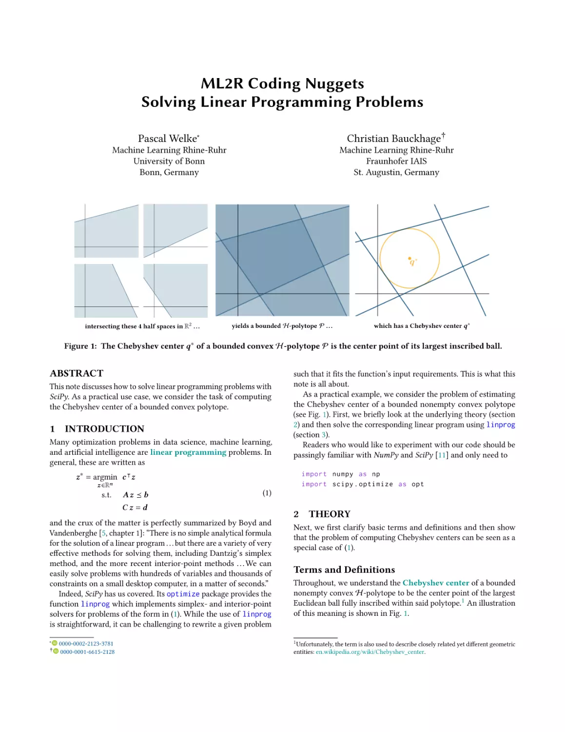
q∗

intersecting these 4 half spaces in R2 . . .

yields a bounded H -polytope P . . .

which has a Chebyshev center 𝒒∗

Figure 1: The Chebyshev center 𝒒∗ of a bounded convex H -polytope P is the center point of its largest inscribed ball.

ABSTRACT
This note discusses how to solve linear programming problems with
SciPy. As a practical use case, we consider the task of computing
the Chebyshev center of a bounded convex polytope.

1

INTRODUCTION

Many optimization problems in data science, machine learning,
and artificial intelligence are linear programming problems. In
general, these are written as

such that it fits the function’s input requirements. This is what this
note is all about.
As a practical example, we consider the problem of estimating
the Chebyshev center of a bounded nonempty convex polytope
(see Fig. 1). First, we briefly look at the underlying theory (section
2) and then solve the corresponding linear program using linprog
(section 3).
Readers who would like to experiment with our code should be
passingly familiar with NumPy and SciPy [11] and only need to
import numpy as np
import scipy . optimize as opt

𝒛 ∗ = argmin 𝒄 ⊺ 𝒛
𝒛 ∈R𝑛

s.t.

𝑨𝒛 ⪯ 𝒃

(1)

𝑪𝒛 =𝒅
and the crux of the matter is perfectly summarized by Boyd and
Vandenberghe [5, chapter 1]: “There is no simple analytical formula
for the solution of a linear program . . . but there are a variety of very
effective methods for solving them, including Dantzig’s simplex
method, and the more recent interior-point methods . . . We can
easily solve problems with hundreds of variables and thousands of
constraints on a small desktop computer, in a matter of seconds.”
Indeed, SciPy has us covered. Its optimize package provides the
function linprog which implements simplex- and interior-point
solvers for problems of the form in (1). While the use of linprog
is straightforward, it can be challenging to rewrite a given problem
∗
†

0000-0002-2123-3781
0000-0001-6615-2128

2

THEORY

Next, we first clarify basic terms and definitions and then show
that the problem of computing Chebyshev centers can be seen as a
special case of (1).

Terms and Definitions
Throughout, we understand the Chebyshev center of a bounded
nonempty convex H -polytope to be the center point of the largest
Euclidean ball fully inscribed within said polytope.1 An illustration
of this meaning is shown in Fig. 1.

1 Unfortunately, the term is also used to describe closely related yet different geometric

entities: en.wikipedia.org/wiki/Chebyshev_center.

P. Welke and C. Bauckhage
Moreover, following Ziegler [13], we say that an 𝑚-dimensional
H -polytope is a set
n
o
P = 𝒙 ∈ R𝑚 𝑾𝒙 ⪯ 𝜽
(2)

(5) together with 𝒛, 𝑨 and 𝒃 allow us to write the collection of
𝑝 individual inequality constraints in (4) in terms of a single
matrix-vector expression, namely

where the matrix-vector expression 𝑾𝒙 ⪯ 𝜽 is a convenient short⊺
hand for a collection of 𝑖 = 1, . . . , 𝑝 inequalities 𝒘𝑖 𝒙 ≤ 𝜃𝑖 .
In other words, each point 𝒙 inside of an H -polytope P is a
solution to a system of 𝑝 linear inequalities. Since each of these
inequalities defines a half-space in R𝑚 , we recognize the definition
in (2) to describe a convex set, namely an intersection of finitely
many half-spaces, hence the name H -polytope. Finally, if there
exists some number 𝑅 ∈ R such that ∥𝒙 ∥ ≤ 𝑅 for all 𝒙 ∈ P, then P
is bounded.
An 𝑚-dimensional Euclidean ball is yet another, arguably more
prosaic bounded convex set, namely
n
o
B = 𝒙 ∈ R𝑚 𝒙 − 𝒒 ≤ 𝑟 .
(3)

All in all, our (re)definitions therefore allow us to (re)write the
optimization problem in (4) as

Here, the two parameters 𝒒 ∈ R𝑚 and 𝑟 ∈ R simply characterize
the ball’s center point and radius.

Chebyshev Centers and Linear Programming
Since a Euclidean ball is defined in terms of its center and radius,
to estimate the Chebyshev center of a bounded H -polytope P is to
estimate the parameters 𝒒∗ and 𝑟 ∗ of the largest ball inscribed in it.
Without retracing all their arguments, we simply note that Boyd
and Vandenberghe [5] show that these parameters coincide with
the solution to the following constrained optimization problem
𝒒∗, 𝑟 ∗ = argmax 𝑟
𝒒,𝑟

s.t.

(4)

⊺

𝑟 · ∥𝒘𝑖 ∥ + 𝒘𝑖 𝒒 ≤ 𝜃𝑖 , 𝑖 = 1, . . . , 𝑝.

Now, in order to see that (4) is indeed but a special case of (1),
we proceed as follows:
(1) we combine the two problem variables 𝒒 ∈ R𝑚 and 𝑟 ∈ R
into a single vector 𝒛 ∈ R1+𝑚 such that
 
𝑟
𝒛=
(5)
𝒒
(2) we introduce yet another vector 𝒄 ∈

R1+𝑚 ,

namely

−1
 
0
 
(6)
𝒄= . 
 .. 
 
0
 
(3) these vectors allow us to rewrite the maximization objective
in equation (4) in terms of a minimization objective which
involves an inner product, because
argmax 𝑟

⇔

argmin −𝑟

𝒒,𝑟

𝒒,𝑟

⇔

argmin 𝒄 ⊺ 𝒛

(7)

𝒒,𝑟

(4) we introduce a matrix 𝑨 ∈ R𝑝×(1+𝑚) together with a vector
𝒃 ∈ R𝑝 which are given by
 ∥𝒘1 ∥

 .
𝑨 =  ..

 ∥𝒘𝑝 ∥


⊺
𝒘1 

.. 
. 
⊺
𝒘𝑝 

and

𝜃 1 
 
.
𝒃 =  .. 
 
𝜃 
 𝑝

(8)

𝑨𝒛 ⪯ 𝒃

(9)

𝒛 ∗ = argmin 𝒄 ⊺ 𝒛
𝒛 ∈R𝑚+1

s.t.

(10)
𝑨 𝒛 ⪯ 𝒃.

This is now easily recognizable as a special case of the more general
linear program in (1), namely as a linear program without equality
constraints.

3

PRACTICAL COMPUTATION

In this section, we discuss how to solve the Chebyshev center
problem using SciPy. Given what we just worked out (equations
(5)–(10)), there is actually not much left to discuss except for details
of the code in Listing 1.
In order to work with a specific (numerical) example, we resort
to the 𝑚 = 2 dimensional polytope P in Fig. 1. This particular
polytope results from plunging
 5.0
−0.26
0.97



 0.42 −0.91
 1.0



𝑾 = 
and
𝜽
=
(11)
 8.0
0.42
 0.91


−0.82 −0.57
−1.5




into (2). Implementing both, matrix 𝑾 and vector 𝜽 , in terms of
NumPy arrays is straightforward
matW = np . array ([[ -0.26 , 0.42 , 0.91 , -0.82] ,
[ 0.97 , -0.91 , 0.42 , -0.57]]). T
vecT = np . array ([5.0 , 1.0 , 8.0 , -1.5])

Likewise, it is easy to compute the norms ∥𝒘𝑖 ∥ of the rows of
matrix 𝑾 . We simply use the following recipe (for an explanation
of the rationale behind this one-liner, see [1])
rowNrmW = np . sqrt ( np . sum ( matW **2 , axis =1))

Next, we need to set up matrix 𝑨 and vector 𝒃 as introduced in
equation (8). To accomplish this, we may proceed as follows
matA = np . vstack (( rowNrmW , matW . T )). T
vecB = vecT

The last ingredient of our linear program is the vector 𝒄 in (6).
Since our current problem is 1 + 𝑚 = 3 dimensional, we can simply
instantiate it like so
vecC = np . array ([ -1 , 0 , 0])

or, more generally, write
vecC = np . zeros ( matA . shape [1])
vecC [0] = -1

At this point, we are good to go and can invoke function linprog
in SciPy’s optimize module. It is called with several parameters of
which the following are most relevant in our current setting:
• c is a 1D array representing the coefficient vector 𝒄 of the
linear objective function we wish to solve
• A_ub and b_ub are a 2D and a 1D array which represent the
matrix 𝑨 and vector 𝒃 which define the inequality (or upper
bound) constraints of our problem

Solving Linear Programming Problems
• although we do not actually need them here, we should
mention that the parameters A_eq and b_eq are a 2D and
a 1D array which would represent matrix 𝑪 and vector 𝒅
which occur in (1) and specify potential equality constraints
• finally, the parameter method is a string used to indicate
which solver we wish to apply; its default value amounts
to ’interior-point’, another reasonable choice would be
’revised simplex’.
Hence, for our current problem, we may use linprog as follows
result = opt . linprog ( vecC , A_ub = matA , b_ub = vecB )

This will cause result to be a variable of type OptimizeResult
which is a class that SciPy uses in order to summarize the outcome
of an optimization procedure. To have a look at our result, we may
therefore simply
print ( result )

which provides us with the following status report
con :
fun :
message :
nit :
slack :
status :
success :
x:

array ([] , dtype = float64 )
-2.666293247661684
' Optimization terminated successfully . '
3
array ([0. , 0. , 1.38093669 , 0.])
0
True
array ([2.66629325 , 2.87626447 , 3.16518324])

Its content is largely self explanatory; explanations of the more
cryptic entries can be found in the SciPy documentation. The most
important thing to us is that the field x contains the solution 𝒛 ∗ to
our problem. In other words, something like
vecZ = result . x
r , c = vecZ [0] , vecZ [1:]

Listing 1: solving the linear program in (10)
matW = np . array ([[ -0.26 , 0.42 , 0.91 , -0.82] ,
[ 0.97 , -0.91 , 0.42 , -0.57]]). T
vecT = np . array ([5.0 , 1.0 , 8.0 , -1.5])
rowNrmW = np . sqrt ( np . sum ( matW **2 , axis =1))
matA = np . vstack (( rowNrmW , matW .T )). T
vecB = vecT
vecC = np . zeros ( matA . shape [1])
vecC [0] = -1
result = opt . linprog ( vecC , A_ub = matA , b_ub = vecB )

4

SUMMARY AND OUTLOOK

This short note discussed how to solve linear programming problems using the method linprog contained in SciPy’s optimize
package. We saw that the use of linprog is intuitive, as long as we
can express the problem we are dealing with in the form expected
by the function. To see how to bring a given problem into this
particular form, we considered the Chebyshev center problem and
rewrote the underlying linear program correspondingly.
While our practical example of computing the Chebyshev center
of a polytope, or, equivalently, of computing its largest inscribed
ball was chosen for didactic purposes, we note that Euclidean balls
are a staple of intelligent data analysis [2–4, 8, 10, 12]. Moreover
and more recently, Euclidean balls have also been used successfully
for informed or structured representation learning [6, 7, 9] and we
will return to these ideas in later notes.

ACKNOWLEDGMENTS

will provide us with radius r and center point c of the largest ball
inscribed within our polytope.

This material was produced within the Competence Center for
Machine Learning Rhine-Ruhr (ML2R) which is funded by the
Federal Ministry of Education and Research of Germany (grant no.
01IS18038A). The authors gratefully acknowledge this support.

3.1

REFERENCES

A Note on “Corner Cases”

Intuitively, it is clear that we can only find a Chebyshev-center of
an nonempty polytope 𝑃. However, no-one keeps
 you from defining
an empty polytope by adding the inequality 1 0 𝑥 ≤ −3:
matW = np . array ([[ -0.26 , 0.42 , 0.91 , -0.82 , 1] ,
[0.97 , -0.91 , 0.42 , -0.57 , 0]]). T
vecT = np . array ([5.0 , 1.0 , 8.0 , -1.5 , -3])

There is no 𝑥 ∈ R2 that satisfies all constraints at once. Luckily,
linprog notices this and results in the following output:
con : array ([] , dtype = float64 )
fun : -0.6671837546213493
message : ' The algorithm terminated successfully and determined
that the problem is infeasible . '
nit : 4
slack : array ([3.47102113 , 1.09568071 , 6.71856309 ,
-1.43242614 , -3.90269694])
status : 2
success : False
x: array ([0.66718375 , 0.23551318 , 0.94865877])

Be careful! As you can see, the result tells you that no solution
exists, but at the same time happily gives you a “solution” vector
result.x. Hence, you must always check the value of result.success
before using result.x!

[1] C. Bauckhage. 2015. NumPy / SciPy Recipes for Data Science: Computing Nearest
Neighbors. researchgate.net. dx.doi.org/10.13140/RG.2.1.4602.0564.
[2] C. Bauckhage, M. Bortz, and R. Sifa. 2020. Shells within Minimum Enclosing
Balls. In Proc. DSAA. IEEE.
[3] C. Bauckhage, R. Sifa, and T. Dong. 2019. Prototypes within Minimum Enclosing
Balls. In Proc. ICANN.
[4] A. Ben-Hur, D. Horn, H.T. Siegelmann, and V. Vapnik. 2001. Support Vector
Clustering. J. of Machine Learning Research 2 (2001).
[5] S. Boyd and L. Vandenberghe. 2004. ConvexOptimization. Cambridge University
Press.
[6] T. Dong, C. Bauckhage, H. Jin, J. Li, O. Cremers, D. Speicher, A.B. Cremers, and J.
Zimmermann. 2019. Imposing Category Trees onto Word-Embeddings Using a
Geometric Construction. In Proc. ICLR.
[7] T. Dong, Z. Wang, J. Li, C. Bauckhage, and A.B. Cremers. 2019. Triple Classification Using Regions and Fine-Grained Entity Typing. In Proc. AAAI.
[8] G.D. Evangelidis and C. Bauckhage. 2013. Efficient Subframe Video Alignment
Using Short Descriptors. IEEE Trans. Pattern Analysis and Machine Intelligence
35, 10 (2013).
[9] T. Le, H. Vu, T.D. Nguyen, and D. Phung. 2018. Geometric Enclosing Networks.
In Proc. IJCAI.
[10] J. Lee and D. Lee. 2005. An Improved Cluster Labeling Method for Support Vector
Clustering. IEEE Trans. Pattern Analysis and Machine Intelligence 27, 3 (2005).
[11] T.E. Oliphant. 2007. Python for Scientific Computing. Computing in Science &
Engineering 9, 3 (2007).
[12] D.M.J. Tax and R.P.W. Duin. 2004. Support Vector Data Description. Machine
Learning 54, 1 (2004).
[13] G.M. Ziegler. 1995. Lectures on Polytopes. Springer.