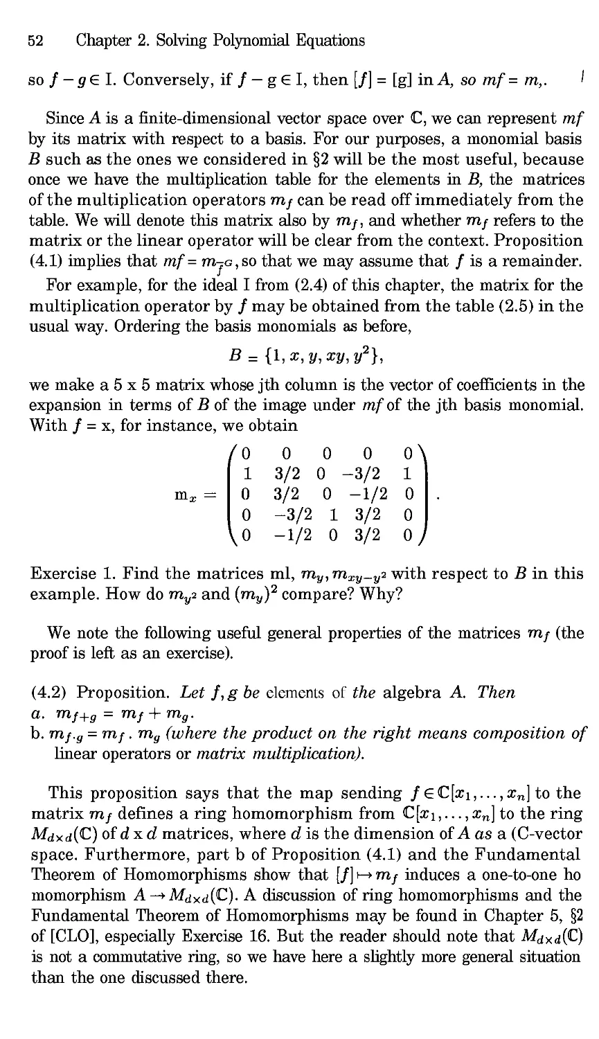
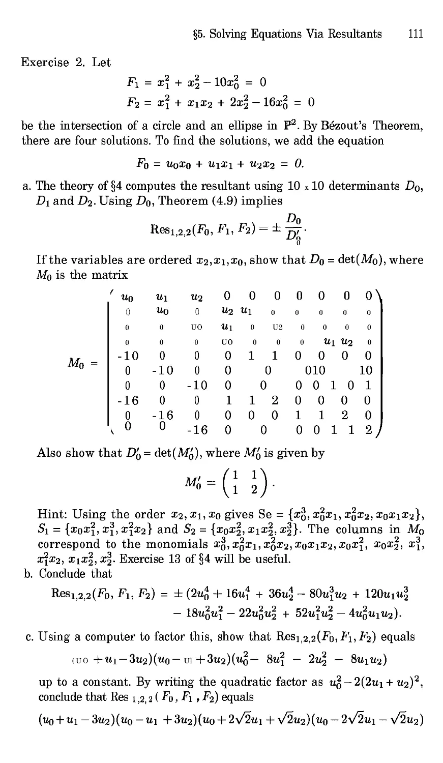
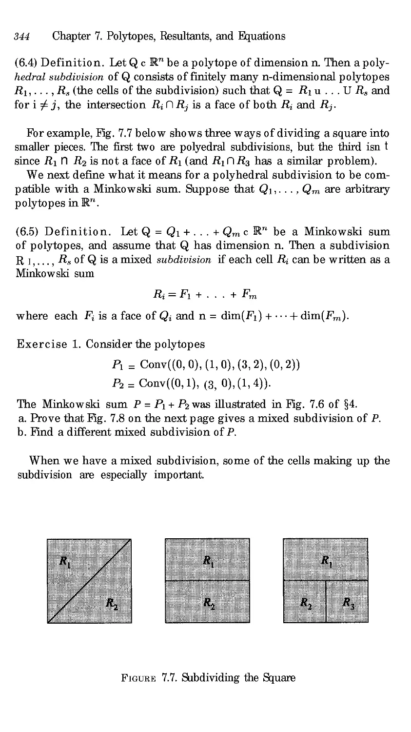
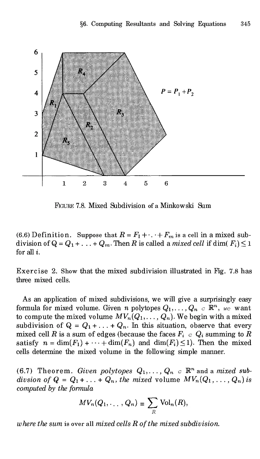
/


Text
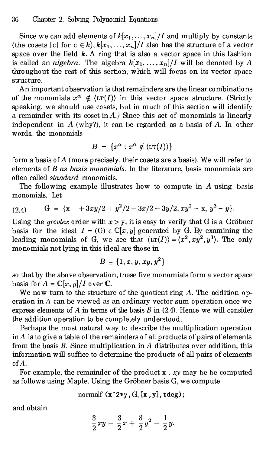
David Cox
John Little
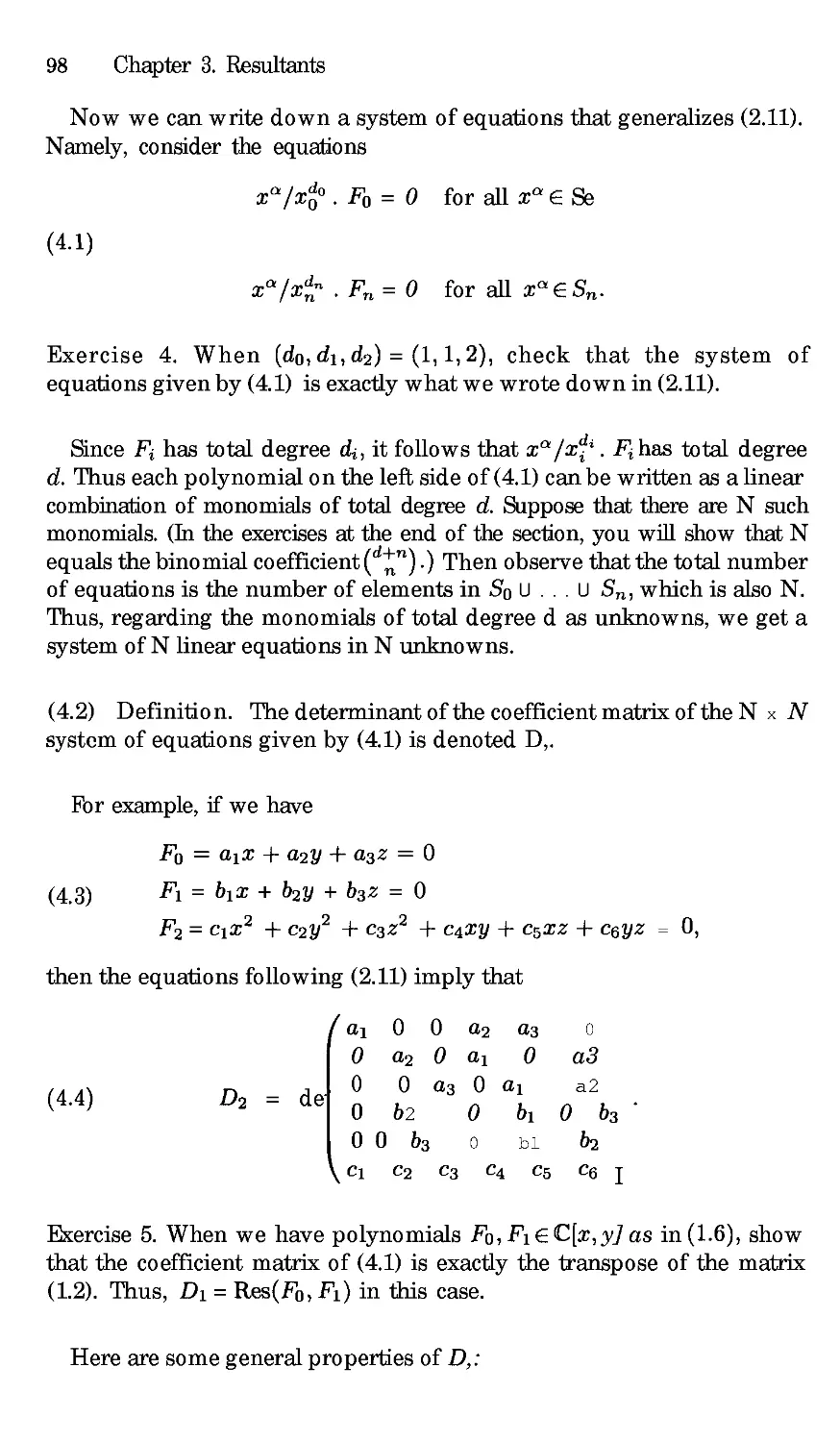
Donal 0 Shea
Using Algebraic
Geometry
With 22 Illustrations
@ Springer
David Cox
Department of Mathematics
and Computer Science
Amherst College
Amherst, MA 0 1002-5000
USA
Donal O Shea
Department of Mathematics, Statistics
and Computer Science
Mount Holyoke College
South Hadley, MA 010751493
USA
John Little
Department of Mathematics
College of the Holy Cross
Worcester, MA 0161 0-2395
USA
Editorial Board
N Axler
Mathematics Department
San Francisco State
University
San Francisco, CA 94132
USA
F.W. Gehring
Mathematics Department
University of Michigan
Ann Arbor, MI 48 IO9
USA
K. A. Ribet
Department of Mathematics
East Hall University of
California at Berkeley
Berkeley, CA 94720-3840
USA
Mathematics Subject Classification (1991): 14-01,13-01,13Pxx
Library of Congress Cataloging-in-Publication Data
Cox, David A.
Using algebraic geometry / David A. Cox, John B. Little, Donal B.
O Shea.
p. cm.-- (Graduate texts in mathematics ;185)
Includes bibliographical references (p.-)and index.
ISBN 0-387-98487-9 (alk. paper). -- ISBN 0-387-98492-S (pbk. :
alk. paper)
I. Geometry, Algebraic. I. Little, John B. II. 0 Shea, Donal,
II1. Title. IV. Series.
QA564.C6883 1998
516.3'5--dc21 98-1 1964
Printed on acid-free paper.
© 1998 Springer-Verlag New York, Inc.
All rights reserved. This work may not be translated or copied in whole or in part without the
written permission of the publisher (Springer-Verlag New York, Inc., 1"75 Fifth Avenue, New York,
NY 10010, LISA), except for brief excerpts in connection with reviews or scholarly analysis. LIse
in connection with any form of information storage and retrieval, electronic adaptation, computer
software, or by similar or dissimilar methodology now known or hereafter developed is forbidden.
The use of general descriptive names, trade names, trademarks, etc., in this publication, even if the
former are not especially identified, is not to be taken as a sign that such names, as understood by
the Trade Marks and Merchandise Marks Act, may accordingly be used freely by anyone.
Production managed by Timothy Taylor; manufacturing supervised by Jacqui Ashri.
Camera-ready copy prepared from the authors ,'[' files.
Printed and bound by R.R. Donnclley and Sons, Harrisonburg, VA.
Printed in the United States of America.
987654321
ISBN0 387 98487-9 Springer-Verlag New York Berlin Heidelberg SPIN 10670077 (hardcover)
ISBN 0-387-98492 5 Springer Verlag New York Berlin Heidelberg SPIN 106701 X2 (softcover)
Preface
In recent years, the discovery of new algorithms for dealing with polyno-
mial equations, coupled with their implementation on inexpensive yet fast
computers, has sparked a minor revolution in the study and practice of
algebraic geometry. These algorithmic methods and techniques have also
given rise to some exciting new applications of algebraic geometry.
One of the goals of Using Algebraic Geometry is to illustrate the many
uses of algebraic geometry and to highlight the more recent applications
of GrSbner bases and resultants. In order to do this, we also provide an
introduction to some algebraic objects and techniques more advanced than
one typically encounters in a first course, but which are nonetheless of
great utility. Finally, we wanted to write a book which would be accessible
to nonspecialists and to readers with a diverse range of backgrounds.
To keep the book reasonably short, we often have to refer to basic re-
suits in algebraic geometry without proof, although complete references are
given. For readers learning algebraic geometry and GrSbner bases for the
first time, we would recommend that they read this book in conjunction
with one of the following introductions to these subjects:
• Introduction to GrSbner Bases, by Adams and Loustaunau [AL]
• GrSbner Bases, by Becker and Weispfenning [BW]
• Ideals, Varieties andAlgorithms, by Cox, Little and O Shea [CLO]
We have tried, on the other hand, to keep the exposition self-contained
outside of references to these introductory texts. We have made no effort
at completeness, and have not hesitated to point out the reader to the
research literature for more information.
Later in the preface we will give a brief summary of what our book covers.
The Level of the Text
This book is written at the graduate level and hence assumes the reader
knows the material covered in standard undergraduate courses, including
abstract algebra. But because the text is intended for beginrSng graduate
viii Preface
students, it does not require graduate algebra, and in particular, the book
does not assume that the reader is familiar with modules. Being a graduate
text, Using Algebraic Geometry covers more sophisticated topics and has
a denser exposition than most undergraduate texts, including our previous
book [CLO].
However, it is possible to use this book at the undergraduate level, pro-
vided proper precautions are taken. With the exception of the first two
chapters, we found that most undergraduates needed help reading prelimi-
nary versions of the text. That said, if one supplements the other chapters
with simpler exercises and fuller explanantions, many of the applications we
cover make good topics for an upper-level undergraduate applied algebra
course. Similarly, the book could also be used for reading courses or senior
theses at this level. We hope that our book will encourage instructors to
find creative ways for involving advanced undergraduates in this wonderful
mathematics.
How to Use the Text
The book covers a variety of topics, which can be grouped roughly as
follows:
• Chapters i and 2: GrSbner bases, including basic definitions, algorithms
and theorems, together with solving equations, eigenvalue methods, and
solutions over R.
• Chapters 3 and 7: Resultants, including multipolynomial and sparse
resultants as well as their relation to polytopes, mixed volumes, toric
varieties, and solving equations.
• Chapters 4, 5 and 6: Commutative algebra, including local rings, stan-
dard bases, modules, syzygies, free resolutions, Hilbert functions and
geometric applications.
• Chapters 8 and 9: Applications, including integer programming, combi-
natorics, polynomial splines, and algebraic coding theory.
One unusual feature of the book s organization is the early introduction
of resultants in Chapter 3. This is because there are many applications
where resultant methods are much more efficient that GrSbner basis meth-
ods. While GrSbner basis methods have had a greater theoretical impact on
algebraic geometry, resultants appear to have an advantage when it comes
to practical applications. There is also some lovely mathematics connected
with resultants.
There is a large degree of independence among most chapters of the book
This implies that there are many ways the book can be used in teaching a
course. Since there is more material than can be covered in one semester,
some choices are necessary. Here are three examples of how to structure a
course using our text.
Prefa ix
• Solving Equations. This course would focus on the use of GrSbner bases
and resultants to solve systems of polynomial equations. Chapters 1, 2,
3 and 7 would form the heart of the course. Special emphasis would be
placed on §5 of Chapter 2, §5 and §6 of Chapter 3, and §6 of Chapter 7.
Optional topics would include §1 and §2 of Chapter 4, which discuss
multiplicities.
• Commutative Algebra. Here, the focus would be on topics from classical
commutative algebra. The course would follow Chapters 1, 2, 4, 5 and 6,
skipping only those parts of 92 of Chapter 4 which deal with resultants.
The final section of Chapter 6 is a nice ending point for the course.
• Applications. A course concentrating on applications would cover integer
programming, combinatorics, splines and coding theory. After a quick
trip through Chapters i and 2, the main focus would be Chapters 8 and
9. Chapter 8 uses some ideas about polytopes from §1 of Chapter 7,
and modules appear naturally in Chapters 8 and 9. Hence the first two
sections of Chapter 5 would need to be covered. Also, Chapters 8 and
9 use Hilbert functions, which can be found in either Chapter 6 of this
book or Chapter 9 of [CLO].
We want to emphasize that these are only three of many ways of using the
text. We would be very interested in hearing from instructors who have
found other paths through the book.
References
References to the bibliography at the end of the book are by the first three
letters of the author s last name (e.g., [Hill for Hilbert), with numbers for
multiple papers by the same author (e.g., [Macl] for the first paper by
Macaulay). When there is more than one author, the first letters of the
authors last names are used (e.g., [BE] for Buchsbaum and Eisenbud),
and when several sets of authors have the same initials, other letters are
used to distinguish them (e.g., [BoF] is by Bormesen and Fenchel, while
[BuF] is by Burden and Faires).
The bibliography lists books alphabetically by the full author s name,
followed (if applicable) by any coauthors. This means, for instance, that
[BS] by Biller-a and Sturmfels is listed before [Bla] by Blahut.
Comments and Corrections
We encourage comments, criticism, and corrections. Please send them to
any of us:
David Cox dac@cs.amherst.edu
John Little little@math.ho lycro ss.edu
Don 0 Shea doshea@mhc.mtholyoke.edu
x Preface
For each new typo or error, we will pay $1 to the first person who reports
it to us. We also encourage readers to check out the web site for Using
Algebraic Geometry, which is at
http://www, cs. amherst, edu/~dac/uag, html
This site includes updates and errata sheets, as well as hnks to other sites
of interest.
Acknowledgments
We would like to thank everyone who sent us comments on initial drafts
of the manuscript. We are especially grateful to thank Susan Colley, Alicia
Dickenstein, Ioannis Emiris, Tom Garrity, Pat Fitzpatrick, Gert-Martin
Greuel, Paul Pedersen, Maurice Rojas, Jerry Shurman, Michael Singer,
Michael Stanfield, Bernd Sturmfels (and students), Moss Sweedler (and
students), Wiland Schmale, and Cynthia Woodburn for especially detailed
comments and criticism.
We also gratefully acknowledge the support provided by National Sci-
ence Foundation grant DUE-9666132, and the help and advice afforded by
the members of our Advisory Board: Susan Colley, Keith Devlin, Arnie
Ostebee, Bernd Sturmfels, and Jim White.
November, 1997
David Cox
John Little
Donal 0 tnea
Contents
Preface
vii
Chapter 1. Introduction
§1. Polynomials and Ideals
§2. Monomial Ordcrs and Polynomial Division
§3. GrSbner Bases
§4. Affine Varieties
Chapter 2. Solving Polynomial Equations
§ 1. Solving Polynomial Systems by Elimination
§2. Finite-Dimensional Algebras
§3. GrSbner Basis Conversion
§4. Solving Equations via Eigenvalues
§5. Real Root Location and Isolation
Chapter 3. Resultants
§1. The Resultant of Two Polynomials
§2. Multipolynomial Resultants
§3. Properties of Resultants
§4. Computing Resultants
§5. Solving Equations Via Resultants
§6. Solving Equations via Eigenvalues
Chapter 4. Computation in Local Rings
§1. Local Rings
§2. Multiplicities and Milnor Numbers
§3. Term Orders and Division in Local Rings
§4. Standard Bases in Local Rings
1
1
6
11
16
24
24
34
46
51
63
71
71
78
89
96
108
122
130
130
138
151
164
xii Comems
Chapter 5. Modules
§ 1. Modules over Rings
§2. Monomial Orders and GrSbner Bases for Modules
§3. Computing Syzygies
§4. Modules over Local Rings
179
179
197
210
222
Chapter 6. Free Resolutions
§1. Presentations and Resolutions of Modules
§2. Hilbert s Syzygy Theorem
§3. Graded Resolutions
§4. Hilbert Polynomials and Geometric Applications
234
234
245
252
266
Chapter 7. Polytopes, Resultants, and Equations
§1. Geometry of Polytopes
§2. Sparse Resultants
§3. Toric Varieties
§4. Minkowski Sums and Mixed Volumes
95. Bernstein s Theorem
§6. Computing Resultants and Solving Equations
290
290
298
306
316
327
342
Chapter 8. Integer Programming, Combinatorics, and
Splines
§ 1. Integer Programming
§2. Integer Programming and Combinatorics
§3. Multivariate Polynomial Splines
359
359
374
385
Chapter 9. Algebraic Coding Theory
§1. Finite Fields
§2. Error-Correcting Codes
§3. Cyclic Codes
94. Reed-Solomon Decoding Algorithms
§5. Codes from Algebraic Geometry
407
407
415
424
435
448
References
468
In dex 4 7 7
Chapter 1
Introduction
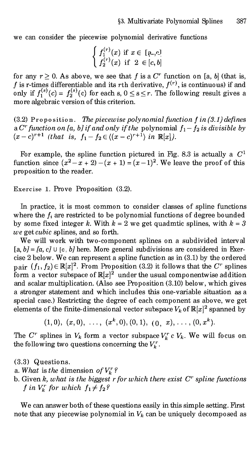
Algebraic geometry is the study of geometric objects defined by polynomial
equations, using algebraic means. Its roots go backto Descartes introduc-
tion of coordinates to describe points in Euclidean space and his idea of
describing curves and surfaces by algebraic equations. Over the long his-
tory of the subject, both powerful general theories and detailed knowledge
of many specific examples have been developed. Recently, with the devel-
opment of computer algebra systems and the discovery (or rediscovery) of
algorithmic approaches to many of the basic computations, the techniques
of algebraic geometry have also found significant applications, for example
in geometric design, combinaterics, integer programming, coding theory,
and robotics. Our goal in Using Algebraic Geometry is to survey these
algorithmic approaches and many of their applications.
For the convenience of the reader, in this introductory chapter we will
first recall the basic algebraic structure of ideals in polynomial rings. In §2
and §3 we will present a rapid summary of the GrSbner basis algorithms de-
veloped by Buchberger for computations in polynomial rings, with several
worked out examples. Finally, in §4 we will recall the geometric notion of
an ane algebraic variety, the simplest type of geometric object defined by
polynomial equations. The topics in §1, §2, and §3 are the common prereq-
uisites for all of the following chapters. §4 gives the geometric context for
the algebra from the earlier sections. We will make use of this language at
many points. If these topics are familiar, you may wish to proceed directly
to the later material and refer back to this introduction as needed.
§1 Polynomials and Ideals
To begin, we will recall some terminology. A monomial in a collection of
variables Xl,..., Xn is a product
(1.1) xl "°
2 Chapter 1. Introduction
where the ai are non-negative integers. To abbreviate, we will sometimes
rewrite (1.1) as x where a = (al,..., an) is the vector of exponents in the
monomial. The total degree ofa monomial x is the sum of the exponents:
al + • • • + an. We will often denote the total degree of the monomial x
by la[. For instance xx2x4 is a monomial of tetal degree 6 in the variables
xl, x2, x3, x4, since a = (3, 2, 0, 1) and [a[ = 6.
Ifk is any field, we can form finite linear combinations of monomials
with coefficients in k. The resulting objects are known as polynomials in
Xl,. • •, Xn. We will also use the word term on occasion to refer to a product
of a nonzero element of k and a monomial appearing in a polynomial. Thus,
a general polynomial in the variables x,..., Xn with coefficients in k has
the form
f -= E
where ca • k for each a, and there are only finitely many terms cx in
the sum. For example, taking k to be the field Q of rational numbers, and
denoting the variables by x, y, z rather than using subscripts,
(1.2) p = x 2 + ½ y2z - z - 1
is a polynomial containing four terms.
In most of our examples, the field of coefficients will be either Q, the
field of real numbers, , or the field of complex numbers, C. Polynomi-
als over finite fields will also be introduced in Chapter 9. We will denote
by k[x,... ,x,] the collection of all polynomials in x,...,Xn with co-
efficients in k. Polynomials in k[Xl,..., x,] can be added and multiplied
as usual, so k[x,...,Xn] has the structure of a commutative ring (with
identity). However, only nonzero constant polynomials have multiplicative
inverses in k[xl .... , x,], so k[Xl .... , Xn] is not a field. However, the set
of rational functions {fg : f,g • k[x,. . ., Xn],g 0} is a field, denoted
A polynomial f is said to be homogeneous if all the monomials appearing
in it with nonzero coefficients have the same total degree. For instance,
f = 4x 3 + 5xy 2- z 3 is a homogeneous polynomial of total degree 3 in
Q[x,y, z], while g = 4x a + 5xy2-z 6 is not homogeneous. When we study
resultants in Chapter 3, homogeneous polynomials will play an important
role.
Given a collection of polynomials, fl,..., fs•k[x, .... Xn], we can
consider all polynomials which can be built up from these by multiplication
by arbitrary polynomials and by taking sums.
(1.3) Definition. Let f,..., fs•k[x,...,Xn]. We let (f,...,
denote the collection
(fl,..., fs) = {Plfl +... + Psfs : Pi • k[x .... , Xn] for i = 1 .... , s}.
§1. Polynomials and Ideals 3
For example, consider the polynomial p from (1.2) above and the two
polynomials
fl: X2 - Z2 -- 1
f2 = x 2 + y2 + (z-l) 2- 4.
We have
1
p = x 2 + y2z-z- 1
1 1)(x 2 z 2
(1.4) = (-z + + - 1) + (½z)(x 2+y2+(z-1) 2-
This shows p •
4).
Exercise 1.
a. Show that x 2 • (x - y2, xy) in k[x, y] (k any field).
b. Show that (x - y2, xy, y2) = (x, y2).
c. Is (x - y2, xy) = (x 2, xy)? Why or why not?
Exercise 2. Show that (fl,..., fs) is closed under sums in k[xl,..., Xn].
Also show that if f • (f,...,fs), and p• k[xl,...,Xn] is an arbitrary
polynomial, then p- f • (f,...,
The two properties in Exercise 2 are the defining properties of ideals in
the ring k[x,..., Xn].
(1.5) Definition. Let I c k[x,... , ×,1 be a non-empty subset. I is said
to be an ideal if
a.]+g• Iwheneverf •Iandg • I, and
b. pf• I whenever f• I, and p•k[x,...,Xn] is an arbitrary
polynomial.
Thus (fl,..., f) is an ideal by Exercise 2. We will call it the ideal
generated by f,..., f because it has the following property.
Exercise 3. Show that (f ,... ,f) is the smallest ideal in k[Xl,...,Xn]
containing f,...,f, in the sense that if Jis any ideal containing
f,..., fs, then (f .... , f) C J.
Exercise 4. Using Exercise 3, formulate and prove a general criterion for
equality of ideals I = (fl,... , fs) and J= (g,..., gt) in k[x,...,Xn].
How does your statement relate to what you did in part b of Exercise 1?
Given an ideal, or several ideals, in k[x,...,xn], there are a number of
algebraic constructions that yield other ideals. One of the most important
of these for geometry is the following.
4 Chapter _. Introduction
(1.6) Definition. LetI c k[xl, • , Xn] be an ideal. The radical of ! is
the set
vf = {g e k[Xl,...,Xn]:gmeI for some m _>1}
An ideal I is said to be a radical ideal if v = I.
For instance,
2 + y • x/(x 2 + 3xy, 3xy + y2)
in Q[x, y] since
(x + y)3 = x(x 2 + 3xy) + y(3xy + y2)• (x + 3xy, 3xy + y2).
Since each of the generators of the ideal Ix2+ 3xy, 3xy + y2 t is homogeneous
of degree 2, it is clear that x + y (x 2 + 3xy, 3xy + y2). It follows that
(x 2 + 3xy, 3xy + y2) is not a radical ideal.
Although it is not obvious from the definition, we have the following
property of the radical.
• (Radical Ideal Property) For every ideal I c k[x, . , Xn] , v is an
ideal containing/.
See [CLO], Chapter 4, §2, for example. We will consider a number of other
operations on ideals in the exercises.
One of the most important general facts about ideals in k[xl,..., Xn] is
known as the Hilbert Basis Theorem. In this context, a basis is another
name for a generating set for an ideal.
• (Hilbert Basis Theorem) Every ideal I in k[xl,...,x,] has a finite gener-
ating set. In other words, given an ideal I, there exists a finite collection
ofpolynomSals {f .... fs} c [x, . , x,l suchthatI={f,...,fs}.
For polynomials in one variable, this is a standard consequence of the one-
variable polynomial division algorithm.
• (Division Algorithm in k[x]) Given two polynomials f, g • k[x], we can
divide f by g, producing a unique quotient q and remainder r such that
f = qg + r,
and either :- = 0, or r has degree strictly smaller than the degree of g.
See, for instance, [CLO], Chapter 1, §5. The consequences of this result for
ideals in k[x] are discussed in Exercise 6 below. For polynomials in several
variables, the Hilbert Basis Theorem can be proved either as a byproduct of
the theory of GrSbner bases to be reviewed in the next section (see [CLO],
Chapter 2, §5), or inductively by showing that if every ideal in a ring R is
finitely generated, then the same is true in the ring R[x] (.'ee [AL], Chapter
1, §1, or [BW], Chapter 4, §1).
§1. Polynomials and Ideals 5
ADDITIONAL EXERCISES FOR §1
Exercise 5. Show that (y - x 2, z - x a) = (z - xy, y - x 2) in Q[x, y, z].
Exercise 6. Let k be any field, and consider the polynomial ring in one
variable, k[x]. In this exercise, you will give one proof that every ideal in
k[x] is finitely generated. In fact, every ideal I c k[x] is generated by a
single polynomial: I = (g) for some g. We may assume I {0} for there is
nothing to prove in that case. Let g be a nonzero element in I of minimal
degree. Show using the division algorithm that every f in I is divisible by
g. Deduce that I = (g).
Exercise 7.
a. Let k be any field, and let n be any positive integer. Show that in k[x],
b. More generally, suppose that
p(x) = (x - al) el.-. (x - am) era.
What is (p?
c. Let k = C, so that every polynomial in one variable factors as in b.
What are the radical ideals in C[x]?
Exercise 8. An ideal I c k[Xl,..., Xn] is said to bepr/me if whenever a
product fg belongs to I, either f E I, or g E I (or both).
a. Show that a prime ideal is radical.
b. What are the prime ideals in C[x]? What about the prime ideals in l[x]
or
Exercise 9. An ideal I c k[xl,..., Xn] is said to be maximal if there
are no ideals Jsatisfying I cJc k[xl,...,xn] other than J= I and
J= k[Xl,..., Xn].
a. Show that (xi, x2, ..., Xn) is a maximal ideal in k[Xl,...,Xn].
b. More generally show that if (al,..., an) is any point in k n, then the
ideal (xl-al,...,Xn- a,) c k[xl,...,Xn] is maximal.
c. Show that I = (x 2 + 1) is a maximal ideal in l[x]. Is I maximal
considered as an ideal in
Exercise 10. Let I be an ideal in k[x,...,Xn] , let g>_ i be an integer,
and let It consist of the elements in I that do not depend on the first g
variables:
It = I 1 k[Xt+l,..., Xn].
It is called the gth elimination ideal of I.
a. For I = (x 2 + y2,x2-za) C k[x,y, z], show that y2 + z a is in the first
elimination ideal I1.
6 Chapter 1. Introduction
b. Prove that It is an ideal in the ring k[Xt+l,..., Xn].
Exercise 11. Let I, Jbe ideals in k[Xl .... , Xn] , and define
I+J={f +g: f eI, gel}.
a. Show that I + J is an ideal in k[Xl,..., Xn].
b. Show that I + J is the smallest ideal containing I U J.
c. If I = (fl, -.., f,) and J -= (gl,. • • , gt), what is a finite generating set
for I+J?
Exercise 12. Let I, Jbe ideals in k[Xl ..... x,].
a. Show that I C J is also an ideal in k[Xl .... , x,].
b. Define IJ to be the smallest ideal containing all the products fg where
f• I, and g •J. Show that /Jc!//J. Give an example where
IJ Ifl J.
Exercise 13. Let Jbe ideals in k[Xl,...,Xn] , and define I: J (called
the quotient ideal of I by J) b y
I: J = {f • k[Xl,. . . , Xn] : fg • I for all g • J}.
a. Show that/: J is an ideal in k[xl .... , Xn].
b. Show that if I Cl (h) = (gl, . . . , gt) (so each gi is divisible by h), then a
basis for I: (h) is obtained by cancelling the factor of h from each gi:
I: (h) = (gl/h, ..., gt/h).
§2 Monomial Orders and Polynomial Division
The examples of ideals that we considered in § 1 were artificially simple. In
general, it can be difficult to determine by inspection or by trial and error
whether a given polynomial f • k[Xl,..., xn] is an element of a given
ideal I = (fl,..., fs), or whether two ideals I = (fl,..., fs) and J =
(gl,- • • , gt) are equal. In this section and the next one, we will consider a
collection of algorithms that can be used to solve problems such as deciding
ideal membership, deciding ideal equality, computing ideal intersections
and quotients, and computing elimination ideals. See the exercises at the
end of§3 for some examples.
The starting point for these algorithms is, in a sense, the polynomial
division algorithm in k[x] introduced at the end of §1. In Exercise 6 of §1,
we saw that the division algorithm implies that every ideal I c k[x] has
the form I = (g) for some g. Hence, if f • k[x], we can also use division
to determine whether f • I.
§2. Monomial Orders and Polynomial Division 7
Exercise 1. Let I = (g) in k[x] and let f E k[x] be any polynomial. Let
q, r be the unique quotient and remainder in the expression f = qg + r
produced by polynomial division. Show that f E I if and only if r = 0.
Exercise 2. Formulate and prove a criterion for equality of ideals I1 =
(gl) and 12 = (g2) in k[x] based on division.
Given the usefulness of division for polynomials in one variable, we may
ask: Is there a corresponding notion for polynomials in several variables?
The answer is yes, and to describe it, we need to begin by considering
different ways to order the monomials appearing within a polynomial.
(2.1) Definition. A monomial order on k[Xl,..., Xn] is any relation > on
the set of monomials x in k[xl,..., Xn] (or equivalently on the exponent
vectors a Zo ) satisfying:
a. > is a total (linear) ordering relation.
b. > is compatible with multiplication in k[xl,...,Xn], in the sense that if
x > x and x is any monomial, then xx = x a+ > x+ = xx .
c. > is a well-ordering. That is, every non-empty collection of monomials
has a smallest element under >.
Condition a implies that the terms appearing within any polynomial f
can be uniquely listed in increasing or decreasing order under >. Then
condition b shows that that ordering does not change if we multiply f by
a monomial x . Finally, condition c is used to ensure that processes that
work on collections of monomials, e.g. the collection of all monomials less
than some fLxed monomial x , will terminate in a finite number of steps.
The division algorithm in k[x] makes use of a monomial order implicitly:
When we divide g into f by hand, we always compare the leading term
(the term of highest degree) in g with the leading term of the intermediate
dividend. In fact there is no choice in the matter in this case.
Exercise 3. Show that the ordy monomial order on k[x] is the degree order
on monomials, given by
• "" X n+l X n "'" X 3 X 2 X 1.
For polynomial rings in several variables, there are many choices of mono-
mial orders. In writing the exponent vectors a and in monomials x and
x z as ordered n-tuples, we implicitly set up an ordering on the variables
in k[xl, . . . , Xn]:
Xl > X 2 > "'" > X,.
With this choice, there are still many ways to define monomial orders. Two
of the most important are given in the following definitions.
8 Chapter 1. Introduction
(2.2) Definition (Lexicographic Order). Let x and x be monomials
in k[Xl,...,x,]. We say x>ex x if in the difference a-EZ n, the
left-most nonzero entry is positive.
Lexicographic order is analogous to the ordering of words used in
dictionaries.
(2.3) Definition (Graded Reverse Lexicographic Order). Let x
and x be monomials in k[xl ..... x,]. We say x >grevx x if n__ 1 a >
n n n
i=1 fi, or if =1 a = = , and in the difference a - fi • Z n, the
right-most nonzero entry is negative.
For instance in k[x, y, z], with x > y > z, we have
(2.4) x3y 2z >sex x2y6z12
since when we compute the difference of the exponent vectors:
(3, 2, 1) - (2, 6, 12) = (1, -4, -11),
the left-most nonzero entry is positive. Similarly,
x3y 6 lex x3y 4z
since in (3, 6, 0) - (3, 4, 1) = (0, 2, -1), the leftmost nonzero entry is posi-
tive. Comparing the lex and grevlex orders shows that the results can be
quite different. For instance, it is true that
x2y 6z12 grevlex x3y2z.
Compare this with (2.4), which contains the same monomials. Indeed, lex
and grevlex are different orderings even on the monomials of the same total
degree in three or more variables, as we can see by considering pairs of
monomials such as x2y2z 2 and xy4z. Since (2, 2, 2) - (1, 4, 1) = (1, -2, 1),
x2y 2z2 lex xY 4z.
On the other hand by the Definition (2.3),
xy4z grevlex x2y2z 2.
Exercise 4. Show that both > and >gre are monomial orders in
k[x,... ,Xn] according to Definition (2.1).
Exercise 5. Show that the monomials of a fixed total degree d in two
variables x > y are ordered in the same sequence by >¢ and >grx.
Are these orderings the same on all of k[x,y] though? Why or why not?
The natural generalization of the leading term (term of highest degree) in
a polynomial in k[x] is defined as follows. Picking any particular monomial
§2. Monomial Orders and Polynomial Division 9
order > on k[xl,..., Xn], we consider the terms in f = cx . Then
the leading term of f (with respect to >) is the product cx where x
is the largest monomial appearing in f in the ordering >. We will use the
notation LT> (f) for the leading term, or just LT (f) if there is no chance of
confusion about which monomial order is being used.
For example, consider f = 3xay 2 + x2yz a in Q[x, Y, z] (with variables
ordered x > y > z as usual). We have
LT>/¢ (f) _-- 3xay 2
since x3y 2 >lex x2yz 3. On the other hand
LT>g.Lx (f) ---- z2yz 3
since the total degree of the second term is 6 and the total degree of the
first is 5.
Choosing any monomial order in k[Xl,..., Xn] gives all the information
necessary to establish a generalized division algorithm.
• (Division Algorithm in k[xl,..., Xn])Fix any monomial order > in
k[Xl,...,Xn], and let F = (]1,..., f) be an ordered s-tuple of poly-
nomials in k[Xl,..., Xn]. Then every f • k[x,..., Xn] can be written
as:
(2.5) f = all1 + "" + afs + r,
where ai, r • k[x,..., Xn], and either r = 0, or r is a linear combination
of monomials, none of which is divisible by any of LT> (fl), • • • , LT> (fs)"
We will call r a remainder of f on division by F.
[CLO], Chapter 2, §3, and [AL], Chapter 1, §5 give one particular algo-
rithmic form of the division process, in which the intermediate dividend
is reduced at each step using the divisor fi with the smallest possible i
such that LW(fi) divides the leading term of the intermediate dividend. A
characterization of the expression (2.5) that is produced by this version
of division can be found in Exercise 11 of Chapter 2, §3 of [CLO]. [AL]
and [BW], Chapter 5, §1 also consider more general forms of division or
polynomial reduction procedures.
You should note two differences between this statement and the division
algorithm in k[x]. First, we are allowing the possibility of dividing f by
an s-tuple of polynomials with s > 1. The reason for this is that we will
usually want to think of the divisors f as generators for some particular
ideal I, and ideals in k[x,..., Xn] for n _> 2 might not be generated by
any single polynomial. Second, although any algorithmic version of division,
such as the one presented in Chapter 2 of [CLO], produces one particular
expression of the form (2.5) for each ordered s-taple F and each f, there are
always different expressions of this form for a given f aS well. Reordering
F or changing the monomial order can produce different ai and r in some
cases. See Exercises 8 and 9 below for some examples.
10 Chapter 1. Introduction
We will sometimes use the notation
(2.6) r = ]F
for a remainder on division by F.
Most computer algebra systems that have GrSbner basis packages pro-
vide implementations of some form of the division algorithm. However, in
most cases the output of the division command is just the remainder
the quotients a are not saved or displayed, and an algorithm different from
the one described in [CLO], Chapter 2, §3 may be used. For instance, the
Maple grobner package contains a function normalf which computes a
remainder on division of a polynomial by any collection of polynomials.
To use it, one must start by loading the grobner package (just once in a
session) with
with (grobner) ;
The format for the normalf command is
normalf (f, F, vars, torder) ;
where f is the dividend polynomial, Fis the ordered list of divisors (in
square brackets, separated by commas), vars is the ordered list of variables
(also in square brackets, separated by commas), and terder is either plex
for >sex or tdeg for >grevx. For instance, if we list Ix,y] for vars and
plex for torder, then we get the > order with x > y. Let us consider
dividing fl = x2y 2- x and f2 = xy 3 + Y into f = x3y 2 + 2xy 4 using the
lex order on Q[x, y] with x > y. The Maple commands
f := x-3,y^2 + 2*x,y^4;
(2.7) F := [x^2*y^2- x, x*y'3 + y] ;
normalf (f ,F, Ix, y],plex) ;
will produce as output
(2.8) x2 - 2Y 2.
Thus the remainder is IF = x 2 - 2y 2. The results from normalf may be
different from those computed by the algorithm from [CLO], Chapter 2, §3
for some inputs.
A DDIIONAL E XERCSES m0R §2
Exercise 6. Verify by hand that the remainder from (2.8) occurs in an
expression
f= alfl + a2f2 ÷ x 2 - 2y 2,
where al = x, a2 = 2y, and fi are as in the discussion before (2.7).
§3. GrSbner Bases 11
Exercise 7. Show that reordering the variables and changing the mono-
mial order to tdeg has no effect in (2.7).
Exercise 8. What happens if you change F in (2.7) to
F = [x2y 2-x a,xy 3-
and take f = x2y 6. Does changing the order of the variables make a
difference now?
Exercise 9. Now change F to
F = [x2y 2-z 4,xy 3-y4],
take f = x2y 6 + z 5, change vats to Ix, y, z] (and permutations of this list)
and change the monomial order. What do you observe?
§3 GrSbner Bases
Since we now have a division algorithm in k[xl,..., xn] that seems to
have many of the same features as the one-variable version, it is natural
to ask if deciding whether a given f E k[xl,..., x] is a member of a
given ideal I = (fl,.. •, fs) can be done along the lines of Exercise 1 in
§2, by computing the remainder on division. One direction is easy. Namely,
from (2.5) it follows that if r = = 0 on dividing by F = (f ..... fs),
then f = af + . . . + af. By definition then, f E (f ..... f). On the
other hand, the following exercise shows that we are not guaranteed to get
iF = 0 for every f (f,..., f) if we use an arbitrary basis F for I.
Exercise 1. Recall from (1.4) that p = x 2 + ½ y2z - z - i is an element
of the ideal I=(x 2+z 2- 1, x 2+y2+(z- 1) - 4). Show, however,
that the remainder on division of p by this generating set F is not zero.
For instance, using >¢x, we get a remainder
F 1 Z 2"
= -y2z--z--
What went wrong here? From (2.5) and the fact that f I in this case,
it follows that the remainder is also an element of I. However, F is not
zero because it contains terms that cannot be removed by division by these
particular generators for I. The leading terms of f = x2 + z 2 _ i and
]2 = x 2 + y2 + (z - 1) 2 - 4 do not divide the leading term of F. In order
for division to produce zero remainders for all elements of I, we need to be
able to remove all leading terms of elements of I using the leading terms
of the divisors. That is the motivation for the following definition.
12 Chapter 1. Introduction
(3.1) Definition. Fix a monomial order > on k[x,...,x], and letI c
k[xl,..., x] be an ideal. A GrSbner basis for I (with respect to >) is a
finite collection of polynomials G = {gl ..... gt} C I with the property
that for every nonzero f E I, LW(f) is divisible by LT(gi) for some i.
We will see in a moment (Exercise 3) that a GrSbner basis for I is indeed
a basis for I, i.e., I = (gl,. • • , gt). Of course, it must be proved that
GrSbner bases st for all I in k[x,..., x]. This can be done in a non-
constructive way by considering the ideal (LT(I)) generated by the leading
terms of all the elements in I (a monomial ideal). By a direct argument
(Dickson s Lemma: see [CLO], Chapter 2, §4, or [BW], Chapter 4, 93, or
[AL], Chapter 1 §4), or by the Hilbert Basis Theorem, the ideal (LT(I)) has
a finite generating set consisting of monomials x (i) for i = 1,..., t. By the
definition of (LT(I)), there is an element giEI such that LT(gi)----X c(i)
for each i = 1 .... ,t.
Exercise 2. Show that if (LT(I)) = (Xa(1),..., xa(t)), and if gi I are
polynomials such that LW(gi)----X a(i) for each i = 1,...,t, then G =
{gl,. • •. gt} is a Grobner basis for I.
Remainders computed by division with respect to a Grobner basis are
much better behaved than those computed with respect to arbitrary sets
of divisors. For instance, we have the following results.
Exercise 3.
a. Show that if G is a GrSbner basis for I, then for any f I, the remainder
on division of f by G (listed in any order) is zero.
b. Deduce that I = (gl ..... gt) if G = {gl ..... gt} is a Grobner basis for
I. (If I = (0), then G = 0 and we make the convention that (0) = {0}.)
Exercise 4. If G is a GrSbner basis for an ideal I, and f is an arbitrary
polynomial, show that if the algorithm of [CLO], Chapter 2, §3 is used, the
remainder on division of f by G is independent of the ordering of G. Hint:
If two different orderings of G are used, producing remainders r and r2,
consider the difference r - r2.
Generalizing the result of Exercise 4, we also have the following important
statement.
• (Uniqueness of Remainders) FLX a monomial order > and let I c
k[x,... , x] be an ideal. Division of f k[x,..., x] by a Grobner
basis for I produces an expression f = g + rwhere g I and no term
in r is divisible by any element of LW(r). Iff = g + r is any other such
expression, then r = r .
§3. GrSbner Bases 13
See [CLO], Chapter 2, §6, [AL], Chapter 1, §6, or [BW], Chapter 5, §2.
In other words, the remainder on division of f by a GrSbner basis for I
is a uniquely determined normal form for f modulo I depending only on
the choice of monomial order and not on the way the division is performed.
Indeed, uniqueness of remainders gives another characterization of Grobner
bases.
More useful for many purposes than the existence proof for Grobner
bases above is an algorithm, due to Buchberger, that takes an arbitrary
generating set{] ..... fs} for/and produces a Grobner basis G for I
from it. This algorithm works by forming new elements of I using expres-
sions guaranteed to cancel leading terms and uncover other possible leading
terms, according to the following recipe.
(3.2) Definition. Let f, g E k[xl,..., xn] be nonzero. Fix a monomial
order and let
LW(f) = cx c and LW(g) = dx ,
where c, d E k. Let x 7 be the least common multiple of x and x . The
S-polynomial off and g, denoted S(f, g), is the polynomial
X q' X q'
S(Lg) = ] - ,z(g). g"
Note that by definition S(f, g) (f, g). For example, with f = x3y -
2x2y 2 + x and g = 3x 4 - y in (}Ix, y], and using >tx, we have x " = x4y,
and
S(f) g) = xf-(y/3)g = -2x3y 2 +x 2 +y2/3.
In this case, the leading term of the Spolynomial is divisible by the
leading term off. We might consider taking the remainder on division by
F = (f, g) to uncover possible new leading terms of elements in (f, g). And
indeed in this case we find that the remainder is
(3.3) S(f, g).F= _4x2y3 + x2 + 2xy + y2/3
and LT(S(---(, g) F) ---- -4x2y is divisible by neither LT(f) nor LT(g). An
important result about this process of forming Spolynomial remainders is
the following statement.
• (Buchberger s Criterion) A finite set G = {gl ..... gt}cIis a Grobner
basis of I if and only if (g,g) = 0 for all pairs ij.
See [CLO], Chapter 2, §7, [BW], Chapter 5, §3, or [AL], Chapter 1, §7.
Using this criterion above, we obtain a very rudimentary procedure for
producing a GrSbner basis of a given ideal.
14 Chapter 1. Introduction
• (Buchberger s Algorithm)
Input: g = (fl,--.,
Output: a GrSbner basis G = {gl, .... gt} for I = (F), with F c G
G:=F
REPEAT
G' := G
FOR each pair pCq in G DO
S := S(p,
IF S 0 THEN G := G U {S}
UNTIL G = G'
See [CLO], Chapter 2, §6, [BW], Chapter 5, §3, or [AL], Chapter 1, §7. For
instance, in the example above we would adjoin h = S(f, g)F from (3.3)
to our set of polynomials. There are two new S-polynomials to consider
now: S(f, h) and S(g, h). Their remainders on division by (f, g, h) would
be computed and adjoined to the collection if they are nonzero. Then we
would continue, forming new S-polynomials and remainders to determine
whether further polynomials must be included.
Exercise 5. Carry out Buchberger s Algorithm on the example above,
continuing from (3.3). (You may want to use a computer algebra system
for this.)
In Maple, there is an implementation of a more sophisticated version of
Buchberger s algorithm in the grobner package. The relevant command is
called gbasis, and the format is
gbas±s (F, vats, torder) ;
Here F is a list of polynomials, vars is the list of variables, and torder
specifies the monomial order. See the description of the normalf command
in §2 for more details. For instance, the commands
F := [x'3*y - 2*x-2*y^2 + x,3*x-4 - y] ;
gbasis(F, Ix,y] ,plex) ;
will compute alex GrSbner basis for the ideal from Exercise 4. The output
is
(3.4) [252x - 624y + 493y 4 - 3y, 6y 4 - 49y 7 + 48y a° - 9y]
(possibly up to the ordering of the terms, which can vary). This is not the
same as the result of the rudimentary form of Buehberger s algorithm given
before. For instance, notice that neither of the polynomials in F actually
§3. Grijbner Bases 15
appears in the output. The reason is that the gbasis function actually
computes what we will refer to as a reduced Grobner basis for the ideal
generated by the list F.
(3.5) Definition. A reduced GrSbner basis for an ideal I c k[x,..., x]
is a Grijbner basis G for I such that for all distinct p, q E G, no monomial
appearing in p is a multiple of m(q). A monic GrSbner basis is a reduced
Grijner basis in which the leading coefficient of every polynomial is 1, or
O if I = (0).
Exercise 6. Verify that (3.4) is a reduced Grobner basis according to this
definition.
Exercise 7. Compute a GrSbner basis G for the ideal I from Exercise 1
of this section. Verify that pc = 0 now, in agreement with the result of
Exercise 3.
A comment is in order concerning (3.5). Many authors include the con-
dition that the leading coefficient of each element in G is 1 in the definition
of a reduced Grobner basis. However, many computer algebra systems (in-
cluding Maple, see (3.4)) do not perform that extra normalization because
it often increases the amount of storage space needed for the Grobner basis
elements when the coefficient field is Q. The reason that condition is often
included, however, is the following statement
(Uniqueness of Monic Grobner Bases) Fix a monomial order > on
k[xl,..., x]. Each ideal I in k[xl .... , x] has a unique monic Grobner
basis with respect to >.
See [CLO], Chapter 2, §7, [AL], Chapter 1, 98, or [BW], Chapter 5, §2.
Of course, varying the monomial order can change the reduced Grijner
basis guaranteed by this result, and one reason different monomial orders
are considered is that the corresponding Grobner bases can have different,
useful properties. One interesting feature of (3.4), for instance, is that the
second polynomial in the basis does not depend on x. In other words, it
is an element of the elimination ideal I n Q[y]. In fact lex Grobner bases
systematically eliminate variables. This is the content of the Elimination
Theorem from [CLO], Chapter 3, §1. Also see Chapter 2, §1 of this book
for further discussion and applications of this remark. On the other hand,
the grevlex order often minimizes the amount of computation needed to
produce a GrSbner basis, so if no other special properties are required, it
can be the best choice of monomial order. Other product orders and weight
orders are used in many applications to produce GrSbner bases with special
properties. See Chapter 8 for some examples.
16 Chapter 1. Introduction
ADDITIONAL EXERCISES FOR §3
Exercise 8. Consider the ideal I = (x2y 2- X, xy 3 + y) from (2.7).
a. Using >tcx in Q[x, y], compute a Grobner basis G for I.
b. Verify that each basis element g you obtain is in/, by exhibiting
equations g = A(x2y 2 - x) + B(xy 3 + y) for suitable A, B E Q[x, y].
c. Let f = x3y 2 + 2xy 4. What is ]c? How does this compare with the
result in (2.7)?
Exercise 9. What monomials can appear in remainders with respect to
the GrSbner basis G in (3.4)? What monomials appear in leading terms of
elements of the ideal generated by G?
Exercise 10. Let G be a Grobner basis for an ideal I o k[xt, . . . , x, 1 and
suppose there exist distinct p, q E G such that LW(p) is divisible by LW(q).
Show that G \ {p} is also a Grobner basis for I. Use this observation,
together with division, to propose an algorithm for producing a reduced
Grobner basis for I given G as input.
Exercise 11. This exercise will sketch a Grobner basis method for
computing the intersection of two ideals. It relies on the Elimination
Theorem for lex Grobner bases, as stated in [CL0], Chapter 3, §1. Let
I = (A,...,fs} c k[xi,..., xn]be an ideal. Given f(t) an arbitrary
polynomial in kit], consider the ideal
f(t)l = (f(t)f,,.... f(t)fs) C k[x, ..... x, t].
a. LetL Jbe ideals in k[Xl, ...,Xn]. Show that
IN J = (tI + (1 - t)J) n k[xi,...,x].
b. Using the Elimination Theorem, deduce that a GrSbner basis G for IN J
can be found by first computing a Grobner basis H for tI + (1 - t) J
using alex order on k[Xl,..., Xn, t] with the variables ordered t > x
for all i, and then letting G = H k[xi,..., xn].
Exercise 12. Using the result of Exercise 11, derive a GrSbner basis
method for computing the quotient ideal I: (h). Hint: Exercise 13 of §1
shows that ff I N (h) is generated by gl ..... gt, then I : (h) is generated by
gl/h, ..., gt/h.
§4 Affine Varieties
We will call the set k = {(al, .... a,) : al, .... a, 6 k} the a.One n-
dimensional space over k. With k = , for example, we have the usual
§4. Affine Varieties 17
coordinatized Euclidean space R. Each polynomial j E k[xl,..., x,] de-
fines a function j :k ' -- k. The value of j at (al,...,a,)Ek ' is
obtained by substituting x = a, and evaluating the resulting expres-
sion in k. More precisely, if we write j = cx for ca k, then
f(al,... , a,) = ca k, where
We recall the following basic fact.
• (Zero Function) If k is an infinite field, then j : k n- k is the zero
function if and only ifj = 0 k[x ..... x,].
See, for example, [CLO], Chapter 1, §1. As a consequence, when k is infinite,
two polynomials define the same function on k if and only if they are equal
in k[x, . . . , x,].
The simplest geometric objects studied in algebraic geometry are the
subsets of affine space defined by one or more polynomial equations. For
instance, in 13, consider the set of (x, y, z) satisfying the equation
x 2 + z 2 - 1 : 0
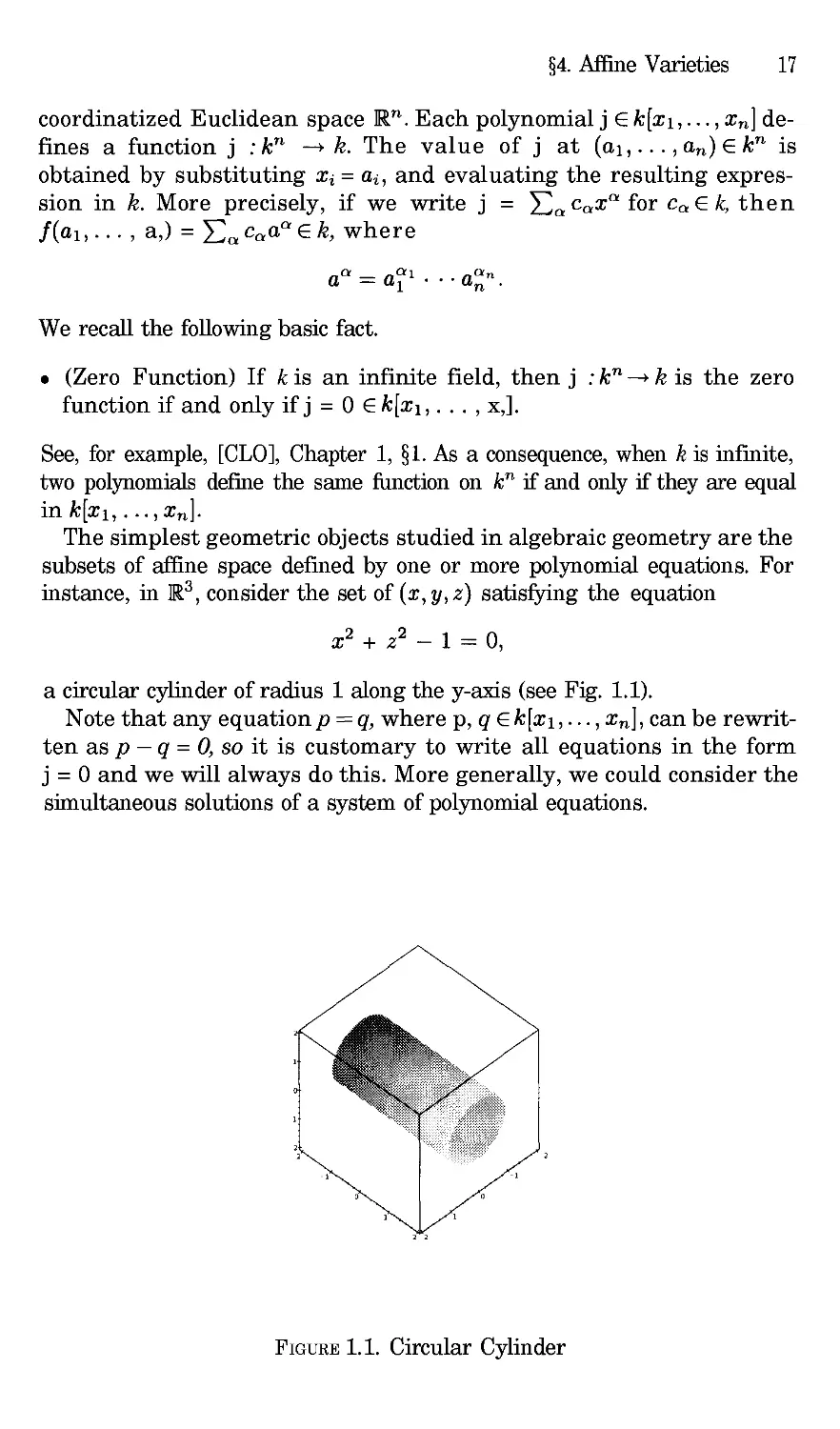
a circular cylinder of radius 1 along the y-axis (see Fig. 1.1).
Note that any equation p = q, where p, q k[x,..., x], can be rewrit-
ten as p - q = O, so it is customary to write all equations in the form
j = 0 and we will always do this. More generally, we could consider the
simultaneous solutions of a system of polynomial equations.
FIGURE 1.1. Circular Cylinder
18 Chapter 1. Introduction
(4.1) Definition. The set of all simultaneous solutions (al,
of a system of equations
Ii(xl,..., x) = 0
f2(z,...,z) = 0
, an) e k
fs(Xl, . . .,Xn) : 0
is known as the affine variety defined by I],...,fs, and is denoted by
V(fl,..., L). A subset V c k is said to be an affine variety if V =
V(A,.... Is) for some collection of polynomials A e k[x ..... x,].
In later chapters we will also introduce projective varieties. For now,
though, we will often say simply variety for "affine variety. For example,
V(x 2 + z 2 - 1) in R3 is the cylinder pictured above. The picture was
generated using the Maple command
implicitplot3d (x'2+z'2-1, x=-2.. 2, y=-2.. 2, z=-2.. 2,
grid= [20,20,20] ) ;
The variety V(x 2+y2+(z- 1) -4) inR 3is the sphere of radius 2
centered at (0, 0, 1) (see Fig. 1.2).
If there is more than one defining equation, the resulting variety can be
considered as an intersection of other varieties. For example, the variety
V(x 2 + z 2 - 1, x 2 + y2 + (z - 1) 2 - 4) is the curve of intersection of the
FIGURE 1.2. Sphere
§4. Affine Varieties 19
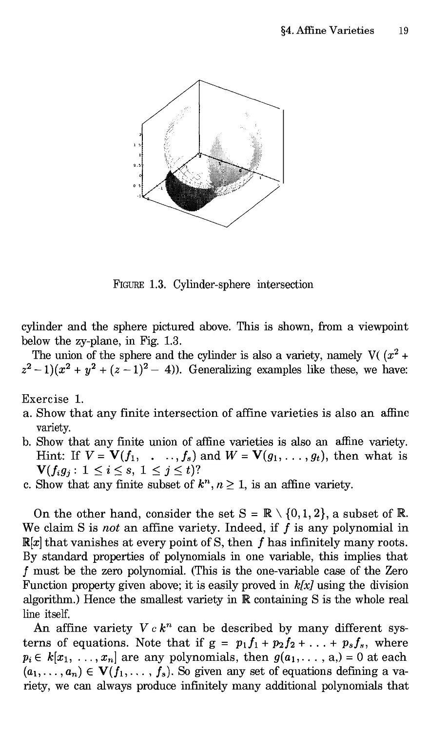
FIGURE 1.3. Cylinder-sphere intersection
cylinder and the sphere pictured above. This is shown, from a viewpoint
below the zy-plane, in Fig. 1.3.
The union of the sphere and the cylinder is also a variety, namely V( (x 2 +
z 2 - 1)(x 2 + y2 + (z- 1) 5- 4)). Generalizing examples like these, we have:
Exercise 1.
a. Show that any finite intersection of affine varieties is also an affine
variety.
b. Show that any finite union of affine varieties is also an aftlne variety.
Hint: If V = V(fl, .., fs) and W = V(gl ..... gt), then what is
V(/gj : 1 <i<s, 1 g j<_t)?
c. Show that any finite subset of k ", n _> 1, is an affine variety.
On the other hand, consider the set S = R \ {0,1, 2}, a subset of R.
We claim S is not an affine variety. Indeed, if f is any polynomial in
R[x] that vanishes at every point of S, then f has infinitely many roots.
By standard properties of polynomials in one variable, this implies that
f must be the zero polynomial. (This is the one-variable case of the Zero
Function property given above; it is easily proved in k[x] using the division
algorithm.) Hence the smallest variety in R containing S is the whole real
line itself.
An affine variety V c k n can be described by many different sys-
terns of equations. Note that if g = Plf + p2f2 + • • • + Psfs, where
pi • k[x, . .., x,] are any polynomials, then g(al,... , a,) = 0 at each
(a,..., aN) • V(],... , ]s). So given any set of equations defining a va-
riety, we can always produce infinitely many additional polynomials that
20 Chapter 1. Introduction
also vanish on the variety. In the language of §1 of this chapter, the g as
above are just the elements of the ideal (fl,-.., fs}. Some collections of
these new polynomials can define the same variety as the fl,..., fs.
Exercise 2. Consider the polynomial p from (1.2). In (1.4) we saw that
pE(x 2+z 2- 1, x 2+y2+(z-1) 2- 4). Show that
(x 2 + z 2-1,x 2+y2+(z-1) 2-4) = (x + z 2-1,y2-22-2)
in Q[x, y, z]. Deduce that
V(x 2+ z 2-1,x 2+ y2+ (z-l) 2- 4) = V(x 2+ z 2-1,y2- 22 - 2).
Generalizing Exercise 2 above, it is easy to see that
• (Equal Ideals Have Equal Varieties) If (fl, .... f/= (g, .... gtl in
k[x,... , x,], then V(f, ..., f) = V(g,..., gt).
See [CL0], Chapter 1, §4. By this result, together with the Hilbert Basis
Theorem from §1, it also makes sense to think of a variety as being defined
by an ideal in k[xl,..., xn], rather than by a specific system of equations.
If we want to think of a variety in this way, we will write V = V(1) where
I c k[xl, ..., x,] is the ideal under consideration.
Now, given a variety V c k , we can also try to turn the construction of
V from an ideal around, by considering the entire collection of polynomials
that vanish at every point of V.
(4.2) Definition. Let Vc k n be a variety. We denote by I(V) the set
{] E k[x, . . . , x,] : f(a, . . . ,a,) = 0 for all (a,... ,a,) V].
We call I(V) the ideal of V for the following reason.
Exercise 3. Show that I(V) is an ideal in k[xl,..., x] by verifying that
the two properties in Definition (1.5) hold.
If V = V(I), is it always true that I(V) = I? The answer is no, as
the following simple example demonstrates. Consider V= V(x 2) in 2.
The ideal I = (x2/ in [x, y] consists of all polynomials divisible by x 2.
These polynomials are certainly contained in I(V), since the corresponding
variety V consists of all points of the form (0, b), b (the y-axis). Note
that p(x, y) = x I(V), but x I. In this case, I(V(I)) is strictly larger
than I.
Exercise 4. Show that the following inclusions are always valid:
c z7 c
where v is the radical of/from Definition (1.6).
§4. Affine Varieties 21
It is also true that the properties of the field k influence the relation
between I(V(I)) and I. For instance, over l, we have V(x 2 + 1) =
and I(V(x 2 + 1)) = ][x]. On the other hand, if we take k = 2, then
every polynomial in C[x] factors completely by the Fundamental Theorem
of Algebra. We find that V(x2+ 1) consists of the two points ±i E C, and
I(V(x 2 + 1)) : (x 2 + 1).
Exercise 5. Verify the claims made in the preceding paragraph. You may
want to start out by showing that if a E C, then I({a}) = (x - a/.
The first key relationships between ideals and varieties are summarized
in the following theorems.
• (Strong Nullstellensatz) If k is an algebraically closed field (such as C)
and I is an ideal in k[xl,..., Xn], then
I(V(I)) = v.
• (Ideal-Variety Correspondence) Let k be an arbitrary field. The maps
affinc varieties ideals
and
ideals v affine varieties
are inclusion-reversing, and V(I(V)) = V for all affine varieties V. If k
is algebraically closed, then
affine varieties - radical ideals
and
radical ideals v_ affine varieties
are inclusion-reversing bijections, and inverses of each other.
See, for instance [CLO], Chapter 4, §2, or [AL], Chapter 2, §2. We con-
sider how the operations on ideals introduced in §1 relate to operations on
varieties in the following exercises.
A DDIIONAL EXERCISES FOR §4
1 2
Exercise 6. In §1, we saw that the polynomial p = x 2 + 5 Y z - z - i is
in the idealI=(x 2+z 2- 1, x 2+y2+ (z-l) 2- 4) cl[x,y,z].
a. What does this fact imply about the varieties V(p) and V(1) in 13?
(V(I) is the curve of intersection of the cylinder and the sphere pictured
in the text.)
b. Using a S-dimensional graphing program (e.g. Maple s ±,,plicitplot3d
function from the plots package) or otherwise, generate a picture of the
variety V(p).
22 Chapter 1. Introduction
c. Show that V(p) contains the variety W = V(x 2 - 1, y2_ 2). Describe
W geometrically.
d. If we solve the equation
x 2 + - y2z - z - 1 = 0
for z, we obtain
x 2- 1
(4.3) z = I-
I y2 '
The right-hand side r(x, y) of(4.3) is a quotient of polynomials or, in the
terminology of §1, a rational function in x, y, and (4.3) is the equation
of the graph of r(x, y). Exactly how does this graph relate to the variety
1 2 1) in ]i3? (Are they the same? Is one a subset of
V(x 2+y z-z-
the other? What is the domain of r(x, y) as a function from 2 to R?)
Exercise 7. Show that for any ideal Io k[xl, .... x,],v/-= x/. Hence
v is automatically a radical ideal.
Exercise 8. Assume k is an algebraically closed field. Show that in
the Ideal-Variety Correspondence, sums of ideals (see Exercise 11 of §1)
correspond to intersections of the corresponding varieties:
V(I + J) = V(1) 1-1 V(J).
Also show that if V and W are any varieties,
I(V r-1 W) = V/I(V) + I(W).
Exercise 9.
a. Show that the intersection of two radical ideals is also a radical ideal.
b. Show that in the Ideal-Variety Correspondence above, intersections
of ideals (see Exercise 12 from §1) correspond to unions of the
corresponding varieties:
V(ICJ) = V(I) u V(J).
Also show that if V and W are any varieties,
I(Y u W) = I(V) ¢ I(W).
c. Show that products of ideals (see Exercise 12 from §1) also correspond
to unions of varieties:
V(IJ) = V(1) u V(J).
Assuming k is algebraically closed, how is the product I( V)I(W) related
to I(V u W)?
Exercise 10. A variety Vis said to be irreducible if in every expression
ofVas a union of other varieties, V= V U V2, either V= Vor V2 = V.
§4. Affine Varieties 23
Show that an affine variety V is irreducible if and only if I(V) is a prime
ideal (see Exercise 8 from §1).
Exercise 11.
a. Show by example that the set difference of two affine varieties:
v\ w = {p e y :pC w}
need not be an affine variety. Hint: For instance, let k be an infinite
field, consider k[x], and let V = k = V(0) and W = {0} = V(z).
b. Show that for any ideals I, Jin k[xl,..., Xn],V(I: J) contains
V(I) \ V(J), but that we may not have equality. (Here I:J is the
quotient ideal introduced in Exercise 13 from §1.)
c. If I is a radical ideal, show that any algebraic variety containing
V(1) \ V(J) must contain V(I: J). Thus V(I: J)is the smallest variety
containing the difference V(1) \ V(J); it is called the Zariski closure of
V(1) \ V(J). See [CLO], Chapter 4, §4.
d. Show that if/is a radical ideal and J is any ideal, then I: J is also a
radical ideal. Deduce that I(V) : I(W) is the radical ideal corresponding
to the Zariski closure of V \ W in the Ideal-Variety Correspondence.
Chapter 2
So lying Po lynomial Equatio ns
In this chapter we will discuss several approaches to solving systems of
polynomial equations. First, we will discuss a straightforward attack based
on the elimination properties of lexicographic GrSbner bases. Combining
elimination with numerical root-finding for one-variable polynomials we get
a conceptually simple method that generalizes the usual techniques used
to solve systems of linear equations. However, there are potentially severe
difficulties when this approach is implemented on a computer using finite-
precision arithmetic. To circumvent these problems, we will develop some
additional algebraic tools for root-finding based on the algebraic structure
of the quotient rings k[xl,..., Xn]/I. Using these tools, we will present
alternative numerical methods for approximating solutions of polynomial
systems and consider methods for real root-counting and root-isolation.
In Chapters 3, 4 and 7, we will also discuss polynomial equation solving.
Specifically, Chapter 3 will use resultants to solve polynomial equations,
and Chapter 4 will show how to assign a well-behaved multiplicity to each
solution of a system. Chapter 7 will consider other numerical techniques
(homotepy continuation methods) based on bounds for the total number
of solutions of a system, counting multiplicities.
§1 Solving Polynomial Systems by Elimination
The main tools we need are the Elimination and Extension Theorems. For
the convenience of the reader, we recall the key ideas:
• (Elimination Ideals) If I is an ideal in k[xl,..., xn] , then the gth
elimination ideal is
Ig : I [' k[Xg+l,...,Xn].
Intuitively, if I = (fx,. • • , f8 ), then the elements o f It are the linear co m-
binations of the ]1, • • • , ]8, with polynomial coefficients, that eliminate
xx,..., xt from the equations f =... = fs = 0.
24
§1. Solving Polynomial Systems by Elimination 25
• (The Elimination Theorem) If G is a Grobner basis for I with respect
to the lex order (xi > x2 >... >Xn)(or any order where monomi-
als involving at least one of Xl,..., x are greater than all monomials
involving only the remaining variables), then
G£ = G ['q k[x£_l,. .. , Xn]
is a Grobner basis of the Cth elimination ideal I.
• (Partial Solutions) A point (a+l, . . , a, ) e V(I)ckn-iscalleda
partial solution. Any solution (al,...,an) E V ( T ) c k n truncates to
a partial solution, but the converse may fail-not all partial solutions
extend to solutions. This is where the Extension Theorem comes in. To
prepare for the statement, note that each f in I_1 can be written as a
polynomial in x, whose coefficients are polynomials in x+ ..... x,:
f = cq(x+,..., Xn)Xq + ""+ co(x+ .... ,Xn).
We call cq the leading coefficient polynomial of f if x is the highest
power of x appearing in f
• (The Extension Theorem) If k is algebraically closed (e.g., k = C), then
a partial solution (a+,..., an) in V(I) extends to (a, a+,..., an) in
V(I_I) provided that the leading coefficient polynomials of the elements
of a lex Grobner basis for I_ 1 do not all vanish at (a+l,..., an).
For the proofs of these results and a discussion of their geometric meaning,
see Chapter 3 of [CLO]. Also, the Elimination Theorem is discussed in $6.2
of [BW] and §2.3 of [AL], and [AL] discusses the geometry of elimination
in §2.5.
The Elimination Theorem shows that a Zex GrSbner basis G successively
eliminates more and more variables. This gives the following strategy for
finding all solutions of the system: start with the polynomials in G with the
fewest variables, solve them, and then try to extend these partial solutions
to solutions of the whole system, applying the Extension Theorem one
variable at a time.
As the following example shows, this works especially nicely when V ( T )
is finite. Consider the system of equations
x 2 + y2 + z 2 = 4
(1.1) x 2 + 2y 2 = 5
xz= ]_
from Exercise 4 of Chapter 3, §1 of [CLO]. To solve these equations, we
first compute a Zex Grobner basis for the ideal they generate using Maple:
with (grobner) :
PList : = [x'2+y2+z2-4, x2+2*y'2-5, x.z-l] ;
VList := [x,y,z];
G : = gbasis (PList ,VList ,plex);
26 Chapter 2. Solving Polynomial Equations
This gives output
G := [2z 3- 32 + x, -1 + y2_ z 2, i + 2z 4- 3z2].
From the GrSbner basis it follows that the set of solutions of this system in
C 3 is finite (why?). To find all the solutions, note that the last polynomial
depends only on z (it is a generator of the second elimination ideal I2 =
I N C[z]) and factors nicely in Q[z]. To see this, we may use
factor(2*z4 - 3.z2 + 1) ;
which generates the output
(z-1)(z + 1)(2z 2- 1).
Thus we have four possible z values to consider:
z = +1, +1//.
By the Elimination Theorem, the first elimination ideal I1 = INC[y,z]is
generated by
y2 _ z 2 _ 1
2z 4 -- 3z 2 + 1.
Since the coefficient of y2 in the first polynomial is a nonzero constant,
every partial solution in V(I2) extends to a solution in V(I1). There are
eight such points in all. To find them, we substitute a root of the last
equation for z and solve the resulting equation for y. For instance,
subs (z=l, G) ;
will produce:
[-1 + x, y2- 2,0],
so in particular, y = +v. In addition, since the coefficient of x in the first
polomial in the GrSbncr basis is a nonzero constant, we can extend each
paial solution in V(I) (uniquely) a point of V(I). For this value of z,
we have x = 1.
Exercise 1. Carry out the same process for the other values of z as well.
You should find that the eight points
(1, +/, 1), (-1, +/,-1), (/, +x//2, 1//), (-/, +x//2,-1//)
form the set of solutions.
The system in (1.1) is relatively simple because the coordinates of the
solutions can all be expressed in terms of square reots of rational numbers.
Unfortunately, general systems of polynomial equations are rarely this nice.
For instance it is known that there are no general formulas involving only
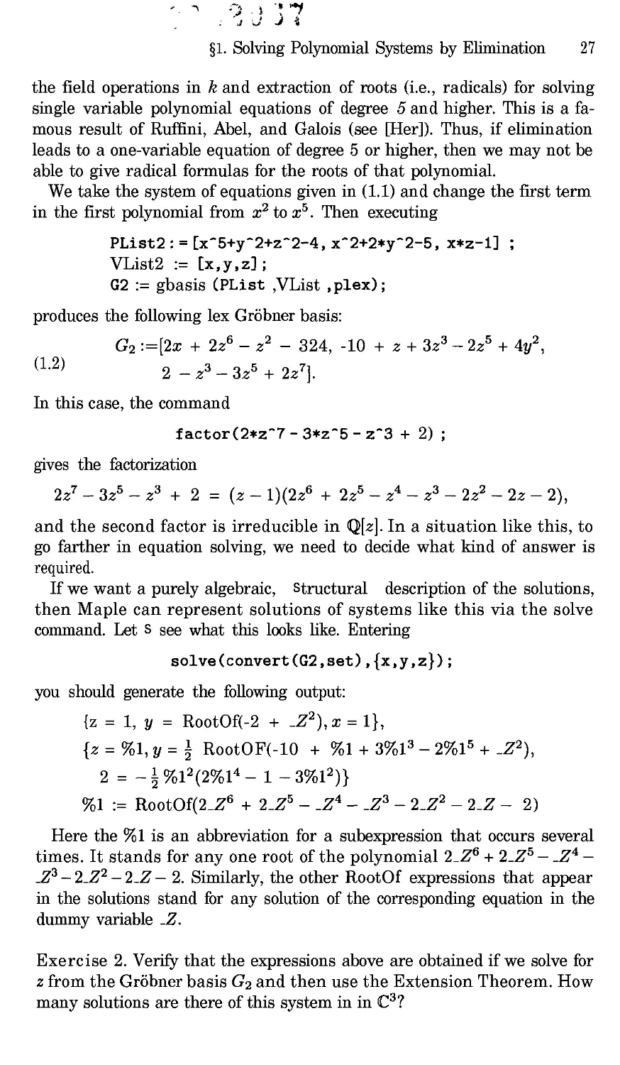
§1. Solving Polynomial Systems by Elimination
27
the field operations in k and extraction of roots (i.e., radicals) for solving
single variable polynomial equations of degree 5 and higher. This is a fa-
mous result of Ruffini, Abel, and Galois (see [Her]). Thus, if elimination
leads to a one-variable equation of degree 5 or higher, then we may not be
able to give radical formulas for the roots of that polynomial.
We take the system of equations given in (1.1) and change the first term
in the first polynomial from x 2 to x 5. Then executing
PList2 : = [x'5+y2+z2-4, x^2+2*y2-5, x*z-1] ;
VList2 := [x,y,z] ;
G2 := gbasis (PList ,VList ,plex);
produces the following lex GrSbner basis:
G2:=[2x + 2z 6-z 2- 324, -10 + z+3z a-2z 5+4y 2,
(1.2)
2-z a-3z 5+ 2z].
In this case, the command
factor(2*z''- 3.z'5- z'3 + 2) ;
gives the factorization
2z 7-3z 5-z 3 + 2 = (z-1)(2z 6 + 2z 5-z 4-z 3-2z 2-2z-2),
and the second factor is irreducible in Q[z]. In a situation like this, to
go farther in equation solving, we need to decide what kind of answer is
required.
If we want a purely algebraic, Structural description of the solutions,
then Maple can represent solutions of systems like this via the solve
command. Let s see what this looks like. Entering
solve (convert (G2, set), {x, y, z} ) ;
you should generate the following output:
{z = 1, y = RootOf(-2 + _Z),x = 1},
{z=%1, y=51 RootOF(-10 + %1+3%1 a-2%15+_Z2),
2 = - ½ %12(2%14- i - 3%12)}
%1 := RootOf(2_Z 6 + 2_Z -_Z 4-_Z a- 2_Z - 2_Z- 2)
Here the %1 is an abbreviation for a subexpression that occurs several
times. It stands for any one root of the polynomial 2_Z 6 + 2_Z 5 - _Z 4 -
_Z a- 2_Z 2- 2_Z- 2. Similarly, the other RootOf expressions that appear
in the solutions stand for any solution of the corresponding equation in the
dummy variable _Z.
Exercise 2. Verify that the expressions above are obtained if we solve for
z from the GrSbner basis G2 and then use the Extension Theorem. How
many solutions are there of this system in in Ca?
28 Chapter 2. Solving Polynomial Equaiions
On the other hand, in many practical situations where equations must
be solved, knowing a numerical approximation to a real or complex solu-
tion is often more useful, and perfectly acceptable provided the results are
sufficiently accurate. In our particular case, one possible approach would
be to use a numerical root-finding method to find approximate solutions of
the one-variable equation
(1.3) 2z 6 + 2z 5-z a-z 3-2z 2-2z- 2 = 0,
and then proceed as before using the Extension Theorem, except that we
now use floating point arithmetic in all calculations. In some examples,
numerical methods will also be needed to solve for the other variables as
we extend.
One well-known numerical method for solving one-variable polynomial
equations in R or C is the Newton-Raphson method or, more simply but
less accurately, Newton s method This method may also be used for equa-
tions involving functions other than polynomials, although we will not
discuss those here. For motivation and a discussion of the theory behind
the method, see [BuF] or [Act].
The Newton-Raphson method works as follows. Choosing some initial
approximation zo to a root ofp(z) = O, we construct a sequence of numbers
by the rule
p(Zk) for k = 0,1, 2,...,
Zk+l - Zk p'(zk)
wherep (z) is the usual derivative ofp from calculus. In most situations,
the sequence zk will converge rapidly to a solution of p(z) = 0, that is,
N = limk_ zk will be a root. Stopping this procedure after a finite number
of steps (as we must!), we obtain an approximation to . For example we
might stop when Zk+l and zk agree to some desired accuracy, or when a
maximum allowed number of terms of the sequence have been computed.
See [BuF], [Act], or the comments at the end of this section for additional
information on the performance of this technique. When trying to find all
roots of a polynomial, the tricldest part of the Newton-Raphson method is
making appropriate choices of zo. It is easy to find the same root repeatedly
and to miss other ones if you don t know where to look!
Fortunately, there are elementary bounds on the absolute values of the
roots (real or complex) of a polynomial p(z). Here is one of the simpler
bounds.
Exercise 3. Show that if p(z) = z n + an_lz n-l+ "'÷ ao is a monic
polynomial with complex coefficients, then all roots of p satisfy I1 _< B,
where
B=max{1, lan_ll+... + lall + laol}.
Hint: The triangle inequality implies that ]a + b] >_ (a(-]b I.
§1. Solving Polynomial Systems by Elimination 29
See Exercise 11 below for another better bound on the roots. Given any
bound of this sort, we can limit our attention to Zo in this region of the
complex plane to search for roots of the polynomial.
Instead of discussing searching strategies for finding roots, we will use a
built-in Maple function to approximate the roots of the system from (1.2).
The Maple function f solve finds numerical approximations to all real (or
complex) roots of a polynomial by a combination of root location and
numerical techniques like Newton-Raphson. For instance, the command
fsolve (2*z6+2*z5-z4-z3-2*z2-2*z-2) ;
will compute approximate values for the real roots of our polynomial (1.3).
The output should be:
-1.395052015, 1.204042437.
(Note: In Maple, 10 digits are carried by default in decimal calculations;
more digits can be used by changing the value of the Maple system variable
Digits. Also, the actual digits in your output may vary slightly if you
carry out this computation using another computer algebra system.) To
get approximate values for the complex roots as well, try:
fsolve (2*z'6+2*z'5-z^4-z-3-2*z2-2*z-2, complex) ;
We illustrate the Extension Step in this case using the approximate value
z = 1.204042437.
We substitute this value into the GrSbner basis polynomials using
subs (z=l. 204042437, G2) ;
and obtain
[2x - 1.661071025, -8.620421528 + 4y 2, -.2 • 10-s].
Note that the value of the last polynomial was not exactly zero at our
approximate value of z. Nevertheless, as in Exercise 1, we can extend this
approximate partial solution to two approximate solutions of the system:
(x, y, z) = (.8305355125, =t=1.468027718, 1.204042437).
Checking one of these by substituting into the equations from (1.2), using
subs (z=l. 204042437, y=l. 468027718,x=. 8305355125, G2) ;
we find
[0,-.4 * 10 -s, -.2 * 10-s],
so we have a reasonably good approximate solution, in the sense that our
computed solution gives values very close to zero in the polynomials of the
system.
30 Chapter 2. Solving Polynomial Equations
Exercise 4. Find approximate values for all other real solutions of this
system by the same method.
In considering what we did hero, one potential pitfall of this approach
should be apparent. Namely, since our solutions of the one-variable equation
are only approximate, when we substitute and try to extend, the remaining
polynomials to be solved for x and y are themselves only approximate. Once
we substitute approximate values for one of the variables, we are in effect
solving a system of equations that is different from the one we started
with, and there is little guarantee that the solutions of this new system are
close to the solutions of the original one. Accumulated errors after several
approximation and extension steps can build up quite rapidly in systems
in larger numbers of variables, and the effect can be particularly severe if
equations of high degree are present.
To illustrate how bad things can get, we consider a famous cautionary
example due to Wilkinson, which shows how much the roots of a polynomial
can be changed by very small changes in the coefficients.
Wilkinson s example involves the following polynomial of degroe 20:
p(z) = (x + 1)(x + 2).-. (x + 20) = x 2° + 210x 19 + ..-+ 20!.
The roots are the 20 integers x = -1, -2 .... , -20. Suppose now that we
Perturb just the coefficient of x 1, adding a very small number. We carry
20 decimal digits in all calculations. First we construct p(z) itself:
Digits := 20:
p :=1:
for k to 20 do p := p*(x+k) od:
Printing expand(p) out at this point will show a polynomial with some
large coefficients indeed! But the polynomial we want is actually this:
q := expand(p + .O00000001*xlg) :
fsolve (q,x, complex) ;
The approximate roots of q= p+.00000000Ix 19 (truncated for simplicity)
are:
- 20.03899, -18.66983 - .35064 I, -18.66983 + .35064 I,
- 16.57173 - .88331 I, -16.57173 + .88331 I,
- 14.37367 -.77316 I, -14.37367 + .77316 I,
- 12.38349 -.10866 I, -12.38349 + .10866 I,
- 10.95660, -10.00771, -8.99916, -8.00005,
- 6.999997, -6.000000, -4.99999, -4.00000,
- 2.999999, -2.000000, -1.00000.
§1. Solving Polynomial Systems by Elimination 31
Instead of 20 real roots, the new polynomial has 12 real roots and 4 com-
plex conjugate pairs of roots. Note that the imaginary parts are not even
especially small!
While this example is admittedly pathological, it indicates that we should
use care in finding roots of polynomials whose coefficients are only approx-
imately determined. (The reason for the surprisingly bad behavior of this p
is essentially the equal spacing of the roots! We refer the interested reader
to Wilkinson s paper [Will for a full discussion.)
Along the same lines, even if nothing this spectacularly bad happens,
when we take the approximate roots of a one variable polynomial and try
to extend to solutions of a system, the results of a numerical calculation can
still be unreliable. Here is a simple example illustrating another situation
that causes special problems.
Exercise 5. Verify that ifx > y, then
G = Ix 2 + 2x + 3 + y5 _ y, y6 _ y2 + 2y]
is alex GrSbner basis for the ideal that G generates in [x, y].
We want to find all real points (x, y) E V(G). Begin with the equation
y6-y2 + 2y = 0,
which has exactly two real roots. One is y = 0, and the second is in the
interval [-2, -1] because the polynomial changes sign on that interval.
Hence there must be a root there by the Intermediate Value Theorem from
calculus. Using fsolve to find an approximate value, we find the nonzero
root is
(1.4) -1.267168305
to 10 decimal digits. Substituting this approximate value for y into G yields
Ix + 2x + .999999995, .7 * 10-s].
Then use
to obtain
f solve (x'2 + 2*x +.999999995);
-1.000070711, -.9999292893.
Clearly these are both close to x = -1, but they are different. Taken
uncritically, this would seem to indicate two distinct real values of x when
y is given by (1.4).
Now, suppose we used an approximate value for y with fewer decimal
digits, say y "-- -1.2671683. Substituting this value for y gives us the
quadratic
x 2 + 2x + 1.000000054.
32 Chapter 2. Solving Polynomial Equations
This polynomial has no real roots at all. Indeed, using the complex option
in f solve, we obtain two complex values for x:
-1. -.0002323790008 I, -1. + .0002323790008 I.
To see what is really happening, note that the nonzero real root of y-
y2 + 2y = 0 satisfies y5_ y + 2 = 0. When the exact root is substituted
into G, we get
Ix 2+2x+ 1,0]
and the resulting equation has a double root x = -1.
The conclusion to be drawn from this example is that equations with
double roots, such as the exzct equation
x 2 + 2x + 1 = 0
we got above, are especially vulnerable to the errors introduced by numer-
ical root-finding. It can be very difficult to tell the difference between a
pair of real roots that are close, a real double root, and a pair of complex
conjugate roots.
From these examples, it should be clear that finding solutions of polyno-
mial systems is a delicate task in general, especially if we ask for information
about how many real solutions there are. For this reason, numerical meth-
ods, for all their undeniable usefulness, are not the whole story. And they
should never be applied blindly. The more information we have about the
structure of the set of solutions of a polynomial system, the better a chance
we have to determine those solutions accurately. For this reason, in §2 and
§3 we will go to the algebraic setting of the quotient ring k[xl,..., xn]/I
to obtain some additional tools for this problem. We will apply those tools
in §4 and §5 to give better methods for finding solutions.
For completeness, we conclude with a few additional words about the
numerical methods for equation solving that we have used. First, if is a
multiple root of p(z) = o, then the convergence of the Newton-Raphson se-
quence z can be quite slow, and a large number of steps and high precision
may be required to get really close to a root (though we give a method for
avoiding this difficulty in Exercise 9). Second, there are some choices of zo
where the sequence zk will fail to converge to a root of p(z). See Exercise
10 below for some simple examples. Finally, the location of in relation to
zo can be somewhat unpredictable. There could be other roots lying closer
to zo. These last two problems are related to the fractal pictures associated
to the Newton-Raphson method over C-see, for example, [PR]. We should
also mention that there are multivariable versions of Newton-Raphson for
systems of equations and other iterative methods that do not depend on
elimination. These have been much studied in numerical analysis. For more
details on these and other numerical root-finding methods, see [BuF] and
[Act]. Also, we will discuss homotopy continuation methods in Chapter 7,
§5 of this book.
§1. Solving Polynomial Systems by Elimination
ADDITIONAL EXERCISES FOR §1
33
Exercise 6. Use elimination to solve the system
0 = x 2 + 2y 2-y-2z
0 = x 2- 8y 2 + 10z- 1
0 = x 2- 7yz.
How many solutions are there in 3; how many are there in C3?
Exercise 7. Use elimination to solve the system
0 = x 2+ y2+z 2- 2x
0 = x 3 - yz - x
O=x-y+2z.
How many solutions are there in R3; how many are there in
Exercise 8. In this exercise we will study exactly why the performance
of the Newton-Raphson method is poor for multiple roots, and suggest a
remedy. Newton-Raphson iteration for any equation p(z) = 0 is an example
ofxed point iteration, in which a starting value zo is chosen and a sequence
(1.5) zk+l g(zk) for k = 0, 1, 2,...
is constructed by iteration of a fixed function g(z). For Newton-Raphson
iteration, the function g(z) is g(z) = Np(z) = z - p(z)/p'(z). If the se-
quence produced by (1.5) converges to some limit , then is a fixed point
ofg (that is, a solution ofg(z) = z). It is a standard result from analysis
(a special case of the Contraction Mapping Theorem) that iteration as in
(1.5) will converge to a fixed point of g provided that Igl()l < 1, and Zo
is chosen sufficiently close to . Moreover, the smaller Igl()l is, the faster
convergence will be. The case g (Z) = 0 is especially favorable.
a. Show that each simple root of the polynomial equation p(z) = 0 is a
fixed point of the rational function Np( z ) = z -p(z)/p'(z).
b. Show that multiple roots of p(z) = 0 are removable singularities of
N(z) (that is, IN(z)l is bounded in a neighborhood of each multiple
root). How should N be defined at a multiple root of p(z) = 0 to make
Np continuous at those points?
c. Show that N() = 0 if is a simple root of p(z) = 0 (that is, if
p() = 0, but p'()# 0).
d. On the other hand, show that if is a root multiplicity k ofp(z) (that
is, ifp(Z) = p (Z) ..... p(k-1)() = 0 but p(k)() ¢ 0), then
1
lim N(z)= 1--
z k '
34 Chapter 2. Solving Polynomial Equations
Thus Newton-Raphson iteration converges much faster to a simple
root of p(z) = 0 than it does to a multiple root, and the larger the
multiplicity, the slower the convergence.
e. Show that replacing p(z) by
p(z)
Pred(Z) - GCD(p(z), p (z))
(see [CL0], Chapter 1, §5, Exercises 14 and 15) eliminates this difficulty,
in the sense that the roots of Pred(Z) = 0 are all simple roots.
Exercise 9. There are cases when the Newton-Raphson method fails to
find a root of a polynomial for lots of starting points zo.
a. What happens if the Newton-Raphson method is applied to solve the
equation z 2 + 1 = 0 starting from a real zo? What happens if you take
zo with nonzero imaginary parts? Note: It can be shown that Newton-
Raphson iteration for the equation p(z) = 0 is chaotic ifzo is chosen in
the Julia set of the rational function Np(z) = z - p(z)/pl(z) (see [PR]),
and exact arithmetic is employed.
b. Let p(z)= z4-z 2 -11/36 and, as above, let Np(z)= z-p(z)/p'(z).
Show that +l/v satisfies N(1/v)=-1/v, Np(-1/v)= 1/v,
and N(1/v) = 0. In the language of dynamical systems, +l/v is
a superattracting2-cycle for N(z). One consequence is that for any zo
close to ±l/v/-, the Newton-Raphson method will not locate a root of
p. This example is taken from Chapter 13 of [Dev].
Exercise 10. This exercise improves the bound on roots of a polynomial
given in Exercise 3. Let p(z) = z n + a_lz -1 + ... + alz + ao be a monic
polynomial in C[z]. Show that all roots ofp satisfy I1 _< B, where
B = 1 + max{la_ll, . . . , lal,laol}.
This upper bound can be much smaller than the one given in Exercise 8.
Hint: Use the Hint from Exercise 3, and consider the evaluation of p(z) by
nested multiplication:
p(z) = (... ((z + a_)z + a_2)z + ... + al)z + ao.
§2 Finite-Dimensional Algebras
This section will explore the remainder arithmetic associated to a
Grbbner basis G = {gl ..... gt} of an ideal I c k[x ..... xn]. Recall from
Chapter 1 that if we divide f E k[x ..... x] by G, the division algorithm
yields an expression
(2.1) f = hlgl +"" ± htgt + --f-G,
§2. Filfite-Dimensional Algebras 35
where the remainder G is a linear combination of the monomiais x
(LT(I)). Furthermore, since G is a GrSbner basis, we know that f • I if
and only if] G = 0, and the remainder is uniquely determined for all
This implies
(2.2) G = G ¢= f _ g • I.
Since polynomials can be added and multiplied, given f, g • k[xl,...,
it is natural to ask how the remainders of f + g and fg can be computed
if we know the remainders of f, g themselves. The following observations
show how this can be done.
• The sum of two remainders is again a remainder, and in fact one can
easily show that + G = --G.
• On the other hand, the product of remainders need not be a remain-
der. But it is also easy to see that . = -, and ]. ye is a
remainder.
We can also interpret these observations as saying that the set of remain-
ders on division by G has naturally defined addition and multiplication
operations which produce remainders as their results.
This remainder arithmetic is closely related to the quotient ring
k[xl,..., xn]/I. We will assume the reader is familiar with quotient rings,
as described in Chapter 5 of [CLO] or in a course on abstract algebra.
Recall how this works: given f•k[xl,..., x,], we have the coset
If] = : + I= {f + h : h • I],
and the crucial property of cosets is
(2.3) [f] = [g] f - g • I.
The quotient ring k[x,..., x]/I consists of all cosets [f] for f •
k[zl,.. . ,
From (2.1), we see that G• If], and then (2.2) and (2.3) show that we
have a one-to-one correspondence
remainders cosets
Thus we can think of the remainder G as a standard representative of its
coset [f] • k[xl,..., x]/I. Furthermore, it follows easily that remainder
arithmetic is exactly the arithmetic in k[x,..., xn]/I. That is, under the
above correspondence we have
--G
?G , IS] • [g].
36 Chapter 2. Solving Polynomial Equations
Since we can add elements of k[xl,..., xn]/I and multiply by constants
(the cosets [c] for c E k), k[xl,..., xn]/I also has the structure of a vector
space over the field k. A ring that is also a vector space in this fashion
is called an algebra. The algebra k[xl,..., xn]/I will be denoted by A
throughout the rest of this section, which will focus on its vector space
structure.
An important observation is that remainders are the linear combinations
of the monomials x (LT(/)) in this vector space structure. (Strictly
speaking, we should use cosets, but in much of this section will identify
a remainder with its coset inA.) Since this set of monomials is linearly
independent in A (why?), it can be regarded as a basis of A. In other
words, the monomials
B = {x: x t (LT(I))}
form a basis of A (more precisely, their cosets are a basis). We will refer to
elements of B as basis monomials. In the literature, basis monomials are
often called standard monomials.
The following example illustrates how to compute in A using basis
monomials. Let
(2.4) G = {x +3xy/2 + y2/2-ax/2-ay/2, xy 2-x,y3-y}.
Using the grevlex order with x > y, it is easy to verify that G is a GrSbner
basis for the ideal I = (G) c C[x, y] generated by G. By examining the
leading monomials of G, we see that (LT(I))= (x2,xy2,y3). The only
monomials not lying in this ideal are those in
B = (1, x,y, xy, y 2}
so that by the above observation, these five monomials form a vector space
basis for A = C[x, y]/I over C.
We now turn to the structure of the quotient ring A. The addition op-
eration in A can be viewed as an ordinary vector sum operation once we
express elements of A in terms of the basis B in (2.4). Hence we will consider
the addition operation to be completely understood.
Perhaps the most natural way to describe the multiplication operation
inA is to give a table of the remainders of all products of pairs of elements
from the basis B. Since multiplication in A distributes over addition, this
information will suffice to determine the products of all pairs of elements
of A.
For example, the remainder of the product x. xy may be be computed
as follows using Maple. Using the GrSbner basis G, we compute
normalf (x^2*y, G, [x, y], tdeg) ;
and obtain
3 3 3 2 1
xy- -
§2. Finite-Dimensional Algebras 37
Exercise 1. By computing all such products, verify that the multiplication
table for the elements of the basis B is:
I x y xy y2
{2.5}
where
I 1 x y xy y
x x axyx
y y xy y2 x y
xy xy ]5 x a xy
.y2 y2 x y xy y2
a =-3xy/2- y2/2 + 3x/2 + 3y/2
]5 = 3xy/2 + 3y2/2 - 3x/2 -
This example was especially nice because A was finite-dimensional as a
vector space over C. In general, for any field k c C, we have the following
basic theorem which describes when k[xl,..., xn]/I is finite dimensional.
• (Finiteness Theorem) Let k c C be afield, and let I k[xl,... , x,] be
an ideal. Then the following conditions are equivalent:
a. The algebra A = k[xl,..., xn]/I is finite-dimensional over k.
b. The variety V{I} C ' is a finite set.
c. If G is a Gr6bner basis for I, then for each i, 1 _< i _< n, there is an
mi 0 such that :m= LT(g) for some g E G.
For a proof of this result, see Theorem 6 of Chapter 5, §3 of[CLO], Theorem
2.2.7 of [AL], or Theorem 6.54 of [BW]. An ideal satisfying any of the above
conditions is said to be zero-dimensional. Thus
A is a finite-dimensional algebra I is a zero-dimensional ideal.
A nice consequence of this theorem is that I is zero-dimensional if and
only if there is a nonzero polynomial in I C k[xi] for each i = 1 ..... n. To
see why this is true, first suppose that I is zero-dimensional, and let G be a
reduced GrSbner basis for any lex order with xi as the "last" variable (i.e.,
xj > xi for j ¢ i). By item c above, there is some g E G with LW(g) = Xi m •
Since we re using alex order with xi last, this implies g k[xi] and hence
g is the desired nonzero polynomial. Note that g generates I rl k[xi] by the
Elimination Theorem.
Going the other way, suppose In k[xi] is nonzero for each i, and let mi be
the degree of the unique monic generater of I rl k[xi] (remember that k[x]
is a principal ideal domain-see Corollary 4 of Chapter 1, §5 of [CLO]).
Then x' @W([)} for any monomial order, so that all monomials not in
{LT(I)} will contain xi to a power strictly less than rni. In other words, the
exponents a of the monomials xt @W([)} will all lie in the rectangular
box"
R = {a eZo" for each i,O<_ai<_mi-1}.
38 Chapter 2. Solving Polynomial Equations
This is a finite set of monomials, which proves that A is finite-dimensional
over k.
Given a zero-dimensional ideal I, it is now easy to describe an algorithm
for finding the set B of all monomials not in (LT(/)). Namely, no matter
what monomial order we are using, the exponents of the monomials in
B will lie in the box R described above. For each • R, we know that
X (LT(I)) if and only if -aG = x . Thus we can list the •R in some
systematic way and compute -G for each one. A vector space basis of A
is given by the set of monomials
B = {x :a • Randx g =x }.
See Exercise 13 below for a Maple procedure implementing this method.
The vector space structure on A = k[xl,...,x,]/I for a zero-
dimensional ideal I can be used in several important ways. To begin, let
us consider the problem of finding the monic generators of the elimina-
tion ideals I f k[x]. As indicated above, we could find these polynomials
by computing several different lex GrSbner bases, reordering the variables
each time to place x last. This is an extremely inefficient method, however.
Instead, let us consider the set of non-negative powers of [x] inA:
s = {1, [xi],[xi]2,...}.
Since A is finite-dimensional as a vector space over the field k, S must
be linearly dependent in A. Let mi be the smallest positive integer for
which (1, [xi], [xi]2,... , [xi] m' } is linearly dependent. Then there is a linear
combination
cj [xil j =[o1
j=0
in A in which cj • k are not all zero. In particular, Cm, 0 since mi is
minimal. By the definition of the quotient ring, this is equivalent to saying
that
= • z.
j----O
Exercise 2. Verify that pi(xi)as in (2.6) is a generater of the ideal
Ifk[xi], and develop an algorithm baaed on this fact to find the monic
generater of I]k[xi], given any GrSbner basis G for a zero-dimensional
ideal I as input.
The algorithm suggested in Exercise 2 often requires far less computa-
tional effort than a lea GrSbner basis calculation. Any ordering (e.g. grevlex)
can be used to determine G, then only standard linear algebra (matrix op-
erations) are needed to determine whether the set { 1, [xi], [xi]2,..., [xi] m }
§2. Finite-Dimensional Algebras 39
is linearly dependent. We note that the finduni function from Maple s
grobner package is an implementation of this method.
We will next discuss how to find the radical of a zero-dimensional ideal
(see Chapter 1 for the definition of radical). To motivate what we will
do, recall from §1 how multiple roots of a polynomial can cause problems
when trying to find roots numerically. When dealing with a one-variable
polynomial p with coefficients lying in a subfield of C, it is easy to see that
the polynomial
P
Pred- GCD(p,p )
has the same roots asp, but all with multiplicity one (for a proof of this, see
Exercises 14 and 15 of Chapter 1, §5 of [CLO]). We call Preg the square-free
part ofp.
The radical / of an ideal I generalizes the idea of the square-free part
of a polynomial. In fact, we have the following elementary exercise.
Exercise 3. Ifp E k[x] is a nonzero polynomial, show that x/ = (Pred).
Since k[x] is a PID, this solves the problem of finding radicals for all
ideals in k[x]. For a general ideal I c k[xl, . • , xn], it is more difficult
to find s/, though algorithms are known and have been implemented
in Axiom, Macaulay, REDUCE, and Singular. Fortunately, when I is
zero-dimensional, computing the radical is much easier, as shown by the
following proposition.
(2.7) Proposition. Let I c C[xl,. • • , :(, ] be a zero-dimeiotml ideal.
For each i = 1,..., n, let pi be the unique monic generator of I
al let Pi,red be the square-free part of pi. Then
v = I + (P,cd .....
PROOF. Write J= I + (Pl,d,. • • ,Pn,red). We first prove that Jis a
radical ideal, i.e., that J= x/. For each i, using the fact that C is alge-
braically closed, we can factor each p,g to obtain p,eg = (x-a)(x-
a2).-. (x - ad,), where the aj are distinct. Then
J= g + PI,d) = N(J + (x-
where the first equality holds since Pl,red Jand the second follows from
Exercise 9 below since Pl,red has distinct roots. Now use P2,red to decompose
each J+ (xl - aj) in the same way. This gives
J- N(J + (x- aj,x2- a2k)).
j,k
40 Chapter 2. Solving Polynomial Equations
If we do this for all i = 1, 2,... , n, we get the expression
J : N (J + (Xl - alj,,...,xn -
11 ,...
Since @1 - a11,..., xn - anon) is a maximal ideal, the ideal J + (xl-
aljl,.. . , Xn -- anj,) is either (xl - alia,... , Xn - anj,) or the whole ring
C[xl,..., x]. It follows that J is a finite intersection of maximal ideals.
Since a maximal ideal is radical and an intersection of radical ideals is
radical, we conclude that J is a radical ideal.
Now we can prove that J = x/. The inclusion I c J is built into
the definition of £ and the inclusion J c x/ follows from the Strong
Nullstellensatz, since the square-free parts of the pi vanish at all the points
of V(I). Hence we have
I c J c v/.
Taking radicals in this chain of inclusions shows that = v. But J is
radical, so = J and we are done. []
A Maple procedure that implements an algorithm for the radical of a
zero-dimensional ideal based on Proposition (2.7) is discussed in Exercise
16 below. It is perhaps worth noting that even though we have proved
Proposition (2.7) using the properties of C, the actual computation of
the polynomials Pi,red will involve only rational arithmetic when the input
polynomials are in Q[x ,..., x].
For example, consider the ideal
(2.8) I = (yax + 3x 3-ya-3x 2,x2y-2x 2, 2yax - x 3 - 2y + x 2)
Exercise 4. Using Exercise 2 above, show that
and
Writing p(x) = x a- x and p2(y) = yS_ 2ya, we can compute the
square-free parts in Maple as follows. The command
will produce
Similarly,
plred :=s±mpl±fy(pl/gcd(pl,d±ff(pl,x)));
Pl,red(X) = X(X -- 1).
P2,,-ed(Y) = Y(Y- 2).
§2. Finite-Dimensional Algebras 41
Hence by Proposition (2.7), v is the ideal
(y4x + 3x 3 - y4 - 3x 2, x2y - 2x , 2y4x - x - 2y 4 + x , x(x - 1), y(y - 2)).
We note that Proposition (2.7) yields a basis, but usually not a GrSbner
basis, for v.
Exercise 5. How do the dimensions of the vector spaces C[x, y]/I and
C[x, y]/v compare in this example? How could you determine the number
of distinct points in V(I)? (There are two.)
We will conclude this section with a very important result relating the
dimension of A and the number of points in the variety V(I), or what is
the same, the number of solutions of the equations fl ..... f8 = 0 in
C " To prepare for this we will need the following lemma.
(2.9) Lemma. Let S= {Pl,...,Pm} be a finite subset ofC n. There exist
polynomials giEC[xl,...,x,],i= 1 .... ,m, such that
fO ifi#j, and
gi(Pj)
1 iyi=j.
For instance, if p = (al,..., an) and the first coordinates a are
distinct, then we can take
]']j#i(z - a)
= 9i(Xl) = ajl)
as in the Lagrange interpolation formula. In any case, a collection of poly-
nomials g with the desired properties can be found in a similar fashion. We
leave the proof to the reader as Exercise 11 below. The following theorem
ties all of the results of this section together, showing how the dimension
of the algebra A for a zero-dimensional ideal gives a bound on the number
of points in V(I), and also how radical ideals are special in this regard.
(2.10) Theorem. Let I be a zero-dimensional ideal in C[x,..., x], and
let A = C[x,..., x]/I. Then dim@(A) is greater than or equal to the
number of points in V(I). Moreover, equality occurs if and only if/is a
radical ideal.
Poo. Let I be a zero-dimensional ideal. By the Finiteness Theorem,
V(I) is a finite set in C , say V(I) = {pl, ... ,Pro}. Consider the mapping
: C[zl,..., z]/I C TM
If] (f (Pl) ..... f(Pm))
given by evaluating a coset at the points of V(I). In Exercise 12 below,
you will show that is a well-defined linear map.
42 Chapter 2. Solving Polynomial Equations
To prove the first statement in the theorem, it suffices to show that o
is onto. Let 91, • •., 9m be a collection of polynomials as in Lemma (2.9).
m
Given an arbitrary (A1,..., Am) E C ", let f = -i=1 Aigi. An easy com-
putation shows that o([f]) = (A1,..., A,). Thus o is onto, and hence
dim(A) _> m.
Next, suppose that I is radical. If [f]E ker(o), then f(Pi) -- 0 for all
i, so that by the Strong Nullstellensatz, f I(V(I)) = x/ = I. Thus
[f] -- [0], which shows that o is one-to-one as well as onto. Then o is an
isomorphism, which proves that dim(A) -- m if I is radical.
Conversely, if dim(A) -- m, then o is an isomorphism since it is an
onto linear map between vector spaces of the same dimension. Hence o is
one-to-one. We can use this to prove that I is radical as follows. Since the
inclusion I c x/ always holds, it suffices to consider f x/ -- I(V(I))
and show that f I. If f x/, then f(Pi) = 0 for all i, which implies
o([f]) -- (0,..., 0). Since o is one-to-one, we conclude that [f] -- [0], or in
other words that f E I, as desired. []
In Chapter 4, we will see that in the case I is not radical, there are
well-defined multiplicities at each point in V(I) so that the sum of the
multiplicities equals dim(A).
ADDITIONAL EXErtCXSES FOrt §2
Exercise 6. Using the grevlex order, construct the monomial basis B for
the quotient algebra A -- C[x, y]/I, where I is the ideal from (2.8) and
construct the multiplication table for B in A.
Exercise 7. In this exercise, we will explain how the ideal I -- (x 2 +
3xy/2 + y2/2 - 3x/2 - 3y/2, xy 2 - x, y3 _ y) from (2.4) was constructed.
The basic idea was to start from a finite set of points and construct a
system of equations, rather than the reverse.
To begin, consider the maximal ideals
11 = (x, y), 12 = (x - 1, y - 1),
I 3 = ( - 1, y -- 1), I 4 = (x - 1, y + 1),
I5 - 2, u + 1)
in C[x, y]. Each variety V(Ij) is a single point in C 2, indeed in Q2 c
C 2. The union of the five points forms an affine variety V, and by the
algebra-geometry dictionary from Chapter 1, V = V(I1 12 ... I5).
An algorithm for intersecting ideals is described in Chapter 1. Use it
to compute the intersection I = 11 12 A ... 15 and find the reduced
GrSbner basis for I with respect to the 9revlex order (x > y). Your result
should be the GrSbner basis given in (2.4).
§2. Finite-Dimensional Algebras 43
Exercise 8.
a. Use the method of Proposition (2.7) to show that the ideal I from (2.4)
is a radical ideal.
b. Give a non-computational proof of the statement from part a using the
following observation. By the form of the generators of each of the ideals
Ij in Exercise 7, V(Ij) is a single point and Ij is the ideal I(V(Ij)). As
a result, Ij = / by the Strong Nullstellensatz. Then use the general
fact about intersections of radical ideals from part a Exercise 9 from §4
of Chapter 1.
Exercise 9. This exercise is used in the proof of Proposition (2.7). Suppose
we have an ideal I c k[xl, .... Xn], and let p = (x - al)... (x - ad),
where al,..., ad are distinct. The goal of this exercise is to prove that
+ = + - aj)).
Prove that I + (p) c + a)).
b. Let pj = 1-aj(x - ai). Prove that pi. (I + (x - ay)) c I + (p).
c. Show that p,..., pn are relatively prime, d conclude at ere e
polynomis h ..... h such at i = j hjpy.
d. ve at (I+ (x-a)) c I + ). Hint: Given h in e inrsecfion,
w h = j hjpj h d use p b.
ercise 10. (e Du ace of k[x,...,x]/I) cl at if Visa
vecr space over a field k, en e dl space of denod V*, is e
k-vecr space of line mappings L : V k. ff Vis fi-dimension,
en so is V*, d dim V= dim V tI be a zero-dimension ide in
k[x,..., x], d consider A = k[x,..., x]/I wi i k-vecr space
stmcre. t G be a GrSbner bis for I wi respect some monomi
orde, d let B = {xa(D,...,xa(d)e e coesponding monomi
bis forA, so at for each fEk[x,... , x],
d
j=l
for some i_(O k.
a. ow at each of e functions c(f) is a line function of f
k[xi,... , Xn]. Moreover, show that cj(f) = 0 for 1 j if d oy if
f I, or eqvenfly [f] = 0 inA.
b. Deduce at e collection B of mappings cj given by fci(f),
j = 1,..., d gives a bis ofe du space A .
c. ow at B* is e dl basis coesponding e bis B ofA. at
is, show at
1 ifi=j
cy(x(i)) = 0 otherwise
44 Chapter 2. Solving Polynomial Equations
Exercise 11. Let S = {Pl,...,Pm} be a finite subset of
a. Show that there exists a linear polynomial/(xl,..., xn) whose values
at the points of S are distinct.
b. Using the linear polynomial / from part a, show that there exist
polynomials gi 6 C[xl,..., x,,], i = 1, ..., m, such that
S0 ifi j, and
)
1 ifi =j.
Hint: Mimic the construction of the Lagrange interpolation polynomials
in the discussion after the statement of Lemma (2.9).
Exercise 12. /%s in Theorem (2.10), suppose that V(I) = {Pl,.-., Pro}.
a. Prove that the map :C[xl,..., x]/I- C m given by evaluation at
pl,..., Pm is a well-defined linear map. Hint: [f] = [g] implies f- g 6 I.
b. We can regard m as a ring with coordinate-wise multiplication. Thus
(al,..., am). (51 ..... bin) (albl,. . . , ambm).
With this ring structure, cm is a direct product of rn copies of C. Prove
that the map o of part a is a ring homomorphism.
c. Prove that o is a ring isomorphism if and only if I is radical. This
means that in the radical case, we can express A as a direct product
of the simpler rings (namely, rn copies of C). In Chapter 4, we will
generalize this result to the nonradical case.
Exercise 13. The following (very rudimentary) Maple procedure auto-
mates the process of finding the monomial basis B for a the quotient algebra
A = k[xl,..., x]/I for a zero-dimensional ideal I.
kbasis := proc (PList,VList,torder)
# returns a list of monomials forming a basis of the quotient
# ring k[VL±stJ/<PL±st> if the ideal is O-dimensional, and
# generates an error if it is not
local B,C,G,v,t,l,m;
if finite(PList,VList) then
G := gbasis(PList,VList,torder);
B := [1] ;
mr v in VL±st do
m:= degree(finduni(v,G,VList),v);
C :=B;
mr t in C do
mr 1to m-1 do
t := t.v;
§2. Finite-Dimensional Algebras 45
if normalf(t,G,VList,torder) =t then
B := Cop(B), t]
fi;
od;
od;
od;
RETURN(B)
else
EKOR('Ideal is not zero-dimensional, no finite basis')
fi
end:
a. Show that this procedure correctly computes {x: x t (LT(I)}} ifA
is a finite-dimensional vector space over k, and terminates for all inputs.
b. Use this kbasis procedure to check the results for the ideal from (2.4).
c. Use this procedure to check your work from Exercise 6 above.
Exercise 14. The algorithm used in the procedure from Exercise 13 can
be improved considerably. The box R that kbasis searches for elements
of the complement of (LT(/)} is often much larger than necessary. This is
because the call to finduni, which finds a monic generater for IHk[x]
for each i, gives an mi such that x 6 (LT(I)}, but mi might not be as
small as possible. For instance, consider the ideal I from (2.4). The monic
generater of I ( C[x] has degree 4 (check this). Hence kbasis computes
x , -a and rejects these monomials since they are not remainders. But
the GrSbner basis G given in (2.4) shows that x 2 6 (LT(/)}. ThUS a smaller
setofa containing the exponents of the monomial basis B can be de-
termined directly by examining the leading terms of the GrSbner basis G,
without using f ±nduni to get the monic generator for I N k [x]. Develop and
implement an improved kbasis that takes this observation into account.
Exercise 15. Using your improved kbasis procedure, develop and
implement a procedure that computes the multiplication table for a
finite-dimensional algebra A.
Exercise 16. Implement the following Maple procedure for finding the
radical of a zero-dimensional ideal given by Proposition (2.7) and test it on
the examples from this section.
zdimradical :=proc (PList ,VList)
#constructs a set of generators for the radical of a
#zero-dimensional ideal.
local p,pred,v,RList ;
46 Chapter 2. Solving Polynomial Equations
if f inite(PList ,VList) then
RList := PList ;
forv in VList do
p := finduni(v,PList,VList) ;
pred := simplify(p/gcd(p,diff(p,v))) ;
RList : = [op (RList), pred] ;
0d;
RETURN (RLi st )
else
ESR(Idealnot zero-dimensional; method does not apply')
fi
end"
§3 Gr6bner Basis Conversion
In this section, we will use linear algebra in A : k[xl,..., xn]/I to show
that a Grobner basis G for a zero-dimensional ideal I with respect to one
mo no mial o rder can be co nverted to a Grobner basis G for the same ideal
with respect to any other monomial order. The process is sometimes called
GrSbner basis conversion, and the idea comes from a paper of Faugre,
Gianni, Lazard, and Mora [FGLM]. We will illustrate the method by con-
verting from an arbitrary Grobner basis G to a lex GrSbner basis Gtex
(using any ordering on the variables). The Grobner basis conversion method
is often used in precisely this situation, so that a more favorable monomial
order (such as grevlex) can be used in the application of Buchberger s al-
gorithm, and the result can then be converted into a form more suited for
equation solving via elimination. For another discussion of this topic, see
[BW], §1 of Chapter 9.
The basic idea of the Faugere-GiannLLazard-Mora algorithm is quite
simple. We start with a Grobner basis G for a zero-dimensional ideal I,
and we want to convert G to alex Grobner basis Gtex for some lex order.
The algorithm steps through monomials in k[xl,..., xn] in increasing lex
order. At each step of the algorithm, we have a list Gtx = {gl,. • •, gk} of
elements in I (initially empty, and at each stage a subset of the eventual
lex Grobner basis), and a list Btx ofmonomials (also initially empty, and
at each stage a subset of the eventual lex monomial basis for A). For each
input monomial x (initially 1), the algorithm consists of three steps:
(3.1) Main Loop. Given the input x , compute -aa. Then:
a. I{ -aa is linearly dependent on the remainders (on division by G) of the
monomials in Bx, then we have a linear combination
Y aa - jcx"O) =0,
§3. GrSbner Basis Conversion 47
where x (j) E Btex and cj E k. This implies that
g = x a - -jcjx °(j) I.
We add g to the list Gtex as the last element. Because the x are con-
sidered in increasing lex order (see (3.3) below), whenever a polynomial
g is added to Gtx, its leading term is LT(9 ) = X a with coefficient 1.
b. If x is hnearly ndependent from the remainders (on division by G)
of the monomials in Btx, then we add x to Bx a2 the last element.
After the Main Loop acts on the monomial x , we test Gx to see if we
have the desired GrSbner basis. This test needs to be done only if we added
a polynomial g to Gte in part a of the Main Loop.
(3.2) Termination Test. If the Main Loop added a polynomial g to G,
then compute LW(g). If LT(g) is a power of x, where x is the greatest
variable in our lex order, then the algorithm terminates.
The proof of Theorem (3.4) below will explain why this is the correct way
to terminate the algorithm. If the algorithm does not stop at this stage, we
use the following procedure to find the next input monomial for the Main
Loop:
(3.3) Next Monomial. Replace x with the next monomial in Zex order
which is not divisible by any of the monomials LW(gi)for gi G.
Exercise 3 below will explain how the Next Monomial procedure works.
Now repeat the above process by using the new x as input to the Main
Loop, and continue until the Termination Test tells us to stop.
Before we prove the correctness of this algorithm, let s see how it works
in an example.
Exercise 1. Consider the ideal
I= (xy + z - xz, x a - z, 2x 3 - xyz - 1)
in Q[x, y, z]. For grevlex order with x > y > z, I has a GrSbner basis
G = (fl, f2, f3, f4}, where
fl = z 4 -3z 3- 4yz + 2z - y + 22 - 2
f2 = yz 2 + 2y.z - 2z u+ 1
f3 = y2- 2yz + z - z
f4 --x+y--z.
48 Chapter 2. Solving Polynomial Equations
Thus (LT(I)) = (Z 4, yz 2, y2, x), B = {1, y, z, z , z 3, yz}, and a remainder
:fG is a linear combination of elements of B. We will use basis conversion
to find alex GrSbner basis for I.. with z > y > x.
a. Carry out the Main Loop for x = 1, x, x , x 3, x 4, x 5, x 6. At the end of
doing this, you should have
Gtex = {x 6-x 5-2x 3 + 1}
Bex = {1, x,x ,x 3,x 4,x5}.
Hint: The following computations will be useful:
T G = 1
5G = _y + z
-G Z
-G=-yz + z
-G Z2
-a =z3 + 2yz-2z 2+ 1
-G Z3"
Note that Ta,..., -a are linearly independent while 6G is a linear
combination oF cT 5 3and a. This is similar to Exercise 2 of §2.
X
b. After we apply the Main Loop to x , show that the monomial provided
by the Next Monomial procedure is y, and after y passes through the
Main Loop, show that
Gt = {x -x 5-2x +l,y-x +x}
Bt = { 1, x, x , x a, X 4, XS}.
c. Show that after y, Next Monomial produces z, and after z passes through
the Main Loop, show that
Gt = {x 6-x - 2x a+ 1, y-x u+x,z- x}
Ble x = { 1, x, X2,X3,X4, X5}.
d. Check that the Termination Test (3.2) terminates the algorithm when
Gt is as in part c. Hint: We r e using lex order with z > y > x.
e. Verify that Gtx from part c is a lea GrSbner basis for/.
We will now show that the algorithm given by (3.1), (3.2) and (3.3)
terminates and correctly computes a lee GrSbner basis for the ideal I.
(3.4) Theorem. The algorithm described above terminates on every in-
put GrSbner basis G generating a zero-dimensional ideal I, and correctly
§3. GrSbner Basis Conversion 49
computes a fez Gr6bner basis Gtx for I and the lex monomial basis Bx
for the quotient ring A.
PROOF. We begin with the key observation that monomials are added
to the list Btex in strictly increasing lex order. Similarly, if Gtex =
{91,..., gk}, then
LT(g) <... < LT(gk),
where >tx is the lex order we are using. We also note that when the Main
Loop adds a new polynomial gk+to Gt = {gl,..., gk}, the leading
term LW(gk+l) is the input monomial in the Main Loop. Since the input
monomials are provided by the Next Monomial procedure, it follows that
for allk,
(3.5) LW(gk+l) is divisible by none of LW(gl),. • • , LW(gk).
We can now prove that the algorithm terminates for all inputs G gener-
ating zero-dimensional ideals. If the algorithm did not terminate for some
input G, then the Main Loop would be executed infirStely many times, so
one of the two alternatives in (3.1) would be chosen infirStely often. If the
frst alternative were chosen infmitely often, Ge would give an infinite list
LT(I) , LT(2), . • . 0f monornials. However, we have:
• (Dickson s Lemma) Given an infirSte list x (1), x(2),.., of monomials
in k[xl,..., xn], there is an integer N such that every x (i) is divisible
by one of x(1),..., x (N).
(See, for example, Exercise 7 of [CLO], Chapter 2, $4). When applied to
LW(gl) , LW(g2),..., Dickson s Lemma would contradict (3.5). On the other
hand, if the second alternative were chosen infinitely often, then Bx would
give infinitely many monomials x (j) whose remainders on division by G
were linearly independent in A. This would contradict the assumption that
I is zero-dimensional. As a result, the algorithm always terminates for G
generating a zero-dimensional ideal I.
Next, suppose that the algorithm terminates with Gx = {gl ..... gk}.
By the Termination Test (3.2), LW(gk) = X , where x >... >t xn.
We will prove that Gt is alex GrSbner basis for I by contradiction.
Suppose there were some g I such that LW(g) is not a multiple of any of
the LW(gi), i = 1 .... , k. Without loss of generality, we may assume that g
is reduced with respect to Ge (replace g by ya).
If w is greater than LW(gk) =x, then one easily sees that LW(g)is
a multiple of LT(gk) (see Exercise 2 below). Hence this case can t occur,
which means that
v(9) < v(9) <
for some i < k. But recall that the algorithm places monomials into Btx
in strictly increasing order, and the same is true for the LW(gi). All the
50 Chapter 2. Solving Polynomial Equations
non-leading monomials in g must be less than LT(g) in the lex order. They
are not divisible by any of LW(gj)forj_i , since g is reduced. So, the non-
leading monomials that appear in g would have been included in Btex by
the time LW(g) was reached by the Next Monomial procedure, and g would
have been the next polynomial after gi included in Gtex by the algorithm
(i.e., g would equal gi+l). This contradicts our assumption on g, which
proves that Gtx is a lex GrSbner basis for I.
The final step in the proof is to show that when the algorithm terminates,
Bt consists of all basis monomials determined by the GrSbner basis Gt.
We leave this as an exercise for the reader. []
ADDITIONAL EXERCISES FOR §3
Exercise 2. Consider the Zex order with xl >... > xn and fix a power
x of xl. Then, for any monomial x in k[xl,..., xn], prove that x > x
if and only if x is divisible by x.
Exercise 3. Suppose Gt = {91 ..... gk}, where LT(gl)<...
and let x be a monomial. This exercise will show how the Next Monomial
(3.3) procedure works, assuming that our Zex order satisfies Xl >..- > x.
Since this procedure is only used when the Termination Test fails, we can
assume that LW(gk) is not a power of
a. Use Exercise 2 to show that none of the LW(gi) divide
b. Now consider the largest i <k< n such that none of the LW(gi) divide
the monomial
xl a--l ak -I
• " " Xk--1 k "
By part a, k = i has this property, so there must be a largest such k. If
x is the monomial corresponding to the largest k, prove that x > x
is the smallest monomial (relative to our Zex order) greater than x
which is not divisible by any of the LT(9i ).
Exercise 4. Complete the proof of Theorem (3.4) by showing that when
the basis conversion algorithm terminates, the set Bt gives a monomial
basis for the quotient ring A.
Exercise 5. Use GrSbner basis conversion to find Zex GrSbner bases for
the ideals in Exercises 6 and 7 from §1. Compare with your previous results.
Exercise 6. What happens if you try to apply the basis conversion algo-
rithm to an ideal that is not zerodimensional? Can this method be used
for general GrSbner basis conversion? What if you have more information
about the Zex basis elements, such as their total degrees, or bounds on those
degrees?
§4. Solving Equations via Eigenvalues 51
Exercise 7. Show that the output of the basis conversion algorithm is
actually a monic reduced lex GrSbner basis for I = (G).
Exercise 8. Implement the basis conversion algorithm outlined in (3.1),
(3.2) and (3.3) in a computer algebra system. Hint: Exercise 3 will be useful.
For a more complete description of the algorithm, see pages 428-433 of
§4 Solving Equations via Eigenvalues
The central problem of this chapter, finding the solutions of a system of
polynomial equations ]1 = ]2 ..... ]8 = 0 over C, rephrases in fancier
language to finding the points of the variety V ( I ), where I is the ideal
generated by fl, • • • , fs. When the system has only finitely many solutions,
i.e., when V ( I ) is a finite set, the Finiteness Theorem from §2 says that
I is a zero-dimensional ideal and the algebra A = C.[xl, .... xn]/I is a
finite-dimensional vector space over (. The first half of this section exploits
the structure of A in this case to evaluate an arbitrary polynomial ] at
the points of V ( I ) ; in particular evaluating the polynomials f = xi gives
the coordinates of the points (Corollary (4.6) below). The values of ] on
V ( ) turn out to be eigenvalues of certain linear mappings on A, and the
remainder of the section discusses techniques for evaluating them.
We begin with the easy observation that given a polynomial ] ¢
E[x,..., xn], we can use multiplication to define a linear map mf from
A = C.[xl,..., x]/I to itself. More precisely, ] gives the coset []] ¢ A,
and we define mr: A -*A by the rule: if [g] A, then
mf([g]) : If]. [g] _-- [fg] e A.
Then mf has the following basic properties.
(4.1) Proposition. Let feC[xl .... , x,]. Then
a. The map mf is a linear mapping from A to A.
b. We have mf =mg exactly when f -gI. Thu two polynomials give
the same linear map if and only if they differ by an element of I. In
particular, mf is the zero map exactly when f ¢ I.
PROOF. The proof of part a is just the distributive law for multiplication
over addition in the ring A. If[g], [h] 6A and c 6k, then
ml(c[g ] + [hD: If]. (c[g] + [hi) : c[f]. [g] + If]. [hi : cml([g D +ml([h])-
Part b is equally easy. Since [1] A is a multiplicative identity, if mi = rag,
then
[I1 = [I1" [1] = = =
52 Chapter 2. Solving Polynomial Equations
so f - g E I. Conversely, if f - g E I, then If] = [g] in A, so mf = m,.
Since A is a finite-dimensional vector space over C, we can represent mf
by its matrix with respect to a basis. For our purposes, a monomial basis
B such as the ones we considered in §2 will be the most useful, because
once we have the multiplication table for the elements in B, the matrices
of the multiplication operators my can be read off immediately from the
table. We will denote this matrix also by my, and whether my refers to the
matrix or the linear operator will be clear from the context. Proposition
(4.1) implies that mf= rata, so that we may assume that f is a remainder.
For example, for the ideal I from (2.4) of this chapter, the matrix for the
multiplication operator by f may be obtained from the table (2.5) in the
usual way. Ordering the basis monomials as before,
B = {1, x, y, xy, y2},
we make a 5 x 5 matrix whose jth column is the vector of coefficients in the
expansion in terms of B of the image under mf of the jth basis monomial.
With f = x, for instance, we obtain
3/2 0 -3/2
mx= 3/2 0-1/2 .
-3/2 i 3/2
-1/2 0 3/2
Exercise 1. Find the matrices ml, mu, rnxu_ with respect to B in this
example. How do m and (m) 2 compare? Why?
We note the following useful general properties of the matrices my (the
proof is left as an exercise).
(4.2) Proposition. Let f, g be elements of the algebra A. Then
a. my+g = my + mg.
b. my.g = my. rng (where the product on the right means composition of
linear operators or matrix multiplication).
This proposition says that the map sending f C[xl,..., xn] to the
matrix my defines a ring homomorphism from C[xl,..., x,] to the ring
Mdxd(C) ofd x d matrices, where d is the dimension of A as a (C-vector
space. Furthermore, part b of Proposition (4.1) and the Fundamental
Theorem of Homomorphisms show that If] my induces a one-to-one ho
momorphism A Mdxd(C). A discussion of ring homomorphisms and the
Fundamental Theorem of Homomorphisms may be found in Chapter 5, §2
of [CLO], especially Exercise 16. But the reader should note that Md×d(C)
is not a commutative ring, so we have here a shghtly more general situation
than the one discussed there.
§4. Solving Equations via Eigenvalues 53
For use later, we also point out a corollary of Proposition (4.2). Let h(t) =
m i m
i=oCt EC[t] be a polynomial. The expression h(f) = i=oC] makes
sense as an element of C[xl,..., x]. Similarly h(mf) = im__o ci(mf) is
a well-defined matrix (the term Co should be interpreted as CoI, where I is
the dx didentity matrix).
(4.3) Corollary. In the situation of Proposition (4.2), let h 2[t] and
fC[xl,...,x]. Then
rnh(i) = h(mi).
Recall that a polynomial f (:Ix1,..., x] gives the coset If] A. Since
A is finite-dimensional, as we noted in §2 for f = xl, the set {1, If], if]2,...}
must be linearly dependent in the vector space structure of A. In other
words, there is a linear combination
m
[sl [ol
inA, where ci C are not all zero. By the definition of the quotient ring,
this is equivalent to saying that
m
(4.4) _, cif i I.
i:0
m i
Hence -=o ci] vanishes at every point of V(I}.
51ow we come to the most important part of this discussion, culminating
in Theorem (4.5) and Corollary (4.6) below. We are looking for the points in
V{I}, I a zero-dimensional ideal. Let h(t) C[t], and let ] C[xl,..., x].
By Corollary (4.3),
h(m) = 0 h([f]) = [0] in A.
The polynomials h such that h(mi) = 0 form an ideal in C[t] by the
following exercise.
Exercise 2. Given a d x d matrix M with entries in a field k, consider
the collection IM of polynomials h(t)in kit] such that h(M) = 0, the d x d
zero matrix. Show that IM is an ideal in kit].
The nonzero monic generater hM of the ideal IM is called the minimal
polynomial of M. By the basic properties of ideals in kit], ifh is any poly-
nomial with h(M) = 0, then the minimal polynomial hM divides h. In
particular, the Cayley-Hamilten Theorem from linear algebra tells us that
hM divides the characteristic polynomial of M. As a consequence, if k = C,
the roots OfhM are eigenvalues of M. Furthermore, all eigenvalues of M
occur as roots of the minimal polynomial. See [Her] for a more complete
54 Chapter 2. Solving Polynomial Equations
discussion of the Cayley-Hamilton Theorem and the minimal polynomial
of a matrix.
Let hf denote the minimal polynomial of the multiplication operator m I
on A. We then have three interesting sets of numbers:
• the roots of the equation hi(t)= O,
• the eigenvalues of the matrix m I, and
• the values of the function ] on V(I), the set of points we are looking
for.
The amazing fact is that all three sets are equal.
(4.5) Theorem. Let I c C[xl,...,x,,] be zero-dimensional, let f6
C[xl,..., x,], and let h I be the minimal polynomial of m I on A =
C[xl, •... xn]/I. Then, for A 6 C, the following are equivalent:
a. Ais a root of the equation hi(t ) = O,
b. A is an eigenvalue of the matrix m I, and
c. A is a value of the function f on V(I).
PRoof. a ¢ b follows from standard results in linear algebra.
b c: Let A be an eigenvalue of m I. Then there is a corresponding
eigenvector [z]# [0] 6A such that [f-A][z] = [0]. Aiming for a con-
tradiction, suppose that A is not a value of ] on V(I). That is, letting
V(I) = {p ..... p,}, suppose that ] (pi) # A for all i = 1 ..... m.
Let g = I-A, so that g(p)# 0 for all i. By Lemma (2.9) of this
chapter, there exist polynomials gi such that gi(Pj) = 0 if i j, and
= m 1
gi(Pi) = 1. COnsider the polynomial g i= /g(Pi)gi" It follows that
g'(Pi)g(Pi) = i for all i, and hence i -g'g 6 I(V(I)). By the Nullstellen-
satz, (1 - g'g)t 6 1 for some g_> 1. Expanding by the binomial theorem
and collecting the terms that contain g as a factor, we get i - 9g 6 1 for
some 9 6 @[xi ..... x,]. InA, this last inclusion implies that [1] = [9][g],
hence g has a multiplicative inverse [9] in A.
But from the above we have [g][z] = [f-A][z]= [0] inA. Multiplying
both sides by [9], we obtain [z] = [O], which is a contradiction. Therefore
A must be a value of ] on V(I).
c a: Let A =tip) for p 6 V(1). Sincehi(ml)= O, Corollary (4.3)
shows h,([/])= [0], and then (4.4) implies hi(])6I. This means hi(f)
vanishes at every point of V(I), so that h I (X) = h I (f (p)) = O. []
Exercise 3. We saw earlier that the matrix of multiplication by x in the
5-dimensional algebra A = C[x, y]/I from (2.4) of this chapter is given by
the matrix displayed before Exercise 1 in this section.
a. Using the minpoly command in Maple (part of the linalg package) or
otherwise, show that the minimal polynomial of this matrix is
h,(t) = t a - 2t 3 - t 2 + 2t.
§4. Solving Equations via Eigenvalues 55
The roots of hx(t) = 0 are thus t = 0, -1, 1, 2.
b. Now find all points of V(I) using the methods of §1 and show that that
the roots ofh, are exactly the distinct values of the function f(x,y) = x
at the points of V(I). (Two of the points have the same x-coordinate,
which explains why the degree and the number of roots are 4 instead of
5!) Also see Exercise 7 from §2 to see how the ideal I was constructed.
c. Finally, find the minimal polynomial of the matrix rny, determine its
roots, and explain the degree you get
When we apply Theorem (4.5) with ] = xi, we get a general result
exactly parallel to this example.
(4.6) Corollary. Let I c 2[xl,..., x,] be zero-dimensional. Then the
eigenvalues of the multiplication operator rnx i onA coincide with the
xi-coordinates of the points o] V(I). Moreover, substituting t = xi in
the minimal polynomial h yields the unique monic generator of the
elimination ideal I C 2[xi].
Corollary (4.6) indicates that it is possible to solve equations by com-
puting eigenvalues of the multiplication operators rn. This fact has been
studied recently by Stetter [Ste], MSllcr [MS1], and others. As a result a
whole array of numerical methods for approximating eigenvalues can be
brought to bear on the root-finding problem, at least in favorable cases.
We include a brief discussion of some of these methods for the convenience
of some readers; the following two paragraphs may be safely ignored if
you are familiar with numerical eigenvalue techniques. For more details, we
suggest [BuF] or [Act].
In elementary linear algebra, eigenvalues of a matrix M are usually
determined by solving the characteristic polynomial equation:
det(M- tI) = O.
The degree of the polynomial on the left hand side is the size of the matrix
M. But computing det(M - tI) for large matrices is a large job itself, and
as we have seen in § 1, exact solutions (and even accurate approximations
to solutions) of polynomial equations of high degree over ]R or 2 can be
hard to come by, so the characteristic polynomial is almost never used in
practice. So other methods are needed.
The most basic numerical eigenvalue method is known as the power
method. It is based on the fact that if a matrix M has a unique do m-
inant eigenvalue (i.e., an eigenvalue satisfying Il > I#1 for all other
eigenvalues # of M), then starting from a randomly chosen vector xo, and
forming the sequence
xk+ = unit vector in direction of Mxk,
56 Chapter 2. Solving Polynomial Equations
we almost always approach an eigenvector for as k --* co. An approxi-
mate value for the dominant eigenvalue A may be obtained by computing
the norm IIMxk[I at each step. If there is no urdque dominant eigenvalue,
then the iteration may not converge, but the power method can also be
modified to eliminate that problem and to find other eigenvalues of M. In
particular, we can find the eigenvalue of M closest to some fixed s by ap
plying the power method to the matrix M = (M-sI) -1. For almost all
choices of s, there will be a ultique dominant eigenvalue of M . Moreover, if
A is that dominant eigenvalue of M , then l/X + s is the eigenvalue of M
closest to s. This observation makes it possible to search for all the eigen-
values of a matrix as we would do in using the Newton-Raphson method to
find all the roots of a polynomial. Some of the same difficulties arise, too.
There are also much more sophisticated iterative methods, such as the LR
and QR algorithms, that canbe used to determine all the (real or complex)
eigenvalues of a matrix except in some very uncommon degenerate situa-
tions. It is known that the QR algorithm, for instance, converges for all
matrices having no more than two eigenvalues of any given magrdtude in
2. Some computer algebra systems (e.g., Maple and Mathematica) provide
built-in procedures that implement these methods.
A legitimate question at this point is this: Why might one consider apply-
ing these eigenvalue techniques for root finding instead of using elimination?
There are two reasons.
The first concerns the amount of calculation necessary to carry out this
approach. The direct attack-solving systems via elimination as in §l--
imposes a choice of monomial order in the GrSbner basis we use. Pure
lex GrSbner bases frequently require a large amount of computation. As
we saw in $3, it is possible to compute a grevlex GrSbner basis first, then
convert it to alex basis using the Faugre-Gianni-Lazard-Mora basis con-
version algorithm, with some savings in total effort. But basis conversion
is unnecessary if we use Corollary (4.6), because the algebraic structure of
2[xl,..., xn}/I is independent of the monomial order used for the GrSbner
basis and remainder calculations. Hence any monomial order can be used
to determine the matrices of the multiplication operators mx.
The second reason concerns the amount of numerical versus symbolic
computation involved, and the potential for numerical instability. In the
frequently-encountered case that the generators for I have rational coef-
ficients, the entries of the matrices rnx, will also be rational, and hence
can be determined exactly by symbolic computation. Thus the numerical
component of the calculation is restricted to the eigenvalue calculations.
There is also a sigrdficant difference even between a naive first idea for
implementing this approach and the elimination method discussed in §1.
Namely, we could begin by computing all the rn, i and their eigenvalues
separately. Then with some additional computation we could determine
exactly which vectors (xl,..., xn) formed using values of the coordinate
functions actually give approximate solutions. The difference here is that
§4. Solving Equations via Eigenvalues 57
the computed values of xi are not used in the determination of the xj,
j # i. In §1, we saw that a major source of error in approximate solutions
was the fact that small errors in one variable could produce larger errors
in the other variables when we substitute them and use the Extension
Theorem. Separating the computations of the values xi from one another,
we can avoid those accumulated error phenomena (and also the numerical
stability problems encountered in other non-elimination methods).
We will see shortly that it is possible to reduce the computational effort
involved even further. Indeed, it suffices to consider the eigenvalues of only
one suitably-chosen multiplication operator mcll+...+ .... . Before devel-
oping this result, however, we present an example using the more naive
approach.
Exercise 4. We will apply the ideas sketched above to find approximations
to the complex solutions of the system:
0 = x 2- 2xz + 5
0 : xy 2 + yz + 1
0 = 3y 2- 8x2.
a. First, compute a GrSbner basis to determine the monomial basis for the
quotient algebra. We can use the grevlex (Maple tdeg) monomial order
and the kbasis procedure from Exercise 13 in $2:
PL±st :-- Ix'2 - 2*x*z + 5, x.y^2 + y*z + 1, 3.y^2 - 8*x*z];
VList := [x,y,z]:
G := gbasis(PList,YList,tdeg);
B :: kbasis(G,VList,tdeg) ;
and obtain the 8 monomials:
[1, x, y, xy, z, z 9, xz, yz].
(You should compare this with the output of kbasis for lex order. Also
print out the lex GrSbner basis for this ideal if you have a taste for
complicated polynomials.)
b. Using the monomial basis B, check that the matrix of the full
multiplication operator ms is
'o -5 0 o 0 -3/16 -3/8 o
1 0 0 0 0 0 0 o
0 0 0 -5 0 0 0 o
0 0 1 3/20 0 0 0 3/40
0 0 0 0 0 5/2 0 0
0 0 0 -2 0 0 0 - 1
0 2 0 0 1 0 0 0
kO 0 0-3/10 0-3/16-3/8-3/20
58 Chapter 2. Solving Polynomial Equations
c. Now, applying the numerical eigenvalue routine eigenvals from Maple,
check that there are two approximate real eigenvalues:
-1.100987715, .9657124563,
and 3 complex conjugate pairs. (These values agree with the results
of finding the monic generator of I n 2[x] and doing numerical root
finding.)
d. Complete the calculation by finding the multiplication operators my,
mz, computing their real eigenvalues, and determining which triples
(x, y, z) give solutions. (There are exactly two real points.) Also see
Exercises 9 and 10 below for a second way to compute the eigenvalues
of rex, my, and m,.
In addition to eigenvalues, there are also eigenvectors to consider. In fact,
every matrix M has two sorts of eigenvectors. The left eigenvectors of M
are the usual ones, which are column vectors v ¢ 0 such that
My = Av
for some A E C. Since the transpose M T has the same eigenvalues A as M,
we can fred a column vector v' ¢ 0 such that
M T v r = Xv •
Taking transposes, we can write this equation as
w M = Aw,
where w = v 'T is a row vector. We call w a right eigenvector of M.
The left and right eigenvectors for a matrix are connected in the following
way. For simplicity, suppose that M is a diagonalizable n x n matrix, so
that there is a basis for C n consisting of left eigenvectors for M. In Exercise
7 below, you will show that there is a matrix equation MQ = QD, where
Q is the matrix whose columns are the left eigenvectors in a basis for
C n, and D is a diagonal matrix whose diagonal entries are the eigenvalues
of M. Rearranging the last equation, we have Q-1M = DQ -. By the
second part of Exercise 7 below, the rows of Q- are a collection of right
eigenvectors of M that also form a basis for C "
For a zero-dimensional ideal I, there is also a strong connection between
the points of V(1) and the right eigenvectors of the matrix rnf relative to
the monomial basis B coming from a GrSbner basis. We will assume that
I is radical. In this case, Theorem (2.10) implies that A has dimension m,
where m is the number of points in V(I). Hence, we can write the monomial
basis B as the cosets
B = {Ix ()] .... , [x(m)]}.
Using this basis, let rn be the matrix of multiplication by f. We can relate
the right eigenvectors of mf to points of V(1) as follows.
§4. Solving Equations via Eigenvalues 59
(4.7) Proposition. Suppose f E 12[x, ...,xn]is chosen such that the
values f(p) are distinct for p V(I). Then the right eigenspaces of
the matrix rn I are 1-dimensional and are spanned by the row vectors
(p() ..... p(m)) for p V(I).
PaOOF. If we write rn I = (rnij), then for each j between 1 and m,
[X(J)f] : mf([x(J)]) - rnl[X (t)] + • • • + rn, [x(m) I.
Now fix p V(fl,-.., fn) and evaluate this equation at p to obtain
pa(j) f(p) = mUpa(1) + ... + mjpa(m)
(this makes sense by Exercise 12 of §2). Doing this for j = 1 ..... m gives
](p)(pa(1), . . . ,pa(m)) = (pa(),..., pa(m)) ml"
Exercise 14 at the end of the section asks you to check this computation
carefully. Note that one of the basis monomials in B is the coset [1] (do
you see why?), which shows that (p,(1) ..... p(m)) is nonzero and hence is
a right eigenvector for rni, with f(p) as the corresponding eigenvalue.
By hypothesis, the tip) are distinct for p V(I), which means that the
m x m matrix m I has m distinct eigenvalues. Linear algebra then implies
that the corresponding eigenspaces (right and left) are 1-dimensional. []
This proposition can be used to find the points in V(I) for any zero
dimensional ideal I. The basic idea is as follows. First, we can assume that
I is radical by replacing I with v as computed by Proposition (2.8). Then
compute a Grhbner basis G and monomial basis B as usual. Now consider
the function
] = cx + ... + cx,
where c .... , c are randomly chosen integers. This will ensure (with small
probability of failure) that the values f(p) are distinct for p V(I). Rel-
ative to the monomial basis B, we get the matrix rni, so that we can
use standard numerical methods to find an eigenvalue A and correspond-
ing right eigenvector v of rn I. This eigenvector, when combined with the
Grhbner basis G, makes it trivial to find a solution p E V(I).
To see how this is done, first note that Proposition (4.7) implies
(4.8) v = .(p( ), . . . , p(m))
for some nonzero constant A and some p V(I). Write p = (al,..., a,).
Our goal is to compute the coordinates ai of p in terms of the coordinates
of v. Equation (4.8) implies that each coordinate of v is of the form £p().
The Finiteness Theorem implies that for each i between 1 and n, there is
mi _> 1 such that x ' is the leading term of some element of G. If mi > 1,
it follows that [xi] B (do you see why?), so that .a i is a coordinate of
v. As noted above, we have [1] B, so that A .is also a coordinate of v.
60 Chapter 2. Solving Polynomial Equaiions
Consequently,
Aai
ai --
is a ratio of coordinates of v. This way, we get the xi-coordinate of p for
all i satisfying mi > 1.
It remains to study the coordinates with rni = 1. These variables appear
in none of the basis monomials in B (do you see why?), so that we turn
instead to the GrSbner basis G for guidance. Suppose the variables with
m = i are xl,..., xe. We will assume that the variables are labeled so
that xl > ... > xn and il > • • • > Q. In Exercise 15 below, you will show
that for j = 1 .... , g, there are elements gj E G such that
gj = xj + terms involving x for i > i.
If we evaluate this at p = (al,..., a,), we obtain
(4.9) 0 = aij + terms involving a for i > ij.
Since we already know a for i{i,...,Q}, these equations make it
a simple matter to find al,...,ae. We start with a. For j = g, (4.9)
implies that ae is a polynomial in the coordinates of p we already know.
Hence we get ae. But once we know a, (4.9) shows that a_, is also a
polynomial in known coordinates. Continuing in this way, we get all of the
coordinates of p.
Exercise 5. Apply this method to find the solutions of the equations given
in Exercise 4. The x-coordinates of the solutions are distinct, so you can
assume ] = x. Thus it suffices to compute the right eigenvectors of the
matrix mx of Exercise 4.
Since the right eigenvectors of mf help us find solutions in V(I), it is
natural to ask about the left eigenvectors. In Exercise 17 below, you will
show that these eigenvectors solve the intcrpolationproblem, which asks
for a polynomial that takes preassigned values at the points of V(I).
This section has discussed several ideas for solving polynomial equations
using linear algebra. We certainly do not claim that these ideas are a com-
putational panacea for all polynomial systems, but they do give interesting
alternatives to other, more traditional methods in numerical analysis, and
they are currently an object of study in connection with the implementa-
tion of the next generation of computer algebra systems. We will continue
this discussion in §5 (where we study real solutions) and Chapter 3 (where
we use resultants to solve polynomial systems).
ADDITIONAL EXERCISES FOR §4
Exercise 6. Prove Proposition (4.2).
§4. Solving Equations via Eigenvalues 61
Exercise 7. Let M, Q, P,D be n x n complex matrices, and assume D is
a diagonal matrix.
a. Show that the equation MQ = QD holds if and only if for each j the
jth column of Q is a left eigenvector of M and the jth diagonal entry
of D is the corresponding eigenvalue.
b. Show that the equation PM = DP holds if and only if for each i the
ith row of P is a right eigenvector of M and the ith diagonal entry of
Dis the corresponding eigenvalue.
c. IfMQ = QD and Q is invertible, deduce that the rows of Q-1 are right
eigenvectors of M.
Exercise 8.
a. Apply the eigenvalue method from Corollary (4.6) to solve the system
from Exercise 6 of§l. Compare your results.
b. Apply the eigenvalue method from Corollary (4.6) to solve the system
from Exercise 7 from §1. Compare your results.
Exercise 9. Let V be the subspacc of A spanned by the non-negative
powers of [xi], and consider the restriction of the multiplication operator
mx:A A to V. Assume (1, [xi], ...,[Xi] mi-1} is a basis for V.
a. What is the matrix of the restriction m Iv, with respect to this basis?
Show that it can be computed by the same calculations used in Exer-
cise 4 of §2 to find the monic generator of I N C[x], without computing
a lex GrSbner basis. Hint: See also Exercise 11 of §1 of Chapter 3.
b. What is the characteristic polynomial of rex, Iy and what are its roots?
Exercise 10. Use part b of Exercise 9 and Corollary (4.6) to give another
determination of the roots of the system from Exercise 4.
Exercise 11. Let I be a zero-dimensional ideal in C[xl,...,x], and
let f E C[x,..., x]. Show that If] has a multiplicative inverse in
C[x,..., x,]/I if and only if tip) 0 for all p E V(I). Hint: See the
proof of Theorem (4.5).
Exercise 12. Prove that a zero-dimensional ideal is radical if and only if
the matrices mx are diagonalizable for each i. Hint: Linear algebra tells
us that a matrix is diagonalizable if and only if its minimal polynomial is
squarefree. Proposition (2.8) and Corollary (4.6) of this chapter will be
useful.
Exercise 13. Let A = C[xl, .... x,]/I for a zero-dimensional ideal I,
and let f C[xl,...,x]. Ifp V(I), we can find g C[x,...,x]
with g(p) = 1, andg(p ) = 0 for allp V(I),p ¢p (see Lemma (2.9)).
Prove that there is an g >_ 1 such that the coset [g] EA is a generalized
egenvector for ml with eigenvalue f(p). (A generalized eigenvector of a
62 Chapter 2. Solving Polynomial Equations
matrix M is a nonzero vector v such that (A4 - )I)mV = 0 for some m _> 1.)
Hint: Apply the Nullstellensatz to (f - f(p))g. In Chapter 4, we will study
the generalized eigenvectors of mf in more detail.
Exercise 14. Verify carefully the formula f(p)(p(1),..., p(,))=
(p(1) ..... p(m)) mf used in the proof of Proposition (4.7).
Exercise 15. Let > be some monomial order, and assume xl >.-. > xn.
Ifg E k[x,..., xn] satisfies LT(g) = Xj, then prove that
g = xj + terms involving x for i > j.
Exercise 16. (The Shape Lemma) Let I be a zero-dimensional radical
ideal such that the x,-coordinates of the points in V(I) are distinct. Let
G be a reduced GrSbner basis for I relative to alex monomial order with
x as the last variable.
a. If V(I) has m points, prove that the cosets 1, [x,] .... ,[x -] are
linearly independent and hence are a basis ofA = k[x,..., x]/I.
b. Prove that G consists of n polynomials
91 : x + h(x)
gn-1 : x,-i + hn_l(xn)
m
g. = x. + h.(x.),
where hi ..... hn are polynomials in x, of degree at most m - 1. Hint:
Start by expressing Ix1],..., [x,_], [x] in terms of the basis of part a.
c. Explain how you can find all points of V(I) once you know their x,-
coordinates. Hint: Adapt the discussion following (4.9).
Exercise 17. This exercise will study the left eigenvectors of the matrix
mI and their relation to interpolation. Assume that I is a zero-dimensional
radical ideal and that the values tip) are distinct for p E V(I). We write
the monomial basis B as {Ix ()] ..... Ix (')] ).
a. Ifp V(I), Lemma (2%) of this chapter gives us g such that g(p) = 1
and g(p) = 0 for allp C pinV(I). Prove that the coset[g]A
is a left eigenvector of m I and that the corresponding eigenspace has
dimension 1. Conclude that all eigenspaces of m I are of this form.
b. If v = (v,..., v,) t is a left eigenvector of m I corresponding to the
eigenvalue tip) forp as in part a, then prove that the polynomial
= vlx() + ... + v,x (')
satisfies (p)¢ 0 and (p) = 0forp Cp inV(I).
§5. Real Root Location and Isolation 63
c. STtow that we can take the polynomial g of part a to be
1
g = (p) "
Thus, once we know the solution p and the corresponding lef eigenvector
of ml, we get an explicit formula for the polynomial g.
d. Given V(I) = {Pl,...,P,} and the corresponding left eigenvectors of
m!, we get polynomials gl ..... gm such that g(p) = i if i = j and 0
otherwise. Each g is given explicitly by the formula in part c. The in-
terpolation problem asks to find a polynomial h which takes preassigned
values ,..., , at the points p ..... p,. This means h(pi)= ) for
all i. Prove that one choice for h is given by
h = Ag + . . . + .mgm.
Exercise 18. Develop and code an algorithm for computing the matrix of
m! onA = k[xl,..., xn]/I, given the polynomial f, a list of polynomials
generating I, a list of variables, and a monomial order. Implement this
algorithm in a computer algebra system, and call it getmatrix. (In one of
the exercises in §5, we will use a Maple version of getmatrix.)
§5 Real Root Location and Isolation
The eigenvalue techniques for solving equations from $4 are only a first way
that we can use the results of §2 for finding roots of systems of polynomial
equations. In this section we will discuss a second application that is more
sophisticated. We follow a recent paper of Pedersen, Roy, and Szpirglas
[PRS] and consider the problem of determining the real roots of a system
of polynomial equations with coefficients in a field k c l (usually k =
Q or a finite extension field of Q). The underlying principle here is that
for many purposes, explicitly determined, bounded regions R c IR n, each
guaranteed to contain exactly one solution of the system can be just as
useful as a collection of numerical approximations. Note also that if we
wanted numerical approximations, once we had such an R, the job of finding
that one root would generally be much simpler than a search for all of the
roots! (Think of the choice of the initial approximation for an iterative
method such as Newton-Raphson.) For one-variable equations, this is also
the key idea of the interval arithmetic approach to computation with real
algebraic numbers (see [Mis)). We note that there are also other methods
known for locating and isolating the real roots of a polynomial system (see
§8.8 of [BW] for a different type of algorithm).
To define our regions R in IR n, we will use polynomial functions in the
following way. Let h E k[xl .... , x] be a nonzero polynomial. The real
points where h takes the value 0 form the variety V(h) n IR . We will denote
64 Chapter 2. Solving Polynomial Equations
this by VR(h) in the discussion that follows. In typical cases, V(h) will
be a hypersurjuce-an (n - D-dimensional variety in I n. The complement
of V(h) in I n is the union of connected open subsets on which h takes
either all positive values or all negative values. We obtain in this way a
decomposition of I n as a disjoint union
(5.1) IR = H+ u H- u V(h),
where H + = {a E ¢' : h(a) > 0}, and similarly for H-. Here are some
concrete examples.
Exercise 1.
a. Let h = (x 2 +y2_ 1)(x 2 +y2_ 2) in [x, y]. Identify the regions H + and
H- for this polynomial. How many connected components does each of
them have?
b. In this part of the exercise, we will see how regions like rectangular
boxes in I may be obtained by intersecting several regions H + or
H-. For instance, consider the box
R = {(x,y) E¢2:a<x<b, c<y<d}.
If hi(x, y) = (x - a)(x - b) and h2(x, y) = (y - c)(y - d), show that
R = HNH = {(x, y) I2:h(x, y) < O, i = 1,2}.
What do H:+,H2 + and H: + NH2 + look like in this example?
Given a region R like the box from part b of the above exercise, and
a system of equations, we can ask whether there are roots of the system
in R. The results of [PRS] give a way to answer questions like this, using
an extension of the results of §2 and §4. Let I be a zero-dimensional ideal
and let B be the monomial basis ofA = k[xl,..., x,,]/I for any monomial
order. Recall that the trace of a square matrix is just the sum of its diagonal
entries. This gives a mapping Tr from dx d matrices to k. Using the trace,
we define a symmetric bilinear form S by the rule:
s(f, g) = • =
(the last equality follows from part b of Proposition (4.2)).
Exercise 2.
a. Prove that S defined as above is a symmetric bilinear form on A, as
claimed. That is, show that S is symmetric, meaning S(j, g) = S(g, j)
for all j, g A, and linear in the first variable, meaning
S(cfl + f2, g) = cS(fl, g) + S(f2,g)
for all f:, f, g A and all c k. It follows that S is linear in the
second variable as well.
§5. Real Root Location and Isolation 65
b. Given a symmetric bilinear form S on a vector space Vwith basis
{vl,....Vd}, the matrix of S is the d x d matrix M = (S(v, vj)). Show
that the matrix of S with respect to the monomial basis B = {ac () }
for A is given by:
M = (Tr(mx(x()) = (Tr(mx(+()).
Similarly, given the polynomial h • k[xl,..., xn] used in the decompo-
sition (5.1), we can construct a bilinear form
sh(f, = =
Let Mh be the matrix of Sh with respect to B.
Exercise 3. Show that Sh is also a symmetric bilinear form on A. What
is the i, j entry of Mh?
Since we assume k c ll, the matrices M and Mh are symmetric matrices
with real entries. It follows from the real spectral theorem (or principal axis
theorem) of linear algebra that all of the eigenvalues of A4 and Mh will be
real. For our purposes the exact values of these eigenvalues are much less
important than their signs.
Under a change of basis defined by an invertible matrix Q, the matrix
M of a symmetric bilinear form S is taken to QtMQ. There are two fun-
damental invariants of S under such changes of basis-the signature a(S),
which equals the difference between the number of positive eigenvalues and
the number of negative eigenvalues of M, and the rank p(S), which equals
the rank of the matrix M. (See, for instance, Chapter 6 of [Her] for more
information on the signature and rank of bilinear forms.)
We are now ready to state the main result of this section.
(5.2) Theorem. Let I be a zero-dimensional ideal generated by polyno-
mials in k[x,... , xn] (k c IR), so that V(I) c C n is finite. Then, for
h • k[xl,..., x], the signature and rank of the bilinear form Sh satisfy:
a(S) = #{a • V(I) ) IR' h(a) >0}- #{a • V(1) ) ll: h(a) < 0}
p(Sh) = #{a • V(I): h(a) 0}.
PROOe. This result is essentially a direct consequence of the reasoning
leading up to Theorem (4.5) of this chapter. However, to give a full proof
it is necessary to take into account the multiplicities of the points in V(I)
in C" as solutions of the corresponding system of equations. Since we will
not give the precise definition of the multiplicity of a point in V(I) until
Chapter 4, we will only sketch the main ideas here.
By Theorem (4.5), for any f, we know that the set of eigenvalues of m!
coincides with the set of values of the f at the points in V(I). The key new
fact we will need is that using the structure of the algebra A, for each point
66 Chapter 2. Solving Polynomial Equations
p in V(I) it is possible to define a positive integer m(p) (the multiplicity)
so that -p m(p) = d = dim(A), and so that (t- f(p)) (p) is a factor of
the characteristic polynomial of m I. (See §2 of Chapter 4 for the details.)
By definition, the i, j entry of the matrix M h is equal to
Tr(mh.xo().xo()).
The trace of the multiplication operator equals the sum of its eigenvalues.
By the previous paragraph, the sum of these eigenvalues is
(5.3) m(p)h(p)P"(i)P (j),
peV(l)
where p() denotes the value of the monomial z () at the point p. List
the points in V(I) as pl,..., Pd, where each point p in V(I) is repeated
rn(p) times consecutivedLy. Let U be the d x d matrix whose jth column
consists of the values pi ) for i = ]... d From (5.3), we obtain a matrix
.
factorization Mh = U-OU t, where D is the diagonal matrix with entries
h(pl),... , h(pd). The equation for the rank follows since U is invertible.
Both U and D may have nonreal entries. However, the equation for the
signature follows from this factorization as well, using the facts that Mh has
real entries and that the nonreal points in V(I) occur in complex conjugate
pairs. We refer the reader to Theorem 2.1 of [PRS] for the details.
The theorem may be used to determine how the real points in V(I) are
distributed among the sets H +, H- and VR(h) determined by h in (5.1).
Theorem (5.2) implies that we can count the number of real points of
V(I) in H + and in H- as follows. The signature of Sh gives the difference
between the number of solutions in H + and the number in H-. By the same
reasoning, computing the signature of Sh 2 we get the number of solutions
in H + u H-, since h 2 > 0 at every point of H + u H-. From this we can
recover #V(I) OH + and #V(I) NH-by simple arithmetic. Finally, we
need to find #V(I) VR(h), which is done in the following exercise.
Exercise 4. Using the form $1 in addition to Sh and Sh2, show that
the three signatures a(S), a(Sh), a(Sh) give all the information needed to
determine #V(I) H +, #V(I) OH- and #V(I) D Va(h).
From the discussion above, it might appear that we need to compute
the eigenvalues of the forms Sh to count the numbers of solutions of the
equations in H + and H-, but the situation is actually much better than
that. Namely, the entire calculation can be done symbolically, so no recourse
to numerical methods is needed. The reason is the following consequence
of the classical Descartes Rule of Signs.
(5.4) Proposition. Let Mh be the matrix of Sh, and let
ph(t) = det(Mh - tI)
§5. Real Root Location and Isolation 67
be its characteristic polynomial. Then the number of positive eigenvalues of
Sh is equal to the number of sign changes in the sequence of coefficients of
ph(t). (In counting sign changes, any zero coefficients are ignored.)
PROOF. See Proposition 2.8 of [PRS], or Exercise 5 below for a proof. []
For instance, consider the real symmetric matrix
1 2 6 9
M= 5 6 7 -1 "
4 9 -1 0
The characteristic polynomial of M is t 4 - 12t a - l19t 2 + 1098t - 1251,
giving three sign changes in the sequence of coefficients. Thus M has three
positive eigenvalues, as one can cheek.
Exercise 5. The usual version of Descartes Rule of Signs asserts that the
number of positive roots of a polynomial p(t) in [t] equals the number of
sign changes in its coefficient sequence minus a non-negative even integer.
a. Using this, show that the number of negative roots equals the number
of sign changes in the coefficient sequence ofp(-t) minus another non-
negative even integer.
b. Deduce (5.4) from Descartes Rule of Signs, part a, and the fact that all
eigenvalues of Mh are real.
Using these ideas to find and isolate roots requires a good searching
strategy. We will not consider such questions here. For an example showing
how to certify the presence of exactly one root of a system in a given region,
see Exercise 6 below.
The problem of counting real solutions of polynomial systems in regions
R c n defined by several polynomial inequalities and/or equalities has
been considered in general by Ben-Or, Kozen, and Reif (see, for instance,
[BKR]). Using the signature calculations as above gives an approach which
is very well suited to parallel computation, and whose complexity is rela-
tively manageable. We refer the interested reader to [PRS] once again for
a discussion of these issues.
ADDITIONAL
Exercise 6.
EXERCISES FOR §5
In this exerdse, you will verifythat the equations
0 = x 2 - 2xz + 5
0 = xy 2 -jz + 1
0 = 3y 2 - 8xz.
68 Chapter 2. Solving Polynomial Equations
have exactly one real solution in the rectangular box
R = {(3%y,z) 611 3:0 < x< 1, -3 < y < -2, 3 < z< 4).
a. Using grevlex monomial order with x > y > z, compute a GrSbner
basis G for the ideal I generated by the above equations. Also find the
corresponding monomial basis B for C[x, y, z]/I.
b. Implement, the following Maple procedure getf or which computes the
matrix of the symmetric bilinear form Sh.
getf orm := proc(h,B,G,VList,torder)
# computes matrix of the symmetric bilinear form S_h,w±th
# respect to the monomial basis B for the quotient algebra
# k[VList]/<G>. G is a Gr\"obner basis with respect to torder
local d,M,i, j ,p,q;
with (linalg) :
d: =nops (B) ;
M := array(symmetric, i..d,l..d) ;
for i to d do
for j from i to d do
p :=normalf(h*B[i]*B[ j], G,VList , torder);
M [i, j ] : =trace (getmatrix (p, B, G, VList, torder) ) ;
od;
od;
RETURN (eval (M))
end :
The call to getmatrix computes the matrix mhx()x() with respect to
the monomial basis B = {x () } for A. Coding getmatrix was Exercise
18 in §4 of this chapter.
c. Then, using
h :=x*(x-1);
S := getform(h,B,G, [x,y,z],tdeg) ;
compute the matrix of the bilinear form Sh for h = x(x - 1).
d. The actual entries of this 8 x 8 rational matrix are rather complicated
and not very informative; we will omit reproducing them. Instead, use
charpoly(eval (S) ,t) ;
to compute the characteristic polynomial of the matrix. Your result,
should be a polynomial of the form:
t 8-al t7 +a2t 6+a3t 5-a4t 4-aSt 3-ast 2 +aTt + as,
where each ai is a positive rational number.
§5. Real Root Location and Isolation 69
e. Use Proposition (5.4) to show that Sh has 4 positive eigenvalues. Since
as # 0, t = 0 is not an eigenvalue. Explain why the other 4 eigenvalues
are strictly negative, and conclude that Sh has signature
o(sh) = 4- 4 = o.
f. Use the second equation in Theorem (5.2) to show that h is nonvanisl/ng
on the real or complex points of V(1). Hint: Show that Sh has rank 8.
g. Repeat the computation for h2:
T := getform(h*h,B,G, [x,y,z] ,tdeg) ;
and show that in the case, we get a second symmetric matrix with ex-
actly 5 positive and 3 negative eigenvalues. Conclude that the signature
of Sh (which counts the total number of real solutions in this case) is
a(Sh 2)= 5--3 = 2.
h. Using Theorem (5.2) and combining these two calculations, show that
#V(I) r-1 H + = #V(I) NH-= 1,
and conclude that there is exactly one real root between the two planes
x = 0 and x = i in l 3. Our desired region R is contained in this infinite
slab in 3. What can you say about the other real solution?
i. Complete the exercise by applying Theorem (5.2) to polynomials in y
and z chosen according to the definition of R.
Exercise 7. Use the techniques of this section to determine the number
of real solutions of
0 = x 2 + 2y 2 - y - 2z
0 = x 2-8y 2 + 10z- 1
0 = x 2 - 7yz
in the boxR={(x,y,z)•l 3 : 0 <x < 1,0 <y< 1,0 < z< 1). (This
is the same system as in Exercise 6 of §1. Check your results using your
previous work.)
Exercise 8. The alternative real root isolation methods discussed in §8.8
of [SW] are based on a result for real one-variable polynomials known as
Sturm s Theorem. Suppose p(t) • Q[t] is a polynomial with no multiple
roots in C. Then GCD(p(t),p'(t)) = 1, and the sequence of polynomials
produced by
po(t) = p(t)
pl(t) : p'(t)
p(t) = -rem(p_l(t),p_2(t), t), i >__ 2
70 Chapter 2. Solving Polynomial Equations
(so pi(t) is the negative of the remainder on division of p-l(t) by p_2(t) in
Q[t]) will eventually reach a nonzero constant, and all subsequent terms will
be zero. Let p,(t) be the last nonzero term in the sequence. This sequence
of polynomials is called the Sturm 'equence associated to p(t).
a. (Sturm s Theorem) If a < b in IR, and neither is a root ofp(t) = O, then
show that the number of real roots of p(t) = 0 in the interval [a, b] is
the difference between the number of sign changes in the sequence of
real numbers Po (a), Pl (a),..., p,(a) and the number of sign changes in
the sequence po(b),pl(b),..., pm(b). (Sign changes are counted in the
same way as for Descartes Rule of Signs.)
b. Give an algorithm based on part a that takes as input a polynomial
p(t) E Q[t] with no multiple roots in C, and produces as output a
collection of intervals [a,b] in l, each of which contains exactly one
root of p. Hint: Start with an interval guaranteed to contain all the
real roots of p(t) = 0 ('ee Exercise 3 of §1, for instance) and bisect
repeatedly, using Sturm s Theorem on each subintecal.
Chapter 3
Result ants
In Chapter 2, we saw how GrSbner bases can be used in Elimination Theory.
An alternate approach to the problem of elimination is given by resultants.
The resultant of two polynomials is well known and is implemented in many
computer algebra systems. In this chapter, we will review the properties
of the resultant and explore its generalization to several polynomials in
several variables. This multipolynomial resultant can be used to eliminate
variables from three or more equations and, as we will see at the end of the
chapter, it is a surprisingly powerful tool for finding solutions of equations.
§1 The Resultant of Two Polynomials
Given two polynomials f, g E k[x] of positive degree, say
f = aox t+'''+at, ao#O, l >0
(i.i)
g = boxm+"'+ b,, bo#O, m>O.
Then the resultant off and g, denoted Res(f, g), is the (l + m) x (l + m)
determinant
(1.2) Res(f, g) = det
ao
al
a2
al
bo
ao bl bo
al ". b2 bl ".
a2 "" ao b2 ".
• ". al bm ".
al a2 bm
al
rn columns 1 columns
bo
b
b2
:
bm
Chapter 3. Resultants
where the blank spaces are filled with zeros. When we want to emphasize
the dependence on x, we will write Res(f, g, x) instead of Res(f, g). As a
simple example, we have
(1.3) Res(x 3 + 4x - 1, 2x 2 + 3x + 7) = det
1 0 2 0 0 /
0 1 3 2 0
4 0 7 3 2 -- 159.
-1 4 0 7 3
0 -1 0 0 7
Exercise 1. Show that Res(f, g) = (-1)'Res(g, f). Hint: What happens
when you interchange two columns of a determinant?
Three basic properties of the resultant are:
• (Integer Polynomial) Res(f, g) is an integer polynomial in the coefficients
of f and g.
• (Common Factor) Res(f, g) = 0 if and only if f and g have a common
factor in k[x].
• (Elimination) There are polynomials A, B E k[x] such that A f + B g =
Res(f, g). The coefficients of A and B are integer polynomials in the
coefficients of f and g.
Proofs of these properties can be found in [CLO], Chapter 3, §5. The Integer
Polynomial property says that there is a polynomial
Rest,, E Z[uo,... , ut, vo,..., Vm]
such that if f, g are as in (1.1), then
Res(f, g) = Res,m(ao,... ,at,bo,.... bin).
Over the complex numbers, the Common Factor property tells us that
f, g C.[x] have a common root if and only if their resultant is zero. Thus
(1.3) shows that x a + x - 1 and 2x 2 + 3x + 7 have no common roots in C
since 159 ¢ 0, even though we don t know the roots themselves.
To understand the Elimination property, we need to explain how resul-
tants can be used to eliminate variables from systems of equations. As an
example, consider the equations
f=xy-l=O
g = x2+y 2- 4 = 0.
Here, we have two variables to work with, but if we regard f and g as
polynomials in x whose coefficients are polynomials in y, we can compute
the resultant with respect to x to obtain
Res(f, g, x) = det -1 y 0 = y4 _ 4y2 + 1.
0 -1 y2 _ 4
§1. The Resultant of Two Polynomials 73
By the Elimination property, there are polynomials A, B E k[x, y] with
A.(xy- 1) + B . (x 2 + y2- 4) = y4_4y + 1. This means Res(f, g, x)
is in the elimination ideal (f, g) N k[y] as defined in §1 of Chapter 2, and it
follows that y4 - 4y 2 + 1 vanishes at any common solution of f = g = 0.
Hence, by solving ya - 4y 2 + 1 = 0, we can find the y-coordinates of the
solutions. Thus resultants relate nicely to what we did in Chapter 2.
Exercise 2. Use resultants to find all solutions of the above equations f =
g = 0. Also find the solutions using Res(f, g, y). In Maple, the command
for resultant is resultant.
More generally, if f and g are any polynomials in k[x, y] in which x
appears to a positive power, then we can compute Res(f, g, x) in the same
way. Since the coefficients are polynomials in y, the Integer Polynomial
property guarantees that Res(f, g, x) is again a polynomial in y. Thus, we
can use the resultant to eliminate x, and as above, Res(f, g, x) is in the
elimination ideal (f, g)Nk[y] by the Elimination Property. For a further
discussion of the connection between resultants and elimination theory, the
reader should consult Chapter 3 of [CLO] or Chapter XI of [vdW].
One interesting aspect of the resultant is that it can be expressed in
many different ways. For example, given f, g E k[x] as in (1.1), suppose
their roots are 1,..., t and 1,..., , respectively (note that these roots
might lie in some bigger field). Then one can show that the resultant is
given by
Res(f,g) m t t fi
= ao bol] - ,j)
i=l j=l
(1.4) = a Hg(i)
A proof of this is given in the exercises at the end of the section.
Exercise 3.
a. Show that the three products on the right hand side of (1.4) are all
equal. Hint: g = bo(x - rll)"" (x - rl,).
b. Use (1.4) to show that Res(f f, g) = Res(fl, g)Res(f, g).
The formulas given in (1.4) may seem hard to use since they involve the
roots of f or g. But in fact there is a relatively simple way to compute
the above products. For example, to understand the formula Res(f, g)=
m l
ao I]= g(), we will use the techniques of §2 of Chapter 2. Thus, consider
74 Chapter 3. Resultants
the quotient ring Af = k[x]/(f), and let the multiplication map mg be
defined by
mg([h]) = [g]. [hi = [gh] e Af,
where [h] E A] is the coset of h k[x]. If we think in terms of remainders
on division by f, then we can regard A] as consisting of all polynomials h
of degree < l, and under this interpretation, m,(h) is the remainder ofgh
on division by f. Then we can compute the resultant Res(f, g) in terms of
m as follows.
(1.5) Proposition. Res(f,g) = adet(m:A]A]).
PROOF. Note that Af is a vector space over k of dimension l (this is clear
from the remainder interpretation of A]). Further, as explained in $2 of
Chapter 2, m.:A] - A] is a linear map. Recall from linear algebra that
the determinant det(m) is defined to be the determinant of any matrix M
representing the linear map m,. Since M and m have the same eigenvalues,
it follows that det(m) is the product of the eigenvalues of m, counted with
multiplicity.
In the special case when g(l),..., g(t) are distinct, we can prove our
result using the theory of Chapter 2. Namely, since {1,..., t } = V(f), it
follows from Theorem (4.5) of Chapter 2 that the numbers g(l),..., g()
are the eigenvalues of m,. Since these are distinct and A] has dimension
l, it follows that the eigenvalues have multiplicity one, so that det(mg)=
g().., g(t), as desired. The general case will be covered in the exercises
at the end of the section. []
Exercise 4. For f = x 3 + x- 1 and g = 2x 2 + 3x + 7 as in (1.3), use the
basis { 1, x, x 2} of Af (thinking of A] in terms of remainders) to show
Res(f,g) = 12det(m) = det 3 5 -1 = 159.
2 3 5
Note that the 3 x 3 determinant in this example is smaller than the 5 x 5
determinant required by the definition (1.2). In general, Proposition (1.5)
tells us that Res(f, g) can be represented as an 1 x I determinant, while the
definition of resultant uses an (l + m) x (l + m) matrix. The getmatrix
procedure from Exercise 7 of Chapter 2, §2 can be used to construct the
the smaller matrix. Also, by interchanging f and g, we can represent the
resultant using an m x m determinant.
For the final topic of this section, we will discuss a variation on Res(f, g)
which will be important for §2. Namely, instead of using polynomials in the
single variable x, we could instead work with homogenous polynomials in
variables x, y. Recall that a polynomial is homogeneous if every term has
the same total degree. Thus, if F, G k[x,y] are homogeneous polynomials
§1. The Resultant of Two Polynomials 75
of total degrees 1, m respectively, then we can write
(1.6)
F = ao xl + alxl-ly + . . . + aly l
G = box m+bxxm-ly+...+ bmy m.
Note that ao or bo (or both) might be zero. Then we define Res(F, G) E k
using the same determinant as in (1.2).
Exercise 5. Show that Res(x t, y ) = 1.
If we homogenize the polynomials f and g of (1.1) using appropriate
powers of y, then we get F and G as in (1.6). In this case, it is obvious that
Res(f, g) = Res(F, G). However, going the other way is a bit more subtle,
for if F and G are given by (1.6), then we can dehomogenize by setting
y = 1, but we might fail to get polynomials of the proper degrees since ao
or bo might be zero. Nevertheless, the resultant Res(F, G) still satisfies the
following basic properties.
(1.7) Proposition. Fix positive integers l and m.
a. There is a polynomial Rest,m E Z[ao,..., at, bo, . . . , bm] such that
Res(F, G) = Rest,m(ao,.. . , at, bo, .... bm)
for all F, G as in (1.6).
b. Over the field of complex numbers, Res(F, G) = 0 if and only ff the
equations F = G = 0 have a solution (x, y) (0,0) in C 2 (this is
called a no ntrivial solution).
PROOF. The first statement is an obvious consequence of the determinant
formula for the resultant. As for the second, first observe that if(u, v) C 2
is a nontrivial solution, then so is ()u, Xv) for any nonzero complex number
. We now break up the proof into three cases.
First, if ao = bo = 0, then note that the resultant vanishes and that we
have the nontrivial solution (x, y) = (1,O). Next, suppose that ao¢ 0 and
bo¢ 0. fiRes(F, G) = 0, then, when we dehomogenize by setting y = 1, we
get polynomials f, g C[x] with Res( f, g) - O. Since we re working over
the complex numbers, the Common Factor property implies f and g must
have a common root x = u, and then (x, y) = (u, 1) is the desired nontrivial
solution. Going the other way, if we have a nontrival solution (u, v), then
our assumption aobo 0 implies that v 0. Then (u/v, 1) is also a
solution, which means that u/v is a common root of the dehomogenized
polynomials. From here, it follows easily that Res(F, G) = 0.
The final case is when exactly one of ao, bo is zero. The argument is a
bit more complicated and will be covered in the exercises at the end of the
section. E1
76 Chapter 3. Resultants
We should also mention that many other properties of the resultant,
along with proofs, are contained in Chapter 12 of [GKZ].
ADDITIONAL EXERCISES FOR §1
Exercise 6. As an example of how resultants can be used to eliminate
variables from equations, consider the parametric equations
x= l+s+t+st
y= 2 + s + st +t 2
z : s+t+s 2.
Our goal is to eliminate s, t from these equations to find an equation
involving only x, y, z.
a. Use GrSbner basis methods to find the desired equation in x, y, z.
b. Use resultants to find the desired equations. Hint: Let f = 1 + s + t +
st-x,g=2+s+st+t 2-yand h=s+t+s 2-z. Then eliminate
t by computing Res(f, g, t) and Res(f, h, t. Now what resultant do you
use to get rid of s?
c. How are the answers to parts a and b related?
Exercise 7. Let f, g be as in (1.1). If we divide g by f, we get g = qf+r,
where deg(r) < deg(g) = rn. Then, assuming that r is nonconstant, show
that
Res( f, g) = an-deg(r)Res( f, r ).
Hint: Let gl = g- (bo/ao)x m-t land use column operations to subtract
bo/ao times the first I columns in the f part of the matrix from the columns
in the g part. Expanding repeatedly along the first row gives Res(f, g) =
a-deg;Ig)Res(f, gl). Continue this process to obtain the desired formula.
Exercise 8. Our definition of Res(f, g) requires that f, g have positive
degrees. Here is what to do when for g is constant.
a. If deg(f) > 0 but g is a nonzero constant bo, show that the determinant
(1.2) still makes sense and gives Res( f, bo) = b.
b. If deg(g) > 0 and ao ¢ 0, what is Res(ao, g)? Also, what is Res(ao, bo)?
What about Res(f, 0) or Res(0, g)?
c. Exercise 7 assumes that the remainder r has positive degree. Show that
the formula of Exercise 7 remains true even if r is constant.
Exercise 9. By Exercises 1, 7 and 8, resultants have the following three
properties: Res(f, g) = (-1)tmRes(g, f); Res(f, bo) = b; and Res(f, g) =
a-deg(r)Res(f, r) when g = q f+ r. Use these properties to describe an
algorithm for computing resultants. Hint: Your answer should be similar
to the Euclidean algorithm.
§1. The Resultant of Two Polynomials 77
Exercise 10. This exercise will give a proof of (1.4).
rn l
a. Given f, g as usual, define res(f, g) = a o l-I=lg(), where 1,-.., t
are the roots of f. Then show that res( f, g) has the three properties of
resultants mentioned in Exercise 9.
b. Show that the algorithm for computing res(f, g) is the same as the
algorithm for computing Res(f, g), and conclude that the two are equal
for all f, g.
Exercise 11. Let f =aox t +alx t-l+... +atEk[x] be a polynomial
with ao ¢ 0, and let Af = k[x]/(f). Given g E k[x], let mg : Af A] be
multiplication by g.
a. Use the basis {1, x,..., x t-1 } of A] (,o ry are thinking of A] a,
consisting of remainders) to show that the matrix of mx is
i 0 ... 0 --at/Co I
0 "'" 0 --at-i/Co|
CI= 1 ... 0 -at-a/co .
0 ... 1 -al/ao ]
This matrix (or more commonly, its transpose) is called the compardon
matrix of f.
b. If g = bo xm -f- • • • + bm, then explain why the matrix of mg is given by
m--1
g(Cf) = boC + blC] +... + bmI,
where I is the I x l identity matrix. Hint: By Proposition (2.4) of
Chapter 2, the map sending g k[x] to mgMtxt(k) is a ring
homomorphism.
c. Conclude that Res(f, g) = a det(g(C])).
Exercise 12. In Proposition (1.5), we interpreted Res(f, g) as the de-
terminant of a linear map. It turns out that the original definition (1.2)
of resultant has a similar interpretation. Let Pn denote the vector space
of polynomials of degree _< n. Since such a polynomial can be written
CoX + ... + an, it follows that {x n, ..., 1} is a basis of
a. Given f, g as in (1.1), show that if (A, B) Pm- @P-I, then A f+B g
is in P+,_. Conclude that we get a linear map ,9 : Pm-1 • Pl-1 --
Pl +m- 1.
b. If we use the bases {x "-1 .... ,1} ofP,_,{xt-1,..., 1} of P_ and
{xt+'-l,..., .1} of P+m-1, show that the matrix of the linear map
¢f,9 from part a is exactly the matrix used in (1.2). Thus, Res(f, g) =
det(¢L ), provided we use the above bases.
c. If Res(f, g) # 0, conclude that every polynomial of degree _< l + m - 1
can be written urdquely as A f+B g where deg(A) < m and deg(B) < I.
Chapter 3. Resultants
Exercise 13. In the text, we only proved Proposition (1.5) in the special
case when g(l) ..... g(t) are distinct. For the general case, suppose f =
ao(x - 1) '1... (x- ,.)', where 1,...,r are distinct. Then we want to
prove that det(mg) r . a
: H :I •
a. First, suppose that f = (x - )a. In this case, we can use basis of Af
given by {(x - )-,..., x - , 1} (as usual, we think of Af as consisting
of remainders). Then show that the matrix of mg with respect to the
above basis is upper triangular with diagonal entries all equal to g().
Conclude that det(m) = g(). Hint: Write g = box m + ... + bm in
the form g = Co(X - )' +-.- + c,_(x- ) + Cm by replacing x with
(x - ) + and using the binomial theorem. Then let x = to get
cm =
b. In general, when f = ao(x- ),1... (x- r) , show that there is a
well defined map
A---(k[x]/{(x- El) )) @... @ (k[x]/{(x - )a})
which preserves sums and products. Hint: This is where working with
cosets is a help. It is easy to show that the map sending [h] E AI to
[hi E k[z]/((z - i) '') is well-defined since (z-i) ' divides f.
c. Show that the map of part b is a ring isomorphism. Hint: First show
that the map is one-to-one, and then use linear algebra and a dimension
count to show it is onto.
d. By considering multiplication by g on
(k[xl/((x -
and using part a, conclude that det(m) = H-I g() as desired.
Exercise 14. This exercise will complete the proof of Proposition (1.7).
Suppose that F, G are given by (1.6) and assume ao ¢ 0 and be .....
br_= 0but b¢ 0. If we dehomogenize by setting y = 1, we get
polynomials f, g of degree l, m - r respectively.
a. Show that Res(F, G) = aRes(f, g).
b. Show that Res(F,G) = 0if and onlyF =G =0has a nontrivial
solution. Hint: Modify the argument given in the text for the case when
ao and bo were both nonzero.
§2 Multipolynomial Resultants
In §1, we studied the resultant of two homogeneous polynomials F, G in
variables x, y. Generalizing this, suppose we are given n + 1 homogeneous
polynomials Fo ..... F in variables xo, ..., x, and assume that each F
has positive total degree. Then we get n + 1 equations in n + i unknowns:
(2.1) Fo(xo,...,x) ..... F(xo,..., x) = O.
§2. Multipolynomial Resultants 79
Because the F/are homogeneous of positive total degree, these equations
always have the solution xo ..... xn = O, which we call the trivial solu-
tion. Hence, the crucial question is whether there is a nontrivial solution.
For the rest of this chapter, we will work over the complex numbers, so
that a nontrivial solution will be a point in C n+l \ {(0,..., 0)}.
In general, the existence of a nontrivial solution depends on the coef-
ficients of the polynomials Fo ..... F: for most values of the coefficients,
there are no nontrivial solutions, while for certain special values, they exist.
One example where this is easy to see is when the polynomials Fi are all
linear, i.e., have total degree 1. Since they are homogeneous, the equations
(2.1) can be written in the form:
Fo = CooXo +--- + CoX = 0
(2.2) :
Fn = cnoxo T . . . T C.nnX n = O.
This is an (n + 1) x (n + 1) system of linear equations, so that by linear
algebra, there is a nontrivial solution if and only if the determinant of the
coefficient matrix vanishes. Thus we get the single condition det(cij) = 0
for the existence of a nontrivial solution. Note that this determinant is a
polynomial in the coefficients cj.
Exercise 1. There was a single condition for a nontrivial solution of (2.2)
because the number of equations (n + 1) equaled the number of unknowns
(also n + 1). When these numbers are different, here is what can happen.
a. If we have r < n + 1 linear equations in n + i unknowns, explain why
there is always a nontrivial solution, no matter what the coefficients are.
b. When we have r > n + 1 linear equations in n + 1 unknowns, things
are more complicated. For example, show that the equations
Fo = coox + coly = 0
FI = cox + cy = 0
F2 = c2o x + c21Y = 0
have a nontrivial solution if and only if the three conditions
det(Coo co):det(Coo co)__det(Co c):0
el0 Cll C20 C21 20 21
are satisfied.
In general, when we have n + i homogeneous polynomials Fo,..., Fn E
E[o, .... x], we get the following Basic Question: What conditions must
the coeicents of Fo,. . . , F satisfy in order that Fo ..... F = 0 has
a nontrivial solution? To state the answer precisely, we need to introduce
some notation. Suppose that di is the total degree of F, so that Fi can be
80 Chapter 3. Resultants
written
F i - ci,a xa.
For each possible pair of indices i, a, we introduce a variable ui,. Then,
given a polynomial P E C[ui,], we let P(Fo .... , F) denote the number
obtained by repladng each variable u, in P th the corresponding coef-
ficient ci. is is what we mean by a polomial in t coecients oft
Fi. We can now answer our Basic Question.
(2.3) Theorem. If we fix positive degrees de,...,d, then there is a
unique polynomial Res EZ[u,] which has the following properties:
a. If Fo,..., FC[xl .... , x,] are homogeneous of degrees do, ...,dn,
then the equations (2.1) have a nontrivial solution over (2if and only if
Res(Fo,...,F) = 0.
b. aes(xg ° ..... xd ) : 1.
C. Res is irreducible, even when regarded as a polynomial in C[u,].
PROOF. A complete proof of the existence of the resultant is beyond the
scope of this book. See Chapter 13 of [GKZ] or §78 of [vdW] for proofs.
At the end of this section, we will indicate some of the intuition behind
the proof when we discuss the geometry of the resultant. The question of
uniqueness will be considered in Exercise 5. []
We call Res(Fo,... ,F) the resultant of Fo ..... F. Sometimes we write
ReSdo ..... dn instead of Res if we want to make the dependence on the degrees
more explicit. In this notation, if each Fi = -]i=oCijXj is linear, then
discussion following (2.2) shows that
Resl ..... (Fo, ..., F) = det(cij).
Another example is the resultant of two polynomials, which was discussed in
§1. In this case, we know that Res(Fo, F1)is given by the determinant (1.2).
Theorem (2.3) tells us that this determinant is an irreducible polynomial
in the coefficients of Fo,FI.
Before giving further examples of multipolynomial resultants, we want to
indicate their usefulness in applications. Let s consider the implicitization
problem, which asks for the equation of a parametric curve or surface. For
concreteness, suppose a surface is given parametrically by the equations
x =f(s,t)
(2.4) y= g(s, t)
z = h(s, t),
where f(s, t), g(s, t), h(s, t) are polynomials (not necessarily homogeneous)
of total degrees do, d,da. There are several methods to find the equation
p(x, y, z) = 0 of the surface described by (2.4). For example, Chapter 3 of
§2. Multipolynomi] Resultants 81
[CLO] uses GrSbner bases for this purpose. We claim that in many cases,
multipolynomial resultants can be used to find the equation of the surface.
To use our methods, we need homogeneous polynomials, and hence we
will homogenize the above equations with respect to a third variable u. For
example, if we write f(s, t) in the form
f(s,t) = fdo(S,t) + fdo--l(S,t) + "" + fo(S, t),
where fy is homogeneous of total degree j in s, t, then we get
F(s, t, u) = fdo(S, t) + fdo_l(S, t)u +... + fo(S, t)u d°,
which is now homogeneous in s, t, u of total degree de. Similarly, g(s, t)
and h(s, t) homogenize to G(s, t, u) and H(s, t, u), and the equations (2.4)
become
(2.5) F(s, t, u) - xu d° = G(s, t, u) - yu d = H(s, t, u) - zu d2 = O.
Note that x, y, z are regarded as coefficients in these equations.
We can now solve the implicitization problem for (2.4) as follows.
(2.6) Proposition. With the above notation, assume that the system of
homogeneous equations
fdo(S,t) = gdl(S,t)= hd2(S,t) = 0
has only the trivial solution. Then, for a given triple (x, y, z)EC 3, the
equations (2.4) have a solution (s, t) C if and only if
ReSdo,dl,d2 (F - xu d°, G - yu d, H - zu d2) O.
PROOF. By Theorem (2.3), the resultant vanishes if and only if (2.5) has
a nontrivial solution (s, t, u). If u 0, then (s/u, t/u) is a solution to
(2.4). However, if u = 0, then (s, t)is a nontrivial solution of fdo(S, t) =
gd(S, t) hd:(S, t) 0, w hi hontradicts our hypothesis. Hence, u = 0
can t occur. Going the other way, note that a solution (s, t) of(2.4) gives
the nontrivial solution (s, t, 1) of (2.5). []
Since the resultant is a polynomial in the coefficients, it follows that
(2.7) p(x, y, z)= ReSdo,d,d(F--xu d°, G --yudl,H--zu d2)
is a polynomial in x, y, z which, by Proposition (2.6), vanishes precisely
on the image of the parametrization. In particular, this means that the
parametrizaton covers all of the surface p(x, y, z)= 0, which is not
true for all polynomial parametrizations-the hypothesis that fdo (S, t) =
gdx (S, t) = hal2 (s, t) = 0 has only the trivial solution is important here.
Exercise 2.
a. If fdo(S, t) = gdx (S, t) = hd(S, t) = 0 has a nontrivial solution, show
that the resultant (2.7) vanishes identically. Hint: how that (2.5) always
has a nontrivial solution, no matter what x, y, z are.
82 Chapter 3. Resultants
b. Show that the parametric equations (x, y, z) = (st, s2t, st 2) define the
surface x 3 = yz. By part a, we know that the resultant (2.7) can t be
used to find this equation. Show that in this case, it is also true that
the parametrization is not onto-there are points on the surface which
don t come from any s, t.
We should point that for some systems of equations, such as
x=l+s+t+st
y= 2+s+3t+st
z=s-t+st,
the resultant (2.7) varSshes identically by Exercise 2, yet a resultant can
still be defined-this is one of the sparse re'ultant' which we will consider
in Chapter 7.
One difficulty with multipolynomial resultants is that they tend to be
very large expressions. For example, consider the system of equations given
by 3 quadratic forms in 3 variables:
Fo = colx 2 + c02Y 2 + c03z 2 + c04xy + c05xz + c06yz = 0
El = CllX 2 + c12Y 2 + c13 Z2 + c14xy + c15xz + Cl6YZ = 0
F2 - c21 x2 - c22Y 2 -- c23 z2 - c24xy -- c25xz -- c26YZ - O.
Classically, this is a system of "three ternary quadrics . By Theorem (2.3),
the resultant Res2,2,2(Fo, F1, F2) varSshes exactly when this system has a
nontrivial solution in 2, y, z.
The polynomial Res2,2,2 is very large: it has 18 variables (one for each
coefficient cij), and the theory of §3 will tell us that it has total degree
12. Written out in its full glory, Res2,2,2 has 21,894 terms (we are grateful
to Bernd Sturmfels for this computation). Hence, to work effectively with
this resultant, we need to learn some more compact ways of representing
it. We will study this topic in more detail in §3 and §4, but to whet the
reader s appetite, we will now give one of the many interesting formulas for
Res,,.
First, let J denote the Jacobian determinant of Fo,F,F2:
J= det
OFo OFo OFo
Ox Oy Oz
O_FI OF_ OF.
Ox Oy Oz
_OF2 O_F OF_
ax Oy O
which is a cubic homogeneous polynomial in x, y, z. This means that the
partial derivatives of J are quadratic and hence can be written in the
§2. Multipolynomial Resultants 83
following form:
OJ
Ox - b°lx2 + b°2y2 + b°3z2 + bo4xy + bo5xz + bo6YZ
0J bllX 2 + b12y2+b13z2+ bl4xy + b15xz + bl6YZ
Oy
- b21x + b2y 2 + b23z 2 + b24xy + b25xz + b26yz.
a2
Note that each bij is a cubic polynomial in the cij. Then, by a classical for-
mula of Salmon (see [Sal], Art. 90), the resultant of three ternary quadrics
is given by the 6 x 6 determinant
-1
(2.8) Res2,2,2(Fo, F, F2) = det
c01 c02 c03 c04 c05 c06
Cll c12 c13 c14 c15 c16
c21 c22 c23 c24 c25 c26
bm bo2 boa bo bo bo6
bll b12 b13 b14 b15 b16
b21 b22 b23 b24 b25 b26
Exercise 3.
a. Use (2.8) to explain why Re82,2,2 has total degree 12 in the variables
C01 • . . C26.
b. Why is the fraction -1/512 needed in (2.8)? Hint: Compute the
resultant Res2,2,2(x 2, y2, z2).
c. Use (2.7) and (2.8) to find the equation of the surface defined by the
equations
x=l+s+t+st
y= 2+s+st+t 2
z=s+t+s 2.
Note that st-- st + t 2-- s 2-- 0has only the trivial solution, so that
Proposition (2.6) applies. You should compare your answer to Exercise 6
of§l.
In §4 we will study the general question of how to find a formula for a
given resultant. Here is an example which illustrates one of the methods
we will use. Consider the following system of three homogeneous equations
in three variables:
Fo = alx + a2y + a3z = 0
(2.9) F1 = blx + b2y + b3z = 0
F 2= ClX 2+ c2y 2+ c3 z2+ c4xy + CsXZ + c6yz O.
Since Fo and F1 are linear and F2 is quadratic, the resultant involved is
ReSl,I,2(Fo, F1,F2). We get the following formula for this resultant.
84 Chapter 3. Resultants
(2.10) Proposition. ReSl,l,2(Fo, F1, F2) is given by the polynomial
a12b2c32 _ ab2b3c6 + ab]c2 - 2aa2bb2c3 + aa2bb3c6
+ aa2b2b3c5 - aa2b]c4 + aa3bb2c6 - 2ala3bb3c2 - aa3bc5
22 a2a3b2c6
2b2 abb3c5 + a2b3c
+ aa3b2b3c4 + a 2 lC3- -
+ a2a3blb2c5 + a2a3bb3c4- 2a2a3b2b3c + a3bc2-
PR00e. Let R denote the above polynomial, and suppose we have a non-
trivial solution (x, y, z) of (2.9). We will first show that this forces a slight
variant of R to vanish. Namely, consider the six equations
(2.11) x. Fo = y. Fo = z. Fo = y. F = z. F = 1.F2 = 0,
which we can write as
alx 2 + 0 + 0 + a2xy + a3xz + 0
0 + a2y 2 + 0 + axy + 0 + a3yz
+ + a3 z2 + + alxz + a2yz
0 + b2y 2 + 0 + bxy + 0 + b3yz = 0
0 ÷ 0 ÷ b3 z3 + 0 + bxz + b2yz = 0
Cl x2 + c2y 2 + c3 z2 + c4xy + c5xz + c6yz O.
If we regard x 2, y2, Z 2, xy, XZ, yz as unknowns , then this system of six
linear equations has a nontrivial solution, which implies that the determi-
nant D of its coefficient matrix is zero. Using a computer, one easily checks
that the determinant is D = -aR.
Thinking geometrically, we have proved that in the 12 dimensional space
C 2 withal ..... c6 as coordinates, the polynomial D vanishes on the set
(2.12) {(al,... , c6) : (2.9) has a nontrivial solution} C C 12.
However, by Theorem (2.3), having a nontrival solution is equivalent to the
vanishing of the resultant, so that D vanishes on the set
V(ReSl,l,2) c C 12.
This means that D E I(V(ReSl,l,2)) = v/(ReSl,l,2/, where the last equality
is by the Nullstellensatz (see §4 of Chapter 1). But ResL1,2 is irreducible,
which easily implies that x/(ReSl,l,2) = (ReSl,l,2). This proves that D E
(Resi,1,2), so that D = -aR is a multiple of ReSl,L2. Irreducibility then
implies that ReSl,l,2 divides either a or R. The results of §3 will tell us
that ReSl,l,2 has total degree 5. It follows that ReSl,l,2 divides R, and since
R also has total degree 5, it must be a constant multiple of ReSl,l,2. By
computing the value of each when (Fo,F,F2) = (x, y, z2), we see that the
constant must be 1, which proves that R = Resl,L2, as desired.
Exercise 4. Verify that R = 1 when (Fo, FI, F2) = (x, y, z2).
The equations (2.11) may seem somewhat unmotivated. In §4 we will see
that there is a systematic reason for chosing these equations.
§2. Multipolynomial Resultants 85
The final topic of this section is the geometric interpretation of the resul-
tant. We will use the same framework as in Theorem (2.3). This means that
we consider homogeneous polynomials of degree de .... , d,, and for each
monomial x of degree di, we introduce a variable ui,. Let M be the total
number of these variables, so that (M is an affine space with coordinates
ui, for all 0 < i < n and Ic I =di. A point of (M will be written (ci,).
Then consider the universal polynomials
Fi = ui,cx c, i = 0 ..... n.
Note that the coefficients of the x are the variables ui,c,. If we evaluate
F0,..., Fn at (ci,c,) E 14, we get the polynomials Fo,..., Fn, where Fi =
lc, l=(h c/, c'xa" Thus, we can think of points of 14 as parametrizing all
possible (n + 1)-tuplcs of homogeneous polynomials of degrees do .... , d,.
To keep track of nontrivial solutions of these polynomials, we will use
projective space P (C), which we write as IP ' for short. Recall the following:
• A point in 1P ' has homogeneous coordinates (as, ...,
are not all zero, and another set of coordinates (be, ..., b,) gives the
same point in 1P ' if and only if there is a complex number , ¢ 0 such
that (be .... , bn) = ,(ao, • • •,
If F(xo,...,Xn) is homogeneous of degree d and (be, ...,
,(ao,..., an) are two sets of homogeneous coordinates for some point
p l ', then
F(bo ..... bn) = ,dF(ao ..... a,).
Thus, we can t define the value of F at p, but the equation F(p) = 0
makes perfect sense. Hence we get the projective variety V(F) c 1P n,
which is the set of points of 1P n where F vanishes.
For a homogeneous polynomial F, notice that V(F) c 1P ' is determined
by the nontrivial solutions of F = 0. For more on projective space, see
Chapter 8 of [CLO].
Now consider the product C x lP n. A point (ci,,ao,..., a,)
can be regarded as n + 1 homogenegous polynomials and a point of IP n. The
"universal" polynomials Fi are actually polynomials on CMx 1P n, which
gives the subset W = V(Fo,..., F,). Concretely, this set is given by
W = {(ci,c, ao,... , an) e C M x ]pn : (ao,..., an) is a
nontrivial solution of Fo ..... Fn = O, where
Fo,..., Fn are determined by (ci,c)}
= {all possible pairs consisting of a set of equations
Fo ..... F, = 0 of degrees do, • • •, dn and
a nontrivial solution of the equations}.
Chapter 3. Resultants
Now comes the interesting part: there is a natural projection map
:C A xP---*C A
defined byr(ci,,ao ..... a,) = (ci,), and under this projection, the
variety W c C x P maps to
r(W) = {(c,) E CM: there is (ao .... , a,) IP '
such that (c,, ao ..... a,) W}
= {all possible sets of equations Fo =. = F = 0 of
degrees dl,..., dn which have a nontrivial solution}.
Note that when the degrees are (do, dl,d2) = {1, 1, 2),r(W) is as in (2.12).
The essential content of Theorem (2.3) is that the set r(W) is defined
by the single irreducible equation ReSdo ..... dn = O. To prove this, first note
that r(W) is a variety in C by the followingresult of elimination theory.
• (Projective Extension Theorem) Given a variety W c C M x Pn and the
projection map r : C x P -* C M, the image r(W) is a variety in C M.
(See, for example, §5 of Chapter 8 of [CLO].) This is one of the key reasons
we work with projective space (the corresponding assertion for affine space
is false in general). Hence r(W) is defined by the vanishing of certain
polynomials on C . In other words, the existence of a nontrivial solution
of Fo ..... Fn = 0 is determined by polynomial conditions on the
coefficients of Fo ..... F.
The second step in the proof is to show that we need only one polynomial
and that this polynomial is irreducible. Here, a rigorous proof requires
knowing certain facts about the dimension and irreducible components of
a variety (see, for example, [Sha], §6 of Chapter I). If we accept an intuitive
idea of dimension, then the basic idea is to show that the variety r(W) c
C is irreducible (can t be decomposed into smaller pieces which are still
varieties) of dimension M- 1. In this case, the theory will tell us that (W)
must be defined by exactly one irreducible equation, which is the resultant
ReSdo,...,d = 0.
To prove this, first note that C x P has dimension M + n. Then
observe that W C C M x Pn is defined by the n + 1 equations Fo = =
F = 0. Intuitively, each equation drops the dimension by one, though
strictly speaking, this requires that the equations be independent in an
appropriate sense. In our particular case, this is true because each equation
involves a disjoint set of coefficient variables u4. Thus the dimension of
W is (M + n) - (n + 1) = M - 1. One can also show that W is irreducible
(see Exercise 9 below). From here, standard arguments imply that r(W)
is irreducible. The final part of the argument is to show that the map
W -* r(W) is one-to-one ost of the time . Here, the idea is that if
Fo ..... F, = 0 do happen to have a nontrivial solution, then thB
solution is usually unique (up to a scalar multiple). For the special c
§2. Multipolynomial Resultants 87
when all of the Fi are linear, we will prove this in Exercise 10 below. For the
general case, see Proposition 3.1 of Chapter 3 of [GKZ]. Since Wr(W)
is onto and one-to-one most of the time, r(W) also has dimension M- 1.
ADDITIONAL EXERCISES FOR §2
Exercise 5. To prove the uniqueness of the resultant, suppose there are
two polynomials Res and Res satisfing the conditions of Theorem (2.3).
a. Adapt the argument used in the proof of Proposition (2.10) to show that
Res divides Res and Res divides Res. Note that this uses conditions a
and c of the theorem.
b. Now use condition b of Theorem (2.3) to conclude that Res = Res .
Exercise 6. A homogeneous polynomial in C[x] is written in the form
ax d. Show that Resd(ax d) = a. Hint: Use Exercise 5.
Exercise 7. When the hypotheses of Proposition (2.6) are satisfied, the
resultant (2.7) gives a polynomial p(x, y, z) which vanishes precisely on the
parametrized surface. However, p need not have the smallest possible total
degree: it can happen that p = qd for some polynomial q of smaller total
degree. For example, consider the (fairly silly) parametrization given by
(x, y, z) = (s, s, t2). Use the formula of Proposition (2.10) to show that in
this case, p is the square of another polynomial.
Exercise 8. The method used in the proof of Proposition (2.10) can be
used to explain how the determinant (1.2) arises from nontrival solutions
F= G = 0, where F, G are as in (1.6). Namely, if (x, Y) is a nontrivial
solution of (1.6), then consider the 1 + m equations
X rn-1 ° /? 0
xm-2y • F - 0
:
¥,-1 .F=0
x -1 • G =0
xt-2y • G - 0
yl-1, G ..0"
Regarding this as a system of linear equations in unknowns x t+m-,
xt+,-2y, ..., yt+m-1, how that coefficient matrix is exactly the trans-
pose of (1.2), and conclude that the determinant of this matrix must vanish
whenever (1.6) has a nontrivial solution.
88 Chapter 3. Resultants
Exercise 9. In this exercise, we will give a rigorous proof that the set W
from (2.13) is irreducible of dimension M- 1. For convenience, we will
write a poin_t of C as (Fo,..., Fn).
a. I f p -- (ao, an),are fixed homogeneous coordinates for a point
p E , show that the map C- C +1 defined by (Fo,..., Fn)H
(Fo(p),... , F(p)) is linear and onto. Conclude that the kernel of this
map has dimension M - n - 1. Denote this kernel by K(p).
b. Besides the projection r : C × F- C used in the text, we also
have a projection map C x P- F, which is projection on the second
factor. If we restrict this map to W, we get a map # : W - Fn defined
by #(Fo, ... ,F,,p) =p. Then show that
#- 1 (p) = g(P) x {p},
where as usual -X(p) is the inverse image of p E under ii, i.e., the
set of all points of W which map to p under #. In particular, this shows
that # : W - Fn is onto and that all inverse images of points are
irreducible (being linear subspaces) of the same dimension.
c. Use Theorem 8 of [Sha], §6 of Chapter 1, to conclude that W is
irreducible.
d. Use Theorem 7 of [Sha], §6 of Chapter 1, to conclude that W has di-
mension M- 1 = n (dimension of ) + M - n - 1 (dimension of the
inverse images).
Exercise 10. In this exercise, we will show that the map W - (W) is
usually one-to-one in the special case when Fo,..., F have degree 1. Here,
n
we know that if Fi = -]j=o cijx, then Res( Fo,..., F) = det (A), where
A = (.c.0 Note that A is a (n + 1) x .(n + 1) matrix.
a. Show that Fo ..... F = 0 has a nontrivial solution if and only if A
has rank < n + 1.
b. IfA has rank n, prove that there is a unique nontrivial solution (up to
a scalar multiple).
c. Given 0 <_i,j _< n, let A i, be the n x n matrix obtained from A by
deleting row i and column j. Prove that A has rank < n if and only if
det(A ,) = 0 for all i,j. Hint: To have rank _> n, it must be possible
to find n columns which are linearly independent. Then, looking at the
submatrix formed by these columns, it must be possible to find n rows
which are linearly independent. This leads to one of the matrices A '.
d. Let Y = V(det(A ') "O<_i,j<_ n). Show that Y c r(W) and that
Y (W). Since r(W) is irreducible, standard arguments show that Y
has dimension strictly smaller than (W) (see, for example, Corollary 2
to Theorem 4 of [Sha], §6 of Chapter I).
e. Show that if a, b W and r(a) = r(b) r(W) \ Y, then a = b. Since
Y has strictly smaller dimension than r(W), this is a precise version of
what we mean by saying the map W - (W) is sually one-to-one .
Hint: Use parts b and c.
§3 Properties of Resultants
§3. Propert/es of Resultants 89
In Theorem (2.3), we saw that the resultant Res(Fo, ..., Fn) vanishes if
and only if Fo ..... F, = 0 has a nontrivial solution, and is irreducible
over C when regarded as a polynomial in the coefficients of the Fi. These
conditions characterize the resultant up to a constant, but they in no way
exhaust the many properties of this remarkable polynomial. This section
will contain a summary of the other main properties of the resultant. No
proofs will be given, but complete references will be provided.
Throughout this section, we will fx total degrees de ..... d. > 0 and let
Res = ReSdo,...,d E Z[Ui,a] be the resultant polynomial from §2.
We begin by studying the degree of the resultant.
(3.1) Theorem. For a fixed j between 0 and n, Res is homogeneous in
the variables uj,, I1 = dj, of degree do'.. dj-ld+l.., d,. This means
that
Res(Fo .... , AF .... , F,) = Ad°'"d-ldJ+l""d"aes(Fo, . . . , F,).
Furthermore, the total degree of Res is -]j=o do... dj-l dj+l.., d,.
PROOF. A proof can be found in $2 of [Jou] or Chapter 13 of [GKZ]. []
Exercise 1. Show that final assertion of Theorem (3.1) is an immediate
consequence of the formula for Res(Fo,..., AFj .... , F). Hint: What is
Res(Fo,..., AF,)?
Exercise 2. Show that formulas (1.2) and (2.8) for Rest,m and Res2,2,2
satisfy Theorem (3.1).
We next study the symmetry and multiplicativity of the resultant.
(3.2) Theorem.
a. If i < j, then
aes(Fo,..., Fi,..., Fj,..., F) =
( --1)d°"'daes(Fo,..., Fj,..., F,..., F,),
where the bottom resultant is for degrees do, ...,d,...,d ..... d,.
b. If F = FF' is a product of homogeneous polynomials of degrees d
and d, then
Res(Fo ..... F .... , F) =
aes(Fo ..... F,..., F)-Res(Fo,..., F',..., F),
where the resultants on the bottom are for degrees do, ..., d},..., d and
.... d,.
90 Chapter 3. Resultants
PROOF. A proof of the first assertion of the theorem canbe found in §5 of
[Jou]. As for the second, we can assume j = n by part a. This case will be
covered in Exercise 9 at the end of the section. []
Exercise 3. Prove that formulas (1.2) and (2.8) for Rest,m and Res2,2,2
satisfy part a of Theorem (3.2).
Our next task is to show that the analog of Proposition (1.5) holds
for general resultants. We begin with some notation. Given homogeneous
polynomials Fo .... , Fn E C[xo,..., xn] of degrees do,..., d, let
f(xo,..., x-l) : F(xo,.... -1, 1)
(3.3) i(xo,.... G-I : Fi(xo, ..., Xn_l,0).
Note that To, ..., -1 are homogeneous in C:[xo, ..., xn-1] of degrees
do, • • •, dn-1.
(3.4) Theorem. If Res(Fo ..... F-I) 0, then the quotient ring A =
C:[xo, ..., x,-]/(fo,..., f,-) has dimension do... d,_ as a vector space
over (;, and
Res(Fo,..., Fn) = Res(Fo, ..., F,_) d" det(mf : A -+ A),
where mf :A -+ A is the linear map given by multiplication by
PROOF. Although we will not prove this result (see [Jou], §§2, 3 and 4 for a
complete proof), we will explain (non-rigorously) why the above formula is
reasonable. The first step is to show that the ring A is a finite dimensional
vector space over C: when Res(o ..... _) 0. The crucial idea is to
think in terms of the projective space ]P. We can decompose P into two
pieces using xn: the affine space (;c P defined by x = 1, and the
hyperplane at infinity P- C Pn defined by x = 0. Note that the
other variables xo,..., x_ play two roles: they are ordinary coordinates
for C P, and they are homogeneous coordinates for the hyperplane at
The equations Fo ..... Fn_ = 0 determine a projective variety VC
]:F . By (3.3),fo ..... f_ = 0 defines the affine part CVCV,
whileo ..... _ = 0 defines the part at infinity P-IVC V.
Hence, the hypothesis Res(Fo .... , Fn_) 0 implies that there are no
solutions at infinity. In other words, the projective variety Vis contained in
C n c P. Now we can apply the following result from algebraic geometry:
• (Projective Varieties in Affine Space) If a projective variety in is
contained in an affine space C c P, then the projective variety must
consist of a finite set of points.
(See, for example, [Sha], §5 of Chapter I.) Applied to V, this tells us that V
must be a finite set of points. Since C is algebraically closed and Vc
§3. Properties of Resultants 91
is defined by fo .... = fn-1 = 0, the Finiteness Theorem from §2
of Chapter 2 implies that A = C[Xo ..... x,-l]/(fo,..., f,-) is finite
dimensional over C. Hence det(my n : A A) is defined, so that the
formula of the theorem makes sense.
We also need to know the dimension of the ring A. The answer is provided
by Bdzout's Theorem:
• (Bdzout's Theorem) ff the equations Fo .... Fn-1 = 0 have de-
gree do ..... dn-1 and finitely many solutions in F, then the number of
solutions (counted with multiplicity) is do... d-l.
(See [Sha], §2 of Chapter II.) This tells us that V has do... d_
points, counted with multiplicity. Because V c ( is defined by fo =
.... fn_l = 0, Theorem (2.2) from Chapter 4 implies that the
number of points in V, counted with multiplicity, is the dimension of
A = ([Xo, • • •, x,-l]/(fo,... , f,-l). Thus, Bzout's Theorem shows that
dim A = do" .. d_l.
We can now explain why Res(o .... , _l)dn dot(my n ) behaves like a
resultant. The first step is to prove that det(my,) vanishes if and only if
Fo ..... Fn = 0 has a solution in n. ff we have a solution p, then
p E V since Fo(p) ..... F,_ (p) = 0. But V ¢ C , so we can write
p = (as .... , a,_i,1),andf,(ao,...,a_)=O since Fn(p) = 0. Then
Theorem (2.6) of Chapter 2 tells us that f,(ao,..., an-i) = 0 is an eigen-
value of rnf,, which proves that det(raf) = 0. Conversely, if det(my,) = 0,
then one of its eigenvaiues must be zero. Since the eigenvalues are f(p)
for p E V (Theorem (2.6) of Chapter 2 again), we have f,(p) = 0 for some
p. Writing p inthe form (ao,..., a_,l), we get a nontrivial solution of
Fo ..... F, = O, as desired.
Finally, we will show that Res(o,..., _)d det(my ) has the homo-
geneity properties predicted by Theorem (3.1). If we replace Fj by AFj for
somej < n and ( \ {0}, then AF = AFt, and neither A nor mi are
affected. Since
Res(Fo, ..., AFt,..., F_) =
we get the desired power of because of the exponent d in the for-
mula of the theorem. On the other hand, if we replace F with AFt, then
Kes(Fo,..., Fn_) and A are unchanged, but my, becomes taxi, = Amy,,.
nce
det(Am/,) = )dim A det(m/,)
it follows that we get the correct power of ), because, as we showed above,
A has dimension do... d_l.
This discussion shows that the formula Res(o,..., _)d, det(my,)
has many of the properties of the resultant, although some important points
92 Chapter 3. Resultants
were left out (for example, we didn t prove that it is a polynomial in the
coefficients of the F). We also know what this formula means geometrically:
it asserts that the resultant is a product of two terms, one coming from
the behavior of Fo,..., Fn-1 at infinity and the other coming from the
behavior of fn = Fn(xo,...,xn-1, 1) on the affine variety determined by
vanishing of fo, ..., fn-1. []
Exercise 4. When n = 2, show that Proposition (1.5) is a special case
of Theorem (3.4). Hint: Start with f, g as in (1.1) and homogenize to get
(1.6). Use Exercise 6 of§2 to compute Res(F).
Exercise 5. Use Theorem (3.4) and getmatrix to compute the resultant
of the polynomials x 2 + y2 + z 2, xy + xz + yz, xyz.
The formula given in Theorem (3.4) is sometimes called the Poisson
Formula. Some further applications of this formula will be given in the
exercises at the end of the section.
In the special case when Fo,..., Fn all have the same total degree d > 0,
the resultant ReSd ..... d has degree d n in the coefficients of each Fi, and its
total degree is (n + 1)d n. Besides all of the properties listed so far, the
resultant has some other interesting properties in this case:
(3.5) Theorem. Res = ReSd,...,d has the following properties:
a. If Fj are homogeneous of total degree d and Gi = -j--o aijFj, where
(aj) is an invertible matrix with entries in C, then
Res(Go,..., G,)= det(aj)dRes(Fo,...
b. If we list all monomials of total degree d as x(1),..., x (g) and pick
n + i distinct indices i _< io < ... < in_< N, the bracket [i...
defined to be the determinant
[i0... in] ---- det(u,()) E Z[ui,()].
Then Res is a polynomial in the brackets [io...
PROOF. See Proposition 5.11.2 of [Jou] for a proof of part a. For part b,
note that if (a)has determinant 1, then part a implies Res(Go, .... Gn) =
Res(Fo,..., Fn), so Res is invariant under the action of SL(n + 1, C) =
{A M(n+)×(n+)(C) : det(A) = 1} on (n + 1)-tuples of homogenous
polynomials of degree d If we regard the coefficients of the universal poly-
nomials F as an (n + 1) x N matrix (u,()), then this action is matrix
multiplication by elements of SL(n + 1, (:). Since Res is invariant under th
action, the Frst Fundamental Theorem of Invariant Theory (see [Stul l,
Section 3.2) asserts that Res is a polynomial in the (n + 1) x (n t 1)
minors of (u,(.)), which are exactly the brackets [io.-.
§3. Properties of Resultants 93
Exercise 6. Show that each bracket [io ... in] = det(ui,(ij)) is invariant
under the action of SL(n + 1, ().
We should mention that the expression of Res in terms of the brackets
[io.. • in] is not unique. The different ways of doing this are determined
by the algebraic relations among the brackets, which arc described by
the Second Fundamental Theorem of Invariant Theory (see Section 3.2
of[Stul]).
As an example of Theorem (3.5), consider the resultant of three ternary
quadrics
F3 -- COl x2 + c02Y 2 + c03 z2 + c04xy c05xz -c06YZ- 0
F1 - Cll x2 - cl2Y 2 - c13 z2 - cl4xy -- Cl5XZ - cl6YZ - 0
F2 -- c21 x2 + c22Y 2 + c23z 2 + c24xy + c25xz + c26YZ = O.
In §2, we gave a formula for Res2,2,2(Fo, F1, F2)as a certain 6 x 6 determi-
nant. Using Theorem (3.5), we get quite a different formula. If we list the
six monomials of total degree 2 as x2,y2,z2, xy, xz, yz, then the bracket
[ioili2] is given by
[ioili2] = d e t ( Clio eli1 eli2 •
\ C2io C2i 1 C2i2
By [KSZ], the resultant Res2,2,2(Fo, F1, F2) is the following polynomial in
the brackets [ioiii2]:
[145] [246l[356] [456] - [146] [156] [246] [356] - [145] [245] [256] [356]
- [145] [246] [346] [345] + [125] [126] [356] [456] - 21124] [156] [256] [356]
- [134] [136] [246] [456] - 21135][146][346][246] + [235][234][145][456]
- 21236][345][245][145] - [126] 21156] [356] - [125] 21256] [356]
- [134121246][346] - [136121146] [246] - [145] [245] [235] 2
- [145][345][234] 2 + 21123][124][356] [456] - [123][125][346][456]
- [123] [134] [256] [456] + 21123][135] [246] [456] - 21123][145] [246] [356]
- [124] 2135612 + 21124] [125][346][356] - 21124] [134][256][356l
- 31124][135][236][456] - 41124][135][246][356] - [125] 2 [346] 2
+ 21125][135][246][346] - [134] 21256] 2 + 21134][135] [246][256]
- 2113512124612 _ [123][126] [136] [456] + 21123][126][146][356]
- 21124] [136] 21256] - 21125][126][136][346] + [123] [125][235][456]
- 21123] [125] [245] [356] - 2 [124] [235] 2 [156] - 21126] [125] [235] [345]
- [123][234] [134] [456] + 21123] [234] [346] [145] - 21236] [13412 [245]
- 21235][234][134][146] + 31136] [125][235] [126] - 31126][135][236][125]
- [136] [125] 2 [236] - [126] 2 [135] [235] - 31134] [136] [126] [234]
t 31124] [134] [136] [236] + [134] 2 [126] [236] + [124] [13612 [234]
94 Chapter 3. Resultants
-3[1241113511234112351 + 3113411234][235111251- [135112341211251
-[124][235121134]- [136121126] 2 -[125121235] 2
- [134121234] 2 + 31123] [124][135][236] + [123][134] [235][126]
+ [123][135][126] [234] + [123][134] [236][125] + [123] [136][125] [234]
+ [123][124][235] [136] - 21123121126] [136] + 21123121125][235]
- 21123121134][234]- [123] 4.
This expression for Res2,2, 2 has total degree 4 in the brackets since the
resultant has total degree 12 and each bracket has total degree 3 in the cij.
Although this formula is rather complicated, its 68 terms are a lot simpler
than the 21,894 terms we get when we express Res2,2,2 as a polynomial in
the cij !
Exercise 7. When Fo = aox 2 + alxy + a2y 2 and F1 = box 2 + blxy + b2y ,
the only brackets to consider are [01] = aobl-albo,[02] = aob2-a2bo
and [12] = alb2- a2bl (why?). Express Res2,2 as a polynomial in these
three brackets. Hint: In the determinant (1.2), expand along the first row
and then expand along the column containing the zero.
Theorem (3.5) also shows that the resultant of two homogeneous poly-
nomials Fo(x,y), Fl(x,y) of degree d can be written in terms of the
brackets [ij]. The resulting formula is closely related to the Bdzout Formula
described in Chapter 12 of [GKZ].
For further properties of resultants, the reader should consult Chapter 13
of [GKZ] or Section 5 of [Jou].
ADDIIONAL E XERCSES m0R §3
Exercise 8. The product formula (1.4) can be generalized to arbi-
trary resultants. With the same hypotheses as Theorem (3.4), let V =
V(fo, ..., fn-) be as in the proof of the theorem. Then
Res(Fo, ..., F,) = Res(o, ...,-n--1) dn 1-I A(P)m(P)'
pV
where m (p) is the multiplicity of p in V. This concept is defined in [Sha], §2
of Chapter II, and §2 of Chapter 4. For this exercise, assume that V consists
of do.- • d_l distinct points (which means that all of the multiplicities
m(p) are equal to 1) and that fn takes distinct values on these points.
Then use Theorem (2.6) of Chapter 2, together with Theorem (3.4), to
show that the above formula for the resultant holds in this case.
§3. Properties of Resultants 95
Exercise 9. In Theorem (3.4), we assumed that the field was C. It turns
out that the result is true over any field k. In this exercise, we will use this
version of the theorem to prove part b of Theorem (3.2) when F, =FF. "
The trick is to chose k appropriately: we will let k be the field of rational
functions in the coefficients of Fo ..... F,_I,F,F I. This means we regard
each coefficient as a separate variable and then k is the field of rational
functions in these variables with coefficients in Q.
a. Explain why Fo,..., Fn-1 are the Universal polynomials of degrees
do,..., d,-i in Xo,..., x,_l, and conclude that Res(Fo,..., Fn-1)is
nonzero.
b. Use Theorem (3.4) (over the field k) to show that
Res(Fo .... , F,) = Res(Fo,..., F). Res(Fo .... , F').
Notice that you need to use the theorem three times. Hint: ray n =
mf o mf;[.
Exercise 10. The goal of this exercise is to generalize Proposition (2.10)
by giving a formula for ReSl,l,d for any d > 0. The idea is to apply Theo-
rem (3.4) when the field k consists of rational functions in the coefficients
of F0, F1, F2 (so wc are using the version of the theorem from Exercise 9).
For concreteness, suppose that
Fo = ax + a2y + a3z = 0
F1 = blX + b2y + b3z = O.
a. Show that Res(Fo, F1)= alb2-a2bl and that the only solution of
fO = fl = 0 is
a2b3 - a3b2 alb3 - a3bl
XO -- alb2 - a2bl Yo = alb2 - a2bl
b. By Theorem (3.4),k[x,y]/(fO, fl) has dimension one over C. Use
Theorem (2.6) of Chapter 2 to show that
det(my2) = f2(xo, Yo).
c. Since .f2(x, y) = F2(x, y, 1), use Theorem (3.4) to conclude that
ReSl,l,d(Fo, El, F2) = F2(a2b3 - a3b2, -(aib3 - a3bl), aib2 - a2bi).
Note that a2b3-a3b2,alb3-a3bl,alb2-a2bl are the 2 x 2 minors of
the matrix
( a a2 a3 )
bl b2 b3 "
d. Use part c to verify the formula for ReSl,,2 given in Proposition (2.10).
e. Formulate and prove a formula similar to part c for the resultant
Res,...,1,d. Hint: Use Cramer s Rule. The formula (with proof) can be
found in Proposition 5.4.4 of [Jou].
96 Chapter 3. Resultants
Exercise 11. Consider the elementary symmetric functions al,..., an E
C[xl,..., xn]. These are defmed by
T1 : Xl + "'" -Xn
-
O" r Xil Xi2"'* Xi r
il (i2(...(ir
Tn - XlX2"'"
Since ai is homogeneous of total degree i, the resultant ReS(al,...,
is defined. The goal of this exercise is to prove that this resultant equals
-1 for all n > 1. Note that this exercise deals with n polynomials and n
variables rather than n + 1.
a. Show that Res(x + y, xy) = -1.
b. To prove the result for n > 2, we will use induction and Theorem (3.4).
Thus, let
i = a(Xl,..., xn-1, 0)
i = ai(Xl .... , Xn--1, 1)
as in (3.3). Prove that Yi is the ith elementary symmetric function in
xl,..., xn-1 and that 5 = a + ai-1 (where Yo = 1).
c. If A = C[Xl,... ,Xn_l]/(51,... ,Sn-1),then use part b to prove that
the multiplication map mo n :A-A is multiplication by (-1) n. Hint:
Observe that 5n =
d. Use induction and Theorem (3.5) to show that Res(al .... , an)=-1
foralln> 1.
Exercise 12. Using the notation of Theorem (3.4), show that
Res(Fo .... , Fn-1, Xd) = Res(o .... , n_l) d.
§4 Computing Resultants
Our next task is to discuss methods for computing resultants. While Theo-
rem (3.4) allows one to compute resultants inductively (see Exercise 5 of §3
for an example), it is useful to have other tools for working with resultants.
In this section, we will give some further formulas for the resultant and
then discuss the practical aspects of computing ReSdo ..... tin. We will begin
by generalizing the method used in Proposition (2.10) to fmd a formula for
Rest,L2. Recall that the essence of what we did in (2.11) was to multiply
§4. Computing Resultants 97
each equation by appropriate monomials so that we got a square matrix
whose determinant we could take.
To do this in general, suppose we have Fo,..., FnC.[xo .... , xn] of
total degrees do ..... d,. Then set
-(n 1) 1
d
= _,,di- + = di- n.
i0 i0
For instance, when (do, dl, d2)= (1,1, 2) as in the example in Section 2,
one computes that d = 2, which is precisely the degree of the monomials
on the left hand side of the equations following (2.11).
Exercise 1. Monomials of total degree d have the following special prop
erty which will be very important below: each such monomial is divisible
d for at least one i between 0 and n. Prove this. Hint: Argue by
by x
contradiction.
Now take the monomials x = xoaO.., xn a of total degree d and divide
them into n sets as follows:
So = {x :]a I=d,xo d° divides x }
S 1 -- {Xa: IO I ----- d, Xo d° doesnt divide x but xz d' does}
(x" d, xdo°, .. x" d, does}.
= • = .,x. 1 don t divide but x. By Exercise 1, every monomial of total degree d lies in one of So,..., S.
Note also that these sets are mutually disjoint. One observation we will
need is the following:
if x S, then we can write x d . x /xd,.
X i
Notice that X/Xd is a monomial of total degree d- d since x S.
Exercise 2. When (do, dl,d2)= {1, 1,2), show that So = {x2, xy, xz},
$1 = {y2, yz}, and $2 = {z2}, where we are using x, y, z as variables.
Write down all of the x/xd in this case and see if you can find these
monomials in the equations (2.11).
Exercise 3. Prove that the number of monomials in S is exactly
do... dn-1. This fact will play an extremely important role in what fol-
lows. Hint: Given integers ao,..., a-i with 0 _< ai _< di- 1, prove that
there is a unique a, such that x ° ... x S. Exercise i will also be
U&ill.
98 Chapter 3. Resultants
Now we can write down a system of equations that generalizes (2.11).
Namely, consider the equations
x/x °. Fo = 0 for allxSe
(4.1)
x/x . F, = 0 for all xSn.
Exercise 4. When (do, dl,d2)= (1,1,2), check that the system of
equations given by (4.1) is exactly what we wrote down in (2.11).
Since Fi has total degree di, it follows that x/x . Fhas total degree
d. Thus each polynomial on the lef side of (4.1) can be written as a linear
combination of monomials of total degree d. Suppose that there are N such
monomials. (In the exercises at the end of the section, you will show that N
equals the binomial coefficient (d+n).) Then observe that the total number
of equations is the number of elements in So u ... u Sn, which is also N.
Thus, regarding the monomials of total degree d as unknowns, we get a
system of N linear equations in N unknowns.
(4.2) Definition. The determinant of the coefficient matrix of the N × N
system of equations given by (4.1) is denoted D,.
For example, if we have
(4.3)
Fo = alx A- a2y -f- a3z = 0
F = bx + b2y + b3z = 0
F2 = cix 2 + c2y 2 A- C3Z 2 -- C4xy -- C5XZ -- c6yz
then the equations following (2.11) imply that
(4.4) D2 =
0 0 a2 a3
a2 0 a 0 a3
de. / ! 0 a3 0 al
b2 0 b 0 b3 "
0 b3 @ bl b2
\c c2 c3 c4 c5 c6 I
Exercise 5. When we have polynomials Fo, F C[x,y] as in (1.6), show
that the coefficient matrix of (4.1) is exactly the transpose of the matrix
(1.2). Thus, D1 = Pes(Fo, F1) in this case.
Here are some general properties of D,:
§4. Computing Resultants 99
Exercise 6. Since Dn is the determinant of the coefficient matrix of (4.1),
it is clearly a polynomial in the coefficients of the Fi.
a. For a fixed i between 0 and n, show that Dn is homogeneous in the
coefficients of Fi of degree equal to the number #i of elements in Si.
Hint: Show that repacing Fi by AFi has the effect of multplying a certain
number (how many?) equations of (4.1) by A. How does this affect the
determinant of the coefficient matrix?
b. Use Exercise 3 to show that Dn has degree de ... d_ 1 as a polynomial
in the coefllcents of F. Hint: If you multiply each coefficient of F by
E 2, show that D gets multiplied by )t d°'''dn-1 .
c. What is the total degree of D, ? Hint: Exercise 19 will be useful.
Exercise 7. In this exercise, you will prove that Dn is divisible by the
resultant.
a. Prove that D vanishes whenever Fo ..... F = 0 has a nontrivial
solution. Hint: If the Fi all vanish at (co ..... c) (0 .... ,0), then
show that the monomials of total degree d in co,..., cn give a nontrivial
solution of (4.1).
b. Using the notation from the end of §2, we have V(Res) c C N, where 2 g
is the affine space whose variables are the coefficients ui, ofFo,..., F.
Explain why part a implies that D vanishes on V(Res).
c. Adapt the argument of Proposition (2.10) to prove that Dn (Res), so
that Res divides D,.
Exercise 7 shows that we are getting close to the resultant, for it enables
us to write
(4.5) D = Res. extraneous factor.
We next show that the extraneous factor doesnt involve the coefficients of
Fn and in fact uses only some of the coefficients of Fo,..., F_ 1.
(4.6) Proposition. The extraneous factor in (3.5) is an integer polyno-
mial in the coecients of Fo,..., F,-I, where Fi = Fi(xo,.... x_l, 0).
PROOF. Since D= is a determinant, it is a polynomial in Z[u,], and we
also know that Res Z[ui,]. Exercise 7 took place in 2[u,] (because of
the Nullstellensatz), but in fact, the extraneous factor (let s call it E) must
lie in Q[u,] since dividing Dn by Res produces at worst rational coeffi-
cients. Since Res is irreducible in Z[u,], standard results about polynomial
rings over Z imply that En E Z[u,] (see Exercise 20 for details).
Since D = Res. E= is homogeneous in the coefficients of F=, Exercise 20
at the end of the section implies that Res and E are also homogeneous
in these coefficients. But by Theorem (3.1) and Exercise 6, both Res and
D have degree do... d_ 1 in the coefficients of F. It follows immediately
that E has degree zero in the coefficients of Fn, so that it depends only
on the coefficients of Fo,..., Fn_ 1.
Chapter 3. Resultants
To complete the proof, we must show that En depends only on the coef-
ficients of the i- This means that coefficients of Fo,..., Fn-1 with xn to
a positive power don t appear in En. To prove this, we use the following
clever argument of Macaulay (see [Macl]). As above, we think of Res, Dn
and En as polynomials in the ui,, and we define the weight of u, to be
the exponent a, of x, (where c = (ao,..., an)). Then, the weight of a
monomial in the u,, say u1,1..- u, is defined to be the sum of the
weights of each uij,aj multiplied by the corresponding exponents. Finally, a
polynomial in the u, is said to be isobaric if every term in the polynomial
has the same weight.
In Exercise 23 at the end of the section, you will prove that every term
in Dn has weight do... dn, so that Dn is isobaric. The same exercise will
show that D = Res. E implies that Res and E are isobaric and that the
weight of D is the sum of the weights of Res and E,. Hence, it suffices to
prove that E, has weight zero (be sure you understand this). To simplify
notation, let u be the variable representing the coefficient of x d in F.
Note that Uo, • • •, u_ have weight zero while u, has weight d,. Then
Theorems (2.3) and (3.1) imply that one of the terms of Res is
(see Exercise 23). This term has weight do--. d, which shows that the
weight of Res is do... d,. We saw above that D has the same weight, and
it follows that E has weight zero, as desired. ]
Although the extraneous factor in (4.5) involves fewer coefficients than
the resultant, it can have a very large degree, as shown by the following
example.
Exercise 8. When d = 2 for 0 < i < 4, show that the resultant has total
degree 80 while D4 has total degree 420. What happens when di = 3 for
0 < i < 4? Hint: Use Exercises 6 and 19.
Notice that Proposition (4.6) also gives a method for computing the
resultant: just factor Dn into irreducibles, and the only irreducible factor
in which all variables appear is the resultant! Unfortunately, this method
is wildly impractical owing to the slowness of multivariable factorization
(especially for polynomials as large as D).
In the above discussion, the sets So,..., S and the determinant D de-
pended on how the variables Xo,..., x were ordered. In fact, the notation
D was chosen to emphasize that the variable xn came last. If we fix i
between 0 and n - 1 and order the variables so that x comes last, then
we get slightly different sets So,... , Sn and a slightly different system of
equations (4.1). We will let D denote the determinant of this system of
equations. (Note that there are many different orderings of the variables
for which x is the last. We pick just one when computing D.)
§4. Computing Resultants 101
Exercise 9. Show that Di is homogeneous in the coefficients of each Fj
and in particular, is homogeneous of degree do... d-ld+l. • • dn in the
coefficients of F.
We can now prove the following classical formula for Res.
(4.7) Proposition. When Fo, • •., ln are universal polynomials as at the
end of §2, the resultant is the greatest common divisor of the polynomials
Do .... , Dn in the ring Z[ui,], i.e.,
Res = +GCD(Do ..... Dn).
PROOF. For each i, there are many choices for D (corresponding to the
(n - 1)! ways of ordering the variables with x last). We need to prove that
no matter which of the various Di we pick for each i, the greatest common
divisor of Do .... , Dn is the resultant (up to a sign).
By Exercise 7, we know that Res divides Dn, and the same is clearly
true for Do,..., Dn-1. Furthermore, the argument used in the proof of
Proposition (4.6) shows that Di = Res • E, where Ei E Z[u,] doesnt
involve the coefficients of F. It follows that
GCD(Do ..... On) = Res. GCD(Eo ..... En).
Since each Ei doesnt involve the variables u,, the GCD on the right
must be constant, i.e., an integer. However, since the coefficients of Dn are
relatively prime (see Exercise 10 below), this integer must be +1, and we
are done. Note that GCD's are only determined up to invertible elements,
and in Z[u,], the only invertible elements are ft. []
Exercise 10. Show that D,(x'g°,...,xdn')=+l, and conclude that as
a polynomial in Z[ui,], the coefficients of Dn are relatively prime. Hint:
If you order the monomials of total degree d appropriately, the matrix of
di
(4.1) will be the identity matrix when F = x .
While the formula of Proposition (4.7) is very pretty, it is not particularly
useful in practice. This brings us to our final resultant formula, which will
tell us exactly how to find the extraneous factor in (4.5). The key idea,
due to Macaulay, is that the extraneous factor is in fact a minor (i.e., the
determinant of a submatrix) of the N x N matrix from (4.1). To describe
this minor, we need to know which rows and columns of the matrix to
delete. Recall also that we can label the rows and columns the matrix of
n
(4.1) using all monomials of total degree d = Y-i=o di - n. Given such a
monomial x , Exercise i implies that x d divides x for at least one i.
(4.8) Definition. Let do,..., dn and d be as usual.
A monomial x of total degree d is reduced if x d divides x a for
exactly
a.
one/.
102 Chapter 3. Resultants
b. Dn is the determinant of the submatrix of the coefficient matrix of (4.1)
obtained by deleting all rows and columns corresponding to reduced
monomials x .
Exercise 11. When (de, dl, d2) = (1, 1, 2), we have d = 2. Show that all
monomials of degree 2 are reduced except for xy. Then show that the D =
al corresponding to the submatrix (4.4) obtained by deleting everything
but row 2 and column 4.
Exercise 12. Here are some properties of reduced monomials and Dn .
a. Show that the number of reduced monomials is equal to
n
Z do'" dj-ldj+'., d,.
j=0
Hint: Adapt the argument used in Exercise 3.
b. Show that Dn has the same total degree as the extraneous factor in (4.5)
and that it doesnt depend on the coefficients of Fn. Hint: Use part a
and note that all monomials in Sn are reduced.
Macaulay s observation is that the extraneous factor in (4.5) is exactly
Dn up to a sign. This gives the following formula for the resultant as a
quotient of two determinants.
{4.9} Theorem. When Fo ..... Fn are universal polynomials, the resul-
tant is given by
Dn
Res : ±-
D'n"
Further, if k is any field and Fo .... , Fn E k[Xo .... , xn], then the above
formula for Res holds whenever Dn O.
PROOF. The only proof we are aware of is in Macaulay s original paper
[Mac2]. []
Exercise 13. Using Xo, x, x2 as variables with xo regarded as last, write
leSl,2,2 as a quotient Do/Do of two determinants and write down the
matrices involved (of sizes 10 x 10 and 2 x 2 respectively). The reason for
using Do/Do instead of D2/D2 will become clear in Exercise 2 of §5. A
similar example is worked out in detail in [BGW].
While Theorem (4.9) applies to all resultants, it has some disadvantages.
In the universal case, it requires dividing two very large polynomials, which
can be very time consuming, and in the numerical case, we have the awk-
ward situation where both D and Dn vanish, as shown by the following
exercise.
§4. Computing Resultants 103
Exercise 14 Give an example of polynomials of degrees 1, 1, 2 for which
the resultant is nonzero yet the determinants D2 and D both vanish. Hint:
See Exercise 10.
Because of this phenomenon, it would be nice if the resultant could be
expressed as a single determinant, as happens with Rest,m. It is not known
if this is possible in general, though many special cases have been found. We
saw one example in the formula (2.8) for Res2,2,2. This can be generalized
(in several ways) to give formulas for Rest,t,t and Rest,t,t,t when l _> 2 (see
[GKZ], Chapter 3, §4 and Chapter 13, §1, and [Sal], Arts. 90 and 91). As an
example of these formulas, the following exercise will show how to express
Rest,t,t as a single determinant of size 2/2 - l when l _> 2.
Exercise 15. Suppose that Fo, F1, F2 E C[x, y, z] have total degree l _> 2.
Before we can state our formula, we need to create some auxilliary equa-
tions. Given nonnegative integers a, b, c with a + b + c = l- 1, show that
every monomial of total degree I in x, y, z is divisible by either x '+1, yb+l,
or z c+1, and conclude that we can write Fo, F,F2 in the form
Fo = x'+IPo + yb+Qo + zC+Ro
(4.10) F = xa+lP + yb+iQ + z+R1
F2 = xa+P2 + yb+IQ2 + zC+R2.
There may be many ways of doing this. We will regard Fo, F, F2 as univeral
polynomials and pick one particular choice for (4.10). Then set
Fa,b,c = d P Q R .
P2 Q2 R2
You should check that F,b,c has total degree 21 - 2.
Then consider the equations
x'.Fo=O,
x • F = O,
(4.11)
x • F = 0,
Fa,b,c " 0,
x of total degree l - 2
x of total degree l - 2
x of total degree l - 2
xaybzc of total degree l - 1.
Each polynomial on the left hand side has total degree 21 - 2, and you
should prove that there are 2/2- l monomials of this total degree. Thus we
can regard the equations in (4.11) as having 2/2 - l unknowns. You should
also prove that the number of equations is 2/2 - I. Thus the coefficient
matrix of (4.11), which we will denote Ct, is a (2/2 - l) x (2/2 - l) matrix.
In the following steps, you will prove that the resultant is given by
Rest,t,t(Fo, F1, F2) = + det(Ct).
104 Chapter 3. Resultants
a. If (u,v,w) ¢ (0,0,0) is a solution of Fo=FI=F2=0, show that
Fa,b,c vanishes at (u, v, w). Hint: Regard (4.10) as a system of equations
in unknowns xa+lyb+l Z c+l.
b. Use standard arguments to show that Rest,t,t divides det(Ct).
c. Show that det(Ct) has degree 12 in the coefficients of Fe. Show that the
same is true for F1 and F2.
d. Conclude that Rest,t,t is a multiple of det(Ct).
e. When (Fo, F, F2) = (x , yt, zt), ahow that det(Ct) = ft. Hint: Show
that Fa,b,c = xl-l-ayl-l-bz l-l-c and that all monomials of total degree
21- 2 not divisible by x,yt,z can be written uniquely in this form. Then
show that C is the identity matrix when the equations and monomials
in (4.11) are ordered appropriately.
f. Conclude that Rest,t,t(Fo, F1, F2) = + det(C).
Exercise 16. Use Exercise 15 to compute the following resultants.
a. Res(x 2 +y2+z 2,xy + xz +yz, x 2 + 2x2 + 3y2).
b. Res(st + su + tu + u2(1- x), st + su + t2 + u2(2- y), s + su + tu- u2z),
where the variables are s, t, u, and x, y, z are part of the coefficients.
Note that your answer should agree with what you found in Exercise 3
of §2.
We will end this section with a brief discussion of some of the practical
aspects of computing resultants. All of the methods we Ve seen involve
computing determinants or ratios of determinants. Since the usual formula
for a N x N determinant involves N! terms, we will need some clever
methods for computing large determinants.
As Exercise 16 illustrates, the determinants can be either numerical,
with purely numerical coefficients (as in part a of the exercise), or sym-
bolic, with coefficients involving other variables (as in part b). Let s begin
with numerical determinants. In most cases, this means determinants whose
entries are rational numbers, which can be reduced to integer entries by
clearing denominators. The key idea here is to reduce modulo a prime p and
do arithmetic over the finite field IF, of the integers mod p. Computing the
determinant here is easier since we are working over a field, which allows
us to use standard algorithms from linear algebra (using row and column
operations) to find the determinant. Another benefit is that we don t have
to worry how big the numbers are getting (since we always reduce mod p).
Hence we can compute the determinant mod p fairly easily. Then we do this
for several primes p,... ,pr and use the Chinese Remainder Theorem to
recover the original determinant. Strategies for how to choose the size and
number of primes p are discussed in [CM] and [Man2], and the sparseness
properties of the matrices in Theorem (4.9) are exploited in [CKL].
This method works fine provided that the resultant is given as a single
determinant or a quotient where the denominator is nonzero. But when we
have a situation like Exercise 14, where the denominator of the quotient,
§4. Computing Resultants 105
is zero, something else is needed. One way to avoid this problem, due to
Canny [Canl], is to prevent determinants from vanishing by making some
coefficients symbolic. Suppose we have Fe ..... Fn E Z[xo ..... Xn]. The
determinants Dn and D from Theorem (4.9) come from matrices we will
denote M and Mn . Thus the formula of the theorem becomes
det(Mn)
Res(Fo,..., Fn) = ± det(M)
provided det(Mn)¢ 0. When det(Mn) = 0, Canny s method is to
introduce a new variable u and consider the resultant
(4.12) Res(Fo -- uxdo°,..., Fn - uxdnn).
Exercise 17. Fix an ordering of the monomials of total degree d. Since
each equation in (4.1) corresponds to such a monomial, we can order the
equations in the same way. The ordering of the monomials and equations
determines the matrices Mn and M. Then consider the new system of
equations we get by replacing F by F - u x d in (4.1) for 0 < i < n.
a. Show that the matrix of the new system of equations is M - u/, where
I is the identity matrix of the same size as Mn.
b. Show that the matrix we get by deleting all rows and columns corre-
sponding to reduced monomials, show that the matrix we get is Mn-u I
where I is the appropriate identity matrix.
This exercise shows that the resultant (4.12) is given by
det(Mn- u I)
Res(Fo - UXdo°,..., Fn - UXdn ) = ± det(Mn _ u I)
since det(Mn - u I) ¢ 0 (it is the characteristic polynomial of Mn). It
follows that the resultant Res(Fo,..., Fn) is the constant term of the poly-
nomial obtained by dividing det( M - u/) by det( Mn - u/). In fact, as
the following exercise shows, we can find the constant term directly from
these polynomials:
Exercise 18. Let F and G be polynomials in u such that F is a multiple
of G. Let G = bru r + higher order terms, where br ¢ 0. Then F = au +
higher order terms. Prove that the constant term of F/G is ar/b.
It follows that the problem of finding the resultant is reduced to comput-
ing the determinants dct(M - u I) and det( Mn - u/). These are called
generalized characteristic polynomials in [Can]].
This brings us to the second part of our discussion, the computation
of symbolic determinants. The methods described above for the numerical
case don t apply here, so something new is needed. One of the most interest-
ing methods involves interpolation, as described in [CM]. The basic idea is
106 Chapter 3. Resultants
that one can reconstruct a polynomial from its values at a sufficiently large
number of points. More precisely, suppose we have a symbolic determinant,
say involving variables Uo,..., un. The determinant is then a polynomial
D(uo,...,u,). Substituting ui = ai, where a E Z for 0 <i< n,
we get a numerical determinant, which we can evaluate using the above
method. Then, once we determine D(ao,..., a,)for sufficiently many
points (ao .... , a,), we can reconstruct D(uo,..., Un)o Roughly speaking,
the number of points chosen depends on the degree of D in the variables
uo,..., Un. There are several methods for choosing points (ao ..... a,),
leading to various interpolation schemes (Vandermonde, dense, sparse,
probabilistic) which are discussed in [CM]. We should also mention that
in the case of a single variable, there is a method of Manocha [Man2] for
finding the determinant without interpolation.
Now that we know how to compute resultants, it s time to put them to
work. In the next section, we will explain how resultants can be used to
solve systems of polynomial equations. We should also mention that a more
general notion of resultant, called the par'e re'ultant, will be discussed in
Chapter 7.
ADDITIONAL EXERCISES FOR §4
Exercise 19. Show that the number of monomials of total degree d in
n + 1 variables is the binomial coefficient (d+nn).
Exercise 20. This exercise is concerned with the proof of Proposi-
tion (4.6).
a. Suppose that E E Z[ui,] is irreducible and nonconstant. If F 6 Q[u,]
is such that D = EF Z[u,], then prove that F 6 Z[ui,a]. Hint:
We can find a positive integer m such that mF Z[ui,]. Then apply
unique factorization to m • D = E. mF.
b. Let D = EF in Z[u,],and that assume that for some j, D is he
mogenous in the uj,, lal = dj. Then prove that E and F are also
homogeneous in the u,, [a I = d.
Exercise 21. In this exercise and the next we will prove the formula for
Res2,2, given in equation (2.8). Here we prove two facts we will need.
a. Prove Euler s formula, which states that if F E k[Xo,...,Xn] is
homogeneous of total degree d, then
d F = xi Oxi "
i=0
Hint: First prove it for a monomial of total degree d and then use
linearity.
§4. Computing Resultants 107
b. Suppose that
A1 A Aa)
M = det B1 B2 B3 ,
CI C2C3
where A,..., C3 are in k[Xo,..., Xn]. Then prove that
OM
[ OA/Ox A2
- det |0B/0x B2 B +
\ OC/Oxi C2
At A OAa/Ox )
+ det B B2 OB3/Ox .
C C OC/Ox
( A OA2/Ox A3 )
de B OB2/Ox B
c ac/axi c
Exercise 22. We can now prove formula (2.8) for Res2,2,2. Fix Fe, F1, F2 E
2[x, y, z] of total degree 2. As in §2, letJ be the Jacobian determinant
OFolOx OFolOy OolOz'
J= det OFi/Ox OF1/Oy
aF2/ax aF/ay aF/az]
a. Prove that J vardshes at every nontrivial solution of Fo = F = F2 = 0.
Hint: Apply Euler s formula (part a of Exercise 21) to Fo, F, F.
b. how that
( Fo OFo/Oy OFo/Oz )
x.J= 2 det FI OF1/Oy OF/Oz ,
F aF/ay aF/az
and derive similar formulas for y • J and z.J. Hint: Use column
operations and Euler s formula
c. By differentiating the formulas from part b for x • J, y • J and z. J
with respect to x, y, z, show that the partial derivatives of J vardsh at
all nontrival solutions of Fo = Ft = F = 0. Hint: Part b of Exercise 21
and part a of this exercise will be useful.
d. Use part c to show that the determinant in (28) vanishes at all nontrival
solutions of Fo = F = F2 = 0.
e. Now prove (2.8). Hint: The proof is similar to what we did in parts b-f
of Exercise 15.
Exercise 23. This exercise will give more details needed in the proof of
Proposition (4.6). We will use the same terminology as in the proof. Let
the weight of the variable u,a be w(u,).
a. Prove that a polynomial P(ui,,) is isobaric of weight m if and only if
P(W(u'.)ui,) = ,kmp(ui,c,) for all nonzero A E C.
b. Prove that if P = QR is isobaric, then so are Q and R. Also show that
the weight of P is the sum of the weights of Q and R. Hint: Use part a.
108 Chapter 3. Resultants
c. Prove that Dn is isobaric of weight de ... d,. Hint: Assign the variables
Xo, • • •, Xn-1, Xn respective weights 0,..., 0, 1. Let x be a monomial
with I1 = d (which indexes a column of D,), and let a E Si (which
indexes a row in Dn). If the corresponding entry in Dn is c%,i, then
show that
= -
_ W(:Co) + { dnO i<i____ nn
tt ( T, 'y )
Note that x and x range over all monomials of total degree d.
d. Use Theorems (2.3) and (3.1) to prove that if u represents the coefficient
of xd in F,then +ul..'d .... un °'''tin-1 is in Res.
§5 Solving Equations Via Resultants
In this section, we will show how resultants can be used to solve polynomial
systems. To start, suppose we have n homogeneous polynomials F1 ..... F
of degree dl, • • •, dn in variables Xo,..., Xn. We want to find the nontrivial
solutions of the system of equations
(5.1) F1 ..... Fn :- O.
But before we begin our discussion of finding solutions, we first need to
review Bzout's Theorem and introduce the important idea of genericity.
As we saw in §3, Bzout's Theorem tells us that when (5.1) has finitely
many solutions in Fn, the number of solutions is dl... d,, counting multi-
picities. In practice, it is often convenient to find solutions in affine space.
In §3, we dehomogenized by setting Xn = 1, but in order to be compatible
with Chapter 7, we now dehomogenize using Xo = 1. Hence, we define:
(5.2) (Xl,.. • , Xn) - Fi(O, Xl,.. -, Xn).
Note that fi has total degree at most d. Inside Fn, we have the affine space
C n c n defined by Xo = 1, and the solutions of the affine equations
(5.3) I ..... fn : 0
are precisely the solutions of (5.1) which lie in C n F n. Similarly, the
nontrivial solutions of the homogeneous equations
F1 ..... Fn -- 0
may be regarded as the solutions which lie at ". We say that (5.3) has
no solutions t c if F1 = -.. = Fn = 0 has no nontrivial solutions. By
Theorem (2.3), this is equivalent to the condition
§5. Solving Equations Via Resultants 109
The proof of Theorem (3.4) implies the following version of Bzout's
Theorem.
(5.5) Theorem (Bdzout's Theorem). Assume that fl,..., fn are de-
fined as in (5.2) and that the affine equations (5.3) have no solutions at
Then these equations have dl.. "dn solutions (counted with multiplicity),
and the ring
A = C[x .... , Xn]/(f,...,
has dimension d.. • dn as a vector space over C.
Note that this result does not hold for all systems of equations (5.3). In
general, we need a language which allows us to talk about properties which
are true for most but not necessarily all polynomials f,..., fn. This brings
us to the idea of genericity.
(5.6) Definition. A property is said to hold generically for polynomials
fl,..., fn of degree at most d,..., d if there is a nonzero polynomial in
the coefficients of the fi such that the property holds for all f,..., fn for
which the polynomial is nonvanishing.
Intuitively, a property of polynomials is generic if it holds for Wost"
polynomials f,..., f,. Our definition makes this precise by defining
Wost to mean that some polynomial in the coefficients of the fi is non-
vanishing. As a simple example, consider a single polynomial axe+ bx + c.
We claim that the property "ax + bx 4- c = 0 has two solutions, counting
multiplicity holds generically. To prove this, we must find a polynomial
in the coefficients a, b, c whose nonvanishing implies the desired property.
Here, the condition is easily seen to be a 7£ 0 since we are working over the
complex numbers.
Exercise 1. Show that the property "ax 2 + bx + c = 0 has two distinct
solutions is generic. Hint: By the quadratic formula, a(b - 4ac)7 £ 0
implies the desired property.
A more relevant example is given by Theorem (5.5). Having no solutions
at c is equivalent to the nonvanishing of the resultant (5.4), and since
Resel ..... an(F,..., F,) is a nonzero polynomial in the coefficients of the
fi, it follows that this version of B6zout's Theorem holds generically. Thus,
for most choices of the coefficients, the equations fl =...= f, = 0
have d... d, solutions, counting multiplicity. In particular, if we choose
polynomials fl .... , fn with random coefficients (say given by some random
number generator), then, with a very high probability, Bzout's Theorem
will hold for the corresponding system of equations.
110 Chapter 3. Resultants
In general, genericity comes in different flavors . For instance, consider
solutions of the equation ax 2 + bx + c = 0:
• Generically, ax 2 + bx + c = 0 has two solutions, counting multiplicity.
This happens when a ¢ 0.
• Generically, ax 2 + bx + c = 0 has two distinct solutions. By Exercise 1,
this happens when a(b - 4ac) ¢ 0.
Similarly, there are different versions of Bzout's Theorem. In particular,
one can strengthen Theorem (5.5) to prove that generically, the equations
fl ..... fn = 0 have dl . . . dn distinct solutions. This means that
generically, (5.3) has no solutions at ¢c and all solutions have multiplicity
one. A proof of this result will be sketched in Exercise 6 at the end of the
section.
With this genericity assumption on ]1,. • •, f, we know the number of
distinct solutions of (5.3), and our next task is to find them. We could
use the methods of Chapter 2, but it is also possible to find the solutions
using resultants. This section will describe two closely related methods,
u-resultants and hidden variables, for solving equations. The next section
will discuss further methods which use eigenvalues and eigenvectors.
The u-Resultant
The basic idea of van der Waerden s u-resultant (see [vdW]) is to start with
the homogeneous equations F1 ..... Fn = 0 of (5.1) and add another
equation Fo =0 to (5.1), so that we have n + i homogeneous equations in
n + 1 variables. We will use
F 0 : toX 0 + . . . + tnXn,
where uo, •. •, Un are independent variables. Because the number of
equations equals the number of variables, we can form the resultant
ReSl,dl ..... dn (Fe, F1,..., Fn),
which is called the u-resultant. Note that the u-resultant is a polynomial
in uo,. • •, Un.
As already mentioned, we will sometimes work in the affine situa-
tion, where we dehomogenize Fo, ..., Fn to obtain fo, ..., f- This is the
notation of (5.2), and in particular, observe that
(5.7) fo : ?tO "{" UlXl -''" -UnXn •
Because fo,..., fn and Fo,. •., Fn have the same coefficients, we write the
u-resultant as Res(fo,..., fn) instead of Res(Fo,..., Fn) in this case.
Before we work out the general theory of the u-resultant, let s do an
example. The following exercise will seem like a lot of work at first, but its
surprising result will be worth the effort.
Exercise 2. Let
§5. Solving Equations Via Resultants 111
F1 -- ÷ -- 0
F 2 : x21 + XlX 2 + 2x22- 16x : 0
be the intersection of a circle and an ellipse in l 2. By Bzout's Theorem,
there are four solutions. To find the solutions, we add the equation
r 0 = t0x 0 + tlXl + t2x2 = 0.
a. The theory of §4 computes the resultant using 10 x 10 determinants Do,
D1 and D2. Using Do, Theorem (4.9) implies
Do
ResL2,2(Fo, F, F2) = + D--, '
o
If the variables are ordered x,x,xo, show that Do = det(Mo), where
Mo is the matrix
U0
o
o
-10
Mo-- 0
0
-16
0
0
u, u2 0 0 0 0 0 0 0
t0 @ t2 tl o o o o o
0 UO U 1 0 U2 0 0 0 0
0 0 UO 0 0 0 tl t2 0
0 0 0 1 1 0 0 0 0
-10 0 0 0 010 10
0 -10 0 0 0 0 1 0 1
0 0 1 1 2 0 0 0 0
-16 0 0 0 0 1 1 2 0
0 -16 0 0 0 0 1 1 2
Also show that D) = det(M), where M is given by
(1 ;)
1 "
Hint: Using the order x, x, Xo gives Se = {x), x]xl, x20x, XoXlX2},
$1 = {XoX2, x3, x2x} and S = {XoX, 3
xx,x}. The columns in Mo
correspond to the monomials x], xx, xx, XoXX, xox, XoX, x,
xx2, xx,2 x2 .3 Exercise 13 of 4 11 be useful.
b. Conclude that
ResL2,2(Fo, F, F2) = • (2u + 16u + 36u - 80uu2 + 120UlU
- 18uu- 22uu + 52uu- 4UUlU2).
c. Using a computer to factor this, show that Resl,2,2(Fo, F1, F2) equals
(uo +Ul-3U2)(Uo-u+3u2)(u-- Su - 2u - Sl2)
up to a constant. By writing the quadratic facMr as u-2(2u + u2) 2,
conclude that Res ,2, 2 ( Fo, F1, F2) equals
(0 + 1 -- 32) (0 -- 1 + 32) (0 + 2 UI + 2) (0 -- 2 1 -- 2 )
112 Chapter 3. Resultants
times a nonzero constant. Hint: If you are using Maple, let the resul-
tant be res and use the command factor(re.). Also, the command
factor (re., Root[lf (x-2-2)) will do the complete factorization.
d. The coefficients of the linear factors of Resl,2,2(Fo, F1, F2)give four
points
(I, I, -3), (1, -i, 3), (I, 2v, v/), (1, -2v/,-v/)
in F2. Show that these points are the four solutions of the equations
F1 = F2 = 0. Thus the solutions in F2 are Precisely the coefficients of
the linear factors of Resl,2,2(Fo, FI, F2)!
In this exercise, all of the solutions lay in the affine space C2z 2
defined by Xo = 1. In general, we will study the u-resultant from the affine
point of view. The key fact is that when all of the multiplicities are one,
the solutions of (5.3) can be found using ReSl,dl,...,d (fo,...,fn).
(5.8) Proposition. Assume that fl ..... fn = 0 have total degrees
bounded by dl,..., dn, no solutions at c, and all solutions of multiplicity
one. If fo = Uo + ux + ... ÷ unx,, where Uo,...,un are independent
variables, then there is a nonzero constant C such that
C II
peV(yl ,...,y,,)
PROOe. Let C = ReSd ,..., d, (1, ..-, fin), which is nonzero by hypothesis.
Since the coefficients of fo are the variables Uo ..... u, we need to work over
the field K = C(uo,..., u,) of rational functions in uo,..., un. Hence, in
this proof, we will work over K rather than over C. Fortunately, the results
we need are true over K, even though we proved them only over
Adapting Theorem (3.4) to the situation of (5.2) (see Exercise 8) yields
ReSl,dx .... ,d(fO ..... fn) = C det(myo),
where myo • A A is the linear map given by multiplication by fo on the
quotient ring
A = K[x,..., Xn]/(fl,..., fn).
By Theorem (5.5),A is a vector space over K of dimension d.-. d, and
Theorem (4.5) of Chapter 2 implies that the eigenvalues of rn, o are the
values fo(P)for p V(f, . • , fn). Since all multiplicities are one, there
are dl-.. dn such points p, and the corresponding values fo(P) are distinct
since fo = uo -3t-UlXl ÷... "3t-UnXn and Uo,..., un are independent variables.
Thus rn, o has dl... dn distinct eigenvalues fo(P), so that
det(myo) = II Yo(P).
peV(y ,...,y)
This proves the proposition.
§5. Solving Equations Via Resultants 113
To see more clearly what the proposition says, let the points of
V(fl ..... fn) be Pi for 1 <i<dl...dn. If we write each point as
pi =(ail,..., a) E C n, then (5.7) implies
fo(p) = uo + alu + ... + anUn,
so that by Proposition (5.8), the u-resultant is given by
dl ...dn
(5.9) ReSl,d, ..... d, (fO, .., f,) : C H (uo + a, lul +... + ai,Un).
We see clearly that the u-resultant is a polynomial in uo,..., u. Further-
more, we get the following method for finding solutions of (5.3): compute
ReS,d, ,..., d (fO,... , f), factor it into linear factors, and then read off the
solutions! Hence, once we have the u-resultant, solving (5.3) is reduced to
a problem in multivariable factorization.
To compute the u-resultant, we use Theorem (4.9). Because of our
emphasis on ]o, we represent the resultant as the quotient
Do
(5.10) ReS,d, ,..., d,, (f0 ..... fn) = ± -.
This is the formula we used in Exercise 2. In §4, we got the determinant Do
by working with the homogenizations F of the fi, regarding xo as the last
variable, and decomposing monomials of degree d = 1 + dl +... + d - n
into disjoint subsets So,..., S. Taking xo last means that So consists of
the dl... d monomials
n
(5.11) So = {Xo x ..'x, :0 < a < d- 1 for i > 0, ,=oa = d}.
Then Do is the determinant of the matrix Mo representing the system of
equations (4.1). We saw an example of this in Exercise 2.
The following exercise simplifies the task of computing u-resultants.
Exercise 3. Assuming that D¢O in (5.10), prove that D does not
involve uo,... , u and conclude that ReSl,dl ..... dn (]o,..., ]) and Do differ
by a constant factor when regarded as polynomials in C[uo,..., u].
We will write Do as Do(uo, ..., Un) to emphasize the dependence on
uo,..., un. We can use Do(uo ..... u,) only when D ¢ 0, but since D is
a polynomial in the coefficients of the ], Exercise 3 means that generically,
the linear factors of the determinant Do(uo, .... u) give the solutions of
our equations (5.3). In this situation, we will apply the term u-resultant to
both ReS1,d ..... dn (fo ..... f,) andDo(uo ..... u).
Unfortunately, the u-resultant has some serious limitations. First, it is
not easy to compute symbolic determinants of large size (see the discussion
at the end of $4). And even if we can find the determinant, multivariable
factorization as in (5.9) is very hard, especially since in most cases, floating
point numbers will be involved.
114 Chapter 3. Resultants
There are several methods for dealing with this situation. We will de-
scribe one, as presented in [CM]. The basic idea is to specialize some of the
coefficients in fo = Uo + ulxl +... ÷ unx,. For example, the argument of
Proposition (5.8) shows that when the x,-coordinates of the solution points
are distinct, the specialization ul ..... u-i = 0, un = -1 transforms
(5.9) into the formula
dl-.-d,
(5.12) ReSl,dl ..... d,(Uo--xn,Sl ..... .fn) : C II (uo - ain),
where ai is the x-coordinate of pi = (ai,..., ain) e V(fl,..., fn). This
resultant is a univariate polynomial in uo whose roots are precisely the
coordinates of solutions of (5.3). There are similar formulas for the other
coordinates of the solutions.
If we use the numerator Do(Uo,..., u) of (5.10) as the u-resultant, then
setting Ul ..... u, = 0, u = -1 gives Do(uo, 0,..., 0,-1), which
is a polynomial in uo. The argument of Exercise 3 shows that generically,
Do(uo,0,... , o, -1) is a constant multiple Res(uo-x,,fl,...,f,),so that,
its roots are also the x-coordinates. Since Do(uo, 0 ..... 0, -1) is given by
a symbolic determinant depending on the single variable Uo, it is much
easier to compute than in the multivariate case. Using standard techniques
(discussed in Chapter 2) for finding the roots of univariate polynomials
such as Do(uo, 0 ..... , -1), we get a computationally efficient method for
finding the xn-coordinates of our solutions. Similarly, wc can find the other
coordinates of the solutions by this method.
Exercise 4. Let Do(uo,u,u2)be the determinant in Exercise 2.
a. Compute Do(uo,-1,0) and Do(uo, 0, -1).
b. Find the roots of these polynomials numerically. Hint: Try the Maple
command f solve. In general, f solve should be used with the complex
option, though in this case it s not necessary since the roots are real.
c. What does this says about the coordinates of the solutions of the equa-
tions x + x=- 10, Xl + XlX2 + 2x2=-16? Can you figure out what
the solutions are?
As this exercise illustrates, the univariate polynomials we get from the
u-resultant enable us to find the individual coordinates of the solutions,
but they don t tell us how to match them up. One method for doing this
(based on [CM]) will be explained in Exercise 7 at the end of the section.
We should also mention that a different u-resultant method for computing
solutions is given in [Can2].
All of the u-resultant methods make strong genericity assumptions on
the polynomials fo, .... fn. In practice, one doesn t know in advance if a
given system of equations is generic. Here are some of the things that can go
wrong when trying to apply the above methods to non-generic equations:
§5. Solving Equations Via Resultants 115
• There might be solutions at infinity. This problem can be avoided by
making a generic linear change of coordinates.
• Ifteo many coefficients are zero, it might be necessary to use the sparse
resultants of Chapter 7.
• The equations (5.1) might have infinitely many solutions. In the language
of algebraic geometry, the projective variety V(Fx ..... F) might have
components of positive dimension, together with some isolated solutions.
One is still interested in the isolated solutions, and techniques for finding
them are described in Section 4 of [Canl].
• The denominator D in the resultant formula (5.10) might vanish. When
this happens, one can use the generalized characteristic polynomials
described in §4 to avoid this difficulty. See Section 4.1 of [CM] for details.
• Distinct solutions might have the same xi-coordinate for some i. The
polynomial giving the xi-coordinates would have multiple roots, which
are computationally unstable. This problem can be avoided with a
generic change of coordinates. See Section 4.2 of [CM] for an example.
Also, Chapter 4 will give versions of (5.12) and Proposition (5.8) for the
case when fl .... f = 0 has solutions of multiplicity > 1.
Hidden Variables
One of the better known resultant techniques for solving equations is the
hidden variable method. The basic idea is to regard one of variables as a
constant and then take a resultant. To illustrate how this works, consider
the affine equations we get from Exercise 2 by setting xo = 1:
fx = + - lO = o
(5.13)
f2 = x2x + xx2 + 2x; - 16 = 0.
If we regard x as a constant, we can use the resultant of §1 to obtain
Res(f, f2) = 2x24 -22x + 36 = 2(x2- 3)(x2 + 3)(x2- v)(x2 + v).
The resultant is a polynomial in x2, and its roots are precisely the x2-
coordinates of the solutions of the equations (as we found in Exercise 2).
To generalize this example, we first review the affine form of the resultant
Given n + 1 homogeneous polynomials Go, .... G, of degrees de .... , d, in
n + 1 variables xo ..... Xn, we get ReSdo ..... d,(Go,. •., Gn). Setting xo = 1
ives
g(xl,... ,x) = G(1, xl,... ,x),
and since the g and G have the same coefficients, we can write the
sultant as ReSdo ,. ,all (go ..... gn). Thus, n + 1 polynomials go,- • • , gn in n
variables x,..., xn have a resultant. It follows that from the affine point
of view, forming a resultant requires that the number of polynomials be one
more than the number of variables.
116 Chapter 3. Resultants
Now, suppose we have n polynomials fl,..., fn of degrees dl,..., dn in
n variables x,..., x. In terms of resultants, we have the wrong numbers
of equations and variables. One solution is to add a new polynomial, which
leads to the u-resultant. Here, we will pursue the other alternative, which
is to get rid of one of the variables. The basic idea is what we did above:
we hide a variable, say x, by regarding it as a constant. This gives n
polynomials f,..., f in n - 1 variables x,..., xn-1, which allows us to
form their resultant. We will write this resultant as
(5.14) Res,...,d (f,..., f).
The superscript xn reminds us that we are regarding xn as constant.
Since the resultant is a polynomial in the coefficients of the f, (5.14) is a
polynomial in x.
We can now state the main result of the hidden variable technique.
(5.15) Proposition. Generically, Res,...,d (fl,..., f) is a polynomial
in x whose roots are the x,-coordinates of the solutions of (5.3).
PROOF. The basic strategy of the proof is that by (5.12), we already know
a polynomial whose roots are the x,-coordinates of the solutions, namely
ReSl,dl ..... dn(Uo-- X,, f .... , f).
We will prove the theorem by showing that this polynomial is the same as
the hidden variable resultant (5.14). However, (5.14) is a polynomial in x,
while Res(uo- x, fl,..., fn) is a polynomial in Uo. To compare these two
polynomials, we will write
ReSdl ..... du(fl,''', fn)
to mean the polynomial obtained from (5.14) by the substitution x = uo.
Using this notation, the theorem will follow once we show that
Resdl ..... d (fl, • • • , fn) ---- ±ReSl,dl ..... d,(UO -- Xn, fi,..., fn)"
We will prove this equality by applying Theorem (3.4) separately to the
two resultants in this equation.
Beginning with Res(uo- x, fl .... , f), first recall that it equals the
homogeneous resultant Res(uoxo - x, F,..., Fn) via (5.2). Since uo is
a coefficient, we will work over the field (:(uo) of rational functions in
Then, adapting Theorem (3.4) to the situation of (5.2) (see Exercise 8), we
see that Res(uoxo-Xn, F1,..., F) equals
(5.16) ReSi,d ..... d-i (--X, 1, • • •, F--I) d det (m,),
where -x, El,..., Fn-1 are obtained from UoXo- x,, F,. . . , Fn_ 1 by
setting xc = 0, and rn, :A -*A is multiplication by f in the ring
A = C(u)[xl,..., xn]/(u- x, fl,..., f).
§5. Solving Equations Via Resultants 117
Next, consider Res '=u° (],... , fn), and observe that if we define
]i(Xl,... , Xn--1) = fi(Xl,.. . , Xn--1, UO),
then ResXn=u°(fl, ..., f) = ReS(]l,..., in). If we apply Theorem (3.4)
to the latter resultant, we see that it equals
(5.17) ReSd: ..... d_: (1,.-., n-1) dn det(m] ),
where is obtained from ] by first homogenizing with respect to xc and
then setting xo = 0, and m],, :A A is multiplication by ] in
A = C(uo)[Xl, ...,
To show that (5.16) and (5.17) are ecal, we first examine (5.17). We
claim that if fi homogenizes to F, then F in (5.17) is given by
(5.18) '(x, .... , x,_,) = F,(O, x, . . . , Xn-1, 0).
To prove this, take a term of F, say
cx °...x , ao+'-'+a =d.
Since xc = 1 #ves f and x = Uo then #ves f, the corresponding term
in f is
c la°x
"'" Xn--1 0 0 " Xn--1 •
en homonizing i th respect to xc, wc want a term of total deee
" is a constant, we t
d in xo,...,x,_. Since o
X0 Xl "" Xn_ 1 = c . . . Xn_ 1 (UoXo) an.
It follows that the homogenization of ] is F (xo,..., x,,_ , UoXo), and since
is obtained by setting xc = 0 in this polynomial, we get (5.18).
Once we know (5.18), Exercise 12 of 3 shows that
ReSl,d,...,d_,(--X,,.. • ,--1) = ReSd ..... d_, (1,.-., -)
since F,(Xl, ..., x)= F(0, Xl,..., x..Also, the ring homomorphism
...,
defined by x uo carries f to (. It follows that this homomorphism
induces a ring isomorphism A A (you 11 check the details of this in
Exercise 8). Moreover, multiplication by f and ] ve a diaam
A
(5.19)
A
118 Chapter 3. Resultants
In Exercise 8, you will show that going across and down gives the same map
A --. A a, going down and across (we say that (5.19) is a commutative
diagram). From here, it is easy to show that det(mfn ) = det(m]), and it
follows that (5.16) and (5.17) are equal. []
The advantage of the hidden variable method is that it involves re-
sultants with fewer equations and variables than the u-resultant. For
example, when dealing with the equations fl = f: = 0 from (5.13), the u-
resultant ReSl,:,2(fo, fl, f2) uses the 10 x 10 matrix from Exercise 2, while
Res,2 (fl, f2) only requires a 4 x 4 matrix.
In general, we can compute Res xn (fl,..., fn) by Theorem (4.9), and as
with the u-resultant, we can again ignore the denominator. More precisely,
if we write
(5.20) Res ..... d (fl, . f) : + D^o
'' 9'
then D doesnt involve x. The proof of this result is a rfce application of
Proposition (4.6), and the details can be found in Exercise 10 at the end
of the section. Thus, when using the hidden variable method, it suffices
to use the numerator Do-when fl .... ,fn are generic, its roots give the
x,-coordinates of the affine equations (5.3).
Of course, there is nothing special about hiding x,-we can hide any of
the variables in the same way, so that the hidden variable method can be
used to find the xi-coordinates of the solutions for any i. One limitation of
this method is that it only gives the individual coordinates of the solution
points and doesnt tell us how they match up.
Exercise 5. Consider the affine equations
f2 = X + X]-- 2
f = + - 2.
a. If we compute the u-resultant with fo = uo + UlXl "]- lt2x2 - lt3x3, show
that Theorem (4.9) expresses Resl,,,(fo, fl, f, f3) 3S a quotient of
dein of sizes 35 x 35 d 15 x 15 respectively.
b. we hide x3, show at Res?2,(f, f2, f3)is a quotient of den
of sizes 15 x 15 d 3 x 3 respectively.
c. Hiding x3 as in pb, use (2.8) express Res?,(f, f, f3) 3S the
deint of a 6 x 6 mat, d show that up a const, the
result is (x + 2x3 - 3) 4. pln the signficance of the exponent 4.
Hint: You will need regd x3 as a const d homogeze the ]
with respect xo. en (2.8) will be easy apply.
§5. Solving Equations Via Resultants 119
The last part of Exercise 5 illustrates how formulas such as (2.8) allow
us, in special cases, to represent a resultant as a 'in31e determinant of
relatively small size. This can reduce dramatically the amount of compu-
tation involved and explains the continuing interest in finding determinant
formulas for resultants (see, for example, [SZ]).
ADDITIONAL EXERCISES FOR §5
Exercise 6. In the text, we claimed that generically, the solutions of n
affine equations fl =" • • = In = 0 have solutions of multiplicity one.
This exercise will prove this result. Assume as usual that the fi come from
homogeneous polynomials Fi of degree d by setting Xo = 1. We will also
use the following fact from multiplicity theory: if F1 ..... Fn = 0 has
finitely many solutions and p is a solution such that the gradient vectors
OF oxOF _
are linearly independent, then p is a solution of multiplicity one.
a. Consider the affine space C M consisting of all possible coefficients of the
F. As in the discussion at the end of §2, the coordinates of C M are ci,,
where for fixed i, the c, are the coefficients of F.Now consider the set
W c C M x ]n x ]n-1 defined by
W = {(c,,,p,a,..., a)e C ,, F,,F-:p is a
nontrivial solution of Fo ..... F, = 0 and
aiVFl(p) +... + anVFn(p) = 0}.
Under the projection map r : C M × × '- C M, explain why
a generalization of the Projective Extension Theorem from §2 would
imply that r(W) c C M is a variety.
b. Show that r(W) c C M is a proper variety, i.e., find F ..... F such
dl
that (F,..., F) e C M \ r(W). Hint: Let F = Hj__(x- jxo) for
l<i<n.
c. By part c, we can find a nonzero polynomial G in the coefficients of the
Fi such that G varSshes on r(W). Then consider G • Res(F, ..., F).
We can regard this as a polynomial in the coefficients of the f. Prove
that if this polynomial is nonvanishing at f,... , ], then the equations
fo ..... fn = 0 have d... d many solutions in C , all of which
have multiplicity one. Hint: Use Theorem (5.5).
Exercise 7. As we saw in (5.12), we can find the x,-coordinates of the
solutions using Res(u- x, f, , . . , f), and in general, the xi-coordinates
can be found by replacing u - xn by u - x in the resultan In this exercise,
we will describe the method given in [CM] for matching up coordinates to
120 Chapter 3. Resultants
get the solutions. We begin by assuming that we Ve found the xx- and x-
coordinates of the solutions. To match up these two coordinates, let a and
/ be randomly chosen numbers, and consider the resultant
R1,2(u) = ReSl,dl ..... d, (U -- (aXl ÷/X2), fl,..., fn).
Use (5.9) to show that
R1,2(u)
C' II (u- (oail + /a{2)) ,
where C is a nonzero constant and, as in (5.9), the solutions are Pi =
(all,.... a,).
b. A random choice of and will ensure that for solutions p,pj, p, wo
have oail +/aj2 7 ozakl + /ak2 except when Pi = Pi = P. Conclude
that the only way the condition
. (an xl-coordinate) + - (an x:-coordinate) = root of
can hold is when the Xl-COordinate and xu-coordinate come from the
same solution.
c. Explain how we can now find the first two coordinates of the solutions.
d. Explain how a random choice of a, , " will enable us to construct a poly-
nomial R1,2,a(u) which will tell us how to match up the xa-coordinates
with the two coordinates already found.
e. In the affine equations fl = f: = 0 coming from (5.13), compute
Res(u - Xl, fl, f:), Res(u - x:, fl, f:) and (in the notation of part a)
Rla(u), using = 1 and = 2. Find the roots of these polynomials
numerically and explain how this gives the solutions of our equations.
Hint: Try the Maple command f.olve. In general, f solve should be
used with the complex option, though in this case it s not necessary
since the roots are real.
Exercise 8. This exercise is concerned with Proposition (5.15).
a. Explain what Theorem (3.4) looks like if we use (5.2) instead of (3.3),
and apply this to (5.16), (5.17) and Proposition (5.8).
b. Show carefully that the the ring homomorphism
C()[Xl,...,Xn] ---+ C()[Zl,..-, Zn-l]
defined by x, -+ u carries fi to ]i and induces a ring isomorphism
A-=.
c. Show that the diagram (5.19) is commutative and use it to prove that
det(ml) = det(m}).
Exercise 9. In this exercise, you will develop a homogeneous version of
hidden variable method. Suppose that we have homogeneous polynomial8
§6. Solving Equations via Eigenvalues 121
F1,..., Fn in xo,... ,xn such that
fi(xl, ..., = Fi(1,
We assume that F has degree d, so that f has degree at most d. Also
define
](xl,...,Xn-l) fi(Xl,...,X-l,U).
As we saw in proof of Proposition (5.15), the hidden variable resultant can
be regarded as the affine resultant Resdl ..... d (],..., ). To get a homoge-
neous resultant, we homogenize ]i with respect to xo to get a homogenous
polynomial i (xo,... , x,-l) of degree d. Then
Resd ..... dn (1,... , ) = ReSd .... , dn (F1,..., Fn).
a. Prove that
•, =
Hint: This is done in the proof of Proposition (5.15).
b. Explain how part a leads to a purely homogeneous construction of the
hidden variable resultant. This resultant is a polynomial in u.
c. State a purely homogeneous version of Proposition (5.15) and explain
how it follows from the affine version stated in the text. Also explain why
the roots of the hidden variable resultant are a,/ao as p = (ao,...,a)
varies over all homogeneous solutions of F ..... F = 0 in F.
Exercise 10. In (5.20), we exprsethe hidden variable resultant as a
quotient of two determinants +Do/D). If we think of this resultant as a
p_.olynomial in u, then use Proposition (4.6) to prove that the denominator
D does not involve u. This will imply that the numerator o can be
regarded as the hidden variable resultant. Hint: By [he preous exercise,
we can write the hidden variable resultant as Res(F,...F). Also note
that Proposition (4.6) assumed that x is last, while here Do and mean
that Xo is taken last Thus, applying Proposition (4.6) to the Fi means
setting xo = 0 in Fi. Then use part a of Exercise 9 to explain why u
disappears from the scene.
Exercise 11. Suppose that f, ..., f are polynomials of total degrees
d,... ,dn in k[xl,...,x,].
a. Use Theorem (2.10) of Chapter 2 to prove that the ideal (]1,..., f,)is
radical for f ,... , f generic. Hint: Use the notion of generic discussed
in Exercise 6.
b. Explain why Exercise 16 of Chapter 2, §4, describes alex GrSbner basis
(assuming x is the last variable) for the ideal (f,...,fi) when the ]
are generic.
122 Chapter 3. Resultants
§6 Solving Equations via Eigenvalues
In Chapter 2, we learned that solving the equations fl ..... fn = 0 can
be reduced to an eigenvalue problem. We did this as follows. The monomials
not divisible by the leading terms of a GrSbner basis G for {fl,..., fn/give
a basis for the quotient ring
(6.1) A = C[x ..... x]/Ifl,...,
(see §2 of Chapter 2). Using this basis, we find the matrix of a multiplication
map m, o by taking a basis element x and computing the remainder of
xfo on division by G (see §4 of Chapter 2). Once we have this matrix, its
eigenvalues are the values fo(P) for p E V(f .... , f) by Theorem (4.5)
of Chapter 2. In particular, the eigenvalues of the matrix for mx are the
xi-coordinates of the solution points.
The amazing fact is that we can do all of this using resultants! We first
show how to find a basis for the quotient ring.
(6.2) Theorem. If f,..., f are generic polynomials of total degree
d, . . . , dn, then the cosets of the monomials
xl ...x n , where O < a < d - i for i = 1,.. ,n
form a basis of the ring A of(6.1).
PaooF. Note that these monomials are precisely the monomials obtained
from So in (5.11) by setting xo = 1. As we will see, this is no accident.
By fl,... ,f generic, we mean that there are no solutions at oo, that all
solutions have multiplicity one, and that the matrix M which appears
below is invertible.
Our proof will follow [ER] (see [PS1] for a different proof). There are
d... dn monomials x 1-.. x with 0 _< ai_< d- 1. Since this is the
dimension of A in the generic case by Theorem (5.5), it suffices to show
that the cosets of these polynomials are linearly independent.
To prove this, we will use resultants. However, we have the wrong number
of polynomials: since f 1, • • • , f are not homogeneous, we need n + 1 poly-
nomials in order to form a resultant. Hence we will add the polynomial
fo = uo "- uxl -- . . . -- u,x,, where uo, ..., u are independent vari-
ables. This gives the resultant Rest,d1 ..... d, (f0 .... , f), which we recognize
as the u-resultant. By (5.10), this resultant is the quotient Do/Do, where
Do = det(Mo) and Mo is the matrix coming from the equations (4.1).
We first need to review in detail how the matrix Mo is constructed.
Although we did this in (4.1), our present situation is different in two ways:
first, (4.1) ordered the variables so that x was last, while here, we want
Xo to be last, and second, (4.1) dealt with homogeneous polynomials, while
here we have dehomogenized by setting xc = 1. Let s see what changes this
makes.
§6. Solving Equations via Eigenvalues 123
As before, we begin in the homogeneous situation and consider monomi-
als x = x °... xr` of total degree d = 1 + dl +... + d,- n (remember
than the resultant is ReSl,d ..... dn ). Since we want to think of Xo as last, we
divide these monomials into n disjoint sets as follows:
dr, divides x }
Sn = {x: lal = d, xn
dr`-1 does}
dr` doesnt divide x but xn_
Sn_ = {x:]al = d, x
dr` ..,X dl dont divide x butxo does}
So = {x 'lal = d, x ,.
(remember that do = 1 in this case). You should check that So is precisely
as described in (5.11). The next step is to dehomogenize the elements of
S by setting xo = 1. If we denote the resulting set of monomials as S,
then S t3 S U... t3 S consists of all monomials of total degree _< d in
x,..., x. Furthermore, we see that S consists of the d... d monomials
in the statement of the theorem.
Because of our emphasis on S, we will use x to denote elements of S
and x to denote elements of S t3 ... t3 S. Then observe that
ifxS, then x has degree _<d- 1,
ifxS, i > 0, then x/xd has degree <_ d-d.
Then consider the equations:
x fo = 0 for all x S
(x/xd ')f = 0 for all x •S
(X/xdr`)f, = 0 for all xS.
Since the x fo and XZ/xd f have total degree <_ d, we can write these
polynomials as linear combinations of the x and x . We will order these
monomials so that the elements x • S come first, followed by the
elements x z • S t3 . . . O S. is ves a square matx Mo such that
where, in the column on the left, the first two elements of S and the first
two elements of S are lisd explicitly. This should make it clear what the
124 Chapter 3. Resultants
whole column looks like. The situation is similar for the column on the
right.
For P EV(fl,...,fn), wc have f(p) ..... fn(p) = 0. Thus,
evaluating the above equation at p yields
Mo p
'P"' fo(P)
P2 fo
0 '
0
To simplify notation, we let p be the column vector (p, p,...)T given
by evaluating all monomials in S at p (and Tmeans transpose)• Similarly,
we let p be the column vector (p, p,...)T given by evaluating all
monomials in S t U . •. U S at p. With this notation, we can rewrite the
above equation more compactly as
.o :
The next step is to partition Mo so that the rows and columns of M0
corresponding to elements of S lie in the upper le hand corner. This
means wng Mo in the form
Mo = Mo M '
where Moo is a x matrN for = dl... dn, and M is also a square
matNx. With this notation, (6.) can be tton
p p
(6.4) (Moo M01 )(p ): (fo(P)
Mo M 0 '
By Lemma 4.4 of [Emil], M is inveible for most choices of fl,...,
Note that this condition is generic since it is ven by det(Ml)# 0 and
det(Ml) is a polynomial in the coefficients of the f. Hence, for generic
f,..., f, w can define the x matrix
(6.5) = Moo- MoiMIMio.
Note that the entes of M are polomials in uo,..., u since these vari.
ables only appear in Moo and Mo. If we multiply each side of (6.4) on th(
le by the matx
0 I
§6. Solving Equations via Eigenvalues 125
then an easy computation gives
This implies
(6.6)
M p" : fo(P) P",
so that for each p E V(]I,..., fn), fo(p) is an eigenvalue of M with p as
the corresponding eigenvector. Since fo = uo + UlXl +... + unx, the eigen-
values fo(P) are distinct for p E V(f,..., f). Standard linear algebra
implies that the corresponding eigenvecters p are linearly independent
We can now prove the theorem. Write the elements of S as xl,..., x . ,
where as usual # = d,..., dn, and recall that we need only show that the
cosets [xl],..., Ix .] are linearly independent in the quotient ring A. So
suppose we have a linear relation among these cosets, say
c [x ÷ .o. ÷ oo
Evaluating this equation at p V(f,..., f) makes sense by Exercise 12
of Chapter 2, §4 and implies that cp +... + c,p ' = 0. In the generic
case, V(fl .... ,f) has #--d ...dn points pl,...,p, which gives #
equations
cp 1 + ...+ c,pl --0
cp +.." + c,p" = O.
In the matrix of these equations, the ith row is "
(Pi ,...,Pi ), which in
the notation used above, is the transpose of the column vector p obtained
by evaluating the monomials in S at pi. The discussion following (6.6)
showed that the vectors p are linearly independent. Thus the rows are
linearly independent, so c ..... c,= 0. We conclude that the cosets
[xl],..., [x ] are linearly independent []
Now that we know a basis for the quotient ring A, our next task it to find
the matrix of the multiplication map mlo relative to this basis. Fortunately,
this is easy since we already know the matrix!
(6.7) Theorem. Let f,. . . , f be generic polynomials of total degrees
d,...,d,, and let fo = uo + ux +...+ux. Using the basis of
A = C[x,... ,x]/(f,... ,f n)from Theorem (6.2), the matrix of the
multiplication map mio is the transpose of the matrix
M = Moo - MoMMIo
from (6.5).
126 Chapter 3. Resultants
PROOF. Let My o = (mj) be the matrix of myo relative to the basis
[xc`l],..., [xc`,] of A from Theorem (6.2), where it = dl... d,. The proof
of Proposition (4.7) of Chapter 2 shows that for pEV(fl,..., fn), we
have
fo(p)(pc` , . . . , pc`, ) = (pC,,,..., pc`, ) Myo.
Letting pc` denote the column vector (pc`',...,pc`,')Tas in the previous
proof, we can take the transpose of each side of this equation to obtain
fo(p) pc` = (fo(p)(pc`l,. . .
= ((pc`',...,pc`')Myo) T
= (Myo) T pc`,
where (Mfo) T is the transpose of Myo. Comparing this to (6.6), we get
(My o)T pc` = . pc`
for all PEV(fl,...,fn). Since fl,...,fn are generic, we have it points
p V(fl, .... fn), and the proof of Theorem (6.2) shows that the corre-
sponding eigenvecter_ss pc` are linearly indep end ent. This implies (My o)T =
M, and then My o = M T follows easily. []
Since fo = uo + UlXl +'" " + UnXn, Corollary (4.3) of Chapter 2 implies
My o = uoI + u Mx +... + u, Mx,,
where M is the matrix of rn relative to the basis of Theorem (6.2). By
Theorem (6.7), it follows that if we write
(6.8) M = uo I + ul M1 + ... + u Mn,
where each has constant entries, then Myo = T implies that M =
(i)T for all i. Thus simultaneously computes the matrices of the n
multiplication maps m, ..... mx,.
Exercise 1. For the equations
fl=Xl 2 "JI- X2 2 -- 10 = 0
/2 = Zl 2 + ZlZ2 + 2Z2 2 -- 16 = 0
(this is the affine version of Exercise 2 of §5), show that M is the matrix
U U 1 U 2 0
= 4Ul U0 0 Ul + U2
6u2 0 u0 Ul -- U2I.
0 3Ul + 3u2 2Ul--2u2 uo
Use this to determine the matrices M 1 and M 2. What is the basis of
C[Xl, x]/(f, f) in th'ls ease? Hint: The matrix Mo of Exercise 2 of §5 is
already partitioned into the appropriate submatdees.
§6. Solving Equations via Eigenvalues 127
Now that we have the matrices Mx, we can find the xi-coordinates of
the solutions of (5.3) using the eigenvalues methods mentioned in Chap
ter 2 (see especially the discussion following Corollary (4.6)). This still
leaves the problem of finding how the coordinates match up. We will follow
Chapter 2 and show how the right eigenvectors of Mfo, or equivalently, the
left eigenvectors of A4 = (M.fo) T, give the solutions of our equations.
Since M involves the variables uo ..... un, we need to specialize them
before we can use numerical methods for finding eigenvectors. Let
CO + ClXl + "'" -CnXn
where co,... , c are constants chosen so that the values fD(P) are distinct
for p • V(fl, • • •, fn). In practice, this can be achieved by making a __ ran-
dom choice of co .... , cn. If we let M be the matrix obtained from M by
letting ui = ci, then (6.6) shows that p is a left eigenvector for M with
eigenvalue f (p). Since we have t = dl... dn distinct eigenvalues in a vec-
tor space of the same dimension, the corresponding eigenspaces all have
dimension 1.
To find the solutions, suppose thatwe ve used a standard numerical
method to find an eigenvector v of M . Since the eigenspaces all have
dimension 1, it follows that v = ), p for some solution p • V(fl,..., fn)
and nonzero constant ),. This means that whenever x is a monomial in
S, the corresponding coordinate of v is Ap . The following exercise shows
how to reconstruct p from the coordinates of the eigenvector v.
Exercise 2. As above, let p = (al,...,an) • V(f , ..., fn) and let v be
an eigenvector of M with eigenvalue f(p). This exercise will explain how
to recover p from v when dl ..... dn are all > 1, and Exercise 5 at the end
of the section will explore what happens when some of the degrees equal 1.
a. Show that 1, x,..., xn • S, and conclude that for some ), 0, the
numbers ),,),a,..., ),an are among the coordinates of v.
b. Prove that aj can be computed from the coordinates of v by the formula
),aj for j = 1 .... , n.
aj- .
This shows that the solution p can be easily found using ratios of certain
coordinates of the eigenvecter v.
Exercise3. For the equations f = f2 = 0 of Exercise 1, consider the
matrix M' comingfromuo, u, u2, u3) = (0, 1, 0, 0). In the notation of
(6.8), this means M= M = (Mx) T. Compute the eigenvectors of this
matrix and use Exercise 2 to determine the solutions of f = f2 = 0.
While the left eigenvectors of M relate to the solutions of f .....
f = 0, the right eigenvectors give a nice answer to the interpolation prob-
lem. This was worked out in detail in Exercise 17 of Chapter 2, §4, which
128 Chapter 3. Resultants
applies without change to the case at hand. See Exercise 6 at the end of
this section for an example.
Eigenvalue methods can also be applied to the hidden variable resul-
tants discussed earlier in this section. We will discuss this very briefly.
In Proposition (5.15), we showed that the x,-coordinates of the solutions
of the equations fl ..... f, = 0 could be found using the resul-
tant Res,...,d n (fl,-.., fn) obtained by regarding xn as a constant. As we
learned in (5.20),
Do
Res ..... d, (f, " " , f,) = +'0'
and ifo is the corresponding matrix (so that _o = det(o)), one could
ask about the eigenvalues and eigenvectors of Mo. It turns out that this
is not quite the right question to ask. Rather, since Mo depends on the
variable x,, we write the matrix as
(6.9) o = Ao + x, A + . . . + xAz,
where each A has constant entries and At 0. Suppose that Mo and the
Ai are m x m matrices. If At is invertible, then we can define the generalized
I o I. o ... o
0 0 I, -.. 0
0 0 0 I,
-AIAo -AIA1 -A[-1A2 ::: -A[-1Az_I
where I, is the m x m identity matrix. Then the correct question to pose
concerns the eigenvalues and eigenvectors of C. One can show that the
eigenvalues of th.,e generaliz_ed companion matrix are precisely the roots of
the polynomial Do = det(Mo), and the corresponding eigenvectors have a
nice interpretation as well. Further details of this technique can be found
in [Man2] and [Man3].
Finally, we should say a few words about how eigenvalue and eigenvector
methods behave in the non-generic case. As in the discussion of u-resultants
in §5, there are many things which can go wrong. All of the problems listed
earlier are still present when dealing with eigenvalues and-eigenvectors, and
there are two new difficulties which can occur:
• In working with the matrix Mo as in the proof of Theorem (6.2), it can
happen that M is not invertible, so that M = Moo- MoIMMo
doesn t make sense.
• In working with the matrix Mo as in (6.9), it can happen that the leading
term At is not invertible, so that the generalized companion matrix C
doesn t make sense.
companion matrix
§6. Solving Equations via Eigenvalues 129
Techniques for avoiding both of these problems are described in [Emi2],
[Manl], [Man2] and [Man3].
Exercise 4. Express the 6 x 6 matrix of part c of Exercise 5 of §5 in the
form Ao + x3A + x]A2 and show that A2 is not invertible.
The idea of solving equations by a combination of eigenvalue methods
and resultants goes back to the work of Auzinger and Stetter [AS]. This has
now become an active area of research, not only for the resultants discussed
here but also for the sparse resultants to be introduced in Chapter 7.
A DDIIONAL EXERCISES FOR
Exercise 5. This exercise will explain how to recover the solution p =
(al,..., a,) from an eigenvector v of the matrix M' in the case when some
of the degrees dl,..., dn are equal to 1. For simplicity, we will assume
d ..... dk = 1 and di> 1 for i > k.
a. Show that So has no monomials involving x,..., xk. Then explain why
the eigenvector v enables you to determine ai for i > k but gives no
information about a,. . . , ak.
b. By substitiuting x = a for i > k into A ..... fn = 0, show that in
the generic case, we can find the remaining k coordinates ofp by solving
a system of k linear equations in k unknowns.
Exercise 6. The equations fl = f2 = 0 from Exercise 1 have solutions
P, P, P3, P4 (they are listed in projective form in Exercise 2 of §5). Apply
Exercise 17 of Chapter 2, 94, to find the polynomials gl, g2, g3, g4 such that
g(pj) = 1 if i = j and 0 otherwise. Then use this to write down explicitly
a polynomial h which takes preassigned values A, A2, A3, A4 at the points
P,P2,p3,p4. Hint: Since the t-coordinates are distinct, it suffices to find
the eigenvectors of Mxl. Exercise 1 will be useful.
Chapter 4
Computation in Local Rings
Many questions in algebraic geometry involve a study of local properties of
varieties, that is, properties of a single point, or of a suitably small neigh-
borhood of a point. For example, in analyzing V(I) for a zero-dimensional
ideal I c k[xl ..... xn], even when k is algebraically closed, it some-
times happens that V(1) contains fewer distinct points than the dimension
d = dimk[xl,... ,xn]/I. In this situation, thinking back to the conse-
quences of unique factorization for polynomials in one variable, it is natural
to ask whether there is an algebraic multiplicity that can be computed
locally at each point in V(I), with the property that the sum of the mul-
tiplicities is equal to d. Similarly in the study of singularities of varieties,
one major object of study are local invariants of singular points. These
are used to distinguish different types of singularities and study their local
structure. In §1 of this chapter, we will introduce the algebra of local rings
which is useful for these both types of questions. Multiplicities and some
first invariants of singularities will be introduced in §2. In §3 and §4, we
will develop algorithmic techniques for computation in local rings parallel
to the theory of GrSbner bases in polynomial rings.
In this chapter, we will often assume that k is an algebraically closed
field containing Q. The results of Chapters 2 and 3 are valid for such fields.
§1 Local Rings
One way to study properties of a variety Vis to study functions on the va-
fiery. The elements of the ring k[x,..., x]/I(V) can be thought of as the
polynomial functions on V. Near a particular pointp E Vwe can also con-
sider rational functions defined at the point, power series convergent at the
point, or even formal series centered at the point. Considering the collec-
tions of each of these types of functions in turn leads us to new rings which
strictly contain the ring of polynomials. In a sense which we shall make
precise as we go along, consideration of these larger rings corresponds to
looking at smaller neighborhoods of points. We will begin with the follow-
130
§1. Local Rings 131
ing example. Lot V= k , and let p = (0 ..... o ) be the origin. The single
pointset{p}isavariety, andI({p})=(xl,... , xnl c k[xl, . . , xn]. f±r-
thermore, a rational function :/g has a well-defined value at p provided
g(p) # O.
(1.1) Definition. We denote by k[xl,..., x](xl ..... x) the collection of all
rational functions f/g of xl,... , xn with g(p) ¢ 0, where p = (0, .... 0).
The main properties of k[x l, . . . , x] (xl ,..., ) are as follows.
(1.2) Proposition. Let R = k[xl,...,x]( .... ,). Then
a. R is a subring of the field of rational functions k(x, . . . , x) containing
. . . , Xn].
b. Let M=(Xl,. . . , , ) c R (the ideal generated by xl,...,xinR).
Then eve y element in R \ M is a unit in R (that is, has a multiplicative
inverse in R).
c. M is a maximal ideal in R, and R has no other maximal ideals.
oo. As above, let p = (0, .... ). Part a follows easily since R is closed
under sums and products in k(x ..... xn). For instance, if f/g and f2/g2
are two rational functions with g(p), g2(P)¢ 0, then
+ : ÷
Since g(P)¢ 0 and g2(P)¢ 0, g(p).g(p)¢ O. Hence the sum is an
element ofR. A similar argument shows that the product (fl/g). (f2/g2)
is in R. Finally, since f = f// is in R for all fk[x,...,x], the
polynomial ring is contained in R.
For part b, we will use the fact that the elements in M = (x, ..., x)
are exactly the rational functions f R such that tip) = O. Hence if
]/g 4 M, then tip) 0 and g(p) 0, andgis a multiplicative inverse
for f/g in R.
Finally, for part c, if N ¢ M is an ideal in R with M c N c R, then
N must contain an element f in the complement of M. By part b, f,/g
is a unit in R, so 1 = (f/g)(g/f) N, and hence N =R. Therefore M
is maximal. M is the only maximal ideal in R, because it also follows from
part b that every proper ideal I c R is contained in M. []
Exercise 1. In this exercise you will show that if p = (al,..., an) k
is any point and
R = {f/g: f,g e k[x, ..., Xn], g(p) 0},
then we have the following statements parallel to Proposition (1.2).
a. R is a subring of the field of rational functions k(x,..., x).
b. Lot M be the ideal generated by x- al,..., x- a, in R. Then every
element in R \ M is a unit in R (i.e., has a multiplicative inverse in R).
132 Chapter 4. Computation in Local Rings
c. M is a maximal ideal in R, and R has no other maximal ideals.
An alternative notation for the ring R in Exercise i is
R : k[Xl,... ,xn](xl_al ..... xn--an},
where (xl - al,..., x - a,) is the ideal I({p}) in k[x,..., x], and in R
we allow denominators that are not elements of this ideal.
In the following discussion, the term ring will always mean a commuta-
tive ring with identity. Every ring has maximal ideals. As we will see, the
ones that give local information are the ones with the property given by
part c of Proposition (1.2) above.
(1.3) Defirdtion. A local ring is a ring that has exactly one maximal
ideal.
The idea of the argument used in the proof of part c of the proposition
also gives one general criterion for a ring to be a local ring.
(1.4) Proposition. A ring R with a proper ideal M c R is a local ring
if every element of R \ M is a unit in R.
PROOF. If every element of R \ M is a urdt in R, the urdque maximal
ideal is M. Exercise 5 below asks you to firdsh the proof. []
Defirdtion (1.1) above is actually a special case of a general procedure
called localization that can be used to construct many additional examples
of local rings. See Exercise 8 below. An even more general construction
of rings of fractions is given in Exercise 9. We will need to use that
construction in §3 and §4.
We also obtain important examples of local rings by considering functions
more general than rational functions. One way such functions arise is as
follows. When studying a curve or, more generally, a variety near a point,
one often tries to parametrize the variety near the point. For example, the
curve
x 2 + 2x + y2 = 0
is a circle of radius i centered at the point (- 1,O). To study this curve
near the origin, we might use parametrizations of several different types.
Exercise 2. Show that one parametrization of the circle near the origin
is given by
-2t 2 2t
x- l+t2 , y= ]--.
Note that both components are elements of the local ring
§1. Local Rings 133
In this case, we might also use the parametrization in terms of
trigonometric functions:
x = -1 + cost, y = sin t.
The functions sin t and cost are not polynomials or rational functions, but
recall from elementary calculus that they can be expressed as convergent
power series in t:
sin t = E(--1)kt2k+l/(2k + 1)!
k=0
cos t =
k=0
In this case paralnetrizing leads us to consider functions more general than
polynomials or rational functions.
If k = C or k = , then we can consider the set of convergent power
series in n variables (expanding about the origin)
k{xl,..., xn} ={,aeoCX a :caEk and the series
(1.5)
converges in some neighborhood of 0 E kn }.
With the usual notion of addition and multiplication, this set is a ring (we
leave the verification to the reader; see Exercise 3). In fact, itis not difficult
to see that k{x,..., x} is also a local ring with maximal ideal generated
by Xl,..., xn.
No matter what field k is, we can also consider the set k[[Xl,..., xn]] of
formal power series
(1.6) ..... Xnl] = { Ea _ oCaXa : ca e
where, now, we waive the condition that the series need converge. Alge-
braically, a formal power series is a perfectly well defined object and can
easily be manipulatod-one mu however, give up the notion of evaluating
it at any point of k other than the origin. As a result a formal power series
defines a function only in a rather limited sense. But in any case we can
define addition and multiplication of formal series in the obvious way and
this makes k[[x, ..., x]] into a ring (see Exercise 3). Formal power series
are also useful in constructing parametrizations of varieties over arbitrary
fields (see Exercise 7 below).
We can now make our comment that successive consideration of
k[x,..., Xn](, ....... ), then k{xl,..., Xn}, then k[[xi,..., x]] corresponds
to looking at smaller neighborhoods of points somewhat more precise. An
element f/g k[xl,..., x,]( ....... ) is defined not just at the origin but
at every point in the complement of V(g). The domain of convergence of
a power series can be a much smaller set than the complement of a vari-
ety. For instance, the geometric series i + x + x 2 + ... converges to the
134 Chapter 4. Computation in Local Rings
sum 1/(1-x)E k[x](x) only on the set of x with Ixl < i in k = ]R or
(2. A formal series in k[[x, ..., xn]] is only guaranteed to converge atthe
origin. Nevertheless, both k{xl,..., Xn} and k[[x,..., Xn]] share the key
algebraic property of k[Xl,..., xn](xl ..... x).
(1.7) Proposition. k[[xl, .... x]] is a local ring. Ilk = ]Ror k = ¢2
thenk{xl ..... x,} is also alocal ring.
PROOf. To show that k[[x, ... ,x]] is a local ring, consider the ideal
M = (xi .... ,x / C k[[x,...,Xn]] generated by xi .... ,Xn. If f M,
then f = co +g with co ¢ 0, and g E M. Using the formal geometric series
expansion
1
-1-t+t 2+-..+(-1)t n + • • ",
l+t
we see that
1 1
co + g co(1 + g/co)
: (l/co)(1- a/co + (g/co): +"" )-
In Exercise 4 below, you will show that this expansion makes sense as
an element of k[ [xi,..., x]]. Hence f has a multiplicative inverse in
k[[xl,..., x]]. Since this is true for every f M, Proposition (1.4) implies
that k[[xi, ..., xn]] is a local ring.
To show that k{xi,..., x,} is also a local ring, we only need to show
that the formal series expansion for 1/(co + g) gives a convergent series.
See Exercise 4. []
All three types of local rings share other key algebraic properties with
rings of polynomials. See the exercises in §4. By considering the power
series expansion of a rational function defined at the origin, as in the proof
above, wehavek[x,... , x]( ..... ,) c k[[x,... , x]].Inthecasek=
or (2, we also have inclusions:
k[Xl,...,Xn](xl ....... ) ( /{Xl,-..,Xn} ( k[[Xl,...,Xn]].
In general, we would like to be able to do operations on ideals in these
rings in much the same way that we can carry out operations on ideals in
a polynomial ring. For instance, we would like to be able to settle the ideal
membership question, to form intersections of ideals, compute quotients,
compute syzygies on a collection of elements, and the like. We will return
to these questions in §3 and §4.
ADDITIONAL EXERCISES FOR §1
Exercise 3. The product operations in k[[x,..., x]] and k(x .... ,
can be described in the following fashion. Grouping terms by total degree,
§1. Local Rings 135
rewrite each power series
as n>O fn(x), where
f(x) = 'o, eZ_oC,X c'
c.x -
eZ_o
is a homogeneous polynomial of degree n. e product ofo sees f()
and g(z) is the sees h(z) for which
a. Show that with this product and the obvious sum, k[[xl, ...,xn]] is a
(commutative) ring (with identity).
b. Now assume k = ]R or k = 2, and suppose f, g E k{Xl,. • •, x,}. From
part a, we know that sums and products of power series give other formal
series. Show that if f and g are both convergent on some neighborhood
U of (0 ..... 0), then f + g and f. g are also convergent on U.
Exercise 4. Let h E(Xl,...,Xn) c k[[xl,.. . , Xn]].
a. Show thatthe formal geometric series expansion
1
-- 1-h +h 2-h 3-t...
l+h
gives a well-defined element of k[[xl,..., x]]. (What are homogeneous
components of the series on the right?)
b. Show thatif h is convergent on some neighborhood of the origin, then
the expansion in part a is also convergent on some (generally smaller)
neighborhood of the origin. (Recall that
1 1 t + t 2 t3+
l+t
is convergent only for t satisfying Itl < 1.)
Exercise 5. Give a complete proof for Proposition (1.4).
Exercise 6. Lot F be a field. A di'crete valuation of F is an onto mapping
v : F \ {0} --* Z with the properties that
1. v(x + y) <_ min{v(x), w(y)}, and
2. v(xy) = v(x) + v(y).
The subset ofF consisting of all elements x satisfying v(x) >_ 0, together
with 0, is called the valuation ring of v.
a. Show that the valuation ring of a discrete valuation is a local ring. Hint:
Use Proposition (1.4).
136 Chapter 4. Computation in Local Rings
b. For example, let F = k(x) (the rational function field in one variable),
and let f be an irreducible polynomial in k[x] c F. If g E k(x), then
by unique factorization in k[x], there is a unique expression for g of the
form g = fa. n/d, where a E Z, and n, d k[x] are not divisible by
f. Let w(g) = a Z. Show that v defines a discrete valuation on k(x).
Identify the maximal ideal of the valuation ring.
c. Let F= Q, and let p be a prime integer. Show that if g Q, then by
unique factorization in Z, there is a unique expression for g of the form
g _= pa . nkl, where a Z, and n, d E Z are not divisible by p. Let
v(g) = a Z. Show that v defines a discrete valuation on Q. Identify
the maximal ideal of this valuation ring.
Exercise 7. (A Formal Implicit Function Theorem) Let f(x, y) k[x, y]
be a polynomial of the form
f(x, y) = yn ÷ Cl(X)yn--1 + ... ÷ Cn--I(X)y ÷ Cn(X),
where ci(x) k[x]. Assume that f(0, y) = 0 has n distinct roots ai k.
a. Starting from °)(x)= a, show that there is a unique ail e k such
that y)(x) = ai + alx satisfies
f(x,yl)(x)) =- 0 mod (x).
b. Show that if we have a polynomial ye>(x) = a + aix + ... ÷ aex ,
that satisfies
f(x, ye)(x))=_ 0 mod
then there exists a unique a,e+ k such that
(e+l),
y Ix; = y)(x) + a,e+x TM
satisfies
f(x, ye+)(x))=_ 0 mod
c. From parts a and b, deduce that there is a unique power series yi(x)E
k[[x]] that satisfies f(x, y(x)) = 0 and yi(0) = a.
Geometrically, this gives a formal series parametrization of the branch of
the curve f(x, y) passing through (0, a): (x, y(x)). It also follows that
f(x, y) factors in the ring k[[x]][y]:
f(x, y) = 1-I(y -- yi(x)).
i=l
Exercise 8. Let R be an integral domain (that is, a ring with no zero-
divisors), and let P c R be a prime ideal (see Exercise 8 of Chapter 1, $1
for the definition, which is the same in any ring R). The localization of R
§1. Local Rings 137
with respect to P, denoted Rp, is a new ring containing R, in which every
element in R not in the specified prime ideal P becomes a unit. We define
Rp = {r/s : r, s E R, s P},
so that Rp is a subset of the field of fractions of R.
a. Using Proposition (1.4), show that Rp is a local ring, with maximal
ideal A4 = {p/s : p P, s P}.
b. Show that every ideal in Rp has the form Ip = {a/s :a I, s tP},
where I is an ideal of R contained in P.
Exercise 9. The construction of Rp in Exercise 8 can be generalized in
the following way. If R is any ring, and S c R is a set which is closed under
multiplication (that is sl, s2 S implies sl. s2 S), then we can form
fractions a/s, with a R, s S. We will say two fractions a/s and bit
are equivalent if there is some u S such that u(at - bs) = 0 in R. We
call the collection of equivalence classes for this relation S- 1R.
a. Show that forming sums and products as with ordinary fractions give
well-defined operations on S- R.
b. Show that S- R is a ring under these sum and product operations.
c. IfR is any ring (not necessarily an integral domain) and P c R is a
prime ideal, show that S = R \ P is closed under multiplication. The
resulting ring of fractions S-R is also denoted Rp (as in Exercise 8).
Exercise 10. Let R = k[x,...,Xn] and I = (fl,...,fm) be an ideal in
R. Let A4 = (x,..., xn) be the maximal ideal of polynomials vanishing
at the origin and suppose that I c M.
a. Show that the ideal M/I generated by the cosets of xi .... , xn in R/I
is a prime ideal.
b. Let IRM denote the ideal generated by the fi in the ring RM, and
let (R/I)M/I be constructed as in Exercise 8. Let r/s RM, let It], Is]
denote the cosets of the numerator and denominator in R//, and let [r/s]
denote the coset of the fraction in RM/IRM. Show that the mapping
o : RM/IRM --* (R/I)M/I
[r/s] [rl/[s]
is well-defined and gives an isomorphism of rings.
Exercise 11. Let R = k[x,..., xn](xl ....... ). Show that every ideal I c
R has a generating set consisting of polynomials f,..., fs E k[xl,..., xn].
Exercise 12. (Another interpretation of k{x,...,x}) If k = (re-
spectively ¢) then each element of k{xl,...,x} converges in some
neighborhood of the origin in (respectively ¢), hence defines an ana-
lytic function on that neighborhood. We say that two analytic functions,
each defined on some neighborhood of the origin, are equivalent if there is
138 Chapter 4. Computation in Local Rings
some (smaller) neighborhood of the origin on which they equal. An equiv-
alence class of analytic functions with respect to this relation is called a
germ of an analytic function .(at the origin).
a. Show that the set of germs of analytic functions at the origin is a ring
under the usual sum and product of functions.
b. Show that this ring can be identified with k{xl,..., x} and that the
maximal ideal is precisely the set of germs of analytic functions which
vanish at the origin.
c. Consider the function f : ]R -* ]R defined by
{e -1/x if x>0
f(x) -= 0 if x_<0.
Show that f is C a on JR, and construct its Taylor series, expanding
at a = 0. Does the Taylor series converge to f(x) for all x in some
neighborhood of 0
If k = JR, the example given in part c shows that the ring of germs of
infinitely differentiable real functions is not equal to k{x,..., x,}. On
the other hand, it is a basic theorem of complex analysis that a complex
differentiable function is analytic.
§2 Multiplicities and Milnor Numbers
In this section we will see how local rings can be used to assign local
multiplicities at the points in V ( I ) for a zero-dimensional ideal I. We will
also use local rings to define the Milnor and urina numbers of an isolated
singular point of a hypersurface.
To see what the issues are, let us turn to one of the most frequent com-
putations that one is called to do in a local ring, that of computing the
dimension of the quotient ring by a zero-dimensional ideal. In Chapter 2, we
learned how to compute the dimension of k[x,..., x,]/I when I is a zer
dimensional polynomial ideal. Recall how this works. For any monomial
order, we have
dim k[x .... , Xn]/I ---- dim k[x, ..., Xn]/(LT(I)),
and the latter is just the number of monomials x such that x it (LT(I)).
For example, if
I = (x 2 + x 3,y2) c k[x,y],
then using the lex order with y > x for instance, the given generators form
a Grhbner basis for I. So
dim k[x,y]/I = dim k[x, y]/(LW(I)l dim k[x,y]/(x3,y2)= 6.
The rightmost equality follows because the cosets ofl,x, x2,y, xy, x2y form
a vector space basis of k[x, y]/(x 3, y2). The results of Chapter 2 show that
§2. Multiplicities and Milnor Numbers 139
there are at most 6 common zeros of x 2 + x 3 and y2 in k 2. In fact, from the
simple form of the generators of I we see there are precisely two distinct
points in V (I) : (-1,0) and (0, 0).
To define the local multiplicity of a solution of a system of equations,
we use a local ring instead of the polynomial ring, but the idea is much
the same as above. We will need the following notation. If I is an ideal
in k[xl,..., x], then we sometimes denote by Ik[xl .... , xn](xl ,. ..... ) the
ideal generated by I in the larger ring k[xl,..., xn](x
(2.1) Definition. Let I be a zero-dimensional ideal in k[xl,..., x], so
that V ( I ) consists of finitely many points in k , and assume that t0, 0 .... ,0)
is one of them. Then the multiplicity of (0, 0 ..... 0) asapointinV(I) is
dimk k[xl .... , x,,](xl ....... ) / Ik[xl, ..., Xn](x ....... ).
Moregenera]ly, ifp=(al, . , a, ) E V(I), then the multiplicity ofp, de-
noted m(p), is the dimension of the ring obtained by localizing k[xl,..., x]
at the maximal ideal M = I({p}) = (x-a,... ,Xn -- a) corresponding
to p, and taking the quotient:
dimk[xl,...,Xn]M/Ik[xl,..., x]M.
Since k[xl .... , X]M is a local ring, it is easy to show that the quo-
tient k[x,..., Xn]M/Ik[xl,... , Xn]M is alSO local (see Exercise 6 below).
The intuition is that since M is the maximal ideal ofp V ( I ) , the ring
k[Xl,..., Xn]M/Ik[Xl,.... Xn]M should reflect the local behavior of I at
p. Hence the multiplicity m(p), which is the dimension of this ring, is a
measure of how complicated I is at p.
We can also define the multiplicity of solution p of a specific system
]1 ..... f = 0 of n equations in n unknowns, provided that p is an
isolated solution (that is, there exists a neighborhood of p in which the
system has no other solutions). From a more sophisticated point of view,
this multiplicity is sometimes called the local intersection multiplicity of
the varieties V(f) atp.
Let us check Definition (2.1) in our example. Let R = k[x, y](,u) be
the local ring of k 2 at (0, 0) and consider the ideal Jgenerated by the
polynomials x 2 + x 3 and y2 inR. The multiplicity of their common zero
(0, 0) is dim R/J.
Exercise 1. Notice that x 2 + x a = x2(1 + x).
a. Show that i + x is a unit in R, so 1/(1 + x) R.
b. Show that x 2 and y2 generate the same ideal in R as x + x 3 and y2.
c. Show that every element fR can be written uniquely as f = g/(1 +
h), where g k[x, y] and h e (x, y) c k[x, y].
d. Show that for each f R, the coset If] R/(x 2, y2)R is equal to the
coset [g(1 - h + h2)], where g, h are as in part d.
140 Chapter 4. Computation in Local Rings
e. Deduce that every coset in R/(x 2, y2)R can be written as [a + bx + cy +
dxy] for some unique a, b, c, d E k.
By the result of Exercise 1,
dim R/J = dim R/(x 2, y2)R = 4.
Thus the multiplicity of (0, 0) as a solution of x 2 + x 3 = y2 = 0 is 4.
Similarly, let us compute the multiplicity of (-1, 0)as a solution of this
system. Rather than localizing at the prime ideal (x + 1, y), we change
coordinates to translate the point (-1,0) to the origin and compute the
multiplicity there. (This often simplifies the calculations; we leave the fact
that these two procedures give the same results to the exercises.) So, set
X = x+l,Y = y (we want X and Y to be 0 when x = -1 andy =0)
and let S- k[X,Y](x:. Then x 2 + x 3 = (X- 1) + (X -1) 3 =
X 3 - 2X 2 + and y2 = and we want to compute the multiplicity
of (0,0) as a solution of X 3- 2X 2 + X = y2 = 0. Now we note that
X 3-2X 2 + X = X(1 - 2X + X 2) and 1/(1- 2X + X 2)E S. Thus,
the ideal generated by X and y2 in S is the same as that generated by
X 3- 2X + X and y2 and, therefore,
dim S/(X 3- 2X 2 + X, y2)S = dim S/(X, y2)S = 2.
Again, the equality on the right follows because the cosets of 1, Y are a basis
of S/(X, y2). We conclude that the multiplicity of (-1,0) as a solution of
x 3+ x 2 = y2 = 0 is 2.
Thus, we have shown that the polynomials x 3 + x 2 and y2 have two
common zeros, one of multiplicity 4 and the other of multiplicity 2. When
the total number of zeros is counted with multiplicity, we obtain 6, in
agreement with the the fact that the dimension of the quotient ring of
k[x, y] by the ideal generated by these polynomials is 6.
Exercise 2.
a. Find all points in V(x 2 - 2x + y2, x 2 _ 4x + 4y 4) c :2 and compute
the multiplicity of each as above.
b. Verify that the sum of the multiplicities is equal to
ddm C[x,y]/(x 2 - 2x + y2, x2-4x + 4y4).
c. What is the geometric explanation for the solution of multiplicity > 1
in this example?
Before turning to the question of computing the dimension of a quotient
of a local ring in more complicated examples, we will verify that the total
number of solutions of a system ]1 ..... Is = 0, counted with multiplic-
ity, is the dimension of k[xl,..., x,]/I when k is algebraically closed and
I = (fl,..., f) is zero-dimensional. In a sense, this is confirmation that
our definition of multiplicity behaves as we would wish. In the following
§2. Multiplicities and Milnor Numbers 141
discussion, if {Pt,... , Pm} is a finite subset of k n, and M = I({p})is the
maximal ideal of k[xt,..., x,] corresponding to pi, we will write
k[xt,. . . , X]M, = (f/g: g(pi) O} = O
for simplicity of notation.
(2.2) Theorem. Let I be a zero-dimensional ideal in k[xt,...,xn] (k
algebraically closed) and let V(I) = {pt,..., p,}. Then, there is a iso-
morphism between k[xt .... ,x]/I and the direct product of the rings
Ai = Oi/IOi, for i = 1 .... , m.
PaOOF. For each i, i = 1 ..... m, there are ring homomorphisms
i : k[xt,...,xn] - Ai
f H [f]i,
where [f]i is the coset of f in the quotient ring 0/I0. Hence we get a
ring homomorphism
: k[xt,..., x,] At x "" x A,
fH([f]l,...,[f]m).
Since feIimplies If]i= 0eAi for all i, we have Ic ker().
So to prove the theorcm, we need to show first that I = kcr() (by
the fundamental theorem on ring homomorphisms, this will imply that
im() k[xt .... , x]/I), and second that is onto.
To prepare for this, we need to establish three basic facts. We use the
notation f--gmod/to mean f-gEL
(2.3) Lemma. Let Mi = I((pi}) in k[xt,..., x].
a. There exists an integer d >_ 1 such that (Aim__tMi) d c I.
b. There are polynomials eiEk[xt .... ,x], i = 1 ..... m, such that
rn __ 2
i=tei---- 1 mod/, eiej -= 0 mod I ifi j, and ei =- ei mod I.
c. Ifg E k[xt,..., x]\Mi, then there exists h E k[xt,..., xn] such that
hg = ei rood I.
PROOF OF THE LEMMA. Part a is an easy consequence of the Nullstel-
lensatz, so wc leave that part to the reader as Exercise 7 below.
Turning to part b, Lemma (2.9) of Chapter 2 implies the existence of
polynomials gi E k[xt,..., xn] such that gi(pj) = Oifi j, and gi(pi) = 1
for each i. Let
(2.4) ei 1 (1 d d
= -- --g) ,
where dis as in part a. Expanding the second term on the right in (2.4)
with the binomial theorem and canceling the 1 s, we see that ej E M d for
all j i. On the other hand, (2.4) implies ei - 1 E M d for all i. Hence for
142 Chapter 4. Computation in Local Rings
each i,
yej-1--e-l+'ej
is an element of M a. Since this is true for all i, e-
Because the M are distinct maximal ideals, M + Mj = k[zl,...,z,]
whenever i j. It follows that a
(f=lM;) = (fq'_lM) a (see Exercise 8
below). Hence ej- 1 (fq_lMi) a c z. The second statement in part
b also follows from what we have said: ,
eiej (fqi=Mi) c I whenever
i ¢ j. The congruence e e mod I follows from the other two statements
in part b. See Exercise 9 below.
For part c, by multiplying by a constant, we may assume g(p) = 1.
Then 1 - g e M, and hence taking h = {1 + {1 - g) + ... + (1 - g)d-)e,
hg = h(1- (1 -g))= (1 - (1 -g)d)e = e-- (1 --g)dei.
Since (1 - g)d M and ei M] for all j ¢ i, as shown above, we have
(1 - g)dei I by part a, and the lemma is established.
We can now complete the proof of Theorem (2.2). Let f ker(v), and
note that that kernel is characterized as follows:
ker() = {f k[x,... , x]:[f]= 0 for all i}
= {f:feIO for all i}
= {f : there exists g ¢ M with gf e I}.
For each of the g, by part c of the lemma, there exists some hi such that
hg = e mod I. As a result, f . =1 hg = =1 h(gf) is an element of
I, since each gf e I. But on the other hand, f. 1 hg =- f. e =
f mod I by part b of the lemma. Combining these two observations, we see
that f e I. Hence ker() C I. Since we proved earlier that I c ker(), we
have I = ker().
To conclude the proof, we need to show that is onto. So let
([n/dl],. . . , [n,/dm]) be an arbitrary element of Alx . . . A,, where
n, d k[x 1,..., x], d ¢ M, and the brackets denote the coset in A. By
part c of the lemma again, there are h k[xl, ..., x] such that hd=
e mod I. Consider the polynomial F= hne k[x, . . . , x].
is easy to see that (F) = [n/di] for each i using part b of the lemma.
Hence is onto. [
An immediate corollary of this theorem is the result we want.
(2.5) Corollary. Let k be algebraically closed, and let I be a zero-
dimensional ideal in k[Xl,..., x=]. Then dim k[Xl,..., x=]/ I is the number
of points of V ( I) counted with multiplicity. Explicitly, if p, . . . ,Pro are the
distinct points of V(I) and O is the ring of rational functions defined at
§2. Multiplicities and Milnor Numbers 143
pi, then
m m
dim k[xl,..., x]/I = = dim Oi/IOi = i=m(pi).
PROOF. The corollary follows immediately from the theorem by taking
dimensions as vector spaces over k. []
A second corollary tolls us when a zero-dimensional ideal is radical.
(2.6) Corollary. Let k be algebmically closed, and let I be a zero-
dimensional ideal in k[xl,..., x=]. Then I is radical if and only if every
p E V(I) has multiplicity re(p) = 1.
PROOF. IfV(I) = {pl,... , p,}, then Theorem (2.10) of Chaptor 2 shows
that dim k[xl,..., x=]/I >_ m, with equality if and only if/is radical.
By Corollary (2.5), this inequality can be written i= m(pi) _> m. Since
m(pi) is always _> 1, it follows that i=m(pi)>_ m is an equality if and
only if all m(p) = 1. []
We next discuss how to compute multiplicities. Given a zero-dimensional
ideal I c k[x,...,x] and a polynomial fek[x .... ,x=], let mf be
multiplication by f on k[xl,..., xn]/I. Then the characteristic polynomial
det(mf - uI) is detormined by the points in V(I) and their multiplicities.
More precisely, we have the following result.
(2.7) Proposition. Let k be an algebraically closed field and let I be a
zero-dimensional ideal in k[x,..., x]. If f e k[x,..., x], then
det(mi - uI) = (-1) H (u - f(p))m(p),
peV(I)
where d = dim k[xl,..., x]/I and mi is the map given by multiplication
by I on k[x,,..., x]/I.
PROOF. Let V(I) = {p,... , p,n}. Using Theorem (2.2), we get a diagram:
k[x,..., x]/I = A x ...× A,
k[xl .... ,x=]/I - Ai x ... x A,
where mf:Ax . . . × A, Aix... ×A, is multiplication by f on each
factor. This diagram commutos in the same sense as the diagram (5.19) of
Chapter 3.
Hence we can work withmi:A × . . × A, Ai × . . . × A,. If
we restrict to mi:Ai -Ai, it suffices to show that det(mi-uI)=
(_l)m(p)(u _ f (pi))'(pi). Equivalently, we must show that f(Pi)is the
only eigenvalue of m I on A.
144 Chapter 4. Computation in Local Rings
To prove this, consider the map i :k[xl,..., x]-Ai defined in the
proof of Theorem (2.2), and let Qi = ker(i). In Exercise 11 below, you
will study the ideal Qi, which is part of the primary decomposition of I. In
particular, you will show that V(Q) = {pi} and that k[xl,..., x]/Q -
Ai. Co nsequently, the eigenvalues of mf on Ai equal the eigenvalues of m!
on k[x,..., x]/Qi, which by Theorem (4.5) of Chapter 2 are the values
off onV(Qi) = {p± } . Itfollowsthat f(pi)is the only eigenvalue, as
desired. []
The ideas used in the proof of Proposition (2.7) make it easy to determine
the generalized eigenvectors of mr. See Exercise 12 below for the details.
If we know the points p,..., Pm ofV ( :[ ) (for example, we could find
them using the methods of Chapters 2 or 3), then iris a simple matter to
compute their multiplicities using Proposition (2.7). First pick f so that
f(P) ..... f(Pm) are distinct, and then compute the matrix of mi relative
to a monomial basis of k[x,..., x]/I as in Chapters 2 or 3. In typical
cases, the polynomials generating I have coefficients in Q, which means
that the characteristic polynomial det(mi - uI) is in Q[u]. Then factor
det(mi - uI) over Q, which can easily bc done by computer (the Maple
command is factor). This gives
det(ml- uI) = h 1. . . h ,
where hi,...,hr are distinct irreducible polynomials over Q. For each
pi E V(I), f(p) is a root of a unique hi, and the corresponding exponent
m is the multiplicity m(p). This follows from Proposition (2.7) and the
properties of irreducible polynomials (see Exercise 13). One consequence is
that those points of V ( :[ ) corresponding to the same irreducible factor of
det(mf- uI) all have the same multiplicity.
We can also extend some of the results proved in Chapter 3 about re-
sultants. For example, the techniques used to prove Theorem (2.2) give
the following generalization of Theorem (5.4) of Chapter 3 (see Exercise 14
below for the details).
(2.8) Proposition. Let f,...,f,ek[x,...,x] (k algebraically
closed) have total degrees at most d, ...,d and no solutions at oc.I]
fo = uo + uxl +... + ux, where Uo,.. ., u are independent variables,
then there is a nonzero constant C such that
aes,d, ..... d,, (f0,..-, f) = C H (uo + ula +... + Unan) re(p),
where a point p e V(f,..., f) is written p = (al, . . . , a,).
This tells us that the u-resultant of Chapter 3, §5, computes not only
the points ofV(fl, . . , f) but also their multiplicities. In Chapter 3, we
§2. Multiplicities and Milnor Numbers 145
also studied the hidden variable method, where we set x = u in the equa-
tions fl = • • • = f = 0 and regard u as a constant. Afar homo,.genizing
with respect to Xo, we get the resultant Res ...... ,xn_l(F1,..., F) from
Proposition (5.9)in Chapter 3, which tells us about the x,-coordinates of
the solutions. In Chapter 3, we needed to assume that the x,-coordinates
were distinct. Now, using Proposition (2.8), it is easy to show that when
.h,. • •,
Resl,dl ..... d,, (u - xn, fl, ..., f) = Resxo ..... n-1 (F1, • •., F)
(2.9) = c II
p_V(fl ..... In)
where p E V(fl ..... f,) is written p = (al ..... a,). See Exercise 14 for
the proof.
The formulas given in (2.9) and Proposition (2.8) indicate a deep relation
between multiplicities using resultants. In fact, in the case of two equations
in two unknowns, one can use resultants to define multiplicities. This is
done, for example, in Chapter 8 of [CLO] and Chapter 3 of [Kir].
Exercise 3. Consider the equations
fl = y2 _ 3 = 0
f2 = 6y-x 3 + 9x,
and let I = (11, f) c k[x,y].
a. Show that these equations have four solutions with distinct x coordi-
nates.
b. Draw the graphs of fl = 0 and f2 = 0. Use your picture to explain
geometrically why two of the points should have multiplicity > 1.
c. Show that the characteristic polynomial of rnx on C[x, y]/I is u 6 - 18x a +
81x 2-108 = (u -3)2(u - 12).
d. Use part c and Proposition (2.7) to compute the multiplicities of the
four solution points.
e. Explain how you would compute the multiplicities using Res(fl,f, y)
and Proposition (2.8). This is the hidden variable method for com-
puting multiplicities. Also explain the meaning of the exponent 3 in
Res(fl, f, x) = (y2 - 3) a.
Besides resultants and multiplicities, Theorem (2.2) has other interest-
ing consequences. For instance, suppose that a collection of n polynomials
fl,... , f has a single zero in k , which we may take to be the origin. Let
I= (fl,.-., fn). Then the theorem implies
(2.10) k[xl, . . . , x]/I - k[x, . . . , x]( ..... )/Ik[xl, . . . , x](,,...,).
This is very satisfying, but there is more to the story. With the above
hypotheses on fl,..., f,, one can show that most small perturbations of
146 Chapter 4. Computation in Local Rings
fl, • • •, f result in a system of equations with distinct zeros, each of which
has multiplicity one, and that the number of such zeros is precisely equal to
the multiplicity of the origin as a solution of fl ..... f = O. Moreover,
the ring k[x, ..., x]/I turns outto be a limit, in a rather precise sense,
of the set of functions on these distinct zeros. Here is a simple example.
Exercise 4. Letk = C so that we can take limits in an elementary sense.
Consider the ideals It = (y -x2,x 3- t) where rE(: is a parameter.
a. What are the points in V(It)for t= 07 Show that each point has
multiplicity 1, so Ai k for each i.
b. Now let t- 0. What is V(Io) and its multiplicity?
c. Using the proof of Theorem (2.2), work out an explicitisomorphism
between C[x,y]/It, and the product of the Ai for t= 0.
d. What happens as t - O? Identify the image of a general f in (:[x, y]/Io,
and relate to the image of f in the product of Ai for t 0.
We also remark that we can compute multiplicities by passing to the for-
mal power series ring or, in the cases k = R or (2, to the ring of convergent,
power series. More precisely, the following holds.
(2.11) Proposition. Let I c k[x, .. ., xn] be a zero-dimensional ideal
such that the origin is a point of V(I) of multiplicity m. Then
m = dim k[x,..., x](xl ..... x)/Ik[xl,..., X](X 1 ,'", Xn )
= dim k[[x .... , x]]/Ik[[xl,..., x]].
If moreover, k = R or C, so that we can talk about whether a power series
converges, then
m = dim k{x .... , x}/Ik{x .... , x}
as well.
To see the idea behind why this is so, consider the example we looked al
in Exercise i above. We showed that dim k[x, y] (,y) / (x 2 + x 3, y2) = 4 b)
noting that in k[x, y](,y), we have
(x + x , y) = (x , y)
because 1/(1 + x)ek[x,y](,u). As in §1, we can represent 1/(1 + x)u
the formal power series i - x + x 2 - x 3 + x 4 .... e k[[x, y]] and then
(x + x)(1-x + x -x + x 4 .... )= x
in k[[x,y]]. This shows that, in k[[x, y]], (x+ x 3, y2)= (x , y). It follows
that
dim k[[x,Y]]/ (x2,Y ) : 4
§2. Multiplicities and Milnor Numbers 147
(as before, the four monomials 1, x, y, xy form a vector space basis of
k[[x, y]]/ (x 2,y2)).ffk = C, the power series i -x+x :-x 3+x 4 ....
is, convergent for x with Ixl < 1, and precisely the same reasoning shows
that (x: + x 3, y:) = (x :, y2) in k{x,y} as well. Therefore,
dim k{x, y}/(x , y:)k{x, y} = 4.
It is possible to prove the proposition by generalizing these observations,
but it will be more convenient to defer it to §4, so that we can make use of
some additional computational tools for local rings.
We will conclude this section by introducing an important invariant in
singularity theory-the Milnor number of a singularity. See [Mill for the
topological meaning of this integer. One says that a holomorphic (=complex
differentiable) function f(xl,..., x) on (: has a singularity at a point
pEC if the n first order partial derivatives of f have a common zero at
p. We will say singular pointp is isolated if there is some neighborhood of
p containing no other singular points of f. As usual, when considering a
given singular point p, one translates p to the origin. If we do this, then
the assertion that the origin is isolated is enough to guarantee that
dim C{xl .... . x}/(Of/Oxl,... . Of/Oz,) < .
Here, we are using the fact that we can view any complex differentiable
function in a neighborhood of the origin as a formal power series at the
origin (in fact, it is actually a convergent power series at the origin).
(2.12) Definition. Let fEC{xl,..., x} have an isolated singularity
atthe origin. The Milnor number of the singular point, denoted #, is given
by
# = dimC{xl,...,x}(0f/0x,...,
In view of Proposition (2.11), if the function f is a polynomial, the Milnor
number of a singular point p of f is just the multiplicity of the common
zerop of the partials off.
Exercise 5. Each of the following f(x, y) E(:[x,y] has an isolated
singular point at (0, 0). For each, determine the Milnor number by
determining
# = dim C[[x, y]]/ (Of /Ox, Of/Oy).
a. f ( z, y) = y - x - x 3 .
b. f(x, y) = y2-x 3.
c. f(x, y) = y2-x 5.
In intuitive terms, the larger the Milnor number is, the more complicated
the structure of the singular point is. To conclude this section, we mention
148 Chapter 4. Computation in Loc] Rings
that there is a closely related invariant of singularities called the Tjurina
number, which is defined by
T = dim k[[xl,..., x,]]/(f, Of/Oxl,..., Of/Ox,).
Over any field k, the Tjurina number is finite precisely when f has an
isolated singular point.
ADDIIONAL EXERCISES FOR §2
Exercise 6. Ifp E v(z) and it4 = I({p}) is the maximal ideal of p, then
prove that k[xx, ..., x,]M/Ik[xx,..., X,]M is a local ring. Also show that
the dimension of this ring, which is the multiplicity re(p), is _> 1. Hint: Show
that the map k[xx,..., Xn]M/Ik[x,..., Xn]M -- k given by evaluating a
coset at p is a well-defined linear map which is onto.
Exercise 7. Using the Nullstellensatz, prove part a of Lemma (2.3).
Exercise 8. Let I and Jbe any two ideals in a ring R such that
(wc sometimes say I and J are comaximal).
a. Show that/J = I n J.
b. From part a, deduce that if d _> 1, then I d 1 jd = (I 1 j)d.
C. Generalize part b to any number of ideals I1,...,/ if li
whenever i ¢ j.
Exercise 9. Show that if ei are the polynomials constructed in (2.4) fo
2
part b of Lemma (2.3), then e i = ei mod I. Hint: Use the other twa
statements in part b.
Exercise 10. In this exercise, we will use Theorem (2.2) to give a new
proof of Theorem (4.5) of Chapter 2. Let Ai be the local ring O/IOi as
in the proof of Theorem (2.2). For f e k[xl,..., xn], let mf : Ai - Ai be
multiplication by f. Also, the coset of f in A will be denoted [f]i.
a. Prove that mf is a vector space isomorphism if and only if [f]i Ai is
invertible, i.e., there is [g]i e Ai such that [f]i[g]i = [1]i.
b. Explain why [f] is in the maximal ideal of Ai if and only if f(pi) = O.
c. Explain why each of the following equivalences is true for a polynomial
f k[xx,..., x.l and A (2: A is an eigenvalue of mi ¢v mi_ is not
invertible <= If - £]i e Ai is not invertible <= [f -A]i is in the maximal
ideal of Ai f(p) = . Hint: Use parts a and b of this exercise and
part b of Exercise i from §1.
d. Combine part c with the isomorphism k[x,...,x,]/I--Ax .....
and the commutative diagram from Proposition (2.7) to give a new proof
of Theorem (4.5) of Chapter 2.
§2. Multiplicities and Milnor Numbers 149
Exercise 1 1. (Primary Decomposition) Let I be a zero-dimensional ideal
with V(1) = {Pl, .... p,}. This exercise will explore the relation be-
tween the isomorphism A = k[xl,.,., x,]/I-Ax.., xA, and the
primary decomposition of/. More details on primary decomposition can
be found in [CLO], Chapter 4, §7. We begin with the homomorphism
: k[x,..., x] - A defined by qa(f)--[f]i E A (this is the nota-
tion used in the proof of Theorem (2.2)). Consider the ideal Qi defined
by
Qi = ker(qai) = {f e k[xl, ... , x] :[f]i = [0]i in
We will show that the ideals Q ..... Qm give the primary decomposition
of/. Let Mi--
a. how that I c Q and that Q = {fek[x,...,x]: there exists u in
k[xl,..., x]\ Mi such that u-y e I}.
b. Ifg,... ,g, are as in the proof of Theorem (2.2), show that for j¢i,
some power of gj lies in Qi. Hint: Use part a and the Nullstellensatz.
C. how thatV(Q) = {pi} andconclude that = Mi. Hint: Use part
b and the Nullstellensatz.
d. how that Qi is a primary ideal, which means that if [g e Qi, then
either [ Qi or some power of g is in Qi. Hint: Use part o. Also, Ai is
a local ring.
e. Prove that I = Q1 fq • -. fq Q,. This is the primary decomposition of I
(see Theorem 7 of [CLO], Chapter 4, §7).
f. how thatk[x,..., x]/Qi-Ai. Hint: how that qai is onto using the
proof of Theorem (2.2).
Exercise 12. (Generalized Eigenspaces) Given a linear map T:V V,
where Vis a finite dimensional vector space, a generalized eigenvector of
e k is a nonzero vector v E V such that (T - AI)'(v) = 0 for some
m >_ 1. The generalized eigenspace of of is the space of the generalized
eigenvectors for ). When k is algebraically closed, Vis the direct sum of its
generalized eigenspaces (see Section 7.1 of [FIS]). We will apply this theory
to the linear map my :A -A to see how the generalized eigenspaces of
rni relate to the isomorphism A A1 x... x A, of Theorem (2.2).
a. In the proof of Proposition (2.7), we proved that f (pi) is the only eigen-
value of mf : Ai - Ai. Use this to show that the generalized eigenspace
of my is all of Ai.
b.If/(p),... , [ (p,) are distinct, prove that the decomposition ofA =
k[x,..., x]/I into a direct sum of generalized eigenspaces for my is
precisely the isomorphism A " A x . . . x A, of Theorem (2.2).
Exercise 13.
a. If h Q[u] is irreducible, prove that all roots of h have multiplicity one.
Hint Compute hd.
150 Chapter 4. Computation in Local Rings
b. Let h E Q[u] be irreducible and let e C be a root of h. If g
and g(X) = 0, prove that h divides g. Hint: If GCD(h, g) = 1, there are
polynomials A, B e Q[u] such that Ah + Bg = 1.
c. If hi and h2 are distinct irreducible polynomials in Q[u], prove that
and h2 have no common roots.
d. Use parts a and c to justify the method for computing multiplicities
given in the discussion following Proposition (2.7).
Exercise 14. Prove of Proposition (2.8) and the formulas given in (2.9).
Hint: Use Proposition (5.9) of Chapter 2.
Exercise 15.
a. Let gl,...,g be homogeneous linear polynomials in k[x ,...,x] with
V(/t .... , g) = {(0,..., 0)}. Compute the multiplicity of the origin as
a solution of g ..... = O.
b. Now let f,..., f generate a zero-dimensional ideal in k[xl,...,
and suppose that the origin is in V(f,..., fn) and the Jacobian matrix
has nonzero determinant at the origin. Compute the multiplicity of the
origin as a solution of f ..... f = O. Hint: Use part a.
Exercise 16. We say f (:[x,..., x] has an ordinary double point at
the origin 0 in (: if f(0) = Of/Oxi(O) = 0 for all i, but the matrix of
second order partial derivative is invertible at 0:
det(O: f /OxiOxj) O.
Find the Milnor number of an ordinary double point. Hint: Use Exercise 15.
Exercise 17. Let I be a zero-dimensional ideal in k[x,..., x] and let
p = (al ..... a,) e V(I). Let X1, .... X be a new set of variables, and
consider the set 7 c k[X, .... X] consisting of all f(X +a,..., X +a)
where f e I.
a. Show that 7 is an ideal in k[X ..... X], and that the origin is a point
in V(T).
b. Show that the multiplicity ofp as a point in V(I) is the same as the
multiplicity of the origin as a point in V(r). Hint: one approach is to
show that
: k[x, . . . ,x]-k[Xl,. . . ,X]
f(x,..., x) f(X ÷ a,... , X ÷ aN)
defines an isomorphism of rings.
§3. Term Orders and Division in Local Rings
§3 Term Orders and Division in Local Rings
When working with an ideal I c k[xl,... , x], for some purposes
we can replace I with its ideal of leading terms (LT(I)/. For example,
if I is zero-dimensional, we can compute the dimension of the quo
tient ring k[xl,..., x]/I by using the fact that dim k[x,..., x]/I
dim k[x,..., x]/(LT(I)I. The latter dimension is easy to compute since
(LT(I)/is a monomial ideal-the dimension is just the number of monomi-
als not in the ideal). The heart of the matter is to compute (LT(I)/, which
is done by computing a GrSbner basis of/.
A natural question to ask is whether something similar might work in a
local ring. An instructive example occurred in the last section, where we
considered the ideal I = (x 2 + x 3, y2). For R = k[x, Y](x,y) or k[[x, y]] or
k{x, y}, we computed dim R/IR by replacing I by the monomial ideal
= (x
Note that is generated by the lowest degree terms in the generators
of I. This is in contrast to the situation in the polynomial ring, where
dim k[x, y]/I was computed from (LT(I)) (X a, y2) using the lex leading
terms.
To be able to pick out terms of lowest degree in polynomials as leading
terms, it will be necessary to extend the class of orders on monomials we
can use. For instance, to make the leading term of a polynomial or a power
series be one of the terms of minimal total degree, we could consider what
are known as degree-anticompatible (or anti-graded) orders. By definition
these are orders that satisfy
(3.1) < IZl x" >
We still insist that our orders be total orderings and be compatible with
multiplication. As in Definition (2.1) of Chapter 1, being a total ordering
means that for any a, E Zo, exactly one of the following is true:
X a X X a X Or X a ( X .
Compatibility with multiplication means that for any E Zo, ifx> x ,
then x + > x +. Notice that property (3.1) implies that-1 > x for all
i, 1 < i < n. Here is a first example.
Exercise 1. Consider terms in k[x].
a Show that the only degree-anticompatible order is the antidegree order:
i > 2 > Xa>X3>....
b. Explain why the antidegree order is not a well-ordering.
152 Chapter 4. Computation in Local Rings
Any total ordering that is compatible with multiplication and that
satifies i > x for all i, l<_i<_n is called a local order. /k degree
anticompatible order is a local order (but not conversely-see Exercise 2
below).
Perhaps the simplest example of a local order in n variables is degre
anticompatible lexicographic order, abbreviated alex, which first sorts by
total degree, lower degree terms preceding higher degree terms, and which
sorts monomials of the same total degree lexicographically.
(3.2) Definition (Anti-graded Lex Order). Leta,EZo. We say
Xr >alex X3 if
il i=1
or if
and x >lex X .
Thus, for example, in k[x, Y], with x > Y, we have
1 >alex X >alex Y >alex X2 >alex xy >alex y2 >alex X3 >alex ....
Similarly one defines degree-anticompatible reverse lexicographic, or
arevlex, order as follows.
(3.3) Definition (Anti-graded Revlex Order). Let a, /3 E Zo. We
say x >arevlex X if -
lal < I11, or lal = ]11 and x >elex X .
So, for example, we have
1 >arevlex X >arevlex Y >arevlex Z >arevlex X2 >arevlex
xy >arevlex y2 >arevlex XZ >arevlex yz >arevlex Z2 >arevlex ". ".
Degree-anticompatible and local orders lack one of the key properties
of the monomial orders that we have used up to this point. Namely, the
third property in Definition (2.1) from Chapter 1, which requires that a
monomial order be a well-ordering relation, does not hold. Local ordea
are not well-orderings. This can be seen even in the one variable case in
Exercise i above.
In §4 of this chapter, we will need to make use of even more general
orders than degree-anticompatible or local orders. Moreover, and somewhat
surprisingly, the whole theory can be simplified somewhat by generalizing
at once to consider the whole class of semigreup orders as in the following
definition.
§3. Term Orders and Division in Local Rings 153
(3.4) Definition• An order > on Z_o, or equivalently, on the set of
monomials x,aEZo in k[xl,...,x,] or any of the local rings
k[xl,..., xu](xl ....... ), kxl,..., xn}, or k[[xl,..., xn]],is said to be a
semigroup order if it satisfies:
a. > s a total ordermg on Zo.
b. > is compatible with multiplication of monomials.
Semigreup orders include the monomial orders, which have the additional
well-ordering property, as well as local orders and other orders which do
not. Since the property of being a well-ordering is often used to assert that
algorithms terminate, we will need to be especially careful in checldng that
procedures using general term orders terminate.
It will be converdent to have a method for describing all possible semi-
greup orders. One such appreach has been given by Robbiano (see [Rob]).
Let U be a real matrix with n columns and some number m of rows• Let
U denote the ith row of U. We can define an ordering >u on zn_>o by
setting a>v/3 if there is some k such that, using the usual dot product,
a. U--/3. U for all i < k, but a. Uk >/3" Uk. Every semigroup order
can be described by giving an apprepriate matrix U. The following exercise
describes the necessary preperty of U and gives some examples.
Exercise 2.
a. Show that >u is compatible with multiplication for every matrix U.
b. Show that >v is a total ordering if and only if ker(U)N Z_ o =
{(0,...,0)}.
c. Show that the lex monomial order with x > x2 >.-. > x is the
order >I, where/is the nv__n identity matrix
d. Show that the alex order it/the order >v defi ! by the matrix
|-1 -1 ....
U=\ ..... L
0 0 ....
e. Showthat the arevlex o/leis the order >u for !
-i .... 1 -i[
\-u ^ o 0 ... 0 -1
_ 0 .... 1 o
U-
0 -1-.. 0 0
f. Find a local order that is not degree-anticompatible. Hint: What is it
about the corresponding matrices that makes alex and arevlex degree-
anticompatible, resp. local?
154 Chapter 4. Computation in Local Rings
If f = cx e k[xl,...,x]is a polynomial and > is a semi-
group order, we define the multidegree, the leading coefficient, the leading
monomial, and the leading term of f exactly as we did for a monomial
order:
multideg(f) = max{a e Z_ o : ca 0}
LC(f) = Cmultideg(f )
LM(f) ---- X multideg(f)
LT(f) : Lc(f).
In addition, each semigroup order > defines a particular ring of fractions
in k(xl,..., x)as in Exercise 9 of§l of this chapter. Namely, given >, we
consider the set
S = (1 + g e k[xl,... , Xn] : g = 0, or LW>(g) < 1}.
S is closed under multiplication since if LW>(g) < land LW>(g p) < 1, then
(l+g)(l+g) =l+g+g +gg, andLT(g+g +gg) < l as well by the
definition of a semigroup order.
(3.5) Definition. Let > be a semigroup order on monomials in the ring
k[xl,...,x] and let S = {1 + g : LT(g)< 1). The localization of
k[x,..., xn] with respect to > is the ring
Loc>(k[x,..., xn]) = S-k[x,... ,x] = (f/(1 + g) : 1 ÷ g e S}.
For example, if > is a monomial order, then there are no nonzero mon
mials smaller than i so S = {1} and Loc>(k[xl .... , x]) = k[x,..., x].
On the other hand, if > is a local order, then since i > x for all i,
{g :g = 0, or LW>(g)< 1} = (X,..., x).
Hence, for a local order, we have that S is contained in the set of units in
k[x,... , xn](x, ..... ) so Loc>(k[xl,..., x])C k[x,..., xn](x ..... ). But
in fact, by adjusting constants between the numerator and the denominator
in a general f/h k[xl,... ,x,](,. ..... ), it is easy to see that f/h =
f/(1 + g) for some 1 + g S. Hence if > is a local order, then
Loc>(k[x,..., xn])= k[x,... , x](, ....... )
The next two exercises give some additional, more general, and also
quite suggestive examples of semigroup orders and their associated rings of
fractions.
Exercise 3. Using >alex on the z-terms, and >t¢ on the y-terms, define
a mixed order >mixed by, xCyl>mixed xa'Y 1' if either y>t¢y , or
y = y' and x )alex Xa •
a. Show that >mixed is a semigroup order and find a matrix U such that
mixed- U •
§3. Term Orders and Division in Local Rings 155
b. how that >mixed is neither a well-ordering, nor degree-anticompatible.
c. Let g ek[xl,..., x,yl,..., Ym]. Show that l>mixedLW>m,(g) if
and only if g depends only on xl,..., xn, and is in (x,..., xn) C
k[x, . . . ,
d. LetR = k[xl,. . ,xn, yl,. . ,y,].DeducethatLoc>,,d(R)isthe
ring k[x,..., x,](x,,...,x) [Y, • • •, Ym], whose elements can be written
as polynomials in the yj, with coefficients that are rational functions of
the Xiink[xl,. . . , xn](x, ....... ).
Exercise 4. If we proceed as in Exercise 3 but compare the,x-te,rms first,
we get a new order defined by >mied' by xy >mixed' xc Y if either
Xa >alex X°t', or X : X ' and y >lex Y'.
a. ow that >mixed' is a semigroup order and find a matrix U such that
>mied' - > U.
b. low that >mixed' is neither a well-ordering, nor degree-anticompatible.
c. Which elements fek[x,...,x,y,...,y] satisfy i >mxed'
d What is Loc>,, (k[x,..., x, y,..., Ym])?
Note that the order >mxed from Exercise 3 has the following elimination
property: If x >mixed x'Y ' , then = 0. Equivalently, any monomial
contairSng one of the yj is greater than all monomials contairSng only the
xi. It follows that if the >mixed leading term of a polynomial depends only
on the xi, then the polynomial does not depend on any of the y. We will
return to this comment in §4 after developing analogs of the division algo-
rithm and GrSbner bases for general term orders, because this is precisely
the property we need for elimination theory.
Given any semigroup order > on monomials in k[x,..., x], there is a
natural extension of > to Loc>(k[x .... , xn]), which we will also denote
by >. Namely, if 1 + g S as in DefirStion (3.5), the rational function
1/(l+g) is a urSt in Loc>(k[x,...,xn]),so it shouldn t matter in defining
the leading term of f/(1 + g). For any heLoc>(k[xl .... ,x]), we write
h = f/(1 + g) and define
multideg(h) = multideg(f)
Lc(h) = Lc(f)
LM(h) = LM(f)
Lw(h) = LW(f).
Exercise 5. Write A = k[x .... , x]. how that these notions are well-
defined in Loc>(A) in the sense that if h = f/(1 + g) = f'/(1 + g ), then
multideg(h), Lc(h), LM(h), Lw(h) will be the same whether f or f' is used
to compute them.
156 Chapter 4. Computation in Local Rings
In Exercise 8, you will show that if > is a local order, there is also a
natural extension of > to k[[xl, ...,xn]] (or k{xl, ...,xn} ifk = R or C).
Moreover, in this case, the multidegree and leading term of h = f/( 1 +g) E
k[xl ..... x](xl,...,x) agree with what one obtains upon viewing h a, a
power series (via the series expansion of 1/(1 + g)).
Our goal in this section is to use general semigroup orders to develop
an extension of the division algorithm in k[xl,..., x] which will yield
information about ideals in R =Loc> (k[x,..., x]). The key step in the
usual polynomial division algorithm in is the reduction of one polynomial,
f, by another, g. If LW(f) m . LW(g), for some term m = cx , we define
Red (f,g)=f-mg,
and say that we have reduced f by g. The polynomial Red (f, g) is just what
is left after the first step in dividing f by g-it is the first partial dividend.
In the one variable case, the division algorithm in which one divides a
polynomial f by another g is just the process of repeatedly reducing by
g until either one gets 0 or a polynomial (i.e. dividend) that cannot be
reduced by g (because its leading term is not divisible LT(g)). In the case of
several variables, the division algorithm, in which one divides a polynomial
by a set of other polynomials, is just the process of repeatedly reducing
the polynomial by members of the set and adding leading terms to the
remainder when no reductions are possible. This terminates in the ce
of polynomials because successive leading terms form a strictly decreasing
sequence, and such sequences always terminate for well-orderings.
In the case of a local order on a power series ring, one can define Red ( f, 9 )
exactly as above. However, a sequence of successive reductions need no
longer terminate. For example, suppose f = X and we decide to divide f
byg = x - x 2, so that we successively reduce by x -x 2. This gives the
reductions:
= Red (:, g) =
f = Red ($, g) = x
Red (f_, g) = x n+,
and so on, which clearly does not terminate. The difficulty, of course, is
that x > x> x 3 > ... is a strictly decreasing sequence of terms under
the antidegree order in k[x](x) or k[[x]] which does not terminate.
We can evade this difficulty with a splendid idea of Mora s. When divid-
ing f by g, for instance, we allow ourselves to reduce not just by g, but
also by the result Of J/pI'V]OtlS reduction. That is we allow reductions
by f itself (which we can regard as the "zeroth" reduction), or by any of
f,..., f_ . More generally, when dividing a set of polynomials or power
series, we allow ourselves to reduce by the original set together with the
§3. Term Orders and Division in Local Rings 157
results of any previous reduction. So, in our example, where we are divid-
ing f = x by g = x - x 2, the first reduction is fl = Red (f, g) = x 2. For
the next reduction, we allow ourselves to reduce fl by )¢ as well as g. One
checks that
Red (fl, f) = Red (x 2, x) = 0,
so that we halt. Moreover, this reduction being zero implies x 2 = xf. If we
combine this with the equation )¢ = 1 .g+x 2 which gives f = Red (f, g) =
x 2, we obtain the relation f = g + x f, or (1 - x)f = g. This last equation
tolls us that in k[x](x), we have
1
1-
1--X
In other words, the remainder on division off by g is zero, as we might
hope, since x and x - x 2 = x(1 - x) generate the same ideal in k[x](x) or
Looking at the above example, one might ask whether it would always
suffice to first reduce by g, then subsequently reduce by f. Sadly, this is not
the case: it is easy to construct examples where the sequence of reductions
does not terminate. Suppose, for example, that we wish to divide f = x+x 2
by g = x + x 3 + x 5.
Exercise 6. Show that in this case too, f and g generate the same ideal
in k[[x]] or
Reducing )¢ by g and then subsequently reducing the results by fo = f
gives the sequence
f =Red (f, g) = x 2- x 3- x
f2 = Red (fl, f) = -2x a - x 5
f3 = Red (f, f) = 2x 4- x
f4 = Red (f3, f) = -3x
f = Red (f4, f) = 3x 6
f = Red (f, f) = -3x 7,
and so on, which again clearly does not terminate. However, we get
something which does terminate by reducing f5 by
f5 = Red (fa, f) = 3x
6 = Red (f5, f4) = 0.
From this, we can easily give an expression for f:
f= 1.g+(x-2x u+2x 3-3xa) .f + (-x) . f.
Since f5 can be expressed as a sum of a polynomial times g plus a polyno-
mial times 1, we can actually express f as a sum of a polynomial times g
158 Chapter 4. Computation in Local Rings
plus a polynomial which vanishes at the origin times ] by backsubstituting:
X + X 2 = 1 "(XA-X 3A-x 5)+(x-2x 2 + 2X 3-3x4) "(xA-x 2)
- x. (-3x 5)
-3x 5 = - 1 • (x + x 3 + x 5) + (1 - x + 2x 2 - 2x3) • (x + x2),
which implies that
x + x 2 = (1 + z)(z + z 3 + x ) + (-x - x4)(x + x),
or, in other words,
f = (unit). g + (polynomial vanishing at 0) • f.
This, of course, is what we want according to Exercise 6; upon transposing
and solving for f, we have f = (unit). g.
Our presentation will now follow the recent paper [GGMNPPSS], which
describes the algorithms underlying the latest version of the computer al-
gebra system Singular. We will introduce this system in the next section.
Since we deal with orders that are not well-orderings, the difficult part is
to give a division process that is guaranteed to terminate. The algorithm
and termination proof from [GGMNPPSS] uses a clever synthesis of ideas
due to Lazard and Mora, but the proof is (rather amazingly) both simpler
and more general than Mora s original one. Using reductions by results of
previous reductions as above, Mora developed a division process for poly-
nomials based on a local order. His proof used a notion called the dcart of a
polynomial, a measurement of the failure of the polynomial to be homoge-
neous, and the strategy in the division process was to perform reductions
that decrease the 6cart. This is described, for instance, in [MPT]. Also see
Exercise 11 below for the basics of this approach. Lazard had shown how to
do the same sort of division by homogenizing the polynomials and using an
appropriate monomial order defined using the local order. In implementing
Singular, the authors of [GGMNPPSS] found that Mora s algorithm could
be made to work for any semigroup order. The same result was found in-
dependently by Gr/ibe (see [Gri]). The following Theorem (8.10) gives the
statement.
To prepare, we need to describe Lazard's idea mentioned above. We will
specify the algorithm by using the homogenizations of f and the f with
respect to a new variable t. Ifg Ek[xl,...,xn] is any polynomial, we will
write gh for the homogenization of g respect to t. That is, if g = cz
and d is the total degree of g, then
gh = catd-lalX a.
(3.6) Definition. Each semigroup order > on monomials in the x extends
to a semigroup order > on monomials in t, xl,...,xn in the following way.
§3. Term Orders and Division in Local Rings 159
We define tax >' tbx if either a + lal > b + I1 or a + lal = b + Il, but
X > X .
In Exercise 12 below, you will show that >' is actually a monomial order
on k[t, x,,..., xn].
By the definition of>', it follows thatff a > ta'x for some a, a, fl with
a = a + ]], then 1 > x . Hence, writing R = Loc>(k[xl .... ,x]),
(3.7) ta > ta'x and a = a + [[ i + x is a unit in R.
It is also easy to see from the definition that if g E k[xl,..., x,,], then
homogenization takes the >-leading term of g to the >P-leading term of
that is, LT>, (gh) __ taLw> (g), where a = d -[multideg> (g)[. Conversely, if
G is homogeneous in kit, xl,..., xn], then dehomogenizing (setting t = 1)
takes the leading term LT>,(G)to LW> (g) where g = GIt=.
Given polynomials f,f,... , fs and a semigroup order >, we want to
show that there is an algorithm (called Mora s normal form algorithm) for
producing polynomials h, u, a,..., as k[x,..., x], where u = 1 + g
and LT(g) < 1 (so u is a unit in Loc>(k[xl .... ,x])), such that
(3.8) U" f = alfl - "'' - asfs - h,
where LW(ai)LW(fi)<_ LT(f) for all i, and either h = 0, or Lw(h)_< LT(f).
It will be enough to be able to guarantee that Lw(h) is not divisible by any
of LW(f,) ..... LW(fs).
Several comments are in order here. First, note that the inputs
],],..., fs, the remainder h, the unit u, and the quotients a, ...,as in
(3.8) are allpolynomials. The equation (3.8) holds in k[Xl,..., x], and as
we will see, all the computations necessary to produce it also take place in a
polynomial ring. We get a corresponding statement in Loc> (k[Xl,..., x])
by multiplying both sides by i/u:
f = (a/u)f, + ...+ (as/u)fs + (h/u).
By Exercise 11 of§l, restricting to ideals generated by polynomials entails
no loss of generality when we are studying ideals in k[x],..., xn](xl,. .....
Loc>(k[Xl,..., x]) for a lo calorder >. But the major reason for restricting
the inputs to be polynomials is that that allows us to specify a completely
algorithmic (i.e. finite) division process. In k[[x,..., Xn]] or k{x],...,
even a single reduction-computing Red (f, g)-would take infinitely many
computational steps if for g were power series with infinitely many non-
zero terms.
Second, when dividing sby ..... fs=in (3.8), we get a remainder'
h whose leading term is not divisible by any of the LW(fi). In contrast, if
we divide using the division algorithm of Chapter 1, §2, we get a remainder
containing no terms divisible by any of the LW(fi). Conceptually, there
would be no problem with removing a term not divisible by any of the
160 Chapter 4. Computation in Local Rings
LT(fi) and continuing to divide. But as in the first comment, this process
may not be finite.
On the surface, these differences make the results of the Mora normal
form algorithm seem weaker than those of the division algorithm. Even so,
we will see in the next section that the Mora algorithm is strong enough
for many purposes, including local versions of Buchberger s criterion and
Buchberger s algorithm.
Instead of working with the f, f, h, a and u directly, our statement of
the algorithm will work with their homogenizations, and with the order >'
from Definition (3.6). Let F = fh and Fi = fh for i = 1, ..., s. We first
show that there are homogeneous polynomials U, A1 ..... A, such that
(3.9) U. F = A1FI ÷... + AsFs + H,
where LT), (U) t a for some a,
a + deg F = deg A + deg F = deg H
whenever Ai, H 0, and no LT(Fi) divides tbLT(H)for any b _> 0. Note
that since U is homogeneous, if LT(U) ---- t a, then by (3.7) when we set,
t = 1, the dehomogenization u is a unit in Loc> (k[xl .... ,
(3.10) Theorem (Mora Normal Form Algorithm). Given homoge-
neous polynomials F, FI , . . . , Fs in k [t, x , . . . , xn] and the monomial order
>P extending the semigroup order > on monomials in the xi, there is
an algorithm for producing homogeneous polynomials H, U, A,...,A,
k[x,..., x,] satisfying
U. F = AF + ...+ AF + H,
where LT(U) = t a for some a,
a + deg(F) = deg(A) + deg(F) = deg(H)
whenever A, H 0, and no LT(Fi) divides tbLw(H)for any b _> 0.
PROOF. We give below the algorithm for computing the remainder H.
(The computation of the Ai and U is described in the correctness argument
below.) An important component of the algorithm is a set L consisting of
possible divisors for reduction steps. As the algorithm proceeds, this set
records the results of previous reductions for later use, according to Mora s
idea.
Input: F, {F .... , F}
Output: H as in the statement of Theorem (3.10)
M := {G e L : LT(G)ILT(taH) for some a}
WHILE M 0 DO
SELECT G e L with a minimal
IFa>OTHEN
§3. Term Orders and Division in Local Rings 161
L:=LU{H}
H := Red (tall, G)
IF tlH THEN
b := highest power of t dividing H
H := Hit b
M := {G E L : LT(G)ILT(taH) for some a}
We claim that the algorithm terminates on all inputs and correctly
computes H as described in the statement of the theorem.
To prove termination, in kit, xl,..., x] let Mj denote the monomial
ideal (LT(G) : G E L) after the jth pass through the WHILE loop (j _>
0). Since the polynomial ring kit, xl,..., xn] satisfies the ascending chain
condition on ideals, there is some N such that MN = MN+I ..... This
implies that no new elements are added to L after the Nth pass through
the WHILE loop. (Otherwise, for some j _> N the value of H at that
point would be a polynomial such that the smallest a for which there exists
Go E L with LT(Go)ItaLT(H) is strictly positive, but LT(H) EMj =
(LT(G) : G EL), a clear contradiction.) Aider the Nth pass through the
WHILE loop, the algorithm continues with a fxed set of divisors L, and at
each step a reduction takes place decreasing the > -leading term of H. Since
>P is a monomial order on kit, xl,..., x], the process must terminate as
in the proof of the usual division algorithm.
The correctness proof is by induction on the number of passes through
the WHILE loop. At the start, we have U = 1, Ai = 0 for all i, and H = F,
so (3.9) is trivially satisfied. Assume we perform the test in the WHILE
at the start of the jth pass with current values of U i of U,Ai,j of A, and
Hj of H satisfying (3.9). Write ak for the exponent of t in LT(Uk) for each
k_< j. We may assume that t--akLT(Hk) > t-aJLT(Hj) for all k <j.
If no LT(F) divides any tbLT(H), then we are done. Otherwise some
G E L satisfies LT(G) I LT (t a Hj ) with a minimal. There are two possibilities
to consider. Either G = Fi for some i, or G = H i for some j < k.
If G = F for some i, and a is chosen as in the statement of the algorithm
above, then we have an equation
taUjF = tA,iF + ... + tA,iF + tH - MF + MF
where M. LT(Fi) = tLT(Hj). Taking Uj+ = taUj,
A,i ifj i
A,i+I tA,i + M if j = i
and Hi+ = tHi- MFi, we get a new expression of the form (3.8) in
which LT(Uj+I) --- t a+aj. Hence ai+ = a + a, and the other required
properties follow easily by the induction hypotheses.
On the other hand, if G is one of the results H of a previous reduction,
we have M. LT(H) = taLT(Hj) and by induction from the previous step
(3.11) UF = A,F + ... + A,F + H,
162 Chapter 4. Computation in Local Rings
taUjF = PA1jF1 + .'. + PA,jF + PHi - MHk + MHk.
Substituting from (3.11) into this last equation, we have a relation of the
form (3.9) with Uj+I = tUj - MUk, Hj+ = tH - MHk, Ai,j+ =
taAi,-MA<. Since t--kLT(H) > LT(Hj), the leading term of U+is
t + , 2o we can take a+ = aj + a as above. The other required properties
follow by induction. []
Next, we claim that after dehomogenizing the result of the Mora
algorithm, we obtain an expression (3.8) satisfying the required conditions.
(3.12) Corollary. Let f, u, a, f, h be the dehornogenizations of the poly-
nomials in an expression produced by Mom's algorithm. Then for all i such
that a ¢ O, hT( ai )LW( f i ) _ LT (f) . Moreover, hw(h) i8 not divisible by any
LT(I ).
Poor. See Exercise 14. []
Exercise 7. Carry out the Mora normal form algorithm dividing f =
x 2 + y2 by fl = x - xy, f2 = y2 + x 3 using the alex order in k[x, y].
In Loc>(k[x,..., x]), but (not always in k[[x,..., x]]), we get a
version of the Mora algorithm which doesn require f to be a polynomial.
(3.13) Corollary. Let > be a semigroup order on rnonomials in the ring
k[x, . . . , x] and let R = Loc>(k[xl,...,x]). Let f R and f , . . . , L
k[xl, ..., x]. There is an algorithm for computing h, al, . . . , a, R such
that
f = all1 + ...+ asfs + h,
where aw(a)aw(f) _< LT(f) f, or all i, and either h = 0, OrLW(h)<_ LT(/)
and aT(h) is not divisible by any OfLW(fl), . . . , LT(fs).
. If we write f in the form f'/u' where f', u k[xn..., x] and
u' is a unit in R, then dividing f' by f, . . . L via homogenizing, applying
Theorem (3.10), then dehomogenizing, gives
u . f' : a'1£ +... + a'sfs + h',
!
where u, h', a[,..., a are as in the theorem. Since the leading term of a
unit is a nonzero constant (see Exercise 2), dividing a polynomial by a unit
doesn effect the leading term (up to multiplication by a nonzero constant).
Thus, dividing the above equation by the unit u u gives
f = af+...+aL+h,
where ai = a/ (uu'), h = h' / (uu') clearly have the required properties.
§3. Tein Orders and Division in Local Rings 163
In the next section, we will use the Mora normal form algorithm to extend
Buchberger s algorithm for GrSbner bases to ideals in local rings.
ADDITIONAL EXERCISES FOR §3
Exercise 8. Let R = k[xl,.. . , x]( 1 ..... :,,), S = k[[xl,.. ., x,]], and let
> be a local order on monomials in R and S. Let i :R S denote
the natural inclusion obtained by writing each element h in R in the form
f/(1 + g), then expanding 1/( 1 + h) in a formal geometric series.
a. Show that multideg(h) = multideg(i(h)).
b. Deduce that
LM>(h) = LM>(i(h)), Lc>(h) = LC>(i(h)), and Lw>(h)= Lw>(i(h)).
Exercise 9. In the Mora normal form algorithm (3.10), if, after dehomog-
enizing, h = O, show that f belongs to the ideal generated by f .... , fs in
the ring R = Loc>(k[x,..., x]). Is the converse always true?
Exercise 10. How should the Mora normal form algorithm (3.10) be ex-
tended to return the quotients Ai and the unit U as well as the polynomial
H? Hint: Use the proof of correctness.
Exercise 11. This exercise describes the way Mora based the original
version of the normal form algorithm (for local orders) on the cart of a
polynomial. Let g ¢ 0 E k[x,..., x,], and write g as a finite sum of
homogeneous, nonzero polynomials of distinct total degrees: g =
g ¢ 0 homogeneous, with deg(g) < .-. < deg(gk). The order of g, de-
noted ord(g), is the total degree of gl. The total degree of g, denoted deg(g)
is the total degree of gk. The dcart of g, denoted E(g), is the difference of
the degree of g and the order of g:
E(g) = deg(g) - ord(g).
By convention, we set E(0) = -1. Thus E(g) _> -1 for all g. (The word
dcart is French for difference or Separation -clearly a good description
of the meaning of E(g)!)
a. Let > be a local order and let f and g be two nonzero polynomials such
that LT(g) divides ]T(f). Then show that
E(Red (f, g)) _< max(E(f ),E(g)).
b. In the one variable case, part a gives a strategy that guarantees termi-
nation of division. Namely, at each stage, among all the polynomials by
which we can reduce, we reduce by the polynomial whose cart is least.
Show that this will ensure that the carts of the sequence of partial
dividends decreases to zero, at which point we have a monomial which
can be used to reduce any subsequent partial dividend to 0.
164 Chapter 4. Computation in Local Rings
c. Apply this strategy, reducing by the polynomial with the smallest pos-
sible cart at each step, to show that g divides f in k[x]() in each of
the following cases.
1. g = x + x 2 + x 3, f = x 2 ÷ 2x 7. Note that there is no way to produce
a sequence of partial dividends with strictly decreasing carts in this
case.
2. g=x+x 2+x 3, f=x ÷x 2 ÷x 3 ÷x 4. Note that after producing
a monomial with the first reduction, the cart must increase.
Exercise 12. Let > be a semigroup order on monomials in k[xl,...,
and extend to >P on monomials in t, xl,..., x as in the text: define
tax > tbx if either a +lal>b+llora+lal=b+ll, butx a>x .
a. Show that >P is actually a monomial order on kit, xl,..., xl.
b. Show that if > = >g for an rn x n matrix U, then >P is the order >v,
where U p is the (m + 1) x (n + 1) matrix
Exercise 13. Show that to prove correctness of the Mora normal form
algorithm given in Theorem (3.10), it suffices to show that there are
homogeneous polynomials U, A1 ..... A, such that
U.F= AFI +... + AF + H,
where LT(U) = t a for some a,
a + deg(F) = deg(A) + deg(F) = deg(H)
whenever A, H ¢ 0, and no LT(F) divides tbLw(H) for any b _> 0.
Exercise 14. Prove Corollary (3.12) using the homogeneous polynomials
produced by the Mora algorithm, as in the proof of Theorem (3.10).
§4 Standard Bases in Local Rings
In this section, we want to develop analogs of Grhbner bases for ideals in
on one of our local rings R = k[x .... , x]( ..... 1, R = k{x .... , xn},
or R = k[[x,..., x]]. Just as for well-orderings, given an ideal I inR, we
defme the the set of leading terms of I, denoted LT(I), to be the set of all
leading terms of elements of I with respect to >. Also, we define the ideal
of leading terms of I, denoted/LT(I)}, to be the ideal generated by the
set LT(I) in R. Also just as for ideals in polynomial rings, it can happen
that I = (f,..., f}but (LT(I)/ ¢ (LW(fl),... LW(fs)} for an ideal I C R.
§4. Standard Bases in Local Rings 165
By analogy with the notion of a Grhbner basis, we make the following
definition.
(4.1) Definition. Let > be a semigroup order and let R be the ring of
fractions Loc>(k[xl,...,
or k{xl,..., xn}. Let I c R be an ideal. A standard basis of I is a set
{gl,... ,g t} c I such that<LW(I)> = <LW(gl),... LW(gt)>.
In the literature, the term "standard basis is more common than
"Grhbner basis when working with local orders and the local rings
R = k[x,..., x](xl ..... , k[[x,..., x]], or k{x,..., x,} so we use that
terminology here.
Every nonzero ideal in these local rings has standard bases. As a result,
there is an analog of the Hilbert Basis Theorem for these rings: every ideal
has a firhte generating set. The proof is the same as for polynomials (see
Exercise 2 of Chapter 1, §3 and Exercise 4 below). Moreover, the Mora
normal form algorithm-Theorem (3.10)--is especially well-behaved when
dividing by a standard basis. In particular, we obtain a zero remainder if
and only if f is in the ideal generated by the standard basis. See part a of
Exercise 4.
However, in order to construct algorithms for computing standard bases,
we will restrict our attention once more to ideals that are generated in
these rings by collections of polynomials. Most of the ideals of interest in
questions from algebraic geometry have this form.
Given polynomial generators for an ideal, how can we compute a stan-
dard basis for the ideal? For the polynomial ring k[x,..., x] and Grhbner
bases, the key elements were the division algorithm and Buchberger s algo-
rithm. Since we have the Mora algorithm, we now need to see if we can carry
Buchberger s algorithm over to the case of local or other semigroup orders.
That is, given a collection fl,..., f of polynomials, we would like to find
a standard basis with respect to some local order of the ideal (f,...,
they generate in a local ring R. More generally, one could also look for
algorithms for computing standard bases of ideals in Loc>(k[x,...,
for any semigroup order.
It is a rather pleasant surprise that the ingredients fall into place with
no difficulty. First, the defirhtion of S-polynomials in this new setting is
exactly the same as in k[x,..., x,] (see Defirhtion (3.2) of Chapter 1),
but here we use the leading terms with respect to our chosen semigroup
order.
Next, recall that Buchberger s algorithm consists essentially in forming
S-polynomials of all elements in the input set F = {f .... , f} of poly-
nomials, finding remainders upon division by F, adding to F any nonzero
remainders, and iterating this process (see §3 of Chapter 1). Since we have
the Mora normal form algorithm, whose output is a sort of remainder on
166 Chapter 4. Computation in Local Rings
division, we can certainly carry out the same steps as in Buchberger s alg
rithm. As with any algorithm, though, we have to establish its correctness
(that is, that it gives us what we want) and that it terminates.
In the case of well-orders, Buchberger s criterion (the statement that a
finite set G is a GrSbner basis if and only if the remainder upon division
by G of every S-polynomial formed from pairs of elements of G is 0-
see Chapter 1, 93) guarantees correctness. The first part of the following
theorem gives an analog.
(4.2) Theorem. Let S be a finite set of polynomials, let > be any semi-
group order, and let I be the ideal in R = Loc>(k[xl,..., xn]) generated
byG.
a. (Analog of Buchberger s Criterion) S = {gl ..... gt} is a standard basis
for I if and only if applying the Mora normal form algorithm given in
Theorem (3.10) to every S-polynomial formed from elements of the set
ofhomogenizations S h = {gh ..... gt h } yields a zero remainder.
b. (Analog of Buchberger s Algorithm) Homogenization, followed by the
version of Buchberger s algorithm using the Morn normal form algo-
rithm in place of remainder on ordinary polynomial division, followed
by dehomogenizatio, computes a polynomial stalard basis for the ideal
generated by S, and terminates after finitely many steps.
PROOF. For notational simplicity, we will write Gi = gh. For part a, we
will write TM for the remainder H computed by Theorem (3.10) on
division of the homogeneous polynomial Fby S h. If S is a standard basis
of I, then since S(gi, gj) E I for all i, j, the result of Exercise 4 implies
that S(g, 9) 'Su'M°ra = 0 for all i,j.
Conversely, we need to show that "S(g h, g) s'M°r = 0 for all i, j
implies that S is a standard basis, or equivalently that (LT(I))=
(LW(gl),..., bW(gt)), using the order >. As in the proof of the usual version
Buchberger s criterion (see, for example, Theorem 6 of Chapter 2, §6 of
[CLO]) we must consider expressions for elements in (Shl in which cancel-
lation of leading terms may have occurred, producing a leading term that is
not a multiple of any of the LT(Gi). (The leading terms of all homogeneous
polynomials are computing using the >t order from Definition (3.6).) Say
(4.3) F = AG
is such a combination, in which LT(AiGi) > LT(F) for some i. Since the G
are homogeneous, we can without loss of generality restrict to considering
equations (4.3) where the A andFare also homogeneous and the left and
right-hand sides have the same total degree. Then the proof of Theorem 6
of Chapter 2, §6 of [CLO] applies in this case too. If LT(Ai)LT(Gi) > LT(F)
for some i, then we can reduce the leading term on the right hand side in
§4. Standard Bases in Local Rings 167
(4.3) by substituting from the expressions for the Spolynomials produced
by Mora s algorithm. But there are only a finite number of monomials
of each fixed total degree, so the reduction process eventually terminates
with an expression (4.3) where LT(F) is a multiple of one of the LT(Gi).
Dehomogenizing yields the desired result
The usual proof that Buchberger s algorithm terminates and yields a
GrSbner basis depends only on the ascending chain condition for poly-
nomial ideals (applied to the chain of monomial ideals generated by
the leading terms of the partial bases constructed as the algorithm
proceeds-see the proof of Theorem 2 of [CLO], Chapter 2, §2). It does
not require that the order used for the division process be a well-order. It
follows that replacing each ordinary remainder computation by a compu-
tation of the remainder from Mora s algorithm, we get an algorithm that
terminates after a finite number of steps. Moreover, on termination, deho-
mogenizing the results gives a standard basis for I because the criterion
from part a is satisfied, cl
The Mora normal form algorithm and standard basis algorithms using lo-
cal orders or more general semigroup orders > are not implemented directly
in the GrSbner basis packages in Maple or Mathernatica. They could be
programmed directly in those systems, however, using the homogenization
process and the order > from Definition (3.6). Alternatively, according to
Lozard s original idea the standard Buchberger algorithm could be applied
to the homogenizations of a generating set for/. This approach is sketched
in Exercise 7 below and can be carried out in any GrSbner basis implemen-
tation. Experience seems to indicate that standard basis computation with
Mora s normal form algorithm is more efficient than computation using
Lazard s approach, however. The CALI package for REDUCE does con-
rain an implementation of Buchberger s algorithm using semigroup orders
including local orders. There is also a powerful package called Singular
available via the World Wide Web from the University of Kaiserslautern
(see the Singular homepage at the URL http: //w.mathematik.tmi-
kl . de/-ca/Singular/) that carries out these and many other calculations.
In particular, Singular is set up so that local orders, monomial orders
(well-orderings), and mixed orders can be specified in a unified way as >u
orders for integer matrices U. This means that it can be used for both
GrSbner and standard basis computations. Here is a very simple Singular
session computing a standard basis of the ideal generated by
x 5 -- xy 6 - z 7, xy + y3 _ z 3, x 2 _ y2 _ Z 2
in R = k[x, y, z](,y,z) using the alex order, and computing the multiplicity
of the origin as a solution of the corresponding system of equations.
> ring r = 32003, (x,y,z), Ds;
> ideal i = xS-xy6+z', xy+y3+z3, x2+y2-z2;
168 Chapter 4. Computation in Local Rings
> ideal j--std(i) ;
4(2) sh.8-s (2) sg..s(3). 10.---sH(ll)
product criterion:8 chain criterion:7
>j;
3 [1] =x2+y2-1z2
j [2] =xy+y3+z3
3 [3] =y3-1yz2-1xy3-1xz3
3 [4]--xz4-1y6+2y4z2-1y3z3+2yzh- lxy6+z7
3 [5] =y2z4-1z6+xy6-2xy4z2+xy3z3-2xyzh+x2y6-1xz7
[6] =yz7
[7] --z9
> vdim(j) ;
24
Singular can work either with a finite field of coefficients or with k = Q
or a finite extension of Q. The first line here defines the characteristic of the
field, the ring variables, and the monomial order. The Ds is an abbreviation
for the alex order, which could also be specified by a matrix as follows
> ring r = 32003, (x,y,z),((-1,-1,-1),(O,-1,-1),(0,0,-1));
as in Exercise 2 of §3. The ideal I is defined by the three polynomials above,
Jcontains the standard basis (7 polynomials in all), and the vdim command
computes the dimension of dim R/( LT(J)). For more information about this
very flexible package, we refer the interested reader to the documentation
available with the program.
We will consider some applications of these methods in the remainder
of this section. The multiplicity, and Milnor and Tjurina number compu-
tations we introduced in §2 can be carried out in an algorithmic fashion
using standard bases. The reason is the following fact.
(4.4) Proposition. Let I be an ideal in a local ring R such that for some
local order >, dim R/(LT(I)) is finite. Then every f E R can be written
uniquely in the form
f =g+r
where g E I and r is a polynomial such that no term of r lies in (LT(/)).
Furthermore, r is unique, and can be computed algorithmically when R =
k[xl,... ,x](xl ..... x).
PROOF. First suppose that R = k[xl .... , x](, ..... ). Then Exercise 11
of §1 implies that I is generated by polynomials, which means that we can
compute a polynomial standard basis G of/. If we divide f by G using
Corollary (3.12), we get
f = gl + ha
§4. Standard Bases in Local Rings 169
where gl E I, LT(hl) t (LT(G)) = (LT(I)) (since G is a standard basis)
and LT(f) LT(hl).
We can write hi = clx (1) + r where x 0) > LT(rl) and cl ¢ 0.
Applying the above process to r gives
r = g2 + h2 = g2 + c2x (2) + r2
with g2 E I, x (2) t (LT(I)} andx (2) > LW(r2). If we combine this with
the formula for .( we obtain
f = g + hl = g + cx () + rl = (g + g2) + cx 0) + c2x (2) + r2,
w h e r e gl + g2 I, x aO), x (2) t (LT(/)} and x () > x (2) > LW(r2).
We can continue this process also long as we have nonzero terms to work
with. However, since there are only finitely many monomials not in (LT(I))
(because of our hypothesis that dim R/{LT(/)} is finite), this process must
eventually terminate, which shows that f has the desired form. We will
leave it for the reader to describe an algorithm which carries out this process
(see Exercise 8 below).
When R = k{xl,...,xn} or R = k[[x,...,xn]], if we assume that we
can perform the Mora Normal Form Algorithm on inputs from R, then the
above argument applies for any f R. The details of how this works will
be discussed in Exercise 4 below.
Once we have f = g + r, where g and r have the desired properties, the
uniqueness of r follows easily (the proof is similar to the case for Grhbner
bases-see Proposition 1 of Chapter 2, §6 of [CLO]). []
When R = k[[x,...,x]] or R = k{x,...,x}, there are more pow-
erful versions of Proposition (4.4) which don t assume that dim R/(LT(I)}
is finite. In these situations, the remainder r is an infmite series, none of
whose terms are in ( LT(I)). See, for example, [Hir] or [MPT]. However, for
R= k[x,..., xn](l ..... 1, it is possible to find ideals I c R where nice
remainders don t exist (see [AMR], Example 2).
A nice application of Proposition (4.4) is the following corollary which
tells us how to compute the dimension of a quotient ring.
(4.5) Corollary. Let I be an ideal in a local ring R, and assume that
dim R/(LT(I)I is finite for some local order >. Then we have
dim RZ = dim
PROOF. Given f R, we write f = g + r as in Proposition (4.4). It
is easy to check that the map sending the coset Ill RZ to the coset
[r] E R/(LT(/)} is well-defined, linear and one-to-one. It is also onto since
the cosets of the monomials not in (LW(/)} form a basis of R/(LT(I)}. See
Exercise 9 for the details. []
170 Chapter 4. Computation in Local Rings
We can use Corollary (4.5) to prove Proposition (2.11), which asse
that
dim k[xl ..... xn]/x 1 ..... x/Ik[xl .... , ]1 .....
-- dim k[[xl,..., x]]/Ik[[xl,..., xll
= dim k{x,..., x}/Ik{x,..., x}
where the last equality assumes k = R or C. This is because a standard ba-
sis for I c k[x,..., x](, ..... ) is also a standard basis for Ik[ [x .....
and Ik{x .... , x} by Buchberger s criterion. Thus, for a fxed local order,
the leading terms are the same no matter which of the local rings R we are
considering. It follows that the quotient R/(T(I)) don t depend on which
R we are using, and then the equalities above follow immediately from
Corollary (4.5). Corollary (4.5) also gives a good method for computing
multiplicities and Milnor and Tjurina numbers as defined in §2.
Standard bases in local rings have other geometric applications as well.
For instance, suppose that V k is a variety and that p = (a,...,
is a point of V. Then the tangent cone to V atp, denoted Cp(V), is defined
to be the variety
C,(V) = V(fp,min : f I(Y)),
where fp, is the homogeneous component of lowest degree in the poly-
nomial f(xl + al .... , x + aN) obtained by translating p to the origin (see
part b of Exercise 17 of §2). A careful discussion of tangent cones, including
a GrSbner basis method for computing them, can be found in Chapter 9,
§7 of [CLO]. However, standard bases give a more direct way to compute
tangent cones than the GrSbner basis method. See Exercise 13 below for
an outline of the main ideas.
Here is another sort of application, where localization is used to con-
centrate attention on one irreducible component of a reducible variety. To
illustrate the ide, we will use an example from Chapter 6, §4 of [CLO]. In
that section, we showed that the hypotheses and the conclusions of a large
class of theorems in Euclidean plane geometry can be expressed as polyn
mial equations on the coordinates of points specified in the construction of
the geometric figures involved in their statements. For instance, consider
the theorem which states that the diagonals of a parallelogram ABCD in
the plane intersect at a point that bisects both diagonals (Example 1 of
[CLO], Chapter 6, $4). We place the vertices A, B, C, D of the parallelogram
as follows:
A =(0,0), B = (u, 0),C = (v, w), D = (a, b),
and write the intersection point of the diagonals AD and BC as N = (c, d).
We think of the coordinates u, v, w as arbitrary; their values determine the
values of a, b, c, d. The conditions thatABCD is a parallelogram and N is
§4. Standard Bases in Local Rings 171
the intersection of the diagonals can be written as the following polynomial
equations:
hl=b-w=O
h= (a-u)w-bv= 0
ha = ad- cw = O
ha= d(v- u) - (c-u)w,
as can the conclusions of the theorem (the equalities between the lengths
AN = DN and BN = CN)
gl = a 2- 2ac - 2cd + b 2 = 0
g2 = 2cu-2cv- 2dw -u 2+ v 2+ w 2 = O.
Since the geometric theorem is true, we might naively expect that the
conclusions gl = g2 = 0 are satisfied whenever the hypothesis equations
hi = hu = h3 = ha = 0 are satisfied. If we work over the algebraically
closed field C, then the Strong Nullstellensatz shows that our naive hope
is equivalent to
gi e I(V(hl, h2, h3, ha)) = x/(hl, h2, h3, ha).
However, as the following exercise illustrates, this is unfortunately not true.
Exercise 1. Use the radical membership test from [CLO], Chapter 4, §2
to show that
gl, gu ¢ v/(hl, h2, h3, ha) c C[u, v, w, a, b, c, a.
Thus neither conclusion gl, gu follows directly from the hypothesis equa-
fioas.
In fact, in [CLO], Chapter 6, 94 we saw that the reason for this was
that the variety V(hl,h2,h3, h4)c C 7 defined by the hypotheses is ac-
tually reducible, and the conclusion equations gi = 0 are not identically
satisfied on several of the irreducible components of H. The points on the
"bad" components correspond to degenerate special cases of the configu-
rationA, B, C, D, N such as Parallelograms in which two of the vertices
A, B, C, D coincide. In [CLO], Chapter 6, §4 we analyzed this situation very
carefully and found the good component of H, on which the conclusions
91 = g2 = 0 do hold. Our purpose here is to point out that what we did
in [CLO] can also be accomplished more easily by localizing appropriately.
Note that taking (u, v, w) = (1,1, 1) gives an honest parallelogram.
If we now translate {1, 1, 1) to the origin as in Exercise 17 of §2, and
write the translated coordinates as (U, V, W, a, b, c, d), the hypotheses and
172 Chapter 4. Computation in Local Rings
conclusions become
hi =b-W-l=O
h2 = (a - U- 1)(W + 1) - b(V + 1) = 0
h3=ad-c(W+ 1) = 0
h, = d(V -U)- (c -U-1)(W + 1)
gl = a2- 2ac - 2cd + b 2 = 0
g2 = 2c(U + 1)-2c(V+ 1) -2d(W+ 1) -(U+ 1) 2
+(V+I) 2+(W+ 1) =0.
We compute a standard basis for the ideal generated by the hi in the
localization R = Q[U,V, W](v,y,w)[a, b, c, 4. Here is a Singular session
carrying out the computations.
> ring r = 0, (a,b,c,d,U,V,/), (Dp(4) ,Ds(3)) ;
> ideal i = b-W-l, (a-U-l) * (/+1)-b* (I/+1), ad-c*(/+l), d* (V-U)-
(c-U-l) * (/+1) ;
> ideal j = std(i);
>j;
j [1] =a+a/-lb-lbY-l-lU-l/-1UI4
j [2]
j [3]--c+c/+dU-ldY-l-lU-l/-1UI4
j [4] --2d+2dU+2d/+2dUI4-1-
The first line sets up the ring R by specifying the coefficient field k =
and a mixed order on the variables as in Exercise 3 of §3 of this chapter, with
alex on the variables U, V, W ordinary lex on a, b, c, d, and all monomials
containing a, b, c, d greater than any monomial in U, V, W alone. If we now
apply the Mora algorithm, which is provided in the Singular command
reduce, we find that both conclusions are actually in the ideal generated
by hl,h2,h3,h4inR. (The reduce command takes inhomogeneous inputs
and returns the dehomogenization of the remainder from Theorem (3.10))
> poly g--a2-2ac-2bd+b2;
> poly h=reduce(g, j);
>h;
0
> poly r, = 2c* (g+l) -2c* (V+l)-2d* (/+ 1) - (g+l) 2+ (V+l) 2+ (/+1) "2;
> poly n = reduce (r,, j) ;
0
This shows that locally near the point with (u,v,w)= {1, 1,1} on the
variety V(hl,h2,h3, h4), the conclusions do follow from the hypotheses.
Using the mixed order in the Mora algorithm, we have an equation
u . gl = ah + • • • - a4h4
§4. Standard Bases in Local Rings 173
where u E Q[U, V, W] is a unit in Q[U, V, W](u,v,w), and a similar equation
for g. In particular, this shows that Proposition 8 of Chapter 6, §4 of [CLO]
applies and the conclusions gl, g2 follow generically from the hypotheses
h/, as defined there.
Along the same lines we have the following general statement, showing
that localizing at a point p in a variety Vimples that we ignore components
of Vthat do not contain p.
(4.6) Proposition. Let I c k[xl, .... xn] and suppose that the origin in
k n is contained in an irreducible component W of V(I). Let fl,..., f E
k[xl, ..., xn] be a standard basis for I with respect to a local order, and let
g e k[Xl,..., xn] .If the remainder of g on division by F= (fl , ..., f)
using the Morn algorithm from Theorem (3.10) is zero, then g I(W) (but
not necessarily in I).
PROOF. If the remainder is zero, after dehomogenizing, the Mora algo-
rithm yields an equation
u . g = alf + ... + asf
where uek[x,...,x] is a unit in k[Xl,...,x](xl ..... xn)" Since W c
V(I), u-g is an element of I(W). But W is irreducible, so I(W) is a prime
ideal, and hence u I(W) or g I(W). The first alternative is not possible
since u(0) 0. Hence g I(W). []
It is natural to ask if we can carry out operations on ideals in local rings
algorithmically in ways similar to the GrSbner basis methods reviewed
in Chapter i for ideals in polynomial rings. In the final part of this sec-
tion, we will show that the answer is yes when R = k[x,..., x,](xl ..... ).
Since many of the proofs in the polynomial case use elimination, we first
need to study elimination in the local context. The essential point will
be to work the new ring k[x, ... ,x](x 1 ..... )[t], whose elements can be
thought of first as polynomials in t whose coefficients are elements of
k[zl,..., x](, ..... ).
In this situation, if we have an ideal I c k[xl,..., xn](x ..... x) It], the
basic problem is to find the intersection
Io = I k[xl,..., x](,...,).
Note that Io is analogous to an elimination ideal of a polynomial ideal. This
elimination problem can be solved using a local order > on the local ring
to construct a suitable semigroup order on S = k[Xl .... , Xn](xl ..... x) It] as
follows (see [AMR] and [Gdi] for the details).
(4.7) Definition. An elimination order on S is any semigroup order >u,n
on the monomials on S defined in the following way. Let > be a local order
174 Chapter 4. Computation in Local Rings
in k[xl,..., x,](xl,...,xnl. Then define
tkxC elim tlxf
for k, lEZ>o, and a,fEZo if and only if k >l, ork =l and
a > f. In other words, an elimination order is a product order combin-
ing the degree order on powers of t and the given local order > on x a
k[xl ..... xn](x, .....
Elimination orders on S are neither local nor well-orders. Hence, the
full strength of the Mora algorithm for general semigroup orders is needed
here. We have the following analog of the Elimination Theorem stated in
Chapter 2, §1.
(4.8) Theorem (Local Elimination). Fix an elimination order >
on S = k[Xl .... ,Xn](l ..... n)[t].Let I c S be an ideal, and let Gbe apol
nornial standard basis for I with respect to >elim. Then G A k[xl ..... xn]
is a standard basis for Io = I t k[Xl .... , xn]. In fact,
{g G : LW(g) does rtot contain t}
is a standard basis of Io.
P. Let G = {g ..... gt} be a standard basis of I and Go = {g e G:
LW(g) does not contain t}. By the definition of >elm, the condition that
LW(g) does not contain t implies that g does not contain t. Since Go C I,
we need only show that iff Io k[x .... , x,] then f can be written a
a combination of elements in Go with coefficients in k[x,..., x,](,...,,).
Exercise 4 below shows that since f I and {g ..... gt} is a standard
basis of I, the Mora algorithm gives (after dehomogenizing)
f = alg +... + atgt,
where LT(f) >_ LW(aii) for all ai¢ 0. By our choice of order, we have
ai = 0 for gi¢Go and and giEk[xl .... ,x,](x ..... ) otherwise, since t
does not appear in LT(f). 5
With this out of the way, we can immediately prove the following:
(4.9) Theorem. Let I, J c k[x .... ,x,]( ..... )and f k[x,... ,xn],
a.Il J = (t.I+(1-t)-J)k[x,...,x,]( ..... x).
b. I:(fk: -I" (Irl {f)).
c. I: f = ff + (1- f . t)) k[x,...,xnl(x, ..... x).
d. f ff a only ff l I + (1 - f . t) in k[x,...,x]( ..... .[t].
F. e proofs e exactly e se as in e case of polynomi
ideas. (e Chapr 1 ofts book, 2 d 3 of Chapr 4 of [CLO], d
[] or [B.)
§4. Standard Bases in Local Rings 175
We remind the reader that if I is an ideal in any ring R, and f E R,
then the stable quotient of/with respect to f, denoted I: foo, is defined
to be the set
I:f°°= {g ER :there exists n_> 1 for which fng I}.
The stable quotient is frequently useful in applications of local algebra. We
also remark that the division in part b, where one divides the common
factor f out from all generators of I t (f) in k[xl,..., x.(x,,...,x), uses
the Local Division Algorithm. []
Just as the ability to do computations in polynomial rings extends to
allow one to do computations in quotients (i.e., homomorphic images of
polynomial rings), so, too, the ability to do computations in local rings
extends to allow one to do computations in quotients of local rings. Sup-
pose that J c k[Xl, . . . , Xn](xl ,..., xa) and let - = k[Xl, . . . , xn](xl ,..., ) / J.
The one can do computations algorithmically in R due to the following
elementary proposition.
(4.10) Proposition. Let I, I2 c R be ideals, and let I, I2 denote their
preimages in k[Xl,. . . , x](,,...,). Let f e k[x,. . . ,x,]( ..... x) and
If] E R be its coset. Then:
a. I1 n 12 -- ((I1 + J) t (I2 d- J))/J.
b. I: If] = ((I + J): f)/g.
c. iI:[f]o = ((I + J): foo)/g.
Using a standard basis of J allows one to determine whether f, g E J
represent the same element in (that is, whether [] = [g].) One can also
compute Hilbert functions and syzygies over R.
The techniques we have outlined above also extend to rings which
are finite algebraic extensions of k[x,..., x]( ..... ) in k[[Xl, ..., Xn]].
This allows us to handle computations involving algebraic power series in
k[[Xl,..., x]] algorithmically. See [AMR] for details. There are still many
open questions in this area, however. Basically, one would hope to handle
any operations on ideals whose generators are defined in some suitably al-
gebraic fashion (not just ideals generated by polynomials), but there are
many instances where no algorithms are known.
ADDITIONAL EXERCISES FOR
Exercise 3. In this exercise and the next, we will show that every ideal
I in one of our local rings R has standard bases, and derive consequences
about the structure of R. Let > be any local order on R.
a. Explain why (LT(/)) has a finite set of generators.
176 Chapter 4. Computation in Local Rings
For each x (i), i = 1 ..... t, in a finite set of generators of (LT(I)), let
giEI be an element with LW(gi) = X a(i). Deduce that G ={gl,...
is a standard basis for/.
Exercise 4. If we ignore the fact that infinitely many computational steps
are needed to perform reductions on power series in k[[xl,...,x,]] or
k{Xl,..., Xn}, then the steps of the Mora normal form algorithm can also
be performed with inputs that are not polynomials. Hence we can assume
that the Mora algorithm works for R, where R is either k[[xl,..., x]] or
k(xi,....Xn}.
a. Let G be a standard basis for an ideal I c R. Show that we obtain a
zero remainder on division of f by G if and only f E L
b. Using part a, deduce that every ideal I c R has a finite basis. (This is
the analog of the Hilbert Basis Theorem for k[x,..., xn].)
c. Deduce that the ascending chain condition holds for ideals in R.
Exercise 5. Let > be any local monomial order on one of our local rings
R. Show that set of monomials x z greater than a fixed monomial x has a
smallest element.
Exercise 6. Carry out the proof of the analog of Buchberger s Crite-
rion for local local orders, using Exercise 5 and the discussion before the
statement of Theorem (4.2).
Exercise 7. This exercise discusses an alternative method due to Lazard
for computing in local rings. Let > be the order in k[x,...,xn,t] from
Definition (3.6). Given polynomials f,..., f, let flh,..., fh be their
homogenizations in k[x,..., x,, t], and let G be a GrSbner basis for
/fh,..., fh) with respect to the >' consisting of homogeneous polynomi-
als (such GrSbner bases always exist-see Theorem 2 in Chapter 8, §3 of
[CLO], for instance). Show that the dehomogenizations of the elements of
G (that is, the polynomials in k[xl,..., x] obtained from the elements of
G by setting t = 1) are a standard basis for the ideal generated by Fin
the local ring R with respect to the alex order.
Exercise 8. Let R = k[x,... , Xn](xl ..... xn)' and let I c R be an ideal
such that dim R/(LT(I)) is finite for some local order on R. Describe an
algorithm which for the input f R computes the remainder r from
Proposition (4.4).
Exercise 9. Complete the proof of Corollary (4.5) by showing that the
map [f] [r] (where f = g + r is the decomposition of Proposition (4.4))
is well-defined, linear, and one-to-one.
§4. Standard Bases in Local Rings 177
Exercise 10.
a. Let fl, ..., fn E k[xl,..., Xn] be homogeneous polynomials of de-
grees dl,...,d,, respectively. Assume that I=/fl,...,f,) is
zero-dimensional, and that the origin is the only point in V(I). Show
that the multiplicity is also the dimension of
k[Xl,...,Xn]/(f,...
and then prove that the multiplicity of 0 as a solution of fl .....
f, = 0 is dl.. • d,. Hint: Regard fo,..., f, as homogeneous polynomi-
als in Xo, xl, ..., x,, where Xo is a new variable. Using Xo, x,...,
as homogeneous coordinates for P', show that f ..... f, = 0 have
no nontrivial solutions when xo = 0, so that there are no solutions at
in the sense of Chapter 3. Then use Bzout's Theorem as stated in
Chapter 3.
b. Let f(x,..., x,) be a homogeneous polynomial of degree d with an
isolated singularity at the origin. Show that the Milnor number of f at
the origin is (d - 1) .
Exercise 11. Determine the multiplicity of the solution at the origin for
each of the following systems of polynomial equations.
a. x 2 + 2xy 4 - y2 .= xy - y3 = O.
b. x 2 + 2y 2 - y - 2z = x 2 - 8y 2 + 10z = x 2 - 7yz = 0.
c. x 2 + y2 + z 2 _ 2x 4 = x 3 - yz - x = x - y + 2z = 0.
Exercise 12. Compute the Milnor and Tjurina numbers at the origin of
the following polynomials (all of which have an isolated singularity at the
origin).
a. f(x, y) = (x 2 + y2)3 _ 4x2y2. The curves V(f) c 2 is the four-leaved
rose---see Exercise 11 of [CLO], Chapter 3, §5.
b. f(x, y) = y2 _ x n, n _> 2. Express the Milnor number as a function of
c. f(x,y, z) = xyz + x 4+y4+z 4.
Exercise 13. (Tangent Cones) For each f E {x, ..., xn), let fmin be the
homogeneous component of lowest degree in f. Let V = V(fl,..., f)c
k" be a variety containing the origin.
a. Let G = {gl,... , gt } be a standard basis for
I =(ft,..., f)k[xl,... , x=](, .......
with respect to a local order >. Explain why LT> (gi) is one of the terms
in gi,min for each i.
b. Show that V(gl,,i, .... gt,,,) is the tangent cone of V at the origin.
c. Consider the variety V = V(x 3 - yz - x, y2 + 2z 3) in k 3. Using the
>atex order on k[x,¥, z](x,,l , with x > y > z, show that the two given
178 Chapter 4. Computation in Local Rings
polynomials in the definition of V are a standard basis for the ideal they
generate, and compute the tangent cone of V at the origin using part b.
Exercise 14. For a r-dimensional linear subspace Lc C n, a polynomial
f EC[xl,.... xn] restricts to a polynomial function fL on L.
a. Show that if f has an isolated singularity at the origin in C , then for al-
most, all r-dimensional subspaces Lc C , fL has an isolated singularity
at the origin in L.
b. One can show, in fact, that there is an open dense set N of all r-
dimensional subspaces of C such that the Milnor number tt(fL)Of]L
at the origin does not depend on the choice of Lin N. This number
is denoted ttr(f). Show that ttl(f) = mult(f)- i where mult(f) (the
multiplicity off) is the degree of the lowest degree term of f that occurs
with nonzero coefficient.
c. Compute #2(f) and tt3(f) if
1. f = x 5 + y4 + zT;
2. f = x 4 + y5 + z 6 + xyz;
3. f = x 5 + xy 6 + yTz + z15;
4. f = x 5 + yTz + z 15.
Note that if n is the number of variables, then #(f) = tt(f), so that
tt3(f) is just the usual Milnor number for these examples. To com-
pute these numbers, use the milnor package in Singular and note that
planes of the form z = ax + by are an open set in the set of all planes
in C 3. One could also compute these Milnor numbers by hand. Note
that examples 1, 3, and 4 are weighted homogeneous polynomials. For
further background, the reader may wish to consult [Dim] or [AGV].
d. A family {ft C[xl,..., xn]} of polynomials with an isolated singular-
ity at the origin for all t near 0 is said to be pot if tt(fo) = #(f,)
for all t near O. Show that the families ft = x 5 + y4 + z 7 + txSy2 and f =
x 5 + txy 6 ÷yTz ÷z 5 are p-constant, but that ft = x 4 + y5 + z 6 + txyz
is not.
e. Iff C[x,..., aN] has an isolated singularity at the origin, the n-tuple
of integers (/z (f),..., tin(f)) is called the Teissier tt*-invariant off,
One says that a family {ft} is tt*-constantiftt*(fo)= tt*(ft). Show
t h a t ft = x 5 + txy ÷YTZ ÷z is p-constant,, but not #* constant.
This is a famous example due to Brianqon and Speder--there are very
few known examples of p-constant families which are not #*-constant.
At the time of writing, it, is not known whether there exist p-constant
families in which #1 is not, constant. The attempt to find such examples
was one of the issues that motivated the development of early versio
of Singular.
Chapter 5
Modules
Modules are to rings what vector spaces are to fields: elements of a given
module over a ring can be added to one another and multiplied by elements
of the ring. Modules arise in algebraic geometry and its applications be-
cause a geometric structure on a variety often corresponds algebraically to
a module or an element of a module over the coordinate ring of the variety.
Examples of geometric structures on a variety that correspond to modules
in this way include subvarieties, various sets of functions, and vector fields
and differential forms on a variety. In this chapter, we will introduce rood-
ules over polynomial rings (and other related rings) and explore some of
their algebra, including a generalization of the theory of GrSbner bases for
ideals.
Modules over Rings
Formally, ifR is a commutative ring with identity, an R-module is defined
as follows.
(1.1) Definition. A module over a ring R (or R-module) is a set M
together with a binary operation, usually written as addition, and an op-
eration of R on M, called (scalar) multiplication, satisfying the following
properties.
a./vj is an abelian group under addition. That is, addition in M is associa-
tive and commutative, there is an additive identity element 0 E M, and
each element f E M has an additive inverse -f satisfying f + (-f) = 0.
b. For all a R and all f, g M, a(f + g) = af + ag.
c. For all a, hER and all f E M, (a + b)f = af + bf.
d. For all a, b R and all f M, (ab)f = a(bf).
e. If 1 is the multiplicative identity in R, if = f for all f E M.
The properties in the definition of a module may be summarized by
saying that the scalar multiplication by elements of R interacts as nicely
180 Chapter 5. Modules
as possible with the addition operation in M. The simplest modules are
those consisting of all rn x 1 columns of elements of R with componentwise
addition and scalar multiplication:
a2 b2 a2 4- b2 a2 ca2
4- = . , c = . ,
aim b am4- bm aim ,Cam
for any al, ..., a,, bl,... , bm, cER. We call any such column a vector
and the set of all such R .
One obtains other examples of R-modules by considering submodules of
R ", that is, subsets of R " which are closed under addition and scalar
multiplication by elements of R and which are, therefore, modules in their
own right.
We might, for example, choose a finite set of vectors fl,..., fs and con-
sider the set of all column vectors which are canbe written as an R-linear
combination of these vectors:
{alfl + .. • + asfs E R TM, where al .... , as R}.
We denote this set If1, ... fs) and leave itte you to show that this is an
R-module.
Alternatively, consider an l x rn matrix A with entries in the ring R. If
we define matrix multplication in the usual way, then for any f R , the
product Af is a vector in R t. We claim (and leave it to you to show) that
the set
kerA-- {fR m : Af = O }
where 0 denotes the vector in R t all of whose entries are 0 is an R-module.
Exercise 1. LetR be any ring, and Rmthe m x 1 column vectors with
entries in R.
a. Show that the set/f,..., f) of R-linear combinations of any finite set
fl,..., f of elements ofR m is a submodule of R
b. IfA is an l x rn matrix with entries in R, show that ker A is a submodule
ofR .
c. LetA be as above. Show that the set
imA= {g R t :g=Af, for some f ER m}
is a submodule of R t. In fact, show that it is the submodule consisting
of all R-linear combinations of the columns of A considered as elements
of R .
d. Compare parts a and c, and conclude that (fl,..., f} = imF where F
is the m x s matrix whose columns are the vectors f,...,
§1. Modules over Rings 181
The modules R m are close analogues of vector spaces. In fact, ifR = k is
a field, then the properties in Definition (1.1) are exactly the same as those
defining a vector space over k, and it is a basic fact of linear algebra that
the vector spaces k m exhaust the collection of (finite-dimensional) k-vector
spaces. (More precisely, any finite dimensional k-vector space is isomorphic
to k m for some m.) However, submodules of R m when R is a polynomial
ring can exhibit behavior very diferent from vector spaces, as the following
exercise shows.
Exercise 2. LetR = k[x,y,z].
a. Let M c R 3 be the module (fl, f2, f3} where
fl= - ,f2 = ,f3 =
0 -
(o)
Show that M = ker A where A is the i x 3 matrix ( x y z ).
b. Show that the set {fl, f2, f3} is minimal in the sense that Me (f,
l_<i<j<_3.
c. Show that the set f, f2, f3} is R-linearly dependent. That is, show that
there exist nonzeroal,a2,a3E R = k[x,y, z] such that afl + a2f2 +
a3f3 = 0, where 0 is the zero vector in R 3.
d. Note that the preceding two parts give an example of a submodule of
k[x,y, z] 3 in which there is a minimal generating set which is not linearly
independent. This phenomenon cannot occur in any vector space.
e. In fact more is true. Show that there is no linearly independent set
of vectors which generate the module M. Hint: First show that any
linearly independent set could have at most two elements. A fairly brutal
computation will then give the result.
On the other hand, some of the familiar properties of vector spaces carry
over to the module setting.
Exercise 3. LetM be a module over a ring R.
a. Show that additive identity 0 E M is unique.
b. Show that each f M has a unique additive inverse.
c. Show that Of= 0 where 0 R on the left hand side is the zero element
of R and 0 M on the right hand side is the identity element in M.
Before moving on, we remark that up to this point in this book, we
have used the letters f, g, h most often for single polynomials (or elements
of the ring R = k[x, .... xn]). In discussing modules, however, it will be
convenient to reserve the letters e, ], g, h to mean elements of modules over
some ring R, most often in fact over R = k[xl .... , xn]. In addition, we
will use boldface letters e, f, g, h for column vectors (that is, elements of
the module R ). This is not logically necessary, and may strike you as
182 Chapter 5. Modules
slightly schizophrenic, but we feel that it makes the text easier to read.
For single ring elements, we will use letters such as a, b, c. Occasionally, for
typographical reasons, we will need to write vectors as rows. In these cases,
we use the notation (al .... , a,) T to indicate column vector which is the
transpose of the row vector ( al ... a,).
Many of the algebraic structures studied in Chapters 1 through 4 of this
text may also be incorporated into the general context of modules as the
exercise below shows. Part of what makes the concept of a module so usefl
is that it simultaneously generalizes the notion of ideal and quotient ring.
Exercise 4.
a. Show that an ideal I o R is an R-module, using the sum and product
operations from R.
b. Conversely, show that if a subset M o R is a module over R, then M
is an ideal in R.
c. Let I be an ideal in R. Show that the quotient ring M = R/I is an
R-module under the quotient ring sum operation, and the scalar mul-
tiplication defined for cosets [g] E R/I, and f E R by fig] = [fg] E
RII.
d. (For readers of Chapter 4) Show that the localization M = Rp of R at
a prime ideal P o R is a module over R, where the sum is the ring sum
operation from Rp, and the scalar product of b/c Rp by a E R i
defined as a. b lc = ablc Rp.
e. Let M, N be two R-modules. The direct sum M @ N is the set of all
ordered pairs(f,g) with fM, and g N. Show that M@Nis
an R-module under the component-wise sum and scalar multiplication
operations. Show that we can think of Rmas the direct sum
Rm=R@R@...@R
of R with itself m times.
We have already encountered examples of submodules of R • More gen-
erally, a subset of any R-module M which is itself an R-module (that ,
which is dosed under addition and multiplication by elements of R) is called
a submodule of M. These are the analogues of vector subspaces of a vector
space.
Exercise 5. Let F o M be a subset and let N o M be the collectionof
all f E M which can be written in the form
f = alf +-.. ÷ anfn,
with ai R and fi F for all i. Show that N is a submodule of M.
The submodule N constructed in this exercise is called the submod
of Mgenerated by F. Since these submodules are natural generalizations
§1. Modules over Rings 183
of the ideals generated by given subsets of the ring R, we will use the
same notation-the submodule generated by a set F is denoted by (F). If
(F) = M, we say that F spans (or generates) M. If there is a firdte set
that generates M, then we say that M is finitely generated.
Exercise 6.
a. Let R be a ring. Show that M = R m is finitely generated for all m. Hint:
Think of the standard basis for the vector space k m and generalize.
b. Show that M = k[x, y] is a module over R = k[x] using the ring sum
operation from k[x, y] and the scalar multiplication given by polynomial
multiplication of general elements of M by elements in R. However, show
that M is not firdtely generated as an R-module.
If N is a submodule of M, then the set of equivalence classes of elements
of M where f E M is deemed equivalent to g E M if and only if f- g N
forms an R-module with the operations induced from M (we ask you to
check this below). It is called the quotient of M by N and denoted by
M/h r .
Exercise 7. As above, let M, N be R-modules with N c M, let [] =
{g M : g - f N} be the set of all elements of M equivalent to f,
and denote the set of all sets of equivalent elements by M/N. These sets
of equivalent elements are called equivalence classes or cosets. Note that
we can write [/7 = f + Y. Show that M/N is an R-module if we define
addition by If] + [g] = If+ g] and the scalar multiplication by a[f] = [af]
by a R. Hint: You need show that these are well-defmed. Also show that
the zero element is the set [0] = N.
The quotient module construction takes a little getting used to, but is
extremely powerful. Several other constructions of modules and operations
on modules are studied in the additional exercises.
After defining any algebraic structure, one usually defme maps that pre-
serve that structure. Accordingly, we consider module homomorphisms, the
analogues of linear mappings between vector spaces.
(1.2) Definition. An R-module homomorphism between two R-modules
M and N is an R-linear map between M and N. That is, a map : M - N
is an R-module homomorphism if for all a R and all f, g M, we have
(f + ) = (f) + ().
This defirdtion implies, of course, that (f + g) = (f) + p(g) and
(a]) = a(]) for all a R and all ], g M.
When M and N are free modules, we can describe module homomor-
phisms in the same way that we specify linear mappings between vector
184 Chapter 5. Modules
spaces. For example, letting M = N = R, every R-module homomorphism
: R - R is given by multiplication by a fixed f E R-if g E R, then
(g) = fg. To see this, given , let f = (1). Then for any a E R,
(a) = (a- 1) = a-(1) = af = fa.
Conversely, by the distributive law in R, multiplication by any ] defines
an R-module homomorphism from R to itself.
More generally is a module homomorphism from R t to R TM if and only
if there exist 1 elements fl,..., ft E R m such that
for all (al,..., at) T R . Given , and letting el, e2 ..... et be the
standard basis vectors in R t (that is e is the column vector with a 1
in the i th row and a 0 in all other rows), we can see this as follows.
For each i, let f = (e). Each (al .... , at) T can be written uniquely
as (al,. • • , at) T = alel + . . . + alet. But then, since is a homomor-
phism, knowing 99(ej) = fj determines the value of ((al,..., at) T) for all
(al,..., at)T R t. Then expanding each fj in terms of the standard basis
in R TM, we see that may be represented as multiplication by a fixed m x i
matrix A = (aij) with coefficients in R. The entries in the jth column give
the coefficients in the expansion of f = (ej) in terms of the standard
basis in R • We record the result of this discussion as follows (the second
part of the proposition is a result of exerise 1).
(1.3) Proposition. Given any R-module homomorhism :Rm-R
there exists an i x m matrix with coe.icients in R such that (f) = Af
for all f R . Conversely, multiplication by any 1 x m matrix defines
R-module homomorphism from R TM to R t.
The discussion above actually shows that an R-module homomorphism
: M- N between two R-modules is always determined once one knov
the action of on a set of generators of M. However, unlike the situationin
which M = R m, one cannot define a homomorphism on M by specifying
arbitrarily on a set of generators of M. The problem is that there may be
relations among the generators, so that one must be careful to choose values
of on the generators so that is well-defined. The following exercise
should illustrate this point.
Exercise 8. Let R = k[x, y].
a. Is there any R-module homomorphism from M = (x 2, y3) c R to R
satisfying (x 2) = y and (ya) = x? Why or why not?
b. Describe all k[x, y]-homomorphisms of (x 2, y3) into k[x, y].
As in the case of vector spaces, one can develop a theory of how the sa
homomorphism can be represented by matrices with respect to different
§1. Modules over Rings 185
of generators. We carry out some of tlis development in the exercises. We
have already defined the kernel and image of matrix multiplication. The
same definitions carry over to arbitrary homomorphisms.
(1.4) Definition. If v : M - N is an R-module homomorphism between
two R-modules M and N, define the kernel of v, denoted ker(v), to be the
set
ker(v) = {f E M: v(f) = 0},
and the image of v, denoted im(v), to be the set
im(v) = {g E N : there exists f E M with v(f) = g}.
The homomorphism v is said to be an isomorphism if it is both one-to-one
and onto, and two R-modules M, N are called isomorphic, written M N
if there is some isomorphism v : M - N.
The proofs of the following statements are the same as those of the
corresponding statements for linear mappings between vector spaces, and
they are left as exercises for the reader.
(1.5) Proposition. Let : M-- Nbe anR-module
between two R-modules M and N. Then
a. (0)= O.
b. ker(v) is a submodule of M.
c. im(v) is a submodule of N.
d. is one-to-one (injective) if and only if ker(v) = {0}.
PROOF. See Exercise 16.
homomorphism
When we introduce the notions of linear combinations and linear inde-
pendence and R is not a field (for example when R = k[xl,..., xn]), the
theory of modules begins to develop a significantly different flavor from that
of vector spaces. As in linear algebra, we say that a subset F = {fl, ..., fn }
of a module M is linearly independent over R (or R-linearly independent)
if the only linear combination alf + ... + af with ai R and f F
which equals 0 M is the trivial one in which al ..... a, = 0. A set
F c M which is R-linearly independent and which spans M is said to be
a basis for M.
Recall from linear algebra that every vector space over a field has a basis.
In Exercise 2, we saw that not every module has a basis. An even simpler
example is supplied by the ideal M = (x 2, y3)c R studied in Exercise 8
(which is the same as the R-module generated by x 2 and y3 in R). The
set {x 2, y3} is not a basis for M as a module because x 2 and y3 are not
R-linearly independent For example, there is a linear dependence relation
y3x2-x2y 3 = O, but the coefficients y3 and -x 2 are certainly not 0. On
the other hand, because {x 2, y3} spans M, it is a basis for M as an ideal.
186 Chapter 5. Modules
More generally, any ideal M in R = k[x,..., x, which requires more
than a single polynomial to generate it cannot be generated by an R-linearly
independent set. This is true because any pair of polynomials fl, f2 E l
that might appear in a generating set (an ideal basis) satisfies a non-trivial
linear dependence relation f2fl - flf2 = 0 with coefficients in R. Thus the
meaning of the word basis depends heavily on the context, and we will
strive to make it clear to the reader which meaning is intended by using the
phrases ideal basis or bdule basis to distinguish between the alter-
natives when there is a possibility of confusion. The following proposition
gives a characterization of module bases.
(1.6) Proposition. Let M be a module over a ring R. A set F . M is
module basis for M if and only if every f E M can be written in one and
only one way as a linear combination
f = alfl + "" + af,
where ai R, and fi F.
PRoof'. The proof is the same as the corresponding statement for bases
of vector spaces. D
The examples above show that, unlike vector spaces, modules need not
have any generating set which is linearly independent. Those that do are
given a special name.
(1.7) Definition. Let M be a module over a ring R. M is said to be a]ru
module ifM has a module basis (that is, a generating set that is R-linearly
independent).
For instance, the R-module M = R TM is a free module. The standar
basis elements
el --
form one basis for M as an R-module. There are many others as well. S
Exercise 19 below.
We remark that just because a module has a single generator, it need
not be free. As an example, let R be any polynomial ring and f e R
a nonzero polynomial. Then M = R/(f) is generated by the set [1]0f
elements equivalent to 1. But [1] is not a basis because f-[1] = [f] = [0] :
OM.
§1. Modules over Rings 187
In the following exercise we will consider another very important class of
modules whose construction parallels one construction of vector subspaces
in k ', and we will see a rather less trivial example of free modules.
Exercise 9. Let al,...,a, ER, and consider the set M of all solutions
(Xl, o .., Xm) T E R m of the linear equation
alX1 c • • • d- amXm = O.
a. Show that M is a submodule of R • (In fact, this follows from exercise
1 because M = kerA where A is the row matrix A = (al • • • am ).)
b. Take R = k[x, y], and consider the following special case of the linear
equation above:
X + x2X2 + (y -2)X3 = 0.
Show that f = (-x 2, 1, 0) T, and f2 = (-Y + 2, 0,1) T form a basis for
M as an R-module in this case.
c. Generalizing the previous part, show that if R = k[xl, ...,x,], and one
of the coefficients a in alX1 +... + amXm = 0 is a non-zero constant,
then the module M of solutions is a free R-module.
It can be difficult to determine whether a submodule of R m is free. For
example, the following, seemingly innocuous, generalization of Exercise 9
follows from the solution in 1976 by Quillen [Qui] and Suslin [Sus] of a
famous problem raised by Serre [Ser] in 1954. We will have more to say
about this problem in the Exercises 25-27 and later in this chapter.
(1.8) Theorem (Quillen-Suslin). Let R = k[xl,...,x,] and sup-
pose that al, ..., a, R are polynomials that generate all of R (that
is (a ..... a,) = (1) = R). Then the module M of all solutions
(Xl,... , Xm) T R TM of the linear equation
alX1+ . . . + amXm = 0
is free.
In 1992, Logar and Sturmfels [LS] gave an algorithmic proof of the
Quillen-Suslin result, and in 1994 Park and Woodburn [PW] an algorithmic
procedure that allows one to compute a basis of ker A where A is an ex-
plicitly given unimodular row. The procedure depends on some algorithms
that we will outline later in this chapter (and is quite complicated).
Exercise 10.
a. Let a,..., a, R. Show that the homomorphism R m--R given by
matrix multiplication f Af by the row matrix A = (al • • • a, )
is onto if and only if (a,...,aml-=R. Hint: A is onto if and only if
1 E im(A). Such a matrix is often called a unimodular row.
188 Chapter 5. Modules
b. Show that Theorem (1.8) generalizes Exercise 9c.
c. Let R = k[x, y] and consider the equation
(1 + x)X1 + (1-y)X2 + (x + xy)X3 = O.
That is, consider ker A in the special case A = (
(l+x 1-yx+xy). Show i E (al,a2,
d. Theorem (1.8) guarantees that one can find a basis for M = ker A in
the special case of part c. Try to find one. Hint: This is hard to do
directly-feel free to give up after trying and to look at Exercise 25.
e. In Exercise 25, we will show that the trivial relations,
hi = -a , h2 = 0 , h3 : a3
0 -al
generate ker A. Assuming this, show that {h, h, h3} is not linearly
independent and no proper subset generates. This gives an example of
a minimal set of generators of a free module that does not contain a
basis.
The fact that some modules do not have bases (and the fact that even
when they do, one may not be able to fmd them) raises the question of
how one explicitly handles computations in modules. The first thing to
note is that one not only needs a generating set, but also the set of ll
relations satisfied by the generators-otherwise, we have no way of knowing
in general whether two elements expressed in terms of the generators a
equal or not.
For instance, suppose you know that M is a Q[x, y]-module and that
fl, f, f3 is a generating set. If someone asks you whether 4f + 5f + 6f3
and fl + 3f + 4f3 represent the same element, then you cannot tell unless
you know whether the difference, 3f + 2f2 + 2f3, equals zero in M. To
continue the example, if you knew that every relation on the f, f2, f3
a Q[x, y]-linear combination of the relations 3f + (1 + x)f2 = O, ]1 +
(22 + 3)f2 + 4y f3 = O, and (2 - 2x)f2 + 4f3 = 0, then you could settle
the problem provided that you could decide whether 3fl + 2f + 2f = 0
is a Q[x, y]-linear combination of the given relations (which it is).
Exercise 11. Verify that (no matter what f are), if every linear relation
on the f, f2, f3 is a Q[x, y]-linear combination of the relations 3f + (1 ÷
x)f2 = O, f + (2x + 3)f2 + 4yf3 = 0 and (2 - 2x)f2 + 4f3 = 0, then
3f + 2f2 + 2f3 = 0 is a Q[x, y]-linear combination of the given relations.
It is worthwhile to say a few more words about relations at this point.
Suppose that F = (f,..., ft) is an ordered t-tuple of elements of so
R-module M, so that f,..., ft M. Then a relation on F is an R-line
§1. Modules over Rings 189
combination of the f which is equal to 0:
all1 + ". + atft = 0 E M.
We think of a relation on Fas a t-tuple (al,...,at) of elements of R.
Equivalently. we think of a relation as an element of R t. Such relations are
also called syzygies from the Greek word avv'a meardng Yoke (and
Copulation ). In fact we have the following statement,
(1.9) Proposition. Let (fl,..-, ft) be an ordered t-tuple of elements f E
M. The set of all (al,. .., at) T R t such that af + . . . + atft = 0 is
an R-submodule of R t , culled the (first) syzygy module of (f,..., ft ), and
denoted Syz(f,..., ft).
IRooF. Let (al,..., at) T, (hi,..., bt) T be elements of Syz(fl,... , ft),
and let c R. Then
alf + ".. + af =o
bfl +... + btft = 0
in M. Multiplying the first equation on both sides by c R, adding to the
second equation and using the distributivity properties from the definition
of a module, we obtain
(ca -t b)fl + ... (cat + bt)ft = O.
This shows (cal + bl,... , cat + bt) T is also an clement of Syz(f,..., ft ).
Hence Syz( ] .... , ft) is a submodule of R t . 3
This proposition allows us to be precise about what it means to know"
all relations on a fixed set of generators of a module. If there are t genera-
tors, then the set of relations is just a submodule of R t. In Exercise 32 (and
in the next section), we will show that any submodule of Rt and hence
any syzygy module, is firdtely generated as a module, provided only that
every ideal of R is firdtely generated (i.e., provided that R is Noetherian).
Hence, we know all relations on a set of generators of a module if we can
find a set of generators for the first syzygy module.
Since we think of elements of R as column vectors, we can think of
a firdte collection of syzygies as columns of a matrix. If M is a module
spanned by the t generators f 1,. • • , ft, then apresentation matrix for M is
any matrix whose columns generate Syz(f,... , ft) c R t. So, for example,
a presentation matrix A for the module of Exercise 11 would be
A= l+x 2x+3 2-2x .
0 4Y 4
IfA is a presentation matrix for a module M with respect to some gen-
erating set of M, then we shall say that A presents the module M. Note
190 Chapter 5. Modules
that the number of of rows of A is equal to the number of generators in
the generating set of M. The following proposition is easy to prove, but
exceedingly useful.
(1.10) Proposition. Suppose that A is an I x m matrix with entries in R,
and suppose that A is the presentation matrix for two different R-modules
M and N. Then
a. M and N are isomorphic as R-modules
b. M (and, hence, N) is isomorphic to Rt/AR m where AR denotes the
image imA of R m under multiplication by A.
PROOF. Part b clearly implies part a, but it is more instructive to prove
part a directly. Since A is a presentation matrix for M, there is a set of
generators ml,..., m such that the columns of A generate the module of
syzygies on m/, ..., m. Similarly, there is a set of generators nl,...,nl
of N such that the columns of A generate Syz(nl,..., n). Define a
momorphism : M -Nby setting (m)= n and extending linearly.
That is, for any c,... ,cER, set (cmi)= ,cn. We leave it to
the reader to show that is well-defined (that is, if cm = , dim; in
M for d,...,dER, then (-cm) = (dm)) and one-one. It is
clearly onto.
To show part b, note that if A is an i x m matrix, then AR is the sub
module of R generated by the columns of A. The quotient module R/AR m
is generated by the cosets e + AR .... , e + AR (where e,...
denotes the standard basis of unit vectors in R), and (c,..., c)TE
Syz(e +AR .... , met + AR ) if and only if (cl,...,ct) T AR if
and only if (c,..., c) T is in the span of the columns of A. This says that
A is a presentation matrix for R/ARm. Now apply part a.
The presentation matrix of a module M is not unique. It depends on the
set of generators that one chooses for M, and the set of elements that one
chooses to span module of syzygies on the chosen set of generators of M.
We could, for example, append the column (3, 2,2) T to the matrixA in
the example preceding Proposition (1.10) above to get a 3 x 4 presentation
matrix (see Exercise 11) of the same module. For a rather more dramatic
example, see Exercise 30 below. In the exercises, we shall give a charac-
terization of the different matrices that can present the same module. The
following exercise gives a few more examples of presentation matrices.
Exercise 12. LetR = k[x,y].
a. Show that 2 x i matrix x presents the R module k[y] @ k[x, y] where
0 0
k[y] is viewed as an R-module by defining multiplication by x to be 0.
b. What module does the i x 2 matrix ( x 0) present? Why does the
i x i matrix (x) present the same module?
c. Find a matrix which presents
module.
§ 1. Modules over Rings 191
the ideal M = (x 2, y3) c R as an R-
The importance of presentation matrices is that once we have a presen-
tation matrixA for a module M, we have a concrete set of generators and
relations for M (actually for an isomorphic copy of M), and so can work
concretely with M. As an example, we characterize the homomorphisms of
M into a free module.
(1.11) Proposition. If A is an l × m presentation matrix for an R-mod&e
M, then any R-module homomorphism : M -* R t can be represented by
at x I matrix B such that BA = O, where 0 denotes the t x m zero matrix.
Conversely, if B is any t x I matrix with entries in R such that BA = O,
then B defines a homomorphism from M to R .
Poos. To see this, note that for M to have an I x m presentation matrix
means that M can be generated by l elements fl,..-, ft, say. Hence, is
determined by (fl),... ,(ft), which we think of as columns of the txl
matrix B. We leave it as an exercise to show that is well-defined if and
only if BA = O.
Conversely, ifA is a presentation matrix of M with respect to a gener-
ating set {A,..., f t], and if B is any t x 1 matrix with entries in R such
that BA = O, then B defines a homomo[phism from M to R t by mapping
c{mitoBcwherec: (cl ..- ct) ERt. Again, we leave the proof
that the homomo rphism is well-defined if BA = 0 as an exercise, cl
ADDIIONAL E XERCSES m0R
Exercise 13. The ring k[x, y] can be viewed as a k-module, as a k[x]-
module, as a k[y]-module, or as a k[x, y]-module. ]]lustrate the differences
between these stmctares by providing a nontrivial example of a map from
k[x, y] to itself which is
a. a k-module homomorphism, but not a k[x]-module, k[y]-module, or
k[x, y]-module homomorphism,
b. a k[x]-module homomorphism, but not a k[y]-module, or k[x, y]-module
homomorphism,
c. a k[y]-module homomorphism, but not a k[x]-module, or k[x, y]-module
homomorphism,
d. a ring homo mo rphism, but no t a k Ix, y]- module homo mo rphism.
Exercise 14. Let N, N2 be submodules of an R-module M.
a. Show that Na+N2={A+f2eM:fiNi} is also a submodule of
M.
b. Show thatNN2 is a submodule of M.
192 Chapter 5. Modules
c. If N1 and N2 are finitely generated, show that N1 + N2 is also finitely
generated.
Exercise 15. ow that every free module with a finite basis is isomorphic
to R m for some m. One can actually show more: namely, that any finitely
generated free module is isomorphic to R • See Exercise 19.
Exercise 16. Prove Proposition (1.5).
Exercise 17. Let R = k[x, y, z] and let M c R 3 be the module described
in exercise 2. Explicitly describe all homomorphisms M R t. Hint: The
set of relations on f, f2, f3 is generated by a single element which you can
easily find.
Exercise 18. Complete the proof of Proposition (1.11).
Exercise 19. Let R = k[x,.. . , x].
a. Show that ifA = (aj) is any invertible s x s matrix with coefficients
in k, then the vectors
fi = ailel + • • • + aises
i = 1,..., s also form abasis of the free module R •
b. Show that a finitely generated module N over a ring R is free if and
only if N is isomorphic to M = R 8 as a module, for some s. (In view
of Exercise 13, the point is to show that if a module is free and has a
finite set of generators, then it has a finite basis.)
c. Show thatA = (aij) is an invertible s x s matrix with coefficients in
R if and only if detA is a non-zero element of k. Repeat part a with A
invertible with coeficients in R. Hint: Co nsider the adjoint matrix o f A
as defined in linear algebrt
Exercise 20. Let M and N be R-modules.
a. Show that the set hom( M, N) of all R-module homomo rphisms from M
to N is an R-module with a suitable definition of addition and scalar
multiplication.
b. IfM is presented by a matrix A, and N is presented by a matrix B, what
conditions must a matrix C representing a homomorphism : M -* N
satisfy? Hint: Compare with Proposition (1.11).
c. Find a matrix D presenting hom(M, N).
Exercise 21. Suppose that M, N are R-modules and N c M.
a. Show that the mapping :M - MV defined by v(f) = [f]=
is an R-module homomorphism.
b. Let : M - N. Show that there is an R-mo dule isomorphism between
MWker() and im().
§1. Modules over Rings 193
Exercise 22. Let N1 and N2 be submodules of an R-module M, and
define
(NI:N2) = {a eR :afeN1 for all feN2}.
Show that (N1 : N2)is an ideal in R. The ideal (0: N) is also called the
annihilator of N, denoted ann(N).
Exercise 23.
a. Let M be an R-module, and let I c R be an ideal. Show that IM =
{af : a E I, f EM} is a submodule of M.
b. We know that M/IM is an R-module. Show that M/IM is also an
R/I-module.
Exercise 24.
a. Let L, M, N be R-modules with L c M c N. Describe the homomor-
phisms which relate the three quotient modules and show that N/M is
isomorphic to (N/L)/(M/L).
b. Let M, N be submodules of R. Show that (M + N)/N is isomorphic to
M/(M N N).
(Note: The result in part a is often called the Third Isomorphism The-
orem and that in part b the Second Isomorphism Theorem. The First
Isomorphism Theorem is the result established in Exercise 21a.)
Exercise 25. This is a continuation of Exercise 10. We let R = k[x, y]
and consider the equation
(1 + x)X1 + (1 -y)X2 + (x + xy)X3 = O.
That is, we consider ker A in the special case A = (ala2 a3):
(l+x 1-y x+xy).Since 1 (al, a2, us) (part c of Exercise 10),
Theorem (1.8) guarantees that one can find a basis for iA = ker A in the
special case of Exercise 10c. We find a basis for M as follows.
a. Find a triple of polynomials f = (]1, f2, f3) T eR 3 such that (1 +X)fl +
(1- y)f2 + (x + xy)f3 : 1.
b. By multiplying the relation Af = 1 in e) above by 1 +x and transposing,
then by 1 - y and transposing, and finally by x + xy and transposing,
find three vectors g, g2, g3 kerA (these vectors are the columns of
the 3 x 3 matrix I - f .A, where I is the 3 x 3 identity matrix). Show
these vectors span ker A. Hint: If Af = 0, then f = {I - f. A}f is a
linear combination of the colums of I - f. A.
c. Show that {gl,g2} is a basis.
d. Use part b to show that the t rivial relations
hi = -al , h2 = , h3 = a3
0 -a -a2
194 Chapter 5. Modules
generate ker A. As pointed out in Exercise 10, they supply and an ex-
ample of a minimal set of generators of a free module that does not
contain a basis.
Exercise 26. The goal of this exercise is to show how Theorem (1.8)
follows from the solution of the Serre problem. An R-module A4 is called
projective if it is a direct summand of a free module: that is, if there is an
R-module N such that M N is a finitely generated free module. In 1954,
Serre asked whether every projective R-module when R is a polynomial
ring is free and Quillen and Suslin independently proved that this was the
case in 1976.
a. Show that Z/6 = Z/3®Z/2, so that Z/3 is a projective Z/
module which is clearly not a free Z/G-module. (So, the answer to
Serre s question is definitely negative if R is not a polynomial ring
b. LetR=k[xl,...,x] and letA =(al ... at)bealxlmatrix
such that 1 e (al ..... at). Then multiplication by A defines an onto
map R t --*R. Show that (ker A) ®R - R", so that kerA is projective.
Hint: Fix f ERt such that Af = 1. Given any h ER t, write h =
hi + h2 (uniquely) with h2 = {/kh}f and hi = h - {/kh}f ker A. The
Quillen-Suslin result now implies Theorem (1.8).
Exercise 27. The purpose of this exercise is to generalize the methods
of Exercise 25 to further investigate the result of Theorem (1.8). Let R =
k[xl,...,x] and let A = (al ... at) bealxlmatrix such that
1 e at).
a. Choose f R t such that Af = 1. Generalize the result of Exercise 25b
to show that the columns of I- f.A are elements of Syz (al, ..., a)
that generate Syz (a, ...,at).
b. Show that one can extract a basis from the columns of I - f. A in the
case that one of the entries of f is a nonzero element of R.
c. The preceding part shows Theorem (1.8) in the special case that there
exists f R t such that Af = 1 and some entry of f is a non-zero
element of k. Show that this includes the case examined in Exercise
Also show that if f is as above, then the set {h E R t :/kh = 1} =
f + Syz(al,...,at).
d. There exist unimodular rows A with the property that no f R t such
that Af = 1 has an entry which is a nonzero element of k. (In the
caseR= k[x,y], the matrix A = (l+xy+x 4 y2 + x _ l s y- 1)
provides such an example.)
Exercise 28. Let : M - N be an R-module homomorphism. The
cokernel of is by definition the module coker() = N/im(). Show that
is onto if and only if coker() = {0}. (Note that in terms of this definition,
Proposition (1.10) says that if M is an R-module with an l x m presentation
§1. Modules over Rings 195
matrix A, show that M is isomorphic to the cokernel of the homomorphism
from R t to R m given by multiplication by A.)
Exercise 29. We have just seen that a presentation matrix determines a
module up to isomorphism. The purpose of this exercise is to characterize
the operations on a matrix which do not change the module it presents.
a. Let A be the m x n matrix representing a homomorphism : R n-
R m with respect to bases F = (fl,..., ]n)ofR and bases G =
(gl,... , gm) ofR . Let F = (f ..... f') be another basis ofR and
P = (Pij) the n × invertible matrix with pj E R such that F = F'P.
Similarly, let G' = (g,..., g'm) be another basis of R m and Q = (qiJ
the m x m invertible matrix with qj E R such that G = G Q Show
that A = QAP -1 represents with respect to the bases F' ofR
and G' of R . Hint: Adapt the proof of the analogous result for vector
spaces.
b. IfA is an m x n presentation matrix for an R-module M, and ifA =
QAP -1 with P any n x n, and Q any m x m, invertible matrices with
coefficients in R, show that A also presents M.
c. In particular if A is an m x n matrix obtained from A by adding c,
c R, times the ith column of A to the jth column of A, or c times
the ith row of A to the jth row of A, show that A and A present the
same module. Hint: If A is obtained from A by adding c times the ith
column of A to the jth column of AthenA =AP where Pis the
m x m matrix with ones along the diagonal and all other entries zero
except the ijth, which equals c.
d. IfA is obtained from A by deleting a column of zeroes (assume that A
is not a single column of zeroes), show that A and A present the same
module. Hint: A column of zeroes represents the trivial relation.
e. Suppose that A has at least two columns and the its jth column is ei
(the standard basis vector of/{m with 1 in the ith row and all other
entries zero), Let A be obtained from A by deleting the ith row and
jth column of A. Show that A and A present the same module. Hint:
To say that a column of A is e is to say that the ith generator of the
module being presented is zero.
Exercise 30. Let R = k[x, y]
the matrix
A=(1
and consider the R-module M presented by
3 o)
+x 2x+3 2-2x
0 4Y 4
(compare Exercise 6 and the discussion preceding Exercise 7). Use the 1
in row 1 and column 2 and elementary row operations to make the second
column e2. Use the operation in part e of the preceding exercise to reduce
to a 2 × 2 matrix. Make the entry in row 2 and column 2 a 1 and use row
196 Chapter 5. Modules
operations to clear the entry in row 2 column 1, and repeat the operation in
part e. Conclude that the 1 x 1 matrix (-8 - 5x + 6y(x - 1)) also presents
M, whence M = k[x, y]/(-8 - 5x + 6y(x - 1)).
Exercise 31. The purpose of this exercise is to show that two matrices
present the same module if and only if they can be transformed into one
another by the operations of Exercise 29.
a. Let A be a presentation matrix of the R-module M with respect to
a generating set fl .... , fm. Suppose that gl ..... g8 E M and write
g = bj fj with bj eR. Let B = (bij). Show that the block matrix
0 I
presents M with respect to the generators (f,..., f,; g,..., g).
b. Suppose that 9 ..... 9 also generate M and that A presents M with
respect to this set of generators. Write fi = cg and let C = (cj).
Show that the block matrix
o)
D= I -C A"
presents M with respect to the generators (f, .... f,; gl ..... gs).
c. Show that D can be reduced to both A and to A by repeatedly applying
the operations of Exercise 20. Hint: Show that row operations give the
block matrix
( A 0 I - B C BA' )
01 -C A"
which reduces by part d of Exercise 20 to the matrix
(A I-BC BA ).
Show that the columns of/-BC and of BA are syzygies, hence spanned
by the columns of A.
d. Show that any presentation matrix of a module can be transformed
into any other by a sequence of operations from Exercise 29 and their
inverses.
Exercise 32.
a. Show that if every ideal I of R is finitely generated (that is, if R
Noetherian), then any submodule M of R t is finitely generated. Hint:
Proceed by induction. If t = 1, M is an ideal, hence finitely generated.
If t > 1, show that the set of first components of vectors in M is an
ideal in R, hence finitely generated. Suppose that r R, 1 < i < s
generate this ideal, and choose column vectors f,'..., f M with
first components r,..., r respectively. Show that the submodule of
M of M consisting of vectors in M with first component 0 is finitely
§2. Monomial Orders and Gr6bner Bases for Modules 197
generated. Show that ]1,... , ]8 together with any generating set of M'
is a generating set of M.
b. Show that if R is Noetherian, any submodule of a finitely generated
R-module M is finitely generated. Hint: If M is generated by fl,..., ]8
it is an image of R under a surjective homomorphism.
Exercise 33. There is another way to view Exercise 31 which is frequently
useful, and which we outline here. If A and A are m x t matrices such that
A = QAP - for an invertible m x m matrix Q and an invertible txt matrix
P, then we say that A and A are equivalent. Equivalent matrices present
the same modules (because we can view P E GL(t, R) and Q E GL(m, R)
as a change of basis in R t and R m respectively).
a. Let A be an m x t matrix and A an r x s matrix with coefficents in R.
Show that A and A present identical modules if and only if the matrices
(0 A 0 0 O)and (0 0 I, O)
/ 0 0 0 0 0 A'
are equivalent. Hint: This is equivalent to Exercise 31.
b. In part a above, show that we can take P =/.
c. Two matrices A and A are called Fitting equivalent if there exist identity
and zero matrices such that
(A 0 0)and (I 0 0)
0 I 0 0 A' 0
are equivalent. Show that A and A present the same module if and only
of A and A are Fitting equivalent.
§2 Monomial Orders and Gr6bner Bases for Modules
Throughout this section R will stand for a polynomial ring k[Xl,...,Xn].
The goals of this section are to develop a theory of monomial orders in the
free modules R m and to introduce GrSbner bases for submodules M c R ",
in order to be able to solve the following problems by methods generalizing
the ones introduced in Chapter 1 for ideals in R.
(2.1) Problems.
. (Submodule Membership) Given a submodule M c R " and f R m,
determine if f M.
b. (Syzygies) Given an ordered s-tuple of elements (f,..., f) of R m (for
example, an ordered set of generators), find a set of generators for the
module Syz(f,..., f) c R of syzygies.
One can restate problem 2.1b as that of finding a presentation matrix
for a submodule ofR . It is easy to see why GrSbner bases might be
198 Chapter 5. Modules
involved in solving the submodule membership problem. When m = 1,
a submodule of R m is the same as an ideal in R (see Exercise 4b of §1).
Division with respect to a GrSbner basis gives an algorithmic solution of the
ideal membership problem, so it is natural to hope that a parallel theory
for submodules of R m might be available for general m. In the next section,
we shall see that GrSbner bases are also intimately related to the problem
of computing syzygies.
As we will see, one rather pleasant surprise is the way that, once we
introduce the terminology needed to extend the notion of monomial orde
to the free modules R m, the module case follows the ideal case almost
exactly. (Also see Exercise 6 below for a way to encode a module asa
portion of an ideal and apply Gdibner bases for ideals.)
Let us first agree that a monomial m in R " is an element of the form
xei for some i. We say m contains the standard basis vector e. Every
element f E R " can be written in a unique way as a k-linear combination
of monomials m
f = CiIlli
i=1
where ci e k, c # 0. Thus for example, in k[x, y]3
(2.2)
5xy2 _ yl0 + 3)
f = 4x 3 + 2y
16x
+3
+ 4 x 3 + 2 + 16
0
= 5xyael- ylOel + 3el + 4xae2 + 2ye2 + 16xe3,
which is a k-linear combination of monomials. The product c • m of a
monomial m with an element c k is called a ten and c is called its
coefficient. We say that the terms cimi, ci 0, in the expansion of f E R
and the corresponding monomials m belong to f.
fire, n are monomials in R m, IIl= xaei, 11 = xej, then we say that
n divides m (or m is divisible by n} if and only if i = j and x divid
x . fin divides m we define the quotient m/n to be x/x R (that i,
m/n = x-). Note that the quotientis an element of the ring R, and ifn
divides m, we have (m/n) • n = m, which we certainly want ff m and n
are monomials containing the same basis element ei, we defme the greatest
common divisor, GCD(m, n), and least common multiple, LCM(m, n) to
be the greatest common divisor and least common multiple, respectively, of
§2. Monomial Orders and GrSbner Bases for Modules 199
x and x z, times e. On the other hand, if m, n contain different standard
basis vectors, we define LCM(m, a} = o.
We say that a submodule M c R m is a monomial submodule if M can
be generated by a collection of monomials. As for monomial ideals, it is
easy to see that f is in a monomial submodule M if and only if every
term belonging to f is in M. Monomial submodules have properties closely
paralleling those of monomial ideals.
(2.3) Proposition.
a. Every monomial submodule of R m is generated by a finite collection of
mo no mi a l s.
b. Every infinite ascending chain M1 c M2 c... ofmonomial submodules
of R m stabilizes. That is, there exists N such that MN= MN+I .....
MN+ .... for all >_ O.
C. Let {m,..., mr} be a set of monomial generators for a monomial sub-
module of R m, and let e,.. ., et denote the standard basis vectors in
R t. Let mj = LCM(m,mj). The syzygy module Syz(m .... ,mr)
is generated by the syzygies a = (mj/m)ei - (miy/m)ej, for all
1 <_ i < j <_ t (ay = 0 unless m and my contain the same standard
basis vector in R' ).
PROOF. For part a, let M be a monomial submodule of R • For each i,
let M = M N Re be the subset of M consisting of elements whose jth
components are zero for all j ¢ i. In Exercise 5 below, you will show that
M is an R-submodule of M. Each element of M has the form ]e for some
f ER. By Exercise 2 of §1 of this chapter, M = Ie for some ideal Ii c R,
and it follows that I must be a monomial ideal. By Dickson s Lemma for
monomial ideals (see, for instance, [CLO], Theorem 5 of Chapter 2, §4),
it follows that I has a finite set of generators x(),..., x (d). But then
the
xa(ll)el, . . . , xa(ldl)el
xa(21)e2, . . . , xa(2d)e2
Xc(ml)em . . . , Xc(mdm)em
generate M.
Part b follows from part a. See Exercise 5 below.
For part c, first observe that if (al ..... at) T is a syzygy on a collection
of monomials and we expand in terms of the standard basis in R':
0 = am +... + atmt = fe + ... + f,e,,
then f ..... f, = O, and the syzygy is a sum of syzygies on subsets
of the mj containing the same e. Hence we can restrict to considering
200 Chapter 5. Modules
co llectio ns o f mo no mials co ntaining the same e:
ml = xC'lei . . . , ms = xCsei .
Now, if (al .... , as) T is a syzygy in Syz(ml ..... m,), we can collect term8
of the same multidegree in the expansion alx 1 +... + asx = O. Each
sum of terms of the same multidegree in this expansion must also be zero,
and the only way this can happen is if the coefficients (in k) of those terms
sum to zero. Hence (al,..., a) T can be written as a sum of syzygies of
the form
(clx-,. . . , csx-,
with cl,..., c E k satisfying Cl +... + c = 0. Such a syzygy is called
a homogeneous syzygy, and we have just shown that all syzygies are sums
of homogeneous syzygies. (Compare with Lemma 7 of Chapter 2, §9 of
[CLO].)
When s = 3, for instance, we can write a syzygy
(ClXO--oI C2XO--2 C3X--o3) T
with c+c2+c3=0 as asum:
(Cl xa-al , --ClX °-°2 , 0) T - (0, (el - C2)X -2 , C3XC--c3) T,
where (cx'-'I,--ClX'-':)T = Cl(X'-',--x'-':) T is a syzygy on
the pair of monomials x',x ' and ((c + c2)x'-':,c3x'-'3)T=
--c3(x'-':,--x'-'3) T is a syzygy on the pair x':,x
In fact, for any s, every homogeneous syzygy can be written as a sum
of syzygies between pairs of monomials in a similar way (see Exercise 5
below). Also observe that given two monomials x
that is a multiple 0 f each, then the syzygy (x- , - x- z) T is a mo no mial
times
a = (LCM(x", xZ)/x ', -LCM(x", xZ)/xZ) T.
From here, part c of the proposition follows easily.
If M = (m,..., m) and fis an arbitrary element of R m, then fM
if and only if every term of f is divisible by some m. Thus, it is easy to
solve the submodule membership problem for monomial submodules.
Extending the theory of GrSbner bases to modules will involve three
things: defining orders on the monomials of/m, constructing a division
algorithm on elements of R m, and extending the Buchberger algorithm to
R . Letus consider each in turn.
The definition of a monomial order on R TM is the same as the definition in
R (see (2.1) from Chapter 1 of this book). Namely, we say that a ordering
relation > on the monomials of R m is monomial ordering if:
§2. Monomial Orders and GrSbner Bases for Modules 201
a. > is a total order,
b. for every pair of monomials m, n E R m with m > n, we have xm >
xn for every monomial x E R, and
c. > is a well-ordering.
Exercise 1. how that condition c is equivalent to xm > m for all
monomials m R TM and all monomials x R such that x ¢ 1.
Some of the most common and useful monomial orders on R m come by
extending monomial orders on R itself. There are two especially natural
ways to do this, once we choose an ordering on the standard basis vectors.
We will always use the top down ordering on the entries in a column:
el > e2 > . . . > em
although any other ordering could be used as well. (Note that this is the
reverse of the numerical order on the subscripts.)
(2.4) Definition. Lot > be any monomial order on R.
a. (TOP extension of >) We say xe >TOP xej if x > x z, or if x = x z
and i<j.
b. (POT extension of >) We say xe >POT xej if i < j, or if i = j and
x a > x .
This terminology follows [AL], DefirStions 3.5.2 and 3.5.3 (except for
the ordering on the e). Following Adams and Loustaunau, TOP stands
for term-over-position, which is certainly appropriate since a TOP order
sorts monomials first by the term order on R, then breaks ties using the
position within the vector in R On the other hand, POT stands for
Po sition-over-term."
Exercise 2. Verify that for any monomial order > on R, both >TOP and
>POT define monomial orders on R
As a simple example, if we extend the lex order on k[x, y] with x > y to
a TOP order on k[x, y]3 we get an order >1 such that the terms in (2.2)
are ordered as follows.
0 0 [ ylO 0 1
If we extend the same lex order to a POT order on k[x, y]3 we get an order
>2 such that
0 0 0 x
202 Chapter 5. Modules
In either case, we have el > e2.
Once we have an ordering > on monomials, we can write any element
: R m as a sum of terms
f = cimi
i=1
with ci ¢ 0 and ml > m2 > ... > mr. We define the leading coefficient,
leading monomial, and leading term of f just as in the ring case:
LC> (:) = Cl
LM>(f) = ml
LT> (f) = clml.
If, for example,
5xy2 _ ylO + 3
f = ( 4x 3+2y ) E k[x,y]3
16x
as in (2.2), and >TOP is the TOP extension of the lex order on
(x > y), then
LC>ToP (f) __-- 4, LM>ro. (f) = x3e2, LT>ro. (f) = 4xae.
Similarly, if >POT is the POT extension of the lex order, then
LC>eor(f)----5, LM>.or(f) = xy2el, LT>PoT(f) = 5xy2el •
Once we have a monomial ordering in R m we can divide by a set F
in exactly the same way we did in R.
(2.5) Theorem (Division algorithm in R ). Fix any monomial or-
dering on R m and let F = (fl, . . . , f) be au ordered s-tuple of elements of
R . Then every R m can be written as
= afl + ...+ af + r,
where a R, r R m, LW(aifi) <_ LT (f) for all i, and either r = 0 or r i
a k-linear combination of monomials none of which is divisible by any of
LM(f), ..., LM(f). We call r the remainder on division by F.
PROOf. TO prove the existence of the ai 6 R and r 6 R m it is sufficient
to give an algorithm for their construction. The algorithm is word-for-word
the same as that supplied in [CLO], Theorem 3 of Chapter 2, §3, or [AL],
Algorithm 1.5.1 in the ring case. (The module version appears in [AL] u
Algorithm 3.5.1). The proof of termination is also identical.
Instead of reproducing the formal statement of the algorithm, we describe
itin words. The key operation in carrying out the division process is the
§2. Monomi] Orders and GrSbner Bases for Modules 203
reduction of the partial dividend p (p = f to start) by an fi such that
LW(fi) divides LT(p). If LT(p) = t. Lw(fi) for a term t E R, we define
Red (p, f)= p - tf
and say that we have reduced p by f. One divides fby Fby successively
reducing by the first f in the list (that is, the element with the smallest
index i) for which reduction is possible, and keeping track of the quotients.
If at some point, reduction is not possible, then LW(p) is not divisible by
any of the LW(fi). In this case, we subtract the lead term of p, place it into
the remainder and again try to reduce with the f. The process stops when
p is reduced to 0.
The following exercise gives a simple example of division in the module
setting. When calculating by hand, it is sometimes convenient to use a
format similar to the polynomial long division from [CLO] Chapter 2, but
we will not do that here.
Exercise 3. Let
f = (5xy2_ ylO + 3, 4x 3 + 2y, 16x) T E k[x, y]3
as in (2.2), and let
fl = (xy + 4x, O, y2)T
f2 = (0, y --1, x--2) T.
Let > stand for the POT extension of the lex order on k[x, y] with x > y.
Then LT(f) = 5x2yel, LT(fl) = xye, and LT(f2) = yes. Let p be the
intermediate dividend at each step of the algorithm-set p = f to start
and a = a = 0 and r = 0.
a. Since LT(fl) divides LT(f), show that the first step in the division will
yield intermediate values al = 5y, a = 0, r = 0, and p = Red (f, fl) =
(-20xy- ym + 3, 4x 3 + 2y, 162 -5y3) T.
b. LT(p) iS still divisible by LT(fl), SO we can reduce by fl again. Show that
this step yields intermediate values a = 5y- 20, a = 0, r = 0, and
p = (80x- yO + 3, 4x 3 + 2y, 162 - 5y 3 + 20y2) T.
c. Show that in the next three steps in the division, the leading term of
p is in the first component, but is not divisible by the leading term of
either of the divisors. Hence after three steps we obtain intermediate
values a = 5y- 10, a2 = 0, r = (80x-y 1° + 3,0,0) T, and p =
(0, 4x 3 + 2y, 162 -5y 3 + 20y2) T.
d. The leading term of p at this point is 4x3e, which is still not divisible
by the leading terms of either of the divisors. Hence the next step will
remove the term 4x3e2 and place that into r as well.
e. Complete the division algorithm on this example.
f. Now use the TOP extension of the lex order and divide f by (fl, f2)
using this new order.
2 0 4 Chapter 5. Modules
The division algorithm behaves best when the set of divisors has the
defining property of a Griibner basis.
{2.e} Definition. Let M be a submodule of R ", and let> be a monomial
order.
a. We will denote by LT(M)) the monomial submodule generated by the
leading terms of all f E M with respect to >.
b. A finite collection G = {gl ..... g,} c M is called a Grdbner basis for
M if (LT(M)) = (LW(gl),..., LW(gs)).
The good properties of ideal GrSoner bases with respect to division
extend immediately to this new setting, and with the same proofs.
(2.7) Proposition. Let be a Gr6bner basis for a submodule M c R TM,
and let f R m .
a. f M if and only if the remainder on division by is zero.
b. A Griibner basis for M generates M as a module: M = (8).
Part a of this proposition gives a solution of the submodule membership
problem stated at the start of this section, provided that we have a GrSbner
basis for the submodule M in question. For example, the divisors fl, f2 in
Exercise 3 do form a Griibner basis for the submodule M they generate,
with respect to the POT extension of the lex order. (This will follow from
Theorem (2.9) below, for instance.) Since the remainder on division off is
not zero, f t M.
Some care must be exercised in summarizing part b of the proposition
in words. It is not usually true that a GrSoner basis is a basis for M as
an R-module-a Griibner basis is a set of generators for M, but it need
not be linearly independent over R. However, GrSbner bases do exist for
all submodules of R m, by essentially the same argument as for ideals.
Exercise 4. By Proposition (2.3), (LT(M)) ---- (ml .... , mr) for some
finite collection of monomials. Let f M be an element with LW(fi) = m i.
a. how that {fl,..., ft} is a GrSoner basis for M.
b. Use Proposition (2.7) to show that every submodule of R m is finitely
generated.
Reduced and monic GrSoner bases may be defined as for ideals, and there
is a unique monic (reduced) GrSoner basis for each submodule in R m once
we choose a monomial order.
Now we tam to the extension of Buchberger s Algorithm to the module
case.
(2.8) Definition. Fix a monomial order on R m, and let f,g R ". The
S-vector off and g, denoted S(f, g), is the following element of R m. Let
$2. Monomial Orders and Grobner Bases for Modules 205
m = LCM(LT(f), LW(g)) as defined above. Then
m m
s(f, g) - f ,,T(g) g
For example, if f = (xy - x, x 3 + y)T and g = (x 2 + 2y 2,x 2-y2)T in
k[x, y]2 and we use the POT extension of the lex order on k = (a, y] with
x > y, then
S(f, g) = xf- yg
= (-x 2 - 2y 3, x 4 - xy + xy + y3)T
The foundation for an algorithm for computing GrSbner bases is the
following generalization of Buchberger s Criterion.
{2.9} Theorem {Buchberger s Criterion for Submodules}. A set
4 = {gl,. • • , gs} c R m is a GrSbner basis for the module it generates if
and only if the remainder on division by of S(g, gj) is O for all i, j.
PROOF. The proof is essentially the same as in the ideal case. []
For example, G = {fl, f2} from Exercise 5 is a GrSbner basis for the
submodule it generates in k[x, y]3, with respect to the POT extension of
the lex order. The mason is that the leading terms of the f contain different
standard basis vectors, so their least common multiple is zero. As a result,
the Svector satfies S(fl, f) = O, and Buchberger s Criterion implies that
is a GrSbner basis.
For a less trivial example, if we define M to be the matrix
f a 2 + 82 a 3- 2bcd a
M = \ c2 _ d2 53 + acd c -- '
over R = k[a, b, c, d] then a TOP grevlex GrSbner basis G for the submodule
generated by the columns of M has four elements:
gl = (b 2, -ac/2 - bc/2 + c2/2 - ad/2 - bd/2 - d2/2) T,
g2 = (a - b, c + d) T
(2.10) g3 = (-2bcd, b 3 - abc/2 + b2c/2 - ac 2 + bc2/2 - abd/2 + b2d/2
+ acd + ad 2- bd2/2) T
g4 = (0, a2c + b2c - ac 2 + bc 2 + a2d + b2d + ad 2 - bd2) T.
Note that LW(gl) = b2el and Lw(g2) = ael for the TOP extension of grevlex
on k[a, b, c, 4. Hence
S(gl, g2) = ag - b2g2
= (b 3, -2cl2 - abc/2 + 212 - ad/2 - abd/2 - ad2/2
-- b2c - b2d) T
= bgl -- (1/2)g4,
206 Chapter 5. Modules
so that S(gl, g2) reduces to 0 on division by G. It is easy to check that all
the other Svectors reduce to 0 modulo G as well.
To compute GrSbner bases, we need a version of Buchberger s Algorithm.
Using Theorem (2.9), this extends immediately to the module case.
(2.11) Theorem (Buchberger s Algorithm for Submodules). Let
F = (fl .... , ft) where fi E R , and fix a monomial order on R . The
following algorithm computes a GrSbner basis forM = (F) C R ", where
S(f, g) denotes the remainder on division by ', using Theorem (2.5):
Input: F= (fl,--., ft) c R m, an order
Output: a GrSbner basis G for M = (, with respect to >
:=F
REPEAT
':=
FOR each pair f ¢ g in G' DO
S := S(f,
IFS¢0THENg:=gU{S}
UNTIL G = G'.
PROOF. Once again, the proof is the same as in the ideal case, using the
fact from Proposition (2.3) that the ascending chain condition holds for
monomial submodules to ensure termination.
Unfortunately, the GrSbner basis packages in Maple and Mathematica do
not allow computation of GrSbner bases for submodules of R m for m > 1 by
the methods introduced above. The CALl package for REDUCE, CoCoA,
Singular and Macaulay do have this capability however. For instance,
the GrSbner basis in (2.10) was computed using the implementation of
Buchberger s Algorithm in the computer algebra system Macaulay (though
in this small example, the computations would also be feasible by hand). In
Exercise 8 below, you will see how the computation was done. In Exercise
9, we re-do the computation using the computer algebra system Singular,
Exercise 10 presents an additional application of the techniques of th
section--computation in the quotient modules Rm/M.
ADDITIONAL EXERCISES FOR §2
Exe r cise 5. This exercise will supply some of the details for the proof
Proposition (2.3).
a. how that if M is a submodule of R m and Ms = M rl Re, then Mi
a submodule of M.
§2. Monomia] Orders and GrSbner Bases for Modules 207
Do
Using part a of Proposition (2.3), show that monomial submodules of
R m satisfy the ascending chain condition. That is, for every infinite
ascending chain M1 c M2 c ... of monomial submodules of R m, there
exists N such that MN = MN+I ..... MN+ for all >_ 0. Hint:
Consider U_I Mn, which is also a monomial submodule.
Exercise 6. In this exercise, we will see how the theory of submodules of
R rn can be emulated via ideals in a larger polynomial ring obtained by
introducing additional variables X1,. • •, X, corresponding to the standard
basis vectors in R . Write S = k[xl,..., x, X,..., Xm], and define a
mapping o:Rm- S as follows. For each f E R m, expand f = -1 fief,
where f E R, and let F = o(f) S be the " -
polynomial F = j=.
a. Show that S can be viewed as an R-module, where the scalar mul-
tiplication by elements of R is the restriction of the ring product in
S.
b. Let S c S denote the vector subspace of S consisting of polynomials
that are homogeneous linear in the X (the k-span of the collection of
monomials of the form xX). Show that S is an R-submodule of S.
c. For each submodule M = (f,..., fs) c R m, let F = o(fi) S. Show
that p(M) equals (FI,..., Fs)S f? $1, where (F,..., F)S denotes the
ideal generated by the F/in S.
d. Show that a GrGbner basis for the module M could be obtained by
applying a modified form of Buchberger s Algorithm for ideals to I =
(FI,..., F)S. The modification would be to compute remainders only
for the S-polynomials S( F/, Fj) that are contained in $1, and ignore all
other S-pairs.
Exercise 7. Let R = k[x], the polynomial ring in one variable. Let M
be a submodule of R m for some m _> 1. Describe the form of the unique
monic reduced GrGbner basis for M with respect to the POT extension of
the degree order on R. In particular, how many GrSbner basis elements
are there whose leading terms contain each e? What is true of the ith
components of the other basis elements if some leading term contains e?
Some Basic Information About Macaulay.
Since we have not used Macaulay before in this book, and since it is
rather different in design from general computer algebra systems such as
Maple, a few words about its set-up are probably appropriate at this point.
For more information on this program, we refer the reader to the man-
ual that is available together with the program via anonymous ftp from
zar±.k±, harvard, edu. Macaulay is a computer algebra system specifically
designed for computations in algebraic geometry and commutative algebra.
Its basic computational engine is a full implementation of Buchberger s
208 Chapter 5. Modules
algorithm for modules over polynomial rings. Built-in commands for ma-
nipulating ideals and submodules in various ways, performing division as in
Theorem (2.5), computing GrSbner bases, syzygies, Hilbert functions, free
resolutions (see Chapter 6 of this book), displaying results of computations,
etc. as well as Scripts for many other geometric operations are provided.
A complete list of the available commands can be obtained by entering the
command commands at the % prompt in a Macaulay session, and typing a
command name will generate a help listing describing the correct format
for the command.
In using Macaulay, two of its key features must be kept in mind. First,
to speed up computation and minimize memory requirements, all com-
putations in Macaulay are done with coefficients in a (finite) prime field
k = Z/(p). The default is p = 31991; the user can also specify a different p
if desired. This means that Macaulay is less appropriate for some applica-
tions (especially elimination-based equation solving over Q). But for other
computations in algebraic geometry, it can be extremely useful because
its GrSbner basis implementation is much faster than that in Maple for
example. Second, all ideals are homogeneous and all modules are graded
modules in Macaulay. That is, all generators for an ideal in R must be h
mogeneous polynomials. Moreover, all generators for a submodule in R
must be column vectors of homogeneous polynomials of the same total d
gree with respect to some grading. Hence examples with non-homogeneous
polynomials are somewhat more difficult to deal with in Macaulay. We will
discuss these matters in more detail in Chapter 6.
Before working with a submodule of R m in Macaulay, the base ring R
must be defined. The most succinct way to do this is to use the <ring script.
Part of the definition of a base ring is a monomial order. The default (which
is what you get via the <r±ng script) is the grevlex order on the polynomial
ring, and a TOP extension to submodules in R m with the standard bas
ordered e, >... > el, as in Definition (2.4). (There is also a ri
command which allows you to specify other monomial orders.)
Exercise 8.
a. In these examples, we will work over R = k[a, b, c, d] with k
Z/(31991), so enter
<r±ng 4 a-d R
at the % prompt in a Macaulay session.
b. To define the submodule generated by the columns of
a 2 - b 2 a 3 - 2bcd a -. bd)
M
c 2- 42 53 + ucd c- _ '
enter the command mat M, then the numbers of rows and columns
the entries as prompted.
$2. Monomial Orders and GrSbner Bases for Modules 209
c. The std command ( standard basis) computes the GrSbner basis for
the module generated by the columns of the matrix. Use it to compute
the GrSbner basis for M and put the result in a new matrix called
d. To see the results, enter putstd MM. Compare with the GrSbner basis
given above in (2.10)--they should be the same. Note: even though the
computation was done over k = Z/(31991), the results are valid with
k = Q as well in this case. This will not always be true!
Using Singular to Compute in Modules.
We used Singular in the last chapter for computations in local rings.
This very powerful program is also very well-suited for computations in
modules over polynomial rings. We demonstrate by redoing Exercise 8 us-
ing Singular. Unlike Macaulay, Singular does not require that ideals be
homogeneous or modules graded. It also allows one to work in character-
istic zero (although complicated computations go faster over finite prime
fields).
Exercise 9.
a. We will work over R = k[a, b, c, d] with k = Q, so enter
ring R=o, (a,b,c,d), (dp,C) ;
at the > prompt in a Singular session. The first term ring R=0" as-
serts that R will be a ring with characteristic 0 and the second that R
have indeterminates a, b, c, d. Had we wanted k = Z/31991 and indeter-
minates x, y, z, we would have entered ring R--31991, (x,y,z)" at the
prompt >. The third term specifies the ordering. Examples of possible
well-orderings on R are lex, grevlex, and grlex, specified by lp, dp and
Dp respectively. In our case, we chose grevlex. The letter C indicates the
t op down order e I > e2 > . . . >em on the standard basis elements
of the free module R ". The lower-case c indicates the reverse, bottom
down order em > • • • > e2 > el on basis elements. The pair (dp,
indicates the TOP extension of dp to R m using the top-down order on
standard basis elements. This is the ordering we used in Exercise 8. Had
we wanted a POT extension, we would have written (C, dp). A POT
extension of a pure lex ordering on R to R m with the bottom down
ordering e, >... > el would be specified by entering (c, lp).
b. To define the submodule M generated by the columns of the matrix M
in Exercise 9b above, enter, for example,
> vector sl = [a2 + b2, c2-
> vector s2 = [a3 -2bed, b3 + acd];
> vector s3 = [a - b, c + d];
> module M =
210 Chapter 5. Modules
(We have shown the prompt > which you should not to-enter.) Note that
the command vector sl = [a2+b2,c2-d2]; defines the vector sl =
(a 2 + b 2,c 2-d2) T E R 2.
c. To define a module N generated by a GrGbner basis of sl, s2, s3, enter
module N = std(M);
after the prompt >.
d. To see the result, type N ; after the prompt >. Verify that you get the
same result (up to multiplication by 2) as in (2.10).
e. In addition to the TOP, top down extension of graded reverse lex, exper-
iment with the following different extensions of the graded reverse lex
order on R to the free modules R': POT and bottom down; TOP and
bottom down; POT and top down. For which of these does the Grhbner
basis of M = (sl, s2, s3) have the fewest number of elements? the let
degree? What about different extensions of the lex order on R?
Exercise 10. In this exercise, we will show how Grhbner bases can be
applied to perform calculations in the quotient modules Rm/M for M c
R.
a. Let be a GrGbner basis for M with respect to any monomial order on
R • Use Theorem (2.5) to define a one-to-one correspondence between
the cosets in Rm/M and the remainders on division of f R m by .
b. Deduce that the set of monomials in the complement of LT(M)) forma
a vector space basis for R"/M over k.
c. Let R = k[a, b, c, d]. Find a vector space basis for the quotient module
R 2/M where M is generated by the columns of the matrix from Exercise
8, using the TOP grevlex GrGbner basis from (2.10). (Note: R2/M is not
finite-dimensional in this case.)
d. Explain how to compute the sum and scalar multiplication operationsin
R"/M using part a. Hint: see Chapter 2, §2 of this book for a discussion
of the ideal case.
e. R = k[xl,... , x,]. State and prove a criterion for finite-dimensionality
ofR'/Mas a vector space over k generalizing the Finiteness Theorem
from Chapter 2, §2 of this book.
§3 Computing Syzygies
In this section, we begin the study of syzygies on a set of elements of a
module, and we shall show how to solve Problem (2.1) b of the last section,
Once again R will stand for a polynomial ring k[xl,..., x,]. Solving t
problem will allow us to find a matrix presenting any submodule of R TM for
which we know a set of generators.
GrGbner bases play a central role here because of the following key ob
servation. In computing a Grhbner basis G = {gl ..... gs} for an ideal
§3. Computing Syzygies 211
I c R with respect to some fixed monomial ordering using Buchberger s
algorithm, a slight modification of the algorithm would actually compute a
set of generators for the module of syzygies Syz(g ..... g) as well as the
gi themselves. The main idea is that Buchberger s S-polynomial criterion
for ideal GrSbner bases is precisely the statement that a set of generators
is a GrSbner basis if and only if every homogeneous syzygy on the leading
terms of the generators Iifts to a syzygy on the generators, in the sense
described in the following theorem. The Iifting is accomplished by the
division algorithm.
To prepare for the theorem, let S(gi, gj) be the S-polynomial of g and
XiJ XiJ
s(g, gj) = LT() " LT() "
where x j is the least common multiple of LM(gi) and LM(gj) (see (2.2)
of Chapter i of this book). Since G is a GrSbner basis, by Buchberger s
Criterion from §3 of Chapter 1, the remainder of S(gi, g.) upon division by
is 0, and the division algorithm gives an expression
where aijk E R, and LT(aijkgk) <_ LT(S(gi, gj)) for all i, j, k.
Let aj E R denote the coln vecr
aij2
j:aijlel + aij2e2 + . . . + aijses •
aijs
and define sj R by setting
(3.1) si -- LW(gi) ei LT [-!,yj ) ej -
Then we have the following theorem of Schreyer from [Schrel].
(3.2) Theorem. Let G = {g, .... g} be a Grdbner basis of an ideal I in
R with respect to some fixed monomial order, and let M = Syz(g ..... g).
The collection {si., 1 _< i,j _< s} from (3.1) generates M as an R-module.
Part of this statement is easy to verify from the definition of the sij.
Exercise 1. Prove that sj is an element of the syzygy module M for all
212 Chapter 5. Modules
The first two terms
XiJ X
-- ej
LW(gi) ei-- LW(gj )
in expression (3.1) for sj form a column vector which is a syzygy on the
leading terms of the g (that is, an element of Syz(LW(gl) ..... LW(gs))). The
lifting referred to above consists of adding the additional terms -aj in
(3.1) to produce a syzygy on the gi themselves (that is, an element of
Syz(gl, ..., g)).
A direct proof of this theorem can be obtained by a careful reconsid-
eration of the proof of Buchberger s Criterion (see Theorem 6 of [CLO],
Chapter 2, §6). Schreyer s proof, which is actually significantly simpler,
comes as a byproduct of the theory of GrSoner bases for modules, and it
establishes quite a bit more in the process. So we will present it here.
First let us note that we can parallel in the module case the observations
made above. Let = (gl ..... g,} be a Gr6bner basis for any submodule
M c R " with respect to some fxed monomial order >. Since 6 is a
GrSoner basis, by Theorem (2.9) now, the remainder of S(g, gj) on division
by is 0, and the division algorithm gives an expression
s(g,,
k=l
where aik R, and LT(aijkgk) _ LT(S(gi, gj)) for all i, j, k.
Write ,..., for the standard basis vectors in R • Let m =
LCM(LT(gi), LT(gj)), and let ai R denote the column vector
aij ai1¢.1 + aij2¢.2 + • • • -[- aijs¢-s R
For the pairs (i, j) such that rnj 0, define sjR by setting
m
inR , and let s be zero otherwise. Since a GrSoner basis for a module
generates the module by Proposition (2.7), the following theorem includes
Theorem (3.2) as a special case. Hence, by proving this more general result
we will establish Theorem (3.2) as well.
(3.3) Theorem (Schreyer s Theorem). Let Gc R'bea GrSbnerb
sis with respect any monomial order> on R • The sj form a GrSbner ba
for the syzygy module M = Syz(g, .... g,) with respect to a monomial or-
der > on R defined as follows: xe
inR , or/f LW>(xagi) = LT>(Xgj) arid i < j.
PROOF. We leave it to the reader as Exercise 1below to show that
monomial order on R . Since S(g,gj) and S(g,g) differ only by a sign,
it suffices to consider the s for i < j only. We claim first that if i < j,
§3. Computing Syzygies 213
then
(3.4) LT>g (sij) -- mij
LT(g) el.
Since we take i < j, this term is larger than (mffaT(g))e" in the >g order.
It is also larger than any of the terms in ai, for the following reason. The
aijk are obtained fia the difision algorithm, difiding S = S(g, g) th
respect to G. Hence Lw>(S)LW>(aijggg) for all £ = 1 .... ,s (in R).
However, by the definition of the S-vector,
LT> ( mi ) bT>(S),
sce the S-veor is aranteed to produce a cancellation of leadg terms.
Puttg these two inequalities together establishes (A).
Now let f = = fiei be any element of the syzy module M, let
z> (fiei) = ie for some term mi appearing in fi. Fuher, let L> (
m% for some , and let
S = uu
where the sum is taken over all u such that muLw>(gu) = mvLW>(gv).
By definition, it follows that s is an element of Syz({LW>(gv) : V i)).
By pa c of Proposition (2.3) of this chapter, it follows that s is an element
of the submodule of R generated by the
muv muv
LT(g) e LT(g) e
where < . It follows that L> <) is fisible by LT>(si#) for some
j > i. So by definition the s form a Gr6bner basis for M th respect to
the ># order.
Exercise 2. Verify that the order >g introduced in the statement of the
theorem is a monomial order on R
Theorem (3.3) gives the outline for an algorithm for computing
Syz(gl,..., g,} for any GrSbner basis G = {gl ..... g,} using the divi-
sion algorithm. Hence we have a solution of Problem (2.1) b in the special
case of computing syzygies for GrSbner bases. Using this, we will see how
to compute the module of syzygies on any set of generators {fl,..., ft} for
a submodule of R .
So suppose that we are given fl,, .., ft R m, and that we compute a
GrSbner basis g = {gl, .... g,} for M = (fl .... , ft) = (). Let F =
(fl ..... ft) and G = (gl, .... g,) be the n x t and n x s matrices in which
the f's and gi's are columns, respectively. Since the columns of F and G
generate the same module, there are a t x s matrix A and an s x t matrix
B, both with entries in R, such that G = FA and F = GB. The matrix
214 Chapter 5. Modules
B can be computed by applying the division algorithm with respect to
G, expressing each fi in terms of the gj. The matrix A can be generated
as a byproduct of the computation of G. This is because each S-vector
remainder that is added to G in the basic Buchberger algorithm, Theorem
(2.11), comes with an expression in terms of the f, computed by division
and substitution. However, the matrix A can also be computed in an ad
hoc way as in simple examples such as the following.
Suppose, for example, that n = 1, so that M is an ideal, say A4 = (f, f)
in R = k[x, y], where
Using the lex monomial order with x > y, the reduced GrSbner basis for
M consists of
gl = x,
Then it is easy to check that
g2 --Y2q -1.
fl = (y + 1)gl
91 : -(1/2)(y-1)fl + (1/2)xf2,
so that
g2)= (fl, f2) (--(y/)/2 0)1 = FA
(3.5)
G=
and
(3.6) F=(f'f2)=(g'g2)( y+IO 0)1 =GB.
If we express G in terms of F using the equation G = FA then substitute
F = GB on the right, we obtain an equation G = GBA. Similarly, F =
FAB. What we have done here is analogous to changing from one basis to
another in a vector space, then changing back to the first basis. However, in
the general R-module case, it is not necessarily true that AB and BA equ
identity matrices of the appropriate sizes. This is another manifestation of
the fact that a module need not have a basis over R. For instance, in th
example from (3.5) and (3.6) above, we have
and
AB (_(y2 _ 1)/2
=\(xy+x)/2 1)'
_(y2 _ 1)/2 0)
BA= 0 1 "
In addition to connecting F with G, the matrices A and B also con
the syzygies on F and G in the following ways.
§3. Computing Syzygies 215
(3.7) Lemma.
a. Let s R (a column vector) be an element o] Syz(gl ..... g), then
the matrix product As is an element of Syz(fl,..., ft).
b. Similarly, if tR t (also a column vector) is an element of
Syz(fl ..... ft), then Bt R 8 is an element of Syz(gl, .... g).
c. Each column of the matrix It - AB also defines an element of
Syz(f,... , raft).
11oo,. Take the matrix equation G = FA and multiply on the right
by the column vector s SyZ(gl ..... g). Since matrix multiplication is
associative, we get the equation
0 = Gs = FAs = F(As).
Hence As is an element of Syz(f ,..., ft). Part b is proved similarly, starting
from the equation F = GB. Finally, F = FAB implies
F(It - AB) = F - FAB = F- F =0,
and part c follows immediately.
Our next result gives the premised solution to the problem of computing
syzygies for a general ordered t-tuple F = (f,..., ft) of elements of R "
(not necessarily a GrSbner basis).
(3.8) Propo sition. Let F = (fl,..., ft) be an ordered t-tuple of elements
of R m, and let G = (g,... , g) be an ordered GrSbner basis for M = (F)
with respect to any monomial order in R'.Let A and B be the matrices
introduced above, and let sij, 1 <_ i, j, <_ s be the basis for Syz(gl ..... gs)
ven by Theorem (3.3) or (3.2). Finally, let S,..., St be the columns of
the t x t matrix It - AB. Then
Syz(f,..., ft) = (Asij, S,..., St).
PROOF. (Asij, S ..... St) is a submodule of Syz(fl .... , ft), so to prove
the proposition, we must show that every syzygy on F can be expressed
as an R-linear combination of the Asij and the Sk. To see this, let t be
any element of Syz(f,..., ft)-By part b of Lemma (3.7), Bt is an element
of Syz(g,..., g). Since the si are a GrSbner basis for that module, and
hence a generating set for Syz(g ..... g), there are aij R such that
Bt = ais.
ij
But multiplying both sides by A on the left, this implies
ABt = y] ajAs,
ij
216 Chapter 5. Modules
so that
t = ((It - AB) + AB)t
= (/t - AB}t + aiAsij.
The first term on the right in the last equation is an R-linear combination
of the columns Sl,..., St of(It -AB), hence t (Asj, Sl,..., St). Since
this is true for all t, the proposition is proved. D
Note that the hypothesis in Proposition (3.8) above that G is a GrSbner
basis is needed only to ensure that the g generate and that the s are
a basis for the module of syzygies. More generally, if we have any set of
generators for a module M, and a set of generators for the module of
syzygies of that set of generators, then we can find the a generating set of
syzygies on any other generating set of M.
{3.9} Corollary. Let the notation be as above, but assume only that G =
(g, • • •, 4,} is a set of generators for M aM that D is a matrix presenting
M, so the columns of D generate Syz(g ..... g). Then the block matr
( A G It- AB )
presents M with respect to the generating set f,..., ft.
PRoof. This follows immediately from the proof of Proposition (3.8)
above. We have also seen this result in part c of Exercise 31 in §1.
As an example of Proposition (3.8), we use the F, G, A, Bfrom (3.5) and
(3.6) and proceed as follows. Since
S(gl, 92} = y2gl -xg2 = -x = -gl,
by Theorem (3.3) we have that
generates Syz(g, g2). Multiplying by A we get
= - •
Exercise 3. Verify directly that As12 gives a syzygy on (f, f2).
Continuing the example, the columns of I2- AB are
o
\-(xy + x)/.2' (
§3. Computing Syzygies 217
So by the proposition
Syz(fl, f) -- (As12, S).
This example has another instructive feature as shown in the following
exercise.
Exercise 4. Show that As2 above is actually a multiple of S by a non-
constant element of R. Deduce that St alone generates Syz(f, f2), yet As12
does not. Compare to Exercise 11.
Hence, the Asij are not alone sufficient to generate the syzygies on F in
some cases.
Let us now return to the situation where M is a submodule of R " and
f,..., f and g,... , g are different sets of generators of M. At first
glance, Corollary (3.9) seems a little asymmetric in that it privileges the
g s over the f s (in Proposition (3.8), this issue does not arise, because it
it seems sensible to privilege a GrSbner basis over the the set of generators
from which it was computed). Given presentations for Syz(fl,..., ft) and
Syz(g,... , gs), Exercise 31 of §1 provides a block matrix which presents
M with respect the combined set of generators f,..., ft, gl,-. •, g (and
which reduces to the matrices F and G separately). It is worth pausing,
and phrasing a result that links the set of syzygies on any two generating
sets of the same module M.
(3.10) Proposition. Suppose that fl .... , ft and g ..... g8 are ordered
sets Of elements of R " which generate the same module M. Then, there
are free R-modules L and L r such that
Syz(f ..... ft) ) L ---- Syz(g,..., g) ® L'.
PROOF. We claim that N = Syz(f,..., f,, gl,..., g,) is a direct sum of
a module isomorphic to Syz(fl,..., ft) and a free module. In fact, N is the
set of vectors (c,..., ct, d .... , ds) T E R t+s such that
cf + ... + ctft + dlg + ...+ dsf = O.
Now consider the submodule of K c N obtained by taking those elements
with all di= 0. Note that Kis clearly isomorphic to Syz(f,..., f t). More-
over, since the fj generate M, we can write gi = afj. Then, each of
the t vectors nk = (ak,..., akt, 0 ..... 0, -1, 0 ..... 0) T, with all terms in
the (t ÷ j)th place, 0 < j _< s, equal to 0 except the (t ÷ k)th term which
is -1, belongs to N. Moreover, the nk, 1 < k < t, are clearly linearly
independent, so they generate a free submodule of N, which we will call
L. Clearly K N L = 0. To see that N = K + L, suppose that we have an
218 Chapter 5. Modules
element (cl,..., ct, dl,..., ds) T E N. Then
0 = clf +...+ctft + dg ..... df8
: cxfx +". + ctft + dl E ajfj +... + d EafJ
: E (c + E djai')f"
so that
(c,...,ct, d,...,d) T + E djnj
: ÷ .... , + o, .... o)
which belongs to K. This proves the claim. Similarly, we show that N is a
direct sum of Syz(gl, .... g,) and the result follows. D
Modules which become isomorphic after addition of free modules are
often called equivalent. The proposition shows that any two modules of
syzygies on any different sets of generators of the same module are equiv-
alent. We leave it as an exercise to show that any modules of syzygies on
equivalent modules are equivalent.
As an application, we will develop a syzygy-based algorithm for com-
puting ideal and submodule intersections. For ideals, this method is more
efficient than the elimination-based algorithm given in Chapter 1, §3, Ex-
ercise 11. We start with the ideal case. The following statement gives
a connection between the intersection I N Jand syzygies on a certain
collection of elements of R 2.
(3.11) Proposition. Let I = (fl,..., ft) and J= (gl,.. ., ga) be ide
in R. A polynomial ho R is an element of I Jif and only if ho appeau
as the first component in a syzygy
(ho, hi .... , ht, ht+l, • • • , ht+s) T R s+t+l
in the module
S = Syz(vo, vl ..... vt,vt+,..., v+t)
where
Vo= (ll),V: (]O),...,vt= (for),
(o)
Vt+l = ...Vs+t =
PROOF.
Suppose that
0 :hovo+ hlVi + -.-+htvt + ht+lVt+l + .. " +hs+tvs+t'
§3. Computing Syzygies 219
From the first components, we obtain an equation
0 = he + hi.f1 + ...+htft+O+...+O,
so ho 6 (fl,...,ft/=I. Similarly from the second components, he 6
(g,.... g) = J. Hence he eI r J.
On the other hand, in Exercise 8 below, you will show that every he 6 Ir
J appears as the first component in some syzygy on the Vo, .... v+t. []
Exercise 5. Show that Proposition (3.11) extends to submodules M, Nc
R " in the following way. Say M = (f .... , ft), N = (gl,... , g,) where
now the fi, gj R m. In R 2", consider the vectors Vow,..., Vo,, where voi
is formed by concatenating two copies of the standard basis vector ei R '
to make a vector in R 2m. Then take v,...,vt, where vi is formed by
appending m zeros after the components of fi, and vt+l,. • •, vt+8, where
vt+j is formed by appending m zeroes before the components of gj. Show
that the statement of Proposition (3.11) goes over to this setting in the
following way: (hol,... , h0m)T M r N if and only if the ho,..., ho,
appear as the first m components in a syzygy in the module
Syz(vo, . .., vo,, v,..., v, vt+,. •., v+t)
in
Exercise 6.
a. Using Propositions (3.8) and (3.11) and the previous exercise, develop
an algorithm for computing a set of generators for M n N.
b. In the ideal case (m = 1), show that if a POT extension of a monomial
order > on R is used and G is a GrSbner basis for the syzygy module
S from Proposition (3.8), then the first components of the vectors in
give a GrSbner basis for I r Jwith respect to >.
Macaulay has a builtAn command syz for computing the module of syzy-
gies on the columns of a matrix using the method developed here. For
instance, with the matrix
M = c 2 - b 3 + acd c + '
from the examples in §2, we could use: syz M -1 MS to compute syzygies.
Note: this produces a set of generators for the syzygies on the columns of the
original matrix M, not the GrSbner basis for the module they generate. The
-1 in the command indicates that we want the syzygies on all the columns
of the matrix; it is also possible to consider subsets of the columns. Try it!
Your output should be:
,syz M -i MS
1.2.3.4.5.6. [126k].
220 Chapter 5. Modules
computation complete after degree 6
Z putmatMS
3
-ab3+b4+a3c+a3d-a2cd+abcd-2bc2d-2bcd2
-a2c-b2c+ac2-bc2-a2d-b2d-ad2+bd2
a2b3+bS-a3c2+a3cd+ab2cd+2bc3d+a3d2-2bcd3
Exercise 7. Show that the syzygy computed by Macaulay is valid over
k = Q in this case even though the computation was done over Z/(31991).
One can also use Singular (or CoCoa or CALI) to compute modules of
syzygies. In fact, since Singular works with k = Q, we can use it to do
Exercise 7. Defining R and M as in Exercise 9 of $2, we enter syz(ld); at
the prompt >. Depending on how wide your screen size is set your output
will be:
>syz (I) ;
_ [I] =a2b3*gen (3) +bS*gen (3) a3c2*gen (3) +a3cd*gen (3) +ab2cd*
gen (3) +2bc3d*gen (3) +a3d2*gen (3) -2bcd3*gen (3) -ab3*gen (i) +
b4*gen (i) +a3c*gen(1) +a3d*gen (1)-a2cd*gen(1) +abcd*gen (1)-
2bc2d*gen ( I ) -2bcd2*gen ( I ) -a2c*gen (2) -b2c*gen (2) +ac2*gen (
2)-bc2*gen(2)-a2d*gen(2)-b2d*gen (2)-ad2*gen(2) +bd2*gen (2
)
Note that Singular uses the notation gen(1), gen(2),.., to refer to
the module dements el, e2,.... There are a range of options for formatting
output To get output in a format closer to that given by Macaulay above,
change the ordering on the module to POT, bottom-down. That is, defme
the ring R using the command
ring R = 0, (a, b, c, d), (c, dp);
Try it.
ADDIIONAL E XERCSES m0R
Exercise 8. Complete the proof of Proposition (3.11) by showing that
every element of the intersection I N Jappears as the first component h
in some syzygy in
S = Syz(vo, v ..... v,vt+,..., v+t).
Exercise 9. Let I = (F) = (xz _y, y2 + z, yz + 22) in k[x,y, z].
a. Find the monic reduced lex GrSbner basis G = (gl ..... g) for I and
the change of basis matrices A,B such that G = FA, F = GB.
§4. Modules over Local Rings
b. Find a set of generators for Syz(G) using Theorem (3.3).
c. Compute a set of generators for Syz(F) using Proposition (3.8).
221
Exercise 10. Let (ml,..., m)be any ordered t-tuple of elements of R m,
and let S = Syz(ml,...,rn)c R . Show that for any i <s< t, the
projection of S onto the first (that is, the top) s components (that is, the
collection N of (al .... , a,) E R s such that al .... , a, appear as the first
s elements in some element of S) forms a submodule ofR . Hint: N is not
the same as Syz(m, ..., ms).
Exercise 11. In this exercise, you use syzygies to compute the ideal quo-
tient I: J. Recall from partb of Exercise 13 from Chapter 1, §1 of this book
that if I N (h) = (gl,..-, g), then I: (h) = (g/h,..., gt/h).
a. Using Proposition (3.11) (not elimination), give an algorithm for
computing I:(h). Explain how the gi/h can be computed without
factoring.
b. Now generalize part a to compute I: J for any ideals I, J. Hint: IfJ =
(hi,..., h,), then by [CLO], Chapter 4, §4, Proposition 10,
I: J = (hi/).
j=l
Exercise 12. Show that a homogeneous syzygy (clx-l,..., csx .... )T
on a collection of monomials xl,..., x * in R can be written as a sum
of homogeneous syzygies between pairs of the x . (See the proof of
Proposition (2.3) part c.)
Exercise 13. Iffl, f2 ER, use unique factorization to show that
Syz(fl, f2) is generated by a single element. Compare with Exercise 4.
Exercise 14.
a. Show that the notion of equivalence defined after Proposition (3.10) is
an equivalence relation on R-modules. (That is, show that it is reflexive,
symmetric and transitive.)
b. Suppose that M and M are two R-modules which are equivalent in the
sense described after Proposition (3.10). That is, there are free modules
L and L such that M @ L is isomorphic to M @ L . Show that any two
modules of syzygies on M and M are equivalent.
Exercise 15. Re-do Exercise 27, parts a and b, from §1 using Proposi-
tion (3.8). In fact, write out and prove Proposition (3.8) in the special
case that F = (fl,..., f,) is a ordered set of elements of R such that
i e (fi,. • • , ft) (in which case the GrSbner basis G consists of the single
element { 1)).
222 Chapter 5. Modules
§4 Modules over Local Rings
The last two sections have dealt with modules over polynomial rings. In
this section, we consider modules over local rings. It turns out that the
adaptation of GrSbner basis techniques to local rings outlined in Chapter 4,
extends without difficulty to the case of modules over local rings. Moreover,
as we shall see, modules over local rings are simpler in many ways than
modules over a polynomial ring.
As in the preceding sections, R will denote the polynomial ring
k[xl,..., x] and we shall let Q denote any one of the local rings obtained
from R considered in Chapter 4. More precisely, corresponding to any point
p -- (pl,..., p) of affine n-space k n, we obtain the localization R of R,
Rp = {f/g:f,g• R andg(p)¢0}
= {rational functions defined at p.}
If k = or C, we can also consider the ring of convergent power series at
p, denoted k{xl - Pl ..... xn - p,}, and for general k, we can study the
ring of formal power series atp, denoted
k[[Xl- pl,...,Xn-- Pnl].
The notation Q will refer to any of these. By the local ring at the point
p, we will mean R,. Whenever convenient, we take the pointp to be the
origin 0 • k in which case Rp = Ro = k[x .... ,
In Chapter 4, we restricted ourselves to ideals in Q generated by polyn
mials. We make the analogous restriction in the case of modules. That
we shall only consider Q-modules which are either submodules of QS which
can be generated by polynomials (that is by vectors all of whose entries
are polynomials) or modules that have a presentation matrix all of wh
entries are in R.
Exercise 1. If Q = k[xl .... , Xn](xl ....... ), show that any submodule of
Qm can be generated by generators which are finite k-linear combinations
of monomials.
Given any R-module M and any point p • k , there is a natural /-
module, denoted Mp and called the localization of M at p, obtained by
allowing the elements of M to be multiplied by elements of R,. IfM is an
ideal I in R, then Mp is just the ideal IRp. If M c R s is generated by
vectors fl,..., ft, then Mp is generated by fl .... , f, where the entries in
the vectors fi are considered as rational functions and one allows multip
cation by elements of Rp. IfM is presented by the m x n matrix A, th
Mp is also presented by A. We leave the proof as an exercise.
Exercise 2. Let M be an R-module, and A a presentation matrix for M.
Ifp • k is any point, show that A is a presentation matrix for the P-
§4. Modules over Local Rings 223
module Mp. Hint: The columns of A continue to be syzygies over Rp, so
one only needs to observe that any Rp-linear relation on the generators is
a multiple of an R-linear relation on the generators.
It is worth noting, however, that even though the presentation matrix
A of M is also a presentation matrix for Mp, the matrixA may simplify
much more drastically over Rp than over R. For example, let R = k[x, y]
and consider the matrix
A= I+Y .
zy
Th_is does not simplify substantially over R under the rules of Exercise 29
from §1. However, over Ro, we can divide the second row by 1 + y, which
is a unit in Ro, and use the resulting 1 in the first column, second row, to
clear out all other elements in the first column. We obtain the matrix on
the left which reduces further as shown
- l+y z2 _ z2 - _
1 - - 1+y ____ .13+Y
+ -xy
0 +
l-y
___+ Ix2 W yx2 -- xy21
_xy3 •
Thus, the matrix A presents an &-module isomorphic to the ideal (y3, x +
xy - y2).
Exercise 3. Let A be as above.
a. Consider the R-module M presented by the matrix A. Prove that M is
isomorphic to the ideal (y3,yx2,-y2 + x + xy).
b. Show that in Ro the ideal (y3, yx 2, _y2 + x + xy) is equal to the ideal
(y3, x + xy - y).
To extend the algorithmic methods outlined in Chapter 4 to submodules
of Qm, one first extends local orders on Q to orders on Q.m. Just as for well
orderings, there are many ways to extend a given local order. In particular,
given a local order on Q one has both TOP and POT extensions to Q . The
local division algorithm (Theorem (3.10) of Chapter 4) extends to elements
of k[xl,... , Xn]xl ..... ) in exactly the same way as the ordinary division
algorithm extends' k[xl,..., Xn] n. One has to give up the determinate
remainder, and the proof of termination is delicate, but exactly the same
as the proof of the local division algorithm. One defines GrSbner (or stan-
dard) bases, and Svectors exactly as in the polynomial case and checks
that Buchberger s criterion continues to hold: that is, a set {fl, .... f} of
224 Chapter 5. Modules
vectors in Qm is a standard basis exactly when each S-vector on any pair
fi, fj E Qm has remainder 0 when divided by {fl,-.-, f}, the division
being done using the extended local division algorithm. This immediately
provides an algorithm for extending a set of polynomial vectors in Qm to
a standard basis of polynomial vectors (provided only that one can show
termination after a finite number of steps, which follows exactly as in the
case of Mora s algorithm for elements of Q). This algorithm is often called
Mora s algorithm for modules, and is implemented on the computer algebra
programs CALl and Singular.
Once we have a method for getting standard bases, we immediately get an
algorithm for for determining whether an element belongs to a submodule
ofQ m generated by polynomial vectors. Likewise, everything we said about
syzygies in the last section continues to hold for modules over local rings.
In particular, a set of generators {fl,-.-, fs} for a submodule of Q is a
standard basis precisely when every syzygy on the leading terms of the f
lifts to a syzygy on the fi, Schreyer s Theorem for computation of syzygies
given a standard basis carries over word for word, and the analogues of
Proposition (3.8) and Corollary (3.9) continue to hold without change.
Thus, we can compute syzygies on any set of polynomial vectors in
In the rest of this section, we shall detail a number of ways in which mod-
ules over local rings are different, and better behaved, than modules over a
polynomial rings. This is important, because one can often establish facts
about modules over polynomial rings, by establishing the corresponding
facts for their localizations.
Minimal generating sets
Given a finitely generated module M over a ring, define the minimal number
of generators of the module M, often denoted #(M), to be the smallest
number of elements in any generating set of M. If the module M is free,
one can show that any basis has p(M) elements (in particular, all bases
have the same number of elements). However, if M is not free (or if you
don t know whether it is free), it can be quite difficult to compute #(M).
The reason is that an arbitrary set of generators for M will not, in general,
contain a subset of p/ elements that generate. In fact, one can easily
fmd examples of sets of generators which are unshortenable in the sense
that no proper subset of them generates.
Exercise 4. Let R be the ring k[x, y] and let M be the ideal generated by
{xy(y - 1), xy(x - 1), x(y - 1)(x - 1)}.
a. Show that this set is unshortenable. Hint: The least inspired way of
doing this is to compute GrSbner bases, which can be done by hand.
A more elegant way is to argue geometrically. Each of the generators
defines a union of three lines and the variety corresponding to M is the
intersection of the three sets of three lines.
§4. Modules over Local Rings
b. Scow that M = (xy 2 - x2y, x - x).
225
We should also mention that Exercise 10e of§l gives an example of a
free module with an unshortenable set ofp(M) + i generators.
For modules M over a local ring Q, however, this problem does not arise.
Unshortenable sets of generators are minimal, and any set of generators
contains an unshortenable set
Exercise 5. LetR = k[x,y]and Mbe as in Exercise 4. Let Mo be the
ideal in Ro obtained by localizing at the origin.
a. Since {xy(y - 1), xy(x- 1), x(y- 1)(x - 1)) generates M in R, it
generates Mo in Ro. Show that this set of generators is shortenable.
What is the shortest unshortenable subset of it that generates Mo?
b. Answer the same questions for the set (xy 2 - x2y, x 2 - x).
c. With the notation of Exercise 10 of § 1, let N be the R-mo dule generated
by hi, h2, h3 c R 3 and No c (Ro) 3 the I&module they generate. Find
an unshortenable subset of {hi, h2, h2 that generates No.
Moreover, it turns out to be easy to compute p(M) when M is a module
over a local ring Q. The reason is the following extremely simple, and ex-
tremely useful, result and its corollaries which hold for all finitely-generated
modules over a local ring.
(4.1) Lemma (Nakayama s Lemma). Let Q be a local ring with max-
imal ideal m, and let M be a finitely generated Q-module. If mM= M,
then M = O.
PROOF. Suppose that M ¢ 0, and let fl,..., fs be a minimal set of
generators of M. Then fs E raM. Thus, fs = alf + ... + asfs for some
al • • •, as E m. Hence,
But 1 - a, is a unit because a, m, so we have that fs is a Q-linear com-
bination of f,... , fs-. This contradicts the minimality of the generating
set. []
As a corollary, we obtain the following (equivalent) statement
(4.2) Corollary. Let Q be a local ring with maximal ideal m, let M be
a finitely generated Q-module, and let N be a submodule of M. If M =
ram + N, then M = N.
PROOF. Note that m(M/N) = (raM + N)/N. Now apply Nakayama s
lemma to M/N. []
Recall from Exercise 23 of §1 of this chapter that if R is any ring, I
any ideal of R, and M an R-module, then M/IM is an R/I-module. If, in
226 Chapter 5. Modules
addition, /is a maximal ideal, then R/is a field, so M/IM is a vector
space over R/(any module over a field k is a k-vector space). If M is
finitely generated, then M/IM is finite-dimensional. In fact, if fl,..., f8
generate M as an R-module, then the residue classes [fl],.-.,[f] in
M/IM span M/IM as a vector space. If R is a local ring Q with maxi-
mal ideal m, then the converse is true: if [fl],..., [f] span M/mM, then
M = (fl ..... f)+mM and Corollary (4.2) to Nakayama s lemma implies
that M = (fl,..., f). In fact, we can say more.
(4.3) Proposition. Let Q, m be a local ring, k = Q/m its residue field
(the underlying field of constants), and M any finitely generated Q-module.
a. fl,. •., f is a minimal generating set of M if and only if the cosets
[fl],.-., [f] form a basis of the k-vector space M/mM.
b. Any generating set of M contains a minimal generating set. Any
unshortenable set of generators of M is a minimal set of generators.
c. One can extend the set fl,... , ft to a minimal generating set of M, i]
and only if the cosets [fl],..., [ft] are linearly independent over k.
P ..... The first statement follows from the discussion preceding the
proposition. The second two statements follow as in linear algebra and
are left as exercises.
An example may make this clearer. Suppose that Q = k[[x,y]] and let
M = (f, f2) c k[[x, y]]2 be the Q-module generated by
x 3 , f2 = y2 + x 5 '
Then, mM= (x, y) M is generated by xf, yfl, xf2, Yf2. Anything in M is of
the form p(x, y)f +q(x, y)f. where p, q are formal power series. Since we can
always write p(x, y) = p(O, O)+xp(x,y) + yp2(x, y) for some (non-unique)
choice of power series Pl, P2 and, similarly, q(x,y) = q(O, O) + xql(x,y) =
yq2(x, y) we see that p(x, y)f +q(x, Y)f'2 is congruent to p(0, 0)fl + q(0, 0)f
modulo (xfl, yf, xf2, Yf2)- The latter is a k-linear combination of If1] and
[f2]. (The reader can also check that If1] and If2] are k-linearly independent,)
IfM is a module over a local ring, then Proposition (4.3) gives a method
to determine #(M) in principle. One might ask, however, if there is a way
to determine #(M) from a presentation of M. Can one, perhaps, find a
presentation matrix of M/mM. There is a very satisfying answer to thh.
First we need little lemma, which applies to any ring.
(4.4) Lemma. Let P be any ring (e.g. R, Q, R,, ...), let I be an ided
in P, let M be any finitely generated P-module, and let A be a presentation
matrix forM. If we let - denote the matrix obtained from A by interpreting
each entry in A as its residue class modulo I, then A presents M/IM.
§4. Modules over Loc] Rings 227
PRoos. To say an m x s matrix A presents it4 is to say that there are
generators fl,..., f, of M and that if all1 + ... + amfm = 0 with
a,...,am EPis any relation, then the column vector (a .... ,am) T
is a P-linear combination of the columns of M. It is clear that the
images If1] , ..., [fm] generate M/IM. So we need only show that the
columns of A span the set of all syzygies on the [fi]. So, suppose that
[r][f] +... + [r,][fm] = 0 in P/I (here riEP and [r] is the coset r + I
it represents). Then rlf +... + rmfm IM. Thus,
rf +..- + r.f. = bfl ÷ --- ÷
for some b I, whence
(rl- bl)/1 + . . . + (r,- bm)fm = o.
By assumption, (rl - bl,..., rm - bin) T is a P-linear combination of the
columns of A. Hence ([r - bl],..., [rm - bm])Tis aPl linear combination
of the columns of . But [r - bi] = [r] because b I, for all i = 1 ..... m.
Thus the columns of A generate all syzygies on [fl],..., [fm], and this
completes the proof. []
And, now, for the result we alluded to above.
(4.5) Proposition. Let M be an R-module, R = k[xi,..., Xn] , and sup-
pose that A is a matrix presenting M. If p k n is any point in ane
n-space, let A(p) be the matrix obtained by evaluating all the entries of
A (which are polynomials aj R) at p. Then A(p) presents Mp/mpMp,
where mp is the unique maximal ideal (xi - Pl,.-., Xn -- P,) in Rp.
PROOF. Write A = (aij). Since A presents M, it also presents the Rp-
module M by Exercise 2 above. By Lemma (4.4), [A] = (aj mod m)
presents M/mMp. But aij = aj (p) mod m (exercise!). cl
(4.6) Corollary. Let M and A be as above. For any p k , #(M) =
m- rk(A(p)), where rk(A(p)) denotes the usual rank of a matrix over a
field k (that is, the number of linearly ilepelent TOWS or columns).
PROOF. By Proposition (4.3), #(M)= dim M/mpM. Suppose that A
is an m x s matrix. We know that A(p) presents M/mM. Then, by
Proposition (1.10), Mp/mpM is isomorphic to km/A(p)k s (where A(p)k
is the image of A(p)), and the dimension of the latter is m - rk(A(p)). []
Minimal presentations
As a result of the discussion above, we have have a privileged set of pre-
sontation matrices of any finitely generated module M over a local ring Q.
Namely, we choose a minimal set of generators of M. The set of syzygies
on this sot is again a module over the local ring Q, so we chooso a minimal
228 Chapter 5. Modules
generating set for this set of syzygies. As usual, we arrange the syzygies s
columns to obtain a matrix, which we call a minimal presentation matri
of M. We claim that the dimensions of this matrix do not depend on the
choice of minimal generating set of M, and that any minimal presentation
matrix can be obtained from another by a change of generators.
(4.7) Proposition.
a. Minimal presentation matrices for finitely generated modules M over
a local ring Q are essentially unique in the following sense. Let F =
(fl,. • •, fm) and G = (gl,. • • , gm) be two minimal generating sets for
M. Let A be an m x s minimal presentation matrix for A4 with respect
to F. Similarly, let B be an m x t minimal presentation matrix jor M
with respect to G. Then s = t and B = CAD, where C is the m x m
change of basis matrix satisfying F= GC, and D is an invertible s x s
matrix with entries in Q.
b. If a presentation matrix A for M is a minimal presentation matrix then
all entries of A belong to the maximal ideal of Q.
PRooF. TO prove part a, first note that we have F = GC and G = FC"
for some m x m matrices with entries in Q. By Proposition (4.3), reducing
mod m, the matrices C and C are invertible m x m matrices over k. By
Corollary (3.9) of this chapter, the columns of CA are in T = Syz(G),
and by the preceding remarks, the cosets of those columns in T/mT must
be linearly independent over k. Hence, we must have s _< t. Similarly, the
columns of C B are in S = Syz(F), and the cosets of those columns in
S/mS must be linearly independent over k. Hence, t <_ s. It follows that
s = t, so that by Proposition (4.3) the columns of CA are a minimal
generating set for Syz(G). Hence, B = CAD for some invertible s x s
matrix D.
For part b, we claim that no entry of a minimal presentation matrix
A can be a unit of Q. Indeed, if the i, j entry were a unit, then fi could
be expressed in terms of the other fk, contradicting the assertion that
{f 1,.--, f,,} is minimal.
If we are given an explicit set of generators for a submodule M of Q ,
then the last assertion of the lemma provides an algorithm for computing
the minimal presentation of M. One prunes the given set of generators so
that it is minimal, computes a basis of the module of syzygies on the chosen
set, and discards any syzygies which involve units.
For example, the minimal presentation matrix of the ideal (x, y, z) c
k[[x, y, z]] is the matrix with Koszul relations as columns
--x 0
0 --x
§4. Modules over Local Rings 229
We have seen that free modules are the simplest modules. However, it is
sometimes difficult to actually determine whether a given module is free.
Given a presentation matrix of a module over a local ring, there is a criterion
which allows one to determine whether or not the module is free. To do
this, we introduce a sequence of ideals which are defined in terms of the
presentation matrix for a module, but which turn out to be independent of
the presentation.
Let M be a finitely generated R-module (R any ring) and let A be a
presentation matrix for M. Then the ideal of i th minors Ii(A) is the ideal
generated by the ith minors of A (that is, by the determinants of i x i
submatrices of A). Here, we define the 0th minor of A to be i (so that
Io(A) = R). More generally, ifi < 0, we define I (A) = R. Ifi exceeds the
number of rows or number of columns of A, we defme the ith minor to be
0, so that Ii(A) = 0 for sufficiently large i. Although defined in terms of
a presentation matrix A, the ideals will turn out to yield invariants of the
module M.
(4.8) Lemma. Let M be an R-module, R any ring. If A and B are ma-
trices that both present M, and that have the same number of rows, then
Ii(A) = Ii(B) for all i.
PROOF. We leave the proof as an exercise-see Exercise 10.
The restriction that the presentation matrices have the same number of
rows is irksome, but necessary. The matrices A = ( O ) and B = (_11)
clearly present the same module (namely, the free module R). Note that
Io(A) = R, II(A) = (0), while Io(B) = R, II(B) = R. It turns out to be
more convenient to change the indexing of the ideals of minors.
(4.9) Definition. IfM is an R-module presented by A, the ith Fitting
invariant F(M) is defined by setting F(M)= Im-i (A) where A has m
rOWS.
Notice that with this shift in index, the Fitting invariants of the free R-
module R are F(R) = R for i > 0 and F(R) = (0) for i _< 0, no matter
whether we use the matrix A or B above to compute the F.
(4.10) Proposition. The Fitting invariants of a module depend only on
the module, and not on the presentation. That is, isomorphic modules have
isomorphic Fitting invariants.
PROOF. This is an immediate corollary of Lemma (4.8) and the definition
of the Fitting invariants. See Exercise 10. []
230 Chapter 5. Modules
For modules over local rings, it is easy to show that necessary and sutti-
cient conditions for a module to be free can be given in terms of the Fitting
invariants.
(4.11) Proposition. Let Q be a local ring, M a finitely generated Q-
module. Then M is free of rank r if and only if Fi(M) = 0 for i < r and
Fi(M) = R for i >_ r.
PROOf. By Proposition (4.10), F(M) does not depend on the choice of
matrix A presenting M. If M is free of rank r, then we can take A to
be the rn x 1 matrix all of whose entries are 0. Computing Fi using this
presentation gives F(M) = 0 for i < r and Fi(M) = R for i _> r.
Conversely, suppose that A is some rn x s matrix presenting M, and
suppose that Io(A) = II(A) ..... Im-(A) = R and Im-+(A) = O.
Since R is local, this means that some (m - r) x (m - r) minor of A is a unit
(an R-linear combination of elements of a local ring which is a unit must
be such that one of the elements is a unit). This minor is a sum of terms,
each a product of rn - r terms of R. Again because R is local, one such
summand must be a unit, and, hence, the rn - r terms that multiply to give
it must be units. By exchanging columns and rows of A, we may assume
that al, a22, • . • , am--r,m-r are units. By row and column operations we
may arrange that a = a22 ..... am--r,m--r ---- 1 and that all other
entries in the first rn - r rows and first m - r columns are zero.
We claim that all other entries of A must be zero. To see this, suppose
that some other entry were nonzero, say f E A. We could arrange that
am--r+l,m--r+l - f by leaving the first rn - r columns and rows fixed,
and exchanging other rows and columns as necessary. But then the (m-
r + 1) x (m - r + 1) minor obtained by taking the determinant of the
submatrix consisting of the first rn - r + 1 rows and columns would equal
f and Im-+(A) could not equal zero.
Since A is m x s, we conclude that A presents a module with m genera
tots, the first rn - r of which are equal to zero and the last r of which only
satisfy the trivial relation. This says that M is free of rank r.
Projective modules
Besides free modules, there is another class of modules over any ring which
are almost as simple to deal with as free modules. These are the so-called
projective modules.
(4.12) Definition. If R is any ring, an R-module M is said to be projective
if there is an R-module N such that M @ N is a free module.
That is, a projective module is a summand of a free module. Such a
notion arises when dealing with syzygies, as shown by the following exercise
(compare Exercise 26 of §1).
§4. Modules over Local Rings 231
Exercise 6.
a. Suppose that a module M has generators gl ..... gs so that the module
of syzygies Syz (gl ..... gs) is free. Then let fl,..., ft be another gener-
ating set of M. Use Proposition (3.10) of the preceding section to prove
that Syz (fl,..-, ft) is projective.
b. Let {fl,. • •, ft} c R, R any ring, be a set of elements such that such
that (fl,..., ft) = R. Show that Syz(fl,..., f) is projective. Hint:
Use part a.
Every free module is clearly a projective module, but not conversely. In
Exercise 26a of §1, we point out that Z/6 = Z/3 @ Z/2, but Z/3 is clearly
not a free (Z/6)-module.
Over a local ring, however, it is easy to show that any projective module
is free.
(4.13} Theorem. IfQ is a local ring, and M a projective Q-module, then
M is free.
PROOF . By assumption, there is a module N such that M@N-Q , some
s. We may harmlessly view Mas a submodule ofQ . Choose a minimal
generating set fl,..., fm of M. If we let m denote the maximal ideal of
Q, then fl + mM .... , f, +mM are a basis of M/raM Since M n N =
{0}, f + raM + raN,..., f, + raM + raN are linearly independent in
M/(raM + raN) c (M + N)/ra(M + N). Therefore, by the second part of
Proposition (4.3), fl,..., f, extend to a minimal generating set of M @N,
which is a basis, hence linearly independent over Q. But then, f,...,
must be linearly independent over Q, and hence a basis of M. Thus, M is
free.
For a long time, it was an open question as to whether the above result
continues to hold for polynomial rings over a field. The assertion that such
is the case (that is, that every projective k[x,..., xn]-module is free) is
known as Serre's conjecture and was finally proved by Quillen and Suslin
independently in 1976 (see Theorem (1.8), and Exercises 26 and 27 of §1
for more information).
Since modules over local rings are so much simpler than modules over
a polynomial ring, one often tries to establish results about modules over
polynomial rings by establishing the result for the localizations of the mod-
ules at all points. One then hopes that this will be enough to establish the
result for modules over the polynomial ring.
We give one example of this here, phrased to make its algorithmic
importance clear. We learned it from M. Artin's Algebra [Art].
{4.14} Theorem. Let M be a finitely generated module over a polynomial
ring R = k[x, . . . , x,] with k = C. and let A be an m x s matrix presenting
232 Chapter 5. Modules
M. Then M is a free module of rank r if and only if for every p C C n the
matrix A(p) has rank rn - r (as above, A(p) is the matrix with entries in
C. obtained by evalutaing the polynomial entries of A at the point p).
PROOF. We prove the easy direction, and make some comments about the
reverse direction. Suppose that A presents M. Choose a free basis el,. •., e
and let A be the r x 1 matrix of zeros presenting M with respect to this
basis. It follows from Exercise 33 of §1 that the matrices
D= ( AO It0) and D' = (I A'0)
are such that rank(D(p)) = rank(D (p)) for all p C k • (See Exercise 12)
However, D is a constant matrix of rank rn. Thus, D(p) has rank m for
all p. It follows that A(p) has rank m - r for all p.
To get the converse, in the exercises we ask you to show that if
rank(A(q)) = m - r for all q in some neighborhood of p (we assumed
that k = 2 to make sense of this), then Mp is free of rank m - r. We then
ask you to show that if Mp is free of rank m - r for all p C n, then M is
projective of rank rn- r. The Quillen-Suslin theorem then implies that M
is free. [
ADDITIONAL EXERCISES FOR §4
Exercise 7.
a. Let M be a finitely generated free R-module. Show that any two bases
ofMhave the same number of elements.
b. Let M be any finitely generated R-module. Show that the maximal
number of R-linearly independent elements in any generating set of M
is the same. (This number is called the rank of M.)
Exercise 8. Prove the second and third parts of Proposition (4.3).
Exercise 9. Suppose that fR=k[xl,...,x]andp=(pl,...,p)E
k • Show that mp = (xl-p .... , x,-p,) is the maximal ideal of/.
Explain why f _= f(p) mod rap. (Compare the proof of Proposition (4.5))
Exercise 10. Show that the Fitting ideals of M are an ascending sequence
of ideals which do not depend on the choice of presentation matrix of M
as follows.
a. Given a finite generating set fl .... , f8 for M, letA = (aij) be the
presentation matrix constructed by choosing one set of generators of
SyZ(fl, .... fs) and let B = (bi) a presentation matrix constructed by
choosing another set of syzygies which generate. Show that the Fitting
ideals constructed from the matrix A are the same as the Fitting ideals
constructed from the matrix B. Hint: The hypotheses imply that the
§4. Modules over Local Rings 233
columns of B can be expressed in terms of the columns of A. It is then
clear that II(A)D II(B). To see that I2(A)D I2(B) write out the two
by two minors of B in terms of the entries of A. Generalize to show that
Ii(A) D Ii(B). Expressing the columns of A in terms of those of B gives
the reverse containments.
b. Show that the Fitting ideals do not depend on the choice of generators
fl,... , f of M. Hint: Compare the ideals generated by the i xi minors
of a presentation matrix with respect to the generators f,..., f and
those generated by the i x i minors of a presentation matrix with respect
to the generators fl,.-., f, f, where f is any element of M.
c. Show that 0 = Fo(M) c FI(M) c . . . F+(M) = R where s is as in
part a.
Exercise 11. In the ring Z[v], show that the ideal (2, 1 + v) c
Z[x/%-] is a projective Z[x/-Z-]-module which is not free.
Exercise 12. Show directly from Exercise 31 of§l (that is, do not use
Exercise 33) that the matrices
D= ( AO IrO) and D' = (I A'0)
in the proof of Theorem (4.14) are such that rank(D(p)) = rank(D'(p)) for
all pEk . Hint: Use the result of Exercise 31, and compare the result of
multiplying the matrix therein on the left by
o)
0 Ir and 0 A' "
Exercise 13. Suppose that k = C, that A presents M. Show that Mp
is free of rank r if and only if rank(A(q)) = m - r, for all q in some
neighborhood of p.
Exercise 14. Let R = k[xl,..., x,]. Show that M is a projective R-
module if and only if Mp is a projective (hence free) Rp-module for all
pEk.
Exercise 15. Let R be a ring and let A = (al... a, ) be a
1 x m unimodular matrix (in this situation, unimodular means that R =
(al,..., a,)).Also note that ker A is the syzygy module Syz(a .... , a,).
Prove that ker A is a free R-module if and only if there exists an invertible
m x m matrix B with coefficients in R whose first row is A. Thus, the
statement that the kernel of any unimodular row is free is equivalent to the
statement that any unimodular row with coefficients in k[x,..., x,]is the
first row of a square matrix with polynomial coefficients and determinant 1.
Chapter 6
Free Resolutions
In Chapter 5, we saw that to work with an R-module M, we needed not
just the generators fl,..., ftofM, but the relations they satisfy. Yet
the set of relations Syz (fl,..., ft) is an R-module in a natural way and,
hence, to understand it, we need not just its generators gl ..... gs, but the
set of relations Syz (gl ..... gs) on these generators, the so-called second
syzygies. The second syzygies are again an R-module and to understand it,
we again need a set of generaters and relations, the third syzygies, and so
on. We obtain a sequence, called a resolution, of generators and relations of
successive syzygy modules of M. In this chapter, we will study resolution8
and the information they encode about M. Throughout this chapter, R
will denote the polynomial ring k[Xl,..., xn] or one of its localizations.
§1 Presentations and Resolutions of Modules
Apart from the possible presence of nonzero elements in the module of
syzygies on a minimal set of generators, one of the important things that
distinguishes the theory of modules from the theory of vector spaces over
a field is that many properties of modules are frequently stated in terms of
homomorphisms and exact sequences. Although this is primarily cultural,
it is very common and very convenient In this first section, we introduce
this language.
To begin with, we recall the definition of exact.
(1.1) Definition. Consider a sequence of R-modules and homomorphisn
a. We say the sequence is exact at Mi ifim(i+x)= ker(oi).
b. The entire sequence is said to be exact if it is exact at each
is not at the beginning or the end of the sequence.
which
234
§1. Presentations and F&solutions of Modules 235
Many important properties of homomorphisms can be expressed by say-
ing that a certain sequence is exact. For example, we can phrase what it
means for an R-module homomorphism v:M- N to be onto, injective,
or an isomorphism:
• : M - N is onto (or surjective) if and only if the sequence
M - N - O
is exact, where N - 0 is the homomorphism sending every element of
N to 0. To prove this, recall that onto means im(v) = N. Then the
sequence is exact at N if and only if im(v) = ker(N 0) = N, as
claimed.
• :M-Nis one-to-one (or injective) if and only if the sequence
O- M - N
is exact, where 0 - M is the homomorphism sending 0 to the additive
identity of M. This is equally easy to prove.
• :M-Nis an isomorphism if and only if the sequence
O- M N- O
is exact. This follows from the above since is an isomorphism if and
only if it is one-to-one and onto.
Exact sequences are ubiquitous. Given any R-module homomorphism or
any pair of modules, one a submodule of the other, we get an associated
exact sequence as follows.
(1.2) Proposition.
a. FOT any R-module homornorphism : M - N, we have an exact
sequence
0 - ker(v) - M N cokcr(v) - 0,
where ker(v)- M is the inclusion mapping and N - coker(v) =
N/im() is the natural homomorphism onto the quotient module, as in
Exercise 12from § 1 of Chapter5.
b. If Q c P is a submodule of an R-module P, then we have an exact
sequence
O - Q - P- P /Q - 0,
where Q - P is the inclusion mapping, and is the natural
homomorphism onto the quotient module.
PROOF. Exactness of the sequence in part a at ker(v) follows from the
above bullets, and exactness at M is the definition of the kernel of a ho-
momorphism. Similarly, exactness at N comes from the definition of the
236 Chapter 6. Free Resolutions
cokernel of a homomorphism (see Exercise 28 of Chapter 5, §1), and exact-
ness at coker(o) follows from the above bullets. In the exercises, you will
show that part b follows from part a. [
Choosing elements of an R-module ira are also conveniently described in
terms of homormorphisms.
(1.3) Proposition. Let M be an R-module.
a. Choosing an element of M is equivalent to choosing a homomorphism
RM.
b. Choosing t elements of M is equivalent to choosing a homomorphism
Rt-- M.
c. Choosing a set oft generators of M is equivalent to choosing a homo-
morphism Rt M which is onto (i.e., an exact sequence R t-
O).
d. If M is free, choosing a basis with t elements is equivalent to choosing
an isomorphism R -- M.
PROOF. To see part a, note that the identity 1 is the distinguished element
of a ring R. Choosing an element f of a module M is the same as choosing
the R-module homomorphism o :R-M which satisfies o(1)= f. Thii
is true since o(1) determines the values of o on all g ER:
o(g) = o(g. 1) = g. o(1) = gf.
Thus, choosing t elements in M can bc thought of as choosing t R-module
homomorphisms from R to M or, equivalently, as choosing an R-module
homomorphism from R t to M. This proves part b. More explicitly, if we
think of R t as the space of column vectors and denote the standard basis in
R t by el, e2, •.., et, then choosing t elements fl,...,ft of M corresponds
to choosing the R-module homomorphism o : R t- M defined by
ting o(ei) = fi, for all i = 1 .... , t. The image of o is the submodule
(fl,. • • , ft} c M. Hence, choosing a set of t generators for M corresponds
to choosing an R-module homomorphism Rt- M which is onto. By our
previous discussion, this is the same as choosing an exact sequence
Rt M 40.
This establishes part c, and part d follows immediately.
In the exercises, we will see that we can also phrase what it means to
be projective in terms of homomorphisms and exact sequences. Even more
useful for our purposes, will be the interpretation of presentation matrices
in terms of this language. The following terminology will be useful.
(1.4) Definition. Let M be an R-module. A presentation for M is am
of generators ]1, • • • , ft, together with a set of generators for the syzygy
module Syz (fl, • • • , ft) of relations among ]1, • • • , It.
§1. Presentations and Resolutions of Modules 237
One obtains a presentation matrix for a module M by arranging the gen-
erators of Syz (fl,...,ft) as columns-being given a presentation matrix
is essentially equivalent to being given a presentation of M. To reinter-
pret Definition (1.4) in terms of exact sequences, note that the generators
fl,..., ft give a surjective homomorphism o:R t M by part c of
Proposition (1.3), which means an exact sequence
RtM O.
The map sends (gl,... , gt ) E R t to -,ti= gifi E M. It follows that a
syzygy on f ..... ft is an element of the kernel of , i.e.,
Syz (f,..., f) : ker( : R M).
By part c of Proposition (1.3), choosing a set of generators for the syzygy
module corresponds to choosing a homomorphism ¢ ofR 8 onto ker() =
Syz (f,..., f). But ¢ being onto is equivalent to ira(C) = ker(), which
is just the condition for exactness at R in the sequence
(1.5) R 8R M- 0.
This proves that a presentation of M is equivalent to an exact sequence of
the form (1.5). Also note that the matrix of ¢ with respect to the standard
bases of R 8 and R t is a presentation matrix for M.
We next observe that every finitely generated R-module has a presenta-
tion.
(1.6) P r o p o sitio n. Let M be a finitely generated R-module.
a. M has a presentation of the form given by (1.5).
b. M is a homomorphic image of a free R-module. In fact, if f,..., ft is
a set ofgenemtors of M, then M - Rt/S where S is the submodule of
R t given by S = Syz(fl,..., ft). Alternatively, if we let the matrix A
represent ¢ in (1.5), then AR = im(¢) and M - Rt/AR .
Paoor. Let fl,..., ft be a finite generating set of M. Part a follows from
the fact noted in Chapter 5, §2 that every submodule of R t, in particular
Syz (fl,..., ft) C R t, is finitely generated. Hence we can choose a finite
generating set for the syzygy module, which gives the exact sequence (1.5)
as above.
Part b follows from part a and Proposition 1.10 of Chapter 5, §1. 2
Here is a simple example. Let I = (x 2 - x, xy, y2 _ y) in R = k[x, y].
In geometric terms, I is the ideal of the variety V= {(0, 0), (1, 0), (0, 1}}
in k 2. We claim that I has a presentation given by the following exact
sequence:
(1.7) R 2 ¢-* R 3 I 0,
238 Chapter 6. Free Resolutions
where o is the homomorphism defined by the 1 x 3 matrix
A = (x 2 - x xy y2 _ y)
and ¢ is defined by the 3 z 2 matrix
B= -x+l y 1 .
The following exercise gives one proof that (1.7) is a presentation of I.
Exercise 1. Let S denote Syz(x 2- x, xy, y2_ y).
a. Verify that the matrix pro ductAB equals the 1 x 2 zero matrix, and ex-
plain why this shows that im(O) (the module generated by the columns
of the matrix B) is contained in S.
b. To show that S is generated by the columns of B, we can use Schreyer s
Theorem-Theorem (3.3) from Chapter 5 of this book. Check that the
generators for I form a lexGrSbner basis for I.
c. Compute the syzygies sx2, 813, 823 obtained from the polynomials on
the generators of I. By Schreyer s Theorem, they generate S.
d. Explain how we could obtain a different presentation
R 3 --' R 3 I - 0
of I using this computation, and find an explicit 3 x 3 matrix
representation of the homomorphism
e. How do the columns of B relate to the generators sx2, 813, 823 of
Why does B have only two columns? Hint: Show that 813E(s12,s3/
in R 3.
We have seen that specifying any module requires knowing both gener-
ators and the relations between the generators. However, in presenting a
module M, we insisted only on having a set of generators for the module of
syzygies. aouldn t we have demanded a set of relations on the generaton
of the syzygy module? These are the so-called second syzygies.
For example, in the presentation from part d of Exercise 1, there it a
relation between the generators sij of Syz(x 2- x, xy, y2_ y), namely
(1.8) ys12- S13 + XS23 = 0,
so {y. -1, X) E R 3 would be a second syzygy.
Likewise, we would like to know not just a generating set for the second
syzygies, but the relations among those generators (the third syzygies), and
so on. As you might imagine, the connection between a module, its f
syzygies, its second syzygies, and so forth can also be phrased in terms of
an exact sequence of modules and homomorphisms. The idea is simple-%
just iterate the construction of the exact sequence giving a presentation. F
instance, starting from the sequence (1.6) corresponding to a presentation
§1. Presentations and Resolutions of Modules 239
for M, if we want to know the second syzygies as well, we need another
step in the sequence:
Rr - R8 ' Rt ' M - O,
where now the image of A : R r R 8 is equal to the kernel of ¢ (the
second syzygy module). Continuing in the same way to the third and higher
syzygies, we produce longer and longer exact sequences. We wind up with
a free resolution of M. The precise definition is as follows.
(1.9) Definition. Let M be an R-module. A free resolution of M is an
exact sequence of the form
...__F2__FI__ Fo-°M__O,
where for all i, F R is a free R-module. if there is a such that
F+I = F+2 ..... O, but F # O, then we say the resolution is finite,
of length L In a finite resolution of length , we will usually write the
resolution as
0 --F--F_I--... --F1--Fo-- M -- O.
For an example, consider the presentation (1.7) for
I= {x 2-x,xy,y2- y)
in R = k[x, y]. If
al -x + 1 + a2 y - 1 = 0 ,
0 -x 0
aiER, is any syzygy on the columns of B with aiER, then looking
at the first components, we see that yal = 0, so al = 0. Similarly from
the third components a2 = 0. Hence the kernel of ¢ in (1.7) is the zero
submodule. An equivalent way to say this is that the columns of B are a
basis for Syz(x2-x, xy, y 2- y), so the first syzygy module is a free module.
As a result, (1.7) extends to an exact sequence:
(1.10) 0 -- R 2 -+ R 3 I - 0.
According to Definition (1.9), this is a free resolution of length 1 for I.
Exercise 2. Show that I also has a free resolution of length 2 obtained
by extending the presentation given in part d of Exercise i above:
(1.11) 0- R- _3 _ R 3 I- 0,
where the homomorphism X comes from syzygy given in (1.8).
240 Chapter 6. Free Resolutions
Generalizing the observation about the matrix B above, we have the
following characterization of finite resolutions.
(1.12) Proposition. In a finite free resolution
o -FeFe_IFe_2-...-FoM-O,
ker@_l) is a free module. Conversely, ifM has a free resolution in which
ker(vt_l) is a free module for some , then M has a finite free resolution
of length .
PROOF. If we have a finite resolution of length , then is one-to-one by
exactness at Fe, so its image is isomorphic to Fe, a free module. Also, ex-
actness at Fe-1 implies ker@_l) = im(v), so ker(t_l) is a free module.
Conversely, if ker@_l) is a free module, then the partial resolution
F_I F_2-...- Fo M-O
can be completed to a finite resolution of length
0 --F'--F-I --F-2'"-Fo M O,
by taking Fe to be the free module ker(_i) and letting the arrow F
F-I be the inclusion mapping. [3
Both (1.11) and the more economical resolution (1.10) came from the
computation of the syzygies sij on the GrSbner basis for I. By Schreyer s
Theorem again, the same process can be applied to produce a free resolu-
tion of any submodule M of a free module over R. IfG = {gl .... ,9} i
a GrGbner basis for M with respect to any monomial order, then the s 0
are a GrGbner basis for the first syzygy module (with respect to the >
order from Theorem (3.3) of Chapter 5). Since this is true, we can iterate
the process and produce GrGbner bases for the modules of second, third,
and all higher syzygies. In other words, Schreyer s Theorem forms the bi
for an algorithm for computing any finite number of terms in a free resolu-
tion. This algorithm is implemented in Singular, in CoCoA, in the CALI
package for REDUCE, and in the res command of Macaulay.
For example, consider the homogeneous ideal
M = (z 3-yw 2,yz- xw, y3_x2z, xz 2_y2w)
in k[x, y, z, w]. This is the ideal of a rational quartic curve in F3. Here ha
Macaulay session calculating and displaying a free resolution for M:
, res MR
1.2.3...4...5...
computation complete after degree 5
'/, pres MR
§1. Presentations and Resolutions of Modules 241
z3-yw2 yz-xw y3-x2zxz2-y2w
0 -x 0 -y
xz yw y2 z2
-w 0-z 0
-y z -x w
-Z
The output shows the matrices in a finite free resolution of the form
(1.13) 0 - R - R 4 - R 4 - M - 0,
from the front of the resolution back. In particular, the first matrix
(1 x 4) gives the generators of M, the columns of the second matrix give gen-
erators for the first syzygies, and the third matrix (4 x 1) gives a generator
for the second syzygy module, which is free.
Exercise 3.
a. Verify by hand that at each step in the sequence (1.13), the image of the
mapping Coming in is contained in the kernel of the mapping 9oing
out ."
b. Verify that the generators of M form a GrSbner basis of M for the grevlex
order with x > y > z > w, and compute the first syzygy module using
Schreyer s theorem. Why is the first syzygy module generated by just 4
elements (the columns of the 4 x 4 matrix), and not 6 = (I) elements
sj as one might expect?
The programs Singular and CALl can be used to compute resolutions of
ideals whose generators are not homogeneous (and, more generally, modules
which are not graded), as well as resolutions of modules over local rings.
Here, for example, is a Singular session computing a resolution of the ideal
(1.14) I = (z 3 - y, yz - x, y3 _ x2z, xz 2 _ y2)
242 Chapter 6. Free Resolutions
in k[x, y, z] (note that I is obtained by dehomogenizing the the generators
of M above).
> ring r=O, (x,y,z), dp;
> ideal I=(z3-y,yz-x,y3-x2z,xz2-y2);
> res(I,0) ;
El]:
_ [1] =z3-y
_ [2] =yz-x
_ [3] =y3-x2z
_ [4] =xz2-y2
[2] :
_ [ 1 ] --x*gen ( 1 ) -y*gen (2) -z*gen (4)
_ [2] =z2*gen (2) -y*gen (1) +l*gen (4)
_ [3] --xz*gen (2)-y*gen (4)- l*gen (3)
[3] :
_ [i] =o
The first line of the input specifies that the characteristic of the field it
0, the ring variables are x, y, z, and the monomial order is graded reverse
lex. The argument 0 in the res command says that the resolution should
have as many steps as variables (the reason for this choice will become
clear in the next section). Here, again, the output is a set of columns that
generate (gen(1), gen(2), gen(3), gen(4) refer to the standard basis
columns ca, e2, e3, e4 of k[x, y, z]4).
See the exercises below for some additional examples. Of course, tl
raises the question whether finite resolutions always exist. Are we in a
situation of potential infinite regress or does this process always stop even-
tually, as in the examples above? See Exercise 11 below for an example
where the answer is no, but where R is not a polynomial ring. We shall
return to this question in the next section.
ADDITIONAL EXERCISES FOR §1
Exercise 4.
a. Prove the second bullet, which asserts that ¢:M- N is one-to-oneif
and only if 0 - M - N is exact.
b. Explain how part b of Proposition (1.2) follows from part a.
Exercise 5. Let M1, M2 be R-submodules of an R-module N. Let M1 $
M2be the direct sum as in Exercise 4 of Chapter 5, §1, andlet M1 t Ms c
N be the sum as in Exercise 14 of Chapter 5, §1.
a. Let e : MIClM2 MI®M2 be the mapping defined by e(rn) = (re, m).
Show that e is an R-module homomorphism.
§1. Presentations and Resolutions of Modules 243
b. Saow that 5:Ml®M2Ml+M2 defined by 5(rnl,rn2)= rn-m2
is an R-module homomorphism.
c. Saow that
0 --MlrhM2AMI®M2 --M1 + M2-- 0
is an exact sequence.
Exercise 6. LetM and M2 be submodules of an R-module N.
a. Saow that the mappings Pi: Mi--M + M2(i = 1,2) defined by
(rnl) = m + 0 E M + M2 and 2(m2) = 0 + m2 E M + M2 are
one-to-one module homomorphisms. Hence M and M2 are submodules
of M1 + M2.
b. Consider the homomorphism : M2 -- (MI + M2)/MI obtained by
composing the inclusion Mu--M+ M2 and the natural homomor-
phism M + Mo(M + M)/M. Identify the kernel of , and
deduce that there is an isomorphism of R-modules (M + M)/MI -
M2/(M n M2).
Exercise 7.
a. Let
0 -- Mn '% Mn-1 - "" -
--- IVln--2 • • • mo 0
be a I ong exact sequence of R-modules and homomorphisms. ow
that ere e Sho exact sequences
0 ker(i) Mi ker(i_) 0
for each i = 1,..., n, where e ow Mi ker(i_) is given by e
homomosm i.
b. Convemely, ven
o ker() M N 0
where Ni = ker(i_)c Mi_, show at ese sho exact sequences
c be spliced geer in a long exact sequence
0 ker(n_l) Mn-1 - -
M-2 • • • M im() 0.
. pln how a resolution of a mode is obed by splicing geer
pmsenfions of sucssive syzy modules.
Exercise 8. Let V,i = 0,..., nbe finite dimensional vector spaces over
a field k, and let
0n--1 0n--2 01
O---' Vn Vn-1 ----' Vn- ---' "'" ---' Vo--'O
244 Chapter 6. Free Resolutions
be an exact sequence of k-linear mappings. Show that the alternating sum
of the dimensions of the V satisfies:
y](-1) e dimk(½) = 0.
e=0
Hint: Use Exercise 7 and the dimension theorem for a linear mapping 0:
V - W:
dimk(V) = dim(ker(o)) + dim(im(o)).
Exercise 9. Let
0 --Fe--...--F2--F1--Fo--M--O
be a finite free resolution of a submodule M c R . Show how to obtain
a finite free resolution of the quotient module Rn/M from the resolution
for M. Hint: There is an exact sequence 0 -- M-- Rn-- Rn/M 0 by
Proposition (1.2). Use the idea of Exercise 7 part b to splice together the
two sequences.
Exercise 10. For each of the following modules, find a free resolution
either by hand or by using a computer algebra system.
a. M = (xy, xz, yz) c k[x, y, z].
b. M = (xy - uv, xz - uv, yz - uv) c k[x, y, z, u, v].
c. M = (xy - xv, xz - yv, yz - xu) c k[x, y, z, u, v].
d. M the module generated by the columns of the matrix
M = c2 - b 3 + acd c +
in k[a, b, c, c 2.
e. M = (x , y, z , xy, xz, yz) c k[x, y, z].
f. M = @3, y3, x2y, xy2) c k[x, y, z].
Exercise 11. If we work over other rings R besides polynomial rings, then
it is not difficult to find modules with no finite free resolutions. For example,
consider R = k[x]/{x2}, and M = {x} c R.
a. What is the kernel of the mapping o : R -- M given by multiplication
by x?
b. Show that
... Z+ R Z. R Z+ M -- 0
is an infinite free resolution of M over R, where x denotes multiplication
by x.
c. Show that every free resolution of M over R is infinite. Hint: One way
is to show that any free resolution of M must contain the resolution
from part b in a suitable sense.
§2. Hilbert s Syzygy Theorem 245
Exercise 12. We say that an exact sequence of R-modules
o ----M f-N --P-- 0
splits if there is a homomorphism : P -* N such that g o = id.
a. Show that the condition that the sequence above splits is equivalent
to the condition that N ---M ® P such that f becomes the inclusion
a H (a, 0) and g becomes the projection (a, b) H b.
b. Show that the condition that the sequence splits is equivalent to the
existence of a homomorphism :N- M such that o f = id. Hint:
use part a.
c. Show that P is a projective module (that is, a direct summand of a free
module-see Definition (4.12) of Chapter 5) if and only if every exact
sequence of the form above splits.
d. Show that P is projective if and only if given every homomorphism
f : P - M1 and any surjective homomorphism g : M2 - M1, there
exists a homomorphism h : P --* M2 such that f = g o h.
§2 Hilbert s Syzygy Theorem
In §1, we raised the question of whether every R-module has a finite free
resolution, and we saw in Exercise 11 that the answer is no if R is the finite-
dimensional algebra R = k[x]/(x2). However, when R = k[xl,..., Xn] the
situation is much better, and we will consider only polynomial rings in this
section. The main fact we will establish is the following famous result of
Hilbert.
{2.1) Theorem {Hilbert Syzygy Theorem). Let R = k[x,...,xn].
Then every finitely generated R-module has a finite free resolution of length
at most n.
A comment is in order. As we saw in the examples in §1, it is not true
that all finite free resolutions of a given module have the same length.
The Syzygy Theorem only asserts the existence of some free resolution of
length _< n for every finitely-generated module over the polynomial ring in
n variables. Also, remember from Definition (1.9) that length _< n implies
that a R-module M has a free resolution of the form
0 ---F--... -FI--Fo-- M, e
This has + 1 < n + 1 free modules, so that the Syzygy Theorem asserts
the existence of a free resolution with at most n + i free modules in it.
The proof we will present is due to Schreyer. It is based on the follow-
ing observation about resolutions produced by the GrSbner basis method
described in §1, using Schreyer s Theorem-Theorem (3.3) of Chapter 5.
246 Chapter 6. Free Fksolutions
(2.2) Lemma. Let be a Gr6bner basis for a submodule M c R t with re-
spect to an arbitrary monomial order, and arrnnge the elements of
an ordered s-tuple G = (gl .... , gs) so that whenever LW(gi) and LW(gj)
contain the same standard basis vector ek and i <j, then LM(g/)/ek >te
LM(gj)/ek, where >l is the lex order onR with xl >... > x,. If the vari-
ables xl, .... Xm do not appear in the leading terms of , then x, ....
do not appear in the leading terms of the sij E Syz(G) with respect to the
order > used in Theorem (3.3) of Chapter 5.
P ROOF OF TH . By the first step in the proof of Theorem (3.3)
of Chapter 5,
(2.3) LW:>g (S/j) - (rnij/LW(gi))E/,
where rn O. = lcm(LW(gi), LW(g')), an4 Ei is the standard basis vector in R .
As always, it suffices to consider only the s such that LW(g/) and LT(gj)
contain the same standard basis vector e in R , and such that i < j.
By the hypothesis on the ordering of the components of G, LM(gi)/ek
LM(gj)/ek. Since x,..., x, do not appear in the leading terms, this implies
that, we can write
LM(i)/e k a
= Xm+lni
LM(gj)/e b
: Xm+lnj
where a _> b, and n, n are monomials in R containing only Xm+2,..., x.
But then lcm(LW(g), LW(g/)) contains x+, and by (2.3), LT>(S) do
no contain xl,.. • ,XmXm4-1.
We are now ready for the proof of Theorem (2.1).
P ROOF OF THE THEOREM. Since we assume A4 is finitely generated a
an R-module, by (1.5) of this chapter, there is a presentation for M of the
form
(2.4) F Fo -* M -* 0
corresponding to a choice of a generating set (fl, .... fo) forM, and a
GrSbner basis Go = {g,-..,g} for Syz(f,...,fo) = im() c F0 =
R TM with respect to any monomial order on Fo. Order the elements of
as described in Lemma (2.2) to obtain a vector Go, and apply Schreyer s
Theorem to compute a GrSbner basis for the module Syz(Go) CF =
R (with respect to the >Co order). We may assume that G1 is reduced.
By the lemma, at least x will be missing from the leading terms of 6.
Moreover if the GrSbner basis contains r2 elements, we obtain an exact
sequence
F2V-FV-Fo-. M - 0
with F2 = R : , and im(2) = Syz(G). Now iterate the process to obtain
i:F- F_, where im(/) = Syz(G_) and / C R is a Griibn
§2. Hilbert's Syzygy Theorem 247
basis for Syz(Gi-1), where each time we order the Gdibner basis Gi-1 to
form the vector Gi-1 so that the hypothesis of Lemma (2.2) is satisfied.
Since the number of variables present in the leading terms of the GrSbner
basis elements decreases by at least one at each step, by an easy induction
argument, after some number _< n of steps, the leading terms of the
reduced GrSbner basis Ge do not contain any of the variables xi .... ,
At this point, we will have extended (2.4) to an exact sequence
(2.5) Fe Fe_I -.... -- FV-4 Fo-- M --* O,
and the leading terms in Ge will be non-zero constants times standard
basis vectors from Fe. In Exercise 7 below, you will show that this implies
Syz(Ge_l) is a free module, and G is a module basis as well as a GrSbner
basis. Hence by Proposition (1.12) we can extend (2.5) to another exact
sequence by adding a zero at the left, and as a result we have produced a
free resolution of length _< n for M.
Here are some additional examples illustrating the Syzygy Theorem. In
the examples we saw in the text in $1, we always found resolutions of
length strictly less than the number of variables in R. But in some cases,
the shortest possible resolutions are of length exactly n.
Exercise 1. Consider the ideal I = (xU-x, xy, y2-y) c k[x,Y] from
(1.7) of this chapter, and let M = k[x,y]/I, which is also a module over
R = k[x,y]. Using Exercise 9 from §1, show that M has a free resolution
of length 2, of the form
In this case, it is also possible using localization (see Chapter 4) to show
that M has no free resolution of length <_ 1. See Exercise 8 below for a
sketcl
On the other hand, we might ask whether having an especially short finite
free resolution indicates something special about an ideal or a module. For
example, if M has a resolution 0 - R r --+ M - 0 of length 0, then M is
isomorphic to R as an R-module. Hence M is free, and this is certainly a
special property! From Chapter 5, §1, we know this happens for ideals only
when M = (f) is principal. Similarly, we can ask what can be said about
free resolutions of length 1. The next examples indicate a special feature
of resolutions of length 1 for a certain class of ideals.
Exercise 2. Let I c k[x, y, z, w] denote the ideal of the twisted cubic in
F 3, with the following generators:
I= (gl,g2, ga> : <xz - y2, xw - yz, yw -
a. Show that the given generators form a grev/ex GrSbner basis for/.
248 Chapter 6. Free Resolutions
b. Apply Schreyer s Theorem to find a GrSbner basis for the module of
first syzygies on the given generators for I.
c. Show that s12 and s23 form a basis for Syz(xz - y2, xw - yz, yw -
d. Use the above calculations to produce a finite free resolution of I, of the
form
0 -R2 A--.R3-I- 0.
e. Show that the determinants of the 2 x 2 minors of A are just the g (up
to signs).
Exercise 3. (For this exercise, you will probably want to use a computer
algebra system.) In k 2 consider the points
P1 (0, 0), P2 (1, 0), P3 (0, 1)
P4 (2, 1), P5 (1, 2), P6 (3, 3),
and let Ii = I({pi}) for each i, so for instance I3 = (x, y - 1).
a. Find a grevlex GrSbner basis for
J= I({pl, ... ,p6}) = I, n... n 16.
b. Compute a free resolution of Jofthe form
0 -R3A--R4-J-* O,
where each entry of A is of total degree at most 1 in x and y.
c. Show that the determinants of the 3 x 3 minors of A are the generators
of J(up to signs).
The examples in Exercises 2 and 3 are instances of the following general
result, which is a part of the Hilbert-Burch Theorem.
(2.6) Pro p o sitio n. Suppose that an ideal I in R = k[x ..... xn] has a
ree resolution of the form
0 -Rm-IAR m B-I-O
for_some m. Then there exists a nonzero element g E R such that B =
(gf ... g-fm), where -fi is the determinant of the (m - 1) x /m 1)
submatrix of A obtained by deleting row i. If k is algebraically closed a
V(I) has dimension n - 2, then we may take g = 1.
1oo. The proof is outlined in Exercise 10 below.
The full Hilbert-Burch Theorem also gives a sufficient condition for t
existence of a resolution of the form given in the proposition. For example,
such a resolution exists when the quotient ring RZ is Cohen-Macaulay o f
codimension 2. This condition is satisfied, for instance, if I c k[x,y,
the ideal of a finite subset of F2 (including the case where one or more
§2. Hi]bert s Syzygy Theorem 249
of the points has multiplicity > 1 as defined in Chapter 4). We will not
give the precise definition of the Cohen-Macaulay condition here. Instead
we refer the interested reader to [Eis], where this and many of the other
known results concerning the shapes of free resolutions for certain classes of
ideals in polynomial and local rings are discussed. In particular, the length
of the shortest finite free resolution of an R-module M is an important
invariant called the projective dimension of M.
ADDITIONAL EXERCISES FOR §2
Exercise 4. Let/be the ideal in k[x,y] generated by the grevlex Gdibner
basis
{gl, 92, g3} = {x 2 + 3/2xy + 1/2y 2 - 3/2x - 3/2y, xy 2 - x, y3 _ y}
This ideal was considered in Chapter 2, §2 (with k = C), and we saw there
that v{I} is a finite set containing 5 points in k 2, each with multiplicity 1.
a. Applying Schreyer s Theorem, show that Syz(gl, g2, g3) is generated by
the columns of the matrix
A = -x-3y/2 + 3/2 y
-y/2 + 3/2 -x
b. Saow that the columns of A form a module basis for Syz(gl, g2, g3), and
deduce that I has a finite free resolution of length 1:
c. Saow that the determinants of the 2 x 2 minors of A are just the g (up
to signs).
Exercise 5. Verify that the resolution from (1.8) of §1 has the form given
in Proposition (2.6). (in this case too, the module being resolved is the
ideal of a finite set of points in k 2, each appearing with multiplicity 1.)
Exercise 6. Let
I = <z 3 - y, yz -x, ya - x2z, xz - y)
be the ideal in k[x,y, z] considered in §1 see (1.16).
a. Saow that the generators of I are a GrSbner basis with respect to the
grevlex order.
b. The sres command in Singular produces a resolution using Schreyer s
algorithm. The Singular session is as follows.
25o Chapter 6. Free Resolutions
) ring r=O, (x,y,z),(dp,C);
) ideal I--(z3-y,yz-x ,y3-x2z ,xz2-y2) ;
> sres(l,O) ;
[I] :
_ [I] =yz-x
_ [] =z3-y
_ [3] =xz2-y2
_ [4] =y3-x2z
[2]:
_ [1] =-z2*gen(1)+y*gen (2)-l*gen (3)
_ [2] =-xz*gen (1) +y*gen (3) +l*gen (4)
_ [3] =-x*gen (2) +y*gen (1) +z*gen (3)
_ [4] =-y2*gen (1) +x*gen (3) +z*gen (4)
[3] :
_ [] =x*en () +y*en (3) -z*en (2) +1*en (4)
Show that the displayed generators are GrSbner bases with respect to
the orderings prescribed by Schreyer s Theorem from Chapter 5, §3.
c. Explain why using Schreyer s Theorem produces a longer resolution in
this case than that displayed in §1.
Exercise 7. Find a free resolution of length 1 of the form given in
Proposition (2.6) for the ideal
I = (x 4-x3y,x3y-x2y 2,x2y 2-xy 3,xy 3-
in R = k[x, y]. Identify the matrix A and the element g 6 R in this
in Proposition (2.6). Why is g #1?
Exercise 8. Let Q be a monic reduced Gdibner basis for a submodule
MC R , with respect to some monomial order. Assume that the leadin
terms of all the elements of Q are constant multiples of standard
vectors in R .
a. Ife is the leading term of some element of , show that it is the leadii
term of exactly one element of G.
b. Show that Syz(G) = {0} c R 8.
c. Deduce that M is a free module.
Exercise 9. In this exercise, we will sketch one way to show that e
free resolution of the quotient R/I for
I= (x 2-2, xy, y2 _ y) C R = k[x,y]
has length >_ 2. In other words, the resolution 0 - R 2- R 3 R
R/I -- 0 from Exercise 1 is as short as possible. We will need to use
ideas from Chapter 4 of this book.
a. LetM be an R-module, and letP be a maximal ideal inR. Generali
the construction of the local ring Rp, define the localization of M at
§2. Hilbert s Syzygy Theorem 251
written MR, to be the set of fractions mr, where m e M, ] t P,
subject to the relation that reC= ml/.f I whenever there is some g e R,
g tP such that g(.flrn-frn ) = 0 in M. Show that MR has the
structure of a module over the local ring Rp. IfM is a free R-module,
show that Mp is a free Rp-module.
b. Given a homomorphism o : M - N of R-modules, show that there is
an induced homomorphism of the localized modules Op : Mp Np
defined by Op(m/f) = o(m)/f for all mf e Mp. Hint: First show
that this rule gives a well-defined mapping from Mp to Np.
c. Let
Ml -2 M2 -- M3
be an exact sequence of R-modules. Show that the localized sequence
(M1)p ( (M2)p (-" (M3)p
is also exact.
d. We want to show that the shortest free resolution of M = R/I for
I = (x 2- x, xy, y2_ y) has length 2. Aiming for a contradiction, suppose
that there is some resolution of length 1:0 --* F1 - Fo --* M - 0.
Explain why we may assume Fo = R.
e. By part c, after localizing at P = (x, y) D I, we obtain a resolu-
tion 0 - (F)p ---, lZlp -.-, Mp --+ O. Show that Mp is isomorphic to
Rp/Ix , y)Rp k as an Rp-module.
f. But then the image of(F1)p --Rp must be (x, y). Show that we obtain
a contradiction because this is not a free Rp-module.
Exercise 10. In R = k[xl,..., xn], consider the ideals
Im= ...,
generated by subsets of the variables, for i < m < n.
a. Find explicit resolutions for the ideals I2,..., I5 in k[x,...,
b. Show in general that Im has a free resolution of length m - i of the
form
R(:) R(m) R(m)
0- --,...- 3 - - -I-0,
where if we index the basis Bk of R() by k-element subsets of
rn :
B = {e... :1 _< i < i < ..- < i _< m},
then the mapping ok:R() -R -': )n the resolution is defined by
k
Ok(eil...i) = (--1)J+lxieil...i_li+l...i ,
252 Chapter 6. Free Resolutions
where in the term with index j, ij is omitted to yield a (k - 1)-element
subset. These resolutions are examples of Koszul complexes. See [Eis]
for more information about this topic.
Exercise 11. In this exercise, we will sketch a proof of Proposition (2.6).
The basic idea is to consider the linear mapping from K m-1 to K m defined
by the matrix A in a resolution
0R "-IR " B I-0,
where K = k(xl,..., xn) is the field of rational functions (the field of
fractions of R) and to use some linear algebra over K.
a. Let Vbe the space of solutions of the the homogeneous system of linear
equations XA = 0 where X E K TM is written as a row vector. Show
that the dimension over K of V is 1. Hint: The columns A1,..., Am-1
of A are linearly independent over R, hence over K.
b. Let B = ( ]1 ... fro) and note that exactness implies that BA = O.
Let i = (-1)i+ldet(A), where A is the (m - 1)_x (m -_1) submatrix
of A obtained by deleting row i. Show that X = (],...,]m)is also an
element of the space V of solutions of XA = 0. Hint: append any one.of
the columns of A to A to form an rn x rn matrixA, and expand det(A)
by minors along the new column.
c. Deduce that there is some r E K such that r = ] for all i = 1 .... , m.
d. Write r = g/h where g, h E R and the fraction is in lowest terms, and
consider the equations g] = h]. We want to show that h must be a
nonzero constant, arguing by contradiction. If not, then let p be any
irreducible factor of h. Show that A,..., Am-1 are linearly dependent
modulo (P/, or in other words that there exist r,..., rm_ not all in
(P/such that rA1 +... -rm-lAm-1 = pB for some BE R .
e. Continuing from part d, show that B E Syz(]l, . . . , Ira) also, so that
B=slA+. . ÷ Sm_lAm_forsomesiER.
f. Continuing from part e, show that (rl-ps,..., r,_-pSm_l) T would
be a syzygy on the columns of A. Since those columns are linearly in-
dependent over R, r - psi = 0 for all i. Deduce a contradiction to the
way we chose the r.
g. Finally, in the case that V(I) has dimension n - 2, show that g must
be a nonzero constant also. Hence by multiplying each ] by a nonzero
constant, we could take g = i in Proposition (2.6).
§3 Graded Resolutions
In algebraic geometry, free resolutions are often used to study the hom
geneous ideals I = I(V) of projective varieties V c Pn and other modul
over k[xo,..., x.. The key fact we will use is that these resolutions have
§3. Graded Resoluons 253
an extra structure coming from the grading on the ring R = k[xo,..., xn],
that is the direct sum decomposition
(3.1) R = R8
into the additive subgroups (or k-vector subspaces)
consisting of the homogeneous polynomials of total degree s, together with
0. To begin this section we will introduce some convenient notation and
terminology for describing such resolutions.
(3.2) Definition. A graded module overR is a module M with a family
of subgroups { Mt : t E Z} of the additive group of M. The elements of Ms
are called the homogeneous elements of degree t in the grading, and the
Mt must satisfy the following properties.
a As additive groups,
b. The decomposition of M in part a is compatible with the multiplication
by elements of R in the sense that R8 Ms e Ms+t for all s >_ 0 and all
tEZ.
It is easy to see from the definition that each Mt is a module over the
subring Ro = k c R, hence a k-vector subspacc of M. If M is finitely-
generated, the Mt are finite dimensional over k.
Homogeneous ideals I c R are the most basic examples of graded
modules. Recall that an ideal is homogeneous if whenever ] E I, the ho-
mogeneous components of ] are all in I as well (see for instance, [CLO],
Chapter 8, §3, Definition 1). Some of the other important properties of
these ideals are summarized in the following statement
(Homogeneous Ideals) Let I c k[xo .... , x] be an ideal. Then the
following are equivalent:
a. I is a homogeneous ideal.
b. I= (]1,-.., ]8) where ]i are homogeneous polynomials.
c. A reduced GrSbner basis for I (with respect to any monomial order)
consists of homogeneous polynomials.
(See for instance [CLO], Theorem 2 of Chapter 8, §3.)
To show that a homogeneous ideal I has a graded module structure, set
It = IN Rt. For t _> 0, this is the set of all homogeneous elements of total
degree t in I (together with 0), and Is = {0} for t < 0. By the definition
of a homogeneous ideal, we have I = @sezls, and RsIs c Is+t is a direct
consequence of the definition of an ideal and the properties of polynomial
multiplication.
254 Chapter 6. Free Resolutions
The free modules R TM are also graded modules over R provided we take
(Rm)t = (Rt) TM. We will call this the standard graded module structure on
R • Other examples of graded modules are given by submodules of the free
modules R TM with generating sets possessing suitable homogeneity proper-
ties, and we have statements analogous to those above for homogeneous
ideals.
(3.3) Proposition. Let M c R m be submodule. Then the following are
equivalent.
a. The standard grading on R TM induces a graded module structure on M,
given by taking Mr= ( l=lt )mN M-the set of elements in M where each
component is a homogeneous polynomial of degree (or o).
b. M = (]1, .... fr) in R m where each ]i is a vectorofhomogeneow
polynomials of the same degree di.
c. A reduced GrSbner basis (for any monomial order on R ) consists o]
vectors of homogeneous polynomials where all the components of each
vector have the same degree.
PROOF. The proof is left to the reader as Exercise 8 below.
Submodules, direct sums, and quotient modules extend to graded mod-
ules in the following ways. If M is a graded module and N is a submodule
of M, then we say N is a graded submodule if the additive subgroups
Nt = Mt C N for t E Z define a graded module structure on N. For exam-
ple, Proposition (3.3) says that the submodules M = (]1,...,]/in/
where each fi is a vector of homogeneous polynomials of the same degree
d are graded submodules of R •
Exercise 1.
a. Given a collection of graded modules M1,..., Mm, we can produce the
direct sum N = M @... @ Mm as usual. In N, let
Nt = (MI), @... @ (Mm)t.
Show that the Nt define the structure of a graded module on N.
b. If N c M is a graded submodule of a graded submodule M, show tN
the quotient module Mu0V also has a graded module structure, defined
by the collection of additive subgroups
(M/N)t = Mt/Nt = Mt/(Mt n N).
Given any graded R-module M, we can also produce modules that
isomorphic to M as abstract R-modules, but with different gradings, by
the following trick of shifting the indexing of the family of submodules.
§3. Graded Resolutions 255
(3.4) Proposition. Let M be a graded R- module, and let d be an integer.
Let M(d) be the direct sum
M(a) = [
tEZ
where M(d), = Md+t. Then M(d) is also agraded R-module.
PROOF. The proof is left to the reader as Exercise 9. []
For instance, the modules (R)(d) = R(d) are called shifted or twisted
graded free modules over R. The standard basis vectors ei still form a
module basis for R(d) , but they are now homogeneous elements of degree
-d in the grading, since [l(d)_d = Ro. More generally, part a of Exercise 1
shows that we can consider graded free modules of the form
R(dl) @... @ R(dm)
for any integers dl,..., din, where the basis vector ei is homogeneous of
degree -d for each i.
Exercise 2. This exercise will generalize Proposition (3.3). Suppose that
we have integers dl,...,dr and elements fl,...,fsE1z m such that
f/ = (f/1,.-',fim) T
where the fig are homogeneous and deg f/ + dl ..... deg f/m + dm
for each i. Then prove that M = (fl .... ,fs) is a graded submodule of
F = R(dl) @. • • @ R(dm). Also show that every graded submodule of F
has a set of generators of this form.
As the examples given later in the section will show, the twisted free
modules we deal with are typically of the form
R(-d)@...@ R(-d,).
Here, the standard basis elements e ..... em have respective degrees
d .... , d,.
Next we consider how homomorphisms interact with gradings on
modules.
(3.5) Definition. LetM, Nbe graded modules over R. A homomorphism
: M -N is said to a graded homomorphism of degree d if qo(Mt) c Nt+d
for all t EZ.
For instance, suppose that M is a graded R-module generated by homo-
geneous elements f, . . . , f, of degrees d, . .., . Then we get a graded
homomorphism
o:R(-d)@--.@ R(-d,) M
256 Chapter 6. Free Resolutions
which sends the standard basis element ei to ]i E M. Note that is onto.
Also, since ei has degree d, it follows that has degree zero.
Exercise 3. Suppose that M is a finitely generated R-module. As usual,
Mt denotes the set of homogeneous elements of M of degree t.
a. Prove that Mt is a finite dimensional vector space over the field k and
that Mt = {0} for t << 0. Hint: Use the surjective map constructed
above.
b. Let ¢ : M --. M be a graded ho momo rphism o f degree zero. Prove that
¢ is an isomorphism if and only if ¢:Mt---* Mt is onto for every t.
Conclude that ¢ is an isomorphism if and only if it is onto.
Another example of a graded homomorphism is given by an m x p matrix
A all of whose entries are homogeneous polynomials of degree d in the
ring R. ThenA defines a graded homomorphism of degree d by matrix
multiplication
: R p _., R m
If desired, we can also consider A as defining a graded homomorphism of
degree zero from the shifted module R(-d) p to R ". Similarly, if the entries
of the jth column are all homogeneous polynomials of degree dj, but the
degree varies with the column, then A defines a graded homomorphism of
degree zero
R(-dl) @... @ R(-dp) nm.
Still more generally, a graded homomorphism of degree zero
R(-dl) @... @ R(-dp) R(-cl)@. . . @ R(-c,)
is defined by an m z p matrixA where the ij entry aijeR is homogeneous
of degree dj - c for all i, j. We will call a matrix A satisfying this condition
for some collection d of column degrees and some collection c of row
degrees a graded matrix over R.
The reason for discussing graded matrices in detail is that these matrices
appear in free resolutions of graded modules over R. For example, consider
the resolution of the homogeneous ideal
M = (z 3-yw 2,yz-xw,y3-x2z,xz 2_y2w)
in R = k[x,y, z, w] from (1.15) of this chapter, computed using Macaulay.
The ideal itself is the image of a graded homomorphism of degree zero
R(-3) @ R(-2) @ R(-3) 2-* R,
§3. Graded Resolutions 257
where the shifts are just the negatives of the degrees of the generators,
ordered as above. The next matrix in the resolution:
A = xz yw y2 z
-y z -x
(whose columns generate the module of syzygies on the generators of M)
defines a graded homomorphism of degree zero
R(-4)4 A R(-3) @ R(-2) @ R(-3) 2.
In other words, dj = 4 for ail j, and cl = c3 = ca = 3, c2 = 2 in the
notation as above, so all entries on rows 1, 3, 4 of A are homogeneous of
degree 4 - 3 = 1, while those on row 2 have degree 4 - 2 = 2. The whole
resolution can be written in the form
(3.6) 0- R(-5) -R(-4)4- R(-3) @ R(-2) @R(-3)2-M- 0,
where all the arrows are graded homomorphisms of degree zero.
Here is the precise definition of a graded resolution.
(3.7) Definition. IfM is a graded R-module, then a graded resolution of
M is a resolution of the form
where each Fe is a twisted free graded module R(-dl) @... @ R(-dp) and
each homomorphism o is a graded homomorphism of degree zero (so that
the o are given by graded matrices as defined above).
The resolution given in (3.6) is clearly a graded resolution. What s nice
is that every finitely generated graded R-module has a graded resolution
of finite length.
(3.8) Theorem (Graded Hilbert Syzygy Theorem). Let R =
k[xl,..., xn]. Then every finitely generated graded R-module has a finite
graded resolution of length at most n.
PROOF. This follows from the proof of Theorem (2.1) (the Syzygy The-
orem in the ungraded case) with minimal changes. The reason is that by
Proposition (3.3) and the generalization given in Exercise 2, if we apply
Schreyer s theorem to find generators for the module of syzygies on a ho-
mogeneous ordered GrSbner basis (gl ..... gs) for a graded submodule of
R(-dl) @... @ R(-dp), then the syzygies sj are also homogeneous and
"live" in another graded submodule of the same form. We leave the details
of the proof as Exercise 5 below. []
258 Chapter 6. Free Resolutions
The res and nres commands in Macaulay will compute a finite graded
resolution using the method outlined in the proof of Theorem (3.8).
However, the resolutions produced by Macaulay are of a very special sort.
(3.9) Definition. Suppose that
• .. --F Fe-1 --...--FoM-- 0
is a graded resolution of M. Then the resolution is minimal if for every
_> 1, the nonzero entries of the graded matrix of have positive degree.
For an example, the reader should note that the resolution (3.6) is a
minimal resolution. But not all resolutions are minimal, as shown by the
following example.
Exercise 4. Show that the resolution from (1.11) can be homogenized to
give a graded resolution, and explain why it is not minimal. Also show that
the resolution from (1.10) is minimal after we homogenize.
In Macaulay, m-es computes a minimal resolution. The resolutions pro-
duced by res, on the other hand, might not be minimal, but they are
minimal after the first step, i.e., they satisfy Definition (3.9) for all g >_ 2.
We will soon see that minimal resolutions have many nice properties.
But first, let s explain why they are called inimal . We say that a set
of generators of a module is minimal if no proper subset generates the
module. Now suppose that we have a graded resolution
• ..--,Fe-A Fe-1 --,... --*Fo--M--* O.
Each oe gives a surjective map Fe --* im(e), so that e takes the stan-
dard basis of Fe to a generating set of im(e). Then we can characterize
minimality as follows.
(3.10) Proposition. The above resolution is minimal if and only if for
each g >_ O, e takes the standard basis of Fe to a minimial generating set
ol im(e).
PROOF. We will prove one direction and leave the other as an exercise.
Suppose that for some g _> i the graded matrix Ae of e has entries of
positive degree. We will show that oe-1 takes the standard basis of Fe-1 to
a minimal generating set of im(g_l). Let el ..... e, be the standard basis
vectors of Fe-x. Ife-x(ex),... , e-1 (e,) is not a minimal generating set,
then some oe-1 (ei) can be expressed in terms of the others. Reordering the
basis if necessary, we can assume that
m
§3. Graded Resolutions 259
Then g-l(el -- a2e2 -... - amem) =0, so (1, -a2,...,-am) e ker(g_l).
By exactness, (1, -a,..., -an)E im(qoe). Since Ae is the matrix of ,
the columns of Ae generate im@e). We are assuming that the nonzero
components of these columns have positive degree. Since the first entry of
(1, -a,..., -an) is a nonzero constant, it follows that this vector cannot
be an R-linear combination of the columns of Ae. This contradiction proves
that the o_l(e) give a minimal generating set of im@g_l). []
The above proposition shows that minimal resolutions are very intuitive.
For example, suppose that we have built a graded resolution of an R-module
M out to stage g - 1:
F_ I Y' F_ 2 --- . . . -- Fo - M - O.
We extend one more step by picking a generating set of ker@e_l) and
defining oe: Fe- ker(og_)c Fe-1 by mapping the standard basis of
Fe to the chosen generating set. To be efficient, we should pick a minimal
generating set, and if we do this at every step of the construction, then
Proposition (3.10) guarantees that we get a minimal resolution.
Exercise 5. Give a careful proof of Theorem (3.8) (the Graded Syzygy
Theorem), and then modify the proof to show that every finitely generated
graded module over k[xl,... , xn] has a minimal resolution of length <_ n.
Hint: Use Proposition (3.10).
We next discuss to what extent a minimal resolution is unique. The first
step is to define what it means for two resolutions to be the same.
(3.11) Definition. Two graded resolutions .-.-* Fo M - 0 and
• '. - Go ¢ M- 0 are isomorphic if there are graded isomorphisms
ae : Fe - Ge of degree zero such that ¢o o so = Oo and, for every g _> 1,
the diagram
Fe Fe-1
(3.12)
Ge ¢- Gg-x
commutes, meaning e-
We will now show that a finitely generated graded module M has a
unique minimal resolution up to isomorphism.
(3.13) Theorem. Any two minimal resolutions of M are isomorphic.
PrtOOF. We begin by defining so: Fo - Go. Ife,..., em is the standard
basis of Fo, then we get oo(ei) e M, and since Go-* M is onto, we can
find gi e Go such that ¢o(gi) = oo(ei). Then setting ao(ei) = gi defines a
260 Chapter 6. Free Resolutions
graded homomorphism ao :Fo Go of degree zero, and it follows easily
that ¢o o ao = o.
A similar argument gives 3o : Go - Fo, also a graded homomorphism
of degree zero, such that qOo o 3o = ¢o- Thus 3o o ao : Fo --* Fo, and if
1Fo :Fo--* Fo denotes the identity map, then
(3.14) qOo o (1Fo- ooao) qOo- (qOooo) oao qOo-¢oOao 0.
We claim that (3.14) and minimality imply that o o ao is an isomorphism.
To see why, first recall from the proof of Proposition (3.10) that the
columns of the matrix representing qol generate im(qol). By minimal-
ity, the nonzero entries in these columns have positive degree. If we let,
(xl,. • •, xn)Fo denote the submodule of Fo generated by xiej for all i,j,
it follows that im(ol) c (xl,..., xn)Fo.
However, (3.14) implies that im(1Fo-oOao) c ker(qoo) = im(T). By
the previous paragraph, we see that v-3oOao(V)e(Xl,...,x,)Fo for
all v E Fo. In Exercise 11 at the end of the section, you will show that this
implies that o o ao is an isomorphism. In particular, ao is one-to-one.
By a similar argument using the minimality of the graded resolution
... Go /t4 O, ao o 3o is also an isomorphism, which implies
that ao is onto. Hence ao is an isomorphism as claimed. Then Exercise
12 at the end of the section will show that ao induces an isomorphism
o : ker(qoo) --* ker(¢o).
Now we can define al. Since qol :Fim(qo)= ker(qoo) is onto, we
get a minimal reso lutio n
• - --. F -A ker(oo) --* 0,
of ker(qoo) (see Exercise 7 of §1), and similarly
. . . --* G ker(¢o) 0
is a minimal resolution of ker(¢o). Then, using the isomorphism 0:
ker(qoo)--*ker(¢o) just constructed, the above argument easily adapts
to give a graded isomorphism a : F1 --. G1 of degree zero such that
&o o 1 = ¢1 o al. Since &o is the restriction of ao to im(ol), it follows
easily that (3.12) commutes (with g = 1).
If we apply Exercise 12 again, we see that al induces an isomorphism
&l: ker(qo)--* ker(¢l). Repeating the above process, we can now define
a2 with the required properties, and continuing for all g, the theorem now
follows easily. [
Since we know by Exercise 5 that a finitely generated R-module Mhasa
finite minimal resolution, it follows from Theorem (3.13) that all minimial
resolutions of M are finite. This fact plays a crucial role in the following
refinement of the Graded Syzygy Theorem.
§3. Graded Resolutions 261
(3.15) Theorem. If
• .. Fe Fe_I-...-FoM-, O,
is any graded resolution of M over k[Xl, ..., x], then the kernel ker(_l)
is free, and
0 -ker(_l)- F_I-... Fo M - 0
is a graded resolution of M.
PROOF. We begin by showing how to simplify a given graded resolution
"'- Fo- M - 0. Suppose that for some g_> 1, : Fe --, Fe-1 is
not minimal, i.e., the matrix Ae of has a nonzero entry of degree zero.
If we order the standard bases {e ..... e,} of Fe and {Ul, ..., u} of Fe-1
appropriately, we can assume that
(3.16) (Vl) : cul + c2u2 + ... ÷ cu
where cl is a nonzero constant (note that (c,... c) T is the first column
of Ae). Then let Ge c Fe and Ge_ c Fe-1 be the submodules generated
by {e2, • • •, era} and {u2,..., u} respectively, and define the maps
as follows:
t b+ is the projection Fe -o Ge (which sends ael +
to a2e2 +... + ame,) composed with +.
If the first row of Ae is (c, d,... , d), then Ce is defined by Ce (e) =
o(ei- c el) for i = 2 .... . m. Since e(ei) .... diu + for i >_ 2, it
follows easily from (3.16) that Ce(e) G-I.
' be-1 is the restriction of e-1 to the submodule Ge-1 c F-I.
We claim that
i.s' still a resolution of M. To prove this, we need to check exactness at F+,
t, G_ and Fe-2. (If we set M = F_I and Fk = 0 for k < -1, then the
above sequence makes sense for all g _> 1.)
We begin with Fe_2. Here, note that applying -1 to (3.16) gives
0 = Cle-l(Ul) + c_l(U) ÷ .-. ÷ c_l(U).
Since Cl is a nonzero constant, -1(Ul) is a R-linear combination of
t_(ui) for i = 2 ..... m, and then im(e_l) = im(b_l) follows from
the definition of be_. The desired exactness im(¢e_l) = ker(e_) is now
an easy consequence of the exactness of the original resolution.
Next consider Ge-1. First note that for i _> 2, ¢e-lO Ce(e) = ¢e-1 o
(ei- el) = 0 since be_l is just the restriction of _. This shows
that im(¢e)c ker(¢_l). To prove the opposite inclusion, suppose that
t_(v) = 0 for some v G-I. Since ¢2-1 is the restriction of e-1,
262 Chapter 6. Free Resolutions
exactness of the original resolution implies that v = oe(aaea+... +oe,).
However, since ua does not appear in v E Ge-a and o(e) = diUl +'" ',
one easily obtains
(3.17) aaca + a2d2 + . .. + amCm = 0
by looking at the coefficients of ua. Then
¢(a2e2 +''' + a,e,) = a2¢(e2) +''' + am¢(em)
= - el) +... + a,, ode,, -
= oe(aac + a2d2 + ... + amCm) = V,
where the last equality follows by (3.17). This completes the proof of
exactness at Ge_ .
The remaining proofs of exactness are straightforward and will be covered
in Exercise 13 at the end of the section.
Since the theorem we re trying to prove is concerned with ker(o,_), we
need to understand how the kernels of the various maps change under the
above simplification process. If ea E Fe has degree d, then we claim that:
ker(oe-1) - R(-d) ® ker(¢e-1)
(3.18) ker(ot) ker(¢t)
ker(oe+l) = ker(¢t+l)
We will prove the first and leave the others for the reader (see Exer-
cise 13). Since b-i is the restriction of ot-1, we certainly have ker(¢t_) e
ker(ot_l). Also, ot(et)e ker(ot_l) gives the submodule Ro(el) C
ker(ot_l), and the map sending ot(el)- 1 induces an isomorphism
Rot(el)-----R(-d). To prove that that we have a direct sum, note that (3.16)
implies Ro(el) Cl G-I = {0} since G- 1 is generated by u2,..., u, and cl
is a nonzero constant. From this, we conclude Rot(el) ker(bt_l) = {0},
which implies
Ro(el) + ker(¢_l) = Ro(el)@ ker(¢t_l).
To show that this equals all of ker(ot_l), let w ker(ot_l) be arbitrary. If
w = alul+...+atut, then set = w- o(el). By (3.16), wehave
Gt-1, and then ker(bt_a) follows easily. Thus w = ot(el)+
Ro(el) @ ker(¢_l), which gives the desired direct sum decomposition.
Hence, we have proved that whenever we have a o with a nonzero matrix
entry of degree zero, we create a resolution with smaller matrices wh0
kernels satisfy (3.18). It follows that if the theorem holds for the smaller
resolution, then it automatically holds for the original resolution.
Now the theorem is easy to prove. By repeatedly applying the above pro-
cess whenever we find a nonzero matrix entry of degree zero in some t,
can reduce to a minimal resolution. But minimal resolutions are isomorphic
by Theorem (3.13), and hence, by Exercise 5, the minimal resolution we gel
has length _< n. Then Proposition (1.12) shows that ker(o,_t)is free f0t
§3. Graded Resolutions 263
the minimal resolution, which, as observed above, implies that ker(T_l)
is free for the original resolution as well.
The final assertion of the theorem, that
0 ker(T_l) F_I -.. Fo -- M 0
is a free resolution, now follows immediately from Proposition (1.12).
The simplification process used in the proof of Theorem (3.15) can be
used to show that, in a suitable sense, every graded resolution of M is the
direct sum of a minimal resolution and a trivial resolution. This gives a
structure theorem which describes all graded resolutions of a given finitely
generated module over k[Xl,..., x]. Details can be found in Theorem 20.2
of [Eis].
Exercise 6. Show that the simplification process from the proof of Theo
rem (3.15) transforms the homogenization of (1.11) into the homogenization
of (1.10) (see Exercise 4).
There is also a version of the theorem just proved which applies to partial
resolutions.
(3.19) Corollary. I]
On--1
E,- -- ""--FoMO
is a partial graded resolution over k[xl,..., x,], then ker(_l) is free, and
0 kcr(_l)F_l-...-Fo M 0
is a graded resolution of M.
PROOF. Since any partial resolution can be extended to a resolution, this
follows immediately from Theorem (3.15). []
One way to think about Corollary (3.19) is that over k[xl,..., xn], the
process of taking repeated syzygies leads to a free syzygy module after at
most n- 1 steps. This is essentially how Hilbert stated the Syzygy Theorem
in his classic paper [Hill, and sometimes Theorem (3.15) or Corollary (3.19)
are called the Syzygy Theorem. Modem treatments, however, focus on
the existence of a resolution of length _< n, since Hilbert s version follows
from existence (our Theorem (3.8)) together with the properties of minimal
resolutions.
As an application of these results, let s study the syzygies of a
homogenous ideal in two variables.
(3.20) Pro p o sitio n. Suppose that fl .... , f8 E k[x, y] are homogeneous
polynomials. Then the syzygy module Syz (f,... ,f s)is a twisted free
module over k[x, y].
264 Chapter 6. Free Resolutions
PROOF. Let I = (fl, • • •, f) C k[x, y]. Then we get an exact sequence
O- I- R- R/ I- O
by Proposition (1.2). Also, the deim_ition of the syzygy module gives an
exact sequence
0 Syz (fl,. • • , fs) R(-dl) @... @ R(-d,) -- I -- 0
where d = deg f. Splicing these two sequences together as in Exercise
of§l, we get the exact sequence
0 Syz (fl,..., f)-- R(-dl) @... @ R(-d,) R -- R/I O.
Since n = 2, Corollary (3.19) implies that kcr() = Syz (f,...,]8)
free, and the preposition is proved.
In §4, we will use the Hilbert polynomial to describe the degrees of the
generators of Syz (fl,... , f) in the special case when all of the f have the
same degree.
ADDITIONAL EXERCISES FOR §3
Exercise 7. Assume that f,..., f E k[x, y] are homogeneous and not
all zero. We know that Syz (f,... , f) is free by Proposition (3.20),
that if we ignore gradings, Syz (fl,..., f) - R m for some m. This giv
an exact sequence
O-- R' -- R-- I-- O.
Prove that m = s- 1 and conclude that we are in the situation of
the Hilbert;Burch Theorem from §2. Hint: As in Exercise 11 of §2, let
K = k(x,..., x,) be the field of rational functions coming from R =
k[xl,..., x,]. Explain why the above sequence gives a sequence
0-K K 8 K 0
and show that this new sequence is also exact The result will then follow
from the dimension theorem of linear algebra (see Exercise 8 of $1). The
ideas used in Exercise 11 of §2 may be useful.
Exercise 8. Prove Proposition (3.3). Hint: Show a c b a.
Exercise 9. Prove Proposition (3.4).
Exercise 10. Complete the proof of Proposition (3.10).
Exercise 11. Suppose that M is a module over k[Xl,..., xn] generated
by fl,..., f. As in the proof of Theorem (3.13), let (x 1,..., x) M be the
§3. Graded Resolutions 265
submodule generated by xfj for all i, j. Also assume that ¢ : M M is a
graded homomorphism of degree zero such that v - g(v) E (Xl, .. •, x,)M
for all v E M. Then prove that ¢ is an isomorphism. Hint: By part b of
Exercise 3, it suffices to show that ¢:Mt Mt is onto. Prove this by
induction on t, using part a of Exercise 3 to start the induction.
Exercise 12.
homomorphisms
Suppose that we have a diagram of R-modules and
A -_, B
C *-D
which commutes in the sense of Definition (3.11). If in addition qo, ¢ are
onto and a, are isomorphisms, then prove that a restricted to ker()
induces an isomorphism : ker(o) ker(¢).
Exercise 13. This exercise is concerned with the proof of Theorem (3.15).
We will use the same notation of that proof, including the sequence of
mappings
• .. F+I 1 C C-1 tl Ft_- ....
m m
a. Prove that ot(=l ae) = 0 if and only if ¢(=2 ae) = 0 and
m
alcl + Y]=2 adi = O.
b. Use part a to prove that the above sequence is exact at
c. Prove that the above sequence is exact at F+. Hint: Do you see why
it suffices to show that ker(ot+) = ker(¢t+)?
d. Prove the second line of (3.18), i.e., that ker(qot)-ker(¢). Hint: Use
part a.
e. Prove the third line of (3.18), i.e., that ker(ot+) = ker(¢+l). Hint:
You did this in part c!
Exercise 14. In the proof of Theorem (3.15), we constructed a certain
homomorphism : G Gt-1. Suppose that At is the matrix of ot:
FtFt-1 with respect to the bases e, .... e, of F and ul,...,ut of
F_. Write At in the form
( Aoo Aol]
At = Alo AI
whereAoo = cl and Ao = (c2,..., ct) as in (3.16), and Alo =
(d2,.... din) T, where the di are from the definition of Ct. If we let Be be
the matrix of ¢ with respect to the bases e2,..., e of Gt and us, ..., ut
ofG_ 1, then prove that
Bt =- Aoo - AolA(Am.
266 Chapter 6. Free Resolutions
What s remarkable is that ths formula is identical to equation (6.5) in
Chapter 3. As happens often in mathematics, the same idea can appear in
very different contexts.
Exercise 15. In k[xo, ... , xn], n _> 2, consider the homogeneous ideal
defined by the determinants of the () 2 x 2 submatrices of the 2 x n matrix
Xl X2 • . . X n
For instance, I2 = (xox2 - x I is the ideal of a conic section in F2. We have
already seen I3 in different notation (where?).
a. Show that/, is the ideal of the rational normal curve of degree n in
IPn--the image of the mapping given in homogeneous coordinates by
(s, t) H (s, -lt,..., t -1, t).
b. Do explicit calculations to find the graded resolutions of the ideals I4,
c. Show that the first syzygy module of the generators for I, is generated
by the three-term syzygies obtained by appending a copy of first (resp.
second) row of M to M, to make a 3 x n matrix M (resp. MII), then
expanding the determinants of all 3 x 3 submatrices ofM' (resp. M )
along the new row.
d. Conjecture the general form of a graded resolution of IN. (Proving t
conjecture requires advanced techniques like the Eagon-Northcott com-
plex. This and other interesting topics are discussed in Appendix A2.6
of [Eis].)
§4 Hilbert Polynomials and Geometric Applications
In ths section, we will study Hilbert functions and Hilbert polynomials.
These are computed using the graded resolutions introduced in §3 and con-
tain some interesting geometric information. We will then give applications
to the ideal of three points in IP 2, parametric equations in the plane, and
invariants of finite group actions.
Hilbert Functions and Hilbert Polynomials
We begin by defining the Hilbert function of a graded module, tecause we
will be dealing with projective space If ', iris convenient to work over the
polynomial ring R = k[xo,..., x] in n + i variables.
IfM finitely generated graded R-module, recall from Exercise 3 of 3
that for each t, the degree t homogeneous part Mt is a finite dimensional
§4. Hilbert Polynomials and Geometric Applications 267
vector space over k. This leads naturally to the definition of the Hilbert
function.
(4.1) Definition. If M is a finitely generated graded module over R =
k[xo,... , xn], then the Hilbert function HM(t) is defined by
HM(t) = dimk Mr,
where as usual, dimk means dimension as a vector space over k.
The most basic example of a graded module is R = k[xo,..., xn] itself.
Since Rt is the vector space of homogeneous polynomials of degree t in
n + 1 variables, Exercise 19 of Chapter 3, §4 implies that for t >_ O, we
have
HR(t)=dimkR= (t+n) 'n
If we adopt the convention that () = 0 if a < b, then the above formula
holds for all t. Similarly, the reader should check that the Hilbert function
of the twisted module R(d) is given by
(4.2) HR(d)(t) = (t ÷ d ÷ n)
n , tEZ.
An important observation is that for t _> 0 and n fixed, the binomial
coefficient (t+) is a polynomial of degree n in t. This is because
['t + n _ (t + n), (t + n)(t + n -1)..-(t+ 1)
(4.3) Jn t!n! - n .
It follows that Ha(s) is given by a polynomial for t sufficiently large (t >_ 0
in this case). This will be important below when we define the Hilbert
polynomial.
Here are some exercises which give some simple properties of Hilbert
functions.
Exercise 1. If it4 is a finitely generated graded R-module and M(d) is
the twist defined in Proposition (3.4), then show that
HM(d)(t) = HM(t + d)
for all t. Note how this generalizes (4.2).
Exercise 2. Suppose that M, N and P are finitely generated graded R-
modules.
a. The direct sum M @ N was discussed in Exercise 1 of §3. Prove that
HMN = HM + HN.
b. More generally, if we have an exact sequence
OM--%PNO
Chapter 6. Free Resolutions
where a and are graded homomorphisms of degree zero, then show
that Hp = HM + HN.
c. Explain how part b generalizes part a. Hint: What exact sequence do
we get from M @ N?
It follows from these exercises that we can compute the Hilbert func-
tion of any twisted free module. However, for more complicated modules,
computing the Hilbert function can be rather nontrivial. There are several
ways to study this problem. For example, if I c R = k[xo,..., xn] is a
homogeneous ideal, then the quotient ring R/I is a graded R-module, and
in Chapter 9, §3 of [CLO], it is shown than if (LT(I)/is the ideal of initial
terms for a monomial order on R, then the Hilbert functions HR/I and
HR/(LT(D) are equal. Using the techniques of Chapter 9, §2 of [CLO], it is
relatively easy to compute the Hilbert function of a monomial ideal. Thus,
once we compute a GrSbner basis of I, we can find the Hilbert function of
R/I. (Note: The Hilbert function Hn/ is denoted HF is [CLO].)
A second way to compute Hilbert functions is by means of graded
resolutions. Here is the basic result.
(4.4) Theorem. Let R = k[xo, . . . , x,] and let M be a grnded R-rnodule.
Then, for any graded resolution of M
0 --}Fk--}Fk-1--}'"--}Fo--} M - O,
we have
HM(t) = dimk M =
k k
E(-1) j dimk(Fj)t = E(--1)JHF (t).
= j=o
PooF. In a graded resolution, all the homomorphisms are homogeneous
of degree zero, hence for each t, restricting all the homomorphisms to the
degree t homogeneous parts of the graded modules, we also have an exact
sequence of finite dimensional k-vector spaces
0 -- (Fk)t -- (Fk-1)t -"" - (Fo)t - Mt - 0.
The alternating sum of the dimensions in such an exact sequence is 0, by
Exercise 8 of §1. Hence
k
dim M, = E(-1) dim(Fj),,
j=O
and the theorem follows by the definition of Hilbert function.
Since we know the Hilbert function of any twisted free module (by (4.2)
and Exercise 2), it follows that the Hilbert function of a graded module
M can be calculated easily from a graded resolution. For example, let s
§4. Hilbert Polynomials and Geometric Applications 269
compute the Hilbcrt function of the homogeneous ideal I of the twisted
cubic in ]p3, namely
(4.5) I = (xz - y2, xw - yz, yw - z 2} c R = k[x, y, z, w].
In Exercise 2 of §2 of this chapter, we found that I has a graded resolution
of the form
0 -- R(-3) 2 -- R(-2) 3 -- I -- 0.
As in the proof of Theorem (4.4), this resolution implies
dimk It = dimk R(-2)t a - dimk R(-3)t 2
for all t. Applying Exercise 2 and (4.2), this can bc rewritten as
3ft-2+3 _ - +
Hi(t)=
Using the exact sequence 0 -- I-- R-- R/I-- O, Exercise 2 implies that
HR/I(t) = HR(t) - HI(t) = C +3)-3(t+l)+2(t3)3 3
for all t. For t= o, 1,2, one (or both) of the binomial coefficients from HI
is zero. However, computing HR/I(t) separately for t g 2 and doing some
algebra, one can show that
(4.6) HR/I(t) = 3t + 1
for all t >_ 0.
In this example, the Hilbert function is a polynomial once t is sufficiently
large (t _> 0 in this case). This is a special case of the following general
result.
(4.7) Proposition. If M is a finitely generated R-module, then there is
a unique polynomial HPM such that
HM (t) = HPM (t)
for all t suIciently large.
PR©©r. The key point is that for a twisted free module of the form
F = R(-dl) @.., @ R(-d,),
Exercise 2 and (4.2) imply that
i=1
270 Chapter 6. Free Resolutions
Furthermore, (4.3) shows that this is a polynomial in t provided t >
max(d1 ..... d,).
Now suppose thatA4 is a finitely generated R-module. We can find a
finite graded resolution
O Fe ... -- Fo M O ,
and Theorem (4.4) tells us that
HM(t) = E(--1)JHFj (t).
jO
The above computation implies that HFj (t) is a polynomial in t for t
sufficiently large, so that the same is true for HM(t).
The polynomial HPM given in Proposition (4.7) is called the Hilbert
polynomial of M. For example, if I is the ideal given by (4.5), then (4.6)
implies that
(4.8) HPR/I(t) = 3t + 1
in this case.
The Hilbert polynomial contains some interesting geometric information.
For example, a homogeneous ideal I c k[xo,.. . , x] determines the pr
jective variety V = V ( :[ ) c , and the Hilbert polynomial tells us the
following facts about V:
• The degree of the Hilbert polynomial HPR/I is the dimension of the
variety V. For example, in Chapter 9 of [CLO], this is the definition of
the dimension of a projective variety.
• If the Hilbert polynomial HPR/I has degree d = dim V, then one can
show that its leading term is (D/dD t m for some positive integer D.
The integer D is defined to be the degree of the variety V. One
also prove that D equals the number of points where V meets a generic
(n- d)-dimensional linear subspace of F.
For example, the Hilbert polynomial HP/I(t) = 3t + 1 from (4.8) shown
that the twisted cubic has dimension 1 and degree 3. In the exercises at
the end of the section, you will compute additional examples of Hilbert
functions and Hilbert polynomials.
The Ideal of Three Points
Given a homogeneous ideal I c k[xo, . , x], we get the projective vahy
V = V ( I ) . We Ve see that a graded resolution enables us to compute the
Hilbert polynomial, which in turn determines geometric invariants of g
such as the dimension and degree. However, the actual terms appearing h
a graded resolution of the ideal I encode additional geometric information
§4. Hilbert Polynomials and Geometric Applications 271
about the variety V. We will illustrate this by considering the form of the
resolution of the ideal of a collection of points in Fu. For example, consider
varieties consisting of three distinct points, namely V = {Pl, P2, P3} c F 2.
There are two cases here, depending on whether the p are collinear or not.
We begin with a specific example.
Exercise 3. Suppose that V={pl,p,p3}={(O, o, 1),{1, 0, 1), (0, 1,1)}.
a. Show that I = I(V) is the ideal (x 2 - xz, xy, y - yz) c R = k[x, y, z].
b. Show that we have a graded resolution
o 3 I o
and explain how this relates to (1.10).
c. Compu that the Hflbe funion of R/I is
ift> 1.
The Hilbert polynomial in Exercise 3 is the constant polynomial 3, so
the dimension is 0 and the degree is 3, as expected. There is also some nice
intuition lying behind the graded resolution
(4.9) 0 -- R(-3) 2 R(-2) 3 -- I -- 0
found in part b of the exercise. First, note that Io = {0} since 0 is the
only constant vanishing on the points, and I1 = {0} since the points of
V = {(0, 0, 1), (1, 0, 1), (0, 1, 1)} are noncollinear. On the other hand, there
are quadratics which vanish on V. One way to see this is to let gij be the
equation of the line vanishing on points pi and pj. Then f = gg3, f =
g3, f3 = g3g3 are three quadratics vanishing precisely on V. Hence
it makes sense that I is generated by three quadratics, which is what the
R(-2) 3 in (4.9) says. Also, notice that f, f, f3 have obvious syzygies of
degree 1, for example, g3fl-g3f = 0. It is less obvious that two of
these syzygies are free generators of the syzygy module, but this is what
the R(-3) 2 in (4.9) means.
From a more sophisticated point of view, the resolution (4.9) is fairly
obvious. This is because of the converse of the Hilbert-Burch Theorem
discussed at the end of $2, which applies here since V c Fu is a finite set
of points and hence is Cohen-Macaulay of dimension 2 - 2 = 0.
The example presented in Exercise 3 is more general that one might sus-
pect. This is because for three noncollinear points p, P2, pa, there is a linear
change of coordinates on I 2 taking P,P,P3 to (0,0,1),(1,0,1), (, 1,1}.
Using this, we see that if I is the ideal of any set of three noncollinear
points, then I has a free resolution of the form (4.9), so that the Hilbert
function of I is given by part c of Exercise 3.
272 Chapter 6. Free Resolutions
The next two exercises will study what happens when the three points
are collinear.
Exercise 4. Suppose that V = {(0, 1, 0), (o, o, 1), (0, £, 1)}, where £ ¢ 0.
These points lie on the line x = 0, so that V is a collinear triple of points.
a. Show that I = I(V) has a graded resolution of the form
0 R(-4) - R(-3) ® R(-1) I 0.
Hint: Show that I = (x, yz(y- Az)).
b. Show that the Hilbert function of R/I is
1 ift = 0,
HR/I(t) = 2 if t = 1,
3 ift _> 2.
Exercise 5. Suppose now that V = {Pl, P, P3} is any triple of collinear
points in F2. Show that I = I(V) has a graded resolution of the form
(4.10) 0 R(-4) R(-3) ® R(-1) I - 0.
and conclude that the Hilbert function of R/I is as in part b of Exercise 4.
Hint: Use a linear change of coordinates in F2.
The intuition behind (4.10) is that in the collinear case, V is the intersec-
tion of a line and a cubic, and the only syzygy between these is the obvious
one. In geometric terms, we say that V is a complete intersection in this
case since its dimension (= 0) is the dimension of the ambient space (=
2) minus the number of defining equations (= 2). Note that a noncollinear
triple isn t a complete intersection since there are three defining equations.
This sequence of exercises shows that for triples of points in F, their
corresponding ideals I all give the same Hilbert polynomial HPR/I = 3.
But depending on whether the points are collinear or not, we get different
resolutions (4.10) and (4.9) and different Hilbert functions, as in part c of
Exercise 3 and part b of Exercise 4. This is quite typical of what happens.
Here is a similar but more challenging example.
Exercise 6. Now consider varieties V = {Pl, p2, P3, P4} in l , and write
I = I(V) c R = k[x,y, z] as above.
a. First assume the points of V are in general position in the sense that no
three are collinear. Show that I2 is 2-dimensional over k, and that I is
generated by any two linearly independent elements of I2. Deduce that
a graded resolution of I has the form
0 R(-4) R(-2) I 0,
and use this to compute HR/I(t ) for all t. Do you see how the R(-2) 2
is consistent with Bzout's Theorem?
§4. Hilbert Polynomials and Geometric Applications 273
b. Now assume that three of the points of Vlie on a line Lc P but the
fourth does not. Show that every element of I is reducible, containing
as a factor a linear polynomial vanishing on L. Show that I does not
generate/in this case, and deduce that a graded resolution of/has the
form
0 R(-3) ® R(-4) - R(-2) 2 ) R(-3) - I - 0.
Use this to compute HR/I (t)for all t.
c. Finally, consider the case where all four of the points are collinear. Show
that in this case, the graded resolution has the form
0 - R(-5) - R(-1) ® R(-4) - I - 0,
and compute the Hilbert function of R /for all t.
d. In which cases is V a complete intersection?
Understanding the geometric significance of the shape of the graded res-
olution of I = I(V) in more involved examples is an area of active research
in contemporary algebraic geometry. One of the most tantalizing unsolved
problems as of this writing is a conjecture made by Mark Green concerning
the graded resolutions of the ideals of canonical curves. See [Schre2], [EH]
for some recent work on those and other topics concerning resolutions. Also,
Section 15.12 of [Eis] has some interesting projects dealing with resolutions,
and some of the exercises in Section 15.11 are also relevant.
Parametric Plane Curves
Here, wc will begin with a curve in k parametrized by rational functions
a(t) b(t)
(4.11) x- c(t)' y- c(t)'
where a, b, c E k[t] are polynomials such that c ¢ 0 and GCD(a, b, c) = 1.
We also set n = max(deg a, deg b, deg c). Parametrizations of this form
play an important role in computer-aided geometric design, and a ques-
tion of particular interest is the implicitization problem, which asks how
the equation f(x, y) = 0 of the underlying curve is obtained from the
parametrization (4.11). An introduction to implicitization can be found in
Chapter 3 of [CLO].
A basic object in this theory is the ideal
(4.12) I = (c(t)x - a(t), c(t)y - b(t)) c k[x, y, t].
This ideal has the following interpretation. Let W c k be the roots of c(t),
i.e., the solutions of c(t) = O. Then we can regard (4.11) as the function
F:k-W k defined by
( a(t) b(t) )
F(t) = c(t) 'c(t) "
274 Chapter 6. Free Resolutions
In Exercise 14 at the end of the section, you will see show that the graph
of F, regarded as a subset of k 3, is precisely the variety V(I). Prom here,
one can prove that the intersection Ix = I Clk[x,y] is an ideal in k[x,y]
such that V(Ix)c k 2 is the smallest variety containing the image of the
parametrization (4.11) (see Exercise 14). In the terminology of Chapter 2,
Ix = I elk[x, y] is an elimination ideal, which we can compute using a
Gr6bner basis with respect to a suitable monomial order.
It follows that the ideal I contains a lot of information about the curve
parametrized by (4.11). Recently, it was discovered (see [SSQK] and [SC])
that I provides other parametrizations of the curve, different from (4.11).
To see how this works, let I(1) denote the subset of I consisting of all
elements of I of total degee at most 1 in x and y. Thus
(4.13) I(1) = {f eI : f = A(t)x + B(t)y + C(t)}.
An element in A(t)x + B(t)y + C(t) E I(1) is called a moving line since
for t fixed, the equation A(t)x + B(t)y + C(t) = 0 describes a line in the
plane, and as t moves, so does the line.
Exercise 7. Given a moving line A(t)x + B(t)y + C(t) I(1), suppose
that tk satisfies c(t) 70. Then show that the point given by (4.11) lies
on the line A(t)x + B(t)y + C(t) = O. Hint: Use I(1) c I.
Now suppose that we have moving lines f, g I(1). Then, for a fixed t,
we get a pair of lines, which typically intersect in a point. By Exercise 7,
each of these lines contains (a(t)/c(t), b(t)/c(t)), so this must be the point
of intersection. Hence, as we vary t, the intersection the moving lines will
trace out our curve.
Notice that our original parametrization (4.11) is given by moving lines,
since we have the vertical line x = a(t)/c(t) and the horizontal line y =
b(t)/c(t). However, by allowing more general moving lines, one can get
polynomials of smaller degree in t. The following exercise gives an example
of how this can happen.
Exercise 8. Consider the parametrization
2t + 4t + 5 3t + t +4
x-- t2+2t+ 3 , y-- t+2t+ 3.
a. Prove that p= (5t + 5)x- y-(lOt + 7) and q =(St- 5)x -(t : 2)y
(-Tt + 11) arc moving lines, i.e., p,qI, where I is as in (4.12).
b. Prove that p and q generate I, i.e., I = (p, q).
In Exercise 8, the original parametrization had maximum degree 2 in t,
while the moving lines p and q have maximum degree 1. This is typical
of what happens, for we will show below that in general, if n is the max-
imum degree of a, b, c, then there are moving lines p, q I such that 1
§4. Hilbert Polynomials and Geometric Applications 275
has maximum degree #_< Ln/2] in t and q has maximum degree n - #.
Furthermore, p and q are actually a basis of the ideal I. In the terminology
of [CSC], this is the mowing line ba'i' orp-ba'i' of the ideal.
Our goal here is to prove this result-the existence of a p-basis-and to
explain what this has to do with graded resolutions and Hilbert functions.
We begin by studying the subset I(1) c I defined in (4.13). It is closed
under addition, and more importantly, I(1) is closed under multiplication
by elements of kit] (be sure you understand why). Hence I(1) has a natural
structure as a k[t]-module. In fact, I(1) is a syzygy module, which we will
now show.
(4.14) Lemma. Let a, b, c E kit] 'atify c 0 and GCD(a, b, c) = 1, and
set I = (cx- a, cy - b). Then, for A, B, C Ek[t],
A(t)x + B(t)y + C(t) I ¢ A(t)a(t) + B(t)b(t) + C(t)c(t) = O.
Thu' the map A(t)x + B(t)y + C(t) (A, B, C) define' an i'omorphi'm
of k[t]-modules I(1) - Syz (a, b, c).
Poo'. To prove , consider the ring homomorphism k[x, y, t]- k(t)
which sends x, y, t to - b(-t
c(t), , t. Since the generators of I map to zero,
at + Bt) b
does
I.
Thus
+
C(t)
so A(t)x + B(t)y + C(t) A(t) at) ( : 0
in k(t), and multiplying by c(t) gives the desired equation.
For the other implication, let S = kit] and consider the sequence
(4.15) S 3 -% S 3 S
where a(hl, h2, h3) = (chl + bh3, ch2 - ah3, -ahl - bh2) and (A, B, C) =
Aa + Bb + Cc. One easily checks that f o ( = 0, so that im(() c ker(f). It
is less obvious that (4.15) is exact at the middle term, i.e., im(a) = ker(f/).
This will be proved in Exercise 15 below. The sequence (4.15) is the Koszul
complex determined by a, b, c (see Exercise 10 of §2 for another example of
a Koszul complex). A Koszul complex is not always exact, but Exercise 15
will show that (4.15) is exact in our case because GCD(a, b, c) = 1.
Now suppose that Aa + Bb + Cc = O. We need to show that Ax +
By + C I. This is now easy, since our assumption on A, B, C implies
(A, B, C) ker(fl). By the exactness of (4.15), (A, B, C) im(fl), which
means we can find hi, h2, h3 E kit] such that
A = chi + bh3, B = ch2-ah3, C = -ahi-bh.
Hence
Ax + By + C = (chl + bh3)x + (ch2-ah3)y-ah-bh2
= (h + yh3)(cx- a) + (h2-xh3)(cy- b) I,
as desired. The final assertion of the lemma now follows immediately. []
276 Chapter 6. Free Resolutions
(4.16) Definition. Given a parametrization (4.11), we get the ideal I
(cx - a, cy - b) and the syzygy module I(1) from (4.13). Then we define
to the minimal degree in t of a nonzero element in I(1).
The following theorem shows the existence of a p-basis of the ideal I.
(4.17) Theorem. Given (4.11) where c ¢ 0 and GCD(a, b, c) = 1, set
n = max(deg a, deg b, deg c) and I = (cx - a, cy - b) as usual. If# is as
in Definition (4.16), then
# _< [n/2J,
and we can find p, q E I such that p has degree # in t, q has degree n - #
in t, and I = (p,q).
looF. We will study the syzygy module Syz (a, b, e) using the methods of
§3. For this purpose, we need to homogenize a, b, e. Let t, u be homogeneous
variables and consider the ring R = kit, u]. Then fi(t, u) will denote the
degree n homogenization of a(t), i.e.,
5(t,u)=u" a( ± )E R
U
In this way, we get degree n homogeneous polynomials 5, , R, and the
reader should check that GCD(a, b, c) = 1 and n = max(deg a, deg b, degc)
imply that 5, , have no common zeros in px. In other words, the only
solution of 5===0ist=u=0.
Now let J = (ii, , ) c R = kit, u]. We first compute the Hilbert poly-
nomial HPj of J. The key point is that since 5 = b = = 0 have only
one solution, no matter what the field is, the Finiteness Theorem from §2
of Chapter 2 implies that the quotient ring R/J = kit, u]/J is a finite di-
mensional vector space over k. But J is a homogeneous ideal, which means
that R/J is a graded ring. In order for S/J to have finite dimension, we
must have dim(R/J)s = 0 for all s sufficiently large (we use s instead of
t since t is now one of our variables). It follows that HPR/j is the zero
polynomial. Then the exact sequence
O-- J-- R-- R/ J-- O
and Exercise 2 imply that
+
= = =s+l
1
since R = kit, u]. For future reference, note also that by (4.2),
HPR(_d)(S) = (s - d + l)
1 =s-d+l.
Now consider the exact sequence
0 -- Syz (a, , ) R(-n) 3 J 0,
§4. Hilbert Polynomials and Geometric Applications 277
where a(A, B, C_ ) = A5 + B) + C5. By Proposition (3.20), the syzygy
module Syz (h, b, 5) is free, which means that we get a graded resolution
(4.19) 0 R(-dl) ) ... ® R(-dm) - R(-n) 3 -% J -- 0.
for some dl .... , din. By Exercise 2, the Hilbert polynomial of the middle
term is the sum of the other two Hilbert polynomials. Since we know HPj
from (4.18), we obtain
3(s - n + 1) = (s - dl + 1) +... + (s -dm + 1) + (s + 1)
= (m + 1)s + m + 1 - dl ..... din.
It follows that m = 2 and 3n -- dl + d2. Thus (4.19) becomes
(4.20) 0 -- R(-dl) ® R(-d2) L R(-n) 3 - g __ 0.
The matrix L representing f is a 3 × 2 matrix
(4.21) L= P2 q2 ,
P3 q3
and since f has degree zero, the first column of L consists of homogeneous
polynomials of degree #1 = dl - n and the second column has degree
# = d2 - n. Then #1 + #2 = n follows from 3n =
We may assume that #; _< #2. Since the first column (Pl, P2, P3) of (4.21)
satisfies p15 + P2/ + p35 = 0, setting u = 1 gives
pl(t, 1)a(t) + p2(t, 1)b(t) + p3(t, 1)c(t) = 0.
Thusp = Pl(t, 1)x+p2(t, 1)y+p3(t, 1) E I(1) by Lemma (4.14). Similarly,
the second column of (4.21) gives q = ql(t, 1)x + q2(t, 1)y + q3(t, 1) E I(1).
We will show that p and q satisfy the conditions of the theorem.
First observe that the columns of L generate Syz (h,/, 5) by exactness.
In Exercise 16, you will show this implies that p and q generate I(1). Since
cx - a and cy - b are in I(1), we obtain I = (cx - a, cy - b) C (p, q). The
other inclusion is immediate from p, q I(1) C I, and I = (p, q) follows.
The next step is to prove #1 = #. We begin by showing that p has degree
#1 in t. This follows because pl(t, u),p2(t, u),p3(t, u) are homogeneous of
degree #1. If the degree of all three were to drop when we set u = 1, then
each Pi would be divisible by u. However, since Pl,P2,p3 give a syzygy
on , , 5, so would pl/u, p2/u, p3/u. Hence we would have a syzygy of
degree < #1. But the columns of L generate the syzygy module, so this is
impossible since #1 _< #2. Hence p has degree #1 in t, and then # _ #1
follows from the definition of #. However, if # < #1, then we would have
Ax + By + C I(1) of degree < #1. This gives a syzygy of a, b, c, and
homogenizing, we would get a syzygy of degree < #1 among h,/, 5. As we
saw earlier in the paragraph, this is impossible.
278 Chapter 6. Free Resolutions
We conclude that p has degree # in t, and then #1 ÷ #2 = n implies that
q has degree #2 = n - # in t. Finally, # <_ In/2] follows from #
and the proof of the theorem is complete.
As already mentioned, the basis p, q constructed in Theorem (4.17) is
called a p-basis of I. One property of the p-basis is that it can be used to
fred the implicit equation of the parametrization (4.11). Here is an example
of how this works.
Exercise 9. The parametrization studied in Exercise 8 gives the ideal
I =((t 2 +2t + 3)x-(2t +4t + 5),(t2+2t + 3)y -(3t 2 +t + 4)).
a. Use GrSbner basis methods to find the intersection Iqk[x, y]. This gives
the implicit equation of the curve.
b. how that the resultant of the generators of I with respect to t giv
the implicit equation.
c. Verify that the polynomials p = (St + 5)x - y - (10t + 7) and 9 =
(St - 5)x - (t + 2)y + (-Tt + 11) are a p-basis for I. Thus # = 1, which
is the biggest possible value of # (since n = 2).
d. how that the resultant of p and q also gives the implicit equation.
Parts b and d of Exercise 9 express the implicit equation as a resultant.
However, if we use the Sylvester determinant, then part b uses a 4 x 4
determinant, while part d uses a 2 x 2 determinant. So the p-basis gives
smaller expression for the resultant In general, one can show (see [CSC])
that for the p-basis, the resultant can be expressed as a (n -#) x(n-#)
determinant. Unfortunately, it can also happen that this method gives
power of the actual implicit equation (see Section 4 of [CSC]).
Earlier in this section, we considered the ideal of three points in
We found that although all such ideals have the same Hilbert polynomial,
we can distinguish the collinear and noncollinear cases using the Hilbert
function. The situation is similar when dealing with p-bases. Here, we
the ideal J = (5, D, ) c R = kit, u] from the proof of Theorem (4.17).
the following exercise you will compute the Hilbert function of
Exercise 10. Let 9' = (ii, , ) be as in the proof of Theorem (4.17). In
the course of the proof, we showed that the Hilbert polynomial of R/J
the zero polynomial. But what about the Hilbert function?
a. Prove that the Hilbert function HR/g is given by
s+l if0 < s < n- 1
3n-2s-2 ifn<s<n+#-I
HR/j(s) = 2n - s - # - 1 if n + # < s < 2n - # - 1
0 if2n- #<_ s.
§4. Hilbert Polynomials and Geometric Applications 279
b. Show that the largest value of s such that HR/j(s ) 0 is s = 2n--#--2,
and conclude that knowning # is equivalent to knowing the Hilbert
function of quotient ring R /.
c. Compute the dimension of R /as a vector space over k.
In the case of the ideal of three points, note that the noncollinear case
is generic. This is true in the naive sense that one expects three randomly
chosen points to be noncollinear, and this can be made more precise using
the notion of generic given in Definition (5.6) of Chapter 3. Similarly, for
p-bases, there is a generic case. One can show (see [CSC]) that among
parametrizations (4.11) with n = max(deg a, deg b, deg c), the generic"
parametrization has # = [n/2], the biggest possible value. More generally,
one can compute the dimension of the set of all parametrizations with a
given #. This dimension decreases as # decreases, so that the smaller the
#, the more special the parametrization.
We should also mention that the Hilbert-Burch Theorem discussed in 92
has the following nice application to p-bases.
(4.22) Proposition. The p-basis coming from the columns of(4.21) can
be chosen such that
5 = P2q3--P3q2, b = -(Plq3-P3ql), = Plq2-Pq2.
Dehomogenizing, this means that a, b, c can be computed from the coeffi-
cients of the p- basis
p = p(t,1)z + p2(t, 1)y + p3(t, 1)
(4.23)
q=ql(t, 1)x + q2(t,1)y+ q3(t, 1).
PRoof. To see why this is true, first note that the exact sequence (4.20)
has the form required by Proposition (2.6) of §2. Then the proposition
implies that if fx,f=,f3 are the 2 x 2 minors of (4.21) (this is the notation
of Pr_op_osition (2.6))_, then there is a poly_nomial g k[t, u] such that
?t = g fl, b = 9f2, = 9f3. However, since 5, b, have no common roots,
g must be a nonzero constant. If we replace Pi with 9Pi, we get a p-basis
with the desired properties. []
Exercise 11. Verify that the p-basis studied in Exercises 8 and 9 satisfies
Proposition (4.24) after changing p by a suitable constant.
It is also possible to generalize Theorem (4.17) by considering curves in
m-dimensional space k " given parametrically by
a, (t) am (t)
(4.24) x- c(t) .... 'Xm-c(t)'
where c # 0 and GCD(a,..., a,)= 1. In this situation, the syzygy
module Syz (al,..., a,, c) and its homogenization play an important role,
280 Chapter 6. Free Resolutions
and the analog of the #-basis (4.13) consists of m polynomials
(4.25) pj = plj(t, 1)xx + . . • + pmj(t, 1)Xm + Pm+lj(t, 1), 1 < j _< m,
which form a basis for the ideal I = (cxx - a,..., CXm - am). If we fix t in
(4.25), then the equation p = 0 is a hyperplane in k m, so that as t varies,
we get a moving hyperplane. One can prove that the common intersection
of the m hyperplanes p = 0 sweeps out the given curve and that if pj has
degree # in t, then #1 + • • • + rn ---- n. Thus we have a m-dimensional
version of Theorem (4.17). See Exercise 1 7 for the proof.
We can use the Hilbert-Burch Theorem to generalize Proposition (4.22)
to the more general situation of (4.24). The result is that up to sign, the
polynomials a,... ,am, c are the m x m minors of the matrix (pij (t, 1))
coming from (4.25). Note that since p has degree #j in t, the m x m minors
(Pij (t, 1)) have degree at most # +-.. + #m = n in t. So the degrees work
out nicely. The details will be covered in Exercise 17 below.
The proof given of Theorem (4.17) makes nice use of the results of $3,
especially Proposition (3.20), and the generalization (4.24) to curves in
k'* shows just how powerful these methods are. The heart of what we did
in Theorem (4.17) was to understand the structure of the syzygy module
Syz (5, D, ) as a free module, and for the m-dimensional case, one needs
to understand Syz (h,..., m, ) for 5,..., hm, E k[t, u]. Actually, in
the special case of Theorem (4.17), one can give a proof using elementary
methods which don t require the Hilbert Syzygy Theorem. One such proof
can be found in [CSC], and another was given by Franz Meyer, all the way
back in 1887 [Mey].
Meyer s article is interesting, for it starts with a problem completely
different from plane curves, but just as happened to us, he ended up with
a syzygy problem. He also considered the more general syzygy module
syz (51, ..., 5,,, ), and he conjectured that this was a free module with
generators of degrees #1,..-, #m satisfying #1 +'. • + #m -- n. Butin spite
of many examples in support of this conjecture, his attempts at a proof
r an into difficulties which I have at this time not been able to overcome"
[Mey, p. 73]. However, three years later, Hilbert proved everything in his
groundbreaking paper [Hill on syzygies. For us, it is interesting to note
that after proving his Syzygy Theorem, Hilbert s first application is to
prove Meyer s conjecture. He does this by computing a Hilbert polynomial
(which he calls the characteristic function) in a manner remarkably similar
to what we did in Theorem (4.17)--see [Hil, p. 516]. Hilbert then concludes
with the Hilbert-Burch Theorem in the special case of kit, u].
Rings of Invariants
The final tepie we will explore is the invariant theory of finite groups.
In contrast to the previous discussions, our presentation will not be self-
contained. Instead, we will assume that the reader is familiar with the
§4. Hilbert Polynomials and Geometric Applications 281
material presented in Chapter 7 of [CLO]. Our goal is to explain how graded
resolutions can be used when working with polynomials invariant under a
finite matrix group.
For simplicity, we will work over the polynomial ring S = ([xl,...,x, 1.
Suppose that G c GL(m, C) is a finite group. If we regard g E G as giving
a change of coordinates on (m, then substituting this coordinate change
into f S = ([xl,..., Xm] gives another polynomial g • f S. Then
define
S G = {f (][Xl,.. • , Xm]: g. f = f for all g G}.
Intuitively, S consists of all polynomials f S which are unchanged (i.e.,
invariant) under all of the coordinate changes coming from elements g E G.
The set S has the following structure:
• (Graded Subring) The set of invariants S c S is a subring of S, meaning
that S is closed under addition and multiplication by elements of S .
Also, if f S , then every homogeneous component of f also lies in S a.
(See Propositions 9 and 10 of Chapter 7, §2 of [CLO].) We say that S a is
a graded subring of S. Hence the degree t homogeneous part St consists
of all invariants which are homogeneous polynomials of degree t. Note that
$ is not an ideal of S.
In this situation, we define the Molien series of S to be the formal
power series
(4.26) F(u) = dimc(St a) u t.
tO
Molien series are important objects in the invariant theory of finite groups.
We will see that they have a nice relation to Hilbert functions and graded
resolutions.
A basic result proved in Chapter 7, §3 of [CLO] is:
• (Finite Generation of Invariants) For a finite group G c GL(m, C), there
are fl,..., f S such that every fS is a polynomial in fl .... ,f.
Furthermore, we can assume that f,..., fs are homogeneous.
This enables us to regard S as a module over a polynomial ring as follows.
Let f .... , fs be homogeneous generators of the ring of invariants S , and
set di = deg fi. Then introduce variables y,..., y and consider the ring
R = C[y .... , y]. The ring R is useful because the map sending Yi to f
defines a ring homomorphism
: R = C[y, .... y] --- S e
which is onto since every invariant is a polynomial in f ,..., fs. An impor-
tant observation is that becomes a graded homomorphism of degree zero
provided we regard the variable y as having degree d = deg fi. Previously,
282 Chapter 6. Free Resolutions
the variables in a polynomial ring always had degree 1, but here we will
see that having deg Yi = di is useful.
The kernel I = ker o c R consists of all polynomial relations among
the fi. Since o is onto, we get an isomorphism R/I-S a. Regarding
S a as an R-module via Yi. f = fir for f S a,R/IS a is an
isomohism of R-modules. Elements of I e called syzygies among the
invants ,... , ,. (Histoficly, syzygies were first defined in invant
theory, and only later was this term used in module theory, where the
meaning is slightly different).
For going y fuher, let s pause for an example. Consider the goup
G = {e, g, 9 ,9 a} c GL(2, ), where
(4.27) g = 1 0 "
The oup G acts on fS= C[xl,x2]viag.f(x,y) = f (-y, x). Then,
as shown in Example 4 of Chapter 7, 3 of [CLO], the ring of invits
S a is generated by the tee polynomis
(.S) I = + , I
This gives :R = C[y , Y,Y3] SG where (yi) = fi. Note that y h
degree 2 and yz, Y3 both have degree 4. One can also show that the kernel
of is I = (y- yy + 4y). This means that all syzygies are generated
by the single relation f- ffz + 4f = 0 among the invariants (4.28).
Returning to our general discussion, the R-module structure on S a shows
that the Molien series (4.26) is built from the Hilbe function of the R-
module S a. This is immediate because
di(Sg) = Hs
In Exercises 24 and 25, we will see more generally that any finitely
generated R-module has a Hilbert series
HM(t) u t.
The basic idea is that one can compute any Hilbert series using a graded
resolution of M. In the case when all of the variables have degree 1, thia is
explained in Exercise 24.
However, we are in a situation where the variables have degree deg Yi =
di (sometimes called the weight ofyi). Formula (4.2) no longer applies, s0
instead we use the key fact (to be proved in Exercise 25) that the Hilbert
series of the weighted polynomial ring R = C[yl ..... y] is
(4.29) HR(t) u t = dirnc(Rt) u t =
tO tO
(1 - udl) ...(1 -- ue) '
§4. Hilbert Polynomials and Geometric Applications 283
Furthermore, if we define the twisted free module R(-d) in the usual way,
then one easily obtains
o ud
(4.30) HR(-d) (t) U =
(1 -ul)... (1 -u s)
0
(see Exercise 25 for the details).
Let us see how this works in the example begun earlier.
Exercise 12. Consider the group G c GL(2, C) given in (4.27) with
invariants (4.28) and syzygy f + ff2 + 4f = O.
a. Show that a minimal free resolution of S as a graded R-module is given
by
0 ----, R(-8) ¢-R ---,R----- 0
where ¢ is the map represented by the 1 x 1 matrix (y] + YY2 + 4y,).
b. Use part a together with (4.29) and (4.30) to show that the Molien series
of G is given by
1 - u 1 + u 4
F(u) = (1- u2)(1- u4) 2 : (1 -u2)(1-u a)
= 1 + u 2 + 3u 4 + 3u 6 + 5u 8 + 5u 10 + ..-
c. The coefficient 1 of u 2 tells us that we have a unique (up to constant)
invariant of degree 2, namely fl. Furthermore, the coefficient 3 of u 4
tells us that besides the obvious degree 4 invariant f, we must have two
others, namely and f3. Give similar explanations for the coefficients
of u 6 and u s and in particular explain where how the coefficient of u s
proves that we must have a nontrivial syzygy of degree 8.
In general, one can show that if the invariant ring of a finite group G is
generated by homogeneous invariants f,..., f of degree d ..... d, then
the Molien series of G has the form
P(u)
FG (U) = l'(---ud ) .-::-.(1--U d. )-
for some polynomial P(u). See Exercise 25 for the proof. As explained in
[Sta2], P(u) has the following intuitive meaning. If there are no nontrivial
syzygies between the fi, then the Molien series would have been
1
(1 - u)... ( - )"
Had R been generated by homogenous elements f, ..., f of degrees
d,..., d, with homogeneous syzygies S ..... S of degrees fz, ...,
284 Chapter 6. Free Resolutions
and no second syzygies, then the Molien series would be corrected to
1 -- u
-
In general, by the Syzygy Theorem, we get
Fa(u) = (1 - y']u z + y']ku "k .... )/l-L(1 - ud').
at most s sums
Our treatment of invariant theory has yet to mention some of the most
important components of the theory. For example, we haven t discussed
Molien's Theorem, which states that the Molien series (4.25) of a finite
group G c GL(m, () is given by the formula
1 x--, 1
Fc(u)
IGI det(/'-ug)
when ]G] is the number of elements in G and I E GL(m, () is the identity
matrix. This theonm is why (4.26) is called a Molien series. The importance
of Molien s theorem is that it allows one to compute the Molien series in
advance. As shown by part c of Exercise 12, the Molien series can predict
the existence of certain invariants and sygygies, which is useful from a
computational point of view (see Section 2.2 of [Stul]).
A second crucial aspect we ve omitted is that the ring of invariants b
is Cohen-Macaulay. This has some far-naching consequences for the in-
variant theory. For example, being Cohen-Macaulay pndicts that then are
algebaically independent invariants 01,..., 0 such that the invariant ring
S e is a free module over the polynomial ring E[0x,...,0]. For example,
in the invariant ring S G = ([fx, f2, f3] considend in Exercise 12, one can
show that as a module over 2[fx, f2],
SG = C[/1, 121 (
(Do you see how the syzygy f'- flf'
of terms involving f3 2, f3 3, etc?) This has
Ac[I1, A].
+ 4f = 0 enables us to get rid
some strong implications for the
Molien series, as explained in [Sta2] or [Stul].
Hence, to really understand the invariant theory of finite groups, one
needs to combine the free resolutions discussed here with a variety of
other tools, some of which are more sophisticated (such as Cohen-Macaulay
rings). Fortunately, some excellent expositions are available in the litera-
ture, and we especially recommend [Sta2] and [Stul]. Additional references
are mentioned at the end of Chapter 7, §3 of [CLO].
This brings us to the end of our discussion of resolutions. The exa-
ples presented in this section-ideals of three points, #-bases, and Molien
series-are merely the beginning of a wonderful collection of topics related
to the geometry of free resolutions. When combined with the eleganceof
§4. Hilbert Polynomials and Geometric Applications 285
the algebra involved, it becomes clear why the study of free resolutions is
one of the richer area of contemporary algebraic geometry.
To learn more about free resolutions, we suggest the references [Eis],
[Schre2] and [EH] mentioned earlier in the section. The reader may also
wish to consult [BH, Chapter 4] for a careful study of Hilbert functions.
ADDITIONAL EXERCISES FOR §4
Exercise 13. The Hilbert polynomial has the property that HM(t)=
HPM (t) for all t sufficiently large. In tiffs exercise, you will derive an explicit
bound on how large t has to be in terms of a graded resolution of M.
a. Equation (4.3) shows that the binomial coefficient (t+n is given by a
polynomial of degree n in t. Show that this identity holds for all t >_ -n
and also explain why it fails to hold when t = -n - 1.
b. For a twisted free module M = R(-dl)@...@ R(-d,), show that
HM(t) : HPM(t) holds for t _> maxi(di- n).
c. Now suppose we have a graded resolution ...--*Fo- M where
Fj = @iR(-dj). Then show that HM(t)= HPM(t) holds for all
t _> maxij (dj - n).
d. For the ideal I c k[x, y, z, w] from (4.5), we found the graded resolution
0 - R(-3) 2 --* R(-2) 3 --* R - R/I --* O.
Use this and part c to show that HR/I(t) = HPR/I(t) for all t >_ 0.
How does this relate to (4.6)?
Exercise 14. Given a parametrization as in (4.11), we get the ideal I =
(c(t)x - a(t), c(t)y - b(t)) c k[x, y, t]. We will assume GCD(a, b, c) = 1.
a. Show that V(I) c k 3 is the graph of the function F : k - W -* k 2
defined by F(t) = (a(t), /c(t), b(t)/c(t)), where W = {t E k : c(t) = 0}.
b. ffll= INk[x,y], prove that V(I1)c k 2 is the smallest variety con-
raining the parametrization (4.11). Hint: This follows by adapting the
proof of Theorem i of Chapter 3, §3 of [CLO].
Exercise 15. This exercise concerns the Koszul complex used in the proof
of Proposition (4.14).
a. Assuming GCD(a, b, c) = 1 in S = kit], prove that the sequence (4.15)
is exact at its middle term. Hint: Our hypothesis implies that there
are polynomials p, q,r kit] such that pa + qb + rc = 1. Then if
(A, B, C) ker(/), note that
A = paA+qbA+rcA
= p(-bB-cC) + qbA + rcA
= c(-pC + rA) + b(-pB + qA).
286 Chapter 6. Pree Resolutions
b. Using Exercise 10 of $2 as a model, show how to extend (4.15) to the
full Koszul complex
0 - S- S & S S- O.
of a, b, c. Also, when GCD(a, b, c) = 1, prove that the entire sequence
is exact.
c. More generally, show that al .... , a, E k[t] give a Koszul complex and
prove that it is exact when GCD(ax, .., a,) = 1. (This is a challenging
exercise.)
Exercise 16. In the proof of Theorem (4.17), we noted that the columns
of the matrix (4.20) generate the syzygy module Syz (fi, b, ). If we define
p, q using (4.23), then prove that p, q generate I(1).
Exercise 17. In this exercise, you will study the m-dimensional version
of Theorem (4.17). Thus we assume that we have a parametrization (4.24)
of a curve in k " such that c ¢ 0 and GCD(al, . .., a,) = 1. Also let
I = (CXl -- al,..., cx, - a,) C k[xl,..., x,, t]
and define
I(1) = {fEI:f = Ai(t)Xl-t-.. . + Ara(t)Xra + C(t)}.
a. Prove the analog of Lemma (4.14), i.e., show that there is a natural
isomorphism I(1) - Syz (a,...,a,, c). Hint: You will use part c of
Exercise 15.
b. Ifn = max(degaa,... ,dega,, c) and 5i,R = k[t,u] are the degree
n homogenizations of ai, c, then explain why there is an injective map
: R(-d) @ . . . @ R(-d,) R(-n) m+x
whose image is Syz (5, ...,,,).
c. Use Hilbert polynomials to show that s = m and that dx +... + d =
(m + 1)n.
d. IfL is the matrix representing f, show that the jth column of L corN
of homogeneous polynomials of degree #j = dj - n. Also explain why
1 + "'" + s : n.
e. Finally, by dehomogenizing the entries of the jth column of L, show tl
we get the polynomial pj as in (4.25), and prove that I = (Pl,...
f. Use the Hilbert-Burch Theorem to show that if Pl is modified by
suitable constant, then up to a constant, al .... ,am, c are the m x
minors of the matrix (pi/(t, 1)) coming from (4.25).
Exercise 18. Compute the Hilbert function and Hilbert polynomial of the
ideal of the rational quartic curve in IP 3 whose graded resolution is given
(3.6). What does the Hilbert polynomial tell you about the dimension and
the degree?
§4. Hilbert Polynomials and Geometric Applications 287
Exercise 19. In k[xo,..., Xn], n >_ 2, consider the homogeneous ideal I,
defined by the determinants of the () 2 x 2 submatrices of the 2 x n matrix
M= (Xo Xl "'" xn-1 ).
271 x2 • • • 27 n
(We studied this ideal in Exercise 15 of 93.) Compute the Hilbert functions
and Hilbert polynomials of 14 and 15. Also determine the degrees of the
curves V(I4) and V(Is) and verify that they have dimension 1. Hint: In
part b of Exercise 15 of §3, you computed graded resolutions of these two
ideals.
Exercise 20. In this exercise, we will show how the construction of the
rational normal curves from the previous exercise and Exercise 15 of §3
relates to the moving lines considered in this section.
a. Show that for each (t, u) E 1, the intersection of the lines V(txo + UXl)
and V(txl + ux2) lies on the conic section V(xox2 - x) in 2. Express
the equation of the conic as a 2 x 2 determinant.
b. Generalizing part a, show that for all n >_ 2, if we construct n moving
hyperplanes H(t, u) = V(txi-1 + uxi) for i = 1 ..... n, then for each
(t, u) in 1, the intersection H(t, u) fq... fq Hn(t, u) is a point on the
standard rational normal curve in It given as in Exercise 15 of §3, and
show how the determinantal equations follow from this observation.
Exercise 21. In k[xo,..., x,], n >_ 3, consider the homogeneous ideal J
defined by the determinants of the (1) 2 x 2 submatrices of the 2 x {n - 1)
matrix
N : (x° 52 "'"
3 1 x3 • 2 n ]
The varieties V(J) are surfaces called rational normal scrolls in It . For
instance, J3 = (xoX3- XlX2) is the ideal of a smooth quadric surface in
a. Find a graded resolution of J4 and compute its Hilbert function and
Hilbert polynomial. Check that the dimension is 2 and compute the
degree of the surface.
b. Do the same for Js-
Exercise 22. The (degree 2) Veronese surface V c F 5 is the image of the
mapping given in homogeneous coordinates by
0 : 2 --- 5
(xo, x,, XO l,
a. Compute the homogeneous ideal I = I(V) c k[xo ..... Xs].
288 Chapter 6. Free Resolutions
b. Find a graded resolution of I and compute its Hilbert function and
Hilbert polynomial. Also check that the dimension and the degree are
both equal to 2.
Exercise 23. Letpl= (0, o, 1),p2={1, o, 1),p3= (0, 1,1),p4={1,1,1)
in p2, and let I = I( {pl, P2, P3, P4}) be the homogeneous ideal of the variety
{P, p2, p3, p4} in R = k[xo, xl,
a. Show that I3 (the degree 3 graded piece of I) has dimension exactly 6.
b. Let fo,..-, f5 be any vector space basis for I3, and consider the rational
mapping qo : p2 _ _ _ F5 given in homogeneous coordinates by
qO(xo, x, x2) : (Yo, ... , Ys) : (fo(xo, x, x2),... , fs(xo, zl, z2)).
Find the homogeneous ideal J of the image variety of
c. Show that Jhas a graded resolution as an S = k[yo,..., ys]-module of
the form
0 - S(-5) - S(-3) 5 S(-2) 5 - J - 0.
d. Use the resolution above to compute the Hilbert function of J.
The variety V = V(J) = qo(F 2) is called a quintic del Pezzo surface, and
the resolution given in part d has some other interesting properties. For
instance, if the ideal basis for J is ordered in the right way and signs
adjusted appropriately, then A is skew-symmetric, and the determinants of
the 4 x 4 submatrices obtained by deleting row i and column i (i = 1 ....
are the squares of the generators of J. This is a reflection of a remarkable
structure on the resolutions of Gorenstein codimension 3 ideals proved by
Buchsbaum and Eisenbud. See [BE].
Exercise 24. One convenient way to Package the Hilbert function//M
for a graded module M is to consider its generating function, the formal
power series
H(M, u) = HM(t)u t.
We will call H(M, u) the Hilbert series for M.
a. Show that for M = R = k[xo,..., xn], we have
n+t ut
= 1/(1 - u) '+,
where the second equality comes from the formal geometric
identity 1/(1 - u) = y't=o u t and induction on n.
b. Show that if R = k[xo, ..., x] and
M = R(-d) @... @ R(-d,)
§4. Hilbert Polynomials and Geometric Applications 289
is one of the twisted graded free modules over R, then
H(M,u) = (u dl + ... + ud')/(1-- u) "+1.
C. Let I be the ideal of the twisted cubic in I 3 studied in Exercise 2 of $2,
and let R = k[x, y, z, w]. Find the Hilbert series H ( R/ I, u).
d. Using part b and Theorem (4.4) deduce that the Hilbert series of any
graded k[xo,..., xn]-module M can be written in the form
H(M, u) = P(u)/(1 - u) '+
where P is a polynomial in u with coefficients in Z.
Exercise 25. Consider the polynomial ring R = k[y,..., y], where Yi
has weight or degree deg yi = di > 0. Then a monomial yal.., y8 has
(weighted) degree t = da ÷.. • das. This gives a grading on R such that
Rt is the set of k-linear combinations of monomials of degree t.
a. Prove that the Hilbert series of R is given by
1
dimk(Rt)ut = (1 - ud) ... (1 -- uds) "
t=O
Hint: 1/(1 - u d') = ,a=oV' ud'. When these series are multiplied to-
gether for i = 1,..., s, do you see how each monomial of weighted
degree t contributes to the coefficient of ut?
b. Explain how part a relates to part a of Exercise 24.
c. IfR(-d) is defined by R(-d)t = Rt-d, then prove (4.30).
d. Generalize parts b, c and d of Exercise 24 to R = k[y ..... y.].
Exercise 26. Suppose that a, b, c E kit] have maximum degree 6. /ks
usual, we will assume c 0 and GCD(a, b, c) = 1.
a. If a = t 6 - t 3 - t 2, b = t 6 - t 4 - t 2 and c = t 6 -- t 5 - t 4 - t - 1, show
that = 2 and find a p-basis.
b. Find an example where # = 3 and compute a p-basis for your example.
Hint: This is the genetic case.
Exercise 27. Compute the Molien series for the following finite matrix
groups in GL(2, C). In each case, the ring of invariants C[xl, x2] can be
computed by the methods of Chapter 7, §3 of [CLO].
a. The Klein four-group generated by ( _01) and (- 1 0
(;1 o)
b. The two-element group generated by g = -1 "
e. The four-element group generated by g = 1 - "
Chapter 7
Polytopes,
Equations
Resultants,
and
In this chapter we will examine some interesting recently-discovered con-
nections between polynomials, resultants, and the geometry of the convex
polytopes determined by the exponent vectors of the monomials appearing
in polynomials.
§1 Geometry of Polytopes
A set C in R n is said to be convex if it contains the line segment connecting
any two points in C. If a set is not itself convex, its convex hull is the
smallest convex set containing it. We will use the notation Conv($) to
denote the convex hull of S c IR n.
More explicitly, all the points in Cony(S) may be obtained by forming
a particular set of linear combinations of the elements in S. In Exercise 1
below, you will prove the following proposition.
(1.1) Proposition. Let S be a subset of IR . Then
Conv(S) {181 + + )rnSrn : 8i E S, )i -- O, Ei:l i : 1}.
Linear combinations of the form AlSl + "'''-)rnSm, where siE S,
m
>_ 0, and ':i=1 A = 1 are called convex combinations.
Exercise 1.
a. Show that if S = {s, s2} then the set of convex combinations is the
straight line segment from Sl to s2 in R . Deduce that Proposition (1.1)
holds in this case.
b. Using part a, show that the set of all convex combinations
{lSl -" . + )rnSrn S i E S, i 0, Ei:l i = 1}.
is a convex subset of R n for every S. Also show that this set contains
290
§1. Geometry of Polytopes 291
c. Show that if C is any convex set containing S, then C also contains the
set of part b. Hint: One way is to use induction on the number of terms
in the sum.
d. Deduce Proposition (1.1) from parts b and c.
By definition, a polytope is the convex hull of a finite set in ]'. If the
finite set is ¢4 --= {ml, • • •, ml} C ], then the corresponding polytope can
be expressed as
Conv(4) = {Alml +... + Alm : Ai _> 0, -i=1 i = 1}.
In low dimensions, polytopes are familiar figures from geometry:
• A polytope in I is a line segment.
• A polytope in I 2 is a line segment or a convex polygon.
• A polytope in I 3 is a line segment, a convex polygon lying in a plane,
or a three-dimensional polyhedron.
As these examples suggest, every polytope Q has a well-defined dimension.
A careful definition of dim Q will be given in the exercises at the end of
the section. For more background on convex sets and polytopes, the reader
should consult [Zie]. Fig. 7.1 below shows a three-dimensional polytope.
For another example, let ,4 = {(0, 0), (2, 0), (0, 5), (1, 1)} C I 2. Here,
Conv(4) is the triangle with vertices (0, 0), (2, 0), and (0, 5) since
(1.2) (1, 1) =
is a convex combination of the other three points in 4.
For us, the most important polytopes will be convex hulls of sets of points
with integer coordinates. These are sometimes called lattice polytopes. Thus
a lattice polytope is a set of the form Conv(4), where 4 C Nn is finite. An
example of special interest to us is when 4 consists of all exponent vectors
FIGURE 7.1. A Three-Dimensional Polytope
292 Chapter 7. Polytopes, Resultants, and Equations
appearing in a collection of monomials. The polytope Q = Conv(A) will
play a very important role in this chapter.
Exercise 2. Let Jtd = {m E Zo:[m [_< d} be the set of exponent
vectors of all monomials of total degree at most d.
a. Show that the convex hull of Ad is the polytepe
n
Qd = {(al .... , a,) I" : ai >_ O, Y]i=la <_ d}.
Draw a picture of Ad and Qd when n = 1, 2, 3 and d = 1, 2, 3.
b. A simplex is defined to be the convex hull of n + 1 points m,..., rnn+
such that m2-m,... , mn+l-m are a basis of l n. Show that the
polytepe Qd of part a is a simplex.
A polytope Q c I" has an n-dimensional volume, which is denoted
Vol, (Q). For example, a polygon Q in R2 has Vol2(Q) > 0, but if we
regard Q as lying in the xy-plane in R3, then Vol3(Q) = 0.
From multivariable calculus, we have
Vol. (Q):J, Jdxl... x,,
where xl, ..., x, are coordinates on R'. Note that Q has positive volume
if and only if it is n-dimensional. A simple example is the unit cube in R n,
which is defined by 0 _< xi _< i for all i and clearly has volume 1.
Exercise 3. Let s compute the volume of the simplex Qd from Exercise 2.
a. Prove that the map ¢ : R" R" defined by
)(Xl,... , Xn) = (1 -Xl, x 1 (1 --X2) , XX2 (1 --X3),..., X'' "X, (1- Xn))
maps the unit cube C c I n defined by 0 <_ xi _< i to the simplex
Hint: Use a telescoping sum to show ¢(C) c Q. Be sure to prove the
opposite inclusion.
b. Use part a and the change of variables formula for n-dimensional
integrals to show that
Vol,Q) ... xn- 1 dx ... dx, = -.. .
c. Conclude that Vol,Qd)= d"n!.
Polytopes have special subsets called its faces. For example, a •
dimensional polytope in R has:
• faces, which are polygons lying in planes,
• edges, which are line segments connecting certain pairs of vertices, and
• vertices, which are points.
In the general theory, all of these will be called faces. To define a face
of an arbitrary polytope Q c R' let u be a nonzero vector in R " An
§1. Geometry of Polytopes 293
ane hyperplane is defined by an equation of the form m. y-- -a (the
minus sign simplifies certain formulas in §3 and §4--see Exercise 3 of §3
and Proposition (4.6)). If
(1.3) aQ(y) = - min(m, y),
mEQ
then we call the equation
=
a supporting hyperplane of Q, and we call an inward pointing normal.
Fig. 7.2 below shows a polytope Q c 2 with two supporting hyperplanes
(lines in this case) and their inward pointing normals.
In Exercise 13 atthe end of the section, you will show that a supporting
hyperplane has the property that
Q.= Q n {m E n:m . --aQ(y)}0,
and, furthermore, Q lies in the half-space
Q c {rn E n : rn. _> -aQ()}.
We call Q.= Q n {m Rn:m . --aQ(y)} the face of Q determined
by . Fig. 7.2 illustrates two faces, one a vertex and the other an edge.
Exercise 4. Draw a picture of a cube in 3 with three supporting hyper-
planes which define faces of dimensions 0, 1, and 2 respectively. Be sure to
include the inward pointing normals in each case.
Every face of Q is a polytope of dimension less than dim Q. Vertices are
faces of dimension 0 (i.e., points) and edges are faces of dimension 1. If
Q has dimension n, then facets are faces of dimension n - 1. Assuming
' upporting
", ,hyperplane
Q is a vertex
",,- supporting hyperplane
<-- Qv is an edge
FIGURE 7.2. Supporting Hyperplanes, Inward Normals, and Faces
294 Chapter 7. Polytopes, Resultants, and Equations
( c n, a facet lies on a unique supporting hyperplane and hence has
a unique inward pointing normal (up to a positive multiple). In contrast,
faces of lower dimension lie in infinitely many supporting hyperplanes. For
example, the vertex at the origin in Fig 7.2 is cut out by infinitely many
lines through the origin.
We can characterize an n-dimensional polytope Q c n in terms of
its facets as follows. If 3 c Q is a facet, we just noted that the inward
normal is determined up to a positive constant. Suppose that Q has facets
'1,.-., 'N with inward pointing normals 1 .... , N respectively. Each
facet 'j has a supporting hyperplane defined by an equation m.
for some aj. Then one can show that the polytope Q is given by
(1.4) Q = {m E ": m .yj_-aj for all j = 1 .... , N}.
In the notation of (1.3), note that aj = aQ().
Exercise 5. How does (1.4) change if we use an outward normal for each
facet?
When Q is a lattice polytope, we can rescale the inward normal vy of a
facet 3 so that yy has integer coordinates. We can also assume that the
coordinates are relatively prime. In this case, we say the y is primitive.
It follows that 3 has a unique primitive inward pointing normal y E Z .
For lattice polytopes, we will always assume that the inward normals have
this property.
Exercise 6. For the lattice polygon Q of Fig. 7.2, find the inward pointing
normals. Also, if el, e2 are the standard basis vectors for R 2, then show that
the representation (1.4) of Q is given by the inequalities
m. el _ 0, m . e2 _ 0, m . (-e2) _ -l, m. (-el - e2) -2.
Exercise 7. Let e,, .., e.be the standard basis of ]'
a. Show that the simplex Qd C n of Exercise 2 is given by the inequalities
m.uo _-d, andm-uj _ 0, j = 1,..., n,
where uo=-el-...-e.nduj=eforj= 1 ..... n.
b. Show that the square Q = Conv({(O, 0), (1, 0), (0, 1), (1, 1)}) c R 2 is
given by the inequalities
m . Ul>_ O, re.u2>_ -1, m.u3>_ 0, and m . u4_> -1,
where el = u = -u2 and e2 = u3 = -u4. A picture of this appears i
Fig. 7.3 on the next page (with shortened inward normals for legibility)
One f the themes of this chapter is that there is very deep connectio
between lattice polytopes and polynomials. To describe the conection, w
§1. Geometry of Polytopes 295
FIGURE 7.3. The Unit Square
will use the following notation. Let f E C[x,..., xn] (or, more generally,
in k[x,..., xn] for any field of coefficients), and write
f = c x.
Zo
The Newton polytope of], denoted NP(f), is the lattice polytope
NP(f) = Conv({a e Z_o • ca # 0}).
In other words, the Newton polytope records the Shape or Sparsity struc-
ture of a polynomial-it tells us which monomials appear with nonzero
coefficients. The actual values of the coefficients do not matter, however,
in the definition of NP(f).
For example, any polynomial of the form
] = axy + bx 2+cy 5+ d
with a, b, c, d 0 has Newton polytope equal to the triangle
( = Conv({(l, i), (2, 0), (0, 5), (0, 0)}).
In fact, (1.2) shows that polynomials of this form with a = 0 would have
the same Newton polytope.
Exercise 8. What is the Newton polytope of a 1-variable polynomial f =
im=o CX , assuming that Cm 0, SO that the degree of f is exactly m?
Are there special cases depending on the other coefficients?
Exercise 9. Write down a polynomial whose Newton polytope equals the
polytope Qd from Exercise 2. Which coefficients must be non-zero to obtain
NP(]) = Qd? which can be zero?
296 Chapter 7. Polytopes, Resultants, and Equations
We can also go the other way, from exponents to polynomials. Suppose
we have a finite set of exponents A = {al, •.., at} C Z0. Then let L(d)
be the set of all polynomials whose terms all have exponents in A. Thus
L(d) = {clx + . . . + cx : ci E C}.
Note that L(d) is a vector space over E of dimension I (= the number of
elements in A).
Exercise 10.
a. If f E L(d), show that NP(f) C Conv(A). Give an example to show
that equality need not occur.
b. Saow that there is a union of proper subspaces W c L(d) such that
NP(f) = Conv(A) for all ] L(d) \ W. This means that NP(f) =
Conv(A) holds for a generic f L(d).
Exercise 11. IfAd is as in Exercise 2, what is L(Ad)?
Finally, we conclude this scction with a slight generalization of the notion
of monomial and polynomial. Since the vertices of a lattice polytope can
have negative entries, it will be useful to have the corresponding algebraic
objects. This leads to the notion of a polynomial whose terms can have
negative exponents.
Let a = (al .... , a,,) Z n be an integer vector. The corresponding
Laurent monomial in variables xl,..., xn is
For example x2y -3 and x-2y 3 are Laurent monomials in x and y whose
product is 1. More generally, we have
x .x =x +and x " x - =l
for all a, Z Finite linear combinations
f = E caxa
of Laurent monomials are called Laurent polynomials, and the collection
of all Laurent polynomials forms a commutative ring under the obvious
sum and product operations. We denote the ring of Laurent polynomials
with coefficients in a field k by k[x ..... x]. See Exercise 15 below for
another way to understand this ring.
The defilfition of the Newton polytope goes over unchanged to Laurent
polynomials; we simply allow vertices with negative components. Thus any
Laurent polynomial f k[x ..... x ] has a Newton polytope NP(f),
which again is a lattice polytope. Similary, given a finite set A C Z n,
we get t]e vector sp ace L(d) of Laurent polynomials with exponents in A.
Although the introduction of Laurent polynomials might seem unmotivated
§1. Geometry of Polytopes 297
at this point, they will prove to be very useful in the theory developed in
this chapter.
ADDITIONAL EXERCISES FOR §1
Exercise 12. This exercise will develop the theory of affine subspaces. An
aine subspaceA c ]n is a subset with the property that
s,.. Sm EA i=lAimiE whenever i= i = 1.
Note that we do not require that Ai _> 0. We also need the following
definition: given a subset S c n and a vector v ' the translate of S
by v is the set v + S ={v+ s:sS}.
a. IfA c "is an affine subspace and v A, prove that the translate
-v + A is a subspace of . Also show that A = v + (-v + A), so that
A is a translate of a subspace.
b. If v, w A, prove that -v + A = -w + A. Conclude that an affine
subspace is a translate of a unique subspace of ]'
c. Conversely, if W c ]n is a subspace and v E ], then show that the
translate v + W is an affine subspace.
d. Explain how to define the dimertsion of an afflne subspace.
Exercise 13. This exercise will define the dimension of a polytope Q c
R n. The basic idea is that the dim Q is the dimension of the smallest affine
subspace containing Q.
a. Given any subset S c R' show that
m
Aft(S) = {AlS + ... + AmSm: Sie S, Ei=Ai = 1}
is the smallest affine subspace containing S. Hint: Use the strategy
outlined in parts b, c and d of Exercise 1.
b. Using the previous exercise, explain how to define the dimension of a
polytope Q c R'.
c. Ifd = {ml .... ,ml}andQ=Conv(A),provethatdimQ=dim W,
where W c ]" is the subspace spanned by m2- ml,. • • , ml- ml.
d. Prove that a simplex in R (as defined in Exercise 2) has dimension n.
Exercise 14. Let Q c n be a polytope and "be a nonzero vector.
a. Show that rn. = 0 defines a subspace of R' of dimension n - i and
that the affine hyperplane rn. = -a is a translate of this subspace.
Hint: Use the linear map R' given by dot product with .
b. Explain why minmeQ (m. y) exists. Hint: Q is closed and bounded, and
m m. y is continuous.
c. If a@(y) is defined as in (1.3), then prove that the intersection
Q = Q {m :m- =-aQ()}
298 Chapter 7. Polytopes, Resultants, and Equations
is nonempty and that
_
Exercise 15. There are several ways to represent the ring of Laurent
polynomials in x,..., xn as a quotient of a polynomial ring. Prove that
k[x ," • • ,x+l|n j" .... k[xl, ,xn, t,. • ., tn]/(XQ -- 1,.. • , xntn-- 1)
_ k [ ..... x, t]/(x,... nt- 1).
Exercise 16. This exercise will study the translates of a polytope. The
translate of a set in Nn is defined in Exercise 11.
a. If A c ' is a finite set and v E', prove that Conv(v + d) =
v + Conv(4).
b. Prove that a translate of a polytope is a polytope.
c. If a polytope Q is represented by the inequalites (1.4), what are the
inequalities defirring v + Q?
Exercise 17. If f k[xll,..., X 1] is a Laurent polynomial and a
how is NP(x f) related to NP(f)? Hint: See the previous exercise.
§2 Sparse Resultants
The multip olynomial resultant ReSdl ..... dn (F1 ..... F, discussed in Chap
ter 3 is a very large polynomial, partly due to the size of the input
polynomials F ..... F, They have lots of coefficients, especially as their
total degree increases. In practice, when people deal with polynomials of
large total degree, they rarely use all of the coefficients. It s much more com-
mon to encounter sparse polynomials, which involve only exponents lying
in a firrite set ,4 c Z This suggests that there should be a corresponding
notion of sparse resultant.
To begin our discussion of sparse resultants, we return to the implic-
itization problem introduced in §2 of Chapter 3. Consider the surface
parametrized by the equations
x = f(s, t) = ao + als + a2t + a3st
(2.1) Y = g(s,t) = bo + bs + b2t + b3st
z = h(s, t) = Co + Os + c2t + c3st,
where as, ..., c3 are constants. This is sometimes called a bilinear surface
parametrizatio We will assume
(2.2) det b b2 b3 # 0
Cl C2 C3
§2. Sparse Resultants 299
In Exercise 7 at the end of the section, you will show that this condition
rules out the trivial case when (2.1) parametrizes a plane.
Our goal is to find the implicit equation of (2.1). This means finding a
polynomial p(x, y, z) such that p(x, y, z) = 0 if and only if x, y, z are given
by (2.1) for some choice of s, t. In Proposition (2.6) of Chapter 3, we used
the resultant
(2.3) p(x, y, z) = Res2,2,2(F - xu 2, G - yu 2, H - zu 2)
to find the implicit equation, where F, G, H are the homogenization of
], g, h with respect to u. Unfortunately, this method fails for the case at
hand.
Exercise 1. Show that the resultant (2.3) vanishes identically when
F, G, H come from homogenizing the polynomials in (2.1). Hint: You
already did a special case of this in Exercise 2 of Chapter 3, §2.
The remarkable fact is that although the multipolynomial resultant from
Chapter 3 fails, a sparse resultant still exists in this case. In Exercise 2
below, you will show that the implicit equation for (2.1) is given by the
determinant
( 2 . 4 ) p(x,y,z)--det
b0 - y bl b2 b3 0 0
C0 Z Cl C2 C3 0 0
a 0 --x 0 a2 al a3
bo-y 0 b2 b b3
C0- X 0 C2 Cl C3
Expanding this 6 x 6 determinant, we see that p(x, y, z) is a polynomial of
total degree 2 in x, y and z.
Exercise 2.
a. If x, y, z are as in (2.1), show that the determinant (2.4) vanishes. Hint:
Consider the system of equations obtained by multiplying the each
equation of (2.1) by 1 and s. You should get 6 equations in the 6 un-
knowns 1, s, t, st, s2,st 2. Notice the similarity with Proposition (2.10)
of Chapter 3.
b. Next assume (2.4) vanishes. We want to prove the existence of s, t such
that (2.1) holds. As a first step, let A be the matrix of (2.4) and explain
why we can find a nonzero column vector v = (1, 2, 3, 4, 5, 6) t
(t denotes transpose) such that Av = O. Then use (2.2) to prove that
a 0. Hint: Write out Av = 0 explicitly and use the first three
equations. Then use the final three.
c. If we take the vector v of part b and multiply by 1/a, we can write v
in th form v = (1, s, t, a, , 7)- Explain why it suffices to prove that
=8t.
300 Chapter 7. Polytopes, Resultants, and Equations
d. Use (2.2) to prove a = st,/9 = s 2 and /= sa. This will complete the
proof that the implicit equation of (2.1) is given by (2.4). Hint: In the
equations Av = O, eliminate ao - x, bo - y, co - z.
e. Explain why the above proof gives a linear algebra method to fred s, t for
a given point (x, y, z) on the surface. This solves the inversion problem
for the parametrized surface. Hint: In the notation of part b, you will
show that s = a2/al and t =
A goal of this section is to explain why a resultant like (2.4) can exist even
though the standard multipolynomial resultant (2.3) vanishes identically.
The basic reason is that although the equations (2.1) are quadratic in s, t,
they do not use all monomials of total degree _< 2 in s, t. The sparse
re'ultant works like the multipolynomial resultant of §2, except that we
restrict the exponents occuring in the equations.
For simplicity, we will only treat the special case when all of the equa-
tions have exponents lying in the same set, leaving the general case
for §6. We will also work exclusively over the field C of complex num-
bers. Thus, suppose that the variables are h,...,tn, and fix a finite set
A = {m%,..., ml} c Z n of exponents. Since negative exponents can occur,
we will use the Laurent polynomials
f :altml+'.. +antmE L(d),
as defined in §1. Given fo, ...,f. L(d), we getn + 1 equations in n
unknowns t,..., t:
fO = aoltml + "'" - aol trot : 0
(2.5)
fn = anl tml +"" q-anl tm = O.
In seeking solutions of these equations, the presence of negative exponents
means that we should consider only nonzero solutions of (2.5). We will use
the notation
c* = c \ {0}
for the set of nonzero complex numbers.
The sparse resultant will be a polynomial in the coefficents aij which
vanishes precisely when we can find a Solution of (2.5). We put "s
lution in quotes because although the previous paragraph suggests that
solutions should lie in (C*) ', the situation is actually more complicated.
For instance, the multipolynomial resultants from Chapter 3 use hom
geneous polynomials, which means that the Solutions lie in projective
space. The situation for sparse resultants is similar, though with a twist:
a "solution" of (2.5) need not lie in (C*)', but the space where it does lie
need notbe F'. For example, we will see in §3 that for equations like (2.1),
the Solutions lie in ]? x ]?1 rather than
§2. Sparse Resultants 301
To avoid the problem of where the solutions lie, we will take a conser-
vative approach and initially restrict the solutions to lie in (C*) n. Then,
in (2.5), the coefficients give a point (aij)E C(n+l)xz, and we consider the
subset
Z,,(d) = {(aij) E C (n+l)xz : (2.5) has a solution in (C*)n}.
Since Zo (A) might not be a variety in C (n+l)t, we use the following fact:
• (Zariski Closure) Given a subset S c C m, there is a smallest affine
variety c C m containing S. We call the Zariski closure of S.
(See, for example, [CLO], §4 of Chapter 4.) Then let Z(d) = Zo(A) be the
Zarisld closure of Z0 (d)
The sparse resultant will be the equation defining Z(d) c C (+l)t. To
state our result precisely, we introduce a variable ui for each coefficient aij.
Then, for a polynomial P C[uij], we let P(fo,..., fn) denote the number
obtained by replacing each variable u with the corresponding coefficient
aij from (2.5). We can now state the basic existence result for the sparse
resultant.
(2.6) Theorem. Let A c Z n be a finite set, and assume that Cony(A) is
an n-dimensional polytope. Then there is an irreducible polynomial Resn
Z[ui#] such that for (aij)C (n+l)l, we have
(aij) e Z(d) ¢= ResA(aij) = 0.
n particular, if (2.5) has a solution with tl,..., t, C*, then
rt s. (fo .... , f,d = o.
PROOF. See [GKZ], Chapter 8. []
The sparse resultant or d-resultant is the polynomial ResA. Notice that
ResA is determined uniquely up to + since it is irreducible in Z[u]. The
condition that the convex hull of .4 has dimension n is needed to ensure
that we have the right number of equations in (2.5). Here is an example of
what can happen when the convex hull has strictly lower dimension.
Exercise 3. Let.4 = {(1,0), (o, 1}} cZ 2, so thatfi=ailt+ai2t2 for
i= o, 1, 2. Show that rather than one condition for fl = f2 = f3 = 0
to have a solution, there are three. Hint: See part b of Exercise i from
Chapter 3, §2.
We next show that the multipolynomial resultant from Chapter 3 is a
special case of the sparse resultant. For d > 0, let
.4d = {m eZo:lml_< d}.
302 Chapter 7. Polytopes, Resultants, and Equations
Also consider variables Xo,..., x, which will be related to tl, • .., tn by
ti = xi/xo for i < i < n. Then we homogenize the f from (2.5) in the
usual way, defining
(2.7) F(xo, ..., xn) = xdof(tl, ..., tn) = xdofi(xl/xO,..., Xn/XO)
for 0 < i < n. This gives n + i homogeneous polynomials F in the n + 1
variables Xo,..., xn. Note that the F all have total degree d.
(2.8) Proposition. For Ad = {m EZ_o:lml<d}, we have
ResA (fo ..... f) = +ReSd ..... d(Fo ..... F),
where Resd ..... d is the multipolynomial resultant from Chapter 3.
ProoF. If (2.5) has a solution (tl .... ,tn)E(C*) n, then (Xo,...,xn)=
(1, tl,...,t) is a nontrivial solution of Fo ..... F = 0. This shows
that ReSd,...,d vanishes on Zo(Ad). By the definition of Zariski closure, it
must vanish on Z(A). Since Z(Ad) is defined by the irreducible equation
ResAd = 0, the argument of Proposition (2.10) of Chapter 3 shows that
Resd ..... d is a multiple of ResAd. But ReSd,...,d is an irreducible polynomial
by Theorem (2.3) of Chapter 3, and the desired equality follows. [3
Because Ad = {m Z_ o : Irnl <_ d} gives all exponents of total degree
at most d, the multipolynomial resultant ReSd,..., d is sometimes called the
dense resultant, in contrast to the sparse resultant Res,4.
We next discuss the structure of the polynomial ResA in more detail.
Our first question concerns its total degree, which is determined by the
convex hull Q = Conv(A). The intuition is that as Q gets larger, so does
the sparse resultant. As in §1, we measure the size of Q using its volume
Vol(Q). This affects the degree of ResA as follows.
(2.9) Theorem. Let A = {ml,... , rot}, and assume that every element
ofZ is an integer linear combination of m2 - ml, .... mt - ml. Then, iJ
we fix i between Oand n, Resn is homogeneous in the coefficients of each
fi of degree n! Vol(Q), where Q = Conv(.A). This means that
ResA(fo,..., ) fi, . . . , fn) = ) n! Vol(Q)ResA (fo, . . . ' fn).
Furthermore, the total degree of PesA is (n + 1)! Voln(Q).
. The first assertion is proved in [GKZ], Chapter 8. As we observed
in Exercise i of Chapter 3, $3, the final assertion follows by considering
For an example of Theorem (2.9), note that A4 =[m Z_ o :/m/<_ d}
satisfies the hypothesis of the theorem, and its convex hull has volume d/n!
by Exercise 3 of §1. Using Proposition (2.8), we conclude that Resd,....a
§2. Sparse Resultants 303
has degree d in/i. This agrees with the prediction of Theorem (3.1) of
Chapter 3.
We can also explain how the hypothesis of Theorem (2.9) relates to
Theorem (2.6). If the mi - ml span over Z, they also span over 11, so that
the convex hull Q = Conv(A) has dimension n by Exercise 13 of §1. Thus
Theorem (2.9) places a stronger condition on A c Z n than Theorem (2.6).
The following example shows what can go wrong if the mi - ml don t span
over Z.
Exercise 4. Let .4 = {0, 2} c Z, so that Voll(Conv(.4)) = 2.
a. Let fo = Col + ao2t 2 and fl =all + a12t 2. If the equations fo = f = 0
have a solution in (C*) 2, show that cola12-ao2a = O.
b. Use part a to prove ResA(fo, fl) = aoa12-- ao2a11.
c. Explain why the formula of part b does not contradict Theorem (2.9).
Using Theorem (2.9), we can now determine some sparse resultants
using the methods of earlier sections, For example, suppose .4 =
{(0, 0), (1, 0), (0, 1), (1, 1)} c Z 2, and consider the equations
f(s,t) = ao + als + a2t + a3st 0
(2.10) g(s, t) = be + bls + b2t + b3st o
h(s, t) Co + cts + c2t + c3st o.
The exercise below will show that that in this case, the sparse resultant is
given by a determinan
(2.11) ResA(f,g,h) = fdet
Co al a2 a3 0 0 /
bo bl_ b2 _b3 0 0
co Cl c2 c3 0 0
0 ao 0 a2 al a3
0 bo 0 b2 bl b3
0 co 0 C2 Cl
Exercise5. Asabove, let.4={ (o, o), (1,0),(0,1),(1,
a. Adapt the argument of Exercise 2 to show that if (2.10) has a solution
in (Cc) , then the determinant in (2.11) vanishes.
b. Adapt the argument of Proposition (2.10) of Chapter 3 to show that
Res A divides the determinant in (2.11).
c. By comparing degrees and using Theorem (2.9), show that the
determinant is an integer multiple of ResA.
d. Show that the integer is +1 by computing the determinant when f =
1 +st, g=s andh=t.
It follows that the imphcitization problem (2.1) can be solved by setting
(2.12) p(x, y, z) = ResA(f - x, g - y, h - z),
304 Chapter 7. Polytopes, Resultants, and Equations
where fit is as above. Comparing this to (2.3), we see from Proposition (2.8)
that Res2,2,2 corresponds to ,42 -- fit U {(2, 0), (0, 2)}. The convex hull of
fit2 is strictly larger than the convex hull of fit. This explains why our earlier
attempt failed--the convex hull was too big!
We also have the following sparse analog of Theorem (3.5) discussed in
Chapter 3.
(2.13) Theorem. When A satisfies the hypothesis of Theorem (2.9), the
resultant ResA has the following properties:
n b
a. If gi = i=o ijfj, where (bij) is an invertible matrix, then
ResA(go,..., gn) = det(bj) n! v°l(Q)ResA(fo, . . . , fn).
b. Given indices 1 <_ ko <_ ." <_ k <_ l, the bracket [ko ... kn] is defined
to be the determinant
[ko... kn] = det(u,kj) e Z[uij].
Then ResA is a polynomial in the brackets [ko ... k,].
PROOF. See [GKZ], Chapter 8. As explained in the proof of Theorem (3.5)
of Chapter 3, the second part follows from the first. In §4, we will prove
that n! Vol(Q) is an integer since Q is a lattice polytopc. [
Exercise 6. As in Exercise 5, let fit = ((0, 0), (1, 0), (0, 1), (1, 1)}. Then
prove that
(2.14) ResA(f, g, h) = [013][023] - [012][123].
Hint: Expand the determinant (2.11) three times along certain well-chosen
rows and columns.
The answer to Exercise 6 is more interesting than first meets the eye. La
bel the points in fit = ((0, 0), (1, 0), (0, 1), (1, 1)} as 0, 1, 2, 3, corresponding
to the subscripts of the coefficients in (2.10). Then the brackets appearing
in (2.14) correspond to the two ways of dividing the square Q -- Conv(A)
into triangles. This is illustrated in Fig. 7.4 on the next page, where the
figure on the right corresponds to [013][023], and the one on the left to
[012][123].
The amazing fact is that this is no accident! In general, when we express
ResA as a polynomial in the brackets [ko ... kn], there is a very deep re-
lationship between certain terms in this polynomial and triangulations of
the polytope Q = Conv(fit). The details can be found in [KSZ]. See also
[Stu4] for some nice examples.
Many of the other properties of multipolynomial resultants mentioned
in §3 and §4 have sparse analogs. We refer the reader to [GKZ, Chapter 8]
and [PS2] for further details.
§2. Sparse Resultants 305
2 3
FIGURE 7.4. Triangulations of the Unit Square
Our account of sparse resultants is by no means complete, and in
particular, we have the following questions:
• When ResA(fo,..., f,) vanishes, the equations (2.5) should have a solu-
tion, but where? In §3, we will see that toric varieties provide a natural
answer to this question.
• What happens when the polynomials in (2.5) have exponents not lying
in the same set A? We will explore what happens in §6.
• How do we compute ResA(fo,... ,f,)? We will (very briefly)sketch one
method in §6.
• What are sparse resultants good for? We Ve used them for implicitization
in (2.12), and applications to solving equations will be covered in $6. A
brief discussion of applications to geometric modeling, computational
geometry, vision and molecular structure can be found in [Emi2].
ADDITIONAL EXERCISES FOR §2
Exercise 7. Let B be the 3 x 3 matrix in (2.2). In this exercise, we will
show that the parametrization (2.1) lies in a plane ax + y + /z = 5 if
and only if det(B) = 0.
a. First, if the parametrization lies in the plane ax+/y+'z = 6, then show
that By = 0, where v = (a, , )t. Hint: If a polynomial in s, t equals
zero for all values of s and t, then the coefficients of the polynomial must
be zero.
b. Conversely, if det(B) = 0, then we can find a nonzero column vector
v = (a, , /)t such that By = 0. Show that ax + y + /z = 5 for an
appropriately chosen 6.
306 Chapter 7. Polytopes, Resultants, and Equations
Exercise 8. Given ,4 = {ml,...,mz} C Z n and v E Z n,let v+A=
{v + ml,..., v + rnz}. Explain why ResA = Resv+.a. Hint: Remember that
in defining the resultant, we only use solutions of the equations (2.5) with
tl,. . . , tn E C*.
Exercise 9. For A = {(0, @), {1, 0), (0, 1), (1, 1), (2, 0)}, compute Res A
using the methods of Exercise 5. Hint: Let the variables be s, t, and let the
equations be f = g = h =0 with coefficients ao,..., c4. Multiply each of
the three equations by 1, s, t. This will give you a 9 x 9 determinant. The
tricky part is fmding polynomials f, g, h such that the determinant is ft.
See part d of Exercise 5.
Exercise 10. This exercise will explore the Dixon resultant introduced by
Dixon in 1908. See Section 2.4 of [Stu4] for some nice examples. Let
A/,m _- {(a,b) Z 2 :O<a< 1, O<b< m}.
Note that At,, has (l + 1)(m + 1) elements. Let the variables be s, t. Our
goal is to fmd a determinant formula for
a. Given f,g,h L(At), we get equations f = g= h =0. Mul-
tiplying these equations by sat b for (a, b) A2t-,m-1, show that
you get a system of 61m equations in the 61m unknowns sat b for
(a, b) A3t-,2m-. Hint: For l = m = 1, this is exactly what you did
in Exercise 1.
b. IfA is the matrix of part a, conclude that det(A) = 0 whenever f =
g = h = 0 has a solution (s, t) E (C*) 2. Also show that det(A) has
total degree 21m in the coefficients of f, and similarly for g and h.
c. What is the volume of the convex hull of A,,?
d. Using Theorems (2.6) and (2.9), show that det(A) is a constant multiple
of PesA.,.
c. Show that the constant is d=l by considering f = i + sZt m, 2, = st and
h = tm. Hint: In this case, A has 41m rows with only one nonzero entry.
Use this to reduce to a 21m x 21m matrix.
§3 Toric Varieties
Let A = {m, .... mr} c Z , and suppose that
fi = all t TM q- " " + aitt m , i = 0,..., n
are n + i Laurent polynomials in L(d). The basic question we want to
answer in this section is: IfResA(fo, .... fn)= 0, where do the equations
(3.1). fo ..... fn : 0
have a solution? In other words, what does it mean for the resultant to
vanish?
§3. Toric Varieties 307
For Ad = {m EZ>o:IMI_<d}, we know the answer. Here, we
homogenize fo,...,fn as in (2.7) to get Fo,...,Fn. Proposition (2.8)
implies
ResAd (fo, • • •, fn) = ReSd ..... d(Fo, . . . , Fn),
and then Theorem (2.3) of Chapter 3 tells us
ReSd d(FO, . . . Fn)= O ¢== ( F° ..... Fn = O
(3.2)
..... ' has a nontrivial solution.
Recall that a nontrivial solution means (Xo ..... xn)# (0, .... 0), i.e., a
solution in l n. Thus, by going from (C*) n to l n and changing to homo-
geneous coordinates in (3.1), we get a space where the vanishing of the
resultant means that our equations have a solution.
To understand what happens in the general case, suppose that A =
{ml,... ,mz} C Zo, and assume that Q = Conv(A) has dimension n.
Then consider the map
defined by
(3.3) CA(tl, "" " ' tn) = ( tml'''" , tml)"
Note that ($ml,..., tml) iS never the zero vector since ti E C* for all i.
Thus CA is defined on all of ((*)n, though the image of CA need not be a
subvariety of z-1. Then the toric variety XA is the Zariski closure of the
image of CA, i.e.,
X A = ¢((C*) n) C /-1,
Toric varieties are an important area of research in algebraic geometry and
feature in many applications. The reader should consult [GKZ] or [Stu2]
for an introduction to toric varieties. There is also a more abstract theory
of toric varieties, as described in [Ful].
For us, the key fact is that the equations fi = ailt TM +.. • + ait m = 0
from (3.1) extend naturally to X A. To see how this works, let Ul,...,u
be homogeneous coordinates on 1- Then consider the linear function
L = alul + .. • + aiuz, and notice that f = L o CA. However, L is not
a function on l t-1 since ul,..., ut are homogeneous coordinates. But the
equation L = 0 still makes sense on -1 (be sure you understand why),
so in particular, L = 0 makes sense on XA. Since Li and f have the same
coefficients, we can write ResA( Lo ..... L,) instead of Res.4(fo,..., fn).
Then we can characterize the vanishing of the resultant as follows.
(3.4) Theorem.
Lo ..... L n = 0
Res.a(Lo,..., L) = 0 has a solution in XA.
308 Chapter 7. Polytepes, Resultants, and Equations
PROOF. See Proposition 2.1 of Chapter 8 of [GKZ]. This result is also
discussed in [KSZ] and is generalized in [Roj5]. []
This theorem tells us that the resultant vanishes if and only if (3.1) has a
solution in the toric variety XA. From a more sophisticated point of view,
Theorem (3.4) says that ResA is closely related to the Chow form of Xa.
To get a better idea of what Theorem (3.4) means, we will work out two
examples. First, if ,44 = {m E Zo :lml _< d}, let s show that XAd = .
Let xo .... , xn be homogeneous &ordinates on pn, so that by Exercise 19
of Chapter 3, §4, there are N = (d+n) monomials of total degree d in
xo,..., xn. These monomials give a map
(i)d : pn N--1
defined by Od(xo, ..., xn) = (..., x,...), where we use all monomials x
of total degree d. In Exercise 6 at the end of the section, you will show
that (I) d is well-defined and one-to-one. We call Od the Veronese map. The
image of I)d is a variety by the following basic fact.
• (Projective Images) Let • : - N-1 be defined by (Xo,..., x) =
(hi, ..., hN), where the hi are homogeneous of the same degree and
don t vanish simultaneously on . Then the image (l n) c l N-1 is a
variety.
(See §5 of Chapter 8 of [CLO].) For tl ..... tn E C*, observe that
(3.5) I)d(l' tl, "- .'tn) ¢,4d(tt".*'tn) '
where CAd is from (3.3) (see Exercise 6). Thus Od(P ) is a variety containing
CAd((C*)n), SO that XA C Od(l). Exercise 6 will show that equality
occurs, so that XA, = Od(ln). Finally, since (I) d is one-to-one, can be
identified with its image under (I)d (we are omitting some details here),
and we conclude that XA, = l n. It follows from Theorem (3.4) that for
homogeneous polynomials Fo, .... Fn of degree d,
Fo ..... F,=0
Resd,..,,d(Fo ..... F) = 0 ¢ has a solution in l
Thus we recover the characterization of ReSd ..... d given in (3.2).
For a second example, you will show in the next exercise that l 1 ×
is the toric variety where the equations (2.10) have a solution when the
resultant vanishes.
Exercise 1. LetA = {(0, o), {1, o), (0, 1), {1, 1}}. Then CA(s,t)=
(1, s, t, st) F a and XA is the Zariski closure of the image of CA. A
formula for ResA is given in (2.11).
a. Let the coordinates on P x F be (u, s, v, t), so that (u, s) are homoge-
neous coordinates on the first F1 and (v, t) are homogeneous coordinates
§3. Toric Varieties 309
on the second. Show that the Segre map • : l 1 × F1 - F 3 defined by
O(u, s, v, t) = (uv, sv, ut, st) is well-defined and one-to-one.
b. Show that the image of • is XA and explain why this allows us to
identify F x F with XA.
c. Explain why the homogenizations of f, g, h from (2.10) are
(3.6)
F(u, s, v, t) = aouv + asv + a2ut + a3st=O
G(u, s, v, t) = bouv + bsv + b2ut + b3st = 0
H(u, s, v, t) = couv + Osv + c2ut + c3st : O.
and then prove that ResA(F, G, H) = 0 if and only if F = G = H = 0
has a solution in l x F. In Exercises 7 and 8 at the end of the section,
you will give an elementary proof of this assertion.
Exercise 1 can be restated as saying that ResA(F, G, H) = 0 if and only
ifF = G = H = 0 has a nontrivial solution (u, s, v, t), where nontrivial
now means (u, s) (0, 0) and (v, t) ¢ (0, 0). This is similar to (3.2),
except that we homogenized (3.1) in a different way, and nontrivial"
has a different meaning.
Our next task is to show that there is a systematic procedure for homog-
enizing the equations (3.1). The key ingredient will again be the polytope
Q = Conv(A). In particular, we will use the facets and inward normals
of Q, as defined in §1. If Q has facets ',...,'N with inward pointing
norIals Yl,..., YN respectively, each facet ' lies in the supporting hy-
perplane defined by m.uj---aj, and according to (1.4), the polytope Q
is given by
(3.7) Q = {m Elan : m.j_>--aj for all j = 1 .... , N}.
As usual, we assume that uj E Z n is the unique primitive inward pointing
normal of the facet
We now explain how to homogenize the equations (3.1) in the general
case. Given the representation of Q as in (3.7), we introduce new vari-
ables Xl, • • •, XN. These facet variables are related to tl,..., tn by the
substitution
(3.8) t 1 . •
----X 1 X 2 "'Xv N', i = 1,...,n
where uji is the ith coordinate of uj. Then the homogenization of
f(t,...,tn) is
(3.9) F(Xl,...,Xn) : H l Xj "',
where each ti is replaced with (3.8). Note the similarity with (2.7). The
homogenization of the monomial t m will be denoted x (m). An explicit
formula for x (m) will be given below.
310 Chapter 7. Polytopes, Resultants, and Equations
Since the inward normals j can have negative coordinates, negative
exponents can appear in (3.8). Nevertheless, the following lemma shows
that x (m) has no negative exponents in the case we are interested in.
(3.10) Lemma. I]m E Q, then x [m) is a monomial in xl,...,xN with
nonnegative exponents.
llOOF. Write m E Z n as m = F,i= aie. Since j = j. e, (3.8) implies
(3.11) t m = x 1x2 . .. XN ,
from which it follows that
x(m) = 1 Xj X 1 X 2 • "" X N
m'l]l --al m'Y2--a2 m'lN-]-aN
X 1 X2 • . . X N
Since m Q, (3.7) implies that the exponents of the x are _> 0. []
Exercise 2. Give a careful proof of (3.11).
Exercise 3. If we used +aj rather than -aj in the description of Q =
Cony(A) in (3.7), what effect would this have on (3.9)? This explains the
minus signs in (3.7): they give a nicer homogenization formula.
From the equations (3.1), we get the homogenized equations
F 0 = col xa(ml) + ... - aolx a(mt)-- 0
F n = anl xc(ml) - • • • - anl xc(mt) = O,
where Fi is the homogenization of fi. Notice that Lemma (3.10) applies
to these equations since mi ¢ .4 c Q for all i. Also note that Fo ..... F
and fo, • • • , f have the same coefficients, so we can write the resultant as
Resn(Fo ..... F).
Exercise 4.
a. For Ad = {m Zo : Iml_< d}, let the facet variables be Xo,...,x,
where we use the labelling of Exercise 3. Show that ti = x/xo and that
the homogenization of f(t .... , t) is given precisely by (2.7).
b. For .4 = {(0, 0), (1, 0), (0, 1), (1, 1)}, the convex hull Q = Conv(.4) in
2 is given by the inequalities
m.r,>_ O, m.r',,k -1, m.r't>_ O, and m.,_> -1,
where e = = -, and e2 =/]t = --/]v. As indicated by the labelling
of the facets, the facet variables are u, s, v, t. This is illustrated in Fig. 7.5
on the next page. Show that the homogenization of (2.10) is precisely
the system of equations (3.6).
§3. Toric Varieties 311
FIGURE 7.5. Facet Normals of the Unit Square
Our final task is to explain what it means for the equations Fo .....
F, = 0 to have a nontrivial solution. We use the vertices of polytope
Q for this purpose. Since Q is the convex hull of the finite set .4 c Z n, it
follows that every vertex of Q lies in d, i.e., the vertices are a special subset
of A. This in turn gives a special collection of homogenized monomials
which will tell us what nontrivial means. The precise definitions are as
follows.
(3.12) Definition. Let xl,..., XN be facet variables for Q = conv(.4).
a. If m E ,4 is a vertex of Q, then we say that x (') is a vertex monomial.
b. A point (Xl,...,XN)E C. N is nontrivialifx(m) 0 for at least one
vertex monomial.
Exercise 5.
a. Let -4d and Xo, • •., xn be as in Exercise 4. Show that the vertex mono-
mials are xod,..., Xn ,d and conclude that (Xo,..., xn) is nontrivial if and
only if (Xo, .... x) (0 ..... o ) .
b. Let A and u, s, v, t be as in Exercise 4. Show that the vertex monomials
are uv, us, vt, 't, and conclude that (u, s, v, t) is nontrivial if and only
if (u, s) (0, 0) and (v, t) (0, 0).
Exercises 4 and 5 shows that the homogenizations used in (2.7) and (3.6)
are special cases of a theory that works for any set -4 of exponents. Once
we have the description (3.7) of the convex hull of A, we can read off
everything we need, including the facet variables, how to homogenize, and
what nontrivial means.
We now come to the main result of this section, which uses the facet
variables to give necessary and sufficient conditions for the vanishing of the
resultant.
312 Chapter 7. Polytopes, Resultants, and Equations
(3.13) Theorem. LetA = {ml, . . , mt} C Zo be finite, and assume
that Q = Conv(A) is n-dimensional. If xl ..... x are the facet variables,
then the homogenized system of equations
Fo = col xc(ml) + • • • -b aolx a(m') = 0
fn = an1 xc(ml)
has a nontrivial solution in C.Nif and only if ResA(Fo .... , Fn) = 0.
IROOF. Let U cC. N consist of all nontrivial points, and notice that
(2") N v U. Then consider the map (I) defined by
(I)(Xl, • • • , XN)
Since the vertex monomials appear among the x (m), we see that
¢(xl,... ,XN) (0 .... ,0) when (xl,...,XN) eU. Thus (I) can be re-
garded as a map (I): U- pt-1. By Theorem (3.4), it suffices to prove
that the image of (I) is the toric variety XA. To prove this, we will use the
following properties of the map (I):
(i) (I)(U) is a variety in
(ii) (I) ((C*) N) is precisely CA ((C*)) •
Assuming (i) and (ii), we see that CA((C*) ) C (I)(V), and since (I)(V)is
a variety, we have XA c (I)(U). Then the argument of part d of Exercise 6
shows that X.a = (I,(U), as desired.
The proofs of (i) and (ii)are rather technical and use results from
[BC] and [Cox]. Since Theorem (3.13) has not previously appeared in the
literature, we will include the details. What follows is for experts only!
For (i), note that [Cox] implies that (I) factors
U - XQ - -,
where XQis the abstract toric variety determined by Q (see [Ful],§l.5).
By Theorem 2.1 of [Cox], U - XO is a categorical quotient, and in fact,
the proof shows that it is a universal categorical quotient (because C has
characteristic O-see Theorem 1.1 of [FM]). A mfiversal categorical quotient
is surjective by §0.2 of [FM], so that U - XO is surjective. This shows
that (I)(U) is the image of XQ - p-l. Since XQ is a ,ooioVariety, a
generalization of the Projective Images principle used earlier in this section
implies that the image of XQ - - is a variety. We conclude that (I)(U)
is a variety in - 1.
For (ii), first observe that the restriction of (I)to (C*) N factors
§3. Toric Varieties 313
where is given by (3.8) and ¢ is given by (3.3). To prove this, note that
by the proof of Lemma (3. 11), we can write
provided we use ¢ to write t m in terms ofxo,..., XN. It follows that
[rN aj
¢(zo,..., zN) : zj ) zN)).
Since we are working in projective space, we conclude that ¢ = ¢4 o 4.
Using Remark 8.8 of [BC], we can identify ¢ with the restriction of
U --* XQ to (C*) N. It follows from [Cox] (especially the discussion following
Theorem 2.1) that ¢ is onto, and it follows that
¢((c.) =
which completes the proof of the theorem. []
The proof of Theorem (3.13) shows that the map ¢ : U - XA is sur-
jective, which allows us to think of the facet variables as homogeneous
coordinates on XA. However, for this to be useful, we need to understand
when two points P, Q E U correspond to the same point in XA. In nice
cases, there is a simple description of when this happens (see Theorem 2.1
of [Cox]), but in general, things can be complicated.
There is a lot more that one can say about sparse resultants and toric
varieties. In Chapter 8, we will discover a different use for teric varieties
when we study combinatorial problems arising from magic squares. Toric
varieties are also useful in studying solutions of sparse equations, which we
will discuss in §5, and the more general sparse resultants defined in §6 also
have relations to toric varieties. But before we can get to these topics, we
first need to learn more about polytopes.
ADDITIONAL EXERCISES FOR §3
Exercise 6. Consider the Veronese map Cd:Pn--PN-1,N=(+dd ),
S in the text.
a. Show that ¢d is well-defined. This has two parts: first, you must show
that ¢d(xo,..., xn) doesnt depend on which homogeneous coordinates
you use, and second, you must show that ¢d(xo,..., x) never equals
the zero vector.
b. Show that ¢d is one-to-one. Hint: If Cd(XO, .... X) = ¢d(Yo ..... y,),
then for some #, #x = y for all Icl = d. Pick i such that x ¢ 0 and
let = y/x. Then show that # = )d and y = )x for all j.
c. Prove (3.5).
d. Prove that ¢d(P n) is the Zariski closure of ¢,te ((C*) ) in FN-1. In con-
crete terms, this means the following. Let the homogeneous coordinates
314 Chapter 7. Polytopes, Resultants, and Equations
on ]N-1 be ux,..., U,N. If a homogeneous polynomial H(ul,..., UN)
vanishes on ¢Aa ((C*)'), then prove that H vanishes on I'd(). Hint:
Use (3.5) to show that Xo... xnH o ¢d vanishes identically on n. Then
argue that H o (I d must vanish on P'.
Exercise 7. Let .4 and F, G, H be as in Exercise 1. In this exercise and
the next, you will give an elementary proof that ResA(F, G, H) = 0 if and
only if F = G = H = 0 has a nontrivial solution (u, s,v, t), meaning
(u, s) # (0, 0) and (v, t) # (0, 0).
a. IfF= G = H= 0 has a nontrivial solution (u, s, v, t), show that the
determinant in (2.11) vanishes. Hint: Multiply the equations by u and s
to get 6 equations in the 6 unknowns u2v, usv, u2t, ust., s2v, s2t. Show
that the unknowns cant all vanish simultaneously.
b. For the remaining parts of the exercise, assume that the determinant
(2.11) vanishes. We will find a nontrivial solution of the equations F =
G = H = 0 by considering 3 x 3 submatrices (there are four of them)
of the matrix
bo bl b2 b3
co c1 c2 3
One of the 3 x 3 submatrices appears in (2.2), and if its determinant
doesnt vanish, show that we can find a solution of the form (1, s, 1, t).
Hint: Adapt the argument of Exercise 2 of §2.
c. Now suppose instead that
ao a2
a3
det bo b2 b3 5 0.
co c2 c3 ]
Show that we can find a solution of the form (u, 1, 1, t).
d. The matrix of part b has two other 3 x 3 submatrices. Show that we can
find a nontrivial solution if either of these has nonvanlshing determinant.
e. Conclude that we can find a nontrivial solution whenever the matrix of
part b has rank 3.
f. If the matrix has rank less than three, explain why it suffices to show
that the equations F = G = 0 have a nontrivial solution. Hence we
are reduced to the case where H is the zero polynomial, which will be
considered in the next exercise.
Exercise 8. Continuing the notation of the previous exercise, we will show
that the equations F = G = 0 always have a nontrivial solution. Write the
equations in the form
(aou + als)v + (a2u + aas) = 0
(bou + blS)V + (b2u + b3s)t = O,
§3. Toric Varieties 315
which is a system of two equations in the unknowns v, t.
a. Explain why we can find (us, so) # (0, 0) such that
det(aouo+ also a2uo + a3so)
bouo + blso b2uo ÷ b3so = O.
b. Given (Uo, so) from part a, explain why we can find (vo, to)¢ (0, 0)
such that (us, So, Vo, to) is a nontrivial solution of F = G = 0.
Exercise 9. In Exercise 8 of§2, you showed that ResA is unchanged if we
translate A by a vector v E Z '. You also know that if Q is the convex hull
of A, then v + Q is the convex hull ofv + .4 by Exercise 16 of §1.
a. If Q is represented as in (3.7), show that v + Q is respresented by thc
inequalities rn
b. Explain why .4 and v + .4 have the same facet variables.
c. Consider rn E Q. Show that the homogenization of t m with respect to
.4 is equal to the homogenization of t v+m with respect to v + A. This
says that the homogenized equations in Theorem (3.13) are unchanged
if we replace .4 with v + A.
Exercise 10. Let xl,...,XN be facet variables for Q = Conv(.4). We say
that two monomials x and x have the same d-degree if there is m Z '
such that
j=am .v"
for j-- 1 .... ,N.
a. how that the monoraials x (m), m Q, have the same d-degree. Thus
the polynomials in Theorem (3.13) are d-homogeneous, which means
that all terms have the same A-degree.
b. If .4a and Xo,..., x are as in par a of Exercise 4, show that -vo
monomials x and x have the same A-degree if and only if they have
the same tetal degree.
c. IfA and u, s, v, t are as in pm b of Exercise 4, show that two monomials
u svt and u b 8bzvb3t ba have the same d-degree if and only if
al q- a2 -- b q- b2 and a3 q- a4 = b3 q- b4.
Exercise 11. This exercise will explore the notion of nontrivial given
in Definition (3.12). Let rn Q = Conv(-4), and let xi .... , XN be the
facet variables. We define the reduced monomial x.d tO be the monomial
obtained from x '(m) by replacing all nonzero exponents by 1.
Prove that
X re d --
(m)
Thus x d is the product of those facet variables corresponding to the
facets not containing m. Hint: Look at the proof of Lemma (3.10) and
remember that m e j if and only if m • uj - -aj.
316 Chapter 7. Polytopes, Resultants, and Equations
(m)
b. Prove that (xl,..., xN) is nontrivial if and only if xre d 0 for all
vertices m E Q.
c. Prove that if rn E Q n Z n is arbitrary, then x (m) is divisible by some
reduced vertex monomial. Hint: The face of Q of smallest dimension
containing m is the intersection of those facets :j for which m-j = -aj.
Then let m be a vertex of Q lying in this face.
d. As in the proof of Theorem (3.13), let U c C N be the set of non-
trivial points. If (xl,..., xn)t U, then use parts b and c to show
that (xl,..., x) is a solution of the homogenized equations Fo =
.... F = 0 in the statement of Theorem (3.13). Thus the points
in C N - U are trivial solutions of our equations, which explains the
name nontrivial for the points of U.
Exercise 12. LetA = {(0, o), {1, @), (0,1), (1,1), (2, 0)}. In Exercise 9 of
§2, you showed that l:tesA(f, g, h) was given by a certain 9 x 9 determinant
The convex hull of ,4 is pictured in Fig. 7.2, and you computed the inward
normals to be el, e2,-e2, -el- e2 in Exercise 6 of §1. Let the corresponding
facet variables be Xl, x2, x3, x4.
a. What does it mean for (Xl,X2, X3,X,) to be nontrivial? Try to make
your answer as nice as possible. Hint: See partb of Exercise 5.
b. Write down explicitly the homogenizations F, G, H of the polynomials
f, g, h from Exercise 9 of 92.
c. By combining parts a and b, what is the condition for l:tesA(F, G, H)
to vanish?
Exercise 13. In Exercise 10 of §2, you studied the Dixon resultant
l:tesA.,, where ,4t,m = {(a, b) e Z 2 : 0 _< a _< l, 0 < b < rn}.
a. Draw a picture of Conv(,4t,m) and label the facets using the variables
u, s, v, t (this is similar to what you did in part b of Exercise 4).
b. What is the homogenization of
c. What does it mean for (u, s, v, t) to be nontrivial?
d. What is the toric variety XA. ? Hint: It s one you ve seen before!
e. Explain how the Dixon resultant can be formulated in terms ofbihomo-
geneous polynomials. A polynomial f e k[u, s, v, t] is bihomogeneous of
degree (1, m) if it is homogeneous of degree l as a polynomial in u, s and
homogeneous of degree m as a polynomial in v, t.
§4 Minkowski Sums and Mixed Volumes
In this section, we will introduce some important constructions in the
theory of convex polytepes. Good general references for this material are
[BoF], [BZ], [Ewa] and [Lei]. [Ful] and [GKZ] also contain brief expositions.
Throughout, we will illustrate the main ideas using the Newton polytopes
§4. Minkowski Sums and Mixed Volumes 317
(see §1) of the following polynomials:
fl(x, y) = ax3y 2 + bx + cy + d
(4.1)
f2(x, y) = exy 4 ÷ fx 3 ÷ gy.
We will assume that the coefficients a .... , g are all non-zero in C.
There are two operations induced by the vector space structure in IR n
that form new polytopes from old ones.
(4.2) Definition. Let P, Q be polytopes in ]R n and let ),_> 0 be a real
number.
a. The Minkowski sum of P and Q, denoted P + Q, is
P+Q={p+q:pEPand qe Q},
where p + q denotes the usual vector sum in ]R .
b. The polytope AP is defined by
AP= {Ap:p P],
where A p is the usual scalar multiplication on/R .
For example, the Minkowski sum of the Newton polytopes P1 =
NP(fl) and P2 = NP(f2) from (4.1) is a convex heptagon with vertices
(0, 1), (3, 0), (4, 0), (6, 2), (4, 6), (1, 6), and (0, 3). In Fig. 7.6, P is indicated
by dashed lines, P2 by bold lines, and the Minkowski sum P + P2 is shaded.
1 2 3 4
5 6
FGURE 7.6. Minkowski Sum of Polytopes
318 Chapter 7. Polytopes, Resultants, and Equations
Exercise 1. In Fig. 7.6, show that the Minkowski sum P1 + P2 can be
obtained by placing a copy of P1 at every point of P2. Illustrate your answer
with a picture. This works because P contains the origin.
Exercise 2. Let
fl a2ox 2 + allxY + ao2Y 2 + alox + aoly + aoo
f2 b30 x3 + b21x2y + b2xy 2 + b3oY 3 + b20 x2 + "'" + boo
be general ( dense ) polynomials of total degrees 2 and 3 respectively.
Construct the Newton polytopes Pi = NP(fi) for i = 1, 2 and find the
Minkowski sum P1 + P2.
Exercise 3.
a. Show that fff,f2eC.[x, . . . , xn] and P = NP(f), then P1 + P2 =
NP(f. f2)-
b. Show in general that if P and P2 are polytopes, then their Minkowski
sum P1 + P2 is also convex. Hint: If P = Conv(A), where J is finite,
what finite set will give P1 + P2?
c. Show that a Minkowski sum of lattice polytopes is again a lattice
polytope.
d. Show that P + P = 2 P for any polytope P. How does this generalize?
Given finitely many polytopes P1,..., P in I n, we can form their
Minkowski sum P +... + Pt, which is again a polytope in I ". In §1,
we learned about the faces of a polytope. A useful fact is that faces of the
Minkowski sum P1 + "'" + P are themselves Minkowski sums. Here is a
precise statement.
(4.3) Proposition. Let P1, ..., P in I be polytopes in I , and let P =
P1 + • • • + Pr be their Minkowski sum. Then every face P' of P can be
expressed as a Minkowski sum
P'=P;+...+P,
where each P[ is a face of Pi.
PROOF. By §1, there is a nonzero vector y E I such that
P = P,= P l-l {meln:m.y=-ap(y)}.
In Exercise 12 at the end of the section, you will show that
P = (P1 +'''+ P) (P) +'-'+ (P),
which will prove the proposition. []
Exercise 4. Verify that Proposition (4.3) holds for each facet of the
Minkowski sum P1 + P2 in Fig. 7.6.
§4. Minkowski Sums and Mixed Volumes 319
We next show how to compute the volume of a n-dimensional lattice
polytope P using its facets. As in §1, each facet 3 of P has a unique
primitive inward pointing normal uy E Z . If the supporting hyperplane
of 3 is m • uy = -ay, then the formula (1.4) for P can be stated as
(4.4) P = N{ m E ln :m.u: >_ -a:},
where the intersection is over all facets 3 of P. Recall also that in the
notation of (1.3), a: = ap(:).
Let denote the (n - 1)-dimensional subspace defined by m. : = 0.
Then u n Z is closed under addition and scalar multiplication by integers.
One can prove that u n Z n is a lattice Of rank n - 1, which means there are
n - 1 vectors wl,.. •, wn_l e u Z such that every element of Z
is a unique linear combination of w,..., w_ with integer coefficients.
We call w,..., w_a basis ofu n Z . The existence of w,...,wn_
follows from the fundamental theorem on discrete subgroups of Euclidean
spaces. Using w ..... w_, we get the set
P = {AlW + ... + )n--lWn--1 : 0 )i
which is the called a fundamental lattice parallelotope of the lattice # ¢Z .
If S is subset of I" lying in any affine hyperplane, we can define
the Euclidean volume Vol_l (S). In particular, we can define Vol_ (3).
However, we also need to take the volume of the fundamental lattice
parallelotope P into account. This leads to the following definition.
(4.5) Definition. The normalized volume of the facet 3 of the lattice
polytope P is given by
Vol_
Vol'_, (') _ VOI,_I(D)'
where P is a fundamental lattice parallelotope for n Z n.
This definition says that the normalized volume is the usual volume
scaled so that the fundamental lattice parallelotope has volume 1. In
Exercise 13, you will show that this definition is independent of which fun-
damental lattice parallelotope we use. We should also mention the following
nice formula:
where Ilull is the Euclidean length of the vector . We omit the proof
since we will not use this result.
For example, let P2 = NP(5) = Cony({(1, 4), (3,0), (0, 1)}) be the
Newton polytope of the polynomial f2 from (4.1). For the facet
3 = Conv({(3, 0), (0, 1)}),
320 Chapter 7. Polytopes, Resultants, and Equations
we have y: = (1, 3), and line containing 3 is x + 3y = 3. It is easy to check
that (3, 0) and (0, 1) are as close together as any pair of integer points in
the line x + 3y = 3, so the line segment from (3, 0) to (0, 1) is a translate
of the fundamental lattice parallelotope. It follows that
Vo 'l(y) = 1.
Notice that the usual Euclidean length of 3 is v-. In general, the
normalized volume differs from the Euclidean volume.
Exercise 5. Let P2 = NP(f2) be as above.
a. Show that for the facet G = Conv({(3, 0), (1, 4)}), we have ug =
(-2,-1) and Vol()= 2.
b. Finally, for the facet = Conv({(O, 1), (1, 4)}), show that t = (3, -1)
and Vol()= 1.
Our main reason for introducing the normalized volume of a facet is the
following lovely connection between the n-dimensional volume of a polytope
and the (n- D-dimensional normalized volumes of its facets.
(4.6) Proposition. Let P be a lattice polytope in I n, and assume that P
is represented as in (.). Then
Voln(P) = 1_ ay Voltn_l(Y),
n
where the sum is taken over all facets of P.
PROOF. See [BoF], [Lei] or [Ewa], Section IV.3. The formula given in these
sources is not specifically adapted to lattice polytopes, but with minor
modifications, one gets the desired result. Note also that this proposition
explains the minus sign used the equation m . u: >_-a: of a supporting
hyperplane. []
For an example of Proposition (4.6), we will compute the area of the
polytope P2 = NP(]2) of Exercise 5. First note that if we label the facet
normals : = (1, 3), g = (-2, -1) and t = (3, -1) as above, then P2
is defined by
m.,:_> 3, m._> -6, and m . ,t_> -1.
It follows that a: = -3, ag = 6 and an = 1. Applying Proposition (4.6),
the area of P2 is given by
(4.7) Vol2(P2) = (1/2)(-3. i + 6 • 2 + 1. 1) = 5.
You should check that this agrees with the result obtained from the
elementary area formula for triangles.
§4. Minkowski Sums and Mixed Volumes 321
Exercise 6. Show that the area of the polytope P1 = NP(fl) for fa from
(4.1) is equal to 4, by first applying Proposition (4.6), and then checking
with an elementary area formula
Proposition (4.6) enables us to prove results about volumes of lattice
poltyopes using induction on dimension. Here is a nice example which is
relevant to Theorem (2.13).
(4.8) Proposition. IfP C n is a lattice polytope, then n. t Voln(P) is an
integer.
PaooF. The proof is by induction on n. Then ease n = 1 is obvious, so
we may assume inductively that the result is true for lattice polytopes in
Rn-1. By Proposition (4.6), we get
n! Vo .(e) = (n - 1)!
Note that a- is an integer. If we can show that (n -1)!Vol_a(k c) is an
integer, the proposition will follow.
A basis wa,... ,wn- of the lattice uAZ n gives ¢:u_ n- which
carries uAZncu to the usual lattice Zn-ac n-1. Since the funda-
mental lattice polytope P maps to {(aa,..., an-i) : 0 _< ai _<1} under ¢,
it follows easily that
Vo',_l(S) = Von_(¢(S)),
where Voln_a is the usual Euclidean volume in n-a. By translating 3,
we get a lattice polytope 3 cu, and then ¢(') c n-a is a lattice
polytope in n- . Since
(n - 1)! Vol'_(U) = (n -1)! Vol'_(U') = (n - 1)! Voln_(¢(U')),
we are done by our inductive assumption. []
Our next result concerns the volumes of linear combinations of polytopes
formed according to Definition (4.2).
(4.9) Proposition. Consider any collection PI,...,P of polytopes in
, and let A, ..., A be nonnegative. Then
VoI(AP + ... + AP)
is a homogeneous polynomial function of degree n in the Xi.
PrtooF. The proof is by induction on n. For n = 1, the P = [g,
are all line segments in (possibly of length 0 if some g = r). The linear
combination A P +... + A P is the line segment [y] Ag, y] Ar], whose
length is clearly a homogeneous linear function of the Xi.
322 Chapter 7. Polytopes, Resultants, and Equations
Now assume the proposition has been proved for all combinations of
polytopes in Rn--1, and consider polytopes P in n and A_> 0. The
polytope Q = AlP1 + + AP depends on A1,..., A, but as long as
A > 0 for all i, the Q s all have the same set of inward pointing facet
normals (see Exercise 14 at the end of the section). Then, using the notation
of (1.3), we can write the formula of Proposition (4.6) as
(4.10) VOln (Q) = aQ(g)VOln_l (Q.,
where the sum is over the set of common inward pointing facet normals .
In this situation, the proof of Proposition (4.3) tolls us that
q, = AI(P1) +.-.+ A(P),.
By the induction hypothesis, for each , the volume VOIn_I (Q) in (4.10)
is a homogeneous polynomial of degree n - i in A1,..., A (the details of
this argument are similar to what we did in Proposition (4.8)).
Turning to aQ(), we noto that by Exercise 12 at the end of the section,
aQ(t) : a),pl+...+),.p,.(t ) : Alapl(t) + .-. + Arap.t).
Since is independent of the Ai, it follows that aQ() is a homogeneous
VOln_I(Q), we see
linear function of A1,..., A. Multiplying aQ () and
that each torm on the right hand side of (4.10) is a homogenous polynomial
function of degree n, and the proposition follows. []
When r = n, we can single out one particular term in the polynomial
VOln(A1P 1 +... q- AnPn) that has special meaning for the whole collection
of polytepes.
(4.11) Definition. The n-dimensional mixed volume of a collection of
p01yt0pesP1 .... , P, denoted
MVn(P1 ..... Pn),
is the coefficient of the monomial AI'A2""An in VOln(AP1 + ""+ AnPn).
Exercise 7.
a. If P is the unit square Conv({(O, 0), (1, 0), (0, 1), (1, 1)}) and P2 is the
triangle Conv({(O, 0), (1, 0), (1, 1)}), show that
1 2
Vol2(A1PI+A2P2) = A21 +
and conclude that MV( P1, P) = 2.
b. Show that if P = P for all i, then the mixed volume is given by
MVn(P, P,..., ) = . Vo,(P).
Hint: First generalize part d of Exercise 3 to prove A P + ... + An P =
Cx + . . . +An) P, and then detormine the coefficient of A1X2...Anin
(Al-" , , + An) n •
§4. Minkowski Sums and Mixed Volumes 323
The basic properties of the n-dimensional mixed volume are given by the
following theorem.
(4.12) Theorem.
a. The mixed volume MVn(P1,.. . ,Pn) is invariant if the P are replaced
by their images under a volume-preserving transformation of n (for
example, a translation).
b. MVn ( PI , . . . , Pn ) is symmetric and linear in each variable.
C. MVn(P1,...,Pn)>__ O. Furthermore, MVn(P1,...,Pn) = 0 if one of
the P has dimension zero (i.e., if Pi consists of a single point), and
MV,(PI, . . . ,Pn) > 0 if every Pi has dimension n.
d. The mixed volume of any collection of polytopes can be computed as
n
MVn(PI,...,Pn) : -(-1) n-k VOln(-
k=l Ic{1,...,n} iEl
where 'e Pi is the Minkowski sum of polytopes.
e. For all collections of lattice polytopes PI,..., Pn,
MVn(P,..., Pn) = aP,()MVn-((P2),.... , (Pn).,
Where ap 1 () is defined in (1.5) and the sum is over all primitive vectors
p E Z n such that (Pi),has dimension >_ i for i = 2,... , n. The no-
tation MV_((P2),..., (P,,), on the right stands for the normalized
mixed volume analogous to the normalized volume in Definition (4.5):
, p. MVn-,((P),..., (Pn),
MV_(( )...., (Pn), = VOln- (P) '
where 7 =' is a fundamental lattice pamllelotope in the hyperplane ±
orthogonal to .
POOF. Part a follows directly from the definition of mixed volumes, as
does part b. We leave the details to the reader as Exercise 15 below.
The normegativity assertion of part c is quite deep, and a proof can be
found in [Full, Section 5.4. This reference also proves positivity when the
P all have dimension n. If P has dimension zero, then adding the term
P merely translates the sum of the other terms in )P +... + )nPn by
a vector whose length depends on i. The volume of the resulting polytepe
does not change, so that Voln(l P1 +"" -nPn) is independent of .
Hence the coefficient of 1. 2"'" "n in the expression for the volume must
be zero.
For part d, see [Full, Section 5.4. Part e is a generalization of the volume
formula given in Proposition (4.6) and can be deduced from that result.
See Exercises 16 and 17 below. Proofs may also be found in [BOF], [Lei]
or [Ewa], Section IV.4. Note that by part b of the theorem, only with
dim (P).0canyield non-zero values for MV_I(( 2). (Pn),. []
324 Chapter 7. Polytopes, Resultants, and Equations
For instance, let s use Theorem (4.12) to compute the mixed volume
MV2(P1, P2) for the Newton polytopes of the polynomials from (4.1). In
the case of two polytopes in 2, the formula of part d reduces to:
MV2(PI,P2) =-Vol2(P1)-Vol2(P2) + Vol2(P1 + P2).
Using (4.7) and Exercise 5, we have Vol2(P) = 4 and Vol2(P2) = 5. The
Minkowski sum P + P2 is the heptagon pictured in Fig. 7.6 above. Its
area may be found, for example, by subdividing the heptagon into four
trapezoids bounded by the horizontal lines y = 0, 1,2,3,6. Using that
subdivision, we fmd
Vol2(P + P2) = 3 + 11/2 + 23/4 + 51/4 = 27.
The mixed volume is therefore
(4.13)
MV2(P,P2) = -4- 5 + 27 = 18.
Exercise 8. Check the result of this computation using the formula of
part e of Theorem (4.12). Hint: You will need to compute ap1 (P.), ap
and ap 1 (PT-/), where =, , are the inward normals to the facets
of P2.
In practice, computing the mixed volume MVn(P,..., Pn) using the
formulas given by parts d and e of Theorem (4.12) can be very time con-
suming. A better method, due to Sturmfels and Huber [HuS1] and Canny
and Emiris [EC], is given by the use of a mixed subdivision of the Minkowski
sum P +... + Pn. A brief description of mixed subdivisions will be given
in §6. See Section 6 of [EC] for references to other methods for computing
mixed volumes.
Exercise 9. Let P,..., Pn be lattice polytopes in
a. Prove that the mixed volume MVn(PI,..., Pn)is an integer.
b. Explain how the result of part a generalizes Proposition (4.8). Hint: Use
Exercise 7.
We should remark that there are several different conventions in the
literature concerning volumes and mixed volumes. Some authors include
an extra factor of 1/n! in the defirdtion of the mixed volume, so that
MVn(P,... , P) will be exactly equal to Voln(P). When this is done, the
right side of the formula from part d of Theorem (4.12) acquires an extra
l/n!. Other authors include the extra factor of n! in the defirdtion of Vol,
itself (so that the Volume" of the n-dimensional simplex is 1). In other
words, care should be taken in comparing the formulas given here with
those found elsewhere!
§4. Minkowski Sums and Mixed Volumes 325
ADDITIONAL EXERCISES FOR §4
Exercise 10. Let P1, • • •, Pr be polytopes in ]I n. This exercise will show
that the dimension of A1P q- .-. q- AP is independent of the the Ai,
provided all Ai > 0.
a. If A > 0 and P0 E P, show that (1 - A)p0 + Aff(AP + Q) -- Aff(P + Q).
This uses the afflne subspaces discussed in Exercises 12 and 13 of §1.
Hint: (1-A)po+Ap+q= A(p+q)-A(po+q)+po+q.
b. Conclude that dim(AP + Q) -- dim(P + Q).
c. Prove that dim(A P q-. • • q-A Pr) is independent of the the Ai, provided
all A > 0.
Exercise 11. Let m • t = -ap(l) be a supporting hyperplane of P =
Conv(.A), where .A C ]I n is finite. Prove that
P.-- Conv({m E .A: m.t -- -ap(t)}).
Exercise 12. Let ap(12) - -- minmep(m • t) be as in (1.3).
a. Show that (AP).-- AP.and aAp(/J) --- /ap(lJ).
b. Show that (P q- Q).-- P.q- Q.and ap+Q(lJ) : ap(lJ) -F aQ(lJ).
c. Conclude that (AP1 q- ... q- AP).-- AI(P).q- ... q- A(P).and
alv+...+v() = av() +.-. + v().
Exercise 13. Let t ± be the hyperplane orthogonal to a nonzero vector
Z", and let {wl, ,Wn} and {w,..., ' be two
... w n_ } any bases for
the lattice t ± Z n.
a. By expanding the w in terms of the wj, show that there is an (n- 1) x
! n--1
(n - 1) integer matrix A = (aij) such that wi = -i= aiywj for all
i = 1,...,n- 1.
b. Reversing the roles of the two lattice bases, deduce that A is invertible,
and A- is also an integer matrix.
c. Deduce from part b that det(A) = +1.
d. Show that in the coordinate system defined by w,..., Wn--, A defines
a volume preserving transformation from t ± to itself. Explain why this
shows that any two fundamental lattice parallelotopes in t ± have the
same (n - 1)-dimensional volume.
Exercise 14. Fix polytopes P,..., P in ]I n such that P1 +. • • + P has
dimension n. Prove that for any positive reals A1,..., A, the polytopes
A P +- • • + A P all have the same inward pointing facet normals. Illustrate
your answer with a picture. Hint: If t is an inward pointing facet normal
for P +... + P, then (P + ... + P).has dimension n - 1. This implies
that (P).+... + (P).has dimension n - 1 by Exercise 12. Now use
Exercise 10.
326 Chapter 7. Polytopes, Resultants, and Equations
Exercise 15.
a. Using Definition (4.1 1), show that the mixed volume MV,(P1, , P)
is invariant under all permutations of the Pi.
b. Show that the mixed volume is linear in each variable:
M Vn ( Px , . . . , .k Pi + # P , . . . , P,O
= AMVn(P1,...,P,...,P,O + #MV,(PI,...,H,...,P,)
foralli = 1,..., n, and all A, # > 0 in . Hint: When i = 1, consider
the polynomial representing Voln(A P, + A' Pi + A2P2 + • " • + A,P,)
and look at the coefficients of AX2..- As and A'A2... An.
Exercise 16. In this exercise, we will consider several additional proper-
ties of mixed volumes. Let P, Q be polytopes in R n.
a. If A,#_> 0 are in R, show that VOln(A P 4- # Q) Can be expressed in
terms of mixed volumes as follows:
1 (n)Ak#n_kMYn(p,...,p,q ' (),
n!
where in the term corresponding to k, P is repeated k times and (2
is repeated n-k times in the mixed volume. Hint: By Exercise 7,
n!Voln(AP + #Q) = MVn(AP + #Q,...,AP + #Q).
b. Using part a, show that MV,(P, . • , P, (2) (wbAch appears in the term
containing An-# in the formula of part a) can also be expressed as
VOln(P + #Q) - Voln(P)
(n - 1)! lim
-0+
c. Explain how part b gives an interpretation of the mixed volume
MVn(P,... , P, Q) as a constant times the surface area of P.
Exercise 17. In this exercise, we will use part b of Exercise 16 to prove
part e of Theorem (4.12). Replacing Q by a translate, we may assume that
the origin is one of the vertices of Q.
a. Show that the Minkowski sum P + #Q can be decomposed into: a sub
polytope congruent to P, prisms over each facet 3 of P with height equal
to #.aQ(l,) >_ 0, where v = vy, and other polyhedra with n-dimensional
volume bounded above by a constant times #2.
b. From part a, deduce that
VOln(P + #Q) = VOln(P) + # aQ(lx)VOln_l(Pu) + 0(# 2)
c. Using part b of Exercise 16, show that
MV,(P,..., P,Q)= (n-1)!aQ(,)Voln_,(P,),
where the sum is over the primitive inward normals v to the facets of
§5. Bernstein s Theorem 327
d. Now, to prove part e of Theorem (4.12), substitute
P = A2P2 +... + nP
and Q = P1 into the formula of part c and use Exercises 7 and 15.
Exercise 1 8. Given polytopes P1,.. •, P in n, this exercise will show
that every coefficient of the polynomial representing
Voln(lP1 + ...- rPr)
is given by an appropriate mixed volume (up to a constant). We will use
the following notation. If a = (ii,..., i) E Zo satisfies lal = n, then A m
is the usual monomial in Xi, ..., At, and let aT = il!i2!.., it!. Also define
MVn( P; a)= MVn( P1 ..... P1,P2,...,P2,...,P ..... P),
where P1 appears il times, P2 appears i2 times, ..., P appears ir times.
Then prove that
Voln(A1P1 +.-. + ArPr) : E --,.MVn(P; a)A a.
Hint: Generalize what you did in part a of Exercise 16.
§5 Bernstein s Theorem
In this section, we will study how the geometry of polytopes can be used
to predict the number of solutions of a general system of n polynomial (or
Laurent polynomial) equations f(xl,... , Xn) = O. We will also indicate
how these results are related to a particular class of numerical root-finding
methods called homotopy continuation methods.
Throughout the section, we will use the following system of equations to
illustrate the main ideas:
0 = fl(x,Y) =ax3y 2 +bx+cy 2+d
(5.1)
0 = f2(X, y) = exy 4 + fx 3 + gy,
where the coefficients a ..... g are in C. These are the same polynomials
used in §4. We want to know how many solutions these equations have.
We will begin by studying this question using the methods of Chapters 2
and 3, and then we will see that the mixed volume discussed in §4 has an
important role to play. This will lead naturally to Bernstein s Theorem,
which is the main result of the section.
Let s first proceed as in §1 of Chapter 2 to find the solutions of (5.1).
Since different choices of a ..... g could potentially lead to different num-
bers of solutions, we will initially treat the coefficients a ..... g in (5.1)
as symbolic parameters. This means working over the field C(a ..... g) of
328 Chapter 7. Polytepes, Resultants, and Equations
rational functions in a ..... g. Using alex GrSbner basis to eliminate y, it
is easy to check that the reduced Grobner basis for the ideal (fl, f2} in the
ring C(a,... , g)[x, y] has the form
(5.2)
where p7(x) and ps(x) are polynomials in x alone, of degrees 17 and
18 respectively. The coefficients in p and Ps are rational functions in
a ..... g. Grobner basis theory tells us we that can transform (5.2) back
inte our original equations (5. 1), and vice versa These transformations will
also have coefficients in C(a,..., g).
Now assign numerical values in C to a ..... g. We claim that for bsf'
choices of a ..... g E C, (5.1) is still equivalent (5.2). This is because trans-
forming (5.1) into (5.2) and back involves a finite number of elements of
C(a ..... g). If we pick a ..... g E C so that none of the denominators
pearing in these elements vanish, then our transformations will still work
for the chosen numerical values of a ..... g. In fact, for most choices, (5.2)
remains a Grobner basis for (5.1) this is related to the idea of special-
ization of a GrSbner basis, which is discussed in Chapter 6, §3 of [CLO],
especially Exercises 7-9.
The equivalence of (5.1) and (5.2) for most choices of a ..... g C can
be stated more geometrically as follows. Let C 7 denote the affine space
consisting of all possible ways of choosing a ..... g C, and letP be
the product of all of the denominators appearing in the transformation of
(5.1) to (5.2) and back. Note that P(a,..., g) 0 implies that all of the
denominators are nonvanishing. Thus, (5.1) is equivalent to (5.2) for all
coefficients (a ..... g) C v such that P(a,... , g) 0. As defined in §5
of Chapter 3, this means that the two systems of equations are equivalent
generically. We will make frequent use of the term "generic" in this section.
Exercise 1. Consider the equations (5.1) with symbolic coefficients.
a. Using Maple or another computer algebra system, compute the exact
form of the Grobner basis (5.2) and identify explicitly a polynomial P
such thatif P(a ..... g) 0, then (5.1) is equivalent to a system of the
form (5.2). Hint: One can transform (5.1) into (5.2) using the division
algorithm. Going the other way is more difficult. The Maple package
described in section on Maple in Appendix D of [CLO] can be used for
this purpose.
b. Show that there is another polynomial P suchthatifP'(a,..., g) 0,
then the solutions lie in (C*) 2, where as usual C* = C \ {0}.
Since (5.2) clearly has at most 18 distinct solutions in C 2, the same is true
generically for (5.1). Exercise 8 will show that for generic (a ..... g),
has distinct solutions, so that (5.1) has precisely 18 solutions in the generic
§5. Bernstein s Theorem 329
case. Then, using part b of Exercise 1, we conclude that genetically, (5.1)
has 18 solutions, all of which lie in (Cc) . This will be useful below.
We next turn to §5 of Chapter 3, where learned about Bezout s Theorem
and solving equations via resultants. Since the polynomials fl and f2 have
total degree 5, Bezout s Theorem predicts that (5.1) should have at most
5.5 = 25 solutions in F2. If we homogenize these equations using a third
variable z, we get
0 = Fl(x, y) = ax3y 2 + bxz 4 + cy2z a + dz 5
0 = f2(x, y) = exy 4 + fx3z 2 + gyz .
Here, solutions come in two flavors: affme solutions, which are the solutions
of (5.1), and solutions at co", which have z = 0. Assuming ae ¢ 0 (which
holds genetically), itis easy to see that the solutions at ec are ( 0, 1,0) and
(1, 0, 0). This, combined with Bezout s Theorem, tells us that (5.1) has at
most 23 solutions in 122 .
Why do we get 23 instead of 18, which is the actual number? One way to
resolve this discrepancy is to realize that the solutions (0, 1,0) and {1, 0,0)
at ec have multiplicities (in the sense of Chapter 4) bigger than 1. By
computing these multiplicities, one can prove that there are 18 solutions.
However, it is more important to realize that by Bezout s Theorem, genetic
equations fl = f2 = 0 of total degree 5 in x, y have 25 solutions in 122.
The key pointis that the equations in (5.1) are not genetic in this sense--a
typical polynomial f(x, y) of total degree 5 has 21 terms, while those in
(5.1) have far fewer. In the terminology of §2, we have sparse polynomials--
those with fixed Newton polytopes-and what we re looking foris a sparse
Bezout s Theorem. As we will see below, this is precisely what Bernstein s
Theorem does for us.
At this point, the reader might be confused about our use of the word
genetic . We just finished saying that the equations (5.1) aren t genetic,
yet in our discussion of GrSbner bases, we showed that genetically, (5.1)
has 18 solutions. This awkwardness is resolved by observing that genetic is
always relative to a particular set of Newtonpolytopes. To state this more
precisely, suppose we fix finite sets A1,..., A c Z n. Each A gives the set
L(A) of Laurent polynomials
Ci,cX c .
Note that we can regard each L(Ai) as an affine space with the coefficients
c4, as coordinates. Then we can define genetic as follows.
(5.3) Definition. A property is said to hold generically for Laurent poly-
nomials (f,..., f) E L(A) x . . • x L(,4n) if there is a nonzero polynomial
in the coefficients of the fi such that the property holds for all f,..., ft
for which the polynomial is nonvanishing.
330 Chapter 7. Polytepes, Resultants, and Equations
This definition generalizes Definition (5.6) from Chapter 3. Also ob
serve that by Exercise 10 of §1, the Newton polytope NP(f) of a generic
f E L(A) satisfies NP(f)= Conv(A). Thus we can speak of generic
polynomials with fixed Newton polytopes. In particular, for polynomials of
total degree 5, Bdzout's Theorem deals with generic relative to the Newton
polytope determined by all monomials xy j with i + j _< 5, while for (5.1),
generic means relative to the Newton polytepes of fl and f2. The difference
in Newton polytepes explains why there is no conflict between our various
uses of the term generic .
One also could ask if resultants can help solve (5.1). This was discussed
in §5 of Chapter 3, where we usually assumed our equations had no so-
lutions at ec. Since (5.1) does have solutions at ec, standard procedure
suggests making a random change of coordinates in (5.1). With high prob
ability, this would make all of the solutions affine, but it would destroy
the sparseness of the equations. In fact, it should be clear that rather than
the classical multipolynomial resultants of Chapter 3, we want to use the
sparse resultants of §2 of this chapter. Actually, we need something slightly
more general, since §2 assumes that the Newton polytopes are all equal,
which is not the case for (5.1). In §6 we will learn about more general sparse
resultants which can be used to study (5.1).
The above discussion leads to the first main question of the section.
Suppose we have Laurent polynomials fl,..., fn (][Xl =el ,''', xq-lln j such
that fl = "" • = fn = 0 have finitely many solutions in (C*) n. Then we
want to know if there a way to predict an upper bound on the number
of solutions of f .... = fn = 0 in (C*) n that is more refined than
the BSzout Theorem bound deg(f)-deg(f2)-., deg(fn). Ideally, we want
a bound that uses only information about the forms of the polynomials
f themselves. In particular, we want to avoid computing GrSbner bases
and studying the ring A = C [ x l , . . . , Xn ] / ( f l .... , f n ) as in Chapter 2, if
possible.
To see how mixed volumes enter the picture, let P and P2 denote the
Newton polytopes of the polynomials f, f2 in (5.1). Referring back to
equation (4.13) from the previous section, note that the mixed volume of
these polytopes satisfies
MV2(P, P2) : 18,
which agrees with the number of solutions of the system (5.1) for generic
choices of the coefficients. Surely this is no coincidence! As a further test,
consider instead two generic polynomials of total degree 5. Here, the New-
ten polytopes are both the simplex Q5 c IR 2 described in Exercise 2 of §1,
which has volume Vol2(Q) = 25/2 by Exercise 3 of that section. Using
Exercise 7 of §4, we conclude that
MV2(Qs, qs) = 2 Vol2(q5 ) = 25,
so that again, the mixed volume predicts the number of solutions.
§5. Bernstein S Theorem 331
Exercise 2. More generally, polynomials of total degrees dl,..., dn in
xl,..., xn have Newton polytopes given by the simplices Qdl ..... Qdn
respectively. Use the properties of mixed volume from §4 to prove that
MVn(Qdl,...,Qd,) =dl... dn,
$0 that the general Bzout bound is the mixed volume of the appropriate
Newton polytopes.
The main result of this section is a theorem of Bernstein relating the
number of solutions to the mixed volume of the Newton polytopes of the
equations. A slightly unexpected fact is that the theorem predicts the num-
bers of solutions in (C*) n rather than in C n. We will explain why at the
end of the section.
(5.4) Theorem (Bernstein s Theorem). Given Laurent polynomials
I1,..., In over C with finitely many common zeroes in (C*) n, let Pi =
NP(fi) be the Newton polytope of f in ]R '. Then the number of com-
mon zeroes of the f in (C*) n is bounded above by the mixed volume
MV(PI,..., Pn). Moreover, for generic choices of the coefficients in the
1, the number of common solutions is exactly MVn(P1,...,
PROOF. We will sketch the main ideas in Bernstein s proof, and indicate
how MVn (P,..., Pn) solutions of a generic system can be found. However,
proving that this construction finds all the solutions of a generic system
in (C*) n requires some additional machinery. Bernstein uses the theory
of Puiseux expansions of algebraic functions for this; a more geometric
understanding is obtained via the theory of projective toric varieties. We
will state the relevant facts here without proof. For this and other details
of the proof, we will refer the reader to [Ber] (references to other proofs
will be given below).
The proof is by induction on n. For n = 1, we have a single Laurent poly-
nomial f(x) = 0 in one variable. After multiplying by a suitable Laurent
monomial x a, we obtain a polynomial equation
(5.5) 0 = ](x) = xaf() = c. " + c._ "-1 +.-. + co,
where m _> 0. Multiplying by x does not affect the solutions of f(x) = 0
in C*. By the Fundamental Theorem of Algebra, we see that both (5.5)
and the original equation f = 0 have m roots (counting multiplicity) in
provided Cm O. Furthermore, as explained in Exercise 8 at the end of
the section, f as distinct roots when co,..., Cm are generic. Thus, gener-
ically, f = 0 has m distinct roots in C*. However, the Newton polytope
P = NP(f) is a translate of NP(f), which is the interval [0, m] in JR. By
Exercise 7 of §4, the mixed volume MV (P) equals the length of P, which
is m. This establishes the base case of the induction.
The induction step will use the geometry of the Minkowski sum P =
P + • • • ÷ Pn. The basic idea is that for each primitive inward-pointing
332 Chapter 7. Polytopes, Resultants, and Equations
facet normal uEZ n of P, we will deform the equations fl ..... fn = 0
by varying the coefficients until some of them are zero. Using the induction
hypothesis, we will show that in the limit, the number of solutions of the
deformed equations is given by
(5.6) ap, () MVn_l( (P2)v, . . . , (Pn)v),
where apl (P) is defined in (1.3) and t .-.,
MV,_I((P2), , (P). is the nor-
malized (n - 1)-dimensional mixed volume defined in Theorem (4.12). We
will also explain how each of these solutions contributes a solution to our
original system. Adding up these solutions over all facet normals of P
gives the sum
(5.7) Y aP 1 (l]) V_l((P2). (Pn),: MVn(P1,... Pn),
where the equality follows from Theorem (4.12). To complete the induction
step, we would need to show that the total number of solutions of the
original system in (C*) is generically equal to, and in any case no larger
than, the sum given by (5.7). The proof is beyond the scope of this book,
so we will not do this. Instead, we will content ourselves with showing
explicitly how each facet normal of P gives a deformation of the equations
fl ..... fn = 0 which in the limit has (5.6) as its generic number of
solutions.
To carry out this strategy, let E Z be the primitive inward-pointing
normal to a facet of P. As usual, the facet is denoted Pv, and we know
from §4 that
P = (P1) q-'.. + (Pn),
where (Pi), is the face (not necessarily a facet) of the Newton polytope
Pi = NP(fi) determined by . By §1, (Pi),, is the convex hull of those a
minimizing - a among the monomials x from fi. In other words, if the
face (P).lies in the hyperplane m. = -ap, (), then for all exponents a
of fi, we have
a. v _> -a(v),
with equality holding if and only if a (Pi),. This means that ] can be
wrin
Before we can deform our equations, we first need to change fl slightly.
If we multiply fl by x - for some a P1, then we may assume that there
is a nonzero constant term cl in f 1- _is means 0 P1, so that ael (u) _> 0
by the above inequality. As noted inthe base ease, changing fl in this way
affects neither the solutions of the system in (C*) ' nor the mixed volume
of the Newton polytepes.
§5. Bernstein s Theorem 333
(5.1o)
We also need to introduce some new coordinates. In Exercise 9 below,
you will show that since v is primitive, there is an invertible n x n integer
matrix B such that v is its first row and its inverse is also an integer matrix.
If we write B = (bj), then consider the coordinate change
n
(5.9) zj IIY •
i=l
This maps xj to the Laurent monomial in the new variables yl ..... Yn
whose exponents are the integers appearing in the jth column of the matrix
-B. (The minus sign is needed because v is an inward-pointing normal.)
Under this change of coordinates, it is easy to check that the Laurent
monomial x maps to the Laurent monomial y-B, where Ba is the usual
matrix multiplication, regarding a as a column vector. See Exercise 10
below.
If we apply this coordinate change to f, note that a monomial x"
appearing in the first sum of (5.8) becomes
= 1 ou2 • • " Yn
(for some integers /2 .... ,/) since . a = -ap i () and is the first row
of B. Similarly, a monomial x" in the second sum of (5.8) becomes
It follows from (5.8) that f transforms into a polynomial of the form
Note also that the Newton polyto of 9(2 ..... ,) is equal to the image
under the linear mapping defined by the matrix B of the face (P).
Thus the equations fl .... = f, = 0 map to the new system
j<aP2(l)
j<a()
under the coordinate change x y-B, As above, the constant term of
f is denoted ct, and we now deform these equations by substituting
Cl Y
c tav( ) , y --
334 Chapter 7. Polytopes, Resultants, and Equations
in (5.10), where t is a new variable, and then multiplying the ith equation
by taP, ('. To see what this looks like, first suppose that ap 1 (y) > 0. This
means that in the first equation of (5.10),Cl is the j = 0 term in the sum.
Then you can check that the deformation has the effect of leaving cl and
the gi unchanged, and multiplying all other terms by positive powers oft.
It follows that the deformed equations can be written in the form
0 : gl(Y2,..., Yn)Y PI() -C1- O(t)
o=g2(y2,..., yn) p() + o(t)
(5.11)
o = gn(2, ..., n)F"()+ o(t),
where the notation O(t) means a sum of terms each divisible by t.
When t = 1, the equations (5.11) coincide with (5.10). Also, from the
point of view of our original equations fi = 0, note that (5.11) corresponds
to multiplying each term in the second sum of (5.8) by a positive power of
t, with the exception of the constant term Cl of fl, which is unchanged.
Now, in (5.11), let t - 0 along a general path in C. This gives the
equations
0 = gl.Y2 ..... yn)y 1( + Cl
o = (y,..., ,)F
o = (,..., )yF (),
which, in terms of solutions in (C*) , are equivalent to
0 = g,Y2,..., Y,)YP'(' + cl
0 = g2,Y2,..., Y,)
(5.12)
o = 9n.,..., ,).
It can be shown that for a sufficiently generic original system of equations,
the equations g...... g,.= 0 in (5.12) are generic with respect to
B • (P)....,B.(P,). Hence, applying the induction hypothesis to the
last n- 1 equations in (5.12), we see that there are
MVn-I(B " (P2)v, ..., B . (Pn),
possible solutions (y,..., y) (C*) n- of these n - 1 equations. In
Exercise 11 below, you will show that
MVn-I(B "(P2),,..., B "(Pn),) = MVn-I((P2),,.. . , (Pn),),
§5. Bernstein s Theorem 335
where MV_ 1 is the normalized mixed volume from Theorem (4.12).
For each (Y2,..., Yn) solving the last n - 1 equations in (5.12), there
are apl(, ) possible values for Yl E C* provided gl.y2,..., Yn) 0 and
c1 0. This is true generically (we omit the proof), so that the total
number of solutions of (5.12) is
ap (u) MVtn_l ((P2)v, • • •, (Pn)v),
which agrees with (5.6).
The next step is to prove that for each solution (yl,...,y) of(5.12), one
can find parametrized solutions (yl(t) ..... y,(t)) of the deformed equations
(5.11) satisfying (yl(0),..., y,(O))= (yl,... ,yn). This step involves some
concepts we haven t discussed (the functions yi(t) are not polynomials in
t), so we will not go into the details here, though the discussion following
the proof will shed some light on what is involved.
Once we have the parametrized solutions (yl (t) ..... y,(t)), we can follow
them back to t = 1 to get solutions (yl(1),...,y(1)) of (5.10). Since
the inverse of the matrix B has integer entries, each of these solutions
(yl(1),..., yn(1)) can be converted back to a unique (x,..., x) using
the inverse of (5.9) (see Exercise 10 below). It follows that the equations
(5.12) give rise to (5.6) many solutions of our original equations.
This takes care of the case when ap (u) > 0. Since we arranged fl so
that ap ()_> 0, we still need to consider what happens when ap 1 () = O.
Here, cl lies in the first sum of(5.8) for fl, so that under our coordinate
change, it becomes the constant term of gl. This means that instead of
(5.11), the first deformed equation can be written as
0 = gluY2,..., Yn)+ O(t)
since ap (u) = 0 and c appears in glu. Combined with the deformed
equations from (5.11) for 2 <i<n, the limit as t--* 0 gives the equations
, v()
0 = gi,(Y2, • • • ,Y,)Yl , 1 < i < n.
As before, the (C*) solutions are the same as the solutions of the equations
0 = gi.Y2,...,Yn), 1 < i < n.
However, one can show that gl.is generic and hence doesn t vanish at the
solutions of g2 ..... gnu = O. This means that generically, the t - 0
limit of the deformed system has no solutions, which agrees with (5.6).
We conclude that each facet contributes (5.6) many solutions to our
original equations, and adding these up as in (5.7), we get the mixed volume
MV,(P .... ,Pn). This completes our sketch of the proof. []
In addition to Bernstein s original paper [Ber], there are closely related
papers by Kushnirenko [Kus] and Khovanskii [Kho]. For this reason, the
mixed volume bound MV,( P ..... P,) on the number of solutions given in
336 Chapter 7. Polytopes, Resultants, and Equations
Theorem (5.4) is sometimes called the BKK bound. A geometric interpre-
tation of the BKK bound in the context of toric varieties is given in [Full
and [GKZ], and a more refined version can be found in [Roj3]. Also, [HuSl]
and [Rojl] study the genericity conditions needed to ensure that exactly
MVn(P1,..., Pn) different solutions exist in (C*) n. These papers use a
variety of methods, including sparse elimination theory and teric varieties.
The proof we sketched for the BKKbound uses the formula
-ap () . MV_,((P2), . . . , (P)) : MV(P1, . . . ,P)
from Theorem (4.12). If you look back at the statement of this theorem in
§4, you I 1 see that the sum is actually taken over all facet normals such
that (P2), ..., (P) all have dimension at least one. This restriction on
relates nicely to the proof of the BKKbound as follows.
Exercise 3. In the proof of Theorem (5.4), we obtained the system (5.10)
of transformed equations. Suppose that for some i between 2 and n, (P)
has dimension zero. Then show that in (5. 10), the corresponding g consists
of a single term, and conclude that in the limit (5.12) of the deformed
equations, the last n - 1 equations have no solutions generically.
Exercise 4. Consider the equations fl = f2 = 0 from (5.1). In this
exercise, you will explicitly construct the coordinate changes used in the
proof of ]]ernstein s theorem.
a. Use the previous exercise to show that in this case, the vectors that
must be considered are all among the facet normals of the polytope
P2 = NP(f). These normals, denoted , and n, were computed
in Exercise 5 of §4 and in the discussion preceeding that exercise. Also,
the mixed volume MV2(P1, P2) = 18 was computed in (4.13).
b. Show that ap 1 (:) = O. Hence the term from (5.7) with = : is zero.
¢. For = , show that
has u as first row. Also show that B -1 has integer entries.
d. Apply the eorrosponding change of variables
X Z2W--I y H Z
to (5.1). Note that we are calling the "old" variables x, y and the new"
ones z, w rather than using subscripts. In particular, z plays the role of
the variable yl used in the proof.
e. After substituting d H d/t and z z/t, multiply by the appropriate
powers of t to obtain
0 = aw-3z s + d + t 6. bw-lz 2 + t 6 . cz 2
0 = (ew -1 + ]w-)z + t . gz.
§5. Bernstein s Theorem 337
f. Let t - 0 and count the number of solutions of the deformed system.
Show that this number equals ap 1 ()MVr(G).
g. Finally, carry out steps c f for the facet T/of P2, and show we obtain
18 solutions.
Exercise 5. Use Bernstein s theorem to deduce a statement about the
number of solutions in (C*) n of a generic system of Laurent polynomial
equations fl ..... fn = 0 when the Newton polytopes of the f are all
equal. (This was the case considered by Khovanskii in [Kho].)
Exercise 6. Use Bernstein s Theorem and Exercise 2 to obtain a version
of the usual Bzout theorem. Your version will be slightly different from
those discussed in §5 of Chapter 3 because of the (C*) n restriction.
While the BKK bound tells us about the number of solutions in (C*) n,
one could also ask about the number of solutions in C . For exam-
ple, for (5.1), we checked earlier that generically, these equations have
MV(P1, P2)= 18 solutions in either C 2 or (C*) 2. However, some surprising
things heppen if we change the equations slightly.
Exercise 7. Suppose that the equations of (5.1) are fl = f2 = 0.
a. Show that generically, the equations fl = X f2 = 0 have 18 solutions in
(C*) and 20 solutions in C 2. Also show that
MV2(NP(fl), NP(x f2)) = 18.
Hint: Mixed volume is unaffected by translation.
b. Show that generically, the equations y fl = x f2 = 0 have 18 solutions
in (C*) 2 and 21 solutions in C 2. Also show that
MV2(NP(y f), NP(x f2)) = 18.
This exercise illustrates that multiplying fl and f2 by monomials changes
neither the solutions in (C*) 2 nor the mixed volume, while the number
of solutions in C 2 can change. There are also examples, not obtained by
multiplying by monomials, which have more solutions in C than in (C*)
(see Exercise 13 below). The consequence is that the mixed volume is really
tied to the solutions in (C*) . In general, finding the generic number of
solutions in C is a more subtle problem. For some recent progress in this
area, see [nuS2], [LW], [Rojl],[Roj3] and [RW].
We will conclude this section with some remarks on how the BKK bound
can be combined with numerical methods to actually find the solutions of
equations like (5.1). First, recall that for (5.1), Bzout's Theorem gives the
upper bound of 25 for the number of solutions, while the BKK bound of 18 is
smaller (and gives the exact number generically). For the task of computing
numerically all complex solutions of (5.1), the better upper bound 18 is
338 Chapter 7. Polytopes, Resultants, and Equations
useful information to have, since once we have found 18 solutions, there
are no others, and whatever method we are using can terminate.
But what sort of numerical method should we use? Earlier, we discussed
methods based on GrSbner bases and resultants. Now we will say a few
words about numerical homotopy continuation methods, which give another
approach to practical polynomial equation solving. The method we will
sketch is especially useful for systems whose coefficients are known only in
some finite precision approximations, or whose coefficients vary widely in
size. Our presentation follows [VVC].
We begin with a point we did not address in the proof of Theorem (5.4):
exactly how do we extend a solution (Yl,.. •, Yn) of (5.12) to a parametric
solution (yl (t) ..... y,(t)) of the deformed equations (5.11)? In general, the
problem is to t rack solutions of systems of equations such as (5.11) where
the coefficients depend on a parameter t, and the solutions are thought of
as functions oft. General methods for doing this were developed by numer-
ical analysts independently, at about the same time as the BKK bound.
See [AG] and [Dre] for general discussion of these homotopy continuation
methods. The idea is the following. For brevity, we will write a system of
equations
fl(xl,... ,xn) ..... : o
more compactly as f(z) = 0. To solve f(x) = 0, we start with a second
system g(z) = 0 whose solutions arc known in advance. In some versions
of this approach, g(x) might have a simpler form than f(x). In others, as
we will do below, one takes a known system which we expect has the same
number of solutions as f(x) = O.
Then we consider the continuous family of systems
(5.13) 0 = h(x, t) = c(1- t)g(x) + tf(x),
depending on a parameter t, where c E C is some constant which is chosen
generically to avoid possible bad special behavior.
When t = O, we get the known system g(z) = 0 (up to a constant).
Indeed, g(z) = 0 is often called the start system and (5.13) is called a
homotopy or continuation system. As t changes continuously from 0 to 1
along the real line (or more generally along a path in the complex plane),
suppose the rank of the Jacobian matrix of h(x, t) with respect to x:
is n for all values of t. Then, by the Implicit Function Theorem, if Xo is a
solution of g(z) = O, we obtain a solution curve x(t) with x(O) = Xo that
is parametrized by algebraic functions of t. The goal is to determine the
values of x(t) at t -- 1, since these will yield the solutions of the system
f(x) = 0 we are interested in.
§5. Bernstein s Theorem 339
To find these parametrized solutions, we proceed as follows. Since we
want h(x(t), t) to be identically zero as a function of t, its derivative
h(x(t), t) should also vanish identically. By the multivariable chain rule,
we see that the solution functions x(t) satisfy
dx(t) Oh
d h(x(t), t) = J(x(t), t) - + - (x(t), t),
0=
which gives a system of ordinary differential equations (ODE s):
dx(t) _ Oh
J(x(t),t) dt Ot (x(t),t)
for the solution functions x(t). Since we also know the initial value x(0) =
Xo, one possible approach is to use the well-developed theory of numerical
methods for ODE initial value problems to construct approximate solu-
tions, continuing this process until approximations to the solution x(1) are
obtained.
Alternatively, we could apply an iterative numerical root-finding method
(such as the Newton-Raphson method) to solve (5.13). The idea is take a
known solutions of (5.13) for t =0 and propagate it in steps of size At
until t = 1. Thus, if we start with a solution Xo = x(0) for t = 0, we can
use it as the initial guess for solving
h(x(At), At) = 0
using our given numerical method. Then, once we have x(At), we use it as
the initial guess for solving
h(x(2At), 2At) = 0
by our chosen method. We continue in this way until we have solved
h(x(1), 1) = 0,whichvill give the desired solution. This method works
because x(t) is continuous a function of t, so that at the step with
t = (k + 1)At, we will generally have fairly good estimates for initial
points from the results of the previous step (i.e., for t =kAt), provided At
is sufficiently small.
When homotopy continuation methods were first developed, the best
commonly-known bound on the number of expected solutions was the
Bzout theorem bound. A common choice for g(x) was a random dense
system with equations of the same total degrees as f(x). But many poly-
nomial systems (for instance (5.1)) have fewer solutions than general dense
systems of the same total degrees! When this is true, some of the numer-
ically generated approximate solution paths diverge to infinity as t- ]
This is because the start equations g(x) = 0 would typically have many
more solutions than the sparse system f(x) = 0. Much computational effort
can be wasted trying to track them accurately.
As a result, the more refined BKK bound is an important tool in ap-
plying homotopy continuation methods. Instead of a random dense start
340 Chapter 7. Polytopes, Resultants, and Equations
system g(x) = 0, a much better choice in many cases is a randomly cho-
sen start system for which the g have the same Newton polytopes as the
corresponding f i :
NP(gi) = NP(A).
Of course, the solutions of g(z) = 0 must be determined as well. Unless
solutions of some specific system with precisely these Newton polytopes is
known, some work must be done to solve the start system before the homo-
topy continuation method can be applied. For this, the authors of [VVC]
propose adapting the deformations used in the proof of Bernstein s theo-
rem, and epplying a continuation method again to determine the solutions
of g(z) = 0. A closely related method, described in [HuS1] and [VGC], uses
the mixed subdivisions to be defined in §6. Also, some interesting numerical
issues are addressed in [HV].
The geometry of polytopes provides powerful tools for understanding
sparse systems of polynomial equations. The mixed volume is an efficient
bound for the number of solutions, and homotopy continuation methods
give practical methods for finding the solutions. This is an active area of
research, and further progress is likely in the future.
ADDITIONAL EXERCISES FOR §5
Exercise 8. If f E C[x] is a polynomial of degree n, its discriminant
Disc(f) is defined to be the resultant
Disc(f) = Resn,n-l(f,
where f' is the derivative of f. One can show that Disc(f) 0 if and only
iff has no multiple roots (see Exercises 7 and 8 of Chapter 3, §5 of [CLO]).
a. Show that the generic polynomial f E C[x] has no multiple roots. Hint:
It suffices to show that the discriminant is a nonzero polynomial in the
coefficients of f. Prove this by writing down an explicit polynomial of
degree n which has distinct roots.
b. Now let PlsC(a,... ,g)[x] be the polynomial from (5.2). To show that
PlS has no multiple roots generically, we need to show that Disc(pls)is
nonzero as a rational function of a .... , g. Computing this discriminant
would be unpleasant since the coefficients of pls are so complicated. So
instead, take pls and make a random choice of a,..., g. This will give a
polynomial in C[x]. Show that the discriminant is nonzero and conclude
that pls has no multiple roots for generic a ..... g.
Exercise 9. Let y Z n be a primitive vector (thus y 0 and the entries
of have no common factor > 1). Our goal is to find an integer nxn matrix
with integer inverse and y as its first row. For the rest of the exercise, we
§5. Bernstein s Theorem 341
will regard u as a column vector. Hence it suffices to find an integer n x n
matrix with integer inverse and t, as its first column.
a. Explain why it suffices to find an integer matrix A with integer inverse
such that At, = '1, where '1 = {1, 0 ..... 0) T is the usual standard
basis vector. Hint: Multiply by A- .
b. An integer row operation consists of a row operation of the following
three types: switching two rows, adding an integer multiple of a row to
another row, and multiplying a row by ft. Show that the elementary
matrices corresponding to integer row operations are integer matrices
with integer inverses.
c. Using parts a and b, explain why it suffices to reduce v to gl using
integer row operations.
d. Using integer row operations, show that v can be transformed to a vector
(hi ..... bn) T where bl > 0 and b<_bi for all i with b 0.
e. With (bl,..., bn)Tas in the previous step, use integer row operations
to subtract multiples of bl from one of the nonzero entries b,i > 1,
until you get either 0 or something positive and smaller than b.
f. By repeatedly applying steps d and e, conclude that we can integer row
reduce v to a positive multiple of '.
g. Finally, show that v being primitive implies that the previous step gives
g exactly. Hint: Using earlier parts of the exercise, show that we have
At, = d'l, where A has an integer inverse. Then use A- to conclude
that d divides every entry of v.
Exercise 1(}.
a. Under the coordinate change (5.9), show that the Laurent monomial x ,
o! E Z n, maps to the Laurent monomial y-B, where Ba is the matrix
product.
b. Show that (5.9) actually induces a one-to-one correspondence between
Laurent monomials in x and Laurent monomials in y.
c. Show that (5.9) defines a one-to-one, onto mapping from ((:*) to itself.
Also explain how -B - gives the inverse mapping.
Exercise 11. Show that
MVn-(B " (P2), • •.. B" (Pn)) : MVn_I((P2), • . . .
where the notation is as in the proof of Bernstein s Theorem.
Exercise 12. Consider the following system of three equations in three
unknowns:
0 = axy2z + bx 4 + cy+dz + el
0 = a2xyz 2 + b2y + c
0 = a3 x3 + b3y 2 + c3z.
What is the BKK bound for the generic number of solutions in (Cc) ?
342 Chapter 7. Polytopes, Resultants, and Equations
Exercise 13. Show that generically, the equations (taken from [RW])
0 = ax2y+ bxy 2+cx + dy
O= exy + fxy + gx + hy
have 4 solutions in (C*) and 5 solutions in C .
§6 Computing Resultants and Solving Equations
The sparse resultant ResA(fl,..., f,`) introduced in §2 requires that the
Laurent polynomials fl,..., f be built from monomials using the same
set ,4 of exponents. In this section, we will discuss what happens when we
allow each fi to involve different monomials. This will lead to the mixed
sparse resultant. We also have some unfinished business from §2, namely the
problem of computing sparse resultants. For this purpose, we will introduce
the notion of a mixed subdivision. These will enable us not only to compute
sparse resultants but also to find mixed volumes and to solve equations
using the methods of Chapter 3.
We begin with a discussion of the mixed sparse resultant. Fix n + 1 finite
sets Ao,..., A, c Z and consider n + i Laurent polynomials fi E L(A).
The rough idea is that the resultant
ResAo ..... AT(fo,..., f)
will measure whether or not the n + 1 equations in n variables
(6.1) fo(xl,..., xn) ..... fn(Xl,. . . , Xn) - 0
have a solution. To make this precise, we proceed as in §2 and let
Z(Ao, . . . ,
be the Zariski closure of the set of all (fo,..-, f,`) for which (6.1) has a
solution in
(6.2) Theorem. Assume that Qi = Conv(A) is an n-dimensional poly-
tope for i = 0,..., n. Then there is an irreducible polynomial ResAo,...,A
in the coe]ficients of the fi such that
(fo,...,fn)e Z(Ao,... ,A) Reso ..... 7,(fo, -.., f) = 0.
In particular, if (6.1) has a solution (t,..., t) (C*) , then
ResAo,.,.,A,,(fo, ...,,f) = O.
This theorem is proved in Chapter 8 of [GKZ]. Note that the mixed sparse
resultant includes all of the resultants considered so far. More precisely, the
(unmixed) sparse resultant from §2 is
ResA(fo,...,fn) = ResA ..... A(fo,.",fn),
§6. Computing Resultants and Solving Equations 343
and the multipolynomial resultant studied in Chapter 3 is
ReSdo ..... d,(Fo,..., F,) -= ReSAo ..... ,4,(fo,..., f,),
where 4i = {m E Zo:]rn]_< d} and F is the homogenization of fi.
We can also determine the degree of the mixed sparse resultant. In §2, we
saw that the degree of ResA involves the volume of the Newton polytope
Cony(A). For the mixed resultant, this role is played by the mixed volume
from §4.
{6.3} Theorem. Assume that Q = Conv(A)is n-dimensional ]or each
i = o ..... n and that Z ' is generated by the differences of elements in
AoU. . • U. Then, if we fix i between 0 and n, ResAo ..... A is homogeneous
in the coefficients of f i of degree MV, ( Qo, . . . , Q i-1, Q i + I , . . . , Q ). Thus
ResAo,...,A, (fo,...,)f,-.. , fn)=
AMVn(Qo,...,Q,-,,Q,+I ..... Q)ResAo,...,A,,(fo," " " ' f,).
A proof can be found in Chapter 8 of [GKZ]. Observe that this result
generalizes both Theorem (3.1) of Chapter 3 and Theorem (2.9) of this
chapter. There are also more general versions of Theorems (6.2) and (6.3)
which don t require that the Q be n-dimensional. See, for instance, [Stu3].
Exercise 9 at the end of the section gives a simple example of a sparse
resultant where all of the Q have dimension < n.
We next discuss how to compute sparse resultants. Looking back at
Chapter 3, recall that there were wonderful formulas for multipolynomial
case, but it general, computing these resultants was not easy. The known
formulas for multipolynomial resultants fall into three main classes:
• Special cases where the resultant is given as a determinant. This includes
the resultants Rest,, and Res2,2,2 from §1 and §2 of Chapter 3.
• The general case where the resultant is given as the GCD of n + 1
determinants. This is Proposition (4.7) of Chapter 3.
• The general case where the resultant is given as the quotient of two
determinants. This is Theorem (4.9) of Chapter 3.
Do sparse resultants behave similarly? In §2 of this chapter, we gave
formulas for the Dixon resultant (see (2.12) and Exercise 10 of §2). Other
determinantal formulas for sparse resultants can be found in [SZ] and IWZ],
so that the first bullet definitely has sparse analogs. We will see below that
the second bullet also has a sparse analog. However, as of this writing, it is
not known if a sparse analog of the third bullet exists-there is no known
systematic way of writing ResA, or more generally Res o ..... (fo ..... f),
as a quotient of two determinants.
We now introduce our main tool for computing sparse resultants. The
idea is to subdivide the Minkowski sum Q = Qo + • • • + Q in a special
way. We begin with what it means to subdivide a polytope.
344 Chapter 7. Polytopes, Resultants, and Equations
(6.4) Definition. Let Q c ]R be a polytope of dimension n. Then a poly-
hedral subdivision of Q consists of firStely many n-dimensional polytopes
R1,.. •, R, (the cells of the subdivision) such that Q = R1 u... U R, and
for i ¢ j, the intersection Ri N Rj is a face of both Ri and Rj.
For example, Fig. 7.7 below shows three ways of dividing a square into
smaller pieces. The first two are polyedral subdivisions, but the third isn t
since R1 n R2 is not a face of R1 (and R N R3 has a similar problem).
We next define what it means for a polyhedral subdivision to be com-
patible with a Minkowski sum. Suppose that Q ..... Qm are arbitrary
polytopes in ]R .
(6.5) Definition. Let Q = Q +... + Qm c n be a Minkowski sum
of polytopes, and assume that Q has dimension n. Then a subdivision
R ..... R of Q is a mixed subdivision if each cell R canbe written as a
Minkow ski sum
Ri=F1 +... + Fm
where each F is a face of Q and n = dim(F) +... + dim(Fm).
Exercise 1. Consider the polytopes
P = Conv((0, 0), (1, 0), (3, 2), (0, 2))
P2 = Cony((0, 1), (3, 0), (1, 4)).
The Minkowski sum P = P + P2 was illustrated in Fig. 7.6 of §4.
a. Prove that Fig. 7.8 on the next page gives a mixed subdivision of P.
b. Find a different mixed subdivision of P.
When we have a mixed subdivision, some of the cells making up the
subdivision are especially important.
FIGURE 7.7. Subdividing the Square
§6. Computing Resultants and Solving Equations 345
4
2
P = P1 + P2
1 2 3 4 5 6
GuP 7.8. Mixed Subdivision ofa Minkowski Sum
(6.6) Definition. Suppose that R = F1 ÷'. • + Fm is a cell in a mixed sub-
division of Q = Q1 +... + Q,- Then R is called a mixed cell if dim(Fi) <_ 1
for all i.
Exercise 2. Show that the mixed subdivision illustrated in Fig. 7.8 has
three mixed cells.
As an application of mixed subdivisions, we will give a surprisingly easy
formula for mixed volume. Given n polytopes Q1 ..... Qn c ]R n, we want
to compute the mixed volume MV,(Q .... , Q,). We begin with a mixed
subdivision of Q = Q1 +... + Q. In this situation, observe that every
mixed cell R is a sum of edges (because the faces Fi Qi summing to R
satisfy u = dim(F)+.-. +dim(F) and dim(Fi)_<l). Then the mixed
cells determine the mixed volume in the following simple manner.
(6.7) Theorem. Given polytopes Q .... , Qn ] and a mixed sub-
divsion of Q = Q +... + Qn, the mixed volume MV(Q, . .., Q) is
computed by the formula
MV(Q,.. . , Q) = Voln(R),
where the sum is over all mixed cells R of the mixed subdivision.
346 Chapter 7. Polytopes, Resultants, and Equat/ons
PROOF. This result was known in the polytope community for some time,
though it was first written up in [Bet]. An independently discovered proof
can be found in [HuS1], which includes not only the above formula but also
formulas for computing the mixed volumes MVn(P; a) from Exercise 18 of
§4 in terms of certain non-mixed cells in the mixed subdivision. []
One feature which makes Theorem (6.7) useful is that the volume of a
mixed cell R is easy to compute. Namely, if we write R = F1 +... + Fn
as a sum of edges Fi and let i be the vector connecting the two vertices
of F, then one can show that the volume of the cell is
Vol(R) = I det(n)l,
where A is the n x n matrix whose columns are the edge vectors gl,...,gn.
Exercise 3. Use Theorem (6.7) and the above observation to compute the
mixed volume MV2(P, P2), where P1 and P2 are as in Exercise 1.
Theorem (6.7) has some nice consequences. First, it shows that the mixed
volume is nonnegative, which is not obvious from the definition given in §4.
Second, since all mixed cells lie inside the Minkowski sum, we can relate
mixed volume to the volume of the Minkowski sum as follows:
MVn(QI,..., Qn) <_ Voln(Q1 + . . . + Qn).
By [Emil], we have a lower bound for mixed volume as well:
MVn(Q1 ..... Qn) >_ n[ ¢/Voln(Q1)... Voln (Qn).
Mixed volume also satisfies the Alcxandrov-Fcnchcl inequality, which is
discussed in [Ewa] and [Full.
Exericse 4. Work out the inequalties displayed above for the polytopes
P and P2 from Exercise 1.
All of this is very nice, except for one small detail: how do we find mixed
subdivisions? Fortunately, they are fairly easy to compute in practice. We
will describe briefly how this is done. The first step is to lift the polytopes
Q,..., Qnc]R to ]R + by picking random vectors ll,..., lEZ and
considering the polytopes
= [(v, l. v) • v E Q} c 1 x 1 = ]n+.
If we regard l as the linear map I - I defined by v - li. v, then i is
the portion of the graph of l l(ing over Q.
Now consider the polytope Q = Q + ... + c I +. We say that a
facet 3 of Q is a lower facet if its outward-pointing normal has a negative
t+ocoordinate, where tn+ is the last coordinate of n+l = ]R X . If the
l are sufficiently generic, one can show that the projection n+l _ n onto
§6. Computing Resultants and Solving Equations 347
the first n coordinates carries the lower facets 3 c onto n-dimensional
polytepes R c Q = Q1 +" • • + Qn, and these polytepes form the cells of a
mixed subdivision of Q. The theoretical background for this construction is
given in [BS] and some nice pictures appear in [CE2] (see also [HuS1],[CE1]
and [EC]). Mixed subdivisions arising in this way are said to be coherent.
Exercise 5. Let Q1 = Cony((0, 0), (1, 0), (0, 1)) be the unit simplex in the
plane, and consider the vectors l = (0, 4)and 12 = (2, 1). This exercise
will apply the above strategy to create a coherent mixed subdivision of
{ = Q1 + Q2, where Q2 = Q1.
a. W^ rite^Q' ad Q as convex hulls of sets of three points, and then express
Q = Q1 + Q2 as the convex hull of 9 points in IR a.
b. In IR3, plot the points of ) found in part a. Note that such each point
lies over a point of Q. _
c. Find the lower facets of Q (there are 3 of them) and use this to determine
the corresponding coherent mixed subdivision of Q. Hint: When one
point lies above another, the higher point can t lie in a lower facet.
d. Show that choosing l = (1, 1) and 12 = (2, 3) leads to a different
coherent mixed subdivision of Q.
Algorithms for computing mixed subdivisions and mixed volumes can be
found in [EC]. It is known that computing mixed volume is #P-complete
(see [Ped]). Being #P-complete is similar to being NP-complete-the dif-
ference is that NP-complete refers to a class of hard decision problems,
while #P-complete refers to certain hard enumerative problems. The pa-
per [EC] also explains how to obtain publicly-available software for doing
these computations.
We now return to our original question of computing the mixed sparse
resultant Res,4o,...,,4 (fo,... , fn). In this situation, we have n+ i polytopes
Qi = Conv(Ai). Our goal is to show that a coherent mixed subdivision of
the Minkowski sum Q = Qo +'. • + Q gives a systematic way to compute
the sparse resultant
To see how this works, first recall what we did in Chapter 3. If we think
of the multipolynomial resultant ReSdo,...,dT (Fo,..., F) in homogeneous
terms, then the method presented in §4 of Chapter 3 goes as follows: we
fixed the set of monomials of total degree do + .-. + d - n and wrote this
set as a disjoint ulfion So LJ . . . LJ S. Then, for each monomial x E Si, we
multiplied F by x/x . This led to the equations (4.1) of Chapter 3:
(xalx')Fi = 0, x a e Si, i = 1 ..... n.
Expressing these polynomials in terms of the monomials in our set gave a
system of equations, and the determinant of the coefficient matrix was the
polynomial Dn in Defirdtion (4.2) of Chapter 3.
By varying this construction slightly, we got determinants Do,..., Dn
the following two properties:
348 Chapter 7. Polytopes, Resultants, and Equations
• Each Di is a nonzero multiple of the resultant.
• For i fixed, the degree of Di as a polynomial in the coefficients of/ is
the same as the degree of the resultant in these coefficients.
(See §4 of Chapter 3, especially Exercise 7 and Proposition (4.6)). From
hero, we easily proved
ReSdo ..... d = ±GCD(Do,..., D,,),
which is Proposition (4.7) of Chapter 3.
We will show that this entiro framework goes through with little change
in sparse case. Suppose we have exponent sets Ao,..., A,, and as above set
Q = Conv(A). Also assume that we have a coheront mixed subdivision
of Q = Qo + • • • + Qn. The first step in computing the sparse resultant is
to fix a set of monomials or, equivalently, a set of exponents. We will call
this set , and we define to be
£=Znn(Q +),
where E n is a small vector chosen so that for every E £, there is a
cell R of the mixed subdivision such that a lies in the interior ofR ÷ .
Intuitively, we displace the subdivision slightly so that the lattice points lie
in the interiors of the cells.
The following exercise illustrates what this looks like in a particularly
simple case. We will refer to this exercise several times as we explain how
to compute ResAo,...,AT.
Exercise 6. Consider the equations
0 = fo= alx + a2y + a3
0 = fl= blx+ b2y+ b3
0 = f2 = Cl x2 - c2y 2 C3 + c4xy + cSX + c6y
obtained by setting z = 1 in equations (2.9) from Chapter 3. If , is the
set of exponents appearing in f, then ResAo,A 1,A2 is the resultant Resl,,
considered in Proposition (2.1(}) of Chapter 3.6.7
a. If we let lo = ((},4),l = (2, 1) and l = (5, 7), then show that we
get the coherent mixed subdivision of Q pictured in Fig. 7.9 on the
next page. This calculation is not easy to do by hand-you should use
a program such as qhull (available from the Geometry Center at the
University of Minnesota) to compute convex hulls.
b. If = (e, e) for small e > (}, show that £ contains the six exponent
vectors indicated by dots in Fig. 7.9. We will think of £ as consisting of
the monomials
x3y, x2y 2, x2y, xy 3, xy 2, xy.
The reason for listing the monomials this way will soon become clear.
§6. Computing Resultants and Solving Equations 349
4
2
1 2 3 4
7.9. A Coherent Mixed Subdivision and its Shift
c. If 5 = (-e,-e) for small e > 0, show that $ consists of 10 exponent
vectors. So different S s can give very different E s!
Now that we have $, our next task is to break it up into a disjoint union
So u ..- USn. This is where the coherent mixed subdivision comes in. Each
cell R of the subdivision is a Minkowski sum
R = Fo+.-.+Fn,
where the Fi c Qi are faces such that n = dim(Fo) +... + dim(Fn). Note
that at least one F must have dim(F) = 0, i.e., at least one F is a vertex.
Sometimes R can be written in the above form in several ways (we will
see an example below), but using the coherence of our mixed subdivision,
we get a canonical way of doing this. Namely, R is the projection of a
lower facet 3 c , and one can show that can be uniquely written as a
Minkowski sum
where / is a face of i. If F C Q is the projection of t, then the
induced Minkowski sum R = Fo +... + F is called coherent. Now, for
each i between 0 and n, we define the subset S, c $ as follows:
S={a$:ifaR+ 5 andR= Fo+...+ F is coherent,
(6.8) then i is the smallest index such that Fi is a vertex}.
This gives a disjoint union $ = Se U...US. Furthermore, if aS, we let
v(a) denote the vertex F in (6.8), i.e., F = {v(a)}. Since Q = Conv(Ai),
it follows that v(a) A.
350 Chapter 7. Polytopes, Resultants, and Equations
Exercise 7. For the coherent subdivision of Exercise 6, show that
So = {x3y, xey2, 2 }, sl = se =
and that
x for x'ESo
x v() -- y for x ES1
1 for
(Here, we regard 8 and the Si as consisting of monomials rather than
exponent vectors.) Hint: The exponent vector a=(1,3) ofxy lies in
Re + 5, where we are using the labelling of Fig. 7.9. If is the lower facet
lying over R, one computes (using a program such as qhu::) that
=edgeofo+ (o, 1,1} + edge of O
which implies that Re = edge ofQo + (0, 1) + edge of Q is coherent. Thus
xy3 Si and x v() = y, and the other monomials are handled similarly.
The following lemma will allow us to create the determinants used in
computing the sparse result ant
(6.9) Lemma. If a Si, then (x'/x('))f L(E).
PROOF . ff aER + 6= Fo+... + F,+ 6, then a=/o+...+,+5,
where j Fj C Q for 0 _< j _< n. Since a e S{, we know that F{ is the
vertex w(a), which implies { = v(a). Thus
a = flo + "'" + fli- + v(a) + + +... + ft, + 5.
It follows that if A, then the exponent vector of (x'/x('))x is
a-v(a)+=o+...+i_ ++i+ +'"+, +6 c Q+&
This vector is integral and hence lies in £ = Z (Q + 6). Since ]i is a
linear combination of the x for fl .Ai, the lemma follows. []
Now consider the equations
(6.10) (x'/x('))fi = O, a S{.
We get one equation for each a, which means that we have IEI equations,
where IEI denotes the number of elements in E. By Lemma (6.9), each
(x/x())f{ can be written as a linear combination of the monomials x
for E. If we regard these monomials as unknowns , then (6.10) is a
system of 181 equations in 181 unknowns.
(6.11) Definition. D is the determinant of the coefficient matrix of the
[1 xlSI system of linear equations given by (6.10).
§6. Computing Resultants and Solving Equations 351
Notice the similarity with Definition (4.2) of Chapter 3. Here is a specific
example of what this determinant looks like.
Exercise 8. Consider the polynomials fo, fl, f2 from Exercise 6 and the
decomposition £ = So U $1 U $2 from Exercise 7.
a. Show that the equations (6.10) are precisely the equations obtained
from (2.11) in Chapter 3 by setting z = 1 and multiplying each equa-
tion by xy. This explains why we wrote the elements of £ in the order
x3y, x2y 2, x2y, xy 3 , xy 2 , xy.
b. Use Proposition (2.10) of Chapter 3 to conclude that the determinant
D2 satisfies
D2 = +alReSl,,2(fo, fl, f2).
This exercise suggests a close relation between Dn and ResAo,...,A,. In
general, we have the following result.
(6.12) Theorem. The determinant D is a nonzero multiple of the mixed
sparse resultant ResA o ..... Am • Furthermore, the degree of D as a polynomial
in the coefficients of fn is the mixed volume MVn(Qo, . • • , Qn-1).
PRoof. If the equations fo ..... fn = 0 have a solution in (C*) ,
then the equations (6.10) have a nontrivial solution, and hence the coeffi-
cient matrix has zero determinant. It follows that D vanishes on the set
Z(Ao,... , c, ) from Theorem (6.2). Since the resultant is the irreducible
defining equation of this set, it must divide D,. (This argument is similar
to one used frequently in Chapter 3.)
To show that D is nonzero, we must find fo, ..-, f for which Dn 0.
For this purpose, introduce a new variable t and let
(6.13) f = t'x ,
aE,A
where the l E are the vectors used in the construction of the coherent
mixed subdivision of Q = Qo + • • • + Q. Section 4 of ICE1] shows that
Dn ¢ 0 for this choice of the f. We should also mention that without
coherence, it can happen that D is identically zero. See Exercise 10 at the
end of the section for an example.
Finally, we compute the degree of D as a polynomial in the coefficients
of f. In (6.10), the coefficients of f appear in the equations coming from
S, so that D has degree ISI in these coefficients. So we need only prove
(6.14) Is l = MVn(Qo, . . . , Qn-).
If a Sn, the word smallest in (6.8) means that a R + 5, where R =
Fo + ..- ÷ F and dim(F) > 0 for i = 0 .... , n - 1. Since the dimensions
of the F sum to n, we must have dim(Fo) ..... dim(F_l) = 1. Thus
R is a mixed cell with F as the unique vertex in the sum. Conversely, any
352 Chapter 7. Polytopes, Resultants, and Equations
mixed cell of the subdivision must have exactly one F which is a vertex
(since the dim(F)_< 1 add up to n). Thus, if R is a mixed cell where F,, is
a vertex, then Z " n (R + 6) c Sn follows from (6.8). This gives the formula
ISnl : I 7]n n (R + 6)1 '
Fn is a vertex
where the sum is over all mixed cells R = Fo + -.. + Fn of the subdivision
of Q for which Fn is a vertex.
We now use two nice facts. First, the mixed cells R where F,, is a vertex
are translates of the mixed cells in a mixed subdivision of Qo +. • • +
Furthermore, Lemma 5.3 of [Emil] implies is that all mixed cells in this
subdivision of Qo +'. • + Q-I appear in this way. Since translation doesn
affect volume, Theorem (6.7) then implies
MVn(Qo .... , On-l)= Voln(R),
Fn is a vertex
where we sum over the same mixed cells as before. The second nice fact is
that each of these cells R is a Minkowski sum of edges (up to translation
by the vertex Fn), so that by Section 5 of ICE1], the volume of R is the
number of lattice points in a generic small translation. This means
Voln(R) = IX n n (R +
and (6.14) now follows immediately. []
This shows that D has the desired properties. Furthermore, we get
other determinants Do,..., D_ 1 by changing how we choose the subsets
S c £. For instance, if we replace smallest by largest in (6.8), then we get a
determinant Do whose degree in the coefficients of fo is MVn(Q1,..., Q).
More generally, for each j between 0 and n, we can find a determinant
Dj which is a nonzero multiple of the resultant and whose degree in the
coefficients of ]j is the mixed volume
MVn(Q1,..., Qj-I,Qj+I .... , Qn)
(see Exercise 11 below). Using Theorem (6.3) of this section and the
argument of Proposition (4.7) of Chapter 3, we conclude that
Rescto .... , ¢t (fo,..., fn) -=- +GCD(Do, ..., Dn).
As in Chapter 3, the GCD computation needs to be done for fo,..., f
with symbolic coefficients.
In practice, this method for computing the sparse resultant is not very
useful, mainly because the Dj tend to be enormous polynomials when the
fi have symbolic coefficients. But if we use numerical coefficients for the
fi, the GCD computation doesnt make sense. Two methods for avoiding
this difficulty are explained in Section 5 of ICE1]. Fortunately, for many
purposes, it suffices to work with just one of the Dj (we will give an example
§6. Computing Resultants and Solving Equations 353
below), and Dj can be computed by the methods discussed at the end of
94 of Chapter 3.
A different but closely related approach to computing resultants is de-
scribed in [EC]. The major advance of [EC] over ICE1] is that it uses smaller
determinants to compute resultants. In a different vein, some theoretical
formulas for resultants can be found in [GKZ]. We should also mention that
[Stu3] studies the combinatorics of the mixed sparse resultant. One of the
major unsolved problems concerning sparse resultants is whether they can
be represented as a quotient of two determinants. In the multipolynomial
case, this is true by Theorem (4.9) of Chapter 3. Does this have a sparse
analog? Nobody knows!
We will end this section with a brief discussion (omitting most proofs)
of how sparse resultants can be used to solve equations. The basic idea is
that given Laurent polynomials fi E L(.Ai), we want to solve the equations
(6.15)
fl(Xl, . . . , Xn) ..... fn(Xl,. . . , Xn) = O.
If we assume that the f are generic, then by Bernstein s Theorem from §5,
the number of solutions in (C*) n is the mixed volume MVn(Q1,..., Q),
where Qi = Conv(Ai).
To solve (6.15), we can use sparse resultants in a variety of ways, similar
to what we did in the multipolynomial case studied in Chapter 3. We begin
with a sparse version of the u-resultant from §5 of Chapter 3. Let
fO ---- t0 + tlXl + "'" -nXn,
where uo .... ,un are variables. The Newton polytope of fo is Qo =
Conv(Ao), where de = (0, gl,..., gn} and gl,..-, 'n are the usual stan-
dard basis vectors. Then the u-resultant of fl,..., fn is the resultant
ResAo,...,An (fo,..., fn), which written out more fully is
IeS,Ao,,A1,...,,An(Uo + UlXl + "'"- UnXn, fl,''', fn)"
For f,... , fn generic, one can show that there is a nonzero constant C
such that
(6.16)
ResAo ..... .n, (fo ..... fn) : C YI fo(p).
pEV(fl ..... fn)f-](C* ) n
This generalizes Theorem (5.8) of Chapter 3 and is proved using a sparse
analog (due to Pedersen and Sturmfels [PS2]) of Theorem (3.4) from
Chapter 3. If p = (a, ... , an) is a solution of (6.15) in (C.)n, then
fo(P) = uo + Ulal + ''' +Unan,
so that factoring the u-resultant gives the solutions of (6.15) in (C*) n.
In (6.16), generic means that the solutions all have multiplicity 1. If some
of the multiplicities are > 1, the methods of Chapter 4 can be adapted to
354 Chapter 7. Polytopes, Resultants, and Equations
show that
aes o ..... (So,..., Sn): C YI S°(P)
peV(fl ..... f.)Cl(C*) n
where m(p) is the multiplicity of p as defined in §2 of Chapter 4.
Many of the comments about u-resultant from §5 of Chapter 3 carry over
without change to the sparse case. In particular, we saw in Chapter 3 that
for many purposes, we can replace the sparse resultant with the determi-
nantDo. This is true in the sparse case, provided we use Do as defined in
this section. Thus, (6.16) holds using Do in place of the sparse resultant,
i.e., there is a constant C such that
Do = C' YI So(p).
peV(fl,...,fn)Cl(C*) n
This formula is reasonable since Do, when regarded as a polynomial in the
coefficients us, ..., Un off0, has degree MVn (Q1 .... , Qn), wb_ich is the
number of solutions of (6.15) in (C*) n. There is a similar formula when
some of the solutions have multiplicities > 1.
We can also find solutions of (6.15) using the eigenvalue and eigenvector
techniques discussed in §6 of Chapter 3. To see how this works, we start
with the ring C[xI,..., x 1 ] of all Laurent polynomials. The Laurent
polynomials in our equations (6.15) give the ideal
($1,..., Sn) C
We want te find a basis for the quotient ring C[xl,..., :1
For this purpose, consider a coherent mixed subdivision of the Minkowski
sum Q + -.. + Qn. If we combine Theorem (6.7) and the proof of
Theorem (6.12), we see that if 6 is generic, then
MVn(Q,..., Q) = IZN (R + 6)1,
R
where the sum is over all mixed cells in the mixed subdivision. Thus the
set o f exp onents
={EZ n:ER+ 6 for some mixed cell R}
has MVn(QI .... , Qn) elements. This set gives the desired basis of our
quotient ring.
(6.17) Theorem. For the set described above, the cosets [x ] for I e
form a basis of the quotient ring C[xll,..., =1
Xn ]/(fl,''', fn)"
POOF. This was proved independently in [ER] and [PS1]. In the termi-
nology of [PS1], the cosets Ix ] for fl E £ 'orm a m/zeal monomial basis
since they come from the mixed ceils of a mixed subdivision.
We will prove this in the following special case. Consider So = uo +
lZl -I- " " " "- nZn, and let Ao and Qo be as above. Then pick a coherent
§6. Computing Resultants and Solving Equations 355
mixed subdivision of Q = Qo + Q1 + • • • + Qn and let £ = Z n H (Q + 6).
Also define S c £ using (6.8) with smallest replaced by largest. Using the
first nice fact used inthe proof of Theorem (6.12), one canshow thatthe
coherent mixed subdivision of Q induces a coherent mixed subdivision of
Q1 + "'" +Q-We will show that the theorem holds for the set coming
from this subdivision.
The first stop in the proof is to show that
(6.18) aESoC==a = v(a)+ /3 for some v(a) EAo and /3.
This follows from the arguments used in the proof of Theorem (6.12). Now
let Mo be the coefficient matrix of the equations (6.10). These equations
begin with
(x/xV())fo = 0, a! •So,
which, using (6.18), can be rewritten as
(6.19) xfo = 0, /3 • .
From here, we will follow the proof of Theorem (6.2) of Chaptor 3. We
partition Mo so that the rows and columns of Mo corresponding to elements
of So lie in the upper left hand corner, so that
Mo -- (M°° Mol)
Mla MI "
By Lemma 4.4 of [Nmil], M is invertible for generic f,..., f since we
are working with a coherent mixed subdivision-the argument is similar to
showing Do^¢ 0 in the proof of Theorem (6.12).
Now let E = {,...,,}, where # = MV(Q,..., Q). Then, for
generic f,..., fn, we define the # x # matrix
(6.20) = Moo - MoMXMm.
Also, for p V(fl ..... f) n (C*) , let p denoto the column vector
p__ • .
Similar to (6.6) in Chaptor 3, one can prove
rp = fo(P) P
because (6.19) gives the rows of Mo coming from So.
The final stop is to show that the cosets[xl],...,[x "] are linearly
independent. The argument is identical to what we did in Theorem (6.2)
of Chaptor 2. []
356 Chapter 7. Polytopes, Resultants, and Equations
Using the mixed monomial basis, the next step is to find the matrix of
the multiplication map mfo :A -A, where
A = C[x 1,
• .., Xn ]/(fl, -..,
and mfo ([g]) = [fog] for [g] EA. As in Chapter 3, this follows immediately
from the previous result.
(6.21) Theorem. Let fi L(A) be generic Laurent polynomials, and
let fo = uo + ulxl + . . . + UnXn. Using the basis from Theorem (6.17),
the matrix of the multiplication map mio :A --+ A defined above is the
transpose of the matrix
= Moo - MoIMIMlo
from (6.20).
If we write M in the form
M=uoI+uM +..-+unMn,
where each M has constant entries, then Theorem (6.21) implies that for
all i, (M) T is the matrix of multiplication by x. Thus, as in Chapter 3,
M simultaneously computes the matrices of the multiplication maps by all
of the variables xl,...,
Now that we have these multiplication maps, the methods mentioned in
Chapters 2 and 3 apply with little change. More detailed discussions of how
to solve equations using resultants, including some substantial examples,
can be found in [Emil], [Emi2], [ER], [Manl], and [Roj4].
We should mention that other techniques introduced in Chapter 3 can
be adapted to the sparse case. For example, the generalized characteristic
polynomial (GCP) from §6 of Chapter 3 can be generalized to the toric
GCP defined in [Roj2]. This is useful for dealing with the types of degen-
eracies discussed in Chapter 3. In a similar vein, there is a refinement of
the u-resultant used in (6.16), called the twisted Chow form [Roj2]. As ex-
plained in Section 2.3 of [Roj2], there are situations where the u-resultant
vanishes identically yet the twisted Chow form is nonzero.
ADDITIONAL
Exercise 9.
EXERCISES FOR §6
Consider the fo]]owing system of equations taken from [Stu3]:
O= fo = ax + by
O=A=cx +dy
O= f 2= ex + fy + g.
a. Explain why the hypothesis of Theorem (6.2) is not satisfied. Hint: Look
at the Newton polytopes.
§6. Computing Resultants and Solving Equations 357
b. Show that the sparse resultant exists and is given by Res(fo, fl, f2) =
ad - bc.
Exercise 10. In Exercise 7, we defined the decomposition £ = So u $1 u $2
using coherent Minkowski sums R = Fo + F1 + F2. This exercise will explore
what can go wrong if we don t use coherent sums.
a. Exercise 7 gave the coherent Minkowski sum R2 = edge ofQo + (0, 1)+
edge of Q2- Show that R2 = (0, 1)+edge of Ql+edge of Q2 also holds.
b. If we use coherent Minkowski sums for R when i 2 and the non-
coherent one from part a when i = 2, show that (6.8) gives So =
{x3Y, x2y 2, x2y, xy 3, xy2}, 1 = O and $2 = {xy}.
c. If we compute the determinant D2 using Se, S,$2 as in part b, show
that D does not involve the coefficients of f and conclude that D is
identically zero in this case. Hint: You don t need explicit computations.
Argue instead that D2 is divisible by Res,,2.
Exercise 11. This exercise will discuss the determinant Dj for j < n.
The index j will be fixed throughout the exercise. Given £ as usual, define
the subset S o £ to consist of all a E £ such that if a E R + 5, where
R = Fo +... + Fn is co herent, then
i= [m/Jin(kCj if dim(Fk)> 0 Vkj
:Fk is a vertex) otherwise.
By adapting the proof of Theorem (6.12), explain why this gives a de-
terminant Dj which is a nonzero multiple of the resultant and whose
degree as a polynomial in the coefficients of fj is the mixed volume
MVn(Q1 .... , Qj-,, Qj+I .... , Qn).
Exercise 12. Prove that as polynomials with integer coefficients, we have
Reso,...,n (fo ..... fn) = +GCD(Do ..... On).
Hint: Since Dj and ResA o ..... An have the same degrees when regarded as
polynomials in the coefficients of fj, it is relatively easy to prove this over Q.
To prove that it is true over Z, it suffices to show that the coefficients of each
Dj are relatively prime. To prove this for j = n, consider the polynomials
f defined in (6.13) and use the argument of Section 4 of ICE1] (or, for a
more detailed account, Section 5 of ICE2]) to show that D has a leading
coefficient i as a polynomial in t.
Exercise 13. Compute the mixed sparse resultant of the polynomials
fo = a + a2xy + a3x2y + a4x
f = by + b2x2y 2 + b3x2y + b4x
f = c + cy + c3xy + c4x.
358 Chapter 7. Polytopes, Resultants, and Equations
Hint: To obtain a coherent mixed subdivision, let lo = (L, L2),ll =
-(L 2, 1) and 12 = (1, -L),where Lis a sufficiently large positive inte-
ger. Also let = -(3/8,1/8). The full details of this example, including
the explicit matrix giving Do, can be found in ICE1].
Chapter 8
Integer Programming,
Combinatorics, and Splines
In this chapter we will consider a series of interrelated topics concerning
polyhedral regions P in I n, the integer points in these regions, and piece-
wise polynomial functions on subdivisions of such regions. In each case
GrSbner basis techniques give important computational and conceptual
tools to deal with problems of interest and practical importance. These
topics are also closely related to the material on polytopes and toric vari-
eties from Chapter 7, but we have tried to make this chapter as independent
as possible from Chapter 7 so that it can be read separately.
§ 1 Integer Programming
This section applies the theory of GrSbner bases to problems in integer
programming. Most of the results depend only on the basic algebra of poly-
nomial rings and facts about GrSbner bases for ideals. From Proposition
(1.12) on, we will also need to use the language of Laurent polynomials,
but the idea should be reasonably clear even if that concept is not familiar.
The original reference for this topic is an article by Conti and Traverso,
[CT], and another treatment may be found in [AL], section 2.8. Further
developments may be found in the article [Tho] and the book [Stu2]. For
a general introduction to linear and integer programming, we recommend
[Sch].
To begin, we will consider a very small, but in other ways typical, applied
integer programming problem, and we will use this example to illustrate the
key features of this class of problems. Suppose that a small local trucking
firm has two customers, A and B, that generate shipments to the same
location. Each shipment from A is a pallet weighing exactly 400 kilos and
taking up 2 cubic meters of volume. Each pallet from B weighs 500 kilos
and and takes up 3 cubic meters. The shipping firm uses small trucks that
can carry any load up to 3700 kilos, and up to 20 cubic meters. B s product
is more perishable, though, and they are willing to pay a higher price for
on-time delivery: $ 15 per pallet versus $ 11 per pallet from A. The question
359
360 Chapter 8. Integer Programming, Combinatorics, and Splines
facing the manager of the trucking company is: How many pallets from each
of the two companies should be included in each truckload to maximize the
revenues generated?
Using A to represent the number of pallets from company A, and simi-
larly B to represent the number of pallets from company B in a truckload,
we want to maximize the revenue function llA + 15B subject to the
following constraints:
4A + 5B <_ .7 (the weight limit, in lO0's)
(1.1) 2A + 3B <_ 20 (the volume limit)
A, B E Z_>o.
Note that both A, B must be integers. This is, as we will see, an important
restriction, and the characteristic feature of integer programming problems.
Integer programming problems are generalizations of the mathemati-
cal translation of the question above. Namely, in an integer programming
problem we seek the maximum or minimum value of some linear function
(A1,... , A,) = clA1 + c2A2 + . . . + cnA,
on the set of (AI ..... A,) E Z_o with Aj _ 0 for all i _< j _< n satisfying
a set of linear inequalities:
aliA1 + a12A2 + "" ÷ alnAn <_ (or _>) bl
a21A1 + a22A2 + -'. + a2nAn <_ (or >_) b2
a.lA + a,2A2 +... + a.nA < (or _>)bm.
We assume in addition that the aij, and the b are all integers. Some of the
coefficients cy, ay, b may be negative, but we will always assume Aj >_ 0
for all j.
Integer programming problems occur in many contexts in engineering,
computer science, operations research, and pure mathematics. With large
numbers of variables and constraints, they can be dicult to solve. It is
perhaps instructive to consider our small shipping problem (1.1) in detail.
In geometric terms we are seeking a maximum for the function llA + 15B
on the integer points in the closed convex polygon P in l 2 bounded above
by portions of the lines 4A + 5B = 37 (slope -4/5), 2A + 3B = 20 (slope
-2/3), and by the coordinate axes A = 0, and B = O. See Fig. 8.1. The
set of all points in l 2 satisfying the inequalities from (1.1) is known as the
feasible region.
(1.2) Definition. The feasible region of an integer programming problem
is the set P of all (A 1 ..... A,) E l n satisfying the inequalities in the
statement of the problem.
§ 1. Integer Programming 361
FIGURE8.1. The feasible region P for (1.1)
For readers of Chapter 7, we note that the inequalities in an integer
programming problem can be written the same form as those in (1.4) of
that chapter. If the feasible region of an integer programming problem
is a bounded set in n, then it is a polytope. But other, more general,
unbounded polyhedral regions also occur in this context.
It is possible for the feasible region of an integer programming problem to
contain no integer points at all. There are no solutions of the optimization
problem in that case. For instance in 2 consider the region defined by
(1.3)
andA, B >_O.
A+B<I
3A-B>I
2A - B _< [,
Exercise 1. Verify directly (for example with a picture) that there are no
integer points in the region defined by (1.3).
When n is small, iris often possible to analyze the feasible set of an inte-
ger programming problem geometrically and determine the integer points
in it. However, even this can be complicated since any polyhedral region
formed by intersecting half-spaces bounded by affine hyperplanes with
equations defined over Z can occur. For example, consider the set P in
362 Chapter 8. Integer Programming, Combinatorics, and Splines
1¢ 3 defined by inequalities:
2A1 + 2A2 + 2A3 _ 5 -2A1 + 2A2 + 2A3 _ 5
2A1 + 2A2 - 2A3 _ 5 -2A + 2A2 - 2A3 _ 5
2A1-2A2 + 2A3 _<5 -2A1-2A2 + 2A3 _<5
2A1- 2A2- 2A3 _<5 -2A1- 2A2- 2A3 _<5.
In Exercise 11, you will show that P is a solid regular octahedron, with 8
triangular faces, 12 edges, and 6 vertices.
Returning to the problem from (1.1), if we did not have the additional
constraints A, B E Z, (if we were trying to solve a linear programming
problem rather than an integer programming problem), the situation would
be somewhat easier to analyze. For instance, to solve (1.1), we could apply
the following simple geometric reasoning. The level curves of the revenue
function g(A, B) = llA + 15B are lines of slope -11/15. The values of
g increase as we move out into the first quadrant. Since the slopes satisfy
-4/5 <-11/15 <-2/3, it is clear that the revenue function attains its
overall maximum on P at the vertex q in the interior of the first quadrant.
Readers of Chapter 7 will recognize q as the face of P in the support line
with normal vector u = (-11, -15). See Fig. 8.2.
revenue level curves
q
FIGURE 8.2. The linear programming maximum for (1.1)
§ 1. Integer Programming 363
That point has rational, but not integer coordinates: q =(11/2, 3).
Hence q is not the solution of the integer programming problem! Instead,
we need to consider only the integer points (A, B) in P. One ad hoc method
that works here is to fx A, compute the largest B such that (A, B) lies in
P, then compute the revenue function at those points and compare values
for all possible A values. For instance, with A = 4, the largest B giving a
point in P is B = 4, and we obtain 5(4, 4) = 104. Similarly, with A = 8, the
largest feasible B is B = 1, and we obtain 5(8, 1) = 103. Note incidentally
that both of these values are larger than the value of at the integer point
closest to q in P-(A, B) = (5, 3), where 5(5, 3) = 100. This shows some
of the potential subtlety of integer programming problems. Continuing in
this way it can be shown that the maximum of occurs at (A, B) = (4, 4).
Exercise 2. Verify directly (that is, by enumerating integer points as sug-
gested above) that the solution of the shipping problem (1.1) is the point
(A, B) = (4, 4).
This sort of approach would be quite impractical for larger problems.
Indeed, the general integer programming problem is known to be NP-
complete, and so as Conti and Traverso remark, even algorithms with
theoretically bad worst case and average complexity can be useful...,
hence deserve investigation."
To discuss integer programming problems in general it will be helpful
to standardize their statement to some extent. This can be done using the
following observations.
1. We need only consider the problem of minimizing the linear function
g(A,... , An) = cA + c2A2 +'.. + cA, since maximizing a function
g on a set of integer n-tuples is the same as minimizing the function -5.
2. Similarly, by replacing an inequality
ailA + aiA2 +...+ anAn >_ bi
by the equivalent form
-aiA - ai2A2 - . . . - anA <_ -b,
we may consider only inequalities involving _<.
3. Finally, by introducing additional variables, we can rewrite the linear
constraint inequalities as equalitie.'. The new variables are called Slack
variables."
For example, using the idea in point 3 here the inequality
3A1-A2 + 2A3_< P
can be replaced by
3A - A2 + 2A3 + At = P
364 Chapter 8. Integer Programming, Combinaterics, and Splines
if A4 = 9 - (3A1 - A2 + 2A3) _> 0 is introduced as a new variable to take
up the slack in the original inequality. Sack variables will appear with
coefficient zero in the function to be minimized.
Applying 1, 2, and 3 above, any integer programming problem can be
put into the standard form:
Minimize: ciA1 + .. • + cnAn, subject to:
aHA + aA + ... + anA = b
a2A + a22A2 + ... + a2A = b2
(1.4)
amA + amA + "" + ammAn = bm
Aj E Z_>o, j = 1,...n,
where now n is the total number of variables (including slack variables).
As before, we will call the set of all real n-tuples satisfying the constraint
equations the feasible region.
For the rest of this section we will explore an alternative approach to
integer programming problems, in which we translate such a problem into
a question about polynomials. We will use the standard form (1.4) and first
consider the case where all the coefficients are normegative: aij _> 0, bi _> 0.
The translation proceeds as follows. We introduce an indeterminate zi for
each of the equations in (1.4), and exponentiate to obtain an equality
ZlAl--aiA2"-...--anAn Zi b
foreachi = 1,..., m. Multiplying the left and right hand sides of these
equations, and rearranging the exponents, we get another equality:
n m m
(1.5) H (II z ) A H b
---- Z i •
j=l i=1
From (1.5) we get the following direct algebraic characterization of the
integer n-tuples in the feasible region of the problem (1.4).
(1.6) Proposition. Letk be a field, and define :k[wl,....w]-
k[Zl, . . . , Zm] by setting
=
il
for each j = 1 ..... n, and (g(wl,..., w))= g((w) ..... (w)) for
a general polynomial g E kiwi,..., w]. Then (AI,..., A,) is an in-
teger point in the feasible region if and only if maps the monomial
bn
A to the monomial zbl . .z
Exercise 3. Prove Proposition (1.6).
§ 1. Integer Programming 365
For example, consider the standard form of our shipping problem (1.1),
with slack variables C in the first equation and D in the second.
: kiwi, w2, w3, w4l k[z1,
4 2
Wl ZlZ 2
5 3
(1.7) w2 zl z2
W3 Zl
W4 z2.
The integer points in the feasible region of this restatement of the problem
are the (A, B, C, D) such that
A B C D 37 20
(wl w w3 w4 ) = zl z .
Exercise 4. Show that in this case every monomial in k[zl, ...,Zm] is the
image of some monomial in kiwi,..., wn].
In other cases, may not be surjective, and the following test for mem-
bership in the image of a mapping is an important part of the translation
of integer programming problems.
Since the image of in Proposition (1.6) is precisely the set of poly-
nomials in k[z,..., Zm] that can be expressed as polynomials in the
fj = 1]=1 z j we can also write the image as k[f,., fn], the sub-
ring of k[zl, • • •, Zm] generated by the fj. The subring membership test
given by parts a and b of the following Proposition is also used in studying
rings of invariants for finite matrix groups (see [CLO], Chapter 7, §3).
(1.8) Proposition. Suppose that ]1 .... ,fnE k[z, .... Zm] are given.
/x a monomial order in k[z,...,Zm,Wl,...,w] with the elimination
property: ay monomial containing one of the z is greater than any
monomial containing only the wj .Let be a GrSbner basis for the ideal
I = (fl - wl,..., f - w) c k[zl, ..., Zm, Wl,..., Wn]
and for each f k[z,... , Zm], let ] be the remainder on division of f
by 6. Then
a. A polynomial f satisfies f k[fl ..... f] if and only ifg =
b. if f k[f .... , fn] and g = -fk[w ..... w,] as in part a, then
f = g(fl,..., f),giving an expression forfas a polynomial in the
c. If each fj and fare monomials and f Ek[fl,...,f], then g is also a
monomial.
In other words, part c says that in the situation of Proposition (1.6), if
b bm is in the image of , then it is automatically the image of some
Z 1 • . • Z m
monomial wA . . . WA '.
366 Chapter 8. Integer Programming, Combinatorics, and Splines
PROOF. Parts a and b are proved in Proposition 7 of Chapter 7, §3 in
[CLO], so we will not repeat them here.
To prove c, we note that each generator of I is a difference of two
monomials. It follows that in the application of Buchberger s algorithm to
compute , each S-polynomial considered and each nonzero S-polynomial
remainder that goes into the Grhbner basis will be a difference of two
monomials. This is true since in computing the S-polynomial, we are sub
tracting one difference of two monomials from another, and the leading
terms cancel. Similarly, in the remainder calculation, at each step we sub
tract one difference of two monomials from another and cancellation occurs.
It follows that every element of will also be a difference of two mon
mials. When we divide a monomial by a Grhbner basis of this form, the
remainder must be a monomial, since at each step we subtract a differ-
ence of two monomials from a single monomial and a cancellation occurs.
Hence, if we are in the situation of parts a and b and the remainder is
g(wl, ..., Wn) E kiwi,..., w], then g must be a monomial. []
In the restatement of our example problem in (1.7), we would consider
the ideal
I 42 53
---- <ZlZ 2 -- Wl ZlZ 2 -- W2 Zl --W3Z2--W4>.
Using the lex order with the variables ordered
Zl > Z2 > W4 > W3 > W2 > Wl
(chosen to eliminate terms involving slack variables if possible), we obtain
a Grhbner basis
(1.9)
gl = Zl- W3
g2 = z2 -- w4
2 4
g3 = W4W 3 -- Wl
g4 : W4W]W2 -- W21
2 2 Wal"
g7 = w3w2-
(Note: An efficient implementation of Buchberger s algorithm is nece
sary for working out relatively large explicit examples using this approach,
because of the large number of variables involved. We used Singular and
Macaulay to compute the examples in this chapter.) So for instance, using
gl and g2 the monomial f = 13722° reduces to w]Tw °. Hence f is in the
image of from (1.7). But then further reductions are also possible, and
the remainder on division is
= W2WlW 3.
§1. Integer Programming 367
This monomial corresponds to the solution of the integer programming
problem (A = 4, B = 4, and slack C = 1) that you verified in Exercise
2. In a sense, this is an accident, since the lex order that we used for
the GrSbner basis and remainder computations did not take the revenue
function g explicitly into account.
To find the solution of an integer programming problem minimizing a
given linear function g(A1,...,An) wewill usually need to use a monomial
order specifically tailored to the problem at hand.
(1.10) Definition. A monomial order on k[zl,..., Zm, w,..., wn] is said
to be adapted to an integer programming problem (1.4) if it has the
following two properties:
a. (Elimination) Any monomial containing one of the zi is greater than
any monomial containing only the w.
b. (Compatibility with g)L,etA = (A,...,A,)and, A = (A ,, ...,A').
If the monomials w A, w A satisfy (w A) = (w A ) and g(A,. ,A,) >
g(A,...,A), then w A > w A'.
(1.11) Theorem. Consider an integer programming problem in stalard
m
form (1.4). Assume all aij, bi >_ 0 and let fj = I]i= zi as before. Let 6
be a GrSbner basis for
I= (fl - w,..., f - w) c k[Zl,...,Zm, W .... ,w]
with respect to any adapted monomial order. Then if f = z 1 . . . Zm
in k[f, ... , f], the remainder E k[wl ..... w,] will give a solution of
(1.4) minimizing . (There are cases where the minimum is not unique and,
if so, this method will only find one minimum.)
'ROOF. Let G be a GrSbner basis for I with respect to an adapted
monomial order. Suppose that wA= SO (w A) = f, but that
A = (A1,..., A,) is not a minimum of g. That is, assume that there is
someA = (A ,, ...,A)7A such that (w A') = f and g(A,...,A) <
g(A1,... ,A,). Consider the difference h = wA--w A'. We have (h) =
f- f = 0. In Exercise 5 below, you will show that this implies h E/.
But then h must reduce to zero under the GrSbner basis G for I. However,
because > is an adapted order, the leading term of h must be w A, and
that monomial is reduced with respect to G since it is a remainder. This
contradiction shows that A must give a minimum of 2. []
Exercise 5. Let fk[zl,...,z],i= 1 ..... n, as above and define a
mapping
: kiwi,..., Wn] -- k[zl ..... Zm]
wi t-i fi
36S Chapter 8. Integer Programming, Combinatorics, and Splines
as in (1.6). Let I = (fl- w,, . . . , fn - w,) e k[z, . . . , Zm, W, . . . , w,].
Show that if h E kiwi,..., w,] satisfies (h) = 0, then h E I n
k[w,... ,w,]. Hint: See the proof of Proposition 3 from Chapter 7, §4
of [CLOI.
Exercise 6. Why did the lex order used to compute the GrSbner basis in
(1.9) correctly find the maximum value of 11A + 15B in our example prob
lem (1. 1)? Explain, using Theorem (1.11). (Recall, w4 and w3 corresponding
to the slack variables were taken greater than w, wl.)
Theorem (1.11) yields a GrSbner basis algorithm for solving integer
programming problems with all aj, bi _> 0:
Input:A, b from (1.4), an adapted monomial order >
Output: a solution of (1.4), if one exists
fj := I z `j
i=1
I := (fl -- Wl,...,fn-- Wn}
G := GrSbner basis of I with respect to >
m
::= IIz
i:l
IF g k[wl,...,w] THEN
its exponent vector gives a solution
ELSE
there is no solution
Monomial orders satisfying both the elimination and compatibility
properties from (1.10) can be specified in the following ways.
First, assume that all c _> 0. Then it is possible to define a weight order
>e on the w-variables using the linear function g (see [CLO], Chapter 2,
$4, Exercise 12). Namely order monomials in the w-variables alone first by
&values:
AN AP A
W: "" . W n W 1 • • • Wn '
if g(AI,..., An) > g(A ..... A') and break ties using any other fixed
monomial order on k[w,..., w]. Then incorporate this order into a prod-
uct order on k[z,..., zm, w,... , w] with the z-variables greater than all
the w-variables, to ensure that the elimination property from (1.10) holds.
§1. Integer Programming 369
If some cj < 0, then the recipe above produces a total ordering on
monomials in k[zl,..., z,, wl,..., wn] that is compatible with multipli-
cation and that satisfies the elimination property. But it will not be a
well-ordering. So in order to apply the theory of GrSbner bases with re-
spect to monomial orders, we will need to be more clever in this case. We
begin with the following observation.
In k[z,..., z,, w,..., wn], define a (non-standard) degree for each
variable by setting deg(zi) = i for all i = 1 ..... m, and deg(wj) =
m
dj = = aj for all j = 1, ..., n. Each dj must be strictly positive,
since otherwise the constraint equations would not depend on Aj. We say
a polynomial f E k[z,..., z,, w,..., w,] is homogeneous with respect
to these degrees if all the monomials zw appearing in f have the same
(non-standard) total degree lal + y dy.
(1.12) Lemma. With respect to the degrees dj on w, the following
statements hold
a. The ideal I = (f-w,..., f- w,) is homogeneous.
b. Every reduced GrSbner basis for the ideal I consists of homogeneous
polynomials.
PRoof. Part a follows since the given generators are homogeneous for
these degrees-since fj = I]m__ z , the two terms in fy - w have the
same degree.
Part b follows in the same way as for ideals that are homogeneous in the
usual sense. The proof of Theorem 2 of Chapter 8, §3 of [CLO] goes over
to non-standard assignments of degrees as well. []
For instance, in the lex GrSbner basis given in (1.9) above, it is easy to
check that all the polynomials are homogeneous with respect to the degrees
deg(z) = 1, deg(w) = 6, dog(w2) = 8, and deg(w3) = deg(w4) = 1.
Since dj > 0 for all j, given the cj from and # > 0 sufficiently large,
all the entries of the vector
(Cl, . . . , Cn) + #(dl, . . . , dn)
will be positive. Let # be any fixed number for which this is true. Consider
the (rn + n)-component weight vectors u, u:
u1=(1 .... ,1,0,...,0)
u2 = (0,...,0, c,...,c,) + t(0,...,0, d,...,d).
Then all entries of u2 are nonnegative, and hence we can define a weight
order >,, by comparing u-weights first, then comparing us-weights if
the u-weights are equal, and finally breaking ties with any other monomial
order >o.
370 Chapter 8. Integer Programming, Combinaterics, and Splines
Exercise 7. Consider an integer programming problem (1.4) in which
aij,bi>_ 0 for all i,j.
a. Show that the order >1,2,o defined above satisfies the elimination
condition from Definition (1.10).
A'
b. Show that if (w n) = (w ), then w n- w n' is homogeneous with
respect to the degrees dj = deg(w).
c. Deduce that >u1,2,o is an adapted order.
For example, our shipping problem (in standard form) can be solved
using the second method here. We take ul = [1, 1, 0, 0, 0, 0), and letting
#=2, we see that
u2 = (0,0, -11, -15,0,0) + 2(0,0,6,8,1,1) = (0,0,1,1,2,2)
has all nonnegative entries. Finally, break ties with >o = graded reverse
lex on all the variables ordered zl>z2>w>w2>w3>w4.Hereisa
Singular session performing the GrSbner basis and remainder calculations.
Note the definition of the monomial order >ul,,o by means of weight
vectors.
> ring I{ = O, (z(l..) ,w(1..4)), (a(1,1,0,0,0,0),
a(O,O, i, i,,) ,dp);
> ideal I = z(1) ^4.z(2) ^2-w(1), z(1) ^5.z(2) ^3-w(2), z(1)-w(3),
z(2)-w(4) ;
> ideal J = std(I);
> J;
J [1] --w(1) *w(3) *w(4) - l*w (2)
J [2] =w(2) ^2*w (3) ^2-1*w(1) ^3
J [3] =w(1) ^4*w(4)-l*w(2) "3"w(3)
J [4] =w (2)*w(3) ^3*w(4)-l*w(1) ^2
J [5] =w(3) ^4*w (4) ^2-1.w(i)
J [6] =z (2) - l*w (4)
J [7] =z(1)-l*w(3)
> poly f = z(1)^37*z(2)^20;
> reduce (f, J) ;
w(1) ^4*w (2) ^4*w (3)
We find
Z37 20 - 4 4
1 2 " WlW2W3
as expected, giving the solution A = 4, B = 4, and C = 1, D = 0.
Finally, we want to discuss general integer programming problems where
some of the aij and bi may be negative. There is no real conceptual differ-
ence in that case; the geometric interpretation of the integer programming
problem is exactly the same, only the positions of the affine linear spaces
bounding the feasible region change. But there is a difference in the alge-
braic translation. Namely, we cannot view the negative a and b directly
§1. Integer Programming 371
as exponents-that is not legal in an ordinary polynomial. One way to fix
this problem is to consider what are called Laurent polynomials in the vari-
ables zi instead-polynomial expressions in the z and z
, as defined in
Chapter 7, §1 of this text. To deal with these more general objects without
introducing a whole new set of m variables, we will use the secol repre-
sentation of the ring of Laurent polynomials, as presented in Exercise 15
of Chapter 7, §1:
k[zl l, ..., Zm 1] k[Zl, ..., Zm, t]/(tzl.., z, - 1).
In intuitive terms, this ismorphism works by introducing a single new vari-
able t satisfying tzl... Zm- 1 = 0, so that formally t is the product of
the inverses of the z: t = z -.. z . Then each of the I-LI z involved
in the algebraic translation of the integer programming problem can be
% where now all aj> O-we can just
rewritten in the form t 1-I_1 z , _
take ej_> 0 to be the negative of the smallest (most negative) a that
• . b i
appears, and aj = aij - ej for each i. Smflarly, l-Ii= zi can be rewritten
in the form t
lli= zi with e >_ 0, and bi >_ 0 for all i. It follows that
the equation (1.5) becomes an equation between polynomial expressions in
Zl, . • • , Zn:
Zi
j:l i=l il
modulo the relation Sz'"Zm- 1 = O. We have a direct analogue of
Proposition (1.6).
(1.13) Proposition. Define a mapping
fl : kiwi,..., wnl " k[Zl 1, ..., Zm 11
by setting
YI ' mod (tZl""Zm-- 1)
O(W) = t Z
fo each j = 1 ..... n, and extending to general g(wl,..,, w,)
k[w, . . . , w,] as before. Then (A,...,A,) is an integer point in the fea-
sible region if and only if (wAw2 A... w A) and tz ' b'
• • • Zn represent
the same element in k[z,.. ., z ] (that is, their difference is divisible by
tzl "'" Zm -- 1).
Similarly, Proposition (1.8) goes over to this more general situation.
We will write S for the image of in k[z,..., z]. Then we have the
following version of the subring membership test.
372 Chapter 8. Integer Programming, Combinatorics, and Splines
(1.14) Proposition. Suppose that fl ..... fnEk[zl ..... Zm, t] are given.
Fx a monomial order in k[zl,..., Zm, t, wl,..., wn] with the elimination
property: any monomial containing one of the z or t is greater than any
monomial containing only the wj. Finally, let be a Gr6bner basis for the
ideal
J= Itz... Zm- 1, f- w,... , fn- w,)
in k[z ..... Zm, t, w,..., w] and for each f k[zl ..... Zm, t], let ] be
the remainder on division off by . Then
a. f represents an element in S if and only if g = -f kiwi,..., Wn].
=
b. If f represents an element in S and g k[w ..... w,] as in part
a, then f = g(f,..., f),giving anexpression for f as apolynomial
in the f j.
c. If each fj and f are monomials and f represents an element in S, then
g is also a monomial.
The proof is essentially the same as the proof for Proposition (1.8) so we
omit it.
We should also mention that there is a direct parallel of Theorem (1.11)
saying that using monomial orders which have the elimination and com-
patibility properties will yield minimum solutions for integer programming
problems and giving an algorithm for their solution. For g with only noimeg-
ative coefficients, adapted orders may be constructed using product orders
as above, making t and the z greater than any wj. For a more general
discussion of constructing monomial orders compatible with a given g, we
refer the reader to [CT].
We will conclude this section with an example illustrating the general
case described in the previous paragraph. Consider the following problem
in standard form:
Minimize:
A + 1000B + C + 1000,
Subject to the constraints:
(1.15)
3A-2B+C= -1
4A+B-C-D=5
A, B, C,D Z_>o.
With the relation tZlZ2- 1 = O, our ideal Jin this case is
J= (tzz2- 1, 34 t2z32 w2,
z z2 - wl, - tz - w3, tz - w4).
If we use an elimination order placing t, z, z2 before the w-variables, and
then the use a weight order compatible with g on the wj (breaking ties with
graded reverse lex), then we obtain a GrSbner basis G for Jconsisting of
§1. Integer Programming 373
the following polynomials:
gl = W2W- W4
g3 = WlW2W -- W3
g4 : WlWW3W54 - 1
W 2 W 4
g5 = Z2--Wl 2W3 4
g6 = Zl- WlW2W
g7 = t- W2W3W 4.
From the right-hand sides of the equations, we consider f = tz.A
remainder computation yields
"= WlWW4"
Since this is still a very small problem, it is easy to check by hand that the
corresponding solution (A = 1, B = 2, C = 0, D = 1) really does mirSmize
g(A, B, C, D) = A + 1000B + C + 100D subject to the constraints.
Exercise 8. Verify directly that the solution (A, B, C, D)= (1, 2,0, 1)of
the integer programming problem (1.15) is correct. Hint: Show first that
B _> 2 in any solution of the constraint equations.
We should also remark that because of the special binomial form of the
generators of the ideals in (1.11) and (1.13) and the simple polynomial
remainder calculations involved here, there are a number of optimizations
one could make in special-purpose GrSbner basis linear programming soft-
ware. See [CT] for more details and for some preliminary results on larger
problems.
ADDITIONAL EXERClSES
Exercise 9. What happens if you apply the GrSbner basis algorithm to
any optimization problem on the polyhedral region in (1.3)?
Note: For the computational portions of the following problems, you will
need to have access to a GrSbner basis package that allows you to specify
mixed elimination-weight monomial orders as in the discussion follow-
ing Theorem (1.11). The built-in GrSbner basis routines in Mathematica
and Maple are not flexible enough for this. Singular and Macaulay, for
instance, are this flexible.
374 Chapter 8. Integer Programrning, Combinatorics, and Splines
Exercise 10. Apply the methods of the text to solve the following integer
programming problems:
a.
Minimize: 2A + 3B + C + 5D, subject to:
3A + 2B +C + D= IO
4A+B+C=5
A, B, C, D E Z>o.
Verify that your solution is correct.
b. Same as a, but with the right-hand sides of the constraint equations
changed to 20, 14 respectively. How much of the computation needs to
be redone?
Maximize: 3A + 4B + 2C, subject to:
3A + 2B + C <_ 45
A + 2B + 3C <_ 21
2A+B+C<_ 18
A, B, C E Z>_o.
Also, describe the feasible region for this problem geometrically, and use
that information to verify your solution.
Exercise 11. Consider the
2A1 + 2A2 + 2A3
2A1 + 2A2 - 2A3
2A1 - 2A2 + 2A3
2A1 - 2A2 - 2A3
set P in ]l 3 defined by inequalities:
_<5 -2A +2A2+2A3 <5
<_ 5 -2A + 2A2- 2A3 _< 5
_< 5 -2A1 - 2A2 + 2A3 <_ 5
_< 5 -2A1-2A2- 2A3 <_ 5.
Verify that Pis a solid (regular) octahedron. (What are the vertices?)
Exercise 12.
a. Suppose we want to consider all the integer points in a polyhedral region
Pc Rn as feasible, not just those with non-negative coordinates. How
could the methods developed in the text be adapted to this more general
situation?
b. Apply your method from part a to the find the minimum of 2A1 - A2 ÷
A3 on the integer points in the solid octahedron from Exercise 11.
§2 Integer Programming and Combinatorics
In this section we will study a beautiful application of commutative algebra
and the ideas developed in §1 to combinatorial enumeration problems. For
§2. Integer Programming and Combinatorics 375
those interested in exploring this rich subject farther, we recommend the
marvelous book [Stall by Stanley. Our main example is discussed them and
far-reaching generalizations are developed using more advanced algebraic
tools. There are also connections between the techrdques we will develop
here, invariant theory (see especially [Stul]), the theory of toric varieties
([Full), and the geometry ofpolyhedra (see [Stu2]). The prerequisites for
this section are the theory of GrSbner bases for polynomial ideals, famil-
iarity with quotient rings, and basic facts about Hilbert functions (see, e.g.
Chapter 6, §4 of this book or Chapter 9, §3 of [CLO]).
Most of this section will be devoted to the consideration of the following
classical counting problem. Recall that a magic square is an n x n integer
matrix M = (mij) with the property that the sum of the entries in each
row and each column is the same. A famous 4 x 4 magic square appears in
the well-known engraving Melancholia by Albrecht Diirer:
16 3 2 13
5 10 11 8
9 6 7 12
4 15 14 1
The row and column sums in this array all equal 34. Although the extra
condition that the mj are the distinct integers 1, 2,..., rt 2 (as in Diirer s
magic square) is often included, we will not make that part of the definition.
Also, many familiar examples of magic squares have diagonal sums equal
to the row and column sum and other interesting properties; we will not
require that either. Our problem is this:
(2.1) Problem. Given positive integers s, n, how many different n x n
magic squares with mj>_ O for all i, j and row and column sum s are
there?
There are related questions from statistics and the design of experiments
of practical as well as purely mathematical interest. In some small cases,
the answer to (2.1) is easily derived.
Exercise 1. Show that the number of 2 x 2 nonnegative integer magic
squares with row and column sum s is precisely s + 1, for each s _> 0. How
are the squares with sum s > 1 related to those with s = 1?
Exercise 2. Show that there are exactly six 3 x 3 magic squares with
nonnegative integer entries and s = 1, twenty-one with s = 2, and fifty-
five with s = 3. How many are there in each case if we require that the
two diagonal sums also equal s?
Our main goal in this section will be to develop a general way to attack
this and similar counting problems where the objects to be counted can be
376 Chapter 8. Integer Programming, Combinatorics, and Splines
identified with the integer points in a polyhedral region in ]I N for some N,
so that we are in the same setting as in the integer programming problems
from §1. We will take a somewhat adhoc approach though, and use only as
much general machinery as we need to answer our question (2.1) for small
values of n.
To see how (2.1) fits into this context, note that the entire set of n x n
normegative integer magic squares A4 is the set of solutions in Z_ n of
a system of linear equations with integer coefficients. For instance, in the
3 x 3 case, the conditions that all row and column sums are equal can be
expressed as 5 independent equations on the entries of the matrix. Writing
t _- (mll m12 m13 m21 m22 m23, m31 m32 m33) T,
the matrix M = (mj) is a magic square if and only if
(2.2) A3fft = 0,
where A3 is the 5 x 9 integer matrix
1 1 0 0 0 -1 -1 -1
(2.3) A3 = 1 1 -1 0 0 -1 0 0
1 0 1 -1 0 1 -1 0
0 -1 1 0 -1 1 0 -1
and mij_> 0 for all i,j. Similarly, the n x n magic squares can be viewed
as the solutions of a similar system Anfft = 0 for an integer matrix A,
with n 2 columns.
Exercise 3.
a. Show that the 3 x 3 normegative integer magic squares are exactly the
solutions of the system of linear equations (2.2) with matrix A3 given
in (2.3).
b. What is the minimal number of linear equations needed to define the
corresponding space of n x n magic squares? Describe an explicit way
to produce a matrix A, as above.
There are three important differences between our situation here and the
optimization problems considered in §1. First, there is no linear function
to be optimized. Instead, we are mainly interested in understanding the
structure of the entire set of integer points in the feasible region. Second,
unlike the regions considered in the examples in §1, the feasible region in
this case is unbounded, and there are infmitely many integer points. Finally,
we have a homogeneous system of equations rather than an inhomogeneous
system, so the points of interest are elements of the kernel of the matrix
A,. In the following, we will write
Kn = ker(A) c
§2. Integer Programming and Combinatorics 377
for the set of all nonnegative integer n x n magic squares. We begin with
a few simple observations.
(2.4) Proposition. For each n,
a. Kn is closed under vector sums in Z n×n, and contains the zero vector.
b. The set C of solutions of A = 0 satisfying E ll_ forms a
convex polyhedral cone in ×, with vertex at the origin.
PRoo. Statement a follows by linearity. For b, C is polyhedral since
the defining equations are the linear equations Afft = 0 and the linear
inequalities mij 0 E . It is a cone since any positive real multiple of
a point in Cn is also in C. Finally, it is convex since if fit and r5 p are two
points in C, any linear combination x = rr5 + (1 -r)r5 p with rE [0, 1]
also satisfies the equations AnX = 0 and has nonnegative entries, hence lies
in C,. 3
A set M with a binary operation is said to be a monoid if the operation
is associative and possesses an identity element in M. For example Z is
a monoid under vector addition. In this language, part a of the proposition
says that Knis a submonoid of Z_ .
To understand the structure of the submonoid K, we will seek to find
a minimal set of additive generators to serve as building blocks for all the
elements of K. The appropriate notion is given by the following definition.
(2.5) Definition. Let Kbe any submonoid of the additive monoid z_>No .
A finite subset / c Kis said to be a Hilbert basis for Kifit satisfies the
following two conditions.
a. For every k E K there exist hi E /and nonnegative integers c such
that k = _ cih, and
b. is minimal with respect to inclusion.
It is a general fact that Hilbert bases exist and are unique for all sub-
monoids K c z>N_o • Instead of giving an existence proof, however, we will
present a GrSbner basis algorithm for finding the Hilbert basis for the sub-
monoid K = ker(A) in z>N_o for any integer matrix with N columns. (This
comes from [Stul], §1.4.) As in §1, we translate our problem from the
context of integer points to Laurent polynomials. Given an integer matrix
A = (ai) with N columns and m rows say, we introduce an indeterminate
z for each row, i = 1 ..... m, and consider the ring of Laurent polynomials:
k[z,. . . , z 1 k[z,. . . , Zm, tl/(tz " " Zm-
(See §1 of this chapter and Exercise 15 of Chapter 7, §1.) Define a mapping
(2.6) l/):k[Vl,.,.,VN,Wl,...,WN].k[Z, . 1. , zml][Wl,... , l/)N l
378 Chapter 8. Integer Programming, Combinatorics, and Splines
as follows. First take
(2.7) b(vj) = wj. II z j
i=l
and b(w) = wj for each j = 1 .... ,N, then extend to polynomials in
k[Vl,..., VN, wl,. • •, WN] so as to make b a ring homomorphism.
The purpose of b is to detect elements of the kernel of A.
(2.8) Proposition. A vector aTE ker(A)if and only if b(v - w ) = 0,
that is if and only if v - w is in the kernel of the homomorphism ¢.
Exercise 4. Prove Proposition (2.8).
As in Exercise 5 of §1, we can write J = ker(b) as
J = I N k[Vl,..., VN, Wl,.. • , WN],
where
I : (wj. II zJ - v : j = 1,... N)
i:1
in the ring k[Zll,..., z][Vl, ... , vg, Wl,..., WN]. The following theorem
of Sturmfels (Algorithm 1.4.5 of [Stul]) gives a way to find Hilbert bases.
(2.9) Theorem. Let be a GrSbner basis for I with respect to any elim-
ination order > for which all zi, t > vj, and all vj > wk. Let S be the
subset of consisting of elements of the form v - w for some E Z>0 .
Then
is the Hilbert basis for K.
PROOF. The idea of this proof is similar to that of Theorem (1.11) of this
chapter. See [Stul] for a complete exposition.
Here is a first example to illustrate Theorem (2.9). Consider the
submonoid of Z4>o given as K = ker(A) N Z4>o, for
To find a Hilbert basis for K, we consider the ideal I generated by
wzz - v, wzz - v, war - va, wzt -v
and Zlzt - 1. Computing a Gr6bner basis with respect to an elimination
order as in (2.9), we find only one is of the desired form:
VlV 3 -- WlW 3
§2. Integer Programming and Combinatorics 379
It follows that the Hilbert basis for K consists of a single element: /=
{ {1, 0, 1,0)}. It is not difficult to verify from the form of the matrix A that
every element in K is an integer multiple of this vector. Note that the
size of the Hilbert basis is not the same as the dimension of the kernel of
the matrix A as a linear mapping on 4. In general, there is no connection
between the size of the Hilbert basis for K = ker(A) n Zo and dim ker(A);
the number of elements in the Hilbert basis can be either larger than, equal
to, or smaller than the dimension of the kernel, depending on A.
We will now use Theorem (2.9) to continue our work on the magic square
enumeration problem. If we apply the method of the theorem to find the
Hilbert basis for ker(A3) n .3×3 (see equation (2.3) above) then we need
>0
to compute a GrSbner basis for the ideal I generated by
V 1 -- WlZlZ2Z4Z 5
222
v3 -- W3Z l z2Z3z4
V 5 -- W5Z2Z3Z5
V 7 -- W7ZlZ4Z5t
V9
222 z
V2 -- W2ZlZ2Z 3 5 t
22
V4 -- W4Z2Z4Z5t
V 6 -- W6Z2Z3Z4t
V8 -- WsZlZ3Z5t
-- WgZlZ3Z4t
and zl... z5t- 1 in the ring
k[Zl . . . z5, t, Vl • • • , vg, wl, • • • , wg].
Using an elimination order as described in Theorem (2.9) with the computer
algebra system Macaulay, one obtains a very large GrSbner basis. (Because
of the simple binomial form of the generators, however, the computation
goes extremely quickly.) However, if we identify the subset S as in the
theorem, there are only six polynomials corresponding to the Hilbert basis
elements:
(2.10)
V3V5V 7 -- W3WsW 7
V2V6V7 -- W2W6W 7
VlV6V 8 -- WlW6W 8
V3V4V 8 -- W3W4W 8
V2V4V 9 -- W2W4W 9
Vl V5V 9 -- Wl W5W 9.
Expressing the corresponding 6-element Hilbert basis in matrix form, we
see something quite interesting. The matrices we obtain are precisely the six
3 x 3 permutation matrices-the matrix representations of the permutations
of the components of vectors in 3. (This should also agree with your results
in the first part of Exercise 2.) For instance, the Hilbert basis element
(0, 0,1, 0, 1, 0,1, 0, 0) from the first polynomial in (2.10) corresponds to
the matrix
T13= 1 0 ,
0 0
380 Chapter 8. Integer Programming, Combinatorics, and Splines
which interchanges xl, x3, leaving x2 fixed. Similarly, the other elements of
the GrSbner basis give (in the order listed above)
S= 0 0 , S 2= 0 0
1 0 1 0
T12 = 0 , T23 = 0 1 , I = 0 1 .
0 1 0 0 0
Here S and S 2 are the cyclic permutations, Tj interchanges x and xj, and
I is the identity.
Indeed, it is a well-known combinatorial theorem that the n x n permu-
tation matrices form the Hilbert basis for the monoid Kn for all n _> 2. See
Exercise 9 below for a general proof.
This gives us some extremely valuable information to work with. By the
defirftion of a Hilbert basis we have, for instance, that in the 3 x 3 case
every element M of K3 can be written as a linear combination
M = aI + bS + cS 2 + dT2 + eTa3 + fT23,
where a, b, c, d, e, f are nonnegative integers. This is what we meant before
by saying that we were looking for building blocks for the elements of
our additive monoid of magic squares. The row and column sum of M is
then given by
s:a+b+c+d+e+ f.
It might appear at first glance that our problem is solved for 3 x 3
matrices. Namely for a given sum value s, it might seem that we just
need to count the ways to write s as a sum of at most 6 normegative
integers a, b, c, d, e, f. However, there is an added wrinkle here that makes
the problem even more interesting: The 6 permutation matrices are not
linearly independent. In fact, there is an obvious relation
(2.11) I+S+S 2 = 1 1 1 =T12+Ta+T2a.
1 1 1
Th_is means that for all s _> 3 there are different combinations of coeffi-
cients that produce the same matrix sum. How can we take this (and other
possible relations) into account and eliminate multiple counting?
First, we claim that in fact every equality
aI + bS + cS 2 + dT2 + eTa3 + fT23
(2.12)
: a'I + b'S + c'S 2 + d'T2 + e'T3 + f'T23,
§2. Integer Programming and Combinatorics 381
where a ..... f, a .... , f' are nonnegative integers, is a consequence of the
relation in (2.11), in the sense that if (2.12) is true, then the difference
vector
(a,b,c,d,e,f)-(al, bl, cl, dl, el, f )
is an integer multiple of the vector of coefficients {1, 1, 1, -1,- 1, -1)in the
linear dependence relation
I + S + S2-T12-T13-T23 = 0,
which follows from (2.11).
This can be verified directly as follows.
Exercise 5.
a. Show that the six 3 x 3 permutation matrices span a 5-dimensional
subspace of the vector space of 3 x 3 real matrices over R.
b. Using part a, show that in every relation (2.12) with a ..... f E Z_>o,
(a, b, c, d, e, f) - (a , b , c', d , e , f ) is an integer multiple of the vector
(1, 1, 1, -1, -1, -1).
Given this, we can solve our problem in the 3 x 3 case by r etranslat-
ing it into algebra. Namely we can identify the 6-tuples of coefficients
(a, b, c, d, e, f) E Z6>_o with monomials in 6 new indeterminates denoted
Xl. • • X6:
a b c de f
a = (a, b, c, d, e, f) 123456.
By (2.11), though, we see that we want to think of xlx2x3 and X4XsX6 as
being the same. This observation indicates that, in counting, we want to
consider the element of the quotient ring
R= k[x,..., x6l/(xx2xa-x4xsx6)
represented by the monomial x . Let MS3(s) be the number of distinct
3 x 3 integer magic squares with nonnegative entries, and row and column
sum equal to s. Our next goal is to show that MS3(s) can be reinterpreted
as the Hilbert function of the above ring R.
We recall from §4 of Chapter 6 that a homogeneous ideal I c
k[x,... , x,] gives a quotient ring R = k[Xl,..., xn]/I, and the Hilbert
function H(s) is defined by
(2.13) H,(s) = dim k[x,..., x,]/I = dim k[xi,..., x,] - dim I,
where k[x,..., x,] is the vector space of homogeneous polynomials of
total degree s, and I is the the vector space of homogeneous polynomials
of total degree s in I. In the notation of Chapter 9, §3 of [CLO], the Hilbert
function of R = k[x ..... x,]/I is written HF (s). Since our focus here is
on the ideal I, in what follows, we will call both H(s) and HFI(s) the
Hilbert function of I. It is a basic result that the Hilbert functions of I
382 Chapter 8. Integer Programming, Combinatorics, and Splines
and (LT(I)/(for any monomial order) are equal. Hence we can compute
the Hilbert function by counting the number of standard monomials with
respect to I for each total degree s-that is, monomials of total degree s in
the complement of (LT(I)/. For this and other information about Hilbert
functions, the reader should consult [CLO], Chapter 9, §3 or Chapter 6, §4
of this book.
(2.14) Proposition. The function MS3(s) equals the Hilbert function
H(s) = HFI(s) of the homogeneous ideal I = (xlx2x3- X4XhX61.
PRoof. The single element set {xlx2x3- XaXhX6} is a Grhbner basis for
the ideal it generates with respect to any monomial order. Fix any order
such that the leading term of the generator is xlx2x3. Then the standard
monomials of total degree s in k[Xl,... , x6] are the monomials of total
degree s that are not divisible by xlx2x3.
Given any monomial x .... b,c,d,e,f let A min(a, b, c), and
I 23456 --
COnStruct
a'= (a -A, b -A, c-A, d + A, e + A, f + A).
Since x ' is not divisible by xx2x3, it is a standard monomial, and you
will show in Exercise 6 below that it is the remainder on division of x" by
XlX2X 3 -- X4XhX 6.
we need to show that the 3 x 3 magic squares with row and column sum
s are in one-to-one correspondence with the standard monomials of degree
s. Let M be a magic square, and consider any expression
(2.15) M aI + bS + cS 2 + dT2 + eTa3 + fTu3
with a = (a .... , f) E Z6>o . We associate to M the standard form in R
of the monomial x , nanely x ' as above. In Exercise 7 you will show
that this gives a well-defined mapping from the set of magic squares to
the collection of standard monomials with respect to I, since by Exercise
5 any two expressions (2.15)for M yield the same standard monomial x "'.
Moreover the row and column sum of M is the same as the total degree of
the image monomial.
This mapping is clearly onto, since the exponent vector a I of any standard
monomial can be used to give the coefficients in an expression (2.15). It is
also one-to-one, since if M in (2.15) and
M = alI + bS + cS 2 + dlT12 + elT13 + fiT23
map to the same standard monomial a I, then writing A = min(a, b, c),
A = min(a, bl, Cl), we have
(a-A,b-A,c-A,d+A,e+A,f +A)
= (a - Al,bl - Al,C -A,d +A,e +A,fl +A).
§2. Integer Programming and Combinatorics 383
It follows that (a .... , f) and (al,..., fl) differ by the vector
(A -A1)(1,1,1, -1, -1, -1).
Hence by Exercise 5 again, the magic squares M and M are equal. []
For readers of Chapter 7, we would like to mention that there is also
a much more conceptual way to understand the relationship between the
monoid K3 from our original problem and the ring R and the corresponding
variety V(XlX2X3 - X4XsX6), using the theory of toric varieties. In partic-
ular, if A --- {rl,..., r6} c Z 9 is the set of integer vectors corresponding
to the 3 x 3 permutation matrices as above (the Hilbert basis for K3), and
we define CA : (C*) 9 --+ F by
= t
as in §3 of Chapter 7, then it follows that the toric variety XA (the Zariski
closure of the image of CA) is the projective variety V(xx2x3-x4xx).
The ideal IA = (xxx3 - x4xx} is called the toric ideal corresponding
to i. The defining homogeneous ideal of a toric variety is always generated
by differences of monomials, as in this example. See the book [Stu2] for
more details.
To conclude, Proposition (2.14) solves the 3 x 3 magic square counting
problem as follows. By the proposition and (2.13), to find MS(s), we
simply subtract the number of nonstandard monomials of total degree s
in 6 variables from the total number of monomials of total degree s in
6 variables. The nonstandard monomials are those divisible by xxx;
removing that factor, we obtain an arbitrary monomial of total degree
s- 3. Hence one expression is the following:
(2.16)
(Also see Exercise 8 below.) For example, MS(1) = 6 (binomial coeffi-
cients (7) withm < g are zero), MS3(2) = 21, and MS3(3) = 56- i = 55.
This is the first time the relation (2.11) comes into play.
For readers who have studied Chapter 6 of this book, we should also
mention how free resolutions can be used to obtain (2.16). The key point
is that the ideal I = (XlX2X 3 - x4x5x6} is generated by a polynomial of
degree 3, so that I - k[xl,..., x6](-3) as k[xl,..., x6]-modules. Hence
R = k[x,..., x6]/I gives the exact sequence
0 -+ k[Xl,..., x6](-3) - k[Xl, • . . , x6]- R - 0.
Since H(s) = HFI(s) = MS3(s) by Proposition (2.14), the formula (2.16)
follows immediately by the methods of Chapter 6, §4.
384 Chapter 8. Integer Programming, Combinatorics, and Splines
These techniques and more sophisticated ideas from commutative alge-
bra, including the theory of toric varieties, have also been applied to the
n × n magic square problem and other related questions from statistics
and the design of experiments. We refer the reader once more to [Stnl] and
[Stu2] for a more complete discussion; we hope this brief introduction has
served to whet his or her appetite to explore the extremely fruitful collab-
oration between algebra, integer programming, and combinatorics that has
developed in recent years.
ADDITIONAL EXERCISES FOR §2
Exercise 6. Let R, a and a' be as in the proof of Proposition (2.14). Show
that
x : q(xl,..., x6)(XlX2X3 -- X4X5X6) + X ,
where
q : ((XlX2X3) a-1 q- (XlX2X3)A-2(X4X5X6) q-... q-(X4Xsx6)A-:) •
xa-A b-A
1
X2 X3 " 4" 5"6 "
Deduce that x ' is the standard form ofx inR.
Exercise 7. Use Exercise 5 to show that if we have any two expressions
as in (2.15) for a given M with coefficient vectors a = (a .... ,f) and
al = (al,..., f), then the corresponding monomials x and x 1 have the
same standard form x ' in R= k[Xl,... ,X6]/(XlX2X3- X4XSX6) .
Exercise 8. There is another formula, due to MacMahon, for the number
of nonnegative integer magic squares of size 3 with a given sum s:
Show that this formula and (2.16) are equivalent. Hint: This can be proved
in several different ways by applying different binomial coefficient identities.
Exercise 9. Verifying that the Hilbert basis for K4 = ker(A4) Iq Z4>
consists of exactly 24 elements corresponding to the 4 x 4 permutation ma-
trices is already a large calculation if you apply the GrSbner basis method
of Theorem (2.9). For larger n, this approach quickly becomes infeasible
because of the large number of variables needed to make the polynomial
translation. Fortunately, there is also a non-computational proof that every
n x n matrix A4 with nonnegative integer entries and row and column sums
all equal to s is a linear combination of n x n permutation matrices with
§3. Multivariate Polynomial Splines 385
normegative integer coefficients. The proof is by induction on the number
of nonzero entries in the matrix.
a. The base case of the induction is the case where exactly n of the entries
are nonzero (why?). how in this case that M is equal to sP for some
permutation matrix P.
b. Now assume that the theorem has been proved for all M with k or fewer
nonzero entries and consider an M with equal row and column sums and
k + i nonzero entries. Using the transversal form of Hall s Tiage"
theorem (see, for instance, [Bry]), show that there is some collection of
n nonzero entries in M, one from each row and one from each column.
c. Continuing from b, let d > 0 be the smallest element in the collection
of nonzero entries found in that part, let P be the permutation matrix
corresponding to the locations of those nonzero entries, and apply the
induction hypothesis to M- dP. Deduce the desired result on M.
d. A doubly stochastic matrix is an n x n matrix with normegative real
entries, all of whose row and column sums equal 1. Adapt the proof
sketched in parts a-c to show that the collection of doubly stochastic
matrices is the convex hull of the set of n x n permutation matrices.
(See Chapter 7, §1 for more details about convex hulls.)
Exercise 10.
a. How many 3 x 3 nonnegative integer magic squares with sum s are there
if we add the condition that the two diagonal sums should also equal s?
b. What about the corresponding question for 4 x 4 matrices?
Exercise 11. Study the collections of symmetric 3x 3 and 4 x 4 normeg-
ative integer magic squares. What are the Hilbert bases for the moaoids of
solutions of the corresponding equations? What relations are there? Find
the number of squares with a given row and column sum s in each case.
§3 Multivariate Polynomial Splines
In this section we will discuss a recent application of the theory of GrSbner
bases to the problem of constructing and analyzing the piecewise polynomial
or spline functions with a specified degree of smoothness on polyhedral sub-
divisions of regions in l n. Two-variable functions of this sort are frequently
used in computer-aided design to specify the shapes of curved surfaces, and
the degree of smoothness attainable in some specified class of piecewise
polynomial functions is an important design consideration. For an intro-
ductery treatment, see [Far]. Uni- and multivariate splines are also used
to interpolate values or approximate other functions in numerical analysis,
most notably in the finite element method for deriving approximate solu-
tions to partial differential equations. The application of GrSbner bases to
this subject appeared first in papers of L. Billera and L. Rose ([BR1], [BR2],
386 Chapter 8. Integer Programming, Combinaterics, and Sphnes
[BR3], [Ros]). For more recent results, we refer the reader to [SS]. We will
need to use the results on GrSbner bases for modules over polynomial rings
from Chapter 5.
To introduce some of the key ideas, we will begin by considering the
simplest case of one-variable spline functions. On the real line, consider the
subdivision of an interval [a, b] into two subintervals [a, c] U [ c, b] given by
any c satisfying a < c < b. In rough terms, a piecewise polynomial function
on this subdivided interval is any function of the form
fl(X) ifx • [a,c]
(3.1) f(x) = f2(x) ifx • [c,b],
where fl and f2 are polynomials in ][x]. Note that we can always make
trivial spline functions using the same polynomial fl = f2 on both subin-
tervals, but those are less interesting because we do not have independent
control over the shape of the graph of each piece. Hence we will usually be
more interested in finding splines with f # f2. Of course, as stated, (3.1)
gives us a well-defined function on [a, b] if and only if f(c) = f2(c), and
if this is true, then f is continuous as a function on [a, b]. For instance,
takinga =0, c= 1, b= 2, and
f(x) { x + 1 if x • [0, 1]
= x2_x + 2 if x•[1,],
we get a continuous polynomial spline function. See Fig. 8.3.
Since the polynomial functions f, f2 are C functions (that is, they
have derivatives of all orders) and their derivatives are also polynomials,
FIGURE 8.3. A continuous spline function
§3. Multivariate Polynomial Splines 387
we can consider the piecewise polynomial derivative functions
fr)(x) if x • [,
f(r)(x) if 2 • [c,b]
for any r _> 0. As above, we see that f is a C function on [a, b] (that is,
f is r-times differentiable and its rth derivative, f(), is continuous) if and
only if fS)(c)= f(S)(c) for each s, 0 < s<r. The following result gives a
more algebraic version of this criterion.
(3.2) Proposition. The piecewise polynornial function f in (3.1) defines
a Cfunction on [a, b] if and only if the polynomial fl - f2 is divisible by
(x -- C) TM (that is, fl - f2 • ((x - ¢)r+l) in [x]).
For example, the spline function pictured in Fig. 8.3 is actually a C 1
function since (x2-x + 2) -(x + 1) = (x-l) 2. We leave the proof of this
proposition to the reader.
Exercise 1. Prove Proposition (3.2).
In practice, it is most common to consider classes of spline functions
where the fi are restricted to be polynomial functions of degree bounded
by some fixed integer k. With k = 2 we get quadmtic splines, with k = 3
we get cubic splines, and so forth.
We will work with two-component splines on a subdivided interval
[a, b] = [a, c] t [c, b] here. More general subdivisions are considered in Exer-
cise 2 below. We can represent a spline function as in (3.1) by the ordered
pair (f, f2) • l[x] 2. From Proposition (3.2) it follows that the C splines
form a vector subspace of l[x] 2 under the usual componentwise addition
and scalar multiplication. (Also see Proposition (3.10) below, which gives
a stronger statement and which includes this one-variable situation as a
special case.) Restricting the degree of each component as above, we get
elements of the finite-dimensional vector subspace Vk ofl[x] 2 spanned by
(1,o), (x,o), ..., (xk, o),(o, 1), (o,
The C splines in V form a vector subspace V[c V. We will focus on
the following two questions concerning the
(3.3) Questions.
a. What is the dimension of V[ ?
b. Given k, what is the biggest r for which there exist C spline functions
f in V for which fl fu ?
We can answer both of these questions easily in this simple setting. First
note that any piecewise polynomial in V can be uniquely decomposed as
388 Chapter 8. Integer Programming, Combinaterics, and Sptines
the sum of a spline of the form (f, f), and a spline of the form (0, g):
(fl, f2) (fl, fl) + (0, f2 -- fl)-
Moreover, both terms on the right are again in Vk. Any spline function of
the form (f, f) is automatically C r for every r_> 0. On the other hand,
by Proposition (3.2), a spline of the form (0, g) defines a C function if
and only if (x - c) r+l divides g, and this is possible only if r + 1 < k. If
r + 1 < k, any linear combination of(0, (x-c) TM) ..... (0, (x- c) ) gives
an element of V[, and these k-r piecewise polynomial functions, together
with the (1, 1), (x, x),..., (x k, x ) give a basis for V[. These observations
yield the following answers to (3.3).
(3.4) Proposition. For one-variable spline functions on a subdivided
interval [a, b] = [a, c] U [c, b], The dimension of the space V[ is
Sk+l ifr+l>k
dim(V)
/
2k-r+l ifr+l<_k.
The space V[ contains spline functions not of the form (f, f) if and only
ifr+l<_k.
For instance, there are C 1 quadratic splines for which f # f2, but no
C 2 quadratic splines except the ones of the form (f, f). Similarly there are
C 2 cubic splines for which fl # f2, but no C 3 cubic splines of ths form.
The vector space V32 ofC 2 cubic spline functions is 5-dimensional by (3.4).
This means, for example, that there is a 2-dimensional space of C 2 cubic
splines with any given values f(a) = A, tic) = C, fib) = B at x = a, b, c.
Because ths freedom gives additional control over the shape of the graph
of the spline function, one-variable cubic splines are used extensively as
interpolating functions in numerical analysis.
The reader should have no difficulty extending all of the above to spline
functions on any subdivided interval [a, b], where the subdivision is specified
by an arbitrary partition.
Exercise 2. Consider a partition
a - Xo < Xl < x2 < • • • < Xm-1 < Xm = b
of the interval [a, b] into m smaller intervals.
a. Let (f,..., f,) E l[x] " be an m-tuple of polynomials. Define f on
[a, b] by setting f }[x,_,,,] = f, Show thatf is a C function on [a, b] if
and only if for each i, i < i < m - 1, fi+ - fi ((x - x)+).
b. What is the dimension of the space of C splines with deg f _< k for all
i? Find a basis. Hint: There exists a fice triangular basis generalizing
what we did in the text for the case of two subintervals.
c. Show that there is a 2-dimensional space of C 2 cubic spline functions
interpolating any specified values at the x, i = 0, .... n.
§. Mulivariate Polynomial Splines 389
We now turn to multivariate splines. Corresponding to subdivisions of
intervals in l, we will consider certain subdivisions of polyhedral regions
in l n. As in Chapter 7, a polytope is the convex hull of a finite set in l n,
and by {1.4} of that chapter, a polytope can be written as the intersection
of a collection of affine half-spaces. In constructing partitions of intervals
in l, we allowed the subintervals to intersect only at common endpoints.
Similarly, in l" we will consider subdivisions of polyhedral regions into
polytopes that intersect only along common faces.
The major new feature in l ", n _> 2 is the much greater geometric free-
dom possible in constructing such subdivisions. We will use the following
language to describe them.
{3.5} Definition.
a. Apolyhedral complex A c l is a finite collection of polytopes such that
the faces of each element of A are elements of A, and the intersection
of any two elements of A is an element of A. We will sometimes refer
to the k-dimensional elements of a complex A as k-cells.
b. A polyhedral complex A e l is said to be pure n-dimensional if every
maximal element of A (with respect to inclusion) is an n-dimensional
polyhedron.
c. Two n-dimensional polytopes in a complex A are said to be adjacent if
they intersect along a common face of dimension n - 1.
d. A is said to be a hereditary complex if for every T E A (including the
empty set), any two n-dimensional polytopes a,a I of A that contain T
Can be connected by a sequence a = al,a2,...,am=a in A such
that each ai is n-dimensional, each ai contains T, and a and a+l are
adjacent for each i.
The cells of a complex give a particularly well-structured subdivision of
the polyhedral region R = Ueaa c l n.
Here are some examples to illustrate the meaning of these conditions. For
example, Fig. 8.4 on the next page is a picture of a polyhedral complex
in l 2 consisting of 18 polytopes in all-the three 2-dimensional polygons
al, a2, a3, eight 1-cells (the edges), six O-cells (the vertices at the endpoints
of edges), and the empty set, .
The condition on intersections in the definition of a complex rules out
collections of polyhedra such as the ones in Fig. 8.5. In the collection on
the left (which consists of two triangles, their six edges, their six vertices
and the empty set), the intersection of the two 2-cells is not a cell of the
complex. Similarly, in the collection on the right (which consists of two
triangles and a rectangle, together with their edges and vertices, and the
empty set) the 2-cells meet along subsets of their edges, but not along entire
edges.
A complex such as the one in Fig. 8.6 is not pure, since T is maximal
and only 1-dimensional.
390 Chapter 8. Integer Programming, Combinaterics, and Sptines
(0,2)
(2,2)
(2,0}
8.4. A polyhedral complex in
A complex is ot hereditary if it is not connected, or if it has maximal
elements meeting only along faces of codimension 2 or greater, with no
other connection via n-cells, as is the case for the complex in Fig. 8.7.
(Here, the cells are the two triangles, their edges and vertices, and finally
the empty set.)
Let A be any pure n-dimensional polyhedral complex in l", let
al,..., a, be a given, fixed, ordering of the n-cells in A, and let R =
U['_la. Generalizing our discussion of univariate splines above, we in-
troduce the following collections of piecewise polynomial functions on
R.
(3.6) Definition.
a. For each r >_ 0 we will denote by Cr(A) the collection of C r functions
f on R (that is, functions such that all rth order partial derivatives
exist and are continuous on R) such that for every 56 A including
those of dimension < n, the restriction f 16 is a polynomial function
I6 ][Xl," • ", Xn]"
b. C;(/X) is the subset off e C (A) such that the restriction of f te each
cell in A is a polynomial function of degree k or less.
§3. Multivariate Polynomial Splines 391
FIGURE 8.5. Collections of polygons that are not complexes
Our goal is to study the analogues of Questions (3.3) for the C(A).
Namely, we wish to compute the dimensions of these spaces over R, and to
determine when they contain nontrivial splines.
We will restrict our attention in the remainder of this section to com-
plexes A that are both both pure and hereditary. If ai,ai are adjacent
n-cells of A, then they intersect along an interior (n- D-cell ai E A, a
polyhedral subset of an affine hyperplane V(ii), where ii E I[xl .... , x]
FIGURE 8.6. A non-pure complex
392 Chapter 8. Integer Programming, Combinaterics, and Splines
8.7. A non-hereditary complex
is a polynomial of total degree 1. Generalizing Proposition (3.2) above, we
have the following algebraic characterization of the elements of Cr(A)in
the case of a pure, hereditary complex.
(3.7) Proposition. Let lk be a pure, hereditary complex with m n-cells a.
Let fE Cr(A), and for each i, 1<i< m, let fi= flaE[Xl,...,Xn].
Then for each adjacent pair ai, aj in tk, f - fj (el). Conversely, any
m-tuple of polynomials (fl,..., f,) satisfying f- fj (ef 1) for each
adjacent pair ai, aj of n-cells in tk defines an element f C ( A ) when we
set flo = f.
The mearfing of Proposition (3.7) is that for pure n-dimensional com-
plexes/k e R, piecewise polynomial functions are determined by their
restrictions to the n-cells al,...,a, in A. In addition, for hereditary
complexes, the C property for piecewise polynomial functions fmay be
checked by comparing only the restrictions f=flo, and fj=fl for
adjacent pairs of n-cells.
PROOF. Iff is an element of C(A), then for each adjacent pair a,aj
of n-cells in/k, fi - fj and all its partial derivatives of order up to and
including r must varfish on a Hay. In Exercise 3 below you will show that
tlis implies f-fj is an element of
Conversely, suppose we have f,..., f, R[x,..., x] such that f-fj
is an element of {gj + ) for each adjacent pair of n-cells in/k. In Exercise 3
below, you will show that tlis implies that f and its partial derivatives of
order up to and including r agree with fj and its corresponding derivatives
at each point of a f3 a. But the f, . . . , f, define a C function on R if
and only if for every E A and every pair of n-cells ap, aq contairting 6
§3. Multivariate Polynomial Splines 393
(not only adjacent ones) fp and its partial derivatives of order up to and
including ragree with fq and its corresponding derivatives at each point
of 6. So let p, q be any pair of indices for which 5 c ap n aq. Since A is
hereditary, there is a sequence of n-cells
each contairring 5, such that a and ai+l are adjacent. By assumption,
this implies that for each j, fit - f+] and all its partial derivatives of
orders up to and including r varrish on ai n ai+l D 6. But
fp - fq = (f, - L:) + (f - f3) + "'" + (fk- -- fk)
and each term the right and its partials up to and including order r varrish
on 5. Hence fl,. • • ,f, define an element of C (A). []
Exercise 3. Let a, a' be two adjacent n-cells in a polyhedral complex A,
and let a n a'c V(). for a linear_t)olynomial .[x,.,., x.l.
Show that if f, f' R[x,...,x] satisfy f_f,(g+l), then the
partial derivatives of all orders _< r of f and f agree at every point in
an a'.
b. Conversely if the partial derivatives of all orders _<r offandf agree
atevery pointin a n u , show thatf-f
Frxing any one ordering on the n-cells a in A, we will represent elements
f of C(A) by ordered m-tuples (f],...,f,)ll[x],...,x,] ", where
f = fl.
Consider the polyhedral complex A in ll from Fig. 8.4, with the num-
bering of the 2-cells given there. It is easy to check that A is hereditary.
The interior edges are given by a] n a c V(s) and a n a c V(y). By the
preceding proposition, an element (f,f2,f),[x,y] 3 gives an element
of C (A) if and only if
f--f2(xr+), and
f2 -- f3 (yr+l).
To prepare for our next result, note that these inclusions can be rewritten
in the form
fl- f2 + xr+lf4 : 0
f- f + y+f = 0
for some f4, f5I[x,y]. These equations can be rewritten again in vector-
matrix form as
(1 -1 0 x+l 0 ) f
0 1 -1 0 y+] fa = •
f4
f
394 Chapter 8. Integer Programming, Combinatorics, and Splines
Thus, elements of Cr(A) are projections onto the first three components
of elements of the kernel of the map l[x, y]5 _ l[x, y]2 defined by
(3.8) M(A,r)= ( -1 0 x +1 0 )
1 -1 0 y+l "
By Proposition (1.10) and Exercise 9 of §3 of Chapter 5, it follows that
C(A) has the structure of a module over the ring l[x, y]. This observation
allows us to apply the theory of GrSbner bases to study splines.
Our next result gives a corresponding statement for C(A) in general. We
begin with some necessary notation. Let A be a pure, hereditary polyhedral
complex in 1 n. Let m be the number of n-cells in A, and let e be the
number of interior (n - D-cells (the intersections ai f aj for adjacent n-
cells). Fix some ordering v,..., v for the interior (n - D-cells and letI, be
a linear polynomial defining the affine hyperplane containing Ts. Consider
the e x (m + e) matrix M(A, r) with the following block decomposition:
(3.9) M(A,r) = (a(A) I D) •
(Note: the orderings of the rows and columns are determined by the or-
derings of the indices of the n-cells and the interior (n - D-cells, but any
ordering can be used.) In (3.9),0(A) is the e x m matrix defined by this
rule: In the sth row, if ' = aifaj with i<j, then
+1 ifk=i
a(A)k = - 1 ifk =j
0 otherwise.
In addition, D is the e x e diagonal matrix
+ .. • 0
0 ..- +
Then as in the example above we have the following statement.
(3.1o) Proposition. Let A be a pure, hereditary polyhedral complex in
', and let M(.A,r) be the matrix defined in (3.9) above.
a. An m-tuple (fl, .. ., f,) is in C(A) if and only if there exist
(fro+l, .... fro+e) such that f = (fl,...,fm, fm+l,...,fm+e) T is an
element of the kernel of the map [x,..., x,] "+¢ ]R[xl,..., Xn] e
defined by the matrix M(A, r).
b. C (A) has the structure of a module over the ring [x .... , xn]. In the
language of Chapter 5, it is the image of the projection homo morphis m
from [x ..... x,] m+¢ onto [x, .... x,] " (in the first m components)
of the module of syzygies on the columns of M(A,r).
c. C(A) is a finite-dimensional vector subspace of C(A).
§3. Multivariate Polynomial Splines 395
PROOF . Part a is essentially just a restatement of Proposition (3.7). For
each interior edge '8 = aiNaj,(i < j) we have an equation
fi - fj =-g+f.+8
for some f,+ E [xl,..., x]. This is the equation obtained by setting
the sth component of the product M(A, r)f equal to zero.
Part b follows immediately from part a as in Chapter 5, Proposition
(1.10) and Exercise 9 of Chapter 5, §3.
Part c follows by a direct proof, or more succinctly from part b, since
CL(A) is closed under sums and products by constant polynomials. O
The GrSbner basis algorithm based on Schreyer s Theorem (Chapter 5,
Theorem (3.3)) may be applied to compute a GrSbner basis for the kernel
of M(A,r) for each r, and from that information the dimensions of, and
bases for, the C[(A) may be determined.
As a first example, let us compute the Cr(A) for the complex A c l 2
from (3.8). We consider the matrix as in (3.8) with r = i first. Using any
monomial order in [x,y] 5 with es > ... > el, we compute a GrSbner
basis for ker(M(A, 1) (thatis, the module of syzygies of the columns of
M(A, 1)) and we find three basis elements, the transposes of
91 = (1, 1, 1, 0, 0)
g2 = (--X2,0,0, 1,0)
g3 = (_y2, _y2,0,0, 1).
(In this simple case, it is easy to write down these syzygies by inspection.
They must generate the module of syzygies because of the form of the
matrix M(A, r)-the last three components of the vector f are arbitary,
and these determine the first two.) The elements of C (A) are given by
projection on the first three components, so we see that the general element
of C (A) will have the form
f(1, 1, 1) + g(-x 2, 0, 0) + h(-y 2, _y2, O)
(3.11)
: (f -- gx 2- hy 2, f- hy 2, f),
where f, g, h E [x, y]2 are arbitrary polynomials. Note that the triples
with g = h = 0 are the t rivial splines where we take the same polynomial
on each a, while the other generators contribute terms supported on only
one or two of the 2cells. The algebraic structure of C (A) as a module over
R[x, y] is very simple-C (A) is a free module and the given generators
form a module basis. (Billera and Rose show in Theorem 4.4 of [BR3] that
the same is true for Cr(A) for any hereditary complex A c 2 and all r _>
1.) Using the decomposition it is also easy to count the dimension of C(A)
for each k. For k = 0, 1, we have only the t rivial splines, so dim Co (A) =
1, and dim C(A) = 3 (a vector space basis is { {1, 1, 1), (x, x, x), (y, y, y)}).
For k >_ 2, there are nontrivial splines as well, and we see by counting
396 Chapter 8. Integer Programming, Combinatorics, and Splines
monomials of the appropriate degrees in f, g, h that
Also see Exercise 9 below for a more succinct way to package the
information from the function m C (A).
For larger r, the situation is entirely analogous in this example. A
GrSbner basis for the kernel of M(A, r) is ven by
gl = (1, 1, 1, 0, 0) T
g2 = (-x +, 0, 0, 1, 0) T
g3 = (_yr+l, _yr+l, 0, 0, 1) T,
and we have that C (A) is a flee module over R[x, for all r 0. us
{ (k2+2) if k < r + 1
dimC(A) = (k2+2) + 2(k- +1) if k _>r + 1.
Our next examples, presented as exercises for the reader, indicate some of
the subtleties that can occur for more complicated complexes. (Additional
examples can be found in the exercises at the end of the section.)
Exercise 4. In 2, consider the convex quadrilateral
R = Conv({(2, 0), (0, 1), (-1, 1), (-1,-2)})
(notation as in §1 of Chapter 7), and subdivide R into triangles by con-
necting each vertex to the origin by line segments. We obtain in this way
a pure, hereditary polyhedral complex A containing four 2-cells, eight 1-
cells (four interior ones), five 0-cells, and 0. Number the 2-cells al,..., a4
proceeding counter-clockwise around the origin starting from the triangle
al = Conv({(2, 0), (0, 0), (0,
ana2 c V(x)
a2 f-1 a3 c V(x + y)
a3 r- a4 c V(2x - Y)
al n a4 c V(y).
I)}). The interior 1-cells of A are then
1 -1 0 0 x r+l 0 0 0
0 1 -1 0 0 (x + y)r+l 0 0
0 0 1 -1 0 0 (2x - y)T+ 0
1 0 0 -1 0 0 0 yT+
for the matrix M(A, r).
a. Using this ordering on the interior 1-cells, show that we obtain
§3. Multivariate Polynomial Splines 397
b. With r = 1, for instance, show that a GrSbner basis for the ]l{[x,
module of syzygies on the columns of M(A, 1) is given by the transposes
of the following vectors
01 = (1,1,1, 1,0,0,0,0)
g2 = (1/4)(3y 2,6x 2 + 3y 2,4x 2- 4xy + y2,0,6, -2, -1, -3)
93 = (2xy2,x2y + 2xy 2jy3, 0, 0, y, --y, @, -2x -- y)
g4 = (--3xy 2- 2y3, x3 --3xy 2- 2y3,0, O,x, -x + 2y, 0,3x +
c. As before, the elements of C (A) are obtained by projection onto the
first four components. From this, show that there are only i rivial"
splines in C] (A) and C (A), but g2 and its multiples give nontrivial
splines in all degrees k >_ 2, while g3 and ga also contribute terms in
degrees k >_ 3.
d. Show that the gi form a basis for CI(A), so it is a free module. Thus
l1 ifk=O
dimC(A) = 37 if k= 1
ifk = 2
We will next consider a second polyhedral complex A in 2 which has
the same combinatorial data as A in Exercise 4 (that is, the numbers of
k-cells are the same for all k, the containment relations are the same, and
so forth), but which is in special position.
Exercise 5. In ]I{ 2, consider the convex quadrilateral
R = Conv({(2,0), (0, I), (-1, 0), (0, -2)}).
Subdivide R into triangles by connecting each vertex to the origin by line
segments. This gives a pure, hereditary polyhedral complex A with four
2-cells, eight 1-cells (four interior ones), five O-cells, and 0. Number the
P-cells al,..., a4 proceeding counter-clockwise around the origin starting
from the triangle a = with vertices (2, 0),(0, 0), (0, 1). The interior 1-cells
of A are then
al[ga2 C V(x)
a2 n 0"3 C V(y)
q3 i-i q4 c V(x)
a 1 [-]O" 4 C V(Y).
This is what we meant before by saying thatA is in special position-the
interior edges lie on only two distinct lines, rather than four of them.
398 Chapter 8. Integer Programming, Combinatorics, and Splines
a. Using this ordering on the interior 1-cells, show that we obtain
1 -1 0 0 x T+l 0 0 0
M(A', r) = 0 1 -1 0 0 y+l 0 0
)
0 0 1 -1 0 0 x r+ 0
1 0 0 -1 0 0 0 yr+l
b. With r = 1, for instance, show that a GrSbner basis for the R[x,y]-
module of syzygies on the columns of M(A', 1) is given by the transposes
of
= (1,1, 1, o,o,o,o)
g = (0, x 2,x 2,0,1,0,-1,0)
g = (y2, y2, 0, 0, 0, -1, 0, -1)
g'4 = (x2Y 2, 0, 0, 0, -y2, 0, 0, -x )
Note that these generators have a different form (in particular, the com-
ponents have different total degrees) than the generators for the syzygies
on the columns of M(A, 1).
c. Check that the g form a basis of C(A'), and that
1 ifk=O
3 if k= 1
dimC(A') = 8 if k=2
16 if k = 3
(e2+2) + 2(2k) + (k2) if k_>3.
Comparing Exercises 4 and 5, we see that the dimensions of C(A) can
depend on more than just the combinatorial data of the polyhedral complex
A-they can vary depending on the positions of the interior (n- D-cells.
The recent paper [Ros] of Lauren Rose sheds some light on examples like
these. To describe her results, it will be convenient to use the following
notion.
(3.12) Definition. The dual graph GA of a pure n-dimensional complex
A is the graph with vertices corresponding to the n-cells in A, and edges
corresponding to adjacent pairs of n-cells.
For instance, the dual graphs for the complexes in Exercises 4 and 5 are
both equal to the graph in Fig. 8.8. By an easy translation of the definition
in (3.5), the dual graph of a hereditary complex is connected.
As before, we will denote by e the number of interior (n- 1)-cells and let
5,..., 5¢ denote some ordering of them. Choose an ordering on the ver-
tices of GA (or equivalently o n the n-cells of A), and co nsider the induced
orientations of the edges. If = jk is the oriented edge from vertex j to
vertex k in GA, corresponding to the interior (n - D-cell = jNak, let
5 be the equation of the affine hyperplane containing 6. By convention, we
§3. Multivariate Polynomial Splines 399
FIGURE 8.8. The dual graph
take the negative, -, as the defining equation for the affine hyperplane
containing the edge kj with reversed orientation. For simplicity, we will
also write i for the linear polynomial gt. Finally, let C denote the set of
cycles in G. Then, following Rose, we consider a module B (A) built out
of syzygies on the g[+.
(3.13) Definition. B (A) c [x,... ,x] is the submodule defined by
B (A) = {(g ..... g)eN[x,...,xn] -for all c 6C,g+1=0}.
6c
In Theorem 2.2 of [Ros], Rose establishes the following connection
between B (A) and the module CT(A) of spline functions.
(3.14) Theorem. If A is hereditary, then CT(A)is isomorphic to
B(A) @ [x ..... x] as an [x, ..., x,]-module.
PROOF. Consider the mapping
:C(A)- B (A) @R[xl,...,x]
defined in the following way. By (3.7), for each f = (f,..., f,) in C(A)
and each interior (n - 1)-cell = a ak, we have f- fk = + for
some g 6 R[x,..., x]. Let
=
(the f is the component in the R[x,..., x] summand). For each cycle c
in the dual graph, e g + equals a sum of the form (fj--fk), which
400 Chapter 8. Integer Programming, Combinatorics, and Splines
cancels completely to 0 since c is a cycle. Hence, the e-tuple (gl,...
is an element of Br(A). It is easy to see that q is a homomorphism of
[xl,..., x,]-modules.
To show that q is an isomorphism, consider any
((g,...,g), f) • Br(A) @ R[xl,...,x,].
Let f = f. For each i, 2 < i < m, since Gx is connected, there is
some path from vertex al to ai in Gx, using the edges in some set E.
Let fi = f + -5eE gsg+, where as above the g5 are defined by fj -
fk = gs+ if 5 is the oriented edge jk. Any two paths between these two
vertices differ by a combination of cycles, so since (gl,..., g) • B(A),
fi well-defined polynomial function on ai, and the m-tuple (f,...,
gives a well-defined element of C(A) (why?). We obtain in this way a
homomorphism
: B (A) -, W(A),
and it is easy to check that and q are inverses. []
The algebraic reason for the special form of the generators of the module
C(A) in Exercise 5 as compared to those in Exercise 4 can be read off
easily from the alternate description of C(A) given by Theorem (3.14).
For the dual graph shown in Fig. 8.8 on the previous page, there is exactly
one cycle. In Exercise 4, numbering the edges counterclockwise, we have
= x 2, = + = - y)2, =
It is easy to check that the dimension over R of the subspace of B(A) with
g constant for all i is 1, so that applying the mapping ¢ from the proof
of Theorem (3.14), the quotient of the space C(A) of quadratic splines
modulo the trivial quadratic splines is 1-dimensional. (The spline g2 from
part b of the exercise gives a basis.) On the other hand, in Exercise 5,
so B(A) contains both (1, 0,-1, 0) and (0, 1, 0,-1). Under ¢, we obtain
that the quotient of C(A) modulo the trivial quadratic splines is two-
dimensional.
As an immediate corollary of Theorem (3.14), we note the following
general sufficient condition for C(A) to be a free module.
(3.15) Corollary. IrA is hereditary and G, is a tree (i.e., a connected
graph with no cycles), then Cr(A) is free for all r >_ O.
PROOF. If there are no cycles, then B(A) is equal to the free module
R[Xl,..., x,] , and the corollary follows from Theorem (3.14). This result
is Theorem 3.1 of [Ros]. [3
§3. Multivariate Polynomial Splines 401
Returning to bivariate splines, for generic pure 2-dimensional hereditary
sirnplicial complexes A in 2 (that is, complexes where all 2-cells are trian-
gles whose edges are in sufficiently general position) giving triangulations of
2-manifolds with boundary in the plane, there is a simple combinatorial for-
mula for dim C(A) first conjectured by Strang, and proved by Billera (see
[Bill]). The form of this dimension formula given in [BR1] is the following:
Here hi and he are determined by purely combinatorial data from A:
(3.17) hi = V- 3 and he=3-2V+E,
where V is the number of O-cells, and E is the number of 1-cells in A.
(Also see Exercise 12 below for Strang s original dimension formula, and
its connection to (3.16).)
For example, the simplicial complex A in Exercise 4, in which the interior
edges lie on four distinct lines (the generic situation) has V = 5 and E = 8,
so hi = 2 and he = 1. Hence (3.16) agrees with the formula from part d
of the exercise. On the other hand, the complex A from Exercise 5 is not
generic as noted above, and (3.16) is not valid for A .
Interestingly enough, there is no corresponding statement for n _> 3.
Moreover, the modules Cr(A) can fail to be free modules even in very
simple cases (see Exercise 10 c below for instance). As of this writing, the
dependence of the dimensions of C(A) on the geometry of the complex A
is still very little understood for n >_ 3, and there are many open questions,
although the recent paper [SS] and further work by Schenck and Stillman
is providing new insights.
ADDITIONAL EXERCISES FOR §3
Exercise 6. Investigate the modules C (A) and Cr( A ), r>_ 2, for the
complexes from Exercises 4 and 5. What are dim C(A) and dim C(A')?
Exercise 7. Let A be the simplicial complex in l e given in Fig. 8.9. The
three interior vertices are at (1/3,1/6), (1/2,1/3), and (1/6,1/2).
a. Find the matrix M(A, r) for each r >_ 0.
b. Show that
dimC(A) = (k+2 2)+6(k-1).2
(where if k < 3, by convention, the second term is taken to be zero).
c. Verify that formula (3.16) is valid for this A.
Exercise 8. In the examples we presented in the text, the components of
our Grhbner basis elements were all homogeneous polynomials. This will
402 Chapter 8. Integer Programming, Combinatorics, and Splines
0.8
0.6
O.4
FIGURE 8.9. Figure for Exercise 7
not be true in general. In particular, this may fail if some of the interior
(n - 1)-cells of our complex A lie on hyperplanes which do not contain the
origin in '. Nevertheless, there is a variant of homogeneous coordinates
used to specify points in projective spaces-see [CLO] Chapter 8-that
we can use if we want to work with homogeneous polynomials exclusively.
Namely, think of a given pure, hereditary complex A as a subset of the
hyperplane x,+l = 1, a copy of I ' in ,+1. By considering the cone
over each k-cell a 6 A with vertex at (0 ..... 0, 0) in IR '+1, we get a new
polyhedral complex in I '+.
a. Show that n-cells r, r' from A are adjacent if and only the corresponding
, r' are adjacent (n + 1)-cells in A. Show that A is hereditary.
b. What are the equations of the interior n-cells in A?
C. Given f = (fl... , fm) e C(A),show that the component-wise ho-
mogenization with respect to x,+l, fh= (f..., fm), gives an element
of C; (A).
d. How are the matrices M(A, r) and M(A', r) related?
e. Describe the relation between dim C(A) and dim C(A).
Exercise 9. In this exercise we will assume that the construction of
Exercise 8 has been applied, so that C(A) is a graded module over
§3. Multivariate Polynomial Splines 403
R[xo,..., xn]. Then the formal power series
H(C(A), u) = dim C¢(A)u k
k=O
is the Hilbert series of the graded module C(A). This is the terminology
of Exercise 24 of Chapter 6, §4, and that exercise showed that the Hilbert
series can be written in the form
(3.18) H(C(A), u) = P(u)/(1 - u) '+1,
where P(u) is a polynomial in u with coefficients in Z. We obtain the series
from (3.18) by using the formal geometric series expansion
1/(l-u) = u k.
a. Show that the Hilbert series for the module CI(A) from (3.8) with r = 1
is given by
(1 + 2u2)/(1- u) 3.
b. Show that the Hilbert series for the module C (A) from Exercise 4 is
(1 + u s + 2u3)/(1-u) 3.
c. Show that the Hilbert series for the module CI(A ') from Exercise 5 is
(1 + 2u 2 + u4)/( 1 -u) .
d. What is the Hilbert series for the module Cl(A) from Exercise 7 above?
Exercise 10. Consider the polyhedral complex A in IR 3 formed by sub
dividing the octahedron with vertices +ei, i = 1, 2, 3 into 8 tetrahedra by
adding an interior vertex at the origin.
a. Find the matrix M(A, r).
b. Find formulas for the dimensions of C (A) and C(A).
c. What happens if we move the vertex of the octahedron at es to (1, 1,1}
to form a new, combinaterially equivalent, subdivided octahedron A ?
Using Macaulay's hilb command, compute the Hilbert series of the
graded module ker M(A', 1) and from the result deduce that CI(A ')
cannot be a free module. Hint: In the expression (3.19) for the dimension
series of a free module, the coefficients in the numerator P(t) must all
be positive; do you see why?
Exercise ll. This exercise uses the language of exact sequences and some
facts about graded modules from Chapter 6. The method used in the text
to compute dimensions of C(A) requires the computation of a GrSbner
basis for the module of syzygies on the columns of M(A, r), and it yields
information leading to explicit bases of the spline spaces C, (A). If bases for
404 Chapter 8. Integer Programming, Combiaatorics, and Spliaes
these spline spaces are not required, there is another method which can be
used to compute the Hilbert series directly from M(A,r) without comput-
ing the syzygy module. We will assume that the construction of Exercise 8
has been applied, so that the last e columns of the matrix M(A, r) consist
of homogeneous polynomials of degree r + 1. Write R = [Xl ..... x] and
co nsider the exact sequence o f graded R-mo dules
0 - ker M(A, r) -- R " ® R(-r - 1) - im M(A, r) - 0.
a. Show that the Hilbert series of R " ® R(-r - 1) is given by
(m + eu'+')/(1- u) n+'
b. Show that the Hilbert series of the graded module ker M(A, r) is the
difference of the Hilbert series from part a and the Hilbert series of the
image ofM(A, r).
The Hilbert series of the image can be computed by applying Buchberger s
algorithm to the module M generated by the columns of M(A, r), then
applying the fact that M and (LT(M)) have the same Hilbert function.
Exercise 12. Strang s original conjectured formula for the dimension of
Ck (A) for a simplicial complex in the plane with F triangles, Eo interior
edges, and Vo interior vertices was
dim Ck(A) = Ck + 2F_ (2k + 1)Eo + 3Vo,
(3.19)
2
]
and this is the form proved in [Bill]. In this exercise, you will show that
this form is equivalent to (3.16), under the assumption that A gives a
triangulation of a topological disk in the plane. Let E and Vbe the total
numbers of edges and vertices respectively.
a. Show that V - E + F = 1 and Vo - Eo + F = 1 for such a triangulation.
Hint: One approach is to use induction on the number of triangles. In
topological terms, the first equation gives the usual Euler characteristic,
and the second gives the Euler characteristic relative to the boundary.
b. Use part a and the edge-counting relation 3F = 2E + Fo to show that
E = 3 + 2Eo-3Voand V= 3 + Eo-2Vo.
c. Show that ifF is eliminated using part a, and the expressions for V
and E from partb are substituted into (3.16), then (3.19) is obtained.
Conversely, show that (3.19) implies (3.16).
Exercise 13. The methods introduced in this section work for some alge-
braic, but non-polyhedral, decompositions of regions in as well. We will
not essay a general development. Instead we will indicate the idea with a
simple example. In l 2 suppose we wanted to construct C piecewise poly-
nomial functions on the urSon R of the regions al,a2,a3 as in Fig. 8.10
on the next page. The outer boundary is the circle of radius i centered at
§3. Multivariate Polynomial Splines 405
-0.5
FGURE 8.10. Figure for Exercise 13
the origin, and the three interior edges are portions of the curves y = x 2,
x = _y2, and y = x 3, respectively.
We can think of this as a non-linear embedding of an abstract
2-dimensional polyhedral complex.
a. Show that a triple (fl, f2, f3) e l[x, y]3 defines a C spline function on
R if and only if
fl-- f2 e ((y -- X2) r+l)
f2 -- f3 e ((X +
fl-fa ((Y-
b. Express the C 1 splines on this subdivided region as the kernel of an ap-
propriate matrix with polynomial entries, and find the Hilbert function
for the kernel.
Exercise 14. (The Courant functions and the face ring of a complex,
see [Stall) Let A be a pure n-dimensional, hereditary complex in IR . Let
vl,.... Vq be the vertices of A (the O-cells).
a. For each i, i <_ i <_ q, show that there is a unique function Xi E C°(A)
(that is, Xi is continuous, and restricts to a linear function on each
406 Chapter 8. Integer Programming, Combinatorics, and Splines
n-cell) such that
1 ifi=j
Xi(vj) = 0 ifiCj.
The Xi are called the Courantfunctions of A.
b. Show that
Xl °v "'" °v Xq m 1,
the constant function 1 on A.
c. Show that if {vii .... , rip } is any collection of vertices which do not
form the vertices of any k-cell in A, then
Xil" Xi ... Xip = 0,
the constant function 0 on A.
d. For a complex A with vertices vl,... Vq, following Stanley and Reisner,
we can define the face ring of A, denoted IRIA], as the quotient ring
][A] _- ][ax,... ' Xq]/IA,
where IA is the ideal generated by the monomials ail aia" "xi; corre-
sponding to collections of vertices which are not the vertex set of any
cell in A. Show using part c that there is a ring homomorphism from
IR[A] to IR[XI ..... Xq] (the subalgebra of C°(A) generated over R by
the Courant functions) obtained by mapping mi to Xi for each i.
Billera has shown that in fac C°(A) equals the the algebra generated by
the Courant functions over IR, and that the induced mapping
+ ... + - 1) -,
(see part b) is an isomorphism of R-algebras. See [Bil2].
Chapter 9
Algebraic Coding Theory
In this chapter we will discuss some applications of techniques from compu-
tational algebra and algebraic geometry to problems in coding theory. After
a preliminary section on the arithmetic of finite fields, we will introduce
some basic terminology for describing error-correcting codes. We will study
two important classes of examples-linear codes and cyclic codes-where
the set of codewords possesses additional algebraic structure, and we will
use this structure to develop good encoding and decoding algorithms. Fi-
nally, we will introduce the Reed-Muller and geometric Goppa codes, where
algebraic geometry is used in the construction of the code itself.
§1 Finite Fields
To make our presentation as self-contained as possible, in this section we
will develop some of the basic facts about the arithmetic of finite fields. We
will do this almost f rem scratch, without using the general theory of field
extensions. However, we will need to use some elementary facts about finite
groups and quotient rings. Readers who have seen this material before may
wish to proceed directly to §2. More complete treatments of this classical
subject can be found in many texts on abstract algebra or Galois theory.
The most basic examples of finite fields are the prime fields ]Fp = Z/ p),
where p is any prime number, but there are other examples as well. To
construct them, we will need to use the following elementary fact.
Exercise 1. Let k be any field, and let g E k[x] be an irreducible poly-
nomial (that is, a non-constant polynomial which is not the product of
two nonconstant polynomials in k[x]). Show that the ideal (g) c k[x] is a
maximal ideal. Deduce that k[x]/(g) is a field ifg is irreducible.
For example, let p = 3 and consider the polynomial g = x + x + 2 E
Fa[x]. Since g is a quadratic polynomial with no roots in F3, g is irreducible
in Fa[x]. By Exercise 1, the ideal (g) is maximal, hence F = Fa[x]/(g) is a
407
408 Chapter 9. Algebraic Coding Theory
field. As we discussed in Chapter 2, the elements of a quotient ring such as
F are in one-to-one correspondence with the possible remainders on division
by g. Hence the elements of F are the cosets of the polynomials ax + b,
where a, b are arbitrary in F3. As a result, F is a field of 32 = 9 elements.
To distinguish more dearly between polynomials and the elements of our
field, we will write a for the element of F represented by the polynomial x.
Thus every element of F has the form aa + b for a, b EF3. Also, note that
a satisfies the equation g(a) = a 2 + a + 2 = O.
The addition operation in F is the obvious one: (aa + b) + (a'a + b ) =
(a + a')c + (b + b ). As in Chapter 2 §2, we can compute products in F by
multiplication of polynomials in a, subject to the relation g(a) = 0. For
instance, you should verify that in F
(a + 1).(2a + 1) = 2a + 1= a
(recall that the coefficients of these polynomials are elements of the field
F3, so that 1 + 2 = 0). Using this method, we may compute all the powers
of a in F, and we find
2 = 2(+1 (3 = 2+2
(1.1) a 4 = 2 5 = 2a
a 6 = a+2 a 7 = a+l,
and a s = 1. For future reference, we note that this computation a]so shows
that the multiplicative group of nonzero elements of F is a cydic group of
order 8, generated by a.
The construction of IF in this example may be generalized in the fol-
lowing way. Consider the polynomial ring Fp[X], and let g E Fp[X] be an
irreducible polynomial of degree n. The ideal (g) is maximal by Exercise
1, so the quotient ring F = Fp[X]/{g) is a field. The elements off may be
represented by the cosets modulo (g) of the polynomials of degree n - i or
less: a,_lx '-1 + .. • + alx + ao, ai Fp. Since the ai are arbitrary, this
implies that F contains p' distinct elements.
Exercise 2.
a. Show that g = x 4 + x + i is irreducible in F2[x]. How many elements
are there in the field F = F[x]/{g)?
b. Writing a for the element of F represented by x as above, compute all
the distinct powers of a.
c. Show that : = {0, 1, a,a °} is a field with four elements contained in
F.
d. Is there a field with exactly eight elements contained in F? Are there
any other subfields? (For the general pattern, see Exercise 10 below.)
In general we may ask what the possible sizes (numbers of elements) of
finite fields are. The following proposition gives a necessary condition.
§1. Finite Fields 409
(1.2) Proposition. Let F be a finite field. Then IF[ = p where p is some
prime number and n >_ 1.
PRooF. Since F is a field, it contains a multiplicative identity, which we
will denote by 1 as usual. Since F is finite, 1 must have finite additive order:
say p is the smallest positive integer such that p • i = i +..-+ i = 0
(p summands). The integer p must be prime. (Otherwise, ifp =mn with
m, n > 1, then we would have p- 1 = (m. 1)(n . 1} = 0 in IF. But since F is
a field, this would imply m. 1 = 0, or n. 1 = 0, which is not possible by the
minimality ofp.) We leave it to the reader to check that the set of elements
of the form m. 1, m = o, 1,... ,p- 1in Fis a subfield [ isomorphic to
Fp. See Exercise 9 below.
The axioms for fields imply that if we consider the addition operation
on IF together with scalar multiplication of elements of F by elements from
K c F, then F has the structure of a vector space over K. Since F is a finite
set, it must be finite-dimensional as a vector space over K. Let n be its
dimension (the number of elements in any basis), and let {a, . . , a, } c
be any basis. Every element of F can be expressed in exactly one way as a
linear combination clal + ... ÷ c,a,, where cl, ..., Cn E K. There are
such linear combinations, which concludes the proof.
To construct finite fields, we will always consider quotient rings
where g is an irreducible polynomial in Fp[x]. There is no loss of generality
in doing this-every finite field can be obtained this way. See Exercise 11
below.
We will show next that for each prime p and each n >_ 1, there exist
finite fields of every size p" by counting the irreducible polynomials of fixed
degree in F[x]. First note that it is enough to consider monic polynomials,
since we can always multiply by a constant in Fp to make the leading
coefficient of a polynomial equal 1. There are exactly p' distinct monic
polynomials x'+ a,_ix'-+ • ..+alx+ao of degree n in Fp[X]. Consider
the generating function for this enumeration by degree: the power series in
u in which the coefficient of u s equals the number of monic polynomials
of degree n, namely p . This is the left hand side in (1.3) below. We treat
this as a purely formal series and disregard questions of convergence. The
formal geometric series summation formula yields
(1.3) Ep,u, 1 .
n=o = 1-pu
Each monic polynomial factors uniquely in Fp[X] into a product of monic
irreducibles. For each n, let N be the number of monic irreducibles of
degree n in F[x]. In factorixations of the form g = g. g... g, where the
g are irreducible (but not necessarily distinct) of degrees n, we have N
choices for the factor g for each i. The total degree of g is the sum of the
degrees of the factors.
410 Chapter 9. Algebraic Coding Theory
Exercise 3. By counting factorizations as above, show that the number
of monic polynomials of degree n (i.e. p ) can also be expressed as the
coefficient of u n in the formal infinite product
1
(l+u+ u 2 +..- )N,. (1 + u 2 + u 4 +.-. )N, .... 1-I
(1
uk)Nk
k=l
where the equality between the left- and right-hand sides comes from the
formal geometric series summation formula. Hint: The term in the product
with index k accounts for factors of degree k in polynomials.
Hence combining (1.3) with the result of Exercise 3, we obtain the
generating function identity
1 1
(1.4)
II (1 - uk) Nk -- 1 - pu
(1.5) Proposition. We have pn= klnkNk, where the sum extends
over all positive divisors k of the integer n.
PROOF. Formally taking logarithmic derivatives and multiplying the re-
sults by u, from (1.4) we arrive at the identity _: kNku/(1- u k) =
pu/(1- pu). Using formal geometric series again, this equality can be
rewritten as
kN(u + u 2 + . . .)= pu + p2u + ....
The proposition follows by comparing the coefficients of u on both sides
of this last equation. []
Exercise 4. (For readers with some background in elementary number
theory.) Use Proposition (1.5) and the Mobius inversion formula to derive
a general formula for Nn.
We will show that N > 0 for all n >_ 1. For n = 1, we have N1 =p
since all x - fl, E Fp are irreducible. Then Proposition (1.5) implies that
N2 = (p2_p)/2> 0, N3 = (pa_p)/3>0, and N4 = (p4_p2)/4> 0.
Arguing by contradiction, suppose that N = 0 for some n. We may
assume n >_ 5 by the above. Then from Proposition (1.5),
(1.6) p' = kNk.
We can estimate the size of the fight-hand side and derive a contradiction
from (1.6) as follows. We write [AJ for the greatest integer less than or
equal to A. Since N <_ p for all k (the irreducibles are a subset of the
§1. Finite Fields 411
whole collection monic polynomials), and any positive proper divisor k of
n is at most [n/2J, we have
Lnl2J
_< Lnl2J
Applying the finite geometric sum formula, the right-hand side equals
[n/2J(pLn/ J+l _ 1)/(p - 1) _<
Hence
p' <_ [n/2JpL'/2J +.
Dividing each side by p[nl2J, we obtain
pn-Ln/2J <_ Ln/2jR"
But this is clearly false for all p and all n _> 5. Hence N > 0 for all n, and
as a result we have the following fact.
(1.7) Theorem. For all primes p and all n _> 1, there exist finite fields
with I]FI = p.
Prom the examples we have seen and from the proof of Theorem (1.7),
it might appear that there are several different finite fields of a given size,
since there will usually be more than one irreducible polynomial g of a given
degree in Fp[X] to use in constructing quotients Fp[X]/(g I. But consider the
following example.
Exercise 5. By Proposition (1.5), there are (2 3- 2)/3 = 2 monic ir-
reducible polynomials of degree 3 in F2[x], namely gl = x 3 + x + 1, and
g2 = x3+x2+l. Hence K1 = F2[x]/(gl)and K2 = F2[x]/(g2) are two finite
fields with 8 elements. We claim, however, that these fields are isomorphic.
a. Writing a for the coset ofx in ]K1 (so gl(a) = 0 in ]K1), show that
g2(a + 1) = 0 in ]K.
b. Use this observation to derive an isomorphism between ]K1 and K2 (that
is, a one-to-one, onto mapping that preserves sums and products).
The general pattern is the same.
{1.8} Theorem. Let K1 and ]K2 be two fields with ILK1] = ILK21 = pn.
Then ]K1 and ]Ks are isomorphic.
See Exercise 12 below for one way to prove this. Because of (1.8), it
makes sense to adopt the uniform notation pn for any field of order p,
and we will use this convention for the remainder of the chapter. When
we do computations in Fpn, however, we will always use an explicit monic
irreducible polynomial g(z) of degree n as in the examples above.
412 Chapter 9. Algebraic Coding Theory
The next general fact we will consider is also visible in (1.1) and in the
other examples we have encountered.
(1.9) Theorem. Let F = Fpn be a finite field The multiplicative group of
nonzero elements of IF is cyclic of order pn_ 1.
PROOF. The statement about the order of the multiplicative group is clear
since we are omitting the single element 0. Write m = pn- 1. By Lagrange s
Theorem for finite groups ([Her]), every element E F \ {0} is a root of
the polynomial equation x TM = 1, and the multiplicative order of each is
a divisor of m. We must show there is some element of order exactly rn
to conclude the proof. Consider the prime factorization of m, say m =
ql.., qk. Let m = m/qi. Since the polynomial x m - i has at most m
roots in the field F, there is some f E IF such that f 1. In Exercise 6
below, you will show that / = y/qT' has multiplicative order exactly q
in F. It follows that the product /1/2 ... /k has order m, since the q are
relatively prime. []
Exercise 6. In this exercise you will supply details for the final two claims
in the proof of Theorem (1.9).
=
a. Using the notation from the proof, show that 7 , has multi-
plicative order exactly q in F. (That is, show that 7' = 1, but that
7 i for all k = 1 .... ,q- 1.)
b. Let 71,72 be elements of a finite abelian group. Suppose that the orders
of T and 72(n and n2 respectively) are relatively prime. Show that
the order of the product 772 is equal to nn2.
A generator for the multiplicative group of Fpn is called a primitive el-
ement. In the fields studied in (1.1) and in Exercise 2, the polynomials g
were chosen so that their roots were primitive elements of the correspond-
ing finite field. This will not be true for all choices of irreducible g of a
given degree n in IF Ix].
Exercise 7. For instance, consider the polynomial g = x2+ 1in IF3[x].
Check that g is irreducible, so that ]K = F3 [x]/(g) is a field with 9 elements.
However the coset ofx in ]K is not a primitive element. (Why not? what is
its multiplicative order?)
For future reference, we also include the following fact about finite fields.
Exercise 8. Suppose that Fp, is neither 0 nor 1. Then show that
n--2
j=o - = 0. Hint: What is (x p"-- 1)/(x-1)?
To conclude this section, we indicate one direct method for performing
finite field arithmetic in Maple. Maple provides a built-in facility (via the
§i. Finite Fields 413
mod operator) by which polynomial division, row operations on matrices,
resultant computations, etc. can be done using coefficients in finite fields.
When we construct a quotient ring Fp[X]/ (g) the coset ofx becomes a root
of the equation g = 0 in the quotient. In Maple, the elements of a finite field
can be represented as (cosets of) polynomials in Root{If expressions (see
Chapter 2, $1). For example, to declare the field Fs = F2[x]/(x 3 + x + 1),
we could use
alias (alpha = Root0f (x-3 + x + 1)) ;
Then polynomials in alpha represent elements of the field Fs as before.
Arithmetic in the finite field can be performed as follows. For instance,
suppose we want to compute b 3 + b, where b = a + 1. Entering
b := alpha + 1;
Normal (b^3 + b) mod 2;
yields
alpha 2 + alpha + 1.
The Normal function computes the normal form for the element of the
finite field by expanding out b 3 + b as a polynomial in a, then finding the
remainder on division by a3 + a + 1, using coefficients in F2.
A technical point: You may have noticed that the Normal function name
here is capitalized. There is also an uncapitalized normal function in Maple
which can be used for algebraic simplification of expressions. We do not
want that function here, however, because we want the function call to be
passed unevaluated to mod, and all the arithmetic to be performed within
the mod environment. Maple uses capitalized names consistently for un-
evaluated function calls in this situation. Using the command normal (b-3
+ b) mod 2 would instruct Maple to simplify b 3 + b, then reduce mod 2,
which does not yield the correct result in this case. Try it!
A DDIIONAL E XERCSES m0R §1
Exercise 9. Verify the claim made in the proof of Proposition (1.2) that
ifF is a field with pn elements, then F has a subfield
K = {0,1,2. 1 .... , (p - 1) .1}
isomorphic to Fp.
Bxercise l@. Using Theorem (1.9), show that Fp contains a subfield Fpm
if and only ifm is a divisor of n. Hint: By (1.9), the multiplicative group
of the subfield is a subgroup of the multiplicative cyclic group Fpm \ {0}.
What are the orders of subgroups of a cyclic group of order pm_ 17 .
414 Chapter 9. Algebraic Coding Theory
Exercise 11. In this exercise, you will show that every finite field F can
be obtained (up to isomorphism) as a quotient f - F,[x]/(9) for some irre-
ducible g 6 p[z]. For this exercise, we will need the fundamental theorem
of ring homomorphisms (see e.g., [CLO] Chapter 5, §2, Exercise 16). Let [
be a finite field, and say I1 = p' (see Proposition (1.2)). Let be a prim-
itive element for (see (1.9)). Consider the ring homomorphism defined
by
o : p[z] --, F
a. Explain why o must be onto.
b. Deduce that the kernel of o must have the form ker(o) = (g) for some
irreducible monic polynomial g k[z]. (The monic generator is called
the minimal polynomial of over Nv.)
c. Apply the fundamental theorem to show that
Exercise 12. In this exercise, you will develop one proof of Theorem (1.8),
using Theorem (1.9) and the previous exercise. Let K and L be two fields
with pn elements. Let be a primitive element for L, and let g a Fv[x] be
the minimal polynomial of B over Fv, so that L---Fp[x]/(g} (Exercise 11).
a. Show that g must divide the polynomial x vn - x in Fv[x]. (Use (1.9))
b. Show that x vn - x splits completely into linear factors in K[x]:
x ; l] (x
c. Deduce that there is some a IK which is a root of g = 0.
d. From part c, deduce that IN is also isomorphic to Fp[X]/(g). Hence,
Exercise 13. Find irreducible polynomials g in the appropriate Fp[z],
such that Fp[X]/(g) Fp,,, and such that a = [x] is a primitive element in
pn for each pn _< 64. (Note: The cases p = 8, 9, 16 are considered in the
text. Extensive tables of such polynomials have been constructed for use
in coding theory. See for instance [PHI.)
Exercise 14. (The Frobenius Automorphism) Let Fq be a finite field. By
Exercise 10, Fq c Fqm for each m_> 1. Consider the mapping F : Fqm -
Fqm defined by F(x) = xq.
a. Show that F is one-to-one and onto, and that F(x + y) = F(x) + F(y)
and F(xy) = F(x)F(y) for all x, y Fq. (In other words, F is an
automorphism of the field Fq-.)
b. Show that F(x) = x if and only if x C Fq c Fq.
§2. Error-Correcting Codes 415
For readers familiar with Galois theory, we mention that the Frobenius
automorphism F generates the Galois group of ]qm over q--8, cyclic group
of order m.
§2 Error-Correcting Codes
In this section, we will introduce some of the basic standard notions from
algebraic coding theory. For more complete treatments of the subject, we
refer the reader to [vLi], [Bla], or [MS].
Communication of information often takes place over noisy channels
which can introduce errors in the transmitted message. This is the case
for instance in satellite transmissions, in the transfer of information within
computer systems, and in the process of storing information (numeric data,
music, images, etc.) on tape, on compact disks or other media, and retriev-
ing it for use at a later time. In these situations, it is desirable to encode
the information in such a way that errors canbe detected and/or corrected
when they occur. The design of coding schemes, together with efficient
techniques for encoding and decoding (i.e. recovering the original message
from its encoded form) is one of the main goals of coding theory.
In some situations, it might also be desirable to encode information in
such a way that unauthorized readers of the received message will not be
able to decode it. The construction of codes for secrecy is the domain of
cryptography, a related but distinct field that will not be considered here.
Interestingly enough, ideas from number theory and algebraic geometry
have assumed a major role there as well. The forthcoming book [Kob]
includes some applications of computational algebraic geometry in modem
cryptography.
In this chapter, we will study one specific type of code, in which all in-
formation to be encoded consists of strings or words of some fxed length k
using symbols from a fixed alphabet, and all encoded messages are divided
into strings called codewords of a fxed block length n, using symbols from
the same alphabet. In order to detect and/or correct errors, some redun-
dancy must be introduced in the encoding process, hence we will always
have n > k.
]]ecause of the design of most electronic circuitry, it is natural to consider
a binary alphabet consisting of the two symbols {0,1}, and to identify the
alphabet with the finite field F2. As in §1, strings of r bits (thought of as
the coefficients in a polynomial of degree r- 1) can also represent elements
of a field F2, and it will be advantageous in some cases to think of
as the alphabet. But the constructions we will present are valid with an
arbitrary finite field Fq as the alphabet.
In mathematical terms, the encoding process for a string from the mes-
sage will be a one-to-one function E "FqFq . The image C =
E(Fq ) c Fq is referred to as the set of codewords, or more succinctly
416 Chapter 9. Algebraic Coding Theory
as the code. Mathematically, the decoding operation can be viewed as a
function D: Fq - Fq such that D o E is the identity on Fq . (This is ac-
tually an over-simplification-most real-world decoding functions will also
return something like an error value in certain situations.)
In principle, the set of codewords can be an arbitrary subset of Fq.
However, we will almost always restrict our attention to a class of codes
with additional structure that is very convenient for encoding and decoding.
This is the class of linear codes. By definition, a linear code is one where
the set of codewords C forms a vector subspace of Fq of dimension k.
In this case, as encoding function E • F - F we may use a linear
mapping whose image is the subspace C. The matrix of E with respect to
the standard bases in the domain and target is often called the generator
matrix G corresponding to E.
It is customary in coding theory to write generator matrices for linear
codes as k x n matrices and to view the strings in F as row vectors w.
Then the encoding operation can be viewed as matrix multiplication of a
row vector on the right by the generator matrix, and the rows of G form
a basis for C. As always in linear algebra, the subspace C may also be
described as the set of solutions of a system of n - k independent linear
equations in n variables. The matrix of coefficients of such a system is
often called a parity check matrix for C. This name comes from the fact
that one simple error-detection scheme for binary codes is to require that
all codewords have an even (or odd) number of nonzero digits. If one bit
error (in fact, any odd number of errors) is introduced in transmission, that
fact can be recognized by multiplication of the received word by the parity
check matrix H = ( i 1 • • • 1)T. The parity check matrix for a linear
code can be seen as a extension of this idea, in which more sophisticated
tests for the validity of the received word are performed by multiplication
by the parity check matrix.
Exercise 1. Consider the linear code C with n = 4, k = 2 given by the
generator matrix
G= 1 0 1 "
a. Show that since we have only the two scalars 0, 1 E F2 to use in making
linear combinations, there are exactly four elements of C:
(0, 0)G = (0, 0, 0, 0), (I, 0)G = (1, 1, 1, 1),
(0, 1)G = (1, 0, 1, 0), (1, 1)G = (0, 1, 0, 1).
b. Show that
H= 1
1
1
§2. Error-Correcting Codes 417
is a parity check matrix for C by verifying that xH = 0 for all x E C.
Exercise 2. Let F4 = F2[a]/{a 2 + a + 1}, and consider the linear code C
in F with generator matrix
(aOa+l 1 O)
11 a 01'
How many distinct codewords are there in C? Find them. Also find a parity
check matrix for C. Hint: Recall from linear algebra that there is a general
procedure using matrix operations for finding a system of linear equations
defining a given subspace.
To study the error-correcting capability of codes, we need a measure
of how close elements of Fq are, and for this we will use the Humming
distance. Let x, y E F. Then the Hamming distance between x and y is
defined to be
d(x, y) = [{i,l<i<n:xy}[.
For instance, if x= (0,0,1,1, 0), andy={1, o, 1, 0,0) inF25,then
d(x, y) = 2 since only the first and fourth bits in x and y differ.
Exercise 3. Verify that the Hamming distance has all the properties of a
metric or distance function on F. (That is, show d(x, y) >_ 0 for all x, y
and d(x,y) = 0 if and only if x = y, the symmetry property d(x, y) =
d(y, x) holds for all x, y, and the triangle inequality d(x, y) _< d(x, z) +
d(z,y) is valid for all x, y, z.)
Given x Fq , we will denote by Br(x) the closed ball of radius r (in
the Hamming distance) centered at x:
Br(x) = {y Fq - d(y,x)<_r}.
(In other words, B(x) is the set of y differing from x in at most r
components.)
The Hamming distance gives a simple but extremely useful way to mea-
sure the error-correcting capability of a code. Namely, suppose that every
pair of distinct codewords x, y in a code C c Fq satisfies d(x,y)>_ d for
some d _> 1. If no more than d- 1 of the components of a valid codeword
are altered, under this hypothesis the result is never another codeword. As
a result, it is possible to tell that errors have occurred. Any d- i or fewer
errors in a received word can be detected.
Moreover if d>_2t + 1 for some t_> 1, then for any z Fq , by
the triangle inequality, d(x, z) + d(z, y) >_ d(x, y) >_ 2t + 1. It follows
immediately that either d(x, z) > t or d(y, z) > t, so Bt(x)CI Bt(y) = O.
As a result the only codeword in Bt(x) is x itself. In other words, if any t
418 Chapter 9. Algebraic Coding Theory
or fewer errors are introduced in transmission of a codeword, those errors
can be corrected by the nearest neighbor decoding function
D(Z) = E-l(c), where c E C minimizes d(x, c)
(and an error value if there is no unique closest element in C).
From this discussion it is clear that the minimum distance
d = min{d(x, y) : x y E C}
is an important parameter of codes, and our observations above can be
summarized in the following way.
(2.1) Proposition. Let C be a code with minimum distance d. Any d - 1
errors in a received word can be detected. Moreover, if d >_2t + 1, any t
errors can be corrected by nearest neighbor decoding.
Since the minimum distance of a code contains so much information, it
is convenient that for linear codes we need only examine the codewords
themselves to determine this parameter.
Exercise 4. Show that for any linear code C the minimum distance d is
the same as minxec\{o} [{i : xi 0} I (the minimum number of nonzero
entries in a nonzero codeword). Hint: Since the set of codewords is closed
under vector sums, x - y C whenever x and y are.
The Hamming codes form a famous family of examples with interesting
error-correcting capabilities. One code in the family is a code over F2 with
n = 7, k = 4. (The others are considered in Exercise 11 below.) For this
Hamming code, the generator matrix is
1 0 0 0
0 i 0 0
(2.2) G ----
0 0 1 0
0 0 0 1
°11/
1 0 1 ,
1 1
1 1
For example w = (1, 1, 0, 1) F2 is encoded by multiplication on the right
by G, yielding E(w) = wG = (1, 1, 0, 1, 0, 0, 1). From the form of the first
four columns of G, the first four components of E(w) will always consist of
the four components of w itself.
The reader should check that the 7
0
1
1
(2.3) H = 1
1
0
0
x 3 matrix
1 1
0 1
1 0
1 1
0 0
1 0
0 1
§2. Error-Correcting Codes 419
has rank 3 and satisfies GH = O. Hence H is a parity check matrix for
the Hamming code (why?). It is easy to check directly that each of the
15 nonzero codewords of the Hamming code contains at least 3 nonzero
components. This implies that d(x, y) is at least 3 when x y. Hence the
minimum distance of the Hamming code is d = 3, since there are exactly
three nonzero entries in row 1 of G for example. By Proposition (2.1), any
pair of errors in a received word can be detected, and any single error in a
received word can be corrected by nearest neighbor decoding. The following
exercise gives another interesting property of the Hamming code.
Exercise 5. Show that the balls of radius i centered at each of the words
of the Hamming code are pairwise disjoint, and cover F27 completely. (A
code C with minimum distance d = 2t + i is called a perfect code if the
union of the balls of radius t centered at the codewords equals Fq.)
Generalizing a property of the generator matrix (2.2) noted above, encod-
ing functions with the property that the symbols of the input word appear
unchanged in some components of the codeword are known as systematic
encoders. It is customary to call those components of the codewords the in-
formation positions. The remaining components of the codewords are called
parity checks. Systematic encoders are sometimes desirable from a practical
point of view because the information positions can be copied directly from
the word to be encoded; only the parity checks need to be computed. There
are corresponding savings in the decoding operation as well. If information
is systematically encoded and no errors occur in transmission, the words
in the message can be obtained directly from the received words by simply
removing the parity checks. (It is perhaps worthwhile to mention again at
this point that the go al o f the encoding schemes w e are co nsid ering here is
reliability of information transmission, not secrecy!)
Exercise 6. Suppose that the generator matrix for a linear code C has
the systematic form G = (Ikl P), where Ik is a k x k identity matrix, and
P is some k x (n - k) matrix. Show that
H= I,_
is a parity-check matrix for C.
We will refer to a linear code with block length n, dimension k, and
minimum distance das an[n, k, d] code. For instance, the Hamming code
given by the generator matrix (2.2) is a [7,4,3] code.
Determining which triples of parameters [n, k, d] can be realized by codes
over a given finite field Fq and constructing such codes are two important
problems in coding theory. These questions are directly motivated by the
decisions an engineer would need to make in selecting a code for a given
420 Chapter 9. Algebraic Coding Theory
application. Since an [n, k, d] code has qk distinct codewords, the choice of
the parameter k will be determined by the size of the collection of words
appearing in the messages to be transmitted. Based on the characteristics
of the channel over which the transmission takes place (in particular the
probability that an error occurs in transmission of a symbol), a value of
d would be chosen to ensure that the probability of receiving a word that
could not be correctly decoded was acceptably small. The remaining ques-
tion would be how big to take n to ensure that a code with the desired
parameters k and d actually exists. It is easy to see that, fixing k, we can
construct codes with d as large as we like by taking n very large. (For
instance, our codewords could consist of many concatenated copies of the
corresponding words in F .) However, the resulting codes would usually be
too redundant to be practically useful. Cod codes are ones for which
the information rateR = k/n is not too small, but for which dis relatively
large. There is a famous result known as Shannon s Theorem (for the pre-
cise statement see, e.g., [vLi]) that ensures the existence of good codes in
this sense, but the actual construction of good codes is one of the main
problems in coding theory.
Exercise 7. In the following exercises, we explore some theoretical results
giving various bounds on the parameters of codes. One way to try to pro-
duce good codes is to fx a block-length n and a minimum distance d, then
attempt to maximize k by choosing the codewords one by one so as to keep
d(x,y) >_ d for all distinct pairs x y.
d--1
a. Show that b = IBd_l(C) given by b = i=o () (q - 1) i for each
c
b. Let d be a given positive integer, and let C be a subset C c F (not
necessarily a linear code) such that d(x,y) >_ d for all pairs x y in
C. Assume that for all z \ C,d(z, c) _< d- i for some cC.
Then show that b . ICl>_q(b as in part a). This result gives one form
of the Gilbert-Varshamov bound. Hint: an equivalent statement is that
ifb "ICI < q, then there exists some z such that every pair of distinct
elements in C tJ {z} is still separated by at least d.
c. Show that ifk satisfies b < qn.k+l, then an [n, k, d] linear code exists.
Hint: By induction, we may assume that an [n, k - 1, d] linear code C
exists. Using part b, consider the linear code C spanned by C and z,
where the distance from z to any word in C is >_ d. Show that C still
has minimum distance d.
d. On the other hand, show that for any linear code d_< n- k + 1. This
result is known as the Singleton bound. Hint: consider what happens
when a subset of d - 1 components is deleted from each of the codewords.
Many other theoretical results, including both upper and lower bounds
on the n, k, d parameters of codes, are also known. See the coding theory
texts mentioned at the start of this section.
§2. Error-Correcting Codes 421
We now turn to the encoding and decoding operations. Our first obser-
vation is that encoding is much simpler to perform for linear codes than
for arbitrary codes. For a completely arbitrary C of size qk there would
be little alternative to using some form of table look-up to compute the
encoding function. On the other hand, for a linear code all the information
about the code necessary for encoding is contained in the generator matrix
(only k basis vectors for C rather than the whole set of qk codewords),
and all operations necessary for encoding may be performed using linear
algebra
Decoding a linear code is also correspondingly simpler. A general method,
known as syndrome decoding, is based on the following observation. If c =
wG is a codeword, and some errors e E F are introduced on transmission
of c, the received word will be x = c + e. Then cH = 0 implies that
xH = (c+e)H = cH +eH = O+eH = ell. Hence xH depends only on the
error. The possible values for eH F -k are known as syndromes, and it is
easy to see that the these syndromes are in one-to-one correspondence with
the cosets of C in F (or elements of the quotient space F/C - F-k),
so there are exactly qn-k of them. (See Exercise 12 below.)
Syndrome decoding works as follows. First, a preliminary calculation is
performed, before any decoding. We construct a table, indexed by the pos-
sible values of the syndrome s = xH, of the element(s) in the corresponding
coset with the smallest number of nonzero entries. These special elements
of the cosets of C are called the coset leaders.
Exercise 8. Say d = 2t + 1, so we know that any t or fewer errors can be
corrected. Show that if there are any elements of a coset of C which have
t or fewer nonzero entries, then there is only one such element, and as a
result the coset leader is unique.
If x F is received, we first compute the syndrome s = xH and
look up the coset leader(s) g corresponding to s in our table. If there is
a unique leader, we replace x by x = x - g, which is in C (why?). (If
s = O, then g = O, and x = x is itself a codeword.) Otherwise, we report
an error value. By Exercise 8, if no more than t errors occurred in x,
then we have found the unique codeword closest to the received word x
and we return E-l(x). Note that by this method we have accomplished
nearest-neighbor decoding without computing d(x, c) for all qk codewords.
However, a potentially large collection of information must be maintained
to carry out this procedure-the table of coset leader(s) for each of the
qn-k cosets of C. In cases of practical interest, n - k and q can be large,
so qn-k Can be huge.
Exercise 9. Compute the table of coset leaders for the [7,4,3] Ham-
ming code from (2.2). Use syndrome decoding to decode the received word
(1, 1,0, I, 1, 1,0).
422 Chapter 9. Algebraic Coding Theory
Here is another example of a linear code, this time over the field F4 =
F2[a]/(a 2 + a + 1). consider the code C with n = 8, k = 3 over F4 defined
by the generator matrix:
(2.4) G = 0 1 1 a a a 2 a .
Note that G does not have the systematic form we saw above for the
Hamming code s generator matrix. Though this is not an impediment to
encoding, we can also obtain a systematic generator matrix for C by row-
reduction (Gauss-Jordan elimination). This corresponds to changing basis
in C; the image of the encoding map E:F43-F is not changed. It is
a good exercise in finite field arithmetic to perform this computation by
hand. It can also be done in Maple as follows. For simplicity, we will write
a for a within Maple. To work in F4 we begin by defining a as a root of
the polynomial x 2 + x + i as above.
alias (a--lootOf (x^2+x+l)) :
The generator matrix G is entered as
m :=array(1..3, 1..8, [[1, 1, 1, 1, 1, I, 1, I],
[0, 0, 1, 1, a, a, a^2, a^2], [0, 1, a, a^2, a, a-2, a, a^2]]) :
Then the command
mr : = Gauss j ord (m) mod 2 ;
will perform Gauss-Jordan elimination with coefficients treated as elements
ofF4. (Recall Maple s capitalization convention for unevaluated function
calls, discussed in §1.) The result should be
10 0 1 a a+l 1 0 N
0 1 0 1 1 0 a+l a ) .
0 0 1 1 a a a÷l a÷l
Note that a is replaced by its reduced form a + 1 everywhere here.
In the reduced matrix, the second row has five nonzero entries. Hence
the minimum distance d for this code is _< 5. It is often quite difficult
to determine the exact minimum distance of a code (especially when the
number of nonzero codewords, qk _ 1, is large). In §5 of this chapter, we
will return to this example and determine the exact minimum distance.
To conclude this section, we will develop a relationship between the rain-
imum distance of a linear code and the form of parity check matrices for
the code.
(2.5) Proposition. Let C be a linear code with purity check matrix H. If
no collection of 6 - i distinct rows of H is a linearly dependent subset of
F -k, then the minimum distance d of C satisfies d >_ 6.
§2. Error-Correcting Codes 423
PROOF. We use the result of Exercise 4. Let x • C be a nonzero codeword.
From the equation xH = 0 in ]F -k, we see that the components of x are
the coefficients in a linear combination of the rows of H summing to the
zero vector. If no collection of 5- i distinct rows is linearly dependent,
then x must have at least 5 nonzero entries. Hence d >_ 6. []
ADDITIONAL EXERCISES FOR §2
Exercise 10. Consider the formal inner product on Fq defined by
73
(a bilinear mapping from Fq x trqn to trq; there is no notion of positive-
definiteness in this context). Given a linear code C, let
n
C ±= {x•Fq • (x, y) = 0 for ally • C},
the subspace of Fq orthogonal to C. If C is k-dimensional, then C ± is a
linear code of block length n and dimension n - k known as the dual code
of C.
a. Let G = (Ik I P) be a systematic generator matrix for C. Determine a
generator matrix for C ±. How is this related to the parity check matrix
for C? (Note on terminology: Many coding theory texts define a parity
check matrix for a linear code to be the transpose of what we are calling
a parity check matrix. This is done so that the rows of a parity check
matrix will form a basis for the dual code.)
b. Find generator matrices and determine the parameters [n, k, d] for the
duals of the Hamming code from (2.2), and the code from (2.4).
Exercise 11. (The Hamming codes) Let q be a prime power, and let
m _> 1. We will call a set S of vectors in trqm a maximal pairwise linearly
independent 'ub'et oftrq if S has the property that no two distinct el-
ements of S are scalar multiples of each other, and if S is maximal with
respect to inclusion. For each pair (q, m) we can construct linear codes C
by taking a parity check matrix H • M,x,(trq) whose rows form a max-
imal pairwise linearly independent subset of Fq , and letting C c trq be
the set of solutions of the system of linear equations xH = O. For instance,
with q = 2, we can take the rows of H to be all the nonzero vectors in tr2k
(in any order)-see (2.3) for the case q = 2, k = 3. The codes with these
parity check matrices are called the Hamming codes.
a. Show that if S is a maximal pairwise linearly independent subset of trq,
then S has exactly (q'- 1)/(q- 1} elements. (This is the same as the
number of points of the projective space ,-1 over trq.)
b. What is the dimension k of a Hamming code defined by an n x m matrix
H?
424 Chapter 9. Algebraic Coding Theory
c. Write down a parity check matrix for a Hamming code with q = 3,
k=2.
d. Show that the minimum distance of a Hamming code is always 3,
and discuss the error-detecting and error-correcting capabilities of these
codes.
e. Show that all the Hamming codes are perfect codes (see Exercise 5
above).
Exercise 12. Let C be an [n, k, d] linear code with parity check matrix
H. Show that the possible values for yH E F '-k (the syndromes) are
in one-to-one correspondence with the cosets of C in F n (or elements of
the quotient space F'/C F-). Deduce that there are qn- different
syndrome values.
§3 Cyclic Codes
In this section, we will consider several classes of linear codes with even
more structure, and we will see how some of the algorithmic techniques in
symbolic algebra we have developed can be applied to encode them. First
we will consider the class of cyclic codes. Cyclic codes may be defined in
several ways-the most elementary is certainly the following: A cyclic code
is a linear code with the property that the set of codewords is closed under
cyclic permutations of the components of vectors in F. Here is a simple
example.
In F24, consider the [4, 2, 2] code C with generator matrix
from Exercise 1 in §2. As we saw there, C contains 4 distinct eodewords.
The eodewords (0, 0, 0, 0) and (1, 1, 1,1) are themselves invariant under all
eyelie permutations. The eodeword [1, , 1, 0) is not itself invariant: shifting
one place to the left (or right) we obtain (, 1,0, 1). But this is another
eodeword: (, 1, 0, 1) = (1, 1)GE C. Similarly, shifting (, 1, 0, 1) one place
to the left or right, we obtain the eodeword (1, 0, 1,o) again. It follows that
the set C is closed under all eyelie shifts.
The property of invarianee under eyelie permutations of the components
has an interesting algebraic interpretation. Using the standard isomorphism
between 'q and the vector space of polynomials of degree at most n - 1
with coefficients in
(ao, al • • . , an-l) ao + alx + • . . + an_l xn-1
we may identify a cyclic code C with the corresponding collection of polyno-
mials of degree n- 1. The right cyclic shift which sends (ao, al,... ,a_l) to
§3. Cyclic Codes 425
(an-l, ao, al,..., an-2) is the same as the result of multiplying the poly-
nomial ao + alx + ... + a,_ix n-1 by x, then taking the remainder on
division by x "- 1.
Exercise 1. Show that multiplying the polynomial p(x) = ao + alx +
• .. ÷ a_x -1 by x, then taking the remainder on division by x n- 1
yields a polynomial whose coefficients are the same as those of p(x), but
cyclically shifted one place to the right.
This suggests that when dealing with cyclic codes we should consider the
polynomials of degree at most n - i as the elements of the quotient ring
R = Fq[x]/(x - 1). The reason is that multiplication of fix) by x followed
by division gives the standard representative for the product xf(x)in R.
Hence, from now on we will consider cyclic codes as vector subspaces of the
ring R which are closed under multiplication by the coset of x in R. Now
we make a key observation.
Exercise 2. Show that if a vector subspce C c R is closed under mul-
tiplication by Ix], then it is closed under multiplication by every coset
[h(x)] • R.
Exercise 2 shows that cyclic codes have the defining property of ideals
in a ring. We record this fact in the following proposition.
(3.2) Proposition. Let R = Fq[x]/Ix - 1).A vector subspace C c R is
a cyclic code if and only if C is an ideal in the ringR.
The ringR shares a nice property with its Parent ring Fq[x].
(3.3) Proposition. Each nonzero ideal I c R is principal, generated by
the coset of a single polynomial g of degree n - 1 or less. Moreover, g is a
divisor of x '- 1 in F[x].
PRoof. By the standard characterization of ideals in a quotient ring (see
e.g. [CLO] Chapter 5, §2, Proposition 10), the ideals in R are in one-to-one
correspondence with the ideals in F[x] containing (x n- 1). Let Jbe the
ideal corresponding to I. Since all ideals in F[x] are principal, Jmust be
generated by some g(x). Since x n - i is in J, g(x) is a divisor of x n - i in
Fq[x]. The ideal I = J/(x n - 1) is generated by the coset of g(x) in R. []
Naturally enough, the polynomial g in Proposition (3.3) is called a
generator polynomial for the cyclic code.
Exercise 3. Identifying the 4-tuple (a, b, c, d) • with [a + bx + cx +
dx 3] •R = F2[x]/(x 4-1}, show that the cyclic code in F2 with generater
426 Chapter 9. Algebraic Coding Theory
matrix (3.1) can be viewed as the ideal generated by the coset ofg = 1 +x 2
in R. Find the codewords of the cyclic code with generator i + x in R.
The Reed-Solomon codes are one particularly interesting class of cyclic
codes used extensively in applications. For example, a clever combination
of two of these codes is used for error control in playback of sound record-
ings in the Compact Disc audio system developed by Philips in the early
1980 s. They are attractive because they have good burst error correcting
capabilities (see Exercise 15 below) and also because efficient decoding al-
gorithms are available for them (see the next section). We will begin with
a description of these codes via generator matrices, then show that they
have the invariance property under cyclic shifts.
Choose a finite field Fq and consider codes of block length n = q- 1
constructed in the following way. Let a be a primitive element for F (see
k-1 i
Theorem (1.9) of this chapter), fix k < q, and let Lk-1 = {,i=o ait :
aiEFq} be the vector space of polynomials of degree at most k- 1 < q- 1
in Fq It]. We make words in IF, -1 by evaluating polynomials in Lk-1 at the
q - i nonzero elements of Fq. By definition
(3.4) c = {(f(1), f(a),..., f(cq-2)) Fqq-l: f Lk-1}
is a Reed-Solomon code, sometimes denoted by RS(k, q). C is a vector
subspace of Fqq-1 since it is the image of the vector space Lk_ 1 under the
linear evaluation mapping
f (f(1), f(c0,... , f(aq-2)).
Generator matrices for Reed-Solomon codes can be obtained by taking
any basis of Lk-1 and evaluating to form the corresponding codewords. The
monomial basis {1, t, t2,..., t k-l} is the simplest. For example, consider
the Reed-Solomon code over 9 with k = 3. Using the basis {1, t, t 2} for
La, we obtain the generator matrix
:11 1 1 1 1 1 1 1
(3.5) G 1
where the first row gives the values of f(t)= 1, the second row gives the
values of f(t) = t, and the third gives the values of f(t) = t 2 at the nonzero
elements of F9 (recall, a s = 1 in Fg). For all k < q, the first k columns
of the generator matrix corresponding to the monomial basis of L_ give
a submatrix of Vandermonde form with nonzero determinant. It follows
that the evaluation mapping is one-to-one, and the corresponding Reed-
Solomon code is a linear code with block length n = q- 1, and dimension
k = dim L_I.
The generator matrix formed using the monomial basis of Lk-1 also
brings the cyclic nature of Reed-Solomon codes into sharp focus. Observe
that each cyclic shift of a row of the matrix G in (3.5) yields a scalar
§3. Cyclic Codes 427
multiple of the same row. For example, cyclically shifting the third row one
space to the right, we obtain
Exercise 4. Show that the other rows of (3.5) also have the property that
a cyclic shift takes the row to a scalar multiple of the same row. Show that
this observation implies this Reed-Solomon code is cyclic. Then generalize
your arguments to all Reed-Solomon codes. Hint: Use the original definition
of cyclic codes-closure under all cyclic shifts. You may wish to begin by
showing that the cyclic shifts are linear mappings on Fq n.
We will give another proof that Reed-Solomon codes are cyclic below,
and also indicate how to find the generator polynomial. However, we pause
at this point to note one of the other interesting properties of Reed-Solomon
codes. Since no polynomial in Lk-1 can have more than k - i zeroes in
Fq, every codeword in C has at least (q - 1) - (k - 1) = q - k nonzero
components (and some have exactly this many). By Exercise 4 of §2, the
minimum distance for a Reed-Solomon code is d = q- k = n- k + 1.
Comparing this with the Singleton bound from part d of Exercise 7 from §2,
we see that Reed-Solomon codes have the maximum possible d for the block
length q- i and dimension k. Codes with this property are called MDS
( xirnurn distance separable ) codes in the literature. So Reed-solomon
codes are good in this sense. However, their fixed, small block length relative
to the size of the alphabet is sometimes a disadvantage. There is a larger
class of cyclic codes known as BCHcodes which contain the Reed-solomon
codes as a special case, but which do not have this limitation. Moreover,
a reasonably simple lower bound on d is known for all BCH codes. See
Exercise 13 below and [MS] or [vLi] for more on BCH codes.
Next, we will see another way to show that Reed-Solomon codes are
cyclic that involves somewhat more machinery, but sheds additional light
on the structure of cyclic codes of block length q - i in general. Recall from
Proposition (3.3) that the generator polynomial of a cyclic code of block
length q - i is a divisor of z ql- 1. By Lagrange s Theorem, each of the
q - i nonzero elements of Fq is a root of x q-1 - i = 0, hence
X q-1 -- 1 = 1-I (x - 3)
in Fq[x], where Fq* is the set of nonzero elements of Fq. Consequently, the
divisors of x q-l- i are precisely the polynomials of the form HZes(x -3)
for subsets S c Fq. This is the basis for another characterization of cyclic
codes.
Exercise 5. Show that a linear code of dimension k in the quotient ring
R = Fq[x]/(x -1 - 1) is cyclic if and only if the codewords, viewed as
428 Chapter 9. Algebraic Coding Theory
polynomials of degree at most q - 2, have some set S of q - k - 1 common
zeroes in Fq. Hint: If the codewords have the elements in S as common
zeroes, then each codeword is divisible by g(z) = l-[oes(x-/3).
Using this exercise, we will now determine the generator polynomial of a
Reed-Solomon code. Let fit) = -]j=o aJ t be an element of Lk-1. Consider
the values ci = f(oz i) for i = 0 .... , q - 2. Using the ci as the coefficients
of a polynomial as in the discussion leading up to Proposition (3.2), write
q--2 i
the corresponding codeword as c(x)= -]=o cix. But then substituting
for ci and interchanging the order of summation, we obtain
q--2
C(Ol g) = Ci Olig
(3.6)
: aj ol i(g-j) .
j=o
Assume that 1 <g<q-k- 1. Then for all 0 _<j_<k- 1, we have
1 < g+j < q- 2. By the result of Exercise 8 of §1, each of the inner sums on
the right is zero so c(a e) = 0. Using Exercise 5, we have obtained another
proof of the fact that Reed-Solomon codes are cyclic, since the codewords
have the set of common zeroes S = {a, a2,...,aq-k-1}. Moreover, we
have the following result.
(3.7) Proposition. Let C be the Reed-Solomon code of dimension k and
minimum distance d = q - k over IF,. Then the generator polynomial of C
has the form
g : (X -- 0)''" (X -- Ol q-k-l) = (X-- 0)''" (X-- od-1).
For example, the Reed-Solomon codewords corresponding to the three
rows of the matrix G in (3.5) above are a = 1 + x +x2+ ...+x 7,
b = l+ax+a2x 2+.. .+aZx 7, and c = l+a2x+a4x 2+a6x 3+...+a6x z.
Using Exercise 8 of 1, it is not difficult to see that the common roots of
a(x) = b(s) = c(x) = 0 in F9 e x=a, a2,...,a5, so the generator
polynomi for this code is
g = - - - - -
Also see Exercise 11 below for another poim of view on Reed-Solomon and
related codes.
From the result of Proposition (3.2), it is natural to consider the following
generalization of the cyclic codes described above. Let R be a quotient ring
of Nq[X,..., Xm] of the fo
R : Fq[x],.. , Xml/(x 1 1,.. , x m -
§3. Cyclic Codes 429
for some nl,. • •, n,. Any ideal I in R will be a linear code closed under
products by arbitrary h(Xl,..., x,)in R. We will call any code obtained
in this way an m-dimensional cyclic code.
. n. _ 1} is a GrSbner basis for the ideal
Note first that /= {x 1- 1,.. ,
it generates, with respect to all monomial orders. (This follows for instance
from Theorem 3 and Proposition 4 of Chapter 2, §9 of [CLO].) Hence
standard representatives for elements of R can be computed by applying
the division algorithm in Fq[xl,..., Xm] and computing remainders with
respect to 1-t. We obtain in this way as representatives of elements of R all
polynomials whose degree in x is ni - i or less for each i.
Exercise 6. Show that as a vector space,
R = Fq[Xl,..., Xrn]/(X?'-- 1 .... , gCn " -- 1) F ''n2"''n'.
Multiplication of an element of R by xl, for example, can be viewed as
a sort of cyclic shift in one of the variables. Namely, writing a codeword
c(xl, • •., x,) E I as a polynomial in xl, whose coefficients are polynomials
nl--1 j
in the other variables: c = j=o cj(x2,..., x,)x 1, multiplication by x,
followed by division by /yields the standard representative xc = c,_1 +
cox1 + ClX2 +... + Cn--2X' -1. Since c E I this shifted polynomial is also
a codeword. The same is true for each of the other variables x2,..., x,.
In the case m = 2, for instance, it is customary to think of the codewords
of a 2-dimensional cyclic code either as polynomials in two variables, or as
matrices of coefficients. In the matrix interpretation, multiplication by xl
then corresponds to the fight cyclic shift on each row, while multiplication
by x2 corresponds to a cyclic shift on each of the columns. Each of these
operations leaves the set of codewords invarian
Exercise 7. Writing F4 = F2[a]/(a 2 +a + 1}, the ideal I c F4[x, y]/(x -
1, y - 1) generated by g(x, y) = x + axy + ay, g(x, y) = y + 1 gives
an example of a 2-dimensional cyclic code with n = 32 = 9. As an exercise,
determine k, the vector space dimension of this 2-dimensional cyclic code,
by determining a vector space basis for I over F. (Answer: k = 7. Also
see the discussion following Theorem (3.9) below.) The minimum distance
of this code is d = 2. Do you see why?
To define an m-dimensional cyclic code, it suffices to give a set of gener-
ators {[f] ..... [f]} c R for the ideal I c R. The corresponding ideal J
in Fq Ix 1, ..., Xm] is
J = (f,..., f) + (c - 1,..., x "- 1).
Fix any monomial order on Fq[x,..., x]. With a Gr6bner basis G =
{gx, • • •, gt } for J with respect to this order we have everything necessary to
determine whether a given element of R is in I using the division algorithm
in Fq[xl, ..., x].
430 Chapter 9. Algebraic Coding Theory
(3.8) Proposition. Let R, I, J, G be as above. A polynomial h(xl .... ,xm)
represents an element of I in R if and only if its remainder on division by
G is zero.
PROOF. This follows because I = J/(x 1 - 1 .... , x - 1) and standard
isomorphism theorems (see Theorem 2.6 of[Jac]) give a ring isomorphism
R/ Fq[Xl,..., Xm]/J.
See Exercise 14 below for the details. []
An immediate consequence of Proposition (3.8) is the following system-
atic encoding algorithm for m-dimensional cyclic codes using division with
respect to a GrSbner basis. 0 ne of the advantages of m-dimensional cyclic
codes over linear codes in general is that their extra structure allows a very
compact representation of the encoding function. We only need to know
a reduced GrSbner basis for the ideal Jcorresponding to a cyclic code to
perform systematic encoding. A Grobner basis will generally have fewer
elements than a vector space basis of 1. This frequently means that much
less information needs to be stored. In the following description of a sys-
tematic encoder, the information positions of a codeword will refer to the k
positions in the codeword that duplicate the components of the element of
Fq k that is being encoded. These will correspond to a certain subset of the
coefficients in a polynomial representative for an element of R. Similarly,
the parity check positions are the complementary collection of coefficients.
(3.9) Theorem Let I o R 'q[Xl,. Xm]/(X 1 "[,.. ,X m
be an m-dimensional cyclic code, and let G be a GrSbner basis for the
correspotwling ideal J c Fq[Xl, . ..... ] with respect to some monomial
order. Then there is a systematic encoding function for I constructed as
follows.
a. The information positions are the coefficients of the nonstandard mono-
rnials for J in which each x appears to a power at most hi-- J-.
(Non-standard monomials are monomials in (LT(¢J) .)
b. The parity check positions are the coecients of the standard monorni-
als. (The standard monomials are those not contained in (LT(J)).)
C. The following algorithm gives a systernatic encoder E for I:
Input: the GrSbner basis G for J,
w, a linear combination of nonstandard monomials
Output: E(w) E I
Uses: Division algorithm with respect to given order
:= (the remainder on division)
E(w) := w -
§3. Cyclic Codes 431
PRoof. The dimension of R/f as a vector space over Fq is equal to the
number of standard monomials for Jsince Rff Fq[xl,..., x,]/J. (See
for instance Proposition 4 from Chapter 5, §3 of [CLO].) The dimension of I
as a vector space over F is equal to the difference dim R-dim Rff. But this
is the same as the number of nonstandard monomials for [ in which each
x appears to a power at most ni - 1. Hence the span of those monomials is
a subspace of R of the same dimension as/. Let w be a linear combination
of only these nonstandard monomials. By the properties of the division
algorithm, is a linear combination of only standard monomials, so the
symbols from w are not changed in the process of computing E(w) = w -.
By Proposition (3.8), the difference w - is an element of the ideal I, so
it represents a codeword. As a result Eis a systematic encoding function
for i []
In the case rn = 1, the GrSbner basis for Jis the generator polynomial
g, and the remainder is computed by ordinary l-variable polynomial
division. For example, let F = F3[a]/(a 2 + a + 2) (a is a primitive ele-
ment by (1.1)) and consider the Reed-Solomon code over F with n = 8,
k = 5. By Proposition (3.7), the generator polynomial for this code is
g = (x - a)(x - a2)(x - a3), and {g} is a GrSbner basis for the ideal Jin
Y[x] corresponding to the Reed-Solomon code. By Theorem (3.9), as in-
formation positions for a systematic encoder we can take the coefficients of
the nonstandard monomials x 7, x6, ..., x 3 in an element of F[x]/(x s- 1).
The parity check positions are the coefficients of the standard monomials
x , x, 1. To encode a word w(x) = x 7 + ax 5 + (a + 1)x z, for instance, we
divide g into w, obtaining the remainder . Then E(w) = w -. Here
is a Maple session performing this computation. We use the method dis-
cussed in §§1,2 for dealing with polynomials with coefficients in a finite
field. First we find the generater polynomial for the Reed-Solomon code as
above, using:
alias (alpha = Root0f (t-2 + t + 2)) ;
g := collect (Expand((x-alpha) * (x-alpha'2)*
(x-alpha'3) mod 3 ,x) ;
This produces output
g := x + alpha x + (1 + alpha)x + 2 alpha + 1.
Then
:=- x-7 + alpha*x^5 + (alpha + 1),x'3:
(w-Rem(w,g,x)) mod 3;
yields output as follows
x 7 + alpha x 5 + (1 + alpha)x 3 + 2(2 + 2 alpha)x 2 + x + 2.
432 Chapter 9. Algebraic Coding Theory
After simplifying the coefficient of x2to a + 1, this is the Reed-Solomon
codeword.
Next, we consider the 2-dimensional cyclic code in Exercise 7. Recall
I c R = ]4[x, y]/(x a - 1, ya- 1) generated by gl (x, y) = x 2 + a2xy t
y, g(x, y) = y + 1. Take F4 = F[a]/(a + a + 1) and note that -1 = +1
in this field. Hence x a- 1 the same as x a + 1, and so forth. As above, we
must consider the corresponding ideal
J= (x 2+oxy+ cry, y + 1, x 3 + 1, y3+ 1)
in F4[x, y]. Applying Buchberger s algorithm to compute a reduced lex
GrSbner basis (x > y) for this ideal, we find
G = {x 2+a2x+a,y+l}.
As an immediate result, the quotient ring F4[x,y]/J-R/I is 2-
dimensional, while R is g-dimensional over F4. Hence I has dimension
9 - 2 = 7. There are also exactly two points in V(J). According to The-
orem (3.9), the information positions for this code are the coefficients of
x , y, xy, x2y, y, xy , x2y , and the parity checks are the coefficients of
1,x. To encode w = x2y for example, we would compute the remain-
der on division by G, which is x2y a = ax + a then subtract to obtain
E(w) = xy + ax + a.
Unfortunately, the grobner package supplied with Maple does not at
present support finite field coefficient arithmetic. (The Domains package
distributed with Release 4 of Maple V does contain the groundwork for ex-
tending the GrSbner basis routines to polynomials over finite fields, so thh
feature may appear in future versions.) Other computer algebra systems
such as Axiom, Singular, and Macaulay can handle these computations.
ADDITIONAL EXERCISES mOR §3
Exercise 8. Let C be a cyclic code in R = Fq[x]/(x "- 1), with monic
generator polynomial g(x) of degree n - k, so that the dimension of C
is k. Write out a generator matrix for C as a linear code, viewing the
encoding procedure of Theorem (3.9) as a linear map from the span of
{X n-k, X n-k+l, ..., X n-1 } to R. In particular show that every row of the
matrix is determined by the first row, i.e. the image E(xn-k). This gives
another way to understand how the cyclic property reduces the amount of
information necessary to describe a code.
Exercise 9. This exercise will study the dual of a cyclic code of block
length q - 1 or (q - 1)" more generally. See Exercise 10 from §2 for the
§3. Cyclic Codes 433
definition of the dual of a linear code. Let R = Fq[X]/(x q-i- 1) as in the
discussion of Reed-Solomon codes.
v,q-2 _ _i and h(x) - bx i represent
a. Show that if f(x) = i=o =
any two elements of R, then the inner product (a, b) of their vec-
tors of coefficients is the same as the constant term in the product
f(x)h(x -) = f(x)h(x -) in R.
b. Let C be a cyclic code in R. Show that the dual code C ± is equal to
the collection of polynomials h(x) such that f(x)h(x -1) = 0 (product
in R) for all f(z) E C.
c. Use partb to describe the generater polynomial for C ± in terms of the
generater g(x) for C. Hint: recall from the proof of Proposition (3.3)
that g(z) is a divisor of x q-- 1 = lz_,q(x-l). The generator
polynomial for C ± will have the same property.
d. Extend these results to m-dimensional cyclic codes in
',,[:,,..., :,]/(:-' - i: i = i .... , ).
Exercise 10. This exercise discusses another approach to the study of
cyclic codes of block-length q - 1, which recovers the result of Exercise 5
in a different way. Namely, consider the ring R = F[x]/(x -- 1). The
structure of the ring R and its ideals may be studied as follows.
a. Saow that
(3.i0)
c(x) (c(1),
defines a bijective mapping, which becomes an isomorphism of rings if
we introduce the component-wise product
(Co,..., cq-) . (do ..... dq-2) : (Codo,..., cq-2dq-)
multiplication operation in Fq q-. (The mapping 0 is a discrete ana-
logue of the Fourier transform since it takes polynomial products in
R-convolution on the coefficients-to the componentwise products in
b. Show that the ideals in the ring Fq q-1 (with the component-wise prod-
uct) are precisely the subsets of the following form. For each collection
of subscripts S c {0, 1 .... , q - 2}, let
Is = {(Co,... ,cq_): c = 0 for all iE S}.
Then each ideal is equal to Is for some S.
c. Using the mapping o, deduce from part b and Proposition (3.2) that
cyclic codes in R are in one-te-one correspondence with subsets S c
{0, 1, ..., q- 2}, or equivalently subsets of the nonzero elements of the
field, Fq*. Given a cyclic code C c R, the corresponding subset of Fq* is
called the set of zeroes of C. For Reed-Solomon codes the set of zeroes
434 Chapter 9. Algebraic Coding Theory
has the form (a,..., a q-k-1 } (a "consecutive string" of zeroes starting
from a).
Exercise 11.
a. By constructing an appropriate transform o analogous to the map
in (3.10), or otherwise, show that the results of Exercise 10 may be
modified suitably to cover the case of m-dimensional cyclic codes of
block length n = (q - 1) m. In particular, an m-dimensional cyclic
- . q-1 - 1) is uniquely spec-
code I in Fq[x,...,Xm]/(x - 1,..,x m
ified by giving a set of zeroes--the points of V(J)--in (Fq*) m =
V(x -1 - 1,..., Xqm - - 1). (Readers of Chapter 2 should compare with
the discussion of finite-dimensional algebras in §2 of that chapter.)
b. Consider the 2-dimensional cyclic code I in Fg[X, y]/(x s - 1, yS _ 1)
generated by g(x, y) = xTy 7 + 1. What is the dimension of I (i.e., the
parameter k)? What is the corresponding set of zeroes in
Exercise 12. In this exercise, we will explore the relation between the
zeroes of a cyclic code and its minimum distance. Let a be a primitive
element of Fq. Consider a cyclic code C of length q - 1 over ]q and suppose
that there exist g and 6 _> 2 such that the 6 - 1 consecutive powers of a:
a t, a TM ' . . . , a t-l-6-2
are distinct roots of the generator polynomial of C.
a. By considering the equations c(a t+i) = 0, j = 0,..., 6 - 2, satisfied by
the codewords (written as polynomials), show that the vectors
(1, a t+i , a 2(t+j) , . . . , a (q-2) (t+j))T,
can be taken as columns of a parity check matrix H matrix for C.
b. Show that, possibly after removing common factors from the rows, all
the determinants of the (6 ' - 1) x (6 ' - 1) submatrices of H formed using
entries in these columns are Vandermonde determinants.
c. Using Proposition (2.5), show that the minimum distance d of C satisfies
d>6.
d. Use the result of part c to rederive the minimum distance of a Reed-
Solomon code.
Exercise 13. (The BCH codes) Now consider cyclic codes C of length
qm _ 1 over Fq for some m _> 1.
a. Show that the result of Exercise 12 extends in the following way. Let a
be a primitive element of Fqm, and suppose that there exist g and 6 _> 2
such that the 6 ' - 1 consecutive powers of a:
a t, a t+l , • .., a t+5-2
are distinct roots of the generator polynomial g(x) E ]q[X] of C. Show
that C has minimum distance d _> 6 .
§4. Reed-Solomon Decoding Algorithms 435
b. The narrow-sense q-ary BCH code BCHq(m, t) is the cyclic code over
Fq whose generator polynomial is the least common multiple of the
minimal polynomials of a, a2,..., a2t E Fm over IF,. (The minimal
polynomial of E Fqm over Fq is the nonzero polynomial of minimal
degree in F[u] with as a root.) Show the the minimum distance of
BCH(m, t) is at least 2t + 1. (The integer t is called the designed
distance of the BCH code.)
c. Construct the generator polynomial for BCH3(2, 2) (a code over F3).
What is the dimension of this code?
d. Is it possible for the actual minimum distance of a BCH code to be
strictly larger than its designed distance? For example, show using
Proposition (2.5) that the actual minimum distance of the binary BCH
code BCH (5, 4) satisfies d_> 11 even though the designed distance
is only 9. Hint: Start by showing that if F is a root of a poly-
nomial p(u) F [u], then so are , 4,..., 2-1. Readers familiar
with Galois theory for finite fields will recognize that we are apply-
ing the Frobenius automorphism of F over F2 from Exercise 14 of §1
repeatedly here.
Exercise 14. Prove Proposition (3.8).
Exercise 15. Reed-Solomon codes are now commonly used in situations
such as communication to and from deep-space exploration craft, the CD
digital audio system, and many others where errors tend to occur in
bursts rather than randomly. One reason is that Reed-Solomon codes
over an alphabet F with r > 1 can correct relatively long bursts of errors
on the bit level, even if the minimum distance d is relatively small. Each
Reed-Solomon codeword may be represented as a string of (2 - 1)r bits,
since each symbol from Fa is represented by r bits. Show that a burst of
re consecutive bit errors will change at most g + 1 of the entries of the
codeword, viewed as elements of F. So if + 1 _< L(d-1)/2], a burst
error of length re can be corrected. Compare with Proposition (2.1).
§4 Reed-Solomon Decoding Algorithms
The syndrome decoding method that we described in §2 can be applied
to decode any linear code. However, as noted there, for codes with large
codimension n - k, a very large amount of information must be stored to
carry it out. In this section, we will see that there are much better methods
available for the Reed-Solomon codes introduced in §3--methods which ex-
ploit their extra algebraic structure. Several different but related decoding
algorithms for these codes have been considered. One well-known method
is due to Berlekamp and Massey (see [Bla]). With suitable modifications,
it also applies to the larger class of BCH codes mentioned in §3, and it
436 Chapter 9. Algebraic Coding Theory
is commonly used in practice. Other algorithms paralleling the Euclidean
algorithm for the GCD of two polynomials have also been considered. Our
presentation will follow two papers of Fitzpatrick ([Fitl], [Fit2]) which
show how GrSbner bases for modules over polynomial rings (see Chapter 5)
can be used to give a framework for the computations involved. Decoding
algorithms for m-dimensional cyclic codes using similar ideas have been
considered by Sakata ([Sak]), Heegard-Saints ([HeS])and others.
To begin, we introduce some notation. We fix a field Fq and a primitive
element a, and consider the Reed-Solomon code C c Fq/(X q-1 - 1) given
by a generator polynomial
g = (x - a)... (x - o d-l)
of degree d - 1. By Proposition (3.7), we know that the dimension of C
is k = q - d, and the minimum distance of C is d. For simplicity we will
assume thatd is odd: d = 2t + 1. Then by Proposition (2.1), any t or fewer
errors in a received word should be correctable.
Let c = - cjxJ be a codeword of C. Since C has generator polyno-
mial g(x), this means that in Fq[X], c is divisible by g. Suppose that c is
transmitted, but some errors are introduced, so that the received word is
y = c + e for some e = ie eix" I is called the set of error locations and
the coefficients ei are known as the error values. To decode, we must solve
the following problem.
(4.1) Problem. Given a received word y, determine the set of error lo-
cations I and the error values e. Then the decoding function will return
E-(y - e).
The set of values Ej = y(J), j = 1,..., d- 1, serves the same purpose
as the syndrome of the received word for a general linear code. (Iris not
the same thing though-the direct analog of the syndrome would be the
remainder on division by the generator. See Exercise 7 below.) First, we
can determine whether errors have occurred by computing the values Ej. If
Ej = y(d) = 0 for all j -- 1 .... , d - 1, then y is divisible by g. Assuming
t or fewer errors occurred, y must be the codeword we intended to send. If
some Ej 0, then there are errors and we can try to use the information
included in the E to solve Problem (4.1). Note that the Ei are the values
of the error polynomial for j = 1,..., d - 1:
Ej = y(a)= c(a i) + e(d) = e(aJ),
since c is a multiple of g. (As in Exercise 10 from §3, we could also think
of the Ey as a portion of the transform of the error polynomial.) The
polynomial
d-I
s(x) o Ejx
§4. Reed-Solomon Decoding Algorithms 437
is called the syndrome polynomial for y. Its degree is d - 2 or less. By
extending the defirdtion of Ej = e(aJ) to all exponents j we can also
consider the formal power series
(4.2) E(x) = Ejx j-1.
(Since aq = a, the coefficients in E are periodic, with period at most q,
and consequently E is actually the series expansion of a rational function
of x; see (4.3) below. One can also solve the decoding problem by finding
the recurrence relation of mirdmal order on the coefficients in E. For the
basics of this approach see Exercise 6 below.)
Suppose we knew the error polynomial e for a received word with t or
fewer errors. Then
= ei( J) i =
iEI iEI
By expanding in formal geometric series, E(x) from (4.2) can be written
as
ii
(4.3) f(x)
h(x)'
where
and
A = H(1- ax )
iI
jI
The roots of A are precisely the - for i E I. Since the error locations
can be determined easily from these roots, we call A the error locator
polynomial. Turning to the numerator f, we see that
In addition,
deg() deg(A)- 1.
gt(a-i) =eiai H (1 - aJa -i) ¢0.
j¢i,jl
Hence f has no roots in common with A. From this we deduce the im-
portant observation that the polynomials f and A must be relatively
prime.
438 Chapter 9. Algebraic Coding Theory
(4.4)
Similarly, if we consider the i ail of the series E,
E(x) - S(x) = j x
d-,
h(x)'
where
r : E II -
iEI ji
jEI
The degree of F is also at most deg(A) - 1.
Combining (4.3) and (4.4), and writing d - 1 = 2t we obtain the relation
(4.5) 12 = AS + x2tF.
For some purposes, it will be more convenient to regard (4.5) as a
congruence. The equation (4.5) implies that
(4.6) 12 = AS mod x 2t.
Conversely, if (4.6) holds, there is some polynomial F such that (4.5) holds.
The congruence (4.6), or sometimes its explicit form (4.5), is called the key
equation for decoding.
The derivation of the key equation (4.6) assumed e was known. But now
consider the situation in an actual decoding problem, assuming that no
more than t errors occurred. Given the received word y, S is computed.
The key equation (4.6) is now viewed as a relation between the known
polynomials S, x t , and the unknowns t, A. Suppose a solution (fl, A) of
the key equation is found, which satisfies the following degree conditions:
{ deg() <_ t
(4.7) deg() < deg()
and in which fl, A are relatively prime. We claim that in such a solution
must be a factor ofx q-1 - 1, and its roots give the inverses of the error
locations. This is a consequence of the following uniqueness statement.
(4.8) Theorem. Suppose that t or fewer errors occur in the received word
y and let S be the corresponding syndrome polynomial. Up to a constant
multiple, there exists a unique solution (t, A) of(4.6) that satisfies the
degree conditions (4.7), and in which t and A are. relatively prime.
P R O O F. As above, the actual error locater A and the corresponding fl give
one such solution. Let (t, A) be any other. From the congruences
-- AS mod x t
t-= AS mod x t,
§4. Reed-Solomon Decoding Algorithms 439
multiplying the second by , the first by A and subtracting, we obtain
h -- 12 mod x 2t.
Since the degree conditions (4.7) are satisfied for both solutions, both sides
of this congruence are actually polynomials of degree at most 2t - 1, so it
follows that
12A = 12A.
Since A and 12 are relatively prime, and similarly for A and 12, A must
divide and vice versa. Similarly for and . As a result, A and differ
at most by a constant multiple. Similarly for 12 and , and the constants
must agree. []
Given a solution of(4.6) for which the conditions of Theorem (4.8) are
satisfied, working backwards, we can determine the roots of = 0 in Fq*,
and hence the error locations-if a-i appears as a root, then i E I is an
error location. Finally, the error values can be determined by the following
observation.
Exercise 1. Let (12, A) be the solution of(4.6) in which the actual error
locater polynomial A (with constant term 1) appears. If i E I, show that
(-) =
where Xi = [Ij¢i( 1 - oJx) • Hence we can solve for e, knowing the error
locations. The resulting expression is called the Forney formula for the
error value.
Theorem (4.8) and the preceding discussion show that solving the decod-
ing problem (4.1) can be accomplished by solving the key equation (4.6).
It is here that the theory of module GrSbner bases can be applied to good
effect. Namely, given the integer t and S e Fq[X], consider the set of all
pairs (, A) Fq[x] 2 satisfying (4.6):
K = {(12, A) : 12 _=_ AS mod x2}.
Exercise 2. Show that K is a Fq[x]-submodule ofFq[x] 2. Also show that
every element of K can be written as a combination (with polynomial
coefficients) of the two generators
(4.9) gl = (x 2t, 0) and gu = (S, 1).
Hint: For the last part it may help to consider the related module
R = {(12, A, F):12 = AS + x2tF}
and the elements (, A, I ) = (x ut, 0, 1), (S, 1,0) in K.
440 Chapter 9. Algebraic Coding Theory
The generators for Kgiven in (4.9) involve only the known polynomials
for the decoding problem with syndrome S. Following Fitzpatrick, we will
now show that (4.9) is a GrSbner basis for K with respect to one monomial
order on Fq[X] 2. Moreover, one of the special solutions (A, )E K given
by Theorem (4.8) is guaranteed to occur in a GrSbner basis for K with
respect to a second monomial order on Fq[x] 2. These results form the basis
for two different decoding methods that we will indicate.
To prepare for this, we need to begin by developing some preliminary
facts about submodules of Fq[x] u and monomial orders. The situation here
is very simple compared to the general situation studied in Chapter 5. We
will restrict our attention to submodules M c IF, Ix] such that the quotient
Fq [x]U/M is fine-dimensional as a vector space over Fq. We will see below
that this is always the case for the module K with generators as in (4.9).
There is a characterization of these submodules that is very similar to the
Finiteness Theorem for quotients k[xl,..., xn]/I from Chapter 2, §2.
(4.10) Proposition. Letk be any field, and letA4 be a submodule of k[x] .
Let > be any monomial order on k[x] . Then the following conditions are
equivalent:
a. The k-vector space k[x]2 /M is finite-dimensional.
b. (LT>(M)) contains elements of the form xUel = (x , O) and xVe2 =
(0, x ) for some u, v >_ O.
PROOF. Let G be a GrSbner basis for M with respect to the monomial or-
der >. As in the ideal case, the elements of k[x]2/M are linear combinations
of monomials in the complement of (LT> (M)). There is a finite number of
such monomials if and only if (LT> (M)) contains multiples of both e and
Every submodule we consider from now on in this section will satisfy the
equivalent conditions in (4.10), even if no explicit mention is made of that
fact.
The monomial orders that come into play in decoding are special cases
of weight orders on Fq [x] . They can also be described very simply from
scratch as follows.
(4.11) Definition. Let r E Z, and define an order >r by the following
rules. First, xmei >r xnei if m > n and i = 1 or 2. Second, xme2 >r xnel
if and only if m + r _> n.
For example, with r = 2, the monomials in k[x] are ordered by >2
follows:
el 2 xel 2 x2el 2 e2 2 x3el 2 xe2 2 x4el 2 "'" •
§4. leed-Solomon Decoding Algorithms 441
Exercise 3.
a. Show that >r defines a monomial order on k[x] 2 for each rEZ.
b. How are the monomials in k[x] ordered under >-2?
c. Show that the >o and >-1 orders coincide with TOP (term overposi-
tion) orders as introduced in Chapter 5 (for different orderings of the
standard basis).
d. Are the POT (position over term) orders special cases of the >r orders?
Why or why not?
Grobner bases for submodules with respect to the > orders have very
special forms.
(4.12) Proposition. Let M be a submodule of k[x] 2, and fixrEZ. As-
sume (LT>(M)/ is generated by Xuel = (X u, O) and xVe2 = (O,x ') for
some u, v _> 0. Then a subset 6c M is a reduced Grbner basis of M with
respect to >if and only if 6 = {gl = (gll,gl2),g2 = (g21,g22) }, where
the gi satisfy the following two properties:
a. LT(gl) = xuel (in gll), and LT(g2) = xVe2 (in g2) for u, v as above.
b. deg(g21) < u and deg(g12) < v.
PROOF. Suppose 6 is a subset of M satisfying conditions a,b. By a, the
leading terms of the elements of generate (LT(M)/, SO by definition 6
is a Grobner basis for M. Condition b implies that no terms in gl can be
removed by division with respect to g and vice versa, so 6 is reduced.
Conversely, if 6 is a reduced Grobner basis for M with respect to > it
must contain exactly two elements. Numbering the generators gl and g2 as
above condition a must hold. Finally b must hold if 6 is reduced. (Note,
fixing the leading terms in gl and g2 implies that the other components
satisfy deg(g12) + r < u and deg(g21) _ v + r.) []
An immediate, but important, consequence of Proposition (4.12) is the
following observation.
(4.13) Corollary. Let = {(S, 1),(x2t,0)} be the generators for the
module K of solutions of the key equation in the decoding problem with
syndrome S. Then is a GrSbner basis for K with respect to the order
>deg(S) .
Note LT>ae(S)((S, 1)) = (0, 1) = e2, so the module of solutions of the key
equation always satisfies the finiteness condition from Proposition (4.10).
We leave the proof of Corollary (4.13) as an exercise for the reader.
The final general fact we will need to know is another consequence of the
defmition of a Grobner basis. First we introduce some terminology.
442 Chapter 9. Algebraic Coding Theory
(4.14) Definition. Let A4 be a submodule of k[x] 2. A minimal element
of M with respect to a monomial order > is a g E M such that LW(g) is
minimal with respect to >.
For instance, from (4.13), (S, 1) is minimal with respect to the order
>deg(S) in ((S, 1), (x 2t, 0)) since
e 2 = LT((S, 1)) <deg(S) LT(( x2t, 0)) = x2tel,
and these leading terms generate (LT(K)) for the >deg(S) order.
Exercise 4. Show that minimal elements ofM c k[x] 2 are unique, up to
a nonzero constant multiple.
As in the example above, once we fix an order >, a minimal element for
M with respect to that order is guaranteed to appear in a GrSbner basis
for M with respect to
(4.15) Proposition. Fix any > order on k[x] 2, and let M be a sub-
module. Every GrSbner basis for M with respect to > contains a minimal
element with respect to >.
We leave the easy proof to the reader. Now we come to the main point.
The special solution of the key equation (4.6) guaranteed by Theorem (4.8)
can be characterized as the minimal element of the module K with respect
to a suitable order.
(4.16) Proposition. Let g = (,A) be a solution of the key equation
satisfying the degree conditions (4.7) and with components relatively prime
(which is unique up to constant multiple by Theorem (4.8)). Then g is a
minimal element of K under the >-1 order.
PRoof. An element y = (, Ai E K satisfies deg(X) > dcg() if and only
if its leading term with respect to >-1 is a multiple of e2. The elements of
K given by Theorem (4.8) have this property and have minimal possible
deg(A), so their leading terms are minimal among leading terms are are
multiples of e2.
Aiming for a contradiction now, suppose that is not minimal, or
equivalently that there is some nonzero h = (A, B) in K such that
LT(h) <-1 LT(). Then by the remarks above, LT(h) must be a multiple of
el, that is, it must appear in A, so
(4.17) deg() > deg(A) _> deg(B).
But both h and y are solutions of the key equation:
A =_ SB mod x 2t
-- S mod x 2t.
§4. Reed-Solomon Decoding Algorithms 443
Multiplying the second congruence by B, the first by A, and subtracting,
we obtain
(4.18) A = B mod x 2t.
We claim this contradicts the inequalities on degrees above. Recall that
dcg() _< t and deg() < deg(), hence dcg()_< t- 1. But from (4.17),
it follows that deg(A)_< t- 1. The product on the left of (4.18) has degree
at most 2t - 1, and the product on the right side has degree strictly less
than the product on the left. But that is absurd. []
Combining (4.16) and (4.15), we see that the special solution of the key
equation that we seek can be found in a Grijbner basis for K with respect to
the > _ 1 order. This gives at least wo possible ways to proceed in decoding.
1. We could use the generating set
{(s, I), (x o)}
for K, apply Buchberger s algorithm (or a suitable variant adapted to
the special properties of modules over the one variable polynomial ring
Fq [x]), and compute a Grijbner basis for K with respect to >-1 directly.
Then the minimal element y which solves the decoding problem will
appear in the GrSbner basis.
2. Alternatively, we could make use of the fact recorded in Corollary (4.13).
Since = {(S, 1), (x 2t, 0)} is already a GrSbner basis for K with respect
to another order, and Fq[x]2/M is finite-dimensional over IF,, we can
use an extension of the Faugere-Gianni-Lazard-Mora (FGLM) Grijbner
basis conversion algorithm from §3 of Chapter 2 (see [Fit2]) to convert
{(S, 1), (x 2, 0)} into a (rSbner basis ' for the same module, but with
respect to the >_ 1 order. Then as in approach 1, the minimal element
in K will be an element of
Yet another possibility would be to build up to the desired solution of
the key equation inductively, solving the congruences
--- AS rood x
for = 1, 2,... , 2t in turn. This approach gives one way to understand the
operations from the Berlekamp-Massey algorithm mentioned above. See
[Fitl] for a GrSbner basis interpretation of this method.
Of the two approaches detailed above, a deeper analysis shows that the
first approach is more efficient for long codes. But both are interesting from
the mathematical standpoint. We will discuss the second approach in the
text to conclude this section, and indicate how the first might proceed in the
exercises. One observation we can make here is that the full analog of the
FGLM algorithm need not be carried out. Instead, we need only consider
the monomials in Fq[x] 2 one by one in increasing >-1 order and stop on
the first instance of a linear dependence among the remainders of those
444 Chapter 9. Algebraic Coding Theory
monomials on division by 6. Here is the algorithm (see [Fit2], Algorithm
3.5). It uses a subalgorithm called nextmonom which takes a monomial u
and returns the next monomial after u in Fq[X] 2 in the >-1 order. (Since
we will stop after one element of the new GrSbner basis is obtained, we do
not need to check whether the next monomial is a multiple of the leading
terms of the other new basis elements as we did in the full FGLM algorithm
in Chapter 2.)
(4.19) Propo sition. The following algorithm computes the minimal ele-
ment of the module K of solutions of the key equation with respect to the
>- 1 order:
Input: G = {(S, 1), (x 2t, 0)}
Output: (, ) minimal in K = (6) with respect to >-1
Uses: Division algorithm with respect to , using >deg(S) order,
nextmonom
tl :---- (0, 1); nl := l ;j := 1
done := false
WHILE done = false DO
tj_ 1 := nextmonom(tj)
Rj+I := tj+----
]:F there are ci E Fq with Rj+I = -i=l ciRi THEN
3
(2, A) := tj+ 1 - citi
done := true
ELSE
j:=j+l
Exercise 5. Prove that this algorithm always terminates and correctly
computes the minimal element of K = (6) with respect to >-1. Hint: See
the proof of Theorem (3.4) in Chapter 2; this situation is simpler in several
ways, though.
We illustrate the decoding method based on this algorithm with an
example. Let C be the Reed-Solomon code over F9, with
- .)(x - .2)(= _ .3)(= _
§4. Reed-Solomon Decoding Algorithms 445
and d = 5. We expect to be able to correct any two errors in a codeword.
We claim that
c=x 7+2x 5+x 2+ 2x + 1
is a codeword for C. This follows for instance from a Maple computation
such as this one. After initializing the field (a below is the primitive element
a for F9), setting c equal to the polynomial above, and g equal to the
generator,
lem(c,g,x) mod 3;
returns 0, showing that g divides c.
Suppose that errors occur in transmission of c, yielding the received word
y=x 7+x 5+(+2)x 2 + 2x + 1.
(Do you see where the errors occurred?) We begin by computing the syn-
drome S. Using Maple, we find y() = + 2, y(2) = y(3) = 2, and
y(a) = 0. For example, the calculation of y(a) can be done simply by
initializing the field, defining y as above, then computing
Normal(subs(x=a,y)) mod 3;
So we have
s = 2x 2 + 2x + + 2.
By Theorem (4.8), we need to consider the module K of solutions of the
key equation
= AS mod x a.
By Corollary (4.13), 6 = {(x a, 0), (2x 2 + 2x + + 2, 1)) is the reduced
GrSbner basis for Kwith respect to the order >2. Applying Proposition
(4.19), we find
t, : (0,1) R,=(x 2+x+ 2 + 1,0)
t = (1,0) R = (1,0)
t3 = (0, x) R3=(x 3+x 2 + (2a + 1)x, 0)
t4 = (x, 0) R4 = (x, 0)
t5 = (0, X 2) R5--(x3+ (2a + 1)x2,0).
Here for the first time we obtain a linear dependence:
R5 = -(R, + ( + 1)R2 + 2R3 + ( + 1)Ra).
Hence,
Otl + (a + 1)t2 + 2t3 + (a + 1)t4 + t5 = (a q- 1 + (a + 1)X, a + 2X + X 2)
is the minimal element (fl, ) of K that we are looking for.
446 Chapter 9. Algebraic Coding Theory
The error locations are found by solving
A(z) = x 2+2x+a= 0.
Recall, by definition A = l-Iiei (1 - aix) has constant term 1, so we need to
adjust constants to get the actual error-locator polynomial and the correct
to use in the determination of the error values, using the Forney formula
of Exercise 1. Dividing by a, we obtain A = (a + 1)x 2 + (2a + 2)x + 1.
By factoring, or by an exhaustive search for the roots as in
for j to 8 do
Normal (subs (x = a'j, Lambda) mod 3 ;
od;
we find that the roots are x = a 3 and x = a 6. Taking the exponents of
the inverses give the error locations: (a3)-1= a 5 and (a6)-1= a 2, so
the errors occurred in the coefficients of x 2 and x 5. (Check the codeword c
and the received word y above to see that this is correct.) Next, we apply
Exercise i to obtain the error values. We have
=(1/a)((a + 1)x + a + 1) = (a + 2)x + a + 2.
For the error location i = 2, for instance, we have X2(x) = 1-a5x, and
a(a -2)
e2- 02X2(0_2 )
=a+l.
This also checks. The error value es = a + 1 is determined similarly; to
decode we subtract e = (a + 1)x 5 + (a + 1)x 2 from y, and we recover the
correct codeword.
In the Exercises below, we will consider how (part of) a direct calcula-
tion of the GrSbner basis for K with respect to >-1 can also be used for
decoding.
A DDIIONAL E XRCSS 0R §4
Exercise g. Let(, A) be any solution of the congruence (4.6), where S
is the svndrom oolvnomial for some correctable error.
-- = -2t g x j- 1
a. Writing A = -] o Aixi and S = zi= i show that (4.6) yields
the following system of t homogeneous linear equations for the t + 1
coefficients in A:
(4.20) _, Ak Et + -k = 0
k=O
for each g = 1,...,t.
Assuming no more than t errors occurred, say in the locations given
by a set of indices I, Et+-k = -iei eiai(t+-k) for some polynomial
§4. Reed-Solomon Decoding Algorithms 447
e(z) with t or fewer nonzero terms. Substitute in (4.20) and rearrange
to obtain
0 = _, AkEt+-k
(4.21)
=
c. Show that the last equation in (4.21) implies that (a -i) = 0 for all
i E I, which gives another proof that A divides A. Hint: the equations
in (4.21) can be viewed as a system of homogeneous linear equations in
the unknowns ei-(a-i). The matrix of coefficients has a notable special
form. Also, ei 0 for i E I.
Solving the decoding problem can be rephrased as finding the linear
recurrence relation (4.20) of minimal order for the the Ej sequence. The
coefficients Ak then give the error locater polynomial.
Exercise 7. A direct analog of syndrome decoding for Reed-Solomon codes
might begin by computing the remainder on division of a received word y by
the generater, giving an expression y = c + R, where c is a codeword. How
is the remainder R related to the error polynomial e? Is this c necessarily
the nearest codeword to y? (There is another decoding method for Reed-
Solomon codes, due to Welch and Berlekamp, that uses R rather than
the syndrome S. It can also be rephrased as solving a key equation, and
GrSbner bases can be applied to solve that equation also.)
Exercise 8. Prove Corollary (4.13).
Exercise 9. Prove Proposition (4.15). Hint: Think about the definition of
a GrSbner basis.
Exercise 10. Consider the Reed-Solomon code over F9 with generater
polynomial g = (x - a)(x - a 2) (d = 3, so this code is i error-correcting).
Perform computations using Proposition (4.19) to decode the received
words
y(5) = x 7+ax 5+(a+2)x 3 + (a + 1)x 2 + x + 2,
and
y(x) = x 7+x 6+ax 5+(a+l)x 3+(a+l)x 2 + x + 2a.
What are the solutions of A = 0 in the second case? How should the
decoder handle the situation?
Exercise 11. In this and the following exercise, we will discuss how a
portion of a direct calculation of the GrSbner basis for K with respect to
448 Chapter 9. Algebraic Coding Theory
>-1 starting from the generating set {g, g2} = {(x 2t, 0), (S, 1)) can also
be used for decoding. Consider the first steps of Buchberger s algorithm.
Recall that S has degree 2t - i or less.
a. Show that the first steps of the algorithm amount to applying the 1-
variable division algorithm to divide S into x 2t, yielding an equation
x 2t = qS + R, with a quotient q of degree i or more, and a remainder R
that is either 0 or of degree smaller than deg S. This gives the equation
( x2t, O) = q(S, 1) + (R,-q).
b. Deduce that g2 and g3 = (R, -q) also generate the module K, so g can
actually be discarded for the GrSbner basis computation.
c. Proceed as in the Euclidean algorithm for polynomial GCD's (see e.g.
[CLO], Chapter 1, §5), working on the first components. For instance,
at the next stage we find a relation of the form
(S, 1) = ql(R,-q) + (R1, qlq + 1).
In the new module element, g4 = (R1, qlq ÷ 1), the degree of the first
component has decreased, and the degree of the second has increased.
Show that after a finite number of steps of this process, we will produce
an element (, A) of the module K whose second component has degree
greater than the degree of the first, so that its >-1 leading term is a
multiple of e2.
d. Show that the element obtained in this way is a minimal element K with
respect to > _ 1. Hint: It is easy to see that a minimal element could be
obtained by removing any factors common to the two components of
this module element; by examining the triple (, A, I ) obtained as a
solution of the explicit form of the key equation: = AS + x2tF, show
that in fact and A are automatically relatively prime.
Exercise 12. Apply the method from Exercise 11 to the decoding problem
from the end of the text of this section. Compare your results with those of
the other method. Also compare the amount of calculation needed to carry
out each one. Is there a clear "winner"?
Exercise 13. Apply the method from Exercise 11 to the decoding
problems from Exercise 10.
§5 Codes from Algebraic Geometry
In the last 15 years, algebraic geometry has been used extensively in the
study of a very interesting class of codes-the geometric Goppa codes,
named after their discoverer, V. D. Goppa. Some of these codes have ex-
tremely good parameters and the 1982 paper [TVZ] establishing this fact
was a major landmark in the history of coding theory. Our goal in this
§5. Codes from Algebraic Geometry 449
section will be to give an introduction to these codes using a somewhat
unconventional approach. We will treat the Goppa codes in parallel with
a second, somewhat simpler family of codes called the Reed-Muller codes.
The constructions we present for both of these families may be seen as
generalizations of the way we developed the Reed-Solomon codes in §3.
Our reason for this approach is that a complete understanding of the
geometric Goppa codes requires many notions from the classical theory of
algebraic curves or function fields of transcendence degree one-divisors,
linear systems, differentials, the Riemarm-Reth theorem, the Jacobian va-
riety, and so forth. Because Goppa s construction uses curves defined over
finite fields, there is also a large number-theoretic, or arithmetic aspect of
the theory. These subjects are, unfortunately, rather far outside the scope
of this book. On the other hand, there is a subclass of the geometric Goppa
codes for which a reasonably elementary description is possible and these
are the ones we will consider. Even though they are not the most general
Goppa codes, they are related by duality to codes that have been studied
intensively by coding theorists. One can construct reasonably efficient de-
coding algorithms for these dual codes, using some of the same ideas as in
our discussion of Reed-Solomon decoding algorithms from §4. See for in-
stance [HeS] and the survey [HP]. We hope our preliminary treatment will
entice the reader to pursue this subject further. To do this, we recommend
consulting either the references [Mor], [vLvG], which give full presentations
of geometric Goppa codes using the language of curves, or [Sti], which uses
the somewhat more direct language of function fields in one variable.
We will begin by discussing the (generalized, or q-ary) Reed-Muller codes.
These codes may be defined using a very direct generalization of the con-
struction of the Reed-solomon codes from §3 of this chapter-in (3.4) we
simply replace the points on the affine line by the points in a higher di-
mensional affine space, and the one-variable polynomials by multivariable
polynomials. Namely, let us fix some numbering {P1, P2,..., Pqm } of the
points of the m-dimensional affine space over F,. (The convention here is
to include the points with zero coordinates to make the block length as big
as possible. We could have done that in (3.4) also; the resulting code would
be what is known as an extended Reed-Solomon code.)
For each v_> 0, let L.be the vector subspace of Fq[tl,..., tm] consisting
of all polynomials of total degree _< v. As in §3, we evaluate the functions
in L.at our set of points Pi to form codewords. Formally, we write the
evaluation mapping as
ev, • L.- Fqq
f " (f(P1),..., f(Pq.)).
Then the Reed-Muller code RMq(m, ) is, by definition, the image of ev,.
It is easy to see that for each m _> 1 and each _> 0, RMq(m, ) is a linear
code of block length qm over
450 Chapter 9. Algebraic Coding Theory
For example, evaluating the polynomials in the basis { 1, tl, t2, t, tt2, t}
for L2 C ]F3[t, t2] at the points in F3 , numbered as
Pl -:-- (0, 0), P2 = (1, 0), P3 ---- (2, 0), P4 ---- (0, 1), P5 = (1, 1),
P6 = (2, 1), P7 = (0,2), Ps = (1,2), P9 ---- (2, 2),
the Reed-Muller code RM3(2, 2) is spanned by the rows of the generator
matrix
(i 1 1 1 1 1 1 1 1 /
1 2 0 1 2 0 1 2
(5.1) G= 0 0 1 1 1 2 2 2
1 1 0 1 1 0 1 1 "
0 0 0 1 2 0 2 1
0 0 1 1 1 1 1 1
Exercise 1. What are the dimension and the minimum distance of the
code RM3(2, 2)?
Binary Reed-Muller codes (those with q = 2) were the first to be intro-
duced (but by a different method from the one presented here). The code
RM2(5, 1) was used, for instance, in communications with the Mariner
Mars exploration craft launched in the late 1960's. There is a very simple
decoding algorithm called majority logic decoding that can be used for the
binary Reed-Muller codes. However, Reed-Muller codes have been largely
superseded in practice by more powerful codes such as the Reed-Solomon
and BCH codes.
The geometric Goppa codes we will discuss can be obtained by punc-
turing certain subcodes of these Reed-Muller codes. Puncturing means
removing some subset of the qm entries of the Reed-Muller codewords to
make words in a new code with a smaller block length. Moreover, we will
evaluate only the polynomials in a vector subspace L C L, for some v at
these remaining points.
Here is an elementary example. In the affine plane (m -- 2) over the field
F4, consider the points satisfying the polynomial equation t3 + t2 + t2 = 0
(the equation of a curve in the plane). There are exactly eight such points.
Writing a for a primitive element of '4 (a root of a 2 + a + 1 = 0), the
eight points can be numbered as follows:
P = (0,0,1) P2 = (0,1,1)
P3 = (1, c,l) P4 = (1, c 2,1)
P5 = (c,c,l) P6 = (c,c2,1)
P7 = (c 2,c,1) Ps = (c 2,c 2,1).
We can construct a code by evaluating the polynomials {1, tl, t2} in L1,
but only at the eight points P/ above (the puncturing as described above).
This gives the following generator matrix for a code of block length n = 8
§5. Codes from Algebraic Geometry 451
over F4:
(5.2) G= 0 1 1
"[ O O 2 O 2 2
(s is h s as h cod from (2.4) of
ha h rows ofs ma finally independent, so h rsulng cod
h direction k = 3. No ha w could vua h polynomis in a
bis for y subspac of on of h L produc a cod a simil
fon. For xpl, using { i,,2,} c L2 would v a pcrd
cod wih n = 8 d = 4 obnd from a subcode of h Rd-Mullr
cod M(2, 2).
Goppa s ky insigh ou s idea of conscng cods by vua
ing funcons w ha spcily inrsng cods cod b obnd ifh
poin rmng r h puncdng opera, on wr h poin wih co-
ordinals in q on gbrc cue X (ha is, a v of dimension D
dfind over h fiId . W cl hs h -raioai poin on X, d
us h noon X(q)for h s of I q-raional p oin on Moreover,
h fcons b vuad shoed b chosen in a suibl vcr spac
of fcons dfind wih rfrnc h c X.
I is prcisly hr ha h mor advcd pics in gbrc gom
ha w wish avoid nr in h gnr conscon. in our pre-
sent, on w will m som srong spons ou X ha low us
rmn wi h polynomi con used for h d-Mur cods.
followg dscdpon of clss of cus d funcons w wl consider
is ndd primely for who
gnr ho of gbrc cus, bu no ncssly of gnr gom
dc Goppa cods. Ohrs may wish sp h followi dfion d h
praphs followg i on a g.
(5.3) Definition. We will say a curve X is in special position if the
following conditions are satisfied.
a. The projective closure X of X in the projective space Fm over an alge-
braic closure F of Fq is a smooth curve, and the homogeneous ideal of
X is generated by polynomials with coefficients in Fq. (More abstractly,
X is defined over the field
b. The projective curve X has only one point Q in the hyperplane at
infinity, V(to), and Q also has coordinates in Fq.
c. Finally, we require that the orders of the poles of the rational functions
ti/to at Q generate the semigroup of pole orders at Q of all rational
functions on X having poles only at Q.
For instance, = V(t 3 + t2to + t2t) in F2 over an algebraic closure of
F4, the curve used in the example above, is in special position. First, X is
defined over F2 c Fa, and it is easy to check that X has no singular points.
452 Chapter 9. Algebraic Coding Theory
Moreover, X fq V(to) = {(0, 0,1)}, so X has only one F4-rational point on
the line at infirtity. Finally, the rational function t/to on X has zeros at
(0, 1, 0) and (1, 0, I), and a pole of order 2 at Q = (0, 0, 1). Similarly, the
rational function t2/to has a zero of order 3 at (1, 0, 0) and a pole of order
3 at Q. The semigroup generated by the pole orders 2, 3 in Z>o omits only
the integer i (it has only one gap ). Since is a curve of genus 1 (see
below), the Weierstrass Gap Theorem (see, for example, [Sti]) implies this
is the entire semigroup of pole orders at Q.
We will only consider codes constructed from curves in special position
in the following. This restriction is strong, but perhaps less strong than it
appears at first. By standard techrSques from algebraic geometry, it can
be shown that given any point Q E X, there exists a different projective
embedding of X such that the image of Q is the only point at infirtity on
the new, but birationally isomorphic, image curve. (See Exercise 13 below
for an example illustrating how this works.) Replacing X by the image of
such an embedding, the rational functions on X with poles only at Q can be
identified with the polynomial functions from Fq[t,..., tm], restricted to
the affine curve X. By the last condition in (5.3), it suffices to consider only
vector subspaces of Fq It1 .... , tm] spanned by collections of monomials in
order to obtain the full class of what are known as one-point geometric
Goppa codes-those constructed by evaluation of functions in one of the
spaces L(aQ) of rational functions on X with poles of order _< a at Q and
no other poles. The duals of these codes form the special class of geometric
Goppa codes mentioned above that has been extensively developed by cod-
ing theorists, and for which relatively good decoding algorithms are now
known to exist.
Let 7 9 = {Pi .... , Pn} be some collection of points on the affine curve
X(as always, in special position), whose coordinates all lie in Fq. LetL be
some Fq-vector space of polynomial functions with coefficients in Fq. Our
geometric Goppa codes are the codes obtained as images of the evaluation
mappings
evL " L -- Fq , f (f(P),..., f(P,)).
We will call the resulting code Cx (79, L), or just C(79, L) if the curve X is
clear from the context.
One reason that Goppa understood that these codes would be interesting
is that, as for the Reed-Solomon codes, the number of zero entries in any
codeword (the number of zeros of a function at the Fq-rational points on
X) is strongly limited by the form of the functions in L. On the other hand,
evaluating functions at the points on a general curve, not just on the affine
line as for Reed-Solomon codes, gives the possibility of finding codes with
bigger values of n, hence more codewords.
Indeed, a celebrated theorem of Hasse and Weil (the analog of the Ri
mann Hypothesis for the function field of the curve) states that the number
of @ ,-rational points on a projective curve over Fq satisfies and equation of
§5. Codes from Algebraic Geometry 453
the form
2g
i=1
where the ai are algebraic numbers in C with lail = Y for all i, and the
integer g _> 0 is an invariant of X called the genus. (See [Mor] or [Sti] for
full discussion of the Hasse-Weil theorem.) It follows that
IX(Fq)I _< 1 + q + 2g/.
One definition of g for a smooth curve X c m is the following. The
ideal I = I(X) c R = ]Fq[tO,...,tin] is a homogeneous ideal, and in §4
of Chapter 6, we studied the Hilbert polynomial HPn/I (u). Recall that for
sufficiently large values of u, the Hilbert polynomial satisfies
HPn/I (u) = dimq (R/I), = dimq R, - dimq I,.
In our situation, X c m is a smooth curve, which, as noted in §4 of
Chapter 6, implies that HPR/I(U) is of the form du + e, where d is the
degree of X (= number of intersections of X with a generic hyperplane in
P ). Then the genus of is defined to be the number g = 1 - e.
For readers familiar with [CLO], note that the Hilbert polynomial
HPn/I (u) used here is identical with the Hilbert polynomial HPI (u)
discussed in Chapter 9, §3 of [CLO].
As an example of how this works, suppose that X is a smooth projective
plane curve of degree d. This means that/= (f)c R = q[to,tl,t2],
where f = 0is the defining equation of X. Then I_R(-d) as an R-module
since f has degree d, which gives the exact sequence
0 - R(-d) - R - R/1 - O.
From here, the techniques of Chapter 6, §4 easily show that for sufficiently
large u,
HPR/I(U) = 2 2
d 2- 3d
(5.4) = du
2
(d - 1)(d - 2)
=du+l-
2
Hence the genus for a plane curve of degree d is given by
(d - 1)(d - 2)
(5.5) g = 2
For readers who haven t studied Chapter 6, we should mention that (5.4)
can be proved by more elementary methods, such as those used to prove
equation (2.16) in Chapter 8. We should also point out that the above
454 Chapter 9. Algebraic Coding Theory
calculation above makes sense for singular plane curves as well. In that
case the number (d - 1)(d- 2)/2 is called the arithrneticgenus.
The genus has a strong effect on the number of Fq-rational points. For
instance, over Fa, a curve of genus zero can have at most 1 + 4 = 5 rational
points, while according to the Hasse-Weil bound, a curve of genus i could
have as many as
1+4+2.1.v/--9
Fa-rational points. Although it is not always possible to find curves over
Fq attaining the Hasse-Weil bound, for g = i and q = 4, they do exist.
Indeed the projective curve = V(t 3 + tto+ t2t)(the projective closure
of the variety used to construct the code given by (5.2)) is such a curve. It
is easy to check that X is a smooth curve of degree 3, so by the formula
(5.5), g = 1. Moreover, X has 9 Faorational points-the eight points used
above, and the one further point Q = (0, 0, 1) onthe line at infinity inF 2.
The curve in this example is the first of the family of Hermitian curves.
There is a Hermitian curve defined over each field of square order, F,2:
m ---- V(t n+l --t to- t2 tn). The following exercise gives some interesting
properties of these curves; there are many others too!
Exercise 2.
a. Show that the projective Hermitian curve Xm is smooth of genus g --
m(m - 1)/2.
b. Find the set P of all 27 F9-rational points on the affine curve X3 =
V(t - t 3 - t2) and construct the generator matrix for the code C(P, L)
where L = {1, tl, t2, t, tits}.
c. How many F16-rational points does the affine curve X16 have? Find
them.
d. Show that for all m, the projective Hermitian curve Xm attains the
Hasse-Wefl bound over F,:
I-m(Fm)l = 1 + m 2 + m(m-1)m = 1 + m 3
(do not forget the point at infinity).
e. (For readers familiar with the theory of algebraic curves or function
fields.) how that every Hermitian curve Xm is in special position as in
Definition (5.3). Hint: Show that the the rational functions t/to and
t2/to have pole orders m and m + i respectively at Q = ( 0, 0, 1). Then
use the Weierstrass Gap Theorem to conclude that these pole orders
generate the whole semigroup of pole orders at Q-the point Q is a
Weierstrass point of high Weierstrass weight.
Exercise 3. (The Klein Quartic curve) Consider the curve
- = V(tt + tto + t]t)
in the projective plane, defined over the field Fs = F[a]/(a 3 + a + 1).
§5. Codes from Algebraic Geometry 455
a. Show that K is smooth of degree 4, hence has genus g = 3.
b. In the next parts of the problem, you will show that K has 24 points
rational over Fs. First show that the three points
Q o = (1,0,0), Q = (0, 1,0), Q2 = (0,0, 1)
are Fs-rational points on K.
c. show that the mappings
(T(t0, tl, t2) = (Ot4t0, Ottl,
and
r(t0, tl, t2) = (tl, t2, tO)
take the set K(Fs) to itself.
d. Deduce that K(]Fs) contains 21 points Pij in addition to the
Pij = "ri ( aJ ( Poo ) ),
where Poo = (1, a2, 2 + a) E K(Fs).
e. Deduce that IK(Fs)I = 24 exactly. Hint: what does the Hasse-Weil
bound say in this case? Then use part c.
f. Does K satisfy Definition (5.3)? Why or why not? Also see Exercise 13
below.
Determining the parameters of the Reed-Muller and geometric Goppa
codes (in particular the minimum distance) is quite subtle, but it forms
a nice application of some of the tools we have developed, so we will
consider this in some detail. We begin with the Reed-Muller codes. To
understand k = dim RMq(m, ), notice that if is sufficiently large, the
polynomial relations t - t = 0 that hold identically on Fq m can produce
linear dependences between the vectors evaf) for f E L,.
To study these dependencies systematically, we will introduce the affine
Hilbert function of an ideal I CFq[t,...,tm],Whichis defined as follows.
Given , let I,be the vector space of elements of total degree _< in I.
Then the affine Hilbert function aHFI()is defined to be
aHFI() = dimq Fq[tl, ..., tm] - dimq I,,
where Fq Its,..., tm],is the set of all polynomials of total degree < . The
affine Hilbert function is studied in detail in Chapter 9, §3 of [CLO]. In
Exercise 14 below, we will see how this relates to the Hilbert functions
discussed in Chapter 6 of this book.
The crucial fact is that dim RMq(m, ) is the affine Hilbert function of
ideal generated by the t - t for 1 < i < m.
(5.6) Proposition. For all m, , the dimension of RMq(m, ) is equal to
the value of the affine Hilbert function HF(,), where I = (tf -ti : i=
456 Chapter 9. Algebraic Coding Theory
PROOF. The kernel of the linear mapping ev, consists of the polynomials
of total degree _< in Fq It1,..., tm] vanishing at all points of Fq . We claim
that this kernel equals I. the vector space of elements of total degree _<
in I. You will prove this in Exercise 8 below. By the dimension theorem of
linear algebra, it follows that
dimq ev(L) = dimq L - dim I.
However, L,is defined to be Fq[tl,..., tm], so that we are done by the
definition of affine Hilbert function. []
Because of the simple form of the generators of I, one easily sees that
(LT(I)) = (t,...,tqm) for any monomial order. By Proposition 4 of Chap
ter 9, §3 of [CLO], the affine Hilbert function of an ideal and its ideal of
leading terms coincide, so that
HF, () = HF([.T(,))() = aHF(t,...,)().
We can use this fact to compute aHFI. For each i = 1 .... , rn, let Si() be
the set of monomials of total degree _< divisible by
Then
aHFI(') = (m + ') - dim I,,
(m+) ,S() U U S.(),.
We have [S,()I = ('_+o'7 q) for each i, IS,( ) fl S()I = (m:,fq) for each
pair i ¢ j, and so fort[. Hence, by the inclusion-exclusion principle (as
elned in Chapr 9, [2 of [CLO]),
=
j=o - jq
In Exercise 14, we 11 see that this formula has a ni inrpretation in
rms of the exactness of a cein Koszul complex.
For example, th m = 2, = 2, q = & we obtain
dimRM3(,,,): (20)(42)- (21)(42-33)+ (22)
This should aee th your result from Exercise 1. The follong exercise
ves another way to compute the dimension ofRMq(m, ), using some
generatg funon tques.
§5. Codes from Algebraic Geometry 457
Exercise 4. The standard monomial basis of the quotient ring
[t,..., t,]l(tT- t: = 1,..., m)
consists of all monomials t where 0 _</i_<q- 1 for all i.
a. Show that the number of such monomials t z of degree exactly equal
to u is the same as the coefficient of u"in the expanded form of the
one-variable polynomial (1 + u +... + uq-1) m in Z[u].
b. Before collecting like terms in this expansion, each term has the form
uOu... U--
for some 0 _< & _< q- 1. Show that using the gi as digits in a base-q
expansion, the coefficient of u"can also be expressed as the number of
integers g in the range 0 < g < a m - 1 whose base-q expansion has digit
sum equal to u.
c. If g = .i gq is the base-q expansion of the integer g, write wq(.) for
the digit sum .i g. Deduce that
dim RMq(m, ) = I{ : 0 < < a m -- 1, and Wq(g) <_ u}l.
The dimensions of geometric Goppa codes can be determined in a similar
fashion, except that the equations defining the curve X must also be taken
into account. For instance, consider the Hermitian curve Xa over the field
F16. Let P be the set of all 64 affine Fin-rational points on X4 (listed in
some particular order), and consider the codes C('P,L)for L = L, the
full vector space of polynomials of degree _< in t, t2. Here the kernel of
the evaluation mapping
eVL : L, --
f (f(Pl) ..... f(P6a))
consists of the elements in J., where
the ideal of the finite set Xa('16). A GrSbner basis for J with respect to
the lex order with tl > tu is given by
= {t , + t + t, t,(t' + t + t + t + 1), t ' t}.
Hence as in Proposition (5.6), the dimension of C(P, L,) can be determined
using the affine Hilbert function of the ideal J. However, this equals the
Hilbert function (as defined in Chapter 6 of this book) of the projective
curve X. This has degree 5 and hence, by (5.5), genus 6. It follows that
its Hilbert polynomial is 5 + 1 - 6 = 5- 5. Hence the dimension of
C(P, L,) is given by
dim C(IP, L,) = 5 • u - 5,
458 Chapter 9. Algebraic Coding Theory
In particular, for = 6, we have dime16 C(7:', L6) = 25. A basis for the
resulting code will consist for example, of the images of the 25 monomials
2 3 t, t4, t, tt2,..., t, tlt,... , t}
{1, tl, t2, t, tlt2, t2, t,..., ..., 4 2
under the evaluation mapping on the points in P. Note that t is not
included because that monomial reduces to the linear combination t + t2
modulo G. For _> 16, we would need to reduce by the t 6 + ti as well.
For proper subspaces of the L spanned by collections of monomials, we
could proceed in a similar fashion, taking remainders on division by G. For
instance, the above calculation also shows that for the subspace L c L
spanned by all monomials of degree _< 6 except t t2 , t, the resulting code
C(P, L) has dimension k = 23.
A more advanced approach valid in general for the one-point codes ob
tained from evaluation of the rational functions in L = L(aQ) would be to
use the Riemann-Roth Theorem to determine the dimension of the vector
space L(aQ). For a _> 2g - 1 for instance, that result would imply
dimv L(aQ)= a + 1- g.
(For a _< 2g - 2, there would also be a non-negative correction term added
to the right-hand side-see [Sti] for details.) Then, the dimension of the
subspace of L(aQ) consisting of functions vanishing at all the points in P,
which can also be computed via Riemann-Roth, would be subtracted to
yield the dimension of C(P, L).
Next we return to Reed-Muller codes and consider the problem of deter-
mine the minimum distance. If we delete codeword entries corresponding to
points in F with some coordinate equal to zero, the resulting punctured
Reed-Muller codes of block length (q - 1) are m-dimensional cyclic codes
as defined in §3, under a suitable reordering of the entries.
Exercise 5. Explain how the remaining entries in the codewords of a
Reed-Muller code can be ordered so that the punctured code is invariant
under all m one-variable cyclic shifts, after the entries corresponding to
points in Fq m with some zero coordinate are deleted to yield codewords of
block length (q - 1) .
Some analogs of this result also exist for geometric Goppa codes from
curves with many automorphisms. See Exercise 12 below for a simple ex-
ample, and [HLS] for a systematic discussion. In the following discussion,
we will denote by RMq(m, )* the code obtained by deleting only the en-
try corresponding to the origin. This resulting once-punctured code has an
even more interesting property.
(5.8) Theorem. Under a suitable reordering of the entries of the
codewords, RM(m, )* is a cyclic code of block length qm _ 1.
§5. Codes from Algebraic Geometry 459
In coding theory texts, this fact is usually expressed by saying that
RMq(m,)* is equivalent to a cyclic code; two codes of block length n
are said to be equivalent if there is some fixed permutation of the entries
in vectors of length n that takes one code into the other.
PROOF. By the results of §1 of this chapter, for each rn _> 1, there exists
an irreducible polynomial of degree m in Fq[u], hence a finite field Fqm of
order a m containing Fq. Pick a primitive element a for Fqm, and write the
monic minimal polynomial of a over Fq as
(5.9) f(u) = u TM + cm_lu m-1 + ... + clu + co.
The powers 1, a, a2,..., a m- form a basis for Fq as a vector space over
Fq, so the mapping
(p : Fq m --
(5.10)
(ao,..., a_) - ao + ac + ... + a_c "-1
defines an isomorphism of Fq-vector spaces and lets us identify Fq
with Fq. Under this identification, the points different from the origin
correspond to the nonzero elements of the field Fq.
LetA be the m x rn companion matrix of the polynomial f from (5.9):
0 1 0 ... 0
0 0 1 ... 0
0 0 0 ... 1
--C O --C 1 --C 2 .... Cm_ 1
In Exercise 9 below, you will show that for all row vectors x E F', (xA) =
a(x), where the righthand side is the product in Fq. It follows that
A q- equals the rn x rn identity matrix. In particular A is invertible so
that if P ( 0 ..... 0), then PA (0, .... 0).
Relabel the elements in Fq \ {(0 ..... 0)} asPi, 0 _<i _<qm- 2, so that
(Pi) = a E Fq for all i. Order the entries in the punctured Reed-Muller
codewords accordingly. Then for each codeword (f(Po), ..., f(Pqm-2))
RMq(m, )*, the word (f(PoA),..., f(Pq-2A)) is just the left cyclic shift.
But now consider the vector of variables t=(t,..., tm). The entries of
tA are homogeneous linear polynomials in the t, so for each f L. the
polynomial f(tA) is also inL,. Putting these observations together, we see
that the cyclic shift on Fq q-I leaves RMq(m,,)* invariant. As a result,
under the reordering of the entries of codewords as above, RMq(m, )* is
a cyclic code. []
By Exercise 12 of §3 of this chapter, we can obtain a lower bound on the
minimum distance from the analysis of the roots of the generater polyno-
mial of a cyclic code. To identify the roots of the generater polynomial of
460 Chapter 9. Algebraic Coding Theory
RMq(rn, u)*, we need the following consequence of Exercise 8 from §1 of
this chapter.
(5.1 l) L e m m a. Let f • Fq [tl,.. ., t,] be any polynomial of total degree
< rn(q- 1). Then
E f(x) -- 0 •
PROOF. By linearity, it is enough to prove the claim when fis a monomial:
f = t:, where ¢ = (Oh,..., ¢,). If some ¢i = 0, then the result follows
immediately since the sum of any q identical terms is zero in Fq. Now
assume 3i > 0 for all i. This implies we can ignore vectors x with zero
components, since
(5.12) E z" = E
Because the monomial t has total degree less than m(q - 1), some fli must
be less than q - 1. Letting a be a primitive element for 'q, since ( ¢ 0, 1
q--2
E x/i = E
q--2
j=O
= 0
by Exercise 8 from $1. Hence the sum on the right of (5.12) is zero.
The roots of RMq (rn, u)* may be found by an argument similar to the
one we used in determining the roots of a Reed-Solomon code (see the
discussion around (3.6) of this chapter). First we express each codeword as
the coset of a polynomial in Fq [x]/(x q' -1_ 1):
(5.13) (f (Po), f (PoA),..., f (PoAq'-2)) E f (P°AJ)xJ"
j=O
Writing g(x) for the generator polynomial of RMq(m, )*, we have the
following description of the roots. For each integer g, let Wq (g) be the sum of
the digits in the base-q expansion of the integer g. (That is, if g = yN=0 lq,
where 0 <_f.i<_q- 1, then wq(f.) =
(5.14) Proposition. Let u< m(q - 1) and leta be the primitive el-
ement for Fq as above. Then m e is a root of the generator polynomial
for RMq(rn, u)* if and only if 0 <_g<qm-- 1, and 0 <Wq(l)<_
rn(q - 1) - - 1.
$5. Codes from Algebredc Geometry 461
PROOF. Prom the identification of F m and Fq, given in (5.10), we have
that the element aJ E Fq, can be expressed using the inner product
as aJ = (PoAJ, b), where b = (1, a,..., a "-1) E F (recall Po corre-
sponds to 1 Fq). Hence if f(PoAY)xY is the polynomial form of
a punctured ed-Muller codeword, then
q 2 q--2
f(PoAJ)(a) y : f(PoAY)(Po Ay,b)
j=0 j0
= f(t)(t,
= f(t). g tb ,
toF T " s=
where the last equiW uses the fact that t = t at the points in F. e
product in the term in the sum on this last line is a polynomial of total
deee = w() in the t. Hence the product th f(t) is a polomi
of total degree v + w(), which is m(q-
By Lemma (5.11), the sum is zero.
It follows that the generator polynomial for RM(m, v)* (and conse-
quently every codeword polynomial) is disible in F Ix] by h(z)=
t(x-a), where g runs over all integers <q- i and satisfng
0 <wa(g)m(q- 1)-v- 1. In fact, raising the roots of h(z) to
the qth power (applng the obeni aumohism of F over F) just
permutes the set of roots, so it is easy to see that h(z) has coefficients
in F. The code th generator polynomial h(z) contains RMa(m, v)*. Its
dimension is qm _ 1 - deg h, which is the se the number of ingers
u in the range 0 uq m - 2 th u = 0, or wa(u)>m(q- 1) -v- 1.
In Exercise 11 below, you show that this is the se as the mension
of RM(m, v)* over F. Hence h(z) is actuary the nerar polomi of
RM(m,v)*, d this comples the proo£
Prom this proposition and Exercise 12 of §3 of this chapter, we deduce
the following statement.
(5.15) Corollary. Let v < m(q- 1) and let r, s be the quotient and
remainder respectively on division of v by q- 1, so that = r(q- 1) + s,
and 0 <_ s < q - 1. Then the minimum distance d of the punctured Reed-
Muller code RMq(m,u)* is at least (q -s)q m--l- 1. The minimum
distance of the unpunctured code RMq(m, ) is at least (q -s)q m-r- .
462 Chapter 9. Algebraic Coding Theory
PROOF. If 0 < wq() < m(q -- 1) -- , then substituting = r(q - 1) + s
we have wq(g) < (m - r - 1)(q - 1) + (q - 1 - s). The smallest integer i0
for which Wq(io) = (m - r - 1)(q - 1) + (q - 1 - s) is
m--v--2
io = (q- 1- s)q ..... 1+ E (q- i)qJ
(5.16) j=0
= (q - 1 - s)q m-- + qm-- _ 1
= (q- s)q m-- - 1
(where the second equality holds because the sum telescopes). By (5.14),
the consecutive powers (, (2..., oiO--1 are all roots of h(x). By Exercise
12 of §3, it follows that the minimum distance is at least i0, which implies
what we wanted to show by the last equality in (5.16). []
The lower bound on d is exact in this case. Continuing with the notation
from (5.15), we have the following observation.
Exercise 6. Let ai, i = 1,..., s be any s < q- 1 distinct nonzero elements
of Fq.
a. Show that the polynomial
f(t,...,tm) = (tq -1 - 1)... (t q- - 1)(t+ - al)... (t+l -
is an element of L which is nonzero at exactly (q - s)q m--I - 1 points
other than the origin in F m.
b. What is the variety V = V(f) in Fm? (By (5.15), among the varieties
V(g) for g E L, V has the largest possible number of Fq-rational
points.)
c. Show that the minimum distance of the code RMq(m, )* is exactly
(q - s)q m-- - 1.
d. Deduce that the minimum distance of the unpunctured code RMq(m, )
is exactly (q - s)q m--.
For example, consider the code RM3(2, 1), which has block length n = 9
and dimension k = 3 over F3. By (5.14), the generator polynomial of the
cyclic code RM3(2, 1)* has roots a t, where 0 _< g < 8 and 0 < w3(g) _<
re(q- 1)-u- 1 = 2(3- 1)- 1- 1 =2. Thisgives= 1,2,3,4,6. The
longest consecutive string has length 4, so the minimum distance is d = 5.
The minimum distances of the geometric Goppa codes are even more
delicate. Indeed, there are very few general statements one can make apart
from a lower bound complementary to the Singleton bound from Exercise
7 of §2. If C is a geometric Goppa code of block length n and dimension k
from a curve X of genus g, then
n+l-k-gdn+l-k.
§5. Codes from Algebraic Geometry 463
We will not prove this statement here-although the proof is not difficult,
it uses the Riemarm-Roth theorem and the basic fact that the number
of zeros of a rational function f on a projective curve is the same as the
number of poles of f (counted with multiplicities). Proofs can be found in
[s].
The exact determination of d for a geometric Goppa code involves the
subtle question of how many zeros a function in L can have at the
rational points on X, so there are both geometric and arithmetic issues
that must be addressed. We will only present a simple example where the
geometry suffices to understand what is going on.
Consider the Hermitian code over F4 given by the generater matrix in
(5.2). By construction, the entries in each column give the homogeneous
coordinates (1, tl, t2) of some F4-rational point on the cubic curve with
homogeneous equation t + tto + t2t] = O. To study the mirSmum distance,
we must consider all possible nonzero codewords, so consider a general
linear combination of the three rows of (5.2). Each entry in such a linear
combination has the form a + btl + ct2 for some a, b, c E F4, and (tl, t2)
X(F). How many of these can be zero? We claim that for each triple
(a, b, c) ¢ (0, 0, 0), the equations
t+t + t = 0
a + bt+ct= 0
have at most 3 common solutions in F. To see this, note that if b is nonzero,
we can eliminate t between the two equations to yield a cubic in t. Sim-
ilarly, if b = 0, but a O, we can eliminate t, yielding a cubic in t. If
b = c = 0, then a 0, and we have codeword with all entries nonzero.
Hence every nonzero codeword has at most 3 zero and at least 5 nonzero
entries. As a result C is an [8, 3, 5] code over ]4. By Proposition (2.1) of
this chapter, any two errors in a transmitted word can be corrected by
nearest neighbor decoding.
Of course, what we have done here is equivalent to applying Bdzout's
Theorem to give an upper bound for the number for the number of zero
entries in a codeword. Because X is a cubic curve, it meets each line V(a +
bx + cy) in at most three points, and this explains our derivation of the fact
d = 5 above. But this upper bound is often not the best bound possible.
We will conclude this section with a brief word about why the geometric
Goppa codes have been such an important development in coding theory.
Several years fter Goppa introduced these codes, a breakthrough was made
by Tsfasman, Vladut, and Zink (see [TVZ]), who realized that geometric
Goppa codes can be constructed whose parameters In, k, d] improve on the
Gilbert-Varshamov bound from Exercise 7 of §2 of this chapter. Recall,
given the parameters n and d for a code, we can ask: How big can k be?
Let
Aq(n, d) = max{q k : there exists a code with parameters [n, k, d]}
464 Chapter 9. Algebraic Coding Theory
Each codeword must be the center of a ball of radius d - I in the Hamming
distance that contains no other codewords, so
(5.17) Aa(n , d) >_ qn/B(n, d - 1),
d--! n
where B(n, d - 1) = -i=o (i) (q - 1) i is the number of words in a ball of
radius d - linFq n. Writing 5 = d/n, we take logarithms and let n
to obtain
1
aq(5) = limsup - log, Aq(n, 5n)
n-oz n
the asymptotic bestvalue for R = k/n. Using Stirling s formula, in the
limit as n - , the bound (5.17) gives an inequality
q(5) > 1- H (5)
where
H(5) = 5 log(q - 1) - 5 log(5) - (1 - 5) logq(1 - 5)
is called the entropy function. This asymptotic form of (5.17) says that the
best possible code has a rate R >_ 1-Ha(5). In a Cartesian coordinate
system, plotting the information rate R = k/n versus the relative minimum
distance 5 = d/n, the graph R = 1 - Hq(5) is decreasing and concave up,
intersecting the R-axis at R = i and the &axis at 5 = (q -1)/q. On
the other hand, Tsfasman, Vladut, and Zink showed that it is possible
to construct a sequence of geometric Goppa codes C with n - from
a sequence of curves Xi over some fixed Fa such that the corresponding
points (P, 5i) converge to a point on the line R + 5 = 1- For
vr4-1 •
q >_ 49, this line lies above the graph R = 1-Ha(5)for 5 in some interval.
Prior to this development many coding theorists apparently believed the
GilbertVarshamov bound was the best possible asymptotic lower bound
for long codes. But the results of [TVZ] show that codes better than the
previous best known lower bound must exist (with q and n big). In other
words geometric Goppa codes are the Current champions for long codes!
The original proof of this result uses the sequence of modular curves
Xo() over Fq, another class of curves with many rational points over t-mite
fields and possessing a long pedigree in number theory. More elementary
constructions of families of curves affording codes exceeding the asymptotic
GilbeVarshamov bound have also be constructed recently by Garcia and
Stichtenoth (see [GS]).
ADDITIONAL EXERCISES FOR §5
Exercise 7. Find the roots of the generater polynomial of RM3(2, 2)*,
and determine the minimum distance of this code and the unpunctured
code.
§5. Codes from Algebraic Geometry 465
Exercise 8. In this exercise, you will complete the proof of Proposition
(5.6). Let F be an algebraically closed field containing Fq, and consider the
finite set Fm C F m. Let denote the ideal generated by the t, q. - t in
the ring Fit1,..., t,]. As in the proof of the lemma, I denotes the ideal
q q[tl, ., t,].
generated by the t - t m ..
a. Show that V(I = F'
q •
b. Show that
dimF IF[t1,..., tm]/ = q' ----]V()l.
c. Deduce that 7 is a radical ideal, so that 7 = I(F). Hint: consult
Theorem (2.10) from Chapter 2 of this book. Note that that theorem
was stated for the field C, but the proof relies only on the fact that C
is algebraically closed so that the Strong Nullstellensatz applies.
d. Deduce that
for all u.
Exercise 9. Show that if A is the companion matrix of the minimal
polynomial of a primitive element of Fa,, over Fq and is the mapping
from (5.5), then for all row vectors x E F m, (xA) = a(x), where the
right-hand side is the product in Fq.
Exercise 10.
a. Show that the Reed-Muller code RMq(m, u) is invariant under the ac-
tion of the full ajfine group Aft (m, Fq), consisting of all transformations
on row vectors x of the form
T •
x - xA + b,
where A is an invertible mx rn matrix with entries in Fq, and b is a row
vector in F.
b. Deduce that if RMq(m, u) is punctured in any one position (not just
the position corresponding to the origin in F), the resulting code is
equivalent to a cyclic code of block length q'- 1.
Exercise 11.
a. Let 0 < u <q' - 1. Show that wa(u) + Wq(q m- i -u) = re(q-l).
Hint: What is the base-q expansion ofq "- 1?
b. Show that the number of integers u in the range 0 < u < qm _ 2 with
either u = 0, or Wq(U) > re(q- 1) - u - i is the same as the number
of integers v, 0 <_ v _< qm_ 2 with wa(v) <_ .
c. Deduce that the number of integers v as in part b is the same as the
dimension of RMa(ra, u)*. Hint: Use Exercise 2.
466 Chapter 9. Algebraic Coding Theory
Exercise 12. (For readers of Chapter 5) Although it is not exactly obvious
at first glance from the generator matrix given in (5.2), the codewords of
the [8, 3, 5] code C over F4 considered there have the property that if the
blocks of columns (3,5,7) and (4,6,8) are simultaneously permuted by the
same cyclic permutation, while columns 1,2 are left unchanged, the result
is another codeword. Lot c2 be the second row of the generator matrix. For
instance, shifting one place to the right within each block, c2 is transformed
as follows:
(0 0 1 laaa 2a 2) -(00a 2 a 211 aa).
The result is a 2 . c2 E C Let S = F4[t]/(t 3- 1).
a. Prove the invariance property claimed for the codewords of C. Hint:
Look at the other two rows of the generator matrix.
b. Using the invariance property described above and following what we did
for cyclic codes in the text, find a way to rewrite the codewords of C as
4-taples of polynomials in such a way that C becomes a module over the
ring S (or over F4[t]). Multiplication by t E S in your module should be
the same as the cyclic permutation on blocks of entries described above.
More generally, any code invariant under a collection of m commuting
block-wise cyclic permutations as in this example can be considered as a
module over a polynomial ring in m variables, and systematic encoders
can be constructed via module GrSbner bases (see Chapter 5). Systematic
encoders for many of the algebraic geometric Goppa codes can be also
constructed by this method. See [HLS] for more details.
Exercise 13. This exercise requires some prior knowledge of algebraic
curves, in particular the Riemann-Roth theorem and how linear systems of
divisors can be used to define mappings of a curve into projective space. We
will show how to re-embed the Klein Quartic curve K from Exercise 3 to
put it in special position, and construct one-point geometric Goppa codes
by evaluating polynomials. Consider the point Q2 = (to, tl, t2) = (0, 0,1)
on = V(t3t2 + tto + ttl) in p2 over Fs.
a. What are the divisors of the rational functions x = t/to and y = t2/to
on K? (Note x, y are just the usual affine coordinates in the plane.)
b. Show that {1, y, xy, y2,x2y} is a basis for the vector space L(TQ2) of
rational functions on K with poles of order _< 7 at Q2 and no other
poles.
c. Show that the rational mapping defined by the linear system [7Q21 is
an embedding of g into 4. (Hint: Show that it separates points and
tangent vectors.)
d. By part b, in concrete terms, the mapping from c is defined on the curve
K by
) :'. 4
(t0, tl, t2) -- (/0, ?Al,?A2,/3, ?A4) = (t,t2t, tlt2to, tto, tt2).
§5. Codes from Algebraic Geometry 467
Show that the image of ¢ is the variety 1 =
V(uou3 + 1u4, + + +
...... of d_eree 7 and genus 3 in F isomorphic to .
e. Show that- is in special position. Hint: What is- N V(uo)?
f. Using the vector space L1 spanned by the functions 1, ul/uo,..., ua/uo
on-, and P -- ¢((Fs)\{Q2}), construct the geometric Goppa code
C(P, L). What are the parameters of this code? (In terms of the original
Klein Quartic, this is the one-point code C(K(Fs)\{Q2}, L(TQ2)).)
Exercise 14. The ideal I=(t-t:l<i<m) c F[tl ..... tm] from
Proposition (5.6) is not homogeneous, so the theory of Hilbert functions
developed in Chapter 6 does not apply. To remedy this, we introduce the
homogeneous ideal
? = (tq - tt-: 1 < i < m) C R = F[to, t,... ,t].
As in Chapter 6, will denote the vector space of homogeneous
polynomials of I of degree .
a. Consider the map/, - F[to, t,..., t,,] defined by
f(tl, . . . ,tm) '* t f(t/to,. .. ,tn/to).
Show that the image of this map is 7, and conclude that the affine
Hilbert function H from Proposition (5.6) equals the Hilbert function
H/y as defined in Chapter 6. Hint: Since t - t is a GrSbner basis
of I, explain why f I can be written f = -m= g" (t- tL) with
degg, _< v - q. (Another way to prove part a is to show that I is the
homogenization of I, as defined in Chapter 8, §4 of [CLO], and then the
equality of Hilbert functions follows from Theorem 12 of Chapter 9, §3
of [CLO].)
b. In order to compute the Hilbert function of R/7 by the methods of
Chapter 6 of this book, we need a free resolution off. The resolution we
will use is the Koszul complex, which is discussed (in a special case) in
Exercise 10 of Chapter 6, §2. Write out the Koszul complex for the ideal
, keeping careful track of the twists used at every step of the complex.
c. Proving that the Koszul complex of part b gives a resolution of involves
some advanced concepts (the polynomials t- tt - form a regular
sequence, and the Koszul complex of a regular sequence is a resolution--
see Chapter 17 of [Eis]). Assuming the exactness of the Koszul complex,
show that this leads directly to the formula (5.7) in the text.
References
[AG]
[AMR]
[AGV]
[Act] F. Acton. Numerical Methods That Work, MAA, Washington DC,
1990.
[AL] W. Adams and P. Loustaunau. An Introduction to GrSbner Bases,
AMS, Providence RI, 1994.
E. Allgower and K. Georg. Numerical Continuation Methods,
Springer-Verlag, New York, 1990.
M. Alonso, T. Mora and M. Raimondo. A computational model
for algebraic power series, J. Pure and Appl. Algebra 77 (1992),
1-38.
V. Arnold, S. Gusein-Zade and V. Varchenko. Singularities of
Differential Maps, Volumes 1 and 2, Birkhuser, Boston, 1985
and 1988.
[Art] M. Artin.Algebra, Prentice-Hall, Englewood Cliffs NJ, 1991.
[AS] W. Auzinger and H. Stetter. An elimination algorithm for the
computation of all zeros of a system of multivariate polynomial
equations, in: Proc. International Conference on Numerical Math-
ematics, International Series in Numerical Mathematics, volume
86, Birkhluser, Basel, 1988, 12 30.
C. Bajaj, T. Garrity and J. Warren. On the applications
of multi-equational resultants, Technical Report CSD-TR-826,
Department of Computer Science, Purdue University, 1988.
V. Batyrev and D. Cox. On the Hodge structure of projective
hypersurfaces, Duke Math. J. 75 (1994), 293-338.
T. Becker and V. Weispfenning. GrSbner Bases, Springer-Verlag,
New York, 1993.
M. Ben-Or, D. Kozen and J. Reif. The complexity of elementary
algebra and geometry, J. of Computation and Systems 32 (1986),
251-264.
[Ber] D. Bernstein. The number of roots of a system of equations,
Functional Anal. Appl. 9 (1975), 1-4.
[Bet] U. Betke. Mixed volumes ofpolytopes, Archiv der Mathematik 58
(1992), 388-391.
[Bill] L. Billera. Homology of smooth splines: Generic triangulations
and a conjecture of Strang, Trans. AMS 310 (1988), 325-340.
[BGW]
[BC]
[BW]
[BKR]
468
References 469
[Bil2]
[BR1}
[Canl]
L. Billera. The algebra of continuous piecewise polynomials,
Advances in Math. 76 (1989), 170-183.
L. Billera and L. Rose. Groebner Basis Methods for Multivariate
Splines, in: Mathematical Methods in Computer Aided Geomet-
ric Design (T. Lyche and L. Schumaker, eds.), Academic Press,
Boston, 1989, 933104.
L. Billera and L. Rose. A Dimension Series for Multivariate
Splines, Discrete Comp. Geom. 6 (1991), 107-128.
L. Billera and L. Rose. Modules of piecewise polynomials and their
freeness, Math. Z. 209 (1992), 485-497.
[BS] L. Billera and B. Sturmfels, Fiber polytopes, Ann. of Math 135
(1992), 527549.
[Bla] R. Blahut. Theory and Practice of Error Control Codes, Addison
Wesley, Reading MA, 1984.
[BoF] T. Bonnesen and W. Fenchel. Theorie der Konvexen Kb'rper,
Chelsea, New York, 1971.
[BH] W. Bruns and J. Herzog. Cohen-Macaulay Rings, Cambridge U.
Press, Cambridge, 1993.
[Bry] V. Bryant. Aspects of Combinatorics, Cambridge U. Press,
Cambridge, 1993.
[BE] D. Buchsbaum and D. Eisenbud. Algebra structures forfinite free
resolutions and some structure theorems for ideals o f codimensio n
3, Amer. J. Math. 99 (1977), 447-485.
[BZ] Yu. Burago and V. Zalgaller, Geometric Inequalities, Springer-
Verlag, New York, 1988.
[BuF] R. Burden and J. Faires. Numerical Analysis, 5th edition, PWS
Publishing, Boston, 1993.
J. Canny. Genemlised characteristic polynomials, J. Symbolic
Comput. 9 (1990), 241-250.
J. Canny. Some algebraic and geometric computations in PSPACE,
in: Proc. 20th Annual ACM Symposium on the Theory of
Computing, ACM Press, New York, 1988, 460-467.
ICE1] J. Canny and I. Emiris. An efficient algorithm for the sparse
mixed resultant, in: Applied Algebra, Algebraic Algorithms and
Error-correcting codes (AAECC-IO) (G. Cohen, T. Mora and
0. Moreno, eds.), Lecture Notes in Computer Science 673,
Springer-Verlag, New York, 1993, 89-104.
J. Canny and I. Emiris. A subdivision-based algorithm for the
sparse resultant, preprint, 1996.
J. Canny, E. Kaltofen and Y. Laksman. Solving systems of nonlin-
ear polynomial equations faster, in: Proceedings of International
Symposium on Symbolic and Algebraic Computation, ACM Press,
New York, 1989.
[CM] J. Canny and D. Manocha. Multipolynomial resultant algorithms,
J. Symbolic Comput. 15 (1993), 99-122.
[CT] P. Conti and C. Traverso. Buchberger algorithm and inte-
ger programming, in: Applied Algebra, Algebraic Algorithms
and Error-correcting codes (AAECC-9) (H. Mattson, T. Mora
ICE2]
[CKL]
470 References
[Cox]
[CLO]
[csc]
[Dim]
(Eis]
[Emil]
[Emi2]
[EC]
[ER]
[Ewa]
[Fa]
[FGLM]
[Fitl]
[Fit2]
[FM]
[FIS]
and T. Rao, eds.), Lecture Notes in Computer Science 539,
Springer-Verlag, New York, 1991, 130-139.
D. Cox. The homogeneous coordinate ring of a toric variety, J.
Algebraic Geom. 4 (1995), 17-50.
D. Cox, J. Little and D. O nea. Ideals, Varieties, and Algorithms,
2nd edition, Springer-Verlag, New York, 1996.
D. Cox, T. Sederberg and F. Chen. The moving line ideal basis
of planar rational curves, preprint, 1997.
R. Devaney. A lrst Course in Chaotic Dynamical Systems,
Addison-Wesley, Reading MA, 1992.
A. Dimca. Singularities and Topology of Hypersurfaces, Springer-
Verlag, New York, 1992.
F. Drexler. A homotopy method for the calculation of zeros of
zero-dimensional ideals, in: Continuation Methods (H. Wacker,
ed.), Academic Press, New York, 1978.
D. Eisenbud. Comrnzztative Algebra with a View Toward Algebraic
Geometry, Springer-Verlag, New York, 1995.
D. Eisenbud and C. Huneke, eds. Free Resolutions in Commuta-
tive Algebra and Algebraic Geometry, Jones and Bartlett, Boston,
1992.
I. Emiris. On the complexity of sparse elimination, Journal of
Complexity 14 (1996), 134-166.
I. Emiris. A general solver based on sparse resultants, in: Proc.
PoSSo (Polynomial System Solving) Workshop on Software,
Paris, 1995, 35-54.
I. Emiris and J. Canny. Efficient incremental algorithms for the
sparse resultant and the mixed volume, J. Symbolic Comput. 20
(1995), 117 149.
I. Emiris and A. Rege. Monomial bases and polynomial system
solving, in: Proceedings of International Symposium on Symbolic
and Algebraic Computation, ACM Press, New York, 1994, 114-
122.
G. Ewald. Combinatorial Convexity and Algebraic Geometry,
Springer-Verlag, New York, 1996.
G. Farin. Curves and Surfaces for Computer Aided Geometric
Design, 2nd edition, Academic Press, Boston, 1990.
J. Faugre, P. Gianni, D. Lazard and T. Mora. Efficient compu-
tation of zero-dimensional Grb'bner bases by change of ordering,
J. Symbolic Comput. 16 (1993),329 344.
P. Fitzpatrick. On the key equation, IEEE Trans. on Information
Theory 41 (1995), 1290-1302.
P. Fitzpatrick. Solving a multivariable congruence by change of
term order, preprint, 1995.
J. Fogarty and D. Mumford. Geometric Invariant Theory, Second
Edition, Springer-Verlag, Berlin, 1982
S. Friedberg, A. Insel and L. Spence. Linear Algebra, 3rd edition,
Prentice-Hall, Englewood Cliffs, NJ, 1997.
W. Fulton. Introduction to Toric Varieties, Princeton U. Press,
Princeton NJ, 1993.
References 471
[GS] A. Garcia and H. Stichtenoth. A tower of Artin-Schreier ex-
tensions of junetion fields attaining the Drinjeld- Vladut bound,
Invent. Math. 121 (1995), 211-222.
[GKZ] I. Gelfand, M. Kapranov and A_ Zelevinsky. Discriminants, Resul-
tants and Multidimensional Determinants, Birkhluser, Boston,
1994.
[Gri] H.-G. Gribe. Algorithms in Local Algebra, J. Symbolic Comput.
19 (1995), 545-557.
[GGMNPPSS] H. Grassmann, G.-M. Greuel, B. Martin, W. Neumann, G.
Pfister, W. Pohl, H. SchSnemann and T. Siebert. Standard
Base, syzygies, and their implementation in SINGULAR, avail-
able as LaTeX source at URL: http://wr.mathemat±k.un±-
kl. de/~zca/Singular/.
[HLS] C. Heegard J. Little and K. Saints. Systematic Encodirg via
GrSbner Bases for a Class of Algebraic-Geometric Goppa Codzs,
IEEE Trans. on Information Theory 41 (1995), 1752-1761.
[HeS] C. Heegard and K. Saints. Algebraic-geometric codzs and multidi-
mensional cyclic codzs: Theory and algorithms for dzcoding using
Gr6bner bases, IEEE Trans. on Information Theory 41 (1995),
173331751.
[Her] I. Herstein. Topics in Algebra, 2nd edition, Wiley, New York,
1975.
[Hill D. Hilbert. Ueber die Theorie dzr algebmischen Formen, Math.
Annalen 36 (1890), 473-534.
(Hir] H. Hironaka. Resolution of singularities of an algebraic variety
over a field of characteristic zero, Ann. of Math. 79 (1964), 109-
326.
[HP] T. Hholdt and R. Pellikaan. On the Decoding of Algebraic Ge-
ometric Codzs, IEEE Trans. on Information Theory 41 (1995),
158991614.
[HuS1] B. Huber and B. Sturmfels. A Polyhedral Method for Solving
Sparse Polynomial Systems, Math. of Computation 64 (1995),
1541-1555.
[HuS2] B. Huber and B. Sturmfels. Bernstein s theorem in aine space,
Discrete Comput. Geom. 17 (1997), 137-141.
[HV] B. Huber and J. Verschelde. Polyhedral end games for polynomial
continuation, Report TW254, Department of Computer Science,
Katholieke Universiteit Leuven, 1997.
[Jac] N. Jacobson. Basic Algebra/, W. H. Freeman, San Francisco,
1974.
[Jou] J. Jouanolou. Le jormalisme du resultant, Advances in Math. 90
(1991), 117-263.
[KSZ] M. Kapranov, B. Sturmfels and A. Zelevinsky. Chow polytopes
and general resultants, Duke Math. J. 67 (1992), 189218.
[Kho] A.G. Khovanskii. Newton polytopes and toric varieties, Func-
tional Anal. Appl. 11 (1977), 289298.
(Kir] F. Kirwan. Complex Algebraic Curves, Cambridge U. Press,
Cambridge, 1992.
472 References
[Kob] N. Koblitz. An Introduction to Cryptography and Polynomial
Algebra, manuscript, 1997.
[Kus] A.G. Kushnirenko. Newton polytopes and the Bgzout theorem,
Functional Anal. Appl. 10 (1976), 233-235.
[Lei] I Leichtweiss. Konwexe Mengen, Springer-Verlag, Berlin, 1980.
[LW] T. Li and X. Wang. The BKK root count in C n, Math. of
Computation, to appear.
[LS] A. Logar and B. Sturmfels. Algorithms for the Quillen-Suslm
Theorem, J. Algebra 145 (1992), 231-239.
[Mac1] F. Macaulay. The Algebraic Theory of Modular Systems, Cam-
bridge U. Press, Cambridge, 1916. Reprint with new introduction,
Cambridge U. Press, Cambridge, 1994.
[Mac2] F. Macaulay. On some formulas in elimination, Proc. London
Math. Soc. 3 (1902), 3-27.
[MS] F. MacWilliams and N. Sloane. The Theory of Error-Correcting
Codes, North Holland, Amsterdam, 1977.
[Manl] D. Manocha. Algorithms for computing selected solutions of poly-
nomial equations, in: Proceedings of International Symposium on
Symbolic and Algebraic Computation, ACM Press, New York,
1994.
[Man2] D. Manocha. E.Ocient algorithms for multipoly no mial resultant,
The Computer Journal 36 (1993), 485-496.
[Man3] D. Manocha. Solving systems of polynomial equations, IEEE
Computer Graphics and Applications, March 1994, 46-55.
[Mey] F. Meyer. Zur Theorie dzr reducibeln ganten Funetionen von n
Variabeln, Math. Annalen 30 (1887), 30 74.
[Mill J. Milnor. Singular Points of Complex Hypersurfaces, Princeton
U. Press, Princeton, 1968.
[Mis] B. Mishra. Algorithmic Algebra, Springer-Verlag, New York, 1993.
[M61] H. M611er. Systems of Algebraic Equations Solved by Means of
Enclomorphisms, in: Applied Algebra, Algebraic Algorithms and
Error-correcting codzs (AAECC-IO) (G. Cohen, T. Mora and 0.
Moreno, eds.), Lecture Notes in Computer Science 673, Springer-
Verlag, New York, 1993, 43-56.
[MPT] T. Mora, A. Pfister and C. Traverso. An introduction to the tan-
gent cone algorithm, Advances in Computing Research 6 (1992),
199270.
[Mor] C. Moreno. Algebraic Curves over lnite lelds, Cambridge U.
Press, Cambridge, 1991.
[PW] H. Park and C. Woodburn. An algorithmic proof of Suslin's
stability theorem for polynomial rings, J. Algebra 178 (1995),
277-298.
[Ped] P. Pedersen. Lecture at AMS-IMSIAM Summer Conference on
Continuous Algorithms and Complexity, Mount Holyoke College,
South Hadley, MA, 1994.
[PRS] P. Pedersen, M.-F. Roy and A. Szpirglas. Counting real zeros in
the multivariate case, in: Computational Algebraic Geometry (F.
Eyssette and A_ Galligo, eds.), Birkhiiuser, Boston, 1993, 203-224.
References 473
[PS1] P. Pedersen and B. Sturmfels. Mixed monomial bases, in: Al-
gorithms in Algebraic Geometry and Applications (L. Gonzalez-
Vega and T. Recio, eds.), Birkhuser, Boston, 1996, 307-316.
[PS2] P. Pedersen and B. Sturmfels. Product formulas for resultants arwl
Chow forms, Math. Z., 214 (1993), 377-396.
[PR] H.-O. Peitgen and P. Richter. The Beauty of Fractals, Springer-
Verlag, Berlin, 1986.
[PHI A. Poli and F. Huguet. Error correcting codes. Prentice Hall
International, Hemel Hempstead, 1992.
[Qui] D. Quillen. Projective modules over polynomial rings, Invent.
Math. 36 (1976), 167-171.
[Rob] L. Robbiano. Term orderings on the polynomial ring, in: Proceed-
ings of EUROCAL 1985, Lecture Notes in Computer Science 204,
Springer-Verlag New York, 513-517.
[Rojl] J. M. Rojas. A convex geometric approach to counting roots of
a polynomial system, Theoretical Computer Science 133 (1994),
105-140.
[Roj2] J. M. Rojas. Toric generalized characteristic polynomials, MSRI
preprint 1997-017.
[Roj3] J. M. Rojas. Toric intersection theory for a.One root counting, J.
Pure and Appl. Algebra, to appear.
[Roj4] J. M. Rojas. Toric laminations, sparse generalized characteristic
polynomials, and a refinement of of Hilbert s tenth problem, in:
FourMations of Computatioal Mathematics, Rio dz Janeiro, I997
(F. Cucker and M. Shub, eds.), Springer-Verlag, New York, to
appear.
[Roj5] J. M. Rojas. Where. do resultants really vanish? Applications to
Diophantine complexity, preprint, 1997.
[RW] J. M. Rojas and X. Wang. Counting a.One roots of polynomial
systems via pointed Newton polytopes, Journal of Complexity 12
(1996), 116-133.
[Ros] L. Rose. Combinatorial and Topological Znvariants of Modules of
Piecewise Polynomials, Advances in Math. 116 (1995), 34-45.
[Sak] S. Sakata. Extension of the Berlekamp-Massey algorithm to n
dimensions, Inform. Comput. 84 (1989), 207-239.
[Sal] G. Salmon. Lessons Introductory to the Modzrn Higher Algebra,
Hodges, Foster and Co., Dublin, 1876.
[S S] H. Schenck and M. Stillman. Local cohomology of bivariate
splines, J. Pure and Applied Alg. 117/118 (1997), 535-548.
[Schrel] F.-O. Schreyer. Die Berechnung von Syzygien mit dem ver-
allgemeinerten Weierstmss chen Divisionssatz, Diplom Thesis,
University of Hamburg, Germany, 1980.
[Schre2] F.-O. Schreyer. A Standard Basis Approach to syzygies of
canonical curves, J. reine angew. Math. 421 (1991), 83-123.
[Schri] A. Schrijver. Theory of Linear and Integer Programming, Wiley-
Interscience, Chichester, 1986.
[SC] T. Sederberg and F. Chen. Zmplicitization using moving curves
and surfaces, in: Computer Graphics Proceedings, Annual Con-
ferenee Series, 1995, 301-308.
474 References
[SSQK] T. Sederberg, T. Saito, D. Qi and K. Klimaszewski. Curve implic-
itization using moving lines, Computer Aided Geometric Design
11 (1994),68706.
[Ser] J.-P. Serre. Faisceaux alggbriques cohdrents, Ann. of Math. 61
(1955), 191-278.
[Sha] I. Shafarevich. Basic Algebraic Geometry, Springer-Verlag, Berlin,
1974.
[Stall R. Stanley. Combinatorics and Commutative Algebra, 2nd edi-
tion, Birkhluser, Boston, 1996.
[Sta2] R. Stanley. Invariants of finite groups and their applications to
combinatorics, Bull. AMS 1 (1979), 475-511.
[Ste] H. Stetter. Multivariate polynomial equations as matrix eigen-
problems, preprint, 1993.
[Sti] H. Stichtenoth. Algebraic Function Fields and Codzs, Springer-
Verlag, Berlin, 1993.
[Stul] B. Sturmfels. Algorithms in Invariant Theory, Springer-Verlag,
Vienna, 1993.
[Stu2] B. Sturmfels. GrSbner Bases and Convex Polytopes, AMS,
Providence RI, 1996.
[Stu3] B. Sturmfels. On the Newton polytope of the resultant, J.
Algebraic Comb. 3 (1994), 207-236.
[Stu4] B. Sturmfels. Sparse elimination theory, in: ComputationaIAlge-
braic Geometry and Commutative Algebra (D. Eisenbud and L.
Robbiano, eds.), Cambridge U. Press, Cambridge, 1993, 264-298.
[SZ] B. Sturmfels and 2 Zelevinsky. Multigraded resultants of Sylvester
type, J. Algebra 163 (1994), 115-127.
[Sus] A. Suslin. Projective modules over a polynomial ring are free,
Soviet Math. Dokl. 17 (1976),1160 1164.
[Tho] R. Thomas. A geometric Buchberger algorithm for integer pro-
gramming, Mathematics of Operations Research, to appear.
[TVZ] M. Tsfasman, S. Vladut and T. Zink. Modular Curves, Shimura
Curves, and Goppa Codzs Better than the Varshamov-Gilbert
Bound, Math. Nachr. 109 (1982), 21-28.
[vdW] B. van der Waerden. Modzrne Algebra, Volume ZZ, Springer-
Verlag, Berlin, 1931. English translations: Mochern Algebra, Vol-
ume ZZ, F. Ungar Publishing Co., New York, 1950; Algebra,
Volume 8, F. Ungar Publishing Co., New York 1970; and Alge-
bra, Volume ZZ, Springer-Verlag, New York, 1991. The chapter on
Elimination Theory is included in the first three German editions
and the 1950 English translation, but all later editions (German
and English) omit this chapter.
[vLi] J. van Lint. Introduction to Coding Theory, 2nd edition, Springer-
Verlag, Berlin, 1992.
[vLvG] J. van Lint and G. van der Geer. Introduction to Coding Theory
and Algebraic Geometry, Birkhiiuser, Basel, 1988.
[VGC] J. Verschelde, K. Gatermann and R. Cools. Mixed volume com-
putation by dynamic lifting applied to polynomial system solving,
Discrete Comput. Geom. 16 (1996), 69-112.
References 475
[WC] J. Verschelde, P. Verlinden and R. Cools. Homotopies Exploiting
Newton Polytopes for Solving Sparse Polynomial Systems, SIAM
J. Nttmer. Anal. 31 (1994),915 930.
[Will J. Wilkinson. The evaluation of the zeroes of ill-conditioned
polynomials, part 1, Nttmerische Mathematik 1 (1959),150-166.
[WZ] J. Weyman and A. Zelevinski, Determinantal formulas for
multigradzd resultants, J. Algebraic Geom. 3 (1994), 569-597.
[Zie] G. Ziegler, Lectures on Polytopes, Springer-Verlag, New York,
1995.
Index
Adapted order, see monomial order,
adapted
d-degree, 315
adjacent cells or polytopes in a
polyhedral complex, 389,
391 394, 402
d-homogeneous, 315
d-resultant, see resultant, sparse
Acton, F., 32, 55, 468
Adams, W., vii, 4, 9, 12 15, 21, 25,
37, 174, 201, 202, 359, 468
Abel, N., 27
affine
group (Aft(m, Fq)), 465
half-space, 389
Hilbert function, see Hilbert
function, affine
hyperplane, 293, 361, 391, 394,
398, 399, 402
linear space, see affine, subspace
n-dimensional space over C
85, 90
n-dimensional space over q (),
415ff, 424ff, 449ff
n-dimensional space over k (k'*),
16, 227
n-dimensional space over JR (R'*),
63ff, 290ff, 359ff
subspace, 297, 325, 370
variety, 18
alex, 152ff, 168, 172, 176, 177
Alexandrov-Fenchel inequality, 346
algebra over a field k, 35
finite-dimensional algebra, 34ft, 41,
51if, 90, 434
algebraic
closure of a field, 451
coding theory, viii-ix, 407, 414,
415ff
curve, 449, 451, 452, 454, 457, 462,
466
decomposition, see subdivision,
algebraic (non-polyhedral)
number, 453
algebraically dosed field, 21, 39, 90,
140, 142, 143, 248, 465
Allgower, E., 338, 468
Alonso, M., 169, 173, 175, 468
alphabet (ofa code), 415, 427, 435
analytic function, see convergent
power series ring
annihilator of N (ann(N)), 193
anti-graded
lex order, see ales
revlex order, see arevlex
order, see degree-anticompatible
order
arevlex, 152ft
arithmetic genus, 454
Arnold, V., 178, 468
Artin, M., 231, 468
ascending chain condition, 176, 206,
2O7
automorphism, see field,
automorphism
Axiom, 39, 432
Auzinger, W., 129, 468
477
478 Index
Bajaj, C., 102, 468
Basic Question of resultants, 79, 80
basis
monomials, 36, 38, 42, 45, 46, 49,
51, 58, 457, 458
of an ideal, 4
of a free module, see module basis
Batyrev, V., 312, 313, 468
BCH code, 427, 434, 435, 450
designed distance of, 435
Becker, T., vii, 4, 9, 12-15, 25, 37,
51, 63, 69, 174, 468
Berlenkamp-Massey algorithm, 435,
443
Berlenkamp-Welch algorithm, 447
Ben-Or, M., 67, 468
Bernstein, D., 331, 335, 337, 468
Bernstein s Theorem, 327, 329, 331ff,
353
Betke, U., 346, 468
Bzout bound, 331, 339
see also Bzout's Theorem
Bzout Formula, 94
B&out s Theorem, 91, 108if, 177,
329, 330, 337, 463
bihomogeneous polynomial, 315
bijective mapping, 433
bilinear mapping, 423
bilinear surface parametrization, 298
Billera, L., ix, 347, 385, 386, 395,
401, 404, 406, 469
binomial (= difference of two
monomials), 373, 379, 383
see also toric, ideal
binomial coefficient, 98, 106, 241,
251, 267, 269, 271, 285, 287,
288, 308, 383, 384, 396-398,
401, 453, 456
binomial theorem, 54, 78
bivariate splines, 401
BKK bound, 336, 337-339, 341
see a/so Bernstein s Theorem
Blahut, R., ix, 415, 435, 469
block length (of a code), 415, 419,
420, 423, 426, 427, 432-434,
449, 450, 458, 459, 462, 465
block matrix, 216, 217
Bonnesen, T., ix, 316, 320, 323, 469
bottom down order, 209
bracket ([ii... in]), 92-94, 304
Brianqon, J., 178
Bruns, W., 285, 469
Bryant, B., 385, 469
Buchsbaum, D., ix, 288, 469
Buchberger s Algorithm, 14, 46, 160,
163, 165ff, 208, 366, 404
in module case, 200, 204, 206-208,
211, 214, 432, 443, 448
Buchberger s Criterion, 13, 160, 166,
175
in module case, 205, 211, 212, 223
Burago, Yu., 316, 320, 323, 469
Burden, R., ix, 32, 55, 469
burst error-correcting, see
error-correcting, burst
C n, see afflne, n-dimensional space
over C
(C*) n, 300-303, 306, 307, 313, 328,
329, 331, 332, 334, 336, 337,
341, 342, 351, 353, 354
C function, 387, 388, 390, 404
C spline, 387, 388
C function, 386
CALI, see REDUCE
Canny, J., 104-106, 114, 115, 119,
324, 347, 351-353, 357, 358,
469, 470
canonical curve, 273
categorical quotient, 312
Cayley-Hamilton Theorem, 53, 54
cell
of a polyhedral or mixed
subdivision, 344-349
of a polyhedral complex, 389394,
396-398, 402, 406
interior, of a polyhedral complex,
394, 396, 398, 399, 401, 402,
404
chain rule, 339
chaos, 34
characteristic function, 280
see also Hilbert function
characteristic polynomial, 53, 55, 68,
105, 143
Chen, F., 274, 278-280, 470, 474
Chinese Remainder Theorem, 104
Chow form, 308
twisted, 356
closed ball, 417
CoCoA, 206, 220, 240
code, 416, 418, 426, 435, 447, 448,
459, 461, 464
alphabet of, see alphabet of a code
BCH, see BCH code
block length of, see block length of
a code
codimension of, see codimension of
a code
cyclic, see cyclic, code
dimension of, see dimension, of a
code
dual, see dual code
equivalent, see equivalent, codes
error-correcting, see
error-correcting code
geometric Goppa, see geometric
Goppa code
Hamming, see Hamming code
Hermetian, see Hermetian, code
linear, see linear code
MDS, see MDS code
minimum distance of, see minimum
distance of
one-point, see one-point code
parameters of, see parameters of a
code
perfect, see perfect code
punctured, see punctured code
Reed-Muller, see Reed-Muller code
Reed-Solomon, see Reed-Solomon,
code
see also algebraic coding theory
codeword, 415-417, 419-421, 423,
424, 426-432, 4344436, 445,
447, 449, 450, 452, 458, 459,
461, 463, 464, 466
codimension of a code, 435
coding theory, see algebraic coding
theory
Cohen-Macaulay ring, 248, 249, 271,
284
coherent
Index 479
Minkowski sum, see Minkowski
sum of polytopes, coherent
mixed subdivision, see mixed
subdivision, coherent
subdivision, see mixed subdivision,
coherent
cokernel, 194, 195, 235
Colley, S., x
collinear points, 271-273, 278
column operation, 230
column vector f (in a free module),
see vector f (in a free module)
comaximal ideals, 148
combinatorial data, 397, 398, 401
combinatorial enumeration problem,
374
see also magic square
combinatorics, viii-ix, 313, 374, 384
Common Factor property of
resultants, 72, 75
commutative algebra, viii-ix, 207,
374, 384
commutative diagram, 118, 120, 143,
148, 259, 265
commutative ring, 2, 135, 179ff
compact disk. 415, 426, 435
companion matrix, 77, 459, 465
compatibility property (of a
monomial order), 367, 368,
372
complete intersection, 272, 273
complex, see polyhedral complex
computational geometry, 305
computer-aided geometric design,
273
computer science, 360
computing determinants
numerically, 104
symbolically, 104, 105, 113
cone, 377
congruence, 438, 439, 442, 443, 445,
446
conic section, 266
connected graph, see graph,
connected
Conti, P., 359, 363, 372, 373, 470
continuation system, 338
Contraction Mapping Theorem, 33
480 Index
convergent power series ring
(k{xl,..., xn}), 133ff, 137,
146, 156, 165, 222
convex
combinations, 290
hull of a set S (Conv(S)), 290-292,
295, 297, 298, 301-304, 307,
310if, 318-320, 325, 330, 332,
342, 343, 347, 348, 353, 385,
389
polygon, 291
polyhedral cone, 377
polytope, see polytope
set, 290, 291
Cools, R., 340, 475
copulation, 189
coset (If] = f + I), 35, 183, 190, 226,
227, 354, 355, 408, 412, 421,
424-426
leader, 421
Courant functions, 405, 406
Cox, D., vii-ix, 4, 9, 10, 12215, 20,
21, 23, 25, 34, 35, 37, 39,
49, 52, 72, 73, 81, 86, 145,
149, 166, 167, 169-171, 173,
174, 176, 177, 199, 202, 203,
212, 221, 253, 268, 270, 273,
278-280, 282, 284, 285, 289,
308, 312, 313, 328, 340, 365,
366, 368, 369, 375, 381, 382,
402, 414, 425, 429, 431, 448,
453, 455, 456, 467, 468, 470
Cramer s Rule, 95
cryptography, 415
cube in 3,293
cubic
curve, 463
spline, 388
curve
algebraic, see algebraic curve
canonical, see canonical, curve
cubic, see cubic, curve
divisor on, see divisor (on an
algebraic curve)
Hermitian, see Hermitian, curve
Klein Quartic, see Klein Quartic
curve
level, see level curve
modular, see modular curve
projective, see projective curve
rational normal, see rational
normal curve
rational quartic, see rational
quartic curve
singular, see singular curve
smooth, see smooth curve
with many automorphisms, 458
cycles (in a graph), 400
cyclic
code, 407, 424ff, 458, 459, 462, 465
dual of, see dual code, cyclic
m-dimensional code, 428-430,
432-434, 436, 458
group, 408, 412, 413
permutation, 380, 424, 466
shift, 426, 427, 429, 458
Decoding, 407, 415, 416, 419-421,
426, 435, 437, 438, 440-442,
444, 447, 448, 452
function, 416, 436
majority logic, 450
nearest neighbor, see nearest
neighbor decoding function
Reed-Solomon, see Reed-Solomon
decoding
syndrome, see syndrome decoding
degenerate special ease, 171
degree
of a polynomial, see total degree
of a variety, 270, 271, 286-288,
453, 455, 467
degree-antieompatible order, 151ff
dehomogenize, 108, 159, 160, 162,
163, 166, 172-174, 176, 279,
286
dense
polynomial, 318
resultant, see resultant, dense
start system, see start system,
dense
system of equations, 339
Descartes, R., 1
Descartes Rule of Signs, 66, 67, 70
designed distance, see BCH code,
designed distance of
Devaney, R., 34, 470
Devlin, K., x
diagonalizable matrix, 58
Dickenstein, A_, x
Dickson s Lemma, 12, 49, 199
difference of varieties (V \ W), 23
differentials, 449
Dimc, A_, 178, 470
dimension
of an affine subspace, 297
of a linear code, 419, 423, 428, 432,
434-436, 450, 457, 458, 461,
462, 465
ofa polytope, 291, 294, 297, 301,
316, 319, 320, 342-344
of a polyhedral complex, 389, 390,
392
of a variety, 27{272, 286-288, 451
dimension theorem for a linear
mapping, 244, 456
direct sum of modules (M ® N), 182,
194, 217, 221, 230, 242, 243,
245
of graded modules, 254ff, 267, 404
discrete Fourier transform, 433
discrete valuation, 135, 136
discriminant of a polynomial f
(Disc(f)), 340
distance function, 417
Division Algorithm
in k[x], 4, 408, 425, 431, 436, 447,
448
in k[xl,..., x,],9, 34, 165, 166,
365, 366, 382, 429, 430, 432,
458, 461
in a free module, 200, 202-204,
211, 212, 214, 444
in a free module over a local ring,
223, 224
in a local ring, 151, 156ff, 175
see also Mora Normal Form
Algorithm
divisors (on an algebraic curve), 449,
466
Dixon, A_, 306
Dixon resultant, 306, 316, 343
doubly stochastic matrix, 385
dual basis, 43
Index 481
dual code, 423, 432, 433, 449, 452
dual graph, see graph, dual
dual space of a vector space V(V*),
43
Drexler, F., 338, 470
Diirer, A., 375
Eagon-Northcott complex, 266
cart, 158, 163, 164
edge
of a graph, 398
oriented, 398, 400
of a polyhedral complex, 389, 390,
393, 404, 406
ofa polytope, 292, 293, 345, 352
eigenvalues, 51, 54ff, 58ff, 61, 69, 91,
128, 129, 144, 354
numerical techniques, 55ff, 127
dominant, 55, 56
generalized, 61, 62, 144, 149
real, 65
eigenspaces, 59
generalized, 149
eigenvectors, 58ff, 126, 128, 129, 354
left, 58, 61, 62, 127
right, 58, 59, 61, 127
Eisenbud, D., ix, 249, 252, 263, 266,
273, 285, 288, 467, 469, 470
elementary row operations, see row
operations
elementary symmetric functions, 96
elimination
ideal, 5, 6, 15, 24, 173, 274
order (>,), 173, 174, 365,
367-369, 372, 378
property of mixed orders, 155
Elimination property of resultants,
72, 73
Elimination Theorem, 15, 16, 25, 37,
173
see also Local Elimination
Theorem
Emiris, I., x, 122, 124, 129, 305, 324,
346, 347, 351-353, 355-358,
469, 470
encoding, 407, 415, 416, 419, 421,
424, 432
function, 415, 430
482 Index
encoding (cont.)
systematic, see systematic, encoder
engineeting, 360
entropy function, 464
Equal Ideals Have Equal Vatieties
ptinciple, 20
equivalent
codes, 459, 465
analytic functions, 137, 138
mattices, 197
modules, 218, 221
errata, x
error, 415, 415, 421, 445
locations, 436, 439, 446
locater polynomial, 437, 438, 446,
447
polynomial, 436, 437, 447
values, 436, 446
error-correcting, 415, 417-419, 424,
435, 436, 445 447, 463
burst, 426, 435
codes, 407, 415ff
error-detecting, 415-417, 419, 424
Euclidean algotithrn, 76, 436, 448
Euclidean geometry, 170
Euler charactetistic, 404
Euler s formula, 106, 107
evaluation mapping, 449, 450, 452,
457, 458
Ewald, G., 316, 320, 323, 346, 470
exact sequence, 234ff, 246, 247,
251, 261, 262, 264, 265, 267,
275277, 285, 383, 403, 404,
453, 456, 467
split, 245
exponent vector of a monomial, see
monomial, exponent vector of
Extension Theorem, 25, 27, 28, 57
extraneous factor, 99ff
F, see affine, n-dimensional space
over Fq
face
of a polytope, 292, 293, 318, 333,
344, 345, 349, 389
ng, 406
facet
of a polytope, 293, 294, 309, 316,
318-320, 324, 326, 332
vatiable, 309, 312, 313, 316
Farin, G., 385, 470
Faires, J., ix, 32, 55, 469
Faugre, J., 46, 56, 443, 470
feasible region, 360, 361, 364, 370,
371, 374, 376
Fenchel, W., ix, 316, 320, 323, 469
FGLM algotithm, see GrSbner basis
conversion
field
algebraically closed, see
algebraically dosed field
autemorphism, 414
finite, see finite field
isomorphism of, 408, 411, 413, 414
of rational functions, see rational
function field
ptime, see ptime field
residue, see residue field
finite-dimensional algebra, see
algebra
finite element method, 385
finite field, 104, 208, 220, 407ff, 415ff,
424ff, 436ff, 449ff
finite free resolution, 239242, 244,
245, 247, 249
graded, 257, 270
minimal, 260
see also free resolution
Finite Generation of Invatiants, 281
finite group, 281, 283, 284, 289, 407
abelian, 412
finite mattix group, see finite group
Finiteness Theorem, 37, 41, 51, 58,
276
in module case, 210, 440
finitely generated module, 183, 192,
196, 226, 228, 230-232, 237,
245, 246, 256, 257, 260, 266,
267, 269, 270, 282
First Fundamental Theorem of
Invatiant Theory, 92
First Isomorphism Theorem, see
Fundamental Theorem of
Homomorphisms
first syzygy module, 189, 239-241,
248, 266
see also syzygy module
Fitting
equivalent mattices, 197
ideal, see Fitting, invatiant
invatiant (F(M)), 230, 232, 233
Fitzpattick, P., x, 436, 440, 443, 444,
47O
fixed point iteration, 33
Fogarty, J., 312, 470
follow genetically, 173
see also genetic
Formal Implicit Function Theorem,
136
formal infinite product, 410
formal power seties, 288, 403, 409,
437
ring (k[[xl .... , xn]]), 133ff, 146,
156, 162, 165, 175, 176, 222,
226,
Forney formula, 439, 446
free module (Rm),180ff, 192, 197ff,
231-233, 236ff, 245ff, 395, 396,
400, 401, 403, 404
graded, see graded free module
over a local ting, 222ff
tccisted, see graded free module
free resolution, viii, 208, 234, 239ff,
245ff, 252, 284, 285, 383, 467
finite, see finite free resolution
graded, see graded, resolution
isomorphism of, see isomorphic
resolutions
partial, see partial graded
resolution
ttivial, see ttivial resolution
Ftiedberg, S., 149, 471
Frobenius autemorphism, 415, 435,
461
Fulton, W., 307, 316, 323, 336, 346,
375, 471
function field, see rational function,
field
fundamental lattice polytope, 319,
320, 323, 325
Fundamental Theorem
of Algebra, 331
Index 483
of Homomorphisms, 52, 141, 414
on Discrete Subgroups of Euclidean
Space, 319
Galois, E., 27
Galois group, 415
Galois theory, 407, 415, 435
Garcia, A., 464, 471
Garrity, T., x, 102,468
Gatermann, K., 340, 475
Gauss-Jordan elimination, 422
GCD, 39, 40, 46, 69, 101, 198, 273,
275, 276, 279, 285, 286, 289,
348, 352, 357, 436, 448
Gelfand, I., 76, 80, 87, 89, 94, 103,
301, 302, 304, 307, 308, 316,
336, 342, 343, 353, 471
generalized charactetistic polynomial,
105, 115, 356
toric, 356
generalized
companion mattix, 128
eigenspace, see eigenspace,
generalized
eigenvector, see eigenvector,
generalized
generating function, 288, 409, 410,
456
generater
matrix (of a linear code), 416419,
421, 424-426, 432, 450, 463,
466
polynomial (of a cyclic code), 425-
428, 431-436, 447, 459462,
464
genetic, 108-110, 116, 118, 121, 122,
125, 279, 328-330, 335-337,
340, 342, 346, 354, 401
linear subspace, 270
polynomial in L(A), 296,
system of equations, 330, 331, 334,
337, 353
number of solutions, 332
genus, 452-454, 462, 467
geometric Goppa code, 407, 448ff
one-point, 466
geomettic modeling, 305
geomettic seties
484 Index
geometric series (cont.)
formal summation formula, 134,
403, 409, 410, 437
finite summation formula, 411
Geometry Center at the University
of Minnesota, 348
Georg, K., 338, 468
germ of an analytic function, 138
getform (Maple procedure), 68, 69
getmatrix (Maple procedure), 63,
68, 73, 92
Gianni, P., 46, 56, 443, 470
GilberVarshamov bound, 420, 463,
464
GL(2, R), 282,283, 289
GL(m, R), 197, 281, 284
Goppa, V., 448,449, 452, 463
Goppa code, see geometric Goppa
code
Gorenstein codimension 3 ideal, 288
Grebe, H., 158, 173, 471
graded
free resolution, see graded,
resolution
graded resolution, 252, 257ff, 266,
268ff, 2855288
homomorphism, 255ff, 268, 281
isomorphism, 259, 262
matrix, 256
minimal resolution, see minimal,
graded resolution
module, 208,209, 241, 253ff, 266ff,
283, 402-404
resolution, 252, 257ff, 266, 268ff,
285-288
submodule, 254, 261
subring, 281
twisted module, see twist of a
graded module M
graded free module, 254ff, 404
standard structure (R), 254
twisted structure (R(dl) ( . . ®
R(dm)), 255ff, 268ff, 283ff
Graded Hilbert Syzygy Theorem,
see Hilbert Syzygy Theorem,
Graded
graded reverse lexicographic order,
see grevlex
graph, 398
connected, 398, 400
dual, 398, 400
edge of, see edge, of a graph
oriented edge of, see edge, oriented
vertex of, see vertex, of a graph
Grassmann, H., 158, 471
greatest common divisor, see GCD
Green, M., 273
Greuel, G.-M., x, 158, 471
grevlex, 8, 10, 15, 36, 38, 42, 46, 47,
56, 57, 68, 205, 2088210, 241,
242, 247, 249
grlex, 209
GrSbner basis, vii-ix, 12, 15, 16, 25,
27, 28, 34, 36, 40, 48, 49, 56,
58, 60, 68, 76, 81, 121, 138,
151, 163, 165-167, 169, 176,
179, 208, 238, 240, 274, 278,
328-330, 338, 375, 377-380,
382, 384, 4299431, 457, 467
in integer programming, 359, 365ff
for modules, 197, 200, 204ff, 210ff
245ff, 257, 385. 386, 394-398,
401, 436, 439-444, 446-448,
466
for modules over local rings, 222ff
monic, 15, 51,204, 207, 250; see
also Uniqueness of Monic
GrSbner Bases
reduced, 15, 37, 42, 62, 204, 207,
214, 247, 253, 254, 328, 369,
430, 432, 441, 445
software for linear programming,
373
specialization of, 328
see also standard basis
GrSbner basis conversion, 46ff, 56,
443, 444
Main Loop, 46ff
Next Monomial, 47ff
Termination Test, 47ff
group
affine, see afline, group
cyclic, see cyclic, group
finite, see finite group
finite matrix, see finite group
Galois, see Galois group
invariant theory of, see invariant
theory, of finite groups
multiplicative, see multiplicative
group
Gusein-Zade, S., 178, 468
Half-space, 361
Hall s marriage theorem, 385
Hamming
code, 418, 419, 421-424
distance, 417, 464
Hasse-Weil
bound, 454, 455
Theorem, 452, 453
Heegard, C., 436, 449, 458, 471
heptagon, 316, 324
hereditary complex, 389-391,393,
395, 398-401
Hermitian
curve, 454, 457
code, 463
Herstein, I., 27, 54, 65, 412, 471
Herzog, J., 285, 469
hidden variables, l15ff, 120, 121, 128,
145
higher syzygies, 239, 240, 243
see also syzygy module
Hilbert, D., ix, 245, 263, 280, 471
GrSbner basis algorithm for, 377,
378
Hilbert basis, 377 380, 384, 385
Hilbert Basis Theorem, 4, 12, 165,
175
HilbertBurch Theorem, 248, 252,
264, 271, 279, 280, 286
Hilbert function, viii, ix, 175, 208,
266ff, 282, 285-288, 375, 381,
382, 404, 455, 457, 467
affine, 455 457, 467
Hilbert polynomial, 264, 266, 270ff,
285-288, 453, 457
Hilbert series, 282, 288, 289, 403, 404
Hilbert Syzygy Theorem, 245, 247,
257
Graded, 257, 259, 260, 263, 280,
284
Hironaka, H., 169, 471
HCholt, T., 449, 471
Index 485
hold generically, 329
see also generic
homogeneous coordinates, 85, 88, 90,
402, 463
homogeneous element of a graded
module, 253, 256
homogeneous ideal, 240, 252, 253,
266, 270, 276, 287, 288, 369,
381, 451, 453, 467
homogeneous polynomial, 2, 74, 78ff,
89ff, 120, 159, 164, 166, 176,
177, 208, 209, 253, 254, 256,
263, 267, 276, 277, 281, 283,
286, 302, 314, 321, 322, 347,
401, 402
weighted, see weighted
homogeneous polynomial
with respect to nonstandard
degrees, 369, 370
homogeneous syzygy, 211, 221, 283
homogenize, 158, 160, 166, 176, 276,
279, 286, 299, 343, 402, 467
a resolution, 258, 263
in the sparse or toric context, 309ff
homomorphism
Fundamental Theorem of, see
Fundamental Theorem of
Homomorphisms
graded, see graded, homomorphism
localization of, see localization, of
a homomorphism
module, see module
homomorphism
ring, see ring, homormorphism of
homotopy continuation method, 327,
338-340
homotepy system, 338
Huber, B., 324, 336, 337, 340, 346,
347, 471
Huguet, F., 414, 473
Huneke C., 273, 284, 470
hyperplane, 319, 323, 325
at infinity, 90, 454
hypersurface, 64
Ideal, 3, 182, 425, 426, 429433, 455,
465, 467
basis of, see basis of an ideal
486 Index
ideal (cont.)
comaximal, see comaximal ideals
elimination, see elimination, ideal
generated by fl , - - , f8
((fl ..... h)), 3
Gorenstein codimension 3, see
Gorenstein codimension 3
ideal
homogeneous, see homogeneous
ideal
intersection, see intersection, of
ideals
maximal, see maximal ideal
mo no mial, see mo no mial ideal
of a variety (I(V)), 20
of ith minors (Ii(A)), 229, 230,
233, 266
of leading terms ((LT(I))), 12, 36,
37, 151, 164, 165, 168, 169,
175, 176, 430, 456; see also
module, of leading terms
primary, see primary, ideal
primary decomposition of, see
primary, decomposition
prime, see prime, ideal
principal, see principal ideal
product, see product, of ideals
quotient, see quotient ideal
radical, see radical, ideal
radical of, see radical, of an ideal
sum, see sum, of ideals
variety of, see variety, of an ideal
zero-dimensional, see
zero-dimensional ideal
Ideal-Variety Correspondence, 21-23
image, 180, 185, 190, 192, 234, 235,
237, 240, 243, 258ff, 404
Implicit Function Theorem, 338
implicitization, 80, 81, 273, 278, 298,
299, 303, 305
inclusion-exclusion principle, 456
information
positions, 419, 430, 432
rate, 420, 464
initial value problem, 339
injective, 235, 242, 260, 286, 313,
341, 382, 414, 415
inner product, 423, 433, 461
Insel, A., 149, 471
Integer Polynomial property of
resultants, 72, 73
integer programming, viii-ix, 359ff,
374, 384
integer programming problem, 360ff,
376
standard form of, see standard
form
GrSbner basis algorithm for
solving, 368, 372
integer row operation, 341
integral domain, 136
interior cell of a polyhedral
complex, see cell, interior,
of a polyhedral complex
Intermediate Value Theorem, 31
interpolation, 60, 62, 63, 105, 127
dense, 106
Lagrange interpolation formula,
41, 44
probabilistic, 106
sparse, 106
Vandermonde, 106
intersection
of ideals (IN J), 6, 16, 22, 218-220
of submodules (N N M), 191, 218,
219, 242, 243
of varieties (V W), 18, 22
interval arithmetic, 63
invariant of a group action, 281-283
invariant theory
First Fundamental Theorem of, see
First Fundamental Theorem
of Invariant Theory
of finite groups, 266, 280ff, 365
relation to combinaterics, 375
Second Fundamental Theorem
of, see Second Fundamental
Theorem of Invariant Theory
inversion problem, 300
invertible matrix with entries in a
ring R, 195
see also GL(m, R)
inward normal, see inward pointing
normal
inward pointing facet normal, see
inward pointing normal
inward pointing normal, 293, 294,
309311, 316, 322, 324, 325,
333, 336
primitive, 294, 309, 319, 326, 331,
332
irreducible
component of a variety, 86, 170,
173
factor, 100, 144
polynomial, 80, 84, 86, 99, 149,
150, 301, 302, 342, 407-412,
414, 459
variety, 22, 23, 86, 88
isobaric polynomial, 100, 107, 108
isolated singularity, see singularity,
isolated
isolated solution, 139
see also singularity, isolated
isomorphic resolutions, 259, 262
isomorphism
field, see field, isomorphism of
graded, see graded, isomorphism
module, see module isomorphism
of resolutions, see isomorphic
resolutions
ring, see ring, isomorphsim of
see also First, Second and Third
lsomorpism Theorems
Jacobian
matrix or determinant, 82, 150
variety, 449
Jacobson, N., 430, 471
Jouanolou, J., 89, 90, 92, 94, 95, 471
Julia set, 34
k n, see affine, n-dimensional space
over k
Kaltefen, E., 104, 469
Kapranov, M., 76, 80, 87, 89, 93, 94,
103, 301, 302, 304, 307, 308,
316, 336, 342, 343, 353, 471
kbasis (Maple procedure), 44, 45, 57
kernel, 180, 181, 185, 188, 192-194,
2333235, 237, 239, 240, 243,
259ff, 3766379, 394-396, 404,
405, 414, 456, 457
key equation, 438, 439, 441-445, 447
Index 487
Khovanskii, A.G., 335, 337, 472
Kirwan, F., 145, 472
Klein Quartic curve, 454, 466, 467
Klimaszewski, I, 274, 474
Koblitz, N., 415, 472
Koszul
complex, 252, 275, 285, 286, 456,
467
relations, 228
Kozen, D., 67, 468
Kushnirenko, A.G., 335, 472
L (d) r 296, 300, 306, 316, 329, 330,
353, 356
see also Laurent polynomial
Lagrange s Theorem, 412, 427
Lakshman, Y., 104, 469
lattice, 319, 321
lattice polytope, 291, 294-296, 304,
318-321, 324
Laurent
monomial, 296, 333, 341
polynomial (k[xl,. ., xl]), 296,
298, 300, 327, 329-331, 337,
342, 350, 353, 354, 356, 359,
371, 377
see also L(d)
Lazard, D., 46, 56, 158, 167, 175,
443, 470
LCM, 13, 198-200, 205, 211, 212, 435
leading
coefficient (LC(f)), 154, 155, 202
monomial (LM(f)), 154,155,202
term (LT(f)), 9, 151, 154 156,
159ff, 164, 166, 167, 202ff,
211if, 246, 441
least common multiple, see LCM
Leichtweiss, K., 316, 320, 323, 472
length of a finite free resolution, 239
level curve, 362
lex, 8, 10, 15, 16, 25, 27, 38, 46ff, 56,
57, 62, 121, 138, 151, 202-204,
209, 214, 238, 328, 366-369,
457
lexicographic order, see lex
Li, W., 337, 472
lift of a poiytope Q (), 346, 347
488 Index
line at infinity, see hyperplane, at
infinity
linear code, 407, 416424, 427, 429,
430, 432, 435, 436, 449
linear programming, 359, 362, 373
linear system, 449, 466
linearly in dependent elements in a
module, 185, 186
see also free module
Little, J., vii-ix, 4, 9, 10, 12-15, 20,
21, 23, 25, 34, 35, 37, 39, 49,
52, 72, 73, 81, 86, 145, 149,
166, 167, 1699171, 173, 174,
176, 177, 199, 202,
203, 212,
221, 253, 268, 270, 273, 282,
284, 285, 289, 308, 328, 340,
365, 366, 368, 369, 375, 381,
382, 402, 414, 425, 429, 431,
448, 453, 455, 456, 458, 467,
470, 471
Local Division Algorithm, see
Division Algorithm, in a local
ring
Local Elimination Theorem, 174
local intersection multiplicity, 139
local order, 152ff, 168, 169, 173
for a module over a local ring, 223
local ring, viii, 130, 132ff, 138ff, 164ff,
169, 170, 175, 222ff, 249
localization, 131if, 139, 146, 156, 175,
182, 222, 223, 234, 247
at a point p, 222,223
of an exact sequence, 251
of a homomorphism, 251
of a module, 222, 223, 250, 251
with respect to >
(Lot> (k[xl,..., xn])), 154,
159, 162 165, 166
Logar, A., 187, 472
logarithmic derivative, 410
Loustaunau, P., vii, 4, 9, 12-15, 21,
25, 37, 174, 201, 202, 359, 468
lower facet, 346, 347, 350
b-basis, 275, 276, 278, 279, 283, 289
p-constant, 178
see also Milnor number
#*-constant, 178
see also Tessier #*-invariant
Macaulay, 39, 2066209, 219, 220, 240,
256, 258, 366, 373, 379, 403,
432
commands, 208
hilb, 4O3
mat, 208
nres, 258
pres, 240
putmat, 220
putstd, 209
ring, 208
<ring script, 208
res, 240, 258
std, 209
syz, 219
Macaulay, F., ix, 101, 102, 472
MacMahon, P., 384
MacWilliams, F., 415, 427, 472
magic squares, 313, 375ff
symmetric, 385
Manocha, D., 104-106, 114, 115, 119,
128, 129, 356, 469, 472
Maple, 10, 14, 15, 18, 21, 25, 28, 36,
38-40, 44, 54, 56658, 63, 68,
73, 108, 114, 120, 144, 167,
206, 208, 328, 373, 412, 413,
422, 431, 432, 445
alias, 413, 422, 431
array, 422
charpoly, 68
collect, 431
Domains package, 431
eigenvals, 58
expand, 30, 45
Expand, 431
factor, 26, 27, 108, 144
finduni, 39, 44, 45, 46
fsolve 28, 30, 31, 114, 120
Gauss j ord, 422
gbasis, 14, 15, 25, 27, 44, 57
grobner package, 10, 14, 39, 432
implicitplot3d, 18, 21
minpoly, 54
mod, 413, 422, 446
normal, 413
Normal, 413, 445, 446
normalf, 10, 36, 45, 68
Rem, 431, 445
resultant, 73
loot{]f, 27, 108, 413, 422, 431
simplify, 40, 46
solve, 27
subs, 26, 28, 445, 446
see also getform, getmatrix,
kbasis, zd±m=ad±cal
Mariner Mars exploration craft, 450
Martin, B., 158, 471
Mathematica, 56, 167, 206, 373
maximal ideal, 5, 131if, 139, 142,
225, 226, 228, 231, 407
maximum distance separable code,
427
m-dimensional cyclic code, see cyclic,
m-dimensional code
MDS code, see maximum distance
separable code
Melancholia, 375
metric, 417
Meyer, F., 280, 472
Milnor, J., 147, 472
Milnor number (#), 138, 147, 150,
168, 170, 177, 178
minimal
element (with respect to a
monomial order), 4422445,
448
graded resolution, 258ff, 283
number of generators of a module
(#(M)), 224ff
polynomial (of a linear map), 53,
54, 61
polynomial (of a primitive
element), 414, 435, 459,
465
presentation, 227-230
resolution, see minimal, graded
resolution
set of generators of a submodule,
188, 224-230, 234, 258, 259
set of generators of a submonoid,
377
minimum distance (of a code),
418-420, 422, 424, 427-429,
434-436, 450, 455, 458, 459,
461-464
Index 489
relative, 464
Minkowski sum of polytopes (P + Q),
317ff, 331, 343ff
coherent, 349, 350, 357
minor of a matrix, 229, 230, 233, 248,
249, 266, 279, 287, 288, 314,
434
Mishra, B., 63, 472
mixed cell of a mixed subdivision,
345, 346, 351, 352, 354
mixed elimination-weight monomial
order, 373
mixed monomial basis, see monomial
basis, mixed
mixed order, 154, 155, 172
mixed sparse resultant, see resultant,
mixed sparse
mixed subdivision, 324, 342, 344ff
coherent, 347-352, 354, 358
mixed volume, viii, 316, 322-324,
326, 327, 330-332, 334-337,
340-343,345, 346, 351-355,
357
computing, 324, 345, 346
normalized, 323, 332, 334, 341
Mobius inversion formula, 410
modular curve, 464
module, viii, ix, 179ff, 234ff, 245ff,
252, 281, 282, 383, 394, 399,
400, 439, 440, 445, 448, 453,
446
basis of, 186, 188, 395; see also free
module
direct sum of, see direct sum of
modules
equivalent, see equivalent, modules
finitely generated, see finitely
generated module
free, see free module
graded, see graded module
graded free, see graded free module
GrSnber basis of, see GrSbner
basis, for modules
homomorphism of, see module
homomorphism
isomorphism, see module
isomorphism
490 Index
module (cont.)
localization of, see localization, of
a module
of leading terms ((LT(M)/), 204,
210, 404, 440, 441
over a local ring, 222ff, 241
presentation of, see presentation of
a module
projective, see projective, module
quotient, see quotient module
quotient of, see quotient of modules
rank of, see rank, of a module
syzygy, see syzygy module
twisted free, see graded free
module, twisted structure
module homomorphism, 183, 184,
192, 194, 195, 197, 234ff, 251,
265, 394, 399, 400
graded, see graded, homomorphism
localization of, see localization, of
a homomorphism
horn(M, N), 192
module isomorphism, 185, 190, 192,
195, 217, 218, 229, 235, 262,
265, 282, 286, 399
graded, see graded, isomorphism
molecular structure, 305
Molien series, 281, 283, 284, 289
Molien s Theorem, 284
MSller, H., 55, 472
monic polynomial, 409411, 414
monoid, 377
monomial, 1, 406, 452, 457
exponent vector of, 290-292, 350,
364, 368
Laurent, see Laurent monomial
weighted, 289
relation to integer programming,
364-366
monomial in a free module, 198ff
belongs to f E R , 198
contains a basis vector, 198
quotient of monomials, 198
monomial basis, 138, 426
determined by a monomial order,
see basis monomials
for generic polynomials, 122, 126
mixed, 354-356
monomial ideal, 12, 151, 199
monomial order, 7, 12, 56, 159, 164,
365, 367, 368, 370, 372, 382
adapted, 367, 370, 372, 429, 430,
440-442, 456
in R m, 197, 2ooff
see also ordering monomials
monomial submodule, 199, 206, 207
Mora, T., 46, 56, 156, 160, 169, 173,
175, 443, 468, 470, 472
Mora s algorithm for modules, 224
Mora Normal Form Algorithm, 159ff,
165ff
Moreno, C., 449, 453, 472
moving
hyperplane, 280, 287
line, 274
line basis, see #-basis
multidegree (multideg(f)), 154, 155
multiplication map (rnf), 51if, 58ff,
74, 77, 78, 91, 96, 112, 116-
118, 125, 126, 143, 144, 148,
149, 356, 429
multiplicative group, 408, 412, 413
multiplicity, 42, 65, 66, 112, 115, 119,
130, 138ff, 168, 170, 177, 249,
329, 330, 340, 353, 354, 463
multipolynomial resultant, see
resultant, multipolynomial
multivariable factorization, 100, 113
multivariate splines, 385, 389
Mumford, D., 312, 470
Nakayama s Lemma, 225, 226
National Science Foundation, x
nearest neighbor decoding function,
418, 419, 421, 463
Neumann, W., 158, 471
Newton polytope of f (NP(f)), 295,
296, 298, 316-318, 320, 321,
324, 329, 330, 332, 333, 336,
337, 340, 343, 353
Newton-Raphson method, 28, 29,
32234, 56, 63, 339
Newton s method, see
Newton-Raphson method
Noetherian ring, 189, 196, 197
noncollinear points, 271, 272, 278,
279
non-generic equations, 114, 115, 128,
129
non-mixed cell in a mixed
subdivision, 346
see also mixed cell
(non-standard) degree, 369
nonstandard monamial, 383, 430,431
see also standard monamial
nontrivial solution, 75, 79, 80, 85, 87,
309
in sparse context, 311, 312
nontrivial splines, 391, 397
normal form, 13
see also remainder
normal vector, 362
see also inward pointing normal
normalized volume, see volume of a
polytope, normalized
NP-complete decision problem. 347,
363
Ntdlstellensatz, see Strong
Nullstellensatz
numerical methods, 28, 32, 56, 60,
338, 339
accumulated errors, 57
homotopy continuation, see
homotopy continuation
met hod
Newton-Raphson, see
Newton-Raphson method
root-finding, 327
Octahedron, 362, 374, 403
one-point code, 456, 467
see also geometric Goppa code,
one-point
one-to-one, see injective
one variable splines, see univariate
splines
onto, see surjective
operations research, 360
optimization, 361
order
of a pole, see pole, order of
of a polynomial g (ord(g)), 163
Index 491
ordering monomials
adapted, see monomial order,
adapted
alex, see alex
anti-graded, see degree-
anticompatible
order
arevlex, see arevlex
degree- anticompataole, see
degree- anticompatible ordor
grevlex, see grevlex
in R ", see monomial order, in R "
lex, see lex
local, see local order
mix.l, see ned order
monamiat see monamial order
POT, see POT order
product, see product order
semigroup, see semigroup, order
TOP, see TOP order
weight, see weight order
ordinary differential equations
(ODEs), 339
ordinary double point, see singularity,
ordinary double point
oriented edge, see edge, oriented
orthogonal subspaee, 423
O Shea, D., vii-i 4, 9, 10, 12-15,
20, 21, 23, 25, 34, 35, 37, 39,
49, 52, 72, 73, 81, 86, 145, 149,
166, 167, 169171, 173, 174,
176, 177, 199, 202, 203, 212,
221, 253,
284, 285,
365, 366,
382, 402,
448, 453,
Ostebee, A., x
268, 270, 273, 282,
289, 368, 328, 340,
368, 369, 375, 381,
414, 425, 429, 431,
455, 456, 467, 470
outward normal, 294
see also inward pointing normal
#P-complete enumerative problem,
347
lP , see projeclive n-dimensional
space
pallet, 359, 360
parallelogram, 170, 171
492 Index
parameters of a code ([n, k, o), 419,
420, 423, 434, 448, 455, 463,
467
parametrization, 76, 80, 81, 87, 132,
133, 266, 273ff, 285, 286, 299,
300, 305
parametrized solution, 335, 338, 339
parity check
matrix, 416, 417, 419, 422-424, 434
position, 419, 430, 431
Park, H., 187, 472
partial differential equations, 385
partial graded resolution, 263
partial solution, 25
partition (of an interval), 388, 389
Pedersen, P., x, 63, 64, 66, 67, 122,
304, 347, 353, 473
Peitgen, H.-O., 32, 34, 473
Pellikaan, R., 449, 471
perfect code, 419, 424
permutation matrix, 3799381, 384,
385
Pfister, P, 158, 169, 471
Pfister, G., 158, 471
PID, 5, 39
piecewise polynomial function, 359,
385-388, 390, 404
Pohl, W., 158, 471
Poisson formula, 92
pole, 451, 452, 454, 463, 466
order of, 451, 452, 454, 466
Poli, A., 414, 473
polyhedral complex, 389-391, 393,
398, 402, 403, 405
cell of, see cell, of a polyhedral
complex
dimension of, see dimension, of a
polyhedral complex
edge of, see edge of a polyhedral
complex
hereditary, see hereditary complex
pure, see pure complex
pure, hereditary, see pure,
hereditary complex
simplicial, see simplicial complex
vertex of, see vertex, of a
polyhedral complex
polyhedral region, 359, 361, 373, 374,
376, 389
unbounded, 361, 376
polyhedral subdivision, 344
see also mixed subdivision and
polyhedral complex
polyhedron, 291
polynomial, 2
relation to polytopes, 290, 294ff
polynomial ring (k[xl .... , x]), 2,
165. 222. 227, 231; 233,. 234,
359: 364'
polynomial splines, see splines
polytope, viii, ix, 290ff, 316ff, 327,
336, 340, 345, 346, 389
convex, see polytope
dimension of, see dimension, of a
polytope
edge of, see edge, ofa polytope
face of, see face, of a polytope
facet of, see facet, of a polytope
fundamental lattice, see
fundamental lattice polytope
lattice, see lattice polytope
lift of, see lift of a polytope
Minokowski sum of, see Minkowski
sum of polytopes
Newton, see Newton polytope
relation to homogenizing sparse
equations, 309, 313
relation to integer programmdng,
359, 361
relation to sparse resultants, 301if,
343, 344
supporting hyperplane of, see
supporting, hyperplane
surface area of, see surface area of
a polytope
vertex of, see vertex, of a polytope
volume of, see volume of a polytope
position-over-term, see POT order
POT order, 201if, 219, 223,441
power method, see eigenvalues
presentation matrix, 189ff, 197, 222,
223, 226ff, 237
ofhom(M, N), 192
see also minimal, presentation
presentation of a module, 234,
23238, 243, 246
primary
decomposition, 144, 149
ideal, 149
prime
field, 407
ideal 5, 23, 136
primitive
element (of a field extension), 412,
414, 426, 431, 434, 436, 445,
450, 459, 460, 465,
inward pointing normal see inward
pointing normal, primitive
principal ideal, 5, 247, 425
Principal Ideal Domain (PID), see
prism, 326
product
of ideals, 22
of rings, 44, 141, 149
product order, 15, 174, 372
projection map, 86, 88, 119
projective
closure, 451, 454
curve, 451, 453, 454, 457, 463
dimension of a module, 249
module, 194, 23233, 245
n-dimensional space (P), 85, 89,
108, 119, 252, 266, 270, 307ff,
Projective
Extension Theorem, 86, 119
Projective Imagos principle, 308,
312
Projective Varieties in Affine Space
principle, 90
projective variety, 18, 85, 90, 252
affine part (C N V), 90
part at infinity (pn-1 n ), 90
Puiseux expansion, 331
punctured codes, 450, 451
pure, hereditary comple 391, 392,
394, 396, 397, 402, 465
pure comple 389, 391, 308
Index 493
qhulL 348, 350
Qi, D., 274, 474
quadratic formula, 109
quadratic splines, 387, 388, 400
Quilln, D., 187, 194, 231, 473
Quillen-Suslin Theorem, 187, 194,
231, 232
quintic del Pezzo surface, 288
quotient ideal ( J), 6, 23, 221
see also stable quotient of ! with
respect to f
quotient module (M/N), 183, 190,
206, 210, 225ff, 235, 244, 440,
443
graded, 254
quotient of modules (M: N), 193
quotient ring (k[xl,.., x]/I), 35,
38, 130, 182, 264, 268, 269,
272, 273, 276, 278, 279, 285,
239, 354, 356, 375, 381, 383,
384, 4066408, 414, 425, 427-
434, 440, 436, 453, 457, 465,
467
R n, see fine, n-dimensional space
overR
radical
ideal 4, 5, 22, 23, 39, 43, 44, 58,
59, 62, 121, 465
membership test, 171
of an ideal [ (v), 4, 5, 20, 39, 40,
171
Ralmondo, M., 169, 173, 175, 468
rank
of a matrix, 65, 69, 232, 233
of a module, 232
rational fimcfion, 2, 131, 252, 437,
451, 452, 454, 458, 463, 466
field (](Xl .... Xn)) 252, 264, 327,
328
field of transcendence degree one,
449, 452, 454
field of a curve, see rational
function, field of
transcendence degree one
rational mapping, 288, 466
494 Index
rational point over Fq (X(Fq)), 451,
452, 454, 455, 457, 462-464,
rational
normal curve, 266, 287
normal scroll, 287
quartic curve, 240, 286
received word, 436, 438, 445-447
recurrence relation, 437, 447
REDUCE, 39, 167, 206, 240
CALl package, 167, 206, 219, 224,
240, 241
reduced Gr6bner basis, see Gr6bner
basis, reduced
reduced monoraial, 101, 102
in toric context, 315
reducible variety, 171
reduction of f by g (Red(f, g)), 156,
157, 160, 161, 163, 164
Reed-Muller code, 407, 449ff
binary, 450
once-punctured, 458
punctured, 458, 459, 461
unpunctured, 461, 462, 464
Reed-Solomon
code, 426-428,431-436,444, 447,
449, 450, 452, 460
decoding, 435ff, 449
extended, 449
Rege, A., 122, 470
regular sequence, 467
Reif, J., 67, 468
Reisner, G., 406
relations among generators, 188, 189,
193
see also syzygy
remainder, 9, 10, 12, 35, 365-367,
373, 382, 408, 425, 429-432,
436, 443, 447, 448, 458, 461
in local case, 159ff, 165, 166, 168,
172, 173
in module case, 202-204, 206, 212,
214
remainder arithmetic, 35
Uniqueness of Remainders, 12
removable singularity, 33
residue classes, 226
see also coset
residue field (k = Q/m), 226
resolution
finite free, see finite free resolution
free, see free resolution
graded, see graded, resolution
graded free, see graded, free
resolution
homogenization of, see
homogenize, a resolution
isomorphsim of, see isomorphic
resolutions
length of, see length of a finite free
resolution
minimal, see miaimal, resolution
minimal graded, see rainimal,
graded resolution
partial graded, see partial graded
resolution
trivial, see trivial resolution
resultant, vii-ix, 71, 290
d-resultant, see resultant, sparse
and multiplicities, 144, 145
computing, 96ff, 342ff
dense, 302
geometric meaning, 85ff
mixed, see resultant, raixed sparse
mixed sparse, 342, 343, 347, 348,
351, 353, 354, 357
multipolynomial, viii, 71, 78ff,
298-302, 304, 307, 308, 330,
343, 347, 348, 353
properties of, 80, 89ff
of two polynomials, 71ff
solving equations via, see solving
polynomial equations
sparse, viii, 82, 106, 129, 298ff,
306ff, 330, 342ff
Sylvester determinant for, 71, 278
u-resultant, see u-resultant
(unmixed) sparse resultant, 342
revenue function, 360, 362, 367, 368
Richter, P., 32, 34, 473
Riemann-Roth Theorem, 449, 458,
463, 466
Riemann Hypothesis, 452
ring
Cohen-Macaulay, see
Cohen-Macaulay ring
commutative, see commutative
ring
convergent power series, see
convergent power series ring
formal power series, see formal
power series ring
homomorphism of, 44, 52, 117,
120, 141, 149, 275, 281, 364,
367, 371, 377, 378, 406, 414
integral domain, see integral
domain
isomorphism of, 44, 137, 149, 150,
406, 430, 433
localization of, see localization
Noetherian, see Noetherian ring
of invariants (SO), 281, 283, 284
polynomial, see polynomial ring
product of, see product of rings
quotient, see quotient ring
valuation, see valuation ring
R , see free module
R-module, see module
Robbiano, L., 153, 473
Rojas, J.M., x, 308, 336, 342, 337,
356, 473
Rose, L., 385, 386, 395, 398-401, 469,
473
row operation, 195, 196, 230
integer, see integer row operation
row reduction, 422
Roy, M.-F., 63, 64, 66, 67, 473
Ruffini, P., 27
Saints, I, 436, 449, 458, 471
Saito, T., 274, 474
Sakata, S., 436, 473
Salmon, G., 83, 103, 473
Schenk, H., 386, 401, 473
Schmale, W., x
Schreyer, F.-O., 211, 212, 273, 284,
473, 474
Schreyer s Theorem, 212, 224, 238,
240, 245ff, 257, 395
Schrijver, A., 359, 474
SchSnemann, H., 158, 471
Second Fundamental Theorem of
Invariant Theory, 93
Second Isomorphism Theorem, 193
Index 495
second syzygies, 234, 238ff, 284
see also syzygy module
Sederberg, T., 274, 278 280,470, 474
Segre map, 309
semigroup
of pole orders, 451, 452, 454
order, 152ff, 164-166, 173
Serre, J.-P., 187, 474
Serre s conjecture, see Serre problem
Serre problem, 187, 194, 231
see also Quillen-Suslin Theorem
Shafarevich, I., 86, 88, 90, 91, 94, 474
Shannon s Theorem, 420
Shape Lemma, 62
shifted module, see twist of a graded
module M
shipping problem, 359, 360, 363, 365,
367, 368, 370
Shurman, J., x
Siebert, T., 158, 471
signature of a symmetric bilinear
form over , 65, 66, 69
simple root, 33
simplex, 292, 294, 324, 330, 347
simplicial complex, 401, 404
Singer, M., x
Singleton bound, 420, 427, 462
Singular, 39, 158, 167, 168, 172, 178,
206, 209, 210, 219, 224, 240,
241, 249, 366, 370, 373, 432
homepage, 167
ideal, 167, 168, 172, 242, 250, 370
milnor package, 178
module, 210
poly, 172, 370
reduce, 172, 370
res, 242
ring, 167, 172, 209, 219, 242, 250,
37O
sres, 249, 250
std, 370
syz, 219
vdim, 168
vector, 209, 210
singular point, see singularity
singular curve, 454
singularity, 130, 147, 148, 451
isolated, 147, 148, 177, 178
496 Index
singularity (cont.)
ordinary double point, 150
skew-symmetric matrix, 288
slack variable, 363-367
Sloane, N., 415, 427, 472
smooth curve, 451, 453, 454, 455, 457
solutions at , 108, 112, 115, 144,
329, 330
see also projective variety, part at
infinity
solving polynomial equations, viii-ix,
46, 60, 327
determinant formulas, 71, 83, 103,
119
generic number of solutions,
real solutions, 63ff, 67
via eigenvalues, viii, 51, 54ff, 122ff,
354
via eigenvectors, 59ff, 127, 354
via elimination, 24ff, 56
via homotopy continuation,
see homotopy continuation
method
via resultants, viii, ix, 71, 108if,
l14ff, 305, 329, 338, 342, 353ff
via toric varieties, 313
see also numerical methods
sparse B6zout's Theorem, see
Bernstein s Theorem
sparse polynomial, 298, 329, 330
see also L(d)
sparse resultant, see resultant, sparse
sparse system of equations, 339, 340
see also sparse polynomial
special position, 451, 452, 454, 467
spectral theorem, 65
Speder, J.-P., 178
Spence, L., 149, 471
splines, viii, ix, 385ff
bivariate, see bivariate splines
C", see C splines
cubic, see cubic, spline
multivariate, see multivariate
splines
nontrivial, see nontrivial splines
one variable, see univariate splines
quadratic, see quadratic splines
trivial, see trivial splines
univariate, see univariate splines
see also piecewise polynomial
functions
split exact sequence, see exact
sequence, split
S-polynomial, 13, 14, 165, 166, 207,
211, 366
square-free part of p (Pred), 39, 40,
149
stable quotient of I with respect to f
(I: f), 175
standard basis
of an ideal, viii, 164ff, 175-177
of a module over a local ring, 223,
224, 441
of R ", 186, 198, 199, 207-209, 219,
220, 236, 242, 246, 250, 255,
258, 259, 261, 294
standard form
of an integer programming
problem, 364
of a polynomial, 382, 425; see also
remainder
standard monomial, 36, 382-384,
430, 431
basis, see basis monomials
see also basis monomials
standard representative, see standard
form, of a polynomial
Stanfield, M., x
Stanley, R., 283, 284, 375, 384, 405,
406, 474
start system, 338, 339
dense, 339, 340
statistics, 375, 384
Stetter, H., 55, 129, 468, 474
Stichtenoth, H., 449, 452, 453, 458,
463, 464, 471, 474
Stillman, M., 386, 401, 473
Stirling s formula, 464
Strang, G., 401, 404
Strong Nullstellensatz, 21, 41, 43, 54,
62, 83, 99, 141, 148, 149, 171,
465
Sturmfels, B., ix, x, 82, 92, 93, 119,
122, 187, 284, 304, 306-308,
324, 336, 337, 340, 343, 346,
347, 353, 354, 356, 359, 375,
377, 378, 383, 384, 386, 401,
469474
Sturm sequence, 70
Sturm s Theorem, 69, 70
S-vector (S(f, g)), 2044206, 212-214
over a local ring, 223
subdivision
algebraic (non-polyhedral), 404,
405
coherent, see mixed subdivision,
coherent
mixed, see mixed subdivision
polyhedral, see polyhedral complex
and polyhedral subdivison
subfield, 408, 409, 413
submatrix, 426
submodule, 180ff, 197ff, 217, 224,
228, 239, 244246, 250, 254,
262, 399, 4409442
generated by elements of R , 182,
217
graded, see graded, submodule
Submodule Membership problem,
197
submonoid, 377
subpolytope, 326
subring
generated by f 1,. • , fn
(k[fl, . . . , f,]), 365
membership test, 365, 371, 372
sum
of ideals (I +J), 6, 22
of submodules (N + M), 191, 242,
243
supporting
hyperplane of a polytope, 293, 294,
309, 319, 320, 325
line, 362
surface area of a polytope, 326
surjective, 235, 245, 265, 281, 312,
313, 365, 382, 414
Suslin, A., 187, 194, 231, 474
Sweedler, M., x
symbolic
computation, 56, 104, 113, 352
parameter, 327
Sylvester determinant, see resultant,
Sylvester determinant for
Index 497
symmetric
bilinear form, 64, 65
magic square, see magic square,
symmetric
syndrome, 421, 424, 436
decoding, 421, 435
polynomial, 437, 438, 440, 445, 446
systematic
encoder, 419, 430, 431, 466
generater matrix, 419, 422, 423
syzygy, 175, 189, 199, 200, 210if, 234,
236ff, 271, 272, 277, 280, 282,
283, 395, 398, 399
homogeneous, see homogeneous
syzygy
over a local ring, 223, 224, 228, 230
syzygy module (Syz (fl ..... f )),
189, 190, 194, 197, 199, 208,
211if, 231-233, 234, 236ff,
245ff, 257, 263, 264, 271,
275-277, 279, 280, 286, 395,
397, 398, 403
Syzygy Problem, 197, 210
Syzygy Theorem, see Hilbert Syzygy
Theorem
Szpirglas, A_, 63, 64, 66, 67, 473
Tangent cone, 170, 177, 178
Taylor series, 138
term, 2, 74
term orders (in local case), 151ff
see also ordering monomials
term-over-position, see TOP order
ternary quadric, 82, 83
Tessier #*-invariant, 178
tetrahedron, 403
Third Isomorphism Theorem, 193
third syzygy, 234, 238-240
see also syzygy module
Thomas, R., 359, 474
urina number, 138, 148, 168, 170,
177
t op down ordering, 201, 209
TOP order, 201ff, 223,441
toric
GCP, see generalized characteristic
polynomial, teric
ideal, 383
498 Index
toric (cont.)
variety, viii, 305, 306, 307ff, 331,
336, 359, 375, 383, 384
total degree of a polynomial f
(deg(f)), 2, 74, 163,455, 456,
460
total ordering, 7, 152, 153, 201, 369
trace of a matrix M (Tr(M)), 64, 66,
translate of a subset in ]n, 297, 298,
320, 321, 326
transpose of a matrix M (MT), 125,
126, 182, 356, 423
Traverso, C., 158, 169, 359, 363, 372,
373, 470, 472
tree, 400
trivial resolution, 263
trivial splines, 395, 397, 398, 400
trucking firm, 359, 360
Tsfasman, M., 448, 463, 464, 474
twist of a graded module M (M(d)),
255, 267
twisted
Chow form, see Chow form,
twisted
cubic, 247, 269, 289
free module, see graded free
module
Unbounded polyhedral region, see
polyhedral region, unbounded
unimodular row, 187, 194, 233
union of varieties (U tJ V), 19, 22
Uniqueness of MonicGr6bner Bases,
15
Uniqueness of Remainders, see
remainder
unit cube in Rn, 292
unit of a ring, 131, 132, 137, 159,
162, 163, 225
univariate splines, 385, 386, 388. 390
universal categorical quotient, 312
Universal polynomials, 85, 95, 101,
102
University of Kaiserslautern, 167
University of Minnesota, 348
unpunctured code, see Reed-Muller
code, unpunctared
unshortenable, 224, 225
u-resultant, ll0ff, 118, 122, 128, 144,
353, 354, 356
Valuation ring, 135, 136
van der Geer, G., 449, 475
van der Waerden, B., 73, 80, 110, 474
Vandermonde determinant, 426, 434
van Lint, J., 415, 420, 427, 449, 475
Varchenko, V., 178, 468
variety, 18, 130, 177, 274, 451, 462
afflne, see a£fine, variety
degree, see degree, of a variety
dimension of, see dimension, of a
variety
ideal of, see ideal, of a variety
irreducible, see irreducible, variety
irreducible component of, see
irreducible, component of a
variety
Jacobian, see Jacobian, variety
of an ideal (V(1)), 20
projective, see projective variety
reducible, see reducible variety
toric, see toric, variety
vector f(in a free module), 180if, 236
Verlinden, P., 338, 340, 475
Veronese
map, 308, 313
surface, 287
Verschelde, J., 338, 340, 471, 475
vision, 305
Vladut, S., 448,463, 464, 474
vertex
of a graph, 398
of a polyhedral complex, 389, 390,
4033405
ofa polytope, 292-294, 311, 326,
349, 352, 362, 374
vertex monomial, 311, 312, 316
volume of a polytope Q (Vol,(Q)),
292, 319-324, 326, 327
normalized, 319-322, 326, 352
relation to sparse resultants,
3022304
relation to mixed volume, 3222324,
326, 327, 345, 346
Wang, X., 337, 342, 472, 473
Warren, J., 102, 468
web site, x, 167
Weierstrass
Gap Theorem, 452, 454
point, 454
weight, 454
weight (of a variable), 100, 107, 108,
282
weight order, 15, 368, 372, 440
weighted degree of a monomial, 289
weighted homogeneous polynomial,
178, 282, 289
Weispfenning, V., vii, 4, 9, 12-15, 25,
37, 51, 63, 69, 174, 468
well-ordering, 7, 152, 155, 201, 369
Weyman, J., 343, 475
White, J., x
Wilkinson, J., 30, 31, 475
Woodburn, C., x, 187, 472
Index 499
words, see codewords
Yoke, 189
Zalgaller, V., 316, 320, 323, 469
Zariski closure, 23,301, 302, 308,
313, 342, 383
zdimradical (Maple procedure), 45
Zelevinski, A., 76, 80, 87, 89, 93, 94,
103, 119, 301, 302, 304, 307,
308, 316, 336, 342, 343, 353,
471, 474
zero-dimensional ideal, 37ff, 41,
44-46, 48, 51, 53, 55, 59, 61,
62, 64, 65, 130, 138ff, 149151,
176
Zero Function, 17
Ziegler, G., 291, 475
Zink, T., 448, 463,464, 474
Graduate Texts in Mathematics
conanuedfrom page ii
61 WHITEHEAD. Elements of Homotopy
Theory.
62 KARGAIOLOVEIt.LZIAKOV. Fundamentals
of the Theory of Groups.
63 BOLLOBAS. Graph Theory.
64 EDWARDS. Fourier Series. Vol. 1 2nd ed.
65 WELLS. Differential Analysis on Complex
Manifolds. 2nd ed.
66 WATERHOUSE. Introduction to Affine
Group Schemes.
67 SERRE. Local Fields.
68 WEIDMANN. Linear Operators in Hilbert
Spaces.
69 LANG. Cyclotomic Fields
70 MASSEY. Singular Homology Theory.
71 FARKAs/KRA. Riemann Surfaces. 2nd ed.
72 STILLWELL. Classical Topology and
Combinatorial Group Theory. 2nd ed.
73 HLYNGERFORD. Algebra.
74 DAVENPORT, Multiplicative Number
Theory, 2nd ed,
75 HOCHSCHILD, Basic Theory of Algebraic
Groups and Lie Algebras.
76 IrrAKA. Algebraic Geometry,
77 He:. Lectures on the Theory of
Algebraic Numbers,
78 BURRIS/SANKAPPANAVAR. A Course in
Universal Algebra.
79 WALTERS. An Introduction to Ergodic
Theory.
80 ROBINSON. A Course in the Theory of
Groups. 2nd ed.
81 FORSTER, Lectures on Riemann Surfaces,
82 BOTT/Tu. Differential Forms in Algebraic
Topology.
83 WASHINGTON, Introduction to Cyclotomic
Fields. 2nd ed.
84 IRELAND/ROSEN, A Classical Introduction
to Modem Number Theory, 2nd ed,
85 EDWARDS, Fourier Series, VoL 1I, 2nd ed,
86 VAN LINT, Introduction to Coding Theory
2nd ed,
87 BRowN. Cohomology of Groups.
88 PIERCE, Associative Algebras,
89 LANG, Introduction to Algebraic and
Abelian Functions, 2nd ed,
9o BRBNDSTED. An Introduction to Convex
Polytopes.
91 BRDOt. On the Geometry of Discrete
Groups.
92 DIESTEL. Sequences and Series in Banach
Spaces.
93 DUBROVIN/FOMENKO/NOV1KOV. Modem
Geometry-Methods and Applications.
Part I. 2nd ed.
94 WARNER. Foundations of Differentiable
Manifolds and Lie Groups.
95 SHIRVAEV. Probability. 2nd ed.
96 CONWAY. A Course in Functional
Analysis. 2nd ed.
97 KOBLrrZ. Introduction to Elliptic Curves
and Modular Forms. 2nd ed.
98 BROCKEP,]TOM DIECK. Representations of
Compact Lie Groups.
99 GROVE]BENSON. Finite Reflection Groups.
2nd ed.
100 BERG/CHRISTENSEN/RESSEL. Harmonic
Analysis on Semigroups: Theory of
Positive Definite and Related Functions.
101 EDWARDS. Galois Theory.
102 VAP,DAP-,JAN. Lie Groups, Lie Algebras
and Their Representations.
103 LANG. Complex Analysis. 3rd ed.
104 DUBROVIN/FOMENKO/NovIKOV. Modem
Geometry-Methods and Applications.
Part
105 LANG. SLa(R).
106 SILvMAN. The Arithmetic of Elliptic
Curves.
107 OLvm Applications of Lie Groups to
Differential Equations. 2nd ed.
108 RANGE. Holomorphic Functions and
Integral Representations in Several
Complex Variables.
109 Lrrro. Univalent Functions and
Teichmtiller Spaces.
110 LANG. Algebraic Number Theory.
1 l l HUSeMOUR. Elliptic Curves.
112 LANG. Elliptic Functions.
113 KARATZAs/SHKEW. Brownian Motion and
Stochastic Calculus. 2nd ed.
114 KOLITZ. A Course in Number Theory
and Cryptography. 2nd ed.
115 BRER/GosatAUX. Differential
Geometry: Manifolds, Curves, and
Surfaces.
116 KELLEWSRNrCASAN. Measure and
Integral. Vol. I.
117 SERRE. Algebraic Groups and Class
Fields.
| 18 PEDERSEN. Analysis Now.
119 ROTmN. An Introduction to Algebraic
Topology.
120 ZmR. Weakly Differentiable Functions:
Sobolev Spaces and Functions of
Bounded Variation.
121 Lz. Cyclotomic Fields I and II.
Combined 2nd ed.
122 RERX. Theory Of Complex Functions.
Readings in Mathematics
123 EBBINGHAus/HERMES et al. Numbers.
Readings in Mathematics
124 DUaROVlN/FoMENKo/NovIKOV. Modem
Geometry--Methods and Applications.
Part III.
125 BRSrn/GAv. Complex Variables: An
Introduction.
126 BOREL. Linear Algebraic Groups. 2nd ed.
127 MASSEY. A Basic Course in Algebraic
Topology.
128 RAUCH. Partial Differential Equations.
129 FcxoN/HAutts. Representation Theory:
A First Course.
Readings in Mathematics
130 DODSoN/PosTON. Tensor Geometry.
131 LAM. A First Course in Noncommutative
Rings.
132 BEARDON. Iteration of Rational Functions.
133 HARRIS. Algebraic Geometry: A First
Course.
134 ROMAN. Coding and Information Theory.
135 ROMAN. Advanced Linear Algebra.
136 Aogas/Wn, rntr. Algebra: An
Approach via Module Theory.
137 AXLER/BOURDON,tRAMEY. Harmonic
Function Theory.
138 COHEN. A Course in Computational
Algebraic Number Theory.
139 BREDON. Topology and Geometry.
140 AUBIN. Optima and Equilibria. An
Introduction to Nonlinear Analysis.
14 1 BECKER/WEISPFENNING/KREDEL. GrObner
Bases. A Computational Approach to
Commutative Algebra.
]42 LANG, Real and Functional Analysis.
3rd ed.
143 DooB. Measure Theory.
144 DENNIS/FARB. Noncommutative
Algebra.
145 VICK. Homology Theory. An
Introduction to Algebraic Topology.
2nd ed.
146 BRIDGES. Computability: A
Mathematical Sketchbook.
147 ROSENBERG. Algebraic K-Theory
and Its Applications.
148 ROTMA. An Introduction to the
Theory of Groups. 4th ed.
149 RATCLIFFE. Foundations of
Hyperbolic Manifolds.
150 EISENBUD. Commutative Algebra
with a View Toward Algebraic
Geometry.
151 SILvERMAN. Advanced Topics in
the Arithmetic of Elliptic Curves.
152 ZIEGLER. Lectures on Polytopes.
153 FULTON. Algebraic Topology: A
First Course.
154 BROWN/PEARCY. An Introduction to
Analysis.
155 KASSEL. Quantum Groups.
156 KECHRIS. Classical Descriptive Set
157 MALLIAVIN. Integration and
Probability.
158 ROMAN. Field Theory.
159 CONWAY. Functions of One
Complex Variable II.
160 LANG. Differential and Riemannian
Manifolds.
161 BORWEIN/ERDILYI. Polynomials and
Polynomial Inequalities.
162 ALPERIN/BELL. Groups and
Representations.
163 DIXON/MOR TIMER. Permutation
Groups.
164 NAHA. Additive Number Theory:
The Classical Bases.
165 NATHANSON. Additive Number Theory:
Inverse Problems and the Geometry of
Sumsets.
166 SHAReE. Differential Geometry: Cartan's
Generalization of Klein s Erlangen
Program.
167 MORANDI. Field and Galois Theory.
168 EWALD. Combinatorial Convexity and
Algebraic Geometry.
169 BHATIA. Matrix Analysis.
170 BRETON. Sheaf Theory. 2nd ed.
17 1 PETERSEN. Riemannian Geometry.
172 REMMERT. Classical Topics in Complex
Function Theory.
173 DIESTEL. Graph Theory.
174 BRIDGES. Foundations of Real and
Abstract Analysis.
175 LICKORISH. An Introduction to Knot
176 LEE. Riemannian Manifolds.
177 NEWMAN. Analytic Number Theory.
178 CLARKE/LEDYAEv/STERN/V/OLENSKI.
Nonsmooth Analysis and Control
179 DOtGLAS. Banach Algebra Techniques in
Operator Theory. 2nd ed.
180 SPdVASTAVA. A Course on Borel Sets.
181 KP,.ESS. Numerical Analysis.
182 WAsrza. Ordinary Differential
Equations.
183 JV[EGGINSON. An Introduction to Banach
Space Theory.
184 Bo55oBAs. Modem Graph Theory.
185 COL,ITTLF/O'SHEA. Using Algebraic
Geometry.
186 R/OvIAKtLISHN,aN/VALENZA. Fourier
Analysis on Number Fields.
187 HARRIS/MORRISON. Moduli of Curves.
188 OOLDBLATT. Lectures on Hyperreals.
189 LAM. Lectures on Rings and Modules.
Graduate Texts in Mathematics
1 TAKEUTI]ZARING. Introduction to
Axiomatic Set Theory. 2nd ed.
2 Ox"roBY. Measure and Category. 2nd ed.
3 SCHAEFER. Topological Vector Spaces.
4 HILTON/STAMMBACH. A Course in
Homological Algebra. 2nd ed.
5 MAC LANE. Categories for the Working
Mathematician. 2nd ed.
6 HUGh.s/Pnt. Projective Planes.
7 SF.R. A Course in Arithmetic.
8 TAKEIYrl]ZARING. Axiomatic Set Theory.
9 HUnh'RYS. Introduction to Lie Algebras
and Representation Theory.
10 Cons. A Course in Simple Homotopy
11 CONWAY. Functions of One Complex
Variable L 2nd ed.
12 BEAL& Advanced Mathematical Analysis.
13 ANDERSON]FULLER. Rings and Categories
of Modules. 2nd ed.
14 GoLunrrsKY/GomLMn. Stable Mappings
and Their Singularities.
15 BRnRtAN. Lectures in Functional
Analysis and Operator Theory.
16 WINTER. The Structure of Fields.
17 RosBtrr. Random Processes. 2nd ed.
] 8 HALMOS. Measure Theory.
19 HALMOS. A Hilbert Space Problem Book.
2nd ed.
20 HUSEMOLLER. Fibre Bundles. 3rd ed.
21 HOMn.EYS. Linear Algebraic Groups.
22 BARNES/MAcK. An Algebraic Introduction
to Mathematical Logic.
23 GRon. Linear Algebra. 4th ed.
24 HOLMES. Geometric Functional Analysis
and Its Applications.
25 HEWIIT/STROMBERG. Real and Abstract
Analysis.
26 MANES. Algebraic Theories.
27 Kr=LLEY. General Topology.
28 ZARISI(I/SAMUEL. Commutative Algebra.
Vol.I.
29 ZARISVd/SArtL. Commutative Algebra.
Vol.II.
30 JACOBSON. Lectures in Abstract Algebra
I. Basic Concepts.
31 JACOBSON. Lectures in Abstract Algebra
II. Linear Algebra.
32 JACOBSON. Lectures in Abstract Algebra
m. Theory of Fields and Galois Theory.
33 HmscH. Differential Topology.
34 SPrrzE. Principles of Random Walk.
2rid ed.
35 ALXAaR/WM. Several Complex
Variables and Banach Algebras. 3rd ed.
36 KLEY/NAMIOKA et al. Linear
Topological Spaces.
37 MONK. Mathematical Logic.
38 GttmtT/Ftrrzscn. Several Complex
Variables.
39 AtVSON. An Invitation to C-Algebras.
40 KZm(/SNL'qAP. Denumerable
Markov Chains. 2rid ed.
41 APOSTOL. Modular Functions and
Dirichlet Series in Number Theory.
2rid ed.
42 SERRE. Linear Representations of Finite
Groups.
43 GILLMAN/JERISON. Rings of Continuous
Functions.
44 KEDm. Elementary Algebraic Geometry.
45 Low. Probability Theory 1. 4th ed.
46 Low. Probability Theory IL 4th ed.
47 MOISE. Geometric Topology in
Dimensions 2 and 3.
48 SACHS/Wu. General Relativity for
Mathematicians.
49 GRUtER6/Wm. Linear Geometry.
2nd ed.
50 EDWARDS. Fermat s Last Theorem.
51 KLINGENBERG A Course in Differential
Geometry.
52 HARTSHORNE. Algebraic Geometry.
53 MANN. A Course in Mathematical Logic.
54 GtwXrxv, rss. Combinatorics with
Emphasis on the Theory of Graphs.
55 BOW/PARCV. Introduction to Operator
Theory I: Elements of Functional
Analysis.
56 MASSEY. Algebraic Topology: An
Introduction.
57 CowtLt/Fox. Introduction to Knot
58 KoIXZ. p-adic Numbers, p-adic
Analysis, and Zeta-Functions. 2rid ed.
59 LANG. Cyclotomic Fields.
60 ARNOLD. Mathematical Methods in
Classical Mechanics. 2rid ed.
continued after index