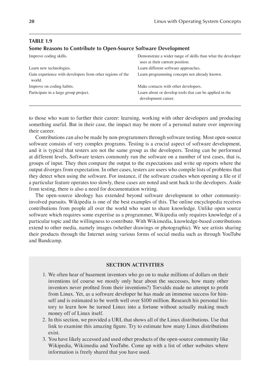
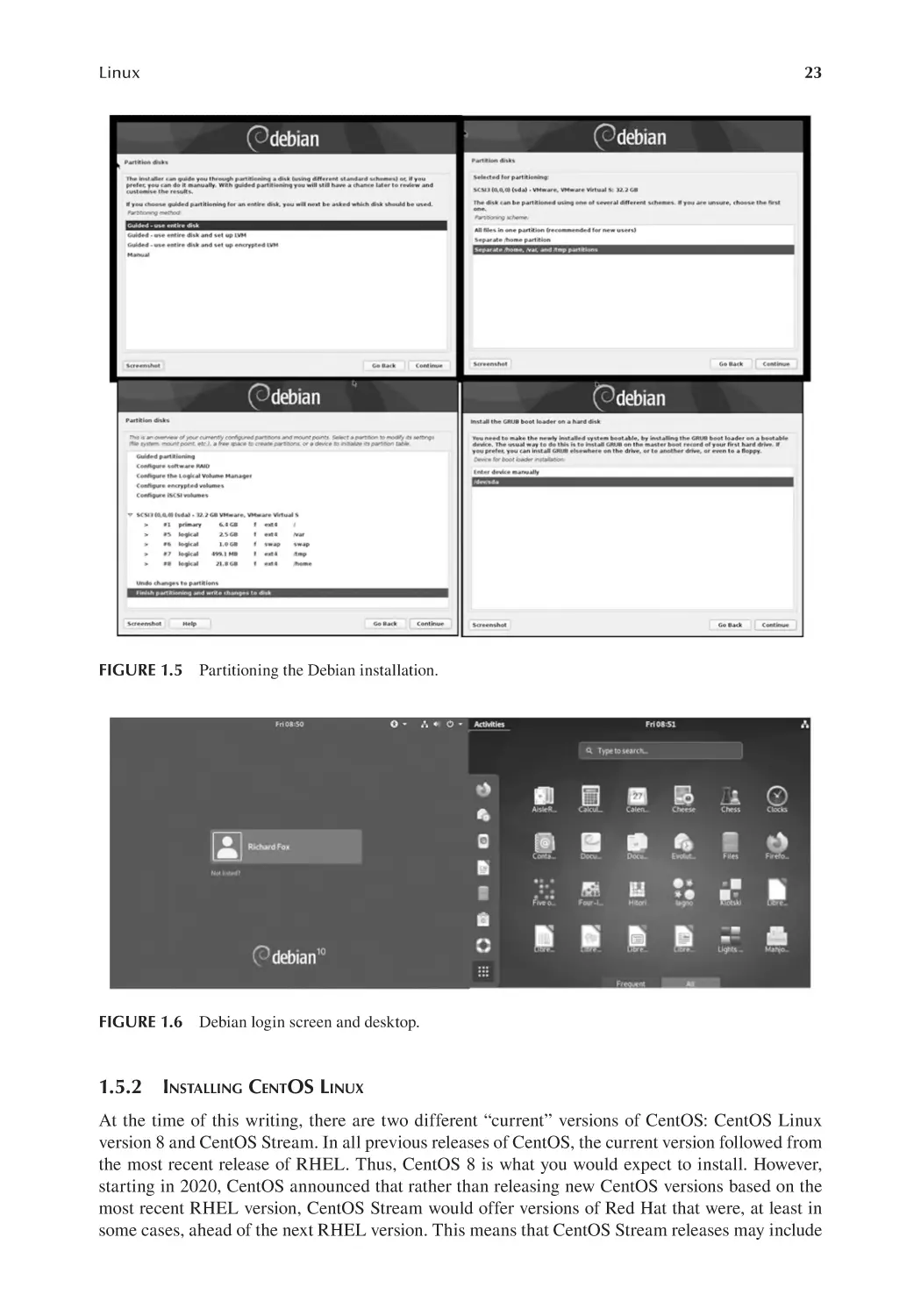
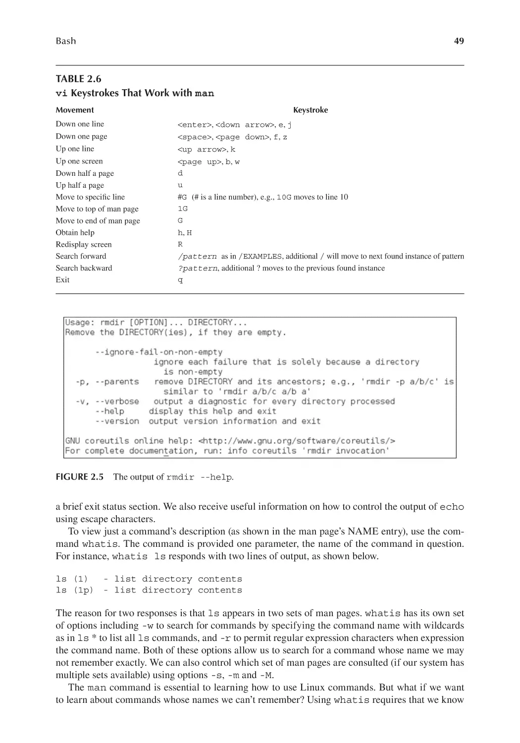
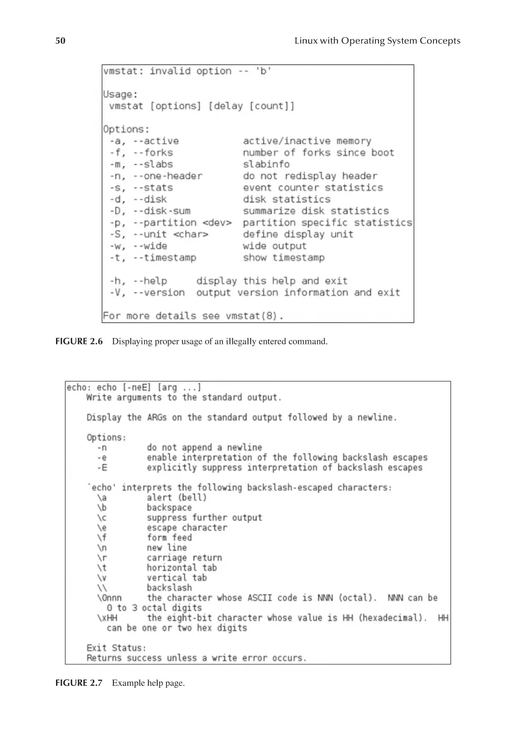
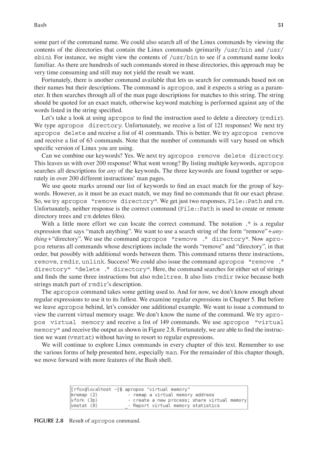
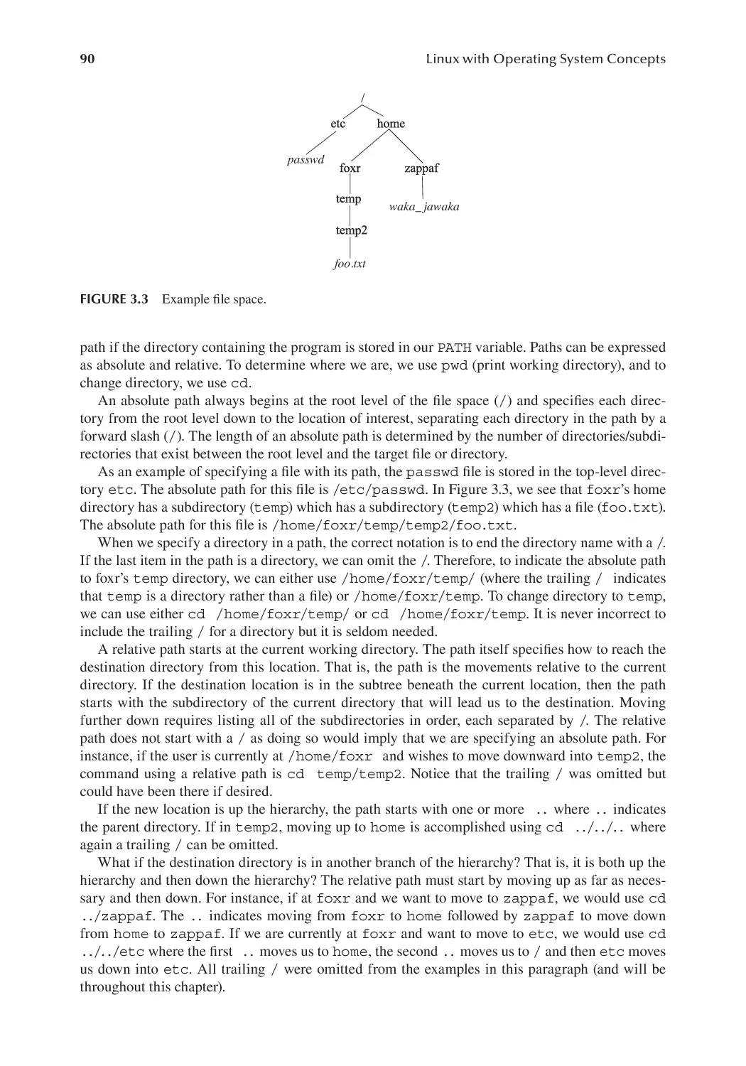
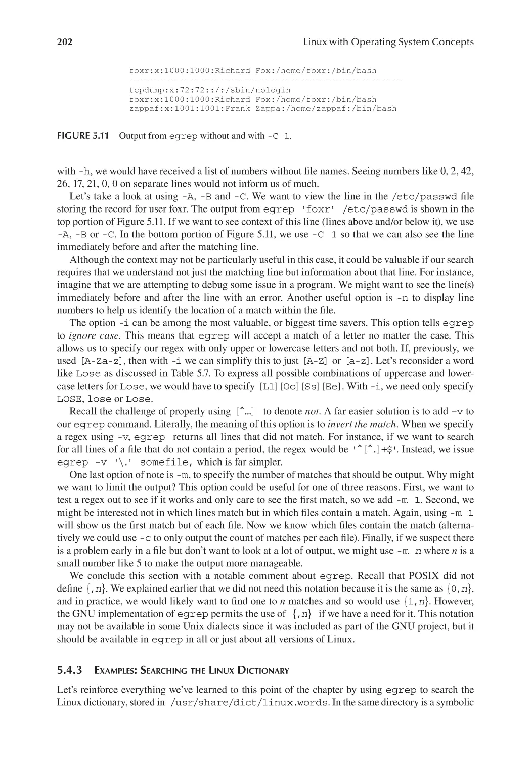
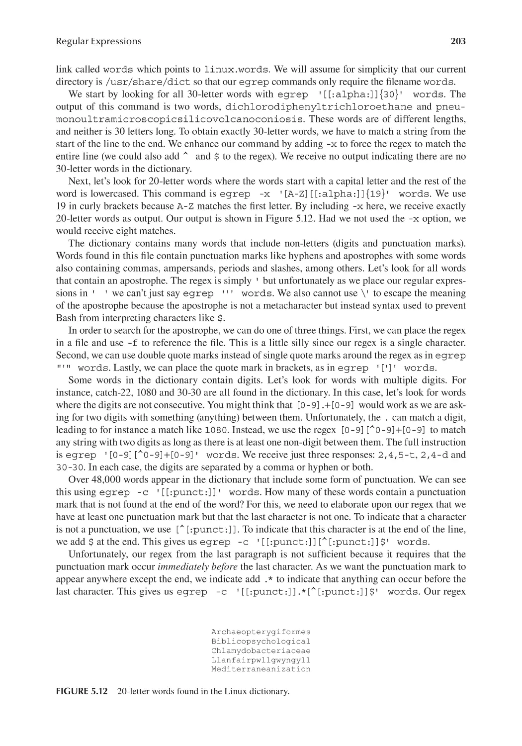
/


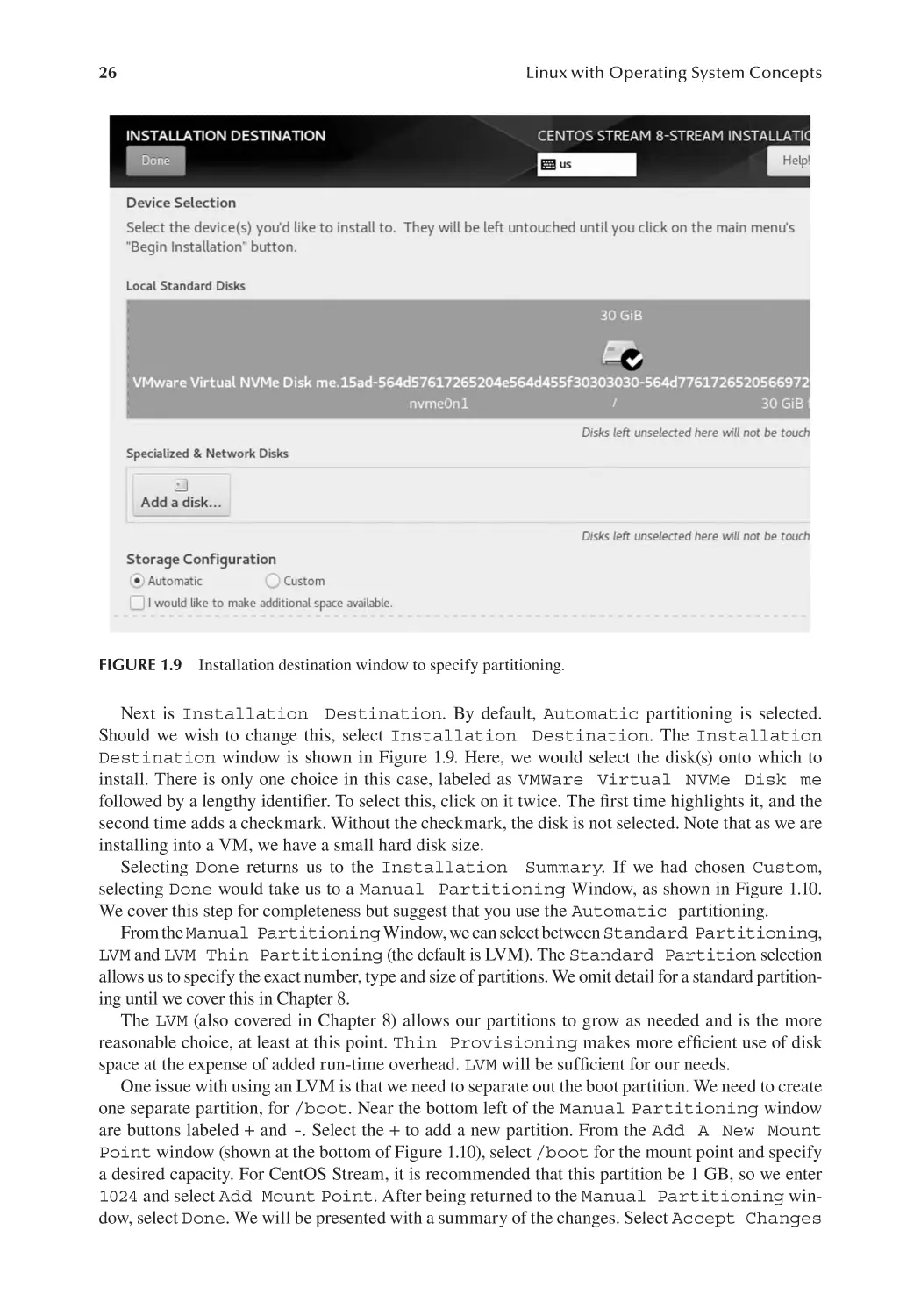
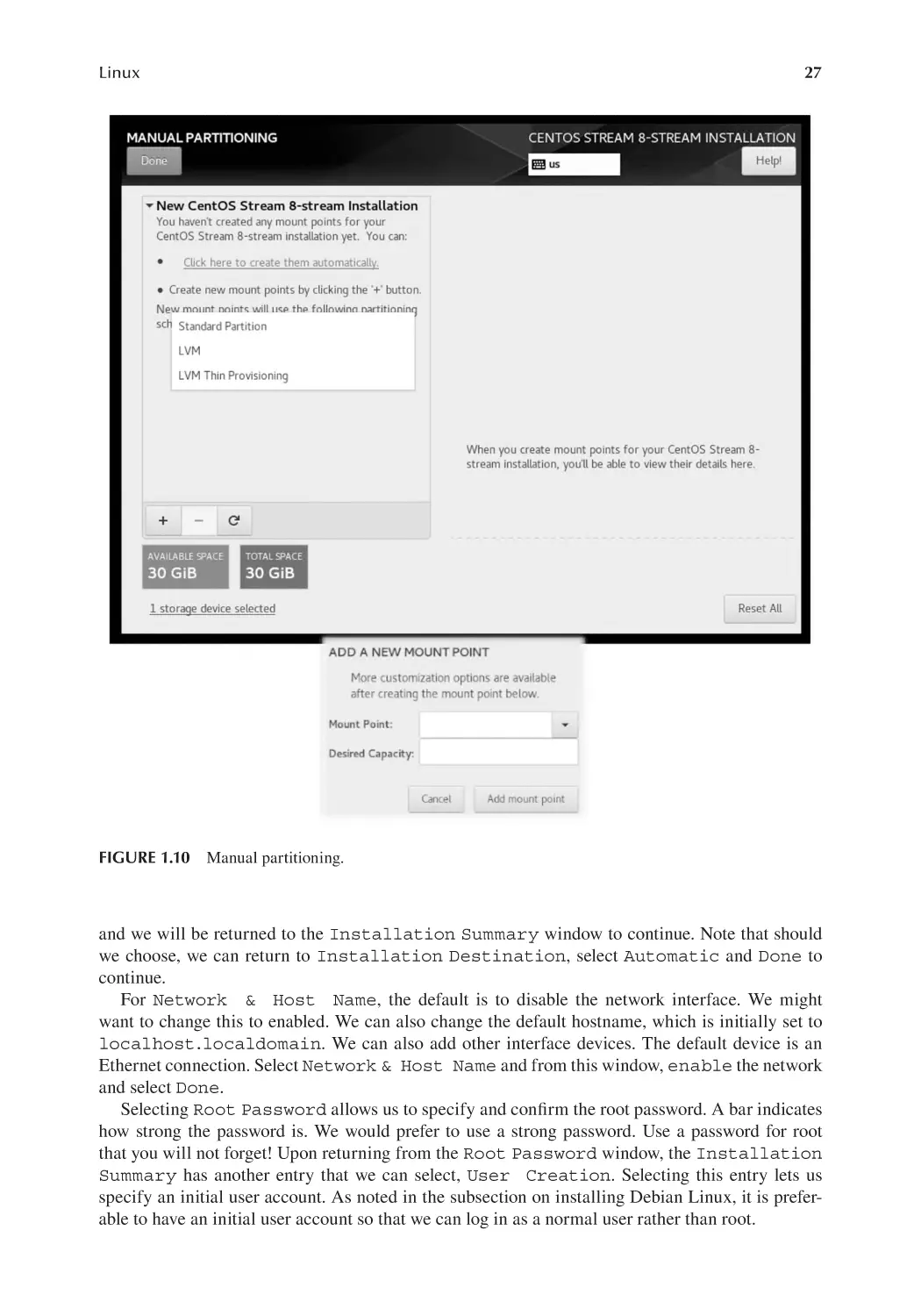


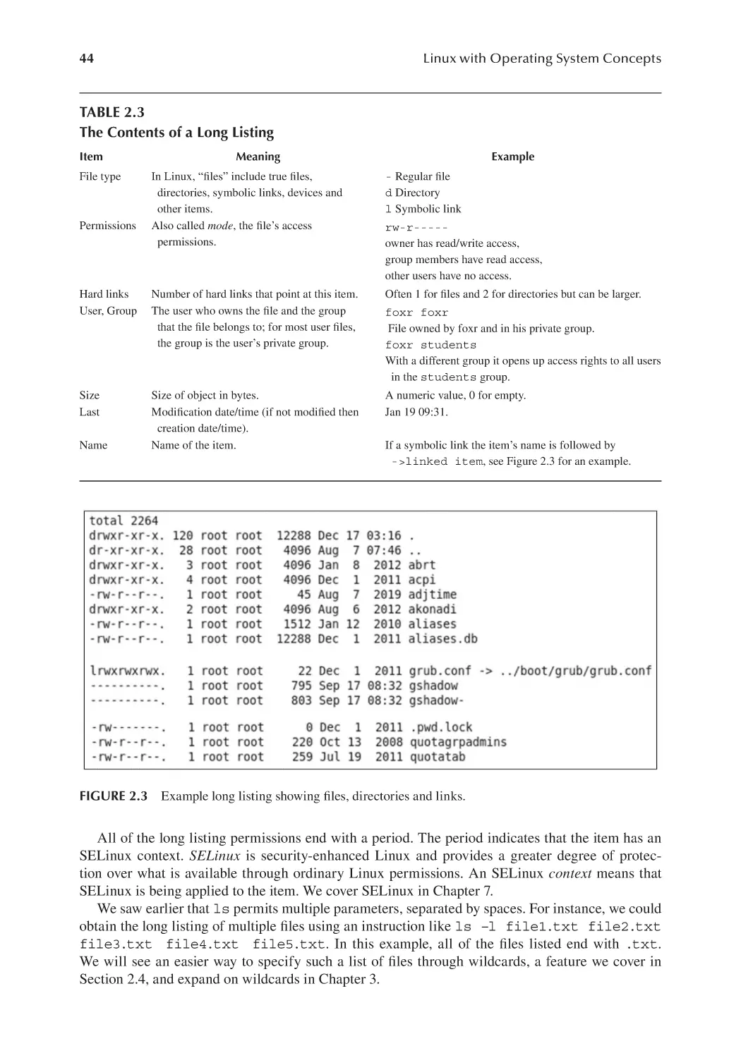


Text
Linux with Operating
System Concepts
Linux with Operating
System Concepts
Second Edition
Richard Fox
Second Edition published 2022
by CRC Press
6000 Broken Sound Parkway NW, Suite 300, Boca Raton, FL 33487-2742
and by CRC Press
2 Park Square, Milton Park, Abingdon, Oxon, OX14 4RN
© 2022 Richard Fox
First edition published by CRC Press 2015
CRC Press is an imprint of Taylor & Francis Group, LLC
Reasonable efforts have been made to publish reliable data and information, but the author and publisher cannot
assume responsibility for the validity of all materials or the consequences of their use. The authors and p
ublishers
have attempted to trace the copyright holders of all material reproduced in this publication and apologize to
copyright holders if permission to publish in this form has not been obtained. If any copyright material has not been
acknowledged please write and let us know so we may rectify in any future reprint.
Except as permitted under U.S. Copyright Law, no part of this book may be reprinted, reproduced, transmitted, or
utilized in any form by any electronic, mechanical, or other means, now known or hereafter invented, including
photocopying, microfilming, and recording, or in any information storage or retrieval system, without written
permission from the publishers.
For permission to photocopy or use material electronically from this work, access www.copyright.com or contact the
Copyright Clearance Center, Inc. (CCC), 222 Rosewood Drive, Danvers, MA 01923, 978-750-8400. For works that are
not available on CCC please contact mpkbookspermissions@tandf.co.uk
Trademark notice: Product or corporate names may be trademarks or registered trademarks and are used only for
identification and explanation without intent to infringe.
Library of Congress Cataloging‑in‑Publication Data
Names: Fox, Richard, 1964- author.
Title: Linux with operating system concepts / Richard Fox.
Description: Second edition. | Boca Raton : CRC Press, 2022. | Includes
bibliographical references and index.
Identifiers: LCCN 2021031731 | ISBN 9781032063454 (paperback) |
ISBN 9781032066707 (hardback) | ISBN 9781003203322 (ebook)
Subjects: LCSH: Linux. | Operating systems (Computers)
Classification: LCC QA76.774.L46 F69 2021 | DDC 005.4/32—dc23
LC record available at https://lccn.loc.gov/2021031731
ISBN: 978-1-032-06670-7 (hbk)
ISBN: 978-1-032-06345-4 (pbk)
ISBN: 978-1-003-20332-2 (ebk)
DOI: 10.1201/9781003203322
Typeset in Times
by codeMantra
Access the Support Material: https://www.routledge.com/9781032063454
With all my love to Cheri Klink, Sherre Kozloff and Laura Smith.
Contents
Preface.............................................................................................................................................. xv
Acknowledgments and Contributions..............................................................................................xix
Author..............................................................................................................................................xxi
Chapter 1
Linux: What, Why, Who and When, and How............................................................. 1
1.1
1.2
Introduction........................................................................................................1
What Is Linux?................................................................................................... 4
1.2.1 Early Operating Systems....................................................................... 4
1.2.2 The Operating System Kernel...............................................................5
1.2.3 Other Operating System Components................................................... 9
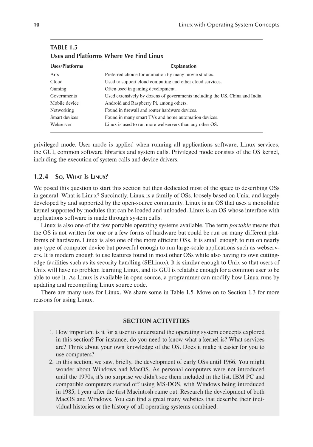
1.2.4 So, What Is Linux?.............................................................................. 10
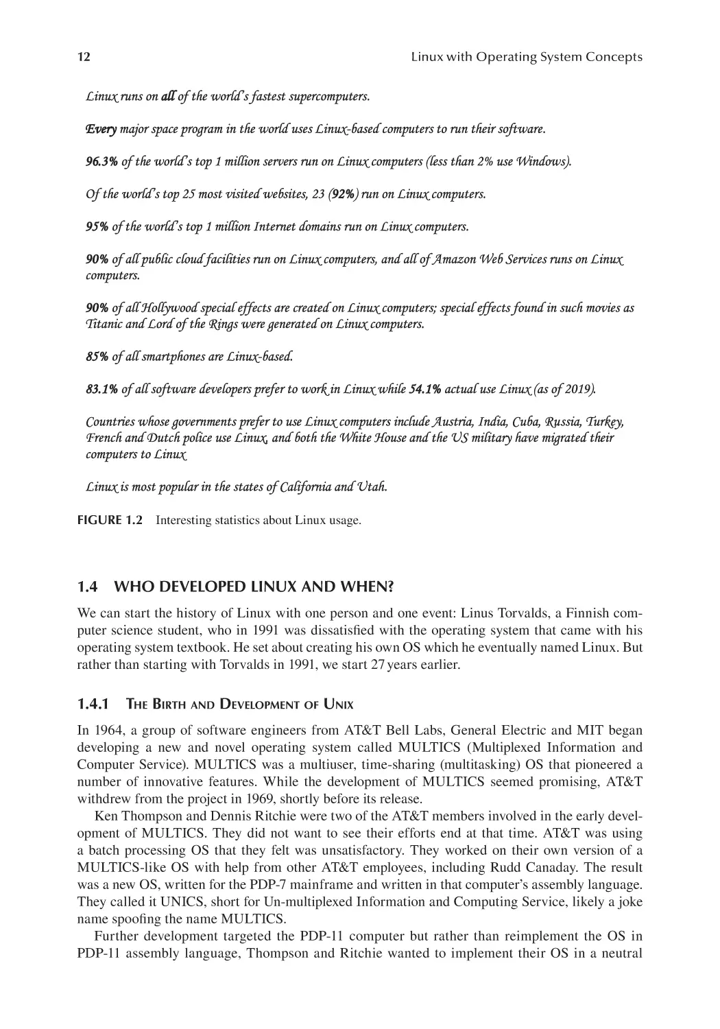
1.3 Why Use Linux?............................................................................................... 11
1.4 Who Developed Linux and When?.................................................................. 12
1.4.1 The Birth and Development of Unix................................................... 12
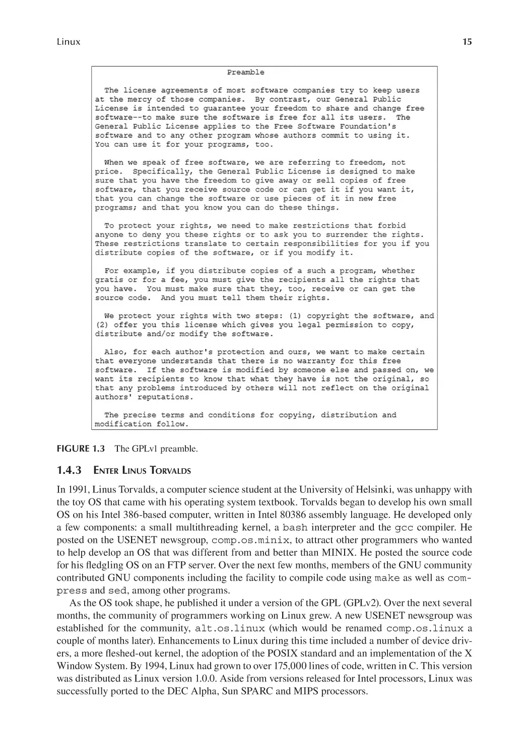
1.4.2 GNU.................................................................................................... 14
1.4.3 Enter Linus Torvalds........................................................................... 15
1.4.4 The Open-Source Community............................................................ 18
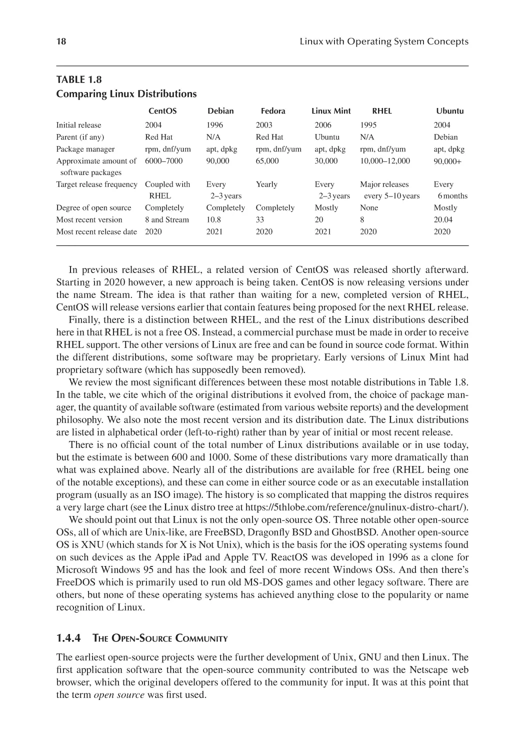
1.5 How Do You Use Linux?.................................................................................. 21
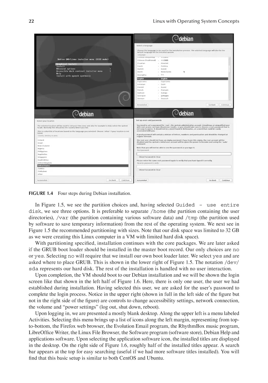
1.5.1 Installing Debian Linux...................................................................... 21
1.5.2 Installing CentOS Linux..................................................................... 23
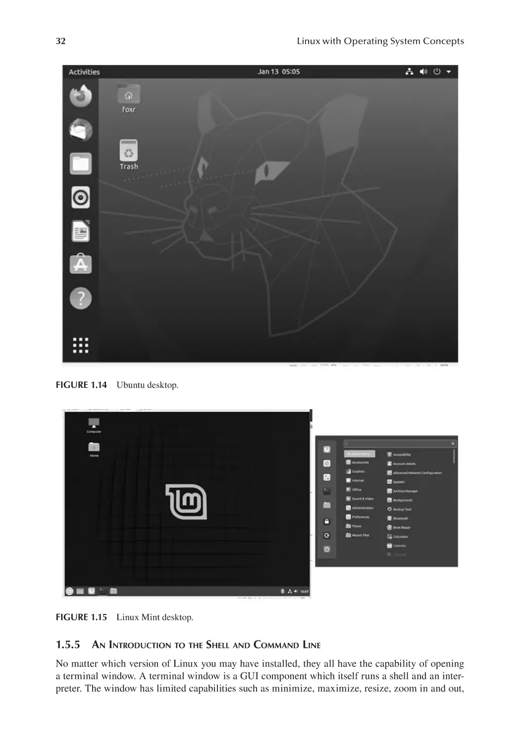
1.5.3 Installing Ubuntu Linux...................................................................... 29
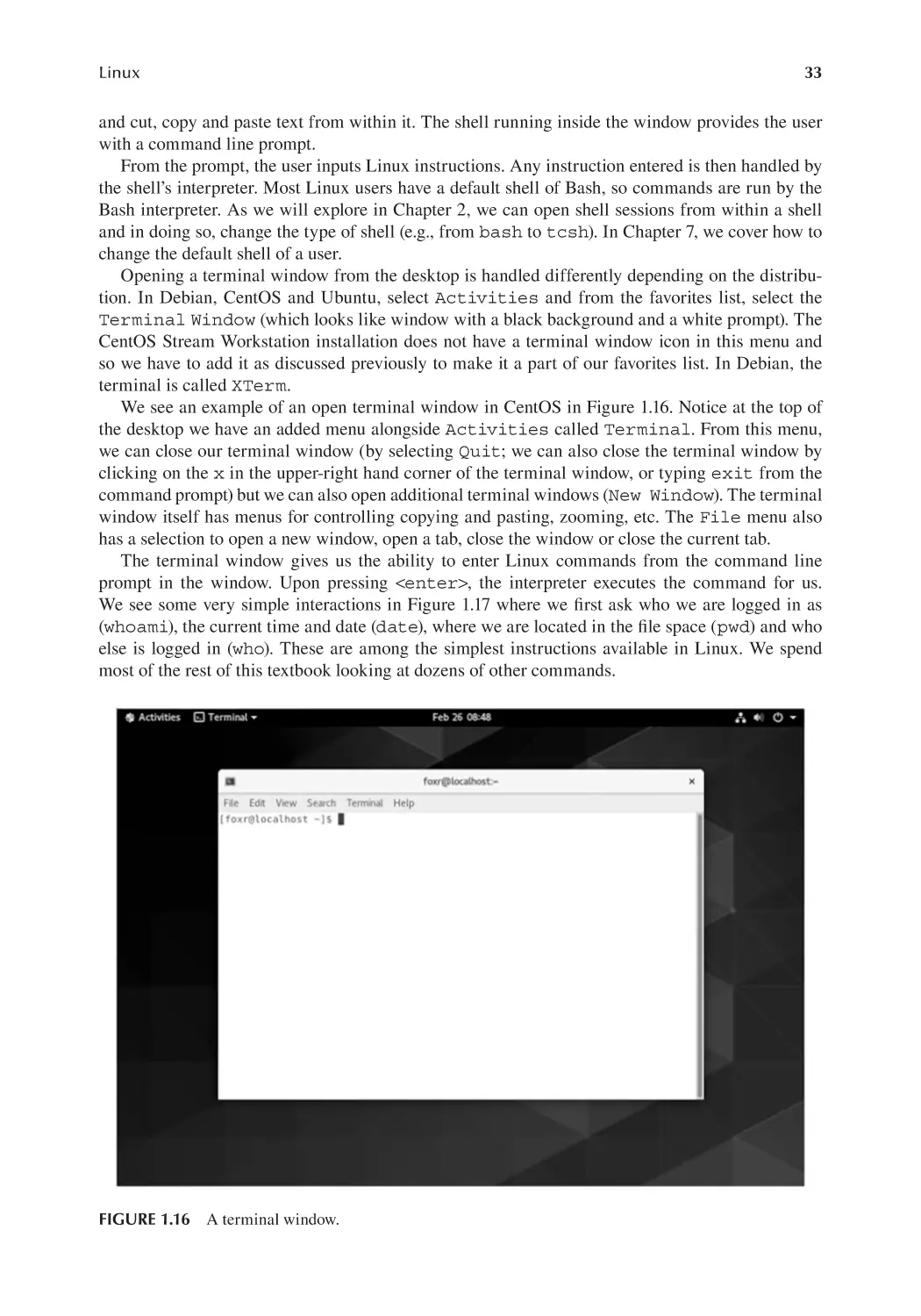
1.5.4 Installing Linux Mint.......................................................................... 30
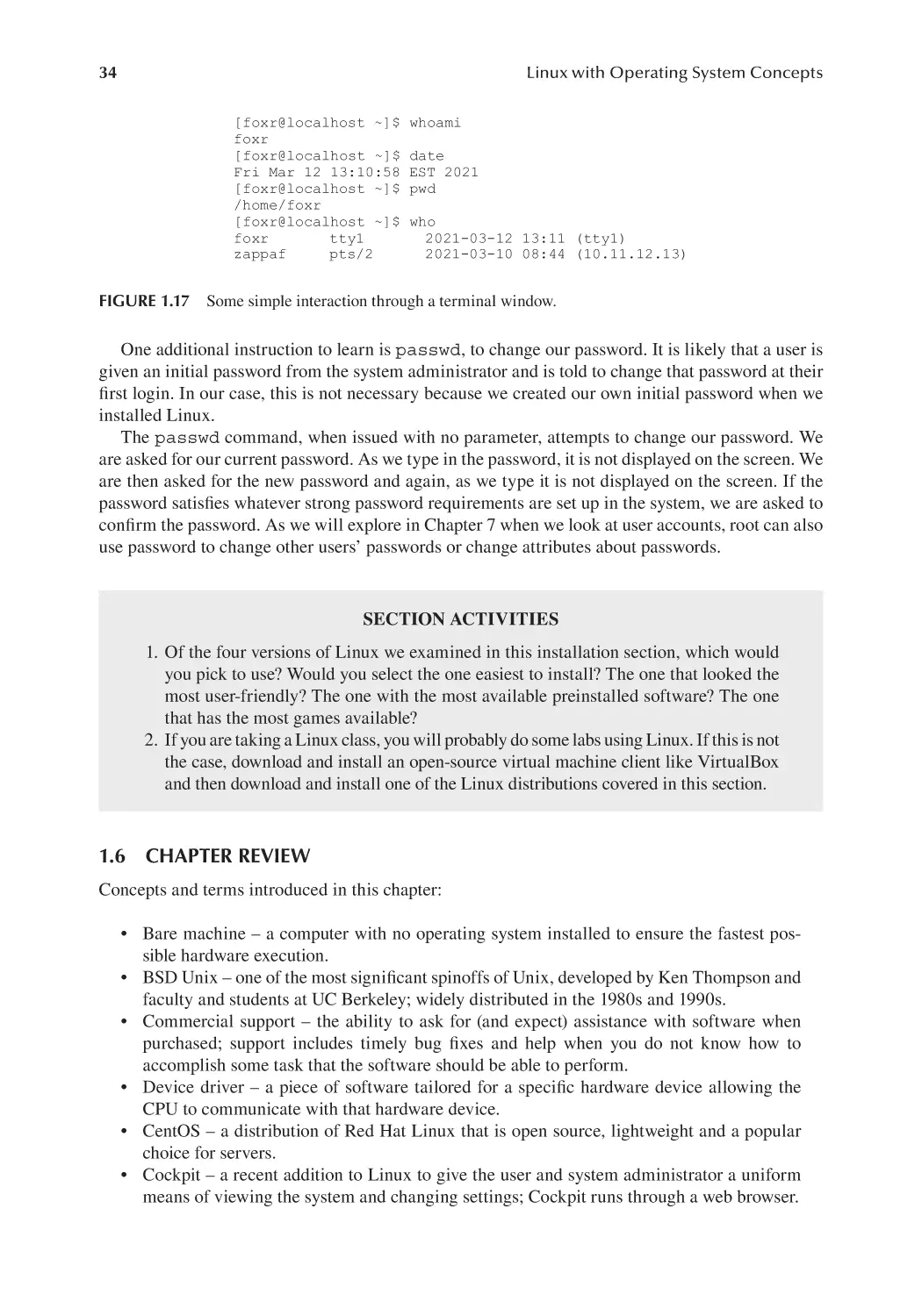
1.5.5 An Introduction to the Shell and Command Line............................... 32
1.6 Chapter Review................................................................................................34
Review Questions........................................................................................................ 37
Chapter 2
Bash............................................................................................................................. 39
2.1
2.2
2.3
2.4
2.5
2.6
Introduction...................................................................................................... 39
Entering Linux Commands.............................................................................. 41
2.2.1 Simple Linux Commands.................................................................... 41
2.2.2 Commands with Options and Parameters........................................... 43
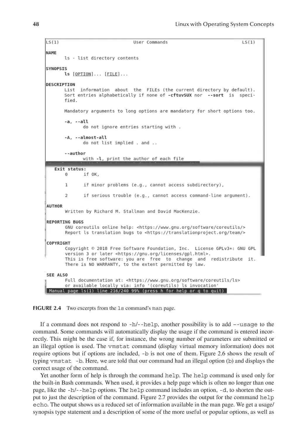
Forms of Linux Help........................................................................................46
2.3.1 man Pages...........................................................................................46
2.3.2 Other Forms of Command-Line Help................................................. 47
Bash Features................................................................................................... 52
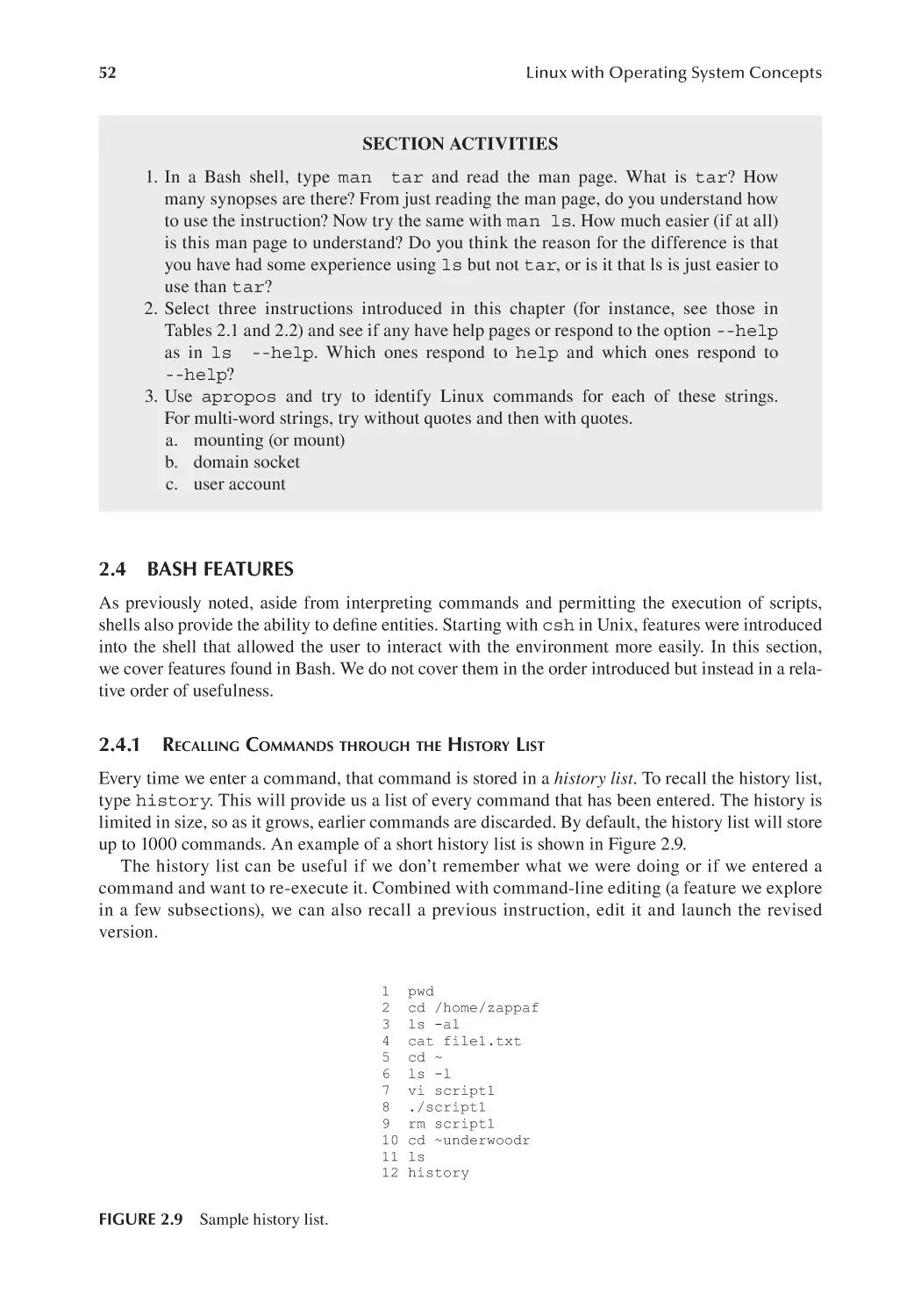
2.4.1 Recalling Commands through the History List.................................. 52
2.4.2 Shell Variables..................................................................................... 53
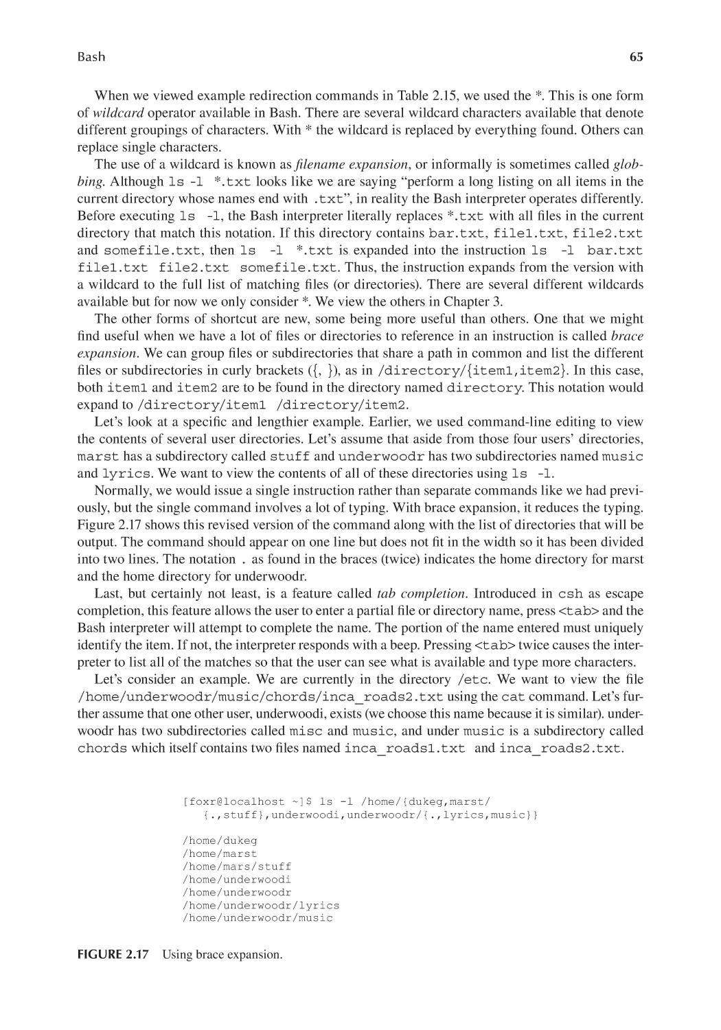
2.4.3 Aliases................................................................................................. 59
2.4.4 Command-Line Editing......................................................................60
2.4.5 Redirection.......................................................................................... 62
2.4.6 Other Useful Bash Features................................................................64
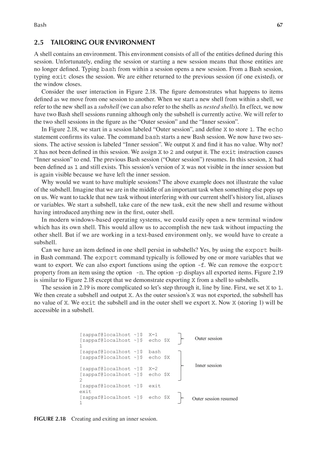
Tailoring Our Environment.............................................................................. 67
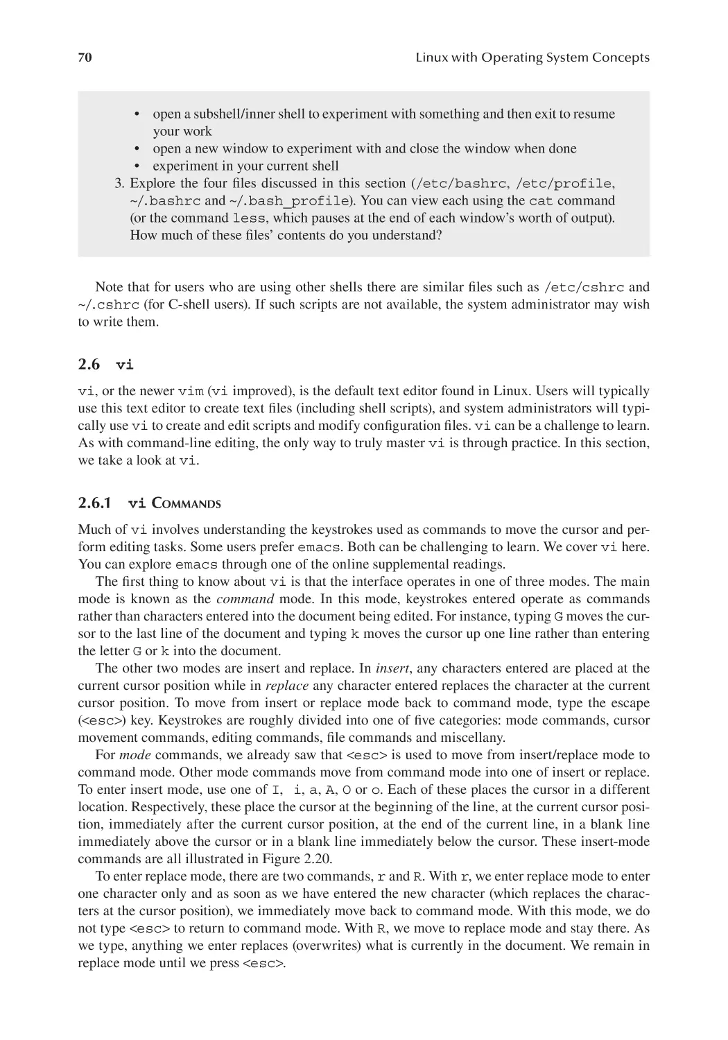
vi..................................................................................................................... 70
2.6.1 vi Commands..................................................................................... 70
2.6.2 An Example to Illustrate How to Use vi............................................ 73
vii
viii
Contents
2.7
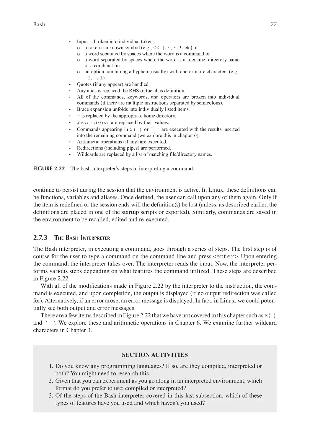
Interpreters....................................................................................................... 74
2.7.1 Interpreters in Programming Languages............................................ 75
2.7.2 Interpreters in Shells........................................................................... 76
2.7.3 The Bash Interpreter............................................................................ 77
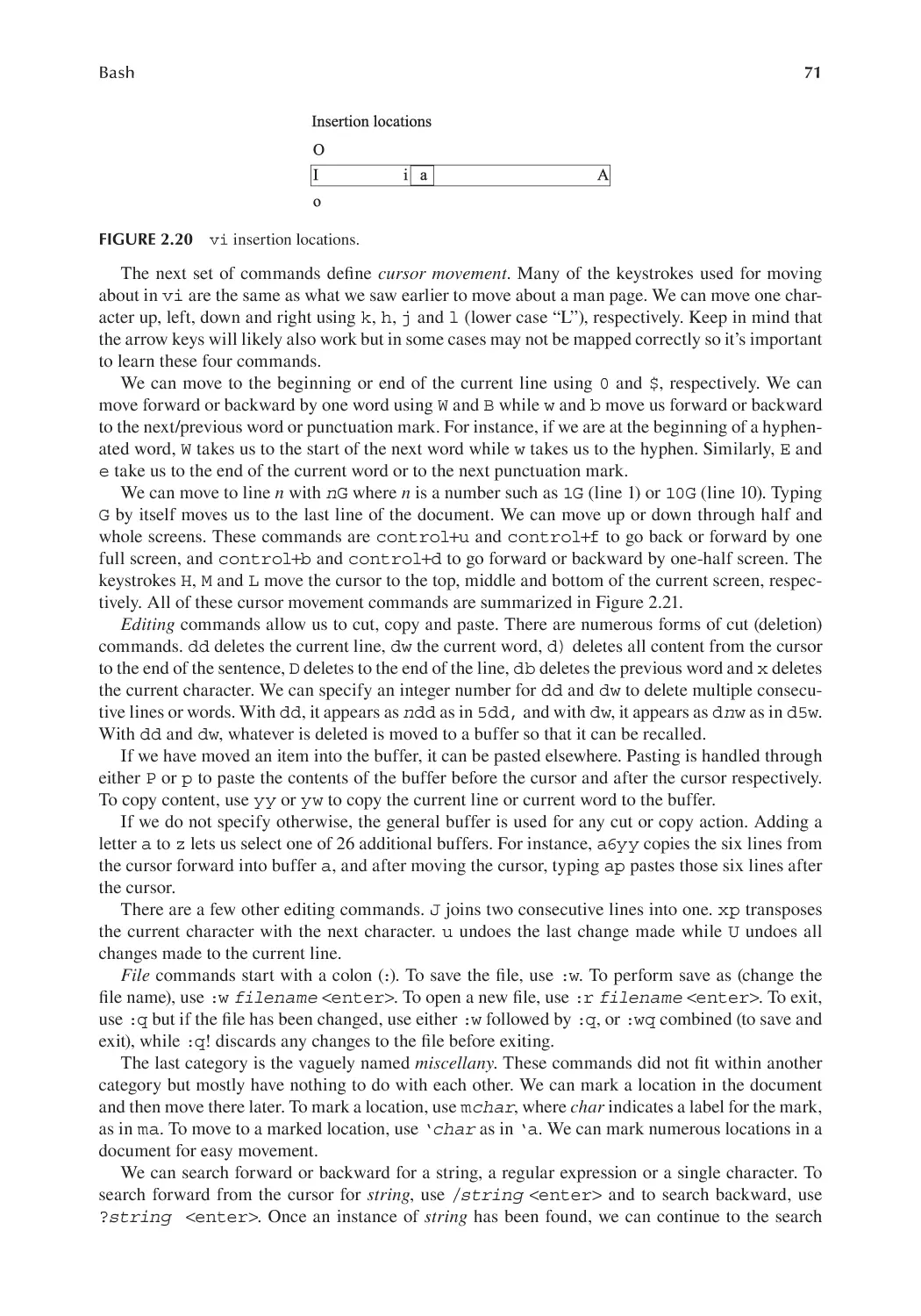
2.8 Chapter Review................................................................................................ 78
Review Questions........................................................................................................80
Chapter 3
Linux File Commands................................................................................................. 85
3.1
3.2
3.3
Introduction...................................................................................................... 85
Storage Terminology........................................................................................ 86
Filename Specification..................................................................................... 89
3.3.1 The Path.............................................................................................. 89
3.3.2 Filename Arguments with Paths......................................................... 91
3.3.3 The PATH Variable..............................................................................92
3.3.4 Specifying Filenames with Wildcards................................................92
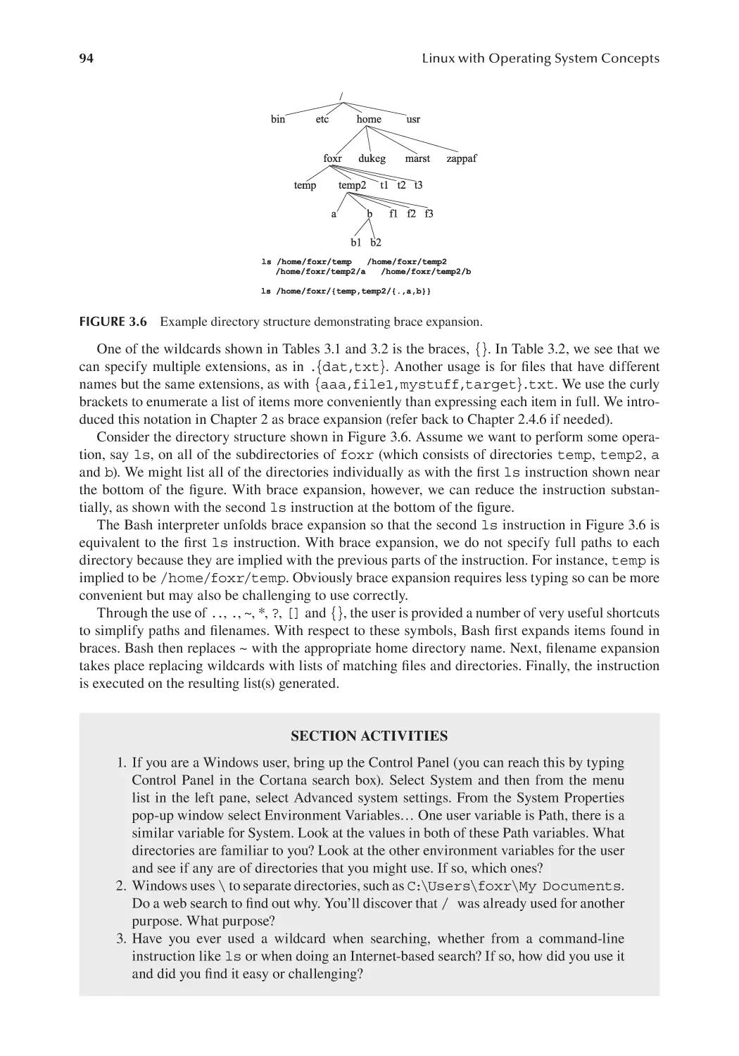
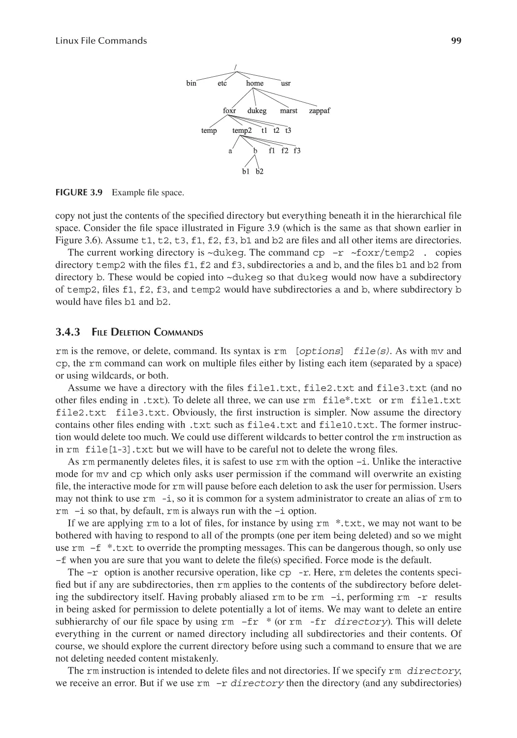
3.4 File Commands................................................................................................ 95
3.4.1 Directory Commands..........................................................................96
3.4.2 File Movement and Copy Commands.................................................97
3.4.3 File Deletion Commands.....................................................................99
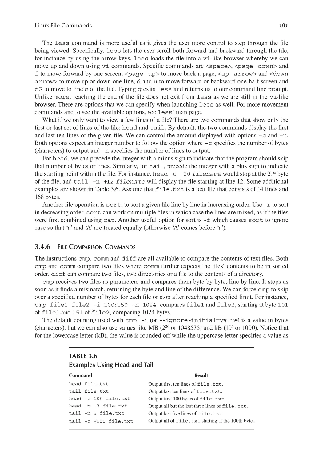
3.4.4 Creating and Deleting Directories.................................................... 100
3.4.5 Textfile Viewing Commands............................................................. 100
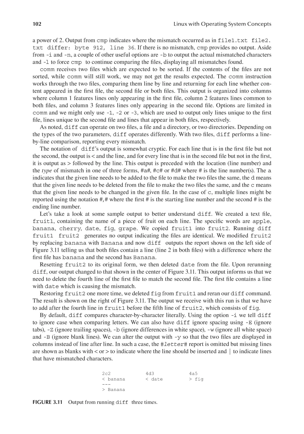
3.4.6 File Comparison Commands............................................................. 101
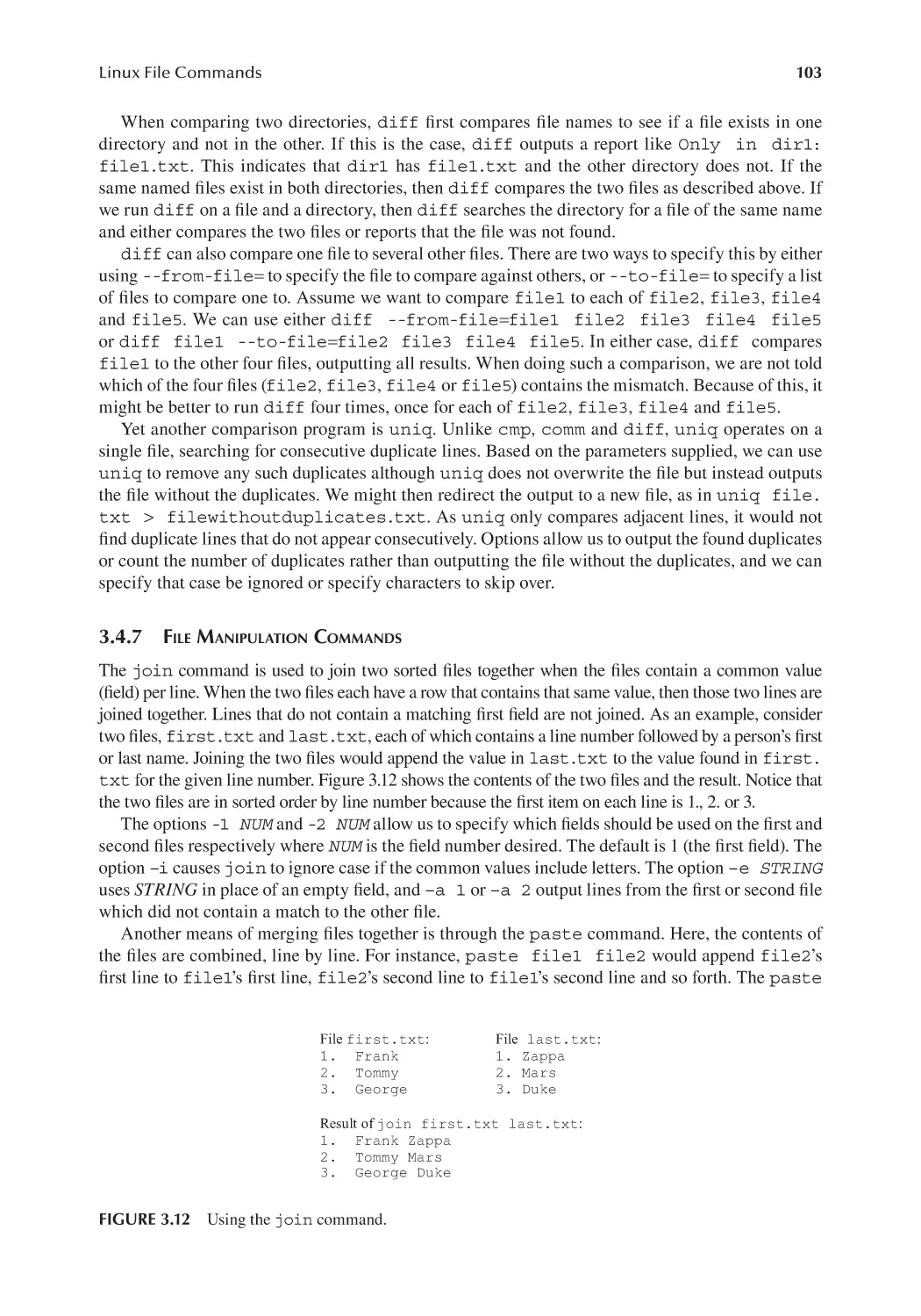
3.4.7 File Manipulation Commands........................................................... 103
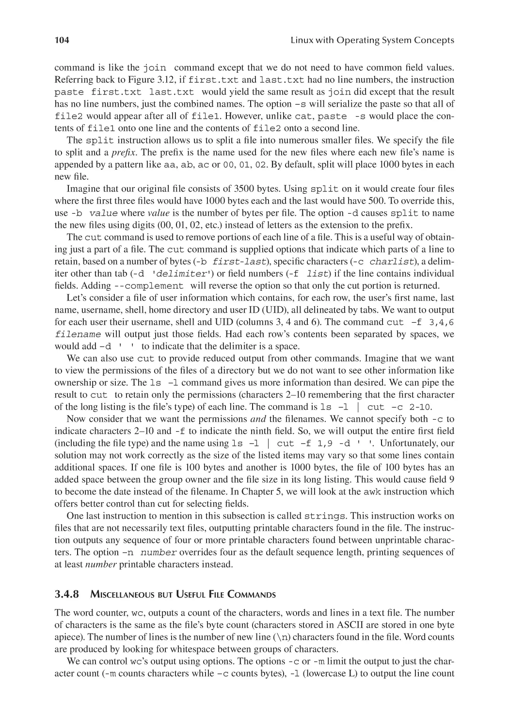
3.4.8 Miscellaneous but Useful File Commands....................................... 104
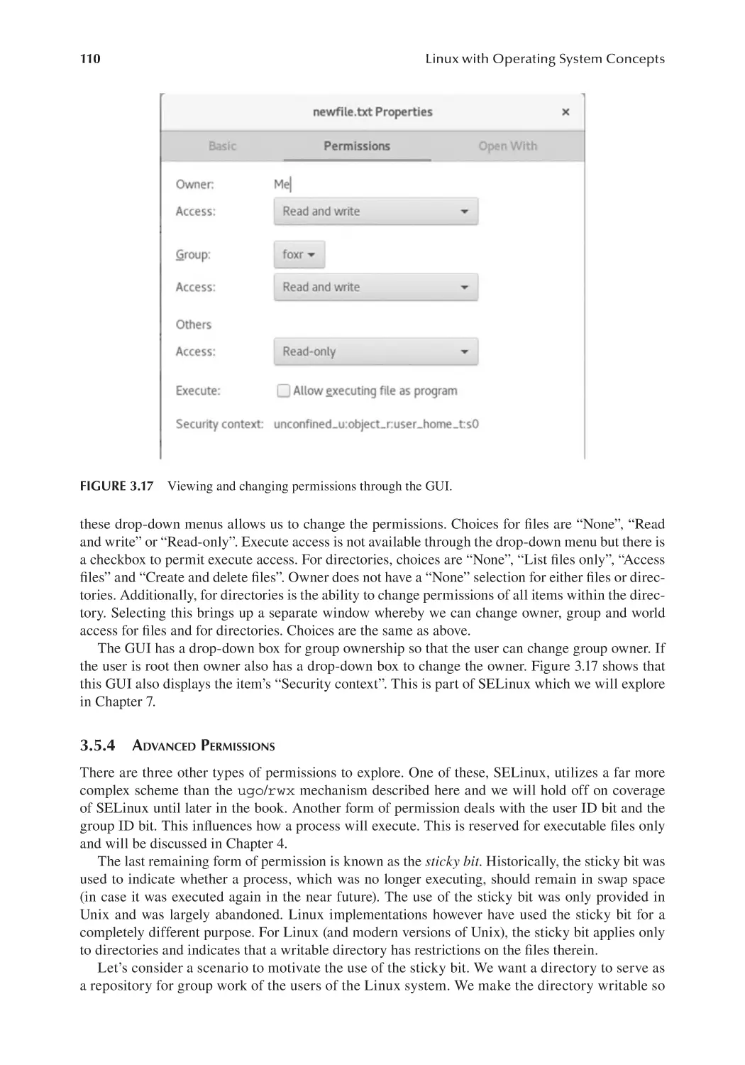
3.5 Permissions..................................................................................................... 106
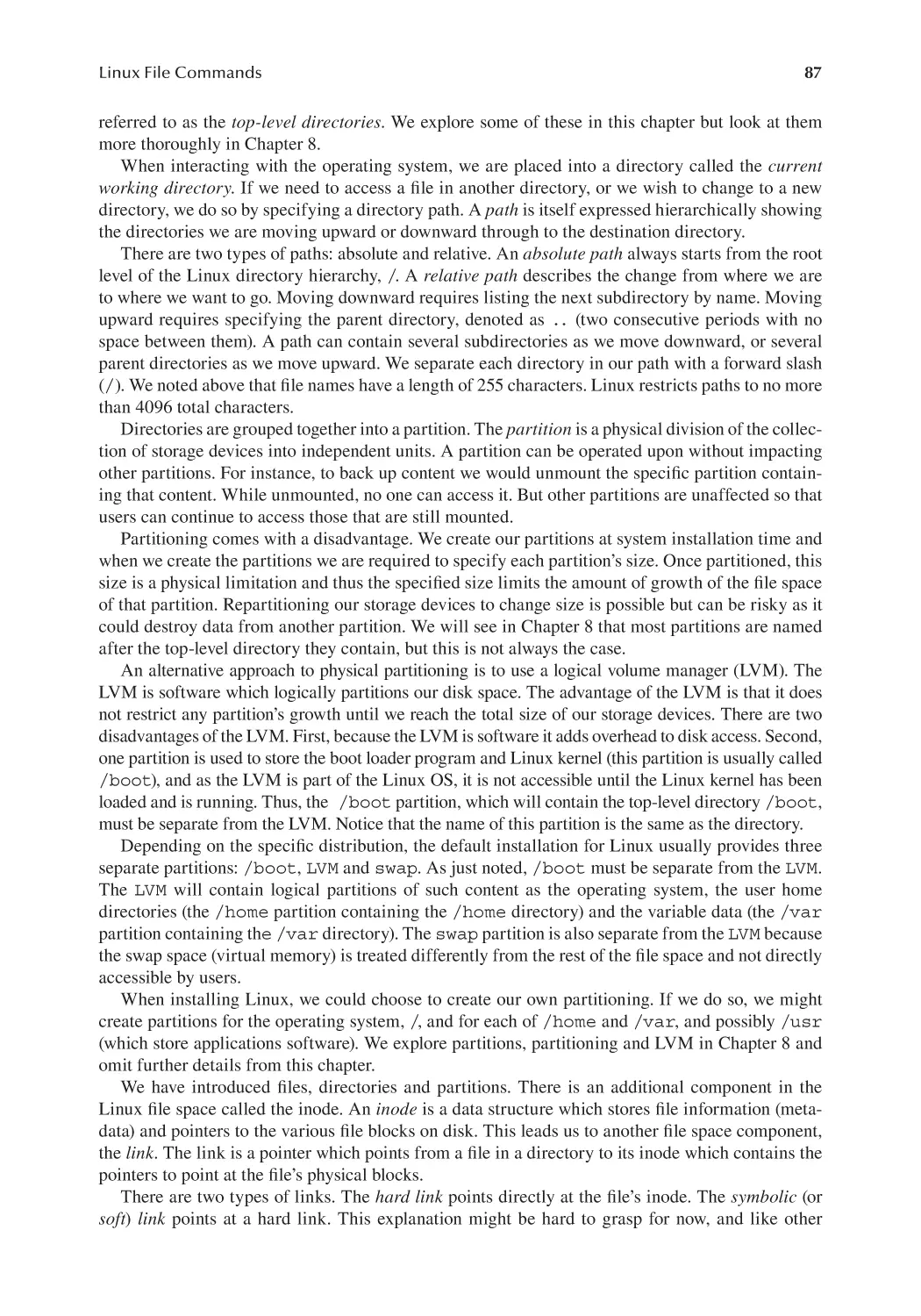
3.5.1 What Are Permissions?..................................................................... 106
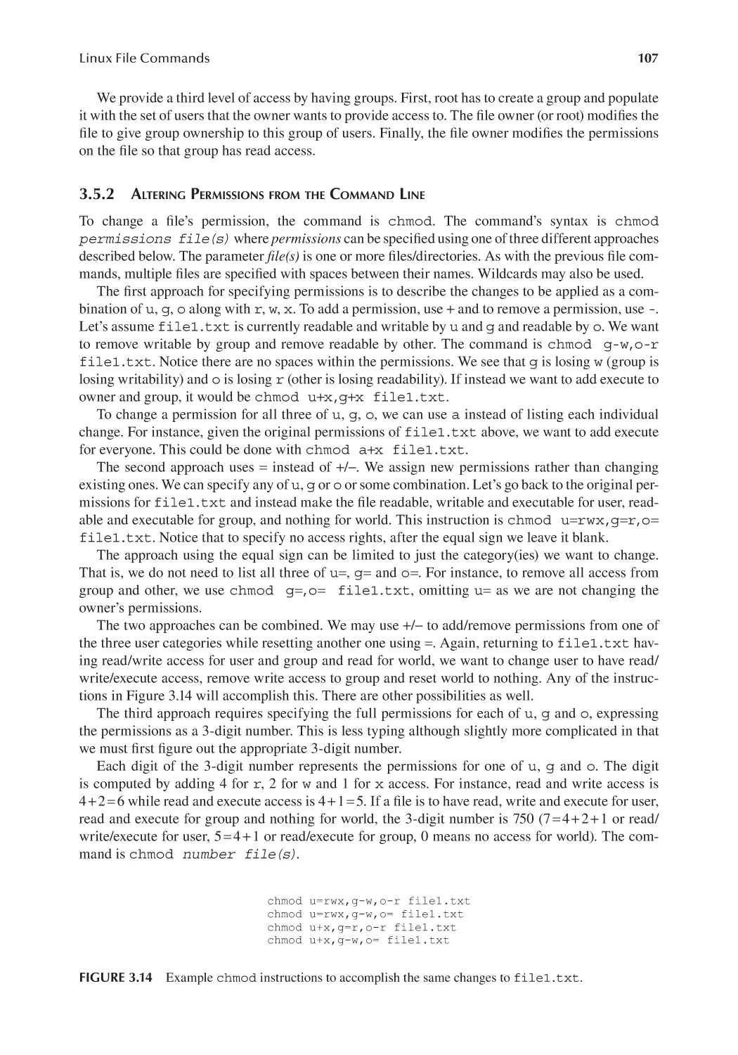
3.5.2 Altering Permissions from the Command Line................................ 107
3.5.3 Altering Permissions from the GUI.................................................. 109
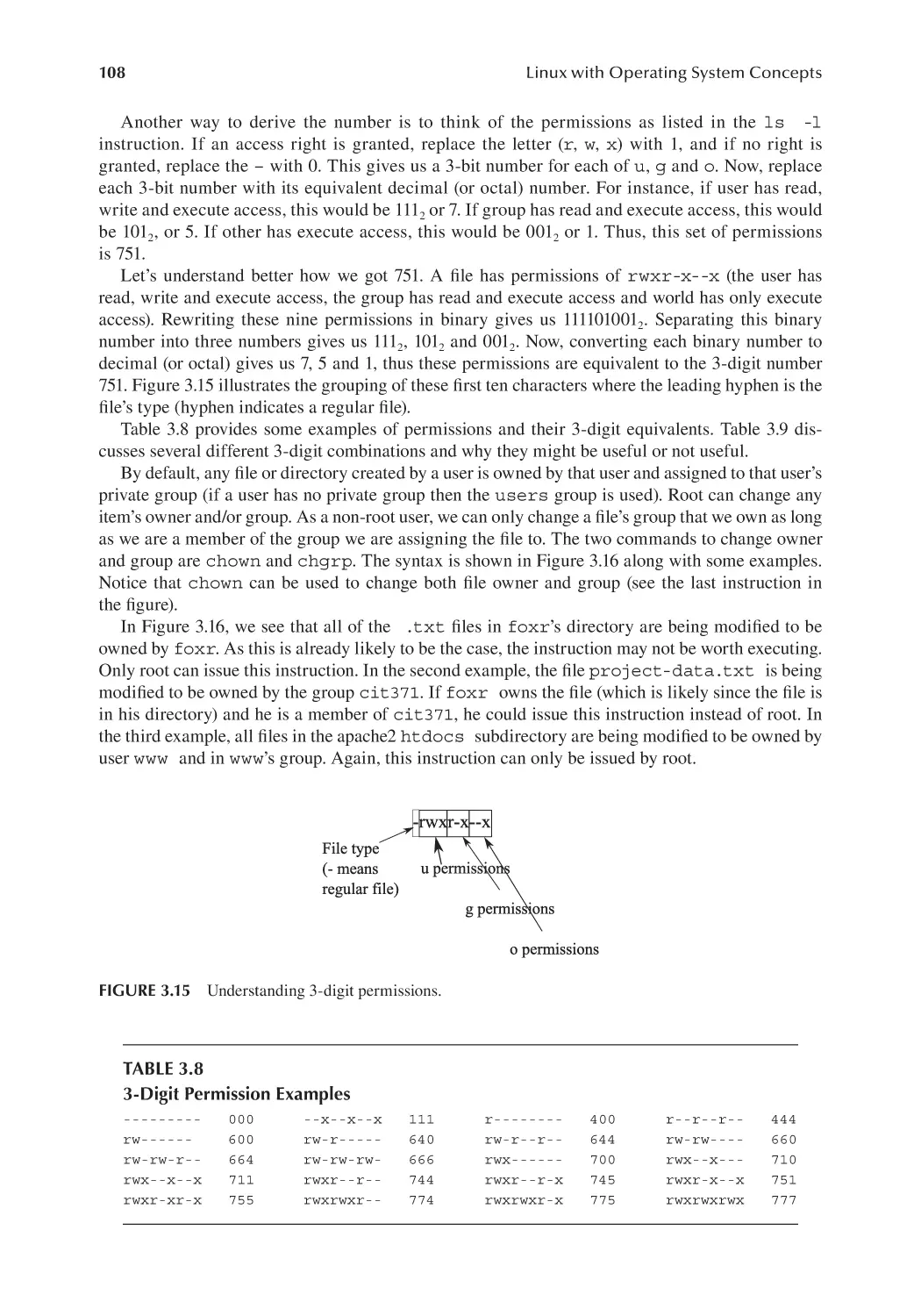
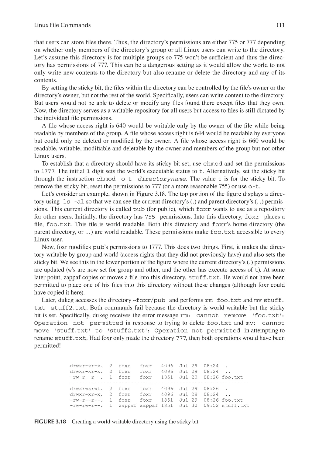
3.5.4 Advanced Permissions...................................................................... 110
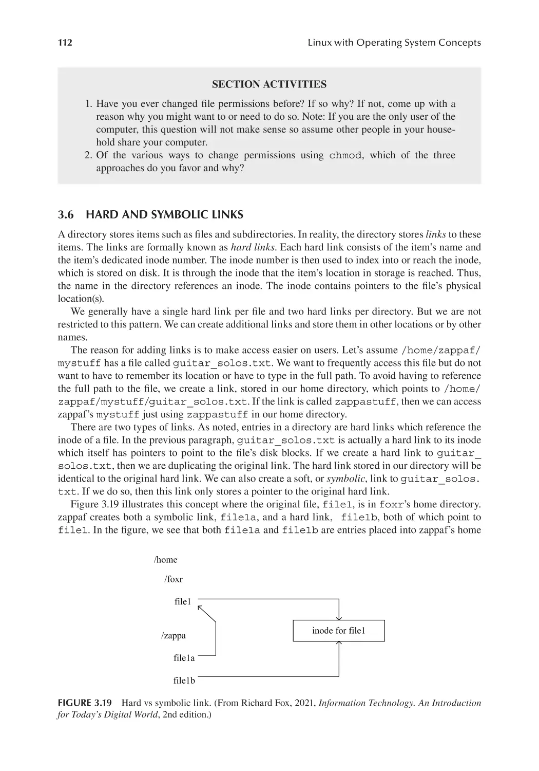
3.6 Hard and Symbolic Links............................................................................... 112
3.7 Locating Files................................................................................................. 114
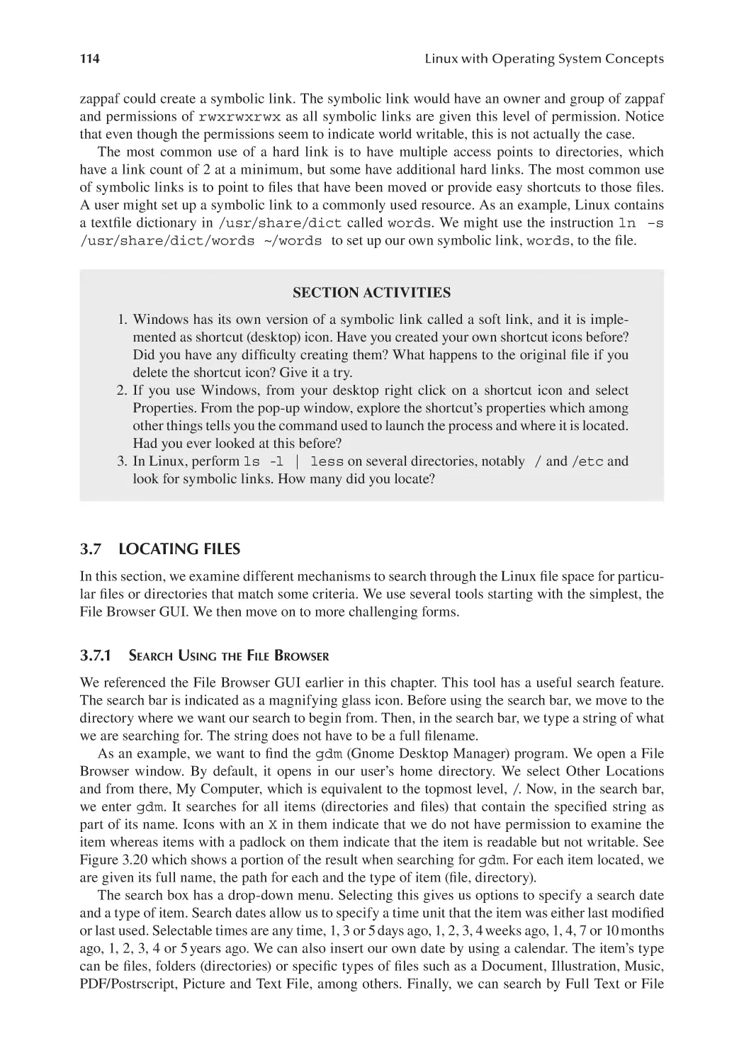
3.7.1 Search Using the File Browser.......................................................... 114
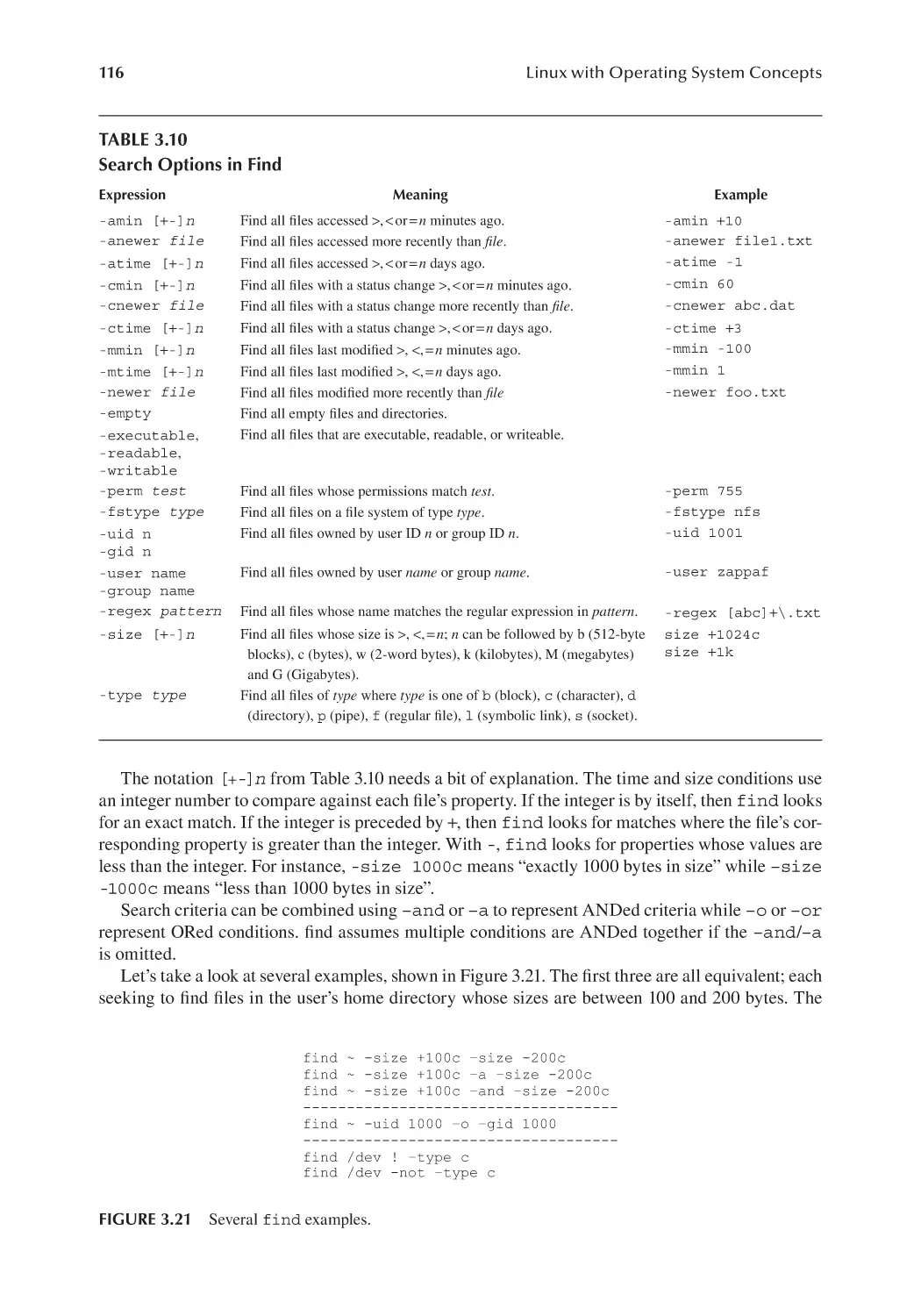
3.7.2 The find Command........................................................................ 115
3.7.3 Other Means of Locating Files......................................................... 118
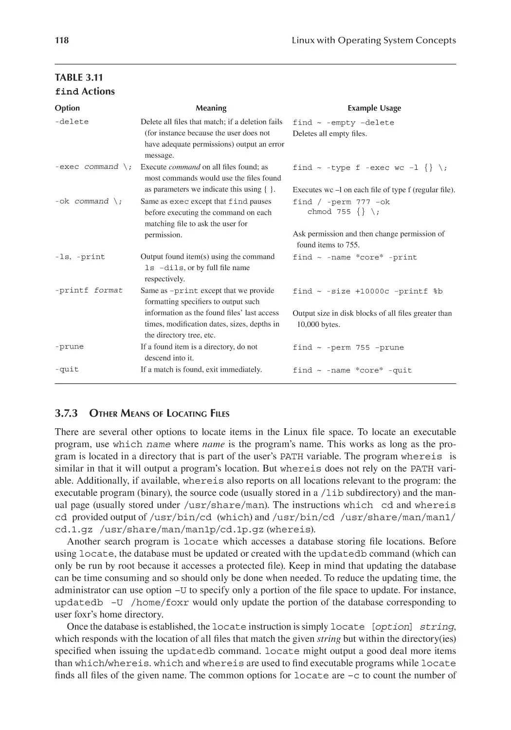
3.8 Secondary Storage Devices............................................................................ 119
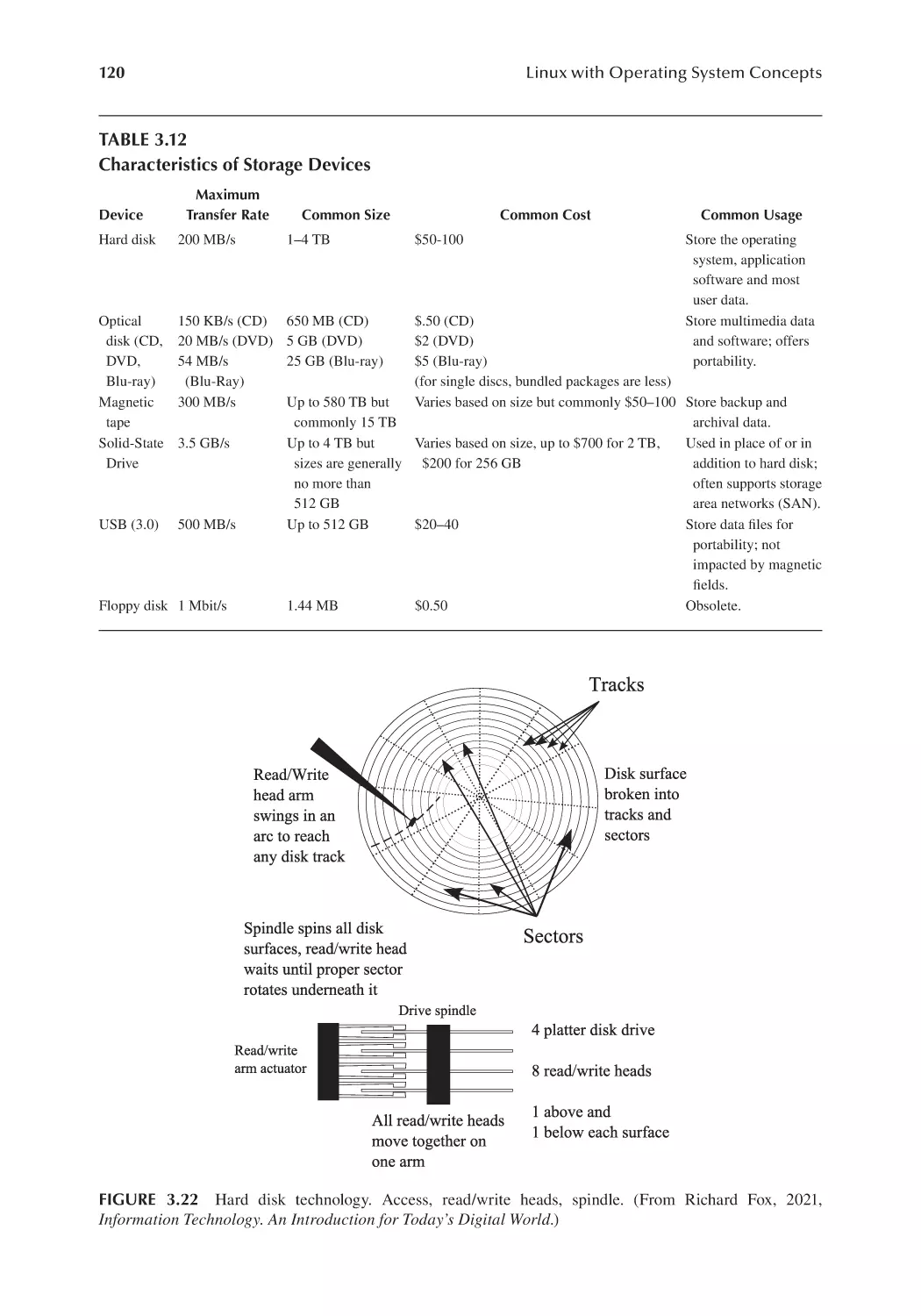
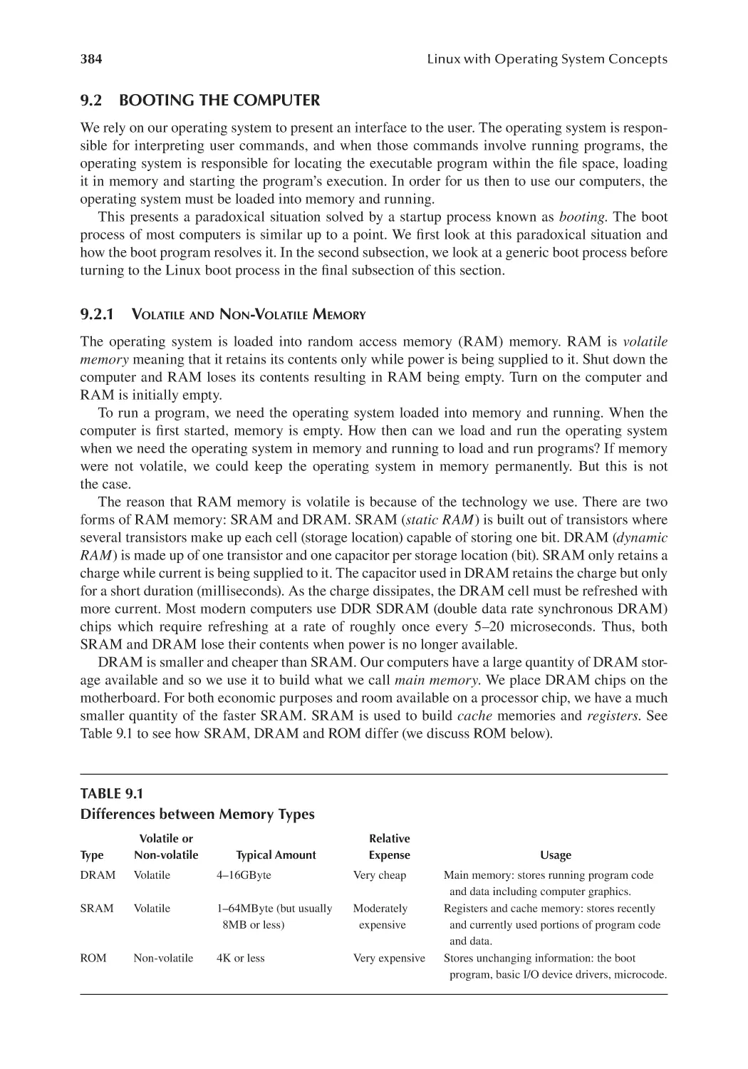
3.8.1 The Hard Disk Drive......................................................................... 119
3.8.2 Magnetic Tape................................................................................... 122
3.8.3 Optical Discs..................................................................................... 122
3.8.4 Flash Memory Drives........................................................................ 123
3.8.5 Device Drivers................................................................................... 124
3.9 File Compression............................................................................................ 124
3.9.1 Types of File Compression................................................................ 124
3.9.2 The Lempel–Ziv Algorithms for Lossless Compression.................. 125
3.9.3 Other Lossless Compression Algorithms.......................................... 126
3.9.4 Compression and Decompression Programs in Linux...................... 127
3.10 Chapter Review.............................................................................................. 127
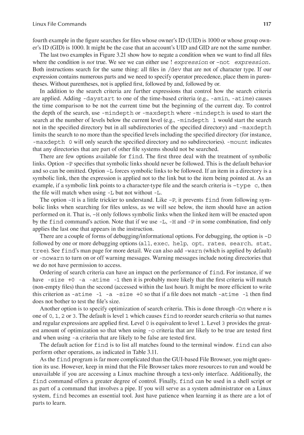
Review Questions...................................................................................................... 130
ix
Contents
Chapter 4
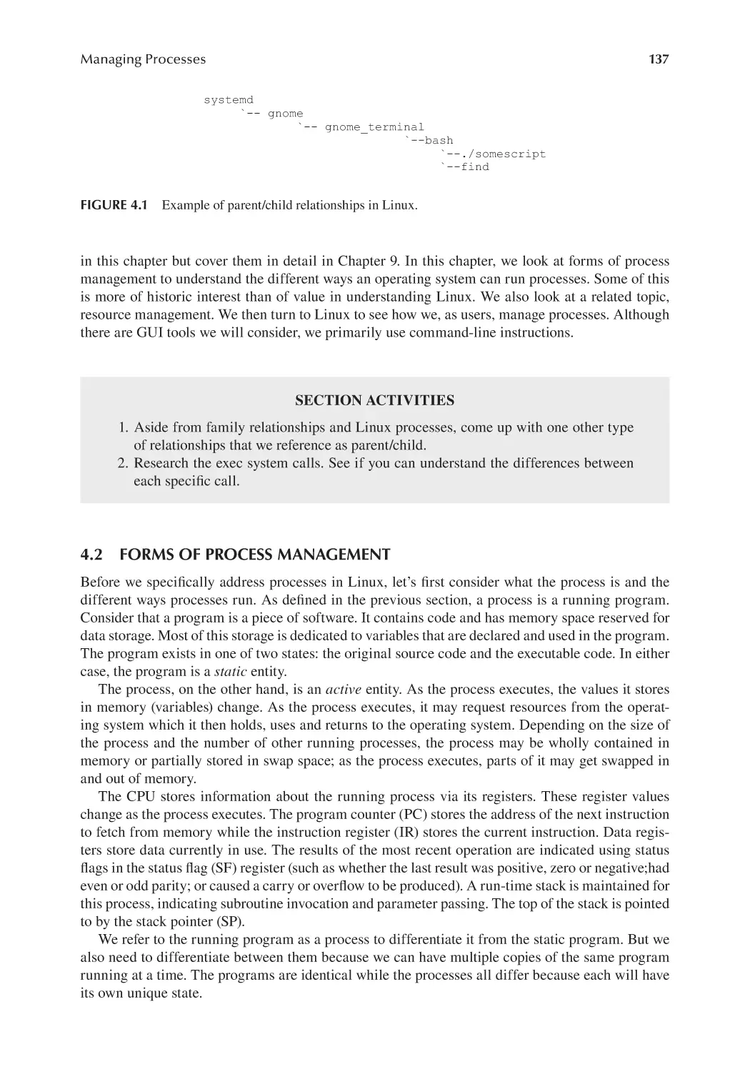
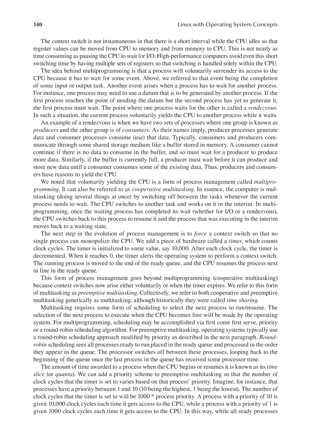
Managing Processes.................................................................................................. 135
4.1
4.2
Introduction.................................................................................................... 135
Forms of Process Management...................................................................... 137
4.2.1 Single-Process Execution.................................................................. 138
4.2.2 Concurrent Processing...................................................................... 139
4.2.3 Interrupt Handling............................................................................. 142
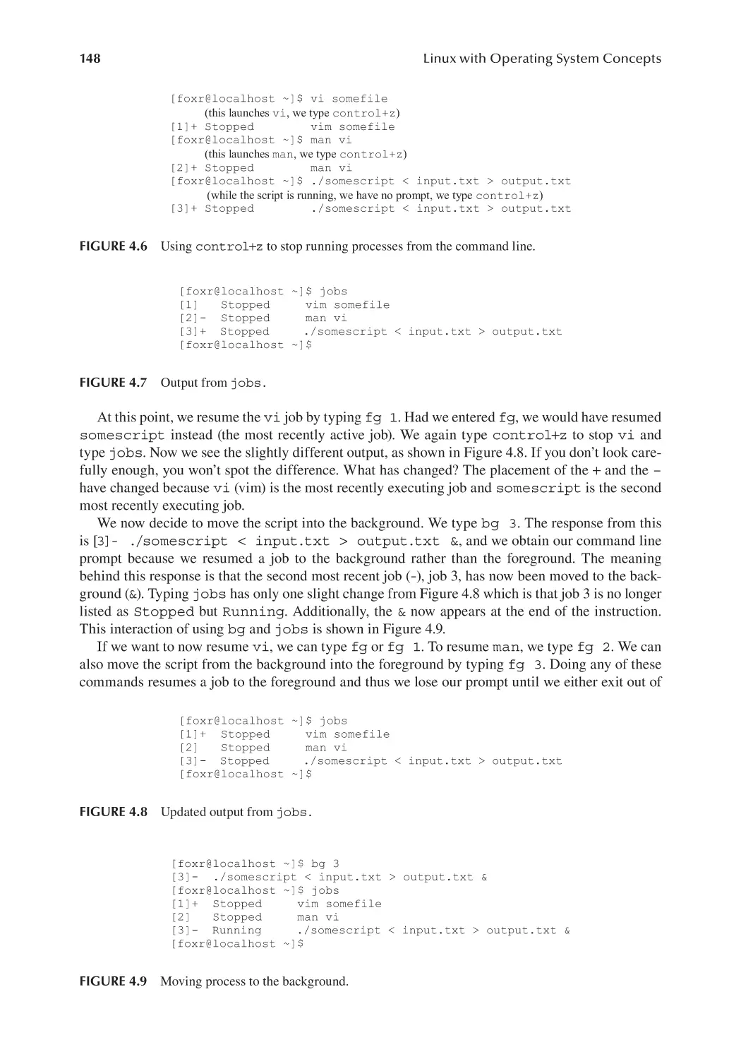
4.3 Starting, Pausing and Resuming Processes.................................................... 143
4.3.1 Ownership of Running Processes..................................................... 144
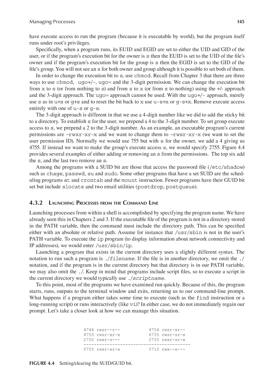
4.3.2 Launching Processes from the Command Line................................ 145
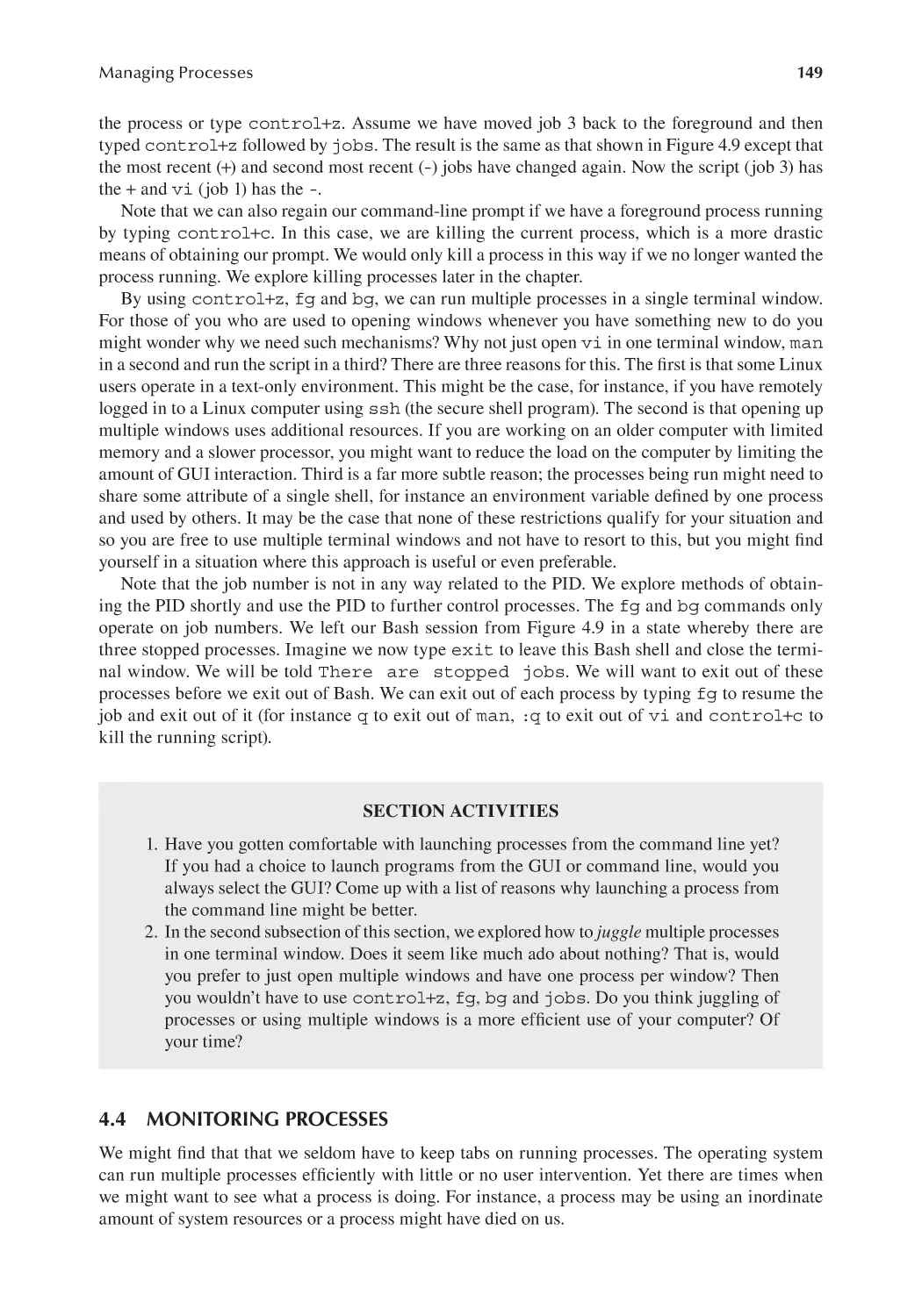
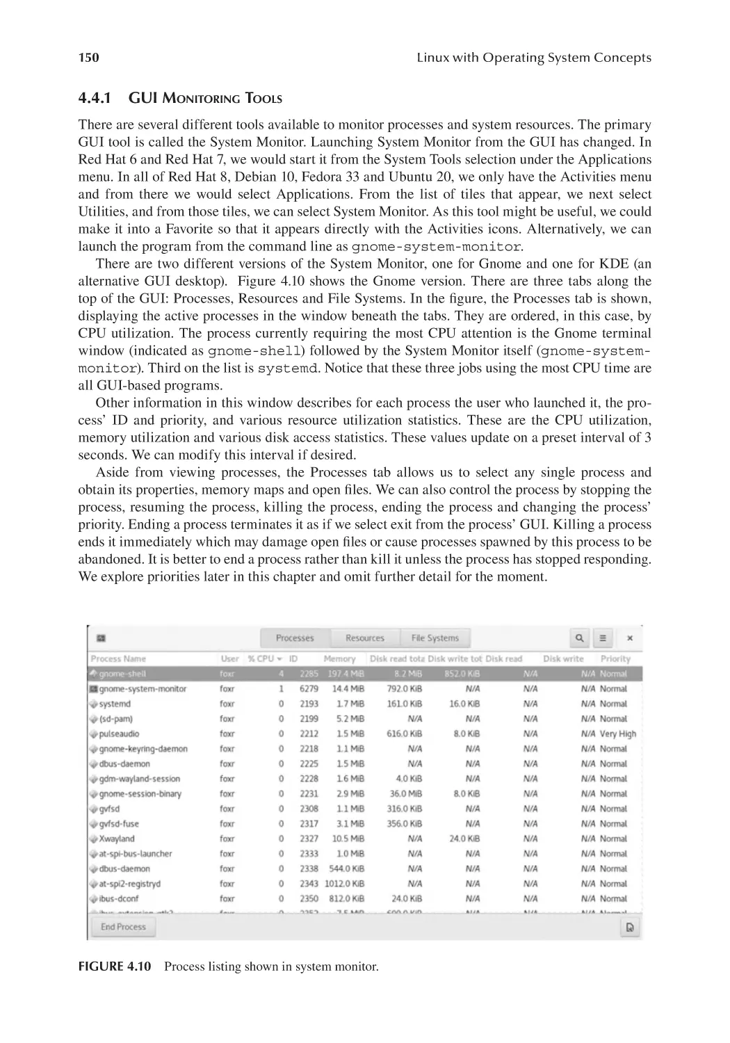
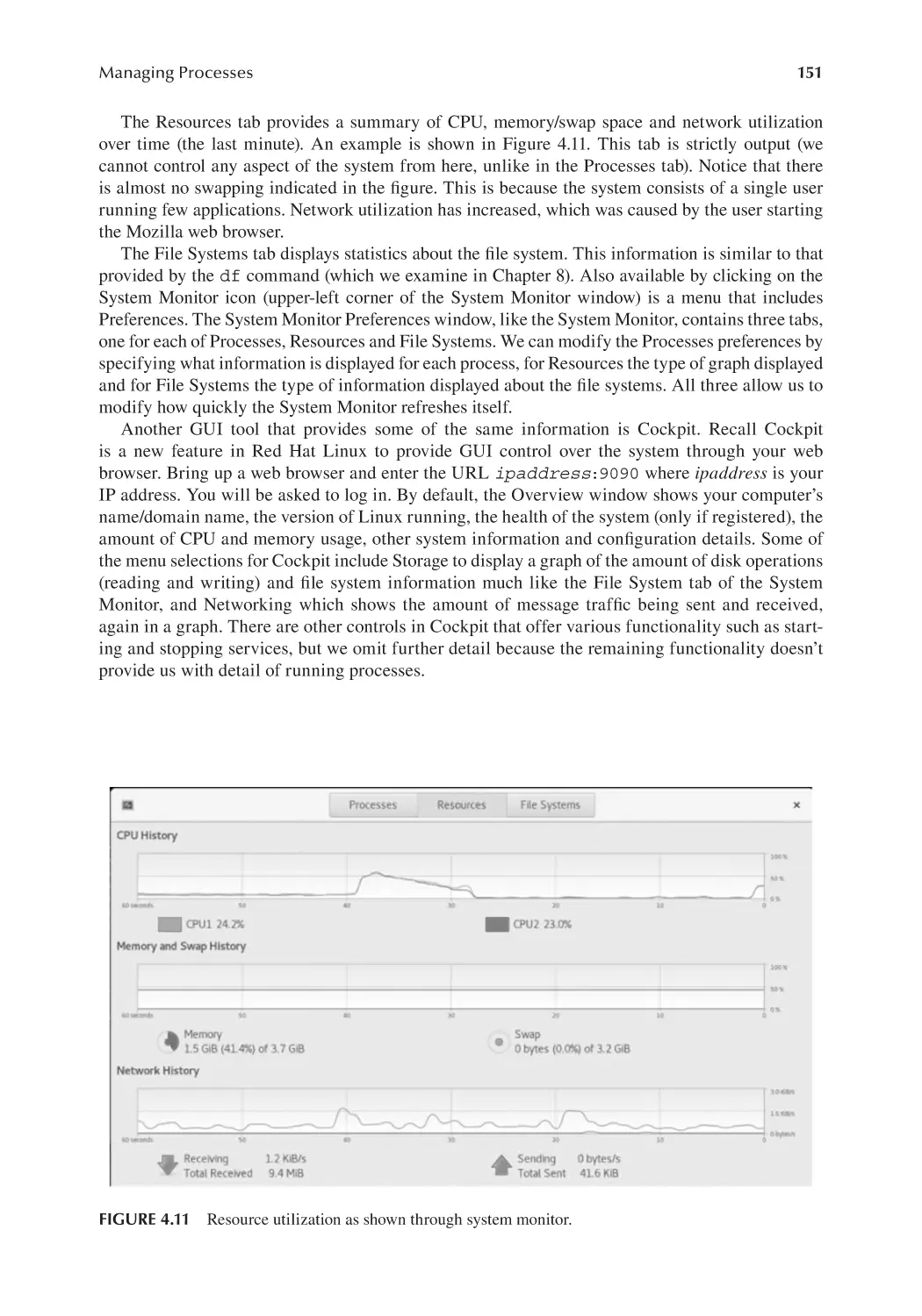
4.3.3 Suspending and Resuming Processes from the Command Line...... 147
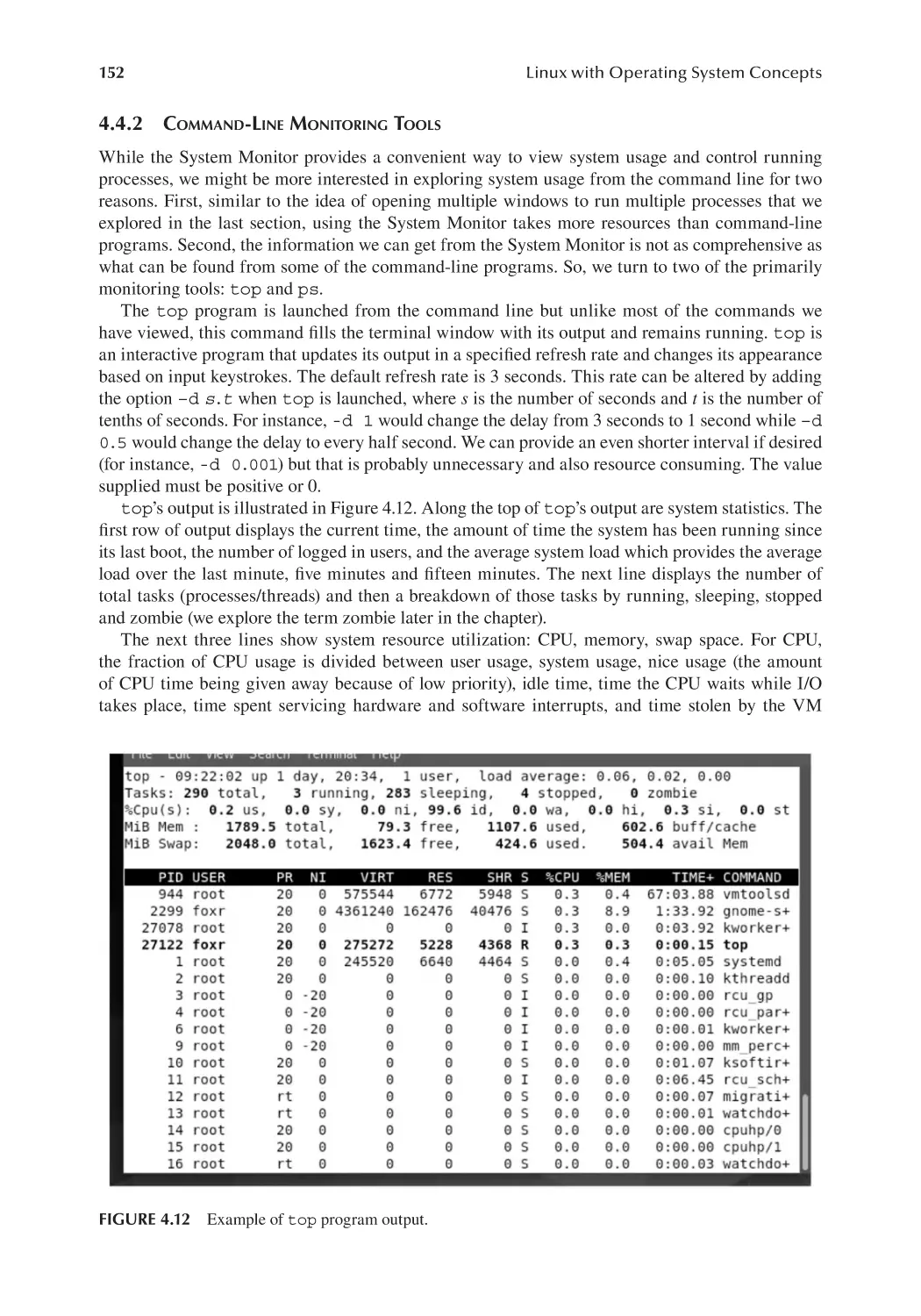
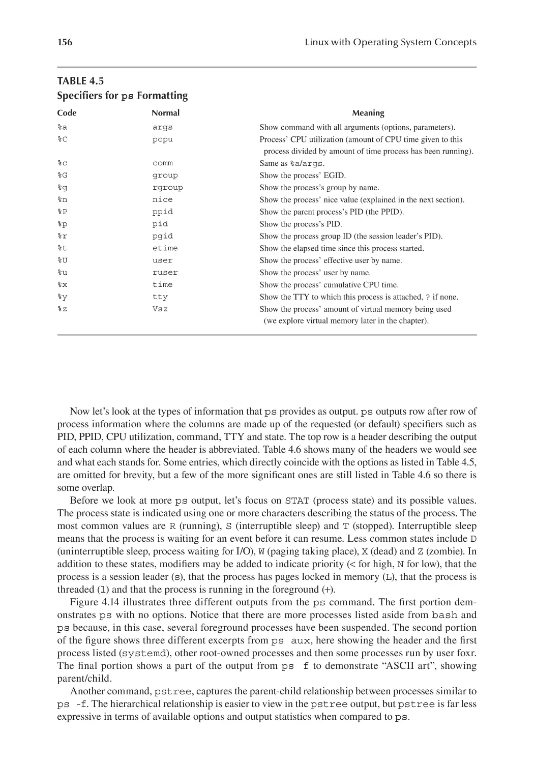
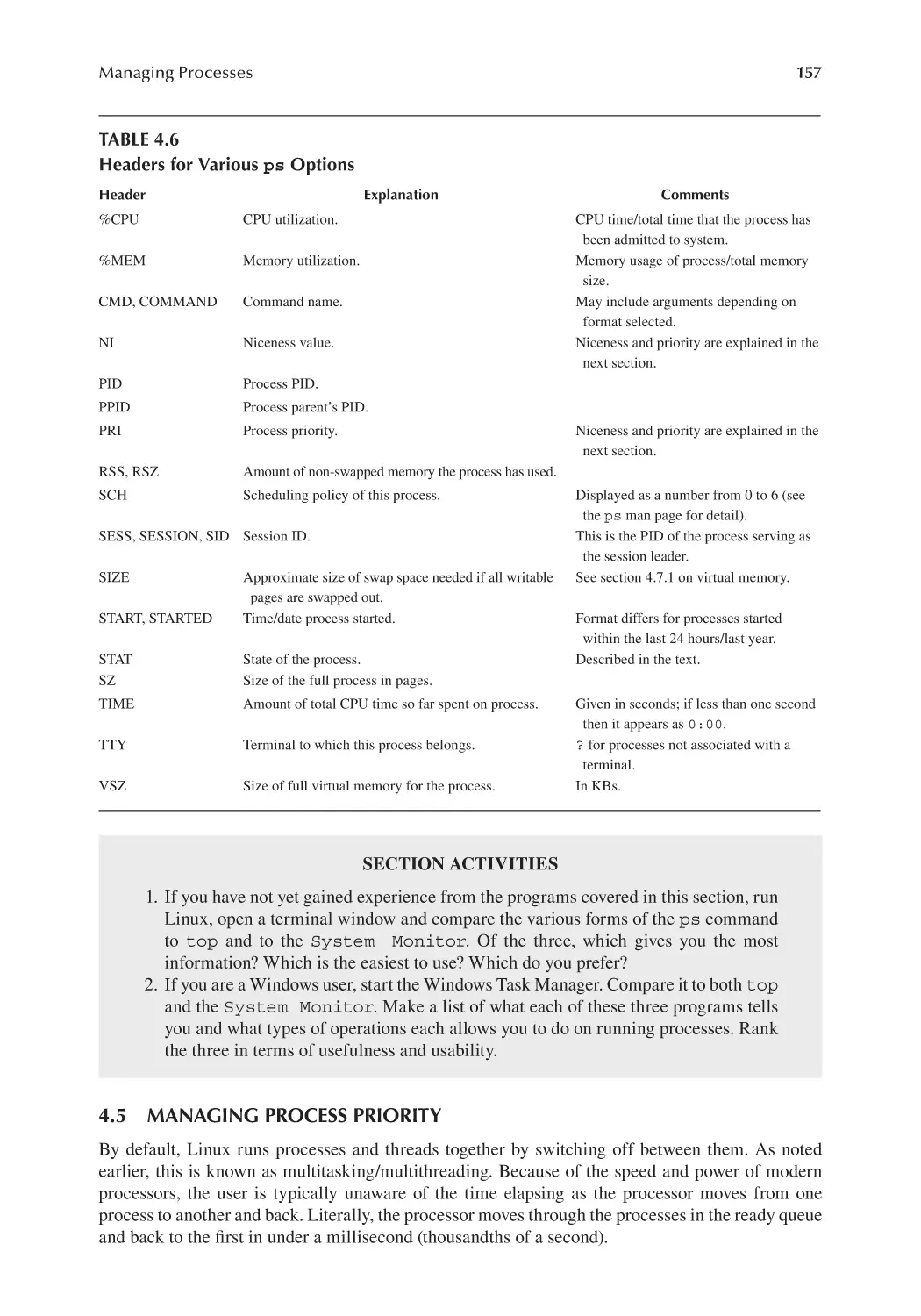
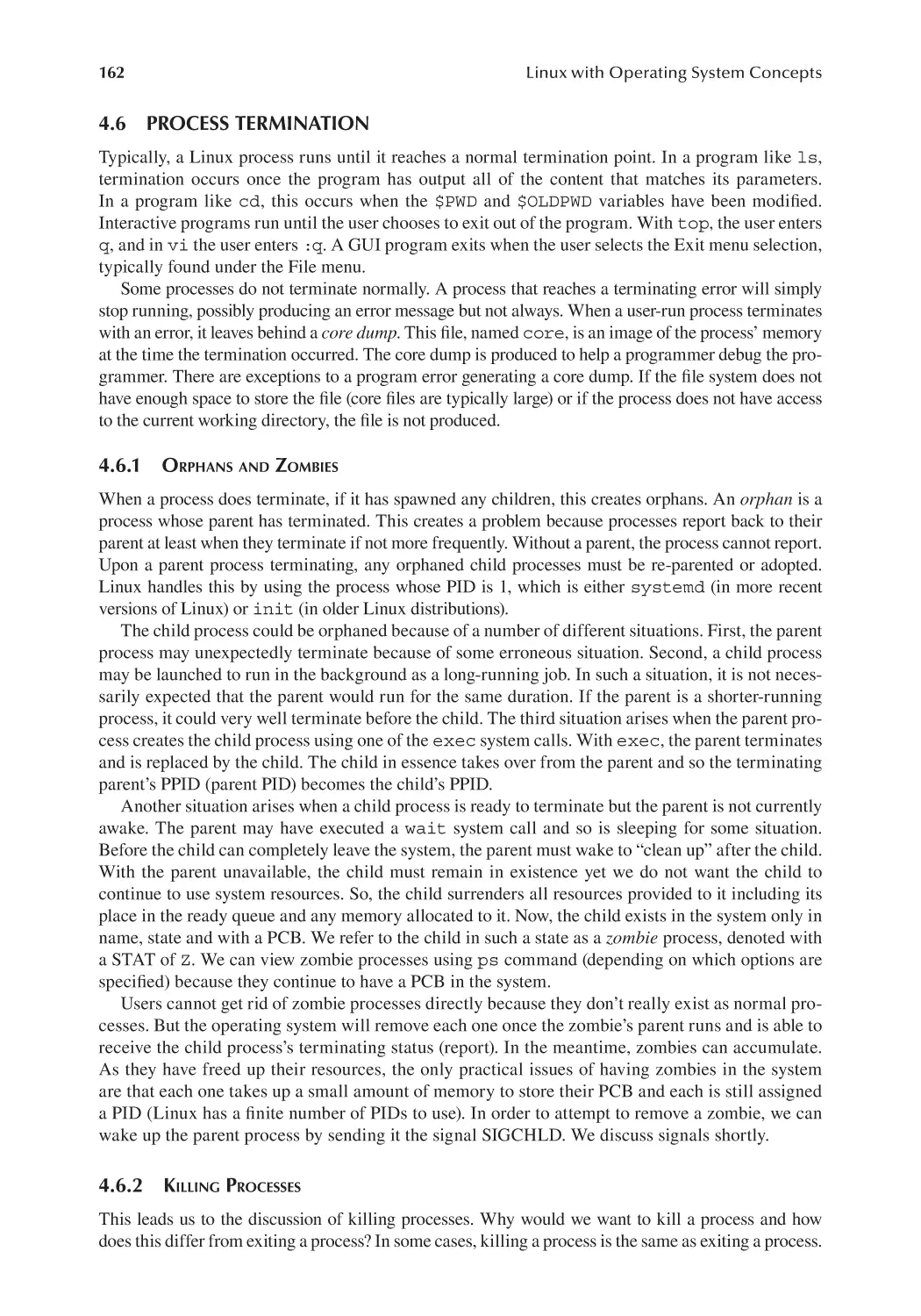
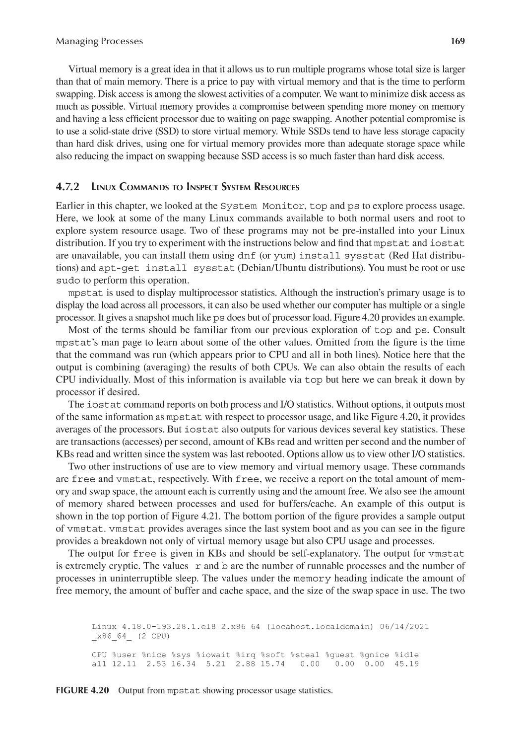
4.4 Monitoring Processes..................................................................................... 149
4.4.1 GUI Monitoring Tools....................................................................... 150
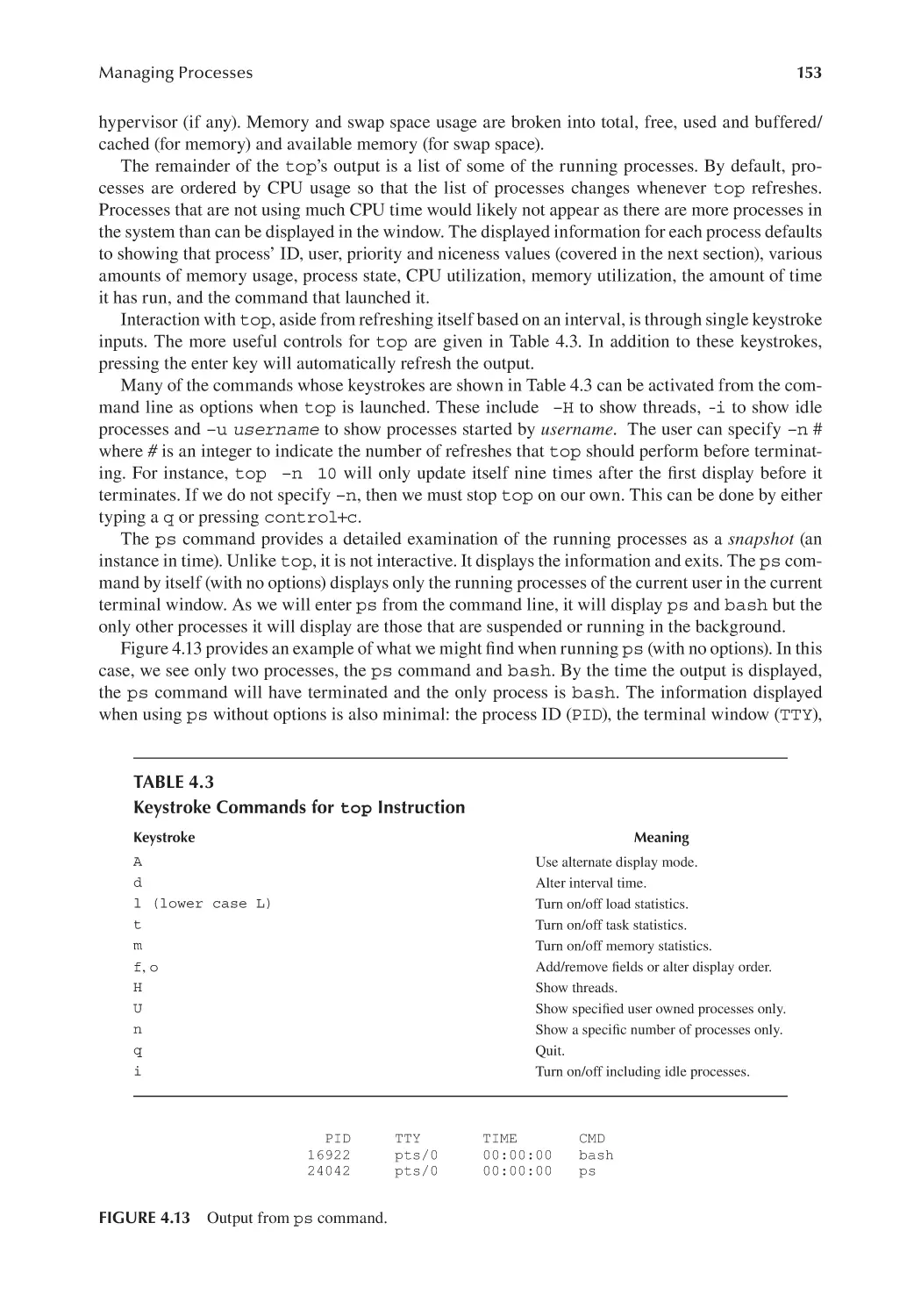
4.4.2 Command-Line Monitoring Tools.................................................... 152
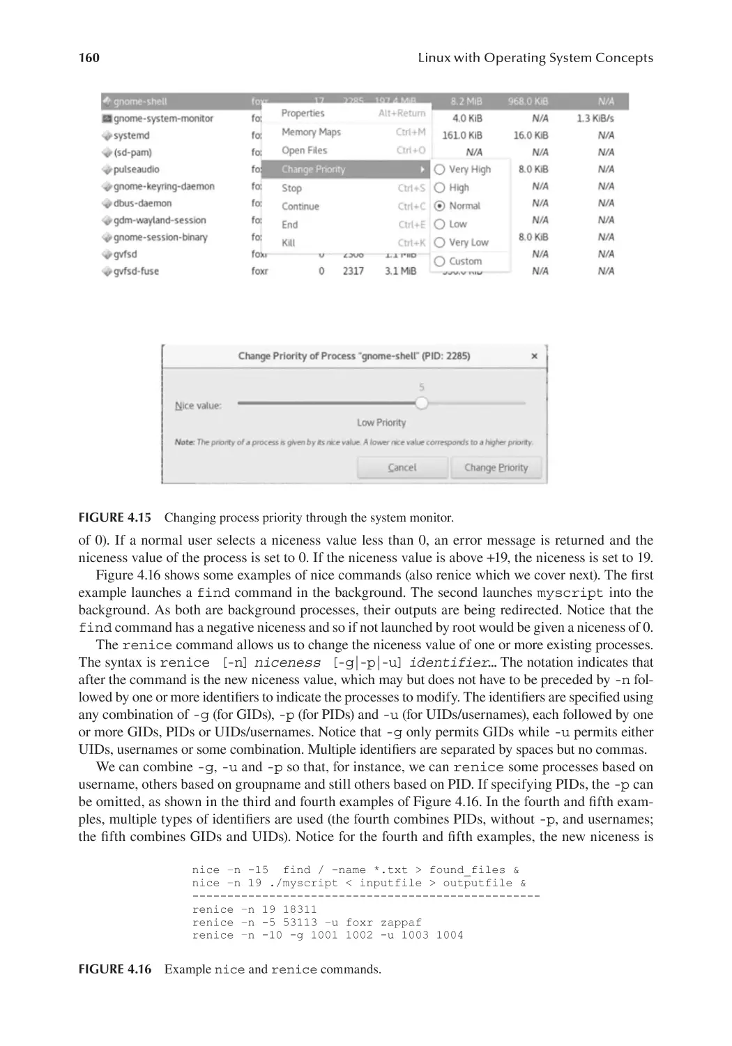
4.5 Managing Process Priority............................................................................. 157
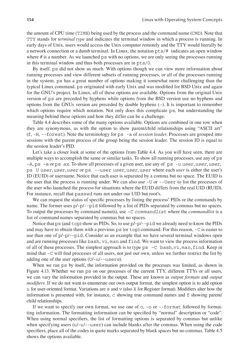
4.6 Process Termination....................................................................................... 162
4.6.1 Orphans and Zombies....................................................................... 162
4.6.2 Killing Processes............................................................................... 162
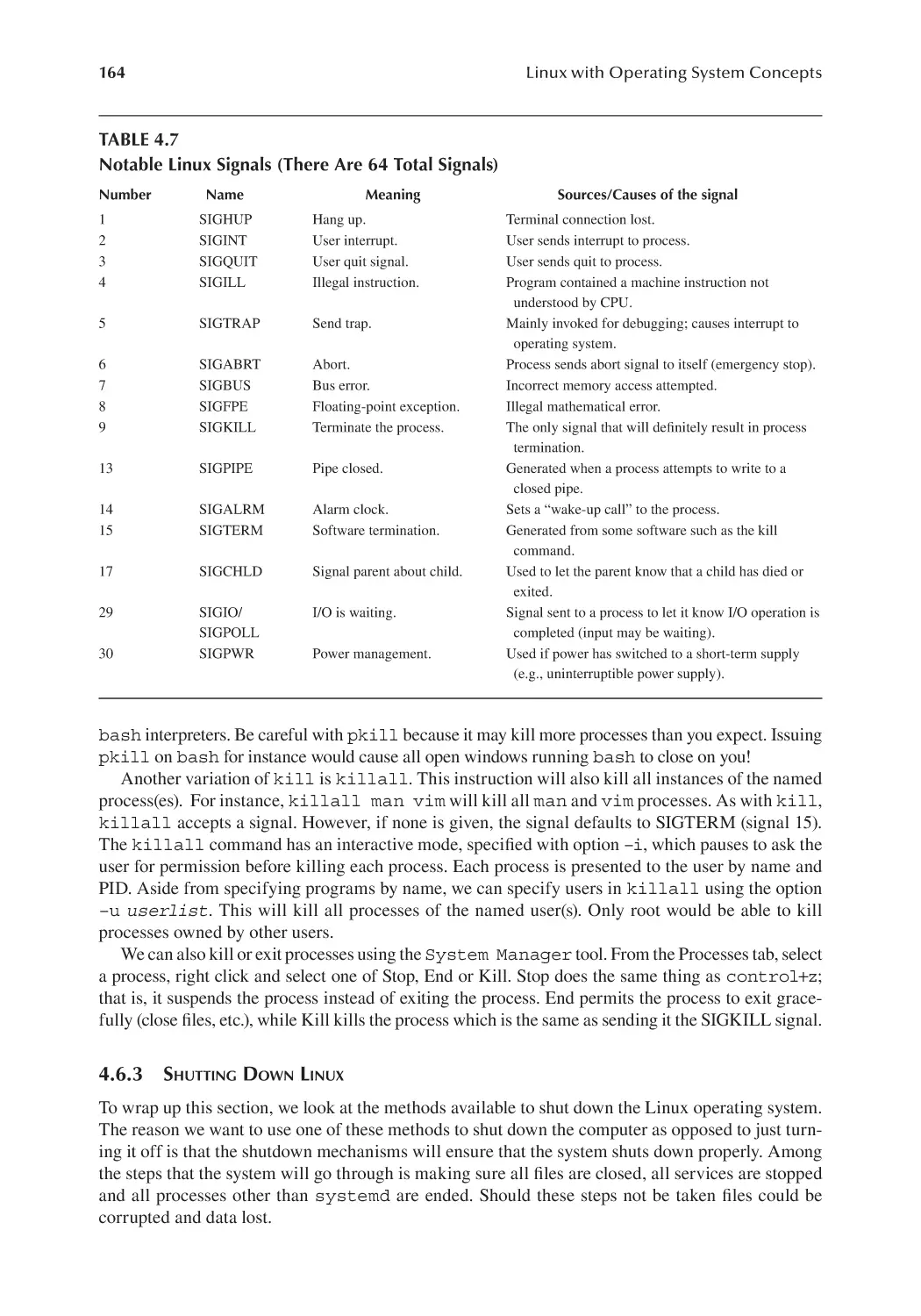
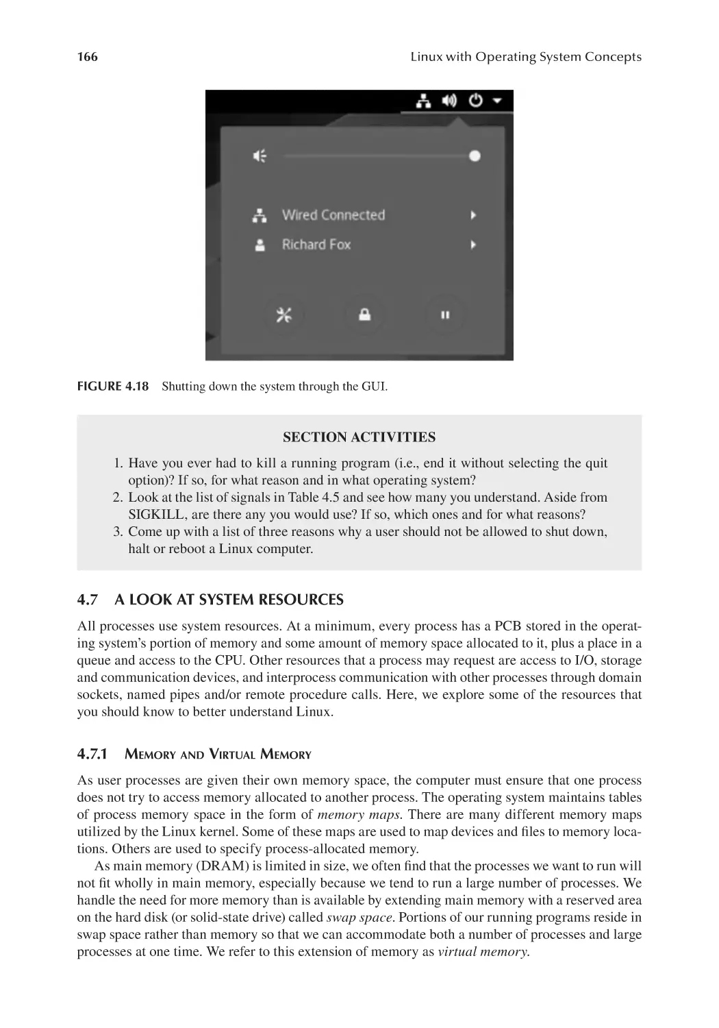
4.6.3 Shutting Down Linux........................................................................ 164
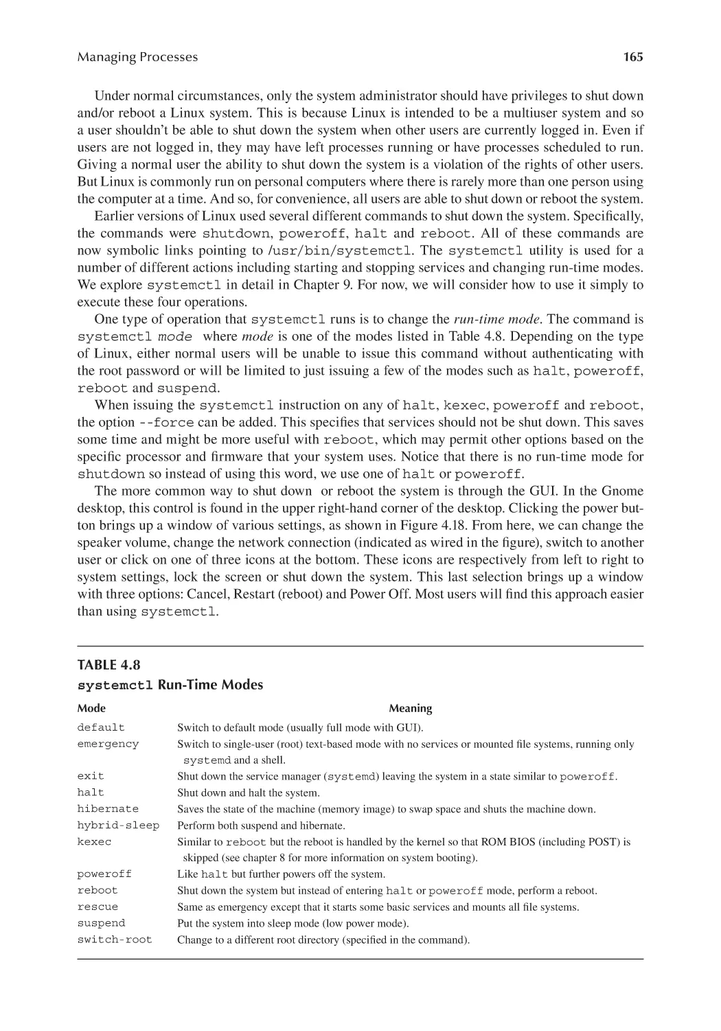
4.7 A Look at System Resources.......................................................................... 166
4.7.1 Memory and Virtual Memory........................................................... 166
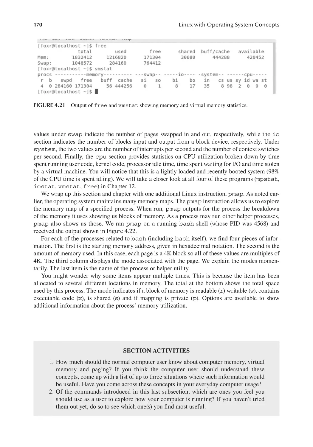
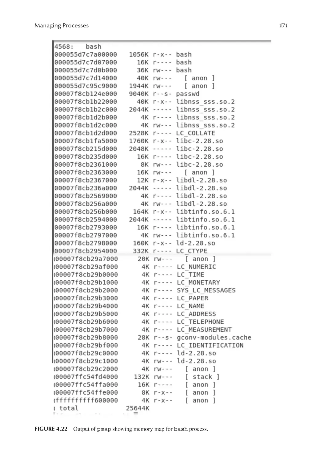
4.7.2 Linux Commands to Inspect System Resources............................... 169
4.8 Chapter Review.............................................................................................. 172
Review Questions...................................................................................................... 175
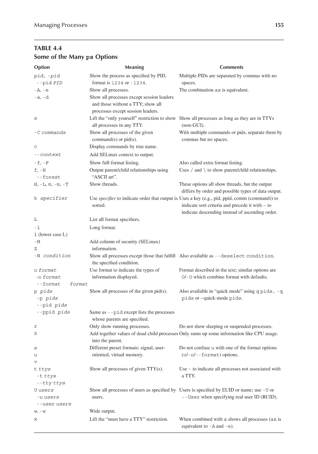
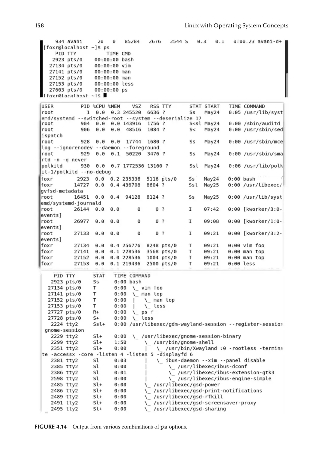
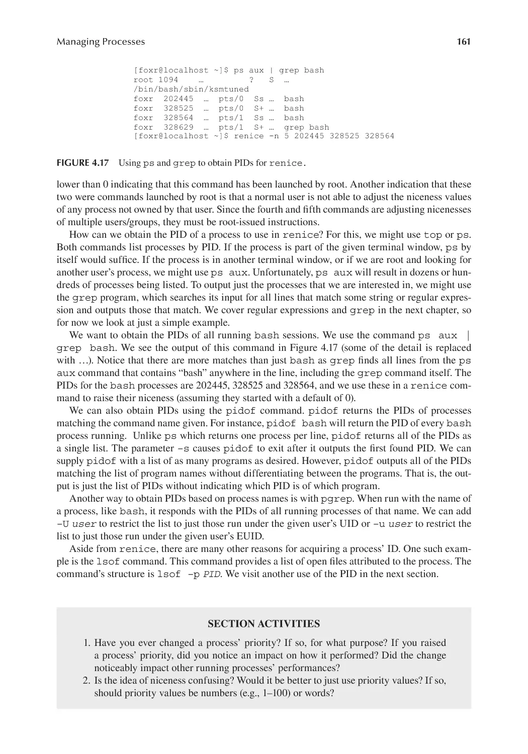
Chapter 5
Regular Expressions.................................................................................................. 179
5.1
5.2
5.3
5.4
5.5
5.6
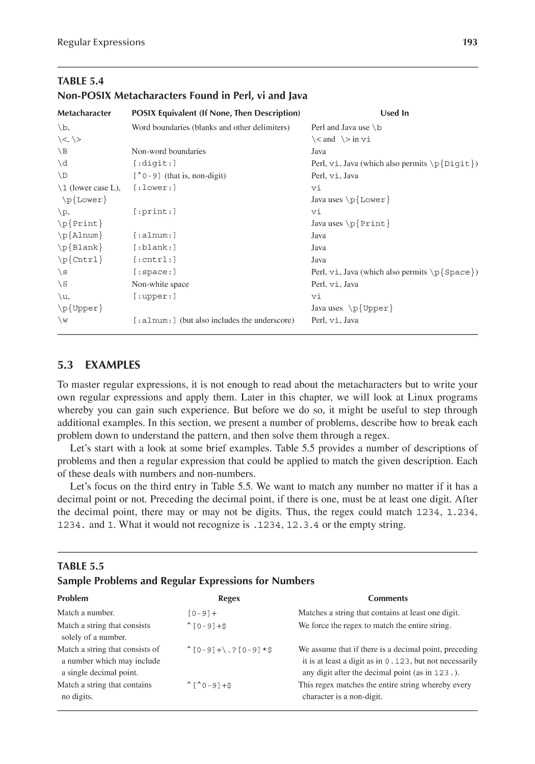
Introduction.................................................................................................... 179
Metacharacters............................................................................................... 180
5.2.1 Controlling Repeated Characters through *, + and ?....................... 182
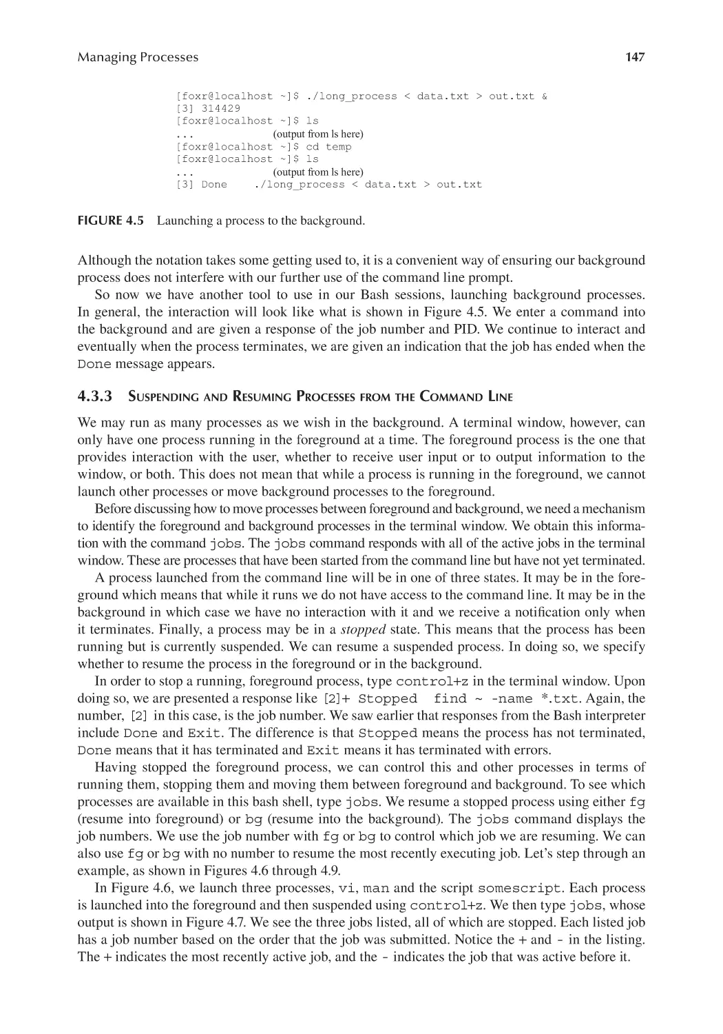
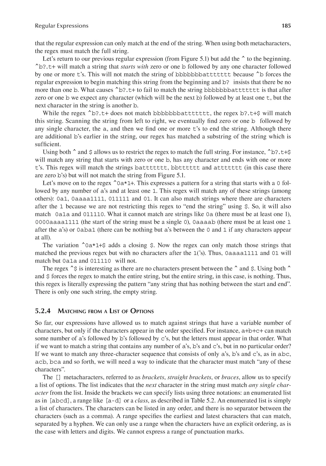
5.2.2 Using and Modifying the . Metacharacter........................................ 183
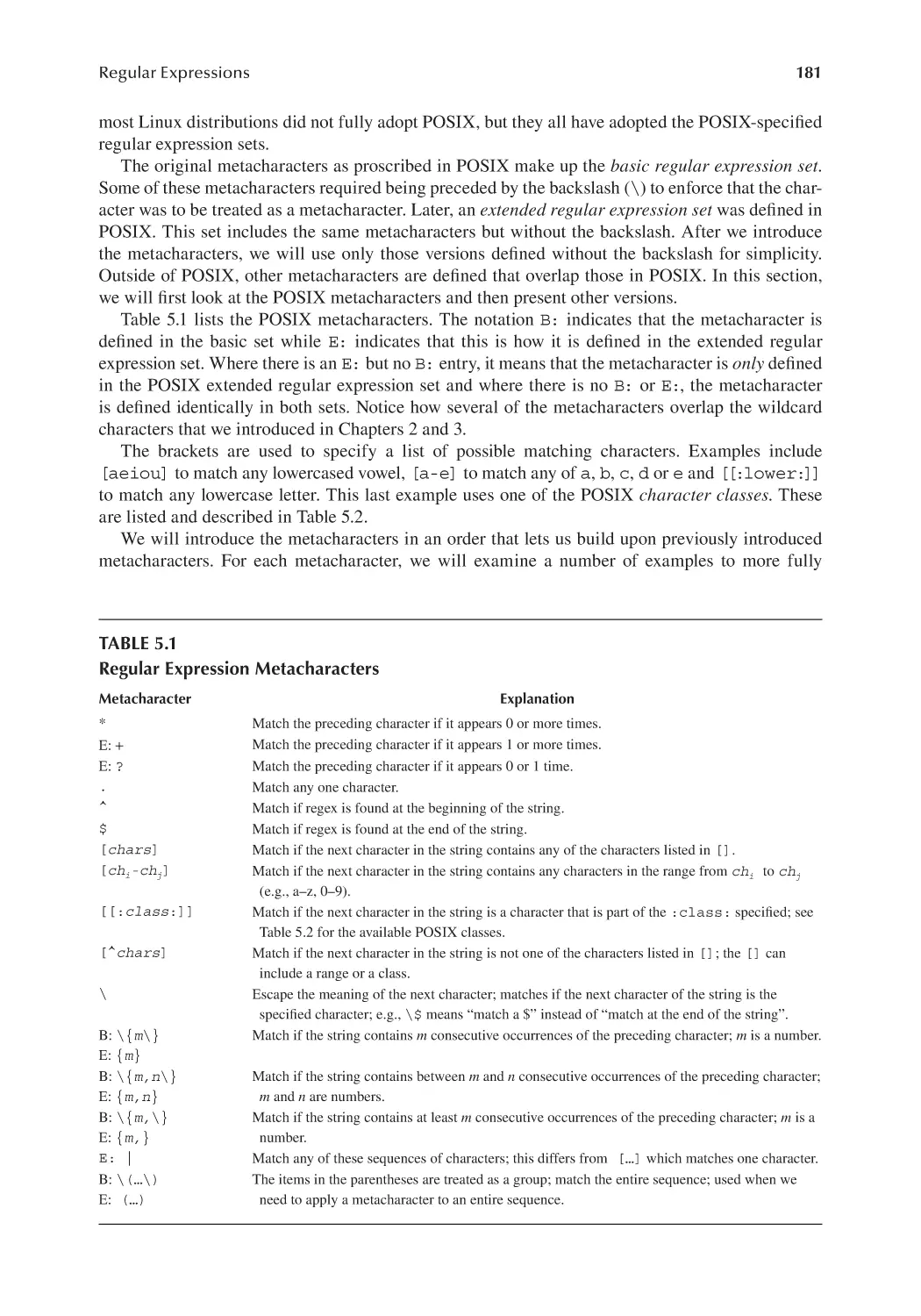
5.2.3 Controlling Where a Pattern Matches............................................... 184
5.2.4 Matching from a List of Options....................................................... 185
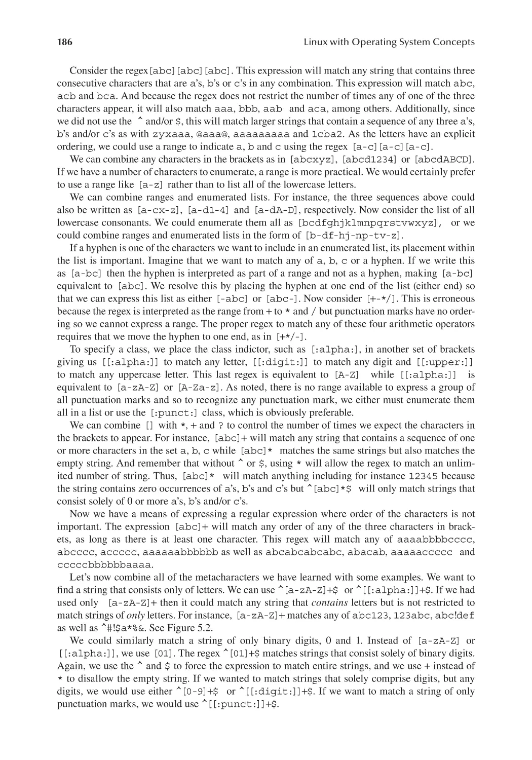
5.2.5 Matching Characters That Must Not Appear.................................... 187
5.2.6 Matching Metacharacters Literally................................................... 188
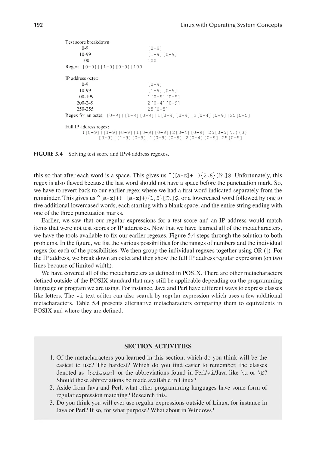
5.2.7 More Precisely Controlling Repetition............................................. 189
5.2.8 Selecting between Sequences............................................................ 190
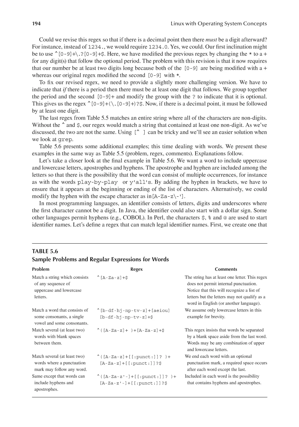
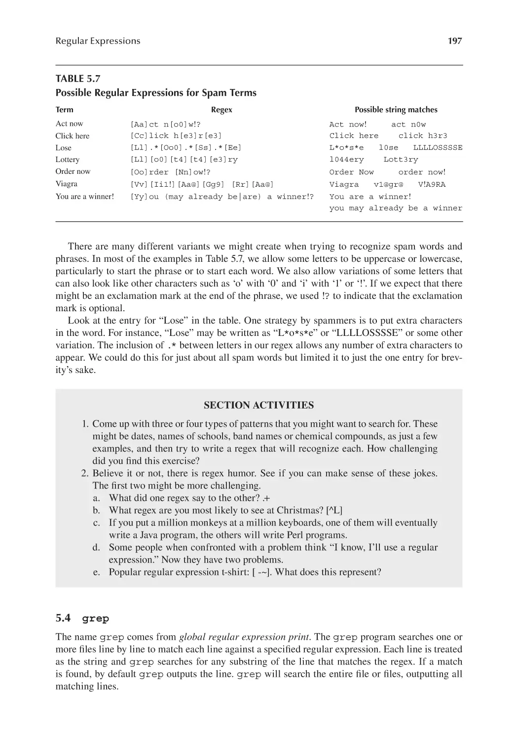
Examples ....................................................................................................... 193
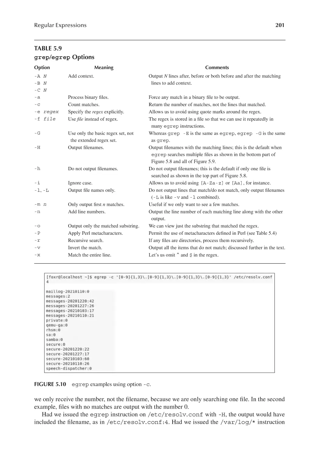
grep...............................................................................................................197
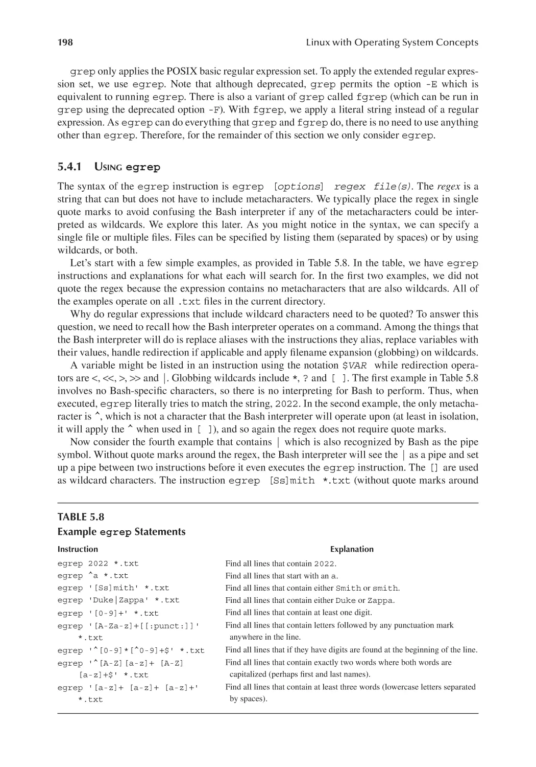
5.4.1 Using egrep..................................................................................... 198
5.4.2 Useful egrep Options......................................................................200
5.4.3 Examples: Searching the Linux Dictionary......................................202
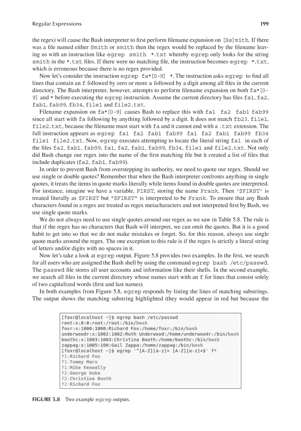
5.4.4 Using egrep to Control the Output of Other Linux Commands.....204
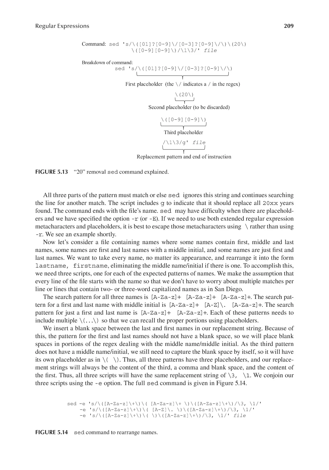
sed.................................................................................................................206
5.5.1 Basic sed Syntax..............................................................................206
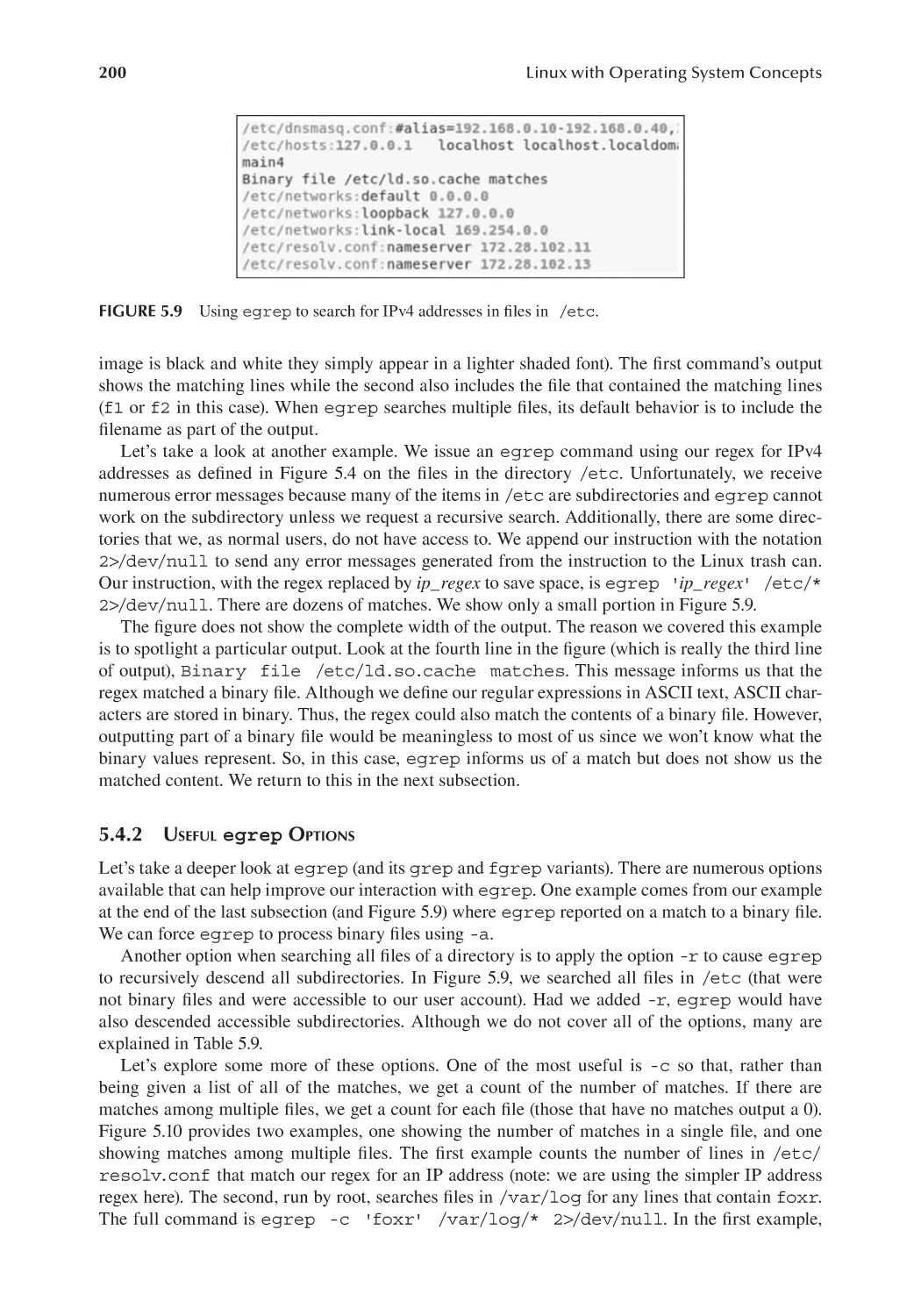
5.5.2 Placeholders.......................................................................................208
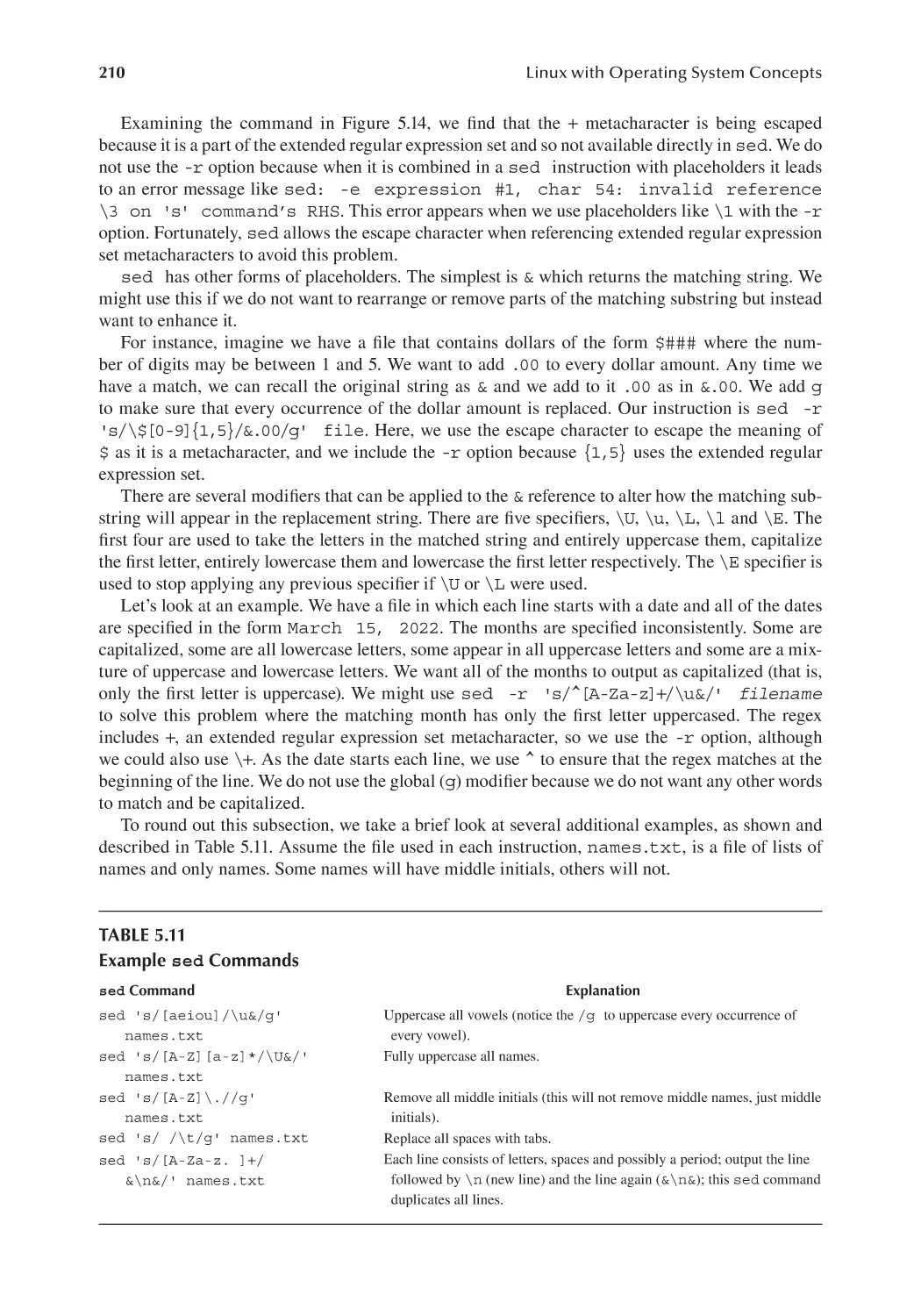
5.5.3 Other sed Capabilities..................................................................... 211
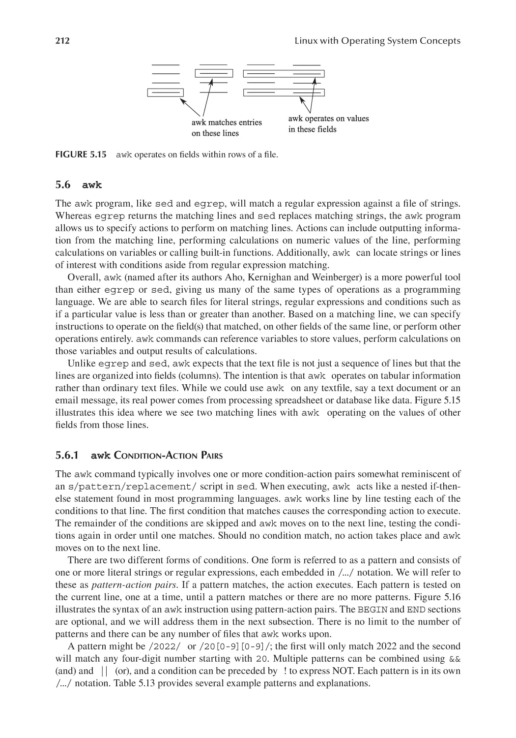
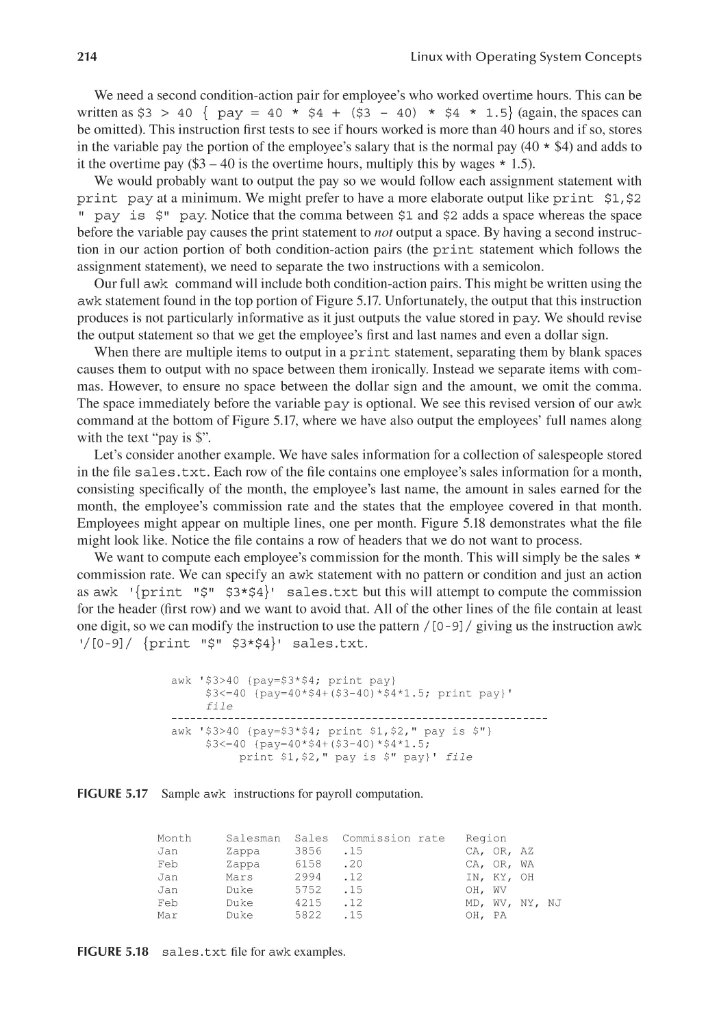
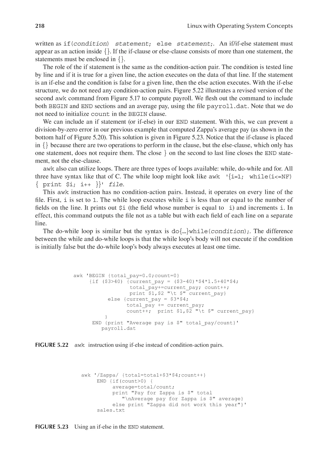
awk................................................................................................................. 212
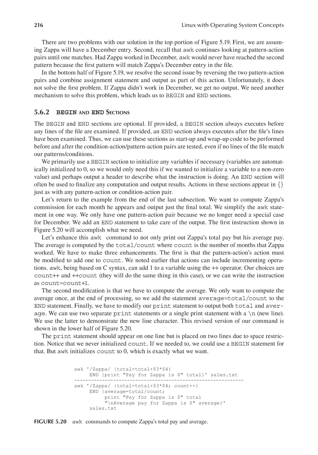
5.6.1 awk Condition-Action Pairs.............................................................. 212
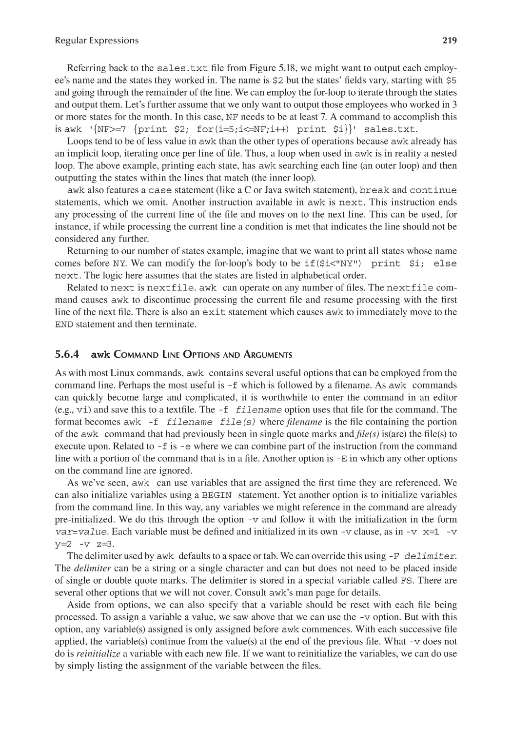
5.6.2 BEGIN and END Sections................................................................. 216
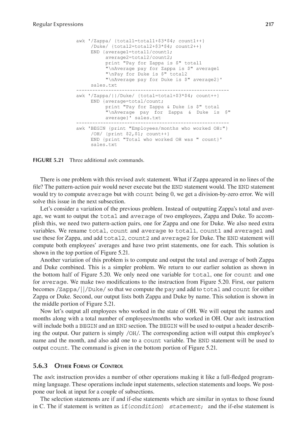
5.6.3 Other Forms of Control..................................................................... 217
x
Contents
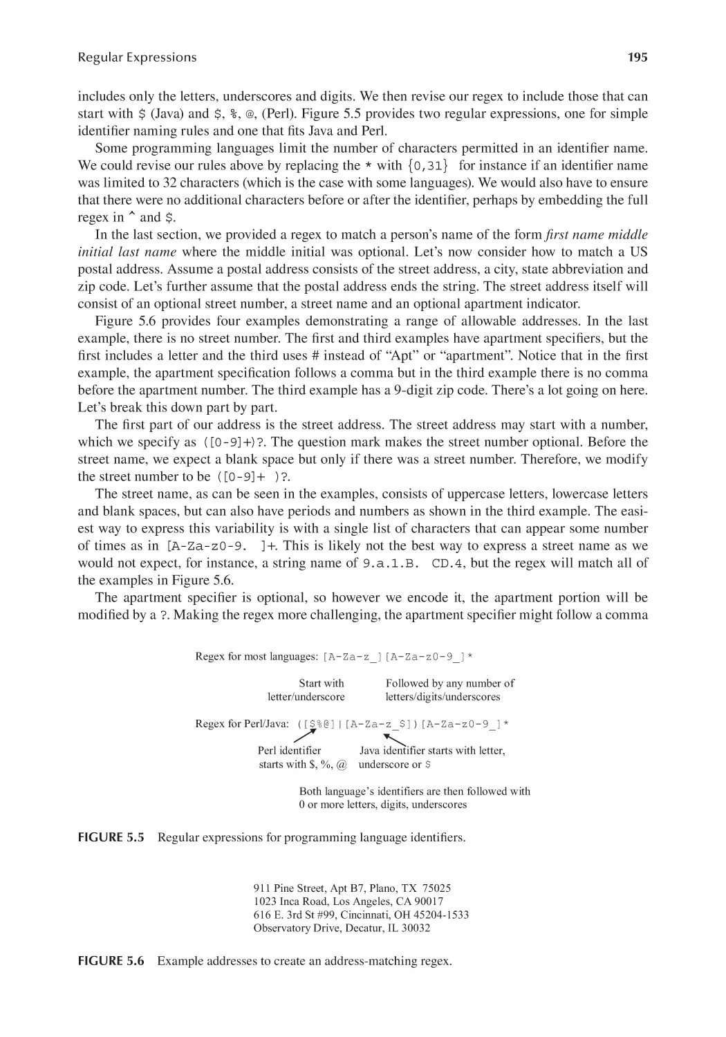
5.6.4 awk Command Line Options and Arguments.................................. 219
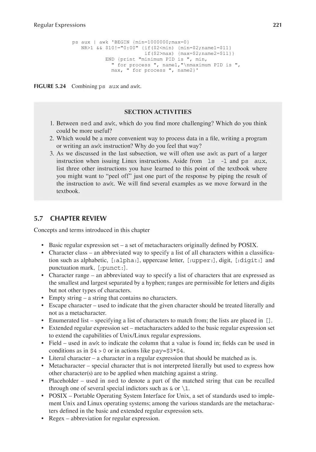
5.6.5 Non-File Input to awk....................................................................... 220
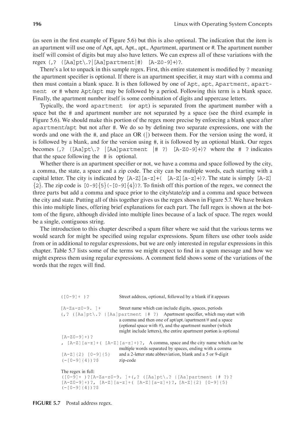
5.7 Chapter Review.............................................................................................. 221
Review Questions...................................................................................................... 222
Chapter 6
Shell Scripting........................................................................................................... 229
6.1
6.2
Introduction.................................................................................................... 229
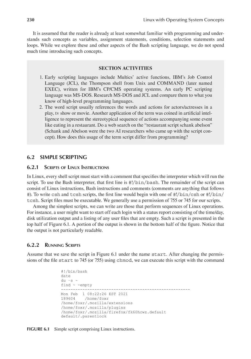
Simple Scripting............................................................................................. 230
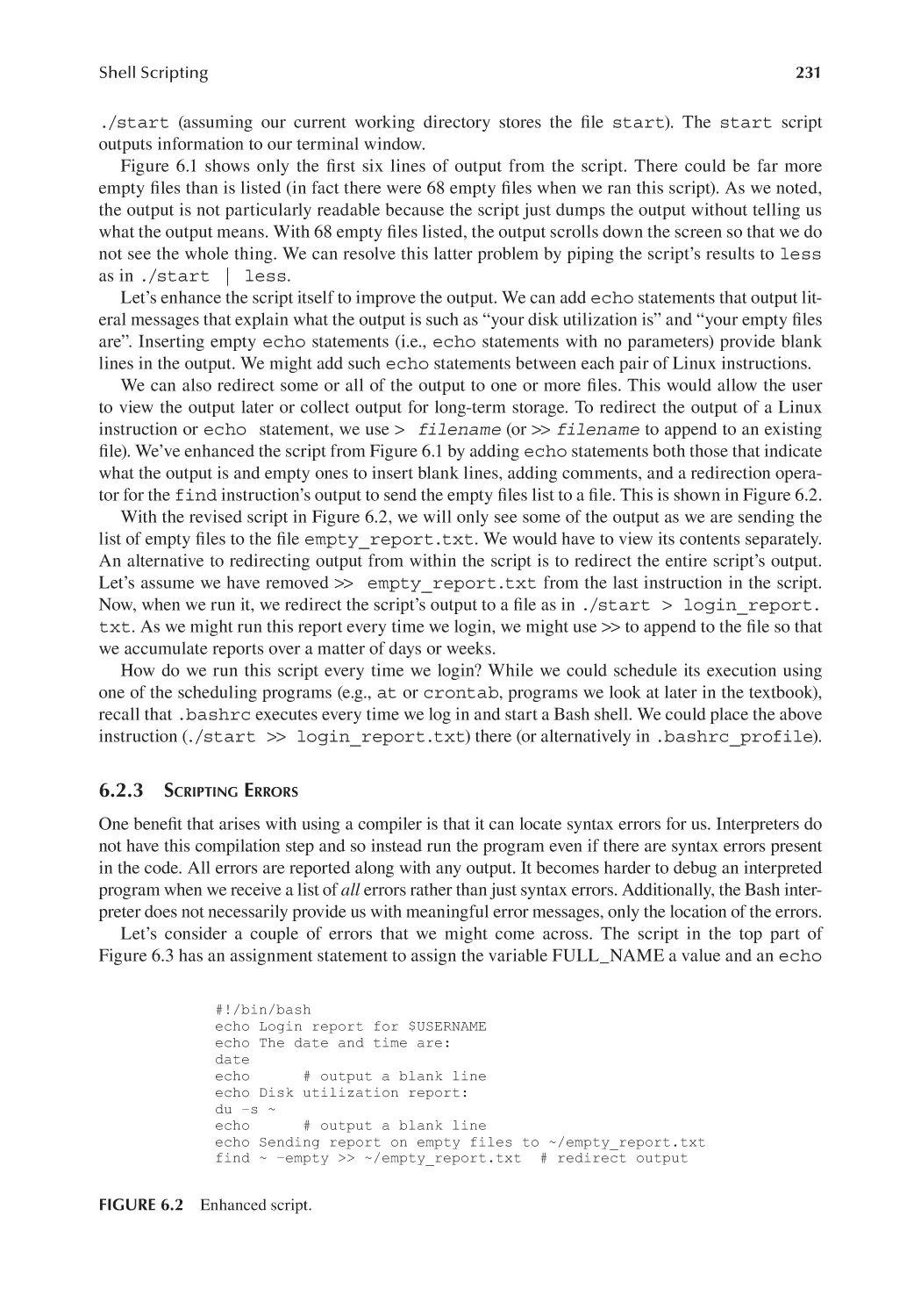
6.2.1 Scripts of Linux Instructions............................................................. 230
6.2.2 Running Scripts................................................................................. 230
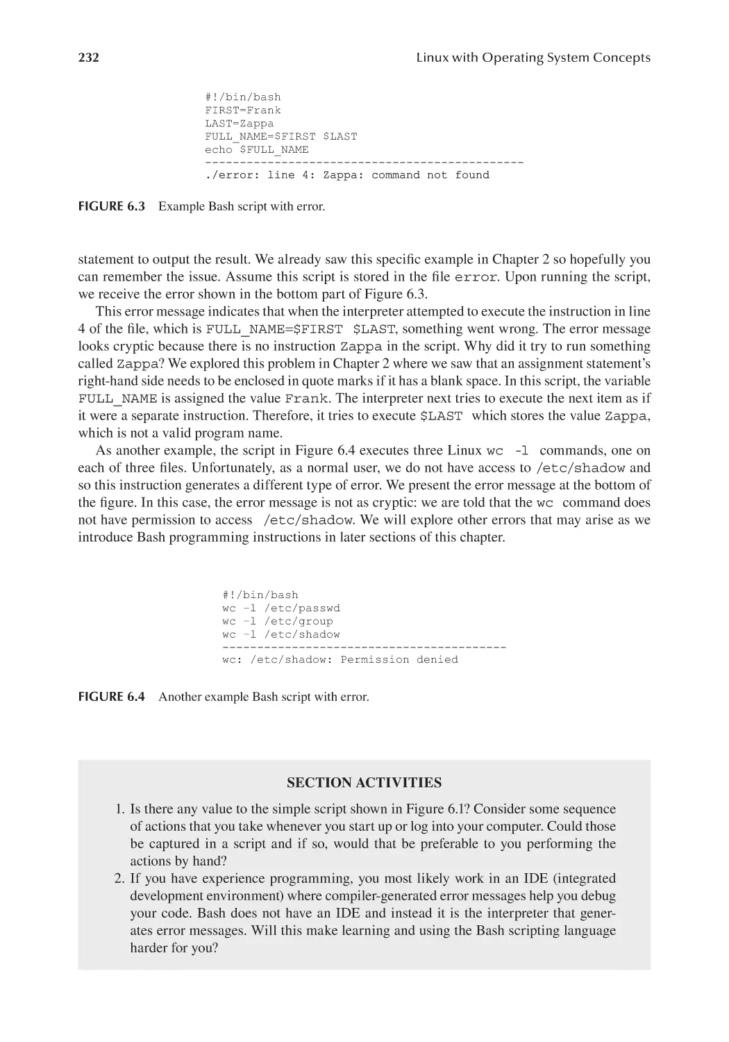
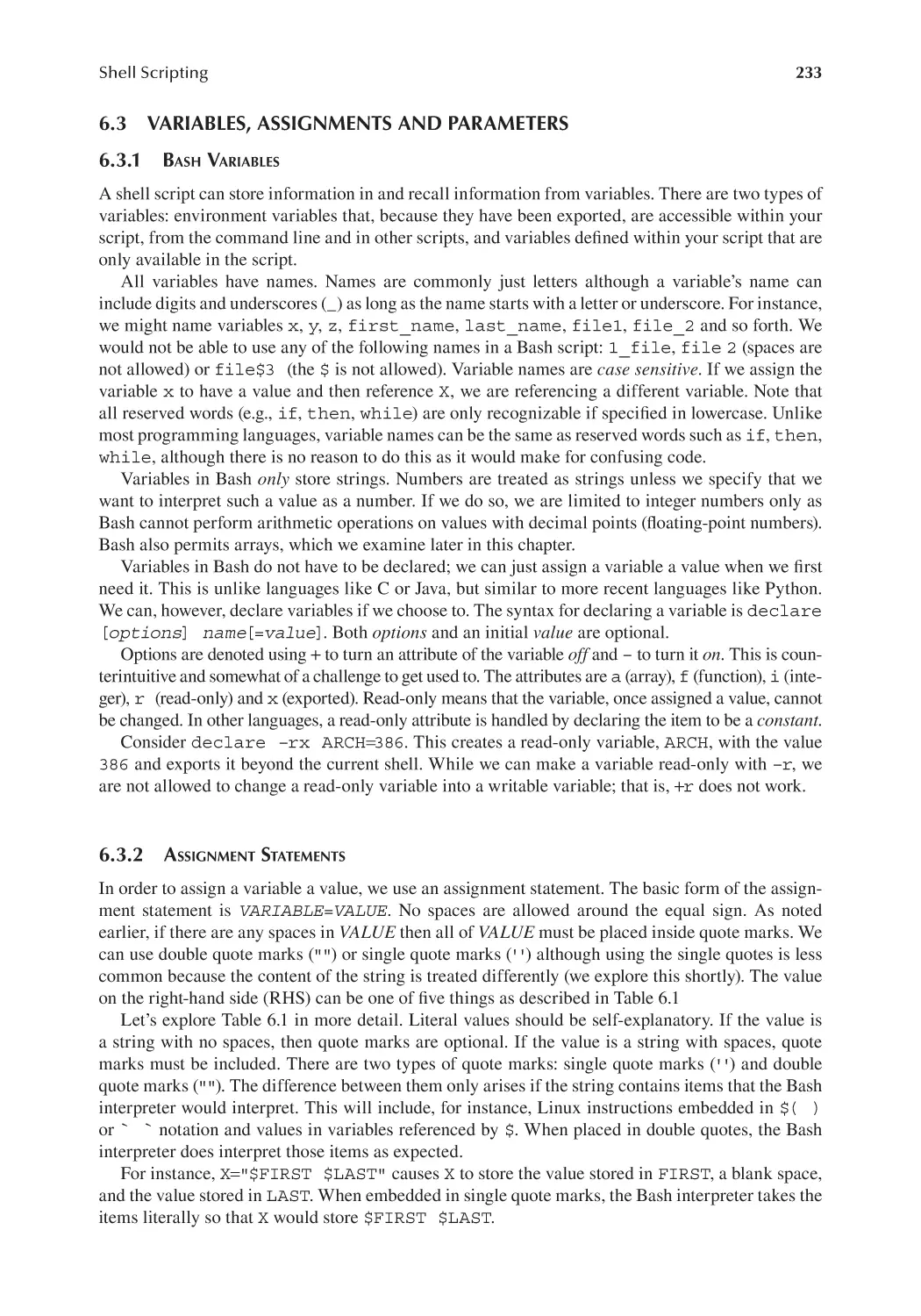
6.2.3 Scripting Errors................................................................................. 231
6.3 Variables, Assignments and Parameters........................................................ 233
6.3.1 Bash Variables................................................................................... 233
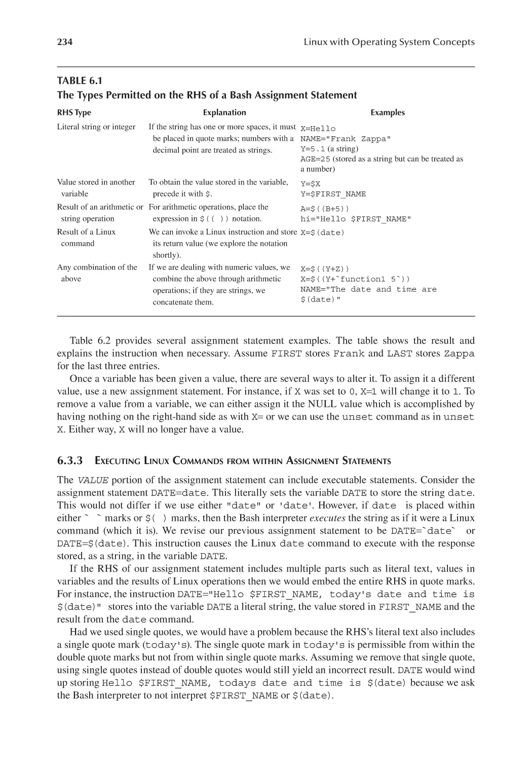
6.3.2 Assignment Statements..................................................................... 233
6.3.3 Executing Linux Commands from within Assignment Statements.. 234
6.3.4 Arithmetic Operations in Assignment Statements............................ 236
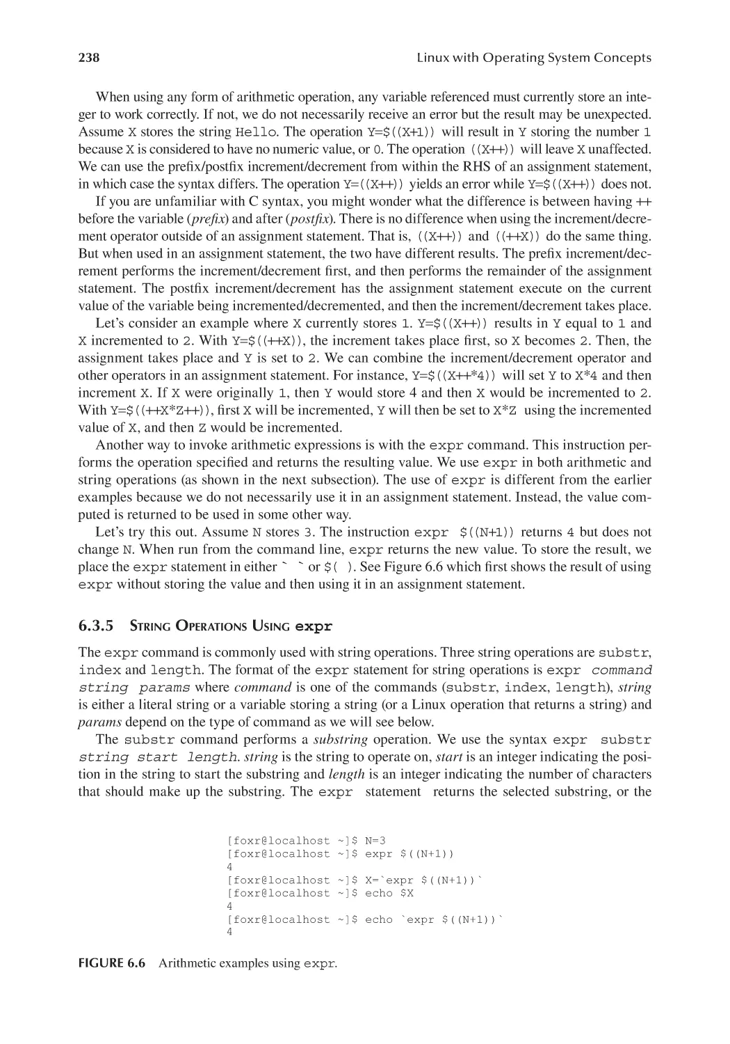
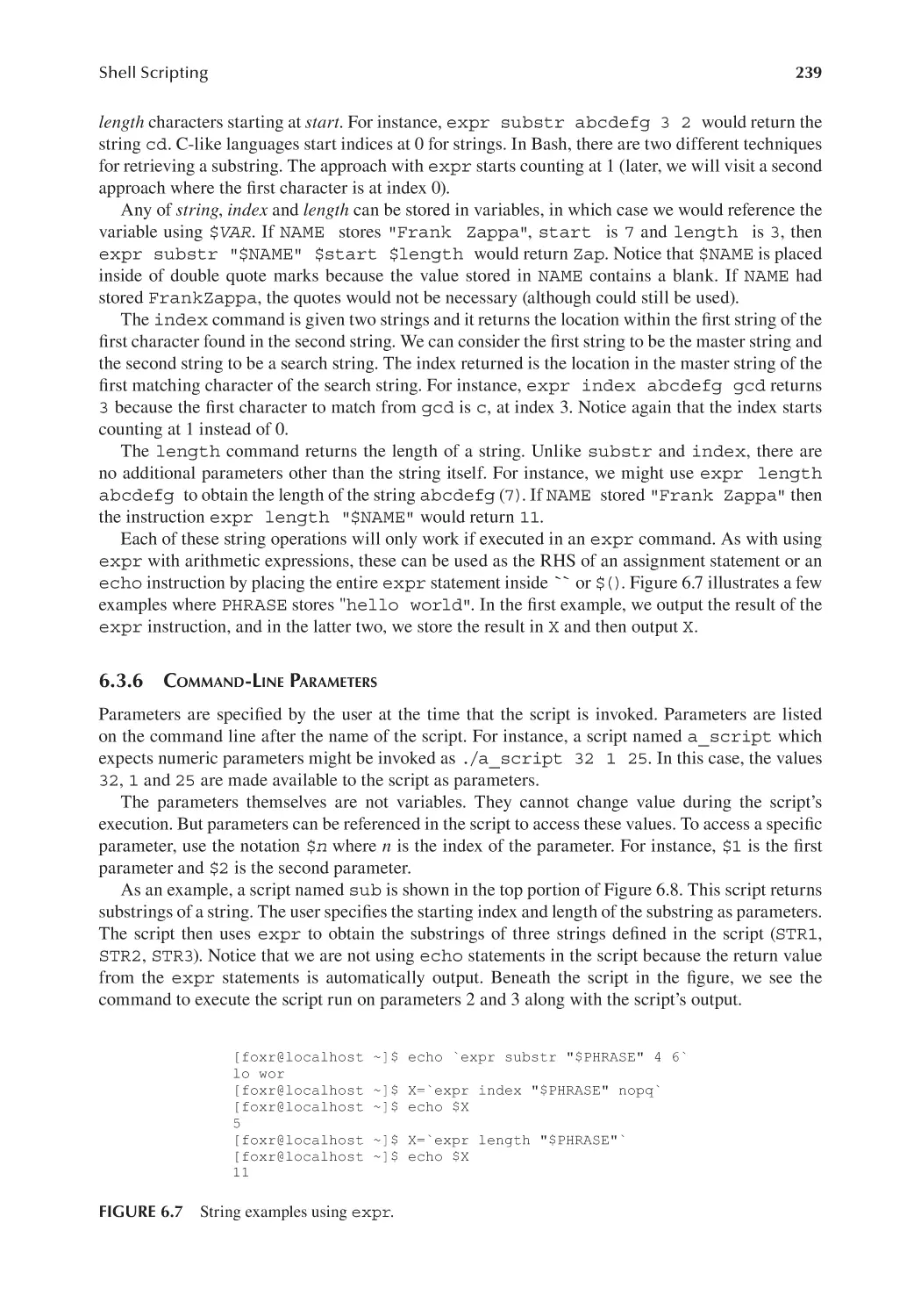
6.3.5 String Operations Using expr......................................................... 238
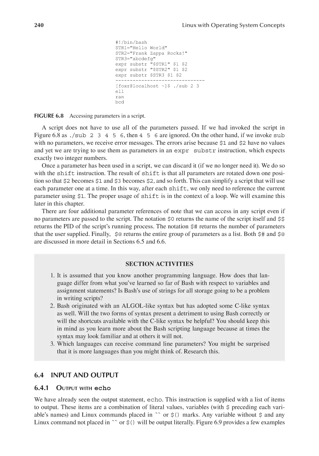
6.3.6 Command-Line Parameters.............................................................. 239
6.4 Input and Output.............................................................................................240
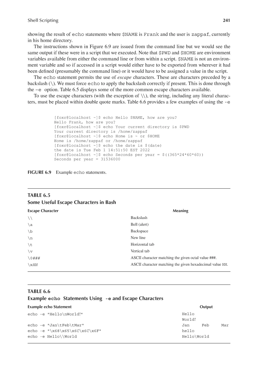
6.4.1 Output with echo.............................................................................240
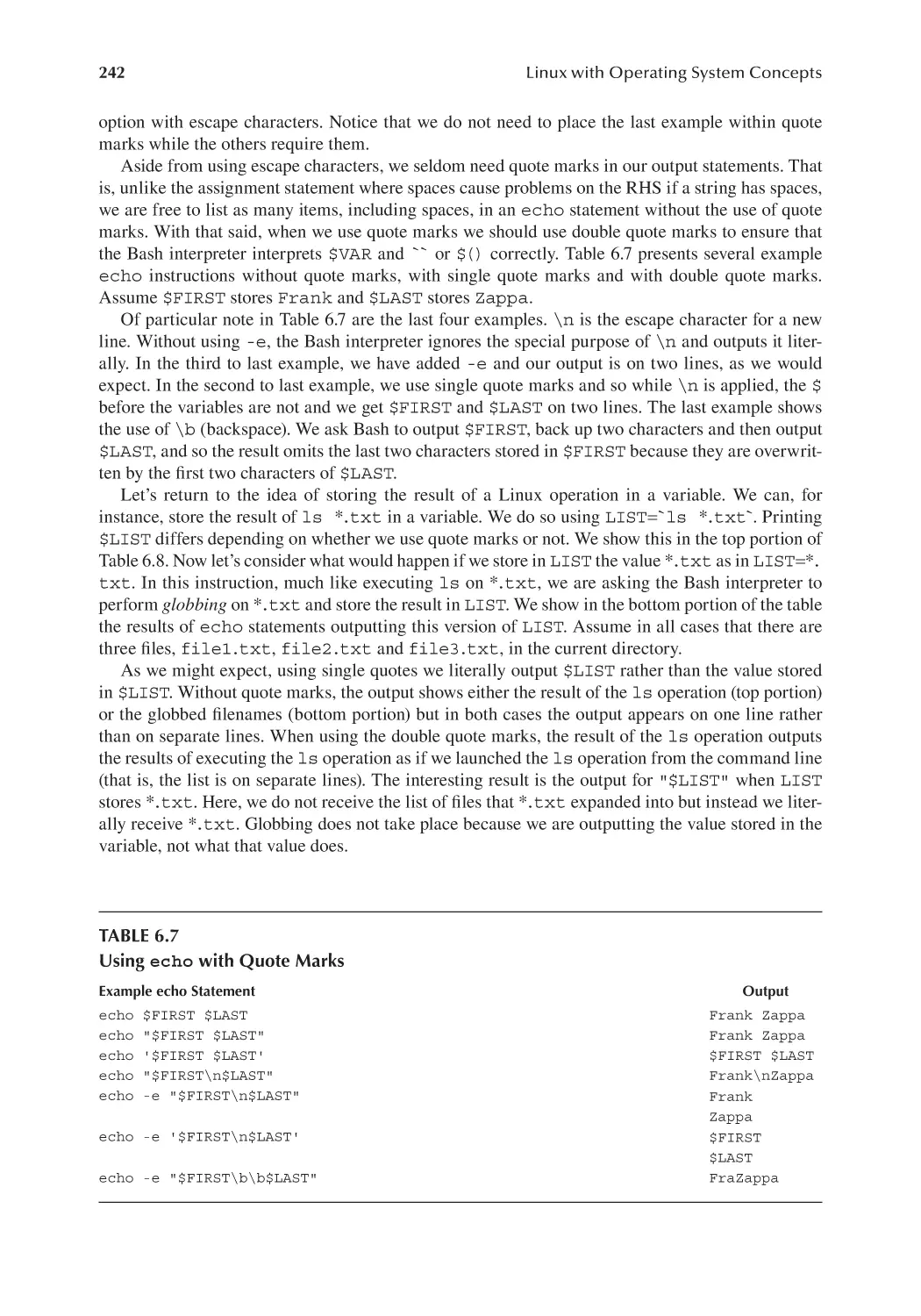
6.4.2 Input with read................................................................................ 243
6.5 Selection Statements....................................................................................... 245
6.5.1 Conditions for Strings and Integers...................................................246
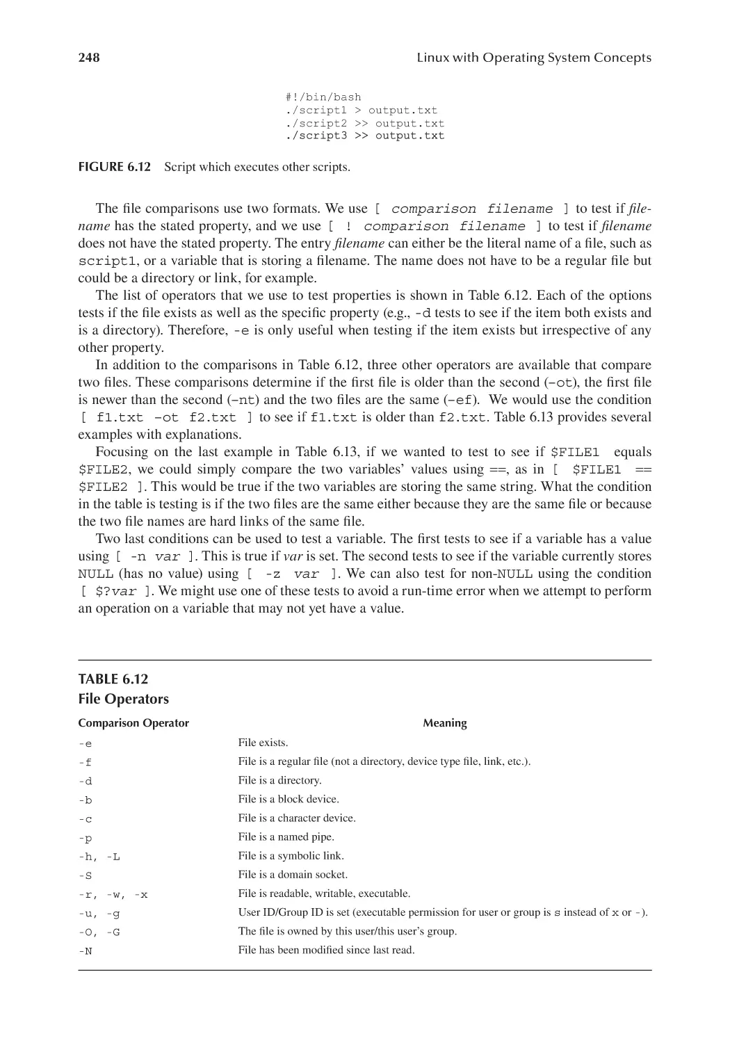
6.5.2 File Conditions.................................................................................. 247
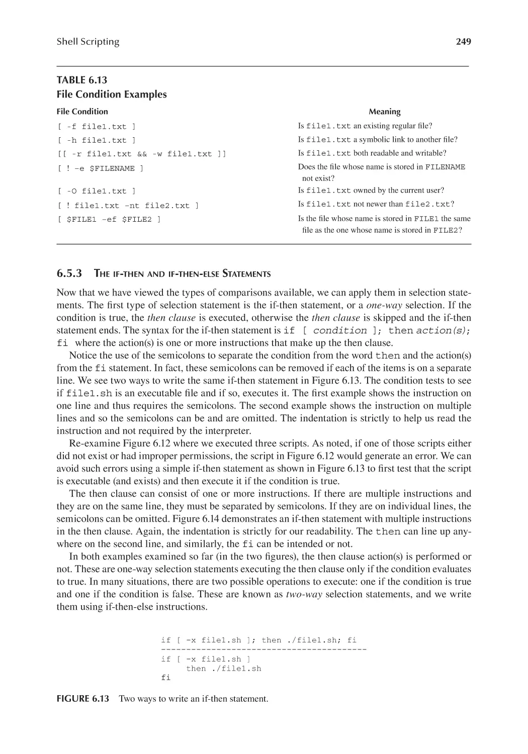
6.5.3 The if-then and if-then-else Statements............................................ 249
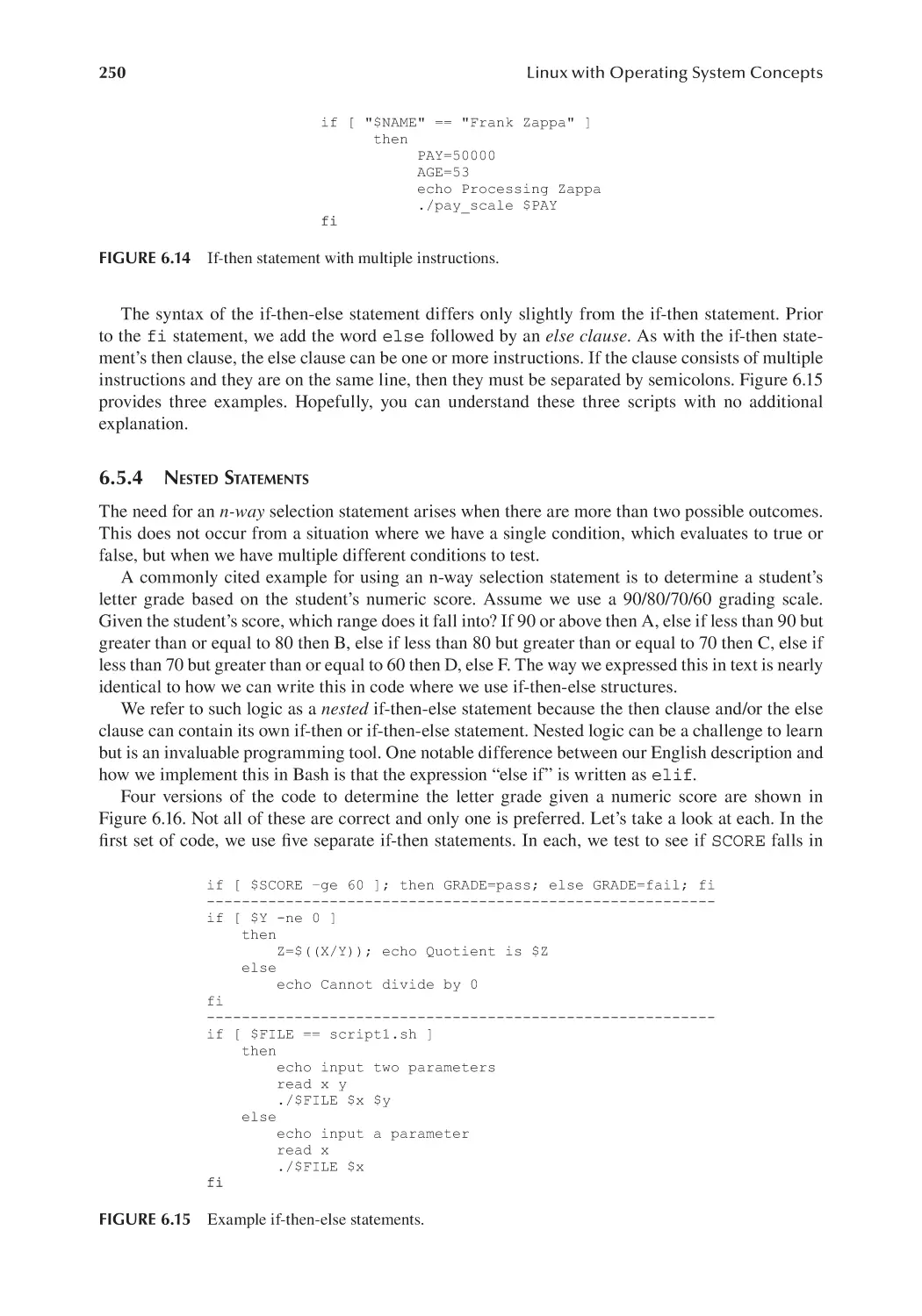
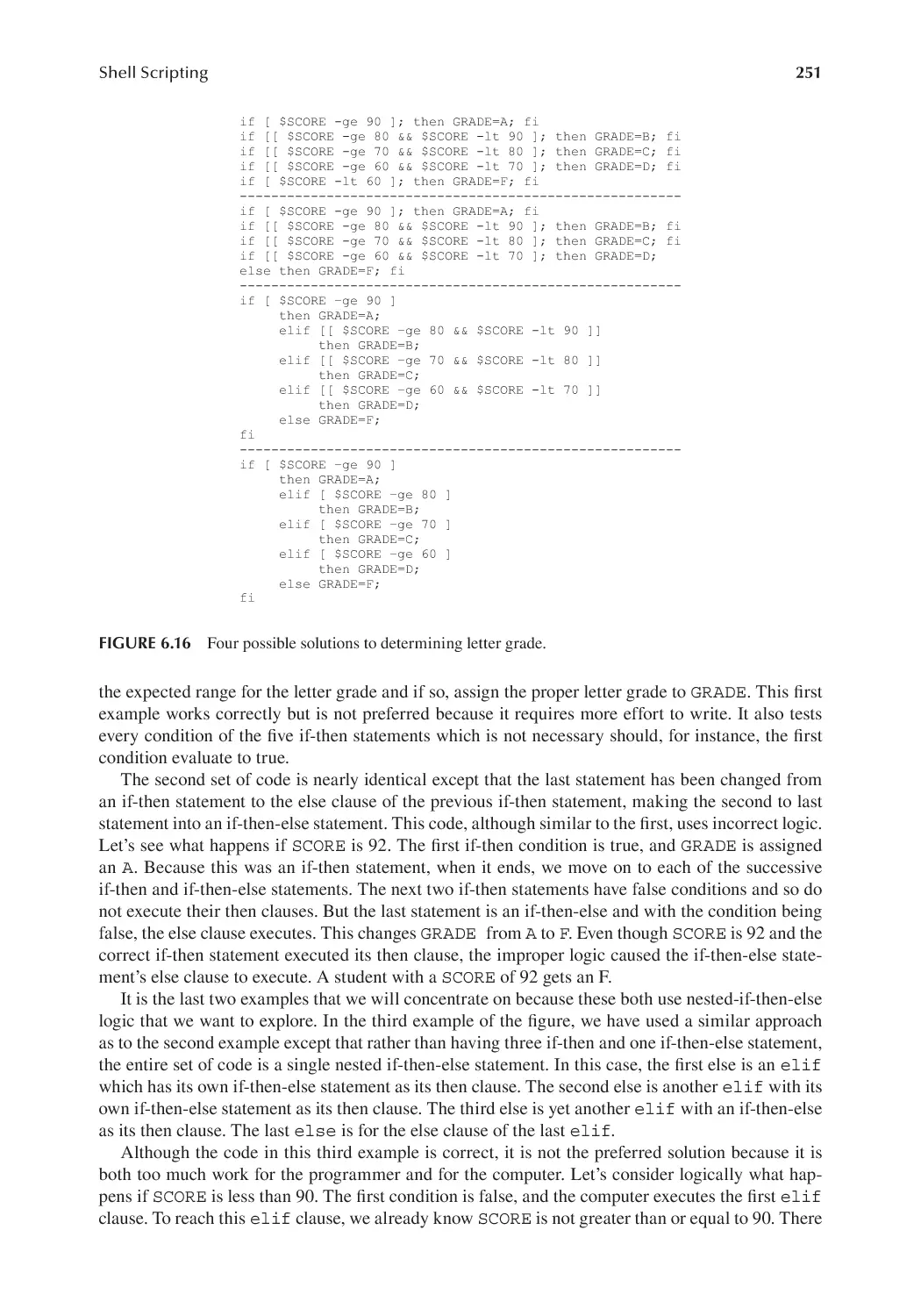
6.5.4 Nested Statements............................................................................. 250
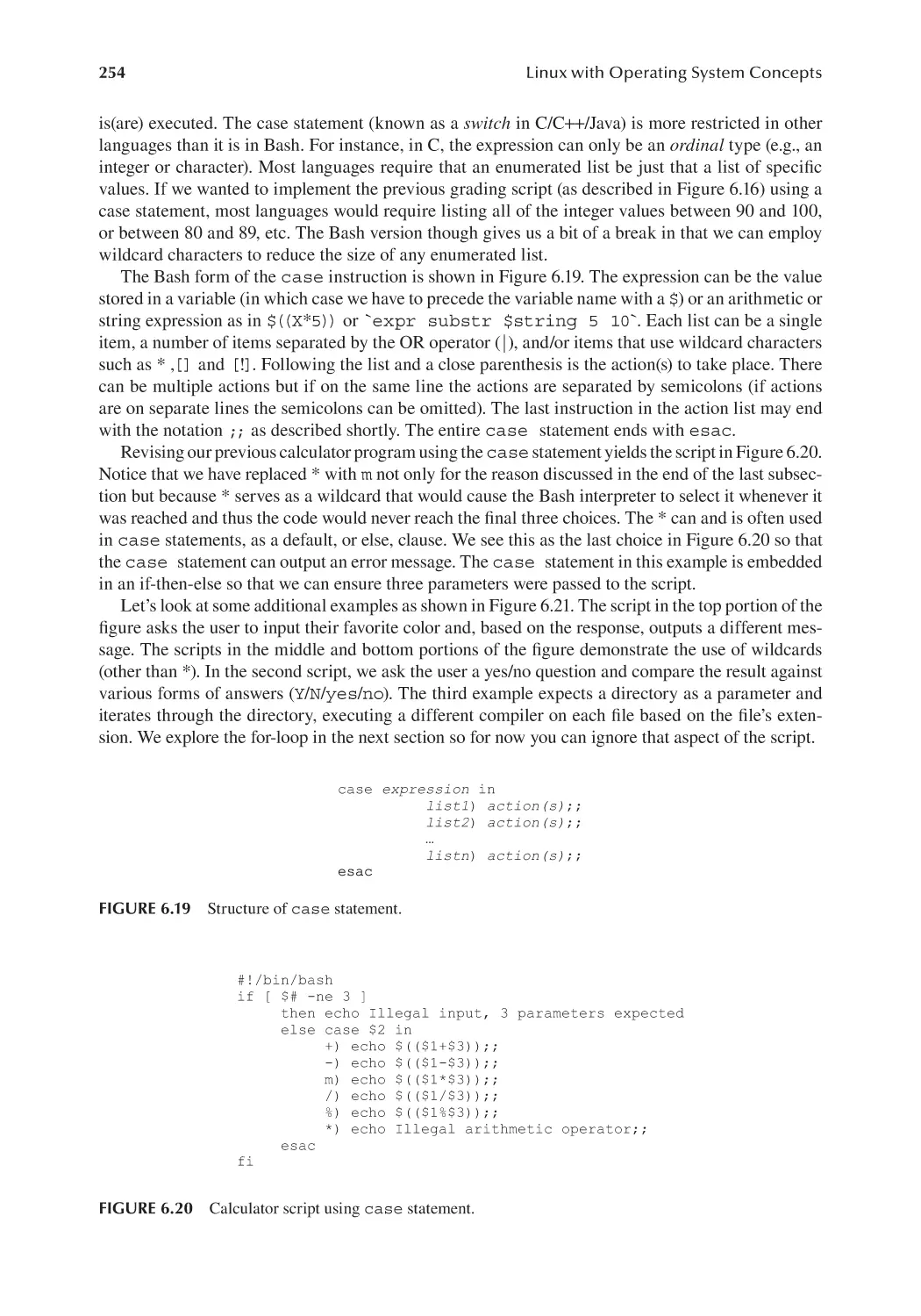
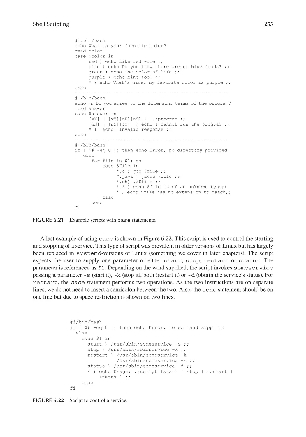
6.5.5 Case Statement.................................................................................. 253
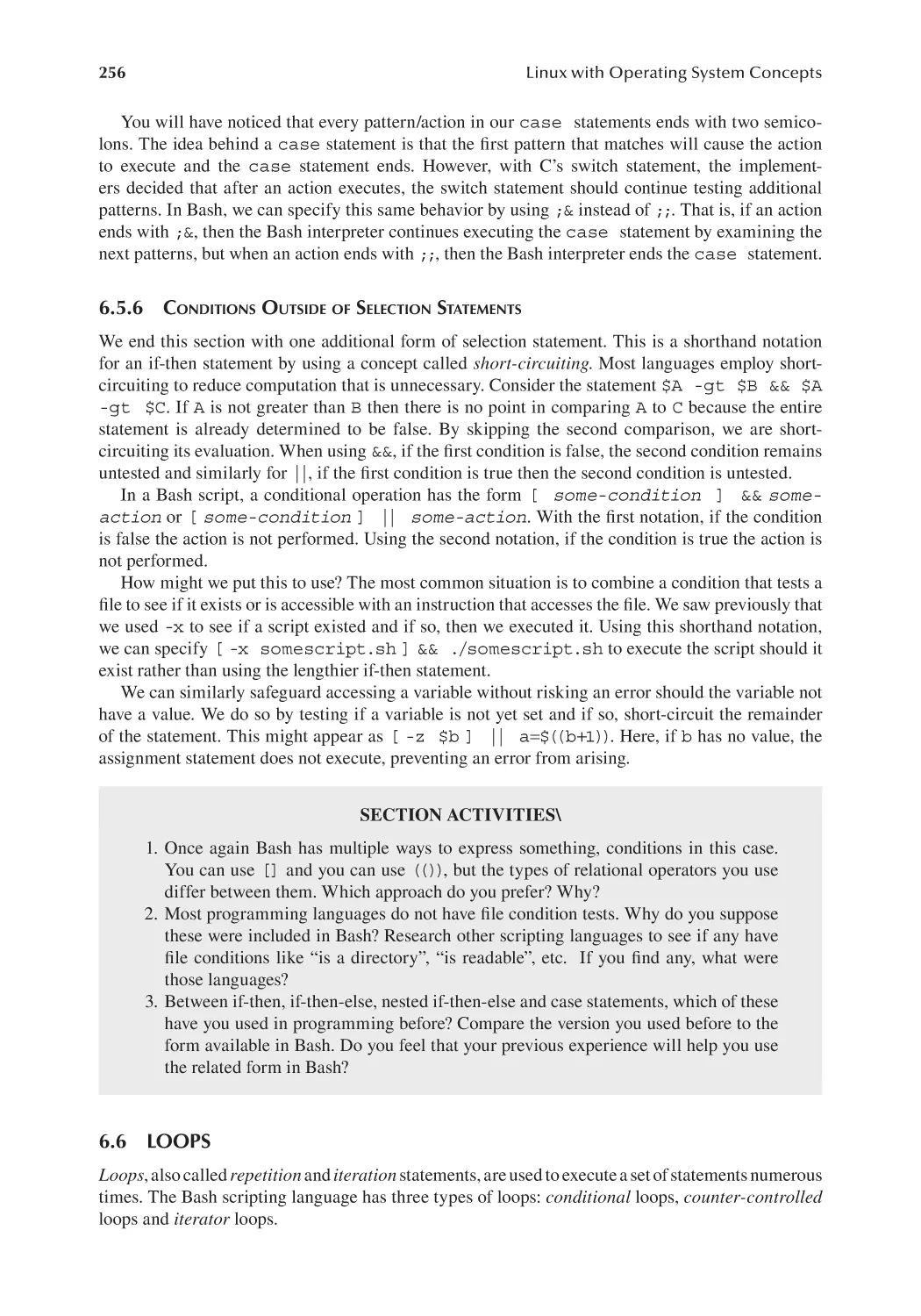
6.5.6 Conditions Outside of Selection Statements..................................... 256
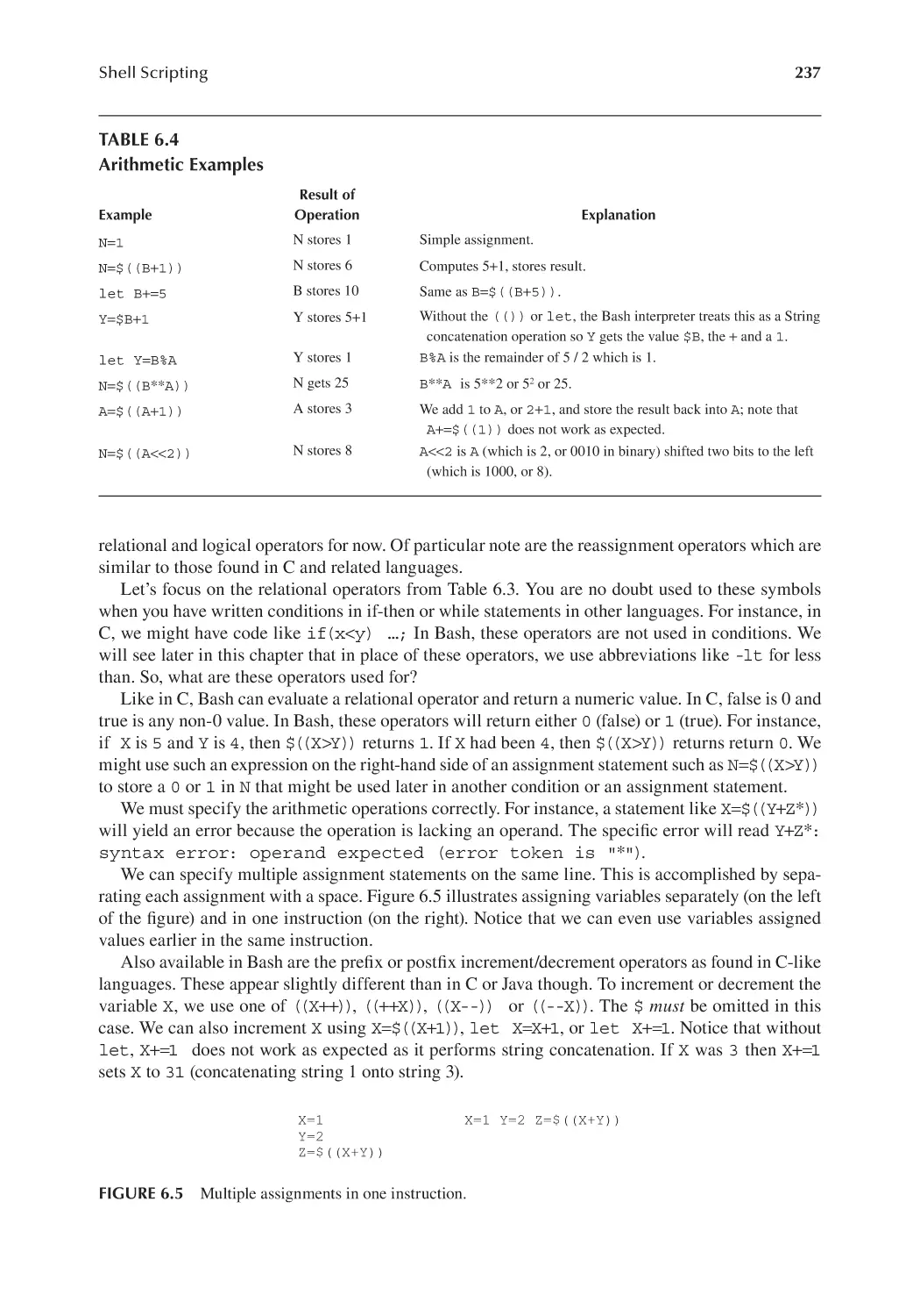
6.6 Loops.............................................................................................................. 256
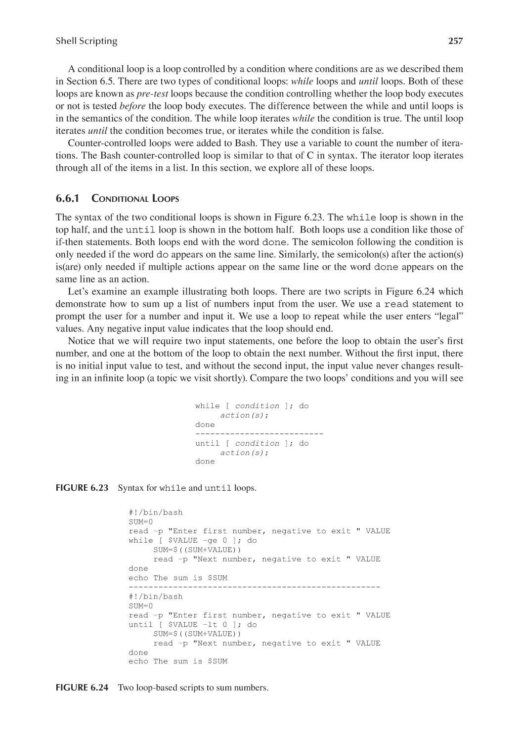
6.6.1 Conditional Loops............................................................................. 257
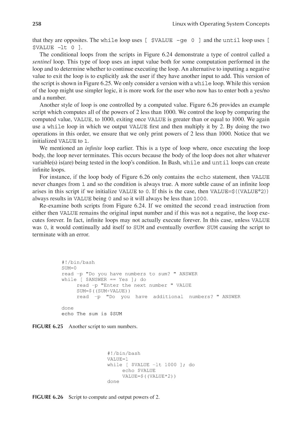
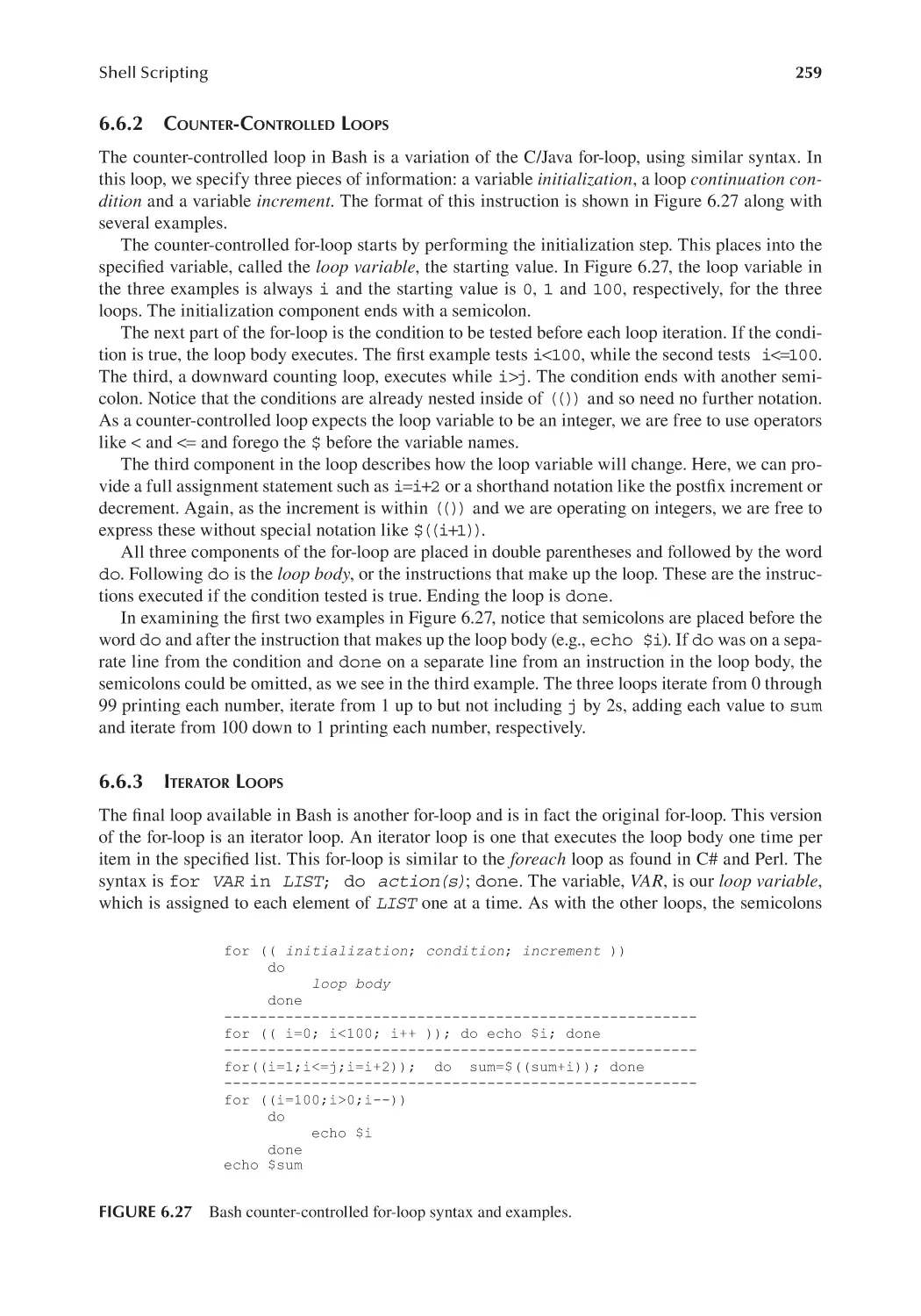
6.6.2 Counter-Controlled Loops................................................................ 259
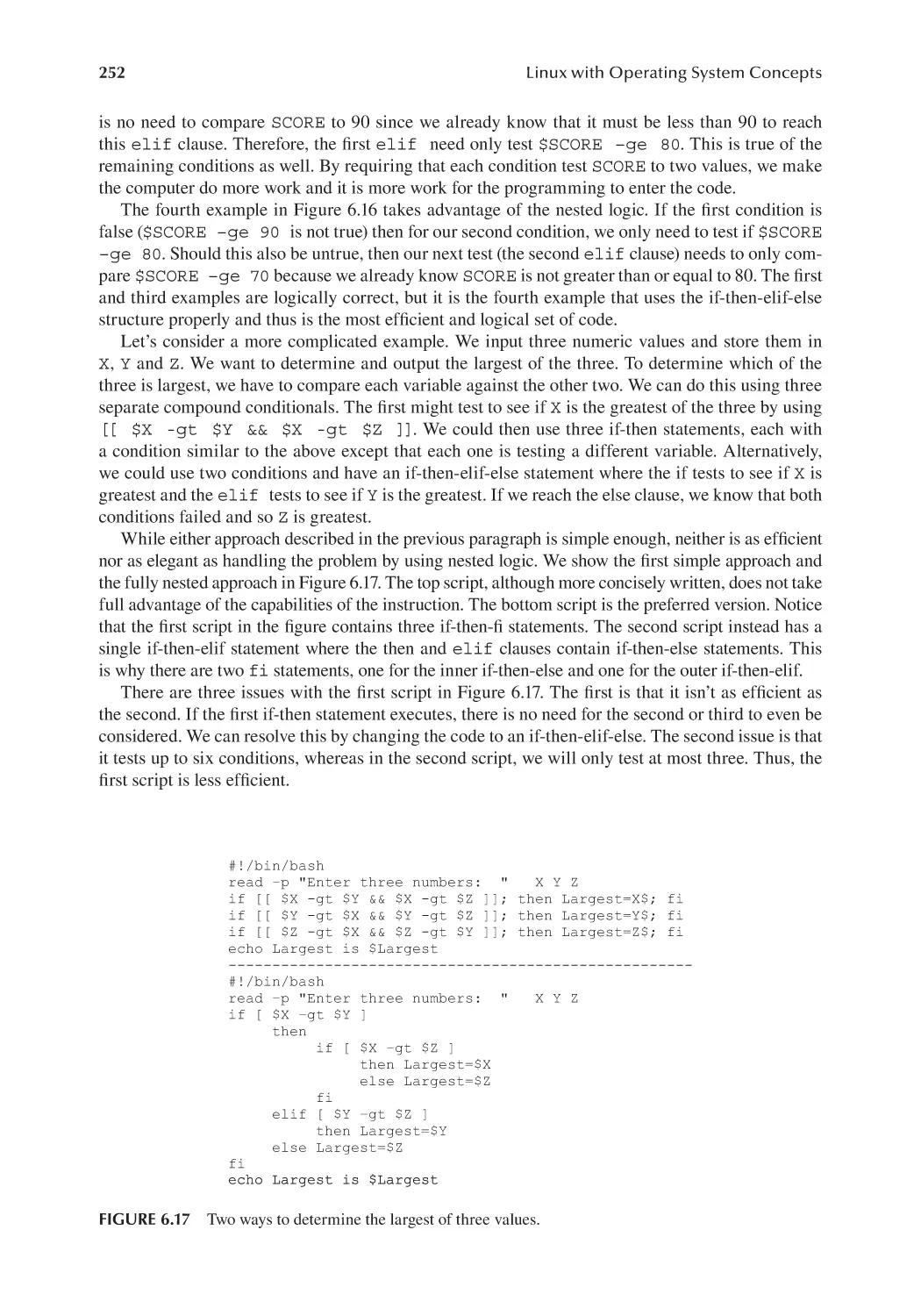
6.6.3 Iterator Loops.................................................................................... 259
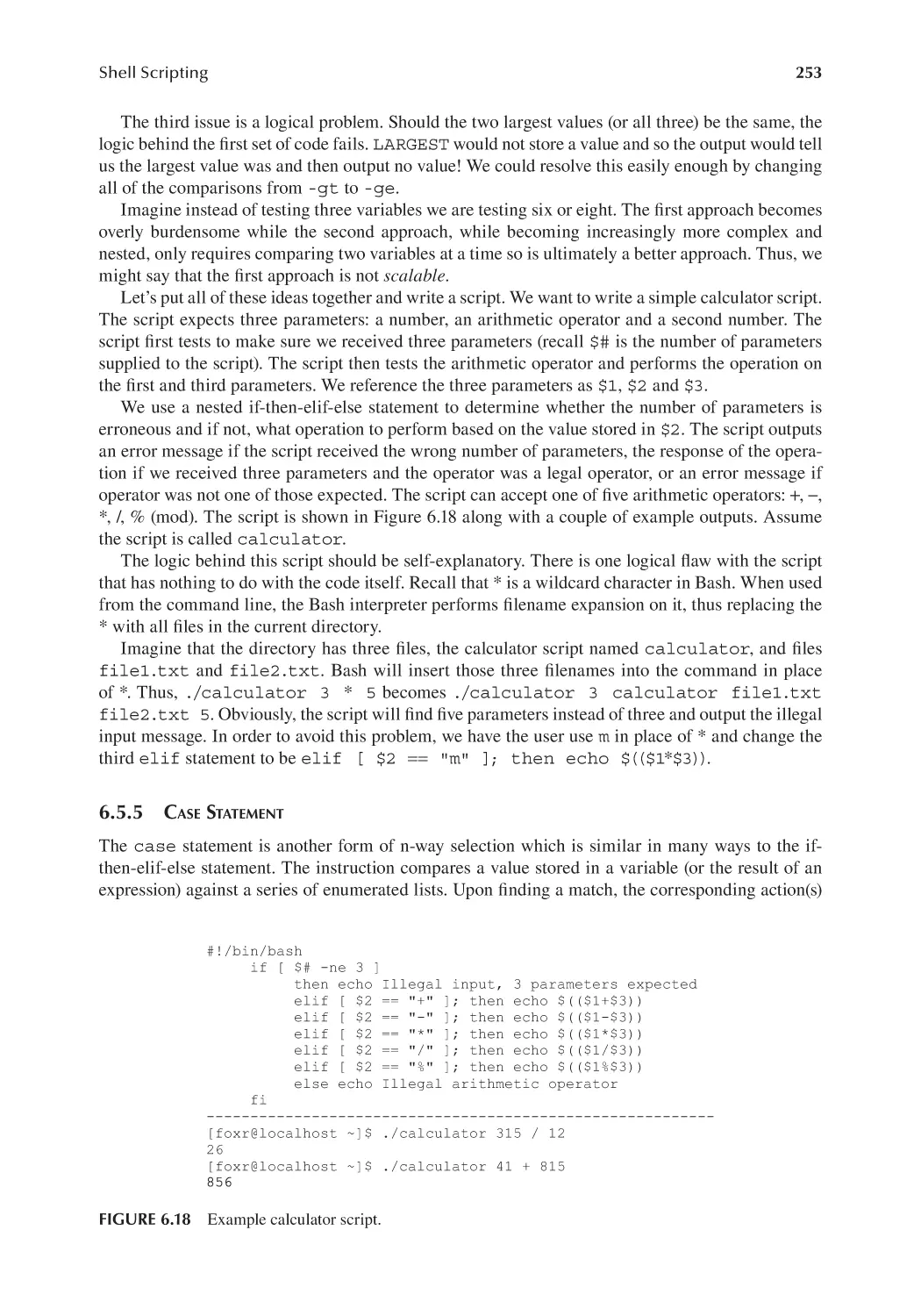
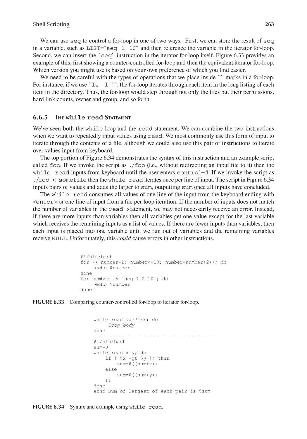
6.6.4 Using the seq Command to Generate a List.................................... 262
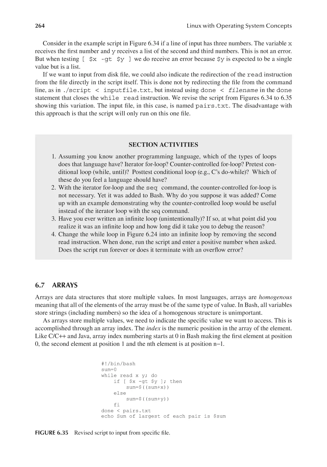
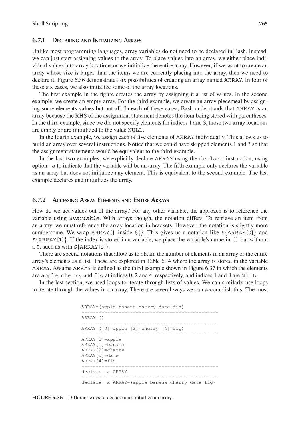
6.6.5 The while read Statement............................................................. 263
6.7 Arrays.............................................................................................................264
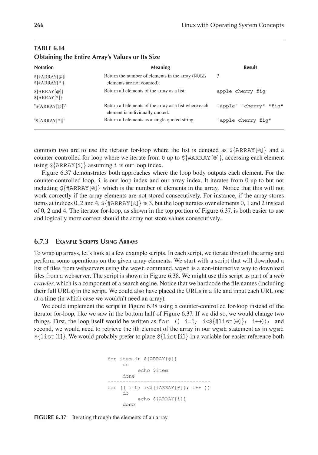
6.7.1 Declaring and Initializing Arrays..................................................... 265
6.7.2 Accessing Array Elements and Entire Arrays.................................. 265
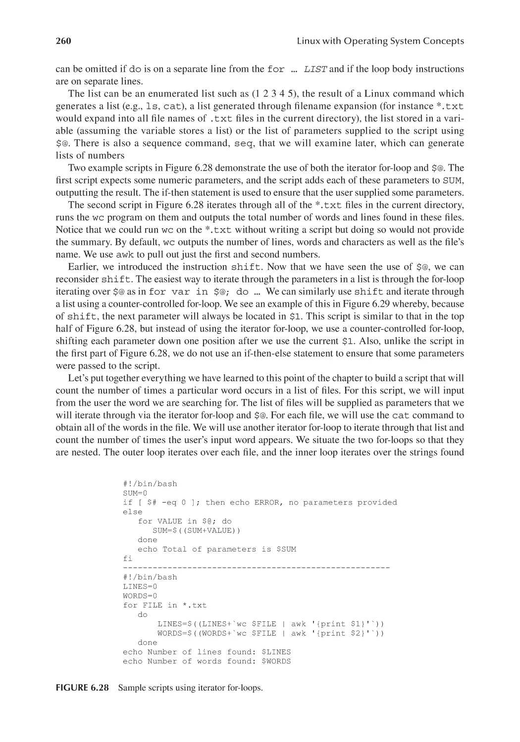
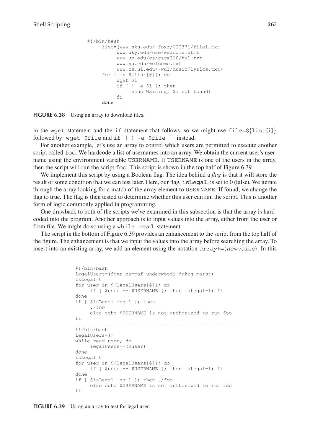
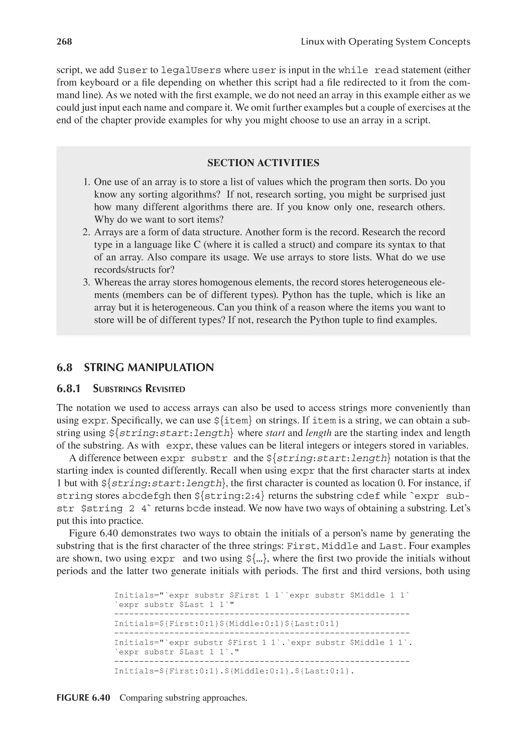
6.7.3 Example Scripts Using Arrays..........................................................266
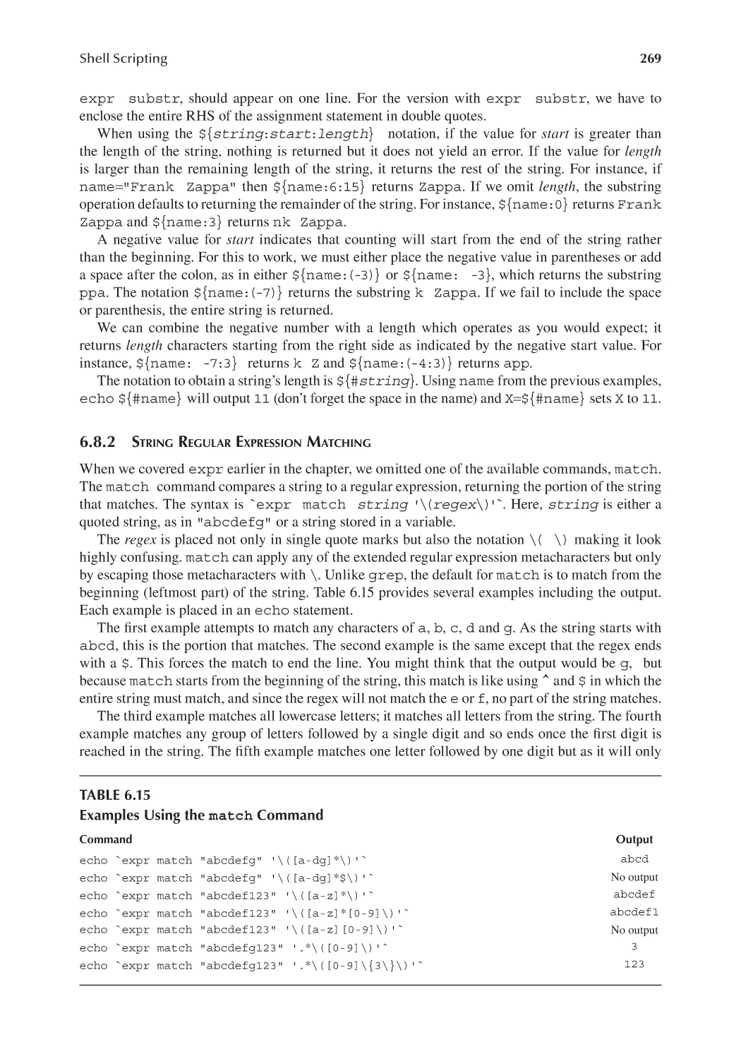
6.8 String Manipulation........................................................................................ 268
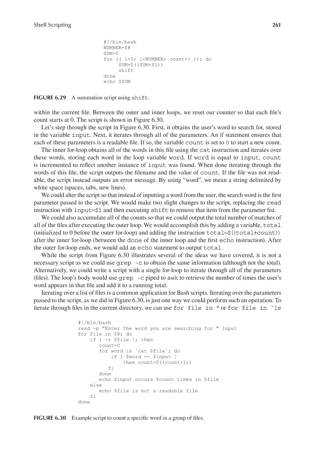
6.8.1 Substrings Revisited.......................................................................... 268
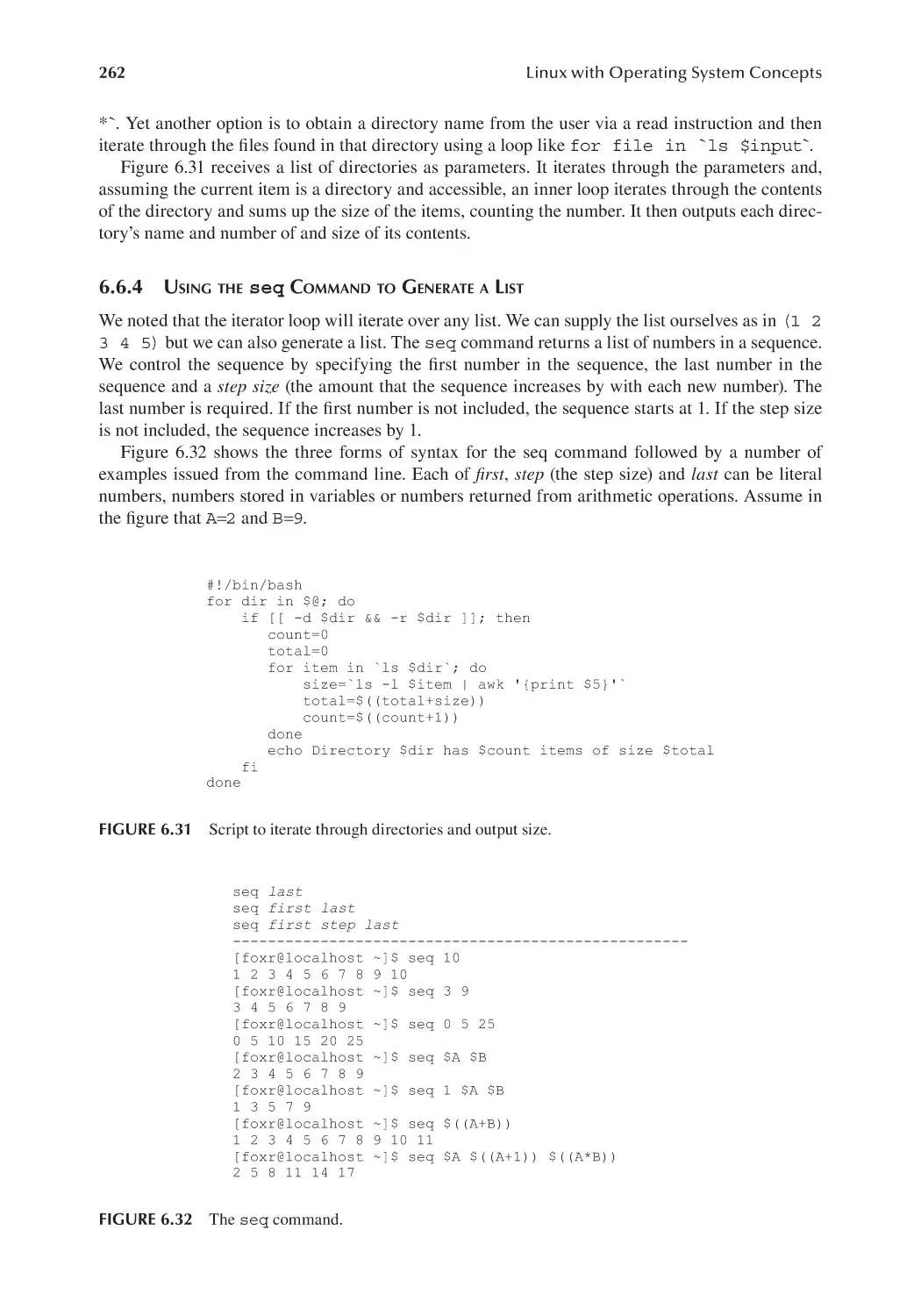
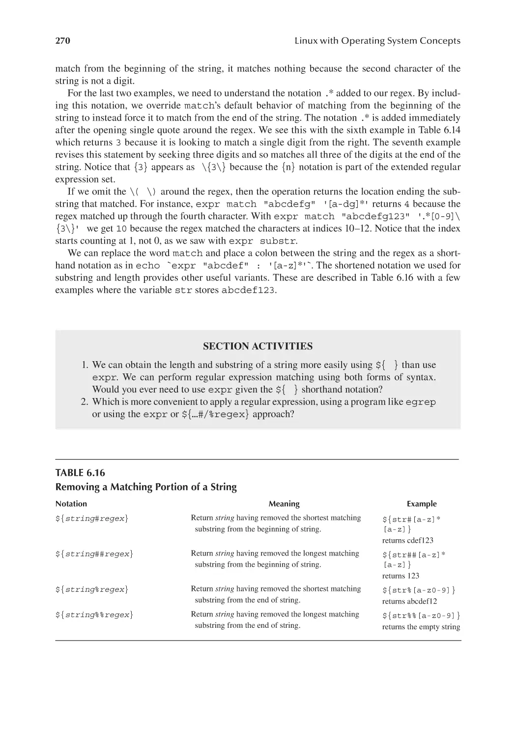
6.8.2 String Regular Expression Matching................................................ 269
6.9 Functions........................................................................................................ 271
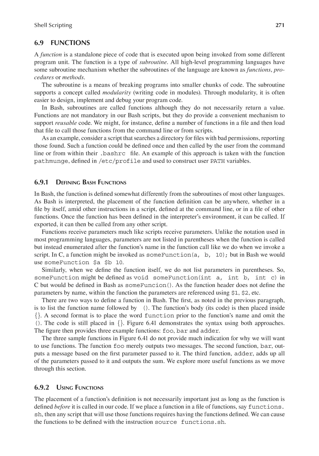
6.9.1 Defining Bash Functions................................................................... 271
6.9.2 Using Functions................................................................................. 271
6.9.3 Functions and Variables.................................................................... 273
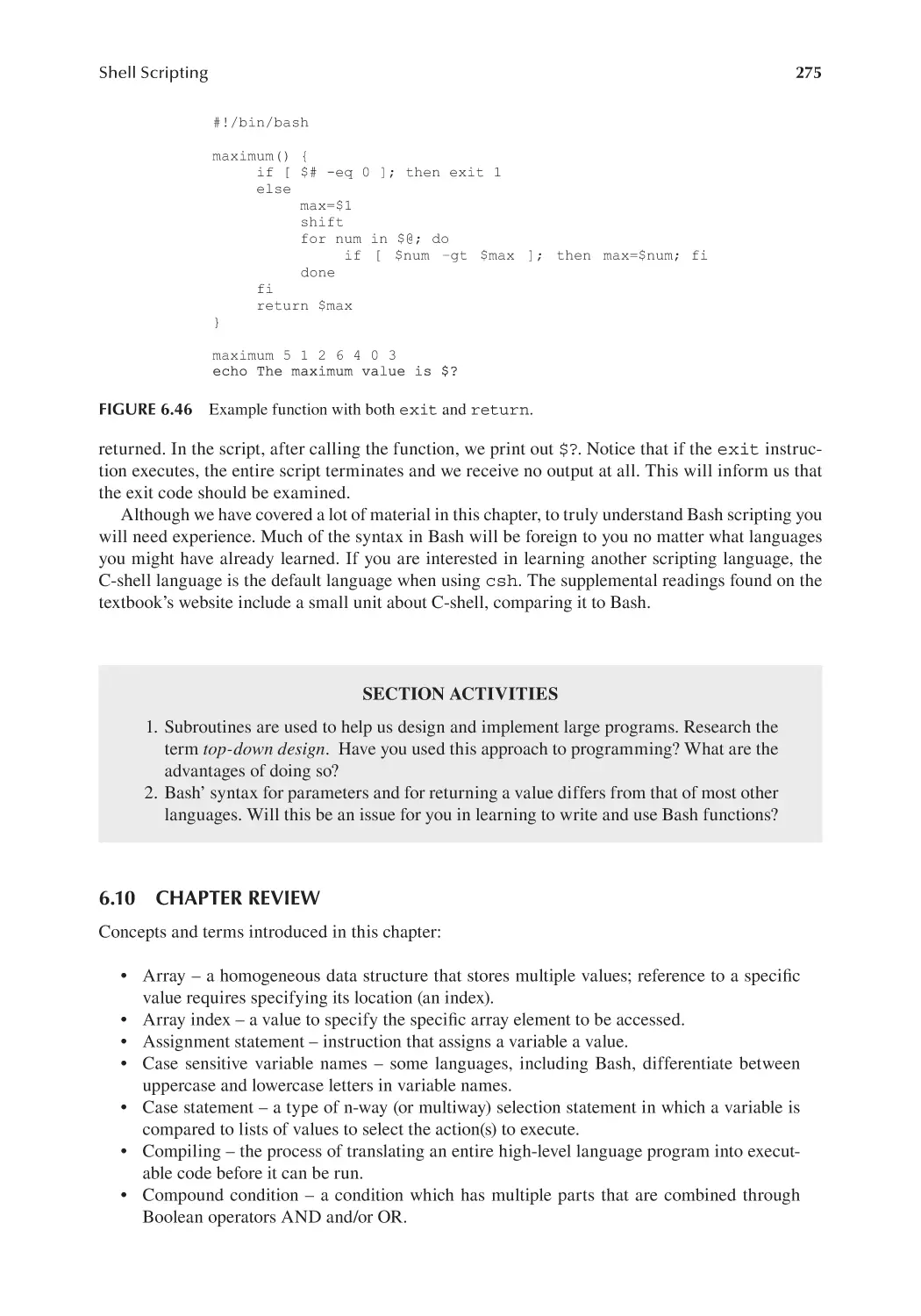
6.9.4 exit and return Statements......................................................... 274
6.10 Chapter Review.............................................................................................. 275
Review Questions...................................................................................................... 278
xi
Contents
Chapter 7
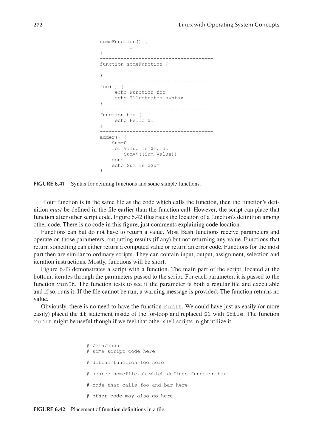
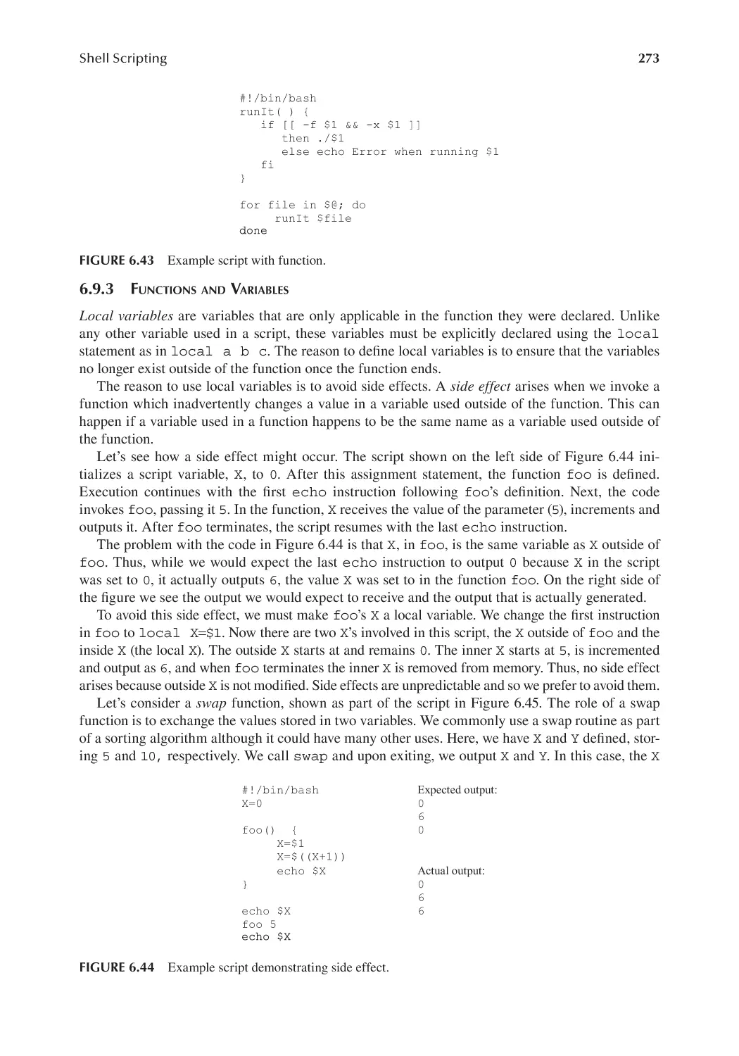
User Accounts........................................................................................................... 283
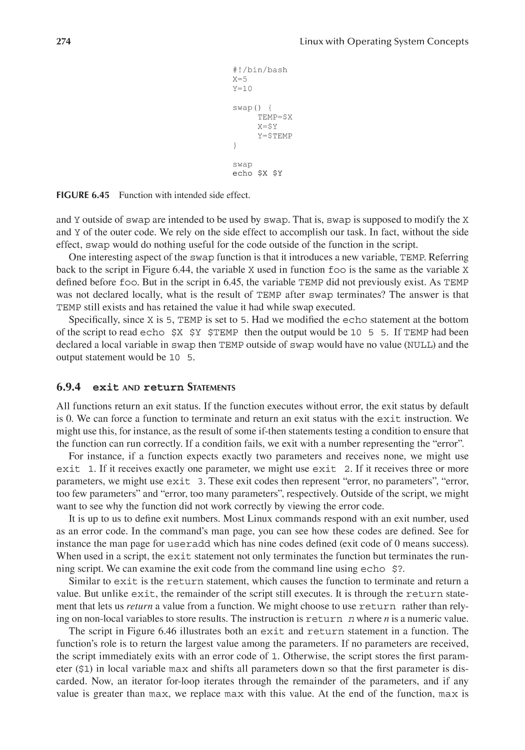
7.1
7.2
Introduction.................................................................................................... 283
Creating Accounts and Groups......................................................................284
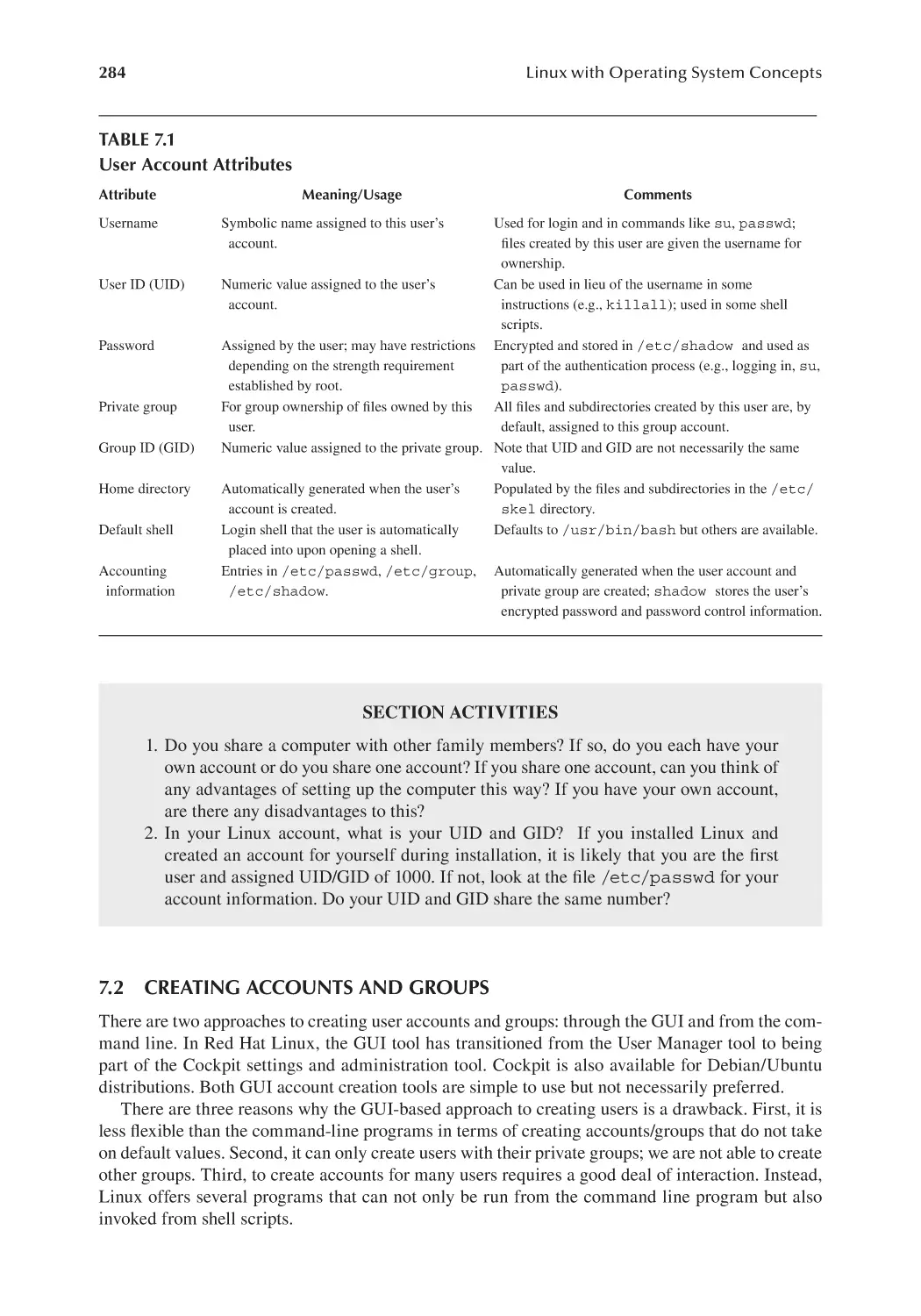
7.2.1 Creating User and Group Accounts through the GUI....................... 285
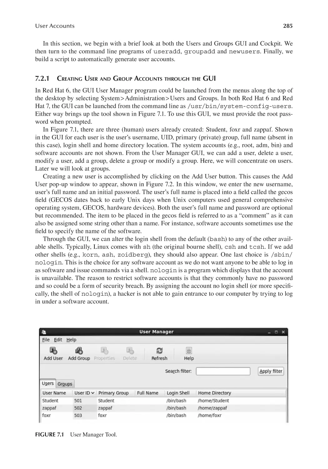
7.2.2 Creating User and Group Accounts from the Command Line......... 289
7.2.3 Creating a Large Number of User Accounts..................................... 293
7.3 Managing Users and Groups.......................................................................... 296
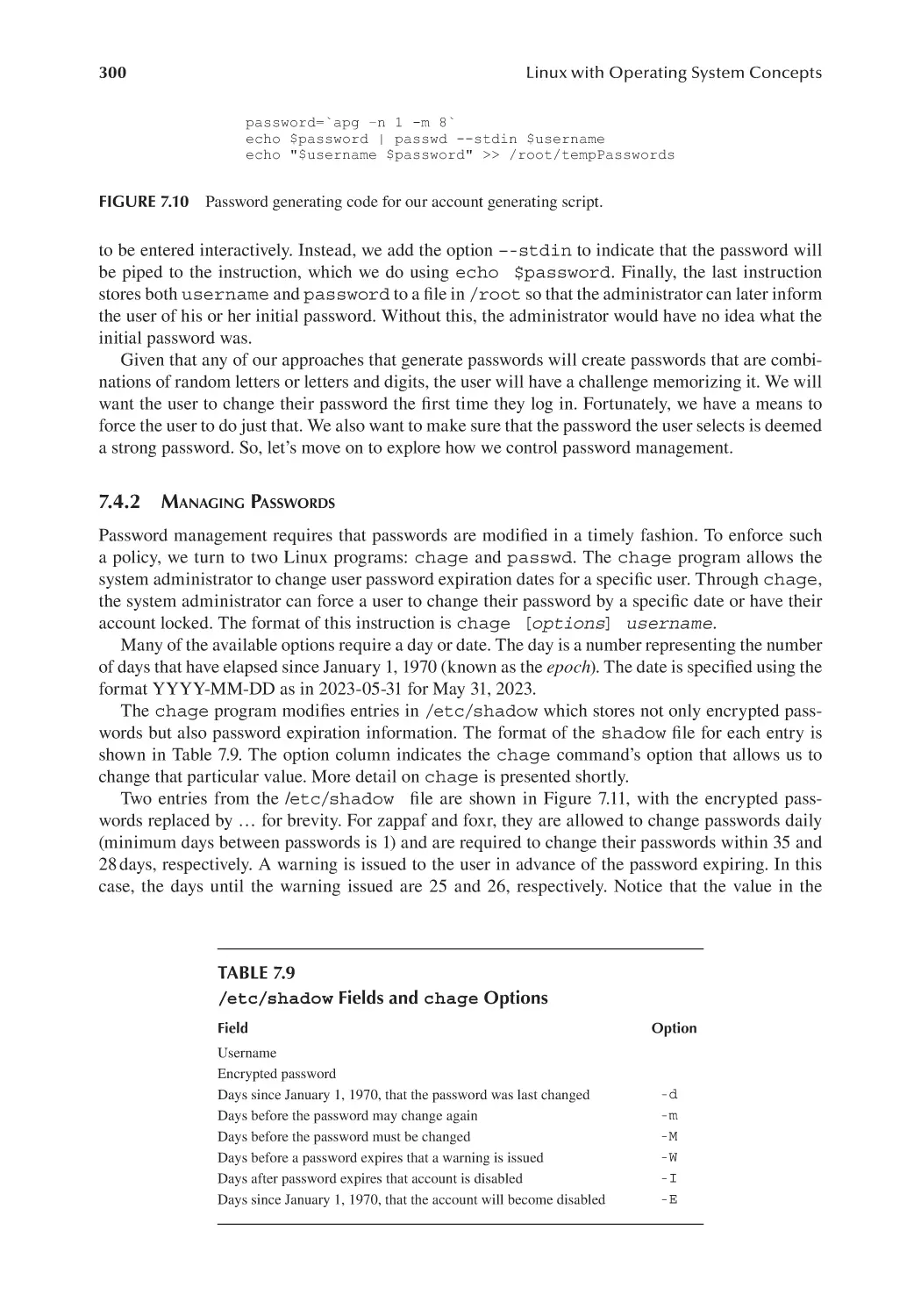
7.4 Password Management................................................................................... 298
7.4.1 Automatically Generating Passwords............................................... 298
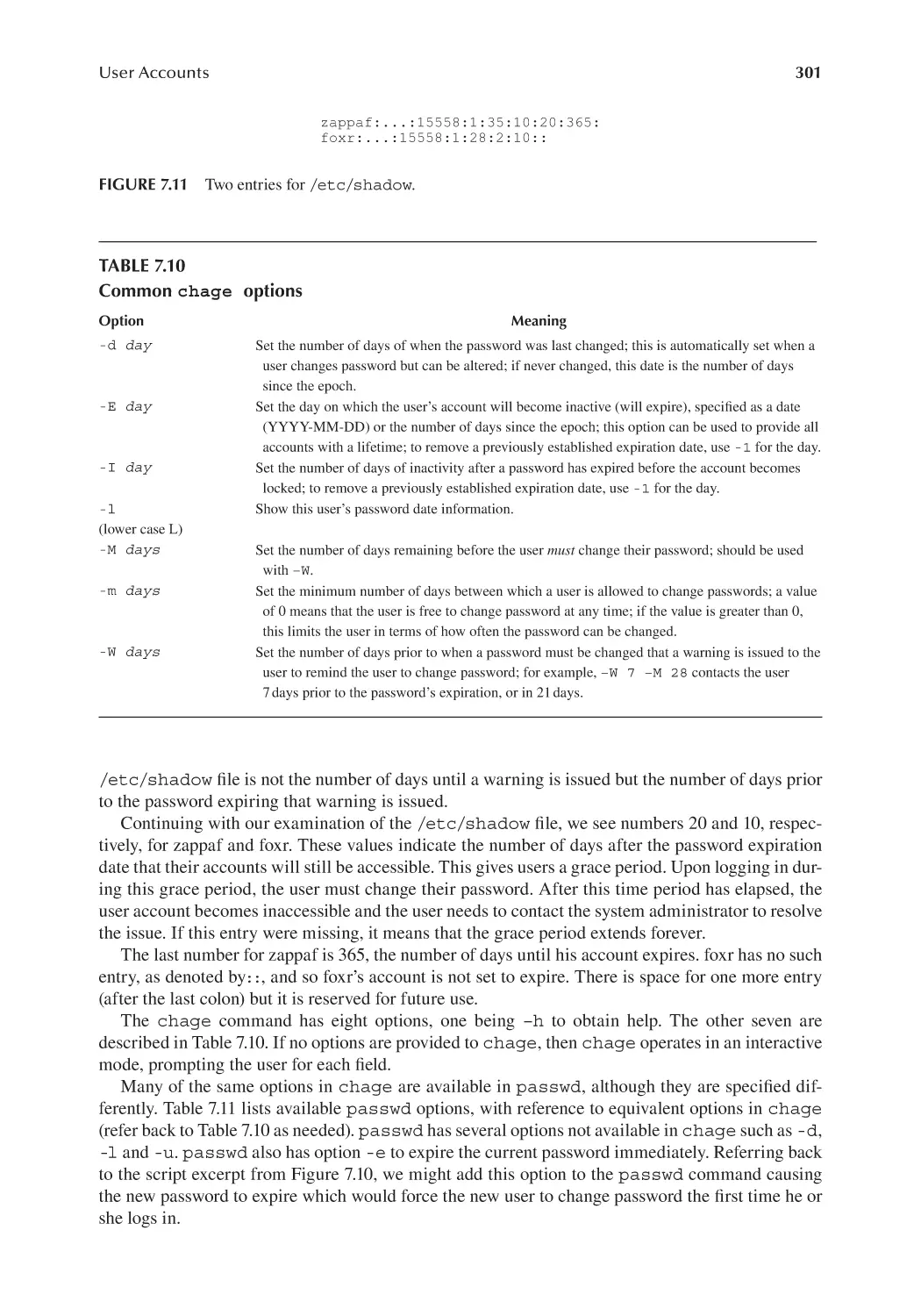
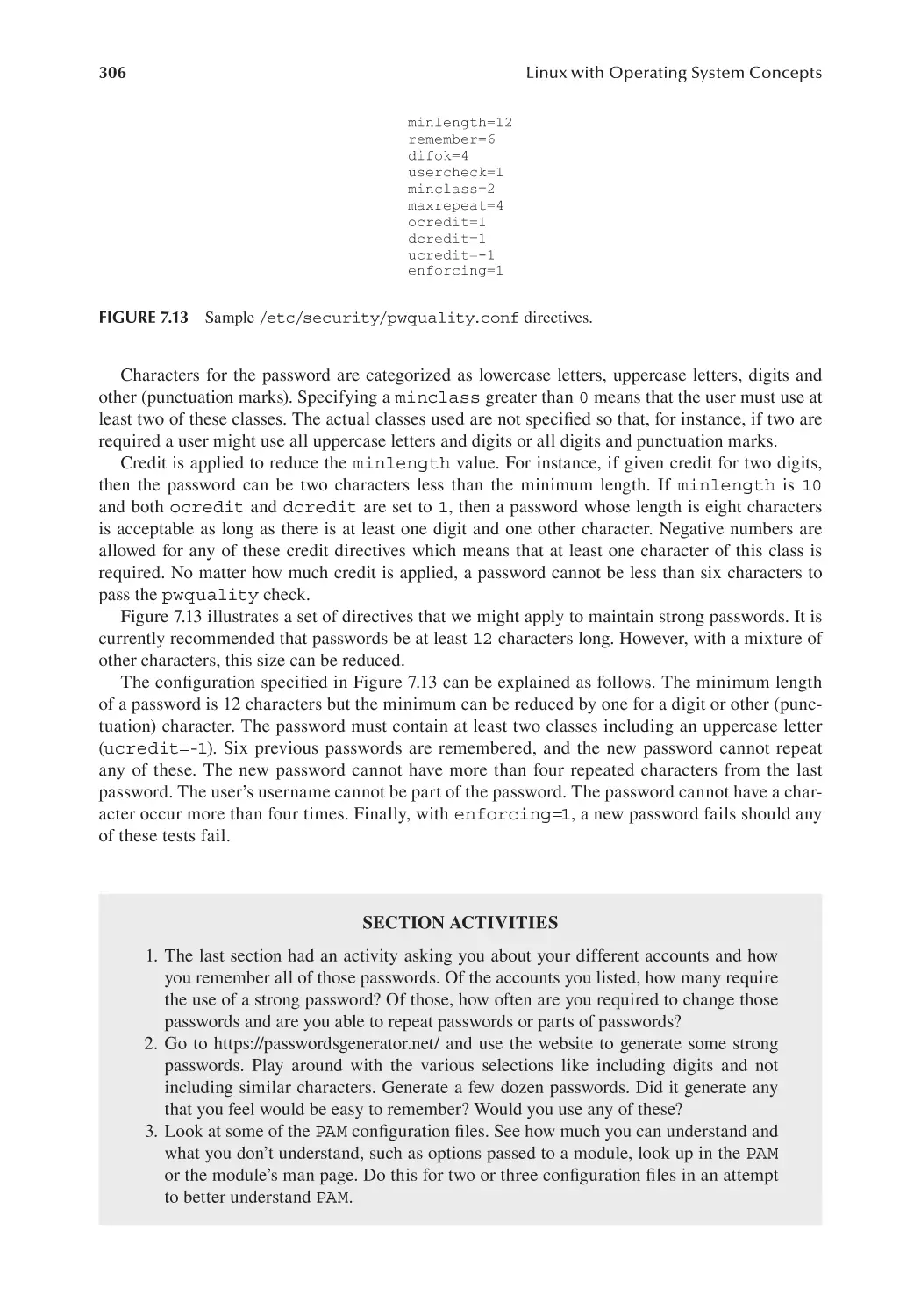
7.4.2 Managing Passwords.........................................................................300
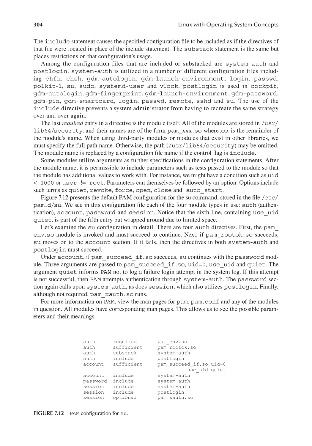
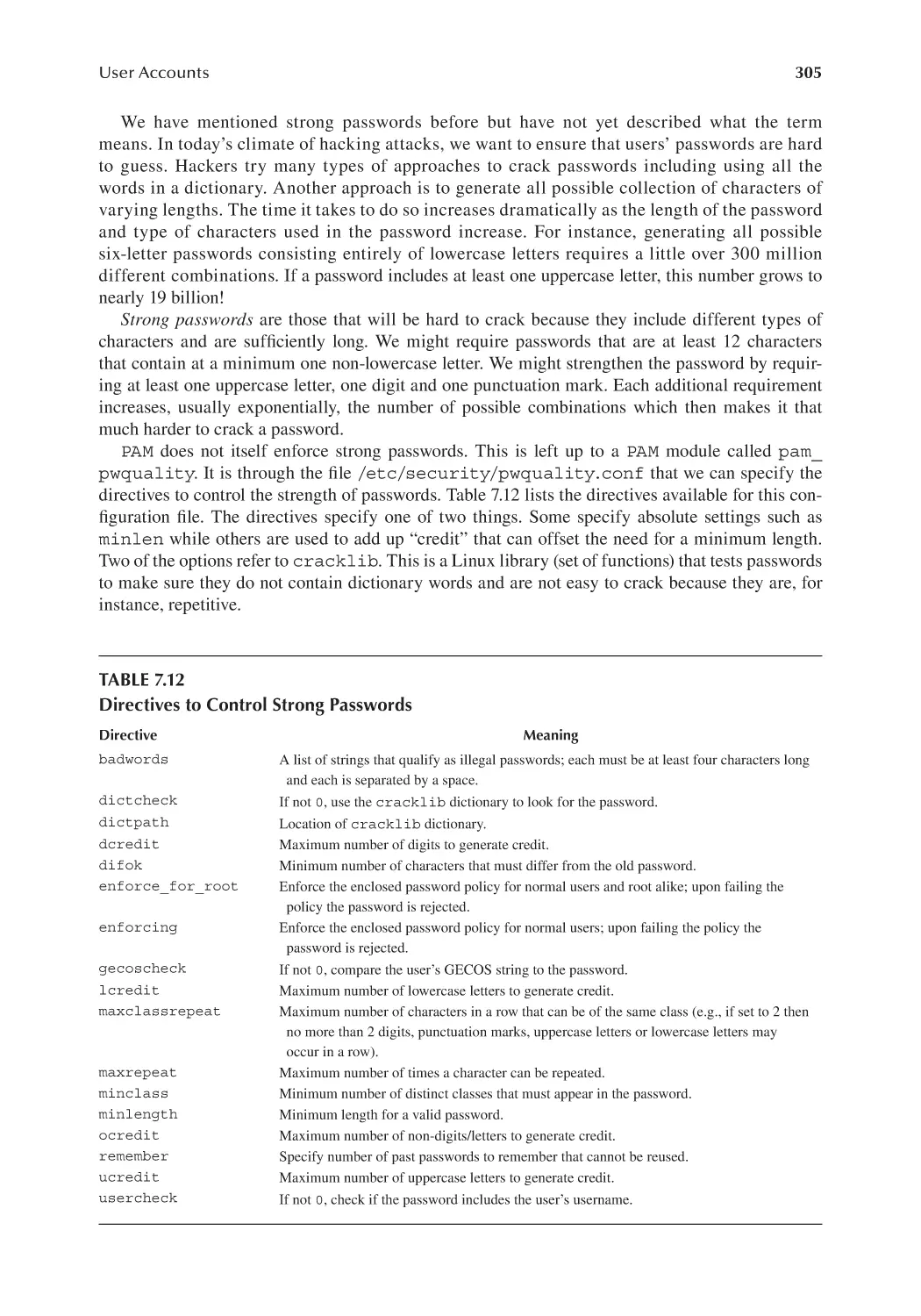
7.5 PAM and Enforcing Strong Passwords..........................................................302
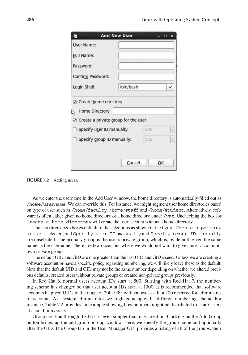
7.6 Establishing Common User Resources..........................................................307
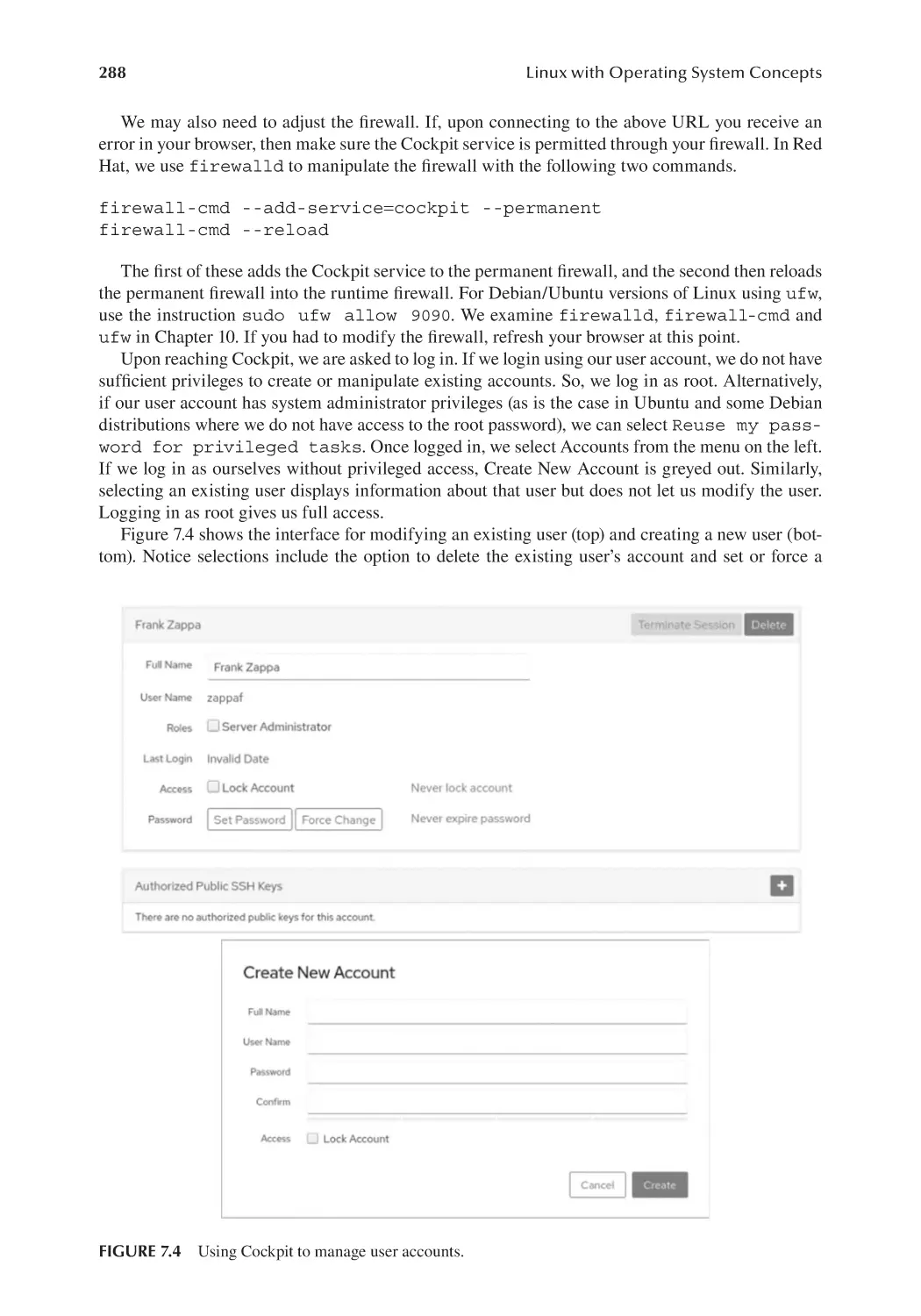
7.6.1 Populating User Home Directories with Initial Files........................307
7.6.2 Initial User Settings and Defaults.....................................................308
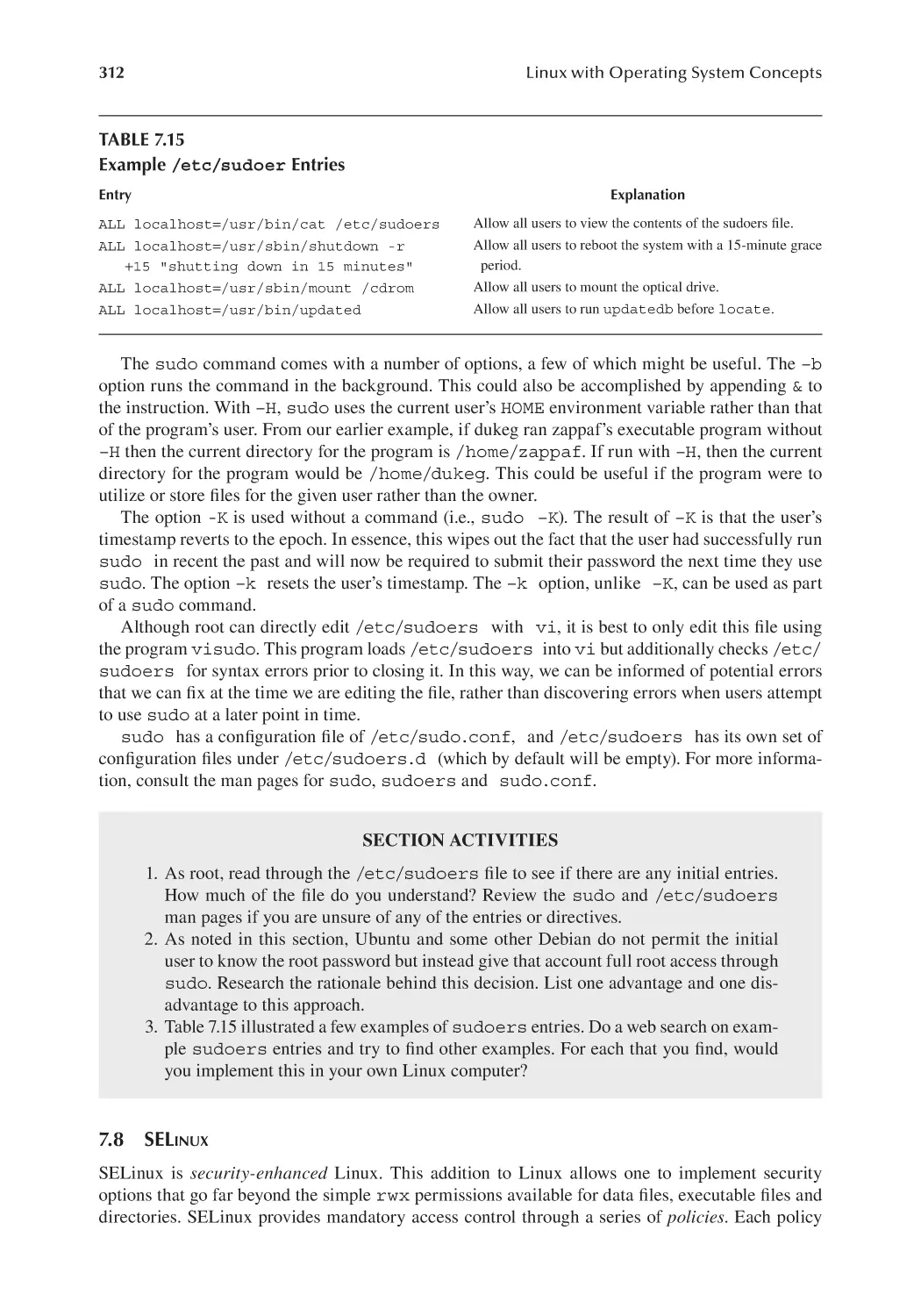
7.7 The sudo Command..................................................................................... 310
7.8 SELinux.......................................................................................................... 312
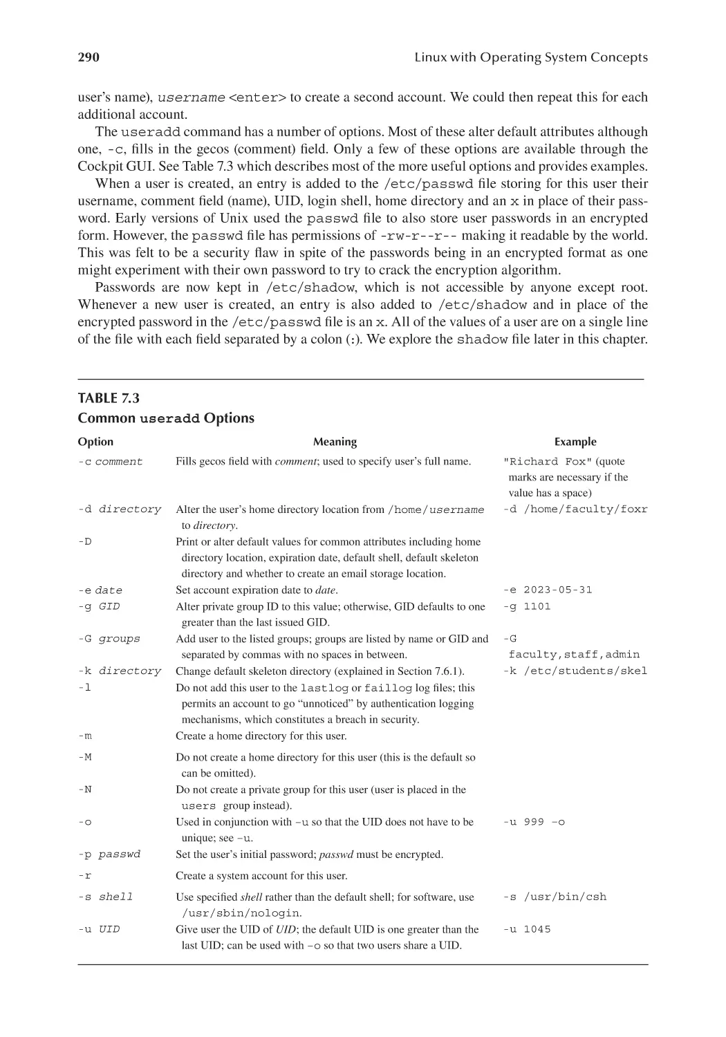
7.8.1 SELinux Components....................................................................... 313
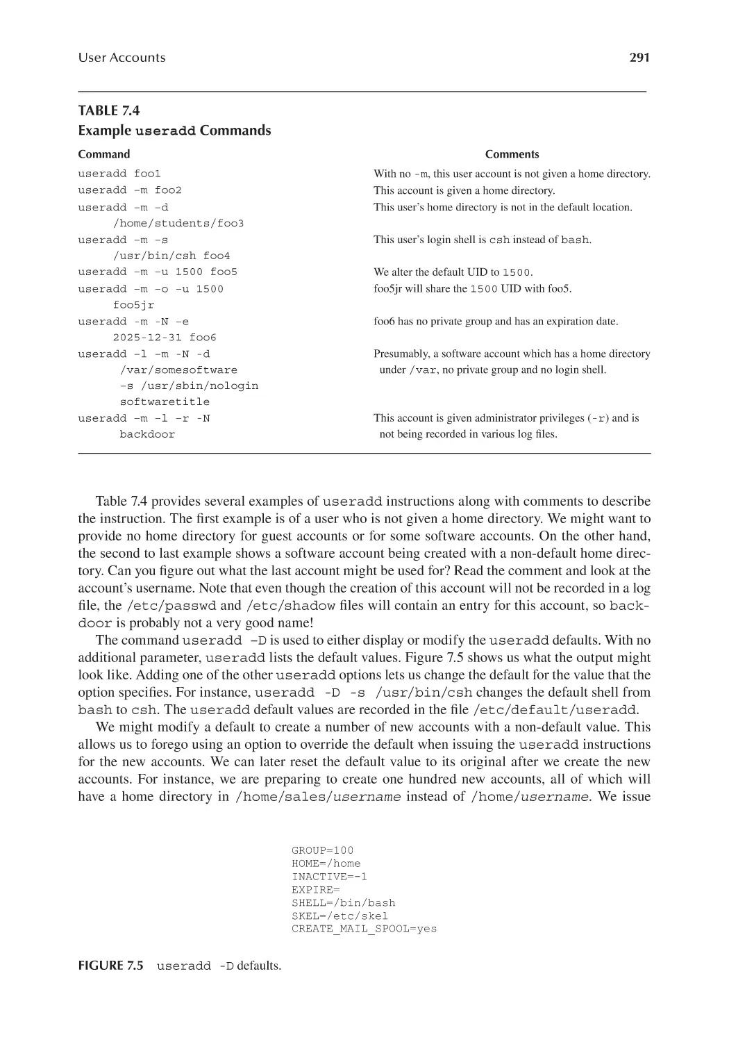
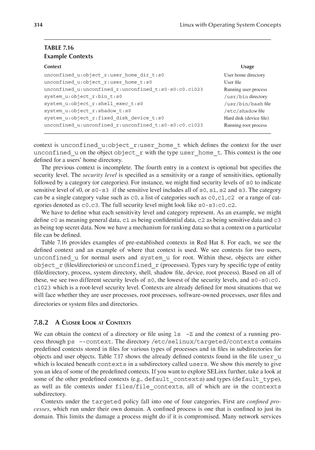
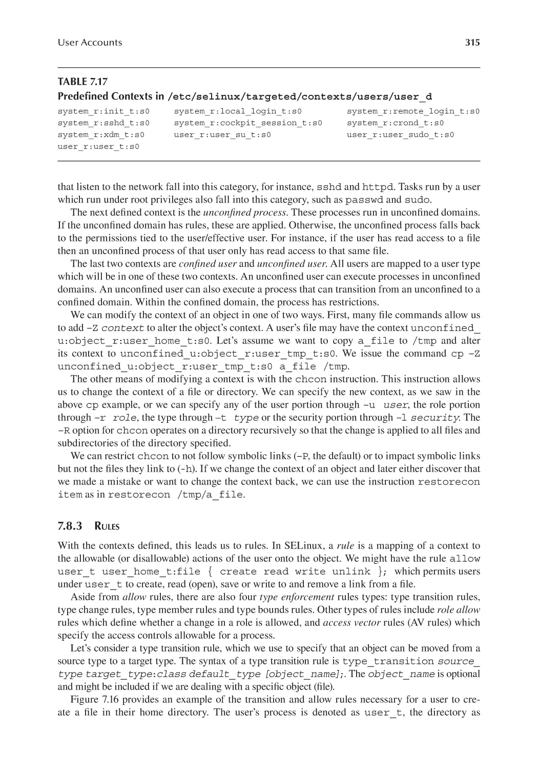
7.8.2 A Closer Look at Contexts................................................................ 314
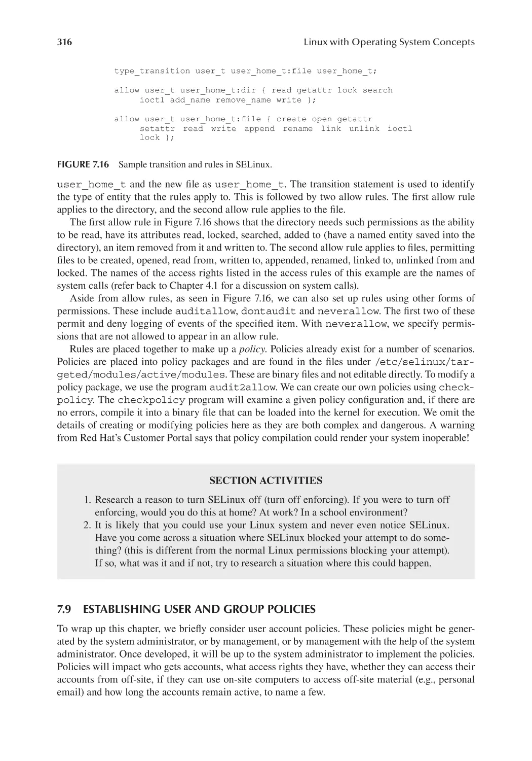
7.8.3 Rules.................................................................................................. 315
7.9 Establishing User and Group Policies............................................................ 316
7.10 Chapter Review.............................................................................................. 319
Review Questions...................................................................................................... 321
Chapter 8
Administering Linux File Systems........................................................................... 327
8.1
8.2
8.3
8.4
8.5
8.6
Introduction.................................................................................................... 327
Storage Access................................................................................................ 328
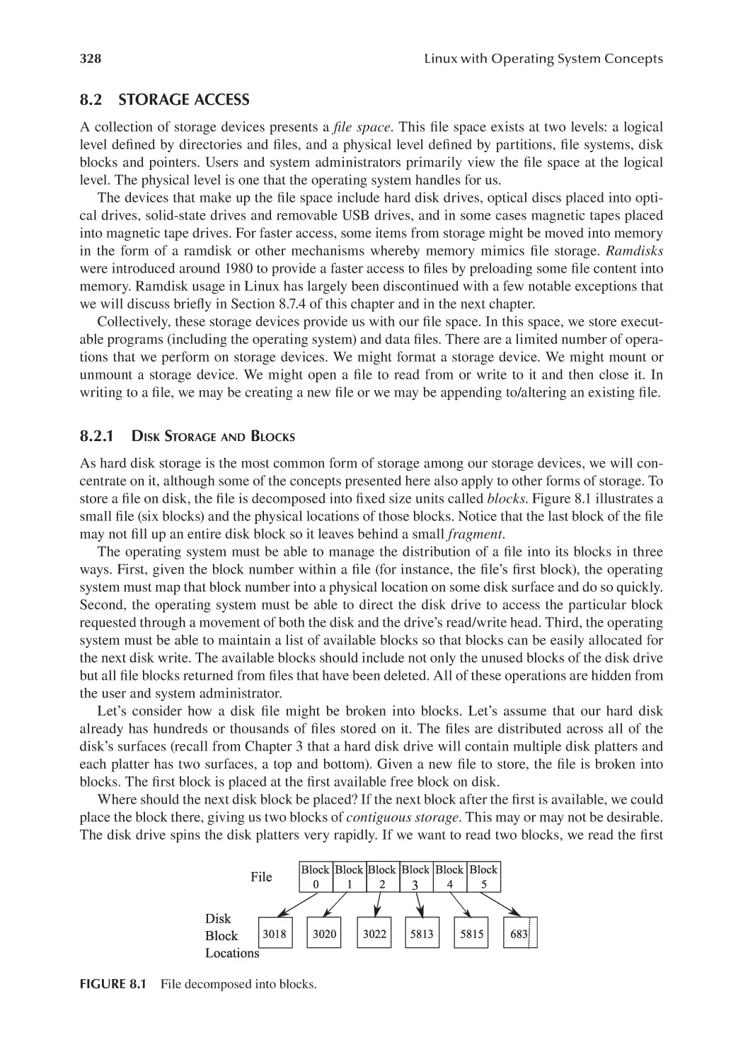
8.2.1 Disk Storage and Blocks................................................................... 328
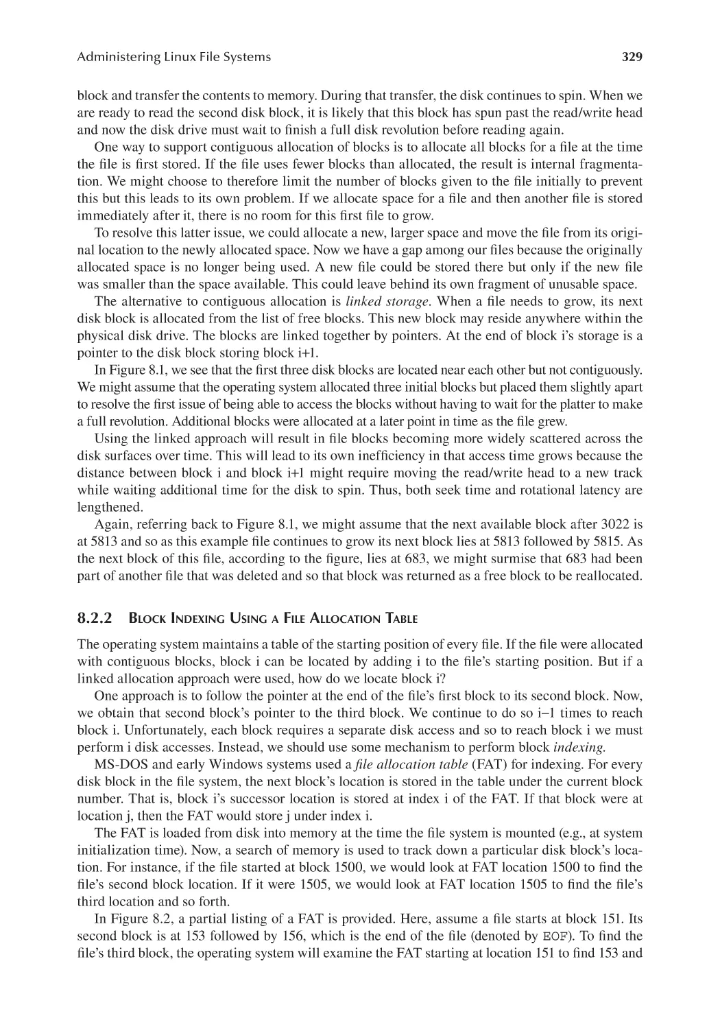
8.2.2 Block Indexing Using a File Allocation Table.................................. 329
8.2.3 Other Disk Storage Details............................................................... 330
8.2.4 File Storage and Object Storage........................................................ 331
Linux Files...................................................................................................... 333
8.3.1 Files versus Directories..................................................................... 333
8.3.2 Non-File File Types........................................................................... 333
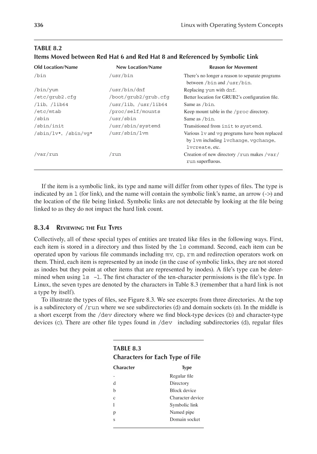
8.3.3 Links as File Types........................................................................... 335
8.3.4 Reviewing the File Types.................................................................. 336
The inode........................................................................................................ 337
8.4.1 inode Metadata.................................................................................. 337
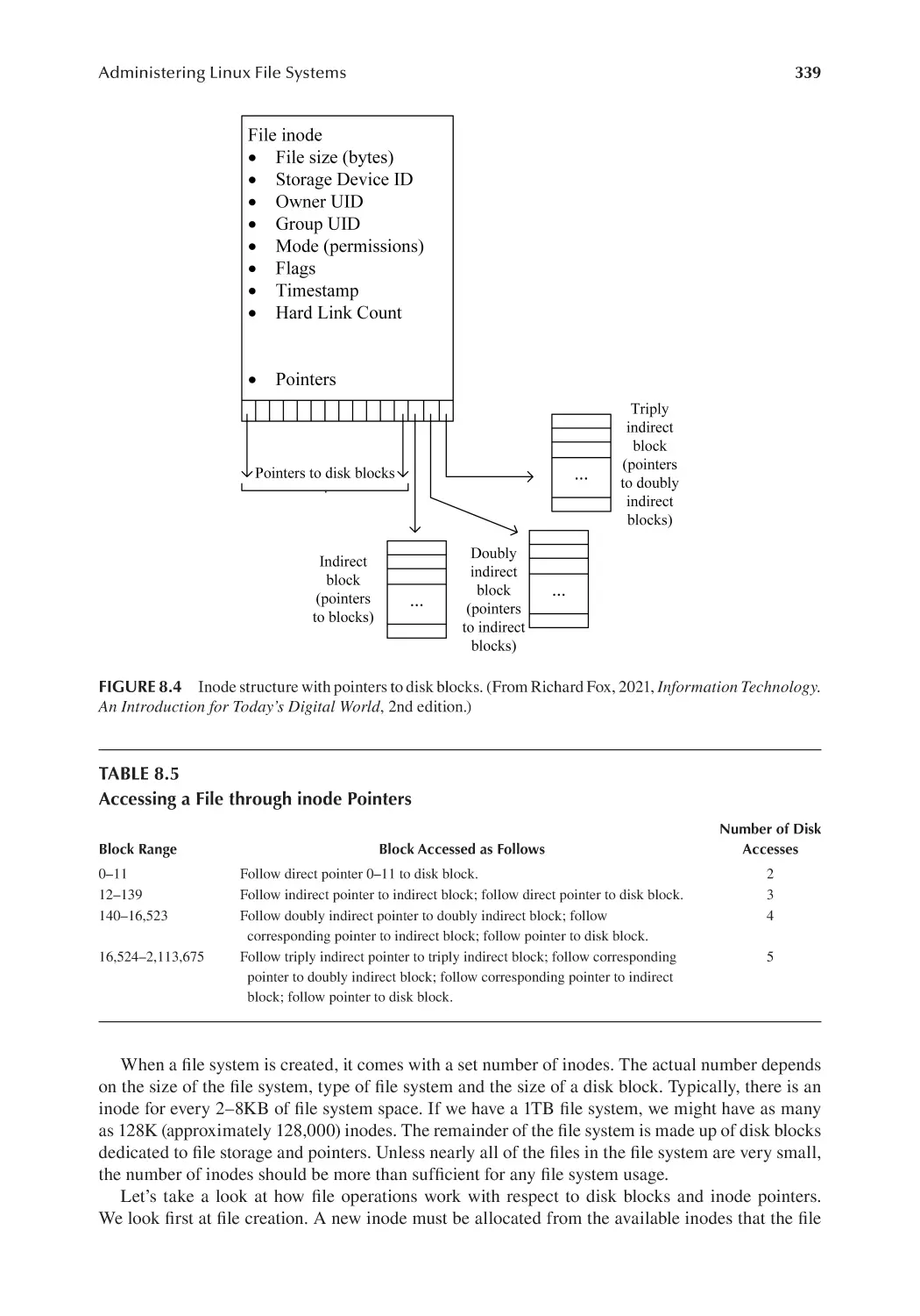
8.4.2 inode Pointers.................................................................................... 338
8.4.3 Linux Commands to Inspect inodes and Files..................................340
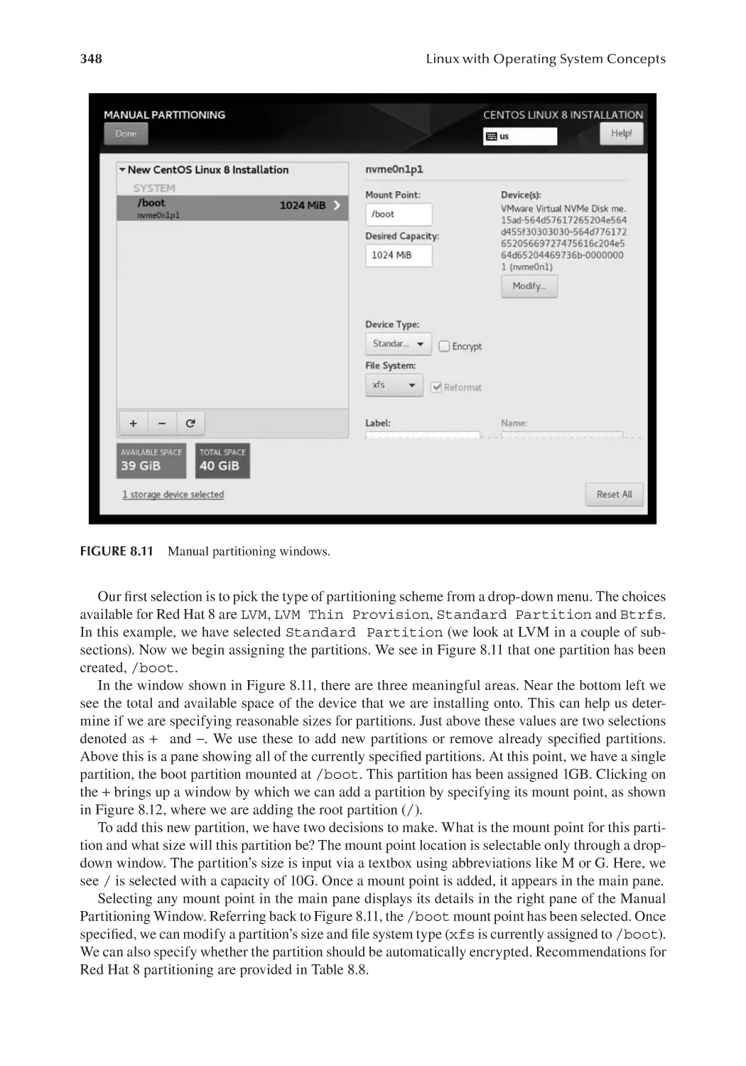
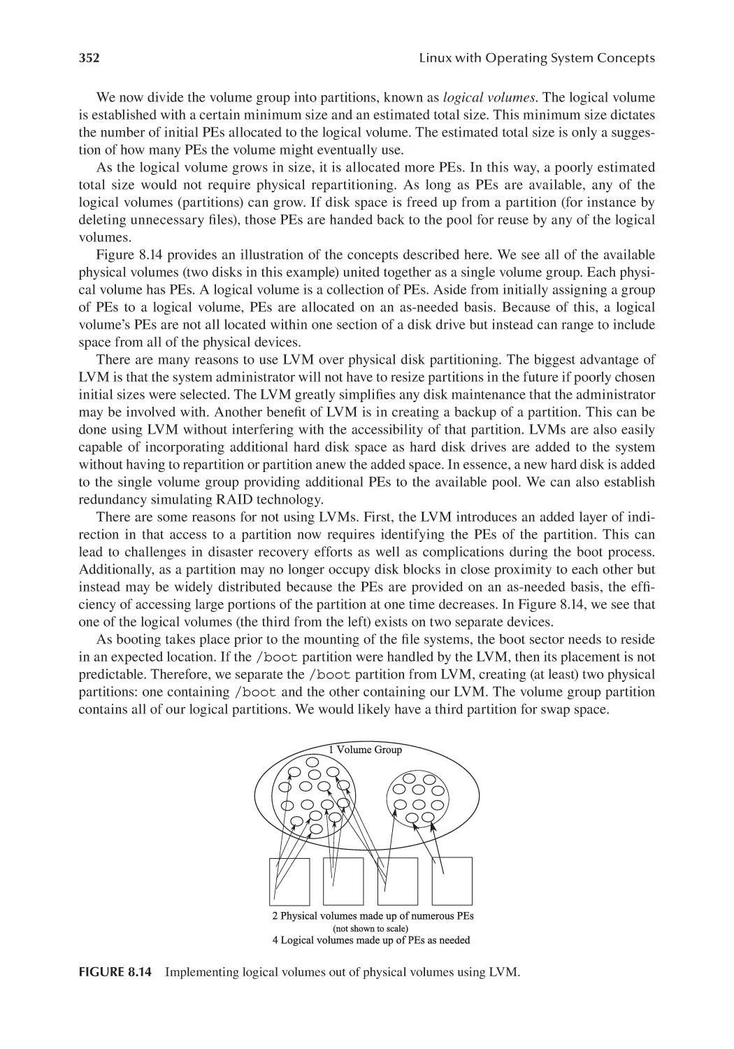
Partitions and File Systems............................................................................344
8.5.1 Why Partition?...................................................................................344
8.5.2 Viewing the Available Partitions....................................................... 345
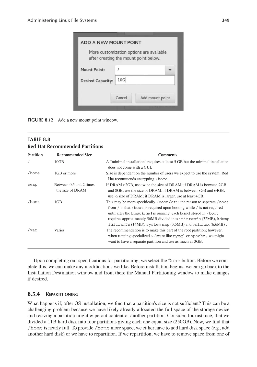
8.5.3 Creating Partitions............................................................................. 347
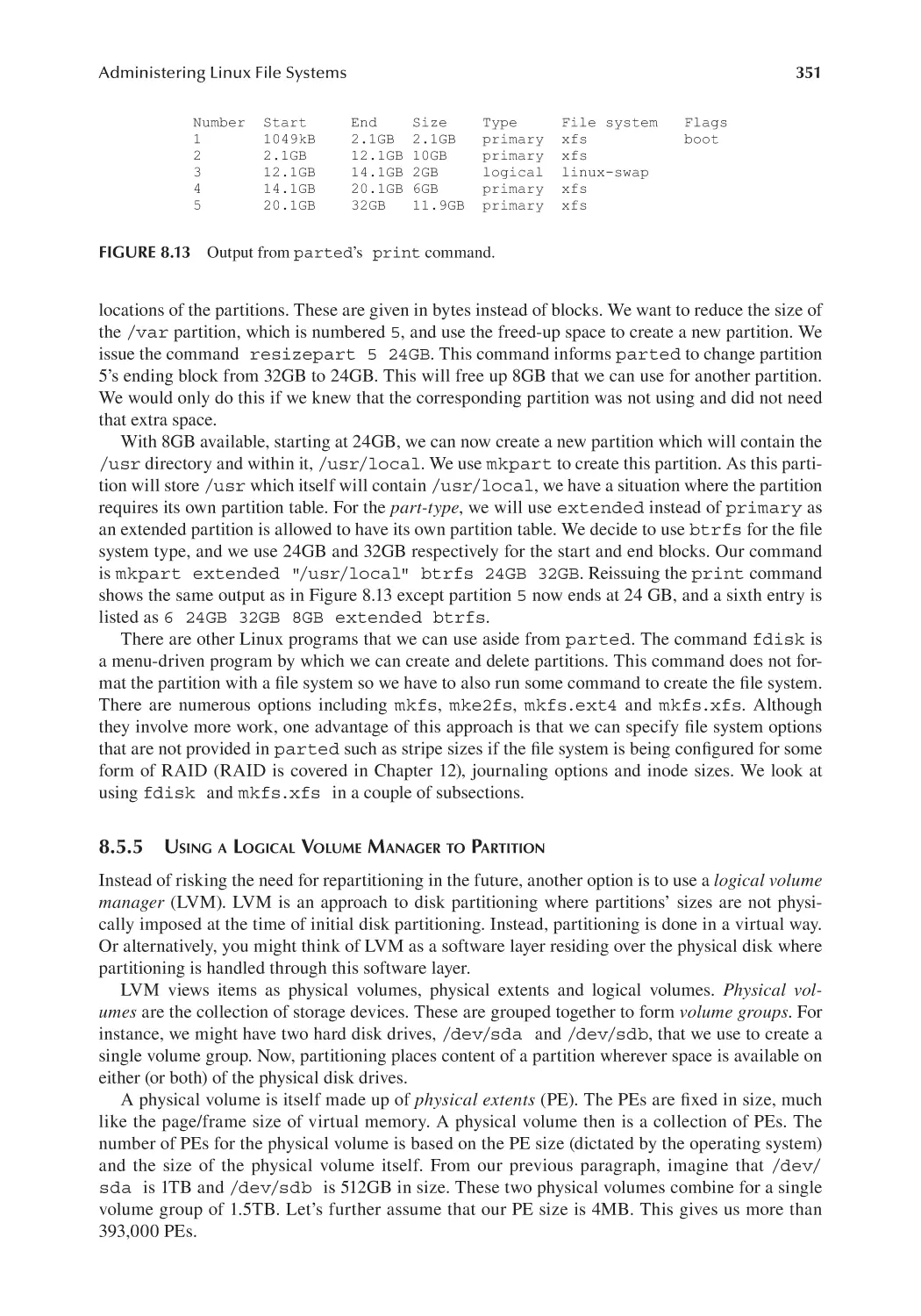
8.5.4 Repartitioning.................................................................................... 349
8.5.5 Using a Logical Volume Manager to Partition.................................. 351
8.5.6 Adding a Disk Drive......................................................................... 353
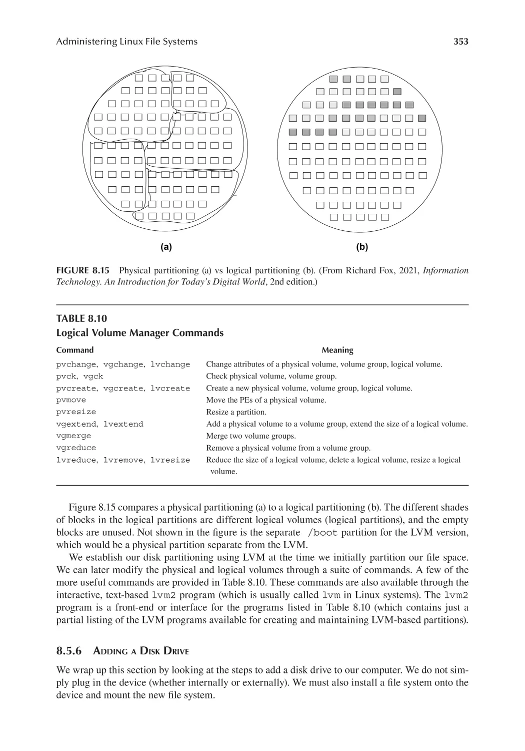
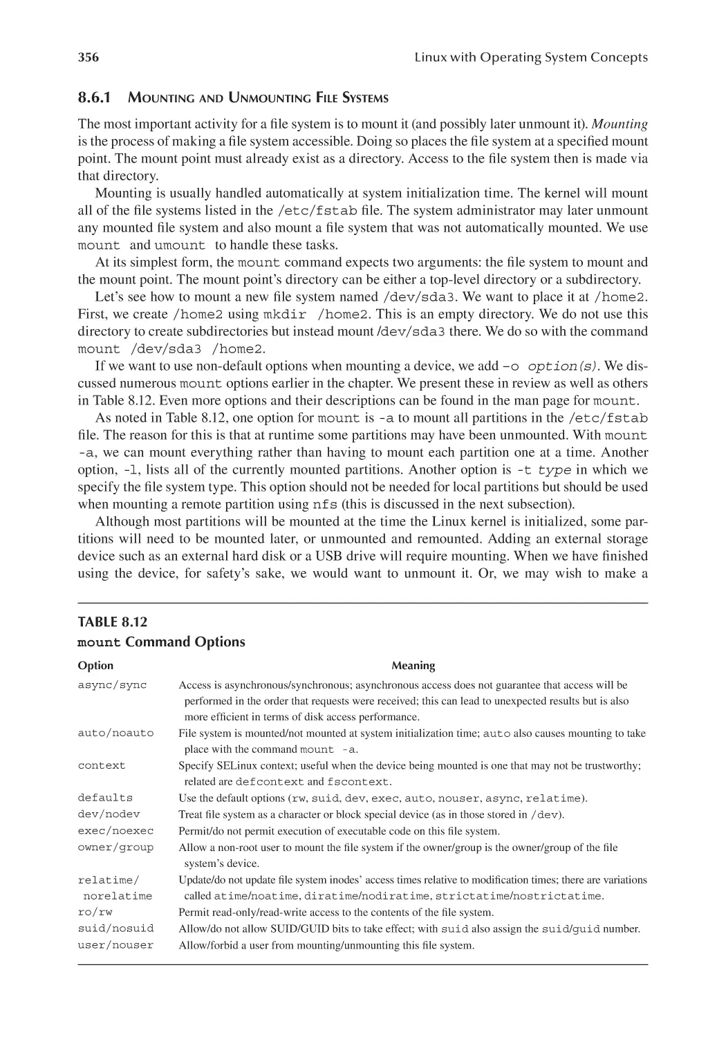
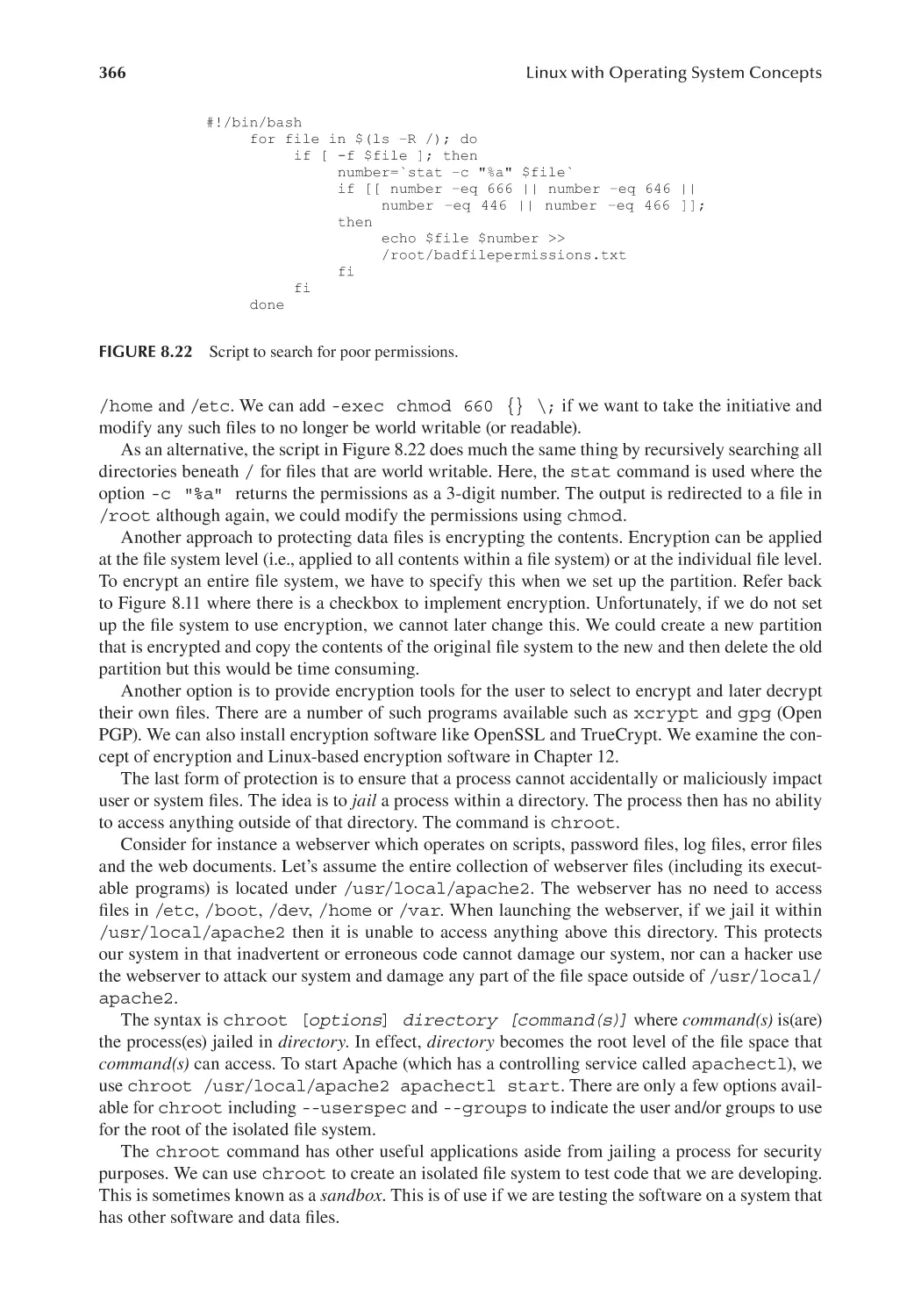
Administrative File System Tasks.................................................................. 355
8.6.1 Mounting and Unmounting File Systems.......................................... 356
8.6.2 Remote File Systems......................................................................... 358
xii
Contents
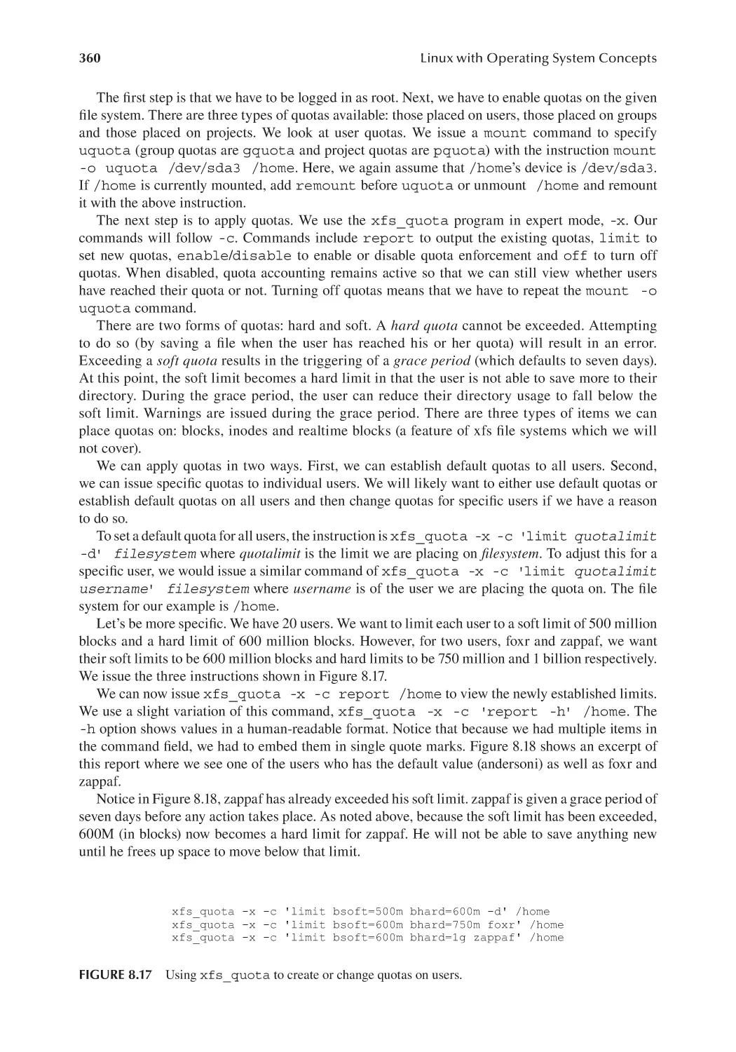
8.6.3 Establishing Quotas on a File System............................................... 359
8.6.4 Miscellaneous Administrative File System Commands................... 361
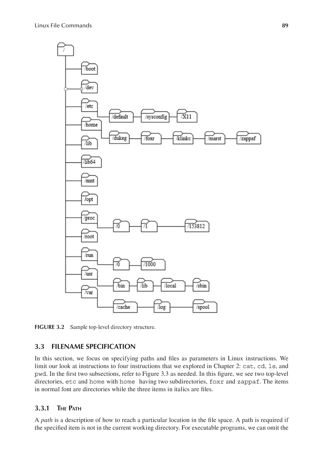
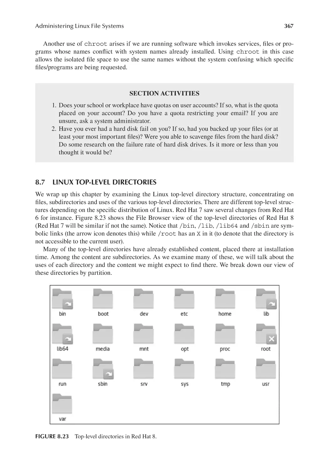
8.7 Linux Top-Level Directories.......................................................................... 367
8.7.1 Root (/) Partition Directories........................................................... 368
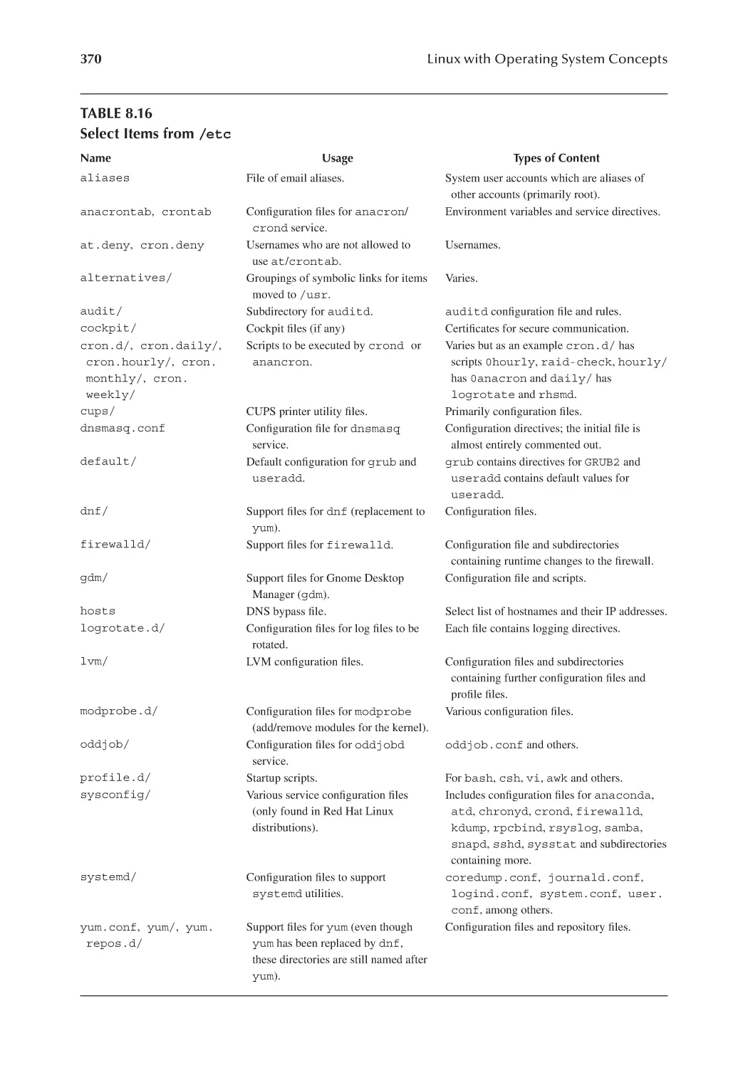
8.7.2 The /etc Directory.......................................................................... 369
8.7.3 The /boot, /home and /var Directories...................................... 369
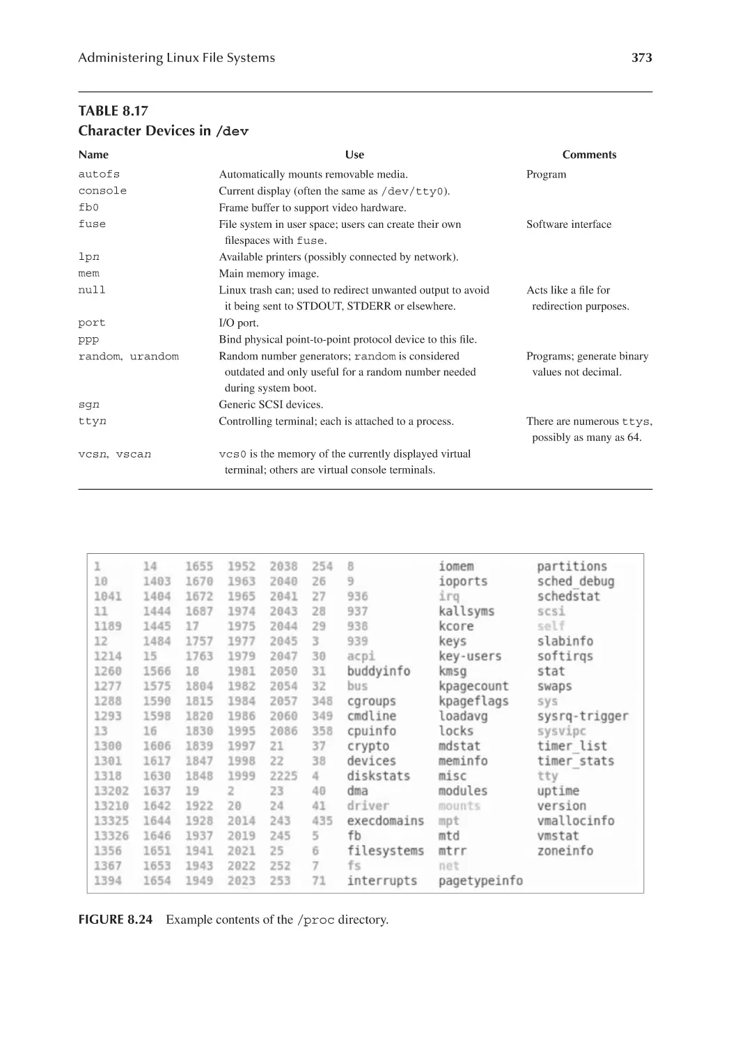
8.7.4 Virtual File System Directories........................................................ 372
8.8 Chapter Review.............................................................................................. 375
Review Problems....................................................................................................... 379
Chapter 9
System Initialization and Services............................................................................ 383
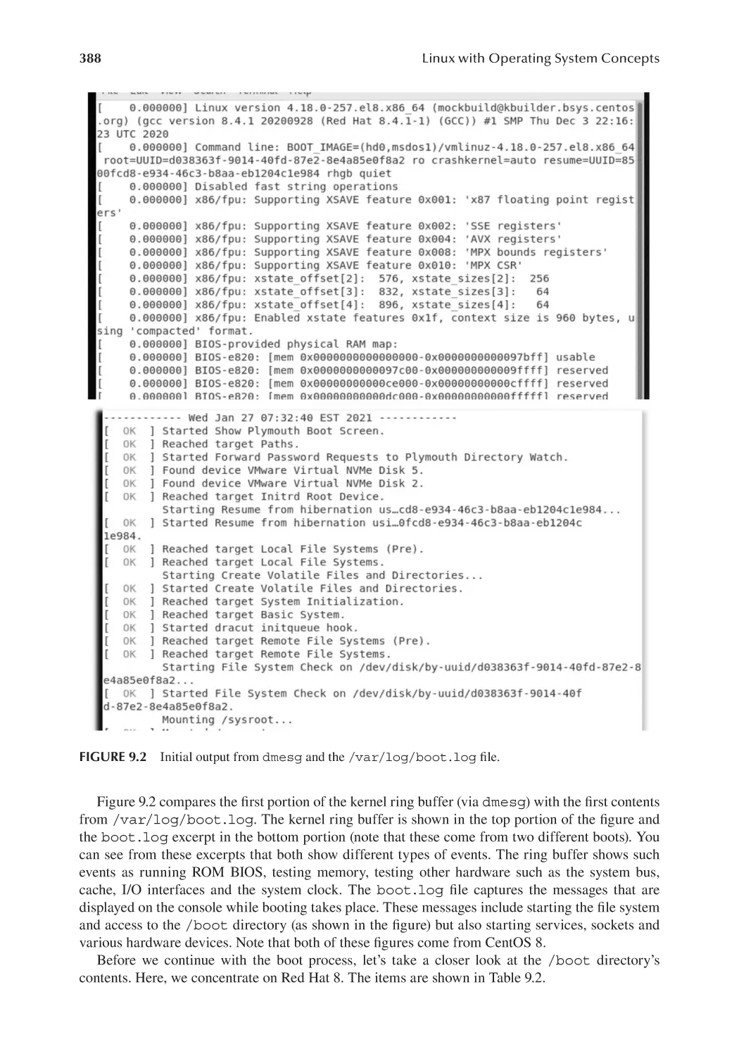
9.1
9.2
Introduction.................................................................................................... 383
Booting the Computer.................................................................................... 384
9.2.1 Volatile and Non-Volatile Memory................................................... 384
9.2.2 The Boot Process.............................................................................. 385
9.2.3 The Linux Boot Process.................................................................... 385
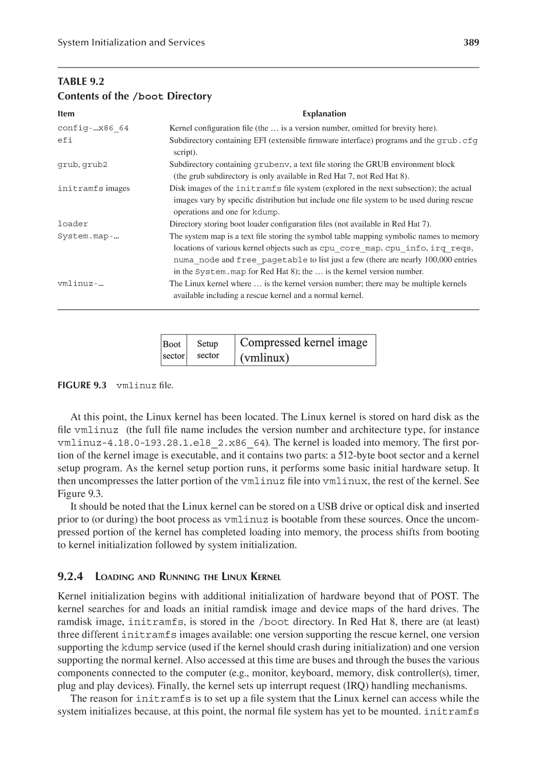
9.2.4 Loading and Running the Linux Kernel........................................... 389
9.3 Initialization of the Linux Operating System................................................. 390
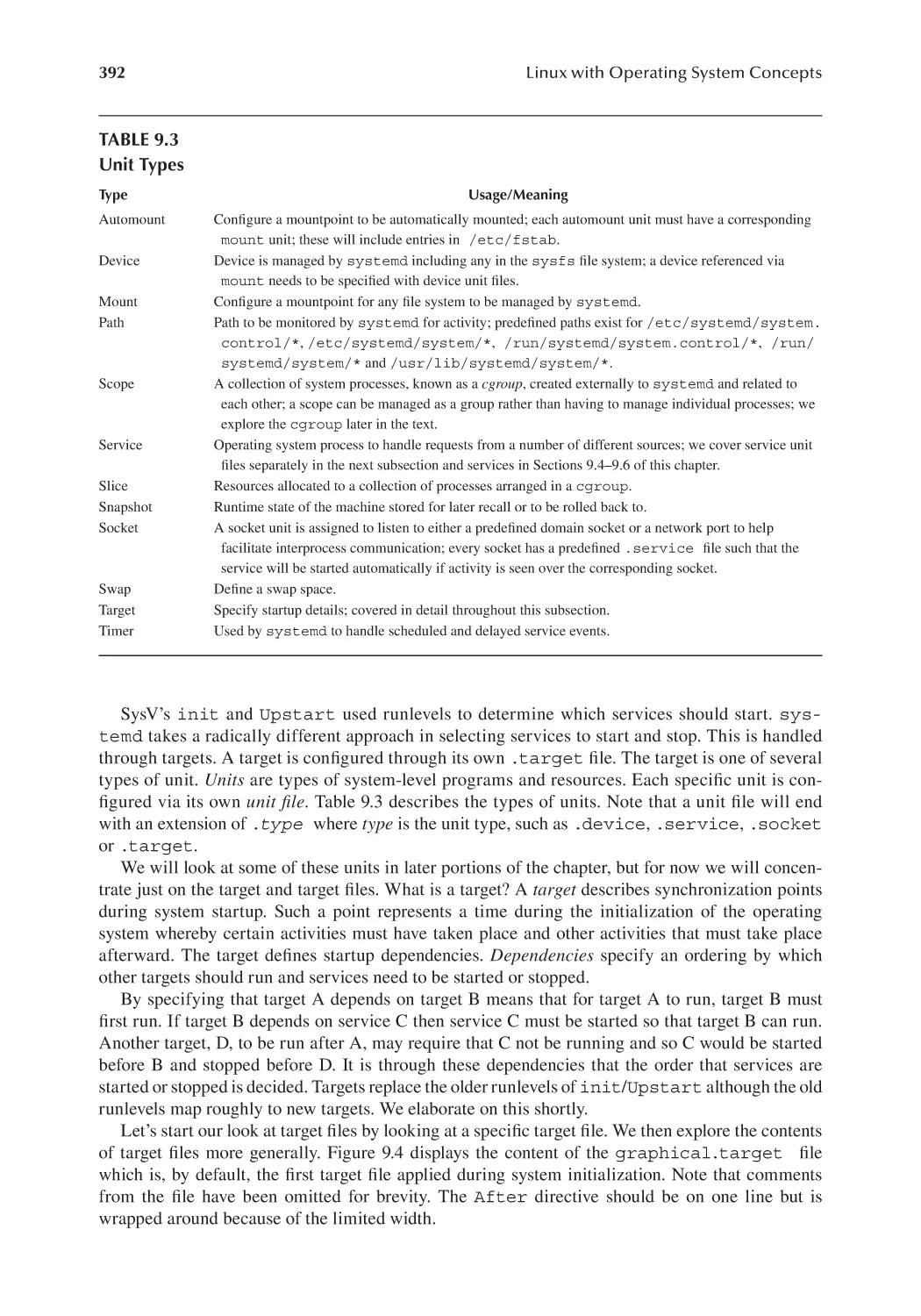
9.3.1 Target Unit Files................................................................................ 391
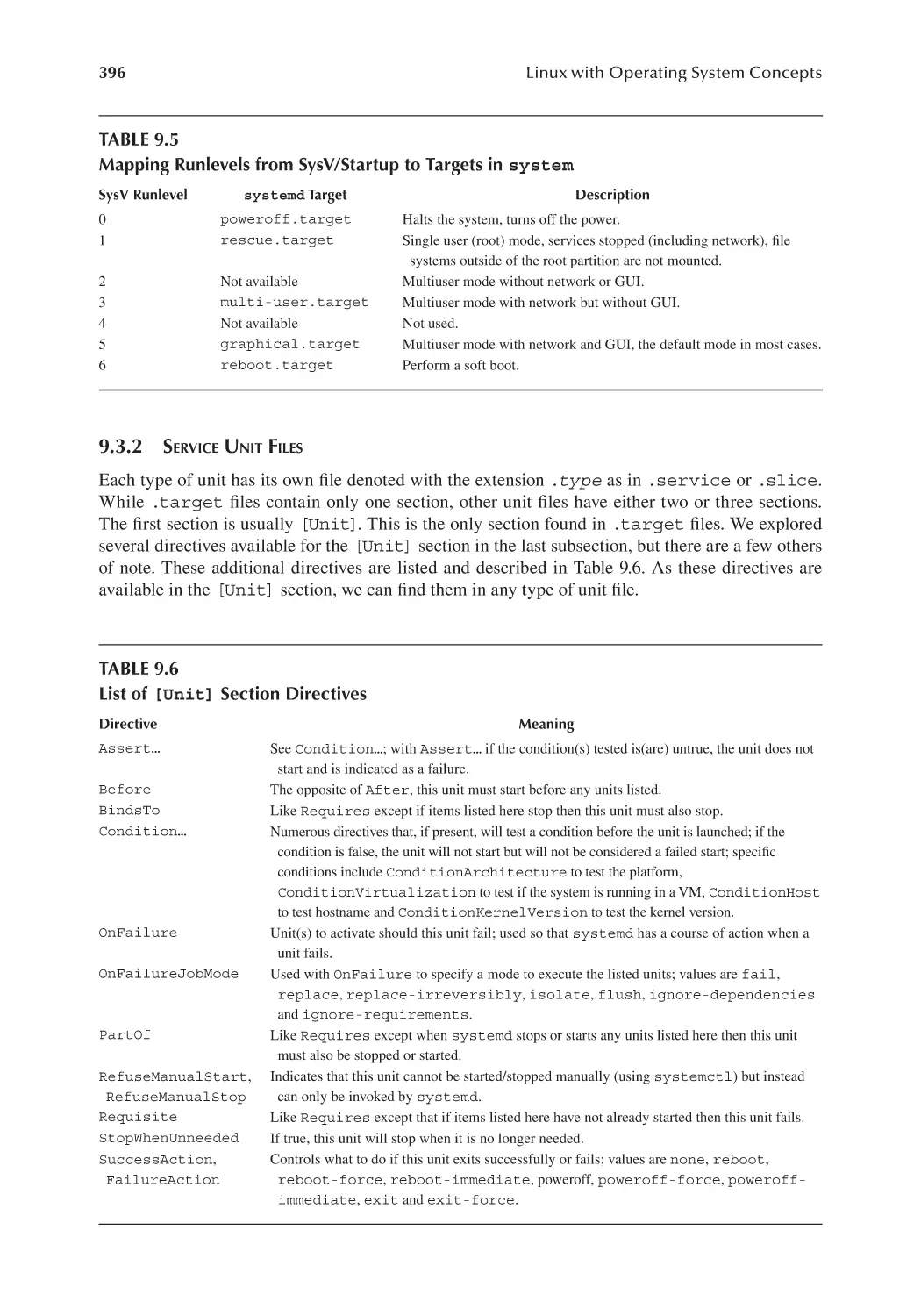
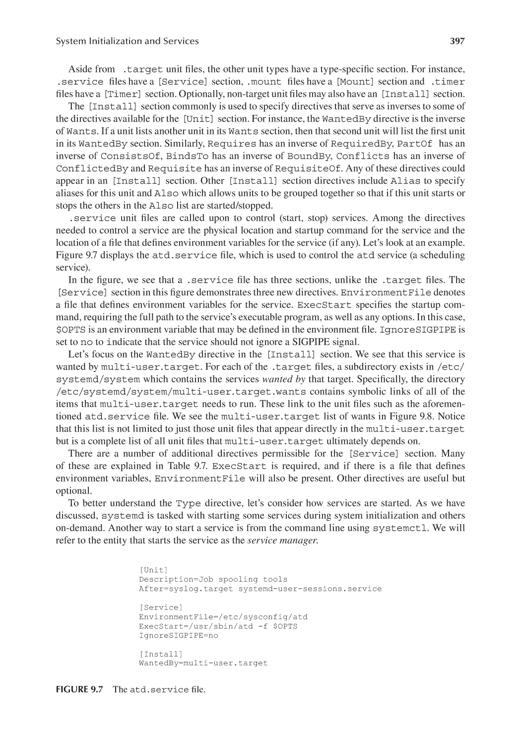
9.3.2 Service Unit Files.............................................................................. 396
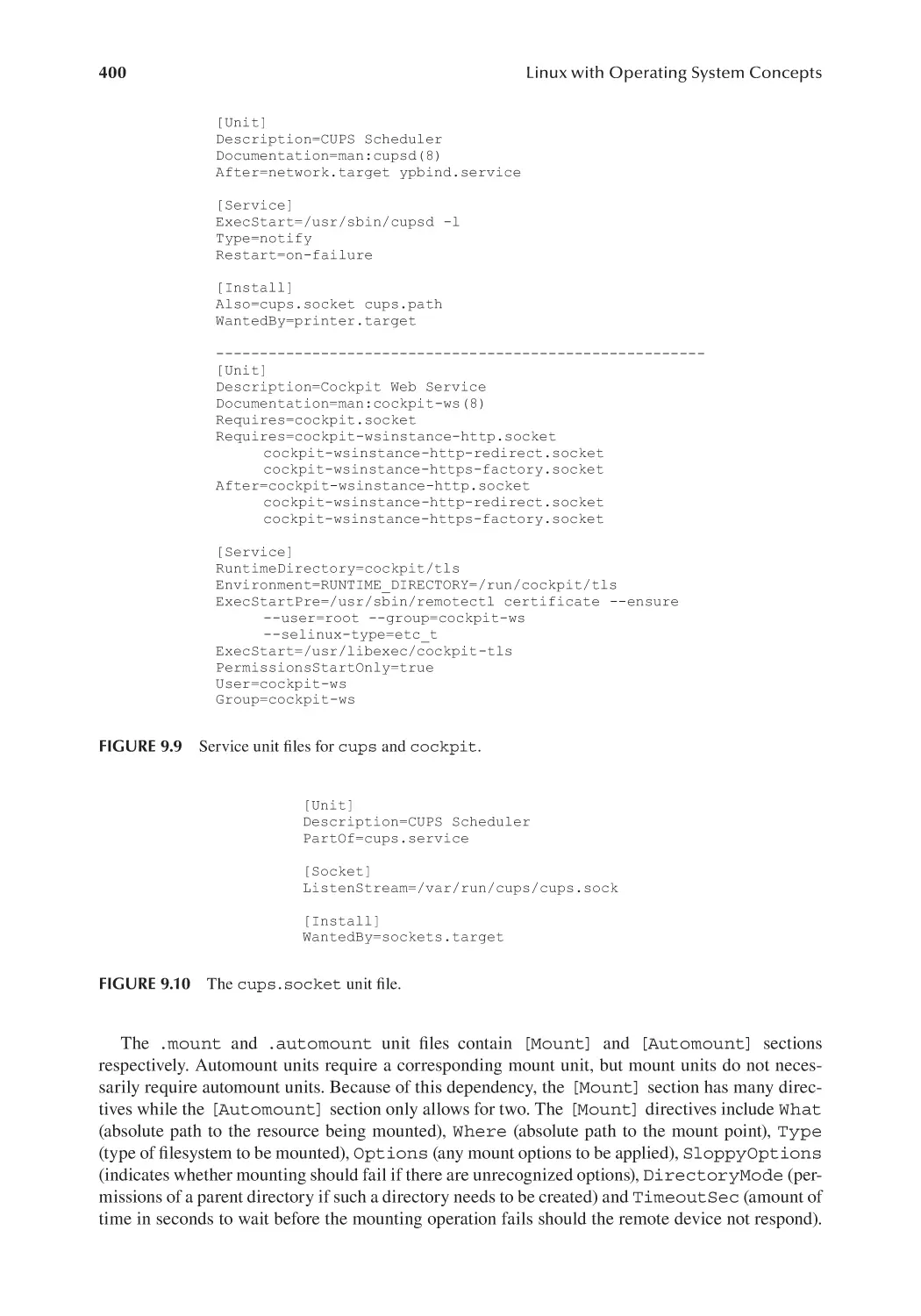
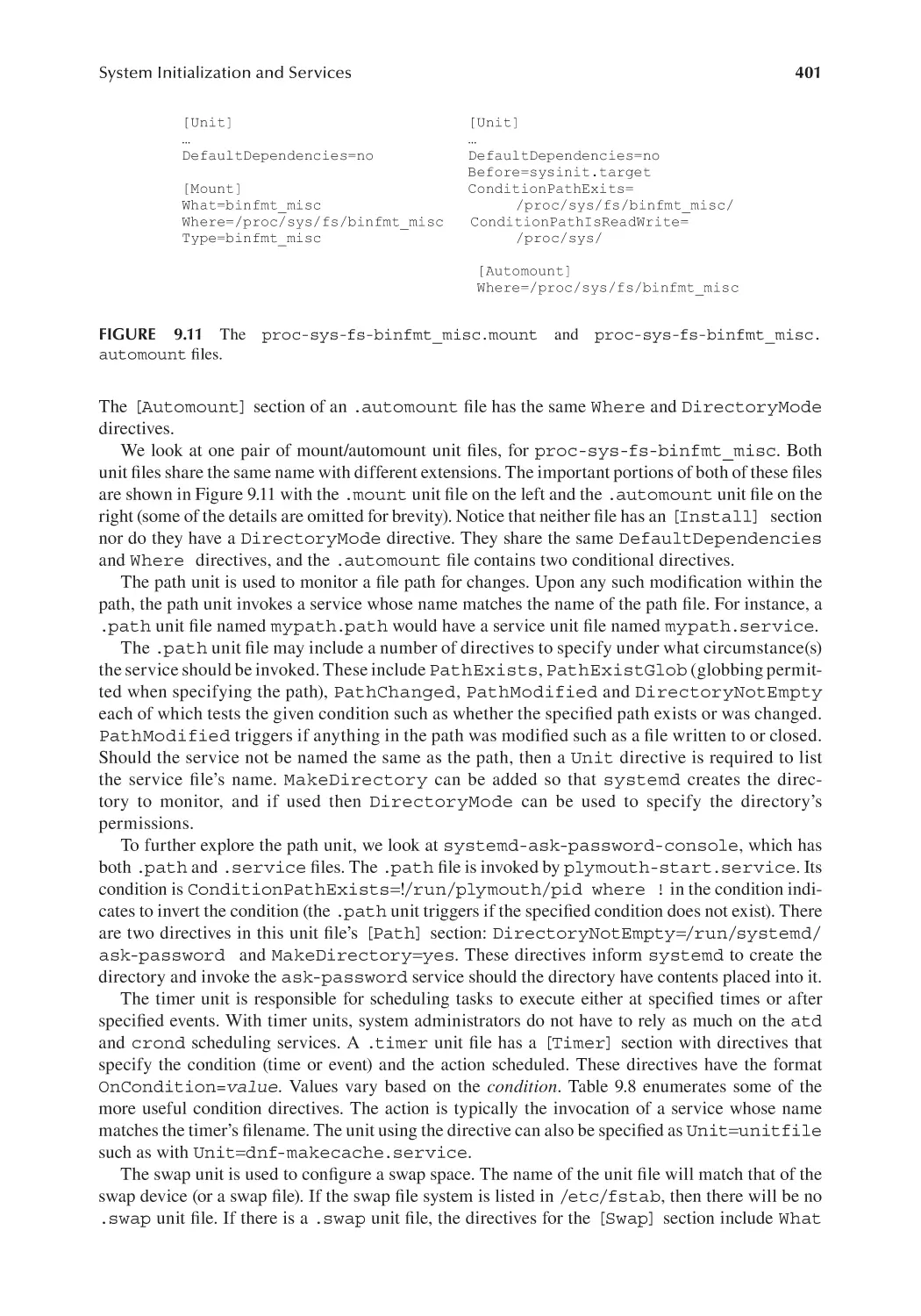
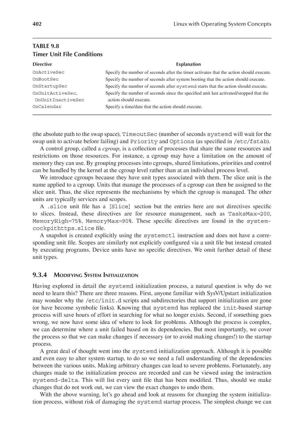
9.3.3 Other Unit File Types........................................................................ 399
9.3.4 Modifying System Initialization.......................................................402
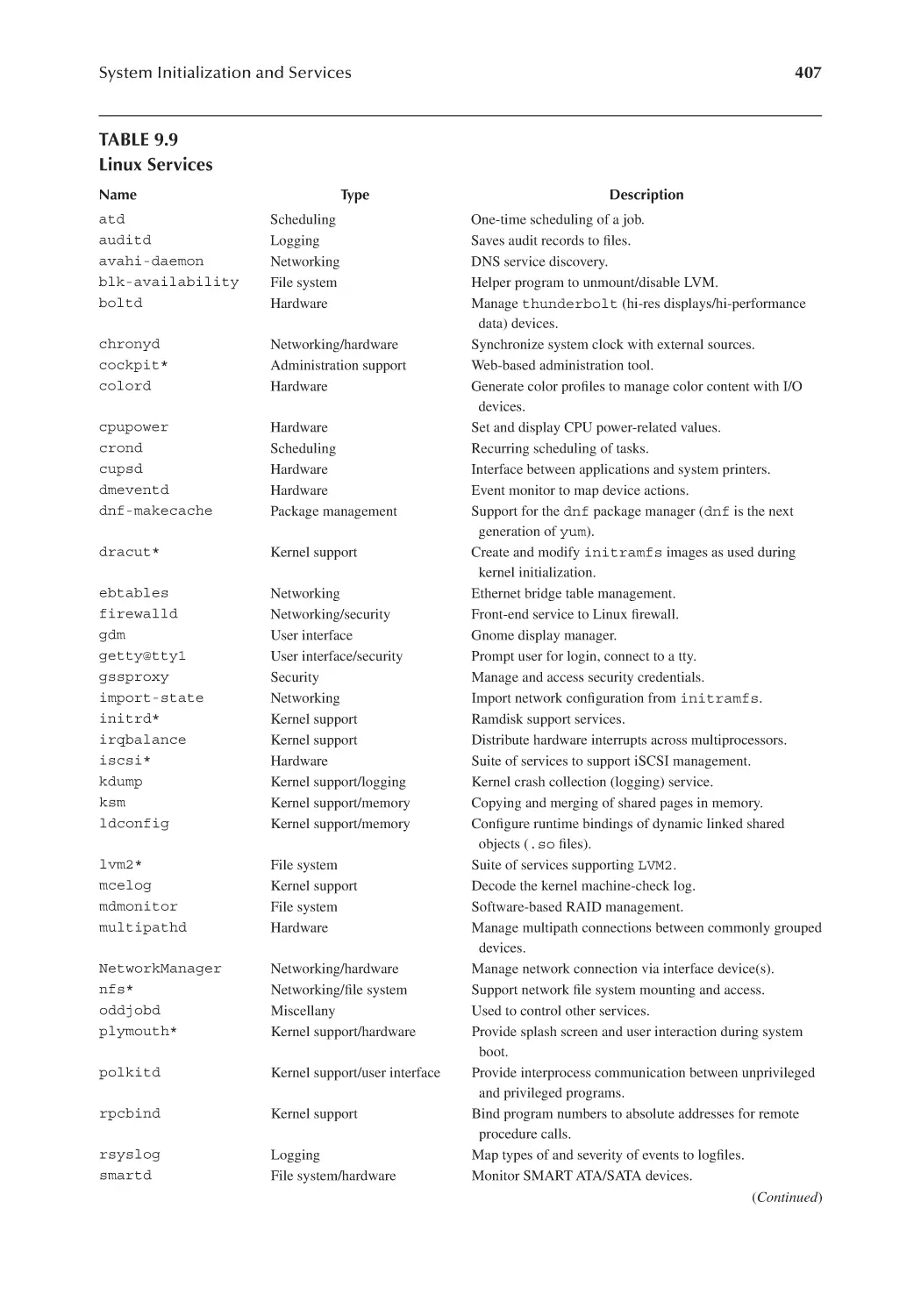
9.4 Linux Services................................................................................................405
9.4.1 What Are Services?...........................................................................405
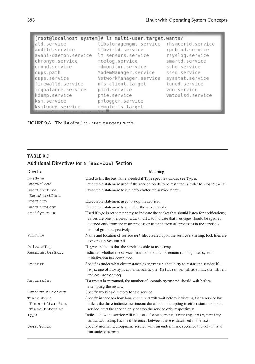
9.4.2 An Examination of Significant Linux Services................................406
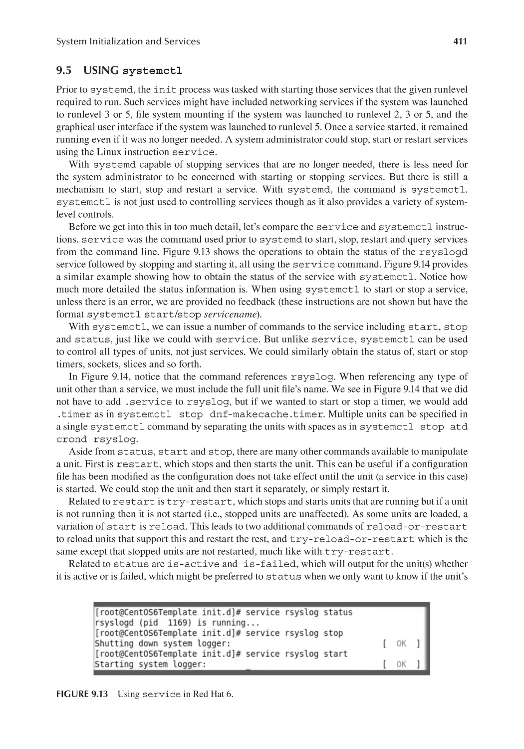
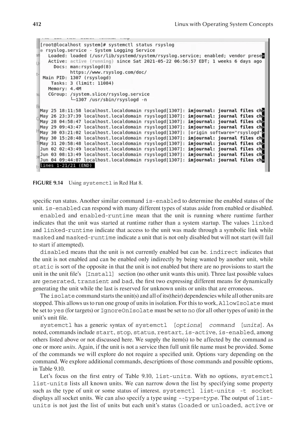
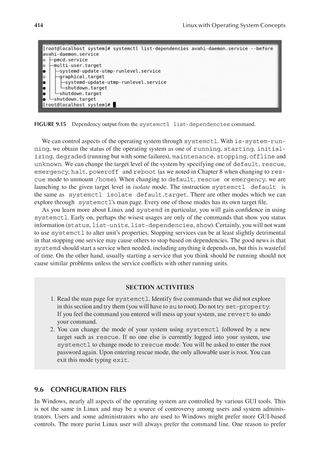
9.5 Using systemctl ........................................................................................ 411
9.6 Configuration Files......................................................................................... 414
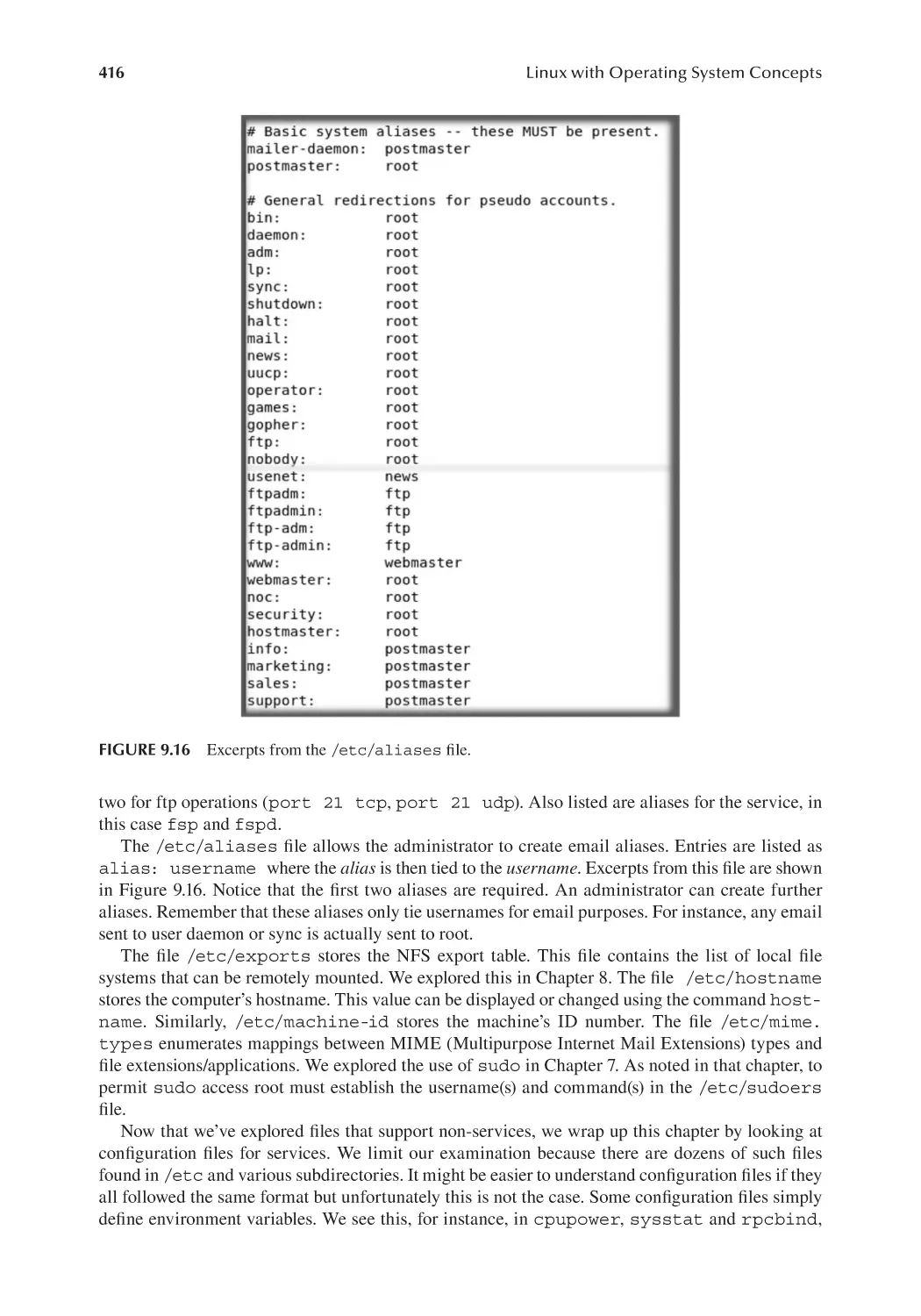
9.6.1 Non-Service Configuration Files....................................................... 415
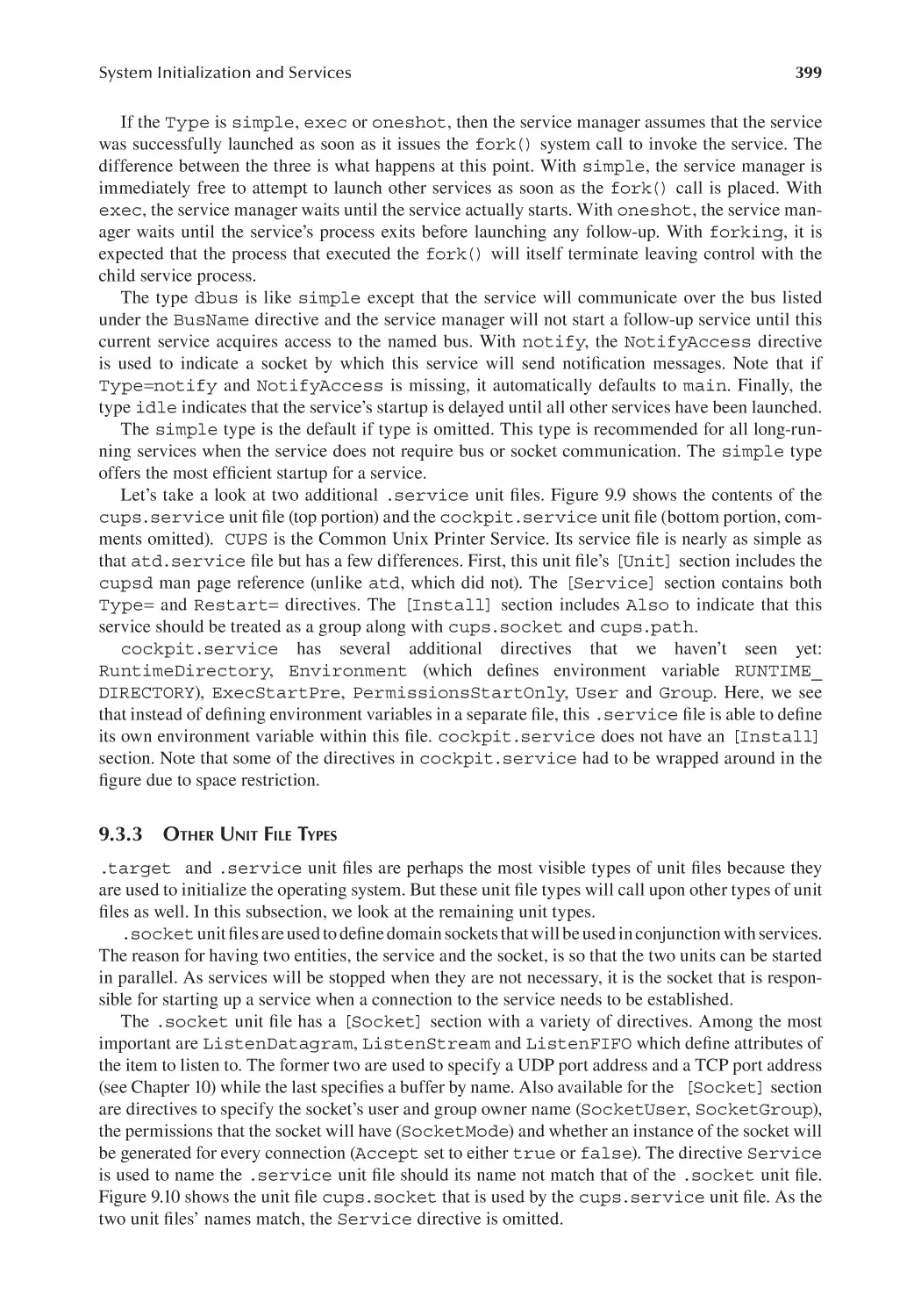
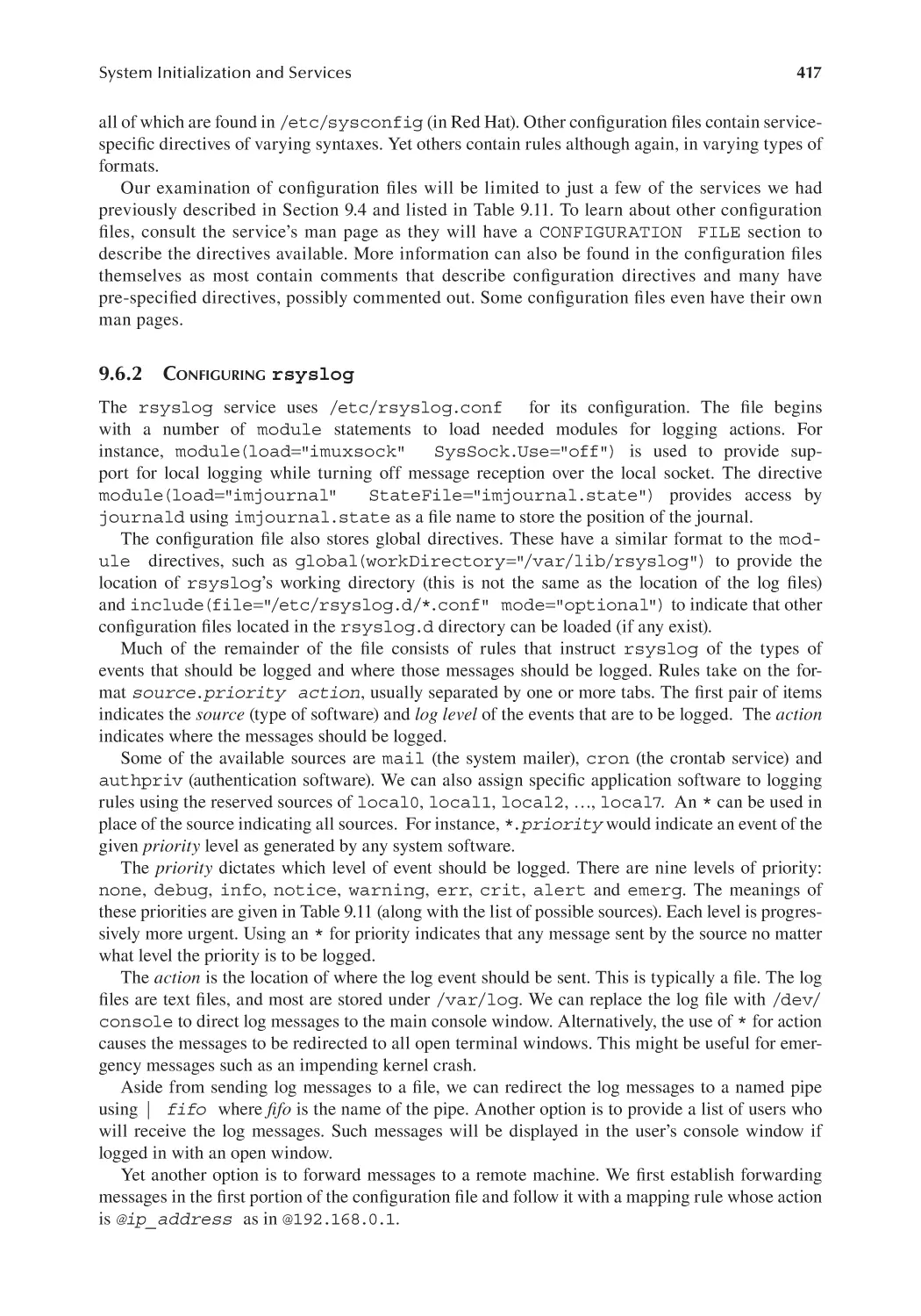
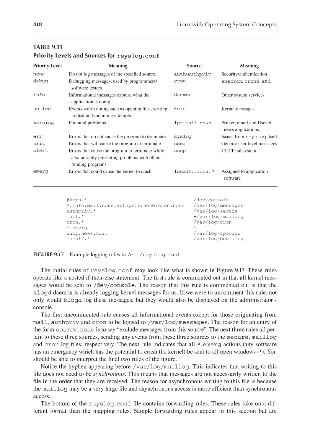
9.6.2 Configuring rsyslog...................................................................... 417
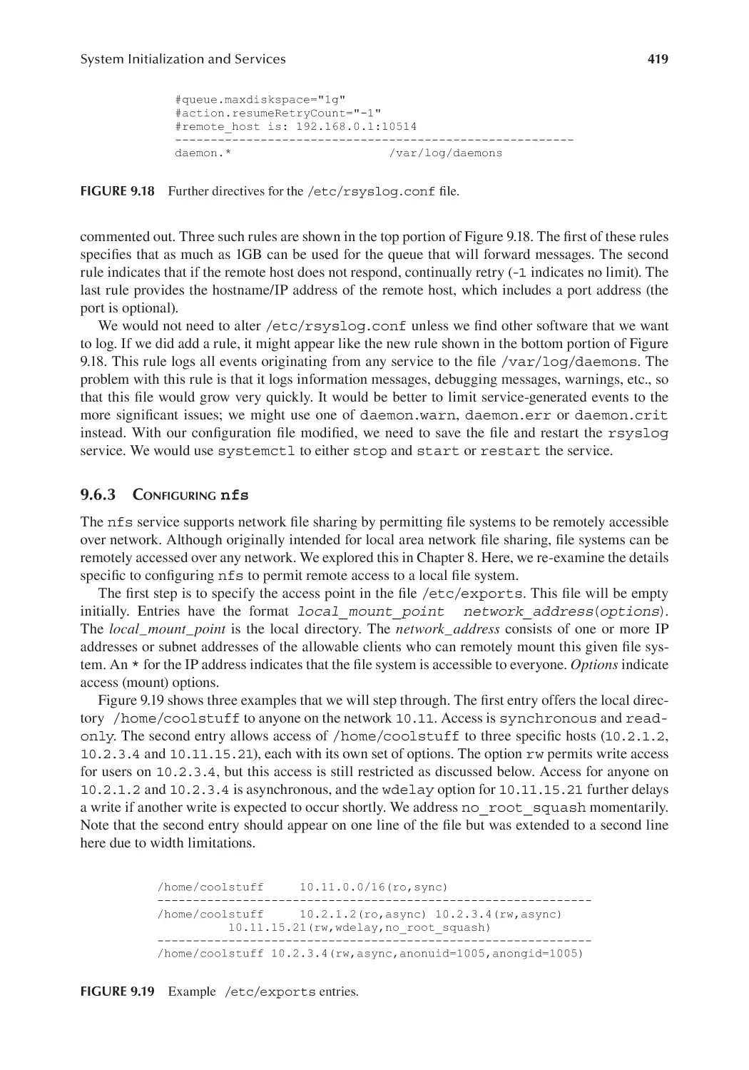
9.6.3 Configuring nfs............................................................................... 419
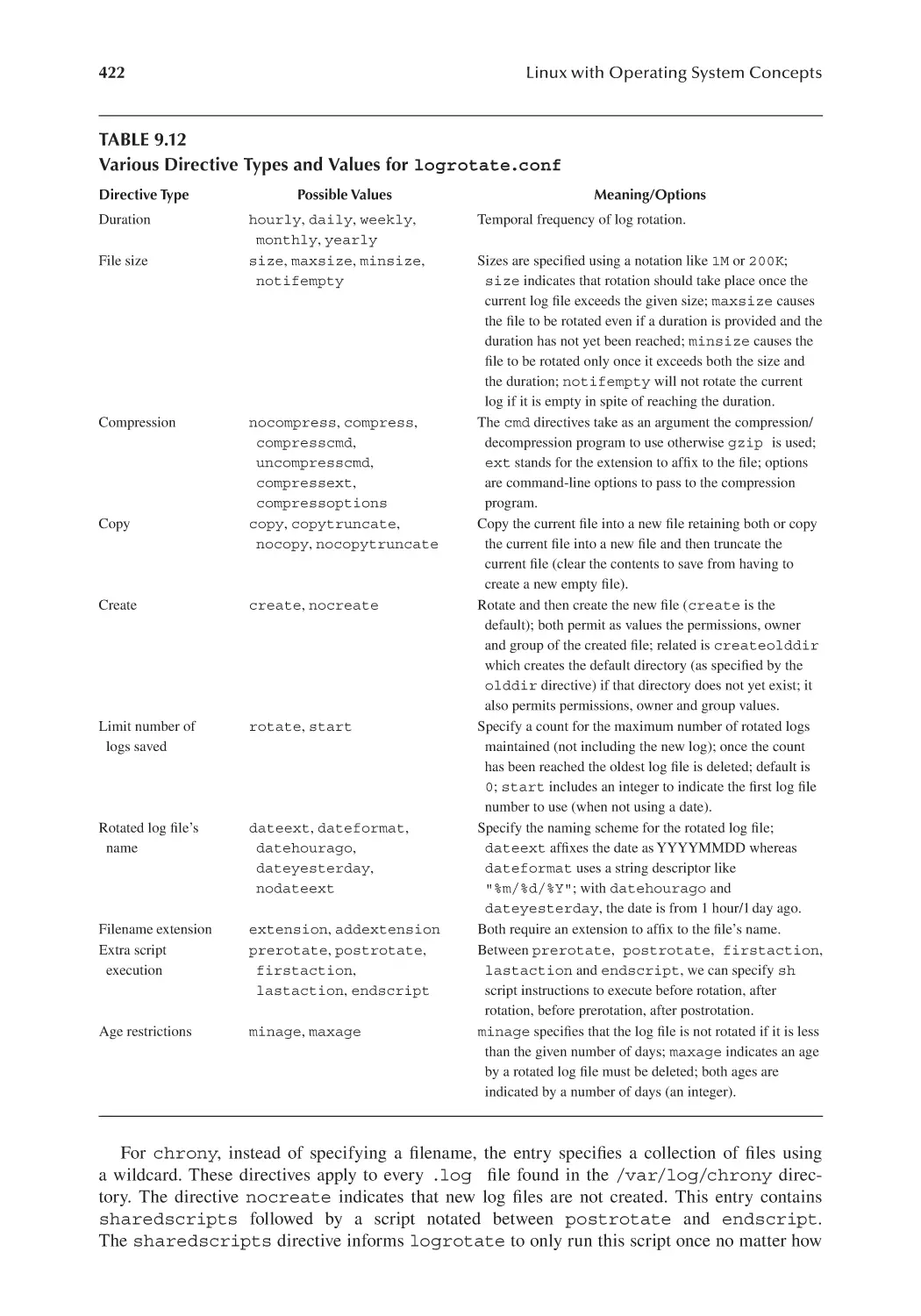
9.6.4 Configuring logrotate................................................................. 421
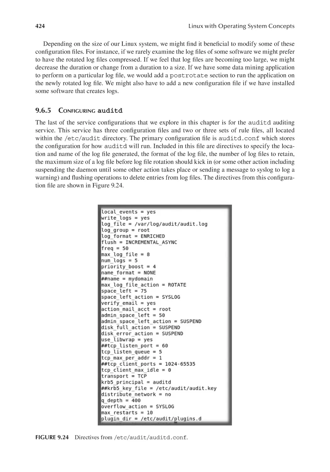
9.6.5 Configuring auditd........................................................................ 424
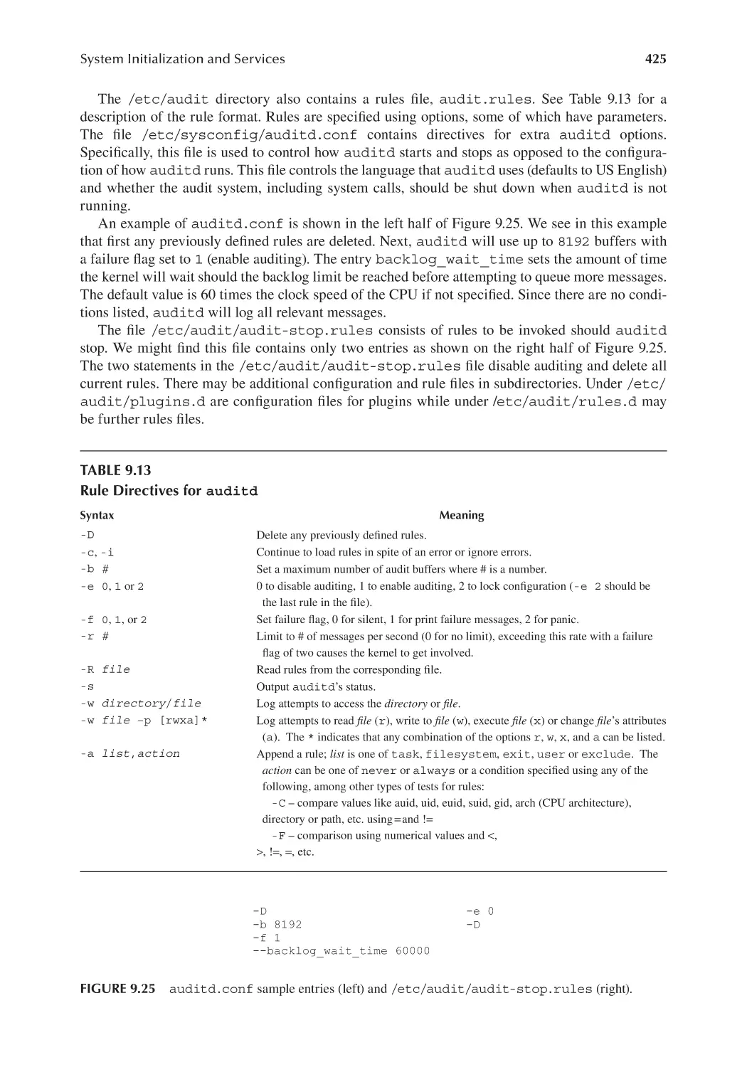
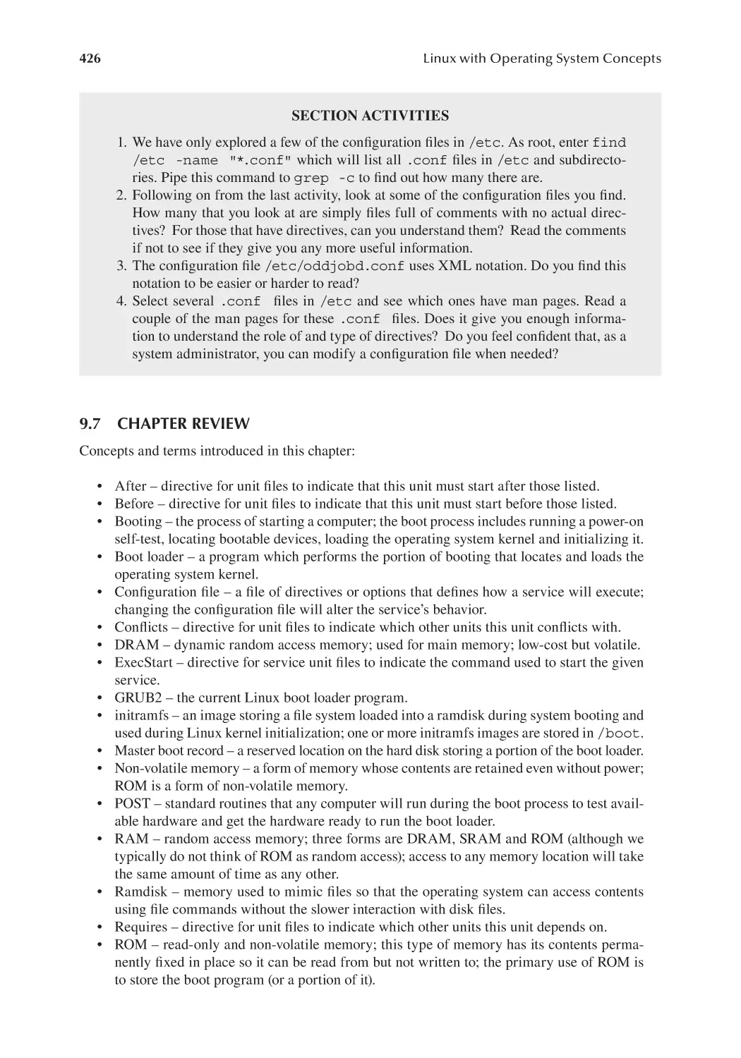
9.7 Chapter Review.............................................................................................. 426
Review Problems....................................................................................................... 428
Chapter 10 Network Configuration.............................................................................................. 433
10.1 Introduction.................................................................................................... 433
10.2 Computer Networks and TCP/IP.................................................................... 434
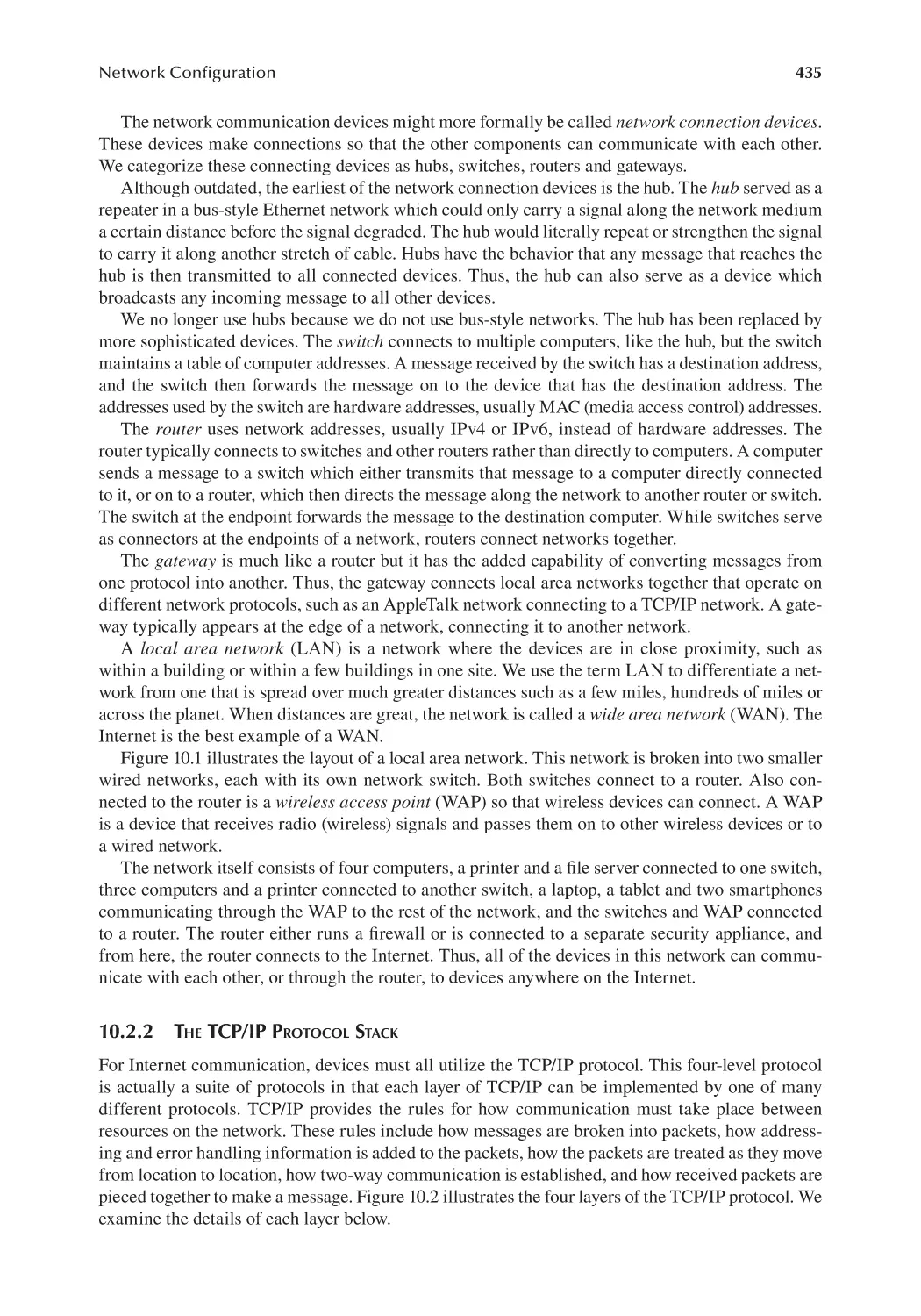
10.2.1 Network Connection Devices............................................................ 434
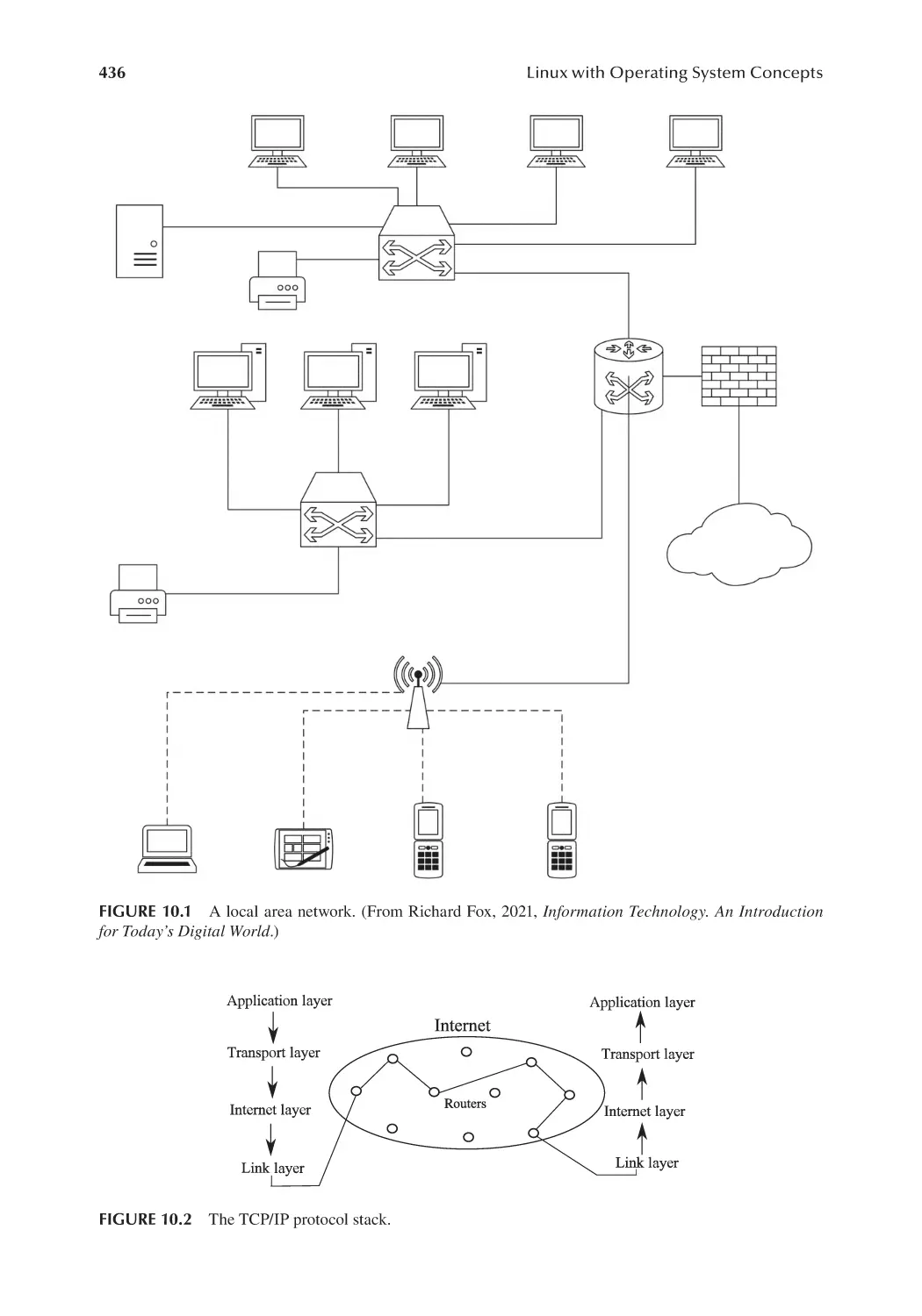
10.2.2 The TCP/IP Protocol Stack............................................................... 435
10.2.3 Ports...................................................................................................440
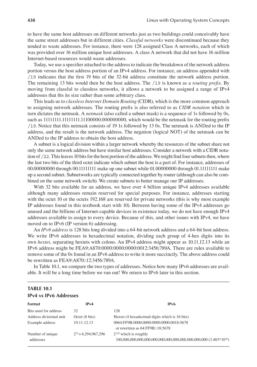
10.2.4 IPv6...................................................................................................440
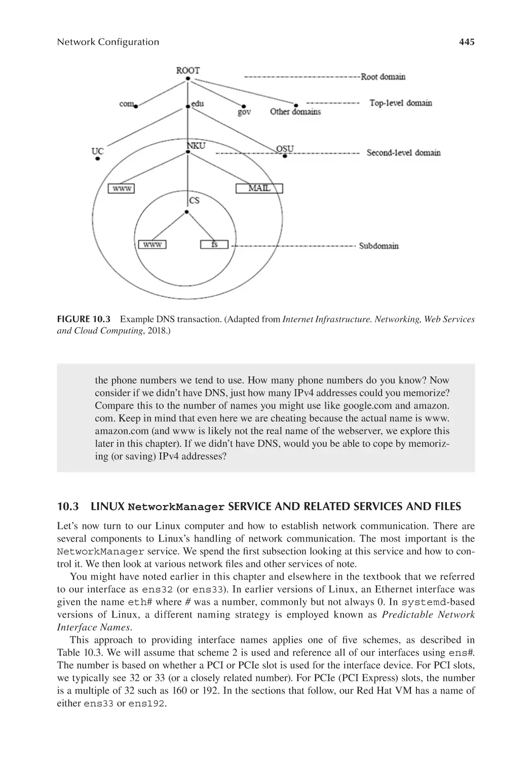
10.2.5 Domains, the Domain Name System and Host Names..................... 442
10.3 Linux NetworkManager Service and Related Services and Files............. 445
10.3.1 NetworkManager..........................................................................446
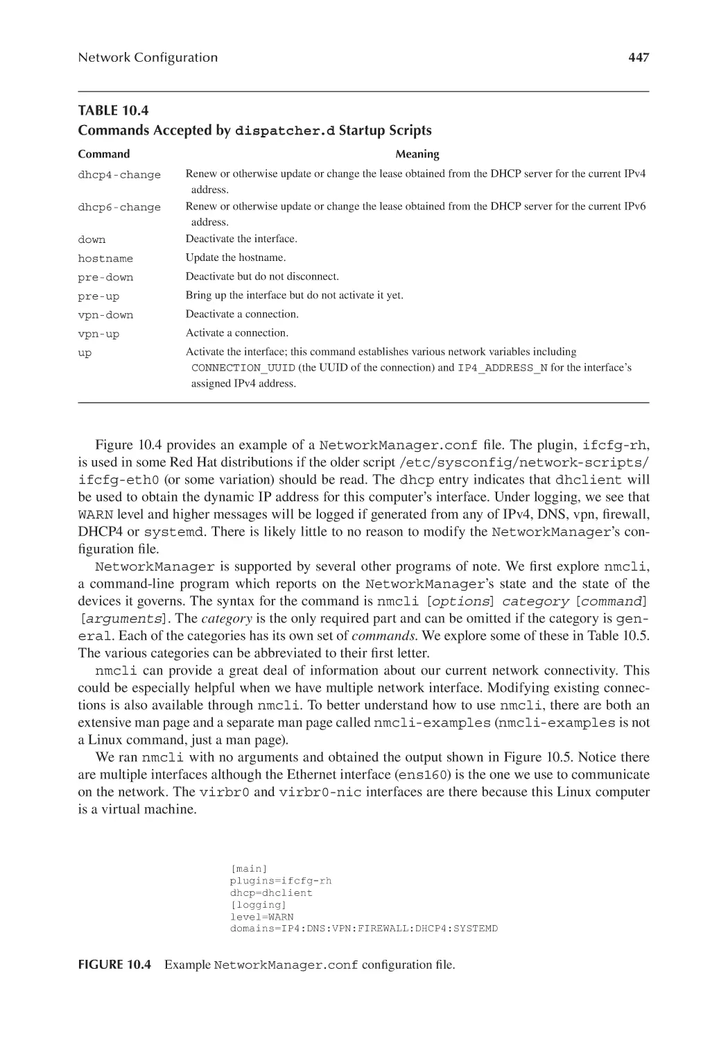
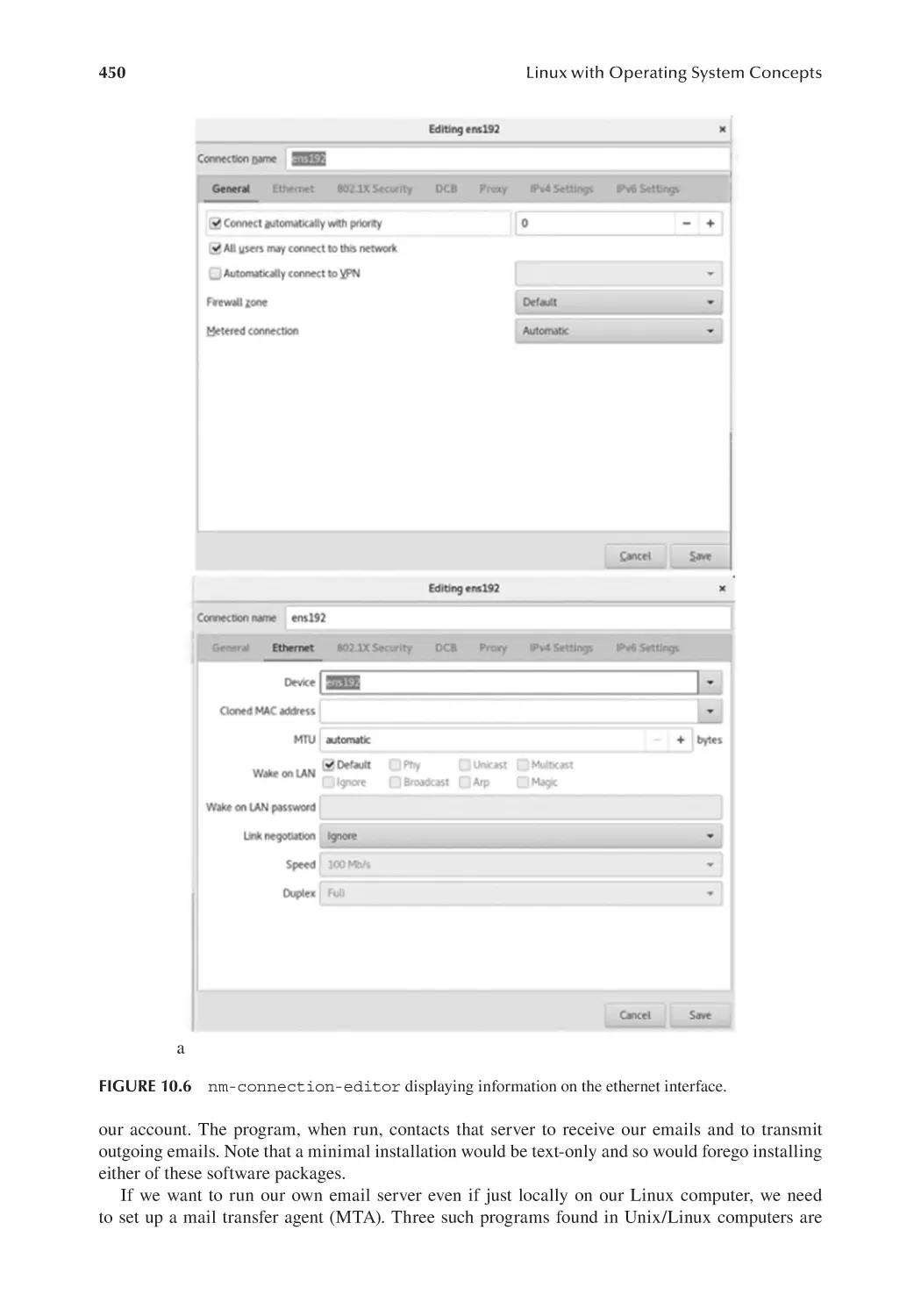
10.3.2 Other Network Services of Note.......................................................449
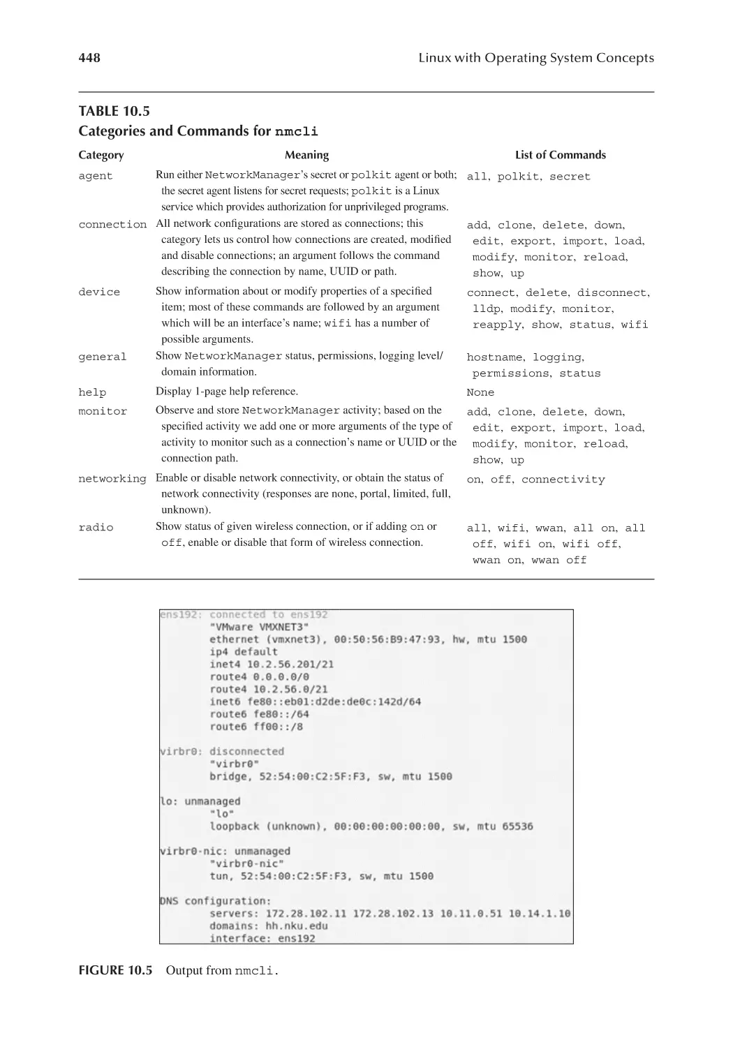
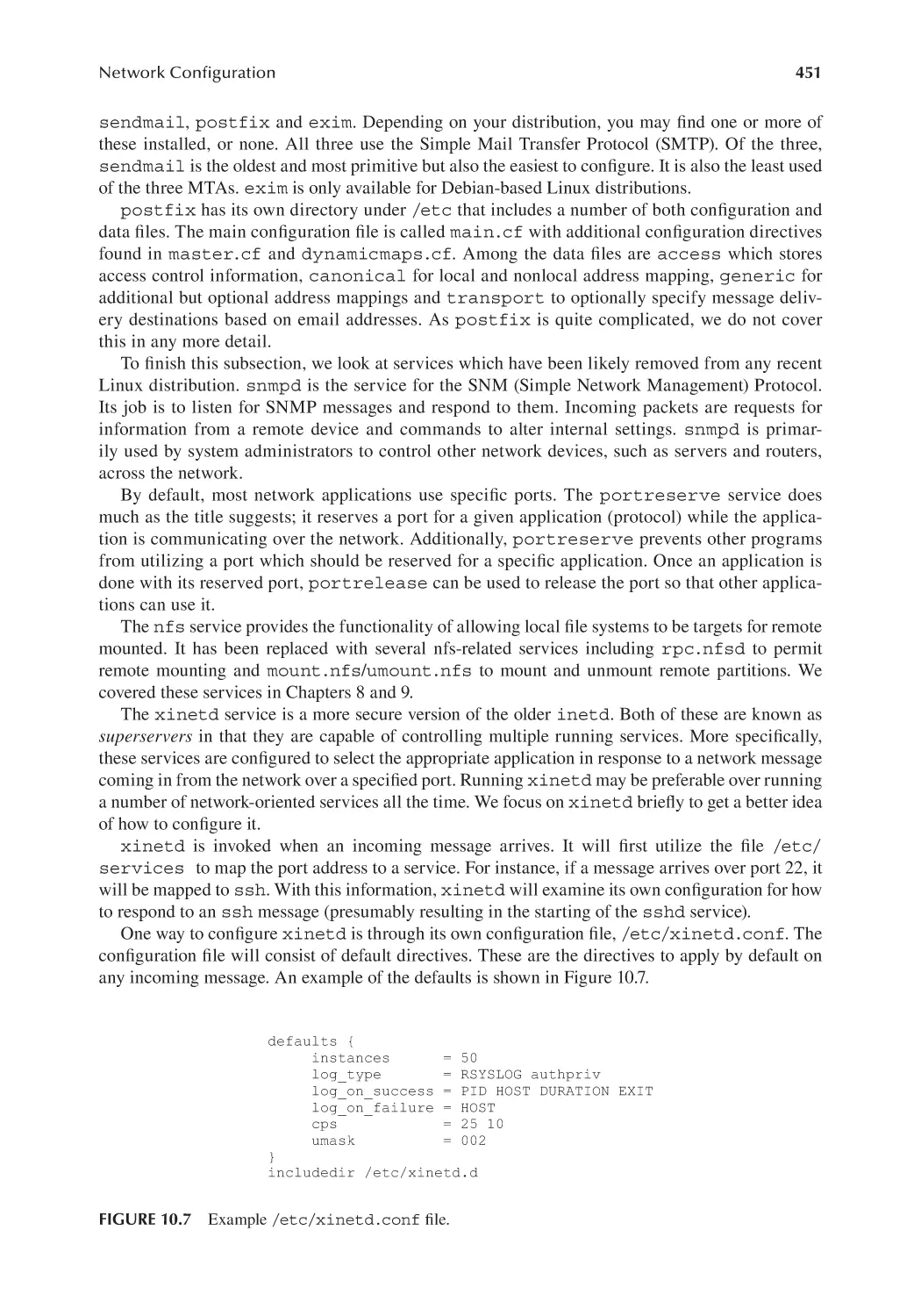
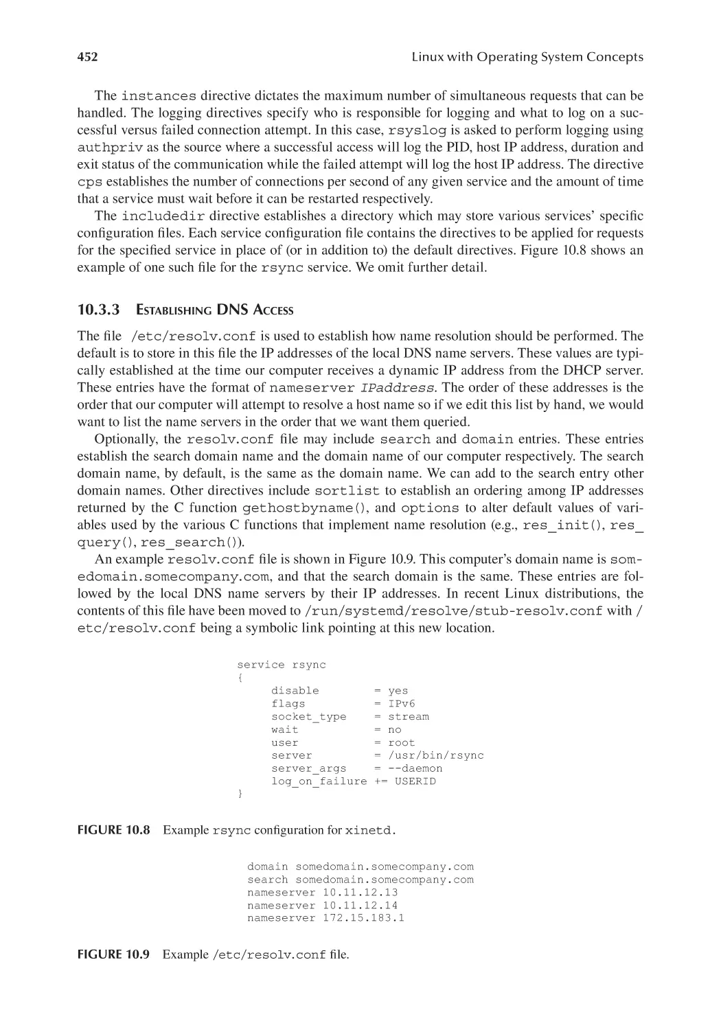
10.3.3 Establishing DNS Access.................................................................. 452
Contents
xiii
10.4 Obtaining IP Addresses.................................................................................. 453
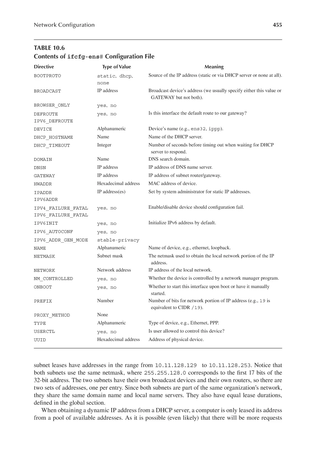
10.4.1 Configuring Our Interface Device(s)................................................. 454
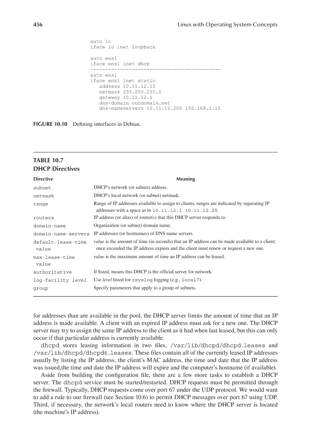
10.4.2 Setting Up a DHCP Server................................................................ 454
10.5 Network Programs.......................................................................................... 457
10.5.1 The ip Program................................................................................ 457
10.5.2 Remote Access and File Transfer Programs..................................... 459
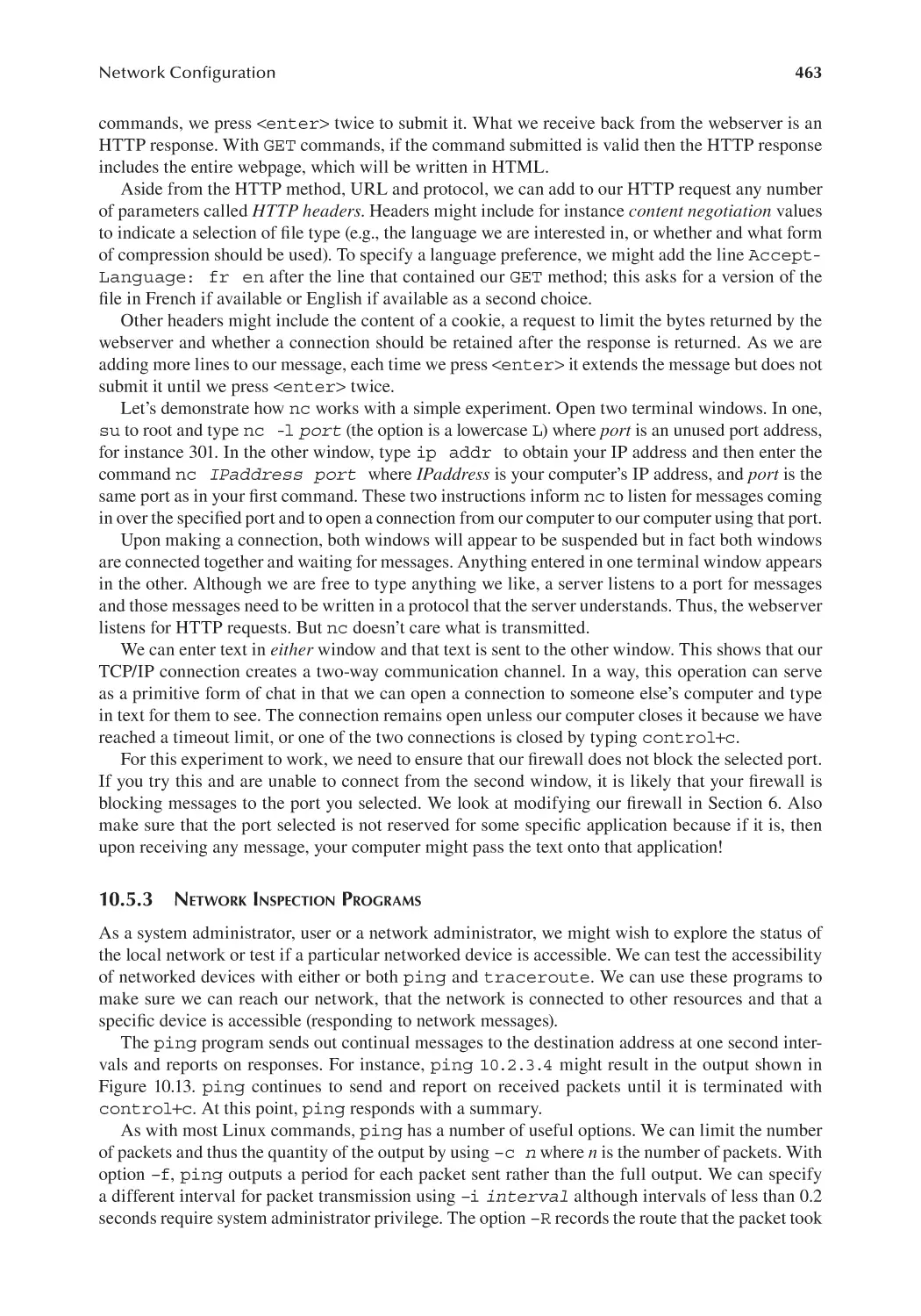
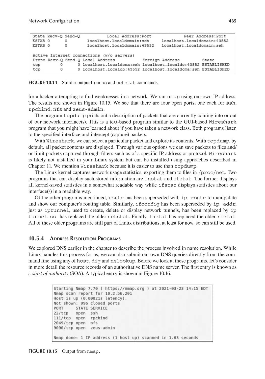
10.5.3 Network Inspection Programs........................................................... 463
10.5.4 Address Resolution Programs...........................................................465
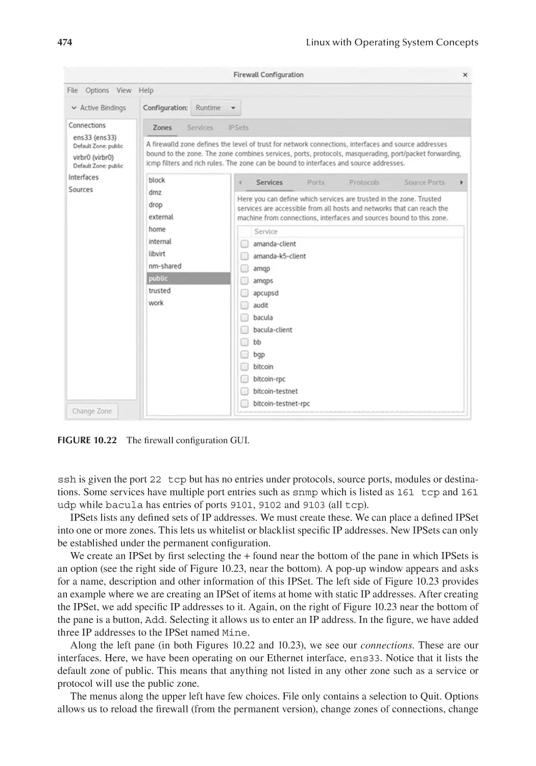
10.6 The Linux Firewall......................................................................................... 471
10.6.1 The firewalld Service.................................................................. 472
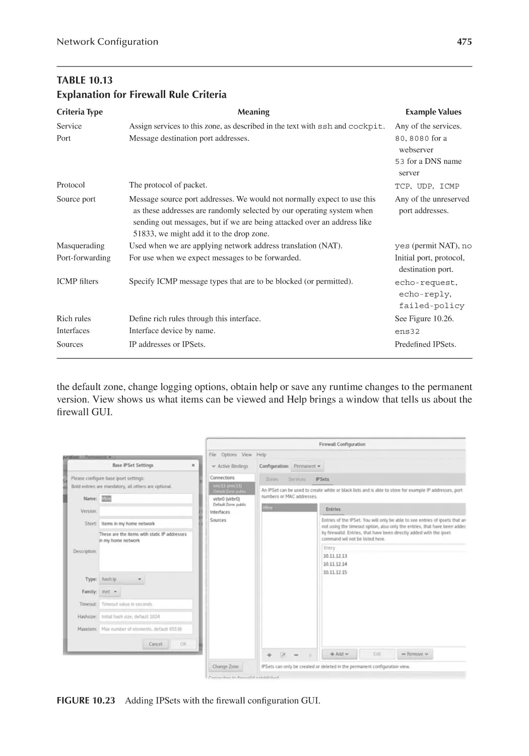
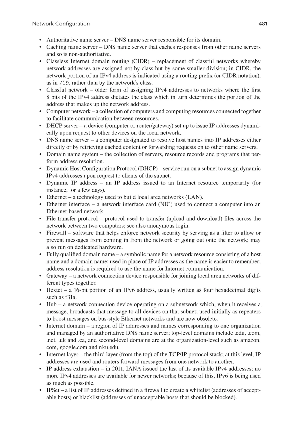
10.6.2 The Firewall Configuration GUI Tool............................................... 473
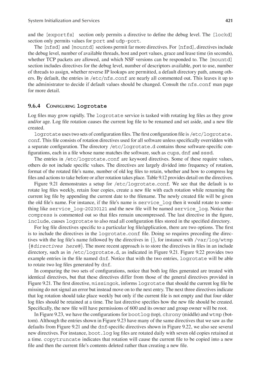
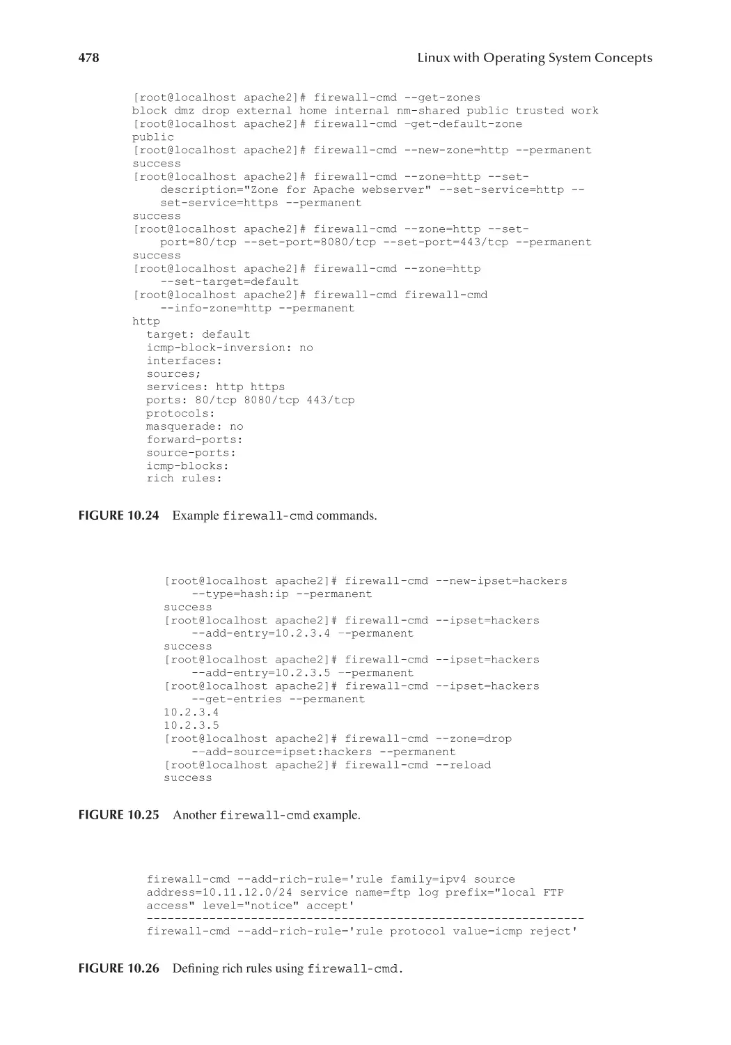
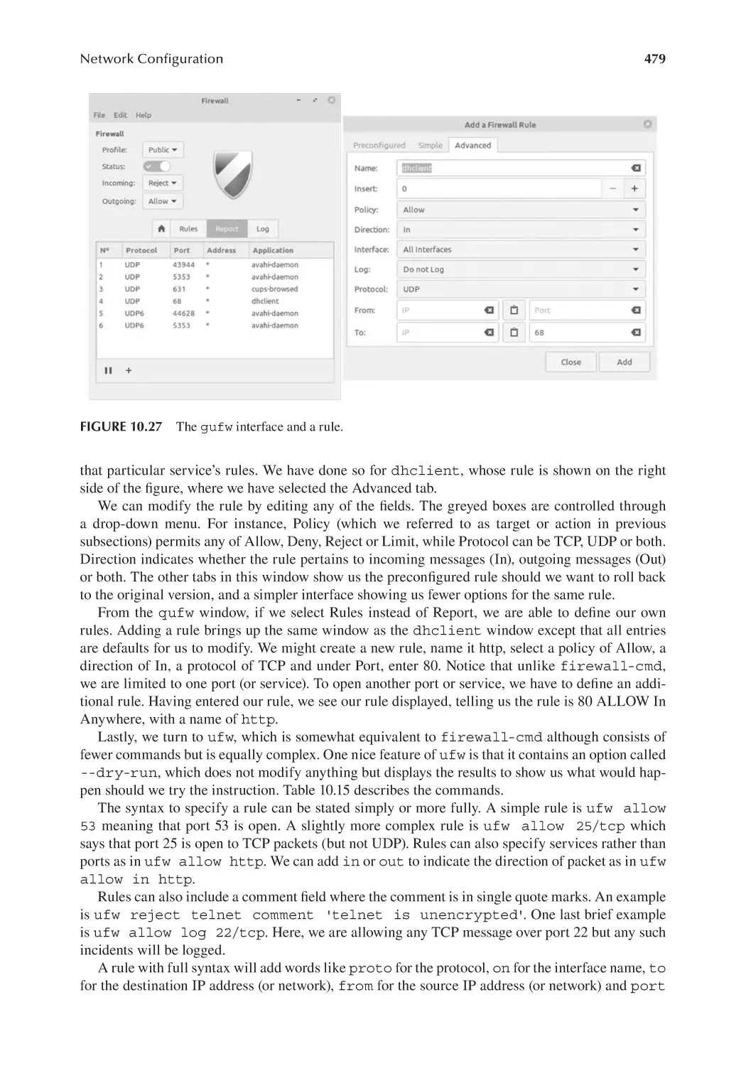
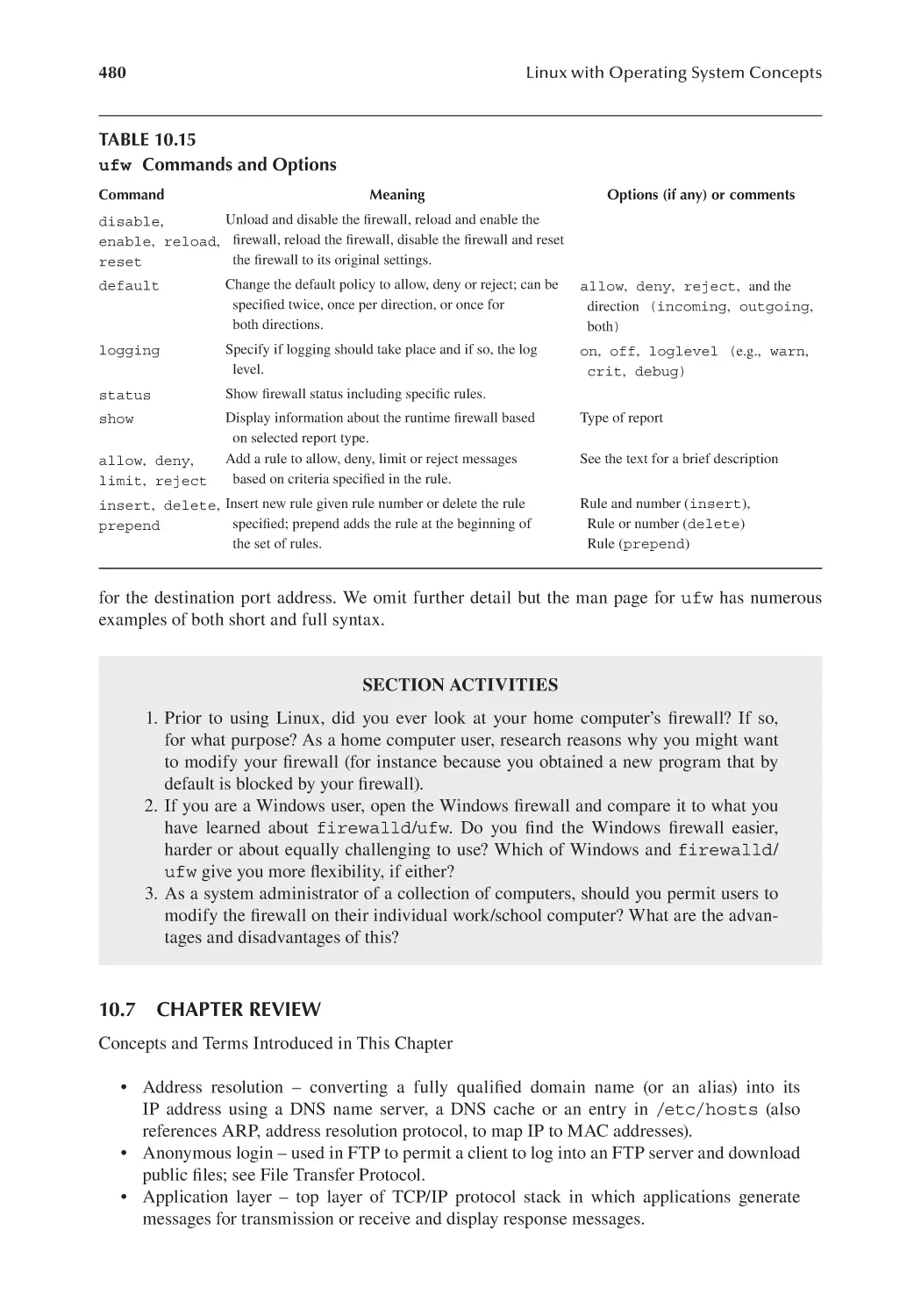
10.6.3 firewall-cmd............................................................................... 476
10.6.4 ufw.................................................................................................... 476
10.7 Chapter Review..............................................................................................480
Review Questions...................................................................................................... 485
Chapter 11 Software Installation and Maintenance.................................................................... 489
11.1 Introduction.................................................................................................... 489
11.2 Software Maintenance Terminology.............................................................. 491
11.2.1 Types of Programming Languages................................................... 491
11.2.2 Types of Software.............................................................................. 492
11.2.3 Types of Software Licenses............................................................... 493
11.2.4 Types of Software Management........................................................ 493
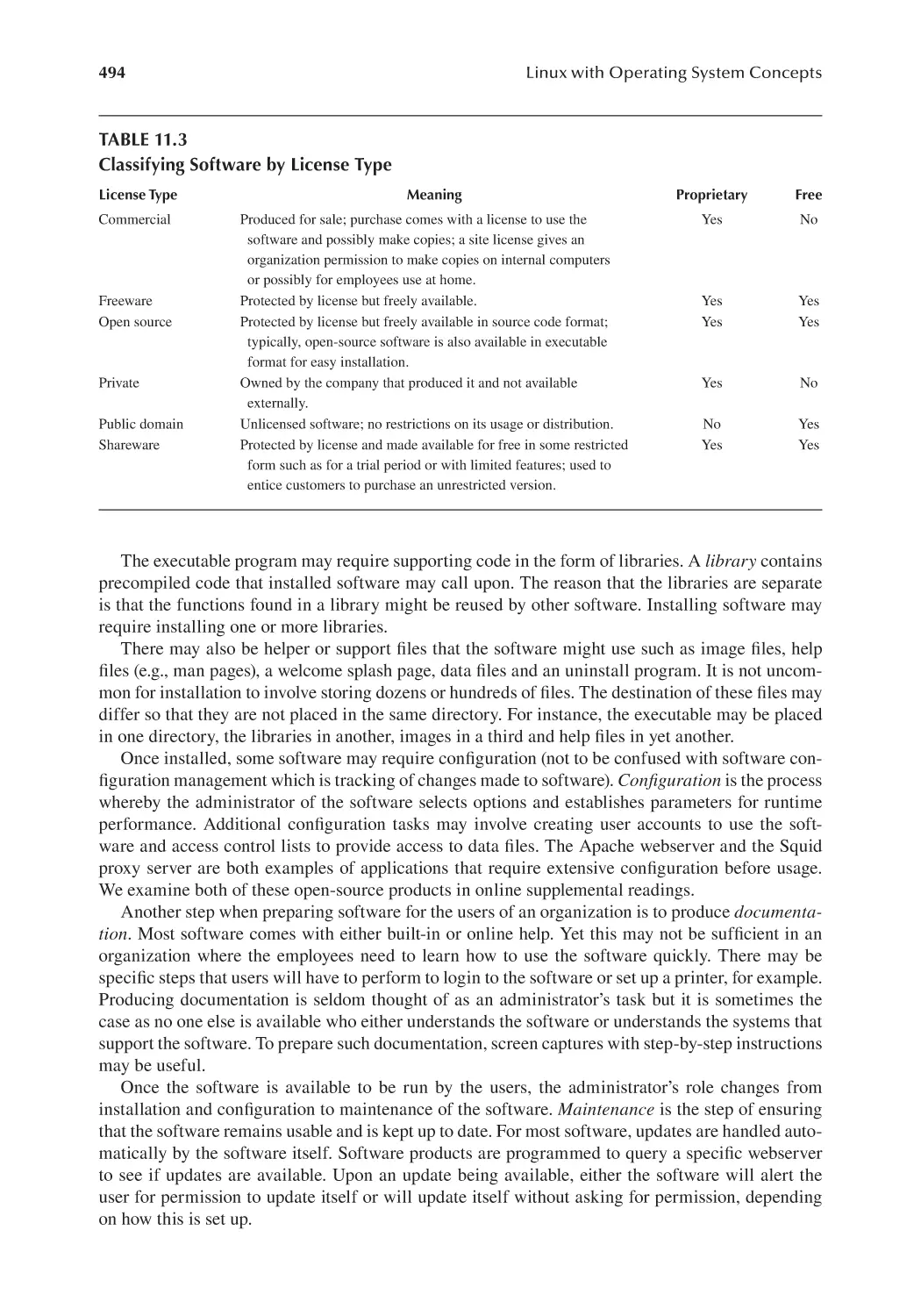
11.3 Installation and Maintenance from a Software Store..................................... 496
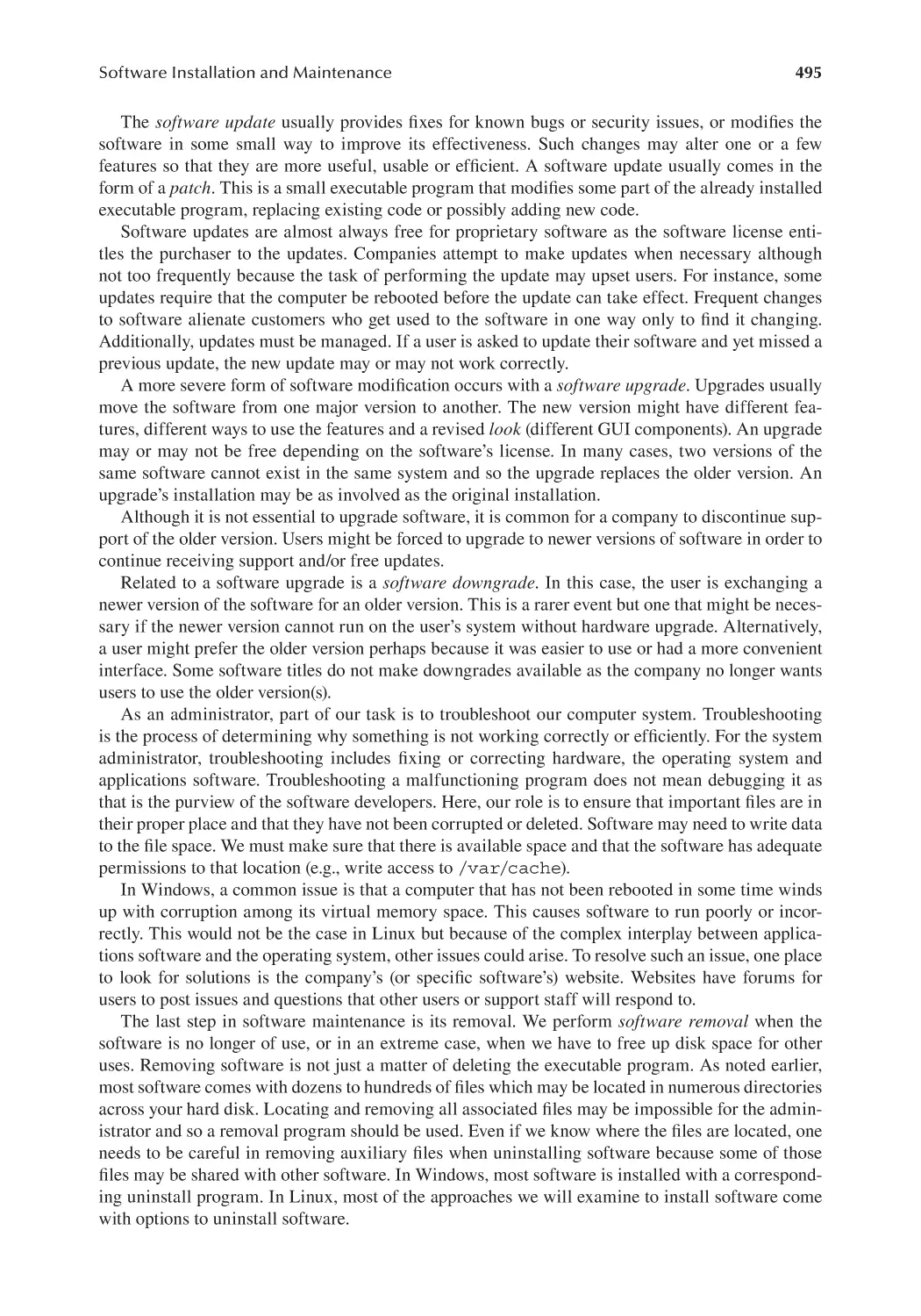
11.3.1 Red Hat Software GUI...................................................................... 496
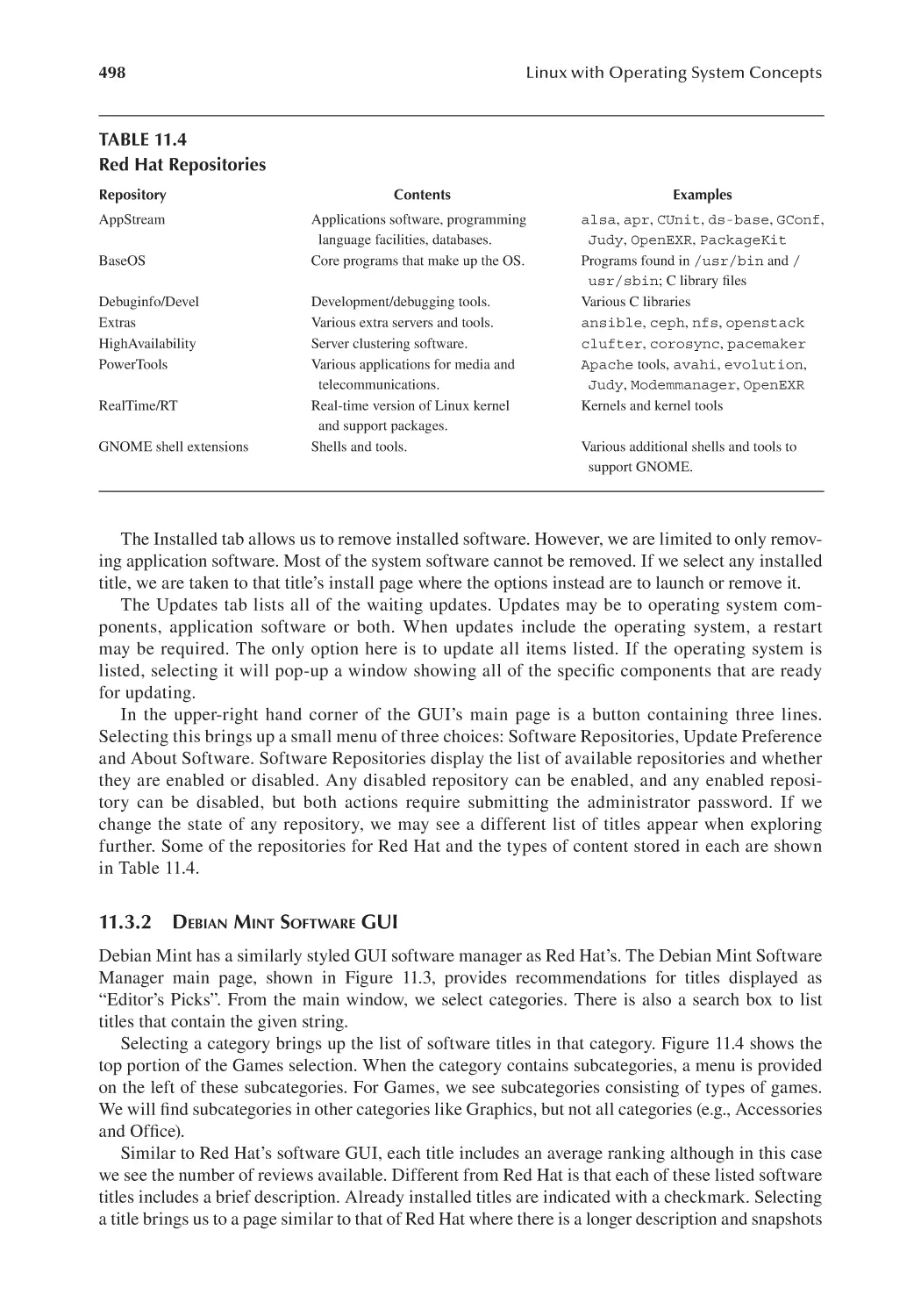
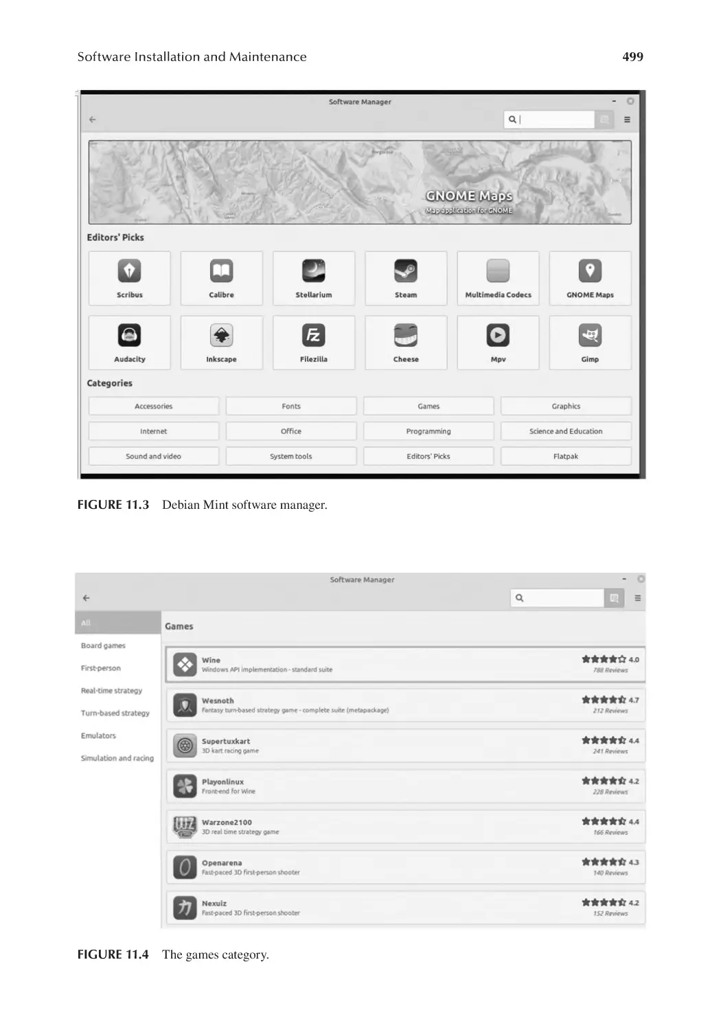
11.3.2 Debian Mint Software GUI............................................................... 498
11.3.3 Ubuntu Software Center.................................................................... 501
11.4 rpm and dpkg............................................................................................... 502
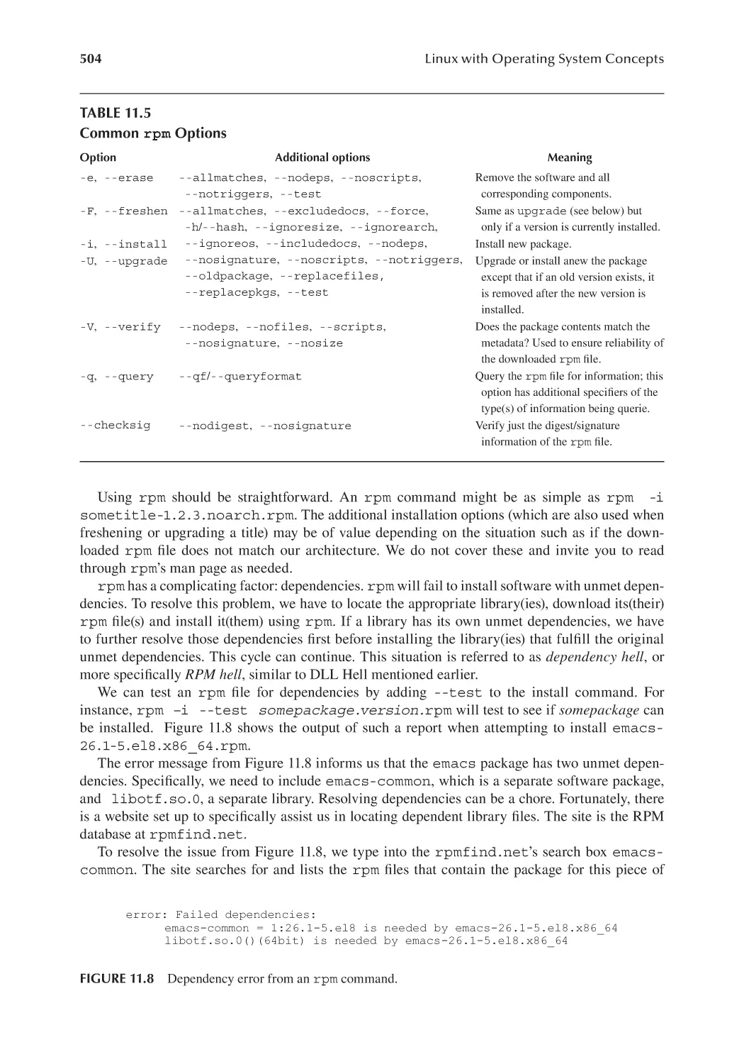
11.4.1 rpm.................................................................................................... 503
11.4.2 dpkg................................................................................................. 505
11.5 dnf/yum and apt......................................................................................... 507
11.6 Installation of Source Code............................................................................ 511
11.6.1 Obtaining Installation Packages........................................................ 512
11.6.2 Extracting from the Archive............................................................. 513
11.6.3 Running the configure Script...................................................... 514
11.6.4 The make Step and the makefile................................................. 514
11.6.5 The make install Step................................................................ 516
11.7 The gcc Compiler.......................................................................................... 517
11.7.1 Preprocessing.................................................................................... 518
11.7.2 Lexical Analysis and Syntactic Parsing............................................ 518
11.7.3 Semantic Analysis, Compilation and Optimization.......................... 520
11.7.4 Linking.............................................................................................. 520
11.7.5 Using gcc......................................................................................... 522
11.8 Software Documentation................................................................................ 523
11.9 Chapter Review.............................................................................................. 525
Review Questions...................................................................................................... 528
xiv
Contents
Chapter 12 Maintaining and Troubleshooting Linux.................................................................. 531
12.1 Introduction.................................................................................................... 531
12.2 File System Integrity: Backups, RAID and Encryption................................. 532
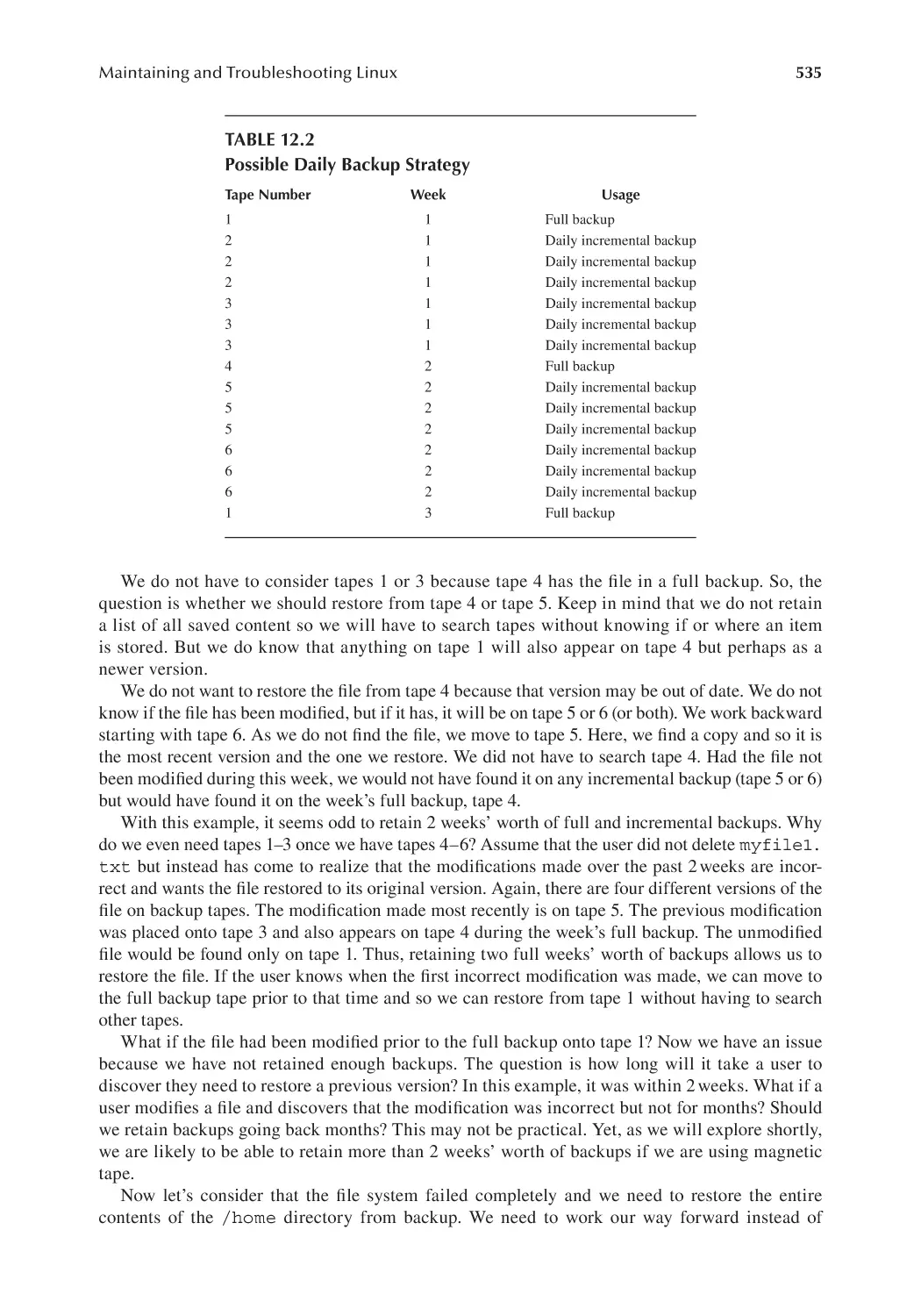
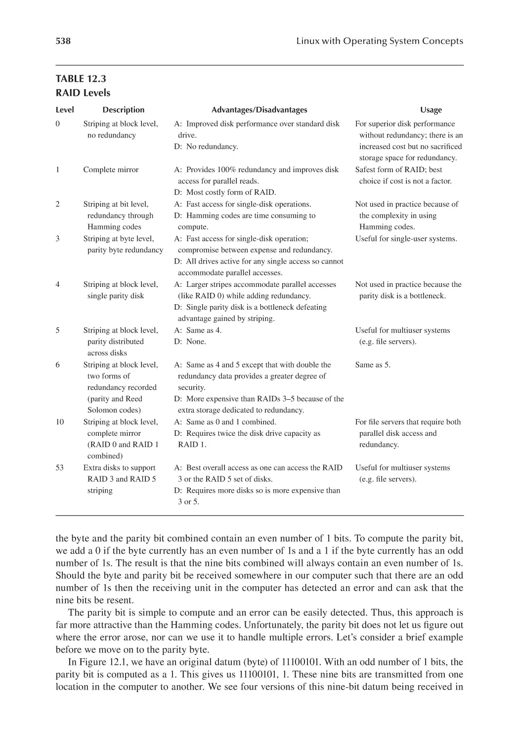
12.2.1 Backups: Why, How and When........................................................ 532
12.2.2 RAID for File System Integrity........................................................ 537
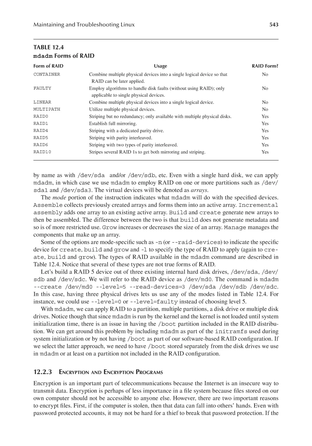
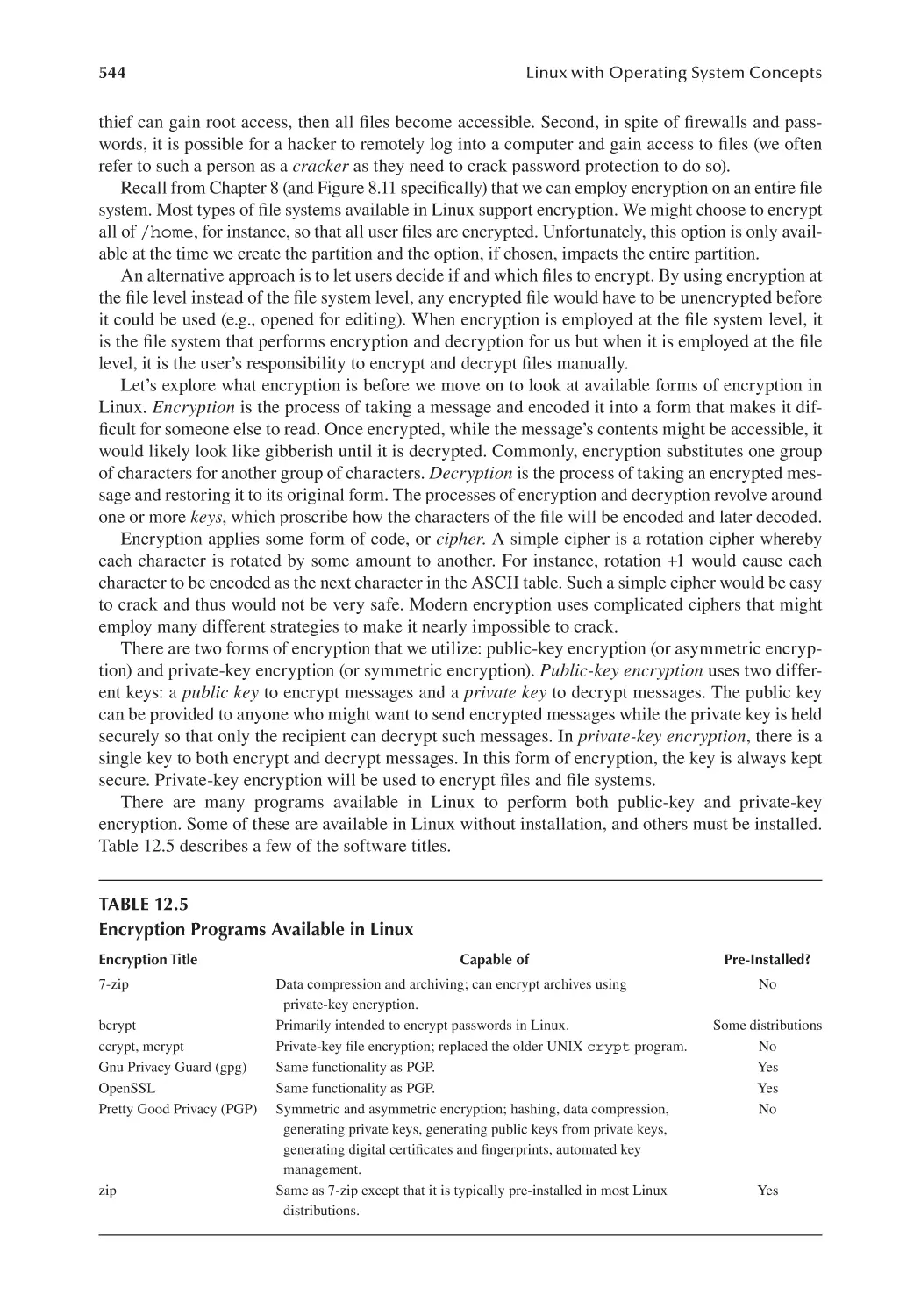
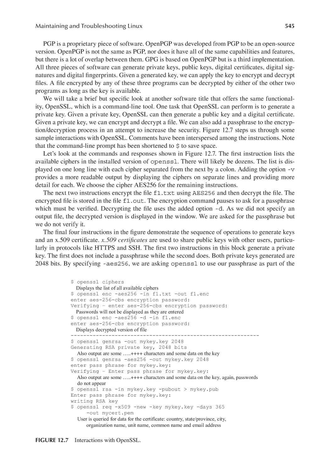
12.2.3 Encryption and Encryption Programs............................................... 543
12.3 Task Scheduling............................................................................................. 547
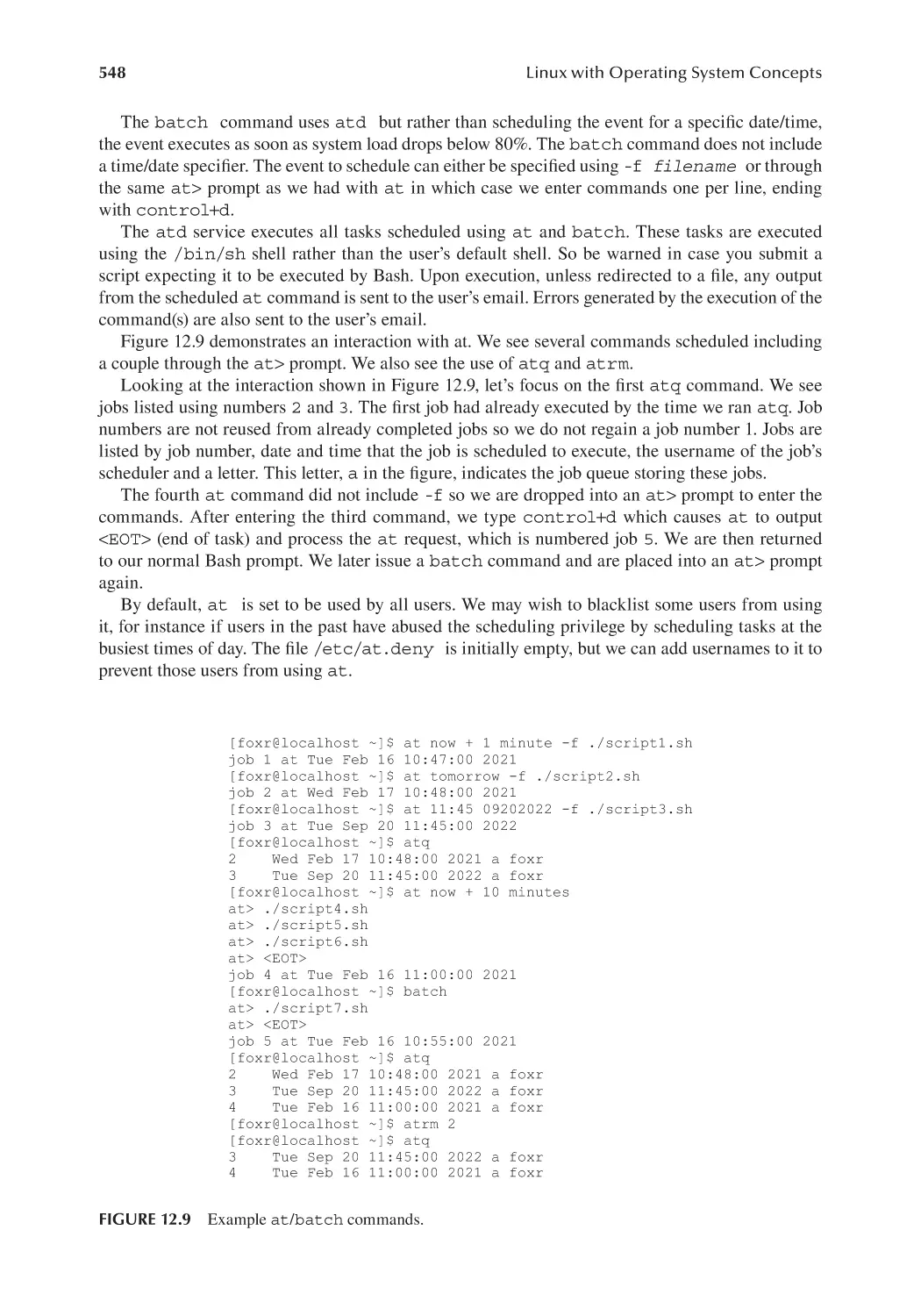
12.3.1 at and atd....................................................................................... 547
12.3.2 crontab and crond....................................................................... 549
12.4 System Monitoring......................................................................................... 551
12.4.1 Operating System Issues That Degrade Performance....................... 551
12.4.2 Processor and Process System Monitoring Tools............................. 554
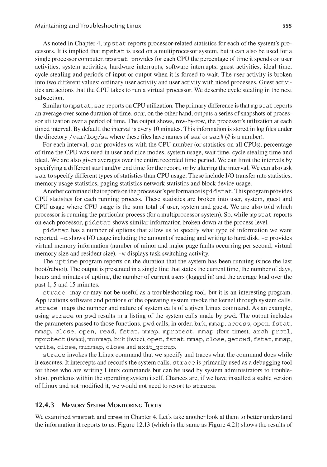
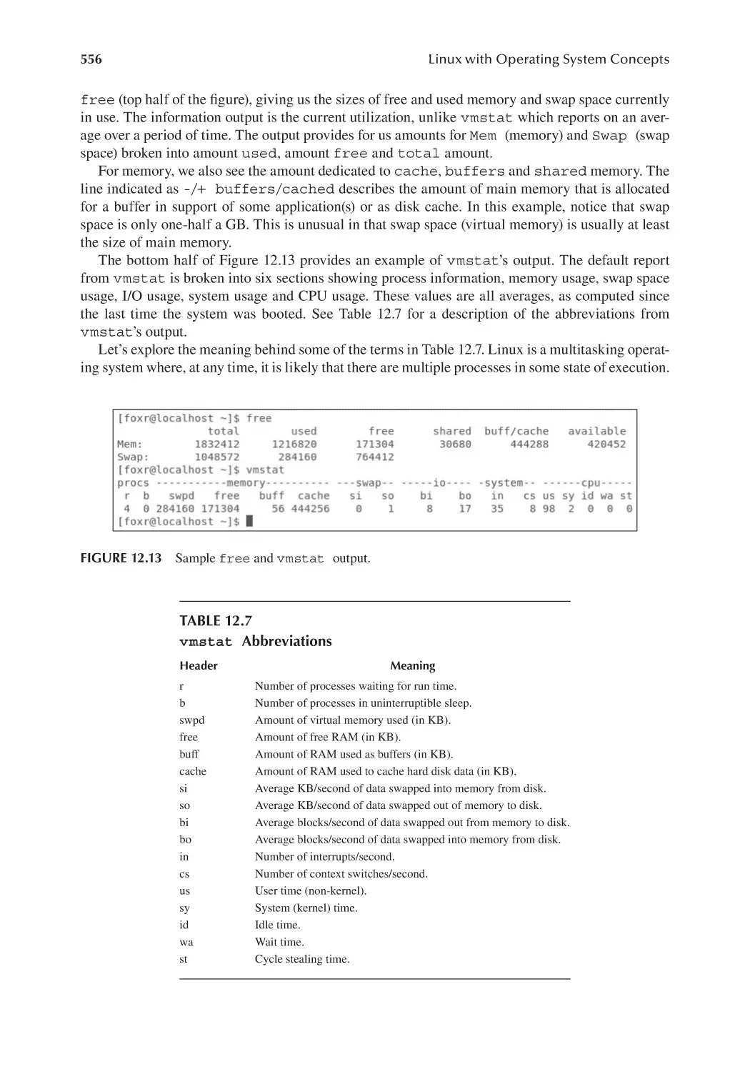
12.4.3 Memory System Monitoring Tools................................................... 555
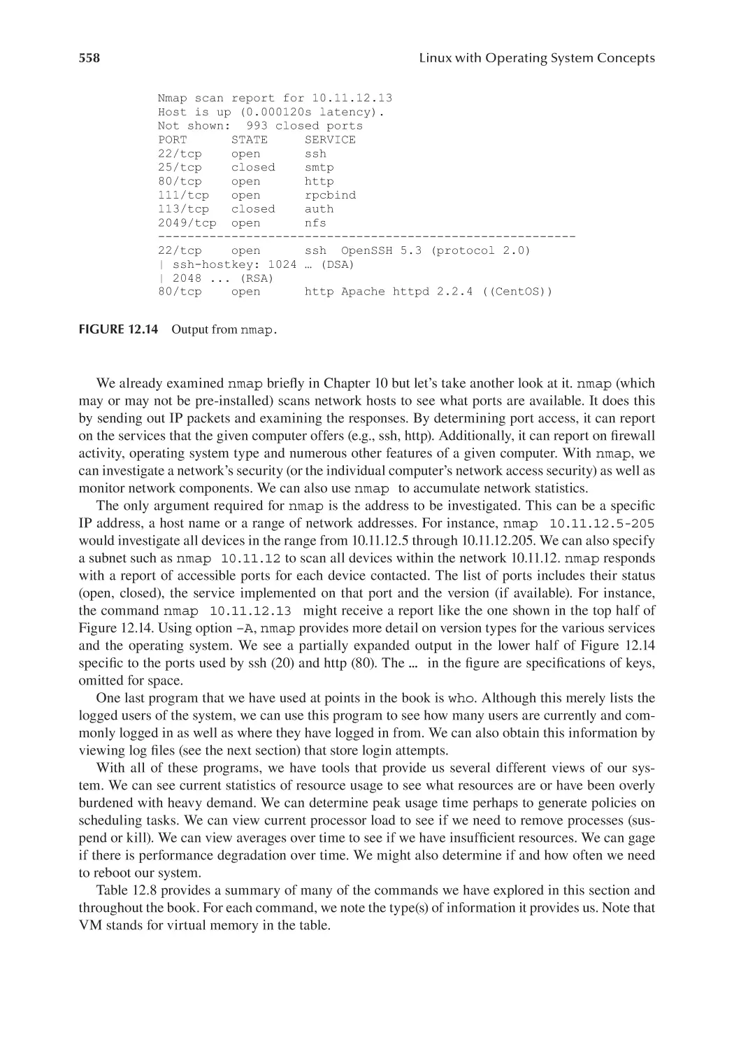
12.4.4 I/O System Monitoring Tools............................................................ 557
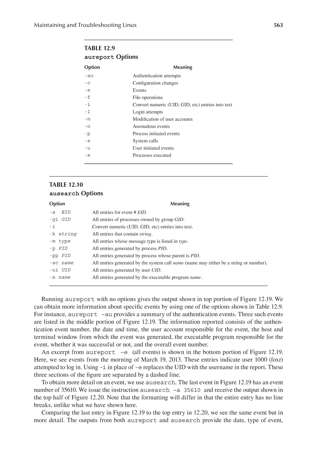
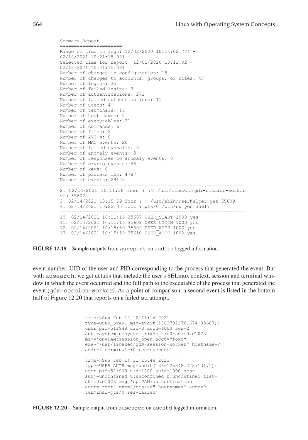
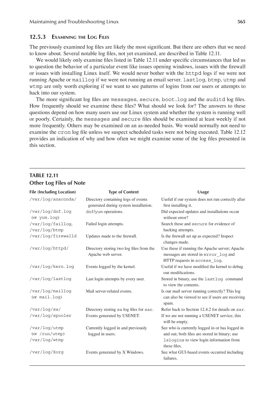
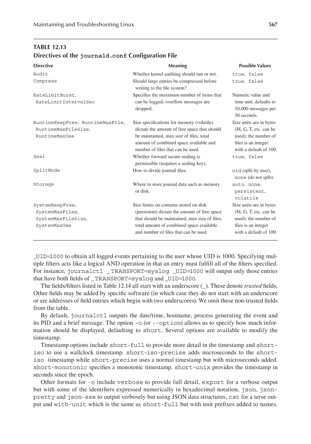
12.5 Log Files......................................................................................................... 560
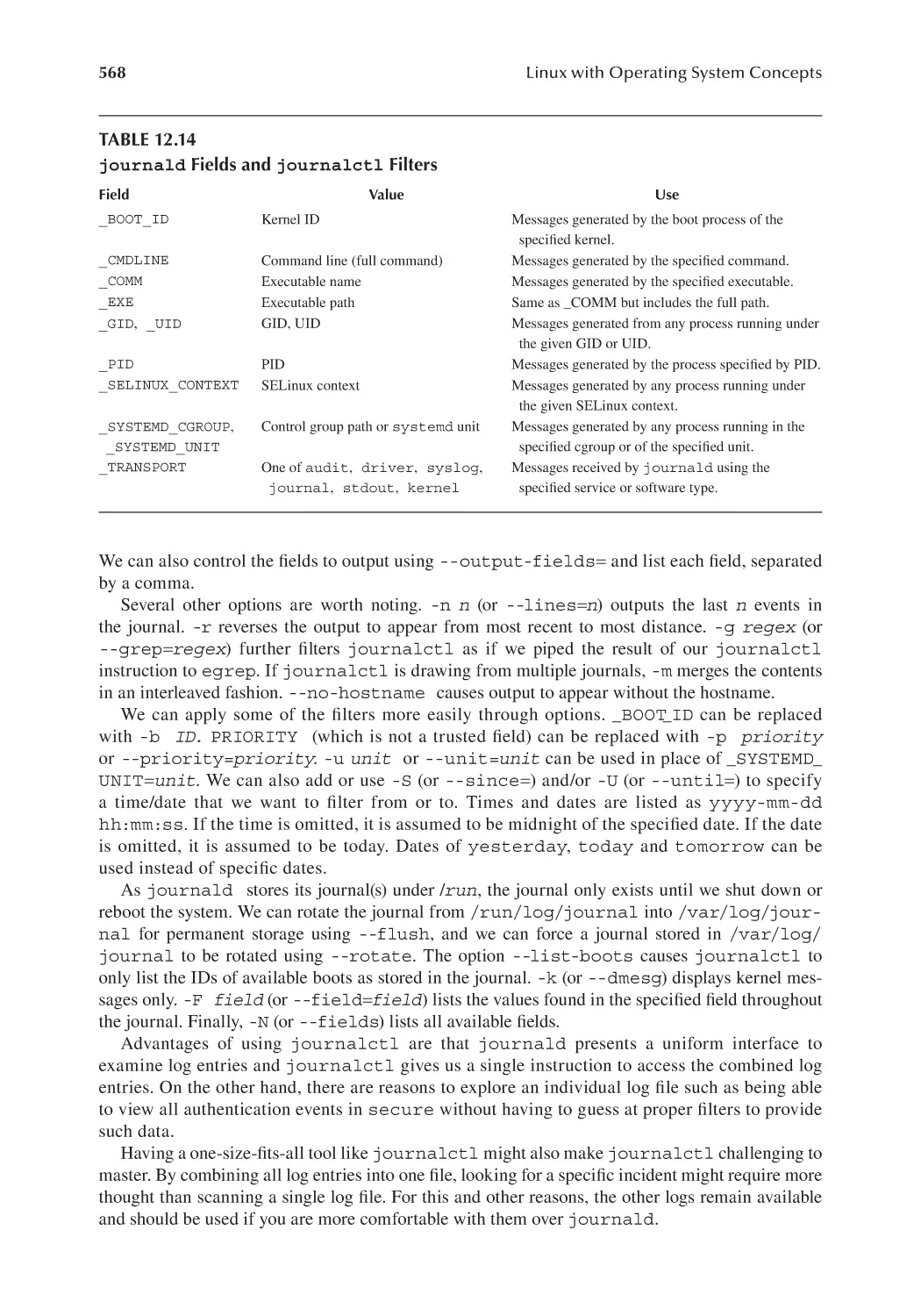
12.5.1 rsyslogd-Created Log Files.......................................................... 560
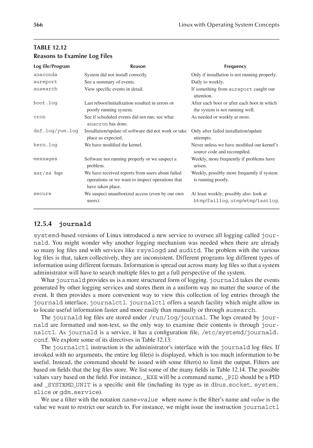
12.5.2 auditd Logs.................................................................................... 561
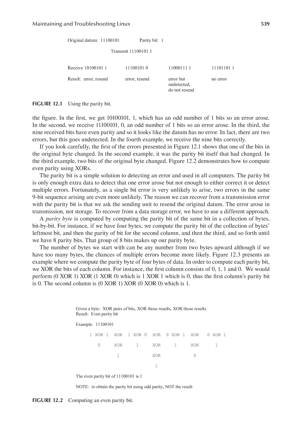
12.5.3 Examining the Log Files................................................................... 565
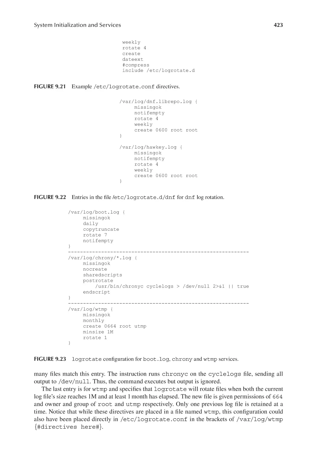
12.5.4 journald........................................................................................ 566
12.6 Troubleshooting.............................................................................................. 569
12.7 Chapter Review.............................................................................................. 574
Review Questions...................................................................................................... 577
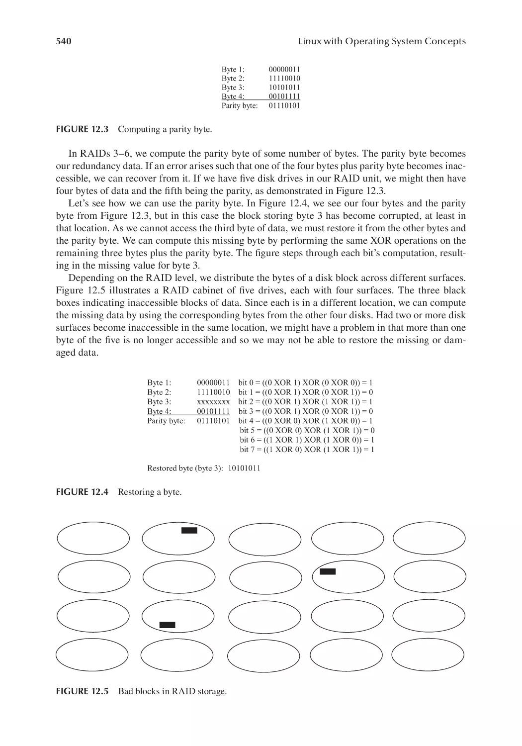
Bibliography.................................................................................................................................. 581
Index............................................................................................................................................... 589
Preface
The Unix/Linux textbook market is full of books for people who are looking to acquire hands-on
knowledge of Unix/Linux, whether as a user or a system administrator. There are almost no books
that serve as textbooks for an academic class. Why not? There are plenty of college courses that cover
or include Unix/Linux. We tend to see conceptual operating system texts which include perhaps a
chapter or two on Unix/Linux or Unix/Linux books that cover almost no operating system concepts.
Most Unix/Linux books either focus on how to use Unix/Linux or how to administer Unix/Linux.
This book is unique. It explores operating system concepts while introducing Linux-specific
content. It is divided roughly into two parts: an introduction to Linux for users and an introduction
to Linux for system administrators. It covers Linux and operating system concepts not as a how-to,
hands-on guide but as a true textbook, complete with definitions, concepts, chapter reviews and a
collection of ancillary material to help support the instructor and student if used in a class.
If you are reading this book, I hope you find it helpful and learn a great deal. My intention is not
to cover all things Linux but to explore Linux and offer background for why things are set up the
way they are.
HOW TO USE THIS TEXTBOOK
In this edition of the textbook, Chapters 1–6 cover Linux from a user perspective, while Chapters
7–12 cover Linux from an administrator’s perspective. Throughout the book are operating system
concepts related to topics of the chapter. This textbook is envisioned to be used in a 1- or 2-semester
course on Linux. A 2-semester course should be able to cover all 12 chapters, dividing the semesters
between user and administrator topics. Such a course could be split between lectures (roughly 50%
of the time) and labs. See the lab manual which accompanies this text (available online).
A 1-semester junior or senior-level IT or computer science course should be able to cover a
majority of the book. An IT course might cut out some of the operating system concepts and use the
lab manual, while a computer science course might include portions of the lab manual and eliminate
some of the less needed topics like sed (Chapter 5), systemd initialization (Chapter 9), opensource software installation (Chapter 11) and system troubleshooting (Chapter 12).
A lower-level 1-semester course that is using this text as an introductory to Linux should cover
Chapters 1–4 in detail and then select relevant topics to fill out the course, for instance including
some portions of user accounts from Chapter 7, file system topics from Chapter 8, network configuration topics from Chapter 10 and software installation from Chapter 11.
Below is a list of topics found in the chapters that can be considered optional. Omitting some of
these topics will not reduce the readability of the remainder of the text.
• Chapter 1: All content outside of Section 1.5, on Linux installation, can be omitted as it
mostly explores a history of operating systems and Linux development.
• Chapter 2: Removing Sections 2.7.1 and 2.7.2 should not be an issue; Section 2.6 on vi can
be skipped if students will not be using vi.
• Chapter 3: Sections 3.2 and 3.8 on storage terminology and devices are not essential; Section
3.9 on file compression (although 3.9.4 might be useful) can be skipped; Section 3.7.1 on
File Browser searching is only needed if students are not to learn the find program.
• Chapter 4: Forms of process management (Section 4.2) and memory and virtual memory
(Section 4.7.1) can be skimmed over if the course is an IT course.
• Chapter 5: Sections 5.5 and 5.6 (sed and awk) can be omitted if these two programs are
not going to be used, although some parts of awk should still be covered as it is referenced
later in the textbook.
xv
xvi
Preface
• Chapter 6: Section 6.3.5 on the expr instruction can be skipped; depending on how much
scripting the student is to learn, Sections 6.7–6.9 on arrays, string pattern matching and
functions may be omitted.
• Chapter 7: Section 7.5 on PAM and strong passwords may not be needed; Section 7.8 on
SELinux could be reduced to just an introduction; Section 7.9 is not necessary.
• Chapter 8: Sections 8.2.1 and 8.2.2 provide background for better understanding inodes but
8.2.2 can be eliminated and 8.2.1 reduced; if the course will not cover topics like partitioning, then Section 8.5 can be skipped.
• Chapter 9: If the course is an IT course, coverage of booting (Section 9.2) may not be warranted; if the course is a computer science course, detailed information about systemd’s
initialization process may not be desired (Section 9.3); some content from Section 9.6 can
be eliminated unless the specific service is going to be examined in detail.
• Chapter 10: Depending on the student’s background, Section 10.2 may not be needed;
Section 10.4.2 is only needed if the course covers DHCP; based on the version of Linux
used, either cover Sections 10.6.1–10.6.3 or Section 10.6.4.
• Chapter 11: Sections 11.2 and 11.8 provide background on software but can be skipped;
depending on whether the course covers Red Hat or Debian-based Linux, subsections
within Sections 11.3–11.5 can be skipped; Section 11.7 can be omitted if the students will
not use gcc.
• Chapter 12: Coverage of RAID (12.2.2) and encryption (12.2.3) may be skipped if the topics are beyond the scope of the course and similarly the content on operating system issues
(12.4.1) may be omitted.
• Chapter 13: This chapter, available online, covers Apache and Squid installation and configuration; it can be skipped entirely if the course will not cover either of these software
titles.
NEW TO THIS EDITION
The first edition of this book was written specifically for Red Hat 6 and correspondingly, CentOS 6.
At the time of its publication, Red Hat 7 had come out, but Red Hat 7 was viewed as an in-between
step as Red Hat was moving from init to systemd. With both Red Hat 6 and Red Hat 7 reaching
the end of their lives, this edition has updated all content to move on to systemd Linux distributions, concentrating on Red Hat 8. While preparing this manuscript, CentOS announced that they
would not support CentOS 8 beyond 2021 and would instead concentrate on CentOS Stream. At the
time of this writing, CentOS 8 and Stream are nearly identical.
So, the first major change between the first edition of this textbook and this new edition is updating to Red Hat 8/CentOS Stream. In an attempt to broaden the appeal of this text, this edition has
a good deal of content on Debian/Ubuntu versions of Linux when those versions differ from Red
Hat. The information on Debian/Ubuntu is not complete, but attempts have been made to note the
differences when space permits.
Chapters 1–7 in the first edition are now Chapters 1–6. Material from Chapter 5 has been moved
(vi is now in Chapter 2, network software is now in Chapter 10, compression is now covered in
Chapter 3, and encryption topics are now in Chapter 12) or removed. Most of these chapters have
been rewritten to improve their clarity with improved examples and more tables and figures. Some
of the removed content has been uploaded to the textbook’s companion website as supplemental
reading material.
Chapter 8 from the first edition has been removed. Content on the Linux kernel is now described
in Chapters 1, 4 and 9. Installation of Linux has been moved to Chapter 1. Other content, such as
virtual memory, has also been moved. With this chapter removed, Chapters 7–12 are primarily what
Chapters 9–14 had been. All content in this part of the book has been updated to systemd-versions
of Linux (primarily Red Hat) and include such new topics as the new top-level directory layout, the
Preface
xvii
xfs file system (briefly), the NetworkManager service, firewalld and ufw as new front-ends to
iptables, the journald service and Cockpit (covered briefly). These chapters have also been
substantially rewritten and new examples, figures and tables added.
Some material from the former Chapters 9–14 are being moved online via supplemental readings, including for instance the Red Hat 6/init initialization process. The former appendix (binary
numbers) is also being removed and made available online.
AVAILABLE ONLINE SUPPLEMENTS
There is a zipped file available for instructors who adopt this book and a zipped file available to everyone. This latter file is available via the textbook’s companion website at
https://www.routledge.com/9781032063454. If you are an instructor, contact your CRC Press/
Taylor & Francis book rep. The contents of these files are listed below.
Instructor-Only Resources
• Instructor’s manual complete with answers to chapter review questions
• Testbank
Other Available Material
• PowerPoint notes
• Glossary of terms from chapter reviews (consolidated into one file)
• Select answers to some chapter review questions
• Complete lab manual (assuming CentOS Stream can be adapted for other Linux
distributions)
• Supplementary readings (reference to first edition chapters)
• The fetch-execute cycle and details on the CPU (previously from Chapter 1)
• Comparing Bash to Csh (previously from Chapters 2 and 7)
• A brief introduction to emacs (previously from Chapter 5)
• vi and emacs cheatsheets
• System V/Upstart initialization process (previously from Chapter 11)
• Some example network scripts (previously from Chapter 12)
• A look at disaster planning and recovery (previously from Chapter 14)
• Review of binary numbers (previously from the Appendix)
• Apache/Squid installation (previously Chapter 15, available only online)
• Perl scripting
Acknowledgments and
Contributions
First, I am indebted to Randi Cohen for her encouragement and patience in my writing and completing this text. I would also like to thank Stan Wakefield for connecting me with Randi and
CRC Press/Taylor & Francis Group. I would like to thank Olivia Snowden, a recent graduate from
Northern Kentucky University (NKU), for so kindly volunteering to proofread the entire manuscript. She caught many errors and typos and helped me improve the book considerably. I would
also like to express my thanks to colleague Dr. Wei Hao (NKU) and to Dr. Jim Furstenberg (Ferris
State University) for proofreading select chapters and providing both corrections and insightful
comments. Dr. Yi Hu (NKU) has maintained a list of errata from the first edition and has given me
some great ideas for this new edition. I would also like to thank Micah Sidebottom, a student who,
while taking our Linux course in fall 2020, pointed out several inconsistencies in the first edition
that I have hopefully corrected. I am also indebted to several former colleagues and associates
for their insight into networking (Professor Scot Cunningham) and Linux (Dr. Xiannong Meng,
Bucknell University and Professor Peter Bartol, San Diego State University).
I would also like to thank everyone in the open-source community who contribute their time and
expertise to better all of our computing lives. Without all of the efforts put into Linux, this book
would obviously not exist!
On a personal note, I would like to thank Cheri Klink for all of her love and support.
xix
Author
Richard Fox is a professor of computer science at Northern Kentucky University (NKU). He primarily teaches artificial intelligence, computer architecture, computer systems, concepts of programming languages, object-oriented programming and Unix systems. He has also taught data
structures, IT fundamentals, web development and web server administration, among other
courses. Dr. Fox, who has been at NKU since 2001, is currently the undergraduate program director of Computer Science and chair of NKU’s University Curriculum Committee. Prior to NKU,
Dr. Fox taught for 9 years at the University of Texas – Pan American. He has received two Teaching
Excellence awards, from the University of Texas – Pan American in 2000 and from NKU in 2012,
and an award for Outstanding Service from NKU in 2016.
Dr. Fox received a Ph.D. in Computer and Information Sciences from The Ohio State University
in 1992. He also has an M.S. in Computer and Information Sciences from Ohio State (1988) and
a B.S. in Computer Science from the University of Missouri Rolla (now Missouri University of
Science and Technology) from 1986.
Dr. Fox has published two other books with CRC Press/Taylor & Francis Group: an introduction to information technology text (in its second edition) and a book on Internet infrastructure
(coauthored by colleague Dr. Wei Hao). He has also authored or coauthored over 45 peer-reviewed
research articles primarily in the area of artificial intelligence.
Richard Fox grew up in St. Louis, Missouri, and now lives in Cincinnati, Ohio. He is a big
science fiction fan and progressive rock fan. As you will see in reading this text, his favorite
composer is Frank Zappa.
xxi
1 What, Why, Who and
Linux
When, and How
This chapter’s learning objectives are to be able to
• Describe what operating systems are and how and why we use them
• Compare the more popular versions of Linux
• Explain the term open source software and the role the open-source community has had in
the development of Linux
• Enumerate reasons why IT personnel should learn Linux
• Identify the roles of the most significant individuals in the development of Linux
• Install Linux
• Use Linux from the GUI to start applications and open terminal windows
1.1 INTRODUCTION
As you are reading this book, you must want to learn about Linux. Why should you learn about
Linux? From a user’s point of view, Linux offers a different approach than other operating systems.
It is an open-source product meaning that you can obtain it for free. Similarly, most software for
Linux is open source. With open-source software, you can also enhance the code (if you have
the capability of doing so). From a system administrator’s perspective, Linux, like Unix, lets you
dive deeply into the operating system (OS) and have more control than you can in Windows or
MacOS. Learning Linux teaches you not only how to use it but more about operating systems and
computers.
The intention of open-source software is to make the software available in its source code
format. Those who are skilled at coding can then enhance or alter the software or develop new
software that uses some portions of the existing software. Although open-source software was
originally synonymous with the development of Unix, Linux and related operating systems, the
open-source community has produced a number of highly useful applications software. You may
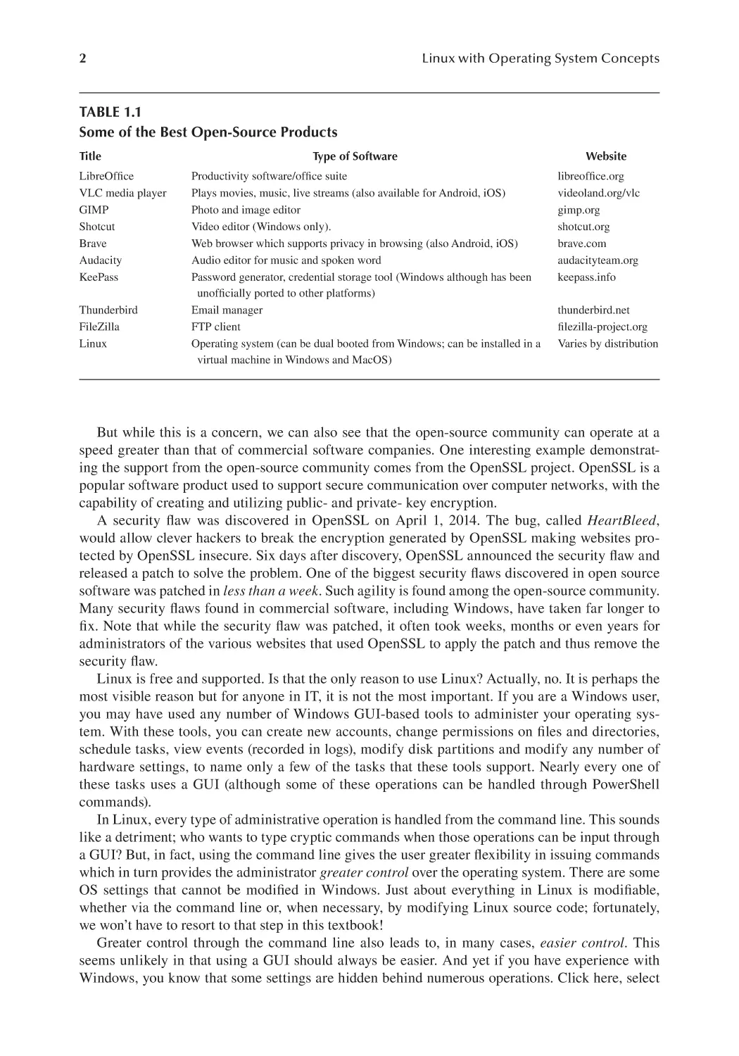
have used open-source software yourself. Table 1.1 lists the top ten open-source products as rated
by TechRadar as of April 2021. All of the software listed in Table 1.1 can run in Linux, Windows
and MacOS unless noted.
One drawback of open-source software is that it does not come with commercial support. When
we buy software, we are not purchasing the software itself but purchasing the right to use the software. With that purchase almost always comes a guarantee that the software developers will provide
timely feedback on issues identified with the software. Bugs will be fixed for us. Security holes will
be resolved and patches released quickly. Manuals (whether printed or online) show users how to
use the software.
Most commercial software comes with a guarantee of this support; open-source software products are supported by those who developed the titles but that support is not guaranteed. This is an
issue that organizations might have when considering the adoption of open-source software. Even
with support available, open source might lag behind commercial software with respect to bug and
security fixes and improved features.
DOI: 10.1201/9781003203322-1
1
2
Linux with Operating System Concepts
TABLE 1.1
Some of the Best Open-Source Products
Title
LibreOffice
VLC media player
GIMP
Shotcut
Brave
Audacity
KeePass
Thunderbird
FileZilla
Linux
Type of Software
Productivity software/office suite
Plays movies, music, live streams (also available for Android, iOS)
Photo and image editor
Video editor (Windows only).
Web browser which supports privacy in browsing (also Android, iOS)
Audio editor for music and spoken word
Password generator, credential storage tool (Windows although has been
unofficially ported to other platforms)
Email manager
FTP client
Operating system (can be dual booted from Windows; can be installed in a
virtual machine in Windows and MacOS)
Website
libreoffice.org
videoland.org/vlc
gimp.org
shotcut.org
brave.com
audacityteam.org
keepass.info
thunderbird.net
filezilla-project.org
Varies by distribution
But while this is a concern, we can also see that the open-source community can operate at a
speed greater than that of commercial software companies. One interesting example demonstrating the support from the open-source community comes from the OpenSSL project. OpenSSL is a
popular software product used to support secure communication over computer networks, with the
capability of creating and utilizing public- and private- key encryption.
A security flaw was discovered in OpenSSL on April 1, 2014. The bug, called HeartBleed,
would allow clever hackers to break the encryption generated by OpenSSL making websites protected by OpenSSL insecure. Six days after discovery, OpenSSL announced the security flaw and
released a patch to solve the problem. One of the biggest security flaws discovered in open source
software was patched in less than a week. Such agility is found among the open-source community.
Many security flaws found in commercial software, including Windows, have taken far longer to
fix. Note that while the security flaw was patched, it often took weeks, months or even years for
administrators of the various websites that used OpenSSL to apply the patch and thus remove the
security flaw.
Linux is free and supported. Is that the only reason to use Linux? Actually, no. It is perhaps the
most visible reason but for anyone in IT, it is not the most important. If you are a Windows user,
you may have used any number of Windows GUI-based tools to administer your operating system. With these tools, you can create new accounts, change permissions on files and directories,
schedule tasks, view events (recorded in logs), modify disk partitions and modify any number of
hardware settings, to name only a few of the tasks that these tools support. Nearly every one of
these tasks uses a GUI (although some of these operations can be handled through PowerShell
commands).
In Linux, every type of administrative operation is handled from the command line. This sounds
like a detriment; who wants to type cryptic commands when those operations can be input through
a GUI? But, in fact, using the command line gives the user greater flexibility in issuing commands
which in turn provides the administrator greater control over the operating system. There are some
OS settings that cannot be modified in Windows. Just about everything in Linux is modifiable,
whether via the command line or, when necessary, by modifying Linux source code; fortunately,
we won’t have to resort to that step in this textbook!
Greater control through the command line also leads to, in many cases, easier control. This
seems unlikely in that using a GUI should always be easier. And yet if you have experience with
Windows, you know that some settings are hidden behind numerous operations. Click here, select
3
Linux
this, open that, select yet another link, change tabs, fill in this form, select OK and then confirm.
Making multiple changes may require repeating the same operations with minor modifications, over
and over. We will learn that Linux offers very convenient ways to recall a previous command line
instruction, make minor modifications to it and execute the revised version. Alternatively, we can
write shell scripts to perform such operations.
If you are a student studying Linux or hold an IT position, another aspect of Linux that you might
not gain in Windows or MacOS is learning about operating systems. Windows and MacOS tend to
shelter many OS concepts from you. You may learn to control processes using a tool like the Task
Manager, learn about disk partitions and file systems, or learn about virtual memory because of
heavy disk usage. But in Linux, you may need to delve into these details. You may want to change
process priorities, launch some processes in the background and change effective user ID of other
processes. You may need to manually mount and unmount partitions. You may need to examine
memory usage statistics to see how frequently your computer is swapping between main and virtual
memory. Learning Linux from the command line forces you to understand, at least to some extent,
what the OS does and how.
In learning Linux, you will expand your knowledge of computers in general. And, well, using
Linux is cool (at least that’s what many people think!).
In this textbook, we look at Linux from two different perspectives. Early on, we learn Linux
as a user. We explore how to enter commands from the command line prompt and navigate
through the Linux file space. We learn how to launch and manage processes. We learn some of
the powerful tools available in Linux including regular expressions and shell scripting. Over
the course of these early chapters, we learn dozens of Linux commands and useful features that
make command line entry easier. Midway through the text, we shift focus to learning Linux as
a system administrator. In this set of material, we look at creating and managing user accounts,
managing files and file systems, the Linux boot and initialization process, controlling services,
configuring network access and installing software. Throughout the book, we introduce OS
concepts.
To get us started in this chapter, we focus on five questions. What is Linux, and more generally
what are operating systems? We define operating systems and examine the components that make
up operating systems before we turn to Linux specifically and its components. Why should we use
Linux? We gave a brief answer to this question but delve more into the significance of Linux as an
OS of choice. Who developed Linux and when? We look at the history of Linux and the important
players, starting with some earlier operating systems that led to or factored into the development of
Linux. Finally, how do we use Linux? Although that is a topic for the entire book, in which chapter
we explore how to install several different versions of Linux. We also introduce different forms of
Linux interfaces, concentrating on how to open a terminal window for command line input, which
we will then use throughout most of the book.
SECTION ACTIVITIES
1. How many operating systems do you have experience with? Count not only desktop/
laptop computers but any servers, mainframes, supercomputers, tablets and smartphones. If you have experience with more than one, what similarities do you find
between those that you know? What differences?
2. Make a list of your own reasons for learning Linux. How do they compare to the
reasons covered in this section?
3. Read about Heartbleed at https://heartbleed.com/. Were you aware of it when the
problem was first announced in 2014?
4
Linux with Operating System Concepts
1.2 WHAT IS LINUX?
We start with something more general, what is an operating system? A computer’s OS is a collection
of programs that, as a whole, support our use of the computer through managing hardware resources
and running processes. Operating systems usually comprise many different programs. The heart of
the OS is a single program called the kernel. The kernel is loaded into memory when a computer is
booted, and it remains resident in memory until the computer is shut down. The kernel’s role is to
handle process and resource management, among other tasks. The kernel calls upon other OS components to accomplish some of its tasks. Some of these components are loaded and run as needed.
Users may also call upon some of these other OS components, again loaded and run as needed.
Although we asked specifically what Linux is, we will concentrate first on operating systems in
general. We then shift to Linux specifically later in this section.
1.2.1 Early Operating Systems
The earliest electronic computers, developed in the mid-1940s through the early to the mid-1950s
were one-of-a-kind devices, created as much to explore how to build computers as to be useful
computational devices. These computers had no operating systems at all. For a “user” to use a computer, that user would write their program code and submit it. Code might have been entered into
the computer by making connections of various components through cables, setting switches on the
computer’s console and pressing the start button. Such programs used no external resources. If a
program required a resource like access to input from magnetic tape or punch cards, the instructions
to perform such input had to be included in the program itself. Otherwise, the computer would not
know how to access the tape drive or punch card reader.
Around 1958, programmers began shifting from low-level machine languages to more sophisticated, high-level languages. Among the first were FORTRAN and COBOL. A program written in one of these languages could not be directly executed. Instead, the program had to be
translated from the high-level language into machine language using a separate program called
a compiler.
The programmer had several distinct steps to run their program. First, they would mount and
load the compiler. Next, they would input their FORTRAN or COBOL program into the running
compiler. The compiler would execute, outputting the executable version of the program onto magnetic tape. Now, the programmer would unmount the compiler and mount the tape containing their
executable program. The programmer would next load and run the executable program. The program’s input would likely come from another tape or punch cards. Remember, every one of these
steps requires that the programmer implement the steps by additional program code. That’s a lot of
work to run a program!
To simplify this process, some of the tasks were captured into a program called the resident
monitor. This program would be loaded into memory after the computer booted. The program
would stay in memory until the computer was shut down, thus the word resident. The term monitor
described the role of this program: to monitor a running program’s requests for access to the system
resources available. The system resources were generally limited to magnetic tape and punch card
reader (printers usually were separate devices that would print data from magnetic tape).
The first resident monitor predates FORTRAN and was released in 1955. By the early 1960s, the
tasks of the monitor had grown to the point that people were referring to these programs as operating systems. Over the course of decades, operating systems have grown in complexity and size.
Table 1.2 examines some of the earliest operating systems/resident monitors.
Today, the OS contains the kernel (what had been the resident monitor) and supporting software
including device drivers, utilities, shells, services and servers. Nearly all of our modern computers
have and require operating systems. Without an operating system, most users would be unable to
use their computer.
5
Linux
TABLE 1.2
Early Resident Monitor/Operating Systems of Note
System
MIT’s Tape Director (1955)
General Motors Operating System
(unnamed, 1955)
GM-NAA I/O (1956)
SHARE OS (1959)
Atlas Supervisor (1957)
BESYS (Bell Labs Systems, 1957)
IBSYS (1960)
Compatible Time-Sharing System
(CTSS, from MIT, 1961)
Master Control Program MCP, 1961)
Bolt, Beranek and Newman (BBN)
Time-Sharing System (1962)
OS/360 (announced 1964, released
1966)
Platform
Notable Features
UNIVAC 1103
IBM 701
Mounting and access to files on tape.
First batch operating system.
IBM 704
Next-generation follow-ups to the General Motors
OS, executing scheduled jobs in a batch mode but
sharing routines that were common across processes.
Managed resources including virtual memory.
Batch processing and tape management, use of punch
cards, program libraries, core dumping.
Batch processing, job control cards to control
operations.
Time sharing (multitasking).
Atlas Computer
IBM 704 (and later 7090
and 7094)
IBM 7090, 7094
IBM 7094
Burroughs mainframes
PDP-1
IBM 360 mainframes
Multiprocessors and virtual memory; the first OS
written in a high-level language.
Time sharing, supported by both the operating
system and specialized hardware.
Batch processing with multiprogramming and a
separate process scheduler.
Computers without an OS are known as bare machines. You might find a bare machine if you
either construct your own computer hardware and run it without installing an OS or delete the existing operating system. The only reason to use a bare machine is to experiment with hardware and to
gauge hardware efficiency irrespective of OS or application software load.
1.2.2 The Operating System Kernel
We identified several types of software that make up the OS in the last subsection. Let’s take a
closer look at each. The kernel, as already noted, is an expanded version of the resident monitor. It
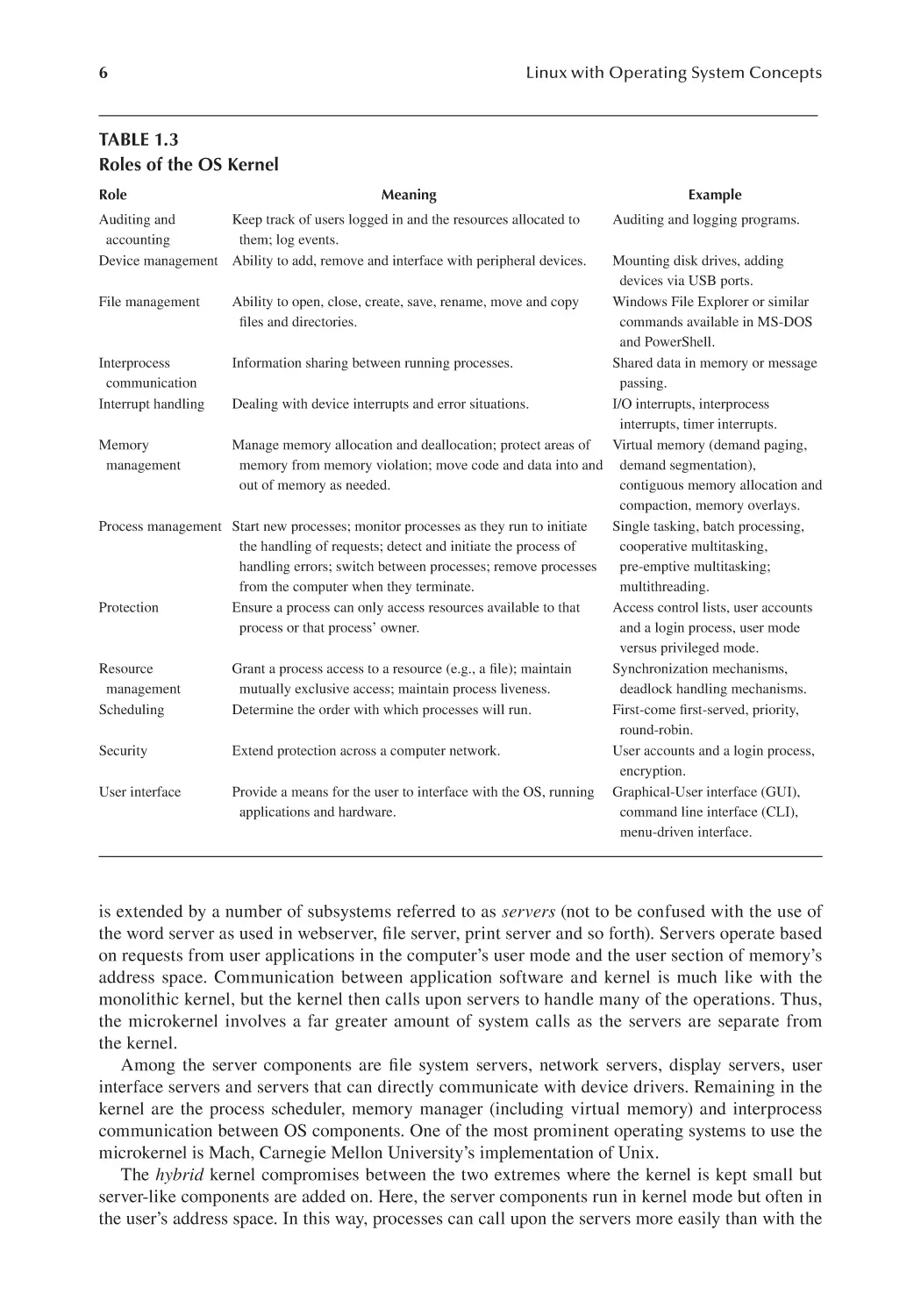
is the kernel that is responsible for most of the important tasks of the OS. We highlight several of
these tasks in Table 1.3. The tasks are listed in alphabetical order rather than in order of importance.
Process management is likely the most important role of any OS.
There are three different types of kernel: monolithic, microkernel and hybrid. A monolithic
kernel is one in which the kernel is a single program which operates solely within the computer’s
privileged mode and in its own address (memory) space. Communication between the user side
(running applications) and the kernel side is handled through system calls. A system call invokes a
specific portion of the OS kernel. Upon receiving a system call, the kernel changes from user mode
to privileged mode. The kernel then ensures that the user program’s request is legitimate, meaning
that the user program (or user) has an appropriate level of access for the call to be carried out.
Early operating systems used a monolithic kernel. But, as these operating systems governed
computers with limited amounts of memory and few system resources, the kernel was not asked to
do a great deal and so the kernel was fairly small (in comparison to later OS kernels). As computer
capabilities grew, operating systems became larger and monolithic kernels became more and more
complex.
In response to the complexity of the monolithic kernel, the microkernel was developed starting in the 1980s. The microkernel is based on a smaller kernel that operates within privileged
mode and in its own address space. In order to support the expected range of functions, the OS
6
Linux with Operating System Concepts
TABLE 1.3
Roles of the OS Kernel
Role
Meaning
Keep track of users logged in and the resources allocated to
Auditing and
accounting
them; log events.
Device management Ability to add, remove and interface with peripheral devices.
Example
Auditing and logging programs.
Mounting disk drives, adding
devices via USB ports.
File management
Ability to open, close, create, save, rename, move and copy
Windows File Explorer or similar
files and directories.
commands available in MS-DOS
and PowerShell.
Interprocess
Information sharing between running processes.
Shared data in memory or message
communication
passing.
Interrupt handling
Dealing with device interrupts and error situations.
I/O interrupts, interprocess
interrupts, timer interrupts.
Memory
Manage memory allocation and deallocation; protect areas of
Virtual memory (demand paging,
management
memory from memory violation; move code and data into and demand segmentation),
out of memory as needed.
contiguous memory allocation and
compaction, memory overlays.
Process management Start new processes; monitor processes as they run to initiate
Single tasking, batch processing,
the handling of requests; detect and initiate the process of
cooperative multitasking,
handling errors; switch between processes; remove processes
pre-emptive multitasking;
from the computer when they terminate.
multithreading.
Protection
Ensure a process can only access resources available to that
Access control lists, user accounts
process or that process’ owner.
and a login process, user mode
versus privileged mode.
Resource
Grant a process access to a resource (e.g., a file); maintain
Synchronization mechanisms,
management
mutually exclusive access; maintain process liveness.
deadlock handling mechanisms.
Scheduling
Determine the order with which processes will run.
First-come first-served, priority,
round-robin.
Security
Extend protection across a computer network.
User accounts and a login process,
encryption.
User interface
Provide a means for the user to interface with the OS, running Graphical-User interface (GUI),
applications and hardware.
command line interface (CLI),
menu-driven interface.
is extended by a number of subsystems referred to as servers (not to be confused with the use of
the word server as used in webserver, file server, print server and so forth). Servers operate based
on requests from user applications in the computer’s user mode and the user section of memory’s
address space. Communication between application software and kernel is much like with the
monolithic kernel, but the kernel then calls upon servers to handle many of the operations. Thus,
the microkernel involves a far greater amount of system calls as the servers are separate from
the kernel.
Among the server components are file system servers, network servers, display servers, user
interface servers and servers that can directly communicate with device drivers. Remaining in the
kernel are the process scheduler, memory manager (including virtual memory) and interprocess
communication between OS components. One of the most prominent operating systems to use the
microkernel is Mach, Carnegie Mellon University’s implementation of Unix.
The hybrid kernel compromises between the two extremes where the kernel is kept small but
server-like components are added on. Here, the server components run in kernel mode but often in
the user’s address space. In this way, processes can call upon the servers more easily than with the
Linux
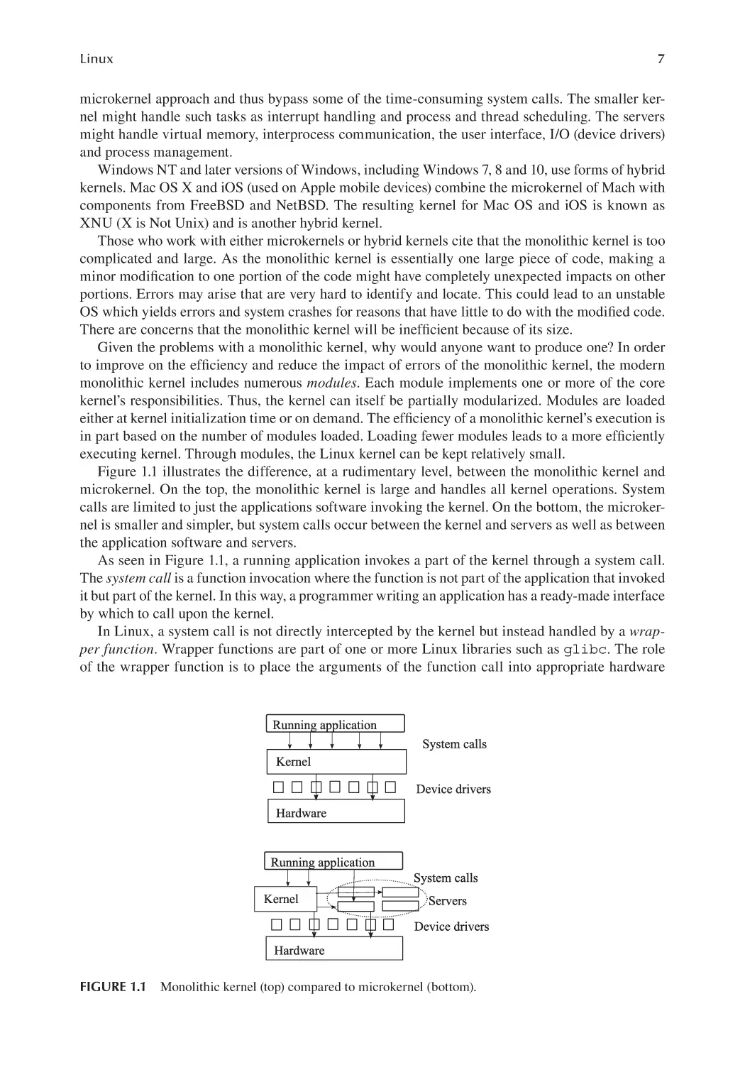
7
microkernel approach and thus bypass some of the time-consuming system calls. The smaller kernel might handle such tasks as interrupt handling and process and thread scheduling. The servers
might handle virtual memory, interprocess communication, the user interface, I/O (device drivers)
and process management.
Windows NT and later versions of Windows, including Windows 7, 8 and 10, use forms of hybrid
kernels. Mac OS X and iOS (used on Apple mobile devices) combine the microkernel of Mach with
components from FreeBSD and NetBSD. The resulting kernel for Mac OS and iOS is known as
XNU (X is Not Unix) and is another hybrid kernel.
Those who work with either microkernels or hybrid kernels cite that the monolithic kernel is too
complicated and large. As the monolithic kernel is essentially one large piece of code, making a
minor modification to one portion of the code might have completely unexpected impacts on other
portions. Errors may arise that are very hard to identify and locate. This could lead to an unstable
OS which yields errors and system crashes for reasons that have little to do with the modified code.
There are concerns that the monolithic kernel will be inefficient because of its size.
Given the problems with a monolithic kernel, why would anyone want to produce one? In order
to improve on the efficiency and reduce the impact of errors of the monolithic kernel, the modern
monolithic kernel includes numerous modules. Each module implements one or more of the core
kernel’s responsibilities. Thus, the kernel can itself be partially modularized. Modules are loaded
either at kernel initialization time or on demand. The efficiency of a monolithic kernel’s execution is
in part based on the number of modules loaded. Loading fewer modules leads to a more efficiently
executing kernel. Through modules, the Linux kernel can be kept relatively small.
Figure 1.1 illustrates the difference, at a rudimentary level, between the monolithic kernel and
microkernel. On the top, the monolithic kernel is large and handles all kernel operations. System
calls are limited to just the applications software invoking the kernel. On the bottom, the microkernel is smaller and simpler, but system calls occur between the kernel and servers as well as between
the application software and servers.
As seen in Figure 1.1, a running application invokes a part of the kernel through a system call.
The system call is a function invocation where the function is not part of the application that invoked
it but part of the kernel. In this way, a programmer writing an application has a ready-made interface
by which to call upon the kernel.
In Linux, a system call is not directly intercepted by the kernel but instead handled by a wrapper function. Wrapper functions are part of one or more Linux libraries such as glibc. The role
of the wrapper function is to place the arguments of the function call into appropriate hardware
FIGURE 1.1 Monolithic kernel (top) compared to microkernel (bottom).
8
Linux with Operating System Concepts
registers where the kernel expects them and to switch processor mode from user mode to privileged
mode. The kernel operates under privileged mode while the user’s process operates under user
mode. If an error arises during the execution of the system call, it is the wrapper’s responsibility
to intercept the error from the kernel and modify this into an error number, stored in the special
variable errno. This variable can then be referenced by the application or the user from the command line. Some wrappers are more complicated and perform various forms of preprocessing and/
or postprocessing.
Table 1.4 provides a list of some of the many system calls available in Linux. Note that system
calls will vary by both distribution and between versions. The system calls in the table, listed in
alphabetical order, are those found in most versions of Linux although the name might vary slightly.
The table describes the listed system calls and provides a basic categorization of the type of activity
it oversees. Keep in mind that any implementation of Linux will likely have several hundred system
calls available.
If you look over the list of system calls you might recognize some of the names by their type
of operation (e.g., open, close, read and write). Others have names similar to that of Linux
instructions like chmod, kill, stat and mount/umount. If you are already familiar with Linux,
the system call pipe should sound familiar.
TABLE 1.4
Some Linux System Calls
Name
access
chdir
chmod
close
creat
Category
fork, vfork
File management
File management
File management
File management
File management
Process management
Process management
Process management
fstat, stat
getpid, getppid
getpriority, setpriority, nice
File management
Process management
Process management
ioctl
lseek
kill
Device management
File management
Interprocess communication
mlock, munlock
mount, umount
open
pipe
poll
Memory management
Device management
File management
Interprocess communication
Process management
read
stat
truncate
write
File management
File management
File management
File management
exec, execv, execve (and others)
exit
Use
Test user permissions on a file.
Change the current working directory.
Change file permissions.
Close a file descriptor.
Create a file or device.
Create a child process.
Terminate current process.
Create a child process, create a child process
while blocking the parent process.
Get file status.
Get the ID of a process, process’ parent.
Get or set the process’ priority, change process
priority.
Send control signal to I/O device.
Move pointer within file to new location.
Send signal to a process (may result in exiting
the process).
Lock/unlock page in memory.
Mount or unmount file system.
Open a file/device, assign to a file descriptor.
Create interprocess channel.
Cause process to wait for event from file
descriptor.
Read from a file descriptor.
Get file status information.
Set a file to a specified length.
Write to a file descriptor.
Linux
9
Before we leave this topic, we have two additional comments. First, the file descriptor is a designator (number) that the kernel assigns to an open file or resource. It is through the designator that the
kernel will control access to that open file or resource. Thus, when we want to read data from an open
file, the operation to the kernel becomes “read from this file descriptor”. Second, the terms exec and
fork are used to express what happens when a process is created. In Linux, all processes are generated, or spawned, by an existing process (with the exception of the first process that runs during system initialization). The system calls of execve and fork/vfork are used so that the current process
can generate a new process. We explore the exec and fork system calls in more detail in Chapter 4.
1.2.3 Other Operating System Components
We wrap up our introduction to the OS with a look at other OS components, first with the device
driver. Referring back to Figure 1.1, you can see that device drivers are positioned between the
kernel and the hardware devices. Each driver is a program written specifically to facilitate communication between the kernel and the device. The reason for device drivers is that I/O devices vary
dramatically in terms of type of operation, quantity of data transmitted and speed of transmission.
It is too much to expect the CPU to be able to communicate directly with the great variety of I/O
devices. Instead, the CPU sends generic instructions to the device which the kernel intercepts and
converts into actions by calling upon the corresponding driver.
Many device drivers are already preinstalled in most operating systems. The device driver
merely needs to be enabled to be used. For less common devices, or devices that were not available
when the OS was implemented, the drivers must be installed. These drivers might come from the
manufacturer on optical disc provided with the device but more commonly are downloaded over the
Internet and installed.
Some OSs, most notably Unix/Linux, Windows and Mac OS, also employ operating system
services. Services run in the background meaning that they run without user interaction. A service
runs on demand when it is needed. When unneeded, it uses few system resources. There are a great
many services in Linux supporting such tasks as process scheduling, management of hardware and
the network, logging and file system handling. We explore services in Chapter 9.
Another component of many OSs is, like the device drivers and services, a collection of programs,
referred to as OS utilities; also possibly referred to as tools. Each utility offers some functionality
in improving system performance. One class of utility pertains to files and file systems. There are
disk defragmenters to make disk access more efficient, disk recoverers to scavenge deleted files
from disk, file system cleaners to remove unused or outdated files, backup and archive utilities and
encryption/decryption utilities. Another form of utility is an anti-malware program which not only
searches your hard disk for computer viruses but also examines website URLs to see if the website
should be avoided as untrustworthy.
Most utilities run at the request of the user. This makes the utility different from other OS components which run as needed or are invoked by application software or requests from other OS
components. And unlike the kernel and OS services, utilities run in the foreground i.e., they present
the user with an interface. Windows has a great number of utilities, some of which are part of the
Windows OS and some are third-party add-ons. Linux has fewer utilities because some of the same
tasks are handled by Linux services. Some utilities are not part of Linux at all and must be installed
as third-party products.
The last “add-on” component to the OS is tailorable user interface. In Windows and Mac OS, the
user can tailor the desktop with files and shortcut icons. In Linux, we more commonly use the shell
to personalize our interface. The shell is an environment in which the user enters commands. The
shell permits definitions and instructions to be recalled later. Definitions include shell scripts and
aliases. We explore the Linux shell in detail in Chapter 2.
We noted earlier that the system call wrapper functions, among other tasks, cause the computer to switch modes. The Linux OS has a clear differentiation of roles between user mode and
10
Linux with Operating System Concepts
TABLE 1.5
Uses and Platforms Where We Find Linux
Uses/Platforms
Arts
Cloud
Gaming
Governments
Mobile device
Networking
Smart devices
Webserver
Explanation
Preferred choice for animation by many movie studios.
Used to support cloud computing and other cloud services.
Often used in gaming development.
Used extensively by dozens of governments including the US, China and India.
Android and Raspberry Pi, among others.
Found in firewall and router hardware devices.
Found in many smart TVs and home automation devices.
Linux is used to run more webservers than any other OS.
privileged mode. User mode is applied when running all applications software, Linux services,
the GUI, common software libraries and system calls. Privileged mode consists of the OS kernel,
including the execution of system calls and device drivers.
1.2.4 So, What Is Linux?
We posed this question to start this section but then dedicated most of the space to describing OSs
in general. What is Linux? Succinctly, Linux is a family of OSs, loosely based on Unix, and largely
developed by and supported by the open-source community. Linux is an OS that uses a monolithic
kernel supported by modules that can be loaded and unloaded. Linux is an OS whose interface with
applications software is made through system calls.
Linux is also one of the few portable operating systems available. The term portable means that
the OS is not written for one or a few forms of hardware but could be run on many different platforms of hardware. Linux is also one of the more efficient OSs. It is small enough to run on nearly
any type of computer device but powerful enough to run large-scale applications such as webservers. It is modern enough to use features found in most other OSs while also having its own cuttingedge facilities such as its security handling (SELinux). It is similar enough to Unix so that users of
Unix will have no problem learning Linux, and its GUI is relatable enough for a common user to be
able to use it. As Linux is available in open source, a programmer can modify how Linux runs by
updating and recompiling Linux source code.
There are many uses for Linux. We share some in Table 1.5. Move on to Section 1.3 for more
reasons for using Linux.
SECTION ACTIVITIES
1. How important is it for a user to understand the operating system concepts explored
in this section? For instance, do you need to know what a kernel is? What services
are? Think about your own knowledge of the OS. Does it make it easier for you to
use computers?
2. In this section, we saw, briefly, the development of early OSs until 1966. You might
wonder about Windows and MacOS. As personal computers were not introduced
until the 1970s, it’s no surprise we didn’t see them included in the list. IBM PC and
compatible computers started off using MS-DOS, with Windows being introduced
in 1985, 1 year after the first Macintosh came out. Research the development of both
MacOS and Windows. You can find a great many websites that describe their individual histories or the history of all operating systems combined.
11
Linux
1.3 WHY USE LINUX?
What makes Linux different from other operating systems? We noted earlier in this chapter that it
is open source and provides the user more control. There are other open-source operating systems,
albeit not that many, and none have been as successful as Linux (Android by Google is perhaps the
most popular alternative but is itself based on a modified version of the Linux kernel). There are
other OSs that provide the user with the degree of control as Linux although the one that equals
Linux is Unix, on which Linux is based.
It’s worth reiterating that open source does not just mean free. With Linux, open source comes
with an entire community of programmers. These programmers work, usually in large groups, on
related projects. Some are involved in enhancing existing Linux versions. Others work on applications that run within one or more versions of Linux. And those same people or others are involved
in providing the support that comes with commercial products.
In addition to the open-source nature of Linux, it was initially built to require few resources. We
might refer to Linux as a lightweight OS compared to that of Mac OS and Windows because of the
approach taken in implementing Linux. Linux should boot and initialize faster than other operating
systems. A computer running Linux should require less memory and should be able to function with
a slower processor. Although these statements are generally true, some versions of Linux require
more resources than others.
Another advantage of Linux is portability. The Unix OS was developed to be run on any platform
of mainframe computer, and later versions were released for workstations, personal computers and
servers. Linux is even more portable. Versions of Linux can run on just about every classification of
computer: supercomputer, mainframe, server, personal computer and laptop, tablet, smartphone and
embedded devices. This level of portability does not exist with other OSs.
Another reason to choose Linux is that it is less attack-prone than Windows. Hackers more commonly target Windows-based computers when attempting to breach computers, inflict viruses or
perform other forms of attacks because there are far more Windows computers than Linux computers (excluding servers and supercomputers). You might think that Linux would be open to attacks
of all kinds because its source code is readily available. In fact, the open-source community takes
great efforts to ensure a lack of security flaws in the OS before a Linux version is released. That is
not to say that they are 100% successful. But because of the efforts taken combined with the lower
incidents of attack, some companies and even whole governments are moving to Linux as the preferred OS because it is, at least currently, more secure.
Linux has become the OS of choice for many computer programmers and system administrators.
It is also an OS of choice for many computer users, hobbyists and companies. But in spite of its
increased popularity, the number of desktop/laptop computers running Linux remains in the minority when compared to Windows and Mac OS. It is estimated that no more than 1.93% of the world’s
desktop computers are currently running Linux. Figure 1.2 highlights some of the more interesting
statistics about Linux usage, as of spring 2021.
SECTION ACTIVITIES
1. What open-source software have you used? Make a list. It’s probably more than ten
titles!
2. The statistics in Figure 1.2 provide an interesting dichotomy: Linux is the operating
system of choice for supercomputers and most servers but few desktops. Why do you
suppose this is the case? Write down three reasons. Now research the topic and see
if your reasons are those cited by others.
12
FIGURE 1.2
Linux with Operating System Concepts
Interesting statistics about Linux usage.
1.4 WHO DEVELOPED LINUX AND WHEN?
We can start the history of Linux with one person and one event: Linus Torvalds, a Finnish computer science student, who in 1991 was dissatisfied with the operating system that came with his
operating system textbook. He set about creating his own OS which he eventually named Linux. But
rather than starting with Torvalds in 1991, we start 27 years earlier.
1.4.1 The Birth and Development of Unix
In 1964, a group of software engineers from AT&T Bell Labs, General Electric and MIT began
developing a new and novel operating system called MULTICS (Multiplexed Information and
Computer Service). MULTICS was a multiuser, time-sharing (multitasking) OS that pioneered a
number of innovative features. While the development of MULTICS seemed promising, AT&T
withdrew from the project in 1969, shortly before its release.
Ken Thompson and Dennis Ritchie were two of the AT&T members involved in the early development of MULTICS. They did not want to see their efforts end at that time. AT&T was using
a batch processing OS that they felt was unsatisfactory. They worked on their own version of a
MULTICS-like OS with help from other AT&T employees, including Rudd Canaday. The result
was a new OS, written for the PDP-7 mainframe and written in that computer’s assembly language.
They called it UNICS, short for Un-multiplexed Information and Computing Service, likely a joke
name spoofing the name MULTICS.
Further development targeted the PDP-11 computer but rather than reimplement the OS in
PDP-11 assembly language, Thompson and Ritchie wanted to implement their OS in a neutral
13
Linux
language so that the OS could be ported more easily to other computers. Ritchie, along with
another AT&T employee, Brian Kernighan, created a new programming language called C. It
was in C that UNICS was rewritten and eventually released in 1973. During this time, the OS
was renamed from UNICS to Unix. Other employees contributed significantly to Unix as it was
developed.
A look at Unix features shows that it was at least partially derived out of the experience
that Thompson and Ritchie gained in their work on MULTICS. Table 1.6 shows some of the
features either introduced in MULTICS and used or enhanced in Unix, or introduced in Unix.
Compare these features to the brief descriptions of other early 1960s OS from Table 1.2, and
you will see that first MULTICS and then Unix popularized many features that had yet to be
developed.
In spite of Unix being referred to as platform-independent, the 1973 version still contained some
code specific to the PDP-11. It was not until 1978 that Unix was successfully ported to another
platform. When distributed by AT&T, Unix was provided in source code format (for a small fee).
Although AT&T released many versions of Unix, they were all referred to as Research Unix. But
because AT&T offered no support in the versions they distributed, it was up to other organizations
to modify the Unix source code as needed to run on different platforms, fix errors and add desired
features. This led to a splintering of Unix into many versions.
One such version was provided to the University of California Berkeley’s computer science
department. At Berkeley, programmers developed their own OS, using some of the Unix code
as components. In 1975, Ken Thompson became a visiting professor at UC Berkeley. Under his
TABLE 1.6
Unix Features (From Richard Fox, 2021, Information Technology: An Introduction for
Today’s Digital World, 2nd edition)
Feature
Command line
interpreter
Commands as programs
Hierarchical file system
Interprocess
communication
Multitasking/multiuser
OS
Portability
Regular expressions
Shells
System calls
Top-level directory
structure
Treating devices as files
Explanation
Comments
Beyond a CLI, Unix’s CLI provides flexibility with operations to redirect input Popularized
and output, define constructs like aliases, and the ability to write shell scripts.
from Multics
Rather than having the kernel handle all operations, many basic commands are First
provided as their own programs such as file system commands, text editing
and processing commands, and process management commands.
Directories can have their own subdirectories and administrators to better
Popularized
organize files.
from Multics
Allows synchronized access to shared data among multitasking processes.
Runs multiple processes of multiple logged-in users at a time.
Unix could be installed on a large variety of computer types.
Ability to search files for strings through command-line programs like grep,
awk and sed and the programming language Perl.
The CLI was one component of a shell; shells introduced convenient shortcut
features to assist the user.
Written in C, Unix made many kernel operations available as C functions
known as system calls, which could be invoked by user programs.
Separate directories for OS components and user files simplify the process of
searching for a file.
Nearly everything in Unix is either a process or a “file”; this allows file
commands to be executed on devices either from the command line or from
a script.
First
Popularized
from Multics
First
First
First
First
14
Linux with Operating System Concepts
guidance, a new version of Unix was produced. This became known as the Berkeley Standard
Distribution (BSD) Unix. Unlike AT&T’s Unix, which was proprietary, BSD Unix was freely distributed under the BSD License (which imposed only minimal restrictions on the use and distribution of this version of Unix). BSD versions 4.2 and 4.3 became leading versions of Unix, distributed
to other organizations. BSD led to other versions such as SunOS, Darwin (which would become
the basis for the Mac OS), FreeBSD and NetBSD. Other versions splintered from Unix to become
IBM’s AIX, HP’s HP-UX, Microsoft’s Xenix and Sun’s Solaris. By 1990, there were dozens of versions of Unix, many of which were proprietary.
1.4.2 GNU
In the early 1980s, Richard Stallman, a researcher at MIT’s artificial intelligence laboratory, wanted
to create his own Unix-like operating system. He wanted to make this OS available in source code
format for free and with no licensing restrictions so that other programmers could modify the OS
as they desired just as long as any modifications would similarly be made available in source code
for the community to use. He called upon many members of the Unix user and programming community for help. He dubbed the project GNU for GNU Not Unix, a recursive definition (recursion is
a programming tool commonly used in artificial intelligence).
Stallman’s group began work on the GNU OS at the same time BSD was becoming popular.
But while BSD became successful, a GNU kernel was never completed. Stallman succeeded,
though, in his version of a free software movement. His vision was that software should be
free. He would explain free as in “free speech” not “free beer”. He opposed proprietary software and saw the software field as one where all programmers could or should contribute to
the development of free software. Software, he felt, were based on ideas and ideas could not be
owned.
Stallman created the GNU General Public License (GNU GPL). The GPL requires that software
published under the GPL must be free for anyone to use for any purpose: free to be studied, free to
be changed, free to be redistributed and free to be improved. The proviso is that anything created by
GPL software would also be published under the GPL so that further distribution of such software
would also be available as source code allowing others the same freedoms.
GPL version 1 was released in February 1989. Its main points are that any software distributed
under the GPL can be copied and distributed in the source code format (as long as it is distributed
exactly as provided) and distributed in any medium, and as long as the redistribution maintains the
exact same notices as the original. The same stipulations apply to modified code: such code must
contain the original notices as well as notices that this version has been modified, including the files
changed and the dates of those changes, and that the new distribution be carried under the GPL. The
GPL also permits distribution of the code in its compiled, executable form (known as object code).
There are ten clauses in GPLv1 including two that clearly indicate that the software comes with no
warranty because it is free.
GPLv2 was released in June 1991 adding a restriction that works covered by the GPL can only
be redistributed if they can satisfy all of the license’s obligations. The inclusion of this clause is to
discourage any form of patent infringement lawsuit being claimed over a GPL-distributed product.
GPLv3 was released in June 2007, which added more detail and language to protect GPL-covered
items (which at this point went beyond software).
Although we will not examine the GPL itself, Figure 1.3 shows the first version’s Preamble,
which is worth reading. It states, right from the start, that the GPL is there to express our freedom
rather than the restrictions found in most software licenses. It is for this reason that Stallman called
the GPL a copyleft instead of a copyright. The entire GPLv1 license, along with all newer versions, is available at https://www.gnu.org/licenses/ with version 1 at https://www.gnu.org/licenses/
old-licenses/gpl-1.0.en.html.
Linux
15
FIGURE 1.3 The GPLv1 preamble.
1.4.3 Enter Linus Torvalds
In 1991, Linus Torvalds, a computer science student at the University of Helsinki, was unhappy with
the toy OS that came with his operating system textbook. Torvalds began to develop his own small
OS on his Intel 386-based computer, written in Intel 80386 assembly language. He developed only
a few components: a small multithreading kernel, a bash interpreter and the gcc compiler. He
posted on the USENET newsgroup, comp.os.minix, to attract other programmers who wanted
to help develop an OS that was different from and better than MINIX. He posted the source code
for his fledgling OS on an FTP server. Over the next few months, members of the GNU community
contributed GNU components including the facility to compile code using make as well as compress and sed, among other programs.
As the OS took shape, he published it under a version of the GPL (GPLv2). Over the next several
months, the community of programmers working on Linux grew. A new USENET newsgroup was
established for the community, alt.os.linux (which would be renamed comp.os.linux a
couple of months later). Enhancements to Linux during this time included a number of device drivers, a more fleshed-out kernel, the adoption of the POSIX standard and an implementation of the X
Window System. By 1994, Linux had grown to over 175,000 lines of code, written in C. This version
was distributed as Linux version 1.0.0. Aside from versions released for Intel processors, Linux was
successfully ported to the DEC Alpha, Sun SPARC and MIPS processors.
16
Linux with Operating System Concepts
In 1992, the first well-known splintering of Linux took place when Canadian software engineer
Peter MacDonald developed Softlanding Linux System (SLS). Whereas Torvald’s Linux was a kernel, device drivers and full utilities like gcc, SLS included a full windowing system (based on X
Windows) and a number of applications software. Computer science student Patrick Volkerding (at
Moorhead State University in Minnesota) downloaded SLS and modified it to fix some bugs. He
distributed his version to fellow students who urged him to publish his version. His version became
known as Slackware.
A German software company, Software und System Entwicklung (Software and System
Development, or SUSE for short) adopted Slackware as a platform, translating it into German and
enhancing it. This led to three different versions from the same branch of the Linux “tree”. All three
versions continued to be updated although SLS was largely ignored in favor of Slackware. But it was
SUSE that found the most popularity in the end and has had several spinoff versions under various
names including SUSE, SuSE, SuSELinux and openSUSE. In comparing SUSE to other versions of
Linux, we find it comes closest to Red Hat Linux, and as SUSE/openSUSE is of limited popularity,
we will not examine it any further.
The SLS/Slackware/SUSE version of Linux leads us to the term distribution, or distro for short.
More and more distributions took place in the 1990s and into the 2000s resulting in a large number
of Linux versions. There are far too many distros to track them all here. The remainder of this subsection looks at some of the more significant developments of the distros.
In 1994, software developer Marc Ewing developed his own version of Linux that he named Red
Hat Linux. Released late in 1994, his business was bought by entrepreneur Bob Young. The new
company was called Red Hat Software and largely revolved around a commercial version of Linux
(both the OS and application software). Unlike the versions of Linux being developed by the opensource community, the intention of Red Hat was to include support so that companies could trust
that bugs would be fixed quickly. Red Hat Software was later renamed Red Hat, Inc., which was
purchased by IBM in 2018.
Two spinoffs of Red Hat are supported by Red Hat, Inc., Fedora and CentOS. Both of these versions are open-source versions of what is now called Red Hat Enterprise Linux (RHEL). There are
a few differences between these three distributions but mostly they are built on the same kernel with
most of the same services, applications and features. Similarities and differences between the three
distributions are described in Table 1.7. Note that the most recent version is of spring 2021.
Debian was first announced in 1993 with the intent to be the first release of a Linux outside of
Torvald’s. The project was headed by programmer Ian Murdock, and the name was a combination
of his girlfriend (Debra) and his first names. Although the first release of Debian (version 0.01) was
in 1993, the first major release did not take place until 1996, thus it trailed both SLS/Slackware and
TABLE 1.7
Comparisons between RHEL, Fedora and CentOS
RHEL
Initial release
License type
Maintained by
Processor targets
Computer types
2000
Commercial
Red Hat, Inc/IBM
x86, ARM, IBM Z, IBM power systems
Servers, mainframes, workstations,
supercomputers
User interface
GNOME
Release targets
2–4 minor releases per year, major
releases every 5 or so years
Most recent version RHEL version 8 (Oct 2020)
Fedora
2003
GPL
Open-source community
x86, ARM, aarch64
Servers, desktops, cloud
CentOS
GNOME
Every 6 months
2004
GPL
Open-source community
x86, ARM64, Power8
Servers, desktops,
workstations, supercomputers
GNOME
Same as RHEL
Version 33 (Oct 2020)
Stream (Dec 2020)
Linux
17
Red Hat. Murdock handed off control of Debian to Bruce Perens in 1996 and then leadership was
established by elections every year (starting in 1999).
Unlike Red Hat which had both commercial and open-source versions, Debian was intended to
be open source from day one. The Debian development community took their time with each version, planning to release a new version only every 2 years. Three different versions of Debian are
available at any time: the current stable version, a testing version of the intended next release and an
unstable version which includes libraries and packages that may not install correctly or at all (that
is, these items are untested).
The deliberative and slow nature of new releases under Debian was a point of contention with
some developers and so Ubuntu spun off from Debian with new releases targeted for every 6 months.
The first version of Ubuntu came out in 2004. Ubuntu attempts to be a more secure version of Linux
and as such, pioneered the idea that rather than users having access to the system administrator
account (root), the first user account would automatically receive access to administrator commands through the sudo command. We explore this later in the text. Other Linux distributions later
adopted this practice.
Two other notable Debian descendants are Knoppix and Linux Mint. Knoppix is noteworthy as a
form of Linux that can be booted and run entirely off of an optical disc. This feature, known as a live
boot, allows the user to use Linux without installing it on their computer. The disadvantage is that
you start with a new version of the OS every time you launch it. Any previously created accounts
or changes made to the OS or environment are lost. Files must be saved externally, for instance via
a USB-based drive. Linux Mint is based on a Ubuntu-derivative called Kubuntu, which was first
released in 2006. As Linux Mint was further developed, it became more based on Debian than
Ubuntu and is now called Linux Mint Debian Edition (LMDE). Two differences between Linux
Mint and Ubuntu are that Linux Mint supposedly uses less memory when running and it has more
preinstalled applications than Ubuntu.
In reading through the distributions listed above you might question why there are so many.
What are their differences? All of the spinoff distributions are based around the same Linux kernel.
Each version’s kernel shares many of the same modules with the other versions. The versions share
many of the same C libraries, system calls, shells and X Windows interface (although the specific
look of the desktop will differ). Many of the same applications run on all of the Linux distributions.
There are perhaps four significant differences between these main distributions. The most significant difference in terms of usage is the package manager program used to perform software
installation and upgrades. A second difference is the quantity of available applications software as
some distributions have fewer titles available or support fewer third-party applications. There is also
a philosophical difference behind the developer’s plans for major version releases. Finally, there is a
different philosophy taken regarding whether the root password is made available.
There are two primary package managers used in today’s Linux distributions: dnf (or the
slightly older yum) and apt. These are built on top of other package manager programs: rpm (Red
Hat Package Manager which dnf/yum uses) and dpkg (Debian Package Manager which apt calls
upon). Amazingly, other than the specific desktop design, this is the single most visible difference
between the various distributions.
In terms of available software, we find most distributions come with a Firefox web browser
(usually built in) and can run the emacs editor (not built in). They also all have the ability to run
an office suite (built in or not), usually LibreOffice. However, some have far more applications
than others. For instance, Ubuntu is a popular choice for gaming enthusiasts.
The development philosophy is less visible but no less impactful. The Debian community takes
a slow but thorough approach when creating and vetting a new version. The target of every 2 years
seems extreme to some Linux users and so they favor the more rapid development and deployment of
Ubuntu. With Red Hat distributions, Red Hat, Inc. drives most of the development but as new versions
are made available, members of the Red Hat community take the source code and use it to develop a
new release of CentOS. So, in fact, CentOS will have mostly the same code and features as RHEL.
18
Linux with Operating System Concepts
TABLE 1.8
Comparing Linux Distributions
CentOS
Initial release
Parent (if any)
Package manager
Approximate amount of
software packages
Target release frequency
2004
Red Hat
rpm, dnf/yum
6000–7000
Coupled with
RHEL
Degree of open source
Completely
Most recent version
8 and Stream
Most recent release date 2020
Debian
Fedora
Linux Mint
RHEL
Ubuntu
1996
N/A
apt, dpkg
90,000
2003
Red Hat
rpm, dnf/yum
65,000
2006
Ubuntu
apt, dpkg
30,000
1995
N/A
rpm, dnf/yum
10,000–12,000
2004
Debian
apt, dpkg
90,000+
Every
2–3 years
Completely
10.8
2021
Yearly
Every
2–3 years
Mostly
20
2021
Major releases
every 5–10 years
None
8
2020
Every
6 months
Mostly
20.04
2020
Completely
33
2020
In previous releases of RHEL, a related version of CentOS was released shortly afterward.
Starting in 2020 however, a new approach is being taken. CentOS is now releasing versions under
the name Stream. The idea is that rather than waiting for a new, completed version of RHEL,
CentOS will release versions earlier that contain features being proposed for the next RHEL release.
Finally, there is a distinction between RHEL, and the rest of the Linux distributions described
here in that RHEL is not a free OS. Instead, a commercial purchase must be made in order to receive
RHEL support. The other versions of Linux are free and can be found in source code format. Within
the different distributions, some software may be proprietary. Early versions of Linux Mint had
proprietary software (which has supposedly been removed).
We review the most significant differences between these most notable distributions in Table 1.8.
In the table, we cite which of the original distributions it evolved from, the choice of package manager, the quantity of available software (estimated from various website reports) and the development
philosophy. We also note the most recent version and its distribution date. The Linux distributions
are listed in alphabetical order (left-to-right) rather than by year of initial or most recent release.
There is no official count of the total number of Linux distributions available or in use today,
but the estimate is between 600 and 1000. Some of these distributions vary more dramatically than
what was explained above. Nearly all of the distributions are available for free (RHEL being one
of the notable exceptions), and these can come in either source code or as an executable installation
program (usually as an ISO image). The history is so complicated that mapping the distros requires
a very large chart (see the Linux distro tree at https://5thlobe.com/reference/gnulinux-distro-chart/).
We should point out that Linux is not the only open-source OS. Three notable other open-source
OSs, all of which are Unix-like, are FreeBSD, Dragonfly BSD and GhostBSD. Another open-source
OS is XNU (which stands for X is Not Unix), which is the basis for the iOS operating systems found
on such devices as the Apple iPad and Apple TV. ReactOS was developed in 1996 as a clone for
Microsoft Windows 95 and has the look and feel of more recent Windows OSs. And then there’s
FreeDOS which is primarily used to run old MS-DOS games and other legacy software. There are
others, but none of these operating systems has achieved anything close to the popularity or name
recognition of Linux.
1.4.4 The Open-Source Community
The earliest open-source projects were the further development of Unix, GNU and then Linux. The
first application software that the open-source community contributed to was the Netscape web
browser, which the original developers offered to the community for input. It was at this point that
the term open source was first used.
Linux
19
As work continued on both Linux and Netscape, the open-source software community fell into
a dispute. Torvalds did not require that modified versions of software be made freely available. He
felt that if a person modified a piece of open-source code, the modified code could continue to be
freely distributed as source code, or it could be freely distributed but as executable code, or it could
even be sold for profit. But some members of the open-source community eschewed commercial
software and felt that anything developed out of the open-source community must remain open
source and freely available.
This rift caused the community to splinter into two groups: the Open-Source Initiative (OSI)
and the Free Software Foundation (FSF). OSI was founded in 1998 by members of the open-source
community developing versions of Linux including Bruce Perens from Debian. FSF was founded
by Richard Stallman in 1985. The difference between the two groups is that OSI is willing to accept
copyrights on some software restricting freedoms that were established under the GPL while the
FSF generally feels that anything created from a GPL-produced product must also be made available in open source under the GPL. Although this rift has driven some projects to splinter, it has not
impacted the productivity of the open-source community and the number of titles being produced.
The shift in perspective from commercial software development to open source not only has
impacted software developers’ perspective of open source but the corporate world. Early on, opensource software was primarily used by hobbyist and people in the open-source community. Opensource software was largely shunned by companies. There was a stigma attached to open source
products that they would have errors that could potentially harm an organization because the software would not work when it was needed. This could result in a loss of productivity and revenue
and cause the organization to receive a bad reputation. Companies preferred the guarantee that
proprietary software would be fully supported such that errors would be fixed in a timely manner.
Today, open-source software competes regularly with proprietary software in part because the
open-source community has been found to be as or more responsive than many of the companies
producing proprietary software. A comparison between open-source software and proprietary software products often shows that open-source software has an equal level of security, is of equal (or
even higher) quality, has a greater degree of interoperability (available on multiple platforms), and
provides a reasonable amount of support. The support might be available for free, or for a fee but
the fee would in most cases still be less than the expense of the proprietary software and its support.
We also find today that the open-source community exists well beyond individual developers
wanting to make contributions to Linux or other projects. For instance, Microsoft, who would have
opposed the open-source initiative years earlier, is now a steady contributor with such products
as .net development tools, the Visual Studio Code editor, PowerShell, and tools for building and
training machine learning systems. Their open-source contributions are not limited to Windows;
they also offer versions of software for MacOS, Linux, Unix and in the cloud via Microsoft Azure.
Other companies that contribute to the open-source community include Adobe, Facebook, Google,
IBM, Intel, LinkedIn, Netflix, Oracle and Twitter.
Why are people willing to contribute their time to the open-source community? It is especially
puzzling because contributions are often made by programmers who develop software for a livelihood. If they are willing to freely contribute, then they are in essence producing for free something
that they could earn a salary for creating instead. It is possible that the software they are helping to
produce might compete against software that they are paid to produce or maintain. And yet being
involved in the open-source community could help their careers. Table 1.9 lists several reasons for
why developers freely contribute to open source projects as a means to further their career.
Participation in open-source development also gives the programmer an opportunity to give back
to the open-source community, or even a larger audience, all computer users. Mozilla’s Firefox, for
instance, is such a success that a contribution to its development can be thought of as a contribution
to much of humanity.
Contributions are not limited to just software developers. There are a lot of open-source programmers who program for a hobby and not as part of their job. Their motivations may be similar
20
Linux with Operating System Concepts
TABLE 1.9
Some Reasons to Contribute to Open-Source Software Development
Improve coding skills.
Learn new technologies.
Gain experience with developers from other regions of the
world.
Improve on coding habits.
Participate in a large group project.
Demonstrate a wider range of skills than what the developer
uses at their current position.
Learn different software approaches.
Learn programming concepts not already known.
Make contacts with other developers.
Learn about or develop tools that can be applied in the
development career.
to those who want to further their career: learning, working with other developers and producing
something useful. But in their case, the impact may be more of a personal nature over improving
their career.
Contributions can also be made by non-programmers through software testing. Most open-source
software consists of very complex programs. Testing is a crucial aspect of software development,
and it is typical that testers are not the same group as the developers. Testing can be performed
at different levels. Software testers commonly run the software on a number of test cases, that is,
groups of input. They then compare the output to the expectations and write up reports where the
output diverges from expectation. In other cases, testers are users who compile lists of problems that
they detect when using the software. For instance, if the software crashes when opening a file or if
a particular feature operates too slowly, these cases are noted and sent back to the developers. Aside
from testing, there is also a need for documentation writing.
The open-source ideology has extended beyond software development to other communityinvolved pursuits. Wikipedia is one of the best examples of this. The online encyclopedia receives
contributions from people all over the world who want to share knowledge. Unlike open source
software which requires some expertise as a programmer, Wikipedia only requires knowledge of a
particular topic and the willingness to contribute. With Wikimedia, knowledge-based contributions
extend to other media, namely images (whether drawings or photographic). We see artists sharing
their products through the Internet using various forms of social media such as through YouTube
and Bandcamp.
SECTION ACTIVITIES
1. We often hear of basement inventors who go on to make millions of dollars on their
inventions (of course we mostly only hear about the successes, how many other
inventors never profited from their inventions?) Torvalds made no attempt to profit
from Linux. Yet, as a software developer he has made an immense success for himself and is estimated to be worth well over $100 million. Research his personal history to learn how he turned Linux into a fortune without actually making much
money off of Linux itself.
2. In this section, we provided a URL that shows all of the Linux distributions. Use that
link to examine this amazing figure. Try to estimate how many Linux distributions
exist.
3. You have likely accessed and used other products of the open-source community like
Wikipedia, Wikimedia and YouTube. Come up with a list of other websites where
information is freely shared that you have used.
Linux
21
1.5 HOW DO YOU USE LINUX?
In this section, we look at the steps to install Linux. We examine several different Linux distributions. In each case, we make the assumption that the installation will be performed onto a virtual
machine. If you want to try any of these on your own computer, it is best to download and install
a virtual machine client program. VirtualBox from Oracle and VMWare Workstation are both
open-source products. For complete information on installing Linux into a VM, see lab 0 in the lab
manual that accompanies this textbook.
To install Linux, we need to get ahold of the Linux installation program, which is in the form of
an iso file. We download the needed iso file directly onto hard disk from which to perform the
installation. The versions of Linux we examine here are free (and available in open-source format
for those interested in looking at or modifying the code) where the iso can be found on the Linux
projects’ websites.
We perform a default installation in most cases although discuss some of the options. Later
in the textbook, we look at the steps required to perform a nonstandard partitioning of the Linux
computer’s file space. This section ends with a brief look at each of the Linux distributions we
installed including their basic desktop setup and how to open and use a terminal window to enter
commands.
1.5.1 Installing Debian Linux
The Debian installation image can be obtained from www.debian.org/distrib. For users who
have slow Internet connections, a small image is available that can be saved onto an optical disc.
Otherwise, the full image can be saved to optical disc or hard disk. A cloud image is available if
you have an account in one of the commercial clouds although it is likely that your cloud provider
already has a Debian image available so that you can skip installation and just create a copy.
Upon starting our VM software, we create a new VM. When asked for the type of OS, we select
Linux and then more specifically Debian. We are asked for a location of the installation image
and we select the downloaded iso file. Figure 1.4 shows the first four screens that we see during
installation. First, we select the type of installation. We have selected Graphical install to
ensure that our Linux installation comes with a GUI. Next, we are asked for our language (the
default is English) and location. The location is used to set the time. We are next asked for the keyboard configuration (not shown in the figure, we selected American English). At this point,
installation begins. A bar indicates the amount of installation completed. Messages appear during
installation describing what is currently being installed. The next step is to specify the root password. Instructions explain the importance of selecting a strong password. We are asked to enter the
password twice in this step.
As installation continues, the next step is to create an initial user account. We want to have a nonroot account available so that when we log in, we log in as a normal user instead of root. Logging in
as root through the GUI can lead to mistakes that could damage components of the OS or accidental
deletion of files. It is best to switch to root sparingly and only from the command line. For the new
user account, we are asked for the user’s full name. Debian creates an account for this user. We are
then asked to enter the new user account’s initial password, twice, much like we did for root.
At this point of installation, we are asked to select how we want the disk space partitioned. The
options are to have a guided approach or to perform partitioning manually. There are three forms
of guided approaches, each uses the entire hard disk available (which in the case of a VM is not our
computer’s full hard disk, just the section reserved for the VM based on the size specified when
we created the VM). One guided approach uses a standard partitioning, one uses a logical volume
manager (LVM, covered in Chapter 8), and one uses an LVM but employs encryption. Note that if
we were installing Linux on a dual boot computer, we would have to perform a manual installation
so that we do not wipe out the existing operating system and files.
22
FIGURE 1.4
Linux with Operating System Concepts
Four steps during Debian installation.
In Figure 1.5, we see the partition choices and, having selected Guided – use entire
disk, we see three options. It is preferable to separate /home (the partition containing the user
directories), /var (the partition containing various software data) and /tmp (the partition used
by software to save temporary information) from the rest of the operating system. We next see in
Figure 1.5 the recommended partitioning with sizes. Note that our disk space was limited to 32 GB
as we were creating this Linux computer in a VM with limited hard disk space).
With partitioning specified, installation continues with the core packages. We are later asked
if the GRUB boot loader should be installed in the master boot record. Our only choices are no
or yes. Selecting no will require that we install our own boot loader later. We select yes and are
asked where to place GRUB. This is shown in the lower right of Figure 1.5. The notation /dev/
sda represents our hard disk. The rest of the installation is handled with no user interaction.
Upon completion, the VM should boot to our Debian installation and we will be shown the login
screen like that shown in the left half of Figure 1.6. Here, there is only one user, the user we had
established during installation. Having selected this user, we are asked for the user’s password to
complete the login process. Notice in the upper right (shown in full in the left side of the figure but
not in the right side of the figure) are controls to change accessibility settings, network connection,
the volume and “power settings” (log out, shut down, reboot).
Upon logging in, we are presented a mostly blank desktop. Along the upper left is a menu labeled
Activities. Selecting this menu brings up a list of icons along the left margin, representing from topto-bottom, the Firefox web browser, the Evolution Email program, the RhythmBox music program,
LibreOffice Writer, the Linux File Browser, the Software program (software store), Debian Help and
applications software. Upon selecting the application software icon, the installed titles are displayed
in the desktop. On the right side of Figure 1.6, roughly half of the installed titles appear. A search
bar appears at the top for easy searching (useful if we had more software titles installed). You will
find that this basic setup is similar to both CentOS and Ubuntu.
23
Linux
FIGURE 1.5 Partitioning the Debian installation.
FIGURE 1.6
Debian login screen and desktop.
1.5.2 Installing CentOS Linux
At the time of this writing, there are two different “current” versions of CentOS: CentOS Linux
version 8 and CentOS Stream. In all previous releases of CentOS, the current version followed from
the most recent release of RHEL. Thus, CentOS 8 is what you would expect to install. However,
starting in 2020, CentOS announced that rather than releasing new CentOS versions based on the
most recent RHEL version, CentOS Stream would offer versions of Red Hat that were, at least in
some cases, ahead of the next RHEL version. This means that CentOS Stream releases may include
24
Linux with Operating System Concepts
features that are proposed but not yet available in the most recent RHEL releases. Because of this
shift in philosophy, CentOS has announced that CentOS 8’s end of life will occur at the end of 2021.
By the time you read this, it is likely that CentOS will have moved entirely on to Stream releases. In
this section and throughout this textbook, we focus on CentOS Stream rather than CentOS 8. With
that said, as of August 2021 the two releases are virtually identical.
We can obtain installation ISOs for both CentOS 8 and CentOS Stream at the centos.org
website. Specifically, we find versions of CentOS 8 at www.centos.org/centos-linux and
versions of CentOS Stream at www.centos.org/centos-stream. Download the iso of the
version you prefer (to match the textbook, Stream is recommended). Upon downloading the iso,
create a new VM and select the iso as the installation image.
The first step in installing CentOS is to select whether we want to install the OS, test the media
and install the OS or troubleshoot. The troubleshooting selection is for a partially or fully installed
OS that is not functioning. As we have just downloaded the iso and stored it on disk, there is no
need to test the media and so we select Install (which should be the first choice). Like with Debian,
we are asked for the language and keyboard layout, both of which default to English. Next, we
will be presented with the Installation Summary window. We see an example of this in
Figure 1.7. From the summary window, we are presented with choices that specify the remainder of
the installation. We step through these choices one at a time.
We must respond to selections which appear with an orange triangle and an exclamation mark
in it with a description listed in orange font. If all selections are in black font then the Begin
FIGURE 1.7 CentOS installation summary.
25
Linux
Installation button is accessible. In Figure 1.7, Installation Destination and Root
Password are the only two selections with the orange triangle. We can select any other item to
override the default but do not have to.
Selecting any item will take us to a new window so that we can specify our choice(s). For each
window, there will be a Done button in the upper left of the window. Selecting it returns us to the
Installation Summary window.
As we had previously selected Keyboard and Language Support, we can skip those.
Time & Date is already set for us and we would only select this if we needed to alter the default.
We will also not need to select Installation Source as this was specified when we started
to create the new VM by specifying the location of the iso. We will not need to modify KDump or
Security Policy. So, for us, we will concentrate on Software Selection, Installation
Destination, Network & Host Name, and Root Password.
The Software Selection defaults to Server with GUI (note that earlier versions of
CentOS defaulted to Minimal Install, which provides a text-based only version of Linux).
Although Server with GUI is fine, if you do not intend to run a server (like a webserver) from
your Linux VM, it may not be the best choice. The list of choices runs along the left pane, as shown
in Figure 1.8. For us, we will select Workstation.
Upon selecting one of these base environments, a list of Additional software is provided
in the right pane. The software listed is specific to the base environment selected. Among the items
available for a workstation are GNOME applications (GNOME is the GUI desktop), Internet
applications, Office suite, legacy UNIX compatibility software and development tools. If we were going to use our Linux computer to write code, we would want the
last of these, perhaps the last two. For us, we will choose GNOME applications only. We select
Done to return to the Installation Summary window.
FIGURE 1.8
Base environment and software selection choices.
26
FIGURE 1.9
Linux with Operating System Concepts
Installation destination window to specify partitioning.
Next is Installation Destination. By default, Automatic partitioning is selected.
Should we wish to change this, select Installation Destination. The Installation
Destination window is shown in Figure 1.9. Here, we would select the disk(s) onto which to
install. There is only one choice in this case, labeled as VMWare Virtual NVMe Disk me
followed by a lengthy identifier. To select this, click on it twice. The first time highlights it, and the
second time adds a checkmark. Without the checkmark, the disk is not selected. Note that as we are
installing into a VM, we have a small hard disk size.
Selecting Done returns us to the Installation Summary. If we had chosen Custom,
selecting Done would take us to a Manual Partitioning Window, as shown in Figure 1.10.
We cover this step for completeness but suggest that you use the Automatic partitioning.
From the Manual Partitioning Window, we can select between Standard Partitioning,
LVM and LVM Thin Partitioning (the default is LVM). The Standard Partition selection
allows us to specify the exact number, type and size of partitions. We omit detail for a standard partitioning until we cover this in Chapter 8.
The LVM (also covered in Chapter 8) allows our partitions to grow as needed and is the more
reasonable choice, at least at this point. Thin Provisioning makes more efficient use of disk
space at the expense of added run-time overhead. LVM will be sufficient for our needs.
One issue with using an LVM is that we need to separate out the boot partition. We need to create
one separate partition, for /boot. Near the bottom left of the Manual Partitioning window
are buttons labeled + and -. Select the + to add a new partition. From the Add A New Mount
Point window (shown at the bottom of Figure 1.10), select /boot for the mount point and specify
a desired capacity. For CentOS Stream, it is recommended that this partition be 1 GB, so we enter
1024 and select Add Mount Point. After being returned to the Manual Partitioning window, select Done. We will be presented with a summary of the changes. Select Accept Changes
Linux
27
FIGURE 1.10 Manual partitioning.
and we will be returned to the Installation Summary window to continue. Note that should
we choose, we can return to Installation Destination, select Automatic and Done to
continue.
For Network & Host Name, the default is to disable the network interface. We might
want to change this to enabled. We can also change the default hostname, which is initially set to
localhost.localdomain. We can also add other interface devices. The default device is an
Ethernet connection. Select Network & Host Name and from this window, enable the network
and select Done.
Selecting Root Password allows us to specify and confirm the root password. A bar indicates
how strong the password is. We would prefer to use a strong password. Use a password for root
that you will not forget! Upon returning from the Root Password window, the Installation
Summary has another entry that we can select, User Creation. Selecting this entry lets us
specify an initial user account. As noted in the subsection on installing Debian Linux, it is preferable to have an initial user account so that we can log in as a normal user rather than root.
28
Linux with Operating System Concepts
From the Create User window, we are asked for the user’s full name. Typing in the name
causes CentOS to automatically create a username using the format first initial last name. We might
prefer to alter the default name. For instance, if we enter Frank Zappa as the user’s name, we are
given the username of fzappa but we might prefer something like zappaf or zappaf1. We are also
asked to specify the user’s initial password and confirm it.
Two checkboxes allow us to require a password for this account (selected by default) and to make
this user an administrator (and thus give this user account access to all administrator programs,
this is not selected by default and we want to leave it unselected). The Advanced… button lets us
tailor this account manually by changing the home directory, change UID/GID and group membership. Do not bother changing the initial user’s default values. We explore such options in Chapter 7.
Selecting Done returns us to the Installation Summary where we are finally ready to perform the installation. We select Begin Installation.
Installation takes some time. Upon completion of installation, we are given a new option,
Reboot. We must reboot to start using Linux. Upon booting (and in all future instances of booting
or rebooting our CentOS VM), the first screen shown asks us which version we want to boot to. By
default, CentOS installs with two kernels: the normal kernel and the rescue kernel. The rescue kernel is only needed if our OS develops some faults and we can’t successfully boot to it. The normal
kernel is selected automatically if we do not make a selection within a few seconds.
After rebooting, we are brought to an Initial Setup window with one choice, to view and
accept the License Information. The license agreement is displayed (its brief!); select I
accept the license agreement and Done. Upon returning to the Initial Setup window, select Finish Configuration in the lower right of the window. The computer then takes
us to a login screen very much like that of Debian (see the left side of Figure 1.6).
The first time a user logs into his or her account, CentOS runs a user setup program. The first
window is a Welcome screen whereby the user selects their language (followed by keyboard language). These will default to whatever language we selected during installation (English in our case).
Next, the user can select whether to permit location services to run or not (privacy). Finally, the user
can select which online accounts the computer should connect to. This step can be skipped. After
this initial user setup is completed, the user is presented with a Ready to Go window, which is a
tutorial for showing us how to use GNOME. Closing this window brings us to the CentOS GNOME
Desktop. We can return to the GNOME Help window any time we like as explained below.
The GNOME Desktop in CentOS is very similar to that of Debian (see the right side of Figure 1.6).
The Activities menu brings up our list of favorites, just as it did in Debian, although the initial
favorites may differ. One of the items in this list looks like a life preserver. Selecting it returns us
to the GNOME Help window. Selecting the last entry expands all installed software. It is likely that
the CentOS Stream installation has fewer titles than Debian’s installation. One item is Utilities.
Selecting this displays the various CentOS utility programs. Two are of particular interest to us,
System Monitor (which is similar to Windows Task Manager and a program we explore in
Chapter 4) and Terminal. Right click on Terminal and select Add to Favorites. This
places the terminal window icon on the activities list for easy access. We can drag this icon to the
top of the list for even more convenient access.
Another of the software selections is called Settings. This presents a GUI much like Windows
10’s Settings tool, although there are fewer selections available. We see some of the selections in
the left pane of Figure 1.11 where we have selected Network. The available network settings are
shown in the right pane. Note that while we can use this GUI to modify settings, we will find other
ways to modify settings as well, including Cockpit (which we explore next) and through programs
launched from the command line.
As Linux users, we would likely not need administrative tools beyond the settings available through
the Settings tool. As a system administrator, we will need to be able to change any number of OS
settings, most of which are not available through the Settings tool. In older versions of CentOS/
RHEL, there were some administrator GUI tools available, including those to manage user and group
29
Linux
FIGURE 1.11
Changing settings in CentOS.
accounts, control KDump, start and stop services and alter the firewall. With Red Hat 8 (CentOS 8,
CentOS Stream, RHEL 8), most of the GUI tools no longer exist and instead we manage these tasks
either through command line or through the new Cockpit interface. Our access to Cockpit is through
a web browser using our computer’s IP address followed by :9090, as in 10.11.12.13:9090.
As Cockpit loads, we are asked to log in. If we log in under our user account, our access will be
restricted to mostly the same items as we saw in Settings. If we log in as root, we are given additional capabilities including user account management. Figure 1.12 shows the Cockpit interface with
System selected to show performance information. The controls along the left pane allow us to view
log files and examine currently used and available storage, network settings, current user accounts,
available software and other items.
1.5.3 Installing Ubuntu Linux
Having started the Ubuntu installation, we are presented with some installation screens like those
shown in Figure 1.13. The last two screens of the figure show some of the information that we are
presented with during installation. We are asked a few installation questions, similar to that of
CentOS: language and keyboard layout, time zone, type of software installation (our choices here
are normal, minimal or other), installation type and initial user account information. For the installation type, if there is already a version of Ubuntu installed, we are asked whether to erase it and
install the new one or install the new version alongside the existing version. Other choices are to
erase the disk, encrypt the installation and use an LVM. We can also select Something else to
specify our own partitioning. We skip these details.
The initial user account selection differs from that in CentOS and Debian in one significant way.
In CentOS and Debian, we are asked to provide a root password so that we can have user accounts
and a separate administrator account. In Ubuntu, the root account’s password is randomly generated and not given to the user. In place of having root-level access, the first user account is given full
30
FIGURE 1.12
Linux with Operating System Concepts
Cockpit.
administrator privileges through sudo. The sudo program, covered in Chapter 7, allows a user to
run programs under different access rights. In the case of Ubuntu, the initial user account is given
access to all system administrator programs so that this user never has to log in as root.
This change in approach to installing Linux originated with Ubuntu and is found in several
Linux distributions, mimicking to some extent Windows 10 installation for home users where the
first user account is given full administrator privileges. To specify the initial user, we are asked for
the user’s name, the username, the computer’s name and a password. We are not, however, asked if
this user should be made an administrator because this choice is made automatically. After installation, we are asked to reboot.
After rebooting, we are presented a login screen which will be similar to that of Debian and
CentOS except for the color scheme. After logging in, the user is presented with a desktop very
similar to that of Debian and CentOS except that there are two desktop icons already created (the
user’s home directory and a trash can). The Ubuntu desktop is shown in Figure 1.14.
1.5.4 Installing Linux Mint
Linux Mint is the easiest of all installations as there is almost no user interaction. Upon creating a
new VM and selecting the Linux Mint iso, we are presented with a menu of installation choices
much like in Debian (the upper left window of Figure 1.4). Installation proceeds from this point with
no interruption. Unlike the other Linux installations, Mint installs with a generic user account and
no initial password. This initial account, like in Ubuntu, has full administrator privileges as the root
password is unknown.
After installation, the desktop appears, as shown in the left half of Figure 1.15. Here, we see two
desktop icons for the computer and for the user home directory, and a list of icons along the bottom left. The leftmost icon brings up a menu similar in style to the Windows 10 Start Button menu.
Upon selecting this start button, the menu, which we see in the right half of Figure 1.15, appears.
The other icons along the lower left, running from left to run, display the desktop (the default view),
open a web browser, open a terminal window and launch the file browser GUI.
31
Linux
FIGURE 1.13
Ubuntu installation.
32
Linux with Operating System Concepts
FIGURE 1.14 Ubuntu desktop.
FIGURE 1.15 Linux Mint desktop.
1.5.5 An Introduction to the Shell and Command Line
No matter which version of Linux you may have installed, they all have the capability of opening
a terminal window. A terminal window is a GUI component which itself runs a shell and an interpreter. The window has limited capabilities such as minimize, maximize, resize, zoom in and out,
33
Linux
and cut, copy and paste text from within it. The shell running inside the window provides the user
with a command line prompt.
From the prompt, the user inputs Linux instructions. Any instruction entered is then handled by
the shell’s interpreter. Most Linux users have a default shell of Bash, so commands are run by the
Bash interpreter. As we will explore in Chapter 2, we can open shell sessions from within a shell
and in doing so, change the type of shell (e.g., from bash to tcsh). In Chapter 7, we cover how to
change the default shell of a user.
Opening a terminal window from the desktop is handled differently depending on the distribution. In Debian, CentOS and Ubuntu, select Activities and from the favorites list, select the
Terminal Window (which looks like window with a black background and a white prompt). The
CentOS Stream Workstation installation does not have a terminal window icon in this menu and
so we have to add it as discussed previously to make it a part of our favorites list. In Debian, the
terminal is called XTerm.
We see an example of an open terminal window in CentOS in Figure 1.16. Notice at the top of
the desktop we have an added menu alongside Activities called Terminal. From this menu,
we can close our terminal window (by selecting Quit; we can also close the terminal window by
clicking on the x in the upper-right hand corner of the terminal window, or typing exit from the
command prompt) but we can also open additional terminal windows (New Window). The terminal
window itself has menus for controlling copying and pasting, zooming, etc. The File menu also
has a selection to open a new window, open a tab, close the window or close the current tab.
The terminal window gives us the ability to enter Linux commands from the command line
prompt in the window. Upon pressing <enter>, the interpreter executes the command for us.
We see some very simple interactions in Figure 1.17 where we first ask who we are logged in as
(whoami), the current time and date (date), where we are located in the file space (pwd) and who
else is logged in (who). These are among the simplest instructions available in Linux. We spend
most of the rest of this textbook looking at dozens of other commands.
FIGURE 1.16
A terminal window.
34
Linux with Operating System Concepts
[foxr@localhost ~]$
foxr
[foxr@localhost ~]$
Fri Mar 12 13:10:58
[foxr@localhost ~]$
/home/foxr
[foxr@localhost ~]$
foxr
tty1
zappaf
pts/2
FIGURE 1.17
whoami
date
EST 2021
pwd
who
2021-03-12 13:11 (tty1)
2021-03-10 08:44 (10.11.12.13)
Some simple interaction through a terminal window.
One additional instruction to learn is passwd, to change our password. It is likely that a user is
given an initial password from the system administrator and is told to change that password at their
first login. In our case, this is not necessary because we created our own initial password when we
installed Linux.
The passwd command, when issued with no parameter, attempts to change our password. We
are asked for our current password. As we type in the password, it is not displayed on the screen. We
are then asked for the new password and again, as we type it is not displayed on the screen. If the
password satisfies whatever strong password requirements are set up in the system, we are asked to
confirm the password. As we will explore in Chapter 7 when we look at user accounts, root can also
use password to change other users’ passwords or change attributes about passwords.
SECTION ACTIVITIES
1. Of the four versions of Linux we examined in this installation section, which would
you pick to use? Would you select the one easiest to install? The one that looked the
most user-friendly? The one with the most available preinstalled software? The one
that has the most games available?
2. If you are taking a Linux class, you will probably do some labs using Linux. If this is not
the case, download and install an open-source virtual machine client like VirtualBox
and then download and install one of the Linux distributions covered in this section.
1.6 CHAPTER REVIEW
Concepts and terms introduced in this chapter:
• Bare machine – a computer with no operating system installed to ensure the fastest possible hardware execution.
• BSD Unix – one of the most significant spinoffs of Unix, developed by Ken Thompson and
faculty and students at UC Berkeley; widely distributed in the 1980s and 1990s.
• Commercial support – the ability to ask for (and expect) assistance with software when
purchased; support includes timely bug fixes and help when you do not know how to
accomplish some task that the software should be able to perform.
• Device driver – a piece of software tailored for a specific hardware device allowing the
CPU to communicate with that hardware device.
• CentOS – a distribution of Red Hat Linux that is open source, lightweight and a popular
choice for servers.
• Cockpit – a recent addition to Linux to give the user and system administrator a uniform
means of viewing the system and changing settings; Cockpit runs through a web browser.
Linux
• Copyleft – a term coined by Richard Stallman about the GPL to express that the license
supports freedom rather than restrictions on software usage.
• Debian – one of the earliest distributions of Linux; popular because of its stable releases.
• Fedora – a distribution of Red Hat Linux that is open source and supported entirely by the
open source community.
• File descriptor – a means for the OS kernel to refer to a resource such as an open file.
• Free software foundation – the name originally given to the open-source community but
after a splintering is the group that feels that all software should be free.
• GNU – a project to develop a Unix-like operating system that was entirely free with no
licensing restrictions; the project was headed by Richard Stallman but never completed;
members of the GNU project contributed time and already implemented code to the development of Linux.
• GPL – the GNU Public License, a copyleft which supports users’ (and developers’) rights
rather than restrictions on using a piece of software.
• HeartBleed – a flaw found in the encryption technology of OpenSSL which was patched
less than a week after the flaw was discovered, showing the responsiveness of the opensource community.
• Hybrid kernel – a type of OS kernel which combines aspects of microkernels and monolithic kernels.
• ISO – the abbreviation references the International Organization of Standards where ISO
9660 specifies optical disc storage; in this context, an ISO is the format used to store Linux
installation programs.
• Kernel module – in order to make a Linux kernel more efficient, components of the kernel,
called modules, can be loaded into and out of memory.
• Knoppix – a distribution of Linux descended from Ubuntu; Knoppix was the first Linux
distribution that featured live booting.
• Lightweight – the idea that an OS (or other piece of software) can run on limited resources;
many Linux distributions are considered lightweight particularly when compared to OSs
like Windows.
• Linux distribution – a specific version of Linux; there are hundreds of different distros
that are all based on the same Linux kernel but have different features, services, available
applications software and GUI components.
• Linux kernel – a monolithic kernel with modules to make it more efficient; most Linux
distributions are based on the same kernel.
• Linux Mint – a Linux distribution based on Debian Linux known for being lightweight.
• Live boot – the ability to boot from and run the OS off of an optical disc (or USB flash
drive) rather than one that is installed on hard disk.
• Microkernel – a form of OS kernel which hands off some of its duties to lesser programs
called servers.
• Monolithic kernel – a form of OS kernel which handles all of its tasks internally and thus
makes the kernel more complex; Linux, while based on a monolithic kernel, hands off
some of its tasks to modules and services (not to be confused with servers).
• MULTICS – an early 1960s operating system that introduced many new OS innovations
and was a basis for many of Unix’s original features.
• Open-source community – people who freely contribute their time and effort to developing
and supporting open-source software.
• Open-source initiative (OSI) – a splinter of the open-source community who believe
that some software can be commercially developed and distributed as opposed to the
Free Software Foundation; the OSI makes up the larger fraction of the open-source
community.
35
36
Linux with Operating System Concepts
• Open-source software – a software product that is made available in its source code format so that developers can download and modify the code; as it is available in source
code format it is freely available and usually also available in an easy-to-install executable
format as well for non-developers.
• Operating System (OS) – a piece of software responsible for monitoring the resources of a
computer and for acting as an intermediary between the user, the application software and
computer hardware.
• OS kernel – the core program of any OS; the kernel is loaded into memory at the time the
computer boots and remains in memory while the computer runs; the kernel is responsible for handling the most important tasks of the OS including process management,
resource management, memory management, interprocess communication and interrupt
handling.
• OS utility – a standalone program that is typically invoked by the user to help manage the
computer system; unlike the kernel and OS services, a utility runs in the foreground and
often presents to the user a GUI-based tool to interface with.
• Portability – the aspect of software where the program is written to run on multiple platforms; Unix was the first OS developed to be platform-independent.
• Privileged mode – most processors run in one of two modes: user mode to run user programs and privileged (or supervisor) mode to run system software.
• Red Hat Enterprise Linux (RHEL) – the version of Red Hat that is only available as a
commercial product but comes with Red Hat, Inc. commercial support; CentOS is an open
source version related to RHEL.
• Red Hat Linux – one of the earliest distributions of Linux and one of the most popular;
Red Hat is somewhat unique because one of its spinoffs, Red Hat Enterprise Linux, is a
commercial product.
• Resident monitor – before OSs were created, many mainframes loaded and ran a resident
monitor to support simple user interactions such as loading and running programs off of
magnetic tape.
• Server – in the context of this chapter, a server is a piece of the OS separate from the kernel
and invoked by the kernel so that the kernel can be smaller in size; this strategy is used in
support of microkernels.
• Service – an OS program separate from the kernel used to support some functionality of
the OS; we find services used in OSs like Linux and Windows.
• Settings – a GUI tool available in most modern Linux distributions so that the user can
change personalized settings; similar in style to modern Windows operating systems
Settings tool.
• SLS/Slackware/SUSE Linux – SLS was the earliest Linux spinoff distribution which was
the basis for the improved Slackware which itself was used to create SUSE Linux.
• System call – an invocation by a user program or OS component to call upon a function
of the kernel.
• Ubuntu – a spinoff of Debian Linux which became popular because of its user-friendly
approach and a large number of software products.
• Unix – developed in the late 1960s by AT&T Bell Labs and modeled somewhat on
MULTICS, Unix became a popular, portable and powerful operating system; Linux’ look
is very similar to that of Unix.
• User mode – the default mode for processors so that user processes can only make requests
of the OS; the processor must switch modes to privileged mode to invoke the OS and
access system resources.
• Wrapper function – a system call invokes a wrapper function which itself invokes the OS
kernel; the wrapper function is responsible for handling pre- and post-invocation tasks
such as reporting an error to the user.
Linux
REVIEW QUESTIONS
1. Why is commercial support desired when purchasing software? What are some of the
guarantees that come with commercial support?
2. In what way is the HeartBleed bug a good indicator that open-source software does not
need commercial support?
3. Are all Linux distributions free?
4. One argument for using Linux over an OS like Windows is greater control. How does
Linux offer greater control?
5. Which of the following is true of the earliest mainframe computers: they were bare machines,
they had resident monitors, they had operating systems or they were virtual machines?
6. Explain the steps by which a FORTRAN programmer would compile and run their
FORTRAN program on a mainframe computer of 1958.
7. At what point in time would a resident monitor be loaded into memory? How long would
it remain in memory?
8. What resident monitor/OS was the first to provide time sharing (multitasking)?
9. Which role of the OS kernel allows multiple running processes to share data in memory?
10. Virtual memory would be considered a feature handled by which of the OS kernel’s roles?
11. Synchronization and deadlock handling are tasks handled by which of the OS kernel’s
roles?
12. Upon receiving a system call from a user process, the kernel switches the processor from
_____ mode to _____ mode.
13. Linux contains which type of kernel: microkernel, monolithic kernel, hybrid kernel?
14. Which of the forms of kernel is the most challenging to debug because of its complexity:
microkernel, monolithic kernel, hybrid kernel?
15. Examine the system calls in Table 1.4 to answer the following questions.
a. Which system call(s) would be involved in creating a new file?
b. Which system call(s) would be involved in starting a new process?
16. True/false: All device drivers are preinstalled into the OS.
17. Linux services run in the foreground or background?
18. List three types of OS utilities.
19. What members of AT&T Bell Labs worked on MULTICS and later started developing Unix?
20. What was the original name for Unix?
21. Who was Richard Stallman and what project did he begin?
22. Read Figure 1.3 (the GPL Preamble). Instead of restrictions on software, it talks about
users’ _____.
23. In what year did Linus Torvalds begin working on Linux? In what year was the first full
implementation made available?
24. Between SLS/Slackware, Debian and Red Hat, which appeared first?
25. List three popular distributions based on Debian Linux.
26. List three popular distributions based on Red Hat Linux.
27. In what way is RHEL different from CentOS?
28. How does CentOS Stream differ from previous CentOS releases?
29. What is the main difference between Debian-based Linux distributions and Red Hat-based
Linux distributions?
30. List three reasons for why a developer might contribute to open-source software.
31. What is an ISO file?
32. True/false: When installing Linux, you must specify how the disk drive is to be partitioned.
33. When installing CentOS Linux, what two choices are you required to specify from the
Installation Summary window? At what point does the Begin Installation button become
accessible?
37
38
Linux with Operating System Concepts
34. When installing a recent version of Debian, CentOS and Ubuntu, there is a similar Desktop.
What is the name of the only menu that appears when the desktop first appears?
35. What is GNOME?
36. As a user, what can you do through the Cockpit interface?
37. What is the name of the one menu available in current versions of Debian and CentOS
Linux?
38. List five types of settings that a user can change.
39. One difference between installing one of Debian or CentOS Linux from Ubuntu is that in
Debian and CentOS you are asked for the root password. How does Ubuntu provide rootlevel access if the user does not know the root password?
2
Bash
This chapter’s learning objects are to be able to
• Explain the role of the shell
• Enter commands via the command line prompt
• Apply history, command-line editing, brace expansion, tilde expansion, wildcards and
redirection
• Define and use aliases and variables from the command line prompt
• Utilize forms of help
• Personalize a shell using .bashrc or .bash_profile
• Use the vi editor
2.1 INTRODUCTION
A shell is a user interface. There are three different types of user interfaces. Although the graphicaluser interface (GUI) is popular today, many operating systems also provide a command-line interface (CLI). A third interface is a text-based menu interface which is largely no longer in use because
the GUI offers the same functionality but is far easier to use.
In Linux, we are offered both a GUI and a CLI. Many Linux users prefer the CLI, for reasons
enumerated in Figure 2.1. Another reason to learn the CLI is that many Linux distributions do not
offer equivalent GUI tools for many of the Linux commands.
New users often complain about having to use the CLI because of the large number of Linux
commands that the user must know to be successful. The learning curve is steep. But to fully learn
Linux, we need to use the CLI early and often. In order to simplify CLI usage, Linux shells have
a number of features making interaction more convenient. Here, we explore the Bash shell and its
many features.
A shell runs an interpreter. The interpreter is a program which accepts user input and determines
how to execute that input. The original Unix shell, the Thompson shell (named after the program’s
author, Ken Thompson), had a built-in interpreter called sh (the executable program). Thompson
built the shell based on the shell available in the MULTICS operating system.
Thompson’s intention of providing a shell was to combine a command line prompt, an interpreter
and an environment. The command-line prompt gives the user the ability to input commands. The
1. Control: Linux commands often have numerous options that provide both flexibility and
power over the defaults when issuing commands by GUI.
2. Speed: many programs issued at the command line are text-based and therefore start faster
and run faster than GUI-based programs.
3. Resources: as with speed, a text-based program uses fewer system resources.
4. Remote access: when remotely logging into a Linux computer, we are usually only presented
with a text-based interface.
5. Reduced health risk: this one sounds odd but excessive mouse usage is one of the most
harmful aspects of using a computer as it strains numerous muscles in our hand and wrist, while
typing is less of a strain (although poor hand placement can also damage our wrist).
FIGURE 2.1
Advantages of using the command-line over the GUI.
DOI: 10.1201/9781003203322-2
39
40
Linux with Operating System Concepts
interpreter’s role is to parse an input, convert that input into an executable statement and execute it.
The environment’s role is to capture definitions and previous commands of the current session to be
recalled by the user to simplify the user’s interaction with the computer.
Features of the Thompson shell included redirection operators so that input and output could
be redirected from default locations to other locations (e.g., input from keyboard instead of file,
output to file instead of monitor) and pipes (redirection of program output to become input for
another program). sh also gave the user the ability to refer to file names using wildcards. For
instance, all files whose names start with an a can be denoted using a*. Developed on top of the
Thompson shell was the Mashey Shell (also called sh). This shell added environment variables
such as the PATH variable as well as an expanded set of shell language instructions to make shell
scripts more useful.
The Thompson shell was written in 1971. By 1977, Stephen Bourne had enhanced it into the
Bourne Shell. Bourne added several new features including a fully defined scripting language
so that the interpreter could be used to interpret commands from the command line or commands placed into a file, called a script. He also introduced the here document for input. This
permits the user to enter unlimited amounts of text from the keyboard while the program is
running. This was somewhat novel in the 1970s when most computers were batch processing
(whereby input had to be submitted to the program by means of input files). The Bourne Shell
was distributed with Unix 7 starting in 1979 and became a standardized shell for most Unix
distributions.
Two criticisms of the Bourne Shell were that it was “user unfriendly” and that the scripting
language’s syntax was based on ALGOL, a language that was rarely used in the United States. Bill
Joy developed the C-shell (csh) in 1978 as his answer to the Bourne shell. csh introduced its own
scripting language based on syntax from the C programming language. It also included features not
found in the Bourne Shell. These features included a history list and the ability to recall instructions
from the history list, command line editing features, tilde (~) notation to indicate the user’s home
directory, the ability to define and recall aliases of instructions and escape completion (in most
modern shells, we now use tab completion). As we find these (or variations of these) features in
Bash, we will describe them more fully in this chapter.
The TC-Shell (tcsh) is backward compatible with csh but adds features including the
use of the up and down arrows on the keyboard to step through the history list. It also provides
more controls for recalling an instruction from the history list. tcsh also saw an expanded
scripting language over csh. Distributed in 1983, it became one of the most popular of the
shells. Also released in 1983 was the Korn shell (ksh), which shared many of the same features.
TC-Shell remained the most popular shell until 1989, when the Bourne Again Shell (Bash) was
released.
Since the release of Bash, we have seen many other shells offer variations of features found in
either bash or tcsh. These include zsh released in 1990 as a merger of tcsh, bash and ksh,
and the Almquist Shell (ash), released in the early 1990s.
Bash is the default shell for Linux users, although this can be altered at the user’s request. Bash
again expanded the scripting language keeping both the ALGOL notation of the Bourne Shell while
later adopting C-like syntax similar to csh for many types of commands. Bash introduced yet other
features including brace expansion and features that could utilize regular expressions. As we move
through this chapter, we will concentrate on the Bash shell. We will look more fully at Bash shell
scripting in Chapter 6.
Modern shells can be tailored by the user. The user is able to define aliases as shortcuts to
commands and define their own environment variables and functions that can be utilized from
the command line or script. The user can set up script files that are automatically executed upon
login or when a new shell is opened. Definitions (whether aliases, variables or functions) can
be placed in these script files so that the environment is already set up as the user likes upon
startup.
41
Bash
SECTION ACTIVITIES
1. Have you had any prior experience with command line entry? Aside from interaction
with an operating system, you may have done this if you have entered programming
instructions in an environment like Python or Ruby. If you have, did you enjoy the
experience?
2. Does Windows have shells and scripts? If you are a Windows user, open PowerShell
(you can find this under Windows PowerShell in the Start menu). This tool operates
in many ways like the Linux shells although has a more complex list of instructions. It has a prompt, it accepts instructions that run commands, it has many features s imilar to Linux shells that you will explore in this chapter like help screens,
history and the ability to define aliases. In PowerShell, type Get-Verb to list the
available commands. Every one of these “verb commands” has accompanying
nouns so that a command is issued as verb-noun such as Get-Date or Test-Path.
Type G
et-Help Test to view the list of Test nouns. NOTE: PowerShell is case
insensitive so you can type get-help test instead. After you play around with
PowerShell briefly, type Exit to close the window.
3. Do a web search on Linux shell and view the different shells to see how they differ.
2.2 ENTERING LINUX COMMANDS
Upon logging into Linux through the GUI, we can run programs from the GUI, but instead let’s
open a terminal window. In the terminal window, a shell runs based on our default shell program.
We will assume its Bash (note that we can refer to Bash as the shell or bash as the program, we will
largely refer to Bash throughout the text).
The shell offers us a prompt, awaiting our commands. The prompt might look like [zappaf@
localhost ~]$. This prompt informs us of several pieces of information: who we are, where we
are, where we are and who we are. You are not seeing double, as we listed both questions twice!
The first “who we are” is our username (zappaf in this case). The first “where we are” is the machine we
are logged into. Localhost means that the shell we have opened is on this computer. The name Localhost
indicates that we have not named our computer, so Bash uses the default name of localhost. Had we
remotely logged into another computer, we would see a different value for the computer’s name.
The second “where we are” is provided by ~ (tilde). This notation indicates that we are in the
user’s home directory, which is likely /home/zappaf for user zapapf. The second “who we are”
is provided by the $, representing that this account is a normal user account. If we had logged in as
root (system administrator), the prompt would be presented as #. The reason for the difference is to
warn a user that they are currently logged in as root in case the user enters a command that could do
harm to the computer. As we will probably know who we are and which machine we are using, the
most useful piece of information in the prompt is the current working directory.
The Bash interpreter awaits our command. To use the interpreter, we type in a command and
press the <enter> key. Whatever was typed is now interpreted. The command, however, may
include a number of the features we named in the introduction. So, the interpreter goes through several steps to execute the command. We will look at these steps near the end of this chapter. In this
section, we will concentrate on commands.
2.2.1 Simple Linux Commands
Although the prompt tells us a lot of information, there are several simple Linux commands that can
tell us who we are, where we are and what can be found at our current location. These commands
are listed in Table 2.1.
42
Linux with Operating System Concepts
TABLE 2.1
Simple Linux Commands
Command
Meaning
Usage
cd
Change working directory.
cd .. (go up one level)
cd /home/foxr (move to foxr’s home directory)
echo
Output a message, including values
stored in variables.
echo Hello world!
echo Hello $USER
hostname
Display the computer’s host name.
ls
ls (list current working directory)
ls /home/foxr (list contents of foxr’s home directory)
pwd
List the items in the current working
(or specified) directory(ies).
Print the current working directory.
vi, emacs
Run the vi or emacs text editor.
may be followed by a filename as in vi newfile1.
txt
who
Print all logged in users.
whoami
Print your username.
Most of the commands in Table 2.1 are simple to use. They require no or few parameters and
have no or few options. We explore the meaning behind parameters and options in the next subsection. From Table 2.1 though, we see that cd, ls and vi/emacs may include parameters. The
echo instruction expects parameters (although using echo without a parameter does not result
in an error).
If you are currently logged into a Linux computer while you read this, try the instructions
hostname, pwd and whoami. You will see that these respond with information that you can
also find in your prompt. If you are logged in as root, whoami returns root. Note that if the
user prompt tells you that you are currently at ~, pwd would still return the full directory path,
such as /home/foxr. Additional, simple, Linux commands are listed in Table 2.2. The passwd
and su command may include a parameter of a username but is not required. The others do not
take parameters.
We can enter multiple commands at once by separating each command with a semicolon (;).
Figure 2.2 shows a short interaction between the user entering commands and the results. First,
three different instructions from Tables 2.1 and 2.2 are entered. Then, the three commands are
entered together as a single instruction. Note that the responses will vary depending on the specifics
of your computer and who is logged in.
TABLE 2.2
Additional Simple Linux Commands
Command
Meaning
arch
Output the computer’s architecture (processor type).
bash
Start a new bash session.
exit
Exit the current bash session and if this is the “outermost” session, exit the current window.
passwd
Change your password; you are prompted to input the current password followed by a new password
twice; if the password entered is not strong enough, you are warned (and depending on settings your
new password may be rejected).
Switch user to the specified user; if no username is provided, switch to root; unless you are currently
root you are queried to enter the user’s password.
Output information about your operating system.
su
uname
43
Bash
[foxr@localhost ~]$ uname
Linux
[foxr@localhost ~]$ arch
x86_64
[foxr@localhost ~]$ who
tty7
2013-10-11 09:42 (:0)
foxr
pts/0
2013-10-11 15:14 (:0)
foxr
[foxr@localhost ~]$ uname; arch; who
Linux
x86_64
tty7
2013-10-11 09:42 (:0)
foxr
foxr
pts/0
2013-10-11 15:14 (:0)
FIGURE 2.2
Simple command-line interaction.
2.2.2 Commands with Options and Parameters
As we explore Linux commands in this and the next several chapters, we will find most Linux commands have a large number of options and may require parameters. The basic format of a Linux
command is command [options] [parameter(s)].
Options typically follow a hyphen (-) and are usually a single letter or sometimes a digit. With
many instructions, some of those same options are available in a longer format. For instance, some
instructions use -f for force and have a variation of --force.
Options vary by instruction but sometimes the same option is used in the same way and has the
same meaning across multiple instructions. For instance, copy (cp), move (mv) and delete (rm) all
have -f/--force for force and -i/--interactive to perform the operation in interactive mode.
Similarly, -r (or --recursive) performs a recursive operation for both cp and rm. Many Linux
instructions use -a for all and -h/--help for help.
Parameters are sometimes required and sometimes optional. Consider the two ls commands
shown in Table 2.1. The first, without a parameter, displays the contents of the current directory.
The second displays the contents of the specified directory. The ls command, like many other
commands, can include any number of parameters. The instruction ls /home/foxr /home/
zappaf /etc/sysconfig /usr/bin /var/log displays the contents of all five of the specified directories.
Depending on the instruction, parameters may be usernames, as used in commands like passwd
and su, processes indicated by their ID, as used in an instruction like kill, or files or directories.
There are other forms of parameters which we will learn about later in this book.
Let’s focus on the ls command. We use ls to list the contents of one or more directories or
details of one or more files. Perhaps the most popular option for ls is -l (lower case “L”), which
results in ls responding with a long listing. The long listing shows detail of the files and directories.
The command ls –l file1.txt provides the long listing for the named file. Table 2.3 explains
the contents displayed in a long listing. Figure 2.3 provides an example of a long listing so that you
can see specifically what it looks like.
The entries shown in Figure 2.3 are excerpted from the full long listing of the directory /etc.
The file types and the permissions are combined together to form a string of ten characters. We
see a variety of different types of permissions among these items. Directories, denoted with a first
character of d, either have rwxr-xr-x or r-xr-xr-x permissions. Regular files, denoted with
a first character of -, are commonly rw-r--r-- in this directory but .pwd.lock has permissions of rw-------. Notice that there is a symbolic link shown in the figure as well. Its type is
denoted with l, and its name includes both the name of the link (grub.conf) and the location
of the linked file (../boot/grub/grub.conf). We explore permissions and directory notation
(e.g., ../grub) in Chapter 3.
44
Linux with Operating System Concepts
TABLE 2.3
The Contents of a Long Listing
Item
Meaning
Example
In Linux, “files” include true files,
directories, symbolic links, devices and
other items.
Also called mode, the file’s access
permissions.
- Regular file
d Directory
l Symbolic link
Hard links
User, Group
Number of hard links that point at this item.
The user who owns the file and the group
that the file belongs to; for most user files,
the group is the user’s private group.
Often 1 for files and 2 for directories but can be larger.
Size
Last
Size of object in bytes.
Modification date/time (if not modified then
creation date/time).
Name of the item.
A numeric value, 0 for empty.
Jan 19 09:31.
File type
Permissions
Name
FIGURE 2.3
rw-r----owner has read/write access,
group members have read access,
other users have no access.
foxr foxr
File owned by foxr and in his private group.
foxr students
With a different group it opens up access rights to all users
in the students group.
If a symbolic link the item’s name is followed by
->linked item, see Figure 2.3 for an example.
Example long listing showing files, directories and links.
All of the long listing permissions end with a period. The period indicates that the item has an
SELinux context. SELinux is security-enhanced Linux and provides a greater degree of protection over what is available through ordinary Linux permissions. An SELinux context means that
SELinux is being applied to the item. We cover SELinux in Chapter 7.
We saw earlier that ls permits multiple parameters, separated by spaces. For instance, we could
obtain the long listing of multiple files using an instruction like ls –l file1.txt file2.txt
file3.txt file4.txt file5.txt. In this example, all of the files listed end with .txt.
We will see an easier way to specify such a list of files through wildcards, a feature we cover in
Section 2.4, and expand on wildcards in Chapter 3.
45
Bash
The default for ls is to display visible items. The term visible indicates items whose names
do not start with period (.). Files whose names start with a period are considered hidden. For
instance, file1.txt is a visible file and .file1 is a hidden file. To view both visible and hidden items, use the option –a (for “list all”). This option not only displays all of the contents of
the directory(ies) but also two special directories indicated by . (the current directory) and ..
(the parent directory).
Instructions with multiple options can usually receive the options in any combination or
order. To provide a long listing including hidden files, we can use ls –al, ls –la, ls –a
–l or ls –l –a. While we can separate the options as shown in the last two cases, it is more
common to combine them using one hyphen to save typing. The output from Figure 2.3 was produced using the instruction ls -al /etc. Thus, the output shows a long listing of all items,
which is why we see the hidden items (., .., .pwd.lock). Had we issued the command ls -l
without the -a, we would not see the entries for the current and parent directories or the .pwd.
lock file.
We have now explored two of the commonly applied options for ls. There are dozens of
others. Table 2.4 describes some of those that you might find useful. We have used the word
link now both in the text and in Table 2.3. There are two types of links in Linux, hard links
and symbolic links. We explore these in Chapter 3 (and later in Chapter 8) and omit any further
detail for now.
Through options, we are able to take greater control of Linux by specifying more precisely
how an instruction should execute. On the flipside of having greater control, understanding the
options and remembering the great variety of them can be a challenge. Fortunately, we can view
all of the options of a command easily through the command’s man page (discussed in the next
section) or by issuing the command followed by the option --help (not all Linux commands
have this option).
TABLE 2.4
Useful Options for ls (Other Than -a and -l)
Option
Meaning
-A
Same as –a except that . and .. are not shown.
-B
Ignore items whose names end with ~; the tilde indicates a backup file.
-C
List entries in columns; fits more items per screen should the directory contain many items.
-d
List directories by name but not their content.
-F
-g
Append listings with item classifications; ends directory names with /, ends executable files with *; ends
symbolic links with @.
Same as –l except that owner is not shown.
-G
Same as –l except that group owner is not shown.
-h
When used with –l modifies file sizes to be “human readable”.
-i
Include inode number; inodes are discussed in Chapter 8.
-L
Dereference links; that is, display information about item being linked to rather than the link itself.
-r
List items in reverse alphabetical order.
-R
Recursive listing (list contents of all subdirectories).
-s
When used with –l, outputs sizes in blocks rather than bytes.
-S
Sort files by size rather than name.
-t
Sort files by modification time rather than name.
-X
Sort files by extension name rather than name.
-1
(the number ‘1’) List files one per line (do not use columns).
46
Linux with Operating System Concepts
SECTION ACTIVITIES
1. Of the instructions listed in Tables 2.1 and 2.2, which do you feel will be the ones
you use most often? Write them down. At the end of Chapter 2, reconsider this and
see if your answer has changed. Do the same at the end of Chapter 3.
2. From a Bash prompt, type man ls and look at all of the options listed. Compare
these to those listed in Table 2.4. Are there options not listed that should be? Are any
of the options listed in Table 2.4 ones that you feel you will never use?
3. What is the benefit of having hidden files? Windows also has hidden objects. Research
on the Internet “hidden files” to see why some files are purposefully hidden. Does this
seem of value to you? Have you ever made hidden files visible in Windows? If so, why?
2.3 FORMS OF LINUX HELP
Using the Linux CLI will initially be a challenge for most users as most users are used to using a
GUI for most or all of their interactions with a computer. Remembering names of commands is
challenging enough but when we add the variety of options and parameters it makes command entry
that much more complicated. Fortunately, Linux comes with several forms of support that we can
take advantage of. The most used form is the command’s man (manual) page. We explore that form
of help in the first subsection. The second subsection offers other forms of help which may or may
not be as useful.
2.3.1 man Pages
The man command expects the name of a Linux command as its argument. The response of the
man command is to display the manual page for that command, called a man page for short. The
man page is displayed within the vi text editor (but without the ability to edit the man page).
Movement and search commands available in vi can be used to move through the man page. We
explore vi at the end of this chapter so for now we will concentrate on what the man page gives us
and just a few basic movement commands.
The man page fills the entire terminal window. At the bottom of the window is a colon (:)
which serves as a prompt. From this prompt, we can enter one of several movements or search
commands.
The man page itself is divided into sections. The specific sections will vary based on the
command although there are several sections that will always appear. We describe many of these
sections in Table 2.5. Figure 2.4 shows excerpts of the ls command’s man page.
As mentioned, the man page is opened in a vi editor but in a view/search-only mode. There are
many convenient commands we can use to move through the man page. Most of these commands
are single characters or a combination of a few characters. Some of the commands used to move
around or search in vi are described in Table 2.6. Once you learn vi (see Section 2.6), you will find
other commands that will work.
Most Linux commands have accompanying man pages (although applications software and
some services do not). One group of commands is known as Bash Built-ins. These commands are
built into Bash instead of being Linux commands; they include alias, cd, exit, history and
jobs. The Bash built-in commands share the same man page. Consulting any of these commands’
man pages displays all of the built-in commands with brief descriptions of each. As this man page
presents dozens of commands, we may need to scroll down or search for the command we are
interested in. Some of these Bash built-in commands also have their own man pages like bash,
kill and pwd.
47
Bash
TABLE 2.5
Sections Found in man Pages
Field
Meaning
Examples
NAME
Command and its name.
ls – list directory contents
pwd – print name of current/working
directory
SYNOPSIS
Syntax (format) for the command; might contain
multiple formats.
ls [OPTION]… [FILE]…
su [options] [-] [user
[argument…]]
DESCRIPTION
Explanation of the command; may include options or
these may be in a separate section.
Complete list of options (if separate from
DESCRIPTION section) along with their meaning
and syntax/usage.
OPTIONS
CONFIGURATION
FILE
EXIT CODE
Many Linux commands/services have configuration
files; this section describes the name/location of the
file and valid entries; we explore services and
configuration files in Chapter 9.
Some commands will exit with a code indicating
success or failure.
FILES
Files that this command uses or are related to the
command.
SEE ALSO
Other man pages (or websites) to consult.
EXAMPLES
Some instructions are complicated enough to include
example usage of the instruction.
AUTHOR,
REPORTING BUGS,
COPYRIGHT
Author name, email address to send bug reports to,
the copyright of the instruction’s executable code.
-a, --all
do not ignore entries starting with .
-A, --almost-all
do not list implied . and ..
The su command lists files /etc/
defaults and /etc/login.
defs and configuration directives like
FAIL_DELAY, and ENV_PATH
Excerpts from passwd command:
0
success
1
passwd/libuser
operation failed
2
unknown user
252
unknown user name
The su command lists multiple files
including /etc/pam.d/su and /
etc/default/su
The su command lists setpriv,
login.defs, shells, pam and
runuser
The tar instruction used to have an
example section but examples have
been moved to the description section;
the ip command includes a few
examples.
2.3.2 Other Forms of Command-Line Help
Reading man pages is something of a learning process in itself. An introductory user might be overwhelmed by the content of even a short man page. Many of the commands have a separate help page
available. If, in searching a man page for a command you find -h/--help, then you can view the
command’s help page in the future. The help page is often limited to one screen’s worth of content,
give or take a few lines.
For instance, rmdir --help displays the help page shown in Figure 2.5. rmdir is used to
delete directories. The help page provides the synopsis (here, called Usage), a brief description,
and common options. The help page may also display other content found in a man page such as exit
codes, examples or other useful information.
48
Linux with Operating System Concepts
FIGURE 2.4 Two excerpts from the ls command’s man page.
If a command does not respond to -h/--help, another possibility is to add –-usage to the
command. Some commands will automatically display the usage if the command is entered incorrectly. This might be the case if, for instance, the wrong number of parameters are submitted or
an illegal option is used. The vmstat command (display virtual memory information) does not
require options but if options are included, -b is not one of them. Figure 2.6 shows the result of
typing vmstat -b. Here, we are told that our command had an illegal option (b) and displays the
correct usage of the command.
Yet another form of help is through the command help. The help command is used only for
the built-in Bash commands. When used, it provides a help page which is often no longer than one
page, like the -h/--help options. The help command includes an option, -d, to shorten the output to just the description of the command. Figure 2.7 provides the output for the command help
echo. The output shows us a reduced set of information available in the man page. We get a usage/
synopsis type statement and a description of some of the more useful or popular options, as well as
49
Bash
TABLE 2.6
vi Keystrokes That Work with man
Movement
Keystroke
Down one line
Down one page
Up one line
Up one screen
Down half a page
Up half a page
Move to specific line
Move to top of man page
Move to end of man page
Obtain help
Redisplay screen
Search forward
Search backward
Exit
FIGURE 2.5
<enter>, <down arrow>, e, j
<space>, <page down>, f, z
<up arrow>, k
<page up>, b, w
d
u
#G (# is a line number), e.g., 10G moves to line 10
1G
G
h, H
R
/pattern as in /EXAMPLES, additional / will move to next found instance of pattern
?pattern, additional ? moves to the previous found instance
q
The output of rmdir --help.
a brief exit status section. We also receive useful information on how to control the output of echo
using escape characters.
To view just a command’s description (as shown in the man page’s NAME entry), use the command whatis. The command is provided one parameter, the name of the command in question.
For instance, whatis ls responds with two lines of output, as shown below.
ls (1)
- list directory contents
ls (1p) - list directory contents
The reason for two responses is that ls appears in two sets of man pages. whatis has its own set
of options including -w to search for commands by specifying the command name with wildcards
as in ls * to list all ls commands, and -r to permit regular expression characters when expression
the command name. Both of these options allow us to search for a command whose name we may
not remember exactly. We can also control which set of man pages are consulted (if our system has
multiple sets available) using options -s, -m and -M.
The man command is essential to learning how to use Linux commands. But what if we want
to learn about commands whose names we can’t remember? Using whatis requires that we know
50
Linux with Operating System Concepts
FIGURE 2.6
Displaying proper usage of an illegally entered command.
FIGURE 2.7
Example help page.
Bash
51
some part of the command name. We could also search all of the Linux commands by viewing the
contents of the directories that contain the Linux commands (primarily /usr/bin and /usr/
sbin). For instance, we might view the contents of /usr/bin to see if a command name looks
familiar. As there are hundreds of such commands stored in these directories, this approach may be
very time consuming and still may not yield the result we want.
Fortunately, there is another command available that lets us search for commands based not on
their names but their descriptions. The command is apropos, and it expects a string as a parameter. It then searches through all of the man page descriptions for matches to this string. The string
should be quoted for an exact match, otherwise keyword matching is performed against any of the
words listed in the string specified.
Let’s take a look at using apropos to find the instruction used to delete a directory (rmdir).
We type apropos directory. Unfortunately, we receive a list of 121 responses! We next try
apropos delete and receive a list of 41 commands. This is better. We try apropos remove
and receive a list of 63 commands. Note that the number of commands will vary based on which
specific version of Linux you are using.
Can we combine our keywords? Yes. We next try apropos remove delete directory.
This leaves us with over 200 response! What went wrong? By listing multiple keywords, apropos
searches all descriptions for any of the keywords. The three keywords are found together or separately in over 200 different instructions’ man pages.
We use quote marks around our list of keywords to find an exact match for the group of keywords. However, as it must be an exact match, we may find no commands that fit our exact phrase.
So, we try apropos "remove directory". We get just two responses, File::Path and rm.
Unfortunately, neither response is the correct command (File::Path is used to create or remote
directory trees and rm deletes files).
With a little more effort we can locate the correct command. The notation .* is a regular
expression that says “match anything”. We want to use a search string of the form “remove” + anything + “directory”. We use the command apropos "remove .* directory". Now apropos returns all commands whose descriptions include the words “remove” and “directory”, in that
order, but possibly with additional words between them. This command returns three instructions,
remove, rmdir, unlink. Success! We could also issue the command apropos "remove .*
directory" "delete .* directory". Here, the command searches for either set of strings
and finds the same three instructions but also mdeltree. It also lists rmdir twice because both
strings match part of rmdir’s description.
The apropos command takes some getting used to. And for now, we don’t know enough about
regular expressions to use it to its fullest. We examine regular expressions in Chapter 5. But before
we leave apropos behind, let’s consider one additional example. We want to issue a command to
view the current virtual memory usage. We don’t know the name of the command. We try apropos virtual memory and receive a list of 149 commands. We use apropos "virtual
memory" and receive the output as shown in Figure 2.8. Fortunately, we are able to find the instruction we want (vmstat) without having to resort to regular expressions.
We will continue to explore Linux commands in every chapter of this text. Remember to use
the various forms of help presented here, especially man. For the remainder of this chapter though,
we move forward with more features of the Bash shell.
FIGURE 2.8 Result of apropos command.
52
Linux with Operating System Concepts
SECTION ACTIVITIES
1. In a Bash shell, type man tar and read the man page. What is tar? How
many synopses are there? From just reading the man page, do you understand how
to use the instruction? Now try the same with man ls. How much easier (if at all)
is this man page to understand? Do you think the reason for the difference is that
you have had some experience using ls but not tar, or is it that ls is just easier to
use than tar?
2. Select three instructions introduced in this chapter (for instance, see those in
Tables 2.1 and 2.2) and see if any have help pages or respond to the option --help
as in ls --help. Which ones respond to help and which ones respond to
--help?
3. Use apropos and try to identify Linux commands for each of these strings.
For multi-word strings, try without quotes and then with quotes.
a. mounting (or mount)
b. domain socket
c. user account
2.4 BASH FEATURES
As previously noted, aside from interpreting commands and permitting the execution of scripts,
shells also provide the ability to define entities. Starting with csh in Unix, features were introduced
into the shell that allowed the user to interact with the environment more easily. In this section,
we cover features found in Bash. We do not cover them in the order introduced but instead in a relative order of usefulness.
2.4.1 Recalling Commands through the History List
Every time we enter a command, that command is stored in a history list. To recall the history list,
type history. This will provide us a list of every command that has been entered. The history is
limited in size, so as it grows, earlier commands are discarded. By default, the history list will store
up to 1000 commands. An example of a short history list is shown in Figure 2.9.
The history list can be useful if we don’t remember what we were doing or if we entered a
command and want to re-execute it. Combined with command-line editing (a feature we explore
in a few subsections), we can also recall a previous instruction, edit it and launch the revised
version.
1
2
3
4
5
6
7
8
9
10
11
12
FIGURE 2.9 Sample history list.
pwd
cd /home/zappaf
ls -al
cat file1.txt
cd ~
ls -l
vi script1
./script1
rm script1
cd ~underwoodr
ls
history
53
Bash
Notice each command in the history list in Figure 2.7 is preceded by a number. We can use this
number to recall that instruction. The ways to recall an instruction are explained in Table 2.7 along
with examples that reference the list from Figure 2.9. For short, the exclamation mark (!) is often
referred to as “bang” so for instance “bang 9” (written as !9) recalls the rm script1 instruction.
When using ! to recall an instruction from the history list, the instruction is re-executed. Another
role of the history list is to allow us to modify an instruction on the history list. For this, we must
recall it on the command line. We review command line editing in a few subsections. The approaches
to recall and print instructions on the history list are shown in Table 2.8.
The history command has a number of options available. The command history by itself
lists the entire history list up to the limit set by the environment variable HISTSIZE (which defaults
to 1000). The options are shown in Table 2.9. Examples in the third column refer back to the sample
history list in Figure 2.9.
2.4.2 Shell Variables
A shell is not just an environment to submit commands with a viewable and recallable history. The
shell remembers items defined in script files and at the command line. Specifically, a shell can
contain variables, aliases and functions. In this and the next subsection, we explore variables and
aliases. We hold off on functions until we look at shell scripting in Chapter 6.
A variable is merely a name that references something stored in memory. Variables are used in
nearly every programming language. Variables, aside from referencing memory, have associated
with them a type. The type dictates what can be stored in that memory location and what kind of
operations can be applied to the value stored there. Bash variables can only store strings but strings
that are storing integer numbers can be treated as integers with special syntax. Floating point values
are treated as strings only.
TABLE 2.7
Recalling Instructions from the History List
Method
Meaning
Examples Using Figure 2.9
!!
Recall last instruction.
Would re-execute history.
!n
Recall instruction n from the history list.
!str
Recall the latest instruction that uniquely starts with str.
control+s str
control+r str
Search forward/backward through the history list for str;
each control+r moves us further back to the previous
str; str does not have to start the command.
command !^
Issue command but use the first parameter/option from the
last instruction.
Issue command but use the last parameter/option from the
last instruction.
Issue command but use all of the parameters/options from
the last instruction.
!7 to recall vi script1
!6 to recall ls -l.
!c to recall instruction 10.
!ca to recall instruction 4.
!ls -a to recall instruction 3.
!l, !ls both recall instruction 11!ls
- recalls instruction 6.
control+r s – recalls history.
control+r – recalls ls
control+r – recalls rm script1.
control+r – recalls ./script1.
control+r – recalls vi script1.
control+r – recalls ls -l.
After instruction 3, typing ls -l !^
recalls ls -a file1.txt.
After instruction 3, typing ls -l !$
recalls ls -l file1.txt.
After instruction 3, typing ls -l !$
recalls ls -al file1.txt.
command !$
command !*
54
Linux with Operating System Concepts
TABLE 2.8
Recalling a Previous Instruction to Edit or Display
Keystroke(s)
Explanation
<up arrow> or control+p
<down arrow> or control+n
!!:p
!:n
!:str
control+<
control+>
Retrieve last instruction; issuing it multiple times steps backward through the
history list.
Move forward to the next instruction in the history list (only useful after having
moved backward through the history list with up arrow/control+p).
Output last instruction from history.
Output instruction n from the history list.
Output last instruction which starts with str from the history list.
Move to beginning of history list.
Move to end of history list.
TABLE 2.9
Options for the history Command
Option
Meaning
-c
-d n
Clear the history list.
Delete entry n from the list, causes the remainder of the list
to “move up”.
-r
-w
-a
-n
Load the history list saved in filename and use it in place of
current history list; save history list to filename; append
current history to filename; read the lines in the history file
that are not in the current history list and place them in the
current history.
Display the corresponding item from the history list but
do not execute it; multiple args are allowable, separated
by spaces.
Save the commands, denoted by arg(s), from the history list
as a single entry.
filename
filename
filename
filename
-p arg [arg…]
-s arg [arg…]
Example
history -d 10 causes ls to
become #10 and history to
become #11 with history -d
10 becoming the latest on the
history list.
history -p "!4" will display
cat file1.txt
history -s "!7" "!8" "!9"
adds a new entry consisting of
vi script1
./script1
rm script1
Bash variables can be defined from the command line and then used later in the same shell session or from within a script and used throughout that script. In order to extend the variable’s usage
beyond the shell or script which defined it, we need to export the variable. We explore this at the
end of this subsection. We generally refer to variables defined and exported from shell scripts as
environment variables because they are variables that are available for us to use in the environment.
To view the environment variables currently defined, use the env instruction. There could be
dozens or more environment variables. In Red Hat 8, there are 45 variables defined by default in
a Bash shell while Debian 11 defines 40 and Ubuntu 20 defines 48. We do not look at them all but
some of the more significant ones are described in Table 2.10.
Aside from env, we can view environment variable values using the echo instruction. The instruction is echo string where string is output. To output the value of a variable, precede the variable name
with a $ as in $USER or $OLDPWD. The instruction echo $USER $SHELL $PWD $OLDPWD $MAIL
outputs all five of the variables’ values, each item separated by a space but output on a single line.
55
Bash
TABLE 2.10
Some of the Bash Environment Variables
Environment
Variable
Usage
Example Value
DESKTOP_
SESSION
Name of desktop GUI.
gnome
HISTSIZE
Size of history list.
1000
LANG
The specified language and character encoding used by this user.
en_US.UTF-8
MAIL
Location of user’s email storage.
/var/spool/mail/foxr
OLDPWD
Current working directory prior to this one; see PWD.
/home/zappaf
PATH
List of directories to search to find executable program.
/home/zappaf/bin:
/usr/bin:
/usr/sbin:
/usr/local/bin:...
PS1
Defines the user’s prompt.
[\u@\h \W]\$
PWD
Current working directory; content of this variable is moved to
OLDPWD when changing directory.
User’s default shell.
/home/foxr
Displays the user’s name based on who they currently are, this is
the response when using whoami.
Same as USER except that if you su to another user, USERNAME
stays as your original value.
zappaf
SHELL
USER
USERNAME
/bin/bash
zappaf
Notice that the environment variables from Table 2.10, and those output by the env command,
are all capitalized. As Linux variables are case sensitive, if we refer to a variable without proper
capitalization, we will not get the value expected. A variable that has no value outputs nothing. For
instance, echo $user $shell will merely output a blank line.
To store a value into variable, we use an assignment statement. The form of assignment statement in Bash is VAR=VALUE with no blank spaces around the equal sign. We may define our own
variable or redefine an existing one. We do not want to change an environment variable unless we
clearly know what we are doing. If we are defining our own variable, the name can consist of letters,
digits and underscores (_) as long as it begins with a letter or underscore.
The VALUE on the right-hand side (RHS) of the assignment statement can comprise a number of
different things such as literal values and values stored in variables (we explore other types of items
that can appear on the RHS in Chapter 6). But there is a restriction. If the RHS has any blank spaces
in it, we must embed the entire RHS in quote marks. We can use single or double quote marks
although we generally use double quote marks as explained later in this subsection.
One of the most significant environment variables is PATH. This variable defines the directories
that the Bash interpreter will search when looking for a command. Recall in Linux that commands
are implemented as programs. These programs are distributed throughout various directories, but
most are found in either /usr/bin or /usr/sbin. The reason we have the PATH variable is to
save us from having to either change directory to the location of the program’s executable before
running it or referencing the directory when entering the command. Thus, we can type ls rather
than /usr/bin/ls.
Without the PATH variable, we would not only have to type more to enter a command but also
remember the location of the various commands. Instead, Bash searches every directory in our
PATH variable, one at a time, for the command we have issued. In Red Hat 8, a user’s PATH is preset
through various startup scripts.
56
Linux with Operating System Concepts
As an example, user zappaf might have for his PATH variable the following.
/home/zappaf/.local/bin:/home/zappaf/bin:/usr/local/bin:
/usr/bin:/usr/sbin
The entries here are of two directories within zappaf’s home directory named .local/bin and
bin followed by /usr/local/bin, /usr/bin and finally /usr/sbin. The notation .local
indicates that this directory is hidden. If a directory does not exist, we do not receive an error but
instead the Bash interpreter will move on to the next directory in the PATH variable.
Another environment variable worth knowing is PS1. This variable defines the user’s prompt. If you
refer back to Table 2.10 you will find a cryptic value stored there. The \char notation indicates a type
of information that the Bash interpreter will fill in to create the prompt. For instance, \u is the user’s
username and \h is the hostname of the computer. Anything that does not appear with a \ is treated
literally so part of our prompt includes the characters [ and ] plus a blank space. Table 2.11 shows what
other values can be stored in the PS1 variable that are used by Bash to control the prompt’s output.
We can redefine our PS1 variable should we prefer a different prompt. Consider changing it
using the assignment statement PS1="[\t - \!]\$". Instead of the prompt as we saw throughout
the chapter, it might now look like [21:49 – 1042]$. In this case, we see the time is 21:49 (9:49
pm), and the next instruction we enter will be placed in the history list at number 1042. There are
also options for changing the color of the prompt and formatting the time and date. We place the
RHS of the above assignment statement in quote marks because it contains blank spaces.
Aside from PS1, there are likely environment variables to define other prompts. PS2, if defined,
is the prompt to use when a command is so long that it needs to be continued on another line. PS3
will be the prompt to use when inside a select loop. PS4 defines the prompt to use when in debug
mode. Finally, PROMPT_COMMAND, if set to non-null, executes the specified command immediately before evaluating PS1.
Let’s focus more attention on both assignment statements and output statements. The top portion
of Figure 2.10 shows two assignment statements whereby we set the variables FIRST and LAST.
The two echo instructions then are used to output those variables’ values.
The two echo statements in Figure 2.10 output six things, each on a single line. The first echo
statement outputs Hello, a space, the value stored in FIRST, a space, the value stored in LAST
and an exclamation mark. What would happen if we omit the $? The second echo statement in
Figure 2.10 shows us the result. We get the same output except that instead of outputting the values
TABLE 2.11
Other Usable Characters for Our PS Variables
Character
Meaning
Character
Meaning
\d
Date.
\v
Bash version.
\h
\V
Bash version + patch version.
\H
Hostname up to the first period
(.).
Full hostname.
\w
Current working directory.
\j
Number of jobs in current shell
\W
\s
Name of shell.
\!
Last part of current working directory
(e.g., foxr instead of /home/foxr).
History list number of this instruction.
\t
Time (24-hour format).
\#
Command number of this instruction.
\T
Time (12-hour format).
\$
Dollar sign.
\@
Time using am/pm.
\nnn
\u
Username.
\n, \\
ASCII character equal to the octal value
of nnn.
Newline, backslash.
57
Bash
[foxr@localhost ~]$
[foxr@localhost ~]$
[foxr@localhost ~]$
Hello Frank Zappa!
[foxr@localhost ~]$
Hello FIRST LAST!
FIRST=Frank
LAST=Zappa
echo Hello $FIRST $LAST!
echo Hello FIRST LAST!
FIGURE 2.10 Sample assignment and echo statements.
[foxr@localhost ~]$ echo
Frank
[foxr@localhost ~]$ echo
Zappa
[foxr@localhost ~]$ echo
Frank[foxr@localhost ~]$
Zappa[foxr@localhost ~]$
FIGURE 2.11
$FIRST
$LAST
-n $FIRST
echo -n $LAST
Additional examples of echo output.
stored in FIRST and LAST, we literally get the strings FIRST and LAST. The $ is required to recall
the value stored in a variable, otherwise echo treats the item as a string.
Let’s look at another interaction, shown in Figure 2.11. Assuming FIRST and LAST store Frank
and Zappa, respectively, the first two echo statements output their values. Although echo does
not have many options, one is -n. With this option we inform echo not to output a new line at the
end of the output. We see the result of this after the third and fourth echo statements. Notice how
the user’s prompt appears immediately after each of these outputs.
The output shown in Figure 2.11 shows why we might not want to use -n as it tends to provide
hard-to-read output. We will likely only use echo -n from within shell scripts when we want several echo statements to have their outputs appear on the same line. As we would not see a prompt
appear after the output (unless the script ended), it would not look messy. Two other options available with echo are -e and -E. These options enable and disable backslash escapes respectively. We
explore the role of backslashes shortly.
Let’s return to the assignment statement. Assuming FIRST and LAST have the values of Frank
and Last, respectively, we can use these in other assignment statements. Let’s create FULL_NAME,
a variable that will store $FIRST and $LAST with a blank space between them. This is shown at
the top of Figure 2.12. Unlike the two assignment statements at the top of Figure 2.10, neither of
which provided output, here we receive a cryptic error message! The output says bash: Zappa:
command not found.
Why did the Bash interpreter think we wanted to execute an instruction called Zappa? The
difference between this assignment statement and the ones from Figure 12.10 is the blank space
on the RHS. The Bash interpreter reaches the blank space found between $FIRST $LAST and
thinks that $LAST is in fact a part of a different operation. Thus, the interpreter does two things.
[foxr@localhost ~]$ FULL_NAME=$FIRST $LAST
bash: Zappa: command not found…
[foxr@localhost ~]$ $FULL_NAME='$FIRST $LAST'
[foxr@localhost ~]$ echo $FULL_NAME
$FIRST $LAST
[foxr@localhost ~]$ $FULL_NAME="$FIRST $LAST"
[foxr@localhost ~]$ echo $FULL_NAME
Frank Zappa
FIGURE 2.12 Using single versus double quote marks.
58
Linux with Operating System Concepts
First, it assigns to FULL_NAME the value stored in FIRST. The interpreter then attempts to execute
$LAST. As LAST is a variable storing Zappa, $LAST is Zappa, so the interpreter tries to execute
Zappa as if it were an instruction. As Zappa is not an instruction, we receive the error.
To resolve the problem, we must tell Bash that the two items on the RHS of the assignment
statement are to be treated as one item. We do so by placing quote marks around the entire RHS.
Interestingly, we get a different behavior depending on whether we use single quote marks, '$FIRST
$LAST', or double quote marks, "$FIRST $LAST".
We see two more interactions in Figure 2.12. In the middle of the figure, we use single quote
marks around the RHS of the assignment statement. When we output $FULL_NAME, we get
$FIRST $LAST instead of the values stored there. The single quote marks inform the Bash interpreter to use the items literally and not apply the $ to retrieve the values from the variables.
We try again using double quotes. With double quotes, the Bash interpreter interprets whatever appears in the quote marks so that $FIRST and $LAST provide the values they store. So,
FULL_NAME is assigned the value stored in $FIRST, a space, and the value stored in $LAST.
Consider the two pairs of instructions in Figure 2.13. The first and second pairs are nearly identical, only differing in the types of quote marks used. Both assignment statements result in the same
value stored in X and thus the same output. This is because there are no items in the quote marks
for Bash to interpret.
Let’s consider another example. Assume FIRST=Frank and LAST=pwd. Here, we are storing
the name of a Linux command in a variable. FULL_NAME=$FIRST $LAST does not yield an
error. Instead, this command assigns FULL_NAME to store the value stored in FIRST and then the
Bash interpreter executes what is stored in LAST, and since LAST stores the value pwd, the Bash
interpreter executes pwd. We receive output from this assignment statement which is the output of
the pwd command.
Let’s return to echo to look at the -e option. Before we do so, we motivate why we might
want to use -e. We have stored in the variable FULL_NAME a user’s full name and in the variable
AMOUNT some numeric amount. We enter the instruction echo $USERNAME owes $$AMOUNT.
The notation $$AMOUNT is meant to convey “output a $ and then output the value in the variable
AMOUNT”. The notation is odd in that there are two dollar signs together, but it is syntactically correct. The output we receive, however, is not what we expect! The output is Frank Zappa owes
4896AMOUNT. What happened?
Unfortunately, $$ has its own unique meaning so that Bash interprets this in an unexpected way.
Instead of outputting a $ followed by the value in AMOUNT, we get the process ID of the running
Bash interpreter. We have to “trick” the Bash interpreter into not treating $$ to mean “return the
PID”. How? Here, we can apply the escape character, \.
The escape character is used to tell the Bash interpreter to treat the character that follows literally
and not to interpret it. We specify \$$AMOUNT to indicate that the first $ is meant to be treated as
a dollar sign. The second $ tells Bash to return the value stored in the variable AMOUNT rather than
the word AMOUNT. In order for echo to treat \$ as expected, we add the option -e. The revised
instruction is echo -e $USERNAME owes \$$AMOUNT. Assuming AMOUNT stores 123, we
get output of Frank Zappa owes $123.
[foxr@localhost ~]$ X="Hello Linux User!"
[foxr@localhost ~]$ echo $X
Hello Linux User!
[foxr@localhost ~]$ X='Hello Linux User!'
[foxr@localhost ~]$ echo $X
Hello Linux User!
FIGURE 2.13 Single versus double quotes often will not change behavior.
59
Bash
TABLE 2.12
Other Escape Characters of Note
Escape Character
Meaning
\\
Output a \
\b
Backspace (back cursor up 1 position)
\n
Newline (start a new line)
\t
Tab
\!
\$
\&
\;
\'
\"
!, $, &, ;, ' and " respectively
Notice that we could have avoided the problem caused by $$ by adding a space between the two
dollar signs as in echo $ $AMOUNT. As the first dollar sign clearly is not modifying the second
dollar sign, the Bash interpreter handles this as we would expect.
There are several other escape characters of note that we might want to use in our echo statements. Some of these are shown in Table 2.12. The most used of these are to insert a new line (\n)
and a tab (\t) although there may be times when we need to output one of the special characters like
a backslash, exclamation mark, dollar sign or other.
2.4.3 Aliases
The history list provides one type of command line shortcut. Another very useful shortcut is the alias.
The alias is used to define an instruction in a shortened form. As with a variable, an alias is defined
using an assignment of a name to a value, but in this case the value is a Linux command. We can then
have that command executed by issuing the alias rather than the command itself. This saves us time.
To define an alias, use an assignment statement preceded by the word alias. The instruction then
expects an assignment statement of the form name=command where name is the alias and command
is the Linux command. The command can but does not have to include options and arguments.
The names we use for our aliases are not as restrictive as with variables since just about any set
of characters can be used. If a command on the RHS includes any blank spaces, the command must
be enclosed in single or double quote marks. The difference between the quote marks is the same
as with assignment statements, so, for the most part, we will want to use double quote marks. It is a
good habit to always use the quote marks whether there are spaces in the command or not.
Aliases are used by users for several reasons. Long commands can be shortened to save typing.
Complicated instructions, once defined in an alias, do not have to be remembered. Common typos
can be “repaired” through aliases so that if we have a command that we commonly mistype, the
alias can be used in its place. Some commands are dangerous and by redefining those commands
using an alias, we can define them to operate in safer modes. To illustrate each of these ideas, we
look at some examples shown in Figure 2.14.
alias ..="cd .."
-------------------------------------------alias ~="cd ~"
alias ~="cd /home/zappaf"
-------------------------------------------alias mountcd="mount /dev/cdrom /cd iso9660
ro,user,noauto"
-------------------------------------------alias lss=less
alias sl=ls
-------------------------------------------alias rm='rm –i'
FIGURE 2.14
Example alias statements.
60
Linux with Operating System Concepts
To reduce the amount of typing, if there is a common instruction that a user issues often, an
alias can be defined. For instance, we see the command cd .. from Figure 2.14 to change to
the parent directory (we talk about this in Chapter 3). It is less typing to enter .. in place of cd
... A related alias is to define ~ for cd ~ so that we can type ~ to return to our home directory.
Figure 2.14 shows two versions of this alias, one where we show the full path to the directory
(/home/zappaf) and one where we use the shortcut ~ notation. We make the assumption that
the user is zappaf.
The mount command shown in Figure 2.14 mounts the optical drive. It is a command that
might be hard to remember and certainly a lot to type. Figure 2.14 shows how we can define the
alias mountcd so that we do not have to recall or enter the lengthier command. Notice that the
command includes a number of options: ro (read-only), user (user is allowed to mount the drive)
and noauto (do not automatically mount at boot time). Should we use mountcd, it is applied as
defined, with all of these options in place. Note that because of a lack of space, this command is
shown in the figure on two lines but would be entered on a single line.
At this point, you may not be very comfortable with command-line input. As you become more
familiar, chances are you will start typing commands at a faster pace which will invariably lead to
typos. Simple typos might include misspelling a command such as by accidentally typing sl for ls
or lss for less. If you find yourself with frequent typos, you might create aliases whereby each
of those typos is converted into the instruction you meant. We see these two examples as the next
two entries in Figure 2.14. These two aliases did not require quote marks because there are no blank
spaces on the RHS of the assignment.
Let’s assume the user has defined sl as an alias. How does this work? The user types sl ~
intending to perform ls ~ (i.e., a listing of their home directory). The Bash interpreter first identifies that sl is an alias and replaces it with ls. Now the instruction is ls ~. Next, the interpreter
replaces ~ with the user’s home directory (the value stored in $HOME). Assuming the user is zappaf,
the instruction is now ls /home/zappaf. The instruction is then executed. Thus, the alias may
not be a complete instruction but can be a portion of an instruction that we can add options and
parameters to once the alias has been replaced.
Dangerous commands include those that manipulate the file system without first asking the user
for confirmation. As an example, the command rm * will remove all files in the current directory.
The rm (remove/delete) command has two modes: force mode (the default) and interactive mode. In
interactive mode, the command pauses before any deletion to ask the user for permission.
Out of carelessness, we might delete something we want, so it’s safer to always use the -i option.
However, if we are in a hurry, we might not think about it or we might be too lazy to add the -i option.
The last alias in Figure 2.14 defines the alias rm to be rm –i so that any use of the rm instruction uses
the interactive mode. Entering the instruction rm * becomes rm –i * as the rm alias is replaced
by the command rm -i.
As with environment variables, some aliases are predefined for us in various startup scripts. We
can view all already defined aliases by just typing alias by itself. We can remove any already
defined alias by using unalias as in unalias sl to remove the alias for sl.
2.4.4 Command-Line Editing
To support the user in entering commands, the Bash interpreter accepts a number of special
keystrokes that, when entered move the cursor or copy, cut or paste portions of whatever is already
on the command line. We give this feature the name command-line editing.
The keystrokes are based on keystrokes used in the emacs text editor. Learning these keystrokes
helps you learn emacs (or vice versa, learning emacs first will help you perform command-line
editing). The keystrokes are combinations of the control key or the escape key and another key on
the keyboard. We have already seen two such keystrokes as control+p and control+n are used
to move through the history list (as mentioned in Table 2.8).
61
Bash
Table 2.13 shows many of the keystrokes available. In the table, control+key is indicated as
c+key and escape+key is indicated as m+key. The use of m for escape is because Unix users
often referred to the escape key as “meta”. The control and escape keys are used differently in that
the control key is held down and then the other key is pressed, while the escape key is pressed first
(and released) followed by the other key. So, for instance, c+p means “press the control key and
while holding it type p” while m+p means “type escape and then type p”. The table does not include
keystrokes that we already know such as the backspace key, delete key, space bar and arrow keys.
Let’s consider an example. Our Linux system has four users named dukeg, marst, underwoodi and
underwoodr. Each of these users has a home directory under /home. We wish to view the contents of
each directory as a long listing. The command we would issue would be ls -l /home/username
as in ls -l /home/dukeg. Rather than entering four separate commands from scratch, we will
use command line editing to recall and edit the previous instruction. We enter the first command, ls
-l /home/dukeg <enter>, in its entirety This displays the contents of dukeg’s directory.
To view the next user’s home directory, marst, we recall the last instruction and use keystrokes as
described in Table 2.14. Remember that c+key stands for control+key and m+key stands for
<escape> followed by key. Having performed the steps in the upper part of the table, we repeat the
steps except that we type underwoodi instead of marst. For the last user, after control+p, the
steps to change underwoodi to underwoodr are shown in the bottom part of the table (the last
three instructions in table 2.14).
TABLE 2.13
Command-Line Editing Keystrokes
Keystroke
Meaning
c+a
Move cursor to beginning of line.
c+e
Move cursor to end of line.
c+n (also up arrow)
c+p (also down arrow)
c+f (also right arrow)
c+b (also left arrow)
c+d (also delete key)
c+k
Move to next instruction in history list.
Move to previous instruction in history list.
Move cursor one character to the right.
Move cursor one character to the left.
Delete character at cursor.
Delete (kill) all characters from cursor to end of line.
c+u
Delete everything from the command line.
c+w
Delete all characters from cursor to previous white space.
c+y
Yank, return all deleted characters (aside from c+d) to cursor position.
m+y
c+_
Rotate the kill ring (those previously deleted) and yank the new top; only permissible if last
command was c+y or m+y.
Undo last keystroke (you can continue to use this to undo multiple keystrokes).
m+f
Move cursor to space after current word.
m+b
Move cursor to beginning of current word.
m+d
Delete the remainder of the word.
m+del (delete key)
m+u
Delete from cursor to beginning of word (does not include white space making this
different from c+d).
Uppercase the word where the cursor is.
m+l
Lowercase the word where the cursor is.
m+c
Capitalize the letter where the cursor is
c+t
Transpose the character at the cursor position and the character after that.
c+l (lower case “L”)
Keep the command on the command line but clear the screen.
62
Linux with Operating System Concepts
TABLE 2.14
Keystrokes to Edit Example Command
Keystroke
Explanation
c+k
Move back one instruction in the history list; now the command line has the previous command,
placing ls -l /home/dukeg on the command line.
Move back to the beginning of the current word; the cursor is now at the d in ls -l /home/
dukeg.
Kills (deletes) the rest of the line leaving ls -l /home/ on the command line.
marst
The instruction now appears as ls -l /home/marst.
<enter>
Causes the instruction to be entered and executed.
<backspace>
Backup over the i after underwood leaving ls -l /home/underwood.
r
The command is now ls -l /home/underwoodr.
<enter>
Causes the instruction to be entered and executed.
c+p
m+b
Note that we could view all of the directories with a single instruction such as ls -l /home/
dukeg /home/marst /home/underwoodi /home/underwoodr <enter> but this is
nearly as much typing as entering four separate instructions. With command-line editing, after typing the first instruction, we only needed to enter a few keystrokes and their usernames. We will see
another approach we could have used near the end of this section. We will visit another example of
command-line editing in Chapter 3.
2.4.5 Redirection
In Linux, there are three predefined locations that Linux commands can interact with. These
are standard input (abbreviated as STDIN), standard output (STDOUT) and standard error
(where to send error messages, abbreviated as STDERR). Typically, a Linux command will
receive its input from STDIN and send its output to STDOUT. By default, STDIN is the keyboard, and both STDOUT and STDERR are the terminal window in which the instruction was
entered.
These three locations are predefined file descriptors. A file descriptor is a means for representing
a file as it is used in a running process. In Linux, file descriptors are denoted as integer numbers with
0, 1 and 2 reserved for STDIN, STDOUT and STDERR, respectively. A redirection is an alteration
from one or more of STDIN, STDOUT and STDERR to other locations. Bash provides us with five
redirection operators so that the specified Linux command receives input from and/or sends output
to a location of our own specification.
There are two forms of output redirection, two forms of input redirection and a form to link the
output of one command to be the input of another command. Output redirection sends output to a
file rather than to the terminal window from which the command was issued. One form writes to the
specified file while the other appends to the file. The difference is that if the file previously existed,
the first approach overwrites the file. If the file doesn’t already exist, writing to and appending to
the file do the same thing.
One form of input redirection accepts input from a text file while the other redirects input from
keyboard. This latter approach uses the previously mentioned here document in that Bash drops us
into an editor to enter the input.
The last category of redirection is known as a pipe. The Linux pipe sends the output of one program to be used as the input to another. This allows us to chain commands together without having
to use temporary files as an intermediate.
63
Bash
To specify redirection, the syntax is typically command operator item. The item varies based
on the redirection/operator. Output redirection operators are > to write to and >> to append to. The
item is a file name.
Input redirection uses either the operator < to input from file where item is a file, or the operator << to input from keyboard. In this case, item is either omitted or is a string. Redirection from
keyboard causes Bash to drop us into the here document. If item is omitted then the Bash interpreter
accepts input until we type control+d. If item is a string, then the interpreter accepts input until
we enter the string on a line by itself.
The pipe operator is |, and item is another command. Table 2.15 provides numerous examples
along with explanations. Note that cat is the concatenate command. It is used to combine multiple
files together and output the result.
Figure 2.15 provides an example of keyboard input using the cat command. Using << drops us
into the here document where the prompt is simply > (which is the prompt defined by our PS2 variable). We now enter content including the <enter> key. Because we included the string done in
our command, input continues until we type done <enter> on a line by itself. At that point, the
entire set of input is sent to the cat command, which simply outputs the result. Notice that done
does not appear in the output.
TABLE 2.15
Redirection Examples
Command
cat *.txt >
newfile.txt
cat *.txt >>
newfile.txt
cat < *.txt
cat << quit
cat *.txt |
sort
Explanation
[foxr@localhost ~]$
> pear
> banana
> cherry
> strawberry
> done
pear
banana
cherry
strawberry
[foxr@localhost ~]$
FIGURE 2.15
Comments
Combine the contents of all files in the current directory This overwrites newfile.txt if it already
whose file names end with .txt and store this
exists; files are concatenated with no extra
combined set of text to the new file newfile.txt.
blank lines to separate their content.
Same as above but appends to newfile.txt.
Same result if the file didn’t already exist
but if newfile.txt exists, the new
content is added at the end of the file.
Send all of the files whose names end with .txt to the As cat accepts files as parameters, this
cat command to be output.
instruction is no different from cat
*.txt; we discuss this further in the text.
Accept all input from the keyboard until the user types
Displays whatever we have typed in after
quit <enter>, sending that input to cat.
typing quit <enter>.
Take the contents of all of the files whose names end
Effectively sorts all of the content rather
with .txt but before displaying them with cat,
than outputting the files line by line.
sort the content.
cat << done
Example of redirection from the here document.
64
Linux with Operating System Concepts
In looking at the example in Figure 2.15, the content that we entered is merely displayed back to
the same terminal window. We might wish to instead redirect the output of cat to a file to save the
entered content. We can do so by adding another redirection operator to our command. In this case,
we want to send the output of cat to a file that we will call fruit. Our command becomes cat
<< done > fruit. This notation is more complex but perfectly acceptable.
If we had specified redirection using << without done, the input would end with control+d.
But doing so, in this case, generates an error. The reason for the error is that Bash can’t handle the
notation << > (or << >>), as in cat << > fruit.
We can see in the above example that we can use multiple redirection operators in a single
instruction. We can similarly use pipes with <<, >, >>, and we can use multiple pipes in one instruction. The instruction cat file1.txt file2.txt file3.txt | sort > newfile.txt
takes the contents of the three .txt files and sends them to newfile.txt but sorts the output
first, so that the lines in the new file appear in alphabetical order.
One last comment to end this subsection. The < redirection operator indicates that we are redirecting STDIN to come from a file. Most Linux instructions receive input from file by default.
We noted that the third entry in Table 2.15, cat < *.txt does the same thing as cat *.txt.
There are not many occasions where we will want to use < with Linux commands. However,
there is a value with < which is to send input from a file to a script. The input instruction is read,
which by default receives input from the keyboard. Using < forces our scripts to input from file
instead of keyboard whenever we have a read instruction. We visit the use of < with scripts in
Chapter 6.
As we progress through this textbook and learn more and more Linux instructions, we will
find more situations where redirection is useful. At times in fact, we may need to use multiple
pipes, possibly combined with > or >>. But to wrap up this subsection, we look at a set of
simple examples. Assume we want to save the output of our ls -l commands from earlier
where we applied command-line editing (see Table 2.14) to a file called user_entries.txt.
Figure 2.16 demonstrates this. Notice that the first command uses > while the remaining three
use >>. If we were using command-line editing, we would have to not only change the username
but also change > to >> when we modify the first instruction into the second. The third and
fourth instructions would not require a change to the redirection operator as it will have already
been changed.
All five forms of redirection can be useful, but the pipe is probably the one you will use the most.
We will hold off on further examples of the pipe until we reach Chapter 3.
2.4.6 Other Useful Bash Features
We wrap up this section by looking at a few additional features that make command-line entry
easier. We have already mentioned two of these, the tilde (~) and the *. The use of ~ is known as tilde
expansion. The Bash interpreter replaces ~ with our home directory as defined in the environment
variable $HOME. Alternatively, ~user is replaced by user’s home directory.
We use tilde expansion to shorten instructions. Most user directories are stored under /home.
For instance, zappaf’s directory is /home/zappaf. By using ~, we shorten any reference by eliminating /home/username (where username would be our username). By using ~username, for
someone else’s username, we eliminate /home/. Thus, cd ~ takes us to our home directory, doing
the same thing as cd /home/username. cd ~zappaf takes us to /home/zappaf.
[foxr@localhost
[foxr@localhost
[foxr@localhost
[foxr@localhost
FIGURE 2.16
Using > and >>.
~]$
~]$
~]$
~]$
ls -l /home/dukeg > user_entries.txt
ls -l /home/marst >> user_entries.txt
ls -l /home/underwoodi >> user_entries.txt
ls -l /home/underwoodr >> user_entries.txt
65
Bash
When we viewed example redirection commands in Table 2.15, we used the *. This is one form
of wildcard operator available in Bash. There are several wildcard characters available that denote
different groupings of characters. With * the wildcard is replaced by everything found. Others can
replace single characters.
The use of a wildcard is known as filename expansion, or informally is sometimes called globbing. Although ls -l *.txt looks like we are saying “perform a long listing on all items in the
current directory whose names end with .txt”, in reality the Bash interpreter operates differently.
Before executing ls -l, the Bash interpreter literally replaces *.txt with all files in the current
directory that match this notation. If this directory contains bar.txt, file1.txt, file2.txt
and somefile.txt, then ls -l *.txt is expanded into the instruction ls -l bar.txt
file1.txt file2.txt somefile.txt. Thus, the instruction expands from the version with
a wildcard to the full list of matching files (or directories). There are several different wildcards
available but for now we only consider *. We view the others in Chapter 3.
The other forms of shortcut are new, some being more useful than others. One that we might
find useful when we have a lot of files or directories to reference in an instruction is called brace
expansion. We can group files or subdirectories that share a path in common and list the different
files or subdirectories in curly brackets ({, }), as in /directory/{item1,item2}. In this case,
both item1 and item2 are to be found in the directory named directory. This notation would
expand to /directory/item1 /directory/item2.
Let’s look at a specific and lengthier example. Earlier, we used command-line editing to view
the contents of several user directories. Let’s assume that aside from those four users’ directories,
marst has a subdirectory called stuff and underwoodr has two subdirectories named music
and lyrics. We want to view the contents of all of these directories using ls -l.
Normally, we would issue a single instruction rather than separate commands like we had previously, but the single command involves a lot of typing. With brace expansion, it reduces the typing.
Figure 2.17 shows this revised version of the command along with the list of directories that will be
output. The command should appear on one line but does not fit in the width so it has been divided
into two lines. The notation . as found in the braces (twice) indicates the home directory for marst
and the home directory for underwoodr.
Last, but certainly not least, is a feature called tab completion. Introduced in csh as escape
completion, this feature allows the user to enter a partial file or directory name, press <tab> and the
Bash interpreter will attempt to complete the name. The portion of the name entered must uniquely
identify the item. If not, the interpreter responds with a beep. Pressing <tab> twice causes the interpreter to list all of the matches so that the user can see what is available and type more characters.
Let’s consider an example. We are currently in the directory /etc. We want to view the file
/home/underwoodr/music/chords/inca_roads2.txt using the cat command. Let’s further assume that one other user, underwoodi, exists (we choose this name because it is similar). underwoodr has two subdirectories called misc and music, and under music is a subdirectory called
chords which itself contains two files named inca_roads1.txt and inca_roads2.txt.
[foxr@localhost ~]$ ls -l /home/{dukeg,marst/
{.,stuff},underwoodi,underwoodr/{.,lyrics,music}}
/home/dukeg
/home/marst
/home/mars/stuff
/home/underwoodi
/home/underwoodr
/home/underwoodr/lyrics
/home/underwoodr/music
FIGURE 2.17 Using brace expansion.
66
Linux with Operating System Concepts
We type cat /h<tab>. As home is the only directory at the top-level that starts with an h,
the Bash interpreter completes this to cat /home/. We type u<tab>, but this cannot be completed fully. Instead, the Bash interpreter completes as much as possible and emits a beep, giving us
cat /home/underwood on the command line. We type r<tab>, and this is completed to cat
/home/underwoodr/.
We continue by typing m<tab> and get a beep again indicating a non-unique name. We type
<tab> twice in a row and Bash responds, on a separate line, with misc/ music/ while the
command line prompt keeps us at the end of cat /home/underwoodr/m. We type u<tab> and
now the c ommand is completed to cat /home/underwoodr/music/. We type c<tab> and this
completes to cat /home/underwoodr/music/chords/.
We type i<tab> and two things happen. First, the command is completed to cat /home/
underwoodr/music/chords/inca_roads and we get a beep. Again, the Bash interpreter
was not able to complete the full file name because it is not unique but completed as much as it could.
We type <tab> twice and find two matching files: inca_roads1.txt inca_roads2.txt.
We type 2<tab> and the command becomes cat /home/underwoodr/music/chords/
inca_roads2.txt. We press <enter> and the command executes.
Tab completion, as seen in this example, can complete directory names and filenames. If there is
only one match, it is completed. If only part of the file/directory name can be completed, it is, but
then we receive a beep. If there are multiple matches, pressing <tab> twice will result in one of
three outputs. If the number of matches is small, it will display them all. If the number of matches
is sufficiently large that it will scroll beyond one screen’s worth, we are shown all that will fit in one
screen and prompted to display more. If there are more than a few dozen responses, we are queried
as to whether we want to display them all. For instance, issuing cat /usr/lib/systemd/system/s<tab><tab> causes the Bash interpreter to respond with a query like Display all 131
possibilities? (y or n).
Tab completion might be the best of the Bash features in terms of saving typing. Try to remember
to use it because it is easy to use. Other features like command-line editing and redirection will
take practice.
SECTION ACTIVITIES
1. Between history, defining/using variables, defining/using aliases, redirection, command-line editing, wildcards, brace expansion, tab completion and tilde expansion,
which do you think you will use the most often and the least often? After using Linux
for a few months, return to this question and see if in fact you were right.
2. In a Bash shell, type history. Experiment with recalling several instructions from
your history list using !n, !str and !!. Do not use !! if your last instruction was
history because that recalls history and the result looks almost identical.
3. Using history combined with command-line editing gives the user the ability to
issue instructions and then change them or correct mistakes. How useful would this
feature be if the keystrokes were easy to remember? What can you to do help remember not only what the keystrokes are but to use them? The author has to remind his
students frequently to use command-line editing. It is a feature that most students
either ignore or forget about! Tab completion is also often forgotten.
4. List two instructions that you have learned to this point that you feel you might want
to define an alias for. Try to define such an alias and use it.
67
Bash
2.5 TAILORING OUR ENVIRONMENT
A shell contains an environment. This environment consists of all of the entities defined during this
session. Unfortunately, ending the session or starting a new session means that those entities are
no longer defined. Typing bash from within a session opens a new session. From a Bash session,
typing exit closes the session. We are either returned to the previous session (if one existed), or
the window closes.
Consider the user interaction in Figure 2.18. The figure demonstrates what happens to items
defined as we move from one session to another. When we start a new shell from within a shell, we
refer to the new shell as a subshell (we can also refer to the shells as nested shells). In effect, we now
have two Bash shell sessions running although only the subshell is currently active. We will refer to
the two shell sessions in the figure as the “Outer session” and the “Inner session”.
In Figure 2.18, we start in a session labeled “Outer session”, and define X to store 1. The echo
statement confirms its value. The command bash starts a new Bash session. We now have two sessions. The active session is labeled “Inner session”. We output X and find it has no value. Why not?
X has not been defined in this session. We assign X to 2 and output it. The exit instruction causes
“Inner session” to end. The previous Bash session (“Outer session”) resumes. In this session, X had
been defined as 1 and still exists. This session’s version of X was not visible in the inner session but
is again visible because we have left the inner session.
Why would we want to have multiple sessions? The above example does not illustrate the value
of the subshell. Imagine that we are in the middle of an important task when something else pops up
on us. We want to tackle that new task without interfering with our current shell’s history list, aliases
or variables. We start a subshell, take care of the new task, exit the new shell and resume without
having introduced anything new in the first, outer shell.
In modern windows-based operating systems, we could easily open a new terminal window
which has its own shell. This would allow us to accomplish the new task without impacting the
other shell. But if we are working in a text-based environment only, we would have to create a
subshell.
Can we have an item defined in one shell persist in subshells? Yes, by using the export builtin Bash command. The export command typically is followed by one or more variables that we
want to export. We can also export functions using the option -f. We can remove the export
property from an item using the option -n. The option -p displays all exported items. Figure 2.19
is similar to Figure 2.18 except that we demonstrate exporting X from a shell to subshells.
The session in 2.19 is more complicated so let’s step through it, line by line. First, we set X to 1.
We then create a subshell and output X. As the outer session’s X was not exported, the subshell has
no value of X. We exit the subshell and in the outer shell we export X. Now X (storing 1) will be
accessible in a subshell.
FIGURE 2.18
[zappaf@localhost
[zappaf@localhost
1
[zappaf@localhost
[zappaf@localhost
~]$
~]$
X=1
echo $X
~]$
~]$
bash
echo $X
[zappaf@localhost
[zappaf@localhost
2
[zappaf@localhost
exit
[zappaf@localhost
1
~]$
~]$
X=2
echo $X
~]$
exit
~]$
echo $X
Creating and exiting an inner session.
Outer session
Inner session
Outer session resumed
68
FIGURE 2.19
Linux with Operating System Concepts
[zappaf@localhost ~]$
[zappaf@localhost ~]$
[zappaf@localhost ~]$
X=1
bash
echo $X
[zappaf@localhost
exit
[zappaf@localhost
[zappaf@localhost
[zappaf@localhost
1
[zappaf@localhost
[zappaf@localhost
[zappaf@localhost
2
[zappaf@localhost
exit
[zappaf@localhost
[zappaf@localhost
[zappaf@localhost
~]$
exit
~]$
~]$
~]$
export X
bash
echo $X
~]$
~]$
~]$
X=2
bash
echo $X
~]$
exit
~]$
~]$
~]$
export -n X
bash
echo $X
[zappaf@localhost
exit
[zappaf@localhost
2
[zappaf@localhost
exit
[zappaf@localhost
1
~]$
exit
~]$
echo $X
~]$
exit
~]$
echo $X
Using export.
We start a new subshell and output X and get the value 1, as expected. Next, we set X to 2.
Notice that we now have two values of X. In the outer shell, X is still 1. X as a variable is still being
exported. We type bash to enter yet another subshell. We output X and get the value 2. We exit
out of this subshell to resume the other subshell. Now, we alter X’s property to not be exported. We
enter another subshell and output X and get no value. We exit this inner subshell and the resumed
subshell still has X=2. We exit this subshell and resume the outer shell where X is 1.
Although we might find a use in defining our own variables, it is the environment variables
that we want to persist. Typing export -p displays all of the exported variables. You might find
dozens of such variables defined, including those we explored earlier in the chapter like USER,
USERNAME, PATH, PWD and OLDPWD. As noted earlier, we can export both variables and functions. We cannot export aliases however. If we want an alias to persist across all of our shell sessions, we have to define it differently. This leads us to shell scripts.
A script is a file that contains instructions to be executed. With Bash, there is a complete language available so that scripts are not limited to Linux commands but can include input, output,
loops, selection statements and so forth. Bash scripts can also include Linux instructions, including
alias instructions (the alias instruction is actually a Bash built-in).
There are several significant scripts already available to users and the system administrator. As
a user, we might want to update one or more of these scripts to tailor our environment. We might
add alias definitions, variables that we export, functions that we export or just code that we want to
run. As a system administrator, we would use these scripts so that user environments are established
using variables, aliases and functions that we want available.
There are four script files of note, two for users and two for system administrators. These are /
etc/profile, /etc/bashrc, ~/.bash_profile and ~/.bashrc. The two in /etc are available for system administrators to modify, and the two in our home directory (~) are for us, the
user, to modify. The two profile files execute for both interactive and non-interactive shell sessions.
A non-interactive shell session is one where a shell is needed to run a script but where there is no
69
Bash
user interaction. When we log in to Linux and open a window, we are running an interactive shell.
In such a case, both the two profile scripts and the two bashrc scripts will execute.
Let’s step through these four files and see what each does and the order that they run. The first to
execute is /etc/profile. This script first defines a function called pathmunge. It is this function that is responsible for constructing the PATH variable. The script then begins defining a number
of environment variables including USER, LOGNAME, MAIL and possibly EUID or UID. With the
user’s ID (EUID/UID) established, pathmunge is called to begin building the PATH variable. The
HOSTNAME, HISTSIZE and HISTCONTROL environment variables are defined. All defined environment variables are exported. A umask instruction is executed (we study umask in Chapter 7).
The script continues by executing all of the scripts stored in the directory /etc/profile.d.
There are potentially dozens of files in this directory that include both .sh (Bash) startup scripts
and .csh (C-shell) startup scripts. For instance, there might be lang.sh and lang.csh both
of which establish the LANG environment variable, and less.sh and less.csh which establish
the LESSOPEN environment variable.
The /etc/bashrc file sets up further environment variables including PS1 and PROMPT_
COMMAND. It also adds to the PATH variable begun in /etc/profile. It has some overlapping
code as /etc/profile in case /etc/profile did not execute. As a system administrator, we
would want to place system-wide functions and aliases in this file.
Now, the user’s ~/.bash_profile executes. This file, by default, has only one executable instruction, an if-statement which tests whether the user has a .bashrc file in the user’s home directory, and
if so, runs it. Users are free to edit their own .bashrc file, adding their own instructions to it.
The ~/.bashrc file tests to see if /etc/bashrc exists and if so, executes it (although by
default it will have already been executed by /etc/profile). The ~/.bashrc file concludes
by adding local bin directories ($HOME/.local/bin and $HOME/bin) to the PATH variable
established by /etc/profile and /etc/bashrc, and then exports the revised PATH variable. At the bottom of the ~./bashrc file is a comment whereby we can add our own aliases
and functions.
A system administrator might wish to define an alias for rm to always invoke rm -i. This
alias would be placed in /etc/bashrc so that it would be defined by all users. A user might
want to define aliases for such commands as cd .., cd ~ and ls -al and place these in their
~/.bashrc file.
One additional file of note is ~/.bash_logout. This file is invoked when a bash session closes.
A user might define code here to run before any session ends to clean up the user’s environment. As
an example, the user might define a function in this or one of the other scripts to locate and delete
empty files. The bash_logout script then can contain the instruction to invoke this function.
Changing a script does not cause the change to be executed. For instance, if we edit ~/.bashrc
and add an alias, that alias is not currently defined. Instead, it would become available only when
we opened a new Bash session (either opening a new window, creating a subshell or logging out and
later logging in). However, we can have a script execute by issuing the source command. Having
modified ~/.bashrc, we can execute source ~/.bashrc. This causes the interpreter to read the
file, executing the statements therein.
SECTION ACTIVITIES
1. List three aliases you might want to define in your .bashrc file.
2. You are currently working on something important and don’t want to interrupt the
flow of instructions but want to experiment with a set of Linux commands. Which
do you think you would do? Try to justify your answer in terms of both your own
convenience and what might happen if you make a mistake.
70
Linux with Operating System Concepts
• open a subshell/inner shell to experiment with something and then exit to resume
your work
• open a new window to experiment with and close the window when done
• experiment in your current shell
3. Explore the four files discussed in this section (/etc/bashrc, /etc/profile,
~/.bashrc and ~/.bash_profile). You can view each using the cat command
(or the command less, which pauses at the end of each window’s worth of output).
How much of these files’ contents do you understand?
Note that for users who are using other shells there are similar files such as /etc/cshrc and
~/.cshrc (for C-shell users). If such scripts are not available, the system administrator may wish
to write them.
2.6
vi
vi, or the newer vim (vi improved), is the default text editor found in Linux. Users will typically
use this text editor to create text files (including shell scripts), and system administrators will typically use vi to create and edit scripts and modify configuration files. vi can be a challenge to learn.
As with command-line editing, the only way to truly master vi is through practice. In this section,
we take a look at vi.
2.6.1 vi Commands
Much of vi involves understanding the keystrokes used as commands to move the cursor and perform editing tasks. Some users prefer emacs. Both can be challenging to learn. We cover vi here.
You can explore emacs through one of the online supplemental readings.
The first thing to know about vi is that the interface operates in one of three modes. The main
mode is known as the command mode. In this mode, keystrokes entered operate as commands
rather than characters entered into the document being edited. For instance, typing G moves the cursor to the last line of the document and typing k moves the cursor up one line rather than entering
the letter G or k into the document.
The other two modes are insert and replace. In insert, any characters entered are placed at the
current cursor position while in replace any character entered replaces the character at the current
cursor position. To move from insert or replace mode back to command mode, type the escape
(<esc>) key. Keystrokes are roughly divided into one of five categories: mode commands, cursor
movement commands, editing commands, file commands and miscellany.
For mode commands, we already saw that <esc> is used to move from insert/replace mode to
command mode. Other mode commands move from command mode into one of insert or replace.
To enter insert mode, use one of I, i, a, A, O or o. Each of these places the cursor in a different
location. Respectively, these place the cursor at the beginning of the line, at the current cursor position, immediately after the current cursor position, at the end of the current line, in a blank line
immediately above the cursor or in a blank line immediately below the cursor. These insert-mode
commands are all illustrated in Figure 2.20.
To enter replace mode, there are two commands, r and R. With r, we enter replace mode to enter
one character only and as soon as we have entered the new character (which replaces the characters at the cursor position), we immediately move back to command mode. With this mode, we do
not type <esc> to return to command mode. With R, we move to replace mode and stay there. As
we type, anything we enter replaces (overwrites) what is currently in the document. We remain in
replace mode until we press <esc>.
Bash
71
FIGURE 2.20 vi insertion locations.
The next set of commands define cursor movement. Many of the keystrokes used for moving
about in vi are the same as what we saw earlier to move about a man page. We can move one character up, left, down and right using k, h, j and l (lower case “L”), respectively. Keep in mind that
the arrow keys will likely also work but in some cases may not be mapped correctly so it’s important
to learn these four commands.
We can move to the beginning or end of the current line using 0 and $, respectively. We can
move forward or backward by one word using W and B while w and b move us forward or backward
to the next/previous word or punctuation mark. For instance, if we are at the beginning of a hyphenated word, W takes us to the start of the next word while w takes us to the hyphen. Similarly, E and
e take us to the end of the current word or to the next punctuation mark.
We can move to line n with nG where n is a number such as 1G (line 1) or 10G (line 10). Typing
G by itself moves us to the last line of the document. We can move up or down through half and
whole screens. These commands are control+u and control+f to go back or forward by one
full screen, and control+b and control+d to go forward or backward by one-half screen. The
keystrokes H, M and L move the cursor to the top, middle and bottom of the current screen, respectively. All of these cursor movement commands are summarized in Figure 2.21.
Editing commands allow us to cut, copy and paste. There are numerous forms of cut (deletion)
commands. dd deletes the current line, dw the current word, d) deletes all content from the cursor
to the end of the sentence, D deletes to the end of the line, db deletes the previous word and x deletes
the current character. We can specify an integer number for dd and dw to delete multiple consecutive lines or words. With dd, it appears as ndd as in 5dd, and with dw, it appears as dnw as in d5w.
With dd and dw, whatever is deleted is moved to a buffer so that it can be recalled.
If we have moved an item into the buffer, it can be pasted elsewhere. Pasting is handled through
either P or p to paste the contents of the buffer before the cursor and after the cursor respectively.
To copy content, use yy or yw to copy the current line or current word to the buffer.
If we do not specify otherwise, the general buffer is used for any cut or copy action. Adding a
letter a to z lets us select one of 26 additional buffers. For instance, a6yy copies the six lines from
the cursor forward into buffer a, and after moving the cursor, typing ap pastes those six lines after
the cursor.
There are a few other editing commands. J joins two consecutive lines into one. xp transposes
the current character with the next character. u undoes the last change made while U undoes all
changes made to the current line.
File commands start with a colon (:). To save the file, use :w. To perform save as (change the
file name), use :w filename <enter>. To open a new file, use :r filename <enter>. To exit,
use :q but if the file has been changed, use either :w followed by :q, or :wq combined (to save and
exit), while :q! discards any changes to the file before exiting.
The last category is the vaguely named miscellany. These commands did not fit within another
category but mostly have nothing to do with each other. We can mark a location in the document
and then move there later. To mark a location, use mchar, where char indicates a label for the mark,
as in ma. To move to a marked location, use ‘char as in ‘a. We can mark numerous locations in a
document for easy movement.
We can search forward or backward for a string, a regular expression or a single character. To
search forward from the cursor for string, use /string <enter> and to search backward, use
?string <enter>. Once an instance of string has been found, we can continue to the search
72
Linux with Operating System Concepts
FIGURE 2.21 vi cursor movement commands.
forward using /<enter> and backward using ?<enter>. The string may be a literal string or
contain a regular expression.
To search for a single character, use fchar, Fchar, tchar and Tchar where f and t search
forward for the character char, positioning the cursor on the character or immediately before the
character respectively, and F and T search backward on the line for the character char, positioning
the cursor on the character or immediately before the character respectively. The command ; is
used to repeat the last f, F, t or T command.
Another form of search is to find the next (or previous) parenthesis. If the cursor is resting on
an open or close paren, the % key moves the cursor to the corresponding close or open paren. For
instance, if we have the text the value of x (heretofore unknown) is not a concern and the cursor is on ), pressing % will move it to the (.
Bash
73
2.6.2 An Example to Illustrate How to Use vi
Let’s put all this together and see how to create, edit and save a document. This little exercise will
help you get started in understanding vi even though only practice will help you memorize the
many keystrokes of vi. If you are going to be a common vi user, download the vi cheatsheet
which is part of the supplemental readings on the textbook’s website.
We start from the command line by typing vi<enter>. Notice we have not yet named the file.
We could also type vi filename<enter> which starts vi in a newly created file named filename.
Type i to enter insert mode. Type the following two lines, pressing <enter> and <esc> where
indicated.
Information is not knowledge,<enter>
knowledge is not music.<esc>
Upon pressing <esc>, we return to command mode. Type 1G and the cursor move to the start of
the document. Move down one row with j (or down arrow). Type o to enter insert mode with a new
line below the cursor. Now type Wisdom is not truth,<esc> in that blank line We now have
three lines in our file.
We realize we have made a mistake on the previous line. Type k to move up to the previous line
and 0 to move to the beginning of the line. The k in knowledge should be uppercased. Type rK. The
r puts us in single character replace mode and K replaces k. We are back in command mode. Type
3w. The 3 indicates that we want to do the w command three times. With each w, we move forward
to the next word. This positions the cursor at the beginning of “music.”. This should be changed
into “wisdom,”. Type R and type wisdom,<esc>. We have successfully replaced the wrong word
with the correct word. Notice that we entered full replace mode here because music has five letters
while wisdom has six.
Type G to move to the end of the file and type o to again enter insert mode in a blank line. Now
type the additional lines shown below.
Love is not music,<enter>
Truth is not beauty,<enter>
Beauty is not love,<enter>
Music is the best!<esc>
If you read through these lines, you might notice a pattern that each line ends with a word that
the next line starts with, except that there is a mistake. The line starting with Love follows the
line ending with beauty. We need to move the line starting with Love to appear below the line
starting with Beauty. As we are currently at the bottom of the file, we want to move back three
lines. Do so typing 4G. The cursor can appear anywhere in the line starting with Love. Type dd
to delete the entire line. The cursor automatically appears in the following line, which starts with
Truth. We want to move one more line down, so type j (or 6G). To paste the cut line below this
current line, type p.
Note that we could also delete the two lines starting with Truth and Beauty and paste them
above the line starting with Love. To accomplish this, we would position the cursor anywhere in
the fifth line (5G) and type 2dd to delete two lines. We would move the cursor up one line (k) and
then type P.
The text is complete. These seven lines are spoken words which make up a small part of the
Frank Zappa song Packard Goose. The spoken word part continues but this is the only part we
will reference. Let’s save our work to a file. Because vi was invoked without a file name, the contents are currently unsaved. Using :w <enter> will cause vi to respond with No file name
error message and the file would remain unsaved. Instead, type :w goose <enter>. Type
:q to quit.
74
Linux with Operating System Concepts
To further your understanding of vi, we will continue with this example. Type vi <enter> to
restart vi. Once in vi, type :r goose <enter>. This step could have been avoided by starting
vi with vi goose <enter> but by using :r you can experience another command.
Move the cursor to the end of the file using G$ (G for last line, $ for end of line) and then back
up to the beginning of the current word using b. Fully capitalize best to BEST. This can be
accomplished in several ways. We can replace each character one at a time using rBrErSrT (each
r enters replace-one-character mode) but this is tedious. It is easier to enter full replace mode and
then type over the four characters, using RBEST<esc>.
Another way to fully uppercase this word is to use the uppercase command. Here’s how we will
accomplish this. Mark the text to change using a mode called visual. While on the b type v and then
move to the right using l (lower case L) until the cursor is over t. Now, to capitalize the selected
text, type gU. The cursor moves back to the beginning of the marked area having uppercased the
entire marked set of characters.
We will make one additional change to the document. Although song lyrics lines often end with
commas, each new line has started with a capital letter. Replace all of the commas with periods.
The search and replace operation is based on the same syntax as a program called sed, which we
will learn about in Chapter 5. The syntax is quite strange. The command, in its entirety, is :%s/,/./
<enter>.
Let’s break down this command. The : gives us access to a prompt to enter the rest of the command. %s indicates a search and replace command. Between the slashes, we put the string to search
for and the string to replace it with. In this case, both strings are individual characters: a comma and
a period. Issue this above command and all of the commas will be replaced with periods.
Notice that u is used to undo the last change. But in this case, if we type u it undoes the entire
search and replace change. Why? Because this was the last command we entered even though it
impacted many lines. If you typed u, you can redo the last command undone by typing control+r.
Type :wq to save and exit vi.
SECTION ACTIVITIES
1. Open vi and follow the instructions covered to create and modify the goose file.
When done, reflect on how challenging it was to use vi. How successful will you be
in remembering the vi keystrokes?
2. Compare using vi to a WYSIWYG (what you see is what you get, or GUIbased) word processor. Under what circumstance might you use vi instead of a
WYSIWYG? Note that there are WYSIWYG word processors available in Linux
such as LibreOffice Writer.
3. Download the supplemental online document on emacs and compare the keystrokes
to control emacs to those of vi. Which seem easier? Notice that the command-line
editing keystrokes all come from emacs. Learning command-line editing will help
you learn emacs should you choose to use emacs instead of or in addition to vi.
2.7 INTERPRETERS
We wrap up this chapter by considering the interpreter. As described in Chapter 1, an interpreter
is a program whose task is to execute instructions. To execute an instruction, the instruction must
be converted into an executable form. In Linux, this means parsing the instruction entered on
the command line into its component parts and then executing the program that the command is
implemented by on the arguments of the rest of the instruction.
Bash
75
For instance, rm *.txt executes the rm program on the list of files supplied as parameters.
Before executing rm, the Bash interpreter checks to see if rm is aliased. Assuming it is, then the
alias rm is replaced with the instruction, which is likely rm -i. Next, the Bash interpreter performs
filename expansion, exchanging *.txt for the list of all .txt files in the current directory. Now,
the instruction can be executed. In this section, we look at interpreters in general before focusing
on the Bash interpreter.
2.7.1 Interpreters in Programming Languages
We generally categorize high-level programming languages as interpreted and compiled languages.
A compiled language, which includes languages like C, C++, COBOL, FORTRAN, Ada, Java and
Pascal, requires that the program written in that language be translated all at once from its source
code into the executable code of machine language. In most of these languages, the entire program
must be completely written before translation can take place. C, C++ and FORTRAN are exceptions in that pieces of code can be compiled separately so that some parts of a program are already
compiled when we compile the remainder.
The compiler is a program which performs this translation process, converting an entire program
into an executable program. The compiled approach to programming is commonly used for largescale applications as will be described below.
The interpreted approach to programming utilizes an environment in which the programmer
enters instructions one at a time. Each instruction, upon being entered, is parsed, converted
into executable code and executed. The parsing, converting and executing steps are all handled
by the interpreter. This approach to programming greatly differs from the compiled approach
because it allows the programmer to experiment with instructions while writing a program.
Thus, a program can be written one instruction at a time. This certainly has advantages for the
programmer who might wish to test out instructions without having to write an entire program
around those instructions.
Having to have a full program written to compile it might be thought of as a disadvantage when
writing programs. Another disadvantage with compiled programs is that the high-level language
program must be compiled to run on a specific platform. If, for instance, we compile a C program
for a Windows computer then that executable program would not run in a Linux environment nor
could it run on an IBM mainframe. Instead, the programmer would separately compile the C program for Windows, for Linux, for IBM mainframe and so forth. Each compilation results in an
executable program that can run on the one platform it was compiled for.
While the translation time is roughly the same between compiling any single instruction and
interpreting any single instruction, we desire to have applications compiled before we make them
available to users. The reason for this is that the entire translation process can be time consuming
(seconds, minutes, even hours for enormous programs). If a large program is being interpreted, then
the user is sitting through this translation process rather than seeing the program execute immediately, as would be the case if the program were already compiled. So, we compile the program and
release the executable code.
From a programmer’s standpoint, the compiler will find syntax errors for us so that we can correct them. If a program with syntax errors was given to a user to run in an interpreted environment,
the user would see the errors and not be able to run the program, perhaps growing frustrated. Of
course, most interpreted programs are thoroughly tested before being released but in general we
prefer to have our software compiled.
There are many situations where interpreting can come in handy. These situations primarily
occur when the amount of code to be executed is small enough that the time to interpret the code
is not noticeable. This happens, for instance, with scripts that are executed on a webserver (serverside scripting) to produce a web page dynamically or in a web browser to provide some type of user
76
Linux with Operating System Concepts
interaction. As the scripts only contain a few to a few dozen instructions, the time to interpret and
execute the code is not a concern.
There are numerous interpreted programming languages available although, historically, most
programming languages have been compiled. One of the earliest interpreted languages was LISP,
a language developed for artificial intelligence research. It was decided early on that a LISP compiler could be developed allowing large programs to be compiled and thus executed efficiently
after compilation. This makes LISP both an interpreted language (the default) and a compiled
language (when the programmer uses the compiler) giving the programmer the ability to both
experiment with the language while developing a program and compile the program to produce
efficient code.
In the 1990s, a new scheme was developed whereby a program could be partially compiled
into a format called byte code. The byte code is a platform-independent but low-level code that
can be quickly interpreted. Having compiled a program into byte code, one would run it using
an interpreter.
The advantage of the byte code approach is that the byte code does not need to be compiled for
every platform it is to run on. Instead, byte code being platform-independent only requires compiling it once. And because byte code is low-level, the time it takes to interpret (translate and execute)
is only slightly more than the time it takes to execute already compiled code.
Java was the first programming language to use this approach where the interpreter is built
into software known as the Java Virtual Machine (JVM). Nearly all web browsers contain a
JVM so that Java code can run inside the web browser. Notice that JVM contains the term
“virtual machine”. The idea behind the JVM is that it is a VM capable of running the Java environment, unlike the more generic usage of VM mentioned in Chapter 1. More recent languages
like Python and Ruby are interpreted but can be compiled into a byte code format for quicker
execution.
2.7.2 Interpreters in Shells
When it comes to operating system usage, using an interpreter does not accrue the same penalty of
slowness as with programming languages. There are several reasons for this. First, the user is using
the operating system in an interactive way so that the user needs to see the result of one operation
before moving on to the next. The result of one operation might influence the user’s next instruction.
Thus, having a pre-compiled list of steps would make little or no sense. Writing instructions to be
executed in order will only work if the user is absolutely sure of the instructions to be executed.
Additionally, as the user is entering commands from the command line, it will probably take the
user longer to enter a command than it will for the interpreter to translate and execute the command.
As the interpreter runs in a shell which is text-based, it means the operating system is spending
more of its time running text-based programs than GUI-based programs. GUI programs are nearly
always going to be more resource intensive than text-based programs. Thus, the command entered
can be interpreted and executed in less time than it would take the operating system to launch the
equivalent GUI-based program.
The other primary advantage to having an interpreter available in the operating system is that
it gives the user the ability to write their own interpreted programs or scripts. A script, at its most
primitive, is merely a list of operating system commands that the interpreter is to execute one at a
time. Most scripting languages today contain instructions similar to those found in any high-level
language. For instance, the Bash scripting language has input and output statements, assignment
statements, loops, selection statements, arrays, functions and function calls. Thus, scripting languages are as, or nearly as, powerful as compiled languages. This gives the user a lot more flexibility when writing scripts to automate activities or perform applications.
The other advantage to interpreted code when interacting with the operating system is that the
interpreter runs within an environment. Within that environment, the user can define entities that
77
Bash
•
•
•
•
•
•
•
•
•
•
•
FIGURE 2.22
Input is broken into individual tokens
o a token is a known symbol (e.g., <<, |, ~, *, !, etc) or
o a word separated by spaces where the word is a command or
o a word separated by spaces where the word is a filename, directory name
or a combination
o an option combining a hyphen (usually) with one or more characters (e.g.,
-l, -al).
Quotes (if any appear) are handled.
Any alias is replaced the RHS of the alias definition.
All of the commands, keywords, and operators are broken into individual
commands (if there are multiple instructions separated by semicolons).
Brace expansion unfolds into individually listed items.
~ is replaced by the appropriate home directory.
$Variables are replaced by their values.
Commands appearing in $( ) or ` ` are executed with the results inserted
into the remaining command (we explore this in chapter 6).
Arithmetic operations (if any) are executed.
Redirections (including pipes) are performed.
Wildcards are replaced by a list of matching file/directory names.
The bash interpreter’s steps in interpreting a command.
continue to persist during the session that the environment is active. In Linux, these definitions can
be functions, variables and aliases. Once defined, the user can call upon any of them again. Only if
the item is redefined or the session ends will the definition(s) be lost (unless, as described earlier, the
definitions are placed in one of the startup scripts or exported). Similarly, commands are saved in
the environment to be recalled, edited and re-executed.
2.7.3 The Bash Interpreter
The Bash interpreter, in executing a command, goes through a series of steps. The first step is of
course for the user to type a command on the command line and press <enter>. Upon entering
the command, the interpreter takes over. The interpreter reads the input. Now, the interpreter performs various steps depending on what features the command utilized. These steps are described
in Figure 2.22.
With all of the modifications made in Figure 2.22 by the interpreter to the instruction, the command is executed, and upon completion, the output is displayed (if no output redirection was called
for). Alternatively, if an error arose, an error message is displayed. In fact, in Linux, we could potentially see both output and error messages.
There are a few items described in Figure 2.22 that we have not covered in this chapter such as $( )
and ` `. We explore these and arithmetic operations in Chapter 6. We examine further wildcard
characters in Chapter 3.
SECTION ACTIVITIES
1. Do you know any programming languages? If so, are they compiled, interpreted or
both? You might need to research this.
2. Given that you can experiment as you go along in an interpreted environment, which
format do you prefer to use: compiled or interpreted?
3. Of the steps of the Bash interpreter covered in this last subsection, which of these
types of features have you used and which haven’t you used?
78
Linux with Operating System Concepts
2.8 CHAPTER REVIEW
Concepts and terms introduced in this chapter
• Alias – a substitute string for a Linux command.
• Bash – a popular shell in Linux whose acronym stands for Bourne Again Shell; Bash
comes with its own interpreter and an active session with variables, aliases, history and
features of command-line editing, tab completion and so forth; syntax is somewhat based
on the ALGOL programming language.
• Bash built-in – commands that are part of Bash instead of Linux and share a man page.
• Bash session – the shell provides an environment for the user so that the user’s interactions
are retained, creating a session; the session contains a history of past commands and any
definitions entered such as aliases, variables or functions.
• Bourne shell – predecessor to Bash; contains a few of the features found in Bash.
• Byte code – languages whereby programs are compiled into an intermediate form to be
later executed by an interpreter; byte code is platform-independent so that the source code
does not need to be compiled to multiple platforms.
• Command-line editing – keystrokes that allow the user to edit/modify a command on
the command line prompt in a Bash session; keystrokes based on those found in emacs.
• Compiler – a program that converts a high-level language program (source code) into an
executable program (machine language); many but not all high-level languages use a compiler (e.g., C, C++, Java, FORTRAN, COBOL, Ada, PL/I).
• C-Shell – a popular Unix and Linux shell that predates Bash; syntax is similar to that of
the C programming language.
• Dot (hidden) files – files whose names start with a period; when using the ls command,
these files only appear if you use the -a (all) or the -A (all but . and ..) option.
• Environment variable – variable defined in a script that can be used by other scripts and the
user; examples include HOME (the user’s home directory), PWD (the current working directory), OLDPWD (the previous working directory), PS1 (the user’s command-line prompt
definition) and USER (the user’s username).
• Filename expansion – replacing wildcards with matching files as performed by the interpreter before executing the command; also called globbing.
• File type – in Linux, “file” extends to many types of entities including directories, physical
devices and symbolic links; the first character of a long listing indicates the file type with
- used for regular file and d for directory.
• Here document – Linux commands expect input from file but input can be redirected
from keyboard using << which inserts the user into the “here document”, an editor to
enter input.
• History list – Bash maintains the list of the most recent instructions entered by the user
(usually limited to the last 1000) during the current session; instructions can be recalled
from the history list and displayed, edited or re-executed.
• Home directory – the user’s home directory, typically stored at /home/username and
can be denoted using the tilde (~) character; see tilde expansion.
• Interpreter – a program that interprets code, that is, receives an instruction from the user,
translates it into an executable form and executes it; Linux shells contain an interpreter so
that the user can enter commands in the shell via a command line.
• Java virtual machine (JVM) – a program which contains a Java byte-code interpreter;
nearly all web browsers contain a JVM so that compiled Java code can be executed without
having to compile a Java program for every platform.
• Long listing – an option (-l) in the ls (list) command to display files and their properties
(permissions, size, last modification date, etc).
Bash
• Man pages – help information available for nearly every Linux instruction; view a man
page using man command as in man ls.
• Options – specifiers to modify how a Linux command operates; most commands have
options; see the command’s man page.
• Parameters – the entity(ies) that the command will execute on; most Linux commands
have files/directories as parameters but some operate on processes, users or other system
entities; some commands require parameters, some have optional parameters; view each
command’s man page for details.
• PATH variable – one of the Bash environment variables which stores a list of all directories
to search through to locate an executable program; without the PATH variable, you would
have to specify the full path to the executable program to run a command like /usr/bin/
ls instead of ls.
• Permissions – access rights to a file/directory; covered in Chapter 3.
• Pipe – a form of redirection in which the output of one Linux command is used as the input
to another; the pipe operator is | which is placed between two commands as in ls –1
*.txt | wc -l.
• Prompt – the command line presents a prompt by which the user enters commands whose
format is specified by the variable PS1.
• PS1 variable – by default, this variable stores [\u@\h \W]\$ so that the user’s prompt
is of the form [foxr@localhost ~]$ indicating the username (foxr), the hostname
(localhost), the current working directory (~, or foxr’s home directory) and the user’s
status (normal user, $).
• Redirection – overriding the default input (STDIN) and output (STDOUT) of a command
using operators <, <<, >, >> and | (the pipe).
• Shell – an environment that includes an interpreter, a command-line prompt, a history and
previously defined entities (variables, functions, aliases).
• STDERR – default output location for the running program to send error messages.
• STDIN – default input source for the running program.
• STDOUT – default output for the running program.
• TC-Shell – a variation of C-shell with updated features, many of which are found in Bash.
• Tilde (~) expansion – the ~ represents the user’s home directory; Bash expands ~ to the
proper location (e.g., /home/foxr); when used as ~username, bash expands this to
/home/username.
• Wildcard – characters used as substitutions for groups of items; in Linux these are typically used to represent collections of files; for instance *.txt is substituted for all .txt
files in the current directory; see Filename expansion.
Linux commands covered in this chapter
• = – used in an assignment statement of the form VAR=VALUE.
• alias – a command used as a substitution for another, perhaps longer, command; to define
an alias use alias name=instruction where instruction must be placed in quote
marks if it includes a blank space; once defined, name can then be used in place of the
instruction from the command line.
• apropos – find instructions whose descriptions match the given string.
• arch – output the architecture (processor type) of the computer.
• bash – start a new Bash session; from within a Bash session, using bash launches a subshell or an inner session; see also exit and export.
• cat – concatenate file(s), by default sending output to the terminal window.
• cd – change working directory to directory specified.
• echo – output the parameters supplied, including literal values and values stored in variables if variable names are preceded by $; for more details, see Chapter 6.
79
80
Linux with Operating System Concepts
• exit – leave current Bash session; if this is not a subshell, exit will also close the terminal
window.
• export – make a variable available in other subshells or to other scripts.
• help – display help page for built-in Bash commands (generally not available for Linux
commands that are not Bash built-ins but many Linux commands have a -h/--help
option).
• history – output the last part of the history list (the number of instructions is based on the
environment variable HISTSIZE).
• hostname – output the computer’s host name.
• ls – list the contents of the specified file(s)/directory(ies), or if no directory is specified, the
current working directory; option -l provides a long listing and option -a outputs hidden
items.
• man – display the given instruction’s man(ual) page.
• passwd – allow the user to change passwords, or if specified with a username allow root to
change the specified user’s password.
• pwd – print the current working directory.
• source – execute the given script by the current interpreter.
• unalias – remove an alias from the environment.
• uname – print the operating system name.
• vi – launch the vi/vim editor.
• who – list all logged in users and their login point.
• whoami – output the current user’s username.
Files of note introduced in this chapter
• /etc/bashrc – script which executes for all user-interactive shell sessions; used by the system
administrator to set up aliases and functions for all users.
• /etc/profile – script which executes for all user-interactive and non-interactive shell sessions;
used by the system administrator to set up an initial environment for all users.
• ~/.bash_profile – script which executes for this user’s interactive and non-interactive shell
sessions; used by this user to tailor their environment.
• ~/.bashrc – script which executes for this user’s interactive shell sessions; used by this user
to define additional items like aliases, functions and variables.
REVIEW QUESTIONS
1. Research Bash and TC-shell (tcsh) and list three differences between them.
2. Research Bash and Ash and list three differences between them.
3. A user prompt appears as [fox@zappa duke]$. Who is the user? What is the name of
the machine? In what directory is the user located?
4. Under what circumstance would your prompt end in # instead of $?
5. How does whoami differ from who?
6. How do the commands arch, hostname and uname differ?
7. True/false: Both the su and passwd commands can be issued with or without a username
as in passwd and passwd foxr.
8. What character is used to separate multiple Linux commands entered on one line (i.e.,
entered at one time rather than separately)?
9. True/false: All Linux instructions have options and parameters.
10. When using ls -l, under what circumstance will the file’s name look like name1 ->
name2?
81
Bash
11. You want to perform a long listing on all contents of the current directory. Which of the
following is the proper way to specify this (there can be multiple answers)?
ls -a -l
ls -a l
ls -al
ls -a-l
ls -a,-l
ls -l -a
ls -la
ls -l a
ls -l,-a
ls -a ls -l
12. Match the following ls options with their usage.
a. -A
i. Output contents in reverse order
b. -B
ii. List items one per line (one column)
c. -C
iii. Sort by file size rather than name
d. -h
iv. List entries in columns
e. -L
v. Show all hidden items but not . and ..
f. -r
vi. Show sizes in “human readable” format
g. -R
vii. Ignore items whose names end with ~ (backup files)
h. -S
viii. Perform a recursive listing
i. -1
ix. Display information about item pointed to rather than the link
13. True/false: The command ls /home/foxr /home/zappaf is erroneous because ls
expects only a single item.
14. True/false: All Linux instructions have man pages using the same fields (e.g., SYNOPSIS,
OPTIONS, EXAMPLES, SEE ALSO).
15. What do you expect to find under the EXIT CODE section of a man page?
16. Under what circumstance will a Linux command have a CONFIGURATION FILE section? What do you find in that section?
17. True/false: The man page for a Linux command will include definitions for all of the command’s options.
18. True/false: While not all Linux commands have a help page, they all respond to the option
-h/--help to display help information.
19. You can’t remember the name of the Linux command to compress a file. Provide a Linux
command that should help you use to locate the command’s name.
20. From the history list in Figure 2.9, how can you recall the instruction cat file1.txt.
There are multiple answers.
21. From the history list in Figure 2.9, which command will be recalled with !v? With !.? With
!c? With !~?
22. Which shell variable is used to display the response to whoami?
23. You are currently at /home/foxr. You type cd /etc. What two environment variables
are updated after executing the cd command?
24. Write assignment statements to do each of the following:
a. Store your first name in the variable FIRST
b. Store your middle initial (without a period) in the variable MIDDLE
c. Store your last name in the variable LAST
d. Store in the variable FULL your name in the form Frank V. Zappa, note that while
MIDDLE does not include a . we want one included here.
25. Assume X stores 5. We execute the following five instructions. What is the output of the
echo statement?
A=X
B=$X
C='$X'
D="$X"
echo $A $B $C $D
26. What will your prompt display if we define PS1 as "<\!: \t> \w \$"
82
Linux with Operating System Concepts
27. What is wrong with the following alias statement? Fix it. alias ~=cd ~
28. Is this legal? alias ...="cd ../.." (note: ../.. moves you up two directories)
29. What does the alias instruction do if there is no assignment statement with it (i.e., alias
by itself)? What does the unalias instruction do?
30. Match the following command-line editing function with the keystroke that provides it
a. Move the cursor to the end of the line
i. c+k
b. Move back one character
ii. c+c. Move forward one word
iii. c+e
d. Delete one character
iv. m+f
e. Retrieve the last instruction entered
v. c+b
f. Undo the last keystroke
vi. c+d
g. Delete all characters from here to the end of the line vii. c+p
31. Your previous instruction was cd /home/foxr/stuff/music. This directory does not
exist. You realize that you meant to type this same command but for zappaf instead of
foxr. Using command-line editing, fix the instruction. Specify in a step-by-step manner
how you will accomplish this. Try not to use the arrow keys at all in your answer. NOTE:
there are multiple answers.
32. When navigating through a man page, you use keys from ____ but when doing commandline editing, you use keys from ____ (fill in the blanks with emacs and vi).
33. Explain what the following instruction does. cat << eof > stuff.txt
34. Explain what the following instruction does. cat *.txt | sort > stuff.txt
35. Under what circumstance might you use the redirection operator <?
36. True/false: Bash permits you to use no more than one pipe per instruction.
37. True/false: The following instruction is illegal. cat << >> stuff.txt.
38. To what directory does ~dukeg reference? What about ~?
39. List all of the directories that will be listed with the following instruction.
ls /home/{abcd/{temp1,temp2},defg,hijk/{sub1,sub2,
sub3/{a,b}},lmno}
40. The current directory has these six files:
abc.txt abd txt.ghi mno.txt mno .txt
a. What is listed with the command ls?
b. What is listed with the command ls *?
c. What is listed with the command ls *.txt?
d. What is listed with the command ls a*?
e. What is listed with the command ls a* m*?
41. Explain what filename expansion is.
42. The current directory has these six files:
abc.txt abd txt.ghi mno.txt mno .txt
a. You type cat a<tab>. What happens?
b. You type cat a<tab><tab>. What happens?
c. You type cat abc<tab>. What happens?
d. You type cat .<tab>. What happens?
43. You have typed the following sequence of commands.
X=1
bash
echo $X
What is output?
83
Bash
44. You have typed the following sequence of commands.
X=1
export X
bash
X=2
exit
echo $X
What is output?
45. You have typed the following sequence of commands.
X=1
export X
bash
echo $X
exit
export -n X
bash
echo $X
What is output with both echo statements?
46. In what order will these files execute?
~/.bash_profile
~/.bashrc
/etc/bashrc
/etc/profile
47. As a user, you want to define an alias. In which of these files would you insert the alias?
~/.bash_profile, ~/.bashrc, /etc/bashrc, /etc/profile
48. Explain the role of the following characters as used in Bash.
a.
b.
c.
d.
~
!
–
*
NOTE: There are no review questions for Sections 2.6 and 2.7.
3
Linux File Commands
This chapter’s learning objectives are to be able to:
• Utilize Linux file commands cat, cd, cmp, comm, cp, diff, head, join, less, ln, ls,
more, mkdir, mv, paste, pwd, rm, rmdir, sort, tail and wc
• Specify both absolute and relative paths
• Apply wildcards in file commands
• Describe the role of and create hard and symbolic links
• Use find to locate files
• Explain the Linux permissions scheme and use commands chgrp, chmod, chown
• Compare the types of storage devices
• Describe lossy versus lossless file compression and utilize file compression programs
3.1 INTRODUCTION
The operating system is there to manage our computers for us. This leaves us free to run applications
without concern for how those applications are run. Aside from starting processes and managing
resources (e.g., connecting to a printer or network, adding hard disks), the primary interaction that
a user has with an operating system is in performing file operations. You no doubt have already had
experience in creating, copying, moving and deleting files in your computer usage. Other operations
include creating and moving directories, searching for files and viewing file and directory properties like their sizes. Because file operations are such a large part of what we do when interacting
with an operating system, early personal computer operating systems usually had a name containing
the phrase “disk operating system” (e.g., MS-DOS, Apple DOS, Quick DOS).
Linux offers a rich and complex set of file operations. Some of these involve file/directory
manipulation: creating files/directories, deleting files/directories, copying files/directories, viewing
directory contents, viewing file contents (for text files), moving/renaming files/directories, modifying file/directory permissions, searching directories for files and searching files for content.
Administrator operations include creating and manipulating partitions, searching for and repairing
disk issues, placing and altering disk quotas on users, mounting/unmounting partitions and backing
up the files.
We divide file commands roughly into two categories: those used by users and those used by
system administrators. In this chapter, we explore the user commands. We return to file commands,
and a deeper examination of files, in Chapter 8 when the focus is on system administration.
We might also break file commands into those that manipulate files at a logical level and those
that manipulate files at a physical level. Our file space is stored on storage media (hard disks, optical
disks, solid-state storage, magnetic tape). We think of a file as a singular object but it is often stored
in smaller units (e.g., blocks). We issue commands from the command line or GUI that operate on
logical constructs: files and directories. The operating system translates our commands into physical actions that operate on blocks and partitions.
It should be noted that users are not actually capable of commanding the operating system.
Instead, users make requests. Recall from Chapter 1 that the computer operates in one of two
modes: user mode and privileged mode. When we run programs and we enter commands from the
command line, we do so in user mode. The operating system receives each request and switches
to privileged mode. In this mode, the operating system determines if we, as a user, have adequate
access rights to perform the operation. If so, then the OS executes the command. This adds a layer
DOI: 10.1201/9781003203322-3
85
86
Linux with Operating System Concepts
of protection on our computer systems so that, for instance, a user cannot alter or delete a file that
the user does not have permission to access.
This chapter explores files and the file space from a user’s perspective. We start with some terminology including the notion of a hierarchical file space. We then introduce numerous Linux commands. We view these in several sections based on the category of instruction. Later in the chapter,
we focus on Linux permissions. We also look at how to perform various types of searches for files.
The chapter ends with a look at storage devices.
SECTION ACTIVITIES
1. When you save files on your home computer (no matter the platform), do you save
them in a My Documents-like folder set up for you by the operating system, do you
create your own set of folders or do you save files on the desktop? Have you created
subdirectories to better organize your files?
2. Do you save all of your files on your internal hard disk (or solid-state drive)? Do you
have any external drives that you connect and disconnect to your computer? If so, are
these hard disks or are they USB drives or both? Do you use cloud storage?
3.2 STORAGE TERMINOLOGY
We will define the file space of our computer as the collection of storage devices which, combined,
make up the locations of all files and directories accessible to the users of the system. When users
view the file space, we see files and directories. This is a logical view of the file space. With various
tools, we can view the file space as devices, partitions, mountings and the breakdown of the files
into their disk blocks. This is the physical view of the file space. It is important to understand that
operating systems have commands that show us both perspectives but that we generally view (and
prefer to view) the file space logically. We have been careful to this point as to not refer to our file
space as a file system because that term has a different meaning, one which we explore in Chapter 8.
The file represents the smallest logical unit within the file space. That is, our file space stores
files. Files can be categorized in multiple ways. We might view files as either programs or data files.
Within this categorization, programs might be executables stored as binary files or scripts stored
in text. Data files might be stored as raw text, formatted text using some form of tag (e.g., XML)
or formatted binary. Files themselves are stored on disk as a collection of disk blocks. Blocks of a
single file are not necessarily stored contiguously on disk but instead scattered across one or more
disk surfaces.
Files have properties. Among them is a filename. Naming rules differ by operating systems by, for
instance, restricting length, restricting characters that can be used to name a file and treating names
case sensitively or insensitively. In Linux, filenames are case sensitive and limited to 255 characters.
Filenames can use only a subset of characters. It is recommended that names include only letters, digits and underscores. Spaces can be used but this can create a challenge when specifying a
name from the command line (because a blank space indicates to Bash that the next item is a different item like a different file). Other punctuation is also available but discouraged and includes
the comma (,), vertical bar (|), colon (:), ampersand (&) and semicolon (;). Because many of these
characters are used in Bash for other purposes, using some of these characters may cause problems
when issuing commands from the command line, unless we explicitly specify the character using
the escape character (\), as in \&. We explore other file properties in this chapter and still others in
Chapter 8.
Directories are a way to organize files. When directories can contain subdirectories, it creates a
hierarchical file space. This is the case with Linux where there is virtually no limit to the number
of subdirectories that can be created. Linux comes with a pre-established set of directories often
Linux File Commands
87
referred to as the top-level directories. We explore some of these in this chapter but look at them
more thoroughly in Chapter 8.
When interacting with the operating system, we are placed into a directory called the current
working directory. If we need to access a file in another directory, or we wish to change to a new
directory, we do so by specifying a directory path. A path is itself expressed hierarchically showing
the directories we are moving upward or downward through to the destination directory.
There are two types of paths: absolute and relative. An absolute path always starts from the root
level of the Linux directory hierarchy, /. A relative path describes the change from where we are
to where we want to go. Moving downward requires listing the next subdirectory by name. Moving
upward requires specifying the parent directory, denoted as .. (two consecutive periods with no
space between them). A path can contain several subdirectories as we move downward, or several
parent directories as we move upward. We separate each directory in our path with a forward slash
(/). We noted above that file names have a length of 255 characters. Linux restricts paths to no more
than 4096 total characters.
Directories are grouped together into a partition. The partition is a physical division of the collection of storage devices into independent units. A partition can be operated upon without impacting
other partitions. For instance, to back up content we would unmount the specific partition containing that content. While unmounted, no one can access it. But other partitions are unaffected so that
users can continue to access those that are still mounted.
Partitioning comes with a disadvantage. We create our partitions at system installation time and
when we create the partitions we are required to specify each partition’s size. Once partitioned, this
size is a physical limitation and thus the specified size limits the amount of growth of the file space
of that partition. Repartitioning our storage devices to change size is possible but can be risky as it
could destroy data from another partition. We will see in Chapter 8 that most partitions are named
after the top-level directory they contain, but this is not always the case.
An alternative approach to physical partitioning is to use a logical volume manager (LVM). The
LVM is software which logically partitions our disk space. The advantage of the LVM is that it does
not restrict any partition’s growth until we reach the total size of our storage devices. There are two
disadvantages of the LVM. First, because the LVM is software it adds overhead to disk access. Second,
one partition is used to store the boot loader program and Linux kernel (this partition is usually called
/boot), and as the LVM is part of the Linux OS, it is not accessible until the Linux kernel has been
loaded and is running. Thus, the /boot partition, which will contain the top-level directory /boot,
must be separate from the LVM. Notice that the name of this partition is the same as the directory.
Depending on the specific distribution, the default installation for Linux usually provides three
separate partitions: /boot, LVM and swap. As just noted, /boot must be separate from the LVM.
The LVM will contain logical partitions of such content as the operating system, the user home
directories (the /home partition containing the /home directory) and the variable data (the /var
partition containing the /var directory). The swap partition is also separate from the LVM because
the swap space (virtual memory) is treated differently from the rest of the file space and not directly
accessible by users.
When installing Linux, we could choose to create our own partitioning. If we do so, we might
create partitions for the operating system, /, and for each of /home and /var, and possibly /usr
(which store applications software). We explore partitions, partitioning and LVM in Chapter 8 and
omit further details from this chapter.
We have introduced files, directories and partitions. There is an additional component in the
Linux file space called the inode. An inode is a data structure which stores file information (metadata) and pointers to the various file blocks on disk. This leads us to another file space component,
the link. The link is a pointer which points from a file in a directory to its inode which contains the
pointers to point at the file’s physical blocks.
There are two types of links. The hard link points directly at the file’s inode. The symbolic (or
soft) link points at a hard link. This explanation might be hard to grasp for now, and like other
88
Linux with Operating System Concepts
drwx------. 3 root
root
4096 Dec 23 01:33
-rw-rw----. 2 root
root
258 Dec 4 09:21
-rw-r--r--. 2 sales sales 18532 Feb 19 11:41
lrwxrwxrwx. 1 root
root
577 Mar 1 06:04
/usr/local/somesoftware/data.txt
lrwxrwxrwx. 1 sales sales
1853 Dec 19 12:01
accounts
config
customers
files ->
data2 -> data
FIGURE 3.1 Sample long listing demonstrating hard and symbolic links.
content, we will hold off on exploring it further until Chapter 8. But before leaving this topic, there
are mechanisms to determine if a link is a hard link or symbolic link. We will use ls -l.
Recall from Chapter 2 that the long listing of an item provides several pieces of information
including file permissions, a hard link count and the file’s name. For a symbolic link, the first character of the permission (the file’s type) is l (lower case L) and the name is indicated as link ->
file where link is the symbolic link (the name) and file is the item being pointed at. Typically, the
file is stored in another directory so file is listed as a full path.
The hard link’s type is not l but instead the type of file being pointed to (e.g., - for a regular file,
d for a directory, etc.). The name is the link’s name. There is no ->, nor is there a separate file name.
The hard link count, though, is greater than one. When a file has a single pointer pointing to it, its
hard link count is one. A file or directory whose link count is greater than one indicates more than
one link to that item. All directories have a link count of at least two.
Figure 3.1 illustrates the long listing for three hard links and two symbolic links. The first three
in the listing are hard links, indicated by no l as the file type (the first character in the listing) and a
hard link count greater than one. The symbolic links (the last two in the figure) show both the link’s
name and the name of the item being pointed to. The first symbolic link points to a file in another
directory while the other points to a file in the current directory.
We noted above that an inode is a data structure that contains information about the file it represents as well as pointers to the disk blocks that physically store the item. An inode is dedicated to
every file, directory and symbolic link in the file space. The information it stores includes the file’s
type, owner, group, permissions and last access/create/modification date. We will largely ignore
inodes in this chapter and return to them in Chapter 8.
We wrap up this introduction with a look at the typical Linux top-level directory structure. Note
that the specific top-level directories will differ by Linux distribution. All Linux distros contain
at a minimum /boot, /dev, /etc, /home, /proc, /var and /usr. One version is shown in
Figure 3.2. Aside from the top-level directory structure, some directories have a pre-established
internal structure. Shown in the figure is that /etc has its own subdirectories (although only a few
of the actual subdirectories are shown), /home has one subdirectory per user, /proc has subdirectories for every running process, /run has subdirectories for users, /usr has subdirectories to
store the various software in logically named places and /var has subdirectories dependent on the
installed software.
SECTION ACTIVITIES
1. What’s the longest file name you’ve ever used? Have you used characters aside from
letters, digits and periods? Have you used upper and lowercase letters? Have you
used blank spaces in your file names (or directory names)? Do you use extensions?
When you view files, do you see the extensions or hide them?
2. Windows, by default, has a single partition for the internal hard disk called C: and
gives you only a few top-level directories. Linux divides the space into several partitions and as noted in Figure 3.2, many more top-level directories. Which approach
do you prefer?
Linux File Commands
FIGURE 3.2
89
Sample top-level directory structure.
3.3 FILENAME SPECIFICATION
In this section, we focus on specifying paths and files as parameters in Linux instructions. We
limit our look at instructions to four instructions that we explored in Chapter 2: cat, cd, ls, and
pwd. In the first two subsections, refer to Figure 3.3 as needed. In this figure, we see two top-level
directories, etc and home with home having two subdirectories, foxr and zappaf. The items
in normal font are directories while the three items in italics are files.
3.3.1 The Path
A path is a description of how to reach a particular location in the file space. A path is required if
the specified item is not in the current working directory. For executable programs, we can omit the
90
Linux with Operating System Concepts
passwd
waka_ jawaka
foo.txt
FIGURE 3.3
Example file space.
path if the directory containing the program is stored in our PATH variable. Paths can be expressed
as absolute and relative. To determine where we are, we use pwd (print working directory), and to
change directory, we use cd.
An absolute path always begins at the root level of the file space (/) and specifies each directory from the root level down to the location of interest, separating each directory in the path by a
forward slash (/). The length of an absolute path is determined by the number of directories/subdirectories that exist between the root level and the target file or directory.
As an example of specifying a file with its path, the passwd file is stored in the top-level directory etc. The absolute path for this file is /etc/passwd. In Figure 3.3, we see that foxr’s home
directory has a subdirectory (temp) which has a subdirectory (temp2) which has a file (foo.txt).
The absolute path for this file is /home/foxr/temp/temp2/foo.txt.
When we specify a directory in a path, the correct notation is to end the directory name with a /.
If the last item in the path is a directory, we can omit the /. Therefore, to indicate the absolute path
to foxr’s temp directory, we can either use /home/foxr/temp/ (where the trailing / indicates
that temp is a directory rather than a file) or /home/foxr/temp. To change directory to temp,
we can use either cd /home/foxr/temp/ or cd /home/foxr/temp. It is never incorrect to
include the trailing / for a directory but it is seldom needed.
A relative path starts at the current working directory. The path itself specifies how to reach the
destination directory from this location. That is, the path is the movements relative to the current
directory. If the destination location is in the subtree beneath the current location, then the path
starts with the subdirectory of the current directory that will lead us to the destination. Moving
further down requires listing all of the subdirectories in order, each separated by /. The relative
path does not start with a / as doing so would imply that we are specifying an absolute path. For
instance, if the user is currently at /home/foxr and wishes to move downward into temp2, the
command using a relative path is cd temp/temp2. Notice that the trailing / was omitted but
could have been there if desired.
If the new location is up the hierarchy, the path starts with one or more .. where .. indicates
the parent directory. If in temp2, moving up to home is accomplished using cd ../../.. where
again a trailing / can be omitted.
What if the destination directory is in another branch of the hierarchy? That is, it is both up the
hierarchy and then down the hierarchy? The relative path must start by moving up as far as necessary and then down. For instance, if at foxr and we want to move to zappaf, we would use cd
../zappaf. The .. indicates moving from foxr to home followed by zappaf to move down
from home to zappaf. If we are currently at foxr and want to move to etc, we would use cd
../../etc where the first .. moves us to home, the second .. moves us to / and then etc moves
us down into etc. All trailing / were omitted from the examples in this paragraph (and will be
throughout this chapter).
Linux File Commands
91
Beginning Linux users often confuse using absolute and relative paths. As an example, a user
currently in foxr who wants to move down to temp2 might use cd /temp/temp2. This will
likely yield an error because the path starts with / indicating an absolute path. cd /temp would
take the user to the top-level directory called temp and as there likely is no such directory this will
cause an error.
Another point of confusion is moving to another branch of the hierarchy. We cannot move down
and then up; we must move up first. For instance, moving from temp2 to zappaf requires moving up until we reach home and then down. The correct relative path is ../../zappaf. While the
path ../../../home/zappaf is not incorrect, it is not as efficient as it goes up one too many levels
before descending.
Should we use an absolute or relative path? This depends on where we are and where we are
going. It is less typing using a relative path if we are moving strictly downward from our current
position. For instance, if we are at foxr and want to go to temp2, cd temp/temp2 is shorter
than cd /home/foxr/temp/temp. If we are moving up, the relative path may be shorter but it
depends on how deep we are in the hierarchy. If we are at temp2 and want to move to foxr, the
relative path is ../.. while the absolute path is /home/foxr. If we are at etc and want to move
up to / then the choices are cd .. and cd /, which are similar in terms of number of keystrokes.
Introductory Linux users may lack confidence or familiarity with the Linux directory structure and
so the relative path may be more challenging.
3.3.2 Filename Arguments with Paths
Many Linux file commands can operate on multiple files at a time. Such commands will accept a list
of files as its parameters. For instance, the file concatenation command, cat, displays the contents
of all of the files specified to the terminal window.
Consider the command cat file1.txt file2.txt file3.txt, which concatenates the
three files specified. Each file listed in the command refers to a file stored in the current working
directory. What if some of the files are stored elsewhere? Then, the command must include the path
to each of those files. Let’s assume as an example that file1.txt is in /home/foxr, file2.
txt is in /home/foxr/temp, and file3.txt is in /home/zappaf, with the current working
directory being /home/foxr.
There are multiple ways to issue the above cat command. Figure 3.4 shows three possibilities.
The ./ notation, as used in the third example, indicates “in the current directory” and can be omitted in this case (we require this notation when executing programs in the current directory but not
when referencing files as parameters). Remember that /home/foxr and /home/zappaf can be
expressed as ~foxr and ~zappaf respectively to shorten the amount of typing. Note that the second example should be on a single line.
Given a filename or a full path to a file, the instructions basename and dirname return the
file’s filename and the path respectively (dirname returns just the path). Figure 3.5 provides an
example of using the two commands and the responses received. This example comes from Red Hat
Linux as Debian-based Linux does not have a sysconfig directory. For the commands basename ~ and dirname ~, we receive username and /home respectively where username is the
current user’s username.
cat file1.txt temp/file2.txt ../zappaf/file3.txt
cat file1.txt /home/foxr/temp/file2.txt
/home/zappaf/file3.txt
cat ./file1.txt ./temp/file2.txt ../zappaf/file3.txt
FIGURE 3.4 Examples of paths for parameters in the cat command.
92
Linux with Operating System Concepts
basename /etc/sysconfig/network-scripts/ifcfg-ens33
Response: ifcfg-ens33
dirname /etc/sysconfig/network-scripts/ifcfg-ens33
Response: /etc/sysconfig/network-scripts
FIGURE 3.5
Examples demonstrating basename and dirname commands.
3.3.3 The PATH Variable
Recall that one of the environment variables set up for us is PATH. This variable contains paths to
various directories that might contain executable programs. For instance, ls, cat and cd are all
stored in /usr/bin. If an executable program is not stored in a directory noted in PATH, or if we did
not have a PATH variable, we would have to indicate the command using a path (absolute or relative).
Assume that we have no PATH variable. Issuing the cat command from Figure 3.4 would
be more complex as we would have to specify the command as /usr/bin/cat. Our full command might become /usr/bin/cat file1.txt temp/file2.txt ../zappaf/file3.txt.
Certainly, having the PATH variable set up for us is more than convenient.
Does the PATH variable save us from having to specify paths of filenames that are parameters to
a command? Unfortunately, no. Even if /home/foxr, /home/foxr/temp and /home/zappaf were in our PATH variable, we would still have to include the paths to the files file1.txt,
file2.txt and file3.txt in our previous cat command. But remember tab completion can
save some typing!
We can modify the PATH variable using an assignment statement. Recall from Chapter 2 that
the form of an assignment statement is VAR=VALUE. VALUE can include the variable’s value
itself, which is obtained using $VALUE, or $PATH in this case. The contents of PATH are a list
of directories, each separated by a colon (:) with the next. To add to the PATH variable, we use
PATH=$PATH:new_directory (or PATH=new_directory:$PATH). This notation says set PATH to
be the current contents of PATH ($PATH), followed by : followed by the new directory, or set PATH
to be the new directory, followed by : followed by the current contents of PATH.
Is there a preference between the ordering of the directories in PATH? Yes. Bash searches the
PATH variable to locate an executable instruction. It searches for the instruction in each directory, in
the order they are listed in PATH. It makes more sense to have the most commonly used directories
listed early and the less used directories listed later. Assume we are not zappaf and we want to add
his directory /home/zappaf/bin to our PATH variable. We would likely use PATH=$PATH:
/home/zappaf/bin so that this new directory is placed at the end of our variable so that it is the
last directory searched since most commands we execute will not be stored there.
3.3.4 Specifying Filenames with Wildcards
A wildcard is a way to express a number of items (files, directories, links) without having to enumerate all of them. The most common wildcard is *, which represents “all items”. By itself, the * will
match any and every item in the current (or specified) directory. For instance, ls * lists all items
in the current directory. Note that ls and ls * respond with the same list.
We can combine the * with a partial description of item names. When appended with .txt, the
notation matches all items whose name ends with .txt. When placed after a, as in a*, it matches
all items that start with an a. The * can go anywhere in the filename specifier such as f*.txt to
indicate all items that start with f and end with .txt. We can use multiple * in any filename specifier as in f*.*, which will match any item that starts with an f and contains a period.
The Bash interpreter performs an operation called filename expansion, or globbing, prior to
executing an instruction. The interpreter replaces the filename(s) listed that contain wildcards with
all matching items. After that replacement, or expansion, the command is executed on the listed
93
Linux File Commands
TABLE 3.1
Wildcards in Linux
Wildcard
Explanation
*
?
[chars]
[char1-char2]
{word1,word2,word3}
[!chars]
Match everything.
Match any one character.
Match any one of the characters in the list (e.g., [aeiou]).
Match any one of the characters in the range from char1 to char2 (e.g., [0-9],
[a-e], [A-Z]).
Match any one of the words
Match any one character not in the list.
files. In the command ls *.txt, the interpreter first expands *.txt into the list of filenames
ending with .txt, while ls a* has Bash first expand a* to the list of all filenames that start with
an a. Table 3.1 lists the base wildcards in Bash. There are additional wildcards that can be used in
Bash but require specific installation.
Table 3.2 provides a number of examples. At the top of the table are the files of the current working directory. Beneath this are several ls commands and the files that match.
Let’s comment on a few of the examples from Table 3.2. The fourth, fifth and sixth examples use ?
as part of the filename. The ? will match any single character. In the case of file?.*, the word file
must be followed by exactly one character followed by . and any extension. In the case of file??.
txt, the word file must be followed by exactly two of any character followed by .txt. For file?.
{dat,txt}. The word file must be followed by any one character and then followed by a period and
either dat or txt. The last entry, [!a]*, will match any name as long as its first character is not a.
Wildcards can be confusing. The best way to learn them is through practice. Later in the text, we
look at regular expressions which also use the characters *, ?, and []. Unfortunately, the interpretation of * and ? differ between the wildcard usage and their usage in regular expressions, which may
further complicate your ability to use them correctly.
TABLE 3.2
Demonstrating Wildcards
Files:
abc
file.txt
file21.txt
file1.dat
ls command
ls *.txt
bcd
file1.txt
file_a.txt
file2.dat
ls *.*
ls *
ls file?.*
ls file??.txt
ls file?.{dat,txt}
ls [abc][abc][abc]
ls [!a]*
aba
file2.txt
file_21
Files Listed
file.txt
file2a.txt
file.txt
file2a.txt
file.dat
All files
bb
file2a.txt
file.dat
file1.txt
file21.txt
file1.txt
file21.txt
file1.dat
file2.txt
file_a.txt
file2.txt
file_a.txt
file2.dat
file1.txt
file2.txt
file1.dat
file2.dat
file2a.txt file21.txt
file_a.txt
file1.txt
file2.txt
file1.dat
file2.dat
aba
abc
All files except for aba and abc
94
Linux with Operating System Concepts
FIGURE 3.6
Example directory structure demonstrating brace expansion.
One of the wildcards shown in Tables 3.1 and 3.2 is the braces, {}. In Table 3.2, we see that we
can specify multiple extensions, as in .{dat,txt}. Another usage is for files that have different
names but the same extensions, as with {aaa,file1,mystuff,target}.txt. We use the curly
brackets to enumerate a list of items more conveniently than expressing each item in full. We introduced this notation in Chapter 2 as brace expansion (refer back to Chapter 2.4.6 if needed).
Consider the directory structure shown in Figure 3.6. Assume we want to perform some operation, say ls, on all of the subdirectories of foxr (which consists of directories temp, temp2, a
and b). We might list all of the directories individually as with the first ls instruction shown near
the bottom of the figure. With brace expansion, however, we can reduce the instruction substantially, as shown with the second ls instruction at the bottom of the figure.
The Bash interpreter unfolds brace expansion so that the second ls instruction in Figure 3.6 is
equivalent to the first ls instruction. With brace expansion, we do not specify full paths to each
directory because they are implied with the previous parts of the instruction. For instance, temp is
implied to be /home/foxr/temp. Obviously brace expansion requires less typing so can be more
convenient but may also be challenging to use correctly.
Through the use of .., ., ~, *, ?, [] and {}, the user is provided a number of very useful shortcuts
to simplify paths and filenames. With respect to these symbols, Bash first expands items found in
braces. Bash then replaces ~ with the appropriate home directory name. Next, filename expansion
takes place replacing wildcards with lists of matching files and directories. Finally, the instruction
is executed on the resulting list(s) generated.
SECTION ACTIVITIES
1. If you are a Windows user, bring up the Control Panel (you can reach this by typing
Control Panel in the Cortana search box). Select System and then from the menu
list in the left pane, select Advanced system settings. From the System Properties
pop-up window select Environment Variables… One user variable is Path, there is a
similar variable for System. Look at the values in both of these Path variables. What
directories are familiar to you? Look at the other environment variables for the user
and see if any are of directories that you might use. If so, which ones?
2. Windows uses \ to separate directories, such as C:\Users\foxr\My Documents.
Do a web search to find out why. You’ll discover that / was already used for another
purpose. What purpose?
3. Have you ever used a wildcard when searching, whether from a command-line
instruction like ls or when doing an Internet-based search? If so, how did you use it
and did you find it easy or challenging?
95
Linux File Commands
3.4 FILE COMMANDS
In this section, we examine many common Linux file commands. This section does not include
commands reserved for system administrators. Keep in mind that we need proper permission to
perform operations on files and directories that are owned by other users. We explore permissions
in Section 3.5 of this chapter. We also visit some more special purpose file system commands later
in this chapter.
One convenient aspect of Linux is that many of the file commands can operate on different
types of items because Linux treats them all as files. The full list of file types is regular files,
directories, symbolic links, named pipes, domain sockets, character and block devices. We discuss
the difference between these types in Chapter 8 although we also look at symbolic links in this
chapter.
The file command describes the type of entity passed to the command. For instance, file
/etc/passwd will tell us that this is ASCII text (a text file), file / will tell us that / is a
directory and file /dev/sda1 will tell us that sda1 is a block special (a special file
for a block device). Other types that might be output from the file command include empty (an
empty text file), a particular type of text file (e.g., C program, Bash shell script, Java program), symbolic link and character special (character-type device). Using the –i option causes
file to output the MIME type of the file as in text/plain, application/x-directory
and text/x-shellscript, among others.
Table 3.3 displays many of the commands we will cover in subsections 3.4.1–3.4.8 of this section,
along with a description of each command and the more common options. Even though we have
already looked at pwd and cd in Chapter 2, we also cover them in the first subsection. To gain a full
understanding of each command, it is best to study the command’s man page.
TABLE 3.3
Common Linux File Commands
Command
Description
pwd
cd
ls
Display current directory.
Change directory.
List contents of directory.
mv
cp
rm
mkdir
rmdir
cat
less
more
head
tail
find
cmp
Move or rename file(s)/directory(ies).
Copy file(s).
Delete file(s).
Create a directory.
Delete a directory.
Concatenate files (display to window).
Display file screen by screen.
Display file screen by screen.
Display first part of a file.
Display end of a file.
Locate file(s).
Compare files.
diff
Compare multiple files.
cut
wc
touch
Remove portions of each line of a file.
Word counter.
Update file’s last access/modification
date but also create an empty text file.
Common Options
-a (all), -l (long listing), -r (reverse), -R (recursive), -S (sort
by file size), -1 (display in one column)
-f (force), -i (interactive), -n (do not overwrite existing file)
same as mv, also -r (recursive)
-f (force), -i (interactive), -r (recursive)
-n (add line numbers), -T (show tabs)
-c (clear screen first), -f (open non-regular files)
−num # (specify screen size in # rows), +# (start at row number #)
-n # (number of lines), -c # (number of bytes)
-n # (number of lines), -c # (number of bytes)
Covered in Tables 3.11 and 3.12
-i #.# (start at the specified bytes),
-n # (compare # bytes)
-i, -E, -Z, -b, -B (ignore case, tabs, trailing space, white
space, blank lines)
-b, -c, -d, -f (control which portion of a line to cut)
-c, -w, -l (output bytes, words, lines of the file)
-a, -m (Update access time, modification time)
96
Linux with Operating System Concepts
3.4.1 Directory Commands
We should always know our current working directory. Without this knowledge, we will not be
able to use relative paths. The command pwd is used to print the current working directory. It is
one of the simplest commands in Linux as it has only two options, neither of which are commonly
used. These options are -L to display the contents of the PWD environment variable and -P to avoid
reference to symbolic links. The command responds with the current working directory as output.
Figure 3.7 shows the interaction with pwd.
We can also identify, at least partially, the current working directory by examining our user
prompt. The default prompt only shows the name of the directory, not its path. In Figure 3.7, we see
we are in ~, which is equivalent to /home/foxr. Imagine that we have changed directory to /etc/
sysconfig. The prompt would change to [foxr@localhost sysconfig]$. We might recognize where we are because sysconfig is an uncommon name. But consider someone has created a subdirectory called TEMP. We cd into it. Now our prompt is [foxr@localhost TEMP]$.
We may not know whose TEMP directory we are in if we do not remember. So even though the
prompt is useful in identifying our location, pwd is simple enough to run whenever we are unsure.
In order to navigate around the file system, we need to change directory. The command to do that
is cd. The command expects the path to the destination directory as its parameter. This path can be
relative or absolute. The destination will always be a directory, not a filename. We provide a number
of cd commands as examples in Table 3.4. Refer back to Figure 3.3 for the sample file space that
these commands apply to. Notice in the table that we do not end any of the commands or directory
names with / but we could.
If we have a lot of different directories that we wish to visit often, we might place them onto the
directory stack. The dirs command displays all directories on the stack. To add a directory, use
pushd dirname. The push operation places the new directory on the top of the stack, so we are
building our list backward. To remove the top directory from the stack, use popd.
[foxr@localhost
/home/foxr
FIGURE 3.7
~]$ pwd
Using pwd.
TABLE 3.4
Example cd Commands with Absolute and Relative Paths
Current Location (top) and Destination (bottom)
Command with Absolute Path
Command with Relative Path
/home/zappaf
/bin
/home/zappaf
/home/marst
/home/zappaf
/home/foxr/temp
/home/zappaf
/home/foxr/temp2/a
/home/foxr/temp2/b
/home/foxr/temp2/a
/home/foxr/temp2/b
/home/foxr/temp
/home/foxr/temp2/b
/home/dukeg
cd /bin
cd ../../bin
cd /home/marst
cd ../marst
cd /home/foxr/temp
cd ../foxr/temp
cd /home/foxr/temp2/a
cd ../foxr/temp2/a
cd /home/foxr/temp2/a
cd ../a
cd /home/foxr/temp
cd ../../temp
cd /home/dukeg
cd ../../../dukeg
Linux File Commands
97
Once we have moved to a new location, we may want to view the contents of the current location.
This is accomplished through the ls command. As we already explored the ls command in some
detail in Chapter 2, we will skip it here.
3.4.2 File Movement and Copy Commands
Now that we can navigate and view the directories of Linux, we want to be able to manipulate the
files and directories. We do this by moving, renaming, copying creating, and deleting files and
directories. The commands mv, cp and rm (move/rename, copy, delete) can work on both files and
directories (rm can be used to delete directories only in a specific case, which we examine in the
next subsection). For each of these, however, the user issuing the command must have proper permissions for the file(s)/directory(ies) listed. We will assume that the commands are being issued on
items whose permissions will not raise errors.
The mv (move) command is used to both move and rename files/directories. The standard format
for mv is mv [options] source destination. To rename a file, source and destination are
the old name and the new name respectively. Otherwise, source and destination must be in different directories. If destination is a directory without a filename, then the file’s name is not changed.
For instance, mv foo1.txt ~/temp moves foo1.txt to the current user’s temp subdirectory
without changing the name. The instruction mv foo1.txt ~/temp/foo2.txt moves the file and
renames it from foo1.txt to foo2.txt.
To indicate that a file from a directory other than the current directory should be moved to the current directory, we specify the destination location using period (.). For instance, mv ~foxr/temp/
foo2.txt . moves foxr’s file foo2.txt, which is in his subdirectory temp, to the current working directory. Notice the use of ~ for the specification of his home directory.
To move a file within the same directory, the command acts as a rename command. Otherwise,
the file is physically moved from one directory to another, thus the file in the source directory is
deleted from that directory. This physical “movement” is only of a link. The file’s contents, stored in
disk blocks, are usually not altered (unless the file is moved from one partition to another).
The mv command can operate on multiple files if we are moving them all to a new directory.
For this to work, we must list all of the files and follow it with a destination directory. For instance,
to move three files named file1.txt, file2.txt and file3.txt in the current directory to
the /home/zappaf directory, we can use the command mv file1.txt file2.txt file3.
txt /home/zappaf. We can reduce this instruction using wildcards to just mv file*.txt
/home/zappaf.
We are not allowed to rename multiple files using a single mv command because when we
rename a file, we are required to specify the destination as a filename, and mv only has a single
destination parameter. Consider, for instance, mv *.txt *.dat. This instruction yields an error
because the destination must be either a directory or a single file name. *.dat implies more than
one destination.
Among the options for mv are -i and -f indicating interactive and force mode, respectively. The
difference only arises if the mv operation is to move a file to a destination where a file of the same
name already exists. In interactive mode, the user is prompted to see if the move should take place
and thus overwrite the existing file in the destination directory. The user responds with a y or n
answer. In force mode, which is the default, the file is moved and the existing file in the destination
is overwritten (deleted). If the destination directory does not contain a file of the same name as the
file being moved, the two modes operate identically.
The copy command is cp. Its format is much the same as mv where we specify a source and
destination. Specifically, the syntax is cp [options] source destination. There are three
different combinations of source and destination that can be used. First, the destination specifier
can be another directory in which case the file is copied into the new directory, and the new file is
given the same name as the original file. Second, if destination is both a directory and filename, then
98
Linux with Operating System Concepts
cp foo.txt ~zappaf/foo1.txt
cp *.txt ~
cp ~zappaf/foo1.txt .
FIGURE 3.8 cp Examples.
the file is copied into the new directory and given the new filename. Third, the destination is a filename in which case the file is copied into the current directory under the new filename. Examples
are shown in Figure 3.8 with explanations in the following paragraph.
The first example in Figure 3.8 copies the file foo.txt from the current working directory to
zappaf’s home directory, changing the name to foo1.txt. The second example copies potentially multiple files. Filename expansion is used to expand *.txt to all .txt files in the current
directory. Each of these files is copied to the user’s home directory with names being unchanged.
The third example copies the file foo1.txt from zappaf’s home directory to the current directory, leaving the name unchanged.
Table 3.5 lists some of the most commonly used options for cp. The use of -i and -f is the same
as with mv. Some of the others should be self-explanatory like -b, -I/-s and -u. Let’s explore the
others. With -L, if the source is actually a symbolic link, the link is followed to the actual file and it
is the file that is copied, not the link. Normally, cp does not report on what has been copied. Adding
-v causes cp to output each file movement as it takes place.
Unlike mv, the file is physically copied so that two versions now exist. By default, when cp copies someone else’s file, its ownership and permissions are updated to that of the user who issued the
cp command. For instance, we copy a file owned by zappaf with zappaf’s default permissions.
The result is that the new file is given our ownership and our default permissions. The -p option
preserves the original ownership and permissions.
Let’s consider a specific example. Assume foo1.txt, foo2.txt and foo3.txt are stored in
/home/zappaf and are owned by zappaf with the group owner being cit371. We issue the
instruction cp ~zappaf/foo*.txt . which copies the three files into the current directory
(presumably ours). The copies have our username as the owner and our private group rather than
zappaf and cit371 respectively. These files are newly created so their creation dates and time
are the current time. If we used cp -p ~zappaf/foo*.txt . then the resulting files have an
owner of zappaf, group of cit371, permissions of the original files and a creation/modification
date of the original files.
The remaining option of cp to explore is -r, which performs a recursive copy. A recursive operation is one that operates on the files and subdirectories of the current directory and also applies to
the contents of any subdirectories of those subdirectories, recursively meaning that the same thing
takes place on anything in the subdirectories of the subdirectories. A recursive copy then is used to
TABLE 3.5
Common Options for the cp Command
Option
Meaning
-b
-f
-i
-I, -s
-L
-p
-r
-u
-v
Create a backup of every destination file.
Force copy, as with mv’s –f.
Prompt the user, as with mv’s –i.
Create hard/symbolic link rather than physical copy.
Follow symbolic links.
Preserve ownership, permissions, time stamp, etc.
Recursive copy (recursion is discussed in the text).
Copy only if source is newer than destination or destination missing.
Verbose (output each step as it happens).
Linux File Commands
99
FIGURE 3.9 Example file space.
copy not just the contents of the specified directory but everything beneath it in the hierarchical file
space. Consider the file space illustrated in Figure 3.9 (which is the same as that shown earlier in
Figure 3.6). Assume t1, t2, t3, f1, f2, f3, b1 and b2 are files and all other items are directories.
The current working directory is ~dukeg. The command cp –r ~foxr/temp2 . copies
directory temp2 with the files f1, f2 and f3, subdirectories a and b, and the files b1 and b2 from
directory b. These would be copied into ~dukeg so that dukeg would now have a subdirectory
of temp2, files f1, f2, f3, and temp2 would have subdirectories a and b, where subdirectory b
would have files b1 and b2.
3.4.3 File Deletion Commands
rm is the remove, or delete, command. Its syntax is rm [options] file(s). As with mv and
cp, the rm command can work on multiple files either by listing each item (separated by a space)
or using wildcards, or both.
Assume we have a directory with the files file1.txt, file2.txt and file3.txt (and no
other files ending in .txt). To delete all three, we can use rm file*.txt or rm file1.txt
file2.txt file3.txt. Obviously, the first instruction is simpler. Now assume the directory
contains other files ending with .txt such as file4.txt and file10.txt. The former instruction would delete too much. We could use different wildcards to better control the rm instruction as
in rm file[1-3].txt but we will have to be careful not to delete the wrong files.
As rm permanently deletes files, it is safest to use rm with the option –i. Unlike the interactive
mode for mv and cp which only asks user permission if the command will overwrite an existing
file, the interactive mode for rm will pause before each deletion to ask the user for permission. Users
may not think to use rm -i, so it is common for a system administrator to create an alias of rm to
rm –i so that, by default, rm is always run with the –i option.
If we are applying rm to a lot of files, for instance by using rm *.txt, we may not want to be
bothered with having to respond to all of the prompts (one per item being deleted) and so we might
use rm –f *.txt to override the prompting messages. This can be dangerous though, so only use
–f when you are sure that you want to delete the file(s) specified. Force mode is the default.
The –r option is another recursive operation, like cp -r. Here, rm deletes the contents specified but if any are subdirectories, then rm applies to the contents of the subdirectory before deleting the subdirectory itself. Having probably aliased rm to be rm –i, performing rm -r results
in being asked for permission to delete potentially a lot of items. We may want to delete an entire
subhierarchy of our file space by using rm –fr * (or rm -fr directory). This will delete
everything in the current or named directory including all subdirectories and their contents. Of
course, we should explore the current directory before using such a command to ensure that we are
not deleting needed content mistakenly.
The rm instruction is intended to delete files and not directories. If we specify rm directory,
we receive an error. But if we use rm –r directory then the directory (and any subdirectories)
100
Linux with Operating System Concepts
will be deleted. Without rm -r, the only way to delete a directory is with rmdir (explained in the
next subsection). Referring back to Figure 3.9, rm –fr /home/foxr/temp2 will delete the files
and directories f1, f2, f3, b1, b2, a, b, temp2 in the order listed.
3.4.4 Creating and Deleting Directories
To create a directory, we use mkdir followed by the directory name as in mkdir TEMP. The
directory is created in the current working directory unless the named directory contains a path.
The directory is initially empty. The permissions for the directory default to our default directory
permissions.
The mkdir command only has a few options. With –m or --mode=MODE, we can specify the initial permissions of the directory to override the default permissions. With -Z or --context=CTX
we can specify the SELinux (security enhanced) context. The context, CTX, provides for rules that
describe access rights. SELinux is discussed in Chapter 7.
We remove a directory with rmdir, but the directory must be empty. If we want to remove a
directory that is not empty, we would have to delete its contents first using rm. Then we can apply
rmdir as in rmdir directory. Attempting to delete a non-empty directory yields the error message rmdir: failed to remove `dirname’: Directory not empty. where dirname
is the name of the directory.
As seen in the previous subsection, we can also delete a directory using rm -r. To remove TEMP,
rm TEMP yields an error even if TEMP is empty, but rm -r TEMP does not. Figure 3.10 provides a
sequence of commands that we might use to delete the directory TEMP by first deleting its contents.
Notice the cd command to move from TEMP to its parent directory, which in this case is our home
directory, for deletion. Obviously, it is much easier to delete a directory using rm –r directory.
Remember that we would be asked permission for each deletion if rm had been aliased to rm -i,
so we might prefer to use rm –rf directory.
rmdir has an option, –p, to recursively delete parent directories as well as the current directory.
In such a case, we specify the path of the directories to delete from top to bottom. Referring back to
Figure 3.5, if all of the directories foxr, temp2 and b were empty, and we wanted to delete them
all, then from /home we could issue the command rmdir –p foxr/temp2/b.
3.4.5 Textfile Viewing Commands
There are a number of commands that allow us to view the contents of files. We have already used
cat in a number of examples. The problem with cat is that the contents are displayed in the window, and if the file is large enough, we only see the last screen’s worth. The commands less and
more let us step through the file, screen by screen. This can often be far more convenient.
The more instruction is the older of the pair. It displays the contents of one screen’s worth and
pauses. As it pauses, waiting for the user to press either <space> or <enter>, more sometimes displays the amount of the file we have already viewed as a percentage. <space> moves
us forward by one screen and <enter> by one line. Upon reaching the end of the file, or typing
q, more exits and returns us to our command line prompt. more has a number of options to
help more precisely control the program’s behavior, for instance by using –n number to specify
the number of lines that appear in each screen or +linenumber to start the display at the given
line number.
[foxr@localhost
[foxr@localhost
[foxr@localhost
FIGURE 3.10 Deleting a non-empty directory.
TEMP]$ rm *
TEMP]$ cd ..
~]$ rmdir TEMP
101
Linux File Commands
The less command is more useful as it gives the user more control to step through the file
being viewed. Specifically, less lets the user scroll both forward and backward through the file,
for instance by using the arrow keys. less loads the file into a vi-like browser whereby we can
move up and down using vi commands. Specific commands are <space>, <page down> and
f to move forward by one screen, <page up> to move back a page, <up arrow> and <down
arrow> to move up or down one line, d and u to move forward or backward one-half screen and
nG to move to line n of the file. Typing q exits less and returns us to our command line prompt.
Unlike more, reaching the end of the file does not exit from less as we are still in the vi-like
browser. There are options that we can specify when launching less as well. For more movement
commands and to see the available options, see less’ man page.
What if we only want to view a few lines of a file? There are two commands that show only the
first or last set of lines of the file: head and tail. By default, the two commands display the first
and last ten lines of the given file. We can control the amount displayed with options –c and –n.
Both options expect an integer number to follow the option where –c specifies the number of bytes
(characters) to output and –n specifies the number of lines to output.
For head, we can precede the integer with a minus sign to indicate that the program should skip
that number of bytes or lines. Similarly, for tail, precede the integer with a plus sign to indicate
the starting point within the file. For instance, head –c -20 filename would stop at the 21st byte
of the file, and tail –n +12 filename will display the file starting at line 12. Some additional
examples are shown in Table 3.6. Assume that file.txt is a text file that consists of 14 lines and
168 bytes.
Another file operation is sort, to sort a given file line by line in increasing order. Use –r to sort
in decreasing order. sort can work on multiple files in which case the lines are mixed, as if the files
were first combined using cat. Another useful option for sort is -f which causes sort to ignore
case so that ‘a’ and ‘A’ are treated equally (otherwise ‘A’ comes before ‘a’).
3.4.6 File Comparison Commands
The instructions cmp, comm and diff are all available to compare the contents of text files. Both
cmp and comm compare two files where comm further expects the files’ contents to be in sorted
order. diff can compare two files, two directories or a file to the contents of a directory.
cmp receives two files as parameters and compares them byte by byte, line by line. It stops as
soon as it finds a mismatch, returning the byte and line of the difference. We can force cmp to skip
over a specified number of bytes for each file or stop after reaching a specified limit. For instance,
cmp file1 file2 –i 100:150 –n 1024 compares file1 and file2, starting at byte 101
of file1 and 151 of file2, comparing 1024 bytes.
The default counting used with cmp -i (or --ignore-initial=value) is a value in bytes
(characters), but we can also use values like MB (220 or 1048576) and kB (103 or 1000). Notice that
for the lowercase letter (kB), the value is rounded off while the uppercase letter specifies a value as
TABLE 3.6
Examples Using Head and Tail
Command
head
tail
head
head
tail
file.txt
file.txt
–c 100 file.txt
–n -3 file.txt
–n 5 file.txt
tail –c +100 file.txt
Result
Output first ten lines of file.txt.
Output last ten lines of file.txt.
Output first 100 bytes of file.txt.
Output all but the last three lines of file.txt.
Output last five lines of file.txt.
Output all of file.txt starting at the 100th byte.
102
Linux with Operating System Concepts
a power of 2. Output from cmp indicates where the mismatch occurred as in file1.txt file2.
txt differ: byte 912, line 36. If there is no mismatch, cmp provides no output. Aside
from -i and -n, a couple of other useful options are -b to output the actual mismatched characters
and -l to force cmp to continue comparing the files, displaying all mismatches found.
comm receives two files which are expected to be sorted. If the contents of the files are not
sorted, while comm will still work, we may not get the results expected. The comm instruction
works through the two files, comparing them line by line and returning for each line whether content appeared in the first file, the second file or both files. This output is organized into columns
where column 1 features lines only appearing in the first file, column 2 features lines common to
both files, and column 3 features lines only appearing in the second file. Options are limited in
comm and we might only use -1, -2 or -3, which are used to output only lines unique to the first
file, lines unique to the second file and lines that appear in both files, respectively.
As noted, diff can operate on two files, a file and a directory, or two directories. Depending on
the types of the two parameters, diff operates differently. With two files, diff performs a lineby-line comparison, reporting every mismatch.
The notation of diff’s output is somewhat cryptic. For each line that is in the first file but not
the second, the output is < and the line, and for every line that is in the second file but not in the first,
it is output as > followed by the line. This output is preceded with the location (line number) and
the type of mismatch in one of three forms, #a#, #c# or #d# where # is the line number(s). The a
indicates that the given line needs to be added to the file to make the two files the same, the d means
that the given line needs to be deleted from the file to make the two files the same, and the c means
that the given line needs to be changed in the given file. In the case of c, multiple lines might be
reported using the notation #,# where the first # is the starting line number and the second # is the
ending line number.
Let’s take a look at some sample output to better understand diff. We created a text file,
fruit1, containing the name of a piece of fruit on each line. The specific words are apple,
banana, cherry, date, fig, grape. We copied fruit1 into fruit2. Running diff
fruit1 fruit2 generates no output indicating the files are identical. We modified fruit2
by replacing banana with Banana and now diff outputs the report shown on the left side of
Figure 3.11 telling us that both files contain a line (line 2 in both files) with a difference where the
first file has banana and the second has Banana.
Resetting fruit2 to its original form, we then deleted date from the file. Upon rerunning
diff, our output changed to that shown in the center of Figure 3.11. This output informs us that we
need to delete the fourth line of the first file to match the second file. The first file contains a line
with date which is causing the mismatch.
Restoring fruit2 one more time, we deleted fig from fruit1 and reran our diff command.
The result is shown on the right of Figure 3.11. The output we receive with this run is that we have
to add after the fourth line in fruit1 before the fifth line of fruit2, which consists of fig.
By default, diff compares character-by-character literally. Using the option -i we tell diff
to ignore case when comparing letters. We can also have diff ignore spacing using -E (ignore
tabs), -Z (ignore trailing spaces), -b (ignore differences in white space), -w (ignore all white space)
and -B (ignore blank lines). We can alter the output with -y so that the two files are displayed in
columns instead of line after line. In such a case, the #letter# report is omitted but missing lines
are shown as blanks with < or > to indicate where the line should be inserted and | to indicate lines
that have mismatched characters.
2c2
< banana
--> Banana
FIGURE 3.11
4d3
< date
Output from running diff three times.
4a5
> fig
103
Linux File Commands
When comparing two directories, diff first compares file names to see if a file exists in one
directory and not in the other. If this is the case, diff outputs a report like Only in dir1:
file1.txt. This indicates that dir1 has file1.txt and the other directory does not. If the
same named files exist in both directories, then diff compares the two files as described above. If
we run diff on a file and a directory, then diff searches the directory for a file of the same name
and either compares the two files or reports that the file was not found.
diff can also compare one file to several other files. There are two ways to specify this by either
using --from-file= to specify the file to compare against others, or --to-file= to specify a list
of files to compare one to. Assume we want to compare file1 to each of file2, file3, file4
and file5. We can use either diff --from-file=file1 file2 file3 file4 file5
or diff file1 --to-file=file2 file3 file4 file5. In either case, diff compares
file1 to the other four files, outputting all results. When doing such a comparison, we are not told
which of the four files (file2, file3, file4 or file5) contains the mismatch. Because of this, it
might be better to run diff four times, once for each of file2, file3, file4 and file5.
Yet another comparison program is uniq. Unlike cmp, comm and diff, uniq operates on a
single file, searching for consecutive duplicate lines. Based on the parameters supplied, we can use
uniq to remove any such duplicates although uniq does not overwrite the file but instead outputs
the file without the duplicates. We might then redirect the output to a new file, as in uniq file.
txt > filewithoutduplicates.txt. As uniq only compares adjacent lines, it would not
find duplicate lines that do not appear consecutively. Options allow us to output the found duplicates
or count the number of duplicates rather than outputting the file without the duplicates, and we can
specify that case be ignored or specify characters to skip over.
3.4.7 File Manipulation Commands
The join command is used to join two sorted files together when the files contain a common value
(field) per line. When the two files each have a row that contains that same value, then those two lines are
joined together. Lines that do not contain a matching first field are not joined. As an example, consider
two files, first.txt and last.txt, each of which contains a line number followed by a person’s first
or last name. Joining the two files would append the value in last.txt to the value found in first.
txt for the given line number. Figure 3.12 shows the contents of the two files and the result. Notice that
the two files are in sorted order by line number because the first item on each line is 1., 2. or 3.
The options -1 NUM and -2 NUM allow us to specify which fields should be used on the first and
second files respectively where NUM is the field number desired. The default is 1 (the first field). The
option –i causes join to ignore case if the common values include letters. The option –e STRING
uses STRING in place of an empty field, and –a 1 or –a 2 output lines from the first or second file
which did not contain a match to the other file.
Another means of merging files together is through the paste command. Here, the contents of
the files are combined, line by line. For instance, paste file1 file2 would append file2’s
first line to file1’s first line, file2’s second line to file1’s second line and so forth. The paste
File first.txt:
1. Frank
2. Tommy
3. George
File last.txt:
1. Zappa
2. Mars
3. Duke
Result of join first.txt last.txt:
1. Frank Zappa
2. Tommy Mars
3. George Duke
FIGURE 3.12 Using the join command.
104
Linux with Operating System Concepts
command is like the join command except that we do not need to have common field values.
Referring back to Figure 3.12, if first.txt and last.txt had no line numbers, the instruction
paste first.txt last.txt would yield the same result as join did except that the result
has no line numbers, just the combined names. The option –s will serialize the paste so that all of
file2 would appear after all of file1. However, unlike cat, paste -s would place the contents of file1 onto one line and the contents of file2 onto a second line.
The split instruction allows us to split a file into numerous smaller files. We specify the file
to split and a prefix. The prefix is the name used for the new files where each new file’s name is
appended by a pattern like aa, ab, ac or 00, 01, 02. By default, split will place 1000 bytes in each
new file.
Imagine that our original file consists of 3500 bytes. Using split on it would create four files
where the first three files would have 1000 bytes each and the last would have 500. To override this,
use -b value where value is the number of bytes per file. The option -d causes split to name
the new files using digits (00, 01, 02, etc.) instead of letters as the extension to the prefix.
The cut command is used to remove portions of each line of a file. This is a useful way of obtaining just a part of a file. The cut command is supplied options that indicate which parts of a line to
retain, based on a number of bytes (-b first-last), specific characters (-c charlist), a delimiter other than tab (-d 'delimiter') or field numbers (-f list) if the line contains individual
fields. Adding --complement will reverse the option so that only the cut portion is returned.
Let’s consider a file of user information which contains, for each row, the user’s first name, last
name, username, shell, home directory and user ID (UID), all delineated by tabs. We want to output
for each user their username, shell and UID (columns 3, 4 and 6). The command cut –f 3,4,6
filename will output just those fields. Had each row’s contents been separated by spaces, we
would add –d ' ' to indicate that the delimiter is a space.
We can also use cut to provide reduced output from other commands. Imagine that we want
to view the permissions of the files of a directory but we do not want to see other information like
ownership or size. The ls –l command gives us more information than desired. We can pipe the
result to cut to retain only the permissions (characters 2–10 remembering that the first character
of the long listing is the file’s type) of each line. The command is ls –l | cut –c 2-10.
Now consider that we want the permissions and the filenames. We cannot specify both -c to
indicate characters 2–10 and -f to indicate the ninth field. So, we will output the entire first field
(including the file type) and the name using ls –l | cut –f 1,9 -d ' '. Unfortunately, our
solution may not work correctly as the size of the listed items may vary so that some lines contain
additional spaces. If one file is 100 bytes and another is 1000 bytes, the file of 100 bytes has an
added space between the group owner and the file size in its long listing. This would cause field 9
to become the date instead of the filename. In Chapter 5, we will look at the awk instruction which
offers better control than cut for selecting fields.
One last instruction to mention in this subsection is called strings. This instruction works on
files that are not necessarily text files, outputting printable characters found in the file. The instruction outputs any sequence of four or more printable characters found between unprintable characters. The option –n number overrides four as the default sequence length, printing sequences of
at least number printable characters instead.
3.4.8 Miscellaneous but Useful File Commands
The word counter, wc, outputs a count of the characters, words and lines in a text file. The number
of characters is the same as the file’s byte count (characters stored in ASCII are stored in one byte
apiece). The number of lines is the number of new line (\n) characters found in the file. Word counts
are produced by looking for whitespace between groups of characters.
We can control wc’s output using options. The options -c or -m limit the output to just the character count (-m counts characters while –c counts bytes), -l (lowercase L) to output the line count
105
Linux File Commands
5
2
16
16
39
20
file1.txt
file2.txt
file3.txt
FIGURE 3.13 Output of wc –l –L *.txt.
and –w for the word count. We can combine these options to output multiple values such as -c -w
to get the number of characters and the number of words. The option –L prints the length of the
longest line. Output is a list of one or more numeric values (the count based on which parameters
you used) and the file’s name.
Let’s assume we have a directory of three text files, file1.txt, file2.txt and file3.txt.
We issue the command wc -l -L *.txt and receive the output shown in Figure 3.13. The first
number is the number of lines in the file, and the second number is the length of the longest line in
the file.
Similar to how we used cut with ls, we can pipe the result of a command to wc to count the
results. If we want to know how many entries are in a directory, we can use the command ls | wc
–l. This instruction takes the list as returned by ls and asks wc to count and output the number of
lines. We could similarly find out how many users are currently logged in by using who | wc –l.
There are numerous options to create files. We have already seen that we can create a file using
vi or combining the cat instruction with redirection as in cat << string > filename. We
can also create a file by redirecting output of one or more commands to the file as in ls -l >
listing. And of course many types of applications software can create files.
We can create an empty text file with the touch command. The command’s true purpose is to
modify the last access/modification time stamps of a file. However, if the file does not currently
exist, an empty text file is created. This can be useful if we wish to ensure that a file exists which
will eventually contain output from some other program such as a shell script. Or, touch can be
used to start a text file that we will later edit using vi.
touch has options of –a and –m to modify the last access time and date and last modification
time and date to the current time, respectively. The option –t allows us to specify a new access and/
or modification date and time. We follow -t with the date and time specification using the format
[[CC]YY]MMDDhhmm[.ss]. This means year, month and date as a 6- or 8-digit number (if CC is
omitted, the year is implied to be from the current century, and if YY is omitted, the year is implied
to be this year). The .ss notation permits seconds, if desired. For instance, -t 2212051415.16
would be 2:15.16 pm on December 5, 2022. touch also has the option –r filename so that the
given filename’s time/date is used in place of the current time/date.
SECTION ACTIVITIES
1. Make a list of all of the instructions we covered in this section. Next to each, check
mark those you have already used. Place an asterisk next to those that offer functionality similar to something you have used in other operating systems, whether a
command-line instruction or a GUI-based instruction. Finally, rank the instructions
in terms of which ones you would be most likely to use and those you are least likely
to use. Use a scale from 1 to 5 where 5 is extremely likely and 1 is extremely unlikely.
2. Consult the man pages for cat, cd, cp, head, less, more, mv, rm, tail and wc.
Rank them in order of easiest to hardest to use.
3. Create two similar text files and experiment with cmp, comm and diff to see how
they work and how their outputs differ. Next, use the cut command to experiment
with how you specify what should be retained using -c and using -f.
106
Linux with Operating System Concepts
3.5 PERMISSIONS
If you have already been experimenting with some of the instructions described in Sections 3.3 and
3.4, you may have found that you did not have proper permissions to perform operations on some of
the files. What are permissions, how do you know what permissions a file or directory has and how
can you modify permissions? In this section, we explore the answers to these questions.
3.5.1 What Are Permissions?
Permissions are a mechanism to support operating system protection. Protection ensures that users
do not misuse system resources. A system’s resources include the CPU, memory and network. But
as users primarily interact with files, the resources that we protect with permissions are directories
and files. Permissions proscribe what access rights a user has to a file or directory. By establishing
permissions, we can share files and directories or make sure that files and directories are inaccessible to other users.
Many operating systems implement file permissions through access control lists (ACLs). An
ACL is attached to a specific resource (e.g., a file) and consists of the list of users and groups that
can access the given resource. For each user/group, the list contains that user’s/group’s access rights
to the resource. For instance, the owner of file1.txt may have read/write/execute access while
four specific users and one group may have read/execute access and all other users have no access.
ACLs can be lengthy depending on the number of users and groups in the system. Linux provides
a shorter version of permissions, establishing access rights for three categories of users: the owner,
members of the group that owns the item and all other users of this Linux computer. We refer to
these three as user (u), group (g) and other (o). u really means the item’s owner but do not confuse
this with o (other), which we also refer to as “the world”.
All files (including directories and symbolic links) are given default permissions based on a setting placed on the user. This setting is established with a command called umask (which we look
at in Chapter 7). The owner of a file, as well as root, can change the permissions at any time. Root
can also change file ownership and group ownership. With adequate access rights, the file owner
can also change the group ownership.
Forms of access are one or more out of read (r), write (w) and execute (x). These three forms of
access differ depending on whether the item is a regular file or a directory. Table 3.7 describes these
access rights. Other operating systems, such as Windows, may provide more access rights such as
modify and full control.
Let’s explore the role of the group by imaging first that we have no groups. A user who creates
a file would then be able to set up two levels of permissions: their own access and everyone else’s
access. Consider that the file owner has read and write access to a text file and other has no access.
But now imagine that there is a set of users that the file owner wants to give read access. Without a
group, the file owner can either open read access to all Linux users or no Linux users, but not this
specific list of users.
TABLE 3.7
File and Directory Access Rights
Access Right
Access for Files
r (read)
w (write)
File can be viewed, copied or opened as read-only.
File can be overwritten (modified).
x (execute)
File can be executed (needed for both programs and
shell scripts).
Access for Directories
Contents can be viewed by ls.
Files can be written here; a file can be deleted
from here if user has w access to the file.
User can cd into this directory.
107
Linux File Commands
We provide a third level of access by having groups. First, root has to create a group and populate
it with the set of users that the owner wants to provide access to. The file owner (or root) modifies the
file to give group ownership to this group of users. Finally, the file owner modifies the permissions
on the file so that group has read access.
3.5.2 Altering Permissions from the Command Line
To change a file’s permission, the command is chmod. The command’s syntax is chmod
permissions file(s) where permissions can be specified using one of three different approaches
described below. The parameter file(s) is one or more files/directories. As with the previous file commands, multiple files are specified with spaces between their names. Wildcards may also be used.
The first approach for specifying permissions is to describe the changes to be applied as a combination of u, g, o along with r, w, x. To add a permission, use + and to remove a permission, use -.
Let’s assume file1.txt is currently readable and writable by u and g and readable by o. We want
to remove writable by group and remove readable by other. The command is chmod g-w,o-r
file1.txt. Notice there are no spaces within the permissions. We see that g is losing w (group is
losing writability) and o is losing r (other is losing readability). If instead we want to add execute to
owner and group, it would be chmod u+x,g+x file1.txt.
To change a permission for all three of u, g, o, we can use a instead of listing each individual
change. For instance, given the original permissions of file1.txt above, we want to add execute
for everyone. This could be done with chmod a+x file1.txt.
The second approach uses = instead of +/−. We assign new permissions rather than changing
existing ones. We can specify any of u, g or o or some combination. Let’s go back to the original permissions for file1.txt and instead make the file readable, writable and executable for user, readable and executable for group, and nothing for world. This instruction is chmod u=rwx,g=r,o=
file1.txt. Notice that to specify no access rights, after the equal sign we leave it blank.
The approach using the equal sign can be limited to just the category(ies) we want to change.
That is, we do not need to list all three of u=, g= and o=. For instance, to remove all access from
group and other, we use chmod g=,o= file1.txt, omitting u= as we are not changing the
owner’s permissions.
The two approaches can be combined. We may use +/− to add/remove permissions from one of
the three user categories while resetting another one using =. Again, returning to file1.txt having read/write access for user and group and read for world, we want to change user to have read/
write/execute access, remove write access to group and reset world to nothing. Any of the instructions in Figure 3.14 will accomplish this. There are other possibilities as well.
The third approach requires specifying the full permissions for each of u, g and o, expressing
the permissions as a 3-digit number. This is less typing although slightly more complicated in that
we must first figure out the appropriate 3-digit number.
Each digit of the 3-digit number represents the permissions for one of u, g and o. The digit
is computed by adding 4 for r, 2 for w and 1 for x access. For instance, read and write access is
4 + 2 = 6 while read and execute access is 4 + 1 = 5. If a file is to have read, write and execute for user,
read and execute for group and nothing for world, the 3-digit number is 750 (7 = 4 + 2 + 1 or read/
write/execute for user, 5 = 4 + 1 or read/execute for group, 0 means no access for world). The command is chmod number file(s).
chmod
chmod
chmod
chmod
u=rwx,g-w,o-r file1.txt
u=rwx,g-w,o= file1.txt
u+x,g=r,o-r file1.txt
u+x,g-w,o= file1.txt
FIGURE 3.14 Example chmod instructions to accomplish the same changes to file1.txt.
108
Linux with Operating System Concepts
Another way to derive the number is to think of the permissions as listed in the ls -l
instruction. If an access right is granted, replace the letter (r, w, x) with 1, and if no right is
granted, replace the – with 0. This gives us a 3-bit number for each of u, g and o. Now, replace
each 3-bit number with its equivalent decimal (or octal) number. For instance, if user has read,
write and execute access, this would be 1112 or 7. If group has read and execute access, this would
be 1012, or 5. If other has execute access, this would be 0012 or 1. Thus, this set of permissions
is 751.
Let’s understand better how we got 751. A file has permissions of rwxr-x--x (the user has
read, write and execute access, the group has read and execute access and world has only execute
access). Rewriting these nine permissions in binary gives us 1111010012. Separating this binary
number into three numbers gives us 1112, 1012 and 0012. Now, converting each binary number to
decimal (or octal) gives us 7, 5 and 1, thus these permissions are equivalent to the 3-digit number
751. Figure 3.15 illustrates the grouping of these first ten characters where the leading hyphen is the
file’s type (hyphen indicates a regular file).
Table 3.8 provides some examples of permissions and their 3-digit equivalents. Table 3.9 discusses several different 3-digit combinations and why they might be useful or not useful.
By default, any file or directory created by a user is owned by that user and assigned to that user’s
private group (if a user has no private group then the users group is used). Root can change any
item’s owner and/or group. As a non-root user, we can only change a file’s group that we own as long
as we are a member of the group we are assigning the file to. The two commands to change owner
and group are chown and chgrp. The syntax is shown in Figure 3.16 along with some examples.
Notice that chown can be used to change both file owner and group (see the last instruction in
the figure).
In Figure 3.16, we see that all of the .txt files in foxr’s directory are being modified to be
owned by foxr. As this is already likely to be the case, the instruction may not be worth executing.
Only root can issue this instruction. In the second example, the file project-data.txt is being
modified to be owned by the group cit371. If foxr owns the file (which is likely since the file is
in his directory) and he is a member of cit371, he could issue this instruction instead of root. In
the third example, all files in the apache2 htdocs subdirectory are being modified to be owned by
user www and in www’s group. Again, this instruction can only be issued by root.
FIGURE 3.15
Understanding 3-digit permissions.
TABLE 3.8
3-Digit Permission Examples
--------rw-----rw-rw-r-rwx--x--x
rwxr-xr-x
000
600
664
711
755
--x--x--x
rw-r----rw-rw-rwrwxr--r-rwxrwxr--
111
640
666
744
774
r-------rw-r--r-rwx-----rwxr--r-x
rwxrwxr-x
400
644
700
745
775
r--r--r-rw-rw---rwx--x--rwxr-x--x
rwxrwxrwx
444
660
710
751
777
109
Linux File Commands
TABLE 3.9
Example 3-Digit Permissions
Permission
000
Explanation
200
No one has any type of access to the item
(root always has access).
Write only.
400
Read only for owner.
444
Read only file.
644
755
Read and write access to owner, read-only
for all others.
World can write but group members
cannot.
Read and write access to owner and group,
no access for world.
Read and write access to owner and group,
read-only for world.
Read and write access to everyone.
Full access for owner, group members and
world can execute the file only.
Full access to owner, group can read while
others can read and execute.
Adds execute access to 644.
775
Adds write access to group on top of 755.
777
Full access to everyone.
646
660
664
666
711
745
Usefulness
Not useful other than system files accessible only by root.
Not useful; need to be able to read the file before writing
back to it.
Useful if file contains confidential read-only information; not
common.
Useful if a file should be readable by everyone; 644 or 664 is
more common.
Very common.
Not useful; we would expect group to have equal or greater
access than world.
Common if file should not be accessed outside of group.
Common for file sharing with group members.
Dangerous.
Sometimes used for directories or some binary executable
programs.
Sometimes used for script files instead of 755.
Very common for executable files and scripts as well as
directories.
Less common than 755 but useful if group needs write access
to directory or script file, or members of group might
compile the program.
Dangerous although found in the top-level directory /tmp.
chown newowner file(s)
chown newowner:newgroup file(s)
chgrp newgroup file(s)
chown foxr /home/foxr/*.txt
chgrp cit371 /home/foxr/cit371/project-data.txt
chown www:www /usr/local/apache2/htdocs/*
FIGURE 3.16
Syntax and examples for chown and chgrp.
3.5.3 Altering Permissions from the GUI
We can also modify a file’s permissions through the GUI. The File Browser is a GUI program that
displays the contents of a directory and allows us to navigate around the file space. It is similar to
Windows’ File Explorer. We can use this to view individual file information, including permissions. From the File Browser, locate the file or directory of interest. Right click on the item in the
main pane and select Properties from the pop-up window. The Properties window appears. It has
three tabs, the middle one being Permissions. Figure 3.17 illustrates a file’s Permissions tab of its
Properties window.
Notice that “Me” is the file’s owner (this is displayed instead of the owner’s name). We can see
the current u/g/o permissions are set to read/write, read/write and read-only respectively. Each of
110
Linux with Operating System Concepts
FIGURE 3.17 Viewing and changing permissions through the GUI.
these drop-down menus allows us to change the permissions. Choices for files are “None”, “Read
and write” or “Read-only”. Execute access is not available through the drop-down menu but there is
a checkbox to permit execute access. For directories, choices are “None”, “List files only”, “Access
files” and “Create and delete files”. Owner does not have a “None” selection for either files or directories. Additionally, for directories is the ability to change permissions of all items within the directory. Selecting this brings up a separate window whereby we can change owner, group and world
access for files and for directories. Choices are the same as above.
The GUI has a drop-down box for group ownership so that the user can change group owner. If
the user is root then owner also has a drop-down box to change the owner. Figure 3.17 shows that
this GUI also displays the item’s “Security context”. This is part of SELinux which we will explore
in Chapter 7.
3.5.4 Advanced Permissions
There are three other types of permissions to explore. One of these, SELinux, utilizes a far more
complex scheme than the ugo/rwx mechanism described here and we will hold off on coverage
of SELinux until later in the book. Another form of permission deals with the user ID bit and the
group ID bit. This influences how a process will execute. This is reserved for executable files only
and will be discussed in Chapter 4.
The last remaining form of permission is known as the sticky bit. Historically, the sticky bit was
used to indicate whether a process, which was no longer executing, should remain in swap space
(in case it was executed again in the near future). The use of the sticky bit was only provided in
Unix and was largely abandoned. Linux implementations however have used the sticky bit for a
completely different purpose. For Linux (and modern versions of Unix), the sticky bit applies only
to directories and indicates that a writable directory has restrictions on the files therein.
Let’s consider a scenario to motivate the use of the sticky bit. We want a directory to serve as
a repository for group work of the users of the Linux system. We make the directory writable so
Linux File Commands
111
that users can store files there. Thus, the directory’s permissions are either 775 or 777 depending
on whether only members of the directory’s group or all Linux users can write to the directory.
Let’s assume this directory is for multiple groups so 775 won’t be sufficient and thus the directory has permissions of 777. This can be a dangerous setting as it would allow the world to not
only write new contents to the directory but also rename or delete the directory and any of its
contents.
By setting the sticky bit, the files within the directory can be controlled by the file’s owner or the
directory’s owner, but not the rest of the world. Specifically, users can write content to the directory.
But users would not be able to delete or modify any files found there except files that they own.
Now, the directory serves as a writable repository for all users but access to files is still dictated by
the individual file permissions.
A file whose access right is 640 would be writable only by the owner of the file while being
readable by members of the group. A file whose access right is 644 would be readable by everyone
but could only be deleted or modified by the owner. A file whose access right is 660 would be
readable, writable, modifiable and deletable by the owner and members of the group but not other
Linux users.
To establish that a directory should have its sticky bit set, use chmod and set the permissions
to 1777. The initial 1 digit sets the world’s executable status to t. Alternatively, set the sticky bit
through the instruction chmod o+t directoryname. The value t is for the sticky bit. To
remove the sticky bit, reset the permissions to 777 (or a more reasonable 755) or use o-t.
Let’s consider an example, shown in Figure 3.18. The top portion of the figure displays a directory using ls -al so that we can see the current directory’s (.) and parent directory’s (..) permissions. This current directory is called pub (for public), which foxr wants to use as a repository
for other users. Initially, the directory has 755 permissions. Into this directory, foxr places a
file, foo.txt. This file is world readable. Both this directory and foxr’s home directory (the
parent directory, or ..) are world readable. These permissions make foo.txt accessible to every
Linux user.
Now, foxr modifies pub’s permissions to 1777. This does two things. First, it makes the directory writable by group and world (access rights that they did not previously have) and also sets the
sticky bit. We see this in the lower portion of the figure where the current directory’s (.) permissions
are updated (w’s are now set for group and other, and the other has execute access of t). At some
later point, zappaf copies or moves a file into this directory, stuff.txt. He would not have been
permitted to place one of his files into this directory without these changes (although foxr could
have copied it here).
Later, dukeg accesses the directory ~foxr/pub and performs rm foo.txt and mv stuff.
txt stuff2.txt. Both commands fail because the directory is world writable but the sticky
bit is set. Specifically, dukeg receives the error message rm: cannot remove 'foo.txt':
Operation not permitted in response to trying to delete foo.txt and mv: cannot
move 'stuff.txt' to 'stuff2.txt': Operation not permitted in attempting to
rename stuff.txt. Had foxr only made the directory 777, then both operations would have been
permitted!
drwxr-xr-x. 2 foxr
foxr
4096 Jul 29 08:24 .
drwxr-xr-x. 2 foxr
foxr
4096 Jul 29 08:24 ..
-rw-r--r--. 1 foxr
foxr
1851 Jul 29 08:26 foo.txt
----------------------------------------------------------foxr
4096 Jul 29 08:26 .
drwxrwxrwt. 2 foxr
drwxr-xr-x. 2 foxr
foxr
4096 Jul 29 08:24 ..
-rw-r--r--. 1 foxr
foxr
1851 Jul 29 08:26 foo.txt
-rw-rw-r--. 1 zappaf zappaf 1851 Jul 30 09:52 stuff.txt
FIGURE 3.18 Creating a world-writable directory using the sticky bit.
112
Linux with Operating System Concepts
SECTION ACTIVITIES
1. Have you ever changed file permissions before? If so why? If not, come up with a
reason why you might want to or need to do so. Note: If you are the only user of the
computer, this question will not make sense so assume other people in your household share your computer.
2. Of the various ways to change permissions using chmod, which of the three
approaches do you favor and why?
3.6 HARD AND SYMBOLIC LINKS
A directory stores items such as files and subdirectories. In reality, the directory stores links to these
items. The links are formally known as hard links. Each hard link consists of the item’s name and
the item’s dedicated inode number. The inode number is then used to index into or reach the inode,
which is stored on disk. It is through the inode that the item’s location in storage is reached. Thus,
the name in the directory references an inode. The inode contains pointers to the file’s physical
location(s).
We generally have a single hard link per file and two hard links per directory. But we are not
restricted to this pattern. We can create additional links and store them in other locations or by other
names.
The reason for adding links is to make access easier on users. Let’s assume /home/zappaf/
mystuff has a file called guitar_solos.txt. We want to frequently access this file but do not
want to have to remember its location or have to type in the full path. To avoid having to reference
the full path to the file, we create a link, stored in our home directory, which points to /home/
zappaf/mystuff/guitar_solos.txt. If the link is called zappastuff, then we can access
zappaf’s mystuff just using zappastuff in our home directory.
There are two types of links. As noted, entries in a directory are hard links which reference the
inode of a file. In the previous paragraph, guitar_solos.txt is actually a hard link to its inode
which itself has pointers to point to the file’s disk blocks. If we create a hard link to guitar_
solos.txt, then we are duplicating the original link. The hard link stored in our directory will be
identical to the original hard link. We can also create a soft, or symbolic, link to guitar_solos.
txt. If we do so, then this link only stores a pointer to the original hard link.
Figure 3.19 illustrates this concept where the original file, file1, is in foxr’s home directory.
zappaf creates both a symbolic link, file1a, and a hard link, file1b, both of which point to
file1. In the figure, we see that both file1a and file1b are entries placed into zappaf’s home
FIGURE 3.19 Hard vs symbolic link. (From Richard Fox, 2021, Information Technology. An Introduction
for Today’s Digital World, 2nd edition.)
Linux File Commands
113
directory. The difference is that file1b points directly at the file’s inode whereas file1a points
at the hard link file1 in foxr’s directory. If this is confusing, we explore hard and symbolic links
and inodes in detail in Chapter 8.
We saw earlier in the chapter that hard and symbolic links appear differently when viewed using
ls -l. With the hard link, the only indicator we have that this item is a duplicate hard link for an
entry elsewhere is the link count. With symbolic links, we clearly see that the item is a symbolic
link (the l file type) and we see what is linked to as indicated by the name.
You might think that the symbolic links are preferred, but the hard link is more efficient. This is
because we are merely duplicating the content of a directory entry. Both entries point at the same
inode. Accessing an item through one hard link takes no more time than accessing the item through
the other hard link. The symbolic link, as shown in Figure 3.19, also creates a new directory entry,
like the hard link. The symbolic link adds another access slowing down the process as to reach the
file through a symbolic link, we first must follow the symbolic link (pointer) to the hard link stored
elsewhere to reach the inode to reach the contents of the file.
Creating a link is handled through the ln instruction. The syntax is ln [–s] existingfile
newfile where the existingfile must permit links (there are permissions that can be established
that forbid links to a file) and newfile is the newly created link. The option -s is used to create a
symbolic link; otherwise, the link by default is a hard link.
There are two other points to raise to differentiate between the two types of links. Hard links
can only point to contents within their current partition. If, for instance, we want to point to a file
/etc/foo from /home/foxr, we cannot use a hard link because /etc and /home are situated
in different partitions. On the other hand, from /home/foxr, we can create a hard link to point to
/home/zappaf/mystuff because both the file and the hard link are in the /home partition.
The other issue is what happens when an item being linked to is deleted. Let’s consider first that
file foo has two hard links to it, one is the original hard link called foo and the other is called
foo2. When we do a long listing on either, we see a link count of 2. If we were to delete either of
these, we are removing a hard link and reducing the link count from 2 to 1. The link count is stored
in the inode. The file itself is not yet deleted because there is at least one hard link pointing to it. All
we have done is remove a hard link from a directory. Deleting the other hard link causes the link
count to become 0 and now the file is deleted.
What happens when foo is a hard link to a file and foo2 is a symbolic link? Deleting foo2 has
no affect at all on foo. Deleting foo though is disastrous for foo2 because foo2 was pointing at
foo the hard link, not foo the file. Now foo no longer exists and so foo2 is pointing at nothing.
When we view foo2 using ls the name has changed color to indicate a dead link. Should we try
to follow foo2, for instance with the instruction cat foo2, we receive an error because the item
being pointed at no longer exists.
We demonstrated creating a link to the file guitar_solos.txt so that our access to the file
was simplified. System administrators will often create links for convenient access. But another role
for a link is when content has been moved. In earlier versions of Linux, user programs were stored
in one of two directories, /bin and /usr/bin, while system administrator programs were divided
among /sbin and /usr/sbin. With systemd-based Linux (e.g., Red Hat starting with Red Hat
7 and Debian starting with Debian 8), all content from /bin has been moved to /usr/bin and all
content from /sbin has been moved to /usr/sbin. /bin and /sbin remain merely as symbolic
links so that a user who forgets and thinks something is in /bin or /sbin will follow the link to
/usr/bin or /usr/sbin. We find many instances of links used for this purpose.
When a user creates a link, what permissions are used for the link? If the item being linked to
is not accessible by the user, the instruction to create the link will fail. When creating a hard link,
the new hard link takes on the same permissions, owner and group as the original. If zappaf tries
to create the hard link in Figure 3.19 to point to foxr’s file1, the ln instruction would likely fail
because zappaf cannot create an item owned by foxr. Root could do this for zappaf if the system
administrator found a reason to do so. On the other hand, if file1 is accessible to zappaf, then
114
Linux with Operating System Concepts
zappaf could create a symbolic link. The symbolic link would have an owner and group of zappaf
and permissions of rwxrwxrwx as all symbolic links are given this level of permission. Notice
that even though the permissions seem to indicate world writable, this is not actually the case.
The most common use of a hard link is to have multiple access points to directories, which
have a link count of 2 at a minimum, but some have additional hard links. The most common use
of symbolic links is to point to files that have been moved or provide easy shortcuts to those files.
A user might set up a symbolic link to a commonly used resource. As an example, Linux contains
a textfile dictionary in /usr/share/dict called words. We might use the instruction ln –s
/usr/share/dict/words ~/words to set up our own symbolic link, words, to the file.
SECTION ACTIVITIES
1. Windows has its own version of a symbolic link called a soft link, and it is implemented as shortcut (desktop) icon. Have you created your own shortcut icons before?
Did you have any difficulty creating them? What happens to the original file if you
delete the shortcut icon? Give it a try.
2. If you use Windows, from your desktop right click on a shortcut icon and select
Properties. From the pop-up window, explore the shortcut’s properties which among
other things tells you the command used to launch the process and where it is located.
Had you ever looked at this before?
3. In Linux, perform ls -l | less on several directories, notably / and /etc and
look for symbolic links. How many did you locate?
3.7 LOCATING FILES
In this section, we examine different mechanisms to search through the Linux file space for particular files or directories that match some criteria. We use several tools starting with the simplest, the
File Browser GUI. We then move on to more challenging forms.
3.7.1 Search Using the File Browser
We referenced the File Browser GUI earlier in this chapter. This tool has a useful search feature.
The search bar is indicated as a magnifying glass icon. Before using the search bar, we move to the
directory where we want our search to begin from. Then, in the search bar, we type a string of what
we are searching for. The string does not have to be a full filename.
As an example, we want to find the gdm (Gnome Desktop Manager) program. We open a File
Browser window. By default, it opens in our user’s home directory. We select Other Locations
and from there, My Computer, which is equivalent to the topmost level, /. Now, in the search bar,
we enter gdm. It searches for all items (directories and files) that contain the specified string as
part of its name. Icons with an X in them indicate that we do not have permission to examine the
item whereas items with a padlock on them indicate that the item is readable but not writable. See
Figure 3.20 which shows a portion of the result when searching for gdm. For each item located, we
are given its full name, the path for each and the type of item (file, directory).
The search box has a drop-down menu. Selecting this gives us options to specify a search date
and a type of item. Search dates allow us to specify a time unit that the item was either last modified
or last used. Selectable times are any time, 1, 3 or 5 days ago, 1, 2, 3, 4 weeks ago, 1, 4, 7 or 10 months
ago, 1, 2, 3, 4 or 5 years ago. We can also insert our own date by using a calendar. The item’s type
can be files, folders (directories) or specific types of files such as a Document, Illustration, Music,
PDF/Postrscript, Picture and Text File, among others. Finally, we can search by Full Text or File
Linux File Commands
115
FIGURE 3.20 Searching through the file browser GUI.
Name. The search in Figure 3.20 is by filename. If we use Full Text, the search examines the search
string against both filenames and contents found within the file. This only works for text files.
Although searching with the File Browser is convenient, it is not as powerful as using the find
command. It is also only available if we have logged in through the GUI. So, let’s turn to…
3.7.2 The find Command
The find program is a very powerful tool. Unfortunately, to master its usage requires a good deal of
practice as it can be complicated. The find command’s format is find directory options
where directory is the starting position in the file space for the search to begin. There are several different forms of options that we discuss below but at least one form of the options (expression) is required.
The simplest form of find is to locate files whose name matches a given string. The string
can include wildcard characters. For this, we use the option -name followed by "string". For
example, we would issue find /etc –name "*.conf" to locate all files ending in .conf in
the /etc directory. A variation of –name is the option –iname which is a case insensitive version
of the same search.
The above find command is similar to using ls /etc/*.conf except that the ls command
only searches the /etc directory, not any of its subdirectories. We could add –R to the ls command
to perform a recursive search so that it becomes equivalent to the above find command.
The find command provides numerous options which increase its usefulness over ls. Options
are divided into three categories. The first set of options are the form of search criteria to perform,
of which -name and -iname are two. The second set of options are like those of other Linux
instructions that alter find’s behavior. The third type of option controls what find will do when
it has located an item that matches the expression(s). We will refer to these three types of options as
search criteria, options and actions.
Let’s look at the search criteria first. Table 3.10 illustrates some of the more useful expressions
available. The search options are expressed using -criteria such as -anewer or -empty. Most,
but not all, of the search expressions require a parameter. In the table, n indicates an integer (time,
size or UID/GID), file indicates a filename, test indicates a set of permissions, type represents either
a file type or a file system type, name is a user or group name, and pattern is a regular expression.
116
Linux with Operating System Concepts
TABLE 3.10
Search Options in Find
Expression
-amin [+-]n
-anewer file
-atime [+-]n
-cmin [+-]n
-cnewer file
-ctime [+-]n
-mmin [+-]n
-mtime [+-]n
-newer file
-empty
-executable,
-readable,
-writable
-perm test
-fstype type
-uid n
-gid n
-user name
-group name
-regex pattern
-size [+-]n
-type type
Meaning
Example
Find all files accessed >, < or = n minutes ago.
Find all files accessed more recently than file.
Find all files accessed >, < or = n days ago.
Find all files with a status change >, < or = n minutes ago.
Find all files with a status change more recently than file.
Find all files with a status change >, < or = n days ago.
Find all files last modified >, <, = n minutes ago.
Find all files last modified >, <, = n days ago.
Find all files modified more recently than file
Find all empty files and directories.
Find all files that are executable, readable, or writeable.
-amin +10
-anewer file1.txt
-atime -1
-cmin 60
-cnewer abc.dat
Find all files whose permissions match test.
Find all files on a file system of type type.
Find all files owned by user ID n or group ID n.
-perm 755
-fstype nfs
-uid 1001
Find all files owned by user name or group name.
-user zappaf
Find all files whose name matches the regular expression in pattern.
-regex [abc]+\.txt
size +1024c
size +1k
Find all files whose size is >, <, = n; n can be followed by b (512-byte
blocks), c (bytes), w (2-word bytes), k (kilobytes), M (megabytes)
and G (Gigabytes).
Find all files of type where type is one of b (block), c (character), d
(directory), p (pipe), f (regular file), l (symbolic link), s (socket).
-ctime +3
-mmin -100
-mmin 1
-newer foo.txt
The notation [+-]n from Table 3.10 needs a bit of explanation. The time and size conditions use
an integer number to compare against each file’s property. If the integer is by itself, then find looks
for an exact match. If the integer is preceded by +, then find looks for matches where the file’s corresponding property is greater than the integer. With -, find looks for properties whose values are
less than the integer. For instance, -size 1000c means “exactly 1000 bytes in size” while –size
-1000c means “less than 1000 bytes in size”.
Search criteria can be combined using –and or –a to represent ANDed criteria while –o or –or
represent ORed conditions. find assumes multiple conditions are ANDed together if the –and/–a
is omitted.
Let’s take a look at several examples, shown in Figure 3.21. The first three are all equivalent; each
seeking to find files in the user’s home directory whose sizes are between 100 and 200 bytes. The
find ~ -size +100c –size -200c
find ~ -size +100c –a –size -200c
find ~ -size +100c –and –size -200c
-----------------------------------find ~ -uid 1000 –o –gid 1000
-----------------------------------find /dev ! –type c
find /dev -not –type c
FIGURE 3.21 Several find examples.
Linux File Commands
117
fourth example in the figure searches for files whose owner’s ID (UID) is 1000 or whose group owner’s ID (GID) is 1000. It might be the case that an account’s UID and GID are not the same number.
The last two examples in Figure 3.21 show how to negate a condition when we want to find all files
where the condition is not true. We see we can either use ! expression or –not expression.
Both instructions search for the same thing: all files in /dev that are not of character type. If our
expression contains numerous parts and we need to specify operator precedence, place them in parentheses. Without parentheses, not is applied first, followed by and, followed by or.
In addition to the search criteria are further expressions that control how the search criteria
are applied. Adding -daystart to one of the time-based criteria (e.g., -amin, -atime) causes
the time comparison to be not the current time but the beginning of the current day. To control
the depth of the search, use -mindepth or -maxdepth where -mindepth is used to start the
search at the number of levels below the current level (e.g., -mindepth 1 would start the search
not in the specified directory but in all subdirectories of the specified directory) and -maxdepth
limits the search to no more than the specified levels including the specified directory (for instance,
-maxdepth 0 will only search the specified directory and no subdirectories). -mount indicates
that any directories that are part of other file systems should not be searched.
There are few options available for find. The first three deal with the treatment of symbolic
links. Option –P specifies that symbolic links should never be followed. This is the default behavior
and so can be omitted. Option –L forces symbolic links to be followed. If an item in a directory is a
symbolic link, then the expression is applied not to the link but to the item being pointed at. As an
example, if a symbolic link points to a character-type file and the search criteria is –type c, then
the file will match when using -L but not without -L.
The option –H is a little trickier to understand. Like –P, it prevents find from following symbolic links when searching for files unless, as we will see below, the item should have an action
performed on it. That is, –H only follows symbolic links when the linked item will be enacted upon
by the find command’s action. Note that if we use -L, -H and -P in some combination, find only
applies the last one that appears in the instruction.
There are a couple of forms of debugging/informational options. For debugging, the option is –D
followed by one or more debugging options (all, exec, help, opt, rates, search, stat,
tree). See find’s man page for more detail. We can also add -warn (which is applied by default)
or -nowarn to turn on or off warning messages. Warning messages include noting directories that
we do not have permission to access.
Ordering of search criteria can have an impact on the performance of find. For instance, if we
have -size +0 -a -atime -1 then it is probably more likely that the first criteria will match
(non-empty files) than the second (accessed within the last hour). It might be more efficient to write
this criterion as -atime -1 -a -size +0 so that if a file does not match -atime -1 then find
does not bother to test the file’s size.
Another option is to specify optimization of search criteria. This is done through -On where n is
one of 0, 1, 2 or 3. The default is level 1 which causes find to reorder search criteria so that names
and regular expressions are applied first. Level 0 is equivalent to level 1. Level 3 provides the greatest amount of optimization so that when using -o criteria that are likely to be true are tested first
and when using -a criteria that are likely to be false are tested first.
The default action for find is to list all matches found to the terminal window. find can also
perform other operations, as indicated in Table 3.11.
As the find program is far more complicated than the GUI-based File Browser, you might question its use. However, keep in mind that the File Browser takes more resources to run and would be
unavailable if you are accessing a Linux machine through a text-only interface. Additionally, the
find command offers a greater degree of control. Finally, find can be used in a shell script or
as part of a command that involves a pipe. If you will serve as a system administrator on a Linux
system, find becomes an essential tool. Just have patience when learning it as there are a lot of
parts to learn.
118
Linux with Operating System Concepts
TABLE 3.11
find Actions
Option
Meaning
-delete
Delete all files that match; if a deletion fails
(for instance because the user does not
have adequate permissions) output an error
message.
-exec command \; Execute command on all files found; as
most commands would use the files found
as parameters we indicate this using { }.
-ok command \;
Same as exec except that find pauses
before executing the command on each
matching file to ask the user for
permission.
-ls, -print
-printf format
-prune
-quit
Output found item(s) using the command
ls –dils, or by full file name
respectively.
Same as –print except that we provide
formatting specifiers to output such
information as the found files’ last access
times, modification dates, sizes, depths in
the directory tree, etc.
If a found item is a directory, do not
descend into it.
If a match is found, exit immediately.
Example Usage
find ~ -empty –delete
Deletes all empty files.
find ~ -type f -exec wc –l {} \;
Executes wc –l on each file of type f (regular file).
find / -perm 777 –ok
chmod 755 {} \;
Ask permission and then change permission of
found items to 755.
find ~ -name *core* -print
find ~ -size +10000c –printf %b
Output size in disk blocks of all files greater than
10,000 bytes.
find ~ -perm 755 –prune
find ~ -name *core* -quit
3.7.3 Other Means of Locating Files
There are several other options to locate items in the Linux file space. To locate an executable
program, use which name where name is the program’s name. This works as long as the program is located in a directory that is part of the user’s PATH variable. The program whereis is
similar in that it will output a program’s location. But whereis does not rely on the PATH variable. Additionally, if available, whereis also reports on all locations relevant to the program: the
executable program (binary), the source code (usually stored in a /lib subdirectory) and the manual page (usually stored under /usr/share/man). The instructions which cd and whereis
cd provided output of /usr/bin/cd (which) and /usr/bin/cd /usr/share/man/man1/
cd.1.gz /usr/share/man/man1p/cd.1p.gz (whereis).
Another search program is locate which accesses a database storing file locations. Before
using locate, the database must be updated or created with the updatedb command (which can
only be run by root because it accesses a protected file). Keep in mind that updating the database
can be time consuming and so should only be done when needed. To reduce the updating time, the
administrator can use option –U to specify only a portion of the file space to update. For instance,
updatedb –U /home/foxr would only update the portion of the database corresponding to
user foxr’s home directory.
Once the database is established, the locate instruction is simply locate [option] string,
which responds with the location of all files that match the given string but within the directory(ies)
specified when issuing the updatedb command. locate might output a good deal more items
than which/whereis. which and whereis are used to find executable programs while locate
finds all files of the given name. The common options for locate are –c to count the number of
119
Linux File Commands
matches found and output the count rather than the matched files, -d file to use file as a substitute
database over the default database, -i to ignore case, -L to follow symbolic links, -n # to exit
after # matches have been found, and -r regex to use the regular expression (regex) instead of
the string.
SECTION ACTIVITIES
1. Have you searched for files before using a GUI? How easy was the task? How long
did it take?
2. The find program can be challenging to use well. Look at the various criteria you
can use to find programs like “all programs older than this one” or “programs that
are greater than X bytes”. Try to come up with reasons for using the various criteria
available for searching.
3.8 SECONDARY STORAGE DEVICES
Let’s focus on secondary storage devices to get a better idea of what they are and how they operate.
Storage devices differ from main memory in three ways. First, we use storage devices for permanent storage whereas main memory is used to store the program code and data that the processor
is using, has used recently or will use in the near future. Second, storage devices are usually nonvolatile forms of storage meaning that they can retain their contents even after the power has been
shut off. This is not the case with DRAM (main memory) or SRAM (cache memory and registers),
which are forms of volatile storage. Third, storage devices have a far greater storage capacity than
main memory. The cost per byte of storage for hard disk is extremely low when compared to that
of DRAM, and flash memory used for secondary storage continues to drop in cost. On the other
hand, DRAM access time is far shorter than hard disk access time and somewhat shorter than flash
memory access time.
There are several different technologies used for storage devices. The primary form is the hard
disk drive. There are also optical disk drives, magnetic tape and flash memory. Although magnetic
tape is seldom used by individual users today, large organizations may still use it for backups.
Another form of storage, which is obsolete, is the floppy disk. Each of these technologies stores
information on a physical medium except for flash memory. In the case of floppy disk, optical disk
and magnetic tape, the media is removable from the storage device. In the case of the hard disk
drive, the disk platters are permanently sealed inside the disk drive. Flash memory may be removable (USB drives which are removable from USB ports) or fixed (solid-state drives). Table 3.12
illustrates differences between these devices.
3.8.1 The Hard Disk Drive
The hard disk drive is the most commonly used form of secondary storage. Most laptop and desktop
computers come with an internal hard disk drive. In most cases, the operating system will be stored
here. Additionally, the user(s) of the computer will most likely install all software and store all data
files onto this drive. Alternatively, some data files may be saved on other drives such as an external
hard disk, optical disk or USB (flash) drive.
The hard disk drive is a self-contained unit that combines the media storing the files with the
technology to access the media. The media are several platters of “hard” (rigid) disks. The disk
drive unit also contains a spindle to spin the platters, two read/write heads for each platter (one
above, one below) and the circuitry to move the read/write heads and perform the disk access. The
surface of the hard disk is broken into logical segments called tracks and sectors. This segmentation is performed during disk formatting. See Figure 3.22 for an illustration of the hard disk drive.
120
Linux with Operating System Concepts
TABLE 3.12
Characteristics of Storage Devices
Device
Maximum
Transfer Rate
Common Size
Hard disk
200 MB/s
1–4 TB
Optical
disk (CD,
DVD,
Blu-ray)
Magnetic
tape
Solid-State
Drive
150 KB/s (CD)
20 MB/s (DVD)
54 MB/s
(Blu-Ray)
300 MB/s
650 MB (CD)
5 GB (DVD)
25 GB (Blu-ray)
USB (3.0)
500 MB/s
3.5 GB/s
Floppy disk 1 Mbit/s
Common Cost
$50-100
Common Usage
Store the operating
system, application
software and most
user data.
Store multimedia data
and software; offers
portability.
$.50 (CD)
$2 (DVD)
$5 (Blu-ray)
(for single discs, bundled packages are less)
Up to 580 TB but
Varies based on size but commonly $50–100 Store backup and
commonly 15 TB
archival data.
Up to 4 TB but
Varies based on size, up to $700 for 2 TB,
Used in place of or in
sizes are generally $200 for 256 GB
addition to hard disk;
no more than
often supports storage
512 GB
area networks (SAN).
Up to 512 GB
$20–40
Store data files for
portability; not
impacted by magnetic
fields.
1.44 MB
$0.50
Obsolete.
FIGURE 3.22 Hard disk technology. Access, read/write heads, spindle. (From Richard Fox, 2021,
Information Technology. An Introduction for Today’s Digital World.)
Linux File Commands
121
The hard disk drive uses a form of magnetic storage. Information is placed onto the surface of
the disk as a sequence of magnetized spots, called magnetic domains or magnetic moments. These
magnetized domains correspond to the magnetization of the atoms of the region. One bit is stored
as a magnetized spot where the atoms in the region are aligned in one of two directions to represent
the 1s and 0s of binary.
Hard disk drives spin their disks very rapidly (anywhere from 5400 to 15,000 revolutions per
minute) and have a high transfer rate. The hard disk drive is sealed so that the environment (dust,
particles of food, hair, etc.) cannot interact with the disk surface. Hard disk technology continues to
improve in terms of both transfer rate and storage capacity.
Information stored on disk is broken into blocks. Each block is of a fixed size. This allows a file
to be distributed in blocks across the surface of the disk and even across multiple surfaces. The
advantages of this are twofold. First, because all blocks are the same size, deleting a file is handled
by indicating that the file’s blocks can be reused. Thus, the file is not physically deleted which allows
us to possibly recover a deleted file if its blocks have yet to be reallocated. Second, as the disk drive
rotates the disk rapidly, placing disk file content in contiguous locations would not be efficient
because the transfer of data takes some time and so the disk will have rotated beyond the next disk
block location when the next block is ready for reading/writing. The drive would have to wait for
another revolution before access could resume.
Disk access time consists of three distinct parts: seek time, rotational latency (or rotational
delay) and transfer time. Seek time is the time it takes for the read/write head to move across the
surface of the disk from its current location to the intended disk track. Rotational latency is the time
it takes for the desired sector to rotate underneath the waiting read/write head. Transfer time is the
time it takes to read the magnetization of the disk’s surface and move that information as binary
data to memory, or the time it takes to receive the binary information from memory and write each
bit as a new magnetic moment onto the disk.
Transfer time for most hard drives has been timed at between 100 and 200 Gigabytes per second.
Seek time is dependent on where the read/write head is now and where it has to move to and the
speed of the read/write head’s arm. Rotational latency is dependent on which sector is currently
under/over the read/write head, which sector is being sought, and how rapidly the disk is spinning.
Since sectors take up more space as the read/write head moves outward from the center of the disk,
rotational latency is also impacted by the specific track that the block in question is located on. Disk
access for a block is measured in milliseconds (thousands of a second).
There are three drawbacks to the hard disk: expense, lack of portability and fragility. As of 2021,
the cost per terabyte of storage is between $20 and $25 where a 4TB drive might cost around $100.
Although this seems cheap (and it is), tape storage gives us a greater amount of storage capacity for
less cost and is portable. However, tape, as we will see in the next subsection, is not a very efficient
form of storage. The storage capacity per penny of an optical disk and a USB drive are both greater
than the hard disk making both forms impractical for large-scale storage (e.g., hard disk backups).
We comment on the third drawback shortly.
The hard disk and the floppy disk are similar in that they both use read/write heads, store magnetic information and rotate to provide access. The floppy disk is removable from its disk drive. This
causes the floppy disk’s surface to be exposed to the environment. Because of this, the floppy disk
has a much lower density of magnetic regions such that floppy disk storage capacity is significantly
less than any other form of storage media. Floppy disk technology has been obsolete for decades.
Hard disk drives are the primary form of storage today. We rely on them to store our operating
systems, application software and data files. But hard disks are also more susceptible to failure than
other components of our computer because they contain moving parts. Because of these two factors, it’s important to back up our significant files onto some other form of storage. This might be
an external hard disk or a hard disk available through cloud storage. If the amount of storage is not
large, one or a few USB flash drives might be used. For large organizations, magnetic tape is often
used.
122
Linux with Operating System Concepts
3.8.2 Magnetic Tape
Magnetic tape is often thought of as obsolete, just like the floppy disk. Like the hard and floppy
disk, magnetic tape stores information as magnetized spots, here on the surface of a specially coated
tape. And like the floppy disk, magnetic tape is removable from the tape drive. But magnetic tape
is more effective than floppy disk in that magnetic tape can store a great deal of information on one
unit (tape). Today, storage capacities of tape cartridges exceed 15 Terabytes and can be as much as
150 TB. The advantage of tape is its ability to back up several hard disks’ contents on a single tape
cartridge. Although tape also offers a form of portability, tape is never used in this way because few
users use tape and the tape must be compatible with the user’s tape drive.
The drawbacks of tape are that to use it we need to also purchase a magnetic tape drive, and tape
offers a much poorer access time than other forms of storage. The tape drive is a one-time purchase
but can cost more than several hard disk drives. Performance is really the more significant issue.
A file is stored on tape in one contiguous block, unlike a disk file which is broken into blocks and
distributed across one or more disk surfaces. While this sounds advantageous in terms of accessing
the full file, it leads to the possibility that a deleted file’s space could not be reused. Consider that we
have three files stored consecutively on tape. We delete the middle file. Can that space be reused? If
you have used either audio cassettes or videotapes to record material, you probably know the issue
here. We do not want to record something in between two or more items for fear of running over
the latter item. Recording over a part of a data file corrupts that file. Thus, reusing freed-up space
is often not possible on tape.
A second performance issue is that the tape must be repositioned so that the file of interest is
under the tape drive’s read/write head. On disk, repositioning requires moving the read/write head’s
arm to the proper track and waiting for the sector to come underneath the read/write head, which
can take milliseconds. On tape, repositioning requires fast-forwarding or rewinding the tape. Tapes
can be as long as half a mile in length so that fast-forwarding or rewinding can take literally minutes
of time.
Because of these drawbacks, tape tends to be used for only two purposes. The first is to back
up the contents of a hard disk. As our hard disk usually stores all of our software and data files,
losing any part of or the entire hard disk’s contents can be devastating. Performing timely backups
ensures that we will not lose much if our hard disk fails or is damaged. Large organizations often
use magnetic tape for backups because it is more cost effective to buy a tape drive and a few to a
few dozen magnetic tapes than it is to buy dozens or hundreds of external hard disks or one or a few
file servers.
The second use of magnetic tape is related to the first, storing information as an archive. The
archive is essentially data from a previous time period (e.g., last year) that the organization hopes
to not need but stores anyway just in case it is needed. Alternatively, an archive might be used for
research into previous customer trends, to perform an audit, or to answer some inquiry into transactions. For either the backup or archive, the items stored will be used infrequently enough that the
poor access time is a worthwhile tradeoff to reduce cost.
3.8.3 Optical Discs
Optical disc was first introduced to the personal computer market in the 1980s. The technology
centers around the use of a laser to shine onto an optical disc. The surface of the disk was normally
reflective but pits would be burned onto the surface. A pit would swallow up the light whereas without a pit, light would shine back. In this way, 1s and 0s could be written onto a disk.
Optical disc was most commonly used as a form of read-only memory because most of the discs
of that day had information permanently burned onto the surface of the disc. Burn marks cannot
be removed. Thus, this technology was called a CD-ROM (compact disc read-only memory). The
CDs would either store music, application software or multimedia data files. Once the technology
Linux File Commands
123
became more commonplace, optical drives were being sold that could burn onto a blank disc. This
form of disc was called a WORM (write-once, read-many).
A different form of optical drive was introduced in 1985 when the NeXT workstation offered
a form of magneto-optical drive (CD-MO). Here, a laser would be used to read the magnetic state
on the surface of the disc to pick up the corresponding bit. To write to the disc, first the given disk
location would have to be erased and then written requiring two separate accesses. In addition to
the laser, an electromagnet would be applied where the laser would heat up the disc and the electromagnet would adjust the bit stored in the given location. Although this technology was superior to
the CD-ROM/WORM approach, it was too cost prohibitive to find a large audience.
In the late 1990s, a different form of readable/writable optical technology was released. The
disc’s surface comprised a crystalline structure which in its natural state is reflective. Instead of
burning information onto the surface and permanently altering its contents, a heated laser is used
to alter the crystalline structure so that it is no longer reflective. This allows us to erase the entire
disc and reuse it, which has led to the more common CD-R and CD-RW formats. No matter which
format of disc was used, it could only be erased wholly or not at all, unlike tape and hard disk which
could be erased at the file/block level.
The optical disc led to both portable storage and a less costly storage device over the hard disk
drives of the era. However, optical discs have a vastly limited storage capacity compared to hard
disks, and this differential has grown over time as hard disk technology improves. Today, DVD and
Blu-Ray formats allow greater storage capacity over CDs but they are still not very useful forms
of storage as they are too slow in access time to replace the hard disk and too costly to be used for
backups (it would take dozens to hundreds of disks to back up a single hard disk drive).
In today’s market, optical discs are primarily used to store multimedia (music, movies/tv shows)
and not normal computer data files. The exception is that operating system installation often comes
on an optical disc because of the large size of the installation programs. Although optical disc drives
were common in most personal computers and laptops, the use of broadband Internet and streaming
audio/video has reduced the need for optical drives and so newer computers may not come with one.
3.8.4 Flash Memory Drives
Flash memory is a form of writable ROM (read-only memory) called EEPROM (electrically erasable programmable ROM). We primarily use flash memory to build two forms of storage: USB
drives and solid-state drives (SSD). Although the technology is similar, their usage differs. USB
drives are portable and plug into a computer via a USB port. SSDs are used either in place of a
computer’s hard disk drive or in addition to the computer’s hard disk drive.
The main advantage of flash memory over hard disk storage is speed. The typical SSD is as much
as 20 times faster than the typical hard disk drive. And the cost of SSD has been dropping significantly over the past decade so that an SSD is perhaps 2–3 times more expensive than a hard disk.
Another advantage is that the SSD does not have moving parts. The hard disk drive is more likely to
fail because of moving parts, especially if you move the computer while it is in use.
There are two drawbacks to the SSD. First, most SSDs are limited to no more than 512 GB of
storage (thus having 4–16 times less storage space than a hard disk drive). The reason that the SSD
is of such limited storage capacity is to keep the cost down, but we are also finding manufacturers
are not willing to produce larger capacity SSDs (for now).
The other drawback is that EEPROMs have a limited number of accesses before the blocks
stored in the EEPROM become unusable. There are both limitations in the number of reads and the
number of writes. Estimates have shown that a specific block of flash memory can become unusable
after perhaps 100,000 erasures. The actual number of erasures before a failure occurs will vary by
specific device but it does indicate a limited lifetime for the device.
As a historical note, magnetic tape is the oldest of these storage media, dating back to the earliest computers. In those days, the media was reel-to-reel tape. Later came audio cassette and video
124
Linux with Operating System Concepts
cassette tape. The tape cartridges available today are far more cost effective because they can store
as much as several to dozens of hard disk drives’ worth of content. In the 1960s, magnetic floppy
disk was introduced, followed by magnetic hard disk. Optical discs were not introduced until the
1980s. Flash memory was available in a rudimentary form in the 1980s, but the USB drive was not
introduced until around 2000. SSDs became available in the 2010s.
The reason for the previous paragraph is to note that it’s not only flash memory that has a limited
number of accesses or duration. The fact is that that most magnetic tape, whether reel-to-reel or
cassette, became unreadable after some decades of storage. Tapes stored in the 1950s and 1960s are
no longer accessible and even those of 20–30 years ago may not be accessible. Optical disc also suffers from degradation over time (particularly CDs). In many cases, CDs have a lifetime of perhaps
10–20 years before data is no longer accessible. It is also thought that a hard disk will only last about
10 years.
3.8.5 Device Drivers
In order for the CPU to communicate with an attached device (whether storage, input, output or
input/output), we need to install the proper device driver. A device driver is software whose role
is to act as an intermediary between the CPU and the device itself. This is a requisite because the
CPU will not know (nor should it) how to communicate with each type of device. Every device has
its own functions, features and peculiarities. Therefore, the device driver program is required to
translate from generic CPU commands to the specific actions needed to control the given device.
It used to be the case that aside from some hardware device drivers installed in ROM BIOS, we
would have to install a device driver for every new piece of hardware. Today, many popular drivers
are pre-installed in the operating system. Other popular device drivers are easily installed over the
Internet. For Linux, most device drivers are pre-installed and available through kernel modules. We
can find these modules under /lib/modules/version/kernel/drivers where version is the
Linux version installed.
SECTION ACTIVITIES
1. Research and compare cost per byte of storage for hard disk, solid-state disk, USB
drive and DVD.
2. One reason we still use tape is to perform backups of our hard disk. Do you back up
your hard disk? If so, to where? An external hard disk? The cloud (which is also hard
disk storage)? Optical disc? USB?
3.9 FILE COMPRESSION
We wrap up this chapter with a brief examination of file compression techniques and the file compression tools available in Linux. The reason to use file compression is to reduce the impact that a
file’s size has on disk storage and to reduce the time it takes to transfer large files over a network.
3.9.1 Types of File Compression
There are two forms of compression that we use to reduce file size: lossy and lossless compression.
In lossy compression, information is discarded from the file. This loss cannot be regained and so
if the information is important, the result is a degraded file. We typically use lossy compression for
multimedia files where the loss will either be unnoticeable or deemed acceptable.
Audio lossy compression, for instance, will often eliminate data of sounds that are outside or at
the very range of human hearing as such audio frequencies are not usually missed. Image and video
Linux File Commands
125
lossy compression discard some of the image data resulting in perhaps a lesser quality image. With
JPEG image compression, the image is slightly blurred as neighboring pixels are grouped together.
The JPEG format can reduce a file’s size to as much as 1/5th of the original file at the expense of
having an image that does not match the original’s quality. GIF image compression (which combines both lossy and lossless compression) uses a scaled-down palette of 256 colors so that, should
the original image requires only colors of that palette, there is no loss in quality.
There are specialized formats for image, video and human speech recordings. In the case of both
video and audio, there are compression algorithms to promote the streaming of content over the
Internet. One idea for streaming video is to encode the starting frame’s image and then describe,
in a frame-by-frame manner, the changes that take place from the previous frame. We can describe
the change between frame i and frame i + 1 much more succinctly than we can describe frame i + 1
in its entirety. Certain frames are stored as true images because, starting with the given frame, a
new image/view/perspective is being presented in the video. Lossy compression of video and audio
files can reduce file sizes as much as ten-fold for audio files while video files might be reduced by
as much as 100-fold!
Lossless compression is a file compression technique whereby the contents of the file are being
changed from one form to another such that the new form requires less storage space. The compressed file is not itself accessed like the original; instead, the compressed file must be uncompressed first before being accessed.
Most lossless compression algorithms revolve around the idea of searching for and exploiting
redundant or repetitive data found within the original file. While this works fine for text files, it can
also be applied to binary files although in many cases with less success. As many of our Linux data
files are text files, we might look to compress these files to save disk space.
3.9.2 The Lempel–Ziv Algorithms for Lossless Compression
There are numerous algorithms that can perform lossless compression. Most are based on the idea
of searching for repeated strings in the original file and then replacing those strings with shorter
strings. Strings found in the file are placed into a dictionary. Their placement in the dictionary is
then used as the replacement. For instance, a string like “The” might be replaced with 1 because
“The” is the first string in the dictionary. Although the approach is more complex than this, this
brief description will serve us adequately for this section.
The first example of a dictionary-based compression algorithm is Lempel–Ziv (LZ), named after
the two mathematicians who derived the algorithm. Two popular versions of LZ are LZ77 and
LZ78, numbered by the years the two algorithms were announced.
In LZ77, no explicit dictionary is built but instead when a string is found that matches an earlier
string, the later string is replaced by a reference (pointer) to the earlier string. When searching for
a matching string, LZ77 uses a “sliding window”. Upon finding a string match, the window size is
increased to see if the match can be made of a larger string. For instance, the algorithm has matched
“The” but the current string is actually “There” so the window is enlarged by one character to see
if the string being matched is “Ther” and if so, the window is increased again to see if the string
being matched is “There”.
Once a string has matched, it is replaced with a pointer to the original string. As the pointers
will be small in size, removing a larger string for a shorter pointer always causes the document’s
size to decrease. The amount of reduction is dependent on repetitiveness found in the document and
the maximum size of the sliding window. The maximum size of the sliding window is a parameter
supplied to the algorithm.
With LZ78, an explicit dictionary is constructed. Replacement of strings matching entries in the
dictionary is then made. With LZ78, the dictionary’s size is restricted by a parameter supplied to
the algorithm. So LZ78 has an upper limit to its usefulness directly dependent on the amount of
repetition in the original document.
126
Linux with Operating System Concepts
There are three types of comparisons we can make between the two algorithms: speed of compression, speed of decompression and amount of compression. LZ78 outperforms LZ77 at compression speed because LZ77’s sliding window takes more time to utilize (when its maximum size
is reasonably large) than the time it takes to produce the dictionary. LZ77 outperforms LZ78 at
decompression speed because replacing the pointer with the matching string is fast while in LZ78,
the dictionary must be recreated. Both algorithms will decompress faster than they will compress
but LZ77’s decompression is significantly faster than its compression.
In terms of the amount of compression, this is dependent on a number of factors including the
size of the sliding window (LZ77), the maximum size of the dictionary (LZ78) and the amount of
repetitiveness found in the document. With that said, the more effective compression algorithm is
based on the type of data being compressed. In a standard text file, LZ78 will reduce the file’s size
more than LZ77. When tested on more repetitive patterns like DNA or bmp (image) files, LZ77
reduced the file’s size to a greater extent.
In general, both algorithms trade compression time for compressed file size. The more time the
algorithm can take to compress a file, the more likely the resulting file will be smaller. A user compressing a file may not want to wait a lengthy period of time. And therefore, the algorithm will have
less time to search and so finds fewer combinations resulting in a less compressed file.
Numerous improvements have been implemented to both LZ77 and LZ78. These include
Lempel–Ziv–Storer–Szymanski (LZSS) which offers an improvement over LZ77 that can, in some
cases, produce more compressed files, and Lempel–Ziv–Welch (LZW) which is a modified version
of LZ78 by having a pre-initialized dictionary so that all dictionary construction begins from the
same starting point.
3.9.3 Other Lossless Compression Algorithms
Aside from the LZ algorithms, another popular algorithm is Burrows–Wheeler. This algorithm
first sorts the text in strings to reorder the characters so that repeated characters appear multiple
times. This allows those repetitions to be encoded into shorter strings. In order to obtain the greatest amount of compression, the algorithm looks for the longest repeated substrings within a group
of characters (one word, multiple words, phrase, sentence). Once rearranged, compression can take
place. Compression uses a substitution code like Huffman coding.
In Huffman coding, strings are replaced such that the more commonly occurring strings have
smaller codes. For instance, if the string “The” appears more times than anything else, it might be
given the code 110 while less commonly occurring strings might have four, five, six, seven, eight or
even nine bits like 1000, 11100, 101011 and so forth. In Huffman coding, we have to make sure that
codes can be uniquely identified when scanned from left to right. For instance, we could not use 00,
01, 10, 11, 000, 001, 011, 101 in our code because the sequence 000101101 would not have a unique
interpretation. We might think that 0001011 is 00 followed by 01 followed by 011 followed by 01, but it
could also be interpreted as 000 followed by 101 followed by 1. A code must be interpretable without
such a conflict. We might therefore pick a better code using sequences like those shown in Figure 3.23.
In this way, 00000101100101010100001010101011101010101 could clearly be identified as starting with 000 001 011 001 010 10100001010101011101010101. As we have not enumerated the rest of
the code, after the first five encoded strings, it is unclear what we have, but the first five are clearly
identifiable.
Most common string: 000
Second most common string: 001
Third most common string: 010
Fourth most common string: 011
All other strings start with a 1 bit and are at least 4 bits long
FIGURE 3.23
Possible encoding scheme.
127
Linux File Commands
3.9.4 Compression and Decompression Programs in Linux
In Linux, there are several programs available for compression and decompression on text files. The
most popular two are gzip and bzip2. gzip is based on the LZ77 and Huffman codes. The use
of LZ77 performs string matching through a sliding window, and the use of Huffman codes permits
the most commonly occurring strings to be encoded in as few bits as possible. To compress a file
using gzip, the command is gzip filename which compresses the file, renaming it by adding
.gz to the file’s name. Notice that this changes the original file by compressing it and renaming it.
The compressed file cannot be viewed until it is decompressed. The decompression command is
either gunzip or gzip –d, and it will remove the .gz extension.
bzip2 uses the Burrows–Wheeler. sorting algorithm combined with Huffman codes for compression. The bzip2 program operates much the same as gzip/gunzip with the instruction being
bzip2 filename which renames the file to filename.bz2. Decompression is achieved using
either bunzip2 or bzip2 –d. As with gunzip, decompression removes the .bz2 extension.
There is also an older bzip program which is based on the LZ77 and LZ78 algorithms.
Another compression program is called zip, which uses the DEFLATE compression algorithm
which combines both LZ77 and Huffman codes. Whereas gzip and bzip2 compress/uncompress
files, zip is used to both bundle and compress files. zip’s syntax is zip destination.zip
sourcefile(s). This differs from gzip/bzip2 because it creates a new file which is the collection of zipped files bundled together. To unzip, use unzip filename.zip.
The Linux kernel is itself a partially compressed file (we examine this in Chapter 9). The compression algorithm used on it is a combination of LZ77, Huffman encoding and finite-state entropy.
Some open-source compression programs use different algorithms. WinRAR uses LZSS. 7zip uses
a variation of LZ77 called Lempel–Ziv Markov chain (LZMA). GIF images are compressed using
LZW while PNG images use DEFLATE (LZ77 and Huffman codes).
SECTION ACTIVITIES
1. The operating system of your main computer (not your Linux computer) should
have some form of built-in compression program for compressing/uncompressing
files. What is it? Have you used it before? Compress a text file. By how much was it
reduced in size?
2. In your Linux computer, compress the textfile goose, which you created in Chapter
2 when learning vi (if you did not create the file, select some other textfile) using
gzip and bzip2 to see which compresses the file more completely. Now try to
compress a binary file (an image or music file, or an executable program like /usr/
bin/ls) for a similar comparison.
3. Research streaming audio and video algorithms. Which forms of compression algorithms were you already familiar with from downloading or creating your own files
and which are new to you?
3.10 CHAPTER REVIEW
Concepts and Terms Introduced in This Chapter
• Absolute path – path from root of the file space to the specified directory/file.
• Access control list (ACL) – form of resource protection by enumerating the users/groups
access rights on the resource; see Linux permissions.
• Archive – setting aside data files for long-term/permanent storage.
• Backup – saving the significant files from the hard disk onto some other medium in case
of data loss.
128
Linux with Operating System Concepts
• DEFLATE – algorithm built into various Linux programs to perform lossless file compression/decompression; based on LZ77 and Huffman coding.
• Device driver – program that permits the CPU to communicate with a hardware device;
drivers are installed as part of the operating system.
• Directory – a unit of organization which can contain files, subdirectories and links.
• File – the basic unit of storage in the logical file system; see also Linux file.
• File compression – process of reducing a file’s size by either discarding data (lossy compression) or replacing strings with shorter replacement strings (lossless compression).
• File decompression (or decompression, uncompression) – restoring a compressed file to its
original format; only available in lossless compression.
• File permissions – access rights placed on a file to control which users can access the file
and the types of access.
• File space – the collection of all devices storing files; or logically the collection of all
accessible files/directories/links.
• Filename – identifier given to a file by which we can reference it; operating systems have
different rules and restrictions on names.
• Filename extension – a portion of a filename, typically following a period, and used to
indicate the file’s type such as .txt, .sh, .c, .gif or .html.
• Group – collection of specific users that share access rights to a file or directory; see also
private group.
• Hard link – an entry in a directory which points at a file’s inode; an inode can be pointed
to by any number of hard links; when an inode is not pointed to by any hard link, the file
is considered deleted and the inode is handed back to the file system.
• Home directory – a given user’s dedicated storage space.
• inode – data structure storing file metadata and pointers to disk file blocks; covered in
more detail in Chapter 8.
• Link – a pointer to an object in the file system; see hard link and symbolic link.
• Linux file – in Linux, “files” include regular files, directories and symbolic links, among
other entities (which we explore in Chapter 8).
• Linux permissions – read, write and execute access assigned to the item’s owner, group owner
and everyone else (world); denoted as the second through tenth characters in a long listing.
• Logical volume manager (LVM) – a means of partitioning the file space logically rather
than physical; covered in more detail in Chapter 8.
• Lossless compression – a form of file compression whereby the file’s size is reduced while
compressed but the file cannot be used until it is uncompressed; commonly applied to text
files.
• Lossy compression – a form of file compression whereby content of the file is removed to
reduce the file’s size; the content cannot be reproduced but is typically not missed; commonly used to reduce the size of multimedia files.
• Mounting – the act of making a file system accessible.
• Parent directory – the directory in which the current directory is contained.
• Partition – a physical separation of the hard disk, each of which contains select directories
and files; partitions can be operated upon independently.
• Path – the list of directories from the current location to the intended location; see absolute
paths and relative paths.
• PATH variable – an environment variable which stores the directories that the Bash interpreter searches for an executable program when a command is entered.
• Permissions – access control to determine who can read, write or execute a file or directory.
• Private group – by default, every user is given their own private group; when they create
files or directories, the new item is assigned to their ownership as user and their private
group; we cover groups in more detail in Chapter 7.
Linux File Commands
129
• Recursive copy/delete – an operation to copy or delete not just the contents of a directory,
but all subdirectories and their contents.
• Relative path – path specified from the current working directory.
• Root directory – denoted by /, this is the topmost directory; the top-level directories are
those found within /.
• Sticky bit – used to place restrictions on file access in a directory that is world writable.
• Top-level Linux directories – a standard collection of directories that help Linux users and
administrators know where to look.
• Wildcards – characters used to express a group of files with similar names; * matches all
characters of a filename,? matches a single character of a filename, [] is used to match any
character in brackets and {} is used to enumerate possible matching strings.
• Working directory – the directory that the user is currently interacting in.
Important Characters Covered in This Chapter
• * – wildcard meaning “match all”
• ? – wildcard meaning “match any single character”
• [...] – wildcard meaning “match any single character in the brackets”
• [!...] – wildcard meaning “match any single character that is not in the brackets”
• {...} – wildcard meaning “match any string in the brackets”
• ~ – user’s home directory
• . – current directory
• .. – parent directory
• / – separate directories in a path
Linux Commands Covered in This Chapter
• basename – return just the name of an item (omitting the directory); see also pathname.
• bzip2/bunzip2 – compress/decompress files using Burrows–Wheeler and Huffman codes.
• cat – concatenate files; often used to display files’ contents to the terminal window.
• cd – change the working directory.
• chgrp – change the group owner of a file; only available to root or if the user owns the file
and is a member of the group being changed to.
• chmod – change the permissions of a file.
• chown – change the owner of a file; only available to root.
• cmp – compare two files byte by byte, displaying the point where the two files differ.
• comm – compare two sorted files, displaying all differences.
• cp – copy one or more files or entire directories to another location.
• cut – remove portions of every line of a file.
• diff – compare two (or more) files and display their differences.
• dirs – display all directories pushed to the directory stack (see also popd, pushd).
• file – output the type of entity, e.g., text file, a directory, a block device.
• find – locate files in the specified directory (and subdirectories) based on some criteria like
name, permissions, owner, last access time.
• gzip/gunzip – compress/uncompress files using LZ77 and Huffman codes.
• head – display the first part of a file.
• join – join lines of files together which have a common value for one of its fields.
• less – display a file screen by screen; allows forward and backward movement.
• locate – locate files in the file system based on name; uses a pre-established database of file
names generated through updatedb.
• ln – create a hard link; creates a symbolic link with the option –s.
• ls – list the contents of the specified or current directory.
• mkdir – create a new directory.
130
Linux with Operating System Concepts
•
•
•
•
•
•
•
•
•
•
•
•
•
•
•
•
•
•
more – display a file screen by screen; allows only forward movement.
mv – move one or more files to a new location or rename a file.
paste – unite files together by lines.
popd – remove and return the top directory off of the directory stack.
pushd – put the current directory onto the top of the directory stack for later recall.
pwd – print the current working directory.
rm – delete one or more files; can delete directories if the –r recursive option is used.
rmdir – delete an empty directory.
sort – sort the contents of a file.
split – distribute a file’s contents into multiple files.
strings – output sequences of printable characters found in non-text-based files.
tail – display the last part of a file.
touch – modify access dates of a file; can also be used to create an empty text file.
uniq – examine a file for duplicated consecutive lines.
updatedb – create or update the file database as used with locate/slocate.
wc – perform a character, word and line count on the given file(s).
whereis – return the location of a program’s executable file, source code file and man page.
which – return the location of the specified executable program as long as the program is
in a directory found in the user’s PATH variable.
• zip – lossless file compression that uses DEFLATE.
REVIEW QUESTIONS
1.
2.
3.
4.
5.
6.
Name two things you would see when viewing the file space logically. Physically.
True/false: The file is the smallest physical unit stored within the file space.
In Linux, filenames are limited to how many characters in length?
Why might you not want to have blank spaces in filenames in Linux?
In order to create a hierarchical file space, which type of file construct do you use?
Which of the following is not a top-level directory in typical Linux systems?
/boot
/dev
/etc
/home
/local
/usr
/var
7. Which of the following Linux file system commands can you issue on a file? On a directory? Some of these operate on both so list all that qualify for both questions.
ls
cd
mv
rm
cp
sort
touch
less
cat
wc
chmod
8. You are user zappaf. You were in the directory /usr and then entered the command cd
/home/foxr/temp. What values would you find in these environment variables? PWD,
OLDPWD, HOME
9. What is the difference between home/foxr and /home/foxr?
10. What does ~ represent? What does ~zappaf represent?
11. Given the directory layout in Figure 3.3, write the path from etc to temp2 using a relative path. Using an absolute path.
12. Given the directory layout in Figure 3.3, write the path from temp to zappaf using a
relative path. Using an absolute path.
13. Given the directory layout in Figure 3.3, if you are currently in temp, what does ../..
refer to?
14. Provide one additional example of how you can reference the three files referenced in
Figure 3.4 that are different from the three cat commands in the figure.
131
Linux File Commands
15. Given the directory layout in Figure 3.6, write the path from a to zappaf using a relative
path. Using an absolute path.
16. Given the directory layout in Figure 3.6, write the path from zappaf to b using a relative
path. Using an absolute path.
17. Given the directory layout in Figure 3.6, write the relative path needed to move from temp
to /.
18. What is the difference between . and .. ?
19. Assume the current directory contains the following items (all of which are files):
abc.txt
bbb.dat
abc1.txt
bbb
abb.txt
bbbb
bbb.txt
c123.txt
ccc.txt
What files from the list are listed for each of the following commands?
a. ls *
b. ls *.txt
c. ls a*.*
d. ls ab?.txt
e. ls bbb*
f. ls bbb.*
g. ls c??.txt
h. ls [ab][ab][ab].*
i. ls [a-c]??.???
j. ls [!c]*
20. Given the list of files in the top portion of Table 3.2, which files will appear with each of
the following ls commands?
a. ls f*
b. ls *b*
c. ls *[a-c]*
d. ls {file,file1,file2}.txt
21. Refer to Figure 3.6 for this problem. Assume you are currently in the directory foxr and
that you have proper permission for each operation.
a. Write a command to copy the files f1, f2, f3 from their current location to directory
b1.
b. Write a command to copy the files t1, t2, t3 from their current location to directory
zappaf.
c. Write a command to copy all of the contents in directory temp (not the directory, just
its contents) to temp2.
d. Redo a to move the files.
e. Redo b to move the files.
22. What is wrong with this mv command? mv *.txt *.dat
23. Is the command mv foo1.txt foo2.txt a movement or a renaming operation? How
do you know?
24. Referring to Figure 3.6, and assuming you are currently in the directory temp2, write a
command to copy the directory a, along with all of its contents, to zappaf. Assume you
have proper permission.
25. How does the -i option differ between cp and rm?
132
Linux with Operating System Concepts
26. Referring to Figure 3.6, you are currently in temp2 and enter the instruction rm -rf *.
In what order will the contents be deleted?
27. Why is it important to alias rm to rm -i?
28. Referring to Figure 3.6, assume temp is empty. What happens when you issue the instruction rm temp? If this does not delete the directory, how should you delete it?
29. Referring to Figure 3.6, you type rmdir temp2. What happens?
30. Which of more and less gives you more control over moving through a file?
31. Provide a command to view from line 10 to the end of the file foo.txt.
32. Provide a command to view the last 50 characters of the file foo.txt.
33. What is the difference between tail –n 10 and tail –n +10 when issued on a file of
100 lines?
34. What is the difference between tail –c 10 and tail –n 10 when issued on a file of
100 lines and 1000 characters?
35. We have run the command diff a.txt b.txt and receive the following outputs.
Explain what the outputs are telling you.
0a1
> something
4c4
< aaaaa
--> bbbbb
36. Match the Linux command with its usage.
a.
b.
c.
d.
cmp
comm
diff
uniq
i.
ii.
iii.
iv.
compares the contents of two sorted files
determines if any lines of a file are repeated
compares the contents of two files for the first mismatch
compares the contents of two or more files for all mismatches
37. What restriction must be true for the join command to work successfully?
38. We have two files as shown below where the left column is file1, the right column is
file2. What does paste file1 file2 return?
aaaa bbbb
cccc dddd
eeee ffff
39. The file foo.txt consists of 2000 bytes. We issue the command split foo.txt new
-d -b 500. What are the files created?
40. What are the three values returned by wc by default?
41. Assume file1.txt exists and file2.txt does not. What happens when we issue the
following instruction? touch file1.txt file2.txt
133
Linux File Commands
42. Assume we have the following long listing result. The ... are other details omitted for brevity. Answer the questions that follow.
-rwxrw-r--rw-rw-rw-rw-r-----rwxrwxr--rwxr-x--x
-rwxr-x---
zappaf
zappaf
zappaf
zappaf
zappaf
zappaf
cool
zappaf
cool
cool
zappaf
cool
...
...
...
...
...
...
file1.txt
file2.txt
file3.txt
file4.txt
file5.txt
file6.txt
a. You are not zappaf and not a member of cool. Which files do you have read access to?
Write access to?
b. You are not zappaf but are a member of cool. Which files do you have write access to?
Execute access to?
c. For each of the six files, convert its permissions to the appropriate 3-digit number.
d. You are zappaf. Issue a chmod command using +/− to change file1.txt so that it is
group and world executable.
e. You are zappaf. Issue a chmod command using the 3-digit approach so that file5.
txt is not accessible by group or world.
f. You are zappaf. Issue a chmod command using whatever approach you like so that
file4.txt loses it’s execute access for user and group but gains write access for
world.
g. You are zappaf. Issue a chmod command using +/− so that file2.txt’s permissions
become 444.
h. You are zappaf. Issue a chmod command using = to change file5.txt so that group
gains write access and all three areas lose execute access.
i. You are zappaf. You want to change file1.txt to be in your private group. What
command do you issue?
j. True/false: zappaf cannot change the owner of any of the six files.
43. Under what circumstance might you expect to see a file with 000 permissions?
44. Why does a directory usually have execute access?
45. What does the permission 1777 mean? Under what circumstance might you want this form
of permission?
46. The directory mystuff currently has permission 755. You want to modify it to 1777. Using
the +/− method of chmod, how would you do this?
47. A file has a link count of 3. You delete the file. What is the result? Is the file deleted? If not,
what is deleted?
48. A symbolic link is pointing at a file. The file gets deleted. What happens to the symbolic
link?
49. Write find commands for each of the following. In each case, start searching from your
home directory.
a. Find all files newer than the file foo.txt.
b. Find all files whose size is more than 1000 bytes.
c. Find all files that are empty and executable.
d. Find all files whose user is yourself and whose group is cool.
e. Find all files that were modified less than 10 minutes ago.
f. Find all files whose size is less than 1K or were accessed more recently than foo.txt.
134
Linux with Operating System Concepts
50. You want to locate all files under your home directory that have been accessed less than
10 minutes ago and are writable and get their word count using wc. Write this find
instruction.
51. You want to change all files under your home directory that are writable and change
their permissions to 644, pausing before each change to ask permission. Write this find
instruction.
52. Which is more likely if you bought a computer today, it would have a hard disk of at least
2TB or it would have an SSD of at least 512GB?
53. True/false: SSDs have a limited number of reads and writes before blocks become
inaccessible.
54. True/false: Disk and flash memory store files in blocks, magnetic tape does not.
55. What is the most common use of optical disc today? What is the most common use of
magnetic tape today?
56. Explain why a user may wish to invest in a magnetic tape drive and magnetic tape
cartridges.
57. What is the difference between lossy and lossless compression? When compressing a textfile using a program like zip or gzip, which form of compression is used?
58. Research the following compression formats and specify whether they are lossy or lossless:
flac, gif, jpeg, mp3, mpeg-1, mpeg-2, mpeg-4, png, tiff, wma.
4
Managing Processes
This chapter’s learning objectives are to be able to:
• Differentiate between the forms of process management
• Utilize Linux commands to launch and control processes from the command line including
moving processes to the foreground and background and changing process priorities,
specifically commands bg, fg, jobs, nice, renice, and keystrokes & and control+z
• Obtain and use process PIDs and explain the role of EUIDs and GUIDs
• Use Linux commands to monitor running processes and process resource utilization,
specifically free, iostat, mpstat, ps, top, vmstat and the System Monitor
• Terminate Linux processes using kill and killall
4.1 INTRODUCTION
A process is a running program. We use the term process rather than program because a program is
a static entity while a process has a state which changes over time. The state of a process is described
in many ways. Is it currently being run by the CPU or waiting? If waiting, where? What are the values of its variables? Where in memory is it currently stored (if in memory)? What resources does it
have assigned to it? The answers to these questions are just some of the ways we describe a process.
In Linux, processes can be started from the GUI or the command line or by other running processes. Some processes interact with the user; some run to completion and report their results in
the terminal window in which they were launched but otherwise have no user interaction; and some
report their results to a file. Those processes that run with user interaction are known as foreground
processes while those that run with no interaction are background processes.
Whenever a process runs, the Linux kernel keeps track of it through a process ID (PID). After the
Linux kernel is loaded and running, the first process it launches is called systemd. systemd is
responsible for starting the run-time environment and then monitoring the environment while in use.
systemd is given a PID of 1. From that point on, each new process gets the next available PID. If your
Linux system has been running for a while, you might find PIDs in the tens or hundreds of thousands.
In Linux, a process can only be created by another process (with the exception of systemd). We
refer to the creating process as the parent and the created process as the child whereby the parent
process spawns the child process. Spawning of a process utilizes a system call of the parent process to
the Linux kernel. There are several forms of child creation system calls. We look at these in Table 4.1.
TABLE 4.1
Linux System Calls to Create Processes
System Call
clone()
exec()
fork()
vfork()
wait()
Result of the Call
Like fork (see below) except there is more control over the child process produced
with respect to what is duplicated and what is shared between parent and child.
Take an existing process and replace its image (executable code) with a new image.
Create a duplicate process of the parent but with its own PID, its own memory and
its own resources; parent and child can run concurrently.
Same as fork except parent is temporarily suspended and child might be permitted
to use the parent’s memory space.
Suspend parent process to wait for an event of a child process.
DOI: 10.1201/9781003203322-4
135
136
Linux with Operating System Concepts
When a process is to be created in Linux, the current process (the parent) invokes one of the
fork() or clone() system calls (note that the parentheses indicate that system calls are functions). There are several different clone system calls named clone(), clone2() and clone3().
The difference between clone(), fork() and vfork() is just how much will be shared between
the parent and the child as the child is a duplicate of the parent. We would use one of the clone()
system calls to spawn a thread (we cover threads in Section 4.2).
vfork() suspends the parent process while the child process runs. Another option is to create the
child with fork() or clone(), and then have the parent invoke wait(). There are several wait system
calls: wait(), waitpid(), waitid(). With wait(), the parent suspends until one child terminates.
With waitpid() and waitid(), the parent suspends until the child with the specified PID terminates.
The wait()/waitpid()/waitid() system calls can be modified so that the parent resumes
under other circumstances than the termination of a child (or the specified child). This makes
wait() more flexible than vfork(). For instance, the parent might need a result from the child and
so suspends itself until the result is available. This is known as a rendezvous, a term we will examine in more detail later in the chapter. The wait() command is also used to implement threads.
fork()/vfork() and clone() create a child that has the same executable code as the parent.
For instance, if we run wc from a bash shell, it is bash that is the parent and when it calls fork()/
vfork(), it creates a child that is also bash. This is where exec() comes in. Given a child process which is a duplicate of the parent process, we want to overwrite the child’s image with the
image of the program that the child should be. In the bash/wc example, exec() would cause the
code of the child to be replaced by the code of wc. There are several versions of exec() known as
the exec family of system calls. These are execl(), execle(), execlp(), execv(), execve()
and execvp(). The differences between these system calls are the parameters passed to them, a
detail we will not concern ourselves with.
It is common to pair up fork() and exec(). First, the parent process issues a fork() (or
vfork() or clone()) system call to create a new process with a new PID. The child now invokes
one of the exec() system calls to change the process to one of a different program.
Let’s consider a more concrete example of parents and children. The first process to run once
the Linux kernel has initialized itself is systemd. After systemd initializes the operating system
including the user interface, we have a child process, the GUI environment itself; let’s assume the
GUI is Gnome and so the program is called gdm. To run some application, it is gdm that spawns a
child process through fork() and exec(). If we are operating in a terminal window, then the terminal window represents one process spawned by gdm. The terminal window then spawns a shell
process (for instance bash). Commands that we enter from the command-line prompt are spawned
by bash. Usually, a process run from the command line executes and terminates before the command line becomes available again to the user. Thus, bash will spawn one process at a time.
Entering a command which contains a pipe actually spawns multiple processes. The instruction
ls –al | grep zappaf | wc -l causes bash to spawn an ls process. The output from ls
is saved and bash spawns a grep process. The saved output is redirected as input to grep. That
output is saved and bash spawns wc, redirecting the saved output to it. That output is displayed in
the terminal window. All three of the processes that bash spawns, ls, grep and wc, will have now
terminated permitting bash to resume.
Let’s assume we have logged into Linux using the GUI and opened a terminal window. Our
default shell is Bash, so the terminal window, upon starting, runs bash. From the Bash shell, we
launch a background process such as a script. Then we launch a foreground process, perhaps a find
operation. We have created a chain of processes. The systemd process spawns the GUI which
spawns a terminal window which spawns bash which spawns both a background and a foreground
process. This example chain is shown in Figure 4.1. Notice in this case that bash has two child
processes, both of which might be active depending on how long each runs.
There are different types of processes that run in the system. As a user, we are mostly interested
in our own processes. From a system’s point of view, there are also services. We will ignore services
137
Managing Processes
systemd
`-- gnome
`-- gnome_terminal
`--bash
`--./somescript
`--find
FIGURE 4.1 Example of parent/child relationships in Linux.
in this chapter but cover them in detail in Chapter 9. In this chapter, we look at forms of process
management to understand the different ways an operating system can run processes. Some of this
is more of historic interest than of value in understanding Linux. We also look at a related topic,
resource management. We then turn to Linux to see how we, as users, manage processes. Although
there are GUI tools we will consider, we primarily use command-line instructions.
SECTION ACTIVITIES
1. Aside from family relationships and Linux processes, come up with one other type
of relationships that we reference as parent/child.
2. Research the exec system calls. See if you can understand the differences between
each specific call.
4.2 FORMS OF PROCESS MANAGEMENT
Before we specifically address processes in Linux, let’s first consider what the process is and the
different ways processes run. As defined in the previous section, a process is a running program.
Consider that a program is a piece of software. It contains code and has memory space reserved for
data storage. Most of this storage is dedicated to variables that are declared and used in the program.
The program exists in one of two states: the original source code and the executable code. In either
case, the program is a static entity.
The process, on the other hand, is an active entity. As the process executes, the values it stores
in memory (variables) change. As the process executes, it may request resources from the operating system which it then holds, uses and returns to the operating system. Depending on the size of
the process and the number of other running processes, the process may be wholly contained in
memory or partially stored in swap space; as the process executes, parts of it may get swapped in
and out of memory.
The CPU stores information about the running process via its registers. These register values
change as the process executes. The program counter (PC) stores the address of the next instruction
to fetch from memory while the instruction register (IR) stores the current instruction. Data registers store data currently in use. The results of the most recent operation are indicated using status
flags in the status flag (SF) register (such as whether the last result was positive, zero or negative;had
even or odd parity; or caused a carry or overflow to be produced). A run-time stack is maintained for
this process, indicating subroutine invocation and parameter passing. The top of the stack is pointed
to by the stack pointer (SP).
We refer to the running program as a process to differentiate it from the static program. But we
also need to differentiate between them because we can have multiple copies of the same program
running at a time. The programs are identical while the processes all differ because each will have
its own unique state.
138
Linux with Operating System Concepts
TABLE 4.2
Process Control Block Information
Item
Process state
Process ID
Other process data
Process location
Process privilege/state
Hardware-stored values
Resource allocation
Use
The run-time state of the process; usually one of new, ready, running, suspended,
terminating, waiting.
Usually a numeric designator to differentiate the process from others.
Parent process (if there is one), process owner, priority and/or scheduling information,
accounting data such as amount of CPU time elapsed.
Which queue the process currently resides in (ready queue, wait queue, job queue).
What mode the process runs in (user, privileged, some other).
PC, IR, SF, SP (and possibly data register values) and interrupt masks.
I/O devices currently allocated to the process; memory in use; page table.
The operating system must keep track of the process’s state and does so through a data structure
often called the process control block (PCB). The PCB is a collection of the most important pieces
of information about the running process. These are described in Table 4.2.
Aside from keeping track of a process’ status, the operating system is in charge of scheduling when processes run, and of changing the process’ status as needed. For instance, a process
which requires time-consuming input will be moved from “ready for CPU” to “waiting for input”.
Handling the startup and termination of, scheduling and movement of, and interprocess communication of processes is called process management. There are many different forms of process
management which we look at in the next two subsections.
4.2.1 Single-Process Execution
In single tasking, the operating system starts a process and then the CPU’s attention is entirely held
by that one running process. The CPU executes this one process until either the process terminates
or requests some operation by the operating system. In the latter case, the CPU switches context from
the running process to the operating system. Upon completion of the request, the context switches
back to the process. This means that the computer is limited to running only one process at a time.
Single tasking is the easiest form of process management to implement but has many drawbacks.
Among them, the user is limited to running one task at a time and so there is no way to switch back
and forth between multiple tasks. Additionally, if the process has to perform some time-consuming
input or output, the CPU remains idle while the input/output (I/O) takes place. Early mainframe
computers ran single tasking although this began to change by the end of the 1950s. Nearly all personal computers from the 1970s through the 1980s were only capable of single tasking.
Batch processing is much like single tasking with three differences. First, in batch processing, the computer is shared among multiple users such that users can submit processes to run at
any time. Since the system can only execute one process at a time, like single tasking, a separate
scheduling operation is required to order the waiting process requests, called jobs. Scheduling may
be performed by some offline system, which is the second difference. Third, since the job may run
any time from immediately to hours or days later, the job cannot be expected to run interactively.
To support the lack of interactivity, a user must submit the input with the job as well as the
destination for the output. Typically, the input was stored as one or more files on magnetic tape or
was encoded on punch cards and input through a punch-card reader. The computer would run the
specified program and load the data from tape or card.
One approach, pioneered by IBM mainframes, was to specify operating system operations such
as loading a file, inputting data off of cards and saving results to file on tape, through a separate set
of operating system instructions. For IBM mainframes, the instructions were written in Job Control
Managing Processes
139
Language (JCL). JCL instructions were themselves encoded onto punch cards and interspersed with
the program code and data. Later versions of IBM mainframes accepted JCL input from keyboard.
Today, if batch processing is used, the input is stored on a disk file whose name is provided when
the process runs and output is typically saved to disk file.
With these early computers, a human was typically tasked with mounting and unmounting tapes.
One tape might store a compiler. Another tape might store the executable program. A third tape
might store the input and output files. After execution, the tape containing the output would be
unmounted from the mainframe computer and remounted onto a printer to be printed. The tape
would be known as a print spool, which is where the term spooler came from.
The offline scheduling system receives user job requests and schedules them using some type
of scheduling algorithm. During the era of batch processing, a number of different scheduling
algorithms were developed. The simplest, and perhaps fairest, is first come first serve (FCFS, also
known as FIFO for first in first out). From a statistical point of view, ordering jobs from shortest to
longest (known as shortest-job first) provides the shortest average wait time for the waiting jobs.
This may or may not be fair as it penalizes jobs that would take a long time to execute. The opposite
approach, longest-job first, statistically would yield the longest wait time but was thought by some
to be a fairer approach. A priority scheme may be used, perhaps coupled with FCFS. A series of
queues (waiting lines) are used to order the processes by priority. A university, for instance, might
have as priorities administration, faculty, graduate students and undergraduate students, in that
order. An interesting legend comes from MIT’s IBM 7094 mainframe where it was discovered that
a low-priority job submitted in 1967 was not executed until 1973!
4.2.2 Concurrent Processing
One of the great inefficiencies of both single tasking and batch processing is that of I/O. Imagine,
for instance, that input is to be read from magnetic tape. Even if the tape is mounted before execution of the process begins, it is possible that the tape needs to be rewound or fast forwarded from its
current location to another location. This could take minutes. The physical reading of the tape and
transferring data to the computer may take many additional seconds of time. While I/O takes place,
the CPU idles. It would be nice to give the CPU something to do while waiting.
The idea of switching from a waiting process to a process ready for execution leads us to an
improved form of process management called multiprogramming. In multiprogramming, the CPU
executes a single process, but if that process needs to perform time-consuming I/O then that process
is set aside and another process is executed.
We noted queues in the last subsection. Here, we have at least two queues. One is the ready
queue which contains those processes that are ready for execution; the other is a wait queue where
processes are moved when they are waiting for I/O. There will likely be multiple waiting queues,
one per I/O device. We might refer to these collectively as I/O queues. It is the operating system’s
job (specifically the scheduler) to select the process that the CPU should switch to. By switching
between processes in this way, it appears to the user that the computer is executing multiple processes at a time. We call this concurrent processing. Multiprogramming is one form of concurrent
processing; we look at others below.
The changing of the CPU from one process to another is known as a context switch. To perform
a context switch, the operating system gets involved. First, the currently executing process’ status
must be saved. The process’ status includes the values stored in various registers: PC, IR, SF and SP
(and possibly others). These must be saved to a new location, usually memory. Now the operating
system starts or resumes the next process in the ready queue by loading its saved status (PC, IR, SF,
SP) from memory into the corresponding registers. Once the registers are loaded, the CPU resumes
executing but now it is running a different process in a different area of memory. To the CPU, it is
immaterial that it has changed processes as it just continues to fetch and execute program instructions. To the users though, the CPU is now executing a different process.
140
Linux with Operating System Concepts
The context switch is not instantaneous in that there is a short interval while the CPU idles so that
register values can be moved from CPU to memory and from memory to CPU. This is not nearly as
time consuming as pausing the CPU to wait for I/O. High-performance computers avoid even this short
switching time by having multiple sets of registers so that switching is handled solely within the CPU.
The idea behind multiprogramming is that a process will voluntarily surrender its access to the
CPU because it has to wait for some event. Above, we referred to that event being the completion
of some input or output task. Another event arises when a process has to wait for another process.
For instance, one process may need to use a datum that is to be generated by another process. If the
first process reaches the point of needing the datum but the second process has yet to generate it,
the first process must wait. The point where one process waits for the other is called a rendezvous.
In such a situation, the current process voluntarily yields the CPU to another process while it waits.
An example of a rendezvous is when we have two sets of processes where one group is known as
producers and the other group is of consumers. As their names imply, producer processes generate
data and consumer processes consume (use) that data. Typically, consumers and producers communicate through some shared storage medium like a buffer stored in memory. A consumer cannot
continue if there is no data to consume in the buffer, and so must wait for a producer to produce
more data. Similarly, if the buffer is currently full, a producer must wait before it can produce and
store new data until a consumer consumes some of the existing data. Thus, producers and consumers have reasons to yield the CPU.
We noted that voluntarily yielding the CPU is a form of process management called multiprogramming. It can also be referred to as cooperative multitasking. In essence, the computer is multitasking (doing several things at once) by switching off between the tasks whenever the current
process needs to wait. The CPU switches to another task and works on it in the interim. In multiprogramming, once the waiting process has completed its wait (whether for I/O or a rendezvous),
the CPU switches back to this process to resume it and the process that was executing in the interim
moves back to a waiting state.
The next step in the evolution of process management is to force a context switch so that no
single process can monopolize the CPU. We add a piece of hardware called a timer, which counts
clock cycles. The timer is initialized to some value, say 10,000. After each clock cycle, the timer is
decremented. When it reaches 0, the timer alerts the operating system to perform a context switch.
The running process is moved to the end of the ready queue, and the CPU resumes the process next
in line in the ready queue.
This form of process management goes beyond multiprogramming (cooperative multitasking)
because context switches now arise either voluntarily or when the timer expires. We refer to this form
of multitasking as preemptive multitasking. Collectively, we refer to both cooperative and preemptive
multitasking generically as multitasking, although historically they were called time sharing.
Multitasking requires some form of scheduling to select the next process to run/resume. The
selection of the next process to execute when the CPU becomes free will be made by the operating
system. For multiprogramming, scheduling may be accomplished via first come first serve, priority
or a round-robin scheduling algorithm. For preemptive multitasking, operating systems typically use
a round-robin scheduling approach modified by priority as described in the next paragraph. Roundrobin scheduling sees all processes ready to run placed in the ready queue and processed in the order
they appear in the queue. The processor switches off between these processes, looping back to the
beginning of the queue once the last process in the queue has received some processor time.
The amount of time awarded to a process when the CPU begins or resumes it is known as its time
slice (or quanta). We can add a priority scheme to preemptive multitasking so that the number of
clock cycles that the timer is set to varies based on that process’ priority. Imagine, for instance, that
processes have a priority between 1 and 10 (10 being the highest, 1 being the lowest). The number of
clock cycles that the timer is set to will be 1000 * process priority. A process with a priority of 10 is
given 10,000 clock cycles each time it gets access to the CPU, while a process with a priority of 1 is
given 1000 clock cycles each time it gets access to the CPU. In this way, while all ready processes
Managing Processes
141
get time with the CPU, higher priority processes get more time and so may complete sooner. We can
alter this simple strategy to age processes over time so that a high priority process’ priority lessens.
Figure 4.2 illustrates the concepts of the context switch in multitasking. In the top portion of the
figure, we see how multiprogramming (cooperative multitasking) operates. Process P3 is executing and the CPU’s registers store information about P3 (its current instruction in the IR, the next
instruction’s location in the PC, etc.). At some point, P3 needs to perform I/O, so the operating
system saves P3’s status information to memory and moves P3 to an I/O queue (not shown in the
figure). The CPU then starts or resumes process P7, the next one in the ready queue. In the bottom
of the figure, a timer has been added so that we can also implement preemptive multitasking. P3
executes and after each clock cycle, the timer is decremented. Upon reaching 0, the timer interrupts
the CPU and the operating system performs the same context switch except that P3 moves to the
back of the ready queue.
Notice in Figure 4.2 that both P3 and P7 have code stored in memory. Aside from switching contexts (register values), the operating system must also ensure that the resumed process is in memory
and available for execution. It is possible that since P7 was last executed portions of its executable
code have been removed from memory. Having to restore P7’s registers takes a short amount of time.
Having to load some of its code (from swap space on hard disk) takes a much longer amount of time.
Therefore, a context switch between processes could be time consuming and during that time, the
CPU idles. Threads are similar to processes, but they represent different instances of the same running
program. Threads then share some of the information and resources that separate processes would not
share. For instance, two threads of the Mozilla Firefox web browser would use the same executable
FIGURE 4.2 Context switch in multiprogramming (top) and multitasking (bottom). (From Richard Fox,
2021, Information Technology. An Introduction for Today’s Digital World).
142
Linux with Operating System Concepts
code and some of the same data. They would differ in that they would have different register values
and their own unique pathways through the code. The advantage of using threads is that context
switching between threads is often accomplished faster than context switching between processes.
Threads are a newer concept in programming but are supported by most operating systems. To take
advantage of threads, the program must be written so that code within the program can run concurrently. That is, there must be a way of running multiple program threads at a time. A multitasking
operating system that is switching off between threads is known as a multithreaded operating system.
As this is the same basic mechanism that is used to support multitasking, we see that a multitasking
system can also be multithreading. More specifically, all multithreaded operating systems perform
both multithreading and multitasking. Older multitasking systems may not be multithreaded.
Another form of process management occurs when the computer has multiple processors (either
multiple CPUs or multiple cores in a single CPU). This is known as multiprocessing. In multiprocessing, the operating system selects a processor to run a given process. Multiple processors can
execute their own processes independently. Typically, once launched onto a processor, the process
remains there. However, load balancing allows the operating system to move processes between
processors as necessary. Some programs can be distributed across multiple processors in which
case one process might execute in parallel on more than one processor, each processor in charge of
some portion of the overall process.
Linux by default uses cooperative and preemptive multitasking and multithreading. Programmers
wishing to take advantage of multiprocessing must include instructions in the program that specify
how to distribute the process. Linux can also perform batch processing on request using the batch
instruction.
4.2.3 Interrupt Handling
We mentioned in the previous subsection that the timer must alert the CPU when it has reached 0.
Consider that left to itself the CPU repeatedly fetches and executes program instructions (what is
known as the fetch-execute cycle) until it finishes executing the current process. The timer reaching
0 is one example of a situation where some hardware component of the computer needs the CPU’s
attention. We need a mechanism whereby the hardware component can interrupt the CPU’s fetchexecute cycle and request that the CPU focus its attention on the hardware component to handle
whatever situation arose. We naturally refer to the process of interrupting the CPU as an interrupt
and the process of requesting an interrupt as an interrupt request (IRQ).
The IRQ may originate from hardware or software. For hardware, the IRQ is carried over a
reserved line on the bus connecting the hardware device to the CPU (or to an interrupt controller
device). For software, an IRQ is submitted as an interrupt signal.
Upon receiving an interrupt request, the CPU finishes the current fetch-execute cycle and then
decides how to respond to the interrupt request. The CPU must determine which device (or software) raised the interrupt. The CPU acknowledges the IRQ to the interrupting device. To handle
the interrupt, the CPU switches from the user process to the operating system (switching processor
modes from user to privileged).
For every type of interrupt, the operating system contains an interrupt handler. Each interrupt
handler is a piece of code written to handle a specific type of interrupting situation. The CPU performs a context switch from the current process to the proper interrupt handler, requiring that the
CPU saves what it was doing with respect to the user process, as explained in the last subsection.
The interrupt handler executes and upon completion, the operating system switches back to the
process that had been running (or a new process if the interrupt were caused by the timer reaching
0), also changing modes back to user mode.
IRQs are prioritized. If the CPU is currently handling an IRQ and a higher priority IRQ arrives,
the CPU will postpone handling the lower priority IRQ for the newer, higher priority IRQ. If the
new IRQ is of a lower priority, the CPU will ignore it until the current IRQ is handled.
143
Managing Processes
0:
12:
59:
64:
80:
FIGURE 4.3
CPU0
20342577
3139
22159
3
4
CPU1
20342119
381
6873
0
12
IO-APIC-edge
IO-APIC-edge
IO-APIC-edge
IO-SAPIC-EDGE
IO-SAPIC-edge
timer
i8042
eth0
ide0
keyboard
Processor interrupts as stored in /proc/interrupts.
In Linux, interrupt handlers are part of the kernel. As the interrupt handler executes, information
about the interrupt is recorded in /proc/interrupts. This file stores the number of interrupts
per I/O device as well as the IRQ number for that device. A computer with multiple CPUs or multiple cores provides a separate listing for each of the CPUs/cores.
We see an example of the /proc/interrupts file in Figure 4.3. In this case, the computer
has two CPUs (or two cores). The first column lists the IRQs by their number. These are currently
occurring IRQs only. The next two columns are the number of interrupts that have arisen on each
processor. Notice that IRQ 64 has only arisen on CPU0 while all of the other IRQs have arisen on
both processors. The fourth column lists the type of interrupt, and the last column is the device’s
name that generated the IRQ. The timer is responsible for the most interrupts by far, which is reasonable as the timer interrupts the CPU hundreds to thousands of times per second.
The file /proc/stat also contains interrupt information. It stores for each IRQ the number of
interrupts received. The first entry is the sum total of interrupts followed by each IRQ’s number of
interrupts. For instance, on the processor above, we would see an entry of intr where the second
number would be 40684696 (the sum of the interrupts from the timer, IRQ 0). The entire intr listing will be a lengthy sequence of integer numbers. Most likely, many of these values will be zero
indicating that no interrupt requests have been received by that particular device.
SECTION ACTIVITIES
1. How often do you run two or more applications at any one time? Would you find
computers as useful if you could only run one at a time and only start another when
the current application ended?
2. Research interrupts and enumerates a list of ten types of interrupts aside from the
timer. How many of the interrupts that you listed are hardware interrupts?
3. Look at the interrupts listed in Figure 4.3. Aside from the first, which is listed as
timer, can you identify what device or situation caused each type of interrupt?
4.3 STARTING, PAUSING AND RESUMING PROCESSES
Starting a Linux process from the GUI is much like starting a process in any other operating
system. Depending on the version of Linux and the GUI being used, there are menu selections
and icons. systemd-based Linux versions that use the Gnome GUI present a single menu called
Activities. Selecting it brings up a list of “favorites”, including for instance a web browser, a terminal window, a file browser, settings and applications. Selecting applications expands the available
applications, presented as desktop icons. Selecting an icon, whether from the favorites list or from
the desktop, will cause Gnome to submit the startup command for that application to the kernel.
As the user runs programs, some are spawned by the GUI. Some application processes will
spawn additional processes. For instance, the user may run the Mozilla web browser. Opening a
new tab requires spawning a child process (actually a thread). Sending a web page’s content to the
printer spawns another process (thread).
144
Linux with Operating System Concepts
With a terminal window open (or when remotely logging in using a text-based login), a shell
runs. The shell presents to the user a command-line prompt. The user enters commands at the
prompt. Commands are programs which the shell interpreter must locate and execute.
4.3.1 Ownership of Running Processes
Whether text-based or GUI-based, the user submits requests to run programs. The parent process
making the request might be the GUI, Bash, another running application or a part of the operating
system (e.g., a service). The kernel’s process manager creates the process and prepares it for execution.
Processes often require access to resources (notably files, but possibly other system resources).
For instance, vi commonly has to open a file and/or save its contents to a file. The files opened and
saved will likely be in the user’s home directory. How does the vi process obtain access rights to
that user’s home directory?
When a process is launched by the user, the process runs under access rights based on its effective user ID (EUID) and effective group ID (EGID). By default, the EUID and EGID are the same
as the user’s ID (UID) and the user’s private group ID (GID). These effective IDs make the process
an extension of the user so that the process has the same access rights as the user. This is perfectly
suitable in many cases.
Some applications require access to their own file space and their own files. For instance, the lp
command (print files) copies the output to be printed to a printer spool file, located in /var/spool.
This space is not accessible to the user. So how does lp write the data there?
When some software is installed, an account is created for that software. lp, for instance, has
its own user account. Examine /etc/passwd (the file storing all accounts on the system) and you
will find, aside from root and user accounts, numerous software accounts with users named mail,
halt, ftp and apache, among others. For lp, it has a home directory of /var/spool/lpd.
Other software accounts have home directories in the top-level directories of /sbin, /proc or
/var. In running lp, the operating system switches from the user’s access rights to lp’s (the software account). Now lp has access to its own file space.
Aside from a program running under the user’s rights, another situation is where a process needs
to access system resources. Consider the passwd command. This program is owned by root. When
a user runs passwd, the program accesses the password file (which is stored in /etc/shadow,
not /etc/passwd) first to ensure that the user has entered the correct current password. Then the
program accesses the file again to modify the password. When a user runs passwd, it should run
under the user’s account. But the shadow file is only accessible to root.
The way Linux gets around this problem is to provide a special bit in the permissions that indicates that the process runs not under the user’s access rights but under the rights of the owner of
the executable file. In the case of passwd, this is root. Because this special permission bit is set,
passwd runs under root’s ownership. Now it can access the /etc/shadow file that is only accessible to root.
To establish that a program executes under the ownership of the file’s owner, we alter the permissions (using chmod as described below). To determine if a process will run under the user’s
ownership or the file’s ownership, inspect the file’s permissions through a long listing. The owner’s
executable bit will either be -, x or s. These three forms of permissions represent that the file is nonexecutable, executable and run under the user’s UID, and executable and run under the file owner’s
UID, respectively. Group executable access has the same three possibilities where s means that the
program runs under the group owner’s ID (GID). Setting the executable bit to s is known as setting
user permission ID or setting group permission ID (SUID, SGID). Programs like passwd, mount
and su are set up in this way.
Let’s take passwd as a specific example. The program, stored in /usr/bin, has permissions of
–r-s--x--x, and its owner and group are both root. When run, passwd runs under root’s access
rights to be able to read and write to files that we, as users, do not have permissions for. We, as users,
145
Managing Processes
have execute access to run the program (because it is executable by world), but the program itself
runs under root’s privileges.
Specifically, when a program runs, its EUID and EGID are set to either the UID and GID of the
user, or if the program’s execution bit for the owner is s then the EUID is set to the UID of the file’s
owner and if the program’s execution bit for the group is s then the EGID is set to the GID of the
file’s group. You will not see an s for both owner and group although it is possible to set both of them.
In order to change the execution bit to s, use chmod. Recall from Chapter 3 that there are three
ways to use chmod, ugo+/-, ugo= and the 3-digit permission. We can change the execution bit
from x to s (or from nothing to s) and from s to x (or from s to nothing) using the +/- approach
and the 3-digit approach. The ugo= approach cannot be used. With the ugo+/- approach, merely
use s as in u+s or g+s and to reset the bit back to x use u-s+x or g-s+x. Remove execute access
entirely with one of u-s or g-s.
The 3-digit approach is different in that we use a 4-digit number like we did to add the sticky bit
to a directory. To establish s for the user, we prepend a 4 to the 3-digit number. To set group execute
access to s, we prepend a 2 to the 3-digit number. As an example, an executable program’s current
permissions are –rwxr-xr-x and we want to change them to –rwsr-xr-x (we want to set the
user permission ID). Normally we would use 755 but with s for the owner, we add a 4 giving us
4755. If instead we want to make the group’s execute access s, we would specify 2755. Figure 4.4
provides several examples of either adding or removing an s from the permissions. The top six add
the s, and the last two remove an s.
Among the programs with a SUID bit are those that access the password file (/etc/shadow)
such as chage, passwd, su and sudo. Some other programs that have a set SUID are the scheduling programs at and crontab and the mount instruction. Fewer programs have their GUID bit
set but include slocate and two email utilities (postdrop, postqueue).
4.3.2 Launching Processes from the Command Line
Launching processes from within a shell is accomplished by specifying the program name. We have
already seen this in Chapters 2 and 3. If the executable file of the program is not in a directory stored
in the PATH variable, then the command must include the directory path. This can be specified
either with an absolute or relative path. Assume for instance that /usr/sbin is not in the user’s
PATH variable. To execute the ip program (to display information about network connectivity and
IP addresses), we would enter /usr/sbin/ip.
Launching a program that exists in the current directory uses a slightly different syntax. The
notation to run such a program is ./filename. If the file is in another directory, we omit the ./
notation, and if the program is in the current directory but that directory is in our PATH variable,
we may also omit the ./. Keep in mind that programs include script files, so to execute a script in
the current directory we would typically use ./scriptname.
To this point, most of the programs we have examined run quickly. Because of this, the program
starts, runs, outputs to the terminal window and exits, returning us to our command-line prompt.
What happens if a program either takes some time to execute (such as the find instruction or a
long-running script) or runs interactively (like vi)? In either case, we do not immediately regain our
prompt. Let’s take a closer look at how we can manage this situation.
4744 rwsr--r-4754 rwsr-xr-6755 rwsr-sr-x
4755 rwsr-xr-x
2750 rwxr-s--2755 rwxr-sr-x
----------------------------------------0755 rwxr-xr-x
0710 rwx--x---
FIGURE 4.4 Setting/clearing the SUID/GUID bit.
146
Linux with Operating System Concepts
Let’s assume we have written a script called myscript which runs for several minutes. We enter
./myscript, and while it runs, we have no access to our prompt. If the script runs without user input,
there is no real reason why we shouldn’t have access to our prompt. But Bash prevents this from occurring because, should the program need user input, the command line cannot be given back to the user.
Bash does not know which programs will require user input and which will not, but we do (or should).
Now let’s consider a slight variation on our script. The script does indeed receive input but that
input comes from a text file instead of keyboard. In order to run our script, we redirect input using
./myscript < mydata.txt. Now the script runs in batch mode as it has no user interaction.
But even in this case, we do not get our command-line prompt back until the script terminates.
Is there something we can do about this? Yes.
Let’s differentiate between two types of process execution: interactive execution and batch mode.
Two programs that demonstrate this difference are vi and find, the former is interactive and the
latter displays its output and terminates. We could redirect find’s output to a file (e.g., find /
-name "*.txt" > all_text_files.txt) so that it has no interaction with the user at all.
For programs that run with no user interaction (either input or output), we can run them in the
foreground or background. A foreground process is one that interacts with the user. Even if the
process requires no interaction with the user the user does not regain their prompt until the process
ends. A background process runs with no user interaction and so the prompt can be returned to the
user to issue further commands.
From the command line prompt, all commands entered run in the foreground by default. To
change this behavior, add an ampersand (&) after the instruction. This informs the Bash interpreter
to run the process in the background. We would only choose to run processes that receive no interactive input as background processes. Output will be displayed when the process is able to display
it, so this might interrupt what we are doing at the time the process ends, and so it makes the most
sense to redirect output of a background process to a file for later viewing.
Let’s revisit the find example from above. We do not need to view its output immediately and since
we believe the process will take some time, we launch it into the background by appending an ampersand. We issue the instruction find / -name "*.txt" > all_text_files.txt &. Notice the
placement of the & at the very end of the command rather than before the redirection operator.
Upon entering the above instruction, we receive a response that looks like [1] 313546. The
[1] indicates that this is the first current job running and the large number is the process ID (PID).
We now have access to our prompt and can enter other instructions. Upon the process terminating,
the Bash interpreter informs us by displaying [1]+ Exit 1
find / -name "*.txt" >
all_text_files.txt. This tells us that job [1] has exited with exit code of 1, and it reiterates
the instruction (although notice the & is omitted). We explore what the + means shortly.
If we had executed the previous instruction as ourselves (rather than root), we would receive
numerous Permission denied error messages because there are many directories in the file
space that we do not have permission to access. The reason these messages are sent to our terminal
window and not redirected to the output file is that it is the Bash interpreter generating these messages, not find.
Can we prevent these error messages? Yes, we can redirect error messages elsewhere. For
instance, we might redirect all error messages to a file in our home directory using find / -name
"*.txt" 2>~/errors > ~/all_text_files.txt &. The notation 2>~/errors specifies
that all output to file descriptor 2, STDERR, should be redirected to the file ~/errors. The notation > ~/all_text_files.txt is the redirection of STDOUT, or the output of the find command. Thus, the output of find goes to one location and error messages to another. The & used in
the instruction causes the process to run in the background.
We usually want to discard error messages rather than save them to a file. To do so, we can
replace 2>filename with 2>/dev/null as /dev/null is a file that serves as the Linux trashcan
(it is not in fact a file, just a location whereby items can be discarded). It is used precisely for p urposes
like this where we want to ignore messages, particularly those generated from a background process.
Managing Processes
147
[foxr@localhost ~]$ ./long_process < data.txt > out.txt &
[3] 314429
[foxr@localhost ~]$ ls
(output from ls here)
...
[foxr@localhost ~]$ cd temp
[foxr@localhost ~]$ ls
(output from ls here)
...
[3] Done
./long_process < data.txt > out.txt
FIGURE 4.5
Launching a process to the background.
Although the notation takes some getting used to, it is a convenient way of ensuring our background
process does not interfere with our further use of the command line prompt.
So now we have another tool to use in our Bash sessions, launching background processes.
In general, the interaction will look like what is shown in Figure 4.5. We enter a command into
the background and are given a response of the job number and PID. We continue to interact and
eventually when the process terminates, we are given an indication that the job has ended when the
Done message appears.
4.3.3 Suspending and Resuming Processes from the Command Line
We may run as many processes as we wish in the background. A terminal window, however, can
only have one process running in the foreground at a time. The foreground process is the one that
provides interaction with the user, whether to receive user input or to output information to the
window, or both. This does not mean that while a process is running in the foreground, we cannot
launch other processes or move background processes to the foreground.
Before discussing how to move processes between foreground and background, we need a mechanism
to identify the foreground and background processes in the terminal window. We obtain this information with the command jobs. The jobs command responds with all of the active jobs in the terminal
window. These are processes that have been started from the command line but have not yet terminated.
A process launched from the command line will be in one of three states. It may be in the foreground which means that while it runs we do not have access to the command line. It may be in the
background in which case we have no interaction with it and we receive a notification only when
it terminates. Finally, a process may be in a stopped state. This means that the process has been
running but is currently suspended. We can resume a suspended process. In doing so, we specify
whether to resume the process in the foreground or in the background.
In order to stop a running, foreground process, type control+z in the terminal window. Upon
doing so, we are presented a response like [2]+ Stopped find ~ -name *.txt. Again, the
number, [2] in this case, is the job number. We saw earlier that responses from the Bash interpreter
include Done and Exit. The difference is that Stopped means the process has not terminated,
Done means that it has terminated and Exit means it has terminated with errors.
Having stopped the foreground process, we can control this and other processes in terms of
running them, stopping them and moving them between foreground and background. To see which
processes are available in this bash shell, type jobs. We resume a stopped process using either fg
(resume into foreground) or bg (resume into the background). The jobs command displays the
job numbers. We use the job number with fg or bg to control which job we are resuming. We can
also use fg or bg with no number to resume the most recently executing job. Let’s step through an
example, as shown in Figures 4.6 through 4.9.
In Figure 4.6, we launch three processes, vi, man and the script somescript. Each process
is launched into the foreground and then suspended using control+z. We then type jobs, whose
output is shown in Figure 4.7. We see the three jobs listed, all of which are stopped. Each listed job
has a job number based on the order that the job was submitted. Notice the + and - in the listing.
The + indicates the most recently active job, and the - indicates the job that was active before it.
148
Linux with Operating System Concepts
[foxr@localhost ~]$ vi somefile
(this launches vi, we type control+z)
[1]+ Stopped
vim somefile
[foxr@localhost ~]$ man vi
(this launches man, we type control+z)
[2]+ Stopped
man vi
[foxr@localhost ~]$ ./somescript < input.txt > output.txt
(while the script is running, we have no prompt, we type control+z)
[3]+ Stopped
./somescript < input.txt > output.txt
FIGURE 4.6
Using control+z to stop running processes from the command line.
[foxr@localhost ~]$ jobs
[1]
Stopped
vim somefile
[2]- Stopped
man vi
[3]+ Stopped
./somescript < input.txt > output.txt
[foxr@localhost ~]$
FIGURE 4.7
Output from jobs.
At this point, we resume the vi job by typing fg 1. Had we entered fg, we would have resumed
somescript instead (the most recently active job). We again type control+z to stop vi and
type jobs. Now we see the slightly different output, as shown in Figure 4.8. If you don’t look carefully enough, you won’t spot the difference. What has changed? The placement of the + and the –
have changed because vi (vim) is the most recently executing job and somescript is the second
most recently executing job.
We now decide to move the script into the background. We type bg 3. The response from this
is [3]- ./somescript < input.txt > output.txt &, and we obtain our command line
prompt because we resumed a job to the background rather than the foreground. The meaning
behind this response is that the second most recent job (-), job 3, has now been moved to the background (&). Typing jobs has only one slight change from Figure 4.8 which is that job 3 is no longer
listed as Stopped but Running. Additionally, the & now appears at the end of the instruction.
This interaction of using bg and jobs is shown in Figure 4.9.
If we want to now resume vi, we can type fg or fg 1. To resume man, we type fg 2. We can
also move the script from the background into the foreground by typing fg 3. Doing any of these
commands resumes a job to the foreground and thus we lose our prompt until we either exit out of
[foxr@localhost ~]$ jobs
[1]+ Stopped
vim somefile
[2]
Stopped
man vi
[3]- Stopped
./somescript < input.txt > output.txt
[foxr@localhost ~]$
FIGURE 4.8 Updated output from jobs.
[foxr@localhost ~]$ bg 3
[3]- ./somescript < input.txt > output.txt &
[foxr@localhost ~]$ jobs
[1]+ Stopped
vim somefile
[2]
Stopped
man vi
[3]- Running
./somescript < input.txt > output.txt &
[foxr@localhost ~]$
FIGURE 4.9 Moving process to the background.
149
Managing Processes
the process or type control+z. Assume we have moved job 3 back to the foreground and then
typed control+z followed by jobs. The result is the same as that shown in Figure 4.9 except that
the most recent (+) and second most recent (-) jobs have changed again. Now the script (job 3) has
the + and vi (job 1) has the -.
Note that we can also regain our command-line prompt if we have a foreground process running
by typing control+c. In this case, we are killing the current process, which is a more drastic
means of obtaining our prompt. We would only kill a process in this way if we no longer wanted the
process running. We explore killing processes later in the chapter.
By using control+z, fg and bg, we can run multiple processes in a single terminal window.
For those of you who are used to opening windows whenever you have something new to do you
might wonder why we need such mechanisms? Why not just open vi in one terminal window, man
in a second and run the script in a third? There are three reasons for this. The first is that some Linux
users operate in a text-only environment. This might be the case, for instance, if you have remotely
logged in to a Linux computer using ssh (the secure shell program). The second is that opening up
multiple windows uses additional resources. If you are working on an older computer with limited
memory and a slower processor, you might want to reduce the load on the computer by limiting the
amount of GUI interaction. Third is a far more subtle reason; the processes being run might need to
share some attribute of a single shell, for instance an environment variable defined by one process
and used by others. It may be the case that none of these restrictions qualify for your situation and
so you are free to use multiple terminal windows and not have to resort to this, but you might find
yourself in a situation where this approach is useful or even preferable.
Note that the job number is not in any way related to the PID. We explore methods of obtaining the PID shortly and use the PID to further control processes. The fg and bg commands only
operate on job numbers. We left our Bash session from Figure 4.9 in a state whereby there are
three stopped processes. Imagine we now type exit to leave this Bash shell and close the terminal window. We will be told There are stopped jobs. We will want to exit out of these
processes before we exit out of Bash. We can exit out of each process by typing fg to resume the
job and exit out of it (for instance q to exit out of man, :q to exit out of vi and control+c to
kill the running script).
SECTION ACTIVITIES
1. Have you gotten comfortable with launching processes from the command line yet?
If you had a choice to launch programs from the GUI or command line, would you
always select the GUI? Come up with a list of reasons why launching a process from
the command line might be better.
2. In the second subsection of this section, we explored how to juggle multiple processes
in one terminal window. Does it seem like much ado about nothing? That is, would
you prefer to just open multiple windows and have one process per window? Then
you wouldn’t have to use control+z, fg, bg and jobs. Do you think juggling of
processes or using multiple windows is a more efficient use of your computer? Of
your time?
4.4 MONITORING PROCESSES
We might find that that we seldom have to keep tabs on running processes. The operating system
can run multiple processes efficiently with little or no user intervention. Yet there are times when
we might want to see what a process is doing. For instance, a process may be using an inordinate
amount of system resources or a process might have died on us.
150
Linux with Operating System Concepts
4.4.1 GUI Monitoring Tools
There are several different tools available to monitor processes and system resources. The primary
GUI tool is called the System Monitor. Launching System Monitor from the GUI has changed. In
Red Hat 6 and Red Hat 7, we would start it from the System Tools selection under the Applications
menu. In all of Red Hat 8, Debian 10, Fedora 33 and Ubuntu 20, we only have the Activities menu
and from there we would select Applications. From the list of tiles that appear, we next select
Utilities, and from those tiles, we can select System Monitor. As this tool might be useful, we could
make it into a Favorite so that it appears directly with the Activities icons. Alternatively, we can
launch the program from the command line as gnome-system-monitor.
There are two different versions of the System Monitor, one for Gnome and one for KDE (an
alternative GUI desktop). Figure 4.10 shows the Gnome version. There are three tabs along the
top of the GUI: Processes, Resources and File Systems. In the figure, the Processes tab is shown,
displaying the active processes in the window beneath the tabs. They are ordered, in this case, by
CPU utilization. The process currently requiring the most CPU attention is the Gnome terminal
window (indicated as gnome-shell) followed by the System Monitor itself (gnome-systemmonitor). Third on the list is systemd. Notice that these three jobs using the most CPU time are
all GUI-based programs.
Other information in this window describes for each process the user who launched it, the process’ ID and priority, and various resource utilization statistics. These are the CPU utilization,
memory utilization and various disk access statistics. These values update on a preset interval of 3
seconds. We can modify this interval if desired.
Aside from viewing processes, the Processes tab allows us to select any single process and
obtain its properties, memory maps and open files. We can also control the process by stopping the
process, resuming the process, killing the process, ending the process and changing the process’
priority. Ending a process terminates it as if we select exit from the process’ GUI. Killing a process
ends it immediately which may damage open files or cause processes spawned by this process to be
abandoned. It is better to end a process rather than kill it unless the process has stopped responding.
We explore priorities later in this chapter and omit further detail for the moment.
FIGURE 4.10 Process listing shown in system monitor.
Managing Processes
151
The Resources tab provides a summary of CPU, memory/swap space and network utilization
over time (the last minute). An example is shown in Figure 4.11. This tab is strictly output (we
cannot control any aspect of the system from here, unlike in the Processes tab). Notice that there
is almost no swapping indicated in the figure. This is because the system consists of a single user
running few applications. Network utilization has increased, which was caused by the user starting
the Mozilla web browser.
The File Systems tab displays statistics about the file system. This information is similar to that
provided by the df command (which we examine in Chapter 8). Also available by clicking on the
System Monitor icon (upper-left corner of the System Monitor window) is a menu that includes
Preferences. The System Monitor Preferences window, like the System Monitor, contains three tabs,
one for each of Processes, Resources and File Systems. We can modify the Processes preferences by
specifying what information is displayed for each process, for Resources the type of graph displayed
and for File Systems the type of information displayed about the file systems. All three allow us to
modify how quickly the System Monitor refreshes itself.
Another GUI tool that provides some of the same information is Cockpit. Recall Cockpit
is a new feature in Red Hat Linux to provide GUI control over the system through your web
browser. Bring up a web browser and enter the URL ipaddress:9090 where ipaddress is your
IP address. You will be asked to log in. By default, the Overview window shows your computer’s
name/domain name, the version of Linux running, the health of the system (only if registered), the
amount of CPU and memory usage, other system information and configuration details. Some of
the menu selections for Cockpit include Storage to display a graph of the amount of disk operations
(reading and writing) and file system information much like the File System tab of the System
Monitor, and Networking which shows the amount of message traffic being sent and received,
again in a graph. There are other controls in Cockpit that offer various functionality such as starting and stopping services, but we omit further detail because the remaining functionality doesn’t
provide us with detail of running processes.
FIGURE 4.11
Resource utilization as shown through system monitor.
152
Linux with Operating System Concepts
4.4.2 Command-Line Monitoring Tools
While the System Monitor provides a convenient way to view system usage and control running
processes, we might be more interested in exploring system usage from the command line for two
reasons. First, similar to the idea of opening multiple windows to run multiple processes that we
explored in the last section, using the System Monitor takes more resources than command-line
programs. Second, the information we can get from the System Monitor is not as comprehensive as
what can be found from some of the command-line programs. So, we turn to two of the primarily
monitoring tools: top and ps.
The top program is launched from the command line but unlike most of the commands we
have viewed, this command fills the terminal window with its output and remains running. top is
an interactive program that updates its output in a specified refresh rate and changes its appearance
based on input keystrokes. The default refresh rate is 3 seconds. This rate can be altered by adding
the option –d s.t when top is launched, where s is the number of seconds and t is the number of
tenths of seconds. For instance, -d 1 would change the delay from 3 seconds to 1 second while –d
0.5 would change the delay to every half second. We can provide an even shorter interval if desired
(for instance, -d 0.001) but that is probably unnecessary and also resource consuming. The value
supplied must be positive or 0.
top’s output is illustrated in Figure 4.12. Along the top of top’s output are system statistics. The
first row of output displays the current time, the amount of time the system has been running since
its last boot, the number of logged in users, and the average system load which provides the average
load over the last minute, five minutes and fifteen minutes. The next line displays the number of
total tasks (processes/threads) and then a breakdown of those tasks by running, sleeping, stopped
and zombie (we explore the term zombie later in the chapter).
The next three lines show system resource utilization: CPU, memory, swap space. For CPU,
the fraction of CPU usage is divided between user usage, system usage, nice usage (the amount
of CPU time being given away because of low priority), idle time, time the CPU waits while I/O
takes place, time spent servicing hardware and software interrupts, and time stolen by the VM
FIGURE 4.12 Example of top program output.
153
Managing Processes
hypervisor (if any). Memory and swap space usage are broken into total, free, used and buffered/
cached (for memory) and available memory (for swap space).
The remainder of the top’s output is a list of some of the running processes. By default, processes are ordered by CPU usage so that the list of processes changes whenever top refreshes.
Processes that are not using much CPU time would likely not appear as there are more processes in
the system than can be displayed in the window. The displayed information for each process defaults
to showing that process’ ID, user, priority and niceness values (covered in the next section), various
amounts of memory usage, process state, CPU utilization, memory utilization, the amount of time
it has run, and the command that launched it.
Interaction with top, aside from refreshing itself based on an interval, is through single k eystroke
inputs. The more useful controls for top are given in Table 4.3. In addition to these keystrokes,
pressing the enter key will automatically refresh the output.
Many of the commands whose keystrokes are shown in Table 4.3 can be activated from the command line as options when top is launched. These include –H to show threads, -i to show idle
processes and –u username to show processes started by username. The user can specify –n #
where # is an integer to indicate the number of refreshes that top should perform before terminating. For instance, top –n 10 will only update itself nine times after the first display before it
terminates. If we do not specify –n, then we must stop top on our own. This can be done by either
typing a q or pressing control+c.
The ps command provides a detailed examination of the running processes as a snapshot (an
instance in time). Unlike top, it is not interactive. It displays the information and exits. The ps command by itself (with no options) displays only the running processes of the current user in the current
terminal window. As we will enter ps from the command line, it will display ps and bash but the
only other processes it will display are those that are suspended or running in the background.
Figure 4.13 provides an example of what we might find when running ps (with no options). In this
case, we see only two processes, the ps command and bash. By the time the output is displayed,
the ps command will have terminated and the only process is bash. The information displayed
when using ps without options is also minimal: the process ID (PID), the terminal window (TTY),
TABLE 4.3
Keystroke Commands for top Instruction
Keystroke
Meaning
A
d
l (lower case L)
t
m
f, o
H
U
n
q
i
Use alternate display mode.
Alter interval time.
Turn on/off load statistics.
Turn on/off task statistics.
Turn on/off memory statistics.
Add/remove fields or alter display order.
Show threads.
Show specified user owned processes only.
Show a specific number of processes only.
Quit.
Turn on/off including idle processes.
PID
16922
24042
FIGURE 4.13 Output from ps command.
TTY
pts/0
pts/0
TIME
00:00:00
00:00:00
CMD
bash
ps
154
Linux with Operating System Concepts
the amount of CPU time (TIME) being used by the process and the command name (CMD). Note that
TTY stands for terminal type and indicates the terminal window in which a process is running. In
early days of Unix, users would access the Unix computer remotely and the TTY would literally be
a network connection or a dumb terminal. In Linux, the notation pts/# indicates an open window
where # is a number. As we launched ps with no options, we are only seeing the processes running
in this terminal window and thus both processes are in pts/0.
By itself, ps did not show us much. With options though we can view more information about
running processes and view different subsets of running processes, or all of the processes running
in the system. ps has a great number of options making it somewhat more challenging than the
typical Linux command. ps originated with early Unix and was modified for BSD Unix and again
for the GNU’s project. In Linux, all of these options are available. Options from the original Unix
version of ps are preceded by hyphens while options from the BSD version use no hyphens and
options from the GNUs version are preceded by double hyphens (--). It is important to remember
which options require which notation. Not only does this complicate ps, but understanding the
meaning behind these options and how they differ can be a challenge.
Table 4.4 describes some of the many options available. Options are combined in one row when
they are synonymous, as with the option to show parent/child relationships using “ASCII art”
(f, -H, --forest). Note the terminology for ps -a of session leader. Processes are grouped into
sessions with the parent process of the group being the session leader. The session ID is equal to
the session leader’s PID.
Let’s take a closer look at some of the options from Table 4.4. As you will have seen, there are
multiple ways to accomplish the same or similar tasks. To show all running processes, use any of ps
–A, ps –e or ps ax. To show all processes of a given user, use any of ps -u user,user,user,
ps U user,user,user or ps --user user,user,user where each user is either the user’s
ID (EUID) or username. Notice that each user is separated by a comma but no space. The EUID is
the user that the process is running under. We can also use -U or --User to list the processes of
the user who launched the process for situations where the EUID differs from the real UID (RUID).
For instance, recall that passwd runs not under our UID but root’s.
We can request the status of specific processes by listing the process’ PIDs or the commands by
name. The former uses p/-p/--pid followed by a list of PIDs separated by commas but no spaces.
To output the processes by command name(s), use –C commandlist where the commandlist is a
list of command names separated by commas but no spaces.
Notice that ps (and top) show us PIDs. So, to use p/-p/--pid we already need to know the PIDs
and may have to obtain them with a previous ps (or top) command. For this reason, -C is easier to
use than one of p/-p/--pid. Consider as an example that we have several terminal windows open
and are running processes like bash, vi, man and find. We want to view the process information
of all of these processes. The simplest approach is to type ps –C bash,vi,man,find. Keep in
mind that –C will find processes of all users, not just our own, unless we further restrict the list by
adding one of the user options (U/-u/--users).
When we ran ps by itself, the information provided on the processes was limited, as shown in
Figure 4.13. Whether we run ps on our processes of the current TTY, different TTYs or all users,
we can vary the information provided in the output. These are known as output formats and output
modifiers. If we do not want to enumerate our own output format, the simplest option is to add option
u for user-oriented format. Variations are s and v (also X for Register format). Modifiers alter how the
information is presented with, for instance, c showing true command names and f showing parent/
child relationships.
If we want to specify our own format, we use one of o, -o or --format followed by formatting information. The formatting information can be specified by “normal” description or “code”.
When using normal specifiers, the list of formatting options is separated by commas but unlike
when specifying users (u/-u/--user) can include blanks after the commas. When using the code
specifiers, place all of the codes in quote marks separated by blank spaces but no commas. Table 4.5
shows the options available.
155
Managing Processes
TABLE 4.4
Some of the Many ps Options
Option
Meaning
c
Show the process as specified by PID,
format is 1234 or -1234.
Show all processes.
Show all processes except session leaders
and those without a TTY; show all
processes except session leaders.
Lift the “only yourself” restriction to show
all processes in any TTY.
Show all processes of the given
command(s) or pid(s).
Display commands by true name.
--context
Add SELinux context to output.
-f, -F
f, -H
--forest
H, -L, m, -m, -T
Show full-format listing.
Output parent/child relationships using
“ASCII art”.
Show threads.
pid, -pid
--pid PID
-A, -e
-a, -d
a
-C commands
k specifier
L
-l
l (lower case L)
-M
Z
-N condition
Comments
Multiple PIDs are separated by commas with no
spaces.
The combination ax is equivalent.
Show all processes as long as they are in TTYs
(non-GUI).
With multiple commands or pids, separate them by
commas but no spaces.
Also called extra format listing.
Uses / and \ to show parent/child relationships.
These options all show threads, but the output
differs by order and possible types of data output.
Use specifier to indicate order that output is Uses a key (e.g., pid, ppid, comm (command)) to
sorted.
indicate sort criteria and precede it with – to
indicate descending instead of ascending order.
List all format specifiers.
Long format.
Add column of security (SELinux)
information.
Show all processes except those that fulfill Also available as --deselect condition.
the specified condition.
Use format to indicate the types of
Format described in the text; similar options are
information displayed.
O/-O which combine format with defaults.
o format
-o format
--format
format
p pids
Show all processes of the given pid(s).
Also available in “quick mode” using q pids, -q
-p pids
pids or --quick-mode pids.
--pid pids
--ppid pids
Same as --pid except lists the processes
whose parents are specified.
r
Only show running processes.
Do not show sleeping or suspended processes.
S
Add together values of dead child processes Only sums up some information like CPU usage.
into the parent.
s
Different preset formats: signal, userDo not confuse u with one of the format options
u
oriented, virtual memory.
(o/-o/--format) options.
v
t ttys
Show all processes of given TTY(s).
Use – to indicate all processes not associated with
-t ttys
a TTY.
--tty ttys
U users
Show all processes of users as specified by Users is specified by EUID or name; use -U or
-u users
users.
--User when specifying real user ID (RUID).
--user users
w, -w
Wide output.
x
Lift the “must have a TTY” restriction.
When combined with a shows all processes (ax is
equivalent to -A and -e).
156
Linux with Operating System Concepts
TABLE 4.5
Specifiers for ps Formatting
Code
Normal
%a
%C
args
pcpu
%c
%G
%g
%n
%P
%p
%r
%t
%U
%u
%x
%y
%z
comm
group
rgroup
nice
ppid
pid
pgid
etime
user
ruser
time
tty
Vsz
Meaning
Show command with all arguments (options, parameters).
Process’ CPU utilization (amount of CPU time given to this
process divided by amount of time process has been running).
Same as %a/args.
Show the process’ EGID.
Show the process’s group by name.
Show the process’ nice value (explained in the next section).
Show the parent process’s PID (the PPID).
Show the process’s PID.
Show the process group ID (the session leader’s PID).
Show the elapsed time since this process started.
Show the process’ effective user by name.
Show the process’ user by name.
Show the process’ cumulative CPU time.
Show the TTY to which this process is attached, ? if none.
Show the process’ amount of virtual memory being used
(we explore virtual memory later in the chapter).
Now let’s look at the types of information that ps provides as output. ps outputs row after row of
process information where the columns are made up of the requested (or default) specifiers such as
PID, PPID, CPU utilization, command, TTY and state. The top row is a header describing the output
of each column where the header is abbreviated. Table 4.6 shows many of the headers we would see
and what each stands for. Some entries, which directly coincide with the options as listed in Table 4.5,
are omitted for brevity, but a few of the more significant ones are still listed in Table 4.6 so there is
some overlap.
Before we look at more ps output, let’s focus on STAT (process state) and its possible values.
The process state is indicated using one or more characters describing the status of the process. The
most common values are R (running), S (interruptible sleep) and T (stopped). Interruptible sleep
means that the process is waiting for an event before it can resume. Less common states include D
(uninterruptible sleep, process waiting for I/O), W (paging taking place), X (dead) and Z (zombie). In
addition to these states, modifiers may be added to indicate priority (< for high, N for low), that the
process is a session leader (s), that the process has pages locked in memory (L), that the process is
threaded (l) and that the process is running in the foreground (+).
Figure 4.14 illustrates three different outputs from the ps command. The first portion demonstrates ps with no options. Notice that there are more processes listed aside from bash and
ps because, in this case, several foreground processes have been suspended. The second portion
of the figure shows three different excerpts from ps aux, here showing the header and the first
process listed (systemd), other root-owned processes and then some processes run by user foxr.
The final portion shows a part of the output from ps f to demonstrate “ASCII art”, showing
parent/child.
Another command, pstree, captures the parent-child relationship between processes similar to
ps -f. The hierarchical relationship is easier to view in the pstree output, but pstree is far less
expressive in terms of available options and output statistics when compared to ps.
157
Managing Processes
TABLE 4.6
Headers for Various ps Options
Header
Explanation
%CPU
CPU utilization.
%MEM
Memory utilization.
CMD, COMMAND
Command name.
NI
Niceness value.
PID
Process PID.
PPID
Process parent’s PID.
PRI
Process priority.
RSS, RSZ
Amount of non-swapped memory the process has used.
SCH
Scheduling policy of this process.
Niceness and priority are explained in the
next section.
SESS, SESSION, SID Session ID.
SIZE
Comments
CPU time/total time that the process has
been admitted to system.
Memory usage of process/total memory
size.
May include arguments depending on
format selected.
Niceness and priority are explained in the
next section.
START, STARTED
Approximate size of swap space needed if all writable
pages are swapped out.
Time/date process started.
STAT
SZ
State of the process.
Size of the full process in pages.
TIME
Amount of total CPU time so far spent on process.
TTY
Terminal to which this process belongs.
VSZ
Size of full virtual memory for the process.
Displayed as a number from 0 to 6 (see
the ps man page for detail).
This is the PID of the process serving as
the session leader.
See section 4.7.1 on virtual memory.
Format differs for processes started
within the last 24 hours/last year.
Described in the text.
Given in seconds; if less than one second
then it appears as 0:00.
? for processes not associated with a
terminal.
In KBs.
SECTION ACTIVITIES
1. If you have not yet gained experience from the programs covered in this section, run
Linux, open a terminal window and compare the various forms of the ps command
to top and to the System Monitor. Of the three, which gives you the most
information? Which is the easiest to use? Which do you prefer?
2. If you are a Windows user, start the Windows Task Manager. Compare it to both top
and the System Monitor. Make a list of what each of these three programs tells
you and what types of operations each allows you to do on running processes. Rank
the three in terms of usefulness and usability.
4.5 MANAGING PROCESS PRIORITY
By default, Linux runs processes and threads together by switching off between them. As noted
earlier, this is known as multitasking/multithreading. Because of the speed and power of modern
processors, the user is typically unaware of the time elapsing as the processor moves from one
process to another and back. Literally, the processor moves through the processes in the ready queue
and back to the first in under a millisecond (thousandths of a second).
158
Linux with Operating System Concepts
FIGURE 4.14 Output from various combinations of ps options.
Managing Processes
159
We mentioned the difference between processes and threads in Section 4.2, but let’s explore this
again. A process is a standalone entity; it has its own code, data and status information. A thread, sometimes called a lightweight process, shares its code and data (or at least some data) with other threads.
Threads are, in essence, portions of a process. Threads will communicate with each other through
shared data. For the processor to switch between threads, it does not have to load new program code
into memory as it is already present. Switching between processes often requires additional overhead.
Let’s also define an application. As users, we run programs like Mozilla Firefox or OpenOffice
Writer. Large applications like these consist of not a single process but many different processes.
Some processes are used to support the application, and others are parts of the application.
Additionally, some of the application’s processes might spawn child processes or threads. For
instance, the Apache web server runs multiple child processes, each assigned to handle a different
incoming HTTP request.
By default, Linux executes processes and threads using multitasking and multithreading.
However, this does not mean that all processes run in this fashion. As a user, we can dictate how
processes run. The Linux command batch, for instance, forces a process to run in batch mode.
A batch process is one that does not interact with the user. Therefore, any batch process must be
provided its input at the time the process is launched. Output from a process run with the batch
command is either sent to a file or is emailed to the user. With batch, the launched process will
execute only when the system load drops below a preset amount, usually 80%.
There are other forms of control the user has over running processes and threads. As described
earlier in the chapter, we can suspend (stop) any running process from the command line and resume
it later. We can also alter a process’ priority. Priorities establish the amount of CPU time that the
process is given each time the CPU switches to it. The higher the priority, the more attention the
CPU provides the given process.
In Linux, a process’ priority is established by setting its niceness value. Niceness refers to how
nice a process is with respect to other processes. With a higher niceness value, a process will offer
some of its CPU time to other processes. Thus, the higher the niceness value, the less CPU time it
will take when it is that process’ turn, and thus higher niceness means lower priority. This might
seem counterintuitive in that we would expect a higher value to mean a higher priority, but in Linux,
it is just the opposite. A lower niceness value means that the process takes CPU time away from
other processes and thus has a higher priority.
There are several ways to set or change a process’ niceness value. From the System Monitor GUI,
under the Processes tab right click on a process and select Change Priority. This provides a submenu
with choices of Very High, High, Normal, Low, Very Low and Custom. We see an example of
changing a process’ priority in the top portion of Figure 4.15. If we select Custom, a pop-up window
appears like that shown in the bottom part of Figure 4.15. Slide the slider to the desired priority
and select the Change Priority button. Notice that the slider sets the process’ niceness rather than
a priority. Moving the slider to the left lowers the process’ niceness while moving the slider to the
right raises the process’ niceness.
As a normal user, we are not allowed to lower a niceness value as this would impinge on other
process’ CPU times. This is true whether we select a higher priority from the list (e.g., Very High)
or through the slider. We can lower the niceness of any of our processes. As root, we can raise or
lower any process priority.
Another way to establish or change a process’ priority is to use one of two instructions: nice
and renice. We use nice when launching a command and renice to change a priority of a
running process. In both cases, we specify the priority as a niceness value. Niceness values range
between +19 (most nice or lowest priority) and −20 (least nice or highest priority) with the default
of 0. Normal users cannot launch a process with a niceness value lower than 0.
The nice command requires that we specify the command as one of its parameters along with
the niceness value. The syntax of the instruction is nice –n # command where # is the niceness
value. If we omit the niceness value, then nice launches the process with a niceness of +10 (instead
160
FIGURE 4.15
Linux with Operating System Concepts
Changing process priority through the system monitor.
of 0). If a normal user selects a niceness value less than 0, an error message is returned and the
niceness value of the process is set to 0. If the niceness value is above +19, the niceness is set to 19.
Figure 4.16 shows some examples of nice commands (also renice which we cover next). The first
example launches a find command in the background. The second launches myscript into the
background. As both are background processes, their outputs are being redirected. Notice that the
find command has a negative niceness and so if not launched by root would be given a niceness of 0.
The renice command allows us to change the niceness value of one or more existing processes.
The syntax is renice [-n] niceness [-g|-p|-u] identifier… The notation indicates that
after the command is the new niceness value, which may but does not have to be preceded by -n followed by one or more identifiers to indicate the processes to modify. The identifiers are specified using
any combination of -g (for GIDs), -p (for PIDs) and -u (for UIDs/usernames), each followed by one
or more GIDs, PIDs or UIDs/usernames. Notice that -g only permits GIDs while -u permits either
UIDs, usernames or some combination. Multiple identifiers are separated by spaces but no commas.
We can combine -g, -u and -p so that, for instance, we can renice some processes based on
username, others based on groupname and still others based on PID. If specifying PIDs, the -p can
be omitted, as shown in the third and fourth examples of Figure 4.16. In the fourth and fifth examples, multiple types of identifiers are used (the fourth combines PIDs, without -p, and usernames;
the fifth combines GIDs and UIDs). Notice for the fourth and fifth examples, the new niceness is
nice –n -15 find / -name *.txt > found_files &
nice –n 19 ./myscript < inputfile > outputfile &
-------------------------------------------------renice –n 19 18311
renice –n -5 53113 –u foxr zappaf
renice –n -10 -g 1001 1002 -u 1003 1004
FIGURE 4.16
Example nice and renice commands.
161
Managing Processes
[foxr@localhost ~]$ ps aux
root 1094
…
?
/bin/bash/sbin/ksmtuned
foxr 202445 … pts/0 Ss
foxr 328525 … pts/0 S+
foxr 328564 … pts/1 Ss
foxr 328629 … pts/1 S+
[foxr@localhost ~]$ renice
| grep bash
S …
…
…
…
…
-n
bash
bash
bash
grep bash
5 202445 328525 328564
FIGURE 4.17 Using ps and grep to obtain PIDs for renice.
lower than 0 indicating that this command has been launched by root. Another indication that these
two were commands launched by root is that a normal user is not able to adjust the niceness values
of any process not owned by that user. Since the fourth and fifth commands are adjusting nicenesses
of multiple users/groups, they must be root-issued instructions.
How can we obtain the PID of a process to use in renice? For this, we might use top or ps.
Both commands list processes by PID. If the process is part of the given terminal window, ps by
itself would suffice. If the process is in another terminal window, or if we are root and looking for
another user’s process, we might use ps aux. Unfortunately, ps aux will result in dozens or hundreds of processes being listed. To output just the processes that we are interested in, we might use
the grep program, which searches its input for all lines that match some string or regular expression and outputs those that match. We cover regular expressions and grep in the next chapter, so
for now we look at just a simple example.
We want to obtain the PIDs of all running bash sessions. We use the command ps aux |
grep bash. We see the output of this command in Figure 4.17 (some of the detail is replaced
with …). Notice that there are more matches than just bash as grep finds all lines from the ps
aux command that contains “bash” anywhere in the line, including the grep command itself. The
PIDs for the bash processes are 202445, 328525 and 328564, and we use these in a renice command to raise their niceness (assuming they started with a default of 0).
We can also obtain PIDs using the pidof command. pidof returns the PIDs of processes
matching the command name given. For instance, pidof bash will return the PID of every bash
process running. Unlike ps which returns one process per line, pidof returns all of the PIDs as
a single list. The parameter –s causes pidof to exit after it outputs the first found PID. We can
supply pidof with a list of as many programs as desired. However, pidof outputs all of the PIDs
matching the list of program names without differentiating between the programs. That is, the output is just the list of PIDs without indicating which PID is of which program.
Another way to obtain PIDs based on process names is with pgrep. When run with the name of
a process, like bash, it responds with the PIDs of all running processes of that name. We can add
–U user to restrict the list to just those run under the given user’s UID or –u user to restrict the
list to just those run under the given user’s EUID.
Aside from renice, there are many other reasons for acquiring a process’ ID. One such example is the lsof command. This command provides a list of open files attributed to the process. The
command’s structure is lsof –p PID. We visit another use of the PID in the next section.
SECTION ACTIVITIES
1. Have you ever changed a process’ priority? If so, for what purpose? If you raised
a process’ priority, did you notice an impact on how it performed? Did the change
noticeably impact other running processes’ performances?
2. Is the idea of niceness confusing? Would it be better to just use priority values? If so,
should priority values be numbers (e.g., 1–100) or words?
162
Linux with Operating System Concepts
4.6 PROCESS TERMINATION
Typically, a Linux process runs until it reaches a normal termination point. In a program like ls,
termination occurs once the program has output all of the content that matches its parameters.
In a program like cd, this occurs when the $PWD and $OLDPWD variables have been modified.
Interactive programs run until the user chooses to exit out of the program. With top, the user enters
q, and in vi the user enters :q. A GUI program exits when the user selects the Exit menu selection,
typically found under the File menu.
Some processes do not terminate normally. A process that reaches a terminating error will simply
stop running, possibly producing an error message but not always. When a user-run process terminates
with an error, it leaves behind a core dump. This file, named core, is an image of the process’ memory
at the time the termination occurred. The core dump is produced to help a programmer debug the programmer. There are exceptions to a program error generating a core dump. If the file system does not
have enough space to store the file (core files are typically large) or if the process does not have access
to the current working directory, the file is not produced.
4.6.1 Orphans and Zombies
When a process does terminate, if it has spawned any children, this creates orphans. An orphan is a
process whose parent has terminated. This creates a problem because processes report back to their
parent at least when they terminate if not more frequently. Without a parent, the process cannot report.
Upon a parent process terminating, any orphaned child processes must be re-parented or adopted.
Linux handles this by using the process whose PID is 1, which is either systemd (in more recent
versions of Linux) or init (in older Linux distributions).
The child process could be orphaned because of a number of different situations. First, the parent
process may unexpectedly terminate because of some erroneous situation. Second, a child process
may be launched to run in the background as a long-running job. In such a situation, it is not necessarily expected that the parent would run for the same duration. If the parent is a shorter-running
process, it could very well terminate before the child. The third situation arises when the parent process creates the child process using one of the exec system calls. With exec, the parent terminates
and is replaced by the child. The child in essence takes over from the parent and so the terminating
parent’s PPID (parent PID) becomes the child’s PPID.
Another situation arises when a child process is ready to terminate but the parent is not currently
awake. The parent may have executed a wait system call and so is sleeping for some situation.
Before the child can completely leave the system, the parent must wake to “clean up” after the child.
With the parent unavailable, the child must remain in existence yet we do not want the child to
continue to use system resources. So, the child surrenders all resources provided to it including its
place in the ready queue and any memory allocated to it. Now, the child exists in the system only in
name, state and with a PCB. We refer to the child in such a state as a zombie process, denoted with
a STAT of Z. We can view zombie processes using ps command (depending on which options are
specified) because they continue to have a PCB in the system.
Users cannot get rid of zombie processes directly because they don’t really exist as normal processes. But the operating system will remove each one once the zombie’s parent runs and is able to
receive the child process’s terminating status (report). In the meantime, zombies can accumulate.
As they have freed up their resources, the only practical issues of having zombies in the system
are that each one takes up a small amount of memory to store their PCB and each is still assigned
a PID (Linux has a finite number of PIDs to use). In order to attempt to remove a zombie, we can
wake up the parent process by sending it the signal SIGCHLD. We discuss signals shortly.
4.6.2 Killing Processes
This leads us to the discussion of killing processes. Why would we want to kill a process and how
does this differ from exiting a process? In some cases, killing a process is the same as exiting a process.
Managing Processes
163
This is especially true if the process does not currently have any open resources. Consider for instance
using vi. We would exit vi normally by saving any open file and typing :q. In saving the file, we
are assured there is no data corruption, and by exiting, we ensure that the file is closed. If the program
does not have an open file, then exiting the program and killing it leave the system in the same state.
We might kill a process if that process was not responding. This happens frequently in the
Windows operating system but is less common in Linux, although it can still happen. In addition, a
process launched into the background has no interface with the user. Aside from changing the process to the foreground to end the process, a user could kill the process instead as it might be faster
to do so. Finally, if an emergency situation arises requiring that the system be shut down quickly,
the system administrator may have no choice but to kill all running processes.
To kill a process, the command is naturally kill. kill requires that we specify what we are
killing and how it should be killed. The what is one or more PIDs. The how is a signal. Signals are
messages that we send to processes to interrupt them. Upon receiving a signal, the process operates
on that signal. Different types of signals cause processes to respond in differing ways. For instance,
we mentioned the signal SIGCHLD in the last subsection; this signal is used to inform a parent
process that it needs to inspect its children.
The syntax for the command is kill [-signal|-s signal|-p] pid(s). Signal can be specified by number or name. There are dozens of signals which we explore momentarily. We are allowed
to specify any number of PIDs in one kill command; we separate multiple PIDs by commas but no
spaces. In place of a PID, we can also specify 0 to indicate all processes of the current process group,
-1 to indicate all processes with a PID larger than 1 (all processes other than systemd/init) or
-pid to indicate all processes in the process group where pid is the session leader’s PID.
kill does not necessarily kill a process. Instead, its role is to send the signal to the process(es).
Some signals will kill processes depending on how the process is set up to handle the given signal.
There are 64 signals. To view the signals by name and number, issue the instruction kill -l (or -L)
with no PID(s) listed. We can also specify a number between 1 and 64 after the –l/-L to see the name
of that specific signal. For instance, the command kill –l 17 returns CHLD, short for SIGCHLD.
When using kill, we can specify signals by their number, full name (e.g., SIGCHLD) or
abbreviated name (e.g., CHLD). The signal can be indicated as –s SIGNAL or as –SIGNAL. For
instance, kill –s 9 PID, kill –s SIGKILL PID, kill –s KILL PID, kill -9 PID,
kill –SIGKILL PID and kill –KILL PID all do the same thing.
Let’s now focus on some of the more significant signals and what they do when used in the kill
command. Table 4.7 presents the ones we are interested in. The table provides both the signal number and its name, along with its meaning. The last column gives a brief indication of what the signal
is used for or what can cause it.
Of the signals available, only SIGKILL (9) is guaranteed to kill a process. Other signals will
cause the process to perform a different type of operation. For instance, a network program receiving SIGHUP will terminate the network connection but leave the process running. With SIGIO
(29), a process that was waiting for I/O can resume. In some cases, a process will still terminate
when receiving a signal other than SIGKILL, for instance if a process generates an illegal memory
address and generates a SIGBUS (7) signal.
Most modern programming languages permit exception handling code. An exception handler is
a piece of code in a program that, upon receiving an exception signal, executes that code to handle
the specified exception. A Java program, for instance, might have an exception handler to deal with
floating-point exceptions so that the SIGFPE signal would not terminate the process. If the program
did not have such an exception handler then it would terminate upon receiving SIGFPE.
Many of the signals will likely cause the process to terminate and in some cases cause the kernel
to generate a core dump. This would happen for instance with signals like SIGABRT, SIGBUS,
SIGFPE and SIGILL. Other signals do not result in termination but instead the process responds to
the signal such as with SIGCHLD or SIGALRM.
To kill all processes of a given program, we can use pkill. The syntax is the same as kill except
that we list the process(es) by name instead of PID. For instance, pkill -9 bash will kill all running
164
Linux with Operating System Concepts
TABLE 4.7
Notable Linux Signals (There Are 64 Total Signals)
Number
Name
Meaning
1
2
3
4
SIGHUP
SIGINT
SIGQUIT
SIGILL
Hang up.
User interrupt.
User quit signal.
Illegal instruction.
5
SIGTRAP
Send trap.
6
7
8
9
SIGABRT
SIGBUS
SIGFPE
SIGKILL
Abort.
Bus error.
Floating-point exception.
Terminate the process.
13
SIGPIPE
Pipe closed.
14
15
SIGALRM
SIGTERM
Alarm clock.
Software termination.
17
SIGCHLD
Signal parent about child.
29
SIGIO/
SIGPOLL
SIGPWR
I/O is waiting.
30
Power management.
Sources/Causes of the signal
Terminal connection lost.
User sends interrupt to process.
User sends quit to process.
Program contained a machine instruction not
understood by CPU.
Mainly invoked for debugging; causes interrupt to
operating system.
Process sends abort signal to itself (emergency stop).
Incorrect memory access attempted.
Illegal mathematical error.
The only signal that will definitely result in process
termination.
Generated when a process attempts to write to a
closed pipe.
Sets a “wake-up call” to the process.
Generated from some software such as the kill
command.
Used to let the parent know that a child has died or
exited.
Signal sent to a process to let it know I/O operation is
completed (input may be waiting).
Used if power has switched to a short-term supply
(e.g., uninterruptible power supply).
bash interpreters. Be careful with pkill because it may kill more processes than you expect. Issuing
pkill on bash for instance would cause all open windows running bash to close on you!
Another variation of kill is killall. This instruction will also kill all instances of the named
process(es). For instance, killall man vim will kill all man and vim processes. As with kill,
killall accepts a signal. However, if none is given, the signal defaults to SIGTERM (signal 15).
The killall command has an interactive mode, specified with option –i, which pauses to ask the
user for permission before killing each process. Each process is presented to the user by name and
PID. Aside from specifying programs by name, we can specify users in killall using the option
–u userlist. This will kill all processes of the named user(s). Only root would be able to kill
processes owned by other users.
We can also kill or exit processes using the System Manager tool. From the Processes tab, select
a process, right click and select one of Stop, End or Kill. Stop does the same thing as control+z;
that is, it suspends the process instead of exiting the process. End permits the process to exit gracefully (close files, etc.), while Kill kills the process which is the same as sending it the SIGKILL signal.
4.6.3 Shutting Down Linux
To wrap up this section, we look at the methods available to shut down the Linux operating system.
The reason we want to use one of these methods to shut down the computer as opposed to just turning it off is that the shutdown mechanisms will ensure that the system shuts down properly. Among
the steps that the system will go through is making sure all files are closed, all services are stopped
and all processes other than systemd are ended. Should these steps not be taken files could be
corrupted and data lost.
165
Managing Processes
Under normal circumstances, only the system administrator should have privileges to shut down
and/or reboot a Linux system. This is because Linux is intended to be a multiuser system and so
a user shouldn’t be able to shut down the system when other users are currently logged in. Even if
users are not logged in, they may have left processes running or have processes scheduled to run.
Giving a normal user the ability to shut down the system is a violation of the rights of other users.
But Linux is commonly run on personal computers where there is rarely more than one person using
the computer at a time. And so, for convenience, all users are able to shut down or reboot the system.
Earlier versions of Linux used several different commands to shut down the system. Specifically,
the commands were shutdown, poweroff, halt and reboot. All of these commands are
now symbolic links pointing to /usr/bin/systemctl. The systemctl utility is used for a
number of different actions including starting and stopping services and changing run-time modes.
We explore systemctl in detail in Chapter 9. For now, we will consider how to use it simply to
execute these four operations.
One type of operation that systemctl runs is to change the run-time mode. The command is
systemctl mode where mode is one of the modes listed in Table 4.8. Depending on the type
of Linux, either normal users will be unable to issue this command without authenticating with
the root password or will be limited to just issuing a few of the modes such as halt, poweroff,
reboot and suspend.
When issuing the systemctl instruction on any of halt, kexec, poweroff and reboot,
the option --force can be added. This specifies that services should not be shut down. This saves
some time and might be more useful with reboot, which may permit other options based on the
specific processor and firmware that your system uses. Notice that there is no run-time mode for
shutdown so instead of using this word, we use one of halt or poweroff.
The more common way to shut down or reboot the system is through the GUI. In the Gnome
desktop, this control is found in the upper right-hand corner of the desktop. Clicking the power button brings up a window of various settings, as shown in Figure 4.18. From here, we can change the
speaker volume, change the network connection (indicated as wired in the figure), switch to another
user or click on one of three icons at the bottom. These icons are respectively from left to right to
system settings, lock the screen or shut down the system. This last selection brings up a window
with three options: Cancel, Restart (reboot) and Power Off. Most users will find this approach easier
than using systemctl.
TABLE 4.8
systemctl Run-Time Modes
Mode
default
emergency
exit
halt
hibernate
hybrid-sleep
kexec
poweroff
reboot
rescue
suspend
switch-root
Meaning
Switch to default mode (usually full mode with GUI).
Switch to single-user (root) text-based mode with no services or mounted file systems, running only
systemd and a shell.
Shut down the service manager (systemd) leaving the system in a state similar to poweroff.
Shut down and halt the system.
Saves the state of the machine (memory image) to swap space and shuts the machine down.
Perform both suspend and hibernate.
Similar to reboot but the reboot is handled by the kernel so that ROM BIOS (including POST) is
skipped (see chapter 8 for more information on system booting).
Like halt but further powers off the system.
Shut down the system but instead of entering halt or poweroff mode, perform a reboot.
Same as emergency except that it starts some basic services and mounts all file systems.
Put the system into sleep mode (low power mode).
Change to a different root directory (specified in the command).
166
Linux with Operating System Concepts
FIGURE 4.18 Shutting down the system through the GUI.
SECTION ACTIVITIES
1. Have you ever had to kill a running program (i.e., end it without selecting the quit
option)? If so, for what reason and in what operating system?
2. Look at the list of signals in Table 4.5 and see how many you understand. Aside from
SIGKILL, are there any you would use? If so, which ones and for what reasons?
3. Come up with a list of three reasons why a user should not be allowed to shut down,
halt or reboot a Linux computer.
4.7 A LOOK AT SYSTEM RESOURCES
All processes use system resources. At a minimum, every process has a PCB stored in the operating system’s portion of memory and some amount of memory space allocated to it, plus a place in a
queue and access to the CPU. Other resources that a process may request are access to I/O, storage
and communication devices, and interprocess communication with other processes through domain
sockets, named pipes and/or remote procedure calls. Here, we explore some of the resources that
you should know to better understand Linux.
4.7.1 Memory and Virtual Memory
As user processes are given their own memory space, the computer must ensure that one process
does not try to access memory allocated to another process. The operating system maintains tables
of process memory space in the form of memory maps. There are many different memory maps
utilized by the Linux kernel. Some of these maps are used to map devices and files to memory locations. Others are used to specify process-allocated memory.
As main memory (DRAM) is limited in size, we often find that the processes we want to run will
not fit wholly in main memory, especially because we tend to run a large number of processes. We
handle the need for more memory than is available by extending main memory with a reserved area
on the hard disk (or solid-state drive) called swap space. Portions of our running programs reside in
swap space rather than memory so that we can accommodate both a number of processes and large
processes at one time. We refer to this extension of memory as virtual memory.
Managing Processes
167
The implementation details for virtual memory differ operating system to operating system.
The typical strategy though is to divide programs into fixed-size units called pages and memory
into fixed-sized units called frames. One page fits precisely into one frame. A program’s pages are
loaded when needed (on demand) by the operating system.
A data structure called a page table contains the information about which of a process’ pages are
in which frames of memory. The page table also indicates which pages are not currently stored in
memory. Each process has its own page table, and all of the page tables are stored in the operating
system’s reserved portion of memory.
As a process runs, the CPU generates memory addresses of instructions and data. A CPU-generated
address is the location of where the item is to be found within the program, which is not the same as
where it will be located in memory. For instance, the CPU might generate address 0 for the very first
instruction of the program. But this instruction is likely not located in memory address 0.
We refer to a CPU-generated address as a virtual address. Its physical location in memory is
known as its physical address. We need a process to translate from a virtual address to a physical
address. This mapping is handled by exchanging the address’ page number for the frame number
containing that page of the program. See Figure 4.19, for process 15 which currently has several
pages stored in DRAM in various frames. Also located on the figure is the process’ page table.
FIGURE 4.19
Virtual to physical address mapping.
168
Linux with Operating System Concepts
In the figure, we see that process 15 currently has four pages in memory. Page 0 is located in
frame 4, page 1 at frame 7, page 2 at frame 1 and page 6 at frame 0. The seven pages of process
15 that are not currently resident in memory are stored in swap space. Other processes have pages
residing in memory and at this point in time, one frame is empty and so is available for whatever
page may be loaded next.
Imagine that the CPU has generated address 500 in process 15’s page 2. The CPU has to use the
page table to map this virtual address to its physical address. It does so by retrieving from the page table
the location of page 2 in memory, which is frame 1. The address within a page or in a frame is known as
an offset, and the value is the same in both the page and the frame since they are of equal sizes. Thus,
the virtual address of page 2, offset 500 is mapped to the physical address of frame 1, offset 500. The
CPU now sends the address of frame 1, offset 500 to memory (encoded as a binary number).
The example shown in Figure 4.19 is unrealistic for several reasons. DRAM will likely consist of
tens of thousands or more frames and processes could contain hundreds, thousands or millions of
pages. We would tend to see far more processes in memory than just three. We would also expect to
see more frames of each process in memory. The operating system kernel would have its own area
of memory reserved and likely starting at frame 0, where process 15 has a page. Finally, as we use
our computer, we fill up memory. It is unlikely that we would have any free frames, at least for long.
When an access is made to a page that is not in memory, a page fault arises. For instance, if the
CPU generates for process 15 the address page 7, offset 0, this is currently an invalid reference since
page 7 is not in memory. A page fault generates an interrupt which causes the processor to switch to
the operating system to handle the page fault. The page fault requires obtaining the needed page from
swap space on disk and moving it into a free frame in memory. In the case of Figure 4.19, page 7 can
be loaded into frame 6. Once the frame has been loaded into memory, the page table is updated to
reflect the change. We refer to the process of moving pages into and out of memory as page swapping.
Unfortunately, as memory is limited in size, it is likely that memory will be full and so there
would be no free frames available. Before swapping in the requested page, the operating system will
first use a replacement strategy to select a page to discard from memory. There are many types of
replacement strategies, but we would like to use one that best predicts a page which won’t be used
again for the longest amount of time. This type of prediction is known as least recently used (or
LRU for short). The idea is that any page that hasn’t been used recently won’t be used again any
time soon. Unfortunately, selecting the least recently used page can be time consuming, so various
approximation algorithms have been created to be used in place of least recently used.
Another strategy to employ is to select a page that has not been modified. Any modified page cannot simply be discarded from memory because we would lose whatever modifications were made.
Instead, we have to write such a page back to swap space. Removing a modified page from memory
requires two disk accesses: one to save the current page to disk and one to copy the requested page
from disk into memory. Two disk access would further slow the swapping process.
When implementing virtual memory, operating system designers have many choices to make.
Upon starting a process how many pages of the program are loaded into frames in memory? Do all
processes get the same number of frames? Which of the program’s pages should be loaded (usually it will be the first n pages if n pages are to be loaded)? When swapping must occur, does the
operating system discard from memory a page of the current process or a different process? In the
latter case, a process’ size in memory can change over time as it might acquire more frames or lose
frames to other processes.
How many pages and frames might there be? This depends on the page/frame size, the size
of a program and the size of memory. Let’s assume that we have a computer whose page/frame
size is 4096 bytes (4 Kbytes). We want to run a program that is 32 MBytes in size on a computer
with 8 GBytes of memory. The number of pages is 32 MBytes / 4KBytes = 8K pages or 8192
pages, and the number of frames is 8 GBytes/4KBytes = 2M or roughly 2 million frames. So,
this computer has over 2 million frames, and this program requires 8192 of those frames to fit
the entire program.
Managing Processes
169
Virtual memory is a great idea in that it allows us to run multiple programs whose total size is larger
than that of main memory. There is a price to pay with virtual memory and that is the time to perform
swapping. Disk access is among the slowest activities of a computer. We want to minimize disk access as
much as possible. Virtual memory provides a compromise between spending more money on memory
and having a less efficient processor due to waiting on page swapping. Another potential compromise is
to use a solid-state drive (SSD) to store virtual memory. While SSDs tend to have less storage capacity
than hard disk drives, using one for virtual memory provides more than adequate storage space while
also reducing the impact on swapping because SSD access is so much faster than hard disk access.
4.7.2 Linux Commands to Inspect System Resources
Earlier in this chapter, we looked at the System Monitor, top and ps to explore process usage.
Here, we look at some of the many Linux commands available to both normal users and root to
explore system resource usage. Two of these programs may not be pre-installed into your Linux
distribution. If you try to experiment with the instructions below and find that mpstat and iostat
are unavailable, you can install them using dnf (or yum) install sysstat (Red Hat distributions) and apt-get install sysstat (Debian/Ubuntu distributions). You must be root or use
sudo to perform this operation.
mpstat is used to display multiprocessor statistics. Although the instruction’s primary usage is to
display the load across all processors, it can also be used whether our computer has multiple or a single
processor. It gives a snapshot much like ps does but of processor load. Figure 4.20 provides an example.
Most of the terms should be familiar from our previous exploration of top and ps. Consult
mpstat’s man page to learn about some of the other values. Omitted from the figure is the time
that the command was run (which appears prior to CPU and all in both lines). Notice here that the
output is combining (averaging) the results of both CPUs. We can also obtain the results of each
CPU individually. Most of this information is available via top but here we can break it down by
processor if desired.
The iostat command reports on both process and I/O statistics. Without options, it outputs most
of the same information as mpstat with respect to processor usage, and like Figure 4.20, it provides
averages of the processors. But iostat also outputs for various devices several key statistics. These
are transactions (accesses) per second, amount of KBs read and written per second and the number of
KBs read and written since the system was last rebooted. Options allow us to view other I/O statistics.
Two other instructions of use are to view memory and virtual memory usage. These commands
are free and vmstat, respectively. With free, we receive a report on the total amount of memory and swap space, the amount each is currently using and the amount free. We also see the amount
of memory shared between processes and used for buffers/cache. An example of this output is
shown in the top portion of Figure 4.21. The bottom portion of the figure provides a sample output
of vmstat. vmstat provides averages since the last system boot and as you can see in the figure
provides a breakdown not only of virtual memory usage but also CPU usage and processes.
The output for free is given in KBs and should be self-explanatory. The output for vmstat
is extremely cryptic. The values r and b are the number of runnable processes and the number of
processes in uninterruptible sleep. The values under the memory heading indicate the amount of
free memory, the amount of buffer and cache space, and the size of the swap space in use. The two
Linux 4.18.0-193.28.1.el8_2.x86_64 (locahost.localdomain) 06/14/2021
_x86_64_ (2 CPU)
CPU %user %nice %sys %iowait %irq %soft %steal %guest %gnice %idle
all 12.11 2.53 16.34 5.21 2.88 15.74
0.00
0.00 0.00 45.19
FIGURE 4.20 Output from mpstat showing processor usage statistics.
170
Linux with Operating System Concepts
FIGURE 4.21 Output of free and vmstat showing memory and virtual memory statistics.
values under swap indicate the number of pages swapped in and out, respectively, while the io
section indicates the number of blocks input and output from a block device, respectively. Under
system, the two values are the number of interrupts per second and the number of context switches
per second. Finally, the cpu section provides statistics on CPU utilization broken down by time
spent running user code, kernel code, processor idle time, time spent waiting for I/O and time stolen
by a virtual machine. You will notice that this is a lightly loaded and recently booted system (98%
of the CPU time is spent idling). We will take a closer look at all four of these programs (mpstat,
iostat, vmstat, free) in Chapter 12.
We wrap up this section and chapter with one additional Linux instruction, pmap. As noted earlier, the operating system maintains many memory maps. The pmap instruction allows us to explore
the memory map of a specified process. When run, pmap outputs for the process the breakdown
of the memory it uses showing us blocks of memory. As a process may run other helper processes,
pmap also shows us those. We ran pmap on a running bash shell (whose PID was 4568) and
received the output shown in Figure 4.22.
For each of the processes related to bash (including bash itself), we find four pieces of information. The first is the starting memory address, given in hexadecimal notation. The second is the
amount of memory used. In this case, each page is a 4K block so all of these values are multiples of
4K. The third column displays the mode associated with the page. We explain the modes momentarily. The last item is the name of the process or helper utility.
You might wonder why some items appear multiple times. This is because the item has been
allocated to several different locations in memory. The total at the bottom shows the total space
used by this process. The mode indicates if a block of memory is readable (r) writable (w), contains
executable code (x), is shared (s) and if mapping is private (p). Options are available to show
additional information about the process’ memory utilization.
SECTION ACTIVITIES
1. How much should the normal computer user know about computer memory, virtual
memory and paging? If you think the computer user should understand these
concepts, come up with a list of up to three situations where such information would
be useful. Have you come across these concepts in your everyday computer usage?
2. Of the commands introduced in this last subsection, which are ones you feel you
should use as a user to explore how your computer is running? If you haven’t tried
them out yet, do so to see which one(s) you find most useful.
Managing Processes
FIGURE 4.22
Output of pmap showing memory map for bash process.
171
172
Linux with Operating System Concepts
4.8 CHAPTER REVIEW
Concepts and Terms Introduced in This Chapter
• Background – processes which run with no user interactivity.
• Batch processing – a form of process management whereby the operating system assigns a
single process to the CPU to execute; as the process may be scheduled at any time, there is
no user interactivity and all input must be submitted with the job.
• Child – a process spawned (started) by another process; in Linux, all processes form a
parent-child relationship with only one process, systemd, having no parent.
• Concurrent processing – any form of process management in which multiple processes are
available to run and the CPU switches off between them.
• Consumer-producer processes – processes where one group produces data that are consumed by the other group; such processes need to be synchronized so that a consumer
does not try to consume data that has not yet been produced; synchronization is typically
handled through a rendezvous.
• Context switch – the CPU switching from one process to another by swapping process
status information.
• Cooperative multitasking – a form of concurrent processing in which the current process
voluntarily gives up the CPU for another process; also known as multiprogramming.
• Core dump – a file containing an abnormally terminating program’s memory image; used
for debugging purposes.
• Effective group ID (EGID) – group owner under which a process runs; the EGID is used
to determine the resources accessible to the running process.
• Effective user ID (EUID) – the user owner under which a process runs; the EUID is used
to determine the resources accessible to the running process.
• Exec – a family of system calls in Linux used to create a new process in place of the current
process; the new process inherits the old process’ PID and environment.
• First come first serve (FCFS, also known as first in first out or FIFO) – a simple scheduling
strategy for ordering waiting processes (jobs) in a queue based on the order that the jobs
arrived in the queue.
• Foreground – processes which run with user interactivity.
• Fork – a family of system calls in Linux used to start a new process which is a duplicate
of the parent process.
• Frame – a fixed-size chunk of memory used to store a program page; pages and frames are
used in operating systems with virtual memory.
• Interrupt – a signal received by the CPU to suspend the current process and perform a
context switch to an interrupt handler in order to handle the interrupting situation.
• Interrupt handler – a part of the operating system kernel set up to handle a specific interrupting situation.
• Interrupt request (IRQ) – a request made by a hardware device or running software to gain
the CPU’s attention; each IRQ is assigned to an interrupt handler.
• Job – generic term for a submitted or running process.
• Least recently used (LRU) – replacement strategy to discard the page in memory that is
least likely to be used in the future.
• Memory map – a mapping of a device or process to the locations in memory that are
reserved for its use.
• Multiprocessing – a form of process management in which processes are divided up by the
operating system to run on different processors (or cores).
• Multithreading – multitasking over threads as well as processes.
• Niceness – how much time a process is willing to give back to the system for other processes; a higher niceness is a lower priority; niceness values in Linux range from −20 (least
nice, highest priority) to +19 (most nice, lowest priority).
Managing Processes
173
• Orphan – an active process whose parent has terminated; as processes report to their parent before they terminate, any orphan must be readopted.
• Page – a fixed-size piece of a program; one page fits into one frame in memory.
• Page fault – in virtual memory, only a portion of a program is placed into memory; a page
fault (interrupt) arises if an address is generated by the CPU of a page that is not currently
in memory; the page fault requires that the operating system swap the needed page into
memory from swap space.
• Page table – operating system data structure storing the location (frame in memory or not
in memory) of all of the pages of a process.
• Parent – the process that spawned this process; all processes in Linux have a parent except
for systemd (or init in older versions of Linux), the first process to run.
• Physical address – the CPU generates a virtual address which specifies the page of the
process and an offset which must be converted into the physical address by replacing the
page number for that page’s frame number.
• Preemptive multitasking – in addition to cooperative multitasking, an operating system can
preempt the running process forcing a context switch when the process’ time limit has expired.
• Priority – a value used by a scheduler to determine when a process should execute and how
much CPU time should be allocated to the process.
• Process – a running program; we differentiate the process from the program because the
process is not just code but has a state including its values stored in memory, resources
allocated to the process and a process state.
• Process control block (PCB) – data structure maintained by the operating system for every
running process which stores process information such as its PID, state, resources allocated to it and page table location.
• Process ID (PID) – a unique identifier assigned to a process; in Linux, PIDs are assigned
sequentially starting at 1 and increasing with each new process; many Linux instructions
reference processes by PID.
• Process management – how the operating system manages running processes; most modern operating systems use concurrent processing in the form of cooperative and preemptive
multitasking and multithreading.
• Process state – the state of a process; in Linux states including running, sleeping/waiting,
uninterruptible sleep and dead among others.
• Queue – a waiting line; used in operating systems to store processes waiting for access to
the CPU or some device like a printer.
• Rendezvous – situation where one process reaches a point in its execution that it must wait
for another process to reach an equivalent point so that both are ready to communicate
with each other.
• Round robin – scheduling algorithm where the CPU operates on each process of the ready
queue one at a time and wrapping around to repeat after visiting the last process in the
queue.
• Scheduling – the task of an operating system to organize waiting processes to decide the
order that the processes will gain access to the CPU.
• Signal – a means of passing a message to a Linux process for action; some signals cause
the process to terminate; signals are used in the kill command.
• Single tasking – an old form of process management whereby the operating system only
permits one process to be active and in memory at a time (aside from the operating system).
• Sleeping – a process’ status when it is either waiting for an event or waiting some amount
of time before resuming.
• Spawn – term used to denote one process creating another process; in Linux, we refer to
the processes as the parent (spawning process) and child (spawned process).
• Swap space – a dedicated area of hard disk used to back up main memory to support virtual memory.
174
Linux with Operating System Concepts
• Swapping (or page swapping) – the process of moving a page between swap space and
memory.
• Thread – a lightweight process which shares code and (at least some) data with other
threads of the same process; context switching between threads is faster than between
processes.
• Time slice – the amount of time a process gets with the CPU before the CPU is forced to
perform a context switch to another process.
• Timer – hardware device used to count the number of clock cycles until a context switch
occurs; used in preemptive multitasking.
• Virtual address – the address that the CPU generates specifying a location within a p rogram;
because of virtual memory, this address will not be the same as the physical address and so
requires mapping into a physical address using the process’ page table.
• Virtual memory – the extension of main memory to the swap space on hard disk so that the
computer can run more and larger processes than could fit in main memory.
• Wait – a Linux system call used to put a process into a sleep mode.
• Zombie – a process which has terminated and freed up its resources but is still in the
system because it must report back to a sleeping parent.
Linux Commands Covered in This Chapter
•
•
•
•
•
•
•
•
•
•
•
•
•
•
•
•
•
•
•
•
•
•
•
•
& – used after a command to launch the process into the background.
2>/dev/null – when added to an instruction sends error messages to the Linux trash can.
bg – resume a suspended process in the background.
control+c – kill the running process.
control+z – suspend (stop) a running process to provide the user access to the commandline prompt.
fg – resume a suspended process to the foreground.
free – display free and used memory and virtual memory.
gnome-system-monitor – launch the System Monitor GUI from the command line.
iostat – output CPU and I/O usage statistics.
jobs – list the processes that are suspended or running in the background of this terminal
window.
kill – send a signal to one or more processes; commonly used to terminate processes.
killall – terminate a collection of processes based on process name, user or group who
launched the process.
mpstat – display processor (or multiple processor) usage statistics.
nice – launch a process with a non-default priority (niceness).
pgrep – list PIDs of all processes of a given name.
pkill – like kill but send signals to processes by name rather than PID.
pmap – display the memory map of the specified process(es).
ps – print the process snapshot of running processes as specified by options, or those in the
current terminal window when no options are provided.
pstree – output running processes indicating the parent/child relationships.
renice – change the niceness of a running process.
System monitor – GUI program displaying running processes, system resource utilization
and file system usage.
systemctl – utility to start and stop services and change run-time modes including poweroff, halt, reboot and suspend.
top – interactive, text-based program to display process status and computer resource usage.
vmstat – display virtual memory statistics.
NOTE: mpstat and iostat may not be installed; if this is the case, you need to
install the package sysstat.
175
Managing Processes
REVIEW QUESTIONS
1. Compare a program and a process. Why do we need two different terms to describe them?
2. What is the first process to always run in Linux (assume Red Hat 8)?
3. From Bash, we run a program foo. This launches a new process for foo. Answer the following.
a. What is foo’s parent if any?
b. To create the new process requires one or more system calls to exec and fork. Which
of these is(are) needed and if both, what order do they run in?
c. Assume we run foo in the background and eventually its parent ends. What happens
to foo?
d. Assume we run foo in the background and its parent goes to sleep. What happens when
foo attempts to terminate?
4. In examining Figure 4.1, what is the relationship between gnome and gnome_terminal?
Between bash and find? Between somescript and find?
5. Redo Figure 4.1 assuming that from your terminal window, you type bash to open an
inner session and from there, run the program ./somescript which itself launches the
program ./somescript2. You do not run find.
6. From the desktop, you start a terminal window. Your default shell is Bash. From the terminal
window, you type a mv command but add & after and then type ps. Show the tree of processes.
7. List four pieces of information that you would find in a process control block.
8. Which form of process management would you find in early personal computers?
9. Batch processing comes closest to which of these forms of processing, single tasking, preemptive multitasking or multiprocessing?
10. Which of shortest-job first, longest-job first, first come first serve and priority would provide the minimal average wait time for the jobs waiting?
11. Name a situation in which a process would voluntarily surrender the use of the CPU.
12. What does the timer count? What happens if the timer reaches 0?
13. What does the CPU do while a context switch is taking place?
14. What does the CPU need to store and restore during a context switch?
15. In preemptive multitasking, if we alter a process’ priority, what specifically changes?
16. What scheduling algorithm is used whereby processes are visited one at a time in a queue
such that after the CPU executes some instructions of the last process it loops around and
resumes from the beginning of the queue?
17. How does a thread differ from a process?
18. True/false: All multitasking systems are also multithreading systems.
19. True/false: IRQs always originate from running programs.
20. Where are interrupt handlers stored?
21. In which file can you find information about interrupts that have arisen in Linux?
22. A process is running, and its EUID and EGID are of your user account and your private
group account. What does this mean?
23. How do you change an executable program from running under your user account to that
of the file’s owner.
24. With chmod, what would it mean if we use the value 4755 to change an executable file’s
permissions?
For questions 25–28, assume we have the following partial long listing of three executable programs:
permissions
-rwsr-xr-x
-rwsr-sr-x
-rwxr-xr-x
owner
user1
user1
user1
group
group2
group2
group2
filename
foo1
foo2
foo3
176
Linux with Operating System Concepts
25. If user foxr runs foo1, foo2 and foo3, which will run under EUID user1?
26. If user foxr runs foo1, foo2 and foo3, which will run under EGID group2?
27. Assume foo1, foo2 and foo3 all access files that are readable and writable only to
user1. If foxr attempts to run all three programs, which can successfully read and write
to this file?
28. If user user1 wishes to change the permissions of foo3 to match those of foo1, what
4-digit value would user1 submit with the chmod command?
29. True/false: When launching a command from the command line, if the program is not
stored in the current directory then you must specify the full path to the location of the
program.
30. Under what circumstance might you run a program using the notation ./ as in
./myscript?
31. You have issued the command man ps from the command line. While you do not want to
stop the command, you want to regain access to your prompt. What do you do?
32. You type jobs and see the following. Assume each question below is independent of the
others (i.e., each question asks about the output as shown below).
[1]
[2][3]
[4]+
a.
b.
c.
d.
e.
33.
34.
35.
36.
37.
38.
39.
40.
41.
42.
43.
44.
45.
46.
47.
48.
49.
50.
Stopped
Stopped
Running
Stopped
vim foo
vim bar
./myscript
man ps
What command should you enter to resume vim foo?
What command should you enter to resume man ps?
For ./myscript, why is it listing as Running instead of Stopped?
How can you move vim bar to the background? Why would you not want to do that?
After resuming vim foo, you stop it with control+z and type jobs. How does the
output differ from what is listed above?
You are in a Bash shell and type exit to close it and are told There are stopped
jobs. What does this mean? Does the Bash session end?
How does a job number, listed when you issue the jobs command, differ from a process’
PID?
From the Resource Monitor GUI under the Processes tab, you right click on a process.
List four things you can do from the pop-up menu.
Aside from the Processes tab, what are the other tabs in the Resource Monitor?
Which of these tools shows current resource utilization and updates itself frequently?
iostat, mpstat, ps, System Monitor, top
True/false: The top program, by default, will update its output every 3 seconds but this
behavior can be changed.
True/false: ps u shows all processes of the current user.
Which option or options in ps is(are) equivalent to ps -e?
Which option(s) in ps show(s) parent/child relationships?
You want to obtain the process snapshot for all running bash and man processes.
What command should you enter?
How do the NI and PRI fields differ in the ps output?
A process has the state of Ss+<, what does this mean?
A process has the state of RN, what does this mean?
A process has the state of Z, what does this mean?
In order to lower a process’ priority, do you increase or decrease its niceness?
True/false: A normal user cannot lower the niceness of one of their processes.
What is the difference between using nice and renice?
How do you modify all of marst’s processes to have a niceness of 10 (assuming you are
either marst or root)? Provide the instruction.
Managing Processes
177
51. True/false: A zombie continues to use system resources even though it is no longer running.
52. Which signal (by name, not number) would you use to ensure that a process terminates
when using kill?
53. What does the SIGPIPE signal indicate?
54. Why might a SIGBUS signal be sent?
55. Write a kill command to send to process 123456 the signal SIGHUP.
56. You are running a script call myscript.sh in your terminal window and so have no
access to your command line prompt. You realize the script is erroneous and you want to
terminate it. Explain how to do this in a step-by-step manner.
57. Write an instruction to shut down and power off your Linux system. Is this something that
a normal user can do or just root?
58. What is the difference between poweroff and halt?
59. What is a memory map? What Linux instruction might you use to display the memory map
of a process?
60. Using the words frame and page, fill in the blanks. A program is broken into fixed-size
______ and main memory is broken into fixed-size ______.
61. True/false: The size of a page is always equal to the size of a frame.
62. In order to convert a virtual address into a physical address, the CPU consults what?
63. A page fault causes what to happen?
64. Which command would you use to inspect the amount of used and available memory?
65. The frame size of a computer is 1KB. A program is 128KB in size. How many pages does
the program consist of?
5
Regular Expressions
This chapter’s learning objectives are to be able to
•
•
•
•
Read and write regular expressions
Use the grep/egrep program for pattern matching
Use the sed program for simple substitution
Use the awk program for basic processing
5.1 INTRODUCTION
A regular expression (regex) is a string that expresses a pattern. The regex consists of a combination of literal characters and metacharacters. The metacharacters modify the literal characters to
provide variability. The result is that the regex can match more than just a literal string. As a simple
example, “aeiou” is a string of all literal characters and can only match the string “aeiou”. The
regex “[aeiou]{5}” will match any string of five lowercase vowels. The characters “[ ]” and “{5}” are
metacharacters expressing how to apply the literal characters of “aeiou”.
We use regular expressions to search strings for patterns of interest. Using the previous vowel
example, we might ask if there are any words in the dictionary that contain five consecutive vowels
(in any order) and use that regex to perform pattern matching. There are programs and programming languages that can apply regular expressions to scan strings for such matches. In this chapter,
we concentrate on three Linux programs that apply regular expressions: grep, sed and awk. But
before we learn these programs, we have to understand regular expressions. And to learn about
regular expressions, we must understand the metacharacters.
The reason this topic is important is that regular expressions provide us with a powerful tool
whether we are Linux users or Linux administrators. Let’s motivate this statement with a couple of
examples. Imagine that we have a file that contains various pieces of information about people but
all we want from this file are the full names. The names are not in any particular location within
the file, such as the first two columns of each row, so we have to search the file. But we can’t search
using a literal string because we don’t know what the names are. Instead, we have to define a regular
expression that expresses the pattern of characters we expect for full names.
To simplify this task, we’ll assume that a full name is a first name, a space and a last name. Each
of the first and last names starts with a capital letter followed by lower case letters. As this pattern
expresses any capitalized word, we differentiate by supplying a regex that consists of two names
with a single space in between. Specifically, the regex will consist of any uppercase letter followed
by some number of lowercase letters followed by a space followed by another uppercase letter followed by some lowercase letters.
We can use the grep program for this task. We pass to grep the regular expression of the pattern
of interest and the file(s) to search. grep searches the file, line by line, attempting to match the regex
to any part of the line. If it matches, the entire line is output. Note that neither grep nor our regex
ensures that the names found are actually people’s names. grep could also match and return lines
that contain two-word cities, states or countries like Green Bay, South Dakota and Great Britain.
Let’s look at a more elaborate example. We want to build a spam filter. This is a program that
will search for words and terms in an incoming email (text) that would lead us to believe that
the email is spam. One such word that is often found in spam messages is “lottery”. Searching
for the literal strings “Lottery” and “lottery” is easy enough. Clever spammers, however, will try
to disguise words that might trigger a spam filter by substituting, adding or removing characters.
DOI: 10.1201/9781003203322-5
179
180
Linux with Operating System Concepts
Our emails are full of words and phrases that are disguised in an attempt to avoid being caught
by our spam filters. We might find for instance that “lottery” appears using different cases as in
“lOTTERY” or “LoTtErY” or that numbers have been substituted for some of the letters as
in “l0ttery” or “lo44ery” or that characters have been placed between the letters of the word as in
“l.o.t.t.e.r.y” or “l-o-t-t-e-r-y”.
To define every possible string would be nearly impossible. Spam filters instead apply regular
expressions to specify a pattern. We might use a regex that contains the letters in “lottery” but where
each letter can appear in upper or lowercase and where the “L” might be replaced by a “1”, the “o”
with a “0” and the “t” with a “4”. The regex would also allow one or more characters to appear
between each letter.
Keep in mind that the spam filter is not tasked with just recognizing if the word “lottery”, or
a variant, appears in the email, but any of a number of words and phrases. The filter should also
search for words and phrases like “apply now”, “click here”, “double your income”, “no strings
attached”, “order now” and “you are a winner!”, along with variations. We would have to come
up with regular expressions for each of these phrases to match the phrases and variations such as
“aPPly N0w” and “doooooouble your incooooooome”.
Recall the wildcard characters we examined in Chapters 2 and 3, such as *, used for filename
expansion. Through a wildcard, we have a convenient means to specify multiple file/directory
names where they overlap in some way such as filenames starting with an a and ending in .txt.
Wildcards present one way to express patterns, but regular expressions allow us to express more
complex patterns. Unfortunately, this also makes regular expressions more challenging to use correctly. To complicate matters further, some of the wildcard characters are also used as metacharacters in regular expressions but their usage differs.
In this chapter, we first study metacharacters to understand how to read and write regular
expressions. We then learn how to apply regular expressions in the programs grep (egrep), sed
and awk.
SECTION ACTIVITIES
1. Does your email server use a spam filter? If so, how accurate do you find it to be?
How often do you find an email in your spam filter that should not have been caught?
How often do you receive an email that should have been caught by the spam filter?
Are there specific words you find that the spam filter catches that it shouldn’t?
2. Aside from the phrases listed in this section, come up with several other phrases or
words that you tend to find in spam emails.
3. Come up with as many different ways as possible to spell “click here” and “apply
now” that a spammer might use to defeat a spam filter.
4. There are many possible applications for regular expressions aside from spam filters.
Two are in a password manager program determining if a new password is too similar to an older password and as a simple chatbot which looks for types of syntactic
structures and words in a sentence. Research uses of regular expressions and identify
three more applications.
5.2 METACHARACTERS
The Portable Operating System Interface for Unix (POSIX) was defined by the IEEE Computer
Society as a series of standards that operating system developers should implement to ensure that
Unix (or Unix-like) operating systems shared features. Among the definitions provided in this standard were signals, the use of pipes, and C library files. In terms of regular expressions and this chapter, POSIX defined the set of regular expression metacharacters. Unix adopted POSIX although
181
Regular Expressions
most Linux distributions did not fully adopt POSIX, but they all have adopted the POSIX-specified
regular expression sets.
The original metacharacters as proscribed in POSIX make up the basic regular expression set.
Some of these metacharacters required being preceded by the backslash (\) to enforce that the character was to be treated as a metacharacter. Later, an extended regular expression set was defined in
POSIX. This set includes the same metacharacters but without the backslash. After we introduce
the metacharacters, we will use only those versions defined without the backslash for simplicity.
Outside of POSIX, other metacharacters are defined that overlap those in POSIX. In this section,
we will first look at the POSIX metacharacters and then present other versions.
Table 5.1 lists the POSIX metacharacters. The notation B: indicates that the metacharacter is
defined in the basic set while E: indicates that this is how it is defined in the extended regular
expression set. Where there is an E: but no B: entry, it means that the metacharacter is only defined
in the POSIX extended regular expression set and where there is no B: or E:, the metacharacter
is defined identically in both sets. Notice how several of the metacharacters overlap the wildcard
characters that we introduced in Chapters 2 and 3.
The brackets are used to specify a list of possible matching characters. Examples include
[aeiou] to match any lowercased vowel, [a-e] to match any of a, b, c, d or e and [[:lower:]]
to match any lowercase letter. This last example uses one of the POSIX character classes. These
are listed and described in Table 5.2.
We will introduce the metacharacters in an order that lets us build upon previously introduced
metacharacters. For each metacharacter, we will examine a number of examples to more fully
TABLE 5.1
Regular Expression Metacharacters
Metacharacter
*
E: +
E: ?
.
^
$
[chars]
[chi-chj]
[[:class:]]
[^chars]
\
B: \{m\}
E: {m}
B: \{m,n\}
E: {m,n}
B: \{m,\}
E: {m,}
E: |
B: \(…\)
E: (…)
Explanation
Match the preceding character if it appears 0 or more times.
Match the preceding character if it appears 1 or more times.
Match the preceding character if it appears 0 or 1 time.
Match any one character.
Match if regex is found at the beginning of the string.
Match if regex is found at the end of the string.
Match if the next character in the string contains any of the characters listed in [].
Match if the next character in the string contains any characters in the range from chi to chj
(e.g., a–z, 0–9).
Match if the next character in the string is a character that is part of the :class: specified; see
Table 5.2 for the available POSIX classes.
Match if the next character in the string is not one of the characters listed in []; the [] can
include a range or a class.
Escape the meaning of the next character; matches if the next character of the string is the
specified character; e.g., \$ means “match a $” instead of “match at the end of the string”.
Match if the string contains m consecutive occurrences of the preceding character; m is a number.
Match if the string contains between m and n consecutive occurrences of the preceding character;
m and n are numbers.
Match if the string contains at least m consecutive occurrences of the preceding character; m is a
number.
Match any of these sequences of characters; this differs from […] which matches one character.
The items in the parentheses are treated as a group; match the entire sequence; used when we
need to apply a metacharacter to an entire sequence.
182
Linux with Operating System Concepts
TABLE 5.2
POSIX Character Classes
Class Name
Full name
Meaning
[:alnum:]
[:alpha:]
[:blank:]
[:cntrl:]
[:digit:]
[:graph:]
[:lower:]
[:print:]
[:punct:]
[:space:]
[:upper:]
[:word:]
Alphanumeric
Alphabetic
Blank
Control
Digit
Graphic characters
Lowercase
Printable
Punctuation
White space
Uppercase
Word character
[:xdigit:]
Hexadecimal
Any letter (either case) or digit.
Any letter (either case).
Blank space or a tab; see [:space:].
Any control character.
Any digit (0–9).
Any visible character (any non-control character).
Any lowercase letter.
Any printable character (combines [:graph:] and [:space:]).
Any punctuation mark.
Any white space (blank space, tab, enter/new line).
Any uppercase letter.
Any alphanumeric character or underscore (_) (this character class is only
available in Bash).
Any hexadecimal digit (0–9, A–F/a–f).
illustrate its usage. You might find this material to be challenging as this is a complicated topic, so
working through the examples presented should help.
5.2.1 Controlling Repeated Characters through *, + and ?
The first three metacharacters from Table 5.1 are all used to express a variable number of times that
the preceding character in the regex can appear in the string. With *, the preceding character can
appear zero or more times. With +, the preceding character can appear one or more times. With ?,
the preceding character can appear zero or one time exactly. We can think of *, + and ? as meaning that the preceding character can occur any number of times, some number of times and once
optionally, respectively.
Consider the three regexes 1*0*, 1+0+ and 1?0?. The first of these will match any sequence of
any 1s followed by any 0s, the second will match any sequence of some 1s followed by some 0s and
the third will match any sequence of zero or one 1 followed by zero or one 0. The first regex, 1*0*,
will match 11111100000, 111111110, 1111111, 10, 0, and the empty string among others. The empty
string is a string of no characters.
The second regex, 1+0+, will match 111111100000, 111111110 and 10 but will not match
11111111, 0 or the empty string. With the +, the character 1 and the character 0 must appear at
least one time so that a string that contains no 1s or no 0s will not match. The third regex, 1?0?,
is interesting because it will match only a finite list of strings as the 1 and the 0 must appear either
zero or one time. Specifically, 1?0? will only match one of these four strings: the empty string,
1, 0 and 10.
Let’s consider these three metacharacters from a different perspective. Table 5.3 lists a number of
strings containing the characters of a, b and c in different numbers and in one case in mixed order.
Which of these regular expressions, a*b*c*, a+b+c+, and a?b?c?, will match the strings in the
table? The table lists the regexes in the last three columns. A checkmark in a column indicates that
the regex will match the string on that row.
From Table 5.3, first notice that all strings match a*b*c* except for abacab because the letters are not in the correct sequence. a*b*c* will match all of the other strings because each of
these strings has the letters of a, b and c in that order in some number (including no occurrences
of each letter). For a+b+c+, there are only three matches because each of the letters, a, b and c,
183
Regular Expressions
TABLE 5.3
Example Regular Expressions with *, + and ?
aaaabbbc
aaaaccccc
abc
ab
abacab
bbbb
abbbccc
Empty string
a*b*c*
a+b+c+
√
√
√
√
√
√
√
√
√
a?b?c?
√
√
√
√
must appear at least once and some of the strings omit some of the characters such as ab and bbbb.
The regex a?b?c? also only matches three of the strings, those that contain zero or one of each of
the letters in order. Thus, abc and ab match and since each letter can occur zero times, and the
empty string matches as each of the letters in the regex is optional.
A regex can contain literal characters without metacharacters modifying them. For instance,
the regex jpe?g specifies that the j, p and g must appear and the e may appear zero or one
time making the e optional. Thus, this regex matches either jpeg or jpg. The regex hello!?
will match either hello or hello!. Each of the letters must appear and the exclamation mark
(!) may appear.
5.2.2 Using and Modifying the . Metacharacter
Perhaps the easiest of the metacharacters to understand and utilize is the period (.). It is a true wildcard metacharacter meaning that it matches anything, but unlike the * wildcard used by Bash in
globbing, the metacharacter . only matches a single character. The regex b.t will match any string
that has b followed by any one character followed by a t, keeping in mind that the “any one character” can be a letter, digit, punctuation mark, white space or even a control character (non-printable).
Thus, b.t will match each of bat, bbt, bit, b0t, b#t and b t. It would not match batt or bt
because the regex is seeking to match exactly three characters.
Let’s consider the regular expression ... which will match any three characters no matter what
those characters are. This regex can match, for instance, abc, a b, 123, 3*5 or ^%#. Notice the
second string contains a blank. In fact, ... could match three blank spaces.
Some metacharacters can modify other metacharacters. This is the case with the *, + and ? when
coupled with the . metacharacter. This allows us to specify any sequence of any characters, some
sequence of any characters and an optional character of any kind. These are specified using the .*,
.+ and .? respectively.
The expression b.?t means b followed by zero or one of anything followed by t. This would
match all of the earlier listed strings, bat, bbt, bit, b0t, b#t and b t, but will also match bt
because the . can be applied zero times. What will the regex .+ match? This regex matches any
sequence of some characters, that is, a sequence of one or more characters. The characters can be
any character where the characters do not need to match each other, for instance abc, abcdefg,
a b c d, and aaaaa. The difference between .+ and .* is that the latter will match the empty
string while the former does not. The regex b.+t will match a b followed by any sequence of some
characters followed by a t, including each of bat, bbbbbbbt, b
t, b!#%&!$t, bait, and
b00t, but not bt.
184
Linux with Operating System Concepts
5.2.3 Controlling Where a Pattern Matches
In the previous two subsections, we have been purposefully misleading when we noted what can
and cannot match a given regex. For instance, a*b*c* will match the string abacab just as b.t
will match match batt. We were misleading for simplicity, but now we have to understand just how
regular expressions work.
A regular expression attempts to match any substring of a string. A substring is a contiguous
sequence of characters found within the larger string. Consider the string bbbbbbbattttttt.
The regular expression b.t will match this string because it matches a substring of the string.
Specifically, it will match the last b, the a and the first t. That sequence, bat, allows b.t to match
bbbbbbbattttttt. Put another way, the regex does not have to match the entire string.
There are many regular expressions that will find a match within bbbbbbbattttttt, including b?.t+. Figure 5.1 shows just where b?.t+ matches within the larger string. The last b in the
sequence of b’s in the string starts the match. That last b is followed by a single character (the a)
to match the . in the regex. Next, the regex attempts to match one or more t’s, which it finds in the
string. So even though the string has seven b’s, the b? does not have to match all seven b’s (and in
fact can match no b’s since it is modified by the ?). Although the regex does not match the entire
string, it does match several substrings including at, att, atttt, bat, batt and battttttt.
Note also in the figure is ^b?.t+. We describe this momentarily.
Fortunately, we have three ways to control where the regex will match. We can force the regex to
match starting from the beginning of a string. We can force the regex to match up through the end
of a string. And we can force the regex to match the entire string. Referring back to the example in
Figure 5.1, if we wanted to try to match from the beginning of the string, the regex would not match
because b?.t indicates that there can be no more than two b’s to start the string (where the period
is serving as the second b). We see this in the bottom of the figure where b? matches the first b, the
period matches the second b, but then t+ does not match as the next character is not a t.
Before we describe how we control where a match takes place, let’s be more specific about what we
mean by string and substring. The string is the item we are matching against. In a program, a string
will be stored in a variable or enclosed in quote marks such as “Hello world!”. In a file, we might
consider a string to be any sequence of characters that is separated from another string by a delimiter
(separator) like a space or tab. Alternatively, as we will see in grep and sed, a string is taken to be
an entire line of a file (the delimiter between strings in this case is the \n end-of-line character). The
substring is any consecutive characters found within the string, including the empty string. With a
regular expression, we are looking to see if the regex will match any substring of the string.
By this new definition, a regular expression that matches the empty string (no characters at all)
will match any and every string no matter what appears in that string. For instance, the regex a*
will match zero or more a’s. If there are no a’s in a string, a*still matches. Any regex of the form
char* where char is any character would match every string.
Let’s revisit the regex a*b*c* from Table 5.3. This string matches abacab (the only string in
the table that it seemed to not match) because we find an a and a b followed by zero c’s consecutively. As the * metacharacter seems to match anything and everything, it seems somewhat useless.
For this reason and others, it is important to be able to control where a regular expression is allowed
to match within the string (or line).
And now we turn to our next two metacharacters: ^ and $. The ^ metacharacter indicates that
the regular expression can only match from the start of the string, and the $ metacharacter indicates
FIGURE 5.1 Controlling where an expression matches.
Regular Expressions
185
that the regular expression can only match at the end of the string. When using both metacharacters,
the regex must match the full string.
Let’s return to our previous regular expression (from Figure 5.1) but add the ^ to the beginning.
^b?.t+ will match a string that starts with zero or one b followed by any one character followed
by one or more t’s. This will not match the string of bbbbbbbattttttt because ^b forces the
regular expression to begin matching this string from the beginning and b? insists that there be no
more than one b. What causes ^b?.t+ to fail to match the string bbbbbbbattttttt is that after
zero or one b we expect any character (which will be the next b) followed by at least one t, but the
next character in the string is another b.
While the regex ^b?.t+ does not match bbbbbbbattttttt, the regex b?.t+$ will match
this string. Scanning the string from left to right, we eventually find zero or one b followed by
any single character, the a, and then we find one or more t’s to end the string. Although there
are additional b’s earlier in the string, our regex has matched a substring of the string which is
sufficient.
Using both ^ and $ allows us to restrict the regex to match the full string. For instance, ^b?.t+$
will match any string that starts with zero or one b, has any character and ends with one or more
t’s. This regex will match the strings battttttt, bbtttttt and attttttt (in this case there
are zero b’s) but will not match the string from Figure 5.1.
Let’s move on to the regex ^0a*1+. This expresses a pattern for a string that starts with a 0 followed by any number of a’s and at least one 1. This regex will match any of these strings (among
others): 0a1, 0aaaa1111, 011111 and 01. It can also match strings where there are characters
after the 1 because we are not restricting this regex to “end the string” using $. So, it will also
match 0a1a and 011110. What it cannot match are strings like 0a (there must be at least one 1),
0000aaaa1111 (the start of the string must be a single 0), 0aaaab (there must be at least one 1
after the a’s) or 0aba1 (there can be nothing but a’s between the 0 and 1 if any characters appear
at all).
The variation ^0a*1+$ adds a closing $. Now the regex can only match those strings that
matched the previous regex but with no characters after the 1(’s). Thus, 0aaaa1111 and 01 will
match but 0a1a and 011110 will not.
The regex ^$ is interesting as there are no characters present between the ^ and $. Using both ^
and $ forces the regex to match the entire string, but the entire string, in this case, is nothing. Thus,
this regex is literally expressing the pattern “any string that has nothing between the start and end”.
There is only one such string, the empty string.
5.2.4 Matching from a List of Options
So far, our expressions have allowed us to match against strings that have a variable number of
characters, but only if the characters appear in the order specified. For instance, a+b+c+ can match
some number of a’s followed by b’s followed by c’s, but the letters must appear in that order. What
if we want to match a string that contains any number of a’s, b’s and c’s, but in no particular order?
If we want to match any three-character sequence that consists of only a’s, b’s and c’s, as in abc,
acb, bca and so forth, we will need a way to indicate that the character must match “any of these
characters”.
The [] metacharacters, referred to as brackets, straight brackets, or braces, allow us to specify
a list of options. The list indicates that the next character in the string must match any single character from the list. Inside the brackets we can specify lists using three notations: an enumerated list
as in [abcd], a range like [a-d] or a class, as described in Table 5.2. An enumerated list is simply
a list of characters. The characters can be listed in any order, and there is no separator between the
characters (such as a comma). A range specifies the earliest and latest characters that can match,
separated by a hyphen. We can only use a range when the characters have an explicit ordering, as is
the case with letters and digits. We cannot express a range of punctuation marks.
186
Linux with Operating System Concepts
Consider the regex[abc][abc][abc]. This expression will match any string that contains three
consecutive characters that are a’s, b’s or c’s in any combination. This expression will match abc,
acb and bca. And because the regex does not restrict the number of times any of one of the three
characters appear, it will also match aaa, bbb, aab and aca, among others. Additionally, since
we did not use the ^ and/or $, this will match larger strings that contain a sequence of any three a’s,
b’s and/or c’s as with zyxaaa, @aaa@, aaaaaaaaa and 1cba2. As the letters have an explicit
ordering, we could use a range to indicate a, b and c using the regex [a-c][a-c][a-c].
We can combine any characters in the brackets as in [abcxyz], [abcd1234] or [abcdABCD].
If we have a number of characters to enumerate, a range is more practical. We would certainly prefer
to use a range like [a-z] rather than to list all of the lowercase letters.
We can combine ranges and enumerated lists. For instance, the three sequences above could
also be written as [a-cx-z], [a-d1-4] and [a-dA-D], respectively. Now consider the list of all
lowercase consonants. We could enumerate them all as [bcdfghjklmnpqrstvwxyz], or we
could combine ranges and enumerated lists in the form of [b-df-hj-np-tv-z].
If a hyphen is one of the characters we want to include in an enumerated list, its placement within
the list is important. Imagine that we want to match any of a, b, c or a hyphen. If we write this
as [a-bc] then the hyphen is interpreted as part of a range and not as a hyphen, making [a-bc]
equivalent to [abc]. We resolve this by placing the hyphen at one end of the list (either end) so
that we can express this list as either [-abc] or [abc-]. Now consider [+-*/]. This is erroneous
because the regex is interpreted as the range from + to * and / but punctuation marks have no ordering so we cannot express a range. The proper regex to match any of these four arithmetic operators
requires that we move the hyphen to one end, as in [+*/-].
To specify a class, we place the class indictor, such as [:alpha:], in another set of brackets
giving us [[:alpha:]] to match any letter, [[:digit:]] to match any digit and [[:upper:]]
to match any uppercase letter. This last regex is equivalent to [A-Z] while [[:alpha:]] is
equivalent to [a-zA-Z] or [A-Za-z]. As noted, there is no range available to express a group of
all punctuation marks and so to recognize any punctuation mark, we either must enumerate them
all in a list or use the [:punct:] class, which is obviously preferable.
We can combine [] with *, + and ? to control the number of times we expect the characters in
the brackets to appear. For instance, [abc]+ will match any string that contains a sequence of one
or more characters in the set a, b, c while [abc]* matches the same strings but also matches the
empty string. And remember that without ^ or $, using * will allow the regex to match an unlimited number of string. Thus, [abc]* will match anything including for instance 12345 because
the string contains zero occurrences of a’s, b’s and c’s but ^[abc]*$ will only match strings that
consist solely of 0 or more a’s, b’s and/or c’s.
Now we have a means of expressing a regular expression where order of the characters is not
important. The expression [abc]+ will match any order of any of the three characters in brackets, as long as there is at least one character. This regex will match any of aaaabbbbcccc,
abcccc, accccc, aaaaaabbbbbb as well as abcabcabcabc, abacab, aaaaaccccc and
cccccbbbbbbaaaa.
Let’s now combine all of the metacharacters we have learned with some examples. We want to
find a string that consists only of letters. We can use ^[a-zA-Z]+$ or ^[[:alpha:]]+$. If we had
used only [a-zA-Z]+ then it could match any string that contains letters but is not restricted to
match strings of only letters. For instance, [a-zA-Z]+ matches any of abc123, 123abc, abc!def
as well as ^#!$a*%&. See Figure 5.2.
We could similarly match a string of only binary digits, 0 and 1. Instead of [a-zA-Z] or
[[:alpha:]], we use [01]. The regex ^[01]+$ matches strings that consist solely of binary digits.
Again, we use the ^ and $ to force the expression to match entire strings, and we use + instead of
* to disallow the empty string. If we wanted to match strings that solely comprise digits, but any
digits, we would use either ^[0-9]+$ or ^[[:digit:]]+$. If we want to match a string of only
punctuation marks, we would use ^[[:punct:]]+$.
187
Regular Expressions
abc123
123abc
matches 3
letters
[a-zA-Z]+
^#!$a*%&
matches
1 letter
FIGURE 5.2 Demonstrating why [a-zA-Z]+ does not match “only letters”.
Let’s build a regex to match any string that consists only of letters but ends with one punctuation mark. Both ^[A-Za-z]+[[:punct:]]+$ and ^[[:alpha:]]+[[:punct:]]+$ capture this
pattern. Now consider that we want to match a string that consists only of letters and punctuation
marks in any order. This problem could be easily resolved if we were looking for any combinations
of letters and digits because we have a class, [:alnum:], that expresses this. Our regex would be
^[[:alnum:]]+$. We could also use ranges as in ^[A-Za-z0-9]+$. However, there is no single
class that combines letters and punctuation marks, and there is no range to express all punctuation.
One solution is to enumerate all of the characters within the two classes of alphabetic and punctuation marks. The regex would be something like ^[A-Za-z!@#$...=-]+$ (where the … consists of
the remaining punctuation marks, note the hyphen is placed at the end). This is not particularly
attractive because there are 32 punctuation marks in all.
Fortunately, we can still resolve this problem by making a list in brackets where the list consists
of the two classes we are interested in. This gives us the regex ^[[:alpha:][:punct:]]+$ (or
alternatively ^[[:punct:][:alpha:]]+$). These two regexes express that the entire string (^...$)
consists of one or more (+) of the characters in the brackets. The characters in the brackets are not an
enumerated list but two different classes, [:alpha:] and [:punct:]. By placing both in the same
outer brackets, we are listing alternatives, much like we would have with [ab] or [01].
To motivate the use of regular expressions, we talked about identifying people’s names in a file.
Let’s expand the pattern slightly to a person’s name of the form first middle last where middle is the
person’s middle initial (a single letter), which is optional. We won’t bother with the period after the
middle initial, at least for now.
The first and last names consist of letters where the first letter is uppercase and the remaining
letters are lowercase. We express these using [A-Z][a-z]+. The middle initial will be a single
uppercase letter if it appears. This can be expressed as [A-Z]? where the question mark permits
the initial to be optional. Our full regex is [A-Z][a-z]+ [A-Z]? [A-Z][a-z]+. Should we want
to match a string that consists only of a name, it becomes ^[A-Z][a-z]+ [A-Z]? [A-Z][a-z]+$.
There is a problem with this regex in that if there is no middle initial we have a regex that looks for a
first name, two blank spaces (one before the omitted middle initial and one after) and the last name.
We will return to this example later in this section.
5.2.5 Matching Characters That Must Not Appear
In some cases, we need to express a pattern whereby the string should not contain a specified character. For instance, we might want to match a string that has no blank spaces in it. You might think
to use ^[…]+$ where the … is “all characters except the blank space”. That would require enumerating quite a list as it would have to include every letter, every digit and every punctuation mark.
There is a more convenient way to specify “must not include” which is to use [^ ]. The ^, when
used inside of brackets means “match if the next character in the string does not match anything in
brackets”. The blank space after ^ indicates that the only character we do not want to match against
is a space.
Unfortunately, our regex [^ ] has the same flaw as earlier expressions when we did not force
a specific location. The regex says “match any string that contains a character other than a space”.
Thus, this regex matches every string that is not solely blank spaces.
188
Linux with Operating System Concepts
String 1:
abc def
Matches a
Does not match because of the space
[^ ]
^[^ ]+$
Matches a
String 2:
Matches because there are no spaces
abcdefghi
FIGURE 5.3 Demonstrating proper use of [^ ].
We can solve this problem by first indicating that the regex must match the entire string using
^ and $. Next, we have to specify that the string can contain multiple characters as long as none
are spaces, which we do by using + to modify “no blank space”. Our regex is ^[^ ]+$. We would
replace + with * if we want to allow the empty string to also match. The use of the[^...] metacharacter is among the most challenging to apply correctly. We will find that the grep program has an
easier way to express “not”.
We compare the two regular expressions [^ ] and ^[^ ]+$ in Figure 5.3, showing why the
first fails and the second succeeds. In the figure, [^ ] will match both strings because it matches
any non-blank. The first string has several non-blank characters (e.g., a) while the second has no
blanks. The regex ^[^ ]+$ will not match the first string because there is a blank somewhere in
the string.
5.2.6 Matching Metacharacters Literally
All of our metacharacters are punctuation marks. What happens when the regular expression
requires one of these punctuation marks as a literal character? For instance, what if we want to
match a decimal point or dollar sign? Let’s write a regex in the form of a dollars and cents amount
where there is at least one digit for the dollar and exactly two digits for the cents. Our first inclination might be to express this as $[0-9]+.[0-9][0-9]. This regex uses two punctuation marks,
neither of which is intended to serve as a metacharacter. We can do this but only if we indicate that
the punctuation marks should be interpreted as literal characters and not metacharacters.
To use a punctuation mark that is a metacharacter but to be found literally, we need to escape the
meaning of that punctuation mark. We use the escape character, \, for this. We change the above
regex to read \$[0-9]+\.[0-9][0-9]. An alternative to using the backslash is to place the punctuation mark in brackets. Thus, the regex could also be written using the notation [$][0-9]+[.][0-9]
[0-9].
For another example, let’s define an expression to match a string in the form of a simple addition
problem. The pattern we seek is number + number = number where number is any integer
number. We use the plus sign in two different ways here. First, a number is expressed as one or more
digits using [0-9]+. Second, we want to match a plus sign.
If we are not careful, we might use the regex [0-9]+ + [0-9]+ = [0-9]+. The problem here
is that the second plus sign is treated as a metacharacter, and therefore, it is modifying a blank space.
Instead, we must enforce that the second plus sign should literally match a plus sign only. We can do
this using either [0-9]+ \+ [0-9]+ = [0-9]+ or [0-9]+ [+] [0-9]+ = [0-9]+.
As the equal sign is not a metacharacter, it does not need to be escaped. Keep in mind that while
these regexes will match addition problems, they do not guarantee that the addition problems are
mathematically correct. These regexes will match both 13 + 27 = 40 and 13 + 27 = 4.
Let’s expand the regex to match any simple arithmetic problem. That is, instead of a +, the operator can be any of +, -, *, /. Because the operator can be one of several choices, we place them in
Regular Expressions
189
brackets. In doing so, we do not need to use the backslash. But recall that when a hyphen appears
in brackets as one of the optional characters, it must be moved to one of the ends of the sequences
of characters so that it is not confused to be part of a range. Thus, [0-9]+ [+-*/] [0-9]+ =
[0-9]+ is incorrect while [0-9]+ [-+*/] [0-9]+ = [0-9]+ and [0-9]+ [+*/-] [0-9]+ =
[0-9]+ are correct. We can place the hyphen anywhere in brackets if we use the escape character,
thus we can also express this regex using [0-9]+ [+\-*/] [0-9]+ = [0-9]+.
We can omit the \ when expressing some metacharacters under limited circumstances. Returning
to our earlier example of dollars and cents, the $ was placed at the beginning of the regex. The $ as
a metacharacter is used to indicate “ends the expression” and so we expect to see the metacharacter
in place only at the end of the regex. If a $ appears anywhere other than at the end of the regular
expression, it is treated literally as a dollar sign and therefore does not require the backslash. This
allows us to rewrite the earlier regex as $[0-9]+\.[0-9][0-9].
In a similar vein, the ^ metacharacter is expected to appear in only two positions: at the beginning of an expression or as the first character inside the []. If a ^ appears anywhere else in a regex,
it is treated literally. On the other hand, the characters [ and ] must be preceded by the \ if we
wish to treat them literally. We would not be able to avoid this like we did the plus sign by inserting
the characters in brackets because we would wind up with [[]] and that is not valid.
5.2.7 More Precisely Controlling Repetition
Through the use of * and +, we indicate that a pattern of characters can be repeated. What we can’t
do using these metacharacters is control the number of repetitions. With ?, we have slight control in
that the number of occurrences is limited to either zero or one. What if we wanted to indicate that a
character could appear multiple times but a limited number of times?
To control the number of repetitions beyond one but less than infinity, we use {}, called the curly
brackets or curly braces. Within the curly braces, we specify one or two integer numbers. These
numbers indicate a minimum and maximum number of occurrences. There are three formats. The
first is {m} to match exactly m occurrences of the preceding character. Second is {m,n} to indicate
that the preceding characters must match between m and n occurrences (where m < n). Third, we
can use {n,}to indicate at least n occurrences of the preceding character. There is no need for {,m}
which indicates no more than m occurrences as we will describe shortly.
Let’s consider [0-9]{5}. This will match exactly five digits which we might use for a US zip
code. A US phone number (without area code) could be written as [0-9]{3}-[0-9]{4}. Notice
that we did not need to use the backslash with the hyphen because the hyphen is only interpreted
as a metacharacter when found in brackets. Both the zip code and phone number examples do not
require {m} as we could enumerate the m occurrences by hand, as in [0-9][0-9][0-9][0-9][0-9],
but obviously [0-9]{5} is simpler.
Now let’s consider a person’s grade on an exam. The largest grade is 100, and the smallest is 0.
Apparently, we want to match any one-, two- or three-digit number. We can express this as [0-9]
{1,3}. Unfortunately, this can match numbers that would not be test scores like 999 and 000. We
will return to this problem later.
Let’s consider a pattern that will result in a similar problem. We want to define a regex to match
an IPv4 address. IPv4 addresses consist of four octets (numbers between 0 and 255), each separated
by a period. A novice at regular expressions might try to specify an IPv4 address-matching regex as
[0-255].[0-255].[0-255].[0-255]. This regex is not correct.
The first problem with this regex is that [0-255] does not express “any number between 0 and
255”. Recall what is placed in brackets is a list of characters that can match the next character of the
string. [0-255] will only match a single character. The list of items consists of a range (0-2) followed by two enumerated characters, both of which are the digit 5. Thus, [0-255] will match any
one digit out of 0, 1, 2, 5 and 5. The second problem is that the period is a metacharacter that can
match any single character. While the regex could match 5.2.0.1 (which is a legal IP address), it
190
Linux with Operating System Concepts
can also match 0a0a0a0 which is not an IPv4 address. It would also fail to match many legal IPv4
addresses like 10.11.12.13 and 123.279.8.16.
To fix our regex, we need to specify that an octet is any sequence of one digit, two digits or three
digits. We can do this using [0-9]{1,3}. Unfortunately, like our grade example, this will match
three-digit numbers greater than 255 while also permitting numbers like 000. We will fix these
problems later in this section. To fix the issue with the period, we use the escape character. Our
(flawed) regex is [0-9]{1,3}\.[0-9]{1,3}\.[0-9]{1,3}\.[0-9]{1,3}, which is better than our
previous attempt.
We noted earlier that there is no need for {,m}. Why not? Let’s consider what [0-9]{,4} means.
It says match any number of digits but no more than four of them. As with the *, “any number of”
includes zero. Thus, [0-9]{,4} will match no digits all the way up to four digits. We could accomplish the same thing using [0-9]{0,4}. Alternatively, if we want to match up to four digits, we
likely would not want to match zero digits, so we might use [0-9]{1,4}. As we clearly have a way
to express “up to m digits”, we do not need {,m}.
To wrap up this subsection, let’s consider one additional example. The regular expression ^[^09]*[0-9]{5}[^0-9]*$ says “match a string that consists entirely of zero or more non-digits followed by five digits followed by zero or more non-digits”. This regular expression will match any
of abc12345abc, 12345abc, abc12345 and 12345. On the other hand, the expression will
not match 1234567 or abc123def because neither of these strings contains exactly five digits in
sequence.
5.2.8 Selecting between Sequences
Now that we can control the exact number of repetitions that we expect to see, let’s revisit our
regular expression to match a zip code. There are two formats for US zip codes, a 5-digit zip code,
which we previously matched using [0-9]{5}, and a 9-digit zip code which consists of five digits,
a hyphen and four additional digits. To match a 9-digit zip code, we could use the regex [0-9]{5}[0-9]{4}. Unfortunately, if we use the latter regex, it would not match a 5-digit zip code. We could
use just the 5-digit zip code regex as any 9-digit zip code has as part of it a 5-digit zip code, but we
could match things other than zip codes as well.
Let’s assume a zip code will always end a string, so we want to add the $ at the end. Our regex
would become [0-9]{5}$. With this change, we can still match 5-digit zip codes at the end of a
string but it would no longer match a 9-digit zip code because such a zip code does not end the string
with five digits. We need a metacharacter where we can express “match this pattern or that pattern”.
The metacharacter to specify “OR” is the vertical bar (|). Unlike the “OR” of the list of characters in brackets, this version of “OR” is used between two or more regular expressions. To express
“match a 5-digit zip code OR a 9-digit zip code to end the string”, we use [0-9]{5}$|[0-9]{5}[0-9]{4}$. This regex expresses “match a string that ends with either a 5-digit number or a 5-digit
number followed by a hyphen followed by a 4-digit number”.
Let’s revisit the telephone number example we covered previously. Phone numbers in the US are
either local numbers, consisting of a 3-digit number, a hyphen and a 4-digit number, or a long distance number in which this 7-digit phone number is preceded by a parenthesized 3-digit area code
followed by a space. We can define two regular expressions for this and insert an “OR” between
them.
One set of metacharacters that we haven’t addressed yet are the parentheses. To match literal
parentheses, we must use the escape characters. An open parenthesis would be recognized using
\( and a close parenthesis by \). To express a phone number as either a 7- or 10-digit number is
[0-9]{3}-[0-9]{4}|\([0-9]{3}\) [0-9]{3}-[0-9]{4}. The blank space after the area code is
required.
Let’s consider another example. The Cincinnati metropolitan region extends into three states,
Ohio, Kentucky and Indiana. These states have two-letter abbreviations of OH, KY and IN
Regular Expressions
191
respectively. What if we want to write a regular expression to match any one of these three? The
first thought might be to use the brackets as in [IKO][NYH]. While this will match any of IN, KY,
and OH, it will also match any of IY, IH, KN, KH, ON and OY. By using the | we can avoid this
problem through IN|KY|OH.
We noted above that the parentheses are metacharacters. What are they used for? They indicate
that the items in the parentheses should be treated as a group. In this way, we can modify an entire
sequence of characters with another metacharacter. For instance, we might use (…)+ to indicate that
the group may repeat, or (…)? to indicate that the group is optional.
Let’s use the parentheses to redo our previous examples of the 5/9-digit zip code and the two
forms of telephone numbers. In the 5/9-digit zip code, the hyphen and extension are optional. Thus,
we require a 5-digit number, and then we group together the hyphen and 4-digit number in parentheses and modify it with the question mark. This gives us [0-9]{5}(-[0-9]{4})?$. We interpret
this as “the end of the string must match a 5-digit number, optionally followed by both a hyphen
and 4-digit number”.
For the telephone number, because the area code appears in parentheses already, and because
we want to indicate that the parentheses and 3-digit number are optional, we wind up having nested
sets of parentheses, or (\([0-9]{3}\) )?[0-9]{3}-[0-9]{4}. This notation is certainly more
of a challenge to read because of all of the metacharacters involved. Notice that the blank space
is inserted in the outer parentheses so that if there is no area code there would be no blank space
preceding the 7-digit phone number.
Now we have the tools to fix our earlier problem of whether a person’s full name has a middle
initial or not. We can also add the period with the middle initial. We will consider a full name to
consist of a first name, an optional middle initial and a last name where each part is separated by a
blank space. The middle initial will be an uppercase letter and a period, and there would be a space
both before and after it. As the middle initial is optional, if it is omitted, we would only have one
blank space, between the first and last names.
Our regex must indicate that one blank space must appear while the other blank space
should only appear if the middle initial does. We create a group consisting of the middle initial
(with the period), and the added space. We make this group optional with the ?. Our regex is
[A-Z][a-z]+ ([A-Z]\. )?[A-Z][a-z]+.
A sentence consists of some number of words separated by one blank space between each word.
The sentence ends with a punctuation mark. For simplicity, assume the punctuation will be a period,
question mark or exclamation mark. The words of the sentence will consist of letters. We will
assume that the words do not contain or end in punctuation marks (for instance, we assume no
apostrophes, commas, colons or semicolons). We do this not because our regex will be useful but to
simplify the example we are presenting. One final assumption is that the only word with an uppercase letter will be the first word of the sentence.
Our sentence then consists of a first word, capitalized, additional words and a punctuation mark.
Each word is separated by a blank space. We will define this pattern as a regex of three items. First
is a capitalized word, expressed as [A-Z][a-z]*. This is followed by a list of one or more words,
each of which start with a blank space and each word consists only of one or more lowercase letters.
We express this using ( [a-z]+)*. We use the * because a sentence could conceivably be a single
word. The sentence ends with a punctuation mark, which we denote using [!?.]$. The full regex is
^[A-Z][a-z]*( [a-z]+)*[!?.]$.
Let’s assume that we want to recognize sentences that consist of more than one word. We would
replace the * after the parentheses with a +. If we want to recognize sentences that consist of
between two and six words, we replace the * with {1,5}. Why did we use {1,5} instead of {2,6}?
Because the first word is already expressed separately in the regex.
Let’s consider a variation of our sentence where the first word is not capitalized. Apparently, we
can now recognize all words of the sentence using the same notation, [a-z]+, with this regex modified by {2,6}. Unfortunately, this is incorrect because it would omit the blank space. So we refine
192
Linux with Operating System Concepts
Test score breakdown
0-9
10-99
100
Regex: [0-9]|[1-9][0-9]|100
[0-9]
[1-9][0-9]
100
IP address octet:
0-9
[0-9]
10-99
[1-9][0-9]
100-199
1[0-9][0-9]
200-249
2[0-4][0-9]
250-255
25[0-5]
Regex for an octet: [0-9]|[1-9][0-9]|1[0-9][0-9]|2[0-4][0-9]|25[0-5]
Full IP address regex:
([0-9]|[1-9][0-9]|1[0-9][0-9]|2[0-4][0-9]|25[0-5]\.){3}
[0-9]|[1-9][0-9]|1[0-9][0-9]|2[0-4][0-9]|25[0-5]
FIGURE 5.4 Solving test score and IPv4 address regexes.
this so that after each word is a space. This gives us ^([a-z]+ ){2,6}[!?.]$. Unfortunately, this
regex is also flawed because the last word should not have a space before the punctuation mark. So,
we have to revert back to our earlier regex where we had a first word indicated separately from the
remainder. This gives us ^[a-z]+( [a-z]+){1,5}[!?.]$, or a lowercased word followed by one to
five additional lowercased words, each starting with a blank space, and the entire string ending with
one of the three punctuation marks.
Earlier, we saw that our regular expressions for a test score and an IP address would match
items that were not test scores or IP addresses. Now that we have learned all of the metacharacters,
we have the tools available to fix our earlier regexes. Figure 5.4 steps through the solution to both
problems. In the figure, we list the various possibilities for the ranges of numbers and the individual
regex for each of the possibilities. We then group the individual regexes together using OR (|). For
the IP address, we break down an octet and then show the full IP address regular expression (on two
lines because of limited width).
We have covered all of the metacharacters as defined in POSIX. There are other metacharacters
defined outside of the POSIX standard that may still be applicable depending on the programming
language or program we are using. For instance, Java and Perl have different ways to express classes
like letters. The vi text editor can also search by regular expression which uses a few additional
metacharacters. Table 5.4 presents alternative metacharacters comparing them to equivalents in
POSIX and where they are defined.
SECTION ACTIVITIES
1. Of the metacharacters you learned in this section, which do you think will be the
easiest to use? The hardest? Which do you find easier to remember, the classes
denoted as [:class:] or the abbreviations found in Perl/vi/Java like \u or \S?
Should these abbreviations be made available in Linux?
2. Aside from Java and Perl, what other programming languages have some form of
regular expression matching? Research this.
3. Do you think you will ever use regular expressions outside of Linux, for instance in
Java or Perl? If so, for what purpose? What about in Windows?
193
Regular Expressions
TABLE 5.4
Non-POSIX Metacharacters Found in Perl, vi and Java
Metacharacter
POSIX Equivalent (If None, Then Description)
\b,
\<, \>
\B
\d
\D
\l (lower case L),
\p{Lower}
\p,
\p{Print}
\p{Alnum}
\p{Blank}
\p{Cntrl}
\s
\S
\u,
\p{Upper}
\w
Word boundaries (blanks and other delimiters)
Non-word boundaries
[:digit:]
[^0-9] (that is, non-digit)
[:lower:]
[:print:]
[:alnum:]
[:blank:]
[:cntrl:]
[:space:]
Non-white space
[:upper:]
[:alnum:] (but also includes the underscore)
Used In
Perl and Java use \b
\< and \> in vi
Java
Perl, vi, Java (which also permits \p{Digit})
Perl, vi, Java
vi
Java uses \p{Lower}
vi
Java uses \p{Print}
Java
Java
Java
Perl, vi, Java (which also permits \p{Space})
Perl, vi, Java
vi
Java uses \p{Upper}
Perl, vi, Java
5.3 EXAMPLES
To master regular expressions, it is not enough to read about the metacharacters but to write your
own regular expressions and apply them. Later in this chapter, we will look at Linux programs
whereby you can gain such experience. But before we do so, it might be useful to step through
additional examples. In this section, we present a number of problems, describe how to break each
problem down to understand the pattern, and then solve them through a regex.
Let’s start with a look at some brief examples. Table 5.5 provides a number of descriptions of
problems and then a regular expression that could be applied to match the given description. Each
of these deals with numbers and non-numbers.
Let’s focus on the third entry in Table 5.5. We want to match any number no matter if it has a
decimal point or not. Preceding the decimal point, if there is one, must be at least one digit. After
the decimal point, there may or may not be digits. Thus, the regex could match 1234, 1.234,
1234. and 1. What it would not recognize is .1234, 12.3.4 or the empty string.
TABLE 5.5
Sample Problems and Regular Expressions for Numbers
Problem
Match a number.
Match a string that consists
solely of a number.
Match a string that consists of
a number which may include
a single decimal point.
Match a string that contains
no digits.
Regex
Comments
[0-9]+
^[0-9]+$
Matches a string that contains at least one digit.
We force the regex to match the entire string.
^[0-9]+\.?[0-9]*$
We assume that if there is a decimal point, preceding
it is at least a digit as in 0.123, but not necessarily
any digit after the decimal point (as in 123.).
This regex matches the entire string whereby every
character is a non-digit.
^[^0-9]+$
194
Linux with Operating System Concepts
Could we revise this regex so that if there is a decimal point then there must be a digit afterward?
For instance, instead of 1234., we would require 1234.0. Yes, we could. Our first inclination might
be to use ^[0-9]+\.?[0-9]+$. Here, we have modified the previous regex by changing the * to a +
for any digit(s) that follow the optional period. The problem with this revision is that it now requires
that our number be at least two digits long because both of the [0-9] are being modified with a +
whereas our original regex modified the second [0-9] with *.
To fix our revised regex, we need to provide a slightly more challenging version. We have to
indicate that if there is a period then there must be at least one digit that follows. We group together
the period and the second [0-9]+ and modify the group with the ? to indicate that it is optional.
This gives us the regex ^[0-9]+(\.[0-9]+)?$. Now, if there is a decimal point, it must be followed
by at least one digit.
The last regex from Table 5.5 matches an entire string where all of the characters are non-digits.
Without the ^ and $, our regex would match a string that contained at least one non-digit. As we’ve
discussed, the two are not the same. Using [^ ] can be tricky and we’ll see an easier solution when
we look at grep.
Table 5.6 presents some additional examples; this time dealing with words. We present these
examples in the same way as Table 5.5 (problem, regex, comments). Explanations follow.
Let’s take a closer look at the final example in Table 5.6. We want a word to include uppercase
and lowercase letters, apostrophes and hyphens. The apostrophe and hyphen are included among the
letters so that there is the possibility that the word can consist of multiple occurrences, for instance
as with the words play-by-play or y'all's. By adding the hyphen in brackets, we have to
ensure that it appears at the beginning or ending of the list of characters. Alternatively, we could
modify the hyphen with the escape character as in[A-Za-z\-'].
In most programming languages, an identifier consists of letters, digits and underscores where
the first character cannot be a digit. In Java, the identifier could also start with a dollar sign. Some
other languages permit hyphens (e.g., COBOL). In Perl, the characters $, % and @ are used to start
identifier names. Let’s define a regex that can match legal identifier names. First, we create one that
TABLE 5.6
Sample Problems and Regular Expressions for Words
Problem
Regex
Match a string which consists
of any sequence of
uppercase and lowercase
letters.
^[A-Za-z]+$
Match a word that consists of
some consonants, a single
vowel and some consonants.
Match several (at least two)
words with blank spaces
between them.
^[b-df-hj-np-tv-z]+[aeiou]
[b-df-hj-np-tv-z]+$
Match several (at least two)
words where a punctuation
mark may follow any word.
Same except that words can
include hyphens and
apostrophes.
^([A-Za-z]+ )+[A-Za-z]+$
^([A-Za-z]+[[:punct:]]? )+
[A-Za-z]+[[:punct:]]?$
^([A-Za-z'-]+[[:punct:]]? )+
[A-Za-z'-]+[[:punct:]]?$
Comments
The string has at least one letter. This regex
does not permit internal punctuation.
Notice that this will recognize a list of
letters but the letters may not qualify as a
word in English (or another language).
We assume only lowercase letters in this
example for brevity.
This regex insists that words be separated
by a blank space aside from the last word.
Words may be any combination of upper
and lowercase letters.
We end each word with an optional
punctuation mark, a required space occurs
after each word except the last.
Included in each word is the possibility
that contains hyphens and apostrophes.
195
Regular Expressions
includes only the letters, underscores and digits. We then revise our regex to include those that can
start with $ (Java) and $, %, @, (Perl). Figure 5.5 provides two regular expressions, one for simple
identifier naming rules and one that fits Java and Perl.
Some programming languages limit the number of characters permitted in an identifier name.
We could revise our rules above by replacing the * with {0,31} for instance if an identifier name
was limited to 32 characters (which is the case with some languages). We would also have to ensure
that there were no additional characters before or after the identifier, perhaps by embedding the full
regex in ^ and $.
In the last section, we provided a regex to match a person’s name of the form first name middle
initial last name where the middle initial was optional. Let’s now consider how to match a US
postal address. Assume a postal address consists of the street address, a city, state abbreviation and
zip code. Let’s further assume that the postal address ends the string. The street address itself will
consist of an optional street number, a street name and an optional apartment indicator.
Figure 5.6 provides four examples demonstrating a range of allowable addresses. In the last
example, there is no street number. The first and third examples have apartment specifiers, but the
first includes a letter and the third uses # instead of “Apt” or “apartment”. Notice that in the first
example, the apartment specification follows a comma but in the third example there is no comma
before the apartment number. The third example has a 9-digit zip code. There’s a lot going on here.
Let’s break this down part by part.
The first part of our address is the street address. The street address may start with a number,
which we specify as ([0-9]+)?. The question mark makes the street number optional. Before the
street name, we expect a blank space but only if there was a street number. Therefore, we modify
the street number to be ([0-9]+ )?.
The street name, as can be seen in the examples, consists of uppercase letters, lowercase letters
and blank spaces, but can also have periods and numbers as shown in the third example. The easiest way to express this variability is with a single list of characters that can appear some number
of times as in [A-Za-z0-9. ]+. This is likely not the best way to express a street name as we
would not expect, for instance, a string name of 9.a.1.B. CD.4, but the regex will match all of
the examples in Figure 5.6.
The apartment specifier is optional, so however we encode it, the apartment portion will be
modified by a ?. Making the regex more challenging, the apartment specifier might follow a comma
Regex for most languages: [A-Za-z_][A-Za-z0-9_]*
Start with
letter/underscore
Followed by any number of
letters/digits/underscores
Regex for Perl/Java: ([$%@]|[A-Za-z_$])[A-Za-z0-9_]*
Perl identifier
starts with $, %, @
Java identifier starts with letter,
underscore or $
Both language’s identifiers are then followed with
0 or more letters, digits, underscores
FIGURE 5.5 Regular expressions for programming language identifiers.
911 Pine Street, Apt B7, Plano, TX 75025
1023 Inca Road, Los Angeles, CA 90017
616 E. 3rd St #99, Cincinnati, OH 45204-1533
Observatory Drive, Decatur, IL 30032
FIGURE 5.6 Example addresses to create an address-matching regex.
196
Linux with Operating System Concepts
(as seen in the first example of Figure 5.6) but this is also optional. The indication that the item is
an apartment will use one of Apt, apt, Apt., apt., Apartment, apartment or #. The apartment number
itself will consist of digits but may also have letters. We can express all of these variations with the
regex (,? ([Aa]pt\.?|[Aa]partment|#) [A-Z0-9]+)?.
There’s a lot to unpack in this sample regex. First, this entire statement is modified by ? meaning
the apartment specifier is optional. If there is an apartment specifier, it may start with a comma and
then must contain a blank space. It is then followed by one of Apt, apt, Apartment, apartment or # where Apt/apt may be followed by a period. Following this term is a blank space.
Finally, the apartment number itself is some combination of digits and uppercase letters.
Typically, the word apartment (or apt) is separated from the apartment number with a
space but the # and apartment number are not separated by a space (see the third example in
Figure 5.6). We should make this portion of the regex more precise by enforcing a blank space after
apartment/apt but not after #. We do so by defining two separate expressions, one with the
words and one with the #, and place an OR (|) between them. For the version using the word, it
is followed by a blank, and for the version using #, it is followed by an optional blank. Our regex
becomes (,? ([Aa]pt\.? |[Aa]partment |# ?) [A-Z0-9]+)? where the # ? indicates
that the space following the # is optional.
Whether there is an apartment specifier or not, we have a comma and space followed by the city,
a comma, the state, a space and a zip code. The city can be multiple words, each starting with a
capital letter. The city is indicated by [A-Z][a-z]+( [A-Z][a-z]+)?. The state is simply [A-Z]
{2}. The zip code is [0-9]{5}(-[0-9]{4})?. To finish off this portion of the regex, we connect the
three parts but add a comma and space prior to the city/state/zip and a comma and space between
the city and state. Putting all of this together gives us the regex shown in Figure 5.7. We have broken
this into multiple lines, offering brief explanations for each part. The full regex is shown at the bottom of the figure, although divided into multiple lines because of a lack of space. The regex would
be a single, contiguous string.
The introduction to this chapter described a spam filter where we said that the various terms we
would search for might be specified using regular expressions. Spam filters use other tools aside
from or in additional to regular expressions, but we are only interested in regular expressions in this
chapter. Table 5.7 lists some of the terms we might expect to find in a spam message and how we
might express them using regular expressions. A comment field shows some of the variations of the
words that the regex will find.
([0-9]+ )?
Street address, optional, followed by a blank if it appears
Street name which can include digits, spaces, periods
[A-Za-z0-9. ]+
(,? ([Aa]pt\.? |[Aa]partment |# ?) Apartment specifier, which may start with
a comma and then one of apt/apt./apartment/# and a space
(optional space with #), and the apartment number (which
might include letters), the entire apartment portion is optional
[A-Z0-9]+)?
, [A-Z][a-z]+( [A-Z][a-z]+)?, A comma, space and the city name which can be
multiple words separated by spaces, ending with a comma
[A-Z]{2} [0-9]{5}
and a 2-letter state abbreviation, blank and a 5 or 9-digit
(-[0-9]{4})?$
zip-code
The regex in full:
([0-9]+ )?[A-Za-z0-9. ]+(,? ([Aa]pt\.? |[Aa]partment |# ?)?
[A-Z0-9]+)?, [A-Z][a-z]+( [A-Z][a-z]+)?, [A-Z]{2} [0-9]{5}
(-[0-9]{4})?$
FIGURE 5.7 Postal address regex.
197
Regular Expressions
TABLE 5.7
Possible Regular Expressions for Spam Terms
Term
Regex
Act now
Click here
Lose
Lottery
Order now
Viagra
You are a winner!
Possible string matches
[Aa]ct n[o0]w!?
[Cc]lick h[e3]r[e3]
[Ll].*[Oo0].*[Ss].*[Ee]
[Ll][o0][t4][t4][e3]ry
Act now!
act n0w
Click here
click h3r3
L*o*s*e
l0se
LLLLOSSSSE
l044ery
Lott3ry
[Oo]rder [Nn]ow!?
[Vv][Ii1!][Aa@][Gg9] [Rr][Aa@]
[Yy]ou (may already be|are) a winner!?
Order Now
order now!
Viagra
v1@gr@
V!A9RA
You are a winner!
you may already be a winner
There are many different variants we might create when trying to recognize spam words and
phrases. In most of the examples in Table 5.7, we allow some letters to be uppercase or lowercase,
particularly to start the phrase or to start each word. We also allow variations of some letters that
can also look like other characters such as ‘o’ with ‘0’ and ‘i’ with ‘1’ or ‘!’. If we expect that there
might be an exclamation mark at the end of the phrase, we used !? to indicate that the exclamation
mark is optional.
Look at the entry for “Lose” in the table. One strategy by spammers is to put extra characters
in the word. For instance, “Lose” may be written as “L*o*s*e” or “LLLLOSSSSE” or some other
variation. The inclusion of .* between letters in our regex allows any number of extra characters to
appear. We could do this for just about all spam words but limited it to just the one entry for brevity’s sake.
SECTION ACTIVITIES
1. Come up with three or four types of patterns that you might want to search for. These
might be dates, names of schools, band names or chemical compounds, as just a few
examples, and then try to write a regex that will recognize each. How challenging
did you find this exercise?
2. Believe it or not, there is regex humor. See if you can make sense of these jokes.
The first two might be more challenging.
a. What did one regex say to the other? .+
b. What regex are you most likely to see at Christmas? [^L]
c. If you put a million monkeys at a million keyboards, one of them will eventually
write a Java program, the others will write Perl programs.
d. Some people when confronted with a problem think “I know, I’ll use a regular
expression.” Now they have two problems.
e. Popular regular expression t-shirt: [ -~]. What does this represent?
5.4
grep
The name grep comes from global regular expression print. The grep program searches one or
more files line by line to match each line against a specified regular expression. Each line is treated
as the string and grep searches for any substring of the line that matches the regex. If a match
is found, by default grep outputs the line. grep will search the entire file or files, outputting all
matching lines.
198
Linux with Operating System Concepts
grep only applies the POSIX basic regular expression set. To apply the extended regular expression set, we use egrep. Note that although deprecated, grep permits the option -E which is
equivalent to running egrep. There is also a variant of grep called fgrep (which can be run in
grep using the deprecated option -F). With fgrep, we apply a literal string instead of a regular
expression. As egrep can do everything that grep and fgrep do, there is no need to use anything
other than egrep. Therefore, for the remainder of this section we only consider egrep.
5.4.1 Using egrep
The syntax of the egrep instruction is egrep [options] regex file(s). The regex is a
string that can but does not have to include metacharacters. We typically place the regex in single
quote marks to avoid confusing the Bash interpreter if any of the metacharacters could be interpreted as wildcards. We explore this later. As you might notice in the syntax, we can specify a
single file or multiple files. Files can be specified by listing them (separated by spaces) or by using
wildcards, or both.
Let’s start with a few simple examples, as provided in Table 5.8. In the table, we have egrep
instructions and explanations for what each will search for. In the first two examples, we did not
quote the regex because the expression contains no metacharacters that are also wildcards. All of
the examples operate on all .txt files in the current directory.
Why do regular expressions that include wildcard characters need to be quoted? To answer this
question, we need to recall how the Bash interpreter operates on a command. Among the things that
the Bash interpreter will do is replace aliases with the instructions they alias, replace variables with
their values, handle redirection if applicable and apply filename expansion (globbing) on wildcards.
A variable might be listed in an instruction using the notation $VAR while redirection operators are <, <<, >, >> and |. Globbing wildcards include *, ? and [ ]. The first example in Table 5.8
involves no Bash-specific characters, so there is no interpreting for Bash to perform. Thus, when
executed, egrep literally tries to match the string, 2022. In the second example, the only metacharacter is ^, which is not a character that the Bash interpreter will operate upon (at least in isolation,
it will apply the ^ when used in [ ]), and so again the regex does not require quote marks.
Now consider the fourth example that contains | which is also recognized by Bash as the pipe
symbol. Without quote marks around the regex, the Bash interpreter will see the | as a pipe and set
up a pipe between two instructions before it even executes the egrep instruction. The [] are used
as wildcard characters. The instruction egrep [Ss]mith *.txt (without quote marks around
TABLE 5.8
Example egrep Statements
Instruction
egrep
egrep
egrep
egrep
2022 *.txt
^a *.txt
'[Ss]mith' *.txt
'Duke|Zappa' *.txt
egrep '[0-9]+' *.txt
egrep '[A-Za-z]+[[:punct:]]'
*.txt
egrep '^[0-9]*[^0-9]+$' *.txt
egrep '^[A-Z][a-z]+ [A-Z]
[a-z]+$' *.txt
egrep '[a-z]+ [a-z]+ [a-z]+'
*.txt
Explanation
Find all lines that contain 2022.
Find all lines that start with an a.
Find all lines that contain either Smith or smith.
Find all lines that contain either Duke or Zappa.
Find all lines that contain at least one digit.
Find all lines that contain letters followed by any punctuation mark
anywhere in the line.
Find all lines that if they have digits are found at the beginning of the line.
Find all lines that contain exactly two words where both words are
capitalized (perhaps first and last names).
Find all lines that contain at least three words (lowercase letters separated
by spaces).
Regular Expressions
199
the regex) will cause the Bash interpreter to first perform filename expansion on [Ss]mith. If there
was a file named either Smith or smith then the regex would be replaced by the filename leaving us with an instruction like egrep smith *.txt whereby egrep only looks for the string
smith in the *.txt files. If there were no matching file, the instruction becomes egrep *.txt,
which is erroneous because there is no regex provided.
Now let’s consider the instruction egrep fa*[0-9] *. The instruction asks egrep to find all
lines that contain an f followed by zero or more a followed by a digit among all files in the current
directory. The Bash interpreter, however, attempts to perform filename expansion on both fa*[09] and * before executing the egrep instruction. Assume the current directory has files fa1, fa2,
fab1, fab99, fb34, file1 and file2.txt.
Filename expansion on fa*[0-9] causes Bash to replace this with fa1 fa2 fab1 fab99
since all start with fa following by anything followed by a digit. It does not match fb23, file1,
file2.txt, because the filename must start with fa and it cannot end with a .txt extension. The
full instruction appears as egrep fa1 fa2 fab1 fab99 fa1 fa2 fab1 fab99 fb34
file1 file2.txt. Now, egrep executes attempting to locate the literal string fa1 in each of
the files fa2, fab1, fab99, fa1, fa2, fab1, fab99, fb34, file1 and file2.txt. Not only
did Bash change our regex into the name of the first matching file but it created a list of files that
include duplicates (fa2, fab1, fab99).
In order to prevent Bash from overstepping its authority, we need to quote our regex. Should we
use single or double quotes? Remember that when the Bash interpreter confronts anything in single
quotes, it treats the items in quote marks literally while items found in double quotes are interpreted.
For instance, imagine we have a variable, FIRST, storing the name Frank. Then '$FIRST' is
treated literally as $FIRST but "$FIRST" is interpreted to be Frank. To ensure that any Bash
characters found in a regex are treated as regex metacharacters and not interpreted first by Bash, we
use single quote marks.
We do not always need to use single quotes around our regex as we saw in Table 5.8. The rule is
that if the regex has no characters that Bash will interpret, we can omit the quotes. But it is a good
habit to get into so that we do not make mistakes or forget. So, for this reason, always use single
quote marks around the regex. The one exception to this rule is if the regex is strictly a literal string
of letters and/or digits with no spaces in it.
Now let’s take a look at egrep output. Figure 5.8 provides two examples. In the first, we search
for all users who are assigned the Bash shell by using the command egrep bash /etc/passwd.
The passwd file stores all user accounts and information like their shells. In the second example,
we search all files in the current directory whose names start with an f for lines that consist solely
of two capitalized words (first and last names).
In both examples from Figure 5.8, egrep responds by listing the lines of matching substrings.
The output shows the matching substring highlighted (they would appear in red but because the
FIGURE 5.8 Two example egrep outputs.
200
Linux with Operating System Concepts
FIGURE 5.9 Using egrep to search for IPv4 addresses in files in /etc.
image is black and white they simply appear in a lighter shaded font). The first command’s output
shows the matching lines while the second also includes the file that contained the matching lines
(f1 or f2 in this case). When egrep searches multiple files, its default behavior is to include the
filename as part of the output.
Let’s take a look at another example. We issue an egrep command using our regex for IPv4
addresses as defined in Figure 5.4 on the files in the directory /etc. Unfortunately, we receive
numerous error messages because many of the items in /etc are subdirectories and egrep cannot
work on the subdirectory unless we request a recursive search. Additionally, there are some directories that we, as normal users, do not have access to. We append our instruction with the notation
2>/dev/null to send any error messages generated from the instruction to the Linux trash can.
Our instruction, with the regex replaced by ip_regex to save space, is egrep 'ip_regex' /etc/*
2>/dev/null. There are dozens of matches. We show only a small portion in Figure 5.9.
The figure does not show the complete width of the output. The reason we covered this example
is to spotlight a particular output. Look at the fourth line in the figure (which is really the third line
of output), Binary file /etc/ld.so.cache matches. This message informs us that the
regex matched a binary file. Although we define our regular expressions in ASCII text, ASCII characters are stored in binary. Thus, the regex could also match the contents of a binary file. However,
outputting part of a binary file would be meaningless to most of us since we won’t know what the
binary values represent. So, in this case, egrep informs us of a match but does not show us the
matched content. We return to this in the next subsection.
5.4.2 Useful egrep Options
Let’s take a deeper look at egrep (and its grep and fgrep variants). There are numerous options
available that can help improve our interaction with egrep. One example comes from our example
at the end of the last subsection (and Figure 5.9) where egrep reported on a match to a binary file.
We can force egrep to process binary files using -a.
Another option when searching all files of a directory is to apply the option -r to cause egrep
to recursively descend all subdirectories. In Figure 5.9, we searched all files in /etc (that were
not binary files and were accessible to our user account). Had we added -r, egrep would have
also descended accessible subdirectories. Although we do not cover all of the options, many are
explained in Table 5.9.
Let’s explore some more of these options. One of the most useful is -c so that, rather than
being given a list of all of the matches, we get a count of the number of matches. If there are
matches among multiple files, we get a count for each file (those that have no matches output a 0).
Figure 5.10 provides two examples, one showing the number of matches in a single file, and one
showing matches among multiple files. The first example counts the number of lines in /etc/
resolv.conf that match our regex for an IP address (note: we are using the simpler IP address
regex here). The second, run by root, searches files in /var/log for any lines that contain foxr.
The full command is egrep -c 'foxr' /var/log/* 2>/dev/null. In the first example,
201
Regular Expressions
TABLE 5.9
grep/egrep Options
Option
-A
-B
-C
-a
-c
-e
-f
N
N
N
regex
file
-G
Meaning
Output N lines after, before or both before and after the matching
lines to add context.
Process binary files.
Count matches.
Specify the regex explicitly.
Use file instead of regex.
Force any match in a binary file to be output.
Return the number of matches, not the lines that matched.
Allows us to avoid using quote marks around the regex.
The regex is stored in a file so that we can use it repeatedly in
many egrep instructions.
Whereas grep -E is the same as egrep, egrep -G is the same
as grep.
Output filenames with the matching lines; this is the default when
egrep searches multiple files as shown in the bottom part of
Figure 5.8 and all of Figure 5.9.
Do not output filenames; this is the default if only one file is
searched as shown in the top part of Figure 5.8.
Allows us to avoid using [A-Za-z] or [Aa], for instance.
Do not output lines that match/do not match, only output filenames
(-L is like -v and -l combined).
Useful if we only want to see a few matches.
Output the line number of each matching line along with the other
output.
We can view just the substring that matched the regex.
Permit the use of metacharacters defined in Perl (see Table 5.4)
If any files are directories, process them recursively.
Output all the items that do not match; discussed further in the text.
Let’s us omit ^ and $ in the regex.
-H
Use only the basic regex set, not
the extended regex set.
Output filenames.
-h
Do not output filenames.
-i
-l, -L
Ignore case.
Output file names only.
-m n
-n
Only output first n matches.
Add line numbers.
-o
-P
-r
-v
-x
Output only the matched substring.
Apply Perl metacharacters.
Recursive search.
Invert the match.
Match the entire line.
FIGURE 5.10
Comments
Add context.
egrep examples using option -c.
we only receive the number, not the filename, because we are only searching one file. In the second
example, files with no matches are output with the number 0.
Had we issued the egrep instruction on /etc/resolv.conf with -H, the output would have
included the filename, as in /etc/resolv.conf:4. Had we issued the /var/log/* instruction
202
Linux with Operating System Concepts
foxr:x:1000:1000:Richard Fox:/home/foxr:/bin/bash
-----------------------------------------------------tcpdump:x:72:72::/:/sbin/nologin
foxr:x:1000:1000:Richard Fox:/home/foxr:/bin/bash
zappaf:x:1001:1001:Frank Zappa:/home/zappaf:/bin/bash
FIGURE 5.11 Output from egrep without and with -C 1.
with -h, we would have received a list of numbers without file names. Seeing numbers like 0, 2, 42,
26, 17, 21, 0, 0 on separate lines would not inform us of much.
Let’s take a look at using -A, -B and -C. We want to view the line in the /etc/passwd file
storing the record for user foxr. The output from egrep 'foxr' /etc/passwd is shown in the
top portion of Figure 5.11. If we want to see context of this line (lines above and/or below it), we use
-A, -B or -C. In the bottom portion of Figure 5.11, we use -C 1 so that we can also see the line
immediately before and after the matching line.
Although the context may not be particularly useful in this case, it could be valuable if our search
requires that we understand not just the matching line but information about that line. For instance,
imagine that we are attempting to debug some issue in a program. We might want to see the line(s)
immediately before and after the line with an error. Another useful option is -n to display line
numbers to help us identify the location of a match within the file.
The option -i can be among the most valuable, or biggest time savers. This option tells egrep
to ignore case. This means that egrep will accept a match of a letter no matter the case. This
allows us to specify our regex with only upper or lowercase letters and not both. If, previously, we
used [A-Za-z], then with -i we can simplify this to just [A-Z] or [a-z]. Let’s reconsider a word
like Lose as discussed in Table 5.7. To express all possible combinations of uppercase and lowercase letters for Lose, we would have to specify [Ll][Oo][Ss][Ee]. With -i, we need only specify
LOSE, lose or Lose.
Recall the challenge of properly using [^…] to denote not. A far easier solution is to add –v to
our egrep command. Literally, the meaning of this option is to invert the match. When we specify
a regex using -v, egrep returns all lines that did not match. For instance, if we want to search
for all lines of a file that do not contain a period, the regex would be '^[^.]+$'. Instead, we issue
egrep –v '\.' somefile, which is far simpler.
One last option of note is -m, to specify the number of matches that should be output. Why might
we want to limit the output? This option could be useful for one of three reasons. First, we want to
test a regex out to see if it works and only care to see the first match, so we add -m 1. Second, we
might be interested not in which lines match but in which files contain a match. Again, using -m 1
will show us the first match but of each file. Now we know which files contain the match (alternatively we could use -c to only output the count of matches per each file). Finally, if we suspect there
is a problem early in a file but don’t want to look at a lot of output, we might use -m n where n is a
small number like 5 to make the output more manageable.
We conclude this section with a notable comment about egrep. Recall that POSIX did not
define {,n}. We explained earlier that we did not need this notation because it is the same as {0,n},
and in practice, we would likely want to find one to n matches and so would use {1,n}. However,
the GNU implementation of egrep permits the use of {,n} if we have a need for it. This notation
may not be available in some Unix dialects since it was included as part of the GNU project, but it
should be available in egrep in all or just about all versions of Linux.
5.4.3 Examples: Searching the Linux Dictionary
Let’s reinforce everything we’ve learned to this point of the chapter by using egrep to search the
Linux dictionary, stored in /usr/share/dict/linux.words. In the same directory is a symbolic
203
Regular Expressions
link called words which points to linux.words. We will assume for simplicity that our current
directory is /usr/share/dict so that our egrep commands only require the filename words.
We start by looking for all 30-letter words with egrep '[[:alpha:]]{30}' words. The
output of this command is two words, dichlorodiphenyltrichloroethane and pneumonoultramicroscopicsilicovolcanoconiosis. These words are of different lengths,
and neither is 30 letters long. To obtain exactly 30-letter words, we have to match a string from the
start of the line to the end. We enhance our command by adding -x to force the regex to match the
entire line (we could also add ^ and $ to the regex). We receive no output indicating there are no
30-letter words in the dictionary.
Next, let’s look for 20-letter words where the words start with a capital letter and the rest of the
word is lowercased. This command is egrep -x '[A-Z][[:alpha:]]{19}' words. We use
19 in curly brackets because A-Z matches the first letter. By including -x here, we receive exactly
20-letter words as output. Our output is shown in Figure 5.12. Had we not used the -x option, we
would receive eight matches.
The dictionary contains many words that include non-letters (digits and punctuation marks).
Words found in this file contain punctuation marks like hyphens and apostrophes with some words
also containing commas, ampersands, periods and slashes, among others. Let’s look for all words
that contain an apostrophe. The regex is simply ' but unfortunately as we place our regular expressions in ' ' we can’t just say egrep ''' words. We also cannot use \' to escape the meaning
of the apostrophe because the apostrophe is not a metacharacter but instead syntax used to prevent
Bash from interpreting characters like $.
In order to search for the apostrophe, we can do one of three things. First, we can place the regex
in a file and use -f to reference the file. This is a little silly since our regex is a single character.
Second, we can use double quote marks instead of single quote marks around the regex as in egrep
"'" words. Lastly, we can place the quote mark in brackets, as in egrep '[']' words.
Some words in the dictionary contain digits. Let’s look for words with multiple digits. For
instance, catch-22, 1080 and 30-30 are all found in the dictionary. In this case, let’s look for words
where the digits are not consecutive. You might think that [0-9].+[0-9] would work as we are asking for two digits with something (anything) between them. Unfortunately, the . can match a digit,
leading to for instance a match like 1080. Instead, we use the regex [0-9][^0-9]+[0-9] to match
any string with two digits as long as there is at least one non-digit between them. The full instruction
is egrep '[0-9][^0-9]+[0-9]' words. We receive just three responses: 2,4,5-t, 2,4-d and
30-30. In each case, the digits are separated by a comma or hyphen or both.
Over 48,000 words appear in the dictionary that include some form of punctuation. We can see
this using egrep -c '[[:punct:]]' words. How many of these words contain a punctuation
mark that is not found at the end of the word? For this, we need to elaborate upon our regex that we
have at least one punctuation mark but that the last character is not one. To indicate that a character
is not a punctuation, we use [^[:punct:]]. To indicate that this character is at the end of the line,
we add $ at the end. This gives us egrep -c '[[:punct:]][^[:punct:]]$' words.
Unfortunately, our regex from the last paragraph is not sufficient because it requires that the
punctuation mark occur immediately before the last character. As we want the punctuation mark to
appear anywhere except the end, we indicate add .* to indicate that anything can occur before the
last character. This gives us egrep -c '[[:punct:]].*[^[:punct:]]$' words. Our regex
Archaeopterygiformes
Biblicopsychological
Chlamydobacteriaceae
Llanfairpwllgwyngyll
Mediterraneanization
FIGURE 5.12 20-letter words found in the Linux dictionary.
204
Linux with Operating System Concepts
now says “find a punctuation mark followed by anything ending with at least one non-punctuation
mark”. As we used -c, we find that there are nearly 45,000 words in the dictionary that match our
regex.
Let’s look at one more example. We want to find all “words” listed in the dictionary that have no
letters. To search for non-letters, we might try to use [^…]. In fact, the regex [^A-Za-z] will not
work because it will match any single non-letter meaning rather than full words of no letters. The
proper regex is ^[^A-Za-z]+$. To simplify our regex, we can add -i (ignore case) and reduce it
to ^[^a-z]+$. However, we can also use the -v option to simplify things. We want to search for all
lines that contain a letter and then return all lines that do not match. Our command is egrep -iv
'[a-z]' words. We find there are only three entries.
5.4.4 Using egrep to Control the Output of Other Linux Commands
In Chapter 4, we briefly introduced the grep command to reduce the output from ps aux.
Specifically, we piped the result from ps to grep to only output lines that contained a particular
string. We can employ grep (or egrep) to reduce the output of any Linux instruction that might
output a lot of content by similarly piping the result of the operation. In this subsection, we look at a
few examples. These examples are provided to illustrate that egrep can further our command-line
capabilities rather than view an output that lists items we are not interested in.
Let’s start with the ls command. We can find all files of a directory that contain certain characters through wildcards such as a* to find all files that start with an a or *.txt to find all files
ending in .txt. What if we have a more involved pattern to search for? We saw in Chapter 3 that we
could use {} and [] to specify either a list of options or alternative characters as in *.{dat,txt}
to search for all files ending with .dat or .txt, and file[0-9].txt to find all files starting with
the word file followed by a digit followed by .txt.
To motivate our use of egrep though, let’s perform ls on files whose names have a 3- or 4-letter
extensions (we don’t care what the extensions are). A 3-letter extension would match the wildcard
.??? (recall that as a wildcard, ? matches any one character as opposed to its role in a regular
expression). To match a 4-letter extension, we could use the wildcard .????. How do we combine
them? We could issue the instruction ls *.??? *.???? so that Bash expands all filenames that
match either set of wildcards.
As an alternative, we can use egrep and provide a slightly more concise instruction. The regex
we search for is '\....?$' where the first period is treated as the period of the extension, the middle
three periods match any character of the extension, and the last period, used to match a fourth
character, is optional. The $ ends the regex enforcing that the regex matches only at the end of the
filename. We could also use '\..{3,4}$'. The full instruction is ls | egrep '\..{3,4}$'.
Notice that we do not specify any files for the egrep command itself because its input is the list of
files from ls. When we type ls, it often displays the contents of a directory in columns, however,
when piping the output to another command, each item of the ls output is provided on its own line.
Let’s consider two simpler uses of egrep. We do not care to see the output of a command like
ls or ps aux but merely the number of items that match some pattern. We can use egrep -c
to count for us. What if we want to count all of the output, not just the items that match some regex?
egrep still requires a regex so we use a regex to indicate everything, or .*. We might issue the
command ls | egrep -c '.*' or ps aux | egrep -c '.*' to output the number of items
in the current directory or the number of running processes.
To wrap up this subsection, we present several additional examples in Table 5.10. The examples
use both ls -l and ps aux. The ls -l examples all list contents from the /etc directory. Brief
explanations are provided in the table. You might try some of these on your own.
Let’s take a quick look at the last entry in the table, ps aux | egrep -v '0:00'. You
might wonder why we didn’t try a regular expression like [0-9]:[0-9][1-9]. This regex would
match 0:01 or 5:31, but it would not match 5:30. It takes a bit of work to express “not 0:00” as, like
205
Regular Expressions
TABLE 5.10
Additional egrep Examples
Command
ls -l /etc | egrep '^-rwx'
ls -l /etc | egrep '.{13}[^1]'
ls -l /etc | egrep -v 'root root'
ps aux | egrep '\?'
ps aux | egrep ' Ss '
ps aux | egrep -v '0:00'
Explanation
Output all regular files whose owner permissions are rwx (notice
the ^ to start the regex).
The first 13 characters of the ls -l output are the filetype,
permissions, a period and two spaces; the next entry is the number
of hard links; this command outputs all items that have more than
one hard link.
The third and fourth fields of the ls -l command are the file
owner and group owner; this instruction searches for all entries
where both are root and inverts the match (return all files that are
not both owned by root and in root’s group)
Find all processes not tied to a TTY (listed as ?); the ? should only
appear in the TTY column but since ? is a metacharacter, we have
to escape its meaning.
Ss is a state of some processes and this command locates just
those processes; notice we use spaces around Ss because
without the spaces we might find processes whose states have
other characters in them like Ss+ or Ssl; additionally, Ss could
potentially appear in a user’s name or process name so by adding
the spaces we ensure that Ss is found by itself, which should only
occur in the STAT column.
Output all processes whose CPU time is more than 0 seconds (in
fact all processes are more than 0 seconds but few are as much as
1 second), again we use -v to invert the match.
we did earlier with legal test scores and IP addresses, we would have to break this into all possible
occurrences that we want to match. If we want to match anything other than 0:00, we have to be
able to match 0:01–0:09, which is the regex provided above, but also 0:10–0:99 and 10:00 through
99:99. Using -v is much easier!
Let’s also look more thoroughly at the second example, ls -l /etc | egrep '.{13}[^1]'.
We want to match any entry in /etc whose 13th character is not 1. The 13th character is either a
1-digit hard link count if the file has fewer than ten hard links, or the second digit of a hard link
count that is at least two digits long. If the file has less than ten hard links, then this regex works
as expected. If, however, the file has say 11 or 21 hard links, then the regex will not match the file.
Fortunately, we don’t really have to worry about this error in practice because no files in /etc have
that many hard links.
Let’s try one other example of piping to egrep. Recalling the Linux dictionary, we want to find
all words that contain a punctuation mark other than a period, hyphen or slash. While this seems
simple enough in that we could write egrep '[…]' words where … are all of the punctuation
marks aside from the three we are not interested in, this is a lot of work. Further, egrep -v '[./-]'
words does not work because this will locate all words that do not have one of these three characters but not necessarily words that have other punctuation marks.
The solution is to pipe the output of one egrep instruction to another egrep instruction. The
first egrep might be used to find all words with punctuation marks. The second egrep might then
be used to remove all entries that contain one of the three punctuation marks we don’t want to see by
using the -v option. Our instruction is egrep '[[:punct:]]' words | egrep -v '[./-]'.
We could have also accomplished this by having the two egrep instructions in opposite order, as
in egrep -v '[./-]' words | egrep '[[:punct:]]'.
206
Linux with Operating System Concepts
SECTION ACTIVITIES
1. The grep program is available in Windows (it is part of the Mac OS already in that
it was implemented in the Mach Operating System which the MacOS is built upon).
If you are a Windows user, do you have any interest in installing it? Why or why not?
Keep in mind that in Linux, most of our data files are text files. This may not be the
case in Windows.
2. In this section, we looked primarily at egrep but also mentioned fgrep. Another
variation is called pgrep. Compare grep, egrep, fgrep and pgrep. You can
read their man pages or research them online. Which of these do you feel you would
use most of the time and why? Which do you think you might never use and why?
3. If you did not try out some of the egrep commands in this section, in your Linux
computer cd to the Linux dictionary directory and try some of the examples presented. Then, come up with some of your own. Make a note of those that did not
work as expected and try to fix them.
5.5
sed
sed is a stream editor which is a program that takes a stream of text and modifies it. A stream is
short for an I/O stream meaning the stream of text characters that are being input from one source
and output to another. The role of sed is to manipulate the text in the stream en route from input to
output. This process can be useful if we want to perform mass substitutions on a text file without
having to manually edit the file. In this section, we take an introductory look at how to use sed.
sed can do many things, but we concentrate on using regular expressions to find strings to modify.
5.5.1 Basic sed Syntax
The syntax for sed is sed [options] script file(s). There are numerous options, some of
which we will explore in this subsection and others we will look at in later subsections. The script
can be one of several types of commands but the one we are most interested in is the search and
replace script of the form 's/pattern/replacement/'. Pattern is a search string, which can be
a literal string or a regular expression, and replacement is the replacement string, which may include
special designators to recall parts of the matching portions of the string. sed operates much like
egrep; it explores the file(s) line by line looking for a match. Upon finding one, the matched item
is replaced with the replacement string. All lines, whether modified or not, are output.
By default, sed outputs to the terminal window so that the original file is unaffected by the sed
command. We can redirect the output to a file but not to the same file because that file is currently
being used as an input file. If we want to modify the input file, we must add the option -i. In doing
so, sed does not actually write over the existing file while running. Instead, it executes, saving
to a temporary file which is then moved in place over the original input file once sed terminates.
Alternatively, we can redirect the output of sed to a new file.
Let’s start with a very basic sed instruction. We have a file, mydata.txt, that contains some
type of data, including the current year. We want to modify the year, updating every instance of 2022
to 2023. We use the instruction sed 's/2022/2023/' mydata.txt. Each line of mydata.txt
is processed by sed and if it finds 2022 on a line, it is replaced by 2023. The output is sent to the
terminal window.
The default behavior of sed is that once it finds a match on a line, the replacement is made, the
line is output, and the next line is processed. That is, sed only makes one replacement per line.
Regular Expressions
207
To modify all instances of the search pattern, we have to indicate a global replacement. We accomplish this by adding g at the end of the script, as in 's/pattern/replacement/g'. Redoing our
previous command, it now reads sed 's/2022/2023/g' mydata.txt. With this change, all
instances of 2022 are replaced by 2023.
Let’s try a variation of the same problem. Again, assume mydata.txt stores information
including years. We want to find all years of the form 20xx and replace them with just xx. That
is, we want to eliminate the 20. This would change 2022 to 22 while leaving years like 1995 intact.
As we want to replace all occurrences, we make the command global by adding the g. We want
to save the result to a new file, mydata2.txt. We come up with the command sed 's/20//g'
mydata.txt > mydata2.txt.
The above instruction causes sed to search for all instances of 20 and replace each with nothing.
Thus, 10/05/2021 becomes 10/05/21 while 10/05/1995 remains unchanged. Unfortunately,
this is not a particularly wise instruction as it removes all instances of 20 no matter where the 20
appears. For instance, the 20 might be part of a phone number or address. Even worse, consider the
date 10/20/1995. sed would replace this date with 10//1995.
To solve our problem, we need a more sophisticated regex to capture 20 as we are only interested
in the 20s that appear as the first two digits of a year. We might think that 20[0-9][0-9] would
suffice, but again, this could match a phone number or address.
Let’s assume all of the dates in the file are stored using the format xx/xx/xxxx. Now we know
that the 20 in the year will always follow a /. We can modify our regex to search for /20[0-9]
[0-9]. Unfortunately, this has its own problem because the forward slash is part of the sed syntax and must be handled differently if we want to use it as part of our regex. This means that sed
's//20[0-9][0-9]//g' mydata.txt > mydata2.txt does not work as expected.
Even if our solution worked with the forward slash, it has another problem which is perhaps
worse. Our replacement string is empty; we are not just removing the 20 but the entire year. The
date 10/05/2022 does not become 10/05/22 but instead 10/05. We resolve this problem in the
next subsection.
Let’s take a look at another example. We want to spell out the word apartment in place of
situations where an address contains an abbreviation such as Apt. or apt. We will assume that
the abbreviation can appear as any of apt., Apt., apt, Apt and #. Our regex can be expressed as
[Aa]pt.?|#. Our instruction is sed 's/[Aa]pt.?|#/apartment/g' file.
There are a couple of issues with this sed statement. One is that the | metacharacter is part
of the extended regular expression set. This is not available in sed by default. We can resolve this
in one of two ways. First, we can use the escape metacharacter (\) prior to any extended regular
expression set metacharacter (e.g., \| or \+). Alternatively, we can use the option -r (or -E). Our
sed instruction becomes one of sed 's/[Aa]pt.?\|#/apartment/g' file or sed -r 's/
[Aa]pt.?|#/apartment/g' file.
The other issue we have with this instruction is that we would expect to see a space appear after
an abbreviation like Apt. but probably not after a #. In the former case, sed replaces a string like
Apt. B7 with apartment B7, but #B7 becomes apartmentB7. We would like to insert a
space after the word apartment but when we match # we do not want to insert a space.
Fortunately, we can tackle this by specifying multiple scripts. We will use one script to search for
[Aa]pt.? and replace this with apartment with no space as we expect the space to already exist
before the apartment number (for instance, Apt B7 becomes apartment B7). A second script
will search for # and replace it with apartment with a space after the word.
To use multiple scripts, sed requires that we place the option -e before each script. Our revised
instruction contains two scripts, each preceded by the -e option. Our instruction becomes sed -e
's/[Aa]pt.?/apartment/g' -e 's/#/apartment /g' file > file2. The replacement
in the second script is the word apartment followed by a blank space. Notice that that we no longer need -r in this version of our instruction because we are no longer using the | metacharacter.
208
Linux with Operating System Concepts
5.5.2 Placeholders
Let’s return to our example of changing 20xx to xx. We want to remove 20 but only in one context:
when the 20 appears in the year. The date has the form ##/##/#### but let’s assume that months
January through September (1–9) may but do not have to have a leading zero and that 1-digit dates
(like January 5) may but do not have to have a leading zero. This gives us dates in four forms:
#/#/####, #/##/####, ##/#/#### and ##/##/####. We will use the ? to indicate that the leading
digit for the month and date are optional. Our new regex is [01]?[0-9]/[0-3]?[0-9]/20[0-9]
[0-9]. Notice that if the year were prior to 20xx, the regex does not match and so sed will not
alter such a date. One issue with our regex, as we noted earlier, is that the slash is a character used
by sed so we have to escape its meaning using the backslash. Our regex becomes [01]?[0-9]\/
[0-3]?[0-9]\/20[0-9][0-9].
We have tackled one issue, but the other issue still remains. Our previous replacement string was
the empty string to simply remove 20. What we need is to locate /20xx among the entire regex and
remove just the 20 while leaving the remainder of the date. How?
One way to tackle this problem is to enumerate multiple scripts, each of which searches for a specific year. The replacement string can be the year without the 20. For instance, if we only expected
three years, 2022, 2023 and 2024, then we provide three scripts. Each script locates the specified
year and replaces it with the last two digits. For instance, one script would be 's/2022/22/g'. This
is not a practical solution though because we might need 100 scripts (one each for the years in the
range of 2000–2099). It also can mistakenly change phone numbers and addresses.
Instead, what we need to do is indicate that a portion of our regex should be recalled as part of
the replacement string. We indicate that portions of the pattern are to be remembered through placeholders. We divide our regex into regions, indicating each region as a placeholder. Our replacement
string can then reference some of these placeholders so that we output those regions that we want
to retain.
Placeholders are indicated as part of our regex itself. We embed the regex inside \(…\) notation.
We recall a substring stored in the placeholder using the notation \n where n is a number indicating
which placeholder we want to recall. n can range from 1 to 9 giving us up to nine placeholders in
any script. More concretely, imagine that we want to search for strings of two patterns and output
them so that the two matching substrings are in reverse order. Our regex would look like \(first
pattern\)\(second pattern\) and our output string would be \2\1.
Returning to our example, our replacement string should include the entire date aside from the
20 that starts the year. We remember the date as three parts: the portion before the year (\1), the
20 portion of the year (\2) and the last two digits of the year (\3). Our replacement string will
consist of the first and third placeholders and so is expressed as \1\3. Our command is shown in
Figure 5.13. It is hard to read thanks to a proliferation of forward and backward slashes so the figure
also shows the command broken into component parts.
Let’s piece apart the instruction in Figure 5.13. The search pattern is broken into three parts. The
first part consists of the month which is either a 1- or 2-digit number and the date, which again can
be a 1- or 2-digit number. Note that because the leading digit is optional but can include 0, the month
and date may appear as 1, 01 and 10, for example. The forward slash between the month and date
and the forward slash after the date must be escaped and thus appear as \/. This entire portion of
the search string is placed into \(...\) to be referred to by the placeholder \1.
The second part of the pattern is literally 20, referred to by the placeholder \2. We will not be
recalling \2 in the replacement string as this is the portion of the date that we want dropped. The
third part of the pattern is the last two digits of the year after the 20. This portion is being retained
via the placeholder \3. Our replacement string is \1\3 indicating the portion of the string that
matched the first pattern followed immediately by the portion of the string that matched the third
pattern. As the / that separates the date from year is part of the first placeholder, we do not need to
specify any of the slashes in the replacement string.
209
Regular Expressions
Command: sed 's/\([01]?[0-9]\/[0-3]?[0-9]\/\)\(20\)
\([0-9][0-9]\)/\1\3/' file
Breakdown of command:
sed 's/\([01]?[0-9]\/[0-3]?[0-9]\/\)
First placeholder (the \/ indicates a / in the regex)
\(20\)
Second placeholder (to be discarded)
\([0-9][0-9]\)
Third placeholder
/\1\3/g' file
Replacement pattern and end of instruction
FIGURE 5.13 “20” removal sed command explained.
All three parts of the pattern must match or else sed ignores this string and continues searching
the line for another match. The script includes g to indicate that it should replace all 20xx years
found. The command ends with the file’s name. sed may have difficulty when there are placeholders and we have specified the option -r (or -E). If we need to use both extended regular expression
metacharacters and placeholders, it is best to escape those metacharacters using \ rather than using
-r. We see an example shortly.
Now let’s consider a file containing names where some names contain first, middle and last
names, some names are first and last names with a middle initial, and some names are just first and
last names. We want to take every name, no matter its appearance, and rearrange it into the form
lastname, firstname, eliminating the middle name/initial if there is one. To accomplish this,
we need three scripts, one for each of the expected patterns of names. We make the assumption that
every line of the file starts with the name so that we don’t have to worry about multiple matches per
line or lines that contain two- or three-word capitalized names as in San Diego.
The search pattern for all three names is [A-Za-z]+ [A-Za-z]+ [A-Za-z]+. The search pattern for a first and last name with middle initial is [A-Za-z]+ [A-Z]\. [A-Za-z]+. The search
pattern for just a first and last name is [A-Za-z]+ [A-Za-z]+. Each of these patterns needs to
include multiple \(...\) so that we can recall the proper portions using placeholders.
We insert a blank space between the last and first names in our replacement string. Because of
this, the pattern for the first and last names should not have a blank space, so we will place blank
spaces in portions of the regex dealing with the middle name/middle initial. As the third pattern
does not have a middle name/initial, we still need to capture the blank space by itself, so it will have
its own placeholder as in \( \). Thus, all three patterns have three placeholders, and our replacement strings will always be the content of the third, a comma and blank space, and the content of
the first. Thus, all three scripts will have the same replacement string of \3, \1. We conjoin our
three scripts using the -e option. The full sed command is given in Figure 5.14.
sed -e 's/\([A-Za-z]\+\)\( [A-Za-z]\+ \)\([A-Za-z]\+\)/\3, \1/'
-e 's/\([A-Za-z]\+\)\( [A-Z]\. \)\([A-Za-z]\+\)/\3, \1/'
-e 's/\([A-Za-z]\+\)\( \)\([A-Za-z]\+\)/\3, \1/' file
FIGURE 5.14 sed command to rearrange names.
210
Linux with Operating System Concepts
Examining the command in Figure 5.14, we find that the + metacharacter is being escaped
because it is a part of the extended regular expression set and so not available directly in sed. We do
not use the -r option because when it is combined in a sed instruction with placeholders it leads
to an error message like sed: -e expression #1, char 54: invalid reference
\3 on 's' command’s RHS. This error appears when we use placeholders like \1 with the -r
option. Fortunately, sed allows the escape character when referencing extended regular expression
set metacharacters to avoid this problem.
sed has other forms of placeholders. The simplest is & which returns the matching string. We
might use this if we do not want to rearrange or remove parts of the matching substring but instead
want to enhance it.
For instance, imagine we have a file that contains dollars of the form $### where the number of digits may be between 1 and 5. We want to add .00 to every dollar amount. Any time we
have a match, we can recall the original string as & and we add to it .00 as in &.00. We add g
to make sure that every occurrence of the dollar amount is replaced. Our instruction is sed -r
's/\$[0-9]{1,5}/&.00/g' file. Here, we use the escape character to escape the meaning of
$ as it is a metacharacter, and we include the -r option because {1,5} uses the extended regular
expression set.
There are several modifiers that can be applied to the & reference to alter how the matching substring will appear in the replacement string. There are five specifiers, \U, \u, \L, \l and \E. The
first four are used to take the letters in the matched string and entirely uppercase them, capitalize
the first letter, entirely lowercase them and lowercase the first letter respectively. The \E specifier is
used to stop applying any previous specifier if \U or \L were used.
Let’s look at an example. We have a file in which each line starts with a date and all of the dates
are specified in the form March 15, 2022. The months are specified inconsistently. Some are
capitalized, some are all lowercase letters, some appear in all uppercase letters and some are a mixture of uppercase and lowercase letters. We want all of the months to output as capitalized (that is,
only the first letter is uppercase). We might use sed -r 's/^[A-Za-z]+/\u&/' filename
to solve this problem where the matching month has only the first letter uppercased. The regex
includes +, an extended regular expression set metacharacter, so we use the -r option, although
we could also use \+. As the date starts each line, we use ^ to ensure that the regex matches at the
beginning of the line. We do not use the global (g) modifier because we do not want any other words
to match and be capitalized.
To round out this subsection, we take a brief look at several additional examples, as shown and
described in Table 5.11. Assume the file used in each instruction, names.txt, is a file of lists of
names and only names. Some names will have middle initials, others will not.
TABLE 5.11
Example sed Commands
sed Command
sed 's/[aeiou]/\u&/g'
names.txt
sed 's/[A-Z][a-z]*/\U&/'
names.txt
sed 's/[A-Z]\.//g'
names.txt
sed 's/ /\t/g' names.txt
sed 's/[A-Za-z. ]+/
&\n&/' names.txt
Explanation
Uppercase all vowels (notice the /g to uppercase every occurrence of
every vowel).
Fully uppercase all names.
Remove all middle initials (this will not remove middle names, just middle
initials).
Replace all spaces with tabs.
Each line consists of letters, spaces and possibly a period; output the line
followed by \n (new line) and the line again (&\n&); this sed command
duplicates all lines.
211
Regular Expressions
5.5.3 Other sed Capabilities
In this subsection, we look at two other sed options and then other forms of sed scripts aside from
the s (search/replace) script. The option -f is followed by the name of a file. This file is the script
file. With this option, we do not place the script in the command but instead in the separate file. This
is a convenient option if we are developing a complex script that we need to experiment with to get
it right. By editing the script in an editor like vi, it is going to take less effort than editing the script
from the command line.
When we run sed on multiple input files, the entire set of files is treated as one combined stream.
The option -s runs sed individually on each file. We might use this option when specifying line
numbers to operate upon.
Now let’s turn to other types of scripts in place of the 's/search/replace/' scripts we’ve
already seen. Other types of scripts use different letters in place of s. Some of these are covered in
Table 5.12 (more complex ones are omitted lest this subsection be too lengthy; review any online
sed manual for more detail).
While the s command searches for a string as a pattern to be replaced, the y command searches for a
character to replace. The source and destination are lists of characters. For instance, if the first character
of source is found, it is replaced by the first character of destination. Consider the string Hello World!
and the command sed 'y/lo!/10L/'. The result is that each l (lower case L) is replaced by 1, each o
by 0 and the ! by L. We get He110 W0r1dL as output. Notice that we do not use g to indicate a global
replacement as sed will search all characters, one at a time, even when there is a match on a line.
The commands a and i can be used to insert text. They insert text on a separate line immediately
after and before the specified line(s) respectively. The command sed '2,4a ****' file will
cause a line with **** to be output after the second and fourth lines. To add text using both a and
i, we add the -e option and specify two separate scripts, as in sed -e '2,4a ****' -e '1,3i
@@@@' file. When using c, we either specify a single line or a range of lines. The text specified
replaces either the single line or the entire range as a single line. For instance, sed '2,4c foo'
file replaces lines 2–4 with the single line foo.
There are many other uses for sed. We do not have the space to examine sed in further detail.
To explore more about sed, check out the sed online user’s manual at https://www.gnu.org/
software/sed/manual/sed.html.
SECTION ACTIVITIES
1. How useful do you find sed? While it is a convenient way to manipulate text, would
you prefer to use sed or edit a textfile by hand? Another possibility is to use a word
processor/text editor’s search and replace feature. Explain your answer.
2. Research the Liddiard Stream Editor and compare its usage to sed.
TABLE 5.12
Other Types of sed Scripts by Command Letter
Command (by letter)
a
c
d
e
i
y
Meaning
Syntax
Append text to each line.
Replace lines with text.
Delete line n or lines m through n.
Execute command whose output becomes part of the stream.
Insert text before the line (opposite of a).
Transliterate matching characters (see discussion in the text).
a text
c text
nd or m,nd
e command
i text
y/source/destination/
212
Linux with Operating System Concepts
FIGURE 5.15 awk operates on fields within rows of a file.
5.6 awk
The awk program, like sed and egrep, will match a regular expression against a file of strings.
Whereas egrep returns the matching lines and sed replaces matching strings, the awk program
allows us to specify actions to perform on matching lines. Actions can include outputting information from the matching line, performing calculations on numeric values of the line, performing
calculations on variables or calling built-in functions. Additionally, awk can locate strings or lines
of interest with conditions aside from regular expression matching.
Overall, awk (named after its authors Aho, Kernighan and Weinberger) is a more powerful tool
than either egrep or sed, giving us many of the same types of operations as a programming
language. We are able to search files for literal strings, regular expressions and conditions such as
if a particular value is less than or greater than another. Based on a matching line, we can specify
instructions to operate on the field(s) that matched, on other fields of the same line, or perform other
operations entirely. awk commands can reference variables to store values, perform calculations on
those variables and output results of calculations.
Unlike egrep and sed, awk expects that the text file is not just a sequence of lines but that the
lines are organized into fields (columns). The intention is that awk operates on tabular information
rather than ordinary text files. While we could use awk on any textfile, say a text document or an
email message, its real power comes from processing spreadsheet or database like data. Figure 5.15
illustrates this idea where we see two matching lines with awk operating on the values of other
fields from those lines.
5.6.1
awk Condition-Action Pairs
The awk command typically involves one or more condition-action pairs somewhat reminiscent of
an s/pattern/replacement/ script in sed. When executing, awk acts like a nested if-thenelse statement found in most programming languages. awk works line by line testing each of the
conditions to that line. The first condition that matches causes the corresponding action to execute.
The remainder of the conditions are skipped and awk moves on to the next line, testing the conditions again in order until one matches. Should no condition match, no action takes place and awk
moves on to the next line.
There are two different forms of conditions. One form is referred to as a pattern and consists of
one or more literal strings or regular expressions, each embedded in /.../ notation. We will refer to
these as pattern-action pairs. If a pattern matches, the action executes. Each pattern is tested on
the current line, one at a time, until a pattern matches or there are no more patterns. Figure 5.16
illustrates the syntax of an awk instruction using pattern-action pairs. The BEGIN and END sections
are optional, and we will address them in the next subsection. There is no limit to the number of
patterns and there can be any number of files that awk works upon.
A pattern might be /2022/ or /20[0-9][0-9]/; the first will only match 2022 and the second
will match any four-digit number starting with 20. Multiple patterns can be combined using &&
(and) and || (or), and a condition can be preceded by ! to express NOT. Each pattern is in its own
/.../ notation. Table 5.13 provides several example patterns and explanations.
213
Regular Expressions
awk 'BEGIN {action0}
/pattern1/ {action1}
/pattern2/ {action2}
/pattern3/ {action3}
…
/patternn/ {actionn}
END {actionn+1}' filename(s)
FIGURE 5.16
Syntax of an awk statement.
TABLE 5.13
Example awk Patterns Using /.../
Pattern
Explanation
/^[A-Z]/
String starts with an uppercase letter.
No digits are found in the string.
!/[0-9]+/
/^[A-Z][a-z]*$/||
String consists solely of letters where the first letter may be capitalized (string must contain
/^[a-z]+$/
at least one letter).
/^[A-Za-z][a-z]*$/ Same as above but simplified to omit the ||
/^[0-9]/&&/[0-9]$/ String begins and ends with a digit (has at least two digits) but can contain other characters.
/[0-9]{5}-[0-9]{4}/ String contains nine digits with a hyphen between the fifth and sixth (perhaps a 9-digit zip code).
/[A-Z]\./
String is a capitalized letter and period (perhaps an initial).
Fields of the files that awk operates on are separated by delimiters which by default are either
spaces or tabs. The field can be referenced by number, denoted as $n where the first field starts at
1. The field $0 constitutes the entire line. The other form of awk condition references a field and
compares it to another field, a literal value or a value stored in a variable. This type of condition
is not placed in /.../ notation but instead specified like a relational expression in a programming
language such as with $1 != $2, $3 > 0 or $1 == x (x is a variable). This form of condition
can also contain multiple parts, connected using && and ||. We use this form to specify conditionaction pairs.
Consider, for instance, that a file consists of payroll information where the first two columns
are the employee’s first and last names, and the next two columns are the hours worked and hourly
wages. To determine if an employee has worked overtime, we use the condition $3 > 40.
Actions are placed in curly braces ({}), and multiple actions in braces are separated by semicolons. The primary forms of actions are assignment statements and output statements. Assignment
statements follow C syntax and can include arithmetic operations, string concatenation, prefix/
postfix increment/decrement operators and function calls.
Output statements use the print command and are followed by a list of items. The items,
when output, are concatenated together as one string. The items can include literal values placed in
double quote marks, values stored in variables and reference to a field using $n. For instance, in our
payroll file, we might output for each employee a message like print $1,$2,"’s earnings
are $pay" where $1 is the first name and $pay is a variable used to store the employee’s pay.
We explore the role of the commas shortly.
Let’s build an awk command to compute and output each employee’s pay. We need to differentiate whether an employee worked overtime or not. Normal pay means that the hours worked were
less than or equal to 40, so we use the condition $3 <= 40. Normal pay is computed as hours *
wages, or $3 * $4 in this case. The full condition-action pair might read $3 <= 40 { pay =
$3 * $4 }. This means that if hours worked are less than or equal to 40 hours, compute pay as
hours * wages. Note that the spaces are not needed and this condition-action pair could be written
as $3<=40 {pay=$3*$4}.
214
Linux with Operating System Concepts
We need a second condition-action pair for employee’s who worked overtime hours. This can be
written as $3 > 40 { pay = 40 * $4 + ($3 – 40) * $4 * 1.5} (again, the spaces can
be omitted). This instruction first tests to see if hours worked is more than 40 hours and if so, stores
in the variable pay the portion of the employee’s salary that is the normal pay (40 * $4) and adds to
it the overtime pay ($3 – 40 is the overtime hours, multiply this by wages * 1.5).
We would probably want to output the pay so we would follow each assignment statement with
print pay at a minimum. We might prefer to have a more elaborate output like print $1,$2
" pay is $" pay. Notice that the comma between $1 and $2 adds a space whereas the space
before the variable pay causes the print statement to not output a space. By having a second instruction in our action portion of both condition-action pairs (the print statement which follows the
assignment statement), we need to separate the two instructions with a semicolon.
Our full awk command will include both condition-action pairs. This might be written using the
awk statement found in the top portion of Figure 5.17. Unfortunately, the output that this instruction
produces is not particularly informative as it just outputs the value stored in pay. We should revise
the output statement so that we get the employee’s first and last names and even a dollar sign.
When there are multiple items to output in a print statement, separating them by blank spaces
causes them to output with no space between them ironically. Instead we separate items with commas. However, to ensure no space between the dollar sign and the amount, we omit the comma.
The space immediately before the variable pay is optional. We see this revised version of our awk
command at the bottom of Figure 5.17, where we have also output the employees’ full names along
with the text “pay is $”.
Let’s consider another example. We have sales information for a collection of salespeople stored
in the file sales.txt. Each row of the file contains one employee’s sales information for a month,
consisting specifically of the month, the employee’s last name, the amount in sales earned for the
month, the employee’s commission rate and the states that the employee covered in that month.
Employees might appear on multiple lines, one per month. Figure 5.18 demonstrates what the file
might look like. Notice the file contains a row of headers that we do not want to process.
We want to compute each employee’s commission for the month. This will simply be the sales *
commission rate. We can specify an awk statement with no pattern or condition and just an action
as awk '{print "$" $3*$4}' sales.txt but this will attempt to compute the commission
for the header (first row) and we want to avoid that. All of the other lines of the file contain at least
one digit, so we can modify the instruction to use the pattern /[0-9]/ giving us the instruction awk
'/[0-9]/ {print "$" $3*$4}' sales.txt.
awk '$3>40 {pay=$3*$4; print pay}
$3<=40 {pay=40*$4+($3-40)*$4*1.5; print pay}'
file
------------------------------------------------------------
awk '$3>40 {pay=$3*$4; print $1,$2," pay is $"}
$3<=40 {pay=40*$4+($3-40)*$4*1.5;
print $1,$2," pay is $" pay}' file
FIGURE 5.17 Sample awk instructions for payroll computation.
Month
Jan
Feb
Jan
Jan
Feb
Mar
Salesman
Zappa
Zappa
Mars
Duke
Duke
Duke
Sales
3856
6158
2994
5752
4215
5822
Commission rate
.15
.20
.12
.15
.12
.15
FIGURE 5.18 sales.txt file for awk examples.
Region
CA, OR,
CA, OR,
IN, KY,
OH, WV
MD, WV,
OH, PA
AZ
WA
OH
NY, NJ
215
Regular Expressions
Notice that we are not storing the computed value in a variable. There is no need to do so since
we only want to print it out. Also notice that, like our first instruction in Figure 5.17, we are just outputting the commission amount, not the employee’s name or month. We should enhance our print
statement to also output $2 and $1 (probably in that order as we would prefer to see the employee’s
name prior to the month). We might use {print $2, $1, "$" $3*$4}.
Now let’s consider that we want to output the employee name, month and commission amount
for all employees who earned a 15% commission rate. We write 15% as .15. This seems to imply
that the pattern should be /.15/. Unfortunately, the period is treated as the metacharacter meaning
“match anything”. This causes awk to process not just the three rows where commission rate is
15% but also Zappa’s February and Duke’s February entries as well.
Why? Both have a string of the form x15 where x is any character (a 6 for Zappa, a 2 for Duke).
We need to escape the period and so redo our pattern as /\.15/. Alternatively, we could test for
the value .15 using the condition $4==.15. With this latter condition, we do not worry about the
decimal point being a metacharacter.
We noted earlier that awk has built-in functions. One is length. This returns the length of
the item specified, which can include a field. As a trivial example, we could output the length of
each employee’s name using the instruction awk '{print $2, length($2)}' sales.txt.
Unfortunately, as we do not have a pattern or condition, this action will also execute on the file’s
header and so print Salesman 8. We should instead use a pattern to prevent the header line from
being included. We change our command to awk '{/[0-9]/ print $2, length($2)}'
sales.txt.
A built-in variable called NF is the number of fields of a line. Re-examine Figure 5.18. Although
it looks like there are just five fields per line, awk considers a field as being separated by a tab or
space. Thus, the number of fields varies based on the number of states listed. Let’s write an awk
statement to output for each line the employee’s name, the month and the number of states covered.
The number of states can be computed as NF – 4 because NF is the total number of fields per line
and four of the fields consist of the month, name, sales amount and commission rate. Our command
is awk '/[0-9]/ {print $2,$1,NF-4}' sales.txt.
Earlier, we computed commission amounts for every employee but did so month-by-month.
Imagine that we want to compute this amount for one employee across all months. We will do so
for Zappa. You might think to use the command awk '/Zappa/ {print $1, "$" $3*$4}'
sales.txt. While this gives us Zappa’s amount for each row where his name is listed, it does not
give us a total.
Having computed the commission for a month ($3*$4), we need to add this to some running total,
which we will store in a variable called total. Our action must become {total = total +
$3*$4}. We can then output the total using print $1 " earned $" total. Our full command
is awk '/Zappa/ {total=total+$3*$4; print $2 " earned $" total}' sales.txt.
Unfortunately, as Zappa appears twice in the file, this awk command outputs two lines, once
with the total as computed for just Jan and once with the total for both Jan and Feb. Had Zappa
appeared 12 times, we would have had 12 outputs, each with a larger total. We only want one total.
Should we use two pattern-action pairs, one to compute total and the other to output the result?
Consider the variation of the previous instruction shown in the top part of Figure 5.19.
awk '/Zappa/ {total=total+$3*$4}
/Zappa/&&/Dec/ {print $2
sales.txt
"
earned
$"
total}'
-------------------------------------------------------------
awk '/Zappa/&&/Dec/ { total=total+$3*$4;
print $2 " earned $" total}
/Zappa/ {total=total+$3*$4}' sales.txt
FIGURE 5.19 Solving the Zappa total pay problem.
216
Linux with Operating System Concepts
There are two problems with our solution in the top portion of Figure 5.19. First, we are assuming Zappa will have a December entry. Second, recall that awk continues looking at pattern-action
pairs until one matches. Had Zappa worked in December, awk would never have reached the second
pattern because the first pattern will match Zappa’s December entry in the file.
In the bottom half of Figure 5.19, we resolve the second issue by reversing the two pattern-action
pairs and combine assignment statement and output as part of this action. Unfortunately, it does
not solve the first problem. If Zappa didn’t work in December, we get no output. We need another
mechanism to solve this problem, which leads us to BEGIN and END sections.
5.6.2
BEGIN and END Sections
The BEGIN and END sections are optional. If provided, a BEGIN section always executes before
any lines of the file are examined. If provided, an END section always executes after the file’s lines
have been examined. Thus, we can use these sections as start-up and wrap-up code to be performed
before and after the condition-action/pattern-action pairs are tested, even if no lines of the file match
our patterns/conditions.
We primarily use a BEGIN section to initialize any variables if necessary (variables are automatically initialized to 0, so we would only need this if we wanted to initialize a variable to a non-zero
value) and perhaps output a header to describe what the instruction is doing. An END section will
often be used to finalize any computation and output results. Actions in these sections appear in {}
just as with any pattern-action or condition-action pair.
Let’s return to the example from the end of the last subsection. We want to compute Zappa’s
commission for each month he appears and output just the final total. We simplify the awk statement in one way. We only have one pattern-action pair because we no longer need a special case
for December. We add an END statement to take care of the output. The first instruction shown in
Figure 5.20 will accomplish what we need.
Let’s enhance this awk command to not only print out Zappa’s total pay but his average pay.
The average is computed by the total/count where count is the number of months that Zappa
worked. We have to make three enhancements. The first is that the pattern-action’s action must
be modified to add one to count. We noted earlier that actions can include incrementing operations. awk, being based on C syntax, can add 1 to a variable using the ++ operator. Our choices are
count++ and ++count (they will do the same thing in this case), or we can write the instruction
as count=count+1.
The second modification is that we have to compute the average. We only want to compute the
average once, at the end of processing, so we add the statement average=total/count to the
END statement. Finally, we have to modify our print statement to output both total and average. We can use two separate print statements or a single print statement with a \n (new line).
We use the latter to demonstrate the new line character. This revised version of our command is
shown in the lower half of Figure 5.20.
The print statement should appear on one line but is placed on two lines due to space restriction. Notice that we never initialized count. If we needed to, we could use a BEGIN statement for
that. But awk initializes count to 0, which is exactly what we want.
awk '/Zappa/ {total=total+$3*$4}
END {print "Pay for Zappa is $" total}' sales.txt
-------------------------------------------------------------
awk '/Zappa/ {total=total+$3*$4; count++}
END {average=total/count;
print "Pay for Zappa is $" total
"\nAverage pay for Zappa is $" average}'
sales.txt
FIGURE 5.20
awk commands to compute Zappa’s total pay and average.
217
Regular Expressions
awk '/Zappa/ {total1=total1+$3*$4; count1++}
/Duke/ {total2=total2+$3*$4; count2++}
END {average1=total1/count1;
average2=total2/count2;
print "Pay for Zappa is $" total1
"\nAverage pay for Zappa is $" average1
"\nPay for Duke is $" total2
"\nAverage pay for Duke is $" average2}'
sales.txt
---------------------------------------------------------
awk '/Zappa/||/Duke/ {total=total+$3*$4; count++}
END {average=total/count;
print "Pay for Zappa & Duke is $" total
"\nAverage pay for Zappa & Duke is
average}' sales.txt
$"
---------------------------------------------------------
awk 'BEGIN {print "Employees/months who worked OH:"}
/OH/ {print $2,$1; count++}
END {print "Total who worked OH was " count}'
sales.txt
FIGURE 5.21 Three additional awk commands.
There is one problem with this revised awk statement. What if Zappa appeared in no lines of the
file? The pattern-action pair would never execute but the END statement would. The END statement
would try to compute average but with count being 0, we get a division-by-zero error. We will
solve this issue in the next subsection.
Let’s consider a variation of the previous problem. Instead of outputting Zappa’s total and average, we want to output the total and average of two employees, Zappa and Duke. To accomplish this, we need two pattern-action pairs, one for Zappa and one for Duke. We also need extra
variables. We rename total, count and average to total1, count1 and average1 and
use these for Zappa, and add total2, count2 and average2 for Duke. The END statement will
compute both employees’ averages and have two print statements, one for each. This solution is
shown in the top portion of Figure 5.21.
Another variation of this problem is to compute and output the total and average of both Zappa
and Duke combined. This is a simpler problem. We return to our earlier solution as shown in
the bottom half of Figure 5.20. We only need one variable for total, one for count and one
for average. We make two modifications to the instruction from Figure 5.20. First, our pattern
becomes /Zappa/||/Duke/ so that we compute the pay and add to total and count for either
Zappa or Duke. Second, our output lists both Zappa and Duke by name. This solution is shown in
the middle portion of Figure 5.21.
Now let’s output all employees who worked in the state of OH. We will output the names and
months along with a total number of employees/months who worked in OH. Our awk instruction
will include both a BEGIN and an END section. The BEGIN will be used to output a header describing the output. Our pattern is simply /OH/. The corresponding action will output this employee’s
name and the month, and also add one to a count variable. The END statement will be used to
output count. The command is given in the bottom portion of Figure 5.21.
5.6.3 Other Forms of Control
The awk instruction provides a number of other operations making it like a full-fledged programming language. These operations include input statements, selection statements and loops. We postpone our look at input for a couple of subsections.
The selection statements are if and if-else statements which are similar in syntax to those found
in C. The if statement is written as if(condition) statement; and the if-else statement is
218
Linux with Operating System Concepts
written as if(condition) statement; else statement;. An if/if-else statement must
appear as an action inside {}. If the if-clause or else-clause consists of more than one statement, the
statements must be enclosed in {}.
The role of the if statement is the same as the condition-action pair. The condition is tested line
by line and if it is true for a given line, the action executes on the data of that line. If the statement
is an if-else and the condition is false for a given line, then the else action executes. With the if-else
structure, we do not need any condition-action pairs. Figure 5.22 illustrates a revised version of the
second awk command from Figure 5.17 to compute payroll. We flesh out the command to include
both BEGIN and END sections and an average pay, using the file payroll.dat. Note that we do
not need to initialize count in the BEGIN clause.
We can include an if statement (or if-else) in our END statement. With this, we can prevent a
division-by-zero error in our previous example that computed Zappa’s average pay (as shown in the
bottom half of Figure 5.20). This solution is given in Figure 5.23. Notice that the if-clause is placed
in {} because there are two operations to perform in the clause, but the else-clause, which only has
one statement, does not require them. The close } on the second to last line closes the END statement, not the else-clause.
awk also can utilize loops. There are three types of loops available: while, do-while and for. All
three have syntax like that of C. The while loop might look like awk '{i=1; while(i<=NF)
{ print $i; i++ }}' file.
This awk instruction has no condition-action pairs. Instead, it operates on every line of the
file. First, i is set to 1. The while loop executes while i is less than or equal to the number of
fields on the line. It prints out $i (the field whose number is equal to i) and increments i. In
effect, this command outputs the file not as a table but with each field of each line on a separate
line.
The do-while loop is similar but the syntax is do{…}while(condition);. The difference
between the while and do-while loops is that the while loop’s body will not execute if the condition
is initially false but the do-while loop’s body always executes at least one time.
awk 'BEGIN {total_pay=0.0;count=0}
{if ($3>40) {current_pay = ($3-40)*$4*1.5+40*$4;
total_pay+=current_pay; count++;
print $1,$2 "\t $" current_pay}
else {current_pay = $3*$4;
total_pay += current_pay;
count++; print $1,$2 "\t $" current_pay}
}
END {print "Average pay is $" total_pay/count}'
payroll.dat
FIGURE 5.22 awk instruction using if-else instead of condition-action pairs.
awk '/Zappa/ {total=total+$3*$4;count++}
END {if(count>0) {
average=total/count;
print "Pay for Zappa is $" total
"\nAverage pay for Zappa is $" average}
else print "Zappa did not work this year"}'
sales.txt
FIGURE 5.23 Using an if-else in the END statement.
Regular Expressions
219
Referring back to the sales.txt file from Figure 5.18, we might want to output each employee’s name and the states they worked in. The name is $2 but the states’ fields vary, starting with $5
and going through the remainder of the line. We can employ the for-loop to iterate through the states
and output them. Let’s further assume that we only want to output those employees who worked in 3
or more states for the month. In this case, NF needs to be at least 7. A command to accomplish this
is awk '{NF>=7 {print $2; for(i=5;i<=NF;i++) print $i}}' sales.txt.
Loops tend to be of less value in awk than the other types of operations because awk already has
an implicit loop, iterating once per line of file. Thus, a loop when used in awk is in reality a nested
loop. The above example, printing each state, has awk searching each line (an outer loop) and then
outputting the states within the lines that match (the inner loop).
awk also features a case statement (like a C or Java switch statement), break and continue
statements, which we omit. Another instruction available in awk is next. This instruction ends
any processing of the current line of the file and moves on to the next line. This can be used, for
instance, if while processing the current line a condition is met that indicates the line should not be
considered any further.
Returning to our number of states example, imagine that we want to print all states whose name
comes before NY. We can modify the for-loop’s body to be if($i<"NY") print $i; else
next. The logic here assumes that the states are listed in alphabetical order.
Related to next is nextfile. awk can operate on any number of files. The nextfile command causes awk to discontinue processing the current file and resume processing with the first
line of the next file. There is also an exit statement which causes awk to immediately move to the
END statement and then terminate.
5.6.4 awk Command Line Options and Arguments
As with most Linux commands, awk contains several useful options that can be employed from the
command line. Perhaps the most useful is -f which is followed by a filename. As awk commands
can quickly become large and complicated, it is worthwhile to enter the command in an editor
(e.g., vi) and save this to a textfile. The -f filename option uses that file for the command. The
format becomes awk -f filename file(s) where filename is the file containing the portion
of the awk command that had previously been in single quote marks and file(s) is(are) the file(s) to
execute upon. Related to -f is -e where we can combine part of the instruction from the command
line with a portion of the command that is in a file. Another option is -E in which any other options
on the command line are ignored.
As we’ve seen, awk can use variables that are assigned the first time they are referenced. We
can also initialize variables using a BEGIN statement. Yet another option is to initialize variables
from the command line. In this way, any variables we might reference in the command are already
pre-initialized. We do this through the option -v and follow it with the initialization in the form
var=value. Each variable must be defined and initialized in its own -v clause, as in -v x=1 -v
y=2 -v z=3.
The delimiter used by awk defaults to a space or tab. We can override this using -F
delimiter.
The delimiter can be a string or a single character and can but does not need to be placed inside
of single or double quote marks. The delimiter is stored in a special variable called FS. There are
several other options that we will not cover. Consult awk’s man page for details.
Aside from options, we can also specify that a variable should be reset with each file being
processed. To assign a variable a value, we saw above that we can use the -v option. But with this
option, any variable(s) assigned is only assigned before awk commences. With each successive file
applied, the variable(s) continue from the value(s) at the end of the previous file. What -v does not
do is reinitialize a variable with each new file. If we want to reinitialize the variables, we can do use
by simply listing the assignment of the variable between the files.
220
Linux with Operating System Concepts
Let’s explore this in detail. First, we start with the following awk command, which simply outputs
each line of a file but with each line preceded by a line number. awk -v count=0 '{count++;
print count, $0}' file. If we had multiple files instead of one, count continues to increase
file-by-file without starting over. We can change this performance by reinitializing count between
each file as with awk -v count=0 '{count++; print count, $0}' file1 count=0
file2 count=0 file3. Notice that we do not need the -v option when resetting count.
5.6.5 Non-File Input to awk
We wrap up this brief but complicated look at awk by discussing two other forms of input aside
from files. All of our examples so far have expected at least one file from which awk will process.
If no filenames are provided, then awk provides us with a prompt to enter input. The format of this
prompt might vary and often is just an empty line. We type in a line of input as if it were a line of a
file. Upon typing control+d, awk processes the line.
As a simple example, we enter awk '$1 > 0 {print $2 * $3}'. With no file at the end
of the command, awk puts us into a buffer. In looking at the command, we are expected to enter
at least three numbers. If the first number is greater than 0, then awk will compute and output the
product of the second and third numbers. Numbers should be separated by the default delimiter
(space or tab). If, for instance, we type 1 2 3 <control+d>, we receive output of 6. If we type
0 1 2 <control+d>, we receive no output. If we type 5 10 15 20 25 30 <control+d>,
we receive 150. The excess fields are not used.
Another alternative is to pipe the output of another instruction to awk. Likely candidates are ls
-l and ps aux. Let’s write a Linux command that takes the long listing of a directory and outputs
those files whose owner is not the same as the group. The condition we want to test is that the third
field (owner) does not equal the fourth field (group), or $3 != $4. The action is {print $0} (the
full line). Our awk command is ls -l | awk '$3 != $4 {print $0}'. We could also use
{print $9} to just print the filename.
Another task we can execute quite easily with awk is to sum up the size of files in a directory. We could do this with another Linux command, du, so let’s make this a little more interesting. We want to sum up all of the regular files which are writable by either group or world. We
use a regular expression to search for files whose long listings respond with permissions that are
either -....w.... or -.......w. where the periods will match any character. We want to obtain
just the file size of matching files, which is the fifth field ($5) of ls -l. Our awk instruction is
awk '/^-....w..../||/^-.......w./ {total=total+$5} END {print total}'. We could
reduce this slightly to awk '/^-....w/||/^-.......w/ {total=total+$5} END {print
total}' as we are only interested in finding the w in either position.
Let’s do one final example, this time using the output of ps aux. Here, we want to determine
the smallest and largest PIDs of all processes whose CPU run time is greater than 0:00. With ps
aux, the PID is the second field and the CPU time is the tenth field. Our condition is $10!="0:00".
We are treating this as a string, thus the quote marks. In order to find the smallest and largest PIDs,
we keep track of a minimum and a maximum. We need to retain both the minimum and maximum
PIDs and the process names of those PIDs. We will use four variables, min, name1, max and
name2, to store these four values, respectively.
We will initialize min to a large value and max to 0 using a BEGIN statement. With each process
whose CPU time is not 0:00, we compare its PID ($2) to min and max to see if this new PID should
replace the current min or max. We not only replace the min or max value but also remember
the process’ name in name1 or name2. We use an END statement to output the result. We must
make one further enhancement to this instruction. ps aux has a header line that we do not want
to process. Another useful variable is NR, which indicates the number of records so far processed.
If NR is 1, then this is the first record and we want to ignore it. The full instruction is provided in
Figure 5.24.
221
Regular Expressions
ps aux | awk 'BEGIN {min=1000000;max=0}
NR>1 && $10!="0:00" {if($2<min) {min=$2;name1=$11}
if($2>max) {max=$2;name2=$11}}
END {print "minimum PID is ", min,
" for process ", name1,"\nmaximum PID is ",
max, " for process ", name2}'
FIGURE 5.24 Combining ps aux and awk.
SECTION ACTIVITIES
1. Between sed and awk, which do you find more challenging? Which do you think
could be more useful?
2. Which would be a more convenient way to process data in a file, writing a program
or writing an awk instruction? Why do you feel that way?
3. As we discussed in the last subsection, we will often use awk as part of a larger
instruction when issuing Linux instructions. Aside from ls -l and ps aux,
list three other instructions you have learned to this point of the textbook where
you might want to “peel off” just one part of the response by piping the result of
the instruction to awk. We will find several examples as we move forward in the
textbook.
5.7 CHAPTER REVIEW
Concepts and terms introduced in this chapter
• Basic regular expression set – a set of metacharacters originally defined by POSIX.
• Character class – an abbreviated way to specify a list of all characters within a classification such as alphabetic, [:alpha:], uppercase letter, [:upper:], digit, [:digit:] and
punctuation mark, [:punct:].
• Character range – an abbreviated way to specify a list of characters that are expressed as
the smallest and largest separated by a hyphen; ranges are permissible for letters and digits
but not other types of characters.
• Empty string – a string that contains no characters.
• Escape character – used to indicate that the given character should be treated literally and
not as a metacharacter.
• Enumerated list – specifying a list of characters to match from; the lists are placed in [].
• Extended regular expression set – metacharacters added to the basic regular expression set
to extend the capabilities of Unix/Linux regular expressions.
• Field – used in awk to indicate the column that a value is found in; fields can be used in
conditions as in $4 > 0 or in actions like pay=$3*$4.
• Literal character – a character in a regular expression that should be matched as is.
• Metacharacter – special character that is not interpreted literally but used to express how
other character(s) are to be applied when matching against a string.
• Placeholder – used in sed to denote a part of the matched string that can be recalled
through one of several special indictors such as & or \1.
• POSIX – Portable Operating System Interface for Unix, a set of standards used to implement Unix and Linux operating systems; among the various standards are the metacharacters defined in the basic and extended regular expression sets.
• Regex – abbreviation for regular expression.
222
Linux with Operating System Concepts
• Regular expression – a string comprising literal characters and metacharacters; used in
pattern matching.
• Spam filter – common program added to an email server or client used to identify if an
email is spam (unwanted) or legitimate; many spam filters use regular expressions.
• Stream – input or output characterized as a sequence of characters that can be intercepted
and operated upon.
• Stream editor – a program that searches for and replaces strings in a stream (usually a file).
• String – any set of characters (including the empty string).
• Substring – any subset of consecutive characters of a string (including the empty string).
Linux commands and files covered in this chapter:
• awk – program that searches a file line by line for matching patterns or conditions and
applies operations to the items in that line; operations include output and assignment statements containing arithmetic operations.
• grep/egrep/fgrep – program that searches for matches of a regular expression to every line
in one or multiple files and report on the matches found.
• sed – a stream editor to search each line of a file for one or more matching strings of a
regular expression and replace all matched items with a replacement string.
• /usr/share/dict/words – the Linux dictionary.
REVIEW QUESTIONS
1.
2.
3.
4.
5.
6.
7.
8.
9.
10.
11.
12.
13.
14.
15.
16.
What is the difference between [0-9]+ and [0-9]*?
What is the difference between [0-9]? and [0-9]+?
What is the difference between [0-9] and [^0-9]?
How would .* be interpreted? How would .+ be interpreted?
Is there any difference between [0-9] and [[:digit:]]?
How does [[:digit:]] differ from [[:xdigit:]]?
Rewrite the regex [A-Za-z0-9] using a character class.
Write a regular expression to match a word that has two vowels in a row. Write a regular
expression to match a word that has two of the same vowel in a row.
We want to match against any sequence of exactly five digits. Why does [0-9]{5} not
work correctly?
Is there any difference between [0-9]{1,} and [0-9]+?
Which of these metacharacters let’s you precisely control the number of times an item
should match?
*
+
?
{m,n}
{m,}
{m}
How does .?.?.?.?.? differ from .{1,5}?
Of the following regular expressions, which have a finite number of strings it could match
against?
a. [A-Z][a-z][a-z]*
b. [A-Z][a-z][a-z]+
c. [A-Z][a-z][a-z]?
d. [A-Z][a-z]{2,5}
The following regular expression should match a person’s name in the form first name
middle initial last name. What is wrong with it? Assume names start with an uppercase
letter and have no other uppercase letters. [A-Z][a-z]+ [A-Z]. [A-Z][a-z]+
Write five strings that will match the regex ^[0-9].+[^0-9]$.
Write three different regular expressions that will match a string that consists solely of
letters (upper and/or lowercase) and spaces as long as the string does not start or end with
a space. The string must contain at least two characters which are letters.
Regular Expressions
223
17. A last name might have multiple capital letters like McCartney or MacArthur. Write a
regular expression that will match a last name that will start with a capital letter and might
have another capital letter in the third or fourth position, but no others, and no more than
two capital letters in total. Assume the full name will be at least four letters long.
18. Interpret [0-999]. If we truly wanted to match any number from 0 to 999, how would we
express it correctly?
19. Imagine that we want to match the fractional value of .10 (that is, 10%). What is wrong
with using this expression , .10?
20. We want to match against any arithmetic expression of the form X op Y = Z where
X, Y, and Z are any numbers and op is any of +, -, *, or /. Write the proper regular
expression.
21. To find four words in a sentence, we might use ([[:alpha:]]+ ){4}. Why is this
incorrect? How would you fix it?
22. Write a regular expression that will match a sentence that has at least two words where
words are letters, the only uppercase letter in the sentence starts the first word, words can
have hyphens and apostrophes in them but not before the first letter, words can end with a
comma, semicolon or colon, all words are separated by one blank space and the last word
ends with a period, exclamation mark or question mark.
23. Write a regex for each of the following patterns.
a. Find a string that contains a 2-digit number.
b. Find a string that contains a 2-digit number but has other characters before and after it.
c. Find a string that contains a 2-digit number but has non-digit characters before and
after it.
d. Find a string that consists solely of a 2-digit number.
24. Write a regex for each of the following patterns.
a. Find a string that contains a punctuation mark but not as its first or last character.
b. Find a string that contains only punctuation marks.
c. Find a string that contains no punctuation marks.
d. Find a string that contains two punctuation marks but not consecutively.
25. Write a regex to match a string that consists solely of a person’s name of the form Title First
Middle Last, Extension. The title is one of Dr., Miss, Mrs., Ms., Mr., but may be omitted.
The middle name, if given, is a full name, but may be omitted. The extension will be one
of Sr., Jr., or I, II, III or IV and if there is no extension, then the last name does not have a
comma after it.
26. We want a regular expression that will match any string that does not start with a capital
letter. We use [^A-Z]. Why is this wrong and how would you fix it?
27. We want a regular expression that will match any string that contains only digits. We use
^[0-9]*$. What is wrong with this and how would you fix it?
28. What is wrong with the following regular expression? [A-Z][+-*/][0-9] How would you
fix it?
For questions 29–32, imagine that we have a file that lists student information, one row per student.
Among the information for each student is every state that the student has lived in. For instance, we
might have one entry with OH and another with OH, MO, NY (states are arranged by the order the
student lived in them, not alphabetically). Further assume that the only use of commas in the entire
line will be to separate the states.
29. Why would [OK][HY] be an incorrect way to specify people who have lived only in OH
or KY?
30. Write a regex to match students who have lived in either OH or KY correctly.
31. Write a regex to match students who have lived in neither OH nor KY.
224
Linux with Operating System Concepts
32. We want to find all students who have lived in at least three states. Write such a regular
expression. Hint: consider the use of the commas.
For questions 33–36, assume a file contains a list of information about people, row by row, where
each row starts with a person’s first name, a comma, and the person’s last name followed by a colon.
Names always start with an uppercase letter and are followed by lowercase letters. After the colon
are other pieces of information about the person so do not assume that the only letters appear in the
two names.
33. Write a regular expression to find anyone whose last name starts with either D, E, F or G.
34. Write a regular expression to find anyone whose first and last names are both exactly six
letters long.
35. Write a regular expression to find anyone whose first and last names do not contain any
A/a’s.
36. Is it possible to write a regular expression to find anyone who has the same letter to start
their first and last names? Why or why not?
37. Explain why in egrep it is better to use -v than [^…] when trying to match strings that
do not contain some character or set of characters.
38. Why should you place your regex in ' ' when using egrep? Under what circumstance(s)
can you avoid using the single quote marks?
39. Write an egrep command to output the number of lines in all *.txt files that match the
following patterns.
a. Contains a string of only letters.
b. Contains a string of only non-letters.
c. Contains at least three distinct strings separated by a space each.
d. Contains a string that starts with letters (at least two), ends with digits (at least two) and
can contain anything in between.
e. Contains any sequence of letters or words as long as there is an a, b, c and d
(uppercase or lowercase) where they appear in that order (not necessarily consecutively). For instance, this should match A bat can die and abacad but not
Becaused.
f. Contains exactly four digits but can contain any other characters before, after or in
between the digits.
g. Contains both a period and a question mark in any order and characters (including
additional periods and question marks) can appear between them.
40. Explain the role of each of these egrep options: -f, -H, -h, -l, -L
41. The egrep option -x allows you to avoid using which metacharacter(s)?
42. Provide a reason for using any of -A, -B or -C in egrep.
For questions 43–51, use the Linux dictionary found in /usr/share/dict/words and egrep;
question 52 asks about the dictionary.
43. Write an egrep instruction to find words that have two consecutive punctuation marks.
44. Write an egrep instruction to find any words whose entries contain a digit with letters on
either side of it.
45. Write an egrep instruction to find all words that begin with an a/A and end with a z/Z.
46. Write an egrep instruction to find all five letter words that end with a c (but not a C).
47. Write an egrep instruction to find all five letter words that start with an a/A and end with
a z/Z.
48. Write an egrep instruction to find any entries that contain a q/Q which is not followed by
a u/U, as in Iraqi.
Regular Expressions
225
49. Write an egrep instruction to find all entries that contain two x’s somewhere in the word
(uppercase or lowercase).
50. Write an egrep instruction to find all entries that contain two o’s as long as they are not
consecutive and not at the beginning or ending of the word.
51. Write an egrep instruction to find all entries that are no more than three letters long (note:
these words may only contain letters, not digits or punctuation marks).
52. Is it possible to use a regex to find the longest word in the dictionary? Explain.
53. What is wrong with the following egrep instruction? egrep abc* foo.txt
54. Assume we have the statement egrep 'someregex' *.txt. Should we use the option
–H? Explain.
55. When using the –c option, will egrep output a 0 for a file that contains no matches?
56. Explain the difference between egrep [^abc] somefile and egrep –v [abc]
somefile.
57. What regular expression metacharacters are not available in grep but are available in egrep?
58. For the following, write a Linux instruction which pipes ls -l to egrep.
a. Find all files in /dev which are block or character devices (these start with b or c as
the first character of the permissions).
b. Find all files in /etc which have at least two hard links (this is the number which follows the permissions). Note that '2' is not an appropriate regex for this task.
c. Find all files in the current directory whose sizes are not 0.
Questions 59–68 pertain to sed.
59. What is erroneous about the following sed command?
sed 's/aaa/bbb/' file1.txt > file1.txt
60. Write a sed command to remove every line break (new line, \n) in the file somefile. These
should be replaced by blank spaces. Output should be sent to the terminal window.
61. What is the difference between \U and \u when used in a sed command?
62. Explain what each of the following sed commands does.
a. sed 's/ //' somefile
b. sed 's/ //g' somefile
c. sed 's/[[:digit:]]\+[[:digit:]]/0/g' somefile
d. sed 's/^[A-Z]+/\L&/' somefile
e. sed 's/\([0-9]\+\)\([A-Za-z]\+\)/\2\1/' somefile
63. Write a sed command to reverse any capitalized word to start with a lowercase letter and
whose remaining characters are all upper case. For instance, Dog becomes dOG while cat
remains cat (because cat is not capitalized). Use the file somefile. Output should be
sent to the terminal window.
64. Write a sed command to replace every occurrence of 1 with one, 2 with two and 3 with
three in the file somefile. Output should be sent to the terminal window.
65. Look at the sample sales.txt file in Figure 5.18. Write a sed command which will
replace each percentage from the form .xx to xx% (for instance, .10 becomes 10%). Save
the result to the file sales2.txt.
66. Write a sed command to add the word done after the first, fifth and eighth lines of the
file somefile. Output should be sent to the terminal window.
67. Write a sed command to delete the second through sixth lines of the file somefile. Output
should be sent to the terminal window.
68. Write a sed command to place the text of the file somefile into a code as follows. Every
a becomes a z, every z becomes a q, every q becomes an x, every x becomes a p, every
p becomes an a, every b becomes a 1, every c becomes a b and every 1 becomes a 0.
Use transliteration to accomplish this. Output should be sent to the terminal window.
226
Linux with Operating System Concepts
Questions 69–92 pertain to awk.
69. What is the difference between a pattern-action pair and a condition-action pair in awk?
Provide an example awk statement to demonstrate the difference.
70. What is a delimiter? What are the default delimiters in awk? How can you change this to
specify your own delimiter?
71. What does the following awk command do?
awk '/^[A-Z]/ {count1++}
/^[a-z]/ {count2++}
/^[0-9]/ {count3++}
END {print count1, count2, count3}' somefile
72. Use the sales.txt file from Figure 5.18 and write an awk command for each of the
following. The header line should not match in any of these questions.
a. Output every employee’s name and month and the number of states served for every
line.
b. Compute the total number of sales entries for the month of February and output this
with a useful message. This will be number of employees who worked in the month.
c. Repeat b but compute and output the total sales amount (the third field) for the month.
d. Count the number of employees who worked both OH and KY and output the count.
e. Output the employee’s name and month for every employee who worked either OH
or KY.
f. Output the employee’s name, month and salary for every employee whose sales totaled
more than 5000.
g. Output the employee’s name and month for every employee who did not work in both
NY and NJ for the month.
h. Repeat g but for employees who did not work in either NY or NJ for the month.
73. True/false: Input to awk can only originate from a file.
74. One use of the BEGIN clause in an awk command is to initialize variables.
a. Why do we not need to use this to initialize numeric values to 0?
b. What other way(s) can you initialize variables when using awk?
75. We do not generally use loops in awk statements. Why not?
For questions 76–82, assume we have a file payroll.dat which contains employee wage
information where each row contains
first_name
last_name
hours
wages
week
where week is a number from 1 to 52 indicating the week of the year. Employees can occur in the
file multiple times each occurrence of an employee will be of a different week and employees may
not occur for all weeks.
76. Write an awk command to output the first and last names of all employees who worked
during week 5. NOTE: make sure the 5 is not part of the hours or wages or a week like
15 or 35.
77. Write an awk command to compute and output the total pay for employee Frank Zappa
assuming overtime receives the same pay rate as normal hours (that is, do not compute
overtime). Assume no other employee has the last name of Zappa.
78. Revise the awk command from question 77 so that the computation includes overtime at
1.5 times the wages specified.
79. Write an awk command to compute the average number of hours worked for each week
that Frank Zappa appears. Assume in this case that there may be other employees with
the last name of Zappa.
Regular Expressions
227
80. Write an awk command to compute the number of times any employee worked overtime.
81. Write an awk command to compute the average wage of all records in the file.
82. Write an awk command to output the employee who worked the most total hours during
the year.
Questions 83–92 all pertain to piping an operation to awk.
83. The du command outputs both the size of the contents of a given directory as well as the
directory’s name. We may want to obtain just the size, which is the first of the two outputs,
and discard the name. Show how we can do this with the current directory by piping du
to awk.
84. The wc (word count) program outputs the number of lines, words and characters of one
or more files. We can use -l, -w, -c to only output the lines, words or characters. But in
every case, the output includes the filename. Write a command which takes the output of
wc -w and pipes it to awk, counts and outputs the total number of words in all of the files
specified. For instance, wc -w *.txt | awk '…'. Note that wc returns a “total” at the
bottom. Make sure you do not include this line in your output.
85. Similar to question 84, use wc on a number *.txt files and pipe the output to awk to
determine which file has the greatest number of words. Output that file’s name and the
number of words of that file. Again, make sure this does not include the total at the end of
the wc output.
86. Write a Linux instruction that pipes ls -l to awk and outputs the name of any file that is
readable, writable and executable by owner and has no other permissions.
87. Write a Linux instruction that pipes ls -l to awk and counts the number of files found
whose type is not regular (-).
88. Write a Linux instruction that pipes ls -l to awk and finds and outputs the largest file
found.
89. Write a Linux instruction that pipes ps aux to awk to find all processes whose state
is R (running) and output those process’ names. The state should not contain any other
characters aside from R. This will require that you determine which field stores the process
name.
90. Revise your answer to question 89 so that the state includes at least one other character
aside from R such as RN or R<.
91. Write a Linux instruction that pipes ps aux to awk and computes and outputs the average PID. This requires obtaining every process’ PID, adding it to a sum, adding one to a
counter and computing and outputting the average. Remember that ps outputs a header
line that you will want to ignore.
92. Write a Linux instruction that pipes ps aux to awk and determines which process has
been given the most current CPU utilization and outputs that process’ name, PID and CPU
time.
6
Shell Scripting
This chapter’s learning objectives (all pertaining to Bash scripting) are to be able to:
•
•
•
•
•
•
•
Use variables and parameters
Write input and output statements
Explain and write conditional statements
Explain and write selection statements
Explain and write loop statements
Use arrays and string operations
Invoke and write functions
6.1 INTRODUCTION
Most computer programs are written in a high-level language (e.g., C++, Java) and compiled into
an executable program. Users run those executable programs. A script is a program that is interpreted instead of compiled. An interpreter takes each instruction in the program, translates it to
an executable statement and executes it. The interpreter runs in an environment so that the result
of each instruction is saved in that environment. With the interpreter and this environment, we
can develop a program one instruction at a time, experimenting with instructions as we work to
write your program.
The downside of running a program using an interpreter is that it is far less efficient. The enduser must wait while each instruction is translated. Compiled programs have already been translated so the end-user can run the program without waiting for translation.
Many Linux users write and run programs that are compiled, using languages like C, C++ or Java.
If the user is a developer, then the compiled version of the program can be distributed to end-users
as a product. But for many Linux users, there may be a need to solve some problem with a program
where that program would only run locally on the user’s computer. In such a case, the program can
be interpreted instead of compiled and so the user can write the program in an interpreted language
like the Bash scripting language or Perl (which we look at it in supplementary reading material).
Small, interpreted programs are usually referred to as scripts. A script, as the name implies, is a
set of operations that the computer will step through to accomplish some needed task. A script, for
instance, might be written to search the file system for files that have poor permissions and report
on those found, or determine if and when to backup stored content. Although scripting is not essential for the Linux user, it becomes a valuable tool. For the system administrator, writing scripts is a
common way to solve problems.
A Bash session has its own environment whereby definitions such as aliases, variables, functions
and the history list persist. As we enter instructions from the command line, we modify this environment. But Bash is not just an interpreter and environment. The Bash interpreter is able to execute
instructions beyond those of Linux commands. It has its own high-level programming language. We
can enter instructions of the Bash language from either the command line or place them in a file
(script) to be executed.
We see in this chapter that the Bash shell scripting language is a programming language similar
to other high-level languages like C and Java. It contains many of the facilities that we expect in a
programming language such as variables, input and output statements, selection statements (if-then,
if-then-else), loops, arrays, functions and function calls.
DOI: 10.1201/9781003203322-6
229
230
Linux with Operating System Concepts
It is assumed that the reader is already at least somewhat familiar with programming and understands such concepts as variables, assignment statements, conditions, selection statements and
loops. While we explore these and other aspects of the Bash scripting language, we do not spend
much time introducing such concepts.
SECTION ACTIVITIES
1. Early scripting languages include Multics’ active functions, IBM’s Job Control
Language (JCL), the Thompson shell from Unix and COMMAND (later named
EXEC), written for IBM’s CP/CMS operating systems. An early PC scripting
language was MS-DOS. Research MS-DOS and JCL and compare them to what you
know of high-level programming languages.
2. The word script usually references the words and actions for actors/actresses in a
play, tv show or movie. Another application of the term was coined in artificial intelligence to represent the stereotypical sequence of actions accompanying some event
like eating in a restaurant. Do a web search on the “restaurant script schank abelson”
(Schank and Abelson were the two AI researchers who came up with the script concept). How does this usage of the term script differ from programming?
6.2 SIMPLE SCRIPTING
6.2.1 Scripts of Linux Instructions
In Linux, every shell script must start with a comment that specifies the interpreter which will run the
script. To use the Bash interpreter, that first line is #!/bin/bash. The remainder of the script can
consist of Linux instructions, Bash instructions and comments (comments are anything that follows
#). To write csh and tcsh scripts, the first line would begin with one of #!/bin/csh or #!/bin/
tcsh. Script files must be executable. We generally use a permission of 755 or 745 for our scripts.
Among the simplest scripts, we can write are those that perform sequences of Linux operations.
For instance, a user might want to start off each login with a status report consisting of the time/day,
disk utilization output and a listing of any user files that are empty. Such a script is presented in the
top half of Figure 6.1. A portion of the output is shown in the bottom half of the figure. Notice that
the output is not particularly readable.
6.2.2 Running Scripts
Assume that we save the script in Figure 6.1 under the name start. After changing the permissions of the file start to 745 (or 755) using chmod, we can execute this script with the command
#!/bin/bash
date
du –s ~
find ~ -empty
-----------------------------------------------------Mon Feb 1 08:22:26 EST 2021
/home/foxr
189604
/home/foxr/.mozilla/extensions
/home/foxr/.mozilla/plugins
/home/foxr/.mozilla/firefox/fk60hcwz.default
default/.parentlock
FIGURE 6.1
Simple script comprising Linux instructions.
231
Shell Scripting
./start (assuming our current working directory stores the file start). The start script
outputs information to our terminal window.
Figure 6.1 shows only the first six lines of output from the script. There could be far more
empty files than is listed (in fact there were 68 empty files when we ran this script). As we noted,
the output is not particularly readable because the script just dumps the output without telling us
what the output means. With 68 empty files listed, the output scrolls down the screen so that we do
not see the whole thing. We can resolve this latter problem by piping the script’s results to less
as in ./start | less.
Let’s enhance the script itself to improve the output. We can add echo statements that output literal messages that explain what the output is such as “your disk utilization is” and “your empty files
are”. Inserting empty echo statements (i.e., echo statements with no parameters) provide blank
lines in the output. We might add such echo statements between each pair of Linux instructions.
We can also redirect some or all of the output to one or more files. This would allow the user
to view the output later or collect output for long-term storage. To redirect the output of a Linux
instruction or echo statement, we use > filename (or >> filename to append to an existing
file). We’ve enhanced the script from Figure 6.1 by adding echo statements both those that indicate
what the output is and empty ones to insert blank lines, adding comments, and a redirection operator for the find instruction’s output to send the empty files list to a file. This is shown in Figure 6.2.
With the revised script in Figure 6.2, we will only see some of the output as we are sending the
list of empty files to the file empty_report.txt. We would have to view its contents separately.
An alternative to redirecting output from within the script is to redirect the entire script’s output.
Let’s assume we have removed >> empty_report.txt from the last instruction in the script.
Now, when we run it, we redirect the script’s output to a file as in ./start > login_report.
txt. As we might run this report every time we login, we might use >> to append to the file so that
we accumulate reports over a matter of days or weeks.
How do we run this script every time we login? While we could schedule its execution using
one of the scheduling programs (e.g., at or crontab, programs we look at later in the textbook),
recall that .bashrc executes every time we log in and start a Bash shell. We could place the above
instruction (./start >> login_report.txt) there (or alternatively in .bashrc_profile).
6.2.3 Scripting Errors
One benefit that arises with using a compiler is that it can locate syntax errors for us. Interpreters do
not have this compilation step and so instead run the program even if there are syntax errors present
in the code. All errors are reported along with any output. It becomes harder to debug an interpreted
program when we receive a list of all errors rather than just syntax errors. Additionally, the Bash interpreter does not necessarily provide us with meaningful error messages, only the location of the errors.
Let’s consider a couple of errors that we might come across. The script in the top part of
Figure 6.3 has an assignment statement to assign the variable FULL_NAME a value and an echo
#!/bin/bash
echo Login report for $USERNAME
echo The date and time are:
date
# output a blank line
echo
echo Disk utilization report:
du –s ~
echo
# output a blank line
echo Sending report on empty files to ~/empty_report.txt
find ~ –empty >> ~/empty_report.txt # redirect output
FIGURE 6.2 Enhanced script.
232
Linux with Operating System Concepts
#!/bin/bash
FIRST=Frank
LAST=Zappa
FULL_NAME=$FIRST $LAST
echo $FULL_NAME
----------------------------------------------
FIGURE 6.3
Example Bash script with error.
statement to output the result. We already saw this specific example in Chapter 2 so hopefully you
can remember the issue. Assume this script is stored in the file error. Upon running the script,
we receive the error shown in the bottom part of Figure 6.3.
This error message indicates that when the interpreter attempted to execute the instruction in line
4 of the file, which is FULL_NAME=$FIRST $LAST, something went wrong. The error message
looks cryptic because there is no instruction Zappa in the script. Why did it try to run something
called Zappa? We explored this problem in Chapter 2 where we saw that an assignment statement’s
right-hand side needs to be enclosed in quote marks if it has a blank space. In this script, the variable
FULL_NAME is assigned the value Frank. The interpreter next tries to execute the next item as if
it were a separate instruction. Therefore, it tries to execute $LAST which stores the value Zappa,
which is not a valid program name.
As another example, the script in Figure 6.4 executes three Linux wc -l commands, one on
each of three files. Unfortunately, as a normal user, we do not have access to /etc/shadow and
so this instruction generates a different type of error. We present the error message at the bottom of
the figure. In this case, the error message is not as cryptic: we are told that the wc command does
not have permission to access /etc/shadow. We will explore other errors that may arise as we
introduce Bash programming instructions in later sections of this chapter.
#!/bin/bash
wc –l /etc/passwd
wc –l /etc/group
wc –l /etc/shadow
----------------------------------------wc: /etc/shadow: Permission denied
FIGURE 6.4 Another example Bash script with error.
SECTION ACTIVITIES
1. Is there any value to the simple script shown in Figure 6.1? Consider some sequence
of actions that you take whenever you start up or log into your computer. Could those
be captured in a script and if so, would that be preferable to you performing the
actions by hand?
2. If you have experience programming, you most likely work in an IDE (integrated
development environment) where compiler-generated error messages help you debug
your code. Bash does not have an IDE and instead it is the interpreter that generates error messages. Will this make learning and using the Bash scripting language
harder for you?
Shell Scripting
233
6.3 VARIABLES, ASSIGNMENTS AND PARAMETERS
6.3.1 Bash Variables
A shell script can store information in and recall information from variables. There are two types of
variables: environment variables that, because they have been exported, are accessible within your
script, from the command line and in other scripts, and variables defined within your script that are
only available in the script.
All variables have names. Names are commonly just letters although a variable’s name can
include digits and underscores (_) as long as the name starts with a letter or underscore. For instance,
we might name variables x, y, z, first_name, last_name, file1, file_2 and so forth. We
would not be able to use any of the following names in a Bash script: 1_file, file 2 (spaces are
not allowed) or file$3 (the $ is not allowed). Variable names are case sensitive. If we assign the
variable x to have a value and then reference X, we are referencing a different variable. Note that
all reserved words (e.g., if, then, while) are only recognizable if specified in lowercase. Unlike
most programming languages, variable names can be the same as reserved words such as if, then,
while, although there is no reason to do this as it would make for confusing code.
Variables in Bash only store strings. Numbers are treated as strings unless we specify that we
want to interpret such a value as a number. If we do so, we are limited to integer numbers only as
Bash cannot perform arithmetic operations on values with decimal points (floating-point numbers).
Bash also permits arrays, which we examine later in this chapter.
Variables in Bash do not have to be declared; we can just assign a variable a value when we first
need it. This is unlike languages like C or Java, but similar to more recent languages like Python.
We can, however, declare variables if we choose to. The syntax for declaring a variable is declare
[options] name[=value]. Both options and an initial value are optional.
Options are denoted using + to turn an attribute of the variable off and – to turn it on. This is counterintuitive and somewhat of a challenge to get used to. The attributes are a (array), f (function), i (integer), r (read-only) and x (exported). Read-only means that the variable, once assigned a value, cannot
be changed. In other languages, a read-only attribute is handled by declaring the item to be a constant.
Consider declare –rx ARCH=386. This creates a read-only variable, ARCH, with the value
386 and exports it beyond the current shell. While we can make a variable read-only with –r, we
are not allowed to change a read-only variable into a writable variable; that is, +r does not work.
6.3.2 Assignment Statements
In order to assign a variable a value, we use an assignment statement. The basic form of the assignment statement is VARIABLE=VALUE. No spaces are allowed around the equal sign. As noted
earlier, if there are any spaces in VALUE then all of VALUE must be placed inside quote marks. We
can use double quote marks ("") or single quote marks ('') although using the single quotes is less
common because the content of the string is treated differently (we explore this shortly). The value
on the right-hand side (RHS) can be one of five things as described in Table 6.1
Let’s explore Table 6.1 in more detail. Literal values should be self-explanatory. If the value is
a string with no spaces, then quote marks are optional. If the value is a string with spaces, quote
marks must be included. There are two types of quote marks: single quote marks ('') and double
quote marks (""). The difference between them only arises if the string contains items that the Bash
interpreter would interpret. This will include, for instance, Linux instructions embedded in $( )
or ` ` notation and values in variables referenced by $. When placed in double quotes, the Bash
interpreter does interpret those items as expected.
For instance, X="$FIRST $LAST" causes X to store the value stored in FIRST, a blank space,
and the value stored in LAST. When embedded in single quote marks, the Bash interpreter takes the
items literally so that X would store $FIRST $LAST.
234
Linux with Operating System Concepts
TABLE 6.1
The Types Permitted on the RHS of a Bash Assignment Statement
RHS Type
Explanation
Examples
Literal string or integer
If the string has one or more spaces, it must X=Hello
be placed in quote marks; numbers with a NAME="Frank Zappa"
Y=5.1 (a string)
decimal point are treated as strings.
AGE=25 (stored as a string but can be treated as
a number)
Value stored in another
variable
To obtain the value stored in the variable,
precede it with $.
Y=$X
Y=$FIRST_NAME
Result of an arithmetic or For arithmetic operations, place the
string operation
expression in $(( )) notation.
A=$((B+5))
hi="Hello $FIRST_NAME"
Result of a Linux
command
X=$(date)
Any combination of the
above
We can invoke a Linux instruction and store
its return value (we explore the notation
shortly).
If we are dealing with numeric values, we
combine the above through arithmetic
operations; if they are strings, we
concatenate them.
X=$((Y+Z))
X=$((Y+`function1 5`))
NAME="The date and time are
$(date)"
Table 6.2 provides several assignment statement examples. The table shows the result and
explains the instruction when necessary. Assume FIRST stores Frank and LAST stores Zappa
for the last three entries.
Once a variable has been given a value, there are several ways to alter it. To assign it a different
value, use a new assignment statement. For instance, if X was set to 0, X=1 will change it to 1. To
remove a value from a variable, we can either assign it the NULL value which is accomplished by
having nothing on the right-hand side as with X= or we can use the unset command as in unset
X. Either way, X will no longer have a value.
6.3.3 Executing Linux Commands from within Assignment Statements
The VALUE portion of the assignment statement can include executable statements. Consider the
assignment statement DATE=date. This literally sets the variable DATE to store the string date.
This would not differ if we use either "date" or 'date'. However, if date is placed within
either ` ` marks or $( ) marks, then the Bash interpreter executes the string as if it were a Linux
command (which it is). We revise our previous assignment statement to be DATE=`date` or
DATE=$(date). This instruction causes the Linux date command to execute with the response
stored, as a string, in the variable DATE.
If the RHS of our assignment statement includes multiple parts such as literal text, values in
variables and the results of Linux operations then we would embed the entire RHS in quote marks.
For instance, the instruction DATE="Hello $FIRST_NAME, today's date and time is
$(date)" stores into the variable DATE a literal string, the value stored in FIRST_NAME and the
result from the date command.
Had we used single quotes, we would have a problem because the RHS’s literal text also includes
a single quote mark (today's). The single quote mark in today's is permissible from within the
double quote marks but not from within single quote marks. Assuming we remove that single quote,
using single quotes instead of double quotes would still yield an incorrect result. DATE would wind
up storing Hello $FIRST_NAME, todays date and time is $(date) because we ask
the Bash interpreter to not interpret $FIRST_NAME or $(date).
235
Shell Scripting
TABLE 6.2
Example Assignment Statements
Example
Assignment
Explanation
Store a literal value.
X=5
Store a String literal value.
X=Frank
Store a String literal value with a
X="Frank
blank space.
Zappa"
X=Frank Zappa An error arises because Zappa is not
a legal instruction.
X=FrankZappa Store a String literal value.
X=`ls *`
X=ls *
X="ls *"
X='ls *'
X=1.2345
X="$FIRST
$LAST"
X=$FIRST
$LAST
X='$FIRST
$LAST'
Value Stored in X
5 (as a string, but we can treat it as a number)
Frank (a string)
Frank Zappa (with the space)
Frank
FrankZappa
Store the result returned by executing The contents of the current directory and all subdirectories.
ls *.
An error arises (bash: Desktop: Need quote marks for this instruction to succeed.
command not found…).
This stores a string but based on how we view the string, we can
Store the string ls *.
obtain the ls command’s output; see the text in Section 6.3.3.
Store a string literal value.
1.2345 (as a string)
Use the values stored in two other
Frank Zappa
variables along with a blank space.
Error arises (bash: Zappa:
Frank
command not found).
Do not interpret $FIRST, $LAST.
$FIRST $LAST
Let’s consider another example of executing a command on the RHS of an assignment statement.
We saw in Table 6.2 that we can issue the instruction X=`ls *` or X=$(ls *). This allows us to
store the listing of directory items in X as a string. But, the contents of the string may not appear
as we expect them to. Assume the current directory stores four files, file1.txt, file2a.txt,
file3ab.txt and file4.txt. The command X=$(ls *) will result in these four filenames
stored as one string in X. The command echo $X will produce the output file1.txt file2a.
txt file3ab.txt file4.txt, that is, the output all appears on a single line. The command ls
* would instead produce the same output but with the files listed on separate lines.
Also shown in Table 6.2 are the assignment statements X="ls *" and X='ls *'. These two
instructions store the string ls * in X. Interestingly though is what happens when we either specify
$X or echo $X. With $X, we are asking Bash to execute $X which is ls *, so $X on the command
line by itself causes ls * to execute. We get the listing as if we had typed ls * on the command
line. With echo $X we do not see ls * but instead what ls * would return. But in this case,
because we executed this in an echo statement, like what we saw in the previous paragraph, the
listing appears on a single line.
What if X had stored something other than a Linux command, for instance X=Frank? If we
place $X on the command line by itself, we get an error because Bash tries to execute $X, or Frank,
which is not an instruction. However, echo $X outputs Frank.
Let’s consider the instruction LIST=*.txt. LIST will store all filenames in the current directory with a .txt extension. Given the list from a few paragraphs previous, LIST would literally
store the list of file1.txt, file2a.txt, file3ab.txt and file4.txt. This is because
the Bash interpreter performs filename expansion on *.txt before executing the assignment
statement.
236
Linux with Operating System Concepts
Other than cute tricks with wildcards, the types of operations we place on the RHS of our assignment statement generally break into two categories: string operations and arithmetic operations.
We explore arithmetic operations in the next subsection and for now concentrate only on one string
operation.
The most commonly used string operation is string concatenation which is the conjoining of
multiple strings to create one larger string. Concatenation is accomplished by listing each string on
the RHS of the assignment statement. If the strings are to be separated by blank spaces or they contain blanks themselves, then the entire sequence must be enclosed within quote marks. The items
concatenated can be any combination of variables, literal strings and Linux operations embedded
in ` ` or $( ). We saw an example earlier of such a message being stored in the variable DATE.
Notice that if we have values in variables X, Y and Z, we can concatenate them as A=$X$Y$Z with
no quote marks since there are no blank spaces on the RHS (assuming that X, Y and Z store values
without blank spaces).
We need to make sure that any command placed inside ` ` or $( ) notation is a legal command which the user, who is running the script, has access to. For instance, Greeting="Hello
$NAME, today is $(dat)" yields an error because dat is not a legal instruction.
6.3.4 Arithmetic Operations in Assignment Statements
For arithmetic operations, we have to denote that the values stored in variables are to be interpreted
as numbers and not strings. We indicate such operations using one of two notations. First, we can
precede the assignment statement with the word let, as in let a=n+1. Second, we embed the
arithmetic operation inside the notation $(( )), as in a=$((n+1)). In either case, n, a variable
which appears on the RHS of the assignment statement, is not preceded by a $. We are allowed to
include the $ before n with either notation but it is not necessary.
The Bash interpreter can perform many arithmetic operations on integer values. It cannot h owever
perform arithmetic operations on values with a decimal point (floating-point values). The operators
available are shown in Table 6.3.
Several examples are shown in Table 6.4. In these examples, assume A=2, B=5 and N has no
value currently. Each example starts with these initial values (i.e., do not assume that values carry
from example to example). We do not cover all of the operators in Table 6.3, and we omit the
TABLE 6.3
Bash Arithmetic Operators
Arithmetic Operators
Meaning
+, -, *, /
Addition, subtraction, multiplication, division
**
Exponent (e.g., x**2 is x2)
%
Modulo (division retaining the remainder only)
~
Negation of 1’s complement value
<, >, <=, >=, ==, <>, !=
<<, >>, &, ^, |
Relational operators, the last two are available for not
equal; see the comments about these operators in the text.
Bit operations (left/right shift, AND, XOR, OR)
&&, ||, !
Logical AND, OR, NOT
=
Assignment
+=, -=, *=, /=, %=
Reassignment (e.g., x=x+y can be written as x+=y)
&=, ^=, |=, , >>=
Reassignment using &, ^, |, <<, >>
237
Shell Scripting
TABLE 6.4
Arithmetic Examples
Example
Result of
Operation
N=1
N stores 1
Simple assignment.
N=$((B+1))
N stores 6
Computes 5+1, stores result.
let B+=5
B stores 10
Same as B=$((B+5)).
Y=$B+1
Y stores 5+1
let Y=B%A
Y stores 1
Without the (()) or let, the Bash interpreter treats this as a String
concatenation operation so Y gets the value $B, the + and a 1.
B%A is the remainder of 5 / 2 which is 1.
N=$((B**A))
N gets 25
B**A is 5**2 or 52 or 25.
A=$((A+1))
A stores 3
N=$((A<<2))
N stores 8
We add 1 to A, or 2+1, and store the result back into A; note that
A+=$((1)) does not work as expected.
A<<2 is A (which is 2, or 0010 in binary) shifted two bits to the left
(which is 1000, or 8).
Explanation
relational and logical operators for now. Of particular note are the reassignment operators which are
similar to those found in C and related languages.
Let’s focus on the relational operators from Table 6.3. You are no doubt used to these symbols
when you have written conditions in if-then or while statements in other languages. For instance, in
C, we might have code like if(x<y) …; In Bash, these operators are not used in conditions. We
will see later in this chapter that in place of these operators, we use abbreviations like -lt for less
than. So, what are these operators used for?
Like in C, Bash can evaluate a relational operator and return a numeric value. In C, false is 0 and
true is any non-0 value. In Bash, these operators will return either 0 (false) or 1 (true). For instance,
if X is 5 and Y is 4, then $((X>Y)) returns 1. If X had been 4, then $((X>Y)) returns return 0. We
might use such an expression on the right-hand side of an assignment statement such as N=$((X>Y))
to store a 0 or 1 in N that might be used later in another condition or an assignment statement.
We must specify the arithmetic operations correctly. For instance, a statement like X=$((Y+Z*))
will yield an error because the operation is lacking an operand. The specific error will read Y+Z*:
syntax error: operand expected (error token is "*").
We can specify multiple assignment statements on the same line. This is accomplished by separating each assignment with a space. Figure 6.5 illustrates assigning variables separately (on the left
of the figure) and in one instruction (on the right). Notice that we can even use variables assigned
values earlier in the same instruction.
Also available in Bash are the prefix or postfix increment/decrement operators as found in C-like
languages. These appear slightly different than in C or Java though. To increment or decrement the
variable X, we use one of ((X++)), ((++X)), ((X--)) or ((--X)). The $ must be omitted in this
case. We can also increment X using X=$((X+1)), let X=X+1, or let X+=1. Notice that without
let, X+=1 does not work as expected as it performs string concatenation. If X was 3 then X+=1
sets X to 31 (concatenating string 1 onto string 3).
X=1
Y=2
Z=$((X+Y))
FIGURE 6.5
X=1 Y=2 Z=$((X+Y))
Multiple assignments in one instruction.
238
Linux with Operating System Concepts
When using any form of arithmetic operation, any variable referenced must currently store an integer to work correctly. If not, we do not necessarily receive an error but the result may be unexpected.
Assume X stores the string Hello. The operation Y=$((X+1)) will result in Y storing the number 1
because X is considered to have no numeric value, or 0. The operation ((X++)) will leave X unaffected.
We can use the prefix/postfix increment/decrement from within the RHS of an assignment statement,
in which case the syntax differs. The operation Y=((X++)) yields an error while Y=$((X++)) does not.
If you are unfamiliar with C syntax, you might wonder what the difference is between having ++
before the variable (prefix) and after (postfix). There is no difference when using the increment/decrement operator outside of an assignment statement. That is, ((X++)) and ((++X)) do the same thing.
But when used in an assignment statement, the two have different results. The prefix increment/decrement performs the increment/decrement first, and then performs the remainder of the assignment
statement. The postfix increment/decrement has the assignment statement execute on the current
value of the variable being incremented/decremented, and then the increment/decrement takes place.
Let’s consider an example where X currently stores 1. Y=$((X++)) results in Y equal to 1 and
X incremented to 2. With Y=$((++X)), the increment takes place first, so X becomes 2. Then, the
assignment takes place and Y is set to 2. We can combine the increment/decrement operator and
other operators in an assignment statement. For instance, Y=$((X++*4)) will set Y to X*4 and then
increment X. If X were originally 1, then Y would store 4 and then X would be incremented to 2.
With Y=$((++X*Z++)), first X will be incremented, Y will then be set to X*Z using the incremented
value of X, and then Z would be incremented.
Another way to invoke arithmetic expressions is with the expr command. This instruction performs the operation specified and returns the resulting value. We use expr in both arithmetic and
string operations (as shown in the next subsection). The use of expr is different from the earlier
examples because we do not necessarily use it in an assignment statement. Instead, the value computed is returned to be used in some other way.
Let’s try this out. Assume N stores 3. The instruction expr $((N+1)) returns 4 but does not
change N. When run from the command line, expr returns the new value. To store the result, we
place the expr statement in either ` ` or $( ). See Figure 6.6 which first shows the result of using
expr without storing the value and then using it in an assignment statement.
6.3.5 String Operations Using expr
The expr command is commonly used with string operations. Three string operations are substr,
index and length. The format of the expr statement for string operations is expr command
string params where command is one of the commands (substr, index, length), string
is either a literal string or a variable storing a string (or a Linux operation that returns a string) and
params depend on the type of command as we will see below.
The substr command performs a substring operation. We use the syntax expr substr
string start length. string is the string to operate on, start is an integer indicating the position in the string to start the substring and length is an integer indicating the number of characters
that should make up the substring. The expr statement returns the selected substring, or the
[foxr@localhost
[foxr@localhost
4
[foxr@localhost
[foxr@localhost
4
[foxr@localhost
4
~]$ N=3
~]$ expr $((N+1))
~]$ X=`expr $((N+1))`
~]$ echo $X
~]$ echo `expr $((N+1))`
FIGURE 6.6 Arithmetic examples using expr.
239
Shell Scripting
length characters starting at start. For instance, expr substr abcdefg 3 2 would return the
string cd. C-like languages start indices at 0 for strings. In Bash, there are two different techniques
for retrieving a substring. The approach with expr starts counting at 1 (later, we will visit a second
approach where the first character is at index 0).
Any of string, index and length can be stored in variables, in which case we would reference the
variable using $VAR. If NAME stores "Frank Zappa", start is 7 and length is 3, then
expr substr "$NAME" $start $length would return Zap. Notice that $NAME is placed
inside of double quote marks because the value stored in NAME contains a blank. If NAME had
stored FrankZappa, the quotes would not be necessary (although could still be used).
The index command is given two strings and it returns the location within the first string of the
first character found in the second string. We can consider the first string to be the master string and
the second string to be a search string. The index returned is the location in the master string of the
first matching character of the search string. For instance, expr index abcdefg gcd returns
3 because the first character to match from gcd is c, at index 3. Notice again that the index starts
counting at 1 instead of 0.
The length command returns the length of a string. Unlike substr and index, there are
no additional parameters other than the string itself. For instance, we might use expr length
abcdefg to obtain the length of the string abcdefg (7). If NAME stored "Frank Zappa" then
the instruction expr length "$NAME" would return 11.
Each of these string operations will only work if executed in an expr command. As with using
expr with arithmetic expressions, these can be used as the RHS of an assignment statement or an
echo instruction by placing the entire expr statement inside `` or $(). Figure 6.7 illustrates a few
examples where PHRASE stores "hello world". In the first example, we output the result of the
expr instruction, and in the latter two, we store the result in X and then output X.
6.3.6 Command-Line Parameters
Parameters are specified by the user at the time that the script is invoked. Parameters are listed
on the command line after the name of the script. For instance, a script named a_script which
expects numeric parameters might be invoked as ./a_script 32 1 25. In this case, the values
32, 1 and 25 are made available to the script as parameters.
The parameters themselves are not variables. They cannot change value during the script’s
execution. But parameters can be referenced in the script to access these values. To access a specific
parameter, use the notation $n where n is the index of the parameter. For instance, $1 is the first
parameter and $2 is the second parameter.
As an example, a script named sub is shown in the top portion of Figure 6.8. This script returns
substrings of a string. The user specifies the starting index and length of the substring as parameters.
The script then uses expr to obtain the substrings of three strings defined in the script (STR1,
STR2, STR3). Notice that we are not using echo statements in the script because the return value
from the expr statements is automatically output. Beneath the script in the figure, we see the
command to execute the script run on parameters 2 and 3 along with the script’s output.
[foxr@localhost
lo wor
[foxr@localhost
[foxr@localhost
5
[foxr@localhost
[foxr@localhost
11
~]$ echo `expr substr "$PHRASE" 4 6`
~]$ X=`expr index "$PHRASE" nopq`
~]$ echo $X
~]$ X=`expr length "$PHRASE"`
~]$ echo $X
FIGURE 6.7 String examples using expr.
240
Linux with Operating System Concepts
#!/bin/bash
STR1="Hello World"
STR2="Frank Zappa Rocks!"
STR3="abcdefg"
expr substr "$STR1" $1 $2
expr substr "$STR2" $1 $2
expr substr $STR3 $1 $2
------------------------------[foxr@localhost ~]$ ./sub 2 3
ell
ran
bcd
FIGURE 6.8
Accessing parameters in a script.
A script does not have to use all of the parameters passed. If we had invoked the script in
Figure 6.8 as ./sub 2 3 4 5 6, then 4 5 6 are ignored. On the other hand, if we invoke sub
with no parameters, we receive error messages. The errors arise because $1 and $2 have no values
and yet we are trying to use them as parameters in an expr substr instruction, which expects
exactly two integer numbers.
Once a parameter has been used in a script, we can discard it (if we no longer need it). We do so
with the shift instruction. The result of shift is that all parameters are rotated down one position so that $2 becomes $1 and $3 becomes $2, and so forth. This can simplify a script that will use
each parameter one at a time. In this way, after each shift, we only need to reference the current
parameter using $1. The proper usage of shift is in the context of a loop. We will examine this
later in this chapter.
There are four additional parameter references of note that we can access in any script even if
no parameters are passed to the script. The notation $0 returns the name of the script itself and $$
returns the PID of the script’s running process. The notation $# returns the number of parameters
that the user supplied. Finally, $@ returns the entire group of parameters as a list. Both $# and $@
are discussed in more detail in Sections 6.5 and 6.6.
SECTION ACTIVITIES
1. It is assumed that you know another programming language. How does that language differ from what you’ve learned so far of Bash with respect to variables and
assignment statements? Is Bash’s use of strings for all storage going to be a problem
in writing scripts?
2. Bash originated with an ALGOL-like syntax but has adopted some C-like syntax
as well. Will the two forms of syntax present a detriment to using Bash correctly or
will the shortcuts available with the C-like syntax be helpful? You should keep this
in mind as you learn more about the Bash scripting language because at times the
syntax may look familiar and at others it will not.
3. Which languages can receive command line parameters? You might be surprised
that it is more languages than you might think of. Research this.
6.4 INPUT AND OUTPUT
6.4.1 Output with echo
We have already seen the output statement, echo. This instruction is supplied with a list of items
to output. These items are a combination of literal values, variables (with $ preceding each variable’s names) and Linux commands placed in `` or $() marks. Any variable without $ and any
Linux command not placed in `` or $() will be output literally. Figure 6.9 provides a few examples
241
Shell Scripting
showing the result of echo statements where $NAME is Frank and the user is zappaf, currently
in his home directory.
The instructions shown in Figure 6.9 are issued from the command line but we would see the
same output if these were in a script that we executed. Note that $PWD and $HOME are environment
variables available from either the command line or from within a script. $NAME is not an environment variable and so if accessed in a script would either have to be exported from wherever it had
been defined (presumably the command line) or it would have to be assigned a value in the script.
The echo statement permits the use of escape characters. These are characters preceded by a
backslash (\). We must force echo to apply the backslash correctly if present. This is done through
the –e option. Table 6.5 displays some of the more common escape characters available.
To use the escape characters (with the exception of \\), the string, including any literal characters, must be placed within double quote marks. Table 6.6 provides a few examples of using the -e
[foxr@localhost ~]$ echo Hello $NAME, how are you?
Hello Frank, how are you?
[foxr@localhost ~]$ echo Your current directory is $PWD
Your current directory is /home/zappaf
[foxr@localhost ~]$ echo Home is ~ or $HOME
Home is /home/zappaf or /home/zappaf
[foxr@localhost ~]$ echo the date is $(date)
the date is Tue Feb 1 14:51:50 EST 2022
[foxr@localhost ~]$ echo Seconds per year = $((365*24*60*60))
Seconds per year = 31536000
FIGURE 6.9
Example echo statements.
TABLE 6.5
Some Useful Escape Characters in Bash
Escape Character
Meaning
\\
Backslash
\a
Bell (alert)
\b
Backspace
\n
New line
\t
Horizontal tab
\v
Vertical tab
\0###
ASCII character matching the given octal value ###.
\xHH
ASCII character matching the given hexadecimal value HH.
TABLE 6.6
Example echo Statements Using -e and Escape Characters
Example echo Statement
echo –e "Hello\nWorld!"
echo –e "Jan\tFeb\tMar"
echo -e "\x68\x65\x6C\x6C\x6F"
echo -e Hello\\World
Output
Hello
World!
Jan
Feb
hello
Hello\World
Mar
242
Linux with Operating System Concepts
option with escape characters. Notice that we do not need to place the last example within quote
marks while the others require them.
Aside from using escape characters, we seldom need quote marks in our output statements. That
is, unlike the assignment statement where spaces cause problems on the RHS if a string has spaces,
we are free to list as many items, including spaces, in an echo statement without the use of quote
marks. With that said, when we use quote marks we should use double quote marks to ensure that
the Bash interpreter interprets $VAR and `` or $() correctly. Table 6.7 presents several example
echo instructions without quote marks, with single quote marks and with double quote marks.
Assume $FIRST stores Frank and $LAST stores Zappa.
Of particular note in Table 6.7 are the last four examples. \n is the escape character for a new
line. Without using -e, the Bash interpreter ignores the special purpose of \n and outputs it literally. In the third to last example, we have added -e and our output is on two lines, as we would
expect. In the second to last example, we use single quote marks and so while \n is applied, the $
before the variables are not and we get $FIRST and $LAST on two lines. The last example shows
the use of \b (backspace). We ask Bash to output $FIRST, back up two characters and then output
$LAST, and so the result omits the last two characters stored in $FIRST because they are overwritten by the first two characters of $LAST.
Let’s return to the idea of storing the result of a Linux operation in a variable. We can, for
instance, store the result of ls *.txt in a variable. We do so using LIST=`ls *.txt`. Printing
$LIST differs depending on whether we use quote marks or not. We show this in the top portion of
Table 6.8. Now let’s consider what would happen if we store in LIST the value *.txt as in LIST=*.
txt. In this instruction, much like executing ls on *.txt, we are asking the Bash interpreter to
perform globbing on *.txt and store the result in LIST. We show in the bottom portion of the table
the results of echo statements outputting this version of LIST. Assume in all cases that there are
three files, file1.txt, file2.txt and file3.txt, in the current directory.
As we might expect, using single quotes we literally output $LIST rather than the value stored
in $LIST. Without quote marks, the output shows either the result of the ls operation (top portion)
or the globbed filenames (bottom portion) but in both cases the output appears on one line rather
than on separate lines. When using the double quote marks, the result of the ls operation outputs
the results of executing the ls operation as if we launched the ls operation from the command line
(that is, the list is on separate lines). The interesting result is the output for "$LIST" when LIST
stores *.txt. Here, we do not receive the list of files that *.txt expanded into but instead we literally receive *.txt. Globbing does not take place because we are outputting the value stored in the
variable, not what that value does.
TABLE 6.7
Using echo with Quote Marks
Example echo Statement
echo
echo
echo
echo
echo
$FIRST $LAST
"$FIRST $LAST"
'$FIRST $LAST'
"$FIRST\n$LAST"
-e "$FIRST\n$LAST"
echo -e '$FIRST\n$LAST'
echo -e "$FIRST\b\b$LAST"
Output
Frank Zappa
Frank Zappa
$FIRST $LAST
Frank\nZappa
Frank
Zappa
$FIRST
$LAST
FraZappa
243
Shell Scripting
TABLE 6.8
Additional echo Examples
Operation
Output
LIST=`ls *.txt`
echo $LIST
echo "$LIST"
list1.txt list2.txt list3.txt
list1.txt
list2.txt
list3.txt
$LIST
echo '$LIST'
LIST=*.txt
echo $LIST
echo "$LIST"
echo '$LIST'
list1.txt list2.txt list3.txt
*.txt
$LIST
By default, the echo statement will cause a line break at the end of the line’s output. We can
prevent echo from outputting the line break by using the option –n. We might use this if we have
several echo statements in our script, and we want a later echo’s output to appear on the same line
as the current echo statement. We may also find this to be useful when we want to prompt the user
for input, as we explore in the next subsection.
6.4.2 Input with read
The input statement is read. The read statement is then followed by one or more variables. If
multiple variables are listed, they are separated by spaces. The variable names are listed without
$ preceding them. read can be used to input any number of variable values. As with assignment
statements that store literal values in variables, all values input into variables are strings. Once
stored in a variable, we can ask Bash to interpret the value as a number by using $((…)) as we saw
in the last section. Table 6.9 presents a few examples of the read instruction. Each is shown with
the presumed input and the result.
Let’s focus on the last two examples in the table. If there are more inputs than variables in
the read instruction, then the last variable takes on the collection of all remaining inputs,
stored as a list. This is why C stores the list 15 20 25 in the second to last example. Both A
TABLE 6.9
Example read Instructions
read Instruction
Input
Result
read A
5
A stores the string 5.
read A
Frank
A stores the string Frank.
read A
Frank Zappa
A stores the list Frank Zappa.
read A
5 10 15
A stores the list 5 10 15.
read A B
Frank Zappa
A stores the string Frank and B stores the string Zappa.
read A B C
5 10 15 20 25
A stores the string 5, B stores the string 10 and C stores the list 15 20 25.
read A B C
Frank Zappa
A stores the string Frank, B stores the string Zappa and C has the value NULL.
244
Linux with Operating System Concepts
Script code
Terminal window I/O
echo Enter your name
read NAME
Enter your name
Frank
echo –n Enter your name
read NAME
Enter your nameFrank
echo –n "Enter your name
read Name
FIGURE 6.10
"
Enter your name
Frank
Adding a prompt before the read instruction.
and B store one value each and the remainder is stored in C. If there are fewer inputs than variables, then the values input are placed in each of the first variables and the remaining variables
are given the value NULL. Outputting a variable’s value which is NULL results in a blank output
(nothing appears). So, for instance, if we execute echo $C after the last read instruction in
Table 6.9, we get a blank line.
Executing a read statement results in the script pausing while the cursor blinks in the terminal
window. This does not inform the user of the expectations behind the input statement. Therefore, it
is wise to always output a prompting statement that explains what the user is expected to do.
There are two ways to prompt the user before an input. The first is through an echo statement
preceding the input statement. We see three versions of this in Figure 6.10. In the first version,
the prompting message appears on one line and the input typed by the user on a separate line. By
using echo -n, the prompting message and input are on the same line, as shown in the second
example of Figure 6.10. There is no space between the prompting message and input in this case,
which may look somewhat sloppy. We fix this in the third example by adding some blanks. For
Bash to output these blanks as part of the echo statement, we put the entire prompt in quote
marks.
The other approach to prompting a user before input is to add -p "prompt" to our read
instruction, prior to the list of variables. The -p option outputs whatever message follows in
quotes before the input takes place. We can add blank spaces at the end of the prompt so that
the blanks appear between the prompt and the user’s input. We can replace the three versions of
our output and input from Figure 6.10 with the instruction: read –p "Enter your name"
NAME.
read has a few other noteworthy options. Option –N allows us to specify an integer number so
that Bash only accepts that many characters for the input string. For instance, read –N 10 NAME
will only read up to the first ten characters to be stored in NAME. The –N option will only store the
input into one variable, so we would not use it if our input was for multiple variables.
The –t option allows us to specify a number of seconds whereby if the input is not received from
keyboard within that number of seconds the instruction times out. A timeout of 0 causes read to
return immediately and thus not input any value. The -s option indicates silent mode in which any
characters typed by the user are not echoed to the terminal window. This can be useful when inputting a password or other sensitive information. Finally, if we perform read with no variables, then
the input is stored in the environment variable REPLY.
#!/bin/bash
read X
read Y
read Z
#!/bin/bash
read X Y Z < datafile.txt
echo $((X+Y-Z))
FIGURE 6.11 Sample script with input from keyboard (left) versus file (right).
245
Shell Scripting
By default, the read statement accepts input from standard input, the keyboard. Recall from
Chapter 2 that one of the forms of redirection is <. Through this form of redirection, the specified Linux command accepts input from a file rather than keyboard. Since most Linux commands
expect their input to come from disk file, < is seldom used. The one instance where we might
clearly want to use it is to change input for the read instruction from keyboard to disk file. We can
do this in a couple of ways, the simplest is by redirecting the input location when the entire script
is invoked from the command line. Another approach is to use redirection in each read statement
from within the script.
Consider the two versions of the script input.sh shown in Figure 6.11. The version on the left
expects input from keyboard. We could run it as ./input.sh, and the read instructions pause the
script to receive keyboard input. If we run this script as ./input.sh < datafile.txt, then
input for X, Y and Z are each obtained from the file datafile.txt. As input.sh expects the
three variables to be input separately, the file datafile.txt must have a value on each of the first
three lines. And as we are using these values in an arithmetic expression, the three values need to
be integers. If the values are not on three lines or are not integers, the script will generate an error.
If datafile.txt has more than three lines of values, the extra lines are ignored by this script.
The revised version of the script on the right-hand side of Figure 6.11 has the single read
instruction inputting from datafile.txt instead of the keyboard. We have to make two changes
to accomplish this. First, in the script we see all three inputs are handled by one read instruction.
Second, the datafile.txt file now has to have the three numbers on the first line. The reason for
these changes is that if we had used three separate read statements like we did in the script on the
left, then each read would re-open the same file and input the first datum each time. By inputting
all three variables with one read statement, we can read three consecutive entries in datafile.
txt, but only if they are on a single line. Another disadvantage of the approach taken by the script
on the right side of the figure is that it lacks flexibility; we are always reading from the same file,
datafile.txt.
SECTION ACTIVITIES
1. There are many cryptic facets to the Bash scripting language like whether to use
single and double quote marks or neither, and when to place a $ before a variable
name. Write down all of the syntax rules you have learned to this point of the chapter
and rank them from easiest to hardest to remember. Share these with other students
to see how their lists compare to yours.
2. We saw in this section that we can prompt the user with an echo statement, with
echo -n and with read -p. Do you have a preference? If so, what and why?
6.5 SELECTION STATEMENTS
Selection statements are instructions used to make decisions. Based on the evaluation of a condition, the selection statement selects which instruction(s) to execute. Languages typically provide several forms of selection statements called if-then (test one condition and execute the then
clause or not), if-then-else (test one condition and execute the then or the else clause), nested
if-then-else (test a condition, if true execute the then clause; otherwise, the else clause is itself an
if-then or if-then-else statement) and a multiway selection often called a case or switch. In Bash,
we have each of these although the nested-if-then-else uses the reserved word elif in place of
the words “else if”. Before we focus on these forms of selection statements, let’s examine conditions in Bash.
246
Linux with Operating System Concepts
6.5.1 Conditions for Strings and Integers
A condition is a test that compares values, evaluating to either true or false. The comparison can
be of a variable to a value, a variable to another variable, a variable to the value of an expression or
the values of two expressions. For instance, does x equal y? is x greater than 5? does y + z not equal
a − b? In Bash, we compare strings, compare integers, test variables to see if they have values and
test file attributes.
The Bash scripting language was based on the Bourne shell and its syntax originally drew from
the language ALGOL. But Bash also incorporated syntactic features similar to C. As a result, there
are two different ways to express conditions. The first approach places conditions in square brackets, [], and the second places conditions in nested sets of parens, (()). Both forms have different
syntactic rules.
Let’s start our look at Bash comparisons with the use of the []. Inside the brackets, we list the
items to compare. To compare strings, use == (equal to) and != (not equal to). We cannot compare
strings using greater than or less than. To compare integers, we use two-letter abbreviations in the
form of -eq, -ne, -lt, -gt, -le, -ge (equal to, not equal to, less than, greater than, less than
or equal to, greater than or equal to, respectively). We explore file comparisons later. Within the
brackets, the items being compared and the comparison operator must all be separated by spaces.
Table 6.10 provides several examples with correct and incorrect syntax. For those that are incorrect,
the last column explains the error.
Let’s focus on the fourth example, [ $X != "Frank Zappa" ]. This will not always cause
an error. When attempting to compare $X to a literal string, if either $X or the literal string have
a blank space, then the item must appear in quote marks to avoid receiving an error listed as “too
many arguments”. Obviously, Frank Zappa has a space and thus we put the string in quote
marks. We could use single or double quote marks for the literal string.
What about $X? It may or may not have a space. If it does not have a space then no error arises.
However, if it is equal to Frank Zappa then it will have a blank space, so we expect $X to have a
blank space at least some of the time. To avoid the error from arising, we use "$X". Notice here we
would not want to use single quotes because '$X' causes Bash to literally compare the string $X
and not the value stored in $X.
TABLE 6.10
Condition Examples
Condition
Meaning
Error Explanation (If Any)
[$X == Frank]
Does variable X store the value
Frank?
Same.
No spaces after [ and before ].
[ $X -eq Frank ]
Same.
Use -eq for numbers only
[ $X != "Frank Zappa"
]
Does variable X store anything
other than Frank Zappa.
Since $X is expected to store a string with a space,
we need to embed $X in double quotes, as in "$X".
[ $a -gt $b ]
[ $a > $b ]
Is the value in a greater than the
value in b?
Same.
Can’t use > in this notation.
[ $a -gt $((b*3)) ]
Is a > b*3?
[ $a -ne "$b" ]
Does the value in a not equal the b is treated as a string because of the quote marks and
value in b?
so can’t be compared using -ne.
[ $X == Frank ]
247
Shell Scripting
As you can see, there are many syntactic restrictions when using []. To avoid these restrictions,
we can use (()) to enclose a condition, but only when comparing numeric values, not strings. The
conditions do not have the archaic spacing requirements of [], we use the more familiar relational
operators of >, <, ==, !=, >= and <= and we can even omit the $ preceding variable names. Some
example conditions are (($x==5)), ((x!=y+z)), (( $x + 1 < y * 2 )) and (($x >= $y)).
String comparisons must still use [] and require proper spacing. If we compare strings using the
(()) notation, the condition always evaluates to true. Thus, while performing a string comparison
in (()) does not result in a syntax error, there is little point in using this notation.
Compound conditions are those that perform multiple comparisons. In order to obtain a single
true/false value, the comparisons are joined together using one of two Boolean operators: AND and
OR. In Bash, AND is denoted as && and OR as ||. For instance, $X –ne $Y && $Y –eq $Z
is true if the value in X does not equal the value in Y and the value in Y is equal to the value in Z. To
further complicate the syntax, a compound conditional cannot be placed in a single set of brackets,
[], but instead must be nested in two sets, [[]], or each condition must be placed in its own set of
brackets. When using (()), we do not have such restrictions. See Table 6.11 for examples.
A variation of evaluating a condition is through the command test. This command is followed
by a condition to be evaluated but without either [] or (()) symbols. If the condition is a compound
condition, conjoin the conditions with -a (AND) or -or (OR). For instance, test $AGE -gt 12
-a $AGE -lt 30 tests to see if AGE is greater than 12 and less than 30. The result of test is
not used within another instruction (like an if-then statement) but instead sets the special parameter
$?. If the condition is true $? is set to 0 and if false then $? is set to 1. We explore $? later in the
chapter but omit any further discussion of the test command.
6.5.2 File Conditions
One feature that is somewhat unique to Bash’s scripting language is the ability to test files for properties. As scripts generally perform administrative tasks, perhaps on files and directories, the ability to
query a file for its property is quite useful. Consider a script that is set up to run other scripts, as shown
in Figure 6.12. Should script1, script2 or script3 not exist or not be a regular file or not an
executable file, the script would yield some errors. In order to safeguard our script from generating
such errors, we can test each file before trying to execute it. We examine how to do this in the next
subsection.
TABLE 6.11
Example Compound Conditions
Condition
[[ $X –ne 0 || $Y –ne 0 ]]
(($X!=0||$Y!=0))
(( $X != 0 || $Y != 0 ))
[[ $X –gt $Y && $Y –gt $Z ]]
(( $X>$Y && $Y>$Z ))
[[ $FIRST == Frank && $LAST == Zappa ]]
[ $FIRST == Frank ] && [ $LAST == Zappa ]
(($FIRST == Frank && $LAST == Zappa))
Explanation
True if X or Y is not 0.
Same with alternate syntax.
Same where spacing is inserted to
make it easier to read.
True if X > Y and Y > Z.
Same with alternate syntax.
True if the values of FIRST and LAST
are Frank and Zappa respectively.
Alternative syntax where each
condition is in its own set of brackets.
Always evaluates to true.
248
Linux with Operating System Concepts
#!/bin/bash
./script1 > output.txt
./script2 >> output.txt
FIGURE 6.12
Script which executes other scripts.
The file comparisons use two formats. We use [ comparison filename ] to test if filename has the stated property, and we use [ ! comparison filename ] to test if filename
does not have the stated property. The entry filename can either be the literal name of a file, such as
script1, or a variable that is storing a filename. The name does not have to be a regular file but
could be a directory or link, for example.
The list of operators that we use to test properties is shown in Table 6.12. Each of the options
tests if the file exists as well as the specific property (e.g., -d tests to see if the item both exists and
is a directory). Therefore, -e is only useful when testing if the item exists but irrespective of any
other property.
In addition to the comparisons in Table 6.12, three other operators are available that compare
two files. These comparisons determine if the first file is older than the second (–ot), the first file
is newer than the second (–nt) and the two files are the same (–ef). We would use the condition
[ f1.txt –ot f2.txt ] to see if f1.txt is older than f2.txt. Table 6.13 provides several
examples with explanations.
Focusing on the last example in Table 6.13, if we wanted to test to see if $FILE1 equals
$FILE2, we could simply compare the two variables’ values using ==, as in [ $FILE1 ==
$FILE2 ]. This would be true if the two variables are storing the same string. What the condition
in the table is testing is if the two files are the same either because they are the same file or because
the two file names are hard links of the same file.
Two last conditions can be used to test a variable. The first tests to see if a variable has a value
using [ -n var ]. This is true if var is set. The second tests to see if the variable currently stores
NULL (has no value) using [ -z var ]. We can also test for non-NULL using the condition
[ $?var ]. We might use one of these tests to avoid a run-time error when we attempt to perform
an operation on a variable that may not yet have a value.
TABLE 6.12
File Operators
Comparison Operator
Meaning
-e
File exists.
-f
File is a regular file (not a directory, device type file, link, etc.).
-d
File is a directory.
-b
File is a block device.
-c
File is a character device.
-p
File is a named pipe.
-h, -L
File is a symbolic link.
-S
File is a domain socket.
-r, -w, -x
File is readable, writable, executable.
-u, -g
User ID/Group ID is set (executable permission for user or group is s instead of x or -).
-O, -G
The file is owned by this user/this user’s group.
-N
File has been modified since last read.
249
Shell Scripting
TABLE 6.13
File Condition Examples
File Condition
Meaning
[ -f file1.txt ]
Is file1.txt an existing regular file?
[ -h file1.txt ]
Is file1.txt a symbolic link to another file?
[[ -r file1.txt && -w file1.txt ]]
Is file1.txt both readable and writable?
[ ! –e $FILENAME ]
[ -O file1.txt ]
Does the file whose name is stored in FILENAME
not exist?
Is file1.txt owned by the current user?
[ ! file1.txt –nt file2.txt ]
Is file1.txt not newer than file2.txt?
[ $FILE1 –ef $FILE2 ]
Is the file whose name is stored in FILE1 the same
file as the one whose name is stored in FILE2?
6.5.3 The if-then and if-then-else Statements
Now that we have viewed the types of comparisons available, we can apply them in selection statements. The first type of selection statement is the if-then statement, or a one-way selection. If the
condition is true, the then clause is executed, otherwise the then clause is skipped and the if-then
statement ends. The syntax for the if-then statement is if [ condition ]; then action(s);
fi where the action(s) is one or more instructions that make up the then clause.
Notice the use of the semicolons to separate the condition from the word then and the action(s)
from the fi statement. In fact, these semicolons can be removed if each of the items is on a separate
line. We see two ways to write the same if-then statement in Figure 6.13. The condition tests to see
if file1.sh is an executable file and if so, executes it. The first example shows the instruction on
one line and thus requires the semicolons. The second example shows the instruction on multiple
lines and so the semicolons can be and are omitted. The indentation is strictly to help us read the
instruction and not required by the interpreter.
Re-examine Figure 6.12 where we executed three scripts. As noted, if one of those scripts either
did not exist or had improper permissions, the script in Figure 6.12 would generate an error. We can
avoid such errors using a simple if-then statement as shown in Figure 6.13 to first test that the script
is executable (and exists) and then execute it if the condition is true.
The then clause can consist of one or more instructions. If there are multiple instructions and
they are on the same line, they must be separated by semicolons. If they are on individual lines, the
semicolons can be omitted. Figure 6.14 demonstrates an if-then statement with multiple instructions
in the then clause. Again, the indentation is strictly for our readability. The then can line up anywhere on the second line, and similarly, the fi can be intended or not.
In both examples examined so far (in the two figures), the then clause action(s) is performed or
not. These are one-way selection statements executing the then clause only if the condition evaluates
to true. In many situations, there are two possible operations to execute: one if the condition is true
and one if the condition is false. These are known as two-way selection statements, and we write
them using if-then-else instructions.
if [ -x file1.sh ]; then ./file1.sh; fi
----------------------------------------if [ -x file1.sh ]
then ./file1.sh
FIGURE 6.13
Two ways to write an if-then statement.
250
Linux with Operating System Concepts
if [ "$NAME" == "Frank Zappa" ]
then
PAY=50000
AGE=53
echo Processing Zappa
./pay_scale $PAY
FIGURE 6.14
If-then statement with multiple instructions.
The syntax of the if-then-else statement differs only slightly from the if-then statement. Prior
to the fi statement, we add the word else followed by an else clause. As with the if-then statement’s then clause, the else clause can be one or more instructions. If the clause consists of multiple
instructions and they are on the same line, then they must be separated by semicolons. Figure 6.15
provides three examples. Hopefully, you can understand these three scripts with no additional
explanation.
6.5.4 Nested Statements
The need for an n-way selection statement arises when there are more than two possible outcomes.
This does not occur from a situation where we have a single condition, which evaluates to true or
false, but when we have multiple different conditions to test.
A commonly cited example for using an n-way selection statement is to determine a student’s
letter grade based on the student’s numeric score. Assume we use a 90/80/70/60 grading scale.
Given the student’s score, which range does it fall into? If 90 or above then A, else if less than 90 but
greater than or equal to 80 then B, else if less than 80 but greater than or equal to 70 then C, else if
less than 70 but greater than or equal to 60 then D, else F. The way we expressed this in text is nearly
identical to how we can write this in code where we use if-then-else structures.
We refer to such logic as a nested if-then-else statement because the then clause and/or the else
clause can contain its own if-then or if-then-else statement. Nested logic can be a challenge to learn
but is an invaluable programming tool. One notable difference between our English description and
how we implement this in Bash is that the expression “else if” is written as elif.
Four versions of the code to determine the letter grade given a numeric score are shown in
Figure 6.16. Not all of these are correct and only one is preferred. Let’s take a look at each. In the
first set of code, we use five separate if-then statements. In each, we test to see if SCORE falls in
if [ $SCORE –ge 60 ]; then GRADE=pass; else GRADE=fail; fi
---------------------------------------------------------if [ $Y -ne 0 ]
then
Z=$((X/Y)); echo Quotient is $Z
else
echo Cannot divide by 0
fi
---------------------------------------------------------if [ $FILE == script1.sh ]
then
echo input two parameters
read x y
./$FILE $x $y
else
echo input a parameter
read x
./$FILE $x
FIGURE 6.15
Example if-then-else statements.
251
Shell Scripting
if [ $SCORE -ge 90 ]; then GRADE=A; fi
if [[ $SCORE -ge 80 && $SCORE -lt 90 ]; then GRADE=B; fi
if [[ $SCORE -ge 70 && $SCORE -lt 80 ]; then GRADE=C; fi
if [[ $SCORE -ge 60 && $SCORE -lt 70 ]; then GRADE=D; fi
if [ $SCORE -lt 60 ]; then GRADE=F; fi
-------------------------------------------------------if [ $SCORE -ge 90 ]; then GRADE=A; fi
if [[ $SCORE -ge 80 && $SCORE -lt 90 ]; then GRADE=B; fi
if [[ $SCORE -ge 70 && $SCORE -lt 80 ]; then GRADE=C; fi
if [[ $SCORE -ge 60 && $SCORE -lt 70 ]; then GRADE=D;
else then GRADE=F; fi
-------------------------------------------------------if [ $SCORE –ge 90 ]
then GRADE=A;
elif [[ $SCORE –ge 80 && $SCORE -lt 90 ]]
then GRADE=B;
elif [[ $SCORE –ge 70 && $SCORE -lt 80 ]]
then GRADE=C;
elif [[ $SCORE –ge 60 && $SCORE -lt 70 ]]
then GRADE=D;
else GRADE=F;
fi
-------------------------------------------------------if [ $SCORE –ge 90 ]
then GRADE=A;
elif [ $SCORE –ge 80 ]
then GRADE=B;
elif [ $SCORE –ge 70 ]
then GRADE=C;
elif [ $SCORE –ge 60 ]
then GRADE=D;
else GRADE=F;
fi
FIGURE 6.16
Four possible solutions to determining letter grade.
the expected range for the letter grade and if so, assign the proper letter grade to GRADE. This first
example works correctly but is not preferred because it requires more effort to write. It also tests
every condition of the five if-then statements which is not necessary should, for instance, the first
condition evaluate to true.
The second set of code is nearly identical except that the last statement has been changed from
an if-then statement to the else clause of the previous if-then statement, making the second to last
statement into an if-then-else statement. This code, although similar to the first, uses incorrect logic.
Let’s see what happens if SCORE is 92. The first if-then condition is true, and GRADE is assigned
an A. Because this was an if-then statement, when it ends, we move on to each of the successive
if-then and if-then-else statements. The next two if-then statements have false conditions and so do
not execute their then clauses. But the last statement is an if-then-else and with the condition being
false, the else clause executes. This changes GRADE from A to F. Even though SCORE is 92 and the
correct if-then statement executed its then clause, the improper logic caused the if-then-else statement’s else clause to execute. A student with a SCORE of 92 gets an F.
It is the last two examples that we will concentrate on because these both use nested-if-then-else
logic that we want to explore. In the third example of the figure, we have used a similar approach
as to the second example except that rather than having three if-then and one if-then-else statement,
the entire set of code is a single nested if-then-else statement. In this case, the first else is an elif
which has its own if-then-else statement as its then clause. The second else is another elif with its
own if-then-else statement as its then clause. The third else is yet another elif with an if-then-else
as its then clause. The last else is for the else clause of the last elif.
Although the code in this third example is correct, it is not the preferred solution because it is
both too much work for the programmer and for the computer. Let’s consider logically what happens if SCORE is less than 90. The first condition is false, and the computer executes the first elif
clause. To reach this elif clause, we already know SCORE is not greater than or equal to 90. There
252
Linux with Operating System Concepts
is no need to compare SCORE to 90 since we already know that it must be less than 90 to reach
this elif clause. Therefore, the first elif need only test $SCORE –ge 80. This is true of the
remaining conditions as well. By requiring that each condition test SCORE to two values, we make
the computer do more work and it is more work for the programming to enter the code.
The fourth example in Figure 6.16 takes advantage of the nested logic. If the first condition is
false ($SCORE –ge 90 is not true) then for our second condition, we only need to test if $SCORE
–ge 80. Should this also be untrue, then our next test (the second elif clause) needs to only compare $SCORE –ge 70 because we already know SCORE is not greater than or equal to 80. The first
and third examples are logically correct, but it is the fourth example that uses the if-then-elif-else
structure properly and thus is the most efficient and logical set of code.
Let’s consider a more complicated example. We input three numeric values and store them in
X, Y and Z. We want to determine and output the largest of the three. To determine which of the
three is largest, we have to compare each variable against the other two. We can do this using three
separate compound conditionals. The first might test to see if X is the greatest of the three by using
[[ $X -gt $Y && $X -gt $Z ]]. We could then use three if-then statements, each with
a condition similar to the above except that each one is testing a different variable. Alternatively,
we could use two conditions and have an if-then-elif-else statement where the if tests to see if X is
greatest and the elif tests to see if Y is the greatest. If we reach the else clause, we know that both
conditions failed and so Z is greatest.
While either approach described in the previous paragraph is simple enough, neither is as efficient
nor as elegant as handling the problem by using nested logic. We show the first simple approach and
the fully nested approach in Figure 6.17. The top script, although more concisely written, does not take
full advantage of the capabilities of the instruction. The bottom script is the preferred version. Notice
that the first script in the figure contains three if-then-fi statements. The second script instead has a
single if-then-elif statement where the then and elif clauses contain if-then-else statements. This
is why there are two fi statements, one for the inner if-then-else and one for the outer if-then-elif.
There are three issues with the first script in Figure 6.17. The first is that it isn’t as efficient as
the second. If the first if-then statement executes, there is no need for the second or third to even be
considered. We can resolve this by changing the code to an if-then-elif-else. The second issue is that
it tests up to six conditions, whereas in the second script, we will only test at most three. Thus, the
first script is less efficient.
#!/bin/bash
X Y Z
read –p "Enter three numbers: "
if [[ $X -gt $Y && $X -gt $Z ]]; then Largest=X$; fi
if [[ $Y -gt $X && $Y -gt $Z ]]; then Largest=Y$; fi
if [[ $Z -gt $X && $Z -gt $Y ]]; then Largest=Z$; fi
echo Largest is $Largest
----------------------------------------------------#!/bin/bash
read –p "Enter three numbers: "
X Y Z
if [ $X –gt $Y ]
then
if [ $X –gt $Z ]
then Largest=$X
else Largest=$Z
fi
elif [ $Y –gt $Z ]
then Largest=$Y
else Largest=$Z
fi
FIGURE 6.17 Two ways to determine the largest of three values.
Shell Scripting
253
The third issue is a logical problem. Should the two largest values (or all three) be the same, the
logic behind the first set of code fails. LARGEST would not store a value and so the output would tell
us the largest value was and then output no value! We could resolve this easily enough by changing
all of the comparisons from -gt to -ge.
Imagine instead of testing three variables we are testing six or eight. The first approach becomes
overly burdensome while the second approach, while becoming increasingly more complex and
nested, only requires comparing two variables at a time so is ultimately a better approach. Thus, we
might say that the first approach is not scalable.
Let’s put all of these ideas together and write a script. We want to write a simple calculator script.
The script expects three parameters: a number, an arithmetic operator and a second number. The
script first tests to make sure we received three parameters (recall $# is the number of parameters
supplied to the script). The script then tests the arithmetic operator and performs the operation on
the first and third parameters. We reference the three parameters as $1, $2 and $3.
We use a nested if-then-elif-else statement to determine whether the number of parameters is
erroneous and if not, what operation to perform based on the value stored in $2. The script outputs
an error message if the script received the wrong number of parameters, the response of the operation if we received three parameters and the operator was a legal operator, or an error message if
operator was not one of those expected. The script can accept one of five arithmetic operators: +, −,
*, /, % (mod). The script is shown in Figure 6.18 along with a couple of example outputs. Assume
the script is called calculator.
The logic behind this script should be self-explanatory. There is one logical flaw with the script
that has nothing to do with the code itself. Recall that * is a wildcard character in Bash. When used
from the command line, the Bash interpreter performs filename expansion on it, thus replacing the
* with all files in the current directory.
Imagine that the directory has three files, the calculator script named calculator, and files
file1.txt and file2.txt. Bash will insert those three filenames into the command in place
of *. Thus, ./calculator 3 * 5 becomes ./calculator 3 calculator file1.txt
file2.txt 5. Obviously, the script will find five parameters instead of three and output the illegal
input message. In order to avoid this problem, we have the user use m in place of * and change the
third elif statement to be elif [ $2 == "m" ]; then echo $(($1*$3)).
6.5.5 Case Statement
The case statement is another form of n-way selection which is similar in many ways to the ifthen-elif-else statement. The instruction compares a value stored in a variable (or the result of an
expression) against a series of enumerated lists. Upon finding a match, the corresponding action(s)
#!/bin/bash
if [ $# -ne 3 ]
then echo Illegal input, 3 parameters expected
elif [ $2 == "+" ]; then echo $(($1+$3))
elif [ $2 == "-" ]; then echo $(($1-$3))
elif [ $2 == "*" ]; then echo $(($1*$3))
elif [ $2 == "/" ]; then echo $(($1/$3))
elif [ $2 == "%" ]; then echo $(($1%$3))
else echo Illegal arithmetic operator
fi
---------------------------------------------------------[foxr@localhost ~]$ ./calculator 315 / 12
26
[foxr@localhost ~]$ ./calculator 41 + 815
FIGURE 6.18
Example calculator script.
254
Linux with Operating System Concepts
is(are) executed. The case statement (known as a switch in C/C++/Java) is more restricted in other
languages than it is in Bash. For instance, in C, the expression can only be an ordinal type (e.g., an
integer or character). Most languages require that an enumerated list be just that a list of specific
values. If we wanted to implement the previous grading script (as described in Figure 6.16) using a
case statement, most languages would require listing all of the integer values between 90 and 100,
or between 80 and 89, etc. The Bash version though gives us a bit of a break in that we can employ
wildcard characters to reduce the size of any enumerated list.
The Bash form of the case instruction is shown in Figure 6.19. The expression can be the value
stored in a variable (in which case we have to precede the variable name with a $) or an arithmetic or
string expression as in $((X*5)) or `expr substr $string 5 10`. Each list can be a single
item, a number of items separated by the OR operator (|), and/or items that use wildcard characters
such as * ,[] and [!]. Following the list and a close parenthesis is the action(s) to take place. There
can be multiple actions but if on the same line the actions are separated by semicolons (if actions
are on separate lines the semicolons can be omitted). The last instruction in the action list may end
with the notation ;; as described shortly. The entire case statement ends with esac.
Revising our previous calculator program using the case statement yields the script in Figure 6.20.
Notice that we have replaced * with m not only for the reason discussed in the end of the last subsection but because * serves as a wildcard that would cause the Bash interpreter to select it whenever it
was reached and thus the code would never reach the final three choices. The * can and is often used
in case statements, as a default, or else, clause. We see this as the last choice in Figure 6.20 so that
the case statement can output an error message. The case statement in this example is embedded
in an if-then-else so that we can ensure three parameters were passed to the script.
Let’s look at some additional examples as shown in Figure 6.21. The script in the top portion of the
figure asks the user to input their favorite color and, based on the response, outputs a different message. The scripts in the middle and bottom portions of the figure demonstrate the use of wildcards
(other than *). In the second script, we ask the user a yes/no question and compare the result against
various forms of answers (Y/N/yes/no). The third example expects a directory as a parameter and
iterates through the directory, executing a different compiler on each file based on the file’s extension. We explore the for-loop in the next section so for now you can ignore that aspect of the script.
case expression in
list1) action(s);;
list2) action(s);;
…
listn) action(s);;
FIGURE 6.19
Structure of case statement.
#!/bin/bash
if [ $# -ne 3 ]
then echo Illegal input, 3 parameters expected
else case $2 in
+) echo $(($1+$3));;
-) echo $(($1-$3));;
m) echo $(($1*$3));;
/) echo $(($1/$3));;
%) echo $(($1%$3));;
*) echo Illegal arithmetic operator;;
esac
fi
FIGURE 6.20
Calculator script using case statement.
255
Shell Scripting
#!/bin/bash
echo What is your favorite color?
read color
case $color in
red ) echo Like red wine ;;
blue ) echo Do you know there are no blue foods? ;;
green ) echo The color of life ;;
purple ) echo Mine too! ;;
* ) echo That's nice, my favorite color is purple ;;
esac
------------------------------------------------------#!/bin/bash
echo –n Do you agree to the licensing terms of the program?
read answer
case $answer in
[yY] | [yY][eE][sS] ) ./program ;;
[nN] | [nN][oO] ) echo I cannot run the program ;;
* ) echo Invalid response ;;
esac
------------------------------------------------------#!/bin/bash
if [ $# -eq 0 ]; then echo Error, no directory provided
else
for file in $1; do
case $file in
*.c ) gcc $file ;;
*.java ) javac $file ;;
*.sh) ./$file ;;
*.* ) echo $file is of an unknown type;;
* ) echo $file has no extension to match;;
esac
done
FIGURE 6.21
Example scripts with case statements.
A last example of using case is shown in Figure 6.22. This script is used to control the starting
and stopping of a service. This type of script was prevalent in older versions of Linux but has largely
been replaced in systemd-versions of Linux (something we cover in later chapters). The script
expects the user to supply one parameter of either start, stop, restart or status. The
parameter is referenced as $1. Depending on the word supplied, the script invokes someservice
passing it parameter -s (start it), -k (stop it), both (restart it) or -d (obtain the service’s status). For
restart, the case statement performs two operations. As the two instructions are on separate
lines, we do not need to insert a semicolon between the two. Also, the echo statement should be on
one line but due to space restriction is shown on two lines.
#!/bin/bash
if [ $# -eq 0 ]; then echo Error, no command supplied
else
case $1 in
start ) /usr/sbin/someservice –s ;;
stop ) /usr/sbin/someservice –k ;;
restart ) /usr/sbin/someservice –k
/usr/sbin/someservice –s ;;
status ) /usr/sbin/someservice –d ;;
* ) echo Usage: ./script [start | stop | restart |
status ] ;;
esac
FIGURE 6.22 Script to control a service.
256
Linux with Operating System Concepts
You will have noticed that every pattern/action in our case statements ends with two semicolons. The idea behind a case statement is that the first pattern that matches will cause the action
to execute and the case statement ends. However, with C’s switch statement, the implementers decided that after an action executes, the switch statement should continue testing additional
patterns. In Bash, we can specify this same behavior by using ;& instead of ;;. That is, if an action
ends with ;&, then the Bash interpreter continues executing the case statement by examining the
next patterns, but when an action ends with ;;, then the Bash interpreter ends the case statement.
6.5.6 Conditions Outside of Selection Statements
We end this section with one additional form of selection statement. This is a shorthand notation
for an if-then statement by using a concept called short-circuiting. Most languages employ short-
circuiting to reduce computation that is unnecessary. Consider the statement $A -gt $B && $A
-gt $C. If A is not greater than B then there is no point in comparing A to C because the entire
statement is already determined to be false. By skipping the second comparison, we are shortcircuiting its evaluation. When using &&, if the first condition is false, the second condition remains
untested and similarly for ||, if the first condition is true then the second condition is untested.
In a Bash script, a conditional operation has the form [ some-condition ] && someaction or [ some-condition ] || some-action. With the first notation, if the condition
is false the action is not performed. Using the second notation, if the condition is true the action is
not performed.
How might we put this to use? The most common situation is to combine a condition that tests a
file to see if it exists or is accessible with an instruction that accesses the file. We saw previously that
we used -x to see if a script existed and if so, then we executed it. Using this shorthand notation,
we can specify [ -x somescript.sh ] && ./somescript.sh to execute the script should it
exist rather than using the lengthier if-then statement.
We can similarly safeguard accessing a variable without risking an error should the variable not
have a value. We do so by testing if a variable is not yet set and if so, short-circuit the remainder
of the statement. This might appear as [ -z $b ] || a=$((b+1)). Here, if b has no value, the
assignment statement does not execute, preventing an error from arising.
SECTION ACTIVITIES\
1. Once again Bash has multiple ways to express something, conditions in this case.
You can use [] and you can use (()), but the types of relational operators you use
differ between them. Which approach do you prefer? Why?
2. Most programming languages do not have file condition tests. Why do you suppose
these were included in Bash? Research other scripting languages to see if any have
file conditions like “is a directory”, “is readable”, etc. If you find any, what were
those languages?
3. Between if-then, if-then-else, nested if-then-else and case statements, which of these
have you used in programming before? Compare the version you used before to the
form available in Bash. Do you feel that your previous experience will help you use
the related form in Bash?
6.6 LOOPS
Loops, also called repetition and iteration statements, are used to execute a set of statements numerous
times. The Bash scripting language has three types of loops: conditional loops, c ounter-controlled
loops and iterator loops.
257
Shell Scripting
A conditional loop is a loop controlled by a condition where conditions are as we described them
in Section 6.5. There are two types of conditional loops: while loops and until loops. Both of these
loops are known as pre-test loops because the condition controlling whether the loop body executes
or not is tested before the loop body executes. The difference between the while and until loops is
in the semantics of the condition. The while loop iterates while the condition is true. The until loop
iterates until the condition becomes true, or iterates while the condition is false.
Counter-controlled loops were added to Bash. They use a variable to count the number of iterations. The Bash counter-controlled loop is similar to that of C in syntax. The iterator loop iterates
through all of the items in a list. In this section, we explore all of these loops.
6.6.1 Conditional Loops
The syntax of the two conditional loops is shown in Figure 6.23. The while loop is shown in the
top half, and the until loop is shown in the bottom half. Both loops use a condition like those of
if-then statements. Both loops end with the word done. The semicolon following the condition is
only needed if the word do appears on the same line. Similarly, the semicolon(s) after the action(s)
is(are) only needed if multiple actions appear on the same line or the word done appears on the
same line as an action.
Let’s examine an example illustrating both loops. There are two scripts in Figure 6.24 which
demonstrate how to sum up a list of numbers input from the user. We use a read statement to
prompt the user for a number and input it. We use a loop to repeat while the user enters “legal”
values. Any negative input value indicates that the loop should end.
Notice that we will require two input statements, one before the loop to obtain the user’s first
number, and one at the bottom of the loop to obtain the next number. Without the first input, there
is no initial input value to test, and without the second input, the input value never changes resulting in an infinite loop (a topic we visit shortly). Compare the two loops’ conditions and you will see
while [ condition ]; do
action(s);
done
-------------------------until [ condition ]; do
action(s);
done
FIGURE 6.23 Syntax for while and until loops.
#!/bin/bash
SUM=0
read –p "Enter first number, negative to exit " VALUE
while [ $VALUE –ge 0 ]; do
SUM=$((SUM+VALUE))
read –p "Next number, negative to exit " VALUE
done
echo The sum is $SUM
--------------------------------------------------#!/bin/bash
SUM=0
read –p "Enter first number, negative to exit " VALUE
until [ $VALUE –lt 0 ]; do
SUM=$((SUM+VALUE))
read –p "Next number, negative to exit " VALUE
done
echo The sum is $SUM
FIGURE 6.24 Two loop-based scripts to sum numbers.
258
Linux with Operating System Concepts
that they are opposites. The while loop uses [ $VALUE –ge 0 ] and the until loop uses [
$VALUE –lt 0 ].
The conditional loops from the scripts in Figure 6.24 demonstrate a type of control called a
sentinel loop. This type of loop uses an input value both for some computation performed in the
loop and to determine whether to continue executing the loop. An alternative to inputting a negative
value to exit the loop is to explicitly ask the user if they have another input to add. This version of
the script is shown in Figure 6.25. We only consider a version with a while loop. While this version
of the loop might use simpler logic, it is more work for the user who now has to enter both a yes/no
and a number.
Another style of loop is one controlled by a computed value. Figure 6.26 provides an example
script which computes all of the powers of 2 less than 1000. We control the loop by comparing the
computed value, VALUE, to 1000, exiting once VALUE is greater than or equal to 1000. We again
use a while loop in which we output VALUE first and then multiply it by 2. By doing the two
operations in this order, we ensure that we only print powers of 2 less than 1000. Notice that we
initialized VALUE to 1.
We mentioned an infinite loop earlier. This is a type of loop where, once executing the loop
body, the loop never terminates. This occurs because the body of the loop does not alter whatever
variable(s) is(are) being tested in the loop’s condition. In Bash, while and until loops can create
infinite loops.
For instance, if the loop body of Figure 6.26 only contains the echo statement, then VALUE
never changes from 1 and so the condition is always true. A more subtle cause of an infinite loop
arises in this script if we initialize VALUE to 0. If this is the case, then VALUE=$((VALUE*2))
always results in VALUE being 0 and so it will always be less than 1000.
Re-examine both scripts from Figure 6.24. If we omitted the second read instruction from
either then VALUE remains the original input number and if this was not a negative, the loop executes forever. In fact, infinite loops may not actually execute forever. In this case, unless VALUE
was 0, it would continually add itself to SUM and eventually overflow SUM causing the script to
terminate with an error.
#!/bin/bash
SUM=0
read –p "Do you have numbers to sum? " ANSWER
while [ $ANSWER == Yes ]; do
read –p "Enter the next number " VALUE
SUM=$((SUM+VALUE))
read –p "Do you have additional numbers? " ANSWER
done
FIGURE 6.25
Another script to sum numbers.
#!/bin/bash
VALUE=1
while [ $VALUE –lt 1000 ]; do
echo $VALUE
VALUE=$((VALUE*2))
done
FIGURE 6.26 Script to compute and output powers of 2.
259
Shell Scripting
6.6.2 Counter-Controlled Loops
The counter-controlled loop in Bash is a variation of the C/Java for-loop, using similar syntax. In
this loop, we specify three pieces of information: a variable initialization, a loop continuation condition and a variable increment. The format of this instruction is shown in Figure 6.27 along with
several examples.
The counter-controlled for-loop starts by performing the initialization step. This places into the
specified variable, called the loop variable, the starting value. In Figure 6.27, the loop variable in
the three examples is always i and the starting value is 0, 1 and 100, respectively, for the three
loops. The initialization component ends with a semicolon.
The next part of the for-loop is the condition to be tested before each loop iteration. If the condition is true, the loop body executes. The first example tests i<100, while the second tests i<=100.
The third, a downward counting loop, executes while i>j. The condition ends with another semicolon. Notice that the conditions are already nested inside of (()) and so need no further notation.
As a counter-controlled loop expects the loop variable to be an integer, we are free to use operators
like < and <= and forego the $ before the variable names.
The third component in the loop describes how the loop variable will change. Here, we can provide a full assignment statement such as i=i+2 or a shorthand notation like the postfix increment or
decrement. Again, as the increment is within (()) and we are operating on integers, we are free to
express these without special notation like $((i+1)).
All three components of the for-loop are placed in double parentheses and followed by the word
do. Following do is the loop body, or the instructions that make up the loop. These are the instructions executed if the condition tested is true. Ending the loop is done.
In examining the first two examples in Figure 6.27, notice that semicolons are placed before the
word do and after the instruction that makes up the loop body (e.g., echo $i). If do was on a separate line from the condition and done on a separate line from an instruction in the loop body, the
semicolons could be omitted, as we see in the third example. The three loops iterate from 0 through
99 printing each number, iterate from 1 up to but not including j by 2s, adding each value to sum
and iterate from 100 down to 1 printing each number, respectively.
6.6.3 Iterator Loops
The final loop available in Bash is another for-loop and is in fact the original for-loop. This version
of the for-loop is an iterator loop. An iterator loop is one that executes the loop body one time per
item in the specified list. This for-loop is similar to the foreach loop as found in C# and Perl. The
syntax is for VAR in LIST; do action(s); done. The variable, VAR, is our loop variable,
which is assigned to each element of LIST one at a time. As with the other loops, the semicolons
for (( initialization; condition; increment ))
do
loop body
done
-----------------------------------------------------for (( i=0; i<100; i++ )); do echo $i; done
-----------------------------------------------------for((i=1;i<=j;i=i+2)); do sum=$((sum+i)); done
-----------------------------------------------------for ((i=100;i>0;i--))
do
echo $i
done
echo $sum
FIGURE 6.27
Bash counter-controlled for-loop syntax and examples.
260
Linux with Operating System Concepts
can be omitted if do is on a separate line from the for … LIST and if the loop body instructions
are on separate lines.
The list can be an enumerated list such as (1 2 3 4 5), the result of a Linux command which
generates a list (e.g., ls, cat), a list generated through filename expansion (for instance *.txt
would expand into all file names of .txt files in the current directory), the list stored in a variable (assuming the variable stores a list) or the list of parameters supplied to the script using
$@. There is also a sequence command, seq, that we will examine later, which can generate
lists of numbers
Two example scripts in Figure 6.28 demonstrate the use of both the iterator for-loop and $@. The
first script expects some numeric parameters, and the script adds each of these parameters to SUM,
outputting the result. The if-then statement is used to ensure that the user supplied some parameters.
The second script in Figure 6.28 iterates through all of the *.txt files in the current directory,
runs the wc program on them and outputs the total number of words and lines found in these files.
Notice that we could run wc on the *.txt without writing a script but doing so would not provide
the summary. By default, wc outputs the number of lines, words and characters as well as the file’s
name. We use awk to pull out just the first and second numbers.
Earlier, we introduced the instruction shift. Now that we have seen the use of $@, we can
reconsider shift. The easiest way to iterate through the parameters in a list is through the for-loop
iterating over $@ as in for var in $@; do … We can similarly use shift and iterate through
a list using a counter-controlled for-loop. We see an example of this in Figure 6.29 whereby, because
of shift, the next parameter will always be located in $1. This script is similar to that in the top
half of Figure 6.28, but instead of using the iterator for-loop, we use a counter-controlled for-loop,
shifting each parameter down one position after we use the current $1. Also, unlike the script in
the first part of Figure 6.28, we do not use an if-then-else statement to ensure that some parameters
were passed to the script.
Let’s put together everything we have learned to this point of the chapter to build a script that will
count the number of times a particular word occurs in a list of files. For this script, we will input
from the user the word we are searching for. The list of files will be supplied as parameters that we
will iterate through via the iterator for-loop and $@. For each file, we will use the cat command to
obtain all of the words in the file. We will use another iterator for-loop to iterate through that list and
count the number of times the user’s input word appears. We situate the two for-loops so that they
are nested. The outer loop iterates over each file, and the inner loop iterates over the strings found
#!/bin/bash
SUM=0
if [ $# -eq 0 ]; then echo ERROR, no parameters provided
else
for VALUE in $@; do
SUM=$((SUM+VALUE))
done
echo Total of parameters is $SUM
fi
-----------------------------------------------------#!/bin/bash
LINES=0
WORDS=0
for FILE in *.txt
do
LINES=$((LINES+`wc $FILE | awk '{print $1}'`))
WORDS=$((WORDS+`wc $FILE | awk '{print $2}'`))
done
echo Number of lines found: $LINES
echo Number of words found: $WORDS
FIGURE 6.28
Sample scripts using iterator for-loops.
261
Shell Scripting
#!/bin/bash
NUMBER=$#
SUM=0
for (( i=0; i<NUMBER; count++ )); do
SUM=$((SUM+$1))
shift
done
echo $SUM
FIGURE 6.29 A summation script using shift.
within the current file. Between the outer and inner loops, we reset our counter so that each file’s
count starts at 0. The script is shown in Figure 6.30.
Let’s step through the script in Figure 6.30. First, it obtains the user’s word to search for, stored
in the variable input. Next, it iterates through all of the parameters. An if statement ensures that
each of these parameters is a readable file. If so, the variable count is set to 0 to start a new count.
The inner for-loop obtains all of the words in this file using the cat instruction and iterates over
these words, storing each word in the loop variable word. If word is equal to input, count
is incremented to reflect another instance of input was found. When done iterating through the
words of this file, the script outputs the filename and the value of count. If the file was not readable, the script instead outputs an error message. By using “word”, we mean a string delimited by
white space (spaces, tabs, new lines).
We could alter the script so that instead of inputting a word from the user, the search word is the first
parameter passed to the script. We would make two slight changes to the script, replacing the read
instruction with input=$1 and then executing shift to remove that item from the parameter list.
We could also accumulate all of the counts so that we could output the total number of matches of
all of the files after executing the outer loop. We would accomplish this by adding a variable, total
(initialized to 0 before the outer for-loop) and adding the instruction total=$((total+count))
after the inner for-loop (between the done of the inner loop and the first echo instruction). After
the outer for-loop ends, we would add an echo statement to output total.
While the script from Figure 6.30 illustrates several of the ideas we have covered, it is not a
necessary script as we could use grep -c to obtain the same information (although not the total).
Alternatively, we could write a script with a single for-loop to iterate through all of the parameters
(files). The loop’s body would use grep -c piped to awk to retrieve the number of times the user’s
word appears in that file and add it to a running total.
Iterating over a list of files is a common application for Bash scripts. Iterating over the parameters
passed to the script, as we did in Figure 6.30, is just one way we could perform such an operation. To
iterate through files in the current directory, we can use for file in * or for file in `ls
#!/bin/bash
read -p "Enter the word you are searching for " input
for file in $@; do
if [ -r $file ]; then
count=0
for word in `cat $file`; do
if [ $word == $input ]
then count=$((count+1))
fi
done
echo $input occurs $count times in $file
else
echo $file is not a readable file
fi
done
FIGURE 6.30
Example script to count a specific word in a group of files.
262
Linux with Operating System Concepts
*`. Yet another option is to obtain a directory name from the user via a read instruction and then
iterate through the files found in that directory using a loop like for file in `ls $input`.
Figure 6.31 receives a list of directories as parameters. It iterates through the parameters and,
assuming the current item is a directory and accessible, an inner loop iterates through the contents
of the directory and sums up the size of the items, counting the number. It then outputs each directory’s name and number of and size of its contents.
6.6.4 Using the seq Command to Generate a List
We noted that the iterator loop will iterate over any list. We can supply the list ourselves as in (1 2
3 4 5) but we can also generate a list. The seq command returns a list of numbers in a sequence.
We control the sequence by specifying the first number in the sequence, the last number in the
sequence and a step size (the amount that the sequence increases by with each new number). The
last number is required. If the first number is not included, the sequence starts at 1. If the step size
is not included, the sequence increases by 1.
Figure 6.32 shows the three forms of syntax for the seq command followed by a number of
examples issued from the command line. Each of first, step (the step size) and last can be literal
numbers, numbers stored in variables or numbers returned from arithmetic operations. Assume in
the figure that A=2 and B=9.
#!/bin/bash
for dir in $@; do
if [[ -d $dir && -r $dir ]]; then
count=0
total=0
for item in `ls $dir`; do
size=`ls -l $item | awk '{print $5}'`
total=$((total+size))
count=$((count+1))
done
echo Directory $dir has $count items of size $total
fi
done
FIGURE 6.31 Script to iterate through directories and output size.
seq last
seq first last
seq first step last
---------------------------------------------------[foxr@localhost ~]$ seq 10
1 2 3 4 5 6 7 8 9 10
[foxr@localhost ~]$ seq 3 9
3 4 5 6 7 8 9
[foxr@localhost ~]$ seq 0 5 25
0 5 10 15 20 25
[foxr@localhost ~]$ seq $A $B
2 3 4 5 6 7 8 9
[foxr@localhost ~]$ seq 1 $A $B
1 3 5 7 9
[foxr@localhost ~]$ seq $((A+B))
1 2 3 4 5 6 7 8 9 10 11
[foxr@localhost ~]$ seq $A $((A+1)) $((A*B))
2 5 8 11 14 17
FIGURE 6.32
The seq command.
263
Shell Scripting
We can use seq to control a for-loop in one of two ways. First, we can store the result of seq
in a variable, such as LIST=`seq 1 10` and then reference the variable in the iterator for-loop.
Second, we can insert the `seq` instruction in the iterator for-loop itself. Figure 6.33 provides an
example of this, first showing a counter-controlled for-loop and then the equivalent iterator for-loop.
Which version you might use is based on your own preference of which you find easier.
We need to be careful with the types of operations that we place inside `` marks in a for-loop.
For instance, if we use `ls -l *`, the for-loop iterates through each item in the long listing of each
item in the directory. Thus, the for-loop would step through not only the files but their permissions,
hard link counts, owner and group, and so forth.
6.6.5 The while read Statement
We’ve seen both the while loop and the read statement. We can combine the two instructions
when we want to repeatedly input values using read. We most commonly use this form of input to
iterate through the contents of a file, although we could also use this pair of instructions to iterate
over values input from keyboard.
The top portion of Figure 6.34 demonstrates the syntax of this instruction and an example script
called foo. If we invoke the script as ./foo (i.e., without redirecting an input file to it) then the
while read inputs from keyboard until the user enters control+d. If we invoke the script as
./foo < somefile then the while read iterates once per line of input. The script in Figure 6.34
inputs pairs of values and adds the larger to sum, outputting sum once all inputs have concluded.
The while read consumes all values of one line of the input from the keyboard ending with
<enter> or one line of input from a file per loop iteration. If the number of inputs does not match
the number of variables in the read statement, we may not necessarily receive an error. Instead,
if there are more inputs than variables then all variables get one value except for the last variable
which receives the remaining inputs as a list of values. If there are fewer inputs than variables, then
each input is placed into one variable until we run out of variables and the remaining variables
receive NULL. Unfortunately, this could cause errors in other instructions.
#!/bin/bash
for (( number=1; number<=10; number=number+2)); do
echo $number
done
for number in `seq 1 2 10`; do
echo $number
FIGURE 6.33
Comparing counter-controlled for-loop to iterator for-loop.
while read varlist; do
loop body
done
----------------------------------------#!/bin/bash
sum=0
while read x y; do
if [ $x -gt $y ]; then
sum=$((sum+x))
else
sum=$((sum+y))
fi
done
echo Sum of largest of each pair is $sum
FIGURE 6.34
Syntax and example using while read.
264
Linux with Operating System Concepts
Consider in the example script in Figure 6.34 if a line of input has three numbers. The variable x
receives the first number and y receives a list of the second and third numbers. This is not an error.
But when testing [ $x -gt $y ] we do receive an error because $y is expected to be a single
value but is a list.
If we want to input from disk file, we could also indicate the redirection of the read instruction
from the file directly in the script itself. This is done not by redirecting the file from the command
line, as in ./script < inputfile.txt, but instead using done < filename in the done
statement that closes the while read instruction. We revise the script from Figures 6.34 to 6.35
showing this variation. The input file, in this case, is named pairs.txt. The disadvantage with
this approach is that the script will only run on this one file.
SECTION ACTIVITIES
1. Assuming you know another programming language, which of the types of loops
does that language have? Iterator for-loop? Counter-controlled for-loop? Pretest conditional loop (while, until)? Posttest conditional loop (e.g., C’s do-while)? Which of
these do you feel a language should have?
2. With the iterator for-loop and the seq command, the counter-controlled for-loop is
not necessary. Yet it was added to Bash. Why do you suppose it was added? Come
up with an example demonstrating why the counter-controlled loop would be useful
instead of the iterator loop with the seq command.
3. Have you ever written an infinite loop (unintentionally)? If so, at what point did you
realize it was an infinite loop and how long did it take you to debug the reason?
4. Change the while loop in Figure 6.24 into an infinite loop by removing the second
read instruction. When done, run the script and enter a positive number when asked.
Does the script run forever or does it terminate with an overflow error?
6.7 ARRAYS
Arrays are data structures that store multiple values. In most languages, arrays are homogenous
meaning that all of the elements of the array must be of the same type of value. In Bash, all variables
store strings (including numbers) so the idea of a homogenous structure is unimportant.
As arrays store multiple values, we need to indicate the specific value we want to access. This is
accomplished through an array index. The index is the numeric position in the array of the element.
Like C/C++ and Java, array index numbering starts at 0 in Bash making the first element at position
0, the second element at position 1 and the nth element is at position n−1.
#!/bin/bash
sum=0
while read x y; do
if [ $x -gt $y ]; then
sum=$((sum+x))
else
sum=$((sum+y))
fi
done < pairs.txt
echo Sum of largest of each pair is $sum
FIGURE 6.35 Revised script to input from specific file.
265
Shell Scripting
6.7.1 Declaring and Initializing Arrays
Unlike most programming languages, array variables do not need to be declared in Bash. Instead,
we can just start assigning values to the array. To place values into an array, we either place individual values into array locations or we initialize the entire array. However, if we want to create an
array whose size is larger than the items we are currently placing into the array, then we need to
declare it. Figure 6.36 demonstrates six possibilities of creating an array named ARRAY. In four of
these six cases, we also initialize some of the array locations.
The first example in the figure creates the array by assigning it a list of values. In the second
example, we create an empty array. For the third example, we create an array piecemeal by assigning some elements values but not all. In each of these cases, Bash understands that ARRAY is an
array because the RHS of the assignment statement denotes the item being stored with parentheses.
In the third example, since we did not specify elements for indices 1 and 3, those two array locations
are empty or are initialized to the value NULL.
In the fourth example, we assign each of five elements of ARRAY individually. This allows us to
build an array over several instructions. Notice that we could have skipped elements 1 and 3 so that
the assignment statements would be equivalent to the third example.
In the last two examples, we explicitly declare ARRAY using the declare instruction, using
option -a to indicate that the variable will be an array. The fifth example only declares the variable
as an array but does not initialize any element. This is equivalent to the second example. The last
example declares and initializes the array.
6.7.2 Accessing Array Elements and Entire Arrays
How do we get values out of the array? For any other variable, the approach is to reference the
variable using $variable. With arrays though, the notation differs. To retrieve an item from
an array, we must reference the array location in brackets. However, the notation is slightly more
cumbersome. We wrap ARRAY[] inside ${}. This gives us a notation like ${ARRAY[0]} and
${ARRAY[1]}. If the index is stored in a variable, we place the variable’s name in [] but without
a $, such as with ${ARRAY[i]}.
There are special notations that allow us to obtain the number of elements in an array or the entire
array’s elements as a list. These are explored in Table 6.14 where the array is stored in the variable
ARRAY. Assume ARRAY is defined as the third example shown in Figure 6.37 in which the elements
are apple, cherry and fig at indices 0, 2 and 4, respectively, and indices 1 and 3 are NULL.
In the last section, we used loops to iterate through lists of values. We can similarly use loops
to iterate through the values in an array. There are several ways we can accomplish this. The most
ARRAY=(apple banana cherry date fig)
-----------------------------------------------ARRAY=()
-----------------------------------------------ARRAY=([0]=apple [2]=cherry [4]=fig)
-----------------------------------------------ARRAY[0]=apple
ARRAY[1]=banana
ARRAY[2]=cherry
ARRAY[3]=date
ARRAY[4]=fig
-----------------------------------------------declare –a ARRAY
-----------------------------------------------declare –a ARRAY=(apple banana cherry date fig)
FIGURE 6.36
Different ways to declare and initialize an array.
266
Linux with Operating System Concepts
TABLE 6.14
Obtaining the Entire Array’s Values or Its Size
Notation
Meaning
Result
${#ARRAY[@]}
${#ARRAY[*]}
Return the number of elements in the array (NULL
elements are not counted).
3
${ARRAY[@]}
${ARRAY[*]}
Return all elements of the array as a list.
apple cherry fig
"${ARRAY[@]}"
Return all elements of the array as a list where each
element is individually quoted.
Return all elements as a single quoted string.
"apple" "cherry" "fig"
"${ARRAY[*]}"
"apple cherry fig"
common two are to use the iterator for-loop where the list is denoted as ${ARRAY[@]} and a
counter-controlled for-loop where we iterate from 0 up to ${#ARRAY[@]}, accessing each element
using ${ARRAY[i]} assuming i is our loop index.
Figure 6.37 demonstrates both approaches where the loop body outputs each element. For the
counter-controlled loop, i is our loop index and our array index. It iterates from 0 up to but not
including ${#ARRAY[@]} which is the number of elements in the array. Notice that this will not
work correctly if the array elements are not stored consecutively. For instance, if the array stores
items at indices 0, 2 and 4, ${#ARRAY[@]} is 3, but the loop iterates over elements 0, 1 and 2 instead
of 0, 2 and 4. The iterator for-loop, as shown in the top portion of Figure 6.37, is both easier to use
and logically more correct should the array not store values consecutively.
6.7.3 Example Scripts Using Arrays
To wrap up arrays, let’s look at a few example scripts. In each script, we iterate through the array and
perform some operations on the given array elements. We start with a script that will download a
list of files from webservers using the wget command. wget is a non-interactive way to download
files from a webserver. The script is shown in Figure 6.38. We might use this script as part of a web
crawler, which is a component of a search engine. Notice that we hardcode the file names (including
their full URLs) in the script. We could also have placed the URLs in a file and input each URL one
at a time (in which case we wouldn’t need an array).
We could implement the script in Figure 6.38 using a counter-controlled for-loop instead of the
iterator for-loop, like we saw in the bottom half of Figure 6.37. If we did so, we would change two
things. First, the loop itself would be written as for (( i=0; i<${#list[@]}; i++)); and
second, we would need to retrieve the ith element of the array in our wget statement as in wget
${list[i]}. We would probably prefer to place ${list[i]} in a variable for easier reference both
for item in ${ARRAY[@]}
do
echo $item
done
---------------------------------for (( i=0; i<${#ARRAY[@]}; i++ ))
do
echo ${ARRAY[i]}
FIGURE 6.37 Iterating through the elements of an array.
267
Shell Scripting
#!/bin/bash
list=(www.nku.edu/~foxr/CIT371/file1.txt
www.uky.edu/cse/welcome.html
www.uc.edu/cs/csce310/hw1.txt
www.xu.edu/welcome.txt
www.cs.ul.edu/~wul/music/lyrics.txt)
for i in ${list[@]}; do
wget $i
if [ ! –e $i ]; then
echo Warning, $i not found!
fi
FIGURE 6.38
Using an array to download files.
in the wget statement and the if statement that follows, so we might use file=${list[i]}
followed by wget $file and if [ ! -e $file ] instead.
For another example, let’s use an array to control which users are permitted to execute another
script called foo. We hardcode a list of usernames into an array. We obtain the current user’s username using the environment variable USERNAME. If USERNAME is one of the users in the array,
then the script will run the script foo. This script is shown in the top half of Figure 6.39.
We implement this script by using a Boolean flag. The idea behind a flag is that it will store the
result of some condition that we can test later. Here, our flag, isLegal, is set to 0 (false). We iterate
through the array looking for a match of the array element to USERNAME. If found, we change the
flag to true. The flag is then tested to determine whether this user can run the script. This is another
form of logic commonly applied in programming.
One drawback to both of the scripts we’ve examined in this subsection is that the array is hardcoded into the program. Another approach is to input values into the array, either from the user or
from file. We might do so using a while read statement.
The script in the bottom of Figure 6.39 provides an enhancement to the script from the top half of
the figure. The enhancement is that we input the values into the array before searching the array. To
insert into an existing array, we add an element using the notation array+=(newvalue). In this
#!/bin/bash
legalUsers=(foxr zappaf underwoodi dukeg marst)
isLegal=0
for user in ${legalUsers[@]}; do
if [ $user == $USERNAME ]; then isLegal=1; fi
done
if [ $isLegal –eq 1 ]; then
./foo
else echo $USERNAME is not authorized to run foo
fi
-----------------------------------------------------#!/bin/bash
legalUsers=()
while read user; do
legalUsers+=($user)
done
isLegal=0
for user in ${legalUsers[@]}; do
if [ $user == $USERNAME ]; then isLegal=1; fi
done
if [ $isLegal –eq 1 ]; then ./foo
else echo $USERNAME is not authorized to run foo
fi
FIGURE 6.39 Using an array to test for legal user.
268
Linux with Operating System Concepts
script, we add $user to legalUsers where user is input in the while read statement (either
from keyboard or a file depending on whether this script had a file redirected to it from the command line). As we noted with the first example, we do not need an array in this example either as we
could just input each name and compare it. We omit further examples but a couple of exercises at the
end of the chapter provide examples for why you might choose to use an array in a script.
SECTION ACTIVITIES
1. One use of an array is to store a list of values which the program then sorts. Do you
know any sorting algorithms? If not, research sorting, you might be surprised just
how many different algorithms there are. If you know only one, research others.
Why do we want to sort items?
2. Arrays are a form of data structure. Another form is the record. Research the record
type in a language like C (where it is called a struct) and compare its syntax to that
of an array. Also compare its usage. We use arrays to store lists. What do we use
records/structs for?
3. Whereas the array stores homogenous elements, the record stores heterogeneous elements (members can be of different types). Python has the tuple, which is like an
array but it is heterogeneous. Can you think of a reason where the items you want to
store will be of different types? If not, research the Python tuple to find examples.
6.8 STRING MANIPULATION
6.8.1 Substrings Revisited
The notation we used to access arrays can also be used to access strings more conveniently than
using expr. Specifically, we can use ${item} on strings. If item is a string, we can obtain a substring using ${string:start:length} where start and length are the starting index and length
of the substring. As with expr, these values can be literal integers or integers stored in variables.
A difference between expr substr and the ${string:start:length} notation is that the
starting index is counted differently. Recall when using expr that the first character starts at index
1 but with ${string:start:length}, the first character is counted as location 0. For instance, if
string stores abcdefgh then ${string:2:4} returns the substring cdef while `expr substr $string 2 4` returns bcde instead. We now have two ways of obtaining a substring. Let’s
put this into practice.
Figure 6.40 demonstrates two ways to obtain the initials of a person’s name by generating the
substring that is the first character of the three strings: First, Middle and Last. Four examples
are shown, two using expr and two using ${…}, where the first two provide the initials without
periods and the latter two generate initials with periods. The first and third versions, both using
Initials="`expr substr $First 1 1``expr substr $Middle 1 1`
`expr substr $Last 1 1`"
----------------------------------------------------------Initials=${First:0:1}${Middle:0:1}${Last:0:1}
----------------------------------------------------------Initials="`expr substr $First 1 1`.`expr substr $Middle 1 1`.
`expr substr $Last 1 1`."
----------------------------------------------------------Initials=${First:0:1}.${Middle:0:1}.${Last:0:1}.
FIGURE 6.40 Comparing substring approaches.
269
Shell Scripting
expr substr, should appear on one line. For the version with expr substr, we have to
enclose the entire RHS of the assignment statement in double quotes.
When using the ${string:start:length} notation, if the value for start is greater than
the length of the string, nothing is returned but it does not yield an error. If the value for length
is larger than the remaining length of the string, it returns the rest of the string. For instance, if
name="Frank Zappa" then ${name:6:15} returns Zappa. If we omit length, the substring
operation defaults to returning the remainder of the string. For instance, ${name:0} returns Frank
Zappa and ${name:3} returns nk Zappa.
A negative value for start indicates that counting will start from the end of the string rather
than the beginning. For this to work, we must either place the negative value in parentheses or add
a space after the colon, as in either ${name:(-3)} or ${name: -3}, which returns the substring
ppa. The notation ${name:(-7)} returns the substring k Zappa. If we fail to include the space
or parenthesis, the entire string is returned.
We can combine the negative number with a length which operates as you would expect; it
returns length characters starting from the right side as indicated by the negative start value. For
instance, ${name: -7:3} returns k Z and ${name:(-4:3)} returns app.
The notation to obtain a string’s length is ${#string}. Using name from the previous examples,
echo ${#name} will output 11 (don’t forget the space in the name) and X=${#name} sets X to 11.
6.8.2 String Regular Expression Matching
When we covered expr earlier in the chapter, we omitted one of the available commands, match.
The match command compares a string to a regular expression, returning the portion of the string
that matches. The syntax is `expr match string '\(regex\)'`. Here, string is either a
quoted string, as in "abcdefg" or a string stored in a variable.
The regex is placed not only in single quote marks but also the notation \( \) making it look
highly confusing. match can apply any of the extended regular expression metacharacters but only
by escaping those metacharacters with \. Unlike grep, the default for match is to match from the
beginning (leftmost part) of the string. Table 6.15 provides several examples including the output.
Each example is placed in an echo statement.
The first example attempts to match any characters of a, b, c, d and g. As the string starts with
abcd, this is the portion that matches. The second example is the same except that the regex ends
with a $. This forces the match to end the line. You might think that the output would be g, but
because match starts from the beginning of the string, this match is like using ^ and $ in which the
entire string must match, and since the regex will not match the e or f, no part of the string matches.
The third example matches all lowercase letters; it matches all letters from the string. The fourth
example matches any group of letters followed by a single digit and so ends once the first digit is
reached in the string. The fifth example matches one letter followed by one digit but as it will only
TABLE 6.15
Examples Using the match Command
Command
echo
echo
echo
echo
echo
`expr
`expr
`expr
`expr
`expr
Output
match
match
match
match
match
"abcdefg" '\([a-dg]*\)'`
"abcdefg" '\([a-dg]*$\)'`
"abcdef123" '\([a-z]*\)'`
"abcdef123" '\([a-z]*[0-9]\)'`
"abcdef123" '\([a-z][0-9]\)'`
echo `expr match "abcdefg123" '.*\([0-9]\)'`
echo `expr match "abcdefg123" '.*\([0-9]\{3\}\)'`
abcd
No output
abcdef
abcdef1
No output
3
123
270
Linux with Operating System Concepts
match from the beginning of the string, it matches nothing because the second character of the
string is not a digit.
For the last two examples, we need to understand the notation .* added to our regex. By including this notation, we override match’s default behavior of matching from the beginning of the
string to instead force it to match from the end of the string. The notation .* is added immediately
after the opening single quote around the regex. We see this with the sixth example in Table 6.14
which returns 3 because it is looking to match a single digit from the right. The seventh example
revises this statement by seeking three digits and so matches all three of the digits at the end of the
string. Notice that {3} appears as \{3\} because the {n} notation is part of the extended regular
expression set.
If we omit the \( \) around the regex, then the operation returns the location ending the substring that matched. For instance, expr match "abcdefg" '[a-dg]*' returns 4 because the
regex matched up through the fourth character. With expr match "abcdefg123" '.*[0-9]\
{3\}' we get 10 because the regex matched the characters at indices 10–12. Notice that the index
starts counting at 1, not 0, as we saw with expr substr.
We can replace the word match and place a colon between the string and the regex as a shorthand notation as in echo `expr "abcdef" : '[a-z]*'`. The shortened notation we used for
substring and length provides other useful variants. These are described in Table 6.16 with a few
examples where the variable str stores abcdef123.
SECTION ACTIVITIES
1. We can obtain the length and substring of a string more easily using ${ } than use
expr. We can perform regular expression matching using both forms of syntax.
Would you ever need to use expr given the ${ } shorthand notation?
2. Which is more convenient to apply a regular expression, using a program like egrep
or using the expr or ${…#/%regex} approach?
TABLE 6.16
Removing a Matching Portion of a String
Notation
Meaning
Example
${string#regex}
Return string having removed the shortest matching
substring from the beginning of string.
${str#[a-z]*
[a-z]}
returns cdef123
${string##regex}
Return string having removed the longest matching
substring from the beginning of string.
${str##[a-z]*
[a-z]}
returns 123
${string%regex}
Return string having removed the shortest matching
substring from the end of string.
${str%[a-z0-9]}
returns abcdef12
${string%%regex}
Return string having removed the longest matching
substring from the end of string.
${str%%[a-z0-9]}
returns the empty string
Shell Scripting
271
6.9 FUNCTIONS
A function is a standalone piece of code that is executed upon being invoked from some different
program unit. The function is a type of subroutine. All high-level programming languages have
some subroutine mechanism whether the subroutines of the language are known as functions, procedures or methods.
The subroutine is a means of breaking programs into smaller chunks of code. The subroutine
supports a concept called modularity (writing code in modules). Through modularity, it is often
easier to design, implement and debug your program code.
In Bash, subroutines are called functions although they do not necessarily return a value.
Functions are not mandatory in our Bash scripts, but they do provide a convenient mechanism to
support reusable code. We might, for instance, define a number of functions in a file and then load
that file to call those functions from the command line or from scripts.
As an example, consider a script that searches a directory for files with bad permissions, r eporting
those found. Such a function could be defined once and then called by the user from the command
line or from within their .bashrc file. An example of this approach is taken with the function
pathmunge, defined in /etc/profile and used to construct user PATH variables.
6.9.1 Defining Bash Functions
In Bash, the function is defined somewhat differently from the subroutines of most other languages.
As Bash is interpreted, the placement of the function definition can be anywhere, whether in a
file by itself, amid other instructions in a script, defined at the command line, or in a file of other
functions. Once the function has been defined in the interpreter’s environment, it can be called. If
exported, it can then be called from any other script.
Functions receive parameters much like scripts receive parameters. Unlike the notation used in
most programming languages, parameters are not listed in parentheses when the function is called
but instead enumerated after the function’s name in the function call like we do when we invoke a
script. In C, a function might be invoked as someFunction(a, b, 10); but in Bash we would
use someFunction $a $b 10.
Similarly, when we define the function itself, we do not list parameters in parentheses. So,
someFunction might be defined as void someFunction(int a, int b, int c) in
C but would be defined in Bash as someFuncion(). As the function header does not define the
parameters by name, within the function the parameters are referenced using $1, $2, etc.
There are two ways to define a function in Bash. The first, as noted in the previous paragraph,
is to list the function name followed by (). The function’s body (its code) is then placed inside
{}. A second format is to place the word function prior to the function’s name and omit the
(). The code is still placed in {}. Figure 6.41 demonstrates the syntax using both approaches.
The figure then provides three example functions: foo, bar and adder.
The three sample functions in Figure 6.41 do not provide much indication for why we will want
to use functions. The function foo merely outputs two messages. The second function, bar, outputs a message based on the first parameter passed to it. The third function, adder, adds up all
of the parameters passed to it and outputs the sum. We explore more useful functions as we move
through this section.
6.9.2 Using Functions
The placement of a function’s definition is not necessarily important just as long as the function is
defined before it is called in our code. If we place a function in a file of functions, say functions.
sh, then any script that will use those functions requires having the functions defined. We can cause
the functions to be defined with the instruction source functions.sh.
272
Linux with Operating System Concepts
someFunction() {
…
}
-------------------------------------function someFunction {
…
}
-------------------------------------foo( ) {
echo Function foo
echo Illustrates syntax
}
-------------------------------------function bar {
echo Hello $1
}
-------------------------------------adder() {
Sum=0
for Value in $@; do
Sum=$((Sum+Value))
done
echo Sum is $Sum
FIGURE 6.41 Syntax for defining functions and some sample functions.
If our function is in the same file as the code which calls the function, then the function’s definition must be defined in the file earlier than the function call. However, the script can place that
function after other script code. Figure 6.42 illustrates the location of a function’s definition among
other code. There is no code in this figure, just comments explaining code location.
Functions can but do not have to return a value. Most Bash functions receive parameters and
operate on those parameters, outputting results (if any) but not returning any value. Functions that
return something can either return a computed value or return an error code. Functions for the most
part then are similar to ordinary scripts. They can contain input, output, assignment, selection and
iteration instructions. Mostly, functions will be short.
Figure 6.43 demonstrates a script with a function. The main part of the script, located at the
bottom, iterates through the parameters passed to the script. For each parameter, it is passed to the
function runIt. The function tests to see if the parameter is both a regular file and executable
and if so, runs it. If the file cannot be run, a warning message is provided. The function returns no
value.
Obviously, there is no need to have the function runIt. We could have just as easily (or more
easily) placed the if statement inside of the for-loop and replaced $1 with $file. The function
runIt might be useful though if we feel that other shell scripts might utilize it.
#!/bin/bash
# some script code here
# define function foo here
# source somefile.sh which defines function bar
# code that calls foo and bar here
FIGURE 6.42
Placement of function definitions in a file.
273
Shell Scripting
#!/bin/bash
runIt( ) {
if [[ -f $1 && -x $1 ]]
then ./$1
else echo Error when running $1
fi
}
for file in $@; do
runIt $file
FIGURE 6.43
Example script with function.
6.9.3 Functions and Variables
Local variables are variables that are only applicable in the function they were declared. Unlike
any other variable used in a script, these variables must be explicitly declared using the local
statement as in local a b c. The reason to define local variables is to ensure that the variables
no longer exist outside of the function once the function ends.
The reason to use local variables is to avoid side effects. A side effect arises when we invoke a
function which inadvertently changes a value in a variable used outside of the function. This can
happen if a variable used in a function happens to be the same name as a variable used outside of
the function.
Let’s see how a side effect might occur. The script shown on the left side of Figure 6.44 initializes a script variable, X, to 0. After this assignment statement, the function foo is defined.
Execution continues with the first echo instruction following foo’s definition. Next, the code
invokes foo, passing it 5. In the function, X receives the value of the parameter (5), increments and
outputs it. After foo terminates, the script resumes with the last echo instruction.
The problem with the code in Figure 6.44 is that X, in foo, is the same variable as X outside of
foo. Thus, while we would expect the last echo instruction to output 0 because X in the script
was set to 0, it actually outputs 6, the value X was set to in the function foo. On the right side of
the figure we see the output we would expect to receive and the output that is actually generated.
To avoid this side effect, we must make foo’s X a local variable. We change the first instruction
in foo to local X=$1. Now there are two X’s involved in this script, the X outside of foo and the
inside X (the local X). The outside X starts at and remains 0. The inner X starts at 5, is incremented
and output as 6, and when foo terminates the inner X is removed from memory. Thus, no side effect
arises because outside X is not modified. Side effects are unpredictable and so we prefer to avoid them.
Let’s consider a swap function, shown as part of the script in Figure 6.45. The role of a swap
function is to exchange the values stored in two variables. We commonly use a swap routine as part
of a sorting algorithm although it could have many other uses. Here, we have X and Y defined, storing 5 and 10, respectively. We call swap and upon exiting, we output X and Y. In this case, the X
#!/bin/bash
X=0
foo()
}
{
X=$1
X=$((X+1))
echo $X
echo $X
foo 5
FIGURE 6.44 Example script demonstrating side effect.
Expected output:
0
6
0
Actual output:
0
6
6
274
Linux with Operating System Concepts
#!/bin/bash
X=5
Y=10
swap() {
TEMP=$X
X=$Y
Y=$TEMP
}
swap
FIGURE 6.45 Function with intended side effect.
and Y outside of swap are intended to be used by swap. That is, swap is supposed to modify the X
and Y of the outer code. We rely on the side effect to accomplish our task. In fact, without the side
effect, swap would do nothing useful for the code outside of the function in the script.
One interesting aspect of the swap function is that it introduces a new variable, TEMP. Referring
back to the script in Figure 6.44, the variable X used in function foo is the same as the variable X
defined before foo. But in the script in 6.45, the variable TEMP did not previously exist. As TEMP
was not declared locally, what is the result of TEMP after swap terminates? The answer is that
TEMP still exists and has retained the value it had while swap executed.
Specifically, since X is 5, TEMP is set to 5. Had we modified the echo statement at the bottom
of the script to read echo $X $Y $TEMP then the output would be 10 5 5. If TEMP had been
declared a local variable in swap then TEMP outside of swap would have no value (NULL) and the
output statement would be 10 5.
6.9.4
exit and return Statements
All functions return an exit status. If the function executes without error, the exit status by default
is 0. We can force a function to terminate and return an exit status with the exit instruction. We
might use this, for instance, as the result of some if-then statements testing a condition to ensure that
the function can run correctly. If a condition fails, we exit with a number representing the “error”.
For instance, if a function expects exactly two parameters and receives none, we might use
exit 1. If it receives exactly one parameter, we might use exit 2. If it receives three or more
parameters, we might use exit 3. These exit codes then represent “error, no parameters”, “error,
too few parameters” and “error, too many parameters”, respectively. Outside of the script, we might
want to see why the function did not work correctly by viewing the error code.
It is up to us to define exit numbers. Most Linux commands respond with an exit number, used
as an error code. In the command’s man page, you can see how these codes are defined. See for
instance the man page for useradd which has nine codes defined (exit code of 0 means success).
When used in a script, the exit statement not only terminates the function but terminates the running script. We can examine the exit code from the command line using echo $?.
Similar to exit is the return statement, which causes the function to terminate and return a
value. But unlike exit, the remainder of the script still executes. It is through the return statement that lets us return a value from a function. We might choose to use return rather than relying on non-local variables to store results. The instruction is return n where n is a numeric value.
The script in Figure 6.46 illustrates both an exit and return statement in a function. The
function’s role is to return the largest value among the parameters. If no parameters are received,
the script immediately exits with an error code of 1. Otherwise, the script stores the first parameter ($1) in local variable max and shifts all parameters down so that the first parameter is discarded. Now, an iterator for-loop iterates through the remainder of the parameters, and if any
value is greater than max, we replace max with this value. At the end of the function, max is
275
Shell Scripting
#!/bin/bash
maximum() {
if [ $# -eq 0 ]; then exit 1
else
max=$1
shift
for num in $@; do
if [ $num –gt $max ]; then max=$num; fi
done
fi
return $max
}
maximum 5 1 2 6 4 0 3
FIGURE 6.46 Example function with both exit and return.
returned. In the script, after calling the function, we print out $?. Notice that if the exit instruction executes, the entire script terminates and we receive no output at all. This will inform us that
the exit code should be examined.
Although we have covered a lot of material in this chapter, to truly understand Bash scripting you
will need experience. Much of the syntax in Bash will be foreign to you no matter what languages
you might have already learned. If you are interested in learning another scripting language, the
C-shell language is the default language when using csh. The supplemental readings found on the
textbook’s website include a small unit about C-shell, comparing it to Bash.
SECTION ACTIVITIES
1. Subroutines are used to help us design and implement large programs. Research the
term top-down design. Have you used this approach to programming? What are the
advantages of doing so?
2. Bash’ syntax for parameters and for returning a value differs from that of most other
languages. Will this be an issue for you in learning to write and use Bash functions?
6.10 CHAPTER REVIEW
Concepts and terms introduced in this chapter:
• Array – a homogeneous data structure that stores multiple values; reference to a specific
value requires specifying its location (an index).
• Array index – a value to specify the specific array element to be accessed.
• Assignment statement – instruction that assigns a variable a value.
• Case sensitive variable names – some languages, including Bash, differentiate between
uppercase and lowercase letters in variable names.
• Case statement – a type of n-way (or multiway) selection statement in which a variable is
compared to lists of values to select the action(s) to execute.
• Compiling – the process of translating an entire high-level language program into executable code before it can be run.
• Compound condition – a condition which has multiple parts that are combined through
Boolean operators AND and/or OR.
276
Linux with Operating System Concepts
• Condition – a comparison that evaluates to true or false, often used in an instruction to
decide what to do.
• Conditional loop – an iteration statement which repeats while a condition remains true (or
false in instructions like until).
• Constant – a variable that once assigned a value, cannot change; in Bash, these are variables with the read-only attribute.
• Counter-controlled loop – an iteration statement which repeats by counting in a sequence
from a start to stop value with an optional step size.
• Else clause – the set of code corresponding with the else statement in a two-way selection
statement; this clause executes when the condition evaluates to false.
• Exit code – an integer returned from a function which terminates early; the exit code is
used to express that the function terminated successfully or had an error.
• File condition – a test of a file to determine if it matches some attribute (e.g., is a directory,
is executable).
• Function – a set of code to be invoked from different areas of a script or program; more
generally a function is a subroutine.
• Function call – an instruction that invokes a function.
• If-then/If-then-else statement – a selection statement that tests a condition and if true executes the instructions in the then clause; if there is an else clause, it executes if the condition is false.
• Infinite loop – a type of loop that, once it starts to iterate, never stops because the condition
never changes.
• Interpreting – translating one instruction into an executable operation and executing it; the
Bash interpreter does this for both instructions entered at the command line and scripts.
• Iterator loop – an iteration statement which repeats once per item in a specified list.
• Local variable – a variable that is accessible only from within a function.
• Loop body – the instructions that execute each time the loop repeats.
• Loop variable – a variable assigned to a counter in a counter-controlled loop or a list item
in an iterator loop; the variable can be referenced in the loop body.
• Loop statement – a programming language instruction which repeats a body of code based
on either a condition, the length of a list or the sequence of counting values supplied.
• N-way selection – a selection statement which has n conditions to select between one of n
groups of actions.
• Nested statement – embedding a loop inside a loop body or an if-then/if-then-else statement in a then clause or else clause; nested statements permit more complex logic.
• One-way selection – the simplest form of selection statement which tests a condition and if true, executes the action(s) listed; if-then statements are one-way selection
statements.
• Parameter – a value passed to a script or a function that the script/function might utilize
during execution.
• Postfix/prefix increment/decrement – a shortcut operation to add or subtract 1 to/from a
variable.
• Repetition statement – another name for an iteration statement or loop.
• Script – a small program executed by an interpreter.
• Selection statement – a programming language instruction which evaluates one or more
conditions to select which corresponding action(s) to execute.
• Short-circuiting – when evaluating a compound condition, if the condition can be determined without evaluating the entire condition, it ends; used to reduce the computation
needed when the first part of an AND is false or the first part of an OR is true.
• Side effect – a situation in which a function alters a variable which exists outside of the
function; side effects are generally unpredictable and can lead to erroneous code.
Shell Scripting
277
• Subroutine – a piece of standalone code that can be invoked from other code; used to support modularity.
• Substring – a contiguous group of characters from a larger string.
• Syntax error – an error that arises because code is not used with grammatical correctness.
• Then clause – the set of code corresponding to the then statement in a one-way or two-way
selection statement; this clause executes when the condition evaluates to true.
• Two-way selection – a selection statement with one condition that executes one of two sets
of code based on whether the condition is true or false; if-then-else statements are a form
of two-way selection.
• Variable – an abstraction of a memory location storing a value; the variable’s name is used
to provide access to the value.
• Variable condition – a condition to test if a variable is storing a value.
Linux (Bash) commands covered in this chapter:
•
•
•
•
•
•
•
•
•
•
•
•
•
•
•
•
•
•
•
•
•
•
•
•
•
•
•
•
•
•
•
•
#!/bin/bash – the instruction that starts every Bash script to indicate the interpreter to use.
$1, $2, $3, ... – notation for referencing parameters in a script or function.
$@ – the entire list of parameters.
$# – the number of parameters.
${#str} – shorthand notation to obtain the length of string str.
${str:value1:value2} – shorthand notation to obtain the substring of string str where value1
is the index and value2 is the length of the substring.
${arr[@]}, ${arr[*]} – shorthand notation to obtain the list of values in the array arr.
[ ], [[ ]], (( )) – symbols used to embed a conditional.
$(( )) – symbols used to embed an integer computation.
==, != – notation used to compare two strings for equality/inequality.
-eq, -ge, -gt, -le, -lt, -ne – numeric comparison operators (equal, greater than or equal, etc.).
&&, ||, ! – Boolean operators for AND, OR and NOT.
case – n-way selection statement.
declare – used to declare a variable or change a variable’s attributes.
echo – output statement.
exit – used in a function to indicate that the function should terminate with a specified error
code; 0 is the default for no error, a positive integer is used to denote an error.
expr – perform an arithmetic or string operation.
for…do…done – syntax of a counter-controlled and iterator for-loop.
if…then…fi – syntax of an if-then statement.
if…then…else…fi – syntax of an if-then-else statement.
if…then…elif…else…fi – syntax of a nested if-then-else statement.
length – an expr operation to return the number of characters stored in a string.
let – used to assign a variable the result of an arithmetic computation.
local – used to declare a variable to be local in a function.
read – input statement.
return – used to exit a function and return an integer value.
seq – generate a list of the numeric sequence given the first and last values in the sequence
and a step size; first and step size are optional and default to 1.
shift – used to move all parameters down one position ($2 becomes $1, $3 to $2, etc.).
unset – used to remove a value (uninitialized) from a variable.
until…do…done – syntax of a conditional loop that iterates while condition is false.
while…do…done – syntax of a conditional loop that iterates while condition is true.
while read…do…done – syntax of a conditional loop which inputs values and executes as
long as there are inputs.
278
Linux with Operating System Concepts
REVIEW QUESTIONS
1. Write a Bash script to execute the date command, ls on the user’s home directory and
the who operation, sending all output to the terminal window.
2. For the script in #1, how would you redirect the output of the script when running from the
command line so that the output goes to the file info.txt? How would you modify the
script itself to redirect all output to the file info.txt?
3. You have written the script foo.sh in your current directory. You go to run it. What
command do you enter to run it? Upon running it you get a permission denied error. Why
might this arise and what should you do?
4. You have entered the following instructions:
FIRST=Frank
LAST=Zappa
NAME=$FIRST $LAST
The third instruction causes an error. Why and how would you fix it?
5. Which of the following are legal variable names in Bash? VARIABLE A_VARIABLE
VARIABLE_1 1_VARIABLE variable A-VARIABLE while WHILE
For questions 6–13, assume X=5, Y=10, Z=15 and N=Frank for each of the problems.
Do not carry a value computed in one problem onto another problem.
6. What will echo $X $Y $Z output?
7. What will X store after executing X=$Y+$Z?
8. What is wrong with each of the following statements either syntactically or logically?
a. Q=$X
b. Q=X
c. $Q=$X
9. Does the following result in an error? If not, what value does X obtain? X=$((Y+N))
10. Does the following result in an error? If not, what value does X obtain? let X=$N
11. What is the value stored in X after the instruction ((--X))?
12. What is the value stored in N after the instruction ((N++))?
13. What is the result of the instruction echo $((Y++))? Would echo $((++Y)) do something different?
For questions 14–18, assume A=one and B=two.
14. What is output with the statement echo $A $B?
15. What is output with the statement echo "$A $B"?
16. What is output with the statement echo '$A $B'?
17. What is output with the statement echo $A$B?
18. What is output with the statement echo "A B"?
19. What is the difference in the output of the following two statements?
ls
echo `ls`
20. You have entered the following instruction: ./foo.sh 5 10 15 20. What are the values
of each of the following? $0, $1, $2, $3, $4, $5, $#, $@.
For questions 21–26, assume X="Hello World", Y=3, Z=5 and S="acegiklnor".
21. What is output from the statement echo `expr substr "$X" $Y $Z`?
Shell Scripting
22.
23.
24.
25.
26.
27.
28.
29.
30.
31.
279
What is output from the statement echo `expr substr "$X" $Z $Y`?
What is output from the statement echo `expr substr $S $Y $Z`?
What is output from the statement echo `expr index "$X" $S`?
What is output from the statement echo `expr length "$X"`?
What is output from the statement echo `expr index $S "$X"`?
Write an echo statement to output on one line the current user’s username, home directory
and current working directory.
Write an echo statement to output “the current date and time are ” followed by the result
of the date command.
Assume we have variables location and work which store the city name and company
name of the current user. Write an echo statement to output a greeting message including
the user’s username, the city name and the company name.
Locate a listing of all ASCII characters. Using the notation \xHH, write an echo statement to output the string Fun! using the ASCII values for each of the characters.
What does the following instruction do assuming NAME stores your name?
echo Hello $NAME, how are you today? >> greeting.txt
32. The script below will input two values from the user and sum them. What is wrong with
the script? (there is nothing syntactically wrong). How would you correct it?
#!/bin/bash
read X Y
SUM=$((X+Y))
echo The sum of $X and $Y is $SUM
33. What is the –p option used for in read?
34. Write a script to input five values from the user via keyboard and output the average of the
five values. The average will be an integer.
35. What would you need to do to the script from #34 so that it would input the data from the
disk file numbers.dat?
36. Write a conditional to test to see if HOURS is greater than or equal to 40.
37. Write a conditional to test to see if the user’s name is not zappaf.
38. What is wrong with the following conditional? There are several errors.
[ $X > $Y && $Y > $Z ]
39.
40.
41.
42.
Write a conditional statement to test if the variable NUM is between 90 and 100.
Write a conditional statement to test to see if the file foo.txt does not exist.
Write a condition to determine if the file foo.txt is neither readable nor executable.
Write a condition to determine if the file foo.txt is owned by both you the user and your
private group.
43. If a person is 21 years or older, they are considered an adult, otherwise they are considered
a child. Write a statement that tests the variable AGE and assigns the variable STATUS to
one of the strings adult or child.
44. Write a script which inputs a user’s name and state (location) as a two-letter abbreviation.
If the user lives in either AZ or CA, they are charged a fee of $25. If the user lives in
either OH, IN or KY, they are charged no fee. Otherwise, they are charged a fee of $10.
If their name is Zappa, Duke or Keneally, their fee is doubled. Output their name
and fee.
280
Linux with Operating System Concepts
45. Write a script to determine the amount of disk space remaining and output this percentage
and the proper response based on the following table:
Amount Available
100%–61%
60%–41%
40%–26%
25%–16%
15%–6%
5%–0%
46.
47.
48.
49.
50.
51.
52.
53.
54.
55.
56.
57.
58.
Response
No need for any action
Keep an eye on the system
Delete unnecessary software
Implement disk quotas on all users
Add a new disk drive
Panic
Assume the program diskcheck –r returns the number of bytes remaining free in
the current file system and diskcheck –a returns the total capacity of the file system.
You will have to use both of these to obtain the percentage of disk space remaining to determine what the user should do. NOTE: do not just divide the amount remaining by the total
because this will be a fraction less than zero and as an integer division will be 0. Instead,
multiple the amount remaining by 100 first, and then divide by the total to get a percentage
remaining. For instance, if diskcheck –r returns 127713651 and diskcheck –a
returns 1000000000, then the program should output 12%, Add a new disk drive.
Revise the calculator program from the top portion of Figure 6.18 to add the operators **
(exponent), << (left shift) and >> (right shift). Since **, << and >> can all be interpreted by
the interpreter as Bash wildcards or redirection, you need to use some other symbol(s) for
these operators (e.g., E for exponent, L for left shift and R for right shift).
Explain why you would not want to rewrite the SCORE/GRADE if-then-elif-else statements from Figure 6.16 (the fourth version of the code) using a case statement.
Rewrite the “favorite color” case statement from Figure 6.21 using an if-then-elif-else
statement.
If the variable FOO has a value, we want to output it. Write such a statement using the
[condition] && (or ||) action syntax.
Like with question #49, write a statement to set FOO to 1 if it currently has no value.
Write a script that contains a while loop and inputs numbers from the user until the user
enters 0. The loop should take each input and test to see if it is the number 100 and if so,
count it (add one to a counter). After the loop, output the count. That is, this script outputs
the number of times the user entered 100.
Redo #51 using an until loop instead of a while loop.
Redo #51 where the user supplies a parameter to the script which will be the number to
compare each input to rather than 100. For instance, if this script is called as ./count.
sh 50 then the script will count the number of times the input is 50.
For questions 54–57, assume X=5 and Y=10. How many times will each loop iterate?
while [ $X –lt $Y ]; do ((X++)); done
while [ $X –gt $Y ]; do ((X++)); done
while [ $X –lt $Y ]; do ((X++)); ((Y++)); done
while [ $X –lt $Y ]; do ((X++)); ((Y--)); done
Rewrite the following iterator for-loop as a counter for-loop.
for num in (1 2 3 4 5); do … done
59. Rewrite the following iterator for-loop as a counter for-loop.
for num in (`seq 5 3 15`); do … done
60. Rewrite the following counter-controlled for-loop to count downward instead of upward.
for ((i=0;i<n;i++)); do … done
Shell Scripting
281
61. Write a script which receives a list of parameters and iterates through them, counting the
number of times the parameter is greater than 0. The script will output the number greater
than 0, or an error message if no parameters are supplied.
62. An infinite loop is a loop which never exits because the condition always causes it to continue to execute. We can write infinite loops using either while, until or counter for-loops
(see the example below), but not iterator for-loops. Why could an iterator for-loop never be
an infinite loop? For both cases below, assume x is initially 0.
Infinite while loop: while [ $x –lt 10 ]; do echo $x; done
Infinite for-loop: for ((i=0;x<10;i++); do echo $i; done
63. A palindrome is a string which reads the same forward as backward, as in radar or
madamimadam (Madam, I’m Adam) but not abacab. Write a script to determine if a
parameter is a palindrome and output the parameter and whether it is or not.
64. Repeat #63 so that the script receives a list of strings and outputs all of those that are
palindromes. Output an error message if the script receives no parameters.
65. Write a script which receives a list of parameters, computes and outputs the average of the
list, or an error if no parameters are supplied.
66. Write a script which receives a list of parameters and outputs the number that is the smallest. If no parameters are supplied, output an error message.
67. Assume the array users stores a list of usernames. Write a loop to iterate through the
usernames and count the number who are currently logged in. You can determine if a user,
x, is logged in by using who | grep $x and see if the response is NULL or a value.
68. Assuming array is a variable storing an array of values, what is the difference
(if any) between ${array[@]} and ${array[*]}? Between "${array[@]}" and
"${array[*]}"?
69. Write a loop to output each letter in the string str using the notation ${str:i:j}.
70. Write a script which receives a list of values input from a file, storing each value in an
array. Next, sort the array in increasing order. You may use any bubble sort, insertion sort
or selection sort. If you do not know any of these sorting algorithms, do a web search for
one of them. Wikipedia, for instance, will list pseudocode versions of each.
71. Write a script which receives a list of values input from either file or keyboard, placing
them in an array. Next, use an iterator for-loop to iterate through each value in the array.
Inside this loop is a nested iterator for-loop (or a counter-controlled loop if you prefer) to
iterate through the values in the array so that you can count how many equal the current
value. Retain whichever value occurs most frequently. The result of the script is to output
the value which appeared most frequently and the number of times it occurred.
72. Write a function which receives a list of values as parameters and computes and outputs
their sum.
73. Write a function which receives a list of values as parameters and computes and returns
their average.
74. Revise your function from #73 to return an error code of 9999 if the function receives no
parameters and so cannot compute an average, otherwise return the average.
75. Rewrite your palindrome script from #63 so that the palindrome checking code is in a
function which returns a 1 if the parameter passed to it is a palindrome and a 0 if it is not
a palindrome.
76. Write a script which has a while loop and inputs from the user strings until the user enters
done. For each string, pass it to the palindrome function you wrote in #75 and output the
string and whether it is a palindrome or not.
77. Redo #76 so that the strings input are first stored in an array. Next, iterate through the
array, passing each array value to the palindrome function.
7
User Accounts
The learning outcomes of this chapter are to be able to:
•
•
•
•
•
•
•
•
•
Explain the role of user and group accounts
Change user using su
Create, modify and delete user and group accounts
Use password management tools
Describe the roles of the passwd, group and shadow files
Use the various Linux facilities to establish user resources
Set up access to and use sudo
Explain the role of and modify SELinux contexts
Create user account policies
7.1 INTRODUCTION
The user account is the mechanism by which the Linux operating system is able to handle the task
of protection. Protection is needed to ensure that users do not maliciously or accidentally destroy
(delete), manipulate or inspect resources that they should not have access to. In Linux, there are
three forms of user accounts: root, user (human) accounts and software accounts.
The root account has access to all system resources. The root account is automatically created
during Linux installation. Most software and configuration files are owned by root. No matter what
permissions a file has, root can access it.
As root lies at one end of the spectrum of access rights, software accounts typically are at
the other end. Most software does not require its own account. However, if the software has
its own files and directory space then the software is often given its own account. A software
account, unlike a user account, usually has no login shell. Thus, if a hacker attempts to log
into a Linux system under a software account, the hacker would be unable to issue commands from
that account.
You might recall from Chapter 4 that we can assign the execution permission to be s rather than
x so that the software runs under the executable file’s owner (or group) permissions rather than the
user’s permissions. The software account allows the software to run under more restricted access
rights than those of root should the software use s for its execute permission.
The user account lies in between these extremes. User accounts are meant for human users. Most
user accounts are created with the same set of initial resources and attributes, although as we will
explore in this chapter, the defaults can be overridden. Table 7.1 presents the typical user attributes
and resources in Linux.
In this chapter, we look at the programs available to create, modify and delete users and groups.
We look at the mechanisms available to the system administrator to automatically establish users
with initial files. We look at controlling passwords (i.e., using Linux tools to require that users
update their passwords in a timely fashion). We provide an overview of SELinux. Finally, we discuss user account policies.
DOI: 10.1201/9781003203322-7
283
284
Linux with Operating System Concepts
TABLE 7.1
User Account Attributes
Attribute
Username
User ID (UID)
Password
Private group
Group ID (GID)
Home directory
Default shell
Accounting
information
Meaning/Usage
Comments
Symbolic name assigned to this user’s
account.
Used for login and in commands like su, passwd;
files created by this user are given the username for
ownership.
Numeric value assigned to the user’s
Can be used in lieu of the username in some
account.
instructions (e.g., killall); used in some shell
scripts.
Assigned by the user; may have restrictions Encrypted and stored in /etc/shadow and used as
depending on the strength requirement
part of the authentication process (e.g., logging in, su,
established by root.
passwd).
For group ownership of files owned by this All files and subdirectories created by this user are, by
user.
default, assigned to this group account.
Numeric value assigned to the private group. Note that UID and GID are not necessarily the same
value.
Automatically generated when the user’s
Populated by the files and subdirectories in the /etc/
account is created.
skel directory.
Login shell that the user is automatically
Defaults to /usr/bin/bash but others are available.
placed into upon opening a shell.
Entries in /etc/passwd, /etc/group, Automatically generated when the user account and
/etc/shadow.
private group are created; shadow stores the user’s
encrypted password and password control information.
SECTION ACTIVITIES
1. Do you share a computer with other family members? If so, do you each have your
own account or do you share one account? If you share one account, can you think of
any advantages of setting up the computer this way? If you have your own account,
are there any disadvantages to this?
2. In your Linux account, what is your UID and GID? If you installed Linux and
created an account for yourself during installation, it is likely that you are the first
user and assigned UID/GID of 1000. If not, look at the file /etc/passwd for your
account information. Do your UID and GID share the same number?
7.2 CREATING ACCOUNTS AND GROUPS
There are two approaches to creating user accounts and groups: through the GUI and from the command line. In Red Hat Linux, the GUI tool has transitioned from the User Manager tool to being
part of the Cockpit settings and administration tool. Cockpit is also available for Debian/Ubuntu
distributions. Both GUI account creation tools are simple to use but not necessarily preferred.
There are three reasons why the GUI-based approach to creating users is a drawback. First, it is
less flexible than the command-line programs in terms of creating accounts/groups that do not take
on default values. Second, it can only create users with their private groups; we are not able to create
other groups. Third, to create accounts for many users requires a good deal of interaction. Instead,
Linux offers several programs that can not only be run from the command line program but also
invoked from shell scripts.
User Accounts
285
In this section, we begin with a brief look at both the Users and Groups GUI and Cockpit. We
then turn to the command line programs of useradd, groupadd and newusers. Finally, we
build a script to automatically generate user accounts.
7.2.1 Creating User and Group Accounts through the GUI
In Red Hat 6, the GUI User Manager program could be launched from the menus along the top of
the desktop by selecting System > Administration > Users and Groups. In both Red Hat 6 and Red
Hat 7, the GUI can be launched from the command line as /usr/bin/system-config-users.
Either way brings up the tool shown in Figure 7.1. To use this GUI, we must provide the root password when prompted.
In Figure 7.1, there are three (human) users already created: Student, foxr and zappaf. Shown
in the GUI for each user is the user’s username, UID, primary (private) group, full name (absent in
this case), login shell and home directory location. The system accounts (e.g., root, adm, bin) and
software accounts are not shown. From the User Manager GUI, we can add a user, delete a user,
modify a user, add a group, delete a group or modify a group. Here, we will concentrate on users.
Later we will look at groups.
Creating a new user is accomplished by clicking on the Add User button. This causes the Add
User pop-up window to appear, shown in Figure 7.2. In this window, we enter the new username,
user’s full name and an initial password. The user’s full name is placed into a field called the gecos
field (GECOS dates back to early Unix days when Unix computers used general comprehensive
operating system, GECOS, hardware devices). Both the user’s full name and password are optional
but recommended. The item to be placed in the gecos field is referred to as a “comment” as it can
also be assigned some string other than a name. For instance, software accounts sometimes use the
field to specify the name of the software.
Through the GUI, we can alter the login shell from the default (bash) to any of the other available shells. Typically, Linux comes with sh (the original bourne shell), csh and tcsh. If we add
other shells (e.g., korn, ash, zoidberg), they should also appear. One last choice is /sbin/
nologin. This is the choice for any software account as we do not want anyone to be able to log in
as software and issue commands via a shell. nologin is a program which displays that the account
is unavailable. The reason to restrict software accounts is that they commonly have no password
and so could be a form of security breach. By assigning the account no login shell (or more specifically, the shell of nologin), a hacker is not able to gain entrance to our computer by trying to log
in under a software account.
FIGURE 7.1 User Manager Tool.
286
FIGURE 7.2
Linux with Operating System Concepts
Adding users.
As we enter the username in the Add User window, the home directory is automatically filled out as
/home/username. We can override this. For instance, we might segment user home directories based
on type of user such as /home/faculty, /home/staff and /home/student. Alternatively, software is often either given no home directory or a home directory under /var. Unchecking the box for
Create a home directory will create the user account without a home directory.
The last three checkboxes default to the selections as shown in the figure. Create a primary
group is selected, and Specify user ID manually and Specify group ID manually
are unselected. The primary group is the user’s private group, which is, by default, given the same
name as the username. There are few occasions where we would not want to give a user account its
own private group.
The default UID and GID are one greater than the last UID and GID issued. Unless we are creating a
software account or have a specific policy regarding numbering, we will likely leave these as the default.
Note that the default UID and GID may not be the same number depending on whether we altered previous defaults, created users without private groups or created non-private groups previously.
In Red Hat 6, normal users account IDs start at 500. Starting with Red Hat 7, the numbering scheme has changed so that user account IDs start at 1000. It is recommended that software
accounts be given UIDs in the range of 200–999, with values less than 200 reserved for administrator accounts. As a system administrator, we might come up with a different numbering scheme. For
instance, Table 7.2 provides an example showing how numbers might be distributed to Linux users
at a small university.
Group creation through the GUI is even simpler than user creation. Clicking on the Add Group
button brings up the add group pop-up window. Here, we specify the group name and optionally
alter the GID. The Group tab in the User Manager GUI provides a listing of all of the groups, their
287
User Accounts
TABLE 7.2
Example Distribution of UIDs
Range of UIDs
1000–1199
1200–2000
2001–2999
3000–4999
5000–9999
User Classification
Description
Administration
Faculty
Staff
Graduate students
Undergraduate students
Deans, chairs, etc.
All instructors
All other employees
Reserved for students in a graduate program
All other students
FIGURE 7.3 Viewing group membership.
GIDs and the users in each group. An example is shown in Figure 7.3. In this example, we see three
private groups: Student, zappaf and foxr. Additionally, a non-private group has been created so that
users can alter file group ownership to have a finer-grained control over file and directory permissions. Here, we see the group cool contains members zappaf and foxr but not Student.
Just as UIDs are generated automatically, so are GIDs with the new group given the GID that
is one greater than the previously used GID. We noted earlier that UIDs and GIDs can diverge. In
Figure 7.3, we see that cool was given the next sequential GID, 504. The next user account to be created would, by default, be given the UID of 504 and the GID of 505. Note that the examples shown
in Figures 7.1–7.3 are from Red Hat 6. As noted, the default starting in Red Hat 7 is to start human
user UIDs/GIDs at 1000.
Starting with Red Hat 8, the User Management GUI is no longer available, and instead the GUI
tool for user management is Cockpit. If Cockpit is not already installed, as root you can install it
using dnf -y install cockpit. Cockpit is also available for Debian and Ubuntu distributions. To install, again as root, use apt as in apt-get install cockpit. If you do not have
access to the root password, use sudo apt-get install cockpit. Once installed, the
cockpit service may not be running so you will need to start it using systemctl start cockpit (or sudo systemctl start cockpit).
Cockpit is accessed through a web browser using the URL ipaddress:9090 where ipaddress
is our computer’s IP address. To view your computer’s IP address, use ip addr and look at the
entry for inet (ip addr is an instruction we examine in Chapter 10). As Cockpit uses HTTPS
and our computer likely has no digital certificate, we receive a security warning. We must accept
the risk in order to proceed.
288
Linux with Operating System Concepts
We may also need to adjust the firewall. If, upon connecting to the above URL you receive an
error in your browser, then make sure the Cockpit service is permitted through your firewall. In Red
Hat, we use firewalld to manipulate the firewall with the following two commands.
firewall-cmd --add-service=cockpit --permanent
firewall-cmd --reload
The first of these adds the Cockpit service to the permanent firewall, and the second then reloads
the permanent firewall into the runtime firewall. For Debian/Ubuntu versions of Linux using ufw,
use the instruction sudo ufw allow 9090. We examine firewalld, firewall-cmd and
ufw in Chapter 10. If you had to modify the firewall, refresh your browser at this point.
Upon reaching Cockpit, we are asked to log in. If we login using our user account, we do not have
sufficient privileges to create or manipulate existing accounts. So, we log in as root. Alternatively,
if our user account has system administrator privileges (as is the case in Ubuntu and some Debian
distributions where we do not have access to the root password), we can select Reuse my password for privileged tasks. Once logged in, we select Accounts from the menu on the left.
If we log in as ourselves without privileged access, Create New Account is greyed out. Similarly,
selecting an existing user displays information about that user but does not let us modify the user.
Logging in as root gives us full access.
Figure 7.4 shows the interface for modifying an existing user (top) and creating a new user (bottom). Notice selections include the option to delete the existing user’s account and set or force a
FIGURE 7.4
Using Cockpit to manage user accounts.
User Accounts
289
password change. These options are unavailable if we have logged in as a normal user. Compare the
new user display with the User Manager’s Add User window from Figure 7.2, and you will find that
Cockpit has fewer choices available. In fact, we cannot alter any of the default values like directory
location or default shell.
Ubuntu also has a facility to create user accounts through Settings (which are available from the
Applications Software desktop icons). We could use this approach rather than installing and using
Cockpit.
7.2.2 Creating User and Group Accounts from the Command Line
The command line-based approach to creating users (and groups) is often preferred because the
GUI is less easy to use when creating numerous new accounts or when the new accounts are to be
created with non-default values. Consider that we have to create 50 new user accounts. We could
issue the first command from the command line and then use command line editing to quickly alter
the command 49 additional times. More effectively would be the creation of a simple script that
reads usernames from a textfile and calls upon the appropriate command or commands to generate
the accounts.
In order to create accounts from the command line, we must be logged in as root. It is unsafe to
log into the GUI as root because we might forget that we are serving as root and issue commands that
cause damage. Instead, the best approach is to log in under our normal user account and then from
the command line, switch to root when needed. We do so using the command su (substitute user).
The su command with no parameter tries to switch us from our current user account to root. We
are asked to supply the root password. We can also change from our current account to any other
account by using su username. We are asked to supply the password for username. One exception to this is if we are already root; when we use su to change from root to another user’s account,
we are not asked to supply a password. To return to our previous account, we enter exit.
Let’s explore su with an example. Assume we are currently logged in as zappaf. We type su
foxr, and if we successfully enter foxr’s password, we are now logged in as foxr. If we type who
and whoami, we get two different responses. who returns zappaf but whoami returns foxr.
From foxr’s account, we type su and enter the root password. We are now root. Typing who and
whoami return zappaf and root, respectively. We now type su dukeg. We are not asked to
provide dukeg’s password because we issued the su command as root. who and whoami now
return zappaf and dukeg, respectively. exit returns us to root. Another exit returns us to foxr.
One final exit returns us to zappaf. Typing exit one more time would close the shell.
Remember to use su whenever needed to switch to root. Upon completing the task at hand,
exit from root so that you don’t forget and mistakenly enter a command that could do harm. For
instance, entering rm -fr * /home as root would delete all user directories but in our own
account would do nothing because we don’t have access to perform that operation.
Another command that we can use that will let us issue commands as another user is through
sudo. As noted in the previous subsection, Ubuntu and some Debian users may not know the root
password so cannot su to root. In such cases, the first user account created in these distributions is
given full administrator access via the sudo command. In order to use sudo, we issue the command
as if we were root but add sudo before the command. The first time we use sudo in a session, we
are asked to provide our account’s password. This is remembered when executing sudo in the future.
Through su (and sudo), we have the means to enter system administrator commands. Now,
let’s learn some of these commands. We start with two commands to create user accounts. The first
is useradd. The other command might be used to create bulk accounts with non-default values,
newusers. We start with and concentrate on useradd.
At a minimum, useradd requires the new user’s username. Likely we will want to create a
home directory for this new user’s account. The command for this is useradd –m username. If
we are planning to create multiple accounts, we could issue the first command, type control+p,
escape+b (which places us at the beginning of the user’s name), control+k (to delete the first
290
Linux with Operating System Concepts
user’s name), username <enter> to create a second account. We could then repeat this for each
additional account.
The useradd command has a number of options. Most of these alter default attributes although
one, -c, fills in the gecos (comment) field. Only a few of these options are available through the
Cockpit GUI. See Table 7.3 which describes most of the more useful options and provides examples.
When a user is created, an entry is added to the /etc/passwd file storing for this user their
username, comment field (name), UID, login shell, home directory and an x in place of their password. Early versions of Unix used the passwd file to also store user passwords in an encrypted
form. However, the passwd file has permissions of -rw-r--r-- making it readable by the world.
This was felt to be a security flaw in spite of the passwords being in an encrypted format as one
might experiment with their own password to try to crack the encryption algorithm.
Passwords are now kept in /etc/shadow, which is not accessible by anyone except root.
Whenever a new user is created, an entry is also added to /etc/shadow and in place of the
encrypted password in the /etc/passwd file is an x. All of the values of a user are on a single line
of the file with each field separated by a colon (:). We explore the shadow file later in this chapter.
TABLE 7.3
Common useradd Options
Option
Meaning
-c comment
Fills gecos field with comment; used to specify user’s full name.
-d directory
Alter the user’s home directory location from /home/username
to directory.
Print or alter default values for common attributes including home
directory location, expiration date, default shell, default skeleton
directory and whether to create an email storage location.
Set account expiration date to date.
Alter private group ID to this value; otherwise, GID defaults to one
greater than the last issued GID.
Add user to the listed groups; groups are listed by name or GID and
separated by commas with no spaces in between.
Change default skeleton directory (explained in Section 7.6.1).
Do not add this user to the lastlog or faillog log files; this
permits an account to go “unnoticed” by authentication logging
mechanisms, which constitutes a breach in security.
Create a home directory for this user.
-D
-e date
-g GID
-G groups
-k directory
-l
-m
-M
-p passwd
Do not create a home directory for this user (this is the default so
can be omitted).
Do not create a private group for this user (user is placed in the
users group instead).
Used in conjunction with –u so that the UID does not have to be
unique; see –u.
Set the user’s initial password; passwd must be encrypted.
-r
Create a system account for this user.
-s shell
Use specified shell rather than the default shell; for software, use
/usr/sbin/nologin.
Give user the UID of UID; the default UID is one greater than the
last UID; can be used with –o so that two users share a UID.
-N
-o
-u UID
Example
"Richard Fox" (quote
marks are necessary if the
value has a space)
-d /home/faculty/foxr
-e 2023-05-31
-g 1101
-G
faculty,staff,admin
-k /etc/students/skel
-u 999 –o
-s /usr/bin/csh
-u 1045
291
User Accounts
TABLE 7.4
Example useradd Commands
Command
useradd foo1
useradd –m foo2
useradd –m –d
/home/students/foo3
useradd –m –s
/usr/bin/csh foo4
useradd –m –u 1500 foo5
useradd –m –o –u 1500
foo5jr
useradd -m -N –e
2025-12-31 foo6
useradd –l –m -N -d
/var/somesoftware
–s /usr/sbin/nologin
softwaretitle
useradd –m –l –r -N
backdoor
Comments
With no -m, this user account is not given a home directory.
This account is given a home directory.
This user’s home directory is not in the default location.
This user’s login shell is csh instead of bash.
We alter the default UID to 1500.
foo5jr will share the 1500 UID with foo5.
foo6 has no private group and has an expiration date.
Presumably, a software account which has a home directory
under /var, no private group and no login shell.
This account is given administrator privileges (-r) and is
not being recorded in various log files.
Table 7.4 provides several examples of useradd instructions along with comments to describe
the instruction. The first example is of a user who is not given a home directory. We might want to
provide no home directory for guest accounts or for some software accounts. On the other hand,
the second to last example shows a software account being created with a non-default home directory. Can you figure out what the last account might be used for? Read the comment and look at the
account’s username. Note that even though the creation of this account will not be recorded in a log
file, the /etc/passwd and /etc/shadow files will contain an entry for this account, so backdoor is probably not a very good name!
The command useradd –D is used to either display or modify the useradd defaults. With no
additional parameter, useradd lists the default values. Figure 7.5 shows us what the output might
look like. Adding one of the other useradd options lets us change the default for the value that the
option specifies. For instance, useradd -D -s /usr/bin/csh changes the default shell from
bash to csh. The useradd default values are recorded in the file /etc/default/useradd.
We might modify a default to create a number of new accounts with a non-default value. This
allows us to forego using an option to override the default when issuing the useradd instructions
for the new accounts. We can later reset the default value to its original after we create the new
accounts. For instance, we are preparing to create one hundred new accounts, all of which will
have a home directory in /home/sales/username instead of /home/username. We issue
GROUP=100
HOME=/home
INACTIVE=-1
EXPIRE=
SHELL=/bin/bash
SKEL=/etc/skel
CREATE_MAIL_SPOOL=yes
FIGURE 7.5 useradd -D defaults.
292
Linux with Operating System Concepts
useradd -D -d /home/sales and then create the 100 new accounts. When done, we issue
useradd -D -d /home to reset the default.
Let’s explore some of the values in Figure 7.5 other than the obvious ones of the home directory
(HOME) and login shell (SHELL). SKEL indicates the location of the skeleton directory. This directory is used to generate the new user’s home directory contents. We explore the contents of this
directory in Section 7.6.1. As a system administrator, we might set up multiple skeleton directories
depending on the role of the user and therefore may need to either change the default or use the -k
option with useradd. The mail spool file is the user’s email file. Specifying yes for CREATE_
MAIL_SPOOL causes useradd to create the file for the user.
Some of the other defaults pertain to account activity. INACTIVE specifies the number of
days that must elapse after a user’s password has expired when that account becomes inactive. An
INACTIVE value of -1 means that there is no inactivity date. EXPIRE indicates the default date by
which new user accounts will expire. This might be set to say 12-31-2025 if we know that all of
the accounts we are about to create should expire on that date.
One last default is specified as GROUP=100. The value for GROUP indicates which group to
assign any new user account should that account not be given its own private group. We specify no
private group with the useradd option –N. Group 100 is named users. Therefore, unless we alter
the default, any user account not given its own private group is placed into the users group. We
might choose to give guest accounts and some software accounts no private group.
The groupadd instruction is simpler than useradd. The syntax is groupadd groupname.
The options available for groupadd are limited. Table 7.5 describes the most common ones. The
most significant option is –g to override the default GID. As noted earlier, creating groups outside
of private groups and generating accounts without private groups will throw off future numbering
for GIDs so that they do not match UIDs. For this reason, if nothing else, we might create nonprivate groups with GIDs in a different range.
Let’s consider an example scenario. We want to place any user who is not issued a private group
account into a group other than users (GID 100). We will call this group others, which we will
assign a GID of 505. First, we create the new group using groupadd –g 505 others. Next, we
reset the default GROUP value 100 to 505 with useradd –D -g 505. Note that for the –D –g
combination to work, the GID must be an already existing group ID. Now, when we use useradd
–N username, username is automatically placed in group 505 instead of 100. Later, we might
reset GROUP to 100 with useradd –D –g 100.
Whenever a new group is created, an entry is added to /etc/group. Since most user accounts
generate a private group, a new user account will usually also add an entry to /etc/group. And
since groups can have passwords, their passwords are placed in the file /etc/gshadow. Thus, new
users will likely cause a new entry in each of /etc/passwd, /etc/shadow, /etc/group and
possibly /etc/gshadow.
TABLE 7.5
Common groupadd Options
Option
-f
-g GID
-o
-p passwd
-r
Meaning
Force groupadd to exit without error if the specified groupname is already in use, in
which case groupadd does not create a new group.
Use the specified GID in place of the default; if used with –f and the GID already
exists, it will cause groupadd to generate a unique GID in place of the specified GID.
Used with –g so that two groups can share a GID.
Assign the group to have the specified passwd.
Create a system group.
293
User Accounts
7.2.3 Creating a Large Number of User Accounts
Consider that we want to add three new accounts: Mike Keneally, George Duke and Ruth Underwood.
We want to use the defaults for all three. We might enter the first instruction as useradd –c
"Mike Keneally" –m keneallym <enter>. Now, we use command line editing to alter this
instruction and modify it for the next user. The sequence of steps is given in Table 7.6. We would
repeat Table 7.6 but with underwoodr as the username and Ruth Underwood as the comment
field.
Alternatively, a nice little shell script would allow us to generate these user accounts without
the command-line editing effort. We place the users’ first and last names in a file. We then run the
script, shown in Figure 7.6, redirecting input to come from the file of user names. We make the
assumption that we want usernames to be the user’s last name followed by their first initial, as in
zappaf. We also assume that the names in the file are fully lowercased so that the generated usernames are also fully lowercased.
This script should be easy to understand. First, the script iterates over each row of the file, inputting the two values of the row (first and last name of a user) and storing them in the variables first
and last, respectively. Next, the value for the variable name is composed of the values in first
and last with a space between them. The name variable is used to fill the comment field.
The script then forms the username as last name and first character of the first name, as in
underwoodr. Now $name and $username are used in the useradd instruction to create the
account. The reason why $name appears in quote marks in useradd is that -c expects a string
that has no spaces, but name has a space. To force the parameter to be treated as a single string,
TABLE 7.6
Modifying the First useradd Instruction to Create Next User
Command Line (Cursor Position Indicated with an
Underline When Not at End of Line)
Keystrokes
control+p
escape+b
useradd –c "Mike Keneally" –m keneallym
useradd –c "Mike Keneally" –m keneallym
control+k
dukeg
useradd –c "Mike Keneally" –m
useradd –c "Mike Keneally" –m dukeg
control+a
useradd –c "Mike Keneally" –m dukeg
escape+f twice,
control+f twice
escape+d twice
George Duke
useradd –c "Mike Keneally" –m dukeg
useradd –c "" –m dukeg
useradd –c "George Duke" –m dukeg
<enter>
#!/bin/bash
while read first last; do
name="$first $last"
username="$last${first:0:1}"
useradd –c "$name" –m $username
done
FIGURE 7.6
Simple user account creation script.
Explanation
Recall last instruction.
Move to beginning of the
username.
Delete the username.
Add the new user’s
username.
Move to beginning of
line.
Move cursor to beginning
of the comment field.
Delete comment field.
Insert new name as a
comment.
Submit command, returns
us to our prompt.
294
Linux with Operating System Concepts
n=`egrep –c $username /etc/passwd`
n=$((n+1))
username=$username$n
FIGURE 7.7
Added code to derive unique username.
we must use quote marks. Using '$name' would result in the comment field containing $first
$last rather than the user’s first and last name.
Assuming this script is called create_users.sh and our list of user first and last names is
stored in new_users.txt, we run the script as ./create_users.sh < new_users.txt.
Notice that this simple script does not attempt to alter any defaults. We consider how to do this
shortly.
What happens if there is already a user in the system with the same username? Let’s assume we
already have an existing user whose name is Tom Fowler and with a username of fowlert. We
now try to add Tim Fowler. We will receive an error generated by useradd because fowlert
already exists. We modify the script from Figure 7.6 with three additional instructions, as shown in
Figure 7.7. These instructions are inserted immediately before the useradd instruction.
These new instructions slightly alter our naming scheme for usernames by appending an integer
at the end, as in fowlert1 or fowlert2. The number makes every username unique. The first
new instruction is an egrep -c instruction to search the /etc/passwd file on the username
which, at this point in the code, is last name first initial (e.g., fowlwert). If there already exists
one or more users whose usernames include this string, then egrep returns a value greater than 0,
otherwise it returns a 0. We add 1 to whatever value egrep returned and tack this number onto the
already formed username.
Let’s be more concrete about this. We already have two user accounts whose names start with
fowlert (fowlert1, fowlert2). The egrep instruction will return 2, and the script stores this
value in the variable n. n is then incremented (to 3). Now, $n is appended to username to give us
fowlert3, a unique name. If there had been no previous fowlert’s in /etc/passwd, then n will
be 0 and then incremented to 1. Thus, the new user would be fowlert1.
What if we want the script to generate user accounts with non-default values? Our script is too
simplistic as is our input data file. We make the following assumptions. Users fall into one of three
categories: faculty, staff and students. Faculty will have home directories under /home/faculty,
staff under /home/staff and students under /home/students. All accounts will use bash
unless tcsh is explicitly listed in the data file. We modify the input data file to include the user’s
category after the last name, and tcsh as a fourth item on any line if the user has requested that
tcsh serve as their default shell.
We modify the while read instruction in the script by adding two new variables: category and tcsh. category will always have a value (faculty, staff, student) whereas
the variable tcsh will either be the string tcsh or NULL (empty). We add two if-then statements prior to the useradd instruction in the script. These are shown in Figure 7.8. The first
tests the value of category to determine which directory to use, and the second tests the value
of tcsh to decide whether to use bash or tcsh. We then modify the useradd instruction,
as shown in the figure. Note that none of the quote marks are needed in the script aside from
those around $name in the useradd instruction but are added here to clearly denote that we
are specifying strings.
The script would become more complex still if we wanted to modify the UID/GID defaults. If
our numbering scheme was based on the user’s category, we would not only have to test the category to determine which range the new UID/GID should be within but also find the largest UID
and GID within that range and add 1 to it. For instance, if faculty have UIDs/GIDs in the range
1200–1999, it’s not enough just to determine that the new user is a faculty. We would then have
295
User Accounts
if [ $category == faculty ]; then dir="/home/faculty"
elif [ $category == staff ]; then dir= "/home/staff"
else dir="/home/students"
fi
if [ $tcsh == tcsh ]; then shell="/usr/bin/tcsh"
else shell="/usr/bin/bash"
fi
useradd -c "$name" -d "$dir" -s "$shell" $username
FIGURE 7.8 Added code to the account creation script to change default settings.
to search the /etc/passwd file to find the largest UID between 1200 and 1999, add 1 to it, using
that new value for this new account’s UID. We would have to similarly search /etc/group for
the largest GID between 1200 and 1999 and add 1 to it. This enhancement would involve a good
deal more logic than what we see in Figure 7.8. We leave it to the reader to think about how to
implement such code.
Creating the initial script from Figure 7.6 and adding the revised code found in Figures 7.7 and
7.8 are simple enough. We might use such a script to generate user accounts where all users get
default values or allow a few modest forms of non-defaults. If we want to create users with other
non-defaults, the script is still writable but more complex. As we permit more and more non-default
specifiers in the useradd instruction, we have to add more content in the input data file. If we want
to go to such an extreme, the better choice is to use the program newusers.
newusers performs mass account creation. We provide the command with a data file that
contains details for each new user account. Unlike the script we developed in Figures 7.6–7.8
which only required first and last names and possibly a category and an optional tcsh, newusers requires that the data file contain seven values describing settings for each new user’s account.
The values are username:passwd:uid:gid:comment:dir:shell. Notice that each value
is separated by a colon (:). All but the username may be omitted, in which case default values are
used. Omitting values will have the appearance of two or more colons as in ::: if two consecutive
values are omitted.
The password is in plain text, and newusers will encrypt it for us. The UID and GID can be
specified by number or name. If the UID/GID already exists, then the UID/GID is shared between
the old and new accounts. When there is no entry, the default value UID/GID is used (one greater
than the last one used). The comment field should be the user’s full name.
The newusers command has some modest error checking, for instance by allowing duplicate
UIDs and GIDs. If the path specified in the directory is erroneous, newusers does not terminate
but continues without generating the directory. Thus, the new user will not have a home directory
and newusers sends an error message to STDERR so that the system administrator can resolve the
problem and create a home directory by hand. If the path is valid but the directory does not exist,
then it is created. No checking is performed on the shell specified. If the shell is erroneously listed,
then the entry in /etc/passwd will also be erroneous.
As newusers will automatically take the text-based password specified for a user and encrypt
it, we are able to specify which encryption algorithm to use. This is accomplished using the –c
method option, where method is one of DES, MD5, NONE, SHA256 or SHA512. The latter two are
only available if the proper library is available. An additional option is –r to create a system account
although this would apply to all accounts created with this submission.
Although this program’s executable file is set to world executable status, only root can actually
run it because only root has write access to the /etc/passwd and /etc/shadow files. Further,
the input file should be protected with proper permissions because it stores unencrypted initial user
296
Linux with Operating System Concepts
passwords. As /root is typically not accessible to any user other than root, it is best to store the
newusers’ input text files underneath /root.
SECTION ACTIVITIES
1. Provide a list of reasons why you should use useradd (or newusers) to create
user accounts instead of the GUI.
2. Assume you are administrator of a Linux computer that you share with family and
friends. How often do you think you would need to use non-default values when
creating new user accounts? Would you find it easier to create user accounts by using
useradd or would you prefer to write a shell script like that of Figures 7.6 and 7.7?
3. If you are learning Linux for school or work, find a system administrator responsible
for creating user accouånts on school/work computers (whether its Windows or Linux
or other) and ask if he/she creates accounts by hand or uses some form of script. If a
script, did this person write the script himself/herself? See if he/she will show you the
script so that you can compare it against the script developed in this section.
7.3 MANAGING USERS AND GROUPS
With users and groups created, we must manage them. Management includes modifying user accounts
(e.g., changing shells, home directories) and groups (e.g., adding users to groups). A useful program
to inspect a user’s information is id. This program returns the given user’s UID, GID of the given
user’s private group and other groups that the user is a member of. For instance, id foxr might
result in output of uid=1003(foxr) gid=1003(foxr) groups=1003(foxr),1004(cool).
If we do not supply the username, id returns the current user’s information, including the SELinux
security context.
Both the older User Manager tool and the newer Cockpit interface permit modest modifications
to user accounts. While the system administrator can use Cockpit, command-line instructions are
far more flexible, and so we concentrate on these instructions. The commands we will examine in
this section are usermod, userdel, groupmod, groupdel and newusers.
The usermod operation has similar options to useradd but rather than overriding defaults,
usermod changes the existing value(s). With -d directory, we change the user’s home directory to the newly specified directory. This does not move any of the user’s old directory’s contents
but instead just updates the entry in /etc/passwd. Add -m to physically move the contents. We
can also specify –l username2 to change the user’s username to the username2. Other options
include -L and -U to lock and later unlock this user’s account. The groupmod instruction has the
same options as groupadd except that it also has a –n newgroup option to change the group
name to newgroup, similar to useradd’s –l option.
The newusers command can be used to modify existing user accounts. It is used identically to
how we create initial accounts. We specify a data file but in this case the file will contain usernames
of existing users. We include any user whose account we wish to modify by placing any or all of
a new password, comment, UID, GID, home directory and default shell in the file for the select
user(s). We can combine the creation of new user accounts with the modification of existing user
accounts in one file.
usermod is probably the better instruction to use when modifying users as usermod allows
us to make a greater variety of changes. With that said, if we find that we have to create some new
accounts and modify some existing accounts, we might combine the tasks into one file and one
newusers command.
297
User Accounts
The userdel command is used to delete user accounts. The command is userdel
username
where username must be an existing user. If the user is logged in, we will be given an error and the
user will not be deleted, unless we force the deletion with the option -f. User files (home directory
and its contents, email file) are not automatically deleted when we delete the user. To delete these
types of user files, add the option -r. Notice that this will not delete files owned by this user that
are outside of the user’s home directory.
Deleting a user removes the user’s entry in /etc/passwd, /etc/shadow, and if the user has
a private group both /etc/group and /etc/gshadow. The user’s name is also removed from all
non-private groups.
The groupdel instruction is perhaps one of the easiest in Linux. There are no options and
the only parameter is the group to delete. The command is simply groupdel groupname. The
group is deleted from the /etc/group and /etc/gshadow files. There may be files owned by
this group in which case we would have to manually search for those files and change their group
ownership (or delete them).
Both userdel and groupdel return a success code. Although we expect them both to be
successful (0), there are other codes worth knowing. These are shown in Table 7.7. Any value other
than 0 means that the instruction failed to perform the deletion.
Care should be taken when deleting a user or a group. Your organization should have policies
established that determine when a user or group can be deleted. Section 7.9 discusses user account
policies. Before deletion, ensure that the user is not logged in or that the group is not a private group.
Finally, after performing the deletion, check the system to make sure that no remnant files owned
by the user or group exist.
Just as we wrote a script to create user accounts, we might similarly create a script to delete user
accounts. The top portion of Figure 7.9 presents an example of such a script. Assume that the user
account names are stored in a text file and we redirect this file to the script to delete each of the listed
accounts. Some questions to answer before writing this script are whether we should force deletion
TABLE 7.7
userdel and groupdel Exit Codes
userdel Exit Code
Meaning
0
1
2
6
8
10
Success.
Cannot update passwd file.
Invalid syntax.
User does not exist.
User currently logged in.
Cannot update group file.
12
Cannot remove home directory.
groupdel Exit Code
0
2
6
8
10
Meaning
Success.
Invalid command.
Group does not exist.
Group is an existing user’s private group.
Cannot update group file.
#!/bin/bash
while read username deletion; do
if [ –z $deletion ]; then userdel $username
else userdel –r $username
fi
done
------------------------------------------------Added instruction for error handling
if [ $? –ne 0 ]; then echo "$username" >>
/root/not_yet_deleted.txt; fi
FIGURE 7.9 Account deletion script.
298
Linux with Operating System Concepts
in case any of these users are currently logged in and whether we want to remove the users’ home
directories and email space.
The script presented in the figure assumes that we do not want to force deletion under any situation and we will delete the user’s directory/email only if there is an entry of yes in the input file
after the username. The script requires that we input up to two values from each row of the file,
the user’s username and an optional value which will either be yes or empty to indicate whether
user files are to be deleted. We will store these in variables named username and deletion.
The script will test to see if deletion has a value using [ -z $deletion ]. The else clause
performs a delete with the option –r.
As we did not force deletions, this script fails to delete users who are logged in and/or have processes currently running. If the system administrator were to run this script, it may not complete the
task fully. We could enhance the script by keeping a record of any user who, when we attempted to
delete them, we received an error code of 8 (user logged in).
We revise the script by adding an if-then statement immediately before the done that ends the
while loop. The condition tests $? which is the result of the last instruction executed, userdel.
$? will store 0 if the userdel was successful. If it is not 0, then the userdel failed and we
should make a note of this. The code is shown in the bottom part of Figure 7.9 where the then clause
appends the username to a file in root’s home directory that lists all users who have not yet been
deleted. We could also output the value of $? so that the administrator has more information about
why the userdel failed.
SECTION ACTIVITIES
1. What is a real-world reason why you might want to user usermod to modify an
existing account?
2. Provide a reason for why you would want to delete user files when deleting a user’s
account and a reason for retaining user files when deleting a user’s account. Is there a
situation whereby you would want to delete a user’s account while the user is logged
in? If so, why?
7.4 PASSWORD MANAGEMENT
In this section, we look at password management. Password management involves three tasks: initial generation of passwords, enforcing a policy whereby passwords are modified in a timely fashion
and enforcing a policy requiring strong passwords.
7.4.1 Automatically Generating Passwords
The apg program is an easy way to generate random passwords. It provides six passwords of eight
characters each, using randomly generated characters from one of the two programs /dev/random or /dev/urandom. The apg program can check the quality of a password by comparing it to
a dictionary file to ensure that no random passwords come close to matching a dictionary entry. The
program has many options, the most useful of which are listed in Table 7.8.
As apg may not be part of the initial Linux installation, we might have to install it. As an alternative, we can use one of the random number generator programs to generate our own passwords.
/dev/urandom is a random number generator program serving as a device. It generates any
ASCII characters, including non-printable characters. To use urandom to create passwords, we
need to remove characters that are not alphabetic or alphanumeric.
299
User Accounts
TABLE 7.8
Useful apg Options
Option
-a
-n
-m
-x
-M
0 or –a 1
num
min
max
mode
-E string
-y
Meaning
Select between /dev/random (0) and /dev/urandom (1); defaults to 0.
Change the number of passwords produced from the default of 6 to num.
Change the minimum length of the passwords produced from 8 to a minimum of min characters.
Change the maximum length of the passwords produced from 8 to a maximum of max characters.
Change the mode which specifies the types of characters generated; modes are S (include at least one
non-alphanumeric character), N (include at least one digit), C (include at least one capital letter).
Do not include any characters specified in the given string; not available for algorithm 0.
Generate passwords and then encrypt them for output.
We can remove characters using the tr program (translate or delete characters). For tr, we add
the –cd option to specify that we want to delete all but the characters provided in the included set.
The set should be one of [:alpha:] or [:alnum:], or a range of characters as in a-z, a-zA-Z
or perhaps bcdfghjklmnpqrstvwxyz if for instance we wanted to generate a string with no
vowels. We issue the tr instruction and redirect input to come from /dev/urandom. We pipe
this result to head (or tail) to leave us with just eight characters. The full instruction is tr –cd
'[:alpha:]' < /dev/urandom | head –c8, which generates a password of eight random
letters. Alter the option of -c8 to some other number for longer (or shorter) passwords and use
[:alnum:] to generate passwords of letters and digits.
Another approach to generating a password is to obtain the current time and date using the
date command and pass this to a hashing function. A hashing function takes a string and returns
a numeric value by combining the characters of the string using some formulaic approach. We use
hashing functions as part of modern encryption.
The sha256sum program takes a string and produces a hash value consisting of hexadecimal
digits. The generated password would then consist of digits 0–9 and letters a–f. We could pipe the
result to head (or tail) to reduce the size from 64 hexadecimal digits (256 bits) to 8 digits. Our
instruction is date +%s | sha256sum | head –c8. Another option is to use an encryption
program like openssl to generate random characters. One such instruction is openssl rand
–base64 8, where the 8 indicates the number of characters to produce.
One other approach to generate a password is to write our own script that draws random entries
from the Linux dictionary and combines random excerpts from the selected entries. For example,
we might generate four random numbers to select four different words from the dictionary and then
generate four additional random numbers to select pairs of characters from those strings, conjoining
them together for a password of eight characters. There is a built-in Bash function called $RANDOM
that can generate random numbers between 0 and 32,767 that we could employ to assist us with
the endeavor (although the file contains nearly 500,000 words so we could only draw a fraction of
the words from the dictionary). As the script would be far more complicated than the approaches
described above, we omit further detail.
We can use an assignment statement to store the generated password having used any of the
previously described approaches. The format of the instruction is password=`...` where ... is the
instruction used to generate the password. For instance, we might use password=`apg -n 1
-m 8` to obtain a single password of eight characters. We then use the passwd command to give
the new user a password.
Figure 7.10 provides the code we might add to our script from Figure 7.6 to generate and assign a
random password to the new account. The first instruction generates the password. We chose to use
apg simply because it is a brief command. In order to assign the password to the current account
($username), we cannot use the passwd command as is because passwd expects the password
300
Linux with Operating System Concepts
password=`apg –n 1 -m 8`
echo $password | passwd --stdin $username
echo "$username $password" >> /root/tempPasswords
FIGURE 7.10 Password generating code for our account generating script.
to be entered interactively. Instead, we add the option –-stdin to indicate that the password will
be piped to the instruction, which we do using echo $password. Finally, the last instruction
stores both username and password to a file in /root so that the administrator can later inform
the user of his or her initial password. Without this, the administrator would have no idea what the
initial password was.
Given that any of our approaches that generate passwords will create passwords that are combinations of random letters or letters and digits, the user will have a challenge memorizing it. We will
want the user to change their password the first time they log in. Fortunately, we have a means to
force the user to do just that. We also want to make sure that the password the user selects is deemed
a strong password. So, let’s move on to explore how we control password management.
7.4.2 Managing Passwords
Password management requires that passwords are modified in a timely fashion. To enforce such
a policy, we turn to two Linux programs: chage and passwd. The chage program allows the
system administrator to change user password expiration dates for a specific user. Through chage,
the system administrator can force a user to change their password by a specific date or have their
account locked. The format of this instruction is chage [options] username.
Many of the available options require a day or date. The day is a number representing the number
of days that have elapsed since January 1, 1970 (known as the epoch). The date is specified using the
format YYYY-MM-DD as in 2023-05-31 for May 31, 2023.
The chage program modifies entries in /etc/shadow which stores not only encrypted passwords but also password expiration information. The format of the shadow file for each entry is
shown in Table 7.9. The option column indicates the chage command’s option that allows us to
change that particular value. More detail on chage is presented shortly.
Two entries from the /etc/shadow file are shown in Figure 7.11, with the encrypted passwords replaced by … for brevity. For zappaf and foxr, they are allowed to change passwords daily
(minimum days between passwords is 1) and are required to change their passwords within 35 and
28 days, respectively. A warning is issued to the user in advance of the password expiring. In this
case, the days until the warning issued are 25 and 26, respectively. Notice that the value in the
TABLE 7.9
/etc/shadow Fields and chage Options
Field
Username
Encrypted password
Days since January 1, 1970, that the password was last changed
Days before the password may change again
Days before the password must be changed
Days before a password expires that a warning is issued
Days after password expires that account is disabled
Days since January 1, 1970, that the account will become disabled
Option
-d
-m
-M
-W
-I
-E
301
User Accounts
zappaf:...:15558:1:35:10:20:365:
foxr:...:15558:1:28:2:10::
FIGURE 7.11
Two entries for /etc/shadow.
TABLE 7.10
Common chage options
Option
Meaning
-d day
Set the number of days of when the password was last changed; this is automatically set when a
user changes password but can be altered; if never changed, this date is the number of days
since the epoch.
Set the day on which the user’s account will become inactive (will expire), specified as a date
(YYYY-MM-DD) or the number of days since the epoch; this option can be used to provide all
accounts with a lifetime; to remove a previously established expiration date, use -1 for the day.
Set the number of days of inactivity after a password has expired before the account becomes
locked; to remove a previously established expiration date, use -1 for the day.
Show this user’s password date information.
-E day
-I day
-l
(lower case L)
-M days
-m days
-W days
Set the number of days remaining before the user must change their password; should be used
with –W.
Set the minimum number of days between which a user is allowed to change passwords; a value
of 0 means that the user is free to change password at any time; if the value is greater than 0,
this limits the user in terms of how often the password can be changed.
Set the number of days prior to when a password must be changed that a warning is issued to the
user to remind the user to change password; for example, –W 7 –M 28 contacts the user
7 days prior to the password’s expiration, or in 21 days.
/etc/shadow file is not the number of days until a warning is issued but the number of days prior
to the password expiring that warning is issued.
Continuing with our examination of the /etc/shadow file, we see numbers 20 and 10, respectively, for zappaf and foxr. These values indicate the number of days after the password expiration
date that their accounts will still be accessible. This gives users a grace period. Upon logging in during this grace period, the user must change their password. After this time period has elapsed, the
user account becomes inaccessible and the user needs to contact the system administrator to resolve
the issue. If this entry were missing, it means that the grace period extends forever.
The last number for zappaf is 365, the number of days until his account expires. foxr has no such
entry, as denoted by::, and so foxr’s account is not set to expire. There is space for one more entry
(after the last colon) but it is reserved for future use.
The chage command has eight options, one being –h to obtain help. The other seven are
described in Table 7.10. If no options are provided to chage, then chage operates in an interactive
mode, prompting the user for each field.
Many of the same options in chage are available in passwd, although they are specified differently. Table 7.11 lists available passwd options, with reference to equivalent options in chage
(refer back to Table 7.10 as needed). passwd has several options not available in chage such as -d,
-l and -u. passwd also has option -e to expire the current password immediately. Referring back
to the script excerpt from Figure 7.10, we might add this option to the passwd command causing
the new password to expire which would force the new user to change password the first time he or
she logs in.
302
Linux with Operating System Concepts
TABLE 7.11
Options for passwd
Option
-d
-i
-k
-l
-n
-S
-u
-x
-w
day
day
day
day
Meaning
Disable the password (make the account password-less).
Same as chage –I day.
Only modify the password if it has expired.
Lock the account (user cannot login until unlocked).
Same as chage –m day.
Output status of password for the given account, similar to chage -l.
Unlock the locked account.
Same as chage –M day.
Same as chage –W day.
SECTION ACTIVITIES
1. How many different user accounts do you have (between your own computer(s),
school and work computer(s) and website accounts)? How do you remember all of
your passwords?
2. Hackers often try to break into accounts by using the most popular passwords or
variations thereof. Each year, the most popular passwords are published. See for
instance https://nordpass.com/most-common-passwords-list/. Look at this list of 200
passwords. Have you ever used any of these?
3. Have you ever had a computer account disabled? If so, for what reason? If not, seek
out your school’s system administrator and ask him or her if they have a policy for
disabling accounts for some reason and what reason(s) they might have.
7.5 PAM AND ENFORCING STRONG PASSWORDS
PAM (or pam) is short for Pluggable Authentication Module. Programs that deal with authentication in any form (chage, passwd, su, sudo, login, ssh, etc.) need to handle such activities as
obtaining the password from the user, authenticating the username and password with a password
file, maintaining a session during which the user does not need to reauthenticate and logging events.
PAM is an extensible piece of software in that the system administrator can configure how a given
authentication program will perform its authentication duties. This is handled through a configuration file that lists for specific applications’ duties, which PAM modules to call upon. PAM is also
extendable by adding our own modules or third-party modules.
Let’s consider as an example the passwd program. This program requires that the user authenticate before changing their password. Authentication is a two-step process of first obtaining the
password from the user and then testing the password against the /etc/shadow file. passwd then
inputs a new password from the user and if it passes whatever strength tests are required, passwd’s
final task is to modify the /etc/shadow file. We are able to specify how each of these steps can
be handled through PAM modules.
Another program that requires user authentication is login, which is called whenever a user
attempts to log in from either the GUI or a text-based program like ssh. The login program differs from passwd because it adds the task of maintaining a session while the user is logged in. The
session, in this case, permits the accessibility of services without requiring that the user reauthenticate. For instance, upon logging in, the user’s session interacts with auditd and the user’s /home
User Accounts
303
directory. In addition, the session maintains the user’s namespace within the user’s context (i.e., the
session is run under the PID of the user with the user’s access rights).
The strength of PAM is in the modules which implement the functions responsible for authentication operations. One function is called pam_open_session() which can be invoked through
the module pam_unix_session.so. The collection of modules provides the proper support for
most programs that require authentication. It is up to the system administrator to tie together those
modules that will be used for the given program.
Before we look at PAM in more detail, keep in mind that PAM is already configured for the
authentication programs available in Linux. We would only add our own configuration specification
if we install some new piece of software that has its own authentication process. We might modify
an existing configuration if we find the default configuration lacking in some way. For instance,
imagine some type of operation is not logged and we want to add logging to the authentication process. Another change might be if a program has an authentication session which is maintained until
the user logs out, and we want to change this to have some upper time limit.
All of the existing configurations are placed in separate files and stored in the directory /etc/
pam.d. Each of these configuration files is named after the authentication program that the configuration supports, such as atd, cockpit, passwd, su and sudo. We would add our own
configuration file named after a new piece of software as needed.
These configuration files consist of directives that specify the steps that the authentication process requires for the program to execute. These directives consist of three parts: the module’s type,
a control flag and the module’s filename (these are all .so files).
There are four module types. The auth module type invokes the appropriate module to obtain
the user’s password and match it against the appropriate password file. Most modules are capable
of using the /etc/shadow file while other modules might call upon password files specific to
software (such as a password file used specifically for an Oracle database). The account module
type handles account restrictions such as whether access is allowed based on a time of day or the
current status of the system. The session type maintains a user session, handling such tasks as
logging the start and end of session, confirming that the session is still open (so that a repeat login
is not required) and maintaining sessions with remotely mounted file system. The password type
deals with changing passwords, as with the passwd command.
The configuration file might include several directives with the same module type. A collection
of directives with the same module type are known as a stack. Within a stack, we have the possibility that all of the modules must run and succeed or that only some of them have to succeed. The
control flag is used to indicate what pattern of modules needs to succeed.
There are four types of control flags. With requisite, the given module must succeed for
access to be permitted. The next control flag type is required. If multiple directives within a
stack are listed as required, then all of the corresponding modules must succeed or it is considered a failure. If there is only one directive in a stack, we can use requisite or required.
The third control flag type is sufficient. Here, if any single module labeled as sufficient
succeeds within the stack then it is considered a success. A stack of required directives acts as
a logical AND operation while a stack of sufficient directives acts as a logical OR operation.
If the module(s) succeeds, this is passed on to the application so that the application can proceed
onto its next step which will be the next stack of modules. If there is a failure of a module leading
to the current stack failing, then control is returned to the application to deal with the failure and
decide how to proceed.
A fourth control flag type is optional. This flag does not impact the success of the module
but can be applied to perform other tasks. For instance, an optional directive whose module
succeeds might indicate that logging should take place. Should that module fail, it does not return a
failure to the application but logging would not take place.
As configurations are available for a number of applications, we can “piggy-back” on prior configurations. This is accomplished using either include or substack in place of a control flag.
304
Linux with Operating System Concepts
The include statement causes the specified configuration file to be included as if the directives of
that file were located in place of the include statement. The substack statement is the same but
places restrictions on that configuration’s usage.
Among the configuration files that are included or substacked are system-auth and
postlogin. system-auth is utilized in a number of different configuration files including chfn, chsh, gdm-autologin, gdm-launch-environment, login, passwd,
p olkit-1, su, sudo, systemd-user and vlock. postlogin is used in cockpit,
gdm-autologin, gdm-fingerprint, gdm-launch-environment, gdm-password,
gdm-pin, gdm-smartcard, login, passwd, remote, sshd and su. The use of the
include directive prevents a system administrator from having to recreate the same strategy
over and over again.
The last required entry in a directive is the module itself. All of the modules are stored in /usr/
lib64/security, and their names are of the form pam_xxx.so where xxx is the remainder of
the module’s name. When using third-party modules or modules that exist in other libraries, we
must specify the full path name. Otherwise, the path (/usr/lib64/security) may be omitted.
The module name is replaced by a configuration file name if the control flag is include.
Some modules utilize arguments as further specifications in the configuration statements. After
the module name, it is permissible to include parameters such as tests passed to the module so that
the module has additional values to work with. For instance, we might have a condition such as uid
< 1000 or user != root. Parameters can themselves be followed by an option. Options include
such terms as quiet, revoke, force, open, close and auto_start.
Figure 7.12 presents the default PAM configuration for the su command, stored in the file /etc/
pam.d/su. We see in this configuration file each of the four module types in use: auth (authentication), account, password and session. Notice that the sixth line, containing use_uid
quiet, is part of the fifth entry but wrapped around due to limited space.
Let’s examine the su configuration in detail. There are four auth directives. First, the pam_
env.so module is invoked and must succeed to continue. Next, if pam_rootok.so succeeds,
su moves on to the account section. If it fails, then the directives in both system-auth and
postlogin must succeed.
Under account, if pam_succeed_if.so succeeds, su continues with the password module. Three arguments are passed to pam_succeed_if.so, uid=0, use_uid and quiet. The
argument quiet informs PAM not to log a failure login attempt in the system log. If this attempt
is not successful, then PAM attempts authentication through system-auth. The password section again calls upon system-auth, as does session, which also utilizes postlogin. Finally,
although not required, pam_xauth.so runs.
For more information on PAM, view the man pages for pam, pam.conf and any of the modules
in question. All modules have corresponding man pages. This allows us to see the possible parameters and their meanings.
auth
auth
auth
auth
account
required
sufficient
substack
include
sufficient
account
password
session
session
session
include
include
include
include
optional
FIGURE 7.12 PAM configuration for su.
pam_env.so
pam_rootok.so
system-auth
postlogin
pam_succeed_if.so uid=0
use_uid quiet
system-auth
system-auth
system-auth
postlogin
pam_xauth.so
305
User Accounts
We have mentioned strong passwords before but have not yet described what the term
means. In today’s climate of hacking attacks, we want to ensure that users’ passwords are hard
to guess. Hackers try many types of approaches to crack passwords including using all the
words in a dictionary. Another approach is to generate all possible collection of characters of
varying lengths. The time it takes to do so increases dramatically as the length of the password
and type of characters used in the password increase. For instance, generating all possible
six-letter passwords consisting entirely of lowercase letters requires a little over 300 million
different combinations. If a password includes at least one uppercase letter, this number grows to
nearly 19 billion!
Strong passwords are those that will be hard to crack because they include different types of
characters and are sufficiently long. We might require passwords that are at least 12 characters
that contain at a minimum one non-lowercase letter. We might strengthen the password by requiring at least one uppercase letter, one digit and one punctuation mark. Each additional requirement
increases, usually exponentially, the number of possible combinations which then makes it that
much harder to crack a password.
PAM does not itself enforce strong passwords. This is left up to a PAM module called pam_
pwquality. It is through the file /etc/security/pwquality.conf that we can specify the
directives to control the strength of passwords. Table 7.12 lists the directives available for this configuration file. The directives specify one of two things. Some specify absolute settings such as
minlen while others are used to add up “credit” that can offset the need for a minimum length.
Two of the options refer to cracklib. This is a Linux library (set of functions) that tests passwords
to make sure they do not contain dictionary words and are not easy to crack because they are, for
instance, repetitive.
TABLE 7.12
Directives to Control Strong Passwords
Directive
badwords
dictcheck
dictpath
dcredit
difok
enforce_for_root
enforcing
gecoscheck
lcredit
maxclassrepeat
maxrepeat
minclass
minlength
ocredit
remember
ucredit
usercheck
Meaning
A list of strings that qualify as illegal passwords; each must be at least four characters long
and each is separated by a space.
If not 0, use the cracklib dictionary to look for the password.
Location of cracklib dictionary.
Maximum number of digits to generate credit.
Minimum number of characters that must differ from the old password.
Enforce the enclosed password policy for normal users and root alike; upon failing the
policy the password is rejected.
Enforce the enclosed password policy for normal users; upon failing the policy the
password is rejected.
If not 0, compare the user’s GECOS string to the password.
Maximum number of lowercase letters to generate credit.
Maximum number of characters in a row that can be of the same class (e.g., if set to 2 then
no more than 2 digits, punctuation marks, uppercase letters or lowercase letters may
occur in a row).
Maximum number of times a character can be repeated.
Minimum number of distinct classes that must appear in the password.
Minimum length for a valid password.
Maximum number of non-digits/letters to generate credit.
Specify number of past passwords to remember that cannot be reused.
Maximum number of uppercase letters to generate credit.
If not 0, check if the password includes the user’s username.
306
Linux with Operating System Concepts
minlength=12
remember=6
difok=4
usercheck=1
minclass=2
maxrepeat=4
ocredit=1
dcredit=1
ucredit=-1
enforcing=1
FIGURE 7.13 Sample /etc/security/pwquality.conf directives.
Characters for the password are categorized as lowercase letters, uppercase letters, digits and
other (punctuation marks). Specifying a minclass greater than 0 means that the user must use at
least two of these classes. The actual classes used are not specified so that, for instance, if two are
required a user might use all uppercase letters and digits or all digits and punctuation marks.
Credit is applied to reduce the minlength value. For instance, if given credit for two digits,
then the password can be two characters less than the minimum length. If minlength is 10
and both ocredit and dcredit are set to 1, then a password whose length is eight characters
is acceptable as long as there is at least one digit and one other character. Negative numbers are
allowed for any of these credit directives which means that at least one character of this class is
required. No matter how much credit is applied, a password cannot be less than six characters to
pass the pwquality check.
Figure 7.13 illustrates a set of directives that we might apply to maintain strong passwords. It is
currently recommended that passwords be at least 12 characters long. However, with a mixture of
other characters, this size can be reduced.
The configuration specified in Figure 7.13 can be explained as follows. The minimum length
of a password is 12 characters but the minimum can be reduced by one for a digit or other (punctuation) character. The password must contain at least two classes including an uppercase letter
(ucredit=-1). Six previous passwords are remembered, and the new password cannot repeat
any of these. The new password cannot have more than four repeated characters from the last
password. The user’s username cannot be part of the password. The password cannot have a character occur more than four times. Finally, with enforcing=1, a new password fails should any
of these tests fail.
SECTION ACTIVITIES
1. The last section had an activity asking you about your different accounts and how
you remember all of those passwords. Of the accounts you listed, how many require
the use of a strong password? Of those, how often are you required to change those
passwords and are you able to repeat passwords or parts of passwords?
2. Go to https://passwordsgenerator.net/ and use the website to generate some strong
passwords. Play around with the various selections like including digits and not
including similar characters. Generate a few dozen passwords. Did it generate any
that you feel would be easy to remember? Would you use any of these?
3. Look at some of the PAM configuration files. See how much you can understand and
what you don’t understand, such as options passed to a module, look up in the PAM
or the module’s man page. Do this for two or three configuration files in an attempt
to better understand PAM.
User Accounts
307
7.6 ESTABLISHING COMMON USER RESOURCES
For a system administrator, the creation of accounts can be a tedious task. For instance, in a large organization, the system administrator may find that he or she is creating dozens or hundreds of accounts
at a time and perhaps has to do this weekly or monthly. A shell script to automate the process is only
one feature that the system administrator will want to employ. There are other mechanisms to help
establish user accounts, including the automatic generation of user files and the establishment of environment variables and aliases. These items are all controlled by the system administrator.
7.6.1 Populating User Home Directories with Initial Files
The /etc/skel directory is, by default, the directory that the system administrator will manipulate to provide initial files for the user. Anything placed in this directory is copied into the new
user’s home directory when the directory is generated. The only change made to these items is the
owner and group which are altered from root to the user’s username and private group name.
Typically, the files in /etc/skel will be limited to user shell startup files and common software configuration files and subdirectories. The CentOS Stream Linux installation has three files
(.bashrc, .bash_profile and.bash_logout) and one subdirectory (.mozilla/, which
contains subdirectories for extensions and plugins). The system administrator is encouraged to keep
these three files as is and instead place system-oriented startup instructions in such files as /etc/
bashrc and /etc/profile. This makes it far easier for the administrator to update startup values like environment variables.
Consider defining an environment variable for the default text editor. This is called EDITOR,
which we might set to /bin/vi. As a system administrator, we might define EDITOR in either
/etc/bashrc (or /etc/profile) or in /etc/skel/.bashrc. The difference between these
three files is that /etc/skel/.bashrc is placed into every new user’s home directory as their
initial .bashrc file. By placing this environment variable’s definition in /etc/skel/.bashrc,
we might later have a problem should we decide to modify this environment variable, say to vim.
Updating the entry in /etc/skel/.bashrc is easy enough but any previously created user
accounts will have EDITOR=/bin/vi in their .bashrc files. How would we modify all of those
files? Instead, placing this assignment statement in /etc/bashrc allows us to make just one
modification and have it affect all users.
The .bash_profile file will usually consist of just an if-then statement to test if the user’s
.bashrc file exists and if so executes it. The .bashrc file uses an if-then statement to test if
/etc/bashrc exists and if so executes it. It then modifies the PATH variable by adding $HOME/
.local/bin and $HOME/bin. The added directories, if they exist, are used by users to store
their own binary (executable) files. The file’s last instruction is to export the updated PATH variable. There are comments to explain to the user what other modifications they might want to make
including adding aliases and functions.
Each user is free to modify and add to either or both of their .bash_profile and .bashrc
files. It is the system administrator who would modify /etc/bashrc (as well as /etc/profile).
The user might, for instance, add further environment variables and aliases to either .bash_profile or .bashrc. The user could also unalias system-wide aliases (although this is not a particularly good idea) and place commands to execute their own scripts.
The /etc startup script files are far more involved than the .bash_profile and .bashrc
files. These script files include /etc/bashrc, /etc/profile, /etc/csh.cshrc and /etc/
csh.login. The /etc/profile script is executed whenever a user logs in, irrelevant of whether
the log in is via the GUI or command line, and irrelevant of any shell utilized. This script first
defines the PATH variable. This variable is established based on the type of user (system administrator or other). Included in the path will be /sbin, /usr/sbin, /usr/local/sbin for root, and
/bin, /usr/bin, /usr/local/bin for normal users, among other directories.
308
Linux with Operating System Concepts
The variables USER, LOGNAME, MAIL, HISTCONTROL, HISTSIZE and HOSTNAME are established and exported. Next, umask is set (discussed in the next subsection). Finally, the .sh scripts in
/etc/profile.d are executed. Most of these files establish further environment variables related to
the type of terminal (or GUI) being used, the language of the user and specific software (e.g., vi). The
system administrator can add further variables and aliases to the /etc/profile startup script.
7.6.2 Initial User Settings and Defaults
One of the actions that /etc/profile takes is to establish the user’s umask value. The umask
instruction sets the default file permissions for any newly created file or directory. The umask
instruction is set for each user. In /etc/profile, we want to establish a umask value for the given
user. The value though depends on whether the user is root or software account, or human account.
The format for umask is umask value where value is a 3-digit number. This is not the actual
permissions (e.g., 755) but instead a number that is first NOTted and then ANDed to either 777 (for
directories) or 666 (for files) to establish the initial permissions.
We might want all users to have permissions of 664 for all files and 775 for all directories that
they create. We would set the umask value to 002 (000 000 010) which would be NOTted to 111
111 101. When ANDed with 777 (111 111 111) and 666 (110 110 110) it results in permissions of 775
and 664. The value for root’s umask is typically set to 022 so that the default values for files is 644
and for directories is 755. An examination of the /etc/profile file shows that the umask value
is set based on the if-then-else statement shown in Figure 7.14.
The if-then-else statement in Figure 7.14 tests the user’s UID and user and group names. The
command id –gn provides the user’s group name, and the command id –un provides the user’s
username. The condition tests to see if the UID is greater than 199 (making the account a nonadministrator account) and if the user’s name and group name match (which will be the case for
most human user accounts). Software accounts are generally given UIDs in the range of 200–999
but may have different username and private group name (if they have a group), and all administrator accounts will have a UID of less than 200. Thus, root and at least some software accounts will
have a umask value of 022, while all other accounts will have a umask value of 002.
Earlier in this chapter, we explored the /etc/default/useradd file to establish default values
for useradd. Another file storing default values is called /etc/login.defs. This file defines a
number of default items that are utilized by various Linux commands. Table 7.13 lists many of the
directives available that the system administrator can use to specify desired system defaults.
Directives like CREATE_HOME, UID_MIN, UID_MAX, GID_MIN and GID_MAX will impact
the useradd instruction. Other entries impact operations like usermod, userdel, groupadd,
groupmod, groupdel, login, passwd and su. The defaults can also impact the contents of
the files /etc/passwd, /etc/group, /etc/shadow and the mail spool files.
Another default that the system administrator is able to apply to users is restrictions that they
have on their shell usage. This can be done through ulimit which does not impact currently running shells or anything launched via the GUI but will impact future shells. Through ulimit we
can, for instance, limit the size of a file created or the amount of memory usage permissible. To view
the current limitations, use ulimit –a. To alter a limit, use ulimit option value where
option is the proper option for the limit. Table 7.14 illustrates some of the more useful options.
if [ $UID –gt 199 ] && [ "`id –gn`" = "`id –un`" ];
then
umask 002
else
umask 022
fi
FIGURE 7.14 Setting umask in /etc/profile.
309
User Accounts
TABLE 7.13
Directives Available for /etc/login.defs File
Directive
Usage
CREATE_HOME
DEFAULT_HOME
ENCRYPT_METHOD
ENV_PATH,
ENV_SUPATH
FAIL_DELAY
MAIL_DIR,
MAIL_FILE
MAX_MEMBERS_
PER_GROUP
PASS_ALWAYS_
WARN
PASS_CHANGE_
TRIES
PASS_MAX_DAYS,
PASS_MIN_DAYS,
PASS_MIN_LEN,
PASS_WARN_AGE
UID_MIN,
UID_MAX,
GID_MIN,
GID_MAX
UMASK
Possible Values
When creating a user account, does useradd default to
automatically creating a home directory or not creating a home
directory?
If user’s home directory is not available (e.g., not mounted), is
login still allowed?
Encryption algorithm used to store encrypted passwords.
To establish the initial PATH variable for logged in users, for root.
Number of seconds after a failed login that the user must wait
before retrying.
Default directory, filename of user mail spool files.
yes, no
yes, no
SHA512, DES
(default), MD5
PATH=/bin:/usr/
bin
0, 5, etc
/var/spool/mail
.mail or
username
0 (unlimited)
Maximum number of users allowable in a group; once reached a
new group of the same name is created adding a new line in /
etc/group that shares the same name and GID (and password).
Whether a warning is made when a weak password is provided (if
weak passwords are allowed).
Maximum number of attempts to change a password if password is
rejected (too weak).
Maximum, minimum number of days a password may be used,
minimum
password length, default warning date as with chage –W.
Numeric value, 99999
for max, 0 for min are
common defaults
Range of UID, GID available for useradd, groupadd.
1000, 60000
Default umask value if none is specified (as in the /etc/
profile).
022
yes, no
0 (unlimited), 3
TABLE 7.14
Useful ulimit Options
Option
-c
-e
-f
-m
-p
-r
-T
-v
-x
Meaning
Maximum core file size, in blocks.
Scheduling priority for new processes.
Maximum size of any newly created file, in blocks.
Maximum memory size useable by a new process, in kbytes.
Maximum depth of a pipe (pipe size).
Real-time priority for new processes.
Maximum number of threads that can be run at one time.
Maximum amount of virtual memory usage, in kbytes.
Maximum number of file locks (number of open files allowable for the shell).
310
Linux with Operating System Concepts
SECTION ACTIVITIES
1. Come up with two items you, as a user, might want to place in your .bashrc file.
2. The /etc/skel directory has only a few items. What might you, as a system administrator, want to add to this directory to share with new users? If you can’t come up
with anything, try to do a web search for ideas.
7.7 THE sudo COMMAND
Earlier in the chapter, we learned about su to change to another user account. Normal users will
not have this ability because they will not know root’s password and should not know other users’
passwords. But there is still a mechanism by which users can execute instructions as other users,
sudo, which you might think of as standing for su-do (su and do) or superuser do.
With sudo, a user can execute a command as if they were another user. Although we will primarily set up sudo so that a user can access some root-level commands, we can use it in another
way. Let’s assume that zappaf has created an executable program which reads data files from zappaf’s home directory. zappaf does not want to give read access to other users for these files so he has
set their permissions so that only he has access. The program, however, is one that he wants dukeg
to be able to use. Instead of creating a group account of which zappaf and dukeg are members,
zappaf decides to provide dukeg access via the sudo command. Now, dukeg can run this program
through sudo.
The format of sudo is sudo [-u username|uid] [-g groupname|gid] command.
The username/UID or groupname/GID is that of owner of the program to be executed, not of the
user wishing to run it. For instance, dukeg could issue sudo –u zappaf program where
program is the program that zappaf wants to share with dukeg. Notice that the user and group are
optional. If not provided, then sudo runs command under root.
With sudo we have a means of allowing ordinary users to run programs that are normally
restricted to root. This seems dangerous. Why would we want to give access to root-level programs
to ordinary users? The reason for this is that we, as system administrators, can control just who gets
access and to only the commands we specify. That is, we are able to restrict sudo usage. We place
these restrictions in the file /etc/sudoers.
As an example, let’s consider the groupadd instruction with permissions of rwxr-x---. As
groupadd has an owner and group of root, this makes groupadd inaccessible by any non-root
user. However, groupadd is a relatively harmless instruction. Why shouldn’t we let other users
create groups? So, we decide to allow select, trustworthy users access to groupadd. How exactly
do we set this up?
To provide administrator access to a command first requires that the system administrator
edit the /etc/sudoers file to add an entry with the format username(s) host=command.
Username(s) is the username(s) of the user(s) who we will allow access to the specified command
through sudo. If a user is not listed under the username, any attempt to use command via sudo
will result in an error message with the event logged. To specify multiple users, list their usernames
separated by commas but with no spaces.
We can define aliases for users. User aliases are defined as User_Alias alias=users where
alias is the aliased name and users are separated by commas. We do this so that we can provide
numerous commands for a select group of users. That is, once we define the alias, we reuse it in
several sudoers listings.
311
User Accounts
As an alternative to using a list of users, we can specify %group to indicate all users in the listed
group are able to use the given command. Another option is to use ALL if the command should be
accessible by all users. We might use this option to let any and all users mount the optical drive.
The value for host indicates for which machine this sudo command is permitted. ALL is used to
indicate that this sudo command is valid on all computers for a networked system; otherwise, we
would use localhost for this computer (or this computer’s name if given a hostname). If /etc
is not shared among multiple computers, there would be no reason to use ALL although doing so
would not impact who could use sudo.
The command(s) listed in the sudoers file must include full paths to the instruction
as sudo executes without access to the user’s PATH variable. Additionally, the command(s)
can include options and/or parameters as needed. Multiple commands can be specified if
separated by spaces.
Let’s allow users foxr and zappaf access to groupadd. The directive in the sudoers file
would be listed as foxr,zappaf localhost=/usr/sbin/groupadd. Once edited, we save
the sudoers file.
With the sudoers file updated, now those specified users can use the instruction. To do so, the
user precedes the instruction with sudo, as in sudo groupadd my_new_group. The sudo
program requires that the user submit his or her password to ensure that this user is authorized to
execute the command. This password is timestamped so that future usage of sudo during the current user session will not require the password. We see later that the timestamp can be reset.
Now that users can create their own groups, can they start populating those groups with users?
The groupadd command does not allow us to insert users into a group. For that, we would need
to provide access to usermod. We do not want users to have full access to usermod as they could
use it to alter existing accounts. However, we could restrict users to access one part of usermod,
usermod -G. We add to the /etc/sudoers file a new entry of foxr,zappaf localhost=
/usr/sbin/usermod –G. By including the option –G in the entry, foxr and zappaf can issue
usermod commands but only if they include the –G option.
Unfortunately, we cannot restrict foxr or zappaf from adding other options after –G. By giving
users access to groupadd and usermod, we have created a security problem. Consider the pair
of instructions in Figure 7.15 where zappaf first creates a new group and then assigns himself to
that group. This is exactly the type of situation we want to permit via sudo, but a closer look at the
new group, hackers, shows why this is an issue. zappaf has used options in groupadd to create a
new group which shares the same GID as the root user group and then added himself to that group.
There are legitimate reasons to use sudo. Table 7.15 provides a few such examples of /etc/
sudoer entries that we might want to create that would be both more valuable and potentially safer
than the example shown in Figure 7.15.
We have noted that in some Debian distributions, the initial user account is given full system
administration privileges. This is done because the root password is generated randomly and not
given to any user. In order to provide this account root privileges, the installation process sets up an
entry in the /etc/sudoers file of username localhost=ALL where username is the name
of the initial user account. The thought is that by having to specify sudo before any root-level command, it helps remind the user that he or she is serving as root for that command and this is deemed
safer than having a root password that might be shared among multiple users.
sudo /usr/sbin/groupadd –g 0 –o hackers
sudo /usr/sbin/usermod –G hackers zappaf
FIGURE 7.15 Using sudo to create and add to a group may not be safe.
312
Linux with Operating System Concepts
TABLE 7.15
Example /etc/sudoer Entries
Entry
Explanation
ALL localhost=/usr/bin/cat /etc/sudoers
ALL localhost=/usr/sbin/shutdown -r
+15 "shutting down in 15 minutes"
ALL localhost=/usr/sbin/mount /cdrom
ALL localhost=/usr/bin/updated
Allow all users to view the contents of the sudoers file.
Allow all users to reboot the system with a 15-minute grace
period.
Allow all users to mount the optical drive.
Allow all users to run updatedb before locate.
The sudo command comes with a number of options, a few of which might be useful. The –b
option runs the command in the background. This could also be accomplished by appending & to
the instruction. With –H, sudo uses the current user’s HOME environment variable rather than that
of the program’s user. From our earlier example, if dukeg ran zappaf’s executable program without
–H then the current directory for the program is /home/zappaf. If run with –H, then the current
directory for the program would be /home/dukeg. This could be useful if the program were to
utilize or store files for the given user rather than the owner.
The option -K is used without a command (i.e., sudo –K). The result of –K is that the user’s
timestamp reverts to the epoch. In essence, this wipes out the fact that the user had successfully run
sudo in recent the past and will now be required to submit their password the next time they use
sudo. The option –k resets the user’s timestamp. The –k option, unlike –K, can be used as part
of a sudo command.
Although root can directly edit /etc/sudoers with vi, it is best to only edit this file using
the program visudo. This program loads /etc/sudoers into vi but additionally checks /etc/
sudoers for syntax errors prior to closing it. In this way, we can be informed of potential errors
that we can fix at the time we are editing the file, rather than discovering errors when users attempt
to use sudo at a later point in time.
sudo has a configuration file of /etc/sudo.conf, and /etc/sudoers has its own set of
configuration files under /etc/sudoers.d (which by default will be empty). For more information, consult the man pages for sudo, sudoers and sudo.conf.
SECTION ACTIVITIES
1. As root, read through the /etc/sudoers file to see if there are any initial entries.
How much of the file do you understand? Review the sudo and /etc/sudoers
man pages if you are unsure of any of the entries or directives.
2. As noted in this section, Ubuntu and some other Debian do not permit the initial
user to know the root password but instead give that account full root access through
sudo. Research the rationale behind this decision. List one advantage and one disadvantage to this approach.
3. Table 7.15 illustrated a few examples of sudoers entries. Do a web search on example sudoers entries and try to find other examples. For each that you find, would
you implement this in your own Linux computer?
7.8
SELinux
SELinux is security-enhanced Linux. This addition to Linux allows one to implement security
options that go far beyond the simple rwx permissions available for data files, executable files and
directories. SELinux provides mandatory access control through a series of policies. Each policy
User Accounts
313
defines access rules for the various users, their roles and types onto the operating system objects.
We will define these entities as they are used in SELinux below, but first let’s look at SELinux more
generally.
SELinux became a standard part of Linux with kernel version 2.6 and has since been added to
most Linux distributions. SELinux implements a number of policies with names such as targeted
(the default), mls (multi-level security protection) and minimum. A fourth policy, strict, has
been merged into targeted. Upon system initialization, SELinux should be enabled with the
policy of targeted.
The SELinux configuration file (/etc/selinux/config) defines two directives:
SELINUX=enforcing, SELINUXTYPE=targeted The SELINUX directive can also take on
values of permissive and disabled. The SELINUXTYPE directive can take on the value of
any of the available policies. We can change the mode of SELinux with the setenforce command followed by Enforcing (or 1) or Permissive (or 0). To see the current mode of SELinux,
use getenforce.
7.8.1 SELinux Components
With these basics stated, let’s now consider SELinux in some detail. First, we define the types of
entities that we deal with in SELinux: users, roles, types, objects. We throw in another entity called
a context.
A user is someone who uses the system. The user is not equivalent to any specific user. That is,
we do not define a context for user foxr and another for zappaf. Instead, there are types of users. We
might have users of type user (general human user), guest and root. SELinux also defines a type of
user called unconfined to provide a user with broader access rights. Usernames are typically specified using the form name_u or name_x where name is one of types listed above. For instance,
already established will be usernames of guest_u, root, staff_u, unconfined_u, user_u
and xguest_x. We can view all of the usernames with the instruction seinfo -u.
Upon logging in, the normal setting is to establish the user as an unconfined_u. A user’s type
can change during a Linux session by running various programs. For instance, the type will change
if the user successfully issues a su or sudo command.
The role allows SELinux to provide access rights (or place access restrictions) on users based on
the role they are currently playing. The idea behind a role comes from role-based access control as
used in database applications. In large organizations, access to data is controlled by the role of the
user. In such an organization, we might differentiate roles between manager, marketing, production,
clerical and research. Some files would be accessible to multiple roles (manager for instance might
have access to all files) while some users might only be assigned to one role such as people in production who would only have access to production-oriented data. The type of access would vary based
on the legitimate use of a particular data for that role. Some data may be made accessible as read-only
to one role and read/write/modify to another role while a third role may have no access whatsoever.
In SELinux, roles are generally assigned to the user categories such as unconfined_r,
guest_r, user_r and system_r. However, it is possible for a user to take on several roles at
different times. The user unconfined_u may operate using the role unconfined_r at one
time and system_r at another time.
The type specifies the level of enforcement. The type is tailored to the type of object being
referenced, whether it is a process, file, directory or other. For instance, types available for a file
include read and write. When a type is placed on a process, it is sometimes referred to as a domain.
The domain dictates which processes the user is able to access. As with users and roles, SELinux
contains predefined types of auditadm_t, sysadm_t, guest_t, staff_t, unconfined_t
and user_t among others.
We can now apply the users, roles and types. We specify a context as a set of three or
four values. These are, at a minimum, a user, a role and a type, separated by colons. One
314
Linux with Operating System Concepts
TABLE 7.16
Example Contexts
Context
unconfined_u:object_r:user_home_dir_t:s0
unconfined_u:object_r:user_home_t:s0
unconfined_u:unconfined_r:unconfined_t:s0-s0:c0.c1023
system_u:object_r:bin_t:s0
system_u:object_r:shell_exec_t:s0
system_u:object_r:shadow_t:s0
system_u:object_r:fixed_disk_device_t:s0
unconfined_u:unconfined_r:unconfined_t:s0-s0:c0.c1023
Usage
User home directory
User file
Running user process
/usr/bin directory
/usr/bin/bash file
/etc/shadow file
Hard disk (device file)
Running root process
context is unconfined_u:object_r:user_home_t which defines the context for the user
unconfined_u on the object object_r with the type user_home_t. This context is the one
defined for a users’ home directory.
The previous context is incomplete. The fourth entry in a context is optional but specifies the
security level. The security level is specified as a sensitivity or a range of sensitivities, optionally
followed by a category (or categories). For instance, we might find security levels of s0 to indicate
sensitive level of s0, or s0-s3 if the sensitive level includes all of s0, s1, s2 and s3. The category
can be a single category value such as c0, a list of categories such as c0,c1,c2 or a range of categories denoted as c0.c3. The full security level might look like s0-s3:c0.c2.
We have to define what each sensitivity level and category represent. As an example, we might
define c0 as meaning general data, c1 as being confidential data, c2 as being sensitive data and c3
as being top secret data. Now we have a mechanism for ranking data so that a context on a particular
file can be defined.
Table 7.16 provides examples of pre-established contexts in Red Hat 8. For each, we see the
defined context and an example of where that context is used. We see contexts for two users,
unconfined_u for normal users and system_u for root. Within these, objects are either
object_r (files/directories) or unconfined_r (processes). Types vary by specific type of entity
(file/directory, process, system directory, shell, shadow file, device, root process). Based on all of
these, we see two different security levels of s0, the lowest of the security levels, and s0-s0:c0.
c1023 which is a root-level security level. Contexts are already defined for most situations that we
will face whether they are user processes, root processes, software-owned processes, user files and
directories or system files and directories.
7.8.2 A Closer Look at Contexts
We can obtain the context of a directory or file using ls –Z and the context of a running process through ps –-context. The directory /etc/selinux/targeted/contexts contains
predefined contexts stored in files for various types of processes and in files in subdirectories for
objects and user objects. Table 7.17 shows the already defined contexts found in the file user_u
which is located beneath contexts in a subdirectory called users. We show this merely to give
you an idea of some of the predefined contexts. If you want to explore SELinx further, take a look at
some of the other predefined contexts (e.g., default_contexts) and types (default_type),
as well as file contexts under files/file_contexts, all of which are in the contexts
subdirectory.
Contexts under the targeted policy fall into one of four categories. First are confined processes, which run under their own domain. A confined process is one that is confined to just its
domain. This limits the damage a process might do if it is compromised. Many network services
315
User Accounts
TABLE 7.17
Predefined Contexts in /etc/selinux/targeted/contexts/users/user_d
system_r:init_t:s0
system_r:sshd_t:s0
system_r:xdm_t:s0
user_r:user_t:s0
system_r:local_login_t:s0
system_r:cockpit_session_t:s0
user_r:user_su_t:s0
system_r:remote_login_t:s0
system_r:crond_t:s0
user_r:user_sudo_t:s0
that listen to the network fall into this category, for instance, sshd and httpd. Tasks run by a user
which run under root privileges also fall into this category, such as passwd and sudo.
The next defined context is the unconfined process. These processes run in unconfined domains.
If the unconfined domain has rules, these are applied. Otherwise, the unconfined process falls back
to the permissions tied to the user/effective user. For instance, if the user has read access to a file
then an unconfined process of that user only has read access to that same file.
The last two contexts are confined user and unconfined user. All users are mapped to a user type
which will be in one of these two contexts. An unconfined user can execute processes in unconfined
domains. An unconfined user can also execute a process that can transition from an unconfined to a
confined domain. Within the confined domain, the process has restrictions.
We can modify the context of an object in one of two ways. First, many file commands allow us
to add –Z context to alter the object’s context. A user’s file may have the context unconfined_
u:object_r:user_home_t:s0. Let’s assume we want to copy a_file to /tmp and alter
its context to unconfined_u:object_r:user_tmp_t:s0. We issue the command cp –Z
unconfined_u:object_r:user_tmp_t:s0 a_file /tmp.
The other means of modifying a context is with the chcon instruction. This instruction allows
us to change the context of a file or directory. We can specify the new context, as we saw in the
above cp example, or we can specify any of the user portion through –u user, the role portion
through –r role, the type through –t type or the security portion through –l security. The
–R option for chcon operates on a directory recursively so that the change is applied to all files and
subdirectories of the directory specified.
We can restrict chcon to not follow symbolic links (–P, the default) or to impact symbolic links
but not the files they link to (-h). If we change the context of an object and later either discover that
we made a mistake or want to change the context back, we can use the instruction restorecon
item as in restorecon /tmp/a_file.
7.8.3 Rules
With the contexts defined, this leads us to rules. In SELinux, a rule is a mapping of a context to
the allowable (or disallowable) actions of the user onto the object. We might have the rule allow
user_t user_home_t:file { create read write unlink }; which permits users
under user_t to create, read (open), save or write to and remove a link from a file.
Aside from allow rules, there are also four type enforcement rules types: type transition rules,
type change rules, type member rules and type bounds rules. Other types of rules include role allow
rules which define whether a change in a role is allowed, and access vector rules (AV rules) which
specify the access controls allowable for a process.
Let’s consider a type transition rule, which we use to specify that an object can be moved from a
source type to a target type. The syntax of a type transition rule is type_transition source_
type target_type:class default_type [object_name];. The object_name is optional
and might be included if we are dealing with a specific object (file).
Figure 7.16 provides an example of the transition and allow rules necessary for a user to create a file in their home directory. The user’s process is denoted as user_t, the directory as
316
Linux with Operating System Concepts
type_transition user_t user_home_t:file user_home_t;
allow user_t user_home_t:dir { read getattr lock search
ioctl add_name remove_name write };
allow user_t user_home_t:file { create open getattr
setattr read write append rename link unlink ioctl
lock };
FIGURE 7.16
Sample transition and rules in SELinux.
user_home_t and the new file as user_home_t. The transition statement is used to identify
the type of entity that the rules apply to. This is followed by two allow rules. The first allow rule
applies to the directory, and the second allow rule applies to the file.
The first allow rule in Figure 7.16 shows that the directory needs such permissions as the ability
to be read, have its attributes read, locked, searched, added to (have a named entity saved into the
directory), an item removed from it and written to. The second allow rule applies to files, permitting
files to be created, opened, read from, written to, appended, renamed, linked to, unlinked from and
locked. The names of the access rights listed in the access rules of this example are the names of
system calls (refer back to Chapter 4.1 for a discussion on system calls).
Aside from allow rules, as seen in Figure 7.16, we can also set up rules using other forms of
permissions. These include auditallow, dontaudit and neverallow. The first two of these
permit and deny logging of events of the specified item. With neverallow, we specify permissions that are not allowed to appear in an allow rule.
Rules are placed together to make up a policy. Policies already exist for a number of scenarios.
Policies are placed into policy packages and are found in the files under /etc/selinux/targeted/modules/active/modules. These are binary files and not editable directly. To modify a
policy package, we use the program audit2allow. We can create our own policies using checkpolicy. The checkpolicy program will examine a given policy configuration and, if there are
no errors, compile it into a binary file that can be loaded into the kernel for execution. We omit the
details of creating or modifying policies here as they are both complex and dangerous. A warning
from Red Hat’s Customer Portal says that policy compilation could render your system inoperable!
SECTION ACTIVITIES
1. Research a reason to turn SELinux off (turn off enforcing). If you were to turn off
enforcing, would you do this at home? At work? In a school environment?
2. It is likely that you could use your Linux system and never even notice SELinux.
Have you come across a situation where SELinux blocked your attempt to do something? (this is different from the normal Linux permissions blocking your attempt).
If so, what was it and if not, try to research a situation where this could happen.
7.9 ESTABLISHING USER AND GROUP POLICIES
To wrap up this chapter, we briefly consider user account policies. These policies might be generated by the system administrator, or by management, or by management with the help of the system
administrator. Once developed, it will be up to the system administrator to implement the policies.
Policies will impact who gets accounts, what access rights they have, whether they can access their
accounts from off-site, if they can use on-site computers to access off-site material (e.g., personal
email) and how long the accounts remain active, to name a few.
User Accounts
317
In order to establish user and group policies, we should ask a number of questions. Do we need
to assign different levels (types) to users? Will users have different types of software that they need
to access and different files that go along with them? Will different levels of users require different
resources, for instance different amounts of hard disk space? Will different users have different
processing needs?
The answers to these questions help inform us how to handle the users. If we have different levels
of users, then we might have different types of accounts. A university might, for instance, provide different disk quotas and resource access to the different categories of users (administrators, staff, faculty
and students). In an organization that clearly delineates duties to different software, we might establish
accounts to access specific software so that only certain users have access. If users are assigned different categories, do we also establish priority levels for user processes based on category?
We have to look at our resources and ask whether we have sufficient resources so that restrictions
are not necessary. Will we need to enforce disk quotas? If so, do we place quotas on all partitions or
on specific partitions? Can different users have different quota limits? See Chapter 8 for a discussion
on disk quotas.
We next need to determine how users will access computers. Will users have sole access to their
own workstation? Will workstations be networked so that users could potentially log into other
workstations? Will resources be sharable? If users have sole access to their workstation, are users
allowed to install software on their own workstations?
We also need to have a policy that dictates the duration of user accounts. Will user accounts
exist for a limited amount of time or be unlimited? What do we do with the account once the user
is no longer with the organization? In a university setting, we might allow students to retain their
accounts for some time after they graduate and faculty to retain their accounts for some time after
they retire or should they leave for another position.
What password policy will we enact? No organization should ever use anything other than strong
passwords. But just how long should the password be? How often should passwords be changed?
Can passwords be repeated and if so with what frequency? Can changed passwords be similar to
previous passwords?
The policies that we establish will be in part based on the type and size of the organization.
Larger organizations will have more resources but also have greater demand for those resources.
Smaller organizations may not be able to afford a more costly file server and so may have greater
restrictions on file space usage.
Policies will also be driven by the results of some form of risk assessment and management. Risk
assessment and management is the process of identifying organizational assets and those assets’
vulnerabilities and threats. Assets are not limited to the physical hardware such as computers, file
servers and printers but include personnel and other non-hardware items. But here, it is the hardware
that are the assets under the purview of the system administrator.
Even more critical than hardware assets are the data gathered by the organization. A company
with clients would not want the client data to be accessible from outside as at least some of the
collected data is likely to be of a confidential nature (e.g., credit card numbers). Any such access
would constitute a breach in the privacy of the client’s data which can then ruin the organization’s
reputation.
Once assets, vulnerabilities and threats are identified, management requires the creation of policies to safeguard those assets from the identified threats. This leads to IT policies. The system
administrators then enact the IT policies and perhaps once a year, management and the system
administrators evaluate their policies to improve them.
Let’s be more concrete about user and group policies and couple them with other means to
protect and safeguard an organization’s assets in a Linux system. We break policy issues into
three categories: user accounts, passwords and file space. For each of these, we discuss possible
options.
318
Linux with Operating System Concepts
We need to identify the type of user we will have in our organization to proscribe the duration of
user accounts. Its considered bad practice for users to share accounts. We would want to enforce this
by never using -o with useradd. We enforce account expiration dates using chage. Our policy
will need to tell us what we should do with user files before deleting accounts. userdel allows us
to either delete or retain files in the user’s home directory and email.
We have other decisions to make when creating user accounts. We will use the /etc/skel
directory to establish initial user resources. We might have multiple skeleton directories if we have
different categories of user. We would likely assign all users the default shell of Bash but will we
allow users to request other default shells? We also need a policy that determines under what circumstances we might establish sudo access for specific users, if ever.
Next up are password policies. We should generate an initial password for each new user account
at the time the account was created. This is better than having initial accounts with no passwords.
We saw a number of possible approaches such as using the apg program. Once accounts are created, we use chage and/or passwd to enforce the frequency by which users must update their
passwords. We use a PAM module to enforce strong passwords. Among our choices are the length of
a strong password, the amount of non-lowercase letters that must occur and whether passwords or
parts of passwords can be repeated.
The last category is the user’s file space. Every user will likely be given their own home directory. Early on, we need to decide whether users’ directories will be maintained on their own workstations or whether the workstations will mount a common /home partition over the network. By
giving users their own /home directories on their own workstations, we do not need to worry about
disk quotas. But the downside to this is that backing up the /home partitions across multiple workstations is more of an effort than backing up a single, shared, /home partition. The disadvantages
of remote mounting a single /home partition are that we would likely have to place disk quotas on
the users and should the remote partition be unavailable, users would likely not be able to get much
work accomplished.
Our policy may enforce limitations of what types of files users are allowed to store. For instance,
users may not be allowed to store personal files or documents downloaded from unauthorized websites. Should the system administrator be tasked with examining user files to make sure they are
legitimate (we would hope not!)? Using firewalls and proxy servers can help enforce that some
content is not downloadable. We explore the Linux firewall in Chapter 10. The Squid proxy server
is covered in supplemental readings.
Earlier in the text, we examined permissions on files and directories through chmod (as well
as chown and chgrp). We also looked at SELinux to establish more specific types of access controls on files and directories. Do we, as system administrators, need to enforce proper file permissions? For organizations where employees share data, we need to identify the location where the
shared data will be stored. We might want to set up special permissions for such data either through
SELinux or by creating software accounts and access control lists specific to the data (e.g., accounts
for an Oracle database management system to ensure only Oracle users can access the shared data).
We also talked about various methods to scan for poor permissions (whether through find or our
own script, for instance). We should use this tool from time to time to make sure users are not using
ill-informed permissions.
On a related topic, how do we protect the organization’s data? Encryption can be placed on any
partition, such as each workstation’s /home partition or the remotely mounted /home partition.
This option is established at the time we create the partition, which will likely be when we install
Linux. Do we want to enforce encryption? If we do not set up /home to be encrypted, then it is up
to users to encrypt their own data files. We need to provide tools to accomplish this.
We need backup policies and procedures for the /home directories. We introduce how to perform backups in Chapter 8 and cover it in more detail, along with backup policies, in Chapter 12.
We also look at disk quotas in Chapter 8. We look at encryption in Chapter 12.
319
User Accounts
SECTION ACTIVITIES
1. If you have a school or work account, are you aware of the policies? Do you have a
disk quota attached to your account? Are you allowed to use the account for personal
use such as email and web surfing? If so, do you know if the system administrator
has the right to look at your email or web surfing behavior?
2. Speak to a system administrator at school or work and ask for a copy of the IT policies used, if one is available. Read through it and see if you agree with the policies.
Are there policies that you would not have thought to create?
3. How many accounts do you have that you no longer use? If you have an account that
you haven’t used in at least 5 years, does that account still exist? Should it?
7.10 CHAPTER REVIEW
Concepts introduced in this chapter:
• Context – SELinux description of the user’s type, user’s role and type of object.
• Default shell – the shell assigned to a user when a terminal window is opened.
• Epoch – the date January 1, 1970, used in some Linux commands to count the number of
days until an action should take place (e.g., modifying a password).
• GID – the ID number assigned to a group; used for bookkeeping.
• Group – a collection of users that permits a third level of access rights beyond owner and
everyone else; Linux users can be assigned to various groups; see also private group.
• PAM – pluggable authentication module allows a system administrator to tailor how a
program or service will achieve authentication by calling upon any number of modules.
• Password – a means of implementing access control by pairing a username with a password known only to that user; passwords, for security purposes, are stored in an encrypted
manner; see also strong password.
• Password management – ensuring users modify their passwords from time to time; in
Linux, we use chage and passwd to control password management options.
• Private (primary) group – a group account generated for a specific user whose name
matches that of the user; the private group should contain only a single user that of the
owner; files and directories created by a user default to being owned by this private group.
• Protection – the role of an operating system to ensure that a user is only able to access
resources that the user has specific access rights to; without this, users could potentially
change or erase resources of the system or other users.
• Risk assessment and management – the process whereby an organization evaluates its
assets for vulnerabilities and threats to generate policies; system administrators are tasked
with implementing IT-related policies.
• Root user – the system administrator account; root has access to all resources.
• SELinux – Security-Enhanced Linux was developed for Red Hat in 2005 as a more sophisticated form of protection beyond file permissions; it has since been added to most Linux
distributions.
• Skeleton directory – a directory containing files and subdirectories used to populate the
home directory of new users.
• Strong password – a set of restrictions placed on passwords to make them hard to crack
typically consisting of at least eight characters (although many prefer at least 12) and a
combination of upper and lowercase letters and at least one non-alphabetic character.
• UID – the ID number assigned to a user; used for bookkeeping.
320
Linux with Operating System Concepts
• User – a person who uses the computer or runs processes.
• User account – the account generated so that a user can log into the computer and have
access to their own and some system resources; three types of user accounts are normal
users (humans), system administrator (root) and software.
• User manager – the Linux GUI application used to create, modify and delete user and group
accounts which has since been replaced by Cockpit; see also the Linux commands groupadd, groupdel, groupmod, newusers, useradd, userdel, and usermod.
• User policies – usage policies established by management in conjunction with the system
administrator(s) and implemented by the system administrator to dictate such aspects of
user capabilities such as software access, download capabilities, file space quotas, website
and email usage and password management.
Linux commands covered in this chapter:
• apg – third-party software to automatically generate random passwords.
• chage – control password expiration information.
• Cockpit – web-based interface to control user and system settings; can be used by root to
create user accounts.
• exit – resume the previous user account after having used su.
• getenforce – output whether SELinux is being enforced or not.
• groupadd – create new group.
• groupdel – delete existing group.
• groupmod – modify existing group (use usermod to add users to a group).
• id – output UID/GID information on the current user.
• newusers – generate new and/or modify user accounts given a text file of user account data.
• passwd – modify a user’s password and also control password expiration information similar to chage.
• setenforce – change whether SELinux is being enforced or not.
• su – allow a user to change to another account, temporarily.
• sudo – allow a user to execute a program as another user; most commonly used so that the
system administrator can give access to some root programs to other users.
• system-config-users – launch the User Manager GUI.
• tr – translate characters from one format to another; couple with /dev/urandom to randomly generate characters for use as random passwords.
• ulimit – establish limits on resources in the shell session.
• umask – set default permissions when new files and directories are created.
• useradd – create a new user.
• userdel – delete an existing user.
• usermod – modify attributes of an existing user.
• visudo – open the /etc/sudoers file in vi for editing and syntax checking.
Linux files covered in this chapter:
• .bash_profile – script placed in user home directories and executed whenever a user opens
a new Bash session; users can modify this file to add environment variables, aliases and
script code.
• .bashrc – script placed in user home directories and executed by .bash_profile; users
can modify this file to add environment variables, aliases, and script code.
• /dev/urandom – software serving as a device which provides random number generation.
• /etc/bashrc – script executed whenever a user starts a new Bash session; controlled by the
system administrator.
User Accounts
321
• /etc/default/useradd – stores the default values used by useradd; use useradd -D to
view or modify the default values.
• /etc/group – file storing all of the groups defined in the system and the groups’ members;
readable by the world.
• /etc/login.defs – default values used by a number of different programs such as useradd.
• /etc/pam.d/ – directory of configuration files used by PAM.
• /etc/passwd – file storing all user account information e.g., user’s username, home directory, login shell, UID, full name) but not passwords; readable by the world.
• /etc/profile – script executed whenever a user logs into the system; controlled by the system
administrator.
• /etc/security/pwquality.conf – configuration file to implement strong password policy.
• /etc/selinux/targeted/modules/active/modules/ – directory containing pre-existing modules for SELinux policies.
• /etc/shadow – file storing password information for all users; passwords are encrypted; also
contains password expirations information; accessible only by root.
• /etc/skel/ – directory controlled by the system administrator containing initial files and
directories to duplicate when a new user is added to the system; anything stored here is
copied into the new user’s home directory upon user account creation.
• /etc/sudoers – file storing sudo access rights; should only be opened using visudo.
REVIEW QUESTIONS
NOTE: in questions dealing with usernames, assume usernames will be of the form lastname followed by first initial like foxr, zappaf or dukeg.
1. Of the types of attributes of a user’s account, which is(are) optional?
username, UID, password, private group, GID, home directory, default shell
2. Using the User Manager GUI, which of the following is not possible when creating a new
user account? If all are possible, use “none of these”.
a. Changing UID from default
b. Changing GID from default
c. Not generating a private group for the user
d. Not generating a home directory
e. Changing home directory location
f. Changing the login shell
g. Assigning an initial password
h. Assigning a value for the comment field
3. Repeat question #2 with the Cockpit interface for creating a new user account.
4. True/false: By default, the next UID used will be one greater than the largest existing UID
and the next GID used will be one greater than the largest existing GID.
5. Provide a reason for not using the default UID and/or GID value.
6. Assume we have always used the default UID and GID values for user accounts. Why
might we find that UID and GID values for a given user’s account are not the same number?
7. How has the UID numbering scheme changed between Red Hat 6 and Red Hat 7?
8. True/false: When using su you always have to enter the new user account’s password.
9. How does su foxr differ from su?
10. Having used su to login as root, you type whoami and who. Do you get the same
responses? If not, how do they differ?
11. With useradd, which option do you use to specify the gecos field?
12. The useradd option -D, when used with no other options or parameters, does what?
13. Which of the useradd options -g and -G is used to add this user to existing groups?
322
Linux with Operating System Concepts
14. In the instruction useradd -k /etc/somedirectory -m someuser, what does
-k /etc/somedirectory do?
15. Assuming that useradd’s CREATE_HOME environment variable is set to yes, which of
the following is the default for useradd, -m or -M?
16. True/false: useradd has -N to not create a private group for this user but no -n to signify
that a private group should be created for this user.
17. Which option would you use in useradd to create a system account?
18. Provide useradd instructions to create a new account for each of the following users. Each
user is given a home directory and should have their gecos field filled with their name.
a. Chad Wackerman using all of the defaults.
b. Chester Thompson using all of the defaults except giving his account a login shell of
/bin/csh.
c. Terry Bozzio using all of the defaults except giving his account a home directory of
/home/musicians/username and adding him to the group musicians.
d. Adrian Belew whose starting home directory will obtain its contents from
/etc/skel2.
19. What is wrong with the following instruction? useradd –c Frank Zappa –m zappaf
20. What is wrong with the following instruction? useradd –m –o underwoodi
21. Provide the useradd instruction needed to create a new account for the software
audacity which will have its own home directory of /var/media/audacity, a login
shell of /sbin/nologin and no private group account.
22. By default, the account expiration date is set to -1 indicating that there should not be an
initial expiration date. You want to change this so that the expiration date is automatically
set for new users to be December 31, 2025. How can you do this?
23. You have just issued the following instruction: useradd -c "Ed Mann" -s /usr/
bin/csh -m manne. You want to use this same command to create an account for
Tommy Mars but with the login shell of /usr/bin/tcsh. Explain in a step-by-step
manner how you will do this solely with command line editing.
24. What is the group with GID 100 used for?
25. Provide the groupadd instruction to create the new group mystudents.
26. Provide the groupadd instruction to create the new group citMajors with a GID of 1999.
27. Put together the account creation script from Figures 7.6 and 7.7 into a single script. Create
a file that consists of a few first and last names and then run your script using this file as
input. If you wind up with errors, fix them and try again.
28. Revise the account creation script from question #27 so that an optional third value is
available in the input file that lists the student’s major. If the student is a CSC major, use
the default shell of /usr/bin/tcsh, and if the major is a ECE major, use the default shell
of /usr/bin/csh, otherwise the shell should be /usr/bin/bash.
29. Revise the account creation script from question #27 so that the input file has a third
value, one of faculty, staff or students. Faculty are given UIDs in the range 1000–1999,
staff 2000–2999 and students 3000 or higher. Given the category, your script will have
to identify the largest UID within the given range and then assign the user account a UID
one greater. For instance, if the largest number between 1000 and 1999 is 1205 and this
user is of type faculty, then this user will be given the UID 1206. However, if this user
is staff and the largest number between 2000 and 2999 is 2221, then this user’s UID will
be 2222.
30. Revise the account creation script from question #27 so that the input file has a third
value, the user’s role, which will be one of Administrator, Database, or Network.
If Administrator, add this user to the existing group called management. If
Database or Network, add the user to the existing group called technical. If
Database, also add the user to the existing group called oracle.
User Accounts
323
31. When we enhanced the account creation script in Figure 7.7, we used the following instructions. Explain what each does individually and then why we used them.
n=`egrep –c $username /etc/passwd`
n=$((n+1))
32. Provide an entry for the newusers input file to create the new user account zappaf with
no initial password, the default UID and GID, a comment field of Frank Zappa and the
default directory and shell.
33. Repeat number #32 but in this case specify an initial password of osfa93!! and a login
shell of /usr/bin/tcsh.
34. Under what circumstance might you issue the instruction userdel -f someuser?
35. Under what circumstance might you issue the instruction userdel -r someuser?
36. How does usermod -m differ from useradd -m?
37. What happens if you issue the instruction usermod -d /home/faculty/foxr
foxr? How does usermod -d /home/faculty/foxr -m foxr differ?
38. You issue userdel foxr and receive an exit code of 6. What does this mean? Did the
instruction execute?
39. You issue userdel foxr and receive an exit code of 8. You want to delete this account.
What should you do?
40. Examine /etc/passwd. What are the home directories established for these users?
a. root
b. bin
c. lp
d. mail
e. halt
41. Examine /etc/passwd. What login shell is specified for the following users?
a. root
b. bin
c. sync
d. shutdown
e. mail
42. Examine /etc/group. What users are members of each of these groups?
a. root
b. bin
c. adm
d. tty
e. lp
43. Type which apg to see if apg is installed. If not, as root type dnf -y install apg
(or yum -y install apg on Red Hat 7 or earlier, or sudo apt-get install
apg if running Ubuntu or Debian Linux). Run each of the following commands and list
the responses.
a. apg
b. apg -n 2
c. apg -m 12
d. apg -n 2 -M "NSC"
e. apg -n 1 -y
44. Issue the instruction tr -cd '[:alpha:]' < /dev/urandom | head -c8. Now
reissue the instruction changing alpha to alnum. How does the output differ?
45. Issue the instruction tr -cd '[:digit:]' < /dev/urandom | head -c10. What
is output? Explain the instruction.
324
Linux with Operating System Concepts
46. In Figure 7.10, we defined code to add initial password generation to our account creation
script. Explain the role of the two echo statements.
47. You forget to specify an expiration date for a new user, martinb. You want his account to
expire on June 1, 2025. How can you do this using usermod?
48. Repeat question #47 using chage.
49. What is the epoch? How is it used with reference to information stored in /etc/
shadow?
50. As root examine /etc/shadow. What does the second field (which will be the longest
entry) of each entry signify?
51. As root examine /etc/shadow. You will likely find many of the entries after the third to
be empty. Why?
52. Imagine that an /etc/shadow entry has the following (the second field is omitted for
brevity). What do the numbers of 2, 30, 5 and 60 represent?
foxr:…:99999:2:30:5:60::
53. Provide a chage command for each of the following users for the purposes described, or
state that it cannot be done with chage.
a. Set keneallym’s password to expire in 30 days, sending a warning 5 days in advance.
b. Set underwoodr’s password to expire in 90 days, sending a warning 10 days in advance.
c. Lock the account for dukeg.
d. Change the minimum time between password changes to 7 days for user marst.
54. Redo question #53a-c using the passwd command.
55. What does it mean to lock an account using the passwd command?
56. Which of the following can you not do using chage?
a. Lock and unlock an account
b. Establish maximum days before a password must be changed
c. Warn the user in advance of when a password must be changed
d. Set the number of days when the password was last changed
57. Repeat question #56 for passwd.
58. Using man, determine what each of the following modules do.
a. pam_env.so
b. pam_rootok.so
c. pam_succeed _ if.so
d. pam_xauth.so
59. In a PAM configuration file, you find three entries with the module auth listed. These are
collectively referred to as a(n) _____.
60. A PAM configuration file for some program, foo, has modules for auth only. What would
you think foo does?
61. What is the difference between the module types auth and account in a PAM configuration file?
62. A PAM configuration file for some program, bar, contains a module of type password.
What would you think bar does?
63. What is the difference between a PAM directive listed as required versus sufficient?
64. Assume there are four session directives for a given PAM configuration file. Three are
listed as required and the fourth as optional. What happens if the third directive’s
call to the given module fails? What happens if the fourth directive’s call to the given module fails?
65. What is the role of the directive include when used in a PAM configuration file?
User Accounts
325
66. In a PAM configuration file is a reference to a module listed as follows: pam_unix.so
nullok. What does nullok mean? (hint: you might need to examine the man page(s) for
pam.d and/or pam_unix.so).
67. Specify the directives for pwquality.conf to enforce strong passwords whose minimum length is ten, must include at least two classes including an uppercase letter, cannot
repeat more than four characters and cannot match any of the last eight passwords.
68. How do the directives difok and remember differ, as used in pwquality.conf?
69. With your Linux account, look at the directory /etc/skel. What do you find there?
70. Which script first creates the user’s PATH variable?
71. As a user, you want to add the directories /opt/bin and ~/myscripts to your PATH
variable. You want to do this in one of the available script files. Which file and how would
you do this?
72. What permissions would a file have if you created the file after doing umask 026?
73. Your umask is set to 002 and you create a file. What are its permissions? You create a
directory. What are its permissions?
74. User umasks default to 002. Consider instead 007 and 077. Provide an argument to use
007 instead of 002 and an argument for 077 instead of 002.
75. In your own words, explain the if-then-else statement from Figure 7.14.
76. One of the directives in /etc/login.defs is DEFAULT_HOME=no. What does this
mean?
77. How would you, as a system administrator, control the number of seconds that would
elapse before a user can attempt to login again after a failed attempt?
78. Notice that /etc/shadow is not readable by anyone but root. As root, you want to give
access to read this file to user zappaf on the local computer via sudo. What entry would
you add to the /etc/sudoers file to establish this?
79. Why should you use visudo to modify the /etc/sudoers file rather than directly editing it in vi?
80. You have just used sudo. You use it again 10 minutes later. Will you have to provide your
password?
81. After having used sudo twice recently, you want to remove the timestamp. How can you
do this?
82. Aside from the examples covered in Section 7.7, name three additional examples of why
you might set up sudo privileges for one or more users.
83. What command can you use to determine if SELinux is currently being used (enforced)?
What command can you use to shut SELinux off (cause it to not be enforced)?
84. True/false: In SELinux, the user as specified in a context differs from the user’s username
and UID.
85. List four already defined users in SELinux.
86. An SELinux context has both user_u and user_r. What is each of these?
87. Provide the SELinux type that would be used to identify a normal user’s home directory
and a file owned by a normal user (note: normal means not root).
88. Which of the following security levels is more restrictive? s0 or s0-s3:c0.c1023
89. What option will you use in ls to obtain the SELinux context of a file or directory?
90. What option will you use in ps to obtain the SELinux context of a process?
91. Which is more restrictive: a confined user or an unconfined user?
92. What do each of the following SELiux rules mean?
a. allow user_t bin _ t:file { read execute };
b. allow system_u system_t:dir { read getattr search };
c. allow kernel_t filesystem_type:filesystem mount;
326
Linux with Operating System Concepts
93. Assume you are the sole system administrator for a small company of 10–20 users. Your
organization has a single file server which primarily stores software and group documents.
User documents can either be stored on the file server or, more often, user workstations.
The company currently has no restrictions placed on users in terms of personal use of
company computers. Answer the following regarding user account policies for this organization. Offer a brief explanation to each answer.
a. Should there be a policy prohibiting users from downloading software on their
workstations?
b. Should users have quotas placed on their file server space should they decide to store
files there?
c. Should the company install a proxy server to store commonly accessed web pages
and also use it to restrict access to websites deemed unrelated to company business?
(you might need to research what a proxy server does)
d. Should users be able to access the file server from off-site computers?
94. You have been asked to propose user account policies for a large company of 250 employees. The company utilizes file servers to store all user files. In addition, the company has
its own webserver and proxy server. Employees are permitted to have their own websites
if they desire them. The company has a policy restricting computer usage to “professional
business” only. Answer the following. Offer a brief explanation to each answer.
a. Should users have disk quotas placed on them for either their file server space or for
web space?
b. Should you establish rules that prohibit certain types of content from employee
websites?
c. Should the proxy server be set up to restrict access to websites such as Facebook and
personal email servers (e.g., Gmail, yahoo mail)? (you might need to research what a
proxy server does)
d. Should the system administrator be allowed to examine individual employee storage to
see if they are storing information that is not related to the business?
95. As a system administrator, describe a policy for enforcing strong passwords (e.g., minimum length, restriction on types of characters used, duration until passwords need to be
changed, etc.).
96. List ten Linux commands that will help you enforce IT policies pertaining to creating/
modification/deletion of user and group accounts, password management, determining if
users are using too much disk space and if files are poorly protected (i.e. is, using unwise
permissions).
8
Administering Linux
File Systems
This chapter’s learning objectives are to be able to:
• Differentiate between the types of objects that Linux treats as files
• Describe the role of and the contents of the inode
• Utilize Linux file system commands of badblocks, cpio, df, du, dump, mkfifo,
mount, stat, umount and tar
• Explain what partitions are and the steps in partitioning and repartitioning, and how
partitions differ from using a logical volume manager
• Establish disk quotas
• Describe the roles of the various top-level Linux directories
8.1 INTRODUCTION
In Chapter 3, we viewed Linux files from a user’s perspective. Here, we examine Linux files from
a system administration point of view. Administrators should know the concepts of partitions and
file systems, inodes and the types of Linux files, top-level directories and mounting. There is a suite
of Linux commands available to handle these and other tasks. We examine many of them in this
chapter.
The chapter first re-examines the file in Linux. Recall that Linux calls several different entities
files; those we learned about in Chapter 3 were regular files, directories and symbolic links. We add
to this list several other “file” types.
We then move on to partitions and file systems. In Chapter 1, when we explored how to perform
a Linux installation, we omitted manual partitioning relying instead on the default partitions. In this
chapter, we look at manual partitioning, repartitioning and the use of a logical volume manager to
avoid partitioning, and how to add a new disk drive to our file space. In our look at partitioning, we
also look at how to mount and unmount partitions, set up disk quotas and select file system types.
This chapter also provides a detailed look at the top-level directory structure. Although we
introduced some of the top-level directories in Chapter 3, we now know enough about Linux to
explore these directories in detail. Finally, we look at other administrative duties related to our files,
partitions, and disks.
SECTION ACTIVITIES
1. If you are a Windows user, which of these tools have you used?
• Disk Management to add or delete partitions or change partition sizes
• A backup utility to automatically back up your hard disk
• Storage Settings to view storage devices and their current capacities, change
where content should be stored or optimize your drives
• A disk utility to perform disk defragmentation and/or search for bad blocks
DOI: 10.1201/9781003203322-8
327
328
Linux with Operating System Concepts
8.2 STORAGE ACCESS
A collection of storage devices presents a file space. This file space exists at two levels: a logical
level defined by directories and files, and a physical level defined by partitions, file systems, disk
blocks and pointers. Users and system administrators primarily view the file space at the logical
level. The physical level is one that the operating system handles for us.
The devices that make up the file space include hard disk drives, optical discs placed into optical drives, solid-state drives and removable USB drives, and in some cases magnetic tapes placed
into magnetic tape drives. For faster access, some items from storage might be moved into memory
in the form of a ramdisk or other mechanisms whereby memory mimics file storage. Ramdisks
were introduced around 1980 to provide a faster access to files by preloading some file content into
memory. Ramdisk usage in Linux has largely been discontinued with a few notable exceptions that
we will discuss briefly in Section 8.7.4 of this chapter and in the next chapter.
Collectively, these storage devices provide us with our file space. In this space, we store executable programs (including the operating system) and data files. There are a limited number of operations that we perform on storage devices. We might format a storage device. We might mount or
unmount a storage device. We might open a file to read from or write to it and then close it. In
writing to a file, we may be creating a new file or we may be appending to/altering an existing file.
8.2.1 Disk Storage and Blocks
As hard disk storage is the most common form of storage among our storage devices, we will concentrate on it, although some of the concepts presented here also apply to other forms of storage. To
store a file on disk, the file is decomposed into fixed size units called blocks. Figure 8.1 illustrates a
small file (six blocks) and the physical locations of those blocks. Notice that the last block of the file
may not fill up an entire disk block so it leaves behind a small fragment.
The operating system must be able to manage the distribution of a file into its blocks in three
ways. First, given the block number within a file (for instance, the file’s first block), the operating
system must map that block number into a physical location on some disk surface and do so quickly.
Second, the operating system must be able to direct the disk drive to access the particular block
requested through a movement of both the disk and the drive’s read/write head. Third, the operating
system must be able to maintain a list of available blocks so that blocks can be easily allocated for
the next disk write. The available blocks should include not only the unused blocks of the disk drive
but all file blocks returned from files that have been deleted. All of these operations are hidden from
the user and system administrator.
Let’s consider how a disk file might be broken into blocks. Let’s assume that our hard disk
already has hundreds or thousands of files stored on it. The files are distributed across all of the
disk’s surfaces (recall from Chapter 3 that a hard disk drive will contain multiple disk platters and
each platter has two surfaces, a top and bottom). Given a new file to store, the file is broken into
blocks. The first block is placed at the first available free block on disk.
Where should the next disk block be placed? If the next block after the first is available, we could
place the block there, giving us two blocks of contiguous storage. This may or may not be desirable.
The disk drive spins the disk platters very rapidly. If we want to read two blocks, we read the first
FIGURE 8.1 File decomposed into blocks.
Administering Linux File Systems
329
block and transfer the contents to memory. During that transfer, the disk continues to spin. When we
are ready to read the second disk block, it is likely that this block has spun past the read/write head
and now the disk drive must wait to finish a full disk revolution before reading again.
One way to support contiguous allocation of blocks is to allocate all blocks for a file at the time
the file is first stored. If the file uses fewer blocks than allocated, the result is internal fragmentation. We might choose to therefore limit the number of blocks given to the file initially to prevent
this but this leads to its own problem. If we allocate space for a file and then another file is stored
immediately after it, there is no room for this first file to grow.
To resolve this latter issue, we could allocate a new, larger space and move the file from its original location to the newly allocated space. Now we have a gap among our files because the originally
allocated space is no longer being used. A new file could be stored there but only if the new file
was smaller than the space available. This could leave behind its own fragment of unusable space.
The alternative to contiguous allocation is linked storage. When a file needs to grow, its next
disk block is allocated from the list of free blocks. This new block may reside anywhere within the
physical disk drive. The blocks are linked together by pointers. At the end of block i’s storage is a
pointer to the disk block storing block i+1.
In Figure 8.1, we see that the first three disk blocks are located near each other but not contiguously.
We might assume that the operating system allocated three initial blocks but placed them slightly apart
to resolve the first issue of being able to access the blocks without having to wait for the platter to make
a full revolution. Additional blocks were allocated at a later point in time as the file grew.
Using the linked approach will result in file blocks becoming more widely scattered across the
disk surfaces over time. This will lead to its own inefficiency in that access time grows because the
distance between block i and block i+1 might require moving the read/write head to a new track
while waiting additional time for the disk to spin. Thus, both seek time and rotational latency are
lengthened.
Again, referring back to Figure 8.1, we might assume that the next available block after 3022 is
at 5813 and so as this example file continues to grow its next block lies at 5813 followed by 5815. As
the next block of this file, according to the figure, lies at 683, we might surmise that 683 had been
part of another file that was deleted and so that block was returned as a free block to be reallocated.
8.2.2 Block Indexing Using a File Allocation Table
The operating system maintains a table of the starting position of every file. If the file were allocated
with contiguous blocks, block i can be located by adding i to the file’s starting position. But if a
linked allocation approach were used, how do we locate block i?
One approach is to follow the pointer at the end of the file’s first block to its second block. Now,
we obtain that second block’s pointer to the third block. We continue to do so i−1 times to reach
block i. Unfortunately, each block requires a separate disk access and so to reach block i we must
perform i disk accesses. Instead, we should use some mechanism to perform block indexing.
MS-DOS and early Windows systems used a file allocation table (FAT) for indexing. For every
disk block in the file system, the next block’s location is stored in the table under the current block
number. That is, block i’s successor location is stored at index i of the FAT. If that block were at
location j, then the FAT would store j under index i.
The FAT is loaded from disk into memory at the time the file system is mounted (e.g., at system
initialization time). Now, a search of memory is used to track down a particular disk block’s location. For instance, if the file started at block 1500, we would look at FAT location 1500 to find the
file’s second block location. If it were 1505, we would look at FAT location 1505 to find the file’s
third location and so forth.
In Figure 8.2, a partial listing of a FAT is provided. Here, assume a file starts at block 151. Its
second block is at 153 followed by 156, which is the end of the file (denoted by EOF). To find the
file’s third block, the operating system will examine the FAT starting at location 151 to find 153 and
330
FIGURE 8.2
Linux with Operating System Concepts
Excerpt of a file allocation table.
then look at location 153 to find 156, the file’s third block. Another file might start at block 154. That
file’s second block is at 155 and its third block is at 732. The entry Bad indicates a bad block on the
disk which should not be used.
More recent versions of Windows operating systems use NTFS (new technology file system)
which utilizes a data structure called a B+ tree for indexing. In Linux, indexing is handled through
the inode data structure. We explore this in Section 8.3 where we will see that every inode contains
pointers to disk blocks that either store data or additional pointers.
8.2.3 Other Disk Storage Details
To this point in the text, we have referred to the files in storage as our file space rather than calling it a file system. The term file system means the implementation of how files will be stored and
retrieved on the physical media of the storage device. There are numerous types of file systems.
Some devices can only use one (or a few) types of file systems. Others are more flexible. Operating
systems use a default form of file system but often can utilize other types. Some of the more common file systems are listed in Table 8.1. The table shows, for the given file system, the type of storage
medium it applies to, the operating systems that use it and some of its more noteworthy features.
There are some terms introduced in Table 8.1 that need some explanation. The B-tree stores
pointers mapping file block numbers to disk blocks similar to the FAT and inodes. However, the
pointers are arranged in such a way as to optimize the search. That is, searching for the pointer will
take a minimal amount of time. The FAT stores pointers to a file’s disk blocks as a linked list so that
searching for the last file block requires first traversing the entire list. The B-tree has a hierarchical
arrangement of pointers instead. As you can see throughout Table 8.1, B-trees, or the B+ tree variant, are a popular means of indexing.
As a file is saved, it tends to grow. As it grows, its file blocks may become more and more distributed across the surface of the disks. This can lead to poorer performance. Defragmentation is an
operation whereby distributed blocks of a file are brought closer together. During defragmentation,
the drive is unavailable.
The term journaling means that disk operations that have been requested but not yet performed
are logged. Should the system crash, journaling will have saved the intended operations so that they
can still take place once the system is brought back up. With journaling, we are reasonably assured
that an operation will take place eventually.
Snapshots are memory images stored on disk. The role of the snapshot is to capture the state of a
computer system at the current point in time. If the system should crash or the user make unintended
changes, we can roll back to the state as stored by the snapshot. Snapshots tend to be large and so
this type of operation is less common than others found in the table. Operating systems may have
their own ability to save snapshots and roll back to a previously saved one.
The extent is an allocated group of contiguous disk blocks. Recall that under most situations, disk
blocks are not contiguous. However, distributing a file’s disk blocks across surfaces of the disk drive
can lead to less efficient access when an entire file is being loaded into memory. With an extent, a
file is placed in contiguous blocks up to a preset amount. As additional blocks are needed, they can
be provided separately (or with additional extents). Using extents limits the amount of defragmentation needed. Extents will cause some internal fragmentation.
331
Administering Linux File Systems
TABLE 8.1
Common File Systems
File System Name
Type of Medium
APFS (Apple File
System)
Hard disk, solid-state
drive, USB drive
MacOS, iOS
Operating Systems That Use It
btfrs (b-tree file
system)
Hard disk
Linux
ext, ext2, ext3, ext4
Hard disk
FAT, FAT16, FAT32
Floppy and hard
disk, USB drive
ISO 9660
Optical discs
Linux; ext2, ext3, ext4 available
with restrictions in other
operating systems including
FreeBSD, MacOS, Windows
MS-DOS/early Windows, most
OS can use FAT and many
devices can use it
Cross-platform
JFS (Journaled File
System)
NFS (Network File
System)
NTFS
Hard disk
IBM operating systems; Linux
n/a
Hard disk, solid-state
drive
Just about any operating system
that uses TCP/IP
Windows 3.1 and later versions;
later made available in Linux,
some Unix dialects and
MacOS (read-only)
Transactional NTFS
Hard disk
Windows (starting with Vista)
XFS
Hard disk
Silicon Graphics OS (Unix),
Linux
Notable Features
inodes and B-trees; supports
snapshots and encryption; Linux
permissions
B-trees; extents; automated
defragmentation; snapshots; RAID
(levels 0, 1 and 10)
inodes (hashed B-trees are used for
large directories); journaling
introduced in ext3; extents (ext4);
Linux permissions
Indexing by FAT (linked lists of file
blocks); easy way to exchange data
between different types of devices
Hierarchical directory tree (similar
to B-tree); extents
B+ tree; inodes with extents
available; journaling
Used for network access to a
remotely stored file system
B+ tree; performs journaling; access
control list implementation for
permissions; inclusion of hard
links; strong encryption and disk
quotas available
Same as NTFS but adds atomic
(uninterruptible) transactions
B+ trees; journaling; extents;
defragmentation; snapshots
The file system also dictates details like the naming schemes for files. It is common today for
names to permit just about any character including blank spaces. Older file systems had limitations
such as eight-character names and names consisting only of letters and digits (and perhaps a few
types of punctuation marks like the hyphen, underscore and period). Some file systems do not differentiate between uppercase and lowercase characters while others do. Most file systems permit but
do not require file name extensions.
File systems also maintain information about the entries (files, directories) like creation date/time,
last modification date/time and last access date/time, owner (and group in many cases) and permissions or access control list. This collection of information is often referred to as metadata.
8.2.4 File Storage and Object Storage
We noted that files are broken into blocks for storage. We refer to this form of storage as block storage. Most storage devices offer block storage, and in Linux, we use block storage. Another form of
storage is file storage (not to be confused with file systems), which offers storage at the level of files.
That is, when loading or saving content, the storage device operates on full files at a time.
Whereas in block storage we rely on the operating system to treat a collection of blocks as a file
and where the operating system maintains directories to point at the files’ blocks, file storage stores
332
Linux with Operating System Concepts
all files wholly and places them into directories. In order to access a file, we need only provide the
path to its location. This provides a more effective means of accessing files as they can be located
without using some complex indexing scheme.
File storage is not without its own costs. We noted that we use block storage because all blocks
are of a fixed size so that, upon deleting a file, we can reuse the blocks for other files. But what about
in file storage? A deleted file will reallocate its space but can we reuse it? Only for a file whose size
is smaller, and in doing so, it leaves behind a fragment. File storage is also not scalable. Rather than
adding storage space, we have to add completely new storage units.
Let’s consider a specific case whereby a user is modifying a file by adding content to the end.
Upon saving the file in block storage, a new block is allocated and attached to the last block of the
file by pointer. Saving one block is fast. In file storage, the file must be copied anew into a new location in storage, marking the old version as obsolete.
File storage tends to be used for network-attached storage, particularly when used for centralized file sharing and data repositories. File storage is implemented with its own operating system so
that it does not require creating a file system before using it. Because of this, file storage is usually
simpler to set up and start using.
A newer form of storage has been developed that is primarily used for cloud storage. Object storage is useful for storing collections of unstructured data. By unstructured, we mean that the files
store items of differing types without a prespecified structure. For instance, we frequently see object
storage used to store collections of multimedia files. Object storage is also commonly used to store
large data sets for big data processing. Objects are stored as whole files, like that of file storage. What
differentiates object storage is two added components: a globally unique identifier and metadata.
The globally unique identifier is how objects are located as object storage is flat storage (no directories). Object files are accessible using HTTP/HTTPS by using the globally unique identifier. This
makes object files available over the Internet without a need to specially mount a storage device.
Metadata is what makes object storage a powerful tool in computing. All three forms of storage
provide metadata but to different degrees. In block storage, the block itself stores no metadata. It is
up to the file system to maintain metadata on the file by storing it separately. In Linux, the metadata
describing a file are stored with the inode which is separate from the data that make up the file. File
storage stores similar types of metadata as block storage. With object storage, the metadata goes far
beyond the data describing the file by type, size, permissions and date.
Let’s consider a file that stores an image of a cat. The metadata will likely include the file’s
format (e.g., “jpg”), creation date and owner. But the metadata could also include the file’s source
(“photograph”), a description of its content (“cat”), date the photograph was taken (as opposed to
the creation date of the file itself) and even the person’s name who took the photograph. With such
a complex set of metadata, software can search for files not based solely on name, type and permissions (like the find comment) but based on some context.
SECTION ACTIVITIES
1. Research ramdisks. What computers popularized their usage in the 1980s? What
value did ramdisks provide? Were there any drawbacks? We have outgrown ramdisks
because we no longer rely on slow floppy disks.
2. If you have a Windows computer, what type is its file system? Likely NTFS. Research
NTFS and compare it to xfs of Linux.
3. We mentioned B-trees and B+ trees in this section. What are they? They are variations of binary search trees. They have a few interesting properties like being heightbalanced and where a node in the tree can have more children than two (which is the
limit for a binary tree). Do a web search for the difference between binary trees and
b-trees and take a look at any images you find.
Administering Linux File Systems
333
8.3 LINUX FILES
In the Linux operating system, everything is treated as a file except for users and processes. What
does this mean? Among other things, Linux file commands and redirection operators can be applied
to entities that are not traditional files. These non-file file types include directories, physical devices
(of two types), named pipes, domain sockets and symbolic links. Aside from physical devices, there
are also some special purpose programs that are called devices and so treated like files (for instance,
the random number generator). Let’s consider each of the types of files in turn.
8.3.1 Files versus Directories
The directory should be familiar to the reader by now. It is a named entity that contains files (or
devices, links, etc.) and subdirectories. The directory offers the user the ability to organize their
files in some reasonable manner, giving the file space a hierarchical structure. Directories can be
created just about anywhere in the file system and can contain just about anything from nothing to
files to directories that themselves contain files and directories.
The directory differs from the file in a few significant ways. First, we expect directories to be
executable. Without that permission, no one (including the owner) can cd into the directory. Second,
the directory does not store content like a file; instead a directory stores a list of names of its contents each with a pointer (hard or symbolic link) to either an inode or a hard link. Third, there are
some commands that operate on directories and not files (e.g., cd, pwd, mkdir) and some commands
that operate on files but not directories (e.g., wc, diff, less, more). We do find that most Linux file
commands will operate on directories themselves including for instance cp, mv, rm (using the
recursive version), and wildcards apply to both files and directories.
8.3.2 Non-File File Types
Many devices are treated as files in Linux. These devices are listed under the /dev directory.
We categorize these devices into character devices and block devices. Character devices are those
that input or output streams of characters. These will include the keyboard, the mouse, a terminal
(as in terminal window) and serial devices such as older MODEMs and printers. The random number generators (/dev/random and /dev/urandom) are also character devices even though they
are not physical devices.
Block devices communicate via blocks of data. The term block is traditionally applied to disk
drives where the files are broken into fixed sized blocks. However, here, block is applied to any
device that communicates by transmitting chunks of data at a time (as opposed to the previously
mentioned character-type). Aside from hard disks, block devices include optical disc and flash
memory.
Aside from the quantity of data movement, another differentiating characteristic between character and block devices is how input and output are handled. For a character device, a program
executing a file command must wait until the character is transferred before resuming. For a block
device, blocks are buffered in memory so that the program can continue once the instruction has
been issued. Further, as blocks are only portions of entire files, it is typically the case that a file command can request one portion of a file. This is often known as random access. The idea is that we
do not have to request block 1 before obtaining block 2. Having to read blocks in order is known as
sequential access. In random access, we can obtain any block desired, and it should take no longer
to access block j than block i.
Another type of file is the domain socket, also referred to as a local socket. This is not to be confused with a network socket. The domain socket is used to open a connection between two local processes in order to facilitate interprocess communication (IPC). IPC is how two processes can share
data. For instance, one process might produce data that another process is to utilize. This would be
the case when some application software is going to print a file. The application software produces
334
Linux with Operating System Concepts
the data to be printed, and the printer’s device driver uses the data. We refer to these processes as
producers and consumers. IPC is also used to create a rendezvous between two processes where a
process must wait for some event from another process.
There are several distinctions between a network and domain socket. The network socket is not
treated as a file while the domain socket is (although the network interface is a device that can interact via file system commands). The network socket is created by the operating system to maintain
communication with a remote computer while domain sockets are created by application software.
Network sockets provide communication lines between computers rather than between processes.
Yet another type of file entity is the named pipe. We have already explored the pipe but the
named pipe differs in that it exists beyond the single usage of a pipe between two Linux commands.
To create a named pipe, use the mkfifo operation. The expression FIFO is short for “first-in-firstout”. FIFO is often used to describe a queue (waiting line) as queues are generally serviced in a firstin, first-out manner. Once the pipe exists, we can assign it to be used between any two processes.
Unlike an ordinary pipe that must be used between two Linux processes in a single command, the
named pipe is typically used in separate instructions.
Let’s consider an example. First, we define our pipe using the instruction mkfifo a_pipe. As
with any file or directory, a_pipe has permissions, user and group owner, creation/modification
date and a size (of 0). With the pipe available, we use it to pipe between the ps aux instruction
and a cat instruction.
In a terminal window, we enter ps aux > a_pipe. Unlike performing ps aux | less,
redirecting the output to the named pipe does not seem to do anything when executed. Our terminal window hangs as there is no output, but neither does the command-line prompt return to us.
What we have done is opened one end of the pipe. Until the other end of the pipe is opened, there is
nowhere for the ps aux instruction’s output to “flow”. To open the other end of the pipe, we issue a
command that can retrieve from it. In this case, our command is cat a_pipe (we could also have
issued commands like less a_pipe, more a_pipe, etc.). This instruction causes the contents
of a_pipe to “flow” out of the pipe, emptying it.
In effect, we have opened the pipe with ps aux and emptied the pipe with cat. But notice that
redirecting the output of ps aux into the pipe causes that terminal window to not respond. We cannot issue the cat command in that same window because we did not get our prompt back. Instead,
we open the pipe from a second window where we enter the cat command. The output of the ps
aux command appears in that second window. Upon emptying the pipe, we get our prompt back in
the first window, and once the cat command completes, we receive a prompt in our second window.
You might ask why we should use a named pipe. In fact, the named pipe is being used much like
an ordinary pipe. One difference is that the named pipe persists so that we can use it many times.
Another difference is that we can control the usage of a pipe whereas processes control their communication when using a named pipe. Further, the named pipe reaches across terminal windows
and shell sessions. Another interesting difference is that the mkfifo instruction allows us to fine
tune the named pipe’s performance. Specifically, we can assign permissions to the result of the pipe
using the option –M mode. Mode is a set of permissions as in –M 600 or –M u=rwx,g=r,o=r.
The named pipe does roughly the same thing as a domain socket; it is a go between for IPC.
There are several differences between the named pipe and the domain socket. Perhaps the most
visible difference from a user’s point of view is that the named pipe is created by the user while the
domain socket is generated through software through various system calls. For instance, socket()
can create a domain socket, assigning it to a variable (of type file descriptor). The socket needs to be
bound to an address using bind(). Once created, processes can now communicate to each other
through the socket via the specified address.
Processes might listen to the socket for incoming messages using listen() and accept calls
from another process via accept(). Alternatively, processes can communicate using some combination of send(), recv(), read() and write(). When a process is through using the socket, it
will use close() to disconnect from the socket.
Administering Linux File Systems
335
The named pipe always transfers one byte (character) at a time. The domain socket is not
limited to byte transfers. Domain sockets can be shared between more than two processes at
a time. The named pipe is merely a conduit for data to travel from one process to another. The
domain socket permits sharing of parameters passed between processes including UID/GID
values and file descriptors. Finally, the named pipe is strictly a one-way communication (one
process generates data used by another process). With a domain socket, although one process
may strictly listen it does not have to be that way. Domain sockets provide a facility for two-way
communication.
8.3.3 Links as File Types
The final file type is the link. There are two forms of links: hard links and symbolic (or soft) links.
A hard link is stored in a directory and points to an inode which itself uses pointers to point to the
file’s blocks. The hard link stores the file’s name and the inode number. When creating a new hard
link, it duplicates the original hard link, storing the new link in a different directory. The symbolic
link is also stored in a directory but merely stores a pointer to a hard link.
The difference between the two types of links is subtle but important. Using a symbolic link to
access a file requires an extra level of indirect access. The operating system must first access the
symbolic link, which is a pointer. The pointer provides access to the hard link. This link then provides access to the file’s inode, which then provides access to the file’s disk blocks.
It may sound like the symbolic link’s drawback makes it less useful than the hard link. However,
hard links cannot link files that exist on separate partitions. Another key difference is that the hard
link is always up to date. If we move the original object, all of the hard links are modified at the
same time. If we delete or move a file that is linked by a symbolic link, any hard links are modified
but not any symbolic link, thus we may have an out-of-date symbolic link. This can lead to errors
at a later time.
With either type of link, it is used so that we can refer to a file that is stored in some other location. Links can be useful when we do not want to add the file’s location to our PATH variable.
For instance, imagine that zappaf has created a program called my_program, which is stored in
~zappaf. We want to run the program (and zappaf was nice enough to set its permissions to 755).
Rather than adding /home/zappaf to our PATH, we create a symbolic link from our home directory to ~zappaf/my_program. Now we can issue the my_program command from our home
directory.
A more tangible use of symbolic links arises when changes are made to Linux. Imagine, for
instance, that a file in /etc has been moved to /usr/lib (which is the case with several files when
Red Hat moved from Red Hat 6 to Red Hat 7). Already written programs and scripts that expect the
file to be located in /etc would no longer function correctly. In place of the moved files are symbolic links pointing to the new files’ locations. In this way, these programs/scripts can still function
without having to be updated to specify the files’ new locations. To a program that references a file,
it doesn’t matter if the specified location is that of the file or that of a link.
Table 8.2 lists some of the entities moved between Red Hat 6 and Red Hat 8. In each case, it is a
symbolic link left behind. This is not an exhaustive list of moved content.
When we view a directory’s contents through the ls command, we are either seeing a hard link
to the inode or a symbolic link to a hard link to the inode. In the former case, ls -l shows us the
file’s type, for instance - for a regular file and d for a directory. We can determine that an item
shares a hard link to the inode by looking at the hard link count. This number will never be less than
one because if it is zero it means there are no hard links and so the file would not exist. However,
the number could be larger than one. Deleting any of the hard links will reduce this number. If upon
deleting a hard link this number becomes zero, then the file’s inode is returned to the file system for
reuse, and thus access to the file is lost. Additionally, all disk space blocks are reallocated to the file
system for reuse.
336
Linux with Operating System Concepts
TABLE 8.2
Items Moved between Red Hat 6 and Red Hat 8 and Referenced by Symbolic Link
Old Location/Name
New Location/Name
/bin
/usr/bin
/bin/yum
/etc/grub2.cfg
/lib, /lib64
/etc/mtab
/sbin
/sbin/init
/sbin/lv*, /sbin/vg*
/usr/bin/dnf
/boot/grub2/grub.cfg
/usr/lib, /usr/lib64
/proc/self/mounts
/usr/sbin
/usr/sbin/systemd
/usr/sbin/lvm
/var/run
/run
Reason for Movement
There’s no longer a reason to separate programs
between /bin and /usr/bin.
Replacing yum with dnf.
Better location for GRUB2’s configuration file.
Same as /bin.
Keep mount table in the /proc directory.
Same as /bin.
Transitioned from init to systemd.
Various lv and vg programs have been replaced
by lvm including lvchange, vgchange,
lvcreate, etc.
Creation of new directory /run makes /var/
run superfluous.
If the item is a symbolic link, its type and name will differ from other types of files. The type is
indicated by an l (for link), and the name will contain the symbolic link’s name, an arrow (->) and
the location of the file being linked. Symbolic links are not detectable by looking at the file being
linked to as they do not impact the hard link count.
8.3.4 Reviewing the File Types
Collectively, all of these special types of entities are treated like files in the following ways. First,
each item is stored in a directory and thus listed by the ls command. Second, each item can be
operated upon by various file commands including mv, cp, rm and redirection operators work on
them. Third, each item is represented by an inode (in the case of symbolic links, they are not stored
as inodes but they point at other items that are represented by inodes). A file’s type can be determined when using ls –l. The first character of the ten-character permissions is the file’s type. In
Linux, the seven types are denoted by the characters in Table 8.3 (remember that a hard link is not
a type by itself).
To illustrate the types of files, see Figure 8.3. We see excerpts from three directories. At the top
is a subdirectory of /run where we see subdirectories (d) and domain sockets (s). In the middle is
a short excerpt from the /dev directory where we find block-type devices (b) and character-type
devices (c). There are other file types found in /dev including subdirectories (d), regular files
TABLE 8.3
Characters for Each Type of File
Character
d
b
c
l
p
s
Type
Regular file
Directory
Block device
Character device
Symbolic link
Named pipe
Domain socket
337
Administering Linux File Systems
FIGURE 8.3
Long listings illustrating file types.
(-) and symbolic links (l). The bottom portion of the figure comes from a user’s home directory
where there are regular files and two named pipes (p). Notice that the fonts are of differing colors to
emphasize types or other properties. The named pipes appear with a black background.
Every file (no matter the type) is stored in a directory. The directory maintains the entities stored
in it through a list. The listing is a collection of hard and symbolic links. A hard link of a file stores
the file’s name and the inode number dedicated to that file. The symbolic link is a pointer to a hard
link stored elsewhere. As the user modifies the contents of the directory, this list is modified.
New files require new hard links pointing to newly allocated inodes. The deletion of a file causes
the hard link to be removed and the numeric entry of hard links to a file to be decremented. The
inode itself remains allocated to the given file unless the hard link count becomes 0.
SECTION ACTIVITIES
1. Pipes, named pipes and domain sockets all facilitate interprocess communication.
Look up the term interprocess communication. What software do you regularly use
that communicates with other software?
2. We explored several uses of symbolic links but hardly any uses of hard links. How
frequently are hard links used in Linux? Use ls -l to view the hard link counts
of various files in your system. You’ll find in nearly every case that the items with
multiple hard links are either directories or devices. If you can, find some regular
files whose link count is greater than one. What did you find?
8.4 THE INODE
When the file system is first established, it comes with a set number of inodes. It is the inode that we
use to access files, and it is the inode that is manipulated when files are moved or deleted. When files
are appended to or copied, physical disk blocks must be allocated and again the inode is modified.
Let’s explore the inode in detail.
8.4.1 inode Metadata
The inode is a data structure used to store file information. There are two types of file information.
The first is metadata describing the file. The metadata is explained in Table 8.4. The other type of
information that inodes store is a collection of pointers that point to physical disk blocks.
338
Linux with Operating System Concepts
TABLE 8.4
Contents of an inode
Item
Device
File type
File permissions
File owner
File group
File size
inode number
Number of blocks allocated
Preferred block size
Timestamp
• last modification date/time
• last access date/time
• creation date/time
• last status change
Link count
Pointers to file blocks
Meaning/Usage
Device number where the inode resides; if the inode points at a device then also
recorded is the device number consisting of a major ID and minor ID.
Type as described in Table 8.3.
User, group, world access rights as in rwxr-xr-x, also any special indicator such
as sticky bit or set UID bit.
UID of file owner.
GID of group owner.
Entity’s size in bytes; directories are typically 4096 bytes, symbolic links’ sizes are
the lengths in characters of the path/name of the item pointed to in bytes.
Numeric value attributed to the inode itself.
Current number of blocks allocated to the file; blocks by default are 512 bytes.
Preferred size of a block for efficient access.
Creation date/time cannot be altered; last modification is updated upon any file
write, and last access is modified on each file read; last status change indicates
when metadata in the inode has been modified such as owner, group, permission.
Number of hard links that point at the inode, must be at least 1.
Described in Section 8.4.2 and in Figure 8.4.
8.4.2 inode Pointers
The inode gives physical access to the file through pointers. The number of pointers directly available in the inode depends on the file system type. Typically, there will be 15 pointers broken into
four types. Direct pointers point directly at disk blocks storing portions of the file. Indirect pointers point to disk blocks that do not store content but instead each stores additional direct pointers.
Doubly indirect pointers point to disk blocks of indirect pointers. Triply indirect pointer point to
disk blocks of doubly indirect pointers.
The typical breakdown of pointers in an inode are 12 direct pointers, one indirect pointer, one
doubly indirect pointer and one triply indirect pointer. See Figure 8.4 which illustrates the inode
and pointers. Mode stores the file’s permissions, and flags represent different features of the file
such as whether it is immutable (cannot be altered), whether the file should be compressed, whether
file updates should be applied synchronously and whether the file uses extents, to name just a few.
Let’s take a look at how to access a Linux file through the inode. We will make a few assumptions. First, our Linux inode will store 12 direct pointers, one indirect pointer, one doubly indirect
pointer and one triply indirect pointer. Next, we assume that a block is 512 bytes in size and pointers are 32-bits. Blocks of pointers then can store up to 128 pointers no matter whether they are
blocks of indirect, doubly indirect or triply indirect pointers. Finally, we assume that we have a file
which consists of 1500 blocks, numbered 0–1499. Our example file then can store up to 1500 * 512
bytes = 768,000 bytes (approximately 750KB).
Table 8.5 shows how to access a given block. The first column lists the range of blocks accessible
through the pointer, the second column describes access and the third column shows how many disk
accesses are required to reach the requested disk block. Remember that the inode is stored on disk
so any disk access requires a minimum of two disk accesses, one to access the inode via the hard
link’s pointer and one to access the block. When indirect/double indirect/triply indirect blocks are
used, the access count increases. As our file in question only contains 1500 blocks, we will not use
the triply indirect pointer at all.
339
Administering Linux File Systems
FIGURE 8.4 Inode structure with pointers to disk blocks. (From Richard Fox, 2021, Information Technology.
An Introduction for Today’s Digital World, 2nd edition.)
TABLE 8.5
Accessing a File through inode Pointers
Block Range
0–11
12–139
140–16,523
16,524–2,113,675
Block Accessed as Follows
Follow direct pointer 0–11 to disk block.
Follow indirect pointer to indirect block; follow direct pointer to disk block.
Follow doubly indirect pointer to doubly indirect block; follow
corresponding pointer to indirect block; follow pointer to disk block.
Follow triply indirect pointer to triply indirect block; follow corresponding
pointer to doubly indirect block; follow corresponding pointer to indirect
block; follow pointer to disk block.
Number of Disk
Accesses
2
3
4
5
When a file system is created, it comes with a set number of inodes. The actual number depends
on the size of the file system, type of file system and the size of a disk block. Typically, there is an
inode for every 2–8KB of file system space. If we have a 1TB file system, we might have as many
as 128K (approximately 128,000) inodes. The remainder of the file system is made up of disk blocks
dedicated to file storage and pointers. Unless nearly all of the files in the file system are very small,
the number of inodes should be more than sufficient for any file system usage.
Let’s take a look at how file operations work with respect to disk blocks and inode pointers.
We look first at file creation. A new inode must be allocated from the available inodes that the file
340
Linux with Operating System Concepts
system maintains. The next available inode in the list is used. The inode’s information is filled in
consisting of the file type, initial permissions (defaulting from the user’s umask value), owner and
group of the user, the file system’s device number and a timestamp for file creation. If the file is to
store some initial contents, disk blocks are allocated from the file system and the direct pointers are
modified in the inode to point at these blocks. Finally, the content can be saved to those blocks. The
directory is modified to store a new hard link to the inode.
What happens to a file which is modified? The typical modification is made at the block level,
by changing an existing block or adding new blocks. When modifying a block, the block on disk
is accessed by pointer(s) and rewritten to contain the new content. If a new block is required, it is
allocated by the file system and a pointer is used to point at it. The pointer selected depends on the
current size of the file. For instance, referring back to Table 8.5, if the new block is the file’s eighth,
it will be pointed to by a direct pointer. If the block will be the file’s 120th, then an access must
be made to the indirect block storing pointers for blocks 12–119 and a new pointer is stored in this
block to point at the new block.
What happens to an inode when a file is copied, moved or deleted? Copying a file means that
the file is duplicated in storage. Each of the file’s blocks is copied from one location to another. At
the destination, disk blocks equal in number to the file need to be allocated and each block of the
original file needs to be copied into the newly allocated blocks. An inode is allocated from the file
system of the destination directory, and its pointers are set to point at the newly allocated blocks.
Finally, the destination directory stores a hard link to the new inode.
Moving a file differs depending on where we are moving the file to. If we move a file within the
same directory, then this is merely a renaming operation and the only change made is to the entry
in the directory. If we move a file within the same partition, then all that happens is the hard link is
moved from the source directory to the destination directory. The inode and file are not altered. If
we move a file to a different partition, then the hard link cannot simply be moved (recall that hard
links cannot reference items on different partitions). Instead, the file is copied to its new partition
and a new inode is used. The original file is then deleted as described below.
Deleting a file requires removing the hard link from the directory listing and decrementing the
file’s inode’s link count. Only if the link count becomes zero is the file physically deleted. File deletion does not physically delete the file from disk but instead returns the allocated disk blocks back
to the file system. The inode itself is also returned to the file system to be reused. By not removing
the content from the disk blocks, we might be able to scavenge the disk at a later time to reclaim a
deleted file’s contents. This is possible if those disk blocks have not been reallocated.
The system administrator is in charge of administering the file system. Rarely, if ever, will the
system administrator have to worry about inodes or pointers. The Linux file system commands
instead operate at a higher level of abstraction, allowing administrators and users alike to operate
on the file entities (files, directories, links, etc.). It is the device drivers, implemented by system
programmers, which must deal with inodes and the location of disk blocks.
8.4.3 Linux Commands to Inspect inodes and Files
There are several tools available to inspect inodes. We examine several commands that provide
inode information. The ls command has an option, -i, to display the file’s inode number along
with the file’s name. This might be useful if we want to compare file inode numbers but otherwise
knowing the file’s inode number is not particularly useful.
The df and stat commands provide more useful information. df displays file system usage statistics. Figure 8.5 demonstrates the output of the df command with the -k and -i options. With -k,
shown at the top of Figure 8.5, we view the number of blocks used and available in 1K chunks. With
-i, shown at the bottom of Figure 8.5, we see the number of used and available inodes.
The stat command is used to display file metadata or file system statistics. The stat command when used without options responds with the name of the file, the size of the file, the number
Administering Linux File Systems
FIGURE 8.5
Results of df -k (top) and df -i (bottom).
FIGURE 8.6
Output of the stat command.
341
of blocks (and their size) allocated to the file, the file’s type, the device storing the file (specified as
a device number), the inode number of the file, the number of hard links to the file, the file’s permissions, UID, GID in both name and number, the SELinux context and the timestamps (last access,
modification, status change, and creation). Figure 8.6 demonstrates the output using stat on a text
file. Notice Birth is not recorded because it is unknown. This is because Linux does not support
this field.
The stat command has a number of useful options. With -L, stat will follow a symbolic
link and output information about the inode being pointed to otherwise stat outputs information
about the symbolic link itself. The option -f displays information about the entire file system containing the specified file. The option -c allows us to specify the metadata we want to view. We use
-c with a string of formatting characters in quote marks. These formatting characters are single
letters following a percent sign (%) as in %b to indicate the number of blocks allocated to the given
file. Table 8.6 lists many of the formatting characters. The top portion of the table displays the
descriptors for files, and the bottom portion shows descriptors for the file system.
Let’s take a closer look at stat with two examples. First, we view information of several regular
files. We use stat to provide for us the size of each file in blocks and bytes, the file name, the inode
342
Linux with Operating System Concepts
TABLE 8.6
Formatting Characters for –c, Bottom Half for –c –f
Formatting Character
%b,
%d,
%f
%g,
%h
%i
%n
%s
%x,
%a
%b
%c
%d
%f
%l
%s
%T
8
8
8
8
8
FIGURE 8.7
%B
%D
%G, %u, %U
%y, %z
Meaning
Number of blocks (file size in blocks), size of blocks
Device number storing file in decimal, in hexadecimal
File type
GID, group name, UID, username
Number of hard links
inode number
File name
Size in bytes
Time of last access, modification, status change
Free blocks available to ordinary users
Total blocks in file system
Total file inodes in use
Free inodes
Total free blocks
Maximum allowable file name length
Block size
Type of file system
361 courses.txt 530970 2013-03-06 07:59:03.458188951 -0500
117 mykey.pub 530991 2013-03-06 07:59:03.436319789 -0500
413 names.txt 530974 2013-03-06 07:59:03.426421446 -0500
80 s1 531019 2013-03-06 07:59:03.440076584 -0500
48 s2 531021 2013-03-06 07:59:03.426421446 -0500
Sample output from stat -c on some files.
number of the file and the time of last access. We use the command stat –c "%b %s %n %i
%x". A partial output is shown in Figure 8.7. Each file consists of only 8 blocks with sizes that vary
from 48 bytes to 413 bytes. The inodes are all in the 53x,xxx range. Finally, the last access time
and date are given.
Next, we use stat to inspect devices from /dev. The command is stat –c "%d %u %h
%i %n %F". The command outputs the device number, UID of the owner, number of hard links,
inode number, file name and file type, written using an English description (%F). The output for this
command is shown in Figure 8.8.
Let’s focus briefly on Figure 8.8 where we see devices of autofs, dm-0, dvdrw, input, log,
pts and vcs. All except pts are located on device number 5. All except vcs are owned by user 0
(root); vcs is owned by vcsa, the virtual console memory owner account. Most of the items have
5 0 1 12556 autofs character special file
5 0 1 6106 dm-0 block special file
5 0 1 10109 dvdrw symbolic link
5 0 3 5341 input directory
5 0 1 2455364 log socket
11 0 2 1 pts directory
5 69 1 5185 vcs character special file
FIGURE 8.8 Sample output from stat -c /dev.
Administering Linux File Systems
343
only one hard link, found in /dev. Both input and pts are directories and have more than one
hard link. The inode numbers vary and are all small except for log which was created after Linux
installation and has an inode number of 2,455,364. The file type demonstrates that Linux files are
made up of a wide variety of entities from block or character files (devices) to symbolic links to
directories to domain sockets. This last field varies in length from one word (directory) to three
(character special file, block special file).
We might want to explore the inode numbers in our file system to see how diverse they are. Each
new file is given the next inode available. As our file system is used, we will find newer files have
higher inode numbers unless a file has been given an inode of a previously deleted file. A script is
shown in Figure 8.9 to output the largest and smallest inode numbers of a list of files passed to it as
parameters. Notice in this script the use of the shift command so that all of the parameters after
the first are shifted down. Since we had already processed the first parameter ($1), we no longer
need it.
Whenever any file is used in Linux, it must first be opened. The opening of a file requires a
special designator known as the file descriptor. The file descriptor is an integer assigned to the
file while it is open and referenced by the process when communicating requests to the Linux
kernel. Three file descriptors are assigned by default as 0 for stdin (the default input device), 1
for stdout (the default output device) and 2 for stderr (the default device to report errors from
a program). Any remaining files that are utilized during the program’s execution need to have file
descriptors assigned before the files can be accessed.
When a file is to be opened, the operating system kernel gets involved. First, it determines if
the user has adequate access rights to the file. If so, it then generates a file descriptor. The kernel creates an entry in the system’s file table, a data structure that stores file pointers for every
open file. The location of this pointer in the file table is equal to the file descriptor generated.
For instance, if the file is given the descriptor 15, then the file’s pointer will be the 16th entry in
the file table (remember that the first item, stdin, has a file descriptor of 0). The pointer itself
will point to an inode for the given file. As devices are treated as files, file descriptors also exist
for every device; such entities include the keyboard, terminal windows, the monitor, the network
interface(s) and the disk drives.
To view the file descriptors of a given process, look at the fd subdirectory of the process’ entry
in the /proc directory (e.g., /proc/16531/fd). There will always be entries labeled 0, 1 and 2
for STDIN, STDOUT and STDERR, respectively. Any other file descriptor assigned to the process
will also be listed.
#!/bin/bash
largest=`stat –c "%i" $1`
largestFile=$1
smallest=`stat –c "%i" $1`
smallestFile=$1
shift
for item in $@; do
number=`stat –c "%i" $item`
if [ $number –gt $largest ]; then
largest=$number; largestFile=$item;
fi
if [ $number –lt $smallest ]; then
smallest=$number; smallestFile=$item;
fi
done
echo The largest inode from the files provided is
echo $largest of file $largestFile. The smallest
echo inode from the files provided is $smallest
echo of file $smallestFile
FIGURE 8.9 Sample script using stat command.
344
Linux with Operating System Concepts
To illustrate, we opened vi on a new file, foo.txt. Five file descriptors have been assigned to
this process, three of which are 0, 1 and 2 as noted above. Two additional file descriptors are 3,
which is of the file /var/lib/sss/mc/passwd, a cache entry indicating that the user has authenticated, and 4, which is a backup file for foo called .foo.txt.swp. All of these file descriptors
are actually symbolic links. We can also view all open files using the lsof command.
SECTION ACTIVITIES
1. Which provides more efficient disk access, a B+ tree or an inode? We saw in this
section the potential number of indirect blocks that must be accessed to access a
particular disk block by following inode pointers. See if you can find a similar analysis of B+ tree accesses to compare the most number of disk accesses that might be
needed to access some random block of a file.
2. Does it make sense to treat the devices (in /dev) as files? Research why this is done
in Unix/Linux operating systems.
8.5 PARTITIONS AND FILE SYSTEMS
The disk drive(s) making up our Linux storage space is(are) divided into partitions. Multiple partitions may be placed on one physical device or a single partition can be distributed across multiple
devices. The distribution of partitions to physical device(s) should be transparent to the user, and
unless a device fails, it should be transparent to the system administrator.
Each partition contains an independent file system. The file system implements how files
are stored and accessed within the partition. We might view this breakdown as devices which are
divided into partitions each of which is implemented as a file system and within each partition are
directories that contain files and subdirectories.
The terms partition and file system are not interchangeable, yet when we refer to an existing partition it will have associated with it a type of file system, and when we refer to a specific file system
we are also referring to the partition that it resides upon. As we describe access to and mounting of a
partition, we will sometimes also refer to the object as a file system. For more information on types
of available file systems, refer back to Section 8.2.3 and Table 8.1.
8.5.1 Why Partition?
The Windows operating system by default divides physical devices to their own partitions. The
internal hard disk is usually labeled as the C: partition, the optical drive as the D: partition and
each externally mounted device assigned to the next available letter such as F: and G:. This naming
convention dates back to the earliest days of the IBM PC when there were two floppy disk drives
labeled as the A: drive and B: drive.
While we are able to repartition the C: drive into multiple partitions, people rarely do. In comparison, the Linux operating system’s file space is divided into several partitions. The reason to
partition at a more finely grained level is that partitions all act independently of each other. We can
perform an operation on one partition without impacting other partitions. As an example, we might
encrypt one partition but not another or unmount a partition in order to back it up while leaving
other partitions accessible. Having the file space partitioned should also reduce damage that might
be done maliciously.
Each partition is assigned a type of file system where the partitions can use different types if
desired. In this way, we can select a file system type that is most advantageous for the type of files
that will be stored there.
345
Administering Linux File Systems
Partitioning does not come without a risk. We set up partitions at the time we install Linux.
At the time we partition the storage space, we have to specify the size of each partition. Once a
partition is created, it is limited to the physical size we allocated to it. Imagine that we have a 1TB
hard drive and we have allocated 200 GB for the /home partition. After adding several dozen user
accounts, we find that the partition is nearly full. What can we do? One solution is repartitioning but
doing so requires taking disk space from another partition, and that could damage files stored in that
other partition. Another solution is to use a logical volume manager (LVM). We explore repartitioning and logical volume managers in later subsections.
The segmentation of the storage devices into partitions is a physical division of space. When
doing so in Linux, the partition creates a new drive. This is not a new physical device but is treated
as an independent device and given its own name. Let’s assume our internal hard disk is labeled as
/dev/sda. Partitioning divides this into devices labeled /dev/sda1, /dev/sda2 and so forth.
While Linux treats each of the partitions as a separate drive logically, they may be stored on
one physical disk. SD, by the way, stands for SCSI device. In older Linux and Unix systems, HD
stood for IDE drives. Linux has largely abandoned the use of HD in favor of SD. As SATA became
popular and USB drives were introduced, they continued to be referenced using SD. The letter at the
end indicates the drive. For instance, sda would be considered the first drive while sdb would be
the second. The number that follows the name indicates a partition within the drive so that /dev/
sda1 is the first partition of sda.
8.5.2 Viewing the Available Partitions
How can we determine which device maps to which partition? One way is to examine the contents
of the /etc/fstab file. This file is the file system table, which specifies which partitions should be
mounted at system initialization time. An example of an /etc/fstab file is shown in Figure 8.10.
The table stores for each partition to be mounted the device’s name, the device’s mount point, the
file system type and the mount options.
In Figure 8.10, the file system’s device name is given in the first column. In more recent versions of Linux, we tend to see the device’s universally unique ID (UUID) specifier instead of the
device name. The UUID is a string of 32 hexadecimal digits like 7AE480BA-C911-1287-15B08ED67C3A021B. The second column shows the mount point. This is the location within our logical
view of the file space that we use to access the partition. Stated another way, this is the directory
where the partition is mounted. Notice that the swap partition has no mount point. Swap space is
not directly accessible by users.
/dev/sda1
/
xfs
defaults
11
/dev/sda3
/home
xfs
defaults
00
/dev/sda2
swap
swap
pri=2000
00
/dev/sda5
/var
xfs
defaults
00
/dev/sda6
/boot
ext4
defaults
12
proc
/proc
proc
defaults
00
/dev/cdrom
/media/cdrom
auto
ro,noauto,user,exec 0 0
tmpfs
/dev/shm
tmpfs
defaults
00
rw,sync
00
www.someserver.com: /home/coolstuff nfs
/home/stuff
FIGURE 8.10 Example /etc/fstab entries.
346
Linux with Operating System Concepts
The third column is the file system type. ext4 had been the default type in Linux for a number
of years. Most Linux distributions have moved from ext4 to xfs. Figure 8.10 comes from a Red
Hat 8 implementation. Notice that the /boot partition still uses ext4. The fourth column contains
mounting options. Most of the entries in the figure list defaults but the optical drive is read-only,
not automatically mounted at system initialize time, can be mounted by the user and content within
that file system can be executed. The final column contains two integer numbers used to specify
the order by which partitions will be examined by the fsck program and will be archived by the
kdump program. The most common entry is 0 0.
The last entry in the table (the bottom row) is a remotely mounted partition. It has been mounted
with options of rw (can be written to) and sync (meaning that access to the partition must be synchronized). We explore these options in more detail below. Also notice for this remotely mounted
partition that we are using NFS, the network file system. This is not the file system of the remote
partition but the means by which we connect to it.
Let’s take a closer look at the options, also called the mount options. The defaults option is
common and the obvious choice if we do not want to make changes. If we want to specify something
other than the default, we list each option separately. To indicate whether a file system is mounted at
boot time or not, we use auto or noauto. The option user/nouser specifies whether ordinary
users can mount the given partition (user) or whether only root can mount it (nouser). Typically,
we find the user option attached to devices that a user should be able to mount and unmount after
system initialization, such as with an optical disc (cdrom) or a USB flash drive.
The exec/noexec option indicates whether binary programs can be executed from the partition or not. We would add the option noexec if we do not want users to be able to run programs
stored in a particular partition. As an example, we may want to place noexec on the /home
partition. This would prevent a user from writing a program, storing it in their home directory and
executing it from there. Instead, any such program would have to be moved to another partition,
for instance /usr (which is likely part of the root partition, /). This restriction may be overly cautious if we expect our users to write and execute their own programs. One reason for this precaution though is that it would prevent users from downloading executable programs into their home
directories and executing them.
Two other options are ro/rw (read-only, read/write) and sync/async. In the former case, the
ro option means that data files on this partition can only be read. We might use this option if the
files are all executable programs, as found in /usr/bin and /usr/sbin. Partitions with data
files such as /var and /home would be rw. The latter option indicates whether files have to be
accessed in a synchronized way or not. With sync, the operation is performed at the time that the
command is issued. Other operations to the same device must wait. With asynchronous access,
operations are not necessarily performed in the order submitted but instead are based on the most
efficient access to the device.
Notice that swap has an option of pri=2000. This option is known as a configuration priority.
When multiple partitions have a priority, mounting is handled in the order of priority where the
larger the number the higher the priority. As swap is the only partition with a priority, the number
we provide is immaterial, but if other partitions had priorities it would make sense for swap to have
a higher priority than some of the others.
We saw the df command in the last section. It outputs for each mounted partition that partition’s used and available capacity. Comparing /etc/fstab to the output of df we can see that df
outputs more partitions. Many of these partitions are not physical partitions but virtual partitions
stored in memory. These virtual partitions include, for instance, /dev and /run.
Another way to view partitions is through the file /etc/mtab. Where /etc/fstab is the file
system mount table used during system initialization, /etc/mtab is the table of currently mounted
partitions. We find a great many virtual partitions in mtab that we do not find in fstab or df. In
most recent distributions, /etc/mtab has been moved to /proc/mounts leaving /etc/mtab
as a symbolic link.
347
Administering Linux File Systems
8.5.3 Creating Partitions
Partitions are created when we first install the operating system. We skipped over most of the details
of partitioning in Chapter 1 because Linux is set up to install its preferred or default partitioning
for us. Should we want to specify our own set of partitions, we do so during installation. We can
modify partitions later using repartitioning. We cover both of these activities in this subsection and
the next subsection respectively.
How do we decide upon the partitions for our system? What size should we reserve for each
partition? What type of file system should each partition be assigned? Where should we mount each
partition?
Answers to the above questions are in part driven by the type of and usage of our computer. A
standalone workstation for a single user might not need as fine-grained a partitioning as a workstation that will host multiple users or a server which will mount potentially dozens of drives. Consider
a single-user system which can have a small /home partition versus a computer that hosts hundreds of users and so will require a very large /home partition. A server will likely make extensive use of the /var directory and so will require a large /var partition; a workstation will not.
Additionally, there is a question of how much application software will be installed in /usr versus
perhaps having some application software mounted remotely.
Fortunately, these partitioning decisions are fairly uniform in that we do not have to consider too
many other questions. This simplifies the partitioning process and lets us have confidence in our
decisions. Table 8.7 shows a possible breakdown of partitions. Again, based on answers to the earlier
questions you may or may not have separate partitions for /var, /usr, /usr/bin or /opt. The
default Red Hat 8 installation provides just three partitions: /boot, / and swap (where /home,
/var and /usr are all placed with /).
Let’s step through how to create our own partitioning, specifically with Red Hat 8. Refer back
to Chapter 1 as needed. When installing Red Hat, we are presented with an Installation Summary
window (see Figure 1.7). From this window, we can specify the location of the Linux installation
source, the type of installation and software to install, connection to the network and installation
destination. The installation destination includes a selection for partitioning.
By default, the installation process will create the partitions for us. This default typically divides
the file space into the three partitions already mentioned (root partition, boot partition and swap
space). Selecting Custom for Storage Configuration takes us to the Manual Partitioning window.
TABLE 8.7
Possible Breakdown of Partitions
Partition Name
Mount Point
Root partition
/
Boot partition
/boot
User partition
Var partition
/home
/var
Swap
Software partition
N/A
/usr (or possibly just
/usr/bin)
/opt
Third-party software
Usage
Contains a majority of the OS including /etc, /root, and possibly
/usr (which itself contains /usr/bin and /usr/sbin).
Contains GRUB, the Linux kernel (vmlinuz) and any initramfs
images needed.
Contains all user home directories excluding /root.
Although part of the operating system, this directory stores variable
data files and so should be separate as it can grow in size unlike the
directories under /.
System swap space.
A separate partition for software may be preferred to keep that
partition separate from the root partition.
If we plan to install third-party software, we might want to place it in
a separate partition so that it cannot impact the operating system.
348
FIGURE 8.11
Linux with Operating System Concepts
Manual partitioning windows.
Our first selection is to pick the type of partitioning scheme from a drop-down menu. The choices
available for Red Hat 8 are LVM, LVM Thin Provision, Standard Partition and Btrfs.
In this example, we have selected Standard Partition (we look at LVM in a couple of subsections). Now we begin assigning the partitions. We see in Figure 8.11 that one partition has been
created, /boot.
In the window shown in Figure 8.11, there are three meaningful areas. Near the bottom left we
see the total and available space of the device that we are installing onto. This can help us determine if we are specifying reasonable sizes for partitions. Just above these values are two selections
denoted as + and −. We use these to add new partitions or remove already specified partitions.
Above this is a pane showing all of the currently specified partitions. At this point, we have a single
partition, the boot partition mounted at /boot. This partition has been assigned 1GB. Clicking on
the + brings up a window by which we can add a partition by specifying its mount point, as shown
in Figure 8.12, where we are adding the root partition (/).
To add this new partition, we have two decisions to make. What is the mount point for this partition and what size will this partition be? The mount point location is selectable only through a dropdown window. The partition’s size is input via a textbox using abbreviations like M or G. Here, we
see / is selected with a capacity of 10G. Once a mount point is added, it appears in the main pane.
Selecting any mount point in the main pane displays its details in the right pane of the Manual
Partitioning Window. Referring back to Figure 8.11, the /boot mount point has been selected. Once
specified, we can modify a partition’s size and file system type (xfs is currently assigned to /boot).
We can also specify whether the partition should be automatically encrypted. Recommendations for
Red Hat 8 partitioning are provided in Table 8.8.
349
Administering Linux File Systems
FIGURE 8.12 Add a new mount point window.
TABLE 8.8
Red Hat Recommended Partitions
Partition
Recommended Size
/
10GB
/home
1GB or more
swap
Between 0.5 and 2 times
the size of DRAM
/boot
1GB
/var
Varies
Comments
A “minimal installation” requires at least 5 GB but the minimal installation
does not come with a GUI.
Size is dependent on the number of users we expect to use the system; Red
Hat recommends encrypting /home.
If DRAM < 2GB, use twice the size of DRAM; if DRAM is between 2GB
and 8GB, use the size of DRAM; if DRAM is between 8GB and 64GB,
use ½ size of DRAM; if DRAM is larger, use at least 4GB.
This may be more specifically /boot/efi; the reason to separate /boot
from / is that /boot is required upon booting while / is not required
until after the Linux kernel is running; each kernel stored in /boot
requires approximately 56MB divided into initramfs (32MB), kdump
initramfs (14MB), system map (3.5MB) and vmlinux (6.6MB) .
The recommendation is to make this part of the root partition; however,
when running specialized software like mysql or apache, we might
want to have a separate partition and use as much as 3GB.
Upon completing our specifications for partitioning, we select the Done button. Before we complete this, we can make any modifications we like. Before installation begins, we can go back to the
Installation Destination window and from there the Manual Partitioning window to make changes
if desired.
8.5.4 Repartitioning
What happens if, after OS installation, we find that a partition’s size is not sufficient? This can be a
challenging problem because we have likely already allocated the full space of the storage device
and resizing a partition might wipe out content of another partition. Consider, for instance, that we
divided a 1TB hard disk into four partitions giving each one equal size (250GB). Now, we find that
/home is nearly full. To provide /home more space, we either have to add hard disk space (e.g., add
another hard disk) or we have to repartition. If we repartition, we have to remove space from one of
350
Linux with Operating System Concepts
the other partitions. Which one, how much and how do we ensure that doing so does not wipe out
content already stored there?
Obviously, this is a non-sensical example because we wouldn’t dedicate 250GB to the swap space
and so that would be an obvious partition to reduce. But imagine that we have a smaller hard disk
to begin with and have stretched it to the limit. Can we remove space from the root partition or the
boot partition? Not likely unless we gave those partitions more than needed space. What about a
/var partition? It depends on what software we might be running.
Assuming we do have space in another partition, then repartitioning is a reasonable solution to
adding space as needed to an existing partition. Before attempting to repartition, we need to back up
whichever partition(s) we will reduce in size. This ensures that if in encroaching on another partition’s disk space it deletes files then we have them available to be restored.
The parted program can be used to handle repartitioning. This is a command-line program
used to view, alter, add and delete partitions. The program can run with or without user interaction.
The non-interactive version requires that we specify the full command on the command line. We
will ignore this aspect of parted and just concentrate on the interactive version.
To launch parted in interactive mode, type parted device where device is the name of the
device, such as /dev/sda. If the device is omitted, parted runs on the first block device found
(which is likely /dev/sda). Running the interactive mode of parted places us into the parted
interpreter with a prompt listed as (parted). From here, we enter (re)partitioning commands.
There are numerous commands available. The more useful ones are listed in Table 8.9. The
value n refers to the numeric value associated with the partition, which can be obtained through
the print command. With certain options, parted runs without interaction, for instance
–l/--list) is the same as the list command. We are unable to perform tasks like mkpart,
mkfs and resize without the interactive interpreter.
Let’s step through an example of using parted. We issue the command parted /dev/sda
and are dropped into the parted interpreter. From here, we enter print which responds with the
output shown in Figure 8.13 (introductory output is omitted).
Figure 8.13 shows that there are five partitions where four are of type xfs and one is of type
linux-swap. Among the information reported is the size of each partition and the start and end
TABLE 8.9
parted Commands
Command/Syntax
align-check type n
mklabel type
mkpart part-type name
fs-type start end
name n name
print [devices | free |
list | all
| n]
rescue start end
resizepart n end
rm n
select device
Meaning
type is either minimal or optimal; this command checks if partition n
aligns to the type specified.
Create an entry in the partition table whose type is type; type is one of bsd,
loop, gpt, mac, msdos, pc98 and sun.
Create a partition where part-type is one of primary, extended or
logical and fs-type is one of ext2, fat16, fat32, hfs, linuxswap, NTFS, reiserfs, ufs or btrfs; start and end are block numbers
on the disk denoted by block numbers using a notation like 0.0 or 500.10.
Assigns name to partition n.
List the partitions; if one of the parameters is provided then only output the
partitions that fit the parameter; list and all do the same thing.
Rescue a lost partition found near start.
Resize partition n to have a new ending block of end.
Delete partition n.
Used to specify the device parted will operate on (needed if the device was
not specified when parted was started from the command line).
351
Administering Linux File Systems
Number
1
2
3
4
5
Start
1049kB
2.1GB
12.1GB
14.1GB
20.1GB
End
2.1GB
12.1GB
14.1GB
20.1GB
32GB
Size
2.1GB
10GB
2GB
6GB
11.9GB
Type
primary
primary
logical
primary
primary
File system
xfs
xfs
linux-swap
xfs
xfs
Flags
boot
FIGURE 8.13 Output from parted’s print command.
locations of the partitions. These are given in bytes instead of blocks. We want to reduce the size of
the /var partition, which is numbered 5, and use the freed-up space to create a new partition. We
issue the command resizepart 5 24GB. This command informs parted to change partition
5’s ending block from 32GB to 24GB. This will free up 8GB that we can use for another partition.
We would only do this if we knew that the corresponding partition was not using and did not need
that extra space.
With 8GB available, starting at 24GB, we can now create a new partition which will contain the
/usr directory and within it, /usr/local. We use mkpart to create this partition. As this partition will store /usr which itself will contain /usr/local, we have a situation where the partition
requires its own partition table. For the part-type, we will use extended instead of primary as
an extended partition is allowed to have its own partition table. We decide to use btrfs for the file
system type, and we use 24GB and 32GB respectively for the start and end blocks. Our command
is mkpart extended "/usr/local" btrfs 24GB 32GB. Reissuing the print command
shows the same output as in Figure 8.13 except partition 5 now ends at 24 GB, and a sixth entry is
listed as 6 24GB 32GB 8GB extended btrfs.
There are other Linux programs that we can use aside from parted. The command fdisk is
a menu-driven program by which we can create and delete partitions. This command does not format the partition with a file system so we have to also run some command to create the file system.
There are numerous options including mkfs, mke2fs, mkfs.ext4 and mkfs.xfs. Although
they involve more work, one advantage of this approach is that we can specify file system options
that are not provided in parted such as stripe sizes if the file system is being configured for some
form of RAID (RAID is covered in Chapter 12), journaling options and inode sizes. We look at
using fdisk and mkfs.xfs in a couple of subsections.
8.5.5 Using a Logical Volume Manager to Partition
Instead of risking the need for repartitioning in the future, another option is to use a logical volume
manager (LVM). LVM is an approach to disk partitioning where partitions’ sizes are not physically imposed at the time of initial disk partitioning. Instead, partitioning is done in a virtual way.
Or alternatively, you might think of LVM as a software layer residing over the physical disk where
partitioning is handled through this software layer.
LVM views items as physical volumes, physical extents and logical volumes. Physical volumes are the collection of storage devices. These are grouped together to form volume groups. For
instance, we might have two hard disk drives, /dev/sda and /dev/sdb, that we use to create a
single volume group. Now, partitioning places content of a partition wherever space is available on
either (or both) of the physical disk drives.
A physical volume is itself made up of physical extents (PE). The PEs are fixed in size, much
like the page/frame size of virtual memory. A physical volume then is a collection of PEs. The
number of PEs for the physical volume is based on the PE size (dictated by the operating system)
and the size of the physical volume itself. From our previous paragraph, imagine that /dev/
sda is 1TB and /dev/sdb is 512GB in size. These two physical volumes combine for a single
volume group of 1.5TB. Let’s further assume that our PE size is 4MB. This gives us more than
393,000 PEs.
352
Linux with Operating System Concepts
We now divide the volume group into partitions, known as logical volumes. The logical volume
is established with a certain minimum size and an estimated total size. This minimum size dictates
the number of initial PEs allocated to the logical volume. The estimated total size is only a suggestion of how many PEs the volume might eventually use.
As the logical volume grows in size, it is allocated more PEs. In this way, a poorly estimated
total size would not require physical repartitioning. As long as PEs are available, any of the
logical volumes (partitions) can grow. If disk space is freed up from a partition (for instance by
deleting unnecessary files), those PEs are handed back to the pool for reuse by any of the logical
volumes.
Figure 8.14 provides an illustration of the concepts described here. We see all of the available
physical volumes (two disks in this example) united together as a single volume group. Each physical volume has PEs. A logical volume is a collection of PEs. Aside from initially assigning a group
of PEs to a logical volume, PEs are allocated on an as-needed basis. Because of this, a logical
volume’s PEs are not all located within one section of a disk drive but instead can range to include
space from all of the physical devices.
There are many reasons to use LVM over physical disk partitioning. The biggest advantage of
LVM is that the system administrator will not have to resize partitions in the future if poorly chosen
initial sizes were selected. The LVM greatly simplifies any disk maintenance that the administrator
may be involved with. Another benefit of LVM is in creating a backup of a partition. This can be
done using LVM without interfering with the accessibility of that partition. LVMs are also easily
capable of incorporating additional hard disk space as hard disk drives are added to the system
without having to repartition or partition anew the added space. In essence, a new hard disk is added
to the single volume group providing additional PEs to the available pool. We can also establish
redundancy simulating RAID technology.
There are some reasons for not using LVMs. First, the LVM introduces an added layer of indirection in that access to a partition now requires identifying the PEs of the partition. This can
lead to challenges in disaster recovery efforts as well as complications during the boot process.
Additionally, as a partition may no longer occupy disk blocks in close proximity to each other but
instead may be widely distributed because the PEs are provided on an as-needed basis, the efficiency of accessing large portions of the partition at one time decreases. In Figure 8.14, we see that
one of the logical volumes (the third from the left) exists on two separate devices.
As booting takes place prior to the mounting of the file systems, the boot sector needs to reside
in an expected location. If the /boot partition were handled by the LVM, then its placement is not
predictable. Therefore, we separate the /boot partition from LVM, creating (at least) two physical
partitions: one containing /boot and the other containing our LVM. The volume group partition
contains all of our logical partitions. We would likely have a third partition for swap space.
FIGURE 8.14 Implementing logical volumes out of physical volumes using LVM.
353
Administering Linux File Systems
FIGURE 8.15 Physical partitioning (a) vs logical partitioning (b). (From Richard Fox, 2021, Information
Technology. An Introduction for Today’s Digital World, 2nd edition.)
TABLE 8.10
Logical Volume Manager Commands
Command
pvchange, vgchange, lvchange
pvck, vgck
pvcreate, vgcreate, lvcreate
pvmove
pvresize
vgextend, lvextend
vgmerge
vgreduce
lvreduce, lvremove, lvresize
Meaning
Change attributes of a physical volume, volume group, logical volume.
Check physical volume, volume group.
Create a new physical volume, volume group, logical volume.
Move the PEs of a physical volume.
Resize a partition.
Add a physical volume to a volume group, extend the size of a logical volume.
Merge two volume groups.
Remove a physical volume from a volume group.
Reduce the size of a logical volume, delete a logical volume, resize a logical
volume.
Figure 8.15 compares a physical partitioning (a) to a logical partitioning (b). The different shades
of blocks in the logical partitions are different logical volumes (logical partitions), and the empty
blocks are unused. Not shown in the figure is the separate /boot partition for the LVM version,
which would be a physical partition separate from the LVM.
We establish our disk partitioning using LVM at the time we initially partition our file space.
We can later modify the physical and logical volumes through a suite of commands. A few of the
more useful commands are provided in Table 8.10. These commands are also available through the
interactive, text-based lvm2 program (which is usually called lvm in Linux systems). The lvm2
program is a front-end or interface for the programs listed in Table 8.10 (which contains just a
partial listing of the LVM programs available for creating and maintaining LVM-based partitions).
8.5.6 Adding a Disk Drive
We wrap up this section by looking at the steps to add a disk drive to our computer. We do not simply plug in the device (whether internally or externally). We must also install a file system onto the
device and mount the new file system.
354
Linux with Operating System Concepts
We will make the assumption that the new device will be placed internally in our computer’s
system unit although this does not need to be the case. By making this assumption, we are assured
that the device will always be available for mounting (as opposed to an external hard disk that might
be plugged in through a USB port and so may or may not be available). Let’s further assume that the
new drive will be used to extend the user directory space. We will call this new partition /home2.
Having inserted the disk drive and rebooted our computer, our first step is to identify the new
device’s name. It will likely be sdb (as our first internal hard disk is named sda). We will find this
item listed in the /dev directory and can identify it by simply performing ls /dev/sd*.
We saw earlier that we use parted to repartition. One capability of parted is to create a new
partition. We must do that here to our new device. But instead, we will use fdisk for this step to
demonstrate this program. As root, we enter the command fdisk /dev/sdb. fdisk runs and
informs us that this drive has no partitions. We are then asked to enter a command, enter m for help.
Table 8.11 displays the various commands available.
Upon entering a command that asks for additional input (e.g., d, i, I, p, t), control+c will exit
from the menu choice but leave us in fdisk. This is useful if we happen to enter a command we did
not intend, such as d to delete a partition. As we have no partitions on our new drive, we want to create one, so we enter n. We are first asked if this will be a primary partition (p) or extended partition
(e). We would only select e if we are adding space to a physical volume in an LVM. We also specify
the partition number, which by default will be 1 greater than the largest current partition. As this is
an unpartitioned disk, the default is 1.
fdisk now asks for the starting and ending sectors that will encompass this partition. We are
given the next available and last available sectors. As this disk has no other partitions, these will
be the first available sector (which is likely to be 2048 instead of 0) and the last sector of the disk
respectively. These are listed as defaults, so we do not need to change anything and just press
<enter> for both. fdisk responds that a new partition will be created of type 'Linux' and
TABLE 8.11
fdisk Menu Commands
Command
Meaning
d
F
g
G
i
I
l (lowercase L)
m
M
n
o
O
p
q
s
t
Delete a partition.
List free unpartitioned spaces.
Create a new empty GPT partition table.
Create a new empty SGI partition table.
Print information about a partition.
Load disk layout from sfdisk script file.
List known partition types.
Print the menu of choices.
Enter protective/hybrid MBR.
Add a new partition.
Create a new empty DOS partition table.
Save disk layout to sfdisk script file.
Print partition table.
Quit without saving changes.
Create a new empty Sun partition table.
Change a partition type.
v
w
x
Verify partition table.
Write table to disk and exit.
Extra functionality.
Comments
Asks for partition number.
GPT (GUID Partition Table) is the modern standard.
For SGI/IRIX type machines.
Asks for partition number.
Asks for filename.
Lists all available types for various Linux distributions.
MBR is a DOS-type partition table.
Asks for partition number, first and last sectors.
Asks for filename.
Sun is a BSD-type partition table.
Asks for partition number and new type (can list all
available types).
Only to be used by fdisk experts
355
Administering Linux File Systems
provides its size. Now, we write this change to disk by entering w. fdisk responds that the partition
table has been altered.
If we exit fdisk and issue ls /dev/sdb*, we will see /dev/sdb and /dev/sdb1. The former is the new disk itself, and the latter is our new partition. As noted earlier, fdisk will create a
partition but will not install a file system onto it. We now need to create the file system. The most
appropriate file system is xfs, so we run mkfs.xfs.
There are a number of options available for mkfs.xfs that can be used to change default values
for such things as the size of blocks, the types of metadata the file system will maintain and the
naming options used. We will settle for all of the default values and only add an option to label
the file system, which is -L label. Our command is mkfs.xfs -L home2 /dev/sdb1. The
command creates the file system on the partition and displays information about the result including the block sizes, number of blocks, number of inodes, naming scheme and logging information.
We may now mount this new file system. We cover mounting in the next section so only describe
the steps minimally here. We first create a new mount point. This is a new directory. We choose
to call it /home2 and use the command mkdir /home2. Next, we issue the mount command,
mount /dev/sdb/sdb1 /home2. Finally, we want this new partition mounted automatically
and so add it to our file system mount table, /etc/fstab. We edit this file and add the entry /dev/
sdb2 /home2 xfs defaults 0 0.
We might want to make one additional change as we are adding this hard disk, in this example,
because /home is full and we want to use /home2 for all new users. Thus, we might modify
useradd’s default to use this new partition with useradd -D -d /home2. In this way, new
user accounts will have home directories placed in /home2 on this new disk drive.
There are many other ways we could use our new hard disk. We could have used it to extend the
/home partition, requiring that we use parted to repartition /home. If we were using an LVM,
we could add the new disk to a physical volume group. Yet another choice is to use an external hard
disk that we either physically mount to our computer by USB port or mount over the network. In
such a case, we would not be able to use this new drive as an extension to /home or as part of our
LVM space as it would not be accessible at all times.
SECTION ACTIVITIES
1. Have you ever partitioned a drive on your computer? It is unlikely that you have.
Unix/Linux used to require setting up partitions at Linux installation time but recent
distributions have either removed this entirely from the user’s control or has left it
as an option. It is likely that when you installed Linux you can just use the default.
Research reasons why you should do your own non-standard partitioning. What did
you find?
2. Windows, by default, places all content on one partition, the C: partition. Other partitions are left for other devices like an optical drive or external hard disk attached
via a USB port. In Linux, there are at least three partitions, /boot, swap and the
LVM. Which approach is better? See if you can come up with a list of reasons for both
philosophies.
8.6 ADMINISTRATIVE FILE SYSTEM TASKS
Now that we’ve learned about partitions and file systems, we can look at different administrative
tasks related to file systems (aside from partitioning/repartitioning). We divide this into four categories: mounting/unmounting, setting up file systems for remote mounting, establishing quotas on a
file system and miscellaneous administrative tasks.
356
Linux with Operating System Concepts
8.6.1 Mounting and Unmounting File Systems
The most important activity for a file system is to mount it (and possibly later unmount it). Mounting
is the process of making a file system accessible. Doing so places the file system at a specified mount
point. The mount point must already exist as a directory. Access to the file system then is made via
that directory.
Mounting is usually handled automatically at system initialization time. The kernel will mount
all of the file systems listed in the /etc/fstab file. The system administrator may later unmount
any mounted file system and also mount a file system that was not automatically mounted. We use
mount and umount to handle these tasks.
At its simplest form, the mount command expects two arguments: the file system to mount and
the mount point. The mount point’s directory can be either a top-level directory or a subdirectory.
Let’s see how to mount a new file system named /dev/sda3. We want to place it at /home2.
First, we create /home2 using mkdir /home2. This is an empty directory. We do not use this
directory to create subdirectories but instead mount /dev/sda3 there. We do so with the command
mount /dev/sda3 /home2.
If we want to use non-default options when mounting a device, we add –o option(s). We discussed numerous mount options earlier in the chapter. We present these in review as well as others
in Table 8.12. Even more options and their descriptions can be found in the man page for mount.
As noted in Table 8.12, one option for mount is -a to mount all partitions in the /etc/fstab
file. The reason for this is that at runtime some partitions may have been unmounted. With mount
-a, we can mount everything rather than having to mount each partition one at a time. Another
option, -l, lists all of the currently mounted partitions. Another option is -t type in which we
specify the file system type. This option should not be needed for local partitions but should be used
when mounting a remote partition using nfs (this is discussed in the next subsection).
Although most partitions will be mounted at the time the Linux kernel is initialized, some partitions will need to be mounted later, or unmounted and remounted. Adding an external storage
device such as an external hard disk or a USB drive will require mounting. When we have finished
using the device, for safety’s sake, we would want to unmount it. Or, we may wish to make a
TABLE 8.12
mount Command Options
Option
async/sync
auto/noauto
context
defaults
dev/nodev
exec/noexec
owner/group
relatime/
norelatime
ro/rw
suid/nosuid
user/nouser
Meaning
Access is asynchronous/synchronous; asynchronous access does not guarantee that access will be
performed in the order that requests were received; this can lead to unexpected results but is also
more efficient in terms of disk access performance.
File system is mounted/not mounted at system initialization time; auto also causes mounting to take
place with the command mount -a.
Specify SELinux context; useful when the device being mounted is one that may not be trustworthy;
related are defcontext and fscontext.
Use the default options (rw, suid, dev, exec, auto, nouser, async, relatime).
Treat file system as a character or block special device (as in those stored in /dev).
Permit/do not permit execution of executable code on this file system.
Allow a non-root user to mount the file system if the owner/group is the owner/group of the file
system’s device.
Update/do not update file system inodes’ access times relative to modification times; there are variations
called atime/noatime, diratime/nodiratime, strictatime/nostrictatime.
Permit read-only/read-write access to the contents of the file system.
Allow/do not allow SUID/GUID bits to take effect; with suid also assign the suid/guid number.
Allow/forbid a user from mounting/unmounting this file system.
Administering Linux File Systems
357
particular partition inaccessible for some time, for instance if moving the physical device or performing a backup of the device’s contents. The partition would be unmounted temporarily and then
remounted.
The umount command unmounts a partition. It is simpler than mount with the syntax
umount mount-point, as in umount /home/coolstuff. There are several useful options
for umount. If we suspect an unmounting will fail, -r changes the file system’s status to read-only.
Option -l unmounts the file system now but cleans up the records of its mounting/unmounting later.
Like mount -a, umount -a can be used to unmount all file systems currently mounted but does
not attempt to unmount the root file system. Use –n to prevent unmounting from being written to
/etc/mtab. This causes the file to become out of date. Finally, –O options will unmount all
file systems that match the specified option(s). For instance, umount -O ro will unmount all
read-only file systems.
Although umount seems easy to use, it is not without complications. To unmount a file system,
two conditions must be true. First, we must be root to issue the command. This differs from mount
where options like owner and user can permit mounting by non-root. Second, the file system cannot be busy to be unmounted. Let’s take as an example an attempt to unmount /home. We receive
the error message umount: /home: device is busy.
A file system is considered busy when there are processes currently accessing the file system.
This will be the case when users have logged in. In such a case, their /home directories become
busy. Even when no users are logged in, running processes might have placed a lock somewhere in
/home. Note that even umount –f (force) will not work on a busy partition.
There are two things we can do about this. The first is to identify the processes using /home
and kill them. Two programs that can identify file system usage are fuser and lsof. Both take
the file system as a parameter (/home in this case).
With fuser, the output is a list of all PIDs that are accessing the given file system. The PID is
followed by one or more letters indicating that the process is using a directory in the file system as
the current working directory (c), it is an executable (e), it is accessing an open file (f), it is writing
to an open file (F), the directory is the process’ root directory (r) or the directory is used by a shared
file (m). If fuser provides no output then there were no processes using that file system.
lsof lists open files by process. Again, having provided a file system, lsof responds with the
processes that have open files within that file system. This output is more detailed. First, the process’ name and PID are listed followed by the user. This is followed by a variety of information: the
file descriptor by name, the type of entity (DIR, REG, BLK, CHR, FIFO, LINK and SOCK, among
others), device’s device number, size of the file or a file offset, node (a unique identifier that might be
an inode number, a device node number or some combination) and the location of the file.
Killing off processes found to be actively using files of a file system can be time consuming. If
there are no users logged in and yet the file system is busy, another approach is to change to rescue
mode (what was runlevel 1 in systems prior to systemd). We can do this using either systemctl
rescue or telinit 1 (note that telinit is an older program which has been replaced by
systemctl in systemd-versions of Linux so that telinit is a symbolic link to systemctl).
Either instruction will shut down our GUI, turn off networking and start up a text-only single-user
(root) mode. We will be asked to log in as root. From here, there should be no processes using files
in /home.
Having killed off all processes using /home or having switched to rescue mode, we are able to
unmount it. As noted above, the command is simply umount /home. Upon completing our work,
we want to remount the file system. To mount, we need to know the device name. We would have
seen this when using the df command. For instance, from figure 8.5 we saw that /home was physically on the device /dev/sda3. If we did not bother to check this or are unsure, we can also view the
/etc/fstab file. Assuming /home is stored on /dev/sda3, then we issue the instruction mount
/dev/sda3 /home. As a last resort, we can also use mount -a to remount all file systems. There
is nothing wrong with this, but it is slightly less efficient than remounting only /home.
358
Linux with Operating System Concepts
If, prior to unmounting /home, we switched to rescue mode, we need to resume the previous
mode. We do so by either entering exit or systemctl default. This resumes the previous
mode which offers multiuser login, network access and the GUI. We look at systemctl and the
various modes of operation in Chapter 9.
We do not have the ability to mount or unmount the swap space, but the swap partition has its
own commands of swapon and swapoff. Normally, we would not shut swap space off. But if we
wanted to move the location of our swap space partition, we would use swapoff, establish the new
swap space and then issue swapon using the new location. When using these commands, the option
–a will turn all swap spaces off or on (should we have multiple swap spaces).
8.6.2 Remote File Systems
The ability to mount and unmount file systems extends beyond the partitions of the internal hard
disk and attached devices. We can also mount and unmount partitions over a network, referring to
these as remote file systems. In this subsection, we first look at mounting a remote file system and
then setting up our own file systems to be remotely mounted.
Let’s take as an example that the remote computer www.someserver.com has a directory
/home/stuff set up for us to remotely mount. We decide to mount this directory under our
own /home/coolstuff directory. In order to do so, three things must be true. First, we have
to create a directory under /home called coolstuff if it does not yet exist. Second, for versions of Linux prior to systemd, the nfs service must be running. Third, we issue the mount
command.
Our command will be mount -t nfs www.someserver.com:/home/stuff /home/
coolstuff. Here, we add the -t option to specify the file system type (nfs). Notice the notation
for specifying the remote device. It is the remote computer’s name (or IP address), a colon and the
location on that machine of the directory to mount. Our mount point is the newly created /home/
coolstuff. We can now cd into /home/coolstuff and see what’s there.
Let’s consider as an example that coolstuff was made available using the option ro and
noexec. Any file we open from coolstuff, for instance into vi, will be read-only. We could
modify the file in the editor but we would be forced to save the modified version somewhere outside
of coolstuff (for instance, in our home directory). With noexec, any binary files in coolstuff could not be run. If we wanted to run such an executable, we would have to first copy the
file to a local location.
Now let’s consider that coolstuff had the option rw. What does that allow us to do? We
would likely still not be able to write content to files or directories in coolstuff because our user
account does not have permission to do so. For instance, imagine /home/stuff (the directory
in the remote file system) has permissions 755 and owned by root. Even though we have rw access
to the mounted file system, we do not have write access to the directory. What if we were root on
our local computer? Even then, we cannot write to the remote directory because we are not root of
www.someserver.com.
There are three conditions where we could write to a file or directory. The first is that we have
an account on the remote machine. This could be the case if this file system is one shared among
the users of our own organization. We could then write content to our own directory on that remote
file system.
The second possibility is that the mounted directory, coolstuff (or a subdirectory) is writable
by world. In such a case, we are free to write content to that writable directory. This permission is
unlikely to be set as it would allow anyone who could mount the partition to write to it.
The third possibility is that /home/stuff was set up for export with the option suid
(or sgid). In such a case, remote accessors are assigned the UID or GID as specified in the option.
359
Administering Linux File Systems
firewall-cmd
firewall-cmd
firewall-cmd
firewall-cmd
FIGURE 8.16
--add-service mountd
--add-service rpc-bind
--add-service nfs
--add-port=2049/tcp
Commands to open the Linux firewall for nfs.
If that UID/GID matched the file’s/directory’s owner, then the remote user would be considered as
the owner.
We now consider how we can take one of our own file systems or directories and make it available for remote mounting. The first step is to specify the access point in the file /etc/exports.
This file denotes the file systems we want to export for remote mounting. The file should already
exist but will be empty.
The entries we add to this file list the local mount points, like the previously mentioned
/home/stuff, along with restrictions of who can mount it and the mount options. The format
is local_mount_point network_address(es)(options). Each entry is on a line by
itself.
The network_address(es) allows us to control who can access this local file system/directory
remotely. This can be one or more IP addresses or one or more subnet addresses. We can also use
* to indicate no limitation on access. The options are as we have previously discussed, many of
which are listed in Table 8.12. The entry /home/stuff *(ro)would make our /home/stuff
available as a read-only file system to everyone. If not specified, the default options are used (again,
refer to Table 8.12).
We have to next execute the command exportfs. This causes any changes to the /etc/
exports file to take effect. There are a few options of note for exportfs. With -a, all items in
the /etc/exports file are exported. This is the default. Adding -o allows us to specify a list of
export options so that we would not have to specify the options in the /etc/exports file itself. If
we have made updates to /etc/exports after having run exportfs, we can flush the runtime
export table using -f and then rerun exportfs.
We also have to make sure the service rpcbind is running. If it is currently running, we
restart it after running exportfs so that rpcbind is also aware of the changes to /etc/
exports. The rpcbind service accepts incoming requests and passes them on to the appropriate nfs service.
Finally, nfs operates over port 2049 (by default). Our firewall is likely not set up to
permit requests over this port, so we have to update our firewall. We can do this through the
four commands shown in Figure 8.16. firewall-cmd is the command line instruction to
interface with the Red Hat firewall. We explore the firewall in more detail in Chapter 10. We
revisit the steps to export a local directory/file system in more detail in Chapter 9 when we look
at services.
8.6.3 Establishing Quotas on a File System
A disk quota limits the amount of space available to a user or a group. We establish quotas on a
per-partition basis. The only partition that makes any sense to establish quotas on is /home as we
would only want to place quotas on the user’s space. Here, we look at steps to establish disk quotas.
Before we start, we need to note that the instructions differ between a partition using the xfs file
system and an older ext file system, like ext4. There are multiple ways to establish quotas but for
xfs we use the following.
360
Linux with Operating System Concepts
The first step is that we have to be logged in as root. Next, we have to enable quotas on the given
file system. There are three types of quotas available: those placed on users, those placed on groups
and those placed on projects. We look at user quotas. We issue a mount command to specify
uquota (group quotas are gquota and project quotas are pquota) with the instruction mount
-o uquota /dev/sda3 /home. Here, we again assume that /home’s device is /dev/sda3.
If /home is currently mounted, add remount before uquota or unmount /home and remount
it with the above instruction.
The next step is to apply quotas. We use the xfs_quota program in expert mode, -x. Our
commands will follow -c. Commands include report to output the existing quotas, limit to
set new quotas, enable/disable to enable or disable quota enforcement and off to turn off
quotas. When disabled, quota accounting remains active so that we can still view whether users
have reached their quota or not. Turning off quotas means that we have to repeat the mount -o
uquota command.
There are two forms of quotas: hard and soft. A hard quota cannot be exceeded. Attempting
to do so (by saving a file when the user has reached his or her quota) will result in an error.
Exceeding a soft quota results in the triggering of a grace period (which defaults to seven days).
At this point, the soft limit becomes a hard limit in that the user is not able to save more to their
directory. During the grace period, the user can reduce their directory usage to fall below the
soft limit. Warnings are issued during the grace period. There are three types of items we can
place quotas on: blocks, inodes and realtime blocks (a feature of xfs file systems which we will
not cover).
We can apply quotas in two ways. First, we can establish default quotas to all users. Second,
we can issue specific quotas to individual users. We will likely want to either use default quotas or
establish default quotas on all users and then change quotas for specific users if we have a reason
to do so.
To set a default quota for all users, the instruction is xfs_quota -x -c 'limit
quotalimit
-d' filesystem where quotalimit is the limit we are placing on filesystem. To adjust this for a
specific user, we would issue a similar command of xfs_quota -x -c 'limit
quotalimit
username' filesystem where username is of the user we are placing the quota on. The file
system for our example is /home.
Let’s be more specific. We have 20 users. We want to limit each user to a soft limit of 500 million
blocks and a hard limit of 600 million blocks. However, for two users, foxr and zappaf, we want
their soft limits to be 600 million blocks and hard limits to be 750 million and 1 billion respectively.
We issue the three instructions shown in Figure 8.17.
We can now issue xfs_quota -x -c report /home to view the newly established limits.
We use a slight variation of this command, xfs_quota -x -c 'report -h' /home. The
-h option shows values in a human-readable format. Notice that because we had multiple items in
the command field, we had to embed them in single quote marks. Figure 8.18 shows an excerpt of
this report where we see one of the users who has the default value (andersoni) as well as foxr and
zappaf.
Notice in Figure 8.18, zappaf has already exceeded his soft limit. zappaf is given a grace period of
seven days before any action takes place. As noted above, because the soft limit has been exceeded,
600M (in blocks) now becomes a hard limit for zappaf. He will not be able to save anything new
until he frees up space to move below that limit.
xfs_quota -x -c 'limit bsoft=500m bhard=600m -d' /home
xfs_quota -x -c 'limit bsoft=600m bhard=750m foxr' /home
xfs_quota -x -c 'limit bsoft=600m bhard=1g zappaf' /home
FIGURE 8.17 Using xfs_quota to create or change quotas on users.
361
Administering Linux File Systems
User quota on /home (/dev/sda3)
Blocks
User ID
Used
Soft
Hard
Warn/Grace
---------------------------------------------------------andersoni 153821
500M
600M
00[--------]
...
foxr
581538
600M
750M
00[--------]
...
zappaf
1247215
600M
1G
00 [7 days]
FIGURE 8.18 Viewing established quotas.
8.6.4 Miscellaneous Administrative File System Commands
In this last subsection, we look at several other administrative tasks related to file systems. The system administrator should use the various Linux commands available to inspect and explore the state
of the file system. This includes looking at free and used disk space, identifying bad blocks and disk
errors, ensuring reasonable permissions are being applied by users and protecting the file system.
To view the file system, we have already seen both the df and stat commands. For a more
specific breakdown of disk usage at the file and directory level, use the du (disk usage) command.
The command receives one or more files/directories. For files, it outputs the size of the item and
its name. For directories, it outputs the size of the contents within the directory and its name. It
performs this task recursively so that will report on each subdirectory, and their subdirectories, etc.
The du command generally is of the form du [options] file(s). Common options for du are
listed in Table 8.13.
The command du –s dir provides a summary of the contents of the given directory and so
only outputs the total size used rather than a breakdown of the contents within the directory. If we
have not implemented quotas on users, we might use du to look at user home directories to see if
any users are using more storage space than is desirable. For instance, we might issue the command
du -s /home/*.
Figure 8.19 provides a script that will iterate through a list of directories supplied as parameters,
and for each directory, compute the size of all regular files (-f as used in the if statement) and output
this summary. Although this is similar to du -s, here we are only computing the size of the files
in the directories. Notice the use of awk in the assignment statement to obtain the size. Remember
that du responds with both the size and the item’s name. We cannot use the name as part of the
computation of sum so we ask awk to return just the first value.
TABLE 8.13
Common du Options
Option
-a
--apparent-size
-B size
-b
-c
-h
-L/-P
-s
--time
Meaning
Provide details on files and directories.
Provide an estimate (quicker).
Provide sizes in blocks of size, e.g., -B 4K.
Provide sizes in bytes.
Provide a total at the end of the listing.
Provide human readable output (K, M, G, T).
Follow/do not follow symbolic links.
Summary only, do not list individual file sizes.
Add last modification time/date for each item.
362
Linux with Operating System Concepts
#!/bin/bash
for dir in $@; do
sum=0
for item in `ls $dir/*`; do
if [ -f $item ]; then
size=`du –s $item | awk '{print $1}'`
sum=$((sum+size))
fi
done
echo Size of files in $dir is $sum
done
FIGURE 8.19
Script to compute file sizes.
Both du and df can give us statistics on file space and file utilization. The stat command provides specific file details on individual files or file systems including, for instance, size, number of
blocks, inode, device number, permissions, last access and modification times and dates.
Linux offers several instructions to examine the file systems for errors. The badblocks
instruction calls upon other programs to do much of the work. For badblocks, specify a device to
scan. This device will be one of the partitions but specified by device name as in /dev/sda3. We
can also supply the first and last blocks to examine. Without these, badblocks will examine all
blocks. The order to list these is last block and then first block. If only one is listed, it is assumed to
be the last block, not the first. Table 8.14 lists some common options for badblocks.
Why might we use -e in badblocks since the point is to locate all bad blocks? If the file system is truly damaged, we may not care to find all bad blocks only to determine that the file system
contains some. After seeing some number, it might convince us to take action. Without this option
(or with -e 0), badblocks examines the entire file system.
If bad blocks are found, our next step is to use the fsck program to attempt to repair those bad
blocks. fsck, file system check, can attempt to both repair file system problems as well as find
them. fsck receives a mount point, file system name or UUID as a parameter. We can specify any
number of file systems to check. If the file systems exist on different physical disk drives then they
can be checked in parallel. If no file system is specified, fsck will examine every file system, in
order, as listed in /etc/fstab.
We can also specify the file system type to be tested using –t type. For instance, -t ext4
would inspect all file systems in /etc/fstab that are of type ext4. With this option, we can
also accompany it with further options that must match that file system to be searched. The list of
options -t ext4 opts=ro,nosync would check file systems of type ext4 which are readonly and asynchronous. Other options in fsck are -C (display progress), -M (do not test mounted
TABLE 8.14
Common Options for badblocks
Option
-c num
-e num
-i file
-p num
-s
-w
Meaning
The number of blocks to scan at a time, the default is 64.
Force badblocks to exit after num bad blocks have been found.
Scan for bad blocks but skip any block numbers which are listed in the file file; this is useful if you already
know of bad blocks and you want badblocks to avoid scanning those particular blocks.
Force badblocks to make num repeated passes; the default is 0.
Show the progress as a percentage of the file system completed.
Use write-mode to test for badblocks; badblocks writes some pattern to each block and then reads the
block to see if it can obtain what was written.
Administering Linux File Systems
363
file systems), -N (do not repair, only report), -R (skip the root file system) and -a (repair with no
user interaction).
fsck is itself a front-end which invokes one of several other fsck programs. There are numerous versions, one per type of file system type, known as filesystem-specific checkers. Among the
specific programs are e2fsck, fsck.ext2, fsck.ext3, fsck.ext4, fsck.fat and fsck.
xfs. Some of the above parameters will not work on some of these checkers, so consult the specific
program’s man page for detail. Note that fsck.xfs actually does nothing, returning success; it
exists merely as a placeholder to be called by fsck. The reason for this is that xfs is a journaling
file system which will repair itself prior to being mounted. To explicitly test an xfs file system, use
xfs_repair.
The system administrator must make sure that the file system is protected so that it is available as
needed. Timely backups are one approach to protecting the contents of the file systems. A backup,
perhaps stored on tape or to a remotely mounted hard disk, allows the system administrator to
replace damaged data files by a simple restoration process. Another precaution to make, if the file
system should remain accessible as much as possible, is to employ a form of redundancy.
Redundancy is supported using RAID (redundant array of independent disks). With RAID, multiple disk drives are employed within a single drive unit. Redundancy data is stored along with the
data files so that, should a bad block arise, the remaining data plus the redundancy data can restore
the corrupted information. Although not a replacement for backups, it is a wise for any organization
that uses a shared file server, database server or webserver to use RAID so that errors do not result
in costly downtime.
We examine RAID and backup strategies in Chapter 12. But here, we will concentrate on various
Linux programs available to support these endeavors. Two programs are dump and restore to
perform backups and restoration, respectively. dump will only operate on entire file systems and so
is not useful if we wish to backup individual files and/or directories.
By default, dump compares the previous backup created to the current state of the file system
using last modification dates of each file to see which files need to be stored in an incremental
backup. We specify the degree of a backup using a dump level. This value is an integer where 0
indicates a full backup and any higher number is used to indicate that updated files backed up with
a lower number should be replaced.
The dump program produces backup files in 10KB block sizes. We can override this by specifying –B blocksize. The maximum block size is 64KB. We can also have dump compress the
backup files as they are being saved. We are also able to alter dump’s behavior based on the target
location of the backup (e.g., remote hard drive, mounted tape drive).
Option -u records data of this backup (the files/directories by name) into the file /etc/
dumpdates. We might issue a command like dump 5uf destination source where
destination is the location of the backup and source is the file system being backed up. The value 5
controls what is backed up and the f indicates destination as the backup location/name. Prior to performing the dump command, it would be wise to run fsck on the file system (as long as it is not a
journaling file system) and change to rescue mode (or runlevel 1). The restore program is able
to restore a full backup, an incremental backup (e.g., files backed up since a particular modification
date), a specific file system, directory or even a single file.
Older programs for performing backups of files are tar and cpio. The tar, tape archive, program was originally intended to copy files into an archive to be stored on tape for backup purposes.
Today, tar is just as commonly used to bundle programs together for convenient transmission over
the Internet. The tar program expects either –cf or –xf to specify that a new archive should be
created (c) or a current archive should be extracted (x). The –f option indicates that the target or
source is a file. When extracted from an archive, we only specify the archive name but when creating an archive, we specify both the file to be created and the files/directories to be archived.
Let’s consider a couple of examples. First, we will tar a collection of files using the command tar –cf archive.tar file1.txt file2.txt file3.txt *.dat. This creates
364
Linux with Operating System Concepts
archive.tar which combines the specified .txt and .dat files. As a second example, we take
the contents of a directory and place them into a tar file. This instruction is simpler in that the
source is only one item, tar –cf archive2.tar /home/foxr. If we later extract the contents
from archive2.tar, it creates a subdirectory of /home/foxr in the current directory.
Untarring (extracting) uses -xf as with tar –xf archive2.tar. As noted above, this would
create /home/foxr with a copy of all of its contents placed into this new directory. We would not
want to untar archive2.tar in /home as it would overwrite the existing /home/foxr directory (unless we were restoring the directory from backup).
The tar command has numerous options. Table 8.15 describes some of the more common ones.
Of particular note are -j, -J and -z to compress/uncompress the tarred file which might be an
invaluable way to save space on the backup media.
In order to archive to some externally mounted device such as a tape (or a floppy disk), we
specify the device’s name in place of the destination file. Let’s save the contents of /home/foxr to
magnetic tape (/dev/tape0). The instruction is tar –cf /dev/tape0 /home/foxr. If we
had chosen to save our backup onto floppy disk (/dev/df0), we might add the option -M to inform
tar to expect to use multiple floppy disks, asking the user to exchange disks when the currently
inserted disk becomes full. This instruction is tar –cfM /dev/df0 /home/foxr.
tar is not used for backups very often these days because it is outdated, but it is used for bundling software that consists of many files and subdirectories into a single file. We return to tar for
the purpose of installing open source software in Chapter 11.
The cpio program is newer than tar and can access either cpio-based or tar-based archives.
cpio runs in one of three modes: copy-in, copy-out and copy-pass. The copy-in and copy-out
modes are similar to extraction and creation operations in tar respectively. This may seem counterintuitive in that “in” usually denotes input into the program, but here “in” references movement of
data with respect to the file system (from archive into file system) and “out” references movement
out of the file system (from file system out to archive). The options for copy-in and copy-out mode
are –i and –o, respectively. The copy-pass mode is like using copy-out and copy-in combined.
Copy-pass takes files from one location and copies them to another, without creating an archive.
cpio in copy-out mode, unlike tar, is interactive. In this mode, we are placed at a prompt
where we enter file names. The instruction for copy-out mode is cpio –o –F filename where
filename is the archive to be created. As we type each file name, that file’s contents are copied into
the archive. We end our input with control+d. A session to create or add to an archive is shown
in Figure 8.20.
Notice that we are not given a cursor when dropped into the cpio interactive mode. At
each line, enter the name of the file we want placed into the specified archive (new_archive
in Figure 8.20). After typing control+d, cpio archives the files whose names were entered.
Once done, cpio responds with the archive’s size in blocks and returns us to our Bash prompt.
TABLE 8.15
Common Options for tar
Option
-A
-d
-r
-t
-u
-j, -J, -z
-I file
Meaning
Concatenate tar file(s) onto an existing tar file.
Use –diff to compare two archives.
Append files onto an existing tar file.
Output just the list of content (file names, directory names) of a tar file, not the content itself.
Append only files newer than the tar file; used for incremental backup; note that this only adds new
files, it does not alter or add modified files.
Compress the tar file using bzip2, xz, gzip.
Compress using the executable compression program file.
365
Administering Linux File Systems
$ cpio –o –F new_archive
file1.txt
file2.txt
file3.txt
<control+d>
1843 blocks
FIGURE 8.20 Interactive session with cpio.
If the archive already exists, it is overwritten. We can append to an existing archive by adding
--append.
The copy-in mode can be used to either output stored content (restore the content) or output the
names of the items in the archive. To extract the files from the archive use cpio –i –F archive
and to list the contents use cpio –i –F archive –t (or –-list).
Another form of backup tool is rsync. This program, while capable of performing backups, is
available as a network-based file copying tool. As such, it is similar to Linux programs rcp (remote
copy) and scp (secure copy). The command that we would issue varies depending on whether we
are doing a remote or local copy and in which direction.
The basic syntax is rsync source destination. There are three possibilities: a local copy,
copy from a remote machine to our local computer and copy from our local computer to a remote
machine. source will be a single file, files denoted using wildcards, or a directory and destination
will be a directory.
When copying from a remote computer the source is indicated using the notation username@
host:source, and when copying to a remote computer the destination is indicated using the notation username@host:destination again with source being one or more files or a directory
and destination being a directory. username@ can be omitted if the user account is the same on
both remote and local computers. We will be asked to provide username’s password. If we omit the
destination, rsync merely outputs the list of course files and does no copying.
Three examples of rsync are shown in Figure 8.21. The first example is the same as performing cp /home/foxr/* /home/foxr/backup. The second example copies all files from foxr’s
home directory on 10.11.12.13 to the current directory. The third example does not perform a copy
at all but instead displays the contents of that remote directory.
We noted earlier that RAID can be used to help recover from disk errors. RAID can be implemented physically by having a RAID storage device or in software to simulate RAID. In Linux, md
and mdadm are two programs used to create a virtual RAID device out of non-RAID storage. md is
the multiple device driver while mdadm is the md administrator program. As md is a device driver,
we have no direct interaction with the program. Details on mdadm are covered in Chapter 12.
Aside from backups and RAID, administrators might want to ensure that users have proper
forms of permission placed on their files and directories. We can use the find command to search
for files whose permissions are unwise and alert users that they should modify them. The find
command find / -perm 666 –or –perm 646 –or –perm 446 reports on all files whose
permissions are set to be world writable.
Note that symbolic links and sockets are world writable as are many virtual system files found in
such directories as /proc and /run. We might want to restrict this search to /home or perhaps
rsync /home/foxr/* /home/foxr/backup
--------------------------------------rsync foxr@10.11.12.13:/home/foxr/* .
--------------------------------------rsync foxr@10.11.12.13:/home/foxr
FIGURE 8.21 Example rsync commands.
366
Linux with Operating System Concepts
#!/bin/bash
for file in $(ls –R /); do
if [ -f $file ]; then
number=`stat –c "%a" $file`
if [[ number –eq 666 || number –eq 646 ||
number –eq 446 || number –eq 466 ]];
then
echo $file $number >>
/root/badfilepermissions.txt
fi
fi
done
FIGURE 8.22
Script to search for poor permissions.
/home and /etc. We can add -exec chmod 660 {} \; if we want to take the initiative and
modify any such files to no longer be world writable (or readable).
As an alternative, the script in Figure 8.22 does much the same thing by recursively searching all
directories beneath / for files that are world writable. Here, the stat command is used where the
option -c "%a" returns the permissions as a 3-digit number. The output is redirected to a file in
/root although again, we could modify the permissions using chmod.
Another approach to protecting data files is encrypting the contents. Encryption can be applied
at the file system level (i.e., applied to all contents within a file system) or at the individual file level.
To encrypt an entire file system, we have to specify this when we set up the partition. Refer back
to Figure 8.11 where there is a checkbox to implement encryption. Unfortunately, if we do not set
up the file system to use encryption, we cannot later change this. We could create a new partition
that is encrypted and copy the contents of the original file system to the new and then delete the old
partition but this would be time consuming.
Another option is to provide encryption tools for the user to select to encrypt and later decrypt
their own files. There are a number of such programs available such as xcrypt and gpg (Open
PGP). We can also install encryption software like OpenSSL and TrueCrypt. We examine the concept of encryption and Linux-based encryption software in Chapter 12.
The last form of protection is to ensure that a process cannot accidentally or maliciously impact
user or system files. The idea is to jail a process within a directory. The process then has no ability
to access anything outside of that directory. The command is chroot.
Consider for instance a webserver which operates on scripts, password files, log files, error files
and the web documents. Let’s assume the entire collection of webserver files (including its executable programs) is located under /usr/local/apache2. The webserver has no need to access
files in /etc, /boot, /dev, /home or /var. When launching the webserver, if we jail it within
/usr/local/apache2 then it is unable to access anything above this directory. This protects
our system in that inadvertent or erroneous code cannot damage our system, nor can a hacker use
the webserver to attack our system and damage any part of the file space outside of /usr/local/
apache2.
The syntax is chroot [options] directory [command(s)] where command(s) is(are)
the process(es) jailed in directory. In effect, directory becomes the root level of the file space that
command(s) can access. To start Apache (which has a controlling service called apachectl), we
use chroot /usr/local/apache2 apachectl start. There are only a few options available for chroot including --userspec and --groups to indicate the user and/or groups to use
for the root of the isolated file system.
The chroot command has other useful applications aside from jailing a process for security
purposes. We can use chroot to create an isolated file system to test code that we are developing.
This is sometimes known as a sandbox. This is of use if we are testing the software on a system that
has other software and data files.
367
Administering Linux File Systems
Another use of chroot arises if we are running software which invokes services, files or programs whose names conflict with system names already installed. Using chroot in this case
allows the isolated file space to use the same names without the system confusing which specific
files/programs are being requested.
SECTION ACTIVITIES
1. Does your school or workplace have quotas on user accounts? If so, what is the quota
placed on your account? Do you have a quota restricting your email? If you are
unsure, ask a system administrator.
2. Have you ever had a hard disk fail on you? If so, had you backed up your files (or at
least your most important files)? Were you able to scavenge files from the hard disk?
Do some research on the failure rate of hard disk drives. Is it more or less than you
thought it would be?
8.7 LINUX TOP-LEVEL DIRECTORIES
We wrap up this chapter by examining the Linux top-level directory structure, concentrating on
files, subdirectories and uses of the various top-level directories. There are different top-level structures depending on the specific distribution of Linux. Red Hat 7 saw several changes from Red Hat
6 for instance. Figure 8.23 shows the File Browser view of the top-level directories of Red Hat 8
(Red Hat 7 will be similar if not the same). Notice that /bin, /lib, /lib64 and /sbin are symbolic links (the arrow icon denotes this) while /root has an X in it (to denote that the directory is
not accessible to the current user).
Many of the top-level directories have already established content, placed there at installation
time. Among the content are subdirectories. As we examine many of these, we will talk about the
uses of each directory and the content we might expect to find there. We break down our view of
these directories by partition.
FIGURE 8.23
Top-level directories in Red Hat 8.
368
Linux with Operating System Concepts
8.7.1 Root (/) Partition Directories
The root partition (/, not to be confused with the top-level directory /) typically contains all or most
of the operating system’s physical files. These files consist of both executable files and data files.
We expect to find the top-level directories of /bin, /etc, /lib, /lib64, /lost+found, /mnt,
/opt, /root, /sbin, /tmp and possibly /usr and /var in this partition.
The /bin directory stores user programs while /sbin stores administrator programs. Many of
the programs in /sbin are executable by normal users but are there more for administrative purposes. There are separate programs found in /usr/bin and /usr/sbin. All of the programs we
have discussed throughout the textbook can be found in one of these four directories.
The differentiation of programs found in /bin and /usr/bin, /sbin and /usr/sbin is
historical. Unix was a popular platform for workstations in the 1980s and 1990s. In order to keep
the cost of these computers down, they often came with no or small hard disk drives. The intention
was to have a majority of the software stored on a file server. These programs would be located in
/bin and /sbin directories that would be remotely mounted onto the local computer’s /usr/bin
and /usr/sbin.
Only the essential startup programs were placed locally in /bin and /sbin. The programs
expected to be used after system initialization were placed in /usr/bin and /usr/sbin. For
this reason, /usr may be in the root partition but with /usr/bin and/or /usr/sbin mounted
remotely, or if a remote file server were not used then /usr might be in its own partition, separate
from the root partition.
The idea of the diskless workstation is outdated and so is this division of programs. In recent
Linux distributions, all of the programs previously in /bin have been moved to /usr/bin (or at
least those that are still part of the standard installation) and similarly programs from /sbin have
been moved to /usr/sbin. Both /bin and /sbin still exist but are now symbolic links to /usr/
bin and /usr/sbin, respectively. We would therefore expect /usr to be part of the root partition
unless we want a more finely grained separation in our partitions.
In a similar vein, /lib and /lib64 are now symbolic links, and their contents have all been
moved into /usr/lib and /usr/lib64, respectively. These directories store shared library
files including scripts, configuration files, text files and .so (shared object) files. Also placed into
the /usr/lib directory is the systemd directory containing unit files, which we examine in
Chapter 9. There was nothing equivalent to do this in earlier versions of Linux. The difference
between /lib and /lib64 is that /lib64 is set up specifically to store content for 64-bit
applications.
/usr comes with its own subdirectories, somewhat mirroring that of the top-level directory
structure. As we’ve noted, /usr contains its own /bin, /lib, /lib64 and /sbin directories.
The top-level directories of these names are now symbolic links to the /usr subdirectories but
prior to this change these directories existed both at the top-level and as separate subdirectories of
/usr. /usr may also have subdirectories of /games, /include, /libexec, /local, /share,
/src and /tmp. The subdirectory local itself has subdirectories that similarly mirror top-level
directories just as /usr does.
The /media and /mnt top-level directories serve as temporary mount points. /media is used
as the mount point for external storage media like an optical disc drive. /mnt is set aside for the
system administrator to mount a remote file system for a short duration.
The /opt top-level directory is set aside for third-party software (which can also be placed in
/usr). /root is the home directory for the root account with permissions of r-xr-x--- meaning
that only root can cd or ls into it. It is not writable but as root has write access to every file and
directory, there is no need to add write-level access to the directory. The reason for these permissions is that root might place password and other secure information here.
/tmp is a directory whose permissions are rwxrwxrwt. Thus, it is writable by all, but the
sticky bit is set. This directory is made available for software that does not have its own home
Administering Linux File Systems
369
directory yet needs a place to write data. Most of the contents of this directory are domain sockets so that a process can write to a socket and thus communicate with another process. The /tmp
directory is initially empty after every boot/reboot.
We have purposefully skipped discussing two directories. The first is /lost+found. This
directory is used to house files that may have been corrupted because they were not closed properly
when the system was shut down. Upon booting, Linux examines the contents of this directory and
if it finds any files here, it knows that there may have been damaged. It then runs fsck to repair
these files.
You might notice that lost+found is missing from Figure 8.23. Once Linux moved from ext4
to xfs as the default file system, this directory became obsolete. Recall that xfs is a journaling file
system that ensures that files are properly written to and closed by keeping audit records of every
file operation. Should a file not be closed when the computer was shut down, the xfs file system
would recover from this mistake at the next system boot without having to resort to examining a
lost+found directory.
The last directory is /etc. While /etc is part of the root partition and very important, we dedicate a separate subsection to it due to its complexity.
8.7.2 The /etc Directory
The /etc directory stores configuration files, data files and scripts used by the system. Configuration
files are used by root to modify how the system runs. Configuration files and most of the other files
in /etc are text files, editable with vi, and many are world readable. The /etc directory also has
several subdirectories which contain further groups of configuration and data files.
We have already seen a few of the files in /etc like passwd, group, shadow, fstab, mtab
and exports. We will examine yet others in later chapters that deal with such tasks as scheduling,
logging and the network.
Table 8.16 lists some of the many files and subdirectories found in /etc. We selected these
particular files and subdirectories because we will reference them or we find them to be particularly significant. We have omitted items we have already discussed in this chapter (e.g., exports,
fstab, mtab) or Chapter 7 (e.g., passwd, group, shadow, bashrc, profile, skel/).
Subdirectories are listed in the table ending with a /. Aside from usage of the item, we list some of
its contents. For subdirectories, these include files found within them.
A significant transition took place when Linux moved to systemd. Prior to this time, Linux
was based on an older initialization strategy called System V (or later Upstart). Under the System V
and Upstart approaches, Linux booted to a specified runlevel. The runlevel defined which services
should be running and which services should be stopped.
To control the starting and stopping of services along with other system initialization tasks,
Linux relied on a number of scripts which were placed in /etc. Many of these scripts were stored
in the subdirectory /etc/init.d, and there were subdirectories like /etc/rc3.d and /etc/
rc5.d, one for each of the runlevels. These directories are now empty or nearly empty as the move
to systemd and unit files has made them obsolete. We explore the systemd initialization process,
with a brief comparison to System V and Upstart, in Chapter 9.
8.7.3 The /boot, /home and /var Directories
We combine these three top-level directories not because they are in any way related but because
two of them will take minimal coverage. We also combine them here because they may be in their
own partitions, separate from the root partition.
The role of the /boot directory is to store the files needed to boot the operating system. This
includes the boot loader program, probably GRUB2, and the Linux kernel, vmlinuz. We omit
further detail for now as we will examine the contents of this directory in Chapter 9, Section 9.2.3.
370
Linux with Operating System Concepts
TABLE 8.16
Select Items from /etc
Name
Usage
aliases
File of email aliases.
anacrontab, crontab
Configuration files for anacron/
crond service.
Usernames who are not allowed to
use at/crontab.
Groupings of symbolic links for items
moved to /usr.
Subdirectory for auditd.
Cockpit files (if any)
Scripts to be executed by crond or
anancron.
at.deny, cron.deny
alternatives/
audit/
cockpit/
cron.d/, cron.daily/,
cron.hourly/, cron.
monthly/, cron.
weekly/
cups/
dnsmasq.conf
default/
dnf/
firewalld/
gdm/
hosts
logrotate.d/
lvm/
modprobe.d/
oddjob/
profile.d/
sysconfig/
CUPS printer utility files.
Configuration file for dnsmasq
service.
Default configuration for grub and
useradd.
Support files for dnf (replacement to
yum).
Support files for firewalld.
Support files for Gnome Desktop
Manager (gdm).
DNS bypass file.
Configuration files for log files to be
rotated.
LVM configuration files.
Configuration files for modprobe
(add/remove modules for the kernel).
Configuration files for oddjobd
service.
Startup scripts.
Various service configuration files
(only found in Red Hat Linux
distributions).
systemd/
Configuration files to support
systemd utilities.
yum.conf, yum/, yum.
repos.d/
Support files for yum (even though
yum has been replaced by dnf,
these directories are still named after
yum).
Types of Content
System user accounts which are aliases of
other accounts (primarily root).
Environment variables and service directives.
Usernames.
Varies.
auditd configuration file and rules.
Certificates for secure communication.
Varies but as an example cron.d/ has
scripts 0hourly, raid-check, hourly/
has 0anacron and daily/ has
logrotate and rhsmd.
Primarily configuration files.
Configuration directives; the initial file is
almost entirely commented out.
grub contains directives for GRUB2 and
useradd contains default values for
useradd.
Configuration files.
Configuration file and subdirectories
containing runtime changes to the firewall.
Configuration file and scripts.
Select list of hostnames and their IP addresses.
Each file contains logging directives.
Configuration files and subdirectories
containing further configuration files and
profile files.
Various configuration files.
oddjob.conf and others.
For bash, csh, vi, awk and others.
Includes configuration files for anaconda,
atd, chronyd, crond, firewalld,
kdump, rpcbind, rsyslog, samba,
snapd, sshd, sysstat and subdirectories
containing more.
coredump.conf, journald.conf,
logind.conf, system.conf, user.
conf, among others.
Configuration files and repository files.
Administering Linux File Systems
371
The /home directory is the location for all normal user home directories. We say normal
because root has its own directory (/root) and software accounts either have no home directory
or will likely have a home directory in /usr or /var. If we expect to have a lot of users, we might
create subdirectories in /home to separate users of different categories into subdirectories, such as
faculty and students or divisions within the company. There is little to say about /home aside from
what we have already discussed in this chapter about assigning quotas and unmounting the directory to create a backup.
We concentrate the rest of this subsection on the /var directory. This directory contains system
and software data files. These data files will change over time, thus the var (variable) name. These
files are kept separate from the software in /usr for several reasons including the desire to protect
the software files in /usr from possibly being accidentally or maliciously written to by running
software and to balance out partition sizes. /usr will likely store a lot of content because it stores
all of the software while /var is a directory whose content grows (and sometimes shrinks) over
time. Having /var on a separate partition allows the contents to increase up until the limit of its
size. We would only expect /usr to change when we add or remove software.
As with /usr, /var will most likely have a set structure of top-level subdirectories. These will
include account, cache, db, games, lock, log, mail, opt, run, spool, tmp, www and yp.
Some of these are worth commenting on. The account directory stores accounting logs (if any).
The crash directory stores any recent system crash dumps, if any. The db directory stores various
databases of system information. For instance, recent use of sudo will include data here that a user
has successfully submitted their password.
The games directory stores any temporary files created by running games. The mail directory
stores user email files as used by the default mail program. Variable data created by software running in the /opt third-party software directory is stored in the opt subdirectory. The run directory stores runtime system data since the last boot although starting with Red Hat 7 this directory
is now a symbolic link pointing at the new top-level directory /run. We explore /run in the next
subsection.
Recall that /tmp (the top-level directory) is used by running software to communicate with each
other. But the top-level /tmp directory’s contents do not persist across boots. For software that create files that need to persist across boots, there is a tmp subdirectory in /var for this purpose. The
yp directory stores network information service (NIS) files, if any.
Now let’s focus on some of the remaining subdirectories whose roles are more complex. The
/var/cache directory is used to store items generated by various applications that may be needed
in the near future. By storing them here, the application does not have to recreate the item. This
directory is broken into several subdirectories based on the type of storage. The man subdirectory
stores recently accessed man pages. The cups subdirectory stores temporary but “long-lived” files
used by cups. fontconfig stores system fonts that have been recently used. The gdm subdirectory stores user GUI configuration settings.
/var/lib contains dozens of subdirectories for the various running applications software
and system services. These processes record important runtime data to these subdirectories. These
files are not text files and are specific to each running process. Altering the directories or files of
this directory will lead to incorrect runtime behavior, and to help protect the system, many of the
subdirectories are not world accessible.
The /var/lock subdirectory stores lock files. Lock files are the system’s way of knowing that a
process is running. A lock file’s purpose is to ensure that if the same process is running in multiple
instances that they do not interfere with each other by attempting to access the same resources. Lock
files are empty text files and only exist while the process runs. Starting with Red Hat 7, the /var/
lock directory is now a symbolic link pointing to the directory /run/lock.
The /var/log subdirectory stores log files and subdirectories of log files. Log files are usually
(but not always) text files storing descriptions of events of note. The files’ contents are generated
by the running software and managed by one of several services like rsyslog. Log files can
372
Linux with Operating System Concepts
be critically important to an administrator in determining what events happened and what events
failed. We explore the rsyslog service in Chapter 9 and look at many log files in Chapter 12.
/var/spool stores data awaiting processing. It is divided into subdirectories based on the type
of processing. Subdirectories here include anacron, at, cron (scheduling services), cups, lpd
(printing), mail and plymouth (system boot splash screen).
8.7.4 Virtual File System Directories
We wrap up our look at top-level directories by examining directories that are not physically stored
on disk. These are known as virtual file systems and labeled as tmpfs (temporary file systems) when
viewed using df or in /etc/mtab. The top-level virtual file systems are /dev, /proc, /run and
/sys. These file systems used to be listed in /etc/fstab as file systems to automatically mount
but were not listed as having a physical device. Now, these directories do not even appear in /etc/
fstab as they will be automatically mounted without needing to be explicitly specified.
The /dev directory stores the interfaces of the devices connected to the computer so that interaction with a device can be treated like a file. The contents of this directory divide into four types
of files: character devices (c), block devices (b), subdirectories (d) and symbolic links (l). The
subdirectories are groupings of devices, such as block for block devices. Within any subdirectory
are symbolic links to the items in the /dev directory. The symbolic links are there because some
devices have been renamed and in other cases because they have been moved to either the /proc
or /run directory.
The block devices are storage devices (e.g., sda, sdb, etc for entire drives, sda1, sda2, etc for
the individual partitions, htn for tape drives, fd n for floppy drives, cdrom for optical disc), LVM
device mappers (dm-0, dm-1) and loopback devices (loop0, loop1, etc). The LVM device mappers are assigned to point to each of the logical partitions (if any). A loopback device is an interface
for mounting file systems which are not located on block devices. We might use a loopback device
to access an ISO file that is not stored on optical disc or to manipulate a file system image without
mounting the file system.
Earlier versions of Linux also had numerous ramdisks devices stored in /dev. The ramdisk
would be stored in RAM (memory) and simulate disk access. The idea was to preload files from
disk into memory for quick startup and access. The ramdisk is an outdated idea primarily used in
computers of the 1980s and 1990s. If there are ramdisk devices, they will go by names like ram1,
ram2, etc.
There are far more character devices than block devices. We describe many of these in
Table 8.17. The table lists these by name as stored in /dev. The use of n indicates that there are
numerous versions of this device where n is an integer number. For instance, there may be several
printers named lp0, lp1, lp2, etc. and dozens of terminal windows (abbreviated as tty) numbered starting with tty0. The comment field in the table indicates if the item is a program or other
useful information.
The /proc directory contains information generated by the Linux kernel about the running
processes. Each running process is given its own subdirectory whose name is a number matching
the process’ PID. An example of this directory is shown in Figure 8.24 where 1, 10, 1041, etc. up
through 2225 are process directories. Other directories contain kernel generated information about
the system itself such as acpi, bus, driver, fs and irq. The remainder of the content of this
directory are files about system processes.
The files in the /proc directory and subdirectories all have sizes of 0 because these are not
true files; instead all content is stored in memory. We find that some of the files in /proc are
repeated within various subdirectories including cgroups, cmdline, schedstat and stat.
The difference is that the files stored directly in /proc pertain to the kernel while the files of the
same name in a subdirectory pertain to that particular process. Table 8.18 explores the use of some
of the files.
373
Administering Linux File Systems
TABLE 8.17
Character Devices in /dev
Name
Use
autofs
console
fb0
fuse
lpn
mem
null
port
ppp
random, urandom
sgn
ttyn
vcsn, vscan
FIGURE 8.24
Automatically mounts removable media.
Current display (often the same as /dev/tty0).
Frame buffer to support video hardware.
File system in user space; users can create their own
filespaces with fuse.
Available printers (possibly connected by network).
Main memory image.
Linux trash can; used to redirect unwanted output to avoid
it being sent to STDOUT, STDERR or elsewhere.
I/O port.
Bind physical point-to-point protocol device to this file.
Random number generators; random is considered
outdated and only useful for a random number needed
during system boot.
Generic SCSI devices.
Controlling terminal; each is attached to a process.
vcs0 is the memory of the currently displayed virtual
terminal; others are virtual console terminals.
Example contents of the /proc directory.
Comments
Program
Software interface
Acts like a file for
redirection purposes.
Programs; generate binary
values not decimal.
There are numerous ttys,
possibly as many as 64.
374
Linux with Operating System Concepts
TABLE 8.18
Select Files Found in /proc and in /proc Subdirectories
Filename
Contents
cmdline
cwd
environ
exe
fd
io
limits
mounts
root
Instruction that launched the process if launched from a command line.
Link to process’s current working directory.
Environment variables of this process (if any).
Link to the process’ executable.
File descriptors (if any).
I/O utilization information.
Any established limits set on this process.
Mount information.
Link to the root directory of the process.
For the system files, cmdline stores the kernel’s startup instruction including all parameters
supplied. Other files stored in /proc include information on CPU usage, memory usage, average
CPU load, file system usage, mounted partitions and their usage, and virtual memory usage.
Whereas /proc stores information about running processes, /sys stores information about
devices and device drivers along with other system configuration data. The /sys directory’s file
system is called sysfs. In /sys, we find subdirectories for block devices, the bus, firmware, file
systems and power management. We also find subdirectories storing crash/core information about
the kernel. A quick look at a long listing of /sys shows that, like /proc, the files here have a
size of 0.
/sys is a more recent addition to Linux, and it developed from content that had previously
been stored in /proc. However, developers felt this content would be better situated in another
location. The reason for the change of location is because /proc grew over the years as more
and more content was added to it. It reached a point where /proc was felt by some to be a chaotic mess. /sys is an attempt to regain some structure by cleanly separating one category of
content (devices/drivers).
Our last directory to examine is also the newest. As noted previously, /var/run has now been
made into its own top-level directory, /run. The role of /run is to store runtime system information which describes the state of the system since its last boot. Each user has his or her own /run
subdirectory, named using the user’s UID. Each running service is denoted with a pid file, storing
the service’s PID. There is a sudo directory that lists attempts to use sudo. Also, as previously
mentioned, the /var/lock directory has been moved to /run/lock. This directory, naturally,
contains lock files.
Why was the shift made from /var to /run and how does /run differ from /proc? The
answer to the first question is that some of the services and programs that record information
in /var need access to the file system early during the initialization process. Since /run is
a virtual file system, it is made available before physical mountings take place and so access to
/run is available earlier than access to /var. The answer to the second question is that /proc
stores statistics about all running processes while /run stores data and only for specific entities (users and system processes). As such, combining the two would make for an inconsistent
collection.
We summarize what we have learned here about the top-level directories in Table 8.19. We take
a modern view of Linux in this summary by assuming this is the breakdown for the most recent
versions of Red Hat (which is mirrored in recent versions of Debian).
375
Administering Linux File Systems
TABLE 8.19
Summary of Top-Level Directories
Directory Name
/bin
/boot
/dev
/etc
/home
/lib, /lib64
/media, /mnt
/opt
/proc
/sbin
/run
swap
/sys
/tmp
/usr
/var
Type of Entity
Role
Symbolic link.
Physical directory on
its own partition.
Virtual file system.
Physical directory on
the root partition.
Physical directory on
its own partition.
Symbolic links.
Physical directories
on the root partition.
Physical directory on
the root partition.
Virtual file system.
Symbolic link.
Virtual file system.
Physical file system.
Virtual file system.
Physical directory on
the root partition.
Physical directory;
may be on the root
partition or its own.
Physical directory on
its own partition.
Content moved to /usr/bin; files are executable programs.
Boot loader program(s) and configuration; Linux kernel;
initramfs images (explored in Chapter 9).
Devices represented as files.
Configuration files, scripts.
User home directories.
Content moved to /usr/lib, /usr/lib64, these directories
contain shared library files and systemd unit files (see Chapter 9).
Temporary mount points.
Empty by default, available to store 3rd party software.
Store running process information.
Content moved to /usr/sbin; files are system administrator
executables.
Store user and running process data.
No mount point; contains system swap space.
Store information on devices, drivers and system settings.
Used for software communication; world writable; typically stores
domain sockets.
Store all application software (other than any stored in /opt); all
content of /bin has been moved to /usr/bin and all content
from /sbin has been moved to /usr/sbin.
Variable data generated by running software; /var/lock and /
var/run have been moved to the /run directory.
SECTION ACTIVITIES
1. Windows tends to have few top-level directories. Linux has a much more specific
breakdown. Now that you have the Linux approach, which do you prefer?
2. As a user, you spend most of your time in your own /home directory and run applications found in /usr/bin and maybe /usr/sbin. As a system administrator,
which directory do you expect to use the most? Take a look through the top-level
directories that we explored in this chapter to come up with an informed answer.
Come up with a list of three reasons why you selected the directory you did.
8.8 CHAPTER REVIEW
Concepts and terms introduced in this chapter:
• B-tree/B+tree – a type of data structure used in many file systems to store disk indexing
pointers in a more efficient manner than the outdated file allocation table (FAT).
376
Linux with Operating System Concepts
• Block – a fixed sized unit of storage in the file space; files are typically broken into blocks
and distributed across the hard disk surfaces.
• Block device – a type of device, denoted by type b in a long listing, that performs input/
output on blocks; most storage devices are block devices.
• Block storage – storage at the block level where the operating system must convert file
access from files to individual blocks.
• Character device – a type of device, denoted by type c in a long listing, that performs
input/output on characters; most non-storage devices are character devices, including for
instance keyboard, mouse and terminal windows.
• Directory – organizational unit to house files and subdirectories; denoted by d in a long
listing.
• Domain socket – mechanism to support interprocess communication; denoted by s in a
long listing.
• ext (extended file system type) – family of file systems supported by Linux; ext is not used
but ext2, ext3 and ext4 are all common; Linux switched recently from using ext4 as the
default to xfs.
• Extent – a feature of more recent file systems in which disk blocks for a file are allocated in
contiguous chunks to prevent the file from being distributed across the disk and thus less
efficiently accessible.
• File allocation table (FAT) – used in older Windows (and MS-DOS) operating systems to
store the disk block layout to access disk blocks distributed across disk surfaces without
requiring numerous disk access; the FAT was loaded from disk into memory upon booting
the system or mounting the disk so that searching for a given block was done in memory.
• FIFO – first-in-first-out, an expression used to describe how elements waiting in a queue
are serviced; in Linux, a fifo is a named pipe.
• File descriptor (fd) – designator assigned when a running process opens a file.
• File space – a collection of devices used for storage, typically consisting of an internal hard
disk, optical disks and USB drives mounted as needed.
• File storage – a form of storage where files are stored wholly inside of directories; primarily used as network-attached storage rather than internally or externally connected hard
disk drives.
• File system – the implementation of a partition that dictates how files will be stored and
accessed.
• File type – Linux denotes file types to differentiate between regular files, directories, symbolic links, block devices, character devices, named pipes and domain sockets; the file type
is indicated as the first letter of the permissions in a long listed and can also be obtained
using the stat command.
• Fragment – the portion of a block of a file that is not currently being used.
• Hard limit – when creating a disk quota, the hard limit is the absolute limit which cannot
be exceeded; any attempt to store beyond the hard limit results in an error; see also quota
and soft limit.
• Hard link – physically stored as the name of the file and its inode number; hard links use
the inode number to point to the inode of a file; two files that are hard linked together
permit access to the file via either link; see also link count and symbolic link.
• Index – a means of identifying where a file block is to be found; a mapping process is
required to convert from a file’s block number to the location on disk of that block.
• Indirect block – inodes come with several direct pointers to the first group of disk blocks
for the file; the remainder of the disk blocks are pointed to by pointers in indirect blocks;
the inode has pointers to indirect blocks, doubly indirect blocks and triply indirect blocks.
• inode – data structure storing file metadata and pointers; the inode is both the indexing
mechanism to access the file’s disk blocks and a means of maintaining file information.
Administering Linux File Systems
377
• Journaling – file system feature in which file operations not yet performed are logged so
that, should the access be interrupted, it can be performed once the system resumes to
prevent file corruption.
• Link – generic name of a pointer to a file; in Linux, there are hard links and symbolic links.
• Link count – part of the inode metadata that indicates how many hard links are pointing
at the inode.
• Lock file – file stored in /run to indicate that a program or service is running so that other
running instances do not interfere with this one.
• Logical volume – logical volume manager (LVM) manages partitions as logical volumes
rather than as physical partitions within the storage device.
• Logical volume manager (LVM) – software means of partition management so that
partition sizes can be changed without requiring direct changes to the file system itself.
• Mounting/unmounting – making a file system accessible or inaccessible.
• Mount options – access controls placed on a mounted file system including, for instance
read-only versus read/write, synchronized vs asynchronized access, among others.
• Mount point – the logical location of a mounted partition; this will be some directory such
as /opt, /mnt or /usr/local/mountpoint.
• Named pipe – file type used to link output of one process to input of another; similar to a
Bash pipe but these items are stored in the file system; denoted by p in a long listing.
• Network file system (NFS) – a form of file system that permits mounting of partitions over
the network.
• Object storage – a newer form of storage where files are objects that contain metadata to
support various forms of search for content; primarily used to support cloud storage.
• Partition – a physical division of the file space to protect the contents from other
partitions.
• Partitioning – the act of dividing the storage space into independent regions; see also
repartitioning and the instruction parted.
• Physical extent (PE) – a fixed size unit of storage allocated to a logical volume on demand
by the LVM.
• Physical volume – the collection of storage devices pooled together for LVM to manage.
• Pointer to disk blocks – the location on disk of a file’s blocks; some indexing scheme is
required to maintain these such as FAT, B-tree or inode; in Linux, there are direct pointers,
indirect pointers, doubly indirect pointers and triply indirect pointers.
• Quota – limit established by the system administrator on the number of blocks (or inodes)
that a given user, group or project is permitted; see also hard limit and soft limit.
• RAID (redundant array of independent disks) – a strategy to protect data by adding
redundancy information; RAID is covered in detail in Chapter 12.
• Ramdisk – using memory to store disk files for faster access; ramdisks are used in Linux
during system initialization; there may be several ramdisk devices in /dev.
• Regular file – Linux treats many entities as files; regular files are true files (data files,
executable programs, scripts); indicated by a hyphen (-) in the long listing.
• Remote file system – partition made available over the network.
• Soft limit – a maximum amount of storage permitted in a disk quota before the user is
unable to store anything else; upon exceeding the soft limit, the user is given a grace period
by which they have to remove content to move below the soft limit.
• Symbolic (soft) link – pointer to a hard link which itself points to an inode; symbolic link
takes up less space in a directory and can extend across partitions while hard links cannot;
soft links are indicated in a long listing as file type l with a name containing the symbolic
link’s name, an arrow (->) and the location of the file being linked to.
• Top-level Linux directories – standardized directories found in any Linux operating
system, all beneath the root level (/).
378
Linux with Operating System Concepts
• UUID – device ID number often used to describe partitions, for instance as may be found
in /etc/fstab.
• Virtual file system – a type of file system which is stored in memory instead of disk; Linux
has several virtual file systems including /dev, /proc, /run and /sys.
• xfs – a more recent type of file system that has become the default for most Linux partitions.
Linux commands covered in this chapter:
• badblocks – locate bad blocks within a particular device or partition.
• chroot – run the given application(s) within the specified directory which becomes the application’s top-level directory making directories outside of it inaccessible; a form of security.
• cpio – backup utility.
• df – report on file system usage (amount available, amount used) for all of the mounted or
specified partitions.
• du – report on disk usage for given file(s) or directory(ies).
• dump/restore – backup utilities to perform incremental backups and recovery from
incremental backups; used in place of cpio for backing up/restoring entire file systems.
• exportfs – export specified file systems to be remotely mounted.
• fdisk – create and delete partitions.
• firewall-cmd – modify Linux firewall (details covered in Chapter 10).
• fsck – file system check; can locate bad blocks and repair files damaged by remaining
open at the last system shutdown; this program is a front-end which calls a more specific
program based on the type of file system such as fsck.ext4 or e2fsck.
• fuser – file system usage program; displays the PIDs of processes that are using files within
the specified file system(s).
• lsof – list open files of the given file system(s).
• lvm2 – handle maintenance on partitions using an LVM.
• mkfifo – create a named pipe.
• mkfs – front-end program which calls specific program like mkfs.ext4 to install a file
system on a partition.
• mount/umount – mount specified partition at the specified mount point; unmount partition
at the specified mount point.
• parted – utility to display, create, delete partitions and resize existing partitions.
• rsync – remote copy program that can be used to backup file content within a computer or
to a remote computer.
• stat – display file statistics (provide details from inodes) or file system statistics.
• swapon/swapoff – turn on/off virtual memory swapping; used to mount/unmount the swap
space which has no mount point.
• systemctl – general Linux utility to control system aspects such as services; covered in
this chapter to change run mode; see also telinit (systemctl is covered in detail in
Chapter 9).
• tar – tape archive, historically used to perform backup to tape but today is more commonly
used to create archives of files and directories.
• telinit – change run mode (runlevel); in systemd-versions of Linux, this is now a
symbolic link to systemctl.
• xfs_quota – program to establish and manage disk quotas on xfs file systems.
Linux directories and files of note discussed in this chapter:
• /bin/ – location of common binary files (Linux commands and programs); contents moved
to /usr/bin and /bin is now a symbolic link to /usr/bin.
379
Administering Linux File Systems
• /boot/ – location of boot loader program (e.g., GRUB) and corresponding configuration files, the Linux kernel and any initramfs ramdisks used during system
initialization.
• /dev/ – virtual file system and directory storing interfaces to most of the available devices
(both physical like hard disk, optical disk, modem and logical like terminal windows (tty),
programs like random, and ramdisks).
• /etc/ – stores system configuration files primarily for system administration use; a few
notable files and subdirectories are listed below.
• /etc/exports – file system export table for the directories/file systems that can be made
available for remote mounting.
• /etc/fstab – file system table specifies mount operations at system initialization time and
for mount -a.
• /etc/mtab – currently mounted partitions; in recent Linux distributions, this has become a
symbolic link to the file in /proc.
• /etc/sysconfig/ - subdirectory containing many service configuration files and scripts;
found in Red Hat Linux distributions only.
• /home/ – the users’ home directory space.
• /lib/, /lib64/ – top-level directories containing runtime libraries and shared object
files; /lib also contains systemd unit files (see Chapter 9); both /lib and /lib64
are now symbolic links with their contents moved to /usr/lib and /usr/lib64,
respectively.
• /lost+found/ – directory used to store file references to files not closed properly at the time
the system was shut down; used to restore possibly corrupted files; this directory has been
removed with systems using xfs because journaling prevents file corruption.
• /proc/ – virtual file system storing information about all running processes.
• /root/ – the system administrator’s home directory.
• /sbin/ – location of system administration executable programs; contents have been moved
to /usr/sbin leaving /sbin as a symbolic link to /usr/sbin.
• /usr/ – collection of all software (outside of any stored in /opt); previously may have
been on its own partition but likely part of the root partition now; /usr/lib/, /usr/
lib64/, /usr/bin/, /usr/sbin/ now combined with the contents formerly in /lib/,
/lib64/, /bin/, /sbin/ respectively.
• /var/ – system data files that persist between reboots; these files typical grow over time;
includes application caches, log files, email files, spooler files as stored in such subdirectories as /var/cache/, /var/log/, /var/mail/, /var/spool/.
REVIEW PROBLEMS
1. Compare a partition to a file system.
2. Compare the FAT form of indexing to the inode form of indexing.
3. Assume we have the following excerpt of a FAT.
Block
Next
4.
5.
6.
7.
500
613
501
508
502
500
503
505
504
EOF
505
501
506
BAD
507
781
508
502
a. One file starts at 501. What are its next three blocks?
b. What does <EOF> mean?
What file systems are available in Linux (note: see Table 8.1).
Of the various file systems, which type is used to operate across a network?
Which file system is the default used in Red Hat 8?
List three types of file systems that use journaling.
380
Linux with Operating System Concepts
8. Match the following Linux file types to the character displayed from an ls -l
command.
a. Block device
i. b. Character device
ii. p
c. Directory
iii. l
d. Domain socket
iv. c
e. Named pipe
v. d
f. Regular file
vi. s
g. Symbolic link
viii. b
9. Provide two differences between a named pipe and a domain socket.
10. Which type of Linux file is used to create a hierarchical structure among the file space?
11. Write a command to create a new named pipe called pipe1.
12. Given a named pipe, pipe1, you execute ls -l /etc > pipe1. What happens?
13. Given a named pipe, pipe1, write two commands so that you can run script1 to fill the
pipe and then send its results to script2 to both process those results and empty the pipe.
Assume both scripts are in the current working directory.
14. We have a file called /home/foxr/foo. The directory /home/foxr is accessible by
zappaf. Write two commands to create a hard link to foo called link1 and a symbolic
link to foo called link2, both to be stored in zappaf’s home directory.
15. A file’s link count is 5. We delete the file. What impact does this have on the inode? On the
file?
16. The file foo is pointed to be the symbolic link mylink. We delete foo. What happens to
mylink?
17. In Red Hat 6 and earlier, /sbin/init was the initial process run once the Linux kernel
finished initializing. What is /sbin/init now in Red Hat 8?
18. In which directory would you expect to find files whose types are indicated by b and c?
19. What are the various timestamps found in an inode?
20. Redo Table 8.5 assuming the same layout of pointers in the inode (15 pointers, 12 direct,
1 each of indirect, doubly indirect, triply indirect) whereby a block size is 512 bytes instead
of 4096 bytes.
21. True/false: Upon deleting a file, the inode is returned to the file system for reuse and the
disk blocks are physically erased.
22. Write a stat command to output the file information on the files in /dev by file name,
type, and time of last access.
23. Write a stat command to output the user home directories displaying each directory’s
name, inode number, owner UID and size in bytes.
24. Write a stat command to output for the /var file system (assume this is /dev/sda5) the
total blocks of the file system, total inodes free and the block size.
25. Write a script which obtains the device number for the /etc/ directory (which will be
stored on the root partition) and outputs all top-level directories on the same device. This
will inform us which directories are part of the root partition. Hint: to obtain the device
number, use stat with %d.
26. By default, file descriptors are assigned to STDERR, STDIN and STDOUT. What file
descriptor numbers are each given?
27. What are the advantages and disadvantages of creating physical disk partitions? Of using
an LVM for partitioning?
28. In Figure 8.10, /dev/sda1 and /dev/sda6 have values other than 0 0 listed in /etc/
fstab. What are their values and what do the values represent?
29. In Figure 8.10, why is /dev/sda2 given a pri (priority) value and the other partitions
not?
30. What options constitute the defaults?
381
Administering Linux File Systems
31. How does the file system mounted at /home/coolstuff in Figure 8.10 differ from the
other partitions?
32. When do you specify your partitions and their sizes?
33. Your computer has 8GB of DRAM, what is the recommended size of the swap partition as
per Red Hat?
34. Of the following top-level directories, which one(s) are recommended to go on partitions
outside of the root partition and swap?
/boot
/etc
/home
/var
/usr
35. You have established partitions but find that the partition for /var is too small. What is
the danger in increasing the /var partition’s size?
36. In the parted program, what command will you use to display all partitions of the
device you are investigating? What command will you use to change the size of an existing
partition?
37. If you use an LVM in lieu of partitioning, you will still create two physical partitions.
a. One of these will store /boot. Why?
b. What will the other partition store?
38. True/false: /dev/sda is a single hard drive while /dev/sda1, /dev/sda2, and /dev/
sda3 are three partitions located on that hard drive.
39. Assume the /home directory is in its own partition and stored on /dev/sda5. Write the
command to first unmount /home and then later remount /home.
40. What does the mount option async mean (the answer is not just “asynchronous”, explain
what this means)? What does the mount option noauto mean? What does the mount
option exec mean?
41. You attempt to unmount a file system only to be told it is busy. List two things you can do
to make it unbusy.
42. Write a command to mount the remote directory on 10.2.3.15 at /usr/local/stuff,
placing it locally at /mnt/other. The mounted partition should be accessible read-only
with an SUID of 1000.
43. How does a soft limit differ from a hard limit in a quota?
44. In Red Hat 8, you can place quotas on users, groups and ______.
45. Write two xfs_quota commands to first establish the default that all users have hard
limits of 8M inodes and soft limits of 5M inodes and then user foxr has hard and soft
limits of 5M/3M, respectively.
46. A user has exceeded his or her disk quota’s soft limit. What happens the next time the user
tries to save a file if the user has not deleted anything?
47. In the script from Figure 8.19 is the instruction size=`du –s $item | awk '{print
$1}'`, explain what this instruction does.
48. What does the fsck program do?
49. If you run fsck.xfs, it always returns success without testing anything. Why?
50. Write a tar command to output the contents of the file /root/repository/stuff.
tar without actually extracting the files.
51. What was tar’s original intended usage and what is it most used for today?
52. How does rsync differ as a backup utility from tar and cpio? How does dump as a
backup utility differ from cpio?
53. Of dump, cpio and tar, which is the easiest to use to perform incremental backups? Of
dump, cpio and tar, which is(are) capable of storing individual files, directories and
whole file systems in the backup archive?
54. We issue the command chroot /usr/local/mysql mysql. What does this
command do?
382
Linux with Operating System Concepts
55. Of the top-level directories in Red Hat 8 (see Figure 8.23), which are actually symbolic
links?
56. Of the top-level directories in Red Hat 8 (see Figure 8.23), which are world writable?
57. Of the top-level directories in Red Hat 8 (see Figure 8.23), which are not readable by
world?
58. Which top-level directories in Red Hat 8 do you expect to find as part of the root partition?
59. How does /, the root of the top-level directory, differ from /, the root partition?
60. Why had there been a separation of programs between /bin/ and /usr/bin/?
61. What is the main distinction between the programs in /usr/bin/ and /usr/sbin/?
62. Which top-level directory might the system administrator use to store third-party applications software?
63. Starting when xfs became the default for file systems, Linux no longer included the
/lost+found/ top-level directory. Why not?
64. In which top-level directory do you find each of the following?
a. Most of the system configuration files?
b. The shared library files?
c. The runtime data files?
d. A list of the running processes and information about them?
e. Domain sockets used for interprocess communication of running processes?
65. Of the top-level directories, which are stored in virtual file systems instead of physical file
systems?
66. Between Red Hat 6 and Red Hat 7, /var/lock/ and /var/run/ have both changed.
What have they changed to and why?
67. What new top-level directory was created starting with Red Hat 7?
68. What is /var/spool/ used for?
69. What is /dev/null and why might you use it?
70. You want to know what instruction was issued at the command line to launch the process
with PID of 18531. How do you determine this?
71. What is stored under /proc/531/exe?
72. What would you find under the environ file found with every process’ data in their /proc
subdirectories?
73. How does /sys/ differ from /proc/?
9
System Initialization
and Services
This chapter’s learning objectives are to be able to:
•
•
•
•
•
•
Explain the boot process and why it is necessary
Illustrate the Linux kernel initialization process
Describe the systemd startup process and the role of unit files
Differentiate between Linux service types and roles
Control services using systemctl
Configure service behavior by modifying configuration files
9.1 INTRODUCTION
The Linux boot and initialization process is well established. It is largely automated requiring little to
no system administrator interaction. However, there are reasons for learning the process. If something
goes wrong, understanding the process will help you troubleshoot and resolve issues. And, there are
some aspects of system initialization that the system administrator may wish to tailor to their needs.
As Linux has become a more complex operating system, so has the startup process. Linux has
moved from System V (which dates back to Unix of the 1980s) to Upstart and now systemd. As
part of our coverage of system initialization, we will make reference to both System V and Upstart
in this chapter.
Services are programs run by the operating system in the background to handle on-demand
requests of various agents. Services use default configurations that the system administrator can
alter. While the operating system is responsible for starting services when needed and stopping
them when they are no longer needed, the system administrator can start and stop services as well.
Services cover a full range of activities including scheduling, logging, network communication, file
system communication, device interaction and power management.
This chapter begins with a look at the boot process for computers. We then focus on the Linux
boot process. This is followed by a look at how Linux performs system initialization through systemd and the use of unit files. We then turn our attention to services, first looking at the types of
services available in Linux and then controlling services. We look at two aspects of controlling services: using systemctl to start, stop and query services, and modifying service behavior through
configuration files.
SECTION ACTIVITIES
1. If you are a Windows user, open Task Manager and select the Services tab. How
many services are there? Can you identify what any of them do?
2. When Linux boots, it outputs messages that describe the steps that it is undergoing.
Have you ever looked at this output? What do the Windows and MacOS do during
booting? If you have access to a Windows or Mac computer, watch while they boot
and compare what you see to the Linux boot process.
3. Have you ever interrupted the boot process before on any computer? If so, why?
DOI: 10.1201/9781003203322-9
383
384
Linux with Operating System Concepts
9.2 BOOTING THE COMPUTER
We rely on our operating system to present an interface to the user. The operating system is responsible for interpreting user commands, and when those commands involve running programs, the
operating system is responsible for locating the executable program within the file space, loading
it in memory and starting the program’s execution. In order for us then to use our computers, the
operating system must be loaded into memory and running.
This presents a paradoxical situation solved by a startup process known as booting. The boot
process of most computers is similar up to a point. We first look at this paradoxical situation and
how the boot program resolves it. In the second subsection, we look at a generic boot process before
turning to the Linux boot process in the final subsection of this section.
9.2.1 Volatile and Non-Volatile Memory
The operating system is loaded into random access memory (RAM) memory. RAM is volatile
memory meaning that it retains its contents only while power is being supplied to it. Shut down the
computer and RAM loses its contents resulting in RAM being empty. Turn on the computer and
RAM is initially empty.
To run a program, we need the operating system loaded into memory and running. When the
computer is first started, memory is empty. How then can we load and run the operating system
when we need the operating system in memory and running to load and run programs? If memory
were not volatile, we could keep the operating system in memory permanently. But this is not
the case.
The reason that RAM memory is volatile is because of the technology we use. There are two
forms of RAM memory: SRAM and DRAM. SRAM (static RAM) is built out of transistors where
several transistors make up each cell (storage location) capable of storing one bit. DRAM (dynamic
RAM) is made up of one transistor and one capacitor per storage location (bit). SRAM only retains a
charge while current is being supplied to it. The capacitor used in DRAM retains the charge but only
for a short duration (milliseconds). As the charge dissipates, the DRAM cell must be refreshed with
more current. Most modern computers use DDR SDRAM (double data rate synchronous DRAM)
chips which require refreshing at a rate of roughly once every 5–20 microseconds. Thus, both
SRAM and DRAM lose their contents when power is no longer available.
DRAM is smaller and cheaper than SRAM. Our computers have a large quantity of DRAM storage available and so we use it to build what we call main memory. We place DRAM chips on the
motherboard. For both economic purposes and room available on a processor chip, we have a much
smaller quantity of the faster SRAM. SRAM is used to build cache memories and registers. See
Table 9.1 to see how SRAM, DRAM and ROM differ (we discuss ROM below).
TABLE 9.1
Differences between Memory Types
Type
Volatile or
Non-volatile
DRAM
Volatile
4–16GByte
Very cheap
SRAM
Volatile
1–64MByte (but usually
8MB or less)
Moderately
expensive
ROM
Non-volatile
4K or less
Very expensive
Typical Amount
Relative
Expense
Usage
Main memory: stores running program code
and data including computer graphics.
Registers and cache memory: stores recently
and currently used portions of program code
and data.
Stores unchanging information: the boot
program, basic I/O device drivers, microcode.
System Initialization and Services
385
As noted, both SRAM and DRAM maintain their storage only if there is a continual supply of
power from a voltage source. SRAM and DRAM are known as volatile forms of memory. Once
power is shut off, all contents stored in these forms of memory are lost. Shutting down the computer
(or just unplugging it from the power supply) causes memory to become empty. Upon rebooting,
memory remains empty and thus we need to first locate and load the operating system.
An alternative form of memory from SRAM and DRAM is called ROM, read-only memory.
This form of memory is non-volatile meaning that when the power is shut off, ROM does not lose
its contents. With the power off, ROM is not accessible but once power has been restored, ROM
retains the contents that it had previously. To build ROM, the contents (data, program code) are
stored permanently. Thus, ROM cannot change or be written to and so we refer to it as read-only.
We use ROM to help us solve the paradox of restoring the operating system in DRAM upon booting/
rebooting the computer. Let’s see how ROM is used.
9.2.2 The Boot Process
We need some initialization program which can, upon starting the computer, locate and load the
operating system into DRAM. This initialization process is called booting (taken from the term
bootstrapping). The boot process begins whenever a computer is turned on (cold booting) or the
computer is restarted while running (soft or warm booting). We store the boot process (a program)
in ROM. However, because ROM is expensive, we actually only store a portion of the boot program
in ROM while a majority of it is stored on hard disk.
For any computer, the first step in the boot process is to access the ROM BIOS, the basic I/O
system. The first task for BIOS is to perform a Power-On Self-Test (POST), which examines various
pieces of hardware connected to the computer to ensure that they are working properly. Specifically,
POST tests the CPU registers, main memory, hardware devices like the interrupt controller, disk
controllers and timer, and then identifies all devices currently connected via the system bus (namely
the keyboard, mouse, monitor).
Additionally, POST assembles a list of all accessible devices that can be booted from (those
devices that could store the operating system). These devices include hard disk(s), floppy disk, optical disk, flash drive and network. The POST step may be skipped during a reboot as these devices
are already on and functioning.
Loading the operating system may start automatically. Or, if instructed to by the user, BIOS can
present the list of bootable devices and await the user’s selection of boot location. Most commonly,
the list of bootable locations is pre-enumerated and ordered. The user can later alter this ordered
list to change the priority by which the devices are tested. Usually, the network is the last on the list
and the hard disk is second to last. In this way, a user can override booting from the default location
(which is probably hard disk) if an operating system is present and bootable from USB flash drive,
optical disc or floppy disk.
As BIOS is not alterable (because it is stored in ROM), computers come with another form of
memory, complementary metal-oxide semiconductor (CMOS). CMOS runs off of a battery placed
on the motherboard. The reason to provide this form of memory is to maintain a prioritized boot
ordering which can be altered by the user if desired. Thus, upon making a change to the boot order,
CMOS remembers the change because ROM cannot. CMOS may also store other alterable boot
information and include a clock of the current date and time. The battery ensures that CMOS retains
its contents at all times.
9.2.3 The Linux Boot Process
Linux begins its boot operation just like most other computers. Upon receiving power, ROM BIOS
is accessed and POST runs. This process is hardware-dependent rather than operating system-
dependent. After POST, the boot loader program runs. BIOS contains the initial boot loading
386
Linux with Operating System Concepts
instructions responsible for locating the remainder of the boot loader program (typically stored on
our hard disk).
The very first sector of the hard disk is set aside for the master boot record (MBR). The MBR
contains this boot loader program (or a portion of it) as well as a partition table and a magic number.
The magic number is used for a validation check only. The partition table contains the location on
disk of active partitions where bootable operating systems can be found. The MBR is 512 bytes in
length. The first part of the MBR consists of 446 bytes that stores a part of the boot loader program.
At this point in running the boot loader in the MBR, the boot loader program shifts the boot process
from running program code in ROM to running code from hard disk.
For Linux computers, there are three commonly used boot loaders: GRUB and GRUB2, both
of which can be used to load different types of operating systems (e.g., Windows and Linux or two
versions of Linux) and LILO, which can be used to load different versions of Linux. These three
boot loader programs are too large to fit in the 512 bytes available, so the boot loaders are divided
into parts generally thought of as the installer and the kernel loader.
LILO (Linux Loader) is the oldest of the boot loaders. It can boot to an operating system stored
on either floppy or hard disk, and it can select any of up to 16 different boot images. LILO is file system independent which is both a weakness (GRUB/GRUB2 are able to access the Linux file system
to obtain configuration information) and a strength (LILO is simpler). It can also be parameterized
based on the boot image selected.
We can alter LILO’s behavior (once Linux has booted) by editing the file /etc/lilo.conf.
This will change how LILO works in future boots. This configuration file stores global options,
such as the boot location, the type of installation (e.g., menu or text-based) and the location of file
system mapping information. The remainder of the file contains specific configuration information
for each of the boot images.
GRUB (GRand Unified Bootloader) is considered obsolete and has largely been abandoned in
favor of GRUB2. We compare the two momentarily, but before that let’s see how GRUB2 operates.
GRUB2 has three stages. The first stage, which executes immediately after POSTfinishes, locates,
loads into memory and begins execution of the remainder of the boot loader program. In GRUB2,
this program is stored as boot.img. This program constitutes stage 1.5. boot.img contains
device drivers so that GRUB2 can access different types of file systems (EXT, FAT, NTFS).
By providing access to the file system, GRUB2 is able to access the /boot partition (which
stores the /boot top-level directory). Now, GRUB2 loads a default configuration file (stored under
/boot/grub2) in order to present to the user a list of kernels to select between. The user can also
use this interface to drop into a GRUB command line. From here, options include changing kernel
parameters, enabling or disabling kernel modules and editing or replacing boot configuration files.
Once the user has selected a kernel to boot to, GRUB2 transitions to stage 2. In stage 2, GRUB2
accesses /boot. In this directory is the Linux kernel, vmlinuz. Stage 2’s role is primarily to
locate the kernel, load it into memory and begin executing it.
A less common boot loader is called loadlin. This boot loader runs under either DOS or an older
Windows operating system. This allows us to boot to Linux from DOS/Windows as opposed to the
more traditional boot loader which runs during the boot process. loadlin replaces the current operating system image (of DOS or Windows) with the Linux kernel. As such, loadlin is more useful if
we desire booting to Linux occasionally from a fully booted Windows machine. Note that loadlin
will not operate with anything newer than Windows ME.
As GRUB2 is the most commonly used boot loader, we will not delve into further details on
either LILO or loadlin. But let’s compare GRUB and GRUB2. The main difference between the two
is that GRUB did not offer easy facilities to change the boot configuration. In GRUB2, this can be
done from the GRUB2 interface, as noted above, or by modifying the configuration file, grub.cfg
(note: the placement of this file varies by distribution but might be found under /boot/grub2,
/boot/efi/EFI/redhat or /boot/efi/EFI/centos). The grub.cfg file is a shell script
System Initialization and Services
387
which is responsible for setting various environment variables and loading kernel modules using
the insmod instruction.
GRUB2 configuration uses a more expressive scripting language than GRUB, permitting an easier and greater degree of configuration modification. It is recommended that rather than modifying
grub.cfg directly, any modification be made to the file /etc/default/grub. This is because
updates to kernel will replace grub.cfg and any modifications made to that file will be lost.
/etc/default/grub is not replaced during a kernel update. This file is accessed by GRUB2,
along with grub.cfg during boot. From an already booted Linux, we can also modify GRUB2’s
boot behavior using the grubby program.
Another difference between the two boot loader versions is that GRUB uses physical and logical
disk addresses whereas GRUB2 uses universally unique identifiers (UUIDs). This makes GRUB2’s
ability to handle initial file system access more reliable. UUIDs also enable GRUB2 to access file
systems implemented using an LVM or using RAID software.
Figure 9.1 shows the default version of the configuration specified in /etc/default/grub.
The GRUB_TIMEOUT directive specifies for how long the GRUB2 splash screen is displayed. Use
0 for GRUB2 to be “hidden”. GRUB_DISTRIBUTOR is used to create a string for output. It is
cryptic looking because it uses sed-like notation (refer back to Chapter 5 for a look at sed).
GRUB_DEFAULT specifies the default kernel to select. It can either be a number, indicating
which entry in the menu of options, or the value saved, indicating that the value specified using
GRUB_SAVEDEFAULT should be used. If the latter is not defined, it uses the value specified in the
grub.cfg file.
Skipping down the list of directives in Figure 9.1, GRUB_COMMAND_LINUX specifies the
options to use in the command to launch the selected kernel. Here, options specify what should
happen if the kernel crashes, how to resume from a kernel crash, the name/location of the LVM and
entries rhgb (boot to GRUB’s GUI) and quiet (disable boot messages). There are dozens of other
directives available for the GRUB2 default configuration file. If you ever find yourself needing to
modify GRUB2’s boot behavior, it would be best to research GRUB2 thoroughly and then create a
copy of this default configuration file before attempting to make any changes.
Boot process events are recorded in the kernel ring buffer, which provides log storage during
system initialization time. Once the system is up and running, boot events are then logged to the file
/var/log/boot.log. The buffer also stores later messages generated by the kernel. As the buffer is of a fixed size, once filled new messages cause older messages to be discarded. Therefore, you
might find the messages of the ring buffer to diverge from what is stored in /var/log/boot.log.
We can view the ring buffer with the command dmesg. The boot.log file, when it becomes
too large, is rotated so that older messages are saved. Also, of note is the /var/log/messages
log file, which stores messages generated by the operating system but only after boot. To trace down
an event that may have occurred during boot or system initialization, we might need to search both
log files and the kernel ring buffer.
GRUB_TIMEOUT=5
GRUB_DISTRIBUTOR="$(sed 's, release .*$,,g'
/etc/system-release)"
GRUB_DEFAULT=saved
GRUB_DISABLE_SUBMENU=true
GRUB_TERMINAL_OUTPUT="console"
GRUB_COMMAND_LINUX="crashkernel=auto
resume=/dev/mapper/cl-swap rd.lvm.lv=cl/root
rd.lvm.lv=cl/swap rhgb quiet"
GRUB_DISABLE_RECOVERY="true"
GRUB_ENABLE_BLSCFG=true
FIGURE 9.1
The grub.cfg file.
388
Linux with Operating System Concepts
FIGURE 9.2 Initial output from dmesg and the /var/log/boot.log file.
Figure 9.2 compares the first portion of the kernel ring buffer (via dmesg) with the first contents
from /var/log/boot.log. The kernel ring buffer is shown in the top portion of the figure and
the boot.log excerpt in the bottom portion (note that these come from two different boots). You
can see from these excerpts that both show different types of events. The ring buffer shows such
events as running ROM BIOS, testing memory, testing other hardware such as the system bus,
cache, I/O interfaces and the system clock. The boot.log file captures the messages that are
displayed on the console while booting takes place. These messages include starting the file system
and access to the /boot directory (as shown in the figure) but also starting services, sockets and
various hardware devices. Note that both of these figures come from CentOS 8.
Before we continue with the boot process, let’s take a closer look at the /boot directory’s
contents. Here, we concentrate on Red Hat 8. The items are shown in Table 9.2.
389
System Initialization and Services
TABLE 9.2
Contents of the /boot Directory
Item
Explanation
config-…x86_64
efi
grub, grub2
initramfs images
loader
System.map-…
vmlinuz-…
FIGURE 9.3
Kernel configuration file (the … is a version number, omitted for brevity here).
Subdirectory containing EFI (extensible firmware interface) programs and the grub.cfg
script).
Subdirectory containing grubenv, a text file storing the GRUB environment block
(the grub subdirectory is only available in Red Hat 7, not Red Hat 8).
Disk images of the initramfs file system (explored in the next subsection); the actual
images vary by specific distribution but include one file system to be used during rescue
operations and one for kdump.
Directory storing boot loader configuration files (not available in Red Hat 7).
The system map is a text file storing the symbol table mapping symbolic names to memory
locations of various kernel objects such as cpu_core_map, cpu_info, irq_reqs,
numa_node and free_pagetable to list just a few (there are nearly 100,000 entries
in the System.map for Red Hat 8); the … is the kernel version number.
The Linux kernel where … is the kernel version number; there may be multiple kernels
available including a rescue kernel and a normal kernel.
vmlinuz file.
At this point, the Linux kernel has been located. The Linux kernel is stored on hard disk as the
file vmlinuz (the full file name includes the version number and architecture type, for instance
vmlinuz-4.18.0-193.28.1.el8_2.x86_64). The kernel is loaded into memory. The first portion of the kernel image is executable, and it contains two parts: a 512-byte boot sector and a kernel
setup program. As the kernel setup portion runs, it performs some basic initial hardware setup. It
then uncompresses the latter portion of the vmlinuz file into vmlinux, the rest of the kernel. See
Figure 9.3.
It should be noted that the Linux kernel can be stored on a USB drive or optical disk and inserted
prior to (or during) the boot process as vmlinuz is bootable from these sources. Once the uncompressed portion of the kernel has completed loading into memory, the process shifts from booting
to kernel initialization followed by system initialization.
9.2.4 Loading and Running the Linux Kernel
Kernel initialization begins with additional initialization of hardware beyond that of POST. The
kernel searches for and loads an initial ramdisk image and device maps of the hard drives. The
ramdisk image, initramfs, is stored in the /boot directory. In Red Hat 8, there are (at least)
three different initramfs images available: one version supporting the rescue kernel, one version
supporting the kdump service (used if the kernel should crash during initialization) and one version
supporting the normal kernel. Also accessed at this time are buses and through the buses the various
components connected to the computer (e.g., monitor, keyboard, memory, disk controller(s), timer,
plug and play devices). Finally, the kernel sets up interrupt request (IRQ) handling mechanisms.
The reason for initramfs is to set up a file system that the Linux kernel can access while the
system initializes because, at this point, the normal file system has yet to be mounted. initramfs
390
Linux with Operating System Concepts
is moved from disk to memory for efficient access, thus the use of the ramdisk. initramfs contains directories some of which will look familiar because they are similar to the Linux top-level
directory structure: bin, dev, etc, lib, loopfs, proc, sbin, sys and sysroot. This allows
the kernel to access a file system of programs, modules and data files without having to mount any
part of the normal Linux file system. This file system is only stored temporarily and removed from
memory midway through kernel initialization.
The initramfs directories are minimal, containing only those executables and configuration
files needed to finalize the kernel initialization process. The /dev directory, for instance, permits
the kernel to communicate with the hardware devices needed during hardware initialization. The
/bin and /sbin contain the executable programs necessary for the kernel to start virtual memory
and mount the root partition.
Once the root file system has been mounted, the kernel executes a command called pivot_
root. This alters the root partition from initramfs to / and removes initramfs from memory. At this point, only the root file system is mounted, consisting of those directories not partitioned
separately. The remainder of the file systems, as listed in /etc/fstab, are not yet mounted.
To complete the boot process, the kernel finds and executes the systemd process. This program is stored in /usr/lib/systemd. systemd is the latest Linux startup process and differs
dramatically from earlier programs that used the System V (SysV) approach. The previous startup
process, /sbin/init, is still present but is merely a symbolic link to systemd. This is available
as a fallback should some software call upon init. Once systemd begins to run, the remainder
of the operating system is made ready for users.
SECTION ACTIVITIES (FOR THESE ACTIVITIES, CD
TO THE /BOOT DIRECTORY IN LINUX)
1. How many kernel files (these all start with vmlinuz) are stored there? How many
initramfs images are there?
2. Under grub2/efi/EFI/centos you will find two grub configuration files, grub.
cfg and grubenv. The latter defines some environment variables. What variables
are defined there? The former is a script. Step through this script to see how much
you understand from what you learned in Chapter 6. load_env is a grub instruction to load environment variables while save_env saves environment variables to
a file and search is a grub command to search for devices based on options. insmod
is a Linux command to load a kernel module. All of the set commands are assignment statement.
3. You might notice that significant parts of grub are located in a directory called efi.
What does EFI stand for and what is its significance with respect to booting?
9.3 INITIALIZATION OF THE LINUX OPERATING SYSTEM
We start this section not with systemd but with a look back at the earlier initialization processes,
starting with System V’s. System V (SysV for short) was the fifth major release of Unix by AT&T,
first made available in 1983. SysV launched the program init to perform system startup. init
would launch to a pre-specified runlevel using a configuration entry in the file /etc/inittab. The
runlevel dictated which services would run (and which wouldn’t).
Each runlevel established a different type of environment. Runlevel 1 would only launch services to support the system administrator with no other users, no network connectivity and no GUI.
Runlevel 2 added multiple users but no network or GUI. Runlevel 3 would add network access.
Runlevel 5 would provide full access (including the GUI). Two further runlevels were identified
System Initialization and Services
391
to immediately shutdown the system (runlevel 0) and reboot (runlevel 6). Runlevel 4 was not used,
being reserved for “future use”.
The starting and stopping of services was controlled by init, running various startup scripts.
These scripts were stored in /etc/init.d. One such script would call upon a runlevel startup
directory where the entries were of the form K##name and S##name where name was the name
of a service. The S denoted that the service should be started, and the K denoted that the service
should be stopped. The ## portion of the filename was a 2-digit number used to specify the order
that services would be stopped or started.
The directory selected matched the runlevel to initialize to. These directories were located
beneath /etc and given names like rc1.d and rc5.d (in actuality, these subdirectories were
located beneath /etc/init.d where /etc/rc5.d and others were symbolic links). The content
of each runlevel directory was a set of symbolic links, each pointing to a file in /etc/init.d.
The files of /etc/init.d were scripts, each used to control a specific service such as /etc/
init.d/atd, used to control the atd service. The scripts contained function definitions, each
of which would perform some task on the service like starting it, stopping it or obtaining status
information on the service (e.g., like whether it was running or stopped). The remainder of these
scripts contained a case statement that, given a parameter, invoked the appropriate function(s). For
instance, if a runlevel called upon starting the nfs service, the code would invoke the service script
and pass it the parameter start.
When Linux was implemented, most distributions adopted the SysV approach. But SysV is not
without issues. Perhaps the most significant issue was that SysV, through init, performed all operations in a pre-specified order. If an operation was slow to start or hung, it paused the initialization
process, possibly indefinitely. As an example, today’s computers are expected to connect to a network during system initialization. If the network was unreachable at the time of system initialization, then init would pause and perhaps never resume. Thus, the system would never complete its
initialization process and reach a usable point.
An improved startup routine was implemented called Upstart. Upstart could operate
asynchronously so that tasks may not necessarily start in a proscribed order. Thus, a step that was
taking some time to start would not postpone other steps. A system could still be brought up to
usability if the network was not responding, as an example. Upstart still ran the init process
and used runlevels. Upstart was initially adopted for Ubuntu 6.10 and later adopted for Red Hat
6 and Fedora 9, among others. Debian never adopted Upstart.
Upstart has since been abandoned in favor of systemd. Fedora 14 was among the first Linux
distributions to adopt systemd, which was later adopted by Debian 8, Red Hat 7 and Ubuntu 13.
The systemd initialization process is completely different from SysV/Upstart, for instance eliminating runlevels, init and startup scripts. The program init (previously found in /sbin) has
been replaced with a symbolic link from /usr/sbin/init to /usr/lib/systemd/systemd
while most of the former /etc/init.d content is missing.
It is systemd that is the first process invoked by the Linux kernel rather than init. Thus,
systemd will always have a PID of 1. systemd uses unit files to determine how to control system
initialization. In this section, we look at the systemd startup process and the use unit files. For
more information about Upstart and the SysV approach, see the supplemental readings on the
init initialization process.
9.3.1 Target Unit Files
Among systemd’s first tasks is to mount all file systems listed in /etc/fstab. This will include
making a swap space available. Also mounted at this point are the virtual file systems of /proc,
/run, /sys and /tmp (recall from Chapter 8 that these virtual file systems are no longer listed in
/etc/fstab). Now systemd is responsible for launching a series of services, but which services
and in what order?
392
Linux with Operating System Concepts
TABLE 9.3
Unit Types
Type
Automount
Device
Mount
Path
Scope
Service
Slice
Snapshot
Socket
Swap
Target
Timer
Usage/Meaning
Configure a mountpoint to be automatically mounted; each automount unit must have a corresponding
mount unit; these will include entries in /etc/fstab.
Device is managed by systemd including any in the sysfs file system; a device referenced via
mount needs to be specified with device unit files.
Configure a mountpoint for any file system to be managed by systemd.
Path to be monitored by systemd for activity; predefined paths exist for /etc/systemd/system.
control/*, /etc/systemd/system/*, /run/systemd/system.control/*, /run/
systemd/system/* and /usr/lib/systemd/system/*.
A collection of system processes, known as a cgroup, created externally to systemd and related to
each other; a scope can be managed as a group rather than having to manage individual processes; we
explore the cgroup later in the text.
Operating system process to handle requests from a number of different sources; we cover service unit
files separately in the next subsection and services in Sections 9.4–9.6 of this chapter.
Resources allocated to a collection of processes arranged in a cgroup.
Runtime state of the machine stored for later recall or to be rolled back to.
A socket unit is assigned to listen to either a predefined domain socket or a network port to help
facilitate interprocess communication; every socket has a predefined .service file such that the
service will be started automatically if activity is seen over the corresponding socket.
Define a swap space.
Specify startup details; covered in detail throughout this subsection.
Used by systemd to handle scheduled and delayed service events.
SysV’s init and Upstart used runlevels to determine which services should start. systemd takes a radically different approach in selecting services to start and stop. This is handled
through targets. A target is configured through its own .target file. The target is one of several
types of unit. Units are types of system-level programs and resources. Each specific unit is configured via its own unit file. Table 9.3 describes the types of units. Note that a unit file will end
with an extension of .type where type is the unit type, such as .device, .service, .socket
or .target.
We will look at some of these units in later portions of the chapter, but for now we will concentrate just on the target and target files. What is a target? A target describes synchronization points
during system startup. Such a point represents a time during the initialization of the operating
system whereby certain activities must have taken place and other activities that must take place
afterward. The target defines startup dependencies. Dependencies specify an ordering by which
other targets should run and services need to be started or stopped.
By specifying that target A depends on target B means that for target A to run, target B must
first run. If target B depends on service C then service C must be started so that target B can run.
Another target, D, to be run after A, may require that C not be running and so C would be started
before B and stopped before D. It is through these dependencies that the order that services are
started or stopped is decided. Targets replace the older runlevels of init/Upstart although the old
runlevels map roughly to new targets. We elaborate on this shortly.
Let’s start our look at target files by looking at a specific target file. We then explore the contents
of target files more generally. Figure 9.4 displays the content of the graphical.target file
which is, by default, the first target file applied during system initialization. Note that comments
from the file have been omitted for brevity. The After directive should be on one line but is
wrapped around because of the limited width.
System Initialization and Services
393
Description=Graphical Interface
Document=man:systemd.special(7)
Requires=multi-user.target
Wants=display-manager.service
Conflicts=rescue.service rescue.target
After=multi-user.target rescue.service rescue.target
display-manager.service
AllowIsolate=yes
FIGURE 9.4 The graphical.target unit file.
Upstart/init, the previous initialization programs of Linux, used executable scripts to start
and stop services. systemd, instead, parses the directives of the target file to determine what needs
to be done. In the case of graphical.target, systemd is told that multi-user.target is
needed via the Requires statement. Further, it specifies that graphical.target must start
after multi-user.target. It may be unintuitive that the directive After pertains to this target
file (graphical.target) rather than those listed, but the way to view it is that this target cannot
run until those listed in After are started.
Notice that listed in After are both rescue.service and rescue.target. Another directive of this target file is Conflicts. A target cannot run if the unit files in the Conflicts list are
currently running. This leads to an interesting situation. Both rescue.service and rescue.
target must run before graphical.target but cannot continue to run for graphical.target to run. Before graphical.target runs, rescue.service and rescue.target must
run and then be stopped. This presents another difference between systemd and Upstart in that
systemd is free to start and stop units whereas Upstart could only start services.
In the After list for graphical.target is display-manager.service. This is also
listed in the Wants directive. This service must run and remain running for graphical.target
to succeed. The other directives of the target file are Description, which provides an English
description of the target; Documentation, which provides the man page to consult for this unit;
and AllowIsolate (this is a somewhat cryptic directive whose meaning ties in with the systemctl instruction which we explore in Section 9.5).
Another way to view graphical.target is that before it runs it will run rescue.service
and rescue.target, both of which check to make sure that this initialization of Linux is correct
(otherwise, it needs “rescuing”). Once systemd knows this initialization does not need rescuing, initialization continues by shutting down both rescue.service and rescue.target, and
then starting both multi-user.target and display-manager.service. The former is a
target file which itself requires other services and targets to run, and the latter is the service that
starts and manages the Linux GUI.
rescue.target looks similar to graphical.target in that it has five of the same seven
directives: Description (Rescue Mode), Documentation (the same man page), Requires
(sysinit.target, rescue.service), After (sysinit.target, rescue.service) and
AllowIsolate (yes). For rescue.target to run, it must first start sysinit.target and
rescue.service. Further, both must remain running for rescue.target to succeed.
sysinit.target is the next target file applied in the startup process. It is needed by rescue.target. The sysinit.target file has directives as follows: Description (System
Initialization), Documentation (same man page), Conflicts (emergency.service,
emergency.target), Wants (local-fs.target, swap.target) and After (local-fs.
target, swap.target, emergency.service, emergency.target). The sysinit.target then must run local-fs.target, swap.target, emergency.service and emergency.target, but cannot run unless emergency.service and emergency.target are
stopped. Thus, sysinit.target causes emergency.service and emergency.target to
run and then stops them both.
394
Linux with Operating System Concepts
Rather than continuing to explore the remaining target files, we will step through what each does
and the order they execute. local-fs.target corresponds to starting the local file system. It must
run after local-fs-pre.target and cannot run if shutdown.target is running. This unit file
contains three directives we haven’t yet seen: DefaultDependencies (set to no), OnFailure
(set to emergency.target) and OnFailureJobMode (set to replace-irreversibly).
local-fs-pre.target has only one new directive, RefuseManualStart (set to yes).
Before starting the file system, systemd notes that the file system cannot be manually started, and
if shutdown.target is running, the file system cannot start. Now, with the file system started,
control resumes with sysinit.target.
Unless an error arose that could not be handled, rescue.service is shut down, and with it,
rescue.target ends. This allows multi-user.target to run and then graphical.target. This completes the target unit files, and with them launching of the needed services. At this
point, the system is up and running. The operating system presents a login screen for the user. This
is shown in Figure 9.5. The list of users is limited to those who recently used the system. Notice
the scroll bar as there are more users not listed. If a user’s name is not listed, the user selects Not
listed? and is given a box to enter their username. After selecting or entering a username, a box
appears to enter their password.
Figure 9.6 illustrates the startup process with respect to target, service and other unit files executed. The figure is not complete as some details are omitted including those of Plymouth-start.
service and path.target. Services listed in italics in the figure are started and then stopped
as they conflict with targets that started them. Ordering is indicated in a left-to-right manner. For
instance, graphical.target calls upon display-manager.service (which is actually
a symbolic link to gdm.service), multi-user.target, rescue.service and rescue.
target. Both rescue.target and rescue.service must be stopped before graphical.
target can run.
All items indented in Figure 9.6 beneath a target or service must start before it. There is some repetition that is not shown in the figure. For instance, multi-user.target also requires that rescue.target and rescue.service run and stop before, while -.slice and system.slice
are required by path.target and slice.target. The list under each item is alphabetized.
FIGURE 9.5
CentOS stream login screen.
395
System Initialization and Services
graphical.target
display-manager.service (this is a symbolic link to gdm.service)
plymouth-quit.service
rc-local.service
systemd-user-sessions.sevice
multi-user.target
basic.target
path.target
slices.target
-.slice (known as the root slice)
system.slice
sockets.target
sysinit.target
emergency.service
shutdown.target (runs after emergency.service)
emergency.target
local-fs.target
local-fs-pre.target
swap.target
timers.target
tmp.mount
rescue.service
plymouth-start.service
rescue.target
FIGURE 9.6 Default order of .target and .service file execution.
This is not necessarily the order that items run as systemd is free to run them in any order.
Missing from the figure would be other targets and services that a system administrator may want
invoked. Table 9.4 lists some of the other .target files that we have not discussed.
While most of the .target unit files are located in /usr/lib/systemd/system along with
other unit files, unit files can also be found in /usr/lib/systemd/user. This directory contains
a few .target files along with numerous .service files and some .socket files. The difference between the two directories is whether the unit files pertain to the operating system or to user
support.
Recall that runlevels no longer exist in systemd. However, they can be referenced as the former runlevels now map to various targets. We see these mappings in Table 9.5. There are even
runlevel .target files which are symbolic links to the target files that they map to. For instance,
Runlevel0.target is a symbolic link to poweroff.target. This is indicated in Table 9.5
under the column systemd Target.
TABLE 9.4
Additional .target Files
File
cryptsetup.target
getty.target
network.target
network-online.target
nsf-client.target
nss-user-lookup.target
remote-fs-pre.target
remote-fs.target
sshd-keygen.target
Usage
For encryption of local file systems.
Generate getty terminals (login prompts).
Ensure network services are up and running.
Test that the network is up and accessible.
Allow remote mounting.
Name service lookup for user and group names.
Like local-fs-pre.target but for remotely mounted file systems.
Like local-fs.target but for remotely mounted file systems.
Start sshd key generation services.
396
Linux with Operating System Concepts
TABLE 9.5
Mapping Runlevels from SysV/Startup to Targets in system
SysV Runlevel
systemd Target
0
1
poweroff.target
rescue.target
2
3
4
5
6
Not available
multi-user.target
Not available
graphical.target
reboot.target
Description
Halts the system, turns off the power.
Single user (root) mode, services stopped (including network), file
systems outside of the root partition are not mounted.
Multiuser mode without network or GUI.
Multiuser mode with network but without GUI.
Not used.
Multiuser mode with network and GUI, the default mode in most cases.
Perform a soft boot.
9.3.2 Service Unit Files
Each type of unit has its own file denoted with the extension .type as in .service or .slice.
While .target files contain only one section, other unit files have either two or three sections.
The first section is usually [Unit]. This is the only section found in .target files. We explored
several directives available for the [Unit] section in the last subsection, but there are a few others
of note. These additional directives are listed and described in Table 9.6. As these directives are
available in the [Unit] section, we can find them in any type of unit file.
TABLE 9.6
List of [Unit] Section Directives
Directive
Meaning
Assert…
See Condition…; with Assert… if the condition(s) tested is(are) untrue, the unit does not
start and is indicated as a failure.
The opposite of After, this unit must start before any units listed.
Like Requires except if items listed here stop then this unit must also stop.
Numerous directives that, if present, will test a condition before the unit is launched; if the
condition is false, the unit will not start but will not be considered a failed start; specific
conditions include ConditionArchitecture to test the platform,
ConditionVirtualization to test if the system is running in a VM, ConditionHost
to test hostname and ConditionKernelVersion to test the kernel version.
Unit(s) to activate should this unit fail; used so that systemd has a course of action when a
unit fails.
Used with OnFailure to specify a mode to execute the listed units; values are fail,
replace, replace-irreversibly, isolate, flush, ignore-dependencies
and ignore-requirements.
Like Requires except when systemd stops or starts any units listed here then this unit
must also be stopped or started.
Indicates that this unit cannot be started/stopped manually (using systemctl) but instead
can only be invoked by systemd.
Like Requires except that if items listed here have not already started then this unit fails.
If true, this unit will stop when it is no longer needed.
Controls what to do if this unit exits successfully or fails; values are none, reboot,
reboot-force, reboot-immediate, poweroff, poweroff-force, poweroffimmediate, exit and exit-force.
Before
BindsTo
Condition…
OnFailure
OnFailureJobMode
PartOf
RefuseManualStart,
RefuseManualStop
Requisite
StopWhenUnneeded
SuccessAction,
FailureAction
System Initialization and Services
397
Aside from .target unit files, the other unit types have a type-specific section. For instance,
.service files have a [Service] section, .mount files have a [Mount] section and .timer
files have a [Timer] section. Optionally, non-target unit files may also have an [Install] section.
The [Install] section commonly is used to specify directives that serve as inverses to some of
the directives available for the [Unit] section. For instance, the WantedBy directive is the inverse
of Wants. If a unit lists another unit in its Wants section, then that second unit will list the first unit
in its WantedBy section. Similarly, Requires has an inverse of RequiredBy, PartOf has an
inverse of ConsistsOf, BindsTo has an inverse of BoundBy, Conflicts has an inverse of
ConflictedBy and Requisite has an inverse of RequisiteOf. Any of these directives could
appear in an [Install] section. Other [Install] section directives include Alias to specify
aliases for this unit and Also which allows units to be grouped together so that if this unit starts or
stops the others in the Also list are started/stopped.
.service unit files are called upon to control (start, stop) services. Among the directives
needed to control a service are the physical location and startup command for the service and the
location of a file that defines environment variables for the service (if any). Let’s look at an example.
Figure 9.7 displays the atd.service file, which is used to control the atd service (a scheduling
service).
In the figure, we see that a .service file has three sections, unlike the .target files. The
[Service] section in this figure demonstrates three new directives. EnvironmentFile denotes
a file that defines environment variables for the service. ExecStart specifies the startup command, requiring the full path to the service’s executable program, as well as any options. In this case,
$OPTS is an environment variable that may be defined in the environment file. IgnoreSIGPIPE is
set to no to indicate that the service should not ignore a SIGPIPE signal.
Let’s focus on the WantedBy directive in the [Install] section. We see that this service is
wanted by multi-user.target. For each of the .target files, a subdirectory exists in /etc/
systemd/system which contains the services wanted by that target. Specifically, the directory
/etc/systemd/system/multi-user.target.wants contains symbolic links of all of the
items that multi-user.target needs to run. These link to the unit files such as the aforementioned atd.service file. We see the multi-user.target list of wants in Figure 9.8. Notice
that this list is not limited to just those unit files that appear directly in the multi-user.target
but is a complete list of all unit files that multi-user.target ultimately depends on.
There are a number of additional directives permissible for the [Service] section. Many
of these are explained in Table 9.7. ExecStart is required, and if there is a file that defines
environment variables, EnvironmentFile will also be present. Other directives are useful but
optional.
To better understand the Type directive, let’s consider how services are started. As we have
discussed, systemd is tasked with starting some services during system initialization and others
on-demand. Another way to start a service is from the command line using systemctl. We will
refer to the entity that starts the service as the service manager.
[Unit]
Description=Job spooling tools
After=syslog.target systemd-user-sessions.service
[Service]
EnvironmentFile=/etc/sysconfig/atd
ExecStart=/usr/sbin/atd -f $OPTS
IgnoreSIGPIPE=no
[Install]
WantedBy=multi-user.target
FIGURE 9.7 The atd.service file.
398
FIGURE 9.8
Linux with Operating System Concepts
The list of multi-user.targets wants.
TABLE 9.7
Additional Directives for a [Service] Section
Directive
BusName
ExecReload
ExecStartPre,
ExecStartPost
ExecStop
ExecStopPost
NotifyAccess
PIDFile
PrivateTmp
RemainAfterExit
Restart
RestartSec
RuntimeDirectory
TimeoutSec,
TimeoutStartSec,
TimeoutStopSec
Type
User, Group
Meaning
Used to list the bus name; needed if Type specifies dbus; see Type.
Executable statement used if the service needs to be restarted (similar to ExecStart).
Executable statement to run before/after the service starts.
Executable statement used to stop the service.
Executable statement to run after the service ends.
Used if type is set to notify to indicate the socket that should listen for notifications;
values are one of none, main or all to indicate that messages should be ignored,
listened only from the main process or listened from all processes in the service’s
control group respectively.
Name and location of service lock file, created upon the service’s starting; lock files are
explored in Section 9.4.
If yes indicates that the service is able to use /tmp.
Indicates whether the service should or should not remain running after system
initialization has completed.
Specifies under what circumstance(s) systemd should try to restart the service if it
stops; one of always, on-success, on-failure, on-abnormal, on-abort
and on-watchdog.
If a restart is warranted, the number of seconds systemd should wait before
attempting the restart.
Specify working directory for the service.
Specify in seconds how long systemd will wait before indicating that a service has
failed; the three indicate the timeout duration in attempting to either start or stop the
service, start the service only or stop the service only respectively.
Indicate how the service will run; one of dbus, exec, forking, idle, notify,
oneshot, simple; the differences between these is described in the text.
Specify username/groupname service will run under; if not specified the default is to
run under daemon.
System Initialization and Services
399
If the Type is simple, exec or oneshot, then the service manager assumes that the service
was successfully launched as soon as it issues the fork() system call to invoke the service. The
difference between the three is what happens at this point. With simple, the service manager is
immediately free to attempt to launch other services as soon as the fork() call is placed. With
exec, the service manager waits until the service actually starts. With oneshot, the service manager waits until the service’s process exits before launching any follow-up. With forking, it is
expected that the process that executed the fork() will itself terminate leaving control with the
child service process.
The type dbus is like simple except that the service will communicate over the bus listed
under the BusName directive and the service manager will not start a follow-up service until this
current service acquires access to the named bus. With notify, the NotifyAccess directive
is used to indicate a socket by which this service will send notification messages. Note that if
Type=notify and NotifyAccess is missing, it automatically defaults to main. Finally, the
type idle indicates that the service’s startup is delayed until all other services have been launched.
The simple type is the default if type is omitted. This type is recommended for all long-running services when the service does not require bus or socket communication. The simple type
offers the most efficient startup for a service.
Let’s take a look at two additional .service unit files. Figure 9.9 shows the contents of the
cups.service unit file (top portion) and the cockpit.service unit file (bottom portion, comments omitted). CUPS is the Common Unix Printer Service. Its service file is nearly as simple as
that atd.service file but has a few differences. First, this unit file’s [Unit] section includes the
cupsd man page reference (unlike atd, which did not). The [Service] section contains both
Type= and Restart= directives. The [Install] section includes Also to indicate that this
service should be treated as a group along with cups.socket and cups.path.
cockpit.service has several additional directives that we haven’t seen yet:
RuntimeDirectory, Environment (which defines environment variable RUNTIME_
DIRECTORY), ExecStartPre, PermissionsStartOnly, User and Group. Here, we see
that instead of defining environment variables in a separate file, this .service file is able to define
its own environment variable within this file. cockpit.service does not have an [Install]
section. Note that some of the directives in cockpit.service had to be wrapped around in the
figure due to space restriction.
9.3.3 Other Unit File Types
.target and .service unit files are perhaps the most visible types of unit files because they
are used to initialize the operating system. But these unit file types will call upon other types of unit
files as well. In this subsection, we look at the remaining unit types.
.socket unit files are used to define domain sockets that will be used in conjunction with services.
The reason for having two entities, the service and the socket, is so that the two units can be started
in parallel. As services will be stopped when they are not necessary, it is the socket that is responsible for starting up a service when a connection to the service needs to be established.
The .socket unit file has a [Socket] section with a variety of directives. Among the most
important are ListenDatagram, ListenStream and ListenFIFO which define attributes of
the item to listen to. The former two are used to specify a UDP port address and a TCP port address
(see Chapter 10) while the last specifies a buffer by name. Also available for the [Socket] section
are directives to specify the socket’s user and group owner name (SocketUser, SocketGroup),
the permissions that the socket will have (SocketMode) and whether an instance of the socket will
be generated for every connection (Accept set to either true or false). The directive Service
is used to name the .service unit file should its name not match that of the .socket unit file.
Figure 9.10 shows the unit file cups.socket that is used by the cups.service unit file. As the
two unit files’ names match, the Service directive is omitted.
400
Linux with Operating System Concepts
[Unit]
Description=CUPS Scheduler
Documentation=man:cupsd(8)
After=network.target ypbind.service
[Service]
ExecStart=/usr/sbin/cupsd -l
Type=notify
Restart=on-failure
[Install]
Also=cups.socket cups.path
WantedBy=printer.target
-------------------------------------------------------[Unit]
Description=Cockpit Web Service
Documentation=man:cockpit-ws(8)
Requires=cockpit.socket
Requires=cockpit-wsinstance-http.socket
cockpit-wsinstance-http-redirect.socket
cockpit-wsinstance-https-factory.socket
After=cockpit-wsinstance-http.socket
cockpit-wsinstance-http-redirect.socket
cockpit-wsinstance-https-factory.socket
[Service]
RuntimeDirectory=cockpit/tls
Environment=RUNTIME_DIRECTORY=/run/cockpit/tls
ExecStartPre=/usr/sbin/remotectl certificate --ensure
--user=root --group=cockpit-ws
--selinux-type=etc_t
ExecStart=/usr/libexec/cockpit-tls
PermissionsStartOnly=true
User=cockpit-ws
Group=cockpit-ws
FIGURE 9.9
Service unit files for cups and cockpit.
[Unit]
Description=CUPS Scheduler
PartOf=cups.service
[Socket]
ListenStream=/var/run/cups/cups.sock
[Install]
WantedBy=sockets.target
FIGURE 9.10
The cups.socket unit file.
The .mount and .automount unit files contain [Mount] and [Automount] sections
respectively. Automount units require a corresponding mount unit, but mount units do not necessarily require automount units. Because of this dependency, the [Mount] section has many directives while the [Automount] section only allows for two. The [Mount] directives include What
(absolute path to the resource being mounted), Where (absolute path to the mount point), Type
(type of filesystem to be mounted), Options (any mount options to be applied), SloppyOptions
(indicates whether mounting should fail if there are unrecognized options), DirectoryMode (permissions of a parent directory if such a directory needs to be created) and TimeoutSec (amount of
time in seconds to wait before the mounting operation fails should the remote device not respond).
401
System Initialization and Services
[Unit]
…
DefaultDependencies=no
[Mount]
What=binfmt_misc
Where=/proc/sys/fs/binfmt_misc
Type=binfmt_misc
[Unit]
…
DefaultDependencies=no
Before=sysinit.target
ConditionPathExits=
/proc/sys/fs/binfmt_misc/
ConditionPathIsReadWrite=
/proc/sys/
[Automount]
Where=/proc/sys/fs/binfmt_misc
FIGURE 9.11 The proc-sys-fs-binfmt_misc.mount and proc-sys-fs-binfmt_misc.
automount files.
The [Automount] section of an .automount file has the same Where and DirectoryMode
directives.
We look at one pair of mount/automount unit files, for proc-sys-fs-binfmt_misc. Both
unit files share the same name with different extensions. The important portions of both of these files
are shown in Figure 9.11 with the .mount unit file on the left and the .automount unit file on the
right (some of the details are omitted for brevity). Notice that neither file has an [Install] section
nor do they have a DirectoryMode directive. They share the same DefaultDependencies
and Where directives, and the .automount file contains two conditional directives.
The path unit is used to monitor a file path for changes. Upon any such modification within the
path, the path unit invokes a service whose name matches the name of the path file. For instance, a
.path unit file named mypath.path would have a service unit file named mypath.service.
The .path unit file may include a number of directives to specify under what circumstance(s)
the service should be invoked. These include PathExists, PathExistGlob (globbing permitted when specifying the path), PathChanged, PathModified and DirectoryNotEmpty
each of which tests the given condition such as whether the specified path exists or was changed.
PathModified triggers if anything in the path was modified such as a file written to or closed.
Should the service not be named the same as the path, then a Unit directive is required to list
the service file’s name. MakeDirectory can be added so that systemd creates the directory to monitor, and if used then DirectoryMode can be used to specify the directory’s
permissions.
To further explore the path unit, we look at systemd-ask-password-console, which has
both .path and .service files. The .path file is invoked by plymouth-start.service. Its
condition is ConditionPathExists=!/run/plymouth/pid where ! in the condition indicates to invert the condition (the .path unit triggers if the specified condition does not exist). There
are two directives in this unit file’s [Path] section: DirectoryNotEmpty=/run/systemd/
ask-password and MakeDirectory=yes. These directives inform systemd to create the
directory and invoke the ask-password service should the directory have contents placed into it.
The timer unit is responsible for scheduling tasks to execute either at specified times or after
specified events. With timer units, system administrators do not have to rely as much on the atd
and crond scheduling services. A .timer unit file has a [Timer] section with directives that
specify the condition (time or event) and the action scheduled. These directives have the format
OnCondition=value. Values vary based on the condition. Table 9.8 enumerates some of the
more useful condition directives. The action is typically the invocation of a service whose name
matches the timer’s filename. The unit using the directive can also be specified as Unit=unitfile
such as with Unit=dnf-makecache.service.
The swap unit is used to configure a swap space. The name of the unit file will match that of the
swap device (or a swap file). If the swap file system is listed in /etc/fstab, then there will be no
.swap unit file. If there is a .swap unit file, the directives for the [Swap] section include What
402
Linux with Operating System Concepts
TABLE 9.8
Timer Unit File Conditions
Directive
OnActiveSec
OnBootSec
OnStartupSec
OnUnitActiveSec,
OnUnitInactiveSec
OnCalendar
Explanation
Specify the number of seconds after the timer activates that the action should execute.
Specify the number of seconds after system booting that the action should execute.
Specify the number of seconds after systemd starts that the action should execute.
Specify the number of seconds since the specified unit last activated/stopped that the
action should execute.
Specify a time/date that the action should execute.
(the absolute path to the swap space), TimeoutSec (number of seconds systemd will wait for the
swap unit to activate before failing) and Priority and Options (as specified in /etc/fstab).
A control group, called a cgroup, is a collection of processes that share the same resources and
restrictions on those resources. For instance, a cgroup may have a limitation on the amount of
memory they can use. By grouping processes into cgroups, shared limitations, priorities and control
can be handled by the kernel at the cgroup level rather than at an individual process level.
We introduce cgroups because they have unit types associated with them. The slice unit is the
name applied to a cgroup. Units that manage the processes of a cgroup can then be assigned to the
slice unit. Thus, the slice represents the mechanisms by which the cgroup is managed. The other
units are typically services and scopes.
A .slice unit file has a [Slice] section but the entries here are not directives specific
to slices. Instead, these directives are for resource management, such as TasksMax=200,
MemoryHigh=75%, MemoryMax=90%. These specific directives are found in the systemcockpithttps.slice file.
A snapshot is created explicitly using the systemctl instruction and does not have a corresponding unit file. Scopes are similarly not explicitly configured via a unit file but instead created
by executing programs. Device units have no specific directives. We omit further detail of these
unit types.
9.3.4 Modifying System Initialization
Having explored in detail the systemd initialization process, a natural question is why do we
need to learn this? There are three reasons. First, anyone familiar with SysV/Upstart initialization
may wonder why the /etc/init.d scripts and subdirectories that support initialization are gone
(or have become symbolic links). Knowing that systemd has replaced the init-based startup
process will save hours of effort in searching for what no longer exists. Second, if something goes
wrong, we now have some idea of where to look for problems. Although the process is complex,
we can determine where a unit failed based on its dependencies. But most importantly, we cover
the process so that we can make changes if necessary (or to avoid making changes!) to the startup
process.
A great deal of thought went into the systemd initialization approach. Although it is possible
and even easy to alter system startup, to do so we need a full understanding of the dependencies
between the various units. Making arbitrary changes can lead to severe problems. Fortunately, any
changes made to the initialization process are recorded and can be viewed using the instruction
systemd-delta. This will list every unit file that has been modified. Thus, should we make
changes that do not work out, we can view the exact changes to undo them.
With the above warning, let’s go ahead and look at reasons for changing the system initialization process, without risk of damaging the systemd startup process. The simplest change we can
System Initialization and Services
403
make is to switch from graphical mode to multiuser mode. This change is made by altering the file
default.target, a symbolic link pointing at graphical.target, to point instead at multiuser.target. We do not physically edit graphical.target or multi-user.target. We
simply change the symbolic link of default.target. Should we decide to change the default
back to graphical.target, we can simply redirect the symbolic link again. The only reason
to make this change is if we prefer to boot to a text-based system, perhaps for efficiency purposes.
Let’s consider a slightly more elaborate change to our system. In this case, we want to add a service to the startup process other than those already started by default. Specifically, let’s assume we
have installed the Apache webserver and want to start its process, httpd, upon system initialization. We do so by adding our own .target file with a Wants directive listing the httpd service.
We have to indicate when this .target file should start. A good place for this is to start this new
.target after network.target has started.
Let’s assume our .target file is called httpd.target. Figure 9.12 shows the directives that
we would likely place in our httpd.target file. We would also need to set up a subdirectory
named httpd.target.wants, placed in /etc/systemd/system. Its contents will be symbolic links to the .service and .target files that the httpd.target wants (that is, that it
depends on). In this case, there will be two symbolic links: one to the httpd.service file and
one to network.target. We might choose to include a Conflicts directive to ensure that
rescue.service and rescue.target are no longer running as we would likely not want to
start Apache should the system need rescuing.
We must also add the name of our .target file to one of the other .target files to indicate
when this new target should run. We could place it in graphical.target or multi-user.
target, adding httpd.target to the list of Requires and Before (as we want to start
httpd.target only after graphical.target or multi-user.target runs).
We would also have to add an httpd.service file. The [Unit] section would include a
Description and possibly a Documentation directive. The [Install] section would
include a WantedBy directive to indicate that this service is wanted by httpd.target.
It is the [Service] section that controls how the httpd service should start. We add an
ExecStart directive to specify the command line instruction to launch the service which might
be ExecStart=/usr/local/apache/bin/apachectl start. We would include at least a
Type statement to indicate how the process should start. As our webserver would not strictly run
as a background service but as its own process, we might want to use forking or dbus, as in
Type=forking. There may be other directives added to handle restarting the service should it
stop and specify the locations of a PID file and Apache’s runtime directory, among others.
Another change we might make to the initialization process is to have one or more services start
as processes rather than as background service. We noted above that httpd might start this way. By
default, all services start in the background, running as daemons. Let’s pick one to run as a process.
autofs.service starts automount, which runs as a daemon. To start autofs as a process,
we make a couple of simple modifications to the autofs.service file. First, the ExecStart
statement would need to be altered to indicate that this program should start in the foreground, such
as with ExecStart=/usr/sbin/automount $OPTIONS --pid-file /run/autofs.
pid. We would add the option –f. Although we could define this as part of the variable OPTIONS,
this variable may be used in other locations, so instead we would simply add –f before or after
$OPTIONS. The Type directive in this file specifies Type=forking. We would instead want the
process to run on its own and not be forked.
Requires=network.target httpd.service
After=multi-user.target rescue.service rescue.target
display-manager.service network.target
FIGURE 9.12
Example of an added .target file.
404
Linux with Operating System Concepts
Yet another change we might make to our startup process is to automatically mount some remote
file system at system initialization time. In SysV and Upstart, there were scripts that init executed
that system administrators could modify. It would have been in one of these scripts that we added
the mount command (along with any other necessary commands) to mount the remote file system.
Those scripts no longer exist in systemd.
Instead, we want to create both a .mount and an .automount unit file that share the same name.
The .mount unit file would specify What and Where to indicate the mount point and the location
of the remote file system. It is likely that we would also want to specify mount options using the
Options directive. TimeoutSec would be useful so that the mount fails should the remote file system be unavailable. For the .automount unit file, we would use the same Where directive.
Now, we must place the two new file names in a Wants directive. We need to position these correctly. Obviously, we do not want to attempt to mount this remote file system until the network is
running and the local file systems have been established. There is also remote-fs.target that
should run first. Remote mounting would likely be among the last of the activities performed during
initialization. As graphical.target calls upon multi-user.target which calls upon sysinit.target, it would be safe to assume that the new .mount and .automount units should
run after sysinit.target runs.
These are just three examples of possible changes we could make to the startup process. None
of these examples are complete and have been left a little bit vague to encourage you to further
research how to make changes to the startup process should you decide to do so. You might prefer
to instead schedule tasks to run or start tasks by hand rather than making changes to the startup
process. If you do make changes to existing unit files, make sure you have backups that you can
recover from.
SECTION ACTIVITIES
1. Most of the unit files are stored in /usr/lib/systemd/system but you can find
others in /usr/lib/systemd/user. Which .target files do you find here and
how do they differ in terms of the types of activities they are responsible for (hint:
consider the names of the two directories)?
2. If you have experience with older versions of Linux that used SysV or Upstart, you
are probably familiar with the directories under /etc/rc.d which contain subdirectories for each of the runlevels. These directories still exist in Red Hat 8. What
do they store? Similarly, /etc/init.d used to store a script for each service. These
have all been removed in favor of .service files. What is left in the /etc/rc.d/
init.d directory?
3. View the README file in /etc/rc.d/init.d. What does it say about the former
contents of this directory? What has replaced them? For further reading, which man
pages does it point you to?
4. Experiment with modifying the systemd startup process. An example is provided
at https://opensource.com/article/20/5/manage-startup-systemd.
Read the full article before getting started so you know what to expect. Now, work
through the example to implement it. First, implement the hello.sh and hello.
service files as per the instructions. Start the service with systemctl (we cover
how to do this in Section 9.5) to make sure it works. NOTE: you may need to disable
SELinux for this experiment. If so, use setenforce 0 before starting the service.
Modify the multi-user.target or graphical.target file and reboot your
Linux computer. When done, remove the new entry from the .target file, delete both
the hello.sh and hello.service files, and reenable SELinux (setenforce 1).
System Initialization and Services
405
9.4 LINUX SERVICES
In this section, we explore various services in Linux. In Linux, a service is generally referred to as
a daemon (pronounced “demon”). In mythology, a daemon is often conveyed as a guiding spirit that
sits in the background, influencing the actions of people. In the case of Linux services, they run in
the background, receiving requests from various sources that need some operating system support,
and handle those requests. To reinforce their role as daemons, most Linux services’ names end with
a d, as in atd which is the “at scheduler daemon”.
There are a great variety of services in Linux. The specific services vary by distribution. Red
Hat 6 had 66 services. This number increased significantly in Red Hat 7 to 143 while Red Hat 8
increases it again to 167. Some older services have been replaced or superseded by other services.
The network service, for instance, which was responsible for enabling our network interface, has
been replaced by NetworkManager starting with Red Hat 7. In Red Hat 7, network remained
available to serve as a backup to NetworkManager. But in Red Hat 8, the network service has
been removed entirely. Similarly, the service iptables, the Linux firewall, was replaced in Red
Hat 7 with firewalld but in this case, iptables has been retained because firewalld acts
as a front-end to control iptables.
In this section, we examine services generically by considering what services are and do. We
look at categories of services. We then focus on some of the more significant Linux services found
in systemd-versions of Linux (and Red Hat 8 in particular). Later in this chapter, we look at how
to control services through the systemctl instruction (Section 9.5) and how to modify service
configuration files (Section 9.6).
9.4.1 What Are Services?
Services are programs that make up part of the operating system separate from the kernel. Each
service runs as a collection of one or more processes. The processes run in the background meaning
that they only run when needed and have no user interface. Services will not take up processor time
unless called upon. Not having a user interface means that the service’s behavior is not influenced
by runtime interaction but instead proscribed by its configuration, usually found in an editable configuration file. The lack of user interface makes services more secure. Other changes to a service’s
behavior might be made through its .service file.
The role of a service is to provide some type of support to the operating system. But the support
is only provided in response to a request. Requests can come from many different sources including
users, running applications, the network, other hardware and other operating system services. Some
services support a range of requests while other services must combine together to support a request.
Services can be running or stopped, and this status is alterable not only by systemd but from
the command line by the system administrator. A Linux service will be listed as active or inactive.
Active services are those that have been loaded into memory. Within this status, services can be
running or exited. An exited service is one that had been running but has been stopped because it
is not currently needed. Any inactive service is considered dead. A disabled service can be enabled
by the system administrator using the systemctl instruction or by systemd. An enabled service
can change state from running to exited by systemd when the service is no longer needed or exited
to running upon demand. Older versions of Linux did not include an exited state as services were
either enabled (running) or disabled (not running).
There are several files related to each service. The most significant is the executable file itself,
which is stored in /usr/sbin, or in some cases /usr/bin (older versions of Linux might also
store some services in /bin or /sbin). Next is the .service file which is used to control the
starting and stopping of a service. As we noted in the previous section, .service files are stored
in /usr/lib/systemd under the system or user subdirectory. Older versions of Linux used
startup scripts that could be found in /etc/init.d.
406
Linux with Operating System Concepts
A service may also have its own environment file, storing environment variable values. A fourth
file associated with many services is the service’s configuration file. This file contains directives and/
or service-specific environment variables that will be applied to the running service. Modification
of values in this file causes the service’s behavior to differ but only when the service is started or
restarted.
Service configuration files are stored under /etc although the specific placement varies by service and Linux distribution. In Red Hat distributions, many configuration files are found under
/etc/sysconfig. This directory does not exist in Debian distributions and so configuration
files are often found under /etc/default. Some services have configuration files stored within
service-specific directories such as /etc/avahi which stores configuration and related files for
the avahi daemon. In some cases, services have multiple configuration files. logrotate.conf
defines the standard configuration for the logrotate service, but there are also files located in
the /etc/logrotate.d directory for rotation directives for specific applications such as /etc/
logrotate.d/cups.
Running services may also generate or add content to other files. For instance, running services
have events logged to either their own or a collective log file. Content generated by a service may be
saved to a cache file. Services may generate email, usually sent to root’s email file. Some services
might generate printer spool data or other types of spool information. Services may generate their
own service-specific data to yet other files. Most of these files can be found under various subdirectories of the /var directory.
Another form of file created by a running service is its lock file. This file is generated by the
operating system to note that a service is running. More recent versions of Linux use pid files to
note the PIDs of running processes. PID files are mostly stored under the /run directory but might
be found in other locations.
Linux services can be broken into one of several categories such as scheduling, logging, network
management and hardware management. Table 9.9 lists some of the many Linux services found in
Red Hat 8. The listed services are categorized by a type and listed with a brief description. Services
denoted with an * in the table are actually a collection of services whose names start with the
name listed. For instance, there are eight different services whose names start with dracut (e.g.,
dracut-pre-pivot, dracut-pre-udev, dracut-shutdown).
In the next subsection, we focus on a handful of the more visible services for both Linux users
and system administrators. Keep in mind that with well over 100 services, we can’t cover them all
and so limit our coverage.
9.4.2 An Examination of Significant Linux Services
anacron is a scheduling service responsible for running tasks (processes, scripts) based on a
specified recurrence but not at a specific time, or for running tasks scheduled at times that the system was not available. anacron runs such tasks at the first opportunity after the system has been
restarted/resumed. The configuration file for anacron is /etc/anacrontab. Of the scheduled
activities that might be pre-set for anacrontab include entries in the directories /etc/cron.
daily, /etc/cron.weekly and /etc/cron.monthly.
The at daemon, atd, is used for one-time scheduling of tasks. It runs processes that were scheduled
through the at and batch commands. In at, the task is scheduled for a specific time and date. The
time/date can be specified using an absolute value such as today 13:50 (1:50 pm), tomorrow
9:00 PM or 12/31/23 2:15 AM. We can also specify the time relative to the time we submit the
command using now + offset where offset is a numeric value and a time unit, such as one of 5
minutes, 2 hours or 1 day. We can also use such terms as noon, midnight and teatime.
Along with at are commands atq and atrm to view scheduled tasks and remove scheduled
tasks. The batch program calls upon atd to execute the scheduled task once CPU load drops
below 80%. In an underused system, the processor load will usually be below 80% and so the
407
System Initialization and Services
TABLE 9.9
Linux Services
Name
Type
atd
auditd
avahi-daemon
blk-availability
boltd
Scheduling
Logging
Networking
File system
Hardware
chronyd
cockpit*
colord
Networking/hardware
Administration support
Hardware
cpupower
crond
cupsd
dmeventd
dnf-makecache
Hardware
Scheduling
Hardware
Hardware
Package management
dracut*
Kernel support
ebtables
firewalld
gdm
getty@tty1
gssproxy
import-state
initrd*
irqbalance
iscsi*
kdump
ksm
ldconfig
Networking
Networking/security
User interface
User interface/security
Security
Networking
Kernel support
Kernel support
Hardware
Kernel support/logging
Kernel support/memory
Kernel support/memory
lvm2*
mcelog
mdmonitor
multipathd
File system
Kernel support
File system
Hardware
NetworkManager
nfs*
oddjobd
plymouth*
Networking/hardware
Networking/file system
Miscellany
Kernel support/hardware
polkitd
Kernel support/user interface
rpcbind
Kernel support
rsyslog
smartd
Logging
File system/hardware
Description
One-time scheduling of a job.
Saves audit records to files.
DNS service discovery.
Helper program to unmount/disable LVM.
Manage thunderbolt (hi-res displays/hi-performance
data) devices.
Synchronize system clock with external sources.
Web-based administration tool.
Generate color profiles to manage color content with I/O
devices.
Set and display CPU power-related values.
Recurring scheduling of tasks.
Interface between applications and system printers.
Event monitor to map device actions.
Support for the dnf package manager (dnf is the next
generation of yum).
Create and modify initramfs images as used during
kernel initialization.
Ethernet bridge table management.
Front-end service to Linux firewall.
Gnome display manager.
Prompt user for login, connect to a tty.
Manage and access security credentials.
Import network configuration from initramfs.
Ramdisk support services.
Distribute hardware interrupts across multiprocessors.
Suite of services to support iSCSI management.
Kernel crash collection (logging) service.
Copying and merging of shared pages in memory.
Configure runtime bindings of dynamic linked shared
objects (.so files).
Suite of services supporting LVM2.
Decode the kernel machine-check log.
Software-based RAID management.
Manage multipath connections between commonly grouped
devices.
Manage network connection via interface device(s).
Support network file system mounting and access.
Used to control other services.
Provide splash screen and user interaction during system
boot.
Provide interprocess communication between unprivileged
and privileged programs.
Bind program numbers to absolute addresses for remote
procedure calls.
Map types of and severity of events to logfiles.
Monitor SMART ATA/SATA devices.
(Continued)
408
Linux with Operating System Concepts
TABLE 9.9 (Continued)
Linux Services
Name
Type
Description
snapd
Package management
sshd
sysstat*
Networking/security
Logging
systemd-askpassword*
systemd-fsck*
systemd-journal*
tuned
user*
Security
Allow for installation and configuration of snaps (thirdparty software).
Permit ssh access to the computer.
Suite of services that collect and store system activity and
provide summaries.
Obtain user password or passphrase.
File system
Logging
Kernel support
Kernel support
File system checks on various file systems.
Run, delete or rebuild the journald logging system.
Dynamically update system settings based on current usage
Services for each logged in user.
batch job would probably execute almost immediately. We explore atd, at, atq and atrm in
more detail in Chapter 12.
auditd is the Linux Auditing System daemon responsible for creating log entries of specified
activities no matter who performs those actions. There are two programs and three files related to
auditd. First is the auditd service itself. Second is auditctl, which the system administrator will use to start and stop the audit daemon. It is auditctl which, when started, will read the
auditd configuration rules. And then there are three different configuration files.
The first of the auditd configuration files is auditd.conf, which is a standard configuration
file. In this file, we would find directives to specify such aspects of auditd as where the audit log
files will be stored, the format for the files, actions to undertake should there be a disk access error,
log rotation specifications and so forth. This file does not specify the logging activities. That information is stored as rules in the file audit.rules. The third file, audit-stop.rules, contains
rules specifying what auditd should do if the service stops running. All three files, along with
any additional auditd configuration data, are stored under /etc/auditd. We explore auditd
in more detail in Chapter 12.
Another scheduler is crond. Users use crontab to schedule tasks that crond then runs based
on the scheduled time(s). Unlike atd, a user is able to submit only a single crontab job, but
each job can contain many scheduled tasks. Also, unlike atd which performs one-time scheduling, crond performs recurring scheduling. The recurrence is specified as five values which are
either numbers or * (wildcard) to denote that the task should execute on the given minute, hour (in
military time), date, month and day of the week. A crontab job contains one line per task to be
scheduled where the line encodes the recurrence and the task.
The crontab command permits options of -l to display the crontab job of this user, -r to
remove the scheduled crontab job of this user or -e to edit the crontab job of this user (in
vi). Otherwise, crontab expects a filename whose contents are the scheduled tasks. We look at
crontab in more detail in Chapter 12.
Common Unix Printing System, cups, is a program used to control print jobs on printers connected to a Linux computer. The cups program uses cupsd to schedule print jobs. The printers
may be directly connected to the computer or available via a network even if the network consists
of computers running different versions of Linux or Unix. When the user issues a printer command (lp, lpr, lpq, lprm), cups takes over to handle the command by accessing the appropriate
printer and calls upon cupsd to handle scheduling. The command lpc allows us to alter a printer’s
properties (this is also available via the Printer Configuration GUI).
dnsmasq is like a mini-domain name system (DNS) server for Linux. The role of dnsmasq
is threefold, all of which revolve around caching DNS information. First, it caches responses from
System Initialization and Services
409
DNS servers so that further repeated accesses can be handled locally while those cached entries
remain valid. Second, it uses the /etc/hosts file to handle DNS requests if the mapping information is stored in that file. This file is set up by the system administrator to bypass DNS when
IP addresses are known and stable (will not change for years). Third, it responds to requests from
DHCP servers regarding hostname to IP address mappings.
With dnsmasq, we reduce the amount of access to the DNS server and thus reduce waiting time
for Internet-based communication. dnsmasq has a configuration file of /etc/dnsmasq.conf. The
configuration file is used to specify such details as a DNS server to query in case the local cache does
not contain the relevant information, what network interface(s) to use and the amount of time that
items should remain cached. If DNS is unfamiliar to you, we cover it in some detail in Chapter 10.
dracut is a service used to create initramfs images. An initramfs image is loaded while
the Linux kernel is initializing, providing an initial file system for kernel access. By default, any
initramfs image is stored in /boot with the name initramfs-….img where … is a version
number and an architecture number (e.g., x86_64). Multiple images can be made available. dracut has both a configuration file and a configuration directory in /etc. It has additional configuration files and a directory of runtime modules in /usr/lib/dracut.
Red Hat 8 comes with several services whose names start with dracut that are used during
the initialization process. These include dracut-cmdline.service, dracut-pre-udev.
service and dracut-pre-trigger.service which are invoked by sysinit.target,
and dracut-pre-mount.service, dracut-mount.serivce and dracut-pre-privot.
service, which are invoked by basic.target. Using dracut is quite complex, and we omit
further detail. For more information, see dracut’s man page as well as dracut.conf’s man page.
Older versions of Linux relied on iptables and ip6tables to serve as the front-end to the
Linux firewall. The more recent versions of Linux use firewalld or ufw to serve as a more userfriendly front-end to iptables. We examine firewalld and ufw in detail in Chapter 10.
Log files accumulate messages at different rates depending on what source(s) is(are) sending
messages to be logged. As a log file fills, it needs to be replaced by an empty file where the current
file is set aside. This process is known as log rotation and handled by the logrotate service. Log
rotation causes the current log file to be renamed and a new, empty, log file to be created. Rotation
may add a number to the log file (for instance, messages might become messages.1) or add the date
of rotation (messages might be renamed messages-12-16-2023).
There are two ways to configure the log rotate service. First is the logrotate.conf configuration file that contains generic directives for handling log rotation. Second, for several specific log
files there are separate configuration files, each with its own directives. All configuration files are
stored under the subdirectory /etc/logrotate.d. We look at logrotate’s configuration later
in this chapter and examine log files in detail in Chapter 12.
To permit the exportation of file systems for remote mounting, we use the Network File System
(nfs). The nfs daemon has been replaced with several services named nfs-… including nfsserver, nfs-idmapd and nfs-mountd and we control the nfs suite of services using the
Linux command rcp.nfsd. We explored how to mount remote file systems and how to export a
local file system for remote mounting in Chapter 8 and cover the specific details of performing file
system exportation later in this chapter.
Service requests are made by the user, external messages coming in from the network, other
software, hardware or by other parts of the operating system. When requests come from software, it
is sometimes the case that the software does not have permission to execute the needed service. The
oddjobd service provides a method so that we can specify a mapping of a specific software title
to specific services so that the software can invoke the service. The oddjobd configuration file is
located in /etc/dbus-1/system.d/oddjob.conf.
Linux offers a mechanism so that the system administrator can define the types of system and
software events that should be logged and where those messages should be logged. Originally, this
service was called syslogd but is now called rsyslogd. The service has predefined logging
rules specified in the configuration file /etc/rsyslog.conf. This file can be edited so that the
410
Linux with Operating System Concepts
rules can be modified or new rules added. Rules indicate for various activities, such as authentication attempts, crond events and emergency messages, what should be logged and where. We
explore rsyslogd and its configuration file, /etc/rsyslog.conf, later in the chapter. A related
service is klogd, which logs kernel messages. klogd is not configurable.
Among the changes brought about by systemd is the inclusion of an automated journaling (logging) facility called journald. journald logs kernel messages, system log messages, structured log
messages, standard output and error of services and audit records. journald collects the data from
a variety of sources.
The actual service that runs journald is called systemd-journald. Its configuration file
is stored at /etc/systemd/journald.conf. systemd-journald uses three socket units
of systemd-journald.socket, systemd-journald-dev-log.socket and systemdjournald-audit.socket. With journald running, it means that rsyslogd is of less
importance but might still be a preferred service of choice by system administrators.
journald stores log messages under the directory /run/log/journal. Data stored
here is in binary and can only be read using the journalctl program (which we present in
Chapter 12). journald messages are only temporary as the log file is recreated at each system
boot. We can set up a new directory of /var/log/journal for permanent log files, adjusting the
configuration file.
Obviously, we have only looked at a few of the many services. Most services will run or stop
based on systemd, and there is little we need to do about this. Similarly, we may not ever need to
reconfigure services. However, it is important to know about services and familiarize ourselves with
the more important ones. For those in the list from Table 9.9 that we did not explore, most have man
pages available to further explore the services and configuration files.
It should be noted that there is some inconsistency between the names of services as specified
using the .service files and service man pages. As one example, cupsd is a service which is
utilized via the cups program. While the service is named cupsd, its unit files are named cups.
path, cups.service and cups.socket. Both cups and cupsd have their own man pages.
Another example is of rsyslog. While the service is called rsyslogd and the man page is found
through man rsyslogd, the service file is rsyslog.service (no d). Viewing the rsyslogd.
service file shows that its documentation is man:rsyslogd(8).
SECTION ACTIVITIES
1. If you have access to Red Hat version 6 or earlier, open the Service Configuration
tool. This tool enumerates all of the services and allows you to stop or stop them.
This GUI tool no longer exists in Red Hat 7 or 8 and so controlling services is
handled by systemd or from the command line.
2. If you have access to both Red Hat 6 (or earlier) and Red Hat version 7 or 8, cd to
/usr/lib/systemd/system in Red Hat 7/8 and type ls *.service. Compare
the list of services in Red Hat 7/8 to those in Red Hat 6. You can view the Red Hat 6
services by looking at the controlling script files in /etc/init.d. How many from
Red Hat 6 are still present in 7/8?
3. You can also view service information through Cockpit. Open your web browser
and enter as the address ipaddress:9090 where ipaddress is your machine’s IP
address. You will be asked to log in, log in using your username and password. Select
Services from the menu on the left and you can see all services and their current
status. Select any service and it brings up information from its .service unit
file like Requires, Before, After. Explore a number of services and see if you
can identify the category that it belongs to. You might find that it belongs in some
category not listed in Table 9.9.
System Initialization and Services
411
9.5 USING systemctl
Prior to systemd, the init process was tasked with starting those services that the given runlevel
required to run. Such services might have included networking services if the system was launched
to runlevel 3 or 5, file system mounting if the system was launched to runlevel 2, 3 or 5, and the
graphical user interface if the system was launched to runlevel 5. Once a service started, it remained
running even if it was no longer needed. A system administrator could stop, start or restart services
using the Linux instruction service.
With systemd capable of stopping services that are no longer needed, there is less need for
the system administrator to be concerned with starting or stopping services. But there is still a
mechanism to start, stop and restart a service. With systemd, the command is systemctl.
systemctl is not just used to controlling services though as it also provides a variety of systemlevel controls.
Before we get into this in too much detail, let’s compare the service and systemctl instructions. service was the command used prior to systemd to start, stop, restart and query services
from the command line. Figure 9.13 shows the operations to obtain the status of the rsyslogd
service followed by stopping and starting it, all using the service command. Figure 9.14 provides
a similar example showing how to obtain the status of the service with systemctl. Notice how
much more detailed the status information is. When using systemctl to start or stop a service,
unless there is an error, we are provided no feedback (these instructions are not shown but have the
format systemctl start/stop servicename).
With systemctl, we can issue a number of commands to the service including start, stop
and status, just like we could with service. But unlike service, systemctl can be used
to control all types of units, not just services. We could similarly obtain the status of, start or stop
timers, sockets, slices and so forth.
In Figure 9.14, notice that the command references rsyslog. When referencing any type of
unit other than a service, we must include the full unit file’s name. We see in Figure 9.14 that we did
not have to add .service to rsyslog, but if we wanted to start or stop a timer, we would add
.timer as in systemctl stop dnf-makecache.timer. Multiple units can be specified in
a single systemctl command by separating the units with spaces as in systemctl stop atd
crond rsyslog.
Aside from status, start and stop, there are many other commands available to manipulate
a unit. First is restart, which stops and then starts the unit. This can be useful if a configuration
file has been modified as the configuration does not take effect until the unit (a service in this case)
is started. We could stop the unit and then start it separately, or simply restart it.
Related to restart is try-restart, which stops and starts units that are running but if a unit
is not running then it is not started (i.e., stopped units are unaffected). As some units are loaded, a
variation of start is reload. This leads to two additional commands of reload-or-restart
to reload units that support this and restart the rest, and try-reload-or-restart which is the
same except that stopped units are not restarted, much like with try-restart.
Related to status are is-active and is-failed, which will output for the unit(s) whether
it is active or is failed, which might be preferred to status when we only want to know if the unit’s
FIGURE 9.13
Using service in Red Hat 6.
412
FIGURE 9.14
Linux with Operating System Concepts
Using systemctl in Red Hat 8.
specific run status. Another similar command is-enabled to determine the enabled status of the
unit. is-enabled can respond with many different types of status aside from enabled or disabled.
enabled and enabled-runtime mean that the unit is running where runtime further
indicates that the unit was started at runtime rather than a system startup. The values linked
and linked-runtime indicate that access to the unit was made through a symbolic link while
masked and masked-runtime indicate a unit that is not only disabled but will not start (will fail
to start if attempted).
disabled means that the unit is not currently enabled but can be. indirect indicates that
the unit is not enabled and can be enabled only indirectly by being wanted by another unit, while
static is sort of the opposite in that the unit is not enabled but there are no provisions to start the
unit in the unit file’s [Install] section (no other unit wants this unit). Three last possible values
are generated, transient and bad, the first two expressing different means for dynamically
generating the unit while the last is reserved for unknown units or units that are erroneous.
The isolate command starts the unit(s) and all of its(their) dependencies while all other units are
stopped. This allows us to run one group of units in isolation. For this to work, AllowIsolate must
be set to yes (for targets) or IgnoreOnIsolate must be set to no (for all other types of unit) in the
unit’s unit file.
systemctl has a generic syntax of systemctl [options] command [units]. As
noted, commands include start, stop, status, restart, is-active, is-enabled, among
others listed above or not discussed here. We supply the item(s) to be affected by the command as
one or more units. Again, if the unit is not a service then full unit file name must be provided. Some
of the commands we will explore do not require a specified unit. Options vary depending on the
command. We explore additional commands, descriptions of those commands and possible options,
in Table 9.10.
Let’s focus on the first entry of Table 9.10, list-units. With no options, systemctl
list-units lists all known units. We can narrow down the list by specifying some property
such as the type of unit or some status of interest. systemctl list-units -t socket
displays all socket units. We can also specify a type using --type=type. The output of listunits is not just the list of units but each unit’s status (loaded or unloaded, active or
413
System Initialization and Services
TABLE 9.10
Other Useful systemctl Commands
Command
Meaning
list-units
List available units; options limit the units
listed based on type or state.
list-sockets
list-timers
list-dependencies
show
List all units of the given type; note that this
is restricted to only these two types.
List the dependencies of a given unit(s).
List properties of the given unit(s) where
properties are values of directives.
Change unit’s runtime properties; note that
the property must be of a changeable type
or the instruction fails.
Like set-property but drops you in an
editor to make changes.
set-property
edit
help
enable
disable
reenable
mask
unmask
revert
get-default
set-default
Display the unit(s) man page(s).
Enable/disable the unit(s); reenable performs
disable followed by enable.
Mask or unmask the specified units; masked
units cause the unit file to map to /dev/
null so that the unit is no longer available
for any operation (except for unmask).
If any of the units listed have been modified
using any of the systemctl commands
of edit, set-property and mask then
revert the unit(s) to the original format.
Returns or changes the startup target by
returning or changing what the symbolic
link default.target points to.
Useful Options
--type=type,
--state=status,
--all (or -a)
Same as for list-units
--after, --before
--property=prop1
[,prop2,…]
PROPERTY=VALUE where PROPERTY
is one of the unit’s directives and
VALUE is a legal value
--full (copy original unit),
--force (creates a new unit if the
specified unit does not exist),
--runtime (change only the runtime
version of the unit), --user (only
make changes for this user, not all users)
Aside from listing units, we can list PIDs
--now
--runtime
set-default requires the unit file of
the new default, e.g., multi-user.
target
inactive), and a type-specific status such as running or listening for sockets, running or exited for services, mounted or waiting for mounts/automounts and running or
waiting for timers.
Another useful command is list-dependencies. The dependencies are the units that the
specified unit depends on. Options are --before and --after. We demonstrate this with the
units that avahi-daemon.service must launch before it. The result is shown in Figure 9.15.
Notice the hierarchical nature of the output shows not only avahi-daemon’s dependencies but
what those depend on. We can use this to track dependencies of any unit type.
systemctl can query other aspects of our system aside from unit files. The command listmachines lists the hostname(s) and status of all running local containers (a consolidated environment of dependent processes). With list-jobs, systemctl lists all jobs in progress that match
the specified units. Use show-environment to view all of the environment variables for systemd and set-environment/unset-environment to change the value of an environment
variable where unset will cause the environment variable to have no value.
414
Linux with Operating System Concepts
FIGURE 9.15
Dependency output from the systemctl list-dependencies command.
We can control aspects of the operating system through systemctl. With is-system-running, we obtain the status of the operating system as one of running, starting, initializing, degraded (running but with some failures), maintenance, stopping, offline and
unknown. We can change the target level of the system by specifying one of default, rescue,
emergency, halt, poweroff and reboot (as we noted in Chapter 8 when changing to rescue mode to unmount /home). When changing to default, rescue or emergency, we are
launching to the given target level in isolate mode. The instruction systemctl default is
the same as systemctl isolate default.target. There are other modes which we can
explore through systemctl’s man page. Every one of those modes has its own target file.
As you learn more about Linux and systemd in particular, you will gain confidence in using
systemctl. Early on, perhaps the wisest usages are only of the commands that show you status
information (status, list-units, list-dependencies, show). Certainly, you will not want
to use systemctl to alter unit’s properties. Stopping services can be at least slightly detrimental
in that stopping one service may cause others to stop based on dependencies. The good news is that
systemd should start a service when needed, including anything it depends on, but this is wasteful
of time. On the other hand, usually starting a service that you think should be running should not
cause similar problems unless the service conflicts with other running units.
SECTION ACTIVITIES
1. Read the man page for systemctl. Identify five commands that we did not explore
in this section and try them (you will have to su to root). Do not try set-
property.
If you feel the command you entered will mess up your system, use revert to undo
your command.
2. You can change the mode of your system using systemctl followed by a new
target such as rescue. If no one else is currently logged into your system, use
systemctl to change mode to rescue mode. You will be asked to enter the root
password again. Upon entering rescue mode, the only allowable user is root. You can
exit this mode typing exit.
9.6 CONFIGURATION FILES
In Windows, nearly all aspects of the operating system are controlled by various GUI tools. This
is not the same in Linux and may be a source of controversy among users and system administrators. Users and some administrators who are used to Windows might prefer more GUI-based
controls. The more purist Linux user will always prefer the command line. One reason to prefer
System Initialization and Services
415
the command-line approach is that an instruction like systemctl gives us greater control and
precision in modifying our system. Another argument in favor of the command line is that many
changes will take less effort through the command line than in opening a GUI tool, modifying and
saving the changes.
It’s a moot point in any event because Linux has few GUI tools that support operating system configuration. In Chapter 1, we got our first peak at Cockpit. We also saw various system settings that
we can modify in Chapter 1 (and elsewhere). We revisited Cockpit in Chapter 7 when we explored
creating user accounts. We will visit the Linux firewall, firewalld, in Chapter 10 and see that
we can view and modify its settings through both the command line and a GUI tool. But aside from
settings, Cockpit and the firewall GUI, nearly all forms of configuration are left to commands and
configuration files. We wrap up this chapter by concentrating on a number of configuration files.
9.6.1 Non-Service Configuration Files
We can divide configuration files into those that proscribe the behavior of a service and those that
are data files, used by various services and programs. These data files typically enumerate rules,
users or other system objects. Configuration files instead specify directives that control aspects of
the service. We start with data files used to configure system performance as these files are generally easier to understand.
The atd and crond scheduling services, by default, are accessible to all users. Linux gives the
administrator the ability to blacklist users to disallow them from using these services. An administrator might choose to do this if a given user has abused scheduling privileges by, for instance,
continually scheduling tasks at peak usage hours. There are two files, /etc/at.deny and /etc/
cron.deny, to create such blacklists. These files are initially empty; root can later add usernames
to either or both files. Earlier versions of Unix and Linux also had /etc/at.allow and /etc/
cron.allow in case the administrator wanted to disallow all users by default and whitelist those
who could use the service(s).
The useradd instruction is not a service but it has its own configuration file of a type. The file
/etc/default/useradd stores the useradd default values. These values can be viewed and
modified using useradd -D (as discussed in Chapter 7). The specific entries in the file define
default values for GROUP (the GID used for user accounts without their own private group), inactive (-1) and expire (none), the default location for the user’s home directory, the default shell, the
default skel directory and whether an email spool file should be generated for the user.
Other user defaults can be found in /etc/logins.def. These values are primarily used to
establish defaults in /etc/shadow for password expiration values. Also in this file are a default
umask, whether a user should be allowed to login should the user’s home directory be unavailable
(CREATE_HOME), and the location of the user’s email file (MAIL_DIR). The file also contains
minimum and maximum UID values for user accounts and system accounts.
Two files that support network communication and in particular domain name system (DNS)
usage are /etc/hosts and /etc/resolv.conf. /etc/hosts allows our computer to bypass
DNS by directly mapping hostnames to IP addresses. The contents of this file are a list of entries,
each entry on a line by itself where the entry is the host’s IP address followed by one or more
aliases for that host. We would use this only for well-known and stable (static) IP addresses. /etc/
resolv.conf is the hostname resolver file. It provides details for how our computer will use DNS.
It can enumerate the options that the resolver should attempt such as to use local cache first, then
the /etc/hosts file before attempting to use a DNS name server. The primary purpose of the file
is to list the IP addresses of the local name servers. We explore both of these files in Chapter 10.
Another file that supports network communication is called /etc/services. This file enumerates well-known port addresses and the services that use those ports (or that should respond to messages coming in over that port). It also lists the datagram type (tcp or udp) expected. For instance,
FTP (file transfer protocol) has four entries, two for ftp data (port 20 tcp, port 20 udp) and
416
FIGURE 9.16
Linux with Operating System Concepts
Excerpts from the /etc/aliases file.
two for ftp operations (port 21 tcp, port 21 udp). Also listed are aliases for the service, in
this case fsp and fspd.
The /etc/aliases file allows the administrator to create email aliases. Entries are listed as
alias: username where the alias is then tied to the username. Excerpts from this file are shown
in Figure 9.16. Notice that the first two aliases are required. An administrator can create further
aliases. Remember that these aliases only tie usernames for email purposes. For instance, any email
sent to user daemon or sync is actually sent to root.
The file /etc/exports stores the NFS export table. This file contains the list of local file
systems that can be remotely mounted. We explored this in Chapter 8. The file /etc/hostname
stores the computer’s hostname. This value can be displayed or changed using the command hostname. Similarly, /etc/machine-id stores the machine’s ID number. The file /etc/mime.
types enumerates mappings between MIME (Multipurpose Internet Mail Extensions) types and
file extensions/applications. We explored the use of sudo in Chapter 7. As noted in that chapter, to
permit sudo access root must establish the username(s) and command(s) in the /etc/sudoers
file.
Now that we’ve explored files that support non-services, we wrap up this chapter by looking at
configuration files for services. We limit our examination because there are dozens of such files
found in /etc and various subdirectories. It might be easier to understand configuration files if they
all followed the same format but unfortunately this is not the case. Some configuration files simply
define environment variables. We see this, for instance, in cpupower, sysstat and rpcbind,
System Initialization and Services
417
all of which are found in /etc/sysconfig (in Red Hat). Other configuration files contain servicespecific directives of varying syntaxes. Yet others contain rules although again, in varying types of
formats.
Our examination of configuration files will be limited to just a few of the services we had
previously described in Section 9.4 and listed in Table 9.11. To learn about other configuration
files, consult the service’s man page as they will have a CONFIGURATION FILE section to
describe the directives available. More information can also be found in the configuration files
themselves as most contain comments that describe configuration directives and many have
pre-specified directives, possibly commented out. Some configuration files even have their own
man pages.
9.6.2 Configuring rsyslog
The rsyslog service uses /etc/rsyslog.conf for its configuration. The file begins
with a number of module statements to load needed modules for logging actions. For
instance, module(load="imuxsock" SysSock.Use="off") is used to provide support for local logging while turning off message reception over the local socket. The directive
module(load="imjournal"
StateFile="imjournal.state") provides access by
journald using imjournal.state as a file name to store the position of the journal.
The configuration file also stores global directives. These have a similar format to the module directives, such as global(workDirectory="/var/lib/rsyslog") to provide the
location of rsyslog’s working directory (this is not the same as the location of the log files)
and include(file="/etc/rsyslog.d/*.conf" mode="optional") to indicate that other
configuration files located in the rsyslog.d directory can be loaded (if any exist).
Much of the remainder of the file consists of rules that instruct rsyslog of the types of
events that should be logged and where those messages should be logged. Rules take on the format source.priority action, usually separated by one or more tabs. The first pair of items
indicates the source (type of software) and log level of the events that are to be logged. The action
indicates where the messages should be logged.
Some of the available sources are mail (the system mailer), cron (the crontab service) and
authpriv (authentication software). We can also assign specific application software to logging
rules using the reserved sources of local0, local1, local2, …, local7. An * can be used in
place of the source indicating all sources. For instance, *.priority would indicate an event of the
given priority level as generated by any system software.
The priority dictates which level of event should be logged. There are nine levels of priority:
none, debug, info, notice, warning, err, crit, alert and emerg. The meanings of
these priorities are given in Table 9.11 (along with the list of possible sources). Each level is progressively more urgent. Using an * for priority indicates that any message sent by the source no matter
what level the priority is to be logged.
The action is the location of where the log event should be sent. This is typically a file. The log
files are text files, and most are stored under /var/log. We can replace the log file with /dev/
console to direct log messages to the main console window. Alternatively, the use of * for action
causes the messages to be redirected to all open terminal windows. This might be useful for emergency messages such as an impending kernel crash.
Aside from sending log messages to a file, we can redirect the log messages to a named pipe
using | fifo where fifo is the name of the pipe. Another option is to provide a list of users who
will receive the log messages. Such messages will be displayed in the user’s console window if
logged in with an open window.
Yet another option is to forward messages to a remote machine. We first establish forwarding
messages in the first portion of the configuration file and follow it with a mapping rule whose action
is @ip_address as in @192.168.0.1.
418
Linux with Operating System Concepts
TABLE 9.11
Priority Levels and Sources for rsyslog.conf
Priority Level
none
debug
info
notice
warning
err
crit
alert
emerg
Meaning
Source
Meaning
Do not log messages of the specified source.
Debugging messages; used by programmers/
software testers.
Informational messages capture what the
application is doing.
Events worth noting such as opening files, writing
to disk and mounting attempts.
Potential problems.
auth/authpriv
cron
Security/authentication
anacron, crond, atd
daemon
Other system services
kern
Kernel messages
lpr, mail, news
Errors that do not cause the program to terminate.
Errors that will cause the program to terminate.
Errors that cause the program to terminate while
also possibly presenting problems with other
running programs.
Errors that could cause the kernel to crash.
syslog
user
uucp
Printer, email and Usenet
news applications
Issues from rsyslog itself
Generic user-level messages
UUCP subsystem
local0…local7
#kern.*
*.info;mail.none;authpriv.none;cron.none
authpriv.*
mail.*
cron.*
*.emerg
uucp,news.crit
local7.*
Assigned to application
software
/dev/console
/var/log/messages
/var/log/secure
-/var/log/maillog
/var/log/cron
*
/var/log/spooler
/var/log/boot.log
FIGURE 9.17 Example logging rules in /etc/rsyslog.conf.
The initial rules of rsyslog.conf may look like what is shown in Figure 9.17. These rules
operate like a nested if-then-else statement. The first rule is commented out in that all kernel messages would be sent to /dev/console. The reason that this rule is commented out is that the
klogd daemon is already logging kernel messages for us. If we were to uncomment this rule, not
only would klogd log these messages, but they would also be displayed on the administrator’s
console.
The first uncommented rule causes all informational events except for those originating from
mail, authpriv and cron to be logged to /var/log/messages. The reason for an entry of
the form source.none is to say “exclude messages from this source”. The next three rules all pertain to these three sources, sending any events from these three sources to the secure, maillog
and cron log files, respectively. The next rule indicates that all *.emerg actions (any software
has an emergency which has the potential to crash the kernel) be sent to all open windows (*). You
should be able to interpret the final two rules of the figure.
Notice the hyphen appearing before /var/log/maillog. This indicates that writing to this
file does not need to be synchronous. This means that messages are not necessarily written to the
file in the order that they are received. The reason for asynchronous writing to this file is because
the maillog may be a very large file and asynchronous access is more efficient than synchronous
access.
The bottom of the rsyslog.conf file contains forwarding rules. These rules take on a different format than the mapping rules. Sample forwarding rules appear in this section but are
System Initialization and Services
419
#queue.maxdiskspace="1g"
#action.resumeRetryCount="-1"
#remote_host is: 192.168.0.1:10514
-------------------------------------------------------daemon.*
/var/log/daemons
FIGURE 9.18
Further directives for the /etc/rsyslog.conf file.
commented out. Three such rules are shown in the top portion of Figure 9.18. The first of these rules
specifies that as much as 1GB can be used for the queue that will forward messages. The second
rule indicates that if the remote host does not respond, continually retry (-1 indicates no limit). The
last rule provides the hostname/IP address of the remote host, which includes a port address (the
port is optional).
We would not need to alter /etc/rsyslog.conf unless we find other software that we want
to log. If we did add a rule, it might appear like the new rule shown in the bottom portion of Figure
9.18. This rule logs all events originating from any service to the file /var/log/daemons. The
problem with this rule is that it logs information messages, debugging messages, warnings, etc., so
that this file would grow very quickly. It would be better to limit service-generated events to the
more significant issues; we might use one of daemon.warn, daemon.err or daemon.crit
instead. With our configuration file modified, we need to save the file and restart the rsyslog
service. We would use systemctl to either stop and start or restart the service.
9.6.3 Configuring nfs
The nfs service supports network file sharing by permitting file systems to be remotely accessible
over network. Although originally intended for local area network file sharing, file systems can be
remotely accessed over any network. We explored this in Chapter 8. Here, we re-examine the details
specific to configuring nfs to permit remote access to a local file system.
The first step is to specify the access point in the file /etc/exports. This file will be empty
initially. Entries have the format local_mount_point network_address(options).
The local_mount_point is the local directory. The network_address consists of one or more IP
addresses or subnet addresses of the allowable clients who can remotely mount this given file system. An * for the IP address indicates that the file system is accessible to everyone. Options indicate
access (mount) options.
Figure 9.19 shows three examples that we will step through. The first entry offers the local directory /home/coolstuff to anyone on the network 10.11. Access is synchronous and readonly. The second entry allows access of /home/coolstuff to three specific hosts (10.2.1.2,
10.2.3.4 and 10.11.15.21), each with its own set of options. The option rw permits write access
for users on 10.2.3.4, but this access is still restricted as discussed below. Access for anyone on
10.2.1.2 and 10.2.3.4 is asynchronous, and the wdelay option for 10.11.15.21 further delays
a write if another write is expected to occur shortly. We address no_root_squash momentarily.
Note that the second entry should appear on one line of the file but was extended to a second line
here due to width limitations.
/home/coolstuff
10.11.0.0/16(ro,sync)
------------------------------------------------------------/home/coolstuff
10.2.1.2(ro,async) 10.2.3.4(rw,async)
10.11.15.21(rw,wdelay,no_root_squash)
------------------------------------------------------------/home/coolstuff 10.2.3.4(rw,async,anonuid=1005,anongid=1005)
FIGURE 9.19
Example /etc/exports entries.
420
Linux with Operating System Concepts
While 10.2.3.4 has write privilege to the /home/coolstuff directory, a user who accesses
the directory through the remote mounting has their own permissions. If the directory is not worldwritable, then the user is unable to copy or move content into the /home/coolstuff directory.
Similarly, if a file is not world-writable, the user on 10.2.3.4 cannot write to or delete an existing
file. Thus, rw access is harmless if proper permissions exist on the local directory.
With that said, imagine that the user of 10.2.3.4 has mounted /home/coolstuff and has
su’ed to root. What access will root of 10.2.3.4 have on our local file system? The answer is that the
local root has the same access rights as other (world) does on 10.2.3.4. This is because local root
is not root of the remote computer. nfs assigns the other users the username and groupname of
nfsnobody by default. This can be overridden by adding anonuid and anongid entries to the
options. The third entry in the figure demonstrates this alternative, specifically for 10.2.3.4. In this
case, any remote user is given local UID/GID of user 1005.
The second entry in the figure includes the option no_root_squash. With this option in
place, if a root user of a local computer saves files to the remote file system, they are not saved under
nfsnobody but instead as root. This can be dangerous and is not recommended and so instead
anonuid/anongid provide a more secure approach, as shown in the third example.
Once the /etc/exports file has been established, we execute exportfs. If we make changes
to already established entries in /etc/exports, it is best to execute exportfs -f to flush the
nfs export table and then execute exportfs -a. We then have to restart the service rpcbind
(this service accepts incoming requests and passes them on to the appropriate nfs service). We also
have to ensure that our firewall is set up to accept requests coming in over the nfs port (by default,
2049). We covered the necessary instructions for this in Chapter 8 but list them again, in Figure 9.20.
NFS requests may use either TCP or UDP packets and so we might want to duplicate the last
command in Figure 9.20 but exchange 2049/tcp with 2049/udp so that the firewall accepts both
forms of packets. firewall-cmd does not let us add both 2049/tcp and 2049/udp in one command, and thus we would use two separate commands.
The instructions in Figure 9.20 only impact the current (runtime) version of the firewall. We need
to add --permanent to each and then issue firewall-cmd --runtime-to-permanent to
ensure that these changes are made both now and whenever we restart the firewall. We will cover
firewalld and firewall-cmd in more detail in Chapter 10.
There is more to nfs than has been presented here. The program and its suite of services have
their own configuration files of note. Most of these services directly or indirectly use the file /etc/
nfs.conf, which is divided into sections.
The service nfs-mountd.service uses the [mountd] section of /etc/nfs.conf. The
service nfs-server.service calls upon exportfs which itself uses the /etc/exports
file, as noted above, and the [exportfs] section of /etc/nfs.conf. nfs-server.service
then runs the service rpc.nfsd, which uses the [nfsd] section of /etc/nfs.conf. The service nfs-blkmapd uses the [general] section of /etc/nfs.conf. Aside from nfs.conf,
the mount command will use /etc/nfsmount.conf for its configuration and /etc/fstab as
mount data for mounting automatically.
As noted above, nfs.conf is divided into sections denoted using [sectionname]. While we
listed several sections above, there are many others. Most sections have only one or two recognized
directives. For instance, [general] is there to specify a directory using pipefs-directory
firewall-cmd
firewall-cmd
firewall-cmd
firewall-cmd
FIGURE 9.20
--add-service mountd
--add-service rpc-bind
--add-service nfs
--add-port=2049/tcp
firewall-cmd instructions to export file system.
System Initialization and Services
421
and the [exportfs] section only permits a directive to define the debug level. The [lockd]
section only permits values for port and udp-port.
The [nfsd] and [mountd] sections permit far more directives. For [nfsd], directives include
the debug level, number of available threads, host and port values, grace and lease time (in seconds),
whether TCP packets are allowed, and which NSF versions can be responded to. The [mountd]
section includes directives for the debug level, number of descriptors available, port to use, number
of threads to assign, whether reverse IP lookups are permitted, a default directory path, among others. By default, the entries in /etc/nfs.conf are nearly all commented out. This leaves it up to
the administrator to decide if default values should be changed. Consult the nfs.conf man page
for more detail.
9.6.4 Configuring logrotate
Log files may grow rapidly. The logrotate service is tasked with rotating log files as they grow
and/or age. Log file rotation causes the current log file to be renamed and set aside, and a new file
created.
logrotate uses two sets of configuration files. The first configuration file is /etc/logrotate.
conf. This file consists of rotation directives used for all software unless specifically overridden with
a separate configuration. The directory /etc/logrotate.d contains those software-specific configurations, each in a file whose name matches the software, such as cups, dnf and sssd.
The entries in /etc/logrotate.conf are keyword directives. Some of these require values,
others do not include specific values. The directives are largely divided into frequency of rotation,
format of the rotated file’s name, number of old log files to retain, whether and how to compress log
files and actions to take before or after rotation takes place. Table 9.12 provides detail on the directives.
Figure 9.21 demonstrates a setup for /etc/logrotate.conf. We see that the default is to
rotate log files weekly, retain four copies, create a new file with each rotation while renaming the
current log file by appending the current date to the filename. The newly created file will be given
the old file’s name. For instance, if the file’s name is service_log then it would rotate to something like service_log-20230121 and the new file will be named service_log. Notice that
compress is commented out so that files remain uncompressed. The last directive in the figure,
include, causes logrotate to also read all configuration files stored in the specified directory.
For log file directives specific to a particular log file/application, there are two options. The first
is to include the directives in the logrotate.conf file. Doing so requires preceding the directives with the log file’s name followed by the directives in {}, for instance with /var/log/wtmp
{#directives here#}. The more recent approach is to store the directives in files in an include
directory, such as in /etc/logrotate.d, as indicated in Figure 9.21. Figure 9.22 provides two
example entries in the file named dnf. Notice that with the two entries, logrotate will be able
to rotate two log files generated by dnf.
In comparing the two sets of configurations, notice that both log files generated are treated with
identical directives, but that these directives differ from those of the general directives provided in
Figure 9.21. The first directive, missingok, informs logrotate that should the current log file be
missing do not signal an error but instead move on to the next entry. The next three directives indicate
that log rotation should take place weekly but only if the current file is not empty and that four older
log files should be retained at a time. The last directive specifies how the new file should be created.
Specifically, the new file will have permissions of 600 and its owner and group owner will be root.
In Figure 9.23, we have the configurations for bootlog (top), chrony (middle) and wtmp (bottom). Although the entries shown in Figure 9.23 have many of the same directives that we saw as the
defaults from Figure 9.21 and the dnf-specific directives shown in Figure 9.22, we also see several
new directives. For instance, boot.log log files are rotated daily with seven old copies retained at
a time. copytruncate indicates that rotation will cause the current file to be copied into a new
file and then the current file’s contents deleted rather than creating a new file.
422
Linux with Operating System Concepts
TABLE 9.12
Various Directive Types and Values for logrotate.conf
Directive Type
Duration
File size
Compression
Copy
Possible Values
hourly, daily, weekly,
monthly, yearly
size, maxsize, minsize,
notifempty
nocompress, compress,
compresscmd,
uncompresscmd,
compressext,
compressoptions
copy, copytruncate,
nocopy, nocopytruncate
Create
create, nocreate
Limit number of
logs saved
rotate, start
Rotated log file’s
name
dateext, dateformat,
datehourago,
dateyesterday,
nodateext
Filename extension
Extra script
execution
extension, addextension
prerotate, postrotate,
firstaction,
lastaction, endscript
Age restrictions
minage, maxage
Meaning/Options
Temporal frequency of log rotation.
Sizes are specified using a notation like 1M or 200K;
size indicates that rotation should take place once the
current log file exceeds the given size; maxsize causes
the file to be rotated even if a duration is provided and the
duration has not yet been reached; minsize causes the
file to be rotated only once it exceeds both the size and
the duration; notifempty will not rotate the current
log if it is empty in spite of reaching the duration.
The cmd directives take as an argument the compression/
decompression program to use otherwise gzip is used;
ext stands for the extension to affix to the file; options
are command-line options to pass to the compression
program.
Copy the current file into a new file retaining both or copy
the current file into a new file and then truncate the
current file (clear the contents to save from having to
create a new empty file).
Rotate and then create the new file (create is the
default); both permit as values the permissions, owner
and group of the created file; related is createolddir
which creates the default directory (as specified by the
olddir directive) if that directory does not yet exist; it
also permits permissions, owner and group values.
Specify a count for the maximum number of rotated logs
maintained (not including the new log); once the count
has been reached the oldest log file is deleted; default is
0; start includes an integer to indicate the first log file
number to use (when not using a date).
Specify the naming scheme for the rotated log file;
dateext affixes the date as YYYYMMDD whereas
dateformat uses a string descriptor like
"%m/%d/%Y"; with datehourago and
dateyesterday, the date is from 1 hour/1 day ago.
Both require an extension to affix to the file’s name.
Between prerotate, postrotate, firstaction,
lastaction and endscript, we can specify sh
script instructions to execute before rotation, after
rotation, before prerotation, after postrotation.
minage specifies that the log file is not rotated if it is less
than the given number of days; maxage indicates an age
by a rotated log file must be deleted; both ages are
indicated by a number of days (an integer).
For chrony, instead of specifying a filename, the entry specifies a collection of files using
a wildcard. These directives apply to every .log file found in the /var/log/chrony directory. The directive nocreate indicates that new log files are not created. This entry contains
sharedscripts followed by a script notated between postrotate and endscript.
The sharedscripts directive informs logrotate to only run this script once no matter how
423
System Initialization and Services
weekly
rotate 4
create
dateext
#compress
include /etc/logrotate.d
FIGURE 9.21
Example /etc/logrotate.conf directives.
/var/log/dnf.librepo.log {
missingok
notifempty
rotate 4
weekly
create 0600 root root
}
/var/log/hawkey.log {
missingok
notifempty
rotate 4
weekly
create 0600 root root
}
FIGURE 9.22 Entries in the file /etc/logrotate.d/dnf for dnf log rotation.
/var/log/boot.log {
missingok
daily
copytruncate
rotate 7
notifempty
}
-----------------------------------------------------------/var/log/chrony/*.log {
missingok
nocreate
sharedscripts
postrotate
/usr/bin/chronyc cyclelogs > /dev/null 2>&1 || true
endscript
}
-----------------------------------------------------------/var/log/wtmp {
missingok
monthly
create 0664 root utmp
minsize 1M
rotate 1
}
FIGURE 9.23 logrotate configuration for boot.log, chrony and wtmp services.
many files match this entry. The instruction runs chronyc on the cyclelogs file, sending all
output to /dev/null. Thus, the command executes but output is ignored.
The last entry is for wtmp and specifies that logrotate will rotate files when both the current
log file’s size reaches 1M and at least 1 month has elapsed. The new file is given permissions of 664
and owner and group of root and utmp respectively. Only one previous log file is retained at a
time. Notice that while these directives are placed in a file named wtmp, this configuration could
also have been placed directly in /etc/logrotate.conf in the brackets of /var/log/wtmp
{#directives here#}.
424
Linux with Operating System Concepts
Depending on the size of our Linux system, we might find it beneficial to modify some of these
configuration files. For instance, if we rarely examine the log files of some software we might prefer
to have the rotated log files compressed. If we feel that log files are becoming too large, we might
decrease the duration or change from a duration to a size. If we have some data mining application
to perform on a particular log file, we would add a postrotate section to run the application on
the newly rotated log file. We might also have to add a new configuration file if we have installed
some software that creates logs.
9.6.5 Configuring auditd
The last of the service configurations that we explore in this chapter is for the auditd auditing
service. This service has three configuration files and two or three sets of rule files, all located
within the /etc/audit directory. The primary configuration file is auditd.conf which stores
the configuration for how auditd will run. Included in this file are directives to specify the location and name of the log file generated, the format of the log file, the number of log files to retain,
the maximum size of a log file before log file rotation should kick in (or some other action including
suspending the daemon until some other action takes place or sending a message to syslog to log a
warning) and flushing operations to delete entries from log files. The directives from this configuration file are shown in Figure 9.24.
FIGURE 9.24 Directives from /etc/audit/auditd.conf.
425
System Initialization and Services
The /etc/audit directory also contains a rules file, audit.rules. See Table 9.13 for a
d escription of the rule format. Rules are specified using options, some of which have parameters.
The file /etc/sysconfig/auditd.conf contains directives for extra auditd options.
Specifically, this file is used to control how auditd starts and stops as opposed to the configuration of how auditd runs. This file controls the language that auditd uses (defaults to US English)
and whether the audit system, including system calls, should be shut down when auditd is not
running.
An example of auditd.conf is shown in the left half of Figure 9.25. We see in this example
that first any previously defined rules are deleted. Next, auditd will use up to 8192 buffers with
a failure flag set to 1 (enable auditing). The entry backlog_wait_time sets the amount of time
the kernel will wait should the backlog limit be reached before attempting to queue more messages.
The default value is 60 times the clock speed of the CPU if not specified. Since there are no conditions listed, auditd will log all relevant messages.
The file /etc/audit/audit-stop.rules consists of rules to be invoked should auditd
stop. We might find this file contains only two entries as shown on the right half of Figure 9.25.
The two statements in the /etc/audit/audit-stop.rules file disable auditing and delete all
current rules. There may be additional configuration and rule files in subdirectories. Under /etc/
audit/plugins.d are configuration files for plugins while under /etc/audit/rules.d may
be further rules files.
TABLE 9.13
Rule Directives for auditd
Syntax
Meaning
-D
-c, -i
-b #
-e 0, 1 or 2
-f 0, 1, or 2
-r #
-R file
-s
-w directory/file
-w file –p [rwxa]*
-a list,action
Delete any previously defined rules.
Continue to load rules in spite of an error or ignore errors.
Set a maximum number of audit buffers where # is a number.
0 to disable auditing, 1 to enable auditing, 2 to lock configuration (-e 2 should be
the last rule in the file).
Set failure flag, 0 for silent, 1 for print failure messages, 2 for panic.
Limit to # of messages per second (0 for no limit), exceeding this rate with a failure
flag of two causes the kernel to get involved.
Read rules from the corresponding file.
Output auditd’s status.
Log attempts to access the directory or file.
Log attempts to read file (r), write to file (w), execute file (x) or change file’s attributes
(a). The * indicates that any combination of the options r, w, x, and a can be listed.
Append a rule; list is one of task, filesystem, exit, user or exclude. The
action can be one of never or always or a condition specified using any of the
following, among other types of tests for rules:
-C – compare values like auid, uid, euid, suid, gid, arch (CPU architecture),
directory or path, etc. using = and !=
-F – comparison using numerical values and <,
>, !=, =, etc.
-D
-b 8192
-f 1
--backlog_wait_time 60000
FIGURE 9.25
-e 0
-D
auditd.conf sample entries (left) and /etc/audit/audit-stop.rules (right).
426
Linux with Operating System Concepts
SECTION ACTIVITIES
1. We have only explored a few of the configuration files in /etc. As root, enter find
/etc -name "*.conf" which will list all .conf files in /etc and subdirectories. Pipe this command to grep -c to find out how many there are.
2. Following on from the last activity, look at some of the configuration files you find.
How many that you look at are simply files full of comments with no actual directives? For those that have directives, can you understand them? Read the comments
if not to see if they give you any more useful information.
3. The configuration file /etc/oddjobd.conf uses XML notation. Do you find this
notation to be easier or harder to read?
4. Select several .conf files in /etc and see which ones have man pages. Read a
couple of the man pages for these .conf files. Does it give you enough information to understand the role of and type of directives? Do you feel confident that, as a
system administrator, you can modify a configuration file when needed?
9.7 CHAPTER REVIEW
Concepts and terms introduced in this chapter:
• After – directive for unit files to indicate that this unit must start after those listed.
• Before – directive for unit files to indicate that this unit must start before those listed.
• Booting – the process of starting a computer; the boot process includes running a power-on
self-test, locating bootable devices, loading the operating system kernel and initializing it.
• Boot loader – a program which performs the portion of booting that locates and loads the
operating system kernel.
• Configuration file – a file of directives or options that defines how a service will execute;
changing the configuration file will alter the service’s behavior.
• Conflicts – directive for unit files to indicate which other units this unit conflicts with.
• DRAM – dynamic random access memory; used for main memory; low-cost but volatile.
• ExecStart – directive for service unit files to indicate the command used to start the given
service.
• GRUB2 – the current Linux boot loader program.
• initramfs – an image storing a file system loaded into a ramdisk during system booting and
used during Linux kernel initialization; one or more initramfs images are stored in /boot.
• Master boot record – a reserved location on the hard disk storing a portion of the boot loader.
• Non-volatile memory – a form of memory whose contents are retained even without power;
ROM is a form of non-volatile memory.
• POST – standard routines that any computer will run during the boot process to test available hardware and get the hardware ready to run the boot loader.
• RAM – random access memory; three forms are DRAM, SRAM and ROM (although we
typically do not think of ROM as random access); access to any memory location will take
the same amount of time as any other.
• Ramdisk – memory used to mimic files so that the operating system can access contents
using file commands without the slower interaction with disk files.
• Requires – directive for unit files to indicate which other units this unit depends on.
• ROM – read-only and non-volatile memory; this type of memory has its contents permanently fixed in place so it can be read from but not written to; the primary use of ROM is
to store the boot program (or a portion of it).
System Initialization and Services
427
• ROM BIOS – basic I/O system stored in ROM so that the computer can access standard
I/O devices during the boot process.
• Runlevel – the mode that the system is initializing to, numbered 0 through 6; the runlevel
dictates the services to start or stop; runlevels have been replaced in systemd with targets.
• Service – an operating system program that responds to requests from any number of
sources; services are background processes which only execute when called upon.
• SRAM – static random access memory, which is more expensive but faster than DRAM;
this form of memory is used to make registers and cache memory; SRAM is volatile.
• System V – a dialect of Unix from the 1980s whose initialization process was adopted by
many later Unix and Linux distributions; in Linux, the SysV initialization process was
eventually replaced by Upstart and now systemd; both SysV and Upstart use runlevels
and the init process.
• Target – type of unit that is used to group together events needed for system startup; targets
rely on other targets and services.
• Unit/unit file – units proscribe initialization events and pertain to such things as startup
targets, services, timers, mount points, collections of processes and process resources,
among other things; each unit has its own unit file whose name is unit.type where
unit is the name of the unit and type is the unit’s type like service, target, slice, swap or
mount.
• Upstart – replaced System V for the Linux startup process; continued to use runlevels but
coordinated startup of services in an event-based way to improve performance; replaced
by systemd.
• Volatile memory – a form of memory that requires a constant power supply to retain its
contents; both SRAM (cache, registers) and DRAM (main memory) are forms of volatile
memory.
• Wants/WantedBy – directives for unit files that describe what other units this one wants or
what other units that want this one; for targets, there is a wants directory that lists all of the
units wanted by the given target.
Linux commands covered in this chapter:
•
•
•
•
•
•
•
•
•
•
•
•
•
•
anacron – service for scheduling recurring tasks at non-specific times.
atd – service for one-time scheduling and called upon by at and batch.
crond – service for recurring scheduling and called upon by crontab.
cups (Common Unix Printer System) – service controlling access to system printers providing the ability to print, track print jobs, cancel print jobs and alter printer configuration
information; cups calls upon cupsd to schedule the print jobs.
dmesg – display the kernel ring (messages generated by the kernel).
dnsmasq – lightweight DNS service that can launch DNS queries and cache responses.
dracut – family of services to create and manipulate initramfs file systems.
exportfs – program to refresh the NFS export file systems table.
firewalld – service that serves as a front-end to the Linux firewall (covered in Chapter 10).
init (/sbin/init) – System V and Upstart’s first process to run after the kernel is loaded and
running; responsible for bringing the system to a usable runlevel.
logrotated – service to rotate log files.
nfs (Network File System) – suite of programs (including rpc.bind, rpc.nfsd and
various services) to permit remote mounting of file systems and to export file systems for
remote mounting.
pivot_root – kernel-issued command to switch from the initramfs file system to the
root file system (/).
rsyslog – configurable logging service.
428
Linux with Operating System Concepts
• systemctl – program to query, manipulate and control units such as starting or stopping
units, listing running units and changing unit properties; replaces the service instruction in older versions of Linux.
• systemd – first process run by the kernel in modern distributions of Linux; responsible for
handling many system duties such as starting and stopping services.
• telinit – outdated command to switch runlevels; replaced by systemctl.
• vmlinuz – the Linux kernel, stored in /boot, and partially compressed.
Linux files, scripts and directories covered in this chapter:
• /boot/ – top-level directory containing the boot loader program(s), configuration files,
Linux kernel and supporting files.
• /boot/grub2/ – directory containing GRUB2 configuration files.
• /boot/initramfs* – disk images storing the initramfs file system(s) used by vmlinuz
during system booting/initialization.
• /boot/vmlinuz* – one or more versions of the Linux kernel; the file is partially compressed
so that upon loading it into memory the boot loader must uncompress the remainder before
the kernel can execute.
• /etc/ – top-level directory containing various configuration files, data files and scripts as
used by Linux programs and especially services.
• /etc/audit/ – subdirectory containing configuration files for the auditd service.
• /etc/audit/auditd.conf – auditd configuration file.
• /etc/audit/audit.rules – auditd rules file.
• /etc/default/useradd – stores default values as used by useradd.
• /etc/exports – NFS exports table storing information about local file systems that can be
remotely mounted.
• /etc/hosts – file of host name to IP address mappings to bypass DNS.
• /etc/login.defs – configuration information used for /etc/shadow password information,
among other settings.
• /etc/logrotate.conf – configuration file for logrotated.
• /etc/logrotate.d/ – directory containing further configuration files for logrotated.
• /etc/resolv.conf – file containing instructions on how to resolve host names using DNS;
primarily used to store the IP addresses of local DNS name servers.
• /etc/rsyslog.conf – configuration file for the rsyslog logging service.
• /etc/sysconfig/ – subdirectory containing numerous configuration files (Red Hat Linux
only).
• /usr/lib/systemd/system/ – subdirectory storing most of the systemd unit files.
• /var/log/boot.log – log file storing boot messages.
• /var/log/messages – log file storing system initialization messages.
REVIEW PROBLEMS
1. Use DRAM, SRAM and ROM to answer the following questions.
a. Which of these forms of memory is non-volatile?
b. Which of these forms of memory is used to form main memory?
c. Which of these forms of memory is the fastest?
d. Which of these forms of memory is the cheapest?
2. List several bootable devices (devices from which the operating system can be booted from).
3. Why might a user want to change the order that bootable devices are tested?
4. You want to set up a dual boot computer between Windows 10 and Red Hat Linux. Which
boot loader program should you use?
System Initialization and Services
429
5. You want to set up a dual boot computer between Ubuntu and Red Hat Linux. Which boot
loader program could you use?
6. In your own words, explain why we need a boot process.
7. Order these steps of the Linux boot process from earliest to latest.
a. Load Linux kernel
b. Load initramfs
c. Load and run systemd
d. Run boot loader program
e. Uncompress Linux kernel
f. Run Linux kernel
g. Execute pivot_root
h. Locate Linux kernel
i. Power-on self test
8. To modify GRUB2’s behavior from within Linux, you would modify which file(s)?
9. What do the directives GRUB_TIMEOUT and GRUB_DEFAULT as found in /etc/
default/grub refer to (see Figure 9.1)?
10. What does the command dmesg do?
11. What is the name of the Linux kernel and where would you find it stored?
12. Name three symbols stored in the System.map file of the /boot directory.
13. What is a ramdisk?
14. True/false: The initramfs disk image contains the entire Linux file system.
15. List a specific operating system that uses/used System V/init as its startup process.
That uses/used Upstart/init. That uses/used systemd.
16. What does pivot_root do?
17. Explain what each of these unit types is used for.
a. Automount
b. Path
c. Service
d. Socket
e. Swap
f. Target
g. Timer
18. A target file has the following directives. What services and targets does this target need
running before it runs? Do any of these need to be stopped before it runs?
Requires=abcd.target efgh.target
Wants=ijkl.service
Conflicts=mnop.target
After=abcd.target efgh.target ijkl.service mnop.target
19. In which directory will you find most of the unit files?
20. Order these targets in terms of the order they will first be called (this does not mean the
order that they run). For targets that can run in any order, group them in parentheses.
a. basic.target
b. graphical.target
c. local-fs.target
d. local-fs-pre.target
e. multi-user.target
f. rescue.target
g. swap.target
h. sysinit.target
21. Which target is responsible for testing to see if the network has been started and is accessible? To permit remote mounting of file systems?
430
Linux with Operating System Concepts
22. Which System V runlevel is roughly equivalent to graphical.target? To multiuser.target?
23. A service, ijkl.service, has the following directives in its unit file. In what order do
the three services start?
After=abcd.service
Before=efgh.service
24. What directive is used in a service unit file to specify the service’s startup command?
25. What directive is used in a service unit file to specify the name and location of a file that
contains environment variables established for this service? Is there a way to establish
environment variables for a service without reference to such a file?
26. Which type of unit has a wants directory? Where are the wants directories stored?
27. Explain each of these service unit file directives.
a. ExecStart
b. ExecStartPre
c. ExecstartPost
d. ExecReload
e. ExecStop
f. ExecStopPost
28. Under what circumstance(s) would you use Type=notify for a service?
29. What is the default type for service if the Type= directive is omitted?
30. All of the unit files will have a unique section [Type] such as [Service] or [Socket]
except for which type?
31. Which of these statements is true?
a. Every mount unit will have a corresponding automount unit.
b. Every automount unit will have a corresponding mount unit.
32. Directives like OnActiveSec, OnStartupSec and OnCalendar would be found in a
file of which type of unit?
33. You have installed a data mining application that will analyze log files and generate a
report daily. You want this application started at system initialization time. The application
is controlled by the service dm.service. Explain how you would modify the systemd
startup process to launch this process but not until just before the GUI (display-manager.service) is launched.
34. Services run in the foreground, background or could be either?
35. List four entities that a service may receive requests from.
36. List a service that provides each of the following types of activities.
a. Scheduling
b. Logging
c. Kernel support
d. File system access
e. Hardware communication
37. Which of these are services and which are programs that use the service? anacron, at,
atd, atq, atrm, crond, crontab
38. Which service is used to cache responses from DNS requests?
39. What service would you use to create your own initramfs image?
40. Specify a systemctl command to display the default target unit. Specify a systemctl
command to modify the default target to mytarget.target.
41. Is there any difference between systemctl status atd and systemctl status
atd.service? Between systemctl status tmp and systemctl status
tmp.mount?
42. What is the difference between the systemctl command restart and try-restart?
System Initialization and Services
431
43. Specify a systemctl command for each of the following:
a. List all of the running mounts
b. List all of the exited services
c. List all units
44. True/false: You can display properties of a unit file but not modify them using systemctl.
45. Provide a systemctl command to list all of the dependent units that must be started
before display-manager.service.
46. True/false: In Red Hat Linux, all service configuration files are found under /etc/
sysconfig.
47. True/false: All services have a (or multiple) configure file(s) and no other Linux programs/
units have configuration files.
48. You want to disallow zappaf and underwoodr from using atd and crond. How can you
do this?
49. Values used as defaults for users in the /etc/shadow file would be found in which
configuration file?
50. The command useradd -D displays default values for new user accounts as per which
configuration file? Using useradd -D, can you update the values in this file?
51. Write a rule for rsyslog.conf to log all messages from the email service that is of err
level to the file /var/log/mail_error.log.
52. Consider the rsyslog.conf rule *.*
* What does this rule mean and why would
this be a bad rule to add to the file?
53. True/false: You can control log file rotation from rsyslog.conf.
54. We want to permit the /usr/local/apache directory to be remotely mounted on
10.2.3.0/8 as read-only and 10.11.12.13 as read-write. What entry(entries) would you
place in the /etc/exports file?
55. Having modified /etc/exports, what else do you need to do to permit the specified
mount points to be remotely mounted?
56. True/false: The /etc/logrotate.conf file contains all log rotation directives.
57. Explain the following specification for log rotation.
weekly
minsize 1M
compresscmd /usr/bin/gzip --fast
dateext
prerotate
/usr/bin/datamine /var/log/mylog > /dev/null 2>&1 || true
endscript
58. Having modified a service configuration file, when does the updated configuration take
effect?
10
Network Configuration
This chapter’s learning objectives are to be able to:
• Describe the components of and means to connect to a computer network
• Explain the TCP/IP protocol stack including the protocols that make up TCP/IP, IP
addresses and the use of port addresses
• Configure a Linux computer to communicate over network through configuration files and
services
• Apply network programs as described in this chapter including curl, dig, ftp, host,
ifstat, ip, nc, nmap, nslookup, ping, ss, ssh, sftp, traceroute, wget
• Establish static and dynamic IP addresses
• Use both the firewalld GUI and firewall-cmd instruction to explore and modify
the firewall
10.1 INTRODUCTION
Without computer network access, we are limited to the software that comes with our computer and
are unable to access any network resources (printers, file servers, web servers, etc.). Few users would
want to work on a computer that is so restricted. With computer networks, we can use resources
available across the local network and communicate with other users of the local network, and if our
local network connects to the Internet, access information and users across the planet.
In this chapter, we examine how to configure our Linux computer to communicate over network
and the Internet. Fortunately, the days of having to perform a number of complex tasks and even
write our own code to accomplish network communication are gone. In modern Linux, we rely on
Linux services and configuration files to handle many of the tasks.
We begin our look at networks with an examination of TCP/IP (which is optional for students
who are already familiar with it). We start with TCP/IP because there are several Linux commands
that explore aspects of our computer’s network usage based on TCP/IP terminology and concepts.
It will also help us understand Linux network communication by knowing more about addressing
schemes. We will also have to understand TCP/IP to understand the Linux firewall.
In order for our computer to communicate over network, at a minimum, we need three things.
The first and most important requirement for network access is that our computer needs to have a
means to connect to the network. This is handled by a specialized piece of hardware in our computers known as a network interface and stored on a network interface card (NIC).
NICs can be wired or wireless. The wired NIC is usually an Ethernet connection where we physically plug our computer into the network through a cable that looks something like a phone jack.
The wireless NIC has a small antenna and broadcasts radio signals to a nearby listening device.
We make the assumption in this chapter that our connection is through a wired NIC to an Ethernet.
Even if you have installed Linux in a VM on a laptop computer that has a wireless NIC, your VM
will still emulate that it has a wired connection.
Note that Ethernet is a type of local area network developed in the 1970s and popularized in the
1980s and 1990s. While this is a type of network, with respect to an interface we use the term to
indicate how a resource connects to the network over some physical medium.
In our Linux computer, we will usually find two interfaces. If we are using an Ethernet connection, one interface is our Ethernet NIC. In earlier versions of Linux, this was denoted as eth#
DOI: 10.1201/9781003203322-10
433
434
Linux with Operating System Concepts
(usually eth0). This has been modified to be ens# where the number will vary but is commonly
ens32. This is the name of our interface to the network.
The other interface is known as the loopback device and is typically labeled as lo. The loopback
device simulates communication over a network but in fact sends any communication back to itself.
The reason for having a loopback device is so that running software can send messages to other
running software as if it was communicating across a network. Thus, one process will send a message to another over lo.
As we have plugged in our computer to the network, or more precisely, we have connected our
computer’s NIC to the network, our network needs to lead to other computers. The second component then is that our connection to the network itself has a connection to some “next hop”. Messages
need to go somewhere once they leave our computer. In a local area network, the next device in the
network is usually a network switch. In a home network, the next device might be a router connected
by phone line or cable to an Internet Service Provider (ISP). Whatever the next hop is, it will be
some form of network communication device.
The last component for network connectivity is to run the proper Linux service(s) needed to
support network communication. In systemd-versions of Linux, this is a single service called
NetworkManager. NetworkManager itself may rely on other services and is responsible for ensuring that such services are running, starting them as needed and stopping those that are no longer needed.
In the next section, we explore some of these concepts in more detail. We then examine the
NetworkManager and supporting services in the section that follows. Later in the chapter, we
focus on Linux commands that use the network, manipulate our network connectivity and/or provide
feedback about network communication. We wrap up the chapter by looking at the Linux firewall.
SECTION ACTIVITIES
1. How does your home computer connect to the Internet? Do you have a home network?
If so, how many computers connect to it? Is the network wired, wireless or both?
2. Have you ever said “the Internet is down”? This is a popular way to express that
you cannot reach the Internet. But the Internet doesn’t operate that way. It is almost
certainly your computer that cannot connect to the network although it could be a
problem with your Internet Service Provider. The irony about this statement is that
the Internet, being a distributed, worldwide network, was set up to survive a nuclear
war. It would take an awful lot of destruction to bring down the Internet. Research
the Internet and see how it is physically implemented.
10.2 COMPUTER NETWORKS AND TCP/IP
To better understand Linux-specific aspects of network configuration, we need to understand TCP/IP.
In this section, we first look at the types of devices used to connect networks together. We then look
at some specific details of TCP/IP including the various protocols that make up the TCP/IP protocol
stack. We separate out some details into their own to ensure that no subsection is overly long.
10.2.1 Network Connection Devices
A computer network is a collection of computers, computer resources and network communication
devices, all connected together. Devices on a network connect together through some medium such
as twisted-wire pair or fiber optic cable. An alternative is for devices to communicate in a wireless
fashion such as by radio signals. Computer resources on a network include printers and networked
storage devices like file servers and magnetic tape drives.
Network Configuration
435
The network communication devices might more formally be called network connection devices.
These devices make connections so that the other components can communicate with each other.
We categorize these connecting devices as hubs, switches, routers and gateways.
Although outdated, the earliest of the network connection devices is the hub. The hub served as a
repeater in a bus-style Ethernet network which could only carry a signal along the network medium
a certain distance before the signal degraded. The hub would literally repeat or strengthen the signal
to carry it along another stretch of cable. Hubs have the behavior that any message that reaches the
hub is then transmitted to all connected devices. Thus, the hub can also serve as a device which
broadcasts any incoming message to all other devices.
We no longer use hubs because we do not use bus-style networks. The hub has been replaced by
more sophisticated devices. The switch connects to multiple computers, like the hub, but the switch
maintains a table of computer addresses. A message received by the switch has a destination address,
and the switch then forwards the message on to the device that has the destination address. The
addresses used by the switch are hardware addresses, usually MAC (media access control) addresses.
The router uses network addresses, usually IPv4 or IPv6, instead of hardware addresses. The
router typically connects to switches and other routers rather than directly to computers. A computer
sends a message to a switch which either transmits that message to a computer directly connected
to it, or on to a router, which then directs the message along the network to another router or switch.
The switch at the endpoint forwards the message to the destination computer. While switches serve
as connectors at the endpoints of a network, routers connect networks together.
The gateway is much like a router but it has the added capability of converting messages from
one protocol into another. Thus, the gateway connects local area networks together that operate on
different network protocols, such as an AppleTalk network connecting to a TCP/IP network. A gateway typically appears at the edge of a network, connecting it to another network.
A local area network (LAN) is a network where the devices are in close proximity, such as
within a building or within a few buildings in one site. We use the term LAN to differentiate a network from one that is spread over much greater distances such as a few miles, hundreds of miles or
across the planet. When distances are great, the network is called a wide area network (WAN). The
Internet is the best example of a WAN.
Figure 10.1 illustrates the layout of a local area network. This network is broken into two smaller
wired networks, each with its own network switch. Both switches connect to a router. Also connected to the router is a wireless access point (WAP) so that wireless devices can connect. A WAP
is a device that receives radio (wireless) signals and passes them on to other wireless devices or to
a wired network.
The network itself consists of four computers, a printer and a file server connected to one switch,
three computers and a printer connected to another switch, a laptop, a tablet and two smartphones
communicating through the WAP to the rest of the network, and the switches and WAP connected
to a router. The router either runs a firewall or is connected to a separate security appliance, and
from here, the router connects to the Internet. Thus, all of the devices in this network can communicate with each other, or through the router, to devices anywhere on the Internet.
10.2.2 The TCP/IP Protocol Stack
For Internet communication, devices must all utilize the TCP/IP protocol. This four-level protocol
is actually a suite of protocols in that each layer of TCP/IP can be implemented by one of many
different protocols. TCP/IP provides the rules for how communication must take place between
resources on the network. These rules include how messages are broken into packets, how addressing and error handling information is added to the packets, how the packets are treated as they move
from location to location, how two-way communication is established, and how received packets are
pieced together to make a message. Figure 10.2 illustrates the four layers of the TCP/IP protocol. We
examine the details of each layer below.
436
Linux with Operating System Concepts
FIGURE 10.1 A local area network. (From Richard Fox, 2021, Information Technology. An Introduction
for Today’s Digital World.)
FIGURE 10.2 The TCP/IP protocol stack.
Network Configuration
437
We break the four layers of TCP/IP into two sets. The top set of layers is TCP, the Transmission
Control Protocol. It comprises the application and transport layers. The bottom set of layers is IP, the
Internet Protocol, which comprises the Internet and link layers. We might think of these two sets of
layers as network-neutral layers and network-specific layers. Most network engineers do not consider
the physical network itself to be a layer in TCP/IP but that TCP/IP sits on top of the physical network.
Any communication starts with some application software initiating the communication process
at the application layer. A user might create an email in an email client or select a hyperlink in
a web browser, as two examples. The software takes the user’s command and produces an initial
message to be transmitted. The message is written in one of the many protocols available in the
application layer. These include DNS, FTP (and the related SFTP and FTPS), HTTP (and the related
HTTPS), IMAP, LDAP, NFS, POP, SSH, SMTP and SNMP to name just a few.
Each protocol has its own syntax and keywords to express how the message should be used at
its destination. For instance, HTTP includes a method like GET, and an object expressed as a URL.
Thus, an HTTP request message might be to GET the webpage at a given location on a specified
webserver. Other pieces of information that make up the HTTP request can be added to the message, like cookie data and a request that a session with the server be maintained.
The transport layer provides a uniform interface between two resources to support host-to-host
communication. It is this layer’s responsibility to support communication between the two resources
no matter what type each device is or what type of network each is operating on. This layer is
responsible for separating the initial message as generated in the application layer into distinct
packets and supplying such information as error correction details (e.g., a checksum) and a count
of the number of packets (e.g., packet 6 of 9) so that the recipient’s transport layer can determine if
an error arose or if the message is incomplete. For a received message, this layer is responsible for
identifying the proper application that the message should apply to. This is handled by the message’s
destination port number. We discuss ports in the next subsection.
There are several different protocols available in the transport layer. The primary protocol is
TCP (Transmission Control Protocol), which is confusing because both the protocol to implement
the layer and the layer itself are referenced by the same name and acronym. Another protocol used
in this layer is UDP (User Datagram Protocol). TCP and UDP dictate different types of packets,
also referred to as datagrams, particularly with UDP. The TCP packet is larger as it contains data
that is used to guarantee delivery. This data comes in two primary forms: a sequence number and an
acknowledgment number (plus flags used by routers). The UDP protocol does not guarantee delivery and so the UDP datagram does not contain the same error handling information. This in turn
makes UDP datagram smaller than the TCP packet, and so can be delivered more rapidly.
A computer which receives a message using TCP in which some packets are missing (as determined by the sequence number) will ask the source device to resend any of the missing packets.
TCP is used for such activities as email and web browsing where every packet is important. UDP
facilitates real-time communication (e.g., streaming video) because dropped packets are not resent.
Aside from TCP and UDP, other protocols at the transport layer include SCTP, DCCP and UDP Lite.
The remainder of the TCP/IP Protocol stack comprises the IP portion (Internet Protocol). It is at
these layers that we see the rules of Internet addressing. Its top layer is the Internet layer, responsible
for addressing packets and sending them across the Internet. Routers operate at this layer whereby
the router receives a packet, examines the destination network address and uses this address to
decide how to forward the packet onward.
The most common form of network address used in the Internet layer is the IPv4 (IP version 4)
address. This is a 32-bit number divided into four sets of 8-bit numbers. We can write this number in
binary or decimal (in which case each byte is a number between 0 and 255), separating each of the
bytes with a period. We refer to each byte, whether written in binary or decimal, as an octet.
Historically, networks were assigned to a class which proscribed the octets that encoded the network address and the octets that encoded the host’s address within the network. These two parts are
in a way like the city/state/zip code/country code and the street address. This allows two computers
438
Linux with Operating System Concepts
to have the same host addresses on different networks just as two buildings could conceivably have
the same street addresses but in different cities. Classful networks were discontinued because they
tended to waste addresses. For instance, there were 128 assigned Class A networks, each of which
was provided over 16 million unique host addresses. A class A network that did not have 16 million
Internet-based resources would waste addresses.
Today, we use a specifier attached to the address to indicate the breakdown of the network address
portion versus the host address portion of an IPv4 address. For instance, an address appended with
/19 indicates that the first 19 bits of the 32-bit address constitute the network address portion.
The remaining 13 bits would then be the host address. The /19 is known as a routing prefix. By
moving from classful to classless networks, it allows a network to be assigned a range of IPv4
addresses that fits its size rather than some arbitrary class.
This leads us to classless Internet Domain Routing (CIDR), which is the more common approach
to assigning network addresses. The routing prefix is also referred to as CIDR notation which in
turn dictates the netmask. A netmask (also called a subnet mask) is a sequence of 1s followed by 0s,
such as 11111111.11111111.11100000.000000000, which would be the netmask for the routing prefix
/19. Notice that this netmask consists of 19 1s followed by 13 0s. The netmask is ANDed to the IP
address, and the result is the network address. The negation (logical NOT) of the netmask can be
ANDed to the IP address to obtain the host address.
A subnet is a logical division within a larger network whereby the resources of the subnet share not
only the same network address but have similar host addresses. Consider a network with a CIDR notation of /22. This leaves 10 bits for the host portion of the address. We might find four subnets then, where
the last two bits of the third octet indicate which subnet the host is a part of. For instance, addresses of
00.00000000 through 00.11111111 make up one subnet while 01.00000000 through 01.11111111 make
up a second subnet. Subnetworks are typically connected together by router (although can also be combined on the same network switch). We create subnets to better manage our IP addresses.
With 32 bits available for an address, we have over 4 billion unique IPv4 addresses available
although many addresses remain reserved for special purposes. For instance, addresses starting
with the octet 10 or the octets 192.168 are reserved for private networks (this is why most example
IP addresses found in this textbook start with 10). Between having some of the IPv4 addresses go
unused and the billions of Internet-capable devices in existence today, we do not have enough IPv4
addresses available to assign to every device. Because of this, and other issues with IPv4, we have
moved on to IPv6 (IP version 6) addressing.
An IPv6 address is 128 bits long divided into a 64-bit network address and a 64-bit host address.
We write IPv6 addresses in hexadecimal notation, dividing each group of 4-hex digits into its
own hextet, separating hextets with colons. An IPv4 address might appear as 10.11.12.13 while an
IPv6 address might be FEA9:A870:0000:0000:0000:0012:3456:789A. There are rules available to
remove some of the 0s found in an IPv6 address to write it more succinctly. The above address could
be rewritten as FEA9:A870::12:3456:789A.
In Table 10.1, we compare the two types of addresses. Notice how many IPv6 addresses are available. It will be a long time before we run out! We return to IPv6 later in this section.
TABLE 10.1
IPv4 vs IPv6 Addresses
Format
IPv4
Bits used for address
Address divisional unit
Example address
32
Octet (8 bits)
10.11.12.13
Number of unique
addresses
232 = 4,294,967,296
IPv6
128
Hextet (4 hexadecimal digits which is 16 bits)
0064:FF9B:0000:0000:0000:0000:0018:5678
or rewritten as 64:FF9B::18:5678
2128 which is roughly
340,000,000,000,000,000,000,000,000,000,000,000,000 (3.403*1038)
Network Configuration
439
Aside from IPv4 and IPv6, other addressing protocols at the Internet layer include ICMP and
ICMPv6, both of which are used to handle network configuration and network error-checking messages. Both the ping and traceroute programs (which we explore later in this chapter) use
ICMP. Another protocol, IGMP, is used for handling multicast communication.
The link layer is the lowest layer in the TCP/IP protocol stack and prepares a packet for physical
communication across the network media. This layer is responsible for converting messages, stored
in binary, to the type of signal that the network medium will handle (e.g., sound, electrical current,
pulses of light) and converting the received signals back into binary. Conversion may require such
network tasks as modulation and multiplexing. This layer may also add start and stop bits to packets.
At the link layer, message delivery from the network to a specific device is handled by the
device’s hardware address. We most commonly use MAC (media access control) addresses, which
are 48-bit addresses allocated uniquely to every Internet device (although a newer 64-bit scheme is
being used in some countries). MAC addresses differ from Internet-based (IPv4, IPv6) addresses
because every device is given its own MAC address which it then uses throughout its lifetime. IP
addresses can and often do change.
Switches operate at the link layer, unlike routers which operate at the Internet layer. The link
layer can differentiate between resources on its local network but not between resources located
outside of the local network. To move a message from one network to another, we use routers and
the Internet layer. The link layer also handles transmission error detection, bit synchronization and
any issues that might arise because of variances in signal strength.
One important protocol of the link layer is the Address Resolution Protocol (ARP). ARP is
responsible for mapping IP addresses to MAC addresses so that a switch, upon receiving a message,
can identify which specific device it should send the message onto. Another link layer protocol is the
Tunnel, which creates a temporary dedicated network connection within a network of another protocol. This is primarily used so that a message that was created within a private network can be sent
over a public network (e.g., the Internet). Some other link-layer protocols are PPP (Point-to-Point
Protocol), ISDN (Integrated Services Digital Network), DSL (Digital Subscriber Line) and Ethernet.
To transmit a message, the message is processed going down the TCP/IP protocol stack from
the application layer to the transport layer to the Internet layer to the link layer. Starting with the
application layer, the original message is placed within a protocol-specific message such as an
HTTP request. At the transport layer, the message is decomposed into packets with error detection
information added to each packet. At the Internet and link layers, yet more information is added in
the form of addressing and further error detection data.
The message is then sent across the network as individual packets. When a packet arrives at an
intermediate location, a router operating at the Internet layer examines the destination address to
decide how to send the packet on its way further across the network. The packets that make up a
message may take different routes across the network.
Packets arriving at a switch are then forwarded to the destination device by consulting the destination MAC address and its own table of connected devices. Once a packet arrives at the destination, the destination device sends a receipt packet (if the packet is a TCP packet) to acknowledge that
the packet was received. For a UDP message, no acknowledgment is sent.
If the received packet is a UDP datagram, then it is immediately sent up the TCP/IP protocol
stack and used by at the application layer. A TCP packet may be one of many and so is set aside
until the remainder of the packets that make up the message are received. Upon receiving all portions of the message, the message is then moved up the TCP/IP protocol stack and presented to the
proper application software. As a message moves its way up the TCP/IP stack, added information is
removed and/or applied to ensure correctness of the data.
No matter what platform of computer is used to create and transmit the message, the recipient need not be using the same platform or even the same application software. The TCP/IP
protocol stack presents a device-to-device communication platform so that the two applications
can communicate with each other and thus the users at these endpoints can communicate with
each other.
440
Linux with Operating System Concepts
As TCP/IP was being developed, the Open Systems Interconnection (OSI) model was also being
developed. Both were suggested as implementations for Internet communication. It was TCP/IP that
was selected, in part because some of the protocols that made up TCP/IP were already in use on the
Internet (which at the time was called the ARPANET). In studying TCP/IP, you will find most of its
functionality is also specified somewhere in OSI.
There are perhaps three significant differences between the two protocol stacks. First, OSI consists of seven layers, more finely specifying functions to layers. Second, OSI’s lowest layer is of the
physical network itself, which is omitted from TCP/IP. Third, no single implementation of OSI has
ever been produced and instead is used as a model or a standard for new network development.
One last comment with respect to OSI is that many network developers will refer to OSI layers
rather than TCP/IP layers. Because of this, switches, which operate in TCP/IP at the link layer, are
often referred to as layer 2 devices because they operate in layer 2 of OSI. Routers, which operate
in TCP/IP at the Internet layer, are usually referred to as layer 3 devices because they operate in
layer 3 of OSI.
10.2.3 Ports
Another form of address is the port. This is a 16-bit number that is assigned to a message to denote
the application that a message is intended for (whether a network service or application software).
There are two port addresses assigned to every packet. The source port is used for return messages
so that the transmitting computer knows which message the response pertains to. These are usually
randomly generated addresses (likely one greater than the last port number used). Destination port
addresses are the ones used to identify the intended application of the message.
There are 65,536 (0–65,535) addresses available in 16 bits. Most destination port addresses are
within the first 1024 (0–1023) as these are set aside for well-known applications and known as the
well-known port addresses. Table 10.2 lists some of the more popular well-known ports. Some of
the ports in the well-known port range are currently unassigned or unofficially assigned such as 531
being reserved for the AOL (America On-line) Instant Messenger and 843 for Adobe Flash software communication. Other unofficially reserved ports exist for VMware, Oracle, Cisco, Novell,
Symantec and multiplayer computer games. Ports in the range of 1,024–49,151 are known as registered ports. Some of these are used as destination ports but most of these, along with any numbered
49,151–65,535, are used by the operating system as source ports.
While the port itself is not a network address, it is used with the IP address to form a more specific destination address that, combined, represents a unique application or service on a destination
device. When including a port with an IP address, the port is added at the end after a colon (:) as in
10.11.12.13:22. Together, the two addresses (IP address, port address) can be used by a firewall to
safeguard a computer from messages that should be discarded rather than processed.
When an application is listening to a port, it is assigned the port address as an IP address:port
address pair, as in 10.11.12.13:22. Once assigned, no other process can be given that same pair. This
results in what is called a port conflict.
Table 10.2 notes whether a port uses TCP, UDP or both. In fact, this is slightly misleading. TCP
has its own set of port addresses and UDP has its own set. They happen to overlap with respect to
the numbers assigned to the applications that make up the well-known ports. So, for instance, TCP
assigns port 80 to HTTP and port 80 is unassigned for UDP while both TCP and UDP assign port
53 for DNS messages.
10.2.4 IPv6
As described earlier and in Table 10.1, IPv4 addressing offers about 4 billion unique addresses.
With the great success of mobile devices and Internet of Things (IoT) devices, the number of unique
IP addresses needed at any time greatly exceeds 4 billion. In 2011, the last of the IPv4 addresses
441
Network Configuration
TABLE 10.2
Well-Known Port Addresses
Port
20
21
22
23
25
43
53
57
67
68
70
80
109, 110
118
123
161
194
443
514
530
636
989
990
992
2049
3128
6660–6669
6888–6900
8008, 8080, 8090
Packet Type
Usage
Both
TCP
Both
Both
TCP
TCP
Both
TCP
UDP
UDP
TCP
TCP
TCP
Both
UDP
UDP
Both
TCP
UDP
Both
Both
Both
Both
Both
Both
TCP
TCP
Both
TCP
FTP data
FTP control
ssh (also SCP, SFTP)
Telnet
SMTP
WHOIS
DNS
Mail transfer protocol
Bootstrap Protocol (used by DHCP)
Bootstrap Protocol (used by DHCP)
Gopher
HTTP
POP2, POP3
SQL
Network time protocol
SNMP
IRC (Internet relay chat)
HTTPS
Syslog (Linux system logging)
RPC
LDAP
FTPS data (FTP over TLS/SSL)
FTPS control (FTP over TLS/SSL)
Telnet over TLS/SSL
NFS
Squid proxy
IRC
BitTorrent
Alternates for HTTP
were awarded by the Internet Assigned Numbers Authority (IANA). IANA is the organization that
assigns IP address ranges to different regions. The last available set of addresses was provided to the
Asia-Pacific Network Information Center (APNIC). Having run out of IPv4 addresses to assign is
known as IP Address Exhaustion. We need to shift to a different form of addressing that provides a
greater number of unique addresses. This is the primary motivation for the creation of IPv6.
We noted the difference in address size and notation earlier. Referring back to Table 10.1, we
presented an IPv6 address and then the same address in a shortened notation. In order to shorten an
IPv6 address, we can apply two shortcut rules. First, multiple hextets that consist solely of zeroes
can be replaced by a single :: notation. This rule can only be applied once so we would choose to
replace the largest collection of zero hextets.
For example, we can reduce the IPv6 address 1234:5678:9a00:0000:0000:0000:98bc:def0 to
1234:5678:9a00::98bc:def0 by eliminating the three hextets of all zeroes. For the address FE09:90A
B:0000:0000:1ABC:0000:1234:4579, we would select the first two zero hextets to replace rather than
the single zero hextet that comes later, reducing the address to FE09:90AB::1ABC:0000:1234:4579.
The second shortening rule is to remove all leading 0s within every hextet. Thus, a hextet of
00AB will be reduced to AB and 0009 will become 9. Slightly changing the second address from
442
Linux with Operating System Concepts
the previous paragraph to FE09:00AB:0000:0000:0ABC:0000:1234:0579, we would apply both
rules to achieve FE09:AB::ABC:0:1234:579. Notice that while we cannot remove the second hextet
of all zeroes, we can reduce it to just a single 0.
Let’s consider two additional IPv6 addresses. The address of all 0s, 0000:0000:0000:0000:
0000:0000:0000:0000 is reduced to ::. The address 0000:0000:0000:0000:0000:0000:0000:0001
is reduced to ::1.
We noted in the last subsection that TCP and UDP have their own port spaces. In fact, with IPv6,
we now have four distinct sets of port addresses. TCP has one set of addresses for IPv4 and one set
for IPv6 while UDP also has one set for IPv4 and one set for IPv6. Like with IPv4, the IPv6 ports
are the same numbers.
As we need to replace IPv4 with IPv6, we need to modify how the Internet works. Unfortunately,
IPv4 and IPv6 messages use different formats and so we refer to the two protocols as non-interoperable.
As a result, until we can completely replace IPv4 with IPv6, we must continue to use both.
To use IPv6, we have to modify both the software that uses TCP/IP and the network hardware.
The first part of this replacement process has been completed in that nearly all modern operating
systems and network-specific software packages are capable of handling IPv6. The larger issue is
that not all networks have been modified to utilize IPv6 addresses. Replacing all of the routers that
were put in place prior to the onset of IPv6 has proven to be challenging. As of May 2021, it is estimated that no more than 22% of all existing networks connected to the Internet are IPv6 compliant
and only around 30% of the world’s top 1000 websites are IPv6 compliant. Until full compliance
occurs, our computers and networks will have to continue to use IPv4. In many cases, networks will
use both and so your computer may be assigned both an IPv4 and an IPv6 address.
IPv6 is significant for more reasons than the (greatly) enlarged address space. Another feature of
IPv6 is that it can make use of security implemented within the protocol itself. TCP/IP with IPv4
lacks any built-in network-based security. For instance, TCP/IP does not include a mechanism for
encryption and therefore encryption must be handled at the application layer. With IPv6, there is the
Internet Protocol Security (IPsec).
Another feature of IPv6 is the ability for a host to automatically configure itself with respect to
addressing and locating its router/gateway. Another difference is that IPv6 packets can use headers
with optional components. The required portion is simplified over the IPv4 header by discarding
seldom used parts. Optional information, or an extension, can be added to specify security options
and specifiers that denote such data as abnormally sized packets. All in all, the design of IPv6 is
well thought out, having been engineered over a period of years starting in 1998. This is not the case
with IPv4 which was designed for an incarnation of the Internet preceding its popularity and in fact
preceding the popularity of widespread personal computer usage.
10.2.5 Domains, the Domain Name System and Host Names
Imagine that we want to send a message from our computer to another computer on the Internet.
This might be an email which is addressed to a specific user and a mail server, or an HTTP request
addressed to a webserver, or a ping request to another computer on our local network. In most
cases, when we create network messages, as humans, we address them using the destination computer’s name. A computer’s name consists of a hostname and a domain name. A host name might
be mycomputer or zappa or www (commonly used for webservers). Domain names include amazon.
com, google.com, nku.edu and wikipedia.org. A fully qualified domain name is the combination of
the hostname and domain name resulting in a name that unambiguously identifies the resource on
the Internet.
Unfortunately, routers cannot handle symbolic names, only numeric addresses (IPv4, IPv6).
Unless we plan to memorize hundreds or thousands of IP addresses, we will need some mechanism
by which we can translate a name into an IP address to use the Internet. This is handled through a
process of address resolution.
Network Configuration
443
Address resolution is implemented for us through the domain name system (DNS). Across the
Internet are DNS name servers whose role is to handle address resolution requests (or DNS requests).
A name server receives a request, looks up the appropriate information in a DNS table and returns
the requested information to the client in the form of a DNS response message. Although we can
send requests directly to name servers, it is generally taken care of for us by either our application
software or our operating system (or both in cooperation).
Let’s see how this works. First, we, while using the Internet, enter a name, for instance into the
address box of a web browser. If our computer maintains its own cache of DNS responses, then this
cache is consulted to see if the address can be resolved locally. If not, then our computer contacts
our network’s local DNS name server, which is either maintained by our own organization or by
our ISP. The local DNS name server will have its own cache of prior address resolution requests and
responses. If found, the IP address is returned to our computer.
If the mapping is not cached by our local DNS name server, then the request must proceed
across the Internet. Our local DNS name server forwards our request onward. Where? This is where
DNS gets complex. DNS comprises a hierarchy of name servers, each one knowledgeable about the
domain it is responsible for. The highest level of this hierarchy is called the DNS root level. The
name servers at this level are root-level domain name servers. The domains that these servers know
of are the top-level domains. Given the fully qualified domain name in our request, one of these
servers examines it for the top-level domain portion of the address.
There are two categories within the top-level domain. First are the top-level generic domains
which use names like .edu, .com, .org and .net. Then there are top-level country domains like .us,
.uk and .ca. The root-level domain name servers know the IP addresses of all of the name servers
responsible for each top-level domain. The request that originated from our computer is forwarded
on to the appropriate top-level domain name server. For instance, if our request is for somecomputer.someorganization.com, then the root-level name server forwards the request to one of the .com
domain name servers.
Just as the root-level domain name servers know the top-level domain servers, the top-level
domain servers know the name servers of the second-level domains. Second-level domains constitute the resources of a specific organization such as the resources found at nku.edu or amazon.com.
In our example, the second-level domain is someorganization.com. The request received by the
top-level domain server is forwarded on to the someorganization.com name server for resolution.
Some second-level domains are further subdivided into subdomains. nku.edu might itself be
divided into cs.nku.edu and math.nku.edu. The domain of a company, say ourcompany.com, might
have subdomains of sales.ourcompany.com, marketing.ourcompany.com and it.ourcompany.com.
A request received by a second-level domain name server will either have the address resolution
information to handle the request or will forward the request on to a subdomain’s name server which
will have that information.
Whether the second-level domain name server can handle the request or it is passed on to a
subdomain’s name server, the requested IP address should be known within the domain so that a
response can be created. This step involves consulting a table that stores all of the local resources’
name to IP address mappings. For instance, someorganization.com’s name server has an entry for
somecomputer, and it is this IP address that is placed in the DNS response. The response is then
returned our local DNS name server, which might cache the response before forwarding it on to
us. Our computer may also cache the response, which is then used to create our TCP/IP message.
The term domain conveys a name space whereby the DNS name server(s) for that domain knows
about the items found within the domain. The root-level knows about the top-level servers. The
top-level servers know about the second-level domains within their domain. The second-level
domains know about their resources and/or their subdomain name servers which know of about
their resources.
DNS name servers come in two forms: authorities and caches. An authority is responsible for its
own domain. This means that, for each domain within DNS, there will be at least one authoritative
444
Linux with Operating System Concepts
DNS server that contains information about that domain. The authority contains the records that
map its resources from names to addresses.
Caches store responses from authorities, at least for some time. The role of a cache is to respond
more quickly. A cache will not be the authority for its cached entries. The response returned from
someorganization.com for somecomputer could be cached by our local DNS server for future
requests and/or our local computer.
Countless copies of an address might exist in numerous caches across the Internet. Cache control
is an issue because addresses could be updated at the authority leaving cached copies to be invalid.
Thus, cached entries should only persist for a limited amount of time.
DNS name server authorities store information about their local domain in resource records.
A resource record describes one of the local resources. It can contain IPv4 addresses, IPv6
addresses, canonical names (the true name of the resource rather than an alias like www) and pointers. The pointer is used for what is known as a reverse IP lookup. In such an address resolution, we
make a request for the name given the IP address. The reason to perform a reverse IP lookup is to
ensure that an IP address provided to us is legitimate.
Let’s step through a concrete example of address resolution. The user has entered www.nku.edu
in her web browser. In order to obtain the web page from the webserver, the name must be converted
into its IP address. The user’s computer does not have this address in its local cache and so it makes
a request and sends it to the user’s ISP DNS name server. That server does not have the address
cached either and so it forwards the request to the root-level name servers. One of those root-level
name servers receives the request and forwards it on to one of the name servers for the .edu domain.
The server that receives the request forwards it on to the name server for the nku.edu domain.
It is at the second-level domain that the name server is the authority for the nku domain. The
nku name server looks up the computer named www and finds the IP address. It sends back a DNS
response which contains this address. The DNS response is received by the user’s local DNS name
server which caches the entry and forwards it on to the user’s computer. That computer pulls out the
IP address and adds it to the HTTP request. Finally, the HTTP request can be transmitted. Although
we say finally, it is likely that this entire process took no more than a couple of seconds. While DNS
is complicated, address resolution is transparent to the user.
Figure 10.3 shows the hierarchy structure of DNS (although limits top-level and second-level
domains to just a few). The NKU domain has two computers listed, named www and mail. But it
also has a subdomain called cs. This subdomain has two entries of www and fs. If the cs subdomain
has its own name server then the IP addresses for its resources (www.cs.nku.edu and fs.cs.nku.edu)
are stored there, otherwise the name server for nku.edu would have resource records for all four of
the named computers. Although two computers at nku.edu are named www, their fully qualified
domain names differ because one is www.nku.edu and the other is www.cs.nku.edu.
SECTION ACTIVITIES
1. How much of an understanding of computer networks do you need to be a computer
users? A Linux user? A system administrator? Go back through this section and
identify which of the sections, if any, would be useful to know for each of the three
types of user.
2. If you are a Windows user, open a command prompt and type ipconfig to view
your IP addresses. If you are a Mac or Linux user, open a terminal window and type
either ifconfig or ip addr. How many interfaces does your computer have? Of
them, do they have IPv4 addresses, IPv6 addresses or both?
3. In bygone days, we generally had to memorize telephone numbers of people we
called frequently. This is no longer needed as we program our smartphones with
Network Configuration
445
FIGURE 10.3 Example DNS transaction. (Adapted from Internet Infrastructure. Networking, Web Services
and Cloud Computing, 2018.)
the phone numbers we tend to use. How many phone numbers do you know? Now
consider if we didn’t have DNS, just how many IPv4 addresses could you memorize?
Compare this to the number of names you might use like google.com and amazon.
com. Keep in mind that even here we are cheating because the actual name is www.
amazon.com (and www is likely not the real name of the webserver, we explore this
later in this chapter). If we didn’t have DNS, would you be able to cope by memorizing (or saving) IPv4 addresses?
10.3 LINUX NetworkManager SERVICE AND RELATED SERVICES AND FILES
Let’s now turn to our Linux computer and how to establish network communication. There are
several components to Linux’s handling of network communication. The most important is the
NetworkManager service. We spend the first subsection looking at this service and how to control it. We then look at various network files and other services of note.
You might have noted earlier in this chapter and elsewhere in the textbook that we referred
to our interface as ens32 (or ens33). In earlier versions of Linux, an Ethernet interface was
given the name eth# where # was a number, commonly but not always 0. In systemd-based
versions of Linux, a different naming strategy is employed known as Predictable Network
Interface Names.
This approach to providing interface names applies one of five schemes, as described in
Table 10.3. We will assume that scheme 2 is used and reference all of our interfaces using ens#.
The number is based on whether a PCI or PCIe slot is used for the interface device. For PCI slots,
we typically see 32 or 33 (or a closely related number). For PCIe (PCI Express) slots, the number
is a multiple of 32 such as 160 or 192. In the sections that follow, our Red Hat VM has a name of
either ens33 or ens192.
446
Linux with Operating System Concepts
TABLE 10.3
Predictable Network Interface Name Schemes
Scheme
1
Type
2
Firmware or BIOS index
number
PCI or PCIe slot index
3
Physical location
4
MAC address
5
Kernel naming scheme
Explanation
For onboard devices if information from the
firmware/BIOS is available.
Used as a fall back to the previous scheme, if
available.
The location of the connection of the hardware,
if available.
Name based on the MAC address, only used if
this is the user’s choice.
Only used if no other choice is available.
Example Name
eno1
ens32, ens160
enp2s0
enx79f3ca42b1a0
enp1s0
10.3.1 NetworkManager
As Linux moved on to systemd, the previously used suite of network services has been replaced
by NetworkManager. NetworkManager establishes the interfaces needed to communicate to
the local area network. This will likely be an Ethernet NIC or wireless NIC, but may also be a
mobile broadband device, a point-to-point connection or some other form of network interface. To
create a connection between the computer’s interface device and the network, the device must be
assigned a network address (e.g., IPv4 and/or IPv6 address) which the NetworkManager oversees. NetworkManager then maintains network information such as the default route(s) to the
local router and the IP addresses of the network’s local DNS name servers. It makes this information
available over the d-bus so that other applications can gain access to it.
NetworkManager runs scripts located in /etc/NetworkManager/dispatcher.d to
control or start other network-related services. The actual scripts found in this directory vary by
Linux distribution and the type of interface being used. We might find scripts to start dhclient
and chrony, for example. dhclient is a service that communicates with a local DHCP server to
obtain a dynamic IP address and manage that address’ lease. chronyd is a service for synchronizing the computer’s system clock with Internet-based time (NTP) servers.
Any scripts found in the dispatcher.d subdirectory are executed by NetworkManager.
Each script expects two parameters: the interface device’s name (e.g., ens32) and a command.
Commands are explored in Table 10.4.
NetworkManager has its own configuration file, NetworkManager.conf. Its location varies by distribution but will likely be in /etc/NetworkManager. The configuration file comprises
three specific parts: [main], [ifupdown] and [logging]. There may be other sections dedicated to the keyfile plugin if NetworkManager is using it. The keyfile plugin supports additional
network connectivity by maintaining information on various types of network connections, as well
as storing network-based passwords and private keys.
[main] is the only required section. It will contain directives to define any plugins, what client will run to obtain a dynamic IP address (dhclient or dhcpcd), a list of interfaces for which
NetworkManager will not create a wired connection and whether NetworkManager will use
wpa_supplicant for wireless communication. Optionally, an [ifupdown] section will specify if interfaces listed in the interfaces file are handled by NetworkManager or not. Also
optional is the [logging] section which indicates the level for logging messages, one of ERR,
WARN, INFO or DEBUG, and which type(s) of communication should be logged such as IP4, IP6,
DNS, PPP, ETHER.
447
Network Configuration
TABLE 10.4
Commands Accepted by dispatcher.d Startup Scripts
Command
Meaning
down
Renew or otherwise update or change the lease obtained from the DHCP server for the current IPv4
address.
Renew or otherwise update or change the lease obtained from the DHCP server for the current IPv6
address.
Deactivate the interface.
hostname
Update the hostname.
pre-down
Deactivate but do not disconnect.
pre-up
Bring up the interface but do not activate it yet.
vpn-down
Deactivate a connection.
vpn-up
Activate a connection.
up
Activate the interface; this command establishes various network variables including
CONNECTION_UUID (the UUID of the connection) and IP4_ADDRESS_N for the interface’s
assigned IPv4 address.
dhcp4-change
dhcp6-change
Figure 10.4 provides an example of a NetworkManager.conf file. The plugin, ifcfg-rh,
is used in some Red Hat distributions if the older script /etc/sysconfig/network-scripts/
ifcfg-eth0 (or some variation) should be read. The dhcp entry indicates that dhclient will
be used to obtain the dynamic IP address for this computer’s interface. Under logging, we see that
WARN level and higher messages will be logged if generated from any of IPv4, DNS, vpn, firewall,
DHCP4 or systemd. There is likely little to no reason to modify the NetworkManager’s configuration file.
NetworkManager is supported by several other programs of note. We first explore nmcli,
a command-line program which reports on the NetworkManager’s state and the state of the
devices it governs. The syntax for the command is nmcli [options] category [command]
[arguments]. The category is the only required part and can be omitted if the category is general. Each of the categories has its own set of commands. We explore some of these in Table 10.5.
The various categories can be abbreviated to their first letter.
nmcli can provide a great deal of information about our current network connectivity. This
could be especially helpful when we have multiple network interface. Modifying existing connections is also available through nmcli. To better understand how to use nmcli, there are both an
extensive man page and a separate man page called nmcli-examples (nmcli-examples is not
a Linux command, just a man page).
We ran nmcli with no arguments and obtained the output shown in Figure 10.5. Notice there
are multiple interfaces although the Ethernet interface (ens160) is the one we use to communicate
on the network. The virbr0 and virbr0-nic interfaces are there because this Linux computer
is a virtual machine.
[main]
plugins=ifcfg-rh
dhcp=dhclient
[logging]
level=WARN
domains=IP4:DNS:VPN:FIREWALL:DHCP4:SYSTEMD
FIGURE 10.4
Example NetworkManager.conf configuration file.
448
Linux with Operating System Concepts
TABLE 10.5
Categories and Commands for nmcli
Category
Meaning
List of Commands
Run either NetworkManager’s secret or polkit agent or both; all, polkit, secret
the secret agent listens for secret requests; polkit is a Linux
service which provides authorization for unprivileged programs.
connection All network configurations are stored as connections; this
add, clone, delete, down,
category lets us control how connections are created, modified
edit, export, import, load,
and disable connections; an argument follows the command
modify, monitor, reload,
describing the connection by name, UUID or path.
show, up
agent
Show information about or modify properties of a specified
item; most of these commands are followed by an argument
which will be an interface’s name; wifi has a number of
possible arguments.
Show NetworkManager status, permissions, logging level/
domain information.
connect, delete, disconnect,
lldp, modify, monitor,
reapply, show, status, wifi
help
Display 1-page help reference.
None
monitor
Observe and store NetworkManager activity; based on the
add, clone, delete, down,
specified activity we add one or more arguments of the type of
edit, export, import, load,
activity to monitor such as a connection’s name or UUID or the modify, monitor, reload,
connection path.
show, up
device
general
networking Enable or disable network connectivity, or obtain the status of
network connectivity (responses are none, portal, limited, full,
unknown).
Show status of given wireless connection, or if adding on or
radio
off, enable or disable that form of wireless connection.
FIGURE 10.5 Output from nmcli.
hostname, logging,
permissions, status
on, off, connectivity
all, wifi, wwan, all on, all
off, wifi on, wifi off,
wwan on, wwan off
Network Configuration
449
Another NetworkManager-related program is nmtui. This serves as a menu-driven (textbased) front-end to make changes to the NetworkManager. Upon running nmtui, we are asked
which option we wish to pursue: edit a connection, activate a connection, set system hostname or quit.
Through editing a connection, we are shown all of our interfaces. Selecting any interface allows
us to edit its name (both the display name and its device name) and modify configuration information (automatic configuration, disabled, enabled, link-local, manual, shared), whether the interface
is available to all users and whether the interface is enabled at boot time (automatically connected).
We can add a new interface from a list of Bond, Bridge, DSL, Ethernet, InfiniBand, IP tunnel,
Team, VLAN and Wi-Fi. We can also delete an interface.
One other notable program is nm-connection-editor, which is a GUI-based program. Running
this opens a window listing our available interfaces. From here, we can add or delete interfaces or select
an interface and edit it. Figure 10.6 shows an example of editing our VM’s Ethernet interface, ens192.
We see two views of this interface, General and Ethernet. The other tabs contain no information.
10.3.2 Other Network Services of Note
Many of the previously used network-oriented services have been deprecated as systemd-versions
of Linux use NetworkManager for most of the same functionality. However, there are still some
network-oriented or supporting services. We first look at those that are found in modern distributions. We then briefly look at some older services. Those services that still exist are placed in /usr/
sbin. Those that have configuration files are noted.
The avahi-daemon performs service discovery across a network. Through avahi, Linux is
able to identify IP addresses of devices on the local network and locate and utilize network services
available to clients of the local area network. Services include print and file services. Avahi is a
zero-configuration service meaning that it can run without user intervention. avahi-daemon has
a configuration file and other supporting files located under the /etc/avahi subdirectory.
The rdisc service locates the subnet’s router. It does so by using the ICMP (Internet Control
Message Protocol) router discovery protocol. Once the router has been identified, this service modifies our computer’s router tables to indicate default routes.
dnsmasq is a lightweight network tool that can perform several tasks although it is most commonly used as a DNS caching server for either a single computer or a small network. It can serve
as a DHCP server. It can announce the availability of a router on the local network when clients
connect to the network. dnsmasq has a configuration file of /etc/dnsmasq.conf. A standard
installation provides a version of this configuration file where all directives are commented out so
that we would have to edit the file. When used as a DHCP server, dnsmasq stores leasing information under /var/lib/dnsmasq/dnsmasq.leases.
httpd is the Apache web server. It may be preinstalled under /usr/sbin with a configuration
file in /etc/httpd/conf/httpd.conf and with a default web space of /var/www. Starting
and stopping httpd is usually handled through a program called apachectl. If we choose to
install a version of Apache from open source, we can move all of the content of the program to one
location, such as /usr/local/apache2. We explore Apache installation and configuration in
detail in the supplemental readings.
SSH, secure shell, permits remote access to a computer. The older Telnet protocol did the same
but SSH uses public-key encryption. ssh, the program, is used to open, maintain and close secure
connections with remote hosts. To permit SSH connections into our computer, we need to set up
the sshd service. There are several configuration files for sshd, all under /etc/ssh, including
ssh_random_seed, sshd_config, ssh_config, ssh_hot_key and ssh_host_key.
pub. In addition, the firewall must be set up to permit SSH messages (which is the default for most
Linux distributions).
Linux installations usually provide one of two GUI-based email client programs: Mozilla
Thunderbird or Evolution. To use either one, we must specify the location of our email server and
450
Linux with Operating System Concepts
a
FIGURE 10.6 nm-connection-editor displaying information on the ethernet interface.
our account. The program, when run, contacts that server to receive our emails and to transmit
outgoing emails. Note that a minimal installation would be text-only and so would forego installing
either of these software packages.
If we want to run our own email server even if just locally on our Linux computer, we need
to set up a mail transfer agent (MTA). Three such programs found in Unix/Linux computers are
Network Configuration
451
sendmail, postfix and exim. Depending on your distribution, you may find one or more of
these installed, or none. All three use the Simple Mail Transfer Protocol (SMTP). Of the three,
sendmail is the oldest and most primitive but also the easiest to configure. It is also the least used
of the three MTAs. exim is only available for Debian-based Linux distributions.
postfix has its own directory under /etc that includes a number of both configuration and
data files. The main configuration file is called main.cf with additional configuration directives
found in master.cf and dynamicmaps.cf. Among the data files are access which stores
access control information, canonical for local and nonlocal address mapping, generic for
additional but optional address mappings and transport to optionally specify message delivery destinations based on email addresses. As postfix is quite complicated, we do not cover
this in any more detail.
To finish this subsection, we look at services which have been likely removed from any recent
Linux distribution. snmpd is the service for the SNM (Simple Network Management) Protocol.
Its job is to listen for SNMP messages and respond to them. Incoming packets are requests for
information from a remote device and commands to alter internal settings. snmpd is primarily used by system administrators to control other network devices, such as servers and routers,
across the network.
By default, most network applications use specific ports. The portreserve service does
much as the title suggests; it reserves a port for a given application (protocol) while the application is communicating over the network. Additionally, portreserve prevents other programs
from utilizing a port which should be reserved for a specific application. Once an application is
done with its reserved port, portrelease can be used to release the port so that other applications can use it.
The nfs service provides the functionality of allowing local file systems to be targets for remote
mounted. It has been replaced with several nfs-related services including rpc.nfsd to permit
remote mounting and mount.nfs/umount.nfs to mount and unmount remote partitions. We
covered these services in Chapters 8 and 9.
The xinetd service is a more secure version of the older inetd. Both of these are known as
superservers in that they are capable of controlling multiple running services. More specifically,
these services are configured to select the appropriate application in response to a network message
coming in from the network over a specified port. Running xinetd may be preferable over running
a number of network-oriented services all the time. We focus on xinetd briefly to get a better idea
of how to configure it.
xinetd is invoked when an incoming message arrives. It will first utilize the file /etc/
services to map the port address to a service. For instance, if a message arrives over port 22, it
will be mapped to ssh. With this information, xinetd will examine its own configuration for how
to respond to an ssh message (presumably resulting in the starting of the sshd service).
One way to configure xinetd is through its own configuration file, /etc/xinetd.conf. The
configuration file will consist of default directives. These are the directives to apply by default on
any incoming message. An example of the defaults is shown in Figure 10.7.
defaults {
instances
= 50
log_type
= RSYSLOG authpriv
log_on_success = PID HOST DURATION EXIT
log_on_failure = HOST
cps
= 25 10
umask
= 002
}
includedir /etc/xinetd.d
FIGURE 10.7 Example /etc/xinetd.conf file.
452
Linux with Operating System Concepts
The instances directive dictates the maximum number of simultaneous requests that can be
handled. The logging directives specify who is responsible for logging and what to log on a successful versus failed connection attempt. In this case, rsyslog is asked to perform logging using
authpriv as the source where a successful access will log the PID, host IP address, duration and
exit status of the communication while the failed attempt will log the host IP address. The directive
cps establishes the number of connections per second of any given service and the amount of time
that a service must wait before it can be restarted respectively.
The includedir directive establishes a directory which may store various services’ specific
configuration files. Each service configuration file contains the directives to be applied for requests
for the specified service in place of (or in addition to) the default directives. Figure 10.8 shows an
example of one such file for the rsync service. We omit further detail.
10.3.3 Establishing DNS Access
The file /etc/resolv.conf is used to establish how name resolution should be performed. The
default is to store in this file the IP addresses of the local DNS name servers. These values are typically established at the time our computer receives a dynamic IP address from the DHCP server.
These entries have the format of nameserver IPaddress. The order of these addresses is the
order that our computer will attempt to resolve a host name so if we edit this list by hand, we would
want to list the name servers in the order that we want them queried.
Optionally, the resolv.conf file may include search and domain entries. These entries
establish the search domain name and the domain name of our computer respectively. The search
domain name, by default, is the same as the domain name. We can add to the search entry other
domain names. Other directives include sortlist to establish an ordering among IP addresses
returned by the C function gethostbyname(), and options to alter default values of variables used by the various C functions that implement name resolution (e.g., res_init(), res_
query(), res_search()).
An example resolv.conf file is shown in Figure 10.9. This computer’s domain name is somedomain.somecompany.com, and that the search domain is the same. These entries are followed by the local DNS name servers by their IP addresses. In recent Linux distributions, the
contents of this file have been moved to /run/systemd/resolve/stub-resolv.conf with /
etc/resolv.conf being a symbolic link pointing at this new location.
service rsync
{
disable
flags
socket_type
wait
user
server
server_args
log_on_failure
}
FIGURE 10.8
= yes
= IPv6
= stream
= no
= root
= /usr/bin/rsync
= --daemon
+= USERID
Example rsync configuration for xinetd.
domain somedomain.somecompany.com
search somedomain.somecompany.com
nameserver 10.11.12.13
nameserver 10.11.12.14
nameserver 172.15.183.1
FIGURE 10.9
Example /etc/resolv.conf file.
453
Network Configuration
If there are machines whose IP addresses are static and which we communicate with often,
we may wish to hardcode these addresses locally so that we can bypass DNS entirely and let the
mapping be performed by our own computer. Linux provides us with a file to specify such mapping information, /etc/hosts. Before any name resolution is attempted, Linux first examines the
host’s file to see if there are any entries that match the request. Entries in this file are denoted as the
IP address followed by host name(s).
Let’s consider a local server with a static IP address of 10.11.12.13 called server1a.
internalnet.com. The organization has aliased this machine to the name ourserver.
internalnet.com. As we might contact this server frequently and since it has a static IP
address, this server seems a useful target for inclusion in the hosts file. We place 10.11.12.13
ourserver.
internalnet.com server1a.internalnet.com in the /etc/hosts file
(this entry should appear on one line). Notice how the entry lists both the name of the server and its
aliased name.
The hosts file can store other information. We can specify which should be examined first in
address resolution, the hosts table or DNS. The two possibilities are labeled as hosts and bind. If
we want to make sure the /etc/hosts table is consulted before a name server, we place the entry
order hosts, bind in the file. The order directive can also include nis to indicate that name
resolution takes place through NIS (network information service).
SECTION ACTIVITIES
1. Open a terminal window in your Linux computer and type cat /etc/resolv.
conf. How many local DNS name servers are listed? Also type cat /etc/hosts.
Are there any entries listed? If not, do you know of any servers or computers that you
could list there?
2. Start your email client on your home computer (not your Linux computer). Try to
identify the name of or IP address of your email server. How did you find it? Now
in your Linux computer, try to set up your email client (Thunderbird or Evolution) to
receive email from the same server.
10.4 OBTAINING IP ADDRESSES
IP addresses can be assigned in two ways: statically and dynamically. Static IP addresses are
assigned once by an administrator and persist over time; they may not be permanent addresses but
they tend to remain the same for years at a time. Changing a static IP address requires manually
modifying DNS resource records and may require other modifications made to network routers and
the machine’s own interface file(s).
Dynamic IP addresses are assigned upon request (usually at system boot time) from a server
responsible for providing IP addresses to clients of its network. Dynamic IP addresses are assigned
using a lease, which limits the duration that the IP address is available. While many servers and
routers are provided static IP addresses, most other Internet-based devices use dynamically allocated IP addresses.
To receive a dynamic IP address, we need some form of dynamic IP address generator. DHCP
(Dynamic Host Configuration Protocol) was developed in the early 1990s to replace the outdated
Bootstrap Protocol and is the commonly used approach to generating dynamic IP addresses.
A DHCP server will supply dynamic IP addresses to clients. The DHCP server is also usually
tasked with providing various forms of network configuration information to its clients, such as the
addresses of the local network’s router and the network’s DNS server(s).
454
Linux with Operating System Concepts
In this section, we look at how to set up static and dynamic IP addresses for our computer.
The methods for establishing these differ by distribution and have also changed with the transition from init to systemd-based kernels. We concentrate on Red Hat Linux but also note the
methods for Debian-based Linux distributions. We then look at configuring our own DHCP server.
10.4.1 Configuring Our Interface Device(s)
Files are set up to specify our interface’s configuration, including how it will obtain an IP address,
and its address if statically assigned. The location of this directory differs by Linux distribution,
being beneath /etc/sysconfig/network-scripts in Red Hat while being found under
/etc/network in Debian. The network-scripts directory contains our interface configuration files. Prior to the switch to the NetworkManager service, this directory also contained a
number of utilities for bringing up and down various interface devices (which have been removed
as unnecessary with NetworkManager). The interface configuration files have the name ifcfginterface such as ifcfg-ens32 (previously, the file might have been named ifcfg-eth0 or
some variation).
The ifcfg-ens# configuration file consists of a number of simple directives that assign
network-related values. Table 10.6 describes the types of values we might find in this file, their
meaning and possible range of values. Some of these entries are required, others are not. The entries
we find in this file will differ depending on whether BOOTPROTO is listed as static or dhcp. In
the former case, the static IP address is included in the file whereas in the latter case, a DHCP server
is used to obtain the IP address. When specifying a static IP address, we provide the address using
the directive IPADDR. We also need to include entries for HOSTNAME, NETWORK, NETMASK and
BROADCAST. These values are provided to our computer by the DHCP server so are not needed if
the IP address is being assigned dynamically.
In Debian, the interface configuration file is /etc/network/interfaces. Entries in this file
describe our interfaces. The notation differs dramatically from that of Red Hat’s ifcfg files. We see
two example entries in Figure 10.10. The first entry defines the loopback device and our Ethernet interface which is given a dynamic address. The lower portion of the figure shows only an Ethernet interface
being given a static IP address. If we were to modify the interfaces file, we would have to restart the
networking service (networking.service) using systemctl to have the changes take effect.
10.4.2 Setting Up a DHCP Server
In order to set up a DHCP server in Linux, we need the dhcp package. We can obtain this via source
code or an executable using dnf or apt-get (as covered in Chapter 11). DHCP comes as both a server
named dhcpd, and a client named dhclient. We are interested in the server in this subsection.
The service will be stored as /usr/sbin/dhcpd. The service has several configuration files, each
in /etc/dhcp. The configuration files are dhclient.conf, dhcpd.conf and dhcpd6.conf.
These files initially contain just a few comments without any directives. To help understand how to configure the DHCP server, a sample configuration is provided in /usr/share/doc/dhcp-server/
dhcpd.conf.sample. Table 10.7 lists the directives for the DHCP server’s configuration file.
The configuration file begins with global directives which apply to all subnets of the local area
network. The domain-name and domain-name-servers directives might be defined here if
they cover the entire network. Also defined here are default and maximum duration lease values
(in seconds). The configuration file will then contain one or more subnet entries. Each subnet entry
includes a netmask and the range of IP addresses that the DHCP will be able to issue to the clients
on that subnet. Options include the broadcast IP address and router IP address. Figure 10.11 demonstrates an example of a DHCP server which hosts two subnets, 10.11.0.0 and 10.11.128.0.
In Figure 10.11, we have two subnets specified, each with its own range of IP addresses. The first
subnet leases have addresses in the range from 10.11.12.0 to 10.11.12.20 while the second
455
Network Configuration
TABLE 10.6
Contents of ifcfg-ens# Configuration File
Directive
Type of Value
Meaning
BOOTPROTO
static, dhcp,
none
Source of the IP address (static or via DHCP server or none at all).
BROADCAST
IP address
Broadcast device’s address (we usually specify either this value or
GATEWAY but not both).
BROWSER_ONLY
yes, no
DEFROUTE
IPV6_DEFROUTE
yes, no
Is this interface the default route to our gateway?
DEVICE
Alphanumeric
Device’s name (e.g., ens32, ippp).
DHCP_HOSTNAME
Name
Name of the DHCP server.
DHCP_TIMEOUT
Integer
DOMAIN
Name
Number of seconds before timing out when waiting for DHCP
server to respond.
DNS search domain.
DNSN
IP address
IP address of DNS name server.
GATEWAY
IP address
IP address of subnet router/gateway.
HWADDR
Hexadecimal address
MAC address of device.
IPADDR
IPV6ADDR
IP address(es)
Set by system administrator for static IP addresses.
IPV4_FAILURE_FATAL
IPV6_FAILURE_FATAL
yes, no
Enable/disable device should configuration fail.
IPV6INIT
yes, no
Initialize IPv6 address by default.
IPV6_AUTOCONF
yes, no
IPV6_ADDR_GEN_MODE
stable-privacy
NAME
Alphanumeric
Name of device, e.g., ethernet, loopback.
NETMASK
Subnet mask
NETWORK
Network address
The netmask used to obtain the local network portion of the IP
address.
IP address of the local network.
NM_CONTROLLED
yes, no
Whether the device is controlled by a network manager program.
ONBOOT
yes, no
PREFIX
Number
Whether to start this interface upon boot or have it manually
started.
Number of bits for network portion of IP address (e.g., 19 is
equivalent to CIDR /19).
PROXY_METHOD
None
TYPE
Alphanumeric
Type of device, e.g., Ethernet, PPP.
USERCTL
yes, no
Is user allowed to control this device?
UUID
Hexadecimal address
Address of physical device.
subnet leases have addresses in the range from 10.11.128.129 to 10.11.128.253. Notice that
both subnets use the same netmask, where 255.255.128.0 corresponds to the first 17 bits of the
32-bit address. The two subnets have their own broadcast devices and their own routers, so there are
two sets of addresses, one per entry. Since both subnets are part of the same organization’s network,
they share the same domain name and local name servers. They also have equal lease durations,
defined in the global section.
When obtaining a dynamic IP address from a DHCP server, a computer is only leased its address
from a pool of available addresses. As it is possible (even likely) that there will be more requests
456
Linux with Operating System Concepts
auto lo
iface lo inet loopback
auto ens1
iface ens1 inet dhcp
-------------------------------------------auto ens1
iface ens1 inet static
address 10.11.12.13
netmask 255.255.255.0
gateway 10.11.12.1
dns-domain ourdomain.net
dns-nameservers 10.11.12.200 192.168.1.15
FIGURE 10.10 Defining interfaces in Debian.
TABLE 10.7
DHCP Directives
Directive
Meaning
subnet
DHCP’s network (or subnet) address.
netmask
DHCP’s local network (or subnet) netmask.
range
routers
Range of IP addresses available to assign to clients, ranges are indicated by separating IP
addresses with a space as in 10.11.12.1 10.11.12.20.
IP address (or alias) of router(s) that this DHCP server responds to.
domain-name
Organization (or subnet) domain name.
domain-name-servers IP addresses (or hostnames) of DNS name servers.
default-lease-time
value
value is the amount of time (in seconds) that an IP address can be made available to a client;
once exceeded the IP address expires and the client must renew or request a new one.
max-lease-time
value
value is the maximum amount of time an IP address can be leased.
authoritative
If listed, means this DHCP is the official server for network.
log-facility level
Use level listed for rsyslog logging (e.g., local7).
group
Specify parameters that apply to a group of subnets.
for addresses than are available in the pool, the DHCP server limits the amount of time that an IP
address is made available. A client with an expired IP address must ask for a new one. The DHCP
server may try to assign the same IP address to the client as it had when last leased, but this can only
occur if that particular address is currently available.
dhcpd stores leasing information in two files, /var/lib/dhcpd/dhcpd.leases and
/var/lib/dhcpd/dhcpd6.leases. These files contain all of the currently leased IP addresses
usually by listing the IP address, the client’s MAC address, the time and date that the IP address
was issued,the time and date the IP address will expire and the computer’s hostname (if available).
Aside from building the configuration file, there are a few more tasks to establish a DHCP
server. The dhcpd service must be started/restarted. DHCP requests must be permitted through
the firewall. Typically, DHCP requests come over port 67 under the UDP protocol. We would want
to add a rule to our firewall (see Section 10.6) to permit DHCP messages over port 67 using UDP.
Third, if necessary, the network’s local routers need to know where the DHCP server is located
(the machine’s IP address).
457
Network Configuration
option domain-name somecompany.com;
option domain-name-servers 10.11.1.1 10.11.1.2;
default-lease-time 600;
max-lease-time 7200;
subnet 10.11.0.0 netmask 255.255.128.0 {
range 10.11.12.0 10.11.12.20;
option broadcast-address 10.11.12.22;
option routers 10.11.12.21;
}
subnet 10.11.128.0 netmask 255.255.128.0 {
range 10.11.128.129 10.11.128.253;
broadcast-address 10.11.128.255;
option routers 10.11.128.254;
}
FIGURE 10.11 Example entries for DHCP server.
SECTION ACTIVITIES
1. Do a web search on reasons for having static IP addresses. Look at several lists.
Do you find any of the reasons to be ones that might fit you? If so, what reason(s)?
2. Research dhcpd in more detail on your own. Learn enough to implement a server
on a Linux computer.
10.5 NETWORK PROGRAMS
The primary duties of the system administrator with respect to the network are to ensure that the
network is accessible and that access to the network is secure. We consider one aspect of security,
the firewall, in Section 10.6. Here, we examine some of the available Linux programs that let the
system administrator (or the user in many cases) query network status.
10.5.1 The ip Program
There have been a whole host of programs available for querying network information. Most of
these are now obsolete with the same functionality woven into the program ip. With ip, we can
inspect routing tables and rules, view connections between devices, obtain data regarding our interfaces, set routing information and create tunnels, among other tasks.
The basic syntax for ip is ip [options] object [command] where object is one of link,
addr, addrlabel, route, rule, neigh, tunnel, maddr, mroute or monitor. The type
of object dictates the type(s) of command(s), and each command might have its own parameters.
Options are –V for version, -s for statistics, -r for resolve, -f for family which is followed by
inet, inet6, ipx, dnet or link, and –o to output on one line. The specified object dictates just
what ip will return or set. Table 10.8 describes each of the options and shows the types of commands available for the given option.
As ip controls a great number of network functions, it can be complex to master. At its simplest,
we might issue the command ip addr to display the values assigned to our interface devices. The
response will show MAC addresses, IPv4 address and IPv6 addresses (if any). We see the response
from ip addr in the top portion of Figure 10.12. Specifically, we see two interface devices, lo
(the loopback device) and ens33 (an Ethernet interface).
458
Linux with Operating System Concepts
TABLE 10.8
Objects and Commands in the ip Command
Option
Meaning
Commands
add, del, show, flush; del deletes a specified
address while flush deletes address(es) based on
some specified criteria.
link
Add, remove or display IP address for
one or more devices; add other
properties for a device.
Label an IPv6 address so that later
instructions can reference item by label.
Status of or alter behavior of an interface.
maddress
Display, add or remove a multicast address.
show, add, delete
monitor
Monitor state of network.
mroute
Manage the multicast routing cache.
show
neigh
Display, add, change or delete link layer
addresses and objects on the subnet
(neighbors).
Manipulate or inspect a routing table of
different types; types are listed in the right
column.
add, change, delete, replace, show
addr
addrlabel
route
Change the route selection algorithm so that
the routing table used in a particular setting
is modified.
Add, change or delete a tunnel (connection
between two devices).
rule
tunnel
add, del, list
Varies but includes alias newname,
allmulticast on/off, arp on/off, mtu
value (max transmission unit), up/down.
add, change, replace, del (delete), show,
flush, get
Types of routing tables include
unicast, unreachable, blackhole,
prohibit, local, broadcast, throw,
nat, anycast, multicast,
add, change, delete
1: lo: <LOOPBACK,UP,LOWER_UP> mtu 65536 qdisc noqueue state UNKNOWN
group default qlen 1000
Link/loopback 00:00:00:00:00:00 brd 00:00:00:00:00:00
inet 127.0.0.1/8 scope host lo
valid_lft forever preferred_lft forever
inet6 ::1/128 scope host
valid_lft forever preferred_lft forever
2: ens33: <BROADCAST,MULTICAST,UP,LOWER_UP> mtu 1500 qdisc noqueue
state UP group default qlen 1000
link/ether 00:50:56:b9:47:93 brd ff:ff:ff:ff:ff
dynamic
inet
10.2.56.201/21
brd
10.2.63.255
scope
global
noprefixroute ens33
valid_lft 564823sec preferred_lft 584823sec
inet6 f380::eb01:d2d3:de0c:142d/64 scope link noprefixroute
valid_lft forever preferred_lft forever
--------------------------------------------------------------------default via 10.2.56.1 dev ens33 proto dhcp metric 100
10.2.56.0/21 dev33 proto kernel scope link src
10.2.56.201
metric 100
FIGURE 10.12
Using ip.
Network Configuration
459
For lo, the IPv4 address is 127.0.0.1 (this is always the case for lo), and its IPv6 address is 31
0s followed by 1, which is reduced to ::1. We also see lo has no MAC address (all 0s). This should
make sense because lo is not a physical device. The loopback device has no broadcast address (no
address from which to broadcast messages) and thus the brd entry is also all 0s. Both the IPv4 and
IPv6 addresses are valid forever.
ens33 has a MAC address (00:50:56:b9:47:93), and a broadcast address (ff:ff:ff:ff:ff:ff).
This interface has an IPv4 address of 10.2.56.201/21 (where /21 indicates the routing prefix
using CIDR notation) and has a broadcast address of 10.2.63.255. We also see that this is a
dynamic IP address whose lease is valid for another 564823 seconds (about 6 ½ days). The IPv6
address is shown in the shortened notation, f380::eb01:d2d3:de0c:142d. As IPv6 addresses
are typically static, we see that it is valid forever.
The lower portion of Figure 10.12 shows the output from the ip route command, displaying
our routing table. Here, we see that the default router for this computer is 10.2.56.1 and that this
entry was established at the time we used DHCP to obtain our dynamic IP address. A second router
is 10.2.56.201. The label metric 100 found in both listings indicates a priority or preference. In
this case, we see that the two routers have equal priority.
The network address for the first router is provided (10.2.56.0/21). The first router was established in our routing table at the time our interface received its IP address (denoted as proto
dhcp, where proto stands for protocol) while the second router was established at the time our
interface was given its IP address (denoted as proto kernel). Notice that the second entry should
be on one line but wraps around.
Aside from viewing the routing table, ip route can be used to modify the routing table by
specifying additional routers and establishing or updating the routing policy. A routing policy is
used to determine which router to select when there are multiple routers available. The metric is
the simplest form of policy, based strictly on priority and availability. Other policies might factor
in packet size, source IP address (instead of destination IP address), number of packets serviced
recently and number of hops the packet has already traversed, among others.
ip has superseded older Linux commands of route, ifconfig and iptunnel. route is similar to ip route, displaying router table information. ifconfig is similar to ip addr, displaying
interface IP address information. iptunnel has been replaced by ip tunnel to create or change
network tunnels. While these programs are simpler to use than ip, the man pages for them report that
they have been deprecated in favor of ip. Sometime in the future, these commands are likely to be
removed entirely. We have only scratched the surface on what ip can do but we omit further detail
and suggest that if you need to know more about ip, consult a network administration text.
10.5.2 Remote Access and File Transfer Programs
One tool that Unix provided from its earlier incarnations was a means to connect to other computers,
telnet. With telnet, our terminal window accepts input and sends it to another computer. That other
computer receives the input as commands, executes them, and output is sent back across the network to
our terminal window to be displayed. In effect, through telnet, we can execute commands on another
computer. We must first log in to the remote computer to gain access, so we must have an account.
The telnet program requires as an argument the remote computer’s IP address. A number
of options are available including –E to prevent escape characters from being interpreted, -a to
attempt automatic login, -b to specify a hostname instead of an IP address, -l to specify a username (this option is only useful if we are also using –a) and –x to turn on encryption. We can also
specify a port number if we do not wish to use the default port (typically 23).
Communication between the two computers is handled by passing ASCII characters as streams
between them. This is unfortunate because it means that all transmitted messages between the two
computers are unencrypted, including for instance the password we send to log into the remote
computer. Therefore, telnet is not secure and for this reason is unused today.
460
Linux with Operating System Concepts
Another means of communicating between computers is through r-utilities (or r-tools). This suite
of network communication programs is intended to be used on a local network of Unix/Linux computers that share the same authentication server. rlogin connects us to a remote computer just as
with telnet, except that we do not need to log in as we have already logged into the host computer
(remember, the two computers share the same authentication server). rsh (remote shell) is used to
run a command remotely on a networked computer. The command opens a shell, runs the specified
command, collects its output and returns the output back to the host computer for display. rsh cannot be used to run interactive commands. rwho performs a who command on the remote computer.
Finally, rcp is a remote copy command to copy files from the remote computer to the host computer.
Although the r-utilities require that we have an account on the remote computer so that we do
not need to authenticate, all interaction is handled in normal text, just as with telnet. Thus, any
communication using either telnet or an r-utility is insecure. In place of telnet is ssh, the
secure shell program. ssh is based on the SSH protocol, which uses public-key encryption. When
we connect to another computer using ssh, our computer is provided a public key to encrypt our
messages. The remote computer has a private key used to decrypt messages.
The ssh command’s syntax is ssh username@IPaddress. If username@ is omitted then ssh
attempts to log the user in using their current username. For instance, if we are logged in as foxr and we
try to ssh to 10.11.12.13, then ssh presents to 10.11.12.13 that our username is foxr. If the IPaddress
is a hostname then DNS will be required to perform address resolution. The first time we login to
a remote host using ssh, we are asked whether we trust the remote computer’s fingerprint (digital
certificate). If we answer yes, we are logged in and provided the public key via the digital certificate.
Another old technology is FTP (file transfer protocol), developed in 1971. With FTP, a user
makes a connection with a remote computer to transfer files. Notice how this differs from telnet
and ssh which both open a shell to the remote computer. With FTP, only files are moved between
remote and host computers. Files can be sent to the remote computer, known as uploading, and
files can be sent from the remote computer to the host computer, known as downloading. In order
to access the remote computer in this way, we must either have an account on that remote computer
or we must log in as an anonymous user. If the remote computer permits anonymous logins, this
provides the user access only to the public area, perhaps a top-level directory called /pub.
The initial FTP command is ftp address where address can be the remote computer’s IP
address or hostname. We are asked to log in. If we are logging in anonymously, we use anonymous for the username and our email address for the password. Although the password is not used
for authentication, it is captured in a log file for record keeping (thus the login is not truly anonymous). Once connected, either with an account on the remote computer or anonymously, we are
given an ftp> prompt.
From the ftp> prompt, there are several commands available. Perhaps the most important is
get to download a document. There is also mget to retrieve multiple documents (this command
can use wildcards). To upload one or more documents, use put and mput. The commands ascii
and binary change the transfer mode to ASCII text mode (the default) or binary mode (necessary
for binary files).
There are ftp commands that are virtually the same as Linux commands: cd, ls, mkdir, pwd
and rmdir, which all operate on the remote computer. We can only cd and ls directories that we
have proper permissions for. We would only be able to use mkdir and rmdir if we had an account
on the remote computer and were operating within our own area like our /home directory. The command lcd performs a cd operation on our host computer so that we can change directories locally
to upload or download content at this new location. The delete command is the same as the Linux
rm command. Other commands are open (to open a new connection to another machine), close
(to close the current connection) and quit (to exit out of the current connection and ftp altogether).
From a closed connection, we can open a new connection using open address. Alternatively,
we can launch ftp without specifying an address, which places us into the ftp> prompt. From
there, we open a connection using open address.
461
Network Configuration
ftp, like telnet, is insecure. There are more secure forms of file transfer available. These
include secure FTP (SFTP) which combines FTP and SSH, FTP Secure, which adds TLS security
to permit secure file transfer, and SCP (secure copy). Two drawbacks of FTP over SSH are that the
remote computer must be able to handle both FTP and SSH and that the user must have an account
on the remote machine because SSH does not permit anonymous logins. However, since SFTP is
found on most Linux distributions as the program sftp, we will concentrate on it.
sftp is much like ssh in that we specify sftp username@IPaddress. If we omit username@ then sftp attempts to log in us under our current username. In either case, we must authenticate with a password. Like with ssh, the first time we login we are asked whether we trust the
remote computer and accept its fingerprint. If we choose yes, we are placed in an sftp> prompt to
enter commands. The sftp commands are described in Table 10.9. Notice that there is no equivalent to open as we must specify the remote host in the initial sftp command itself, and no equivalent to ascii or binary.
Today, there are many GUI-based secure FTP programs. These typically have a drag-and-drop
feel so that we can copy individual or multiple files very easily. We can change local and remote
directories, view contents of local and remote directories, create and delete directories and so forth.
FileZilla is one of the more popular GUI-based FTP programs available in Linux.
The newer HTTP (hypertext transfer protocol) and HTTPS (hypertext transfer protocol secure)
protocols have largely replaced using FTP/SFTP because most users find it easier to access the
world wide web than to use copy commands. HTTP has just a few commands, the most significant
are GET (to request a file), HEAD (to request an HTTP response header without the file itself), PUT
(to upload a file) and POST (to upload data to a server, such as a post to a discussion board). We
don’t tend to notice the HTTP commands because we largely access files by clicking on links. But
there are mechanisms whereby we can enter HTTP requests from the command line (we explore
one approach using netcat later in this subsection).
TABLE 10.9
sftp Commands
SFTP Command
Meaning
bye, exit, quit
Exit sftp.
cd
Change directory on the remote host.
chgrp, chmod, chown Change the group, permissions or owner of the file/directory on the remote host.
df
get, put
lcd, lls, lpwd
Display statistics of the current directory (or the file system if no directory is specified) on the
remote host.
Download/upload specified item(s); wildcards can be used; the instruction can include a local
directory to indicate where to store/retrieve the content (otherwise, all items are stored/
retrieved to/from the current working directory); options include -a to force a resumption if
the transfer is interrupted, -P/-p to copy the items’ permissions and -r for a recursive copy.
cd, ls and pwd commands but issued on the local host.
ls, mkdir, pwd, rm,
rmdir
Perform ls, mkdir, pwd, rm, rmdir on the specified directory of the remote host.
reget, reput
rename
Same as get and put except that these versions resume a download or upload (like using -a
with get/put).
Rename an item on the remote host.
symlink
Create a symbolic link between two items on the remote host.
!
Change from sftp to ssh on the remote host; upon exiting brings the user back to the sftp
prompt.
Execute command in a local shell on the remote host.
!command
462
Linux with Operating System Concepts
HTTPS is a secure form of HTTP using an X.509 digital certificate. This certificate performs two
functions. It provides to the client a copy of the public key so that public-key encryption can be used,
and, having been signed by a certificate authority, allows the client to know that the website is legitimate.
wget is a command line program that allows us to download content from a webserver rather than
using a web browser. wget is non-interactive. The user enters the complete URL of the file of interest
(the URL includes the server’s IP address or name). The server responds with the file, which is stored
locally on hard disk instead of being displayed in a web browser. In essence, wget serves the same
purpose as FTP except that the remote computer is a webserver and there is no log in process.
wget supports a recursive download so that the command can retrieve not only a target file by
URL but all of the files that the target file links to, recursively. For instance, if a web page has hyperlinks to three other web pages, then using the recursive download will fetch all four web pages.
But then, it operates recursively on those three additional pages. If not done cautiously, a recursive
download could result in downloading an entire website! The recursive version of the command is
useful for a web spider which attempts to accumulate all pages of a web server.
At its simplest, a wget command will look like wget www.nku.edu/~foxr/index.html
which downloads the index file from the foxr user directory. The recursive option is -r. There are
GUI-based interactive versions of wget available.
Similar to wget is curl, which is a file transfer program that can communicate with a number
of different types of servers using different protocols including FTP, SFTP, SCP, HTTP, HTTPS
and email protocols like SMPT and POP3. Files can be uploaded or downloaded, and communication can be encrypted. The command’s arguments must include the remote host, directory and
filename(s). The syntax for the command varies depending on the particular protocol being used.
We concentrate on using curl like we did wget above and ignore non-HTTP protocols. To download foxr’s index file, we use curl www.nku.edu/~foxr/index.html.
Multiple files can be specified using globbing as in curl www.nku.edu/~foxr/file
[1-3].html. We can also use brace expansion to indicate multiple files or multiple servers. Here,
we download index files from three different webservers using the one command curl www.
{location1,location2,location3}.com/index.html. Note that curl displays all
downloaded content by default. To save to a file, add -o filename to the command.
While curl can accomplish the same task as wget, curl is far more complex. To support the
large variety of protocols that curl can use, it comes with a lengthy set of options. Most options
are specific to a type of protocol, for instance those pertaining to FTP, those pertaining to HTTP
and those pertaining to email. There are options for dealing with digital certificates and encryption
keys and other options for overriding default session values like timeouts and keepalive values. We
omit any further detail and suggest that the reader explore the curl man page.
nc, or the netcat program, has been called the “Swiss army knife” of network programs. Its
primary use is to open a network connection with another computer by which we can enter TCP/IP
messages directly from the command line. Doing so can be tedious and is generally of value only to
someone who is writing network software, learning about TCP/IP or exploring how to accomplish
networking tasks. Here, we concentrate on using nc to send an HTTP command to a webserver.
The first step in using nc is to establish a connection to a remote computer. We specify that
computer’s IP address/name and the destination port address. For HTTP, we use port 80. We might
issue the command nc www.nku.edu 80. Upon establishing a connection, our terminal window
becomes a message buffer. Anything we enter is sent to the remote computer. As TCP/IP commands
may cover multiple lines, pressing <enter> does not complete the command and instead requires
that we press <enter> twice to submit the command.
As noted earlier, HTTP messages contain a command (known as an HTTP method) where GET
is used to download a file from the webserver. Having connected to www.nku.edu:80, we might
enter the command GET /index.html HTTP/1.1. This command requests that the webserver
return its index file using HTTP protocol 1.1. To obtain foxr’s index page, we issue a slightly different command, GET /foxr/index.html HTTP/1.1. Remember that after each of these
Network Configuration
463
commands, we press <enter> twice to submit it. What we receive back from the webserver is an
HTTP response. With GET commands, if the command submitted is valid then the HTTP response
includes the entire webpage, which will be written in HTML.
Aside from the HTTP method, URL and protocol, we can add to our HTTP request any number
of parameters called HTTP headers. Headers might include for instance content negotiation values
to indicate a selection of file type (e.g., the language we are interested in, or whether and what form
of compression should be used). To specify a language preference, we might add the line AcceptLanguage: fr en after the line that contained our GET method; this asks for a version of the
file in French if available or English if available as a second choice.
Other headers might include the content of a cookie, a request to limit the bytes returned by the
webserver and whether a connection should be retained after the response is returned. As we are
adding more lines to our message, each time we press <enter> it extends the message but does not
submit it until we press <enter> twice.
Let’s demonstrate how nc works with a simple experiment. Open two terminal windows. In one,
su to root and type nc -l port (the option is a lowercase L) where port is an unused port address,
for instance 301. In the other window, type ip addr to obtain your IP address and then enter the
command nc IPaddress port where IPaddress is your computer’s IP address, and port is the
same port as in your first command. These two instructions inform nc to listen for messages coming
in over the specified port and to open a connection from our computer to our computer using that port.
Upon making a connection, both windows will appear to be suspended but in fact both windows
are connected together and waiting for messages. Anything entered in one terminal window appears
in the other. Although we are free to type anything we like, a server listens to a port for messages
and those messages need to be written in a protocol that the server understands. Thus, the webserver
listens for HTTP requests. But nc doesn’t care what is transmitted.
We can enter text in either window and that text is sent to the other window. This shows that our
TCP/IP connection creates a two-way communication channel. In a way, this operation can serve
as a primitive form of chat in that we can open a connection to someone else’s computer and type
in text for them to see. The connection remains open unless our computer closes it because we have
reached a timeout limit, or one of the two connections is closed by typing control+c.
For this experiment to work, we need to ensure that our firewall does not block the selected port.
If you try this and are unable to connect from the second window, it is likely that your firewall is
blocking messages to the port you selected. We look at modifying our firewall in Section 6. Also
make sure that the port selected is not reserved for some specific application because if it is, then
upon receiving any message, your computer might pass the text onto that application!
10.5.3 Network Inspection Programs
As a system administrator, user or a network administrator, we might wish to explore the status of
the local network or test if a particular networked device is accessible. We can test the accessibility
of networked devices with either or both ping and traceroute. We can use these programs to
make sure we can reach our network, that the network is connected to other resources and that a
specific device is accessible (responding to network messages).
The ping program sends out continual messages to the destination address at one second intervals and reports on responses. For instance, ping 10.2.3.4 might result in the output shown in
Figure 10.13. ping continues to send and report on received packets until it is terminated with
control+c. At this point, ping responds with a summary.
As with most Linux commands, ping has a number of useful options. We can limit the number
of packets and thus the quantity of the output by using –c n where n is the number of packets. With
option –f, ping outputs a period for each packet sent rather than the full output. We can specify
a different interval for packet transmission using –i interval although intervals of less than 0.2
seconds require system administrator privilege. The option –R records the route that the packet took
464
Linux with Operating System Concepts
64 bytes from 10.2.3.4: icmp_seq=1
64 bytes from 10.2.3.4: icmp_seq=2
64 bytes from 10.2.3.4: icmp_seq=3
<control+c>
3 packets transmitted, 3 received,
time 2798ms rrt min/avg/max/mdev =
FIGURE 10.13
ttl=60 time=0.835 ms
ttl=60 time=0.961 ms
ttl=60 time=1.002 ms
0% packet loss,
0.835/0.933/1.002/0.071
Output from ping.
to reach the destination. This is output after the first packet’s response. We can also specify our own
route if we have knowledge of router addresses that would permit our message to be routed between
your computer and the remote computer.
The traceroute command is similar to ping –R. traceroute sends out packets to a
remote address and reports statistics on the route (or routes) that the packets took. While ping is
useful in testing that a remote device is accessible, traceroute can be used to determine if parts
of the local network are reachable or not, and if any routers in the routes taken are dropping packets
(perhaps because of heavy message traffic). A newer version of the program, traceroute6 (or
traceroute -6), uses IPv6 addresses rather than IPv4 addresses.
The packets that traceroute sends out are known as probes. In order to successfully reach
the next network location (called a hop), three probes must be received by the device at that hop
and responses successfully returned to our computer. Probes have a preset time-to-live (TTL) value.
Should the time in transit exceed the TTL, then whatever receives the packets next drop them rather
than forwarding them on to the next hop. The TTL is initially small but if a probe is unsuccessful in
reaching the next location, a probe is resent with a larger TTL. If probes are not successful, traceroute reports that a particular hop is unreachable by outputting * * *.
Both ping and traceroute communicate using the ICMP protocol. While both programs
can be exceedingly useful, they can also provide a security hole in a network. A hacker could use
one or both of these programs to test various IP addresses to locate addresses of resources within
someone’s local area network. This form of inquiry into a network is called a reconnaissance attack
and may be a prelude to a larger attack such as a denial of service (DOS) attack on a server. traceroute can permit a hacker to identify router addresses. In order to help protect their network,
many network administrators block ICMP packets so that ping and traceroute do not function.
Several other useful programs, particularly for the system administrator, are ss, nmap, tcpdump, ifstat and lnstat. There are also older, outdated or deprecated programs of ifconfig,
iptunnel, netstat, route and rtstat. We wrap up this subsection with a brief look at the
non-deprecated programs, starting with ss. This program displays socket usage statistics. Sockets
are endpoints in network communication as assigned by applications software. That is, a program
creates a socket to be one point of a network message. The socket is assigned a port.
ss displays the sockets currently in use. Without options, ss displays all open non-listening
sockets. We can output both listening and non-listening sockets with the option -a. We can narrow
down the sockets listed using any or some combination of -4, -6, -t and -u to display sockets
that are communicating via IPv4, IPv6, TCP and UDP, respectively. Adding -r causes ss to try
to resolve numeric addresses/ports into names, and -p shows the process’ name that created or is
using the socket.
ss is intended to replace the older netstat which displays current network connections as well
as routing tables, interface usage statistics and other information. Figure 10.14 shows first an excerpt
of ss -4 -t -r followed by netstat -4 -t. If you have not yet tried the experiment from
the last subsection using nc, try it and suspend one of the windows (control+z) to enter ss to see
that the port you selected is currently being listened to.
nmap is called a network exploration tool. Its role is to send packets onto the network to various
network hosts and see what ports are open. In this way, a network administrator can use nmap to
find potential security holes in the network. Unfortunately, nmap can just as easily be used as a tool
Network Configuration
FIGURE 10.14
465
Similar output from ss and netstat commands.
for a hacker attempting to find weaknesses in a network. We ran nmap using our own IP address.
The results are shown in Figure 10.15. We see that there are four open ports, one each for ssh,
rpcbind, nfs and zeus-admin.
The program tcpdump prints out a description of packets that are currently coming into or out
of our network interface(s). This is a text-based program similar to the GUI-based Wireshark
program that you might have learned about if you have taken a network class. Both programs listen
to the specified interface and intercept (capture) packets.
With Wireshark, we can select a particular packet and explore its contents. With tcpdump, by
default, all packet contents are displayed. Through various options we can save packets to files and/
or limit packets captured through filters such as of a specific IP address or protocol. Wireshark
is likely not installed in your Linux system but can be installed using approaches described in
Chapter 11. We mention Wireshark because it is easier to use than tcpdump.
The Linux kernel captures network usage statistics, exporting them to files in /proc/net. Two
programs that can display such stored information are lnstat and ifstat. The former displays
all kernel-saved statistics in a somewhat readable way while ifstat displays statistics about our
interface(s) in a readable way.
Of the other programs mentioned, route has been superseded with ip route to manipulate
and show our computer’s routing table. Similarly, ifconfig has been superseded by ip addr,
just as iptunnel, used to create, delete or display network tunnels, has been replaced by ip
tunnel. ss has replaced the older netstat. Finally, lnstat has replaced the older rtstat.
All of these older programs are still part of Linux distributions, at least for now, so can still be used.
10.5.4 Address Resolution Programs
We explored DNS earlier in the chapter to describe the process involved in name resolution. While
Linux handles this process for us, we can also submit our own DNS queries directly from the command line using any of host, dig and nslookup. Before we look at these programs, let’s consider
in more detail the resource records of an authoritative DNS name server. The first entry is known as
a start of authority (SOA). A typical entry is shown in Figure 10.16.
FIGURE 10.15 Output from nmap.
466
Linux with Operating System Concepts
cs.nku.edu. IN
(
2021091001;
3600;
1800;
604800;
86500;
)
FIGURE 10.16
SOA
ns1.cs.nku.edu.
root.cs.nku.edu.
serial number
refresh
retry
expire
minimum TTL
Example SOA.
The first entry in the SOA is the domain name. If it had previously been listed in the file, the
domain name can be replaced with @. The example in Figure 10.16 defines the domain cs.nku.
edu. The entry IN indicates an Internet device. The next entry is a list of server names that can serve
as aliases to this name server. We separate multiple aliases with spaces, not commas. The names all
end with periods. The list of five values in parentheses specify expiration information. We explore
these in more detail in Table 10.10, where they are shown in the order listed in the SOA.
Two terms used in Table 10.10 are master and slave. Many domains utilize multiple authoritative
DNS name servers to support what could be heavy request loads. To simplify the process of maintaining multiple servers, we can designate one server as a master and the others as slaves. When we
modify the servers’ resource records, we only modify those of the master name server. From time to
time, the slave servers query the master server to see if any updates have been made. This is handled
through the serial number. If the serial number has not been modified, then no update is waiting.
The first four values in the SOA, as described in Table 10.10, control the slave and master interaction. Upon updating any records in the master, the administrator updates the serial number. This
might be a simple increment to the number but more commonly includes the date of the update. In
Figure 10.16, the serial number is the date of the update followed by a numeric value of the day’s
update. Ending in 01 means that this was the first update made on the given date.
The slave contacts the master in intervals based on the refresh rate. The master responds with
the SOA record. If the serial numbers match, no further action is needed by the slave because its
records are up to date. However, if the serial number of the master’s record is larger, then at least
one update has been made. The slave requests the full set of records to update itself. Should the
master not respond to the slave’s requests, the slave attempts further communication based on the
retry interval. If the master continues to be inaccessible, the slave must void its own entries after
the expiration period elapses.
The last entry in the SOA, the time to live (TTL), is unrelated to the master/slave interaction. Any
DNS response from either the domain’s master or slave(s) includes this TTL value. Upon receipt of
an authoritative response, a local DNS name server or a client computer may choose to cache the
entry. If so, it is cached using the TTL as its expiration date. The entry may remain cached beyond
TABLE 10.10
SOA Values
Value
Serial number
Refresh rate
Retry interval
Expiration period
Time to live
Meaning
A number indicating if resource records have been modified; used to determine if a slave name server
is up to date.
The rate by which a slave will attempt to contact the master name server for updates.
Should the master not respond, this interval is the amount of time before the slaves should try again.
Should the master not respond, this interval is the time until the slave should consider its records out
of date and not respond to further requests.
This value is attached to all DNS responses to indicate the amount of time the entry is allowed to be
cached by a non-authoritative DNS name server before the entry expires.
467
Network Configuration
the TTL but the cache should not respond with the IP address as it would be deemed out of date.
The TTL is a form of cache control so that caches across the Internet do not continue to use IP
addresses that have expired.
Let’s return to the example SOA in Figure 10.16. It has a refresh rate of 3600 (1 hour), a retry
interval of 1800 (30 minutes), expiration period of 604800 (1 week) and time to live of 86400 (1 day).
An Internet client attempts to resolve www.cs.nku.edu but does not have this information cached
locally, nor is it available in the local DNS name server. A query is submitted which arrives at ns1.
cs.nku.edu (the cs.nku.edu domain’s name server). Let’s assume in this case that it is the master
DNS name server. It responds and that value is returned to the client, but also cached by the client’s
local DNS name server with a time to live of 1 day.
Within the next 24 hours, an update is made to the master DNS name server. The slave contacts
the master every hour, and after the latest update is made, the slave receives a copy of the master’s
SOA. The serial number has been modified, so the slave accepts this as an update and requests the
entire set of records. All is well at this point.
Hourly, the slave continues to contact the master. At one point over the next week, no response is
received. The slave waits 30 minutes and tries again. This continues repeatedly until either the master responds or the expiration period, one week, is reached. Let’s assume a week has now elapsed
and the slave has not yet heard back from the master.
Returning to our Internet client, it again tries to resolve www.cs.nku.edu. In its attempt to resolve
the name, it sends a new request. The local DNS name server does not respond with its cached
entry since it is no longer valid and so forwards the request. The request eventually makes its way
to the ns1.cs.nku.edu but this name server does not respond to the request because it is inaccessible. Another name server, ns2.cs.nku.edu, is the slave and is available. But it too does not respond
because its own entry for www is now considered invalid. To the client, the name goes unresolved
and so www.cs.nku.edu is inaccessible (note that if the client knows the IP address, the webserver
can still be reached).
The remainder of a name server’s entries are the resource records of the various named devices
found in the domain. When a name server responds to a request, it does so with information found
in one or more resource records. Resource records can encode several types of information about a
local resource but in most cases, they map from the device’s name (its true name or an aliased name)
to its IP address. We describe the common types of entries in Table 10.11, although we omit dozens
of types that are less frequently used.
TABLE 10.11
Resource Record Types
Record Type
Meaning
A
Resource’s IPv4 Address.
AAAA
Resource’s IPv6 Address.
CAA
Certificate authority authorization record.
CNAME
A device’s canonical name.
MX
NS
One of the domain’s mail servers; priority numbers are included to indicate which of the
mail servers should be consulted first.
One of the domain’s name servers.
PTR
Maps the resource’s IPv4 address to its name.
SPF
Sender policy framework lists mail servers which are permitted to send mail from this
domain (useful for preventing fraudulent emails).
Service record maps from a service or server to a domain name in case the domain
offers multiple services each handled by a different device.
SVR
468
Linux with Operating System Concepts
Most of the entries in Table 10.11 are self-explanatory but let’s take a quick look at two. First is
CNAME, the device’s canonical, or true name. We tend to provide hostnames that are fairly short
and easy to remember, such as mycomputer, zappa or hal. But administrators tend to name computers based on some kind of organizing principle such as the office number where the computer is
housed, the year the computer was purchased, or a count. For instance, pc17y2022 might be used to
indicate that this was the 17th PC purchased in 2022. The CNAME resource record is used to equate
a computer’s alias to its true name.
The PTR resource record maps the IP address to the resource’s name. This entry is used for what
is known as a reverse IP lookup. This form of lookup is used as a security measure. IP addresses
can be spoofed by other computers whereby the user of that computer attempts to intercept messages by claiming to have the IP address of some other computer. To ensure that a computer’s IP
address is legitimate, we can take the further step of mapping its IP address to its name to see that
they match correctly.
Figure 10.17 provides a short example of a domain’s resource records. First, we see $ORIGIN
defining the subnet for this domain being 10.11 (notice the numbers are written in reverse order, ending with IN-ADDR.ARPA). The records denoted as @ are defined for ORIGIN. These are the name
server with the name m15-2022.csc.nku.edu and an alias of the same computer, ns.csc.
nku.edu. Next are two resources (computers) named zappa and hackett. For zappa, its IPv4
address is 10.11.12.14 and it has a true name of h1c2, while hackett has both IPv4 and IPv6
addresses defined.
Now that we have some understanding of DNS records, we can explore the DNS query commands. Of the three programs, nslookup is the oldest and most primitive, but this also makes
it the easiest to use. nslookup expects as a parameter the hostname of the computer whose IP
address we wish to look up. Optionally, we can specify a DNS server’s IP address to act as the server
to query (without this, our query is sent to our local DNS name server). The format of the instruction
is nslookup hostname [DNS_IP_address]where the DNS_IP_address is optional.
The response from nslookup provides all IP addresses known for the specified name and also
lists the IP address of the DNS server used. Consider the three nslookup command responses in
Figure 10.18. The first example is a request to look up www.nku.edu, sent to a DNS server that is
the master for that domain and so the response is authoritative. The second example requests the IP
address for www.centos.com and has a non-authoritative response because the response did not
come from a centos.com authority. The third is also a non-authoritative response but is of interest
because of the number of responses. We receive multiple IP addresses because google has several
physical IP addresses to support their servers.
Both the dig (domain information groper) and host programs permit a number of options
to obtain more detailed feedback than nslookup. Both commands return portions of the actual
resource records of the DNS name server. With dig, the –t option allows us to specify the type of
entry we are interested in. We might, for instance, use dig –t MX google.com to request of
google.com’s authoritative name information about their mail server(s).
A response to the above query might be google.com 460 IN MX 20 address (although
there will likely be several such entries in the response as Google has numerous mail servers). The
value 460 indicates a TTL. The value 20 in this example specifies a priority among the mail servers
$ORIGIN 11.10.IN-ADDR.ARPA.
@
IN
NS
m15-2022.csc.nku.edu.
@
IN
PTR
ns.csc.nku.edu.
zappa
IN
A
10.11.12.14
zappa
IN
CNAME
h1c2.csc.nku.edu.
hackett
IN
A
10.11.12.15
hackett
IN
AAAA
e140:f8b0:4010::53e:a1
FIGURE 10.17
Example resource records.
Network Configuration
469
$ nslookup www.nku.edu
Server:
172.28.102.11
Address:
172.28.102.11#53
www.nku.edu
canonical name = hhilwb6005.hh.nku.edu.
Name: hhilwb6005.hh.nku.edu
Address: 172.28.119.82
----------------------------------------------------------$ nslookup www.centos.com
;; Got recursion not available from 172.28.102.11, trying
next server
;; Got recursion not available from 172.28.102.13, trying
next server
Server:
10.11.0.51
Address:
10.11.0.51#53
Non-authoritative answer:
Name: www.centos.com
Address: 87.106.187.200
----------------------------------------------------------$ nslookup www.google.com
Server:
172.28.102.11
Address:
172.28.102.11#53
Non-authoritative answer:
www.google.com canonical name = www.l.google.com.
Name: www.l.google.com
Address: 74.125.227.51
Name: www.l.google.com
Address: 74.125.227.49
Name: www.l.google.com
Address: 74.125.227.48
[additional addresses omitted]
FIGURE 10.18
nslookup command responses.
for load balancing purposes (other mail services will likely have different values). The command
dig –t NS google.com to obtain similar information on google.com’s name servers gives
much the same type of response except that the TTL is very large and there is no load balancing
value specified.
The dig command responds with several different sections. The first section repeats the command’s arguments. It then summarizes the response as a header, a type of operation (Query), status
(NOERROR), an ID number, flags and the number of responses received from the DNS server.
These are divided into a question (or query) section which in essence repeats the request and then
summarizes what we will see in the other sections by listing the number of items we will find in
the following ANSWER section, the number of items that appear in the AUTHORITY section
and the number of items to appear in the final section called ADDITIONAL. Figure 10.19 demonstrates the result from the query dig –t NS www.nku.edu. In this case, we are querying a name
server for a specific machine’s information so there are fewer entries in the response.
The option –c is used to query an entity by type of class. All of the classes seen in our examples
are IN, for Internet. There are other classes but we won’t see them when querying Internet resources.
Other options include -p to specify a port, -6 to indicate that only IPv6 addresses should be used
and –b to send the dig command to a specified DNS server. We can request responses of multiple
machines and/or domain names. If preferred, we can place the request information in a file using
dig –f filename address.
The host program by default responds with the IP address of the given name. The option –d (or
–v) provides more detail or a verbose response. Like dig, host will respond with question, answer,
authority and additional sections. Unlike dig, host when supplied with –d (or –v) responds with
information from the SOA record. For instance, the instruction host –d www.nku.edu will
470
Linux with Operating System Concepts
; <<>> DiG 9.7.3-P3-RedHat-9.7.3-8.P3.el6_2.1 <<>> -t NS www.nku.edu
;; global options: +cmd
;; Got answer:
;; ->>HEADER<<- opcode: QUERY, status: NOERROR, id: 57418
;; flags: qr aa rd ra; QUERY: 1, ANSWER: 1, AUTHORITY: 0,
ADDITIONAL: 0
;; QUESTION SECTION:
;www.nku.edu.
;; ANSWER SECTION:
www.nku.edu.
;;
;;
;;
;;
IN
3600 IN
NS
CNAME hhilwb6005.hh.nku.edu.
Query time: 1 msec
SERVER: 172.28.102.11#53(172.28.102.11)
WHEN: Tue Aug 28 14:23:32 2012
MSG SIZE rcvd: 57
FIGURE 10.19 dig command response.
provide an AUTHORITY SECTION. Figure 10.20 provides the results of host –d www.nku.
edu. The information is similar to that from dig, but we see that the response includes more than
information about the single machine as it includes information about the domain (nku.edu). host
–i asks the DNS server to perform a reverse IP lookup.
Trying "www.nku.edu"
;; ->>HEADER<<- opcode: QUERY, status: NOERROR, id: 2258
;; flags: qr aa rd ra; QUERY: 1, ANSWER: 2, AUTHORITY: 0, ADDITIONAL: 0
;; QUESTION SECTION:
;www.nku.edu.
;; ANSWER SECTION:
www.nku.edu.
hhilwb6005.hh.nku.edu.
3600
3600
IN
A
IN
IN
CNAME hhilwb6005.hh.nku.edu.
A
172.28.119.82
Received 73 bytes from 172.28.102.11#53 in 2 ms
Trying "hhilwb6005.hh.nku.edu"
;; ->>HEADER<<- opcode: QUERY, status: NOERROR, id: 84
;; flags: qr aa rd ra; QUERY: 1, ANSWER: 0, AUTHORITY: 1, ADDITIONAL: 0
;; QUESTION SECTION:
;hhilwb6005.hh.nku.edu.
IN
AAAA
;; AUTHORITY SECTION:
hh.nku.edu.
3600 IN
SOA
nkuserv1.hh.nku.edu.
postmaster.exchange.nku.edu. 37369675 900 600 86400 3600
Received 104 bytes from 172.28.102.11#53 in 5 ms
Trying "hhilwb6005.hh.nku.edu"
;; ->>HEADER<<- opcode: QUERY, status: NOERROR, id: 15328
;; flags: qr aa rd ra; QUERY: 1, ANSWER: 0, AUTHORITY: 1, ADDITIONAL: 0
;; QUESTION SECTION:
;hhilwb6005.hh.nku.edu.
IN
MX
;; AUTHORITY SECTION:
hh.nku.edu.
3600 IN
SOA
nkuserv1.hh.nku.edu.
postmaster.exchange.nku.edu. 37369675 900 600 86400 3600
Received 104 bytes from 172.28.102.11#53 in 3 ms
FIGURE 10.20
host command response.
471
Network Configuration
SECTION ACTIVITIES
1. In a terminal window, type ip addr and ifconfig. Which instruction provides
clearer output, if either? Now try ip route and route.
2. In a terminal window, type nslookup google.com and make a note of the
server’s address. Now type nslookup www.nku.edu. Did you get an authoritative or non-authoritative answer? Next type nslookup www.nku.edu IPaddr
where IPaddr is the address from Google. In this case, you are using one of the
Google name servers rather than either your local DNS name server or nku’s name
server. Did the result differ at all?
10.6 THE LINUX FIREWALL
A firewall is a program which examines incoming and outgoing network messages and decides
which ones are permitted to be passed along. The firewall itself uses a collection of rules that define
attributes of messages and the actions that should be taken on a message that matches those attributes. Typical actions are to allow the message through, reject or drop the message, log information
about the message, and in the case of a router, forward the message on to another router or network
location. Rules can pertain to incoming messages only, outgoing messages only or both. The criteria
tested by the rules can examine source or destination IP addresses (or subnet addresses), source and
destination port addresses, protocol(s), message size and the interface device receiving/transmitting
the message, to name some of the many attributes.
A stateful firewall is able to extend its decisions across groups of messages that make up an ongoing connection. This is useful as a packet is typically just one of many that make up a message. A
message may be one of many in an established session between two machines. By maintaining a state,
the firewall can reason over more than just the specifics of the one packet. As an example, a firewall
can count the number of packets received from a specific IP address, and if this number exceeds
some threshold, it can begin blocking any future messages. This could potentially prevent a denial of
service attack.
A firewall can be set up to protect a single computer or an entire network. Typically, an organization will employ multiple firewalls. One will be positioned at the Internet point of presence, perhaps
as a proxy server (or in addition to a proxy server) or as a dedicated hardware device. Firewalls may
run on some or every router. And it is likely that every computer will run its own firewall as part of
its operating system.
In Linux, the firewall is called netfilter, which is part of the Linux kernel. We do not manipulate netfilter directly. Instead, our interface to the firewall is through the programs iptables
and ip6tables. These programs accept a series of rules which specify how to handle incoming
and outgoing packets based on attributes of the packets as described earlier. Figure 10.21 lists a few
rules defined using the directives found in iptables. Comments explain each rule.
We see two forms of actions in Figure 10.21, ACCEPT and DROP. Other actions are REJECT,
FORWARD, RETURN and LOG. The difference between rejecting and dropping a message is that
# Accept any TCP packets coming in to port 22 (SSH messages)
-A INPUT –p tcp --dport 22 –j ACCEPT
# Drop any packet coming in over port 80 or 8080
# (drop packets intended for a web server)
-A INPUT –-dport 80,8080 –j DROP
# Accept any message that is in response to an established
# communication such as a previous outgoing message
-A INPUT –m state --state ESTABLISHED –j ACCEPT
FIGURE 10.21
Example iptables rules.
472
Linux with Operating System Concepts
rejecting a message still causes a response to be sent to the source so that the sender knows the message was received. Dropping a message ignores the message entirely. Forwarding is primarily used
by routers to decide whether a received packet should continue on its way to the next network hop
or be dropped. The RETURN action causes the current chain of rules to be discarded and the next
set of rules to be examined (see below). Logging can be applied to other actions such as a dropped
message, or it can be performed without other actions.
In iptables/ip6tables, rules are cumulative in that if one rule matches, other rules could
still be applied. Thus, rules can form chains of logic. One rule might lead to another rule. A chain
continues to be examined until either a final action is reached (e.g., ACCEPT or DROP), a RETURN
statement is reached or a condition is found to be false. Rules are defined in files that constitute permanent firewall rules (e.g., /etc/sysconfig/iptables) but rules can also be added dynamically from the command line. iptables/ip6tables also utilize their own configuration files.
iptables can be a challenge to use. Most versions of Linux have added a more convenient
front-end so that rules do not have to be directly entered from the command line or via one of
the iptable rule files. In Red Hat, we use the firewalld service, and in Debian-based versions (including Ubuntu), the front-end is called ufw. In the next three sections, we concentrate on
firewalld and its interfaces firewall-config and firewall-cmd. We wrap up this section
with a brief look at ufw.
10.6.1 The firewalld Service
With the shift to systemd, Red Hat has added firewalld, a service that serves as a front-end
to iptables’ configuration. There are two different methods to modify the firewalld settings,
and thus the rules that iptables uses. The first is from the command line using firewall-cmd.
The second is with a GUI tool called firewall-config. In Red Hat 7, the GUI could be found
under the Sundry menu. But with the shift to Red Hat 8, the various menus are no longer present. We
might find firewall-config preinstalled. If not, we can install it using dnf (see Chapter 11).
Before we explore firewall-config and firewall-cmd, let’s understand what firewalld is. Whereas iptables is divided into rules, firewalld divides network communication
into zones of trust. There are numerous default zones, described in Table 10.12.
The zones in Table 10.12 are listed in alphabetical order rather than trust. The zone of least trust
is the drop zone. This zone drops all packets. If we know of sources that are completely untrusted,
we might specify those sources (IP addresses, protocols, ports, etc.) in this zone. The most trusted
sources might be placed in the trusted zone, which accepts everything. The other zones are in
between these two extremes.
Each zone defines rules and actions. That is, we attach to a zone the various criteria that specify
the trust level with respect to ports, IP addresses, protocols, etc. Also attached to a zone is an action
such as drop or accept. Although firewalld comes with zones pre-established, we can alter an
existing zone by adding new criteria (items) to the zone or removing existing criteria from the zone.
We can also define our own zones.
We see in Table 10.12 the predefined items that each zone accepts. ssh messages, for instance,
are accepted in many of the zones. If you think about dmz and public, these are zones where
security should be increased. Why then should ssh messages be accepted? Because the SSH protocol requires authentication to gain entrance to our computer. Similarly, cockpit requires a login
which is why it also appears in numerous zones.
firewalld exists in two different sets of definitions, the current runtime definition and the permanent definition. By default, changes made to the firewall are made to the runtime version. We can
save our runtime definition to the permanent firewall. Alternatively, we can specify that a change
is to be made to the permanent version. This does not impact the current firewall and requires
reloading the firewall from the permanent version. The runtime firewall’s definitions are stored in
one location and the permanent version in another to ensure that the two versions are kept separate.
473
Network Configuration
TABLE 10.12
firewalld Default Zones
Zone
Usage
Preset Values
block
Reject incoming packets.
None
dmz
For use in a “demilitarized zone” which is, at least in part, publicly
accessible; only select items should be accepted.
Drop incoming packets.
ssh
drop
external
home
For use on external networks where some entities of the network are
masked to help protect them; these items are considered untrustworthy
and only select items should be accepted.
Used in a home network which is protected; items here are largely trusted
but only select items should be accepted.
None
ssh, masquerade zone
enabled for IP forwarding
cockpit, dhcpv6client, mdns,
samba-client, ssh
internal
Used for internal networks where most items are trusted, but only select
items should be accepted.
cockpit, dhcpv6client, mdns,
samba-client, ssh
public
For use in public areas; these items should not be trusted; accept only
select items in this zone.
cockpit, dhcpv6client, ssh; Ethernet
interface
None
trusted
All items are trusted and should be accepted.
work
Areas related to or owned by an organization to which we belong
(e.g., our company’s network, our school’s network). Most items in this
zone are trustworthy but only select items should be accepted.
cockpit, dhcpv6client, ssh
10.6.2 The Firewall Configuration GUI Tool
The firewalld GUI interface is called Firewall Configuration and can be started from the
command line with the instruction firewall-config (assuming it is installed). Starting the
GUI requires being root. Upon running firewall-config, the GUI opens with the view
shown in Figure 10.22.
The Firewall Configuration GUI has several sets of controls. The default view shows us zones,
and within zones, services. These are the Linux services. In the figure, none of the shown services
are selected meaning that none of these services are permitted in the given zone, public. Scrolling
down through the list of services, we would find that cockpit, dhcpv6-client and ssh are all
selected for this zone, public.
Across the inner set of menus, we can change the view for the selected zone from services to
ports, protocols, and source ports assigned to this zone. There is a right arrow at the end of the
row. This lets us scroll through further options which are of masquerading, port-forwarding, ICMP
filters, rich rules, interfaces, and sources. See Table 10.13 for an explanation of each.
The top of the main pane has a drop-down menu for the configuration type. The default is runtime but can also be permanent. Depending on which configuration is selected, the GUI tool
loads from and writes to a different set of files. Changes made to the permanent firewall do not
impact the current version unless reloaded. Changes made to the runtime firewall are not permanently saved unless specified. Along the upper left of the GUI are menus. Under Options is a selection named Runtime to Permanent, which will take any runtime changes and save them permanently.
Beneath the configuration selection is a row of additional menus. Services is the default item
selected, displaying all available services. Selecting any service gives us an inner list of menus to
see what the service has been assigned in terms of ports, protocols, source ports, modules and destinations. Most services have been assigned ports (including protocols) but nothing else. For instance,
474
Linux with Operating System Concepts
FIGURE 10.22 The firewall configuration GUI.
ssh is given the port 22 tcp but has no entries under protocols, source ports, modules or destinations. Some services have multiple port entries such as snmp which is listed as 161 tcp and 161
udp while bacula has entries of ports 9101, 9102 and 9103 (all tcp).
IPSets lists any defined sets of IP addresses. We must create these. We can place a defined IPSet
into one or more zones. This lets us whitelist or blacklist specific IP addresses. New IPSets can only
be established under the permanent configuration.
We create an IPSet by first selecting the + found near the bottom of the pane in which IPSets is
an option (see the right side of Figure 10.23, near the bottom). A pop-up window appears and asks
for a name, description and other information of this IPSet. The left side of Figure 10.23 provides
an example where we are creating an IPSet of items at home with static IP addresses. After creating
the IPSet, we add specific IP addresses to it. Again, on the right of Figure 10.23 near the bottom of
the pane is a button, Add. Selecting it allows us to enter an IP address. In the figure, we have added
three IP addresses to the IPSet named Mine.
Along the left pane (in both Figures 10.22 and 10.23), we see our connections. These are our
interfaces. Here, we have been operating on our Ethernet interface, ens33. Notice that it lists the
default zone of public. This means that anything not listed in any other zone such as a service or
protocol will use the public zone.
The menus along the upper left have few choices. File only contains a selection to Quit. Options
allows us to reload the firewall (from the permanent version), change zones of connections, change
475
Network Configuration
TABLE 10.13
Explanation for Firewall Rule Criteria
Criteria Type
Meaning
Example Values
Service
Port
Assign services to this zone, as described in the text with ssh and cockpit.
Message destination port addresses.
Any of the services.
80, 8080 for a
webserver
53 for a DNS name
server
Protocol
The protocol of packet.
TCP, UDP, ICMP
Source port
Any of the unreserved
port addresses.
Masquerading
Port-forwarding
Message source port addresses. We would not normally expect to use this
as these addresses are randomly selected by our operating system when
sending out messages, but if we are being attacked over an address like
51833, we might add it to the drop zone.
Used when we are applying network address translation (NAT).
For use when we expect messages to be forwarded.
ICMP filters
Specify ICMP message types that are to be blocked (or permitted).
echo-request,
echo-reply,
failed-policy
Rich rules
Interfaces
Define rich rules through this interface.
Interface device by name.
See Figure 10.26.
Sources
IP addresses or IPSets.
Predefined IPSets.
yes (permit NAT), no
Initial port, protocol,
destination port.
ens32
the default zone, change logging options, obtain help or save any runtime changes to the permanent
version. View shows us what items can be viewed and Help brings a window that tells us about the
firewall GUI.
FIGURE 10.23 Adding IPSets with the firewall configuration GUI.
476
Linux with Operating System Concepts
10.6.3
firewall-cmd
While firewall-config is easy to use, it has its own limitations. We can perform
more complex and complete modifications to the firewall using the command-line program
firewall-cmd. The instruction’s syntax is firewall-cmd command [options] where
options depend on the command specified. Like systemctl and ip, firewall-cmd has a
large number of commands, each with its own set of options although some commands do not
require or have options.
Table 10.14 presents just a few of the commands. By default, any command issued applies to the
runtime version of the firewall. To change this behavior, add --permament to the command so
that the command modifies the permanent firewall (but not the runtime firewall). Some commands
can only apply to the permanent firewall (noted in the table by stating that the command can only
be issued with the specifier --permanent).
Figure 10.24 provides examples of issuing some of the commands listed in Table 10.14. The first
two commands list the zones and the default zone. These are simple instructions. The remainder of
the commands illustrates how to create our own zone, called http. We issue separate instructions
to create the zone and then define its attributes. We separately add ports to the zone as firewallcmd does not permit us to add both services and ports in one instruction. We finalize the zone by
assigning it to a target (the action to take place should a message be placed in this zone). We use
the default action although we could have also stated ACCEPT. The last command in the figure
outputs the contents of this new zone.
All of the commands regarding this new zone use --permanent to indicate that the changes
are to be made to the permanent firewall. These changes do not take effect until we reload the firewall from the permanent version. Note in the figure that some lines extend beyond the margin so
they are indented in the line(s) beneath.
In Figure 10.25, we illustrate how to create an IPSet using firewall-cmd. First, we define
the IPSet, called hackers. We then add two IP addresses from which known denial of service
attacks have originated. We then add the IPSet to the drop zone to ensure any message from
one of those IP addresses is dropped. The notation for adding the IPSet to the zone is --addentry=ipset:name where name is the name of the IPSet (hackers in this case). We could
also specify the IP addresses directly using two --add-entry statements as in --addentry=10.2.3.4 and --add-entry=10.2.3.5. The last command in Figure 10.25 loads our
permanent firewall into the runtime firewall so that we can start using the changes we made.
One entry in Table 10.13 from the previous subsection referenced rich rules. Through either the
GUI or firewall-cmd, we can specify a mapping of protocols, ports, IP addresses and ports
to zones and actions, and we can also define our own rules by hand. We present just a couple of
examples of defining rich rules, in Figure 10.26. The first rule accepts FTP messages coming in
from the local network (assuming our network is 10.11.12.0/24). The rule logs attempts with the
prefix “local FTP access”. The second rule rejects any ICMP messages. Neither rule is necessary as
we could place 10.11.12.0 in an IPSet and either create a zone that allows the FTP protocol from
this IPSet access with an ACCEPT action, or place these in a trusted zone. We can similarly place
ICMP into the block zone.
For more information on firewall-cmd, view its man page. You can also find more material
on firewalld in its online manual at fedoraproject.org/wiki/Firewalld. This manual
includes numerous examples of firewalld settings, commands and rich rules.
10.6.4
ufw
The Uncomplicated Firewall (ufw) presents a different front-end approach to controlling i
ptables.
Depending on the Debian distribution, it and/or the graphical front-end gufw might be preinstalled.
A third-party implementation of ufw can be installed in Red Hat.
477
Network Configuration
TABLE 10.14
Some of the Many firewall-cmd Commands
Command
Meaning
Comments
--delete-zone=zone
Test the permanent firewall configuration file
for errors.
Remove the zone.
--get-active-zones,
--get-zones
List all active zones along with the interfaces
assigned to each; list all defined zones.
--get-default-zone,
--set-default-zone
Output or set the default zone.
Default zone is to public
--get-zone-of-interface=
interface
Print the zone the interface is bound to.
Outputs no zone if the interface is
not bound to a zone
--info-zone=zone
Display information about zone.
--ipset=ipset
Create a new IP set, ipset.
--ipset=ipset
--set-description=descr
View or create a description for ipset.
--check-config
Requires the specifier
--permanent
Requires the specifier
--permanent
Add or remove IP addresses to ipset or list all
--ipset=ipset --adddefined entries of ipset.
entry=entry, --removeentry=entry, --get-entries
--reload
--new-zone=zone
--runtime-to-permanent
--zone=zone
Load the permanent firewall configuration
into the runtime firewall (useful if we have
changed the permanent firewall).
Create a new zone called zone.
Save the active configuration; for use when
your firewalld-cmd instructions have
changed the runtime firewall.
Add, modify or delete one or more attributes
for this zone; attributes include service,
target, port, description,
interface, rich-rule.
--zone=zone
--get-description
Output a description of zone.
--zone=zone --list-all
List all information about zone (if zone is
omitted, output the default zone).
For zone output its action or change to a new
action.
--zone=zone --get-target,
--set-target=target
Once created, we define attributes
of the zone using --zone
(see below).
Overwrite the permanent firewall
so be careful when using this!
Notation is
--add-attribute=value,
--change-attribute=value,
--set-attribute=value and
--remove-attribute
Requires the specifier
--permanent
Actions are one of default,
ACCEPT, DROP, REJECT
Requires the specifier
--permanent.
Let’s start with a brief look at gufw. When first launched, the default view is of the “Home”
page. This shows us the standard interface but in place of specific firewall information, it contains
help. On the left side of Figure 10.27, we see gufw with the Reports tab selected. In the figure, we
see that we are viewing the Public profile, which is enabled and by default rejects incoming messages and allows outgoing messages. Reports show us applications (services) whose behavior differs
from the default. Selecting one of these and clicking the plus sign at the bottom of the window opens
478
Linux with Operating System Concepts
[root@localhost apache2]# firewall-cmd --get-zones
block dmz drop external home internal nm-shared public trusted work
[root@localhost apache2]# firewall-cmd –get-default-zone
public
[root@localhost apache2]# firewall-cmd --new-zone=http --permanent
success
[root@localhost apache2]# firewall-cmd --zone=http --setdescription="Zone for Apache webserver" --set-service=http -set-service=https --permanent
success
[root@localhost apache2]# firewall-cmd --zone=http --setport=80/tcp --set-port=8080/tcp --set-port=443/tcp --permanent
success
[root@localhost apache2]# firewall-cmd --zone=http
--set-target=default
[root@localhost apache2]# firewall-cmd firewall-cmd
--info-zone=http --permanent
http
target: default
icmp-block-inversion: no
interfaces:
sources;
services: http https
ports: 80/tcp 8080/tcp 443/tcp
protocols:
masquerade: no
forward-ports:
source-ports:
icmp-blocks:
rich rules:
FIGURE 10.24 Example firewall-cmd commands.
[root@localhost apache2]# firewall-cmd --new-ipset=hackers
--type=hash:ip --permanent
success
[root@localhost apache2]# firewall-cmd --ipset=hackers
--add-entry=10.2.3.4 –-permanent
success
[root@localhost apache2]# firewall-cmd --ipset=hackers
--add-entry=10.2.3.5 –-permanent
[root@localhost apache2]# firewall-cmd --ipset=hackers
--get-entries --permanent
10.2.3.4
10.2.3.5
[root@localhost apache2]# firewall-cmd --zone=drop
-–add-source=ipset:hackers --permanent
[root@localhost apache2]# firewall-cmd --reload
success
FIGURE 10.25 Another firewall-cmd example.
firewall-cmd --add-rich-rule='rule family=ipv4 source
address=10.11.12.0/24 service name=ftp log prefix="local FTP
access" level="notice" accept'
--------------------------------------------------------------firewall-cmd --add-rich-rule='rule protocol value=icmp reject'
FIGURE 10.26 Defining rich rules using firewall-cmd.
Network Configuration
479
FIGURE 10.27 The gufw interface and a rule.
that particular service’s rules. We have done so for dhclient, whose rule is shown on the right
side of the figure, where we have selected the Advanced tab.
We can modify the rule by editing any of the fields. The greyed boxes are controlled through
a drop-down menu. For instance, Policy (which we referred to as target or action in previous
subsections) permits any of Allow, Deny, Reject or Limit, while Protocol can be TCP, UDP or both.
Direction indicates whether the rule pertains to incoming messages (In), outgoing messages (Out)
or both. The other tabs in this window show us the preconfigured rule should we want to roll back
to the original version, and a simpler interface showing us fewer options for the same rule.
From the qufw window, if we select Rules instead of Report, we are able to define our own
rules. Adding a rule brings up the same window as the dhclient window except that all entries
are defaults for us to modify. We might create a new rule, name it http, select a policy of Allow, a
direction of In, a protocol of TCP and under Port, enter 80. Notice that unlike firewall-cmd,
we are limited to one port (or service). To open another port or service, we have to define an additional rule. Having entered our rule, we see our rule displayed, telling us the rule is 80 ALLOW In
Anywhere, with a name of http.
Lastly, we turn to ufw, which is somewhat equivalent to firewall-cmd although consists of
fewer commands but is equally complex. One nice feature of ufw is that it contains an option called
--dry-run, which does not modify anything but displays the results to show us what would happen should we try the instruction. Table 10.15 describes the commands.
The syntax to specify a rule can be stated simply or more fully. A simple rule is ufw allow
53 meaning that port 53 is open. A slightly more complex rule is ufw allow 25/tcp which
says that port 25 is open to TCP packets (but not UDP). Rules can also specify services rather than
ports as in ufw allow http. We can add in or out to indicate the direction of packet as in ufw
allow in http.
Rules can also include a comment field where the comment is in single quote marks. An example
is ufw reject telnet comment 'telnet is unencrypted'. One last brief example
is ufw allow log 22/tcp. Here, we are allowing any TCP message over port 22 but any such
incidents will be logged.
A rule with full syntax will add words like proto for the protocol, on for the interface name, to
for the destination IP address (or network), from for the source IP address (or network) and port
480
Linux with Operating System Concepts
TABLE 10.15
ufw Commands and Options
Command
Meaning
Options (if any) or comments
Unload and disable the firewall, reload and enable the
disable,
enable, reload, firewall, reload the firewall, disable the firewall and reset
the firewall to its original settings.
reset
default
Change the default policy to allow, deny or reject; can be
specified twice, once per direction, or once for
both directions.
allow, deny, reject, and the
direction (incoming, outgoing,
both)
logging
Specify if logging should take place and if so, the log
level.
on, off, loglevel (e.g., warn,
crit, debug)
status
Show firewall status including specific rules.
show
Display information about the runtime firewall based
on selected report type.
Add a rule to allow, deny, limit or reject messages
based on criteria specified in the rule.
allow, deny,
limit, reject
insert, delete, Insert new rule given rule number or delete the rule
specified; prepend adds the rule at the beginning of
prepend
the set of rules.
Type of report
See the text for a brief description
Rule and number (insert),
Rule or number (delete)
Rule (prepend)
for the destination port address. We omit further detail but the man page for ufw has numerous
examples of both short and full syntax.
SECTION ACTIVITIES
1. Prior to using Linux, did you ever look at your home computer’s firewall? If so,
for what purpose? As a home computer user, research reasons why you might want
to modify your firewall (for instance because you obtained a new program that by
default is blocked by your firewall).
2. If you are a Windows user, open the Windows firewall and compare it to what you
have learned about firewalld/ufw. Do you find the Windows firewall easier,
harder or about equally challenging to use? Which of Windows and firewalld/
ufw give you more flexibility, if either?
3. As a system administrator of a collection of computers, should you permit users to
modify the firewall on their individual work/school computer? What are the advantages and disadvantages of this?
10.7 CHAPTER REVIEW
Concepts and Terms Introduced in This Chapter
• Address resolution – converting a fully qualified domain name (or an alias) into its
IP address using a DNS name server, a DNS cache or an entry in /etc/hosts (also
references ARP, address resolution protocol, to map IP to MAC addresses).
• Anonymous login – used in FTP to permit a client to log into an FTP server and download
public files; see File Transfer Protocol.
• Application layer – top layer of TCP/IP protocol stack in which applications generate
messages for transmission or receive and display response messages.
Network Configuration
481
• Authoritative name server – DNS name server responsible for its domain.
• Caching name server – DNS name server that caches responses from other name servers
and so is non-authoritative.
• Classless Internet domain routing (CIDR) – replacement of classful networks whereby
network addresses are assigned not by class but by some smaller division; in CIDR, the
network portion of an IPv4 address is indicated using a routing prefix (or CIDR notation),
as in /19, rather than by the network’s class.
• Classful network – older form of assigning IPv4 addresses to networks where the first
8 bits of the IPv4 address dictates the class which in turn determines the portion of the
address that makes up the network address.
• Computer network – a collection of computers and computing resources connected together
to facilitate communication between resources.
• DHCP server – a device (computer or router/gateway) set up to issue IP addresses dynamically upon request to other devices on the local network.
• DNS name server – a computer designated to resolve host names into IP addresses either
directly or by retrieving cached content or forwarding requests on to other name servers.
• Domain name system – the collection of servers, resource records and programs that perform address resolution.
• Dynamic Host Configuration Protocol (DHCP) – service run on a subnet to assign dynamic
IPv4 addresses upon request to clients of the subnet.
• Dynamic IP address – an IP address issued to an Internet resource temporarily (for
instance, for a few days).
• Ethernet – a technology used to build local area networks (LAN).
• Ethernet interface – a network interface card (NIC) used to connect a computer into an
Ethernet-based network.
• File transfer protocol – protocol used to transfer (upload and download) files across the
network between two computers; see also anonymous login.
• Firewall – software that helps enforce network security by serving as a filter to allow or
prevent messages from coming in from the network or going out onto the network; may
also run on dedicated hardware.
• Fully qualified domain name – a symbolic name for a network resource consisting of a host
name and a domain name; used in place of IP addresses as the name is easier to remember;
address resolution is required to use the name for Internet communication.
• Gateway – a network connection device responsible for joining local area networks of different types together.
• Hextet – a 16-bit portion of an IPv6 address, usually written as four hexadecimal digits
such as f31a.
• Hub – a network connection device operating on a subnetwork which, when it receives a
message, broadcasts that message to all devices on that subnet; used initially as repeaters
to boost messages on bus-style Ethernet networks and are now obsolete.
• Internet domain – a region of IP addresses and names corresponding to one organization
and managed by an authoritative DNS name server; top-level domains include .edu, .com,
.net, .uk and .ca, and second-level domains are at the organization-level such as amazon.
com, google.com and nku.edu.
• Internet layer – the third layer (from the top) of the TCP/IP protocol stack; at this level, IP
addresses are used and routers forward messages from one network to another.
• IP address exhaustion – in 2011, IANA issued the last of its available IPv4 addresses; no
more IPv4 addresses are available for newer networks; because of this, IPv6 is being used
as much as possible.
• IPSet – a list of IP addresses defined in a firewall to create a whitelist (addresses of acceptable hosts) or blacklist (addresses of unacceptable hosts that should be blocked).
482
Linux with Operating System Concepts
• IPv4 address – 32-bit unique address assigned to any Internet resource; usually written as
four octets of numbers between 0 and 255 separated by periods, as in 10.11.12.13.
• IPv6 address –128-bit address unique address assigned to an Internet resource; offers a far
greater range of addresses than IPv4 addresses; as not all networks are IPv6 compliant, not
all Internet resources receive IPv6 addresses.
• Lease – when a dynamic IPv4 address is allocated by a DHCP server, the address is only
granted temporarily, known as a lease.
• Link layer – the bottom layer of the TCP/IP protocol; at this layer, messages receive hardware addresses and are directed by the network switch.
• Loopback device – an interface in Linux computers that allows software to communicate
to other software on the computer as if the messages were coming over the network.
• Master DNS name server – a DNS name server that is not only an authority for a domain
but is the point of contact for all other authoritative name servers (slaves) so that only the
one name server needs to be modified.
• Media access control (MAC) address – hardware addresses usually given to specific interfaces like Ethernet cards; these addresses are used by switches in the link layer of TCP/IP;
MAC addresses are 48 bits consisting of 12 hexadecimal digits organized in pairs of digits,
separated by colons, as in 00:12:34:56:78:9A.
• Network connection device – one of four types of devices which receive network messages
from other network resources and transmit the messages to one or more other resources;
the devices are hubs, switches, routers and gateways.
• Network protocol – rules by which devices can communicate over a network; the protocol
describes the specific syntax, data structures and steps needed to convert a message into
one that can be delivered across the network and interpretable by the recipient; example
protocols are FTP, HTTP, TCP, UDP, DHCP, DNS and ARP.
• Netmask – a binary number used to AND to an IPv4 address to obtain the network address
for the device.
• Network resource – any device connected to a computer network that can send or receive
messages such as computers, printers, file servers, switches and routers.
• Octet – one part of an IPv4 address consisting of 8 bits or an integer between 0 and 255.
• Open System Interconnection (OSI) model – a protocol stack describing the functionality
of computer networks; never completely implemented but often cited by network architects.
• Port – an address assigned to an application and type of communication protocol and used
in conjunction with a network address to specify the source and destination of a message.
• Predictable network interface name – Linux naming strategy to provide a consistent naming scheme for network interfaces.
• Protocol – a set of rules used to describe how entities should interact and/or communicate;
see network protocol.
• Resource record – a datum describing a network resource in terms of its IPv4 and/or IPv6
address(es) and name; resource records make up the entries in a DNS name server’s tables.
• Reverse IP lookup – mapping an IP address to a name; used to ensure that a message is
from a legitimate source and not a spoofed address.
• Router – a network connection device used for forward messages from one network to
another; routers operate on IP addresses.
• Routing prefix – the number of bits that make up the network portion of an IPv4 address;
also called CIDR notation.
• R-utility – collection of Linux/Unix programs that operate within a local area network
whereby user accounts are shared among all computers allowing users to access other
computers of the network without having to log in.
• Slave DNS name server – an authoritative DNS name server which requests and receives
updates to its resource records from a master DNS name server.
Network Configuration
483
• Start of authority (SOA) record – an entry in an authoritative DNS name server’s table
that specifies how frequently slaves should communicate with masters while also setting a
default time to live for DNS caches.
• Static IP address – an IP address assigned to a computing resource permanently (or at least
for a long period of time); changing it requires modifying DNS resource records.
• Subnet – a logical division or subset of a local area network where all computers share not
only the same network address but most of the same bits of host addresses.
• Switch – a network connection device operating on a subnetwork; when it receives a message it transmits that message to a single device on the subnetwork based on a table it
maintains that maps the devices connected and their MAC address.
• TCP/IP – a network protocol stack and the protocol used to implement the Internet;
TCP/IP consists of four layers each of which can be implemented by a number of lesser
protocols.
• Time to live – the amount of time that an IP address can be stored in a DNS cache before
it expires or the amount of time (or hops) that a packet can be transmitted before the packet
should be dropped for not reaching its destination.
• Transport layer – the second layer (from the top) of the TCP/IP protocol stack; at this layer
sessions are established between resources and TCP or UDP packets created.
• Tunnel – a temporary dedicated network communication link between two resources that
uses a different protocol than the network, such as using an encryption utility to send
encrypted data over an unencrypted Internet connection.
• Wireless access point (WAP) – a network connection device used by wireless devices; the
WAP transmits any incoming message out to all devices in its region or sends the message
to a router via a wired connection.
• Zero-configuration service – a network service which can locate network resources such as
a DHCP server without being configured to.
• Zone – the firewalld divides message types into zones and assigns zones different targets (actions); zones can be assigned specific services, interfaces, ports, IP addresses and
other attributes of incoming and outgoing messages.
Linux Commands Covered in This Chapter
• Avahi – service to discover local area network resources (neighbors).
• chrony – service to synchronize computer clocks with networked resources using NTP
(network time protocol).
• curl – non-interactive, text-based program to communicate with servers of various protocols; can accomplish the same tasks as wget but is more powerful.
• dhclient – client program to request dynamic IPv4 addresses from DHCP servers.
• dhcpd – DHCP server program to maintain pools of IPv4 addresses and issue them upon
request.
• dig – query DNS name servers for resource records; see also host.
• dnsmasq – service that can act as a DNS cache and a lightweight DHCP server (for small
networks).
• firewall-cmd – command-line program to view settings of and modify the Linux firewall;
passes messages on to the firewalld service which itself modifies iptables data.
• firewall-config – GUI program to view settings of and modify the Linux firewall; see also
firewall-cmd and firewalld.
• firewalld – service that serves as a front-end to the iptables Linux firewall.
• ftp – command-line program that uses the File Transfer Protocol (FTP) to upload and
download files with another network compute; outdated and largely replaced by secure
forms of FTP.
484
•
•
•
•
•
•
•
•
•
•
•
•
•
•
•
•
•
•
•
•
•
•
•
•
•
Linux with Operating System Concepts
gufw – graphical front-end to the Uncomplicated Firewall program, ufw.
host – DNS name servers for resource records; see also dig.
httpd – program name for the Apache webserver.
ifstat – display network interface activity.
ip – view, modify, add and delete network connectivity data such as IP addresses, routing tables and neighbors; ip has replaced older programs like ifconfig, route and
iptunnel.
iptables/ip6tables – Linux firewall; newer front-end services (firewalld in Red
Hat Linux and ufw in Debian) are available to simplify modifications to iptables/
ip6tables.
lnstat – display kernel-collected network statistics.
nc (netcat) – general network communication utility to open network connections with
other networked devices and pass messages directly to that device.
NetworkManager – service in charge of establishing and handling network communications; this newer Linux service has replaced numerous older Linux network services so that
network communications can be managed much more easily.
nmap – network resource discovery program which attempts to locate open ports on networked devices; can be used to secure a network.
nmcli – command line front-end to modify the NetworkManager configuration and
obtain network information from the NetworkManager.
nmtui – menu-based front-end to modify the NetworkManager configuration and obtain
network information from the NetworkManager.
nslookup – submit simple DNS queries.
ping – send ICMP packets to another network-based resource to test for its availability.
postfix – Linux mail transfer agent program.
rdisc – service to discover local area network routers.
ss – socket investigation program, used to output statistics on current socket usage.
ssh – remote access program that uses encryption; replaces the insecure and obsolete telnet.
sshd – service to allow a computer to be remotely logged into via ssh; requires setting up
private and public keys and a digital certificate.
tcpdump – packet capture and exploration program so that you can view incoming and
outgoing TCP/IP packets.
telnet – obsolete program for remote access to another computer; replaced by ssh.
traceroute – send ICMP packets to some network resource and output the pathways taken
(including routers).
ufw – Uncomplicated Firewall, used as a text-based front-end to iptables in Debian
versions of Linux.
wget – text-based non-interactive program to download files from a webserver; similar to
ftp except that files come from a webserver; see also curl.
xinetd – a superserver capable of invoking appropriate network services based on the ports
of incoming messages.
Linux Files and Directories of Note Covered in This Chapter
• /etc/avahi/ - directory storing Avahi configuration and other data files.
• /etc/dnsmasq.conf – configuration file for dnsmasq.
• /etc/hosts – store name to IP address mapping information for resources that a computer
will often communicate with.
• /etc/network/interfaces – used in Debian versions of Linux to define interface data especially when issuing static IP addresses.
• /etc/resolv.conf – store IP addresses of the local name server(s).
Network Configuration
485
• /etc/ssh/ – directory storing data files used by sshd, particularly the keys and digital
certificate.
• /etc/sysconfig/network-scripts/ifcfg-ens# – used in Red Hat to store configuration information for interface device including whether IPv4 address will be static or dynamic.
• /var/lib/dnsmasq/dnsmasq.leases – information on leased IP addresses if dnsmasq is
being used as a DHCP server.
REVIEW QUESTIONS
1.
2.
3.
4.
5.
6.
7.
8.
9.
10.
11.
12.
13.
14.
15.
16.
17.
18.
19.
Which of a gateway, hub, router and switch would we not expect to find in a modern LAN?
How does a gateway differ from a router?
Wireless devices can communicate to each other using a _____.
List the layers of the TCP/IP protocol stack from top to bottom.
Protocols like DNS, HTTP, MIME and SSH are implemented at which layer of the TCP/
IP protocol stack?
If a TCP packet is dropped, what does the destination computer do? How does this differ
from a UDP packet being dropped?
To obtain the network address given an IPv4 address, we ____ the address with the netmask. Choose one of AND, OR, XOR, Add, Subtract.
We have the following IPv4 address: 192.179.205.144. What is the network address given
each of the following router prefixes?
a. /14
b. /16
c. /19
d. /22
e. /26
Assume your computer’s IP address is 10.145.201.12. Compute your network address given
each of the following netmasks.
a. 255.255.255.128
b. 255.255.255.0
c. 255.255.192.0
d. 255.255.128.0
e. 255.255.0.0
f. 255.240.0.0
g. 255.224.0.0
With IPv4 addresses, we need a mechanism to divide it between its network address and
its host address. Why do we not need such a mechanism for IPv6 addresses?
Routers operate at which layer of TCP/IP? Switches operate at which layer of TCP/IP?
What type of addresses do switches operate with?
What range of addresses are reserved for the well-known ports?
Destination port addresses are based on the protocol (application) of the message. How are
source ports assigned to a message?
True/false: Some protocols can send messages using either (or both) TCP and UDP. For
such protocols, the destination port for TCP packets will differ from the destination port
for UDP packets.
Approximately when did IP address exhaustion occur?
Explain the notation 1.2.3.4:55.
Let’s assume there are 7.7 billion people on the planet. Explain why IPv4 addressing does
not provide a sufficient number of IP addresses.
Assume there are 7.7 billion people on the planet. Approximately how many different IPv6
addresses could each person be awarded given the 128-bit size for IPv6?
486
Linux with Operating System Concepts
20. Why can we not yet use IPv6 exclusively? That is, why are we still using IPv4?
21. Use the shortcut notation rules to reduce the following IPv6 addresses in size.
a. 1234:5678:90AB:CDEF:0123:4567:0000:0123
b. 3A05:9000:0000:0000:0000:0000:0093:06B8
c. 1020:3040:0506:0708:0000:0000:009A:0BCD
d. FE34:090C:D804:0012:3404:09A0:00C0:000F
e. FE00:0000:0000:0001:0000:0001:2345:6789
22. For the following shortened IPv6 addresses, restore them to their full addresses.
a. A80:EF01::98:11:1234
b. E0E1:6:9860:153::1
c. ABCD:EF01:2345:6789:123:4567:789A:BC
d. 84:AB5::70C4:66F:0:12
23. We use DNS to convert a(n) _____ into a(n) ______.
24. What is the difference between a caching DNS name server and an authoritative DNS
name server?
25. What role do the root-level DNS name servers play in address translation?
26. List three top-level generic domains and three top-level country domains.
27. What is the difference between a top-level domain and a second-level domain? What is the
difference between a second-level domain and a subdomain?
28. Why should a cached DNS entry expire? What controls the time until it expires?
29. We would expect an interface to be named ens160 when using which predictable naming
scheme?
30. Explain the role of the /etc/hosts file.
31. Under what circumstance might you put an entry into the /etc/hosts file?
32. The computer h3dee9.ourorganization.org is aliased to ourserver.ourorganization.org and has an IP address of 10.2.3.15. We want to bypass DNS to
translate this address. What entry would we put in our /etc/hosts file?
33. Your /etc/resolv.conf file is empty. Does this mean that you cannot access the
Internet at all? If not, what restriction(s) might this place on your Internet usage?
34. What type of computer is most likely to receive a static IP address?
35. What are the advantages and disadvantages of using dynamic IP addresses?
36. What single Linux service is responsible for ensuring network communication?
37. Which program(s) might you use to interact with or modify the settings of
NetworkManager?
38. We run nmcli and see the following information. Explain what it means.
ens32: connected to ens32
ethernet, 00:48:58:A7:33:21
ip4 default
inet4 10.11.12.13/22
route4 10.11.1.0/22
39. Match the service below with its role in supporting the network.
a. avahi-daemon
i. Permit SSH connections
b. dnsmasq
ii. Discover routers in the network
c. rdisc
iii. Map messages to services based on port
d. sshd
iv. Serve as a DNS cache or DHCP server
e. xinetd
v. Perform zero-configuration network service discovery
Network Configuration
487
40. In Red Hat, what file (including the directory) is used to specify whether an interface uses
DHCP or has a static address? In Debian Linux?
41. Refer to Figure 10.11. Why are there two subnet entries? What range of IP addresses are
available to this DHCP server?
42. How does ip addr differ from ip route? How does ip route differ from ip
tunnel?
43. For ip addr, what does del do? What does flush do?
44. List three different things you can use ip for.
45. You type ip addr and are shown only one interface, lo. What can you conclude from this?
46. What are the IPv4 and IPv6 addresses assigned to your loopback (lo) interface?
47. You issue ip addr and see that your Ethernet interface has an entry for inet but not
inet6. What can you conclude by this?
48. Using ip route, you see three different routers with metrics of 1, 50 and 100. Which of
the three routers would be the preferred choice?
49. Why do we no longer use telnet? What has replaced it?
50. Which r-utility is most closely related to the telnet program?
51. What Linux command is most closely related to rcp?
52. How do ssh zappaf@10.11.12.13 and ssh 10.11.12.13 differ?
53. With ftp, you have connected to another computer. You type mget *.txt. What does
this command do?
54. True/false: Using ftp, the command rmdir can be used to delete the specified directory
on the remote computer.
55. What does reget and reput do in sftp?
56. True/false: Using sftp, we can issue shell commands.
57. Which command is wget closest to, ftp, ssh or nc?
58. How do these two instructions differ in terms of the response you receive?
a. wget www.nku.edu/~foxr/index.html
b. curl www.nku.edu/~foxr/index.html
59. True/false: curl only works when attempting to download files from a webserver.
60. What does the -l option do when used with nc?
61. Both ping and traceroute rely on which protocol?
62. You run traceroute and receive responses of * * *. What does this tell you?
63. You type ss -t. What do you expect to see?
64. Which network tool that we covered in this chapter would be your choice for testing open
ports on a computer to see what might need protection?
65. You want to view statistics about your interface. What Linux program should you use?
66. The first value in an SOA’s list of numbers is the serial number. How is this used?
67. A slave DNS name server will contact its master DNS name server based on what value as
stored in the SOA?
68. Should a master DNS name server not respond to a slave name server’s repeated requests
and the expiration period elapses, what does the slave do?
69. What is the difference between an A and an AAAA resource record?
70. An entry in a DNS table indicates that xxx has a CNAME of yyy. What are xxx and yyy?
71. You use nslookup and the response says Non-authoritative answer. What can
you conclude from this?
72. What Linux command is similar to host -d?
73. What is a firewall? What is a stateful firewall?
74. True/false: Firewalls only run on computers.
75. What is the difference between a DROP and a REJECT action in a firewall?
76. What is the relationship between firewalld and iptables?
488
Linux with Operating System Concepts
77. What is the default zone used in firewalld?
78. List three services that are already placed in the default zone in firewalld.
79. What action does the block zone automatically perform on all messages that are placed
in that zone?
80. True/false: You are unable to add your own zones to firewalld but you can change the
existing zones.
81. When you make edits to firewalld, by default does it impact the permanent or runtime
version?
82. What is an IPSet and why might you define one?
83. Write a firewall-cmd instruction to display all information on the work zone.
84. Write a firewall-cmd instruction to save the runtime firewall so that it becomes the permanent firewall.
85. You issue the instruction firewall-cmd --zone=block --set-target=ACCEPT.
What have you just done?
86. Write a firewall-cmd instruction to modify the block zone by adding all icmp messages (ICMP is a protocol) to it.
87. Write a firewall-cmd instruction to add port 80 using TCP packets to the internal
zone.
88. You can establish an IPSet and add it to a zone in the runtime firewall, permanent firewall,
both or neither?
89. True/false: ufw can only run in Debian-based Linux distributions.
90. What is the name of the program which runs a graphical interface for ufw?
11
Software Installation
and Maintenance
This chapter’s learning objectives are to be able to:
•
•
•
•
•
•
Answer questions about whether and how to install new software
Use rpm or dpkg and dnf/yum or apt to install, upgrade and remove software
Identify and resolve software dependencies using rpmfind.net
Download and install open-source software using configure, make, make install
Compile C programs using gcc (optional)
Describe the role of the system administrator with respect to documentation
11.1 INTRODUCTION
Software maintenance, from an administrator’s point of view involves selecting, installing, configuring, updating and uninstalling software. There are any number of tools to accomplish the installation, updating and uninstalling steps in Linux, as we will see in this chapter.
Software installation has been greatly simplified in just about all operating systems so that users
can install new software with little interaction. In Windows, one downloads an installation program
stored as an msi file and runs it. The installation program may ask a few basic questions like the
destination folder for the executable program and whether a start menu or desktop shortcut icon
should be created, but otherwise runs uninterrupted. Even simpler is the “store”, a GUI that handles
all of the installation steps. We find the “store”-like approach available in Windows, Mac OS and
Linux as well as on our smart phones. Linux also has several command-line programs to handle
software installation that can range from simple to somewhat more challenging. But also available
in Linux is the ability to download the software in its source code format and install from that. We
explore all of these approaches in Linux in this chapter.
As a user, how should we decide when and what software to obtain and install? In most cases, a
person installs new software because they either have a need for it or a desire to use it. A need for
software may be driven by business or personal goals. For instance, if someone is writing a book
then that person will need some form of word processor or desktop publishing software. Designing
figures would require some kind of drawing and/or image editing software.
The system administrator is often informed that software is needed. It might be up to the administrator to select a software title given a description of the need. This may require some research.
Alternatively, the employer may have already selected the software, and it’s the administrator’s role
to purchase and install it.
Let’s explore some questions we should ask before attempting to install software. The first question we should ask is whether we need the software. If so, are there alternative titles to explore?
What specific features will be needed of the software? Is price a concern?
Do we have similar software already installed? If so, can we make do with the current software,
possibly upgrading it rather than obtaining something new? If we are upgrading existing software,
is the upgrade free? Are there several versions available to upgrade to and if so, do we know their
differences?
Do we or our users already have familiarity with the software. Familiarity reduces the learning curve in mastering the software. Even if we are unfamiliar with a specific title, we might have
DOI: 10.1201/9781003203322-11
489
490
Linux with Operating System Concepts
experience using other software from the same vendor and the software might have similar features
and controls (e.g., the same menu layout).
When it comes to selecting the specific title, we find that the software market is full of competitors for just about every type of software. Let’s just focus on one type, drawing software. Table 11.1
compares several different titles along with cost and features. Note that this is not a comprehensive
list.
Given a list of software titles, cost is not the only factor in selecting which version we may want
to acquire and install. Software has requirements. Such requirements might include a minimum
amount of memory, a certain type of processor or operating system, enough hard disk capacity to
support the software and a need for specific types of input or output devices. Does our computer
meet those requirements? If not, our choices are to upgrade our computer or select a different title.
Most Linux software is free but free software comes with the risk of being unsupported. Even
with free software, there may be costs involved. Do we need to upgrade hardware to support the
software? Does the company or organization that provides the software offer support and if so, is
that free? If not, should we purchase support?
How frequently does the software vendor issue updates and upgrades? We differentiate between
updates and upgrades in the next section. Are updates free? Are upgrades free? How much support
is provided with the software? Does the company producing the software have a reputation for
buggy or insecure products?
We might also ask what installation entails. If we are a user of a computer instead of an administrator, do we have access rights to install software? Is installation an arduous task or an easy one?
Software used to be purchased and provided in the form of an executable program on one or more
floppy disks or optical discs. Today, most software is provided as a download over the Internet and
usually in the form of an installation program. The installation program is not the software itself but
instead an executable program that, when run, downloads the required software and accompanying
files and installs them onto our computer.
As a system administration, we will need to know whether the software is intended to run on a
standalone computer, on multiple computers or over a server. This might influence our selection.
TABLE 11.1
Comparing Drawing Software
Title
Adobe Fresco
Clip Studio
Paint
Corel Painter
GIMP2
ibisPaint
Paint Tool SAI
Photoshop
Cost
Uses
Free for Adobe
Illustrations, comics,
Creative Cloud
drawing
subscribers, $10 a
month otherwise
$50 or $220 depending Illustration, animation,
on version
comics, drawing
$424
Illustration, comics,
drawing
Free (open source)
Illustrations, photo
editing, drawing effects
Free (see comments)
Illustration, drawing,
comics
$53
Less than $100
Platform
Windows, iPad
Comments
Familiarity with other
Adobe products makes this
easier to learn/use.
Windows, Mac, iPad/ Can be rented by the month.
iPhone, Android
Windows, Mac
Very versatile for drawing/
painting.
Windows, Mac,
To fully utilize, may require
Linux
other computing skills.
iPad/iPhone
Free version is limited; you
can also purchase an
ad-free version for $8.
Illustration, drawing
Windows
Fewer features than others.
Illustration, photo editing, Windows, Mac
Similar to GIMP2 but with
custom artwork, drawing
more features.
effects
Software Installation and Maintenance
491
For software that will run on multiple computers, does the vendor offer a site license or some form
of discount for purchasing multiple copies?
When installing software, aside from installing the executable program, there are likely to be
other steps. Environment variables may need to be established and added to the system. The PATH
variable of the system may need to be modified. Accounts may need to be created. The software
may need to be configured (if not required, this step may be useful). In Windows, installation also
involves placing one or more entries in the Windows Registry. Are there similar registration steps
required in Linux?
SECTION ACTIVITIES
1. What software titles have you installed on your home computer? Create a list. Looking
over the list, is it more or less software than you thought?
2. Table 11.1 compares various drawing software. Create your own table for one of the
following software types where you can compare versions. Your table does not have
to be complete but should have several different software titles.
• Word processor
• Music composition/sequencer software
• IDE (integrated development environment) for a programming language of your
choice (e.g., Java, C++)
• Web browser
11.2 SOFTWARE MAINTENANCE TERMINOLOGY
The term software maintenance is often used to describe a part of the software development lifecycle. Having produced a piece of software, some of the developers are tasked with maintaining
it. This involves fixing errors and updating the software based on new needs. In the context of this
chapter, we refer to software maintenance as the tasks required by the system administrator to
select, install, configure, update and, at some point, possibly uninstall software.
Software is the name we use to describe programs. A program is the implementation of an algorithm. An algorithm is a strategy for solving a problem. A program then is the implementation, in
some programming language, of a solution to solve some problem. Solutions are themselves based
on ideas and ideas are not tangible (physical). Programs similarly do not exist in any tangible, physical form. Instead, software exists either as current flowing through circuitry in memory and the
CPU, as magnetized information stored on disk or tape or encoded through crystals stored on optical disc. Thus, we refer to programs as software as opposed to the hardware because the programs
cannot be touched or held, unlike the physical components of our computer.
We might further differentiate between a program and software. The program is usually referred
to as a single entity. Software on the other hand might comprise a collection of files. These files will
include one or more executable programs and supporting files like image files and documentation
files.
11.2.1 Types of Programming Languages
Programs must be converted into the computer’s native machine language to be executed. We can
write programs directly in machine language, but this is both challenging because machine language is a low-level language and unnecessary because we have programming language translators
that can perform the task for us. Machine languages are written entirely in binary (or hexadecimal)
where instructions are encoded into operations (op codes) and operands (values, storage locations).
492
Linux with Operating System Concepts
Operations are limited to very simple tasks such as performing an arithmetic operation on two numbers, performing a bit-level operation (e.g., a shift) on one number, moving a result from a register to
memory, comparing two values and deciding whether to branch to another location in the program
based on the result of a comparison.
Instead of writing code directly in machine language, programmers today use language translation software to convert a program from a higher-level language into machine language. One
slightly higher-level language is assembly language. The main distinction between machine and
assembly language is that assembly code is expressed using short English-like descriptions (called
mnemonics) for the operations. Examples might include sub for subtract, shl for left shift and
mov for data movement. Operands can be referenced as literal values written in decimal (rather
than binary) and variables can be referenced using variable names. Most programmers avoid
assembly language for the same reason they do not write in machine language: it is challenging
and unnecessary.
Today, nearly all programs are written in high-level languages. These languages are written using a combination of words (like for, while, if), variable names and numeric literals,
arithmetic, relational and Boolean expressions, and data structures like arrays and classes. High-
level language instructions can express higher-level ideas than machine or assembly language
instructions. Assignments of a variable can be complex as with x = y * (a – 1) / z.
Decision-making instructions can be written in a more English-like (or mathematical) way such as
if(x > 0) y = sqrt(x). In machine or assembly code, both of these two example instructions
would take several (perhaps from five to ten) individual operations! In general, a single high-level
language instruction might be able to convey what it would take several to dozens of machine or
assembly language instructions.
As a computer cannot directly execute a program written in a high-level language, we must
translate a program written in one of these languages into the computer’s machine language first.
We do so by one of two types of language translators: a compiler and an interpreter. The compiler
translates an entire program into an executable at one time. The executable is then saved or installed
and run at a later time. To compile a program, the program must be complete and somewhat self-
contained (portions of a program may, in some languages, be compiled separately in the form of
libraries, a topic we will explore later in this chapter).
The interpreter takes one program instruction, translates it into machine language and executes
it. The interpreter allows a programmer to build a program in a piecemeal fashion by typing in an
instruction to see what it does, and only when successful, the programmer can move on to the next
instruction. As you know, Bash contains an interpreter. It interprets Linux commands and Bash
scripting language instructions, whether entered one at a time from the command line or presented
to the interpreter in the form of a script.
11.2.2 Types of Software
We can classify software in many ways. The broadest division of software is into two categories:
applications software and system software. Applications software are the programs we run in order
to accomplish some task. Examples of applications are listed in Table 11.2. System software is the
collection of programs that make up the operating system.
There are several forms of operating system software. The most important part of the operating
system is the kernel. The kernel is loaded into memory when the computer is booted and remains
in memory until the system is shut down. Other types of operating system software are services,
device drivers, utility programs and tailorable interfaces such as shells or desktops.
We have already explored the kernel (to some extent), services and shells. Device drivers are
programs that serve as interfaces between the operating system and a piece of hardware such as an
input or output device. The driver’s role is to intercept operating system commands and translate
them into specific actions for the device.
493
Software Installation and Maintenance
TABLE 11.2
Some Types of Applications Example
Type
Usage
Type
Drawing/image
Art and photo creation/editing
Personal assistant
Education
Classroom management, grading,
also productivity software
Productivity software
Enterprise software
Media
Entertainment
Supply chain/inventory, payroll,
accounts receivable/payable
See media, games
Financial software
Accounting, banking, investing, tax Simulation
Games
Network
Entertainment, education
Email, web browser
Music/sound
Software development
Word processing/desktop
Usage
Address book/contacts,
calendar/planner
Database management,
presentation spreadsheets,
word processing
Music player, TV/movie player
Music and sound creation/
editing
Scientific, manufacturing,
flight/driving
Compilers, interpreters, editors
Create, edit and format text
documents
Utility programs are similar to services except that it is the user that usually launches the utility
and interacts with the utility. As such, utilities are not background processes, and many utility programs provide a GUI-based interface. Examples of utilities include file browsers, disk defragmentation programs, disk formatters and partitioning software, disk backup programs, antiviral software
and various forms of diagnostic software.
11.2.3 Types of Software Licenses
Another way to classify software is by the type of license that governs the software’s usage.
Software is written by humans, some of whom produce the software as part of their livelihood.
Other software is written by humans who give it away freely to a community of users or to anyone interested in it. Licenses are used to protect the programmers whether the software is sold or
given away.
Table 11.3 describes the types of licenses we commonly find applied to software. The column
marked proprietary indicates whether someone claims ownership of the software. As you can see,
all but public domain software is considered proprietary. However, this does not mean that all
proprietary software must be purchased. The column free indicates those forms of software that
typically can be obtained without monetary transaction.
Most Linux software, both operating systems and applications, fall under the open-source branch
of software and so are free. They are, however, proprietary software governed by a type of license
called the GPL (refer back to Chapter 1, Section 1.4.2). Notice that private software is listed as not
free as the company that produces it pays programmers to develop the software. Another word to
describe this form of software is in-house.
11.2.4 Types of Software Management
Let’s explore some terminology specific to software management. The steps involved in software
management are installation, configuration, maintenance and removal. Installation is the process of
obtaining and placing the software on the computer. Installation typically involves more than just
copying the executable file from its source location (e.g., optical disc, a webserver on the Internet)
to a directory in your computer system.
494
Linux with Operating System Concepts
TABLE 11.3
Classifying Software by License Type
License Type
Meaning
Proprietary
Free
Commercial
Produced for sale; purchase comes with a license to use the
software and possibly make copies; a site license gives an
organization permission to make copies on internal computers
or possibly for employees use at home.
Protected by license but freely available.
Protected by license but freely available in source code format;
typically, open-source software is also available in executable
format for easy installation.
Owned by the company that produced it and not available
externally.
Unlicensed software; no restrictions on its usage or distribution.
Protected by license and made available for free in some restricted
form such as for a trial period or with limited features; used to
entice customers to purchase an unrestricted version.
Yes
No
Yes
Yes
Yes
Yes
Yes
No
No
Yes
Yes
Yes
Freeware
Open source
Private
Public domain
Shareware
The executable program may require supporting code in the form of libraries. A library contains
precompiled code that installed software may call upon. The reason that the libraries are separate
is that the functions found in a library might be reused by other software. Installing software may
require installing one or more libraries.
There may also be helper or support files that the software might use such as image files, help
files (e.g., man pages), a welcome splash page, data files and an uninstall program. It is not uncommon for installation to involve storing dozens or hundreds of files. The destination of these files may
differ so that they are not placed in the same directory. For instance, the executable may be placed
in one directory, the libraries in another, images in a third and help files in yet another.
Once installed, some software may require configuration (not to be confused with software configuration management which is tracking of changes made to software). Configuration is the process
whereby the administrator of the software selects options and establishes parameters for runtime
performance. Additional configuration tasks may involve creating user accounts to use the software and access control lists to provide access to data files. The Apache webserver and the Squid
proxy server are both examples of applications that require extensive configuration before usage.
We examine both of these open-source products in online supplemental readings.
Another step when preparing software for the users of an organization is to produce documentation. Most software comes with either built-in or online help. Yet this may not be sufficient in an
organization where the employees need to learn how to use the software quickly. There may be
specific steps that users will have to perform to login to the software or set up a printer, for example.
Producing documentation is seldom thought of as an administrator’s task but it is sometimes the
case as no one else is available who either understands the software or understands the systems that
support the software. To prepare such documentation, screen captures with step-by-step instructions
may be useful.
Once the software is available to be run by the users, the administrator’s role changes from
installation and configuration to maintenance of the software. Maintenance is the step of ensuring
that the software remains usable and is kept up to date. For most software, updates are handled automatically by the software itself. Software products are programmed to query a specific webserver
to see if updates are available. Upon an update being available, either the software will alert the
user for permission to update itself or will update itself without asking for permission, depending
on how this is set up.
Software Installation and Maintenance
495
The software update usually provides fixes for known bugs or security issues, or modifies the
software in some small way to improve its effectiveness. Such changes may alter one or a few
features so that they are more useful, usable or efficient. A software update usually comes in the
form of a patch. This is a small executable program that modifies some part of the already installed
executable program, replacing existing code or possibly adding new code.
Software updates are almost always free for proprietary software as the software license entitles the purchaser to the updates. Companies attempt to make updates when necessary although
not too frequently because the task of performing the update may upset users. For instance, some
updates require that the computer be rebooted before the update can take effect. Frequent changes
to software alienate customers who get used to the software in one way only to find it changing.
Additionally, updates must be managed. If a user is asked to update their software and yet missed a
previous update, the new update may or may not work correctly.
A more severe form of software modification occurs with a software upgrade. Upgrades usually
move the software from one major version to another. The new version might have different features, different ways to use the features and a revised look (different GUI components). An upgrade
may or may not be free depending on the software’s license. In many cases, two versions of the
same software cannot exist in the same system and so the upgrade replaces the older version. An
upgrade’s installation may be as involved as the original installation.
Although it is not essential to upgrade software, it is common for a company to discontinue support of the older version. Users might be forced to upgrade to newer versions of software in order to
continue receiving support and/or free updates.
Related to a software upgrade is a software downgrade. In this case, the user is exchanging a
newer version of the software for an older version. This is a rarer event but one that might be necessary if the newer version cannot run on the user’s system without hardware upgrade. Alternatively,
a user might prefer the older version perhaps because it was easier to use or had a more convenient
interface. Some software titles do not make downgrades available as the company no longer wants
users to use the older version(s).
As an administrator, part of our task is to troubleshoot our computer system. Troubleshooting
is the process of determining why something is not working correctly or efficiently. For the system
administrator, troubleshooting includes fixing or correcting hardware, the operating system and
applications software. Troubleshooting a malfunctioning program does not mean debugging it as
that is the purview of the software developers. Here, our role is to ensure that important files are in
their proper place and that they have not been corrupted or deleted. Software may need to write data
to the file space. We must make sure that there is available space and that the software has adequate
permissions to that location (e.g., write access to /var/cache).
In Windows, a common issue is that a computer that has not been rebooted in some time winds
up with corruption among its virtual memory space. This causes software to run poorly or incorrectly. This would not be the case in Linux but because of the complex interplay between applications software and the operating system, other issues could arise. To resolve such an issue, one place
to look for solutions is the company’s (or specific software’s) website. Websites have forums for
users to post issues and questions that other users or support staff will respond to.
The last step in software maintenance is its removal. We perform software removal when the
software is no longer of use, or in an extreme case, when we have to free up disk space for other
uses. Removing software is not just a matter of deleting the executable program. As noted earlier,
most software comes with dozens to hundreds of files which may be located in numerous directories
across your hard disk. Locating and removing all associated files may be impossible for the administrator and so a removal program should be used. Even if we know where the files are located, one
needs to be careful in removing auxiliary files when uninstalling software because some of those
files may be shared with other software. In Windows, most software is installed with a corresponding uninstall program. In Linux, most of the approaches we will examine to install software come
with options to uninstall software.
496
Linux with Operating System Concepts
In the next three sections, we examine approaches to install, update/upgrade/downgrade and
remove software. We later look at installing software from open source although we do not consider
updating/upgrading/downgrading/removing such software.
SECTION ACTIVITIES
1. Have you installed a piece of shareware? If so, did it come with restrictions like a
time limit? What restrictions? If there were restrictions, did using the software entice
you to buy a copy, did you continue to use the shareware version or did you discontinue using it, perhaps after the time limit expired?
2. There are open-source titles in just about any category of software you can think
of. For each commercial product that you have installed on your computer, see if
you can find at least one open-source title that is roughly equivalent. Were there any
types of software on your computer that you could not find a similar open-source
title for?
3. Documentation sometimes is poorly written or does not answer the question you may
have. Open a piece of software and select help in whatever form is available. Think
of type of problem that you do not know how to solve in the software and search the
help available to see if you can find the instructions needed to perform the task. Were
you successful? If not, search online to see if someone has posted the instructions.
4. How frequently do you remove software from your computer and for what reason?
It is likely that you only remove software that you downloaded for free to try out
but remove it after the trial period ends (or if you discover you do not want the software). How many titles have you removed (estimate)? Have you had other reasons
for removing software? If so, what are they?
11.3 INSTALLATION AND MAINTENANCE FROM A SOFTWARE STORE
Most operating systems have taken a newer approach for users to easily add, update and remove
software using online web portals often referred to as a software store. In Windows, there is the
Microsoft Store. For Mac and iOS users, it’s the Apple Store. Google has its own Chrome Store for
Chrome and Android devices. Preceding these stores was the Ubuntu Software Center, which was
first made available in 2009. Today, both Red Hat and Debian Linux distributions have their own
versions of stores/software centers. In this section, we concentrate on the software GUIs for Red
Hat/CentOS, Debian Mint and Ubuntu.
All of these stores operate by connecting to a software repository. A software repository is a
storehouse of available software along with metadata describing each software title. Such metadata would include the last modification date made to the software so that our store can determine
whether an installed piece of software is ready for an update. Quite often, repositories are stored on
webservers for easy access.
11.3.1 Red Hat Software GUI
Red Hat started offering a “store-based” approach with Red Hat 7, an example of which is shown in
Figure 11.1. The main page of this GUI presents the user/administrator with three options: Explore,
Installed and Updates. Explore shows software categories. Installed shows the software currently
installed. Updates shows the currently installed software that has an update available. In this case,
there are seven updates available.
Having selected Explore, we are presented with the categories shown in Figure 11.1. Selecting
a category gives us a list of “featured” titles and the full list of available software for this category.
Software Installation and Maintenance
FIGURE 11.1
497
Explore page in the Red Hat software GUI.
Also, in the Explore window is a search icon that brings up a search box. Any string entered will
result in the list of titles that contain the string specified.
Figure 11.2 shows the choices under the Productivity category. Most of these software titles are
of LibreOffice, the open-source Office Suite for Linux. The left arrow button in the upper-left corner returns us to the Explore page from Figure 11.1. Notice that Evince has a blue checkmark in its
upper-right corner. This indicates that the title is already installed. The titles listed have an average
ranking based on user reviews.
Upon selecting a title to install, we are taken to that software title’s installation page. On this page
is a description of the software, details about the software (current version, license, download size
and so forth) and reviews. Some software pages include screenshots of the software. If the software
title is not installed our only choice is to install it. If already installed, our choice is to launch it.
There is also an option to write a review for any title.
FIGURE 11.2 Productivity software selections.
498
Linux with Operating System Concepts
TABLE 11.4
Red Hat Repositories
Repository
Contents
Examples
AppStream
Applications software, programming
language facilities, databases.
Core programs that make up the OS.
alsa, apr, CUnit, ds-base, GConf,
Judy, OpenEXR, PackageKit
Programs found in /usr/bin and /
usr/sbin; C library files
Various C libraries
ansible, ceph, nfs, openstack
clufter, corosync, pacemaker
Apache tools, avahi, evolution,
Judy, Modemmanager, OpenEXR
Kernels and kernel tools
BaseOS
Debuginfo/Devel
Extras
HighAvailability
PowerTools
RealTime/RT
GNOME shell extensions
Development/debugging tools.
Various extra servers and tools.
Server clustering software.
Various applications for media and
telecommunications.
Real-time version of Linux kernel
and support packages.
Shells and tools.
Various additional shells and tools to
support GNOME.
The Installed tab allows us to remove installed software. However, we are limited to only removing application software. Most of the system software cannot be removed. If we select any installed
title, we are taken to that title’s install page where the options instead are to launch or remove it.
The Updates tab lists all of the waiting updates. Updates may be to operating system components, application software or both. When updates include the operating system, a restart
may be required. The only option here is to update all items listed. If the operating system is
listed, selecting it will pop-up a window showing all of the specific components that are ready
for updating.
In the upper-r ight hand corner of the GUI’s main page is a button containing three lines.
Selecting this brings up a small menu of three choices: Software Repositories, Update Preference
and About Software. Software Repositories display the list of available repositories and whether
they are enabled or disabled. Any disabled repository can be enabled, and any enabled repository can be disabled, but both actions require submitting the administrator password. If we
change the state of any repository, we may see a different list of titles appear when exploring
further. Some of the repositories for Red Hat and the types of content stored in each are shown
in Table 11.4.
11.3.2 Debian Mint Software GUI
Debian Mint has a similarly styled GUI software manager as Red Hat’s. The Debian Mint Software
Manager main page, shown in Figure 11.3, provides recommendations for titles displayed as
“Editor’s Picks”. From the main window, we select categories. There is also a search box to list
titles that contain the given string.
Selecting a category brings up the list of software titles in that category. Figure 11.4 shows the
top portion of the Games selection. When the category contains subcategories, a menu is provided
on the left of these subcategories. For Games, we see subcategories consisting of types of games.
We will find subcategories in other categories like Graphics, but not all categories (e.g., Accessories
and Office).
Similar to Red Hat’s software GUI, each title includes an average ranking although in this case
we see the number of reviews available. Different from Red Hat is that each of these listed software
titles includes a brief description. Already installed titles are indicated with a checkmark. Selecting
a title brings us to a page similar to that of Red Hat where there is a longer description and snapshots
Software Installation and Maintenance
FIGURE 11.3
Debian Mint software manager.
FIGURE 11.4
The games category.
499
500
FIGURE 11.5
Linux with Operating System Concepts
Selecting a software source (repository).
of the software along with reviews and slightly more information (package, version, size). Our only
choice for uninstalled software is to install it. For installed software, we can either launch it or
remove it.
Unlike the Red Hat Software GUI where we can update installed packages, Debian Mint has a
separate Update Manager. The first time we use this GUI, it presents us with a software sources
window (see Figure 11.5) to select either an official repository or add other repositories. We can also
bring up this GUI tool separately.
The Update Manager will list any waiting updates and allow us to select any or all of these titles
to update. We can also select Preferences which brings up the window shown in Figure 11.6. In the
FIGURE 11.6
Update manager preferences.
Software Installation and Maintenance
501
figure, the Options tab is selected. Blacklist allows us to enumerate packages that should never be
updated. We might do this with third-party software that is causing issues with our system. The
Automation tab lets us specify whether updates should be handled automatically.
11.3.3 Ubuntu Software Center
Ubuntu was the first of the mainstream Linux distributions to offer a store-like installation program,
originally called the Ubuntu Software Center. The current version is shown in Figure 11.7. This GUI
is nearly identical to the Red Hat software GUI except that there are more categories, and within
categories likely more titles. This is because the Ubuntu Software Center includes software from
multiple sources whereas Red Hat only provides access to official Red Hat software. Software for
Ubuntu include titles provided by Ubuntu, titles provided by “canonical partners”, proprietary software and software provided by independent programmers.
In summary, the software GUIs allow us to install software, remove installed software and
update software. In Debian Mint, updating software is handled through a separate tool from installation and removal, which are handled with no need for user interaction.
FIGURE 11.7
Ubuntu software GUI.
502
Linux with Operating System Concepts
SECTION ACTIVITIES
1. Have you used the Apple and/or Microsoft Store? Have you used it to purchase
music? software? movies? Do you prefer to install from a store-type interface or do
you prefer to download an installation program and install from the program? Come
up with a reason to support each approach.
2. There is far less software available in the Red Hat store than Debian and Ubuntu.
Would this make a good argument for using Debian or Ubuntu Linux instead of Red
Hat? Consider the risks of using third-party software in your Linux installation when
compared to using software produced by Red Hat software developers for Red Hat.
11.4 rpm AND dpkg
A package manager is a program used by users or system administrators to install, update, upgrade
or remove software. The stores described in the last section are GUI-based package managers. As is
typical with all things Linux, there are command line approaches to package management as well.
In general, a package manager, or a package management system, provides several different useful functions for both installation and maintenance of software. The package manager operates as
an archival tool in that it can unpack and uncompress the files in the package. Since the packages
typically consist of executable files, library files and supporting files (e.g., documentation, data
files), there is no need to compile any portion of the software. However, the files must be placed
correctly. The package manager performs installation by testing files and moving them to their
destination directories.
The package manager can be used to verify the correctness of the contents of a package.
Correctness means that the files have proper checksum values and the package itself is signed with
the proper digital signature. A checksum is a number that is derived through some computation of
the bytes of the file. A corrupted file (whether maliciously changed or damaged during download)
will likely not match its stored checksum and so installation may fail on those grounds.
A digital signature encodes the programmer’s name to verify that the version we are installing
is legitimate. The digital signature is not necessary for software installation but having one lets the
package manager know that the software is from the source it claims to be. Having an incorrect signature or no signature is grounds for not trusting the package and therefore perhaps not installing it.
Another form of testing involves checking for dependencies. A software dependency arises when
a piece of software calls upon functions that are not part of the package itself. Such functions are
gathered together into one or more library files. Unmet dependencies because the needed library(ies)
is(are) not present can result in a failed installation.
The reason that dependencies exist is that programmers will rely on other, already implemented,
software components to simplify their own programming process. Without libraries, programmers
would have to implement code that performs tasks whose code has already been implemented by
others. Libraries may include, for instance, capabilities like “save as” and “open” windows, virtual
memory handling and security mechanisms.
Libraries in Linux consist of .so files (shared object). These are typically C functions compiled
into object files. The .so file plays a similar role in Linux as the .dll (dynamic linked library) file
does in Windows. However, in Linux .so files are versioned meaning that they are stored based on
the version number of the Linux system or software that will use them. In Windows, a newer version
of the same .dll file will replace an older version so that software requiring the given library is
forced to use the most recent version. This may or may not complicate matters in running the older
software. This leads to a situation that many Windows programmers have dubbed “DLL Hell”.
Software Installation and Maintenance
503
Library files in Linux have names of the form lib followed by the library’s name followed
by .so.version where version is a version number. For instance, one library your system probably has is gdm whose file is named libgdm.so.4.0.0 (or some similar version number). Library
files are generally stored under /usr/lib and /usr/lib64 (others may be found in other directories such as /var/lib). These two /usr directories are divided into subdirectories for classes
of library files. For instance, security library files are generally found under /usr/lib/security
and/or /usr/lib64/security.
The problem with using libraries is that a programmer cannot guarantee that the needed
library(ies) has(have) been installed onto everyone’s system. Some package managers will fail when
trying to install a package which relies on dependencies that are not currently installed in the system.
Package managers can also be used to update installed software by installing newer versions,
patches or additional library files. The package manager can be used to remove software packages if
those software titles are no longer of use. This is the antithesis of installation in that the files placed
in various directories must be identified, and those that are not involved with dependencies of other
packages are deleted.
In this section, we explore the more primitive package managers, rpm for Red Hat and dpkg
for Debian. rpm stands for Red Hat Package Manager, and dpkg stands for Debian Package. In
the next section, we explore more usable managers called dnf (or yum) for Red Hat and apt for
Debian.
11.4.1 rpm
To use rpm, we first have to download an rpm file. The rpm file is an archive compressed using
gzip containing the executable code of the program and any other files required for installation.
We can obtain rpm files from an RPM repository. There are many RPM repositories. A good
place to look for rpm files is at www.rpmfind.net/linux/RPM. We can find other repositories
at rpmfusion.org (rpm files for Fedora and Red Hat) and mirror.centos.org/centos
(CentOS).
The rpm files are given very expressive names, divided into four sections. The first three sections are separated by hyphens and state the software’s name (title), version number and release
number. A package name like title-2.3.1-3 means that this is title’s version 2.3.1, release number 3.
Following these three sections is a period followed by the intended architecture type. As the
rpm file contains compiled software in the form of executable files, the file is intended for a
particular platform. Some examples we might see include i386 for Intel 386 (or later), i686 for
Intel 686 (Pentium II or later), aarch64 for 64-bit ARM, variations of arm, as in armv7hl or
armv5tel, for other ARM processors, ppc for PowerPC processors, s390x for IBM mainframes
and sparc for Sun Sparc workstations. The label noarch means that the rpm file should install
correctly on any architecture. The reason noarch can install on any platform is that the contents
of such an rpm file should not contain any executable code but instead shell scripts, text files and
man pages.
Having selected and downloaded the rpm file(s), the rpm instruction is then used to perform the
installation. To use rpm, we must be root. The command is rpm [options] file(s) where the
file(s) is(are) the rpm file(s). There are two categories of options. The first are maintenance tasks
(e.g., install, remove). The second category consists of general options that control rpm’s behavior.
Table 11.5 lists the maintenance options along with some of the options that are specific to the
type of maintenance operation. For instance, --force is available to be applied to installing/
upgrading/freshening a package. This option attempts to perform the operation even if there are
errors. General options include -
v (verbose), -
v v (very verbose, outputs debugging information),
--q uiet (output as little information as possible) and --d bpath PATH (to specify the RPM
database directory rather than the default of /var/lib/rpm).
504
Linux with Operating System Concepts
TABLE 11.5
Common rpm Options
Option
Additional options
-e, --erase
--allmatches, --nodeps, --noscripts,
--notriggers, --test
-F, --freshen --allmatches, --excludedocs, --force,
-h/--hash, --ignoresize, --ignorearch,
-i, --install --ignoreos, --includedocs, --nodeps,
-U, --upgrade --nosignature, --noscripts, --notriggers,
--oldpackage, --replacefiles,
--replacepkgs, --test
-V, --verify
--nodeps, --nofiles, --scripts,
--nosignature, --nosize
-q, --query
--qf/--queryformat
--checksig
--nodigest, --nosignature
Meaning
Remove the software and all
corresponding components.
Same as upgrade (see below) but
only if a version is currently installed.
Install new package.
Upgrade or install anew the package
except that if an old version exists, it
is removed after the new version is
installed.
Does the package contents match the
metadata? Used to ensure reliability of
the downloaded rpm file.
Query the rpm file for information; this
option has additional specifiers of the
type(s) of information being querie.
Verify just the digest/signature
information of the rpm file.
Using rpm should be straightforward. An rpm command might be as simple as rpm -
i
sometitle-
1.2.3.noarch.rpm. The additional installation options (which are also used when
freshening or upgrading a title) may be of value depending on the situation such as if the downloaded rpm file does not match our architecture. We do not cover these and invite you to read
through rpm’s man page as needed.
rpm has a complicating factor: dependencies. rpm will fail to install software with unmet dependencies. To resolve this problem, we have to locate the appropriate library(ies), download its(their)
rpm file(s) and install it(them) using rpm. If a library has its own unmet dependencies, we have
to further resolve those dependencies first before installing the library(ies) that fulfill the original
unmet dependencies. This cycle can continue. This situation is referred to as dependency hell, or
more specifically RPM hell, similar to DLL Hell mentioned earlier.
We can test an rpm file for dependencies by adding --test to the install command. For
instance, rpm –i --test somepackage.version.rpm will test to see if somepackage can
be installed. Figure 11.8 shows the output of such a report when attempting to install emacs-
26.1-
5.el8.x86_64.rpm.
The error message from Figure 11.8 informs us that the emacs package has two unmet dependencies. Specifically, we need to include emacs-
common, which is a separate software package,
and libotf.so.0, a separate library. Resolving dependencies can be a chore. Fortunately, there
is a website set up to specifically assist us in locating dependent library files. The site is the RPM
database at rpmfind.net.
To resolve the issue from Figure 11.8, we type into the rpmfind.net’s search box emacs-
common. The site searches for and lists the rpm files that contain the package for this piece of
error: Failed dependencies:
emacs-common = 1:26.1-5.el8 is needed by emacs-26.1-5.el8.x86_64
libotf.so.0()(64bit) is needed by emacs-26.1-5.el8.x86_64
FIGURE 11.8
Dependency error from an rpm command.
505
Software Installation and Maintenance
software. We similarly search for libotf (without the .so extension). Both searches will result in
a lengthy list of .rpm files. We select the two files that match our architecture and operating system
(e.g., CentOS 8-stream for x86_64). Once downloaded, we use rpm to try to install both of these
dependent packages before we attempt to install emacs again. We can view rpm dependencies with
the rpmgraph command.
As noted earlier, rpm may also fail should the rpm file either contain no digital signature (called
a key) or have a non-matching digital signature. These two situations are reported as NOKEY and
BAD respectively where the latter is an error and the former is a warning. The warning will not
prevent the package from being installed/upgraded while the error will.
With all the problems using rpm, you might wonder why we should use it. The answer is that
we shouldn’t. In the next section, we find better command-line tools. But if you do choose to use
rpm, there are additional options worth knowing. First are --ignoresize, --ignorearch
and --ignoreos. These three options cause rpm to skip testing if there is adequate disk space to
install, that the rpm file is of the appropriate architecture and that the rpm file is of the appropriate
operating system. Using any of these options is risky because rpm will try to force an installation
resulting in a program that may fail to run.
Similarly, we can avoid the dependency and bad key errors through the options --nodeps
(do not test for dependencies) and --nosignature respectively. Again, using these will force
rpm to install the software. But if dependencies exist, the software will not run. Installing without testing the signature may result in correctly installed software but is considered a security
risk.
11.4.2 dpkg
dpkg is to Debian what rpm is to Red Hat. With dpkg, we first download the installation package
which is stored in a .deb file. We then issue the dpkg instruction from the command line. To issue
a dpkg instruction, we need to be root. As some Debian installations do not provide us with a root
password, the first user account is given administrator-level access via sudo.
The main actions for dpkg are shown in Table 11.6. Most of these are followed by the package’s
name. Some of these operations permit an option of -
R (or --recursive) which then operates
not on a package but all packages found in the specified directory.
TABLE 11.6
dpkg Commands
Option
-i or --install
-l (lower case L) or --list
-L or --listfiles
-p or --print-avail
-P or --purge
-r or --remove
-s or --status
-V or --verify
--configure
--triggers-only
--unpack
--update-avail
Meaning
Install the package(s).
List installed packages matching the specified pattern.
List files installed from specified package(s).
Print information about specified package(s).
Remove package(s) including all related files.
Remove package(s) excluding configuration files.
Print status of specified package(s).
Verify the integrity of the downloaded package file(s).
Perform configuration step on an unpacked package(s).
Process all pending triggers (see Table 11.7).
Unpack package(s) but do not configure or install.
Update the dpkg database of available packages (related to
this is -A/--record-avail).
506
Linux with Operating System Concepts
TABLE 11.7
dpkg Package and Selection States
Selection state
Meaning
conf-files
Package state
System only has configuration files.
deinstall
half-configured
Configuration started but not completed.
hold
half-installed
Installation started but not completed.
install
installed
Installation complete.
purge
not-installed
Package not installed.
unknown
Package selected for removal
of all components excluding
configuration files.
Package will not be handled
by dpkg.
Package selected to be
installed.
Package selected for complete
removal.
Package is in an unknown
selection state and may be
removed from the database.
triggers-awaited
Awaiting installation of another package.
triggers-pending
Another package has been installed
triggering this package.
Package unpacked but not configured.
unpacked
Meaning
Many of the dpkg commands have additional options. We briefly discuss the most significant.
As with rpm, dpkg will fail under a number of circumstances such as dependencies or bad or
missing keys (signatures). We can force an installation adding --force-
option where option can
include all, breaks (install even if the installation harms another installed package), depends
(turn any dependency errors into warnings), downgrade (to install an older version) and overwrite (install the new version’s files over any existing files). We can also specify that dependency
checking should be ignored by using --ignore-
depends=packages where packages are the
packages to be installed.
The option -
R /--recursive can be applied to installation and unpacking in which case we
specify a directory which contains the .deb files rather than the file(s). The -
G option causes
dpkg to skip installation of a package if a newer version is already installed, while -
E causes dpkg
to skip installation if the package is the same version of an already installed version.
dpkg maintains states for a given package. There are package states and package selection
states. These are all described in Table 11.7. There are also two flags set for any given package, ok
in which the package has a specified state but may not yet be completely installed, and reinstreq
for a broken package which requires reinstallation.
There are several supporting programs for dpkg. dpkg-
deb can be used to unpack or display
information of specified packages. It has various options to build a package, extract from a package,
provide information about a package or list the package’s contents, among others. dpkg-
q uery
can be used to query the dpkg database. Other helper programs include dpkg-
name, dpkg-
deb
and dpkg-
split. dpkg invokes these various programs as needed depending on options supplied
so that we primarily use dpkg and not the helper programs.
We did not explore either rpm or dpkg in much detail or with numerous examples because,
frankly, we don’t need to use these programs as there are better programs available which are far
easier to use. We cover these, dnf and apt, in the next section. But should you find yourself needing to use either dpkg or rpm, it is best to consult the program’s man page to explore all of the
options.
Software Installation and Maintenance
507
SECTION ACTIVITIES
1. Visit rpmfind.net and search through the various software titles available. Locate
three titles that you want to install and download the corresponding .rpm files. As
root, try to install each one. Do they install or do they have issues like dependencies
or bad/missing keys?
2. One of the most significant differences between Red Hat and Debian distributions is
the package manager: rpm vs dpkg. Research the reasons why the two approaches
have been taken. In your research, also see if you can find any Linux distributions
that can use both package managers.
11.5
d nf/yum AND apt
There are many challenges in using rpm/dpkg but the most frustrating aspect of these programs is
the dependency hell that causes an install to fail. To succeed, we must install the dependent packages first. In order to avoid using rpm or dpkg, Linux provides improved package managers which
can resolve dependencies for us. These package managers use rpm or dpkg, so we refer to these as
front-end package managers.
In Red Hat, the package manager had been called yum (short for Yellowdog Updater Manager).
Starting with Red Hat 8, yum has been replaced with dnf (Dandefied yum). In Debian Linux, the
program is referred to as apt (advanced package tool) although in fact apt consists of a suite of
programs whose names all start with apt. As with rpm/dpkg, we must be root (or use sudo) to
use dnf/yum/apt.
Both Red Hat versions of Linux and Debian Linux maintain repository lists. Upon issuing a
dnf or apt command, the program uses the available repository lists to locate the needed .rpm or
.deb file(s), download the file(s) and perform the specified operation, such as installing the packages. In some cases, .rpm/.deb files may be preloaded and stored in /var to reduce the amount
of downloading needed.
We start our look at these two package managers with dnf. From a user’s point of view, dnf is
far simpler to use than rpm even though it has a great many commands and options. We examine
some of the more useful commands in Table 11.8 and then look at some of the most useful options
in the text below. Note that yum has nearly identical commands although a couple of differences
are that yum has separate update and upgrade commands while in dnf they do the same thing,
and that resolvedep does not exist in dnf, but dnf does have a command provides does
something similar.
Among the options available, perhaps the most useful is -
y which causes dnf to execute without
pausing for permission. The -
b/--best option, when used with upgrade, asks dnf to select the
best available package that matches the name specified. The option --skip-
broken causes dnf
to skip any specified packages that are causing errors because of unresolved dependency issues.
dnf can also be used to enable or disable a repository with --enable and --disable, respectively. With these options, we specify the repository(ies) instead of package(s).
As noted earlier, dnf does not require that we have already downloaded the needed rpm files.
Instead, dnf maintains a list of repositories and has the ability to search for any needed rpm files
from one or more of those repositories. Another difference between dnf and rpm is that the package name(s) specified in a dnf command is not the specific rpm file but instead the name of the
package. For instance, in rpm we might install emacs using rpm -
i emacs-
27.1-
4.3.x86_64.
rpm while in dnf it is dnf install emacs.
508
Linux with Operating System Concepts
TABLE 11.8
dnf Commands
dnf Command
alias
check
check-update
clean
downgrade
history
info
install
list
remove
repolist
repoquery
search
upgrade
Meaning
Define, list, manage and remove aliases defined within dnf.
Check the dnf database for problems.
Check if updates to specified packages are available.
Clean up any temporary files regarding repositories.
Downgrade an installed package to an earlier version.
Display previous dnf operations.
Display information about installed and available packages.
Install the package and all dependencies.
List specific package names based on the string supplied; the string
can include wildcards such as *gnome* or gimp[0-9].
Remove the specified software package(s) and all of its dependencies
so long as the dependencies are not required by other installed
packages; can also be used to remove older installed versions while
retaining the most recent version.
List known enabled/disabled (or all) repositories.
Search repositories to respond to a specific query such as listing
packages that match a string; requires dnf.plugin.repoquery.
Search package(s) for metadata that matches given keywords.
Update package(s) to the most recent version; note that the command
update does the same thing.
Yet another difference between dnf and rpm, and perhaps the best reason to use it, is that
dnf performs dependency handling for us. Specifically, dnf examines the dependencies of an
rpm package and tests to see if any of these dependencies are not met by the installed libraries of
our system. For every unmet dependency, dnf locates the appropriate rpm file that will fulfill the
dependency and downloads and installs it for us. It does this until all dependencies are met.
dnf maintains a cache in the directory /var/cache/dnf. The cache stores already downloaded repository files and repository locations (URLs). dnf has a configuration file of /etc/
dnf/dnf.conf. Configuration for the dnf repositories can be found in the directory at /etc/
yum.repos.d.
In Figure 11.9, we illustrate output from a dnf command. Here, we are installing the software
package emacs, using the previously listed command. We have added the option -
y (assume yes)
so that dnf does not pause for permission to install the package. Notice in this example that while
dnf performed a dependency check, it found no additional packages that required installation. This
will certainly not always be the case. Using -
y to force installation no matter what may not be wise
if there are a number of dependencies because unexpected dependencies will involve using more
disk space and more download and installation time.
Aside from installing, upgrading or downgrading a specific software package, we can also
update all software awaiting update. This is handled through dnf upgrade (or update). dnf
will examine all software titles which have updates available and handle all of these updates for us.
This is a convenient way to update our operating system with a single instruction.
Debian Linux uses apt (for Advanced Packaging Tool) as the front-end to dpkg. apt works like
dnf in that it contacts one or more repositories that store packages. The file /etc/apt/sources.
list stores the URLs of repositories to try (additional files may be stored in the directory /etc/
apt/sources.list.d). apt has its own configuration file, /etc/apt/apt.conf. Another file,
/etc/apt/preferences, is used to control preferred locations from the sources.list file for
509
Software Installation and Maintenance
different software versions. Retrieved packages and status information are stored in caches under /
var/cache/apt/archives and /var/lib/apt/lists respectively.
One of the most complex components in apt is a program which performs topological sorting
to work out inter-package dependencies to determine the order that packages should be installed.
Topological sorting is a graph algorithm often used to organize a sequence of tasks such that any
task that has dependencies is executed only after those dependent tasks are executed.
As noted, apt is not a program itself but the name given to a suite of software maintenance
tools. The primary program for software maintenance is apt-
get, whose syntax is apt-
get
[options] command package(s). The commands available for apt-
get are listed in
Table 11.9. Options include -
d (download only), -
f (attempt to fix broken dependencies), -
m
(ignore missing or corrupt packages), -
y (assume yes) and --no-
upgrade (when used with
install causes apt to install only new packages, not update already installed packages).
While apt-
get is the most important of the apt tools, there are three others to note. apt-
cache is used to query the apt package cache, which consists of downloaded packages and portions of packages. While this command will not alter the stored data, it can be used to retrieve and
summarize information on what has been downloaded. apt-
file inspects a package to find out
what specific files are included in that package. Finally, apt-
secure can be used to ensure the
integrity and authenticity of a package through digital signature checking.
Loaded plugins: fastestmirror, refresh-packagekit, security
Loading mirror speeds from cached hostfile
* base: ftp.linux.ncsu.edu
* extras: mirror.serversurgeon.com
* updates: mirror.linux.duke.edu
Setting up Install Process
Resolving Dependencies
--> Running transaction check
---> Package emacs.x86_64 1:23.1-21.el6_2.3 will be installed
--> Finished Dependency Resolution
Dependencies Resolved
=============================================================================
Package
Arch
Version
Repository
Size
=============================================================================
Installing:
emacs
x86_64
1:23.1-21.el6_2.3
base
2.2 M
Transaction Summary
=============================================================================
Install
1 Package(s)
Total download size: 2.2 M
Installed size: 11 M
Downloading Packages:
emacs-23.1-21.el6_2.3.x86_64.rpm
Running rpm_check_debug
Running Transaction Test
Transaction Test Succeeded
Running Transaction
Installing : 1:emacs-23.1-21.el6_2.3.x86_64
Verifying : 1:emacs-23.1-21.el6_2.3.x86_64
Installed:
emacs.x86_64 1:23.1-21.el6_2.3
Complete!
FIGURE 11.9
Output from dnf installing emacs.
| 2.2 MB
00:00
1/1
1/1
510
Linux with Operating System Concepts
TABLE 11.9
apt-get Commands
Command
build-dep
check
clean
(also autoclean)
dist-upgrade
install
remove
source
update
upgrade
Meaning
Install (or remove) dependencies of the specified package.
Update package caches and checks for broken dependencies.
Remove everything from the local repository (autoclean
only removes packages that can no longer be downloaded).
Same as upgrade but uses a “smart” conflict resolution tool.
Install specified packages.
Remove specified packages.
Download but do not install source packages.
Update the local repository listing of available packages.
Install the most recent version of all installed packages.
The apt suite of programs all operate via the command line. Another front-end tool in Debian
distributions is aptitude. This program is interactive and uses a menu-based interface (i.e., it is
text-based instead of GUI-based but controlled through menus that can be selected using arrow
keys). Figure 11.10 illustrates aptitude. In aptitude, a number of choices are presented to the
user to select between: Security Updates, Upgradable Packages, Installed Packages, Not Installed
Packages, Virtual Packages and Tasks. Within any one of these categories are subcategories and
subsubcategories. Additionally, the menus offer the ability to search for packages, resolve packages
and so forth.
We started off our look at Linux package managers with the GUI-based ones. These all serve as
front-end interfaces to one of dnf/yum or apt. Yet another front-end GUI is the Synaptic Package
Manager, shown in Figure 11.11. This figure shows upgradable packages. Commands available
FIGURE 11.10
Debian-based aptitude interface.
Software Installation and Maintenance
FIGURE 11.11
511
Debian-based synaptic Package Manager.
include determining a package’s status (installed, not installed, upgradable), location (origin), filters
(e.g., broken, community maintained, missing recommends) and available architectures. Selecting a
package then allows us to install, reinstall, upgrade or remove the package. While Synaptic is available in Debian distributions, it can handle either or both .deb packages and .rpm packages. One
more front-end GUI of note is the Adept Package Manager, which can be found in Debian
distributions running the KDE desktop.
SECTION ACTIVITIES
1. In your Linux system, use the GUI-based software manager available to see if any of
your software (whether applications or operating system) has updates waiting. If so,
use the appropriate dnf/yum or apt command to list the waiting updates and then
perform the updates. See if you can figure out the necessary commands through the
package manager’s man page.
2. Read the website https://linuxconfig.org/comparison-of-majorlinux-package-management-systems which describes the various package
managers we covered in this and the previous section. Does it give you a better
understanding of the strengths and weaknesses of each approach?
11.6 INSTALLATION OF SOURCE CODE
One of the greatest strengths of Linux is its openness. This comes from the availability of both
the operating system and much of the application software in source code format. Source code is
512
Linux with Operating System Concepts
the original high-level language code, as opposed to a compiled executable. With source code, we
can examine, modify and compile the software. By modifying the software, we can improve existing code, add new features or alter available features to perform or appear differently. Of course,
any modification to source code requires expertise in programming. One must first understand the
source code to figure out how to make the desired changes.
Because of the availability of the software as source code, some administrators will download
software packages not in executable form but in the source code form. Such packages are often
stored in .tar files and compressed using gzip or bzip2. This allows for easy storage and transport (over network) of the packages. However, because most of the software we are dealing with
consists of many files, the compilation and installation process can be very challenging. In this section, we step through the process of installation of source code.
Most open-source software is written in C or C++. To install such open-source software, we need
a C/C++ compiler. The expected compiler is the GNU’s C/C++ compiler (gcc). If you are installing
open-source software, first make sure gcc is installed by typing which gcc. You should find
it in /usr/bin. If it is not available, install it using dnf/apt-
get, for instance using dnf –y
install gcc.
11.6.1 Obtaining Installation Packages
The first step in installing an open-source software package is to obtain the package. Most open-
source software has its own website managed by the developers who created the software. This is
the most common location where to find the installation packages. For instance, the Apache webserver is available for download at httpd.apahce.org while the Squid proxy server is available
at www.squid-
cache.org.
In addition to websites dedicated to the software product, most open-source developers make
versions of their software available via the SourceForge site at sourceforge.net. This site
offers thousands of open-source software titles. Note that SourceForge also contains commercial
and shareware forms of software. Another location for open-source software is GitHub, which
is more commonly used as a location where programmers share their open-source code as they
develop their projects.
The main page of SourceForge provides menus for open-source software, business software and
resources. Selecting Open-Source Software takes you to the Browse Open-Source Software page.
Along the left side of this page are filters including the operating system (Windows, Linux, Mac,
BSD and others) and categories of software such as Internet, Games/Entertainment, Multimedia,
Office/Business and Text Editors to name a few. A search box lets you enter keywords. The page
also presents the most recent Top Apps.
Upon reaching some particular software’s page, we will find a variety of information on the software. Among the information are the authors (provided as links to the authors’ SourceForge pages),
reviews, number of times the software was recently downloaded, a summary of the software’s features and screen captures, what support the authors (or the open-source community) offer and links
to the software’s own page (if any).
Both the software’s website and SourceForge offer multiple versions of the software title (both
the most recent stable version and older versions) and in both executable and source formats.
On the software’s website will likely be a link to a Download page. This page will contain any
download packages, whether some form of installation program, one or more .rpm/.deb files
and/or source files packaged in a compressed .tar file (and if installing for Windows, files will
likely be in .zip format). We might also find encrypted versions using one of PGP, MD5, or
SHA1 (among others). Moving forward in this section, we consider only source code for Linux,
packaged using tar.
Software Installation and Maintenance
513
11.6.2 Extracting from the Archive
Once the installation package has been downloaded, our next step is to extract the files from its
archive. We can handle this by issuing a single tar command. If, for instance, we are installing the package somepackage version 3.1.8 then we will have probably downloaded a file named
somepackage-
3.1.8.tar.gz (or .bz2). The command tar –xzf somepackage3.1.8.tar.gz will both uncompress the file (z) and extract its contents (x). If the file were compressed to .bz2 format, we change z to j.
As the package itself most likely contains a directory which itself contains files (and possibly subdirectories), extracting from the package results in a new directory appearing in the current directory. Within this directory will be files and possibly subdirectories. Assuming the file
was called somepackage-
3.1.8.tar.gz, the above command should create a directory called
somepackage-
3.1.8. With the directory created, cd into it.
Inside the software’s installation directory, we will find a README file. This text file contains
the instructions for installation, alerting the system administrator to any specific requirements
and options for installation. There may be other text files with names like LICENSE, CHANGES,
NOTIFICATION (or NOTICE), ABOUT and VERSION.
There will also be at least one script present, makefile (alternatively Makefile or Makefile.
in). makefile/Makefile is a script that, when run, performs the necessary compilation and
installation steps. There may be a configure file which is another script that we use to configure
the software. Its role is to either create or modify the makefile. If there is no makefile then
the configure script uses Makefile.in to generate the makefile. Among the subdirectories, we will likely find build (C program code), docs (man page documentation or other forms
of documentation), include (C header, or .h, files) and modules (add-on code that the system
administrator might wish to add to increase the functionality of the software).
Figure 11.12 comes from untarring the open-source package apg (automated password generator). Here, we see most of the source code (the .c and .h files) is located in the top-level
directory. The subdirectories of bfconvert, cast and sha contain additional source code for
extra functionality. The perl subdirectory contains perl code to be used if we want apg to run
on a server. The files whose names are all in capital letters are instructions, acknowledgments
and a to-do list. The two files install-
sh and mkinstalldirs, are scripts used to start
and stop apg and related services. Finally, Makefile contains the compilation and installation
operations. The apg software was packaged without a configure script, so any changes that
we want to make to the compilation and installation process would have to be done by hand by
altering Makefile.
Assuming the package contains all necessary code, and assuming our system has gcc installed
to compile and install the given package, the next steps should be straightforward. If these steps
fail, it is usually because our system is not set up as the installation process expects. If this is the
case, we may need to modify the configure file, the makefile or other files, or we might need
FIGURE 11.12
Contents of untarred open source archive.
514
Linux with Operating System Concepts
to define some needed environment variables or perform other types of installation. It is critical to
review the README before attempting installation.
11.6.3 Running the configure Script
The first step may be optional, which is to run the configure script. If there is a makefile present, we are not making modifications to the code and we want to use the default installation, we skip
the configure step. We would also skip this step if there is no configure script. If, however,
there is no file named makefile (or Makefile), then we must run configure. In such a case,
we would find a file, probably named Makefile.in. This is not a makefile but instead a partial,
or initial, makefile that will be used as a starting point by configure to generate the makefile. If we wish to alter the default installation, we will specify these changes when invoking the
configure script as a series of options.
For large pieces of software, either the README file or configure will include instructions on
how to use configure. To execute configure, since it is a script, enter the command ./configure. To obtain help, try ./configure –h (or --help). Some of the options available might
be to specify installation directories and modules to compile. If we do not provide any options with
our ./configure command, our installation will place all components in default directories and
the software will be compiled to use the standard features and modules. We view common options
in Table 11.10.
The configure step may take seconds or minutes depending on the complexity of the software.
The result will not only be a great deal of output sent to our terminal window, but also the creation
of a makefile. By default, configure will send a tremendous amount of output to the terminal
window, showing every step it is taking. Adding the option -
q (or --quiet or --silent) will
cause configure to run without displaying this output.
11.6.4 The make Step and the makefile
Once the makefile is successfully generated, our next step is quite easy. Just type make. The
make command in Linux causes the makefile/Makefile script to execute. There are numerous
options available for make, but perhaps the only significant ones are –i to ignore errors that may
occur during compilation, -
k to continue to work as much as possible even if errors arise and –I
dir to specify an include directory. If there are include statements, this directory is searched in
place of the current directory. As with the configure step, the make step may take seconds or
TABLE 11.10
Common configure Options
Option
Parameter Type
Meaning
--bindir=dir
--libdir=dir
--infodir=dir
--prefix=dir
--enable-all
--enable-module=module(s)
Directory name
Directory name
Directory name
Directory name
None
Module(s)
--disable-module=module(s)
--with-feature=value(s)
Module(s)
Value(s)
Specify destination directory for binary code.
Specify destination directory for library files (object code).
Specify destination directory for documentation.
Specify umbrella directory to store all program components.
Enable all modules.
Enable only modules listed; the list of modules is separated
by spaces.
Disable those modules listed.
Feature is the feature name to establish; some features
require values which are feature-specific.
Software Installation and Maintenance
515
minutes and will result in numerous messages being displayed. Notice that we do not execute the
makefile directly through ./makefile.
Most makefiles are written in parts. These parts may include a compilation section, an installation section, a clean-up section and an archiving section, among others. To run the compilation
section, just issue the make command by itself. To perform the installation separately (which is
usually required), use the command make install. If we have already attempted to compile
and/or install the software and it failed, before trying again, issue make clean. Finally, if we
want to take the files and wrap them up (or back up) into an archive, use make tar. The command make all should perform a make clean, make and make install all in one. Not all
makefiles will have all of these sections and we can find out which sections are available in the
README file.
The makefile itself consists of variable definitions, called macros, and commands. Variables
store program names, gcc options and flags, and destination directories. The top portion of
Figure 11.13 provides an example of some commonly used macros. We see, among other things, that
CC defines the name of the compiler, FLAGS specify a gcc option (in this case -
Wall to enable
all warnings) and LIBS and LIBM define library options. The directories specify destination locations; these directories were established by using options in the ./configure step. Notice how
these macros are assignment statements but unlike those that we issue in Bash (from the command
line or a Bash script), we can have blank spaces around the equal sign.
Variables storing program names often store lists of programs. These lists are used during different compilation steps. We might divide programs into source code files, header files and already-
compiled (object) files. The variable PROGRAM_NAME might be used to store an English description
of the program being installed. The source files will be C/C++ programs, usually ending with either
a .c or .cpp extension. Header files use a .h extension and object files a .o extension. We might
find, for instance, the two variable definitions shown in the bottom of Figure 11.13 to define the
source and object files.
After variables are defined, we then find the various sections of the makefile. Most sections are named with the terms that make will respond to, such as an install section and
a clean section. One section will be given the name of the software, or possibly defined as
$(PROGRAM_NAME). This will be the set of instructions executed by make when issued without
a section name.
We see a partial example of the sections portion of a makefile in Figure 11.14. We assume the
variables from Figure 11.13 had been defined earlier in this file. If the command provided is make
all, then the all section indicates that the name section should be invoked (where name is the
name of the software like apg). The name section issues the command ${CC} which, as defined
in Figure 11.13, invokes gcc. It uses ${FLAGS}, or -
Wall, and then compiles the files listed under
${SOURCES} using the ${LIBS} and ${LIBM} options, delivering as a result an executable program named ${PROGRAM_NAME} (the -
o option in gcc specifies the executable file’s name).
CC = gcc
FLAGS = -Wall
LIBS = -lcrypt
LIBM = -lm
INSTALL_PREFIX = /usr/local
BIN_DIR = /bin
MAN_DIR = /man/man1
BIN_DIR_D = /sbin
-------------------------------------------SOURCES = file1.cpp file2.cpp file3.cpp
OBJECTS = file4.o file5.o file6.o
FIGURE 11.13
makefile macros (variables).
516
Linux with Operating System Concepts
all:
name
name:
${CC} ${FLAGS} –o ${PROGRAM_NAME} ${SOURCES}
${LIBS} ${LIBM}
install:
mv ${PROGRAM_NAME} /usr/bin
clean:
rm –f ${PROGRAM_NAME} ${OBJECTS} *core*
FIGURE 11.14
Example makefile.
The install section simply moves the executable to the directory denoted by $INSTALL_
PREFIX. Note that we would not need to be root to issue the ./configure and make steps, but
make install will likely fail if we are not root because our normal user account would not have
write access to /usr/bin. The clean section removes any object files, executable and core files
that might have been generated in a previous attempt to build the program.
Makefiles can be far more complex than this brief example. We limit our discussion to what
we have already covered. Interested readers should consult an online manual on makefiles such
as the one at https://www.gnu.org/software/make/.
11.6.5 The make install Step
We noted in the last subsection that the makefile may contain an install section. If so, we
are not done with our open-source installation. Once the make step has completed, we run make
install. The install section is primarily comprised of Linux operations to move the files to
their destination. Figure 11.14 showed the absolute minimal install section. It is likely that more
components need to be moved and it is possible that they will be moved to differing destination
directories.
The destination locations are stored in the previously defined variables, which are either default
values or are values specified when issuing the ./configure command. The default destination
locations tend to place files in numerous locations. We might find, for instance, the executable program placed in /usr/bin as /usr/bin/name, service programs placed in /usr/sbin/name
(or perhaps /usr/sbin/named) and documentation in /usr/share/man. Many complex pieces
of software have configuration files. It is likely that such a file will be placed somewhere in /etc,
perhaps as /etc/name.conf or /etc/name.d/name.conf. These destination locations will be
overridden if we had specified our own destinations individually (e.g., with --bin-
dir=) or using
--prefix=.
Instead of using mv or cp instructions, the make install section will probably use the Linux
install command. This command has the ability to not only move files but also change the permissions of those files. In this way, the files generated by the make command are not limited to the
permissions of the gcc compiler (or the user who issued the make command(s)). Nor will the author
of the makefile have to include chmod commands. We might see an instruction like install
–m 0755 ${PROGRAM_NAME} ${BIN_DIR}/${PROGRAM_NAME}. This instruction causes the
compiled program to be moved to the location specified as the destination directory changing the
permissions to 755.
Let’s consider a more complex installation section than the one presented in Figure 11.14.
Assume the make command resulted in the creation of an executable to be placed in $BIN_DIR,
a script file to control the executable to be placed in $SCRIPT_DIR, a man page to be placed
in $MAN_DIR, a configuration file to be placed in $INSTALL_PREFIX/conf/ and a group of
icons (.png files) to be placed in $INSTALL_PREFIX/icons/. The install section of the
Software Installation and Maintenance
517
test –d $INSTALL_PREFIX || mkdir $INSTALL_PREFIX
test –d $INSTALL_PREFIX/conf || mkdir $INSTALL_PREFIX/conf
test –d $INSTALL_PREFIX/icons ||
mkdir $INSTALL_PREFIX/icons
install –m 0700 a.out $BIN_DIR/$PROGRAM_NAME
install –m 0700 $PROGRAM_NAME.sh $SCRIPT/$PROGRAM_NAME
install –m 664 $PROGRAM_NAME.man $MAN_DIR
install –m 644 $PROGRAM_NAME.conf $INSTALL_PREFIX/conf
install –m 644 *.png $INSTALL_PREFIX/icons
FIGURE 11.15
Example install section for a makefile.
makefile might then look like the code shown in Figure 11.15. The test commands are used
to determine if a given directory exists and if not, create it. This is necessary before we attempt to
move files into those directories via the install commands. Note that a.out is the name of the
executable file created by gcc if the name is not overridden, and this file is being renamed to the
value stored in $PROGRAM_NAME.
The last step in the installation process, if desired, is to issue make clean. We would do this if
either an error arose during compilation or installation, or to finalize the process so that any temporary files created during this process can be cleaned up (deleted). If the makefile does not have a
specific clean section, then we might have to perform the removal operation by hand.
If there is a tar section in the makefile, we might issue make tar to automatically package up the important files produced during the compilation process. We could then delete the entire
set of files used to compile and install the software. We would cd up one directory from where we
used the make commands and type rm –rf dir as in rm –rf somepackage-
3.1.8. This
will remove the entire directory and all of its contents. We might either keep the original tar.gz
file or take the files created by make tar and move it/them to some location to archive the installation package. In this way, should we ever need to reinstall the package, we can bypass the original
download. Of course, by the time we might need to reinstall, there could be newer versions available
for us to download.
SECTION ACTIVITIES
1. Search sourceforge.net for ten open-source software titles that might be of
interest to you. Of those you found, how many have executable installation programs
available? Of those, which are available for your Linux version?
2. We noted github but didn’t talk much about it. Research github and compare its use
to that of sourceforge. How do they differ? Which of these sites would you more
commonly look at to install open-source software?
3. Find a piece of open-source software and try to install it. List any issues you had and
share it with others to see if they have had similar issues.
11.7 THE gcc COMPILER
This optional section is provided for readers who are interested in learning more about the GNU C/
C++ compiler (gcc). gcc was originally a C compiler, but later versions were updated to compile
C and C++ programs.
gcc is an essential tool in Linux because most open-source software is written in C or C++.
Although we can install a good deal of Linux software from executable code, to modify software
we will need to obtain the source code, modify it and compile it. Thus, we will need gcc. As noted
in the last section, if gcc is not already installed, we can install it easily using dnf/apt-
get.
518
Linux with Operating System Concepts
To use gcc, we will need to have some C or C++ source code. The gcc program then allows us
to perform preprocessing, compilation, assembly and linking of the gcc files. Compilation is the
process of converting source code of a program into executable code. Compilation has multiple,
distinct phases. Compilers handle these in order and usually if one phase cannot be completed
because of an error, the compiler abandons the attempt and provides the programmer with syntax
error messages.
11.7.1 Preprocessing
In C/C++, preprocessing occurs before compilation. This step involves the compiler executing compiler directives. These instructions are indicated with a pound (#) symbol. Collectively, compiler
directives are placed at the top of a file prior to any C/C++ code. They can be placed in .c, .cpp or
.h files. Table 11.11 describes some of the more common compiler directives. Note that the second
example for #define in Table 11.11 should appear on one line but is placed on two lines due to
space restriction.
11.7.2 Lexical Analysis and Syntactic Parsing
The first step in the compilation process is lexical analysis, whereby the program is broken into
component parts. These parts are referred to as lexemes. Each lexeme is then categorized using a
token. In English, we have tokens that describe the grammatical category of words, such as “noun”,
“verb” and “adjective”. In C/C++, tokens include “identifier”, “literal”, “for-operator”, “semicolon”,
“arithmetic-operator” and so forth. The “for-operator” is literally the word for, used to denote
the beginning of a for loop. An arithmetic-
operator is any legal arithmetic operator in C/
C++ such as +, -
, *, /, % (mod), << (shift) or & (bitwise AND). The token literal may be more
precisely defined as string-
literal, char-
literal, int-
literal and float-
literal.
A literal is a specific value such as 0, 1.234 or “Frank”, hard-coded in the source code. The identifier token is applied to named entities, which consist of variables (and constants), functions/
methods, classes and user-defined types.
Lexical analysis may result in errors if any particular lexeme does not have a corresponding
category. For instance, words that do not match any reserved word and yet are not identifiers result
TABLE 11.11
Common C/C++ Compiler Directives
Directive
Meaning
#define
Macro substitution definition to replace a given string with
another string.
#include
Include specified header file’s contents into this file.
#ifdef… #endif
If a parameter has been defined, perform the following task.
#ifndef…#endif
If a parameter is not defined, perform the following task.
#if…
#else…
#endif
Test given parameter and perform associated action(s) based
on results; #else clause is optional; #elif clauses are
also permitted.
Example
#define MAX 1000
#define getmax(a,b)
((a>b)?(a):(b))
#include <stdio.h>
#include "myheader.h"
#ifdef MAX
int a[MAX];
#endif
#ifndef MAX
#define MAX 1000
#endif
#if MAX>500
int a[500];
#else
int a[MAX];
#endif
Software Installation and Maintenance
519
in lexical errors. Two examples are For (capitalization) and whle (misspelled). Other lexical errors
might arise if some punctuation is used that is not recognized in C/C++. Should a lexical error be
found, compilation ceases and all such errors are reported. Otherwise, compilation continues.
With lexemes identified and labeled, syntactic parsing groups lexemes together into higher-
level categories. These categories are not necessarily full instructions but identifiable constructs
within instructions. An assignment statement, for instance, will consist of an identifier, the
equal-
operator and an expression. The expression’s form can vary based on the type of
identifier (it might be a string expression, an arithmetic expression, a Boolean expression, etc.).
One example is an identifier, an arithmetic-
operator and an int-
literal, as found
in the expression x + 5. Thus, an assignment-
statement might be composed of identifier equal-
operator expression where the expression is composed of identifier
arithmetic-
operator int-
literal.
Figure 11.16 provides an example C if-statement which we will examine to better understand
syntactic analysis. The if-statement consists of if-
operator (the word if), condition (in
parentheses) and block. The block itself is decomposed into open-
block-
operator,
assignment-
statement, assignment-
statement and close-
block-
operator. The
first assignment statement consists of identifier, assignment-
operator, arithmetic-
expression and semicolon-
operator. The arithmetic-
expression is identifier,
arithmetic-
operator and float-
value. The second assignment statement uses the postfix
increment and might be categorized as identifier, postfix-
operator and semicolon.
The compiler creates what is known as a parse tree to represent the syntactic structure of the
code. Figure 11.17 illustrates the parse tree for the C code from Figure 11.16. Creation of the parse
if(x > y - z) {
x = x + 1.5;
z++;
}
FIGURE 11.16
Example C if statement to demonstrate parsing.
FIGURE 11.17
Sample parse tree for example C if statement.
520
Linux with Operating System Concepts
tree requires analyzing the code recursively by continuing to group together tokens into larger
categories. For instance, x + 1.5; makes up an arithmetic expression which itself is part of the
right-hand side of an assignment statement which is part of a block which is the if clause which is
part of the if-statement.
Syntactic parsing may discover errors and so parsing would be aborted at that point with all such
syntax errors reported. Slight variations of the code in Figure 11.16 could result in errors such as
omitting the first semicolon. Such an omission would lead the compiler to view the if clause as being
x = x + 1.5 z++; which is lacking an arithmetic operator between 1.5 and z++. Alternatively,
omitting one of the plus signs in z++; would similarly be flagged as an error. Another error would
arise if either the open or close parenthesis or curly brace was omitted.
11.7.3 Semantic Analysis, Compilation and Optimization
Semantic analysis is next performed. This step ensures that instructions are being used appropriately based on the context of the instruction. For instance, does the comparison in the if statement compare items that can be compared? This will be the case if the operator applies to the data
types of the two values being compared and that the data types are compatible with each other.
Two examples whereby this if statement’s condition would cause semantic errors are comparing
strings using < or > and subtracting a string from a string. That is, should x, y or z be a string, then
a semantic error will have been found.
The if statement’s block could also have semantic errors. For instance, if x is an int variable,
then there is an error because we cannot add 1.5 to an int and store the result in an int. Or, if x is an
array or string, the error arises because we cannot add 1.5 to a string or an entire array. Similarly, if
z is a type that cannot be incremented through ++, it is another semantic error.
While lexical and syntactic errors are misuses of the programming language itself, semantic
errors are misapplications of the programming language. Misuse means that the syntax is incorrect
while misapplication means that the statement is syntactically correct but used in an inappropriate
way or context.
If the semantic analysis completes without error, the code can now be translated. Typically, as
an intermediate stage, the code is first converted to assembly language; thus, we have an assembly
component to compilation. Next, the assembly code is converted by an assembler within gcc to
machine language code (executable code).
Even here, gcc is not finished. Optionally, we can ask gcc to perform optimization on the code.
Optimization asks the compiler to rearrange the machine code in such a way that the instructions
can take the most advantage of the parallel hardware available. Optimization may require several
additional passes through the code. The result of compilation (assuming no errors arose) is an
executable program (or multiple executable programs).
11.7.4 Linking
Earlier in this chapter, we examined the role of the library file and the need to track down dependencies for a successful installation. The C/C++ programming languages use library files extensively.
This allows us to utilize pieces of precompiled code without having to write our own versions.
Libraries in both C and C++ are extensive and include such necessary functions as input and output
operations, string and character operations, random number generation, dynamic memory allocation functions, math functions and type conversion operations to name just a few.
In order to utilize a function written in an external file, we must include the function’s prototype.
This is a definition of the function, similar to a function header. For instance, the function prototype for the printf output function is int printf(const char *format, …); We can
interpret this particular prototype as defining the function printf which returns an int value and
Software Installation and Maintenance
521
expects to receive at least one parameter, a char pointer (string). The … indicates optional parameters
may also be passed to the function.
To simplify the use of library functions, header files collect together information that the compiler will need in order to use library functions. A header file will include at a minimum the function
prototypes of the functions defined in the given library. A header file may also include definitions
for constants and data types. Header files may include their own precompiler directives, particularly
#include and #define statements to include yet other header files and define constants.
If we are to place such definitions into one or more header files, we then need to indicate that our
C program needs to include that or those header file(s). Header files are labeled with a .h extension. In our program, we provide statements of the form #include <somelibrary.h> and
#include "myheader.h". The use of <> is for header files that are part of standard C libraries
while those indicated in "" are our own header files.
If our C code uses library file functions, then we require another step in the compilation process
known as linking. Linking can take place either during compilation, in which case it is known as
static linking, or at run-time, in which case it is known as dynamic linking. Linking takes already-
compiled functions and links the components together.
If linking is done statically, then our program will be completely translated into an executable
during the compilation process. The advantage here is that the execution of the program is not
slowed by run-time linking. Our program can also be completely optimized at compile time. The
advantage of dynamic linking is that there are some, perhaps many, functions that a program might
never use. Why link to those functions unnecessarily?
Another process is called loading. At the time the program starts, its executable is loaded into
memory. If linking was used, then there is a question of when those linked functions are loaded. If
statically linked, the executable is the entire program, including linked functions, and so loading
takes place all at one time. If dynamic linking is being used, then external functions are linked only
if they are called upon and loaded at that time. This process is called dynamic linking and loading
and gives rise to .dll files in Windows. Dynamic linking and loading requires run-time overhead,
slowing down the program’s execution.
Figure 11.18 illustrates the benefit of using dynamic linking and loading. Here, the code includes
several function calls (foo1, foo2, foo3, foo4, foo5). These functions are only invoked if x is
less than 0. If this condition is rarely true, it is better to dynamically link and load these five functions because statically linking and loading them may be a waste of time and effort.
In C/C++, functions default to being dynamically linked but this can be overridden by using the
reserved word static. When compiling our program, statically linked files use the .a extension
while dynamically linked files use the .o extension. As noted here, linking is a separate compilation step. In the next subsection, we examine gcc specifically and see that we can include linking
with compilation or perform linking separately.
void foo(int x) {
// other code goes here
if (x < 0) {
foo1();
foo2();
foo3();
foo4();
foo5();
}
// other code may go here
}
FIGURE 11.18
Example benefitted by dynamic linking and loading.
522
Linux with Operating System Concepts
11.7.5 Using gcc
The gcc command can range from simple to convoluted depending upon the operations that the
user wishes to perform. At its simplest, we specify gcc [compilation-
option] filename.
Compilation options are one of –c, -
S or –E where –c performs compilation or assembly but no
linking, -
S performs compilation but no assembly and –E forces the compiler to stop after preprocessing. If no compilation option is given, then compilation performs preprocessing, compilation,
linking and assembly combined.
By using –c, the output produced by the compiler is an object file (with a .o extension). We
would use –c to create a library file that other programs might link to. By itself, the .o file is not
executable and can only be used by the compiler to produce other compiled programs. Without the
-
c option, the default is to create an executable file named a.out in the current directory. To alter
the output file name, add the option –o filename. Thus, gcc foo.c produces a.out while gcc
foo.c –o foo produces foo.
There are a number of different options available to specify the type of language that gcc is
to compile. These include -
ansi for ANSI (standard) C, adding -
std=standard to specify
the standardized version desired, and –x language where language specifies which language
is included with the C code. It is possible, for instance, to include Ada or FORTRAN code in a C
program (among other languages).
Although not important from gcc’s point of view, there are a number of naming conventions used for file extensions. The .c and .cpp extensions are typical for C and C++ source
code respectively. A .i or .ii file contains C and C++ source code that should not be preprocessed. The .m extension is used with objective-C source code. The .h and .o files are
C/C++/Objective-C header and object files, respectively. There are extensions for FORTRAN
source code including .f, .for and .ftn, while .f90 and .f95 represent FORTRAN 90 and
FORTRAN 95, respectively. Ada code is placed in .ads or .adb files. Assembly code is commonly placed in .s or .S files.
As gcc is expected to compile very large files, compiler warnings can be crucial in discovering potential problems or flaws with the source code. There are a great number of different
warning options available. Each warning option is preceded by –W. These options include the
aforementioned –Wall which informs the compiler to use all warning options. More specific options include –Wcast-
align, -
Wfatal-
errors, -
Wno-
overflow, -
Wnonnull,
-
Wpointer-
arith, -
Wsign-
conversion, -
Wtype-
limits, -
Wunused-
value and
–Wunused-
variable to mention but a few. Similarly, there are a number of debugging
options available. These are best explored by programmers who are looking for specific debugging assistance.
gcc provides a large number of optimization choices. These are specified using –O options
and include -
O, -
O1, -
O2, -
O3, -
Os, -
O0, -
Og, -
Ofast. Aside from the general optimizations, we can also specify a machine-dependent option to indicate the intended destination
architecture. Such architectures include mainframe computers produced by DEC, Intel-based
architectures like i386 and x86-6 4, and ARM processors often found in handheld devices.
Table 11.12 provides example gcc commands with explanations. All commands should be on a
single line.
One last comment about gcc. There are alternate programs available that also compile C/
C++ programs. First is g++, a variant of gcc which will treat any C file as a C++ file instead.
Although it is a subtle difference, many C++ programmers prefer to use g++ as it is specifically
tuned to compile C++ rather than C. This is especially true if the C++ program links to the standard libraries in C++ (which gcc is not capable of handling). GNAT is a version of gcc which
specifically will compile Ada programs. While gcc can handle multiple languages, GNAT is
specific to Ada. There is also gdb, the GNUs Debugger, which is not a replacement for gcc but
an addition to gcc.
523
Software Installation and Maintenance
TABLE 11.12
Example gcc Commands
Command
Explanation
gcc -Wall hello.c
–o helloworld
gcc –Wall –O –mpower
hello.c –o helloworld
gcc –Wall hello1.c
hello2.c hello3.c
–o helloworld
gcc –Wall –g hello.c
–o helloworld
gcc –Wall –I ../lib
hello.c –o helloworld
gcc –c hello.c –o
hello.o
Compile the program hello.c into the executable
helloworld using the –Wall warning option.
Same as above but optimize executable for the
PowerPC processor.
Compile three different .c files into one executable
file called helloworld.
Same as the first example except that this version
includes debugging help.
Same as the first example except that hello.c
uses header files found in the directory ../lib.
Compile hello.c into the object file hello.o
rather than an executable; the object file could
then be used as a library for other programs.
SECTION ACTIVITIES
1. Download and install gcc (use dnf/yum or apt-get). Write a hello world program
(see below) saved as hello.c. Try to compile it. List any difficulties you had.
#include <stdio.h>
int main() {
printf("hello world!\n\n");
return 0;
}
2. As an IT person, should you learn C? Why do you feel that way? If you learn C and
are a Windows or Mac user, is there any reason to learn gcc? Why or why not?
Consult the IT people you know to see how many of them know C or some other
high-level language and see how much programming they do as part of their job.
11.8 SOFTWARE DOCUMENTATION
We noted early in this chapter that one aspect of software maintenance is the production of documentation. There are many forms of documentation including information intended for the system
administrator and information intended for the user. In this section, we look at both forms and discuss how the system administrator might need to use the former and write the latter.
As system administrators, we will need to research the software we are installing to ensure that
it fulfills the need it was selected for, that our system has adequate resources to support the software
and to see if there are special installation instructions. If we are installing from a GUI, an installation executable, or dnf/apt-
get, we may not need to explore installation any further. If we are
installing using rpm/dpkg, we might want to explore the chain of dependencies before performing
the installation. If we are installing from source code, we should explore the various help text files
(e.g., README, INSTALLATION) that come with the software package.
After installation, we might need to configure the software. The Apache webserver, Squid
proxy server and BIND DNS name server are examples of software that require specific types of
524
Linux with Operating System Concepts
configuration instructions. Software that requires adjustments to configuration usually come with
instructions for modifying the configuration file(s). These instructions might be bundled with the
software although it is also common to find such instructions on the project’s website (or alternatively, in books that either come with the software or that you can purchase). Additionally, configuration files often are commented to explain how to modify the files based on your needs. In many
cases, Linux offers man pages for configuration files as well.
Once installed and configured, the administrator may need further instruction on how to maintain the software. Those developers of the software product may have ideas for the frequency of
updates or specific instructions that need to be performed prior to an update. For instance, it would
not be uncommon to require that users discontinue accessing the software during the update.
Another maintenance task is bug reporting whereby we, as the system administrator, may be tasked
with compiling issues that arise while our users use the software and submit those issues.
There may also be documentation available to support the software’s use. If not, now it falls on
us, the system administrators, to produce this documentation. There are three forms of such documentation. The first are instructions for how to run the software. In our system, we might need users
to set up environment variables, have a separate software-specific login or establish other settings
before running the software. We would learn about the settings needed as we prepare the software
for general use. It is best to document our work so that we can return to it later to produce the user’s
manual for our users.
The second form is a true user’s manual to explain how to use the software. This might include
instructions to operate the software’s features. It may be a step-by-step document showing how to
create, modify and save artifacts. Likely, we would include screen captures to illustrate how users
perform the various actions. Documentation may only be required for more advanced operations of
the software depending on the users’ familiarity with this or related software titles.
The third and final form is errata. While we might compile such problems for bug reports, we
would also collect the issues to warn other users. For instance, if a user has discovered a sequence of
operations causes the software to crash then it might be our responsibility to report this to all other
users so that they do not have the same issue.
In most cases, the system administrator is not tasked with producing the user’s manual. One
should be available as any good software product should have such documentation available.
However, we will likely be tasked with the first and third form of documentation if necessary. And
of course, if the system administrator learns the software to produce documentation, this makes the
administrator a go-to person for questions from the users of the software. To write useful documentation, learning how to perform technical report writing could be advantageous.
SECTION ACTIVITIES
1. Select any piece of software that you have on your Windows or Mac computer and
run it. Examine the available form(s) of help. Now in your Linux computer, do the
same. Compare the forms of help (e.g., GUI-based, takes you to a website, man
pages). Which of the platforms offers the better form(s) of help?
2. Have you ever written a description of how to accomplish a task step-by-step? For
this exercise, write one. It doesn’t matter what the task is. It could be how to run a
piece of software, how to cook a meal, how to wash clothes or how to pick a song to
listen to. See how well you can do in writing your “guide to” solving the given task.
If possible, add pictures to your description.
Software Installation and Maintenance
525
11.9 CHAPTER REVIEW
Concepts and terms introduced in this chapter:
• Algorithm – the description of a solution to a problem.
• Application software – the category of software that users use to solve a problem.
• Architecture – in the context of this chapter, architecture refers to the type of processor;
.rpm and .deb files are executables and so are processor-specific.
• Assembly language – low-level programming language that is slightly more readable and
usable than machine language.
• BAD error – an RPM error indicating that the digital signature does not match the expected
signature.
• Checksum – a number added to a file used as an error-checking mechanism to ensure the
software package has not been corrupted or tampered with.
• Compiler – language translation program that translates a program in a specific high-level
language (e.g., C) to a specific machine language (e.g., Intel x86).
• Deb file – software package containing the executable code and auxiliary files needed to
install and use a piece of software; .deb files are used by dpkg and apt in Debian Linux.
• Dependency – a piece of software which uses already-compiled functions stored in one or
more library files; if the library is not installed, either it needs to be installed or the installation will fail.
• Dependency hell – the name given to a situation where you are forced to track down libraries that the software to be installed requires only to find that those libraries have dependencies of other libraries.
• Digital signature – a file included in software packages to ensure the integrity of the software product; a bad or missing signature might result in a failed installation attempt.
• Dynamic linking and loading – the process of linking to an already-compiled function and
loading it only when it is needed at run-time.
• Freeware – the category of software that is freely available in an executable form but
restricted by a license in terms of how the software can be used.
• Front-end manager – a program that serves as an interface between the user and another
program.
• GNU C compiler (gcc) – the standard C/C++ compiler used in Linux; required to install
open-source software.
• High-level language – a programming language in which instructions are at a higher-level
and so easier to use; most programming uses high-level languages rather than low-level
assembly or machine language.
• Language translation software – a program that takes a program in one language and creates an equivalent program in a different language; the most commonly used language
translators are compilers and interpreters, but assemblers also fall into this category.
• Lexeme – a collection of characters that are grouped together to comprise a component of
a program such as a numeric literal value, the name of a variable or a reserved word.
• Lexical analysis – a step in the compilation process whereby the compiler breaks the program into lexemes and categorizes each as a category (token).
• Library file – a collection of already-compiled functions that can be used by multiple
programs.
• License – an agreement between a user and a programmer or company describing the
rights assigned to the user to use the software; licenses had previously only come with
purchased software but are now common for most software.
526
Linux with Operating System Concepts
• Linking – the step in the compilation process whereby subroutine calls are linked to
already-compiled subroutines; linking can be done at compile time (static) or while the
program executes (dynamic).
• Loading – the process of loading the executable code of a program into memory; this is
handled prior to the beginning of program execution unless dynamically linked functions
are involved in which case those functions are loaded when first called.
• Machine language – the language native to a processor and the only language of which
programs can run on a computer; machine language is written in binary and most instructions are simple/low-level operations.
• Makefile/makefile – a script called upon by the make command to compile and install
open-source software.
• NOKEY error – an RPM error if there is no digital signature in the package to be installed.
• Open-source software – software produced by the open-source community and made
available both for free and in source code format (most open-source software is also available for free in executable format).
• Optimization – the process of rearranging program instructions to take advantage of
hardware to improve execution performance; optimization is an optional step of some
compilers.
• Package manager – a program that helps facilitate the installation, upgrading and removal
of software.
• Parse tree – the product of syntactic parsing; the parse tree shows the breakdown of the
input (instruction, sentence) into tokens and then lexemes.
• Patch – a small program that serves to update an installed piece of software; patches usually fix errors or resolve security issues by making minor modifications to existing code.
• Preprocessing – a step in C/C++ program compilation whereby the compiler adds to or
changes some of the source code; C preprocessing steps are indicated using a # before the
command as in #define and #include.
• Program – a list of instructions written in some programming language that encodes an
algorithm to solve a problem.
• Proprietary software – a category of software that is sold by the programmer (or company)
to individuals and organizations for use; aside from software produced “in-house”, proprietary software has the most restrictions in its licensing agreement.
• Public domain software – a category of software in which ownership of the software no
longer exists and users are free to use the software with no restrictions.
• README file – when installing open-source software, a text file of this name is usually
available to describe to the administrator or user how to install the software.
• Repository – a central location that contains a collection of available software; there are
many Linux repositories of different kinds to support the different Linux versions.
• RPM File – a file used by the rpm (and dnf/yum) programs to install, remove and upgrade
Red Hat Linux software.
• rpmfind.net – a website that stores rpm files.
• Semantic analysis – a step in the compilation process whereby instructions are examined
to make sure they are being used correctly such as that the values being multiplied are
numeric or that the result of a numeric operation is being stored in a numeric variable.
• Shareware – a category of software in which the software is available for free but with
restrictions (like a limited number of uses or limited features); offered for free to entice
users to purchase the full version of the software.
• Software – term to describe programs as opposed to physical devices (hardware); while a
program is considered a singular item, software typically includes one or more executable
programs, library files, help files data files and other auxiliary files.
Software Installation and Maintenance
527
• Software configuration – the step of establishing or modifying software settings to tailor
how the software runs.
• Software downgrade – changing installed software from the current version to an older
version.
• Software installation – the process of saving onto your system the executable software and
all related files so that the software can run.
• Software maintenance – the steps involved in installing, configuring, troubleshooting and
removing software.
• Software package – a bundle of the files necessary to perform the installation of software
onto a computer.
• Software removal – the step of removing software from a system; removal involves removing the executable file(s) along with auxiliary files related to the software and deleting
directories and making other modifications to the system.
• Software requirements – the hardware needed for a piece of software to run, or to run
effectively, such as a minimum amount of DRAM, hard disk space, processor speed and
type and needed I/O devices; requirements will also include a type of operating system.
• Software store – a website or GUI portal that presents to the user available software and
software upgrades; in Linux, these GUI-based package managers are front-ends to one of
apt or dnf/yum.
• Software update – installing and running a patch to fix bugs/security holes or modify
existing features in software; purchasing software usually gives you access to free updates.
• Software upgrade – installing a new version of the software which may include new features/functionality; purchasing software may or may not give you access to free upgrades.
• Source code – program code written in a high-level language (e.g., C/C++, Java) which
cannot be directly executed on a computer and must be translated into machine language
by a compiler or interpreter; software developers work on the source code while most users
only interact with the executable code.
• sourceforge.net – website storing thousands of primarily open-source software packages;
the open-source software is available in both source code and executable forms.
• Syntactic parsing – a step in the compilation process whereby the tokens identified in lexical analysis are combined into meaningful instructions; this step creates a parse tree.
• System software – categorization of any software that is part of the operating system; this
includes the kernel, services, device drivers, utilities and shells.
• Software version – a specific release of some software package, typically identified by a
naming and numbering scheme such as sometitle.5.3 meaning the fifth major version and
the third minor release of the fifth major version.
• Token – the category assigned to a lexeme such as integer-
literal, identifier or
semicolon-
operator.
• Topological sorting – a graph problem whose solution is used by apt to determine the order
that dependencies should be met.
• Update manager – in some Linux distributions, updating repositories is handled separately
from the package manager; if so, it is the update manager’s responsibility.
• User’s manual – a document that describes how to use the software.
Linux commands and files covered in this chapter:
• apt – an umbrella term for the apt command line package manager tools for Debian Linux.
• apt-get – the specific program of apt used to install, upgrade, update and remove software; front-end to dpkg.
• aptitude – a text-based, menu-driven version of apt.
528
Linux with Operating System Concepts
• configure – a script written using Linux instructions to generate a makefile as part of the
process of installing open-source software.
• dnf – Dandefied yum (yum’s replacement), front-end tool to rpm for software management; unlike rpm, dnf will track down and install dependent packages.
• dpkg – the Debian package manager program which operates on .deb files; as this is a
more primitive tool that does not perform dependency handling, apt is preferred.
• gcc – the GNU’s C/C++ compiler which is a requisite program for installing most open-
source software.
• install – similar to mv but allows you to change a file’s permissions before moving the it to
its destination location.
• make – a command to execute the makefile script which is in charge of compiling large
pieces of open-source software.
• make all – typically this command handles all of the parts of the make operation (make
clean, make, make install and possibly make tar).
• make clean – when a make command fails, use make clean to clean up any temporary
or partially created files before trying make again.
• make install – this portion of the make process is used to move the produced executable
and supporting files to their destination directories.
• make tar – some makefiles contain a portion that allows you to package the result of the
compilation process into a single file.
• rpm – the RedHat package manager command line program which can install software
from an .rpm file.
• tar – the tape archive program used to package together and unpackage files and directories; while it is used for backup purposes, it is commonly used by the open-source community to create software packages for easy transport over the Internet.
• test – used to test if a directory or file already exists.
REVIEW QUESTIONS
1. What is an msi file and for what operating system(s) would you find it?
2. Examine Table 11.1. Given the expense of some of these titles, provide an argument for
selecting an open-source or free version and an argument for selecting a commercial
product.
3. Before installing software, what questions should you ask?
4. List three types of three requirements of software that you should know about your system
before you attempt to install some software.
5. Make an argument for why already familiar software should be favored over unfamiliar
software, particularly for an organization. Can you think of any drawbacks of basing a
choice on familiarity? If so, what?
6. Compare an algorithm and a program.
7. What are the types of language translators?
8. What are the two categories of software?
9. The operating system is not just the kernel. List three other components of the Linux operating system.
10. What is the difference between the following?
a. Freeware and shareware
b. Freeware and open-source software
c. Freeware and public domain software
11. Of the various classifications of software licenses listed in Table 11.3, which form is the
only one where software is available in a form that a person can modify the code?
Software Installation and Maintenance
529
12. To install software, do you have to do anything more than store the executable program
somewhere? If so, what other steps are required?
13. List three types of documentation a system administrator might be required to develop for
employees.
14. Compare a software update and a software upgrade. Which is the more significant form of
installation? A patch is associated with which of the two?
15. Open the Software GUI in your Linux distribution. Step through all of the categories to see
the list of available titles and answer the following.
a. Which category has the most titles in it?
b. How many titles are available in all and how many are already installed?
16. What is a package dependency?
17. What is an .so file and what does one store?
18. Where are you likely to find most of the .so files of your Linux computer?
19. What is the relationship between dnf and rpm? Between apt and dpkg?
20. A .rpm file has the name mysoftware-
3.1.5-
2.i386.rpm. What is the version number of this software package? What is the release number?
21. What does noarch mean when found in a .rpm file’s title?
22. What is the difference between upgrading and freshening an rpm package?
23. What does the --ignorearch option mean when attempting to install or upgrade software in rpm?
24. What does the --nodeps option mean when attempting to install software in rpm?
25. You want to install a piece of software using rpm but do not want to install any documentation (e.g., man pages). What option should you add to your command?
26. What happens if, when using rpm to install a package, there are dependencies that are unmet?
27. What option can you add to an rpm instruction to attempt an installation even if there are
unmet dependencies?
28. What information can you find at rpmfind.net?
29. What happens if, when using rpm to install a package, there is no digital signature?
30. What happens if, when using rpm to install a package, the digital signature is not recognized?
31. How can you test for an rpm file’s digital signature before trying to install it?
32. What is the difference between the message BAD and NOKEY when reported by rpm?
33. What does the option --force-
depends do when used with dpkg?
34. What do the options -
G and -
E do when used with dpkg?
35. What is a package state and a selection state in dpkg?
36. What is the relationship between dnf and yum?
37. What is a software repository? Of apt, dnf, dpkg and rpm, which maintain a list of
repositories?
38. What does the instruction dnf list * do?
39. What does dnf’s downgrade option do?
40. What is the difference between dnf install somesoftware and dnf -
y install
somesoftware?
41. You specify dnf upgrade. What do you expect to happen?
42. Which specific command from the apt suite of tools do you use to install software?
43. The GUI-based Synaptic program is a front-end to which package manager program?
44. Why might you want to install open-source software from source code rather than an
already created executable or installation program?
45. What website is a common location for software developers to post their open-source
software?
46. If software is available via open source, is it likely to only be available in that format and
not available as an already compiled executable to be installed by an installation program?
530
Linux with Operating System Concepts
47. What program will you probably need to have in your Linux system to successfully install
open-source software from its source code?
48. You have downloaded the file mysoftware.tar.gz. What tar command should you
issue to untar this file?
49. Having untarred an open-source software package, which file should you review to see
installation instructions and other comments that might help you install the software?
50. Examine Figure 11.12. What are the .c files? The .h files? doc is a subdirectory, what do
you expect to find there?
51. Why might you want to run ./configure when installing open-source software?
52. What types of options might you specify when running the configure script?
53. You want to install the components of a piece of software under /usr/local/piece-
of-
software. What configure option would you use?
54. What is the difference between make and makefile?
55. When might you run make clean?
56. What is the difference between make and make install?
57. What does the test instruction do and why might we expect to find it used in a makefile’s install section?
58. How does the install instruction differ from mv?
59. Explain what the following C compiler directives will do.
#ifndef MAX
#define MAX 1000
#endif
60. Draw a parse tree for the following C instruction.
x=y*z++;
61. Draw a parse tree for the following C instruction:
while(x>=0)
x=x-
y;
62. Assume in the following C code that x and y are both int values and z is an int array. For
each of the following instructions, will they cause a lexical error, syntactic parsing error,
semantic parsing error or no error?
a. if(z[x]>z[y]) x++; else y++;
b. if(x>y) x++; else y+;
c. if(x>y) x++ else y++;
d. if(x>y) x=x+1.5;
63. What does optimization mean with respect to compilation?
64. In gcc, what does -
Wall mean?
65. Why might you use the –c option in gcc so that compilation does not include linking?
66. What is the difference between using the –o option in gcc and not using it?
67. If you were asked to produce documentation on how to use a piece of installed software,
what information might you include?
12
Maintaining and
Troubleshooting Linux
This chapter’s learning objectives are to be able to:
•
•
•
•
•
Explain the importance of backups and how to implement a backup strategy
Differentiate between RAID levels and be able to compute parity bits and parity bytes
Describe encryption/decryption algorithms and use Linux encryption software
Schedule tasks using at, batch and crontab
Select appropriate Linux performance tools and apply them to understand the state of the
system
• Examine log files in order to determine what events took place
• Perform operating system troubleshooting
12.1 INTRODUCTION
So, you’ve successfully installed Linux, created accounts, mounted file systems, automated the
initialization process, configured your network and installed software. There is nothing more to do
and you can coast for the rest of your career, right? Wrong. These steps have established your Linux
system, giving users the ability to log in and use your Linux system. But this is only half of your job.
Now you have to maintain the system.
Maintaining a computer system requires that we examine the usage of system resources to ensure
that our users have adequate resources. We have to monitor for external threats over the network.
We have to keep our software updated. We need to ensure the integrity of the data files in the system
by protecting files through encryption and safeguarding files through backups. We should examine
log files at regular intervals to explore if something has happened or gone wrong so that we can correct the issue and/or prevent it from happening again.
We have already examined how to update software, so in this chapter we examine four other
activities that all relate to system maintenance and troubleshooting. First, we look at maintaining
file system integrity. This examination explores how to perform backups, what RAID can do for
us and how to encrypt files. We then turn to task scheduling. We saw briefly the services atd and
crond in Chapter 9, but here we look at how to use these in more detail. We next explore numerous Linux tools for system monitoring, some of which we introduced in previous chapters. Finally,
we turn our attention to log files and the content we can expect to find in them. We put all of these
ideas together by covering some troubleshooting scenarios: problems, ways to discover the cause(s)
and solutions.
SECTION ACTIVITIES
1. Have you troubleshooted your own PC? If so, what did you have to do? In Windows,
how often do you use the Task Manager to see what’s going on in your computer
and possibly kill processes? Have you used other OS utilities such as the Device
Manager and Computer Manager? Make a list of some of the tools you have used.
As you work through this chapter, compare the Linux tools to similar tools in
Windows (or Mac).
DOI: 10.1201/9781003203322-12
531
532
Linux with Operating System Concepts
2. We troubleshoot all the time. Why did the light not turn on? Why does the car not
start? Why is the milk suddenly spoiled? There is mud in the entryway, who left
it? Think of three situations where you had to troubleshoot (other than of your computer) and list what you did to solve the problem in each case.
12.2 FILE SYSTEM INTEGRITY: BACKUPS, RAID AND ENCRYPTION
In Chapter 8, we explored file system administration. Although we discussed encryption and backups in that chapter, we did not go into detail. In this section we look at three forms of ensuring the
integrity of a file system: through timely backups and a sound backup strategy, using some form of
RAID storage and encrypting the files of the file system.
12.2.1 Backups: Why, How and When
Although this may sound unintuitive, it is the hard disk that is both the most important component
of our computer and the one most liable to failure. The reason that the hard disk is so important
is that it is where we store our files. Our files might store anything from important work to school
assignments to financial records to sensitive personal data to photographs/keepsakes. The value of
the information in the files might range from days’ worth of effort to priceless.
Why is the hard disk more valuable than the CPU or memory (components necessary to run our
programs)? Quite simply because the CPU and memory, along with most other hardware in the
computer are replaceable. Should one fail, although it may cost money, it can be replaced. The hard
disk can also be replaced, but the hard disk’s contents cannot.
Why is the hard disk most liable to fail? Surprisingly, it is one of the only components of our
computer with moving parts. The disk platters spin and the read/write heads move across the surface
of those platters. A motor drives the entire unit. As the disk platters are permanently sealed inside
the disk drive unit, should the drive fail then the information on those platters becomes inaccessible.
For these reasons, it is important to back up the contents of a computer’s hard disk onto some
other form of storage. Most people back up their hard disk to another hard disk, either a local but
external hard drive or to the cloud, accessed over the Internet.
The advantage of the former approach is that external hard disks are readily available and inexpensive. Additionally, any confidential data never leaves the user’s possession. Disadvantages are
that external hard disks are portable and so could be stolen (although then so could a person’s
computer) and because people have a tendency to keep the external hard disks near their computer;
should the computer be damaged by fire, flood or similar disaster, it is likely that the external hard
disk would be similarly damaged.
The advantages of cloud storage are that the cloud provides remote access so that damage to both
a computer and the cloud storage is unlikely, and that the cloud company is charged with ensuring its security. Remote access also makes the files available anywhere there is Internet access, as
opposed to an external hard disk that can only be accessed when it is in the same place as the computer. Security provided by the cloud company should ensure that no one can access the storage and
that the storage is backed up in a timely fashion. The disadvantages of the cloud are that confidential
data is now being held by a third party and that it costs money to store data in the cloud (although
many cloud companies offer small amounts of storage for free).
For the sake of this subsection, we will concentrate solely on maintaining our own backups. The
destination might be magnetic tape, another partition of our computer, or a remotely mounted file
server. We concentrate on the how and when of backups, starting with when.
In Chapter 8, we examined possible partitions for our system. If we explicitly created our own
partitions, rather than using an LVM, it is easier to back up our content, partition-by-partition.
533
Maintaining and Troubleshooting Linux
TABLE 12.1
Partitions and Backups
Partition
/
Usage
/boot
Core components of the operating
system outside of the kernel;
includes directories of /etc, /
root, /bin, /lib, /sbin,
possibly /usr.
Boot sector and Linux kernel.
/home
All user files.
/var
System data files including log files.
/usr
All software and support files (e.g.,
configuration files).
Virtual memory, refreshes with each
boot.
Various system files stored in memory.
swap
Virtual file systems
Frequency of backup
It might be helpful to back up any updated configuration
files in /etc and important data files in /root, but
otherwise backing up / can be done infrequently,
perhaps when system updates are made, and possibly
never as the system can be reinstalled if needed.
Only if changes were made for instance to grub
configuration or a new initramfs created.
Depends on number of users but at least weekly if not
more frequently.
Depends on system load but probably at least once a week
to ensure log files and other data file are backed up.
Only when updates are made to the software or support
files, if ever.
Never as this partition does not contain permanent data
storage.
Never as these file systems are stored in memory.
Table 12.1 describes the common partitions, their uses and an indication of the frequency for performing backups. The partition storing /home is by far the most important to back up with the
/var partition being the second most important to back up.
We need to determine the frequency that each partition should be backed up: daily, weekly,
monthly, less frequently or never. The /home directory will be the partition that requires the
most frequent backups. If we are dealing with a single workstation used by only one or a few
users, we might be able to perform weekly backups. If we have more users, say dozens, who use
a single workstation, the frequency of backups is increased, possibly to daily backups. Since
backing up /home will likely require unmounting it, we should perform our backups during
off-hours.
If we have many workstations, say one per user, then backing up the hard disks becomes more
of a burden because we have to perform backups individually, perhaps by working on each computer or by remotely logging in to each computer. Centralizing all of the /home directories on a
networked file server would be far easier. But this in itself would require more frequent backups
because the amount of content to back up would be greater and change more often. Fortunately,
backing up a single server is easier than backing up several or dozens of individual workstations.
The /var directory would be the next most common file system in need of backing up. As with
/home, when /var is backed up, it is best to unmount it. We have the same issue when backing up
/var as we would with individual /home directories, having to work on individual computers.
While /home might be centrally mounted, it is more likely that each computer would have its own
/var partition.
What content on /var needs to be backed up? Certainly, the log files will be significant as
we might need to explore older logs to track down the root cause of issues. Log rotation ensures
that there is adequate disk space available for logs but log rotation also deletes older log files,
so we need to backup these older files before we might lose them. If we have implemented mail,
then it becomes critical to back up the /mail directory in /var. This directory might grow
rapidly but we can institute disk quotas on user files to force users to move a majority of their
emails to their /home directories or delete them. Alternatively, email might be implemented on
a separate server.
534
Linux with Operating System Concepts
Many of the other /var directories are not as critical although this will vary based on just what
software we are running. The Apache webserver, for instance, has a default subdirectory under
/var to store the website. If placed there, it could be modified frequently such that it should be
backed up frequently. Therefore, the frequency of backups for /var will have to be determined by
the computer’s usage, but backing up /var once per week might be a reasonable goal.
As noted in Table 12.1, the other partitions require backups less often, if at all. Although it is
reasonable to think that / should be backed up frequently, it is likely that the only content that
changes among the operating system files are configuration files (mostly in /etc) and anything the
administrator places in /root. Thus, the root partition could be backed up only when significant
changes have been made and we need only back up those changed files.
Once we’ve decided to perform backups, we need to explore how long a backup should be saved.
Imagine that we back up the entire contents of our hard disk drive every day, storing its entire contents onto an external hard disk. Let’s assume we only have one external hard disk so we reuse it
daily. We modify a file a day later and then modify it again another day later. Now, two days after
the file was first modified, we discover that the file needs to be restored to its original version. The
problem is that the backup of the unmodified file is now deleted because we erased the backup of
two days ago when performing a backup yesterday. It might be wise to not erase our backup for a
new backup. This requires retaining multiple backups.
The problem with retaining multiple backups, in this scenario, is that each backup is of our full
hard disk and that means we need one equivalently sized external hard disk for each backup we
retain. That could be a lot of hard disks! It may not be practical for a user or a company to have
several or dozens of backups per computer. Fortunately, this scenario is unrealistic for two reasons.
As discussed above, we do not need to regularly back up the full hard disk, only one or two partitions (/home and /var). Additionally, we do not need to resort to creating a new backup every day.
Instead, we can merely save those files that have been updated. This is the difference between a full
backup and an incremental backup.
A full backup, as the name implies, is a backup of the entire contents of the partition. An
incremental backup is a backup of only files that are newly created or modified since the last
backup. Incremental backups are preferable because they take up less storage space and take less
time to perform the backup. Full backups are still necessary from time to time, perhaps weekly if
we are performing daily incremental backups.
Consider the following strategy where we back up /home to magnetic tape. Once per week,
we perform a full backup onto tape 1. During that week, we perform incremental daily backups. As these are not nearly as sizeable, we can store several such incrementable backups on a
single tape. We see in Table 12.2 a pattern of storing incrementable backups until the tape is
full and then moving onto the next tape. Assuming that six days of incrementable backups will
take up two tapes, we can see that we use three tapes per week. At the beginning of each week,
we perform a full backup onto one tape. Over the next three days, we perform incrementable
backups on a second tape. For the last three days of the week, we perform incremental backups
on a third tape. Should we only have six total tapes, we would have to start reusing tapes beginning in week 3. Tapes actually store far more than a single hard disk and so it is likely that two
or three full backups and several incremental backups (say 2 weeks’ worth) could be stored on
a single tape.
Let’s look at how we restore files from the backups, referencing the tape numbers listed in
Table 12.2. Imagine that a user’s file, myfile1.txt, was backed up on tape 1 as part of the week
1 full backup. The file was modified at the end of the week and so was placed on an incremental
backup (tape 3). During week 2, the file was again backed up during the full backup, and so now
exists also on tape 4. The user modified this file early in the week and was also backed up during
one of the nightly incremental backups onto tape 5. The user accidentally deletes myfile1.txt
and wants it restored from backup. Of the four versions backed up onto tape, which version should
we restore?
535
Maintaining and Troubleshooting Linux
TABLE 12.2
Possible Daily Backup Strategy
Tape Number
1
2
2
2
3
3
3
4
5
5
5
6
6
6
1
Week
Usage
1
1
1
1
1
1
1
2
2
2
2
2
2
2
3
Full backup
Daily incremental backup
Daily incremental backup
Daily incremental backup
Daily incremental backup
Daily incremental backup
Daily incremental backup
Full backup
Daily incremental backup
Daily incremental backup
Daily incremental backup
Daily incremental backup
Daily incremental backup
Daily incremental backup
Full backup
We do not have to consider tapes 1 or 3 because tape 4 has the file in a full backup. So, the
question is whether we should restore from tape 4 or tape 5. Keep in mind that we do not retain
a list of all saved content so we will have to search tapes without knowing if or where an item
is stored. But we do know that anything on tape 1 will also appear on tape 4 but perhaps as a
newer version.
We do not want to restore the file from tape 4 because that version may be out of date. We do not
know if the file has been modified, but if it has, it will be on tape 5 or 6 (or both). We work backward
starting with tape 6. As we do not find the file, we move to tape 5. Here, we find a copy and so it is
the most recent version and the one we restore. We did not have to search tape 4. Had the file not
been modified during this week, we would not have found it on any incremental backup (tape 5 or 6)
but would have found it on the week’s full backup, tape 4.
With this example, it seems odd to retain 2 weeks’ worth of full and incremental backups. Why
do we even need tapes 1–3 once we have tapes 4–6? Assume that the user did not delete myfile1.
txt but instead has come to realize that the modifications made over the past 2 weeks are incorrect and wants the file restored to its original version. Again, there are four different versions of the
file on backup tapes. The modification made most recently is on tape 5. The previous modification
was placed onto tape 3 and also appears on tape 4 during the week’s full backup. The unmodified
file would be found only on tape 1. Thus, retaining two full weeks’ worth of backups allows us to
restore the file. If the user knows when the first incorrect modification was made, we can move to
the full backup tape prior to that time and so we can restore from tape 1 without having to search
other tapes.
What if the file had been modified prior to the full backup onto tape 1? Now we have an issue
because we have not retained enough backups. The question is how long will it take a user to
discover they need to restore a previous version? In this example, it was within 2 weeks. What if a
user modifies a file and discovers that the modification was incorrect but not for months? Should
we retain backups going back months? This may not be practical. Yet, as we will explore shortly,
we are likely to be able to retain more than 2 weeks’ worth of backups if we are using magnetic
tape.
Now let’s consider that the file system failed completely and we need to restore the entire
contents of the /home directory from backup. We need to work our way forward instead of
536
Linux with Operating System Concepts
backward through the tapes. We start with the most recent full backup (in this case, tape 4) and
copy its contents into a newly created version of the /home partition. Next, we work through each
incremental backup, replacing versions of files that were just restored with the newer versions.
Restoration of an entire file system will likely take far more time than restoration of a single file.
Why did we work our way forward? Had we started with the most recent incremental backup, we
would wind up erasing one version of a file for an older version in other incremental backups or
in the full backup.
We retain the contents of our hard disk (or at least /home) to create archives. While backups
are kept so that we can restore files should damage or accident occur, archives are stored for permanence (or at least for years). The archive is a form of security to ensure an electronic copy of the
organization’s (or individual’s) files exists in case we need to refer back to earlier files. For personal
records, we might archive our taxes and expenses. A company might archive all transactions of a
fiscal year. It is possible that a company might keep archival data indefinitely, years at least. Some
companies retain data for decades.
Our example in Table 12.2 is not particularly realistic because incremental backups will likely
not be very large. Additionally, if we store our backups onto tape, we should be able to store far more
onto a single tape than the contents of a hard disk. Let’s use some numbers to see how long it might
take to fill up our backup medium.
Assume we are only backing up /home and that this partition is on a shared file server, comprising 1TB of storage. Let’s further assume that no more than 10% of this partition changes in any one
day. A daily incremental backup will be 100GB. A full backup plus six incremental backups would
take up roughly 1.6TB of storage space for a week. If we were backing these up to a 1TB external
hard disk, we could store one full backup or 10 incremental backups. If we were backing up to a
15TB tape, we could store over 9 weeks’ worth of backup content on the one tape! Returning to our
previous question of how long should we retain a backup, using tape might allow us to retain months
of backups on just a few tapes.
Home computer users will likely not use magnetic tape for backups and so may need a more
reasonable backup strategy to ensure that contents are backed up in a timely fashion but also that
significant files are retained going back multiple versions. Organizations would be best served with
magnetic tape because they provide a cost-effective way to back up a lot of content.
We shift now to the how of backups. The tar program has several benefits over other approaches.
We can run tar without unmounting the file system being backed up, leaving it accessible during
the backup. It is easy to use and the contents can be compressed during archiving.
tar is also capable of incremental backups although not as easily controlled as through dump.
One way to perform an incremental backup is to specify in a separate file, filename, all of the files
(and directories) that have been modified or created since the last backup using find -
cnewer and
-
anewer. With this file created, we can then add –g filename or --listed-
incremental=
filename to our tar command so that the files archived are those listed in filename. There is
also a –-
newer=date option available in tar.
Newer archiving programs are cpio and dump. Both cpio and tar have an advantage over dump
in that we can select specific files or directories or both to archive. dump operates only on the level
of file systems and so is unable to create an archive in a piecemeal fashion. On the other hand, dump
provides an easy facility for incremental backups by using a level. We denote a full backup as level
0. Our next backup would be indicated as level 1. Any files created or modified since the level 0
backup are saved on the level 1 backup. We continue to increase the level with each new incremental
backup. Our next full backup would again use level 0.
dump’s partner, restore, lets us interactively find and restore specific files. So, while we perform a backup of all files in the file system (full backup) or those new or modified files (incremental
backup), we can locate and restore any single files we need. cpio is in some ways a compromise
between tar and dump in that it has a slightly improved incremental backup facility over tar
while allowing us to save and restore individual files as well as file systems.
Maintaining and Troubleshooting Linux
537
12.2.2 RAID for File System Integrity
When performing a backup, we may have to make the partition inaccessible. Certainly, if restoring
files from a backup, those files are inaccessible until the restoration is complete. For a single user,
the impact of downtime during backup and restoration may not be particularly significant. For a
company, inaccessible data might be a loss in productivity, revenue and reputation. It is important
in such cases that such files are always available.
It seems impossible that a file can always be accessible when that file may be damaged or
destroyed. One way to mitigate the problem is to store not just the file but redundancy data. In
doing so, a damaged file might still be accessible by restoring the inaccessible data from the portions of the file that are not damaged and redundancy data. This permits continuous access to the
file without having to restore it from backup. RAID technology provides this form of accessibility.
RAID, redundant array of independent disks, provides a storage unit that consists not of one
disk drive but several disk drives. Each drive can be accessed independently. Independent access
can improve disk performance. By providing extra disks, we can store more data. We dedicate (or
sacrifice) part of this additional space to store redundancy data.
The advantages of RAID are twofold. Because of redundancy, it is possible, even likely, that
a data file can be accessed even when a portion of the file has been damaged. Because of having
independent disk drives, if we are clever with how data is distributed across disk surfaces, we can
improve the performance of disk access. Combined, these ideas constitute the R and I of RAID. The
disadvantage of RAID is its expense because of the need for increased storage combined with the
hardware needed to control the RAID storage device. To offset the increased expense, early forms
of RAID offered inexpensive disk drive units in the RAID cabinet, and thus RAID could also stand
for redundant array of inexpensive disks.
There are several different forms of RAID. These are known as RAID levels. The lowest level is
RAID 0. As we increase levels we are not building upon the previous level. Some levels are related
while others are not. There are seven commonly cited RAID levels (although not all are used) along
with some hybrid levels. There are also proprietary RAID levels which we will not comment on.
The seven RAID levels and two of the hybrid levels are described in Table 12.3. We concentrate on
levels 0, 1, 3, 5 and 6 below.
We can break down the forms of redundancy into four categories. RAID 0 has no redundancy
and so does not count. RAID 1 uses a mirror, duplicating all data from one set of disks onto another.
RAID 2 uses Hamming Distance Codes. RAIDs 3–6 use parity bytes. RAID 6 uses both parity
bytes and Reed-Solomon redundancy.
RAID 1’s mirror has an obvious advantage in that it maintains a complete copy of the data, offering 100% redundancy. Perhaps less obvious is that with a mirror two disk reads can be performed
simultaneously, one to the original and one to the mirror. As a write must be made to both the
original and mirror simultaneously, a write cannot be accomplished simultaneously with a read or a
second write. The disadvantage of RAID 1 is the expense as 50% of the storage space is dedicated
to the mirror.
In Hamming Distance Codes, a byte of data is used to generate error detection and correction information. This information is encoded through four additional bits. Although this is not as
expensive as RAID 1, it still requires sacrificing a good deal of storage space to redundancy. With
these codes, we can detect and correct an error, or detect up to three errors. Unfortunately, should
there be multiple errors, we cannot recover from them. The Hamming Distance Codes were proposed for RAID 2 but in practice are not used because Hamming Distance Codes take some time to
compute, require more complex hardware and require more disk space than other forms of RAID
(outside of RAID 1).
RAID levels 3–6 all use the parity byte to encode redundancy. This requires a brief explanation.
A parity bit is a simple error detection mechanism. The bit is added to any byte of data to encode
the evenness or oddness of the byte. Let’s assume we are using even parity. We want to ensure that
538
Linux with Operating System Concepts
TABLE 12.3
RAID Levels
Level
Description
Advantages/Disadvantages
0
Striping at block level,
no redundancy
A: Improved disk performance over standard disk
drive.
D: No redundancy.
1
Complete mirror
2
Striping at bit level,
redundancy through
Hamming codes
Striping at byte level,
parity byte redundancy
A: Provides 100% redundancy and improves disk
access for parallel reads.
D: Most costly form of RAID.
A: Fast access for single-disk operations.
D: Hamming codes are time consuming to
compute.
A: Fast access for single-disk operation;
compromise between expense and redundancy.
D: All drives active for any single access so cannot
accommodate parallel accesses.
A: Larger stripes accommodate parallel accesses
(like RAID 0) while adding redundancy.
D: Single parity disk is a bottleneck defeating
advantage gained by striping.
A: Same as 4.
D: None.
3
4
Striping at block level,
single parity disk
5
Striping at block level,
parity distributed
across disks
Striping at block level,
two forms of
redundancy recorded
(parity and Reed
Solomon codes)
Striping at block level,
complete mirror
(RAID 0 and RAID 1
combined)
Extra disks to support
RAID 3 and RAID 5
striping
6
10
53
Usage
For superior disk performance
without redundancy; there is an
increased cost but no sacrificed
storage space for redundancy.
Safest form of RAID; best
choice if cost is not a factor.
Not used in practice because of
the complexity in using
Hamming codes.
Useful for single-user systems.
Not used in practice because the
parity disk is a bottleneck.
Useful for multiuser systems
(e.g. file servers).
A: Same as 4 and 5 except that with double the
redundancy data provides a greater degree of
security.
D: More expensive than RAIDs 3–5 because of the
extra storage dedicated to redundancy.
A: Same as 0 and 1 combined.
D: Requires twice the disk drive capacity as
RAID 1.
Same as 5.
A: Best overall access as one can access the RAID
3 or the RAID 5 set of disks.
D: Requires more disks so is more expensive than
3 or 5.
Useful for multiuser systems
(e.g. file servers).
For file servers that require both
parallel disk access and
redundancy.
the byte and the parity bit combined contain an even number of 1 bits. To compute the parity bit,
we add a 0 if the byte currently has an even number of 1s and a 1 if the byte currently has an odd
number of 1s. The result is that the nine bits combined will always contain an even number of 1s.
Should the byte and parity bit be received somewhere in our computer such that there are an odd
number of 1s then the receiving unit in the computer has detected an error and can ask that the
nine bits be resent.
The parity bit is simple to compute and an error can be easily detected. Thus, this approach is
far more attractive than the Hamming codes. Unfortunately, the parity bit does not let us figure out
where the error arose, nor can we use it to handle multiple errors. Let’s consider a brief example
before we move on to the parity byte.
In Figure 12.1, we have an original datum (byte) of 11100101. With an odd number of 1 bits, the
parity bit is computed as a 1. This gives us 11100101, 1. These nine bits are transmitted from one
location in the computer to another. We see four versions of this nine-bit datum being received in
539
Maintaining and Troubleshooting Linux
Original datum: 11100101
Parity bit: 1
Transmit 11100101 1
Receive 10100101 1
11100101 0
11000111 1
11101101 1
Result: error, resend
error, resend
error but
undetected,
do not resend
no error
FIGURE 12.1 Using the parity bit.
the figure. In the first, we get 10100101, 1, which has an odd number of 1 bits so an error arose.
In the second, we receive 11100101, 0, an odd number of 1 bits so an error arose. In the third, the
nine received bits have even parity and so it looks like the datum has no error. In fact, there are two
errors, but this goes undetected. In the fourth example, we receive the nine bits correctly.
If you look carefully, the first of the errors presented in Figure 12.1 shows that one of the bits in
the original byte changed. In the second example, it was the parity bit itself that had changed. In
the third example, two bits of the original byte changed. Figure 12.2 demonstrates how to compute
even parity using XORs.
The parity bit is a simple solution to detecting an error and used in all computers. The parity bit
is only enough extra data to detect that one error arose but not enough to either correct it or detect
multiple errors. Fortunately, as a single bit error is very unlikely to arise, two errors in the same
9-bit sequence arising are even more unlikely. The reason we can recover from a transmission error
with the parity bit is that we ask the sending unit to resend the original datum. The error arose in
transmission, not storage. To recover from a data storage error, we have to use a different approach.
A parity byte is computed by computing the parity bit of the same bit in a collection of bytes,
bit-by-bit. For instance, if we have four bytes, we compute the parity bit of the collection of bytes’
leftmost bit, and then the parity of bit for the second column, and then the third, and so forth until
we have 8 parity bits. That group of 8 bits makes up our parity byte.
The number of bytes we start with can be any number from two bytes upward although if we
have too many bytes, the chances of multiple errors become more likely. Figure 12.3 presents an
example where we compute the parity byte of four bytes of data. In order to compute each parity bit,
we XOR the bits of each column. For instance, the first column consists of 0, 1, 1 and 0. We would
perform (0 XOR 1) XOR (1 XOR 0) which is 1 XOR 1 which is 0, thus the first column’s parity bit
is 0. The second column is (0 XOR 1) XOR (0 XOR 0) which is 1.
Given a byte: XOR pairs of bits, XOR those results, XOR those results
Result: Even parity bit
Example: 11100101
1 XOR 1
XOR
1 XOR 0
XOR
0 XOR 1
XOR
0 XOR 1
0
XOR
1
XOR
1
XOR
1
1
XOR
1
The even parity bit of 11100101 is 1
NOTE: to obtain the parity bit using odd parity, NOT the result
FIGURE 12.2 Computing an even parity bit.
0
540
Linux with Operating System Concepts
Byte 1:
Byte 2:
Byte 3:
Byte 4:
Parity byte:
00000011
11110010
10101011
00101111
01110101
FIGURE 12.3 Computing a parity byte.
In RAIDs 3–6, we compute the parity byte of some number of bytes. The parity byte becomes
our redundancy data. If an error arises such that one of the four bytes plus parity byte becomes inaccessible, we can recover from it. If we have five disk drives in our RAID unit, we might then have
four bytes of data and the fifth being the parity, as demonstrated in Figure 12.3.
Let’s see how we can use the parity byte. In Figure 12.4, we see our four bytes and the parity
byte from Figure 12.3, but in this case the block storing byte 3 has become corrupted, at least in
that location. As we cannot access the third byte of data, we must restore it from the other bytes and
the parity byte. We can compute this missing byte by performing the same XOR operations on the
remaining three bytes plus the parity byte. The figure steps through each bit’s computation, resulting in the missing value for byte 3.
Depending on the RAID level, we distribute the bytes of a disk block across different surfaces.
Figure 12.5 illustrates a RAID cabinet of five drives, each with four surfaces. The three black
boxes indicating inaccessible blocks of data. Since each is in a different location, we can compute
the missing data by using the corresponding bytes from the other four disks. Had two or more disk
surfaces become inaccessible in the same location, we might have a problem in that more than one
byte of the five is no longer accessible and so we may not be able to restore the missing or damaged data.
Byte 1:
Byte 2:
Byte 3:
Byte 4:
Parity byte:
00000011 bit 0 = ((0 XOR 1) XOR (0 XOR 0)) = 1
11110010 bit 1 = ((0 XOR 1) XOR (0 XOR 1)) = 0
xxxxxxxx bit 2 = ((0 XOR 1) XOR (1 XOR 1)) = 1
00101111 bit 3 = ((0 XOR 1) XOR (0 XOR 1)) = 0
01110101 bit 4 = ((0 XOR 0) XOR (1 XOR 0)) = 1
bit 5 = ((0 XOR 0) XOR (1 XOR 1)) = 0
bit 6 = ((1 XOR 1) XOR (1 XOR 0)) = 1
bit 7 = ((1 XOR 0) XOR (1 XOR 1)) = 1
Restored byte (byte 3): 10101011
FIGURE 12.4 Restoring a byte.
FIGURE 12.5 Bad blocks in RAID storage.
Maintaining and Troubleshooting Linux
541
RAID 6 adds a further form of redundancy, Reed-Solomon error correction code. We will not
cover this form of code. But with RAID 6, we need additional storage to accommodate the additional form of redundancy data. On the positive side, having an extra set of redundancy allows us to
potentially recovery from multiple errors.
Aside from the type of redundancy, the other difference between the RAID levels is the strategy
of distributing data (both original and redundancy) across the disks to take advantage of the disk
independence. In RAIDs 0, 4, 5 and 6, a disk block is decomposed into smaller parts, called stripes,
which are then distributed across disk surfaces. For instance, a block might be divided into two
stripes, locating the first half of the block on drive 0 and the second half in the same location on
drive 1.
With large stripes, a block will consist of only a few stripes while small stripe sizes cause a
block to be stored broken into more stripes and so are distributed across more disk surfaces. With
large stripes, we can potentially have simultaneous disk accesses of different blocks. Consider, for
instance from Figure 12.5 that one block is located on disks 1 and 2 and a second block on disks 3
and 4. If two processes need to access these two blocks at the same time, both could be accessed
because each of the four drives can act independently of each other.
If our stripe size was smaller, a block might be spread across too many disk surfaces to permit
parallel access. Assume a block is placed on four surfaces. Thus, accessing a block employs four of
the five disk drives. Since another block would also employ four of the five drives, only one access
could take place at a time.
Figure 12.6 illustrates the differences between RAIDs 4, 5 and 6. In RAID 4, no matter what the
stripe size is, all parity information is recorded on one drive. In RAID 5, the parity information is
interleaved (distributed) across all drives. RAID 6 is the same as RAID 5 except that there are two
forms of redundancy data gathered and these are interleaved across all drives.
RAID 4, because of a single drive being dedicated as a parity drive, is unused. The reason
is that, even with large stripe sizes, we could never accommodate two parallel accesses because
both would require access to the parity drive. The parity drive is a bottleneck. RAIDs 5 and 6
have the potential for parallel disk accesses depending on the size of the stripes and the location
of the stripes of the blocks that are to be accessed. As RAID 6 will have an additional disk over
RAID 5, it is likely that RAID 6 could accommodate parallel disk accesses more frequently than
RAID 5.
In RAIDs 2 and 3, the idea of small stripes is taken to the extreme. Here, disk blocks are broken into bits and distributed across every disk surface. In this way, any disk access involves every
surface. This provides for a faster single-disk access. If there are five disks of three platters each,
the RAID cabinet then comprises a total of 30 surfaces (remember that we use both the top and
bottom surfaces of every platter). The actual time it takes to access a block (not including seek time,
rotation latency or transfer time) is as much as 1/30th the time it would take to access the file in a
non-RAID storage unit.
As noted in Table 12.3 and discussed above, RAID 2 is not used because of the time-consuming
nature of computing and using Hamming distance codes. In RAID 4, having all parity data on one
drive creates a bottleneck. In theory, RAID 3 offers the maximum speedup available for a single-
disk access which would be beneficial for a computer being used by a single person. In practice,
though, RAID 3 is seldom used because RAID is primarily intended for organizations and file
servers and so we want to accommodate parallel accesses (via RAID 5 or 6) rather than fast single
accesses
There are two ways to utilize RAID. The more traditional approach is through RAID hardware.
A RAID cabinet appears to the computer as a single drive unit. However, internally, striping, redundancy and independence are handled through hardware controllers. Between the extra hardware
from controllers and the greater storage capacity needed to encode redundancy (if not using RAID
0), RAID hardware tends to be more expensive than non-RAID hard disk drives, but not outrageously so.
542
Linux with Operating System Concepts
FIGURE 12.6 Comparing RAID 4, RAID 5 and RAID 6. (From Richard Fox, 2021, Information Technology.
An Introduction for Today’s Digital World, 2nd edition.)
The other approach in using RAID is to simulate RAID through software. With only one internal
hard disk, software-based RAID cannot improve disk access performance because the single drive
has a single set of read/write heads and so there is no independent access available. Software-based
RAID can provide forms of redundancy though. Alternatively, if we have two internal hard disks,
we can employ software-based RAID and gain some disk independence that might improve disk
performance.
In Linux, software-based RAID is offered through the mdadm (multiple device administration)
program. mdadm itself calls upon the md device driver. To create a RAID drive, specify mdadm
mode virtual-
device(s) [options] physical-
device(s). As seen in the instruction’s
syntax, there are two forms of devices: virtual and physical. The physical hard disk(s) is(are) denoted
543
Maintaining and Troubleshooting Linux
TABLE 12.4
mdadm Forms of RAID
Form of RAID
CONTAINER
FAULTY
LINEAR
MULTIPATH
RAID0
RAID1
RAID4
RAID5
RAID6
RAID10
Usage
RAID Form?
Combine multiple physical devices into a single logical device so that
RAID can be later applied.
Employ algorithms to handle disk faults (without using RAID); only
applicable to single physical devices.
Combine multiple physical devices into a single logical device.
Utilize multiple physical devices.
Striping but no redundancy; only available with multiple physical disks.
Establish full mirroring.
Striping with a dedicated parity drive.
Striping with parity interleaved.
Striping with two types of parity interleaved.
Stripes several RAID 1s to get both mirroring and striping.
No
No
No
No
Yes
Yes
Yes
Yes
Yes
Yes
by name as with /dev/sda and/or /dev/sdb, etc. Even with a single hard disk, we can apply
mdadm, in which case we use mdadm to employ RAID on one or more partitions such as /dev/
sda1 and /dev/sda3. The virtual devices will be denoted as arrays.
The mode portion of the instruction indicates what mdadm will do with the specified devices.
Assemble collects previously created arrays and forms them into an active array. Incremental
assembly adds one array to an existing active array. Build and create generate new arrays to
then be assembled. The difference between the two is that build does not generate metadata and
so is of more restricted use. Grow increases or decreases the size of an array. Manage manages the
components that make up an array.
Some of the options are mode-specific such as -
n (or --raid-
devices) to indicate the specific
device for create, build and grow and -
l to specify the type of RAID to apply (again to create, build and grow). The types of RAID available in the mdadm command are described in
Table 12.4. Notice that several of these types are not true forms of RAID.
Let’s build a RAID 5 device out of three existing internal hard disk drives, /dev/sda, /dev/
sdb and /dev/sdc. We will refer to the RAID device as /dev/md0. The command is mdadm
--create /dev/md0 --level=5 --read-
devices=3 /dev/sda /dev/sdb /dev/sdc.
In this case, having three physical drives lets us use any of the modes listed in Table 12.4. For
instance, we could use --level=0 or --level=faulty instead of choosing level 5.
With mdadm, we can apply RAID to a partition, multiple partitions, a disk drive or multiple disk
drives. Notice though that since mdadm is run by the kernel and the kernel is not loaded until system
initialization time, there is an issue in having the /boot partition included in the RAID distribution. We can get around this problem by including mdadm as part of the initramfs used during
system initialization or by not having /boot as part of our software-based RAID configuration. If
we select the latter approach, we need to have /boot stored separately from the disk drives we use
in mdadm or at least on a partition not included in the RAID configuration.
12.2.3 Encryption and Encryption Programs
Encryption is an important part of telecommunications because the Internet is an insecure way to
transmit data. Encryption is perhaps of less importance in a file system because files stored on our
own computer should not be accessible to anyone else. However, there are two important reasons
to encrypt files. First, if the computer is stolen, then that data can fall into others’ hands. Even with
password protected accounts, it may not be hard for a thief to break that password protection. If the
544
Linux with Operating System Concepts
thief can gain root access, then all files become accessible. Second, in spite of firewalls and passwords, it is possible for a hacker to remotely log into a computer and gain access to files (we often
refer to such a person as a cracker as they need to crack password protection to do so).
Recall from Chapter 8 (and Figure 8.11 specifically) that we can employ encryption on an entire file
system. Most types of file systems available in Linux support encryption. We might choose to encrypt
all of /home, for instance, so that all user files are encrypted. Unfortunately, this option is only available at the time we create the partition and the option, if chosen, impacts the entire partition.
An alternative approach is to let users decide if and which files to encrypt. By using encryption at
the file level instead of the file system level, any encrypted file would have to be unencrypted before
it could be used (e.g., opened for editing). When encryption is employed at the file system level, it
is the file system that performs encryption and decryption for us but when it is employed at the file
level, it is the user’s responsibility to encrypt and decrypt files manually.
Let’s explore what encryption is before we move on to look at available forms of encryption in
Linux. Encryption is the process of taking a message and encoded it into a form that makes it difficult for someone else to read. Once encrypted, while the message’s contents might be accessible, it
would likely look like gibberish until it is decrypted. Commonly, encryption substitutes one group
of characters for another group of characters. Decryption is the process of taking an encrypted message and restoring it to its original form. The processes of encryption and decryption revolve around
one or more keys, which proscribe how the characters of the file will be encoded and later decoded.
Encryption applies some form of code, or cipher. A simple cipher is a rotation cipher whereby
each character is rotated by some amount to another. For instance, rotation +1 would cause each
character to be encoded as the next character in the ASCII table. Such a simple cipher would be easy
to crack and thus would not be very safe. Modern encryption uses complicated ciphers that might
employ many different strategies to make it nearly impossible to crack.
There are two forms of encryption that we utilize: public-key encryption (or asymmetric encryption) and private-key encryption (or symmetric encryption). Public-key encryption uses two different keys: a public key to encrypt messages and a private key to decrypt messages. The public key
can be provided to anyone who might want to send encrypted messages while the private key is held
securely so that only the recipient can decrypt such messages. In private-key encryption, there is a
single key to both encrypt and decrypt messages. In this form of encryption, the key is always kept
secure. Private-key encryption will be used to encrypt files and file systems.
There are many programs available in Linux to perform both public-key and private-key
encryption. Some of these are available in Linux without installation, and others must be installed.
Table 12.5 describes a few of the software titles.
TABLE 12.5
Encryption Programs Available in Linux
Encryption Title
7-zip
bcrypt
ccrypt, mcrypt
Gnu Privacy Guard (gpg)
OpenSSL
Pretty Good Privacy (PGP)
zip
Capable of
Data compression and archiving; can encrypt archives using
private-key encryption.
Primarily intended to encrypt passwords in Linux.
Private-key file encryption; replaced the older UNIX crypt program.
Same functionality as PGP.
Same functionality as PGP.
Symmetric and asymmetric encryption; hashing, data compression,
generating private keys, generating public keys from private keys,
generating digital certificates and fingerprints, automated key
management.
Same as 7-zip except that it is typically pre-installed in most Linux
distributions.
Pre-Installed?
No
Some distributions
No
Yes
Yes
No
Yes
Maintaining and Troubleshooting Linux
545
PGP is a proprietary piece of software. OpenPGP was developed from PGP to be an open-source
version. OpenPGP is not the same as PGP, nor does it have all of the same capabilities and features,
but there is a lot of overlap between them. GPG is based on OpenPGP but is a third implementation.
All three pieces of software can generate private keys, public keys, digital certificates, digital signatures and digital fingerprints. Given a generated key, we can apply the key to encrypt and decrypt
files. A file encrypted by any of these three programs can be decrypted by either of the other two
programs as long as the key is available.
We will take a brief but specific look at another software title that offers the same functionality, OpenSSL, which is a command-line tool. One task that OpenSSL can perform is to generate a
private key. Given a private key, OpenSSL can then generate a public key and a digital certificate.
Given a private key, we can encrypt and decrypt a file. We can also add a passphrase to the encryption/decryption process in an attempt to increase the security. Figure 12.7 steps us through some
sample interactions with OpenSSL. Comments have been interspersed among the instructions. Note
that the command-line prompt has been shortened to $ to save space.
Let’s look at the commands and responses shown in Figure 12.7. The first instruction lists the
available ciphers in the installed version of openssl. There will likely be dozens. The list is displayed on one long line with each cipher separated from the next by a colon. Adding the option -
v
provides a more readable output by displaying the ciphers on separate lines and providing more
detail for each. We choose the cipher AES256 for the remaining instructions.
The next two instructions encrypt the file f1.txt using AES256 and then decrypt the file. The
encrypted file is stored in the file f1.out. The encryption command pauses to ask for a passphrase
which must be verified. Decrypting the file uses the added option -
d. As we did not specify an
output file, the decrypted version is displayed in the window. We are asked for the passphrase but
we do not verify it.
The final four instructions in the figure demonstrate the sequence of operations to generate keys
and an x.509 certificate. x.509 certificates are used to share public keys with other users, particularly in protocols like HTTPS and SSH. The first two instructions in this block generate a private
key. The first does not include a passphrase while the second does. Both private keys generated are
2048 bits. By specifying -
aes256, we are asking openssl to use our passphrase as part of the
$ openssl ciphers
Displays the list of all available ciphers
$ openssl enc -aes256 -in f1.txt -out f1.enc
enter aes-256-cbs encryption password:
Verifying – enter aes-256-cbs encryption password:
Passwords will not be displayed as they are entered
$ openssl enc -aes256 -d -in f1.enc
enter aes-256-cbs encryption password:
Displays decrypted version of file
-----------------------------------------------------------$ openssl genrsa -out mykey.key 2048
Generating RSA private key, 2048 bits
Also output are some …..++++ characters and some data on the key
$ openssl genrsa -aes256 -out mykey.key 2048
enter pass phrase for mykey.key:
Verifying – Enter pass phrase for mykey.key:
Also output are some …..++++ characters and some data on the key, again, passwords
do not appear
$ openssl rsa -in mykey.key -pubout > mykey.pub
Enter pass phrase for mykey.key:
writing RSA key
$ openssl req -x509 -new -key mykey.key -days 365
-out mycert.pem
User is queried for data for the certificate: country, state/province, city,
organization name, unit name, common name and email address
FIGURE 12.7 Interactions with OpenSSL.
546
Linux with Operating System Concepts
generated key. We issue the genrsa command twice, once without the passphrase. We use the
same output file, mykey.key, so the key generated by the first genrsa command is overwritten
by the second version of the instruction.
The next instruction in the figure uses the rsa command to apply our private key in order to generate a public key, stored in the file mykey.pub. Had we not issued the second genrsa command,
we would not have needed to input a passphrase when generating the public key. The final command
shown in Figure 12.7 generates an x.509 certificate by using the previously generated private key.
x.509 certificates have an expiration date. For ours, we specify that the certificate will be valid
for 365 days. After entering the command, we are asked by openssl for information about our
organization. This information is placed into the certificate and includes the organization’s location
(country, state/province, city), name, subunit name (if any), a common name and an email address
for the person who will maintain the certificate.
The result of this final command is a certificate that has no signature. We next should either generate a certificate request so that a certificate authority can sign our certificate and thus validate it or
sign it ourselves creating a self-signed certificate (which web browsers are built to distrust). To sign
it ourselves, we add req to the instruction (prior to -
x509). To generate a certificate request, we add
the option -
x509toreq to the command, or openssl -
x509 -
x509toreq -
in mycert.
pem -
out mycert.csr -
signkey mykey.key.
In the few commands from Figure 12.7 and the one in the previous paragraph, we have used
several different file extensions. We made up our own extension of .enc to indicate an encrypted
text file and .pub to indicate a public key. Standard extensions when dealing with keys and x.509
certificates are .key (for keys), pem (used for certificates), .crt (or .cer or .cert, also used for
certificates) and .csr (for certificate signing requests).
PEM is short for Privacy Enhanced Mail which is a form of encoding that uses Base64 ASCII
to represent, as text, sequences of bits. Specifically, Base64 ASCII stores 6-bit binary sequences
as an equivalent ASCII character using the upper and lowercase letters, digits and the + and / characters. Figure 12.8 shows a public key in PEM format generated from a private key using the RSA
cipher. The key itself is a sequence of bits, but stored in PEM format, it is a series of Base64 ASCII
characters.
We have only touched on a few of the many uses of programs like gpg and openssl. More
detail is beyond the scope of this textbook. If you are interested in learning more, first study the
man pages of the given program. For more information, consult both software titles’ web pages.
You can also find numerous examples on the web stepping you through their usages. Information
on modern encryption techniques can be found in both cryptography texts and computer security
texts.
SECTION ACTIVITIES
1. Do you back up the important files on your home computer? If so, to where? Have
you explored other choices? Research your choices for backups, which include
external hard disks, USB flash drives, optical discs, magnetic tape and cloud storage.
Create a list and enumerate each one’s advantages and disadvantages.
2. As a home computer user, do you use RAID? Is there a need for using RAID as a
home computer user? Review the material on RAID in this section and decide how
you might go about it (software-based, hardware-based) and which level you might
want to apply.
3. Have you ever encrypted a file? If so, for what purpose(s) and how? When encrypting a file, you specify a passphrase. Did you use strong password concepts for the
passphrase?
Maintaining and Troubleshooting Linux
547
-----BEGIN PUBLIC KEY----MIGfMA0GCSqGSIb3DQEBAQUAA4GNADCBiQKBgQDKiy3wq4QnkYP2/81MJGsLP7gD
NeGulHwURDIdY+xHuD8tRi4iSdtdJ03Q52peL10Ho38HHWwfo1kHZhHWgZRmPBHt
u5UGjsIV1c4PL/OH76dPFL2jQjbH54IWvcGz+MxLIg2QXFr2ICgaEkO1GIVbX8q4
J3jsmajF2nK/sllyWwIDAQAB
-----END PUBLIC KEY-----
FIGURE 12.8 Example encryption key in PEM format.
12.3 TASK SCHEDULING
We had previously looked at one-time scheduling with at through the atd service and recurring
scheduling with crontab through the crond service (Chapter 9). The reason to schedule tasks is
to increase the amount of automation in our system so that we are not burdened with remembering
to execute operations and then having to enter the commands. We take a closer look at these services and how to use them to schedule tasks. We first look at the at program and then at crontab
separately.
12.3.1 at and atd
at is a program that the user uses to submit one-time scheduling requests. These requests are handled by the atd service. We specify the time that the event should take place and the command(s)
to be executed. The time includes both the date and the time on that date. Time and date are either
absolute values or are relative to when the command is issued.
For an absolute specifier, the time format is HH:MM, optionally followed by AM or PM. If AM/PM
is omitted, then the time is interpreted as being in military notation. Thus, 12:00 PM and 12:00 are
treated the same but 1:00 PM would be noted as 13:00 in military time (1:00 would be interpreted as
1:00 AM). The military time for 12:00 AM is 0:00. If we use AM or PM, it can be listed using either
uppercase or lowercase letters. For convenience, three prespecified times are available as noon,
midnight and teatime (4 PM).
The date is specified using one of four formats: MMDDYY, MM/DD/YY, DD.MM.YY or YYYY-
MM-
DD. If no date is provided, then the event is scheduled to take place at the next occurrence of
the listed time. For instance, if it is currently 3:35 PM and we schedule a task for 14:30 (2:30 PM),
then the event is scheduled to take place tomorrow at 2:30 PM. We can also use the words today
and tomorrow for the date.
To specify a relative time, we use the notation now + count unit where count is an integer
and unit is a temporal unit such as minutes, hours or days. For instance, now + 5 minutes
will launch the task 5 minutes after being scheduled and now + 4 weeks will launch the task
in exactly 4 weeks. We are not allowed to combine multiple units as in now + 1 day 2 hours.
The result would be a Garbled time message.
We can combine both absolute and relative values but doing so may lead to confusion. tomorrow + 2 hours will schedule the task to run 26 hours from now, and 1:00 PM + 2 days
will schedule the task to run 2 days from now but at 1:00 PM. But consider tomorrow + 2 days.
While at will accept this, the task will be scheduled for 3 days from now.
The event to be scheduled is commonly specified in a script and added to the at command using
-
f filename as in at tomorrow 5:00AM –f ./my_event.sh. Without the –f option, at
places us into an interactive buffer allowing us to enter one or more commands. The prompt provided is at> and the input ends when we type control+d.
Once we have scheduled events, we can examine all of our scheduled events using atq. The
response is a list of each waiting event scheduled through either the at or batch program for the
current user. Each event is given its own job number. We can delete a scheduled item using atrm
followed by the job number, as in atrm 2 to remove the second item in the scheduled list.
548
Linux with Operating System Concepts
The batch command uses atd but rather than scheduling the event for a specific date/time,
the event executes as soon as system load drops below 80%. The batch command does not include
a time/date specifier. The event to schedule can either be specified using -
f filename or through
the same at> prompt as we had with at in which case we enter commands one per line, ending
with control+d.
The atd service executes all tasks scheduled using at and batch. These tasks are executed
using the /bin/sh shell rather than the user’s default shell. So be warned in case you submit a
script expecting it to be executed by Bash. Upon execution, unless redirected to a file, any output
from the scheduled at command is sent to the user’s email. Errors generated by the execution of the
command(s) are also sent to the user’s email.
Figure 12.9 demonstrates an interaction with at. We see several commands scheduled including
a couple through the at> prompt. We also see the use of atq and atrm.
Looking at the interaction shown in Figure 12.9, let’s focus on the first atq command. We see
jobs listed using numbers 2 and 3. The first job had already executed by the time we ran atq. Job
numbers are not reused from already completed jobs so we do not regain a job number 1. Jobs are
listed by job number, date and time that the job is scheduled to execute, the username of the job’s
scheduler and a letter. This letter, a in the figure, indicates the job queue storing these jobs.
The fourth at command did not include -
f so we are dropped into an at> prompt to enter the
commands. After entering the third command, we type control+d which causes at to output
<EOT> (end of task) and process the at request, which is numbered job 5. We are then returned
to our normal Bash prompt. We later issue a batch command and are placed into an at> prompt
again.
By default, at is set to be used by all users. We may wish to blacklist some users from using
it, for instance if users in the past have abused the scheduling privilege by scheduling tasks at the
busiest times of day. The file /etc/at.deny is initially empty, but we can add usernames to it to
prevent those users from using at.
[foxr@localhost ~]$ at now + 1 minute -f ./script1.sh
job 1 at Tue Feb 16 10:47:00 2021
[foxr@localhost ~]$ at tomorrow -f ./script2.sh
job 2 at Wed Feb 17 10:48:00 2021
[foxr@localhost ~]$ at 11:45 09202022 -f ./script3.sh
job 3 at Tue Sep 20 11:45:00 2022
[foxr@localhost ~]$ atq
Wed Feb 17 10:48:00 2021 a foxr
2
3
Tue Sep 20 11:45:00 2022 a foxr
[foxr@localhost ~]$ at now + 10 minutes
at> ./script4.sh
at> ./script5.sh
at> ./script6.sh
at> <EOT>
job 4 at Tue Feb 16 11:00:00 2021
[foxr@localhost ~]$ batch
at> ./script7.sh
at> <EOT>
job 5 at Tue Feb 16 10:55:00 2021
[foxr@localhost ~]$ atq
Wed Feb 17 10:48:00 2021 a foxr
2
3
Tue Sep 20 11:45:00 2022 a foxr
4
Tue Feb 16 11:00:00 2021 a foxr
[foxr@localhost ~]$ atrm 2
[foxr@localhost ~]$ atq
3
Tue Sep 20 11:45:00 2022 a foxr
4
Tue Feb 16 11:00:00 2021 a foxr
FIGURE 12.9 Example at/batch commands.
549
Maintaining and Troubleshooting Linux
12.3.2 crontab and crond
at and batch perform one-time scheduling. crontab is used to issue recurring scheduling.
crontab is used to schedule tasks, and the service crond is responsible for executing those
scheduled tasks. Unlike at/batch which allows a user to submit any number of jobs, crontab
permits up to one job per user. However, that job can consist of any number of scheduled tasks.
The syntax for running crontab is crontab filename where filename contains the list of
recurring tasks to run. Once submitted, we can view our list of tasks using crontab -
l, remove
our crontab job with crontab -
r and edit our list of scheduled tasks using crontab -
e. In
the latter case, all scheduled tasks are displayed in a vi editor so that we can modify, delete or add
to the list. We can issue crontab -
e without first issuing crontab filename whereby we enter
our tasks in the editor directly.
The listing of tasks in the file, or entered in the editor, is one task per line. The line specifies the
recurrence and the task to execute. Because each line must be self-contained, the event(s) scheduled
will need to be limited in size to fit on the one line. To avoid this restriction, we might place the
commands to be executed in a script and then place the script name as the event to execute.
Specifying recurrences is where crontab becomes complicated. Every task’s recurrence is indicated with five values. These values are listed in a row of the file, separated by spaces. The five values
indicate the minute of the hour (0–59), hour of the day (0–23, using military time), date of the month
(1–31), month of the year (1–12) and day of the week (0–7 where both 0 and 7 represent Sunday and
1–6 are Monday through Saturday). Each of these values can be a specific integer or the wildcard *,
which indicates every unit of the time period. For instance, 30 8 * * 1 means 8:30 AM on Monday
for every date (the first *) and every month (the second *). The notation 0 * 1 1 * means January
1st on the hour (0 minutes) for every hour (the first *) no matter the day of the week (second *).
We can specify multiple times within a specified interval by listing the time units separated by
commas. For instance, 0,30 for the minute would mean that the task should execute on the hour and
at 30 past the hour. The notation 0,30 * * * * means to execute the task twice an hour, on the hour
and at 30 minutes past the hour, every day. If there are several recurrences to specify, we can use the
notation time/x to indicate the given time at intervals of x units. The notation 0/10 12 1 1 *
specifies that the given task will run at 12:00, 12:10, 12:20, 12:30, 12:40 and 12:50 PM on January 1st.
Table 12.6 presents numerous examples. Each line omits the actual command being scheduled
(for brevity). If we wanted to execute myscript.sh, the first entry in its entirety would appear
as 30 1 15 * * ./myscript.sh. See if you can determine the recurrence specified in each of
the examples before reading the meaning column, which explains the recurrences.
TABLE 12.6
Example crontab Recurrences
Recurrence
Meaning
30
0
0
15
0,15,30,45
0/5
1
12
0
3
19
9
15
*
13
14,28
*
1
*
*
*
*
*
*
*
6
5
2
0
*
45
0/10
18
0,12
*
*
*
*
1,4
*
59
23
31
12
*
1:30 AM, the 15th of every month.
12:00 PM every Saturday.
Every Friday the 13th at midnight.
3:15 AM on the 14th and 28th of each month if the day falls on a Tuesday.
7:00, 7:15, 7:30 and 7:45 PM every Sunday.
Every 5 minutes from 9:00 AM through 9:55 AM on the first of every
month.
Every Monday and Thursday at 6:45 PM.
Every 10 minutes starting from midnight to 12:50 AM and again from
noon to 12:50 PM daily.
11:59 PM on December 31.
550
Linux with Operating System Concepts
Root can view and control other users’ crontab jobs by adding –u username to the instruction. In this way, root can view (using -
l), edit (-
e) and delete (-
r) other users’ jobs. However,
should we, as root, delete or modify another user’s crontab job we should inform the user(s).
When atd runs a scheduled job, it uses /bin/sh to run the instructions. When crond executes
scheduled commands, it has a few environment variables set. These are HOME, LOGNAME, SHELL
and a limited PATH variable which consists solely of the directories /sbin, /bin, /usr/sbin
and /usr/bin. Thus, crond will run scheduled tasks under the user’s username, using that user’s
default SHELL and that user’s HOME directory. The PATH used may or may not include all of
the necessary directories. In order to establish our PATH when crond executes one of our jobs,
we might include source $HOME/.bashrc as the first executable instruction in the script we
specify. This runs our .bashrc file so that we can ensure the PATH is as we want it to be.
Similar to atd, there is /etc/cron.deny to blacklist users so that they cannot issue crontab
jobs. crond also has five directories set up in /etc. Four of these directories are named cron.
daily, cron.hourly, cron.monthly and cron.weekly. Placing a script in one of these
directories causes crond to execute that script based on the recurrence of the directory (e.g., daily
or hourly). We might place a script in one of these directories if we have a task that we need to be
executed in that recurrence, such as monthly, but not at a specific time. Some scripts are likely
already placed in some of these directories, such as the script logrotate in /etc/cron.daily.
logrotate executes under /bin/sh and runs the service /usr/sbin/logrotate on the data
file /etc/logrotate.conf.
There is another scheduler named anacron. Its role is like crond but it does not assume that
the computer is running at a time when a scheduled task is to take place and so executes the task
when it can. anacron runs tasks no more than daily. We do not schedule anacron from the command line, unlike crontab and at. Instead, we would modify the anacron configuration file,
/etc/anacrontab. Recurrences are specified by an interval of days (e.g., 1 for daily, 7 for
weekly) and a delay in minutes to start after the system boots.
We will likely find the three lines shown in Figure 12.10 already in the configuration file. The
command run-
parts invokes the scripts and executables located in the given directory. In the figure, we see that the /etc/cron-
daily directory’s contents should be executed by run-
parts
daily, with a delay of 5 minutes after system initialization; cron.weekly every week after a delay
of up to 25 minutes; and cron.monthly every month with a delay of up to 45 minutes. Missing
from the figure is the establishment of environment variables defined in the anacrontab file such
as those for SHELL and PATH.
SECTION ACTIVITIES
1. List five activities that you might want to schedule on your home computer. If you
struggle coming up with enough activities, do a web search to get some ideas.
2. If you are a Windows user, open the Task Scheduler (right-click on the Start button, select Computer Management, and in the left pane, expand System Tools and
click on Task Scheduler). In the right pane, select Create Basic Task and from the
pop-up window, type in a name and then select Next so you can see the options for
Trigger, Action and Finish. Cancel the task. Compare this tool versus using at and
crontab. Which is easier? Which is more flexible?
1
7
@monthly
FIGURE 12.10
5
25
45
cron.daily
cron.weekly
cron.monthly
nice run-parts /etc/cron.daily
nice run-parts /etc/cron.weekly
nice run-parts /etc/cron.monthly
/etc/anacrontab file contents.
Maintaining and Troubleshooting Linux
551
12.4 SYSTEM MONITORING
We need to ensure that our Linux systems are running effectively. We have a suite of tools available
to inspect resource utilization so that we can determine what system resources are being stressed.
We have already explored a number of programs for system monitoring including top, ps, the
System Monitor, vmstat and free. In this section, we look at these and other programs. Before
we do so, let’s gain a better understanding of a reasonably running system by examining some
operating system concepts.
12.4.1 Operating System Issues That Degrade Performance
The idea that a process is making progress toward completion is known as liveness. To promote
liveness, resources that the process needs during its execution must be made available such that
the process is not forced to wait an indefinite period of time. The opposite of liveness is starvation,
which means that the resources that the process needs are continually being withheld from the process resulting in the process not being able to proceed toward completion.
Resources include access to the operating system, a sufficient amount of main memory, access to
the file system and specific files within the file system, network access and most especially execution cycles from the CPU. The reason that starvation may arise is subtle but has to do with concurrent processing in operating systems (refer back to Chapter 4). Let’s examine why.
Imagine that we have two running processes, P0 and P1, both of which need to operate on a
shared file, F0, which stores the single value 0. P0 is going to read the file and update the datum by
adding 3 to it. P1 is going to read the file and update the datum by subtracting 2 from it. Both processes will write the modified datum back to the file. No matter which order P0 and P1 execute, the
resulting value stored in the file after both accesses complete should be the 1 (0 + 3 – 2 = 1).
If the operating system is multitasking, then it might alternate between the two processes, running some number of instructions of P0 followed by some instructions of P1 before resuming with
P0. The actual pattern is not possible to predetermine as a process may suspend itself, another
process may enter the system and one or both process priorities might be changed during execution.
Figure 12.11 illustrates one possible path through the sequence of steps that the two processes are
taking.
The issue arising from the pattern we see in Figure 12.11 is that P0 reads 0 from the file into
X and then P1 reads 0 from the file into Y. Unfortunately, three copies of the datum now exist: X,
Y and what is stored in the file. As time continues, the values stored in X and Y diverge from the
original value, 0. Based on the order that X and Y are written back to the file, we have different
possible results.
We can avoid this problem if we either move step 5 from Figure 12.11 up to follow step 1b or
move step 1 below step 3c. These changes resolve our issue because the two processes are now
accessing the datum not in an overlapped fashion but in a sequential order. However, the order of
1. P0 begins executing
a. P0 reads the datum from the file and stores the datum in a local variable, X.
b. P0 adds 3 to X. X is now 3 (the file is still storing 0).
2. The CPU is interrupted by the timer and the operating system performs a
context switch to P1.
3. P1 begins executing
a. P1 reads the datum from the file and stores the datum in a local variable, Y.
b. P1 subtracts 2 from Y. Y is now -2 (the file is still storing 0).
c. P1 writes Y back to the file (the file now stores -2).
4. The CPU is interrupted by the timer and the operating system performs a
context switch back to P0.
5. P0 writes X (3) back to the file (the file now stores 3).
FIGURE 12.11
One possible sequence of operations between multitasking processes.
552
Linux with Operating System Concepts
the steps shown in Figure 12.11 is not predeterminable because of multitasking and so we run the
risk of the sequence causing an overlapped access.
We refer to the situation in Figure 12.11 as a race condition. The problem is that two processes
are racing each other to store their differing results back into the shared datum. If we allow the race
condition to occur, then we could have data corruption. As seen in Figure 12.11, the shared datum
winds up storing 3 instead of 1. Should the order of 3c and 5 be swapped, we would have had yet
another result.
In order to prevent race conditions, we need a mechanism to enforce mutually exclusive
access to the shared datum in the file. This means that once one process has started to access
the datum, we lock access to the datum. This causes any other process that requests access to
the datum to be blocked. Blocking should result in that process having to wait until the process
using the datum frees the datum. In Figure 12.11, we should lock access to the datum once
P0 reads the datum into X (step 1a). When P1 reaches step 3a, it finds that access to the file is
blocked and so P1 must wait.
Operating systems implement mutually exclusive access to a shared datum through some form of
synchronization. This permits one process to request and gain access to a datum and then any other
requesting process that requests the datum is blocked. A blocked process is forced to wait for access
which results in the process not moving forward toward execution.
While synchronization is a reasonable way to avoid data corruption, it can lead to two significant
problems: starvation and deadlock. Starvation arises when a process is continually forced to wait
for access to a shared resource. Deadlock occurs when two or more processes are holding resources
that the other process(es) need so that neither process can make progress.
Returning to Figure 12.11, imagine that there are three processes in the system where process P2
has no interest in the shared data. P0 begins (steps 1 and 2 in the figure) and a context switch starts
P1. P1 requests the shared datum and is blocked, so waits. The operating system switches to P2 to
let it run for a while. Upon the next context switch, the operating system resumes P0, which writes
its shared datum back to the file, thus freeing it up.
Before the next context switch takes place, P0 again asks for access to the file. As the file is currently available, access is granted to P0, which again holds the file. The next context switch resumes
P1 but it must wait again, so a context switch moves on to P2. After P2 runs for a while, a context
switch resumes P0. P0 again writes its result to the file, runs a while, requests access to the file and
is granted access, just before another content switch causes the CPU to switch to P1. If this cycle
continues indefinitely, then P1 starves because every time it gains access to the CPU it is still in a
blocked state.
If programmers are careless about implementing synchronization, starvation may be the result.
The reason why is that our example from the previous paragraph shows our implementation of
synchronization uses an unfair policy. We can achieve, or at least attempt to achieve, a fairer
policy by placing P1 in a waiting queue upon suspending it initially. When P0 frees its hold on
the shared file, the operating system can look to see if any other process is waiting for it. As P1 is
in the wait queue for that file, it can be resumed at this point so that it can gain access to the file.
This prevents the previously described scenario where P0 gets to access the file again before P1
gets its next attempt.
Deadlock is a more complicated situation, so let’s take a closer look at it. Figure 12.12 continues
the demonstration of two processes, P0 and P1, but now there are two files being accessed, F0 and
F1. Both processes run concurrently using multitasking. Both processes request access to one of the
two files. The issue arises in step 5a when one process requests access to the file currently held by
the other process.
By the time the situation in Figure 12.12 reaches step 7c, we have both P0 and P1 waiting. What
are they waiting for? For the other process to release its hold on the file it has been allocated. When
will each process release that file? Unfortunately, P0 cannot continue executing and so will not
reach a point where it can free P0. Similarly, P1 cannot continue executing and so will not reach
Maintaining and Troubleshooting Linux
553
1. P0 begins execution.
a. P0 requests access to F0.
b. As no other process is using F0, the operating system grants P0 access.
2. A context switch forces the CPU to switch to P1.
3. P1 begins executing.
a. P1 request access to F1.
b. As no other process is using F1, the operating system grants P1 access.
4. A context switch forces the CPU to switch to P0.
5. P0 resumes executing.
a. While holding onto F0, P0 requests access to F1.
b. The operating system denies access to P0 as P1 is holding onto F1.
c. P0 enters a waiting state
6. With P0 waiting, the CPU performs a context switch to P1.
7. P1 resumes executing.
a. While holding onto F1, P1 requests access to F0.
b. The operating system denies access to P1 as P0 is holding onto F0.
c. P1 enters a waiting state.
FIGURE 12.12 Multitasking situation resulting in deadlock.
a point where it can free P1. Both processes are in a waiting state meaning that neither can move
forward. As neither moves forward, neither releases its held file leaving the other process waiting.
This could virtually go on forever. Deadlock.
The situation might be worse than described. Imagine the system starts process P2 and it requests
file F2. No process is using F2 and so the access is granted. Later, P2 also requests F1. As F1 is
held, P2 cannot be granted access so it is forced to wait. Process P3 requests access to F0. Process
P4 requests access to F2. All five processes are now deadlocked. As deadlocked processes make no
progress toward completion, all five processes are starving.
Operating systems handle deadlock in differing ways. Some aggressively prevent deadlock from
arising by keeping processes that might cause a deadlock waiting before they can begin execution.
Known as deadlock prevention, it might result in our system only running one process at a time
(single tasking) since running multiple processes might cause a deadlock.
Another approach is to run processes as they are requested but not to allocate a requested resource
to a process if the action might result in a deadlock. In this strategy, called deadlock avoidance, we
are multitasking but possibly forcing processes to wait as soon as they request any resources.
Another strategy is to ignore the possibility of deadlock when granting resource requests and
to look for deadlocks from time to time (such as every few minutes). If a deadlock is detected, the
deadlock is resolved by arbitrarily killing off some of the processes involved. This is known as
deadlock detection and handling.
In fact, the most common approach to deadlock is to ignore deadlock entirely. Instead, deadlocks
can arise and it is up to the user (or administrator) to detect the issue and handle it. To handle it,
we might need to kill one or more of the deadlock processes and restart them later. This (lack of)
approach to deadlock has been called the Ostrich algorithm, a sarcastic name alluding to the operating system “burying its head in the sand”.
Linux handles deadlock in two ways. For kernel processes, deadlocks are avoided because kernel processes are granted access to resources in a specific order. A particular resource will only be
granted to a kernel process when it is that process’ turn to access any or all resources. For user processes, Linux uses the Ostrich algorithm allowing deadlocks to arise for any non-kernel processes
and letting the users deal with the consequences!
Another situation leading to poor system performance is known as thrashing. Thrashing occurs
when the operating system spends more time performing page swapping than processing. Recall
that virtual memory stores portions of our running processes on hard disk. When a particular portion (page) is needed that is not in memory, the operating system performs page swapping, locating
the page on disk and swapping it with a page currently in memory.
554
Linux with Operating System Concepts
As disk access is slow, paging slows down processing. When memory is full, the operating system must select a page to discard. If it selects poorly, the discarded page may be needed in the near
future requiring another round of paging. Thrashing can arise if the operating system continually
selects pages to discard from memory that are still needed and thus has to move them back into
memory.
Let’s consider a simple but unrealistic situation. Memory consists of 16 frames, each of which
stores one program page. Currently, there are four processes running, each of which is allocated
four frames. Process P0 is currently executing; it accesses a portion of the process not currently
in memory. The needed page, page 7224, is only going to be accessed for a few cycles before the
process requires another page, 4813. When the operating system retrieves page 7224 from disk, it
discards page 4813 as this page hasn’t been accessed recently. Page 7224 is loaded into memory,
accessed, and then the process needs to access 4813 again. Discarding 4813 was a poor choice. In
this case, page 7224 is discarded to make room for the return of 4813. But after only a few cycles,
page 7224 is needed again. Assume this situation continues for several iterations. The operating
system is paging more frequently than the CPU is executing instructions. As paging is far more
time consuming than executing program instructions, performance degrades, badly. Again, this
is unrealistic as any process is most likely granted dozens or hundreds of frames in memory but
thrashing does happen.
12.4.2 Processor and Process System Monitoring Tools
The Linux System Monitor provides us with both an overview and detail of what is going on with
many system resources. Specifically, we can see the amount of CPU usage, memory usage, network
usage, virtual memory usage and file system usage. For CPU, memory, swap space and network
utilization, the tool shows us the changes taking place over the past minute.
As a system administrator, a quick look at this tool can indicate that our system is running
smoothly. We would hope to see that CPU load is not approaching or at 100% for any length of time
and that memory utilization is not at or close to 100%. If we see memory utilization running high,
then we would probably see swapping occurring more frequently. If we find frequent swapping, it
means that our system is doing a lot of very inefficient paging.
Through the System Monitor or top, we can inspect the running processes and see the status,
CPU and memory usage of the processes. We might use this program to see if either there are too
many processes running or if a handful of processes are trying to monopolize the CPU. We can
then look to suspend or kill processes. Are there root-owned processes that can be postponed? Are
any user processes running in the background that can be postponed? Can we modify some running
user processes by lowering their priority (raising their niceness)? Are there scheduled tasks that are
running that can be rescheduled for a later time?
If memory utilization is approaching capacity causing a lot of virtual memory usage, we might
select some of the processes to kill off and schedule to run at a later time. Lowering process priority
will likely have no impact on memory usage so may not be an adequate solution to this problem. We
might decide that we have too many users for the amount of memory in our computer. This might
argue for decreasing the number of users (impractical), buying more computers or increasing the
size of memory.
See Chapter 4 for more details on both the System Monitor and top. Other tools for querying
the system are command-line programs. These include ps, mpstat, sar, pidstat, uptime,
vmstat, free, stat, df, du, netstat, nmap, ip, ss, strace, iostat, lnstat and
lpstat. We have already looked at some of these programs in Chapters 3, 4, 8 and 10. We examine the remainder here and re-examine mpstat. Recall that some of these commands may not
be installed in your version of Linux; to install mpstat, iostat and others, install the package
sysstat.
Maintaining and Troubleshooting Linux
555
As noted in Chapter 4, mpstat reports processor-related statistics for each of the system’s processors. It is implied that mpstat is used on a multiprocessor system, but it can also be used for a
single processor computer. mpstat provides for each CPU the percentage of time it spends on user
activities, system activities, hardware interrupts, software interrupts, guest activities, ideal time,
cycle stealing and periods of input or output when it is forced to wait. The user activity is broken
into two different values: ordinary user activity and user activity with niced processes. Guest activities are actions that the CPU takes to run a virtual processor. We describe cycle stealing in the next
subsection.
Similar to mpstat, sar reports on CPU utilization. The primary difference is that mpstat reports
an average over some duration of time. sar, on the other hand, outputs a series of snapshots of processor utilization over a period of time. The output shows, row-by-row, the processor’s utilization at each
timed interval. By default, the interval is every 10 minutes. This information is stored in log files under
the directory /var/log/sa where these files have names of sa# or sar# (# is a number).
For each interval, sar provides us with the CPU number (or statistics on all CPUs), percentage
of time the CPU was used in user and nice modes, system usage, wait time, cycle stealing time and
ideal. We are also given averages over the entire recorded time period. We can limit the intervals by
specifying a different start and/or end time for the report, or by altering the interval. We can also ask
sar to specify different types of statistics than CPU usage. These include I/O transfer rate statistics,
memory usage statistics, paging statistics network statistics and block device usage.
Another command that reports on the processor’s performance is pidstat. This program provides
CPU statistics for each running process. These statistics are broken into user, system, guest and
CPU usage where CPU usage is the sum total of user, system and guest. We are also told which
processor is running the particular process (for a multiprocessor system). So, while mpstat reports
on each processor, pidstat shows similar information broken down at the process level.
pidstat has a number of options that allow us to specify what type of information we want
reported. –d shows I/O usage including the amount of reading and writing to hard disk. –r provides
virtual memory information (number of minor and major page faults occurring per second, virtual
memory size and resident size). -
w displays task switching activity.
The uptime program reports on the duration that the system has been running (since the last
boot/reboot). The output is presented in a single line that states the current time, the number of days,
hours and minutes of uptime, the number of current users (logged in) and the average load over the
past 1, 5 and 15 minutes.
strace may or may not be useful as a troubleshooting tool, but it is an interesting program.
Applications software and portions of the operating system invoke the kernel through system calls.
strace maps the number and nature of system calls of a given Linux command. As an example,
using strace on pwd results in a listing of the system calls made by pwd. The output includes
the parameters passed to those functions. pwd calls, in order, brk, mmap, access, open, fstat,
mmap, close, open, read, fstat, mmap, mprotect, mmap (four times), arch_prctl,
mprotect (twice), munmap, brk (twice), open, fstat, mmap, close, getcwd, fstat, mmap,
write, close, munmap, close and exit_group.
strace invokes the Linux command that we specify and traces what the command does while
it executes. It intercepts and records the system calls. strace is primarily used as a debugging tool
for those who are writing Linux commands but can be used by system administrators to troubleshoot problems within the operating system itself. Chances are, if we have installed a stable version
of Linux and not modified it, we would not need to resort to strace.
12.4.3 Memory System Monitoring Tools
We examined vmstat and free in Chapter 4. Let’s take another look at them to better understand
the information it reports to us. Figure 12.13 (which is the same as Figure 4.21) shows the results of
556
Linux with Operating System Concepts
free (top half of the figure), giving us the sizes of free and used memory and swap space currently
in use. The information output is the current utilization, unlike vmstat which reports on an average over a period of time. The output provides for us amounts for Mem (memory) and Swap (swap
space) broken into amount used, amount free and total amount.
For memory, we also see the amount dedicated to cache, buffers and shared memory. The
line indicated as -
/+ buffers/cached describes the amount of main memory that is allocated
for a buffer in support of some application(s) or as disk cache. In this example, notice that swap
space is only one-half a GB. This is unusual in that swap space (virtual memory) is usually at least
the size of main memory.
The bottom half of Figure 12.13 provides an example of vmstat’s output. The default report
from vmstat is broken into six sections showing process information, memory usage, swap space
usage, I/O usage, system usage and CPU usage. These values are all averages, as computed since
the last time the system was booted. See Table 12.7 for a description of the abbreviations from
vmstat’s output.
Let’s explore the meaning behind some of the terms in Table 12.7. Linux is a multitasking operating system where, at any time, it is likely that there are multiple processes in some state of execution.
FIGURE 12.13 Sample free and vmstat output.
TABLE 12.7
vmstat Abbreviations
Header
r
b
swpd
free
buff
cache
si
so
bi
bo
in
cs
us
sy
id
wa
st
Meaning
Number of processes waiting for run time.
Number of processes in uninterruptible sleep.
Amount of virtual memory used (in KB).
Amount of free RAM (in KB).
Amount of RAM used as buffers (in KB).
Amount of RAM used to cache hard disk data (in KB).
Average KB/second of data swapped into memory from disk.
Average KB/second of data swapped out of memory to disk.
Average blocks/second of data swapped out from memory to disk.
Average blocks/second of data swapped into memory from disk.
Number of interrupts/second.
Number of context switches/second.
User time (non-kernel).
System (kernel) time.
Idle time.
Wait time.
Cycle stealing time.
Maintaining and Troubleshooting Linux
557
The CPU switches off between processes, giving each a little bit of CPU time. The number of waiting processes (r) are those that are active (loaded in memory) but not being executed at that moment
by the CPU. Some processes had been executing but have suspended themselves and so are sleeping.
There are two categories of sleeping processes: interruptible and uninterruptible. Some processes
are uninterruptible because interrupting them could damage data. Portions of the kernel run in
uninterruptible sleep. vmstat reports on those uninterruptible processes have put themselves to
sleep (b).
Most context switches between running processes occur because of the time limit imposed by
process niceness. Other switches occur because of interrupts. The number of context switches per
second (cs) can give us an indication of how readily our processor is executing our processes.
Other values of note are us, sy, id and wa which are the amounts of time that the processor is
spending on user processes, system processes, idling (no process executing) and waiting on I/O
respectively.
Cycle stealing (st) is a situation where memory needs to be accessed by both the CPU and an
I/O device. Governing the I/O device’s communication with memory is a direct memory access
(DMA) controller. Cycle stealing arises when the CPU’s access is postponed to give priority to the
DMA controller. The CPU is not usually idle during a stolen cycle but instead turns its attention to
a non-memory operation before access can be regained.
The snapshot of the vmstat command shown in the bottom part of Figure 12.13 indicates a
system with a light load. There are few processes running, and a more than sufficient amount of
main memory so that disk swapping is not needed at the moment and no significant cycle stealing
has arisen. A majority of the CPU time is spent idling rather than either running the user processes
or system processes.
12.4.4 I/O System Monitoring Tools
There are a number of programs that report on I/O performance. These are iostat to report on
the file system, lpstat to report on the printer, network programs like ip, ss, nstat, lnstat,
rtacct and nmap and file system commands stat, df and du. We explored the file system commands and some of the network programs earlier in the textbook. Here, we will concentrate on those
we haven’t seen. Remember we can also view resource usage in files stored in /proc.
The iostat command gives us the flexibility to obtain three types of reports: CPU utilization,
device utilization and network filesystem utilization. CPU utilization provides the percentage of
CPU time used for ordinary and niced user applications, system operations, cycle stealing time, I/O
wait time and idle time. The device report lists each type of connected block device. This report
displays the average number of transfers per second, blocks read per second, blocks written per
second and total number of blocks read and written.
If there are any mounted file systems (including USB or CD-ROM mounted devices), iostat
also provides a report for each of these by listing the filesystem name, number of blocks read and
written per second and total number of blocks read and written. We can obtain more detailed information on any one device by using -
x devicename, as in iostat -
x /dev/sda5. This report
includes the number of sectors read/written per second, the average size of requests and the average
wait time.
Two network programs we have not yet explored are nstat and rtacct. Both provide network
interface statistics. These are useful if we want to examine the types of messages that we have
received or sent. Messages are specified in categories like IcmpInErrors (ICMP incoming message errors), IpOutRequests (outgoing message requests), TcpActiveOpens (TCP active
ports) and Ip6InDelivers (incoming IPv6 messages). The lnstat program provides network
routing cache statistics and additional network statistics from the Linux kernel, as stored in the
directory /proc/net/stat.
558
Linux with Operating System Concepts
Nmap scan report for 10.11.12.13
Host is up (0.000120s latency).
Not shown: 993 closed ports
PORT
STATE
SERVICE
22/tcp
open
ssh
25/tcp
closed
smtp
80/tcp
open
http
111/tcp
open
rpcbind
113/tcp
closed
auth
2049/tcp open
nfs
--------------------------------------------------------22/tcp
open
ssh OpenSSH 5.3 (protocol 2.0)
| ssh-hostkey: 1024 … (DSA)
| 2048 ... (RSA)
80/tcp
open
http Apache httpd 2.2.4 ((CentOS))
FIGURE 12.14
Output from nmap.
We already examined nmap briefly in Chapter 10 but let’s take another look at it. nmap (which
may or may not be pre-installed) scans network hosts to see what ports are available. It does this
by sending out IP packets and examining the responses. By determining port access, it can report
on the services that the given computer offers (e.g., ssh, http). Additionally, it can report on firewall
activity, operating system type and numerous other features of a given computer. With nmap, we
can investigate a network’s security (or the individual computer’s network access security) as well as
monitor network components. We can also use nmap to accumulate network statistics.
The only argument required for nmap is the address to be investigated. This can be a specific
IP address, a host name or a range of network addresses. For instance, nmap 10.11.12.5-
205
would investigate all devices in the range from 10.11.12.5 through 10.11.12.205. We can also specify
a subnet such as nmap 10.11.12 to scan all devices within the network 10.11.12. nmap responds
with a report of accessible ports for each device contacted. The list of ports includes their status
(open, closed), the service implemented on that port and the version (if available). For instance,
the command nmap 10.11.12.13 might receive a report like the one shown in the top half of
Figure 12.14. Using option –A, nmap provides more detail on version types for the various services
and the operating system. We see a partially expanded output in the lower half of Figure 12.14
specific to the ports used by ssh (20) and http (80). The … in the figure are specifications of keys,
omitted for space.
One last program that we have used at points in the book is who. Although this merely lists the
logged users of the system, we can use this program to see how many users are currently and commonly logged in as well as where they have logged in from. We can also obtain this information by
viewing log files (see the next section) that store login attempts.
With all of these programs, we have tools that provide us several different views of our system. We can see current statistics of resource usage to see what resources are or have been overly
burdened with heavy demand. We can determine peak usage time perhaps to generate policies on
scheduling tasks. We can view current processor load to see if we need to remove processes (suspend or kill). We can view averages over time to see if we have insufficient resources. We can gage
if there is performance degradation over time. We might also determine if and how often we need
to reboot our system.
Table 12.8 provides a summary of many of the commands we have explored in this section and
throughout the book. For each command, we note the type(s) of information it provides us. Note that
VM stands for virtual memory in the table.
559
Maintaining and Troubleshooting Linux
TABLE 12.8
Comparing System Administration Monitoring Programs
Processor
Info
Name
Process
Info
Memory
Info
VM
Info
File
System
Info
df
*
du
*
*
free
iostat
*
I/O
Info
Comments
*
*
*
*
*
lnstat
*
lpstat
mpstat
Network
Info
*
netstat
*
nmap
*
Deprecated, replaced by ss
*
nstat
pidstat
*
*
ps
*
*
*
*
*
*
*
rtacct
System monitor
sar
*
*
*
*
*
*
*
*
*
*
*
*
*
*
Graphical, persistent
*
ss
*
stat
strace
*
*
*
top
*
uptime
*
vmstat
*
*
*
Persistent
System uptime
*
*
*
*
who
Lists logged in users
SECTION ACTIVITIES
1. There are topics from the first subsection of this section that are covered in computer
science operating system courses. If you are taking an IT course, how important is
it that you should learn these topics?
2. The System Monitor looks like a poor man’s Windows Task Manager. If you are a
Windows user, compare the two in terms of features both have and features one has
that the other does not.
3. Of the Linux tools described in this section, which have you already had experience
with? Of those, which do you regularly use? Do you use them for administrative
purposes or other reasons?
560
Linux with Operating System Concepts
12.5 LOG FILES
Logging is an automated process in Linux. It is up to the system administrator to review the log
files for evidence of problems that need to be resolved. Log files usually contain different types of
event information that, collectively, can give us a picture of how our system is running. We will find,
among other pieces of information, who is logged in and who has tried to authenticate, what services
have successfully started or have stopped, what software has been successfully installed or updated,
any errors generated because of hardware issues and what scheduled tasks have run successfully. In
this section, we concentrate on a few specific log files to better understand the types of information
we will find there. We also explore the frequency by which we might examine these logs.
12.5.1
rsyslogd-Created Log Files
Recall the rsyslog.conf file proscribes the types of events rsyslogd will log and where those
messages will be logged. We repeat the default list of this file in Figure 12.15. This informs us that
the rsyslogd-
created files are all stored in /var/log with the names of messages, secure,
maillog, cron, spooler and bootlog. Inspecting these log files will show that they store different types of information but they all contain the date and time of the event, the hostname of the
computer, the name of the program that caused the event to be generated and a short description of
the event. In most logs, entries are one line of text or less. If the process that generated the message
is not rsyslogd or klogd, then that process’ PID is included.
The messages file stores events from a variety of sources. Among entries stored here will be
non-kernel errors generated during booting and system initialization and messages generated from
some of the services that support user applications. Some messages might overlap entries found in
the kernel ring buffer, which can be viewed through the dmesg command. In Debian-based Linux,
these events are recorded in the file /var/log/syslog.
The secure log (which is called auth.log in Debian distributions) stores information generated by authorization and authentication software. These events occur when users attempt to log in
to the system or must otherwise provide a password (e.g., when using su, sudo or passwd). An
example of some secure log entries is shown in Figure 12.16. The first three messages pertain to
successful authentication events while the bottom half consists of a single attempt that results in
unsuccessful authentication.
The first logged message from Figure 12.16 is of a user attempting to log into mycomputer
using ssh over port 22. The second message indicates an attempt to enter a password through the
GUI by foxr. uid=0 means that root has handled the log in attempt. The third entry line denotes
that foxr (UID of 1000) attempted to su to root. The last three items show foxr attempting to su to
root and failing. All three entries are of a single event. While the successful authentication attempts
may be useful, it is likely that unsuccessful attempts will inform us of more important events such
as a potential hacker repeatedly trying to log in.
Figure 12.17 contains excerpts from the log file /var/log/cron of events generated by
anacron and crond. For the crond entries, we see that the user who submitted the crontab
*.info
mail.none
authpriv.none
cron.none
authpriv.*
mail.*
cron.*
uucp,news.crit
local7.*
/var/log/messages
/var/log/messages
/var/log/messages
/var/log/messages
/var/log/secure
/var/log/maillog
/var/log/cron
/var/log/spooler
/var/log/boot.log
FIGURE 12.15 Default rsyslog.conf log file mappings.
561
Maintaining and Troubleshooting Linux
Nov 23 10:29:16 mycomputer sshd[1781]: Server listening
on 0.0.0.0 port 22.
Nov 23 10:29:41 mycomputer pam: gdm-password[2041]:
pam_unix(gdm-password:session): session opened for user
foxr by (uid=0)
Nov 23 10:32:18 mycomputer su: pam_unix(su:session):
session opened for user root by foxr(uid=1000)
-------------------------------------------------------Nov 23 11:37:20 mycomputer su: pam_unix(su:session):
session opened for user root by foxr(uid=1000)
Nov 23 11:37:27 mycomputer unix_chkpwd[4993]: password
check failed for user (root)
Nov
23
11:37:27
mycomputer
su:
pam_unix(su:auth):
authentication failure; logname=foxr uid=1000 euid=0
tty=ptrs/1 ruser=foxr rhost= user=root
FIGURE 12.16
Excerpts from the secure log file.
Nov 20 11:01:01 mycomputer anacron[5013]: Anacron started on
2012-11-20
Nov
20
15:10:01
mycomputer
CROND[5042]:
(./my_scheduled_script >> output.txt)
(foxr)
CMD
Nov 20 16:43:01 mycomputer CROND[5311]: (foxr) CMD (echo "did
this work?")
Nov 18 03:49:01 mycomputer run-parts(/etc/cron.daily)[14361]:
starting logrotate
Nov 18 03:49:01 mycomputer run-parts(/etc/cron.daily)[14364]:
finishing logrotate
FIGURE 12.17 Excerpts from /var/log/cron.
jobs was foxr. The second of the entries in the figure shows that foxr scheduled the script
my_script to run and send output to output.txt while the third entry shows that crontab
performed an echo instruction as the scheduled task. The first, fourth and fifth entries were of
events generated by anacron. The first shows that anacron started. The fourth and fifth are of
anacron running run-
parts to execute the logrotate script stored in /etc/cron.daily.
The fourth entry records when the script started, and the fifth entry records when the script ended.
The boot.log file contains logged entries of events that took place during the last boot and
system initialization attempt. These entries, unlike the previous log file entries, are of a single event,
a system boot, and so only contains the date/time once (Dec 15, 2020 in this case). The events are
segmented into groups based on the phase of the initialization step. Figure 12.18 shows several
excerpts, each part separated by a dashed line. The first of the excerpts shows steps starting the boot
process. Later is the message “Starting Switch Root”. Steps that follow include system initialization
steps starting (and stopping) various services as target files are utilized. The figure only shows a
small portion of a boot.log file.
12.5.2
auditd Logs
A subdirectory of /var/log is audit which is used by the auditd service to store its log information. auditd is responsible for logging general activities of the users. A few of the types of
562
Linux with Operating System Concepts
------------ Tue Dec 15 08:21:44 EST 2020 -----------[[0;32m OK [0m] Mounted /sysroot.
[[0;32m OK [0m] Reached target Initrd Root File System.
Starting Reload Configuration from the Real Root...
[[0;32m OK [0m] Started Reload Configuration from the Real Root.
[[0;32m OK [0m] Reached target Initrd File Systems.
[[0;32m OK [0m] Reached target Initrd Default Target.
Starting dracut pre-pivot and cleanup hook...
[[0;32m OK [0m] Started dracut pre-pivot and cleanup hook.
Starting Cleaning Up and Shutting Down Daemons...
[[0;32m OK [0m] Stopped dracut pre-pivot and cleanup hook.
[[0;32m OK [0m] Stopped target Remote File Systems.
[[0;32m OK [0m] Stopped target Remote File Systems (Pre).
[[0;32m OK [0m] Stopped target Initrd Default Target.
[[0;32m OK [0m] Stopped target Initrd Root Device.
------------------------------------------------------------------------Starting Switch Root...
------------------------------------------------------------------------[[0;32m OK [0m] Started Monitoring of LVM2 mirrors, snapshots etc.
using dmeventd or progress polling.
[[0;32m OK [0m] Started LVM event activation on device 8:3.
[[0;32m OK [0m] Started udev Wait for Complete Device Initialization.
[[0;32m OK [0m] Reached target Local File Systems (Pre).
Mounting Mount unit for gtk-common-themes, revision 1514...
Mounting Mount unit for gnome-3-34-1804, revision 60...
Starting File System Check on /dev/disk/by-uuid/7AE9-808C...
------------------------------------------------------------------------[[0;32m OK [0m] Mounted /boot.
Mounting /boot/efi...
[[0;32m OK [0m] Mounted /boot/efi.
[[0;32m OK [0m] Reached target Local File Systems.
Starting Tell Plymouth To Write Out Runtime Data...
Starting Import network configuration from initramfs...
Starting Restore /run/initramfs on shutdown...
[[0;32m OK [0m] Started Restore /run/initramfs on shutdown.
[[0;32m OK [0m] Started Tell Plymouth To Write Out Runtime Data.
[[0;32m OK [0m] Started Import network configuration from initramfs.
Starting Create Volatile Files and Directories...
[[0;32m OK [0m] Started Create Volatile Files and Directories.
------------------------------------------------------------------------[[0;32m OK [0m] Started Login Service.
[[0;32m OK [0m] Started firewalld - dynamic firewall daemon.
[[0;32m OK [0m] Reached target Network (Pre).
Starting Network Manager...
[[0;32m OK [0m] Started Network Manager.
Starting Network Manager Wait Online...
[[0;32m OK [0m] Reached target Network.
Starting OpenSSH server daemon...
FIGURE 12.18
Excerpts from the boot.log.
activities that we can find logged include successful and failed login attempts, opening of terminal
windows, opening, closing and saving files, launching of executable programs, successful and failed
system calls of user processes and cryptographic events including the generation of keys. The audit
log files are quite large so we will view their content using two handy programs, aureport, which
summarizes events, and ausearch, which root can use to query the audit log files for specific
types of information.
For ausearch, we specify a type of event that we are interested in. In some cases, we also
include a specific value to match against. For instance, we might include a UID to search for entries
of a particular user or a PID for entries generated by a particular process. Tables 12.9 and 12.10 provide options for aureport and ausearch, respectively. The ausearch program is more complex but gives us more detailed feedback as it outputs specific audit entries rather than summaries.
563
Maintaining and Troubleshooting Linux
TABLE 12.9
aureport Options
Option
-
au
-
c
-
e
-
f
-
i
-
l
-
m
-
n
-
p
-
s
-
u
-
x
Meaning
Authentication attempts
Configuration changes
Events
File operations
Convert numeric (UID, GID, etc) entries into text
Login attempts
Modification of user accounts
Anomalous events
Process initiated events
System calls
User initiated events
Processes executed
TABLE 12.10
ausearch Options
Option
-
a EID
-
gi GID
-
i
-
k string
-
m type
-
p PID
-
pp PID
-
sc name
-
ui UID
-
x name
Meaning
All entries for event # EID.
All entries of processes owned by group GID.
Convert numeric (UID, GID, etc) entries into text.
All entries that contain string.
All entries whose message type is listed in type.
All entries generated by process PID.
All entries generated by process whose parent is PID.
All entries generated by the system call name (name may either be a string or number).
All entries generated by user UID.
All entries generated by the executable program name.
Running aureport with no options gives the output shown in top portion of Figure 12.19. We
can obtain more information about specific events by using one of the options shown in Table 12.9.
For instance, aureport –au provides a summary of the authentication events. Three such events
are listed in the middle portion of Figure 12.19. The information reported consists of the authentication event number, the date and time, the user account responsible for the event, the host and
terminal window from which the event was generated, the executable program responsible for the
event, whether it was successful or not, and the overall event number.
An excerpt from aureport –e (all events) is shown in the bottom portion of Figure 12.19.
Here, we see events from the morning of March 19, 2013. These entries indicate user 1000 (foxr)
attempted to log in. Using -
i in place of -
e replaces the UID with the username in the report. These
three sections of the figure are separated by a dashed line.
To obtain more detail on an event, we use ausearch. The last event in Figure 12.19 has an event
number of 35610. We issue the instruction ausearch –a 35610 and receive the output shown in
the top half of Figure 12.20. Note that the formatting will differ in that the entire entry has no line
breaks, unlike what we have shown here.
Comparing the last entry in Figure 12.19 to the top entry in 12.20, we see the same event but in
more detail. The outputs from both aureport and ausearch provide the date, type of event,
564
Linux with Operating System Concepts
Summary Report
======================
Range of time in logs: 12/02/2020 10:11:02.774 –
02/18/2021 10:21:15.081
Selected time for report: 12/02/2020 10:11:02 –
02/18/2021 10:21:15.081
Number of changes in configuration: 18
Number of changes to accounts, groups, or roles: 47
Number of logins: 35
Number of failed logins: 9
Number of authentications: 271
Number of failed authentications: 11
Number of users: 4
Number of terminals: 16
Number of host names: 2
Number of executables: 21
Number of commands: 6
Number of files: 2
Number of AVC's: 0
Number of MAC events: 20
Number of failed syscalls: 0
Number of anomaly events: 3
Number of responses to anomaly events: 0
Number of crypto events: 68
Number of keys: 0
Number of process IDs: 4787
Number of events: 29145
----------------------------------------------------------------2. 02/14/2021 10:11:16 foxr ? :0 /usr/libexec/gdm-session-worker
yes 35602
3. 02/14/2021 10:15:59 foxr ? ? /usr/sbin/userhelper yes 35609
4. 02/14/2021 10:22:35 root ? pts/0 /bin/su yes 35617
----------------------------------------------------------------10. 02/14/2021 10:11:16 35607 USER_START 1000 yes
11. 02/14/2021 10:11:16 35608 USER_LOGIN 1000 yes
12. 02/14/2021 10:15:59 35609 USER_AUTH 1000 yes
13. 02/14/2021 10:15:59 35610 USER_ACCT 1000 yes
FIGURE 12.19 Sample outputs from aureport on auditd logged information.
event number, UID of the user and PID corresponding to the process that generated the event. But
with ausearch, we get details that include the user’s SELinux context, session and terminal window in which the event occurred and the full path to the executable of the process that generated the
event (gdm-
session-
worker). As a point of comparison, a second event is listed in the bottom
half of Figure 12.20 that reports on a failed su attempt.
time->Sun Feb 14 10:11:16 2021
type=USER_START msg=audit(1363702276.674:35607):
user pid=511948 uid=0 auid=1000 ses=2
subj=system_u:system_r:xdm_t:s0-s0:c0.c1023
msg='op=PAM:session_open acct="foxr"
exe="/usr/libexec/gdm-session-worker" hostname=?
addr=? terminal=:0 res=success'
-----------------------------------------------time->Sun Feb 14 11:15:48 2021
type=USER_AUTH msg=audit(1366125348.228:13171):
user pid=521909 uid=1000 auid=1000 ses=1
subj=unconfined_u:unconfined_r:unconfined_t:s0s0:c0.c1023 msg='op=PAM:authentication
acct="root" exe="/bin/su" hostname=? addr=?
terminal=pts/0 res=failed'
FIGURE 12.20
Sample output from ausearch on auditd logged information.
565
Maintaining and Troubleshooting Linux
12.5.3 Examining the Log Files
The previously examined log files are likely the most significant. But there are others that we need
to know about. Several notable log files, not yet examined, are described in Table 12.11.
We would likely only examine files listed in Table 12.11 under specific circumstances that led us
to question the behavior of a particular event like issues opening windows, issues with the firewall
or issues with installing Linux itself. We would never bother with the httpd logs if we were not
running Apache or maillog if we were not running an email server. lastlog, btmp, utmp and
wtmp are only worth exploring if we want to see patterns of logins from our users or attempts to
hack into our system.
The more significant log files are messages, secure, boot.log and the auditd log files.
How frequently should we examine these files? What should we look for? The answers to these
questions depend on how many users use our Linux system and whether the system is running well
or poorly. Certainly, the messages and secure files should be examined at least weekly if not
more frequently. Others may be examined on an as-needed basis. We would normally not need to
examine the cron log file unless we suspect scheduled tasks were not being executed. Table 12.12
provides an indication of why and how often we might examine some of the log files presented in
this section.
TABLE 12.11
Other Log Files of Note
File (Including Location)
/var/log/anaconda/
/var/log/dnf.log
(or yum.log)
/var/log/faillog,
/var/log/btmp
/var/log/firewalld
Type of Content
Directory containing logs of events
generated during system installation.
dnf/yum operations.
Failed login attempts.
Updates made to the firewall.
/var/log/httpd/
Directory storing two log files from the
Apache web server.
/var/log/kern.log
Events logged by the kernel.
/var/log/lastlog
Last login attempts by every user.
/var/log/maillog
(or mail.log)
Mail server-related events.
/var/log/sa/
/var/log/spooler
Directory storing sa log files for sar.
Events generated by USENET.
/var/log/utmp
(or /run/utmp)
/var/log/wtmp
Currently logged in and previously
logged in users.
/var/log/Xorg
Events generated by X Windows.
Usage
Useful if our system does not run correctly after
first installing it.
Did expected updates and installations occur
without error?
Search these and secure for evidence of
hacking attempts.
Is the firewall set up as expected? Inspect
changes made.
Use these if running the Apache server; Apache
messages are stored in error_log and
HTTP requests in access_log.
Useful if we have modified the kernel to debug
our modifications.
Stored in binary, use the lastlog command
to view the contents.
Is our mail server running correctly? This log
can also be viewed to see if users are receiving
spam.
Refer back to Section 12.4.2 for details on sar.
If we are not running a USENET service, this
will be empty.
See who is currently logged in or has logged in
and out; both files are stored in binary; use
lslogins to view login information from
these files.
See what GUI-based events occurred including
failures.
566
Linux with Operating System Concepts
TABLE 12.12
Reasons to Examine Log Files
Log file/Program
Reason
Frequency
anaconda
aureport
ausearch
System did not install correctly.
See a summary of events.
View specific events in detail.
boot.log
Last reboot/initialization resulted in errors or
poorly running system.
See if scheduled events did not run; see what
anacron has done.
Installation/update of software did not work or take Only after failed installation/update
place as expected.
attempts.
We have modified the kernel.
Never unless we have modified our kernel’s
source code and recompiled.
Software not running properly or we suspect a
Weekly, more frequently if problems have
problem.
arisen.
We have received reports from users about failed
Weekly, possibly more frequently if system
operations or we want to inspect operations that
is running poorly.
have taken place.
We suspect unauthorized access (even by our own
At least weekly; possibly also look at
users).
btmp/faillog, utmp/wtmp/lastlog.
cron
dnf.log/yum.log
kern.log
messages
sar/sa logs
secure
Only if installation is not running properly.
Daily to weekly.
If something from aureport caught our
attention.
After each boot or after each boot in which
the system is not running well.
As needed or weekly at most.
12.5.4 journald
systemd-based versions of Linux introduced a new service to oversee all logging called journald. You might wonder why another logging mechanism was needed when there are already
so many log files and with services like rsyslogd and auditd. The problem with the various
log files is that, taken collectively, they are inconsistent. Different programs log different types of
information using different formats. Information is spread out across many log files so that a system
administrator will have to search multiple files to get a full perspective of the system.
What journald provides us is a more structured form of logging. journald takes the events
generated by other logging services and stores them in a uniform way no matter the source of the
event. It then provides a more convenient way to view this collection of log entries through the
journald interface, journalctl. journalctl offers a search facility which might allow us
to locate useful information faster and more easily than manually or through ausearch.
The journald log files are stored under /run/log/journal. The logs created by journald are formatted and non-text, so the only way to examine their contents is through journalctl. As journald is a service, it has a configuration file, /etc/systemd/journald.
conf. We explore some of its directives in Table 12.13.
The journalctl instruction is the administrator’s interface with the journald log files. If
invoked with no arguments, the entire log file(s) is displayed, which is too much information to be
useful. Instead, the command should be issued with some filter(s) to limit the output. Filters are
based on fields that the log files store. We list some of the many fields in Table 12.14. The possible
values vary based on the field. For instance, _EXE will be a command name, _PID should be a PID
and _SYSTEMD_UNIT is a specific unit file (including its type as in dbus.socket, system.
slice or gdm.service).
We use a filter with the notation name=value where name is the filter’s name and value is the
value we want to restrict our search to. For instance, we might issue the instruction journalctl
567
Maintaining and Troubleshooting Linux
TABLE 12.13
Directives of the journald.conf Configuration File
Directive
Audit
Compress
RateLimitBurst,
RateLimitIntervalSec
RuntimeKeepFree, RuntimeMaxFile,
RuntimeMaxFileSize,
RuntimeMaxUse
Seal
SplitMode
Meaning
Whether kernel auditing should run or not.
Should large entries be compressed before
writing to the file system?
Specifies the maximum number of items that
can be logged; overflow messages are
dropped.
Size specifications for memory (volatile)
dictate the amount of free space that should
be maintained, max size of files, total
amount of combined space available and
number of files that can be used.
Whether forward secure sealing is
permissible (requires a sealing key).
How to divide journal files.
Storage
Where to store journal data such as memory
or disk.
SystemKeepFree,
SystemMaxFiles,
SystemMaxFileSize,
SystemMaxUse
Size limits on contents stored on disk
(persistent) dictate the amount of free space
that should be maintained, max size of files,
total amount of combined space available
and number of files that can be used.
Possible Values
true, false
true, false
Numeric value and
time unit, defaults to
10,000 messages per
30 seconds.
Size units are in bytes
(M, G, T, etc. can be
used); the number of
files is an integer
with a default of 100.
true, false
uid (split by user),
none (do not split)
auto, none,
persistent,
volatile
Size units are in bytes
(M, G, T, etc. can be
used); the number of
files is an integer
with a default of 100.
_UID=1000 to obtain all logged events pertaining to the user whose UID is 1000. Specifying multiple filters acts like a logical AND operation in that an entry must fulfill all of the filters specified.
For instance, journalctl _ TRANSPORT=syslog _UID=1000 will output only those entries
that have both fields of _ TRANSPORT=syslog and _UID=1000.
The fields/filters listed in Table 12.14 all start with an underscore (_). These denote trusted fields.
Other fields may be added by specific software (in which case they do not start with an underscore
or are addresses of field entries which begin with two underscores). We omit these non-trusted fields
from the table.
By default, journalctl outputs the date/time, hostname, process generating the event and
its PID and a brief message. The option -
o (or --option) allows us to specify how much information should be displayed, defaulting to short. Several options are available to modify the
timestamp.
Timestamp options include short-
full to provide more detail in the timestamp and short-
iso to use a wallclock timestamp. short-
iso-
precise adds microseconds to the short-
iso timestamp while short-
precise uses a normal timestamp but with microseconds added.
short-
monotonic specifies a monotonic timestamp. short-
unix provides the timestamp in
seconds since the epoch.
Other formats for -
o include verbose to provide full detail, export for a verbose output
but with some of the identifiers expressed numerically in hexadecimal notation, json, json-
pretty and json-
sse to output verbosely but using JSON data structures, cat for a terse output and with-
u nit which is the same as short-
full but with unit prefixes added to names.
568
Linux with Operating System Concepts
TABLE 12.14
journald Fields and journalctl Filters
Field
Value
_BOOT_ID
Kernel ID
_CMDLINE
_COMM
_EXE
_GID, _UID
Command line (full command)
Executable name
Executable path
GID, UID
_PID
_SELINUX_CONTEXT
PID
SELinux context
_SYSTEMD_CGROUP,
_SYSTEMD_UNIT
_TRANSPORT
Control group path or systemd unit
One of audit, driver, syslog,
journal, stdout, kernel
Use
Messages generated by the boot process of the
specified kernel.
Messages generated by the specified command.
Messages generated by the specified executable.
Same as _COMM but includes the full path.
Messages generated from any process running under
the given GID or UID.
Messages generated by the process specified by PID.
Messages generated by any process running under
the given SELinux context.
Messages generated by any process running in the
specified cgroup or of the specified unit.
Messages received by journald using the
specified service or software type.
We can also control the fields to output using --output-
fields= and list each field, separated
by a comma.
Several other options are worth noting. -
n n (or --lines=n) outputs the last n events in
the journal. -
r reverses the output to appear from most recent to most distance. -
g regex (or
--grep=regex) further filters journalctl as if we piped the result of our journalctl
instruction to egrep. If journalctl is drawing from multiple journals, -
m merges the contents
in an interleaved fashion. --no-
hostname causes output to appear without the hostname.
We can apply some of the filters more easily through options. _BOOT_ID can be replaced
with -
b ID. PRIORITY (which is not a trusted field) can be replaced with -
p priority
or --priority=priority. -
u unit or --u nit=unit can be used in place of _SYSTEMD_
UNIT=unit. We can also add or use -
S (or --since=) and/or -
U (or --u ntil=) to specify
a time/date that we want to filter from or to. Times and dates are listed as yyyy-
m m-
dd
hh:mm:ss. If the time is omitted, it is assumed to be midnight of the specified date. If the date
is omitted, it is assumed to be today. Dates of yesterday, today and tomorrow can be
used instead of specific dates.
As journald stores its journal(s) under /run, the journal only exists until we shut down or
reboot the system. We can rotate the journal from /run/log/journal into /var/log/journal for permanent storage using --flush, and we can force a journal stored in /var/log/
journal to be rotated using --rotate. The option --list-
boots causes journalctl to
only list the IDs of available boots as stored in the journal. -
k (or --dmesg) displays kernel messages only. -
F field (or --field=field) lists the values found in the specified field throughout
the journal. Finally, -
N (or --fields) lists all available fields.
Advantages of using journalctl are that journald presents a uniform interface to
examine log entries and journalctl gives us a single instruction to access the combined log
entries. On the other hand, there are reasons to explore an individual log file such as being able
to view all authentication events in secure without having to guess at proper filters to provide
such data.
Having a one-size-fits-all tool like journalctl might also make journalctl challenging to
master. By combining all log entries into one file, looking for a specific incident might require more
thought than scanning a single log file. For this and other reasons, the other logs remain available
and should be used if you are more comfortable with them over journald.
Maintaining and Troubleshooting Linux
569
SECTION ACTIVITIES
1. In Windows, you can view events with the Event Viewer tool. Run it and take a look.
Can you find anything useful in the logged messages?
2. Windows uses the Event Viewer, thus consolidating all logging under one tool. As
we see in Linux, logging is handled in a variety of ways. journald is an attempt to
provide one mechanism to view logs. Which approach do you prefer, a single Event
Viewer which logs and displays log messages, the older Linux approach where logs
are creating by different software and viewed by different software, or the journald approach where there are still different logs being created but journald consolidates log entries and journalctl lets you view messages with a single tool?
3. Look at the log files and subdirectories under /var/log to see which are readable
to non-root users. Why do you suppose these specific log files are set this way and
the others are not?
12.6 TROUBLESHOOTING
We have now presented the tools available to troubleshoot a system. Which tools should we apply
and when? This section examines a number of technical problems and discusses system administration efforts to resolve those problems. For each problem, we look at steps to further identify the
cause of the problem followed by easy or short-term solutions and then more involved or long-term
solutions. The solutions described in these scenarios are not intended to be complete but should
illustrate some of the types of efforts that you, the system administrator, should take when faced
with similar problems.
Problem 1: System is running ineffectively.
Description: Simple tasks are taking too long to execute. Login is taking more time than expected.
There is a delay between issuing a command and seeing its result.
Steps to determine the problem:
1. Use one or more of top, ps, the system monitor, mpstat, sar and pidstat to view the
running processes.
a. Is CPU load heavy, approaching 100%?
b. Are there processes that are taking most of the CPU time or are there many processes
taking little time but combined cause a heavy load?
2. Use vmstat and free to examine main memory and swap space utilization.
a. Is main memory full?
b. Is the system spending a lot of time swapping?
c. Are there too many processes in memory?
3. Use who to determine if there are currently a lot of users logged in.
a. Are there more users than expected?
4. Use uptime to see how long the system has been running without a reboot. While Linux
seldom needs to be rebooted, a reboot may resolve some problems.
Short-term solutions: Identify system processes that can be halted and rerun later. Possibly schedule
some of these. Identify processes whose priorities can be lowered through renice, or processes which
could be moved to the background. Contact users of some of the resource-heavy processes and ask
them to discontinue their processes and/or log off. Ask them to schedule their processes at times you
consider as non-peak times. Reboot the computer if the above steps do not solve the problem.
570
Linux with Operating System Concepts
Long-term solutions: Purchase more main memory, increase the size of the swap partition (possibly add a second hard disk to contain more of the swap partition) possibly purchase a more powerful
processor (or additional processors). Separate users across multiple Linux computers if absolutely
necessary.
Problem 2: Service not responding.
Description: Some service fails to respond such that users are receiving error messages when
they attempt to use it. For instance, HTTP requests to a webserver result in server not found.
Steps to determine the problem:
1. Identify the service in question (from the users), and if this information is not readily available, consult /var/log/messages for evidence of a service stopping.
2. See if the service is running (e.g., systemctl status servicename).
3. See if the service’s supporting programs are running.
4. View the configuration file for the service to see if it is configured correctly.
5. View the log file(s) generated as a response to the service.
6. If the service is one that listens over the network, make sure the port it listens to is open
and that the port is open through the firewall.
Short-term solutions: Restart the service. Restart supporting services. Make sure the network is
running correctly (restart NetworkManager if needed, look at the firewall). If absolutely necessary,
reboot (softboot) the computer.
Long-term solution: If the problem is related to a server (not service) which is not functioning
correctly, reinstall the server or view the server’s websites to see if there are solutions to the given
problem. If the service failed for a known reason, investigate that reason. It may require reconfiguring the service through the service’s configuration file.
Problem 3: Inadequate hard disk space.
Description: One or more of the file systems is filling up or has become full. Users cannot save
files. Or, swap space is commonly low on available space.
Steps to determine the problem:
1. Use df to view how full each file system is. To identify specific directories’ sizes, use du.
2. Use find /home -
size +c to search for inordinately large user files (using a value
of c that you feel is too large for files) if /home is low on space. Look at the log files’
sizes in /var/log to see if any need rotating and rotate them by hand. Look at the
files used in other /var directories including cache (including dnf/yum), mail,
spool.
3. If swap space is low, examine swap history using vmstat, sar and pidstat.
Short-term solutions: Back up the file system which is running out of space to ensure that everything
is available should the system fail. Delete (or at least compress) overly large files and warn the user/
owner of the files (e.g., “I have removed several core dumps found in your directory”). Ask users
to clean up their file space. Implement disk quotas, if necessary, to prevent user spaces from filling
up in the future. Initiate mail quotas. Move large log files to an archive and/or modify log rotation
behavior (e.g., start compressing rotated files).
Long-term solutions: Back up all file systems. Purchase additional hard disks and either divide
up the previous file system that was filling up across the disks (e.g., divide user home directories
across the disks) or repartition the file systems to use the added disk space and enlarge the file systems filling up.
Maintaining and Troubleshooting Linux
571
Problem 4: Suspicious system behavior.
Description: Services or programs are not working as they should. System might be too slow.
Files might have disappeared. Processes are being run by users that shouldn’t be running them.
Steps to determine the problem:
1. Examine the log files, particularly secure, lastlog and btmp, to look for unusual patterns of logins. Examine the sa files using sar or auditd files using ausearch and
look for activities of file deletions that should not occur.
2. Look for running processes with peculiar ownership.
3. Use ausearch to look at authentication events, particularly failed ones.
4. Look for evidence of computer virus or Trojan horse.
Short-term solutions: Kill any suspicious processes (with apologies to any users who own those
processes). Run antiviral software. Reboot the computer if needed. Examine the firewall to make
sure it is running.
Long-term solutions: Implement a more secure authentication system and a more secure firewall.
Implement an intrusion detection system. Discuss account protection with the users. Require all
users to change passwords at the next log in, increasing the strength of passwords. Delete any suspicious user accounts.
Problem 5: Scheduled event did not take place.
Description: An event scheduled through crontab, at, batch or anacron did not take place
as expected.
Steps to determine the problem:
1.
2.
3.
4.
Examine the cron log file to see if other events did not take place as planned.
See if system downtime occurred when the event was scheduled.
Check to see if the event took place at the next boot (via anacron).
Check to see if the event failed because the scheduler did not have adequate permission
(e.g., the scheduler’s user name appears in /etc/cron.deny or /etc/at.deny, or if the
user attempted to run a program that the user does not have access to).
5. See if the event took place but generated an error, through the audit or cron log.
Short-term solution: Re-schedule the event.
Long-term solution: Move the event from cron to one of the /etc/cron directories (e.g.,
cron.daily). Change the scheduled event date and time. Remove the user from the blacklist file
if the user has been blacklisted or schedule the event yourself in lieu of the blacklisted user.
Problem 6: Network not responding.
Description: Users are unable to reach other computers via web browser or other network tools.
Steps to determine the problem:
1. See if the NetworkManager is running.
2. Check the physical connection to the network to see if there is something wrong with the
cable or port.
3. Use ip to check the status of your interface device(s) to make sure it is up and running
and has an IP address. Use ip route to make sure there is a connection to a gateway
(router). Test various network resources using ping and/or traceroute. There might
be network access but not access outside of the local area, or the computer that the user is
trying to reach may be inaccessible.
572
Linux with Operating System Concepts
4. Make sure there is access to a DNS name server. Make sure /etc/resolv.conf has IP
addresses of your DNS name servers. Test a DNS lookup using nslookup, host or dig.
If the local DNS name server is inaccessible, use a public one like google’s or try to connect to the computer of interest using the IP address rather than a hostname.
5. See if other users are also unable to communicate via the network.
Short-term solution: Restart the NetworkManager service. Examine the interface configuration
file (e.g., ifcfg-
ens33) and correct any mistakes found (for instance, if a netmask is listed and
is inaccurate, fix this). If using DHCP, make sure the DHCP server is responding, possibly asking
the network administrator to restart it. Test the local name servers to make sure they are responding. If they are unavailable, network and Internet access may still be available but only through IP
addresses. If there is an issue with the local name servers, you might change to using a public one
such as those available from Google). Add address resolution information to your /etc/hosts file.
Ask the network administrator to reboot the local switch and/or routers if any are not responding. If
nothing else works, try to reboot your computer.
Long-term solutions: Reconfigure the network itself by replacing the DHCP server and/or hardware (switches, routers, gateway). Test all network cables (not just the one leading to your computer).
Try an alternate network interface device (e.g., replace your Ethernet card with a new one).
Problem 7: Software not running correctly.
Description: Some software that was previously running is no longer running correctly.
Steps to determine the problem:
1. View the messages and audit logs to see if the software is causing errors.
2. Check the dnf (yum) log to see if the software is in need of an update.
3. Examine the software’s configuration and/or rules file(s) (if any) and see if they have been
inappropriately modified.
4. View the software’s website to see if known errors have been found recently.
Short-term solution: Using dnf/yum, upgrade the software. If this fails, attempt to remove the software and install it anew, possibly moving to a newer version. If the software was recently updated,
see if rolling it back to the previous version resolves the issue.
Long-term solution: If the software comes with support, contact the support team and detail the
problem. If there is a website that permits problem uploads, upload the problem there. Explain what
has been tried but failed, and any modifications made to the software since the installation. Usually
tech support in these websites requires very detailed information about the computer, operating
system and specific steps that already tried and the results.
Problem 8: Device failure.
Description: Hardware device is not functioning.
Steps to determine the problem:
1. Check the device’s physical connection(s) to the computer.
2. Make sure the device is turned on, or if the device has its own power source, make sure it
is plugged in or that the battery is adequate.
3. Make sure the device’s driver software is installed in your system.
4. Check the boot.log and messages log file to see if an error message was generated at
the last reboot (or if this is a plug and play device, when the device was connected).
5. If the device uses a service, see if the service is running.
Short-term solution: Restart any necessary service(s). Disconnect and reconnect the device and
check the power. Reboot the device if it is bootable. Reboot the computer.
Maintaining and Troubleshooting Linux
573
Long-term solution: Connect the device to another computer to see if it works from there. If so,
check the port/connection on the computer where it was not working. Replace the device driver on
that computer. If the device still does not work on different computers, then replace the device.
Problem 9: Cannot access file system.
Description: Root file system available but other file system(s) unavailable.
Steps to determine the problem:
1. Use df and examine /etc/mtab to see if the partition is mounted and /etc/fstab to
make sure the file system is listed as one that should be mounted.
2. Check the mode of the computer to see if you are in rescue mode or a state where file systems are not mounted.
3. Run fsck on the file system to see if it is damaged.
4. If the file system is to be remotely mounted, make sure rpc.mountd (the NFS mount
daemon) is running and that the network is accessible.
Short-term solution: Use systemctl to change modes to multiuser or graphical mode if in rescue
mode. Attempt to mount the file system by hand using mount. Update /etc/fstab if the entry
is missing or erroneous. If the file system is not on the internal hard drive, make sure the external
device is connected and accessible over network. Restart NetworkManager. The problem may be
with your network connectivity.
Long-term solution: Repartition to create a new version of the file system (if it is damaged); add
hard disk space as needed. If the file system is being remotely mounted, contact the system administrator of the remote system and make sure the file system is available.
Problem 10: System does not initialize correctly.
Description: Upon boot/reboot, the operating system does not come up in a usable mode.
Steps to determine the problem:
1.
2.
3.
4.
5.
6.
Check dmesg for errors during system boot.
If the system initializes to Linux, see what target the system initialized to.
Does /usr/sbin/systemd exist?
Is the root file system being mounted?
Examine GRUB2 to make sure it is configured correctly.
Examine /boot to make sure there is at least one usable vmlinuz image available.
Short-term solution: If errors arose during boot (from dmesg), try to diagnose the cause of
those errors (bad device, bad kernel image), fix the issue and reboot. If the system came up in
the wrong target level, use systemctl to initialize to the desired level and then use systemctl to change the default target. See if any of your partitions are full requiring repartitioning
of one or more of your file systems. If the system does not come up at all, interrupt the boot
process to reach the GRUB2 command line and make sure that GRUB2 is configured and can
find and access the Linux kernel. Another issue might be that GRUB2 cannot locate /boot.
Test to make sure /boot is accessible and contains both the proper initramfs and vmlinuz
images.
Long-term solution: Reinstall the OS.
Although the above ten troubleshooting scenarios cover serious problems, they are only a few
possible situations that you may encounter. Hopefully in reading this text, you know enough now to
explore problems and find solutions. Remember that there are tens of thousands of Linux users and
administrators who regularly contribute to the community. Don’t be afraid to ask your questions on
a Linux website.
574
Linux with Operating System Concepts
SECTION ACTIVITIES
1. Of the scenarios explored in this section, have you had similar incidents occur on
your home computer? If so, what tools did you use to identify the problem and
solve it?
2. There are dozens of websites for people to post questions seeking help for problems
with their operating system. Have you visited any of these? If so, for what reason?
If not, do a search on some issue your computer is having and see what sites you find.
12.7 CHAPTER REVIEW
Concepts and Terms Introduced in This Chapter
• Archive – moving files deemed no longer needed to long-term/permanent storage; companies typically archive transactions, tax records, etc., from previous years.
• Backup – storing files from a hard disk onto a separate media in case damage occurs to
the hard disk.
• Backup media – physical storage media used to store backup files (or archive); commonly,
a remote or external hard disk or magnetic tape but may also be USB flash drive or optical
disc.
• Backup strategy – plan that specifies the partitions to backup and the frequency of those
backups, a duration that backup media is retained, and the pattern of full versus incremental backups.
• Cycle stealing – situation where the CPU waits for another device before it is allowed to
access memory.
• Certificate authority – organization trusted to sign an x.509 digital certificate to ensure the
certificate’s authenticity.
• Data corruption – result of a race condition in which a datum’s value is modified incorrectly due to overlapping access by multiple processes.
• Deadlock – two or more processes holding resources that the other processes have requested
resulting in the processes involved all remaining indefinitely in a blocked state.
• Digital certificate – used in telecommunications to both provide users with a public key
and to show that the organization can be trusted to facilitate monetary transactions; specifically we use x.509 certificates to support public key encryption in HTTPS and other
Internet protocols (e.g., SSH).
• Encryption – the process of encoding a message or file into a form which is unintelligible
if read.
• Full backup – storing the entire contents of a file system onto a backup medium.
• Hamming code – mathematical process encoding error detection and correction bits; proposed for use in RAID storage but not used due to the complexity of the mathematical
process involved; used in some forms of telecommunication.
• Incremental backup – backing up only those files in the file system that are new or have
been modified since the last full or incremental backup.
• Liveness – the state of a process which is making progress toward eventual completion and
termination.
• Log file – a collection of messages that describe events that may be of use to the system
administrator; log files are generated automatically by logging software.
• Mirror – using two sets of disk drives so that any file is stored on both sets providing 100%
redundancy on all storage; this form of redundancy is used in RAID 1.
Maintaining and Troubleshooting Linux
575
• Mutually exclusive access – disallowing any process from accessing a datum while another
process is accessing the datum; this form of access removes potential race condition; typically implemented using some form of synchronization.
• One-time scheduling – scheduling an event to run one time at a specific time and date; the
atd service runs one-time scheduled tasks as scheduled by at and/or batch.
• Ostrich algorithm – ignoring the possibility of deadlock; most operating systems use this
approach (or lack of approach) in dealing with deadlocks.
• Parity – the use of an extra bit to facilitate error detection; even parity requires that the
number of 1 bits is even.
• Parity bit – bit added to a byte to encode evenness or oddness of the number of 1 bits in the
byte; the parity bit is used for simple error detection in computers.
• Parity byte – encoding a parity bit for each bit of a group of bytes; the parity byte is a common form of redundancy used in many RAID levels.
• Privacy Enhanced Mail (PEM) – format used to store encryption keys and digital certificates taking the binary data and storing each 6-bit sequence as one of 64 ASCII characters.
• Private key – a key used to both encrypt (in private-key encryption) and decrypt (in public-
key and private-key encryption) files/network messages; the key is kept secret to ensure the
integrity of the files/messages.
• Private-key encryption – a type of encryption algorithm that applies a private key using a
passphrase so that the user can encrypt and decrypt files and messages.
• Public key – a key that can be shared publicly so that users can encrypt files and messages;
the public key cannot be used to decrypt messages encrypted by a public key; public keys
are generated from private keys.
• Public-key encryption – type of encryption algorithm that uses two keys, a publicly available public key for encryption and a secretly held private key for decryption.
• Race condition – two or more multitasking processes accessing a shared datum in an overlapped fashion, whereby each process has a different value to write back to the shared
storage unit and thus the pattern of writes corrupts the datum.
• RAID – redundant array of independent (or inexpensive) disks to provide file storage
integrity if some contents become corrupted; redundancy encodes extra data so that corrupted data can be recovered while independent disk accesses support more efficient disk
accesses; there are several different forms of RAID technology known as levels.
• RAID level – a type of strategy used to provide redundancy and independence of disk
accesses; there are seven commonly cited levels (although not all of them are used) along
with hybrid and proprietary forms.
• Recurrent scheduling – scheduling of tasks to be performed in a recurring pattern such
as at a specific time every day or a specific time and day every week; users can schedule
such tasks using crontab with services crond and anacron being responsible for
executing such scheduled jobs.
• Restoration – a process of copying damaged, destroyed or lost files from a backup to a
computer’s hard disk.
• Self-signed certificate – a type of digital certificate that was signed by the owner rather
than a certificate authority and so may not be trustworthy.
• Starvation – a situation where a process is not able to progress toward completion because
resources that it needs are continually being held by other processes.
• Stripe – a strategy in RAID storage in which a file’s block is further subdivided and distributed across multiple disks to promote faster disk access.
• Synchronization – controlling access to shared resources so that once a process is holding
a resource, all other processes requesting that resource are blocked from access and forced
into a waiting state.
576
Linux with Operating System Concepts
• Thrashing – a situation in which the operating system is spending too much time
paging between main memory and virtual memory and so little to no processing is
accomplished.
• X.509 digital certificate – a format of digital certificate used to support encrypted forms of
telecommunication in HTTPS and SSH.
Linux Commands Covered in This Chapter
•
•
•
•
•
•
•
•
•
•
•
•
•
•
•
•
•
•
•
•
•
•
•
•
•
•
•
•
•
•
•
•
anacron – service to execute scheduled events in a recurring pattern but not at a specific time.
at – program to schedule one-time events at a specific date and time.
atd – service to run one-time scheduled tasks submitting using at and batch.
atq – list a user’s at/batch scheduled tasks.
atrm – delete at/batch-based scheduled tasks.
auditd – service which logs software events.
aureport – query auditd log files for summaries of types of events.
ausearch – query auditd log files for details of types of events.
batch – schedule tasks when system load drops below 80%.
cpio – backup utility that can store individual files, directories or partitions; contains a
crude incremental backup facility.
crond – service to run recurring scheduled events as scheduled by crontab.
crontab – schedule recurring tasks; unlike at in which a user can schedule any number of
events, each user is able to submit a single crontab job which can include many different
schedules and tasks.
df – display file system usage statistics.
du – display amount of disk usage for files and directories.
dump – backup utility which only operates on file systems but can perform full and incremental backups.
free – report on the amount of used and available memory.
iostat – display processor, I/O, virtual memory and file system usage statistics.
klogd – the kernel logging daemon.
journalctl – interface with journald log files.
journald – systemd service used to consolidate all logging.
lnstat – display network statistics including routing cache information.
lpstat – display printer statistics.
mdadm – set up RAID storage for Linux; can be used to simulate some RAID levels on a
single drive or group multiple drives into a logical RAID unit.
mpstat – report on processor utilization, primarily intended for multiprocessor systems.
nmap – scan a network host’s available ports.
openssl – open-source program used for encryption, decryption, generation of public and
private keys and generation of digital certificates.
pidstat – report on processor utilization broken down by process.
ps – process snapshot program to display the currently running processes and their resource
utilization.
run-parts – used by the anacron schedule to run scripts.
sar – report on statistics compiled into the sa log files; logged events are snapshots of the
system at specified intervals (usually every 10 minutes).
strace – trace through the system calls made by executing a Linux program; useful for
debugging the kernel.
syslogd – logging daemon for non-kernel system events.
Maintaining and Troubleshooting Linux
577
• System monitor – GUI program to display running processes and their resource utilization
as well as system-wide resource utilization.
• tar – tape archive program for creating and extracting archives; originally intended for
backups but primarily used today as a package manager utility.
• top – text-based program to display running processes and their resource utilization as well
as system-wide resource utilization.
• uptime – report on the time since the last boot.
• vmstat – report on the amount of memory and virtual memory utilization during the current uptime.
• who – output usernames who are currently logged in.
Linux Log Files under /var/log Covered in This Chapter
•
•
•
•
•
•
•
•
•
•
•
•
•
•
audit/ – directory storing the auditd log files.
boot.log – events related to the last boot.
btmp – failed login attempts.
cron – scheduled events executed by anacron and crontab.
dnf.log – may also be yum.log, repository of dnf/yum update and installation actions.
faillog – failed login attempts.
lastlog – users’ last login information.
maillog – messages related to the mail program.
messages – system events as logged by rsyslog and klogd.
sa/ -directory storing snapshots of the system in intervals (usually 10 minutes) as used by
sar.
secure – authentication events as generated by any authentication program.
utmp – up-to-date status of all login/logout events and related system events since the last
boot.
wtmp – compilation of utmp logs.
Xorg – X Windows operations of different console windows.
REVIEW QUESTIONS
1. Why is the hard disk the component most liable to fail in a computer?
2. Assume you back up your hard disk every week. Is there a reason to retain a week-old
backup when you replace it with the next week’s backup? If so, why?
3. Rank these partitions in terms of the frequency of backups from most to least: /, /boot,
/home, /var, /usr, swap
4. What is the advantage of using incremental backups rather than full backups? What is the
disadvantage of using incremental backups?
5. You perform a full backup of /home the first day of the month and incremental backups
every 3 days afterward (9 incremental backups). Assuming /home stores 512MB and that
approximately 5% of /home changes every 3 days, what is the total size of the backups for
the month?
6. For a standalone Linux workstation, how often should you back up /home? /var?
7. For a file server storing dozens of users’ home directories, how often should you back
up /home?
8. What are the advantages of using tar over dump for backups? What are the advantages
of using dump over tar for backups?
578
Linux with Operating System Concepts
9. You perform a full backup of /home on the first day of the month (refer to this as backup 0)
and an incremental backup each week afterward (assume three total incremental backups,
referred to as backups 1, 2 and 3, respectively).
a. A user reports a corrupted file. In what order are the backups searched for a copy of the
file?
b. A user reports that he mistakenly changed a file sometime in the last month but can’t
remember when. In what order will you search the backups to find an unchanged version of the file?
c. Will your answer to part b change if the user says he updated it several times during
the month?
d. /home has been damaged and you need to restore dozens of files. In what order will
you restore the files from the backups?
10. You have three tapes to store backups on. You plan to put a full backup on one tape and
then incremental backups on the other two tapes doing the incremental backups every
other day. You estimate that you can place 4 incremental backups on each tape. How
many days will it be before you run out of tapes and must overwrite the full backup on
the first tape?
11. How does RAID 1 differ from RAID 0?
12. Why is RAID 2 not used?
13. How does RAID 4 differ from RAID 5? What aspect of RAID 5 alleviates the problem
that RAID 4 presents?
14. RAID 1 is the most expensive because it uses 50% of the storage space for redundancy.
Which level would be the second most expensive? Which level is the cheapest?
15. If you use RAID 1, does this mean you don’t need to back up your hard disk?
16. Compute the parity byte for the six bytes listed here: 00000001, 11111111, 01010101,
11110000, 01110101, 01100111.
17. In Figure 12.4, if the parity byte were 01101011 instead of 01110101, what should byte 3
be?
18. True/false: Using parity byte redundancy, you can recover a missing byte given the other
bytes and the parity byte but you would not be able to recover two missing bytes given the
other bytes and the parity byte.
19. Why would you not want to implement RAID 0 on a single disk?
20. Which of these programs that can encrypt files would you expect to find pre-installed in a
Linux distribution? 7-
zip, ccrypt, gpg, pgp, zip
21. Which of a public key and a private key do you use to decrypt files in public-key encryption?
22. In private-key encryption, we use a private key. Do we also use a public key?
23. Which of these is true?
a. We use a public key to generate a private key.
b. We use a private key to generate a public key.
c. We generate the public and private keys independently.
24. In Figure 12.7, the last command generates an X.509 digital certificate. Explain what each
of the options in the command refers to.
25. Given the following three strings, use a Base64 table (for instance, at https://en.wikipedia.
org/wiki/Base64) to convert each character to its equivalent binary code (6 bits) and then
group the binary into 8-bit sequences and convert each 8 bits to a character using an ASCII
table (you can find an ASCII table at http://www.asciitable.com/).
a. QUJDREVGR0g
b. Rlogcm9ja3Mh
c. SXMgTGludXggZnVuPz8/
Maintaining and Troubleshooting Linux
579
26. It is currently 6:15 PM on 12/25/23. When will each of the following commands execute?
a. at teatime -
f foo.sh
b. at tomorrow -
f foo.sh
c. at 6:16 -
f foo.sh
d. at now + 15 hours -
f foo.sh
e. at 22:22 020224 -
f foo.sh
27. You have submitted five at jobs and realize that you want to cancel the third one. What
steps do you take to accomplish this?
28. What happens when you submit an at command without using the -
f option?
29. As the system administrator, you have decided to disallow user zappaf from using at.
How do you enforce this?
30. Specify the following occurrences using the five values in a crontab job. Remember to
use * when needed.
a. Every day at 10 AM.
b. The first Monday of every month at 12:01 AM.
c. The 1st and 15th of January and June at 2 PM.
d. Every 5 minutes between 12:00 PM and 1:00 PM (inclusive) on August 10.
e. Every December 31st at 11:59 PM.
31. What is the difference between crontab –e and crontab filename where fi lename
is a file storing crontab scheduling information?
32. What is the recurrence that each of the following specifies for a crontab job?
a. *
*
1
*
5
b. 0
1,13
*
*
*
c. 30
19
*
6
*
d. */5
23
*
*
*
e. 59
11
15
3
*
33. True/false: When crond runs a scheduled job, it runs under the user’s permissions and
environment variables.
34. What type of item would you place in the directory /etc/cron.daily and why would
you do this?
35. Are starvation and deadlock the same thing? If not, how do they differ?
36. Similar to Figure 12.11, assume we have two processes, P0 and P1, sharing a datum X,
which is initially 1. P0 will add 3 to the datum and P1 should then double the resulting
datum. If synchronization is not properly employed, what possible results values could
result in the shared datum X after both P0 and P1 run?
37. Can we have a race condition in a single-tasking system? Why or why not?
38. What approach does Linux take with deadlock of user processes?
39. What is cycle stealing?
40. True/false: iostat reports I/O statistics but no other useful information.
41. When viewing the report from vmstat, there are fields listed as us, sy, id, wa. What do
these four items tell us?
42. Which of these Linux programs provides information about network usage? mpstat,
netstat, nmap, nstat, pidstat, sar, strace
43. True/false: There is no reason to use mpstat if your computer has a single processor.
44. You want to see how much space is still available in a partition. Should you use df, du, stat
or vmstat?
45. What does the program uptime tell you?
46. You suspect a scheduled process did not run correctly. What log file(s) might you examine?
47. By default, what are the intervals of data collected by sar? Where is the data stored?
580
Linux with Operating System Concepts
48. You suspect that a user has been trying to su to root. What log file(s) should you examine
for such attempts?
49. During the last boot, you suspect a piece of hardware failed. What log file should you look
at to see if a failure event was logged?
50. The cron log file(s) stores information on crond events. Does it also store information
on atd events? anacron events?
51. What command would you enter to find the number of login attempts since your operating
system was last booted? The number of system calls?
52. Which of ausearch and aureport provide more detail about a single event?
53. Provide a command to display all auditd log messages from the user whose UID is 1501.
54. The aureport –m option displays user modification events. What is a user modification
event and what programs can you think of that would generate such an event?
55. What would ausearch –sc open do?
56. Explain the auditd log entry shown in the bottom half of Figure 12.20. What was the
event and what user (by UID) caused the event to happen?
57. Given the following audit log entry, explain each part that is underlined.
time-
>Wed Jul 17 12:20:10 2014
type=CRED_ACQ msg=audit(1374078010.023:59603): user pid=3102 uid=501
auid=501 ses=1 subj=unconfined_u:unconfined_r:unconfined_t:s0-
s0:c0.
c1023 msg='op=PAM:setcred acct="root" exe="/bin/su" hostname=? addr=?
terminal=pts/2 res=success'
58. Which of the log files stored under /var are stored in a non-text format?
59. True/false: journald stores its log information in memory rather than on disk.
60. What is the difference between the journald.conf directive RuntimeKeepFree and
SystemKeepFree?
61. Specify a command to obtain all of the journald log events of the user whose UID is 1501.
62. Specify a command to obtain all of the journald log events of the process whose PID is
123456 and which was logged by rsyslogd.
63. Provide a reason for using journalctl to examine log entries rather than searching logs by
hand. Provide a reason to still look at logs by hand rather than using journalctl.
64. Your Linux computer boots to rescue mode. How will you troubleshoot the situation?
Provide an analysis similar to the 10 troubleshooting scenarios presented in Section 12.6.
65. A user is not able to log into his or her account even though other users can. How will you
troubleshoot the situation? Provide an analysis similar to the 10 troubleshooting scenarios
presented in Section 12.6.
66. A remotely mounted file system is no longer accessible. How will you troubleshoot the
situation? Provide an analysis similar to the 10 troubleshooting scenarios presented in
Section 12.6.
67. Too much disk swapping seems to be taking place. How will you troubleshoot the situation?
Provide an analysis similar to the 10 troubleshooting scenarios presented in Section 12.6.
Bibliography
Abrams, M., LaPadula, L., Eggers, K., and Olson, I. A Generalized Framework for Access Control: An Informal
Description, Proceedings of the 13th National Computer Security Conference, pp. 135–143, 1990.
Accetta, M., Baron, R., Bolosky, W., Golub, D., Rashid, R., Tevanian, A., and Young, M. Mach: A New Kernel
Foundation for Unix Development, Proceedings of the Summer 1986 USENIX Conference, pp. 93–112,
1986.
Adelstein, T., and Lubanovic, B. Linux System Administration, Sebastopol, CA: O’Reilly, 2007.
Aho, A., Kernighan, B., and Weinberger, P. The AWK Programming Language, Boston, MA: Addison-Wesley,
1988.
Al-Hafeedh, A., Crochemore, M., Ilie, L., Kopylova, E., Smyth, W., Tishcler, G., and Yusufu, M. A Comparison
of index-based Lempel-Ziv LZ77 factorization algorithms, ACM Computing Surveys, Vol. 45, Issue 1,
5:9–5:17, Article 5, 2012.
Allen, N. Network Maintenance and Troubleshooting Guide: Field Tested Solutions for Everyday Problems,
Boston, MA: Addison-Wesley, 2009.
Almesberger, W. Booting Linux: The History and the Future, Proceedings of the Ottawa Linux Symposium,
2000.
Almgren, M., Debar, H., and Dacier, M. A Lightweight Tool for Detecting Web Server Attacks, Networks and
Distributed System Security Symposium, pp. 157–170, 2000.
Anderson, K. Convergence: A holistic approach to risk management, Network Security, Vol. 2007, Issue 5,
pp. 4–7, Amsterdam: Elsevier Science Publishers, 2007.
Aulds, C. Linux Apache Web Server Administration, Laguna Beach, CA: SYBEX, 2000.
Bach, M. The Design of the Unix Operating System, Hoboken, NJ: Prentice-Hall, 1999.
Bagherzadeh, M., Kahani, N., Bezemer, C., Hassan, A., Dingel, J., and Cordy, J. Analyzing a decade of Linux
system calls. Empirical Software Engineering, Vol. 23, Issue 3, pp. 1519–1551, New York: Springer, 2018.
Balasubramanian, K., and Johnson, D. Linux Memory Management Overview, The Linux Kernel Hacker’s
Guide, http://www.redhat.com:8080/HyperNews/get/memory/memory.html, 1993.
Bar, M. Linux File Systems, New York: McGraw-Hill, 2001.
Barrett, D., Silverman, R., and Byrnes, R. Linux Security Cookbook, Newton, MA: O’Reilly, 2003.
Bembenek, J., and Klus, A. Grep Pocket Reference, Newton, MA: O’Reilly, 2009.
Bennett, H. CD-E: Call It Erasable, Call It Rewritable, but Will It Fly? CD-ROM Professional, 1996.
Benvenuti, C. Understanding Linux Network Internals, Newton, MA: O’Reilly, 2006.
Berry, D. Copy, Rip, Burn: The Politics of Copyleft and Open Source, London: Pluto Press, 2008.
Billimoria, K. Linux Kernel Programming: A Comprehensive Guide to Kernel Internals, Writing Kernel
Modules, and Kernel Synchronization, Birmingham: Packt, 2021.
Black, D., Golub, D., Julin, D., Rashid, R., Draves, R., Dean, R., Forin, A., Barrera, J., Tokadu, H., Malan, G.,
and Bohman, D. Microkernel Operating System Architecture and Mach, Proceedings of the USENIX
Workshop on Micro-Kernels and Other Kernel Architectures, pp. 11–30, 1992.
Blum, R., and Bresnahan, C. Linux Command Line and Shell Scripting Bible, Hoboken, NJ: Wiley & Sons, 2021.
Bonaccorsi, A., and Rossi, C. Why open source software can succeed, Research Policy, Vol. 32, Issue 7,
pp. 1149–1292, Elsevier, 2003.
Both, D. systemd, Using and Administering Linux, Vol. 2, pp. 379–410, Berkeley, CA: Apress, 2020.
Bourne, S.R. The UNIX Shell, The Bell System Technical Journal, NJ: American Telephone and Telegraph
Company, Vol. 57, Issue 6, pp. 1971–1990, 1978.
Bovet, D. Understanding the Linux Kernel, Newton, MA: O’Reilly, 2005.
Bradley, D. The Divergent Anarcho-Utopian discourses of the open source software movement, Canadian
Journal of Communication, Vol. 30, pp. 585–611, 2005.
Bridger, R. Introduction to Human Factors and Ergonomics, Orlando, FL: CSC Press, 2017.
Brinch, P. Classic Operating Systems: From Batch Processing to Distributed Systems, New York: SpringerVerlag, 2001.
Brookshear, J. Computer Science: An Overview, Boston, MA: Pearson, 2018.
Brown, F. Boolean Reasoning: The Logic of Boolean Equations, New York: Dover, 2012.
Brown, G. zOS JCL (Job Control Language), Hoboken, NJ: John Wiley & Sons, 2002.
Burtch, K. Linux Shell Scripting with Bash, Boston, MA: Pearson, 2004.
581
582
Bibliography
Calderon, P. Nmap: Network Exploration and Security Auditing Cookbook, Birmingham: Packt Publishing,
2017.
Callaghan, B. NFS Illustrated, Boston, MA: Addison-Wesley, 2000.
Ceruzzi, P. A History of Modern Computing, Cambridge, MA: The MIT Press, 2003.
Chau, P. Selection of packaged software in small business, European Journal of Information Systems, Vol. 3,
Issue 4, pp. 292–302, 1994.
Chen, P., Lee, E., Gibson, G., Katz, R., and Patterson, D. RAID: High-performance, reliable secondary storage,
ACM Computing Surveys, Vol. 26, Issue 2, pp. 145–185, 1994.
Chervenak, A., Vellanki, V., and Kurmas, Z. Protecting File Systems: A Survey of Backup Techniques,
Proceedings of the Joint NASA and IEEE Mass Storage Conference, 1998.
Cheung, W., and Loong, A. Exploring issues of operating systems structuring: From microkernel to extensible
systems, Operating Systems Review, Vol. 29, pp. 4–16, 1995.
Ciampa, M. Security+ Guide to Network Security Fundamentals, Boston, MA: Thomson Course Technologies,
2011.
Clements, A. The Principles of Computer Hardware, New York: Oxford, 2006.
Cole, E. Network Security Bible, Hoboken, NJ: Wiley and Sons, 2009.
Comer, D. Internetworking with TCP/IP, Boston, MA: Addison-Wesley, 2013.
Corner, D. Computer Networks and Internets, Boston, MA: Pearson, 2014.
Cox, R., Muthitacharoen, A., and Morris, R. Serving DNS using a peer-to-peer lookup service, Lecture Notes
in Computer Science, Vol. 2429, pp. 155–165, New York: Springer, 2002.
Cramer, R., and Shoup, V. Design and analysis of practical public-key encryption schemes secure against adaptive chosen ciphertext attack, SIAM Journal on Computing, Vol. 33, pp. 167–226, 2001.
Crawley, D. The Accidental Administrator: Linux Server Step-by-Step Configuration Guide, Seattle, WA:
CreateSpace, 2010.
Dada, E., Bassi, J., Chiroma, H., Adetunmbi, A. and Ajibuwa, O. Machine learning for Email spam filtering:
Review, approaches and open research problems, Heliyon, Vol. 5, Issue 6, pp. e01802, 2019.
Dallheimer, M., and Welsh, M. Running Linux, Newton, MA: O’Reilly, 2005.
Davis, D., and Swick, R. Network security via private-key certificates, ACM SIGOPS Operating Systems
Review, Vol. 24, Issue 4, pp. 64–67, 1990.
De Goyeneche, J. Loadable kernel modules, IEEE Software, Vol. 16, Issue 1, pp. 65–71, 1999.
Denning, P. Thrashing: Its Causes and Prevention, Proceedings of the December 9–11 1968 AFIPS Fall Join
Computer Conference, pp. 915–922, New York: ACM, 1968.
Denning, P. Virtual memory, ACM Computing Surveys, Vol. 2, Issue 3, pp. 153–189, 1970.
Denning, P. A Short Theory of Multiprogramming, Proceedings of the 3rd International Workshop on Modeling,
Analysis and Simulation of Computer and Telecommunication Systems, pp. 2–7, 1995.
Dijkstra, E. The structure of the THE multiprogramming system, Communications of the ACM, Vol. 11, Issue
5, pp. 341–346, New York: ACM, 1968.
Doeppner, T. Operating Systems in Depth: Design and Programming, Hoboken, NJ: Wiley and Sons, 2010.
Droms, R. Automated configuration of TCP/IP with DHCP, IEEE Internet Computing, Vol. 3, Issue 4,
pp. 45–53, 1999.
Durumeric, Z., Li, F., Kasten, J., Amann, J., Beekman, J., Payer, M., Weaver, N., Adrian, D., Paxson, V.,
Bailey, M. and Halderman, J. The Matter of Heartbleed, Proceedings of the 2014 Conference on Internet
Measurement Conference, pp. 475–488, New York: ACM, 2014.
Easttom, W. Computer Security Fundamentals, Boston, MA: Pearson, 2019.
Ebrahim, M. and Mallett, A. Mastering Linux Shell Scripting: A Practical Guide to Linux Command-line, Bash
Scripting and Shell Programming, Birmingham: Packt, 2018.
Economides, N., and Katsamakas, E. Linux vs. windows: a comparison of application and platform innovation incentives for open source and proprietary software platforms, The Economics of Open Software
Development, J. Bitzer and P. Schroder (eds), Amsterdam: Elsevier, 2006.
Elmasri, R., Carrick, A., and Levine, D. Operating Systems: A Spiral Approach, New York: McGraw-Hill,
2009.
Fedora DOCS, https://docs.fedoraproject.org/en-US/docs/.
Fenwick, P. The burrows-wheeler transform for block sorting text compression: Principles and improvements,
Computer Journal, Vol. 39, Issue 9, pp. 731–740, New York: Oxford University Press, 1996.
Fitzgerald, B. The transformation of open source software, MIS Quarterly, Vol. 30, Issue 30, pp. 587–598,
2006.
Forouzan, B. TCP/IP Protocol Suite, New York: McGraw-Hill, 2010.
Forouzan, B. Data Communications and Networking, New York: McGraw-Hill, 2012.
Bibliography
583
Fox, R. Information Technology: An Introduction for Today’s Digital World, Boca Raton, FL: CRC Press, 2021.
Fox, R., and Hao, W. Internet Infrastructure: Networking, Web Services and Cloud Computing, Boca Raton,
FL: CRC Press, 2017.
Friedl, J. Mastering Regular Expressions, Newton, MA: O’Reilly, 2006.
Frisch, E. Essential System Administration, Newton, MA: O’Reilly, 2002.
Gajewska, H., Manasse, M., and McCormack, J. Why X is not our ideal window system, Software—Practice
& Experience, Vol. 20, Issue S2, 1990.
Galov, N. 111+ Linux Statistics and Facts – Linux Rocks!, Hosting Tribunal blog, https://hostingtribunal.com/
blog/linux-statistics/.
Gancarz, M. Linux and the Unix Philosophy, Daytona Beach, FL: Digital Press, 2003.
Garfinkel, S., Spafford, G., and Schwartz, A. Practical Unix and Internet Security, Newton, MA: O’Reilly,
2003.
Garrels, M. Bash Guide for Beginners, CA: Fultus Corporation, 2010.
Garrido, J., and Schlesinger, R. Principles of Modern Operating Systems, Burlington, MA: Jones and Bartlett,
2011.
Gay, J., Stallman, R., and Lessig, L. Free Software, Free Society: Selected Essays of Richard M. Stallman,
Seattle, WA: CreateSpace, 2009.
Geisshirt, K. Pluggable Authentication Modules, Birmingham: Packt, 2007.
Gillay, C. Linux User’s Guide: Using the Command Line and Gnome Red Hat Linux, OR: Franklin, Beedle &
Associates, 2003.
GNU/Free Software Foundation, General Public License, http://www.gnu.org/copyleft/gpl.html.
GNU/Free Software Foundation, GNU Make, https://www.gnu.org/software/make/
Goldman, D., and Bonzini, P. Definitive Guide to Sed: Tutorial and Reference, Renton, WA: EHDP Press, 2013.
Gomberg, M., Evard, R., and Stacey, C. A Comparison of Large-Scale Software Installation Methods on NT
and Unix, Proceedings of USENIX Technical Program on Large Installation System Administration of
Windows NT Conference, pp. 37–48, 1998.
Goodheart, B., and Cox, J. The Magic Garden Explained: The Internals of UNIX System V Release 4 An Open
Systems Design, Hoboken, NJ: Prentice-Hall, 1994.
Goyal, V., Horman, N., Ohmichi, K., Soni, M., and Garg, A. Kdump: Smarter, Easier, Trustier, Ottawa Linux
Symposium, 2007.
Goyvaerts, J., and Levithan, S. Regular Expressions Cookbook, Newton, MA: O’Reilly, 2012.
Grampp, F., and Morris, R. UNIX operating-system security, AT&T Bell Laboratories Technical Journal,
Vol. 63, pp. 1649–1672, 1984.
Green, R., Baird, A., and Davies, J. Designing a fast, on-line backup system for a log-structured file system,
Digital Technical Journal of Digital Equipment Corporation, Vol. 8, Issue 2, pp. 32–45, 1986.
Gregg, J. Ones and Zeros: Understanding Boolean Algebra, Digital Circuits, and the Logic of Sets, Hoboken,
NJ: Wiley-IEEE Press, 1998.
Groom, F. The structure and software of the internet, Annual Review of Communications, Vol. 50, pp. 695–707,
1997.
Guttman, E. Service location protocol: automatic discovery of IP network services, IEEE Internet Computing,
Vol. 3, Issue 4, pp. 71–80, 1999.
Haff, G. How Open Source Ate Software: Understanding the Open Source Movement and So Much More,
Hoboken, NJ: Apress, 2018.
Hagen, S. IPv6 Essentials, Newton, MA: O’Reilly, 2014.
Halsall, F. Data Communications, Computer Networks, and Open Systems, Boston, MA: Addison-Wesley,
1996.
Hamming, R. Error detecting and error correcting codes, Bell System Technical Journal, Vol. 29, Issue 2,
pp. 147–160, 1950.
Hansen, P. (editor). Classic Operating Systems: From Batch Processing to Distributed Systems, New York:
Springer, 2010.
Harker, J., Brede, D., Pattison, R., Santana, G., and Taft, L. A quarter century of disk file innovation, IBM
Journal of Research and Development, Vol. 25, Issue 5, pp. 677–689, 1981.
Harkins, M. Managing Risk and Information Security: Protect to Enable, Hoboken, NJ: Apress, 2016.
Hartig, H., Hohmuth, M., Liedtke, J., Schonberg, S., and Wolter, J. The Performance of Micro-Kernel-Based
Systems, Proceedings of the 16th ACM Symposium on Operating Systems Principles, 1997.
Hecker, F. Setting up shop: the business of open-source software, IEEE Software, Vol. 16, Issue 1, pp. 45–51,
1999.
Helmke, M. Ubuntu Unleashed, Boston, MA: Addison-Wesley, 2020.
584
Bibliography
Hennessy, J. and Patterson, D. Computer Architecture: A Quantitative Approach, San Francisco, CA: Morgan
Kaufman, 2017.
Hicks, B., Rueda, S., St. Clair, L., Jaeger, T., and McDaniel, P. A logical specification and analysis for SELinux
MLS policy, ACM Transactions on Information and System Security, Vol. 13, Issue 3, pp. 26–31, Article
26, 2010.
Hill, B., Burger, C., Jesse, J., and Bacon, J. The Official Ubuntu Book, Boston, MA: Pearson, 2016.
Holcombe, C., and Holcombe, J. Survey of Operating Systems, New York: McGraw-Hill Education, 2019.
Howser, G. Computer Networks and the Internet: A Hands-On Approach, New York: Springer, 2019.
Hunt, C. TCP/IP Network Administration, Newton, MA: O’Reilly, 2002.
Jacob, B., and Mudge, T. Virtual memory in contemporary multiprocessors, IEEE Micro Magazine, Vol. 18,
pp. 60–75, 1998.
Jacob, B., and Wang, D. Memory Systems: Cache, DRAM, Disk, San Francisco, CA: Morgan Kaufmann, 2007.
Jang, M. Security Strategies in Linux Platforms and Applications, Burlington, MA: Jones and Bartlett, 2015.
Kalkhanda, S. CentOS Quick Start Guide: Get Up and Running with CentOS Server Administration,
Birmingham: Packt, 2018.
Kalkhanda, S., Learning AWK Programming: A Fast and Simple Cutting-edge Utility for Text-Processing on the
Unix-like Environment, Birmingham: Packt, 2018.
Kamel, M., Keast, J., and Pal, C. Concrete Architecture of the Linux Kernel, technical report, University of
Waterloo, Waterloo, Ontario, N2L 3G1. Department of Electrical and Computer Engineering, Department
of Computer Science, 1998.
Katz, J., and Lindell, Y. Introduction to Modern Cryptography, Boca Raton, FL: CRC Press, 2020.
Kernighan, B. UNIX: A History and a Memoir, Independently Published, 2019.
Kernighan, B., and Pike, R. The Unix Programming Environment, Boston, MA: Pearson, 2015.
Kernighan, B., and Ritchie, D. The C Programming Language, Hoboken, NJ: Prentice-Hall, 1988.
Kiddle, O., Stephenson, P., and Peek, J. From Bash to Z Shell: Conquering the Command Line, Hoboken, NJ:
Apress Media LLC, 2004.
Kirkbride, P. systemd, Basic Linux Terminal Tips and Tricks, pp. 221–234, Berkeley, CA: Apress, 2020.
Kirtch, O. Linux Network Administrator’s Guide, Newton, MA: O’Reilly, 1995.
Knuth, D. Dynamic huffman coding, Journal of Algorithms, Vol. 6, Issue 2, pp. 163–180, Amsterdam: Elsevier,
1985.
Krishnamurthy, B., and Rexford, J. Web Protocols and Practice: HTTP/1.1, Networking Protocols, Caching
and Traffic Measure, Boston, MA: Addison-Wesley, 2001.
Kumar, A. Migration from Microsoft to Linux on Servers and Desktops, Proceedings of the 20th Annual
Conference of the National Advisory Committee on Computing Qualifications, S. Mann and N. Bridgeman
(eds), pp. 117–123, 2007.
Langfeldt, N. The Concise Guide to DNS and Bind, Indianapolis, IN: Que Corp, 2000.
Laurent, A. Understanding Open Source and Free Software Licensing, Newton, MA: O’Reilly, 2004.
Leach, R. Advanced Topics in UNIX: Processes, Files and Systems, Hoboken, NJ: Wiley and Sons, 1994.
LeBlanc, D., and Yates, I. Linux Install and Configuration Little Black Book: The Must-Have Troubleshooting
Guide to Installing and Configuring Linux, Scottsdale, AZ: Coriolis Open Press, 1999.
Ledin, J. Modern Computer Architecture and Organization: Learn x86, ARM and RISC-V Architectures and the
Design of Smartphones, PCs, and Cloud Servers, Birmingham: Packt, 2020.
Lempel, A., and Ziv, J. On the complexity of finite sequences, IEEE Transactions on Information Theory,
Vol. 22, Issue 1, pp. 75–81, 1976.
Lerner J., Pathak P. A., and Tirole, J. The dynamics of open source contributors, American Economic Review,
Vol. 96, Issue 2, pp. 114–118, 2006.
Lewine, D. POSIX Programmer’s Guide: Writing Portable Unix Programs, Newton, MA: O’Reilly, 1992.
Li, Y., Li, W., and Jiang, C. A Survey of Virtual Machine Systems: Current Technology and Future Trends,
Proceedings of the Third International Symposium on Electronic Commerce and Security, 2010.
Liang, Y. and Liang, Y., Introduction to Java Programming and Data Structures, Boston, MA: Pearson, 2017.
Liedtke, J. On Micro-Kernel Construction, Proceedings of the Fifteenth ACM Symposium on Operating Systems
Principles, 1995.
Liedtke, J. Toward real microkernels, Communications of the ACM, Vol. 39, Issue 9, pp. 70–79, 1996.
Limoncelli, T., Hogan, C., and Chalup, S. The Practice of System and Network Administration, Boston, MA:
Addison-Wesley, 2016.
Lin, Y., Hwang, R., and Baker, F. Computer Networks: An Open Source Approach, New York: McGraw-Hill,
2011.
Liu, C. DNS and BIND on IPv6: DNS for the Next-Generation Internet, Newton, MA: O’Reilly, 2011.
Bibliography
585
Loscocco, P., and Smalley, S. Integrating Flexible Support for Security Policies into the Linux Operating
System, Proceedings of the FREENIX Track: 2001 USENIX Annual Technical Conference, The USENIX
Association, pp. 29–42, CA: USENIX Association, 2001.
Love, R. Linux Kernel Development, Hoboken, NJ: Addison-Wesley, 2010.
Lu, L., Arpaci-Dusseau, A, Arpaci-Dusseau, R., and Lu, S. A study of Linux file system evolution, ACM
Transactions on Storage, Vol. 10, Issue 1, pp. 1–32, 2014.
Luotonen, A., and Altis, K. World-Wide Web Proxies, Computer Networks and ISDN Systems, Vol. 27, Issue 2,
pp. 147–154, Amsterdam: Elsevier, 1994.
Mallett, A. CentOS System Administration Essentials, Birmingham: Packt, 2014.
Mann, S., and Mitchell, E. Linux System Security: The Administrator’s Guide to Open Source Security Tools,
Hoboken, NJ: Prentice-Hall, 2002.
Mansfield, K., and Antonakos, J. Computer Networking for LANs to WANs: Hardware, Software and Security,
Boston, MA: Thomson Course Technology, 2009.
Markatos, E., Katevenis, M., Pnevmatikatos, D., and Flouris, M. Secondary Storage Management for Web
Proxies, Proceedings of USITS 99: The 2nd Conference on USENIX Symposium on Internet Technologies
and Systems, Vol. 2, pp. 93–114, CA: USENIX, 1999.
Matotek, D., Turnbull, J. and Lieverdink, P. Pro Linux System Administration: Learn to Build Systems for Your
Business Using Free and Open Source Software, Hoboken, NJ: Apress, 2017.
Matthews, J. Computer Networking: Internet Protocols in Action, Hoboken, NJ: Apress, 2005.
Mauelshagen, H. Logical Volume Manager (LVM2). Red Hat Magazine, 2004.
Mauerer, W. Professional Linux Kernel Architecture, Hoboken, NJ: Wrox, 2008.
Meeker, H. The Open Source Alternative: Understanding Risks and Leveraging Opportunities, Hoboken, NJ:
Wiley & Sons, 2008.
Melve, I., Slettjord, L., Bekker, H., and Verschuren, T. Building a Web Caching System—Architectural
Considerations, Proceedings of the 1997 NLANR Web Cache Workshop, CA: National Laboratory for
Applied Network Research, 1997.
Menezes, A., Oorschot, P., and Vanstone, S. Handbook of Applied Cryptography (Discrete Mathematics and Its
Applications), Boca Raton, FL: CRC Press, 1996.
Miles, S. Linux Closing in on Microsoft Market Share, Study Says, CENT News.com, http://news. com.
om/2100-1001-243527.html?tag=mainstry, 2000.
Mockapetris, P., and Dunlap, K. Development of the Domain Name System, SIGCOMM 88 Symposium
Proceedings on Communications Architectures and Protocols, pp. 123–133, New York: ACM, 1988.
Moody, G. Rebel Code: Linux and the Open Source Revolution, New York: Basic Books, 2009.
Morris, R., and Thompson, K., Password security: a case history, Communications of the ACM, Vol. 22,
Issue 11, pp. 594–597, New York: ACM, 1979.
Moshe, B. Linux File Systems, New York: McGraw-Hill, 2001.
Mustonen, M. Copyleft—the economics of Linux and other open source software, Information Economics and
Policy, Vol. 15, Issue 1, pp. 99–121, Amsterdam: Elsevier, 2003.
Negus, C., and Boronczyk, T. CentOS Bible, Hoboken, NJ: Wiley and Sons, 2009.
Negus, C., and Bresnahan, C. Linux Bible, Hoboken, NJ: Wiley and Sons, 2020.
Nemeth, E., Snyder, G., Hein, T., Whaley, B., and Mackin, D. Unix and Linux System Administration Handbook,
Boston, MA: Addison-Wesley, 2017.
Newham, C. Learning the Bash Shell: Unix Shell Programming, Newton, MA: O’Reilly, 2005.
Null, L., and Lobur, J. The Essentials of Computer Organization and Architecture, Burlington, MA: Jones and
Bartlett, 2018.
Odom, W. Computer Networking First-Step, Indianapolis, IN: Cisco Press, 2004.
O’Regan, G. Introduction to the History of Computing, New York: Springer, 2016.
Otero, A. Information Technology Control and Audit, Boca Raton, FL: Auerbach Publications, 2020.
Paar, C., and Pelzl, J. Understanding Cryptography, New York: Springer. 2010.
Pate, S. UNIX Filesystems: Evolution, Design and Implementation, Hoboken, NJ: Wiley and Sons, 2003.
Patterson, D., Gibson, G., and Katz, R. A Case for Redundant Arrays of Inexpensive Disks (RAID), Proceedings
of SIGMOD ‘88, pp. 109–116, New York: ACM, 1988.
Patterson, D., and Hennessy, J. Computer Organization and Design: The Hardware/Software Interface,
San Francisco, CA: Morgan Kaufmann, 2011.
Peek, J., Powers, S., O’Reilly, T., and Loukides, M. Unix Power Tools, Newton, MA: O’Reilly, 2007.
Peterson, L., and Davie, B. Computer Networks: A Systems Approach, San Francisco, CA: Morgan Kaufmann,
2021.
Petersen, R. Linux: The Complete Reference, New York: McGraw-Hill, 2007.
586
Bibliography
Pfleeger, C., and Pfleeger, S. Security in Computing, Boston, MA: Pearson, 2018.
Plank, J. A Tutorial on reed-solomon coding for fault-tolerance in RAID-like systems, Software Practice and
Experience, Vol. 27, Issue 9, pp. 995–1012, Hoboken, NJ: Wiley and Sons, 1997.
Portnoy, M. Virtualization Essentials, Hoboken, NJ: Sybex, 2016.
Prabhakaran, V., Arpaci-Dusseau, A., and Arpaci-Dusseau, R. Analysis and Evolution of Journaling File
Systems, USENIX ‘05 Online Proceedings, pp. 105–120, 2005.
Prasse, P., Sawade, C., Landwehr, N. and Scheffer, T. Learning to identify concise regular expressions that
describe email campaigns, Journal of Machine Learning Research, Vol. 16, Issue 1, pp. 3687–3720,
2015.
Puryear, D. Best Practices for Managing Linux and Unix Servers, New York: Penton, 2006.
Quarterman, J., and Hoskins, H. Notable computer networks, Communications of the ACM, Vol. 29, Issue 10,
pp. 932–971, New York: ACM, 1986.
Quigley, E. UNIX Shells by Example, Hoboken, NJ: Prentice-Hall, 2001.
Ramey, C., and Fox, B. Bash Reference Manual, http://www.gnu.org/software/bash/manual, Network Theory
LTD, 2012.
Rash, M. Linux Firewalls: Attack Detection and Response with iptables, psad and fwsnort, San Fransico, CA:
No Starch Press, 2007.
Raymond, E. The Cathedral and the Bazaar: Musings on Linux and Open Source by an Accidental Revolutionary,
Newton, MA: O’Reilly, 2001.
Red Hat Inc, Product Documentation for Red Hat Enterprise Linux 8, https://access.redhat.com/documentation/
en-US/Red_Hat_Enterprise_Linux/8/, 2021.
Refsdal, A., Solhaug, B. and Stolen, K. Cyber-Risk Management, New York: Springer, 2015.
Rescorla, E. An introduction to openssl programming, Linux Journal, Vol. 2001, Issue 89, p. 3, Article 3, 2001.
Reynolds, G. Ethics in Information Technology, Boston, MA: Cengage, 2018.
Riehle, D. The economic motivation of open source: stakeholder perspectives, IEEE Computer, Vol. 40, Issue
4, pp. 25–32, 2007.
Ritchie, D. The Evolution of the UNIX Time-Sharing System, Language Design and Programming Methodology,
Lecture Notes on Computer Science, Vol. 79, Berlin: Springer-Verlag, 1979.
Ritchie, D., and Thompson, K. The UNIX time-sharing system, Communications of the ACM, Vol. 17, Issue 7,
pp. 365–375, 1974.
Robbins, A. VI Editor Pocket Reference, Newton, MA: O’Reilly, 1999.
Robbins, A. Sed and Awk: A Pocket Reference, Newton, MA: O’Reilly, 2002.
Robbins, A. Bash Pocket Reference, Newton, MA: O’Reilly, 2016.
Robbins, A., and Beebe, N. Classic Shell Scripting, Newton, MA: O’Reilly, 2005.
Rodeh, O., Bacik, J. and Mason, C. BTRFS: the Linux B-tree filesystem. ACM Transactions on Storage, Vol. 9,
Issue 3, pp. 1–32, 2013.
Rosenfeld, L. and Downey, A. Think Perl 6: How to Think Like a Computer Scientist, Newton, MA: O’Reilly,
2017.
Ross, K. and Kurose, J. Computer Networking: A Top-Down Approach, Boston, MA: Pearson, 2017.
Royon, Y., and Frenot, S. A Survey of Unix Init Schemes, Technical report arXiv:0706.2748v2, Cornell
University Library, 2007.
Rusen, C. Networking Your Computers & Devices Step by Step, Redmond, WA: Microsoft Press, 2011.
Rusling, D. The Linux Kernel, http://sunsite.unc.edu/Linux/LDP/tlk/tlk.html, 2001.
Ryan, P. Linux Market Share Set to Surpass Win 98, OS X Still Ahead of Vista, http://arstechnica. com/
apple/2007/09/linux-marketshare-set-to-surpass-windows-98, 2007.
Saini, K. Squid Proxy Server 3.1: Beginner’s Guide, Birmingham: Packt Publishing, 2011.
Salas, P. The Daemon, the GNU and the Penguin, Virginia Beach, VA: Reed Media Services, 2008.
Salus, P. (ed). A Quarter Century of Unix, Boston, MA: Addison-Wesley, 1994.
Samar, V. Unified Login with Pluggable Authentication Modules, Proceedings of the 3rd ACM Conference on
Computer and Communications Security, pp. 1–10, ACM Press, 1996.
Sandberg, R., Goldberg, D., Kleiman, S., Walsh, D., and Lyon, B. Design and Implementation of the
Sun Network File System, Proceedings of the 1985 USENIX Summer Conference, pp. 119–130, 1985.
Sandhu, R., and Samarati, P. Access control: principles and practice, IEEE Communications, Vol. 32, pp. 40–48,
1994.
Sarwar, S., and Koretsky, R. Unix: The Textbook, Boca Raton, FL: CRC Press, 2016.
Sawicki, E. Guide to Apache, Boston, MA: Thomson, 2008.
Schach, S., Jin, B., Wright, D., Heller, G., and Offutt, A. Maintainability of the Linux Kernel, IEE Proceedings—
Software, Vol. 149, Issue 1, pp. 18–23, London: Institute of Engineering and Technology, 2002.
Bibliography
587
Scheifler, R., and Gettys, J. X Window System: Core and Extension Protocols: X Version 11, Releases 6 and 6.1,
Daytona Beach, FL: Digital Press, 1996.
Schneier, B. Applied Cryptography: Protocols, Algorithms and Source Code in C, Hoboken, NJ: Wiley & Sons,
2015.
Schwartz, M. Linux Job Scheduling, Linux Journal, Vol. 2000, Issue 77, Article 8, 2000.
Sebesta, R. Concepts of Programming Languages, Boston, MA: Addison-Wesley, 2015.
Shoch, J., Dalal, Y., Redell, D., and Crane, R. Evolution of the ethernet local computer network, Computer,
Vol. 15, Issue 8, pp.10–27, 1982.
Shotts Jr., W. The Linux Command Line: A Complete Introduction, San Fransico, CA: No Starch Press, 2019.
Siever, E., Weber, A., Figgins, S., Love, R., and Robbins, A. Linux in a Nutshell: A Desktop Quick Reference,
Newton, MA: Riley, 2009.
Silberschatz, A., Galvin, P., and Gagne, G. Operating System Concepts, Hoboken, NJ: Wiley & Sons, 2021.
Silva, S. Web Server Administration, Boston, MA: Thomson Course Technology, 2008.
Sloan, J. Network Troubleshooting Tools, Newton, MA: O’Reilly, 2001.
Smalley, S., and Fraser, T. A Security Policy Configuration for the Security-Enhanced Linux, NAI Labs
Technical Report, 2001.
Smyth, N. Red Hat Enterprise Linux 8 Essentials: Learn to Install, Administer and Deploy RHEL 8 Systems,
Cary, NC: Payload, 2019.
Sobell, M. A Practical Guide to Ubuntu Linux, Boston, MA: Pearson, 2015.
Sobell, M. A Practical Guide to Linux Commands, Editors, and Shell Programming, Boston, MA: AddisonWesley, 2017.
Spafford, E. The internet worm: crisis and aftermath, Communications of the ACM, Vol. 32, Issue 6, pp. 6 78–687,
1989.
St. Laurent, A. Understanding Open Source and Free Software Licensing, Newton, MA: O’Reilly, 2004.
Stallings, W. Data and Computer Communications, Boston, MA: Pearson, 2013.
Stallings, W. Computer Organization and Architecture, Boston, MA: Pearson, 2015.
Stallings, W. Cryptography and Network Security: Principles and Practices, Boston, MA: Pearson, 2016.
Stallings, W. Operating Systems: Internals and Design Principles, Boston, MA: Pearson, 2017.
Stallings, W., and Brown, L. Computer Security: Principles and Practices, Boston, MA: Pearson, 2017.
Stallman, R. The GNU Operating System and the Free Software Movement, Open Sources: Voices from
the Open Source Revolution, C. DiBona, S. Ockman and M. Stone (eds), Sebastopol, CA: O’Reilly,
1999.
Stallman, R. Why ‘Free Software’ Is Better than ‘Open Source’, http://www.gnu.org/philosophy/freesoftware-for-freedom.html, 2007.
Stallman, R., and Gay, J. Free Software, Free Society: Selected Essays of Richard M. Stallman, New York:
SoHo Books, 2002.
Stankovic, J. Software communication mechanisms: procedure calls versus messages, Computer, Vol. 15,
Issue 4, pp. 19–25, 1982.
Statcounter, Operating System Market Share Worldwide, https://gs.statcounter.com/os-market-share.
Stewart, J. and Kinsey, D. Network Security, Firewalls, and VPNs, Burlington, MA: Jones and Bartlett, 2020.
Stubblebine, T. Regular Expression Pocket Reference, Newton, MA: O’Reilly, 2003.
Tam, L., Glassman, M. and Vandenwauver, M. The psychology of password management: a tradeoff between
security and convenience. Behaviour & Information Technology, Vol. 29, Issue 3, pp. 233–244, 2010.
Tanenbaum, A. Structured Computer Organization, Boston, MA: Pearson, 2016.
Tanenbaum, A. Modern Operating Systems, Boston, MA: Pearson, 2016.
Tanenbaum, A. Feamster, N. and Wetherall, D. Computer Networks, Boston, MA: Pearson, 2020.
Tanenbaum, A., Herder, J., and Bos, H. Can we make operating systems reliable and secure? Computer, Vol. 39,
Issue 5, pp. 44–51, 2006.
Tevanian, A., Rashid, R., Golub, D., Black, Dl, Cooper, E., and Young, M. Mach Threads and the UNIX Kernel:
The Battle for Control, Proceedings of the Summer 1987 USENIX Conference, 1987.
Tirgari, V. Information technology policies and procedures against unstructured data: a phenomenological study
of information technology professionals. Journal of Management Information and Decision Sciences,
Vol. 15, Issue 2, pp. 87–106, 2012.
Toigo, J. Disaster Recovery Planning: Preparing for the Unthinkable, Hoboken, NJ: Prentice-Hall, 2002.
Tominaga, A., Nakamura, O., Teraoka, F., and Murai, J. Problems and Solutions of DHCP, Proceedings of INET
95, 1995.
Toxen, B. Real World Linux Security: Intrusion Prevention, Detection, and Recovery, Hoboken, NJ: PrenticeHall, 2003.
588
Bibliography
Ts’o, T., and Tweedie, S. Planned Extensions to the Linux Ext2/Ext3 Filesystem, Proceedings of the FREENIX
Track: 2002 USENIX Annual Technical Conference, pp. 235–243, 2002.
Ubuntu Documentation Team, Official Ubuntu Documentation, https://help.ubuntu.com/.
Uti, N. Real Time Mobile Video Streaming Using Wavelet Transformation and Run-Length Coding, Proceedings
of the 2009 International Conference on Wireless Networks, 2 (ICWN ‘09), pp. 368– 373, 2009.
Vacca, R. Computer and Information Security Handbook, San Francisco, CA: Morgan Kaufmann, 2017.
Van Winkle, L. Hands-On Network Programming with C, Birmingham: Packt, 2019.
Vance, N. and Polik, W. Understanding firewalld in Multi-zone Configurations, Linux Journal, Vol. 269,
pp. 80–88, 2016.
Vermeulen, S. SELinux Cookbook. Birmingham: Packt, 2014.
Viega, J., Messier, M. and Chandra, P. Network Security with openSSL: Cryptography for Secure
Communications, Newton, MA: O’Reilly, 2002.
Warford, J. Computer Systems, Burlington, MA: Jones and Bartlett, 2016.
Watt, A. Beginning Regular Expressions (Programmer to Programmer), Hoboken, NJ: Wrox, 2005.
Welch, T. A., A technique for high performance data compression, IEEE Computer, Vol. 17, Issue 6, pp. 8–19,
1984.
Wells, N. The Complete Guide to Linux System Administration, Boston, MA: Thomson Course Technology,
2005.
Wessels, D. Squid: The Definitive Guide, Newton, MA: O’Reilly, 2009.
West, J., Dean, T. and Andrews, J. Network+Guide to Networks, Boston, MA: Cengage, 2018.
Whitesitt, J. Boolean Algebra and Its Applications, New York: Dover, 2010.
Williams, S. Free as in Freedom: Richard Stallman’s Crusade for Free Software, Seattle, WA: CreateSpace,
2009.
Wirzenius, L. (ed). Linux System Administrator’s Guide, Linux Documentation Project, http://www.tldp.org/
LDP/sag/html/index.html.
Wright, C. Linux Security Module Framework, Proceedings of the Linux Symposium, pp. 604–610, 2002.
Wu, C., Gerlach, J., and Young, C. An empirical analysis of open source software developers’ motivations and
continuance intentions, Information and Management, Vol. 44, pp. 253–262, Amsterdam: Elsevier, 2007.
Ziv, J., and Lempel, A. Compression of individual sequences via variable-rate coding, IEEE Transactions on
Information Theory, Vol. 24, Issue 5, pp. 530–536, CA: IEEE, 1978.
Index
Note: Bold page numbers refer to tables; italic page numbers refer to figures.
access control list (ACL) 106
activities menu 22, 28, 33
address resolution 442–444, 460
algorithm 491
alias 59–60, 69, 307–308
anonymous login 460–461
architecture 503
archive 122, 363–365, 536
array 264–268; index 264
assembly language 492
background 9, 135, 146–147; see also bg under Linux
commands/services
backup 122, 363–365, 532–536; see also cpio, dump/
restore, tar under Linux commands/
services
full 534–536
incremental 534–536
media 536
restore/restoration 534–536
strategy 535
BAD error 505; see also rpm under Linux commands/
services
bare machine 5
Bash 40
built-in instructions 46
interpreter 77, 77
session 67
Bash programming instructions/syntax
! 236, 247 (see also awk under Linux commands/
services)
#!/bin/bash 230
$1, $2, etc 239–240 (see also sed under Linux
commands/services)
$#, $@ 240
$(()) 234, 236
$? 274–275, 275, 297, 298
${}, ${#}, ${[@]}, ${[*]} 265–266, 266, 268–269
&& 236, 247, 256 (see also awk under Linux
commands/services)
(()) 246–247, 247
[] 246–247, 246
[!] 248, 249
[[]] 246–247, 247
|| 236, 247, 256 (see also awk under Linux
commands/services)
++/-- (postfix/prefix increment/decrement) 238
= 51, 233
==, != 236, 246–248
2>/dev/null 146, 200
case..esac 253–254, 255
declare 238
echo (see echo under Linux commands/services)
exit 274
expr 238–239, 239, 269–270, 269
for..do..done 259–260
function 271–272
function call 271–272
if..then..fi 249–250
if..then..elif..else..fi 250–253
let 236–238, 237
local 273
read 243–245, 243, 244
return 274
seq 262–263, 262
shift 240, 260–261, 261
unset 234
until..do..done 257–258
while read..do..done 263–264, 263
while..do..done 257–258
Bash redirection operators
< 63–64, 63, 245, 263–264
<< 63–64, 63, 63
> 63–64, 63, 64, 231
>> 63–64, 63, 64, 231
| 63–64, 63
Bash symbols (tokens)
~ 40, 60, 64, 77, 94 (see also tilde expansion)
. 45, 145
.. 42, 45, 87, 90–91 (see also parent directory)
; 42, 43
! 53, 53, 54, 56 (see also history list)
& 146, 147 (see also background)
$ 54–55, 57–59, 57, 58
Bash wildcards 40, 65, 77, 92–94; see also brace
expansion, filename expansion
batch processing 138–139; see also batch under Linux
commands/services
block 328–330, 331–332, 333, 338–340
contiguous storage 328–329 (see also extent)
device 333, 372
linked storage 329
storage 331–332
blocking 552
boot loader 369, 385–386
booting 384, 385–387
Bourne shell 40
brace expansion 65, 65, 93, 94
b-tree/b+tree 330, 331
bug reporting 524
byte code 76
CentOS 16, 16, 18, 19, 19, 23–29
Installation Summary (window) 24–28, 24, 347
Stream 19, 23–29
certificate authority 546
cgroup 402
character class 181, 182
character device 333, 372
checksum 502
clone system call 135, 136
cipher 544–545
589
590
Cockpit 29, 30, 151, 287–289, 288
command-line editing 60–62
command-line prompt 33, 39, 41–42, 55, 56; see also PS1
variable
commercial support 1
Common Unix Printer System (CUPS) 399, 400,
408, 410
Compiler 26, 492
compression 124–127; see also bzip2, gzip, zip under
Linux commands/services
DEFLATE 127
Huffman coding 126
Lempel-Ziv 125–127
lossless 125–126
lossy 124–125
computer network see network
concurrent processing 139
condition 246–248, 246, 248
compound 247, 247
file 247–248, 249
configuration file 369, 370, 414–415, 417–425
constant 233
consumer 140, 334
context switch 139–142
cooperative multitasking 140–141
copyleft 14
core dump 162
c-shell (csh) 40, 230
cycle stealing 557
daemon 405
data corruption 552
deadlock 552–553
deb file 505; see also dpkg under Linux commands/
services
Debian 16–17, 17, 21–23
default shell 55, 284, 290
delimiter 104, 184, 219
denial of service (DOS) attack 464
dependency hell 526
device driver 6, 9, 124, 365, 542
dictionary 125–126; see also /usr/share/dict/words
under Linux files/directories
digital certificate 460, 462, 545; see also X.509
digital signature 502
directory 86–87, 89–91, 106, 106, 333
home 40, 41, 284, 285–286, 290, 291–292, 291
top-level 13, 87–88, 89, 367–375, 367
working 41, 42, 55, 56, 87, 90
disk operating system 85
domain socket 248, 333–335, 336
DRAM see memory
dynamic linking and loading (DLL) 502, 521; see also
linking, loading
effective group ID (EGID) 144–145, 156
effective user ID (EUID) 144–145, 156
else clause 250
emacs 17, 42, 60, 70
empty string 182
encryption (and decryption) 299, 309, 318, 366, 543–546
private key 544–545
private-key encryption 544
public key 449, 462
Index
public-key encryption 449, 462, 544
environment variable 40, 54–56, 55, 68–69
epoch 300, 301
escape character 58, 59, 188, 241–242, 241
Ethernet 27, 433; interface 445, 447, 454
Ewing, Marc 16
exec system call 135, 136, 162
exit code 47, 274–275, 297
extended file system type (ext) 331
extent 330, 331
Fedora 16, 16, 18
file 86, 328–330, 333; see also block
allocation table (FAT) 329–330, 330
compression/decompression (see compression)
descriptor 9, 62, 343–344, 374
extension 86
index 329–330
metadata 87, 331, 332, 337, 338, 340–341
name 86
permissions 107–108, 107, 108, 108, 109, 109
properties 86
regular file 43, 88, 106, 106
space 86, 328
storage 331–332
system 330–331, 331
system table 345 (see also /etc/fstab under Linux
files/directories)
Linux file types 333–337, 336
File Browser 109, 110, 114, 115, 367, 367
filename expansion (globbing) 65
firewall 471–472; see also firewalld, iptables,
ufw under Linux commands/services;
stateful 471
flash memory (solid state drive, SSD) 119, 120, 123–124
force mode 43, 60, 97; see also cp, mv, rm under Linux
commands/services
foreground 9, 135, 146–147; see also fg under Linux
commands/services
fork system call 135, 136, 399
fragment 328
frame 167–168
Free Software Foundation (FSF) 19
freeware 494
front-end package manager 507
function 271–275; call 271
gateway 435, 455, 456
GECOS field 285, 290, 290
globbing see filename expansion
Gnome 16, 25, 28; see also gdm under Linux commands/
services
GNU 14, 15, 18; see also Stallman, Richard
C/C++ compiler 15, 512, 517 (see also gcc under
Linux commands/services)
public license (GPL) 14–15, 15, 16, 19, 493 (see also
copyleft)
group 44, 98, 106–108, 109, 284–285, 290; see also
group ID (GID), groupadd, groupdel,
groupmod under Linux commands/services
ID (GID) 144–145, 284, 286–287, 290, 292
owner 98, 106
private (primary) 98, 108, 284, 286, 290
GRUB2 386–387, 387, 389
Index
Hamming distance code 537–538, 538, 541
hard disk drive 119–121, 120, 328–330, 331
hard limit 360
hard link see link
header file 513, 515, 518, 521
HeartBleed 2
help page 48, 49, 50
here document 40, 62–63, 63
hextet 438, 438, 441–442
hidden (dot) file 45
hierarchical file space 13, 108, 333
high-level language 75–76, 229, 492
history list 40, 52, 52; see also history under Linux
commands/services
hub 435
infinite loop 258
initramfs 347, 349, 375, 389, 389–390, 409, 533; see also
dracut under Linux services
inode 87–88, 112–113, 330, 331, 332, 335, 337–341, 338, 339
instruction register (IR) 137, 138
interactive mode 43, 60, 97; see also cp, mv, rm under
Linux commands/services
Internet 433, 435; see also TCP/IP; service provider (ISP)
434
interpreter 39–40, 74–77, 229, 492; see also Bash
interpreter
interrupt 142–143, 143, 163, 170, 555; see also /
proc/interrupts under Linux files and
directories, and signals
handling/handler 6, 142–143
interruptible sleep 156, 557 (see also sleeping under
process)
request (IRQ) 142–143, 389
uninterruptible sleep 156, 169, 556, 557 (see also
sleeping under process)
IPSet 474, 475, 476
ISO 21
iteration statement see repetition statement
Java virtual machine (JVM) 76
job 138–139, 146–149; see also jobs under Linux
commands/services
Job Control Language (JCL) 138–139
number 147
scheduling 6, 138, 138–140, 157
journaling 330, 331, 363, 410; see also journalctl,
journald under Linux commands/services
kernel see operating system
kernel ring buffer 387–388, 560; see also dmesg under
Linux commands/services
Kernigham, Brian 13
Knoppix 17
Kubuntu 17
lease 447, 453–455, 456, 457
least recently used (LRU) 168
lexeme 518–519
lexical analysis 518
lexical error 518
library file 368, 375, 498, 502–503, 520–522; see also
/lib/, /lib64/ under Linux files and
directories
591
license see software license
lightweight 11
link 87; see also ln under Linux commands/services
count 88, 113–114, 336–337, 338, 340
hard 44, 87–88, 112–114, 335–337, 340
pointer 87–88, 112, 328–329
symbolic (soft) 87–88, 112–114, 335–337, 336
linking 521–522
Linux (and Bash) commands/services; see also Bash
programming instructions, unit file directives
alias 59–60, 59, 77
anacron 370, 406, 418, 550, 550
apg 298–299, 299, 300, 513
apropos 51
apt 17, 18, 508–510, 510
aptitude 510
arch 42, 43
at 406, 547–548, 548
atd 406, 407, 415, 418, 547–548
atq 547–548, 548
atrm 547–548, 548
auditd 407, 408, 424–425, 424, 425, 425, 561
aureport 562–564, 563, 564
ausearch 562–564, 563, 564
avahi-daemon 407, 449
awk 212–221
badblocks 362, 362
basename 91, 92
bash 42, 67, 68, 68
batch 406, 547–548, 548
bg 147–148, 148
bzip2/bunzip2 127, 364, 512
cat 63–64, 63, 91, 91, 95
cd 42, 60, 90–91, 95, 96, 96
chage 300–301, 300, 301
chgrp 108, 109
chmod 107–108, 107, 111, 144–145
chown 108, 109
chrony 407
chroot 366, 367
cmp 95, 101–102
comm 102
configure (script) 514, 514
cp 43, 95, 97–99, 98, 98
cpio 364–365, 365, 536
crond 370, 407, 408, 415, 418, 549–550
crontab 370, 408, 549–550, 549
curl 462
cut 95, 104
declare 233, 265, 265
df 340, 341, 346, 559
dhclient 446–447, 447, 454
dhcpd, 454, 456, 457
diff 95, 102–103, 103
dig 468–470, 470
dirs 96
dmesg 387–388, 388, 560
dnf 17, 18, 370, 407, 507–508, 507, 509
dnsmasq 370, 408–409, 449
dpkg 505–506, 505, 506
dracut 406, 407, 409
du 361, 361, 362, 559
dump 363, 536
echo 42, 42, 54–59, 57, 59, 240–243, 241, 242, 243
592
exit 33, 42, 67–68, 67, 68
export 67–68, 68
exportfs 359, 420
expr 238–239, 238, 268–271, 268, 270
fdisk 354–355, 354
fg 147–148
file 95
find 95, 115–118, 116, 116, 118
firewall-cmd 476, 477, 478
firewalld 405, 407, 409, 472–475, 473, 473, 474,
475, 475
free 169–170, 170, 556, 556, 559
fsck 346, 362–363, 369
ftp 460 (see also sftp)
fuser 357
gcc 515, 517–518, 522, 523
gdm 114, 136, 370, 371, 394, 407
getenforce 313
gnome-system-monitor 150
grep/egrep/fgrep 18, 161, 197–205, 198, 199, 200,
201, 201, 202, 203, 205
groupadd 292, 292
groupdel 297, 297
groupmod 296
gufw 477, 479, 479
gzip/gunzip 127, 364, 503, 512
head 95, 101, 101, 299
help 48, 50
history 52–53, 52, 53, 54
host 468–470, 470
hostname 42, 42
httpd 403, 403, 449
id 296, 308, 308
ifstat 465
init 162, 163, 336, 390–393
install 517, 517
iostat 169, 557, 559
ip 457–459, 458, 458
iptables/ip6tables 405, 409, 471–472, 471
jobs 147–149, 148
join 103, 103
journalctl 410, 566–568, 568
journald 408, 410, 566–568, 567
kill 163–164
killall 164
klogd 410, 418
less 95, 100–101
let 236–238, 237
ln 113–114
lnstat 465, 557, 557
local 273
locate 118–119
logrotate 406, 409, 421–424, 422, 423
lpstat 557, 559
ls 42, 43–45, 44, 44, 45, 93
lsof 161, 357
lvm2 353, 353, 407
make 514–516
make all 515
make clean 515, 517
make install 515–517
make tar 515, 517
man 46, 47
mdadm 365, 542–543, 543
Index
mkdir 95, 100
mkfifo 334
mkfs 351, 355
more 95, 100–101
mount 356, 356, 358
mpstat 169, 169, 555, 559
mv 43, 95, 97
nc (netcat) 462–463
netfilter 471
NetworkManager 405, 407, 434, 446–449, 447, 448
newusers 295, 296
nice 159, 160
nmap 464–465, 465
nmcli 447, 448, 448
nmtui 449
nslookup 468, 469
oddjobd 407, 409
openssl 299, 545–546, 545
parted 350–351, 350, 351
passwd 34, 42, 144, 284, 294, 299–300, 300, 301, 302
paste, 103–104
pgrep 161
pidstat 555, 559
ping 439, 442, 463–464, 464
pivot_root 390
pkill 163–164
pmap 170, 171
popd 96
ps 153–156, 153, 155, 156, 157, 158, 559
pstree 157
pushd 96
pwd 42, 42, 90, 95, 96, 96
rdisc 449
read 243–245, 243, 244
renice 160, 160
restore 363, 536
rm 43, 60, 95, 99–100
rmdir 95, 100, 100
rpm 503–505, 504, 504
rsync 365, 365
rsyslog 407, 409–410, 417–419, 418, 418, 419,
560, 560
sar 555, 559
sed 13, 206–211, 209, 210, 211
seq 262–263, 262, 263
service 411, 411
setenforce 313
sftp 461, 461
shift 240, 260–261, 261, 275
sort 63, 101
source 69
split 104
ss 464, 465
ssh 441, 449, 460
sshd 408, 449
stat 340–342, 342, 342
strace 555, 559
strings 104
su 289
sudo 289, 310–312, 311
swapon/swapoff 358
systemctl 165, 165, 357–358, 411–414, 412, 413, 414
systemd 135–136, 137, 162, 336, 370, 390–391
systemd-journal 408, 410
Index
systemd-delta 402
tail 95, 101, 101, 299
tar 363–364, 364, 513
tcpdump 465
telinit 357
telnet 459–460
test 517, 517
top 152–153, 152, 153, 554, 559
touch 59, 105
tr 299
traceroute 439, 463–464
ufw 409, 479–480, 480 (see also gufw under Linux
commands/services)
ulimit 308
umask 106, 308, 308, 309
umount 356, 357
unalias 60
uname 42, 43
uniq 103
unset 234
updatedb 118, 312
uptime 555, 559
useradd 289–292, 290, 291, 308, 309, 370, 415
userdel 297–298, 297, 297
usermod 296, 311
vi (vim) 42, 46, 49, 70–74, 101
visudo 312
vmstat 169–170, 170, 555–556, 556
wc 95, 104–105
wget 266–267, 267, 462
whereis 118
which 118
who 34, 42, 289, 558, 559
whoami 34, 42, 55, 289
xfs_quota 360, 360
xinetd 451–452, 451
zip 127, 544
Linux distribution 16, 18
Linux files and directories
/ 87, 90, 368–369
/bin/, /usr/sbin/ 51, 55, 113, 347, 368, 375
/boot/ 369, 375, 386, 389, 389–390
/boot/grub2/ 386, 389
/boot/initramfs* 347, 349, 389, 389–390, 407,
409
/boot/vmlinuz* 347, 369, 386, 389, 389, 389
/dev/ 372, 373
/dev/urandom 298, 299, 299, 333
/etc/ 369, 370
/etc/audit/ 408
/etc/audit/audit.rules 408, 425, 425
/etc/audit/auditd.conf 408, 425, 425
/etc/avahi/ 406, 449
/etc/bashrc 68–69, 307
/etc/default/grub 387
/etc/default/useradd 291, 308, 415
/etc/dnsmasq.conf 409, 449
/etc/exports 359, 416, 419–420, 419
/etc/fstab 345–346, 345, 356
/etc/group 284, 292, 297, 308, 309
/etc/hosts 409, 415, 453
/etc/login.defs 308, 309
/etc/logrotate.conf 409, 421, 422, 423, 423
/etc/logrotate.d/ 406, 409, 421, 423
593
/etc/mtab 336, 346, 357, 372
/etc/network/interfaces 454
/etc/pam.d/ 303–304
/etc/passwd 144, 284, 290–292, 295, 297, 308
/etc/profile 68–69, 307–308, 308, 309
/etc/resolv.conf 415, 452, 452
/etc/rsyslog.conf 409–410, 417–419, 418, 418,
419, 560, 560
/etc/security/pwquality.conf 305–306, 306
/etc/selinux/targeted/contexts 314, 315
/etc/selinux/targeted/modules/active/
modules/ 316
/etc/shadow 140, 284, 290–291, 297, 300–301,
300, 301
/etc/skel/ 284, 291, 307
/etc/ssh/ 449
/etc/sudoers 310–312, 312
/etc/sysconfig/ 406, 417, 425
/etc/sysconfig/network-scripts/ 447, 454
/etc/systemd/system/multi-user.target.
wants/ 397, 398
/home/ 60, 87, 286, 290, 291–292, 291, 347,
370, 375
/lib/, /lib64/, /usr/lib/, /usr/lib64/ 118,
124, 304, 336, 368, 375, 503 (see also /usr/
lib/systemd/system/)
/lost+found/ 369
/media/ 345, 368, 375
/mnt/ 368, 375
/opt/ 347, 368, 371, 375
/proc/ 88, 143, 143, 336, 343, 365, 372, 373, 374,
374, 375
/proc/cmdline 372, 374
/proc/fd 343, 374
/proc/interrupts 143, 143
/root/ 296, 300, 347, 368
/run/ 88, 336, 371, 374, 375
/sbin/, /usr/sbin/ 51, 55, 113, 347, 368, 375
/usr/ 87, 346, 347, 347, 368, 371, 375
/usr/lib/systemd/system/ 392, 395
/usr/lib/systemd/system/atd.service 397,
397
/usr/lib/systemd/system/cockpit.
service 399, 400
/usr/lib/systemd/system/cups.service
399, 400
/usr/lib/systemd/system/cups.socket 399,
400
/usr/lib/systemd/system/default.target
393
/usr/lib/systemd/system/graphical.
target 393–394, 395
/usr/lib/systemd/system/multi-user.
target 393–394, 395
/usr/lib/systemd/system/proc-sys-fsbinfmt_misc.mount 401, 401
/usr/lib/systemd/system/proc-sys-fsbinfmt_misc.automount 401, 401
/usr/lib/systemd/system/cups.service
399, 400
/usr/lib/systemd/system/rescue.target
393–394, 395
/usr/lib/systemd/system/sysinit.target
393, 395
594
Linux files and directories (cont.)
/usr/share/dict/words 114, 202–203
/var/ 87–88, 286, 347, 347, 349, 371–372, 375
/var/lib/dnsmasq/dnsmasq.leases 449
/var/log/audit/ 561, 564
/var/log/boot.log 387–388, 388, 418, 423, 560,
561, 562, 565, 566
/var/log/btmp 565, 565, 566
/var/log/cron 418, 560, 560, 561, 566
/var/log/dnf.log 565, 566
/var/log/faillog 290, 565, 566
/var/log/lastlog 565, 565, 566
/var/log/maillog 418, 418, 560, 565, 565
/var/log/messages 387, 418, 418, 560, 560, 565
/var/log/sa/ 555, 565, 566
/var/log/secure 418, 418, 560, 560, 561,
565, 566
/var/log/utmp 565, 565, 566
/var/log/wtmp 565, 565, 566
/var/log/Xorg 565
~/.bash_profile 68–69, 307
~/.bashrc 68–69, 307
Linux Min 17–18, 18, 30, 32
literal character 179, 183, 188, 241
live boot 17
liveness 551
loading 521
local variable 273–274
lock file 371, 374, 398, 406
log file 370, 371–372, 387, 406, 409, 417–418, 421–424,
422, 533, 560–568, 565, 566; rotation 409, 421,
422, 533; see also logrotate under Linux
commands/services
logical volume 352
logical volume manager (LVM) 87, 336, 351–353, 352,
353, 353, 370, 407
long listing 43–45, 44, 44
loop 218–219, 256–262
body 259
conditional 257–258, 257, 258
counter-controlled 259, 259, 261
infinite 258
iterator 259–260, 260, 261
pre-test 257
sentinel 258
variable 259
loopback device 372, 434
MacDonald, Peter 16
Mach 6–7
machine language 491–492
magnetic tape 120, 122, 363, 534–536
mail transfer agent (MTA) 451–452
makefile 513–517, 515, 516, 517
man page 46, 47, 48, 49
master boot record 386
Media Access Control (MAC) address 435, 439, 446, 455,
457, 459
memory; see also virtual memory
dynamic random access memory (DRAM) 119,
166–168, 349, 384–385, 384
main 119, 166, 384, 384, 556
map 170, 171
Index
read-only memory (ROM) 123, 384–386, 384
read-only memory basic I/O system (ROM BIOS)
385, 388
static random access memory (SRAM) 119,
384–385, 384
metacharacter see regular expression
mirror 537, 538, 543
mounting/unmounting 356–358; see also unit type/unit file
configuration priority 346
options 346, 356, 419
point 345, 347, 348, 356
MULTICS 12–13, 13
multiprocessing 142
multiprogramming 139
multipurpose Internet mail extensions (MIME) 95, 416
multithreading 142, 159
Murdock, Ian 16
mutually exclusive access 552
named pipe 334–335, 336
netmask 438, 455
network 434–435; see also Internet
connection device 435
interface card (NIC) 433, 446
NetworkManager (see Linux commands/services)
protocol 435 (see also TCP/IP)
resource 434
network file system (NFS) 331, 407, 409, 419–421
niceness 157, 159–161; see also priority, niceness,
renice under Linux commands/services
NOKEY error 505; see also rpm under Linux commands/
services
non-volatile memory 384, 385
object storage 332
octet 437–438
one-time scheduling 406, 547
one-way selection statement 249
open source 1–2, 2, 11, 18–20, 494, 512; community 11,
16, 18–20
Open Source Initiative (OSI) 19
Open System Interconnection (OSI) model 440
operating system 4–10
kernel 4, 5–9, 6, 347, 349, 369, 372–374, 386–387,
389–390
hybrid 6–9
microkernel 5–9, 7
monolithic 5–9, 7
module 7, 124, 370
utility 9
optical disc 21, 120, 122–123, 331, 346, 368
optimization 520
options 43, 45, 45, 47
orphan 162
ostrich algorithm 553
package manager 17, 18, 502–503
page see page/paging under virtual memory
parameter 42, 43, 239–240, 240, 271–272
parent directory 45, 87, 111
parity bit 537–538
parity byte 537–540
parse tree 519, 519
Index
partition/partitioning 21–22, 26, 26, 85, 86–87, 344–349;
repartitioning 21, 26, 26, 349–351; see also
logical volume manager, parted under Linux
commands/services
password 34, 42, 284; see also passwd under Linux
commands/services
management 298–302
root 17, 21, 25, 27, 29–30
strong 305–306
patch 495
path 87, 89–91, 96
absolute 87, 90–91, 96
relative 87, 90–91, 96
PATH variable 40, 55, 55–56, 69, 90, 92, 307
Perens, Bruce 17, 19
permissions see file permissions
physical extent 351
physical volume 351
pipe 8, 62–64, 77; see also | under Bash redirection
operators
placeholder (sed) 208, 209
pluggable authentication module (PAM) 302–306, 304
pointer see link
port see TCP/IP
portability 11, 13
POSIX 180–181
Power-On Self Test (POST) 385
predictable network interface name 445, 446
preemptive multitasking 140–142
preprocessing 518
priority 6, 8, 138, 139–141; see also niceness
Privacy Enhanced Mail (PEM) 546, 547
privileged mod 5, 6, 8, 142
process 135–138
child 8, 135–136, 137, 154, 155
ID (PID) 135–136, 138, 153, 153, 156, 157, 161, 161
management 6, 8, 137–142
parent 8, 135–136, 137, 138, 154, 155, 162
process control block (PCB) 138, 138
sleeping 152, 162, 557
state 135, 138, 156, 157
suspended 135, 136, 147, 148
producer 140, 334
program 135, 137
program counter (PC) 137, 138
proprietary software 493, 494
protection 6, 106, 283
PS1 variable 55, 56, 69
public domain software 493, 494
queue 138, 139–141, 141
quota 317, 359–360, 360, 361
grace period 360, 361
hard 360
soft 360
race condition 552
RAID 363, 365, 407, 537–543; see also mdadm under
Linux commands/services
level 537–543, 538, 542
virtual 365
ramdisk 328, 372, 389–390, 407
README file 513–515
595
reconnaissance attack 464
recurring scheduling 408, 548
recursive 43, 95, 98, 98, 99, 115, 462
Red Hat Linux 16, 16, 17–18; Red Hat Enterprise Linux
(RHEL), 16, 16, 17–18, 18; see also CentOS
and Fedora
redirection 40, 62–64, 63, 63, 77; see also Bash
redirection operators, pipe
regular expression 51, 161, 179
basic regular expression set 181, 181
character class 181, 182, 186
extended regular expression set 181, 181, 198, 201,
207, 209–210
metacharacters 179, 181 (see also Bash wildcards)
$ 184–185
() 191–192, 192
* 181, 182, 183
. 184
? 181, 182–183, 183
[] 185–187, 187
[^] 187–188, 187
\ 188–189
^ 184–185, 184
{} 189–190
| 190–192, 192
+ 181, 182, 183
remote file system 358, 368
rendezvous 136, 140, 334
repetition statement 256–262
replacement strategy 168
repository see software repository
resident monitor 4, 5
resource record see domain name system under TCP/IP
rich rules 475, 476, 478
risk assessment and management 317
Ritchie, Dennis 12–13
ROM see memory
root
directory (/) or root level) 87, 90
partition (/) 347, 349, 368–369
user 17, 41, 42, 283 (see also root password under
password)
round-robin 6, 140
router 435, 436, 437–439, 446, 449, 454, 455, 456, 459
routing policy 459
rpm file 503; see also rpm under Linux commands/
services
rpmfind.net 503–504
runlevel 369, 390–392, 396
r-utility 460
sandbox 366
scheduling 401, 406, 407, 408, 415, 547–550; algorithms
139; see also scheduling under job, anacron,
at, atd, crond, crontab under Linux
commands/services
script 40, 53–54, 68, 76, 145–146, 229, 230–231; sed
script 206–207, 211
selection statement 245, 249–256
self-signed certificate 546
SELinux 44 155, 312–316
context 44, 100, 296, 314, 314–315
policy 313, 316
596
SELinux (cont.)
rules 315–316, 316
semantic analysis 520
semantic error 520
server 6
service 9, 47, 165, 370, 374, 383, 405–410, 407–408; see
also unit type/unit file, configuration file
settings 28–29, 29
shared object (.so) file 368, 503
shareware 494
shell 9, 13, 32–33, 39, 41; see also Bash, Bourne shell,
c-shell, tc-shell, Thompson shell
short circuiting 256
side effect 273–274
signal 8, 163, 164
single tasking 138
skeleton directory 290, 292, 318
sleeping see process
SLS/Slackware/SUSE Linux 16
soft limit 360
software 491
configuration 494
dependency 502
downgrade 495, 508
installation 489, 493
license 493, 494
maintenance 489, 494
package 502–503, 512–514 (see also package manager)
removal 495
repository 370, 496, 498, 500, 503, 507–508
requirements 490
store 496–501
update 495
upgrade 495
version 503–504, 504
source code 1, 13–14, 137, 494, 511–512
sourceforge.net 512
spam filter 179–180
spawn 9, 135–136
SRAM see memory
stack pointer (SP) 137, 138
Stallman, Richard 14, 19
starvation 551, 552
status flags (SF) register 137, 138
STDERR 62, 146, 343, 373
STDIN 62, 64, 343
STDOUT 62, 146, 343, 373
sticky bit 110–111, 111
storage device 86–87, 119–124, 120, 328, 321, 372
stream 206, 333; editor 206
string 53, 184, 233; see also empty string, substring
stripe 538, 541, 543
subnet 438, 454, 455, 456, 457
subroutine 271
subshell 67–68
substring 184, 238–239, 268–269
swap space see swap space under virtual memory
swapping see swapping under virtual memory
symbolic (soft) link see link
synchronization 552
synopsis 47, 47, 49
syntactic parsing 519–520
syntax error 75, 231
system call 5, 7–8, 7, 8, 13, 135–136, 135, 555
Index
system monitor 150–151, 150, 151, 554
system software 492
System V (SysV) 369, 383, 390, 392
tab completion 40, 65–66
target see target under unit type/unit file
tc-shell (tcsh) 40, 230
temporary file system (tmpfs) 345, 372
terminal type (TTY) 153, 154, 155, 156, 157, 158, 372, 373
then clause 249–250
Thompson, Ken 12, 39–40
Thompson shell 39–40
thread 141–142
tilde expansion 64
time slice 140
time to live (TTL) 464, 466, 466
timer 140–141, 141, 143, 385; see also timer under unit
type
timestamp 311–312, 338, 340–341, 567
token 518
topological sorting 509
Torvalds, Linus 15
Transmission Control Protocol/Internet Protocol (TCP/
IP) 435–444
Address Resolution Protocol (ARP) 439
application layer 436, 437, 439
classful network 438
classless Internet domain routing (CIDR) 438, 455, 459
(see also routing prefix)
domain name system (DNS) 442–444, 445
authoritative name server 443–444, 456, 465–466,
466, 468
authority 443
DNS cache/caching name server 444, 449; see also
dnsmasq under Linux commands/services
domain 443
fully qualified domain name 442
local name server 415, 443–444, 446, 452,
467–468
master name server 466–467, 466
name server 443
resource record 444, 465–468, 466, 467, 468
reverse IP lookup 444, 468, 470
root level 443, 445
second-level domain 443, 445
slave name server 466–467, 466
start of authority (SOA) record 465–466, 466, 466
subdomain 444, 445
top-level domain 443, 445
Dynamic Host Configuration Protocol (DHCP) 441,
453–454; DHCP server 409, 447, 449, 453,
454–457, 456, 457 (see also dhcpd in Linux
commands/services)
File Transfer Protocol (FTP) 460–461 (see also Secure
File Transfer Protocol)
Hypertext Transfer Protocol/Hypertext Transfer
Protocol Secure (HTTP/HTTPS) 437,
461–463, 565
Internet layer 436, 437
Internet Protocol (IP) 437
IP address (see also domain name system)
dynamic IP address 446–447, 452–455
IP address exhaustion 441
IPv4 435, 437–438, 438, 442, 444, 459
597
Index
IPv6 435, 438, 438, 440–442, 444, 459
static IP address 415, 453–454
link layer 436, 439
routing prefix 438, 459
Secure File Transfer Protocol (SFTP) 461, 461
Transmission Control Protocol (TCP) 437
transport layer 436, 437
port address 339, 415, 437, 440, 441, 451, 463, 471
TCP packet 415, 437, 439
UDP datagram 415, 437, 439
tunnel 439, 458, 459
two-way selection statement 249
Ubuntu 17, 18, 29–30; Ubuntu Software Center 496, 501
unit type/unit file 392
automount 392, 400–401, 401
device 392, 402
mount 392, 400–401, 401
path 392, 401
scope 392, 402
service 392, 396–399, 396, 397, 398, 398, 399
slice 392, 402
socket 392, 399, 400
swap 392, 401–402
target 391–396, 392, 393, 394, 395, 396
timer 392, 401, 402
unit file directives
After 392–393, 393
Before 396
Conflicts 393, 393
ExecStart 397, 397, 398, 400
NotifyAccess 398, 399
Requires 393, 393, 396
Type 398, 399
Wants 393, 393, 397
WantedBy 397
universally unique identifier (UUID) 345, 387
Unix (also UICS) 12–14, 13, 39–40, 180, 368, 390;
Berkeley Standard Distribution 14
Update Manager 500, 500
Upstart 369, 383, 391–393
usage page 48, 50
user account 21, 27, 29, 283
attributes 284
ID (UID) 144–145, 284, 285–286, 290, 290
username 28, 42, 55, 284, 285–286, 289–290
user mode 5–6, 6, 8, 85, 142
User Manager 284–286, 285, 286
user policies 316–318
user’s manual 524
variable 53, 55–58, 57, 233 see also environment variable
virtual file system 372–374, 391
virtual memory 6, 51, 166–170, 170, 554–556, 556, 556;
see also vmstat under Linux commands/
services
frame 167–168
page/paging/swapping 6, 156, 157, 167–168, 167,
553–554
page fault 168
page table 138, 167
physical address 167–168
replacement strategy 168
swap partition 87, 347, 358
swap space 87, 157, 166, 168–169, 345, 347, 358, 375
thrashing 553–554
virtual address 167–168
vmlinuz 347, 369, 386, 389, 389
volatile memory 141, 384–385, 384
volume group 351
Volkerding, Patrick 16
wait system call 135, 136
wildcard see Bash wildcards
wireless access point (WAP) 435
Wireshark 465
wrapper function 7, 9
X.509 digital certificate 462, 545–546
xfs 331, 346, 355, 359–360, 363, 369; see also xfs_
quota under Linux commands/services
X Windows 16–17, 565
Young, Bob 16
zero-configuration service 449
zombie 156, 162
zone 472–476, 473, 477, 478
Taylor & Francis eBooks
www.taylorfrancis.com
A single destination for eBooks from Taylor & Francis
with increased functionality and an improved user
experience to meet the needs of our customers.
90,000+ eBooks of award-winning academic content in
Humanities, Social Science, Science, Technology, Engineering,
and Medical written by a global network of editors and authors.
TAYLOR & FRANCIS EBOOKS OFFERS:
A streamlined
experience for
our library
customers
A single point
of discovery
for all of our
eBook content
Improved
search and
discovery of
content at both
book and
chapter level
REQUEST A FREE TRIAL
support@taylorfrancis.com